Diffusion of radiation belt protons by whistler waves
151
PL-TR-96-2032 ON THE MODELLING OF SPACE PLASMA DYNAMICS AND STRUCTURE Jay Albert Stephen Anderson Michael Silevitch Elena Villalon Northeastern University 360 Huntington Avenue Boston, MA 02115 15 November 1995 Final Report 1 December 1992-30 November 1994 APPROVED FOR PUBLIC RELEASE; DISTRIBUTION UNLIMITED ^x PHILLIPS LABORATORY yffi\( Directorate of Geophysics AIR FORCE MATERIEL COMMAND *W HANSCOM AFB, MA 01731-3010 19960227 094 DSC QÜALITI IIJGPEGTED I
-
Upload
independent -
Category
Documents
-
view
0 -
download
0
Transcript of Diffusion of radiation belt protons by whistler waves
PL-TR-96-2032
ON THE MODELLING OF SPACE PLASMA DYNAMICS AND STRUCTURE
Jay Albert Stephen Anderson Michael Silevitch Elena Villalon
Northeastern University 360 Huntington Avenue Boston, MA 02115
15 November 1995
Final Report 1 December 1992-30 November 1994
APPROVED FOR PUBLIC RELEASE; DISTRIBUTION UNLIMITED
^x PHILLIPS LABORATORY yffi\( Directorate of Geophysics
AIR FORCE MATERIEL COMMAND *W HANSCOM AFB, MA 01731-3010
19960227 094 DSC QÜALITI IIJGPEGTED I
"This technical report has been reviewed and is approved for publication."
WILLIAM J. BURKE Contract Manager
DAVID A. HARDY Branch Chief
SI
it* r
r^r RITA C. SAGALYN Division Director
This report has been reviewed by the ESC Public Affairs Office (PA) and is releasable to the National Technical Information Service (NTIS).
Qualified requestors may obtain additional copies from the Defense Technical Information Center.
If your address has changed, or if you wish to be removed from the mailing list, or if the addressee is no longer employed by your organization, please notify PL/TSI, Hanscom AFB, MA 01731-5000. This will assist us in maintaining a current mailing list.
Do not return copies of this report unless contractual obligations or notices on a specific document requires that it be returned.

THIS DOCUMENT IS BEST
QUALITY AVAILABLE. THE
COPY FURNISHED TO DTIC
CONTAINED A SIGNIFICANT
NUMBER OF PAGES WHICH DO
NOT REPRODUCE LEGIBLY.
REPORT DOCUMENTATION PAGE Form Approved
OMB No. 0704-0188
'^m^^^^mmmm^m^ 1. AGENCY USE ONLY (Leave blank) 2. REPORT DATE
15 November 1995 3. REPORT TYPE AND DATES COVERED
Final (1 December 1992-30 November 1994)
4. TITLE AND SUBTITLE On the Modelling of Space Plasma Dynamics and Structure
6. AUTHOR(S)
Jay Albert Stephen Anderson Michael Silevitch
Elena Villalon
5. FUNDING NUMBERS
PE 62101F PR 2311 TA G6 WU NU
Contract F19628-92-K-0007
7. PERFORMING ORG North eastern 360 Huntington Avenue Boston, MA 02115
IIZATION NAME(S) AND ADDRESS(ES) university
.SPQN^RING/JVIQNITORjNG AGENCY NAME(S) AND ADDRESS(ES)
29 Randolph Road Hanscom AFB, MA 01731-3010
Contract Manager: William Burke/GPSG 11. SUPPLEMENTARY NOTES
8. PERFORMING ORGANIZATION REPORT NUMBER
10. SPONSORING/MONITORING AGENCY REPORT NUMBER
PL-TR-96-2032
12a. DISTRIBUTION/AVAILABILITY STATEMENT
Approved for public release; distribution unlimited
12b. DISTRIBUTION CODE
13. ABSTRACT (Maximum 200 words) The research described in this report was focused into two related areas, were:
These
(A) A study of nonadiabatic particle orbits and the electrodynamic structure of the coupled magnetosphere-ionosphere auroral arc system.
(B) An examination of electron acceleration and pitch-angle scattering due to wave-particle interactions in the ionosphere and radiation belts.
14. SUBJECT TERMS
Radiation belts Auroral arcs
Wave-particle interactions
17. SECURITY CLASSIFICATION OF REPORT
Unclassified
18. SECURITY CLASSIFICATION OF THIS PAGE
Unclassified
19. SECURITY CLASSIFICATION OF ABSTRACT
Unclassified
15. NUMBER OF PAGES
150 16. PRICE CODE
20. LIMITATION OF ABSTRACT
SAR
NSN 7540-01-280-5500 Standard Form 298 (Rev. 2-89) Prescribed by ANSI Std. 239-18 2S8-102
CONTENTS
Introduction 1
Description of Research 1
Publications:
O" Phase Bunching and Auroral Arc Structure 5
Single Ion Dynamics and Multiscale Phenomena 15
Particle Dynamics in a Spatially Varying Electric Field 19
Test Particle Motion in the Cyclotron Resonance Regime 30
Cyclotron Resonance in an Inhomogeneous Magnetic Field 49
Quasi-Linear Pitch Angle Diffusion Coefficients: Retaining High Harmonics 56
Proton-Whistler Interactions in the Radiation Belts 61
Whistler Interactions With Energetic Protons 72
Proton Diffusion by Plasmaspheric Whistler Waves 84
Proton Whistler Interactions Near the Equator in the Radiation Belts 96
Diffusion of Radiation Belt Protons by Whistler Waves 109
Whistler Wave Interactions: Sources for Diffuse Aurora Electron Precipitation? 121
Pitch Angle Scattering of Diffuse Auroral Electrons by Whistler Mode Waves 129
Interaction of Ring Current and Radiation Belt Protons With Ducted Plasma- 13 8 spheric Hiss. 2. Time Evolution of the Distribution Function
Introduction
This document is a final report describing the research activities performed under the contract F19628-K-92-0007, "On the Modelling of Space Plasma Dynamics and Structure." The research was focused into two related areas. These were:
(A) A study of nonadiabatic particle orbits and the electrodynamic structure of the coupled magnetosphere-ionosphere auroral arc system.
(B) An examination of electron acceleration and pitch-angle scattering due to wave- particle interactions in the ionosphere and radiation belts.
In the next section we present a more detailed description of the two research areas. Following that are copies of the refereed publications which resulted from the research investigations.
Description of Research
In this section we present a more detailed synopsis of the research areas which were inves- tigated during the period of the contract.
(A) A study of nonadiabatic particle orbits and the electrodynamic structure of the coupled magnetosphere-ionosphere auroral arc system.
In this area we have focused on the development of a self-consistent model of an auroral arc system. This includes elements such as the structure of the magnetospheric generator mechanism, the role of heavy ions such as oxygen in determining the arc structure, and the interplay between the large scale background magnetospheric electric and magnetic fields and the small scale auroral arcs embedded within them.
It has long been recognized that there is a coupling between microscopic single ion dynamics, as defined by the ion gyroradius, and macroscopic MHD phenomena. Two ob- vious examples are kinetic Alfven waves and the ion tearing mode. Another important example is the effect of the large scale electric field variation near the Harang discontinuity on single ions as they drift earthward from the magnetotail. We found that under substorm growth phase conditions, single oxygen ion trajectories were modified and caused macro- scopic density striations. Current conservation of the associated inertial currents implied a connection between the striations and auroral arc formation. This result is of importance because it provides a natural mechanism for the formation of thin ordered structures (the arcs) from a uniform source of plasma flowing in from the geotail region. This work was published in the Journal of Geophysical Research and is reproduced in this report. We have extended the above analysis by examining the regions of strong curvature inherent in the large scale magnetospheric electric fields within the Harang discontinuity region. It
- 1-
was found that for sufficiently strong curvature in the earthward electric field, the heavy ions became untrapped. Thus there are situations which invalidate even a nonideal MHD theory which treats finite orbit effects in a perturbative manner. It was recently shown that these heavy ions can contribute to substorm onset [AGU Geophysical Monograph 93; JGR 1995 (both reprinted in this report)].
In addition to this work we have also developed the theory that parallel auroral arc structure is determined by resonant kinetic Alfven waves bouncing from pole to pole. Be- cause they do not travel exactly along the magnetic field, but deviate slightly, they bounce off the ionosphere in slightly different positions with each bounce, giving rise naturally to the observed arc spacing and resonant frequencies. The results have been expressed in terms of a Green's function solution for the incoming and outgoing fluctuating magnetic fields.
Our current research is focused on the effects caused by the variation of the magnetic fields in the vicinity of the magnetospheric auroral arc structure. These fields can arise from two sources: the large scale background field and the self-consistent fields generated by the currents within the arc itself. Although our work is still in its preliminary stages, we have already determined that the constraints imposed on the system by the large scale field can help provide an explanation for the limited spatial region that is associated with auroral arc formation. The small scale fields will be integral to the development of a self-consistent theory of the magnetospheric arc generator.
(B) An examination of electron acceleration and pitch-angle scattering due to wave- particle interactions in the ionosphere and magnetosphere.
In this area we have studied the following problems:
(1) The interaction of a relativistic test particle with an electromagnetic wave in a spa- tially varying magnetic field. Observations of proton pitch-angle scattering apparently induced by artifically produced VLF waves motivated this study of a ubiquitous phe- nomenon. Under a previous contract, we had studied cyclotron-resonant behavior with the simplifying assumption of constant background magnetic field, which deter- mines the particle's cyclotron frequency. Significant changes in energy and pitch angle were found to occur when the Doppler-shifted wave frequency was a multiple of the cy- clotron frequency. Here, we considered the complication that as a particle moves along a field line, the cyclotron frequency changes, so that the particle enters, experiences, and leaves distinct regions of resonance. This time-dependent interaction was shown to have two distinct regimes, depending on the relative strength of the magnetic field inhomogeneity. In the weak regime, the effect of each resonance is proportional to the square root of the wave amplitude, and individual resonances combine additively. In the strong regime, the effect of each resonance is proportional to the wave amplitude, and individual resonances combine independently, giving a random walk (diffusion) in energy and pitch angle. This work resulted in a paper published in The Journal of Geophysical Research.
(2) The quasilinear interaction of radiation belt electrons with a turbulent spectrum of whistler waves (hiss). The prevailing theory of particle-hiss interaction was exam- ined, and it was found that the corresponding numerical calculations in the literature were inadequate; only 5 harmonic interactions were considered in the evaluation of the pitch-angle diffusion coefficients, which is insufficient for electrons with energy above 500 keV. Efficient algorithms were developed, based on upper bounds, and the calculations were redone keeping up to 100 harmonics. The diffusion coefficients were naturally increased, and the corresponding particle flux distribution functions were decreased in the outer zone. This work resulted in a paper published in The Journal
of Geophysical Research.
(3) The response of outer zone electrons and protons to a model of the sudden storm commencement (SSC) of March 24, 1991. An explicit model for the pulse profile, developed by the group at Dartmouth, has been used in test particle simulations to demonstrate the rapid injection and energization of electrons and protons to form the "second belt." Analytical work on the resulting guiding center equations of motion have yielded insights into the physical mechanism, and indicate when such pulses are likely to be effective, and for which particles. This work has been presented as an AGU meeting, and is still in progress.
(4) Proton radiation belt structure and evolution as observed by CRRES. The quiet and active models derived from Protel observations have been used to study^ flux and phase space density profiles parameterized by constant first adiabatic invariant. The steady-state diffusion model has been shown not to be a good description even for the quiet, pre-storm period. Adjustment of parameters, variation of boundary fluxes, even imposition of ad hoc wave-particle effects have been considered and rejected as explanations for the descrepancy. On the other hand the hypothesis of a drastic, non-adiabatic disturbance prior to the launch of CRRES, followed by conventional diffusive relaxation during the first half of the CRRES mission, is a plausible and consistent scenario. This conclusion follow from comparing observed time variation of the data with explicitly evaluated diffusion and loss terms prescribed by diffusion theory. Even so, detailed agreement is achieved only for energy below about 20 MeV and L less than about 2.5, beyond which the data is too variable to evaluate the derivatives reliably. Progress on this work has been presented at AGU meetings, the GEM meeting (Snowmass, 1994), the Workshop on Radiation Belts (Brussels, 1995), and is being written up for publication in JGR.
(5) A study of the interaction of protons and whistler waves near the quasi-electro static limit in equatorial regions of the plasmasphere. The interaction of protons with quasi- electrostatic whistler waves were investigated using a test particle Hamiltonian for- malism, and quasilinear diffusion theory. A number of experimental observations [Kovrazhkin et al, 1983, 1984; Koons, 1975, 1977] have shown that VLF transmis- sions pulses from the ground can precipitate 80 to 500 keV protons into the ionosphere. The predominant feature of the whistler proton interaction is the crosssing of multiple harmonics of the proton gyrofrequency near equatorial regions of the plasmasphere. The wave frequency spectrum is coherent, and varies as a function of the distance
along the field line, thus the inhomogeneity of the magnetic field is compensated by the frequency variation. This way proton whistler interactions satisfy the conditions for second-order resonances for all the gyroharmonics. The combined contributions of all the harmonics allow the protons which are near the loss cone to diffuse toward smaller pitch angles. The quasilinear diffusion coefficients in energy, cross energy/pitch angle, and pitch angle are obtained for second-order resonant interactions.
(6) The interaction of ring current and radiation belt protons with ducted plasmaspheric hiss. We have also studied the interaction of ring current and radiation belt protons with ducted plasmaspheric hiss [Kozyra et al, 1995]. The evolution of the bounce- averaged ring current/radiation belt proton distribution is obtained for multiple har- monic resonances crossing with the plasmaspheric hiss. Because the wave spectrum is incoherent, only first-order resonances contribute. The interaction with the elec- trons mantains the level of the waves, thus the energy is transferred between energetic electrons and protons using the hiss as an intermediary. The similarity between the distributions observed by the OGO 5 satellite, and those resulting from the simula- tions raises the possibility that interaction with plasmaspheric hiss may play a role in forming and mantaining the characteristic zones of anisotropic proton precipitation in the subauroral ionosphere.
(7) Pitch angle scattering of low energy electrons by whistler mode waves in equatorial regions of the plasmasheet. The interaction of oblique whistler waves and electrons of energy below 10 keV, to describe diffuse auroral precipitation. Whistler waves of large enough amplitude have been observed in the outer magnetosphere. Figure 3 of Burke et al. [1995] gives an example of these waves as observed by the CRRES satellite. Experimental observations [Johnstone, et al, 1993], show that the low energy electrons (< 10 keV) are precipitated by the whistler waves whose frequencies are close to the electron cyclotron frequency. We investigated a theoretical model to explain the experimental results. Second-order resonant interactions are shown to be very efficient in precipitating the electrons toward the atmospheric loss cone. The frequency spectrum is assumed to be coherent as present in chorus emissions, and the waves propagate at large angles with respect to the geomagnetic field so that they are near the quasi-electrostatic limit.
(8) The generation of whistler chorus outside the plasmasphere. The generation of cho- rus and triggered emissions in the magnetosphere through resonant first harmonic interactions with energetic electrons. The mechanism of dynamical spectrum forma- tion inside a chorus element is closely connected with the triggering emission problem [Trakhtengerts, 1994]. The basic theory for triggered emisions was laid out by Helli- well, [1967]. It is well known that chorus emissions are generated in the plasmasheet from monochromatic wavelets in the underlying hiss [Hattori et al, 1991}. Presently we are investigating the non-linear current that result from second-order resonant en- ergetic electrons, and that generates the chorus. When these emissions propagate at large angles then they interact coherently with the low energy electrons (< 10 keV) that form the diffuse aurora.
-4
JOURNAL OF GEOPHYSICAL RESEARCH, VOL. 99, NO. A2, PAGES 2461-2470, FEBRUARY 1, 1994 The U.S. Government is authorized to reproduce and sell this report. Permission for further reproduction by others must be obtained from the copyright owner.
O + phase bunching and auroral arc structure
Paul L. Roth well Geophysics Research Directorate, Phillips Laboratory, Hanscom Air Force Base, Bedford, Massachusetts
Michael B. Silevitch Center for Electromagnetics Research, Northeastern University, Boston, Massachusetts
Lars P. Block and Carl-Gunne Fälthammar Department of Plasma Physics, Alfvön Laboratory, Royal Institute of Technology, Stockholm, Sweden
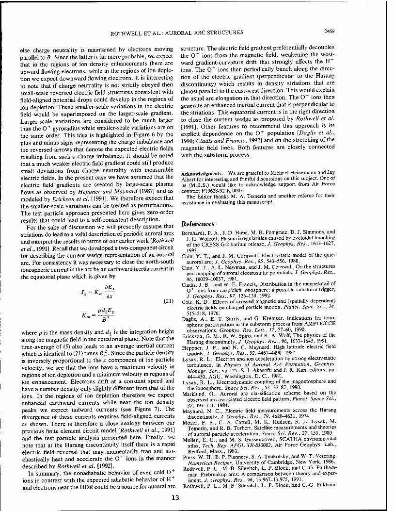
Abstract. The equations of motion are solved for ions moving in a model electric field that corresponds to the nightside equatorial region of the magnetosphere. The model represents the poleward region of the Harang discontinuity mapped to the magnetosphere. Within this region the model electric field has a constant earthward gradient superimposed on a constant dawn-to-dusk electric field. In combination with the earthward drift motion due to the dawn-to-dusk field, the electric field gradient introduces an earthward inertia drift, which is proportional to the ion mass and therefore faster for 0+ ions than for H+ ions or electrons. It is also found that the entry of the ions into the gradient region causes phase bunching and as a result ion density striations form. The striations are enhanced for more abrupt changes in the electric field gradient, a weaker magnetic field, a stronger cross-tail electric field and colder 0+ ions. The first two conditions apply during the growth phase of a substorm. Using the Tsyganenko (1987) model a minimum electric field gradient value of 1 x 10 ~9 V/m2 ((1 mV7m)/1000 km) at L = 6-7 is found. Charge neutrality requires coupling with the ionosphere through electrons moving along magnetic field lines, and such electrons may be the cause of multiple auroral arcs.
Introduction
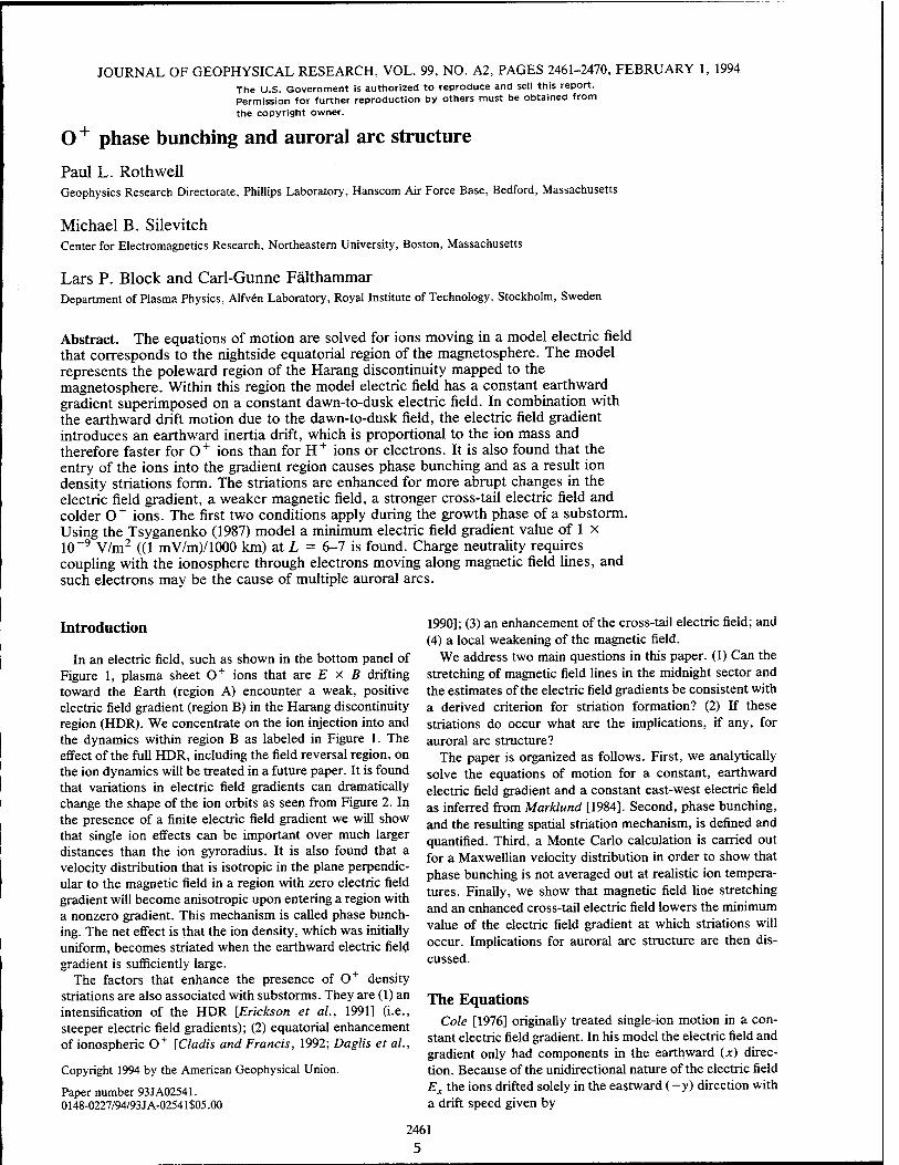
In an electric field, such as shown in the bottom panel of Figure 1, plasma sheet 0+ ions that are E x B drifting toward the Earth (region A) encounter a weak, positive electric field gradient (region B) in the Harang discontinuity region (HDR). We concentrate on the ion injection into and the dynamics within region B as labeled in Figure 1. The effect of the full HDR, including the field reversal region, on the ion dynamics will be treated in a future paper. It is found that variations in electric field gradients can dramatically change the shape of the ion orbits as seen from Figure 2. In the presence of a finite electric field gradient we will show that single ion effects can be important over much larger distances than the ion gyroradius. It is also found that a velocity distribution that is isotropic in the plane perpendic- ular to the magnetic field in a region with zero electric field gradient will become anisotropic upon entering a region with a nonzero gradient. This mechanism is called phase bunch- ing. The net effect is that the ion density, which was initially uniform, becomes striated when the earthward electric field gradient is sufficiently large.
The factors that enhance the presence of 0+ density striations are also associated with substorms. They are (1) an intensification of the HDR [Erickson et al., 1991] (i.e., steeper electric field gradients); (2) equatorial enhancement of ionospheric 0+ [Cladis and Francis, 1992; Daglis et al.,
Copyright 1994 by the American Geophysical Union.
Paper number 93JA02541. 0148-0227/94/93 JA-02541 $05.00
1990]; (3) an enhancement of the cross-tail electric field; and (4) a local weakening of the magnetic field.
We address two main questions in this paper. (1) Can the stretching of magnetic field lines in the midnight sector and the estimates of the electric field gradients be consistent with a derived criterion for striation formation? (2) If these striations do occur what are the implications, if any, for auroral arc structure?
The paper is organized as follows. First, we analytically solve the equations of motion for a constant, earthward electric field gradient and a constant east-west electric field as inferred from Marklund [1984]. Second, phase bunching, and the resulting spatial striation mechanism, is defined and quantified. Third, a Monte Carlo calculation is carried out for a Maxwellian velocity distribution in order to show that phase bunching is not averaged out at realistic ion tempera- tures. Finally, we show that magnetic field line stretching and an enhanced cross-tail electric field lowers the minimum value of the electric field gradient at which striations will occur. Implications for auroral arc structure are then dis- cussed.
The Equations Cole [1976] originally treated single-ion motion in a con-
stant electric field gradient. In his model the electric field and gradient only had components in the earthward (x) direc- tion. Because of the unidirectional nature of the electric field Ex the ions drifted solely in the eastward (-y) direction with a drift speed given by
2461 5
2462 ROTHWELL ET AL.: AURORAL ARC STRUCTURES
10 12 -X (RE)
Figure 1. A simplified Harang discontinuity model as seen in the (upper) ionosphere and the (bottom) equatorial plane. The upper panel was obtained from the lower panel by mapping the electric field in invariant latitude using the Tsyganenko [1987] model, Kp = 5, at local midnight. The letters A and B denote the regions of interest for the present paper. It is interesting to note the similarity between these results and the observations of Maynard [1974].
O)- EQ
yo n- where
n- = to' e dEx
M dx
(1)
(2)
E0 is the electric field value at the initial ion position, e is the electronic charge, B is the magnetic field value, Vy0 is the y component of the initial velocity, and to = eBIM is the ion magnetic gyrofrequency.
Therefore in a region of a positive E field gradient the effective drift velocity exceeds the usual EIB value and for a negative gradient it is less. Note in (2) that the first term on the right-hand side varies asM"2, while the second term varies as M~l. Heavy ions therefore are more efficiently affected by an electric field gradient. This is the source of the preferential decoupling of the 0+ ions relative to protons (H + ) that was mentioned above. Lysak [1981] and Yang and Kan [1983] have suggested that the enhanced ion drift velocity as given by (2) is responsible for ion conies in narrow arc structures where one would expect large electric field gradients.
In this paper we extend Cole's analysis to include an Ey
component of the electric field. The equations of motion in a two-dimensional electric field are given by
dVx e — =-{Ex[x(t)]+VyB} dt M
(3) dVy e
= -{Ey- VXB) dt M
These equations can easily be recast as a single second-order inhomogeneous differential equation:
d2Vx I , e dEx\ co2Ey ^ + W \VX = ~ (4) dt2 \ M dx ) x B
Equation (4) represents a harmonic oscillator with a fre- quency that is modified by the presence of an E field gradient. Its solution is
6
to2 £,, VM) = — — + x n2 B ' xO
0) - Ey. > • —T — I COS (fit)
+ - [ Vy0 + j I sin (Or) (5)
where Vx0 and Vy0 are determined by the initial conditions at t = 0. E0 is the value of the x component of the electric field for x < x0, which in the present instance is zero. It is assumed that dEJdx > 0 only for x > x0. The subscript B will be used to denote parameters defined in this region. The letter A denotes the region x < x0. Ey is the cross-tail electric field which is assumed to be constant. It is important to note that positive E field gradients demagnetize the particle while negative E field gradients simulate a more intense magnetic field. If O2 < 0 [Cole, 1976], the particle is exponentially accelerated. If O2 = 0, then Vx increases quadratically with time. The x component of the velocity for the case O2 > 0 is given by (5). Equation (6) is the expression for the y component of the velocity.
Vy{t) = V,0 n2 v y0 B + —)[1 -cos (Or)]
01
n CO' £\.
Vxn ^ — sin (ftf) - , „ x0 a2 B I n'Bz
2£v dEY
dx (6)
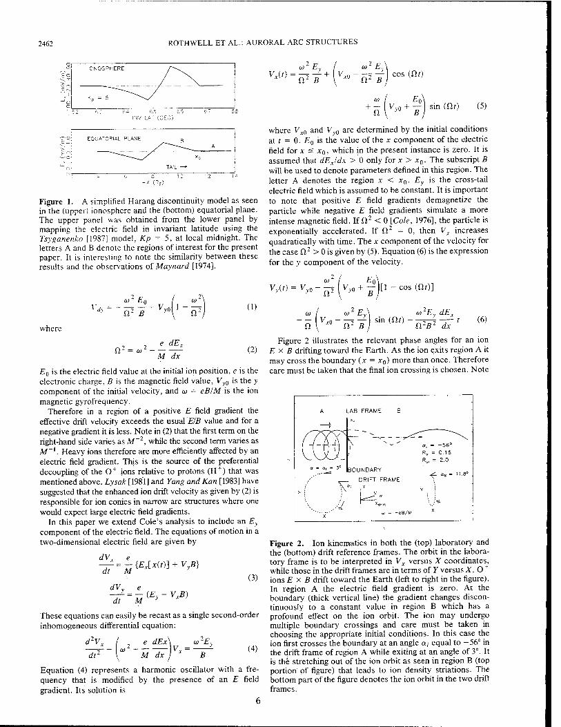
Figure 2 illustrates the relevant phase angles for an ion E x B drifting toward the Earth. As the ion exits region A it may cross the boundary (x = xQ) more than once. Therefore care must be taken that the final ion crossing is chosen. Note
LAB FRAME B
BOUNDARY
DRIFT FRAME
a, = -56° Rv = 0.16 R„ = 2.0
<£. <*B - " -8°
•\ «i Y
M
Figure 2. Ion kinematics in both the (top) laboratory and the (bottom) drift reference frames. The orbit in the labora- tory frame is to be interpreted in Vx versus X coordinates, while those in the drift frames are in terms of Y versus X. O +
ions E x B drift toward the Earth (left to right in the figure). In region A the electric field gradient is zero. At the boundary (thick vertical line) the gradient changes discon- tinuously to a constant value in region B which has a profound effect on the ion orbit. The ion may undergo multiple boundary crossings and care must be taken in choosing the appropriate initial conditions. In this case the ion first crosses the boundary at an angle a; equal to -56° in the drift frame of region A while exiting at an angle of 3°. It is the stretching out of the ion orbit as seen in region B (top portion of figure) that leads to ion density striations. The bottom part of the figure denotes the ion orbit in the two drift frames.
ROTHWELL ET AL.: AURORAL ARC STRUCTURES 2463
that a and aB are defined in the respective drift frames of regions A and B. In Figure 2 we have chosen a = 3°. The corresponding phase angle aB in the region B drift frame is 11.8°. This difference is discussed in detail below. The components of the initial velocity can be written:
Vx0 = V cos (a) + —
Vv0= Vsin (a)- —
(7)
B
where V is the ion gyrovelocity in the zero gradient region (region A) and a is the phase angle of V relative to the x axis at x = x0. We now assume that (5) and (6) for region B can be expressed in the following form:
Vx(t) = Vdx + VB cos (ftf - aB)
Vy(t) = Vdy{t) - VB - sin (Sit - aB
(8)
where Vdx and Vdy(t) are the drift terms from (5) and (6), respectively. The coefficients of the trigonometric terms in (8) correspond to an elliptical polarization of the velocity vector in the drift frame [Cole, 1976]. Expanding the trigo- nometric functions in (8) the usual way and equating the results to (5) and (6) with the initial conditions as defined in (7), we find the results shown in (9) that hold for all r a 0. It is possible to show that at t = 0, (8) reduces to (7) if the appropriate drift velocities are used together with the rela- tions shown in (9).
VB cos (aB) = V cos (a) + 1 a
VB sin (aB) = — V sin (a)
Ey i (9a)
(9b)
Phase Bunching
First, we note that the two expressions in (9) can be combined as
tan (aB) =■ a sin (a)
^^-^l^"1 (10)
The relationship between Ra and the corresponding electric field gradient is given by
,2
Equation (9a) represents the continuation of the x compo- nent of the velocity in the laboratory frame; i.e., V xB(\&b) = VxA(\ab) at t = 0. The x component of the drift velocity in region B is (oVO)2 times that in region A. Therefore the x component of the gyration velocity as seen at the boundary from the drift frame of region B is less than that in region A. In fact, if the relative drift velocity between regions B and A is sufficiently large then all ions entering region B are seen as moving tailward in the region B drift frame. (They have a phase angle TT/2 < aB < 3 TT/2.) This is the source of phase bunching and the resulting density striations. We will now quantify these statements.
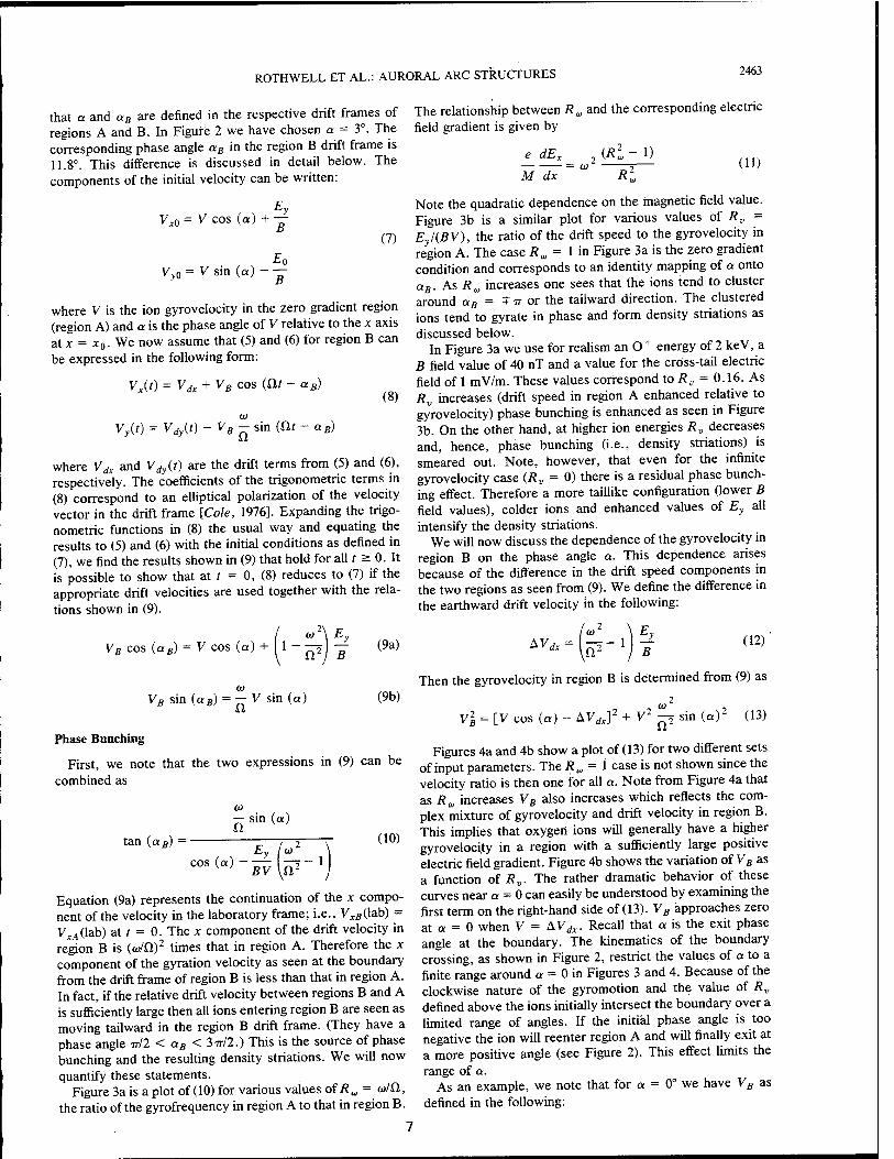
Figure 3a is a plot of (10) for various values of Ra = cola, the ratio of the gyrofrequency in region A to that in region B.
e dEx
M dx
(K ~ i) (ID
Note the quadratic dependence on the magnetic field value. Figure 3b is a similar plot for various values of Rv = Ey/(BV), the ratio of the drift speed to the gyrovelocity in region A. The case Rw = 1 in Figure 3a is the zero gradient condition and corresponds to an identity mapping of a onto aB. As Ru increases one sees that the ions tend to cluster around aB = + IT or the tailward direction. The clustered ions tend to gyrate in phase and form density striations as discussed below.
In Figure 3a we use for realism an 0+ energy of 2 keV, a B field value of 40 nT and a value for the cross-tail electric field of 1 mV/m. These values correspond to Rv = 0.16. As Rv increases (drift speed in region A enhanced relative to gyrovelocity) phase bunching is enhanced as seen in Figure 3b. On the other hand, at higher ion energies Rv decreases and, hence, phase bunching (i.e., density striations) is smeared out. Note, however, that even for the infinite gyrovelocity case (Rv = 0) there is a residual phase bunch- ing effect. Therefore a more taillike configuration (lower B field values), colder ions and enhanced values of Ey all intensify the density striations.
We will now discuss the dependence of the gyrovelocity in region B on the phase angle a. This dependence arises because of the difference in the drift speed components in the two regions as seen from (9). We define the difference in the earthward drift velocity in the following:
AV^ = Ey
a2" 1) B (12)
Then the gyrovelocity in region B is determined from (9) as
2
V2B = [V cos (a) - AVdJ
2 + V2 ^ sin (a)2 (13)
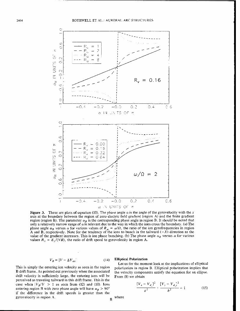
Figures 4a and 4b show a plot of (13) for two different sets of input parameters. The Ra = 1 case is not shown since the velocity ratio is then one for all a. Note from Figure 4a that as Ra increases VB also increases which reflects the com- plex mixture of gyrovelocity and drift velocity in region B. This implies that oxygen ions will generally have a higher gyrovelocity in a region with a sufiiciently large positive electric field gradient. Figure 4b shows the variation of VB as a function of Rv. The rather dramatic behavior of these curves near a = 0 can easily be understood by examining the first term on the right-hand side of (13). VB approaches zero at a = 0 when V = &Vdx. Recall that a is the exit phase angle at the boundary. The kinematics of the boundary crossing, as shown in Figure 2, restrict the values of a to a finite range around a = 0 in Figures 3 and 4. Because of the clockwise nature of the gyromotion and the value of Rv
defined above the ions initially intersect the boundary over a limited range of angles. If the initial phase angle is too negative the ion will reenter region A and will finally exit at a more positive angle (see Figure 2). This effect limits the range of a.
As an example, we note that for a = 0° we have VB as defined in the following:
2464 ROTHWELL ET AL.: AURORAL ARC STRUCTURES
-0.2 0.2 0.4 0.6
a IN UNITS OF TT
-0.4 -0.2 -0.0 0.2 0.4 0.6
a IN UNITS OF TT
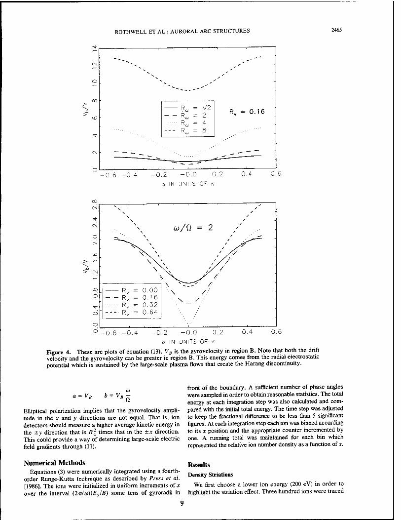
Figure 3. These are plots of equation (10). The phase angle a is the angle of the gyrovelocity with the x axis at the boundary between the region of zero electric field gradient (region A) and the finite gradient region (region B). The parameter aB is the corresponding phase angle in region B. It should be noted that only a relatively narrow range of a is relevant due to the way in which the ions cross the boundary, (a) The phase angle aB versus a for various values of Ra = co/Q., the ratio of the ion gyrofrequencies in region A and B, respectively. Note for the tendency of the ions to bunch in the tailward (-X) direction as the value of the gradient increases. This is ion phase bunching, (b) The phase angle aB versus a for various values Rv = Ey/(VB), the ratio of drift speed to gyrovelocity in region A.
VR=\V-AV, (14)
This is simply the entering ion velocity as seen in the region B drift frame. As pointed out previously when the associated drift velocity is sufficiently large, the entering ions will be perceived as traveling tailward in this drift frame. This is the case when |VB/V| > 1 as seen from (12) and (10). Ions entering region B with zero phase angle will have aB > 90° if the difference in the drift speeds is greater than the gyrovelocity in region A.
Elliptical Polarization Let us for the moment look at the implications of elliptical
polarization in region B. Elliptical polarization implies that the velocity components satisfy the equation for an ellipse. From (8) we obtain
[Vx - VA2 [Vy - Vd
■= 1 (15)
8 where
ROTHWELL ET AL.: AURORAL ARC STRUCTURES 2465
oo
>
o
Rw =
R„ = R,, =
V2 2 4
Rv = 0.16
■0.6 -0.4 -0.2 -0.0 0.2
a IN UNITS OF TT
0.4 0.6
oo CM
CM
o CM
CO
> <~ _o
> CM
CO
Ö
d
s s
s \
——i 1 1 T
\ co/Q = 2
/
1
'
1
1
I 1/
^
\ \ \
V \
/ /
/ y
/•■■
■>?
Rv Rv Rv
Rv
=
0.00 0.1 6 0.32 0.64
\ \ '■•. \
-
— —
, . i
■0.6 -0.4 -0.2 -0.0 0.2 0.4 0.6
a IN UNITS OF TT
Figure 4. These are plots of equation (13). VB is the gyro velocity in region B. Note that both the drift velocity and the gyrovelocity can be greater in region B. This energy comes from the radial electrostatic potential which is sustained by the large-scale plasma flows that create the Harang discontinuity.
a=Vc * = V*ä Elliptical polarization implies that the gyrovelocity ampli- tude in the x and y directions are not equal. That is, ion detectors should measure a higher average kinetic energy in the ±y direction that is Rl times that in the ±x direction. This could provide a way of determining large-scale electric field gradients through (11).
front of the boundary. A sufficient number of phase angles were sampled in order to obtain reasonable statistics. The total energy at each integration step was also calculated and com- pared with the initial total energy. The time step was adjusted to keep the fractional difference to be less than 5 significant figures. At each integration step each ion was binned according to its x position and the appropriate counter incremented by one. A running total was maintained for each bin which represented the relative ion number density as a function of x.
Numerical Methods Equations (3) were numerically integrated using a fourth-
order Runge-Kutta technique as described by Press et al. [1986]. The ions were initialized in uniform increments of x over the interval (2ir/a))(Ey/B) some tens of gyroradii in
Results Density Striations
We first choose a lower ion energy (200 eV) in order to highlight the striation effect. Three hundred ions were traced
2466 ROTHWELL ET AL.: AURORAL ARC STRUCTURES
DENSITY STRiAT.OKS
£; = 200 eV ^
© dEx/dx = 7x10~9 V/m2
- B = 40 nT - o o
1© o
1© I©
o o o
o
«i = 1000 eV dE„/dx = 7x10⁻⁹ V/m2
B = 40 nT
"0"
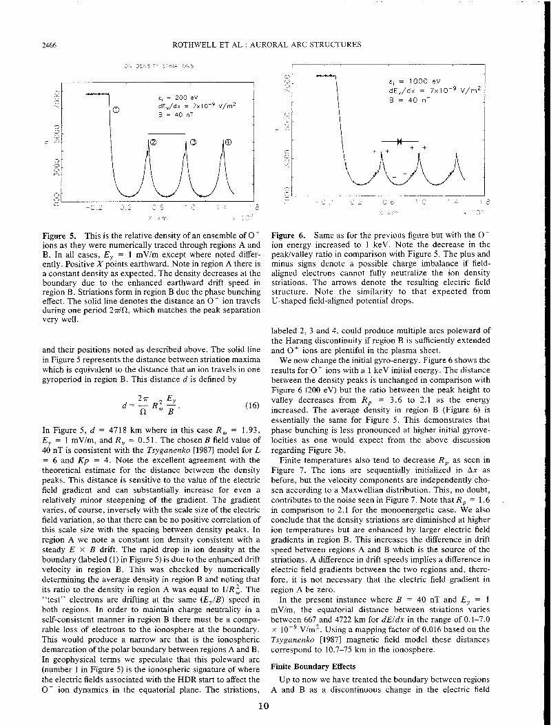
Figure 5. This is the relative density of an ensemble of 0 ~ ions as they were numerically traced through regions A and B. In all cases, Ey = 1 mV/m except where noted differ- ently. Positive X points earthward. Note in region A there is a constant density as expected. The density decreases at the boundary due to the enhanced earthward drift speed in region B. Striations form in region B due the phase bunching effect. The solid line denotes the distance an 0+ ion travels during one period 2TT/CI, which matches the peak separation very well.
and their positions noted as described above. The solid line in Figure 5 represents the distance between striation maxima which is equivalent to the distance that an ion travels in one gyroperiod in region B. This distance d is defined by
ITT , Ey (16)
In Figure 5, d = 4718 km where in this case Ra = 1.93, E.. = 1 mV/m, and R,, = 0.51. The chosen B field value of 40 nT is consistent with the Tsyganenko [1987] model for L = 6 and Kp = 4. Note the excellent agreement with the theoretical estimate for the distance between the density peaks. This distance is sensitive to the value of the electric field gradient and can substantially increase for even a relatively minor steepening of the gradient. The gradient varies, of course, inversely with the scale size of the electric field variation, so that there can be no positive correlation of this scale size with the spacing between density peaks. In region A we note a constant ion density consistent with a steady E x B drift. The rapid drop in ion density at the boundary (labeled (1) in Figure 5) is due to the enhanced drift velocity in region B. This was checked by numerically determining the average density in region B and noting that its ratio to the density in region A was equal to l/i?~. The "test" electrons are drifting at the same (EyIB) speed in both regions. In order to maintain charge neutrality in a self-consistent manner in region B there must be a compa- rable loss of electrons to the ionosphere at the boundary. This would produce a narrow arc that is the ionospheric demarcation of the polar boundary between regions A and B. In geophysical terms we speculate that this poleward arc (number 1 in Figure 5) is the ionospheric signature of where the electric fields associated with the HDR start to affect the 0+ ion dynamics in the equatorial plane. The striations,
Figure 6. Same as for the previous figure but with the O ion energy increased to 1 keV. Note the decrease in the peak/valley ratio in comparison with Figure 5. The plus and minus signs denote a possible charge imbalance if field- aligned electrons cannot fully neutralize the ion density striations. The arrows denote the resulting electric field structure. Note the similarity to that expected from U-shaped field-aligned potential drops.
labeled 2, 3 and 4, could produce multiple arcs poleward of the Harang discontinuity if region B is sufficiently extended and 0+ ions are plentiful in the plasma sheet.
We now change the initial gyro-energy. Figure 6 shows the results for 0+ ions with a 1 keV initial energy. The distance between the density peaks is unchanged in comparison with Figure 6 (200 eV) but the ratio between the peak height to valley decreases from Rp = 3.6 to 2.1 as the energy increased. The average density in region B (Figure 6) is essentially the same for Figure 5. This demonstrates that phase bunching is less pronounced at higher initial gyrove- locities as one would expect from the above discussion regarding Figure 3b.
Finite temperatures also tend to decrease Rp as seen in Figure 7. The ions are sequentially initialized in Ax as before, but the velocity components are independently cho- sen according to a Maxwellian distribution. This, no doubt, contributes to the noise seen in Figure 7. Note that Rp = 1.6 in comparison to 2.1 for the monoenergetic case. We also conclude that the density striations are diminished at higher ion temperatures but are enhanced by larger electric field gradients in region B. This increases the difference in drift speed between regions A and B which is the source of the striations. A difference in drift speeds implies a difference in electric field gradients between the two regions and, there- fore, it is not necessary that the electric field gradient in region A be zero.
In the present instance where B = 40 nT and Ey = 1 mV/m, the equatorial distance between striations varies between 667 and 4722 km for dEldx in the range of 0.1-7.0 x 10~9 V/m2. Using a mapping factor of 0.016 based on the Tsyganenko [1987] magnetic field model these distances correspond to 10.7-75 km in the ionosphere.
Finite Boundary Effects
Up to now we have treated the boundary between regions A and B as a discontinuous change in the electric field
10
ROTHWELL ET AL.: AURORAL ARC STRUCTURES 2467
MAXWELLIAN
Si = 1000 eV
\ dEx/dx = 7x1 0-9 V/m2.
- I B = 40 nT
I i TAIL EARTH >
I CURRENTS " \ 11 U ii \ IT JLT L _
\ / \ j \ j
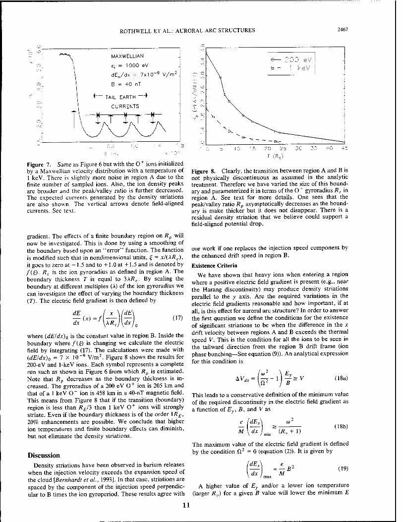
Figure 7. Same as Figure 6 but with the O + ions initialized by a Maxwellian velocity distribution with a temperature of 1 keV. There is slightly more noise in region A due to the finite number of sampled ions. Also, the ion density peaks are broader and the peak/valley ratio is further decreased. The expected currents generated by the density striations are also shown. The vertical arrows denote field-aligned currents. See text.
gradient. The effects of a finite boundary region on Rp will now be investigated. This is done by using a smoothing of the boundary based upon an "error" function. The function is modified such that in nondimensional units, £ = xl(kRc), it goes to zero at -1.5 and to +1.0 at +1.5 and is denoted by /(£). Rc is the ion gyroradius as defined in region A. The boundary thickness T is equal to 3Ai?c. By scaling the boundary at different multiples (A) of the ion gyroradius we can investigate the effect of varying the boundary thickness (T). The electric field gradient is then defined by
dE I x \(dE\
Tx{x)=f[lR-c)\Tx)ü
(17)
where (dE/dx)0 is the constant value in region B. Inside the boundary where /(£) is changing we calculate the electric field by integrating (17). The calculations were made with (dE/dx)0 = 7 x 10 ~9 V/m2. Figure 8 shows the results for 200-eV and 1-keV ions. Each symbol represents a complete run such as shown in Figure 6 from which Rp is estimated. Note that Rp decreases as the boundary thickness is in- creased. The gyroradius of a 200 eV 0+ ion is 205 km and that of a 1 keV 0+ ion is 458 km in a 40-nT magnetic field. This means from Figure 8 that if the transition (boundary) region is less than RE/3 then 1 keV 0+ ions will strongly striate. Even if the boundary thickness is of the order IRE, 20% enhancements are possible. We conclude that higher ion temperatures and finite boundary effects can diminish, but not eliminate the density striations.
Discussion Density striations have been observed in barium releases
when the injection velocity exceeds the expansion speed of the cloud [Bernhardt et al., 1993]. In that case, striations are spaced by the component of the injection speed perpendic- ular to B times the ion gyroperiod. These results agree with
Figure 8. Clearly, the transition between region A and B is not physically discontinuous as assumed in the analytic treatment. Therefore we have varied the size of this bound- ary and parameterized it in terms of the 0+ gyroradius Rc in region A. See text for more details. One sees that the peak/valley ratio Rp asymptotically decreases as the bound- ary is make thicker but it does not disappear. There is a residual density striation that we believe could support a field-aligned potential drop.
our work if one replaces the injection speed component by the enhanced drift speed in region B.
Existence Criteria
We have shown that heavy ions when entering a region where a positive electric field gradient is present (e.g., near the Harang discontinuity) may produce density striations parallel to the y axis. Are the required variations in the electric field gradients reasonable and how important, if at all, is this effect for auroral arc structure? In order to answer the first question we define the conditions for the existence of significant striations to be when the difference in the x drift velocity between regions A and B exceeds the thermal speed V. This is the condition for all the ions to be seen in the tailward direction from the region B drift frame (ion phase bunching—See equation (9)). An analytical expression for this condition is
AV dx (ti
B ■> V (18a)
This leads to a conservative definition of the minimum value of the required discontinuity in the electric field gradient as a function of Ey, B, and V as
e
M dx (*„+!) (18b)
The maximum value of the electric field gradient is defined by the condition O2 = 0 (equation (2)). It is given by
S =LB2 dx j M
I max
(19)
A higher value of Ey and/or a lower ion temperature (larger Rv) for a given B value will lower the minimum E
11
2468 ROTHWELL ET AL.: AURORAL ARC STRUCTURES
CN
O
o
O c > CO
O X ~0
<J)
O :
O
:
o
o :
□ : 500 eV 1000 eV 5000 eV IUUUU Qv
. A . ' °60 62 Ki /U 72
A (dec
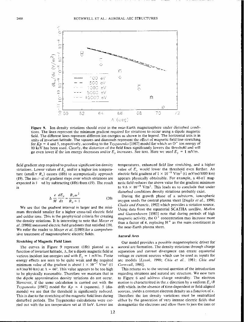
Figure 9. Ion density striations should exist in the near-Earth magnetosphere under disturbed condi- tions. The lines represent the minimum gradient required for striations to occur using a dipole magnetic field. The different lines represent different ion energies as shown in the legend. The horizontal axis is in units of invariant latitude. The squares and diamonds represent the effect of magnetic field line stretching for Kp = 4 and 5, respectively, according to the Tsyganenko [1987] model for which an 0+ ion energy of 10 keV has been used. Clearly, the distortion of the field lines significantly lowers the threshold and will go even lower if the ion energy decreases and/or Ey increases. See text. Here we used Ey = 1 mV/m.
field gradient step required to produce significant ion density striations. Lower values of Ey and/or a higher ion tempera- ture (smaller Rv) causes (18b) to asymptotically approach (19). The inter 'al of gradient steps over which striations are expected is f tid by subtracting (18b) from (19). The result is
e dEx Rvoi~
M dx R„ + 1 (20)
We see that the gradient interval is larger and the mini- mum threshold smaller for a higher cross-tail electric field and colder ions. This is the geophysical criteria for creating the density striations. It is interesting to note that Mozer et al. [1980] measured electric field gradients that satisfied (19). We refer the reader to Mozer et al. [1980] for a comprehen- sive treatment of magnetospheric electric fields.
Stretching of Magnetic Field Lines
The curves in Figure 9 represent (18b) plotted as a function of invariant latitude, A, for a dipole magnetic field at various incident ion energies and with Ey = 1 mV/m. Finite energy effects are seen to be quite weak and the required minimum value of the gradient is about 1 x 10~7 V/m2 ((1 mV/m)/10 km) at A = 66°. This value appears to be too high to be physically reasonable. Therefore we maintain that in the dipole approximation density striations do not occur. However, if the same calculation is carried out with the Tsyganenko [1987] model for Kp = 4 (squares), 5 (dia- monds) we see that the threshold is significantly reduced. This is due to the stretching of the magnetic field lines during disturbed periods. The Tsyganenko calculations were car- ried out with the ion temperature set at 10 keV. Lower ion
temperatures, enhanced field line stretching, and a higher value of Ey would lower the threshold even further. An electric field gradient of 1 x 10"9 V/m2 ((1 mV/m)/1000 km) appears physically obtainable. For example, a 40-nT mag- netic field reduces the above value for the gradient minimum to 9.6 x 10~9 V/m2. This leads us to conclude that under disturbed conditions density striations probably exist.
During the growth phase of a substorm, ionospheric oxygen seeds the central plasma sheet [Daglis et al., 1990; Cladis and Francis, 1992] which provides a striation source. Using data from the equatorial SCATHA satellite, Mullen and Gussenhoven [1983] note that during periods of high magnetic activity, the 0T concentration may increase more than a factor of 4, replacing H+ as the main constituent in the near-Earth plasma sheet.
Auroral Arcs
Our model provides a possible magnetospheric driver for auroral arc formation. The density striations through charge separation and current divergence can create equatorial voltage or current sources which can be used as inputs for arc models [Lysak, 1990; Chiu et al., 1981; Chiu and Cornwall, 1980].
This returns us to the second question of the introduction regarding striations and auroral arc structure. We now turn to Figure 6 and address charge neutrality. The electron motion is characterized in the x direction by a uniform EyIB drift which, in the absence of time-dependent or field-aligned sources, yields a constant electron density as a function of x. Therefore the ion density variations must be neutralized either by the generation of very intense electric fields that demagnetize the electrons and allow them to join the ions or
12
ROTHWELL ET AL.: AURORAL ARC STRUCTURES 2469
else charge neutrality is maintained by electrons moving parallel to B. Since the latter is far more probable, we expect that in the regions of ion density enhancements there are upward flowing electrons, while in the regions of ion deple- tion we expect downward flowing electrons. It is interesting to note that if charge neutrality is not strictly obeyed then small-scale reversed electric field structures consistent with field-aligned potential drops could develop in the regions of ion depletion. These smaller-scale variations in the electric field would be superimposed on the larger-scale gradient. Larger-scale variations are considered to be much larger than the 0+ gyroradius while smaller-scale variations are on the same order. This idea is highlighted in Figure 6 by the plus and minus signs representing the charge imbalance and the reversed arrows that denote the expected electric fields resulting from such a charge imbalance. It should be noted that a much weaker electric field gradient could still produce small deviations from charge neutrality with measurable electric fields. In the present case we have assumed that the electric field gradients are created by large-scale plasma flows as observed by Heppner and Maynard [1987] and as modeled by Erickson et al. [1991]. We therefore expect that the smaller-scale variations can be treated as perturbations. The test particle approach presented here gives zero-order results that could lead to a self-consistent description.
For the sake of discussion we will presently assume that striations do lead to a valid description of periodic auroral arcs and interpret the results in terms of our earlier work [Rothwell et al., 1991]. Recall that we developed a two-component circuit for describing the current wedge representation of an auroral arc. For consistency it was necessary to close the north-south ionospheric current in the arc by an earthward inertia current in the equatorial plane which is given by
Jx — K„ dEx
Km —
dx
pd\\Ey
B*
(21)
where p is the mass density and d\\ is the integration height along the magnetic field in the equatorial plane. Note that the time-average of (5) also leads to an average inertial current which is identical to (21) times R2
a. Since the particle density is inversely proportional to the x component of the particle velocity, we see that the ions have a maximum velocity in regions of ion depletion and a minimum velocity in regions of ion enhancement. Electrons drift at a constant speed and have a number density only slightly different from that of the ions. In the regions of ion depletion therefore we expect enhanced earthward currents while near the ion density peaks we expect tailward currents (see Figure 7). The divergence of these currents requires field-aligned currents as shown. There is therefore a close analogy between our previous finite element circuit model [Rothwell et al., 1991] and the test particle analysis presented here. Finally, we note that at the Harang discontinuity itself there is a rapid electric field reversal that may momentarily trap and sto- chastically heat and accelerate the 0+ ions in the manner described by Rothwell et al. [1992].
In summary, the nonadiabatic behavior of even cold 0 +
ions in contrast with the expected adiabatic behavior of H +
and electrons near the HDR could be a source for auroral arc
structure. The electric field gradient preferentially decouples the 0+ ions from the magnetic field, weakening the west- ward gradient-curvature drift that strongly affects the H +
ions. The 0+ ions then periodically bunch along the direc- tion of the electric gradient (perpendicular to the Harang discontinuity) which results in density striations that are almost parallel to the east-west direction. This would explain the usual arc elongation in that direction. The 0+ ions then generate an enhanced inertial current that is perpendicular to the striations. This equatorial current is in the right direction to close the current wedge as proposed by Rothwell et al. [1991]. Other features to recommend this approach is its explicit dependence on the 0+ population [Daglis et al., 1990; Cladis and Francis, 1992] and on the stretching of the magnetic field lines. Both features are closely connected with the substorm process.
Acknowledgments. We are grateful to Michael Heinemann and Jay Albert for interesting and fruitful discussions on this subject. One of us (M.B.S.) would like to acknowledge support from Air Force contract F19628-92-K-0007.
The Editor thanks M. A. Temerin and another referee for their assistance in evaluating this manuscript.
References Bernhardt, P. A., J. D. Huba, M. B. Pomgratz, D. J. Simmons, and
J. H. Wolcott, Plasma irregularities caused by cycloidal bunching of the CRESS G-2 barium release, J. Geophys. Res., 1613-1627, 1993.
Chiu, Y. T., and J. M. Cornwall, Electrostatic model of the quiet auroral arc, J. Geophys. Res., 85, 543-556, 1980.
Chiu, Y. T., A. L. Newman, and J. M. Cornwall, On the structures and mapping of auroral electrostatic potentials, J. Geophys. Res., 86, 10029-10037, 1981.
Cladis, J. B., and W. E. Francis, Distribution in the magnetotail of 0+ ions from cusp/cleft ionosphere: a possible substorm trigger, J. Geophys. Res., 97, 123-130, 1992.
Cole, K. D., Effects of crossed magnetic and (spatially dependent) electric fields on charged particle motion, Planet. Spac. Sei., 24, 515-518, 1976.
Daglis, A., E. T. Sarris, and G. Kremser, Indications for iono- spheric participation in the substorm process from AMPTE/CCE observations, Geophys. Res. Lett., 17, 57-60, 1990.
Erickson, G. M., R. W. Spiro, and R. A. Wolf, The physics of the Harang discontinuity, J. Geophys. Res., 96, 1633-1645, 1991.
Heppner, J. P., and N. C. Maynard, High latitude electric field models, J. Geophys. Res., 92, 4467-4490, 1987.
Lysak, R. L., Electron and ion acceleration by strong electrostatic turbulence, in Physics of Auroral Arc Formation, Geophys. Monogr. Ser., vol. 25, S.-I. Akasofu and J. R. Kan, editors, pp. 444-450, AGU, Washington, D. C, 1981.
Lysak, R. L., Electrodynamic coupling of the magnetosphere and the ionosphere, Space Sei. Rev., 52, 33-87, 1990.
Marklund, G., Auroral arc classification scheme based on the observed arc-associated electric field pattern, Planet. Space Sei., 32, 193-211, 1984.
Maynard, N. C, Electric field measurements across the Harang discontinuity, J. Geophys. Res., 79, 4620-4631, 1974.
Mozer, F. S., C. A. Cattell, M. K. Hudson, R. L. Lysak, M. Temerin, and R. B. Torbert, Satellite measurements and theories of auroral particle acceleration, Space Sei. Rev., 27, 155, 1980.
Mullen, E. G., and M. S. Gussenhoven, SCATHA environmental atlas, Tech. Rep. AFGL TR-830002, Air Force Geophys. Lab., Bedford, Mass., 1983.
Press, W. H., B. P. Flannery, S. A. Teukolsky, and W. T. Vetenng, Numerical Recipes, University of Cambridge, New York, 1986.
Rothwell, P. L., M. B. Silevitch, L. P. Block, and C.-G. Fältham- mar, Prebreakup arcs: A comparison between theory and exper- iment, J. Geophys. Res., 96, 13,967-13,975, 1991.
Rothwell, P. L., M. B. Silevitch, L. P. Block, and C.-G. Fältham-
13
2470 ROTHWELL ET AL.: AURORAL ARC STRUCTURES
mar Acceleration and stochastic heating of ions drifting through P. L. Rothwell, Geophysics Research Directorate, Phillips Labo- an auroral arc, J. Geophys. Res., 97, 19,333-19,339, 1992. ratory, 29 Randolph Road, Hanscom Air Force Base, MA 01731-
Tsyganenko, N. A., Global quantitative models of the geometric 3010. field in the cislunar magnetosphere for different disturbance M. B. Silevitch, Center for Electromagnetics Research, North- levels, Planet. Space Sei., 35, 1347-1358, 1987. eastern University, Boston, MA 02115. (e-mail: [email protected].
Yang, W. H., and J. R. Kan, Generation of conic ions by auroral edu) electric fields, J. Geophys. Res., 88, 465-468, 1983.
L. P. Block and C.-G. Falthammar, Department of Plasma Physics, Alfven Laboratory, Royal Institute of Technology, S 10044 (Received February 26, 1993; revised August 25, 1993; Stockholm 70, Sweden, (e-mail: SPAN.plafys::falthammar) accepted September 3, 1993.)
14
The U.S. Government is authorized to reproduce and sell this report. Permission for further reproduction by others must be obtained from the copyright owner.
Single Ion Dynamics and Multiscale Phenomena
P. L. Rothwell
Geophysics Research Directorate, Phillips Laboratory, HanscomAFB, Bedford, Massachusetts
M. B. Silevitch
Center for Electromagnetics Research, Northeastern University, Boston, Massachusetts
Lars P. Block and Carl-Gunne Fälthammer
Division of Plasma Physics, Alfven Laboratory, Royal Institute of Technology, Stockholm, Sweden
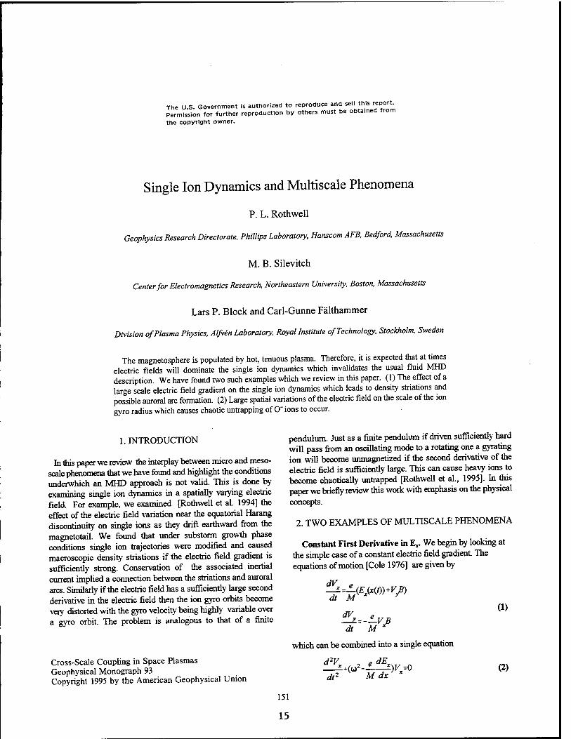
The magnetosphere is populated by hot, tenuous plasma. Therefore, it is expected that at times electric fields will dominate the single ion dynamics which invalidates the usual fluid MHD description. We have found two such examples which we review in this paper. (1) The effect of a large scale electric field gradient on the single ion dynamics which leads to density striations and possible auroral arc formation. (2) Large spatial variations of the electric field on the scale of the ion gyro radius which causes chaotic untrapping of 0+ ions to occur.
1. INTRODUCTION
In this paper we review the interplay between micro and meso- scale phenomena that we have found and highlight the conditions underwhich an MHD approach is not valid. This is done by examining single ion dynamics in a spatially varying electric field. For example, we examined [Rothwell et al. 1994] the effect of the electric field variation near the equatorial Harang discontinuity on single ions as they drift earthward from the magnetotail. We found that under substorm growth phase conditions single ion trajectories were modified and caused macroscopic density striations if the electric field gradient is sufficiently strong. Conservation of the associated inertial current implied a connection between the striations and auroral arcs. Similarly if the electric field has a sufficiently large second derivative in the electric field then the ion gyro orbits become very distorted with the gyro velocity being highly variable over a gyro orbit. The problem is analogous to that of a finite
Cross-Scale Coupling in Space Plasmas Geophysical Monograph 93 Copyright 1995 by the American Geophysical Union
pendulum. Just as a finite pendulum if driven sufficiently hard will pass from an oscillating mode to a rotating one a gyrating ion will become unmagnetized if the second derivative of the electric field is sufficiently large. This can cause heavy ions to become chaotically untrapped [Rothwell et al., 1995]. In this paper we briefly review this work with emphasis on the physical
concepts.
2. TWO EXAMPLES OF MULTISCALE PHENOMENA
Constant First Derivative in E„. We begin by looking at the simple case of a constant electric field gradient. The equations of motion [Cole 1976] are given by
^--luElxiftYVJS) dt M y
dV e —L = -±-VB dt M ^
which can be combined into a single equation
(1)
dE. i+(or dt2 M dx
)K=0 (2)
151
15
152 SINGLE ION DYNAMICS
ION DENSITY STRIATIONS ^ =
Ei = 1000 eV
dE„/dx = 7x10~9 V/m2
= 40 nT >
0.6
X km x 10"
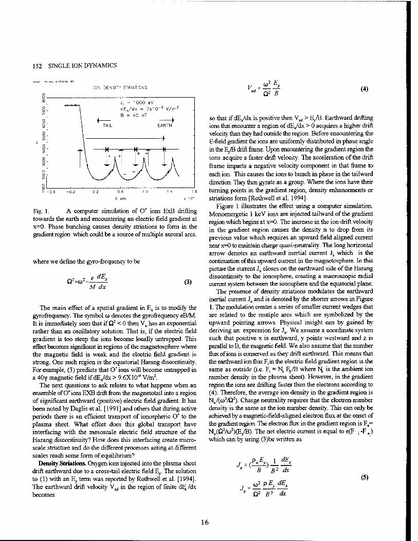
Fig. 1. A computer simulation of 0+ ions ExB drifting towards the earth and encountering an electric field gradient at x=0. Phase bunching causes density striations to form in the gradient region which could be a source of multiple auroral arcs.
where we define the gyro-frequency to be
0»=^-e dE* M dx
(3)
The main effect of a spatial gradient in Ex is to modify the gyrofrequency. The symbol u denotes the gyrofrequency eB/M. It is immediately seen that if Q2 < 0 then Vx has an exponential rather than an oscillatory solution. That is, if the electric field gradient is too steep the ions become locally untrapped. This effect becomes significant in regions of the magnetosphere where the magnetic field is weak and the electric field gradient is strong. One such region is the equatorial Harang discontinuity. For example, (3) predicts that 0+ ions will become untrapped in a 40Y magnetic field if dE/dx > 9.6X10-' V/m2.
The next questions to ask relates to what happens when an ensemble of 0+ions EXB drift from the magnetotail into a region of significant earthward (positive) electric field gradient. It has been noted by Daglis et al. [1991] and others that during active periods there is an efficient transport of ionospheric 0+ to the plasma sheet. What effect does this global transport have interfacing with the mesoscale electric field structure of the Harang discontinuity? How does this interfacing create micro- scale structure and do the different processes acting at different scales reach some form of equilibrium?
Density Striations. Oxygen ions injected into the plasma sheet drift earthward due to a cross-tail electric field Ey. The solution to (1) with an Ey term was reported by Rothwell et al. [1994]. The earthward drift velocity Vxd in the region of finite dF, /dx becomes
Q2 B (4)
so that if dEJdx is positive then Vxd > Ej/B. Earthward drifting ions that encounter a region of dEj/dx > 0 acquires a higher drift velocity than they had outside the region. Before encountering the E-field gradient the ions are uniformly distributed in phase angle in the EJB drift Same. Upon encountering the gradient region the ions acquire a faster drift velocity. The acceleration of the drift frame imparts a negative velocity component in that frame to each ion. This causes the ions to bunch in phase in the tailward direction. They then gyrate as a group. Where the ions have their turning points in the gradient region, density enhancements or striations form [Rothwell et al. 1994].
Figure 1 illustrates the effect using a computer simulation. Monoenergetic 1 keV ions are injected tailward of the gradient region which begins at x=0. The increase in the ion drift velocity in the gradient region causes the density n to drop from its previous value which requires an upward field aligned current near x=0 to maintain charge quasi-neutrality. The long horizontal arrow denotes an earthward inertial current Jx which is the continuation of this upward current in the magnetosphere. In this picture the current Jx closes on the earthward side of the Harang discontinuity to the ionosphere, creating a macroscopic radial current system between the ionosphere and the equatorial plane.
The presence of density striations modulates the earthward inertial current Jx and is denoted by the shorter arrows in Figure 1. The modulation creates a series of smaller current wedges that are related to the mutiple arcs which are symbolized by the upward pointing arrows. Physical insight can by gained by deriving an expression for Jx. We assume a coordinate system such that positive x is earthward, y points westward and z is parallel to B, the magnetic field. We also assume that the number flux of ions is conserved as they drift earthward. This means that the earthward ion flux F;in the electric field gradient region is the same as outside (i.e. F; = N„ Ey/B where 1^ is the ambient ion number density in the plasma sheet). However, in the gradient region the ions are drifting faster than the electrons according to (4). Therefore, the average ion density in the gradient region is N0/(to
2/Q2). Charge neutrality requires that the electron number density is the same as the ion number density. This can only be achieved by a magnetic-field-aligned electron flux at the onset of the gradient region. The electron flux in the gradient region is F = N0(Q
2/o>2)(Ey/B). The net electric current is equal to e(F ; -F,)' which can by using (3)be written as
J p E 1 dEr
B B2 dx
_ w2 p Ey dEx
' Q2 B3 dx
(5)
16
ROTHWELLETAL. 153
GAUSS Thu Sep 23 14-:28:31 1993 l l l l
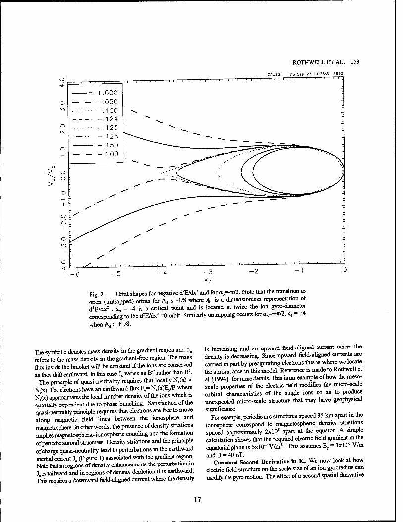
Fig 2 Orbit shapes for negative cffi/dx2 and for a0=-u/2. Note that the transition to open (untrapped) orbits for A„ <; -1/8 where 4 is a dimensionless representation of d2E/dx2 . x, = -4 is a critical point and is located at twice the ion gyro-diameter corresponding to the d'E/dx2 =0 orbit. Similarly untrapping occurs for a=+n/2, x,, = +4
when Aj * +1/8.
The symbol p denotes mass density in the gradient region and p„ refers to the mass density in the gradient-free region. The mass flux inside the bracket will be constant if the ions are conserved as they drift earthward. In this case Jx varies as B"2 rather than B3.
The principle of quasi-neutrality requires that locally Ne(x) = Nj(x). The electrons have an earthward flux Fe= Ne(x)E,/B where N^(x) approximates the local number density of the ions which is sp'atially dependent due to phase bunching. Satisfaction of the quasi-neutrality principle requires that electrons are free to move along magnetic field lines between the ionosphere and magnetosphere. In other words, the presence of density striations implies magnetospheric-ionospheric coupling and the formation of periodic auroral structures. Density striations and the principle of charge quasi-neutrality lead to perturbations in the earthward inertial current Jx (Figure 1) associated with the gradient region. Note that in regions of density enhancements the perturbation in Jx is tailward and in regions of density depletion it is earthward. This requires a downward field-aligned current where the density
is increasing and an upward field-aligned current where the density is decreasing. Since upward field-aligned currents are carried in part by precipitating electrons this is where we locate the auroral arcs in this model. Reference is made to Rothwell et al. [1994] for more details. This is an example of how the meso- scale properties of the electric field modifies the micro-scale orbital characteristics of the single ions so as to produce unexpected micro-scale structure that may have geophysical significance.
For example, periodic arc structures spaced 35 km apart in the ionosphere correspond to magnetospheric density striations spaced approximately 2x10s apart at the equator. A simple calculation shows that the required electric field gradient in the equatorial plane is 5xl0"9 V/m2. This assumes Ey = lxlO3 V/m andB = 40nT.
Constant Second Derivative in Er We now look at how electric field structure on the scale size of an ion gyroradius can modify the gyro motion. The effect of a second spatial derivative
17
154 SINGLE ION DYNAMICS
of Ex will now be considered. The presence of a constant second derivative in E^ can be examined by expanding the first derivative about the initial position x0 of the ion.
dE. dE. d2E.
dx dx -JL\ + H*-*J
dx2 (6)
Then equation (1) can be rewritten as
%x-x}Vx=0 d2V , - d2E —x-+a 2v -e
dt< M dx7 (7)
where Q0 is the gyro-frequency as defined in equation (3) with dEx/dx = dE^/dxl^,,. This is to be distinguished from the gyro- frequency Q which reflects a constant second derivative in Ex. Equation (7) can be easily integrated by noting that Vx =dx/dt in the second and third terms . A subsequent integration is also trivial after the previous result is multiplied by Vx. The final result is cast into the following form.
was shown to produce a set of nested current systems between the ionosphere and the magnetosphere. Presently, we are investigating the self-consistency of the structure shown in Figure 1. That is, the upward current regions are associated with field-aligned potential drops. The question is whether the equatorial electric fields associated with these currents are sufficiently strong as to scatter the ions and, therebye, destroy the striations. The result depends on the auroral arc model used. In the second case small scale electric field structure strongly affected the orbital dynamics of trapped ions. In both examples that were considered the unifying idea is that when (3) becomes small or negative then finite orbit effects become important. Another important example that depends on this concept is the stochastic heating of ions [Rothwell et al. 1992]. A negative value of (3) implies that in the x-direction the
ion's increase in momentum due to the electric field gradient is larger than the ion's decrease in momentum due to the magnetic field. This is the physical basis of untrapping.
dx. {-/?= Ad{xd-a}{xd-b}(xd-c}
dx (8)
where the subscript 'd' refers to dimensionless quantities. Equation (8) is solved in terms of Jacobian Elliptic functions
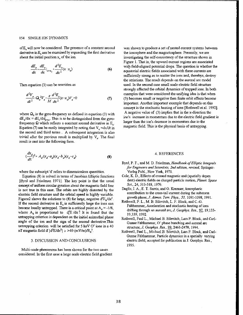
[Byrd and Friedman 1971]. The key point is that the usual concept of uniform circular gyration about the magnetic field line is not true in this case. The orbits are highly distorted by the electric field structure and the orbital speed is highly variable. Figure2 shows the solutions to (8) for large, negative d^/dx2. If the second derivative in Ex is sufficiently large the ions can become locally untapped. There is a critical point at A^ = -1/8, where A,j is proportional to d*E /dx2 It is found that the untrapping criterion is dependent on the initial azimuthal phase angle of the ion and the sign of the second derivative.This untrapping criterion will be satisfied for 5 keV O* ions in a 40 nT magnetic field if | d^/dx21 ;> >40 (mV/m)/RE
2.
3. DISCUSSION AND CONCLUSIONS
Multi-scale phenomena has been shown for the two cases considered. In the first case a large scale electric field gradient
4. REFERENCES
Byrd, P. F., and M. D. Friedman, Handbook of Elliptic Integrals for Engineers and Scientists, 2nd edition, revised, Springer- Verlag Publ., New York, 1971.
Cole, K. D., Effects of crossed magnetic and (spatially depen dent) electric fields on charged particle motion, Planet. Space Sei., 24, 515-518, 1976.
Daglis, I. A., E. T. Sarris, and G. Kremser, Ionospheric contribution to the cross-tail current during the substorm growth phase, J. Atmos. Terr. Phys., 53, 1091-1098, 1991.
Rothwell, P. L., M. B. Silevitch, L. P. Block, and C.-G. Fälthammar, Acceleration and stochastic heating of ions drifting through an auroral arc, J. Geophys. Res., 97,19,133- 19,339,1992.
Rothwell, Paul L., Michael B. Silevitch, Lars P. Block, and Carl- Gunne Fälthammar, O* phase bunching and auroral arc structure, J. Geophys. Res., 99,2461-2470,1994.
Rothwell, Paul L., Michael B. Silevitch, Lars P. Block, and Carl- Gunne Fälthammar, Particle dynamics in a spatially varying electric field, accepted for publication in J. Geophys. Res., 1995.
18
The U.S. Government is authorized to reproduce and sell this report. Permission for further reproduction by others must be obtained from the copyright owner.
JOURNAL OF GEOPHYSICAL RESEARCH, VOL. 100, NO. A8, PAGES 14,875-14,885, AUGUST 1, 1995
Particle dynamics in a spatially varying electric field
Paul L. Rothwell Geophysics Research Directorate, Phillips Laboratory, Hanscom Air Force Base, Bedford, Massachusetts
Michael B. Silevitch Center for Electromagnetics Research, Northeastern University, Boston, Massachusetts
Lars P. Block and Carl-Gunne Fälthammar Division of Plasma Physics, Alfven Laboratory, Royal Institute of Technology, Stockholm, Sweden
Abstract. For an MHD description of a plasma a distinct separation between the macroscopic and microscopic spatial and temporal scales is assumed. In this paper we solve the particle dynamics with finite first and second spatial derivatives in the electric field. We find that ( 1) MHD (ideal and nonideal) becomes invalid for a sufficiently strong constant electric field gradient perpendicular to the magnetic field; (2) a sufficiently large second derivative in the electric field can cause heavy ions to become chaotically untrapped; (3) for an electric field with a constant gradient the ion drift velocity is equal to (ExB)/|B|2 as long as the orbit-averaged value of E is used. There are no finite currents associated with the ion drift for such an electric field; (4) perturbation technique gives a poor approximation to the ion drift velocity even for values of the second derivative that may well occur in the magnetosphere. Results 1 and 2 provide necessary criteria for the applicability of magnetospheric MHD models of spatially varying electric fields They also predict an asymmetry in the heavy ion fluxes, a feature that could be useful in inferring magnetospheric electric field structure. We illustrate these results by applica- tion to the Harang discontinuity. It is found that if the interplanetary magnetic field swings northward under substorm growth conditions the orbits of the equatorial 0+ may dramatically change due to result 2. This effect may contribute to the substorm onset process.
the first and second spatial derivatives of a coexisting electric 1. Introduction fidd ^ signincant. The single-ion dynamics for a constant one-
It has long been recognized that there is a coupling between component electric field gradient have been previously treated the microscopic single-ion dynamics as defined by the ion tyCole [1976]. Cole argued that the ion drift velocity in the -y gyroradius and macroscopic MHD phenomena. Two obvious direction ^^ greater than -EJ&IB and therefore a current in that examples are the kinetic Alfven wave [Hasegawa, 1976; Goertz, direction was present. Here we show that for a one-dimensional 1984] and the ion tearing mode [Galeev and Zelenyi, 1976]. electric field there is no drift current. In section 2 we treat the ion More recently, we showed that the chaotic behavior of single- dynamics for a constant electric field gradient. We also show in ion trajectories may cause macroscopic heating and accelera- section 2 that the ion drift velocity is still equal to -Ex(x)IB if the tion as they drift through an auroral arc [Rothwell et a!., 1992]. vaiue 0f the electric field at the center of the ion gyro-orbit is Another important example is the effect of the electric field used m sections 3 and 4 we treat the more general case of a variation near the Harang discontinuity on single ions as they constant second derivative in £, Exact solutions are found in drift earfliward from the magnetotail. We found [Rothwell et al., tsnas 0f jaCobian elliptic functions (JEF). The orbit shape can 1994] that under substorm growth phase conditions, single-ion become severely distorted by the electric field, and the concept of trajectories were modified and caused macroscopic density a panicle uniformly rotating about B in a circular path is no striations. Current conservation of the associated inertial longer sound. For sufficiently large values of the second deriva- current implied a connection between the striations and auroral trve m Ex the ions become untrapped. There are therefore arcs. situations in which even a nonideal MHD that treats finite orbit
In this paper we examine single-ion dynamics in a spatially effects in a perturbative manner is not valid. Also, our results varying one-dimensional electric field Ex(x) which is perpendicu- provide criteria for the applicability of magnetospheric MHD lar to a magnetic field B = Bt. We analytically solve and models for spatially varying electric fields in the magnetosphere. numerically analyze single-ion motion in a magnetic field when m section 5 these results are applied to the Harang discontinuity
for the case when the interplanetary magnetic field swings northward. It is argued that the change in orbital characteristics
Copyright 1995 by the American Geophysical Union. of ^ ions m ^ ^^ 0fme Harang where the electric field has u nriimo. sufficient curvature may contribute to substorm onsets. Con-
S!SSS/SAÄ$05.00 elusions and a short discussion are contained in section 6.
14,875 19
14,876 ROTHWELL ET AL.: SPATIALLY VARYING ELECTRIC FIELD
2. A Constant First Derivative of Ex
We choose a coordinate system such that the z axis is parallel to the magnetic field B. In addition to B there is an electric field in the x direction with a constant gradient. The equations of motion [Cole, 1976] are given by
TS(I-MI'^ <WV e -^L = -JL-V B dt M x
which can be combined into a single equation:
(1)
d2V. , ±dE,
dt2 M dx ^(a)2_i._£)K=0
The solutions for Vx(f) and V(t) are
F(/)=Focos(Q/)+...
■♦5<V^>*«>
G>2 E CO
^ Q2 *° B
.(1 -cos(Q/)) - —Vxo sin<pf)
(2)
(3)
(4)
In that case the ion drift speed equals -(£x(x0)/£)(u2/Q2), and a net current is implied since the electrons were assumed to have a drift speed equal to -Ex(x0)/B. On the other hand, the orbit average of (1) implies that
yd
<E> X
B (7)
where the angle brackets denote the orbit average. Since one can identify an electron located at Ex{x) = <E. > for each ion, (7) implies zero net current. There is serious disagreement between the two results. The point is that V does not consist solely of a gyrating component The ion at t=0 has an additional velocity in the -y direction. We have
V = V sin(aJ yo o v <y B (8)
where a0 is the initial phase angle relative to the positive x axis. Note that the phase angle average of (8) is consistent with (7).
It will now be shown that (8) leads to <£x> = £,(0) for the case of a constant first derivative in Ex where x=0 corresponds to the gyrocenter. Inserting (8) into (6), we find
V- Ex(x) adExVoSm(a}
B B dx Q2 (9)
Substituting (8) into (3) and (4), we rewrite (3) and (4) in the form
F(/)=Fcos(Q/-(0
Q2=co2 e_d_E^
M dx (5)
F/')=^-^FxQ/-o Q (10)
where x0 is the initial position of the ion and Vxo and V are the velocity components at f=0. Ex(xc) is the value of Ex(x(t)) at t=0. The coordinate origin (x=0) is assumed to be located at the gyrocenter. Note that Ex(x^) is different for each initial position along the trajectory as defined by (3) and (4). In addition, (2) will only describe trapped orbits if Q2 > 0 or dEJdx<(e/M)B2 ; otherwise, the ions are exponentially accelerated by the electric field. For 0 < dEJdx < (e/M)B\ w2/Qr > 1, and for dE, /dx < 0, G)2/Q2< 1. Equations (3) and (4) represent an elliptical gyration plus a constant drift in the -y direction. The drift velocity V^ is given by
V* yo ^ yo (6)
where aa and Va are defined by
^cosCa^FcosCeg
to, V sin(aj=—V sin(a J
(>>,
V
tan(aa)=^tan(a^
^[oosCeg2-'^ (^sinCa^2]^ (11)
Cole [1976] assigned a purely gyrating component to the initial velocity V^ which averaged to zero for Maxwellian distributions.
20
This transformation allows us to recast the problem in terms of a particle with a constant gyration velocity Va following an elliptical path. We will shortly show that Va is a constant of the motion. Note that V=V0(a,) due to the variation of the electro-
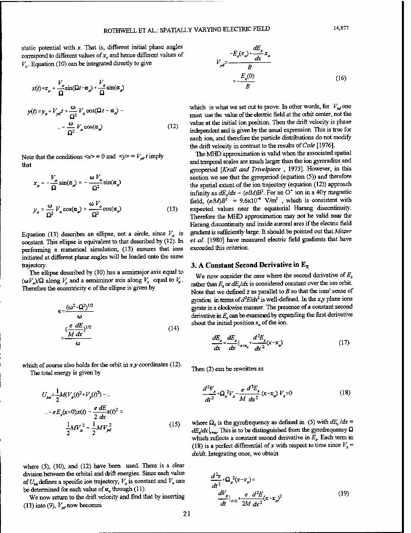
ROTHWELL ET AL.: SPATIALLY VARYING ELECTRIC FIELD 14,877
static potential with x. That is, different initial phase angles correspond to different values of x0 and hence different values of V0. Equation (10) can be integrated directly to give
V va x(t)=xo + -gsmfpt-a} + — sinCa^
V
dEx
-E*^-d7x° B
_ * (°) B
(16)
a) X') =ya *VJ+—, vo ^C0' - a*>
Q2
(0
Ö2 ^««(og (12)
Note that the conditions <x> = 0 and <y> = V^ t imply that
V coK x^-^sin^-^sü*«,)
(0 o>K_ y = — K cos(aJ = cos(aJ
° Q2 Q2 (13)
Equation (13) describes an ellipse, not a circle, since Va is constant. This ellipse is equivalent to that described by (12). In performing a numerical simulation, (13) ensures that ions initiated at different phase angles will be loaded onto the same trajectory.
The ellipse described by (10) has a semimajor axis equal to (<aVa)/Q along Vy and a serniminor axis along Vx equal to Va. Therefore the eccentricity e of the ellipse is given by
(a)2-Q2),/2
to
( e dEya Mdx
(14)
0)
which is what we set out to prove. In other words, for V^ one must use the value of the electric field at the orbit center, not the value at the initial ion position. Then the drift velocity is phase independent and is given by the usual expression. This is true for each ion, and therefore the particle distributions do not modify the drift velocity in contrast to the results of Cole [1976].
The MHD approximation is valid when the associated spatial and temporal scales are much larger than the ion gyroradius and gyroperiod [Krall and Trivelpiece , 1973]. However, in this section we see that the gyroperiod (equation (5)) and therefore the spatial extent of the ion trajectory (equation (12)) approach infinity as dEJdx - (e/MjB2. For an 0+ ion in a 40y magnetic field, (e/M)B2 = 9.6xlO"9 V/m2 , which is consistent with expected values near the equatorial Harang discontinuity. Therefore the MHD approximation may not be valid near the Harang discontinuity and inside auroral arcs if the electric field gradient is sufficiently large. It should be pointed out that Mozer et al. [1980] have measured electric field gradients that have exceeded this criterion.
3. A Constant Second Derivative in Ex
We now consider the case where the second derivative of Ex
rather than Ex or dEJdx is considered constant over the ion orbit. Note that we defined z as parallel to B so that the ions' sense of gyration in terms ofd'E/dx2 is well-defined. In the xy plane ions gyrate in a clockwise manner. The presence of a constant second derivative in Ex can be examined by expanding the first derivative about the initial position x0 of the ion.
dx dx lx=x< dx2 (17)
which of course also holds for the orbit in xy coordinates (12). The total energy is given by
Then (2) can be rewritten as
U^MiVßf-VÄfh-
-eE(x=0)x(f)-^x(.if- 2dx
.MV} + -MV yd (15)
where (5), (10), and (12) have been used. There is a clear division between the orbital and drift energies. Since each value of Uu defines a specific ion trajectory, Va is constant and V0 can be determined for each value of a„ through (11).
We now return to the drift velocity and find that by inserting (13) into (9), V^novf becomes
d2Vx
IF &?V- ed2Et
Mdx2 ' x (18)
where Qo is the gyroftequency as defined in (5) with dE,. /dx = dEJdx [_„,. This is to be distinguished from the gyrofrequency Q which reflects a constant second derivative in Ex. Each term in (18) is a perfect differential of x with respect to time since Vx = dxldt. Integrating once, we obtain
$+Q'2(X"'Vo)
l/=o dt
e d2E
2Mdx2 (x-xf (19)
21
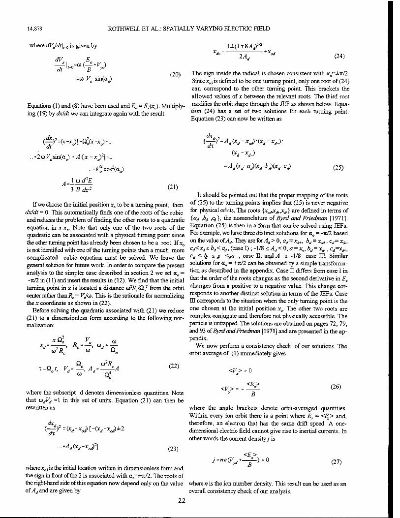
14,878 ROTHWELL ET AL.: SPATIALLY VARYING ELECTRIC FIELD
where dVJdtl^ is given by
dV X
It =co(_£
=co Vo sinCa^ (20)
Equations (1) and (8) have been used and E0 = EJxJ. Multiply- ing (19) by dxldt we can integrate again with the result
1 ±(1+8,4/
2A~, *-od (24)
The sign inside the radical is chosen consistent with a0=±it/2. Since x^is defined to be one turning point, only one root of (24) can correspond to the other turning point. This brackets the allowed values of x between the relevant roots. The third root modifies the orbit shape through the JEF as shown below. Equa- tion (24) has a set of two solutions for each turning point. Equation (23) can now be written as
(f)2=(X"*o)[~Q°(X~*o)+" *-2G>F sin(a ^ +A (x -xj2i+..
..+F02ccs2(cg
Iurf2£ A=-
IBdx2 (21)
If we choose the initial position x0 to be a turning point, then dxldt = 0. This automatically finds one of the roots of the cubic and reduces the problem of finding the other roots to a quadratic equation in x-x0. Note that only one of the two roots of the quadratic can be associated with a physical turning point since the other turning point has already been chosen to be a root. If x0
is not identified with one of the turning points then a much more complicated cubic equation must be solved. We leave the general solution for future work. In order to compare the present analysis to the simpler case described in section 2 we set a0 = -7i/2 in (11) and insert the results in (12). We find that the initial turning point in x is located a distance <ö
2RJQ0
2 from the orbit
center rather than/?,. = VJu>. This is the rationale for normalizing the x coordinate as shown in (22).
Before solving the quadratic associated with (21) we reduce (21) to a dimensionless form according to the following nor- malization:
u2R CO
Q d CO d
CO
<o2R -Z-A (22)
Q:
where the subscript d denotes dimensionless quantities. Note that u>dVd =1 in this set of units. Equation (21) can then be rewritten as
dx A2. ^r-(xd-xj[<xd-xj±2
■■^d{xd-xJ^ (23)
where x^is the initial location written in dimensionless form and the sign in front of the 2 is associated with a0=±n/2. The roots of the right-hand side of this equation now depend only on the value of Ad and are given by
22
(25)
It should be pointed out that the proper mapping of the roots of (25) to the turning points implies that (25) is never negative for physical orbits. The roots {x^^j} are defined in terms of {ad ,bd ,q,}, the nomenclature of Byrd and Friedman [1971]. Equation (25) is then in a form that can be solved using JEFs. For example, we have three distinct solutions for a0 = -7t/2 based on the value ofAd. They are for 4, > 0, ad = xd+, bd = xod,cd= x^, cd<xd<. bd<ad, (case I) ; -1/8 * Ad<0,a = xo, bd = xd., cd=x^, cd < b/ if <da , case II; arjd A <. -1/8 case III. Similar solutions for a0 = +jt/2 can be obtained by a simple transforma- tion as described in the appendix. Case II differs from case I in that the order of the roots changes as the second derivative in Ex
changes from a positive to a negative value. This change cor- responds to another distinct solution in terms of the JEFs. Case HI corresponds to the situation when the only turning point is the one chosen at the initial position x0. The other two roots are complex conjugate and therefore not physically accessible. The particle is untrapped The solutions are obtained on pages 72, 79, and 93 of Byrd and Friedman [1971] and are presented in the ap- pendix.
We now perform a consistency check of our solutions. The orbit average of (1) immediately gives
<V>=0 X
<E> <V>
y (26)
B
where the angle brackets denote orbit-averaged quantities. Within every ion orbit there is a point where Ex = <Et> and, therefore, an electron that has the same drift speed. A one- dimensional electric field cannot give rise to inertial currents. In other words the current density/' is
<E> (27)
where n is the ion number density. This result can be used as an overall consistency check of our analysis.
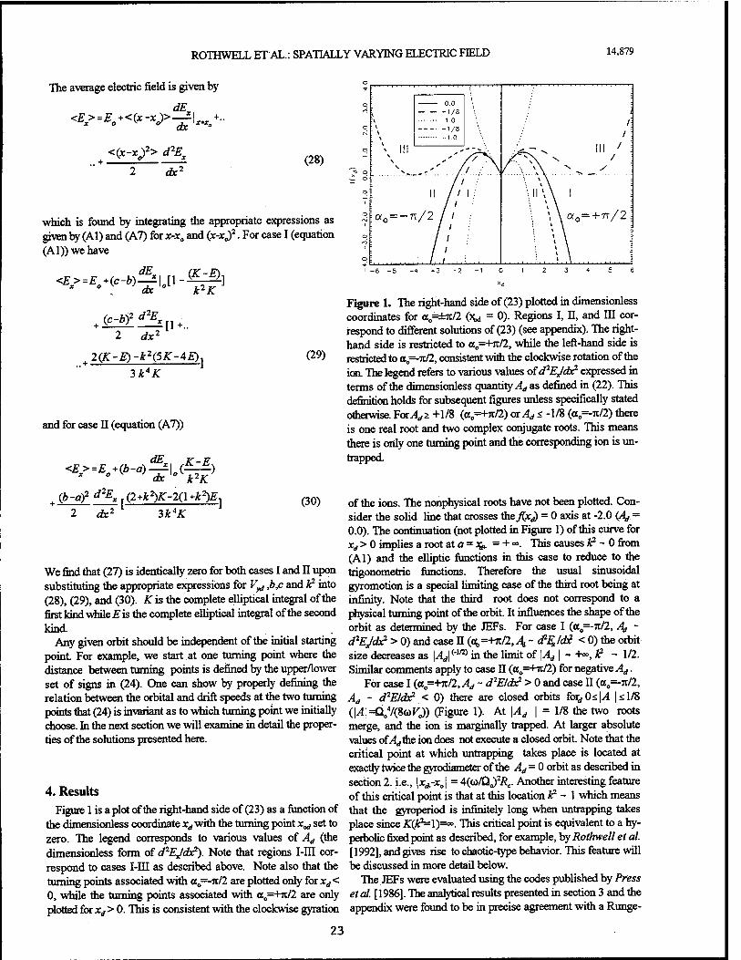
ROTHWELL ET AL.: SPATIALLY VARYING ELECTRIC FIELD 14,879
The average electric field is given by
<E>=E0+<(x-x}>-£\x=Xc+..
<(x-xf> d%
"+ 2 ~dxT (28)
which is found by integrating the appropriate expressions as given by (Al) and (A7) for x-x0 and (x-xj2 ■ For case I (equation (Al)) we have
El dx
(K-E) <E>=E +(c-6)—-I [1
(c-bf d%
k2K
2 dx2
1-2,
[1
; 2(K-E)-k2(5K-AE),
3k4K
and for case II (equation (A7))
dE, K-E
(fe-a)2 d% (2^2)^-2(l^2)£1
2 dx2 3k4K
(29)
(30)
We find that (27) is identically zero for both cases I and II upon substituting the appropriate expressions for V^ ,b,c and k2 into (28), (29), and (30). K is the complete elliptical integral of the first kind while £ is the complete elliptical integral of the second kind.
Any given orbit should be independent of the initial starting point For example, we start at one turning point where the distance between turning points is defined by the upper/lower set of signs in (24). One can show by properly defining the relation between the orbital and drift speeds at the two turning points that (24) is invariant as to which turning point we initially choose. In the next section we will examine in detail the proper- ties of the solutions presented here.
■* • ' :
o 0.0 : rO : +1/8 /
■ \ 1.0 /; q ■ \ \
-1/8 -1.0 / :
III ' ] o : V III ^ -~iA *~ \ '' /'A y ^ >. N /
o \
.,''' /'. ■■.'..>
/ \ \ '■.... ,\ y ^ y
>s _- o // : q II // 1 . \ll\ \ ' J ' / ' \ j o \a0=-n/2 / / ; ': \ a0=+7r/2i 1
/ ' t \ 1 \
o \ \ IO \ \ '. ' / '
\ \ q /, / , 1 . , \ \
4. Results
Figure 1 is a plot of the right-hand side of (23) as a function of the dimensionless coordinate xd with the turning point x^ set to zero. The legend corresponds to various values of Ad (the dimensionless form of d}EJd£). Note that regions I-III cor- respond to cases I-III as described above. Note also that the turning points associated with a0=-ir/2 are plotted only for xd< 0, while the turning points associated with a0=-Hi/2 are only plotted for xd > 0. This is consistent with the clockwise gyration
23
Figure 1. The right-hand side of (23) plotted in dimensionless coordinates for a0=±it/2 (x^ = 0). Regions I, II, and HI cor- respond to different solutions of (23) (see appendix). The right- hand side is restricted to a0=-ht/2, while the left-hand side is restricted to a=-iz/2, consistent with the clockwise rotation of the ion The legend refers to various values of d^Jdx2 expressed in terms of the dimensionless quantity^ as defined in (22). This definition holds for subsequent figures unless specifically stated otherwise. For4,:> +1/8 (a=+n/2) orAd s -1/8 (a0=-7i/2) there is one real root and two complex conjugate roots. This means there is only one turning point and the corresponding ion is un- tapped.
of the ions. The nonphysical roots have not been plotted. Con- sider the solid line that crosses üießxj = 0 axis at -2.0 (4/ = 0.0). The continuation (not plotted in Figure 1) of this curve for xrf>0impliesarootata = ^. = + <*>. This causes k2 - 0 from (Al) and the elliptic functions in this case to reduce to the trigonometric functions. Therefore the usual sinusoidal gyromotion is a special limiting case of the third root being at infinity. Note that the third root does not correspond to a physical turning point of the orbit. It influences the shape of the orbit as determined by the JEFs. For case I (a0=-Ti/2, Aj ~ d2EJ<b? > 0) and case H (c^+Jt/2,4, ~ #%!<& < 0) the orbit size decreases as |^4d|('lß) in the limit of \Ad \ - +», # - 1/2. Similar comments apply to case II (a0=+rc/2) for negative Ad.
For case I (a„=-Hr/2, Ad - d2E/dx? > 0 and case II (a0=-it/2, Ad ~ d^Eldx2 < 0) there are closed orbits fbfcOspl | rs 1/8 (\A\=Q0
4/(ßti>Vj) (Figure 1). At \Ad | = 1/8 the two roots merge, and the ion is marginally tapped. At larger absolute values oL4rfthe ion does not execute a closed orbit. Note that the critical point at which untrapping takes place is located at exactly twice the gyrodiameter of the Ad = 0 orbit as described in section 2. i.e., Ix^-xJ = 4(u/ü0)2Ä<.. Another interesting feature of this critical point is that at this location k? - 1 which means that the gyroperiod is infinitely long when untrapping takes place since K(k2=l)=<^. This critical point is equivalent to a hy- perbolic fixed point as described, for example, by Rothwell et al. [1992], and gives rise to chaotic-type behavior. This feature will be discussed in more detail below.
The JEFs were evaluated using the codes published by Press et cd. [1986]. The analytical results presented in section 3 and the appendix were found to be in precise agreement with a Runge-
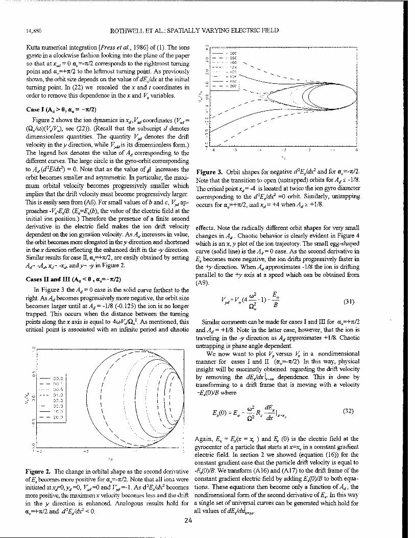
14,880 ROTHWELL ET AL.: SPATIALLY VARYING ELECTRIC FIELD
Kutta numerical integration [Press et al, 1986] of (1). The ions gyrate in a clockwise fashion looking into the plane of the paper so that at x^ - 0 a0=-7t/2 corresponds to the rightmost turning point and a0=+rc/2 to the leftmost turning point. As previously shown, the orbit size depends on the value ofdEJdx at the initial turning point. In (22) we rescaled the x and / coordinates in order to remove this dependence in the x and Vx variables.
Case I (Ad > 0, a„ = -7t/2)
Figure 2 shows the ion dynamics in Xj^^ coordinates (V^,— (Q,JiS){VJVX see (22)). (Recall that the subscript d denotes dimensionless quantities. The quantity V^ denotes the drift velocity in they direction, while F^is its dimensionless form.) The legend box denotes the value of Ad corresponding to the different curves. The large circle is the gyro-orbit corresponding to Ad (d2E/dx2) = 0. Note that as the value of A increases the orbit becomes smaller and asymmetric. In particular, the maxi- mum orbital velocity becomes progressively smaller which implies that the drift velocity must become progressively larger. This is easily seen from (A6). For small values of b and c, V^ ap-
proaches -V-EJB. (E=Ex(b), the value of the electric field at the initial ion position.) Therefore the presence of a finite second derivative in the electric field makes the ion drift velocity dependent on the ion gyration velocity. As Ad increases in value, the orbit becomes more elongated in they direction and shortened in the x direction reflecting the enhanced drift in the -y direction. Similar results for case II, a0=+7i/2, are easily obtained by setting Ad- -A* xr -Xj, andy- -y in Figure 2.
Cases II and III (Ad < 0 , o =-rc/2)
In Figure 3 the Ad = 0 case is the solid curve farthest to the right As Ad becomes progressively more negative, the orbit size becomes larger until at Ad = -1/8 (-0.125) the ion is no longer trapped. This occurs when the distance between the turning points along the x axis is equal to 4wK0/Q0
2. As mentioned, this critical point is associated with an infinite period and chaotic
Figure 3. Orbit shapes for negative d2EJdx2 and for a0=-n/2. Note that the transition to open (untrapped) orbits forAd < -1/8. The critical point xd= -4 is located at twice the ion gyro diameter corresponding to the d^EJdx2 =0 orbit. Similarly, untrapping occurs for a=+n/2, and xd = +4 when Ad s. +1/8.
effects. Note the radically different orbit shapes for very small changes in Ad . Chaotic behavior is clearly evident in Figure 4 which is an x,y plot of the ion trajectory. The small egg-shaped curve (solid line) is the^rf= 0 case. As the second derivative in Ex becomes more negative, the ion drifts progressively faster in the +y direction. When Ad approximates -1/8 the ion is drifting parallel to the +y axis at a speed which can be obtained from (A9).
or V .= V (4 —-1)-
B (31)
Similar comments can be made for cases I and III for a0=+7t/2 and Ad = +1/8. Note in the latter case, however, that the ion is traveling in the -y direction as Ad approximates +1/8. Chaotic untrapping is phase angle dependent.
We now want to plot Vy versus Vx in a nondimensional manner for cases I and II (a0=-Tt/2). In this way, physical insight will be succinctly obtained regarding the drift velocity by removing the dEJdx\.=X0 dependence. This is done by transforming to a drift frame that is moving with a velocity -Ex(0)/B where
EM E --R ° Q2 dx
(32)
Figure 2. The change in orbital shape as the second derivative of Ex becomes more positive for a0=-n/2. Note that all ions were initiated at.r/O,yrf=0, F^=0 and Vyd=-\. As d2EJdx2 becomes more positive, the maximum x velocity becomes less and the drift in the y direction is enhanced. Analogous results hold for a=+Tzll and d2EJdx2 < 0.
24
Again, E0 = Ex(x = % ) and 2£ (0) is the electric field at the gyrocenter of a particle that starts at x=x0 in a constant gradient electric field. In section 2 we showed (equation (16)) for the constant gradient case that the particle drift velocity is equal to -EJS>)IB. We transform (A16) and (A17) to the drift frame of the constant gradient electric field by adding Ex(0)/B to both equa- tions. These equations then become only a function of Ad, the nondimensional form of the second derivative of is,.. In this way a single set of universal curves can be generated which hold for all values of dEJdx\.=xo.
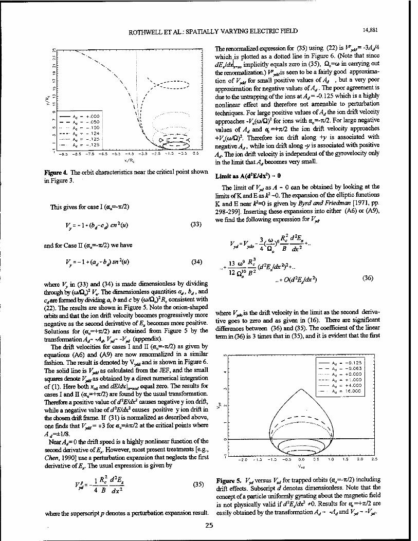
ROTHWELL ET AL.: SPATIALLY VARYING ELECTRIC FIELD 14,881
' -9.5 -8.5 -7.5 -6.5 -5.5 -4.5 -3.5 -2.5 -1.5 -0.5 0.5
x/Rc
Figure 4. The orbit characteristics near the critical point shown in Figure 3.
This gives for case I (a0=-it/2)
Vy=-\+(pd-c)cn\u)
and for Case II (a0=-Tc/2) we have
V=-\+{a4-b)sn\v)
(33)
(34)
where Vy in (33) and (34) is made dimensionless by dividing through by (w/Qo)2 V„. The dimensionless quantities ad, bd, and crfare formed by dividing a, b and c by (u>IQ^2Rc consistent with (22). The results are shown in Figure 5. Note the onion-shaped orbits and that the ion drift velocity becomes progressively more negative as the second derivative of Ex becomes more positive. Solutions for (a0=+rc/2) are obtained from Figure 5 by the transformation 4,- -A* V^- -V^ (appendix).
The drift velocities for cases I and II (a—nil) as given by equations (A6) and (A9) are now renormalized in a similar fashion. The result is denoted by V^ and is shown in Figure 6. The solid line is V^ as calculated from the JEF, and the small squares denote V^ as obtained by a direct numerical integration of (1). Here both x«, and dEldx\x=tad equal zero. The results for cases I and II (a0=+it/2) are found by the usual transformation. Therefore a positive value of dPEIdb? causes negative y ion drift, while a negative value of d2E/dx? causes positive y ion drift in the chosen drift frame. If (31) is normalized as described above, one finds that Vydd= * 3 for a0=±ir/2 at the critical points where Ad=±l/S.
Near 4,= 0 the drift speed is a highly nonlinear function of the second derivative of Er However, most present treatments [e.g., Chen, 1990] use a perturbation expansion that neglects the first derivative of Ev The usual expression is given by
The renormalized expression for (35) using (22) is F^= -3^y4 which is plotted as a dotted line in Figure 6. (Note that since dEjMxm„ implicitly equals zero in (35), £L,=o> in carrying out the renormalization) V^is seen to be a fairly good approxima- tion of Vyx for small positive values of Ad , but a very poor approximation for negative values of Ad. The poor agreement is due to the untrapping of the ions at Ad = -0.125 which is a highly nonlinear effect and therefore not amenable to perturbation techniques. For large positive values of Ad the ion drift velocity approaches -VJa/Qf for ions with a0=-it/2. For large negative values of Ad and <£ =+n/2 the ion drift velocity approaches +F0(G)/Q)2. Therefore ion drift along +y is associated with negative Ad, while ion drift along -y is associated with positive Ad. The ion drift velocity is independent of the gyrovelociry only in the limit that Ad becomes very small.
Limit as A(d2E/dx2)-0
The limit of V^ as A - 0 can be obtained by looking at the limits of K and E as A2 -0. The expansion of the elliptic functions K and E near P=0 is given by Byrd and Friedman [1971, pp. 298-299]. Inserting these expansions into either (A6) or (A9), we find the following expression for V^
v*r y^-^ri .Rld2E_
ydo 4 Q ' B dx7
R^.h(d2E/dx^.. l2tf°B2
.. + 0(d2EJdx2) (36)
where V^ is the drift velocity in the limit as the second deriva- tive goes to zero and as given in (16). There are significant differences between (36) and (35). The coefficient of the linear term in (36) is 3 times that in (35), and it is evident that the first
vk 1 *c d%
4 B dx2 (35)
Figure 5. V^ versus V^ for trapped orbits (o0=-it/2) including drift effects. Subscript d denotes dimensionless. Note that the concept of a particle uniformly gyrating about the magnetic field is not physically valid if d^EJdx2 *0. Results for oi=-hi/2 are
where the superscript/? denotes a perturbation expansion result, easily obtained by the transformation Ad - -Ad and V^ - -V^.
25
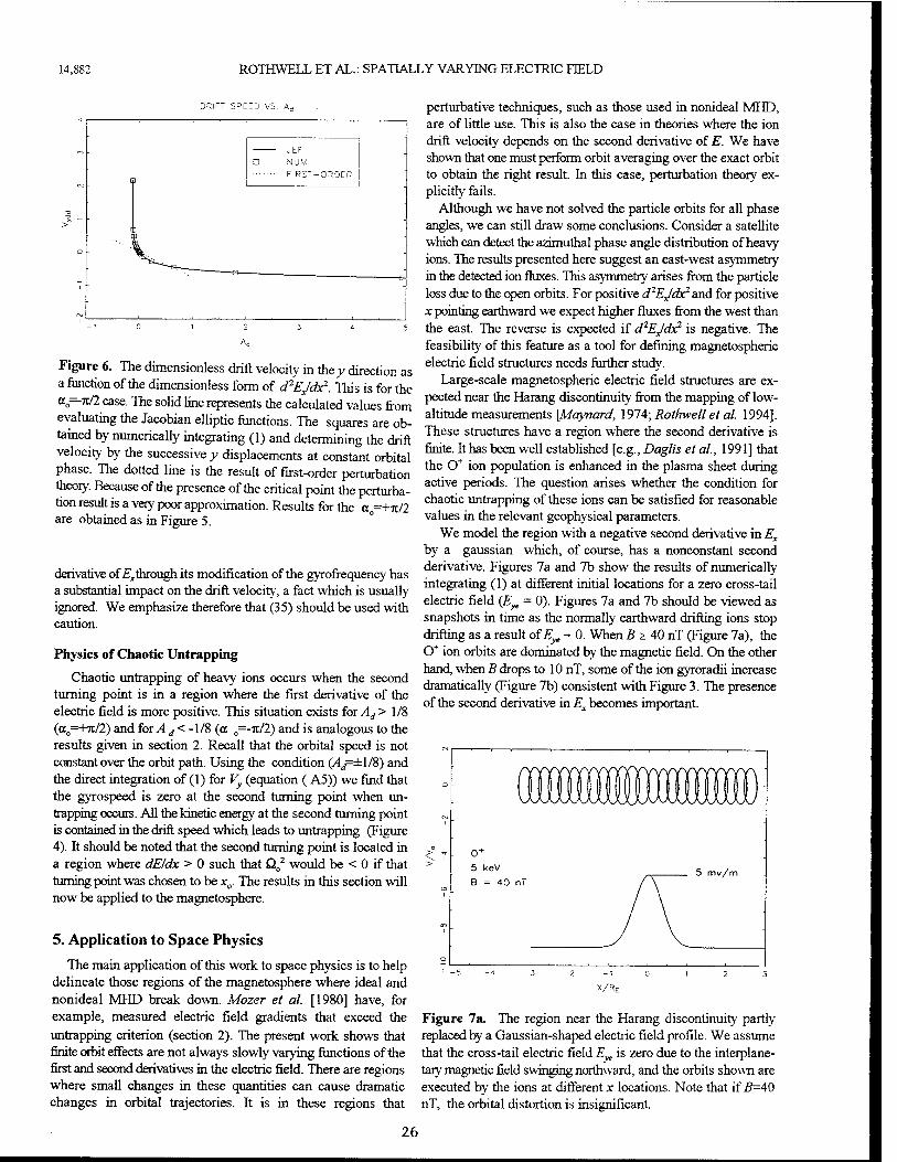
14,882 ROTHWELL ET AL.: SPATIALLY VARYING ELECTRIC FIELD
DRIFT SPEED VS. Ae
JEF a NUM
9 FIRST -ORDER
i: -
- -
Figure 6. The dimensionless drift velocity in the y direction as a function of the dimensionless form of d2EJd£. Tins is for the a =-JC/2 case. The solid line represents the calculated values from evaluating the Jacobian elliptic functions. The squares are ob- tained by numerically integrating (1) and determining the drift velocity by the successive y displacements at constant orbital phase. The dotted line is the result of first-order perturbation theory. Because of the presence of the critical point the perturba- tion result is a very poor approximation. Results for the a0=+Tr/2 are obtained as in Figure 5.
derivative of £x through its modification of the gyrofrequency has a substantial impact on the drift velocity, a fact which is usually ignored. We emphasize therefore that (35) should be used with caution.
Physics of Chaotic Untrapping
Chaotic untrapping of heavy ions occurs when the second turning point is in a region where the first derivative of the electric field is more positive. This situation exists for Ad > 1/8 (a0=+7t/2) and for ^4 d < -1/8 (a 0=-7c/2) and is analogous to the results given in section 2. Recall that the orbital speed is not constant over the orbit path. Using the condition (Ad=±l/S) and the direct integration of (1) for Vy (equation ( A5)) we find that the gyrospeed is zero at the second turning point when un- trapping occurs. All the kinetic energy at the second turning point is contained in the drift speed which leads to untrapping (Figure 4). It should be noted that the second turning point is located in a region where dEldx > 0 such that Q0
2 would be < 0 if that turning point was chosen to be x0. The results in this section will now be applied to the magnetosphere.
5. Application to Space Physics
The main application of this work to space physics is to help delineate those regions of the magnetosphere where ideal and nonideal MHD break down. Mozer et al. [1980] have, for example, measured electric field gradients that exceed the
untrapping criterion (section 2). The present work shows that finite orbit effects are not always slowly varying functions of the first and second derivatives in the electric field. There are regions where small changes in these quantities can cause dramatic changes in orbital trajectories. It is in these regions that
perturbative techniques, such as those used in nonideal MHD, are of little use. This is also the case in theories where the ion drift velocity depends on the second derivative of E. We have shown that one must perform orbit averaging over the exact orbit to obtain the right result. In this case, perturbation theory ex- plicitly fails.
Although we have not solved the particle orbits for all phase angles, we can still draw some conclusions. Consider a satellite which can detect the azimuthal phase angle distribution of heavy ions. The results presented here suggest an east-west asymmetry in the detected ion fluxes. This asymmetry arises from the particle loss due to the open orbits. For positive d2EJdy? and for positive x pointing earthward we expect higher fluxes from the west than the east. The reverse is expected if d2EJdx2 is negative. The feasibility of this feature as a tool for defining magnetospheric electric field structures needs further study.
Large-scale magnetospheric electric field structures are ex- pected near the Harang discontinuity from the mapping of low- altitude measurements [Maynard, 1974; Rothwell et al. 1994]. These structures have a region where the second derivative is finite. It has been well established [e.g., Daglis et al., 1991] that the 0+ ion population is enhanced in the plasma sheet during active periods. The question arises whether the condition for chaotic untrapping of these ions can be satisfied for reasonable values in the relevant geophysical parameters.
We model the region with a negative second derivative in Ex
by a gaussian which, of course, has a nonconstant second derivative. Figures 7a and 7b show the results of numerically integrating (1) at different initial locations for a zero cross-tail electric field (£ = 0). Figures 7a and 7b should be viewed as snapshots in time as the normally earthward drifting ions stop drifting as a result of E^ - 0. When B 2. 40 nT (Figure 7a), the 0+ ion orbits are dominated by the magnetic field. On the other hand, when B drops to 10 nT, some of the ion gyroradii increase dramatically (Figure 7b) consistent with Figure 3. The presence of the second derivative in Ex becomes important.
o+
5 keV
B = 40 nT 5 mv/m
x/RE
Figure 7a. The region near the Harang discontinuity partly replaced by a Gaussian-shaped electric field profile. We assume that the cross-tail electric field E is zero due to the interplane- tary magnetic field swinging northward, and the orbits shown are executed by the ions at different x locations. Note that if 5=40 nT, the orbital distortion is insignificant.
26
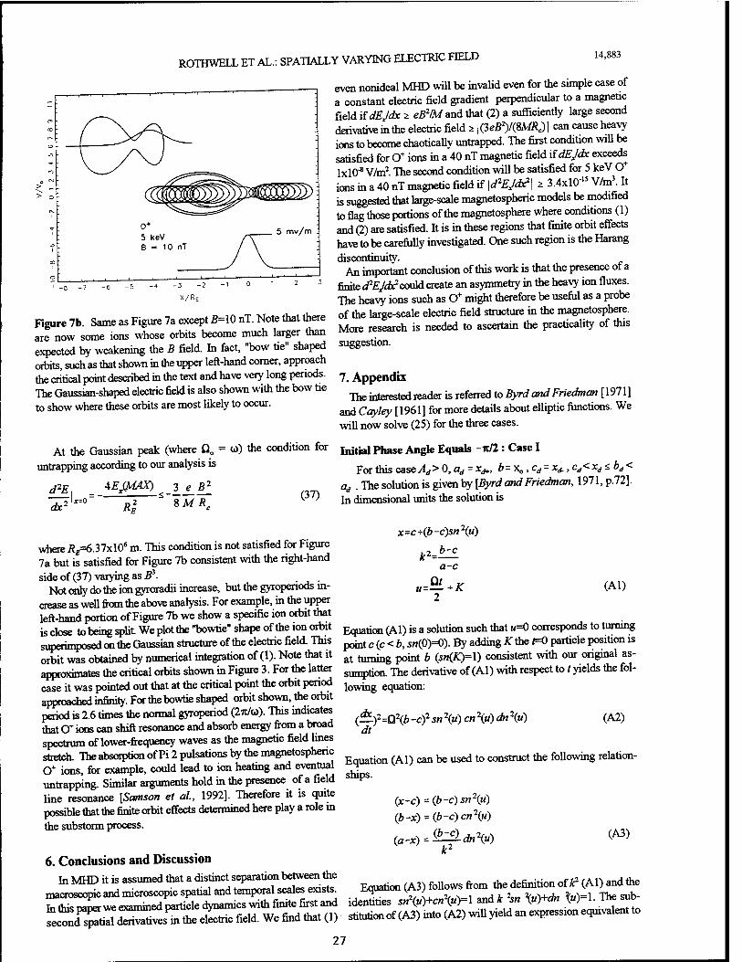
ROTHWELL ET AL.: SPATIALLY VARYING ELECTRIC FIELD 14,883
Figure 7b. Same as Figure 7a except 5=10 nT. Note that there are now some ions whose orbits become much larger than expected by weakening the B field. In fact, "bow tie" shaped orbits, such as that shown in the upper left-hand comer, approach the critical point described in the text and have very long periods. The Gaussian-shaped electric field is also shown with the bow tie to show where these orbits are most likely to occur.
At the Gaussian peak (where Q0 = o>) the condition for untrapping according to our analysis is
e B'< d2Ef 4EX(MAX) _3
dx- lx=0"
Ri (37)
even nonideal MHD will be invalid even for the simple case of a constant electric field gradient perpendicular to a magnetic field if dEJdx ;> eB2/M and that (2) a sufficiently large second derivative in the electric field * | (3aB*)/(8MJy | can cause heavy ions to become chaotically untrapped. The first condition will be satisfied for 0+ ions in a 40 nT magnetic field if dEJdx exceeds lxlO"8 V/m2 The second condition will be satisfied for 5 keV 0+
ions in a 40 nT magnetic field if \d2EJcb?\ * 3.4xl0"15 V/m\ It is suggested that large-scale magnetospheric models be modified to flag those portions of the magnetosphere where conditions (1) and (2) are satisfied. It is in these regions that finite orbit effects have to be carefully investigated. One such region is the Harang discontinuity.
An important conclusion of this work is that the presence of a finite (fEJdfcmAd create an asymmetry in the heavy ion fluxes. The heavy ions such as 0+ might therefore be useful as a probe of the large-scale electric field structure in the magnetosphere. More research is needed to ascertain the practicality of this suggestion.
7. Appendix The interested reader is referred to Byrd and Friedman [1971]
and Cayley [1961] for more details about elliptic functions. We will now solve (25) for the three cases.
Initial Phase Angle Equals -ir/2 : Case I
For this case^rf> 0,ad = xd+, b=\0,cd = xd., cd< xd<bd< ad . The solution is given by [Byrd and Friedman, 1971, p.72]. In dimensional units the solution is
where ģ=6.37xl06 m. This condition is not satisfied for Figure 7a but is satisfied for Figure 7b consistent with the right-hand side of (37) varying as B3.
Not only do the ion gyroradii increase, but the gyroperiods in- crease as well fiom the above analysis. For example, in the upper left-hand portion of Figure 7b we show a specific ion orbit that is close to being split We plot the "bowtie" shape of the ion orbit superimposed on the Gaussian structure of the electric field. This orbit was obtained by numerical integration of (1). Note that it approximates the critical orbits shown in Figure 3. For the latter case it was pointed out that at the critical point the orbit period approached infinity. For the bowtie shaped orbit shown, the orbit period is 2.6 times the normal gyroperiod (2it/o). This indicates that 0+ ions can shift resonance and absorb energy from a broad spectrum of lower-frequency waves as the magnetic field lines stretch The absorption of Pi 2 pulsations by the magnetospheric 0+ ions, for example, could lead to ion heating and eventual untrapping. Similar arguments hold in the presence of a field line resonance [Samson et al., 1992]. Therefore it is quite possible that the finite orbit effects determined here play a role in the substorm process.
6. Conclusions and Discussion In MHD it is assumed that a distinct separation between the
macroscopic and microscopic spatial and temporal scales exists. In this paper we examined particle dynamics with finite first and second spatial derivatives in the electric field. We find that (1)
x=c+(b-c)sn2(u)
t2. b~C
a-c
2 (Al)
Equation (Al) is a solution such that u=0 corresponds to turning point c (c < b, s«(0)=0). By adding K the f=0 particle position is at turning point b (sn(K)=l) consistent with our original as- sumption. The derivative of (Al) with respect to t yields the fol- lowing equation:
(^)2=Q2(*-c)2 sn\u) cn\u) dn\u) dt
(A2)
Equation (Al) can be used to construct the following relation- ships.
(x-c) = (b-c)sn\u)
(b-x) = (b-c)cn\u)
(a-x) (b-c) dn\u) (A3)
Equation (A3) follows from the definition of ft2 (Al) and the identities sn\ü)+cn\u)=\ and* 2sw \u)+dn fy)=l. The sub- stitution of (A3) into (A2) will yield an expression equivalent to
27
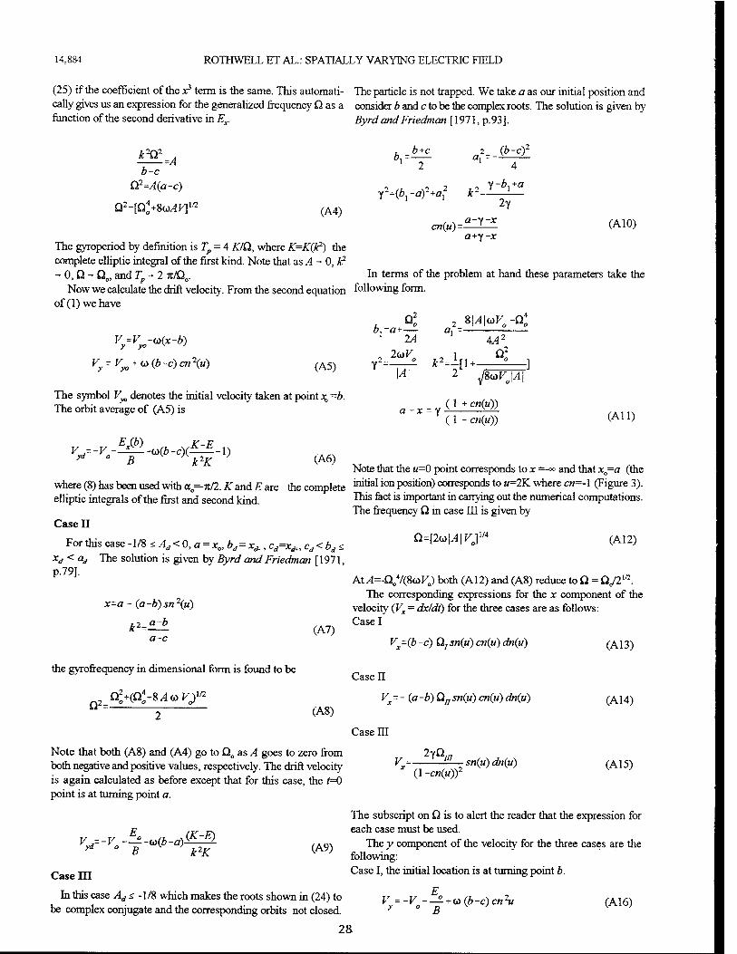
14,884 ROTHWELL ET AL.: SPATIALLY VARYING ELECTRIC FIELD
(25) if the coefficient of the x3 term is the same. This automati- The particle is not trapped. We take a as our initial position and cally gives us an expression for the generalized frequency Q as a consider b and c to be the complex roots. The solution is given by function of the second derivative in Ex. Byrd and Friedman [1971, p.93].
k2®2 . -A b-c
Q2=A(a-c)
Q2=[QA0+SwAV]m (A4)
(A10) a+y-x
The gyroperiod by definition is Tp = 4 KIÜ, where K^Kik2) the complete elliptic integral of the first kind. Note that as A - 0, k2
- 0, Q - Q0, and T - 2 TC/Q . In terms of the problem at hand these parameters take the Now we calculate the drift velocity. From the second equation following form.
of(l) we have
Q2 2 &\A\aVe-Q40
b. =a+— <3, = V=V -a>(x-b) 2A AA2
y *° 2uV i Q2
V^V^ + oQ-dicnW (A5) y2=—rf k^U , ° -1
V b+c
~2~ 2 _ (b-c)2
4
=(*. -a)2 2 ffll k2 =
y-b{+a
2Y
cn(u)= a-y -x
The symbol V^ denotes the initial velocity taken at point JJ =b. The orbit average of (A5) is a - x = y <■* + cnW>
Ml 2 fiu>Vo\A\
( 1 + cn(u)) (\-cn(u)) (A11>
£*(£,) ,. „K-E -—-o(6-c)( .. ., ,N 5 A:2^ CA6) V-^-^-^-^^e-i)
Note that the «=0 point corresponds to x =-«> and that x0=a (the where (8) has been used with a0=-n/2. K and E are the complete initial ion P°sition) corresponds to «=2K where cw=-l (Figure 3). elliptic integrals of the first and second kind. lhis fact ^ important in carrying out the numerical computations.
The frequency Q in case III is given by Case II
Forthiscase-l/S^^O^^^^x^c^c^^, ^[AWf* (A12) xd < ad The solution is given by Byrd and Friedman [1971, p.79].
At/1=-Q04/(8G>*''0) both (Al2) and (A8) reduce to Q = QJ2m.
The corresponding expressions for the x component of the x=a - (a-b) sn (w) velocity (Vx = dxldt) for the three cases are as follows:
,-, a-b Case I k2= (A7)
a-c vx=(b -c) ü7sn(u) cn(u) dn(u) (Al3)
the gyrofrequency in dimensional form is found to be
Q
Case II
Q2+(Q<+8,4 (o Vyn V = - (a-b) Qnsn(u) cn(u) dn(u) (A14)
(A8)
Case m
g ,„. r^ each case must be used.
Note that both (A8) and (A4) go to Q0 as A goes to zero from 2Y^OT
both negative and positive values, respectively. The drift velocity *=~7T"_ ~~TJ sn^> "w(") (A 15) is again calculated as before except that for this case, the /=0 point is at turning point a.
The subscript on Q is to alert the reader that the expression for
SK~E)
* K following: Case III ^ase *' me initial location is at turning point b.
In this case Ad<, -1/8 which makes the roots shown in (24) to V =-V - — +a(b-c)cn2u (A\6) be complex conjugate and the corresponding orbits not closed. y ° B
28
Vyd~ " ^o " ~ _0)(* ~a)—-— (A9) The y component of the velocity for the three cases are the
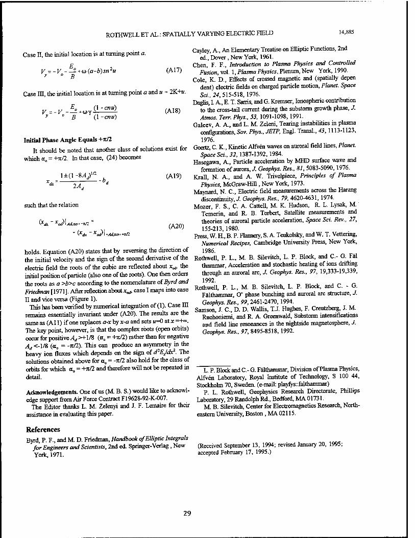
ROTHWELL ET AL.: SPATIALLY VARYING ELECTRIC FIELD 14,885
Case II, the initial location is at turning point a.
V =-V - — +<i>(a-b)sn2u y ° B
Case III, the initial location is at turning point a and u - 2K+«.
(A18) , E0 (1 +cnu) V =-V - —+ü>Y- - y ° B (1 -cnu)
Initial Phase Angle Equals +u/2
It should be noted that another class of solutions exist for which a0 =-Hi/2. In that case, (24) becomes
\±{\-%A$a
x, = —+ b. 2Ad
such that the relation
(xd± " Xod>^Aiao---nn. '
~ (Xfc ~ xaj)\ -Ad,ao=-m/2
holds. Equation (A20) states that by reversing the direction of the initial velocity and the sign of the second derivative of the electric field the roots of the cubic are reflected about x^, the initial position of particle (also one of the roots). One then orders the roots as a >b>c according to the nomenclature of Byrd and Friedman [ 1971 ]. After reflection about x^ case I maps into case n and vice versa (Figure 1).
This has been verified by numerical integration of (1). Case III remains essentially invariant under (A20). The results are the same as (Al 1) if one replaces a-x by x-a and sets u=0 at x =+». The key point, however, is that the complex roots (open orbits) occur for positive Ad >+l/8 (cc0 = -Hi/2) rather than for negative Ad <-l/8 (a0 = -rc/2). This can produce an asymmetry in the heavy ion fluxes which depends on the sign ofd^EJdx2. The solutions obtained above for a0 = -7t/2 also hold for the class of orbits for which a0 = +TI/2 and therefore will not be repeated in detail.
Acknowledgements. One of us (M. B. S.) would like to acknowl- edge support from Air Force Contract F19628-92-K-007.
The Editor thanks L. M. Zelenyi and J. F. Lemaire for their assistance in evaluating this paper.
References Byrd, P. F., and M. D. Friedman, Handbook of Elliptic Integrals
for Engineers and Scientists, 2nd ed. Springer-Verlag, New York, 1971.
Cayley, A., An Elementary Treatise on Elliptic Functions, 2nd ed., Dover, New York, 1961.
Chen, F. F., Introduction to Plasma Physics and Controlled (A17) Fusion, vol. I, Plasma Physics, Plenum, New York, 1990.
Cole, K. D., Effects of crossed magnetic and (spatially depen dent) electric fields on charged particle motion, Planet. Space Sei., 24, 515-518,1976.
Daglis, L A, E. T. Sarris, and G. Kremser, Ionospheric contribution to the cross-tail current during the substorm growth phase, J. Atmos. Terr. Phys., 53, 1091-1098,1991.
Galeev, A. A., and L. M. Zeleni, Tearing instabilities in plasma configurations, Sov. Phys., JETP, Engl. Transl., 43,1113-1123, 1976.
Goertz, C. K., Kinetic Alfven waves on auroral field lines, Planet. Space Sei., 32,1387-1392,1984.
Hasegawa, A., Particle acceleration by MHD surface wave and formation of aurora, J. Geophys. Res., 81,5083-5090,1976.
(A19) Krall, N. A., and A. W. Trivelpiece, Principles of Plasma Physics, McGraw-Hill, New York, 1973.
Maynard, N. C, Electric field measurements across the Harang discontinuity, J. Geophys. Res., 79. 4620-4631,1974.
Mozer, F. S., C. A. Cattell, M. K. Hudson, R. L. Lysak, M. Temerin, and R. B. Torbert, Satellite measurements and theories of auroral particle acceleration, Space Sei. Rev., 27,
(A20) 155-213,1980. Press, W. H, B. P. Flannery, S. A Teukolsky, and W. T. Vettenng,
Numerical Recipes, Cambridge University Press, New York, 1986.
Rothwell, P. L., M. B. Silevitch, L. P. Block, and C- G Fäl thammar, Acceleration and stochastic heating of ions drifting through an auroral arc, J. Geophys. Res., 97, 19,333-19,339, 1992.
Rothwell, P. L., M. B. Silevitch, L. P. Block, and C. - G. Fälthammar, O* phase bunching and auroral arc structure, J. Geophys. Res., 99,2461-2470,1994.
Samson, J. C, D. D. Wallis, T.J. Hughes, F. Creutzberg, J. M. Ruohoniemi, and R. A. Greenwald, Substorm intensifications and field line resonances in the nightside magnetosphere, J. Geophys. Res., 97, 8495-8518,1992.
L. P. Block and C- G. Fälthammar, Division of Plasma Physics, Alfven Laboratory, Royal Institute of Technology, S 100 44, Stockholm 70, Sweden, (e-mail: playfys::falthammar)
P. L. Rothwell, Geophysics Research Directorate, Phillips Laboratory, 29 Randolph Rd., Bedford, MA 01731.
M. B. Silevitch, Center for Electromagnetics Research, North- eastern University, Boston, MA 02115.
(Received September 13, 1994; revised January 20, 1995; accepted February 17, 1995.)
29
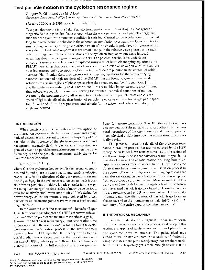
Test particle motion in the cyclotron resonance regime Gregory P. Ginet and Jay M. Albert Geophysics Directorate, Phillips Laboratory, Hanscom Air Force Base, Massachusetts 01731
(Received 20 March 1991; accepted 12 July 1991)
Test particles moving in the field of an electromagnetic wave propagating in a background magnetic field can gain significant energy when the wave parameters and particle energy are such that the cyclotron resonance condition is satisfied. Central to the acceleration process and long time scale periodic behavior is the coherent accumulation over many cyclotron orbits of a small change in energy during each orbit, a result of the circularly polarized component of the wave electric field. Also important is the small change in the relative wave phase during each orbit resulting from relativistic variations of the cyclotron frequency and wave-induced streaming along the background magnetic field. The physical mechanisms underlying cyclotron resonance acceleration are explored using a set of heuristic mapping equations (the PMAP) describing changes in the'particle momentum and relative wave phase. More accurate (but less transparent) descriptions of the particle motion are pursued in the context of orbit- averaged Hamiltonian theory. A discrete set of mapping equations for the slowly varying canonical action and angle are derived (the QMAP) but are found to generate inaccurate solutions in certain regions of phase space when the resonance number / is such that | /1 = 1 and the particles are initially cold. These difficulties are avoided by constructing a continuous time orbit-averaged Hamiltonian and solving the resultant canonical equations of motion. Assuming the momentum is small relative to mc (where m is the particle mass and c is the speed of light), details of the distribution of particle trajectories in the action-angle phase space for | /1 =1 and j / | = 2 are presented and criteria for the existence of orbits oscillatory in angle are derived.
I. INTRODUCTION
When constructing a kinetic-theoretic description of the interaction between an electromagnetic wave and a mag- netized plasma, it is important to know the trajectory of test particles in the presence of the electromagnetic wave and background magnetic field. A particularly interesting re- gime of wave-test particle interaction occurs when the wave frequency a and the particle momentum satisfy the cyclo- tron resonance condition,
co-k:uz - |/|n ~o, (i) where fi is the cyclotron frequency, / is the resonance num- ber, and k, and vz are the wave vector and particle velocity, respectively, in the direction of the background magnetic field B0 = B0 ez. In the cyclotron resonance regime, it is pos- sible for test particles to achieve kinetic energies far in excess of the "quiver energy" on time scales of many wave periods, even for relatively small wave amplitudes.1"7 We define the quiver energy as the maximum energy achieved by a test particle in an electromagnetic wave without a background magnetic field.
In the work of Ginet and Heinemann6 (hereafter Paper I), a Hamiltonian pseudopotential (HPP) theory was devel- oped and used to predict the maximum kinetic energy C/max
(normalized to the rest mass energy) and acceleration time T (normalized to the wave period) resulting from the cyclo- tron resonance acceleration process in the limit of small wave amplitude. Although the HPP theory proves to be a useful predictive tool, as demonstrated by the extensive com- parison of HPP predictions with those obtained from nu- merical solutions of the full equations of motion given in
Paper I, there are limitations. The HPP theory does not pre- dict any details of the particle trajectory other than the tem- poral dependence of the kinetic energy and does not provide much physical insight into how the acceleration process ac- tually works.
This paper addresses the details of the cyclotron reso- nance interaction process that are not covered by the HPP theory. As in Paper I, we restrict ourselves to the regime of small wave amplitude so that particles are not trapped in the troughs of a wave and chaotic motion resulting from over- lapping resonances does not occur. In Sec. II, we discuss the physical mechanism underlying the acceleration process in the context of a set of pedagogical mapping equations that describes the change in particle momentum and wave phase from one cyclotron orbit to the next. More accurate (but less transparent) methods for computing details of the cyclotron orbit-averaged particle trajectory based on Hamiltonian the- ory are presented in Sec. III. At the end of Sec. Ill, we study in some detail the distribution of particle trajectories in phase space when the momentum is small [|p|/(mc) <1]. A summary of the entire paper is contained in Sec. IV.
II. THE PHYSICAL MECHANISM
To better understand the physical mechanism responsi- ble for the resonance acceleration process, we develop in this section a mapping of particle momentum and phase from one cyclotron orbit to another. The pedagogical map (PMAP) will be derived from the equations of motion by using estimates of the particle trajectory that are characteris- tic of the true trajectory yet simple enough to allow us to
2994 Phys. Fluids B 3 (11), November 1991 0899-8221 /91 /112994-19302.00 © 1991 American Institute of Physics 2994
The U.S. Government is authorized to reproduce and sell this report. 30 Permission for further reproduction by others must be obtained from the copyright owner.
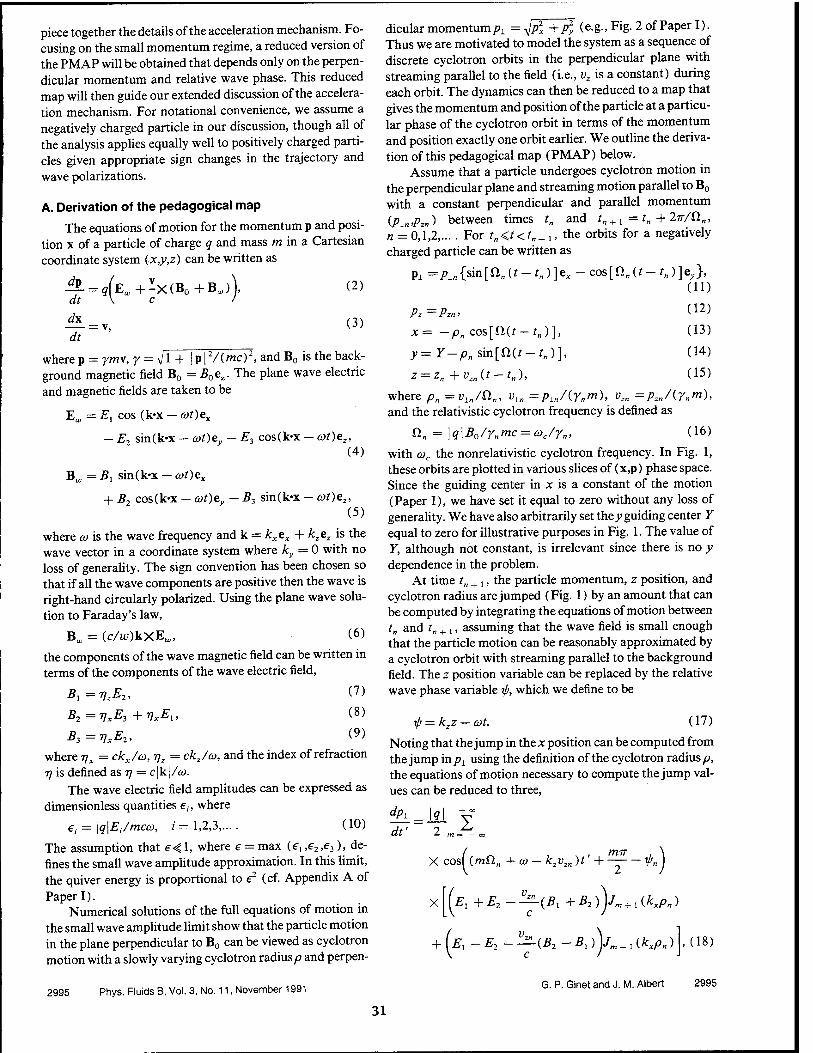
piece together the details of the acceleration mechanism. Fo- cusing on the small momentum regime, a reduced version of the PMAP will be obtained that depends only on the perpen- dicular momentum and relative wave phase. This reduced map will then guide our extended discussion of the accelera- tion mechanism. For notational convenience, we assume a negatively charged particle in our discussion, though all of the analysis applies equally well to positively charged parti- cles given appropriate sign changes in the trajectory and wave polarizations.
A. Derivation of the pedagogical map
The equations of motion for the momentum p and posi- tion x of a particle of charge q and mass mina Cartesian coordinate system (x,y,z) can be written as
£-«(* ^-XCBo+BJ), c
dx
dt = v»
(2)
(3)
where p = ym\, y = Vl + \p\2/(mc)2, and B0 is the back- ground magnetic field B0 = B0ez. The plane wave electric and magnetic fields are taken to be
E„, = Ex cos (k-x — cot)ex
- E2 sin(k'x - at)e - E3 cos(k-x - cot)ez, (4)
B„ = 5, sin(k-x — a>t)ex
+ B2 cos(k-x - cot)ey - B3 sin(k-x — cot)ez, (5)
where co is the wave frequency and k = kxex + kzez is the wave vector in a coordinate system where ky = 0 with no loss of generality. The sign convention has been chosen so that if all the wave components are positive then the wave is right-hand circularly polarized. Using the plane wave solu- tion to Faraday's law,
B„ = (c/w)kxEw, (6)
the components of the wave magnetic field can be written in terms of the components of the wave electric field,
B,=VzE2, (7)
B2=VxE3+rlxEx, <8>
B3=VxE2, (9)
where yx = ckx/o>, r?2 = ckz/a, and the index of refraction 77 is defined as 77 = c]k|/<y.
The wave electric field amplitudes can be expressed as dimensionless quantities e„ where
et = \q\Et/mca, 1 = 1,2,3,.... (10)
The assumption that €41, where e = max (e, ,e2,e3), de- fines the small wave amplitude approximation. In this limit, the quiver energy is proportional to e2 (cf. Appendix A of Paper I).
Numerical solutions of the full equations of motion in the small wave amplitude limit show that the particle motion in the plane perpendicular to B0 can be viewed as cyclotron motion with a slowly varying cyclotron radius p and perpen-
2995 Phys. Fluids B, Vol. 3, No. 11, November 1991
dicular momentum^ = ^p2x + p2 (e.g., Fig. 2 of Paper I).
Thus we are motivated to model the system as a sequence of discrete cyclotron orbits in the perpendicular plane with streaming parallel to the field (i.e., vz is a constant) during each orbit. The dynamics can then be reduced to a map that gives the momentum and position of the particle at a particu- lar phase of the cyclotron orbit in terms of the momentum and position exactly one orbit earlier. We outline the deriva- tion of this pedagogical map (PMAP) below.
Assume that a particle undergoes cyclotron motion in the perpendicular plane and streaming motion parallel to B0
with a constant perpendicular and parallel momentum (Pin>Pzn) between times tn and tn+l =tn+2ir/Cl„, n = 0,1,2,... . For ?„<r<f„+1, the orbits for a negatively charged particle can be written as
Pi =JPi„{sin[Ün (t - tn) ]ex - cos[ü„ (t- tH )]ey}, (11)
(12)
(13)
(14)
(15)
Pz =Pzn>
x= -p„ cos[ft(r-*„)],
y=Y-p„sm[a(t-tn)],
z = z„ +vzn(t-tn),
where p„ =vln/Cln, vln =pLn/{y„m), vzn =pzn/(ynm), and the relativistic cyclotron frequency is defined as
Sln = \q\B0/y„mc = oc/yn, (16)
with cac the nonrelativistic cyclotron frequency. In Fig. 1, these orbits are plotted in various slices of (x,p) phase space. Since the guiding center in x is a constant of the motion (Paper I), we have set it equal to zero without any loss of generality. We have also arbitrarily set the j> guiding center Y equal to zero for illustrative purposes in Fig. 1. The value of Y, although not constant, is irrelevant since there is no y dependence in the problem.
At time tn+l, the particle momentum, z position, and cyclotron radius are jumped (Fig. 1) by an amount that can be computed by integrating the equations of motion between t„ and t„ + ,, assuming that the wave field is small enough that the particle motion can be reasonably approximated by a cyclotron orbit with streaming parallel to the background field. The z position variable can be replaced by the relative wave phase variable if), which we define to be
r/j — kxz-cot. (17)
Noting that the jump in the x position can be computed from the jump in/71 using the definition of the cyclotron radius p, the equations of motion necessary to compute the jump val- ues can be reduced to three,
dPi_
dt'
X cosl {mQ.n +co — kzvzn)t' + : i>„
x -(Bl+B2))jm+l(kxPn)
*.)) (B2-Bi)Jm_1(kxPn)
G. P. Ginet and J. M. Albert
(18)
2995
31
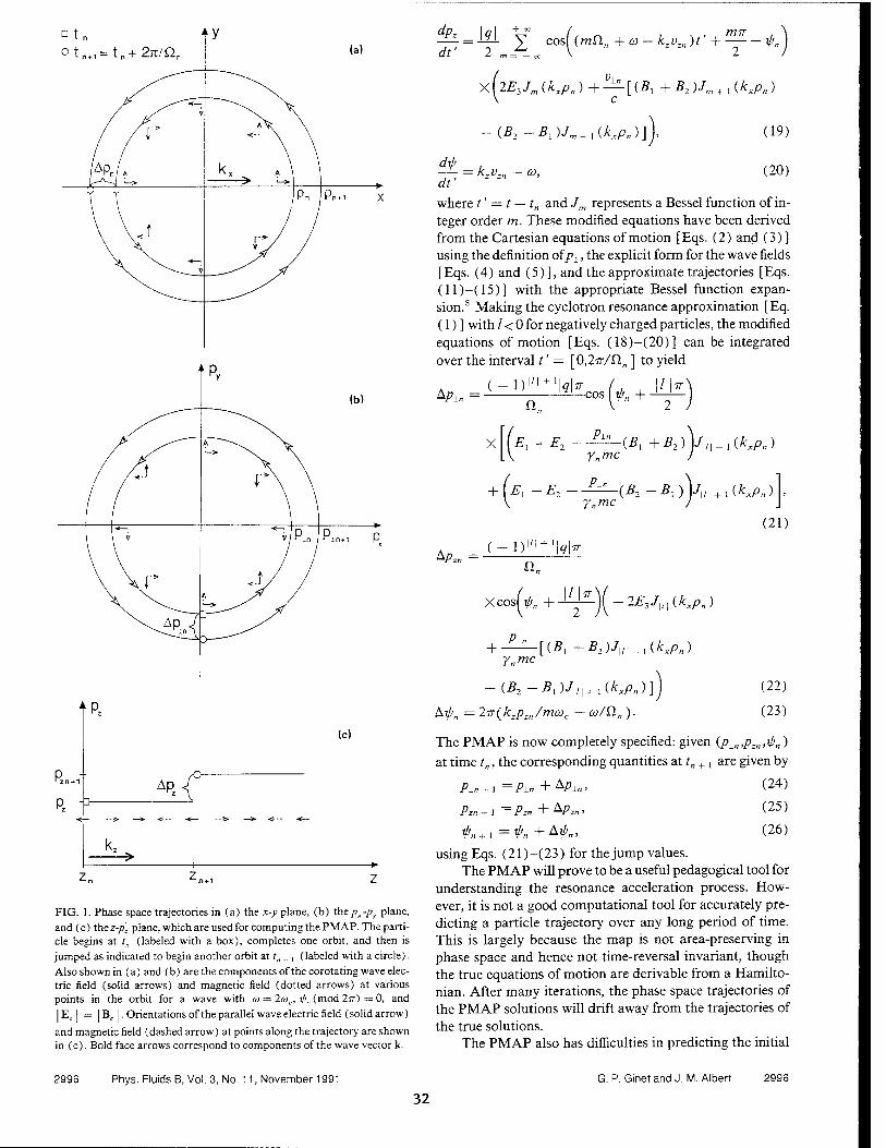
°t„ otn<1=tn+27T/Qn
P - rzn + 1
R
(c)
AR
FIG. 1. Phase space trajectories in (a) the x-y plane, (b) the px-py plane, and (c) thez-p. plane, which are used for computing the PMAP. The parti- cle begins at r„ (labeled with a box), completes one orbit, and then is jumped as indicated to begin another orbit at tn+ , (labeled with a circle). Also shown in (a) and (b) are the components of the corotating wave elec- tric field (solid arrows) and magnetic field (dotted arrows) at various points in the orbit for a wave with co = 2coc, rp„ (mod 2ir) = 0, and IE A = I Bc I. Orientations of the parallel wave electric field (solid arrow)
and magnetic field (dashed arrow) at points along the trajectory are shown in (c). Bold face arrows correspond to components of the wave vector k.
dp
~dt i = M £ cos,({mtin
m — — oo
. x , mil , co-kzuzn)t + — -1JJ„
X (lE,Jm (kxPn) + -^4 (Bl + B2 )Jm+ , (kxPn)
-(£,-£,)/„ (kxP„)\ (19)
k,v,„ — co, (20) dxf>
dt'
where t' = t — t„ and Jm represents a Bessel function of in- teger order m. These modified equations have been derived from the Cartesian equations of motion [Eqs. (2) and (3) ] using the definition ofpL, the explicit form for the wave fields [Eqs. (4) and (5)], and the approximate trajectories [Eqs. (11)—(15) ] with the appropriate Bessel function expan- sion.8 Making the cyclotron resonance approximation [Eq. (1) ] with / < 0 for negatively charged particles, the modified equations of motion [Eqs. (18)-(20)] can be integrated over the interval t' = [0,2fr/fl„ ] to yield
Apln = ■ n„
cos \ibn + ■ 77
X Ex +E2
+ \EX-E2-
Pln
ynmc
Pin
(5, +B2)\Jm_,{kxPn)
Y„mc {B2-B,)\JU] + x{kxPn)
(21)
^Pzn = (-n|,i + 'l<7k
Xcos(V„ + -^)( - 2E3Jin (kxPn
+ _^[(5, +B2)J[n_,{kxPn) ynmc
+ (B2 -Bx)J^ + ,{kxPny
Lip„ = 2tr{kzpzn/m(oc - co/D.n).
(22)
(23)
The PMAP is now completely specified: given (plr,,pz„,ift„) at time tn, the corresponding quantities at tn + , are given by
Pzn+1 =Pzn +^Pzn, (25)
<£„+1=^„+A^, (26)
using Eqs. (21)-(23) for the jump values. The PMAP will prove to be a useful pedagogical tool for
understanding the resonance acceleration process. How- ever, it is not a good computational tool for accurately pre- dicting a particle trajectory over any long period of time. This is largely because the map is not area-preserving in phase space and hence not time-reversal invariant, though the true equations of motion are derivable from a Hamilto- nian. After many iterations, the phase space trajectories of the PMAP solutions will drift away from the trajectories of the true solutions.
The PMAP also has difficulties in predicting the initial
2996 Phys. Fluids B, Vol. 3, No. 11, November 1991 G. P. Ginetand J. M.Albert 2996
32
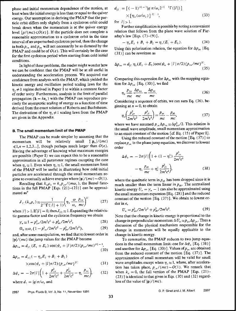
phase and initial momentum dependence of the motion, at least when the initial energy is less than or equal to the quiver energy. Our assumption in deriving the PMAP that the par- ticle orbit differs only slightly from a cyclotron orbit could break down when the momentum is at the quiver energy level [p/(mc)^0(e)]. If the particle does not complete a reasonable approximation to a cyclotron orbit in the time interval of an unperturbed cyclotron period, then the change in both/>in andpzn will not necessarily be as dictated by the PMAP and could be of 0{e). This will certainly be the case for the first cyclotron period when starting from cold initial conditions.
In light of these problems, the reader might wonder how we can be confident that the PMAP will be at all useful in understanding the acceleration process. We acquired our confidence from analysis with the PMAP, which yielded the kinetic energy and oscillation period scaling laws for the rjz # 1 regime derived in Paper I to within a constant factor of order unity. Furthermore, analysis in the limit of parallel propagation (k = kez) with the PMAP can reproduce pre- cisely the asymptotic scaling of energy as a function of time derived from the exact solution of Roberts and Buchsbaum. The derivations of the t]z # 1 scaling laws from the PMAP are given in the Appendix.
B. The small momentum limit of the PMAP
The PMAP can be made simpler by assuming that the momentum will be relatively small l\v„\/(mc) 4l,n = 1,2,3...], though perhaps much larger than 0(e). Having the advantage of knowing what maximum energies are possible (Paper I) we can expect this to be a reasonable approximation in all parameter regimes excepting the case when rjz ~ 1. Even when r)z ~ 1, the small momentum limit of the PMAP will be useful in illustrating how cold initial particles are accelerated through the small momentum re- gime to eventually achieve energies where | p | / (mc) ~ O (1).
Recalling that kxpn = kxpln/(mcac), the Bessel func- tions in the full PMAP [Eqs. (21)-(23)] can be approxi- mated as9
J\i\(.kxpn): 1
Til"" CO Pin
co, mc (27)
2l/|ni/| + when | /1 > 1. If | /1 = 0, then /,, | =; 1. Expanding the relativis- tic gamma factor and the cyclotron frequency we obtain
Yn^l+plJ2m2c2+p2zn/2m2c2, (28)
an ^coc (1 -p\J2m2e -p2zn/2m2c2), (29)
and, after some manipulation, we find that to lowest order in |p|/( mc) the jump values for the PMAP become
Apin=dlll(El +E2)cos(i{>„ + |/|7r/2)(/?1„/mc)1"-1
A^„= <*,„(-77^3+5, +B2)
Xcos(^„ + \l\ir/2){pLn/mCy,]
pin A^„= -2IT\I\ 1+ , ,
where d] = \q\ir/coc and
• + • 2m~c
PA mc)
(30)
(31)
(32)
^i;i=[(-l)!/,-'k!^c2,'i-T(|/|)]
X[yx(a>/coc)y,l-\ (33)
-for |/|>1. Further simplification is possible by noting a convenient
relation that follows from the plane wave solution of Far- aday's law [Eqs. (7)-(9)],
~VxEi+B1+B2=Vz(E,+E2). (34)
Using this polarization relation, the equation for Apzn [Eq. (31)] can be rewritten as
&P:n=d\nVAEi +E2)cos(ipn + \l\ir/2)(pln/mc) \'\
(35)
Comparing this expression for Apzn with the mapping equa- tion for Apln [Eq. (30)], we find
Pin ^Pln &Pzn Vz (36)
mc mc mc Considering a sequence of orbits, we can sum Eq. (36), be- ginning at n = 0, to obtain
(37) (Pin „2
PLO Pzn_
mc PzO
mc 2m2c2)
where we have assumed pL„ Apln -x.Ap\n/2. This relation is the small wave amplitude, small momentum approximation to an exact constant of the motion [cf. Eq. (15) of Paper I].
Using the reduced constant of the motion [Eq. (37) ] to replace/?^ in the phase jump equation, we discover to lowest order
A^„ = -27r|/|n + (l-7722) Pin
2m2c2
PrO , 2 Vz + Vz
mc Plo
2m2c2 (38)
where the quadratic term inp^ has been dropped since it is much smaller than the term linear in p^. The normalized kinetic energy U„ = yn — 1 can also be approximated using the small momentum expansion [Eq. (28)] and the reduced constant of the motion [Eq. (37)]. We obtain to lowest or- der in e,
Un=p2i_„/2m2c2+p2
T0/2m2c2. (39)
Note that the change in kinetic energy is proportional to the change in perpendicular momentum A U„ ~px„ Apin. Thus a discussion of the physical mechanism responsible for the change in momentum will be equally applicable to the change in kinetic energy.
To summarize, the PMAP reduces to two jump equa- tions in the small momentum limit: one for Aip„ [Eq. (38) ] and another for ApL„ [Eq. (30) ]. Values oipz„ are obtained from the reduced constant of the motion [Eq. (37)]. The approximation of small momentum will be valid for small wave amplitudes except when TJZ ^ 1, where, after accelera- tion has taken place, px„/(mc)~0(l). We remark that when kx = 0, the full version of the PMAP [Eqs. (21)- (23) ] is identical to that given in Eqs. (30) and (32) regard- less of the value of | p | / (mc).
2997 Phys. Fluids B, Vol. 3, No. 11, November 1991 G. P. Ginet and J. M. Albert 2997
33
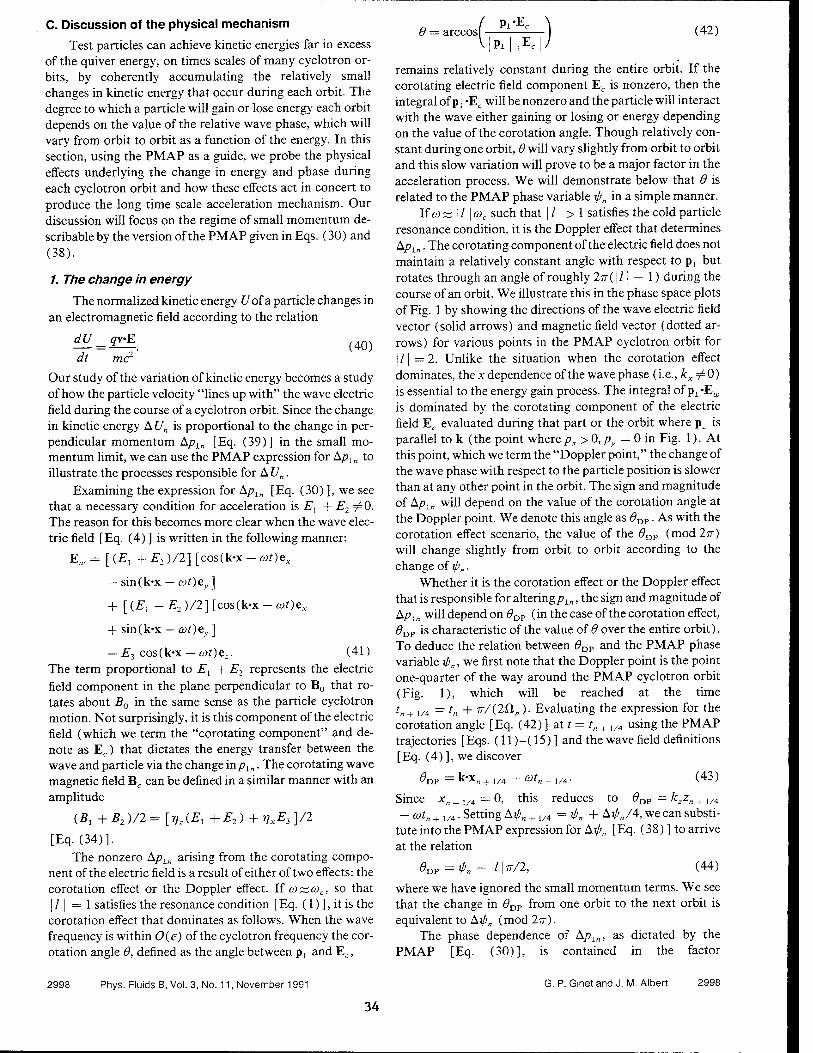
C. Discussion of the physical mechanism
Test particles can achieve kinetic energies far in excess of the quiver energy, on times scales of many cyclotron or- bits, by coherently accumulating the relatively small changes in kinetic energy that occur during each orbit. The degree to which a particle will gain or lose energy each orbit depends on the value of the relative wave phase, which will vary from orbit to orbit as a function of the energy. In this section, using the PMAP as a guide, we probe the physical effects underlying the change in energy and phase during each cyclotron orbit and how these effects act in concert to produce the long time scale acceleration mechanism. Our discussion will focus on the regime of small momentum de- scribable by the version of the PMAP given in Eqs. (30) and (38).
/. The change in energy
The normalized kinetic energy Uof a particle changes in an electromagnetic field according to the relation
M. = £*. (40) dt mc2
Our study of the variation of kinetic energy becomes a study of how the particle velocity "lines up with" the wave electric field during the course of a cyclotron orbit. Since the change in kinetic energy A U„ is proportional to the change in per- pendicular momentum Apln [Eq. (39)] in the small mo- mentum limit, we can use the PMAP expression for ApLn to illustrate the processes responsible for A U„.
Examining the expression for Apln [Eq. (30) ], we see that a necessary condition for acceleration is is, + E2 ^0. The reason for this becomes more clear when the wave elec- tric field [Eq. (4) ] is written in the following manner:
Ea, = [(£•,+ E2 )/2] [cos(k-x - cot)ex
— sin(k-x — at)ey]
+ [(£",- E2 )/2] [cos(k-x - (ot)ex
+ sin(k-x — cot)e]
9 = arccosi
■ E3 cos(k-x — o)t)ez. (41) The term proportional to Ex + E2 represents the electric field component in the plane perpendicular to B0 that ro- tates about B0 in the same sense as the particle cyclotron motion. Not surprisingly, it is this component of the electric field (which we term the "corotating component" and de- note as Ec) that dictates the energy transfer between the wave and particle via the change mpL„. The corotating wave magnetic field Bc can be defined in a similar manner with an amplitude
(5, +B2)/2=[Vz(E1 + E2)+VxE,]/2
[Eq. (34)]. The nonzero Apln arising from the corotating compo-
nent of the electric field is a result of either of two effects: the corotation effect or the Doppler effect. If co~coc, so that
j / | = 1 satisfies the resonance condition [Eq. (1) ], it is the corotation effect that dominates as follows. When the wave frequency is within 0(e) of the cyclotron frequency the cor- otation angle 9, defined as the angle between pL and Ec,
V Pi Ec / (42)
remains relatively constant during the entire orbit. If the corotating electric field component Ec is nonzero, then the integral of px -Ec will be nonzero and the particle will interact with the wave either gaining or losing or energy depending on the value of the corotation angle. Though relatively con- stant during one orbit, 9 will vary slightly from orbit to orbit and this slow variation will prove to be a major factor in the acceleration process. We will demonstrate below that 9 is related to the PMAP phase variable ip„ in a simple manner.
lfco~\l\coc such that | / | > 1 satisfies the cold particle resonance condition, it is the Doppler effect that determines ApLn. The corotating component of the electric field does not maintain a relatively constant angle with respect to px but rotates through an angle of roughly 2v( \l\ — 1) during the course of an orbit. We illustrate this in the phase space plots of Fig. 1 by showing the directions of the wave electric field vector (solid arrows) and magnetic field vector (dotted ar- rows) for various points in the PMAP cyclotron orbit for ]/| =2. Unlike the situation when the corotation effect dominates, the * dependence of the wave phase (i.e., kx =^0) is essential to the energy gain process. The integral of pL'Ew
is dominated by the corotating component of the electric field Ec evaluated during that part or the orbit where px is parallel to k (the point wherepx >0,py = 0 in Fig. 1). At this point, which we term the "Doppler point," the change of the wave phase with respect to the particle position is slower than at any other point in the orbit. The sign and magnitude of Apln will depend on the value of the corotation angle at the Doppler point. We denote this angle as 9DP. As with the corotation effect scenario, the value of the 9DP (mod277) will change slightly from orbit to orbit according to the change of ip„.
Whether it is the corotation effect or the Doppler effect that is responsible for altering pln, the sign and magnitude of ApLn will depend on ÖDP (in the case of the corotation effect, 9DP is characteristic of the value of 9 over the entire orbit). To deduce the relation between <9DP and the PMAP phase variable t/>„, we first note that the Doppler point is the point one-quarter of the way around the PMAP cyclotron orbit (Fig. 1), which will be reached at the time tn+ i/4 =tn + ir/(2£l„). Evaluating the expression for the corotation angle [Eq. (42) ] at t = t„ + I/4 using the PMAP trajectories [Eqs. (11)-(15) ] and the wave field definitions [Eq. (4) ], we discover
6>DP = k-x„_Hl/4 -cotnJrUA. (43)
Since x„ = 0, this reduces to krz„
t. Setting Aijjn. xjin + Aipn/4, we can substi- tute into the PMAP expression for Aip„ [Eq. (38) ] to arrive at the relation
0DP=^-|/k/2, (44)
where we have ignored the small momentum terms. We see that the change in 9DP from one orbit to the next orbit is equivalent to Aili„ (mod 2-rr).
The phase dependence of Apin, as dictated by the PMAP [Eq. (30)], is contained in the factor
2998 Phys. Fluids B, Vol. 3, No. 11, November 1991 G. P. Ginet and J. M. Albert 2998
34
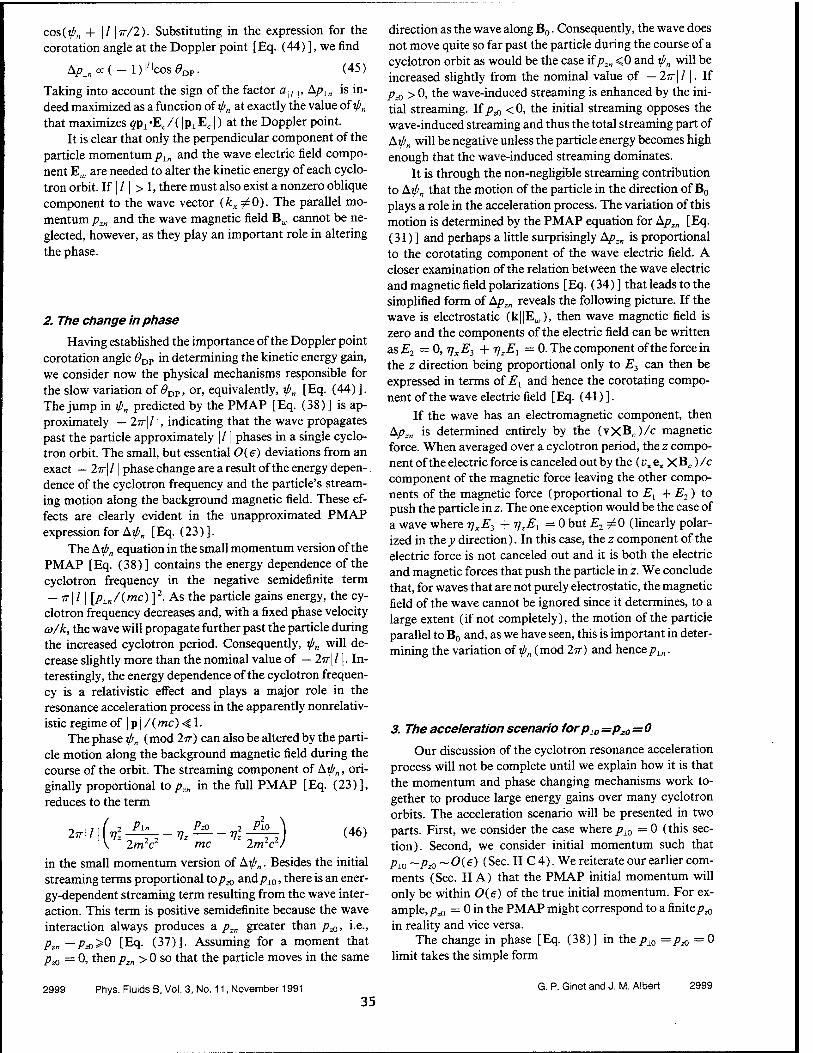
cos(^„ + |/ j 77-/2.) - Substituting in the expression for the corotation angle at the Doppler point [Eq. (44) ], we find
ApiBa(- D^cos^Dp. (45)
Taking into account the sign of the factor a^n, Apln is in- deed maximized as a function of if/„ at exactly the value of $„ that maximizes qpL-Ec/( |p±Ec |) at the Doppler point.
It is clear that only the perpendicular component of the particle momentum pL„ and the wave electric field compo- nent E^ are needed to alter the kinetic energy of each cyclo- tron orbit. If | / | > 1, there must also exist a nonzero oblique component to the wave vector (kx #0). The parallel mo- mentum pzn and the wave magnetic field B„ cannot be ne- glected, however, as they play an important role in altering the phase.
2. The change in phase
Having established the importance of the Doppler point corotation angle 8DP in determining the kinetic energy gain, we consider now the physical mechanisms responsible for the slow variation of 0DP, or, equivalently, rfr„ [Eq. (44)]. The jump in ip„ predicted by the PMAP [Eq. (38)] is ap- proximately — 2ir\l\, indicating that the wave propagates past the particle approximately \l \ phases in a single cyclo- tron orbit. The small, but essential 0(e) deviations from an exact — 2v\l | phase change are a result of the energy depen-. dence of the cyclotron frequency and the particle's stream- ing motion along the background magnetic field. These ef- fects are clearly evident in the unapproximated PMAP expression for Arf>„ [Eq. (23)].
The Aipn equation in the small momentum version of the PMAP [Eq. (38)] contains the energy dependence of the cyclotron frequency in the negative semidefinite term — v\l\ [pin/(mc)]2. As the particle gains energy, the cy- clotron frequency decreases and, with a fixed phase velocity co/k, the wave will propagate further past the particle during the increased cyclotron period. Consequently, ip„ will de- crease slightly more than the nominal value of — 2ir\l |. In- terestingly, the energy dependence of the cyclotron frequen- cy is a relativistic effect and plays a major role in the resonance acceleration process in the apparently nonrelativ- istic regime of | p | /(mc) -41.
The phase tp„ (mod 2v) can also be altered by the parti- cle motion along the background magnetic field during the course of the orbit. The streaming component of Aif>„, ori- ginally proportional to pzn in the full PMAP [Eq. (23)], reduces to the term
277-1/ Tz Pin
2m2c2
PzO 2 Vz Vz
mc
_2 Pi.0
2m2c2 (46)
in the small momentum version of Aipn. Besides the initial streaming terms proportional top^ and/>10, there is an ener- gy-dependent streaming term resulting from the wave inter- action. This term is positive semidefinite because the wave interaction always produces a pzn greater than p^, i.e., Pzn —Pzo>® [Eq. (37)]. Assuming for a moment that Pa = 0, then pzn > 0 so that the particle moves in the same
direction as the wave along B0. Consequently, the wave does not move quite so far past the particle during the course of a cyclotron orbit as would be the case if pzn <0 and ifi„ will be increased slightly from the nominal value of —2ir\l\. If Pa > 0, the wave-induced streaming is enhanced by the ini- tial streaming. If p^ <0, the initial streaming opposes the wave-induced streaming and thus the total streaming part of Aip„ will be negative unless the particle energy becomes high enough that the wave-induced streaming dominates.
It is through the non-negligible streaming contribution to Atf>„ that the motion of the particle in the direction of B0
plays a role in the acceleration process. The variation of this motion is determined by the PMAP equation for Apz„ [Eq. (31) ] and perhaps a little surprisingly Apz„ is proportional to the corotating component of the wave electric field. A closer examination of the relation between the wave electric and magnetic field polarizations [Eq. (34) ] that leads to the simplified form of Apzn reveals the following picture. If the wave is electrostatic (kHE,,), then wave magnetic field is zero and the components of the electric field can be written as£"2 =0, rjxE3 + r/zEl — 0. The component of the force in the z direction being proportional only to E3 can then be expressed in terms of Er and hence the corotating compo- nent of the wave electric field [Eq. (41) ].
If the wave has an electromagnetic component, then Apzn is determined entirely by the (vXBc)/c magnetic force. When averaged over a cyclotron period, the z compo- nent of the electric force is canceled out by the (vx ex X Bc) /c component of the magnetic force leaving the other compo- nents of the magnetic force (proportional to Ex + E2) to push the particle in z. The one exception would be the case of a wave where TJXE3 + VZ
E\ = ° but E2 #° (linearly polar-
ized in the y direction). In this case, the z component of the electric force is not canceled out and it is both the electric and magnetic forces that push the particle in z. We conclude that, for waves that are not purely electrostatic, the magnetic field of the wave cannot be ignored since it determines, to a large extent (if not completely), the motion of the particle parallel to B0 and, as we have seen, this is important in deter- mining the variation of if>„ (mod 2ir) and hencepln.
3. The acceleration scenario forp10 =pz0=0
Our discussion of the cyclotron resonance acceleration process will not be complete until we explain how it is that the momentum and phase changing mechanisms work to- gether to produce large energy gains over many cyclotron orbits. The acceleration scenario will be presented in two parts. First, we consider the case where pi0 = 0 (this sec- tion). Second, we consider initial momentum such that pw —p^ —0(e) (Sec. II C 4). We reiterate our earlier com- ments (Sec. II A) that the PMAP initial momentum will only be within O(e) of the true initial momentum. For ex- ample, Pa = 0 in the PMAP might correspond to a finitep^ in reality and vice versa.
The change in phase [Eq. (38)] in the pi0 = p^ = 0 limit takes the simple form
2999 Phys. Fluids B, Vol. 3, No. 11, November 1991 35
G. P. Ginet and J. M. Albert 2999
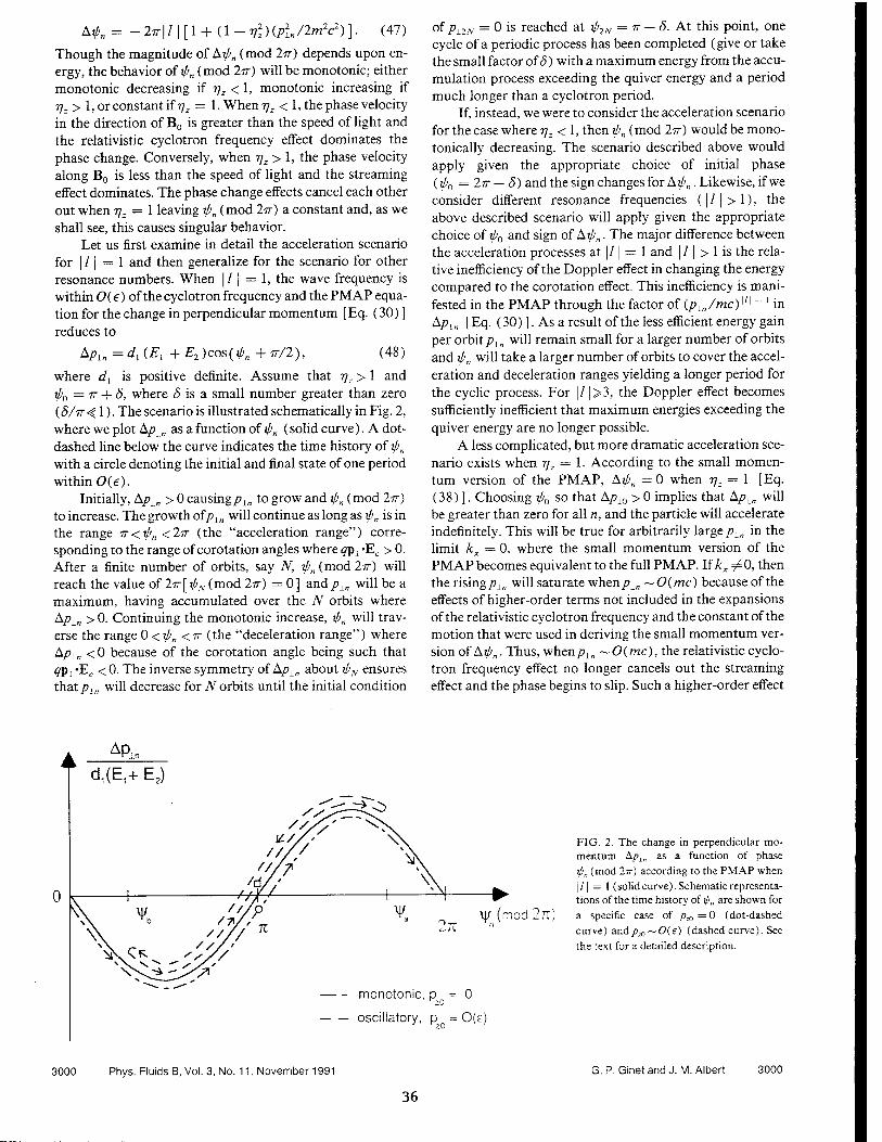
A^„ = -2ir\l\[\ + (l-V2
z)(p2ln/2m2c2)]. (47)
Though the magnitude of Aip„ (mod 277-) depends upon en- ergy, the behavior of rp„ (mod 27?-) will be monotonic; either monotonic decreasing if t]z < 1, monotonic increasing if 77. > 1, or constant if 77. = 1. When 77. < 1, the phase velocity in the direction of B0 is greater than the speed of light and the relativistic cyclotron frequency effect dominates the phase change. Conversely, when rjz > 1, the phase velocity along B0 is less than the speed of light and the streaming effect dominates. The phase change effects cancel each other out when TJZ = 1 leaving ipn (mod 2ir) a constant and, as we shall see, this causes singular behavior.
Let us first examine in detail the acceleration scenario for I /1 = 1 and then generalize for the scenario for other resonance numbers. When \l | = 1, the wave frequency is within 0(e) of the cyclotron frequency and the PMAP equa- tion for the change in perpendicular momentum [Eq. (30)] reduces to
Apln =d1(E1 +E2)cos(iI;n +7T/2), (48)
where dx is positive definite. Assume that 77.. > 1 and rp0 = TT + 8, where 8 is a small number greater than zero (<5/7T< 1). The scenario is illustrated schematically in Fig. 2, where we plot Apln as a function of if>„ (solid curve). A dot- dashed line below the curve indicates the time history of ip„ with a circle denoting the initial and final state of one period within 0{e).
Initially, Apln > 0 causingpln to grow and ipn (mod 2TT)
to increase. The growth ofpin will continue as long as fn is in the range ir<ip„ <2ir (the "acceleration range") corre- sponding to the range of corotation angles where gpx -Ec > 0. After a finite number of orbits, say N, ip„ (mod 277) will reach the value of 277-[^( mod 27r) = 0] and/>x„ will be a maximum, having accumulated over the TV orbits where ApLn > 0. Continuing the monotonic increase, i[>n will trav- erse the range 0 < ip„ <77 (the "deceleration range") where Apln < 0 because of the corotation angle being such that 9Pi-Ec <0. The inverse symmetry of Apin about ipN ensures that pln will decrease for N orbits until the initial condition
of pnN = 0 is reached at tf>2N = ir — 8. At this point, one cycle of a periodic process has been completed (give or take the small factor of <5) with a maximum energy from the accu- mulation process exceeding the quiver energy and a period much longer than a cyclotron period.
If, instead, we were to consider the acceleration scenario for the case where r]z < 1, then ipn (mod 2TT) would be mono- tonically decreasing. The scenario described above would apply given the appropriate choice of initial phase (rp0 = 2TT — (5) and the sign changes for Aip„. Likewise, if we consider different resonance frequencies (| /1 > 1), the above described scenario will apply given the appropriate choice of ip0 and sign of Atp„. The major difference between the acceleration processes at | /1 = 1 and | / | > 1 is the rela- tive inefficiency of the Doppler effect in changing the energy compared to the corotation effect. This inefficiency is mani- fested in the PMAP through the factor of (pln/mc)U} " ' in ApLn [Eq. (30) ]. As a result of the less efficient energy gain per orbit pln will remain small for a larger number of orbits and ipn will take a larger number of orbits to cover the accel- eration and deceleration ranges yielding a longer period for the cyclic process. For |/1>3, the Doppler effect becomes sufficiently inefficient that maximum energies exceeding the quiver energy are no longer possible.
A less complicated, but more dramatic acceleration sce- nario exists when 77., = 1. According to the small momen- tum version of the PMAP, Arpn =0 when 77. = 1 [Eq. (38) ]. Choosing if>0 so that Api0 >0 implies that Apln will be greater than zero for all n, and the particle will accelerate indefinitely. This will be true for arbitrarily large pln in the limit kx = 0, where the small momentum version of the PMAP becomes equivalent to the full PMAP. If kx #0, then the rising p±„ will saturate when/?in ~0(mc) because of the effects of higher-order terms not included in the expansions of the relativistic cyclotron frequency and the constant of the motion that were used in deriving the small momentum ver- sion of Aipn. Thus, when/7in —O(mc), the relativistic cyclo- tron frequency effect no longer cancels out the streaming effect and the phase begins to slip. Such a higher-order effect
mod In)
monotonic, p = 0
oscillatory, p - O(e)
FIG. 2. The change in perpendicular mo- mentum A/>ln as a function of phase 1/1 „ (mod 2~) according to the PMAP when j/| = 1 (solid curve). Schematic representa- tions of the time history of ^„ are shown for a specific case of p^ = 0 (dot-dashed curve) and^A~0(e) (dashed curve). See the text for a detailed description.
3000 Phys. Fluids B, Vol. 3, No. 11, November 1991 G. P. Ginetand J. M.Albert 3000
36
would explain why the maximum energies observed when 77z = 1 and kx ^0 are independent of wave amplitude and resonance frequency (Paper I).
The reader may have noted that the descriptions of the acceleration scenarios all depend upon a judicious choice of the initial phase xf>0. If ip0 is not chosen properly, the PMAP can predict negative values ofpla, an unphysical situation. As we have emphasized, this failure of the PMAP to eluci- date the initial phase dependence is a consequence of the cyclotron orbit sometimes failing to be a good approxima- tion to the particle trajectory when/>i0 <0(e).
4. The acceleration scenario forp10 ~pz0 ~ 0(e) Let us consider briefly how the acceleration mechanism
works when the initial particle energy is of the order of the quiver energy. When formulated in terms of the PMAP, the predominant changes in the acceleration scenario with re- spect to the/>10 = Pro = ° case wiN be due t0 the effect of the Px term in the Ai!/„ relation [Eq. (38) ]. This term provides a constant streaming phase change in addition to the phase changes stemming from the energy-dependent streaming and relativistic cyclotron frequency terms. The behavior of ifin, and hence pln, depends on the relative sign of the p& term with respect to the energy-dependent terms that are proportional to (1 — rj]).
If the sign of/?^ is opposite that of (1 — rj1), the accel- eration process is little changed from the pzO=0 scenario. The behavior of if>„ is monotonic increasing or decreasing (depending on the value of 77J, with the background streaming effect simply increasing the rate of change. An increased rate of change means that ipn passes through the acceleration range in fewer orbits. This decreases the sum of ApLn over the acceleration range and, consequently, lowers the maximum energy.
If pa has the same sign as (\—7]\), then the back- ground streaming term contributes to Axpn with a sign oppo- site to that of the energy-dependent effects. To illustrate how this alters the acceleration scenario, we consider the case where | /1 = 1, T/Z < 1, and pa > 0, i.e., a regime where the relativistic cyclotron frequency effect dominates the energy- dependent contribution to At/>„. These parameters lead to the simplified Apin relation given in Eq. (48). To help guide the reader through the scenario, we display in Fig. 2 a sche- matic of the time history of rp„ on the Apin vs if>„ plot (dashed line above the solid curve) with the square denoting the initial and final states of a long period to within 0(e).
Initially, the background streaming dominates the phase change since \pz0/mc\ > \p\0/m2cl\ and $„ will in- crease. Given the appropriate choice of initial phase (if>0 = ir + S), ApL„ will initially be positive and remains positive as long as IT < ipn < In. lip^ is not too large, then the rate of change of ip„ will be slow enough to allow pln to build up to a level that allows the energy-dependent term in Aip„ to cancel out and then exceed the background streaming term. Assume that the cancellation of the two terms [Aipn(mod2ir) =0] occurs at ip„=ipa, where ir<ij>a
< 2w. The phase will begin to decrease but Apln remains positive until i/>„ = ir, at which pointpin has reached a maxi-
mum. Continuing to decrease, ifrn enters the deceleration range (0 < rfr„ < IT), where Apln < 0. The perpendicular mo- mentum decreases and at the point if>b =ir—t//a, the back- ground streaming term will begin again to dominate Aip„. The phase begins to increase while Apx„ remains negative until if>„ =TT — 8 and the cycle is complete.
This acceleration scenario applies equally well to the rjz > 1 and p^ < 0 case, provided the appropriate changes in initial phase, acceleration-deceleration ranges, and sign of Aif>„ (mod 2ir) are made. The scenario is similar to the Pa = 0 scenario in that maximum energies much larger than the quiver energy occur with periods of variation much larg- er than a cyclotron period. In contrast with the/?^ = 0 sce- nario, if>„ exhibits oscillatory behavior instead of monotonic behavior. Maximum kinetic energies with an oscillatory ipn
can often exceed maximum kinetic energies with a monoton- ic rp„ because an oscillating if/„ spends more cyclotron orbits in the acceleration range.
Oscillatory ipn behavior disappears when p^ exceeds some critical value, say pzc, and the background streaming propels xpn through the acceleration range before the energy- dependent contributions to A^„ can "shut off" the back- ground streaming. For p# >pzc, the phase monotonically changes and the maximum pin decreases as p^ increases. Numerical solutions of the full equations of motion have verified that this type of phase behavior occurs with values of pzc within order unity of those estimated by the PMAP.
As was the case when/^ = 0, it is not wise to press the PMAP too far since problems with the initial phase and mo- mentum dependence thwart the PMAP predictive power. This becomes obvious when we ask what happens when Pa —0. Sticking to the oscillatory scenario described in this section for/^ ~0(e), we would expect that the oscillation period and maximum energy would decrease to zero. But this is not what happens; the initial phase changes to differ- ent values so that, when p^ —0, we have the/?^ = 0 accel- eration scenario as discussed in Sec. II C 3 with large maxi- mum energies. Let us appreciate the physical intuition that the PMAP has given us and move on to a more complex Hamiltonian analysis that will satisfy our quantitative needs.
III. REDUCED HAMILTONIAN EQUATIONS OF MOTION
To probe the details of the cyclotron resonance accelera- tion process that fell through the cracks of the PMAP we turn to a Hamiltonian formulation of the test particle prob- lem. Hamiltonian methods were used in Paper I to derive a pseudopotential function that was able to describe the be- havior of the kinetic energy on time scales longer than a cyclotron period. In this section, we extend the Hamiltonian formulation of Paper I to produce reduced equations of mo- tion capable of predicting cyclotron orbit-averaged details of the particle trajectory either analytically or in far less com- putational time than it would take to compute solutions of the full equations of motion.
In Cartesian coordinates, the Hamiltonian for a test par- ticle in the electromagnetic wave fields described in Sec. II [Eqs. (4) and (5)], is
^(x,p;f) = [m2c4 + (Pc - qA)2}w2, (49)
3001 Phys. Fluids B, Vol. 3, No. 11, November 1991 G. P. Ginet and J. M. Albert 3001
37
where the canonical momenta are defined in terms of the physical momenta as P = p + qA/c. The components of the vector potential can be reduced to
Ax = (mc2/\q\)[ - (ac/co)y + €l sin/?], (50)
Av = (mc2€2/\q\)cosß, (51)
Az = -{mc2ei/\q\) sinß, (52)
where e, is given by Eq. (10) and we have introduced the
phase variable
ß(x,z,t) = kxx + kzz - at. (53)
A number of canonical transformations of the Cartesian Hamiltonian must be performed before a sufficiently useful time-independent Hamiltonian and corresponding set of ca- nonical coordinates is produced. We refer the reader to Pa- per I for details on the sequence of transformations that we employ and will only present here the resultant Hamiltonian and the definitions of the corresponding canonical coordi- nates in terms of physical coordinates.
The Hamiltonian of interest [Eq. (24) of Paper I] can
be written to 0{e) as
H(£ÄPSJ,P, ) = H0 {PjlP^) + H{ (ijfj^ ), (54)
where
H0(P;j,pli)=r-ps,
1
2Y„ Hx (£<M>,,/,/>„)
(55)
JT a„ sin[£ + 5(« — l)d>],
(56)
with H0~O{\) and //, —0(e). We have introduced the following quantities into the H representation:
V{P?JJP„)= [1 + (2ö»(/+i/Pj)
+ (VA-VXPI,)2V/2> (57)
a„ (PgJ,Ptt) = - (ac/a)p[{ex + e2 )J„ , , (yxp)
+ (e, -e2)J„_x(VxP)]
+ 2se3 (v:Pg - V*P„ )J,,(Vxp)> (58)
where
p(P,J) = [(2co/coc) (7 + slP,) ]l/2 (59)
and s is the sign of the charge. Unlike the Paper I representa- tion of H, we have chosen to use dimensionless canonical variables. In particular, the canonical momenta (P£,I,Pß) are in units normalized to co/mc2 and the Hamiltonian H is
normalized to mc2. To maintain the canonical properties of the Hamiltonian system it is necessary to introduce the nor- malized time variable t = cot. In our set of dimensionless variables, derivatives with respect to time are expressed with the independent variable t.
The canonical variables (^,d>,Ps,I,Pfl) are defined in terms of the physical variables by the relations,
i = ß+ (Cü/OC)srjx (py/mc + se2 cosß ) + sl<b, (60)
/ — {p /mc + s€j cos/?) arctan
\ s(px/mc + set sin/?) (61)
1 ( P* , P= —\lx + V, 77-\ mc mc
srjxy + s(V^i -77-e, )sm/3 c
P* , • a h 56, sin/i . mc
(63)
2<y..
Pv + se, cos ß mc
■ slP.. (64)
1 / Px Pz P„ =—[v= Vx —
77-V mc mc
-577.^ + 5(77,6, +77,6, )sin/? c
(65)
with ß(x,z,t) given by Eq. (53). Inverting these definitions, we obtain the following expressions for the physical vari- ables as functions of the canonical variables:
x = (c/(orf-)(T]:p + T]xzt
— slf]xd> + rjxt + srpp sin d>), (66)
y= {c/co)[ -s{cD/a)c){rjxPs+r]zPfl) + pcas&],
z = (C/WT)2) (77.$ - rjxp - slyJb + r/.t),
px/mc = (scoc/co)p cos <b
— 56, sin(£ — sty + sr)xp sind>),
pv/mc = — {(t)c/co)p sin d>
— se2 cos(£ — sty + S7]xp sind>),
p,/mc = rj.Ps — 77.P,,
+ 56, sin(§ — sty + srjxp sin &),
(67)
(68)
(69)
(70)
(71)
p = kxx — kzz — (a/coc )srjz (py/mc + 5e, cos ß ), (62)
with p(Ps, 1) given by Eq. (60). In Paper 1, the relation between the canonical coordinates (g,d>,p,Pc,I,Pß ) and con- ventional action-angle guiding center canonical variables is discussed. The Hamiltonian H and corresponding canonical variables differ from Hamiltonian formulations used in pre- vious studies of wave-particle interactions510 in that there is no singular behavior in the canonical coordinates as 17, — 0.
The cyclotron resonance approximation used in Paper I and in the construction of the PM AP (Sec. II) is founded on the assumption that there are two widely varying dynamical time scales, with the faster time scale being on the order of the nonrelativistic cyclotron period. In the Hamiltonian for- mulation, this separation of time scales is determined by the relative magnitude of the two frequencies a, = dt, /dt and
co2 = dd/dt. These nondimensional frequencies can be com- puted from H and are found to be
ö, = (1/T) [ {slcojco) + 77, (V:P, - vxPt,) ]
-1+0«:), (72)
ü)2=coc/Tü) + 0(e). (73)
Defining the winding number r to be the ratio of the slow to fast frequency, we see
r = sl+ (co/coc)rjAy-P-~ -yxP,J - (OJ/COC)T + O(e). (74)
3002 Phys. Fluids B, Vol. 3, No. 11, November 1991 38
G. P. Ginet and J. M. Albert 3002
The cyclotron resonance approximation assumes r~0(e) with / chosen to satisfy this as well as possible. When ex- pressed in terms of the physical variables, the assumption of small winding number is equivalent to the resonance condi- tion [Eq. (1)] normalized to the relativistic cyclotron fre- quency il. In the above analysis, it has been implicitly as- sumed that dHx /dP§ —0(e), which seems reasonable given Hx -0(e). We shall discover later (Sec. Ill C 2) that this is not always the case.
Reduction of the Hamiltonian H in the cyclotron reso- nance approximation can be carried out either discretely or continuously. Though the discrete mapping approach pre- sented in Sec. Ill A is often the method of choice (since the time averaging process is explicit), there are difficulties with accuracy in certain regions of phase space. We are thus led to construct equations of motion with a continuous time vari- able in Sec. Ill B from an orbit-averaged reduced Hamilto- nian. Details of the particle trajectories in the small momen- tum limit are studied in Sec. Ill C.
A. Orbit-averaged mapping equations
Our goal in this section is to construct a set of area- preserving mapping equations that will approximate the par- ticle trajectory in the canonical variable phase space. The mapping equations will determine the slowly varying vari- ables Ps and I" on the phase space surface of constant ^(mod 2ir) with successive iterations of the map (denoted by the subscript n) indicating an increase of ^ by 2ir, i.e., (f>n + , = <^„ + 2ir. The map construction outlined below em- ployees standard methods of Hamiltonian analysis that are discussed in detail elsewhere.11
We seek a mapping of the form
ps. + t=ps.+*pi.(ps.+ ,>£n'>> (75)
§« + i =in+2irr(P^i)+giP£n+JH), (76)
where r is the winding number given by Eq. (74) without the "0(e)" term. When 6 = 0, then APS% = g = 0 and P, is a constant of the motion. In this limit, |"„ will advance by an amount equal to the slow frequency cox times the fast period T= 2w/co2, with co2 given by Eq. (73) without the "0(e)" term.
The first-order correction APg to the trivial zeroth-or- der behavior of i>s- is computed by integrating the equation of motion for dP£/dt from time tn to t„ + T,
Ms. n - dP, dt-
dt
= - dt Jo d£
(|-„+<MÄ+«2?,P£n+,,7),
(77)
where the zeroth-order trajectories are substituted in for the canonical variables in the integrand. For purposes of area preservation, the value Ps t is used instead of P.- . Also, / is a constant to 0(e2) independent of«. This can be deduced by integrating the expression dl /dt = — dH, /dip to lowest or- der between t„ and tn + T.
Evaluating the AP, integral [Eq. (77)] using the first-
3003 Phys. Fluids B, Vol. 3, No. 11, November 1991
order Hamiltonian [Eq. (56)] and keeping in mind the reso- nance approximation, we find
AP, £n (Trco/coc)a, cos£„, (78)
where a, (P^) is given by Eq. (58) withPs% + ] substituted in forP^.
The first-order correction g to the zeroth-order rotation of £„ is determined by demanding that the map be area- preserving in (P£,£) phase space. A consideration of the Ja- cobian of the map transformation defined by Eqs. (75) and (76) yields the following condition for area preservation:
<3(AP^)
dP ■ +
£M
Jg_ din
0. (79)
This differential equation can be easily integrated upon sub- stitution of the AP^ expression [Eq. (78)] to yield
g = (ire)/coc )a'i sin |„, (80)
where
a',= -{sl2/p)[{ex -€2)Jl_,(T]xp)
- (e, + e2 )Jl+ , {VxP) ] ~ 2s!rixe2J,(r}xp)
+ 2se3{vJ,(.Vxp) + (slco/p2coc)(vzP,n +, - VxP„)
XlVxfr-AvJl-UdVxp)]}- (81) The map is now complete. Starting with values for (£n ,P5%), the value of P- t is obtained by solving the Pg map equation [Eq. (75)] for+P^+i given the function AP^(Ps%+i,|-J [Eq. (78)]. Direct substitution of Ps%i+i and |„ into the £ map equation (76) with r(P^+i) given by Eq. (75) and g(Pin+l,i„) given by Eq. (80) yields £„+1. Initial condi- tions fix the value of ^(mod 2ir) and the constants of the motion 7 and PM. We denote the map constructed above as the "QMAP" since it is more quantitatively accurate than the PMAP constructed in Sec. II.
The QMAP can be simplified by assuming small mo- menta. In physical variables, the small momentum limit de- mands |p//nc| 41, which, when translated to canonical vari- ables, is equivalent to the conditions I + slP£ <1 and rjxPs — r/xPM < 1. Expanding the APsV co, and g functions of the QMAP in the small arguments [making use of Eq. (27) ] we arrive at the following set of mapping equations for negatively charged particles:
P, = P, -(ira/oc)binpl''<cos£n, (82)
in- ■■i„+24\i\ (J+I'l^.,,)
TlTCO
TTO) — I /1 _ 2 • i- + C|/|/o' ' smin, (83)
where
*1/|= -(-^I'I-'M*.+*2)/2"|-,n|/|)*>,
c,;| = (\l\2co/ü)c)bin,
(84)
(85)
G. P. Ginet and J. M. Albert 3003
39
and p(i°ä%^,) is given by Eq. (59) with P- -P^ , • In the small momentum approximation /> < 1.
To see if the QMAP provided a reasonably accurate esti- mate of the true phase space trajectories, we compared QMAP solutions with numerical solutions of the full equa- tions of motion [Eqs. (2) and (3) ] over a range of the free parameters (|/1, co/coc, rj, a, e, k-x0) for cold initial condi- tions (p0 =0). We found good agreement when | /1 >2, al- beit we did not do as complete a survey as will be discussed in Sec. Ill B. There is a problem, however, when | /1 = 1 and the true behavior of £ in certain regions of phase space is not well modeled by the QMAP.
This difficulty can be understood as follows. When [/1 = 1, the i QMAP equation [Eq. (83) ] contains a term proportional to (sin|"„)//9(P5-n+i). For cold initial parti- cles, there are portions of the phase space orbits (where the momenta are very small) that pass very close to those values of P.- that make/? = 0. Fortunately, the true phase trajectory is also in a region near J" = 0 or IT so that the value of sin £„ also approaches 0. The behavior of the ratio (sin | /p(P?) is extremely sensitive to the exact values of (|\ Ps-) to the ex- tent that a slight deviation from the true trajectory as g-> 0 or TT results in a value much greater than unity. Unfortunately, as a consequence of the fixed time-step size of the QMAP and the implicit nature in which the quantities are advanced, the discrete jump in Ps is computed before the corresponding jump in |, and the quantity (|"„,P^+i) deviates enough from the true trajectory that QMAP ratio sin £„//5(Ps- t) becomes extremely large. The deviation is enough, in fact, to cause large inaccuracies in the values of £„ +, ~i„- More will be said about these regions of singular behavior in Sec. IIIC.
In trying to circumvent this problem, we are immediate- ly led to consider the possibility of decreasing the time step of the jump so that the quantity (|„, Ps%+ _) more closely ap- proximates the desired quantity [g(t), P? (t) ]. This can be done most effectively by abandoning the discrete jumps of a map altogether and constructing orbit-averaged equations of motion with a continuous time variable.
S, (|-,<£,P,,/,P,J
£ - cos[£ + s(n-/)^] (87) 2coc „= _ « s(n — /)
_ a^PeJJPj^ is given by Eq. (58) with (PS,I,P )—"(Pf,/,PM). To 0(e), the new canonical vari- ables ($,5,P,7) are defined in terms of the old variables according to the relations
and
<?S, 5 = :s •+- dp/
4> = --4> + Si'
fi = = n + dSl
dP,'
?! = P, dSx
3i
7= ~l-
P. = P, j
(88)
(89)
(90)
(91)
(92)
(93)
where (P.-,7,PM) have been substituted in for (P.-,/,PM) in the 5, definition [Eq. (87)]. The Hamiltonian H [Eq. (54) ] transforms to H, where
H=T-PS + (a;/2Y)sinf (94)
and_ T(P-,7iPÄ_)_ is given by Eq. (57) with (P£,I,Pfi)^(Ps,I,P/1). By choosing 5, properly, the fast varying terms have been displace_d to 0(e2) in transforming from H to H. What remains in H is essentially H averaged over one period in ~4> while the other variables are held con- stant. Thus, like the QMAP, dynamic details occurring on time scales less than 2ir/co2 (roughly the cyclotron period) are absent. _
From the orbit-averaged Hamiltonian H, we can com- pute the orbit-averaged equations of motion for the canoni- cal variables J and Pe:
B. Orbit-averaged continuum equations
With the aid of adiabatic canonical perturbation theo- ry,12 it is possible to transform the Hamiltonian if to a new Hamiltonian H that will depend only on slowly varying vari- ables to 0(e), provided the resonance approximation is sat- isfied. This transformation was used in the course of deriving the HPP theory in Appendix B of Paper I. We outline the transformation below in the context of the dimensionless canonical variables that have been introduced in this paper.
The generating function 5 for the transformation can be written as a function of the old coordinates and new momen- tum as
SdÄ^P.j^ )=£PS + ^7+/zp; + s, (|,^,P,,7,P^ ), (86)
where
4-= dt
dPg
~~dT~
T 1 ( . T , - 1 H a - a, sin $,
2TV Y
2Y COS£,
(95)
(96)
where
Y = slcoJcoT + (97Z/Y) (VzPs - r]xPß ) (97)
and a', is given by Eq. (81) with Ps — P5- and I-»/. The ca- nonical momenta I and P^ are constants of the motion and the linear time variation of the corresponding angles can be written as
-7 7 dH-
ai
j"=i"0 + dH -
dP»
(98)
(99)
In the small momentum limit, the orbit-averaged equa-
3004 Phys. Fluids B, Vol. 3, No. 11, November 1991 40
G. P. Ginet and J. M. Albert 3004
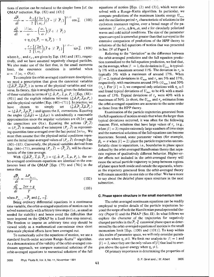
tions of motion can be reduced to the simpler form [cf. the QMAP reduction, Eqs. (82) and (83)]
dP, h *— — dt 2
dl _ \l 0)c
dt
(^)(7+|/|Ä)
\?+|/|Pf)
j'l/2 _ cos £ (100)
+ 77,(77^-77^)-!
2co\~T (I+\l\Ps) sin |, (10i;
where 6-, and cu , are given by Eqs. (84) and (85), respec- tively, and we have assumed negatively charged particles. We also make use of the fact that, in the small momenta limit, the resonance condition is satisfied when Cü= \l\coc + 0{e).
To complete the orbit-averaged continuum description, we need a prescription that gives the canonical variables [g,d>.PsJ,ß^Pfl) in terms of the physical variables and vice versa. In theory, this is straightforward, given the definitions of these variables in terms of ($, <j>, P., I, fi, P,,) JEqs^ (88)- (93)] and the explicit relations between {^,P?,I,ß,Ptl) and the physical variables [Eqs. (60)-(71)]. Inpractice^we have chosen_ to simply set (g,(f>,Pi:,I,ß,Pll) = (g,<j>,Ps,I,fiJtl) and ignore the 5, corrections. Equating
the angles (f,5,/2) = (,i,<f>,/*) is undoubtedly a reasonable approximation since the angular variations are 0(277)_and the corrections are 0(e). Equating the _actions (P,J) = (PSJ) is reasonable if we interpret (Ps, I) as represent-
ing quantities time-averaged over the fast period 2ir/co2. We must then assume that the physical initial conditions repre- sent the initial time-averaged values of (P., /) through Eqs. (60)-(65). Conversely, the physical variables derived from Eqs. (66)-(71), assuming (P., I) = (P,,/), will be charac- teristic of the time average.
With (1,^,7, ß, PM ) = (£, d>, Pf, 1,11, P„ ), the or- bit-averaged continuum equations are identical to the con- tinuous limit of the QMAP [Eqs. (75) and (76)] in the sense that
dP, AP,
dt T
dg _2irr + g
~d7~ T '
(102)
(103)
when PSi +, ~Pg and £„->£. Being ordinary differential equations in a continuous
time variable, the orbit-averaged equations of motion can be solved numerically with arbitrary time steps (i.e., as small as needed for stability) and hence avoid the difficulties that were imposed on the QMAP by a fixed time step interval. The freedom to impose an arbitrary time step should be viewed solely as a mathematical convenience since short time-scale physical effects have been averaged out.
To numerically solve the equations of motion, we use a standard fourth-order accurate Runge-Kutta13 algorithm. As a demonstration of the validity of the orbit-averaged con- tinuum approach, we compare numerical solutions of the orbit-averaged equations to numerical solutions of the full
equations of motion [Eqs. (2) and (3)], which were also solved with a Runge-Kutta algorithm. In particular, we compare predictions of the maximum kinetic energy £/max
and the oscillation period rp characteristic of solutions in the cyclotron resonance regime, over a broad range of the pa- rameters I /1 ,co/coc,T]M'x0,a, and e for circularly polarized waves and cold initial conditions. The size of the parameter space surveyed is somewhat greater than that surveyed in the extensive comparison of predictions of the HPP theory to solutions of the full equations of motion that was presented in Sec. IV of Paper I.
Referring to the "deviation" as the difference between the orbit-averaged prediction and the full equation predic- tion normalized to the full equation prediction, we find that, on the average, when |/1 = 1, the deviation in £/max is typical- ly 1% with a maximum around 11%. The deviation in TP is typically 3% with a maximum of around 17%. When |/1 = 2, typical deviations in C/max and rp are 5% and 17%, respectively, with maximums around 39% (£/max) and 50% (r ). For I /1 = 3, we compared only solutions with 77, ~ 1 and found typical deviations of {7max to be 4% with a maxi- mum of 13%. Typical deviations of TP were 40% with a maximum of 56%. In short, the t/max and rp estimates from the orbit-averaged equations are accurate to the same order as those from the HPP theory.
Examination of the particle trajectories generated from the full equations of motion reveals that when the larger than typical deviations occurred, it was often for the following reasons. First, solutions that have large values of rp (e.g., when I /1 = 3) require extremely large numbers of time steps and the numerical solutions of the full equations can become inaccurate. Second, some parameter values (for example, ß0 = IT when |/1 =2) place the particle trajectories uncom- fortably close to separatices, i.e., boundaries in phase space defined by the orbit-averaged Hamiltonian theory that sepa- rate regimes of qualitatively different behavior. Higher-or- der effects not included in the orbit-averaged theory will cause the actual particle trajectory to jump between regions of phase space both inside and outside the separatrix, where- as the trajectory generated from the orbit-averaged theory will remain smoothly on one side or the other. We have more to say about the detailed phase space structure in the next subsection.
C. Phase space structure in the small momentum limit
The orbit-averaged continuum equations can be readily employed to predict details of the particle trajectories be- yond the scope of both the Hamiltonian pseudopotential the- ory (Paper I) and the PMAP (Sec. II). In what follows we explore the character _of_the trajectories for negatively charged particles in the Ps-g canonical phase space as deter- mined by the orbit-averaged equations of motion in the small momentum limit [Eqs. (100) and (101)]. To keep within this realm of parameter space, we will only consider param- eter sets where 77, # l. We limit our analysis to \1 \ = l and
I /1 =2, since they are the only values of | / j that lead to ener- gies above the quiver energy when 77.. /1.
Of primary importance in determining the properties of
3005 Phys. Fluids B, Vol. 3, No. 11, November 1991 G. P. Ginet and J. M. Albert 3005
41
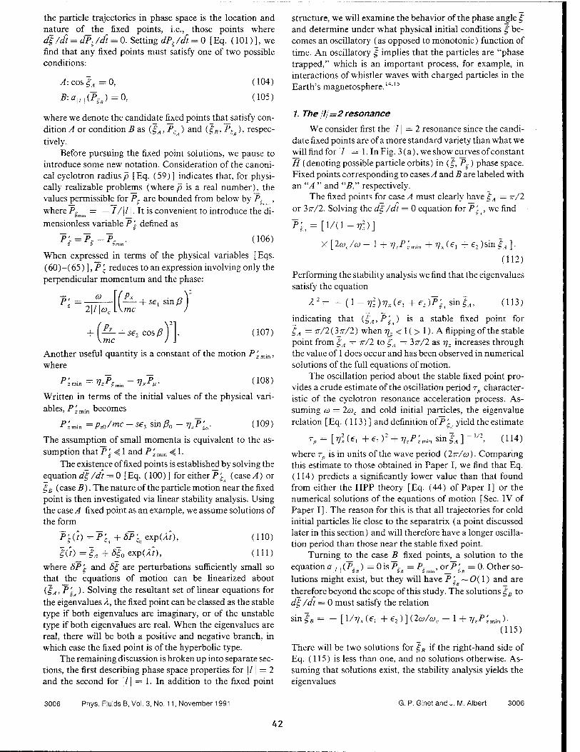
the particle trajectories in phase space is the location and nature of the fixed points, i.e., those points where dl/di = dPJdt = 0. Setting dP^/dt = 0 [Eq. (101)], we find that any fixed points must satisfy one of two possible conditions:
A: cos^ =0,
B:aU](P,) = 0,
(104)
(105)
where we denote the candidate fixed points that satisfy con- dition A or condition B as (L\A, P^A ) and QB, PSB), respec- tively.
Before pursuing the fixed point solutions, we pause to introduce some new notation. Consideration of the canoni- cal cyclotron radius p [Eq. (59)] indicates that, for physi- cally realizable problems (where p is a real number), the values permissible for Ps are bounded from below by P£ , where P~mm = — I/\l j. It is convenient to introduce the di- mensionless variable P'- defined as
P'r=P, (106)
When expressed in terms of the physical variables [Eqs. (60)-(65) ], P1 reduces to an expression involving only the perpendicular momentum and the phase:
v2
P'*=- CO
21/1 (P* _L ■ flV \-sex sin ß \mc J
+ ( —^- + se2 cos ß KTHC
(107)
Another useful quantity is a constant of the motion P'zr
where
P' vA ■IxPu- (108)
Written in terms of the initial values of the physical vari- ables, P'zmm becomes
•Pzmin =pz0/mc-seJ sin^0 -t]zP\ (109)
The assumption of small momenta is equivalent to the as- sumption that P 't 4,1 and Pzmm4,l.
The existence of fixed points is established by solving the equation df /dt = 0 [Eq. (100)] for either P^ (case,4) or \%B (case B). The nature of the particle motion near the fixed point is then investigated via linear stability analysis. Using the case A fixed point as an example, we assume solutions of the form
P'sCt)=Pi+öP'Soexp(Ah, (HO)
where 8P~ and S§ are perturbations sufficiently small so that the equations of motion can be linearized about (iA,P'g )■ Solving the resultant set of linear equations for the eigenvalues A, the fixed point can be classed as the stable type if both eigenvalues are imaginary, or of the unstable type if both eigenvalues are real. When the eigenvalues are real, there will be both a positive and negative branch, in which case the fixed point is of the hyperbolic type.
The remaining discussion is broken up into separate sec- tions, the first describing phase space properties for | /1 = 2 and the second for |/[ = 1. In addition to the fixed point
structure, we will examine the behavior of the phase angle If and determine under what physical initial conditions £ be- comes an oscillatory (as opposed to monotonic) function of time. An oscillatory J implies that the particles are "phase trapped," which is an important process, for example, in interactions of whistler waves with charged particles in the Earth's magnetosphere.14'15
/. The ///=2 resonance
We consider first the | /1 = 2 resonance since the candi- date fixed points are of a more standard variety than what we will find for | /1 = 1. In Fig. 3 (a), we show curves of constant H (denoting possible particle orbits) in (|\ Ps) phase space. Fixed points corresponding to cases A and B are labeled with an "A " and "2?," respectively.
The fixed points for case A must clearly have t,A = IT/2
or 3TT/2. Solving the dlf /dt = 0 equation for P t , we find
Pi = p/U-17?)] X[2coc/co- 1+17.-P;min +VA^ +e2)sinJ/(].
(112)
Performing the stability analysis we find that the eigenvalues satisfy the equation
A2= -(1-^)^(6, +e2)P'gAsm£A, (113)
indicating that ($,,,P- ) is a stable fixed point for £A = TT/2(3_77-/2) when rj^ < 1 ( > 1). A flipping of the stable point from gA = TT/2 to £A = 3ir/2 as rjz increases through the value of 1 does occur and has been observed in numerical solutions of the full equations of motion.
The oscillation period about the stable fixed point pro- vides a crude estimate of the oscillation period rp character- istic of the cyclotron resonance acceleration process. As- suming co = 2coc and cold initial particles, the eigenvalue relation [ Eq. (113)] and definition off ^ yield the estimate
r, = [*£(*, +e2)2 + VzP'zmnsmlA]-
t/2, (114)
where rp is in units of the wave period (2ir/co). Comparing this estimate to those obtained in Paper I, we find that Eq. (114) predicts a significantly lower value than that found from either the HPP theory [Eq. (44) of Paper I] or the numerical solutions of the equations of motion [ Sec. IV of Paper I]. The reason for this is that all trajectories for cold initial particles lie close to the separatrix (a point discussed later in this section) and will therefore have a longer oscilla- tion period than those near the stable fixed point.
Turning to the case B fixed points, a solution to the equation a,, ,(Pf )= OisP^ = P? ,orP't =0.Otherso- lutions might exist, but they will have P? —0(1) and are therefore beyond the scope of this study. The solutions §B to df/dt = 0 must satisfy the relation
sin 1B= -[ I/77* (e, + e,) ] (2co/coc - 1 + -qzPzm^ )- (115)
There will be two solutions for JB if the right-hand side of Eq. (115) is less than one, and no solutions otherwise. As- suming that solutions exist, the stability analysis yields the eigenvalues
3006 Phys. Fluids B, Vol. 3, No. 11, November 1991 G. P. Ginetand J. M.Albert 3006
42
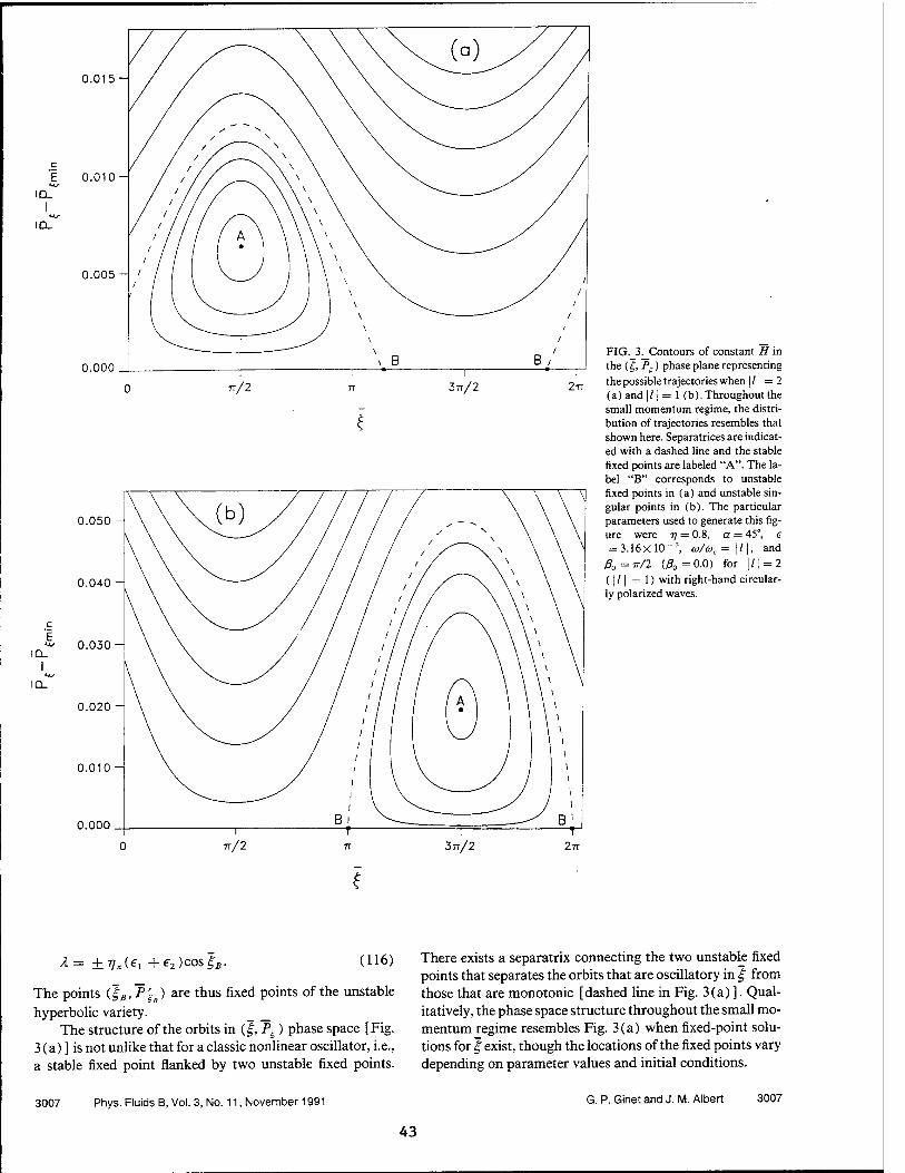
0.015
0.010
IQ_
0.005-1
0.000
0.050
0.000
FIG.S^Contours of constant H in the (£, Ps) phase plane representing the possible trajectories when |/1 = 2 (a) and |/1 = 1 (b). Throughout the small momentum regime, the distri- bution of trajectories resembles that shown here. Separatrices are indicat- ed with a dashed line and the stable fixed points are labeled "A". The la- bel "B" corresponds to unstable fixed points in (a) and unstable sin- gular points in (b). The particular parameters used to generate this fig- ure were rj = 0.8, a = 45°, e = 3.16xl0--\ a)/oc= \l\, and
ß0=ir/2 (Ä,=0.0) for ]/|=2 (| /1 = 1) with right-hand circular- ly polarized waves.
377/2
^= ±Vx(€\ +e2)cosJ'i3 (116)
The points {^B,P'E ) are thus fixed points of the unstable hyperbolic variety.
The structure of the orbits in (£, P£) phase space [Fig. 3(a) ] is not unlike that for a classic nonlinear oscillator, i.e., a stable fixed point flanked by two unstable fixed points.
There exists a separatrix connecting the two unstable fixed points that separates the orbits that are oscillatory in £ from those that are monotonic [dashed line in Fig. 3(a) ]. Qual- itatively, the phase space structure throughout the small mo- mentum regime resembles Fig. 3(a) when fixed-point solu- tions for i exist, though the locations of the fixed points vary depending on parameter values and initial conditions.
3007 Phys. Fluids B, Vol. 3, No. 11, November 1991 G. P. Ginet and J. M. Albert 3007
43
Whether f is monotonic or oscillatory in time depends on which side of the separatrix the initial conditions place the trajectory. This can be determined in the following man- ner. When j]z < 1 we consider the functional dependence of H on 1 as we move along line of constant P'% when PI = ~P'S Starting at the stable fixed point gA = 7r/2jind moving in the direction of increasing g, we see that H is monotonically decreasing in the interval £,— [-n-/2,3ir/2]. Thus, if the value of if corresponding to a. given set of initial conditions is greater than the value of H evaluated on the separatrix, HB =HQBJP'^), the orbit will be oscillatory in f. Evaluating H and HB [Eq. (54) ]_ interim of the initial conditions using the estimates for (gB,P'iB) and assuming a = 2coc, the oscillatory conditionH — HB>0can be writ- ten
sin|0+77r/':min/^(e. +*2)>0. (117)
When T]z > 1, the stable fixed point shifts to £A = 3TT/2 and //(J,P; ) is monotonically increasing as 1 decreases from 3TT/2 to ~/2. In this case, the condition for oscillatory | behavior H - HB < 0 and the direction of the inequality in Eq. (117) must be reversed.
As an example, we investigate the condition for oscilla- tory | when 77. < 1 and the particles are initially cold. We first note that whether the orbits are oscillatory or not, they will all be close to the separatrix in the sense that the initial conditions place H much closer to the value of HB then to the value of H at the stable fixed point. This claim follows from the fact that f: /P^ —0(e) 1 for the initially cold particles. Recalling the definitions of the canonical variables in terms of the physical variables [Eqs. (60)-(65)], the oscillatory condition can be written to lowest order as
(118)
G2 =sin/30
e\ sin2 ß0 - ej cos2 ß0 + 2e, e2 cos2 ß0
e\ sin2 ß0 +4 cos2 ß0
+ ■ Vz^i
VA^i +e2) (119)
G2 (/?0) > 0, where
Figure 4(a) contains plots of G2 for circularly polarized waves as a function of the initial phase ß0. Several different curves are shown, each with a unique value of the propaga- tion angle a. The condition for oscillatory £ behavior is satis- fied for a variety of initial conditions and exhibits a nontri- vial dependence on angle. These predictions of the onset of oscillatory behavior agree with numerical solutions of the orbit-averaged equations of motion. Comparing to the solu- tions of the full equations motion, we find good agreement for a = 5" and 45°. When a = 85°, the full equation solutions have a tendency to jump between the oscillatory and mono- tonic branches if ß0 is not close to 7r/2 or 3TT/2.
2. The ///= 1 resonance
In Fig. 3(b), curves of constant Hzxt plotted in (f, P',) phase space for the [/1 = 1 resonance. The curves look qual- itatively similar to the | /1 =2 curves and in many ways they are. Both resonances have stable fixed points (labeled by "A") and have a clear separation between the orbits that oscillate in f and those that do not. The primary difference between the two resonances is that for \l j = 1, there are no fixed points that satisfy condition B [Eq. (106)]. Rather, "singular points" satisfying condition B exist and they be- have like fixed points in certain respects.
Before considering the details of case B, we examine case A. For angles 1,A = TT/2, 3IT/2 the d^/dt = 0 equation dic- tates that P'- satisfies the relation
o
-2.
11
i 1 i 1
i i i 1
1 \ i 1
• •-- a- 5 - - a=45
-- a-85
\ ■' '
rr/2
/?C
FIG. 4. The function G2 versus initial phase/?0 when [/ [ = 2 for various angles of propagation a when 77 = 0.8, £=3.16 X 10 -3, and 03 = 2coc for cold initial par- ticles and right-hand circularly polarized waves. When G, > 0, the behavior of |" is oscillatory.
3TT/2 2TT
3008 Phys. Fluids B, Vol. 3, No. 11, November 1991
44
G. P. Ginetand J. M.Albert 3008
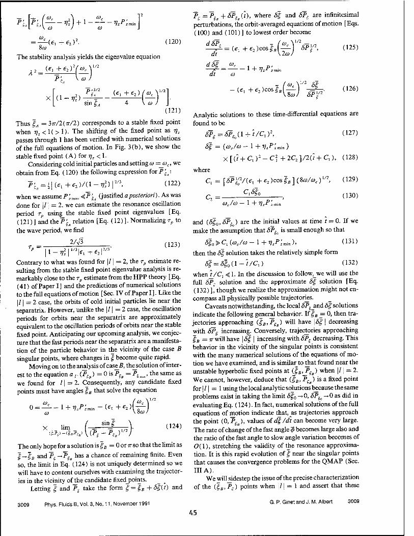
pl C0C -
= -^(6,+£2)2.
6C0
CO ■v P' ■ Iz* z mm
(120)
The stability analysis yields the eigenvalue equation
X- (e, +e2r
X
P'r
(1
CO,
CO
1/2
■vl)
D'3/2 SA (f i + *2 )
1/2
(121)
Thus gA = 3ir/2(ir/2) corresponds to a stable fixed point when T]Z < 1( > 1). The shifting of the fixed point as T)Z
passes through 1 has been verified with numerical solutions of the full equations of motion. In Fig. 3(b), we show the stable fixed point (A) for J]z < 1.
Considering cold initial particles and setting co =_coc, we obtain from Eq. (120) the following expression for P'^:
P'£ ={{(€,+e2)/(l-vl) I 2/3 (122)
when we assume P'zmm <P'?/I (justified a posteriori). As was done for \l j = 2, we can estimate the resonance oscillation period rp using the stable fixed point eigenvalues [Eq. (121) ] and the P 'SA relation [ Eq. (12) ]. Normalizing rp to the wave period, we find
T = y^L . (123) p II ^2 I 1/3|, , , |2/3
| 1 — Vz I Fl + 62 I Contrary to what was found for |/1 = 2, the rp estimate re- sulting from the stable fixed point eigenvalue analysis is re- markably close to the rp estimate from the HPP theory [Eq. (41) of Paper I] and the predictions of numerical solutions to the full equations of motion [Sec. IV of Paper I]. Like the |/1 = 2 case, the orbits of cold initial particles lie near the separatrix. However, unlike the [/1 = 2 case, the oscillation periods for orbits near the separatrix are approximately equivalent to the oscillation periods of orbits near the stable fixed point. Anticipating our upcoming analysis, we conjec- ture that the fast periods near the separatrix are a manifesta- tion of the particle behavior in the vicinity of the case B singular points, where changes in g become quite rapid.
Moving on to the analysis of casei?, thesolution of inter- est to the equation a,,, (P§B) = 0 is PSs = P^mln, the same as we found for |/| = 2. Consequently, any candidate fixed points must have angles gB that solve the equation
co (<*cXn
0 = ^_l + ^mjn-(,I+,2)(-)
sinf X _ lim _
(Pt-PtJ 1/2
(124)
The only hope for a solution is gB = 0 or ir so that the limit as
1—IB and f- -~~P* has a chance of remaining finite. Even so, the limit in Eq. (124) is not uniquely determined so we will have to content ourselves with examining the trajector- ies in the vicinity ofthe candidate fixed_points.
Letting g and P, take the form g = gB + sg0) and
3009 Phys. Fluids B, Vol. 3, No. 11, November 1991
P. =P. +SP~ 0), where Sg and SP£ are infinitesimal perturbations, the orbit-averaged equations of motion [Eqs. (100) and (101) ] to lowest order become
dSP, N , (co^wl s= (e, + e2)cosgB\
dt
d8j_coc
dt co
- (e, + e2)cos£
2co spy2, (125)
isJ 2 Sg
spy2' (126)
Analytic solutions to these time-differential equations are found to be
SPS =<5P&(1 + //C,)2, (127)
Sg = (coc/co-l+yzP'zmin)
X[(?+C1)2-C2+2C2]/2(? + C1), (128)
where
C, = [5Py2/{e, + e2)cos gB](Sco/coc)]/2, (129)
C, = COJCO— 1 + VzP'zmin
(130)
and (8g0, 5P,o) are the initial values at time t = 0. If we make the assumption that SPSo is small enough so that
8g0>C,{coc/co-\+T]zP'zmin), (131)
then the Sg solution takes the relatively simple form
8g = 8g0{\-hCx) (132)
when ?/C, 41. In the discussion to follow,_we will use the full SPs; solution and the approximate Sg solution [Eq. (132) ], though we realize the approximation might not en- compass all physically possible trajectories.
Caveats notwithstanding, the local SP^and Sg solutions indicate the following general behavior. If gB = 0, then tra- jectories approaching (gB,PSe) will have \8g\ decreasing with SPg increasing. Conversely, trajectories approaching gB = TT will have | Sg | increasing with SPS decreasing. This behavior in the vicinity of the singular points is consistent with the many numerical solutions of the equations of mo- tion we have examined, and is similar to that found near the unstable hyperbolic fixed points at (|B,_P^) when |/1 = 2. We cannot, however, deduce that (gB, PSB) is a fixed point for | /1 = 1 using the local analytic solutions because the same problems exist in taking the limit Sg0 —0, 8Pio ->0 as did in evaluating Eq. (124). In fact, numerical solutions ofthe full equations of motion indicate that, as trajectories approach the point (0, ~PSB), values oidg/dt can become very large. The rate of change ofthe fast angle $ becomes large also and the ratio ofthe fast angle to slow angle variation becomes of 0(1), stretching the validity ofthe resonance approxima- tion. It is this rapid evolution of g near the singular points that causes the convergence problems for the QMAP (Sec. Ill A).
We will sidestep the issue ofthe precise characterization of the CgB,~P^ points when |/1 = 1 and assert that these
G. P. Ginet and J. M. Albert 3009
45
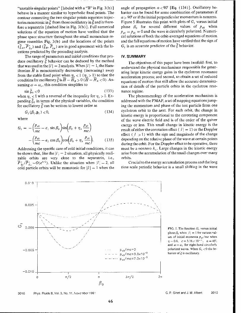
"unstable singular points" [labeled with a "B" in Fig. 3(b)] behave in a manner similar to hyperbolic fixed points. The contour connecting the two singular points sep_arates trajec- tories monotonic in £ from those oscillatory in J" and is there- fore a separatrix [dashed line in Fig. 3(b) ]. Full numerical solutions of the equation of motion have verified that the phase space structure throughout the small momentum re- gime resembles Fig. 3(b) and the locations of the points
(§A>P'§ ) and (£B> ^£„) are in g00^ agreement with the lo- cations predicted by the preceding analysis.
The range of parameters and initial conditions that pro- duce oscillatory J behavior can be deduced by the method that was used in the | /1 =2 analysis. When | /1 = 1, the Ham- iltonian H is monotonically decreasing (increasing) away from the stable fixed point when TJ_Z < 1 (TJ^> l)_so that the condition for oscillatory gisH — HB>0(H — HB <0). As- suming co = coc, this condition simplifies to
sinf0<0 (133) when T]z < 1 with a reversal of the inequality for rjz>\. Ex- panding f0 in terms of the physical variables, the condition for oscillatory J can be written to lowest order as
(134) G1(Ä,po)<0,
where
G, Pxo mc
PyO
ex sin/?0 sin [ß0 + rj
cos/?0 )cos(/?0 Vx (135)
PyO
mo
PyO
mc / \ mcj Addressing the specific case of cold initial conditions, it can be shown that, like the | /1 = 2 situation, all physically reali- zable orbits are very close to the separatrix, i.e., T'~ /~P'- ~0(€4/3). Unlike the situation when 1/1=2, all
SO $A ' '
cold particle orbits will be monotonic for | / j = 1 when the
angle of propagation a<90° [Eq. (134)]. Oscillatory be- havior can be found for some combination of parameters if a > 90° or if the initial perpendicular momentum is nonzero. Figure 5 illustrates this point with plots of G^ versus initial phase ß0 for several different values of pM when Pyo = Pa = 0 and the wave is circularly polarized. Numeri- cal solutions of both the orbit-averaged equations of motion and the full equations of motion have verified that the sign of G, is an accurate predictor of the 1 behavior.
IV. SUMMARY
The objectives of this paper have been twofold: first, to understand the physical mechanisms responsible for gener- ating large kinetic energy gains in the cyclotron resonance acceleration process; and second, to obtain a set of reduced equations of motion that still allow the accurate determina- tion of details of the particle orbits in the cyclotron reso- nance regime.
The phenomenology of the acceleration mechanism is addressed with the PMAP, a set of mapping equations jump- ing the momentum and phase of the test particle from one cyclotron orbit to the next. For each orbit, the change in kinetic energy is proportional to the corotating component of the wave electric field and is of the order of the quiver energy or less. This small change in kinetic energy is the result of either the corotation effect (j / j = 1) or the Doppler effect (\l | > 1) with the sign and magnitude of the change depending on the relative phase of the wave at certain points during the orbit. For the Doppler effect to be operative, there must be a nonzero kx. Large changes in the kinetic energy arise from the accumulation of the small changes over many orbits.
Crucial to the energy accumulation process and the long time scale periodic behavior is a small shifting in the wave
O
^-•-•---.^ / N
/ N / \
/ \ / \
0.005 -
\
' ' ' ' ~~ ~~ ^ x
0.000 \ \ \
\ \ \ /
/ /
/ /
/'
0.005- Pxo/ mc u
px0/mc = 3.0x10~3
px0/mc = 7.0x10~3
0.010
FIG. 5. The function G, versus initial phaseß0 when |/1 = 1 for various val- ues of initial momenta pM/mc when 17 = 0.8, <f=3.16xlCT\ a = 45*, and 0 = coc for right-hand circularly polarized waves. When G, < 0 the be- havior of § is oscillatory.
77/2 3TT/2 277
ßc
3010 Phys. Fluids B, Vol. 3, No. 11, November 1991 G. P. Ginet and J. M. Albert 3010
46
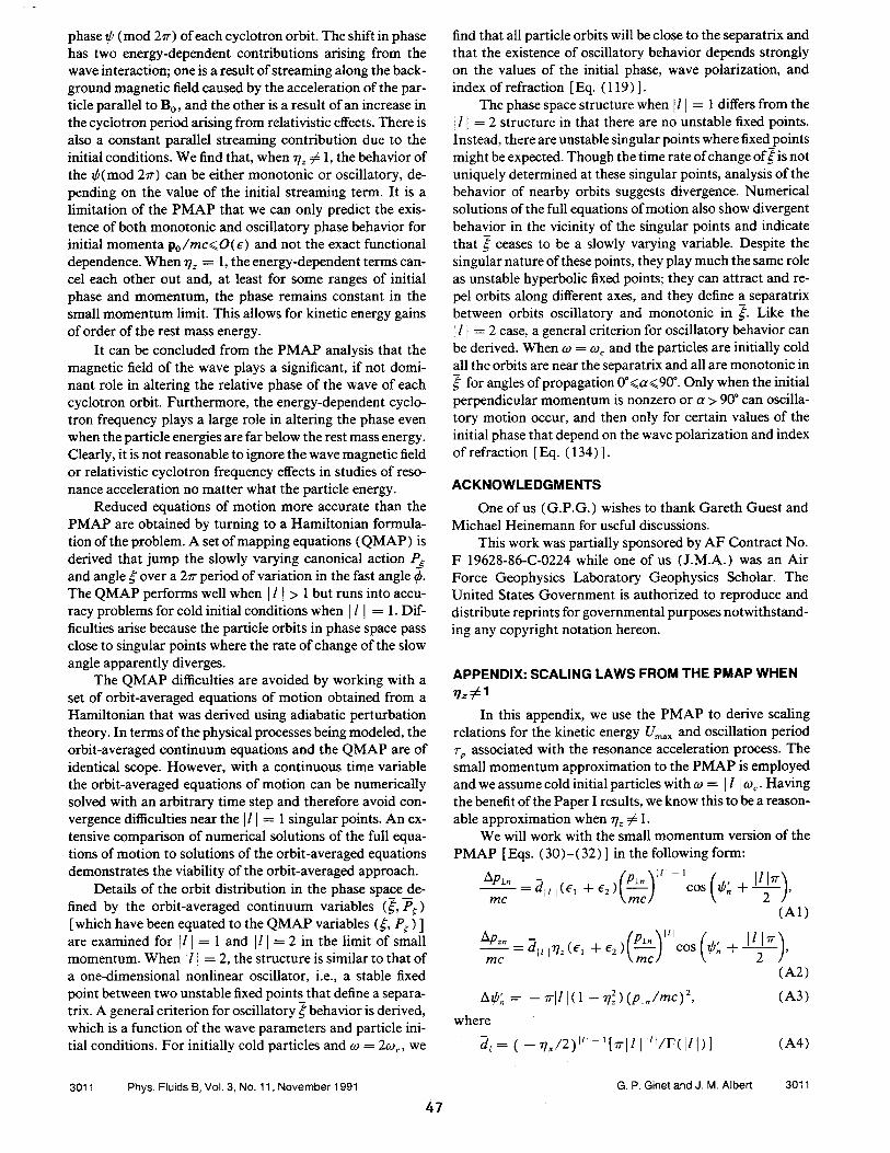
phase t/r (mod 2IT) of each cyclotron orbit. The shift in phase has two energy-dependent contributions arising from the wave interaction; one is a result of streaming along the back- ground magnetic field caused by the acceleration of the par- ticle parallel to B0, and the other is a result of an increase in the cyclotron period arising from relativistic effects. There is also a constant parallel streaming contribution due to the initial conditions. We find that, when rjz ^ 1, the behavior of the ^(mod 277") can be either monotonic or oscillatory, de- pending on the value of the initial streaming term. It is a limitation of the PMAP that we can only predict the exis- tence of both monotonic and oscillatory phase behavior for initial momenta p0/mc<O(e) and not the exact functional dependence. When r/z = 1, the energy-dependent terms can- cel each other out and, at least for some ranges of initial phase and momentum, the phase remains constant in the small momentum limit. This allows for kinetic energy gains of order of the rest mass energy.
It can be concluded from the PMAP analysis that the magnetic field of the wave plays a significant, if not domi- nant role in altering the relative phase of the wave of each cyclotron orbit. Furthermore, the energy-dependent cyclo- tron frequency plays a large role in altering the phase even when the particle energies are far below the rest mass energy. Clearly, it is not reasonable to ignore the wave magnetic field or relativistic cyclotron frequency effects in studies of reso- nance acceleration no matter what the particle energy.
Reduced equations of motion more accurate than the PMAP are obtained by turning to a Hamiltonian formula- tion of the problem. A set of mapping equations (QMAP) is derived that jump the slowly varying canonical action Pj and angle £ over a 2ir period of variation in the fast angle 4>. The QMAP performs well when | / | > 1 but runs into accu- racy problems for cold initial conditions when | /1 = 1. Dif- ficulties arise because the particle orbits in phase space pass close to singular points where the rate of change of the slow angle apparently diverges.
The QMAP difficulties are avoided by working with a set of orbit-averaged equations of motion obtained from a Hamiltonian that was derived using adiabatic perturbation theory. In terms of the physical processes being modeled, the orbit-averaged continuum equations and the QMAP are of identical scope. However, with a continuous time variable the orbit-averaged equations of motion can be numerically solved with an arbitrary time step and therefore avoid con- vergence difficulties near the \l | = 1 singular points. An ex- tensive comparison of numerical solutions of the full equa- tions of motion to solutions of the orbit-averaged equations demonstrates the viability of the orbit-averaged approach.
Details of the orbit distribution in the phase space de- fined by the orbit-averaged continuum variables (f, Ps) [which have been equated to the QMAP variables (g,Pg)\ are examined for |/1 = 1 and |/1 = 2 in the limit of small momentum. When \l \ = 2, the structure is similar to that of a one-dimensional nonlinear oscillator, i.e., a stable fixed point between two unstable fixed points that define a separa- trix. A general criterion for oscillatory ^behavior is derived, which is a function of the wave parameters and particle ini- tial conditions. For initially cold particles and co = 2coc, we
find that all particle orbits will be close to the separatrix and that the existence of oscillatory behavior depends strongly on the values of the initial phase, wave polarization, and index of refraction [Eq. (119)].
The phase space structure when |/1 = 1 differs from the j /1 = 2 structure in that there are no unstable fixed points. Instead, there are unstable singular points where fixedpoints might be expected. Though the time rate of change of £ is not uniquely determined at these singular points, analysis of the behavior of nearby orbits suggests divergence. Numerical solutions of the full equations of motion also show divergent behavior in the vicinity of the singular points and indicate that i ceases to be a slowly varying variable. Despite the singular nature of these points, they play much the same role as unstable hyperbolic fixed points; they can attract and re- pel orbits along different axes, and they define a separatrix between orbits oscillatory and monotonic in £. Like the \l | = 2 case, a general criterion for oscillatory behavior can be derived. When co = coc and the particles are initially cold all the orbits are near the separatrix and all are monotonic in f for angles of propagation 0°<a<90°. Only when the initial perpendicular momentum is nonzero or a > 90° can oscilla- tory motion occur, and then only for certain values of the initial phase that depend on the wave polarization and index of refraction [Eq. (134)].
ACKNOWLEDGMENTS
One of us (G.P.G.) wishes to thank Gareth Guest and Michael Heinemann for useful discussions.
This work was partially sponsored by AF Contract No. F 19628-86-C-0224 while one of us (J.M.A.) was an Air Force Geophysics Laboratory Geophysics Scholar. The United States Government is authorized to reproduce and distribute reprints for governmental purposes notwithstand- ing any copyright notation hereon.
APPENDIX: SCALING LAWS FROM THE PMAP WHEN
In this appendix, we use the PMAP to derive scaling relations for the kinetic energy C/max and oscillation period rp associated with the resonance acceleration process. The small momentum approximation to the PMAP is employed and we assume cold initial particles with co = \ I \ ac. Having the benefit of the Paper I results, we know this to be a reason- able approximation when rj2 # 1.
We will work with the small momentum version of the PMAP [Eqs. (30)-(32)] in the following form:
APL tn. M'l-i
mc = dudel +e2) (£) -(*^>
(Al)
N>, mc
= d,n7]2(e, +e2 £)"'-(« ^> A# = -Tr\l\(\-V
2z)(pin/mc)2,
where
5/=(-77x/2)"!-1[7T|/|"t/r(|/|)]
(A2)
(A3)
(A4)
3011 Phys. Fluids B, Vol. 3, No. 11, November 1991
47
G. P. Ginet and J. M. Albert 3011
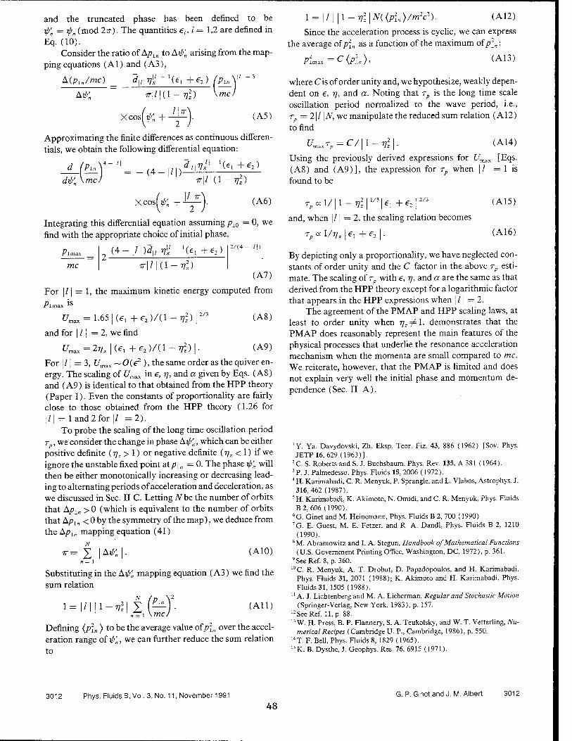
and the truncated phase has been defined to be ip'n = rpn (mod 2ir). The quantities e,, / = 1,2 are defined in Eq. (10).
Consider the ratio of ApLn to Axp'n arising from the map- ping equations (Al) and (A3),
A(pln/mc) ^„i/j/'-'U, +e2) /^V'1"3
■.me) A&
X cosl rl>
ir\l\{l-r,l)
( ,. . \l\ir (A5;
Approximating the finite differences as continuous differen- tials, we obtain the following differential equation:
d fM4""1
dip'n \mcJ = -(4-|/|)
Xcos[ip'n +
dmri^--l{€l + e2)
irl/Kl-^2)
\l\iry
(A6)
Integrating this differential equation assuming pw = 0, we find with the appropriate choice of initial phase,
(4-|/|)Jj/|77l/i-,(e1 +e2) 2/(4- |/|)
(A8)
(A9)
mc ir\l | (1 — 7}z) (A7)
For |/1 = 1, the maximum kinetic energy computed from
Amax IS
C/max = 1.65|(e1+e2)/(l-77z2)|2/3
and for | /1 = 2, we find
£^=277,1^, +€2)/{\-r,l)\.
For |/1 = 3, f/max —Oie2 ), the same order as the quiver en- ergy. The scaling of Um3X in e, 77, and a given by Eqs. (A8) and (A9) is identical to that obtained from the HPP theory (Paper I). Even the constants of proportionality are fairly close to those obtained from the HPP theory (1.26 for |/| = land2for|/j =2).
To probe the scaling of the long time oscillation period rp,v/e consider the change in phase Aip'„, which can be either positive definite (77z > 1) or negative definite (77., < 1) if we ignore the unstable fixed point atpln = 0. The phase ip'n will then be either monotonically increasing or decreasing lead- ing to alternating periods of acceleration and deceleration, as we discussed in Sec. II C. Letting N be the number of orbits that Apln >0 (which is equivalent to the number of orbits that Apln < 0 by the symmetry of the map), we deduce from the Apln mapping equation (41)
ir= X |A^ (A10)
Substituting in the Arfi'„ mapping equation (A3) we find the sum relation
1= l/lll- 1 ~x \mc/ (All;
Defining {p\n) to be the average value of p\„ over the accel- eration range of ip'„, we can further reduce the sum relation to
1= \l\\\-T,l\N{{p\n)/m2c2). (A12)
Since the acceleration process is cyclic, we can express the average of p\n as a function of the maximum of p\n:
pl^=C{P\n), (A13)
where Cis of order unity and, we hypothesize, weakly depen- dent on 6, 77, and a. Noting that rp is the long time scale oscillation period normalized to the wave period, i.e., 7- = 2|/ |Af, we manipulate the reduced sum relation (A 12) to find
U„ = C/\l-ril (A14)
Using the previously derived expressions for £/max [Eqs. (A8) and (A9)], the expression for rp when |/ j = 1 is found to be
TB«l/\l-yl 1/31 f, +e2
and, when |/ j = 2, the scaling relation becomes
rp <x 1/77* I e, + e2 |.
(A15)
(A16)
By depicting only a proportionality, we have neglected con- stants of order unity and the C factor in the above rp esti- mate. The scaling of rp with e, rj, and a are the same as that derived from the HPP theory except for a logarithmic factor that appears in the HPP expressions when | /1 = 2.
The agreement of the PMAP and HPP scaling laws, at least to order unity when 77.^1, demonstrates that the PMAP does reasonably represent the main features of the physical processes that underlie the resonance acceleration mechanism when the momenta are small compared to mc. We reiterate, however, that the PMAP is limited and does not explain very well the initial phase and momentum de- pendence (Sec. II A).
'Y. Ya. Davydovski, Zh. Eksp. Teor. Fiz. 43, 886 (1962) [Sov. Phys. JETP16, 629 (1963)].
2C. S. Roberts and S. J. Buchsbaum, Phys. Rev. 135, A 381 (1964). 3P. J. Palmedesso, Phys. Fluids 15, 2006 (1972). 4H. Karimabadi, C. R. Menyuk, P. Sprangle, and L. Vlahos, Astrophys. J. 316,462 (1987).
5 H. Karimabadi, K. Akimoto, N. Omidi, and C. R. Menyuk, Phys. Fluids B2, 606 (1990).
6G. Ginet and M. Heinemann, Phys. Fluids B 2, 700 (1990). 7G. E. Guest, M. E. Fetzer, and R. A. Dandl, Phys. Fluids B 2, 1210
(1990). SM. Abramowitz and I. A. Stegun, Handbook of Mathematical Functions
(U.S. Government Printing Office, Washington, DC, 1972), p. 361. 9 See Ref. 8, p. 360.
10 C. R. Menyuk, A. T. Drobut, D. Papadopoulos, and H. Karimabadi, Phys. Fluids 31, 2071 (1988); K. Akimoto and H. Karimabadi, Phys. Fluids31, 1505 (1988).
11 A. J. Lichtenberg and M. A. Lieberman, Regular and Stochastic Motion (Springer-Verlag, New York, 1983), p. 157.
12 See Ref. 11, p. 88. 13 W. H. Press, B. P. Flannery, S. A. Teukolsky, and W. T. Vetterling, Nu-
merical Recipes (Cambridge U. P., Cambridge, 1986), p. 550. 14 T. F. Bell, Phys. Fluids 8, 1829 (1965). 15K. B. Dysthe, J. Geophys. Res. 76, 6915 (1971).
3012 Phys. Fluids B, Vol. 3, No. 11, November 1991
48 G. P. Ginet and J. M.Albert 3012
The U.S. Government is authorized to reproduce and sell this report. Permission for further reproduction by others must be obtained from the copyright owner.
Cyclotron resonance in an inhomogeneous magnetic field Jay M. Albert Center for Electromagnetics Research, Northeastern University, Boston, Massachusetts 02115
(Received 23 December 1993; accepted 28 April 1993)
Relativistic test particles interacting with a small monochromatic electromagnetic wave are studied in the presence of an inhomogeneous background magnetic field. A resonance-averaged Hamiltonian is derived which retains the effects of passage through resonance. Two distinct regimes are found. In the strongly inhomogeneous case, the resonant phase angle at successive resonances is random, and multiple resonant interactions lead to a random walk in phase space. In the other, adiabatic limit, the phase angle is determined by the phase portrait of the Hamiltonian and leads to a systematic change in the appropriate canonical action (and therefore in the energy and pitch angle), so that the cumulative effect increases directly with the number of resonances.
I. INTRODUCTION
Charged particle motion is considered under the com- bined influence of an inhomogeneous background magnetic field and an electromagnetic wave. When there is a reso- nance between harmonics of the cyclotron frequency and the Doppler-shifted wave frequency, even a weak wave can significantly perturb the particle motion. This process has been studied by many authors, particularly for radiation belt particles in the Earth's dipole field, where phase bunching leads to further, coherent whistler wave emis- sion, and pitch angle scattering into the loss cone leads to particle precipitation.1-5 These effects have also been stud- ied in laboratory experiments, especially in the context of electron cyclotron heating applications.6"8 For sufficiently II. THE EQUATIONS OF MOTION
2-dependent electromagnetic wave perturbation of finite ex- tent, propagating perpendicular to a constant background magnetic field.16'17 The results obtained here find the phase angle restricted to a narrow range about a deterministic value, leading to a systematic change of the momentum, so that after a series of resonant interactions the cumulative change can be much larger than for the nonadiabatic ran- dom walk. Numerical simulations check the resonance- averaged Hamiltonian against the full equations of motion, and demonstrate the different resonant phase-angle ranges and cumulative effects of many resonances in the two re- gimes.
large amplitude waves, large changes in the particle energy and pitch angle are possible due to both stochastic9-11 and coherent, surfatronlike12 mechanisms.
Ginet and Heinemann13 and Ginet and Albert14 stud- ied in detail a relativistic particle interacting with a small- amplitude electromagnetic wave propagating at arbitrary angle to the background magnetic field B0. A two- dimensional, resonance-averaged Hamiltonian was devel- oped which allowed simple and accurate determination of the motion. The major restriction was to a constant B0, so that the effect of passage through resonance was not in- cluded. In the present paper, the spatial dependence of the resonance condition is considered as a crucial feature of the dynamics. This type of behavior has also been studied for nonrelativistic particles and electrostatic waves by Shklyar,15 in connection with observed proton precipita- tion from the radiation belts. He considers the case of strong inhomogeneity, and derives a random walk for the appropriate particle canonical momentum, assuming the relevant phase angle at resonance to be randomly distrib- uted over (0,2ir). Here, connection is made with that anal- ysis, using a time-dependent pendulum model. It is also shown that in the opposite, weakly inhomogeneous limit, adiabatic considerations apply, giving a different expres- sion for the change in canonical momentum. The use of adiabatic invariants is similar to the methodology used by several researchers to consider the power absorbed from a
For simplicity a slab model is used, with background magnetic field determined by the vector potential AQ= — yBag{z)x, where the inhomogeneity function g sat- isfies g(0) = l, g'(0)=0. The resultant B0=(0, —yBog'yBfg) satisfies V • B=0 exactly for any g. The elec- tromagnetic wave is specified by
AW=AX sin ipeL +A2 cos ^e8 — A^ sin t/«|| , (1)
f -J k'dx—cot. (2)
A constant kL is used, and k\\ is considered only as a function of z because the perpendicular scale length over which it changes is large compared to the Larmor radius p, although kt p is taken —0(1)- With k=fc|| ey +kiei , the angle between k and z is a and between ex and x is ß; thus ey =z, eL =cos/?x+sin/?y, and e8=e|| Xex
= — sin/?x + cos/3y. In the homogeneous situation, the (x,y) axes could be rotated to set ß=0 without loss of generality, but here the inhomogeneity introduces a phys- ical distinction between x and y. Note that the decompo- sition of k into k|| and kx is done relative to B0 at z=0; g' (z) is tacitly assumed small enough that a and ß do not change much over the distances involved. Rigorously in- troducing curvilinear coordinates and their associated Jacobian factors, as done by Shklyar,15 leads to the same results as those obtained below.
2744 Phys. Fluids B 5 (8), August 1993 0899-8221 /93/5(8)/2744/7/$6.00
49
© 1993 American Institute of Physics 2744
The relativistic Hamiltonian of the particle motion in the combined fields is given by
H{V,x;t)=mc\\\ + P-qA/c
mc (3)
where P is the canonical momentum and A = A0 + AW. De- fining 0= \q\Bo/mc and s=q/\q\, a canonical transfor- mation is made from (x,Px,y,Py,z,Pz) toJ,X,Px,<f),I,z,Pz) via the generating function F(x,y,tf>,Px,z,Pz):
F=m£lg 1 sPy
2 V + mQ,g tan (f> +
xPx
milg +zPz, (4)
which is effectively the same as the one used in Refs. 10 and 11 with f2 replaced by fig. In the new variables, the Hamiltonian is given by
- fig- , fig- H=J\+2 — /-f-ö^-i-2, 2 — /(-eiSin^cos^i
\ CO \ CO
+ s€2 cos ip sin 0,) + 2se^Pz sin xp, (5)
where Q=PZ- (g'/g)sin <f>(Icos<f>—spPx) and p is de- fined in Eq. (9) below. (Actually, Q is just Pz/mc.) The wave amplitudes are expressed by e,— \q\A/mc2, /=( 1,2,3). The overbarred variables (X,Px,<t>,7,z,Pz,7) are the normalized quantities
(coX/c,Px/mc,<f>,coI/mc2,coz/c,Pz/mc,cot)
and H is H/mc2. From now on, the overbars will be sup- pressed. The higher-order terms (e^ + e^sin2 ^+e| cos2 tfr in Eq. (5) have been dropped, and Pz has been used instead of the full expression for Q in the e3 term. To zeroth order in e, I is equal to the usual adiabatic invariant \x times constant factors.
After using the familiar Bessel function identity
exp(/asin0)= X J„(a)exp(in8) n= — co
and expanding to first order in eh the Hamiltonian takes the form
mX,Px,<f>,Ij,Pz;t)
g' _ I cos <f>-spPx ^ =Y—sin<£ ^ + L 2T 2T
where
T= 1 + 2 — I+P] co
1/2
sin^, (6)
(7)
fig ■-ß. — I[(ex-e2)Jn_x + {ex+e2)Jn+x}
\ co
+ 2sPze3J„,
co 2ngJ'
§„=8+sn(f>i, (f>x = <f>+sß,
2745 Phys. Fluids B, Vol. 5, No. 8, August 1993
(8)
(9)
(10)
J co
8 = 7]XX + 7\zdz-t-ST]y — PX, (11)
and V(x,y,z) = kix,y,z) c/co is the index of refraction. The quantity T is the canonical analog of the usual relativistic factor y.
In the neighborhood of the lib. resonance, all terms in the sum except n = / can be dropped by averaging over the rapidly oscillating cyclotron phase <b, which also eliminates the term proportional to g'/g. Then constants of the mo- tion, cx=Px—rjxH and c2=I—slH, can be used to elimi- nate Px and Pz:
Px=cx+jla-c2),
P^afv, P0(I,z); i i-ci\z fig __: -1-2 — 7,
Si j CO
(12)
(13)
where az is the sign of Pz. Here, Pz is given neglecting terms of order e, which will be adequate. To this approx- imation, T and a, are functions only of J and z. A closed set of equations of motion can now be written as
dl a, ~r= — si ^^ cos i> dt 2T b
dt~ T
fig +sl-^-\+srqy — Px-jt
co
'fig'
g' dz + 0(0,
(14)
(15)
(16)
(17)
dz aJPr,
or, following Shklyar,
dl a,
dz=-sla*2P0C°S^
d£ azVzP0+siag/co-r co g' ~T= D +ST]y7rpx— + 0(e). (18) dz ofo ,y fig A g
The resonance condition is di/dz=0, which is equivalent to lowest order to the familiar condition co — k^^sKl/y. For an electron in /= — 1 resonance with a right-hand cir- cularly polarized wave propagating along B0, the standard scenario for whistler emissions in the magnetosphere,1"5
£+77-/2 is the angle between vi and the wave magnetic field Bw.
To a good approximation, this nonautonomous system of two ordinary differential equations can be derived from a Hamiltonian with lj degrees of freedom, with z playing the role of time:
K(J,i;z) =K0(I,z) +eKl(I,z)Sm £
co g
'figg
(19)
K0(I,i;z) = ( T)z+sr]y — — cx j (I-c2)
+^-T^-7^7- (I-c2)2-slazP0(Irz),
2 sing g
Jay M. Albert
(20)
2745
50
Ki=slaz 0/
2P0' (21)
where an explicit factor of e has been introduced in Eq. (19) as a reminder that at consists of terms proportional to 6(12,3)- The location(s) of resonance can be found approx- imately from (dK0/dI)(Ii^res)=0, where /, is the initial value of /. The equation for dg/dz deriving from K does not agree with Eq. (18) in the 0(e) terms, but this is acceptable by virtue of the following argument. It is only important to evaluate d^/dz accurately near resonance, since otherwise the deviations in / are small and average to
;{d2i/di)^{z-Z^,
(22)
zero. Near resonance, where d^/dzz one has
5?= [dz+dz dl+~dz dg) dz "
Using d%/dz=(dK0/dI) + e(dK2/dI)sin£ to define K2UJZ), the last two terms in Eq. (22) have the estimates
°cos|+0(e2), dl d d£ Tzmdl~eKl~dir (23)
d-zdid-z^irwco^+oi^- (24)
Now, since near resonance (dKf/dl) is 0(e) while Kx, (tfKo/dl2), and (8K2/dI) are 0( 1), K2 only affects d%/dz through a term small by a factor of e. Therefore, the form of K2 does not appreciably affect the dynamics and may be replaced by Ku so that Eqs. (19)—(21) may be used.
Writing the normalized relativistic kinetic energy of the particle in terms of the mechanical (noncanonical) momentum, U = Jl + (p/mc)2 - 1, expressing this in terms of the transformed variables, and evaluating P2 via Eq. (13) yields U=(I-c2)/sl+0(e). This shows the di- rect relationship between a change in / of 81 and the cor- responding 8U=8I/sl. Similarly, changes in the pitch an- gle £ induced by changes in / can be found through sin2£=yi /v2 = mgI/a[(U+l)2-l).
111. ANALYSIS
Shklyar considers the strongly inhomogeneous case where, by definition, the first term on the right-hand side of Eq. (22) dominates the other two. Conditions for this to hold will be arrived at below. In this case,
^res + ö (Z--Zres)2. a = CPKQ
dzdl (25)
and the change in / across the resonance is
(5J)i= f" -eKx cos £ dz J — CO
\l~TT I IT = -e/:itacosrres±4
(26)
where ± is + if a > 0 and vice versa. Taking the resonant phase |res uniformly random over (0,27r) yields a random walk for the action /. Since both the energy and pitch angle
can be expressed as functions of / plus terms of order e oscillating with frequency O, they, too, undergo a random walk.
In the other limit, when the inhomogeneity term in Eq. (22) is small compared to the last two terms on the right- hand side of (22), which taken alone represent one-degree- of-freedom motion, it is worthwhile to consider contours of K(I,Ü;z) in the (7,|)-plane for fixed z. The picture is like the standard one for a plane pendulum, with an island of closed orbits inside a separatrix, outside of which lie open orbits. At any z, the location of the fixed points is given approximately by (dA,/(9/)(/res,z)=0, with |=ir/2 and — ir/2. In the homogeneous case, motion would be along a curve of constant K, and these contours would be station- ary. The z dependence has two related effects: The particle trajectory is not strictly along lines of constant K, and the entire picture of K contours moves with the passage of "time" z, as described by the above estimate for /res(z).
Intuitively, when the island is at large / from the par- ticle, the particle approximately moves at constant /=;/, and dg/dzzzdKo/dl. As the island slowly approaches /,, the particle is affected, still moving roughly along the curved K contours while slowly crossing them. The island edge, or separatrix, guides the particle towards the x point, which is a resonance since dg/dz=0 there; therefore, the particle should cross the resonance near |,=|x. Following the separatrix leads to a change in / of order the island width, which is 0( -Je). In more detail, the oscillation c?|/ dz is usually much faster than the speed of the x point so that the particle almost follows a K contour, but near the x point d^/dz goes to zero, so that the particle is stationary while the island structure passes through it. As soon as it does, the particle resumes its fast motion at nearly constant I. This is illustrated numerically in Sec. IV below.
To be more quantitative, K is Taylor expanded in / about 7res(z) to get the model Hamiltonian
M(/,£z)=y [J-/res(z)]2+ivsin! (27)
and with Gr=(d2Ko/dI2)(Jies^res), Fr=Kx(I^ie&), 7res(z) given approximately by (dKo/dI)(Ires^)=0 as above. This form for M neglects the small, slow deforma- tion of the separatrix shape. Defining <jF to be the sign of Fr and aG to be the sign of G>, a canonical transformation from (/,£) to (P,Q) via the generating function Jr(|,/')=P(|+a/<7(^r/2) yields
M(P,Oz)=ac(- [P-Pres(z)]2-Fcos Q (28)
with F=aFFr>0, G=acGr>0, and />res(z)=/res(z).
Then, M(P,Q;z) is clearly the Hamiltonian for a pendulum with linearized frequency a0 = ^FG and island width W = 4 ^F/G, moving in P with time z, with o point at 0=0 and x point at Q= ±ir. The sign aG only affects the sense of the (P,Q) motion.
As above, the strongly inhomogeneous analysis yields 8P = - OQF 42tr/1 GP'tes | sin (ßres ± w/4), where ± is - if cr^es > 0. In the other limit, it is valid to use the adia-
2746 Phys. Fluids B, Vol. 5, No. 8, August 1993 51
Jay M. Albert 2746
batic invariant ST= <f> PdQ/lir to calculate 8P. When the particle is outside the separatrix 3~ has the form
jr=/>res(z)±JT0(,c), (29)
4 IF M ^O(K)^-,\-K^(\/K), 2K2EE1+—-, (30)
where f is the complete elliptic integral of the second kind. The argument k is greater than 1 outside the separa- trix, less than 1 inside, and equal to 1 on the separatrix. The choice of sign in the expression for 3~ is critical, and is different before and after crossing the resonance. It may be determined by noting that for z-> ± oo, the island is far from the particle so P is approximately constant and T^P, while J~0-* \P~Pres(z) |. For Eq. (29) to be sat- isfied, if Pres(z) increases with increasing z, ± must be — for z— oo and + for z-+ — oo. Thus 5" tends to the value of P for large positive and negative z, while suffering a jump as the particle crosses the resonance, where the adiabatic condition is violated. The jump in P is therefore equal to the jump in ST across the resonance. This may be esti- mated by evaluating ST just before and after the particle crosses the separatrix, where #c=l. Thus, for PKS(z) in- creasing with z,
8P=P(z= oo ) -P(z= - oo )
=5JT~[Pres(zres) -^-0(K=1 + )]
-[^resUres)+^o(*=l + )]
(31)
As throughout, Pies(z) refers to the resonant value of P for a given z; Pies(zres) is that value actually attained by the particle when it hits the resonance at zres. Evaluating PTes(z) as Presides) assumes that Pres(z) does not change much in the time it takes the particle to go across the island.
For PTSS(z) decreasing with z, the jump in P has the opposite sign. The corresponding change in I is just
(8I)2=-ar (32)
where o> is the sign of dITes/dz, which itself is given by
dITes_ etKp/dz 91
~lz~^~ tfKo/dl2 " (33)
The magnitude of (81)2 is just 2/u times the width of the island, confirming the intuitive analysis presented above.
It is interesting to note that, from Eq. (22), the con- dition for adiabatic behavior to hold, leading to (81)2, is
<2? = cP-Ko/dzdl
K^ctKo/dl2) •41 (for adiabaticity), (34)
while (81)i applies in the opposite limit. Ignoring con- stants of order unity, & is also seen to be essentially the ratio of the island oscillation period, 2ir/a>0, to the time it takes the island to move across its own width,
W/(dITes/dz). This is exactly the quantity one would ex- pect to control the adiabaticity of the motion.
The magnitudes of the two expressions for 81 have the ratio (81)2/(81) i zz ^2$- Therefore, the applicable 81 is always the smaller of the two. A harmonic mean, [l/(6/)1 + l/(5/)2]~1, might be a convenient composite estimate for the jump due to a single resonance. Crossing many resonances, however, brings in an important differ- ence: The strongly inhomogeneous mechanism involves a random phase, which leads jumps at isolated resonances to combine diffusively, as in a random walk, while for the adiabatic case the sign of the jump in action is systemati- cally determined by the motion of the resonance island. If this has the same direction for many consecutive reso- nances, the jumps in 81 add directly, leading to much larger cumulative changes in / and in quantities that de- pend on /, such as the particle energy and pitch angle.
It can also be seen that 6ft is related to the ratio of wave-particle interaction times for the two mechanisms. For the strongly inhomogeneous case, the interaction time is estimated15 from Eq. (25) to be r{ = v~l ■ a~U2, while for the adiabatic process r2 = v~l • W/(dITes/dz), so that ^ = (T,/T2)
2. Therefore, Eq. (34) implies that of the two
mechanisms, the applicable one is the one with the longer interaction time. Note that this concept of interaction time is not the same as the "effective time,"18 which might be defined here as u"1 • (817e).
Next, we make some simple estimates of these expres- sions in terms of physical variables. Using the Oth order constancy of energy and / leads to
d2Kc
d2K0
dzdl
^-1 ' Sty*
l-7Wz(l+2tan2f
(35)
(36)
where p is the mechanical momentum, normalized by mc, and g'/g can be interpreted as the normalized inverse scale length (a)L2/c)~x. Estimating K] is more difficult because the Bessel functions involved, especially for large index, are sensitive to their argument, which is approximately kL p. It can be written as
üT,=s/CTz{-itan2£[(e1-e2)//_I + (e1 + e2).//+1]
+563//}, ^slajeJi. (37)
Using these estimates to approximate !% in Eq. (34) gives
l-Wl+-tan2£
: eJ,(r,l-l) (38)
As is well known, for large |/|, J;(x) is small for \x\ < |/|, quickly reaches its maximum near |*| = |/|, and oscillates with slowly decreasing amplitude for |JC| > |/|.
2747 Phys. Fluids B, Vol. 5, No. 8, August 1993 52
Jay M. Albert 2747
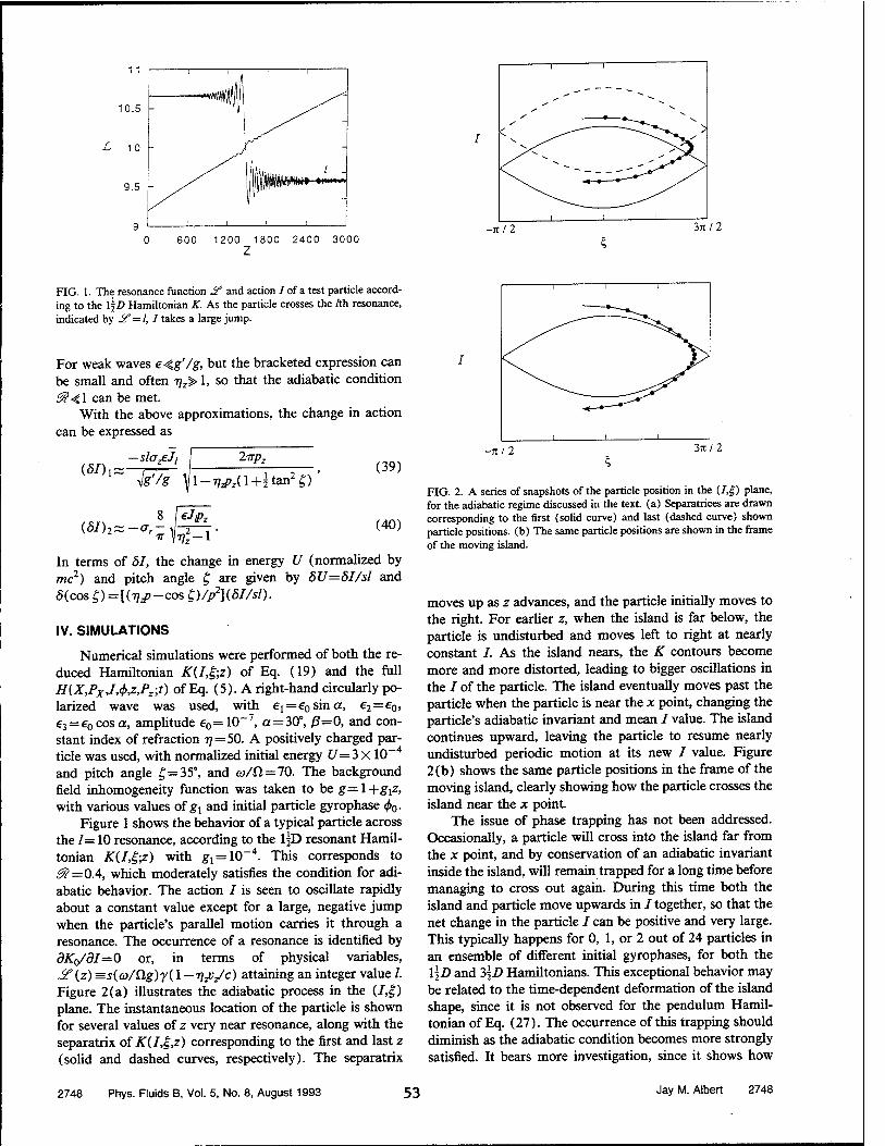
10.5 -
L 1 0
9.5
1 [■ I
c ,^--~~~ -^^^-~ ' ^ ^^^ ^^-T^»^
1 1 1
600 1200 1800 2400 3000 -Kl 2 3JC/2
FIG. 1. The resonance function Jif and action / of a test particle accord- ing to the \\D Hamiltonian K. As the particle crosses the Ah resonance, indicated by ¥ = l, I takes a large jump.
For weak waves e4g'/g, but the bracketed expression can be small and often i7z>l, so that the adiabatic condition 2%4\ can be met.
With the above approximations, the change in action can be expressed as
(&Di —SIOJEJI 2irpz
l-^zd+ltan2^)
(fi/)2SS-ar- 8 \eJpz
Vz 1
(39)
(40)
In terms of 81, the change in energy U (normalized by mc2) and pitch angle £ are given by ÖU=ÖI/sl and 5(cos £) = [(i«>-cos £)/p2](8I/sl).
IV. SIMULATIONS
Numerical simulations were performed of both the re- duced Hamiltonian K{I,&) of Eq. (19) and the full H{X,Px,I,fa,Pz;t) of Eq. (5). A right-hand circularly po- larized wave was used, with el=e0sm.a, e2
=eo> ej = e0cosa, amplitude e0=10~7, a = 30°, ß=0, and con- stant index of refraction 7j = 50. A positively charged par- ticle was used, with normalized initial energy E/=3X 10" and pitch angle £=35°, and <u/O = 70. The background field inhomogeneity function was taken to be g= 1 -\-g\Z, with various values off! and initial particle gyrophase <j>0.
Figure 1 shows the behavior of a typical particle across the /= 10 resonance, according to the l|D resonant Hamil- tonian K(I,fe) with gI = 10-4. This corresponds to ^=0.4, which moderately satisfies the condition for adi- abatic behavior. The action / is seen to oscillate rapidly about a constant value except for a large, negative jump when the particle's parallel motion carries it through a resonance. The occurrence of a resonance is identified by dKo/dI=0 or, in terms of physical variables, Jf (z)=s(a/£lg)y(l— u/c) attaining an integer value /. Figure 2(a) illustrates the adiabatic process in the (/,£) plane. The instantaneous location of the particle is shown for several values of z very near resonance, along with the separatrix of K(I,&) corresponding to the first and last z (solid and dashed curves, respectively). The separatrix
-jc/2 371/2
FIG. 2. A series of snapshots of the particle position in the (/,|) plane, for the adiabatic regime discussed in the text, (a) Separatrices are drawn corresponding to the first (solid curve) and last (dashed curve) shown particle positions, (b) The same particle positions are shown in the frame of the moving island.
moves up as z advances, and the particle initially moves to the right. For earlier z, when the island is far below, the particle is undisturbed and moves left to right at nearly constant /. As the island nears, the K contours become more and more distorted, leading to bigger oscillations in the / of the particle. The island eventually moves past the particle when the particle is near the x point, changing the particle's adiabatic invariant and mean / value. The island continues upward, leaving the particle to resume nearly undisturbed periodic motion at its new / value. Figure 2(b) shows the same particle positions in the frame of the moving island, clearly showing how the particle crosses the island near the x point.
The issue of phase trapping has not been addressed. Occasionally, a particle will cross into the island far from the x point, and by conservation of an adiabatic invariant inside the island, will remain trapped for a long time before managing to cross out again. During this time both the island and particle move upwards in / together, so that the net change in the particle / can be positive and very large. This typically happens for 0, 1, or 2 out of 24 particles in an ensemble of different initial gyrophases, for both the \\D and 3\D Hamiltonians. This exceptional behavior may be related to the time-dependent deformation of the island shape, since it is not observed for the pendulum Hamil- tonian of Eq. (27). The occurrence of this trapping should diminish as the adiabatic condition becomes more strongly satisfied. It bears more investigation, since it shows how
2748 Phys. Fluids B, Vol. 5, No. 8, August 1993 53 Jay M. Albert 2748
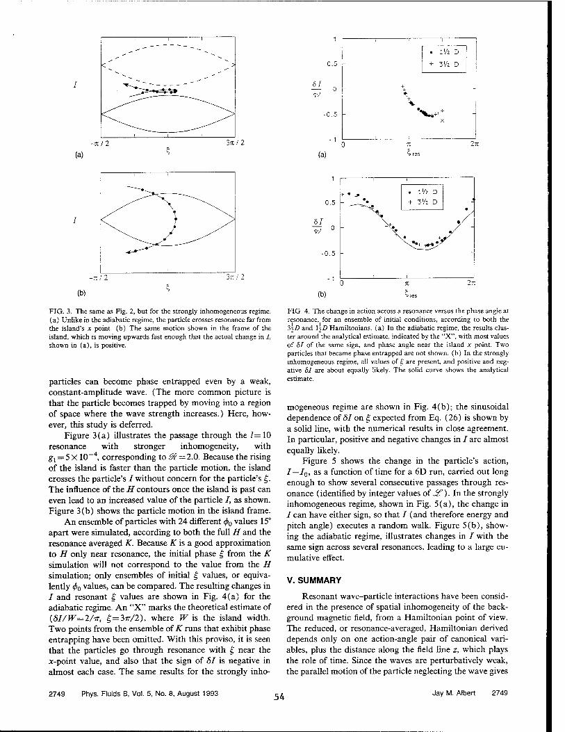
-Till In II
1 1 1
• l'/2 D
0.5 - + 3'/2 D -
5/ 0 IV
-4- -
-0.5 X
(a) (a)
7C
^ res
In
-Till
(b)
FIG. 3. The same as Fig. 2, but for the strongly inhomogeneous regime, (a) Unlike in the adiabatic regime, the particle crosses resonance far from the island's x point, (b) The same motion shown in the frame of the island, which is moving upwards fast enough that the actual change in /, shown in (a), is positive.
particles can become phase entrapped even by a weak, constant-amplitude wave. (The more common picture is that the particle becomes trapped by moving into a region of space where the wave strength increases.) Here, how- ever, this study is deferred.
Figure 3(a) illustrates the passage through the /=10 resonance with stronger inhomogeneity, with g, = 5 X10⁻⁴, corresponding to ^? =2.0. Because the rising of the island is faster than the particle motion, the island crosses the particle's I without concern for the particle's |. The influence of the H contours once the island is past can even lead to an increased value of the particle I, as shown. Figure 3(b) shows the particle motion in the island frame.
An ensemble of particles with 24 different <f>0 values 15° apart were simulated, according to both the full H and the resonance averaged K. Because AT is a good approximation to H only near resonance, the initial phase £ from the K simulation will not correspond to the value from the H simulation; only ensembles of initial £ values, or equiva- lent^ <pQ values, can be compared. The resulting changes in I and resonant £ values are shown in Fig. 4(a) for the adiabatic regime. An "X" marks the theoretical estimate of (8I/W=2/ir, |-=3ir/2), where W is the island width. Two points from the ensemble of AT runs that exhibit phase entrapping have been omitted. With this proviso, it is seen that the particles go through resonance with £ near the jc-point value, and also that the sign of 57 is negative in almost each case. The same results for the strongly inho-
0.5
51 VJ
-0.5
1 i
H- • * . l'/z D •. + Viz D i
- %/
(b)
In
FIG. 4. The change in action across a resonance versus the phase angle at resonance, for an ensemble of initial conditions, according to both the 35.0 and lj-D Hamiltonians. (a) In the adiabatic regime, the results clus- ter around the analytical estimate, indicated by the "X", with most values of 81 of the same sign, and phase angle near the island x point. Two particles that became phase entrapped are not shown, (b) In the strongly inhomogeneous regime, all values of £ are present, and positive and neg- ative 81 are about equally likely. The solid curve shows the analytical estimate.
mogeneous regime are shown in Fig. 4(b); the sinusoidal dependence of 81 on £ expected from Eq. (26) is shown by a solid line, with the numerical results in close agreement. In particular, positive and negative changes in I are almost equally likely.
Figure 5 shows the change in the particle's action, I—I0, as a function of time for a 6D run, carried out long enough to show several consecutive passages through res- onance (identified by integer values of J¥"). In the strongly inhomogeneous regime, shown in Fig. 5(a), the change in I can have either sign, so that I (and therefore energy and pitch angle) executes a random walk. Figure 5(b), show- ing the adiabatic regime, illustrates changes in / with the same sign across several resonances, leading to a large cu- mulative effect.
V. SUMMARY
Resonant wave-particle interactions have been consid- ered in the presence of spatial inhomogeneity of the back- ground magnetic field, from a Hamiltonian point of view. The reduced, or resonance-averaged, Hamiltonian derived depends only on one action-angle pair of canonical vari- ables, plus the distance along the field line z, which plays the role of time. Since the waves are perturbatively weak, the parallel motion of the particle neglecting the wave gives
2749 Phys. Fluids B, Vol. 5, No. 8, August 1993 54 Jay M. Albert 2749
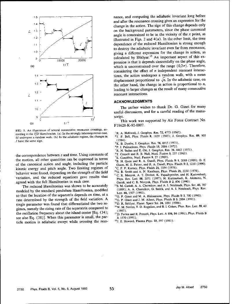
FIG. 5. An illustration of several consecutive resonance crossings, ac- cording to the 3^D Hamiltonian. (a) In the strongly inhomogeneous case, SI undergoes a random walk, (b) In the adiabatic regime, the changes in / have the same sign.
the correspondence between z and time. Using constants of the motion, all other quantities can be expressed in terms of the canonical action and angle, including the particle kinetic energy and pitch angle. Two limiting regimes of behavior were found, depending on the strength of the field variation, and the reduced equations gave results that agreed with the full Hamiltonian in each case.
The reduced Hamiltonian was shown to be accurately modeled by the standard pendulum Hamiltonian, modified so that the location of the separatrix depends on time, at a rate determined by the strength of the field variation. A single parameter was found that differentiated the two re- gimes, namely the rising rate of the separatrix compared to the oscillation frequency about the island center [Eq. (34); see also Eq. (38)]. When this parameter is small, the par- ticle motion is adiabatic except while crossing the reso-
nance, and computing the adiabatic invariant long before and after the resonance crossing gives an expression for the change in the action. The sign of this change depends only on the background parameters, since the phase canonical angle is constrained to be in the vicinity of the x point, as illustrated in Figs. 2 and 4(a). In the other limit, the time dependence of the reduced Hamiltonian is strong enough to destroy the adiabatic invariant even far from resonance, giving a different expression for the change in action, as calculated by Shklyar.15 An important aspect of this ex- pression is that it depends sinusoidally on the phase angle, which is unconstrained over the range (0,2ir). Therefore, considering the effect of n independent resonant interac- tions, the action undergoes a random walk, with a mean displacement proportional to -Jit. In the adiabatic case, on the other hand, the change in action is proportional to n, leading to larger changes as the result of many consecutive resonant interactions.
ACKNOWLEDGMENTS
The author wishes to thank Dr. G. Ginet for many useful discussions, and for a careful reading of the manu- script.
This work was supported by Air Force Contract No. F19628-K-92-0007.
'R. A. Helliwell, J. Geophys. Res. 72, 4773 (1967). 2T. F. Bell, Phys. Fluids 8, 1829 (1965); J. Geophys. Res. 89, 905
(1984). 3K. B. Dysthe, J. Geophys. Res. 76, 6915 (1971). 4P. J. Palmadesso, Phys. Fluids 15, 2006 (1972). 5R. N. Sudan and E. Ott, J. Geophys. Res. 76, 4463 (1971). 6T. Consoli and R. B. Hall, Nucl. Fusion 3, 237 (1963). 7E. Canobbio, Nucl. Fusion 9, 27 (1969). 8B H. Quon and R. A. Dandl, Phys. Fluids B 1, 2010 (1989); G. E. Guest, M. E. Fetzer, and R. A. Dandl, Phys. Fluids B 2, 1210 (1990).
9C. F. F. Karney, Phys. Fluids 21, 1584 (1978). 10G. R. Smith and A. N. Kaufman, Phys. Fluids 21, 2230 (1978). "C. R. Menyuk, A. T. Drobot, K. Papadopoulos, and H. Karimabadi,
Phys. Rev. Lett. 58, 2071 (1987); H. Karimabadi, K. Akimoto, N. Omidi, and C. R. Menyuk, Phys. Fluids B 2, 606 (1990).
12S. M. Carioli, A. A. Chernikov, and A. I. Neishtadt, Phys. Scr. 40, 707 (1989); A. A. Chernikov, G. Smith, and A. I. Neishtadt, Phys. Rev. Lett. 68, 1507 (1992).
13G. P. Ginet and M. A. Heinemann, Phys. Fluids B 2, 700 (1990). 14G. P. Ginet and J. M. Albert, Phys. Fluids B 3, 2994 (1991). ,5D. R. Shklyar, Planet. Space Sei. 34, 1091 (1986). 16W. M. Nevins, T. D. Rognlien, and B. I. Cohen, Phys. Rev. Lett. 59, 60
(1987). 17D. Farina and R. Pozzoli, Phys. Lett. A 156, 84 (1991); Phys. Fluids B
3, 1570 (1991). 18J. E. Howard, Plasma Phys. 23, 597 (1981).
2750 Phys. Fluids B, Vol. 5, No. 8, August 1993 55 Jay M. Albert 2750
JOURNAL OF GEOPHYSICAL RESEARCH, VOL. 99. NO. A12. PAGES 23,741-23.745. DECEMBER 1. 1994
The U.S. Government is authorized to reproduce and sell this report. Permission for further reproduction by others must be obtained from the copyright owner.
Quasi-linear pitch angle diffusion coefficients: Retaining high harmonics
J. M. Albert Center for Electromagnetics Research, Northeastern University, Boston, Massachusetts
Abstract. Diffusion coefficients for electrons pitch angle scattered by plasmaspheric hiss are reconsidered, as given by quasi-linear theory, overcoming practical problems in keeping high cyclotron harmonics n. Upper bounds are used to identify ranges of latitude, n, and wave-normal angle which give only negligible contributions, so that the detailed computation of these values may be avoided, resulting in large savings of computational effort. A simple way of obtaining precipitation lifetimes from the diffusion coefficients is also given, using a shooting method. The lifetimes and steady state fluxes are computed, leading to shorter lifetimes and lower fluxes than previously reported, for energies above 500 keV and Mcllwain parameter L greater than 3.
Introduction
Pitch angle scattering of radiation belt electrons by plasmaspheric hiss is of continuing interest. Although two decades old, the formulation of Lyons et al. [1972], in terms of a bounce-averaged quasi-linear pitch angle diffusion coefficient [Lyons et at, 1971], remains stan- dard. A key innovation of the earlier work was the retention, in principle, of all harmonics to account for resonant interations at all latitudes. However, the nu- merical results included only a limited number (namely, —5 < n < 5), since even with a drastically simplified dispersion relation for the whistlers, the evaluation of these diffusion coefficients can be computationally ex- pensive (L. R. Lyons, personal communication, 1993). Here some analytical techniques are used that reduce the computations to manageable levels, making it fea- sible to include as many cyclotron harmonics terms as required to obtain any specified accuracy. Keeping more harmonics naturally leads to larger diffusion co- efficients. It is also shown how to use them to obtain precipitation lifetimes, using a shooting method. Life- times and the resulting steady state fluxes are recom- puted with the full range of cyclotron harmonics, for a specific set of wave parameters, leading to shorter pre- cipitation lifetimes and lower flux levels.
The expressions for the diffusion coefficients are dou- ble integrals over latitude A and wave-normal angle 6, summed over all cyclotron resonance numbers n, plus the Landau term n = 0. At each A, only a few har- monics contribute, and only for restricted ranges of 0; thus there can be much wasted computation of terms
Copyright 1994 by the American Geophysical Union.
Paper number 94JA02345. 0148-0227/94/94 JA-02345S05.00
in regions where their contributions are negligible. Be- cause the interactions take place for wide and overlap- ping ranges of A, n, and 0, it is unsatisfactory to try to simply estimate which terms seem to be unimpor- tant, in an ad hoc fashion. Instead, by exploiting the tractable form of the functions used to model the waves, analytical upper bounds can be used to identify regions of integration whose results are guaranteed in advance to be less than a given value, and rigorously reject them. Computer time is then spent only on significant contri- butions. The effect of the additional harmonics is found to be significant for the outer electron belt, at energies above 500 keV.
Upper Bounds
With a few additions, the underlying physical for- mulation and notation are the same as that of Lyons et al. [1972]. Wave energy is distributed in frequency u) as a Gaussian centered at wm with width 8u> and lower cutoff L^LC, and distributed over 9 with weight exp(— ta.n2 9 / tan2 9W). The Earth's magnetic field is represented as a dipole, with strength Bo — Beqh(X) = (0.31G/L3)/i(A), where L is the usual Mcllwain parame- ter and h{A) is the dipole function (1 +3 sin2 A) 2 / cos6 A. The local pitch angle a is given in terms of A and the equatorial pitch angle QO by sin a/sin an = h(X). The quantity fle is the magnitude of the cyclotron frequency of a nonrelativistic electron and has the value Qeq at the equator, so that Q.e = Qeq h(X). A useful quantity is P\\<m, given by P^m = me(Qe/ujm)(B$/4-KN), where me
is the electron rest mass and the cold electron density N depends on L only. This is approximately the parallel momentum Pjj required for primary cyclotron resonance with a wave of frequency wm and 0 = 0. Pm is further defined as Pjjm at A = 0, so that P\\>m — Pm h* (A). In the whistler dispersion relation, all terms of order u/Qe
and Qi/u) have been dropped.
23,741 56
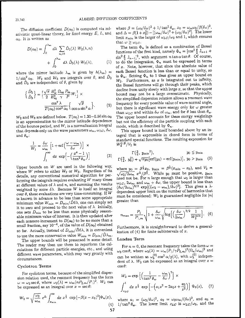
23,742 ALBERT: DIFFUSION COEFFICIENTS
The diffusion coefficient D(a0) is computed via rel- ativists quasi-linear theory, for fixed energy E, L, and ao- It is written as
D(ao)= f md\ ££2(A) W2(X,n)
+ f m dX D3(X) W3(X), (1) Jo
where the mirror latitude Am is given by h(Xm) = l/sin2Q0- W2 and W3 are integrals over 9, and D2
and D3 are independent of Q, given by
it- «'"WA y^F Bj Cleq Pm
2 B^ 7 P
COS7 X ( yfg
T(ao) cos2 a0 1 cos a sin2 ■ I ^ }. I cos a sin2 a ->
(2)
W2 and W3 are defined below. T(a0) = 1.30-0.56 sin a0
is an approximation to the mirror latitude dependence of the bounce period, and Wx is a normalization integral that depends only on the wave parameters wm, WLC, 6U,
and 6W:
1 <5w
r l+erf( —
dx exp — f
<5w -1
tan2 0„ )] (3)
Wo
where ß = (UJ2/8U>)7 + 1/tan2 9W, x0 = wmw2//3(<5w)2>
and A = 0(1 + xg) - [(^m/^)2 + (w2/M2]- The lower
limit xmin is the larger of UJLC/U2 and 1, which ensures that Lü > uJLC-
The term <E>„ is defined as a combination of Bessel functions of the first kind, namely $„ = [cos2 § Jn+i + sin2 | Jn-i]2, with argument ntanatanö. Of course, to do the integration, <£>„ must be expressed in terms of x. Note, however, that since the absolute value of each Bessel function is less than or equal to unity, so is $„. Setting $n to 1 thus gives an upper bound on W2. Furthermore, as x is integrated out to infinity, the Bessel functions will go through their peaks, which decline from unity slowly with large x, so that the upper bound may not be a large overestimate. Physically, the simplified dispersion relation allows a resonant wave frequency for every possible value of wave-normal angle, but there is significant wave energy only for u greater than UJLC and within 8u> of wm, and for 6 less than 9W. The upper bound accounts for these energy weightings but not the efficiency of the particle coupling with each mode, which is described by <l?n.
This upper bound is itself bounded above by an in- tegral that is expressible in closed form in terms of standard special functions. The resulting expression for W%B/V2 is
Upper bounds on W are used in the following way, where W refers to either W2 or W3. Regardless of its details, any conventional numerical algorithm for per- forming the integrals requires evaluating W many times at different values of A and n, and summing the results weighted by some 6X. Because W is itself an integral over 0, these evaluations are very time-consuming. If W is known in advance to be less than some appropriate minimum value Wm-m = Dmin/D6X, one can simply set it to zero and proceed to the next value of A. Initially, one sets Dm\n to be less than some physically reason- able minimum value of interest. It is then updated after each nonzero increment to D(a0) to be no more than a small fraction, say 10~4, of the value of D{a0) obtained so far. Actually, instead of Dmin/D8X, it is convenient to use the more conservative value Wm-m = Dmm/DXm.
The upper bounds will be presented in some detail. The reader may then use them to reperform the cal- culations for different particle energies, etc., and using different wave parameters, which may vary greatly with circumstances.
Cyclotron Terms
For cyclotron terms, because of the simplified disper- sion relation used, the resonant frequency has the form w - uj2sec9, where LJ2(X) = üjm(nPlUm/P\\)2. W2 can be expressed as an integral over x = secö:
dxxi exp[-/3(x-x0)2]$„(x),
(4) 57
T(,4i 2/min )■>
r(|, vl) + v/^ö[erf(2/o) - erf(j/„ »)]
where yo = ß2^o, 3/r ßi(x min
2/0 < 2/min
2/0 > 2/min (5)
XQ), and V2
v/w2/2wm eA/ß*. While yo must be positive, ym\n
need not be. For n large enough that w2 is larger than UJLC, 2wm, and ojm + 6u, the upper bound is less than (8üj/2wm)z'2 exp[({w2 - ujm}/8w)2}. This gives a A- dependent upper limit on the number of harmonics that must be considered: W2 is guaranteed negligible for \n\ greater than
■i 1+^\MG£;)
3/2
w2min (6)
Furthermore, it is straightforward to derive a general- ization of (4) for finite subintervals of x.
Landau Term
For n = 0, the resonant frequency takes the form w = w3cos<?, where u3(X) = 0Jm{P\\/lP\\,m)2(^e/^m)2 and
can be written as u^ cos2 a/g{X), with w3 indepen- dent of A. W3 can be expressed as an integral over z = cosö:
W3
r-l
: exp ( 1
tan2 0, 6w)
f dz z? exp -(aiz2-2a2z + ^§) *o0), (7)
where ai = (io3/8u;)2, a2 = w3wm/(<5a;)2, and a3 = 1/tan26W. The lower limit zLC is ULCIU3, and the
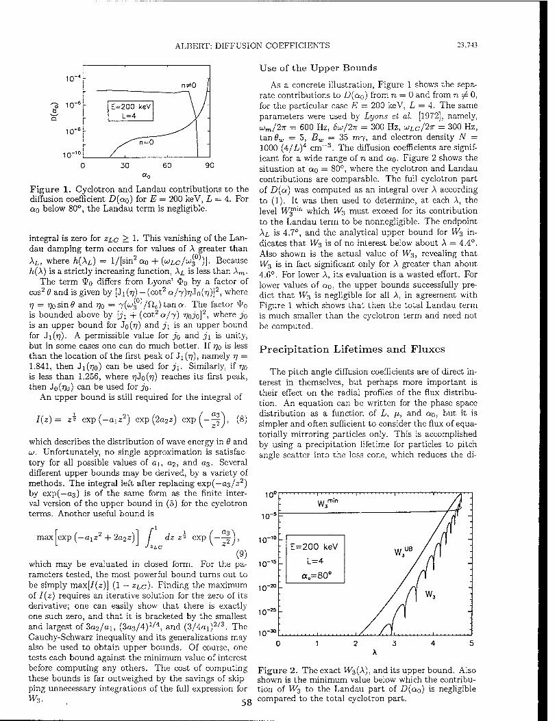
ALBERT: DIFFUSION COEFFICIENTS 23,743
io-4-
10"
10"
10"
- — n*0
E=200 keV L=4
^^n^Ö -
30 60 90
Figure 1. Cyclotron and Landau contributions to the diffusion coefficient D(a0) for E = 200 keV, L = 4. For Qo below 80°, the Landau term is negligible.
integral is zero for z^c > 1- This vanishing of the Lan- dau damping term occurs for values of A greater than AL, where h(Xi) — l/[sin2a0 + (WLC/^4 )]• Because h(X) is a strictly increasing function, A/, is less than Am.
The term ^o differs from Lyons' <E>0 by a factor of cos2 0 and is given by [Ji (77) — (cot2 0/7)77.10 (T?)]
2, where
77 = 770 sin 0 and 770 = 7(^3 /f2e)tana. The factor \I>o is bounded above by [jx + (cot2 a/7) ijojofi where jQ
is an upper bound for 3o(v) an<^ Ji is an uPPer bound for Ji(??)- A permissible value for jo and ji is unity, but in some cases one can do much better. If 770 is less than the location of the first peak of Ji (77), namely 77 = 1.841, then JI(T7O) can be used for j\. Similarly, if 770 is less than 1.256, where r]3o(r]) reaches its first peak, then Jo(770) can be used for jo-
An upper bound is still required for the integral of
I{z) = z? exp (—a\z2) exp (2a.2z) exp ( — (8)
which describes the distribution of wave energy in Q and w. Unfortunately, no single approximation is satisfac- tory for all possible values of a\, 02, and a3. Several different upper bounds may be derived, by a variety of methods. The integral left after replacing exp(— a3/z
2) by exp(—03) is of the same form as the finite inter- val version of the upper bound in (5) for the cyclotron terms. Another useful bound is
: exp (—aiz2 + 2<22z) / dz Jzi.r.
Z2 exp [--j
(9) which may be evaluated in closed form. For the pa- rameters tested, the most powerful bound turns out to be simply max[/(z)] (1 — zic)- Finding the maximum of I(z) requires an iterative solution for the zero of its derivative; one can easily show that there is exactly one such zero, and that it is bracketed by the smallest and largest of Za2/au {2,a3/A)l/A, and (3/4a02/3. The Cauchy-Schwarz inequality and its generalizations may also be used to obtain upper bounds. Of course, one tests each bound against the minimum value of interest before computing any others. The cost of computing these bounds is far outweighed by the savings of skip- ping unnecessary integrations of the full expression for W*- 58
Use of the Upper Bounds
As a concrete illustration, Figure 1 shows the sepa- rate contributions to D(a0) from n = 0 and from n^0, for the particular case E = 200 keV, L = 4. The same parameters were used by Lyons et al. [1972], namely, ojm/2ir = 600 Hz, SLJ/2TT = 300 Hz, toLCßn = 300 Hz, tan#w = 5, Bw = 35 7717, and electron density N = 1000 (4/Z/)4 cm-3. The diffusion coefficients are signif- icant for a wide range of n and ao- Figure 2 shows the situation at ao = 80°, where the cyclotron and Landau contributions are comparable. The full cyclotron part of D(a) was computed as an integral over A according to (1). It was then used to determine, at each A, the level W™in which W3 must exceed for its contribution to the Landau term to be nonnegligible. The endpoint AL is 4.7°, and the analytical upper bound for W3 in- dicates that W3 is of no interest below about A = 4.4°. Also shown is the actual value of W3, revealing that W3 is in fact significant only for A greater than about 4.6°. For lower A, its evaluation is a wasted effort. For lower values of ao, the upper bounds successfully pre- dict that W3 is negligible for all A, in agreement with Figure 1 which shows that then the total Landau term is much smaller than the cyclotron term and need not be computed.
Precipitation Lifetimes and Fluxes
The pitch angle diffusion coefficients are of direct in- terest in themselves, but perhaps more important is their effect on the radial profiles of the flux distribu- tion. An equation can be written for the phase space distribution as a function of L, fi, and ao, but it is simpler and often sufficient to consider the flux of equa- torially mirroring particles only. This is accomplished by using a precipitation lifetime for particles to pitch angle scatter into the loss cone, which reduces the di-
10°
10
10"
-5
10' ■15 _
10"
10"
10"
w3min /}:
■
// '
-
E=200 keV L=4
ao=80°
W3UB /f] '-_
- / f\ w> ":
Figure 2. The exact W3(X), and its upper bound. Also shown is the minimum value below which the contribu- tion of W3 to the Landau part of D(ao) is negligible compared to the total cyclotron part.
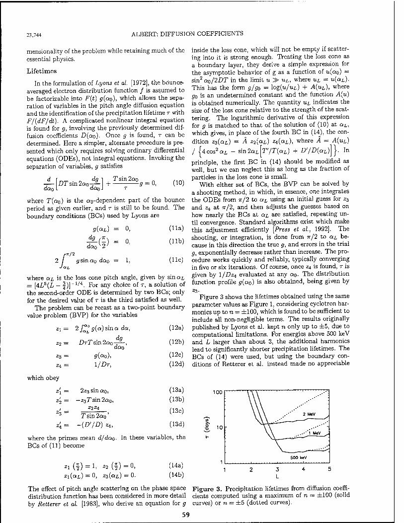
23,744 ALBERT: DIFFUSION COEFFICIENTS
mensionality of the problem while retaining much of the essential physics.
Lifetimes
In the formulation of Lyons et al. [1972], the bounce- averaged electron distribution function / is assumed to be factorizable into F(t) g(a0), which allows the sepa- ration of variables in the pitch angle diffusion equation and the identification of the precipitation lifetime r with F/{dF/db). A complicated nonlinear integral equation is found for g, involving the previously determined dif- fusion coefficients D(ao). Once g is found, r can be determined. Here a simpler, alternate procedure is pre- sented which only requires solving ordinary differential equations (ODEs), not integral equations. Invoking the separation of variables, g satisfies
—- \ DT sin 2a0^- dcto I dao J
Tsin2a0 + —-—g (10)
where T(ao) is the ao-dependent part of the bounce period as given earlier, and r is still to be found. The boundary conditions (BCs) used by Lyons are
,TT/2
Jar,
9{<*L) = o, (11a)
dg ,7Tv _
da0{2J o, (lib)
gsinao dao = 1, (lie)
where at is the loss cone pitch angle, given by sin ai = [4L5(L - f )]_1/4- For any choice of T, a solution of the second-order ODE is determined by two BCs; only for the desired value of r is the third satisfied as well.
The problem can be recast as a two-point boundary value problem (BVP) for the variables
■zi
Z2
23 =
Zi =
2/"L°p(a)sina da,
DTT sin 2a0 -^-, dao
g(<*o), l/Dr,
(12a)
(12b)
(12c)
(12d)
which obey
z, =
2z3 sin ao,
-z3Tsin2ao, Z2Z4
Tsin2a0' z'A= -(D'/D)z4,
where the primes mean d/dao. BCs of (11) become
(13a)
(13b)
(13c)
(13d)
In these variables, the
zi(aZ/) = 0, z3(aL) = 0.
(14a)
(14b)
inside the loss cone, which will not be empty if scatter- ing into it is strong enough. Treating the loss cone as a boundary layer, they derive a simple expression for the asymptotic behavior of g as a function of u(ao) = sin2a0/2DT in the limit u > uL, where uL = u(aL). This has the form g/g0 = \og(u/uL) + A(uL), where go is an undetermined constant and the function A(u) is obtained numerically. The quantity uL indicates the size of the loss cone relative to the strength of the scat- tering. The logarithmic derivative of this expression for g is matched to that of the solution of (10) at aL, which gives, in place of the fourth BC in (14), the con- dition z3(aL) = A z2{aL) z4{aL), where A = A(uL)
I {4cos2aL - sin2aL[T'/T(aL) + £>7Z)(aL)]}. In
principle, the first BC in (14) should be modified as well, but we can neglect this as long as the fraction of particles in the loss cone is small.
With either set of BCs, the BVP can be solved by a shooting method, in which, in essence, one integrates the ODEs from 7r/2 to aL using an initial guess for z3
and z4 at 7r/2, and then adjusts the guesses based on how nearly the BCs at a^ are satisfied, repeating un- til convergence. Standard algorithms exist which make this adjustment efficiently [Press et al, 1992]. The shooting, or integration, is done from 7r/2 to a/, be- cause in this direction the true g, and errors in the trial g, exponentially decrease rather than increase. The pro- cedure works quickly and reliably, typically converging in five or six iterations. Of course, once z4 is found, T is given by 1/Dz4 evaluated at any ao- The distribution function profile g{a0) is also obtained, being given by
Z3- Figure 3 shows the lifetimes obtained using the same
parameter values as Figure 1, considering cyclotron har- monics up to n = ±100, which is found to be sufficient to include all non-negligible terms. The results originally published by Lyons et al. kept n only up to ±5, due to computational limitations. For energies above 500 keV and L larger than about 3, the additional harmonics lead to significantly shorter precipitation lifetimes. The BCs of (14) were used, but using the boundary con- ditions of Retterer et al. instead made no appreciable
100F
o ■D
The effect of pitch angle scattering on the phase space distribution function has been considered in more detail by Retterer et al. [1983], who derive an equation for g
59
Figure 3. Precipitation lifetimes from diffusion coeffi- cients computed using a maximum of n = ±100 (solid curves) or n = ±5 (dotted curves).
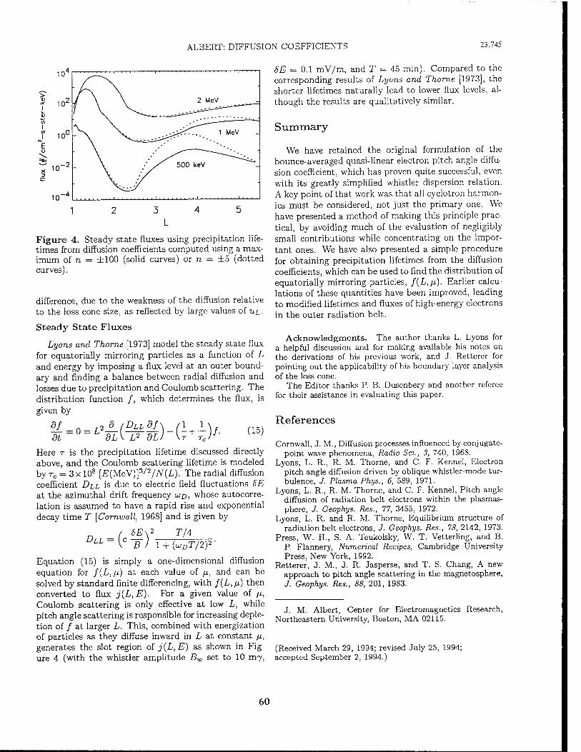
ALBERT: DIFFUSION COEFFICIENTS 23,745
L
Figure 4. Steady state fluxes using precipitation life- times from diffusion coefficients computed using a max- imum of n = ±100 (solid curves) or n = ±5 (dotted curves).
difference, due to the weakness of the diffusion relative to the loss cone size, as reflected by large values of UL-
Steady State Fluxes
Lyons and Thome [1973] model the steady state flux for equatorially mirroring particles as a function of L and energy by imposing a flux level at an outer bound- ary and finding a balance between radial diffusion and losses due to precipitation and Coulomb scattering. The distribution function /, which determines the flux, is given by
£-°-^(%rl)-(^)/- <"> Here r is the precipitation lifetime discussed directly above, and the Coulomb scattering lifetime is modeled by rc = 3x 10⁸ [E(MeV)]3/2/N(L). The radial diffusion coefficient DLL is due to electric field fluctuations 6E at the azimuthal drift frequency LUD, whose autocorre- lation is assumed to have a rapid rise and exponential decay time T [Cornwall, 1968] and is given by
DLL T/A 6E\*
~B~) 1 + (WjDT/2)2
Equation (15) is simply a one-dimensional diffusion equation for f(L, fj.) at each value of fj,, and can be solved by standard finite differencing, with f(L, fi) then converted to flux j(L,E). For a given value of /z, Coulomb scattering is only effective at low L, while pitch angle scattering is responsible for increasing deple- tion of / at larger L. This, combined with energization of particles as they diffuse inward in L at constant //, generates the slot region of j(L,E) as shown in Fig- ure 4 (with the whistler amplitude Bw set to 10 rrry,
8E = 0.1 mV/m, and T = 45 min). Compared to the corresponding results of Lyons and Thome [1973], the shorter lifetimes naturally lead to lower flux levels, al- though the results are qualitatively similar.
Summary
We have retained the original formulation of the bounce-averaged quasi-linear electron pitch angle diffu- sion coefficient, which has proven quite successful, even with its greatly simplified whistler dispersion relation. A key point ofthat work was that all cyclotron harmon- ics must be considered, not just the primary one. We have presented a method of making this principle prac- tical, by avoiding much of the evaluation of negligibly small contributions while concentrating on the impor- tant ones. We have also presented a simple procedure for obtaining precipitation lifetimes from the diffusion coefficients, which can be used to find the distribution of equatorially mirroring particles, f(L,fi). Earlier calcu- lations of these quantities have been improved, leading to modified lifetimes and fluxes of high-energy electrons in the outer radiation belt.
Acknowledgments. The author thanks L. Lyons for a helpful discussion and for making available his notes on the derivations of his previous work, and J. Retterer for pointing out the applicability of his boundary layer analysis of the loss cone.
The Editor thanks P. B. Dusenbery and another referee for their assistance in evaluating this paper.
References
Cornwall, J. M., Diffusion processes influenced by conjugate- point wave phenomena, Radio Sei., 3, 740, 1968.
Lyons, L. R., R. M. Thorne, and C. F. Kennel, Electron pitch angle diffusion driven by oblique whistler-mode tur- bulence, J. Plasma Phys., 6, 589, 1971.
Lyons, L. R., R. M. Thorne, and C. F. Kennel, Pitch angle diffusion of radiation belt electrons within the plasmas- phere, J. Ceophys. Res., 77, 3455, 1972.
Lyons, L. R. and R. M. Thorne, Equilibrium structure of radiation belt electrons, J. Geophys. Res., 78, 2142, 1973.
Press, W. H., S. A. Teukolsky, W. T. Vetterling, and B. P. Flannery, Numerical Recipes, Cambridge University Press, New York, 1992.
Retterer, J. M., J. R. Jasperse, and T. S. Chang, A new approach to pitch angle scattering in the magnetosphere, J. Geophys. Res., 88, 201, 1983.
J. M. Albert, Center for Electromagnetics Research, Northeastern University, Boston, MA 02115.
(Received March 29, 1994; revised July 25, 1994; accepted September 2, 1994.)
60
Proton-Whistler Interactions in the Radiation Belts
E. Villalon1 and W.J. Bwrke2
1 Center for Electromagnetics Research, Northeastern University, Boston, MA 02115, USA
2Geophysics Directorate, PL/OL-AA, Hanscom AFB, MA 01731
The interactions of whistlers with radiation belt protons b investigated. In the inho-
mogeneous geomagnetic field, near the equator, the spacing between cyclotron resonances
is very small. After crossing multiple harmonic resonances, a significant change of par-
ticle energy takes place, and the protons pitch-angle scatter toward the atmospheric loss
cone. A test-particle hamiltonian formalism is investigated for first and second order res-
onant protons. Quasilinear theory is applied for first-order resonant particles to obtain
bounce-averaged, diffusion coefficients. The Fokker Planck equation, containing pitch-
angle, energy and the cross energy/ pitch-angle diffusion terms, is investigated to calculate
diffusion life times.
I. INTRODUCTION
We consider the interaction of plasmaspheric electrons and protons with whistler waves.
The particles are trapped within the earth's radiation belts moving back and forth along
field lines between magnetic mirror points. We call rB the bounce period, the time required
for a particle to go from one mirror point to the other and return. In the region of interest,
the geomagnetic field, B„, is described as a dipole. The interaction region is limited to
the plasmasphere, L < 4, where L is the equatorial distance of the field line measures
in Earth radii (iJE). The plasmashere is made up of cold particles of ionospheric origin
whose distribution is isotropic and Maxwellian. During magnetic storms the radiation
belts fill with energetic, trapped particles whose density is much smaller than that of the
cold plasma. Whistlers are right-hand polarized electromagnetic waves whose magnetic
field, |Bk| < B„. Often they propagate in field-aligned ducts due to density depletions
in local flux tubes. They can either be launched from ground sources or be generated in
the plasmasphere. The dielectric properties for wave propagation are determined by the
magnetized cold plasma distribution. These waves interact with the energetic particles,
if the Doppler-shifted frequency of the waves is some harmonic of the gyrofrequency. For
electron-whistler interactions the waves and particles travel in opposite directions. For
protons they travel in the same direction and the wave phase velocity is very close to the
proton parallel velocity. The situation is depicted in the Figure 1.
199
61
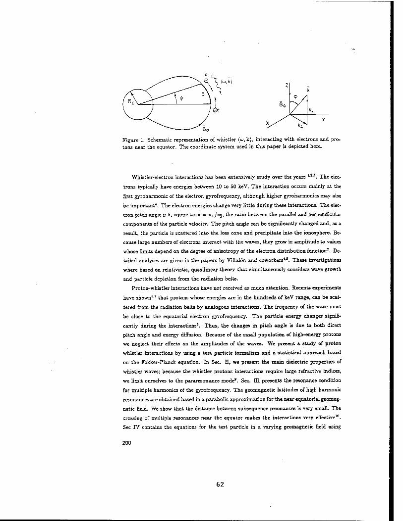
(u,k)
Figure 1. Schematic representation of whistler (w,k), interacting with electrons and pro- tons near the equator. The coordinate system used in this paper is depicted here.
Whistler-electron interactions has been extensively study over the years 1-J-3. The elec-
trons typically have energies between 10 to 50 keV. The interaction occurs mainly at the
first gyrohaxmonic of the electron gyrofrequency, although higher gyroharmonics may also
be important''. The electron energies change very little during these interactions. The elec-
tron pitch angle is 6, where tan 8 = vj./vp, the ratio between the parallel and perpendicular
components of the particle velocity. The pitch angle can be significantly changed and, as a
result, the particle is scattered into the loss cone and precipitate into the ionosphere. Be-
cause large numbers of electrons interact with the waves, they grow in amplitude to values
whose limits depend on the degree of anisotropy of the electron distribution function3. De-
tailed analyses are given in the papers by Villalon and coworkers'4,5. These investigations
where based on relativistic, quasilinear theory that simultaneously considers wave growth
and particle depletion from the radiation belts.
Proton-whistler interactions have not received as much attention. Recents experiments
have shown0,7 that protons whose energies are in the hundreds of keV range, can be scat-
tered from the radiation belts by analogous interactions. The frequency of the wave must
be close to the equatorial electron gyrofrequency. The particle energy changes signifi-
cantly during the interactions8. Thus, the changes in pitch angle is due to both direct
pitch angle and energy diffusion. Because of the small population of high-energy protons
we neglect their effects on the amplitudes of the waves. We present a study of proton
whistler interactions by using a test particle formalism and a statistical approach based
on the Fokker-Planck equation. In Sec. II, we present the main dielectric properties of
whistler waves; because the whistler protons interactions require large refractive indices,
we limit ourselves to the pararesonance mode8. Sec. HI presents the resonance condition
for multiple harmonics of the gyrofrequency. The geomagnetic latitudes of high harmonic
resonances are obtained based in a parabolic approximation for the near equatorial geomag-
netic field. We show that the distance between subsequence resonances is very small. The
crossing of multiple resonances near the equator makes the interactions very pfToc.tivr"1.
Sec TV contains the equations for the test particle in a varying geomagnetic field using
200
62
hamiltonian formalism. Sec V studies the evolution of the action (/) angle (&) variables
as function of the distance (a) along the flux tube using Taylor expansions around isolated
resonances. Let us expand & around the equator: &(s) = ^(Oj + ^f'a + ^'s1. First-order
resonant particles are such that £J1J = 0 (i. e., at the equator d&/ds = 0). This is the
resonance condition as given in Eq. (5). The second-order term $] ~ dB,/da + 0(Bk).
For large wave amplitudes 0{B„) is larger than the contribution of the inhomogeneous
geomagnetic field dB./da. In this case, we say that protons which are in gyroresonance (i.
e ^(i) _ 0)7 satisfy the second-order resonance condition. This is because to zero order in
the electric field amplitudes d^Jda = dt&ds1 si 0. For first-order resonant particles, the
change in action is proportional to the electric field amplitude. For second-order resonant
protons the change in action is proportional to the square root of the electric field ampli-
tude. The second-order resonance condition is met when the field amplitude is large11,12,
the threshold is calculated in this paper. Sec. VI contains a quasilinear formulation for
the distribution function of first order resonant protons. We assume that the protons are
unmagnetized in time scales of the order of 2JT/W, where u is the frequency of the whistler
wave. They are magnetized in times comparable to the bounce period. Because diffusion
occurs over many bounce periods, we average the diffusion equation along the fiux tube.
The bounce averaged, Fokker-Planck equation contains the diffusion coefficients for the
pitch angle, energy, and the cross energy/ pitch angle terms. These coefficients are shown
to have the same orders of magnitude. We reduce the equation to a one-dimensional diffu-
sion equation to be solved for the energy part of the distribution function. This eigenvalue
equation gives the diffusion life-times of protons in the radiation belts.
IT. QUASI-ELECTROSTATIC WHISTLER WAVES
We consider a whistler wave of frequency w and wave vector k, propagating in a field
aligned duct. The geomagnetic field B„ is along the z direction and $ is the angle between
k and B0. The dispersion relation for the refractve index n = ck/ui is
" -i+(n,H|cos^|-i
where up and fie are the electron plasma and gyro frequencies, respectively.
The electric fields components are denoted by £t = £u £» = tc*i. and & = -&« where
£* = J_ KM2
i\ rf-i (n«/w)-|costf| (2)
£1 _ 1'KM''(1'sin^1 (3) £3 rj2 sin<j> cos<f>
For the case where w ~ nt(L)|cos<p|, the equatorial refractive index 7:(L) > 1, then
£t/£i < 1, and £i/£3 sin <p/cos «. The wave becomes quasi-electrostatic, i.e. E is
201
63
in the direction oi' k, and the group velocities vc ~ I./77 are very small. These waves can
interact with proions which energies arc in the hundreds of keV.
Near the equator, the Earth's magnetic field approximates a parabolic profile
n(X) V where s = R.BLi/>, RE is the Earth's radius, L is the magnetic shell and v is the geomagnetic
latitude (see the figure), and rL = (x/2/3)ÄEL. The equatorial gyrofrequency is a(L); fl
stands for the gyrofrequencies either for electrons or protons, along the field line.
m. RESONANT PROTON-WHISTLEE. INTERACTIONS
For whistler waves to interact strongly with protons near equatorial regions, they must
satisfy the resonance condition
u - fcjvj -air-o (5)
where, I = 0,1,2...; n? is the proton gyrofrequency, and fcg and 05 are the parallel compo-
nents of the wave vector and particle's velocity, respectively. We call y. = sin5 9U, where
BL is the equatorial pitch .angle. Here BL > BC{L), where 9,{L) is the pitch angle at the
boundary of the loss cone, and pc the corresponding value of p. As function of the L shell,
the mirror ratio is a = l/pc = Lz (4 - 3/L)1'2. To zero order in electric field amplitudes, the
first adiabatic invariant is conserved. Then we may write for the parallel and perpendicular
components of the particle velocity v. u„ = v{l - pn/n(L)]V\ v± = v^j^L)]1'1.
If we assume that at the equator the protons interact with the harmonic 1=1, the
energy of resonant particles is found solving for the equation: u> - fcj vs - Ü?{L) = 0. We
show 1 = l L_ d _ üh /) (e) e T){L) cos« (1-M)
1/J "h> "
where L denotes equatorial values, mCJI are the electron, proton masses, and /, = Üt(L)/u.
By solving for Eq. (5), using the parabolic profile in Eq. (4) , we find the geomagnetic
latitude V>i of higher order resonances (i.e., I > 1),
where
g(ß) = -£- (| cos «I - T) + I cos <f>\. (8) 1 — /* Je
The distance along the flux tube where resonant interactions take place is given by, st =
REL4>i. The distance between sequential resonances is &st = RsL[1>i+x _ V"«)-
For example, we take L = 3.5, «,/n«W = 7"9> w/n«(i) = °-75' and fli = 10°- F°f
4, = 37", we show that rj[L) = 41.4 and the energy of the resonant protons is 437 keV.
202
64
The location along the geomagnetic Seid of the gyroresonancea are: $j = 0-25", 0j =
0.35",..., jil7 = 1.°. As another example we take $ = 40*, then TJ(L) = 72 and the
proton energy is 158.6 keV. The location of the gyroresonancea are: & = 0.15", fa =
0.21°,..., $«7 = 1.'. Thus there are multiple resonances crossings (17 for the first and 47
for the second examples) within one degree of the magnetic equator, which makes the
proton whistler interactions very efficient.
TV. THE HAMTLTONIAN EQUATIONS
We normalize time t to ß7(i), velocity v to e~l, and length s to r£', and from now on
we always refer to these normalized variables. Let us define
a.tt+j^w-jJjLjt (9)
where tan A = vy/vx, and uIlV are the components of the particle velocity in the x and y
directions, respectively. The dimensionless electric field amplitudes are
«--£- (10)
for i = 1,2,3, and where q is the proton charge. The action-angle variables are (/,A),
where
To first order in the electric field amplitudes e,-, the normalize, time-dependent hamil-
tonian, as function of the canonical pairs, (uj.s), and action-angle variables, is
*=7+' m+JLsin 6 {* n Ji{ki-P) ~ {m)]1,t T'} (12)
Here
r« = (ei - e-t) Jl+1{k±p) + (e, + e,) Jt-i(k±p) (13)
where Je are Bessel functions whose arguments are kLp = (ckj_/tlp) [Zlil/^L)]1^2. If, in
addition to the electromagnetic wave, there is an electrostatic potential <£„, then we replace
in Eq. (12), c3 by s3 + £„/«], where e. = qtp„/mpi^.
For particles crossing a single isolated cyclotron resonance, we consider only one term
I in the summation in Eq. (12). In this case, we find the following constant of motion
Gt'a-mI (14)
By calling x = (w/fy») s'n2 9{s)> where 0[s) is the local pitch angle, we find
tu I x~n,(L) c< + [u/nr(L)\i (15)
This defines the evolution of the pitch angle as a function of the action /.
203
65
By defining v, so that )l = rJ/2 -f IU/7l(L), we obtain
-^lllC^Ji^TT-^)]}1'' (16)
We can now reduce the problem to one-dimension; in which case we find
v, = v. + sin & J -e, Jt(k±p) + i [^yl1/2 r<
is i . in „,,
To zero order in £,, the dimensionless length 5 = t v„. The equation of motion for / as
a function of 5 is
dl — = «cos&T^,».) (18)
Tt[I,v.) = -£lMk±p)~^-[J^}^Tc (19)
As £,• —» 0, then
-r-^+iu^: {20)
The gyroresonance condition is obtained by setting Eq. (20) equal to zero. When this is
satisfied s = sc (the resonance length) which is defined as s£ = 3/y/2 ij>t and ^t is given in
Eq. (7).
By assuming that the protons are in gyroresonance, we show that & satisfies the second
order differential equation
<£ = a( + ^\d-L (2i) is1 v. I as
Here
a< = W) * (22)
*-^)-2g+^Mi (23)
where <*n/<£s = 2s n(i).
V. SECOND-ORDER RESONANCE
We next solve the pair of coupled Eqs. (18) and (21) under the assumption that s is
very close to the resonance length st. The parallel velocity ve is given by setting Eq. (20)
equal to zero, i.e.
In this case we may use a Taylor expansion around s^, then
204
66
(25)
(26)
where /<(£),&(£) are constants, and i2 denotes values at the resonance (a = J<). Here
(<U/<U)W is given by Eqs. (18) and (19), with & = &(£),/ = /(£), and t», = t>,(JZ),
evaluated for resonant values. For protons satisfying the resonance condition, Q — 0.
For convenience we choose cos(&(.K)] = 1.
Using Eq. (14) and setting v. = o,(Ä), we find
u /(*) = i-tfpü(R)/n{L)\ {-Ct+'-vüR)} (27)
where fp = üT{L)/u < 1, and a(R)/ii{L) = 1 + 4- Bv substituting Eq. (26) into Eq.
(21) we show
where a<(JZ) is evaluated at the resonance.
The change of the action / after crossing the c'th resonance, AI, obtained by integrating
Eq. (18), is approximately
A/=(£)(*)**€ (29) as •
The change in x after crossing a resonance is
1 1//, Ax = x{R) I{R) Ct + I{R)/fp\
lis
where x{R) is given by Eq. (15) setting / =• I{R)-
The resonance length 8at is defined as
(JT)<*) 5;5<
/—HJO
5st= I ds cos 44 J—CO
By combining Eqs. (26), (28), and integrating along a we show
Sst =■ T(l/2) cos(7r/4) I1/2
itf'U
(30)
(31)
(32)
The condition of isolated resonances is Sst < As«, where &st = 3/V2 (j>c+i - i>c) and ^
is given in Eq. (7).
In the case where the inhomogeneity of the magnetic field is larger than the contribution
of the resonance, we may neglect the term proportional to (dl/da)^) in Eq. (28), we get
A/ = (g)(Ä)r(l/2)cosW4)[|^-|1/2
where ßi(R) is given by Eq. (23) and must be evaluated at resonance. From the definition
of Te in Eq. (13), the change in the action is proportional to the electric field amplitudes.
205
(33)
67
For interactions such that the contribution of a((R) in Eq. (28) is smaller than the
contribution of {dIids)R. we get
^^[l.^'^^^f^cos^) (34,
where the ± sign depends on the sign of (dI/ds)R. We see that the change in particle
momentum / is now proportional to the square root of the electric field amplitudes, i.e.
JT,. We call this the second order resonance condition because to zero order in the electric
field amplitudes d2 £c/dsz c= 0. For the case of equatorial interactions (st = 0), the condition
for the validity of this approximation is
>ft(A)r(l/2) cosw/4 (35)
Note that for a fix value of u> the second order resonance condition is most likely satisfied
for equatorial interactions, because then the inhomogeneity of the magnetic field is small.
Thus the first harmonic will dominate the second-order interactions. If we allow u to be a
function of J, then „ 1 dn dk* du . , a^^m^+TL^^ (36)
By changing ui so that ac{R) = 0 for sc > 0, the second-order resonance condition is
satisfied for other harmonics, and the change in the particle velocity is proportional to
y/F,. This should be contrasted with the result in Eq. (33) where the change in action is
linear with the electric fields and thus smaller than when the condition for second order
resonance is satisfied.
VI. QUASMNEAR THEORY
The distribution function of protons which satisfy the first order resonance condition
is given by solving for the quasilinear equation Lyons and Williams (1984):
(_L+ *)/s=x,* £ / -|^|G + ^ö]Ä(Vn-«W)ec(k)G/ (37)
where p is momentum and T^„, the atmospheric loss time is defined in1. By assuming
that w/Hp <£ sin2 0C (where 3C is the local pitch angle at the loss cone boundary) we may
approximate
c = z n.(£) PI.3 a , P± 9 p nt p dß p dp
up± P2 dp P ne p 3/i p p|
(38)
(39)
206
68
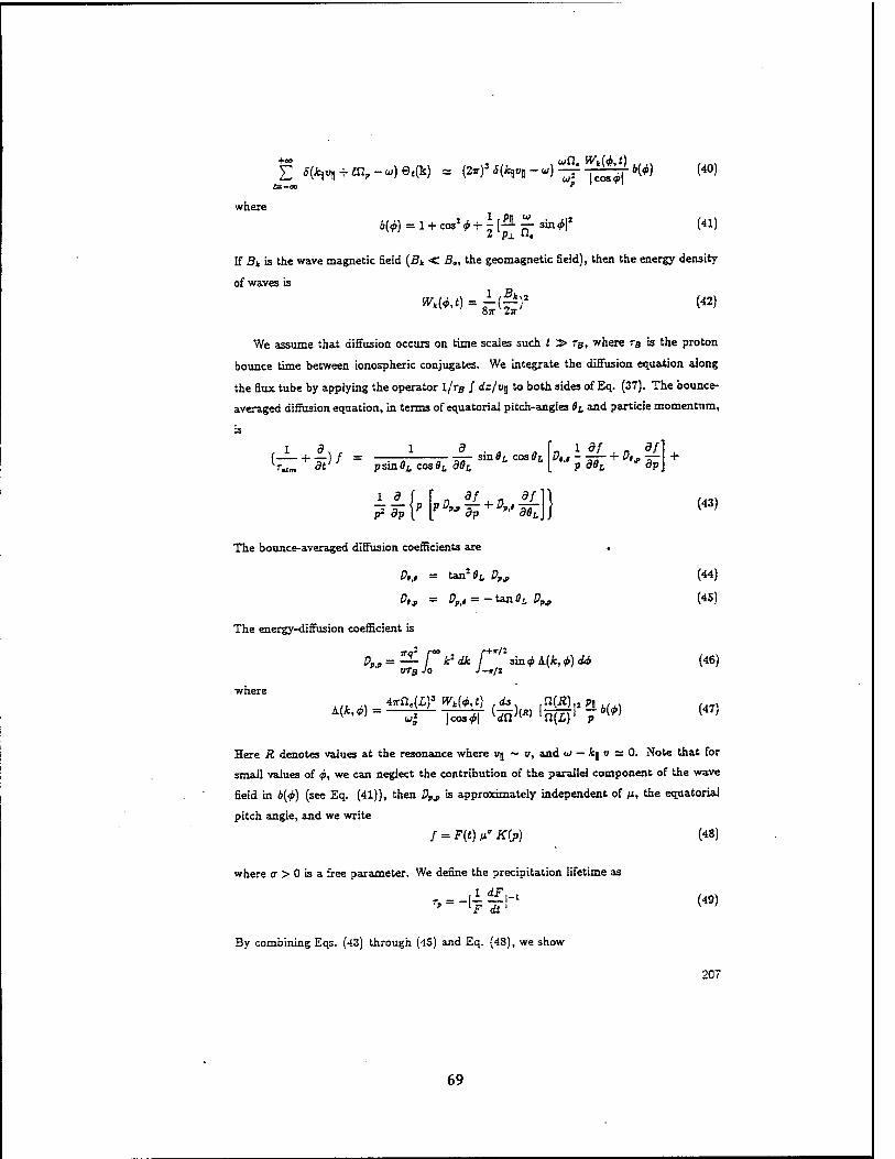
where
g *(V» + m7-u,)e<(k) * (2,)»*(A,«I-W)^^M4(*)
bU) = l + co8i<fi+\[2L£- sin<£]' Z Pi. w«
(40)
(41)
If Bk is the wave magnetic field (Bt < B„ the geomagnetic field), then the energy density
of waves is
<W) = £<£)' (42)
We assume that diffusion occurs on time scales such t > Tg, where Tg is the proton
bounce time between ionospheric conjugates. We integrate the diffusion equation along
the flux tube by applying the operator \jrB / dz/v$ to both sides of Eq. (37). The bounce-
averaged diffusion equation, in terms of equatorial pitch-angles 9L and particle momentum,
is
1 d
£ + 5" psintfi, cosflj, 301 sinOt. cos0t
'■< ;%+'-%>
l a 3f df PD"-ät + D>-'aTL
(43)
The bounce-averaged diffusion coefficients axe
P,,, = tan20t DPJ>
The energy-diffusion coefficient is
where
A(*,*) =
DPJ,= -2- k2dk sin*A(M)<t* " VTB JO J-T/2
Icos^i IS'WWT*1
(44)
(45)
(46)
(47)
Here R denotes values at the resonance where vj ~ v, and u — Aj v = 0. Note that for
small values of <j), we can neglect the contribution of the parallel component of the wave
field in b{<j>) (see Eq. (41)), then DPJ> is approximately independent of n, the equatorial
pitch angle, and we write
/ = F(t) p° K{p) (48)
where a > 0 is a free parameter. We define the precipitation lifetime a3
' {F dtl
By combining Eqs. (43) through (45) and Eq. (48), we show
(49)
207
69
; — - -IA [p) = ; '- Dv,rK -r — \DrJ. —I - •D ■:■ V d]> &p
where /ce = A^[e",'1,. This is an eigenvalue equation for rp as a function of the free parameer
CT. The eigenfunction AT(p) is such that must be regular as p — 0, and well behaved ijr
large p, i. e. as p — oo then A" < p":.
Vn. SUMMARY AND CONCLUSIONS
We have presented a theoretical analysis of proton-whistler interactions near the ec=a-
tor in the plasmasphere. Whistler waves which are near the paxaresonance mode3, can
interact with protons whose energies are in the hundreds of keV. In an inhomogeneons
geomagnetic field, we show that the spacing between subsequence cyclotron resonances is
very small. Because of that, protons are scattered into the atmospheric loss cone aher
crossing multiple resonances. A test-particle hamiltonian formalism is given in term» of
the action (/), angle (&), variables as function of the distance (a) along the flux tub«. "*"e
show that for second-order resonant protons, d^t/ds = d^^/ds2 = 0, and the change in the
particle's momentum is proportional to the square root of the electric field amplitude«. The
thresholds in electric fields for second-order resonance conditions are calculated. A qnsi-
Iinear formulation for the distribution function of first-order resonant protons is presetted.
The bounce-averaged diffusion equation contains diffusion coefficients for the pitch mnz*,
energy, and cross energy/ pitch angle terms. They are shown to be of the same orders
of magnitude. We reduce the diffussion equation to a one-dimensional energy dependent
equation to be solved for the precipitation life times of protons in the Radiation Belt».
Acknowledgements. This work has been supported in part by the U. S. Air Force
contract F19628-89-K-0014 with Northeastern university.
REFERENCES
1. L. R. Lyons and D. J. Williams, Quantitative Aspects of Magnetospheric Physic*. D.
Reidel Publising Company, The Netherlands, 1984.
2. C. F. Kennel and H. E. Petschek, J. Geophys. Res., 1966, 71, 1.
3. P. A. Bespalov and V. Yu. Trakhtpngerts, Rev. Plasma Phys., 1980, 10, 88.
4. E. Villalön and W. J. Burke, J. Geophys. Res., 1991, g£, 9655.
5. E. Villalön, W. J. Burke, P. L. Rothwell, M. B. Silevitch, J. Geophys. Res., 1980, "H,
15243.
208
70
6. H. C. Koons, Geophys. Res. Lett., 1975, 2, 281.
7. R. A. Kovrazhkin, M. M. Mogilevskii, 0. A. Molchaaov, Yu. L Gal'perin, N. V.
Dzhordzhio, Zh. M. Bosbe, and A. Rem, JETP Lett., 1984, 39, 228.
8. R. Gendrin, J. Atmospheric Terrest. Phys., 1968, 2Q. 1313.
9. M. G. Morgan, J. Geophys. Res., 1980, 25, 130.
10. D. R. Shklyar, Planet. Space Phys., 1986, 21, 1091.
11. R. A. Helliwell, J. Geophys. Res., 1967, 72, 4773.
12. K. B. Dysthe, J. Geophys. Res., 1971, 7§, 6915.
209
71
The U.S. Government is authorized to reproduce and sell this report. Permission for further reproduction by others must be obtained from the copyright owner.
PHYSICS OF SPACE PLASMAS (1991) 473 SPI Conference Proceedings and Reprint Series, Number 11
WHISTLER INTERACTIONS WITH ENERGETIC PROTONS
Elena Villalon Center for Electromagnetics Research,
Northeastern University, Boston MA 02115
William J. Burke Geophysics Directorate, PL/OL-AA, Hanscom AFB, MA 01731
ABSTRACT
Whistler waves, near the electrostatic limit, can interact with trapped, energetic protons close to the equator in the Earth's Radiation Belts. In an inhomogeneous geomagnetic field, the spacing between cyclotron resonances is very small due to large ion Larmor radii. After crossing multiple reso- nances, the pitch angles change significantly and the protons are scattered toward the atmospheric loss cone. A test-particle, Hamiltonian formalism is investigated. For second-order resonant protons, the change in particle momentum is proportional to the square root of the wave electric field ampli- tudes. The thresholds in electric fields for second-order resonance conditions are calculated. Quasilinear theory is studied to describe the distribution functions and calculate the diffusion life times of first-order resonant pro- tons. The diffusion coefficients for the energy, pitch angle, and the cross energy/ pitch angle terms are shown to be of the same orders of magnitude.
I. INTRODUCTION
Interactions between whistler waves and energetic electrons in the mag- netosphere have been the subject of intensive research during the past two decades [1 — 3]. The wave-electron, resonant interactions are believed to ac- count for many phenomena such as growth of signals ; 2], emissions of varying frequencies [4] and electron precipitation into the ionosphere [5]. Most of the theoretical work is based on resonant interactions at the first harmonic of the electron gyrofrequency, although higher harmonics interactions may also be important [1]. Detailed theoretical analyses taking into account wave growth and particle depletion, is given in the papers by Villalon and coworkers (see Refs. [6, 7] and references therein).
The interactions of plasmaspheric protons and whistler waves have not re- ceived as much attention. This is because the energies required are very large and the population of protons with energies larger than 500 keV, is small. Since the proton gyrofrequency QP, is much lower than the wave frequency UJ, the resonant velocity v\\ is of the order of the wave phase velocity w/fcy
Scientific Publishers, Inc., Cambridge, MA 02139
72
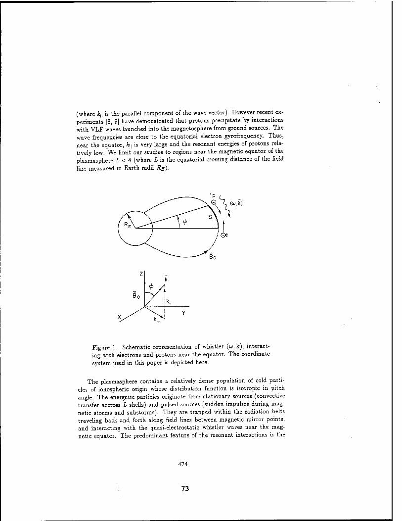
(where fy is the parallel component of the wave vector). However recent ex- periments [8, 9] have demonstrated that protons precipitate by interactions with VLF waves launched into the magnetosphere from ground sources. The wave frequencies are close to the equatorial electron gyrofrequency. Thus, near the equator, ife|| is very large and the resonant energies of protons rela- tively low. We limit our studies to regions near the magnetic equator of the plasmasphere L < 4 (where L is the equatorial crossing distance of the field
line measured in Earth radii RE)-
(oj,k)
Figure 1. Schematic representation of whistler (w, k), interact- ing with electrons and protons near the equator. The coordinate system used in this paper is depicted here.
The plasmasphere contains a relatively dense population of cold parti- cles of ionospheric origin whose distribution function is isotropic in pitch angle. The energetic particles originate from stationary sources (convective transfer accross L shells) and pulsed sources (sudden impulses during mag- netic storms and substorms). They are trapped within the radiation belts traveling back and forth along field lines between magnetic mirror points, and interacting with the quasi-electrostatic whistler waves near the mag- netic equator. The predominant feature of the resonant interactions is the
474
73
crossing of multiple harmonics of the proton gyrofrequency. The proton pitch angle is 9, where tan 8 — v±.lv\\ (the ratio between the perpendicular and parallel components of the velocity). The pitch angles can change due to direct pitch-angle scattering or to energy diffusion [10]. This should be contrasted with the analogous whistler-electron interactions, where the pre- dominant harmonic is the first. Also, electron energies do not change during the interactions. For proton-whistler interactions, the waves and particles travel in the same direction, with the waves slightly overtaking the protons. For electron-whistler interactions the waves and particles travel in opposite
directions. The situation is depicted in the Figure 1. The paper is organized as follows: Sec. II describes the propagation
of whistler waves in a cold plasma, near the electrostatic limit [11]. Sec. Ill studies the resonance conditions for multiple harmonics of the proton gyrofrequency. The inhomogeneous, near-equatorial geomagnetic field is de- scribed by a parabolic profile. Due to the large ion Larmor radii, we show that the distance between resonances is very small. Because of the inclu- sion of multiple harmonics, these interactions are very effective [12!. The test-particle Hamiltonian formalism for each isolated cyclotron resonance, is given in Sec. IV. Sec V studies the evolution of the action (/) and angle (&) variables as function of the distance (5) along the flux tube using Taylor expansions around isolated resonance points. Let us expand & around the equator: £t(s) = &(0) 4- Q s -f 1/2 Q2' s2. First-order resonant particles are
such that Q1' = 0. That is, at the equator d(i/ds = 0, which is the resonance
condition as given in Eq. (5). The second-order term Q ~ dBo/ds + 0(Bk). For large wave amplitudes O(Bk) is larger than the contribution of the in- homogeneous geomagnetic field dBajds. In this case, we say that protons
which are in gyroresonance (i. e. Q = 0), satisfy the second-order reso- nance condition. This is because to zero order in the electric field amplitude d£i/ds — d2(i/ds2 ~ 0. For first-order resonant particles, the change in action is proportional to the electric field amplitude. For second-order reso- nant protons, the change in action is proportional to the square root of the electric field amplitude. The second-order resonance condition is met when the field amplitude is large [13, 14]. The thresholds in electric fields, are then calculated. Sec. VI contains a quasilinear formulation for the distribution function of first order resonant protons. We assume that the protons are unmagnetized m time scales of the order of 2n jui, where u> is the frequency of the whistler wave. They are however magnetized in times comparable to the bounce period. Because diffusion occurs over many bounce periods, we average the diffusion equation along the flux tube. The bounce averaged, Fokker-Planck equation contains the diffusion coefficients for the pitch an- gle, energy, and the cross energy/ pitch angle terms. These coefficients are shown to have the same orders of magnitude. We reduce the equation to a
475
74
one-dimensional diffusion equation to be solved for the energy part of the distribution function. This eigenvalue equation estimates the VLF diffusion
life times of protons in the radiation belts.
II. QUASI-ELECTROSTATIC WHISTLER WAVES
We consider a whistler wave of frequency w and wave vector k, prop- agating in a field-aligned duct. The geomagnetic field B0 is along the z direction and <j> is the angle between k and B0- The dispersion relation for the refractve index 77 = ck/ui is
V = 1+ ("»' (1) (n«/w) 1 cos 01-1
where uip and fie are the electron plasma and gyro frequencies, respectively.
The electric field is [15]
E = x £l cos $ - y £2 sin ¥ - z £3 cos $ (2)
where x, y and z are unit vectors; * = k± x + k\\ z - u t, and % kL are the components along and perpendicular to B0 of the wave vector. The ratios
of electric field components are
1 ( **i"? V3 -1 (fieM - 1 cos <b\
1 -te ,n2 - (v sin <f)2
£1
£3 T]2 sin 4> cos 6
(3)
(4)
For the case where u ~ fie(I)| cos <j>\, the equatorial refractive index 7]2(L) > 1, then £2/£i < 1, and £i/£3 ~ -sin^/cos^. The wave becomes quasi- electrostatic,!, e. E has a significant component in the direction of k, and the group velocity vg ~ I/77. This wave can interact with protons which energies
are in the hundreds of keV. Near the equator, the Earth's magnetic field may be approximated as
having a parabolic profile
° l + (-)2 (5)
where s ~ RE Lip and ip is the geomagnetic latitude (see the figure), and TL = [y/2/Z)REL. The equatorial gyrofrequency is denoted by fi(£), and fi stands for the gyrofrequencies either for electrons or protons at a location s away from the equator along the field line.
476
75
III. RESONANCE PROTON WHISTLER INTERACTIONS
For whistler waves to interact strongly with protons near equatorial re-
gions, they must satisfy the resonance condition
w - fc||V|| - lttv = 0 (6)
where, t = 0,1,2...; flp is the proton gyrofrequency, and v\\ is the parallel component of the particle's velocity. We call fi - sin2 9L, where BL is the
equatorial pitch angle. Here BL > 9C{L), where 8C{L) is the pitch angle at the boundary of the loss cone, and p.c the corresponding value of fi. As function of the L shell, the mirror ratio is <r = l/fic = P (4 - 3/L)1/2. To zero order in electric field amplitudes, the first adiabatic invariant is conserved. Then we may write for the parallel and perpendicular components of the particle velocity v. v{l = v[l - fiQ/QiL)}1'2, v± = v[ßQ/Q(L)Y't2.
At the equator the protons interact with the harmonic £ = 0. and then the energy of resonant particles is found solving for the equation: ui — k\\ v« = 0.
We show v- = I I (7) c V(L) cos0 (1-M)
1/2
where -q(L) denotes equatorial values of the refractive index, and /e =
nt{L)/w. By solving for Eq. (6), using the parabolic profile in Eq. (5) , we find
the geomagnetic latitude Tpt of higher order resonances (i.e., I > 0),
# = iü^(/e|C0S^|_i) J_ (8) 9 mp g{p)
where . 5(/i) = -^-(|cos^|-7-)-r|cos0i. (9)
where mCiP are the electron, proton masses. The distance along the flux tube where resonant interactions take place is given by, st = RE Lib i. The distance between two subsequent resonances is obtained from Asc = REL(TI>I+\ —ipi)-
For example, we take L = 3.5, wp/ne(I) = 7.9, w/nc(L) = 0.75, and &L = 10°. For (j) = 37°, we find that rj(L) - 41.4 and the energy of the resonant protons is 437 keV. The location along the geomagnetic field of the gyroresonances are: ib2 = 0.25", ib3 = 0.35°,..., VIT = l-°- As another example we take <f> = 40°, then TJ{L) = 72 and the proton energy is 158.6 keV. The location of the gyroresonances are: ib2 = 0.15°. u--2 = 0.21°, ...,VA7 = 1.°. We also show that ibt is very weakly dependent upon pitch angle p. Thus there are multiple resonances crossings (17 for the first and 47 for the second examples) within one degree of the magnetic equator, which makes the proton whistler interactions very efficient.
477
76
IV. THE HAMILTONIAN EQUATIONS
We normalize time t to ÜP(L), velocity v to c_\ and length, s to r£\ and from now on we always refer to these normalized variables. Let us define
^^J^'r^w-m' (10)
where tan A = vy/vx, and vx,y are the components of the particle velocity in the x and y directions, respectively. The dimensionless electric field ampli-
tudes are p
* = -^- (11) <.pc
for i = 1,2,3, and where q is the proton charge. The action-angle variables
are (7, A), where
, _ zi n?(L) (i2) 2 np
To first order in the electric field amplitudes £;, the normalize, time- dependent hamiltonian, as function of the canonical pairs, (•ü||, S), and action-
angle variables, is
n 4+j w)+Jlsin u i63 u"Jt{kLP) ~[^)]1/2 r'l (13)
Here Ti is a linear combination of Bessel functions Ji,
Tt = (fi - ea) J<+l(fcxP) + (ffi + £2) Ji-i(*j.p) (14)
whose arguments are fcx p = (cfcx/np) [27n/n(7)j1/2. If, in addition to the electromagnetic wave, there is an electrostatic potential <j>„, then we replace
in Eq. (13), £3 by £3 + £o/v\\, where e0 = q(p0/mpc2. For particles crossing a single isolated cyclotron resonance, we consider
only one term £ in the summation in Eq. (13). In this case, we find the
following constant of motion
C'-n-m1 (15)
The criterion for overlapping of resonances is given later on in Eq. (37). By defining v0 so that H = v*/2 + m/fl(L), we obtain
np(L) n(L)- *.= 7[G + /(7^7T-*öfn)] ' (16)
478
77
We can now reduce the problem to one-dimension, in which case we find
V|| = v0 + sin& Tt(I,v0)
§ - ^7JwrfT"mi' (17)
where T/(/,i/0) is denned in Eq. (19). To zero order in £;, the dimensionless length a = t v0. The equation of
motion for las a function of s is
^ = *cos&T<(J,*0) (18) ds
UI,v.) = -3^p) + ^[^y]1/2r, (19)
As £i —» 0, then
(£.5 UP{L)v0
The gyroresonance condition is obtained by setting Eq. (20) equal to zero. When this is satisfied a = st (the resonance length) which is defined as
at = 3/V2ipi and ipt is given in Eq. (8). By assuming that the protons are in gyroresonance, we show that (t
satisfies the second order differential equation
Here
ai
ds2 ' v0 £ ds
ßi du
(21)
(22) Ü{L) ds
m-, dk\\ 1 .1 Ci, ,.„, ßt = np(L)rL S.-J-+ -[- + -] (23)
ms d\le v0 I v*
where dQ./ds = 2.3 Ü(L).
V. SECOND ORDER RESONANCE
We next solve the pair of coupled Eqs. (18) and (21) under the assump- tion that 5 is very close to the resonance length st. The parallel velocity v0
is given by setting Eq. (20) equal to zero, i.e.
Vo{R) = ^-—1— (l-*£) (24)
479
78
In this case we may use a Taylor expansion around st, then
{ds I ~ It(R) + {fu{s-'i) (25)
u = WÄ) + dl) (--'*) +T (J" *|)J (26)
where h(R),&(R) are constants, and Ä denotes values at the resonance (j = st). Here {dI/ds){R) is given by Eqs. (18) and (19), with fc = fc(Ä), J = I(R), and v0 = v0{R), evaluated for resonant values. For protons satisfying
the resonance condition, $] = 0. For convenience we choose cos[6(Ä)] = 1- The constant of motion CL is obtained evaluating Eq. (15) at the equator,
we show 2
n _f__l__ c ) -i-F£ + 4 (27) °l~ \V2 V(L) cos <pVp(L)rL) I - » U
where fp = QP{L)/LJ « 1. Using Eq. (16) and setting v0 = v0{R), we find
W-im^/ndnH'^H (28)
where fl(Ä)/n(I) = 1 + 5?. By substituting Eq. (26) into Eq. (21) we show
fW - a,(fl) + (*"r£)2 ~ (-)fm (29)
where at(R) is evaluated at the resonance. The change of the action I after crossing the f th resonance, AI, obtained
by integrating Eq. (18), is approximately
A/ = (g)(fi) Sst (30)
The resonance length 6st is defined as
Ssi= /'°° <£scos£z (31) J-OO
By combining Eqs. (26), (29), and integrating along s we show
Sst = T{l/2) COS(TT/4) ia 1/2
(32)
Resonances are isolated in space if 6st < As*, where As* = Z/V2{i>i+i-4>i)
and V/ is given in Eq. (8). In the case where the inhomogeneity of the magnetic field is larger than
480
79

the contribution of the resonance, we may neglect the term proportional to {dI/ds){R) in Eq. (29), we get
,dl. AI = (-){R) r(l/2) cos(*/4)
['ßi(R)ai\
1/2
(33)
where ßt[R) is given by Eq. (23) and must be evaluated at resonance. From the definition of Vt in Eq. (14), the change in the action is proportional to the electric field amplitudes.
For interactions such that the contribution of Q-c{R) in Eq. (29) is smaller than the contribution of [dl/ds)n, we get
AI = ± l< (£)<*,! 1/2 r(1/2) ^mn cos(:r/4) h\rL
(34)
where the ± sign depends on the sign of (dl/ds)^. We see that the change in particie momentum I is now proportional to the square root of the electric field amplitudes, i.e. -Jzi. We call this the second order resonance condition because to zero order in the electric field amplitudes d2£i/ds2 ~ 0. For the case of equatorial interactions (si = 0), the condition for the validity of this approximation is
h\TL / 1 ,,dl
Vivo V {TM
1/2
>ßi{R)T{\/2) COSTT/4 (35)
Note that for a fix value of ui the second order resonance condition is most likely satisfied for equatorial interactions, because then the inhomogeneity of the magnetic field is small. Thus the first harmonic will dominate the second-order interactions. If we allow ui to be a function of s, then
at = ßt 1 du dk\\ du
£l(L) da du ds (36)
By changing w so that ai(R) = 0 for 3i > 0, the second-order resonance condition is satisfied for other harmonics, and the change in the particle velocity is proportional to ^/Fi. This should be contrasted with the result in Eq. (33) where the change in action is linear with the electric fields and thus smaller than when the condition for second order resonance is satisfied.
We have carried out some preliminary calculations applying the theory presented in this section; for waves such that 0.5 < u/Qt < 1, and cos© > u/ne, and for electric field amplitudes which are in the range 10_s to 10~4
Volt/cm. They show the contribution of large harmonic resonances, i.e. £> 50 in the change of the action AJ as defined in Eq. (30). As a matter of fact
481
80
of fact the largest contributions to AJ come from values of I which are close to the argument of the Bessel functions kL p. For equatorial pitch angles between 7.5 and 20 degrees, at the L shell 3.5, the values of I which give maximum change in the action are larger than 50 and smaller than 150.
Overlapping of resonances occur when
A/ > 1 (37) h-AR)-h{R)
For electric fields greater than 10-4 Volt/cm all resonances (150 > I > 1) overlap, but for smaller electric fields only some of them do for particles which equatorial pitch angles are near the loss cone. Note that even if resonances overlap in space (see comments after Eq. (32)), we must still treat them as independent of each other if the criterion in Eq. (37) is not met.
VI. QUASILINEAR THEORY
The distribution function of protons which satisfy the first order reso- nance condition is given by solving for the quasilinear equation Lyons and
Williams (1984):
Vaem dt1J ^J (2TT)3 u,p,
where p is momentum and ratm, the atmospheric loss time is defined in [lj. By assuming that u/Clp < sin2 9Z (where 9C is the local pitch angle at the
loss cone boundary) we may approximate
' , w-Vll 1 d 2 ■ a 2 Q'(L) Pll d (?±\3P_ + up, ?2 dp v ne P dy. P P\\
(39)
G = J.MV{?±y± + ?±± (40) p ne p dp p dp
g 5(kn + mp - u) 0«(k) ^ (2x)» 5( Vll - u) ^ ^M h{4)) (41) £= —CO ?
where 1
6(?) = l + cos^4-^^sine]2 (42)
If Bk is the wave magnetic field (Bk < B„ the geomagnetic field), then the
energy density of waves is
w^ = h&2 (43)
482
81
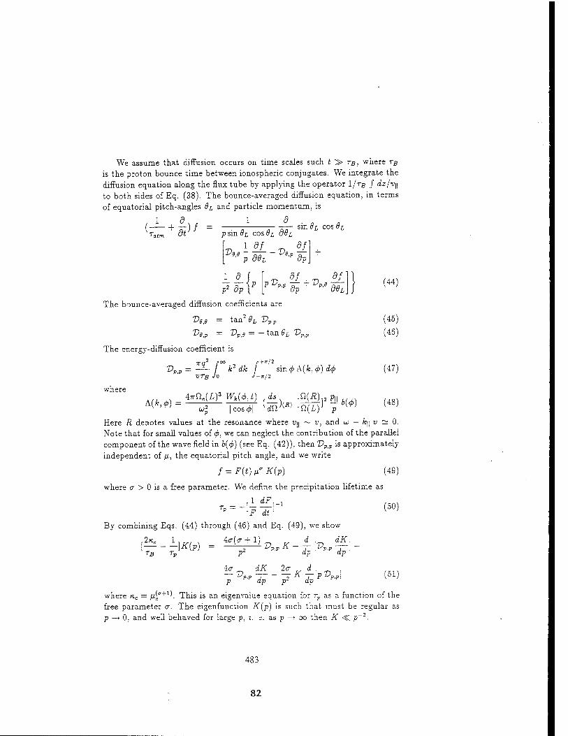
We assume that diffusion occurs on time scales such i > r^, where Tß is the proton bounce time between ionospheric conjugates. We integrate the diffusion equation along the flux tube by applying the operator l/rB / dz/v\\ to both sides of Eq. (38). The bounce-averaged diffusion equation, in terms of equatorial pitch-angles öj, and particle momentum, is
dt )f p sm ai cos Bi
v deL
sm #L cos ai
Ve + Vs*8-P
1_ d_ 7)2 fi-n
vVM
dJ c
dl dp
+ VB
The bounce-averaged diffusion coefficients are
Vs.e = 'eL XL
VBiP = VV.B = - tan ( •'p.ff V,
The energy-diffusion coefficient is „2
V„ t-f/2
— k2 dk sin<pA(fc,« VTß JO J-w/2
d6
(44)
(45)
(46)
(47)
(48)
~ 0. Note that for small values of <j>, we can neglect the contribution of the parallel component of the wave field in b(<f>) (see Eq. (42)), then Vp<v is approximately independent of ß, the equatorial pitch angle, and we write
f = F{t)fi'K(p) (49)
where a > 0 is a free parameter. We define the precipitation lifetime as
,1 dF\ ,
where MU ^ 47rQe(L)3 Wk(<f>,t) ds Ü(R) Pll
Here R denotes values at the resonance where vy ~ v, and ui — k\
lF dt'
By combining Eqs. (44) through (46) and Eq. (49), we show
(50)
[^ - -}K(P) TB TP
4<r(<7 + 1) „ d . dK.
^ dK 2a Td . ^ } V--d^'fKdp[vV^
(51) 4<T
p ' ' dp p"
where KC = fi%'+l1. This is an eigenvalue equation for rp as a function of the free parameter a. The eigenfunction K(jp) is such that must be regular as p —+ 0, and well behaved for large p, i. e. as p —► oo then K <C p~2 ■
483
82
ACKNOWLEDGEMENTS
We are grateful to J. M. Albert and J. U. Kozyra for helpful conversations. This work has been supported in part by the U. S. Air Force contract F19628-
89-K-0014 with Northeastern University.
REFERENCES
[ 1 ] L. R. Lyons and D. J. Williams, Quantitative Aspects of Magneto- spheric Physics (D. Reidel Publising Company, The Netherlands, (1984).
[ 2 ] C. F. Kennel and H. E. Petschek, J. Geophys. Res. 71, 1 (1966). [ 3 ] P. A. Bespalov and V. Yu. Trakhtengerts, Rev. Plasma Phys. 10, 88
(1980). [ 4 ] R. A. Helliwell, J. Geophys. Res. 72, 4773 (1967). [ 5 ] W.L. Imhof, H.D. Voss, J.B. Reagan, D.W. Datlowe, E.E. Gaines, J.
Mobilia and D.S. Evans, J. Geophys. Res. 91, 3077 (1986). [ 6 ] E. Villalön, W. J. Burke, P. L. Rothwell, M. B. Silevitch, J. Geophys.
Res. 94, 152 (1989). [ 7 ] E. Villalön and W. J. Burke, J. Geophys. Res. 96, 9655 (1991). [ 8 ] H. C. Koons, Geophys. Res. Lett. 2, 281 (1975). [ 9 ] R. A. Kovrazhkin, M. M. Mogilevskii, 0. A. Molchanov, Yu. I. Gal'penn,
N. V. Dzhordzhio, Zh. M. Bosbe, and A. Rem, JETP Lett. 39, 228
(1984). [1 0] R. Gendrin, J. Atmospheric Terrest. Phys. 30, 1313 (1968). [1 lj M. G. Morgan, J. Geophys. Res, 85, 130 (1980). [12] D. R. Shklyar, Planet. Space Phys. 34, 1091 (1986). [1 3] K. B. Dysthe, J. Geophys. Res. 76, 6915 (1971). [1 4] D. Nunn, Planet. Space Sei. 19, 1141 (1971). [1 5] E. Villalön and W. J. Burke, Phys. Fluids, 30, 3695 (1987).
484
83
PHYSICS OF SPACE PLASMAS (1993), Number 13 535
PROTON DIFFUSION BY PLASMASPHEPJC WHISTLER WAVES
Elena VElalon Center for Electromagnetics Research,
Northeastern University, Boston MA 02115
William J. Burke
Phillips Laboratory, Hanscom AFB, MA 01731
ABSTRACT
Whistler waves propagating near the quasi-electrostatic limit can interact with energetic protons (80 - 500 keV), that axe transported into the inner radiation belts. The waves may be launched either from the ground or gen- erated in the magnetosphere due to the resonant interactions with trapped electrons. The wave frequencies are significant fractions of the equatorial electron gyxofrequency, and propagate obliquely to the geomagnetic field. Because of the finite wave spectrum, the inhomogeneity of the geomagnetic field is compensated by the frequency variation, thus the protons stay in gyroresonance with the waves over long distances along the field line. The Fokker-Planck equation is integrated along the flux tube considering the contribution of multiple resonances crossing. The quasilinear diffusion co- efficients in energy, cross energy/ pitch angle and pitch angle are obtained for second-order resonant interactions. They are shown to be proportional to the electric fields amplitudes. Numerical calculations for the second order interactions, shows that diffusion dominates near the loss cone and is almost negligible at large pitch angles. The dominant diffusion coefficient is in en- ergy, although the cross energy/ pitch angle diffusion term is also important for small pitch angles. This may explain the induced proton precipitation observed in active space experiments [1, 2].
I. INTRODUCTION
Experimental observations of proton precipitation by controlled VLF transmission experiments occur in a wide range of plasmaspheric L shells. Whistler waves transmitted from the ground are ducted along the field lines to the magnetic equator where they become quasi-electrostatic [1, 2], and interact with the protons in the energy range (80 - 500 keV). It is also known that Eghtning discharges [3] generate VLF waves that, after entering the magnetosphere, can become trapped bouncing back and forth between hemispheres. These waves can also interact with energetic protons.
The waves considered here are such that the ratios of the wave frequen- cies to the equatorial electron gyrofrequencies are 0.5 < w/fle(i) < 1. The
MJT Center for Theoretical GeoiCosmo Plasma Physics, Cambridge, MA
84
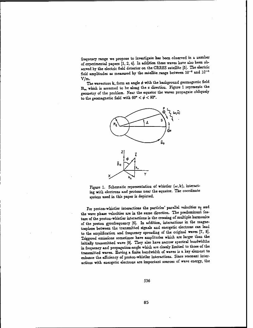
frequency range we propose to investigate has been observed in a number of experimental papers [1, 2, 4]. In addition these waves have also been ob- served by the electric field detector on the CREES satellite [5]. The electric field amplitudes as measured by the satellite.range between 10~s and 10-4
V/m. The wavectors k, form an angle ^ with the background geomagnetic field
B„ which is assumed to be along the z direction. Figure 1 represents the geometry of the problem. Near the equator the waves propagate obliquely to the geomagnetic field with 60° < <j> < 90°.
Im.k)
Figure 1. Schematic representation of whistler (w, k), interact- ing with electrons and protons near the equator. The coordinate system used in this paper is depicted.
For proton-whistler interactions the particles' parallel velocities vy and the wave phase velocities are in the same direction. The predominant fea- ture of the proton-whistler interactions is the crossing of multiple harmonics of the proton gyrofrequency {6]. In addition, interactions in the magne- tosphere between the transmitted signals and energetic electrons can lead to the amplification and frequency spreading of the original waves [7, 8]. Triggered emissions sometimes have amplitudes which are larger than the initially transmitted wave [9]. They also have narrow spectral bandwidths in frequency and propagation-angle which axe closely limited to those of the transmitted waves. Having a finite bandwidth of waves is a key element to enhance the efficiency of proton-whistler interactions. Since resonant inter- actions with energetic electrons are important sources of wave energy, the
536
85
proton-whistler interaction is a complicated process, involving more than one
plasma species. Finite wave bandwidths allow protons and whistlers to satisfy the condi-
tions for second-order resonances [9, 10], where inhomogeneities of the mag- netic field are compensated by frequency variations. Thus, the wave packets and particles may remain in resonance for long distance along magnetic field lines. The resonant wave frequency varies as a function of the distance along the field line, compensating for the variation of the geomagnetic field.
This article extends previous work using a Hamiltonian formulation [11] for test-particle interactions with the whistlers which, near the magneto- spheric equatorial plane, appear Doppler shifted to some harmonic of the proton gyrofrequency. The affected protons both gain energy from the waves and decrease their pitch-angles while crossing many resonances. Here, we evaluate the diffusion coefficients, for second-order, resonant interactions be- tween protons and whistlers based on this Hamiltonian formulation. The diffusion coefficients are shown to be linearly proportional to the wave's electric field amplitudes.
The paper is organized as follows. Section II contains the resonance con- dition for the proton whistler interactions at multiple harmonics of the proton gyrofrequency. For a given bandwidth we present the equations that describe the length of the interaction region along the flux tube, and the number of interacting harmonics cover by this length. In Section III the quasilinear dif- fusion equation is integrated along the flux tube considering the contribution of all harmonics. Section IV contains the diffusion coefficients for the case of a weakly inhomogeneous plasma, where the inhomogeneity of the magnetic field is compensated by the frequency spread of the wave packet. Numeri- cal applications are given in Section V. The main results of our anylisis are summarized in Section VI.
E. RESONANT PROTON WHISTLER INTERACTIONS
We consider a whistler wave of frequency w and wave vector k, prop- agating in a field aligned duct. The geomagnetic field B0 is along the z direction and <f> is the angle between k and B0- The dispersion relation for the refractve index rj = cfc/w is
, . , KM2 (1) 71 +(fie/u,)|cos?l-l l ;
where u>? and Qt are the electron plasma and gyro frequencies, respectively. The electric field is E = x Zx cos * - y £2 sin * - z £3 cos $, where x, y
and z are unit vectors; $ = k± x + k^ z — w t, and k\\,k± are the components
537
86
along and perpendicular to B0 of the wave vector. For the case of waves propagating near the resonance cone, w ~ flr(i)|cos^|, the equatorial re- fractive index i]2(L) > 1. The wave electric field which is linearly polarized, has components Zi\Z\ < 1, and Si/Es ~ — sm<f>/cos<f>. In this case the wave becomes quasi-electrostatic since E is almost in the direction of k, and the group velocities va ~ l/rj are very small.
Near the equator, we approximate the Earth's magnetic field by a parabolic profile
mr1+& (2) where t ~ RELA, RE is the Earth's radius, L is the magnetic shell param- eter, A is the geomagnetic latitude, and rL = (y/2/Z)RsL. The equatorial gyrofrequency is denoted by ß(£), and fl stands for the gyrofrequencies ei- ther for electrons or protons at a location s away from the equator along the field line.
Whistler-proton interactions satisfy the resonance condition
u - kn -lüp^O (3)
where, 1 = 0, ±1, ±2... is the harmonic number; üj, is the proton gyrofre- quency; and Vji is the parallel components of the particle's velocity. We call fi = sin20£, where 0£ is the equatorial pitch angle. Here &i > 6e, where 6C is the pitch angle at the boundary of the loss cone, and pe the corresponding value of fi. As a function of the L shell, the mirror ratio is <r = fi~l = Ls (4—Z/L)1^2. Protons of energies less than a few hundreds keV, satisfy the resonance condition with waves whose refractive indices 17 axe very large. In fact, the numerical calculations show that 17 > 50, for energies > 50 keV. As proton energies decrease and pitch angles increase, 77 increases. If 17 becomes too large the dispersion relation in Eq. (1) is no longer valid. In this case, we must consider thermal corrections for the plasmaspheric elec- tron population that supports the waves as described by Sazhin, [12]. These thermal corrections limit the magnitudes of T^ = 17 u>/ne(£), to finite values. These finite values of »7, yield the lower limits for the proton energies, and the upper limits for the pitch angles that may satisfy the resonance condition in Eq. (3).
Here we assume a given wave frequency spectrum of width A«/w. The interaction region along the flux tube extend to geomagnetic latitudes such 0 < A < AA, where
v ' 9 w l + tanJMl ,nm) (4)
This interaction region is such that 0 < £2e-fle(L) < AflC) where Afie/ße(I-):
4.5 (AA)S. The number of possible interacting harmonics, n, cover by this
538
87
spectrum is, m, cos? , (5)
m€(Ci€(L)H\ cos 4>\-I {^}
If p = v^jQ.p, is the Laimor radius and v± is the perpendicular component of the particle velocity, we show n < k± p. Combining Eqs. (4) and (5), yields the number of contributing resonant harmonics n as function of the
width of the spectrum Aw/ui. The interaction region along the field line has a maximum extent in ge-
omagnetic latitude AAi, i.e. AA < AAL. We show [11]
(AAL)3 = —- kxp ( —) (6> v 9rJ0p w \cos<f>\
Note that AAL increases with the particle energy and with the pitch angle. By substituting in Eq. (4), AA by AAL, and solving for the bandwidth leads to (Au/u)i. If the widths of the spectrum are equal or larger than (Au/w)i the entire range of resonant harmonics is included in the interactions.
EL THE DIFFUSION EQUATION
We normalize velocity v by c~\ length s by rj1, call r = t£l,(L), and define n = ÜP(L) TL/C ~ 1. The dimen signless electric field amplitudes axe
a = (.')
for i = 1,2,3, and where q is the proton charge. The relative wave-proton phase angle is
*=a+r*'^M-ä£r (8)
where A = arctanfvy/i^]. In terms of the three components of the normalized electric field ampli-
tudes, the diffusion equation as given by Lyons [13] is:
df v«df w is; r.c.3 <P\ r- , i , , —- -i- — — = > (—) ;—rr G~ (1 — 77 cos ©will
«^ ■ A-l) fv^^T,)" G f (9) 5(77 cos <i vi|
where the operator G is a function of d/dp. and d/öv, and is denned in [13].
Here Tz is
T, = I [(£1 - ea) Jm(*± P) + (ei + «*) Ji-i(*± P) 1 ^ " ^ MkJ- P) (10)
539
88
where Jt axe Bessel functions of argument k±p. To include the effects of the atmospheric loss cone, we introduce the term
f/Tatm. Here ratm = TB/2, if #z is within the loss cone and T^ = oo, if BL
is outside the loss cone. The proton bounce period, rg, is the the time for a particle to travel from one mirror point to the other and back again. Next integrate along the flux tube by applying the operator: £!"~ ds/(rB va) to both sides of Eq. (9), which becomes:
%- + —= £ /" V7dV r'] smW±Tt or Tut» .f-L Jo J-*/i v2
where
rt =
(ii)
d_
d
r2?-^ + 2?^^
dv ' d d
f +
f (12)
The diffusion coefficients are obtained after integrating along the field lines as follows:
T>„ = u
«] T?
fl^(I) ' 4TTBV V\&UI*S*\
V,
Vu = V[<^-i]2^.. W fi
(13)
(14)
(15)
where T/ must be evaluated at the resonance, 75 v ~ 6\/5« X 1.3802 is independent of v, and tPfa/ds2 will be defined in Eq. (22).
We define the diffusion functions
(16)
(17)
(18)
where
ß~v[LTmL){%)L][^ (19)
540
89
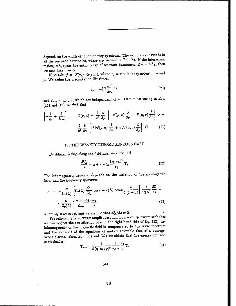
depends on tie width of the frequency spectrum. The summation extends to all the resonant harmonics, where n is denned in Eq. (5). If the interaction region, AA, spans the entire range of resonant harmonics, AA = AAL, then
we may take JX —♦ co. Next take / = F{r.) G{v,n), where r«, = r v is independent of v and
fi. We define the precipitation life times,
T>= -[F OT) (20)
^ ^ _ Tam v> wiich are independent of v. After substituting in Eqs.
(11) and (12), we find that
G^A = hh vMM^ + VM^
v2 dv v2W(p,v)— + vtf(p,v) —
G ~
(21)
IV. THE WEAKLY INHOMOGENEOUS CASE
By differentiating along the field line, we show [11]
ifs cos& —' li (22)
The ^homogeneity factor a depends on the variation of the geomagnetic
field, and the frequency spectrum,
u) r dv fi 1 1 du
u d[ri casi) duii, K 0,(1) dwi, ds
where w^ = w/ cos (p, and we assume that d&/ds = 0. For sufficiently large waves amplitudes, and for a wave spectrum
we can neglect the contribution of a in the right-hand-side of Eq. inhomogeneity of the magnetic field is compensated by the wave and the solutions of the equations of motion resemble that of a neous plasma. From Eq. (13) and (22) we obtain that the energy
coefficient is: 1 1
Vv,v = - — —: -r T<
(23)
such that (22), the spectrum homoge- diffusion
8 (17 cos<£)s rBv v (24)
541
90
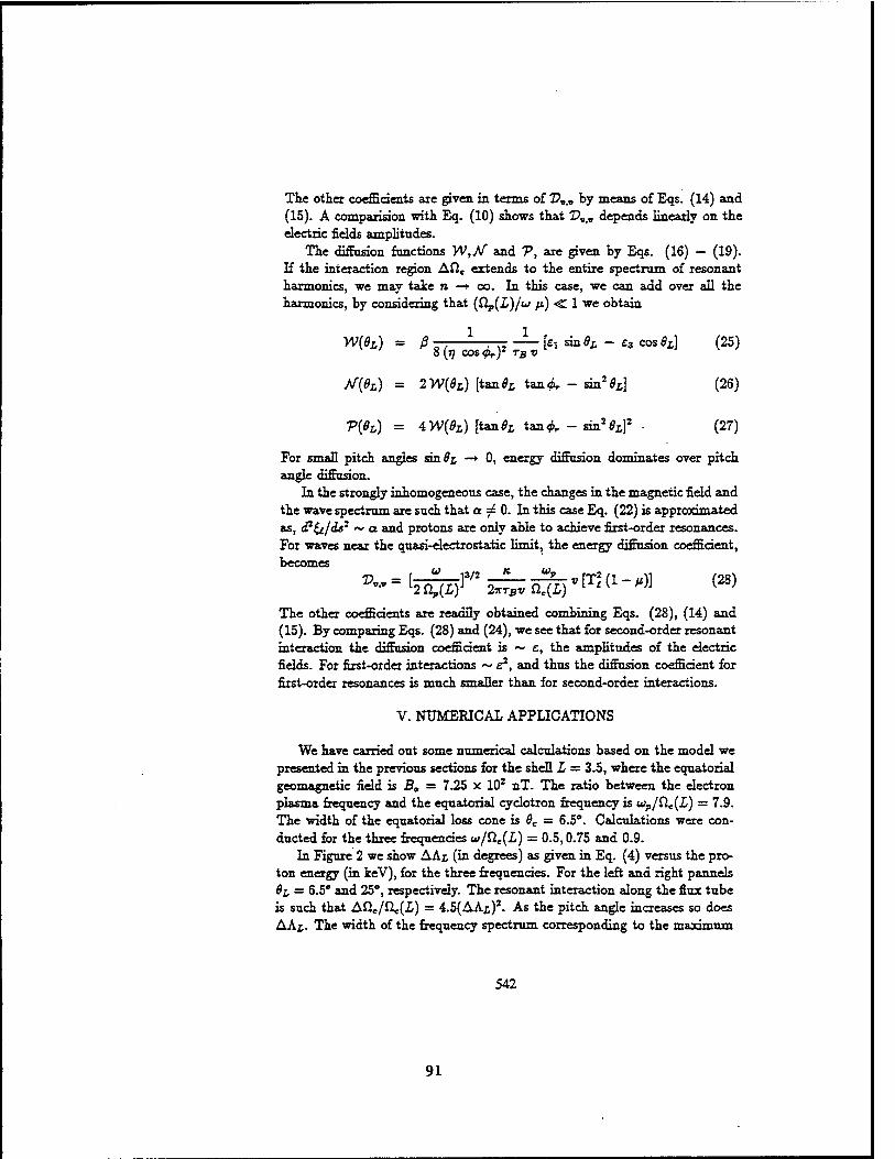
The other coefficients axe given in terms of £>„,„ by means of Eqs. (14) and (15). A compaxision with Eq. (10) shows that VViV depends linearly on the electric fields amplitudes.
The diffusion functions W.-A/* and V, axe given by Eqs. (16) - (19). If the interaction region Afle extends to the entire spectrum of resonant harmonics, we may take n —+ co. In this case, we can add over all the harmonics, by considering that (Clj,(L)/u fi) <C 1 we obtain
W(^) = P o/ * .« — [£i ™^ - £» «***] (25) 8 (TJ COS 4>T) TB v
M"{eL) = 2W(0£) [tan0L tan& - sin20£] (26)
V{6L) = 4W(0L) [tan*L tan& - sin2 0s]2 • (27)
For small pitch angles sinfli —♦ 0, energy diffusion dominates over pitch angle diffusion.
In the strongly inhomogeneous case, the changes in the magnetic field and the wave spectrum are such that a ^ 0. In this case Eq. (22) is approximated as, dPii/ds1 ~ a and protons are only able to achieve first-order resonances. For waves near the quasi-electrostatic limit, the energy diffusion coefficient, becomes
The other coefficients are readily obtained combining Eqs. (28), (14) and (15). By comparing Eqs. (28) and (24), we see that for second-order resonant interaction the diffusion coefficient is ~ c, the amplitudes of the electric fields. For first-order interactions ~ e2, and thus the diffusion coefficient for first-order resonances is much smaller than for second-order interactions.
V. NUMERICAL APPLICATIONS
We have carried out some numerical calculations based on the model we presented in the previous sections for the shell L = 3.5, where the equatorial geomagnetic field is B„ = 7.25 x 10² nT. The ratio between the electron plasma frequency and the equatorial cyclotron frequency is wp/Qe(L) = 7.9. The width of the equatorial loss cone is 6C = 6.5°. Calculations were con- ducted for the three frequencies w/£le(L) = 0.5,0.75 and 0.9.
In Figure 2 we show AAt (in degrees) as given in Eq. (4) versus the pro- ton energy (in keV), for the three frequencies. For the left and right pannels 8L = 6.5° and 25°, respectively. The resonant interaction along the flux tube is such that Aße/ßt(£) = 4.5(AAi)2. As the pitch angle increases so does AAi.. The width of the frequency spectrum corresponding to the maximum
542
91
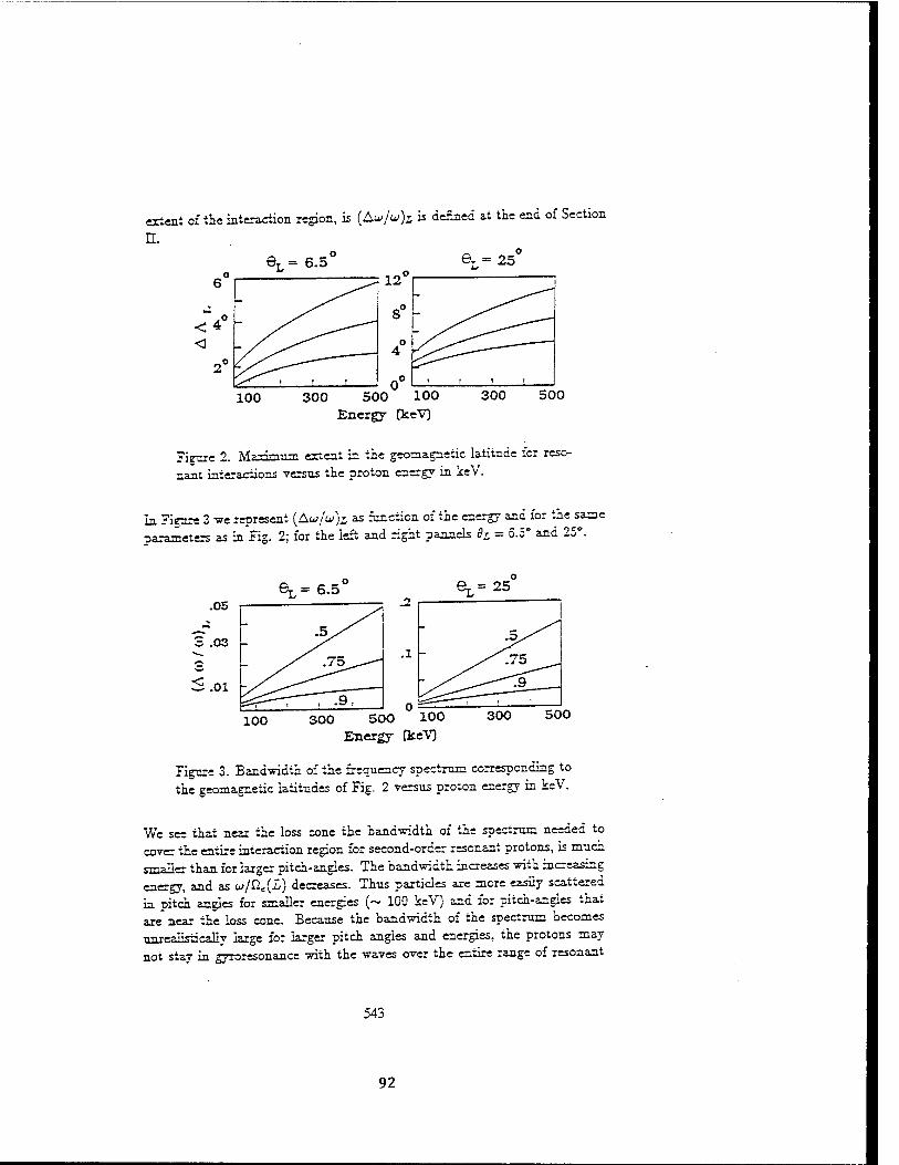
extent of the interaction region, is (Aw/«")i is denned at the end of Section
n. eL=6.5°
100 300 500 100 Energy fkeY)
300 500
Figure 2. Maximum extent in the geomagnetic latitude for reso- nant interactions versus the proton energy in keV.
In Figure 3 we represent (Au/w)i as function of the energy and for the same parameters as in Fig. 2; for the left and right pannels 9L = 6.5° and 25°.
.05
3 .03
S.01
eL= 6.5
- •Sy^
- yS .75^--
—r ^sT
^=25
100 300 50O 100 Energy (kcV)
300 500
Figure 3. Bandwidth of the frequency spectrum corresponding to the geomagnetic latitudes of Fig. 2 versus proton energy in keV.
We see that near the loss cone the bandwidth of the spectrum needed to cover the entire interaction region for second-order resonant protons, is much smaller than for larger pitch-angles. The bandwidth increases with increasing energy, and as w/flc(i) decreases. Thus particles are more easily scattered in pitch angles for smaller energies (~ 100 keV) and for pitch-angles that are' near the loss cone. Because the bandwidth of the spectrum becomes unrealistically large for larger pitch angles and energies, the protons may not stay in gyroresonance with the waves over the entire range of resonant
543
92
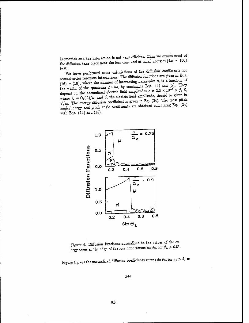
harmonics and the »tenet»» i. ** «y *&**■ ^ ™~?«* »»f * the diffusion take place near the loss cone and at small energies (».e. ~ 1W)
keV We have performed some calculations of the diffusion coemaents for
second-order resonant interactions. The diffusion functions are given m Eqs (16) - (18), where the number of interacting harmonics * » a »»*«o£ ihe width of the spectrum Aw/«, by combining Eos. (4) ana (5) They defend on the normalized electric field ampJitudes c = 2.0 x 10 x U t,
where f = Q (£)/«, *** *, tie dectric fidd ^P^"' sn0Uid be ^ ? V/£ The e^gy'dksion 'coefficient is given in Eq (24). The «. P- angle/energy and pitch angle coefficients are ooiained comoining Eq. (24)
with Eqs. (14) and (15).
a C s o.o
(=4
c o n
0.2 0.4 0.6 0.8
0.2 0.4 0.6 0.8
Sin0L
Figure 4. Diffusion functions normalized to the values of the en- ergy term at the edge of the loss cone versus sin 8L, lor SL > 6.0 .
Figure 4 gives the normalized diffusion coefficients versus sin 8L, for 8Z>6<:
544
93
6.5°, for 100 keV protons, and for a spectral bandwidth of Aw/u = 0.01. The upper and lower pannels correspond to w/^l{L) = 0.75 and 0.9, respec- tively. The diffusion functions axe normalized to the value that the energy diffusion function, W, takes at the edge of the loss cone which is represented by we = Wc/£i. Here s\ ~ e sin <?$,., and Wc is given by Eq. (25) taking
h = 0c Significant diffusion takes place mostly near the loss cone. It extends to
larger pitch angles as u —♦ Clt(L). The reasons for this have already been
explained since near the loss cone protons and whistlers stay in gyroreso- nance over the entire range of possible resonant harmonics that contribute to the interaction. We also observed that the dominant diffusion coefficient
is the energy term. However the contribution of the cross energy /pitch an- gle coefficient is also significant. For w/Cl(L) = 0.75, the normalized energy diffusion function at the edge of the loss cone is wc = 2.5 x 10⁻³. For ui/Q.(L) = 0.9, wc = 3. x 10-3. We have calculated wc for 500 keV protons, and UJ/Q(L) = 0.75, and found that i.e. wc = 2. x 10-7. In addition, protons and waves do not stay in gyroresonance over the whole length of resonant interaction for larger energies even at the edge of the loss cone. Thus as explained above, second-order resonant diffusion will is more efficient for protons with energies of ~ 100, keV and with pitch angles are near the loss cone.
VI. CONCLUSIONS
We have investigated the diffusion of protons by quasi-electrostatic whistler waves, by using the Fokker-Planck diffusion equation. We assume a spectrum snch that the ratios of the waves- to the equatorial electron gyro-frequencies are 0.5 < w/Qc(L) < 1. The main results of our theoretical analysis and the numerical applications are:
(1) For second-order resonant interactions the inhomogeneity of the geo- magnetic field is compensated by the frequency variation along the field line, and protons and waves can stay in gyroresonance over long distance along the field lines.
(2) The extent of the regions of resonant interactions along the flux tube decrease with the protons energies and pitch angles. The interactions are most efficient for protons of relatively small energies (~ 100 keV), and small pitch angles.
(3) For second-order resonant interactions, the diffusion coefficients are linearly proportional to the amplitudes of the electric fields .
(4) The dominant diffusion coefficient is in energy but the cross energy/ pitch angle coefficients is also significant for pitch angles near the loss cone.
545
94
ACKNOWLEDGEMENTS
This work has been supported in part by the U. S. Air Force contract F19628-89-K-0014 with Northeastern university.
REFERENCES
[1 ] H. C. Koons, Geophys. Res. Lett. 2, 281 (1975). [2 ] R. A. Kovrazhkm, M. M. Mogilevskii, 0. A. Molchanov, Yu. L Gal'perin,
N. V. Dzhordzhio, Zh. M. Bosie, and A. Rem, JETP Lett. 39, 228 (1984).
[3 ] W. C. Burgess, and U. S. Laan, Geophys. Res. Lett., 17, 259 (1990). [4 j R L. Dowden, A. D. Mckay, L. E. S. Amon, H. C. Koons and M. H.
Dazey, J. Geophys. Res. 83, 169 (1978). [5 ] M. S. Gussenhoven, E. G. Mullen and R C. Sagalyn, CRRES/SPACERAD
Experiment Descriptions, Enviromeutal Research Papers, No. 906, AFGL-TR-85-0017. Air Force Geophysics Laboratory, Hanscom AFB 01731.
[6 ] D. R ShHyar, Planet. Space Phys. 34, 1091 (1986). [7 ] C. F. Kennel and H. E. Petschek, J. Geophys. Res. 71, 1 (1966). [8 j P. A. Bespalov and V. Yu. Trakhtengerts, Rev. Plasma Phys. 10, 88
(1980). [9 ] R. A. Hefliwell, J. Geophys. Res. 72, 4773 (1967). [10] K. B. Dysihe, J. Geophys. Res. 76, 6915 (1971). [11] E. Vfflalön and W. J. Burke, J. Geophys. Res. 98, 13,509 (1993). [12] S. Sazhin, Whistler-Mode Waves in a Sot Plasma (Cambridge Atmo-
spheric and Space Science Series, Cambridge University Press, Great Britain, 1993).
[13] L. R Lyons and D. J. Williams, Quantitative Aspects of Magneto- spheric Physics (D. Radel Publising Company, The Netherlands, 1984).
546
95
The U.S. Government Is authorized to reproduce and sell this report. Permission for further reproduction by others must be obtained from the copyright owner.
JOURNAL OF GEOPHYSICAL RESEARCH, VOL. 98. NO. A8, PAGES 13,509-13,521, AUGUST 1, 1993
Proton Whistler Interactions Near the Equator in the Radiation Belts ELENA VILLALON
Center for Electromagnetics Research, Northeastern University, Boston, Massachusetts
WILLIAM J. BURKE
Geophysics Directorate, Sanscom Air Force Base, Massachusetts
Tie interactions of energetic protons with whistlers propagating near the quasi-electro- static limit, are investigated using a test particle, Hamiltonian formalism. We assume that wave packets exist with finite bandwidths of frequencies, which are close to the equatorial electron gyrofrequency and propagate obliquely with respect to the geomagnetic field. Near the equator the protons interact with the waves which appear Doppler shifted to some harmonic of their cyclotron frequency. In an inhomogeneous geomagnetic field the spacing between cyclotron harmonic resonances is very small. The Hamiltonian equations of motion are solved including multiple, independent harmonics for each resonance. Ine wave frequency varies as a function of the distance along the field kne, with only one frequency being resonant at a given point. Thus the inhomogeneity of the magnetic field is compensated by the frequency variation. The proton whistler interactions satisfy the conditions for second-order resonances for all the harmonics. The resonances may also overlap in phase space, leading to significant changes in the protons energies and pitch aneles The combined contributions of positive and negative harmonics allow protons to diffuse toward smaller pitch, angles. Numerical calculations applying this formalism to parameters relevant to the plasmasphere and controlled VLF transmission experiments are presented.
1. INTRODUCTION
The interactions between whistler waves and elec- trons in the plasmasphere [see, Lyons and Williams, 1984, and references therein], account for phenomena such as energetic electron precipitation [Imhof et al, I986;lnan, 19S7;Schulz and Davidson, 1988] enhance- ments of naturally occuring waves [Kennel and Petschek, 1966; Bespalov and Trakhtengerts, 1980], and the arti- ficially triggered emissions [Selliwell, 1967, 1988; Dys- the, 1971;Siidan and Ott, 1971]. These phenomena are most likely due to the resonant interactions at some har- monic of the electron gyrofrequency. The first harmonic and the Landau resonance play the most important role in the electron whistler interactions, although higher harmonics may also contribute [Villalon et al, 1989; Villalon and Burke, 1991]. They are most significant at the magnetospheric equator where the geomagnetic field changes slowly allowing particles to stay in reso- nance over relatively long distances. The component of the wave phase velocities along the Earth's magnetic field w/fc|| of whistlers and the parallel velocities v\\ of resonant electrons are opposittely directed.
Interactions of whistlers with protons have not re- ceived as much attention as those with electrons [Gen- drin, 1972]. However, a number of experimental ob- servations [Kovrazhkin et al, 1983, 1984;Koons, 1975, 1977] have shown that VLF transmission pulses can precipitate 80- to 500-keV protons into the ionosphere. They occur in a range of plasmaspheric L shells, and are due to the resonant interactions near the magnetic equa- tor. In the quasi-electrostatic limit [Sazhin, 1986;Mor- gan, 1980] the whistlers satisfy the relationship, w ~
Copyright 1993 by the American Geophysical Union.
Paper Number 93JA00727. 0148-0227/93/93JA-00727J05.00
ne(L) cos<t>, where <p is the angle between the wave vector, k, and the geomagnetic field, B0 and Cle(L) is the equatorial electron gyrofrequency. Here the parallel component of the wave vector fc|| is large and the res- onant energies of protons relatively low. In this paper we assume that the propagation properties of waves in the plasmasphere are described by a dense population of cold particles of ionospheric origin whose distribution function is isotropic in pitch angle. The predominant feature of the whistler proton interactions is the cross- ing of multiple harmonics of the proton gyrofrequency [Shklyar, 1985]. As summarized in Figure 1, resonant protons and whistlers travel in the same direction, with the wave phase velocity which may be slightly larger or smaller than the proton parallel velocity, depending on the interacting harmonics. By way of contrast, res- onant whistler electron interactions travel in opposite directions and the dominant harmonic is the first.
Shklyar [1986] devised an electrostatic, single-frequen- cy wave theory to explain the proton whistler interac- tions as causes of experimentally observed proton pre- cipitations. It is based on a Hamiltonian analysis that includes multiple-cyclotron resonances in a strongly in- homogeneous field. He finds that for large wave ampli- tudes (~ 10-2 V/m), resonances can overlap and lead to pitch angle diffusion toward the loss cone. Here we also present a Hamiltonian formulation of proton whistler interactions for multiple-resonances crossing. However, we use an electromagnetic formulation of the Hamil- tonian, and take the quasi-electrostatic limit near the magnetic equator where most of the significant interac- tions occur. Our work also differs from Shklyar's in that we invoke interactions with the multiple-frequencies of a propagating wave packet. We assume the wave fre- quency with which a test particle interacts, is a func- tion of the distance along the field line s, with only one frequency being resonant at a given location. Thus
13,509
96
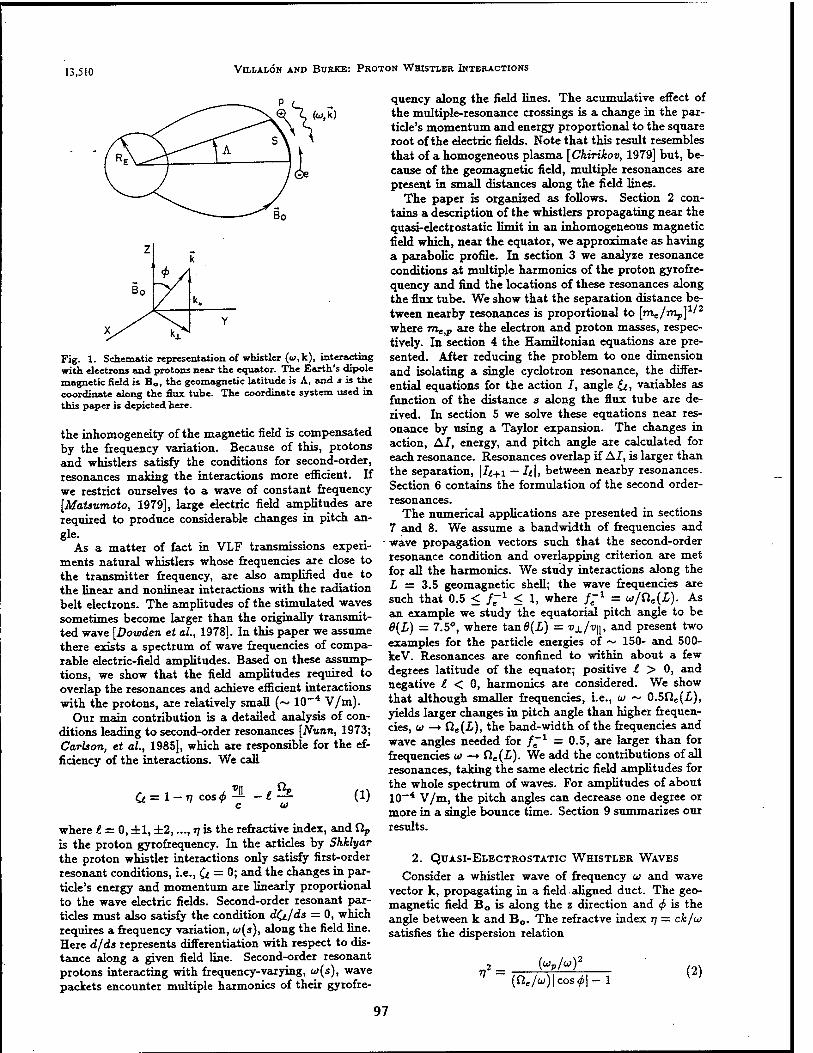
13,510 VlLLALÖN AND BURKE: PROTON WHISTLER INTERACTIONS
Fig. 1. Schematic representation of whistler (w,k), interacting with electrons and protons near the equator. The Earth's dipole magnetic field is B0, the geomagnetic latitude is A, and s is the coordinate along the flux tube. The coordinate system used in this paper is depicted here.
the inhomogeneity of the magnetic field is compensated by the frequency variation. Because of this, protons and whistlers satisfy the conditions for second-order, resonances making the interactions more efficient. If we restrict ourselves to a wave of constant frequency [Matswnoto, 1979], large electric field amplitudes are required to produce considerable changes in pitch an- gle.
As a matter of fact in VLF transmissions experi- ments natural whistlers whose frequencies are close to the transmitter frequency, are also amplified due to the linear and nonlinear interactions with the radiation belt electrons. The amplitudes of the stimulated waves sometimes become larger than the originally transmit- ted wave [Dowden et al., 1978]. In this paper we assume there exists a spectrum of wave frequencies of compa- rable electric-field amplitudes. Based on these assump- tions, we show that the field amplitudes required to overlap the resonances and achieve efficient interactions with the protons, are relatively small (~ 10~4 V/m).
Our main contribution is a detailed analysis of con- ditions leading to second-order resonances [Nunn, 1973; Carlson, et al., 1985], which are responsible for the ef- ficiency of the interactions. We call
O = l-r,cos^_,^ (1)
where 1 = 0, ±1, ±2,..., rj is the refractive index, and ÜP
is the proton gyrofrequency. In the articles by Skklyar the proton whistler interactions only satisfy first-order resonant conditions, i.e., Q = 0; and the changes in par- ticle's energy and momentum are linearly proportional to the wave electric fields. Second-order resonant par- ticles must also satisfy the condition dCt/ds = 0, which requires a frequency variation, w(s), along the field line. Here d/ds represents differentiation with respect to dis- tance along a given field line. Second-order resonant protons interacting with frequency-varying, w(s), wave packets encounter multiple harmonics of their gyrofre-
quency along the field lines. The acumulative effect of the multiple-resonance crossings is a change in the par- ticle's momentum and energy proportional to the square root of the electric fields. Note that this result resembles that of a homogeneous plasma [Chirikov, 1979] but, be- cause of the geomagnetic field, multiple resonances are present in small distances along the field lines.
The paper is organized as follows. Section 2 con- tains a description of the whistlers propagating near the quasi-electrostatic limit in an inhomogeneous magnetic field which, near the equator, we approximate as having a parabolic profile. In section 3 we analyze resonance conditions at multiple harmonics of the proton gyrofre- quency and find the locations of these resonances along the flux tube. We show that the separation distance be- tween nearby resonances is proportional to [me/mp]1'2
where me>p are the electron and proton masses, respec- tively. In section 4 the Hamiltonian equations are pre- sented. After reducing the problem to one dimension and isolating a single cyclotron resonance, the differ- ential equations for the action I, angle &, variables as function of the distance s along the flux tube are de- rived. In section 5 we solve these equations near res- onance by using a Taylor expansion. The changes in action, AI, energy, and pitch angle are calculated for each resonance. Resonances overlap if AI, is larger than the separation, \It+i — It\, between nearby resonances. Section 6 contains the formulation of the second order- resonances.
The numerical applications are presented in sections 7 and 8. We assume a bandwidth of frequencies and
• wave propagation vectors such that the second-order resonance condition and overlapping criterion are met for all the harmonics. We study interactions along the L = 3.5 geomagnetic shell; the wave frequencies are such that 0.5 < /T1 < 1, where f~x = w/Ue(L). As an example we study the equatorial pitch angle to be 9{L) = 7.5°, where tan0(£) = vi_/v\\, and present two examples for the particle energies of ~ 150- and 500- keV. Resonances are confined to within about a few degrees latitude of the equator; positive t > 0, and negative £ < 0, harmonics are considered. We show that although smaller frequencies, i.e., w ~ 0.5Cle(L), yields larger changes in pitch angle than higher frequen- cies, w —♦ ne(-£)> the band-width of the frequencies and wave angles needed for f'1 = 0.5, are larger than for frequencies w —► £le(L). We add the contributions of all resonances, taking the same electric field amplitudes for the whole spectrum of waves. For amplitudes of about 10-4 V/m, the pitch angles can decrease one degree or more in a single bounce time. Section 9 summarizes our results.
2. QUASI-ELECTROSTATIC WHISTLER WAVES
Consider a whistler wave of frequency u and wave vector k, propagating in a field aligned duct. The geo- magnetic field B0 is along the z direction and <j> is the angle between k and B0. The refractve index 77 = ck/u satisfies the dispersion relation
n2 = {"P/"
(ne/w)|cos#|-i (2)
97
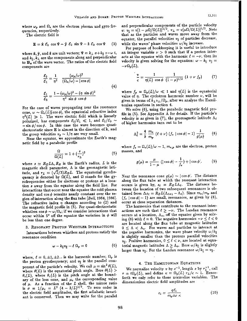
VELLALöN AND BURKE: PROTON WHISTLER INTERACTIONS 13,511
where u>p and Oe are the electron plasma and gyro fre- quencies, respectively.
The electric field is
E = x £i cos $ - y £2 sin * - z £3 cos * (3)
where x, y, and z are unit vectors; *$ = k±_ z+k\\ z—w t, and ifc||, i_L are the components along and perpendicular to B0 of the wave vector. The ratios of the electric field components are
h. £1
KM2
772 ($Je/w)-|cosfl
(4)
gx 1 - {wv/wf - (77 sin <j>)2
£3 T)2 sm<f> zos<p
For the case of waves propagating near the resonance cone, u ~ ile(L)\cos<j>\, the equatorial refractive index ■q2{L) > 1. The wave electric field which is linearly polarized, has components £2/^1 •C 1, and £\/£3 ~ — sin <£/cos <£. In this case the wave becomes quasi- electrostatic since E is almost in the direction of k, and the group velocities vg ~ I/77 are very small.
Near the equator, we approximate the Earth's mag- netic field by a parabolic profile
fi
n(L) i + C-H2 (5)
where s ~ RELA,RE is the Earth's radius, L is the magnetic shell parameter, A is the geomagnetic lati- tude, and TL = {V2/3)RBL. The equatorial gyrofre- quency is denoted by Ö(£), and ß stands for the gy- rofrequencies either for electrons or protons at a loca- tion s away from the equator along the field line. For interactions that occur near the equator the cold plasma density and cos $ remains nearly constant over the re- gion of interaction along the flux tube [Bell, 1984,1986]. The refractive index r\ changes according to (2) and the magnetic field profile in (5). For quasi-electrostatic whistlers cos<£ ~ w/Oe; if we consider interactions that occur within 5° off the equator the variation in <f> will be less than one degree.
3. RESONANT PROTON WHISTLER INTERACTIONS
Interactions between whistlers and protons satisfy the resonance condition
-Jbi \\v\\ ■I QP = 0 (6)
where, t = 0, ±1, ±2... is the harmonic number; fip is the proton gyrofrequency; and u|| is the parallel com-
ponent of the particle's velocity. We call [i — sin2 6{L), where 9{L) is the equatorial pitch angle. Here 6(L) > 6C(L), where 6C{L) is the pitch angle at the bound- ary of the loss cone, and pc the corresponding value of M- As a function of the L shell, the mirror ratio is a = 1/MC = L3 (4 - 3/L)1/2. To zero order in the electric field amplitudes, the first adiabatic invari- ant is conserved. Then we may write for the parallel
and perpendicular components of the particle velocity v. *„ = V[l-MVfi(£)]1/2, vJ.=v\j*l/n(L)]1'2. Note that as the particles and waves move away from the equator, the parallel velocities v\\ of particles decrease, while the waves' phase velocities w/k\\ increase.
For purpose of bookkeeping it is useful to introduce an integer variable v > 0 such that if a proton inter- acts at the equator with the harmonic I = —v, then its velocity is given solving for the equation: w — fc|| v^ =
-vQP{L),
T){L) cos<f> [l-v)1'2 (1 + v fP) (7)
where fp = £lP(L)/u> < 1 and T](L) is the equatorial value of 77. The cyclotron harmonic number v, will be given in terms of k±v±/£lp, after we analyze the Hamil- tonian equations in section 4.
We solve (6), using the parabolic magnetic field pro- file in (5). See Appendix A for details. If the particle's velocity is as given in (7), the geomagnetic latitude A^ of higher harmonics turn out to be
4 m, K2 = l^{l+v){fe lcos^l-1)
rrtp 9{P) (8)
where fe — fie(£)/w ~ 1, me)P are the electron, proton masses, and
s(M) = 7±-(|cos^|--J-) + |cos^|. (9) 1 - M /<=
Near the resonance cone g{p) ~ |cos^|. The distance along the flux tube at which the resonant interaction occurs is given by, si = RELAI. The distance be- tween the location of two subsequent resonances is ob- tained from Asi = REL(Ai+i - Ai). Since me/mp and (/e |cos(£| — 1) are small, resonances, as given by (8), occur at close separation distances.
The harmonics that contribute to the resonant inter- actions are such that I > —v. The Landau resonance occurs at a location, A0, off the equator given by solv- ing (8) with 1 = 0. The negative harmonics — v < £ < 0 are located along the flux tube at magnetic latitudes 0 < A < A0. For waves and particles to interact at the negative harmonics, the wave phase velocity u/k\\ is slightly smaller than the protons parallel velocities i/||. Positive harmonics, 0 < I < v, are located at equa- torial magnetic latitudes A > A0. Here w/fc|| is slightly larger than vn. For the Landau resonance w/ky = V||.
4. THE HAMILTONIAN EQUATIONS
We normalize velocity v by c-1, length s by r£ , call T = <np(L), and define K = fip(i) rL/c ~ 1. Hence- forth we only refer to these normalize variables. The dimensionless electric field amplitudes are
£i q£{
rripC (10)
98
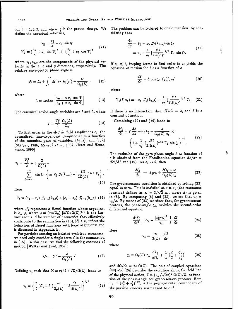
13,512 VlLLAiON AND BURKE: PROTON WHISTLER INTERACTIONS
for i = 1,2, 3, and where q is the proton charge. We The problem can be reduced to one dimension, by con- define the canonical velocities,
V[| = — - e3 sin *
Vl=(— + Sl sin*)2 + (^-+£2 cos*)2
K K
(11)
where »i|, vXiV are the components of the physical ve- locity in the z, x and y directions, respectively. The relative wave-proton phase angle is
& = £A + / <fa'rLi||(s')- Jo av{L)
where
A = arctan vy + K £2 cos *
«x + « si sin *
(12)
(13)
sidering that
ds_
dr = Vji + e3 Jt{kxp) sin ii
= viA m f Tt sin&.
vL L2ft(£)
If a <C 1, keeping terms to first order in Si yields the equation of motion for I as a function of s
— =1 cos& Tt(I,vt)
where
W,^) = -«,Ä(*xp) + i[5^j
(20)
!1/2 r< (21)
The canonical action-angle variables are I and A, where If there is no interaction then dl/ds = 0, and I is a constant of motion.
1 = 2 n- (14)
To first order in the electric field amplitudes £j, the normalized, time-dependent Hamiltonian is a function of the canonical pairs of variables, (V}|,s), and (I, A) [Shklyar, 1986; Menytik et al, 1987; Ginet and Eeine- mann, 1990]
Combining (12) and (19) leads to
i7 = li:+r^\i- ds ds
1 +
Op(L) vt
in ^2ft(£)
fr« sinfc (22)
+
The evolution of the gyro phase angle A as function of 3 is obtained from the Hamiltonian equation dX/dr = dH/dl and (19). As a -> 0, then
£ sin6{^,^xP)-[^]l/2r/[. — - irL. äI»
ßP(£K (23)
te-00
Here
(I5) The gyroresonance condition is obtained by setting (23) equal to zero. This is satisfied at 3 = s/ (the resonance location) denned as st = 3/\/2 A^, where A^ is given
?t = (£1 - £2) Ji+x(ki.p) + (£1 + £2) Jt-i(kxp) (16) ä (8). By comparing (6) and (23), we see that vt = V\\/K. By means of (23) we show that, for gyroresonant protons, the phase-angle it, satisfies the second-order
where Jt represents a Bessel function whose argument differential equation is kL p, where p = (oc/fiP) [2in/Q(L)]1/2 is the Lar- mor radius. The number of harmonics that effectively contribute to the summation in (15), |£| < v, reflect the behaviors of Bessel functions with large arguments and is discussed in Appendix B.
For particles crossing an isolated cyclotron resonance, we need only consider a single term I in the summation in (15). In this case, we find the following constant of motion [Walker and Ford, 1969]:
ds2 vt £ ds
Here
where
at = It dQ
0(£) ds
Ct-tK- nP(L) (17)
dk\\ 1 r^ Cii
(24)
(25)
(26)
Defining vL such that H = vj/2 + m/Cl{L), leads to
vt 2 , CJ
'n(i)'
1/2
(18)
and dQ/ds = 2s Q(L). The pair of coupled equations (20) and (24) describe the evolution along the field line of the physical action, I = (VJ./\/2ä)
2 Cl(L)/ft, as func-
tion of the phase-angle for gyroresonant protons. Here v± = (v2 + vV)ll2, is the perpendicular component of
the particle velocity normalized to c-1.
99
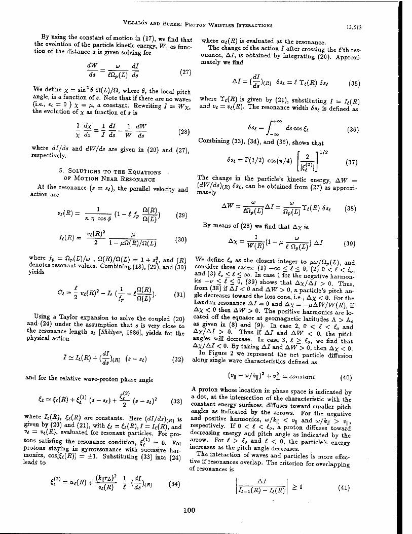
VllLALON AND BURKE: PROTON WHISTLER INTERACTIONS 13,513
By using the constant of motion in (17), we find that the evolution of the particle kinetic energy, W, as func- tion of the distance s is given solving for
dW u dl
where at(R) is evaluated at the resonance. The change of the action I after crossing the ^'th res-
onance, AI, is obtained by integrating (20). Approxi- mately we find
ds tÜP{L) ds (27) ,dl
We define X = sin2 6 a(L)/Q, where 6, the local pitch angle, is a function of s. Note that if there are no waves (i.e., ei = 0 ) x = H, a constant. Rewriting I = Wx, the evolution of x as function of 5 is
AI = *5s)<*> 6si = l T^Ä) Ssi (35)
where T*(£) is given by (21), substituting I = It{R) and vt = Vi(R). The resonance width 6s<. is defined as
1 dx _ 1 d£_ J_ dW_ X ds ~ I ds W ds (28)
where dl/ds and dW/ds are given in (20) and (27), respectively.
5. SOLUTIONS TO THE EQUATIONS
OF MOTION NEAR RESONANCE
At the resonance (s = st), the parallel velocity and action are
dscos & •oo
Combining (33), (34), and (36), shows that
1/2
6st = T(l/2) cos(7r/4)
M (2),
(36)
(37)
The change in the particle's kinetic energy, AW - (dW/ds)(R) Ssu can be obtained from (27) as approxi- mately
MR) =
h{R) =
K Tj COS <p
MR?
«(A). AW =
"""•Ofi)
2 1 - ixQ(R)/n(L)
(29)
(30)
l^(LJAI=^L)'T^Ssi (38)
By means of (28) we find that AX is
Ax W(R)
[l-ß u>
£ QP(L) ] AI (39)
where fp = Qp(L)/u , 0(A)/ft(£) = 1 + ,|, and (R) denotes resonant values. Combining (18), (29), and (30) yields
Cl = ivt(R)>-It(±.-. J fp
MR), 'n(L)' (31)
Using a Taylor expansion to solve the coupled (20) and (24) under the assumption that 5 is very close to the resonance length st [Shklyar, 1986], yields for the physical action
J~/,(£) + (g)(Ä) (s-Sl) (32)
and for the relative wave-proton phase angle
ii - MR) + tP (s - „) + k_ (, _ Si)2 (33)
where It(R), &(£) are constants. Here (dI/ds),R) is given by (20) and (21), with & = £(£), I = £(£), ^ vt — v^R), evaluated for resonant particles. For pro-
tons satisfing the resonance condition, ^(1) = 0. For protons staying in gyroresonance with sucessive har- monics, cos[&(i?)] = ±l. Substituting (33) into (24) leads' to
We define l0 as the closest integer to ßju/OptL), and consider three cases: (1) -00 < £ < 0, (2) 0 < £ < £0j
and (3) 4 < £ < 00. In case 1 for the negative harmon- ics -v <£<0, (39) shows that AX/AI > 0. Thus, from (38) if AI < 0 and AW > 0, a particle's pitch an- gle decreases toward the loss cone, i.e., Ax < 0. For the Landau resonance AI = 0 and Ax = -ßAW/W(R) if AX < 0 then AW > 0. The positive harmonics are lo- cated off the equator at geomagnetic latitudes A > A0
as given in (8) and (9). In case 2, 0 < £ < £0 and AX/AI > 0. Thus if AI and AW < 0, the pitch angles will decrease. In case 3, £ >J0, we find that AX/AI < 0. By taking AI and AW > 0, then Ax < 0.
In Figure 2 we represent the net particle diffusion along single wave characteristics defined as
(v\\ ~ <"/*||)2 + vl ■ constant (40)
A proton whose location in phase space is indicated by a dot, at the intersection of the characteristic with the constant energy surfaces, diffuses toward smaller pitch angles as indicated by the arrows. For the negative and positive harmonics, u/fy < „,, and u/k« > v», respectively. If 0 < £ < £0, a proton diffuses toward decreasing energy and pitch angle as indicated by the arrow. For / > £0 and £ < 0, the particle's energy increases as the pitch angle decreases.
The interaction of waves and particles is more effec- tive if resonances overlap. The criterion for overlapping of resonances is
e(*). MR) + MR) 1 (57}^ (34) AI
2i_ !(£)-£(£) > 1 (41)
100
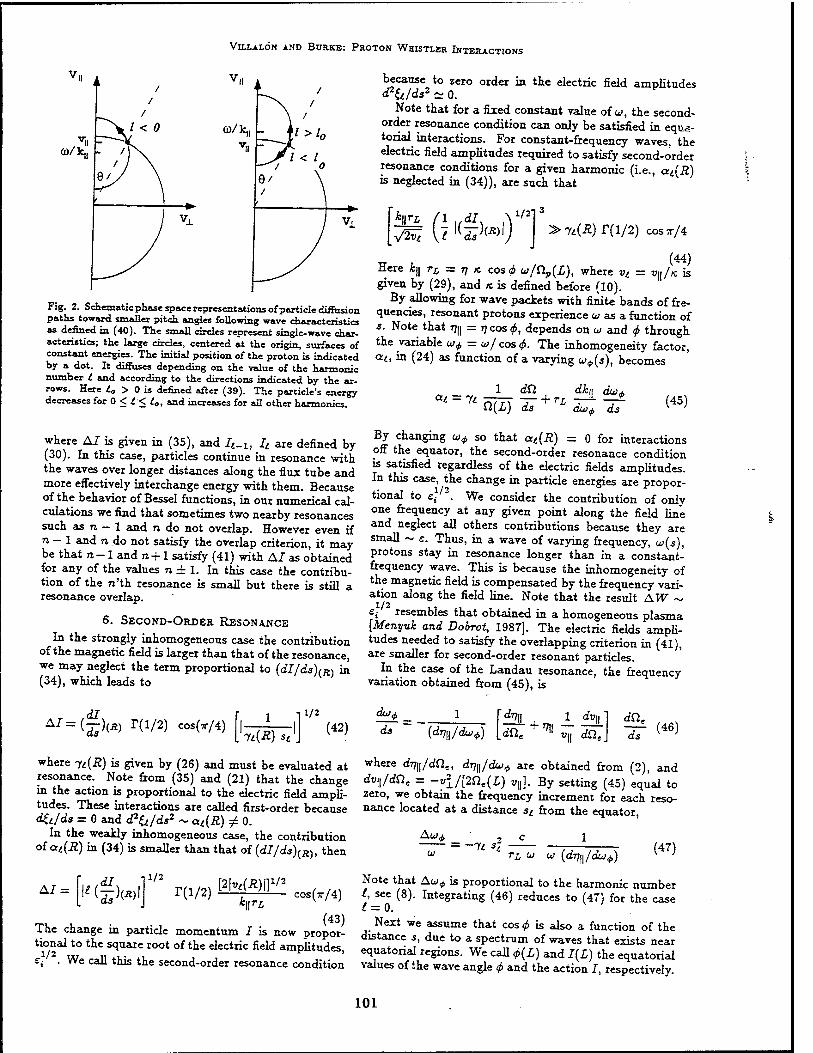
VlLLALÖN AND BURKE: PROTON WHISTLER INTERACTIONS
because to zero order in the electric field amplitudes <Ptt/ds2 ~ 0.
Note that for a fixed constant value of w, the second- order resonance condition can only be satisfied in equa- torial interactions. For constant-frequency waves, the electric field amplitudes required to satisfy second-order resonance conditions for a given harmonic (i.e., <xt(R) is neglected in (34)), are such that
> 7*(22) r(l/2) cosx/4
(44) V||//C is
Fig. 2. Schematic phase space representations of particle diffusion paths toward smaller pitch angles following wave characteristics as defined in (40). The small circles represent single-wave char- acteristics; the large circles, centered at the origin, surfaces of constant energies. The initial position of the proton is indicated by a dot. It diSuses depending on the value of the harmonic number t and according to the directions indicated by the ar- rows. Here A. > 0 is denned after (39). The particle's energy decreases for 0 < I < lg, and increases for all other harmonics.
Here k\\ rL = rj K cos <j> w/Qp(L), where vL
given by (29), and K is defined before (10). By allowing for wave packets with finite bands of fre-
quencies, resonant protons experience w as a function of s. Note that r7fl = V cos 6, depends on w and <f> through the variable u^ = w/cos<£. The inhomogeneity factor, alt in (24) as function of a varying u/^(s), becomes
al = ji du dku
Q{L) as du>£ dwj,
ds 7± -77 (45)
where AI is given in (35), and It.u lL are defined by (30). In this case, particles continue in resonance with the waves over longer distances along the flux tube and more effectively interchange energy with them. Because of the behavior of Bessel functions, in our numerical cal- culations we find that sometimes two nearby resonances such as n — 1 and n do not overlap. However even if n - 1 and n do not satisfy the overlap criterion, it may be that n - 1 and n +1 satisfy (41) with AI as obtained for any of the values n ± 1. In this case the contribu- tion of the n'th resonance is small but there is still a resonance overlap.
6. SECOND-ORDER RESONANCE
In the strongly inhomogeneous case the contribution of the magnetic field is larger than that of the resonance, we may neglect the term proportional to (dI/ds)(R) in (34), which leads to
By changing u^ so that at(R) = 0 for interactions off the equator, the second-order resonance condition is satisfied regardless of the electric fields amplitudes. In this case, the change in particle energies are propor-
tional to e{ 2. We consider the contribution of only
one frequency at any given point along the field line and neglect all others contributions because they are small ~ e. Thus, in a wave of varying frequency, w(s), protons stay in resonance longer than in a constant- frequency wave. This is because the inhomogeneity of the magnetic field is compensated by the frequency vari- ation along the field line. Note that the result AW ~
e{ resembles that obtained in a homogeneous plasma [Menyuk and Dobroi, 1987]. The electric fields ampli- tudes needed to satisfy the overlapping criterion in (41), are smaller for second-order resonant particles.
In the case of the Landau resonance, the frequency variation obtained from (45), is
,dl 4I=(-H(Ä) T(l/2) cos(7r/4)
1 1/2
~fi(R)*i (42)
where yi(R) is given by (26) and must be evaluated at resonance. Note from (35) and (21) that the change in the action is proportional to the electric field ampli- tudes. These interactions are called first-order because d&/ds = 0 and (P^/ds2 ~ ai(R) £ 0.
In the weakly inhomogeneous case, the contribution of at(R) in (34) is smaller than that of (dI/ds)(R), then
AJ = !<)(*)! 11/3
r(i/2) [2k(*)|] 1/2
COS(T/4)
The change in particle momentum I is now propor- tional to the square root of the electric field amplitudes,
£i . We call this the second-order resonance condition
duA
ds {dr^/dui^)
dr>\\ , „ dv\\ dti.
dne
ds (46)
where dj^/dQe, dq^/du^ are obtained from (2), and dv\\/dSle = -yl/[2Cle(L) wH]. By setting (45) equal to zero, we obtain the frequency increment for each reso- nance located at a distance si from the equator,
Aw, 4> 2
rL u> u; {dqw/duj,) (47)
Note that Au^ is proportional to the harmonic number t, see (8). Integrating (46) reduces to (47) for the case £ = 0.
Next we assume that cos 4> is also a function of the distance s, due to a spectrum of waves that exists near equatorial regions. We call 4>(L) and 1(1) the equatorial values of the wave angle 4> and the action I, respectively.
101
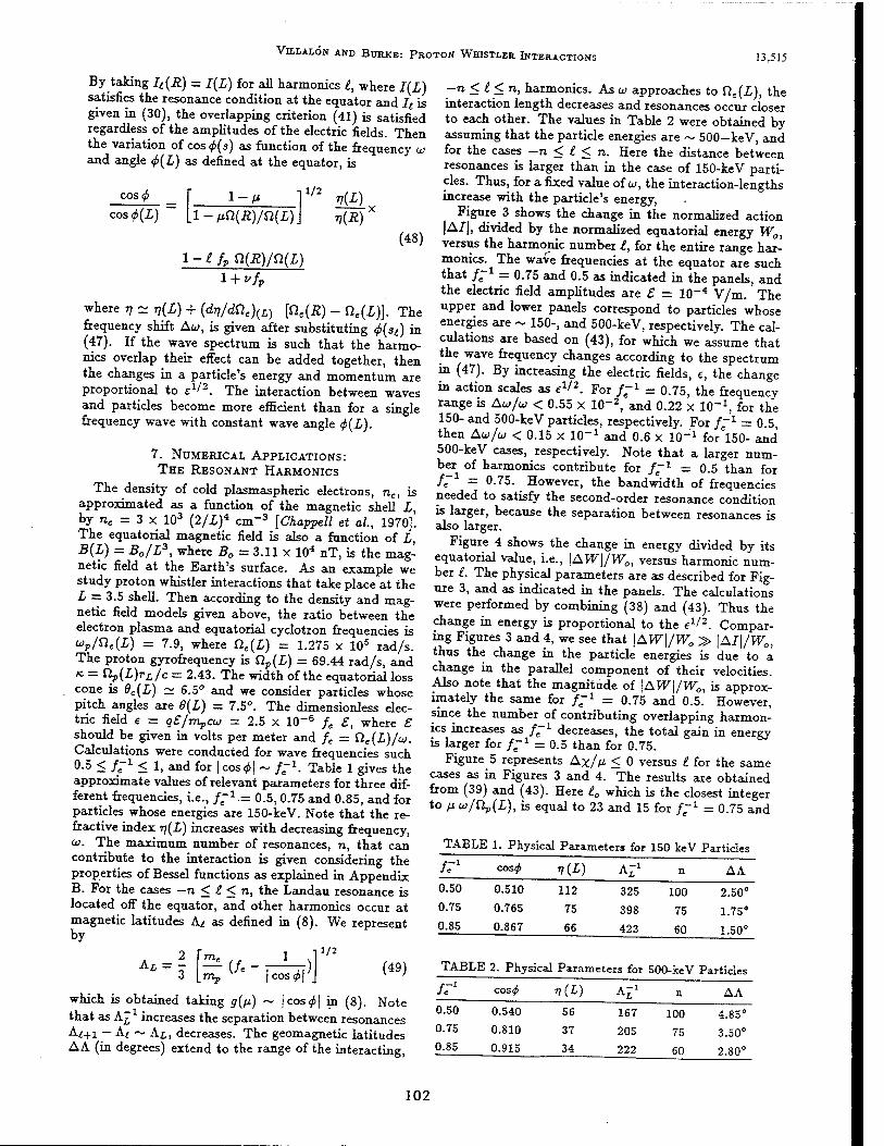
VlLLALÖN AND BURKE: PROTON WHISTLER INTERACTIONS 13,515
By taking Ii(R) = I(L) for all harmonics I, where I(L) satisfies the resonance condition at the equator and IL is given in (30), the overlapping criterion (41) is satisfied regardless of the amplitudes of the electric fields. Then the variation of cos c*(s) as function of the frequency u> and angle <f>(L) as defined at the equator, is
cosci 1/2
cos 4>{L) [l-ßÜ{R)/ü{L)
\-lfv U{R)/Ü{L)
(48)
where r, ~-v(Q + {dV/dÜt)(L) [Üe{R) - Ue{L)]. The frequency shift Aw, is given after substituting <j>(st) in (47). If the wave spectrum is such that the harmo- nics overlap their effect can be added together, then the changes in a particle's energy and momentum are proportional to e1!2. The interaction between waves and particles become more efficient than for a single frequency wave with constant wave angle <f>(L).
7. NUMERICAL APPLICATIONS:
THE RESONANT HARMONICS
The density of cold plasmaspheric electrons, nc, is approximated as a function of the magnetic shell L, by nc = 3 x 10³ (2/I)4 cm"3 [Chappell et al., 1970]. The equatorial magnetic field is also a function of L, B{L) = B0/L
3, where B0 = 3.11 x 10⁴ nT, is the mag- netic field at the Earth's surface. As an example we study proton whistler interactions that take place at the L = 3.5 shell. Then according to the density and mag- netic field models given above, the ratio between the electron plasma and equatorial cyclotron frequencies is wP/Sle(L) = 7.9, where ÜC(L) = 1.275 x 10⁵ rad/s. The proton gyrofrequency is £lP(L) = 69.44 rad/s, and K. = np(L)rL/c = 2.43. The width of the equatorial loss cone is 6C(L) ~ 6.5° and we consider particles whose pitch angles are 8{L) = 7.5°. The dimensionless elec- tric field e = qS/mpCu = 2.5 x 10~6 ft £, where £ should be given in volts per meter and fe = Cle(L)/w. Calculations were conducted for wave frequencies such 0.5 < /T1 < 1, and for | cos^| ~ f~x. Table 1 gives the approximate values of relevant parameters for three dif- ferent frequencies, i.e., f'1 .= 0.5, 0.75 and 0.85, and for particles whose energies are 150-keV. Note that the re- fractive index -q{L) increases with decreasing frequency, w. The maximum number of resonances, n, that can contribute to the interaction is given considering the properties of Bessel functions as explained in Appendix B. For the cases — n < £ < n, the Landau resonance is located off the equator, and other harmonics occur at magnetic latitudes At as defined in (8). We represent by
Ai = nip cosc^l
1/2
(49)
which is obtained taking g(/i) ~ |cosci| in (8). Note that as A£ increases the separation between resonances A*+i — Ai ~ AL, decreases. The geomagnetic latitudes AA (in degrees) extend to the range of the interacting,
-rc < t < "> harmonics. As u approaches to QC(L), the interaction length decreases and resonances occur closer to each other. The values in Table 2 were obtained by assuming that the particle energies are ~ 500-keV, and for the cases -n < £ < n. Here the distance between resonances is larger than in the case of 150-keV parti- cles. Thus, for a fixed value of w, the interaction-lengths increase with the particle's energy,
Figure 3 shows the change in the normalized action |A/|, divided by the normalized equatorial energy W0, versus the harmonic number £, for the entire range har- monics. The wave frequencies at the equator are such that /e = 0.75 and 0.5 as indicated in the panels, and the electric field amplitudes are £ = 10-4 V/m. The upper and lower panels correspond to particles whose energies are ~ 150-, and 500-keV, respectively. The cal- culations are based on (43), for which we assume that the wave frequency changes according to the spectrum in (47). By increasing the electric fields, e, the change in action scales as e1/2. For f~l = 0.75, the frequency range is Aw/w < 0.55 x 10~2, and 0.22 x 10"1, for the 150- and 500-keV particles, respectively. For f'1 = 0.5, then Aw/w < 0.15 x 10"1 and 0.6 x 10"1 for"150- and 500-keV cases, respectively. Note that a larger num- ber of harmonics contribute for /e
_1 = 0.5 than for /,. = 0.75. However, the bandwidth of frequencies needed to satisfy the second-order resonance condition is larger, because the separation between resonances is also larger.
Figure 4 shows the change in energy divided by its equatorial value, i.e., \AW\/W0, versus harmonic num- ber £. The physical parameters are as described for Fig- ure 3, and as indicated in the panels. The calculations were performed by combining (38) and (43). Thus the change in energy is proportional to the e1/2. Compar- ing Figures 3 and 4, we see that \AW\/W0 > \AI\/W0, thus the change in the particle energies is due to a change in the parallel component of their velocities. Also note that the magnitude of \AW\/W0, is approx- imately the same for f'1 = 0.75 and 0.5. However, since the number of contributing overlapping harmon- ics increases as /T1 decreases, the total gain in energy is larger for f~x =0.5 than for 0.75.
Figure 5 represents Ax/ß < 0 versus £ for the same cases as in Figures 3 and 4. The results are obtained from (39) and (43). Here £0 which is the closest integer to p u/Qp(L), is equal to 23 and 15 for f'1 = 0.75 and
TABLE 1. Physical Parameters for 150 keV Particles
fc COS<f>
112
75
66
AI1 R AA
0.50 0.510
0.75 0.765
0.85 0.867
325
398
423
100 2.50°
75 1.75°
60 1.50°
TABLE 2. Physical Param =ters for 500-keV Particles
fc cos^ V(L) AZ1 n AA
0.50 0.540
0.75 0.810
0.85 0.915
56
37
34
167
205
222
100 4.85°
75 3.50°
60 2.80°
102
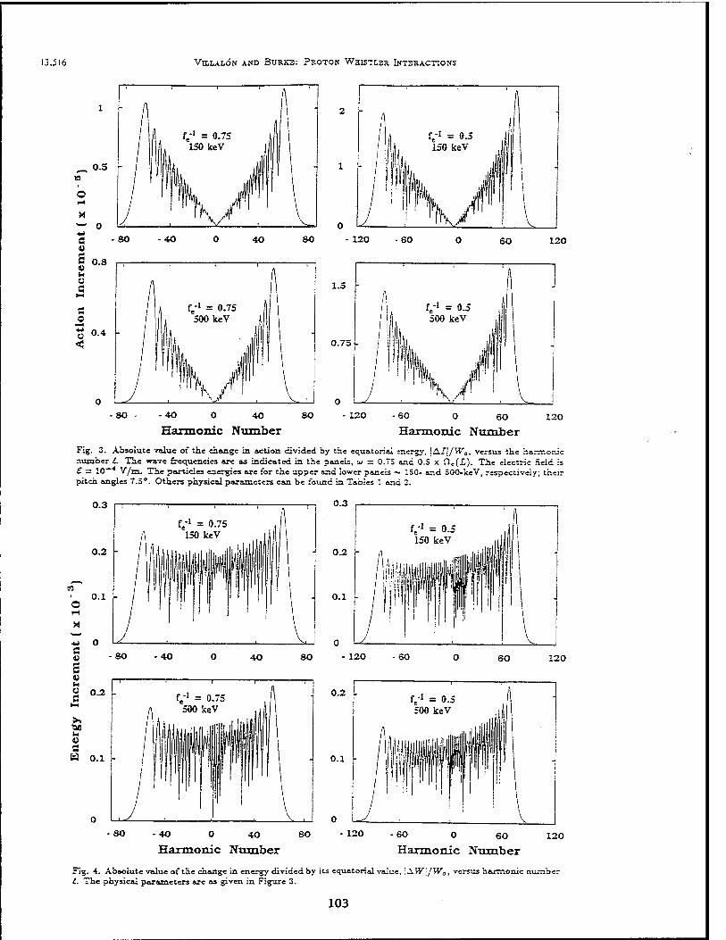
13.516 VlLLALÖN AND BURKE: PHOTON WHISTLER INTERACTIONS
80 - 120 - 60
1.5
SO 120
0.75
1
V! = 0.5 500 keV
\:
• 40 0 40
Harmonic Number so - 120 - 60 0 60
Harmonie Number 120
Fig. 3. Absolute value of the change in action divided by the equatorial energy, !A/|/W0, versus the harmonic number t. The wave frequencies are as indicated in the panels, ui — 0.73 and 0.5 X f),(L). The electric field is £ = 10~* V/ra. The particles energies axe for the upper and lower panels ~ 150- and 300-keV, respectively; their pitch angles 7.5*. Others physical parameters can be found in Tables i and 2.
O
0.3
0.2
0.1
0.2
-M 0 C V
S U hi o a
■at u U e
0.3
0.2 -
0.1
80 40 40 80 - 120 - 60 60 120
0.1 -
0.2
0.1 -
80 - 40 0 40
Harmonic Number 80 120 60 0 60
Harmonic Number 120
Fig. 4. Absolute value of the change in energy divided by its equatorial value, \^W\/Wa, versus harmonic number I. The physical parameters are as given in Figure 3.
103
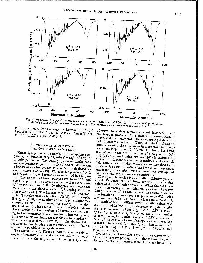
VlLLALÖN AND BüRKE: PROTON WHISTLER INTERACTIONS 13,517
120
-40 0 40
Harmonic Number 60 o so Harmonie Number
120 -p- r m —-»vim, ilUUiUCr
X^' rfT?rCtivdy- F°r the ne«ative Harmonics A7 < 0
ForV^ >A°VIf n- ^ **> AI < ° and th- ^ < 0 For £ > 4, AI > 0 and APT > 0.
8. NUMERICAL APPLICATIONS:
THE OVERLAPPING CRITERION
Figure 6, represents the number of overlapping reso- nances, as a function oflg(£), with £ = (£1
2+/2+£2)i/2 m volts per meter. The wave propagation angles cos tf
fk ,? ^ftant,S «Iven " TabIes 1 ^d 2. We assume a bandwidth in frequencies so that AI is calculated for each harmonic as in (43). We consider positive / > 0 and negative / < 0, harmonics as indicated in the pan-
2?« TTS* UPPel and l0Wer paneIs refer to ~ 150- and
500-keV protons; the equatorial wave frequencies are
chcjjf f^ °J85- 0veri*PPkg resonances are calculated as explained in section 5, following the crite- rion given in (41). The harmonics with the largest pos- sible^ overlap first as function of ]g(f). For example, ? 0 < .*| < 70, the number of overlapping harmonics
SiTS t0 'r ~J£|- ReS°nanCeS °VerIaP * the «S- tnc held amplitudes exceed certain thresholds. Above tnese thresholds, the numbers of harmonics contribut- ing to the interaction reach some limits increasing verv little-with £. These limits are established for amplitudes which are larger than ~ 10~4 V/m. The electric fields required for overlapping become smaller as w — Q (n) and as the particle's energy decreases. . ;
The calculations in Figure 6, assume a wave field of varymg-frequency „(*), and constant values for cos^ They illustrate the importance of having a spectrum
of waves to achieve a more efficient interaction with the trapped protons. As a matter of companion n a constant frequency wave, the overlapping criterion £
aSB"tBPMITtT1 t0 €- ThUS' the dectric fields ~ quire to overlap the resonances in a constant frequency
Jcos/16 rsti thr,i(r2 v/m- °» the oth JIZI and (48), the overlapping criterion (41) is satisfied for aU the contributing resonances regardless of the electric field amphtudes. In what follows we assume that there ex^ts such spectrum with a bandwidth in frequencies and propagat angleS) ^ ^ ^^ Woe,
satefy second-order resonance conditions. if the particle motion is essentially a diffusive process
values of the distribution function. When the net flux is
damaD R
mCleaSlnf It PartkleS ener*ies then the —es damp. Because of the atmospheric loss cone, distribu- tion functions are anisotropic in pitch angle 6(L), with a minimum at 8(1) - 0. Near the loss cone 8F/B6 > 0 ax,d particles tend to diffuse toward smaller values of 6. As ulus rated m Figure 2, to decrease the pitch angles
5)fe?/V7 / ^ for ° < * < 4, AW < 0 and of cent K ,° V <0>AW> 0- Since the number A^!- n f\ gharm°mCS k Iar*er if AW > 0 «** if 1, < °'*heie «a net «^ of energy for the interacting
08d
5 'IiOIt{L) = 7-5° and for f.'1 = 0.5,0.75, and 0.85, respectively. '
hasLwidth?SUme thele CXiStS a SpeCtlUm of waves *^h d« A?lVr„Pi0Paga^0n angleS A^ and fre<*u- cies Ao;, so that all harmonics meet the conditions for
104
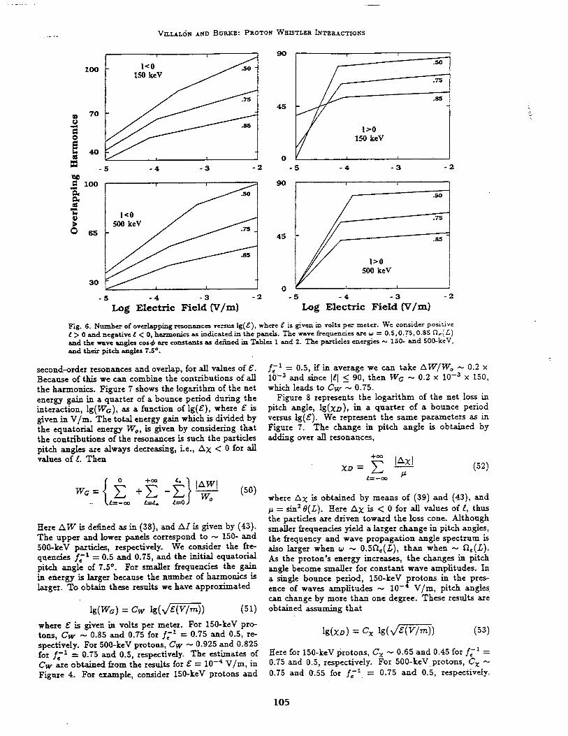
VULALÖN AND BüRXE: PROTON WHISTLER INTERACTIONS
90
100
1
KO 150 keV
i
70
■ " .88
40 ^^ i
45
-2 na S 100 o, Q. es 'S v > O 65
30 "
1
i<o y 500 keV X
^—""^■75 -
^_^—-—■■"'""JSS
~-^^ i -
90
45
5 -4 -3
i
.50
" 775
1>0 500 keV
.85 "
5 -4 -3 Log Electric Field fV/m)
-2 5 -4 -3 Log Electric Field (V/m)
Fig. 6. Number of overlapping resonances versus lg(£), where £ is given in volts per meter. We consider positive i > 0 and negative I < 0, harmonics as indicated in the panels. The wave frequencies are u> = 0.5,0.75,0.85 fJe(£) and the wave angles cos^ are constants as defined in Tables 1 and 2. The particles energies ~ 150- and 500-keV, and their pitch angles 7.5*.
second-oider resonances and overlap, for all values of £. Because of this we can combine the contributions of all the harmonics. Figure 7 shows the logarithm of the net energy gain in a quarter of a bounce period during the interaction, lg(Wc), as a function of lg(£), where £ is given in V/m. The total energy gain which is divided by the equatorial energy W0, is given by considering that the contributions of the resonances is such the particles pitch angles are always decreasing, i.e., Ax < 0 for all values of L Then
0.2 x x 150,
Z"1 = 0.5, if in average we can take AW/W0 - 10'-3 and since \l\ < 90, then WG ~ 0.2 x 10"3
which leads to Cw ~ 0.75. Figure 8 represents the logarithm of the net loss in
pitch angle, lg(xi>)> i& a quarter of a bounce period versus lg(£). We represent the same parameters as in Figure 7. The change in pitch angle is obtained by adding over all resonances,
|AX|
{0 +CO t0 "!
£ +E-Ei Z=-co *=/„ fc0>
\AW\ W0
+CO
/=-oo ^
(52)
(50)
Here AW is denned as in (38), and AI is given by (43). The upper and lower panels correspond to ~ 150- and 500-keV particles, respectively. We consider the fre- quencies f~x = 0.5 and 0.75, and the initial equatorial pitch angle of 7.5°. For smaller frequencies the gain in energy is larger because the number of harmonics is larger. To obtain these results we have approximated
lg(Wc) = CW l%{y/£(V/m)) (51)
where Ax is obtained by means of (39) and (43), and /x = sin2 8{L). Here Ax is < 0 for all values of I, thus the particles are driven toward the loss cone. Although smaller frequencies yield a larger change in pitch angles, the frequency and wave propagation angle spectrum is also larger when u ~ 0.5Oe(L), than when ~ fl«(£). As the proton's energy increases, the changes in pitch angle become smaller for constant wave amplitudes. In a single bounce period, 150-keV protons in the pres- ence of waves amplitudes ~ 10~4 V/m, pitch angles can change by more than one degree. These results are obtained assuming that
where £ is given in volts per meter. For 150-keV pro- tons, Cw ~ 0.85 and 0.75 for f'1 = 0.75 and 0.5, re- spectively. For 500-keV protons, Cw ~ 0.925 and 0.825 for f'1 = 0.75 and 0.5, respectively. The estimates of Cw are obtained from the results for £ = 10-4 V/m, in Figure 4. For example, consider 150-keV protons and
lg(xi>) = Cx lg(v'Wm)) (53)
Here for 150-keV protons, Cx ~ 0.65 and 0.45 for f'1
0.75 and 0.5, respectively. 0.75 and 0.55 for f~l =
For 500-keV protons, Cx ~ 0.75 and 0.5, respectively.
105
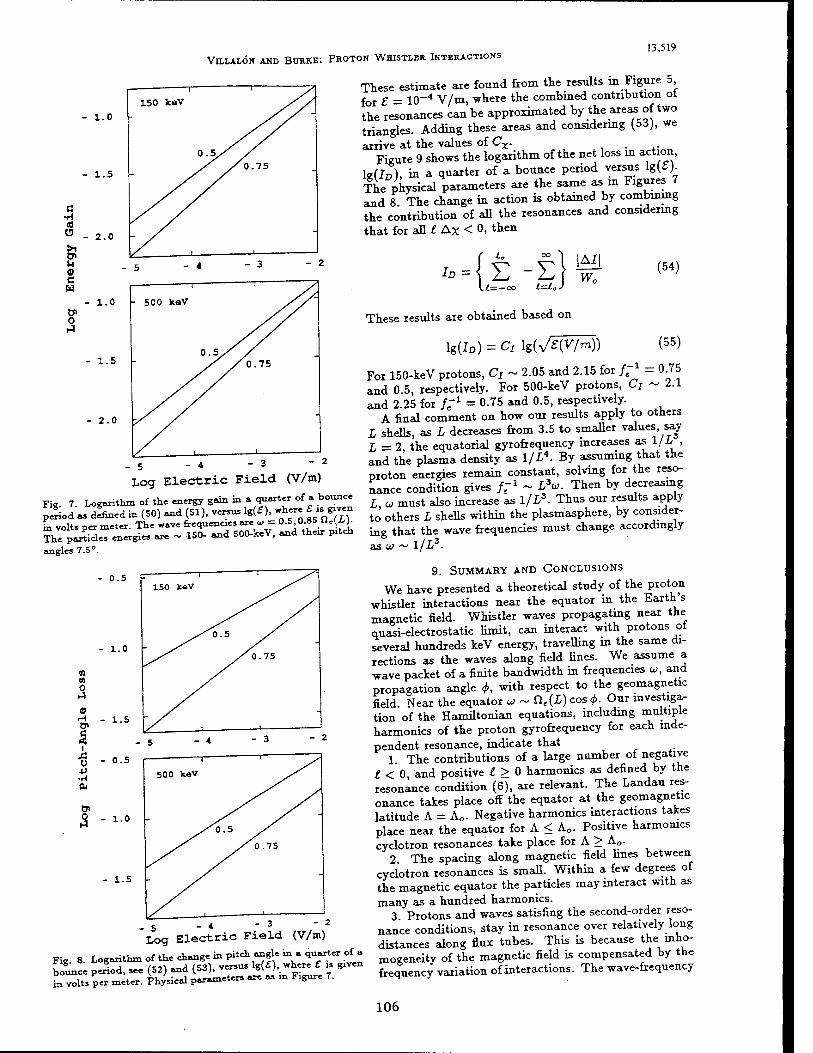
VlLLALÖN AND BURKE: PROTON WHISTLER INTERACTIONS 13,519
- 1.0
1.5
u
c w
- 2.0
- 1.0
O
- 1.5
- 2.0
These estimate are found from the results in Figure 5, for £ = 10~4 V/m, where the combined contribution oi the resonances can be approximated by the areas of two triangles. Adding these areas and considering (53), we
arrive at the values of Cx. . Figure 9 shows the logarithm of the net loss in action,
W(Io), in a quarter of a bounce period versus lg(£)_ The physical parameters are the same as in Figures 7 and 8. The change in action is obtained by combining the contribution of all the resonances and considering
that for all I AX < 0, then
. 5 - 4 - 3 - 2
Log Electric Field (V/m)
Fig. 7. Logarithm of the energy gain in a quarter of a bounce period as denned in (50) and (51), versus lg(£). whe« £1S given in volts per meter. The wave frequencies are « = 0.5,0.85 OeW- £he particles energies axe ~ 150- and 500-keV, and then- pitch
angles 7.5°.
M m O i-3
0.5
1.0
0>
I A O
■A
0> O ►3
- 1.5
- 0.5
1.0
1.5 -
(54)
- 5 " * " 3 - 2
Log Electric Field (V/m)
Fig 8. Logarithm of the change in pitch angle in a quarter of a Wee period, see (52) and (53), versus lg(£), where £ » g,vcn fc volts per meter. Physical parameters are as m Figure 7.
*-{£-i: f V./= — oo L=U0'
These results are obtained based on
Ig^) = Cx lg(v/f(y/m)) (55)
For 150-keV protons, Cj ~ 2.05 and 2.15 for f~l = 0.75 and 0.5, respectively. For 500-keV protons, d ~ 2.1 and 2.25 for f~l = 0.75 and 0.5, respectively.
A final comment on how our results apply to others L shells, as L decreases from 3.5 to smaller values, say L = 2 the equatorial gyrofrequency increases as 1/L , and the plasma density as 1/i4. By assuming that the proton energies remain constant, solving for the reso- nance condition gives fr1 ~ L*u. Then by decreasing L u must also increase as 1/L3. Thus our results apply to others L shells within the plasmasphere, by consider- ing that the wave frequencies must change accordingly
as u ~ l/L3.
9. SUMMARY AND CONCLUSIONS
We have presented a theoretical study of the proton whistler interactions near the equator in the Earth s magnetic field. Whistler waves propagating near the quasi-electrostatic limit, can interact with protons ot several hundreds keV energy, travelling in the same di- rections as the waves along field Hues. We assume a wave packet of a finite bandwidth in frequencies w, and propagation angle 4>, with respect to the geomagnetic field. Near the equator u> ~ Oe(£) cos <fi. Our investiga- tion of the Hamiltonian equations, including multiple harmonics of the proton gyrofrequency for each inde- pendent resonance, indicate that
1. The contributions of a large number of negative I < 0 and positive I > 0 harmonics as defined by the resonance condition (6), are relevant. The Landau res- onance takes place off the equator at the geomagnetic latitude A = A0. Negative harmonics interactions ta*es place near the equator for A < A„. Positive harmonics cyclotron resonances take place for A > A„.
2 The spacing along magnetic field hues between cyclotron resonances is small. Within a few degrees of the magnetic equator the particles may interact with as many as a hundred harmonics.
3 Protons and waves satisfing the second-order reso- nance conditions, stay in resonance over relatively long distances along flux tubes. This is because the^ho- mogeneity of the magnetic field is compensated by the frequency variation of interactions. The wave-frequency
106
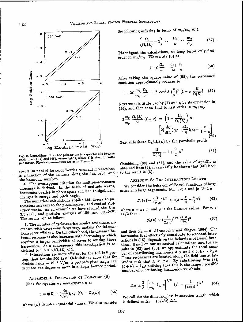
13,520 VrLLALON AND BUKKE: PROTON WHISTLER INTERACTIONS
O
c o •H ii O <
o
- 2
- 3
- 4
- 5
- 3
- 5
the following ordering in terms of me/mp <C 1
(Jh l\ ~ ^ ~ ^ (57)
Throuhgout the calculations, we keep terms only first order in mjmp. We rewrite (6) as
V U) c (58)
After taking the square value of (58), the resonance condition approximately reduces to
•-^7=''«'";)'|1-'iiffl1 (59)
Next we substitute v/c by (7) and r, by its expansion in (56), and then show that to first order in me/mp
d.T) ne, O« <>>-i^ M. (60)
- 5 - « " 3 "2
Log Electric Field (V/m)
Fie 9 I^garithmofthechangeinactioniniiquarterofabouii« period, see (54) and (55), versus lg(5). where £ is given in volts per meter. Physical parameters are as in Figure 7.
spectrum needed for second-order resonant interactions is a function of the distance along the flux tube, and the harmonic number.
4 The overlapping criterion for multiple-resonance crossings is derived. In the fields of multiple waves harmonics overlap in phase space and lead to significant changes in energy and pitch angle.
The numerical calculations applied this theory to pa- rameters relevant to the plasmasphere and control VLi experiments. As au example we have studied the L- 3.5 shell, and particles energies of 150- and 500-keV. The results are as follows:
1 The number of cyclotron-harmonics resonances in- creases with decreasing frequency, making the interac- tions more efficient. On the other hand, the distance be- tween resonances also increases with decreasing u which requires a larger bandwidth of waves to overlap those harmonics. As a consequence this investigation is re- stricted to 0.5 < w/ne(X) < 1.
2 Interactions are more efficient for the 150-keV pro- tons than for the 500-keV. Calculations show that for electric fields ~ 10"4 V/m, a proton's pitch angle can decrease one degree or more in a single bounce period.
APPENDIX A: DERIVATION OF EQUATION (8)
Near the equator we may expand r\ as
v = v(L) + (£-\L) (n.-n.(X)) (w)
where (L) denotes equatorial values. We also consider
(61)
Next substitute Qjile{L) by the parabolic profile
JL = 1 + iA* a{L) 2
Combining (60) and (61), and the value of dr,/dQc as obtained from (2), it can easily be shown that (60) leads to the result in (8).
APPENDIX B: THE INTERACTION LENGTH
We consider the behavior of Bessel functions of large order and large arguments. For n < x and |x| > 1 is
Ä(.)~(£)i/a«»(*-f-r> <62)
where x = ij. P, and p is the Larmor radius. For n > ex 12 then
«■l-lK»""'^ <63)
and then Jn -* 0 [Abramowitz and Siegun, 1964]. The harmonics that effectively contribute to resonant inter- actions in (15), depends on the behaviors of Bessel func- tions. Based on our numerical calculations and the re- sults in (62) and (63), we approximate the total num- ber of contributing harmonics n > and < 0 by ~ k±p. These resonances are located along the field line at lat- itudes such that A < AA. By substituting into (8), (/+ „) ~ kxp noticing that this is the largest possible number of contributing harmonics we obtain,
AA =m-r (/«- cos<£| 1/2 (64)
We call Az the dimensionless interaction length, which is defined as Az = (3/v/2) A A.
107
VlLLALON AND BURKE: PROTON WHISTLER INTERACTIONS 13,521
Acknowledgment*. We acknowledge helpful conversations with J. Albert, R. Helliwell, H. Koons, and J. Kozyra. We thanks G. Ginet for a careful reading of the manuscript. This work has been supported by the U.S. Air Force under contract F19628-89- K-0014 with Northeastern University.
The Editor thanks U. S. Inan, A. Draganov, and H. Karimabadi for their assistance in evaluating this paper.
REFERENCES
Abramowitz, M., and I. A. Stegun, Sandbook of Mathemati- cal Functions, Appl. Math. Ser., vol. 55, National Bureau of Standards, United States Department of Commerce, Washington, D. C, 1964. . .
Bell, T. F., The nonlinear gyroresonance interaction be- tween energetic electrons and coherent VLF waves prop- agating at an arbitrary angle with respect to the Earth s magnetic field. J. Geophys. Res.,.89, 905, 1984.
Bell, T. F., The wave magnetic field amplitude threshold for nonlinear trapping of energetic gyroresonant and Lan- dau resonant electrons by nonducted VLF waves in the magnetosphere, J. Geophys. Res., 91, 4365, 1986.
Bespalov, P. A., and V. Yu. Trakhtengerts, Cyclotron in- stability of Earth radiation belts, Rev. Plasma Phys., 10,
Carlson, C. R., R. A. Helliwell, and D. L. Carpenter, Van- able frequency VLF signals in the magnetosphere: As- sociated phenomena and plasma diagnostics, /. Geophys. Res., 90, 1507, 1985. . , ,
Chappell, C. R-, K. K. Harris, and G. W. Sharp, A study of the influence of magnetic activity on the location of the plasmapause as measured by OGO 5, J. Geophys. Res., 75, 50, 1970. .
Chirikov, B. V., A Universal instability of many-dimensional oscillator systems,P/iyj. Rep., 5, 263, 1979.
Dysthe K. B., Some studies of triggered whistler emissions, J. Geophys. Res., 76, 6915, 1971.
Dowden, R. L., A. D. McKay, and L. E. S. Amon, Linear and nonlinear amplification in the magnetosphere during a 6.6 kHz transmission, J. Geophys. Res., 83, 169, 1978.
Gendrin, R., Gyroresonant wave particle interactions, Sol. Terr. Phys., part III, Astrophys. Space Sei. li&r., vol 29, Edited by E. R. Dyer, p. 236, Kluwer Academic, Boston, Mass. 1972.
Ginet G. P., and M. Heinemann, Test particle acceleration by 'small amplitude electromagnetic waves in a uniform magnetic field, Phys. Fluids B, 2, 700, 1990.
Helliwell, R. A., A theory of discrete VLF emissions from the magnetosphere, J. Geophys. Res., 72, 4773, 1967.
Helliwell, R. A-, VLF wave stimulation experiments in the magnetosphere from Siple station, Antarctica, J. Geo- phys. Res., 26, 551, 1988.
Imhof, W. L-, H. D. Voss, J. B. Reagan, D. W. Datlowe, E. E. Gaines, J. Mobilia, and D. S. Evans, Relativist«: electron and energetic ion precipitations spikes near the plasmapause, J. Geophys. Res., 91, 3077, 1986
Inan, U. S., Gyroresonant pitch angle scattering by coher- ent and incoherent whistler mode waves in the magneto- sphere, /. Geophys. Res., 92, 127 1987.
Kennel, C. F., and H. E. Petschek, Limit on stably trapped particle fluxes, J. Geophys. Res., 71, 1, 1966.
Koons, H. C, Proton precipitation by a whistler-mode wave from a VLF Transmitter, Geophys. Res. Lett., 2, 281, 1975.
Koons, H. C, Stimulation of Pc limcropukations by con- trolled VLF transmissions, J. Geophys. Res., 8Z, Hoi,
1977 ., M. M. Mogilevskii, Zh. M. Boske, Yu. V. Dzhordzhio, Yu. V. Lisakov, O. A. A. Rem, JETP Lett., Engl. Transl, 38,
Kovrazhkin, R. A I. Gal'perin, N. Molchanov, and 397, 1983.
Kovrazhkin, R. A nlml, xv. „., M. M. Mogilevskii, O. A. Molchanov Yu. I. Gal'perin, N. V. Dzhordzhio, Zh. M. Boske, and A. Rem, Precipitation of protons from the Earth's magne- tosphere stimulated by artificial low-frequency radiation, JETP Lett., Engl. Transl., 39, 228, 1984.
Lyons, L. R., and D. J. Williams, Quantitative aspects of magnetospheric physics, D. Reidel, Hingham, Mass., 1984.
Matsumoto, H., Nonlinear whistler-mode interaction and triggered emissions in the magnetosphere: A review, in Wave Instabilities in Space Plasma, edited by P. J. Pal- madesso and K. Papadopoulos, pp. 163-190, D. Reidel, Dordrecht-Holland, 1979.
Menyuk, C. R., A. T. Dobrok, K. Papadopoulus, and H. Karimabadi, Stochastic electron acceleration in obliquely propagating electromagnetic waves, Phys. Rev. Lett., 58, 2071, 1987.
Morgan, M. G., Some features of pararesonance (PR) whist- lers, J. Geophys. Res., 85, 130, 1980.
Nunn, D., A self-consistent theory of triggered VLF emis- sions, Planet. Space Sei., 22, 349, 1973.
Sazhin, S. S., Quasielectrostatic wave propagation in a hot anisotropic plasma, Planet. Space Sei., 34, 497, 1986.
Schulz, M., and G.T. Davidson, Limiting energy spectrum of a saturated Radiation Belt, /. Geophys. Res., 93, 59, 1988. . .± i#
Shklyar, D. R., Mechanism for proton precipitation trig- gered by a VLF wave injected into the magnetosphere, JETP Lett, Engl. Transl, 41, 448, 1985.
Shklyar, D. R., Particle interaction with an electrostatic VLF wave in the magnetosphere with an application to proton precipitation, Planet. Space Sei., 34, 1091, 1986.
Sudan, R. N., and E. Ott, Theory of triggered VLF emis- sions, J. Geophys. Res., 76, 4463, 1971.
Villalon, E., and W. J. Burke, Relativistic particle accel- eration by obliquely propagating electromagnetic fields, Phys. Fluids, 30, 3695, 1987.
Villalon, E., W. J. Burke, P. L. Rothwell, and M. B. Süe- vitch, Quasilinear wave particle interactions in the Earth s radiation belts, J. Geophys. Res., 94, 15243, 1989
Villalon, E., and W. J. Burke^Near-equatonal pitch angle diffusion of energetic electfbns by oblique whistler waves, J. Geophys. Res., 96, 9655, 1991.
Walker, G. H., and J. Ford, Amplitude instability and er- godic behavior for conservative nonlinear oscillaltor sys- tems, Phys. Rev., 188, 416, 1969.
W. J. Burke, Geophysics Directorate, PL/GPSG, Hanscom Air Force Base, MA 01731.
E. Villalon, Center for Electromagnetics Research, Northeast- ern University, Boston, MA 02115.
(Received November 2, 1992; revised February 3, 1993; accepted March 4, 1993.)
108
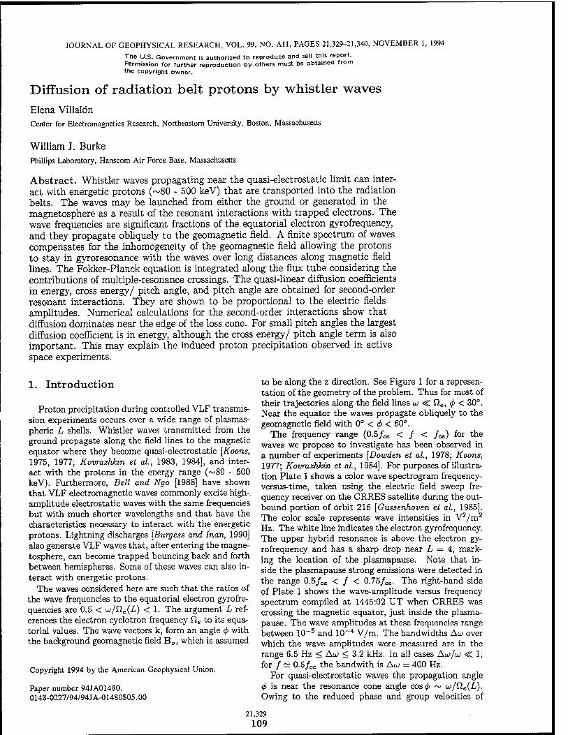
JOURNAL OF GEOPHYSICAL RESEARCH, VOL. 99, NO. All, PAGES 21,329-21,340, NOVEMBER 1, 1994 The U.S. Government is authorized to reproduce and sell this report. Permission for further reproduction by others must be obtained from the copyright owner.
Diffusion of radiation belt protons by whistler waves
Elena Villalön Center for Electromagnetics Research, Northeastern University, Boston, Massachusetts
William J. Burke Phillips Laboratory, Hanscom Air Force Base, Massachusetts
Abstract. Whistler waves propagating near the quasi-electrostatic limit can inter- act with energetic protons (~80 - 500 keV) that are transported into the radiation belts. The waves may be launched from either the ground or generated in the magnetosphere as a result of the resonant interactions with trapped electrons. The wave frequencies are significant fractions of the equatorial electron gyrofrequency, and they propagate obliquely to the geomagnetic field. A finite spectrum of waves compensates for the inhomogeneity of the geomagnetic field allowing the protons to stay in gyroresonance with the waves over long distances along magnetic field lines. The Fokker-Planck equation is integrated along the flux tube considering the contributions of multiple-resonance crossings. The quasi-linear diffusion coefficients in energy, cross energy/ pitch angle, and pitch angle are obtained for second-order resonant interactions. They are shown to be proportional to the electric fields amplitudes. Numerical calculations for the second-order interactions show that diffusion dominates near the edge of the loss cone. For small pitch angles the largest diffusion coefficient is in energy, although the cross energy/ pitch angle term is also important. This may explain the induced proton precipitation observed in active space experiments.
1. Introduction
Proton precipitation during controlled VLF transmis- sion experiments occurs over a wide range of plasmas- pheric L shells. Whistler waves transmitted from the ground propagate along the field lines to the magnetic equator where they become quasi-electrostatic [Koons, 1975, 1977; Kovrazhkin et at, 1983, 1984], and inter- act with the protons in the energy range (~80 - 500 keV). Furthermore, Bell and Ngo [1988] have shown that VLF electromagnetic waves commonly excite high-, amplitude electrostatic waves with the same frequencies but with much shorter wavelengths and that have the characteristics necessary to interact with the energetic protons. Lightning discharges [Burgess and Inan, 1990] also generate VLF waves that, after entering the magne- tosphere, can become trapped bouncing back and forth between hemispheres. Some of these waves can also in- teract with energetic protons.
The waves considered here are such that the ratios of the wave frequencies to the equatorial electron gyrofre- quencies are 0.5 < uj/£le(L) < 1. The argument L ref- erences the electron cyclotron frequency £le to its equa- torial values. The wave vectors k, form an angle <f> with the background geomagnetic field BOJ which is assumed
Copyright 1994 by the American Geophysical Union.
Paper number 94JA01480. 0148-0227/94/94J A-01480S05.00
to be along the z direction. See Figure 1 for a represen- tation of the geometry of the problem. Thus for most of their trajectories along the field lines w -C fie, 4> < 30°. Near the equator the waves propagate obliquely to the geomagnetic field with 0° < <j> < 60°.
The frequency range (0.5/ce < f < fce) for the waves we propose to investigate has been observed in a number of experiments [Dowden et at, 1978; Koons, 1977; Kovrazhkin et al., 1984]. For purposes of illustra- tion Plate 1 shows a color wave spectrogram frequency- versus-time, taken using the electric field sweep fre- quency receiver on the CRRES satellite during the out- bound portion of orbit 216 [Gussenhoven et al, 1985]. The color scale represents wave intensities in V2/m2
Hz. The white line indicates the electron gyrofrequency. The upper hybrid resonance is above the electron gy- rofrequency and has a sharp drop near L = 4, mark- ing the location of the plasmapause. Note that in- side the plasmapause strong emissions were detected in the range 0.5/ce < / < 0.75/ce. The right-hand side of Plate 1 shows the wave-amplitude versus frequency spectrum compiled at 1445:02 UT when CRRES was crossing the magnetic equator, just inside the plasma- pause. The wave amplitudes at these frequencies range between 10-5 and 10~4 V/m. The bandwidths Aw over which the wave amplitudes were measured are in the range 6.5 Hz < Aw < 3.2 kHz. In all cases Aw/w >C 1; for / ~ 0.5/ce the bandwith is Aw = 400 Hz.
For quasi-electrostatic waves the propagation angle <j> is near the resonance cone angle cos<£ ~ w/f2e(L). Owing to the reduced phase and group velocities of
21,329 109
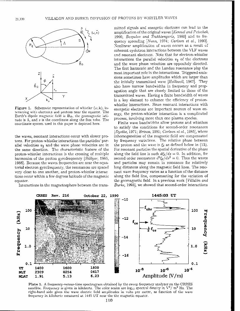
21,330 VILLALON AND BURKE: DIFFUSION OF PROTONS BY WHISTLER WAVES
(w,k)
Figure 1. Schematic representation of whistler (w,k), in- teracting with electrons and protons near the equator. The Earth's dipole magnetic field is Bo, the geomagnetic lati- tude is A, and s is the coordinate along the flux tube. The coordinate system used in this paper is depicted here.
the waves, resonant interactions occur with slower pro- tons. For proton-whistler interactions the particles' par- allel velocities v^ and the wave phase velocities are in the same direction. The characteristic feature of the proton-whistler interactions is the crossing of multiple harmonics of the proton gyrofrequency [Shklyar, 1985, 1986]. Because the waves frequencies are near the equa- torial electron gyrofrequency, the resonances are spaced very close to one another, and proton-whistler interac- tions occur within a few degrees latitude of the magnetic equator.
Interactions in the magnetosphere between the trans-
mitted signals and energetic electrons can lead to the amplification of the original waves [Kennel and Petschek, 1966; Bespalov and Trakhtengerts, 1980] and to fre- quency spreading [Nunn, 1974; Carlson et al, 1990]. Nonlinear amplification of waves occurs as a result of coherent cyclotron interactions between the VLF waves and resonant electrons. Note that for electron-whistler interactions the parallel velocities VJJ of the electrons and the wave phase velocities are oppositely directed. The first harmonic and the Landau resonance play the most important role in the interactions. Triggered emis- sions sometimes have amplitudes which are larger than the initially transmitted wave [Helliwell, 1967]. They also have narrow bandwidths in frequency and prop- agation angle that are closely limited to those of the transmitted waves. Having a finite bandwidth of waves is a key element to enhance the efficiency of proton- whistler interactions. Since resonant interactions with energetic electrons are important sources of wave en- ergy, the proton-whistler interaction is a complicated process, involving more than one plasma species.
Finite wave bandwidths allow protons and whistlers to satisfy the conditions for second-order resonances [Dysthe, 1971; Brinca, 1981; Carlson et al, 1985], where inhomogeneities of the magnetic field are compensated by frequency variations. The relative phase between the proton and the wave is & as defined below in (13). For resonant particles the spatial derivative of the phase along the field line is such d^/ds = 0. In addition, for second order resonances d2&/ds2 = 0. Thus the waves and particles may remain in resonance for relatively long distances along the magnetic field lines. The reso- nant wave frequency varies as a function of the distance along the field line, compensating for the variation of the geomagnetic field. In a previous work [Villalon and Burke, 1993], we showed that second-order interactions
October 22, 1990
^ 100 N «
>i O c o
0 u
10
1.0
0.1 UT MLT MLAT
1445:03 UT -10
I- -12
W." -14
<- -16
1 Mm
100
10
1.0
0.1
10" 10 -6 10"
*1 H ID
ID 3 O
X N
Amplitude (V/m)
Plate 1. A frequency-versus-time spectrogram obtained by the sweep frequency analyzer on the CRRES satellite. Frequency is given in kilohertz. The color scales are logio spectral density in V2/ m2 Hz. The right-hand side gives the wave electric field amplitudes in volts per meter, as function of the wave frequency in kilohertz measured at 1445 UT near the the magnetic equator.
110
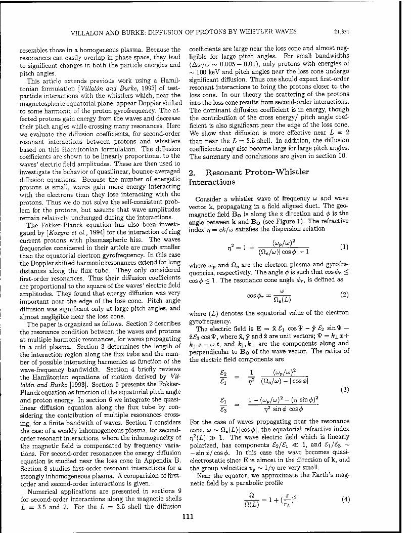
VILLALON AND BURKE: DIFFUSION OF PROTONS BY WHISTLER WAVES 21,331
resembles those in a homogeneous plasma. Because the resonances can easily overlap in phase space, they lead to significant changes in both the particle energies and pitch angles.
This article extends previous work using a Hamil- tonian formulation [Villalön and Burke, 1993] of test- particle interactions with the whistlers which, near the magnetospheric equatorial plane, appear Doppler shifted to some harmonic of the proton gyrofrequency. The af- fected protons gain energy from the waves and decrease their pitch angles while crossing many resonances. Here we evaluate the diffusion coefficients, for second-order resonant interactions between protons and whistlers based on this Hamiltonian formulation. The diffusion coefficients are shown to be linearly proportional to the waves' electric field amplitudes. These are then used to investigate the behavior of quasilinear, bounce-averaged diffusion equations. Because the number of energetic protons is small, waves gain more energy interacting with the electrons than they lose interacting with the protons. Thus we do not solve the self-consistent prob- lem for the protons, but assume that wave amplitudes remain relatively unchanged during the interactions.
The Fokker-Planck equation has also been investi- gated by [Kozyra et at, 1994] for the interaction of ring current protons with plasmaspheric hiss. The waves frequencies considered in their article are much smaller than the equatorial electron gyrofrequency. In this case the Doppler shifted harmonic resonances extend for long distances along the flux tube. They only considered first-order resonances. Thus their diffusion coefficients are proportional to the square of the waves' electric field amplitudes. They found that energy diffusion was very important near the edge of the loss cone. Pitch angle diffusion was significant only at large pitch angles, and almost negligible near the loss cone.
The paper is organized as follows. Section 2 describes the resonance condition between the waves and protons at multiple harmonic resonances, for waves propagating in a cold plasma. Section 3 determines the length of the interaction region along the flux tube and the num- ber of possible interacting harmonics as function of the wave-frequency bandwidth. Section 4 briefly reviews the Hamiltonian equations of motion derived by Vil- lalön and Burke [1993]. Section 5 presents the Fokker- Planck equation as function of the equatorial pitch angle and proton energy. In section 6 we integrate the quasi- linear diffusion equation along the flux tube by con- sidering the contribution of multiple resonances cross- ing, for a finite bandwith of waves. Section 7 considers the case of a weakly inhomogeneous plasma, for second- order resonant interactions, where the inhomogeneity of the magnetic field is compensated by frequency varia- tions. For second-order resonances the energy diffusion equation is studied near the loss cone in Appendix B. Section 8 studies first-order resonant interactions for a strongly inhomogeneous plasma. A comparision of first- order and second-order interactions is given.
Numerical applications are presented in sections 9 for second-order interactions along the magnetic shells L = 3.5 and 2. For the L = 3.5 shell the diffusion
coefficients are large near the loss cone and almost neg- ligible for large pitch angles. For small bandwidths (AUI/UJ ~ 0.005 - 0.01), only protons with energies of ~ 100 keV and pitch angles near the loss cone undergo significant diffusion. Thus one should expect first-order resonant interactions to bring the protons closer to the loss cone. In our theory the scattering of the protons into the loss cone results from second-order interactions. The dominant diffusion coefficient is in energy, though the contribution of the cross energy/ pitch angle coef- ficient is also significant near the edge of the loss cone. We show that diffusion is more effective near L = 2 than near the L = 3.5 shell. In addition, the diffusion coefficients may also become large for large pitch angles. The summary and conclusions are given in section 10.
2. Resonant Proton-Whistler Interactions
Consider a whistler wave of frequency u and wave vector k, propagating in a field aligned duct. The geo- magnetic field B0 is along the z direction and <j> is the angle between k and B0 (see Figure 1). The refractive index 77 = cfc/w satisfies the dispersion relation
77^ = 1 + {wp/wf
{Sle/üj)\cos4>\ - 1 (1)
where u)p and Sle are the electron plasma and gyrofre- quencies, respectively. The angle <f> is such that cos <f>r < cos<j> < 1. The resonance cone angle <pT, is defined as
cos<^r = Sle{L)
(2)
where (L) denotes the equatorial value of the electron gyrofrequency.
The electric field is E = x £1 costf - y £2 sin^ - ±£3 cos V, where x, y and z are unit vectors; $ = k±x+ fey z - UJ t, and k\\,kj_ are the components along and perpendicular to Bo of the wave vector. The ratios of the electric field components are
£2 £1
£L £3
("PM2
772 (Sle/uj) — I COS <
1 -(ujp/ui)2 - (77 sm<p)7
?72 sixi(f> cos4>
(3)
For the case of waves propagating near the resonance cone, uj ~ Sle(L)\cos<p\, the equatorial refractive index r]2{L) > 1. The wave electric field which is linearly polarized, has components £2/^1 ^ 1. an<* £\/^3 ~ - sin <f>/ cos <f>. In this case the wave becomes quasi- electrostatic since E is almost in the direction of k, and the group velocities vg ~ I/77 are very small.
Near the equator, we approximate the Earth's mag- netic field by a parabolic profile
SI Sl(L) 1 + &2 (4)
111
21,332 VILLALON AND BURKE: DIFFUSION OF PROTONS BY WHISTLER WAVES
where 5 ~ RE LA, RE is the Earth's radius, L is the magnetic shell parameter, A is the geomagnetic lati- tude, and rL = (V2/3)REL. The equatorial gyrofre- quency is denoted by Q(L), and fi stands for the gy- rofrequencies either for electrons or protons at a lo- cation s away from the equator along the field line. Equation (4) is obtained from a Taylor expansion of the dipole field and is an excellent representation of the magnetic geometry within ±20° of the equator.
Whistler-proton interactions satisfy the resonance con- dition
w-kl]vll-enp = o (5)
where, £ = 0, ±1,±2,..., is the harmonic number; fip
is the proton gyrofrequency; and v\\ is the parallel components of the particle's velocity. We call p. = sin20£, where 6L is the equatorial pitch angle. Here 6L > 0C, where 6C is the pitch angle at the edge of the loss cone, and p,c is the corresponding value of p. As a function of the L shell, the mirror ratio is a = p~l = L3 (4 - 3/L)1/2. To zero order in the electric field amplitudes, the particle's magnetic mo- ment is conserved. Then we may write for the parallel and perpendicular components of the particle velocity v. v,| = «[1 -p,9./Q.{L)]1'2, vx =v[ßCl/n(L)}^2. Note that as the particles and waves move away from the equator, the parallel velocities uy of particles decrease, while the waves' phase velocities w/k\\ increase.
Protons of energies less than a few hundred keV, sat- isfy the resonance condition with waves whose refractive indices 77 are very large. As the proton energy decreases and the pitch angle increases, 77 increases. If 77 becomes very large the dispersion relation in (1) is no longer valid. In this case we must consider thermal corrections for the plasmaspheric electron population that supports the waves as described by Sazhin [1993]. These thermal corrections limit the magnitudes of rj^ = rj w/fle(L), to finite values. This means that as vy —> 0, resonant interactions described by (5) may not be possible. As the particles energies decreases, the resonant pitch an- gles must be closer to the loss cone. Interactions for larger pitch angles required larger energies. Thus there could exist a lower value in particle energy, and an up- per value in the pitch angle needed to satisfy (5). These values depend on the thermal corrections that defined the possible upper limits of the refractive indices.
3. Interaction Region
We assume that a proton interacts at the equator with the harmonic £ — -v, where u > 0. The geomag- netic latitude A^ of higher-order resonances has been obtained by [Villalon and Burke, 1993] and turn outs to be
1 9 mD (£+u)
cos<£| (^ I cos 01-1) (6)
We consider a spectrum of waves that is centered at a certain value of ut, and propagates near the res- onance cone angle in (2). The widths of this spectrum are Aw(C w), and A4>(<S. cpr). The interaction regions Afie, where 0 < Oe — fie(£) < Afle, are functions of the waves' frequency bandwidths. The geomagnetic lat- itudes for resonant interactions, A, extend over 0 < A < AA. From (4) we get that (AA)2 = (2/9) Afie/fte(L). Refering to (46) of [Villalon and Burke, 1993], in terms of the waves' frequency bandwidths we show
(AA)2 2 Aw d77||
9 u) dud
dm 1 dv»
dfle " v» d£l„ (7)
where rj\\ = 77 cos<p and depends on w and <j> through the variable u)$ = UJ/ cos4>. Here dr}\\/dQe, d^/dui^ are obtained from (1), and dv^/düe = — v2
L/[2f2e(L) v\\]. The number of possible interacting harmonics cov-
ered by this spectrum is n, where — n < I < n, is ap- proximated as
— m"P cos ^ A A \2 71 ~ ^ (fie(L)/w)|cos^|-l ( } (8)
Combining (7) and (8), we find the number of contribut- ing resonant harmonics n as function of the width of the spectrum Aw/w.
The interaction region along the field line has a max- imum extent in geomagnetic latitude ~ AA^, that is, AAi > AA, for any value of Aw/w. It is obtained by substituting (£ + 1/) by ~ 2k±p in (6), which leads to
1 (AAL) = - k±p{
am» UJ COS( r) (9)
Note that AA^, increases with the particle energy and with the pitch angle. By substituting in (7) AA by AA/,, and solving for the bandwiths yields (AUJ/UJ)L.
( )L = UJ
.3AA ̂ 12
v/2 l+tan20L(l TFTTT-O cos0fie(L) (10)
If the widths of the spectrum are equal or larger than (Aw/w)i, the entire range of possible resonant harmon- ics is included in the interactions.
For equatorial interactions that occur near the loss cone, resonant particles must have energies in the range: 0 < v2 < v2
M. For a finite width spectrum such that 4>r > 4> > 4>r — A0, we show
fie(L) VM = tan^v sinA^
1/2
(11)
where v < k±p, and p = v±/£lp is the Larmor radius. For reasons explained below the resonant harmonics that effectively contribute to the proton-whistler inter- actions are such that -k±p < £ < k±p, where k± p > 1.
112
4. Equations of Motion In this section we briefly summarize the Hamiltonian
formulation presented by [Villalon and Burke, 1993], to provide the main equations that are relevant to the theory developed here. We normalize the proton v and canonical V velocities, by c~l, length s by r^1, call T = tflp(L), and define « = Clp(L) rL/c ~ 1. The dimensionless electric field amplitudes are
Si (12)
VILLALON AND BURKE: DIFFUSION OF PROTONS BY WHISTLER WAVES 21,333
for i = 1,2,3, and where q is the proton charge. The relative wave-proton phase angle is
&= £X + I ds'rLk\{{s) - Jo np(L) (13)
The change in particle kinetic energy W is
dW _ UJ d£ 17 ~ mp(L) ds
(21)
P "' We define x = to(L)/£l sin2 6, where 6 is the local pitch where, in terms of the canonical velocities in the y angie. The evolution of % as a function of s is
u> , dl and x directions, A = arctan(Vj,/J4). To zero order in the electric fields amplitudes, X = t Clp(L). The canonical action-angle variables are / and A, where / = (y2/2) p(L)/n.
To first order in the electric field amplitudes et, the normalized, time-dependent Hamiltonian is a function of the canonical pairs of variables, (Vj|,s), and (7,A),
&--U-U. ds~w[ ^mp(LYds
(22)
5. Diffusion Equation
H-V*+I ° - Vj| £ sin&T, (14)
Consider the diffusion equation [Lyons and Williams, 1984]:
Here
Vx
2Vj,
- esMx)
[ (ei - e2) Je+i{x) + (ei + e2) Jt-i{x)}
(15)
21 *» df _ u; dr K ds fip(L)
1
£=-oo
^k (2TT)3
G-\ (1 - T) COS (j) V|| )
where Je are Bessel functions, whose argument is x = fcj. p, and p = Vl/^p- The behavior of Bessel func- tions for large arguments is such that if I < k\p, then where the operators:
.%l «||+^-l) v± ) Gf (23)
[Abramowitz and Stegun, 1964]
.£(*) = (i-)1/2 Cos(^ - 1% - Iff) (16)
if £ > fcxp then the contribution of the Bessel functions are negligible. In the numerical calculations we find that near the loss cone, where v± is small, the argument of the Bessel functions is large. Equation (16) may still be used near the loss cone provided the harmonic £ is smaller than the argument of the Bessel function.
A ,fi(i) V± ?Qp - (-L)2
l a
d ^L9_
dfi v dv (24)
G + —(1-77,,^) = -j— ^sin0 v±
+ 2 il(L) v\\ d
fl v dfj,
v2 dv
A-(^)2 W V
v± V v«
For a particle crossing an isolated cyclotron resonance (j, = sin2öLl 6L is the equatorial pitch angle, and v is we need only consider a single term £ in the summation the normalized proton velocity, in (14). In this case we find that
dI , c v — =£ cos&T* ds
For the phase angle we find
ds2 a + cos& — T*
(17)
(18)
We can further rewrite the diffusion equation as
5?+7&-A yy ~2vSe (25)
The inhomogeneity factor a depends on the variation of the geomagnetic field, and the frequency spectrum, we show
dr)\\ _ ,T\ M U) a =
fip(L)
1
n^g-^2a-rij
where
Se = Ü — v dfj.
+ 1 9
v2 dv
A I **"•" 3M. }
ft(L) ds -r- + « w dn\\ duij,
Clp(L) dojf ds (19)
vd">"fo+do" dfl.
The diffusion coefficients are defined in terms of
,o 1
/
/(26)
where w^ = u/cos cj>, rj\\ = rj cos<j>, and for resonant protons d£e/ds = 0. By using the resonance condition (£ = 0) we estimate that
A«= ( w (3L)2 T2 5(fl), (27) Airvo v± as
lCl(L) ds
dQ.]2 ^ g np(L)
1-M + I
| cos</>|
cos <^| - a;/fie(L) (20)
where v0 = vy/«, and T^ is given in (15). Here d^e/ds = fc||rz, + (££lp - w)/«ofip(I'); and for resonant protons, d£e/ds = 0. Because of the behavior of Bessel functions for large arguments, the number of harmonics that give nonzero contribution to the summation in (25), is such
113
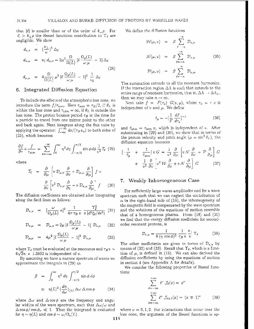
21.334 VILLALON AND BURKE: DIFFUSION OF PROTONS BY WHISTLER WAVES
that \£\ is smaller than or of the order of k±p. For \£\ > k±_p the Bessel functions contribution to T^ are negligible. We show
v±. dv,v = (—) A£
u)P v\\ dßtV = 2p
n
n
Q(L)
I« np(L)
UJ p
I]2
1]A,
(28)
6. Integrated Diffusion Equation
To include the effects of the atmospheric loss cone, we introduce the term //ratm. Here ratm = TB/2, if 6i is within the loss cone and ratm = oo, if OL, is outside the loss cone. The proton bounce period TB is the time for a particle to travel from one mirror point to the other and back again. Next integrate along the flux tube by applying the operator: /_^ ds/{TBv0) to both sides of (25), which becomes
£= —CO dr
where
r\ drj r/2 1
/ sin4>d4>^T£ (29) /-7T/2 ^
T, = ^r- 8_
du
8_ dv
vV„
v2V„
dv P-|, / +
dv + VV^Tp\ I (30)
The diffusion coefficients are obtained after integrating along the field lines as follows:
T>v,v
Vv„
Vn
Tj lClp(L)
v^v = 2(j, [e
A-KTQV v \cfi&/ds2\
fip(L)
V np{L) U! fj,
U> fl
- I]2 V,
1] vVtV
(31)
(32)
(33)
where Te must be evaluated at the resonance and TBS~
6\/2«: x 1.3802 is independent of v. By assuming we have a narrow spectrum of waves we
approximate the integrals in (29) as
ß = T] drj
r/2
7/2
^)2(J)(i)Aa
sin <f> dxj>
Acos< (34)
We define the diffusion functions ■j-n
+n
N{p,v) = /?£ e=-r
v(ß,v) = ßjr
V»
vn
(35)
The summation extends to all the resonant harmonics. If the interaction region AA is such that extends to the entire range of resonant harmonics, that is, AA —> A AL,
then we may take n —> oo. Next take / = F(T0) G(v,p), where r0 = r v is
independent of v and /x. We define
dF, , r„ = -
1
F dr0 (36)
and fatm = ratm v, which is independent of v. After substituting in (29) and (30), we show that in terms of the proton velocity and pitch angle (p = sin2^), the diffusion equation becomes
1 +
+ ' atm v2 dp, l dv dp
l d v2 dv
n d , d v2W — + vN1-
dv dp, G (
G
(37)
7. Weakly Inhomogeneous Case
For sufficiently large waves amplitudes and for a wave spectrum such that we can neglect the contribution of a in the right-hand side of (18), the inhomogeneity of the magnetic field is compensated by the wave spectrum and the solutions of the equations of motion resemble that of a homogeneous plasma. From (18) and (31) we find that the energy diffusion coefficient for second- order resonant protons, is
1 1
8 (rj cos 4>) TB v T, (38)
The other coefficients are given in terms of VVtV by means of (32) and (33). Recall that Ye, which is a func- tion of p:, is defined in (15). We can also derived the diffusion coefficients by using the equations of motion in section 4 (see Appendix A for details).
We consider the following properties of Bessel func- tions:
where Aw and Acos^!> are the frequency and angu- lar widths of the wave spectrum, such that Aw/w and A cos <f>/ cos 4>T <C 1. Thus the integrand is evaluated for rj ~ rj(L) and cos<?i ~ w/fie(L).
114
-+-00
E TOO
£ i=-oo
lv Je(x) = xu
fJtti(i)= (x =F 1)" (39)
where v = 0,1, 2. For interactions that occur near the loss cone, the argument of the Bessel functions is ap-
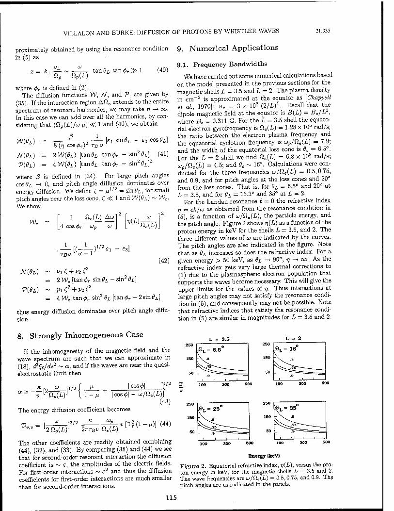
VILLALON AND BURKE: DIFFUSION OF PROTONS BY WHISTLER WAVES 21,335
proximately obtained by using the resonance condition in (5) as
u VJ- Slp(L)
tan 9L tan <fiT > 1 (40)
where <pr is defined in (2). The diffusion functions W, Af, and V, are given by
(35). If the interaction region Af2e extends to the entire spectrum of resonant harmonics, we may take n —> oo. In this case we can add over all the harmonics, by con- sidering that (fip(L)/wA*) < 1 and (40), we obtain
W(0L) = ß
8 (77 COS<pT)2 Tß V
tf(0L) = 2W(9L) [tanöL tan0
T>{BL) = AW(0L) [tan0L tan<fc
[ei sm9L - 63 cosOL]
sin20L] (41)
sin20L]2
where ß is defined in (34). For large pitch angles cos 91 -» 0, and pitch angle diffusion dominates over energy diffusion. We define C = M1/2 = sin ®L, for small pitch angles near the loss cone, C < 1 and W(tfL) ~ Wc. We show
Wr. = 1
4 cos<
ne(L) Aa;12
1/2 -, _
vW ne(L)
-L.[(-^-)^6l TRü <7 — i
£3
(42)
A/"0?Z,) ~ I/lC+**C = 2 Wc [tan 0r sin 0L - sin2 0L]
v{eL) ~ PiC2 + PzC3
= 4 Wc tan 0r sin2 0L [tan <j>r - 2 sin 0L]
thus energy diffusion dominates over pitch angle diffu- sion.
8. Strongly Inhomogeneous Case
If the inhomogeneity of the magnetic field and the wave spectrum are such that we can approximate in (18), d?&/ds2 ~ a, and if the waves are near the quasi- electrostatic limit then
__ro_r__ a- v«[lnp(L) 11/2 M I cos<£|
1 - (i I cos0| — uj/Qe(L)
The energy diffusion coefficient becomes
,1/2
(43)
P„,„ 13/2 OV,
L2QP(L)J 2-KTBv nc{L) v[TJ(l-^)} (44)
9. Numerical Applications
9.1. Frequency Bandwidths
We have carried out some numerical calculations based on the model presented in the previous sections for the magnetic shells L = 3.5 and L = 2. The plasma density in cm-3 is approximated at the equator as [Chappell et ai, 1970]: nc = 3 x 10³ (2/L)4. Recall that the dipole magnetic field at the equator is B{L) = B0/L , where B0 = 0.311 G. For the L - 3.5 shell the equato- rial electron gyrofrequency is üe{L) = 1.28 x 10⁵ rad/s; the ratio between the electron plasma frequency and the equatorial cyclotron frequency is ujp/Q.e(L) = 7.9; and the width of the equatorial loss cone is 6C = 6.5°. For the L - 2 shell we find fie(L) = 6.8 x 10⁵ rad/s; wp/fie(L) = 4.5; and 0C ~ 16°. Calculations were con- ducted for the three frequencies w/Qe{L) = 0.5,0.75, and 0.9, and for pitch angles at the loss cones and 20° from the loss cones. That is, for 0L = 6.5° and 20° at L = 3.5, and for 9L = 16.3° and 35° at L = 2.
For the Landau resonance t = 0 the refractive index 77 = ck/uj as obtained from the resonance condition in (5), is a function of Lu/Qe(L), the particle energy, and the pitch angle. Figure 2 shows r](L) as a function of the proton energy in keV for the shells L = 3.5, and 2. The three different values of u are indicated by the curves. The pitch angles are also indicated in the figure. Note that as 9L increases so does the refractive index. For a given energy > 50 keV, as 6L -* 90°, r\ -> 00. As the refractive index gets very large thermal corrections to (1) due to the plasmaspheric electron population that supports the waves become necessary. This will give the upper limits for the values of rj. Thus interactions at large pitch angles may not satisfy the resonance condi- tion in (5), and consequently may not be possible. Note that refractive indices that satisfy the resonance condi- tion in (5) are similar in magnitudes for L — 3.5 and 2.
The other coefficients are readily obtained combining (44), (32), and (33). By comparing (38) and (44) we see that for second-order resonant interaction the diffusion coefficient is ~ e, the amplitudes of the electric fields. For first-order interactions ~ e2 and thus the diffusion coefficients for first-order interactions are much smaller than for second-order interactions.
L = 3.5 L = 2 2SO
150
50
^ = 6.5°
-\^ .8
^75
- .9 f 1 I
500 300
250
VL = 25° 150 -\
\L5
50
1
^9 ^====== 1 1 I
250
150
50
\L_ 35° .5
N^ ~-£*~~
1 1 1 , J
Energy (keV)
Figure 2. Equatorial refractive index, T?(L), versus the pro- ton energy in keV, for the magnetic shells L = 3.5 and 2. The wave frequencies are w/fie(L) = 0.5,0.75, and 0.9. The pitch angles are as indicated in the panels.
115
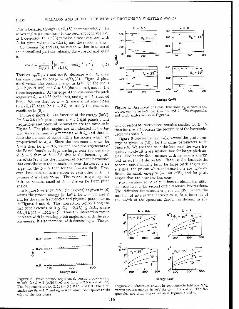
21,336 VILLALON AND BURKE: DIFFUSION OF PROTONS BY WHISTLER WAVES
This is because, though up/fte(L) decreases with L, the waves angles <j> come closer to the resonant cone angle 4>r
as L decreases, thus rj(L) remains almost constant with L, for given values of u>/Q.e(L) and the proton energy.
Combining (5) and (1), we can show that in terms of the normalized particle velocity, the wave normal angle
is
COSi^> = ne(L) r oe(L) cosfc^j 1 (45)
Thus as ujp/Qe(L) and COSOL decrease with L, coscp becomes closer to cos^r = u;/Qe(L). Figure 3 plots cos cfi versus the proton energy in keV, for the shells L = 2 (solid line), and L — 3.5 (dashed line), and for the three frequencies. At the edge of the loss cones the pitch angles are 6L = 16.3° (solid line), and 0L = 6.5° (dashed line). We see that for L = 2, cos<£ must stay closer to Lü/üe(L) than for L — 3.5, to satisfy the resonance condition in (5).
Figure 4 shows k±p as function of the energy (keV), for L = 3.5 (left panels) and L = 2 (right panels). The frequencies and physical parameters are the same as in Figure 3. The pitch angles are as indicated in the fig- ure. As we can see, k±p increases with 9i and thus, so does the number of contributing harmonics which are proportional to k±p. Since the loss cone is wider for L = 2 than for L = 3.5, we find that the arguments of the Bessel functions, k±p, are larger near the loss cone at L = 2 than at L — 3.5, due to the increasing val- ues of sm9L. Thus the numbers of resonant harmonics that contribute to the interactions near the loss cone are larger for the L = 2 than for the L = 3.5 shells. How- ever these harmonics are closer to each other at L = 2 because <f> is closer to <j>r. The extent in geomagnetic latitude remains small at L = 2 even for large pitch angles.
In Figure 5 we show AAL (in degrees) as given in (9) versus the proton energy (in keV), for L = 3.5 and 2, and for the same frequencies and physical parameter as in Figures 4 and 6. The interaction region along the flux tube extends to 0 < fie - fie(L) < Afie, where Ane/Qe(L) = 4.5(AAL)2. Thus the interaction region increases with increasing pitch angle, and with the pro- ton energy. It also increases with decreasing w. The ex-
0.9 «
0.75 o O
0.5 100 300
Energy (keV} 500
Figure 3. Wave normal angle cos(f>, versus proton energy in keV, for L = 2 (solid line) and for L = 3.5 (dashed line). The frequencies are cj/Qe(L) = 0.5, 0.75, and 0.9. The pitch angles are ÖL = 16° and 6L = 6.5° which correspond to the edge of the loss cones.
J
180
140
100
60
800
L = = 3.5
.5 0L=6.5°
.75
.9 I i T—-—
L = = 2 500
400 .5
©L " 16°
300 .75
.9
200 i i i I
500 500
- .5 eL = 25°
=-
.75
.9 1- -i— .4
1200 .5
eL= 35°
800 " .75
~5 I 1
300 100
Energy (keVl
Figure 4. Argument of Bessel functions k± p, versus the proton energy in keV, for L = 3.5 and 2. The frequencies and pitch angles are as in Figure 4.
tent of resonant interactions remains smaller for L = 2 than for L = 3.5 because the proximity of the harmonics decreases with L.
Figure 6 represents (Aw/w)i versus the proton en- ergy as given in (10), for the same parameters as in Figure 6. We see that near the loss cone the wave fre- quency bandwidths are smaller than for larger pitch an- gles. The bandwidths increase with increasing energy, and as u/Q,e{L) decreases. Because the bandwidths become unrealistically large for large pitch angles and energies, the proton-whistler interactions are more ef- ficient for small energies (~ 100 keV), and for pitch angles that are near the loss cone.
Next we show some calculations to obtain the diffu- sion coefficients for second order resonant interactions. The diffusion functions are given in (35), where the number of interacting harmonics n, is a function of the width of the spectrum Au/w, as defined in (8).
L = 3.5 o
b ®L- *^><r
4° - „ / ̂ ---^^75
2° -—-"" !$) t 1 t
L = 2 b
®I,= 16° *^ ^^T5_
3°
^-^ ^--^9
o 1 i i i
100 300 500 100 300 500
< -eL- 25° :5--
.75_-
i i \
.9
» ©L- 35° •3^--
4° / ^75_—
T9~~~
o 1 i ' 100 300 500 100 300 500
Energy (keV}
Figure 5. Maximum extent in geomagnetic latitude AAz, versus proton energy in keV for L = 3.5 and 2. The fre- quencies and pitch angles are as in Figures 4 and 6.
116
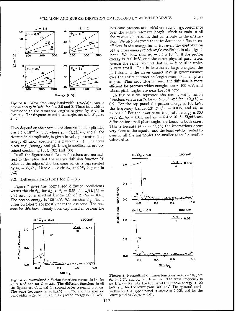
VILLALON AND BURKE: DIFFUSION OF PROTONS BY WHISTLER WAVES 21,337
L = 3.5
03
01
6L = 6.5° /
.5-/
.04 L = 2
«r- 16° .5/^
02
-y/. 1
.75
£-
100 300 500 lOO 300 500
_0L= 25° .5^-^^
.75^.
.—( i
"79
100 300 .00
500 100
Energy (keV)
©L = 35°
.5 _
.75^--
i i i
300 500
Figure 6. Wave frequency bandwidth, (Aw/u)i, versus proton energy in keV, for L = 3.5 and 2. These bandwidths correspond to the resonance lengths as given by A Ax,, in Figure 7. The frequencies and pitch angles are as in Figures 4-7.
They depend on the normalized electric field amplitudes e = 2.5 x 10~6 x /e 6, where fe = fie(L)/w, and £, the electric field amplitude, is given in volts per meter. The energy diffusion coefficient is given in (38). The cross pitch angle/energy and pitch angle coefficients are ob- tained combining (38), (32) and (33).
In all the figures the diffusion functions are normal- ized to the value that the energy diffusion function W takes at the edge of the loss cone which is represented by wc = WcAi- Here ei ~ e sin<pr, and Wc is given in (42).
9.2. Diffusion Functions for L = 3.5
Figure 7 gives the normalized diffusion coefficients versus the sin£>£,, for 6L > 9C = 6.5°, for u/Qe(L) = 0.75 and for a spectral bandwidth of A«/w = 0.01. The proton energy is 100 keV. We see that significant diffusion takes place mostly near the loss cone. The rea- sons for this have already been explained since near the
CO / ße = 0.75 100 keV
§
1.0
0.5
0.0 0.2 0.4 0.6 0.8
Sin©L
Figure 7. Normalized diffusion functions versus sin öL, for 9L > 6.5° and for L = 3.5. The diffusion functions in all the figures are obtained for second-order resonant protons. The wave frequency is u/Q.s(L) = 0.75, and the spectral bandwidth is Aw/w = 0.01. The proton energy is 100 keV.
loss cone protons and whistlers stay in gyroresonance over the entire resonant length, which extends to all the resonant harmonics that contribute to the interac- tion. We also observed that the dominant diffusion co- efficient is the energy term. However, the contribution of the cross energy/pitch angle coefficient is also signif- icant. We show that wc = 2.5 x 10~3. If the proton energy is 500 keV, and the other physical parameters remain the same, we find that wc = 2. x 10~6 which is very small. This is because at large energies, the particles and the waves cannot stay in gyroresonance over the entire interaction length even for small pitch angles. Thus second-order resonant diffusion is more efficient for protons which energies are ~ 100 keV, and whose pitch angles are near the loss cone.
In Figure 8 we represent the normalized diffusion functions versus sin 0L for 0L > 6.5°, and for u/tt&{L) = 0.9. For the top panel the proton energy is 100 keV, the frequency bandwidth Aw/w = 0.005, and wc = 7.5 x 10~4 For the lower panel the proton energy is 300 keV, Aw/w = 0.01, and wc = 5.4 x 10~4. Significant diffusion for small pitch angles are found in both cases. This is because as w —» Sle(L) the interactions occur very close to the equator and the bandwidths needed to overlap all the harmonics are smaller than for smaller values of w.
IB a o
a o
co/ne = 0.9 100 keV
1.0 - A2L= 0.005 £0
0.5 - W
0.0 0.2 0.4 0.6 0.8
CO / fle = 0.9 300 keV
s 10
0.5
0.0 0.2 0.4 0.6 0.8
Sin0L
Figure 8. Normalized diffusion functions versus sin ÖL, for 6L > 6.5°, and for for L = 3.5. The wave frequency is w/Qe(L) = 0.9. For the top panel the proton energy is 100 keV, and for the lower panel 300 keV. The spectral band- widths for the upper panel is Aw/a; = 0.005, and for the lower panel is Aw/w = 0.01.
117
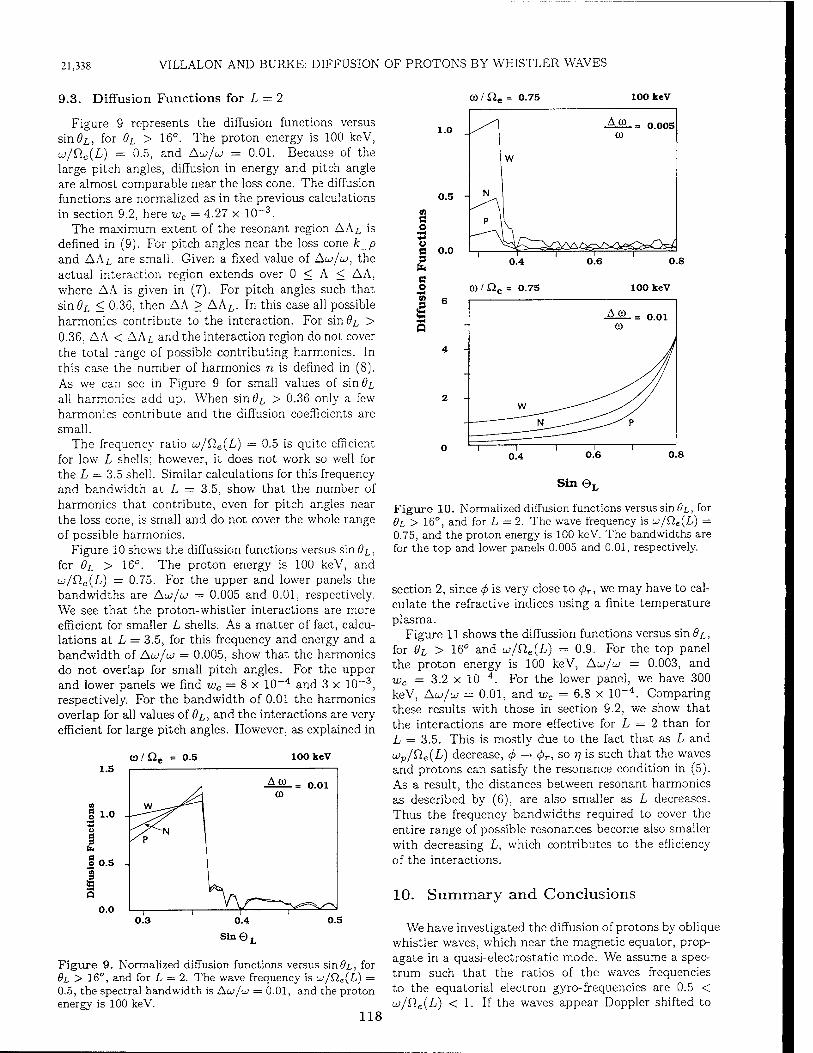
21,338 VILLALON AND BURKE: DIFFUSION OF PROTONS BY WHISTLER WAVES
9.3. Diffusion Functions for L = 2
Figure 9 represents the diffusion functions versus sin#L, for 0L > 16°. The proton energy is 100 keV, u/Qe(L) = 0.5, and Au/w = 0.01. Because of the large pitch angles, diffusion in energy and pitch angle are almost comparable near the loss cone. The diffusion functions are normalized as in the previous calculations in section 9.2, here wc = 4.27 x 10~3.
The maximum extent of the resonant region AAL is defined in (9). For pitch angles near the loss cone k±p and A At are small. Given a fixed value of Au/w, the actual interaction region extends over 0 < A < AA, where A A is given in (7). For pitch angles such that sin 91 < 0.36, then AA > AAj> In this case all possible harmonics contribute to the interaction. For sin 6i > 0.36, AA < AAt and the interaction region do not cover the total range of possible contributing harmonics. In this case the number of harmonics n is defined in (8). As we can see in Figure 9 for small values of sin 6i all harmonics add up. When sin#L > 0.36 only a few harmonics contribute and the diffusion coefficients are small.
The frequency ratio u>/fle(L) = 0.5 is quite efficient for low L shells; however, it does not work so well for the L = 3.5 shell. Similar calculations for this frequency and bandwidth at L = 3.5, show that the number of harmonics that contribute, even for pitch angles near the loss cone, is small and do not cover the whole range of possible harmonics.
Figure 10 shows the diffussion functions versus sin 0i, for 0i > 16°. The proton energy is 100 keV, and w/Qc(L) = 0.75. For the upper and lower panels the bandwidths are Au/w = 0.005 and 0.01, respectively. We see that the proton-whistler interactions are more efficient for smaller L shells. As a matter of fact, calcu- lations at L = 3.5, for this frequency and energy and a bandwidth of Aw/w = 0.005, show that the harmonics do not overlap for small pitch angles. For the upper and lower panels we find wc = 8 x 10~4 and 3 x 10~3, respectively. For the bandwidth of 0.01 the harmonics overlap for all values of 8L, and the interactions are very efficient for large pitch angles. However, as explained in
CD / Oe = 0.75 100 keV
1.5
1.0
CO/Qe = 0.5 100 keV
o 0.5
S Q
0.0 0.5
Figure 9. Normalized diffusion functions versus sin ÖL, for 6L > 16°, and for L = 2. The wave frequency is w/fic(L) = 0.5, the spectral bandwidth is Au/u = 0.01, and the proton energy is 100 keV.
118
SinOL
Figure 10. Normalized diffusion functions versus sin ÖL, for 6L > 16°, and for L = 2. The wave frequency is uj/Qe(L) = 0.75, and the proton energy is 100 keV. The bandwidths are for the top and lower panels 0.005 and 0.01, respectively.
section 2, since 4> is very close to <fir, we may have to cal- culate the refractive indices using a finite temperature plasma.
Figure 11 shows the diffussion functions versus sin 9i, for 6L > 16° and w/fte(L) = 0.9. For the top panel the proton energy is 100 keV, Aw/u = 0.003, and wc = 3.2 x 10~4. For the lower panel, we have 300 keV, AUJ/LO = 0.01, and wc = 6.8 x 10~4. Comparing these results with those in section 9.2, we show that the interactions are more effective for L = 2 than for L = 3.5. This is mostly due to the fact that as L and Lüp/Q.e(L) decrease, <j> —> cV, so -q is such that the waves and protons can satisfy the resonance condition in (5). As a result, the distances between resonant harmonics as described by (6), are also smaller as L decreases. Thus the frequency bandwidths required to cover the entire range of possible resonances become also smaller with decreasing L, which contributes to the efficiency of the interactions.
10. Summary and Conclusions
We have investigated the diffusion of protons by oblique whistler waves, which near the magnetic equator, prop- agate in a quasi-electrostatic mode. We assume a spec- trum such that the ratios of the waves frequencies to the equatorial electron gyro-frequencies are 0.5 < w/fie(L) < 1. If the waves appear Doppler shifted to
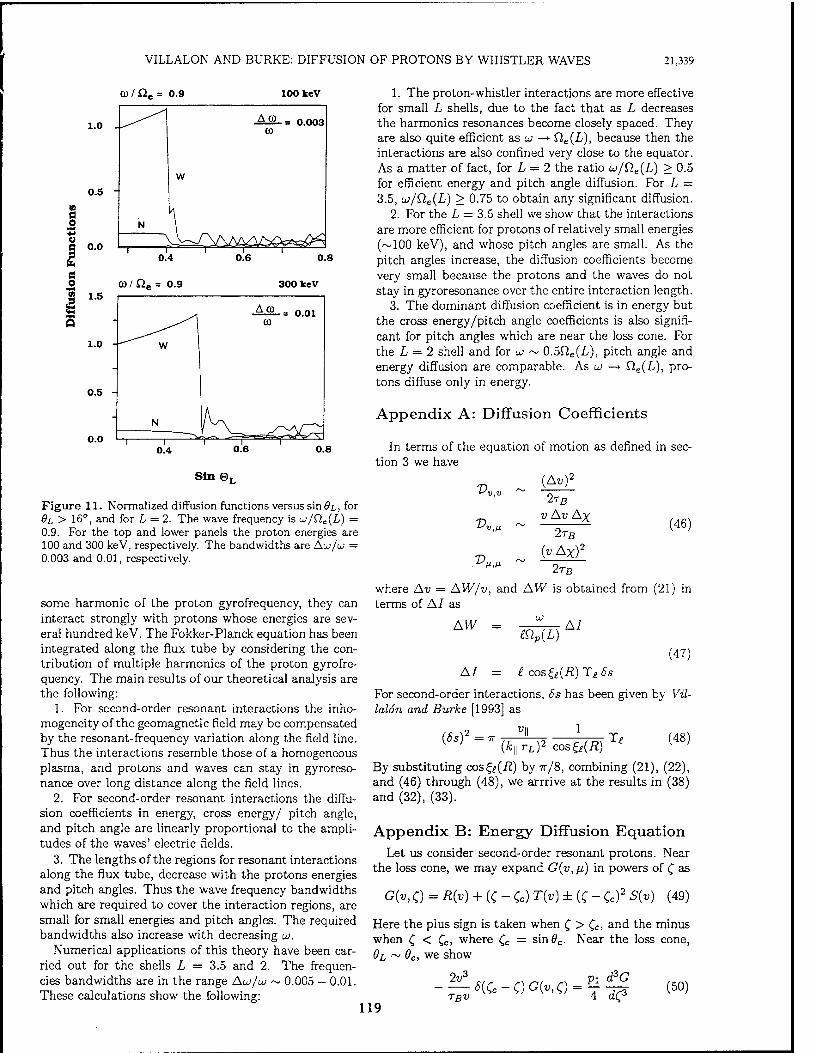
VILLALON AND BURKE: DIFFUSION OF PROTONS BY WHISTLER WAVES 21,339
CO / Q. = 0.9 100 keV
1.0
0.5
a o
Am _ CO
0.003
w
N
Ov-^/\/ -\ l°T i \ i i
0.4
300 keV
0.8
0.4 0.6 0.8
Sin 0L
Figure 11. Normalized diffusion functions versus sin <?L, for 6i > 16°, and for L = 2. The wave frequency is u>/0.e(L) = 0.9. For the top and lower panels the proton energies are 100 and 300 keV, respectively. The bandwidths are ALO/LJ = 0.003 and 0.01, respectively.
some harmonic of the proton gyrofrequency, they can interact strongly with protons whose energies are sev- eral hundred keV. The Fokker-Planck equation has been integrated along the flux tube by considering the con- tribution of multiple harmonics of the proton gyrofre- quency. The main results of our theoretical analysis are the following:
1. For second-order resonant interactions the inho- mogeneity of the geomagnetic field may be compensated by the resonant-frequency variation along the field line. Thus the interactions resemble those of a homogeneous plasma, and protons and waves can stay in gyroreso- nance over long distance along the field lines.
2. For second-order resonant interactions the diffu- sion coefficients in energy, cross energy/ pitch angle, and pitch angle are linearly proportional to the ampli- tudes of the waves' electric fields.
3. The lengths of the regions for resonant interactions along the flux tube, decrease with the protons energies and pitch angles. Thus the wave frequency bandwidths which are required to cover the interaction regions, are small for small energies and pitch angles. The required bandwidths also increase with decreasing w.
Numerical applications of this theory have been car- ried out for the shells L = 3.5 and 2. The frequen- cies bandwidths are in the range Aw/w ~ 0.005 - 0.01. These calculations show the following:
1. The proton-whistler interactions are more effective for small L shells, due to the fact that as L decreases the harmonics resonances become closely spaced. They are also quite efficient as w —* Qe(L), because then the interactions are also confined very close to the equator. As a matter of fact, for L = 2 the ratio w/fie(L) > 0.5 for efficient energy and pitch angle diffusion. For L = 3.5, w/Qe(L) > 0.75 to obtain any significant diffusion.
2. For the L = 3.5 shell we show that the interactions are more efficient for protons of relatively small energies (~100 keV), and whose pitch angles are small. As the pitch angles increase, the diffusion coefficients become very small because the protons and the waves do not stay in gyroresonance over the entire interaction length.
3. The dominant diffusion coefficient is in energy but the cross energy/pitch angle coefficients is also signifi- cant for pitch angles which are near the loss cone. For the L = 2 shell and for w ~ 0.5fie(L), pitch angle and energy diffusion are comparable. As u -> Qe(L), pro- tons diffuse only in energy.
Appendix A: Diffusion Coefficients
In terms of the equation of motion as defined in sec- tion 3 we have
Vv,v (Av)2
v Av Ax 1TB
(v Ax)2
2TB
(46)
where Av = AW/v, and AW is obtained from (21) in terms of AI as
AW = mp(L)
AI
(47)
A7 = £cos^(R)T£6s
For second-order interactions, 6s has been given by Vil- lalon and Burke [1993] as
uii 1 (6sY = 7T (48)
(fcll rLf cos6(A)
By substituting cos^(fi) by 7r/8, combining (21), (22), and (46) through (48), we arrrive at the results in (38) and (32), (33).
Appendix B: Energy Diffusion Equation Let us consider second-order resonant protons. Near
the loss cone, we may expand G(v,[i) in powers of £ as
G(v, 0 = R(v) + (C - Ce) T(v) ± (C - Cc)2 S(v) (49)
Here the plus sign is taken when £ > Qc, and the minus when £ < fc, where £c = sinöc. Near the loss cone, QL ~ 6c, we show
119 S*-o^-?f (50)
21,340 VILLALON AND BURKE: DIFFUSION OF PROTONS BY WHISTLER WAVES
where pi is defined in (42). Integrating (50) from £ = £c - e to Cc + e. letting e -> 0, substituting G by its expression in (49) we find
2 v3
S(v) = R(v) TBV pi
(51)
Next we solve (37) for 0 < C - Cc < Cc, by equaling powers of £c we find
2^ dR(v) T(v) = v ——
■pi dv (52)
The function R(v) satisfies the second-order differential equation
2 d2RM v 5-^
dv2 V¥M + A2 v3 R(v) = 0 (53)
where
A2
dv
1,1ft (54) Wc Lfß fj,m fp
where fß = T% V, /xm = sin2#m, and 8C < 9L < 0m. The solutions to (53) are Bessel functions. By choosing the solution that goes to zero as v —► 0 we get
R(v)= C WiÄ{-\2/3v) + B'(-X2/3
V)\ (55)
where C is a constant. The functions A and B are derivatives of the Airy functions.
Consider that 0 < v < vM, where VM is given in (11). For energies v2 < v2^ the precipitation life times, fp, of protons near the loss cone are obtained from (dR/dv) =
3/2 0 at v = VM- This leads to Xv^ ~ 3, which solves for fp as function of the velocity VM, bounce time TB, and the waves amplitudes through Wc as given in (42).
Acknowledgments. This work has been supported by the U.S. Air Force under contract with Northeastern Univer- sity, F19628-89-K-0014, and the Air Force Office of Scientific Research, task 2311PL03.
The Editor thanks J. U. Kozyra and R. A. Helliwell for their assistance in evaluating this paper.
References
Abramowitz, M., and I. A. Stegun, Handbook of Mathemati- cal Functions, Appl. Math. Ser., vol. 55, National Bureau of Standards, Gaithersburg, Md., 1964.
Bell, T. F., and H. D. Ngo, Electrostatic waves stimulated by coherent VLF signals in and near the inner radiation belts, J. Geophys. Res., 93, 2599, 1988.
Bespalov, P.A., and V. Yu. Trakhtengerts, Cyclotron insta- bility of Earth radiation belts, Rev. Plasma Phys., 10, 88, 1980.
Brinca, A. L., Enhancing whistler wave-electron interaction by the use of specially modulated VLF wave injection, J. Geophys. Res., 86, 792, 1981.
Burgess, W. C, and U. S. Inan, Simultaneous disturbance of conjugate ionospheric regions in association with indi- vidual lightning flashes, Geophys. Res. Lett., 17, 259, 1990.
Carlson, C. R., R. A. Helliwell, and D. L. Carpenter, Vari-
able frequency VLF signals in the magnetosphere: As- sociated phenomena and plasma diagnostics, J. Geophys. Res., 90, 1507, 1985.
Carlson, C. R., R. A. Helliwell, and U. S. Inan, Space-time evolution of whistler mode wave growth in the magneto- sphere, J. Geophys. Res., 95, 15,073, 1990.
Chappell, C. R., K. K. Harris, and G. W. Sharp, A study of the influence of magnetic activity on the location of the plasmapause as measured by OGO 5, J. Geophys. Res., 75, 50, 1970.
Dowden, R. L., A. D. McKay, and L. E. S. Amon, Linear and nonlinear amplification in the magnetosphere during a 6.6 kHz transmission, J. Geophys. Res., 83, 169, 1978.
Dysthe, K. B., Some studies of triggered whistler emissions, J. Geophys. Res., 76, 6915, 1971.
Gussenhoven, M. S., E. G. Mullen, and R. C. Sagalyn, CRRES/SPACERAD Experiment Descriptions, Environ. Res. Pap., 906, AFGL-TR-85-0017, Phillips Lab., Hanscom Air Force Base, Mass., 1985.
Helliwell, R. A. , A theory of discrete VLF emissions from the magnetosphere, J. Geophys. Res., 72, 4773, 1967.
Kennel, C.F., and H. E. Petschek, Limit on stably trapped particle fluxes, J. Geophys. Res., 71, 1, 1966.
Koons, H. C, Proton precipitation by a whistler-mode wave from a VLF transmitter, Geophys. Res. Lett, 2, 281, 1975.
Koons, H. C, Stimulation of Pc 1 micropulsations by con- trolled VLF transmissions, J. Geophys. Res., 82, 1163, 1977.
Kovrazhkin, R. A., M. M. Mogilevskii, Zh. M. Boske, Yu. I. Gal'perin, N. V. Dzhordzhio, Yu. V. Lisakov, O. A. Molchanov and A. Rem, Observation of particle precipi- tation from the ring-current zone stimulated by a powerful ground-base VLF transmitter, JETP Lett, Eng. Transl, 38, 397, 1983.
Kovrazhkin, R. A., M. M. Mogilevskii, O. A. Molchanov, Yu. I. Gal'perin, N. V. Dzhordzhio, Zh. M. Boske, and A. Rem, Precipitation of protons from the Earth's magne- tosphere stimulated by artificial low-frequency radiation, JETP Lett, Engl. Transl, 39, 228, 1984.
Kozyra, J. U., C. E. Rasmussen, and L. R. Lyons, The in- teraction of ring current and radiation belt protons with ducted plasmaspheric hiss. 1. Diffusion coefficients and timescales, J. Geophys. Res., 99, 4069, 1994.
Lyons, L. R., and D. J. Williams, Quantitative Aspects of Magnetospheric Physics, D. Reidel, Norwell, Mass., 1984.
Nunn, D., A self-consistent theory of triggered VLF emis- sions, Planet. Space Sei., 22, 349, 1974.
Sazhin, S.S., Whistler-Mode Waves in a Hot Plasma, Cam- bridge Atmos. and Space Sei. Ser., Cambridge University Press, New York, 1993.
Shklyar, D. R., Mechanism for proton precipitation trig- gered by a VLF wave injected into the magnetosphere, JETP Lett, Engl. Transl., 41, 448, 1985.
Shklyar, D. R., Particle interaction with an electrostatic VLF wave in the magnetosphere with an application to proton precipitation, Planet. Space Sei., 34, 1091, 1986.
Villalön, E., and W. J. Burke, Proton whistler interactions near the equator in the radiation belts, J. Geophys. Res., 98, 13,509, 1993.
W. J. Burke, Phillips Laboratory, Hanscom Air Force Base, MA 01731.
E. Villalön, Center Electromagnetics Research, North- eastern University, Boston, MA 02115. (e-mail: vil- [email protected])
(Received November 30, 1993; revised May 31, 1994; accepted May 31, 1994.)
120
WHISTLER WAVE INTERACTIONS: SOURCES FOR DIFFUSE AURORA ELECTRON PRECIPITATION ?
Elena Villalon Center for Electromagnetics Research,
Northeastern University, Boston MA 02115
William J. Burke Phillips Laboratory, Hanscom AFB, MA 01731
ABSTRACT
Resonant electron-whistler interactions in the plasma sheet are investi- gated as possible explanations of the nearly isotropic fluxes of low-energy electrons observed above the diffuse aurora. Whistler-mode waves, prop- agating obliquely to the geomagnetic field with frequencies near or larger than half the equatorial electron cyclotron frequency, can interact with the low-energy electrons found in the plasma sheet. A Hamiltonian formulation is developed for test particles interacting with a coherent, chorus-emission spectra. We consider the second-order resonance condition which requires that inhomogeneities in the Earth's magnetic field be compensated by a finite bandwidth of wave frequencies to maintain resonance for extended distances along field lines. Numerical calculations are presented for the magnetic shell L = 5.5 for wave amplitudes of ~ 10"6 V/m, using different frequency and magnetospheric conditions.
I. INTRODUCTION
The diffuse aurora is formed by nearly isotropic fluxes of electrons, mostly with energies <10 keV, that precipitate from the plasma sheet [1, 2j. A num- ber of studies have attempted to explain the diffuse aurora by the interaction of the electrons with electrostatic electron cyclotron harmonic (ECH) waves. However, it does not appear that the amplitudes of ECH waves are large enough to account for the observed electron precipitation [3]. Ref. [4] pro- posed that the < 10 keV electrons that form the diffuse aurora, are precipi- tated by whistler-mode waves that propagate along the magnetic field with frequencies u; —»• Q.e. They sucessfully explained how the resonant energy of the electrons could be well below the characteristic energy or magnetic en- ergy per particle Ec. Normalized to the electron rest energy Ec — (f2e/u/P) , where Cle and OJP are the electron gyro and plasma frequencies respectively.
Refs. [2], and [5], have interactions between low energy electrons and obliquely propagating chorus emissions. They consider first-order resonant
121
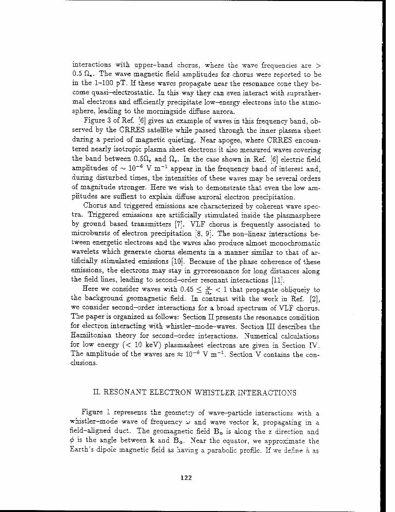
interactions with, upper-band chorus, where the wave frequencies are > 0.5 Qr. The wave magnetic field amplitudes for chorus were reported to be in the 1-100 pT. If these waves propagate near the resonance cone they be- come quasi-electrostatic. In this way they can even interact with suprather- mal electrons and efficiently precipitate low-energy electrons into the atmo- sphere, leading to the morningside diffuse aurora.
Figure 3 of Ref. [6] gives an example of waves in this frequency band, ob- served by the CURES satellite while passed through the inner plasma sheet during a period of magnetic quieting. Near apogee, where CRRES encoun- tered nearly isotropic plasma sheet electrons it also measured waves covering the band between 0.5Oe and (3e. In the case shown in Ref. [6] electric field amplitudes of ~ 10-6 V m_1 appear in the frequency band of interest and, during disturbed times, the intensities of these waves may be several orders of magnitude stronger. Here we wish to demonstrate that even the low am- plitudes are suffient to explain diffuse auroral electron precipitation.
Chorus and triggered emissions are characterized by coherent wave spec- tra. Triggered emissions are artificially stimulated inside the plasmasphere by ground based transmitters [7]. VLF chorus is frequently associated to microbursts of electron precipitation [8, 9]. The non-linear interactions be- tween energetic electrons and the waves also produce almost monochromatic wavelets which generate chorus elements in a manner similar to that of ar- tificially stimulated emissions [10]. Because of the phase coherence of these emissions, the electrons may stay in gyroresonance for long distances along the field lines, leading to second-order resonant interactions [111.
Here we consider waves with 0.45 < j*- < 1 that propagate obliquely to the background geomagnetic field. In contrast with the work in Ref. [2], we consider second-order interactions for a broad spectrum of VLF chorus. The paper is organized as follows: Section II presents the resonance condition for electron interacting with whistler-mode-waves. Section III describes the Hamiltonian theory for second—order interactions. Numerical calculations for low energy (< 10 keV) plasmasheet electrons are given in Section IV. The amplitude of the waves are zz 10-6 V m-1. Section V contains the con- clusions.
II. RESONANT ELECTRON WHISTLER INTERACTIONS
Figure 1 represents the geometry of wave-particle interactions with a whistler-mode wave of frequency io and wave vector k, propagating in a field-aligned duct. The geomagnetic field B0 is along the z direction and <t> is the angle between k and B0. Near the equator, we approximate the Earth's dipole magnetic field as having a parabolic profile. If we define h as
122
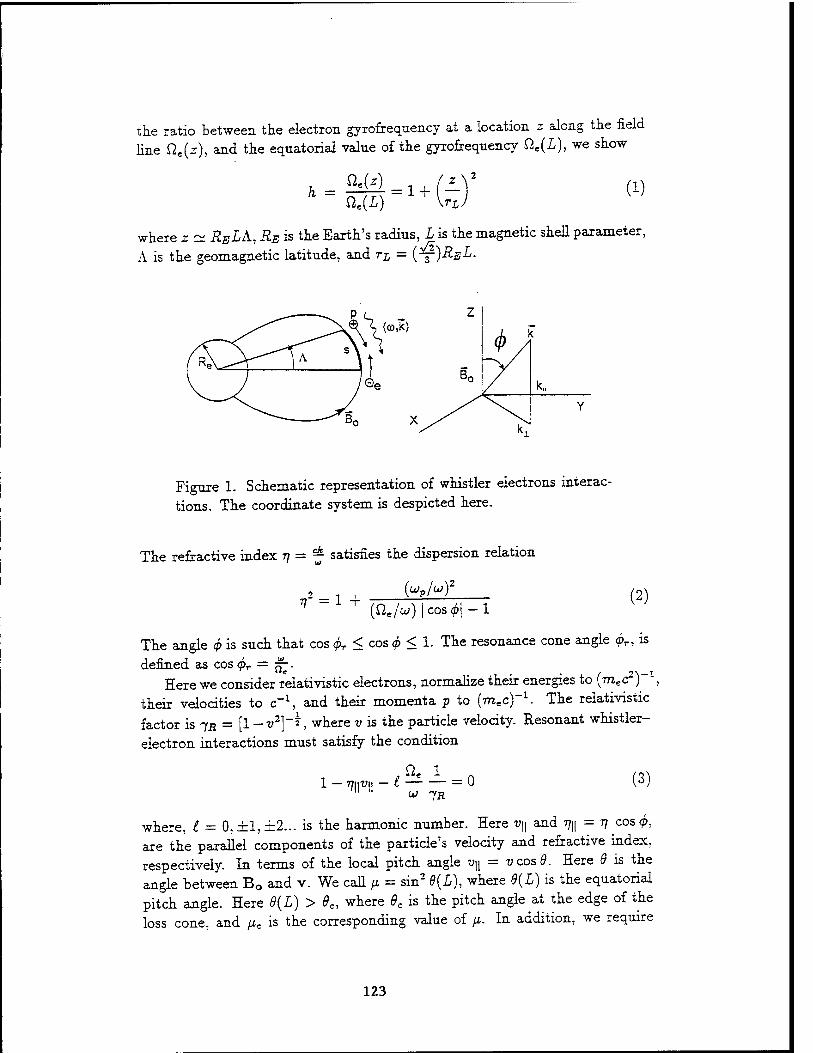
the ratio between the electron gyrofrequency at a location z along the field line ße(z), and the equatorial value of the gyrofrequency Sle(L), we show
h = Qe(L) ' \rL)
(1)
where z ~ RELA, RE is the Earth's radius, L is the magnetic shell parameter,
A is the geomagnetic latitude, and ri = (~)REL.
Figure 1. Schematic representation of whistler electrons interac- tions. The coordinate system is despicted here.
The refractive index 77 = ^ satisfies the dispersion relation
f = i (tie/u) I cos <pj — 1
(2)
The angle <p is such that cos <pr < cos 6 < 1. The resonance cone angle <x>r, is
defined as cos <pr = 77-. Here we consider relativistic electrons, normalize their energies to {mec) ,
their velocities to c~\ and their momenta p to (mec)-1. The relativistic
factor is jR = [1 -v2}'*, where v is the particle velocity. Resonant whistler-
electron interactions must satisfy the condition
1 - Tt\\V\\ - I = 0 m (3) U> JR
where, t = 0,±1,±2... is the harmonic number. Here v\\ and T\\\ = 77 cos©, are the parallel components of the particle's velocity and refractive index, respectively. In terms of the local pitch angle v\\ = vcos9. Here 9 is the angle between BQ and v. We call \i = sin2 9{L), where 9(L) is the equatorial pitch angle. Here 8(L) > 0C, where 8C is the pitch angle at the edge of the loss cone, and pe is the corresponding value of \i. In addition, we require
123
that 9{L) < 9M, thus the range of resonant equatorial pitch angles is: fie <
p < fiat- lithe waves propagate near the equator in the region 1 < h < hM, where
h is defined in Eq. (1), then there exists a mapping between h and fi. From Eq. (3) we obtain the following relation between \iM and hM as function of
the resonant energy TR and 9C,
1 — pM — V 1 ~ P-c h>M 1 + hlR 2-M hiR.
where we define fL = -g^fa. The waves exist near the equator and their ex-
tend along the field lines is such that h<kM, where h is defined in Eq. (1). Because interactions take place near equatorial regions, then hM is close to one. The upper limit on the resonant equatorial pitch angles 9M, is obtained from Eq. (4) and depends on the extend of the interaction region as given
by hM-
III. HAMILTONIAN THEORY
We normalize length s by r£\ call r = tüe(L), and define K = u^L)rL <
1. The dimensionless electric field amplitudes are a = £^, for z = 1,2,3, where & are the components of the wave electric field. The relative phase
angle between the wave and the electron is:
& = l\ + rL I &|| ds' Jo
(5) ße(£)
where A = arctan(^), Pr,y are components of the canonical momentum. For
resonant electrons § = 0, which leads to the resonance condition in Eq. (3). To first order in wave electric field amplitudes, the time-dependent Hamil-
tonian [12] is:
H = lo-~ £ T<(I,iV)sm^ (6) lo i=-oo
where P = J~fi - 1, and P\\ is the parallel component of the canonical
momentum. Here
1 /77 ß 2P P,i
T, = -± hl^ [{Sl + e2) JU^P) + (- " -) J^(^P)}
c-3 y Jt{k±p) (?)
124
where the J's are Bessel functions and p = (^) [%$\ *, is the Larmor radius. In terms of Pj_, the perpendicular component of the canonical mo- mentum, the canonical action is I = -^-p PL.
After differentiating Eq. (5) twice with respect to s, we show
<?Zi ds2
l J2) 7 = Q-<*i
(«Pll)2 ti-^ivpj1 T< (8)
where the constant aL depends on the magnetic field inhomogeneities and the wave frequency. For second-order resonances the inhomogeneity of the magnetic field is compensated by variation of the resonant frequency along the field lines [13]. In this case at = 0, which leads to the frequency variation
along the field line
u) ds Ik h-l
1 — fih
'2£ 7R
y/l-ph - A(L,v)fl (9)
where A(I,v) = jjjgy. After solving for the equations of motion the change in action, energy
and pitch angle are
(10)
(11)
(12) -1RP A7ä
where ^2) is defined in Eq. (8). Note that for second-order resonances, at = 0, and then the changes in the physical variables are proportional to £t
1/2. This is to be contrasted to first-order interactions where these changes are linear with the electric field amplitudes.
IV. NUMERICAL APPLICATIONS
We have conducted some numerical calculations based on this model for the magnetic shell L = 5.5. The equatorial electron gyrofrequency is Qe(L) = 0.33 x 10⁵ s"1. The ratio between the electron plasma and the equatorial cyclotron frequencies, is ■£— = 3. The width of the loss cone is 9C = 3.25°. Calculations were conducted for the frequencies j^y = 0.55, and 0.75. We assume that the waves have a coherent spectrum of finite fre- quency bandwidth, as occurs in the chorus and triggered emissions.
125
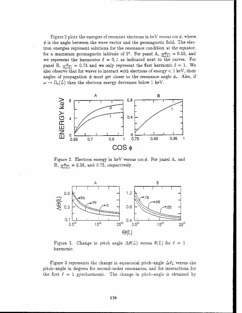
Figure 2 plots the energies of resonant electrons in keV versus cos <p, where <p is the angle between the wave vector and the geomagnetic field. The elec- tron energies represent solutions for the resonance condition at the equator, for a maximum geomagnetic latitude of 5°. For panel A, n 7n = 0-55, and we represent the harmonics £ = 0,1 as indicated next to the curves. For panel B, ne(£) = 0.75 and we only represent the first harmonic 1 = 1. We also observe that for waves to interact with electrons of energy < 1 keV, their angles of propagation <f> must get closer to the resonance angle <pT. Also, if tjj —+ Cle(L) then the electron energy decreases below 1 keV.
0.8 B
i t 1
""I _
0.4
n i 1 ' 1
-
0.55 0.7 0.9 1 0.75 0.85 0.95 1
COS(j)
Figure 2. Electron energy in keV versus cos 6. For panel A, and B, fW£> = 0.55, and 0.75, respectively.
Figure 3. Change in pitch angle Ad(L) versus 9(L) for £ = 1 harmonic.
Figure 3 represents the change in equatorial pitch-angle A#£ versus the pitch-angle in degrees for second-order resonances, and for interactions for the first £ = 1 gyroharmonic. The change in pitch-angle is obtained by
126
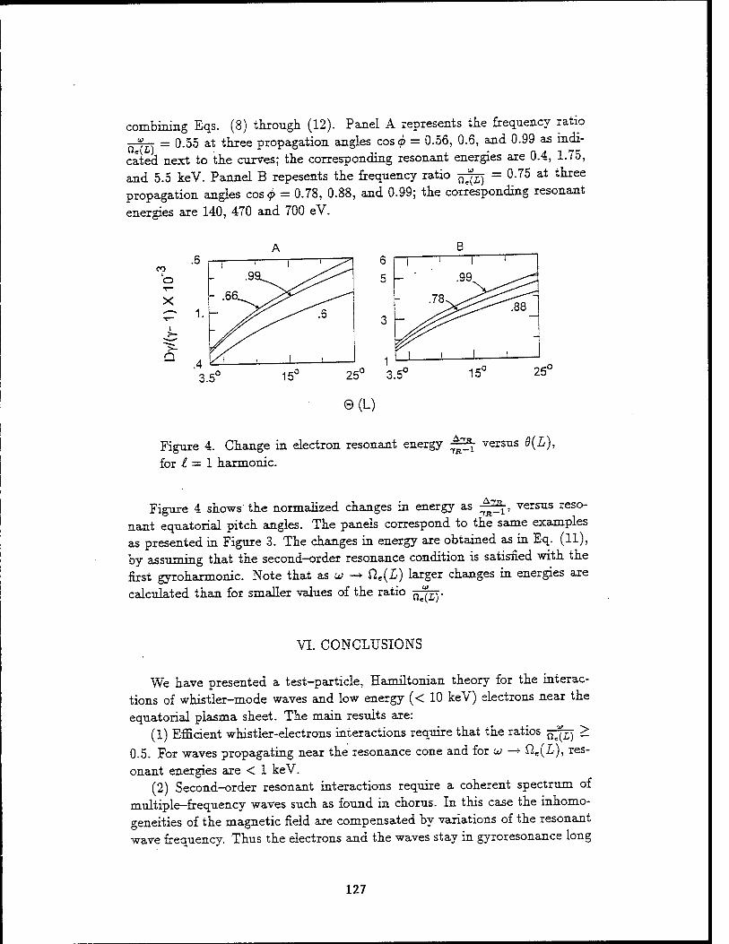
combining Eqs. (8) through (12). Panel A represents the frequency ratio = 0.55 at three propagation angles cos <f> = 0.56, 0.6, and 0.99 as mdi-
o.(L). cated next to the curves; the corresponding resonant energies are 0.4, 1.75, and 5.5 keV. Pannel B repesents the frequency ratio -^^ = 0.75 at three propagation angles cos <p = 0.78, 0.88, and 0.99; the corresponding resonant
energies are 140, 470 and 700 eV.
'o
B 1 1 1
.99
i
1
.78.
! ! i
25u 3.5*
e(L)
15c 25c
Figure 4. Change in electron resonant energy ^^ versus 0(£),
for £ = 1 harmonic.
Figure 4 shows the normalized changes in energy as ^^, versus reso- nant equatorial pitch angles. The panels correspond to the same examples as presented in Figure 3. The changes in energy are obtained as in Eq. (11), by assuming that the second-order resonance condition is satisfied with the first gyroharmonic. Note that as u -* Qe(I) larger changes in energies are calculated than for smaller values of the ratio n7£>.
VI. CONCLUSIONS
We have presented a test-particle, Hamiltonian theory for the interac- tions of whistler-mode waves and low energy (< 10 keV) electrons near the equatorial plasma sheet. The main results are:
(1) Efficient whistler-electrons interactions require that the ratios ^^y >
0.5. For waves propagating near the resonance cone and for u; —*• tie(L), res-
onant energies are < 1 keV. (2) Second-order resonant interactions require a coherent spectrum of
multiple-frequency waves such as found in chorus. In this case the inhomo- geneities of the magnetic field are compensated by variations of the resonant wave frequency. Thus the electrons and the waves stay in gyroresonance long
127
distances along the field lines, which render the interactions very efficient. (3) Numerical calculations have been conducted for the L = 5.5 shell.
As an example we considered wave amplitudes of 10~6 V m_1, consistent with observations from the CRRES satellite. Changes in pitch-angle can be > 1° for electrons with pitch-angles near the edge of the loss cone. Thus, whistler-electron interactions are viable explanations of the nearly isotropic precipitation of low-energy electrons from the plasma sheet to form the dif- fuse aurora.
ACKNOWLEDGEMENTS
This work has been supported in part by the U. S. Air Force contract with Northeastern University, F19628-92-K-0007. We are grateful to Dr. David Hardy of the Phillips Laboratory for suggesting this problem.
[1 [2
[3
[4
[5
[6
[7
[8
[9
[10
[11 [12
[13
REFERENCES
A. D. Johnstone, Ann. Geophys., 1, 4, 397 (1983).
U. S. Inan, Y. T. Chiu and G. T. Davidson, Geophys. Res. Lett., 19, 653 (1992).
J. L. Roeder, and H. C. Koons, J. Geophys. Res., 94, 2529 (1989).
A. D. Johnstone, D. M. Walton, R. Liu, and D. A. Hardy, J. Geophys. Res., 98, 5959 (1993).
U. S. Inan, and T. F. Bell, Geophys. Res. Lett, 18, 49 (1991).
W. J. Burke, A. G. Rubin, D. A. Hardy and E. G. Holeman, J. Geo- phys. Res., 100, in press (1995).
W. J. Burtis, and R. A. Helliwell, J. Geophys. Res., 80,-1007 (1976). D. A. Hardy, W. J. Burke, and E. Villaion, J. Geophys. Res., 95, 6451 (1990).
G. T. Davidson, and Y. T. Chiu, Geophys. Res. Lett., 14, 1166 (1987).
S. S. Sazhin, and M. Hayakawa, Planet. Space Sei. 40, 681 (1992). K. B. Dysthe, J. Geophys. Res. 76, 6915 (1971).
G. P. Ginet, and M. Heinemann, Phys. Fluids B, 2, 700 (1990).
E. Villalon, and W. J. Burke, J. Geophys. Res., 98, 13,509 (1993).
128
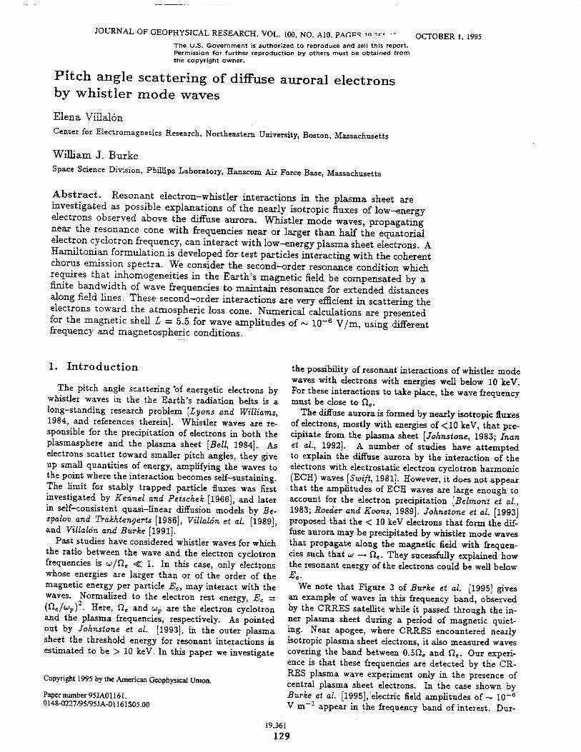
JOURNAL OF GEOPHYSICAL RESEARCH, VOL. 100, NO. A10. PAOF-5 10 ~. - OCTOBER 1, 1995 The U.S. Government is authorized to reproduce and sell this report. Permission for further reproduction by others must be obtained from the copyright owner.
Pitch angle scattering of diffuse auroral electrons by whistler mode waves
Elena Villalon
Center for Electromagnetics Research, Northeastern University, Boston, Massachusetts
William J. Burke
Space Science Division, Phillips Laboratory, Hanscom Air Force Base, Massachusetts
Abstract. Resonant electron-whistler interactions in the plasma sheet are investigated as possible explanations of the nearly isotropic fluxes of low-energy electrons observed above the diffuse aurora. Whistler mode waves, propagating near the resonance cone with frequencies near or larger than half the equatorial electron cyclotron frequency, can interact with low-energy plasma sheet electrons. A Hamiltoruan formulation is developed for test particles interacting with the coherent chorus emission spectra. We consider the second-order resonance condition which requires that inhomogeneities in the Earth's magnetic field be compensated by a finite bandwidth of wave frequencies to maintain resonance for extended distances along field lines. These second-order interactions are very efficient in scattering the electrons toward the atmospheric loss cone. Numerical calculations are presented for the magnetic shell L = 5.5 for wave amplitudes of ~ 10"6 V/m, using different frequency and magnetospheric conditions.
1. Introduction
The pitch angle scattering "of energetic electrons by whistler waves in the the Earth's radiation belts is a long-standing research problem [Lyons and Williams, 1984, and references therein]. Whistler waves are re- sponsible for the precipitation of electrons in both the plasmasphere and the plasma sheet [Bell, 1984]. As electrons scatter toward smaller pitch angles, they give up small quantities of energy, amplifying the waves to the point where the interaction becomes self-sustaining. The limit for stably trapped particle fluxes was first investigated by Kennel and Petschek [1966], and later in self-consistent quasi-linear diffusion models by Be- spalov and Trakhtengerts [1986], Villalon et al. [1989], and Villalon and Burke [1991].
Past studies have considered whistler waves for which the ratio between the wave and the electron cyclotron frequencies is w/Qe < 1. In this case, only electrons whose energies are larger than or of the order of the magnetic energy per particle Ec, may interact with the waves. Normalized to the electron rest energy, Ec — (fte/wp)". Here, fie and up are the electron cyclotron and the plasma frequencies, respectively. As pointed out by Johnstone et al. [1993], in the outer plasma sheet the threshold energy for resonant interactions is estimated to be > 10 keV. In this paper we investigate
Copyright 1995 by the American Geophysical Union.
Paper number 95JA01161. 0148-0227/95/95JA-01161S05.00
the possibility of resonant interactions of whistler mode waves with electrons with energies well below 10 keV. For these interactions to take place, the wave frequency must be close to fie.
The diffuse aurora is formed by nearly isotropic fluxes of electrons, mostly with energies of <10 keV, that pre- cipitate from the plasma sheet [Johnstone, 1983; Inan et al., 1992]. A number of studies have attempted to explain the diffuse aurora by the interaction of the electrons with electrostatic electron cyclotron harmonic (ECH) waves [Swift, 1981]. However, it does not appear that the amplitudes of ECH waves are large enough to account for the electron precipitation [Belmont et al., 1983; Roeder and Koons, 1989]. Johnstone et al. [1993] proposed that the < 10 keV electrons that form the dif- fuse aurora may be precipitated by whistler mode waves that propagate along the magnetic field with frequen- cies such that u — Cle. They sucessfully explained how the resonant energy of the electrons could be well below
We note that Figure 3 of Burke et al. [1995] gives an example of waves in this frequency band, observed by the CRRES satellite while it passed through the in- ner plasma sheet during a period of magnetic quiet- ing. Near apogee, where CRRES encountered nearly isotropic plasma sheet electrons, it also measured waves covering the band between 0.5fte and fte. Our experi- ence is that these frequencies are detected by the CR- RES plasma wave experiment only in the presence of central plasma sheet electrons. In the case shown by Burke et al. [1995], electric field amplitudes of ~ 10~6
V m-- appear in the frequency band of interest. Dur-
19,361 129
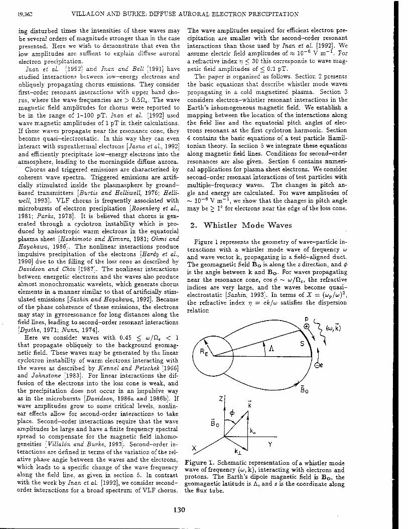
19,362 VILLALON AND BURKE: DIFFUSE AURORAL ELECTRON PRECIPITATION
ing disturbed times the intensities of these waves may be several orders of magnitude stronger than in the case presented. Here we wish to demonstrate that even the low amplitudes are suffient to explain diffuse auroral electron precipitation.
Inan et al. [1992; and Inan and Bel! [1991] have studied interactions between low-energy electrons and obliquely propagating chorus emissions. They consider first-order resonant interactions with upper band cho- rus, where the wave frequencies are > 0.5fte. The wave magnetic field amplitudes for chorus were reported to be in the range of 1-100 pT. Inan et al. [1992] used wave magnetic amplitudes of 1 pT in their calculations. If these waves propagate near the resonance cone, they become quasi-electrostatic. In this way they can even interact with suprathermal electrons [Jasna et al., 1992] and efficiently precipitate low-energy electrons into the atmosphere, leading to the morningside diffuse aurora.
Chorus and triggered emissions are characterized by- coherent wave spectra. Triggered emissions are artifi- cially stimulated inside the plasmasphere by ground- based transmitters [Burtis and Helliwell, 1976; Helli- well, 1993]. VLF chorus is frequently associated with microbursts of electron precipitation [Rosenberg et al., 1981; Parks, 1978]. It is believed that chorus is gen- erated through a cyclotron instability which is pro- duced by anisotropic warm electrons in the equatorial plasma sheet [Hashimoto and Kiraura, 1981; Ohmi and Hayakawa, 1986]. The nonlinear interactions produce impulsive precipitation of the electrons [Hardy et al., 1990] due to the filling of the loss cone as described by Davidson and Chiu [1987]. The nonlinear interactions between energetic electrons and the waves also produce almost monochromatic wavelets, which generate chorus elements in a manner similar to that of artificially stim- ulated emissions [Sazhin and Hayakawa, 1992]. Because of the phase coherence of these emissions, the electrons may stay in gyroresonance for long distances along the field lines, leading to second-order resonant interactions [Dysthe, 1971; Nunn, 1974].
Here we consider waves with 0.45 < w/£2e < 1 that propagate obliquely to the background geomag- netic field. These waves may be generated by the linear cyclotron instability of warm electrons interacting with the waves as described by Kennel and Petschek [1966] and Johnstone [1983]. For linear interactions the dif- fusion of the electrons into the loss cone is weak, and the precipitation does not occur in an impulsive way as in the microbursts [Davidson, 1986a and 1986b]. If wave amplitudes grow to some critical levels, nonlin- ear effects allow for second-order interactions to take place. Second-order interactions require that the wave amplitudes be large and have a finite frequency spectral spread to compensate for the magnetic field inhomo- geneities [Villalon and Burke, 1993]. Second-order in- teractions are defined in terms of the variation of the rel- ative phase angle between the waves and the electrons, which leads to a specific change of the wave frequency along the field line, as given in section 5. In contrast with the work by Inan et al. [1992], we consider second- order interactions for a broad spectrum of VLF chorus.
The wave amplitudes required for efficient electron pre- cipitation are smaller with the second-order resonant interactions than those used by Inan et al. [1992]. We assume electric field amplitudes of ä 10-6 V m"1. For a refractive index r? < 30 this corresponds to wave mag- netic field amplitudes of < 0:1 pT.
The paper is organized as follows. Section 2 presents the basic equations that describe whistler mode waves propagating in a cold magnetized plasma. Section 3 considers electron-whistler resonant interactions in the Earth's inhomogeneous magnetic field. We establish a mapping between the location of the interactions along the field line and the equatorial pitch angles of elec- trons resonant at the first cyclotron harmonic. Section 4 contains the basic equations of a test particle Hamil- tonian theory. In section 5 we integrate these equations along magnetic field lines. Conditions for second-order resonances are also given. Section 6 contains numeri- cal applications for plasma sheet electrons. We consider second-order resonant interactions of test particles with multiple-frequency waves. The changes in pitch an- gle and energy are calculated. For wave amplitudes of ~ 10-6 V in-1, we show that the changes in pitch angle may be > 1° for electrons near the edge of the loss cone.
2. Whistler Mode Waves
Figure 1 represents the geometry of wave-particle in- teractions with a whistler mode wave of frequency u> and wave vector k, propagating in a field-aligned duct. The geomagnetic field B0 is along the z direction, and <fr is the angle between k and B0- For waves propagating near the resonance cone, cos <p ~ u>/Cle, the refractive indices are very large, and the waves become quasi- electrostatic [Sazhin, 1993]. In terms of X = (up/w)2, the refractive index rj = ck/w satisfies the dispersion relation
Kk)
Figure 1. Schematic representation of a whistler mode wave of frequency (w,k), interacting with electrons and protons. The Earth's dipole magnetic field is B0, the geomagnetic latitude is A, and s is the coordinate along the flux tube.
130
VILLALON AND BURKE: DIFFUSE AURORAL ELECTRON PRECIPITATION 19,363
X V = 1 + T
n (i)
6 — —-|cos<£| — 1 u
Near the equator, the angle <f> is such that cos<£T < cos<£ < 1. The resonance cone angle, <pT, is denned as
COSl^T = ne{L)
(2)
We use the argument {L) to denote equatorial values of physical quantities. If we call 6(L) the value of 6 at the magnetic equator, we show that when <j> = <j)T, then 6{L) = 0.
The group velocity in the parallel direction can read- ily be obtained from (1) considering vg^ = du/dk\\. Normalizing vgn to c-*, we find that
V9,\\ ~ ZT *(*' $) T7H
(3)
i(<5,0) = l + cos^U-j^)
where rj|j = rj cos <t>. Note that as S —♦ 0, t(S, <j>) —» sin* <j>. The electric field, E, of the wave is represented by
E = x Si cos * - y £2 sin ¥ - z £3 cos * (4)
where i, y, and z are unit vectors, \P = Äx x + k\\ z-wt, and ib||, &x are the components of the wave vector along and perpendicular to B0- The ratios of the electric field components are
£2
£3
1 X
V2 )-l cos<^|
1- •X- -(77 i >in^)2 (5)
7j2 sin<£ cos$
For the case of waves propagating near the resonance cone, w ~ ße(£)|cos0|, the equatorial refractive index rj2{L) > 1. Its electric field is linearly polarized, having components |£2/£il < 1 and |£i/£3| (sin<£/cos0). In this case the wave becomes quasi-electrostatic, since E is almost in the direction of k, and the group veloci- ties vg ~ T7-1 are very small.
Near the equator, we approximate the Earth's dipole magnetic field as having a parabolic profile
h = a
a{i) = 1 +
& (6)
from a Taylor expansion of the dipole field and is an ex- cellent representation of the magnetic geometry within ±20° of the equator.
3. Resonant Electron-Whistler Interactions
Here we consider relativistic electrons and normal- ize their energies to (mec
2)-1, their velocities to c_1, and their momenta p to (mgc)-1. In what follows we only refer to these normalized quantities. The relativis- tic factor is 7ß = [1 - v2]~lf2, where v is the particle velocity. Resonant' whistler-electron interactions must satisfy the condition
where z ~ RELA,RE is the Earth's radius, L is the magnetic shell parameter, A is the geomagnetic lati- tude, and rL - (21/2/3)£BL. The equatorial gyrofre- quency is n(I), and 0 represents the gyrofrequencies of dither electrons or protons at locations s away from the equator along the field line. Equation (6) is obtained
,fie 1 1 - 77||«|| - £ = 0
U3 1R (7)
where I — 0, ±1,±2,... is the harmonic number, and ß« = \q\B0/mec is the electron gyrofrequency. Here, vii and 7711 = 77 cos <f> are the parallel components of the particle's velocity and refractive index, respectively.
In terms of the local pitch angle, vjj = vcos9. Here, 9 is the angle between Bo and v. We call p = sin2 9(L), where 9{L) is the equatorial pitch angle. Here, 9{L) > 9C, where 6C is the pitch angle at the edge of the loss cone, and pc is the corresponding value of p. In ad- dition, we require that 9(L) < 9M; thus the range of resonant equatorial pitch angles is pc < p < PM- The upper limit 9M depends on the extent of the res- onant region along the field line, as we shall explain below. As a function of L shell, the mirror ratio is a = p~x = L3 (4 - 3/I)1/2. To zero order in the elec- tric field amplitudes, a particle's magnetic moment is conserved. Then we may write for the parallel and perpendicular components of the particle velocity v, v]l = v[i-pn/n(L)]1'2,vx = v[pn/n(L)]1'2.
As the particles move away from the equator, their parallel velocities V|| decrease. We assume, however, that the waves' phase velocities w/fc|| remain constant. That is, variations in Qe, w, and cos<0 are such that r/|| is constant along the near-equatorial parts of field lines. Given a resonant energy for the I the harmonic, yR = (1 +p2)s, interactions take place at geomagnetic latitudes such that 1 < h < KM, where h is defined in (6). For h = 1 we take 9(L) = 9M, and for h = /ijw then 9(L) = 9C. Thus there exists a mapping between h and p, which may be obtained by solving for the resonance condition in (7).
In terms of the resonant parallel momentum pi\\, where pq = pt [1 - p £l/Q,(L)\xl2, (7) becomes
Vt\\ _1_
^11
ine 1 7 "1T + V1+P<- (8)
The equatorial parallel velocity is obtained from v\^ =
^||(1+P?||)-1- To find the resonant energy, we consider interactions
that take place at the equator h = 1, such that the resonant pitch angle is 9(L) = 9M- Next we define
131
19,364 VILLALON AND BURKE: DIFFUSE AURORAL ELECTRON PRECIPITATION
A0 = 7?jj cos" 6M — 1
D0
£fUL) 2 7J|| COS OM
C0 =
Then we show
ene(L)
(9)
We introduce the normalized time r — t£le(L) and length 5 = Z/TL, and define the canonical momenta and action:
- 1
Pi = ~ Do 2A0
K2A0> C0 lo.
1/2
^11 =
PX =
Pv =
(10)
which solves for the electron momentum. The plus sign must be taken for £ > 0, and the minus sign for £ < 0. Note that for £ > 0, cosfl(i) < 0, and for £ < 0, then cos 0(1/) > 0, so that in all cases D0 < 0. Also note that as cos^ —» cos$r, 8(L) —* 0, rj^ —* oo, and pi —* 0, and
I = -
P|l + £3 sin ^
px — £X sin *
ps — £2 cos * —
1 Cl(L)
Q.e(s)x
2 n(s) P> + iPy + ?M±r-
and call
7o 1 + Pf + 21 n(s) Tl/2
n(L).
(15)
(16)
(17)
thus the energy of the resonant electron is very small The relative phase angle between the wave and the elec- (i.e., < 1 keV). When the frequency of the waves w —► tron is fle(£), then cos<j>T —» 1, and again we have 6(L) —» 0,
In addition, we also consider interactions that occur Jo Me(L) at h = fejif and for pitch angles at the edge of the loss (18) cone 8(L) = 8C. From (8) we obtain the following rela- /p .0 (s) x/cs
tion between PM and hj^ eis a function of the resonant ^ — —A— energy 7.R and 0C:
A = arctan
%/l - PM = \/l - Me A. •Jif 1 + /i7K
.-/i&f + /i7Ä.
To first order in wave electric field amplitudes, the (11) time-dependent Hamiltonian is [Ginet and Heinemann,
1990; Albert, 1993; Villalön and Burke, 1993]
+00 where we define fj, = u>/£Q.e{L). The waves exist near the equator, and their extent along the field lines is such that h < hj^, where h is defined in (6). Because interactions take place near equatorial regions, h>M is close to one. The upper limit on the resonant equatorial wj.ere p _ (^2 _ 1U/2 anJ pitch angles 8 a is obtained from (11) and depends on ° the extent of the interaction region as given by KM.
Solving (7) for hi as a function of /x, we show that for £?0,
7o f=-oo
(19)
T< = es 5L ä(«) - £ 21 n
n(L)
ht = bt+ [bl + (fL »,„ p)2 - -,% /*]
where r\ypfL = (-1 + -yRfL) (1 - fiM)~1/2
Landau resonance (£ = 0),
211/2
(12)
■ [(ei + £2) Ji-i{a) + (£1 - £2) Ä+i(a)3 (20)
where the .J values are Bessel functions of argument
a = kxp and p = (c/üe) [21 n/fi(I)]*/2 is the Larmor radius. A constant of motion is
h0=- P
1- (V\\ v)2
For the
(13)
Ct = m - Vc(L)
(21)
Next we solve for the equations of motion for a single isolated resonance. To zero order in the electric fields
For a given value of the electron energy 7Ä, (11) to (13) dsldr = K P\\h<» where * = ^lTL^c{L) < 1. For establish a one- to- one correspondence between the example, at L = 5 we show that K = 4.5 x 10 . Dif- resonant equatorial pitch angles 6(L) and the geomag- netic latitudes A at which the interactions are taking place.
ferentiating (18) with respect to s, the length along the field line, to zero order in the electric field amplitudes, we show
4. Hamiltonian Theory
The dimensionless electric field amplitudes are
\q\Ei
«*fc _ , , me -1» 7, d7 ~rLk" + QAL)KP WKP\\
(22)
Ci = mecijj
(14)
For resonant electrons, d£i/ds — 0. Then the equations of motion for the canonical variables reduce to those of the physical variables at the resonance. Referring to the physical action and parallel momentum, in term of the
132
VLLLALON AND BURKE: DIFFUSE AURORAL ELECTRON PRECIPITATION 19,365
length 5 along the field line, we find that to first order in the electric fields, h{R) = ?Mv_jL
dl t p dl = --^(/.py.-jcosfc
2 1 - p ht (31)
ds KTLkn dl 1 dQ
I ds p|| n(£) ds
(23)
(24)
The evolution of the electron resonant energy IR , and the equatorial pitch angle p = sin2 0£, is
djR
ds dl
ine{L) ds
dp _ 2 fine
ds ~ 7»-l I w 7Ä
(25)
17 <»>
where &£ is given in (12) and (13). At the resonance we also obtain si = (ht — l)1/2.
Using a Taylor expansion around s = st, we obtain for the phase angle [Villalon and Burke, 1993]
ii = 6(A) + tf> (* - *) + | d2) (* - »i? (32)
Here, $> = 0, and
Ü3)=at(R)+ßt(R) 1 dl_ I ds
(A)
(33)
Differentiating (22) with respect to s and assuming that dit/ds = 0 yields
where the subscript (R) denotes values taken at the resonance, for It = I(R) and py = p^.
We define the length of resonant interaction as
d2i ds2 i = «t+ ßt
ld£ I ds
(27) \h\ r(2}
Here,
dh\ at = rL
7R d" 7R h-1 Hm)+§-A (34)
ds /cp||fie(i) ds «p||
0t =
2£ 7H
/cp|,
y/l-ph - A(£,u)/i
(4 -1) U)
[n.(i)J 2
■ ph
(28)
(29)
Near resonance the change in action, energy, and pitch angle is given by
where A(X, v) = T^ 1; w/Qe(£); all other variable are defined throughout the paper. For second-order reso- nant electrons the. inhomogeneity of the magnetic field is compensated by the frequency variation, and then at = 0. In addition, if -r?n = 1, then ßt = 0; this is the case of infinite acceleration studied by Roberts and Buchsbaum [1964].
Combining equations (24) and (25), we obtain
AI =
AyR =
AM =
d£ ds
w
Ssi
(A)
Here,
dl_ ds
2
I p
AI
'XI, u -1RP
(35)
(36)
AJR (37)
(R) K Pt\\ Tt[li(R),ptll(R),s] (38)
djR ds
l_ *!L + L l ^ , ds p|| n(L) ds _ = 0 (30)
The diffusion curves, or single-wave characteristics, are obtained by integrating (30) along 5. These are the curves along which the representative point of a particle in the P||, p± plane will move. If we neglect magnetic in- homogeneities, we obtain the diffusion curves for homo- geneous, relativistic plasmas [l + pjj + Pl]1/2-P||/f?|| = const.
5. Equations of Motion Near Resonance
At the resonance the parallel component of the mo- mentum, Pi\\(R), is given by solving for (8). The phys- ical action is obtained from
133
where It is defined in (20) for the resonant values of I and p||.
If the electric field amplitudes are small compared to the inhomogeneity of the plasma, then we may ap- proximate ^2) ~ at(R). For this case the changes in action, energy, and pitch angle are proportional to Ci, the electric field amplitudes. In contrast, for second- order resonances, ßL [(1/^) (dI/ds)]{R) » at, and then
^2) ~ ßt(R) [{1/1) (dIJds)\R). For second-order in- teractions the changes in action, energy and pitch angle
1/2 are proportional to ej . Second-order resonances require that the inhomo-
geneity of the magnetic field be compensated by wave frequency variations along the field line [Dysthe, 1971; Nunn, 1974]. By considering (27) and (28), we require that for second-order interactions, at —» 0, which leads to the frequency variation along the field line as
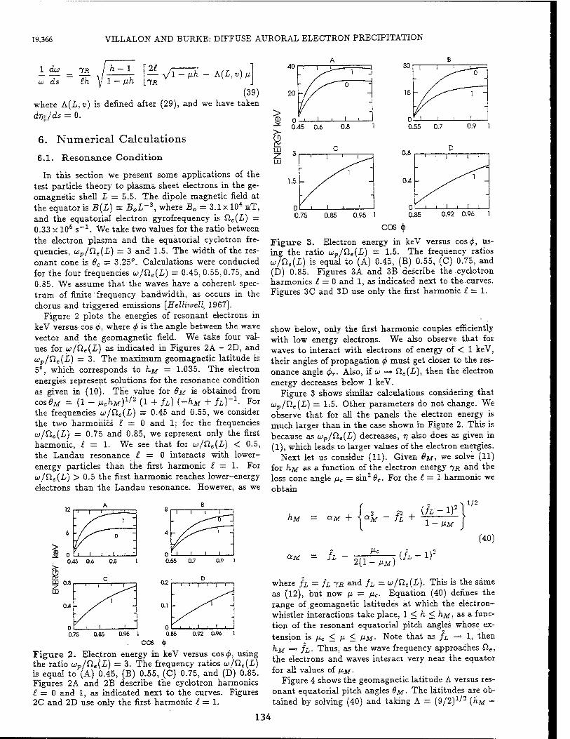
19,366 VILLALON AND BURKE: DIFFUSE AURORAL ELECTRON PRECIPITATION
2£_
7fl y/1- ph - A(L,v) ß
1 40
6. Numerical Calculations
6.1. Resonance Condition
In this section we present some applications of the test particle theory to plasma sheet electrons in the ge- omagnetic shell L = 5.5. The dipole magnetic field at the equator is B{L) = B0L~3, where B0 - 3.1 x 10⁴ nT, and the equatorial electron gyrofrequency is f2e(L) = 0.33 x 10⁵ s_1. We take two values for the ratio between the electron plasma and the equatorial cyclotron fre- quencies, u>p/Cle(L) = 3 and 1.5. The width of the res- onant cone is 8C = 3.25°. Calculations were conducted for the four frequencies w/Q,e(L) = 0.45, 0.55, 0.75, and 0.85. We assume that the waves have a coherent spec- trum of finite' frequency bandwidth, as occurs in the chorus and triggered emissions [Helliwell, 1967].
Figure 2 plots the energies of resonant electrons in keV versus cos <f>, where 4> is the angle between the wave vector and the geomagnetic field. We take four val- ues for w/Q,e{L) as indicated in Figures 2A - 2D, and up/ne(L) = 3. The maximum geomagnetic latitude is 5°, which corresponds to KM = 1-035. The electron energies represent solutions for the resonance condition as given in (10). The value for 8 M is obtained from cos6M = (1 - ßchM)1/2 (1 + h) (~hM + h)-1- For the frequencies u>/Cle(L) = 0.45 and 0.55, we consider the two harmonics I = 0 and 1; for the frequencies w/Cle(L) = 0.75 and 0.85, we represent only the first harmonic, £ = 1. We see that for u>/Q,e(L) < 0.5, the Landau resonance £ = 0 interacts with lower- energy particles than the first harmonic £ — 1. For w/Q.e{L) > 0.5 the first harmonic reaches lower-energy electrons than the Landau resonance. However, as we
i 2 LU
■^1 0.45 0.6 0.8
0.8 c
1 1 _
- OJi -
- -
0 i I 1
0.75 0.85 0.9S 1
COS
Figure 2. Electron energy in keV versus cos<f>, using the ratio wP/Cle(L) = 3. The frequency ratios w/Qs(i) is equal to (A) 0.45, (B) 0.55, (C) 0.75, and (D) 0.85. Figures 2A and 2B describe the cyclotron harmonics £ = 0 and 1, as indicated next to the curves. Figures 2C and 2D use only the first harmonic £ = 1.
(39) 20 where A(L,v) is defined after (29), and we have taken dr}\\/ds = 0. ^ o
A
: / ^ ■+T —-i
0 -
! i i i -
> 0.45 0.6 0.8 0.55 0.7 0.9 1
3
1.5
c i 1 1^
n ! \ \ ! 0.75 0.85 0.95 1
COS $
Figure 3. Electron energy in keV versus cos<^>, us- ing the ratio up/Q.e{L) = 1.5. The frequency ratios w/Cle(L) is equal to (A) 0.45, (B) 0.55, (C) 0.75, and (D) 0.85. Figures 3A and 3B describe the cyclotron harmonics £ = 0 and 1, as indicated next to the curves. Figures 3C and 3D use only the first harmonic £ — 1.
show below, only the first harmonic couples efficiently with low energy electrons. We also observe that for waves to interact with electrons of energy of < 1 keV, their angles of propagation <f> must get closer to the res- onance angle 4>T. Also, if u —* £le{L)> tnen tne electron energy decreases below 1 keV.
Figure 3 shows similar calculations considering that up/Cle(L) = 1.5. Other parameters do not change. We observe that for all the panels the electron energy is much larger than in the case shown in Figure 2. This is because as wp/Qe(L) decreases, r\ also does as given in (1), which leads to larger values of the electron energies.
Next let us consider (11). Given 8M, we solve (11) for h.M as a function of the electron energy -yn and the loss cone angle fic = sin2 6C. For the £ = 1 harmonic we obtain
hjvt = Q.M + ZM
O-M h ~ 2(1 - KM\
-/£ +
(h
(h 1) 1/2
1 - MM
(40)
where fL = fL tR and fL = u/Cle(L). This is the same as (12), but now p, — ßc. Equation (40) defines the range of.geomagnetic latitudes at which the electron- whistler interactions take place, 1 < h < KM , as a func- tion of the resonant equatorial pitch angles whose ex-
tension is fa < £i < fiM- Note that as /x, -+ 1, then h-M —* II- Thus, as the wave frequency approaches ne, the electrons and waves interact very near the equator for all values of fj,M ■
Figure 4 shows the geomagnetic latitude A versus res- onant equatorial pitch angles 8M ■ The latitudes are ob- tained by solving (40) and taking A = (9/2)1/2 (hM -
134
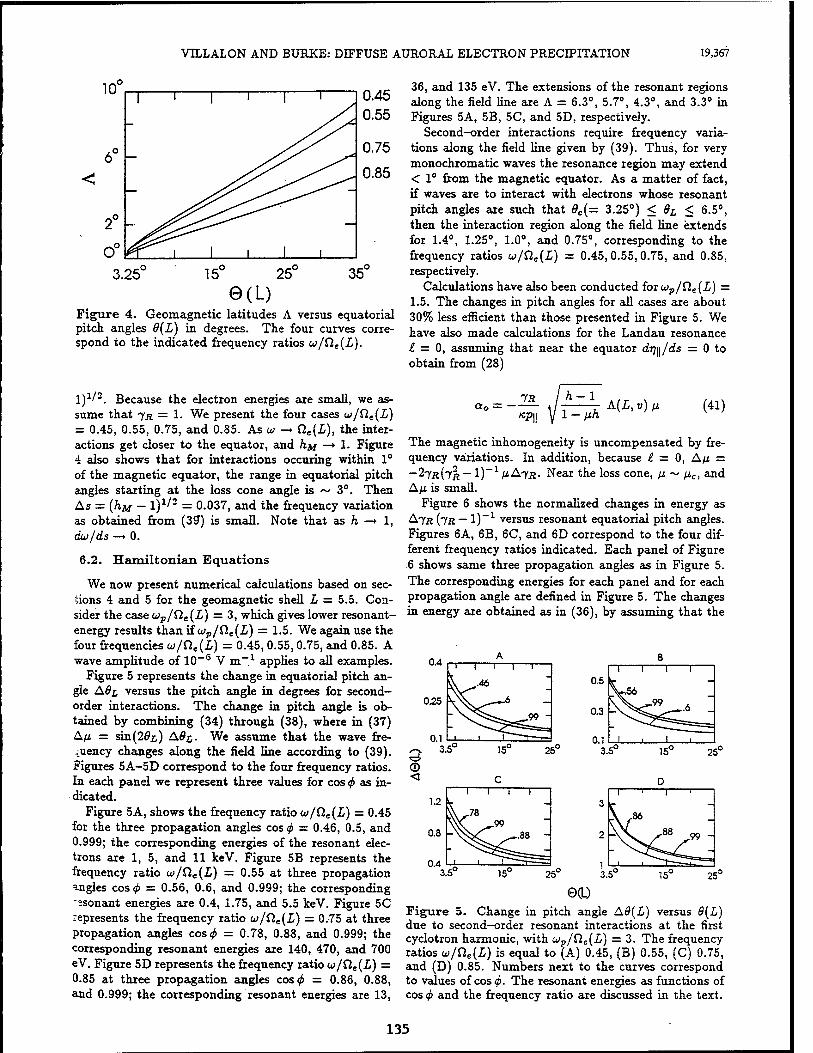
VTLLALON AND BURKE: DIFFUSE AURORAL ELECTRON PRECIPITATION 19,367
l(f
6" -
3.25u 15" 25" 35^
e(L) Figure 4. Geomagnetic latitudes A versus equatorial pitch angles 8(L) in degrees. The four curves corre- spond to the indicated frequency ratios v/£le(L).
I)1/2. Because the electron energies are small, we as- sume that 7JJ = 1. We present the four cases w/fie(i) = 0.45, 0.55, 0.75, and 0.85. As«-« toe{L), the inter- actions get closer to the equator, and h\t —► 1. Figure 4 also shows that for interactions occuring within 1° of the magnetic equator, the range in equatorial pitch angles starting at the loss cone angle is ~ 3°. Then As = (/IM- — l)1/2 = 0.037, and the frequency variation as obtained from (3?) is small. Note that as h —* 1, dw/ds —> 0.
6.2. Hamiltonian Equations
We now present numerical calculations based on sec- tions 4 and 5 for the geomagnetic shell L = 5.5. Con- sider the case wp/fie(Z) = 3, which gives lower resonant- energy results than if vp/Qe(L) = 1.5. We again use the four frequencies w/ße(i) = 0.45,0.55, 0.75, and 0.85. A wave amplitude of 10-6 V m-1 applies to all examples.
Figure 5 represents the change in equatorial pitch an- gle A0£ versus the pitch angle in degrees for second- order interactions. The change in pitch angle is ob- tained by combining (34) through (38), where in (37) Aß = sin(2öi) A0£. We assume that the wave fre- quency changes along the field line according to (39). Figures 5A-5D correspond to the four frequency ratios. In each panel we represent three values for cos$ as in- dicated.
Figure 5A, shows the frequency ratio w/fie(£) = 0.45 for the three propagation angles cos <j> = 0.46, 0.5, and 0.999; the corresponding energies of the resonant elec- trons are 1, 5, and 11 keV. Figure 5B represents the frequency ratio u>/£le(L) = 0.55 at three propagation angles cos4> = 0.56, 0.6, and 0.999; the corresponding sonant energies are 0.4, 1.75, and 5.5 keV. Figure 5C
represents the frequency ratio w/ße(X) = 0.75 at three propagation angles cos0 = 0.78, 0.88, and 0.999; the corresponding resonant energies are 140, 470, and 700 eV. Figure 5D represents the frequency ratio w/Sle(L) = 0.85 at three propagation angles cos^ = 0.86, 0.88, and 0.999; the corresponding resonant energies are 13,
36, and 135 eV. The extensions of the resonant regions along the field line are A = 6.3°, 5.7°, 4.3°, and 3.3° in Figures 5A, 5B, 5C, and 5D, respectively.
Second-order interactions require frequency varia- tions along the field line given by (39). Thus, for very monochromatic waves the resonance region may extend < 1° from the magnetic equator. As a matter of fact, if waves are to interact with electrons whose resonant pitch angles are such that 9e(= 3.25°) < BL < 6.5°, then the interaction region along the field line extends for 1.4°, 1.25°, 1.0°, and 0.75°, corresponding to the frequency ratios w/fie(I) = 0.45,0.55,0.75, and 0.85, respectively.
Calculations have also been conducted for wP/Qe(L) = 1.5. The changes in pitch angles for all cases are about 30% less efficient than those presented in Figure 5. We have also made calculations for the Landau resonance £ — 0, assuming that near the equator dr^/ds = 0 to obtain from (28)
a0 = - 1-ßh
A(L,v) ß (41)
The magnetic inhomogeneity is uncompensated by fre- quency variations. In addition, because i. — 0, Aß = —2JR{1R — l)-1 ß A7.R- Near the loss cone, ß ~ ßc, and Aß is small.
Figure 6 shows the normalized changes in energy as &7[R (IR — I)-1 versus resonant equatorial pitch angles. Figures 6A, 6B, 6C, and 6D correspond to the four dif- ferent frequency ratios indicated. Each panel of Figure .6 shows same three propagation angles as in Figure 5. The corresponding energies for each panel and for each propagation angle are defined in Figure 5. The changes in energy are obtained as in (36), by assuming that the
04 A
1 1 > 1
^ .46
1
0.25 AVv^--—6 - _99 "
0.1 . , 1 —
B
0.5 1 1 1 1
__
0.3 -^ v56
„99 —6 -
0.1 I , 1 ,
3 © <
3.5" 15"
C
25°
1.2 1 i—r 1
0.8
ri4
\k,.78 „99
».88 -
3.5" 15" 25°
3.5"
3
2
1 3.5"
15°
D
25°
1 '
1 T- ■"■
^86 _
\ .88 S99 ~
" >
-
15" 25"
00.) Figure 5. Change in pitch angle A8(L) versus 9(L) due to second-order resonant interactions at the first cyclotron harmonic, with up/Qe(L) = 3. The frequency ratios w/£le(L) is equal to (A) 0.45, (B) 0.55, (C) 0.75, and (D) 0.85. Numbers next to the curves correspond to values of cos <j>. The resonant energies as functions of cos0 and the frequency ratio are discussed in the text.
135
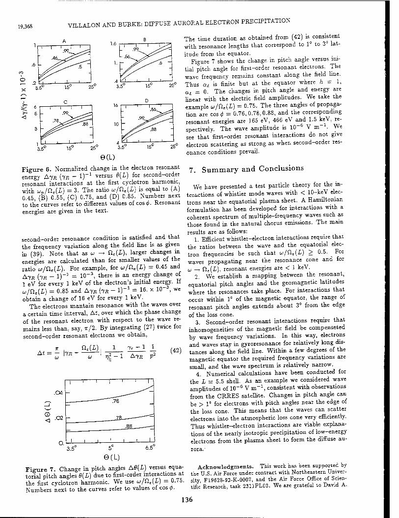
19,368 VILLALON AND BURKE: DIFFUSE AURORAL ELECTRON PRECIPITATION
1.6 1 i 1 .99
i. ̂
-.56 "^
- JZ'^ ̂^£> — ' /7/^^ -
A , i ~
3.5°
16
10
15"
D
25"
1 1
'< - .99 - — —
A
.88
1 L
-
3.5" 15c 25"
e(D Figure 6. Normalized change in the electron resonant energy AfR {JR - 1)_1 versus 9(L) for second-order resonant interactions at the first cyclotron harmonic, with wv/Cle{L) = 3. The ratio w/fie(£) is equal to (A) 0.45, (B) 0.55, (C) 0.75, and (D) 0.85. Numbers next to the curves refer to different values of cos q>. Resonant energies are given in the text.
second-order resonance condition is satisfied and that the frequency variation along the field line is as given in (39). Note that as u -► üe{L), larger changes in energies are calculated than for smaller values of the ratio u/Qe{L). For example, for w/Q.e{L) = 0.45 and
AfR (7P. - i)-1 = 10_3' there is an enersy ciianSe of
1 eV for every 1 keV of the electron's initial energy. If -3 we w/f2e(L) = 0.85 and A-yR (7* - I)-1 = 16- x 10
obtain a change of 16 eV for every 1 keV. The electrons mantain resonance with the waves over
a certain time interval, At, over which the phase change of the resonant electron with respect to the wave re- mains less than, say, */2. By integrating (27) twice for second-order resonant electrons we obtain,
At = — \fR w
9AH\ _J— *z± - (42) 1 A7.R p2
%
©
0(L) Figure 7. Change in pitch angles A6{L) versus equa- torial pitch angles 9{L) due to first-order interactions at the first cyclotron harmonic. We use w/üe{L) - 0.75. Numbers next to the curves refer to values of cos <p.
The time duration as obtained from (42) is^consistent with resonance lengths that correspond to 1° to 3° lat-
itude from the equator. Figure 7 shows the change in pitch angle versus ini-
tial pitch angle for first-order resonant electrons. The wave frequency remains constant along the field line. Thus at is finite but at the equator where h = 1, at = 0. The changes in pitch angle and energy are linear with the electric field amplitudes. We take the example w/fie(I) = 0.75. The three angles of propaga- tion are cos 4> = 0.76,0.78,0.88, and the corresponding resonant energies are 165 eV, 466 eV and 1.5 keV, re- spectively. The wave amplitude is 10 6 V m .We see that first-order resonant interactions do not give electron scattering as strong as when second-order res-
onance conditions prevail.
7. Summary and Conclusions
We have presented a test particle theory for the in- teractions of whistler mode waves with < 10-keV elec- trons near the equatorial plasma sheet. A Hamiltonian formulation has been developed for interactions with a coherent spectrum of multiple-frequency waves such as those found in the natural chorus emissions. The mam
results are as follows: 1. Efficient whistler-electron interactions require that
the ratios between the wave and the equatorial elec- tron frequencies be such that w/fte(L) > 0-5. For waves propagating near the resonance cone and for u -> Sle{L), resonant energies are < 1 keV.
2. We establish a mapping between the resonant, equatorial pitch angles and the geomagnetic latitudes where the resonances take place. For interactions that occur within 1° of the magnetic equator, the range of resonant pitch angles extends about 3° from the edge
of the loss cone. 3. Second-order resonant interactions require that
inhomogeneities of the magnetic field be compenseted by wave frequency variations. In this way, electrons and waves stay in gyroresonance for relatively long dis- tances along the field line. Within a few degrees of the magnetic equator the required frequency variations are small, and the wave spectrum is relatively narrow.
4. Numerical calculations have been conducted for the L = 5.5 shell. As an example we considered wave amplitudes of 10-6 V m_1, consistent with observations from the CRRES satellite. Changes in pitch angle can be > 1° for electrons with pitch angles near the edge of the loss cone. This means that the waves can scatter electrons into the atmospheric loss cone very efficiently. Thus whistler-electron interactions are viable explana- tions of the nearly isotropic precipitation of low-energy electrons from the plasma sheet to form the diffuse au-
rora.-
Acknowledgments. This work has been supported by the U.S. Air Force under contract with Northeastern Univer- sity, F19628-92-K-0007, and the Air Force Office of Scien- tific Research, task 2311PL03. We are grateful to David A.
136
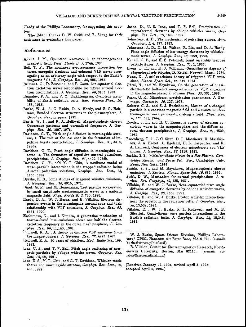
VILLALON AND BURKE: DIFFUSE AURORAL ELECTRON PRECIPITATION 19,369
Hardy of the Phillips Laboratory, for suggesting this prob- lem.
The Editor thanks D. W. Swift and R. Skoug for their assistance in evaluating this paper.
References
Albert, J. M., Cyclotron resonance in an inhomogeneous magnetic field, Phys. Fluids B, 5, 2744, 1993.
Bell, T. F., The nonlinear gyroresonance interaction be- tween energetic electrons and coherent VLF waves prop- agating at an arbitrary angle with respect to the Earth's magnetic field, /. Geophys. Res., 89, 905, 1984.
Belmont, G., D. Fontaine, and P. Canu, Are equatorial elec- tron cyclotron waves responsible for diffuse auroral elec- tron precipitation?, J. Geophys. Res., 88, 9163, 1983.
Bespalov, P. A., and V. Y. Trakhtengerts, Cyclotron insta- bility of Earth radiation belts, Rev. Plasma Phys., 10, 155, 1986.
Burke, W. J., A. G. Rubin, D. A. Hardy, and E. G. Hole- man, Banded electron structures in the plasmasphere, J. Geophys. Res., in press, 1995.
Burtis, W. J., and R. A. Helliwell, Magnetospheric chorus: Occurence patterns and normalized frequency, /. Geo- phys. Res., 80, 1007, 1976.
Davidson, G. T., Pitch angle diffusion in morningside auro- rae, 1, The role of the loss cone in the formation of im- pulsive bursts precipitation, J. Geophys. Res., 91, 4413, 1986a.
Davidson, G. T., Pitch angle diffusion in morningside au- rorae, 2, The formation of repetitive auroral pulsations, precipitation, J. Geophys. Res., 91, 4429, 1986b.
Davidson, G. T., and Y. T. Chiu, A nonlinear model of wave-particle interactions in the trapped radiation belts: Auroral pulsation solutions, Geophys. Res. Lett., 14, 1166, 1987.
Dysthe, K. B., Some studies of triggered whistler emissions, J. Geophys. Res., 76, 6915, 1971.
•inet, G. P., and M. Heinemann, Test particle acceleration by small amplitude electromagnetic waves in a uniform magnetic field, Phys. Fluids B, 2, 700, 1990.
Hardy, D. A., W. J. Burke, and E. Villalon, Electron dis- persion events in the morningside auroral zone and their relationship with VLF emissions, J. Geophys. Res., 95, 6451, 1990.
Hashimoto, K-, and I. Kimura, A generation mechanism of narrow-band hiss emissions above one half the electron cyclotron frequency in the outer magnetosphere, J. Geo- phys. Res., 86, 11,148, 1981.
TTslliwell, R. A. , A theory of discrete VLF emissions from the magnetosphere, /. Geophys. Res., 72, 4773, 1967.
Helliwell, R. A., 40 years of whistlers, Mod. Radio Sei., 189, 1993.
Inan, U. S., and T. F. Bell, Pitch angle scattering of ener- getic particles by oblique whistler waves, Geophys. Res. Lett, 18, 49, 1991.
Inan, U. S., Y. T. Chiu, and G. T. Davidson, Whistler-mode chorus and morningside aurorae, Geophys. Res. Lett., 19, 653, 1992.
Jasna, D-, U. S. Inan, and T. F. Bell, Precipitation of suprathermal electrons by oblique whistler waves, Geo- phys. Res. Lett., 19, 1639, 1992.
Johnstone, A. D., The mechanism of pulsating aurora, Ann. Geophys., 1, 4, 397, 1983.
Johnstone, A. D., D. M. Walton, R. Liu, and D. A. Hardy, Pitch angle diffusion of low-energy electrons by whistler- mode waves, J. Geophys. Res., 98, 5959, 1993.
Kennel, C. F., and H. E. Petschek, Limit on stably trapped particle fluxes, J. Geophys. Res., 71, 1, 1966.
Lyons, L. R., and D. J. Williams, Quantitative Aspects of Magnetospheric Physics, D. Reidel, Norwell, Mass., 1984.
Nunn, D., A self-consistent theory of triggered VLF emis- sions, Planet. Space Sei., 22, 349, 1974.
Ohmi, N., and M. Hayakawa, On the generation of quasi- electrostatic half-electron-gyrofrequency VLF emissions in the magnetosphere, /. Plasma Phys., 35, 351, 1986.
Parks, G. K., Microburst precipitation phenomena, J. Geo- magn. Geoelectr., 30, 327, 1978.
Roberts C. S., and S. J. Buchsbaum, Motion of a charged particle in a constant magnetic field and a tranverse elec- tromagnetic wave propagating along a field, Phys. Rev. A, 135, 381, 1964.
Roeder, J. L., and H. C. Koons, A survey of electron cy- clotron waves in the magnetosphere and the diffuse au- roral electron precipitation, /. Geophys. Res., 94, 2529, 1989.
Rosenberg, T. J., J. C. Siren, D. L. Matthews, K. Marthin- sen, J. A. Holtet, A. Egeland, D. L. Carpenter, and R. A. Helliwell, Conjugacy of electron microbursts and VLF chorus, J. Geophys. Res., 86, 5819, 1981.
Sazhin, S. S., Whistler-Mode Waves in a Hot Plasma, Cam- bridge Atmos. and Space Sei. Ser., Cambridge Univ. Press, New York, 1993.
Sazhin, S. S., and M. Hayakawa, Magnetospheric chorus emissions: A Review, Planet. Space Sei. 40, 681, 1992.
Swift, D. W., Mechanism for auroral precipitation: A re- view, Rev. Geophys., 19, 185, 1981.
Villalon, E., and W. J. Burke, Near-equatorial pitch angle diffusion of energetic electrons by oblique whistler waves, J. Geophys. Res., 96, 9655, 1991.
Villalon, E., and W. J. Burke, Proton whistler interactions near the equator in the radiation belts, J. Geophys. Res., 98, 13,509, 1993.
Villalon, E. , W. J. Burke, P. L. Rothwell, and M. B. Silevitch, Quasi-linear wave particle interactions in the Earth's radiation belts, J. Geophys. Res., 94, 15,243, 1989.
W. J. Burke, Space Science Division, Phillips Labora- tory/ GPSG, Hanscom Air Force Base, MA 01731. (e-mail: [email protected])
E. Villalon, Center for Electromagnetics Research, North- eastern University, Boston, MA 02115. (e-mail: vil- [email protected])
(Received January 27, 1995; revised April 3, 1995; accepted April 4, 1995.)
137
JOURNAL OF GEOPHYSICAL RESEARCH, VOL. 100, NO. All, PAGES 21,911-21,919. NOVEMBFR ], 1995
The U.S. Government is authorized to reproduce and sell this report. Permission for further reproduction by others must be obtained from the copyright owner.
Interaction of ring current and radiation belt protons with ducted plasmaspheric hiss 2. Time evolution of the distribution function
J. U. Kozyra, C. E. Rasmussen, and R. H. Miller Space Physics Research Laboratory, Atmospheric, Oceanic and Space Sciences Department, University
of Michigan, Ann Arbor
E. Villalon Center of Electromagnetic Research, Northeastern University, Boston, Massachusetts
Abstract. The evolution of the bounce-averaged ring current/radiation belt proton distribution is simulated during resonant interactions with ducted plasmaspheric hiss. The plasmaspheric hiss is assumed to be generated by ring current electrons and to be damped by the energetic protons. Thus energy is transferred between energetic electrons and protons using the plasmaspheric hiss as a mediary. The problem is not solved self-consistently. During the simulation period, interactions with ring current electrons (not represented in the model) are assumed to maintain the wave amplitudes in the presence of damping by the energetic protons, allowing the wave spectrum to be held fixed. Diffusion coefficients in pitch angle, cross pitch angle/energy, and energy were previously calculated by Kozyra et al. (1994) and are adopted for the present study. The simulation treats the energy range, E > 80 keV, within which the wave diffusion operates on a shorter timescale than other proton loss processes (i.e., Coulomb drag and charge exchange). These other loss processes are not included in the simulation. An interesting result of the simulation is that energy diffusion maximizes at moderate pitch angles near the edge of the atmospheric loss cone. Over the simulation period, diffusion in energy creates an order of magnitude enhancement in the bounce-averaged proton distribution function at moderate pitch angles. The loss cone is nearly empty because scattering of particles at small pitch angles is weak. The bounce- averaged flux distribution, mapped to ionospheric heights, results in elevated locally mirroring proton fluxes. OGO 5 observed order of magnitude enhancements in locally mirroring energetic protons at altitudes between 350 and 1300 km and invariant latitudes between 50° and 60° (Lundblad and Soraas, 1978). The proton distributions were highly anisotropic in pitch angle with nearly empty loss cones. The similarity between the observed distributions and those resulting from this simulation raises the possibility that interactions with plasmaspheric hiss play a role in forming and maintaining the characteristic zones of anisotropic proton precipitation in the subauroral ionosphere. Further assessment of the importance of this process depends on knowledge of the distribution in space and time of ducted plasmaspheric hiss in the inner magnetosphere.
1. Introduction during this interaction with the energetic protons and then
OGO 5 observed enhancements in locally mirroring protons damPed by thermal electrons during the course of their at altitudes between 350 and 1300 km on field lines associated propagation through the inhomogenous magnetosphenc with stable aurora] red (SAR) arcs in the subauroral ionosphere environment [Cornwall et al., 1971]. The energy transferred to [Lundblad and Soraas, 1978]. Pitch angle distributions, the thelmal electron Sas fa *" Process leads t0 ceased observed by the OGO 5 spacecraft, were highly anisotropic in temperatures at the foot of these field lines and to an assorted the sense that fluxes at small pitch angles were orders of enhancement in 6300 A emissions characteristic of SAR arcs, magnitude less than locally mirroring ones. Protons that are However, in the ensuing time period, ion cyclotron waves have , „ ... ,.._ j . .. . .. been observed only rarely in the outer plasmasphere. During a locally mirroring at these altitudes map to the equator near the J J y . * b
, f.i.. u-i TU u J-_I. recent survey of Pc 1 waves in the inner magnetosphere edge of the atmospheric loss cone. The observed mcomplete J b * rn. c ,u i J . • J- . , •, u [Anderson et al., 1992], an occurrence frequency of 1% was filling of the loss cone was assumed to indicate weak pitch L '' ~*i J
angle scattering near the equatorial plane. Resonance with ion found at L values less ^ 5 for lon «^tron waves Wlth
cyclotron waves was proposed as the source of this weak pitch frequencies between 0.1 and 4 Hz and amplitudes greater than angle scattering [Cornwall et al, 1971; Lundblad and Soraas, °"8 S^' fo contrast- ** zones of P1010" Palpitation, 1978]. The ion cyclotron waves were thought to be amplified ascribed by Lundblad and Soraas [1978] and Voss and SmUh
[1980] are a characteristic feature of the subauroral ionosphere,
Copyright 1995 by the American Geophysical Union. ■* «« ** temperature enhancements associated with SAR arcs. The present work assumes no direct relationship between
Paper number 95IA01556. SAR arcs and the enhanced locally mirroring proton fluxes on 0148-0227/95/95JA-01556S05.00 the same field lines but makes use of reported observations by
21.911
138
21,912 KOZYRA ET AL.: ENERGETIC PROTON RESONANCE WITH DUCTED HISS
the Dynamics Explorer (DE) satellite pair at high and low altitudes on SAR arc field lines [Kozyra, 1986; Kozyra et al., 1987a] to propose an alternative explanation for the collocation of these phenomena. The DE spacecraft were in coplanar polar orbits and thus were occasionally in the position to observe the magnetospheric source and ionospheric sink regions on SAR arc field lines nearly simultaneously. Magnetically conjugate DE 1 and 2 data sets revealed the presence of large-scale density structures and associated regions of enhanced plasmaspheric hiss amplitudes at high altitudes on field lines that thread SAR arcs in the ionosphere. Theoretical models using these and other data sets, in combination with ground-based photometric observations of 6300 Ä emission, demonstrated that Coulomb drag transfers sufficient energy from the ring current to the thermal electron gas to maintain the observed ionospheric electron temperatures and associated SAR arc emissions [Kozyra et al., 1987b, 1993] without the need for wave damping. The possible role of waves in enhancing the transport of energy from the plasmaspheric thermal electron populations into the underlying ionosphere is still under debate [Thorne and Home, 1992]. Coulomb drag as a mechanism for the energy transfer was first proposed by Cole [1965]. However, the importance of ring current oxygen ions as a dominant energy source for the thermal electrons only became clear during the DE mission [Kozyra et al., 1987b].
The unique nature of the DE data sets also allowed a detailed comparison between the thermal plasma characteristics at high and low altitudes. Structures in the electron temperature signatures and associated SAR arc emissions at ionospheric heights (i.e., structured temperature peaks, multiple temperature peaks, etc.) map along field lines to single or multiple, large-scale density structures in the outer plasmasphere [Horwitz et al., 1986; Kozyra, 1986; Kozyra et al., 1987a]. This relationship is not surprising. The Coulomb collision frequency is proportional to both the energetic ring current ion flux and the thermal plasma density. Therefore elevated collision frequencies, energy transfer rates and ionospheric electron temperatures are expected to occur on field lines associated with thermal plasma density enhancements in the outer plasmasphere.
Apart from their role in structuring Coulomb energy transfer rates, large-scale density enhancements can directly affect the propagation of plasmaspheric hiss through ducting. Plasmaspheric hiss is a right-hand-polarized, whistler mode emission that fills the plasmasphere almost continuously [Thorne et al., 1973]. Ducting, which maintains small wave normal angles along the ray path, occurs in the presence of gradients in the thermal plasma. Such gradients can be found hi association with detached plasma regions, the plasmapause and density structures (ledges, double plasmapauses, etc.) in the outer plasmasphere and dusk bulge region. Hayakawa et al. [1986a] derived hiss wave normal directions of less than 25° in detached plasma regions near the equatorial plane. They also presented evidence which reasonably suggests that signatures of the detached plasma regions extend into the topside ionosphere and that the hiss may be ducted down to these altitudes. As mentioned previously, Kozyra et al. [1987a] presented observations of intense hiss emissions within large- scale density structures at plasmaspheric altitudes on SAR-arc field lines. Though a direct experimental determination of the wave-normal directions of the enhanced hiss emissions was not possible, it is very likely that the waves were ducted. The
evidence for this is indirect. Nearly simultaneous observations by DE 1 and 2 [Kozyra, 1986] at high and low altitudes on the same field lines indicate enhanced wave electric fields over the frequency interval 100 Hz to several kHz. Enhanced wave amplitudes over the same range of L values at low altitudes imply that these waves are ducted. Ducting maintains small wave normal angles and allows the waves to reach low altitudes. In contrast, during unducted propagation, hiss emissions will most likely reflect at the lower hybrid frequency and never reach the ground [Church and Thorne, 1983; Huang and Goertz, 1983].
Observations confirm that the plasmapause density gradient is also capable of ducting plasmaspheric hiss. Small wave normal angles were observed just inside the plasmapause near the equatorial plane by Hayakawa et al. [1986b]; however, two different groups of wave normal angles, one moderate and one large, were observed deeper in the plasmasphere. In all cases studied by these authors at high geomagnetic latitudes, two different groups of wave normal angles were seen, both large. In fact, recent observational evidence suggests that hiss wave normal angles are quite oblique throughout much of the plasmasphere [Storey et al., 1991; Sonwalker and I nan, 1988]. The present work does not deal with these regions of oblique hiss but focuses on hiss emissions generated within detached plasma regions or large-scale density structures in the outer plasmasphere.
Wave amplification via cyclotron resonance with ring current electrons is maximized in the presence of small wave- normal angles and occurs over a larger fraction of the flux tube. The observed order of magnitude increase in the hiss amplitudes within the plasmaspheric density structures is interpreted to result from the favorable effects of ducting on wave amplification. An interesting consequence of ducting in the context of the present theory is that maintaining small wave- normal angles decreases resonant proton energies to values of the order of ring current and radiation belt energies. Past studies have ignored proton resonances with whistler mode waves, assumed to be propagating at highly oblique wave- normal angles, because the required proton energies for the resonant interaction reach MeV energies.
The association between large hiss amplitudes and thermal density enhancements has been pointed out by a number of authors [Angerami, 1970; Carpenter et al., 1981; Chan and Hölzer, 1976; Chan et al., 1974; Scarf and Chappell, 1973] in relation to detached plasma regions. More recently, Koons [1989] observed intense hiss in association with whistler ducts in the outer plasmasphere (4 to 7 R ). The density enhancements (up to 190%) associated with the ducts were much larger than values (<40%) reported for ducts at larger radial distances in the studies referenced above. Hiss emissions within the detached plasma structures and whistler ducts were an order of magnitude stronger than hiss emissions on adjacent field lines. The relative enhancement of the hiss within these regions agrees very well with observations in the outer plasmasphere (L< 4) reported by Kozyra et al. [1987aJ.
The significance to ring current dynamics of resonant proton interactions with strong ducted hiss emissions depends on the amount of time that protons spend traveling through regions containing these emissions. A major assumption in the present work is that ring current electrons are able to resonate with and amplify hiss under conditions present in the outer plasmasphere. When the hiss is maintained at small wave normal angles (e.g., by ducting along density gradients).
139
KOZYRA ET AL.: ENERGETIC PROTON RESONANCE WITH DUCTED HISS 21,913
protons at ring current energies are able to resonate with and damp the waves. A fundamental question is what portion of the time do energetic ion orbits intersect with density enhancements in the outer plasmasphere. During the initial phase of ring current injection there is probably no interaction with the plasmasphere, because the same electric fields which cause the injection of energetic ions into the inner magnetosphere will evacuate the plasmasphere in the midnight region filled by the newly injected ring current. However, as the energetic ions drift clockwise around the Earth, they will first likely encounter detached plasmaspheric regions in the dusk sector and then the main body of the plasmasphere drifting sunward in the dayside in response to the increased dawn-to-dusk electric fields. As the enhanced electric fields subside, the plasmasphere will begin to refill and the energetic ion orbits will intersect with an increasing greater region of
the plasmasphere. Information on the spatial extent, duration and frequency of
occurrence of regions of ducted hiss would allow an estimation of their cumulative effect on the proton distribution. A complete characterization of these density structures has not yet been achieved but some information is available. Recent studies indicate that large-scale density irregularities, similar to the ducts discussed above, extend well into the outer plasmasphere [Carpenter et al., 1993; Horwitz et al., 1990]. These studies do not examine the hiss emissions associated with the density irregularities. Density irregularities in the outer plasmasphere were reported as far back as the mid 1970s. Chappell [1974] described the difficulty in defining detached plasma regions that occur very near the plasmapause as different from the density irregularities inside the plasmasphere. Horwitz et al. [1990] performed a statistical study of the plasmapause location and structure using DE 1 satellite data. They found that a double-ledge structure was the most common plasmapause shape on the eveningside, occurring some 50% of the time. Other more complicated large-scale density structures also occurred in this local time sector. Carpenter et al. [1993] carried out a study of the outer plasmasphere and dusk bulge region using thermal density data inferred from whistler observations by ground stations and measured in situ by the DE 1, ISEE 1 and GEOS 2 satellites. They observed density irregularities (with factor of 2 to 10 enhancement factors) routinely near the plasmapause in the postdusk sector following magnetic storms. These density irregularities were inferred to be a consequence of the physical processes involved in the erosion of the plasmasphere and formation of the sharp plasmapause boundary. They persist during an extended period of calm following the storm perturbations. Large-scale density gradients associated with these structures should be effective at guiding whistler mode emissions. Since density irregularities in a range of scale sizes are a common feature in the outer plasmasphere, ducted plasmaspheric hiss must also be a frequent occurrence in the evening local time sector.
To determine the effects of ducted plasmaspheric hiss on the ring current proton distribution, Kozyra et al. [1994] calculated diffusion coefficients, averaged over a bounce orbit, for protons in resonance with right-hand polarized whistler mode waves. A wave distribution spanning frequencies 100 - 1100 Hz characteristic of plasmaspheric hiss in the outer plasmasphere, with reasonable amplitudes (5x10s -//Hz), and a distribution of wave-normal angles between 0° and 45° was adopted. During the wave-proton interaction, the proton
experiences multiple resonances with the hiss band due both to the finite frequency bandwidth of the waves and the longitudinal inhomogeneity in the magnetic field. The inhomogeneity in the magnetic field produces a constant variation in the pitch angle (and parallel velocity) of the proton as it bounces between mirror points and a resulting transition between resonances. The crossing of multiple resonances greatly enhances the diffusion experienced by the proton during the interaction. The important enhancement in proton diffusion due to the crossing of multiple resonances was pointed out in a different context by Villalon and Burke [1992, 1994]. They examined the interaction between radiation belt protons and whistler mode waves at frequencies between 0.5 /^ and 1.0 / , where/^ is the proton gyrofrequency. These are considerably higher "frequencies than are treated in the present study. Significant diffusion into the loss cone was achieved during second-order resonance with the whistler mode waves. In the present study, only first order resonance was treated. The diffusion coefficients were summed over resonances between n=100 and n=-100. Pitch angle diffusion dominates for large wave-normal angles; energy diffusion becomes important for small pitch angles, near the edge of the atmospheric loss cone. The filling of the loss cone is minimal. Lifetimes for diffusion in energy were estimated to be of the order of a few days at pitch angles near ~25°-30°. These lifetimes are comparable to Coulomb energy loss and charge exchange lifetimes for protons with energies > 80 keV.
In the present work, the time-dependent bounce-averaged diffusion equation is solved, including pitch angle and energy diffusion, and the evolution of the proton distribution function is examined during resonant interactions with ducted plasmaspheric hiss. The problem is not solved self- consistently. The wave characteristics are fixed during the simulation period. The plasmaspheric hiss is assumed to have been generated using the free energy contained in the ring current electron distribution (not represented in the simulation) and to be damped by high-energy ring current and radiation belt protons. This constitutes an energy exchange between medium-energy (tens of keV) electrons and high-energy (> 80 - 100 keV) protons using the plasmaspheric hiss as a mediary. The high-energy (> 100 keV) proton population decays over very long timescales due to Coulomb drag and charge exchange losses [cf. Fok et al., 1991], responding adiabatically to changes in the magnetic field produced by the lower-energy (1 - 80 keV) ring current ion injections associated with magnetic storms. The damping of the plasmaspheric hiss by protons in the high-energy tail of the distribution is expected to be much smaller than the amplification of the hiss by the tens of keV ring current electrons. Diffusion coefficients, used in the present study, are those given by Kozyra et al. [1994] but scaled to more-conservative wave amplitudes of 1.3 x 10' •//Hz. It will be shown that energy diffusion at equatorial pitch angles near 25° is capable of producing enhancements in the locally mirroring high-energy proton flux at low altitudes that are confined to field lines threading regions of enhanced hiss amplitudes in the outer plasmasphere. The model proton distributions are consistent with observations of energetic proton fluxes in the topside ionosphere.
2. Diffusion Model In the present treatment, the time-dependent bounce-
averaged diffusion equation is solved numerically. This
140
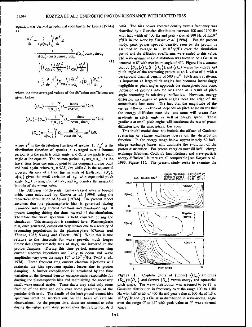
21,914 KOZYRA ET AL.: ENERGETIC PROTON RESONANCE WITH DUCTED HISS
equation was derived in spherical coordinates by Lyons [1974a] as
& vK) o dt 1 /^
-—r : -—s(a0)cosa0 since, ^ajvcosa^sina,, da0
\ aa/v 3a. \ av/ ^
(1)
\ va/v da„ \ w/ av
1 d 2 +~TTV
vz av
where the time-averaged values of the diffusion coefficients are given below;
(\ t cm i a0) J
0 cosX
(D^iD^-^fD, sin a s(a») o avcosa0sina<,
s7\dk
<^> = T^T?A sin2 a
s(aa) • wcosasin a, -cos7 Xttk
where / is the distribution function of species £, / ' is the distribution function of species £ averaged over a bounce period, a is the particle pitch angle, and a„ is the particle pitch angle at the equator. The bounce period, xB =x„s(a0), is the travel time from one mirror point to the conjugate mirror point and back again, where xo =4LRE /v; while L is the equatorial crossing distance of a field line in units of Earth radii (RE), s(a0) gives the small variation of xB with equatorial pitch angle aB,X is magnetic latitude, and X.M denotes the magnetic latitude of the mirror point.
The diffusion coefficients, time-averaged over a bounce orbit, were calculated by Kozyra et al. [1994] using the theoretical formulation of Lyons [1974b]. The present model assumes that the plasmaspheric hiss is generated during resonance with ring current electrons and maintained against proton damping during the time interval of the simulation. Therefore the wave spectrum is held constant during the simulation. This assumption is examined here. Plasmaspheric hiss, once generated, damps out very slowly due to a scarcity of resonating populations in the plasmasphere [Church and Thome, 1983; Huang and Goertz, 1983]. While this is true relative to the timescale for wave growth, much longer timescales (approximately tens of days) are involved in the proton damping. During this time period, numerous ring current electron injections are likely to occur and wave amplitudes vary over the range 10"* to 10'7 //Hz [Smith et al., 1974]. These frequent ring current electron injections will maintain the hiss spectrum against losses due to proton damping. A further complication is introduced by the time variation in the thermal density enhancements responsible for ducting the plasmaspheric hiss and maintaining the necessary small wave-normal angles. These ducts may exist only some fraction of the time and only over some percentage of the particles drift orbit. The details of the background ducted hiss spectrum must be worked out on the basis of satellite observations. At the present time, ducts are assumed to exist during the entire simulation period over the full proton drift
orbit. The hiss power spectral density versus frequency was described by a Gaussian distribution between 100 and 1100 Hz with half width of 400 Hz and peak value at 600 Hz of 5xl0'5
•//Hz in the work by Kozyra et al. [1994]. For the present study, peak power spectral density, seen by the proton, is assumed to average to 1.3x10' //Hz over the simulation period and the diffusion coefficients were scaled to this value. The wave-normal angle distribution was taken to be a Gaussian centered at 0° with maximum angle of 45°. Figure 1 is a contour plot of (Daa),(£»ov)(=(Z)vo)), and (Dw) versus the energy and pitch angle of the resonating proton at an L value of 4 with a background thermal density of 500 cm"3. Pitch angle scattering is important at large pitch angles but becomes increasingly negligible as pitch angles approach the atmospheric loss cone. Diffusion of protons into the loss cone as a result of pitch angle scattering is relatively ineffective. However, energy diffusion maximizes at pitch angles near the edge of the atmospheric loss cone. The fact that the magnitude of the energy diffusion coefficient depends on pitch angle means that the energy diffusion near the loss cone will create flux gradients in pitch angle as well as energy space. These gradients at small pitch angles will accelerate the rate of proton diffusion into the atmospheric loss cone.
This initial model does not include the effects of Coulomb scattering or charge exchange losses on the distribution function. In the energy range below approximately 80 keV, charge exchange losses will dominate the evolution of the proton distribution. For proton energies near 80 keV, charge exchange lifetimes, Coulomb loss lifetimes and wave-particle energy diffusion lifetimes are all comparable [see Kozyra et al., 1993, Figure 11]. The present study seeks to examine the
L=4, Ne=500cmJ Contour Spacing: 5x10 cm2s"3
Minimum Value: 1x10'cm2 J
Maximum Value: 1x10"cm2s"3
1000
E(kev)
10
1000
E(kev)
1000
E(kev)
\ u ! ! j \ <Daa>/ / I ;\
Figure 1. Contour plots of (upper) {D^} (middle) (Doev) = (Dva) and (lower) (Dw) versus energy and equatorial pitch angle. The wave distribution was assumed to be (1) a Gaussian distribution in frequency over the range 100 to 1100 Hz with half width of 400 Hz and peak value at 600 Hz of 1.3 x 10"5 "//Hz and (2) a Gaussian distribution in wave-normal angle over the range 0° to 45° with peak value at 0° wave-normal angle.
141
KOZYRA ET AL.: ENERGETIC PROTON RESONANCE WITH DUCTED HISS 21,915
effects of resonance with plasmaspheric hiss on protons with energies above -80 keV. In this energy range, resonance with plasmaspheric hiss will have a significant effect on the evolution of the proton distribution function; other loss processes will be neglected.
3. Numerical Technique
The bounce-averaged diffusion equation can be conveniently solved in conservative form. Thus (1) is rewritten as
:V- (<D>-V)(/0)-(/0) ^((D)V) (2)
where a = s{a0)cosa0, and f0 - afa. The quantity s(aD), which gives the small variation in the bounce period with equatorial pitch angle, is approximately s(cc„) = 1.38 - 0.32(sinao + -y/sina,,) [Lyons, 1974b]. Note that the normalized distribution function /„ is the conserved quantity, rather than /, due to the temporal averaging of Boltzmann's equation over one bounce period. As particles with a given energy bounce back and forth between mirror points, they fill a certain volume in configuration space. This volume depends on the location of the minor points. Thus, as the mirror points change, the particle distribution at any point along the field line must also vary, in order to maintain a constant number of particles within the changing volume in configuration space.
Equation (2) was solved by a finite volume technique. In this numerical method, the volume-average change in /, during a time step 8f, is proportional to the sum of the fluxes F.leaving each face of the volume element, times the interface area A{:
#=*XM- (3)
where V is the volume of the element. The fluxes in the two coordinate directions, v and a, are given by
F -In \3/ + <D«>y ?(D") da
da da
F -In \3/ + (D->3/ KD~) da x ' dv v da av da
(4)
The partial derivatives in (4) were calculated numerically at each face with a second-order central difference scheme. It should be noted that the transformation x = log10(£ = 77iv2/2) was actually used in the numerical solution (leading to a slightly altered form of (4)). This was done so that high resolution could be maintained at low energies in E while still maintaining a relatively large overall range in energy. Energies ranged from 10 keV to 1000 keV, while pitch angles ranged from 0 to Jt. Constant cell widths Aa and Ax were employed, with 45 steps in a and 51 in x, giving a total of 2295 volume elements. Boundary conditions were chosen so that no flux could enter or leave the computational domain, except through the lower-energy boundary. At this boundary, E = 10 keV, the flux entering the computational domain was chosen to maintain a constant value for/.
A two-step Runge-Kutta method was selected to advance the numerical solution in time. This method leads to second-order accuracy in time, accompanying the second-order accuracy of the spatial discretization. The numerical method was found to be stable as long as the time step was sufficiently small, At < 2 hours. Several other numerical methods, such as Lax-Wendroff,
were found to be unstable. The major stability problem was caused by the combined hyperbolic and diffusive nature of (2).
The effects of a loss cone were artificially added by including a loss term for pitch angles less than or equal to 9 deg. Loss timescales were chosen to be slower than naturally occurring precipitation timescales in order to speed up the numerical solution and to maintain a stable solution near the loss cone. In the present solution, the edge of the loss cone is under resolved and artificially broad, leading to an underestimation of transport into the loss cone. However, the net effect on transport in the interior of the simulation domain, away from the loss cone, is negligible.
4. Time Evolution of the Proton Distribution Function
The initial conditions for the simulation were taken from Williams et al. [1976], who present observations of ring current ions, assumed to be protons, in the energy range of a few to several hundred keV. These observations were made on field lines approximately associated with SAR arc emissions in the ionosphere. The distribution function versus energy was represented by the sum of three different analytical fits over specified energy intervals as follows:
/(E)=1.94xl07£-a6" 1.2keV<E<9keV
9keV<E<28keV (5) f(E) = 4.50xl06E°
28keV<E<280keV f(E)^1.63xJ0'°E-25w
The pitch angle distribution was taken to be isotropic independent of the proton energy with the exception of an artificially introduced loss cone. Contours of the initial distribution function versus pitch angle and energy are presented in Plate la.
The evolution of the proton distribution function is followed during resonance with the ducted plasmaspheric hiss spectrum described in section 2. Plates lb and lc are snapshots of the distribution function after 20 and 40 days, respectively. After 40 days time, the pitch angle distribution has changed dramatically from the isotropic initial condition to exhibit a distinct maximum at pitch angles near the edge of the atmospheric loss-cone. The peak shifts to larger pitch angles with decreasing proton energy. Significant energization of the protons occurs at the location of the peak. The peak in the distribution function at modest pitch angles is a result of energy diffusion that depends on pitch angle and maximizes near 25°. Energy diffusion near the edge of the loss cone will create a steep gradient in the distribution function and enhance pitch angle diffusion into the loss cone. However, even in the presence of this steep gradient, pitch angle diffusion is weak.
Figure 2 is a plot of the distribution function versus pitch angle at a fixed proton energy of 250 keV at selected times during the simulation. Protons with moderate pitch angles damp wave energy and diffuse from lower to higher energies during the simulation time interval producing a buildup in the distribution function. The reason for the buildup in the distribution function at moderate pitch angles is clearly illustrated in Figure 3. Energy diffusion lifetimes reach a minimum value at pitch angles near 27°. Diffusion in energy occurs most rapidly in a band of pitch angles centered about the lifetime minimum. As a consequence fluxes build up at these moderate pitch angles as shown in Figure 2. At larger pitch angles energy diffusion is too slow to produce significant
142
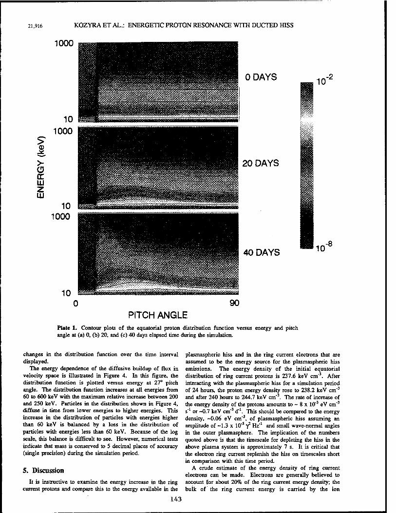
21,916 KOZYRA ET AL.: ENERGETIC PROTON RESONANCE WITH DUCTED HISS
1000
io m
ODAYS 10-2
1000 9
>
w z UJ
10 1000
20 DAYS
10
•*■
BET--- '^^^^■•\S&OG^KSB
Hr< —-~-~ — ^—^i^_> • .<•--":- "•T?V;V^->I
-SX-SÄ^ÄGÄ
40 DAYS 10 -8
90 PITCH ANGLE
Plate 1. Contour plots of the equatorial proton distribution function versus energy and pitch angle at (a) 0, (b) 20, and (c) 40 days elapsed time during the simulation.
changes in the distribution function over the time interval displayed.
The energy dependence of the diffusive buildup of flux in velocity space is illustrated in Figure 4. In this figure, the distribution function is plotted versus energy at 27° pitch angle. The distribution function increases at all energies from 60 to 600 keV with the maximum relative increase between 200 and 250 keV. Particles in the distribution shown in Figure 4, diffuse in time from lower energies to higher energies. This increase in the distribution of particles with energies higher than 60 keV is balanced by a loss in the distribution of particles with energies less than 60 keV. Because of the log scale, this balance is difficult to see. However, numerical tests indicate that mass is conserved to S decimal places of accuracy (single precision) during the simulation period.
5. Discussion
It is instructive to examine the energy increase in the ring current protons and compare this to the energy available in the
plasmaspheric hiss and in the ring current electrons that are assumed to be the energy source for the plasmaspheric hiss emissions. The energy density of the initial equatorial distribution of ring current protons is 237.6 keV cm"3. After interacting with the plasmaspheric hiss for a simulation period of 24 hours, the proton energy density rose to 238.2 keV cm"3
and after 240 hours to 244.7 keV cm"3. The rate of increase of the energy density of the protons amounts to ~ 8 x 10"3 eV cm"3
s'1 or -0.7 keV cm"3 d'1. This should be compared to the energy density, -0.06 eV cm" , of plasmaspheric hiss assuming an amplitude of -1.3 x 10's "y2 Hz'1 and small wave-normal angles in the outer plasmasphere. The implication of the numbers quoted above is that the timescale for depleting the hiss in the above plasma system is approximately 7 s. It is critical that the electron ring current replenish the hiss on timescales short in comparison with this time period.
A crude estimate of the energy density of ring current electrons can be made. Electrons are generally believed to account for about 20% of the ring current energy density; the bulk of the ring current energy is carried by the ion
143
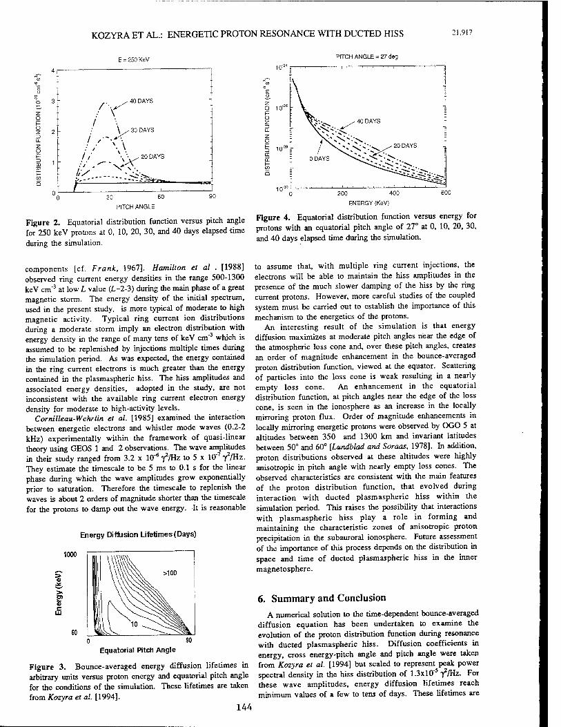
KOZYRA ET AL.: ENERGETIC PROTON RESONANCE WITH DUCTED HISS 21,917
E = 250KeV PITCH ANGLE = 27 deg
z O H Ü
Z> m cc H w a
31-
2 -
f'Y 40 DAYS
/ \ y 30 DAYS
\ ■.
V x< 20 DAYS
------^j»^.
30 60
PITCH ANGLE
90
Figure 2. Equatorial distribution function versus pitch angle for 250 keV protons at 0, 10, 20, 30, and 40 days elapsed time during the simulation.
components [cf. Frank, 1967]. Hamilton et al . [1988] observed ring current energy densities in the range 500-1300 keV cm"3 at low L value (L-2-3) during the main phase of a great magnetic storm. The energy density of the initial spectrum, used in the present study, is more typical of moderate to high magnetic activity. Typical ring current ion distributions during a moderate storm imply an electron distribution with energy density in the range of many tens of keV cm' which is assumed to be replenished by injections multiple times during the simulation period. As was expected, the energy contained in the ring current electrons is much greater than the energy contained in the plasmaspheric hiss. The hiss amplitudes and associated energy densities, adopted in the study, are not inconsistent with the available ring current electron energy density for moderate to high-activity levels.
Cornilleau-Wehrlin et al. [1985] examined the interaction between energetic electrons and whistler mode waves (0.2-2 kHz) experimentally within the framework of quasi-linear theory using GEOS 1 and 2 observations. The wave amplitudes in their study ranged from 3.2 x 10"6 flHz to 5 x 10"7 yVHz. They estimate the timescale to be 5 ms to 0.1 s for the linear phase during which the wave amplitudes grow exponentially prior to saturation. Therefore the timescale to replenish the waves is about 2 orders of magnitude shorter than the timescale for the protons to damp out the wave energy. It is reasonable
Energy Diffusion Lifetimes (Days)
1000
5» 0)
a c w
40 DAYS
20 DAYS
D 200 400
ENERGY (KeV)
Figure 4. Equatorial distribution function versus protons with an equatorial pitch angle of 27° at 0, and 40 days elapsed time during the simulation.
600
energy for 10, 20, 30,
Equatorial Pitch Angle
Figure 3. Bounce-averaged energy diffusion lifetimes in arbitrary units versus proton energy and equatorial pitch angle for the conditions of the simulation. These lifetimes are taken from Kozyra et al. [1994].
144
to assume that, with multiple ring current injections, the electrons will be able to maintain the hiss amplitudes in the presence of the much slower damping of the hiss by the ring current protons. However, more careful studies of the coupled system must be carried out to establish the importance of this mechanism to the energetics of the protons.
An interesting result of the simulation is that energy diffusion maximizes at moderate pitch angles near the edge of the atmospheric loss cone and, over these pitch angles, creates an order of magnitude enhancement in the bounce-averaged proton distribution function, viewed at the equator. Scattering of particles into the loss cone is weak resulting in a nearly empty loss cone. An enhancement in the equatorial distribution function, at pitch angles near the edge of the loss cone, is seen in the ionosphere as an increase in the locally mirroring proton flux. Order of magnitude enhancements in locally mirroring energetic protons were observed by OGO 5 at altitudes between 350 and 1300 km and invariant latitudes between 50° and 60° [Lundblad and Soraas, 1978]. In addition, proton distributions observed at these altitudes were highly anisotropic in pitch angle with nearly empty loss cones. The observed characteristics are consistent with the main features of the proton distribution function, that evolved during interaction with ducted plasmaspheric hiss within the simulation period. This raises the possibility that interactions with plasmaspheric hiss play a role in forming and maintaining the characteristic zones of anisotropic proton precipitation in the subauroral ionosphere. Future assessment of the importance of this process depends on the distribution in space and time of ducted plasmaspheric hiss in the inner magnetosphere.
6. Summary and Conclusion A numerical solution to the time-dependent bounce-averaged
diffusion equation has been undertaken to examine the evolution of the proton distribution function during resonance with ducted plasmaspheric hiss. Diffusion coefficients in energy, cross energy-pitch angle and pitch angle were taken from Kozyra et al. [1994] but scaled to represent peak power spectral density in the hiss distribution of 1.3xl0"5 '//Hz. For these wave amplitudes, energy diffusion lifetimes reach minimum values of a few to tens of days. These lifetimes are
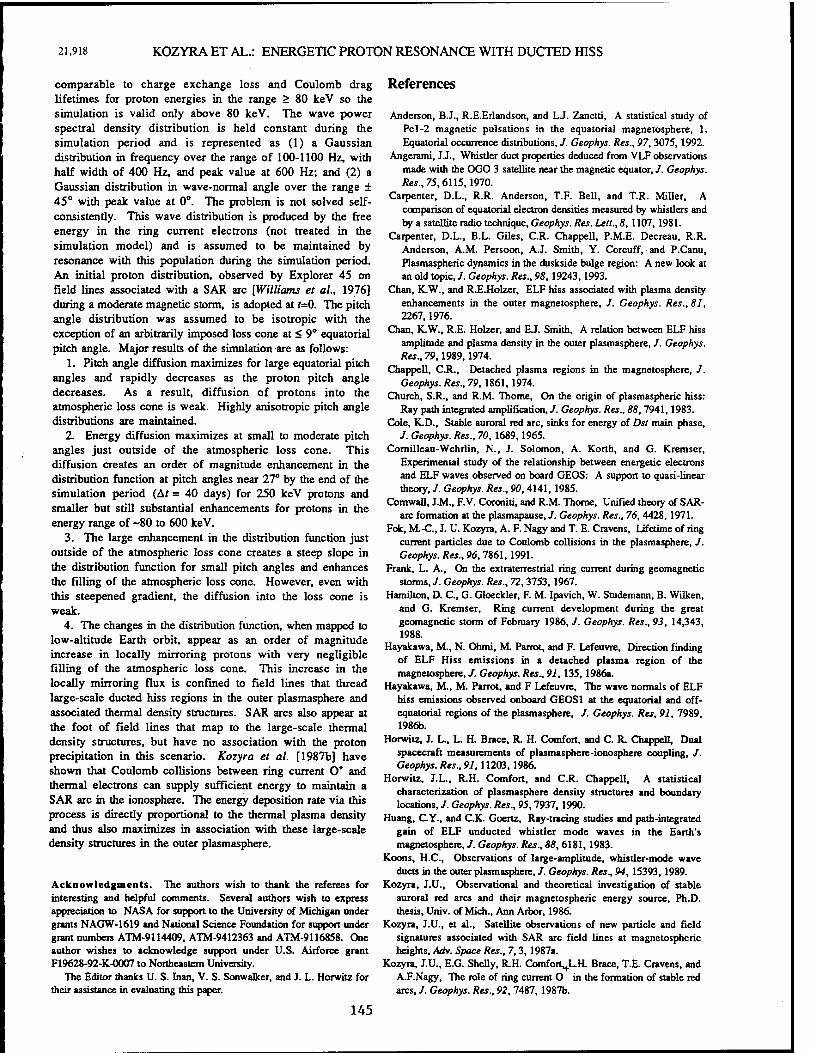
21,918 KOZYRA ET AL.: ENERGETIC PROTON RESONANCE WITH DUCTED HISS
comparable to charge exchange loss and Coulomb drag lifetimes for proton energies in the range > 80 keV so the simulation is valid only above 80 keV. The wave power spectral density distribution is held constant during the simulation period and is represented as (1) a Gaussian distribution in frequency over the range of 100-1100 Hz, with half width of 400 Hz, and peak value at 600 Hz; and (2) a Gaussian distribution in wave-normal angle over the range ± 45° with peak value at 0°. The problem is not solved self- consistently. This wave distribution is produced by the free energy in the ring current electrons (not treated in the simulation model) and is assumed to be maintained by resonance with this population during the simulation period. An initial proton distribution, observed by Explorer 45 on field lines associated with a SAR arc [Williams et al., 1976] during a moderate magnetic storm, is adopted at f=0. The pitch angle distribution was assumed to be isotropic with the exception of an arbitrarily imposed loss cone at < 9° equatorial pitch angle. Major results of the simulation are as follows:
1. Pitch angle diffusion maximizes for large equatorial pitch angles and rapidly decreases as the proton pitch angle decreases. As a result, diffusion of protons into the atmospheric loss cone is weak. Highly anisotropic pitch angle distributions are maintained.
2. Energy diffusion maximizes at small to moderate pitch angles just outside of the atmospheric loss cone. This diffusion creates an order of magnitude enhancement in the distribution function at pitch angles near 27° by the end of the simulation period (At = 40 days) for 250 keV protons and smaller but still substantial enhancements for protons in the energy range of ~80 to 600 keV.
3. The large enhancement in the distribution function just outside of the atmospheric loss cone creates a steep slope in the distribution function for small pitch angles and enhances the filling of the atmospheric loss cone. However, even with this steepened gradient, the diffusion into the loss cone is weak.
4. The changes in the distribution function, when mapped to low-altitude Earth orbit, appear as an order of magnitude increase in locally mirroring protons with very negligible filling of the atmospheric loss cone. This increase in the locally mirroring flux is confined to field lines that thread large-scale ducted hiss regions in the outer plasmasphere and associated thermal density structures. SAR arcs also appear at the foot of field lines that map to the large-scale thermal density structures, but have no association with the proton precipitation in this scenario. Kozyra et al. [1987b] have shown that Coulomb collisions between ring current O* and thermal electrons can supply sufficient energy to maintain a SAR arc in the ionosphere. The energy deposition rate via this process is directly proportional to the thermal plasma density and thus also maximizes in association with these large-scale density structures in the outer plasmasphere.
Acknowledgments. The authors wish to thank the referees for interesting and helpful comments. Several authors wish to express appreciation to NASA for support to the University of Michigan under grants NAGW-1619 and National Science Foundation for support under grant numbers ATM-9114409, ATM-9412363 and ATM-9116858. One author wishes to acknowledge support under U.S. Airforce grant F19628-92-K-O007 to Northeastern University.
The Editor thanks U. S. Inan, V. S. Sonwalker, and J. L. Horwitz for their assistance in evaluating this paper.
References
Anderson, B.J., R.E.Erlandson, and LJ. Zanetti, A statistical study of Pel-2 magnetic pulsations in the equatorial magnetosphere, 1. Equatorial occurrence distributions, /. Geophys. Res., 97,3075,1992.
Angerami, JJ., Whistler duct properties deduced from VLF observations made with the OGO 3 satellite near the magnetic equator, J. Geophys. Res., 75,6115,1970.
Carpenter, D.L., R.R. Anderson, T.F. Bell, and T.R. Miller, A comparison of equatorial electron densities measured by whistlers and by a satellite radio technique, Geophys. Res. Lett., 8, 1107, 1981.
Carpenter, D.L., B.L. Giles, C.R. Chappell, P.M.E. Decreau, R.R. Anderson, A.M. Persoon, A.J. Smith, Y. Corcuff, and P.Canu, Plasmaspheric dynamics in the duskside bulge region: A new look at an old topic, /. Geophys. Res., 98, 19243,1993.
Chan, K.W., and R.E.Holzer, ELF hiss associated with plasma density enhancements in the outer magnetosphere, /. Geophys. Res.,81, 2267,1976.
Chan, K.W., R.E. Holzer, and E.J. Smith, A relation between ELF hiss amplitude and plasma density in the outer plasmasphere, /. Geophys. Res., 79,1989,1974.
Chappell, C.R., Detached plasma regions in the magnetosphere, /. Geophys. Res., 79, 1861,1974.
Church, S.R., and R.M. Thome, On the origin of plasmaspheric hiss: Ray path integrated amplification, J. Geophys. Res., 88, 7941,1983.
Cole, K.D., Stable auroral red arc, sinks for energy of Dst main phase, /. Geophys. Res., 70, 1689,1965.
Comilleau-Wehrlin, N., J. Solomon, A. Korth, and G. Kremser, Experimental study of the relationship between energetic electrons and ELF waves observed on board GEOS: A support to quasi-linear theory, J. Geophys. Res., 90, 4141, 1985.
Cornwall, J.M., F.V. Coroniti, and R.M. Thome, Unified theory of SAR- arc formation at the plasmapause, /. Geophys. Res., 76, 4428,1971.
Fok, M-C, J. U. Kozyra, A. F. Nagy and T. E. Cravens, Lifetime of ring current particles due to Coulomb collisions in the plasmasphere, /. Geophys. Res., 9(5,7861, 1991.
Frank, L. A., On the extraterrestrial ring current during geomagnetic storms,/. Geophys. Res., 72,3753, 1967.
Hamilton, D. C, G. Gloeckler, F. M. Ipavich, W. Studemann, B. Wilken, and G. Kremser, Ring current development during the great geomagnetic storm of February 1986, /. Geophys. Res., 93, 14343, 1988.
Hayakawa, M., N. Ohmi, M Parrot, and F. Lefeuvre, Direction finding of ELF Hiss emissions in a detached plasma region of the magnetosphere, /. Geophys. Res., 91, 135, 1986a.
Hayakawa, M., M. Parrot, and F Lefeuvre, The wave normals of ELF hiss emissions observed onboard GEOS1 at the equatorial and off- equatorial regions of the plasmasphere, /. Geophys. Res, 91, 7989, 1986b.
Horwitz, J. L., L. H. Brace, R. H. Comfort, and C. R. ChappelL Dual spacecraft measurements of plasmasphere-ionosphere coupling, /. Geophys. Res., 91,11203, 1986.
Horwitz, J.L., R.H. Comfort, and C.R. Chappell, A statistical characterization of plasmasphere density structures and boundary locations, /. Geophys. Res., 95,7937,1990.
Huang, C.Y., and C.K. Goertz, Ray-tracing studies and path-integrated gain of ELF unducted whistler mode waves in the Earth's magnetosphere, /. Geophys. Res., 88, 6181,1983.
Koons, H.C., Observations of large-amplitude, whistler-mode wave ducts in the outer plasmasphere, /. Geophys. Res., 94, 15393,1989.
Kozyra, J.U., Observational and theoretical investigation of stable auroral red arcs and their magnetospheric energy source, Ph.D. thesis, Univ. of Mich., Ann Arbor, 1986.
Kozyra, J.U., et al.. Satellite observations of new particle and field signatures associated with SAR arc field lines at magnetospheric heights, Adv. Space Res., 7,3,1987a.
Kozyra, J.U., E.G. Shelly, R.H. Comfort^L.H. Brace, T.E. Cravens, and A.F.Nagy, The role of ring current O in the formation of stable red arcs, /. Geophys. Res., 92, 7487, 1987b.
145
KOZYRA ET AL.: ENERGETIC PROTON RESONANCE WITH DUCTED HISS 21,919
Kozyra, J. U., M. O. Chandler, D. C. Hamilton, W. K. Peterson, D. M. Klumpar D. W. Slater, M. J. Buonsanto, and H. C. Carlson, The role of ring current nose events in producing stable auroral red arc intensifications during the main phase: Observations during the September 19-24, 1984, equinox transition study, J. Geophys. Res., 98,
9267, 1993. Kozyra, J.U., C.E. Rasmussen, R.H. Miller, and L.R.Lyons, The
interaction of ring current and radiation belt protons with ducted plasmaspheric hiss. 1. Diffusion coefficients and timescales, /. Geophys. Res., 99, 4069, 1994.
Lundblad, J.A., and F. Soraas, Proton observations supporting the ion cyclotron wave heating theory of SAR arc formation, Planet. Space
Sei., 2(5,245,1978. Lyons, L.R., General relations for resonant particle diffusion in pitch
angle and energy, /. Plasma Phys., 12, 45, 1974a. Lyons, L.R., Pitch angle and energy diffusion coefficients from resonant
interactions with ion-cyclotron and whistler waves, J. Plasma Phys.,
12,417,1974b. Scarf, F.L., and C.R. Chappell, An association of magnetospheric
whistler dispersion characteristics with changes in local plasma density,/. Geophys. Res., 78, 1597,1973.
Smith, E.J., A.M.A. Frandsen, B.T. Tsurutani, R.M. Thome, and K.W. Chan, Plasmaspheric hiss intensity variations during magnetic storms,
/. Geophys. Res., 79, 2507, 1974. Sonwalker, V.S., and U. S. Inan, Wave normal direction and spectral
properties of whistler mode hiss observed on the DE 1 satellite, /. Geophys. Res., 93, 7493, 1988.
Storey, LR.O., F. Lefeuvre, M. Parrot, L Cairo, and R. R. Anderson,
Initial survey of the wave distribution functions for plasmaspheric hiss observed by ISEE 1, /. Geophys. Res., 86, 19,469, 1991.
Thome, R.M., and R. B. Home, The contribution of ion-cyclotron waves to electron heating and SAR-arc excitation near the storm-time plasmapause, Geophys. Res. Lett., 19, 417, 1992.
Thome, R.M., EJ. Smith, R.K. Burton, and R.E. Hölzer, Plasmaspheric
hiss,/. Geophys. Res., 78, 1581, 1973. Villalon, E., and W. J. Burke, Whistler interactions with energetic
protons, in Physics of Space Plasmas (1991), p. 473, SPI Conf. Proc. Reprint Ser. no. 11, edited by T. Change, G. B. Crew and J. R. Jasperse, Scientific, Cambridge, Mass., 1992.
Villalon, E., and W. J. Burke, Diffusion of radiation belt protons by whistler waves, /. Geophys. Res., 99, 21,329, 1994.
Voss, H.D.. and L.G. Smith, Global zones of energetic particle precipitation, /. Atmos. Terr. Phys., 42, 227, 1980.
Williams, D.J., G. Hernandez, and L.R. Lyons, Simultaneous observations of the proton ring current and stable auroral red arcs, /.
Geophys. Res., 81, 608, 1976.
J. U. Kozyra, R. H. Miller, and C. E. Rasmussen, Space Physics Research Laboratory, Atmospheric, Oceanic and Space Sciences Department, University of Michigan, Ann Arbor, MI 489109-2143.
E. Villalon, Center for Electromagnetic Research, Northeastern
University, Boston, MA 02115.
(Received April 28, 1994; revised May 12,1995; accepted May 16, 1995.)
146