Intelligent Maintenance of Belt Conveyors Using Machine ...

13th International Conference on Bulk Materials Storage, Handling and Transportation 9-11 July 2019

Mantra on View, Surfers Paradise Gold Coast, Queensland Australia

Intelligent Maintenance of Belt Conveyors Using Machine Learning

Xiangwei Liu1, Deli Pei1, Gabriel Lodewijks2, Zhangyan Zhao3 1Truth Plaza, No. 7 Zhichun Road, Beijing 100191, P.R. China

2School of Aviation, The University of New South Wales, NSW 2052, Sydney, Australia 3School of Logistics Engineering, Wuhan University of Technology, Wuhan 430063, P.R. China

Email of first author: [email protected]

Abstract

Maintenance of idler rolls remains a challenge to reliable performance of belt conveyor systems. In-

time detection of idler roll failures is critical for maintenance planning. Fault diagnosis based on

sound emission of idler rolls recently gains its popularity due to its easiness of data acquisition.

However, sound emission is observed with big diversity, large volume, and strong noise. This paper

presents an intelligent idler roll fault diagnosis approach based on Mel Frequency Cepstrum

Coefficients and Gradient Boost Decision Tree algorithm (GBDT). Mel Frequency Cepstrum

Coefficients are a sequence of features inspired from the human auditory perception mechanism.

Gradient Boosting algorithm is very capable of achieving accurate predictions with “poor”

performance Decision Trees. Acoustic emission signals are obtained from healthy rolls and purposely

damaged rolls in a laboratory belt conveyor system. The collected data are divided into a training

dataset and a testing dataset. Thirteen cepstral features are selected and used as diagnosis features. A

GBDT algorithm is developed and trained. After training, the GBDT algorithm is applied to the

testing dataset. Results show that the proposed approach can achieve an accuracy level up to 96.17%,

and recall rate up to 99.7%. The study verifies the applicability of proposed Machine Learning

approach on fault diagnosis of belt conveyor idler rolls.

Keywords: belt conveyor; idler roll; sound emission; machine learning; gradient boost; decision tree;

MFCC

1. Introduction

Belt conveyor systems are widely utilized for continuous transport of dry bulk materials (i.e. coal,

iron ore) over varying distances. The reliability of belt conveyor systems is of major concern for

conveyor operators. Breakdowns of belt conveyor systems cause disturbing downtime of the

conveying and associated production process, consequently increasing operational cost of belt

conveyor systems.

The performance of idlers has a large impact on the reliability of belt conveyor systems [1], [2].

Nevertheless, belt conveyor idlers lack the due attention from researchers and operators [3]. So far

idler rolls are the most difficult to be monitored in automated ways due to their large amount, the

scale of monitoring systems and the spatial distribution of rolls [4].

Idler maintenance can be divided into three categories of activities: condition monitoring, decision

making, and roll replacement [5]. Common condition monitoring of idlers consists of periodical

inspections by human conveyor inspectors through “eye watching” and “ear listening”. Recently,

sensors which can monitor temperature [6], vibration [7] and acoustic emission [8] are introduced

into condition monitoring of idler rolls [9]. Compared to temperature and vibration measurements,

acoustic emission (AE) based condition monitoring has several advantages such as early detection of

failure, non-contact data acquisition, and less ambient environment influence.



AE based fault diagnosis on idler rolls has been carried out in time, frequency, and time-frequency

domains. Envelope analysis is a widely applied approach for AE based fault diagnosis. For instance

the SKF Idler Sound Monitor Kit utilizes features like peak and root sum square from AE envelope

analysis for fault diagnosis [8]. However, fault diagnosis based on AE envelope analysis is not very

robust.

This paper aims to investigate the applicability of Mel Frequency Cepstrum Coefficients (MFCCs)

and Gradient Boost Decision Tree (GBDT) on fault diagnosis of belt conveyor idler rolls. Section 2

introduces the basis of MFCCs and GBDT. Section 3 describes an experimental setup, in which AE

signal of healthy and purposely damaged rolls during running are obtained. Section 4 presents the

results and discussion.

2. Theory

Raw AE data are commonly observed with noise, irrelevant and redundant signals [10], therefore it

is very difficult to find the underneath relationship between acquired AE data and actual machine

condition. MFCCs have been widely applied in audio analysis such as speech recognition [11], fault

classification of engines [12], and early detection of bearing failures [13]. MFCCs are a sequence of

frequency feature vectors, which are derived from AE signals in short time frames. MFCCs have the

advantages of requiring simple data pre-processing, being very informative, and big classification

potential. By combining decision trees of poor performance, GBDT can produce accurate

classification and predictions for regression problems by continuously improving prediction accuracy

during iteration. Other merits of GBDT include providing interpretable results, requiring little data

processing, robust to noise, able to handle different types of predictor variables, fitting complex

nonlinear relationships and so on [14]. All these advantages make MFCCs+GBDT a good candidate

for fault diagnosis problems.

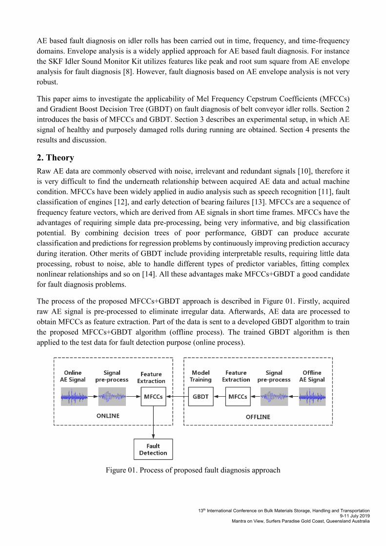
The process of the proposed MFCCs+GBDT approach is described in Figure 01. Firstly, acquired

raw AE signal is pre-processed to eliminate irregular data. Afterwards, AE data are processed to

obtain MFCCs as feature extraction. Part of the data is sent to a developed GBDT algorithm to train

the proposed MFCCs+GBDT algorithm (offline process). The trained GBDT algorithm is then

applied to the test data for fault detection purpose (online process).

Figure 01. Process of proposed fault diagnosis approach



2.1 Mel Frequency Cepstrum Coefficients

Current idler roll inspection practice relies on “ear listening” of conveyor inspectors. This means

auditory features of AE from failed idler rolls can be picked up by human ears. MFCCs are calculated

according to Mel frequency, which is to simulate human auditory perception characteristics. In

addition, MFCCs are a sequence of feature vectors obtained from a moving short time window.

Through moving average operation, the formants of AE signal can be enhanced [15]. Enhanced

formants are supposed to improve detectability of AE signal. Therefore MFCCs may be reliable

indicators of roll failures.

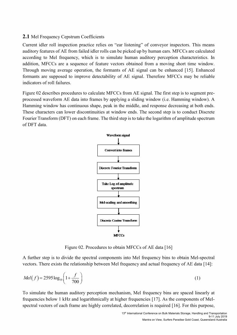
Figure 02 describes procedures to calculate MFCCs from AE signal. The first step is to segment pre-

processed waveform AE data into frames by applying a sliding window (i.e. Hamming window). A

Hamming window has continuous shape, peak in the middle, and response decreasing at both ends.

These characters can lower discontinuities at window ends. The second step is to conduct Discrete

Fourier Transform (DFT) on each frame. The third step is to take the logarithm of amplitude spectrum

of DFT data.

Figure 02. Procedures to obtain MFCCs of AE data [16]

A further step is to divide the spectral components into Mel frequency bins to obtain Mel-spectral

vectors. There exists the relationship between Mel frequency and actual frequency of AE data [14]:

( ) 102595log 1700

fMel f

= +

(1)

To simulate the human auditory perception mechanism, Mel frequency bins are spaced linearly at

frequencies below 1 kHz and logarithmically at higher frequencies [17]. As the components of Mel-

spectral vectors of each frame are highly correlated, decorrelation is required [16]. For this purpose,



Discrete Cosine Transform is applied to the Mel-spectral vectors and MFCCs for each frame can be

obtained. The MFCCs are calculated as follows [17]:

( ) 1

cos 0.5 / , for 1,2, ,N

i k i

k

C X k N i p=

= − = (2)

in which iC is MFCC, k is the number of DFT magnitude coefficients, kX is the kth order log-

energy output from the filter bank, and N is the number of filters (normally 20), p is the order. For

this study, thirteen MFCCs are obtained and used as features for the GBDT algorithm.

2.2 Gradient Boost Decision Tree

GBDT is a Machine Learning technique which combines Gradient Boost and Decision Tree for

regression and classification problem solving. By approximating a parameterized function or base

learner to current pseudo residuals with a loss function at each iteration, Gradient Boost builds

sequentially additive regression models to find the best approximation function with a given dataset

[18]. Assuming a dataset ( ) ( )1 1, , , ,n nx y x y is available, Friedman gave out the Gradient Boost

algorithm for an approximation function as follows [19], [20]:

Step 1, calculate the initial guess ( )0F x as

( ) ( )0

1

arg min ,n

i

i

F x L y

=

= (3)

or simply assume ( )0 0F x . ( ),L is a loss function, is a multiplier.

Step 2, for 1, ,t T= , perform a series of iterations and calculate the following values in each

iteration:

( )( )

( )( ) ( )1

~ ,, 1, ,

m

i i

i

iF x F x

L y F xy i n

F x−=

= − =

(4)

( )2

~

,1

arg min ;n

t

i i

i

y h x

=

= −

(5)

( ) ( )( )1

1

arg min , ;n

t t t

i i i

i

L y F x h x

−

=

= + (6)

( ) ( ) ( )1 ;t t t tF x F x h x −= + (7)

in which ( );h is base learner.

Step 3 end the iteration and ( )tF x is the final approximation function.

In addition, Decision Tree theory is briefly introduced as follows. For each data collection, suppose

there exist useful features (1 2, ,... nT T T ) for distinguishing the healthy condition and the fault condition

after the Gradient Boost process above. Firstly, for each feature, order the events by the values of

featureiT . Correspondingly, all events can be divided into two groups (healthy and fault group),



depending on the value score for feature iT . Now decide on the best splitting value for feature

iT which

gives the best splitting result compared to prior known conditions.

Initially there is a collection of samples at a “node”. With the first process as illustrated above, the

“node” develops two “branches”. For each “branch”, repeat the process of finding the best value for

each feature to split the samples in the “branch” into two groups. The course continues until there are

too few samples in a “branch” or in each “branch” the samples are in exclusive collection. The end

“branches” are also called “leaves”.

3. Experimental setup

A test rig was developed to collect AE data of healthy idler rolls and purposely damaged rolls at Delft

University of Technology, the Netherlands [5]. The test rig (Figure 03) consists of a belt conveyor,

an idler set, a control box, and a data acquisition system. The idler rolls used in the experiments have

a shell diameter of 108 mm, shell length of 380 mm, and the diameter of the shaft end is 30 mm. The

type of bearings inside each roll are deep groove ball bearings (6206). A Uni-directional microphone

(Electret microphone breakout BOB – 09964) is used to collect acoustic emission during tests. The

sensitivity of the microphone is -46 at 1 kHz. The sampling frequency is 30kHz. As shown in Figure

03, the microphone is placed with a distance of 150 mm to the roll shaft end.

Figure 03. The test rig for AE data collection [5]

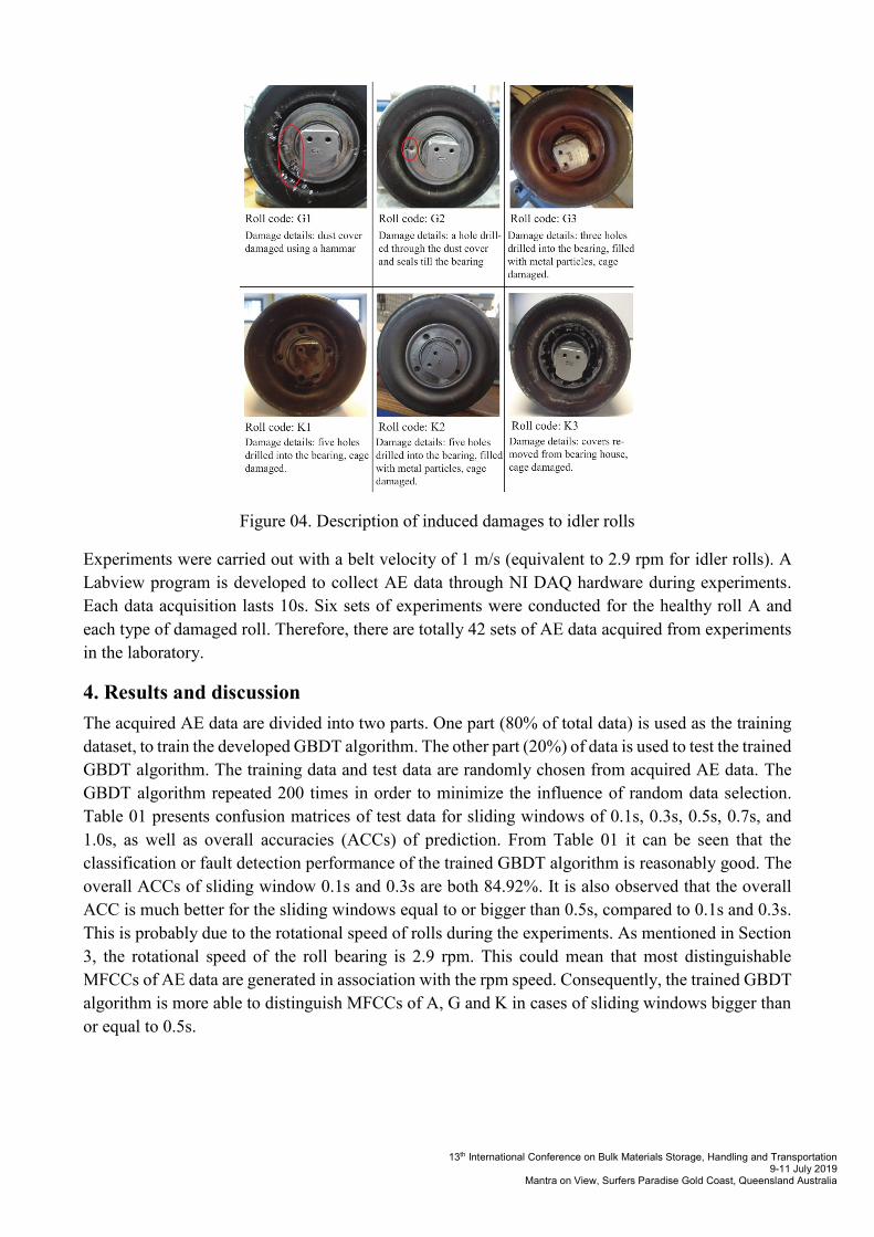
The inducement of damages to idler rolls is presented in Figure 04. Different types of damages are

induced in order to simulate different levels of roll failures. The inducement of damages to rolls G3,

K1 and K2 is similar to the way described in reference [6]. Healthy idler rolls are labelled as A.



Figure 04. Description of induced damages to idler rolls

Experiments were carried out with a belt velocity of 1 m/s (equivalent to 2.9 rpm for idler rolls). A

Labview program is developed to collect AE data through NI DAQ hardware during experiments.

Each data acquisition lasts 10s. Six sets of experiments were conducted for the healthy roll A and

each type of damaged roll. Therefore, there are totally 42 sets of AE data acquired from experiments

in the laboratory.

4. Results and discussion

The acquired AE data are divided into two parts. One part (80% of total data) is used as the training

dataset, to train the developed GBDT algorithm. The other part (20%) of data is used to test the trained

GBDT algorithm. The training data and test data are randomly chosen from acquired AE data. The

GBDT algorithm repeated 200 times in order to minimize the influence of random data selection.

Table 01 presents confusion matrices of test data for sliding windows of 0.1s, 0.3s, 0.5s, 0.7s, and

1.0s, as well as overall accuracies (ACCs) of prediction. From Table 01 it can be seen that the

classification or fault detection performance of the trained GBDT algorithm is reasonably good. The

overall ACCs of sliding window 0.1s and 0.3s are both 84.92%. It is also observed that the overall

ACC is much better for the sliding windows equal to or bigger than 0.5s, compared to 0.1s and 0.3s.

This is probably due to the rotational speed of rolls during the experiments. As mentioned in Section

3, the rotational speed of the roll bearing is 2.9 rpm. This could mean that most distinguishable

MFCCs of AE data are generated in association with the rpm speed. Consequently, the trained GBDT

algorithm is more able to distinguish MFCCs of A, G and K in cases of sliding windows bigger than

or equal to 0.5s.



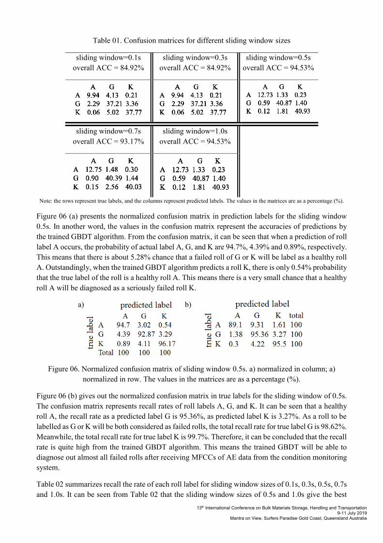
Table 01. Confusion matrices for different sliding window sizes

sliding window=0.1s

overall ACC = 84.92%

sliding window=0.3s


sliding window=0.5s


sliding window=0.7s


sliding window=1.0s


Note: the rows represent true labels, and the columns represent predicted labels. The values in the matrices are as a percentage (%).

Figure 06 (a) presents the normalized confusion matrix in prediction labels for the sliding window

0.5s. In another word, the values in the confusion matrix represent the accuracies of predictions by

the trained GBDT algorithm. From the confusion matrix, it can be seen that when a prediction of roll

label A occurs, the probability of actual label A, G, and K are 94.7%, 4.39% and 0.89%, respectively.

This means that there is about 5.28% chance that a failed roll of G or K will be label as a healthy roll

A. Outstandingly, when the trained GBDT algorithm predicts a roll K, there is only 0.54% probability

that the true label of the roll is a healthy roll A. This means there is a very small chance that a healthy

roll A will be diagnosed as a seriously failed roll K.

a) b)

Figure 06. Normalized confusion matrix of sliding window 0.5s. a) normalized in column; a)

normalized in row. The values in the matrices are as a percentage (%).

Figure 06 (b) gives out the normalized confusion matrix in true labels for the sliding window of 0.5s.

The confusion matrix represents recall rates of roll labels A, G, and K. It can be seen that a healthy

roll A, the recall rate as a predicted label G is 95.36%, as predicted label K is 3.27%. As a roll to be

labelled as G or K will be both considered as failed rolls, the total recall rate for true label G is 98.62%.

Meanwhile, the total recall rate for true label K is 99.7%. Therefore, it can be concluded that the recall

rate is quite high from the trained GBDT algorithm. This means the trained GBDT will be able to

diagnose out almost all failed rolls after receiving MFCCs of AE data from the condition monitoring

system.

Table 02 summarizes recall the rate of each roll label for sliding window sizes of 0.1s, 0.3s, 0.5s, 0.7s

and 1.0s. It can be seen from Table 02 that the sliding window sizes of 0.5s and 1.0s give the best



recall performance with given AE data in this study. It is considered that a sliding window size

between 0.5s and 1.0s is suitable for the experimental conditions in this study. Again, it is considered

to be correlated with the rotational speed (2.9 rpm) of rolls during the experiments.

Table 02. Recall rates for different sliding window sizes

Sliding window size (s)

Recall rate 0.1 0.3 0.5 0.7 1.0

roll A (%) 69.61 69.61 89.1 87.7 89.1

roll G (%) 86.82 86.82 95.36 94.5 94.5

roll K (%) 88.14 88.14 95.50 93.7 95.5

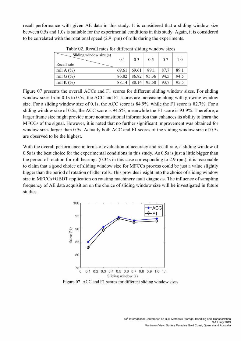
Figure 07 presents the overall ACCs and F1 scores for different sliding window sizes. For sliding

window sizes from 0.1s to 0.5s, the ACC and F1 scores are increasing along with growing window

size. For a sliding window size of 0.1s, the ACC score is 84.9%, while the F1 score is 82.7%. For a

sliding window size of 0.5s, the ACC score is 94.5%, meanwhile the F1 score is 93.9%. Therefore, a

larger frame size might provide more nontransitional information that enhances its ability to learn the

MFCCs of the signal. However, it is noted that no further significant improvement was obtained for

window sizes larger than 0.5s. Actually both ACC and F1 scores of the sliding window size of 0.5s

are observed to be the highest.

With the overall performance in terms of evaluation of accuracy and recall rate, a sliding window of

0.5s is the best choice for the experimental conditions in this study. As 0.5s is just a little bigger than

the period of rotation for roll bearings (0.34s in this case corresponding to 2.9 rpm), it is reasonable

to claim that a good choice of sliding window size for MFCCs process could be just a value slightly

bigger than the period of rotation of idler rolls. This provides insight into the choice of sliding window

size in MFCCs+GBDT application on rotating machinery fault diagnosis. The influence of sampling

frequency of AE data acquisition on the choice of sliding window size will be investigated in future

studies.

Figure 07 ACC and F1 scores for different sliding window sizes



5. Conclusions

In this study, a MFCCs+GBDT approach is proposed and developed to detect idler roll failures based

on AE data. With AE data obtained from healthy rolls and failed rolls under normal running

conditions, MFCCs are calculated and used to train a GBDT algorithm. The trained GBDT algorithm

is further verified with test data. It is found that the optimum sliding window size can be just a bit

bigger than the period of rotation of idler rolls. It is also found that the proposed MFCCs+GBDT

approach can achieve an accuracy level of 96.17% for seriously failed rolls labelled as K. The total

recall rate for true label K rolls could reach 99.7%. It can be concluded that the proposed approach is

a reliable method to detect idler roll failures based on AE data.

The limitation of this study is that the AE data samples are quite limited. For further study, vast

amounts of AE data from on-site belt conveyors will be acquired to further verify the proposed

MFCCs+GBDT appraoch.

References:

[1] W. Bartelmus and W. Sawicki, “Progress in quality assessment of conveyor idlers,” in

Proceedings of the 16th IMEKO World Congress, 2000.

[2] F. Geesmann, E. Nagy, and J. Bati, “Design of heavy-duty idlers for the upper run of belt

conveyors Part II: Engineering design of idlers,” Aufbereit. Tech., vol. 50, no. 3, pp. 4–24,

2009.

[3] A. V. Relcks, “Belt conveyor idler roll behaviors,” in Bulk Material Handling By Conveyor

Belt 7, M. A. Alspaugh, Ed. Littleton, Colo.: Society for Mining, Metallurgy, and

Exploration, 2008, pp. 35–40.

[4] Y. Pang and G. Lodewijks, “The application of RFID technology in large-scale dry bulk

material transport system monitoring,” in Proceedings of the IEEE Workshop on

Environmental Energy and Structural Monitoring Systems, 2011, pp. 5–9.

[5] X. Liu, “Prediction of belt conveyor idler performance,” Delft University of Technology,

2016.

[6] M. Fernandez et al., “Early detection and fighting of fires in belt conveyor,” 2013.

[7] J. König and O. Burkhard, “Girlandenprüfstand zur Zustandsdiagnose gebrauchter

Tragrollen,” in Proceedings of the Fachtagung Schüttgutfördertechnik “Treffpunkt für

Forschung & Praxis,” 2013.

[8] SKF, “SKF idler sound monitor kit,” 2012. [Online]. Available:

http://www.skf.com/caribbean/industry-solutions/metals/Processes/upstream-steel-

making/conveyors/SKF-idler-sound-monitor-kit.html. [Accessed: 13-Aug-2015].

[9] Health and Safety Executive, “Safety and health in mines research advisory board - Annual

review 2004,” online, 2004. [Online]. Available:

http://www.hse.gov.uk/aboutus/meetings/committees/shmrab/shmrab04b.htm. [Accessed:

15-Jan-2016].

[10] B. Ahn, J. Kim, and B. Choi, “Artificial intelligence-based machine learning considering

flow and temperature of the pipeline for leak early detection using acoustic emission,” Eng.



Fract. Mech., no. March, pp. 0–1, 2018.

[11] S. S. Tirumala, S. R. Shahamiri, A. S. Garhwal, and R. Wang, “Speaker identification

features extraction methods: A systematic review,” Expert Syst. Appl., vol. 90, pp. 250–271,

2017.

[12] V. Singh and N. Meena, “Engine fault diagnosis using DTW, MFCC and FFT,” in First

International Conference on Intelligent Human Computer Interaction, 2009.

[13] F. V. Nelwamondo, T. Marwala, and U. Mahola, “Early classifications of bearing faults

using hidden Markov models, Gaussian mixture models, Mel-Frequency cepstral coefficients

and fractals,” Int. J. Innov. Comput. Inf. Control, vol. 2, no. 6, pp. 1281–1299, 2006.

[14] Y. Zhang and A. Haghani, “A gradient boosting method to improve travel time prediction,”

Transp. Res. Part C Emerg. Technol., vol. 58, pp. 308–324, 2015.

[15] B. Mak, Y. Tam, and P. Li, “Discriminative auditory features for robust speech recognition,”

IEEE Trans. Speech Audio Process., vol. 12, no. 1, pp. 27–36, 2004.

[16] B. Logan, “Mel frequency cepstral coefficients for music modeling,” in Proceedings of the

1st International Symposium of Music Information Retrieval (ISMIR), 2000.

[17] P. D. Polur and G. E. Miller, “Effect of high-frequency spectral components in computer

recognition of dysarthric speech based on a Mel-cepstral stochastic model,” J. Rehabil. Res.

Dev., vol. 42, no. 3, p. 363, 2005.

[18] J. H. Friedman, “Stochastic gradient boosting,” Comput. Stat. Data Anal., vol. 38, no. 4, pp.

367–378, 2002.

[19] J. H. Friedman, “Greedy function approximation : A gradient boosting machine,” Ann. Stat.,

vol. 29, no. 5, pp. 1189–1232, 2001.

[20] P. Bühlmann and T. Hothorn, “Boosting algorithms: Regularization, prediction and model

fitting,” Stat. Sci., vol. 22, no. 4, pp. 477–505, 2007.

Intelligent Maintenance of Belt Conveyors Using Machine ...

Documents

Transcript of Intelligent Maintenance of Belt Conveyors Using Machine ...