Differential EvolutionA Simple Evolution Strategy for Fast Optimization

Napapan Piyasatian

Evolutionary Computation 2

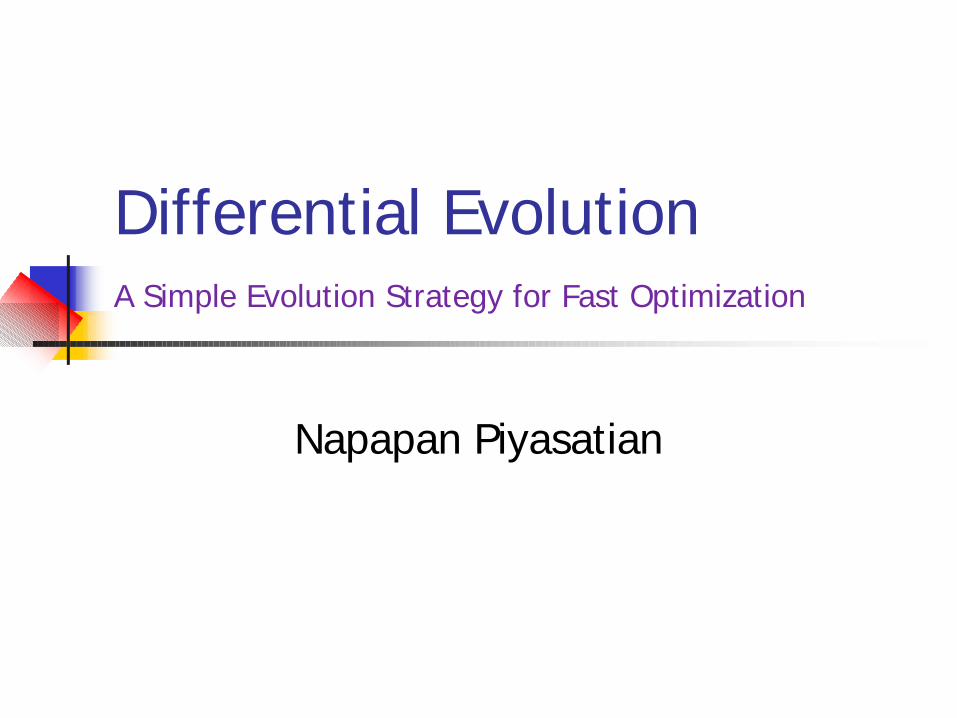
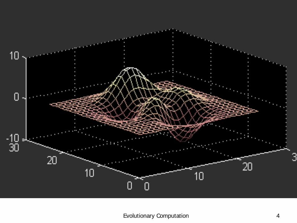
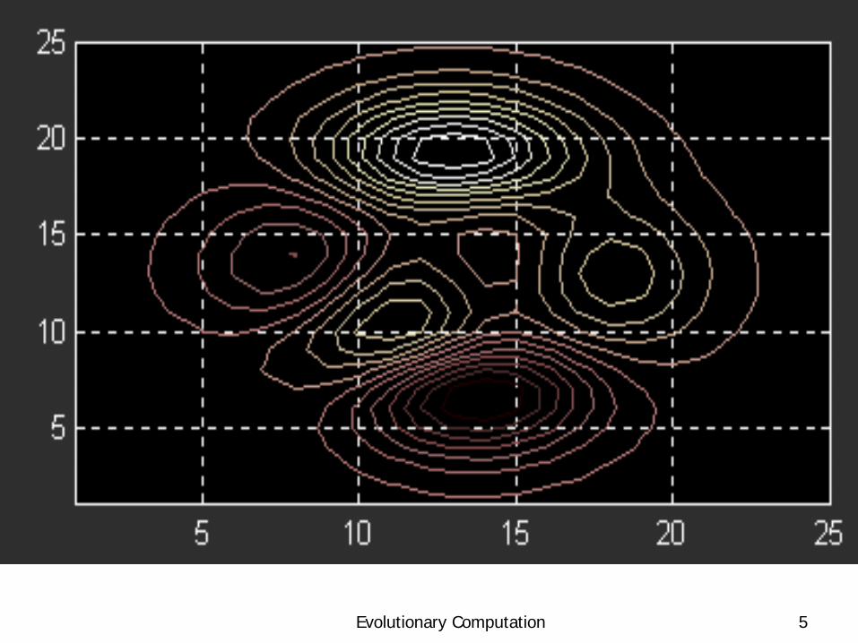
Numerical Optimization (1)

• Nonlinear objective function:¶ Many variables¶ Tortured, multidimensional topography

(response surface) with many peaks and valleys

¶ Example 1(a): f(X) = X12 + X2

2 + X32

f(Xmin) = 0, where Xmin = {0, 0, 0}

Evolutionary Computation 3

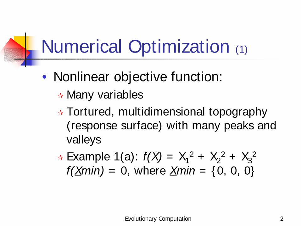
Numerical Optimization (2)

• Optimization multi-modal functions:¶ Nonrandom or deterministic search

algorithms¶ Random or stochastic algorithms (more

suitable)

Evolutionary Computation 4

Evolutionary Computation 5

Evolutionary Computation 6

Genetic Algorithms

• Fitness or cost • Initialization of a population of

candidate solutions• Mutation• Recombination or crossover• Selection

Evolutionary Computation 7

Fitness or Cost

• The value of a “Objective function” at a point

• To max. a function: the more fitness, the more optimal solutions

Evolutionary Computation 8

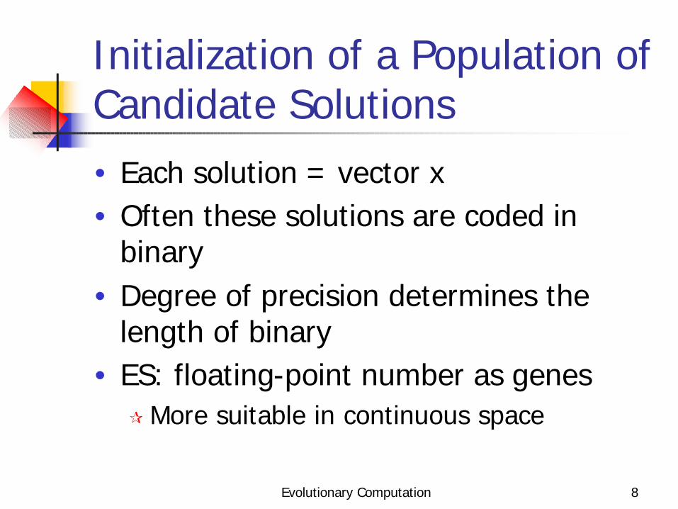
Initialization of a Population of Candidate Solutions

• Each solution = vector x• Often these solutions are coded in

binary• Degree of precision determines the

length of binary• ES: floating-point number as genes¶ More suitable in continuous space

Evolutionary Computation 9

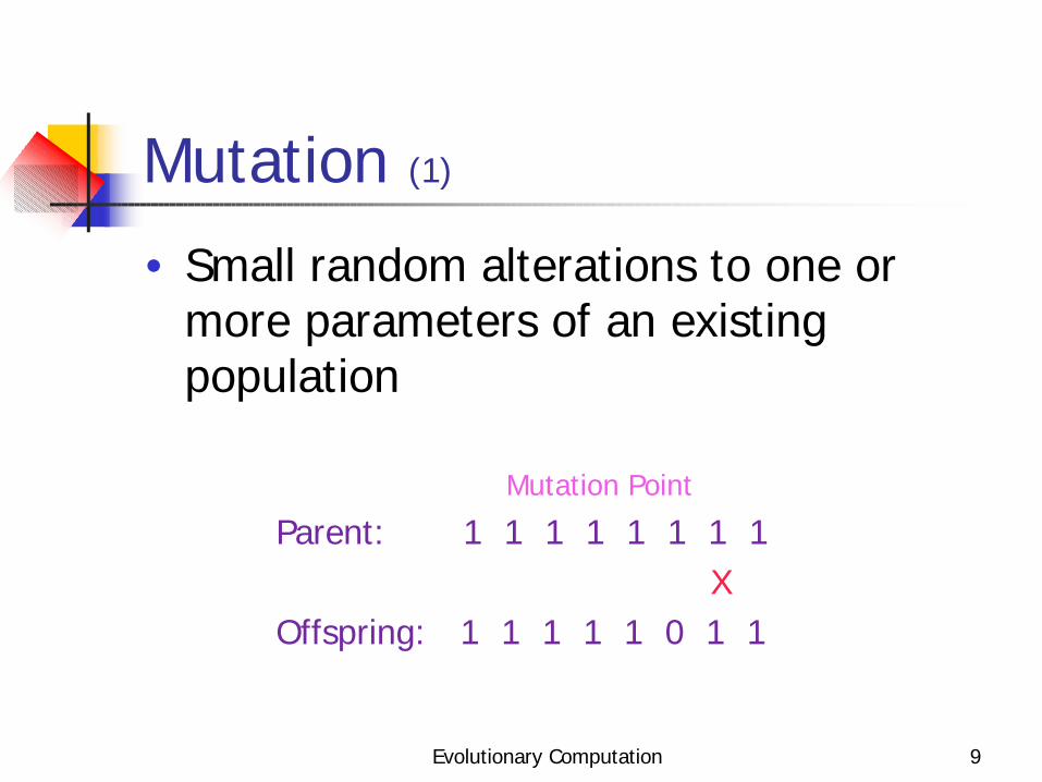
Mutation (1)

• Small random alterations to one or more parameters of an existing population

Mutation Point

Parent: 1 1 1 1 1 1 1 1 X Offspring: 1 1 1 1 1 0 1 1

Evolutionary Computation 10

Mutation (2)

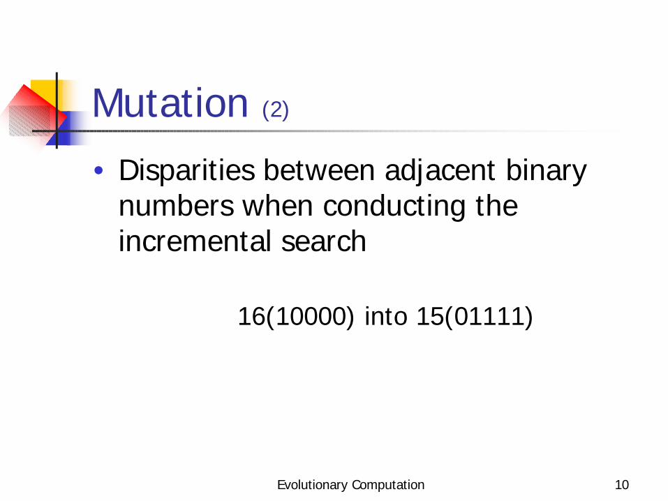
• Disparities between adjacent binary numbers when conducting the incremental search

16(10000) into 15(01111)

Evolutionary Computation 11

Mutation (3)

• Adding operation¶ The question is how much to add not

which bits to flip¶ DE: must ensure that the mutation

increment automatically scaled to the correct magnitude

Evolutionary Computation 12

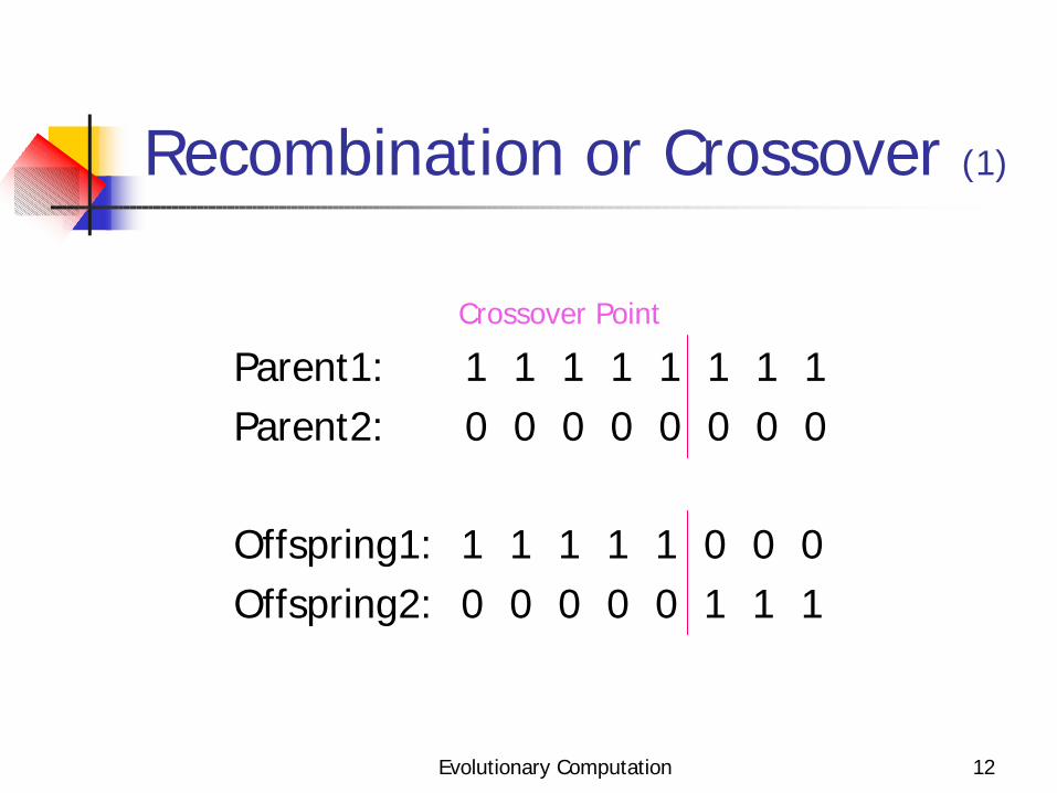
Recombination or Crossover (1)

Crossover Point

Parent1: 1 1 1 1 1 1 1 1 Parent2: 0 0 0 0 0 0 0 0

Offspring1: 1 1 1 1 1 0 0 0 Offspring2: 0 0 0 0 0 1 1 1

Evolutionary Computation 13

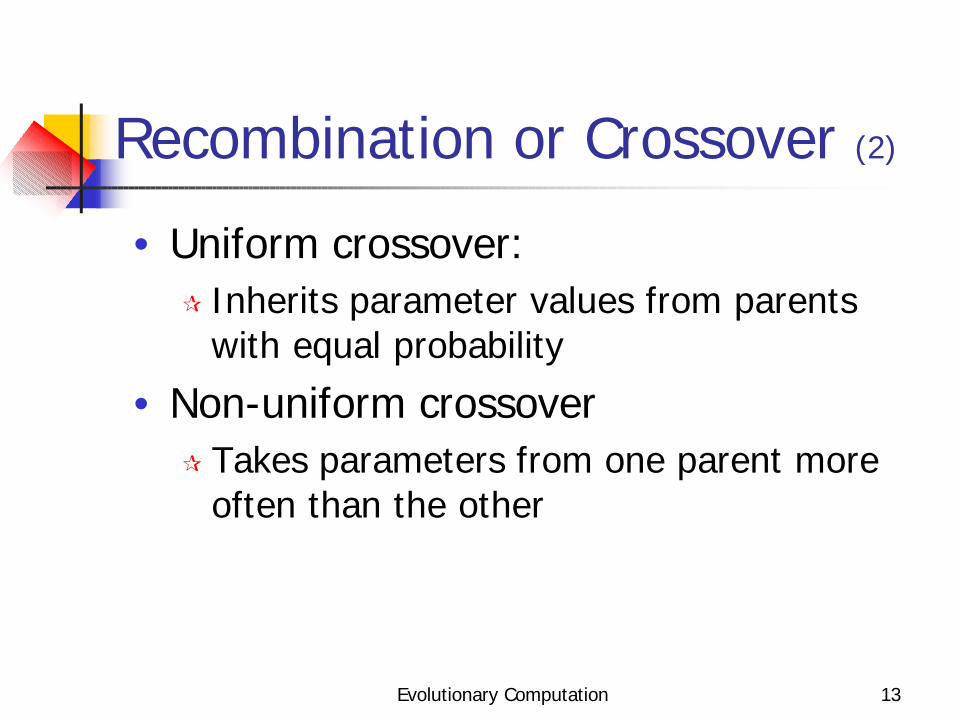
Recombination or Crossover (2)

• Uniform crossover: ¶ Inherits parameter values from parents

with equal probability

• Non-uniform crossover¶ Takes parameters from one parent more

often than the other

Evolutionary Computation 14

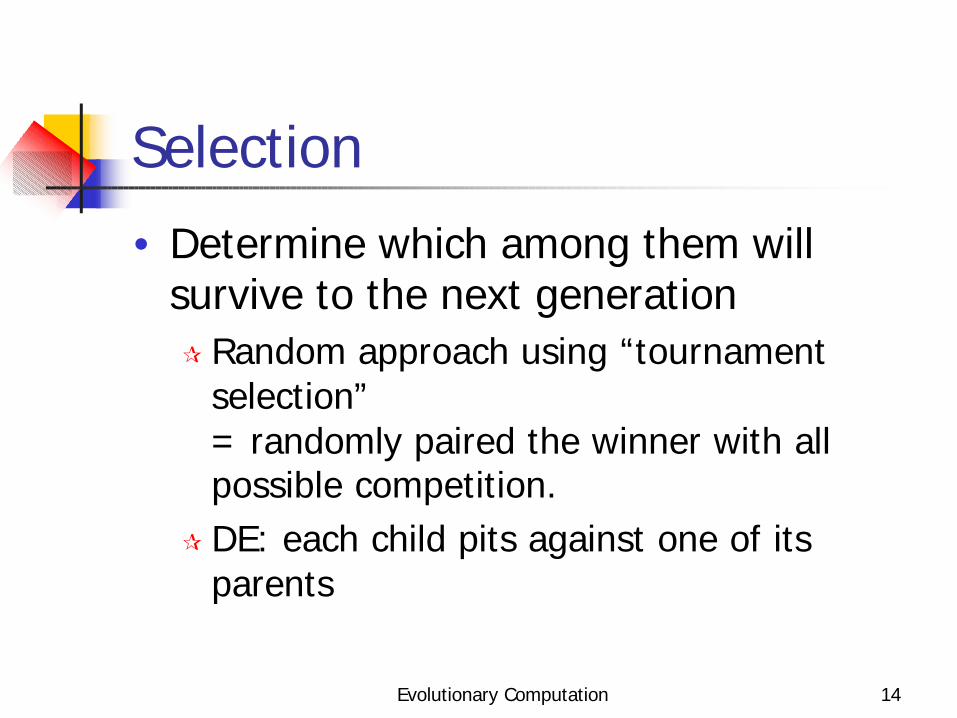
Selection

• Determine which among them will survive to the next generation¶ Random approach using “tournament

selection”= randomly paired the winner with all possible competition.

¶ DE: each child pits against one of its parents

Evolutionary Computation 15

Basic Mechanisms of DE (1)

• Initialization¶ Parameter limits should be defined¶ If not, parameter ranges should cover the

suspected optimum

Evolutionary Computation 16

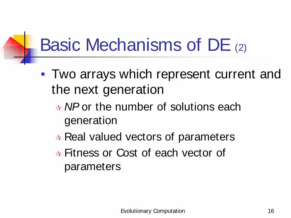
Basic Mechanisms of DE (2)

• Two arrays which represent current and the next generation¶ NP or the number of solutions each

generation¶ Real valued vectors of parameters¶ Fitness or Cost of each vector of

parameters

Evolutionary Computation 17

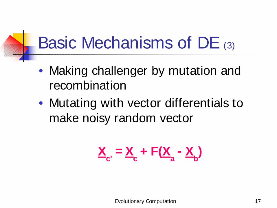
Basic Mechanisms of DE (3)

• Making challenger by mutation and recombination

• Mutating with vector differentials to make noisy random vector

Xc'

= Xc

+ F(Xa

- Xb)

Evolutionary Computation 18

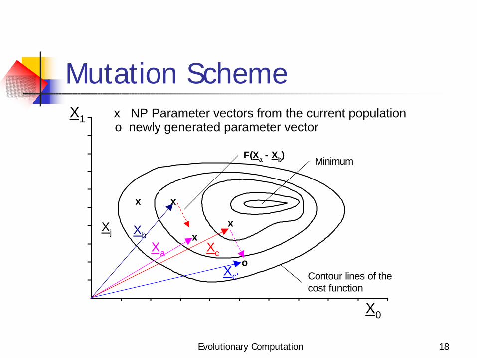
Mutation Scheme

Minimum

Contour lines of thecost function

X0

x NP Parameter vectors from the current populationo newly generated parameter vector

X1

Xj

x x

xx

o

Xb

Xa

F(Xa - Xb)

Xc

Xc'

Evolutionary Computation 19

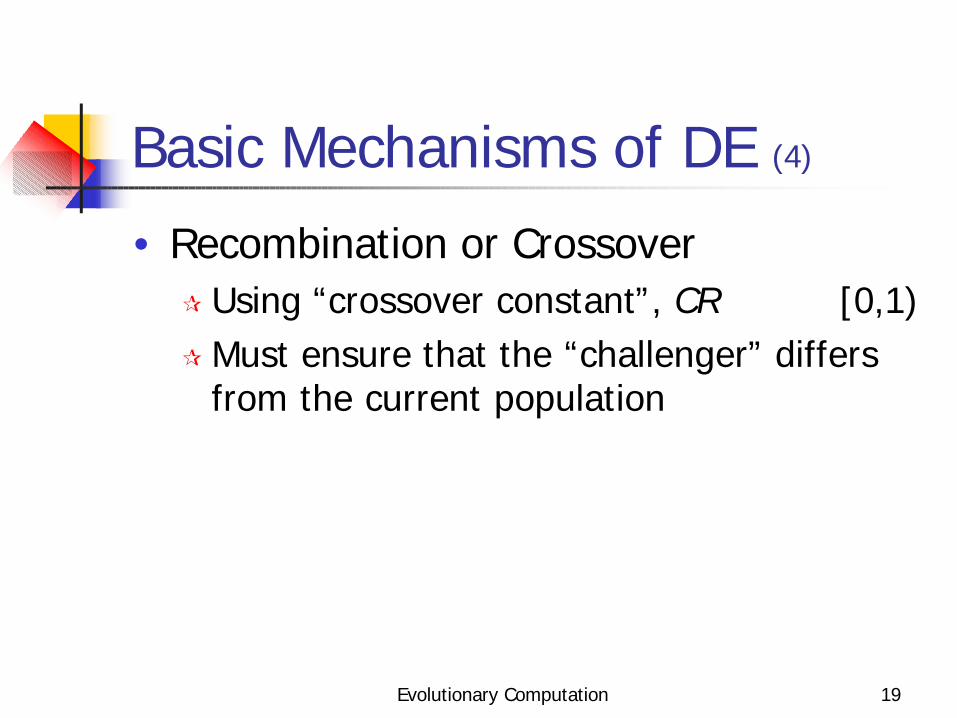
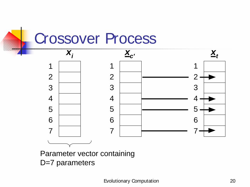
Basic Mechanisms of DE (4)

• Recombination or Crossover¶ Using “crossover constant”, CR [0,1)¶ Must ensure that the “challenger” differs

from the current population

∈

Evolutionary Computation 20

Crossover Process

1234567

xi

Parameter vector containingD=7 parameters

1234567

xc'

1234567

xt

Evolutionary Computation 21

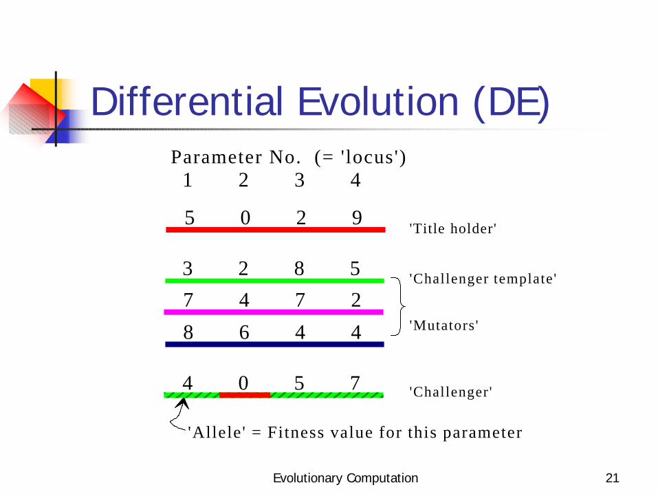
Differential Evolution (DE)Parameter No. (= 'locus')

'Allele' = Fitness value for this parameter

1 2 3 4

7 4 7 2

5 0 2 9

3 2 8 5

8 6 4 4

4 0 5 7

'Title holder'

'Challenger template'

'Mutators'

'Challenger'

Evolutionary Computation 22

A Nasty Little Function

• Non-differentiable at some points• Many local optima that partially

surrounded by very flat surface¶ Cause the solution stray outside the design

limits

Evolutionary Computation 23

Practical Advice

• NP = 5 or 10 times of number of parameter in a vector

• If solutions get stuck:¶ F = 0.5 and then increase F or NP¶ F [0.4, 1] is very effective range

• CR = 0.9 or 1 for a quick solution∈

Evolutionary Computation 24

Conclusion (1)

• Advantages¶ Immediately accessible for practical

applications¶ Simple structure¶ Ease of use¶ Speed to get the solutions¶ Robustness

Evolutionary Computation 25

Conclusion (2)

• Need¶ A way to quantify the quality of the

potential solutions “Fitness function” or “Objective function”