Diagnosing model error in canopy-atmosphere exchange using

empirical orthogonal function analysis

Darren T. Drewry1 and John D. Albertson1,2

Received 11 August 2005; revised 21 January 2006; accepted 2 March 2006; published 27 June 2006.

[1] The application of complex land surface models to long-term estimation of water,energy, and CO2 exchange suffers from possible static parameterization of inherently time-varying properties. This paper presents a method by which structural (i.e., spatial)patterns in model output errors can be identified and associated with errors in a singleparameter or set of interacting parameters. We focus on CO2 concentration profiles as theobserved quantity containing spatial information on model performance. The core of themethod relies on the empirical orthogonal function (EOF) analysis of an ensemble ofmodel error profiles produced by synthetically inducing parameter biases. EOF analysesof the error profiles associated with photosynthetic capacity, stomatal conductance,radiation interception, soil respiration, and turbulent mixing parameters concentratedgreater than 94% of the error pattern variability in the first two EOFs, producing verycompact (two member) basis sets. Application of the EOFs to the identification ofparameter error sources was performed with three sets of synthetic tests. The method wasbroadly successful at identifying the primary error source when one or two error sourceswere present, using single-parameter basis sets. Two-parameter basis sets were able toidentify strongly interacting parameter errors (i.e., errors of approximately equalmagnitude). Environmental classification of photosynthetically active radiation and windspeed regimes was effective at untangling error influences for the tightly coupledphotosynthetic, radiation, and stomatal conductance parameters. Data analysis ofmeasured concentration profiles was used to derive the environmental classes.

Citation: Drewry, D. T., and J. D. Albertson (2006), Diagnosing model error in canopy-atmosphere exchange using empirical

orthogonal function analysis, Water Resour. Res., 42, W06421, doi:10.1029/2005WR004496.

1. Introduction

[2] Estimation of the exchange of water vapor, energyand carbon dioxide (CO2) between the land surface and theoverlying atmosphere has become a major focus forresearchers attempting to quantify the impact of forestecosystems on the global water and carbon budgets. Re-cently, with long-term eddy covariance flux records becom-ing available, examination of the seasonal-to-annualvariability of the processes driving land-atmosphere ex-change, at scales ranging from a single, homogeneous standto more extensive and heterogeneous sites, has receivedincreasing attention. Several factors have been identified ascauses of net ecosystem exchange (NEE) variation overtimescales of one month or more. These include droughtinduced water stress [Baldocchi, 1997; Ellsworth, 2000;Wilson et al., 2000a; Hollinger et al., 2004], leaf age andphysiological change [Sullivan et al., 1997; Chen et al.,1999; Ellsworth, 2000; Wilson et al., 2000a], acclimation tolight [Middleton et al., 1997; Morecroft and Roberts, 1999]and environmental conditions [Greco and Baldocchi, 1996;

Baldocchi et al., 1997; Chen et al., 1999; Lloyd et al., 2002;Hollinger et al., 2004], and changes in ambient CO2

concentration [Ellsworth, 1999] and soil temperature[Middleton et al., 1997].[3] With the increasing need for accurate, long-term

estimation of canopy-atmosphere exchange, the challengepresented by the temporal variability of vegetation func-tioning has driven the growth in mechanistic detail andcomplexity of models designed to estimate land-atmospherefluxes of CO2, water vapor and energy. One modelingframework that has been broadly used as a tool for hypoth-esis testing and flux estimation is based on the verticaldiscretization of a plant canopy into multiple layers. Thisframework, referred to here as a multilayer canopy processmodel (MLCPM), consists of a set of coupled componentsubmodels representing the physical and biological processesgoverning mass and energy exchanges across the canopy-atmosphere interface. Models of this type have provenrelatively accurate with respect to net (i.e., vertically inte-grated) flux estimation across a broad range of ecosystems[e.g., Baldocchi and Harley, 1995; Leuning et al., 1995; Guet al., 1999; Lai et al., 2000b; Pyles et al., 2000; Styles etal., 2002]. Despite their broad applicability, unique param-eterizations are required in each case [Wullschleger, 1993].Most often these parameters are treated as static values,despite being known to vary seasonally and interannually,as canopy structure [Pinard and Wilson, 2001; Baldocchi etal., 2002], leaf age [Wilson et al., 2000a, 2001], and

1Department of Civil and Environmental Engineering, Duke University,Durham, North Carolina, USA.

2Nicholas School of the Environment and Earth Sciences, DukeUniversity, Durham, North Carolina, USA.

Copyright 2006 by the American Geophysical Union.0043-1397/06/2005WR004496

W06421

WATER RESOURCES RESEARCH, VOL. 42, W06421, doi:10.1029/2005WR004496, 2006

1 of 13

environmental conditions vary [Ellsworth, 2000; Law et al.,2000; Wilson et al., 2000b; Cai and Dang, 2002; Medlyn etal., 2002; Xu and Baldocchi, 2003]. This limits the appli-cability of MLCPMs to short-term integrations with similarenvironmental conditions to those for which the submodelparameters were measured.[4] Recently, methodologies have been presented to op-

timize static parameter values through the minimization ofresiduals between modeled fluxes and concentrations andthose measured within and above plant canopies. Styles etal. [2002] optimized nine MLCPM parameter values againstmeasured scalar concentrations, and concluded the modelcould not significantly distinguish the parameter influences,resulting in potential interdependencies among the opti-mized values. Using the CSIRO biospheric model andmeasured fluxes of CO2, water vapor and heat in a nonlinearinversion framework, Wang et al. [2001] found that amaximum of three or four parameters could be indepen-dently resolved. Strong correlation between parameters,similar effects of parameter perturbations on model outputs,and model insensitivity to specific parameters were allreasons for the limitation.[5] Franks et al. [1997] note that multiple sets of param-

eters may achieve an optimization goal equally well in acomplex land-atmosphere scheme (i.e., the equifinalityproblem). Monte Carlo–based methods have been devel-oped to deal with equifinality by estimating the uncertaintyof models and parameter sets, notably the GLUE method-ology of Beven and Freer [2001] and the Metropolisalgorithm of Kuczera and Parent [1998]. Multiobjectiveoptimization has also been applied successfully to deal withuncertainty in large parameter spaces [e.g., Gupta et al.,1999; Mackay et al., 2003]. However, to our knowledge, noattempt has been made to examine spatial error structures inthe predictions associated with specific model errors as away to select the most likely sources of error for use in anoptimization scheme.[6] This paper presents a method by which structural (i.e.,

spatial) patterns in model output errors can be identified andassociated with errors in a single, or set of interacting,parameters. The core of the method relies on the empiricalorthogonal function (EOF) analysis of model error struc-tures produced by synthetically inducing specific parameterbiases. EOF analysis produces an orthogonal decompositionof a spatial covariance matrix, in this case model errorcovariances, information critical to the success of moderndata assimilation systems, [e.g., Reichle et al., 2001;Margulis and Entekhabi, 2003]. The orthogonal nature ofthe EOF patterns allows them to naturally form basis setsonto which model/data residuals may be projected. Themethod is applied to the identification of the primarysource(s) of parameter error in modeled canopy sublayerCO2 concentration profiles through a set of synthetic experi-ments in which single and multiple error source cases areconsidered. Concentration profiles are a data source primar-ily collected to calculate mass storage (e.g. CO2) within thecanopy airspace [Hollinger et al., 1994; Baldocchi et al.,1996; Lai et al., 2000a]. We propose here the use of residualconcentration profiles as a vertical gauge of MLCPMfidelity.[7] Successful MLCPM validations for short time periods,

and studies demonstrating the divergence of modeled and

measured fluxes at longer timescales, point to model biascaused by parameter error as a major concern [Baldocchiand Wilson, 2001; Katul et al., 2001]. In this preliminarystudy, potential error sources are limited to parametervalues, omitting consideration of measurement error andmodel structural error. We also address the potential forconditioning the analysis on background environmentalconditions (e.g. photosynthetically active radiation andwind speed) as a means to separate the effects of differenterror sources.

2. Theory

2.1. Empirical Orthogonal Function (EOF) Analysis

2.1.1. General Overview and Example Application[8] EOF analysis, also known as Principal Component

analysis, owes its origins to Pearson [1901] and Hotelling[1933]. The technique was originally introduced into mete-orology [Lorenz, 1956] as a method for extracting thedominant modes of spatial variability in meteorologicalfields. The spatial patterns optimally describe the varianceof the original data set [von Storch and Zwiers, 1999], suchthat, in many cases, a large fraction of the degrees offreedom of the original data set can be eliminated asunimportant, while retaining the majority of the informationcontained in the original data set.[9] We examine the properties of EOF analysis by

considering an application to a set of measured CO2

concentration profiles collected at 0.75, 1.5, 3.5, 5.5, 7.5,9.5, 11.5, 13.5, and 15.5 m above the soil surface in theDuke Forest Loblolly pine stand between the months ofApril and October in 2000. Details concerning the datacollection methodology are given by Lai et al. [2000a,2000b] and Siqueira et al. [2000]. Leaf area density profiles(L) defined the canopy height to be 16 meters.[10] An r-by-n data matrix, D, is constructed such that the

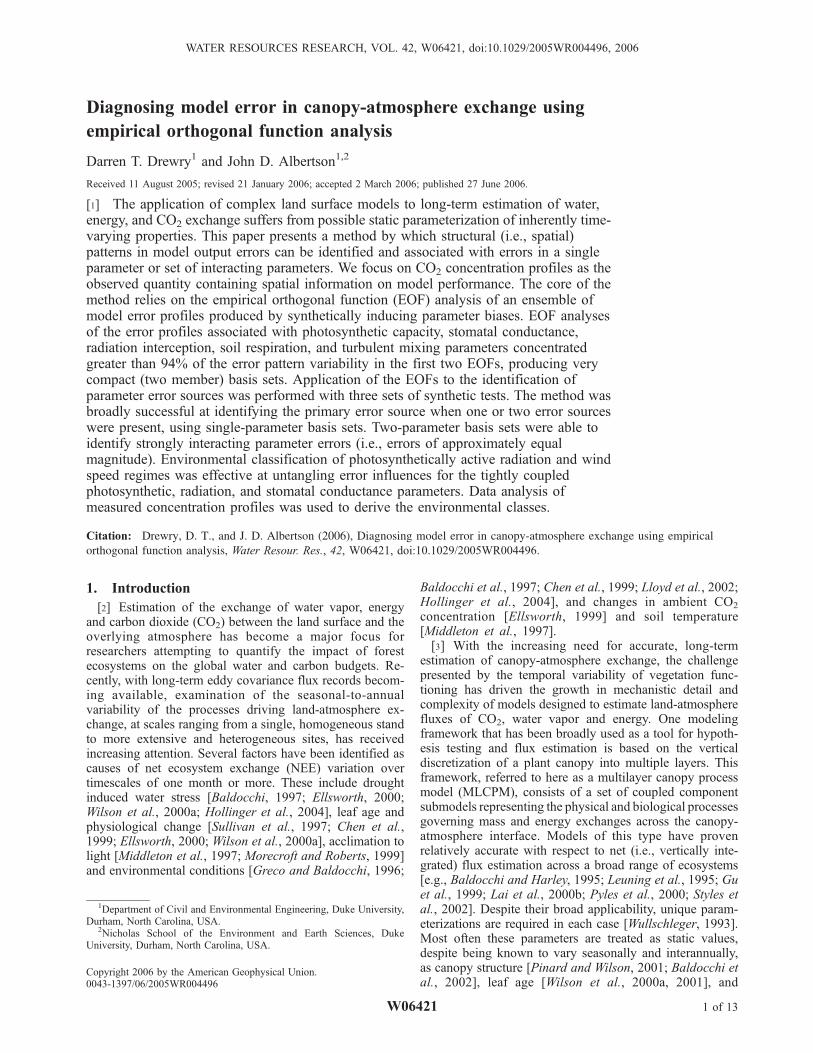
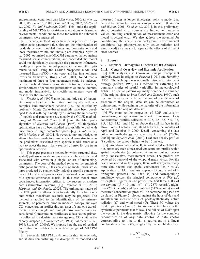
n columns are each a measured concentration profile with rspatial coordinates (z) collected at unique, but not neces-sarily consecutive, measurement times. The profiles arecentered by removal of the temporal mean vector. For thecases considered in this paper, there will always be manymore data vectors than spatial coordinates (i.e., r � n).Application of EOF analysis expands D into a set of rorthogonal patterns, the EOFs (F), and correspondingamplitude vectors, the principal components or PCs (w),of length n. Figures 1a–1c present the first three EOFs ofthe daytime (Q > 10 mmol m�2 s�1, 2879 records), night-time (2295 records) and the combined (5174 records) sets ofmeasured concentration profiles. The corresponding PCs aredisplayed in Figure 2, plotted against the hour of day andsimultaneous measurements of photosynthetically activeradiation (Q) and wind speed (U). These PC values areused to partition Q and U into environmental classes in thesynthetic experiments that follow. The full set of EOFs spanthe vectors in the data matrix, allowing for the completereconstruction of any data vector. A data vectorcorresponding to time t, dt, is equivalent to a linearcombination of the EOFs, weighted by the amplitudes for t.

dt ¼Xr

k¼1

wk tð Þfk ð1Þ

2 of 13

W06421 DREWRY AND ALBERTSON: DIAGNOSING LAND-ATMOSPHERE MODEL ERROR W06421

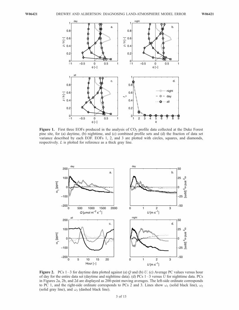
Figure 1. First three EOFs produced in the analysis of CO2 profile data collected at the Duke Forestpine site, for (a) daytime, (b) nighttime, and (c) combined profile sets and (d) the fraction of data setvariance described by each EOF. EOFs 1, 2, and 3 are plotted with circles, squares, and diamonds,respectively. L is plotted for reference as a thick gray line.

Figure 2. PCs 1–3 for daytime data plotted against (a) Q and (b) U. (c) Average PC values versus hourof day for the entire data set (daytime and nighttime data). (d) PCs 1–3 versus U for nighttime data. PCsin Figures 2a, 2b, and 2d are displayed as 200-point moving averages. The left-side ordinate correspondsto PC 1, and the right-side ordinate corresponds to PCs 2 and 3. Lines show w1 (solid black line), w2

(solid gray line), and w3 (dashed black line).

W06421 DREWRY AND ALBERTSON: DIAGNOSING LAND-ATMOSPHERE MODEL ERROR

3 of 13

W06421

Three concentration profile reconstructions, using the EOFsin Figure 1a, are presented in Figure 3.[11] The EOFs can be shown to be the eigenvectors of the

sample spatial covariance matrix of D [von Storch andZwiers, 1999]. The jth eigenvalue, lj, is the variance ofthe data set described by Fj [von Storch, 1999]. The fractionof the variance (fv) that can be attributed to Fj is calculatedas

fv jð Þ ¼ lj

,Prk¼1

lk

: ð2Þ

Plots of fv in Figure 1d display a rapid decrease invariability described by each EOF, with the first EOFcontaining approximately 88% of data set variability, andthe first three EOFs describing almost all of the profilevariation. The amplitude vector of the kth EOF, Wk, iscalculated as

Wk ¼ FTkD: ð3Þ

The optimality of EOF analysis concentrates data variancein the first few spatial patterns. This allows the truncation ofthe series in (1), keeping only the first few significantpatterns, while effectively capturing the majority of thesignal in the data set.2.1.2. Multilayer Canopy Process Model Formulation[12] The focus of this study is to demonstrate the effects

of parameter perturbations on the vertical geometry ofmodel solutions, and to use the unique spatial structuresassociated with errors in each parameter, or set of param-eters, to deduce the primary source of model error. AnMLCPM capable of producing a solution of the verticallyresolved radiation, wind speed, air temperature, scalarconcentration and scalar source/sink strength profiles withinthe canopy was used to produce the error patterns and testthe method described below. Model inputs include meteo-rological forcing at the canopy top, a leaf area densityprofile, and canopy-specific component submodel parame-ter values. While variation in component submodel formu-lations exist, a large number of studies have demonstratedthe ability of MLCPMs to capture reasonably well the half-

hour variability in canopy top fluxes when rigorous param-eterization is performed under conditions similar to thosefor which the model is applied [Baldocchi and Harley,1995; Leuning et al., 1995; Williams et al., 1996; Gu etal., 1999; Lai et al., 2000b; Styles et al., 2002; Ogee et al.,2003]. In the present study the MLCPM structure was keptsimple and general, and is based primarily on that usedpreviously to model the Duke Forest loblolly pine canopy[Lai et al., 2000a, 2000b]. For brevity, we refer the reader tothese studies for details regarding the model formulationand parameterization. Only those equations related to theparameters being investigated, or deviations in formulationfrom these studies, are presented here.[13] A brief description of the component submodel

formulations critical to the error determination methodologyfollows. The wind speed profile is computed using thesteady state and horizontally homogeneous mean momen-tum equation,

�KM

d2U

dz2� dKM

dz

dU

dzþ 1

2CdLU jU j ¼ 0; ð4Þ

with a K theory closure for the Reynolds stress and aclosure for the aerodynamic force dependent on the dragcoefficient (Cd) and L [Poggi et al., 2004]. Turbulent scalartransport is similarly computed using the temporallyaveraged conservation of mass equation, assuming negli-gible scalar storage [Poggi et al., 2004]. The eddydiffusivity (KM) is computed using the K theory closure

KM ¼ l2mixdU

dz

��������; ð5Þ

with a simple mixing length (lmix) model,

lmix ¼a � h z < dð Þ

a � hþ 0:4 � z� dð Þ z dð Þ

8<: ; ð6Þ

and d being the zero-plane displacement height [Katul et al.,2004; Poggi et al., 2004]. The parameter a is static anddetermined by calibration.

Figure 3. Reconstructions of three measured CO2 concentration profiles using the first one (solidblack line), two (dashed black line), and three (dotted black line) daytime EOFs. The measured profilesare displayed as thick gray lines. The day of year and time of each profile measurement are labeled onthe subplot as well as the measured photosynthetically active radiation (Q) and wind speed (U) (in[mmol m�2 s�1] and [m s�1], respectively).

4 of 13

W06421 DREWRY AND ALBERTSON: DIAGNOSING LAND-ATMOSPHERE MODEL ERROR W06421

[14] The radiation submodel algorithms compute sepa-rately the vertical interception of both direct beam anddiffuse radiation in short- and long-wave bands [Campbelland Norman, 1998]. The extinction coefficient for beamradiation (Kb),

Kb yð Þ ¼ b �ffiffiffiffiffiffiffiffiffiffiffiffiffiffiffiffiffiffiffiffiffiffiffiffiffiffiy2 þ tan2 yð Þ

pyþ 1:774 � yþ 1:182ð Þ�0:733

; ð7Þ

depends on solar zenith angle (y) and the geometry of theleaf angle distribution (y). A multiplicative factor (b) is usedin this equation as a parameter value that may induce errorinto the radiation submodel.[15] The model of photosynthetic CO2 uptake [Farquhar

et al., 1980; Collatz et al., 1991] considers the biochemicallimitations associated with electron transport (Aj) andRubisco activity (Ac),

Ac ¼V ci � Gð Þ

ci þ Kc 1þ O2½ �=Ko2ð Þ ; ð8Þ

where G* is the light compensation point for CO2

assimilation, Kc and Ko2 are Michaelis constants for thefixation of CO2 and oxygen inhibition, respectively, [O2] isthe ambient oxygen concentration, and V is a parameterrepresenting Rubisco activity at 25C.[16] A linear relationship between stomatal conductance

(gs) and the product of photosynthetic uptake (An), relativehumidity at the leaf surface (hs) and CO2 concentration atthe leaf surface (Cs), couples stomatal dynamics to photo-synthesis [Ball et al., 1987]:

gs ¼ mAnhs

Cs

þ b0: ð9Þ

The slope (m) and intercept (b0) are empirically determinedparameters. Leaf energy balance is calculated using alinearized form of the leaf energy budget [Campbell andNorman, 1998], and the iterative technique of Tracy et al.[1984].[17] Soil respiration flux (fr) was modeled as an expo-

nential function of soil temperature (Ts),

fr ¼ R10 � exp 308:56 � 1

56:02� 1

Ts � 227:13

�� ; ð10Þ

with R10 the respiration rate at 10C [Lloyd and Taylor,1994]. Energy fluxes at the soil surface were calculatedfrom algorithms presented by Noilhan and Mahfouf [1996].[18] Six model parameters, associated with photosynthetic

uptake (V), canopy turbulent dispersion (a and Cd), radia-tion interception (b), stomatal conductance (m) and soilrespiration (R10), were chosen to study the effects ofparameter error on model error structures. These six param-eters will be referred to as candidate parameters in thefollowing methodological description. The control valuesused for these parameters were

pc ¼ V c;ac;Ccd; b

c;mc;Rc10

� �¼ 59; 0:1; 0:2; 1:0; 5:9; 1:8f g;

ð11Þ

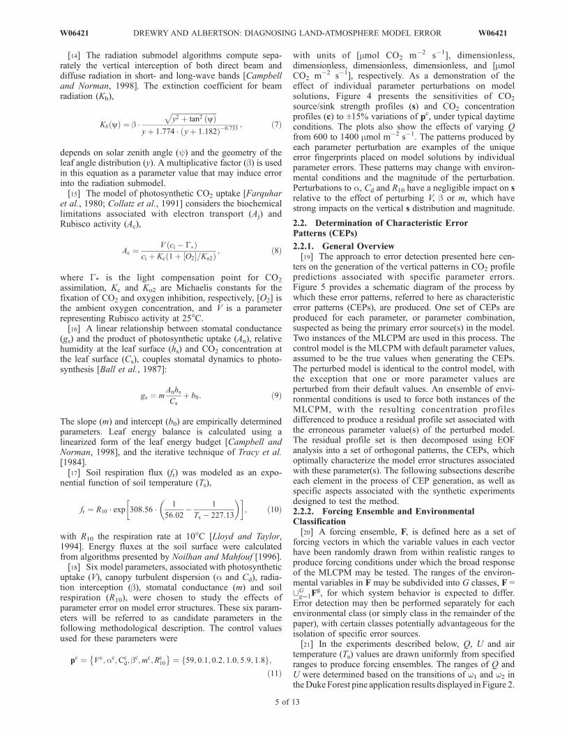
with units of [mmol CO2 m�2 s�1], dimensionless,dimensionless, dimensionless, dimensionless, and [mmolCO2 m�2 s�1], respectively. As a demonstration of theeffect of individual parameter perturbations on modelsolutions, Figure 4 presents the sensitivities of CO2

source/sink strength profiles (s) and CO2 concentrationprofiles (c) to ±15% variations of pc, under typical daytimeconditions. The plots also show the effects of varying Qfrom 600 to 1400 mmol m�2 s�1. The patterns produced byeach parameter perturbation are examples of the uniqueerror fingerprints placed on model solutions by individualparameter errors. These patterns may change with environ-mental conditions and the magnitude of the perturbation.Perturbations to a, Cd and R10 have a negligible impact on srelative to the effect of perturbing V, b or m, which havestrong impacts on the vertical s distribution and magnitude.

2.2. Determination of Characteristic ErrorPatterns (CEPs)

2.2.1. General Overview[19] The approach to error detection presented here cen-

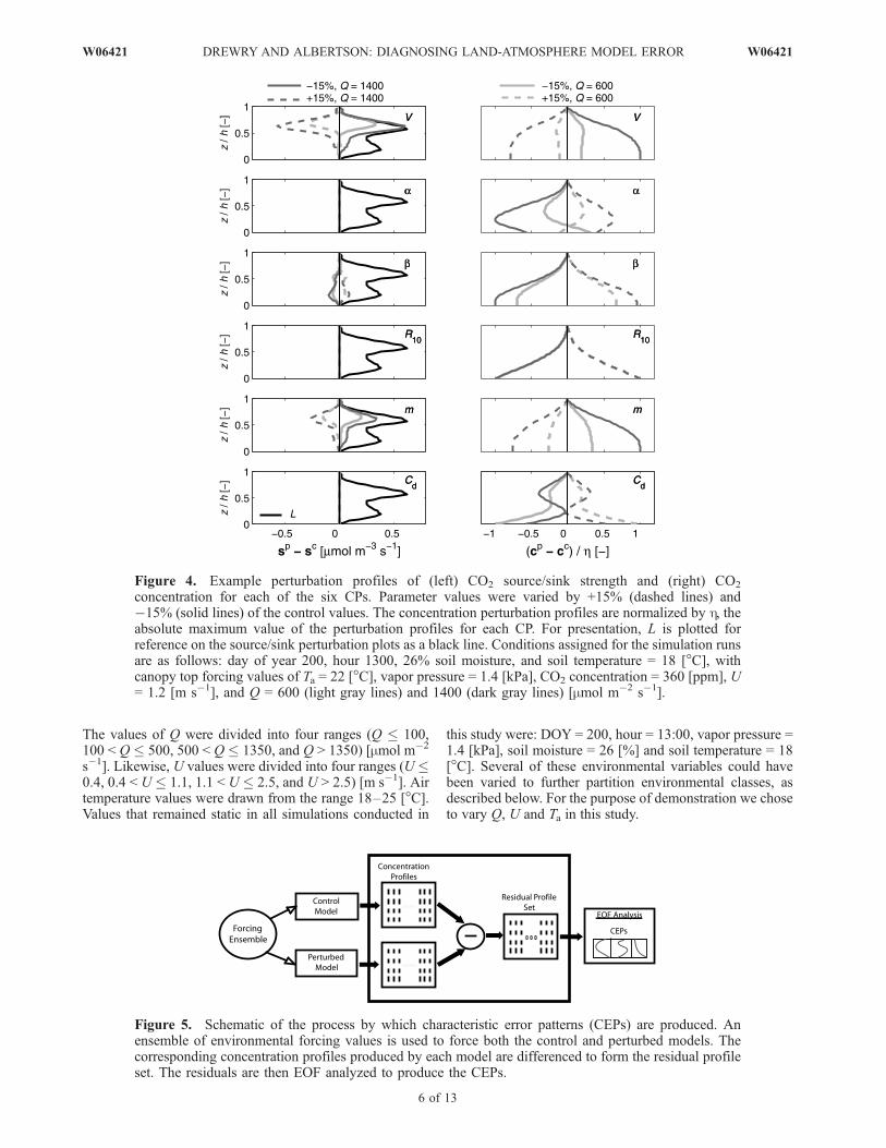
ters on the generation of the vertical patterns in CO2 profilepredictions associated with specific parameter errors.Figure 5 provides a schematic diagram of the process bywhich these error patterns, referred to here as characteristicerror patterns (CEPs), are produced. One set of CEPs areproduced for each parameter, or parameter combination,suspected as being the primary error source(s) in the model.Two instances of the MLCPM are used in this process. Thecontrol model is the MLCPM with default parameter values,assumed to be the true values when generating the CEPs.The perturbed model is identical to the control model, withthe exception that one or more parameter values areperturbed from their default values. An ensemble of envi-ronmental conditions is used to force both instances of theMLCPM, with the resulting concentration profilesdifferenced to produce a residual profile set associated withthe erroneous parameter value(s) of the perturbed model.The residual profile set is then decomposed using EOFanalysis into a set of orthogonal patterns, the CEPs, whichoptimally characterize the model error structures associatedwith these parameter(s). The following subsections describeeach element in the process of CEP generation, as well asspecific aspects associated with the synthetic experimentsdesigned to test the method.2.2.2. Forcing Ensemble and EnvironmentalClassification[20] A forcing ensemble, F, is defined here as a set of

forcing vectors in which the variable values in each vectorhave been randomly drawn from within realistic ranges toproduce forcing conditions under which the broad responseof the MLCPM may be tested. The ranges of the environ-mental variables in F may be subdivided into G classes, F =[Gg¼1F

g, for which system behavior is expected to differ.Error detection may then be performed separately for eachenvironmental class (or simply class in the remainder of thepaper), with certain classes potentially advantageous for theisolation of specific error sources.[21] In the experiments described below, Q, U and air

temperature (Ta) values are drawn uniformly from specifiedranges to produce forcing ensembles. The ranges of Q andU were determined based on the transitions of w1 and w2 intheDuke Forest pine application results displayed in Figure 2.

W06421 DREWRY AND ALBERTSON: DIAGNOSING LAND-ATMOSPHERE MODEL ERROR

5 of 13

W06421

The values of Q were divided into four ranges (Q � 100,100 < Q � 500, 500 < Q � 1350, and Q > 1350) [mmol m�2

s�1]. Likewise, U values were divided into four ranges (U �0.4, 0.4 < U � 1.1, 1.1 < U � 2.5, and U > 2.5) [m s�1]. Airtemperature values were drawn from the range 18–25 [C].Values that remained static in all simulations conducted in

this study were: DOY = 200, hour = 13:00, vapor pressure =1.4 [kPa], soil moisture = 26 [%] and soil temperature = 18[C]. Several of these environmental variables could havebeen varied to further partition environmental classes, asdescribed below. For the purpose of demonstration we choseto vary Q, U and Ta in this study.

Figure 5. Schematic of the process by which characteristic error patterns (CEPs) are produced. Anensemble of environmental forcing values is used to force both the control and perturbed models. Thecorresponding concentration profiles produced by each model are differenced to form the residual profileset. The residuals are then EOF analyzed to produce the CEPs.

Figure 4. Example perturbation profiles of (left) CO2 source/sink strength and (right) CO2

concentration for each of the six CPs. Parameter values were varied by +15% (dashed lines) and�15% (solid lines) of the control values. The concentration perturbation profiles are normalized by h, theabsolute maximum value of the perturbation profiles for each CP. For presentation, L is plotted forreference on the source/sink perturbation plots as a black line. Conditions assigned for the simulation runsare as follows: day of year 200, hour 1300, 26% soil moisture, and soil temperature = 18 [C], withcanopy top forcing values of Ta = 22 [C], vapor pressure = 1.4 [kPa], CO2 concentration = 360 [ppm], U= 1.2 [m s�1], and Q = 600 (light gray lines) and 1400 (dark gray lines) [mmol m�2 s�1].

6 of 13

W06421 DREWRY AND ALBERTSON: DIAGNOSING LAND-ATMOSPHERE MODEL ERROR W06421

[22] Five classes of Q and U were chosen for theexperimental tests and are indicated in Table 1. Of the 16Q/U classes, we limit our discussion here to daytime valuesin which the canopy is not well mixed, eliminating theregions in which Q � 100 and U > 2.5. Of the remainingclasses, we focus on the five in which most data fall, aswind speeds typically increase during the day with radia-tion. These five classes are indicated in Table 1.2.2.3. Forward Model[23] The MLCPM, or simply the forward model (f),

accepts as input an ensemble of environmental forcingconditions, F = {fiji = 1,. . .,nf}, and a vector of componentsubmodel parameter values, p = {piji = 1,. . .,np}. Eachvector f in the forcing ensemble contains the values of themeteorological variables and other environmental inputsnecessary to run the MLCPM. The forward model producesas output a set of CO2 concentration profiles, D = {diji =1,. . ., nf}, one for each forcing vector:

D ¼ f F; pð Þ: ð12Þ

2.2.4. Control Profile Set[24] MLCPM formulations require a large number of

component submodel parameters, each with some level ofuncertainty and temporal variability. A subset of these arechosen to be the candidate parameters (CPs), those param-eters whose values have a large degree of uncertainty, areknown to vary considerably, or for which the sensitivity ofmodel outputs is high. The CPs have control values, pc ={pi

cji = 1,. . .,nc} (see equation (11)), where nc is thenumber of CPs. The set of control profiles produced byrunning the forward model with F and pc, i.e., Dc =f(F,pc), is

Dc ¼

dc 1; 1ð Þ � � � dc 1; nfð Þ

..

. ...

dc r; 1ð Þ � � � dc r; nfð Þ

266664

377775 ¼ dc1; . . . ; d

cnf

h i: ð13Þ

2.2.5. Perturbed Parameter Sets[25] An input parameter vector for the perturbed model,

pp, is identical to pc with a subset of the CPs, n � pc,perturbed a fractional amount d. Each CP has a range ofallowable perturbations from which d is drawn uniformly. Aunique value of d is drawn for each member of f and eachperturbed parameter. Maximum perturbation magnitudes foreach CP are based on knowledge of reasonable ranges of theCPs, or the degree to which model outputs are sensitive toperturbations. An example of a perturbation vector with n ={pi

c} is given in equation (14), and the entire set of

perturbation vectors necessary to produce the perturbedprofile set, Dn

p = f(F,Pnp), is given in equation (15).

ppn;j ¼ pc1; . . . ; p

ci þ di;jpci ; . . . ; p

cncji 2 1; . . . ; nc; j 2 1; . . . ; nf

n oð14Þ

Ppn ¼ p

pn;1; . . . ; p

pn;nf

h ið15Þ

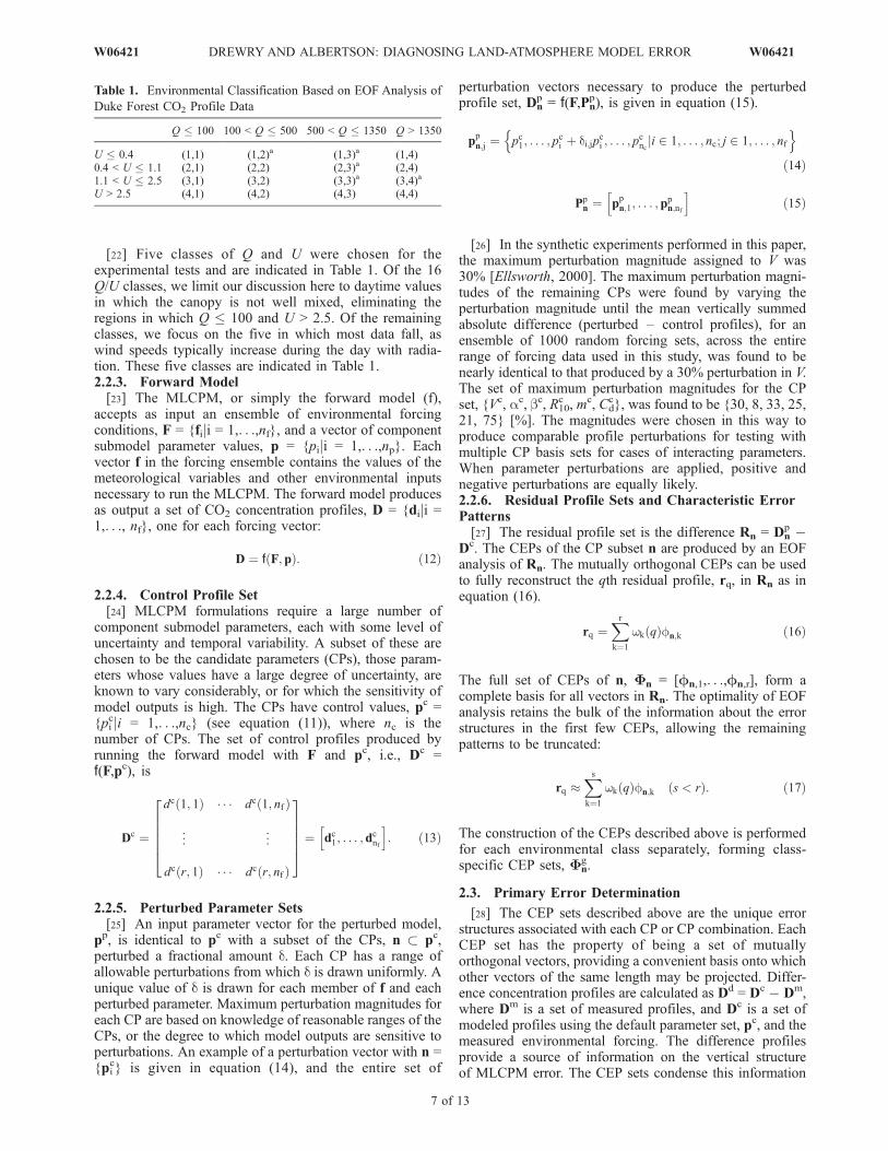
[26] In the synthetic experiments performed in this paper,the maximum perturbation magnitude assigned to V was30% [Ellsworth, 2000]. The maximum perturbation magni-tudes of the remaining CPs were found by varying theperturbation magnitude until the mean vertically summedabsolute difference (perturbed – control profiles), for anensemble of 1000 random forcing sets, across the entirerange of forcing data used in this study, was found to benearly identical to that produced by a 30% perturbation in V.The set of maximum perturbation magnitudes for the CPset, {Vc, ac, bc, R10

c , mc, Cdc}, was found to be {30, 8, 33, 25,

21, 75} [%]. The magnitudes were chosen in this way toproduce comparable profile perturbations for testing withmultiple CP basis sets for cases of interacting parameters.When parameter perturbations are applied, positive andnegative perturbations are equally likely.2.2.6. Residual Profile Sets and Characteristic ErrorPatterns[27] The residual profile set is the difference Rn = Dn

p �Dc. The CEPs of the CP subset n are produced by an EOFanalysis of Rn. The mutually orthogonal CEPs can be usedto fully reconstruct the qth residual profile, rq, in Rn as inequation (16).

rq ¼Xr

k¼1

wk qð Þfn;k ð16Þ

The full set of CEPs of n, %n = [Fn,1,. . .,Fn,r], form acomplete basis for all vectors in Rn. The optimality of EOFanalysis retains the bulk of the information about the errorstructures in the first few CEPs, allowing the remainingpatterns to be truncated:

rq �Xs

k¼1

wk qð Þfn;k s < rð Þ: ð17Þ

The construction of the CEPs described above is performedfor each environmental class separately, forming class-specific CEP sets, %n

g.

2.3. Primary Error Determination

[28] The CEP sets described above are the unique errorstructures associated with each CP or CP combination. EachCEP set has the property of being a set of mutuallyorthogonal vectors, providing a convenient basis onto whichother vectors of the same length may be projected. Differ-ence concentration profiles are calculated as Dd = Dc � Dm,where Dm is a set of measured profiles, and Dc is a set ofmodeled profiles using the default parameter set, pc, and themeasured environmental forcing. The difference profilesprovide a source of information on the vertical structureof MLCPM error. The CEP sets condense this information

Table 1. Environmental Classification Based on EOF Analysis of

Duke Forest CO2 Profile Data

Q � 100 100 < Q � 500 500 < Q � 1350 Q > 1350

U � 0.4 (1,1) (1,2)a (1,3)a (1,4)0.4 < U � 1.1 (2,1) (2,2) (2,3)a (2,4)1.1 < U � 2.5 (3,1) (3,2) (3,3)a (3,4)a

U > 2.5 (4,1) (4,2) (4,3) (4,4)

W06421 DREWRY AND ALBERTSON: DIAGNOSING LAND-ATMOSPHERE MODEL ERROR

7 of 13

W06421

into a few vertical patterns associated with a CP or CPcombination.[29] Primary error sources are determined by projecting

each difference profile, d, in Dd separately onto each CEPset. The approximation of d by projection onto the basisspecified by the parameter subset n, composed of j basisvectors, for the gth environmental class, is given by

~dn ¼Xj

d;fgn;j

D Efgn;j; ð18Þ

where the brackets represent a vector dot product.[30] The basis set which best reconstructs the vectors in

Dd is determined to be the primary error source. Accuracyof the reconstruction of a profile in this paper is quantifiedusing the L-2 norm:

ei ¼k d� ~di k2 : ð19Þ

The primary error source contributing to the error residual isdetermined to be the CP set having the minimum e value.We note that several other valid choices for the criteriondescribing the accuracy of the reconstruction exist [Janssenand Heuberger, 1995].

3. Results

[31] We examine the ability of the error patterns associ-ated with each CP, and CP pairs, to identify sources ofparameter error due to single and paired parameter pertur-bations. Three synthetic tests of the method were per-formed. The advantage of synthetic tests is that the truesource of model error is known, allowing conclusions to bedrawn about the effectiveness of the method. Synthetictesting also allows focus to be placed on the specific aspectof the error detection problem addressed here, the identifi-cation of model bias caused by errors in parameter values,

excluding the complicating factors of measurement andmodel structural errors. Each test required a forcing ensem-ble, which was used to create a synthetic truth (referred tohereafter as measured) and a perturbed (referred to hereafteras modeled) profile ensemble.[32] Two synthetic tests were performed using the six

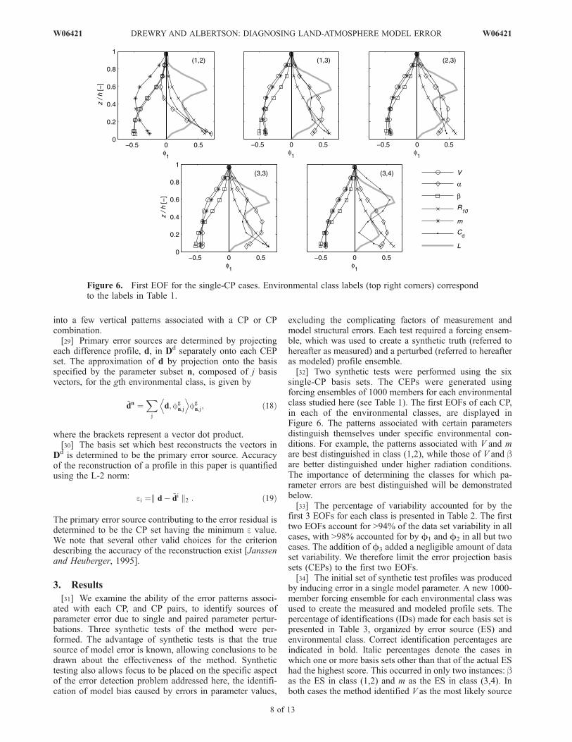
single-CP basis sets. The CEPs were generated usingforcing ensembles of 1000 members for each environmentalclass studied here (see Table 1). The first EOFs of each CP,in each of the environmental classes, are displayed inFigure 6. The patterns associated with certain parametersdistinguish themselves under specific environmental con-ditions. For example, the patterns associated with V and mare best distinguished in class (1,2), while those of V and bare better distinguished under higher radiation conditions.The importance of determining the classes for which pa-rameter errors are best distinguished will be demonstratedbelow.[33] The percentage of variability accounted for by the

first 3 EOFs for each class is presented in Table 2. The firsttwo EOFs account for >94% of the data set variability in allcases, with >98% accounted for by F1 and F2 in all but twocases. The addition of F3 added a negligible amount of dataset variability. We therefore limit the error projection basissets (CEPs) to the first two EOFs.[34] The initial set of synthetic test profiles was produced

by inducing error in a single model parameter. A new 1000-member forcing ensemble for each environmental class wasused to create the measured and modeled profile sets. Thepercentage of identifications (IDs) made for each basis set ispresented in Table 3, organized by error source (ES) andenvironmental class. Correct identification percentages areindicated in bold. Italic percentages denote the cases inwhich one or more basis sets other than that of the actual EShad the highest score. This occurred in only two instances: bas the ES in class (1,2) and m as the ES in class (3,4). Inboth cases the method identified V as the most likely source

Figure 6. First EOF for the single-CP cases. Environmental class labels (top right corners) correspondto the labels in Table 1.

8 of 13

W06421 DREWRY AND ALBERTSON: DIAGNOSING LAND-ATMOSPHERE MODEL ERROR W06421

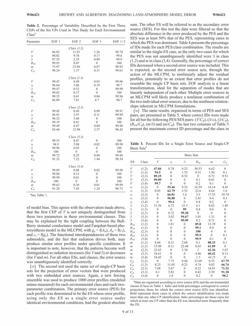
of model bias. This agrees with the observation made above,that the first CEP of V is not uniquely distinguished fromthese two parameters in these environmental classes. Thismay be explained by the tight coupling between the Ball-Berry stomatal conductance model and Farquhar-based pho-tosynthesis model in the MLCPM, with gs = f(An), An = f(ci),and ci = f(gs). The functional interdependencies of these twosubmodels, and the fact that radiation drives both, mayproduce similar error profiles under specific conditions. Itis important to note, however, that the patterns become welldistinguished as radiation increases (for Vand b) or decreases(for V and m). For all other ESs, and classes, the error sourcewas unambiguously identified correctly.[35] The second test used the same set of single-CP basis

sets for the projection of error vectors that were producedwith two embedded error sources. Again, a new forcingensemble was used to produce 1000 error profiles (modeledminus measured) for each environmental class and each two-parameter combination. The primary error source (PES) foreach profile was determined to be the ES whose error profile,using only the ES as a single error source underidentical environmental conditions, had the greatest absolute

sum. The other ES will be referred to as the secondary errorsource (SES). For this test the data were filtered so that theabsolute difference in the error produced by the PES and theSES was at least 50% that of the PES, representing cases inwhich the PESwas dominant. Table 4 presents the percentageof IDs made for each PES/class combination. The results aresimilar to the single-ES case, as the only two cases for whichthe PES was not unambiguously identified were b in class(1,2) andm in class (3,4). Generally, the percentage of correctIDs decreased when a second error source was included. Thisis expected, as the second error source acts, through theaction of the MLCPM, to nonlinearly adjust the residualprofiles, potentially to an extent that error profiles do notresemble the single CP basis sets. EOF analysis is a lineartransformation, ideal for the separation of modes that arelinearly independent of each other. Multiple error sources inan MLCPM will likely produce a nonlinear combination ofthe two individual error sources, due to the nonlinear relation-ships inherent in MLCPM formulations.[36] The same results, organized in terms of PES and SES

pairs, are presented in Table 5, where correct IDs were madefor all but the following PES/SES pairs: (V/Cd), (b/a), (b/Cd),(R10/Cd), (m/b) and (m/Cd). The last two columns of Table 5present the maximum correct ID percentage and the class in

Table 2. Percentage of Variability Described by the First Three

CEPs of the Six CPs Used in This Study for Each Environmental

Classa

Parameter EOF 1 EOF 2 EOF 3 EOF 1+2

Class (1,2)V 86.83 11.91 1.26 98.74a 90.02 9.78 0.17 99.8b 97.55 2.35 0.09 99.9R10 99.93 0.07 0 100m 75.97 23.96 0.07 99.92Cd 98.24 1.37 0.31 99.61

Class (1,3)V 99.47 0.49 0.03 99.96a 96.64 3.06 0.19 99.7b 99.47 0.52 0 99.99R10 99.82 0.17 0 100m 99.35 0.61 0.04 99.96Cd 86.89 7.81 4.7 94.7

Class (2,3)V 99.45 0.45 0.09 99.91a 96.91 2.97 0.11 99.89b 96.32 3.68 0 100R10 99.19 0.81 0 100m 99.49 0.47 0.04 99.96Cd 83.44 12.98 3.57 96.42

Class (3,3)V 99.53 0.47 0 100a 94.9 5.08 0.02 99.98b 99.98 0.02 0 100R10 100 0 0 100m 99.72 0.25 0.04 99.96Cd 91.32 7.22 1.44 98.54

Class (3,4)V 99.89 0.08 0.02 99.98a 99.88 0.12 0 100b 99.99 0.01 0 100R10 100 0 0 100m 99.63 0.36 0.01 99.99Cd 91.28 7.45 1.24 98.73

aSee Table 1.

Table 3. Percent IDs for a Single Error Source and Single-CP

Basis Setsa

ES Class

Basis Sets

V a b R10 m Cd

V (1,2) 47.84 8.78 6.23 30.53 6.62 0V (1,3) 94.5 0 1.53 0.31 3.56 0.1V (2,3) 89.25 0 0.52 0 0.72 9.51V (3,3) 99.09 0 0 0.1 0.81 0V (3,4) 99.7 0 0 0.2 0.1 0a (1,2) 0 55.46 9.35 16.59 14.14 4.45a (1,3) 0.85 62.79 3.52 22.6 8.64 1.6a (2,3) 0 66.81 1.6 3.3 17.55 10.74a (3,3) 0 96.88 0 2.41 0.4 0.3a (3,4) 0 99.4 0 0.4 0.2 0b (1,2) 51.56 6.72 33.5 6.1 0.62 1.49b (1,3) 0 0 99 0.4 0.6 0b (2,3) 0 0.72 99.28 0 0 0b (3,3) 0 3.02 94.67 1.01 1.31 0b (3,4) 0 0 99.09 0.2 0.71 0R10 (1,2) 0 1.81 0 85.8 12.39 0R10 (1,3) 0 0 0 99.1 0.9 0R10 (2,3) 0 0 0 100 0 0R10 (3,3) 0 0 0 99.9 0 0.1R10 (3,4) 0 0 0 99.9 0.1 0m (1,2) 8.66 0.21 2.68 0.1 88.25 0.1m (1,3) 15.09 0.11 22.48 0.43 61.89 0m (2,3) 32.63 0 2.34 1 62.36 1.67m (3,3) 34.61 0 0 4.86 60.42 0.12m (3,4) 54.45 0 0 1.3 44.25 0Cd (1,2) 0 7.75 0.44 23.69 0.33 67.79Cd (1,3) 8.23 11.05 0.23 4.74 9.02 66.74Cd (2,3) 7.68 5.67 0 0.22 14.91 71.52Cd (3,3) 0.1 5.82 0 0.42 2.39 91.28Cd (3,4) 0 1.6 0 0.2 0 98.2

aData are organized according to error source (ES) and the environmentalclasses (Class) in Table 1. Italic and bold percentages correspond to correctprojections, those for which the correct error source (ES) was identified.Bold represents those cases in which the correct identification was mademore than any other CP identification. Italic percentages are those cases forwhich at least one CP other than the ES was identified more frequently thanthe ES.

W06421 DREWRY AND ALBERTSON: DIAGNOSING LAND-ATMOSPHERE MODEL ERROR

9 of 13

W06421

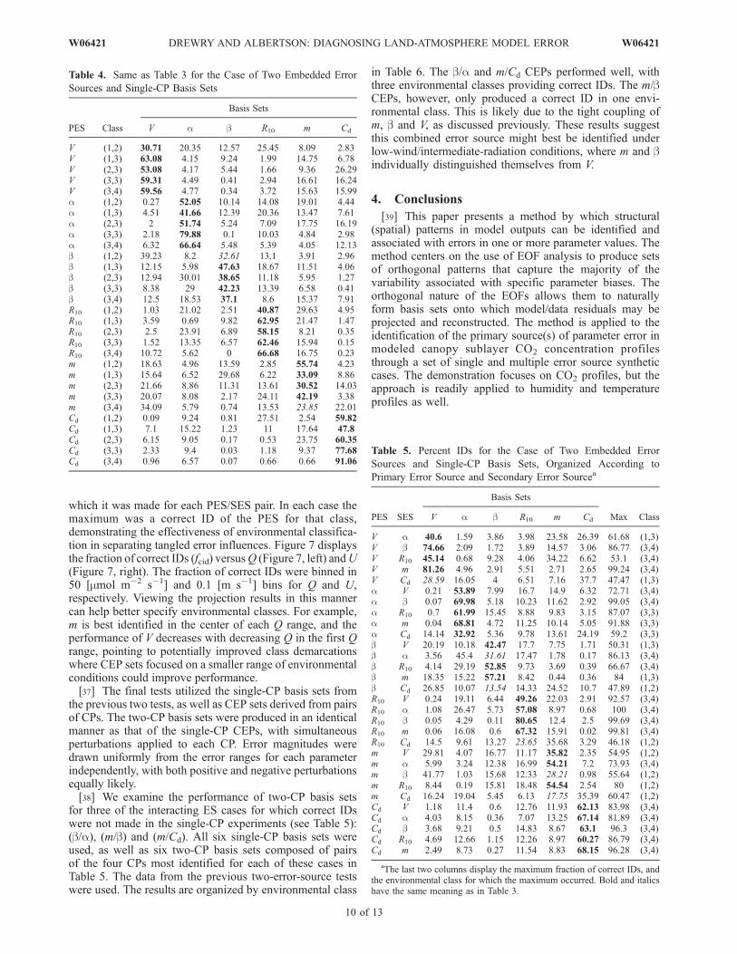
which it was made for each PES/SES pair. In each case themaximum was a correct ID of the PES for that class,demonstrating the effectiveness of environmental classifica-tion in separating tangled error influences. Figure 7 displaysthe fraction of correct IDs (fcid) versusQ (Figure 7, left) andU(Figure 7, right). The fraction of correct IDs were binned in50 [mmol m�2 s�1] and 0.1 [m s�1] bins for Q and U,respectively. Viewing the projection results in this mannercan help better specify environmental classes. For example,m is best identified in the center of each Q range, and theperformance of V decreases with decreasing Q in the first Qrange, pointing to potentially improved class demarcationswhere CEP sets focused on a smaller range of environmentalconditions could improve performance.[37] The final tests utilized the single-CP basis sets from

the previous two tests, as well as CEP sets derived from pairsof CPs. The two-CP basis sets were produced in an identicalmanner as that of the single-CP CEPs, with simultaneousperturbations applied to each CP. Error magnitudes weredrawn uniformly from the error ranges for each parameterindependently, with both positive and negative perturbationsequally likely.[38] We examine the performance of two-CP basis sets

for three of the interacting ES cases for which correct IDswere not made in the single-CP experiments (see Table 5):(b/a), (m/b) and (m/Cd). All six single-CP basis sets wereused, as well as six two-CP basis sets composed of pairsof the four CPs most identified for each of these cases inTable 5. The data from the previous two-error-source testswere used. The results are organized by environmental class

in Table 6. The b/a and m/Cd CEPs performed well, withthree environmental classes providing correct IDs. The m/bCEPs, however, only produced a correct ID in one envi-ronmental class. This is likely due to the tight coupling ofm, b and V, as discussed previously. These results suggestthis combined error source might best be identified underlow-wind/intermediate-radiation conditions, where m and bindividually distinguished themselves from V.

4. Conclusions

[39] This paper presents a method by which structural(spatial) patterns in model outputs can be identified andassociated with errors in one or more parameter values. Themethod centers on the use of EOF analysis to produce setsof orthogonal patterns that capture the majority of thevariability associated with specific parameter biases. Theorthogonal nature of the EOFs allows them to naturallyform basis sets onto which model/data residuals may beprojected and reconstructed. The method is applied to theidentification of the primary source(s) of parameter error inmodeled canopy sublayer CO2 concentration profilesthrough a set of single and multiple error source syntheticcases. The demonstration focuses on CO2 profiles, but theapproach is readily applied to humidity and temperatureprofiles as well.

Table 4. Same as Table 3 for the Case of Two Embedded Error

Sources and Single-CP Basis Sets

PES Class

Basis Sets

V a b R10 m Cd

V (1,2) 30.71 20.35 12.57 25.45 8.09 2.83V (1,3) 63.08 4.15 9.24 1.99 14.75 6.78V (2,3) 53.08 4.17 5.44 1.66 9.36 26.29V (3,3) 59.31 4.49 0.41 2.94 16.61 16.24V (3,4) 59.56 4.77 0.34 3.72 15.63 15.99a (1,2) 0.27 52.05 10.14 14.08 19.01 4.44a (1,3) 4.51 41.66 12.39 20.36 13.47 7.61a (2,3) 2 51.74 5.24 7.09 17.75 16.19a (3,3) 2.18 79.88 0.1 10.03 4.84 2.98a (3,4) 6.32 66.64 5.48 5.39 4.05 12.13b (1,2) 39.23 8.2 32.61 13.1 3.91 2.96b (1,3) 12.15 5.98 47.63 18.67 11.51 4.06b (2,3) 12.94 30.01 38.65 11.18 5.95 1.27b (3,3) 8.38 29 42.23 13.39 6.58 0.41b (3,4) 12.5 18.53 37.1 8.6 15.37 7.91R10 (1,2) 1.03 21.02 2.51 40.87 29.63 4.95R10 (1,3) 3.59 0.69 9.82 62.95 21.47 1.47R10 (2,3) 2.5 23.91 6.89 58.15 8.21 0.35R10 (3,3) 1.52 13.35 6.57 62.46 15.94 0.15R10 (3,4) 10.72 5.62 0 66.68 16.75 0.23m (1,2) 18.63 4.96 13.59 2.85 55.74 4.23m (1,3) 15.64 6.52 29.68 6.22 33.09 8.86m (2,3) 21.66 8.86 11.31 13.61 30.52 14.03m (3,3) 20.07 8.08 2.17 24.11 42.19 3.38m (3,4) 34.09 5.79 0.74 13.53 23.85 22.01Cd (1,2) 0.09 9.24 0.81 27.51 2.54 59.82Cd (1,3) 7.1 15.22 1.23 11 17.64 47.8Cd (2,3) 6.15 9.05 0.17 0.53 23.75 60.35Cd (3,3) 2.33 9.4 0.03 1.18 9.37 77.68Cd (3,4) 0.96 6.57 0.07 0.66 0.66 91.06

Table 5. Percent IDs for the Case of Two Embedded Error

Sources and Single-CP Basis Sets, Organized According to

Primary Error Source and Secondary Error Sourcea

PES SES

Basis Sets

Max ClassV a b R10 m Cd

V a 40.6 1.59 3.86 3.98 23.58 26.39 61.68 (1,3)V b 74.66 2.09 1.72 3.89 14.57 3.06 86.77 (3,4)V R10 45.14 0.68 9.28 4.06 34.22 6.62 53.1 (3,4)V m 81.26 4.96 2.91 5.51 2.71 2.65 99.24 (3,4)V Cd 28.59 16.05 4 6.51 7.16 37.7 47.47 (1,3)a V 0.21 53.89 7.99 16.7 14.9 6.32 72.71 (3,4)a b 0.07 69.98 5.18 10.23 11.62 2.92 99.05 (3,4)a R10 0.7 61.99 15.45 8.88 9.83 3.15 87.07 (3,3)a m 0.04 68.81 4.72 11.25 10.14 5.05 91.88 (3,3)a Cd 14.14 32.92 5.36 9.78 13.61 24.19 59.2 (3,3)b V 20.19 10.18 42.47 17.7 7.75 1.71 50.31 (1,3)b a 3.56 45.4 31.61 17.47 1.78 0.17 86.13 (3,4)b R10 4.14 29.19 52.85 9.73 3.69 0.39 66.67 (3,4)b m 18.35 15.22 57.21 8.42 0.44 0.36 84 (1,3)b Cd 26.85 10.07 13.54 14.33 24.52 10.7 47.89 (1,2)R10 V 0.24 19.11 6.44 49.26 22.03 2.91 92.57 (3,4)R10 a 1.08 26.47 5.73 57.08 8.97 0.68 100 (3,4)R10 b 0.05 4.29 0.11 80.65 12.4 2.5 99.69 (3,4)R10 m 0.06 16.08 0.6 67.32 15.91 0.02 99.81 (3,4)R10 Cd 14.5 9.61 13.27 23.65 35.68 3.29 46.18 (1,2)m V 29.81 4.07 16.77 11.17 35.82 2.35 54.95 (1,2)m a 5.99 3.24 12.38 16.99 54.21 7.2 73.93 (3,4)m b 41.77 1.03 15.68 12.33 28.21 0.98 55.64 (1,2)m R10 8.44 0.19 15.81 18.48 54.54 2.54 80 (1,2)m Cd 16.24 19.04 5.45 6.13 17.75 35.39 60.47 (1,2)Cd V 1.18 11.4 0.6 12.76 11.93 62.13 83.98 (3,4)Cd a 4.03 8.15 0.36 7.07 13.25 67.14 81.89 (3,4)Cd b 3.68 9.21 0.5 14.83 8.67 63.1 96.3 (3,4)Cd R10 4.69 12.66 1.15 12.26 8.97 60.27 86.79 (3,4)Cd m 2.49 8.73 0.27 11.54 8.83 68.15 96.28 (3,4)

aThe last two columns display the maximum fraction of correct IDs, andthe environmental class for which the maximum occurred. Bold and italicshave the same meaning as in Table 3.

10 of 13

W06421 DREWRY AND ALBERTSON: DIAGNOSING LAND-ATMOSPHERE MODEL ERROR W06421

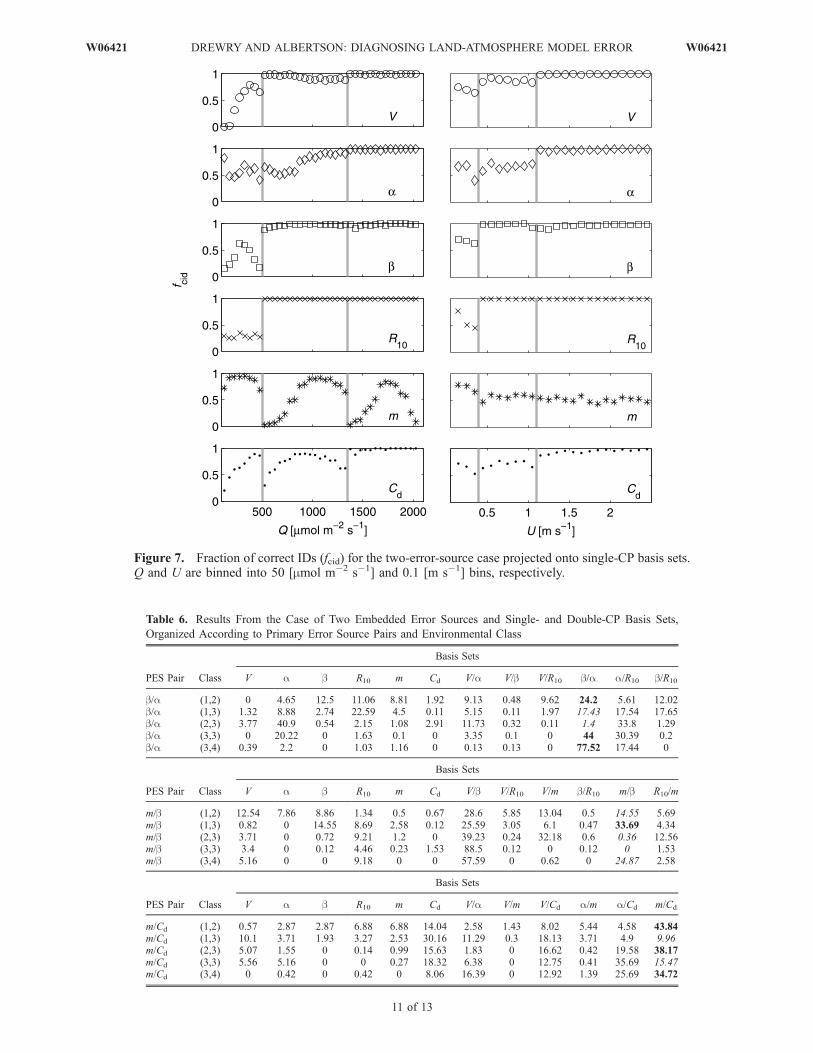
Figure 7. Fraction of correct IDs (fcid) for the two-error-source case projected onto single-CP basis sets.Q and U are binned into 50 [mmol m�2 s�1] and 0.1 [m s�1] bins, respectively.

Table 6. Results From the Case of Two Embedded Error Sources and Single- and Double-CP Basis Sets,

Organized According to Primary Error Source Pairs and Environmental Class

PES Pair Class

Basis Sets

V a b R10 m Cd V/a V/b V/R10 b/a a/R10 b/R10

b/a (1,2) 0 4.65 12.5 11.06 8.81 1.92 9.13 0.48 9.62 24.2 5.61 12.02b/a (1,3) 1.32 8.88 2.74 22.59 4.5 0.11 5.15 0.11 1.97 17.43 17.54 17.65b/a (2,3) 3.77 40.9 0.54 2.15 1.08 2.91 11.73 0.32 0.11 1.4 33.8 1.29b/a (3,3) 0 20.22 0 1.63 0.1 0 3.35 0.1 0 44 30.39 0.2b/a (3,4) 0.39 2.2 0 1.03 1.16 0 0.13 0.13 0 77.52 17.44 0

PES Pair Class

Basis Sets

V a b R10 m Cd V/b V/R10 V/m b/R10 m/b R10/m

m/b (1,2) 12.54 7.86 8.86 1.34 0.5 0.67 28.6 5.85 13.04 0.5 14.55 5.69m/b (1,3) 0.82 0 14.55 8.69 2.58 0.12 25.59 3.05 6.1 0.47 33.69 4.34m/b (2,3) 3.71 0 0.72 9.21 1.2 0 39.23 0.24 32.18 0.6 0.36 12.56m/b (3,3) 3.4 0 0.12 4.46 0.23 1.53 88.5 0.12 0 0.12 0 1.53m/b (3,4) 5.16 0 0 9.18 0 0 57.59 0 0.62 0 24.87 2.58

PES Pair Class

Basis Sets

V a b R10 m Cd V/a V/m V/Cd a/m a/Cd m/Cd

m/Cd (1,2) 0.57 2.87 2.87 6.88 6.88 14.04 2.58 1.43 8.02 5.44 4.58 43.84m/Cd (1,3) 10.1 3.71 1.93 3.27 2.53 30.16 11.29 0.3 18.13 3.71 4.9 9.96m/Cd (2,3) 5.07 1.55 0 0.14 0.99 15.63 1.83 0 16.62 0.42 19.58 38.17m/Cd (3,3) 5.56 5.16 0 0 0.27 18.32 6.38 0 12.75 0.41 35.69 15.47m/Cd (3,4) 0 0.42 0 0.42 0 8.06 16.39 0 12.92 1.39 25.69 34.72

W06421 DREWRY AND ALBERTSON: DIAGNOSING LAND-ATMOSPHERE MODEL ERROR

11 of 13

W06421

[40] The results demonstrated significant skill in identi-fying the primary source of model error when one source ofbias was present. Single candidate parameter (CP) basis setsshowed strong performance with two embedded error sour-ces, when one source was dominant. As well, basis setsformed with pairs of interacting parameters were used withsuccess to identify combined error sources of comparablemagnitude, nonlinearly mixed by the MLCPM.[41] The ability of the method to resolve model error will

likely be dependent on the selection of the CP set and theenvironmental classification used, as coupling between sub-models may cause parameter errors to form similar errorpatterns. The classification of environmental conditions wasdemonstrated to be effective at separating errors in coupledmodel parameters (i.e., V, b and m). The classificationscheme used in this paper was based on a principal compo-nents analysis of measured concentration profiles. In prac-tice, data analysis provides a method for obtaining generalclassification boundaries. This can be used in conjunctionwith a detailed sensitivity analysis of the model, such as thatperformed in the synthetic experiments in this paper, tofurther specify class boundaries useful for resolving theeffects of strongly coupled parameters. While, for demon-stration purposes, the classification scheme in this paper wasfocused solely on Q and U, other controlling environmentalvariables such as time of day, season, air temperature, soilmoisture status, and vapor pressure deficit may be used tomore precisely classify environmental regimes.[42] The focus of this study was the presentation of the

method and initial synthetic testing using CO2 profiles as anexample. The confounding effects of measurement andmodel structural error provide challenges for future studies.Simultaneous use of multiple scalar profiles (CO2, Ta, H2O)is likely to further constrain model error source identifica-tions. Application of techniques such as the one described inthis paper could prove useful for higher-dimensional mod-els, such as distributed hydrological models, in whichparameter optimization is a critical issue.

[43] Acknowledgment. This research was funded by the Office ofScience (BER), U.S. Department of Energy, under cooperative agreementDE-FCO3-90ER61010, and the NASA Earth System Science Fellowshipprogram.

ReferencesBaldocchi, D. (1997), Measuring and modelling carbon dioxide and watervapour exchange over a temperate broad-leaved forest during the 1995summer drought, Plant Cell Environ., 20(9), 1108–1122.

Baldocchi, D. D., and P. C. Harley (1995), Scaling carbon-dioxide andwater-vapor exchange from leaf to canopy in a deciduous forest:2. Model testing and application, Plant Cell. Environ., 18(10), 1157–1173.

Baldocchi, D. D., and K. B. Wilson (2001), Modeling CO2 and water vaporexchange of a temperate broadleaved forest across hourly to decadal timescales, Ecol Modell., 142(1–2), 155–184.

Baldocchi, D., R. Valentini, S. Running, W. Oechel, and R. Dahlman(1996), Strategies for measuring and modelling carbon dioxide and watervapour fluxes over terrestrial ecosystems, Global Change Biol., 2(3),159–168.

Baldocchi, D. D., C. A. Vogel, and B. Hall (1997), Seasonal variation ofcarbon dioxide exchange rates above and below a boreal jack pine forest,Agric. For. Meteorol., 83(1–2), 147–170.

Baldocchi, D., K. Wilson, and G. Lianhong (2002), How the environment,canopy structure and canopy physiological functioning influence carbon,water and energy fluxes of a temperate broad-leaved deciduous forest:An assessment with the biophysical model CANOAK, Tree Physiol., 22,1065–1077.

Ball, J. T., I. E. Woodrow, and J. A. Berry (1987), A model predictingstomatal conductance and its contribution to the control of photosynth-esis under different environmental conditions, in Progress in Photosynth-esis Research, vol. IV, Proceedings of the International Congress onPhotosynthesis, edited by J. Biggens, pp. 221–224, Martinus Nihjoff,Zoetermeer, Netherlands.

Beven, K., and J. Freer (2001), Equifinality, data assimilation, and uncer-tainty estimation in mechanistic modelling of complex environmentalsystems using the GLUE methodology, J. Hydrol., 249(1–4), 11–29.

Cai, T., and Q.-L. Dang (2002), Effects of soil temperature on parameters ofa coupled photosynthesis-stomatal conductance model, Tree Physiol., 22,819–827.

Campbell, G. S., and J. M. Norman (1998), An Introduction to Environ-mental Biophysics, Springer, New York.

Chen, W. J., et al. (1999), Effects of climatic variability on the annualcarbon sequestration by a boreal aspen forest, Global Change Biol.,5(1), 41–53.

Collatz, G. J., J. T. Ball, C. Grivet, and J. A. Berry (1991), Physiologicaland environmental-regulation of stomatal conductance, photosynthesisand transpiration: A model that includes a laminar boundary-layer, Agric.For. Meteorol., 54(2–4), 107–136.

Ellsworth, D. S. (1999), CO2 enrichment in a maturing pine forest: Are CO2

exchange and water status in the canopy affected?, Plant Cell Environ.,22(5), 461–472.

Ellsworth, D. S. (2000), Seasonal CO2 assimilation and stomatal limitationsin a Pinus taeda canopy, Tree Physiol., 20(7), 435–445.

Farquhar, G. D., S. V. Caemmerer, and J. A. Berry (1980), A biochemical-model of photosynthetic CO2 assimilation in leaves of C-3 species,Planta, 149(1), 78–90.

Franks, S. W., K. J. Beven, P. F. Quinn, and I. R. Wright (1997), On thesensitivity of soil-vegetation-atmosphere transfer (SVAT) schemes: Equi-finality and the problem of robust calibration, Agric. For. Meteorol.,86(1–2), 63–75.

Greco, S., and D. D. Baldocchi (1996), Seasonal variations of CO2 andwater vapour exchange rates over a temperate deciduous forest, GlobalChange Biol., 2(3), 183–197.

Gu, L. H., H. H. Shugart, J. D. Fuentes, T. A. Black, and S. R. Shewchuk(1999), Micrometeorology, biophysical exchanges and NEE decomposi-tion in a two-story boreal forest: Development and test of an integratedmodel, Agric. For. Meteorol., 94(2), 123–148.

Gupta, H. V., L. A. Bastidas, S. Sorooshian, W. J. Shuttleworth, and Z. L.Yang (1999), Parameter estimation of a land surface scheme using multi-criteria methods, J. Geophys. Res., 104, 19,491–19,503.

Hollinger, D. Y., F. M. Kelliher, J. N. Byers, J. E. Hunt, T. M. McSeveny,and P. L. Weir (1994), Carbon-dioxide exchange between an undisturbedold-growth temperate forest and the atmosphere, Ecology, 75(1), 134–150.

Hollinger, D. Y., et al. (2004), Spatial and temporal variability in forest-atmosphere CO2 exchange, Global Change Biol., 10(10), 1689–1706.

Hotelling, M. (1933), Analysis of a complex of statistical variables intoprincipal components, J. Educ. Psychol., 24, 498–520.

Janssen, P. H. M., and P. S. C. Heuberger (1995), Calibration of process-oriented models, Ecol. Modell., 83(1–2), 55–66.

Katul, G., C. T. Lai, K. Schafer, B. Vidakovic, J. Albertson, D. Ellsworth,and R. Oren (2001), Multiscale analysis of vegetation surface fluxes:From seconds to years, Adv. Water Resour., 24(9–10), 1119–1132.

Katul, G. G., L. Mahrt, D. Poggi, and C. Sanz (2004), One- and two-equation models for canopy turbulence, Boundary Layer Meteorol.,113(1), 81–109.

Kuczera, G., and E. Parent (1998), Monte Carlo assessment of parameteruncertainty in conceptual catchment models: The Metropolis algorithm,J. Hydrol., 211(1–4), 69–85.

Lai, C. T., G. Katul, D. Ellsworth, and R. Oren (2000a), Modelling vegeta-tion-atmosphere CO2 exchange by a coupled Eulerian-Langrangian ap-proach, Boundary Layer Meteorol., 95(1), 91–122.

Lai, C. T., G. Katul, R. Oren, D. Ellsworth, and K. Schafer (2000b),Modeling CO2 and water vapor turbulent flux distributions within aforest canopy, J. Geophys. Res., 105(D21), 26,333–26,351.

Law, B. E., M. Williams, P. M. Anthoni, D. D. Baldocchi, and M. H.Unsworth (2000), Measuring and modelling seasonal variation of carbondioxide and water vapour exchange of a Pinus ponderosa forest subjectto soil water deficit, Global Change Biol., 6(6), 613–630.

Leuning, R., F. M. Kelliher, D. G. G. Depury, and E. D. Schulze (1995),Leaf nitrogen, photosynthesis, conductance and transpiration: Scalingfrom leaves to canopies, Plant Cell Environ., 18(10), 1183–1200.

Lloyd, J., and J. A. Taylor (1994), On the temperature-dependence of soilrespiration, Funct. Ecol., 8(3), 315–323.

12 of 13

W06421 DREWRY AND ALBERTSON: DIAGNOSING LAND-ATMOSPHERE MODEL ERROR W06421

Lloyd, J., O. Shibistova, D. Zolotoukhine, O. Kolle, A. Arneth, C. Wirth,J. M. Styles, N. M. Tchebakova, and E. D. Schulze (2002), Seasonaland annual variations in the photosynthetic productivity and carbonbalance of a central Siberian pine forest, Tellus, Ser. B, 54(5), 590–610.

Lorenz, E. N. (1956), Empirical orthogonal functions and statistical weatherprediction, Stat. Forecast. Proj. Sci. Rep. 1, 49 pp., Dep. of Meteorol.,Mass. Inst. of Technol., Cambridge.

Mackay, D. S., S. Samanta, R. R. Nemani, and L. E. Band (2003), Multi-objective parameter estimation for simulating canopy transpiration inforested watersheds, J. Hydrol., 277(3–4), 230–247.

Margulis, S. A., and D. Entekhabi (2003), Variational assimilation of radio-metric surface temperature and reference-level micrometeorology into amodel of the atmospheric boundary layer and land surface,Mon. WeatherRev., 131(7), 1272–1288.

Medlyn, B. E., D. Loustau, and S. Delzon (2002), Temperature response ofparameters of a biochemically based model of photosynthesis. I. Seaso-nal changes in mature maritime pine (Pinus pinaster Ait.), Plant CellEnviron., 25, 1155–1165.

Middleton, E. M., J. H. Sullivan, B. D. Bovard, A. J. Deluca, S. S. Chan,and T. A. Cannon (1997), Seasonal variability in foliar characteristics andphysiology for boreal forest species at the five Saskatchewan tower sitesduring the 1994 Boreal Ecosystem-Atmosphere Study, J. Geophys. Res.,102, 28,831–28,844.

Morecroft, M. D., and J. M. Roberts (1999), Photosynthesis and stomatalconductance of mature canopy Oak (Quercus robur) and Sycamore (Acerpseudoplatanus) trees throughout the growing season, Funct. Ecol.,13(3), 332–342.

Noilhan, J., and J. F. Mahfouf (1996), The ISBA land surface parameter-isation scheme, Global Planet. Change, 13(1–4), 145–159.

Ogee, J., Y. Brunet, D. Loustau, P. Berbigier, and S. Delzon (2003),MUSICA, a CO2, water and energy multilayer, multileaf pine forestmodel: Evaluation from hourly to yearly time scales and sensitivityanalysis, Global Change Biol., 9(5), 697–717.

Pearson, K. (1901), On lines and planes of closest fit to systems of points inspace, Philos. Mag., 2, 559–572.

Pinard, J. D., and J. D. Wilson (2001), First- and second-order closuremodels for wind in a plant canopy, J. Appl. Meteorol., 40, 1762–1768.

Poggi, D., A. Porporato, L. Ridolfi, J. D. Albertson, and G. G. Katul(2004), The effect of vegetation density on canopy sub-layer turbulence,Boundary Layer Meteorol., 111(3), 565–587.

Pyles, R. D., B. C. Weare, and K. T. Paw U (2000), The UCD advancedcanopy-atmosphere-soil algorithm: Comparisons with observations fromdifferent climate and vegetation regimes, Q. J. R. Meteorol. Soc.,126(569), 2951–2980.

Reichle, R. H., D. B. McLaughlin, and D. Entekhabi (2001), Variationaldata assimilation of microwave radiobrightness observations for landsurface hydrology applications, IEEE Trans. Geosci. Remote Sens.,39(8), 1708–1718.

Siqueira, M., C. T. Lai, and G. Katul (2000), Estimating scalar sources,sinks, and fluxes in a forest canopy using Lagrangian, Eulerian, andhybrid inverse models, J. Geophys. Res., 105, 29,475–29,488.

Styles, J. M., et al. (2002), Soil and canopy CO2, CO2–C-13, H2O andsensible heat flux partitions in a forest canopy inferred from concentra-tion measurements, Tellus, Ser. B, 54(5), 655–676.

Sullivan, J. H., B. D. Bovard, and E. M. Middleton (1997), Variability inleaf-level CO2 and water fluxes in Pinus banksiana and Picea mariana inSaskatchewan, Tree Physiol., 17(8–9), 553–561.

Tracy, C. R., F. H. Vanberkum, J. S. Tsuji, R. D. Stevenson, J. A. Nelson,B. M. Barnes, and R. B. Huey (1984), Errors resulting from linear-approximations in energy-balance equations, J. Therm. Biol., 9(4),261–264.

von Storch, H. (1999), Spatial patterns: EOFs and CCA, in Analysis ofClimate Variability: Applications of Statistical Techniques, edited byH. von Storch and A. Navarra, pp. 227–257, Springer, New York.

von Storch, H., and F. W. Zwiers (1999), Statistical Analysis in ClimateResearch, 494 pp., Cambridge Univ. Press, New York.

Wang, Y. P., R. Leuning, H. A. Cleugh, and P. A. Coppin (2001), Parameterestimation in surface exchange models using nonlinear inversion: Howmany parameters can we estimate and which measurements are mostuseful?, Global Change Biol., 7(5), 495–510.

Williams, M., E. B. Rastetter, D. N. Fernandes, M. L. Goulden, S. C.Wofsy, G. R. Shaver, J. M. Melillo, J. W. Munger, S. M. Fan, and K. J.Nadelhoffer (1996), Modelling the soil-plant-atmosphere continuum in aQuercus-Acer stand at Harvard forest: The regulation of stomatal con-ductance by light, nitrogen and soil/plant hydraulic properties, Plant CellEnviron., 19(8), 911–927.

Wilson, K. B., D. D. Baldocchi, and P. J. Hanson (2000a), Quantifyingstomatal and non-stomatal limitations to carbon assimilation resultingfrom leaf aging and drought in mature deciduous tree species, TreePhysiol., 20(12), 787–797.

Wilson, K. B., D. D. Baldocchi, and P. J. Hanson (2000b), Spatial andseasonal variability of photosynthetic parameters and their relation-ship to leaf nitrogen in a deciduous forest, Tree Physiol., 20(9),565–578.

Wilson, K. B., D. D. Baldocchi, and P. J. Hanson (2001), Leaf age affectsthe seasonal pattern of photosynthetic capacity and net ecosystemexchange of carbon in a deciduous forest, Plant Cell Environ., 24(6),571–583.

Wullschleger, S. D. (1993), Biochemical limitations to carbon assimilationin C3 plants: A retrospective analysis of the a/Ci curves from 109 species,J. Exp. Bot., 44(262), 907–920.

Xu, L., and D. Baldocchi (2003), Seasonal trends in photosynthetic para-meters and stomatal conductance of blue oak (Quercus douglasii) underprolonged summer drought and high temperature, Tree Physiol., 23,865–877.

����������������������������J. D. Albertson and D. T. Drewry, Department of Civil and

Environmental Engineering, 217 Hudson Hall, Box 90827 DukeUniversity, Durham, NC 27708-0287, USA. (darren.drewry@duke.edu)

W06421 DREWRY AND ALBERTSON: DIAGNOSING LAND-ATMOSPHERE MODEL ERROR

13 of 13

W06421