Development of Techniques for Trace Gas Detection in Breath
230
Development of Techniques for Trace Gas Detection in Breath A thesis submitted for the degree of Doctor of Philosophy Cathryn E Langley Jesus College, University of Oxford Trinity Term 2012
-
Upload
khangminh22 -
Category
Documents
-
view
0 -
download
0
Transcript of Development of Techniques for Trace Gas Detection in Breath
Development of Techniques for
Trace Gas Detection in Breath
A thesis submitted for the degree of Doctor of Philosophy
Cathryn E Langley
Jesus College, University of Oxford
Trinity Term 2012
Development of Techniques for Trace Gas Detection in Breath
A thesis submitted for the degree of Doctor of Philosophy
Cathryn E Langley, Jesus College, University of Oxford
Trinity Term 2012
Abstract
This thesis aims to investigate the possibility of developing spectroscopic techniques for
trace gas detection, with particular emphasis on their applicability to breath analysis and
medical diagnostics. Whilst key breath molecules such as methane and carbon dioxide will
feature throughout this work, the focus of the research is on the detection of breath acetone,
a molecule strongly linked with the diabetic condition.
Preliminary studies into the suitability of cavity enhanced absorption spectroscopy (CEAS)
for the analysis of breath are carried out on methane, a molecule found in varying quantities
in breath depending on whether the subject is a methane-producer or not. A telecommu-
nications near-infrared semiconductor diode laser (∼1.6 µm) is used with an optical cavity-
based detection system to probe transitions within the 2ν3 vibrational overtone of methane.
Achieving a minimum detectable sensitivity of 600 ppb, the device is used to analyse the
breath of 48 volunteers, identifying approximately one in three as methane producers. Fol-
lowing this, a second type of laser source, the novel and widely tunable Digital Supermode
Distributed Bragg Reflector (DS-DBR) laser, is characterised and the first demonstration
of its use in spectroscopy documented. Particular emphasis is given to its application to
CEAS and to probing the transitions of the two Fermi resonance components of the CO2
3ν1 + ν3 combination bands found within the spectral range (1.56 - 1.61 µm) of the laser,
providing the means to determine accurate 13CO2/12CO2 ratios for use in the urea breath
test.
Not all molecules exhibit narrow, well-resolved ro-vibrational transitions and the next sec-
tion of the thesis focuses on the detection of molecules, such as acetone, with broad, con-
gested absorption features which are not readily discernible using narrowband laser sources.
To provide the necessary specificity for these molecules, two types of broadband source, a
Superluminescent Light Emitting Diode (SLED) and a Supercontinuum source (SC), both
emitting over the 1.6 - 1.7 µm region, are used in the development of a series of broadband
cavity enhanced absorption (BB-CEAS) spectrometers. The three broadband absorbers
investigated here, butadiene, acetone and isoprene, all exhibit overtone and combination
bands in this spectral region and direct absorption measurements are taken to determine
absorption cross-sections for all three molecules. The first BB-CEAS spectrometer couples
the SLED device with a dispersive monochromator, attaining a minimum detectable sen-
sitivity of 6 × 10⁻⁸ cm−1, which is further enhanced to 1.5 × 10⁻⁸ cm−1 on replacing the
monochromator with a Fourier Transform interferometer. The spectral coverage is then
extended to 1.5 - 1.7 µm by coupling the first SLED with a second device, providing a
demonstration of simultaneous multiple species detection. Finally, a SC source is used to
provide greater power and uniform spectral intensity, resulting in an improved minimum
detectable sensitivity of ∼5 ×10⁻⁹ cm−1, or 200 ppb, 400 ppb and 200 ppb for butadiene,
acetone and isoprene respectively. This device is then applied to acetone-enriched breath
samples; the resulting spectra are fitted with a simulation to return the acetone levels
present in the breath-matrix.
Following this, the development of a prototype breath acetone analyser, carried out at
Oxford Medical Diagnostics Ltd. (OMD), is described. To fulfill the requirements of a
compact and commercially-viable device, a diode laser-based system is used, which neces-
sitates a thorough investigation into all possible sources of absorption level change. Most
notably, this includes a study into the removal and negating of interfering species, such as
water vapour, and to a lesser extent, methane. A novel solution is presented, utilising a
water-removal device in conjunction with molecular sieve so that each breath sample gen-
erates its own background, which has allowed breath acetone levels to be measured within
an uncertainty of 200 ppb.
Spectroscopic detection then moves to the mid-infrared with the demonstration of a contin-
uous wave 8 µm quantum cascade laser, which allows the larger absorption cross-sections
associated with fundamental vibrational modes to be probed. Following the laser’s charac-
terisation using methane, including a wavelength modulation spectroscopy study, the low
effective laser linewidth is utilised to resolve rotational structure in low pressure samples
of pure acetone. Absorption cross-sections are determined before the sensitivity of the sys-
tem is enhanced for the detection of dilute concentrations of acetone using two types of
multipass cells, firstly a White cell and secondly a home-built Herriott cell. This allows
an acetone minimum detectable absorption of 350 ppb and 20 ppb to be attained, respec-
tively. Following this, an optical cavity is constructed and, on treating breath samples in a
water-removal device prior to analysis, breath acetone levels determined and corroborated
with a mass spectrometer.
Finally, a preliminary study probing acetone in the ultraviolet is presented. Utilising an
LED centred at ∼280 nm with a low finesse optical cavity and an imaging spectrograph, de-
tection of 25 ppm of acetone is demonstrated and possible vibronic structure resolved. Com-
bining large absorption cross-sections with the potential to be compact and commercially-
viable, further development of this arrangement could ultimately represent the optimum
solution for breath acetone detection.
Acknowledgements
I think this is arguably the most important part of my thesis (and not just because it will
be the most read bit!) as without the help and support of these people, everything which
follows would not have been possible. First and foremost, thank you to Gus for accepting
me into his group as a D.Phil student; his experience, insight and great knowledge have been
instrumental over the course of my studies. Thank you to Grant, not only for his helpful
advice and direction but also for his great enthusiasm - his positivity is infectious! A special
thanks has to go to Rob - and not just for helping me fix my bike from time to time! His
experimental expertise is second-to-none, and he has been a huge support throughout my
D.Phil, from the early days of the SPEX, through to my time on my industrial placement at
OMD. Thanks to Wolfgang, for help and guidance as my industrial supervisor - I thoroughly
enjoyed my time at OMD (and won’t forget his air guitar to Meat Loaf any time soon!).
Thanks must also go to Meez, for his support and advice with the broadband work.
Thank you to all the post-docs who have helped me throughout my time in the group
- their experience and expertise have been invaluable. Thanks to Graham for LabView
programming and for being a general go-to person for everything! Thanks to JP for his
stripes and assistance throughout my doctorate; to Michelle for help and advice - and
acquiring the FTIR! - and to Luca (aka Tin Tin), also for LabView programming and for
his clear explanations and help around the lab, although he is mistaken over Britney... Is
the safety on Old Betsy? None of this work would have been completed without the able
assistance and skills of workshops and electronics, and for that I am truly grateful.
So many people have helped shaped my time here in Oxford. Dr Horrocks - not only has
she been a great source of advice and support over the years, she got me into this laser
stuff in the first place!! Stuart and Claire - my lab parents as a Part II student, those days
still make me smile! Thanks to Claire for always being there for me. Lee, my partner in
crime! Thanks for all the great food (nom nom nom), LATEX help and, of course, the Cheryl
shrine! And who can forget AngeLEEna?! Certainly not Grant...! Thanks to Ann for all
her understanding, kindness and friendship. Switzerland is most definitely steep! Thanks
to Beth for her encouragement, help and advice (but not for kidnapping Bendo); to Kim,
for all those sweet treats; to James, for doughnuts and t-shirts; to Julian, for making me
laugh (and eating more than me); to the comic genius that is Sarah G; to the lovely Elin,
who brings a smile to everyone’s face; to the ‘lads’, Rich W, Alex, Rich D and Martin
and to TEAM TALLINN! (aka Michelle, Elin, Julian, Sarah, Lee, Graham) - watch out for
pigeon-lady... Thanks to my Part IIs, Matt and Simon, for all their hard work and thanks
to all the guys I worked with at OMD - Dave, Tom, Mike, John, Diana, Rowley and Tony -
I had a fantastic time. I feel an honourable mention to doughnuts (and cookies - especially
those triple chocolate ones) is also required.
iii

Thanks to everyone. I feel privileged to have worked alongside not only some very smart
individuals, but more importantly, such a lovely bunch of people.
I should also thank my friends outside of the lab, my fellow ex-Univites and all my team-
mates over the years! My time in Oxford would not have been complete without sport. A
special mention should go to Charlotte and Ruth, two great friends who have been with
me throughout my 8 years in Oxford.
Finally, thank you to my family; to my grandparents, to my sister, Rosy and brother,
Harry, and to my parents, Mum and Dad. Without your love, support and encouragement
throughout my life, none of this would have been possible. This is for you.
List of Publications and Patents
Near-infrared broad-band cavity enhanced absorption spectroscopy using
a superluminescent light emitting diode.
W Denzer, M L Hamilton, G Hancock, M Islam, C E Langley, R Peverall, G A D
Ritchie
The Analyst, 134, 11, 2220-3 (2009)
Trace species detection in the near infrared using Fourier transform broad-
band cavity enhanced absorption spectroscopy: initial studies on potential
breath analytes.
W Denzer, G Hancock, M Islam, C E Langley, R Peverall, G A D Ritchie, D Taylor
The Analyst, 136, 4, 801-806 (2011)
Demonstration of a widely tunable digital supermode distributed Bragg
reflector laser as a versatile source for near-infrared spectroscopy.
L Ciaffoni, G Hancock, P L Hurst, M Kingston, C E Langley, R Peverall, G A D
Ritchie, K E Whittaker
Applied Physics B, DOI: 10.1007/s00340-011-4869-5 (2012)
Demonstration of a Mid-infrared Cavity Enhanced Absorption Spectrom-
eter for Breath Acetone Detection.
L Ciaffoni, G Hancock, J J Harrison, J H van Helden, C E Langley, R Peverall, G A
D Ritchie, S Wood
In press
WO 2011/117572 A1 (Patent)
Detection of Acetone in Breath
v
Contents
Abstract i
Acknowledgements iii
List of Publications and Patents v
Abbreviations ix
1 Breath Analysis for Medical Diagnostics 1
1.1 Breath Analysis . . . . . . . . . . . . . . . . . . . . . . . . . . . . . . . . . . 1
1.2 Techniques for analysing breath . . . . . . . . . . . . . . . . . . . . . . . . . 6
1.3 Acetone . . . . . . . . . . . . . . . . . . . . . . . . . . . . . . . . . . . . . . 11
1.4 Overview of Thesis . . . . . . . . . . . . . . . . . . . . . . . . . . . . . . . . 15
2 Absorption Spectroscopy: principles and light sources 18
2.1 Absorption Spectroscopy . . . . . . . . . . . . . . . . . . . . . . . . . . . . . 18
2.2 Overview of Light Sources . . . . . . . . . . . . . . . . . . . . . . . . . . . . 23
2.2.1 Narrowband Sources . . . . . . . . . . . . . . . . . . . . . . . . . . . 23
2.2.2 Broadband Sources . . . . . . . . . . . . . . . . . . . . . . . . . . . . 27
3 Application of laser-based CEAS to the detection of breath biomarkers 32
3.1 Cavity-Enhanced techniques . . . . . . . . . . . . . . . . . . . . . . . . . . . 32
3.1.1 Optical cavities . . . . . . . . . . . . . . . . . . . . . . . . . . . . . . 33
3.1.2 Cavity Ring-Down Spectroscopy (CRDS) . . . . . . . . . . . . . . . 37
3.1.3 Cavity Enhanced Absorption Spectroscopy (CEAS) . . . . . . . . . 39
3.2 Methane in breath: an initial study . . . . . . . . . . . . . . . . . . . . . . . 41
3.2.1 Methane in breath . . . . . . . . . . . . . . . . . . . . . . . . . . . . 41
3.2.2 The Spectroscopy of Methane . . . . . . . . . . . . . . . . . . . . . . 42
3.2.3 Experimental . . . . . . . . . . . . . . . . . . . . . . . . . . . . . . . 43
3.2.4 Subjects and sampling . . . . . . . . . . . . . . . . . . . . . . . . . . 45
3.2.5 Data processing and analysis . . . . . . . . . . . . . . . . . . . . . . 45
3.2.6 Results and Discussion . . . . . . . . . . . . . . . . . . . . . . . . . . 47
3.3 Demonstration of a widely tunable laser source to spectroscopic applications 51
3.3.1 Digital Supermode Distributed Bragg Reflector (DS-DBR) . . . . . 52
3.3.2 Carbon dioxide . . . . . . . . . . . . . . . . . . . . . . . . . . . . . . 53
3.3.3 Characterising the source . . . . . . . . . . . . . . . . . . . . . . . . 54
vi
Contents vii
3.3.4 CEAS . . . . . . . . . . . . . . . . . . . . . . . . . . . . . . . . . . . 55
3.4 Conclusions . . . . . . . . . . . . . . . . . . . . . . . . . . . . . . . . . . . . 63
4 Broadband Cavity Enhanced Absorption Spectroscopy (BB-CEAS) 64
4.1 Broadband Spectroscopy . . . . . . . . . . . . . . . . . . . . . . . . . . . . . 64
4.2 Butadiene, Acetone and Isoprene . . . . . . . . . . . . . . . . . . . . . . . . 69
4.3 BB-CEAS Theory . . . . . . . . . . . . . . . . . . . . . . . . . . . . . . . . 70
4.4 Detection Systems . . . . . . . . . . . . . . . . . . . . . . . . . . . . . . . . 73
4.4.1 Dispersive Spectrometer . . . . . . . . . . . . . . . . . . . . . . . . . 73
4.4.2 Fourier Transform Interferometer . . . . . . . . . . . . . . . . . . . . 74
4.5 Development of the initial detection system: SLED with a dispersive spec-trometer . . . . . . . . . . . . . . . . . . . . . . . . . . . . . . . . . . . . . . 77
4.5.1 Experimental set-up . . . . . . . . . . . . . . . . . . . . . . . . . . . 77
4.5.2 Lock-in Detection . . . . . . . . . . . . . . . . . . . . . . . . . . . . 78
4.5.3 Determination of resolution and frequency calibration . . . . . . . . 80
4.5.4 Preparation of samples . . . . . . . . . . . . . . . . . . . . . . . . . . 80
4.5.5 Results . . . . . . . . . . . . . . . . . . . . . . . . . . . . . . . . . . 81
4.6 SLED with Fourier Transform Interferometer . . . . . . . . . . . . . . . . . 82
4.6.1 Experimental set-up and results . . . . . . . . . . . . . . . . . . . . 82
4.6.2 Discussion and extension of the method . . . . . . . . . . . . . . . . 90
4.7 Supercontinuum Source with a Fourier transform Interferometer . . . . . . 93
4.7.1 Experimental set-up . . . . . . . . . . . . . . . . . . . . . . . . . . . 93
4.7.2 Sensitivity Determination . . . . . . . . . . . . . . . . . . . . . . . . 94
4.7.3 Breath . . . . . . . . . . . . . . . . . . . . . . . . . . . . . . . . . . . 96
4.8 Conclusions . . . . . . . . . . . . . . . . . . . . . . . . . . . . . . . . . . . . 99
5 Development of a Device for Detecting Breath Acetone 101
5.1 The detection of acetone with a narrowband laser . . . . . . . . . . . . . . . 101
5.1.1 Acetone . . . . . . . . . . . . . . . . . . . . . . . . . . . . . . . . . . 102
5.2 Initial development of a device for ‘dry’ samples . . . . . . . . . . . . . . . . 104
5.2.1 Experimental . . . . . . . . . . . . . . . . . . . . . . . . . . . . . . . 107
5.3 Applying the device to breath samples . . . . . . . . . . . . . . . . . . . . . 109
5.3.1 Water vapour . . . . . . . . . . . . . . . . . . . . . . . . . . . . . . . 111
5.3.2 Methane . . . . . . . . . . . . . . . . . . . . . . . . . . . . . . . . . . 120
5.3.3 Breath . . . . . . . . . . . . . . . . . . . . . . . . . . . . . . . . . . . 122
5.4 Conclusions . . . . . . . . . . . . . . . . . . . . . . . . . . . . . . . . . . . . 125
6 Detection of Acetone in the Mid-Infrared 126
6.1 Introduction . . . . . . . . . . . . . . . . . . . . . . . . . . . . . . . . . . . . 126
6.2 Characterising the QCL . . . . . . . . . . . . . . . . . . . . . . . . . . . . . 127
6.2.1 Methane . . . . . . . . . . . . . . . . . . . . . . . . . . . . . . . . . . 129
6.2.2 Direct absorption . . . . . . . . . . . . . . . . . . . . . . . . . . . . . 133
6.2.3 Wavelength Modulation Spectroscopy (WMS) . . . . . . . . . . . . . 134
6.3 Acetone absorption cross-section determination . . . . . . . . . . . . . . . . 140
6.4 Extending the pathlength . . . . . . . . . . . . . . . . . . . . . . . . . . . . 151
6.5 Conclusions . . . . . . . . . . . . . . . . . . . . . . . . . . . . . . . . . . . . 165
7 Future Directions and Conclusions 167

Contents viii
A Radiation Sources in the Mid-Infrared 175
B Characterisation of the DS-DBR laser 178
C The Fundamental Vibrational Modes of Acetone 182
Bibliography 183

Abbreviations
DFB Distributed Feedback
DS-DBR Digital Supermode-Distributed Bragg Reflector
SLED Superluminescent Light Emitting Diode
SC Supercontinuum
LED Light Emitting Diode
QCL Quantum Cascade Laser
NIR Near Infrared
MIR Mid Infrared
UV Ultra Violet
CRDS Cavity Ring Down Spectroscopy
CEAS Cavity Enhanced Absorption Spectroscopy
BB-CEAS Broadband Cavity Enhanced Absorption Spectroscopy
FTIR Fourier Transform Infrared interferometer
ppt parts per trillion (1 in 1×10¹²)
pptv parts per trillion by volume (1 in 1×10¹²)
pmol mol−1 picomol per mol (1 in 1×10¹²)
ppb parts per billion (1 in 1×10⁹)
ppm parts per million (1 in 1×10⁶)
FWHM Full Width Half Maximum
HWHM Half Width Half Maximum
GC-MS Gas Chromatography Mass Spectrometry
PTR-MS Proton Transfer Reaction Mass Spectrometry
SIFT-MS Selected Ion Flow Tube Mass Spectrometry
IMR-MS Ion-Molecule Reaction Mass Spectrometry
EI-MS Electron Ionisation Mass Spectrometry
ix
If the preceding subject was fat, our next one, Mrs. B., was a veritable pork barrel...
O. Folin and W. Denis
‘On Starvation and Obesity, with Special Reference to Acidosis’
Journal of Biological Chemistry (1915)
Chapter 1
Breath Analysis for Medical
Diagnostics
This chapter begins with a brief overview of breath analysis as a means for the diagnosis of
particular metabolic conditions and diseases. A description of the two officially recognised
breath tests, namely that for NO and the urea breath test, is then given and a selection
of notable other biomarkers are discussed. The second section of the chapter deals with
the various methods used to analyse breath samples, including mass spectrometry-based
techniques, electrochemical-based sensors and laser spectroscopy-based analyses. The final
section of the chapter is devoted to acetone, a molecule which features prominently in this
thesis. Its long history of association with diabetes is considered, as are the various means
that have been used to detect it, together with a detailed account of its metabolic synthesis
from fat deposits. Finally, the chapter concludes with an overview of the content of this
thesis.
1.1 Breath Analysis
Ever since the ancient Greeks [1] it has been widely accepted that studies of breath, and
breath odour in particular, can provide a means for determining the well-being of a subject
[2]. For example, Rollo reported in 1798 on the decaying apple odour on the breath of those
suffering from Diabetes Mellitus [3], whilst kidney diseases are associated with an ammonia
smell and liver complications with a rotten egg odour [4]. However, it was not until 1971
and the ground-breaking discovery by Pauling that breath was composed of hundreds of
volatile organic compounds (VOCs) [5], in addition to atmospheric molecules, that breath
analysis started to become a viable form of diagnosis. The advent of greater selectivity and
sensitivity due to the advancement of gas chromatography (GC) and mass spectrometry
1
Breath Analysis for Medical Diagnostics 2
during this period allowed gaseous samples to be separated into their constituent parts and
detected. Since then over a thousand compounds have been identified in exhaled human
breath [6], with approximately 35 of these believed to be potential biomarkers for certain
conditions, some of which are summarised in Table 1.1. These compounds found in breath
can be categorised as either endogenously or exogenously synthesised molecules [1]: the
latter find their way into breath either through absorption through the skin and then into
the bloodstream or though inhalation, whilst the former are a result of metabolism within
the body. Once in the bloodstream, these species can diffuse into the lungs and are excreted
in exhaled breath; thus the presence of these molecules in a breath sample can provide an
insight into body metabolism.
Whilst the presence of certain endogenously synthesised molecules in breath can indicate
particular metabolisms taking place in the body, a second type of breath test involves the
administration of a known concentration of an isotopically-labelled substance to a subject
and the analysis of the subsequently metabolised products [1]. This second type of breath
test is perhaps the most widespread (apart from ethanol testing) in use worldwide. The
most common compound analysed in this way is carbon dioxide, as it is a major product
of metabolism and the initial substrate administered can be readily isotopically labelled.
One such example of this is the urea breath test, which is discussed below [7, 8].
The Urea Breath Test
The urea breath test represents a non-invasive tool to diagnose the presence of Helicobacter
pylori infection [9]. H. pylori resides in the stomach and duodenum of over 50% of the
world’s population and, whilst the vast majority of those people exhibit no symptoms of
the infection, it is linked to the development of duodenal ulcers, stomach cancer and gastritis
[10, 11]. The most reliable method for detecting the presence of the bacterium is to take a
biopsy during an endoscopy, which by definition is a highly invasive technique, whilst the
most common techniques for diagnosis involve blood tests for the presence of antibodies to
H. pylori and stool antigen detection. Therefore, the development of the urea breath test
provides a very desirable alternative method for detecting the presence of H. pylori, as it is
a sensitive, selective and crucially, a non-invasive and rapid technique [12]. The test centres
on measuring the isotopic ratio of 13CO2/12CO2 in the exhaled breath of the subject, both
before and after an isotopically-labelled sample of urea is ingested. The 13C isotope is
utilised because it is not radioactive, and so does not pose a health threat to humans. The
initial ratio determined acts as a baseline value for comparison with the subsequent ratio
obtained following the ingestion of the urea: an increase in the ratio indicates the presence
of the bacterium, as only H. pylori can metabolise urea. Via the catalytic action of urease,
an enzyme produced by H. pylori, the isotopically-labelled urea is broken down into H2O,
Breath Analysis for Medical Diagnostics 3
NH3 and CO2:
∗CO(NH2)2 + H+ + H2Ourease−−−−→ H∗CO−3 + 2 NH+
4
H∗CO−3 + H+ −−→ H2O + ∗CO2
The CO2 produced will consequently also contain 13C, and this isoptopically-labelled carbon
dioxide will then diffuse into the bloodstream, where it will be transported to the lungs
and exhaled in breath. Clearly, if H. pylori is present in the upper gastrointestinal tract,
the isotopic ratio determined from the breath of the subject will be higher than before the
isotopically-labelled urea was consumed. The change in the isotopic ratio observed before
(R0) and after (R) the administering of the 13C-urea is commonly reported as follows:
δ13C =R−R0
R0× 1000 (1.1)
This internationally accepted formalism is expressed in , and a 1 detected change
is considered the highest level of accuracy required for diagnosis. The reference ratio,
R0, can also be provided by the ratio obtained from the marine fossil Pee Dee Belemnite
(PDB) [13, 14], which is regarded as the ‘zero-point’ of the δ13C scale. It has an
anomalously high ratio so that most natural material will consequently give a negative
δ13C in comparison to it. Although the presence of H. Pylori has been reported with a 2.4
change in the isotopic ratio, generally, a change of less than 5 is taken to mean that
there is no infection, as much higher changes (often greater than 40 ) are observed when
H. pylori is present [12, 15]. The sensitivities attained by Isotope Ratio Mass Spectrometry
(IRMS), the conventional means with which to analyse the breath samples, are comfortably
better than the ‘gold standard’ 1 [16] level required for diagnosis. However, the main
problems associated with the technique are that it cannot distinguish between masses of
the same molecular weight, such that 13C16O2 appears the same as 12C16O17O, a naturally
occurring isotopologue, whilst 14N162 O interferes with 12CO2; plus there is a need to employ
a separation technique on the sample prior to its analysis in the mass spectrometer using
gas chromatography, and the equipment required is relatively expensive [17]. In addition,
in the UK very few hospitals have access to mass spectrometry facilities so samples have
to be sent away to be analysed, meaning patients have to wait a few weeks before getting
their test results. These problems can be clearly overcome using a laser spectroscopy-based
method, given that it exploits the fact that every molecular species has its own individual
spectral fingerprint, providing specificity, and it has the potential to be a relatively quick,
cheap and convenient diagnostic tool given the speed at which an absorption spectrum
can be obtained and the plethora of lasers available from the telecommunications industry.
Many spectroscopic methods have been applied to the determination of δ13C ratios, and
Breath Analysis for Medical Diagnostics 4
some, as will be discussed later in this chapter, approach the levels of precision attained
with mass spectrometry [18, 19].
Nitric Oxide
A second clinically recognised [20] breath test involves nitric oxide, with the first breath
device for measuring exhaled NO (or fraction of exhaled nitric oxide) approved by the U.S
Food and Drug Administration in 2003 [21]. It had been discovered that high levels of NO
are found in the breath of asthmatics [22], and furthermore, that the levels detected are
reduced following the administration of effective corticosteroids [23]. NO is produced dur-
ing the conversion of L-arginine to L-citrulline by nitric oxide synthases: inducible (iNOS),
endothelial (eNOS), and neuronal (nNOS) [24]. Whilst eNOS and nNOS consistently syn-
thesise NO in their respective tissues (endothelial cell and neurons, respectively) for the
many physiological processes in which the molecule is involved [25], the production of NO
by iNOS is induced by inflammation [24]. Therefore, iNOS represents the main contributor
of the elevated levels of NO found in the breath of asthmatics [26].
Traditionally, breath NO is measured using chemiluminescence [20], whereby the NO in
breath reacts with ozone, forming NO2 in an electronically excited state. On returning
to its ground state, radiation is emitted and its intensity is directly proportional to the
concentration of the NO. However, alternative methods, including electrochemical sensors
and optics-based devices are also being developed [27–33], and this will be discussed in a
later section of this thesis.
Selected other biomarkers
Although currently not a clinically approved breath test, ammonia and the structurally-
related methylamines represent other nitrogen-based compounds that are found in breath.
NH3 is produced by the catabolism of amino acids, but under normal circumstances most
of it is reused in the urea cycle, with what remains excreted in urine. However, in end-stage
kidney disease this does not happen and there is a build up of the metabolites from the
amino acids in the blood [1]. As well as ammonia, these also include monomethylamine
(MMA), dimethylamine (DMA) and trimethylamine (TMA), all of which diffuse into the
lungs and are excreted in exhaled breath. Therefore, individuals suffering from kidney
disease have elevated levels of these compounds in their breath compared to normal subjects
[34, 35]. Similarly, these species can also be found at high levels in the breath of those
suffering from liver disease, given that the liver is involved in converting ammonia into urea
[36].
Many hydrocarbons are found in breath and one of the most abundant is isoprene. The
concentration of isoprene (2-methyl-1,3-butadiene) in human breath (typically ∼100-200
ppb [37]) is considered a biomarker of biosynthesised cholesterol and as such, if found at
elevated levels, can be used to diagnose those who have an increased risk of heart disease
Breath Analysis for Medical Diagnostics 5
[1]. Studies [38] have shown that the administering of lovastatin, a pharmacological agent
that blocks the enzyme 3-hydroxy-3-methylglutaryl-CoA reductase (HMG-CoA reductase),
causes a decrease in the levels of isoprene found in exhaled breath [39]. HMG-CoA reduc-
tase catalyses the production of mevalonic acid from HMG-CoA during the biosynthesis
of cholesterols and it represents the rate-determining intermediate in the pathway, thus
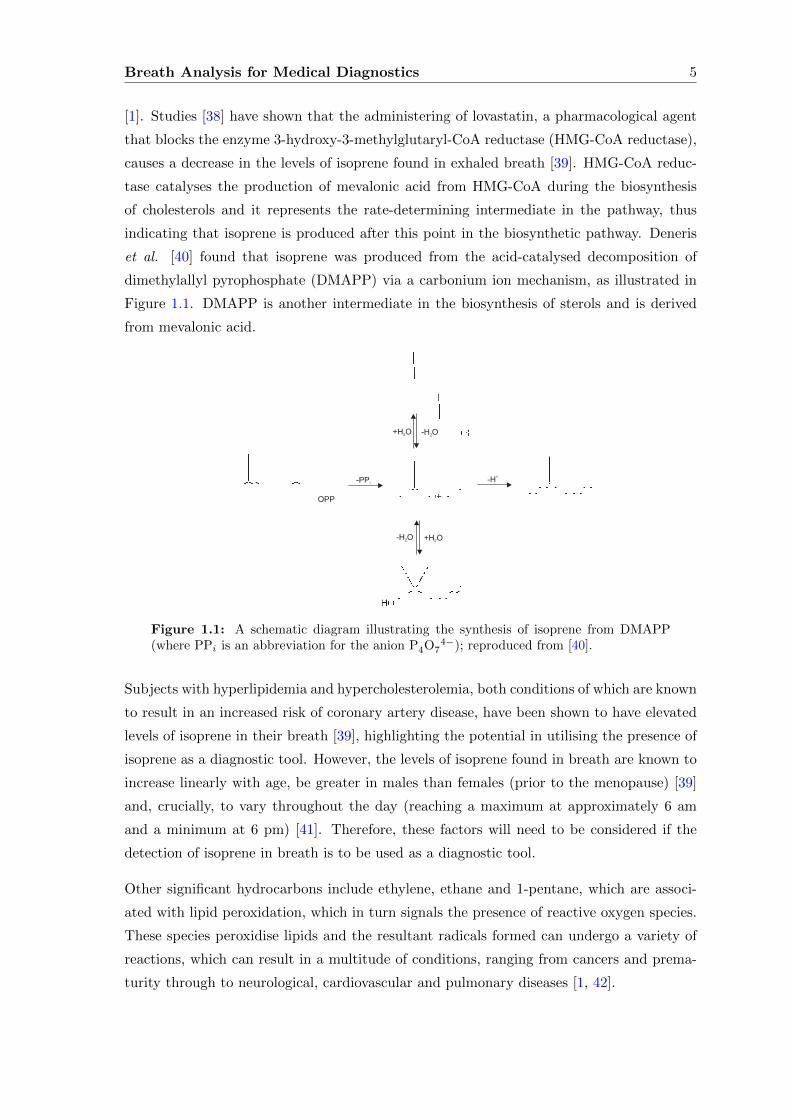
indicating that isoprene is produced after this point in the biosynthetic pathway. Deneris
et al. [40] found that isoprene was produced from the acid-catalysed decomposition of
dimethylallyl pyrophosphate (DMAPP) via a carbonium ion mechanism, as illustrated in
Figure 1.1. DMAPP is another intermediate in the biosynthesis of sterols and is derived
from mevalonic acid.
Figure 1.1: A schematic diagram illustrating the synthesis of isoprene from DMAPP(where PPi is an abbreviation for the anion P4O7
4−); reproduced from [40].
Subjects with hyperlipidemia and hypercholesterolemia, both conditions of which are known
to result in an increased risk of coronary artery disease, have been shown to have elevated
levels of isoprene in their breath [39], highlighting the potential in utilising the presence of
isoprene as a diagnostic tool. However, the levels of isoprene found in breath are known to
increase linearly with age, be greater in males than females (prior to the menopause) [39]
and, crucially, to vary throughout the day (reaching a maximum at approximately 6 am
and a minimum at 6 pm) [41]. Therefore, these factors will need to be considered if the
detection of isoprene in breath is to be used as a diagnostic tool.
Other significant hydrocarbons include ethylene, ethane and 1-pentane, which are associ-
ated with lipid peroxidation, which in turn signals the presence of reactive oxygen species.
These species peroxidise lipids and the resultant radicals formed can undergo a variety of
reactions, which can result in a multitude of conditions, ranging from cancers and prema-
turity through to neurological, cardiovascular and pulmonary diseases [1, 42].
Breath Analysis for Medical Diagnostics 6
Sulphur-based compounds are also found in breath, with excess levels of these often be-
ing an indication of liver-related diseases. These compounds include hydrogen sulphide,
methanethiol (methyl mercaptan), ethanethiol (ethyl mercaptan), dimethyl sulphide and
dimethyl disulphide, which are produced following the incomplete metabolism of methion-
ine [1, 43] and are generally found at the ∼10 ppb level (an order of magnitude less than
isoprene).
Often a species can be a biomarker for more than one disease, and similarly a particular
condition may have more than one biomarker. Acetone (which will be discussed at length
later in this chapter), as well as being the signature molecule of diabetes, has also been
linked with lung cancer, congestive heart failure and brain seizure [6]. Meanwhile, butane
is also a reported marker for lung cancer, as are an array of other hydrocarbons and some
sulphur compounds [6, 44]. Schizophrenia is identified by carbon disulphide and pentane
[45], whilst the peroxidation of lipids is marked by the presence of pentane and ethane [46]:
therefore, a correct diagnosis cannot be given from the elevated presence of pentane alone
in a subject’s breath, highlighting the need for any breath analysis technique to be specific
to the target disease. Of these biomarkers, a handful are found at ppm, or sub-ppm levels
(acetone, isoprene, methane, propanol, hydrogen, CO) and a further 400 or so are at the
ppb and ppt level.
As the physiological links between certain molecules and conditions are strengthened, so
the concept of breath analysis becomes more realistic [2]. In principle it allows for a non-
invasive means to diagnose and monitor metabolic statuses by simply collecting a breath
sample. In addition to high sensitivity and selectivity, ideally such a device should be low-
cost, compact and with a real-time response, thus realising point-of-care disease diagnostics.
Currently, there are a number of ways breath samples can be analysed, which can be divided
into three main groups: mass spectrometry-based techniques, laser spectroscopy methods
and other techniques, including electrochemical-based sensors. These methods are briefly
discussed in the following section.
1.2 Techniques for analysing breath
Traditionally, mass spectrometry, coupled with gas-chromatography (GC-MS), has been
utilised to detect and analyse the volatile species found in breath samples [5, 43]. The
breath sample passes through the gas chromatograph, which separates the constituent
molecules based on their chemical properties: different molecules will elute from the column
at different times. The separated mix then passes into the mass spectrometer, which ionises
the molecules before they are detected and identified using their mass-to-charge ratio. Early
mass spectrometers used electron ionisation (EI) to create ions but this frequently leads to
Breath Analysis for Medical Diagnostics 7
fragmentation of the parent molecule, often making assignments difficult. Softer means of
achieving ionisation have been developed, for example, using ion-molecule reaction (IMR)
MS. This uses EI to produce primary ions (for example, Hg+, Xe+), which then pass
into a sample chamber and, via ion-molecule reactions, cause the formation of ions from
the sample under analysis. The mass spectrometer used in this thesis combines both of
these techniques and a full description of it will be given in Chapter 5. In addition, often
mass spectroscopy is combined with pre-concentration techniques [47, 48] to increase the
attainable level of sensitivity.
Further advances have included the development of selected ion flow tube mass spectrometry
(SIFT-MS) [49] and proton transfer reaction mass spectrometry (PTR-MS) [50], both of
which do not require calibration against standard gas mixtures. These techniques are also
based on chemical ionisation, where initial ions are created via a gas discharge source
before being used to ionise the sample of interest. However, in contrast to conventional
IMR-MS, with SIFT-MS the initial ions are separated out by their mass-to-charge ratio
and fed into an inert carrier gas before being transported through the flow tube into which
the sample for analysis is injected [49]. The resulting ions formed are then separated by
their mass-to-charge ratio and detected via the electrical current that is induced from the
ion hitting the detector. In order for the technique to be quantifiable, it is necessary to
know the likelihood of an ionisation occurring when an initial ion encounters a sample
molecule. Thus, a knowledge of the rate constant of the reaction between the ions and
the sample allows the original concentration of the sample to be determined. PTR-MS
[50] works along a similar principle, with H3O+ representing the primary reactant ion.
Proton transfer occurs for every collision as nearly all volatile organic compounds (VOCs)
have proton affinities larger than H2O and the processes tend to be non-dissociative so that
cluster ions are less likely to form, resulting in simpler ion chemistry to analyse. In addition,
there is no requirement for a mass filter, so a greater flow rate of H3O+ ions can enter the
flow tube, and the use of an electric field to coax the ions along the length of the tube
reduces diffusive losses to the sides of the flow-drift tube. Consequently, higher levels of the
H3O+ ions are available, resulting in a higher analytical sensitivity than that attainable
with SIFT-MS. However, accurate quantification is more difficult to achieve with PTR-MS
as, unlike SIFT-MS, the reaction time and the kinetics for the ion-molecule reaction are not
well defined [49] and often the sample concentrations are determined using a standardised
value for the rate constant. It has been argued that for this reason, PTR-MS has mainly
found application in air analysis and environmental studies, rather than in breath analysis
where greater accuracy is more vital [49]. Despite this, a number of studies have used
PTR-MS for breath profiling [37, 51], though it is SIFT-MS that has really led the way in
clinical breath analysis [48, 49, 52].
Breath Analysis for Medical Diagnostics 8
Despite the advantages associated with mass spectrometry, most notably the very high
sensitivities attainable and the fact that multiple species can be monitored, the technique
is restricted to use in clinical laboratories, which limits its practicality in routine medical
applications to breath. With its high cost and limited portability, it does not currently
offer a point-of-care (POC) means for breath diagnostics.
A potential solution includes the use of chemical and electrochemical sensors, which are
both compact and relatively inexpensive. One such example is the so-called ‘electronic nose’
which consists of arrays of non-selective chemical sensors, formed from quartz microbalance
(QMB) sensors [27, 53]. The application of an alternating current induces oscillations
in the quartz crystal; on adsorption to the sensors, the molecules generate a variation
in the resonance frequency of the QMB, which is then detected and attributed to the
concentration of the sample. However, the very nature of these devices means that they
merely detect similarities and differences between samples as they are not sensitive to
a particular species. Therefore, they require thorough calibration with other methods
and a suitable data analysis to infer the significance of the changes observed [53]. A
further disadvantage is that sometimes one does not just want to distinguish between two
populations, but actually monitor the absolute levels of a species in a sample, and this
technique does not offer this. Other examples of solid state-based sensors utilise metal
oxides, such as WO3, which in its ε-phase demonstrates selective and quantitative detection
of acetone [54]. This is a result of the increase in its spontaneous electric dipole moment on
interaction with species with high dipole moments, which leads to a measurable decrease in
the resistance of the device. Although the sensitivity of the instrument to acetone is much
higher than that to other molecules found in breath, it still records signals at 14% and 21%
of the signal level due to 600 ppb of acetone for typical water vapour and ethanol levels
found in breath. Although the selectivity for acetone is increased under conditions of higher
humidity (as would be present in breath), the sensitivity of the device is reduced by 67%
[54]. Despite this, against a background of 90% relative humidity, the sensor was able to
distinguish 20 ppb levels of acetone (though the question arises how accurate the recorded
reading of acetone would be in real breath samples, in which there is not a controlled level of
humidity from which to compare). Unfortunately, although chemical-based sensors do offer
a compact and relatively cheap method for breath analysis, the lack of absolute selectivity
for the target molecule is a common feature of the devices [27].
In contrast, laser spectroscopy offers a very high level of selectivity, whilst still maintaining
very good sensitivity. Laser spectroscopy encompasses a wide range of techniques, including
laser-induced fluorescence (LIF), where a molecule is excited to a higher electronic energy
state by incident radiation before fluorescing; Raman spectroscopy, where following excita-
tion to a virtual energy level, the molecule relaxes to a vibrational or rotational state which
Breath Analysis for Medical Diagnostics 9
is different from its initial level, emitting radiation at a frequency which is shifted rela-
tive to the excitation wavelength by the frequency difference between the initial and final
state; and photoacoustic spectroscopy, where the absorption of modulated radiation by the
molecular sample is transformed into a sound wave and detected with a microphone. How-
ever, absorption spectroscopy, the measurement of the radiation absorbed by a molecule
as a function of the wavelength incident on it, forms the focus of this thesis and it will
be discussed in detail in the following chapter. Absorption spectroscopy offers a real-time
response, is affordable (when based on telecommunications diode laser technology) and has
the potential to be compact: as such, its use represents a realistic point-of-care diagnostic
device. The technology is not without its drawbacks, most notably that the level of sensi-
tivity attainable depends on the molecule being studied and that generally the number of
species that can be monitored simultaneously is restricted. Despite this, there has been a
surge of interest in developing breath analyser devices using laser-based techniques in recent
years, and a number of excellent reviews have been written on the subject [1, 6, 28, 55]. It
is important to note, however, that there are several definitions of sensitivity, so care has
to be taken in comparing the results of the different authors in the following discussion.
Nitric oxide has featured heavily in spectroscopic studies of breath as a result of its strong
absorption band at 5 µm and due to its role as an officially recognised biomarker for asthma.
Techniques have centred on the use of an optical cavity [29, 30, 33, 56, 57] or a multipass
Herriott cell [31, 58] to enhance the absorption signal, and modulation spectroscopy to
reduce the noise levels in the detected signal [32] (a full description of these techniques will
follow in later chapters).
Similarly, measurements of the carbon isotope ratios with CO2 have also featured promi-
nently, thanks to the wide-spread use of the urea breath test for diagnosing the presence
of H. pylori. A wide range of techniques have been employed, including Fourier Transform
spectroscopy [59], photoacoustic spectroscopy [60] and the use of a multipass Herriott cell
with modulation spectroscopy [61]. Several studies with optical cavities have also been
reported, such as Kasyutich et al. [13], which utilised off-axis Cavity Enhanced Absorption
Spectroscopy (CEAS) and Crosson et al. [18], who not only reported a precision of 0.22
with a cavity ring down spectroscopy (CRDS) instrument, but also demonstrated that
on real breath samples their sensor matched the levels reported by Isotopic Ratio Mass
Spectrometry (IRMS). A number of studies have involved the development of carbon iso-
tope sensors for volcanic gas emissions [62, 63], highlighting a non-breath related use for
measuring isotopic ratios. McManus et al. [19] designed a neat experiment where a multi-
pass cell was used with a Pb-salt laser to provide two different pathlengths to measure the
two isotopic absorptions. This ensured that the absorption depth for the two transitions
was approximately the same, and it allowed them to report an impressive 0.2 precision.
A very similar experiment was also undertaken by Uehara et al. [64] on isotopic ratios in
Breath Analysis for Medical Diagnostics 10
methane, and Zare et al. [65] demonstrated the use of a continuous flow cavity ring-down
spectrometer (CRDS) for carbon isotope measurements on ethane and propane.
The less well-established biomarkers have also been the subject of a number of laser-based
investigations. Sigrist et al. [66, 67] have conducted studies into detecting the methylamines
in breath, utilising a cavity ring down spectrometer in the near infrared (NIR) to probe
the first overtone of the N-H stretch vibration at ∼1.52 µm in monomethylamine (MMA)
and dimethylamine (DMA), and a difference frequency generation (DFG) method to probe
the 3.5 - 3.9 µm region in the mid-infrared (MIR). The former yielded sensitivities of 350
ppb and 1.6 ppm for MMA and DMA, respectively, in synthetic mixtures of the gases,
decreasing to 10 ppm and 60 ppm when interfering species were taken into account. The
MIR study allowed trimethylamine (TMA) to also be probed, as the transitions in the 3 µm
region correspond to C-N stretches. In addition, the absorption cross-sections are larger
than those in the NIR and there is less spectral interference from competing species in
breath, which allowed the group to attain sensitivities of 900 ppb, 450 ppb and 120 ppb
for MMA, DMA and TMA, respectively. Ammonia itself has been the subject of laser-
based spectroscopic studies, with Manne et al. [68] demonstrating a device based on cavity
ring down spectroscopy (CRDS) with a pulsed quantum cascade laser source at 970 cm−1,
achieving a sensitivity of 50 ppb. This was followed with a study based on the use of
an astigmatic Herriott cell with the same laser. Using both an interpulse and intrapulse
methodology, detection levels for ammonia and ethylene (which was also studied) were
found for the interpulse technique to be 4 ppb and 7 ppb, respectively, and 3 ppb and 5
ppb for the intrapulse method. Both of these techniques were then applied to an actual
breath sample with promising results.
Using a CO laser, Dahnke et al. have developed an instrument capable of real-time mon-
itoring of ethane levels in human breath [69], achieving detection levels of 500 ppt with a
cavity leak out spectrometer. This was followed with further studies, which also included
the measurement of expirograms [70], and the use of an optical parametric oscillator system
at 3 µm to achieve impressive sensitivities of 0.5 ppt [71] for the same molecule.
Carbonyl sulphide, elevated levels of which have been identified in patients who have expe-
rienced acute allograft rejection following lung transplantation [72], has been the subject
of a number of laser-based studies [73, 74]. For example, Wysocki et al. [75] developed a
compact Herriott cell in the mid-infrared using a pulsed quantum cascade laser (QCL) at
4.85 - 4.87 µm for the sensing of OCS in breath, achieving a detection limit of 1.2 ppb in
a 0.4 s acquisition time.
Although laser-based techniques are limited by the number of species that can be moni-
tored simultaneously, a number of studies have demonstrated that modest multiple species
detection can be comfortably achieved. Moskalenko et al. [76] monitored ammonia, carbon
Breath Analysis for Medical Diagnostics 11
monoxide, methane and carbon dioxide in the breath of smokers and non-smokers using
tunable diode laser spectroscopy (TDLS) with a multipass cell, whilst Wang et al. [14]
have presented a continuous wave cavity ring down (cw-CRD)-based sensor for monitoring
methane and carbon dioxide isotopes by multiplexing two distributed feedback diode lasers.
Utilising optical frequency comb spectroscopy, Thorpe et al. [77] were able to cover an im-
pressive 200 nm with 800 MHz resolution. They used the device to record CO2 isotope
measurements, together with CO and NH3, the latter for which they attained a sensitivity
limit of 18 ppb, which although was too high to detect ammonia in healthy individuals,
was at a sufficiently sensitive level to detect the early stages of renal failure. However, such
techniques are very far from being implemented outside a laser laboratory.
1.3 Acetone
Acetone is the most abundant VOC found in human breath, and coupled with its strong
link with diabetes, it represents a particularly interesting molecule to study with regard
to breath analysis. It is essentially produced when the body turns to its fat deposits as
a source of energy in the absence of glycogen stores [78]. The triglyceride molecules are
cleaved via lypolysis to produce a glycerol molecule and 3 fatty acid chains. The fatty acid
chains are then utilised in β-oxidation to generate energy and produce the acetyl co-enzyme
A (Acetyl CoA) required for the Krebs Cycle, which is then used to generate more energy.
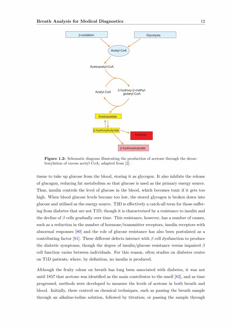
Excess acetyl CoA is converted into acetoacetate and D-β-hydroxybutyrate in the liver,
from which the carboxylation of the former results in the production of acetone [79], as
illustrated in Figure 1.2. These ketone bodies then diffuse into the bloodstream and are
also oxidised via the Krebs Cycle in peripheral tissue to generate energy [1, 2]. However, in
times of stress when fat stores are used instead of carbohydrates, the rate of ketone body
production outstrips their use by the peripheral tissues and their concentration builds up
in the bloodstream. In the case of acetone, which is a small, volatile compound that easily
diffuses from the bloodstream and into the lungs, this results in elevated levels of acetone
in exhaled breath. These periods of stress which cause fat deposits to be used as energy
sources could be the result of intense exercise, dieting or a lack of insulin resulting in a
reduced uptake of glucose by the liver.
Therefore, untreated diabetes would be expected to result in higher levels of acetone than
normally found in breath. Diabetes mellitus can be split up into type 1 (T1D) and type 2
(T2D) categories. Whilst the latter tends to be developed later in life and is often asso-
ciated with obesity, the former is typically juvenile-onset. T1D subjects are characterised
by a lack of insulin-production, due to the destruction of β cells in the islets of Langerhans
of the pancreas which produce the hormone [78]. Insulin causes the liver, muscle and fat
Breath Analysis for Medical Diagnostics 12
Figure 1.2: Schematic diagram illustrating the production of acetone through the decar-boxylation of excess acetyl CoA; adapted from [2].
tissue to take up glucose from the blood, storing it as glycogen. It also inhibits the release
of glucagon, reducing fat metabolism so that glucose is used as the primary energy source.
Thus, insulin controls the level of glucose in the blood, which becomes toxic if it gets too
high. When blood glucose levels become too low, the stored glycogen is broken down into
glucose and utilised as the energy source. T2D is effectively a catch-all term for those suffer-
ing from diabetes that are not T1D, though it is characterised by a resistance to insulin and
the decline of β cells gradually over time. This resistance, however, has a number of causes,
such as a reduction in the number of hormone/transmitter receptors, insulin receptors with
abnormal responses [80] and the role of glucose resistance has also been postulated as a
contributing factor [81]. These different defects interact with β cell dysfunction to produce
the diabetic symptoms, though the degree of insulin/glucose resistance versus impaired β
cell function varies between individuals. For this reason, often studies on diabetes centre
on T1D patients, where, by definition, no insulin is produced.
Although the fruity odour on breath has long been associated with diabetes, it was not
until 1857 that acetone was identified as the main contributor to the smell [82], and as time
progressed, methods were developed to measure the levels of acetone in both breath and
blood. Initially, these centred on chemical techniques, such as passing the breath sample
through an alkaline-iodine solution, followed by titration; or passing the sample through
Breath Analysis for Medical Diagnostics 13
sodium bisulphite solution and using a mercuric cyanide reagent [83–88] to determine the
levels of acetone present from the resulting turbidity. Needless to say, these methods were
quite tedious and not very sensitive. It was not until the 1960s that studies into breath
acetone advanced, thanks to the development of GC-MS. These studies demonstrated that
the measurement of acetone could be used in conjunction with blood glucose measurements
to determine the exact diabetic status of the patient: for example, a high level of acetone
coupled with normal blood glucose levels would reveal that the patient is not taking enough
insulin or eating enough, which could then be corrected for [89–91]; indeed Crofford et al.
[92] documented a ‘clinical use of breath acetone measurement’ in which the diet or insulin
in-take would be altered depending on the particular combinations of breath acetone and
blood glucose present in the patient.
However, since the development of the first blood glucose meter in the early 1980s, the
measurement of breath acetone has become less prominent. The reasons for this are two-
fold: it became apparent that intensive control and monitoring of diabetes was required
to avoid the development of long-term complications [93], and this requirement for rigor-
ous self-monitoring resulted in the decline in the use of breath acetone levels for diabetes
monitoring as at the time there was no means to measure breath acetone out of clini-
cal laboratories; and secondly, blood measurements of β-hydroxybutyrate can give similar
information on blood ketones.
More recently, the monitoring of breath acetone has seen a resurgence as advances in mass
spectrometry have allowed more detailed and comprehensive studies on VOCs in general.
Turner et al. [94] measured the real-time breath acetone levels from type 1 diabetics
and monitored their blood glucose levels, which were controlled using a hypoglycaemic
clamp technique. From the small study, they demonstrated that although there was a
strong positive correlation between blood glucose and breath acetone, the relationship was
different for each patient. Another mass spectroscopy-based study by Minh et al. [95],
building on work from an earlier study into the correlation between breath acetone and
ethanol with glucose serum [96], has attempted to infer the blood glucose levels from breath
via an indirect method employing a chemical reagent to convert the acetone into something
measurable. From this study, only four molecular markers were identified as being required
to determine the blood glucose levels from breath, and that acetone is by far the most
significant. Wang et al. [97] have used a UV laser-based cavity ring-down method to
measure breath acetone and attempted to show a general trend amongst T1D subjects,
with a linear correlation between the average breath acetone levels and the average blood
glucose levels when the patients are grouped by different blood glucose levels. In another
study, Spanel and Smith [98] demonstrate that although a predicted increase in the level
of acetone is observed in the breath of those on a ketogenic diet, there is a wide variation
Breath Analysis for Medical Diagnostics 14
observed in the concentrations as a result of natural intra-individual biological and daily
variability.
Therefore, it is clear from these studies and recent reviews [99–101] that more work is
needed to firmly establish the exact link between blood glucose and breath acetone, as
there is a certain degree of variability in the relationship between the two for different
individuals. Despite this, the interest in developing a device for measuring breath acetone
has grown rapidly, especially with the promise of reducing or even eradicating the need for
blood testing, which is particularly painful for children.
One such device is an enzymatic electrode sensor [102] which is based on a series of enzyme
reactions, which cause acetone to be converted into H2O2, which is then detected by elec-
trochemical means. On breathing into the sensor, one waits for 3 minutes before the voltage
is applied across the electrodes. A detection limit of 0.25 ppm (v/v) above the background
current was demonstrated, although it was acknowledged that electroactive impurities in
the enzymes or from the electrode itself could cause this to vary, and that this was a subject
of future work. In addition, secondary alcohols are potential interferents from the enzy-
matic reaction and although most are at levels too low to be significant, acetaldehyde is
known to be at a level that could cause a problem, particularly after alcohol consumption.
However, the sensor was successfully used in a study on the effect of diet on acetone levels,
where the acetone levels reported were found to correlate well with those returned by the
mass spectrometer used in the study (R2 ≥ 0.950).
Using a similar principle, a company called ‘positiveID’ [103] is developing a sensor which is
based on the colour change associated with acetone and sodium nitroprusside, which they
then claim can be used to infer blood glucose levels.
Within optical-based techniques, Bakhirkin et al. [104] have demonstrated the use of a
quantum cascade laser at ∼8 µm to detect 1 ppm of acetone in air using direct absorption
spectroscopy and a 1 m length sample cell. On application of wavelength modulation
spectroscopy, the detecting limit was improved to 100 ppbv, and although this illustrates the
potential of laser-based devices for the detection of acetone, given the size of the instrument
it does not represent a practical breath analyser. Wang et al. have developed a UV-based
CRDS sensor for detecting acetone [105–107], which was then used in their 2010 study
described previously [97]. Although reporting a theoretical minimum sensitivity of 0.13
ppmv (based on the baseline stability of the instrument), the authors acknowledge the
values returned represent the upper limit on the breath acetone levels (as a consequence
of interfering species in the region and scattering effects), and the reported levels were not
verified against a secondary device.
Breath Analysis for Medical Diagnostics 15
1.4 Overview of Thesis
This thesis will investigate a variety of absorption spectroscopy-based techniques for the po-
tential application to breath analysis, with particular emphasis on the detection of acetone.
The following chapter will firstly introduce the fundamentals of absorption spectroscopy,
outlining the techniques that can be applied to increase its sensitivity before discussing
the types of radiation sources utilised in this body of work. The first experimentally-based
chapter, Chapter 3, introduces a preliminary study into the measurement of methane in
breath using a diode laser-based cavity-enhanced detection system (CEAS) in the near-
infrared (NIR) at 1.65 µm. The second half of Chapter 3 details the characterisation of
a novel, widely tunable laser source, a digital supermode distributed Bragg reflector (DS-
DBR), demonstrating the first application of this device to spectroscopy by probing NIR
vibrational bands of CO2 from 1.56 - 1.61 µm.
Whilst diode-based lasers are ideal for the detection of small molecules, such as CH4 and
CO2, which have well-resolved, narrow transitions, acetone (together with other important
VOCs) has broad, congested vibrational spectra, typically spanning tens of nanometres,
making it difficult to identify using such sources. Therefore, Chapter 4 describes the de-
velopment of a broadband radiation-based CEAS spectrometer. Two types of broadband
source are considered, a Superluminescent Light Emitting Diode (SLED) and a Supercon-
tinuum (SC) source, whilst the use of both a dispersive monochromatic spectrometer and
a Fourier transform spectrometer are demonstrated and compared. Butadiene, a molecule
with a broad absorption feature spread across the spectral region of study (∼1.6 - 1.7 µm),
is used to characterise the instruments developed, before they are applied to the detection
of acetone and isoprene, and finally to real breath samples. Building on this work, Chapter
5 describes the development of a prototype breath acetone analyser carried out at Oxford
Medical Diagnostics Ltd. Given the requirements of a compact, commercially-viable device,
a diode laser-based system is employed and the chapter deals with an investigation into
negating and removing the effects of interfering species, most notably water vapour, before
demonstrating and calibrating its performance against a mass spectrometer.
In the final experimental chapter, spectroscopic detection moves to the mid-infrared and
8 µm with the use of a continuous wave (cw) quantum cascade laser (QCL), allowing the
stronger, fundamental transitions of acetone to be probed, providing the potential for a
greater level of sensitivity to be achieved. The low effective laser linewidth is utilised to
resolve rotational structure in low pressure samples of acetone and to determine the relevant
absorption cross-sections. Following this, the sensitivity of the system is progressively
increased using multipass cells (White and Herriott) and finally an optical cavity. Exploiting
the water-removing devices developed at Oxford Medical Diagnostics Ltd., the cavity-based
spectrometer is then used to detect acetone in breath samples, and cross-checked with a

Breath Analysis for Medical Diagnostics 16
mass spectrometer. Finally, the work demonstrated in this thesis is reviewed, prior to the
presentation of some preliminary experimental results on the detection of acetone at 280
nm, together with a discussion on the future directions of the detection of breath acetone.

Breath Analysis for Medical Diagnostics 17
Biomarker Physiological basis Metabolic disorder
acetaldehyde ethanol metabolism alcoholism,liver-related diseases, lung cancer
acetone decarboxylation of acetoacetate diabetes, lung cancer,congestive heart failure, brain seizure
ammonia protein metabolism renal diseases, asthma/bacterial metabolism
carbon monoxide heme catabolism catalysed oxidative stress,by heme oxygenases respiratory infection, anaemias
carbon dioxide respiration isotopic labelling used to diagnosepresence of H. pylori, oxidative stress
carbonyl sulphide gut bacterial oxidation of liver related diseasesreduced sulphur species
ethane lipid peroxidation oxidative stress, vitamin E deficiencyin children, peroxidation of lipids
ethanol gut bacterial metabolism of sugars production of gut bacteria
ethylene lipid peroxidation uv radiation damage of skin,peroxidation of lipids
hydrogen carbohydrate metabolism colonic fermentation, intestinal upset
hydrogen sulphide anaerobic bacterial metabolism liver-related diseaseof thiol proteins
isoprene cholesterol biosynthesis blood cholesterol
methane gut bacterial metabolism intestinal problems,lung diseases colonic fermentation
methanethiol methionine metabolism halitosis
methylamine protein metabolism protein metabolism in the body
nitric oxide involved in vasodilatation, or asthma, bronchiectasis,neurotransmission; production catalysed hypertension, rhinitis,by nitric oxide synthases lung diseases
pentane lipid peroxidation peroxidation of lipids,liver disease, schizophrenia,breast cancer, rheumatoid arthritis
Table 1.1: A selection of potential biomarkers found in breath, adapted from [1, 6].
Chapter 2
Absorption Spectroscopy:
principles and light sources
Absorption spectroscopy represents a very powerful means for quantitative trace gas de-
tection. In principle the energies that are absorbed are specific to each species, reflecting
its unique set of internal molecular energy states (electronic and ro-vibrational), allowing a
high level of selectivity to be attained. Furthermore, the technique can be quantitative via
the use of the Beer-Lambert law, which allows absolute number densities of the species of
interest to be straightforwardly determined from the measured absorbance. However, there
is an inherent lack of sensitivity associated with direct absorption spectroscopy, as a direct
consequence of measuring a small change on a large background, which must be improved
upon to realise trace gas detection. This chapter initially describes the basis of absorption
spectroscopy and presents a brief outline of the factors influencing its sensitivity, before
discussing the specific light sources used to perform the absorption studies in this thesis.
2.1 Absorption Spectroscopy
Absorption spectroscopy is primarily based on the interaction of the electric field of light
with the electric dipole moment associated with the molecular transition of interest [108]
(although electric quadrupole and magnetic dipole interactions can also occur). Quantum
mechanically this interaction is described in terms of the electric dipole moment operator, µ,
which acts on the initial state of the atom/molecule (ψi) to give the new, excited final state
(ψ∗f ). The degree of coupling between the initial and final states, or transition amplitude,
is given by:
18
Absorption Spectroscopy: principles and light sources 19
µfi =
∫ψ∗f µψi dτ (2.1)
and is known as the transition dipole moment. The probability of the transition occurring
is then proportional to the square of the transition dipole moment. Therefore, in order
for the transition to occur, the integral in 2.1 must be non-zero. The rate at which the
transition occurs (per unit spectral density of the electromagnetic field) is given by the
Einstein co-efficient of absorption, Bif [108]:
Bif =|µfi|2
6ε0~2(2.2)
where ε0 is the vacuum permittivity and ~ = h/2π. Hence, the larger the transition rate, the
larger the measured absorbance. The Einstein co-efficient is then related to the absorbance
via:
Bifhν
c=
∫ ∞0
σif (ν) dν = σint (2.3)
where σif (ν) is the frequency-dependent absorption cross-section for the transition f ← i
at frequency ν and σint is the integrated absorption cross-section. From the absorption
cross-section, the familiar Beer-Lambert law [109, 110] can be derived:
I(ν) = I0 exp(−σ(ν)CL) (2.4)
which links the frequency-dependent absorption cross-section to the intensity attenuation
observed as radiation passes through a length L of a sample of concentration C, with I0
and I(ν) the incident and transmitted radiation, respectively. Due to broadening effects,
the observed absorption transition is not a δ function centred on a frequency, ν0, but has
a well defined lineshape which is discussed below [108]. However, it is noted that the
integrated absorption cross-section, σint, is independent of the environmental conditions of
the molecule and is therefore a constant (at a particular temperature).
The minimum linewidth associated with all transitions is a result of natural linewidth
broadening, which may be thought of as a direct consequence of the Heisenberg uncertainty
principle. Given that the lifetime (τ) of the upper state of the transition is finite, an
uncertainty is introduced into the corresponding energy of the transition [108]:
τδE ≈ 1
2~ (2.5)
Absorption Spectroscopy: principles and light sources 20
Thus the transition occurs over a range of frequencies, directly related to δE. However, this
effect is generally very small in comparison to the broadening induced by both collisional
and Doppler effects at room temperature, typically ranging from 10−4 Hz associated with
rotational energy states, through to a few MHz in excited electronic levels, as a result of
the ν3 dependence of Afi, the Einstein coefficient for spontaneous emission. Collisional,
or pressure broadening arises from a decrease in the lifetime of both states involved in the
transition as a result of increased collision frequency between molecules, which causes an
increase in the uncertainty of the associated energy of the transition, in accordance with
equation 2.5, and leads to a broadening of the absorption lineshape. Clearly, as the pressure
increases, the number of collisions will increase, resulting in greater line broadening. For a
given pressure, the degree to which the absorption profile broadens due to collisional effects
is quantified by the pressure-broadening coefficient, γ, which in turn is dependent on the
nature of the pressure broadening gas (and thus the type of collisional energy transfer
processes which can take place). Lineshapes which are dominated by pressure broadening
have a Lorentzian profile [110]:
L(ν) =∆νL
2π[(∆νL
2 )2 + (ν − ν0)2] (2.6)
where ν0 is the central frequency of the absorption profile and the Lorentzian width (full
width half maximum, FWHM), ∆νL, is related to the pressure-broadening coefficient via
∆νL = 2γp, where p is the pressure of the broadening gas.
In the low pressure regime (where p ∼ few Torr or less), Doppler broadening is the dominant
line broadening mechanism. The molecules in a gaseous sample at a certain temperature
will exhibit a range of velocities, given by the Maxwell-Boltzmann distribution [110]. The
motion of these molecules relative to the propagation direction of the radiation passing
through the sample leads to a shift in the observed frequency at which each molecule
absorbs. Thus, a distribution of absorption frequencies is observed, reflecting the velocity
distribution of the molecules and results in a Gaussian lineshape profile:
G(ν) =2
∆νG
√ln 2
πexp
[− 4 ln 2(ν − ν0)2
∆ν2G
](2.7)
where ∆νG is the FWHM Gaussian linewidth, defined via:
∆νG(T ) = 2ν0
√2kT ln 2
mc2(2.8)
Absorption Spectroscopy: principles and light sources 21
where T is the temperature, k is the Boltzmann constant, m is the mass of the molecule
and ν0 is the central frequency of the transition.
At pressures where there is an observable contribution from collisional broadening as well
as Doppler broadening, the absorption linewidth can be described by a convolution of the
Gaussian and Lorentzian lineshapes; the Voigt profile:
V (ν) =2
∆νG
√ln 2
π
y
π
∫ +∞
−∞
e−t2
y2 + (x− t)2dt (2.9)
where x and y are given by
x =√
ln 22(ν − ν0)
∆νGy =√
ln 2∆νL∆νG
(2.10)
Notable other, more complex, lineshape profiles include Galatry and Rautian lineshapes
which are typically employed when collisional-narrowing effects take place. These processes
occur when the lifetime of the upper state is large compared to the time between collisions
(i.e. the mean free path of the absorber is significantly less than the wavelength of the
transition being studied), so that many elastic collisions will affect the species’ velocity
during the absorption of a photon, leading to a reduction in the Doppler broadening of the
line [111].
Sensitivity
The sensitivity of direct absorption spectroscopy is inherently low given the need to mea-
sure a small change on a large background (i.e. the decrease in signal intensity due to
absorption by the molecular species is very small in comparison to the overall detected sig-
nal). However, it can be improved by increasing the absorbance or by reducing the level of
noise in the system, or sometimes both (such as in Noise Immune Cavity Enhanced Optical
Heterodyne Molecular Spectroscopy, NICE-OHMS [112]).
A quick glance at the Beer-Lambert law (2.4) indicates that the level of absorption can be
enhanced by (a) increasing the concentration of the sample, C, (b) using a transition with
a larger absorption cross-section, σ(ν), or (c) by increasing the pathlength, L. The first
is not necessarily always an option, especially for trace gas detection, whilst the second
can be exploited by carefully selecting the wavelength with which to probe the molecule.
This could, for example, include moving to the MIR spectral region in order to probe the
fundamental vibrational transitions, which have much larger absorption cross-sections than
the overtone and combination bands found in the NIR. The third option, increasing the
pathlength, can be achieved either by using a multipass absorption cell, such as a Herriott
cell, or by using an optical cavity. Both of these techniques will be described fully later
Absorption Spectroscopy: principles and light sources 22
in this thesis, with multipass cells featuring in Chapter 6 and the basis of cavity-enhanced
techniques introduced in the following chapter.
A reduction in the noise associated with the measurement will also increase the level of
sensitivity. There are three major types of noise in absorption spectroscopy measurements.
The first is due to quantum fluctuations inherent both in the laser source and in the
photocurrent of the detector. This is known as shot noise and it is a statistical phenomenon
due to random emissions and the quantised nature of energy and charge carriers. The shot
noise limit represents the fundamental limit of all detection methods when there are no
external noise sources and is given by [113]:
(S
N
)SNL
=ηP0
2hν∆f(2.11)
in terms of the signal to noise ratio, where η is the quantum efficiency of the detector (i.e.
the ratio of the number of carriers produced to the number of absorbed photons), P0 is the
power incident on the detector, h is Planck’s constant, ν is the wavelength of the radiation
and ∆f is the bandwidth of the detector.
In practice, it is very rare for any measurement to approach the shot noise limit because
external noise sources accumulate and cause the sensitivity to decrease. An example is
noise due to environmental fluctuations in the experimental set-up. These could include
mechanical instabilities in the system as a result of pressure differentials, which alter the
optical alignment of the system, or thermal or acoustic fluctuations. This also covers
fluctuations in the laser output itself as a result of environmental factors. This type of
noise is linearly dependent on the intensity of the light, and is otherwise referred to as 1/f
noise. White noise, so called because its power spectral density is invariant with frequency,
represents the final noise source. It is associated with thermal, or Johnson-Nyquist, noise
which arises from the thermal fluctuations of charge carriers, such as in the conversion of
photon energy to electrical signal in a photodiode.
The level of noise in a system can be reduced using modulation spectroscopic techniques,
which help to reduce the environmentally-induced noise component, the 1/f noise. This
involves applying a high modulation to the laser output so that detection is shifted to
a higher frequency, hence reducing the effects of 1/f noise. An overview of modulation
techniques, with particular emphasis on the wavelength modulation spectroscopy variant,
will be presented in Chapter 6.
There are several ways to quote the sensitivity of an absorption measurement. Throughout
this thesis, the minimum detectable absorption co-efficient, αmin, is taken to represent the
Absorption Spectroscopy: principles and light sources 23
noise equivalent absorption, in other words:
αmin =αpeak
SNR(2.12)
where SNR is the signal to noise ratio and αpeak = σpeakC, where C is the number density
of the species and σpeak is derived from the integrated absorption cross-section (σint):
σpeak =σint
∆ωΓ(2.13)
where Γ is the lineshape parameter, a constant which takes into account the lineshape
profile of the absorption feature and ∆ω is the FWHM of the absorption feature [114].
In addition, to take into account the data acquisition time, a time-reduced form can also
be used. This is generated simply by multiplying αmin by√
(nτ), where n is the number of
averages and τ is the period for one scan, and has units of cm−1 s1/2. A third method utilises
the bandwidth-reduced sensitivity, quoted in cm−1 Hz−1/2, where αmin is normalised to the
bandwidth of the detection electronics by multiplying by√nπτ , where in this instance
τ is the time constant of the detection system. Which form is used depends largely on
the nature of the experiment: for example, sensitivities are generally quoted in the form
cm−1 with regards to broadband radiation based experiments, whereas with diode laser-
based experiments, where the laser rapidly scans over the absorption feature in a fraction
of a second, the time-reduced form is often used, whilst the bandwidth-reduced form lends
itself to application within modulation spectroscopy, when a lock-in detector is utilised.
Given a significant degree of this thesis involves broadband spectroscopy, sensitivities will
be quoted in terms of cm−1 throughout this work for consistency, with the duration of the
measurement quoted separately.
2.2 Overview of Light Sources
Absorption spectroscopy naturally requires a source of light that is resonant with the gaps
between internal energy levels to selectively probe the molecular species of interest. A wide
variety of radiation sources have been used throughout this thesis, which have been divided
into two categories, namely ‘narrowband’ and ‘broadband’ sources.
2.2.1 Narrowband Sources
Narrowband sources encompasses the use of lasers which allow lineshape determination of
a single ro-vibrational transition in small, gas phase molecules. Two types of laser that
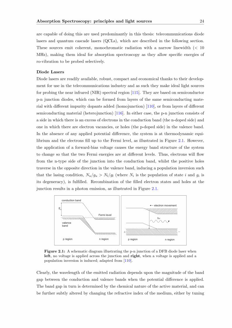
Absorption Spectroscopy: principles and light sources 24
are capable of doing this are used predominantly in this thesis: telecommunications diode
lasers and quantum cascade lasers (QCLs), which are described in the following section.
These sources emit coherent, monochromatic radiation with a narrow linewidth (< 10
MHz), making them ideal for absorption spectroscopy as they allow specific energies of
ro-vibration to be probed selectively.
Diode Lasers
Diode lasers are readily available, robust, compact and economical thanks to their develop-
ment for use in the telecommunications industry and as such they make ideal light sources
for probing the near infrared (NIR) spectral region [115]. They are based on semiconductor
p-n junction diodes, which can be formed from layers of the same semiconducting mate-
rial with different impurity dopants added (homojunction) [110], or from layers of different
semiconducting material (heterojunction) [116]. In either case, the p-n junction consists of
a side in which there is an excess of electrons in the conduction band (the n-doped side) and
one in which there are electron vacancies, or holes (the p-doped side) in the valence band.
In the absence of any applied potential difference, the system is at thermodynamic equi-
librium and the electrons fill up to the Fermi level, as illustrated in Figure 2.1. However,
the application of a forward-bias voltage causes the energy band structure of the system
to change so that the two Fermi energies are at different levels. Thus, electrons will flow
from the n-type side of the junction into the conduction band, whilst the positive holes
traverse in the opposite direction in the valence band, inducing a population inversion such
that the lasing condition, Nu/gu > Nl/gl (where Ni is the population of state i and gi is
its degeneracy), is fulfilled. Recombination of the filled electron states and holes at the
junction results in a photon emission, as illustrated in Figure 2.1.
Figure 2.1: A schematic diagram illustrating the p-n junction of a DFB diode laser whenleft, no voltage is applied across the junction and right, when a voltage is applied and apopulation inversion is induced; adapted from [110].
Clearly, the wavelength of the emitted radiation depends upon the magnitude of the band
gap between the conduction and valence bands when the potential difference is applied.
The band gap in turn is determined by the chemical nature of the active material, and can
be further subtly altered by changing the refractive index of the medium, either by tuning
Absorption Spectroscopy: principles and light sources 25
the injection current or the temperature of the device. In general, the gain bandwidth is
tens of nm wide and supports many lasing modes. Thus, the wavelength of the emitted
radiation is reinforced whilst the other modes are suppressed using optical feedback: a
grating preferentially selects a particular wavelength, which is injected back into the active
medium, stimulating further emission at that particular frequency. The optical resonator
can either be external or internal to the active medium; external cavity diode lasers (ECDL)
are examples of the former [110], where the wavelength is selected by tuning the grating
external to the active medium, whilst distributed feedback (DFB) lasers are examples of the
latter [110], where a Bragg diffraction grating is written into one of the layers surrounding
the active medium of the laser. A Bragg diffraction grating, also known as a Bragg reflector,
consists of a series of layers of materials with differing refractive indices so that only a
wavelength which satisfies λ = 2Λneff (where Λ is the period of the grating and neff is the
effective refractive index) is strongly reflected. In a distributed Bragg reflector (DBR) laser,
the grating is instead located at the surface of the active region [117].
Although diode lasers offer many advantages, such as the provision of single-mode operation
at room temperature, a typical linewidth of a few MHz, relatively high power and tunability
(∼5 nm), they are restricted to the NIR spectral region (∼500 - 2700 nm), which limits the
spectroscopist to the weak overtone and combination bands of molecules (although very
recent advances in mid-IR diodes have been demonstrated by Meyer et al. [118], but are
yet to be commercially available in single mode). In order to access the strong fundamental
transitions of species, alternative laser sources are required.
Quantum Cascade Lasers (QCL)
Traditionally, the mid-infrared (MIR) spectral region has been accessed by Pb-salt, CO and
CO2 lasers, with difference frequency generation (DFG) and optical parametric oscillators
(OPO) providing more recent techniques. Whilst a more detailed overview of these devices
will be presented in Appendix A, the technical workings of the MIR source used in this
thesis, the quantum cascade laser (QCL), will be dealt with here.
Like the diode lasers described previously, the QCL is also a semiconductor laser but rather
than the emitted wavelength depending upon the recombination of electron-hole pairs, it is
dictated by the discrete conduction band states within quantum wells and the subsequent
electron transitions between them. These states are generated from the deposition of layers
of semiconductor via molecular beam epitaxy [119]. The layers are of precisely engineered
thickness approaching the De Broglie wavelength of the material, which allows the formation
of quantum wells. The laser consists of three levels, as illustrated in Figure 2.2. The electron
injected into the upper excited state (3) falls to the lower state (2), emitting a photon in
the process at the frequency corresponding to the energy gap, before relaxing to the ground
state (1). As a result of the carefully constructed layers of semiconductor, the difference
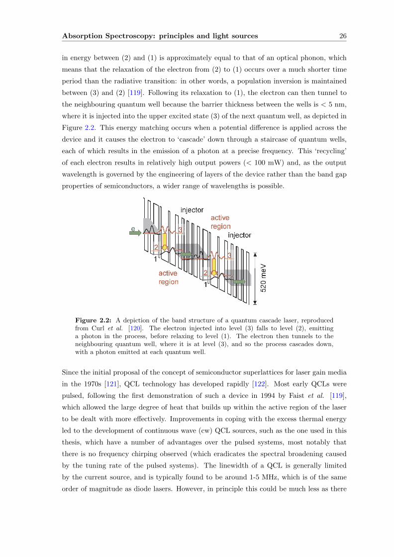
Absorption Spectroscopy: principles and light sources 26
in energy between (2) and (1) is approximately equal to that of an optical phonon, which
means that the relaxation of the electron from (2) to (1) occurs over a much shorter time
period than the radiative transition: in other words, a population inversion is maintained
between (3) and (2) [119]. Following its relaxation to (1), the electron can then tunnel to
the neighbouring quantum well because the barrier thickness between the wells is < 5 nm,
where it is injected into the upper excited state (3) of the next quantum well, as depicted in
Figure 2.2. This energy matching occurs when a potential difference is applied across the
device and it causes the electron to ‘cascade’ down through a staircase of quantum wells,
each of which results in the emission of a photon at a precise frequency. This ‘recycling’
of each electron results in relatively high output powers (< 100 mW) and, as the output
wavelength is governed by the engineering of layers of the device rather than the band gap
properties of semiconductors, a wider range of wavelengths is possible.
Figure 2.2: A depiction of the band structure of a quantum cascade laser, reproducedfrom Curl et al. [120]. The electron injected into level (3) falls to level (2), emittinga photon in the process, before relaxing to level (1). The electron then tunnels to theneighbouring quantum well, where it is at level (3), and so the process cascades down,with a photon emitted at each quantum well.
Since the initial proposal of the concept of semiconductor superlattices for laser gain media
in the 1970s [121], QCL technology has developed rapidly [122]. Most early QCLs were
pulsed, following the first demonstration of such a device in 1994 by Faist et al. [119],
which allowed the large degree of heat that builds up within the active region of the laser
to be dealt with more effectively. Improvements in coping with the excess thermal energy
led to the development of continuous wave (cw) QCL sources, such as the one used in this
thesis, which have a number of advantages over the pulsed systems, most notably that
there is no frequency chirping observed (which eradicates the spectral broadening caused
by the tuning rate of the pulsed systems). The linewidth of a QCL is generally limited
by the current source, and is typically found to be around 1-5 MHz, which is of the same
order of magnitude as diode lasers. However, in principle this could be much less as there
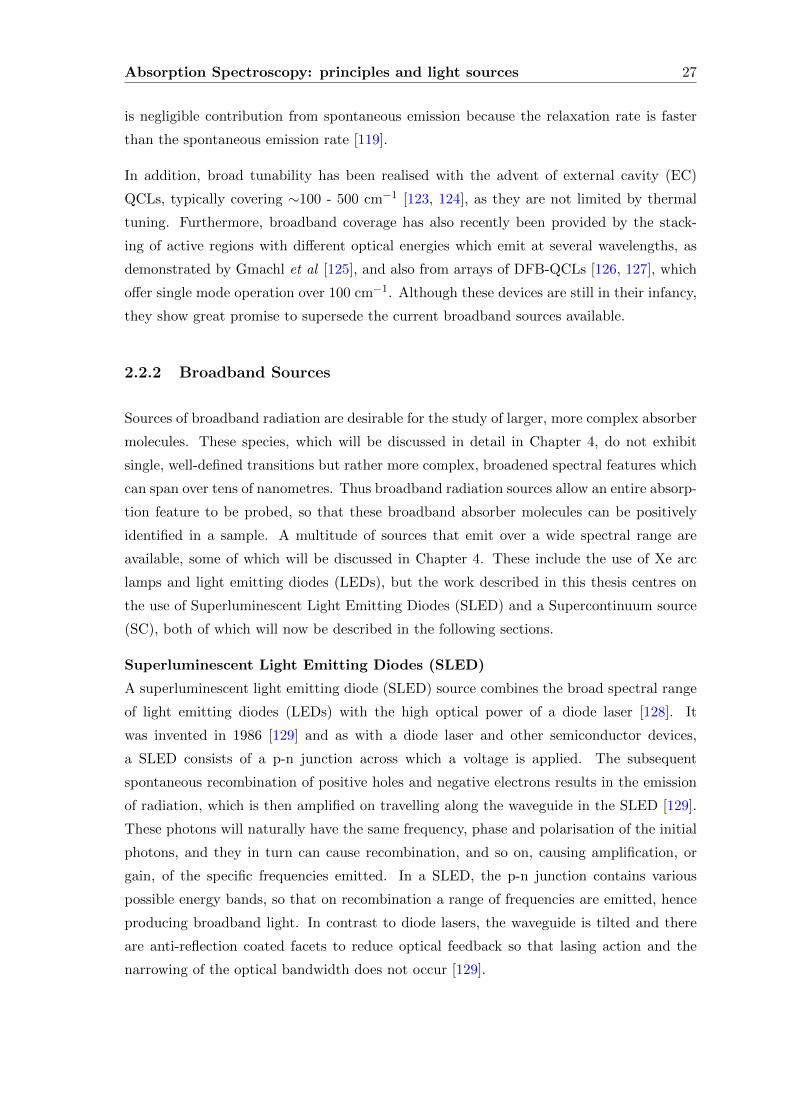
Absorption Spectroscopy: principles and light sources 27
is negligible contribution from spontaneous emission because the relaxation rate is faster
than the spontaneous emission rate [119].
In addition, broad tunability has been realised with the advent of external cavity (EC)
QCLs, typically covering ∼100 - 500 cm−1 [123, 124], as they are not limited by thermal
tuning. Furthermore, broadband coverage has also recently been provided by the stack-
ing of active regions with different optical energies which emit at several wavelengths, as
demonstrated by Gmachl et al [125], and also from arrays of DFB-QCLs [126, 127], which
offer single mode operation over 100 cm−1. Although these devices are still in their infancy,
they show great promise to supersede the current broadband sources available.
2.2.2 Broadband Sources
Sources of broadband radiation are desirable for the study of larger, more complex absorber
molecules. These species, which will be discussed in detail in Chapter 4, do not exhibit
single, well-defined transitions but rather more complex, broadened spectral features which
can span over tens of nanometres. Thus broadband radiation sources allow an entire absorp-
tion feature to be probed, so that these broadband absorber molecules can be positively
identified in a sample. A multitude of sources that emit over a wide spectral range are
available, some of which will be discussed in Chapter 4. These include the use of Xe arc
lamps and light emitting diodes (LEDs), but the work described in this thesis centres on
the use of Superluminescent Light Emitting Diodes (SLED) and a Supercontinuum source
(SC), both of which will now be described in the following sections.
Superluminescent Light Emitting Diodes (SLED)
A superluminescent light emitting diode (SLED) source combines the broad spectral range
of light emitting diodes (LEDs) with the high optical power of a diode laser [128]. It
was invented in 1986 [129] and as with a diode laser and other semiconductor devices,
a SLED consists of a p-n junction across which a voltage is applied. The subsequent
spontaneous recombination of positive holes and negative electrons results in the emission
of radiation, which is then amplified on travelling along the waveguide in the SLED [129].
These photons will naturally have the same frequency, phase and polarisation of the initial
photons, and they in turn can cause recombination, and so on, causing amplification, or
gain, of the specific frequencies emitted. In a SLED, the p-n junction contains various
possible energy bands, so that on recombination a range of frequencies are emitted, hence
producing broadband light. In contrast to diode lasers, the waveguide is tilted and there
are anti-reflection coated facets to reduce optical feedback so that lasing action and the
narrowing of the optical bandwidth does not occur [129].
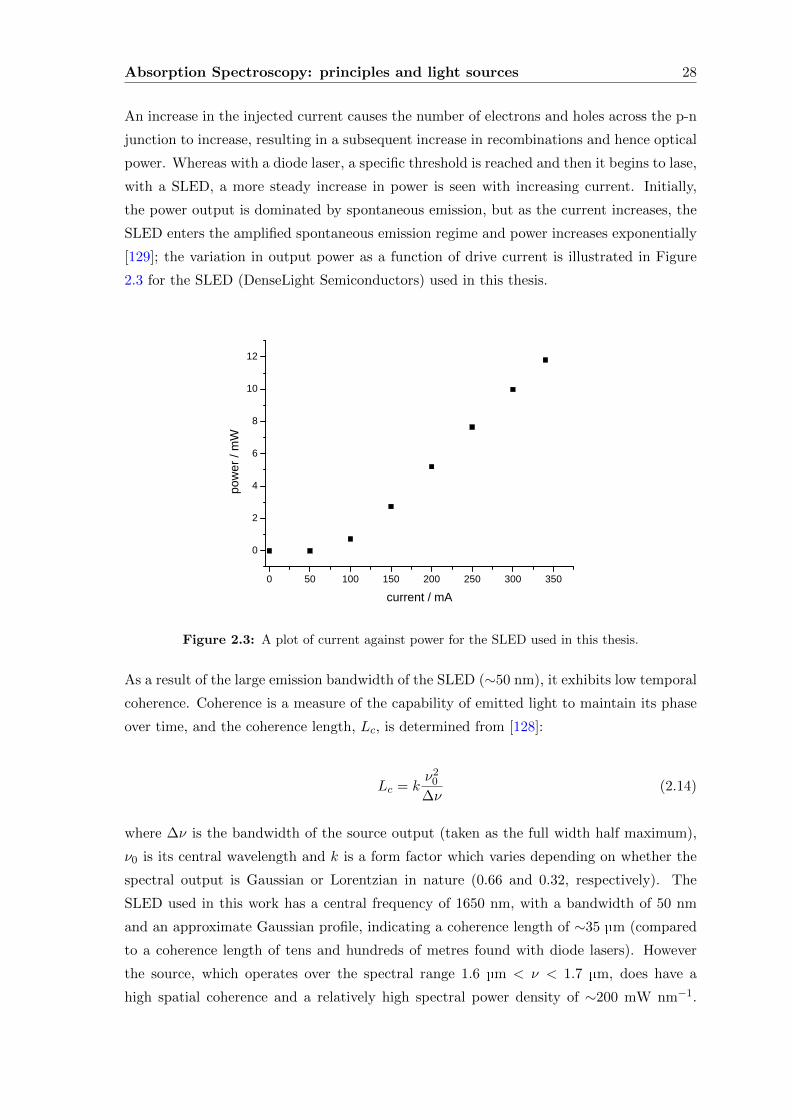
Absorption Spectroscopy: principles and light sources 28
An increase in the injected current causes the number of electrons and holes across the p-n
junction to increase, resulting in a subsequent increase in recombinations and hence optical
power. Whereas with a diode laser, a specific threshold is reached and then it begins to lase,
with a SLED, a more steady increase in power is seen with increasing current. Initially,
the power output is dominated by spontaneous emission, but as the current increases, the
SLED enters the amplified spontaneous emission regime and power increases exponentially
[129]; the variation in output power as a function of drive current is illustrated in Figure
2.3 for the SLED (DenseLight Semiconductors) used in this thesis.
0 5 0 1 0 0 1 5 0 2 0 0 2 5 0 3 0 0 3 5 0
0
2
4
6
8
1 0
1 2
powe
r / mW
c u r r e n t / m A
Figure 2.3: A plot of current against power for the SLED used in this thesis.
As a result of the large emission bandwidth of the SLED (∼50 nm), it exhibits low temporal
coherence. Coherence is a measure of the capability of emitted light to maintain its phase
over time, and the coherence length, Lc, is determined from [128]:
Lc = kν2
0
∆ν(2.14)
where ∆ν is the bandwidth of the source output (taken as the full width half maximum),
ν0 is its central wavelength and k is a form factor which varies depending on whether the
spectral output is Gaussian or Lorentzian in nature (0.66 and 0.32, respectively). The
SLED used in this work has a central frequency of 1650 nm, with a bandwidth of 50 nm
and an approximate Gaussian profile, indicating a coherence length of ∼35 µm (compared
to a coherence length of tens and hundreds of metres found with diode lasers). However
the source, which operates over the spectral range 1.6 µm < ν < 1.7 µm, does have a
high spatial coherence and a relatively high spectral power density of ∼200 mW nm−1.
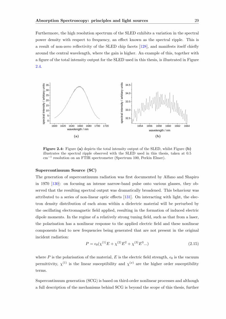
Absorption Spectroscopy: principles and light sources 29
Furthermore, the high resolution spectrum of the SLED exhibits a variation in the spectral
power density with respect to frequency, an effect known as the spectral ripple. This is
a result of non-zero reflectivity of the SLED chip facets [128], and manifests itself chiefly
around the central wavelength, where the gain is higher. An example of this, together with
a figure of the total intensity output for the SLED used in this thesis, is illustrated in Figure
2.4.
1 6 0 0 1 6 2 0 1 6 4 0 1 6 6 0 1 6 8 0 1 7 0 0 1 7 2 005
1 01 52 02 53 03 5
w a v e l e n g t h / n m
spec
tral in
tensity
/ arbi
tary u
nits
(a)
1 6 5 4 1 6 5 6 1 6 5 8 1 6 6 0 1 6 6 2 1 6 6 4
3 2 . 5
3 3 . 0
3 3 . 5
3 4 . 0
3 4 . 5
spec
tral in
tensity
/ arbi
tary u
nits
w a v e l e n g t h / n m(b)
Figure 2.4: Figure (a) depicts the total intensity output of the SLED, whilst Figure (b)illustrates the spectral ripple observed with the SLED used in this thesis, taken at 0.5cm−1 resolution on an FTIR spectrometer (Spectrum 100, Perkin Elmer).
Supercontinuum Source (SC)
The generation of supercontinuum radiation was first documented by Alfano and Shapiro
in 1970 [130]: on focusing an intense narrow-band pulse onto various glasses, they ob-
served that the resulting spectral output was dramatically broadened. This behaviour was
attributed to a series of non-linear optic effects [131]. On interacting with light, the elec-
tron density distribution of each atom within a dielectric material will be perturbed by
the oscillating electromagnetic field applied, resulting in the formation of induced electric
dipole moments. In the regime of a relatively strong tuning field, such as that from a laser,
the polarisation has a nonlinear response to the applied electric field and these nonlinear
components lead to new frequencies being generated that are not present in the original
incident radiation:
P = ε0(χ(1)E + χ(2)E2 + χ(3)E3...) (2.15)
where P is the polarisation of the material, E is the electric field strength, ε0 is the vacuum
permittivity, χ(1) is the linear susceptibility and χ(x) are the higher order susceptibility
terms.
Supercontinuum generation (SCG) is based on third-order nonlinear processes and although
a full description of the mechanisms behind SCG is beyond the scope of this thesis, further
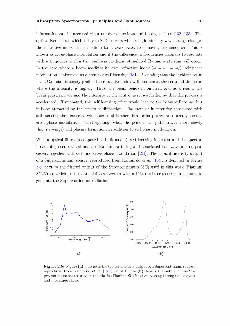
Absorption Spectroscopy: principles and light sources 30
information can be accessed via a number of reviews and books, such as [132, 133]. The
optical Kerr effect, which is key to SCG, occurs when a high intensity wave, I(ω2), changes
the refractive index of the medium for a weak wave, itself having frequency ω1. This is
known as cross-phase modulation and if the difference in frequencies happens to resonate
with a frequency within the nonlinear medium, stimulated Raman scattering will occur.
In the case where a beam modifies its own refractive index (ω = ω1 = ω2), self-phase
modulation is observed as a result of self-focusing [131]. Assuming that the incident beam
has a Gaussian intensity profile, the refractive index will increase at the centre of the beam
where the intensity is higher. Thus, the beam bends in on itself and as a result, the
beam gets narrower and the intensity at the centre increases further so that the process is
accelerated. If unabated, this self-focusing effect would lead to the beam collapsing, but
it is counteracted by the effects of diffraction. The increase in intensity associated with
self-focusing then causes a whole series of further third-order processes to occur, such as
cross-phase modulation, self-steepening (when the peak of the pulse travels more slowly
than its wings) and plasma formation, in addition to self-phase modulation.
Within optical fibres (as opposed to bulk media), self-focusing is absent and the spectral
broadening occurs via stimulated Raman scattering and associated four-wave mixing pro-
cesses, together with self- and cross-phase modulation [131]. The typical intensity output
of a Supercontinuum source, reproduced from Kaminiski et al. [134], is depicted in Figure
2.5, next to the filtered output of the Supercontinuum (SC) used in this work (Fianium
SC450-4), which utilises optical fibres together with a 1064 nm laser as the pump source to
generate the Supercontinuum radiation.
Inten
sity (n
J/nm)
w a v e l e n g t h ( n m )
(a)
1 5 5 0 1 6 0 0 1 6 5 0 1 7 0 0 1 7 5 0 1 8 0 00
1 0
2 0
3 0
4 0
5 0
SC ou
tput /
arbita
ry un
its
w a v e l e n g t h / n m(b)
Figure 2.5: Figure (a) illustrates the typical intensity output of a Supercontinuum source,reproduced from Kaminiski et al. [134]; whilst Figure (b) depicts the output of the Su-percontinuum source used in this thesis (Fianium SC450-4) on passing through a longpassand a bandpass filter.

Absorption Spectroscopy: principles and light sources 31
This chapter has presented a brief introduction to the principles behind absorption spec-
troscopy, discussing the issues associated with the sensitivity of the technique and describ-
ing the diverse array of light sources applied to it throughout this thesis. The following
chapter will introduce and demonstrate one way in which the sensitivity of an absorption
spectroscopy measurement can be improved: by increasing the effective pathlength using
an optical cavity.
Chapter 3
Application of laser-based CEAS
to the detection of breath
biomarkers
This chapter deals with preliminary studies investigating the feasibility of using cavity
enhanced absorption spectroscopy (CEAS) for breath analysis. The first half of the chapter
initially provides an introduction to CEAS-based techniques before the focus shifts to the
detection of methane in breath using a DFB diode laser. The first spectroscopic application
of a digital supermode distributed Bragg reflector (DS-DBR) laser, a novel, widely tunable,
diode laser source, is described in the second half of the chapter with the detection of CO2.
3.1 Cavity-Enhanced techniques
As described in Chapter 1, laser-based spectroscopic techniques offer a non-invasive and
rapid means to identify species found in breath. Diode lasers in particular represent a rela-
tively cheap, compact and readily available radiation source thanks to their ubiquitous use
in the telecommunications industry. In the near-infrared (NIR) these devices enable the
vibrational overtones and combination bands of many small molecules to be probed. Al-
though the absorption cross-sections, σ, associated with these transitions are much smaller
than those of the fundamental vibrations and electronic transitions in the mid-infrared
(MIR) and the ultraviolet (UV) respectively, an increase in the pathlength of the radiation
through the sample, L, will compensate for this and increase the sensitivity of the spectro-
scopic method to the molecular species. This can be achieved using multipass cells, such as
the White and Herriott cells, which can provide pathlengths of up to 50 - 250 m [135] and
will be described in later sections of this thesis. There are many examples of breath analysis
32
Application of laser-based CEAS to the detection of breath biomarkers 33
with diode lasers and multipass cells, a selection of which have been described in Chapter
1 [1, 6]. Moskalenko et al. [76] studied CO and CO2 in breath using tunable diode laser
spectroscopy in the MIR with a Herriott cell, accessing the wavelengths at 4.76 and 4.91 µm
(for CO and CO2, respectively), 10.34 µm (for NH3) and 3.35 µm (for CH4). Herriott cells
have also been used in the detection of exhaled nitric oxide [31, 58], in the measurement of
carbon isotope ratios [19, 61] and in monitoring carbonyl sulphide [75]. However, multipass
cells are often limited by optical fringing and mechanical instabilities, and the large volumes
often associated with such instruments (of the order of several litres, for example 16 l in [31]
and 3.5 l in [57]) are not ideal for breath sampling, although the use of astigmatic mirrors
can minimise the volume and the Namjou study [58] demonstrated the use of a compact
Herriott cell (0.3 l) for breath analysis. However, far greater pathlengths can be obtained
from utilising an optical cavity, a device consisting of two highly reflective mirrors a set
distance apart, which in addition typically have much smaller volumes, making them more
suitable for breath analysis.
3.1.1 Optical cavities
The simplest optical cavity is based on the Fabry-Perot interferometer used in etalons,
which provide frequency calibration for spectroscopic measurements. A Fabry-Perot cavity
consists of two parallel plane highly reflective mirrors, with R the geometric mean of the
reflectivities [115]. The transmitted light intensity through such an arrangement, IT , when
illuminated by a perfect, coherent, white light source, [136] is given by the Airy function:
ITI0
=1
1 + 4R(1−R)2
sin2 δ2
(3.1)
where I0 is the radiation incident on the resonator and δ = 2nl cos θ + 2η, the phase
difference between successive transmitted waves; η is the phase change on reflection from
the mirrors of the Fabry-Perot interferometer and 2nl cos θ is the optical path difference
between successive transmitted waves (with θ the angle at which the beam hits the mirrors
of the resonator, l the interface spacing and n the refractive index between the interfaces).
Physically, this results in a comb-like transmission function, as depicted in Figure 3.1. The
maxima in the function correspond to longitudinal cavity modes, and are the result of the
constructive interference which occurs when the separation between the cavity mirrors is
equal to an integer number of half wavelengths, nλ2 . The separation between the consecutive
longitudinal modes is known as the free spectral range (FSR) and is given by [115]:
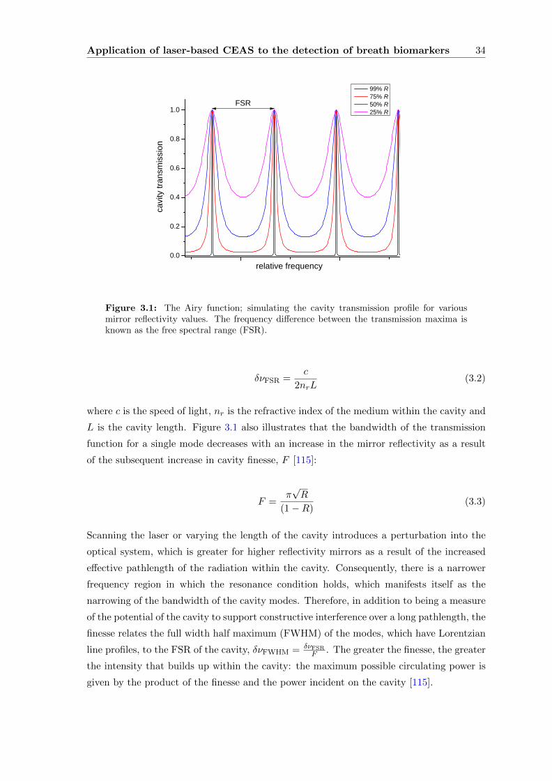
Application of laser-based CEAS to the detection of breath biomarkers 34
0 . 0
0 . 2
0 . 4
0 . 6
0 . 8
1 . 0
cavity
trans
missi
on
r e l a t i v e f r e q u e n c y
9 9 % R 7 5 % R 5 0 % R 2 5 % R
F S R
Figure 3.1: The Airy function; simulating the cavity transmission profile for variousmirror reflectivity values. The frequency difference between the transmission maxima isknown as the free spectral range (FSR).
δνFSR =c
2nrL(3.2)
where c is the speed of light, nr is the refractive index of the medium within the cavity and
L is the cavity length. Figure 3.1 also illustrates that the bandwidth of the transmission
function for a single mode decreases with an increase in the mirror reflectivity as a result
of the subsequent increase in cavity finesse, F [115]:
F =π√R
(1−R)(3.3)
Scanning the laser or varying the length of the cavity introduces a perturbation into the
optical system, which is greater for higher reflectivity mirrors as a result of the increased
effective pathlength of the radiation within the cavity. Consequently, there is a narrower
frequency region in which the resonance condition holds, which manifests itself as the
narrowing of the bandwidth of the cavity modes. Therefore, in addition to being a measure
of the potential of the cavity to support constructive interference over a long pathlength, the
finesse relates the full width half maximum (FWHM) of the modes, which have Lorentzian
line profiles, to the FSR of the cavity, δνFWHM = δνFSRF . The greater the finesse, the greater
the intensity that builds up within the cavity: the maximum possible circulating power is
given by the product of the finesse and the power incident on the cavity [115].
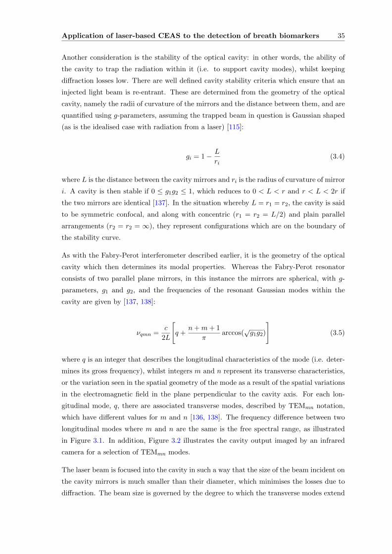
Application of laser-based CEAS to the detection of breath biomarkers 35
Another consideration is the stability of the optical cavity: in other words, the ability of
the cavity to trap the radiation within it (i.e. to support cavity modes), whilst keeping
diffraction losses low. There are well defined cavity stability criteria which ensure that an
injected light beam is re-entrant. These are determined from the geometry of the optical
cavity, namely the radii of curvature of the mirrors and the distance between them, and are
quantified using g-parameters, assuming the trapped beam in question is Gaussian shaped
(as is the idealised case with radiation from a laser) [115]:
gi = 1− L
ri(3.4)
where L is the distance between the cavity mirrors and ri is the radius of curvature of mirror
i. A cavity is then stable if 0 ≤ g1g2 ≤ 1, which reduces to 0 < L < r and r < L < 2r if
the two mirrors are identical [137]. In the situation whereby L = r1 = r2, the cavity is said
to be symmetric confocal, and along with concentric (r1 = r2 = L/2) and plain parallel
arrangements (r2 = r2 = ∞), they represent configurations which are on the boundary of
the stability curve.
As with the Fabry-Perot interferometer described earlier, it is the geometry of the optical
cavity which then determines its modal properties. Whereas the Fabry-Perot resonator
consists of two parallel plane mirrors, in this instance the mirrors are spherical, with g-
parameters, g1 and g2, and the frequencies of the resonant Gaussian modes within the
cavity are given by [137, 138]:
νqmn =c
2L
[q +
n+m+ 1
πarccos(
√g1g2)
](3.5)
where q is an integer that describes the longitudinal characteristics of the mode (i.e. deter-
mines its gross frequency), whilst integers m and n represent its transverse characteristics,
or the variation seen in the spatial geometry of the mode as a result of the spatial variations
in the electromagnetic field in the plane perpendicular to the cavity axis. For each lon-
gitudinal mode, q, there are associated transverse modes, described by TEMmn notation,
which have different values for m and n [136, 138]. The frequency difference between two
longitudinal modes where m and n are the same is the free spectral range, as illustrated
in Figure 3.1. In addition, Figure 3.2 illustrates the cavity output imaged by an infrared
camera for a selection of TEMmn modes.
The laser beam is focused into the cavity in such a way that the size of the beam incident on
the cavity mirrors is much smaller than their diameter, which minimises the losses due to
diffraction. The beam size is governed by the degree to which the transverse modes extend
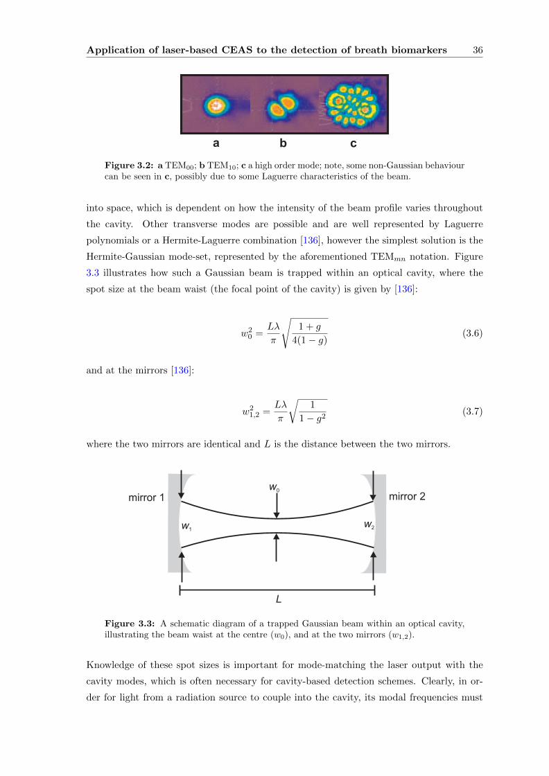
Application of laser-based CEAS to the detection of breath biomarkers 36
Figure 3.2: a TEM00; b TEM10; c a high order mode; note, some non-Gaussian behaviourcan be seen in c, possibly due to some Laguerre characteristics of the beam.
into space, which is dependent on how the intensity of the beam profile varies throughout
the cavity. Other transverse modes are possible and are well represented by Laguerre
polynomials or a Hermite-Laguerre combination [136], however the simplest solution is the
Hermite-Gaussian mode-set, represented by the aforementioned TEMmn notation. Figure
3.3 illustrates how such a Gaussian beam is trapped within an optical cavity, where the
spot size at the beam waist (the focal point of the cavity) is given by [136]:
w20 =
Lλ
π
√1 + g
4(1− g)(3.6)
and at the mirrors [136]:
w21,2 =
Lλ
π
√1
1− g2(3.7)
where the two mirrors are identical and L is the distance between the two mirrors.
mirror 1 mirror 2
w1
w2
w0
L
Figure 3.3: A schematic diagram of a trapped Gaussian beam within an optical cavity,illustrating the beam waist at the centre (w0), and at the two mirrors (w1,2).
Knowledge of these spot sizes is important for mode-matching the laser output with the
cavity modes, which is often necessary for cavity-based detection schemes. Clearly, in or-
der for light from a radiation source to couple into the cavity, its modal frequencies must
Application of laser-based CEAS to the detection of breath biomarkers 37
resonate with those of the cavity. In addition, the greater the spatial overlap between the
laser and cavity modes, the greater the efficiency of the system and the greater the build
up of intensity within the cavity. In such a system, the mode-matching optics are chosen
so that the beam size and divergence of the incident radiation matches that of the TEM00
mode supported by the cavity geometry so that it is preferentially excited. This is essential
for mode-locked techniques, such as Optical Feedback Cavity Enhanced Absorption Spec-
troscopy (OF-CEAS) [139], and for Cavity Ring-Down Spectroscopy (CRDS) [140]. Cavity
Enhanced Absorption Spectroscopy (CEAS) [141, 142], on the other hand, which forms the
basis of the work in this chapter, has less stringent requirements and is described in section
3.1.3.
3.1.2 Cavity Ring-Down Spectroscopy (CRDS)
In Cavity Ring-Down Spectroscopy (CRDS), after power is allowed to build up within the
cavity the light injected into it is rapidly switched off, such that the temporal evolution of
the light intensity which leaks out can be measured. The following description is based on
that detailed in Engeln and Berden [136]. The early work on CRDS [140] used ns pulsed
lasers, where the pulse provides a well-defined point in time from which to monitor the
‘ring-down’ time of the cavity. On injection of a pulse into the cavity, and assuming the
duration of the pulse is shorter than that of the round-trip time within it, the first pass
will result in a detected intensity given by [143]:
I0 = IinT2 exp (−αd) (3.8)
where T is the transmission of the mirrors (i.e. T = 1−R, where R is the geometric mean
of the reflectivity of the mirrors) and exp(−αd) is the reduction in the initial intensity due
to the absorption or scattering loss of the sample (with α the absorption coefficient and
d the length of the sample within the cavity). On the second pass, the intensity detected
will be further reduced by a factor of R2 exp(−2αd), on account of the light reflecting off
both of the mirrors and passing through the sample twice before reaching the detector.
Therefore for n round trips the intensity is:
In = I0R2n exp(−2nαd) (3.9)
Normally, the detector is not fast enough to detect each discrete pulse, so it records a time-
smoothed exponential decay in intensity. This allows the number of round trips, a discrete
variable, to be converted into a continuous time variable via t = 2Lnc , where L is the length
of the cavity. Equation 3.9 then becomes:
Application of laser-based CEAS to the detection of breath biomarkers 38
I(t) = I0 exp[− tcL
(− lnR+ αd)] (3.10)
The time constant for the decaying light intensity, known as the ring-down time of the
cavity, is thus:
τ =L
c(− lnR+ αd)(3.11)
In the situation where the mirrors are of high-reflectivity (R→ 1), this reduces to
τ =L
c[(1−R) + αd](3.12)
as lnR ≈ −(1 − R). Typical ringdown times are of the order of µs for mirrors of R
∼ 0.9999, whilst sensitivities are regularly ∼×10−9 cm−1Hz−12 . Equation 3.12 highlights
an important characteristic of CRDS, in that the ring-down time is independent of any
intensity fluctuations of the laser. Furthermore, knowledge of the ring-down times when an
absorber is present and absent, τ and τ0 respectively, can be used to determine the absolute
concentration of the absorber if the absorption cross-section for that particular frequency
is known.
α(ω) = σ(ω)C (3.13)
=∆τ
τ0τ
L
cd(3.14)
where α(ω) is the absorption coefficient, σ(ω) is the absorption cross-section, C is the
species concentration, ∆τ is τ0− τ , c is the speed of light, L is the length of the cavity and
d is the length of the sample within L.
Although pulsed lasers have high powers, they generally have high bandwidths (resulting
in low spectral resolution) and have relatively poor spatial properties such that they often
excite more than one cavity mode, which results in a multi-exponential decay as each mode
excited will decay at a slightly different rate. More recently, continuous wave (cw) lasers
have been used with CRDS, which allow far greater spatial resolution but do require the
laser radiation incident on the cavity to be rapidly switched off. This is usually achieved
using an acoustic-optic modulator (AOM): as light is injected into the cavity, a power
build up will only occur when the laser and cavity modes are in resonance; therefore, by
monitoring the intensity output a trigger can then be sent to the AOM the moment that
this occurs, which will then cause the laser beam to be deflected from the cavity and the
resultant ring-down trace can be recorded.
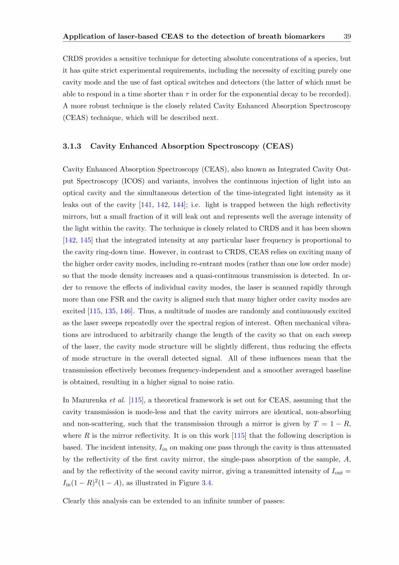
Application of laser-based CEAS to the detection of breath biomarkers 39
CRDS provides a sensitive technique for detecting absolute concentrations of a species, but
it has quite strict experimental requirements, including the necessity of exciting purely one
cavity mode and the use of fast optical switches and detectors (the latter of which must be
able to respond in a time shorter than τ in order for the exponential decay to be recorded).
A more robust technique is the closely related Cavity Enhanced Absorption Spectroscopy
(CEAS) technique, which will be described next.
3.1.3 Cavity Enhanced Absorption Spectroscopy (CEAS)
Cavity Enhanced Absorption Spectroscopy (CEAS), also known as Integrated Cavity Out-
put Spectroscopy (ICOS) and variants, involves the continuous injection of light into an
optical cavity and the simultaneous detection of the time-integrated light intensity as it
leaks out of the cavity [141, 142, 144]; i.e. light is trapped between the high reflectivity
mirrors, but a small fraction of it will leak out and represents well the average intensity of
the light within the cavity. The technique is closely related to CRDS and it has been shown
[142, 145] that the integrated intensity at any particular laser frequency is proportional to
the cavity ring-down time. However, in contrast to CRDS, CEAS relies on exciting many of
the higher order cavity modes, including re-entrant modes (rather than one low order mode)
so that the mode density increases and a quasi-continuous transmission is detected. In or-
der to remove the effects of individual cavity modes, the laser is scanned rapidly through
more than one FSR and the cavity is aligned such that many higher order cavity modes are
excited [115, 135, 146]. Thus, a multitude of modes are randomly and continuously excited
as the laser sweeps repeatedly over the spectral region of interest. Often mechanical vibra-
tions are introduced to arbitrarily change the length of the cavity so that on each sweep
of the laser, the cavity mode structure will be slightly different, thus reducing the effects
of mode structure in the overall detected signal. All of these influences mean that the
transmission effectively becomes frequency-independent and a smoother averaged baseline
is obtained, resulting in a higher signal to noise ratio.
In Mazurenka et al. [115], a theoretical framework is set out for CEAS, assuming that the
cavity transmission is mode-less and that the cavity mirrors are identical, non-absorbing
and non-scattering, such that the transmission through a mirror is given by T = 1 − R,
where R is the mirror reflectivity. It is on this work [115] that the following description is
based. The incident intensity, Iin on making one pass through the cavity is thus attenuated
by the reflectivity of the first cavity mirror, the single-pass absorption of the sample, A,
and by the reflectivity of the second cavity mirror, giving a transmitted intensity of Iout =
Iin(1−R)2(1−A), as illustrated in Figure 3.4.
Clearly this analysis can be extended to an infinite number of passes:
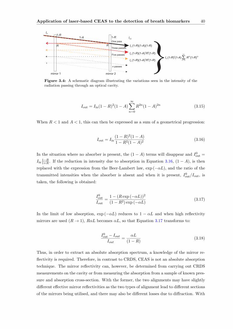
Application of laser-based CEAS to the detection of breath biomarkers 40
Figure 3.4: A schematic diagram illustrating the variations seen in the intensity of theradiation passing through an optical cavity.
Iout = Iin(1−R)2(1−A)∞∑n=0
R2n(1−A)2n (3.15)
When R < 1 and A < 1, this can then be expressed as a sum of a geometrical progression:
Iout = Iin(1−R)2(1−A)
1−R2(1−A)2(3.16)
In the situation where no absorber is present, the (1−A) terms will disappear and I0out =
Iin1−R1+R . If the reduction in intensity due to absorption in Equation 3.16, (1 − A), is then
replaced with the expression from the Beer-Lambert law, exp (−αL), and the ratio of the
transmitted intensities when the absorber is absent and when it is present, I0out/Iout, is
taken, the following is obtained:
I0out
Iout=
1− (R exp (−αL))2
(1−R2) exp (−αL)(3.17)
In the limit of low absorption, exp (−αL) reduces to 1 − αL and when high reflectivity
mirrors are used (R→ 1), RαL becomes αL, so that Equation 3.17 transforms to:
I0out − IoutIout
=αL
(1−R)(3.18)
Thus, in order to extract an absolute absorption spectrum, a knowledge of the mirror re-
flectivity is required. Therefore, in contrast to CRDS, CEAS is not an absolute absorption
technique. The mirror reflectivity can, however, be determined from carrying out CRDS
measurements on the cavity or from measuring the absorption from a sample of known pres-
sure and absorption cross-section. With the former, the two alignments may have slightly
different effective mirror reflectivities as the two types of alignment lead to different sections
of the mirrors being utilised, and there may also be different losses due to diffraction. With
Application of laser-based CEAS to the detection of breath biomarkers 41
the latter, the accuracy of the mirror reflectivity calibration is dependent on the accuracy
of the pressure reading of the sample. An additional issue with CEAS is that amplified
spontaneous emission (ASE) from the laser will often constitute some of the signal, causing
a broad, frequency independent background signal to contribute to the cavity enhanced
signal. This can be readily removed either by filtering the output of the laser or by mis-
aligning the cavity and taking a reading from the detector: the signal produced will be
solely due to “uncoupled” light passing straight through the cavity.
Finally, CEAS centres on the recording of intensity, rather than the time-domain measure-
ments of CRDS. This means that it is dependent on intensity fluctuations of the laser, and
as such, generally is a less sensitive technique than an equivalent CRDS experiment: CRDS
regularly attains sensitivities ∼ 10−9 cm−1Hz−1/2, whilst CEAS tends to be in the range
10−8 − 10−9 cm−1Hz−1/2 [136] (although sensitivities reaching 10−10 − 10−11 cm−1Hz−1/2
have been reported [147] using an ‘off-axis’ technique). However, for most applications the
level of detection provided by CEAS is more than sufficient and coupled with the relatively
straightforward and robust experimental arrangement, it is far more suitable for practical
applications.
3.2 Methane in breath: an initial study
Methane is an ideal molecule to test the suitability of CEAS in breath analysis as it is present
in widely varying quantities depending on whether the subject is a methane-producer or
not, it has well-resolved narrow absorption transitions which are easily probed with a diode
laser, and it has sufficiently large NIR absorption cross-sections which are easily detectable
using standard cavity-based techniques.
3.2.1 Methane in breath
Between 30 - 50% of people in western populations are so-called CH4 producers [148],
with breath levels of CH4 above that found naturally in the atmosphere (∼1.8 ppm [149]).
Methane production does not occur through normal metabolic activity in the body, but
may occur through the action of enteric methanogenic archaea, such as Methanobrevibacter
smithii [150–152], in the intestinal tract. Under the anaerobic conditions found in the colon,
these bacteria will reduce CO2, a byproduct of digestion, to CH4 by using the H2 produced
by another set of flora, hydrogenic bacteria (like Prevotellaceae), which also thrive in this
environment. CH4 and H2 from the colon are then absorbed into the bloodstream via the
intestinal wall and transported to the lungs where they diffuse into the alveoli before being
excreted during pulmonary respiration. As the human body does not metabolise CH4, if
Application of laser-based CEAS to the detection of breath biomarkers 42
the levels of methane in a breath sample exceed the 1.8 ppm baseline CH4 concentration
in ambient air by more than 1 ppm, it is a reasonable indicator of methane production in
the intestine and that the subject is a methane producer. Thus, the ability to measure
exhaled levels of CH4 and H2 sensitively are of significant interest as potential probes of
gastro-intestinal physiology [153–157]. For example, the measurement of CH4 and H2 in
breath following the ingestion of lactose is used in lactose intolerance testing [158–160]:
in a lactose tolerant person, the lactase enzyme in their small intestine will digest the
lactose ingested; however, lactose intolerant individuals lack this enzyme so the lactose will
pass, undigested, into the colon where it is metabolised by anaerobic bacteria. This gives
rise to elevated levels of H2, some of which will then be converted into CH4 by methane-
producers. Therefore, the monitoring of the concentration of both gases in breath is required
for accurate interpretation of the results [161]. Similar tests can also be performed to
determine malabsorption of other sugars [162, 163].
The small intestine, by contrast, is normally substantially free from bacterial colonisation,
but an increase in the number of bacteria (above 105 CFU/ml, where CFU is colony form-
ing units) leads to Small Intestinal Bacterial Overgrowth (SIBO) [164]. There is growing
evidence that SIBO is a contributing factor in a large number of patients suffering from
Irritable Bowel Syndrome (IBS). Lactulose (or glucose) can be used as a test for SIBO; if
the sugar is metabolised by bacteria in the small intestine, there will be an early onset of
elevated breath H2 following ingestion [165, 166]. As with lactose intolerance testing, simul-
taneous measurement of CH4 is desirable to identify when the sugar has rapidly traversed
to the colon: this will result in the metabolism of lactulose by methanogens. In addition,
Hwang et al. have established that elevated breath methane is strongly correlated with
constipation-predominant IBS [167], and as such CH4 may have use as a diagnostic marker
to guide appropriate therapy. Finally, recent studies have shown a higher prevalence of
intestinal methanogens amongst obese individuals as compared to people of normal weight,
or those having undergone a gastric-bypass [168, 169], perhaps suggesting a possible role
for breath methane monitoring as a tool in treating obesity.
Therefore, laser spectroscopy could be used as a non-intrusive way to obtain quick and
reliable identification of methane in a breath sample, the presence of which could then
provide diagnosis of gastrointestinal conditions.
3.2.2 The Spectroscopy of Methane
Breath methane concentrations were monitored using the absorption feature at ∼6057.09
cm−1, which consists of 4 ro-vibrational transitions within the 2ν3 vibrational overtone. The
degeneracy of the vibrational band is lifted by Coriolis forces, which describe the interaction
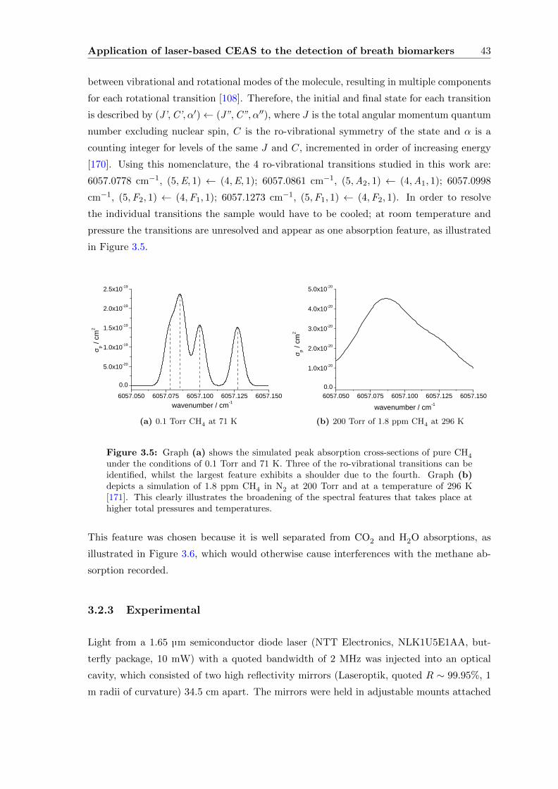
Application of laser-based CEAS to the detection of breath biomarkers 43
between vibrational and rotational modes of the molecule, resulting in multiple components
for each rotational transition [108]. Therefore, the initial and final state for each transition
is described by (J’,C’, α′)← (J”,C”, α′′), where J is the total angular momentum quantum
number excluding nuclear spin, C is the ro-vibrational symmetry of the state and α is a
counting integer for levels of the same J and C, incremented in order of increasing energy
[170]. Using this nomenclature, the 4 ro-vibrational transitions studied in this work are:
6057.0778 cm−1, (5,E, 1) ← (4,E, 1); 6057.0861 cm−1, (5,A2, 1) ← (4,A1, 1); 6057.0998
cm−1, (5,F2, 1) ← (4,F1, 1); 6057.1273 cm−1, (5,F1, 1) ← (4,F2, 1). In order to resolve
the individual transitions the sample would have to be cooled; at room temperature and
pressure the transitions are unresolved and appear as one absorption feature, as illustrated
in Figure 3.5.
6 0 5 7 . 0 5 0 6 0 5 7 . 0 7 5 6 0 5 7 . 1 0 0 6 0 5 7 . 1 2 5 6 0 5 7 . 1 5 00 . 0
5 . 0 x 1 0 - 2 0
1 . 0 x 1 0 - 1 9
1 . 5 x 1 0 - 1 9
2 . 0 x 1 0 - 1 9
2 . 5 x 1 0 - 1 9
σ p / cm2
w a v e n u m b e r / c m - 1
(a) 0.1 Torr CH4 at 71 K
6 0 5 7 . 0 5 0 6 0 5 7 . 0 7 5 6 0 5 7 . 1 0 0 6 0 5 7 . 1 2 5 6 0 5 7 . 1 5 00 . 0
1 . 0 x 1 0 - 2 0
2 . 0 x 1 0 - 2 0
3 . 0 x 1 0 - 2 0
4 . 0 x 1 0 - 2 0
5 . 0 x 1 0 - 2 0
σ p / cm2
w a v e n u m b e r / c m - 1
(b) 200 Torr of 1.8 ppm CH4 at 296 K
Figure 3.5: Graph (a) shows the simulated peak absorption cross-sections of pure CH4
under the conditions of 0.1 Torr and 71 K. Three of the ro-vibrational transitions can beidentified, whilst the largest feature exhibits a shoulder due to the fourth. Graph (b)depicts a simulation of 1.8 ppm CH4 in N2 at 200 Torr and at a temperature of 296 K[171]. This clearly illustrates the broadening of the spectral features that takes place athigher total pressures and temperatures.
This feature was chosen because it is well separated from CO2 and H2O absorptions, as
illustrated in Figure 3.6, which would otherwise cause interferences with the methane ab-
sorption recorded.
3.2.3 Experimental
Light from a 1.65 µm semiconductor diode laser (NTT Electronics, NLK1U5E1AA, but-
terfly package, 10 mW) with a quoted bandwidth of 2 MHz was injected into an optical
cavity, which consisted of two high reflectivity mirrors (Laseroptik, quoted R ∼ 99.95%, 1
m radii of curvature) 34.5 cm apart. The mirrors were held in adjustable mounts attached
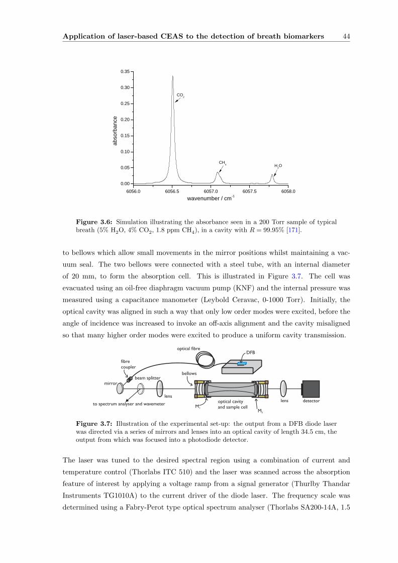
Application of laser-based CEAS to the detection of breath biomarkers 44
6 0 5 6 . 0 6 0 5 6 . 5 6 0 5 7 . 0 6 0 5 7 . 5 6 0 5 8 . 00 . 0 0
0 . 0 5
0 . 1 0
0 . 1 5
0 . 2 0
0 . 2 5
0 . 3 0
0 . 3 5
C H 4 H 2 O
abso
rbanc
e
w a v e n u m b e r / c m - 1
C O 2
Figure 3.6: Simulation illustrating the absorbance seen in a 200 Torr sample of typicalbreath (5% H2O, 4% CO2, 1.8 ppm CH4), in a cavity with R = 99.95% [171].
to bellows which allow small movements in the mirror positions whilst maintaining a vac-
uum seal. The two bellows were connected with a steel tube, with an internal diameter
of 20 mm, to form the absorption cell. This is illustrated in Figure 3.7. The cell was
evacuated using an oil-free diaphragm vacuum pump (KNF) and the internal pressure was
measured using a capacitance manometer (Leybold Ceravac, 0-1000 Torr). Initially, the
optical cavity was aligned in such a way that only low order modes were excited, before the
angle of incidence was increased to invoke an off-axis alignment and the cavity misaligned
so that many higher order modes were excited to produce a uniform cavity transmission.
optical cavity
and sample cellto spectrum analyser and wavemeter
M1
M2
bellows
lens
optical fibreDFB
fibre
coupler
mirrorbeam splitter
detectorlens
Figure 3.7: Illustration of the experimental set-up: the output from a DFB diode laserwas directed via a series of mirrors and lenses into an optical cavity of length 34.5 cm, theoutput from which was focused into a photodiode detector.
The laser was tuned to the desired spectral region using a combination of current and
temperature control (Thorlabs ITC 510) and the laser was scanned across the absorption
feature of interest by applying a voltage ramp from a signal generator (Thurlby Thandar
Instruments TG1010A) to the current driver of the diode laser. The frequency scale was
determined using a Fabry-Perot type optical spectrum analyser (Thorlabs SA200-14A, 1.5
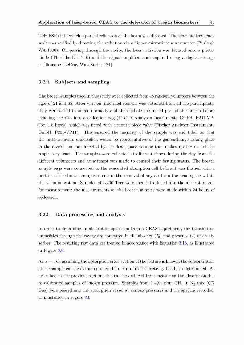
Application of laser-based CEAS to the detection of breath biomarkers 45
GHz FSR) into which a partial reflection of the beam was directed. The absolute frequency
scale was verified by directing the radiation via a flipper mirror into a wavemeter (Burleigh
WA-1000). On passing through the cavity, the laser radiation was focused onto a photo-
diode (Thorlabs DET410) and the signal amplified and acquired using a digital storage
oscilloscope (LeCroy WaveSurfer 424).
3.2.4 Subjects and sampling
The breath samples used in this study were collected from 48 random volunteers between the
ages of 21 and 65. After written, informed consent was obtained from all the participants,
they were asked to inhale normally and then exhale the initial part of the breath before
exhaling the rest into a collection bag (Fischer Analysen Instrumente GmbH, F201-VP-
05c, 1.5 litres), which was fitted with a mouth piece valve (Fischer Analysen Instrumente
GmbH, F201-VP11). This ensured the majority of the sample was end tidal, so that
the measurements undertaken would be representative of the gas exchange taking place
in the alveoli and not affected by the dead space volume that makes up the rest of the
respiratory tract. The samples were collected at different times during the day from the
different volunteers and no attempt was made to control their fasting status. The breath
sample bags were connected to the evacuated absorption cell before it was flushed with a
portion of the breath sample to ensure the removal of any air from the dead space within
the vacuum system. Samples of ∼200 Torr were then introduced into the absorption cell
for measurement; the measurements on the breath samples were made within 24 hours of
collection.
3.2.5 Data processing and analysis
In order to determine an absorption spectrum from a CEAS experiment, the transmitted
intensities through the cavity are compared in the absence (I0) and presence (I) of an ab-
sorber. The resulting raw data are treated in accordance with Equation 3.18, as illustrated
in Figure 3.8.
As α = σC, assuming the absorption cross-section of the feature is known, the concentration
of the sample can be extracted once the mean mirror reflectivity has been determined. As
described in the previous section, this can be deduced from measuring the absorption due
to calibrated samples of known pressure. Samples from a 49.1 ppm CH4 in N2 mix (CK
Gas) were passed into the absorption vessel at various pressures and the spectra recorded,
as illustrated in Figure 3.9.
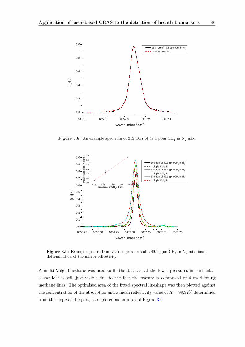
Application of laser-based CEAS to the detection of breath biomarkers 46
6 0 5 6 . 6 6 0 5 6 . 8 6 0 5 7 . 0 6 0 5 7 . 2 6 0 5 7 . 4
0 . 0
0 . 2
0 . 4
0 . 6
0 . 8
1 . 0
[I 0-I] / I
w a v e n u m b e r / c m - 1
2 1 3 T o r r o f 4 9 . 1 p p m C H 4 i n N 2 m u l t i p l e V o i g t f i t
Figure 3.8: An example spectrum of 212 Torr of 49.1 ppm CH4 in N2 mix.
6 0 5 6 . 2 5 6 0 5 6 . 5 0 6 0 5 6 . 7 5 6 0 5 7 . 0 0 6 0 5 7 . 2 5 6 0 5 7 . 5 0 6 0 5 7 . 7 50 . 00 . 10 . 20 . 30 . 40 . 50 . 60 . 70 . 80 . 91 . 0
[I 0-I] / I
w a v e n u m b e r / c m - 1
1 9 9 T o r r o f 4 9 . 1 p p m C H 4 i n N 2 m u l t i p l e V o i g t f i t 3 3 0 T o r r o f 4 9 . 1 p p m C H 4 i n N 2 m u l t i p l e V o i g t f i t 5 7 9 T o r r o f 4 9 . 1 p p m C H 4 i n N 2 m u l t i p l e V o i g t f i t
0 . 0 1 0 0 . 0 1 5 0 . 0 2 0 0 . 0 2 5 0 . 0 3 00 . 0 60 . 0 80 . 1 00 . 1 20 . 1 40 . 1 60 . 1 8
area o
f abs
orptio
n prof
ile
p r e s s u r e o f C H 4 / T o r r
Figure 3.9: Example spectra from various pressures of a 49.1 ppm CH4 in N2 mix; inset,determination of the mirror reflectivity.
A multi Voigt lineshape was used to fit the data as, at the lower pressures in particular,
a shoulder is still just visible due to the fact the feature is comprised of 4 overlapping
methane lines. The optimised area of the fitted spectral lineshape was then plotted against
the concentration of the absorption and a mean reflectivity value of R = 99.92% determined
from the slope of the plot, as depicted as an inset of Figure 3.9.
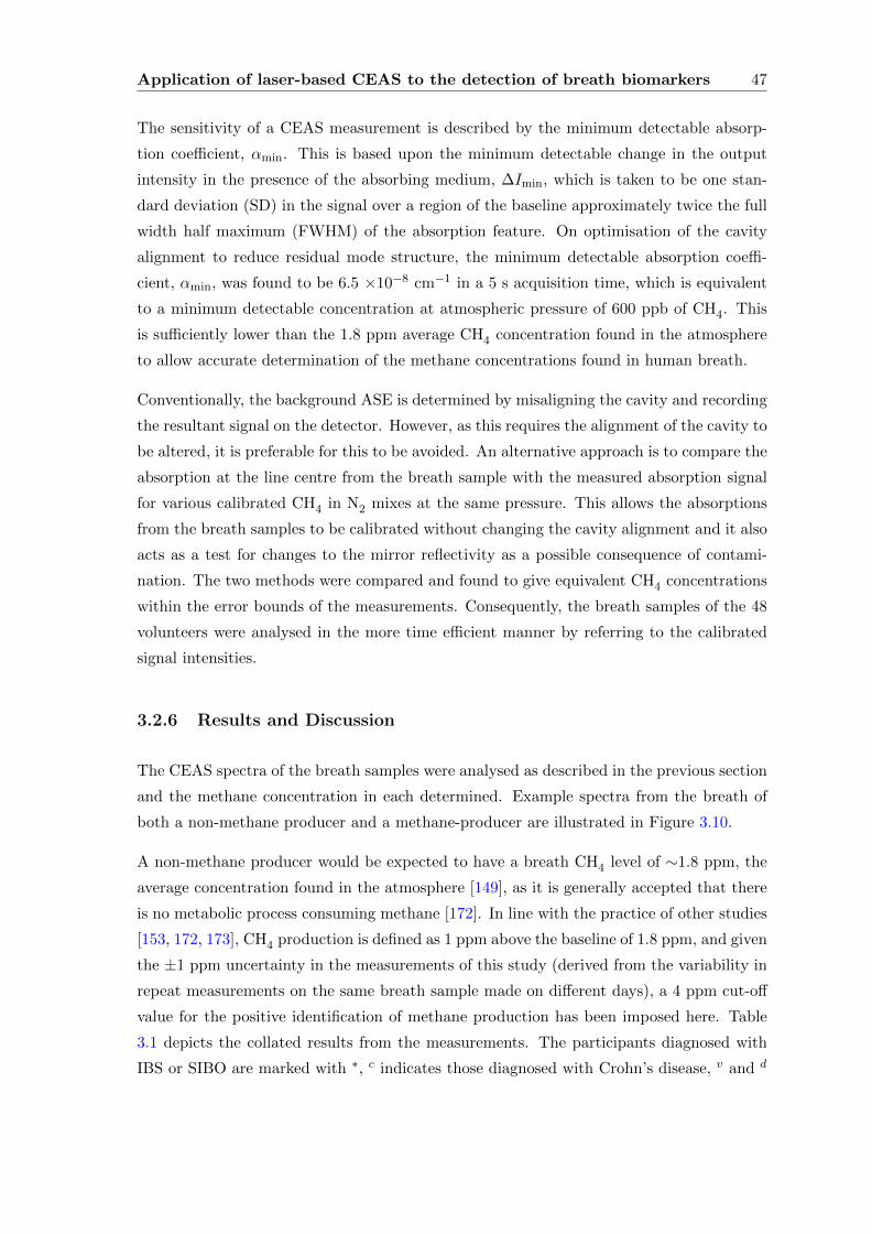
Application of laser-based CEAS to the detection of breath biomarkers 47
The sensitivity of a CEAS measurement is described by the minimum detectable absorp-
tion coefficient, αmin. This is based upon the minimum detectable change in the output
intensity in the presence of the absorbing medium, ∆Imin, which is taken to be one stan-
dard deviation (SD) in the signal over a region of the baseline approximately twice the full
width half maximum (FWHM) of the absorption feature. On optimisation of the cavity
alignment to reduce residual mode structure, the minimum detectable absorption coeffi-
cient, αmin, was found to be 6.5 ×10⁻⁸ cm−1 in a 5 s acquisition time, which is equivalent
to a minimum detectable concentration at atmospheric pressure of 600 ppb of CH4. This
is sufficiently lower than the 1.8 ppm average CH4 concentration found in the atmosphere
to allow accurate determination of the methane concentrations found in human breath.
Conventionally, the background ASE is determined by misaligning the cavity and recording
the resultant signal on the detector. However, as this requires the alignment of the cavity to
be altered, it is preferable for this to be avoided. An alternative approach is to compare the
absorption at the line centre from the breath sample with the measured absorption signal
for various calibrated CH4 in N2 mixes at the same pressure. This allows the absorptions
from the breath samples to be calibrated without changing the cavity alignment and it also
acts as a test for changes to the mirror reflectivity as a possible consequence of contami-
nation. The two methods were compared and found to give equivalent CH4 concentrations
within the error bounds of the measurements. Consequently, the breath samples of the 48
volunteers were analysed in the more time efficient manner by referring to the calibrated
signal intensities.
3.2.6 Results and Discussion
The CEAS spectra of the breath samples were analysed as described in the previous section
and the methane concentration in each determined. Example spectra from the breath of
both a non-methane producer and a methane-producer are illustrated in Figure 3.10.
A non-methane producer would be expected to have a breath CH4 level of ∼1.8 ppm, the
average concentration found in the atmosphere [149], as it is generally accepted that there
is no metabolic process consuming methane [172]. In line with the practice of other studies
[153, 172, 173], CH4 production is defined as 1 ppm above the baseline of 1.8 ppm, and given
the ±1 ppm uncertainty in the measurements of this study (derived from the variability in
repeat measurements on the same breath sample made on different days), a 4 ppm cut-off
value for the positive identification of methane production has been imposed here. Table
3.1 depicts the collated results from the measurements. The participants diagnosed with
IBS or SIBO are marked with ∗, c indicates those diagnosed with Crohn’s disease, v and d
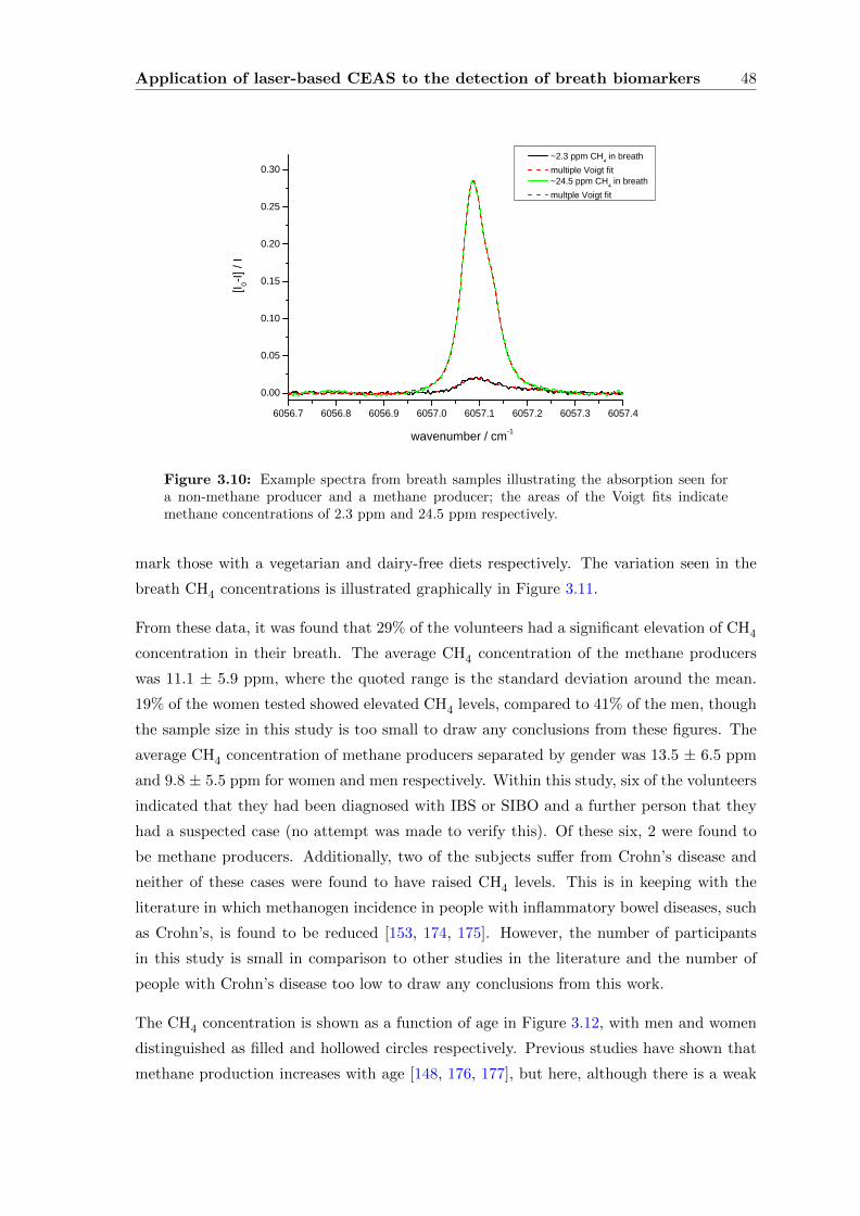
Application of laser-based CEAS to the detection of breath biomarkers 48
6 0 5 6 . 7 6 0 5 6 . 8 6 0 5 6 . 9 6 0 5 7 . 0 6 0 5 7 . 1 6 0 5 7 . 2 6 0 5 7 . 3 6 0 5 7 . 40 . 0 0
0 . 0 5
0 . 1 0
0 . 1 5
0 . 2 0
0 . 2 5
0 . 3 0
w a v e n u m b e r / c m - 1
[I 0-I] / I
~ 2 . 3 p p m C H 4 i n b r e a t h m u l t i p l e V o i g t f i t ~ 2 4 . 5 p p m C H 4 i n b r e a t h m u l t p l e V o i g t f i t
Figure 3.10: Example spectra from breath samples illustrating the absorption seen fora non-methane producer and a methane producer; the areas of the Voigt fits indicatemethane concentrations of 2.3 ppm and 24.5 ppm respectively.
mark those with a vegetarian and dairy-free diets respectively. The variation seen in the
breath CH4 concentrations is illustrated graphically in Figure 3.11.
From these data, it was found that 29% of the volunteers had a significant elevation of CH4
concentration in their breath. The average CH4 concentration of the methane producers
was 11.1 ± 5.9 ppm, where the quoted range is the standard deviation around the mean.
19% of the women tested showed elevated CH4 levels, compared to 41% of the men, though
the sample size in this study is too small to draw any conclusions from these figures. The
average CH4 concentration of methane producers separated by gender was 13.5 ± 6.5 ppm
and 9.8 ± 5.5 ppm for women and men respectively. Within this study, six of the volunteers
indicated that they had been diagnosed with IBS or SIBO and a further person that they
had a suspected case (no attempt was made to verify this). Of these six, 2 were found to
be methane producers. Additionally, two of the subjects suffer from Crohn’s disease and
neither of these cases were found to have raised CH4 levels. This is in keeping with the
literature in which methanogen incidence in people with inflammatory bowel diseases, such
as Crohn’s, is found to be reduced [153, 174, 175]. However, the number of participants
in this study is small in comparison to other studies in the literature and the number of
people with Crohn’s disease too low to draw any conclusions from this work.
The CH4 concentration is shown as a function of age in Figure 3.12, with men and women
distinguished as filled and hollowed circles respectively. Previous studies have shown that
methane production increases with age [148, 176, 177], but here, although there is a weak
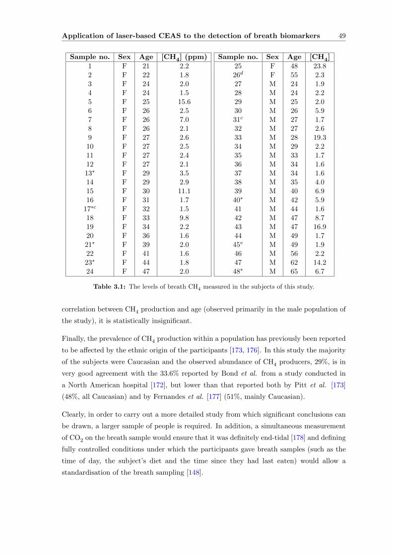
Application of laser-based CEAS to the detection of breath biomarkers 49
Sample no. Sex Age [CH4] (ppm)
1 F 21 2.22 F 22 1.83 F 24 2.04 F 24 1.55 F 25 15.66 F 26 2.57 F 26 7.08 F 26 2.19 F 27 2.610 F 27 2.511 F 27 2.412 F 27 2.113∗ F 29 3.514 F 29 2.915 F 30 11.116 F 31 1.7
17∗c F 32 1.518 F 33 9.819 F 34 2.220 F 36 1.621∗ F 39 2.022 F 41 1.623∗ F 44 1.824 F 47 2.0
Sample no. Sex Age [CH4]
25 F 48 23.826d F 55 2.327 M 24 1.928 M 24 2.229 M 25 2.030 M 26 5.931c M 27 1.732 M 27 2.633 M 28 19.334 M 29 2.235 M 33 1.736 M 34 1.637 M 34 1.638 M 35 4.039 M 40 6.940∗ M 42 5.941 M 44 1.642 M 47 8.743 M 47 16.944 M 49 1.745v M 49 1.946 M 56 2.247 M 62 14.248∗ M 65 6.7
Table 3.1: The levels of breath CH4 measured in the subjects of this study.
correlation between CH4 production and age (observed primarily in the male population of
the study), it is statistically insignificant.
Finally, the prevalence of CH4 production within a population has previously been reported
to be affected by the ethnic origin of the participants [173, 176]. In this study the majority
of the subjects were Caucasian and the observed abundance of CH4 producers, 29%, is in
very good agreement with the 33.6% reported by Bond et al. from a study conducted in
a North American hospital [172], but lower than that reported both by Pitt et al. [173]
(48%, all Caucasian) and by Fernandes et al. [177] (51%, mainly Caucasian).
Clearly, in order to carry out a more detailed study from which significant conclusions can
be drawn, a larger sample of people is required. In addition, a simultaneous measurement
of CO2 on the breath sample would ensure that it was definitely end-tidal [178] and defining
fully controlled conditions under which the participants gave breath samples (such as the
time of day, the subject’s diet and the time since they had last eaten) would allow a
standardisation of the breath sampling [148].
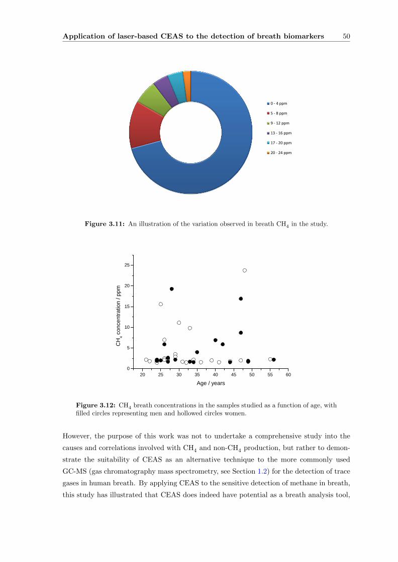
Application of laser-based CEAS to the detection of breath biomarkers 50
0 - 4 ppm
5 - 8 ppm
9 - 12 ppm
13 - 16 ppm
17 - 20 ppm
20 - 24 ppm
Figure 3.11: An illustration of the variation observed in breath CH4 in the study.
2 0 2 5 3 0 3 5 4 0 4 5 5 0 5 5 6 00
5
1 0
1 5
2 0
2 5
CH4 co
ncen
tratio
n / pp
m
A g e / y e a r s
Figure 3.12: CH4 breath concentrations in the samples studied as a function of age, withfilled circles representing men and hollowed circles women.
However, the purpose of this work was not to undertake a comprehensive study into the
causes and correlations involved with CH4 and non-CH4 production, but rather to demon-
strate the suitability of CEAS as an alternative technique to the more commonly used
GC-MS (gas chromatography mass spectrometry, see Section 1.2) for the detection of trace
gases in human breath. By applying CEAS to the sensitive detection of methane in breath,
this study has illustrated that CEAS does indeed have potential as a breath analysis tool,
Application of laser-based CEAS to the detection of breath biomarkers 51
and the flexibility afforded by this technique may allow its future application to other trace
species found in breath that act as biomarkers for diseases, a theme pursued throughout
this thesis.
3.3 Demonstration of a widely tunable laser source to spec-
troscopic applications
The methane study described previously utilised a DFB diode laser; however, these sources
are restricted by their spectral coverage (typically a few nm), limiting the amount of in-
formation that can be gathered from a measurement [179]. Access to a greater number
of transitions presents the opportunity to determine a very accurate value for parameters
such as the sample temperature (via Boltzmann statistics) by measuring several transitions
simultaneously, for monitoring the concentrations of several species in a mixture, or for
accurate isotopic ratio measurements. In addition, the wider spectral coverage provided by
such a source could allow molecules with continuous absorption spectra to be probed with
some spectral recognition. The laser used in this study, a Digital Supermode Distributed
Bragg Reflector (DS-DBR), is an example of a laser with extended spectral coverage which
has been developed for the requirements of the telecommunications industry. It is one of a
variety of similar lasers which provide an extended spectral coverage across the whole C- or
L- band (terms for the regions 1530 - 1565 nm and 1565 - 1625 nm, respectively, in fibre-
optic communications) that have been developed relatively recently. This has been achieved
by using both external cavity arrangements [180, 181] and devices with an integrated pair
of current-tuning gratings [182–184]. This section focuses on the use of one of the latter
devices, where the tuning ability is based on a comb reflector with multiple reflection peaks,
coupled with a second dispersive element for peak selection. These devices are monolithic
and as such, their mechanical stability is maximised and they can support fast modulations.
Examples of such devices include the modulated grating Y-branch (MG-Y; with the name
referring to the shape of the device) and the sampled grating distributed Bragg reflector
(SG-DBR), which utilise Vernier tuning between two grating combs to access a wide spec-
tral range. Their potential application to spectroscopy, for example in detecting multiple
species using a digital form of WMS [185], have recently been demonstrated [186, 187].
The DS-DBR laser used in this study was developed for optical switching and wavelength
division multiplexing in telecommunication equipment but this is the first demonstration of
its applicability to spectroscopy. Offering a wavelength coverage of 50 nm over the L-band,
coupled with a ∼1 MHz laser linewidth [188], the device has the potential to be a powerful
spectroscopic tool, facilitating high resolution measurements of molecular species across a
relatively large spectral range.
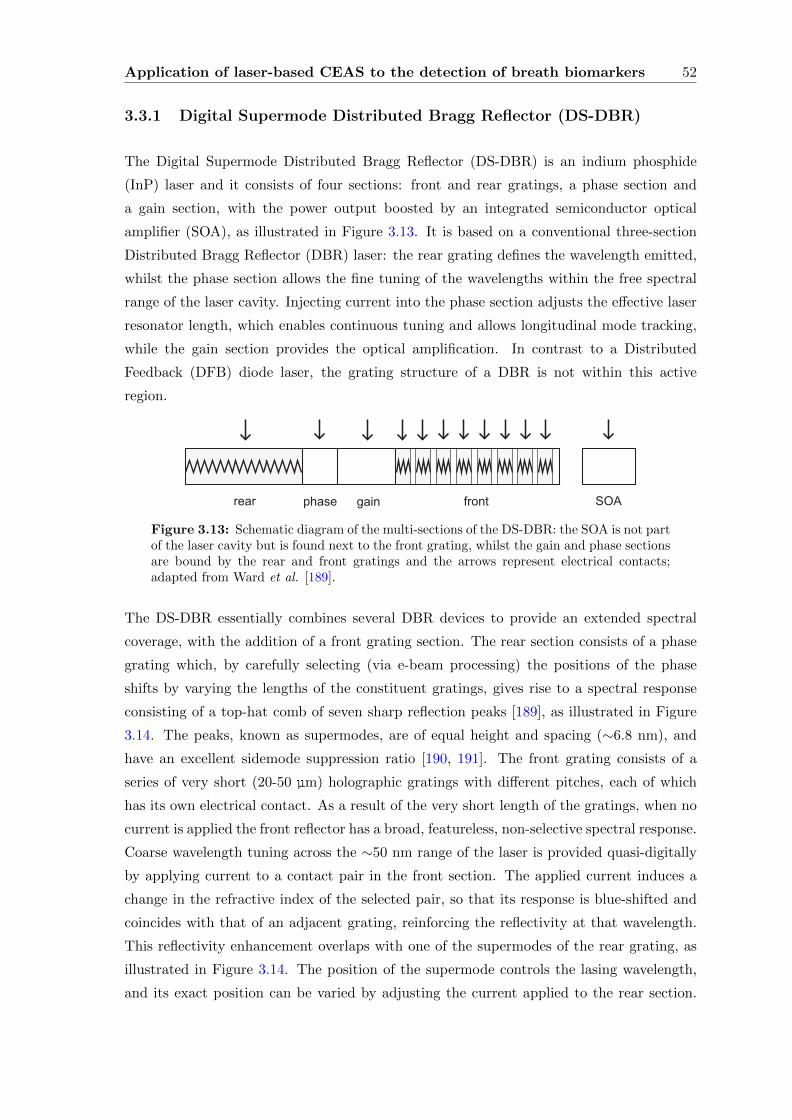
Application of laser-based CEAS to the detection of breath biomarkers 52
3.3.1 Digital Supermode Distributed Bragg Reflector (DS-DBR)
The Digital Supermode Distributed Bragg Reflector (DS-DBR) is an indium phosphide
(InP) laser and it consists of four sections: front and rear gratings, a phase section and
a gain section, with the power output boosted by an integrated semiconductor optical
amplifier (SOA), as illustrated in Figure 3.13. It is based on a conventional three-section
Distributed Bragg Reflector (DBR) laser: the rear grating defines the wavelength emitted,
whilst the phase section allows the fine tuning of the wavelengths within the free spectral
range of the laser cavity. Injecting current into the phase section adjusts the effective laser
resonator length, which enables continuous tuning and allows longitudinal mode tracking,
while the gain section provides the optical amplification. In contrast to a Distributed
Feedback (DFB) diode laser, the grating structure of a DBR is not within this active
region.
Figure 3.13: Schematic diagram of the multi-sections of the DS-DBR: the SOA is not partof the laser cavity but is found next to the front grating, whilst the gain and phase sectionsare bound by the rear and front gratings and the arrows represent electrical contacts;adapted from Ward et al. [189].
The DS-DBR essentially combines several DBR devices to provide an extended spectral
coverage, with the addition of a front grating section. The rear section consists of a phase
grating which, by carefully selecting (via e-beam processing) the positions of the phase
shifts by varying the lengths of the constituent gratings, gives rise to a spectral response
consisting of a top-hat comb of seven sharp reflection peaks [189], as illustrated in Figure
3.14. The peaks, known as supermodes, are of equal height and spacing (∼6.8 nm), and
have an excellent sidemode suppression ratio [190, 191]. The front grating consists of a
series of very short (20-50 µm) holographic gratings with different pitches, each of which
has its own electrical contact. As a result of the very short length of the gratings, when no
current is applied the front reflector has a broad, featureless, non-selective spectral response.
Coarse wavelength tuning across the ∼50 nm range of the laser is provided quasi-digitally
by applying current to a contact pair in the front section. The applied current induces a
change in the refractive index of the selected pair, so that its response is blue-shifted and
coincides with that of an adjacent grating, reinforcing the reflectivity at that wavelength.
This reflectivity enhancement overlaps with one of the supermodes of the rear grating, as
illustrated in Figure 3.14. The position of the supermode controls the lasing wavelength,
and its exact position can be varied by adjusting the current applied to the rear section.
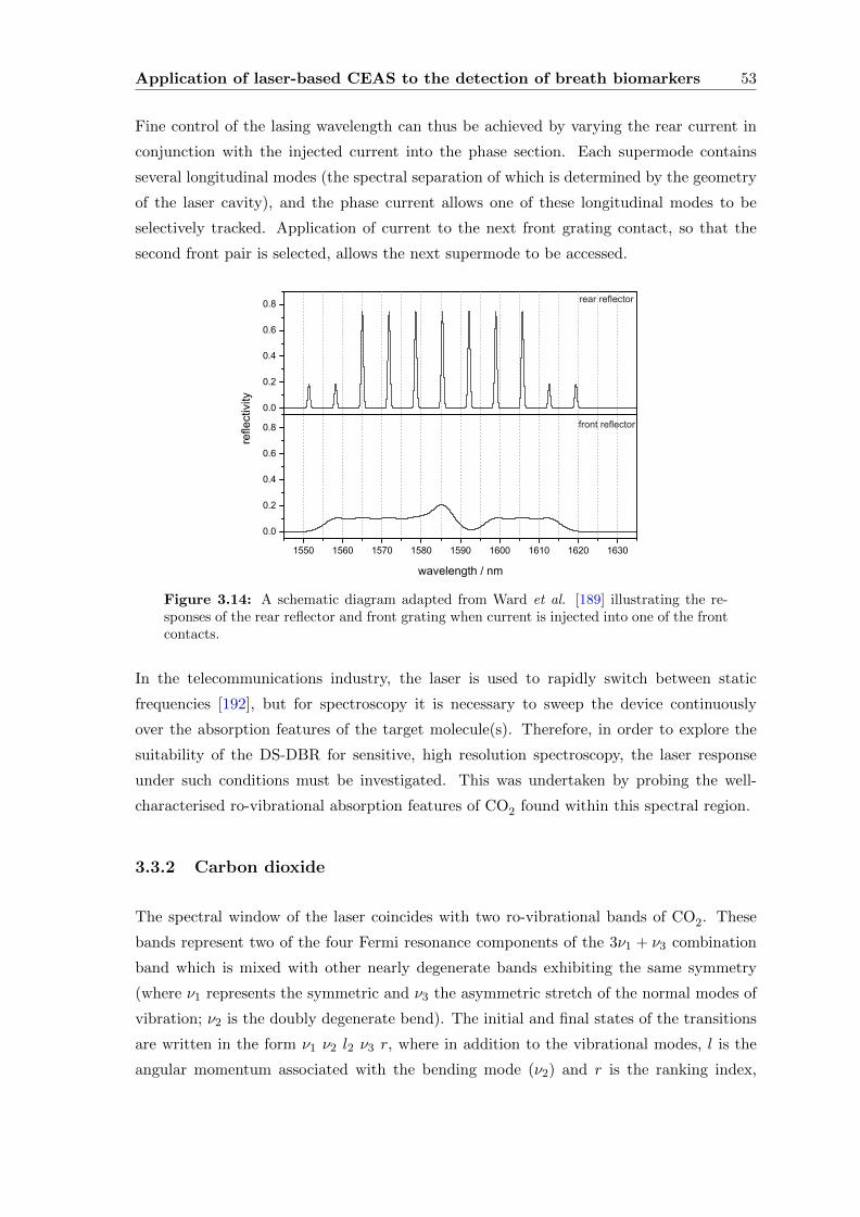
Application of laser-based CEAS to the detection of breath biomarkers 53
Fine control of the lasing wavelength can thus be achieved by varying the rear current in
conjunction with the injected current into the phase section. Each supermode contains
several longitudinal modes (the spectral separation of which is determined by the geometry
of the laser cavity), and the phase current allows one of these longitudinal modes to be
selectively tracked. Application of current to the next front grating contact, so that the
second front pair is selected, allows the next supermode to be accessed.
Figure 3.14: A schematic diagram adapted from Ward et al. [189] illustrating the re-sponses of the rear reflector and front grating when current is injected into one of the frontcontacts.
In the telecommunications industry, the laser is used to rapidly switch between static
frequencies [192], but for spectroscopy it is necessary to sweep the device continuously
over the absorption features of the target molecule(s). Therefore, in order to explore the
suitability of the DS-DBR for sensitive, high resolution spectroscopy, the laser response
under such conditions must be investigated. This was undertaken by probing the well-
characterised ro-vibrational absorption features of CO2 found within this spectral region.
3.3.2 Carbon dioxide
The spectral window of the laser coincides with two ro-vibrational bands of CO2. These
bands represent two of the four Fermi resonance components of the 3ν1 + ν3 combination
band which is mixed with other nearly degenerate bands exhibiting the same symmetry
(where ν1 represents the symmetric and ν3 the asymmetric stretch of the normal modes of
vibration; ν2 is the doubly degenerate bend). The initial and final states of the transitions
are written in the form ν1 ν2 l2 ν3 r, where in addition to the vibrational modes, l is the
angular momentum associated with the bending mode (ν2) and r is the ranking index,
Application of laser-based CEAS to the detection of breath biomarkers 54
which equals unity for the highest vibrational level of a Fermi resonating group. The wide-
tunability of the DS-DBR makes it very well suited to the measurement of isotopic ratios,
and in particular the δ13C ratio used in the urea breath test, a potential application which
will be discussed later in this chapter. Initially, however, it is necessary to fully investigate
the tuning characteristics of the laser.
3.3.3 Characterising the source
The DS-DBR unit (Bookham Technology PLC, now Oclaro Inc.), has an internal TEC and
is packaged in a standard 26-pin butterfly pigtail module. It was placed in a commercial
diode laser mount (ILX Lightwave LDM-4989), but controlled by a homemade driver unit,
which allows the current levels for each section of the device to be set independently.
The wavelength of the emitted radiation is controlled by the current settings applied to the
different sections of the laser, as specified in the manufacturer’s look-up table. A fibre-optic
collimator was used to direct the beam into a multipass cell set-up, before the transmitted
radiation was collected by an InGaAs photodiode (Thorlabs DET410). The fibre-coupled
output power was measured as 20 mW, whilst a relative frequency scale calibration was
provided by a spectrum analyser (Melles-Griot 13SAE906; free spectral range of 2 GHz),
into which a fraction of the light was directed via a beam splitter positioned before the
sample cell. An absolute scale was then derived for the spectral region covered by the laser
from the CO2 absorption features assigned in the HITRAN database, aided by a wavemeter
(Burleigh WA-1000) into which a portion of the light was directed via a flipper mirror.
The SOA and gain sections had fixed applied currents of 120 mA and 150 mA respectively,
whilst a fixed current of 5 mA was injected into the first contact of the selected front pair.
The phase section, rear grating and second contact of the front pair had a sawtooth mod-
ulation of the input current applied, the amplitudes and offsets of which were determined
from the manufacturer’s look-up table, depending on the target wavelength. All three were
modulated at the same frequency, as set by the driver unit.
Initially, the device was set to 1610.88 nm (6207.787 cm−1) and the radiation directed into
a White cell, a multipass cell with a maximum pathlength enhancement of 20 m (Specac,
Tornado; 2 m pathlength steps; 4.7 l volume), providing the system with an increased level
of sensitivity (see Section 6.4). The transition R(15) at 6207.663 cm−1, in the hot band
(3 1 1 1 3)← (0 1 1 0 1), was probed at various pressures of CO2 to investigate the suitability
of the DS-DBR for spectroscopic measurements. With this initial measurement, the laser
was operated over a relatively short wavelength region where no mode hops occur. Figure
3.15 illustrates some sample spectra at CO2 pressures of 26 Torr, 41 Torr and 69 Torr with
Voigt line profiles fitted in this regime where pressure broadening effects are observed. On
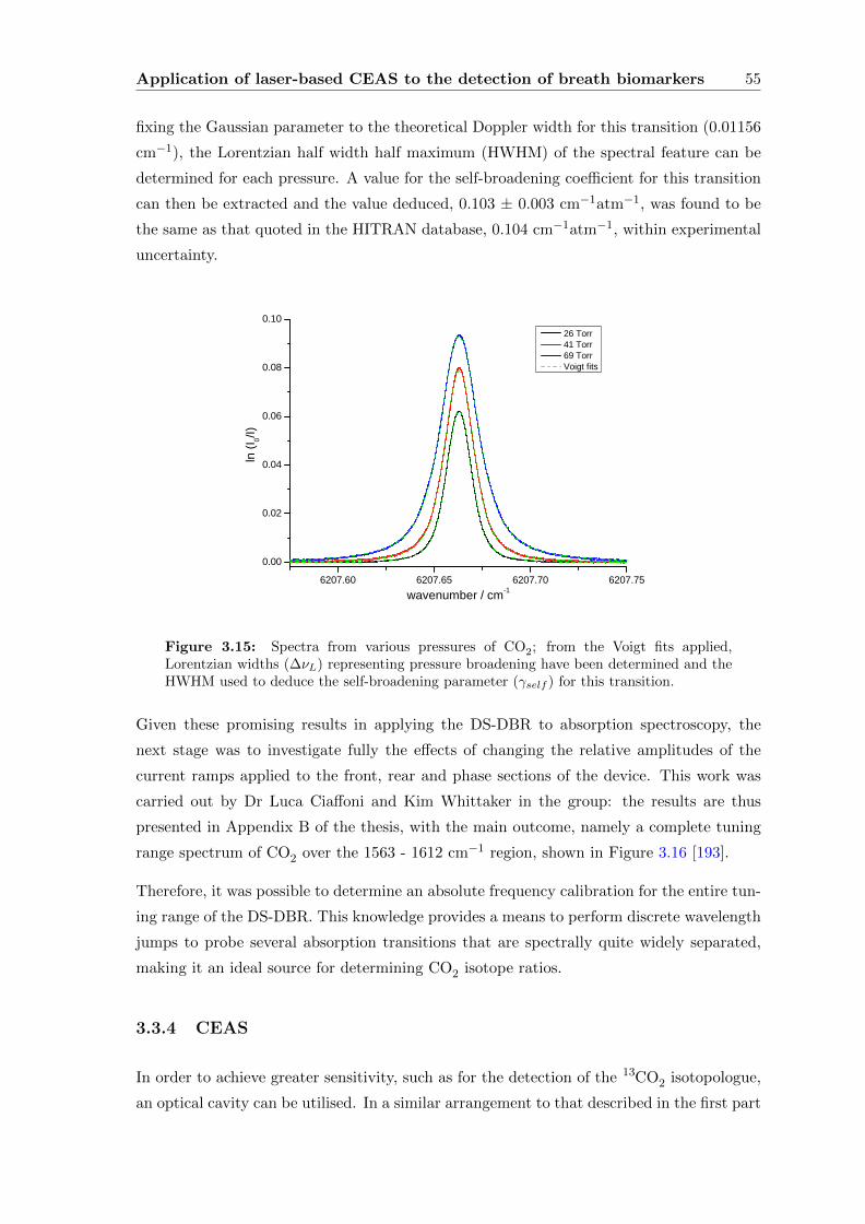
Application of laser-based CEAS to the detection of breath biomarkers 55
fixing the Gaussian parameter to the theoretical Doppler width for this transition (0.01156
cm−1), the Lorentzian half width half maximum (HWHM) of the spectral feature can be
determined for each pressure. A value for the self-broadening coefficient for this transition
can then be extracted and the value deduced, 0.103 ± 0.003 cm−1atm−1, was found to be
the same as that quoted in the HITRAN database, 0.104 cm−1atm−1, within experimental
uncertainty.
6 2 0 7 . 6 0 6 2 0 7 . 6 5 6 2 0 7 . 7 0 6 2 0 7 . 7 50 . 0 0
0 . 0 2
0 . 0 4
0 . 0 6
0 . 0 8
0 . 1 0
ln (I 0/I)
w a v e n u m b e r / c m - 1
2 6 T o r r 4 1 T o r r 6 9 T o r r V o i g t f i t s
Figure 3.15: Spectra from various pressures of CO2; from the Voigt fits applied,Lorentzian widths (∆νL) representing pressure broadening have been determined and theHWHM used to deduce the self-broadening parameter (γself ) for this transition.
Given these promising results in applying the DS-DBR to absorption spectroscopy, the
next stage was to investigate fully the effects of changing the relative amplitudes of the
current ramps applied to the front, rear and phase sections of the device. This work was
carried out by Dr Luca Ciaffoni and Kim Whittaker in the group: the results are thus
presented in Appendix B of the thesis, with the main outcome, namely a complete tuning
range spectrum of CO2 over the 1563 - 1612 cm−1 region, shown in Figure 3.16 [193].
Therefore, it was possible to determine an absolute frequency calibration for the entire tun-
ing range of the DS-DBR. This knowledge provides a means to perform discrete wavelength
jumps to probe several absorption transitions that are spectrally quite widely separated,
making it an ideal source for determining CO2 isotope ratios.
3.3.4 CEAS
In order to achieve greater sensitivity, such as for the detection of the 13CO2 isotopologue,
an optical cavity can be utilised. In a similar arrangement to that described in the first part
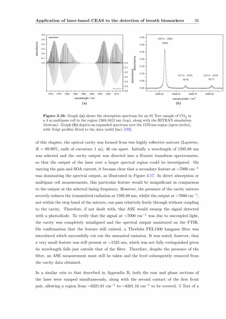
Application of laser-based CEAS to the detection of breath biomarkers 56
(a) (b)
Figure 3.16: Graph (a) shows the absorption spectrum for an 85 Torr sample of CO2 ina 4 m multipass cell in the region 1563-1612 nm (top), along with the HITRAN simulation(bottom). Graph (b) depicts an expanded spectrum over the 1570 nm region (open circles),with Voigt profiles fitted to the data (solid line) [193].
of this chapter, the optical cavity was formed from two highly reflective mirrors (Layertec,
R ∼ 99.99%, radii of curvature 1 m), 46 cm apart. Initially a wavelength of 1595.88 nm
was selected and the cavity output was directed into a Fourier transform spectrometer,
so that the output of the laser over a larger spectral region could be investigated. On
varying the gain and SOA current, it became clear that a secondary feature at ∼7000 cm−1
was dominating the spectral output, as illustrated in Figure 3.17. In direct absorption or
multipass cell measurements, this particular feature would be insignificant in comparison
to the output at the selected lasing frequency. However, the presence of the cavity mirrors
severely reduces the transmitted radiation at 1595.88 nm, whilst the output at ∼7000 cm−1,
not within the stop band of the mirrors, can pass relatively freely through without coupling
to the cavity. Therefore, if not dealt with, this ASE would swamp the signal detected
with a photodiode. To verify that the signal at ∼7000 cm−1 was due to uncoupled light,
the cavity was completely misaligned and the spectral output monitored on the FTIR.
On confirmation that the feature still existed, a Thorlabs FEL1500 longpass filter was
introduced which successfully cut out the unwanted emission. It was noted, however, that
a very small feature was still present at ∼1525 nm, which was not fully extinguished given
its wavelength falls just outside that of the filter. Therefore, despite the presence of the
filter, an ASE measurement must still be taken and the level subsequently removed from
the cavity data obtained.
In a similar vein to that described in Appendix B, both the rear and phase sections of
the laser were ramped simultaneously, along with the second contact of the first front
pair, allowing a region from ∼6221.61 cm−1 to ∼6201.16 cm−1 to be covered. 5 Torr of a
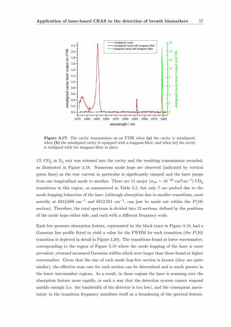
Application of laser-based CEAS to the detection of breath biomarkers 57
1 3 7 5 1 4 0 0 1 4 2 5 1 4 5 0 1 4 7 5 1 5 0 0 1 5 2 5 1 5 5 0 1 5 7 5 1 6 0 00 . 00 . 20 . 40 . 60 . 81 . 01 . 21 . 41 . 61 . 82 . 02 . 2
0
2
4
6
8
1 0
1 2
1 4
1 6
realign
ed ca
vity la
ser o
utput
on FT
IR
misa
ligned
cavity
lase
r outp
ut on
FTIR
w a v e l e n g t h / n m
m i s a l i g n e d c a v i t y m i s a l i g n e d c a v i t y w i t h l o n g p a s s f i l t e r r e a l i g n e d c a v i t y w i t h l o n g p a s s f i l t e r
Figure 3.17: The cavity transmission on an FTIR when (a) the cavity is misaligned;when (b) the misaligned cavity is equipped with a longpass filter; and when (c) the cavityis realigned with the longpass filter in place.
1% CO2 in N2 mix was released into the cavity and the resulting transmission recorded,
as illustrated in Figure 3.18. Numerous mode hops are observed (indicated by vertical
green lines) as the rear current in particular is significantly ramped and the laser jumps
from one longitudinal mode to another. There are 11 major (σint ∼ 10−23 cm2cm−1) CO2
transitions in this region, as summarised in Table 3.2, but only 7 are probed due to the
mode hopping behaviour of the laser (although absorption due to smaller transitions, most
notably at 6212.689 cm−1 and 6212.551 cm−1, can just be made out within the P (18)
section). Therefore, the total spectrum is divided into 13 sections, defined by the positions
of the mode hops either side, and each with a different frequency scale.
Each low pressure absorption feature, represented by the black trace in Figure 3.18, had a
Gaussian line profile fitted to yield a value for the FWHM for each transition (the P (10)
transition is depicted in detail in Figure 3.20). The transitions found at lower wavenumber,
corresponding to the region of Figure 3.18 where the mode hopping of the laser is more
prevalent, returned measured Gaussian widths which were larger than those found at higher
wavenumber. Given that the size of each mode hop-free section is known (they are quite
similar), the effective scan rate for each section can be determined and is much greater in
the lower wavenumber regions. As a result, in these regions the laser is scanning over the
absorption feature more rapidly, in such a way that the detection system cannot respond
quickly enough (i.e. the bandwidth of the detector is too low), and the consequent uncer-
tainty in the transition frequency manifests itself as a broadening of the spectral feature.
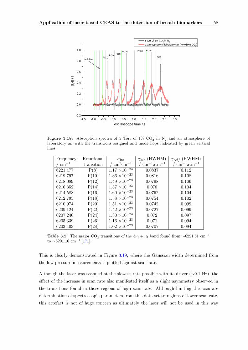
Application of laser-based CEAS to the detection of breath biomarkers 58
- 1 . 5 - 1 . 0 - 0 . 5 0 . 0 0 . 5 1 . 0 1 . 5 2 . 0 2 . 5 3 . 0- 0 . 2
0 . 0
0 . 2
0 . 4
0 . 6
0 . 8
1 . 0
[I 0-I] / I
o s c i l l o s c o p e t i m e / s
5 t o r r o f 1 % C O 2 i n N 2 1 a t m o s p h e r e o f l a b o r a t o r y a i r ( ~ 0 . 0 3 9 % C O 2 )
P ( 8 )
P ( 1 0 )P ( 1 2 )P ( 1 6 )P ( 1 8 )P ( 2 0 )P ( 2 2 )m o d e h o p s
Figure 3.18: Absorption spectra of 5 Torr of 1% CO2 in N2 and an atmosphere oflaboratory air with the transitions assigned and mode hops indicated by green verticallines.
Frequency Rotational σint γair (HWHM) γself (HWHM)/ cm−1 transition / cm2cm−1 / cm−1atm−1 / cm−1atm−1
6221.477 P(8) 1.17 ×10⁻²³ 0.0837 0.1126219.797 P(10) 1.36 ×10⁻²³ 0.0816 0.1086218.089 P(12) 1.49 ×10⁻²³ 0.0798 0.1066216.352 P(14) 1.57 ×10⁻²³ 0.078 0.1046214.588 P(16) 1.60 ×10⁻²³ 0.0762 0.1046212.795 P(18) 1.58 ×10⁻²³ 0.0754 0.1026210.974 P(20) 1.51 ×10⁻²³ 0.0742 0.0996209.124 P(22) 1.42 ×10⁻²³ 0.0727 0.0996207.246 P(24) 1.30 ×10⁻²³ 0.072 0.0976205.339 P(26) 1.16 ×10⁻²³ 0.071 0.0946203.403 P(28) 1.02 ×10⁻²³ 0.0707 0.094
Table 3.2: The major CO2 transitions of the 3ν1 + ν3 band found from ∼6221.61 cm−1
to ∼6201.16 cm−1 [171].
This is clearly demonstrated in Figure 3.19, where the Gaussian width determined from
the low pressure measurements is plotted against scan rate.
Although the laser was scanned at the slowest rate possible with its driver (∼0.1 Hz), the
effect of the increase in scan rate also manifested itself as a slight asymmetry observed in
the transitions found in those regions of high scan rate. Although limiting the accurate
determination of spectroscopic parameters from this data set to regions of lower scan rate,
this artefact is not of huge concern as ultimately the laser will not be used in this way
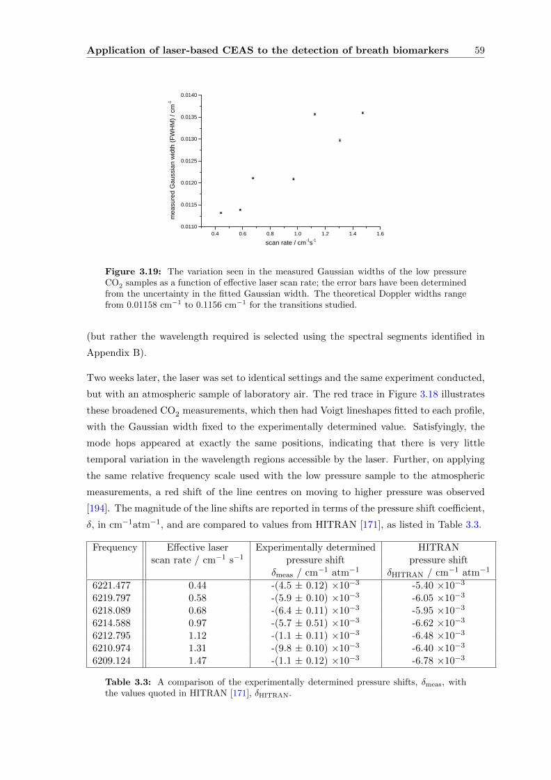
Application of laser-based CEAS to the detection of breath biomarkers 59
0 . 4 0 . 6 0 . 8 1 . 0 1 . 2 1 . 4 1 . 60 . 0 1 1 0
0 . 0 1 1 5
0 . 0 1 2 0
0 . 0 1 2 5
0 . 0 1 3 0
0 . 0 1 3 5
0 . 0 1 4 0
meas
ured G
aussi
an wi
dth (F
WHM)
/ cm-1
s c a n r a t e / c m - 1 s - 1
Figure 3.19: The variation seen in the measured Gaussian widths of the low pressureCO2 samples as a function of effective laser scan rate; the error bars have been determinedfrom the uncertainty in the fitted Gaussian width. The theoretical Doppler widths rangefrom 0.01158 cm−1 to 0.1156 cm−1 for the transitions studied.
(but rather the wavelength required is selected using the spectral segments identified in
Appendix B).
Two weeks later, the laser was set to identical settings and the same experiment conducted,
but with an atmospheric sample of laboratory air. The red trace in Figure 3.18 illustrates
these broadened CO2 measurements, which then had Voigt lineshapes fitted to each profile,
with the Gaussian width fixed to the experimentally determined value. Satisfyingly, the
mode hops appeared at exactly the same positions, indicating that there is very little
temporal variation in the wavelength regions accessible by the laser. Further, on applying
the same relative frequency scale used with the low pressure sample to the atmospheric
measurements, a red shift of the line centres on moving to higher pressure was observed
[194]. The magnitude of the line shifts are reported in terms of the pressure shift coefficient,
δ, in cm−1atm−1, and are compared to values from HITRAN [171], as listed in Table 3.3.
Frequency Effective laser Experimentally determined HITRANscan rate / cm−1 s−1 pressure shift pressure shift
δmeas / cm−1 atm−1 δHITRAN / cm−1 atm−1
6221.477 0.44 -(4.5 ± 0.12) ×10−3 -5.40 ×10⁻³
6219.797 0.58 -(5.9 ± 0.10) ×10−3 -6.05 ×10⁻³
6218.089 0.68 -(6.4 ± 0.11) ×10−3 -5.95 ×10⁻³
6214.588 0.97 -(5.7 ± 0.51) ×10−3 -6.62 ×10⁻³
6212.795 1.12 -(1.1 ± 0.11) ×10−3 -6.48 ×10⁻³
6210.974 1.31 -(9.8 ± 0.10) ×10−3 -6.40 ×10⁻³
6209.124 1.47 -(1.1 ± 0.12) ×10−3 -6.78 ×10⁻³
Table 3.3: A comparison of the experimentally determined pressure shifts, δmeas, withthe values quoted in HITRAN [171], δHITRAN.
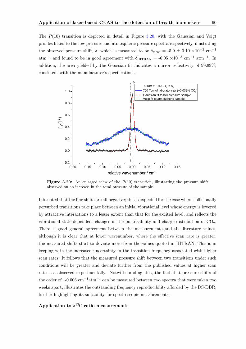
Application of laser-based CEAS to the detection of breath biomarkers 60
The P (10) transition is depicted in detail in Figure 3.20, with the Gaussian and Voigt
profiles fitted to the low pressure and atmospheric pressure spectra respectively, illustrating
the observed pressure shift, δ, which is measured to be δmeas = -5.9 ± 0.10 ×10⁻³ cm−1
atm−1 and found to be in good agreement with δHITRAN = -6.05 ×10⁻³ cm−1 atm−1. In
addition, the area yielded by the Gaussian fit indicates a mirror reflectivity of 99.99%,
consistent with the manufacturer’s specifications.
- 0 . 2 0 - 0 . 1 5 - 0 . 1 0 - 0 . 0 5 0 . 0 0 0 . 0 5 0 . 1 0 0 . 1 5- 0 . 2
0 . 0
0 . 2
0 . 4
0 . 6
0 . 8
1 . 0 5 T o r r o f 1 % C O 2 i n N 2 7 6 0 T o r r o f l a b o r a t o r y a i r ( ~ 0 . 0 3 9 % C O 2 ) G a u s s i a n f i t t o l o w p r e s s u r e s a m p l e V o i g t f i t t o a t m o s p h e r i c s a m p l e
[I 0-I] / I
r e l a t i v e w a v e n u m b e r / c m - 1
δ
Figure 3.20: An enlarged view of the P (10) transition, illustrating the pressure shiftobserved on an increase in the total pressure of the sample.
It is noted that the line shifts are all negative; this is expected for the case where collisionally
perturbed transitions take place between an initial vibrational level whose energy is lowered
by attractive interactions to a lesser extent than that for the excited level, and reflects the
vibrational state-dependent changes in the polarisability and charge distribution of CO2.
There is good general agreement between the measurements and the literature values,
although it is clear that at lower wavenumber, where the effective scan rate is greater,
the measured shifts start to deviate more from the values quoted in HITRAN. This is in
keeping with the increased uncertainty in the transition frequency associated with higher
scan rates. It follows that the measured pressure shift between two transitions under such
conditions will be greater and deviate further from the published values at higher scan
rates, as observed experimentally. Notwithstanding this, the fact that pressure shifts of
the order of ∼0.006 cm−1atm−1 can be measured between two spectra that were taken two
weeks apart, illustrates the outstanding frequency reproducibility afforded by the DS-DBR,
further highlighting its suitability for spectroscopic measurements.
Application to δ13C ratio measurements
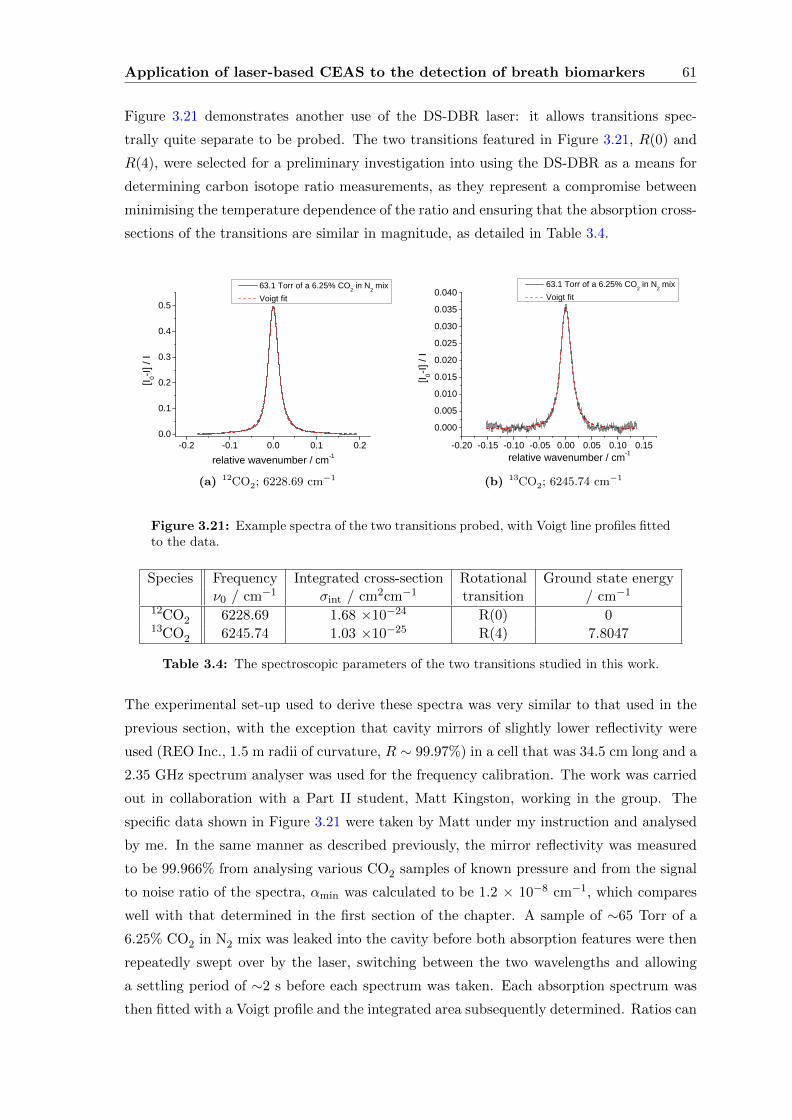
Application of laser-based CEAS to the detection of breath biomarkers 61
Figure 3.21 demonstrates another use of the DS-DBR laser: it allows transitions spec-
trally quite separate to be probed. The two transitions featured in Figure 3.21, R(0) and
R(4), were selected for a preliminary investigation into using the DS-DBR as a means for
determining carbon isotope ratio measurements, as they represent a compromise between
minimising the temperature dependence of the ratio and ensuring that the absorption cross-
sections of the transitions are similar in magnitude, as detailed in Table 3.4.
- 0 . 2 - 0 . 1 0 . 0 0 . 1 0 . 20 . 0
0 . 1
0 . 2
0 . 3
0 . 4
0 . 5 6 3 . 1 T o r r o f a 6 . 2 5 % C O 2 i n N 2 m i x V o i g t f i t
[I 0-I] / I
r e l a t i v e w a v e n u m b e r / c m - 1
(a) 12CO2; 6228.69 cm−1
- 0 . 2 0 - 0 . 1 5 - 0 . 1 0 - 0 . 0 5 0 . 0 0 0 . 0 5 0 . 1 0 0 . 1 50 . 0 0 00 . 0 0 50 . 0 1 00 . 0 1 50 . 0 2 00 . 0 2 50 . 0 3 00 . 0 3 50 . 0 4 0 6 3 . 1 T o r r o f a 6 . 2 5 % C O 2 i n N 2 m i x
V o i g t f i t
[I 0-I] / I
r e l a t i v e w a v e n u m b e r / c m - 1
(b) 13CO2; 6245.74 cm−1
Figure 3.21: Example spectra of the two transitions probed, with Voigt line profiles fittedto the data.
Species Frequency Integrated cross-section Rotational Ground state energyν0 / cm−1 σint / cm2cm−1 transition / cm−1
12CO2 6228.69 1.68 ×10⁻²⁴ R(0) 013CO2 6245.74 1.03 ×10⁻²⁵ R(4) 7.8047
Table 3.4: The spectroscopic parameters of the two transitions studied in this work.
The experimental set-up used to derive these spectra was very similar to that used in the
previous section, with the exception that cavity mirrors of slightly lower reflectivity were
used (REO Inc., 1.5 m radii of curvature, R ∼ 99.97%) in a cell that was 34.5 cm long and a
2.35 GHz spectrum analyser was used for the frequency calibration. The work was carried
out in collaboration with a Part II student, Matt Kingston, working in the group. The
specific data shown in Figure 3.21 were taken by Matt under my instruction and analysed
by me. In the same manner as described previously, the mirror reflectivity was measured
to be 99.966% from analysing various CO2 samples of known pressure and from the signal
to noise ratio of the spectra, αmin was calculated to be 1.2 × 10⁻⁸ cm−1, which compares
well with that determined in the first section of the chapter. A sample of ∼65 Torr of a
6.25% CO2 in N2 mix was leaked into the cavity before both absorption features were then
repeatedly swept over by the laser, switching between the two wavelengths and allowing
a settling period of ∼2 s before each spectrum was taken. Each absorption spectrum was
then fitted with a Voigt profile and the integrated area subsequently determined. Ratios can
Application of laser-based CEAS to the detection of breath biomarkers 62
then be calculated for each isotopic pair, and the standard deviation deduced from a linear
fit to the ratios. The estimated uncertainty in the mean ratio value is then determined from
weighting the standard deviation with the number of measurements taken of the isotopic
pair [195]. This value, 1.85×10⁻⁴, then yields an instrument sensitivity of δ13Cmin = 2.98
, which is comparable with the δ13Cmin obtained by Kasyutich et al. [13] (3.7 ) and
Ciaffoni [196] (8.0 ). However, as discussed in Chapter 1, for application to the urea
breath test, a ‘gold standard’ precision of <1 is recommended.
It is immediately obvious that a degree of uncertainty in the measurements of this study
will arise from the poorly defined wings of the 13CO2 absorption feature, which will man-
ifest itself as an uncertainty in the determination of the integrated area of the transition.
One way in which to reduce this effect could be to improve the sensitivity of the instrument
by either increasing the physical pathlength of the cavity, or by using higher reflectivity
mirrors. However, this could cause dynamic range problems when probing the 12CO2 tran-
sition. Potentially, this could be overcome by selecting a pair of transitions with more
comparable absorption line strengths, at the expense of a greater difference in the tem-
perature dependence of the two transitions. The Boltzmann distribution indicates that
temperature affects the absorption line strength, so in order to minimise the influence of
any temperature fluctuations during measurements of the two isotopes, two transitions that
were as close as possible in ground state energy (given the restrictions on the relative ab-
sorption line strengths of the two transitions) were chosen. This provided a temperature
dependence of the isotopic ratio of ∼0.127 δ K−1 at 298 K (determined via a theoret-
ical approximation ∆δ 13C∆T = hc∆E
kBT 2 × 1000 [197], where ∆δ 13C∆T is expressed in δ K−1 at
a defined temperature and ∆E is the difference in the ground state energy levels of the
two transitions). Whilst this minimal temperature dependence clearly demonstrates an
advantage of the DS-DBR over a laser with a more narrow spectral range (where one is
restricted to transitions which are found relatively close together, which tend to suffer from
a large temperature dependence as they originate from quite different J states), this leads
to a required temperature stability of < 8 K in order to obtain the 1 ‘gold standard’
precision. Given the laboratory temperature can be comfortably maintained within 1 K,
this would suggest that there is a certain degree of flexibility available in selecting two
different transitions so that the 13C/12C absorption line strength ratio can be maximised.
Alternatively, the wide tuning range of the DS-DBR could be exploited to measure several
different lines of isotopic pairs. Not only would this remove the temperature dependence
issue (it would allow the sample temperature to be deduced), it would also statistically
enhance the ratio determined, consequently providing a greater level of precision and a
lower δ13Cmin.
Application of laser-based CEAS to the detection of breath biomarkers 63
3.4 Conclusions
This chapter initially illustrated the applicability of laser-based absorption spectroscopy
as a viable means of breath analysis, by measuring the levels of methane in breath in a
study on a small sample of people using a DFB diode laser and a CEAS detection scheme.
This was followed by the characterisation of a novel, widely tunable laser source, the DS-
DBR, and the first demonstration of its use in absorption spectroscopy. A preliminary
investigation into its suitability for determining δ13C was also conducted and although the
sensitivity value determined is lower than recommended for diagnosis, it would be possible
to improve it by monitoring multiple isotopic ratios.
However, sometimes the molecules of interest in breath do not have narrow transitions,
but instead exhibit absorption features spanning tens of nanometres. In such situations,
alternative radiation sources must be utilised and this is the subject of the next chapter.
Chapter 4
Broadband Cavity Enhanced
Absorption Spectroscopy
(BB-CEAS)
Many of the biomarkers identified in Chapter 1 have broad, congested absorption features
which are consequently not readily discernible using narrowband laser sources. As such,
this chapter deals with the application of broadband sources to cavity enhanced absorption
spectroscopy for the detection of three broadband absorbers: butadiene, acetone and iso-
prene. Two types of broadband source, a Superluminiscent Light Emitting Diode (SLED),
with a spectral output covering ∼1600 to ∼1700 nm, and a Supercontinuum (SC) source,
which emits from 450 nm to 2.5 µm, but will be used primarily in the same spectral region
as the SLED, will be demonstrated in conjunction with two detection systems: dispersion
using a monochromatic spectrometer and interferometry using FTIR spectroscopy. Initial
work centres on the determination of the absorption cross-sections of these molecules and
the subsequent detection of these species in dilute samples using BB-CEAS, before the
broadband spectrometer is developed further and applied to real breath samples.
4.1 Broadband Spectroscopy
Narrowband diode lasers are ideal for studying small molecules, such as methane and carbon
dioxide, as they can easily scan over the narrow absorption features. However, if the target
molecule is somewhat larger, it may have quasi-continuous absorption features which span
over several nanometres. In this case, the use of a broadband source can provide specificity,
as is illustrated in Figure 4.1. Additionally, if it is desirable to measure several compounds
64
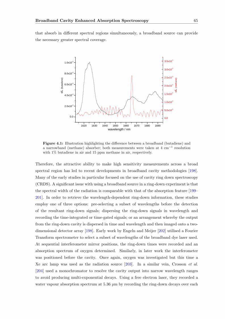
Broadband Cavity Enhanced Absorption Spectroscopy 65
that absorb in different spectral regions simultaneously, a broadband source can provide
the necessary greater spectral coverage.
1 6 2 0 1 6 3 0 1 6 4 0 1 6 5 0 1 6 6 0 1 6 7 0 1 6 8 0 1 6 9 0
0 . 0
2 . 0 x 1 0 - 4
4 . 0 x 1 0 - 4
6 . 0 x 1 0 - 4
8 . 0 x 1 0 - 4
1 . 0 x 1 0 - 3αL
(butad
iene)
w a v e l e n g t h / n m
0 . 0
5 . 0 x 1 0 - 6
1 . 0 x 1 0 - 5
1 . 5 x 1 0 - 5
2 . 0 x 1 0 - 5
2 . 5 x 1 0 - 5
3 . 0 x 1 0 - 5
3 . 5 x 1 0 - 5
αL (m
ethan
e)
Figure 4.1: Illustration highlighting the difference between a broadband (butadiene) anda narrowband (methane) absorber; both measurements were taken at 4 cm−1 resolutionwith 1% butadiene in air and 15 ppm methane in air, respectively.
Therefore, the attractive ability to make high sensitivity measurements across a broad
spectral region has led to recent developments in broadband cavity methodologies [198].
Many of the early studies in particular focused on the use of cavity ring down spectroscopy
(CRDS). A significant issue with using a broadband source in a ring-down experiment is that
the spectral width of the radiation is comparable with that of the absorption feature [199–
201]. In order to retrieve the wavelength-dependent ring-down information, these studies
employ one of three options: pre-selecting a subset of wavelengths before the detection
of the resultant ring-down signals; dispersing the ring-down signals in wavelength and
recording the time-integrated or time-gated signals; or an arrangement whereby the output
from the ring-down cavity is dispersed in time and wavelength and then imaged onto a two-
dimensional detector array [198]. Early work by Engeln and Meijer [202] utilised a Fourier
Transform spectrometer to select a subset of wavelengths of the broadband dye laser used.
At sequential interferometer mirror positions, the ring-down times were recorded and an
absorption spectrum of oxygen determined. Similarly, in later work the interferometer
was positioned before the cavity. Once again, oxygen was investigated but this time a
Xe arc lamp was used as the radiation source [203]. In a similar vein, Crosson et al.
[204] used a monochromator to resolve the cavity output into narrow wavelength ranges
to avoid producing multi-exponential decays. Using a free electron laser, they recorded a
water vapour absorption spectrum at 5.36 µm by recording the ring-down decays over each
Broadband Cavity Enhanced Absorption Spectroscopy 66
narrow range selected by the spectrometer. In studying the mid-infrared absorptions of thin
films of C60, Marcus and Schwettman [205] employed the same principle, with the ring-down
events recorded in a time-resolved manner. The work of Czyzewski et al. [206] represents an
example of the second option described above. In this case, the radiation from a Nd:YAG
pumped dye laser was dispersed in wavelength by a spectrograph before being detected using
a charge-coupled device (CCD) with a gated image intensifier. Whereas in the previous
studies sections of the broadband radiation are detected in a consecutive manner over
time, here the full bandwidth of the light is used for each measurement, but the temporal
evolution of the cavity output has to be built up from consecutive measurements. This
means that the decay trace comes from different laser shots, which necessarily introduces
additional noise to the decay and greater uncertainty in the derived ring-down time.
Finally, it is possible to resolve both time and wavelength simultaneously, in so-called two-
dimensional broadband cavity ring-down [198]. Ring-down spectral photography (RSP)
was developed by Scherer [207], and it resolves the ring-down event both in wavelength and
in time along the x− and y− co-ordinates by reflecting the cavity output off a rotating
mirror and onto a diffraction grating. Hence the physical position of the radiation on the
grating is determined by the time delay with respect to the laser pulse, and the dispersion
from the grating is dependent on the wavelength of the radiation. Therefore, the spatial
dispersion of the radiation imaged onto the CCD camera is dependent on both the time
it left the cavity and its wavelength. A proof-of-principle study for this technique was
carried out on propane using a narrowband dye laser [207], in which the laser was tuned
in steps of 1 nm to mimic a broadband source, before the technique was applied to a
broadband source, a YAG-pumped dye laser, to probe propane and oxygen [208]. Ball et
al. [209] also achieved two-dimensional broadband cavity ring-down detection by utilising
a ‘clocked’ two-dimensional CCD detector. The light leaving the cavity was projected onto
the CCD via an astigmatic imaging spectrograph, which wavelength-resolved the radiation.
Incident radiation on the CCD chip generated photocharge which was trapped by potential
wells within each pixel. On application of voltages to the electrodes along the time axis of
the CCD, the photocharge was transferred between rows of pixels in a ‘clocking sequence’.
Thus, as this sequence progressed, time and wavelength resolved spectra were collected until
the complete ring-down event was recorded. At this point the charge was reverse clocked
so that the original arrangement was restored, ready for the next capture sequence. In
addition to the NO3 radical studied in [209], the authors later also applied this technique
to molecular oxygen, NO3 and mixtures of NO3 and water vapour [198], highlighting a
major application of sensitive broadband techniques in studying atmospheric trace species.
Indeed, in a later publication from the same group [210], this instrument was actually used
for field measurements to measure the levels of NO3, N2O5, I2 and OIO during the 2002
North Atlantic Marine Boundary Layer Experiment (NAMBLEX).
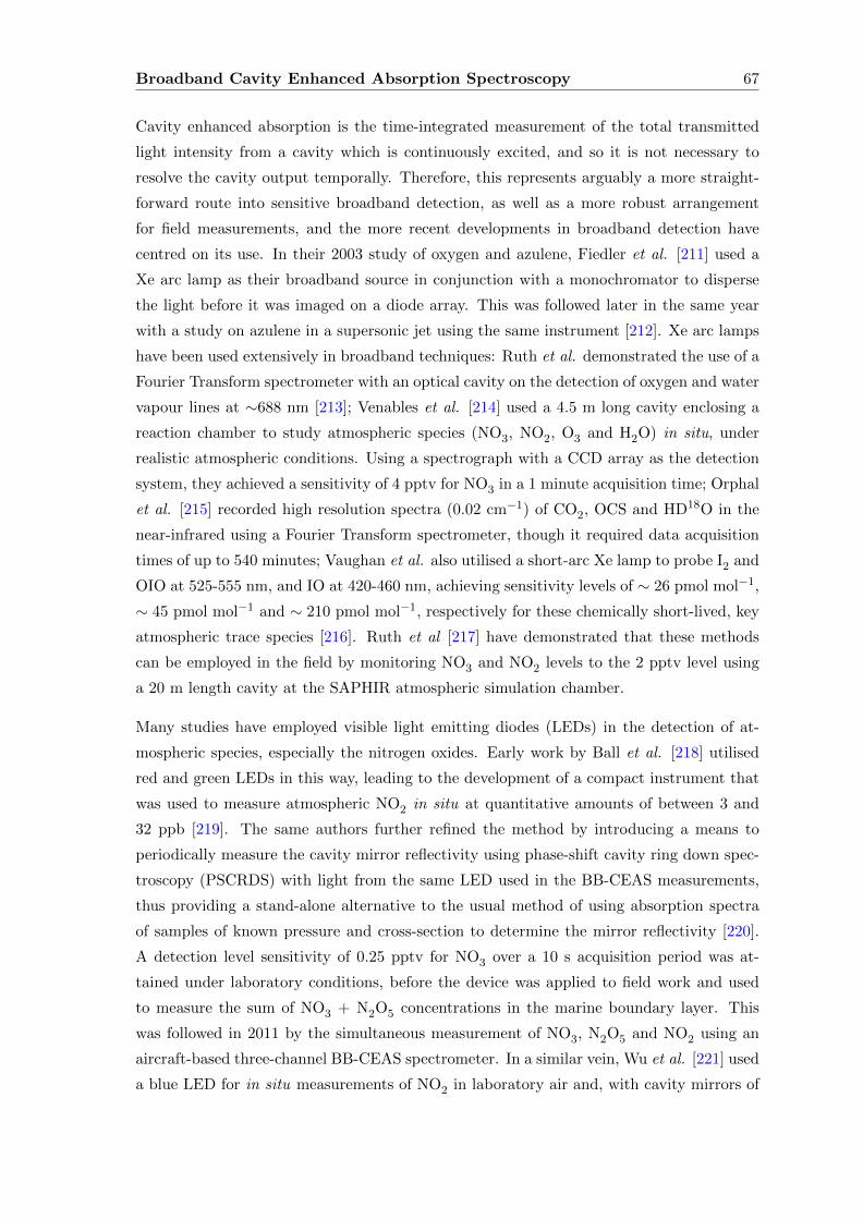
Broadband Cavity Enhanced Absorption Spectroscopy 67
Cavity enhanced absorption is the time-integrated measurement of the total transmitted
light intensity from a cavity which is continuously excited, and so it is not necessary to
resolve the cavity output temporally. Therefore, this represents arguably a more straight-
forward route into sensitive broadband detection, as well as a more robust arrangement
for field measurements, and the more recent developments in broadband detection have
centred on its use. In their 2003 study of oxygen and azulene, Fiedler et al. [211] used a
Xe arc lamp as their broadband source in conjunction with a monochromator to disperse
the light before it was imaged on a diode array. This was followed later in the same year
with a study on azulene in a supersonic jet using the same instrument [212]. Xe arc lamps
have been used extensively in broadband techniques: Ruth et al. demonstrated the use of a
Fourier Transform spectrometer with an optical cavity on the detection of oxygen and water
vapour lines at ∼688 nm [213]; Venables et al. [214] used a 4.5 m long cavity enclosing a
reaction chamber to study atmospheric species (NO3, NO2, O3 and H2O) in situ, under
realistic atmospheric conditions. Using a spectrograph with a CCD array as the detection
system, they achieved a sensitivity of 4 pptv for NO3 in a 1 minute acquisition time; Orphal
et al. [215] recorded high resolution spectra (0.02 cm−1) of CO2, OCS and HD18O in the
near-infrared using a Fourier Transform spectrometer, though it required data acquisition
times of up to 540 minutes; Vaughan et al. also utilised a short-arc Xe lamp to probe I2 and
OIO at 525-555 nm, and IO at 420-460 nm, achieving sensitivity levels of ∼ 26 pmol mol−1,
∼ 45 pmol mol−1 and ∼ 210 pmol mol−1, respectively for these chemically short-lived, key
atmospheric trace species [216]. Ruth et al [217] have demonstrated that these methods
can be employed in the field by monitoring NO3 and NO2 levels to the 2 pptv level using
a 20 m length cavity at the SAPHIR atmospheric simulation chamber.
Many studies have employed visible light emitting diodes (LEDs) in the detection of at-
mospheric species, especially the nitrogen oxides. Early work by Ball et al. [218] utilised
red and green LEDs in this way, leading to the development of a compact instrument that
was used to measure atmospheric NO2 in situ at quantitative amounts of between 3 and
32 ppb [219]. The same authors further refined the method by introducing a means to
periodically measure the cavity mirror reflectivity using phase-shift cavity ring down spec-
troscopy (PSCRDS) with light from the same LED used in the BB-CEAS measurements,
thus providing a stand-alone alternative to the usual method of using absorption spectra
of samples of known pressure and cross-section to determine the mirror reflectivity [220].
A detection level sensitivity of 0.25 pptv for NO3 over a 10 s acquisition period was at-
tained under laboratory conditions, before the device was applied to field work and used
to measure the sum of NO3 + N2O5 concentrations in the marine boundary layer. This
was followed in 2011 by the simultaneous measurement of NO3, N2O5 and NO2 using an
aircraft-based three-channel BB-CEAS spectrometer. In a similar vein, Wu et al. [221] used
a blue LED for in situ measurements of NO2 in laboratory air and, with cavity mirrors of
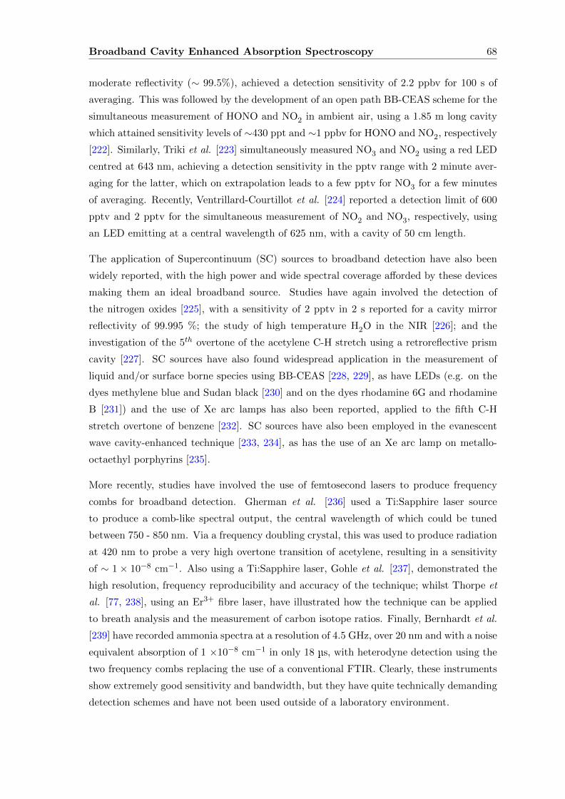
Broadband Cavity Enhanced Absorption Spectroscopy 68
moderate reflectivity (∼ 99.5%), achieved a detection sensitivity of 2.2 ppbv for 100 s of
averaging. This was followed by the development of an open path BB-CEAS scheme for the
simultaneous measurement of HONO and NO2 in ambient air, using a 1.85 m long cavity
which attained sensitivity levels of ∼430 ppt and ∼1 ppbv for HONO and NO2, respectively
[222]. Similarly, Triki et al. [223] simultaneously measured NO3 and NO2 using a red LED
centred at 643 nm, achieving a detection sensitivity in the pptv range with 2 minute aver-
aging for the latter, which on extrapolation leads to a few pptv for NO3 for a few minutes
of averaging. Recently, Ventrillard-Courtillot et al. [224] reported a detection limit of 600
pptv and 2 pptv for the simultaneous measurement of NO2 and NO3, respectively, using
an LED emitting at a central wavelength of 625 nm, with a cavity of 50 cm length.
The application of Supercontinuum (SC) sources to broadband detection have also been
widely reported, with the high power and wide spectral coverage afforded by these devices
making them an ideal broadband source. Studies have again involved the detection of
the nitrogen oxides [225], with a sensitivity of 2 pptv in 2 s reported for a cavity mirror
reflectivity of 99.995 %; the study of high temperature H2O in the NIR [226]; and the
investigation of the 5th overtone of the acetylene C-H stretch using a retroreflective prism
cavity [227]. SC sources have also found widespread application in the measurement of
liquid and/or surface borne species using BB-CEAS [228, 229], as have LEDs (e.g. on the
dyes methylene blue and Sudan black [230] and on the dyes rhodamine 6G and rhodamine
B [231]) and the use of Xe arc lamps has also been reported, applied to the fifth C-H
stretch overtone of benzene [232]. SC sources have also been employed in the evanescent
wave cavity-enhanced technique [233, 234], as has the use of an Xe arc lamp on metallo-
octaethyl porphyrins [235].
More recently, studies have involved the use of femtosecond lasers to produce frequency
combs for broadband detection. Gherman et al. [236] used a Ti:Sapphire laser source
to produce a comb-like spectral output, the central wavelength of which could be tuned
between 750 - 850 nm. Via a frequency doubling crystal, this was used to produce radiation
at 420 nm to probe a very high overtone transition of acetylene, resulting in a sensitivity
of ∼ 1 × 10⁻⁸ cm−1. Also using a Ti:Sapphire laser, Gohle et al. [237], demonstrated the
high resolution, frequency reproducibility and accuracy of the technique; whilst Thorpe et
al. [77, 238], using an Er3+ fibre laser, have illustrated how the technique can be applied
to breath analysis and the measurement of carbon isotope ratios. Finally, Bernhardt et al.
[239] have recorded ammonia spectra at a resolution of 4.5 GHz, over 20 nm and with a noise
equivalent absorption of 1 ×10⁻⁸ cm−1 in only 18 µs, with heterodyne detection using the
two frequency combs replacing the use of a conventional FTIR. Clearly, these instruments
show extremely good sensitivity and bandwidth, but they have quite technically demanding
detection schemes and have not been used outside of a laboratory environment.
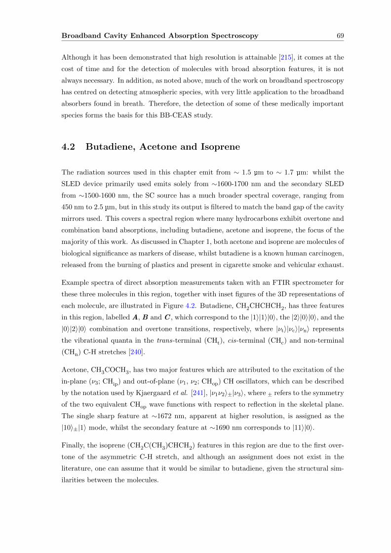
Broadband Cavity Enhanced Absorption Spectroscopy 69
Although it has been demonstrated that high resolution is attainable [215], it comes at the
cost of time and for the detection of molecules with broad absorption features, it is not
always necessary. In addition, as noted above, much of the work on broadband spectroscopy
has centred on detecting atmospheric species, with very little application to the broadband
absorbers found in breath. Therefore, the detection of some of these medically important
species forms the basis for this BB-CEAS study.
4.2 Butadiene, Acetone and Isoprene
The radiation sources used in this chapter emit from ∼ 1.5 µm to ∼ 1.7 µm: whilst the
SLED device primarily used emits solely from ∼1600-1700 nm and the secondary SLED
from ∼1500-1600 nm, the SC source has a much broader spectral coverage, ranging from
450 nm to 2.5 µm, but in this study its output is filtered to match the band gap of the cavity
mirrors used. This covers a spectral region where many hydrocarbons exhibit overtone and
combination band absorptions, including butadiene, acetone and isoprene, the focus of the
majority of this work. As discussed in Chapter 1, both acetone and isoprene are molecules of
biological significance as markers of disease, whilst butadiene is a known human carcinogen,
released from the burning of plastics and present in cigarette smoke and vehicular exhaust.
Example spectra of direct absorption measurements taken with an FTIR spectrometer for
these three molecules in this region, together with inset figures of the 3D representations of
each molecule, are illustrated in Figure 4.2. Butadiene, CH2CHCHCH2, has three features
in this region, labelled A, B and C , which correspond to the |1〉|1〉|0〉, the |2〉|0〉|0〉, and the
|0〉|2〉|0〉 combination and overtone transitions, respectively, where |νt〉|νc〉|νn〉 represents
the vibrational quanta in the trans-terminal (CHt), cis-terminal (CHc) and non-terminal
(CHn) C-H stretches [240].
Acetone, CH3COCH3, has two major features which are attributed to the excitation of the
in-plane (ν3; CHip) and out-of-plane (ν1, ν2; CHop) CH oscillators, which can be described
by the notation used by Kjaergaard et al. [241], |ν1ν2〉±|ν3〉, where ± refers to the symmetry
of the two equivalent CHop wave functions with respect to reflection in the skeletal plane.
The single sharp feature at ∼1672 nm, apparent at higher resolution, is assigned as the
|10〉±|1〉 mode, whilst the secondary feature at ∼1690 nm corresponds to |11〉|0〉.
Finally, the isoprene (CH2C(CH3)CHCH2) features in this region are due to the first over-
tone of the asymmetric C-H stretch, and although an assignment does not exist in the
literature, one can assume that it would be similar to butadiene, given the structural sim-
ilarities between the molecules.
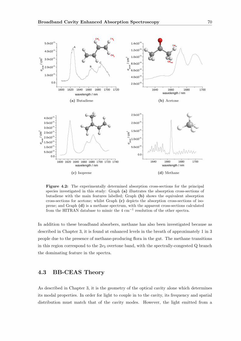
Broadband Cavity Enhanced Absorption Spectroscopy 70
1 6 0 0 1 6 2 0 1 6 4 0 1 6 6 0 1 6 8 0 1 7 0 0 1 7 2 0
0 . 0
1 . 0 x 1 0 - 2 1
2 . 0 x 1 0 - 2 1
3 . 0 x 1 0 - 2 1
4 . 0 x 1 0 - 2 1
5 . 0 x 1 0 - 2 1
CB
σ peak
/ cm2
w a v e l e n g t h / n m
A
(a) Butadiene
1 6 4 0 1 6 6 0 1 6 8 0 1 7 0 02 . 0 x 1 0 - 2 2
4 . 0 x 1 0 - 2 2
6 . 0 x 1 0 - 2 2
8 . 0 x 1 0 - 2 2
1 . 0 x 1 0 - 2 1
1 . 2 x 1 0 - 2 1
1 . 4 x 1 0 - 2 1
w a v e l e n g t h / n m
σ peak
/ cm2
(b) Acetone
1 6 0 0 1 6 2 0 1 6 4 0 1 6 6 0 1 6 8 0 1 7 0 0 1 7 2 0 1 7 4 00 . 0
5 . 0 x 1 0 - 2 21 . 0 x 1 0 - 2 11 . 5 x 1 0 - 2 12 . 0 x 1 0 - 2 12 . 5 x 1 0 - 2 13 . 0 x 1 0 - 2 13 . 5 x 1 0 - 2 14 . 0 x 1 0 - 2 1
σ peak
/ cm2
w a v e l e n g t h / n m(c) Isoprene
1 6 4 0 1 6 6 0 1 6 8 0 1 7 0 0
0 . 0
5 . 0 x 1 0 - 2 2
1 . 0 x 1 0 - 2 1
1 . 5 x 1 0 - 2 1
2 . 0 x 1 0 - 2 1
2 . 5 x 1 0 - 2 1
w a v e l e n g t h / n m
σ peak
/ cm2
(d) Methane
Figure 4.2: The experimentally determined absorption cross-sections for the principalspecies investigated in this study: Graph (a) illustrates the absorption cross-sections ofbutadiene with the main features labelled; Graph (b) shows the equivalent absorptioncross-sections for acetone; whilst Graph (c) depicts the absorption cross-sections of iso-prene; and Graph (d) is a methane spectrum, with the apparent cross-sections calculatedfrom the HITRAN database to mimic the 4 cm−1 resolution of the other spectra.
In addition to these broadband absorbers, methane has also been investigated because as
described in Chapter 3, it is found at enhanced levels in the breath of approximately 1 in 3
people due to the presence of methane-producing flora in the gut. The methane transitions
in this region correspond to the 2ν3 overtone band, with the spectrally-congested Q branch
the dominating feature in the spectra.
4.3 BB-CEAS Theory
As described in Chapter 3, it is the geometry of the optical cavity alone which determines
its modal properties. In order for light to couple in to the cavity, its frequency and spatial
distribution must match that of the cavity modes. However, the light emitted from a

Broadband Cavity Enhanced Absorption Spectroscopy 71
broadband source is temporally incoherent and, in contrast to that from a diode laser,
cannot be described by a single Gaussian beam; it is treated as an infinite series of Gaussian
beams [242] and as such, it is impossible to mode match to a single mode. However, as
stated above, the existence of cavity modes is independent of the coherence length of the
light source used to excite the cavity [243]. Consequently, broadband light will still couple
into the cavity, but it will excite many transverse electromagnetic modes (TEM) [223], and
the coupling efficiency will necessarily be lower than that achieved with a coherent diode
laser source. It follows that the cavity output is a superposition of all these excited modes
[242] and, given that the free spectral range is much smaller than the bandwidth of the
detection system, any interference effects cannot be detected and the cavity output can be
described in terms of light intensities rather than electric field strengths [243].
As with any cavity experiment, the cavity mirrors greatly reduce the intensity of the light
transmitted, resulting in an intensity-dependent signal to noise ratio which is lower than
that obtained with a single pass measurement. However, because the effective absorption
pathlength is enhanced by a factor of 1(1−R) by the cavity mirrors for small losses, the
signal to noise ratio for the absorption coefficient will be greater than that achieved with
a single pass measurement [223]. As described by Fiedler et al. [232], in the regime where
the absorption loss, A, is A < (1−R), with mirror reflectivities R1 and R2, the maximum
enhancement of the signal to noise ratio, with respect to a single pass measurement, is given
by:
RIBBCEAS(α) =
√(1−R1)(1−R2)(1−A)
[1−R1R2(1−A)2](1−√R1R2)2
Rsingle(α) (4.1)
For very small losses, such that A → 0, and assuming 1 − R2 ≈ 2(1 − R) for mirror
reflectivities R = R1 ≈ R2, this becomes:
RIBBCEAS(α) ≈
√1
2(1−R)Rsingle(α) (4.2)
√1
2(1−R) is known as the signal-to-noise (SNR) enhancement factor, and it represents the
maximum enhancement by which the signal-to-noise ratio of α is improved via BB-CEAS
when compared to a single pass measurement, which is less than the enhancement found
in a laser-based CEAS experiment. Low spectral density, together with the difficulty in
injecting an appreciable fraction of the light into the cavity (formed by relatively small
diameter mirrors) and the reduced throughput of the cavity (due to high R), means that
the photon intensity being detected is much reduced in comparison with studies utilizing
higher power (coherent) sources. In a diode laser-based CEAS experiment (or a BB-CEAS
Broadband Cavity Enhanced Absorption Spectroscopy 72
experiment using an intense and well collimated source, such as a Supercontinuum source),
the increase in the absorption, αL, that one measures is 1(1−R) larger than that measured in
a single pass over a distance L. This result leads to the concept of an effective pathlength; it
is, however, clear that this is not a physical pathlength but it instead represents the change
of the average photon lifetime in the cavity caused by the presence of an absorber. It should
be noted that the ratio of the minimum absorption measurable in the CEAS experiment to
that in a single pass, i.e. αmin (CEAS)/αmin (SINGLE PASS) (or the SNR enhancement factor),
is not given by the same 1(1−R) factor as the markedly reduced light intensity falling on
the detector in a CEAS experiment will affect this quantity. For many of these laser-based
experiments, however, there is still plenty of light incident upon the detector so that the
ratio αmin (CEAS)/αmin (SINGLE PASS) is near to 1(1−R) and the detection sensitivity is limited
by residual mode noise. However, as demonstrated by Fieldler et al. [211, 212, 232], with
incoherent BB-CEAS the αmin (CEAS)/αmin (SINGLE PASS) ratio can be significantly lower
than the 1(1−R) factor. In addition, equation 4.2 just takes into account the effects of
quantum noise, i.e the shot noise limit, and neglects the effects of the dark noise of the
detector. If the intensity of the light is reduced too much by the cavity mirrors, the dominant
noise source is no longer the shot noise, or indeed the noise due to external environmental
factors, but instead the intensity-independent noise associated with the detector. In this
regime, the enhancement of the signal-to-noise ratio in incoherent BB-CEAS is even less
than that predicted by equation 4.2. Given broadband sources necessarily have a lower
spectral density to begin with, in contrast to laser-based CEAS, this scenario is one which
must be considered: often as a result of this it is found that lower reflectivity mirrors
produce a higher signal to noise ratio.
Fiedler et al. [242] also investigated a number of cavity parameters influencing the output
intensity in broadband CEAS. They firstly concluded that the f number (the ratio of the
focal length to the effective aperture) of the cavity should be adapted to the f number of
the spectrometer used. In other words, in keeping with the general condition of dispersive
grating spectroscopy, the light intensity at the entrance slit of the spectrometer should be
maximised (to increase the signal to noise ratio) and the dispersive grating in the spec-
trometer should be fully illuminated (to maximise the spectral resolution), and then the
cavity set-up adjusted accordingly to match this optical arrangement. Secondly, a focused
light injection scheme should be used and a confocal cavity, if possible. The group found
that a focused light injection scheme produced fewer losses in comparison to a parallel light
injection, and that it was less susceptible to misalignments. The focused light injection
produces an image at the centre of the cavity, whilst the very nature of the parallel light
injection means that an additional reflection by the first mirror is required before the image
encounters the second lens, as the image is formed after the first reflection from the second
Broadband Cavity Enhanced Absorption Spectroscopy 73
cavity mirror. By varying the cavity length they also found that a confocal cavity arrange-
ment produced the optimum transmitted light intensity. A confocal cavity results in the
f number of the beam not changing following multiple reflections in the cavity, and hence
the image of the light source in the cavity can be imaged sharply into the spectrometer by
a lens after the cavity. If the cavity is non-confocal, not all the images distributed over the
cavity can be imaged optimally, and this results in a mixture of blurred and sharp images
on top of each other at the slit of the spectrometer, as they are imaged in different planes.
In addition to the drop in light intensity, this also results in a poorly defined aperture angle.
The spectral resolution is then reduced as a result of the grating only partially being illu-
minated, thanks to the effect of the small aperture angles of the blurred images. However,
the authors note that this effect can be overcome by using an optical fibre, which generates
an almost uniform angular distribution of the light intensity at the fibre exit.
With regards to the optimum aperture angle (which is limited by the diameter of the
mirrors and the cavity length) for a confocal BB-CEAS cavity, it was noted that larger
beam diameters result in more significant spherical aberrations of the mirrors and lenses,
and the effects of small aberrations become more noticeable as the number of reflections
increases, hence smaller beam diameters are preferentially utilised. Spherical aberrations
increase with smaller radii of curvature (r), so mirrors with a large r and the consequent
use of longer cavities should reduce these effects. Similarly, the larger the size of the image
at the detector, the smaller the effect of aberration becomes compared to the image size;
however, the authors note that although this suggests a large light source spot size might
be desirable as a consequence, the reduction in the SNR enhancement factor is not too
much on moving to a small spot size, and the higher radiance that results from the latter
produces an improved single to noise ratio (SNR).
4.4 Detection Systems
An added complication when using broadband sources is the necessity to resolve the various
wavelengths present in the spectral output. In the work described in this thesis, both a dis-
persive monochromator (SPEX Industries) with lock-in detection and a Fourier transform
interferometer (Spectrum 100, Perkin Elmer) have been demonstrated and compared. The
following sub-sections will present an overview of the operation of both of these instruments.
4.4.1 Dispersive Spectrometer
The basic schematic of a dispersive scanning monochromator spectrometer is illustrated in
Figure 4.3. Essentially, the light source is imaged onto the entrance slit of the spectrometer
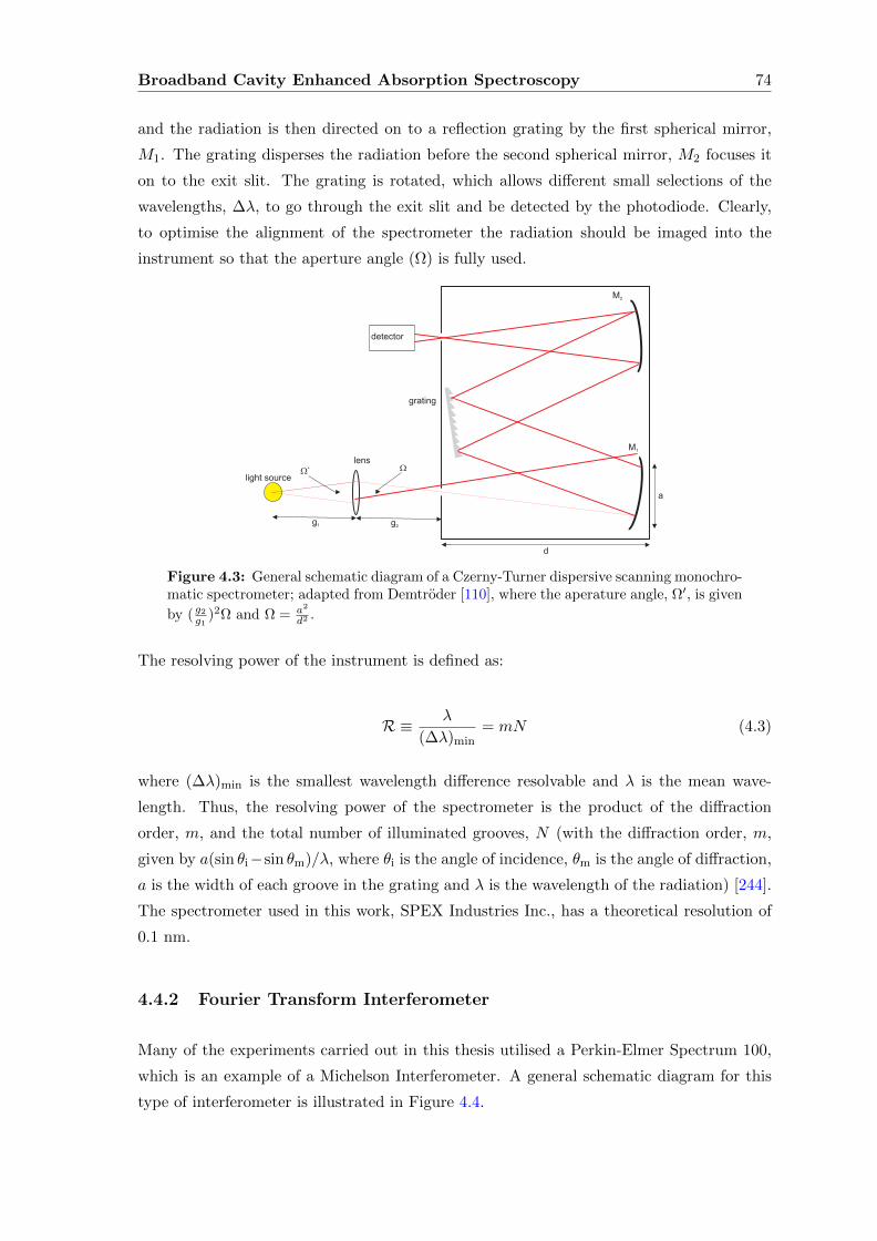
Broadband Cavity Enhanced Absorption Spectroscopy 74
and the radiation is then directed on to a reflection grating by the first spherical mirror,
M1. The grating disperses the radiation before the second spherical mirror, M2 focuses it
on to the exit slit. The grating is rotated, which allows different small selections of the
wavelengths, ∆λ, to go through the exit slit and be detected by the photodiode. Clearly,
to optimise the alignment of the spectrometer the radiation should be imaged into the
instrument so that the aperture angle (Ω) is fully used.
Figure 4.3: General schematic diagram of a Czerny-Turner dispersive scanning monochro-matic spectrometer; adapted from Demtroder [110], where the aperature angle, Ω′, is given
by ( g2g1 )2Ω and Ω = a2
d2 .
The resolving power of the instrument is defined as:
R ≡ λ
(∆λ)min= mN (4.3)
where (∆λ)min is the smallest wavelength difference resolvable and λ is the mean wave-
length. Thus, the resolving power of the spectrometer is the product of the diffraction
order, m, and the total number of illuminated grooves, N (with the diffraction order, m,
given by a(sin θi−sin θm)/λ, where θi is the angle of incidence, θm is the angle of diffraction,
a is the width of each groove in the grating and λ is the wavelength of the radiation) [244].
The spectrometer used in this work, SPEX Industries Inc., has a theoretical resolution of
0.1 nm.
4.4.2 Fourier Transform Interferometer
Many of the experiments carried out in this thesis utilised a Perkin-Elmer Spectrum 100,
which is an example of a Michelson Interferometer. A general schematic diagram for this
type of interferometer is illustrated in Figure 4.4.
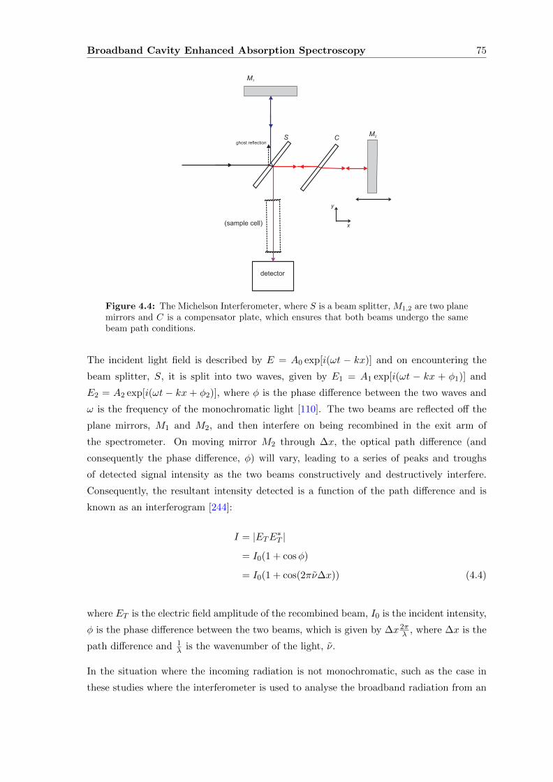
Broadband Cavity Enhanced Absorption Spectroscopy 75
Figure 4.4: The Michelson Interferometer, where S is a beam splitter, M1,2 are two planemirrors and C is a compensator plate, which ensures that both beams undergo the samebeam path conditions.
The incident light field is described by E = A0 exp[i(ωt − kx)] and on encountering the
beam splitter, S, it is split into two waves, given by E1 = A1 exp[i(ωt − kx + φ1)] and
E2 = A2 exp[i(ωt − kx + φ2)], where φ is the phase difference between the two waves and
ω is the frequency of the monochromatic light [110]. The two beams are reflected off the
plane mirrors, M1 and M2, and then interfere on being recombined in the exit arm of
the spectrometer. On moving mirror M2 through ∆x, the optical path difference (and
consequently the phase difference, φ) will vary, leading to a series of peaks and troughs
of detected signal intensity as the two beams constructively and destructively interfere.
Consequently, the resultant intensity detected is a function of the path difference and is
known as an interferogram [244]:
I = |ETE∗T |
= I0(1 + cosφ)
= I0(1 + cos(2πν∆x)) (4.4)
where ET is the electric field amplitude of the recombined beam, I0 is the incident intensity,
φ is the phase difference between the two beams, which is given by ∆x2πλ , where ∆x is the
path difference and 1λ is the wavenumber of the light, ν.
In the situation where the incoming radiation is not monochromatic, such as the case in
these studies where the interferometer is used to analyse the broadband radiation from an
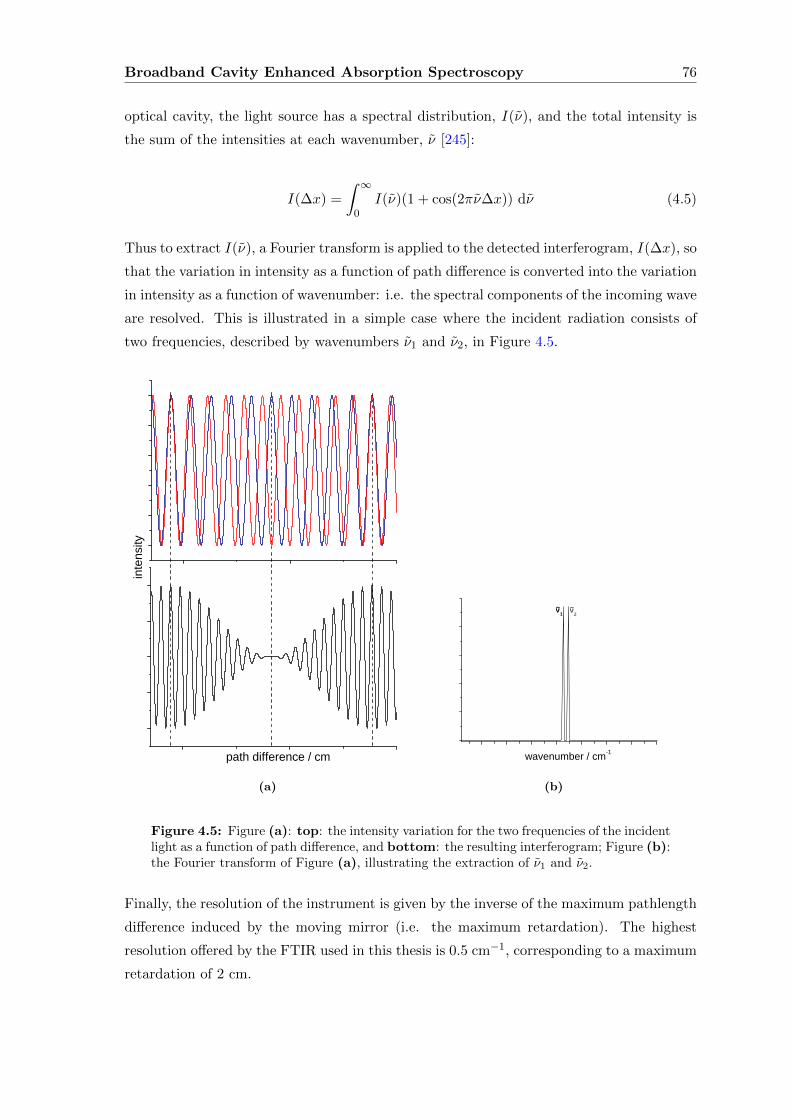
Broadband Cavity Enhanced Absorption Spectroscopy 76
optical cavity, the light source has a spectral distribution, I(ν), and the total intensity is
the sum of the intensities at each wavenumber, ν [245]:
I(∆x) =
∫ ∞0
I(ν)(1 + cos(2πν∆x)) dν (4.5)
Thus to extract I(ν), a Fourier transform is applied to the detected interferogram, I(∆x), so
that the variation in intensity as a function of path difference is converted into the variation
in intensity as a function of wavenumber: i.e. the spectral components of the incoming wave
are resolved. This is illustrated in a simple case where the incident radiation consists of
two frequencies, described by wavenumbers ν1 and ν2, in Figure 4.5.
inten
sity
p a t h d i f f e r e n c e / c m(a)
ν1
w a v e n u m b e r / c m - 1
~ν1
~ ν2
~
(b)
Figure 4.5: Figure (a): top: the intensity variation for the two frequencies of the incidentlight as a function of path difference, and bottom: the resulting interferogram; Figure (b):the Fourier transform of Figure (a), illustrating the extraction of ν1 and ν2.
Finally, the resolution of the instrument is given by the inverse of the maximum pathlength
difference induced by the moving mirror (i.e. the maximum retardation). The highest
resolution offered by the FTIR used in this thesis is 0.5 cm−1, corresponding to a maximum
retardation of 2 cm.
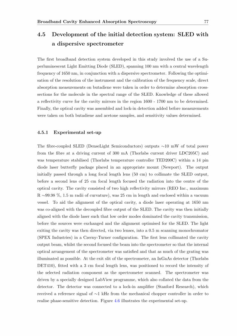
Broadband Cavity Enhanced Absorption Spectroscopy 77
4.5 Development of the initial detection system: SLED with
a dispersive spectrometer
The first broadband detection system developed in this study involved the use of a Su-
perluminescent Light Emitting Diode (SLED), spanning 100 nm with a central wavelength
frequency of 1650 nm, in conjunction with a dispersive spectrometer. Following the optimi-
sation of the resolution of the instrument and the calibration of the frequency scale, direct
absorption measurements on butadiene were taken in order to determine absorption cross-
sections for the molecule in the spectral range of the SLED. Knowledge of these allowed
a reflectivity curve for the cavity mirrors in the region 1600 - 1700 nm to be determined.
Finally, the optical cavity was assembled and lock-in detection added before measurements
were taken on both butadiene and acetone samples, and sensitivity values determined.
4.5.1 Experimental set-up
The fibre-coupled SLED (DenseLight Semiconductors) outputs ∼10 mW of total power
from the fibre at a driving current of 300 mA (Thorlabs current driver LDC205C) and
was temperature stabilised (Thorlabs temperature controller TED200C) within a 14 pin
diode laser butterfly package placed in an appropriate mount (Newport). The output
initially passed through a long focal length lens (50 cm) to collimate the SLED output,
before a second lens of 25 cm focal length focused the radiation into the centre of the
optical cavity. The cavity consisted of two high reflectivity mirrors (REO Inc., maximum
R ∼99.98 %, 1.5 m radii of curvature), was 25 cm in length and enclosed within a vacuum
vessel. To aid the alignment of the optical cavity, a diode laser operating at 1650 nm
was co-aligned with the decoupled fibre output of the SLED. The cavity was then initially
aligned with the diode laser such that low order modes dominated the cavity transmission,
before the sources were exchanged and the alignment optimised for the SLED. The light
exiting the cavity was then directed, via two lenses, into a 0.5 m scanning monochromator
(SPEX Industries) in a Czerny-Turner configuration. The first lens collimated the cavity
output beam, whilst the second focused the beam into the spectrometer so that the internal
optical arrangement of the spectrometer was satisfied and that as much of the grating was
illuminated as possible. At the exit slit of the spectrometer, an InGaAs detector (Thorlabs
DET410), fitted with a 3 cm focal length lens, was positioned to record the intensity of
the selected radiation component as the spectrometer scanned. The spectrometer was
driven by a specially designed LabView programme, which also collated the data from the
detector. The detector was connected to a lock-in amplifier (Stanford Research), which
received a reference signal of ∼1 kHz from the mechanical chopper controller in order to
realise phase-sensitive detection. Figure 4.6 illustrates the experimental set-up.
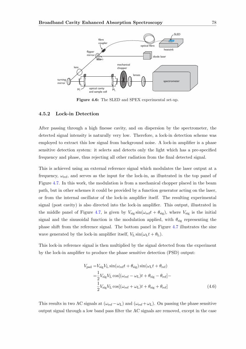
Broadband Cavity Enhanced Absorption Spectroscopy 78
optical cavity
and sample cell
mechanical
chopper
M1 M2
lenses
lens
turning
mirror
optical fibre
SLED
heatsink
spectrometer
fibre
coupler
flipper
mirrordiode laser
Figure 4.6: The SLED and SPEX experimental set-up.
4.5.2 Lock-in Detection
After passing through a high finesse cavity, and on dispersion by the spectrometer, the
detected signal intensity is naturally very low. Therefore, a lock-in detection scheme was
employed to extract this low signal from background noise. A lock-in amplifier is a phase
sensitive detection system: it selects and detects only the light which has a pre-specified
frequency and phase, thus rejecting all other radiation from the final detected signal.
This is achieved using an external reference signal which modulates the laser output at a
frequency, ωref, and serves as the input for the lock-in, as illustrated in the top panel of
Figure 4.7. In this work, the modulation is from a mechanical chopper placed in the beam
path, but in other schemes it could be provided by a function generator acting on the laser,
or from the internal oscillator of the lock-in amplifier itself. The resulting experimental
signal (post cavity) is also directed into the lock-in amplifier. This output, illustrated in
the middle panel of Figure 4.7, is given by Vsig sin(ωreft + θsig), where Vsig is the initial
signal and the sinusoidal function is the modulation applied, with θsig representing the
phase shift from the reference signal. The bottom panel in Figure 4.7 illustrates the sine
wave generated by the lock-in amplifier itself, VL sin(ωLt+ θL).
This lock-in reference signal is then multiplied by the signal detected from the experiment
by the lock-in amplifier to produce the phase sensitive detection (PSD) output:
Vpsd =VsigVL sin(ωreft+ θsig) sin(ωLt+ θref)
=1
2VsigVL cos[(ωref − ωL)t+ θsig − θref]−
1
2VsigVL cos[(ωref + ωL)t+ θsig + θref] (4.6)
This results in two AC signals at (ωref−ωL) and (ωref +ωL). On passing the phase sensitive
output signal through a low band pass filter the AC signals are removed, except in the case
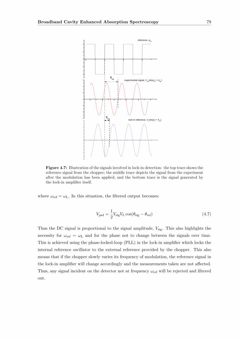
Broadband Cavity Enhanced Absorption Spectroscopy 79
e x p e r i m e n t a l s i g n a l , V s i g s i n ( ωr e f t + θs i g )
l o c k - i n r e f e r e n c e , V L s i n ( ωL t + θr e f )
r e f e r e n c e , ωr e f
θs i g
θr e f
Figure 4.7: Illustration of the signals involved in lock-in detection: the top trace shows thereference signal from the chopper; the middle trace depicts the signal from the experimentafter the modulation has been applied; and the bottom trace is the signal generated bythe lock-in amplifier itself.
where ωref = ωL. In this situation, the filtered output becomes:
Vpsd =1
2VsigVL cos(θsig − θref) (4.7)
Thus the DC signal is proportional to the signal amplitude, Vsig. This also highlights the
necessity for ωref = ωL and for the phase not to change between the signals over time.
This is achieved using the phase-locked-loop (PLL) in the lock-in amplifier which locks the
internal reference oscillator to the external reference provided by the chopper. This also
means that if the chopper slowly varies its frequency of modulation, the reference signal in
the lock-in amplifier will change accordingly and the measurements taken are not affected.
Thus, any signal incident on the detector not at frequency ωref will be rejected and filtered
out.
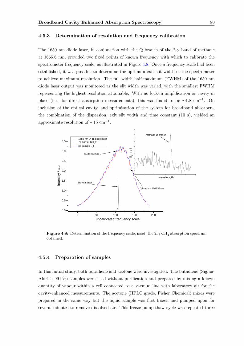
Broadband Cavity Enhanced Absorption Spectroscopy 80
4.5.3 Determination of resolution and frequency calibration
The 1650 nm diode laser, in conjunction with the Q branch of the 2ν3 band of methane
at 1665.6 nm, provided two fixed points of known frequency with which to calibrate the
spectrometer frequency scale, as illustrated in Figure 4.8. Once a frequency scale had been
established, it was possible to determine the optimum exit slit width of the spectrometer
to achieve maximum resolution. The full width half maximum (FWHM) of the 1650 nm
diode laser output was monitored as the slit width was varied, with the smallest FWHM
representing the highest resolution attainable. With no lock-in amplification or cavity in
place (i.e. for direct absorption measurements), this was found to be ∼1.8 cm−1. On
inclusion of the optical cavity, and optimisation of the system for broadband absorbers,
the combination of the dispersion, exit slit width and time constant (10 s), yielded an
approximate resolution of ∼15 cm−1.
0 5 0 1 0 0 1 5 0 2 0 00 . 0
0 . 5
1 . 0
1 . 5
2 . 0
2 . 5
3 . 0
3 . 5
inten
sity / a
.u
u n c a l i b r a t e d f r e q u e n c y s c a l e
1 6 5 0 n m D F B d i o d e l a s e r 7 6 T o r r o f C H 4 ( I ) n o s a m p l e ( I 0 )
Q b r a n c h a t 1 6 6 5 . 5 9 n m
S L E D s t r u c t u r e
1 6 5 0 n m l a s e rw a v e l e n g t h
[I 0- I] / I
M e t h a n e Q b r a n c h
Figure 4.8: Determination of the frequency scale; inset, the 2ν3 CH4 absorption spectrumobtained.
4.5.4 Preparation of samples
In this initial study, both butadiene and acetone were investigated. The butadiene (Sigma-
Aldrich 99+%) samples were used without purification and prepared by mixing a known
quantity of vapour within a cell connected to a vacuum line with laboratory air for the
cavity-enhanced measurements. The acetone (HPLC grade, Fisher Chemical) mixes were
prepared in the same way but the liquid sample was first frozen and pumped upon for
several minutes to remove dissolved air. This freeze-pump-thaw cycle was repeated three
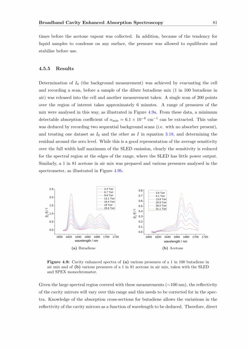
Broadband Cavity Enhanced Absorption Spectroscopy 81
times before the acetone vapour was collected. In addition, because of the tendency for
liquid samples to condense on any surface, the pressure was allowed to equilibrate and
stabilise before use.
4.5.5 Results
Determination of I0 (the background measurement) was achieved by evacuating the cell
and recording a scan, before a sample of the dilute butadiene mix (1 in 100 butadiene in
air) was released into the cell and another measurement taken. A single scan of 200 points
over the region of interest takes approximately 6 minutes. A range of pressures of the
mix were analysed in this way, as illustrated in Figure 4.9a. From these data, a minimum
detectable absorption coefficient of αmin = 6.1 × 10⁻⁸ cm−1 can be extracted. This value
was deduced by recording two sequential background scans (i.e. with no absorber present),
and treating one dataset as I0 and the other as I in equation 3.18, and determining the
residual around the zero level. While this is a good representation of the average sensitivity
over the full width half maximum of the SLED emission, clearly the sensitivity is reduced
for the spectral region at the edges of the range, where the SLED has little power output.
Similarly, a 1 in 81 acetone in air mix was prepared and various pressures analysed in the
spectrometer, as illustrated in Figure 4.9b.
1 6 0 0 1 6 2 0 1 6 4 0 1 6 6 0 1 6 8 0 1 7 0 0 1 7 2 00 . 0
0 . 5
1 . 0
1 . 5
2 . 0
2 . 5
[I 0-I] / I
3 . 4 T o r r 6 . 7 T o r r 9 . 9 T o r r 1 3 . 1 T o r r 1 6 . 4 T o r r 1 9 T o r r 2 3 . 6 T o r r
w a v e l e n g t h / n m(a) Butadiene
1 6 0 0 1 6 2 0 1 6 4 0 1 6 6 0 1 6 8 0 1 7 0 0 1 7 2 00 . 00 . 10 . 20 . 30 . 40 . 50 . 60 . 70 . 8 3 . 6 T o r r
9 . 1 T o r r 1 3 . 8 T o r r 2 0 . 9 T o r r 2 6 . 0 T o r r 3 1 . 1 T o r r
[I 0-I] / I
w a v e l e n g t h / n m(b) Acetone
Figure 4.9: Cavity enhanced spectra of (a) various pressures of a 1 in 100 butadiene inair mix and of (b) various pressures of a 1 in 81 acetone in air mix, taken with the SLEDand SPEX monochromator.
Given the large spectral region covered with these measurements (∼100 nm), the reflectivity
of the cavity mirrors will vary over this range and this needs to be corrected for in the spec-
tra. Knowledge of the absorption cross-sections for butadiene allows the variations in the
reflectivity of the cavity mirrors as a function of wavelength to be deduced. Therefore, direct
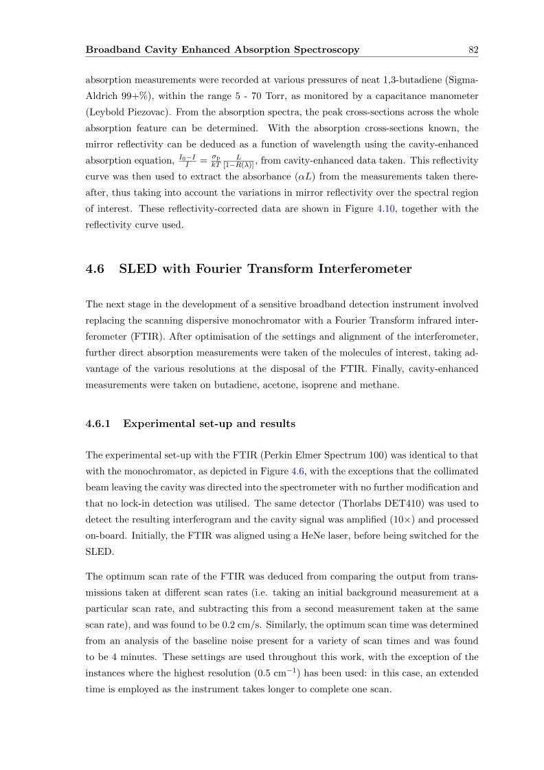
Broadband Cavity Enhanced Absorption Spectroscopy 82
absorption measurements were recorded at various pressures of neat 1,3-butadiene (Sigma-
Aldrich 99+%), within the range 5 - 70 Torr, as monitored by a capacitance manometer
(Leybold Piezovac). From the absorption spectra, the peak cross-sections across the whole
absorption feature can be determined. With the absorption cross-sections known, the
mirror reflectivity can be deduced as a function of wavelength using the cavity-enhanced
absorption equation, I0−II =σpkT
L[1−R(λ)] , from cavity-enhanced data taken. This reflectivity
curve was then used to extract the absorbance (αL) from the measurements taken there-
after, thus taking into account the variations in mirror reflectivity over the spectral region
of interest. These reflectivity-corrected data are shown in Figure 4.10, together with the
reflectivity curve used.
4.6 SLED with Fourier Transform Interferometer
The next stage in the development of a sensitive broadband detection instrument involved
replacing the scanning dispersive monochromator with a Fourier Transform infrared inter-
ferometer (FTIR). After optimisation of the settings and alignment of the interferometer,
further direct absorption measurements were taken of the molecules of interest, taking ad-
vantage of the various resolutions at the disposal of the FTIR. Finally, cavity-enhanced
measurements were taken on butadiene, acetone, isoprene and methane.
4.6.1 Experimental set-up and results
The experimental set-up with the FTIR (Perkin Elmer Spectrum 100) was identical to that
with the monochromator, as depicted in Figure 4.6, with the exceptions that the collimated
beam leaving the cavity was directed into the spectrometer with no further modification and
that no lock-in detection was utilised. The same detector (Thorlabs DET410) was used to
detect the resulting interferogram and the cavity signal was amplified (10×) and processed
on-board. Initially, the FTIR was aligned using a HeNe laser, before being switched for the
SLED.
The optimum scan rate of the FTIR was deduced from comparing the output from trans-
missions taken at different scan rates (i.e. taking an initial background measurement at a
particular scan rate, and subtracting this from a second measurement taken at the same
scan rate), and was found to be 0.2 cm/s. Similarly, the optimum scan time was determined
from an analysis of the baseline noise present for a variety of scan times and was found
to be 4 minutes. These settings are used throughout this work, with the exception of the
instances where the highest resolution (0.5 cm−1) has been used: in this case, an extended
time is employed as the instrument takes longer to complete one scan.
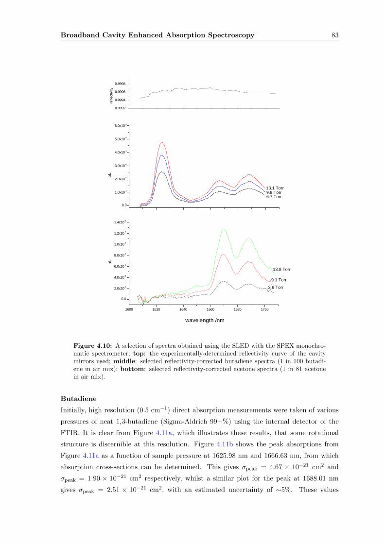
Broadband Cavity Enhanced Absorption Spectroscopy 83
0 . 0
1 . 0 x 1 0 - 4
2 . 0 x 1 0 - 4
3 . 0 x 1 0 - 4
4 . 0 x 1 0 - 4
5 . 0 x 1 0 - 4
6 . 0 x 1 0 - 4
1 3 . 1 T o r r6 . 7 T o r r9 . 9 T o r r
0 . 9 9 9 20 . 9 9 9 40 . 9 9 9 60 . 9 9 9 8
reflec
tivity
1 6 0 0 1 6 2 0 1 6 4 0 1 6 6 0 1 6 8 0 1 7 0 0
0 . 0
2 . 0 x 1 0 - 5
4 . 0 x 1 0 - 5
6 . 0 x 1 0 - 5
8 . 0 x 1 0 - 5
1 . 0 x 1 0 - 4
1 . 2 x 1 0 - 4
1 . 4 x 1 0 - 4
αLαL
1 3 . 8 T o r r9 . 1 T o r r
3 . 6 T o r r
w a v e l e n g t h / n m
Figure 4.10: A selection of spectra obtained using the SLED with the SPEX monochro-matic spectrometer; top: the experimentally-determined reflectivity curve of the cavitymirrors used; middle: selected reflectivity-corrected butadiene spectra (1 in 100 butadi-ene in air mix); bottom: selected reflectivity-corrected acetone spectra (1 in 81 acetonein air mix).
Butadiene
Initially, high resolution (0.5 cm−1) direct absorption measurements were taken of various
pressures of neat 1,3-butadiene (Sigma-Aldrich 99+%) using the internal detector of the
FTIR. It is clear from Figure 4.11a, which illustrates these results, that some rotational
structure is discernible at this resolution. Figure 4.11b shows the peak absorptions from
Figure 4.11a as a function of sample pressure at 1625.98 nm and 1666.63 nm, from which
absorption cross-sections can be determined. This gives σpeak = 4.67 × 10⁻²¹ cm2 and
σpeak = 1.90 × 10⁻²¹ cm2 respectively, whilst a similar plot for the peak at 1688.01 nm
gives σpeak = 2.51 × 10⁻²¹ cm2, with an estimated uncertainty of ∼5%. These values
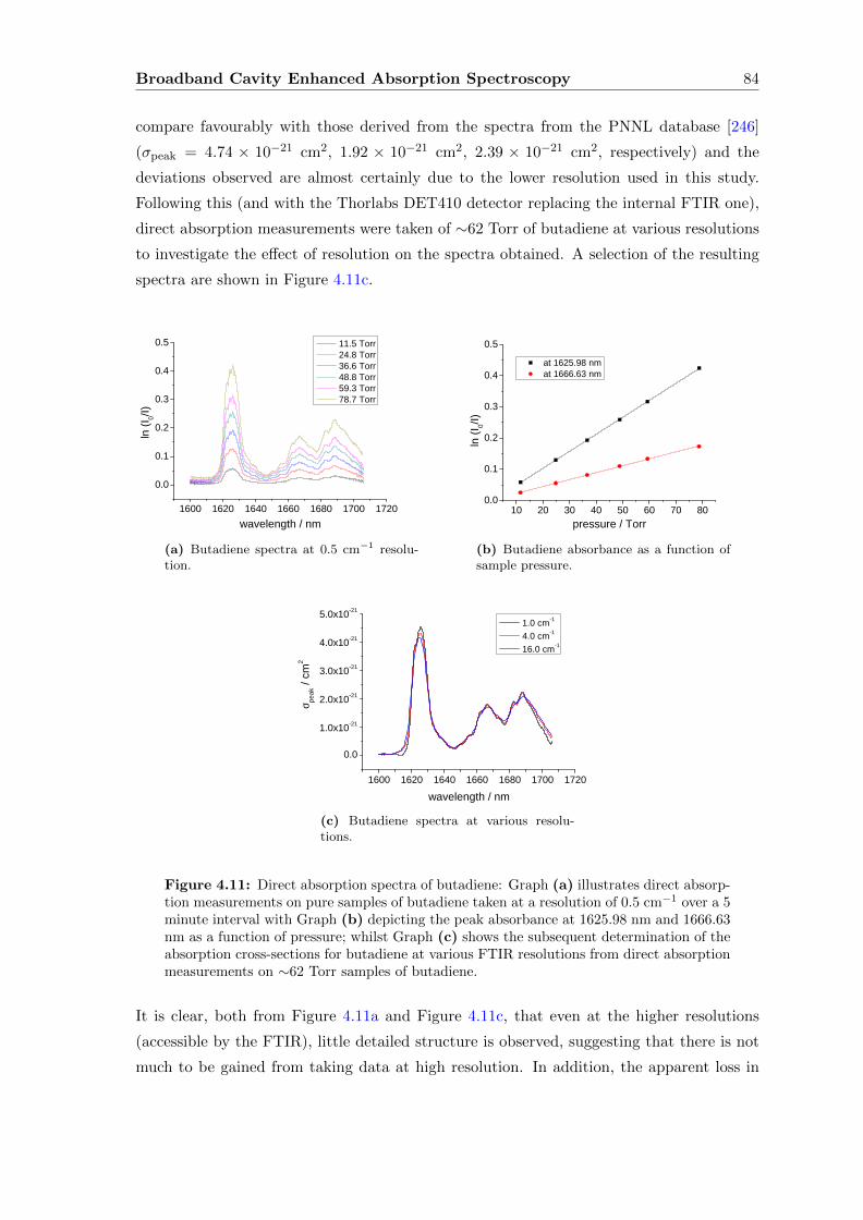
Broadband Cavity Enhanced Absorption Spectroscopy 84
compare favourably with those derived from the spectra from the PNNL database [246]
(σpeak = 4.74 × 10⁻²¹ cm2, 1.92 × 10⁻²¹ cm2, 2.39 × 10⁻²¹ cm2, respectively) and the
deviations observed are almost certainly due to the lower resolution used in this study.
Following this (and with the Thorlabs DET410 detector replacing the internal FTIR one),
direct absorption measurements were taken of ∼62 Torr of butadiene at various resolutions
to investigate the effect of resolution on the spectra obtained. A selection of the resulting
spectra are shown in Figure 4.11c.
1 6 0 0 1 6 2 0 1 6 4 0 1 6 6 0 1 6 8 0 1 7 0 0 1 7 2 00 . 0
0 . 1
0 . 2
0 . 3
0 . 4
0 . 5
ln (I 0/I)
w a v e l e n g t h / n m
1 1 . 5 T o r r 2 4 . 8 T o r r 3 6 . 6 T o r r 4 8 . 8 T o r r 5 9 . 3 T o r r 7 8 . 7 T o r r
(a) Butadiene spectra at 0.5 cm−1 resolu-tion.
1 0 2 0 3 0 4 0 5 0 6 0 7 0 8 00 . 0
0 . 1
0 . 2
0 . 3
0 . 4
0 . 5 a t 1 6 2 5 . 9 8 n m a t 1 6 6 6 . 6 3 n m
ln (I 0/I)
p r e s s u r e / T o r r(b) Butadiene absorbance as a function ofsample pressure.
1 6 0 0 1 6 2 0 1 6 4 0 1 6 6 0 1 6 8 0 1 7 0 0 1 7 2 0
0 . 0
1 . 0 x 1 0 - 2 1
2 . 0 x 1 0 - 2 1
3 . 0 x 1 0 - 2 1
4 . 0 x 1 0 - 2 1
5 . 0 x 1 0 - 2 1
σ peak
/ cm2
w a v e l e n g t h / n m
1 . 0 c m - 1
4 . 0 c m - 1
1 6 . 0 c m - 1
(c) Butadiene spectra at various resolu-tions.
Figure 4.11: Direct absorption spectra of butadiene: Graph (a) illustrates direct absorp-tion measurements on pure samples of butadiene taken at a resolution of 0.5 cm−1 over a 5minute interval with Graph (b) depicting the peak absorbance at 1625.98 nm and 1666.63nm as a function of pressure; whilst Graph (c) shows the subsequent determination of theabsorption cross-sections for butadiene at various FTIR resolutions from direct absorptionmeasurements on ∼62 Torr samples of butadiene.
It is clear, both from Figure 4.11a and Figure 4.11c, that even at the higher resolutions
(accessible by the FTIR), little detailed structure is observed, suggesting that there is not
much to be gained from taking data at high resolution. In addition, the apparent loss in
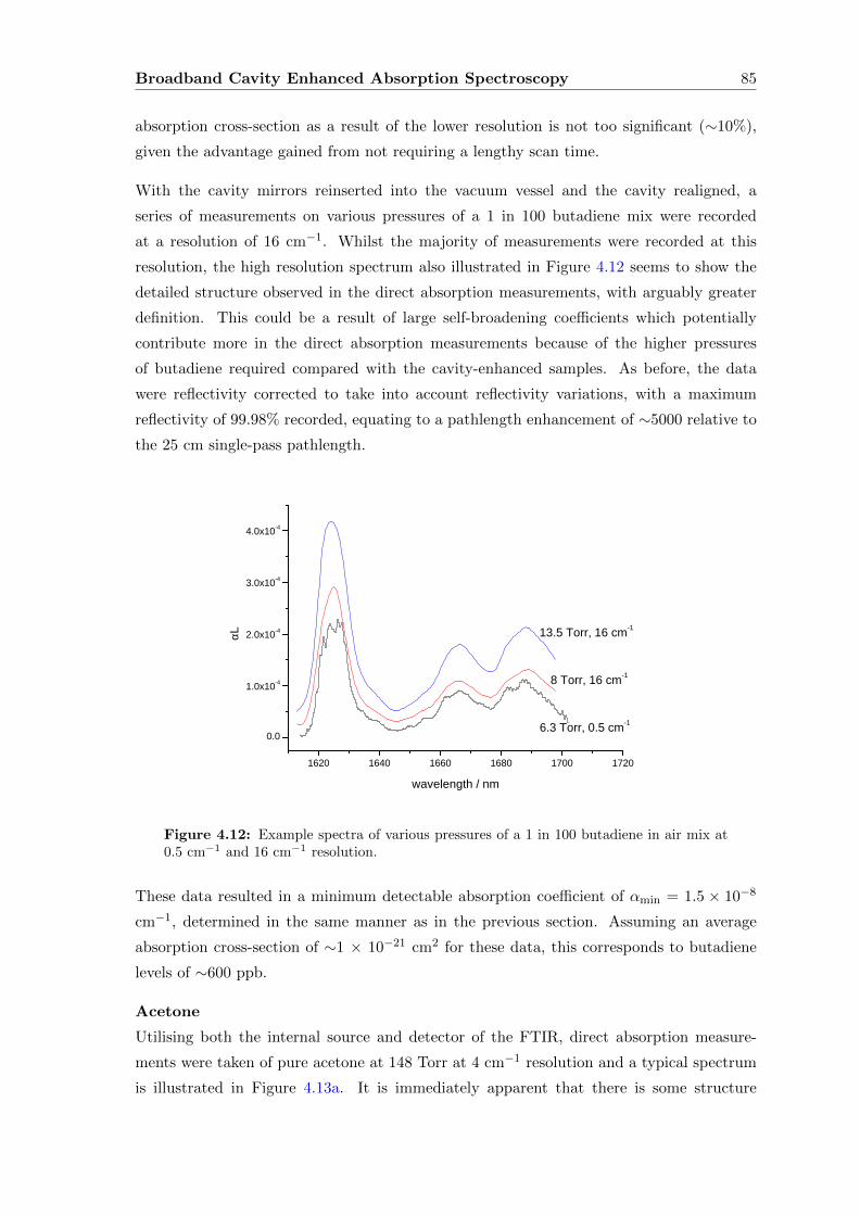
Broadband Cavity Enhanced Absorption Spectroscopy 85
absorption cross-section as a result of the lower resolution is not too significant (∼10%),
given the advantage gained from not requiring a lengthy scan time.
With the cavity mirrors reinserted into the vacuum vessel and the cavity realigned, a
series of measurements on various pressures of a 1 in 100 butadiene mix were recorded
at a resolution of 16 cm−1. Whilst the majority of measurements were recorded at this
resolution, the high resolution spectrum also illustrated in Figure 4.12 seems to show the
detailed structure observed in the direct absorption measurements, with arguably greater
definition. This could be a result of large self-broadening coefficients which potentially
contribute more in the direct absorption measurements because of the higher pressures
of butadiene required compared with the cavity-enhanced samples. As before, the data
were reflectivity corrected to take into account reflectivity variations, with a maximum
reflectivity of 99.98% recorded, equating to a pathlength enhancement of ∼5000 relative to
the 25 cm single-pass pathlength.
1 6 2 0 1 6 4 0 1 6 6 0 1 6 8 0 1 7 0 0 1 7 2 0
0 . 0
1 . 0 x 1 0 - 4
2 . 0 x 1 0 - 4
3 . 0 x 1 0 - 4
4 . 0 x 1 0 - 4
αL
w a v e l e n g t h / n m
1 3 . 5 T o r r , 1 6 c m - 1
8 T o r r , 1 6 c m - 1
6 . 3 T o r r , 0 . 5 c m - 1
Figure 4.12: Example spectra of various pressures of a 1 in 100 butadiene in air mix at0.5 cm−1 and 16 cm−1 resolution.
These data resulted in a minimum detectable absorption coefficient of αmin = 1.5 × 10⁻⁸
cm−1, determined in the same manner as in the previous section. Assuming an average
absorption cross-section of ∼1 × 10⁻²¹ cm2 for these data, this corresponds to butadiene
levels of ∼600 ppb.
Acetone
Utilising both the internal source and detector of the FTIR, direct absorption measure-
ments were taken of pure acetone at 148 Torr at 4 cm−1 resolution and a typical spectrum
is illustrated in Figure 4.13a. It is immediately apparent that there is some structure
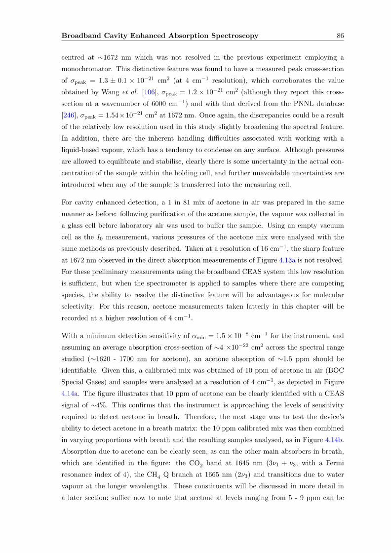
Broadband Cavity Enhanced Absorption Spectroscopy 86
centred at ∼1672 nm which was not resolved in the previous experiment employing a
monochromator. This distinctive feature was found to have a measured peak cross-section
of σpeak = 1.3 ± 0.1 × 10⁻²¹ cm2 (at 4 cm−1 resolution), which corroborates the value
obtained by Wang et al. [106], σpeak = 1.2 × 10⁻²¹ cm2 (although they report this cross-
section at a wavenumber of 6000 cm−1) and with that derived from the PNNL database
[246], σpeak = 1.54×10⁻²¹ cm2 at 1672 nm. Once again, the discrepancies could be a result
of the relatively low resolution used in this study slightly broadening the spectral feature.
In addition, there are the inherent handling difficulties associated with working with a
liquid-based vapour, which has a tendency to condense on any surface. Although pressures
are allowed to equilibrate and stabilise, clearly there is some uncertainty in the actual con-
centration of the sample within the holding cell, and further unavoidable uncertainties are
introduced when any of the sample is transferred into the measuring cell.
For cavity enhanced detection, a 1 in 81 mix of acetone in air was prepared in the same
manner as before: following purification of the acetone sample, the vapour was collected in
a glass cell before laboratory air was used to buffer the sample. Using an empty vacuum
cell as the I0 measurement, various pressures of the acetone mix were analysed with the
same methods as previously described. Taken at a resolution of 16 cm−1, the sharp feature
at 1672 nm observed in the direct absorption measurements of Figure 4.13a is not resolved.
For these preliminary measurements using the broadband CEAS system this low resolution
is sufficient, but when the spectrometer is applied to samples where there are competing
species, the ability to resolve the distinctive feature will be advantageous for molecular
selectivity. For this reason, acetone measurements taken latterly in this chapter will be
recorded at a higher resolution of 4 cm−1.
With a minimum detection sensitivity of αmin = 1.5× 10⁻⁸ cm−1 for the instrument, and
assuming an average absorption cross-section of ∼4 ×10⁻²² cm2 across the spectral range
studied (∼1620 - 1700 nm for acetone), an acetone absorption of ∼1.5 ppm should be
identifiable. Given this, a calibrated mix was obtained of 10 ppm of acetone in air (BOC
Special Gases) and samples were analysed at a resolution of 4 cm−1, as depicted in Figure
4.14a. The figure illustrates that 10 ppm of acetone can be clearly identified with a CEAS
signal of ∼4%. This confirms that the instrument is approaching the levels of sensitivity
required to detect acetone in breath. Therefore, the next stage was to test the device’s
ability to detect acetone in a breath matrix: the 10 ppm calibrated mix was then combined
in varying proportions with breath and the resulting samples analysed, as in Figure 4.14b.
Absorption due to acetone can be clearly seen, as can the other main absorbers in breath,
which are identified in the figure: the CO2 band at 1645 nm (3ν1 + ν3, with a Fermi
resonance index of 4), the CH4 Q branch at 1665 nm (2ν3) and transitions due to water
vapour at the longer wavelengths. These constituents will be discussed in more detail in
a later section; suffice now to note that acetone at levels ranging from 5 - 9 ppm can be
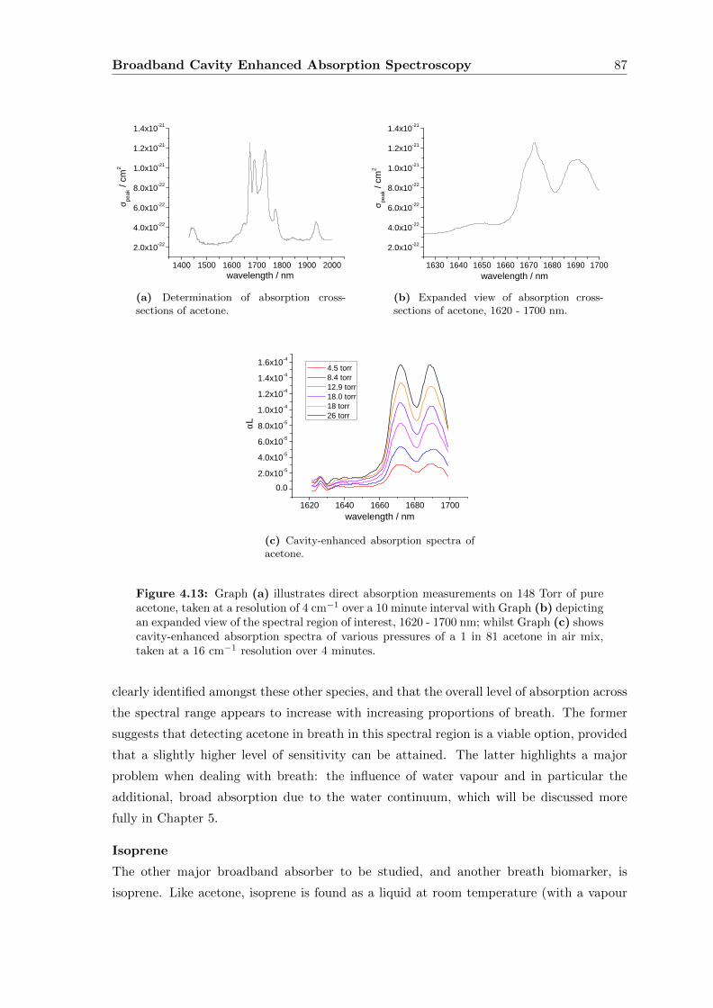
Broadband Cavity Enhanced Absorption Spectroscopy 87
1 4 0 0 1 5 0 0 1 6 0 0 1 7 0 0 1 8 0 0 1 9 0 0 2 0 0 02 . 0 x 1 0 - 2 2
4 . 0 x 1 0 - 2 2
6 . 0 x 1 0 - 2 2
8 . 0 x 1 0 - 2 2
1 . 0 x 1 0 - 2 1
1 . 2 x 1 0 - 2 1
1 . 4 x 1 0 - 2 1
w a v e l e n g t h / n m
σ peak
/ cm2
(a) Determination of absorption cross-sections of acetone.
1 6 3 0 1 6 4 0 1 6 5 0 1 6 6 0 1 6 7 0 1 6 8 0 1 6 9 0 1 7 0 02 . 0 x 1 0 - 2 2
4 . 0 x 1 0 - 2 2
6 . 0 x 1 0 - 2 2
8 . 0 x 1 0 - 2 2
1 . 0 x 1 0 - 2 1
1 . 2 x 1 0 - 2 1
1 . 4 x 1 0 - 2 1
w a v e l e n g t h / n m
σ peak
/ cm2
(b) Expanded view of absorption cross-sections of acetone, 1620 - 1700 nm.
1 6 2 0 1 6 4 0 1 6 6 0 1 6 8 0 1 7 0 00 . 0
2 . 0 x 1 0 - 54 . 0 x 1 0 - 56 . 0 x 1 0 - 58 . 0 x 1 0 - 51 . 0 x 1 0 - 41 . 2 x 1 0 - 41 . 4 x 1 0 - 41 . 6 x 1 0 - 4
4 . 5 t o r r 8 . 4 t o r r 1 2 . 9 t o r r 1 8 . 0 t o r r 1 8 t o r r 2 6 t o r r
αL
w a v e l e n g t h / n m(c) Cavity-enhanced absorption spectra ofacetone.
Figure 4.13: Graph (a) illustrates direct absorption measurements on 148 Torr of pureacetone, taken at a resolution of 4 cm−1 over a 10 minute interval with Graph (b) depictingan expanded view of the spectral region of interest, 1620 - 1700 nm; whilst Graph (c) showscavity-enhanced absorption spectra of various pressures of a 1 in 81 acetone in air mix,taken at a 16 cm−1 resolution over 4 minutes.
clearly identified amongst these other species, and that the overall level of absorption across
the spectral range appears to increase with increasing proportions of breath. The former
suggests that detecting acetone in breath in this spectral region is a viable option, provided
that a slightly higher level of sensitivity can be attained. The latter highlights a major
problem when dealing with breath: the influence of water vapour and in particular the
additional, broad absorption due to the water continuum, which will be discussed more
fully in Chapter 5.
Isoprene
The other major broadband absorber to be studied, and another breath biomarker, is
isoprene. Like acetone, isoprene is found as a liquid at room temperature (with a vapour
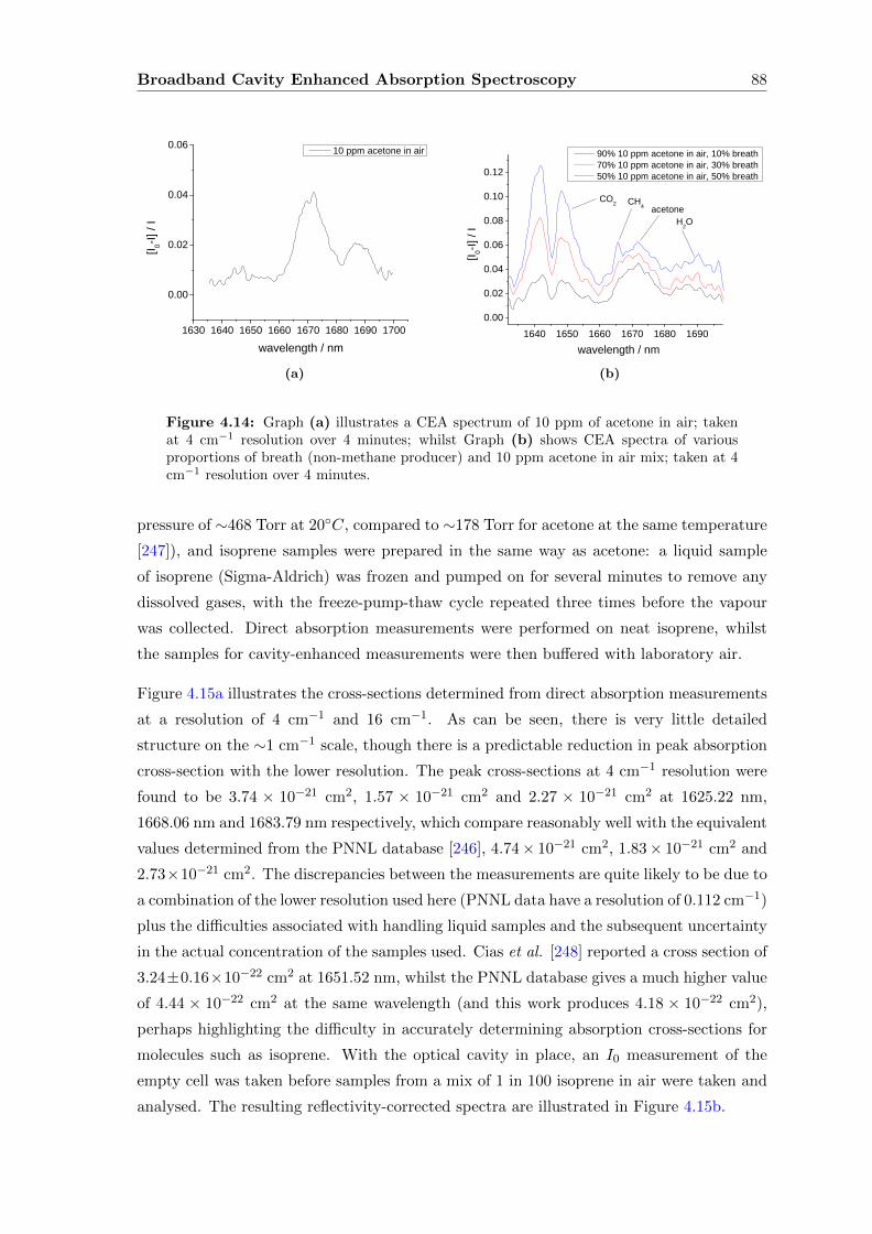
Broadband Cavity Enhanced Absorption Spectroscopy 88
1 6 3 0 1 6 4 0 1 6 5 0 1 6 6 0 1 6 7 0 1 6 8 0 1 6 9 0 1 7 0 0
0 . 0 0
0 . 0 2
0 . 0 4
0 . 0 6[I 0-I]
/ I
w a v e l e n g t h / n m
1 0 p p m a c e t o n e i n a i r
(a)
1 6 4 0 1 6 5 0 1 6 6 0 1 6 7 0 1 6 8 0 1 6 9 00 . 0 00 . 0 20 . 0 40 . 0 60 . 0 80 . 1 00 . 1 2
[I 0-I] / I
w a v e l e n g t h / n m
9 0 % 1 0 p p m a c e t o n e i n a i r , 1 0 % b r e a t h 7 0 % 1 0 p p m a c e t o n e i n a i r , 3 0 % b r e a t h 5 0 % 1 0 p p m a c e t o n e i n a i r , 5 0 % b r e a t hC O 2 C H 4 a c e t o n e
H 2 O
(b)
Figure 4.14: Graph (a) illustrates a CEA spectrum of 10 ppm of acetone in air; takenat 4 cm−1 resolution over 4 minutes; whilst Graph (b) shows CEA spectra of variousproportions of breath (non-methane producer) and 10 ppm acetone in air mix; taken at 4cm−1 resolution over 4 minutes.
pressure of ∼468 Torr at 20C, compared to ∼178 Torr for acetone at the same temperature
[247]), and isoprene samples were prepared in the same way as acetone: a liquid sample
of isoprene (Sigma-Aldrich) was frozen and pumped on for several minutes to remove any
dissolved gases, with the freeze-pump-thaw cycle repeated three times before the vapour
was collected. Direct absorption measurements were performed on neat isoprene, whilst
the samples for cavity-enhanced measurements were then buffered with laboratory air.
Figure 4.15a illustrates the cross-sections determined from direct absorption measurements
at a resolution of 4 cm−1 and 16 cm−1. As can be seen, there is very little detailed
structure on the ∼1 cm−1 scale, though there is a predictable reduction in peak absorption
cross-section with the lower resolution. The peak cross-sections at 4 cm−1 resolution were
found to be 3.74 × 10⁻²¹ cm2, 1.57 × 10⁻²¹ cm2 and 2.27 × 10⁻²¹ cm2 at 1625.22 nm,
1668.06 nm and 1683.79 nm respectively, which compare reasonably well with the equivalent
values determined from the PNNL database [246], 4.74× 10⁻²¹ cm2, 1.83× 10⁻²¹ cm2 and
2.73×10⁻²¹ cm2. The discrepancies between the measurements are quite likely to be due to
a combination of the lower resolution used here (PNNL data have a resolution of 0.112 cm−1)
plus the difficulties associated with handling liquid samples and the subsequent uncertainty
in the actual concentration of the samples used. Cias et al. [248] reported a cross section of
3.24±0.16×10⁻²² cm2 at 1651.52 nm, whilst the PNNL database gives a much higher value
of 4.44 × 10⁻²² cm2 at the same wavelength (and this work produces 4.18 × 10⁻²² cm2),
perhaps highlighting the difficulty in accurately determining absorption cross-sections for
molecules such as isoprene. With the optical cavity in place, an I0 measurement of the
empty cell was taken before samples from a mix of 1 in 100 isoprene in air were taken and
analysed. The resulting reflectivity-corrected spectra are illustrated in Figure 4.15b.
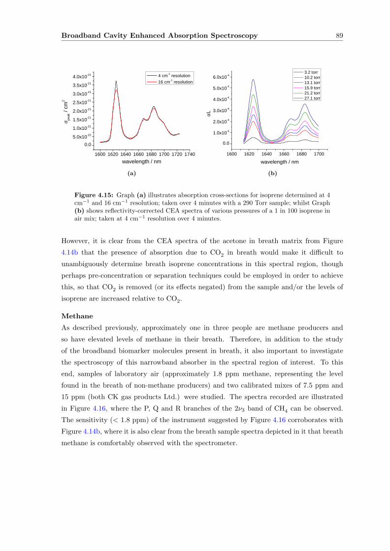
Broadband Cavity Enhanced Absorption Spectroscopy 89
1 6 0 0 1 6 2 0 1 6 4 0 1 6 6 0 1 6 8 0 1 7 0 0 1 7 2 0 1 7 4 00 . 0
5 . 0 x 1 0 - 2 21 . 0 x 1 0 - 2 11 . 5 x 1 0 - 2 12 . 0 x 1 0 - 2 12 . 5 x 1 0 - 2 13 . 0 x 1 0 - 2 13 . 5 x 1 0 - 2 14 . 0 x 1 0 - 2 1
σ peak
/ cm2
w a v e l e n g t h / n m
4 c m - 1 r e s o l u t i o n 1 6 c m - 1 r e s o l u t i o n
(a)
1 6 0 0 1 6 2 0 1 6 4 0 1 6 6 0 1 6 8 0 1 7 0 00 . 0
1 . 0 x 1 0 - 4
2 . 0 x 1 0 - 4
3 . 0 x 1 0 - 4
4 . 0 x 1 0 - 4
5 . 0 x 1 0 - 4
6 . 0 x 1 0 - 4 3 . 2 t o r r 1 0 . 2 t o r r 1 3 . 1 t o r r 1 5 . 9 t o r r 2 1 . 2 t o r r 2 7 . 1 t o r r
αL
w a v e l e n g t h / n m(b)
Figure 4.15: Graph (a) illustrates absorption cross-sections for isoprene determined at 4cm−1 and 16 cm−1 resolution; taken over 4 minutes with a 290 Torr sample; whilst Graph(b) shows reflectivity-corrected CEA spectra of various pressures of a 1 in 100 isoprene inair mix; taken at 4 cm−1 resolution over 4 minutes.
However, it is clear from the CEA spectra of the acetone in breath matrix from Figure
4.14b that the presence of absorption due to CO2 in breath would make it difficult to
unambiguously determine breath isoprene concentrations in this spectral region, though
perhaps pre-concentration or separation techniques could be employed in order to achieve
this, so that CO2 is removed (or its effects negated) from the sample and/or the levels of
isoprene are increased relative to CO2.
Methane
As described previously, approximately one in three people are methane producers and
so have elevated levels of methane in their breath. Therefore, in addition to the study
of the broadband biomarker molecules present in breath, it also important to investigate
the spectroscopy of this narrowband absorber in the spectral region of interest. To this
end, samples of laboratory air (approximately 1.8 ppm methane, representing the level
found in the breath of non-methane producers) and two calibrated mixes of 7.5 ppm and
15 ppm (both CK gas products Ltd.) were studied. The spectra recorded are illustrated
in Figure 4.16, where the P, Q and R branches of the 2ν3 band of CH4 can be observed.
The sensitivity (< 1.8 ppm) of the instrument suggested by Figure 4.16 corroborates with
Figure 4.14b, where it is also clear from the breath sample spectra depicted in it that breath
methane is comfortably observed with the spectrometer.
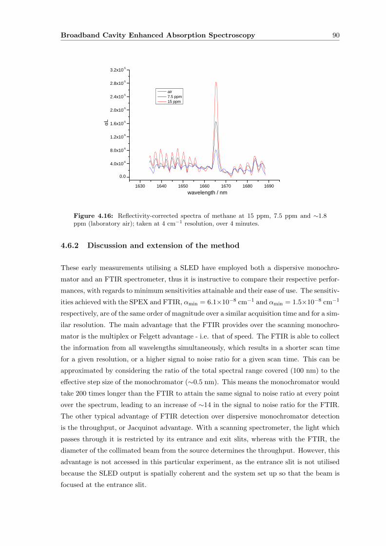
Broadband Cavity Enhanced Absorption Spectroscopy 90
1 6 3 0 1 6 4 0 1 6 5 0 1 6 6 0 1 6 7 0 1 6 8 0 1 6 9 00 . 0
4 . 0 x 1 0 - 6
8 . 0 x 1 0 - 6
1 . 2 x 1 0 - 5
1 . 6 x 1 0 - 5
2 . 0 x 1 0 - 5
2 . 4 x 1 0 - 5
2 . 8 x 1 0 - 5
3 . 2 x 1 0 - 5
w a v e l e n g t h / n m
αL a i r 7 . 5 p p m 1 5 p p m
Figure 4.16: Reflectivity-corrected spectra of methane at 15 ppm, 7.5 ppm and ∼1.8ppm (laboratory air); taken at 4 cm−1 resolution, over 4 minutes.
4.6.2 Discussion and extension of the method
These early measurements utilising a SLED have employed both a dispersive monochro-
mator and an FTIR spectrometer, thus it is instructive to compare their respective perfor-
mances, with regards to minimum sensitivities attainable and their ease of use. The sensitiv-
ities achieved with the SPEX and FTIR, αmin = 6.1×10⁻⁸ cm−1 and αmin = 1.5×10⁻⁸ cm−1
respectively, are of the same order of magnitude over a similar acquisition time and for a sim-
ilar resolution. The main advantage that the FTIR provides over the scanning monochro-
mator is the multiplex or Felgett advantage - i.e. that of speed. The FTIR is able to collect
the information from all wavelengths simultaneously, which results in a shorter scan time
for a given resolution, or a higher signal to noise ratio for a given scan time. This can be
approximated by considering the ratio of the total spectral range covered (100 nm) to the
effective step size of the monochromator (∼0.5 nm). This means the monochromator would
take 200 times longer than the FTIR to attain the same signal to noise ratio at every point
over the spectrum, leading to an increase of ∼14 in the signal to noise ratio for the FTIR.
The other typical advantage of FTIR detection over dispersive monochromator detection
is the throughput, or Jacquinot advantage. With a scanning spectrometer, the light which
passes through it is restricted by its entrance and exit slits, whereas with the FTIR, the
diameter of the collimated beam from the source determines the throughput. However, this
advantage is not accessed in this particular experiment, as the entrance slit is not utilised
because the SLED output is spatially coherent and the system set up so that the beam is
focused at the entrance slit.
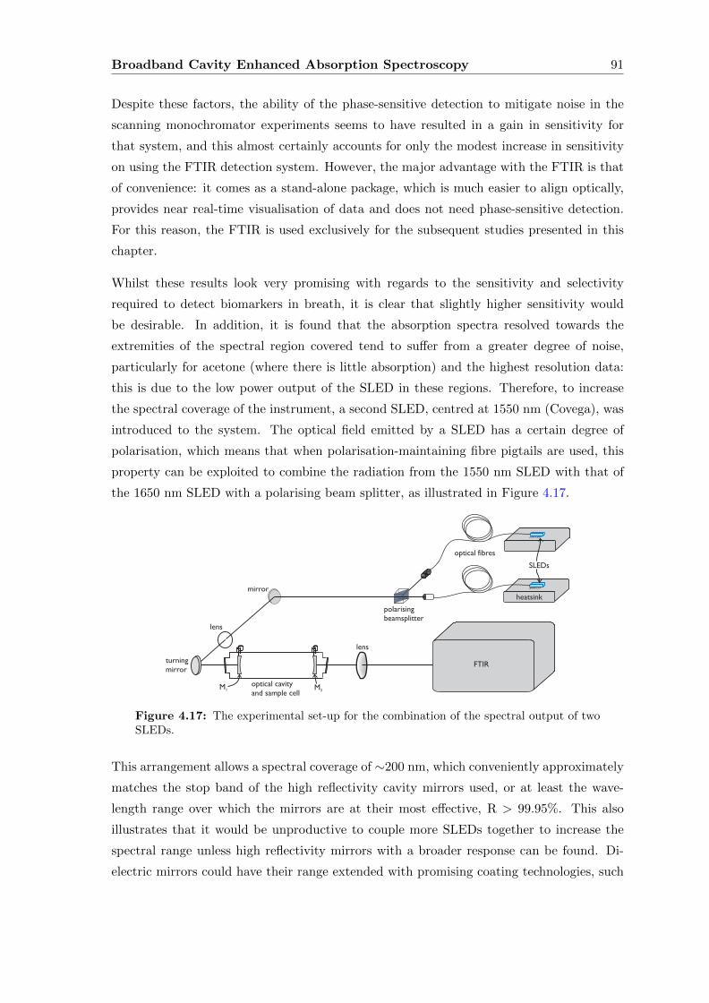
Broadband Cavity Enhanced Absorption Spectroscopy 91
Despite these factors, the ability of the phase-sensitive detection to mitigate noise in the
scanning monochromator experiments seems to have resulted in a gain in sensitivity for
that system, and this almost certainly accounts for only the modest increase in sensitivity
on using the FTIR detection system. However, the major advantage with the FTIR is that
of convenience: it comes as a stand-alone package, which is much easier to align optically,
provides near real-time visualisation of data and does not need phase-sensitive detection.
For this reason, the FTIR is used exclusively for the subsequent studies presented in this
chapter.
Whilst these results look very promising with regards to the sensitivity and selectivity
required to detect biomarkers in breath, it is clear that slightly higher sensitivity would
be desirable. In addition, it is found that the absorption spectra resolved towards the
extremities of the spectral region covered tend to suffer from a greater degree of noise,
particularly for acetone (where there is little absorption) and the highest resolution data:
this is due to the low power output of the SLED in these regions. Therefore, to increase
the spectral coverage of the instrument, a second SLED, centred at 1550 nm (Covega), was
introduced to the system. The optical field emitted by a SLED has a certain degree of
polarisation, which means that when polarisation-maintaining fibre pigtails are used, this
property can be exploited to combine the radiation from the 1550 nm SLED with that of
the 1650 nm SLED with a polarising beam splitter, as illustrated in Figure 4.17.
optical cavity
and sample cellM1 M2
lens
lens
turning
mirror
optical fibres
SLEDs
heatsink
FTIR
mirror
polarising
beamsplitter
Figure 4.17: The experimental set-up for the combination of the spectral output of twoSLEDs.
This arrangement allows a spectral coverage of ∼200 nm, which conveniently approximately
matches the stop band of the high reflectivity cavity mirrors used, or at least the wave-
length range over which the mirrors are at their most effective, R > 99.95%. This also
illustrates that it would be unproductive to couple more SLEDs together to increase the
spectral range unless high reflectivity mirrors with a broader response can be found. Di-
electric mirrors could have their range extended with promising coating technologies, such
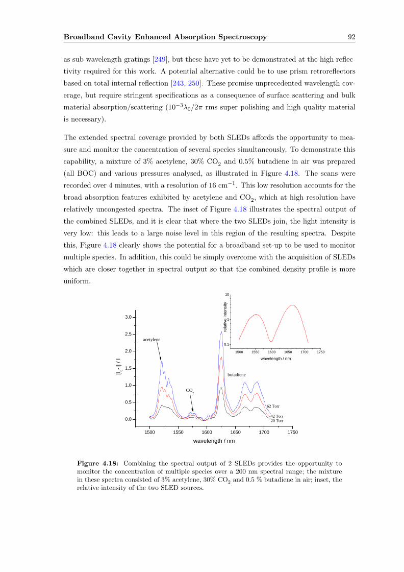
Broadband Cavity Enhanced Absorption Spectroscopy 92
as sub-wavelength gratings [249], but these have yet to be demonstrated at the high reflec-
tivity required for this work. A potential alternative could be to use prism retroreflectors
based on total internal reflection [243, 250]. These promise unprecedented wavelength cov-
erage, but require stringent specifications as a consequence of surface scattering and bulk
material absorption/scattering (10−3λ0/2π rms super polishing and high quality material
is necessary).
The extended spectral coverage provided by both SLEDs affords the opportunity to mea-
sure and monitor the concentration of several species simultaneously. To demonstrate this
capability, a mixture of 3% acetylene, 30% CO2 and 0.5% butadiene in air was prepared
(all BOC) and various pressures analysed, as illustrated in Figure 4.18. The scans were
recorded over 4 minutes, with a resolution of 16 cm−1. This low resolution accounts for the
broad absorption features exhibited by acetylene and CO2, which at high resolution have
relatively uncongested spectra. The inset of Figure 4.18 illustrates the spectral output of
the combined SLEDs, and it is clear that where the two SLEDs join, the light intensity is
very low: this leads to a large noise level in this region of the resulting spectra. Despite
this, Figure 4.18 clearly shows the potential for a broadband set-up to be used to monitor
multiple species. In addition, this could be simply overcome with the acquisition of SLEDs
which are closer together in spectral output so that the combined density profile is more
uniform.
1 5 0 0 1 5 5 0 1 6 0 0 1 6 5 0 1 7 0 0 1 7 5 0
0 . 0
0 . 5
1 . 0
1 . 5
2 . 0
2 . 5
3 . 0
1 5 0 0 1 5 5 0 1 6 0 0 1 6 5 0 1 7 0 0 1 7 5 00 . 1
1
1 0
[I 0-I] / I
w a v e l e n g t h / n m
a c e t y l e n e
C O 2
b u t a d i e n e
2 0 T o r r4 2 T o r r
6 2 T o r r
relati
ve in
tensity
w a v e l e n g t h / n m
Figure 4.18: Combining the spectral output of 2 SLEDs provides the opportunity tomonitor the concentration of multiple species over a 200 nm spectral range; the mixturein these spectra consisted of 3% acetylene, 30% CO2 and 0.5 % butadiene in air; inset, therelative intensity of the two SLED sources.
Broadband Cavity Enhanced Absorption Spectroscopy 93
4.7 Supercontinuum Source with a Fourier transform Inter-
ferometer
A second potential way to uniformly increase the spectral coverage of the broadband system
is to use a Supercontinuum source (SC) in conjunction with the FTIR, replacing the SLED
sources used previously. The SC source has a significantly higher output power than the
SLED (∼40 mW in the region 1.6 µm - 1.7 µm, ∼4 times that of the SLED), and broader,
uniform spectral coverage so that the output intensity detected is limited solely by the stop
band of the cavity mirrors used. This means a higher level of detection sensitivity should
be possible with the source so that < 1 ppm acetone levels can be discerned. Initially,
dilute mixes of butadiene, acetone, isoprene and methane are investigated and a minimum
sensitivity value determined. Following this, a series of experiments are undertaken to
further investigate the possibility of detecting biomarkers in real breath samples, taking
into account the spectral interference of other species present in breath.
4.7.1 Experimental set-up
The Supercontinuum (SC) source (Fianium SC450-4 (UK)) emits 4 W of power across 450
nm to 2.5 µm, so in theory it provides the possibility for cavity-enhanced absorption spec-
troscopy to be applied to a much larger spectral region. However, as mentioned previously,
the useful operating spectral range for CEAS is limited by the stop band of the cavity
mirrors used, 1.5 - 1.7 µm in this case. Everything either side of this spectral range passes
straight through the cavity and so it is essential that these wavelengths are cut out, as
they will otherwise saturate the detector. To this end, two filters are employed: a Thorlabs
FEL1500 longpass and bk interferenzoptik bandpass bk-1655-60-B (centred around 1655 nm
with a 60 nm bandwidth). On passing through these filters, the power entering the cavity
is reduced to ∼40 mW. The output of the SC is pulsed at 40 MHz, but this does not pose
any problems with the experimental set-up: it is essentially treated as a continuous source
as the pulse length is of the order of picoseconds. Finally, to minimise intensity fluctuations
within the SC source it was operated at full power for 2-3 hours before measurements were
taken.
The experimental set-up, other than the introduction of the two filters, was identical to
that with the SLED: the cavity was 25 cm in length and placed within a vacuum vessel, the
cavity transmission was directed through a convex lens (25 cm focal length) and straight
into the FTIR and onto the detector (Thorlabs InGaAs DET410) that resided in the FTIR
sample compartment.
Broadband Cavity Enhanced Absorption Spectroscopy 94
4.7.2 Sensitivity Determination
Dilute samples of butadiene (∼1%), acetone (∼2%) and isoprene (∼1%) were prepared in
the same manner as previously described, whilst the calibrated methane mixes of 15 ppm
and 7.5 ppm (BOC) were used together with the laboratory air to provide the methane
samples for the analysis. As before, data were acquired over a 4 minute period and corrected
for reflectivity variations in the cavity mirrors, allowing the absorbance, αL, to be extracted
from the raw data; sample spectra are illustrated in Figure 4.19.
The sensitivity of this technique was determined with the same method as previously de-
scribed: successive backgrounds, I0 (i.e. no absorber present), were recorded over a period
of 0.5 h, and alternate scans were treated as I. On application of the cavity equation (3.18),
the resulting standard deviation of the linear fit to the ‘absorption’ was used to determine
the minimum detectable absorption coefficient. In principle this method leads to a more
realistic value, rather than just determining the noise on a particular dataset from a broad-
band absorber, as it also reflects the stability of the system, to a certain extent. With the
SC source, αmin ∼ 5 × 10⁻⁹ cm−1 compared to a value of αmin ∼ 2 × 10⁻⁸ cm−1 for the
SLED (a range from 4 − 6 × 10⁻⁹ cm−1 and 1.5 − 2.3 × 10⁻⁸ cm−1 was obtained for the
SC and SLED source respectively, as a consequence of R(λ), and that due to uncertainties
in the determination of the reflectivity there is a 10% uncertainty quoted on these values).
This enhancement in sensitivity cannot be attributed to the increase in power incident on
the cavity alone, as after the SC has passed through the filters it has a power of 40 mW,
compared to the 10 mW entering the cavity from the SLED. It has been speculated that
the remaining difference is perhaps due to some residual coherence in the cw SLED that
leads to interference noise, or possibly a slight susceptibility to optical feedback, leading to
amplitude noise. Alternatively, it could be due to a serendipitous advantageous alignment
that is difficult to optimise at this level, or an approach of the noise floor of the detection
apparatus. It is felt that it is unlikely to be the former, however, as the effect seems repro-
ducible over several misalignment-realignment operations when swapping between the SC
and SLED source.
The sensitivities attained in this work are amongst the highest reported when compared
to other BB-CEAS studies but direct comparison of sensitivity values reported in the lit-
erature should be undertaken with caution, as there are certain parameters that are not
always easily determinable and others that are not reported, but required to make a fair
comparison. Venables et al. [214] report the highest sensitivity to date of 5 ×10⁻¹⁰ cm−1
over a 60 s period, but this was achieved using an optical cavity length of 4.5 m - over 18
times longer than the one used in this study. In addition, it is noted that these type of
experiments can be optimally configured for the target species: for example, increasing the
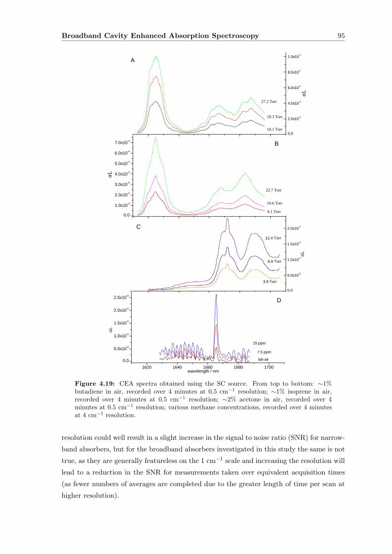
Broadband Cavity Enhanced Absorption Spectroscopy 95
0 . 01 . 0 x 1 0 - 4
2 . 0 x 1 0 - 4
3 . 0 x 1 0 - 4
4 . 0 x 1 0 - 4
5 . 0 x 1 0 - 4
6 . 0 x 1 0 - 4
7 . 0 x 1 0 - 4
D
C
B
6 . 1 T o r r
αL
αL
2 2 . 7 T o r r
1 0 . 6 T o r r
A
0 . 0
5 . 0 x 1 0 - 5
1 . 0 x 1 0 - 4
1 . 5 x 1 0 - 4
2 . 0 x 1 0 - 4
6 . 9 T o r r
αL
1 2 . 4 T o r r
3 . 9 T o r r
1 6 2 0 1 6 4 0 1 6 6 0 1 6 8 0 1 7 0 00 . 0
5 . 0 x 1 0 - 6
1 . 0 x 1 0 - 5
1 . 5 x 1 0 - 5
2 . 0 x 1 0 - 5
2 . 5 x 1 0 - 5
αL
w a v e l e n g t h / n m
7 . 5 p p m1 5 p p m
l a b a i r
0 . 0
2 . 0 x 1 0 - 4
4 . 0 x 1 0 - 4
6 . 0 x 1 0 - 4
8 . 0 x 1 0 - 4
1 . 0 x 1 0 - 3
1 0 . 1 T o r r
1 9 . 3 T o r r
2 7 . 2 T o r r
Figure 4.19: CEA spectra obtained using the SC source. From top to bottom: ∼1%butadiene in air, recorded over 4 minutes at 0.5 cm−1 resolution; ∼1% isoprene in air,recorded over 4 minutes at 0.5 cm−1 resolution; ∼2% acetone in air, recorded over 4minutes at 0.5 cm−1 resolution; various methane concentrations, recorded over 4 minutesat 4 cm−1 resolution.
resolution could well result in a slight increase in the signal to noise ratio (SNR) for narrow-
band absorbers, but for the broadband absorbers investigated in this study the same is not
true, as they are generally featureless on the 1 cm−1 scale and increasing the resolution will
lead to a reduction in the SNR for measurements taken over equivalent acquisition times
(as fewer numbers of averages are completed due to the greater length of time per scan at
higher resolution).
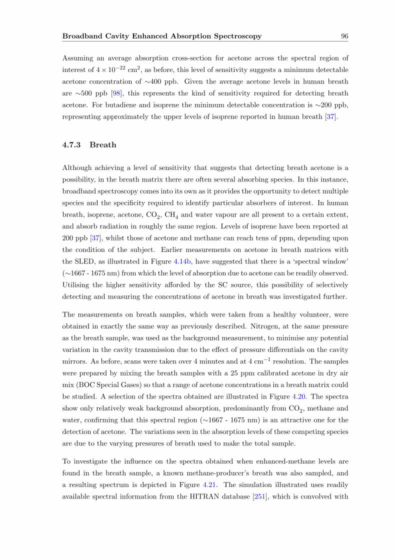
Broadband Cavity Enhanced Absorption Spectroscopy 96
Assuming an average absorption cross-section for acetone across the spectral region of
interest of 4× 10⁻²² cm2, as before, this level of sensitivity suggests a minimum detectable
acetone concentration of ∼400 ppb. Given the average acetone levels in human breath
are ∼500 ppb [98], this represents the kind of sensitivity required for detecting breath
acetone. For butadiene and isoprene the minimum detectable concentration is ∼200 ppb,
representing approximately the upper levels of isoprene reported in human breath [37].
4.7.3 Breath
Although achieving a level of sensitivity that suggests that detecting breath acetone is a
possibility, in the breath matrix there are often several absorbing species. In this instance,
broadband spectroscopy comes into its own as it provides the opportunity to detect multiple
species and the specificity required to identify particular absorbers of interest. In human
breath, isoprene, acetone, CO2, CH4 and water vapour are all present to a certain extent,
and absorb radiation in roughly the same region. Levels of isoprene have been reported at
200 ppb [37], whilst those of acetone and methane can reach tens of ppm, depending upon
the condition of the subject. Earlier measurements on acetone in breath matrices with
the SLED, as illustrated in Figure 4.14b, have suggested that there is a ‘spectral window’
(∼1667 - 1675 nm) from which the level of absorption due to acetone can be readily observed.
Utilising the higher sensitivity afforded by the SC source, this possibility of selectively
detecting and measuring the concentrations of acetone in breath was investigated further.
The measurements on breath samples, which were taken from a healthy volunteer, were
obtained in exactly the same way as previously described. Nitrogen, at the same pressure
as the breath sample, was used as the background measurement, to minimise any potential
variation in the cavity transmission due to the effect of pressure differentials on the cavity
mirrors. As before, scans were taken over 4 minutes and at 4 cm−1 resolution. The samples
were prepared by mixing the breath samples with a 25 ppm calibrated acetone in dry air
mix (BOC Special Gases) so that a range of acetone concentrations in a breath matrix could
be studied. A selection of the spectra obtained are illustrated in Figure 4.20. The spectra
show only relatively weak background absorption, predominantly from CO2, methane and
water, confirming that this spectral region (∼1667 - 1675 nm) is an attractive one for the
detection of acetone. The variations seen in the absorption levels of these competing species
are due to the varying pressures of breath used to make the total sample.
To investigate the influence on the spectra obtained when enhanced-methane levels are
found in the breath sample, a known methane-producer’s breath was also sampled, and
a resulting spectrum is depicted in Figure 4.21. The simulation illustrated uses readily
available spectral information from the HITRAN database [251], which is convolved with
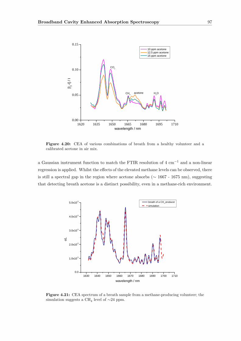
Broadband Cavity Enhanced Absorption Spectroscopy 97
1 6 2 0 1 6 3 5 1 6 5 0 1 6 6 5 1 6 8 0 1 6 9 5 1 7 1 00 . 0 0
0 . 0 5
0 . 1 0
0 . 1 5 1 0 p p m a c e t o n e 1 2 . 5 p p m a c e t o n e 1 5 p p m a c e t o n e
[I 0-I] / I
w a v e l e n g t h / n m
C O 2
H 2 OC H 4 a c e t o n e
Figure 4.20: CEA of various combinations of breath from a healthy volunteer and acalibrated acetone in air mix.
a Gaussian instrument function to match the FTIR resolution of 4 cm−1 and a non-linear
regression is applied. Whilst the effects of the elevated methane levels can be observed, there
is still a spectral gap in the region where acetone absorbs (∼ 1667 - 1675 nm), suggesting
that detecting breath acetone is a distinct possibility, even in a methane-rich environment.
1 6 3 0 1 6 4 0 1 6 5 0 1 6 6 0 1 6 7 0 1 6 8 0 1 6 9 0 1 7 0 0 1 7 1 00 . 0
1 . 0 x 1 0 - 5
2 . 0 x 1 0 - 5
3 . 0 x 1 0 - 5
4 . 0 x 1 0 - 5
5 . 0 x 1 0 - 5
αL
w a v e l e n g t h / n m
b r e a t h o f a C H 4 p r o d u c e r s i m u l a t i o n
Figure 4.21: CEA spectrum of a breath sample from a methane-producing volunteer; thesimulation suggests a CH4 level of ∼24 ppm.
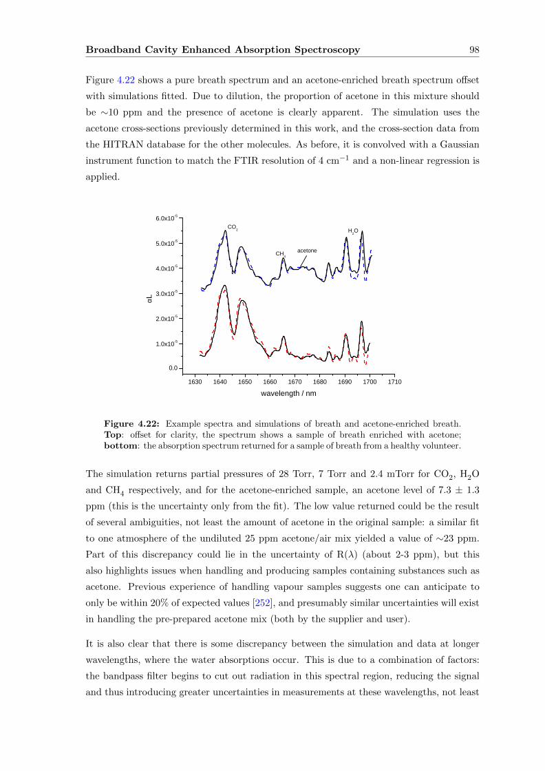
Broadband Cavity Enhanced Absorption Spectroscopy 98
Figure 4.22 shows a pure breath spectrum and an acetone-enriched breath spectrum offset
with simulations fitted. Due to dilution, the proportion of acetone in this mixture should
be ∼10 ppm and the presence of acetone is clearly apparent. The simulation uses the
acetone cross-sections previously determined in this work, and the cross-section data from
the HITRAN database for the other molecules. As before, it is convolved with a Gaussian
instrument function to match the FTIR resolution of 4 cm−1 and a non-linear regression is
applied.
1 6 3 0 1 6 4 0 1 6 5 0 1 6 6 0 1 6 7 0 1 6 8 0 1 6 9 0 1 7 0 0 1 7 1 00 . 0
1 . 0 x 1 0 - 5
2 . 0 x 1 0 - 5
3 . 0 x 1 0 - 5
4 . 0 x 1 0 - 5
5 . 0 x 1 0 - 5
6 . 0 x 1 0 - 5
αL
w a v e l e n g t h / n m
C O 2
C H 4
H 2 O
a c e t o n e
Figure 4.22: Example spectra and simulations of breath and acetone-enriched breath.Top: offset for clarity, the spectrum shows a sample of breath enriched with acetone;bottom: the absorption spectrum returned for a sample of breath from a healthy volunteer.
The simulation returns partial pressures of 28 Torr, 7 Torr and 2.4 mTorr for CO2, H2O
and CH4 respectively, and for the acetone-enriched sample, an acetone level of 7.3 ± 1.3
ppm (this is the uncertainty only from the fit). The low value returned could be the result
of several ambiguities, not least the amount of acetone in the original sample: a similar fit
to one atmosphere of the undiluted 25 ppm acetone/air mix yielded a value of ∼23 ppm.
Part of this discrepancy could lie in the uncertainty of R(λ) (about 2-3 ppm), but this
also highlights issues when handling and producing samples containing substances such as
acetone. Previous experience of handling vapour samples suggests one can anticipate to
only be within 20% of expected values [252], and presumably similar uncertainties will exist
in handling the pre-prepared acetone mix (both by the supplier and user).
It is also clear that there is some discrepancy between the simulation and data at longer
wavelengths, where the water absorptions occur. This is due to a combination of factors:
the bandpass filter begins to cut out radiation in this spectral region, reducing the signal
and thus introducing greater uncertainties in measurements at these wavelengths, not least
Broadband Cavity Enhanced Absorption Spectroscopy 99
in the reflectivity curve used to correct the data; from the manufacturer’s specifications
the reflectivity of the mirrors is known to drop off rapidly in this region and in conjunction
with the greater uncertainty in determining the reflectivity curve at these wavelengths, this
significant change in R(λ) is not going to be accurately determined; and finally, there is
an additional, broad and featureless level of absorption due to water vapour known as the
water continuum that is not included in the HITRAN database as it is not attributed to
specific ro-vibrational transitions of water. This latter effect will be discussed more fully in
the next chapter.
At the lower concentrations of acetone, its distinctive spectral feature becomes less visible
but the simulation, which takes into account the other absorbing species, allows acetone
levels to still be determined. From this, it is apparent that the instrument can reach an
acetone sensitivity of ppm levels in a breath matrix, which is approaching the levels required
to detect acetone in healthy human breath. One way the sensitivity could be increased is
by lengthening the physical cell: even from 25 cm to 50 cm would increase the effective
pathlength to 2,500 m.
4.8 Conclusions
This chapter has detailed the development of three broadband radiation-based cavity en-
hanced systems for the detection of molecules with biological significance. Initially, the
absorption cross-sections of the three broadband absorbing molecules, butadiene, acetone
and isoprene, were determined from direct absorption measurements, which could then be
used to deduce the sensitivities of the broadband CEAS systems developed. The first de-
vice combined a Superluminescent Light Emitting Diode (SLED) broadband source with
a dispersive monochromatic spectrometer and phase-sensitive detection to undertake ini-
tial measurements on both butadiene and acetone, the former a known human carcinogen
and the latter a biomarker for diabetes. The reasonable sensitivity of 6 × 10⁻⁸ cm−1 was
enhanced to 1.5 × 10⁻⁸ cm−1 on moving to an FTIR detection system. The increase in sen-
sitivity resulted in the detection of atmospheric methane and led to preliminary studies on
acetone in breath samples, which demonstrated the suitability of the spectral region (with
regards to interfering species) for the detection of breath acetone. A second SLED was also
introduced to provide, in conjunction with the original SLED, a total spectral coverage
of 200 nm, which allowed the demonstration of multiple species detection and in doing so
highlighted another application of broadband detection. Finally, a Supercontinuum source
(SC) was incorporated into the system and the greater power provided by this source re-
sulted in an improved sensitivity of ∼5 × 10⁻⁹ cm−1, or a detection level of 400 ppb for
pure acetone. Following this, the instrument was applied to breath samples enhanced with
Broadband Cavity Enhanced Absorption Spectroscopy 100
varying amounts of acetone. Utilising a simulation to extract the absorption due to acetone
alone, the device illustrated that it was capable of measuring acetone in breath at the level
of a few ppm.
Although this could be improved with a cavity of longer physical length, an inherent ma-
jor drawback of this arrangement is the relatively low acetone cross-sections in the near-
infrared. Moving to the mid-infrared opens up the possibility of probing larger absorption
cross-sections; this avenue is pursued in Chapter 6. Alternatively, one can remain in the
near-infrared, taking advantage of the plethora of robust, convenient, cheap and commer-
cially available diode lasers. These naturally have a greater power density than broadband
sources, and provided the spectroscopy of the spectral region of interest is well known, can
also be employed in the detection of acetone, as described in the following chapter.
Chapter 5
Development of a Device for
Detecting Breath Acetone
This chapter details work carried out whilst on an industrial placement at Oxford Medical
Diagnostics Ltd. (OMD) as part of my CASE Award studentship. The investigation builds
on work described in the previous two chapters, utilising the narrowband DFB diode laser
CEAS technique detailed in Chapter 3 but drawing on the knowledge gained from the
broadband studies on acetone in Chapter 4.
As has been discussed previously in this thesis, the presence of elevated levels of acetone in
breath is an indicator that the body is burning fat stores, which in turn could signify a lack
of insulin and that the subject is suffering from diabetes. Being able to diagnose diabetes
and monitor the condition in a non-invasive way using breath analysis would represent a
significant breakthrough in the treatment of diabetes and absorption spectroscopy offers a
selective, sensitive and relatively low cost technique with which to do this. The average level
of acetone found in the breath of non-sufferers is ∼500 ppb [98], whilst this can increase to
several ppm in those predominantly burning fat. Therefore, a device which can comfortably
detect the 500 ppb level would be desirable, as this effectively represents the baseline of
breath acetone measurements.
5.1 The detection of acetone with a narrowband laser
As discussed in the previous chapter, the absorption features encountered with acetone
lend themselves to detection using a broadband radiation source, given that conventional
narrowband diode lasers do not have the tunability to sweep over an entire feature. However,
the use of a broadband source is not particularly well-suited for application to a breath
101
Development of a device for detecting breath acetone 102
analyser device: it necessarily requires a means to visualise the spectral output by resolving
its constituent wavelengths, and this tends to involve bulky, cumbersome devices such as
a Fourier Transform spectrometer. Further to this, the most powerful broadband sources,
such as SC devices, represent a substantial investment and as such are not a financially
viable option for use in a potential commercial product.
In contrast, diode lasers are relatively cheap thanks to their use in the telecommunications
industry and they do not require very complex detection systems. In addition, diode lasers
have a greater spectral density than broadband sources so that the effective pathlength
enhancement is reflected in the sensitivity values determined.
In order to regain the specificity lost due to the absence of detailed structure in the absorp-
tion features of acetone, the spectral region of interest must be chosen carefully. Clearly,
sweeping over a very small fraction of the acetone feature is going to result in an absorp-
tion spectrum that merely resembles an ‘offset’. Therefore, in order to use a narrowband
source for the detection of acetone it is essential to select a region which has no spectral
interference from other species that might be found in breath, so that the absorption seen is
solely due to acetone. Secondly, it is imperative that the zero absorption level of the cavity
output does not vary between the I0 and I measurements: in contrast to measurements
with narrow transitions, there is no reference zero baseline in the absorption spectrum, as
the entire spectral region scanned is part of the larger absorption feature. Therefore, the
reference point comes solely from a measurement taken prior to the sample measurement,
so if there is any variation in the zero level between these measurements, it will manifest
itself in the calculated absorption level. Finally, although a spectral region can be selected
with no competing transitions within it, the influence of the water continuum cannot be
ignored. This is a smooth, broad absorption due to water vapour found in addition to its
narrow ro-vibrational transitions that pervades large regions of the entire electromagnetic
spectrum and will be discussed later in this chapter. Its presence necessitates the reduction
of the water vapour content of a breath sample before it is analysed, as it will otherwise
add to the absorption level seen due to acetone. Therefore, this chapter can be split up
into two sections, the first dealing with the optimisation of the device with regards to sys-
tem stability and its application to ‘dry’ samples of acetone; and the second, building on
those foundations with an investigation into the treatment of real breath samples (i.e. ‘wet’
acetone samples) for use with the device.
5.1.1 Acetone
Given the requirements of the breath acetone device to be compact, robust and relatively
cheap to construct, the most obvious spectral region to probe is the near-infrared (NIR),
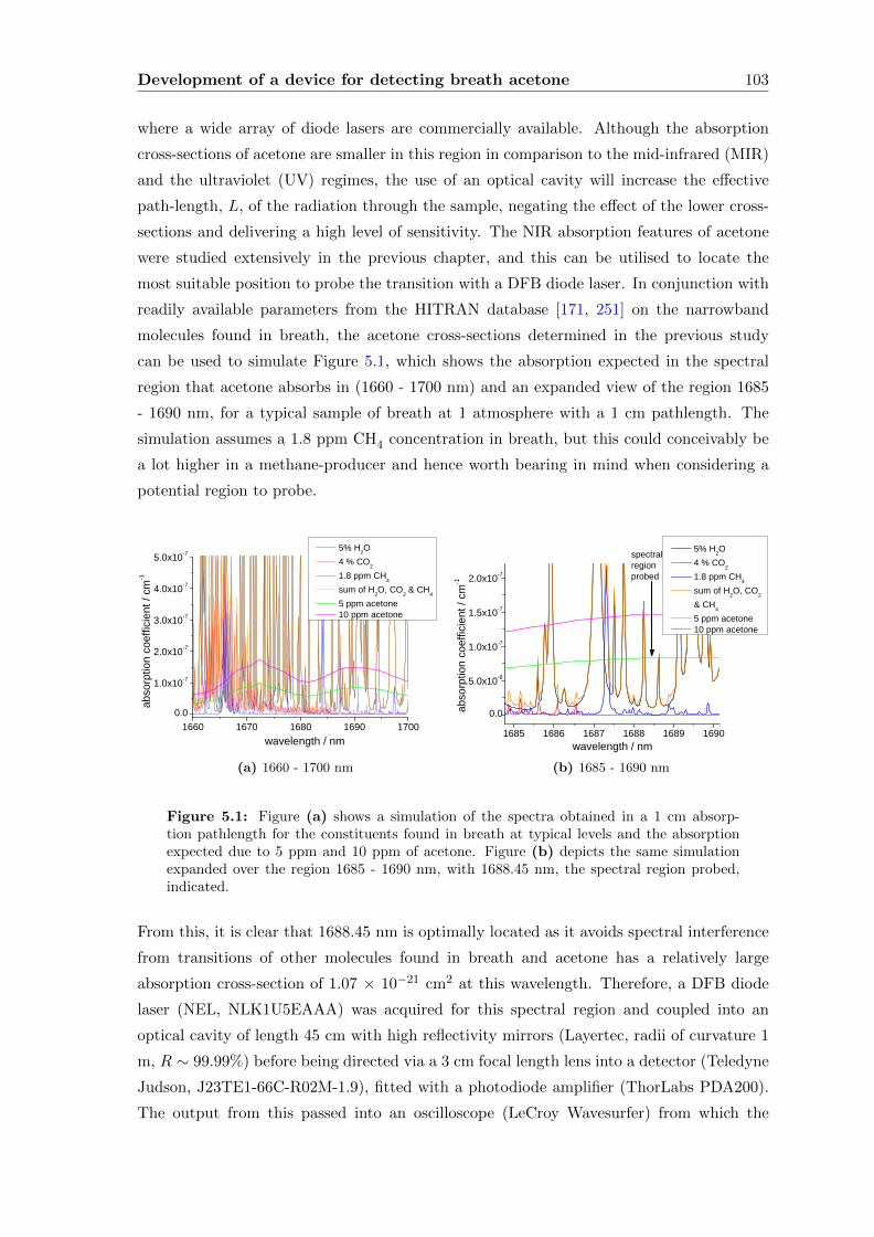
Development of a device for detecting breath acetone 103
where a wide array of diode lasers are commercially available. Although the absorption
cross-sections of acetone are smaller in this region in comparison to the mid-infrared (MIR)
and the ultraviolet (UV) regimes, the use of an optical cavity will increase the effective
path-length, L, of the radiation through the sample, negating the effect of the lower cross-
sections and delivering a high level of sensitivity. The NIR absorption features of acetone
were studied extensively in the previous chapter, and this can be utilised to locate the
most suitable position to probe the transition with a DFB diode laser. In conjunction with
readily available parameters from the HITRAN database [171, 251] on the narrowband
molecules found in breath, the acetone cross-sections determined in the previous study
can be used to simulate Figure 5.1, which shows the absorption expected in the spectral
region that acetone absorbs in (1660 - 1700 nm) and an expanded view of the region 1685
- 1690 nm, for a typical sample of breath at 1 atmosphere with a 1 cm pathlength. The
simulation assumes a 1.8 ppm CH4 concentration in breath, but this could conceivably be
a lot higher in a methane-producer and hence worth bearing in mind when considering a
potential region to probe.
1 6 6 0 1 6 7 0 1 6 8 0 1 6 9 0 1 7 0 00 . 0
1 . 0 x 1 0 - 7
2 . 0 x 1 0 - 7
3 . 0 x 1 0 - 7
4 . 0 x 1 0 - 7
5 . 0 x 1 0 - 7
abso
rption
coeff
icient
/ cm-1
5 % H 2 O 4 % C O 2 1 . 8 p p m C H 4 s u m o f H 2 O , C O 2 & C H 4 5 p p m a c e t o n e 1 0 p p m a c e t o n e
w a v e l e n g t h / n m(a) 1660 - 1700 nm
1 6 8 5 1 6 8 6 1 6 8 7 1 6 8 8 1 6 8 9 1 6 9 00 . 0
5 . 0 x 1 0 - 8
1 . 0 x 1 0 - 7
1 . 5 x 1 0 - 7
2 . 0 x 1 0 - 7
5 % H 2 O 4 % C O 2 1 . 8 p p m C H 4 s u m o f H 2 O , C O 2
& C H 4 5 p p m a c e t o n e 1 0 p p m a c e t o n e
abso
rption
coeff
icient
/ cm-1
w a v e l e n g t h / n m
s p e c t r a l r e g i o n p r o b e d
(b) 1685 - 1690 nm
Figure 5.1: Figure (a) shows a simulation of the spectra obtained in a 1 cm absorp-tion pathlength for the constituents found in breath at typical levels and the absorptionexpected due to 5 ppm and 10 ppm of acetone. Figure (b) depicts the same simulationexpanded over the region 1685 - 1690 nm, with 1688.45 nm, the spectral region probed,indicated.
From this, it is clear that 1688.45 nm is optimally located as it avoids spectral interference
from transitions of other molecules found in breath and acetone has a relatively large
absorption cross-section of 1.07 × 10⁻²¹ cm2 at this wavelength. Therefore, a DFB diode
laser (NEL, NLK1U5EAAA) was acquired for this spectral region and coupled into an
optical cavity of length 45 cm with high reflectivity mirrors (Layertec, radii of curvature 1
m, R ∼ 99.99%) before being directed via a 3 cm focal length lens into a detector (Teledyne
Judson, J23TE1-66C-R02M-1.9), fitted with a photodiode amplifier (ThorLabs PDA200).
The output from this passed into an oscilloscope (LeCroy Wavesurfer) from which the
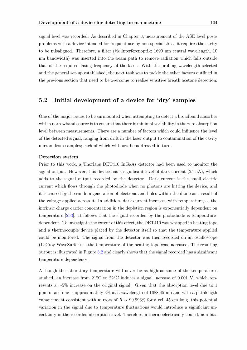
Development of a device for detecting breath acetone 104
signal level was recorded. As described in Chapter 3, measurement of the ASE level poses
problems with a device intended for frequent use by non-specialists as it requires the cavity
to be misaligned. Therefore, a filter (bk Interferenoptik; 1690 nm central wavelength, 10
nm bandwidth) was inserted into the beam path to remove radiation which falls outside
that of the required lasing frequency of the laser. With the probing wavelength selected
and the general set-up established, the next task was to tackle the other factors outlined in
the previous section that need to be overcome to realise sensitive breath acetone detection.
5.2 Initial development of a device for ‘dry’ samples
One of the major issues to be surmounted when attempting to detect a broadband absorber
with a narrowband source is to ensure that there is minimal variability in the zero absorption
level between measurements. There are a number of factors which could influence the level
of the detected signal, ranging from drift in the laser output to contamination of the cavity
mirrors from samples; each of which will now be addressed in turn.
Detection system
Prior to this work, a Thorlabs DET410 InGaAs detector had been used to monitor the
signal output. However, this device has a significant level of dark current (25 nA), which
adds to the signal output recorded by the detector. Dark current is the small electric
current which flows through the photodiode when no photons are hitting the device, and
it is caused by the random generation of electrons and holes within the diode as a result of
the voltage applied across it. In addition, dark current increases with temperature, as the
intrinsic charge carrier concentration in the depletion region is exponentially dependent on
temperature [253]. It follows that the signal recorded by the photodiode is temperature-
dependent. To investigate the extent of this effect, the DET410 was wrapped in heating tape
and a thermocouple device placed by the detector itself so that the temperature applied
could be monitored. The signal from the detector was then recorded on an oscilloscope
(LeCroy WaveSurfer) as the temperature of the heating tape was increased. The resulting
output is illustrated in Figure 5.2 and clearly shows that the signal recorded has a significant
temperature dependence.
Although the laboratory temperature will never be as high as some of the temperatures
studied, an increase from 21C to 22C induces a signal increase of 0.001 V, which rep-
resents a ∼5% increase on the original signal. Given that the absorption level due to 1
ppm of acetone is approximately 3% at a wavelength of 1688.45 nm and with a pathlength
enhancement consistent with mirrors of R ∼ 99.996% for a cell 45 cm long, this potential
variation in the signal due to temperature fluctuations would introduce a significant un-
certainty in the recorded absorption level. Therefore, a thermoelectrically-cooled, non-bias
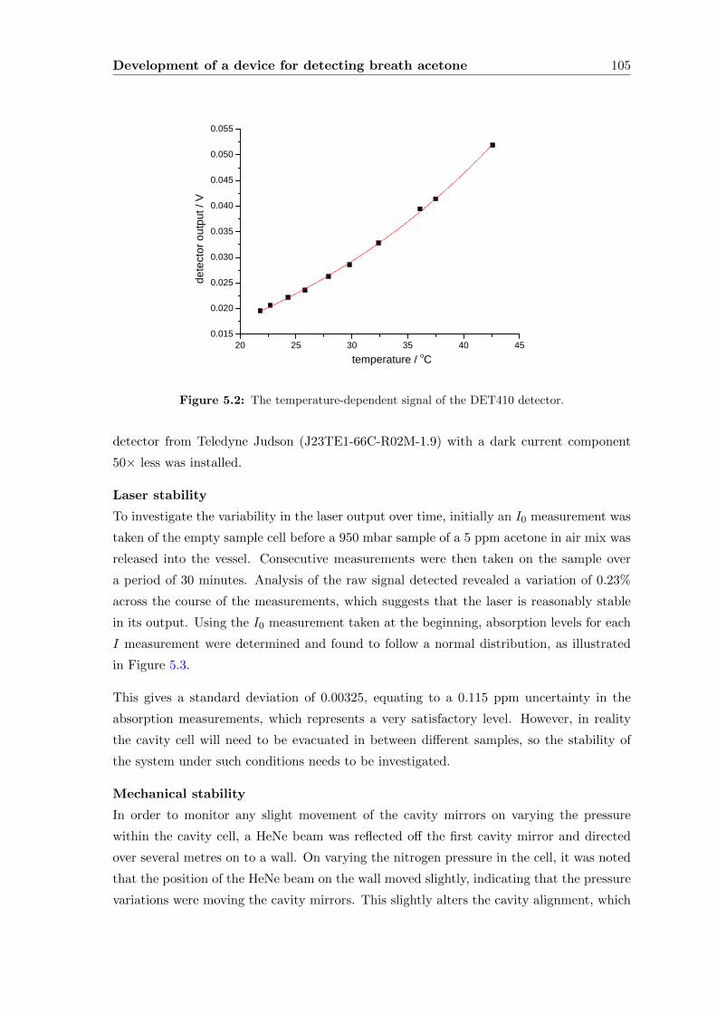
Development of a device for detecting breath acetone 105
2 0 2 5 3 0 3 5 4 0 4 50 . 0 1 5
0 . 0 2 0
0 . 0 2 5
0 . 0 3 0
0 . 0 3 5
0 . 0 4 0
0 . 0 4 5
0 . 0 5 0
0 . 0 5 5
detec
tor ou
tput /
V
t e m p e r a t u r e / o C
Figure 5.2: The temperature-dependent signal of the DET410 detector.
detector from Teledyne Judson (J23TE1-66C-R02M-1.9) with a dark current component
50× less was installed.
Laser stability
To investigate the variability in the laser output over time, initially an I0 measurement was
taken of the empty sample cell before a 950 mbar sample of a 5 ppm acetone in air mix was
released into the vessel. Consecutive measurements were then taken on the sample over
a period of 30 minutes. Analysis of the raw signal detected revealed a variation of 0.23%
across the course of the measurements, which suggests that the laser is reasonably stable
in its output. Using the I0 measurement taken at the beginning, absorption levels for each
I measurement were determined and found to follow a normal distribution, as illustrated
in Figure 5.3.
This gives a standard deviation of 0.00325, equating to a 0.115 ppm uncertainty in the
absorption measurements, which represents a very satisfactory level. However, in reality
the cavity cell will need to be evacuated in between different samples, so the stability of
the system under such conditions needs to be investigated.
Mechanical stability
In order to monitor any slight movement of the cavity mirrors on varying the pressure
within the cavity cell, a HeNe beam was reflected off the first cavity mirror and directed
over several metres on to a wall. On varying the nitrogen pressure in the cell, it was noted
that the position of the HeNe beam on the wall moved slightly, indicating that the pressure
variations were moving the cavity mirrors. This slightly alters the cavity alignment, which
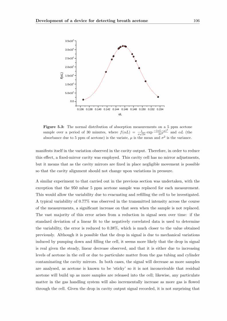
Development of a device for detecting breath acetone 106
0 . 1 3 6 0 . 1 3 8 0 . 1 4 0 0 . 1 4 2 0 . 1 4 4 0 . 1 4 6 0 . 1 4 8 0 . 1 5 0 0 . 1 5 2 0 . 1 5 4
0 . 0
5 . 0 x 1 0 3
1 . 0 x 1 0 4
1 . 5 x 1 0 4
2 . 0 x 1 0 4
2 . 5 x 1 0 4
3 . 0 x 1 0 4
3 . 5 x 1 0 4
f(αL)
αL
Figure 5.3: The normal distribution of absorption measurements on a 5 ppm acetone
sample over a period of 30 minutes, where f(αL) = 1σ√2π
exp −(αL−µ)2
2σ2 and αL (the
absorbance due to 5 ppm of acetone) is the variate, µ is the mean and σ2 is the variance.
manifests itself in the variation observed in the cavity output. Therefore, in order to reduce
this effect, a fixed-mirror cavity was employed. This cavity cell has no mirror adjustments,
but it means that as the cavity mirrors are fixed in place negligible movement is possible
so that the cavity alignment should not change upon variations in pressure.
A similar experiment to that carried out in the previous section was undertaken, with the
exception that the 950 mbar 5 ppm acetone sample was replaced for each measurement.
This would allow the variability due to evacuating and refilling the cell to be investigated.
A typical variability of 0.77% was observed in the transmitted intensity across the course
of the measurements, a significant increase on that seen when the sample is not replaced.
The vast majority of this error arises from a reduction in signal seen over time: if the
standard deviation of a linear fit to the negatively correlated data is used to determine
the variability, the error is reduced to 0.38%, which is much closer to the value obtained
previously. Although it is possible that the drop in signal is due to mechanical variations
induced by pumping down and filling the cell, it seems more likely that the drop in signal
is real given the steady, linear decrease observed, and that it is either due to increasing
levels of acetone in the cell or due to particulate matter from the gas tubing and cylinder
contaminating the cavity mirrors. In both cases, the signal will decrease as more samples
are analysed, as acetone is known to be ‘sticky’ so it is not inconceivable that residual
acetone will build up as more samples are released into the cell; likewise, any particulate
matter in the gas handling system will also incrementally increase as more gas is flowed
through the cell. Given the drop in cavity output signal recorded, it is not surprising that
Development of a device for detecting breath acetone 107
when the absorption levels for each I are determined from the initial I0 measurement the
standard deviation increases to 0.0135, which equates to an uncertainty of 0.423 ppm.
Therefore, the same experiment was conducted as before, but an empty cell I0 measurement
was recorded before every sample (I) measurement. This effectively ‘zeros’ the baseline
before each data set is taken, and reduces the standard deviation of the absorption levels
recorded to 0.00875, or a 0.364 ppm uncertainty.
Clearly, however, a greater control over the sample itself will improve this further.
Sample control
In order to control the flow of gases into the cell, needle valves were introduced in addition
to the Swagelok taps already in place. This greater control reduces the chances of a cavity
mirror being misaligned by the sudden influx of gas into the system. In addition, the intro-
duction of a 0.5 µm particulate filter ensured that any small particles that may be present
in the gas tubing, gas cylinder, or from the breath sample, would be extracted before the
gas filled the cavity cell, thus eliminating a source of potential mirror contamination. Sec-
ondly, methods to ensure that acetone was completely removed in between measurements
were investigated. Initially efforts focused on heating the cell in an attempt to vapourise
condensed acetone found on the surfaces so that it could then be removed via the pump.
However, this method instead caused a far greater variability in the cavity output and it
has been hypothesised that the heating tape in fact induced convection currents within
the cell. It was discovered that the most effective way to prepare the cell for the next
sample was to flush the whole device with N2. Using this method, it was found that the
maximum variation in the I0 measurements over a period of an hour was 0.5%, which is
reduced further for consecutive measurements. Therefore, by recording an I0 measurement
both before and after the sample and taking the average value as the I0 to be used in the
determination of the sample absorption, a reasonably accurate reflection of the actual zero
measurement whilst the sample spectrum is taken is obtained; it allows any subtle changes
in the output over the duration of the measurements to be taken into account.
With the system attaining a level of stability that would suggest sub-1 ppm levels of acetone
could be comfortably detected, the device was applied to the analysis of dry mixes of known
concentration of acetone.
5.2.1 Experimental
The experimental set-up was identical to that described previously and the value taken for
each measurement from the oscilloscope was the average obtained within an interval in the
middle section of the scan over a total period of ∼4 s. It was assumed that over the short
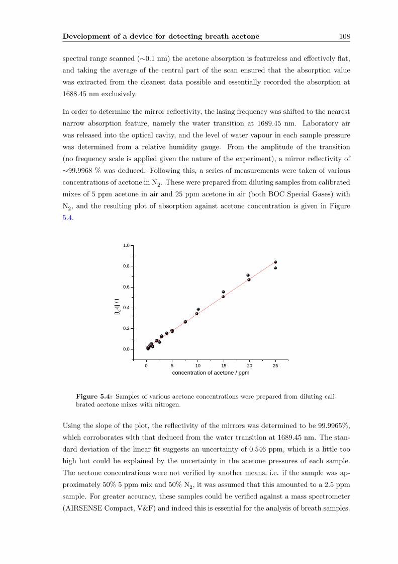
Development of a device for detecting breath acetone 108
spectral range scanned (∼0.1 nm) the acetone absorption is featureless and effectively flat,
and taking the average of the central part of the scan ensured that the absorption value
was extracted from the cleanest data possible and essentially recorded the absorption at
1688.45 nm exclusively.
In order to determine the mirror reflectivity, the lasing frequency was shifted to the nearest
narrow absorption feature, namely the water transition at 1689.45 nm. Laboratory air
was released into the optical cavity, and the level of water vapour in each sample pressure
was determined from a relative humidity gauge. From the amplitude of the transition
(no frequency scale is applied given the nature of the experiment), a mirror reflectivity of
∼99.9968 % was deduced. Following this, a series of measurements were taken of various
concentrations of acetone in N2. These were prepared from diluting samples from calibrated
mixes of 5 ppm acetone in air and 25 ppm acetone in air (both BOC Special Gases) with
N2, and the resulting plot of absorption against acetone concentration is given in Figure
5.4.
0 5 1 0 1 5 2 0 2 5
0 . 0
0 . 2
0 . 4
0 . 6
0 . 8
1 . 0
[I 0-I] / I
c o n c e n t r a t i o n o f a c e t o n e / p p m
Figure 5.4: Samples of various acetone concentrations were prepared from diluting cali-brated acetone mixes with nitrogen.
Using the slope of the plot, the reflectivity of the mirrors was determined to be 99.9965%,
which corroborates with that deduced from the water transition at 1689.45 nm. The stan-
dard deviation of the linear fit suggests an uncertainty of 0.546 ppm, which is a little too
high but could be explained by the uncertainty in the acetone pressures of each sample.
The acetone concentrations were not verified by another means, i.e. if the sample was ap-
proximately 50% 5 ppm mix and 50% N2, it was assumed that this amounted to a 2.5 ppm
sample. For greater accuracy, these samples could be verified against a mass spectrometer
(AIRSENSE Compact, V&F) and indeed this is essential for the analysis of breath samples.
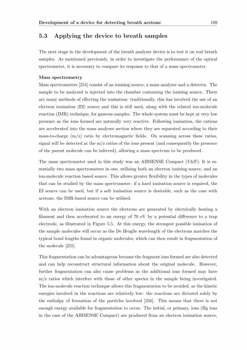
Development of a device for detecting breath acetone 109
5.3 Applying the device to breath samples
The next stage in the development of the breath analyser device is to test it on real breath
samples. As mentioned previously, in order to investigate the performance of the optical
spectrometer, it is necessary to compare its response to that of a mass spectrometer.
Mass spectrometry
Mass spectrometers [254] consist of an ionising source, a mass analyser and a detector. The
sample to be analysed is injected into the chamber containing the ionising source. There
are many methods of effecting the ionisation: traditionally, this has involved the use of an
electron ionisation (EI) source and this is still used, along with the related ion-molecule
reaction (IMR) technique, for gaseous samples. The whole system must be kept at very low
pressure as the ions formed are naturally very reactive. Following ionisation, the cations
are accelerated into the mass analyser section where they are separated according to their
mass-to-charge (m/z) ratio by electromagnetic fields. On scanning across these ratios,
signal will be detected at the m/z ratios of the ions present (and consequently the presence
of the parent molecule can be inferred), allowing a mass spectrum to be produced.
The mass spectrometer used in this study was an AIRSENSE Compact (V&F). It is es-
sentially two mass spectrometers in one, utilising both an electron ionising source, and an
ion-molecule reaction based source. This allows greater flexibility in the types of molecules
that can be studied by the mass spectrometer: if a hard ionisation source is required, the
EI source can be used, but if a soft ionisation source is desirable, such as the case with
acetone, the IMR-based source can be utilised.
With an electron ionisation source the electrons are generated by electrically heating a
filament and then accelerated to an energy of 70 eV by a potential difference to a trap
electrode, as illustrated in Figure 5.5. At this energy, the strongest possible ionisation of
the sample molecules will occur as the De Broglie wavelength of the electrons matches the
typical bond lengths found in organic molecules, which can then result in fragmentation of
the molecule [255].
This fragmentation can be advantageous because the fragment ions formed are also detected
and can help reconstruct structural information about the original molecule. However,
further fragmentation can also cause problems as the additional ions formed may have
m/z ratios which interfere with those of other species in the sample being investigated.
The ion-molecule reaction technique allows this fragmentation to be avoided, as the kinetic
energies involved in the reactions are relatively low: the reactions are dictated solely by
the enthalpy of formation of the particles involved [256]. This means that there is not
enough energy available for fragmentation to occur. The initial, or primary, ions (Hg ions
in the case of the AIRSENSE Compact) are produced from an electron ionisation source,
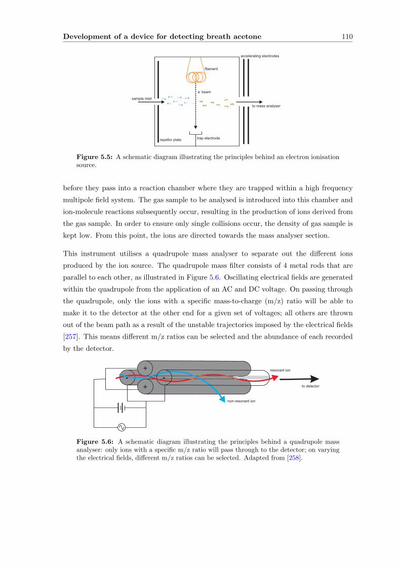
Development of a device for detecting breath acetone 110
sample inlet
repellor plate trap electrode
filament
e beam-
+
+
+
+
++
+
accelerating electrodes
to mass analyser
Figure 5.5: A schematic diagram illustrating the principles behind an electron ionisationsource.
before they pass into a reaction chamber where they are trapped within a high frequency
multipole field system. The gas sample to be analysed is introduced into this chamber and
ion-molecule reactions subsequently occur, resulting in the production of ions derived from
the gas sample. In order to ensure only single collisions occur, the density of gas sample is
kept low. From this point, the ions are directed towards the mass analyser section.
This instrument utilises a quadrupole mass analyser to separate out the different ions
produced by the ion source. The quadrupole mass filter consists of 4 metal rods that are
parallel to each other, as illustrated in Figure 5.6. Oscillating electrical fields are generated
within the quadrupole from the application of an AC and DC voltage. On passing through
the quadrupole, only the ions with a specific mass-to-charge (m/z) ratio will be able to
make it to the detector at the other end for a given set of voltages; all others are thrown
out of the beam path as a result of the unstable trajectories imposed by the electrical fields
[257]. This means different m/z ratios can be selected and the abundance of each recorded
by the detector.
+
-
+
-
resonant ion
non-resonant ion
to detector
Figure 5.6: A schematic diagram illustrating the principles behind a quadrupole massanalyser: only ions with a specific m/z ratio will pass through to the detector; on varyingthe electrical fields, different m/z ratios can be selected. Adapted from [258].
Development of a device for detecting breath acetone 111
5.3.1 Water vapour
The first experimental evidence that water vapour absorbs infrared radiation was presented
by Tyndall [259], but it was not until 1918 that the first detailed water vapour spectrum over
a broad spectral range was determined by Hettner [260] and not until 1938 that Elsasser
noted that there was emission at wavelengths at which water did not possess rotation or
ro-vibrational bands [261–263]. This broad, slowly varying component of absorption found
in addition to the individual spectral lines is known as the water continuum and it is split
into two components: the self-continuum and the foreign-continuum. The former is a result
of the interactions between water molecules whilst the latter describes the interaction of
water molecules with ‘foreign’ molecules found in the atmosphere, such as N2 and O2. Since
those early days, the water continuum has been the subject of countless studies because of
its importance in atmospheric science whilst its physical origin has been a point of heated
debate over the years, a full discussion of which is beyond the scope of this thesis but can
be found in a number of reviews [264–266].
Generally, the water continuum is deduced by subtracting the contribution from the narrow
absorption features from the absorption measured experimentally [267, 268]. Typically,
the narrow absorptions are defined by a pressure-broadened Lorentzian lineshape (some
authors use a Voigt profile [264, 267]), derived from the spectroscopic parameters found
in the HITRAN database [171] with the absorption taken to extend 25 cm−1 from the
line centre. The continuum is then assumed to be everything beyond that 25 cm−1 cut-
off point and, in order to obtain a smoother continuum which is easier to tabulate, also
the small section below the local line shape which is depicted in grey in Figure 5.7. This
means, however, that some absorption due to the local line transitions is included in the
continuum absorption, but this is estimated to contribute < 5-7% in the bands and < 1%
in the windows of the total continuum absorption in the NIR [269].
The self-continuum is known to scale quadratically with water number density whilst the
foreign-continuum is proportional to the product of the water vapour pressure and the sum
of the partial pressures of the broadening gases. In addition, the self-continuum has a
strong negative temperature dependence, whereas the effect is much weaker in the foreign-
continuum. The former property has led to the speculation that the continuum is due
to the superposition of the wings of the spectral lines [266] (the far-wing theory), as the
pressure broadening of the Lorentzian lineshape is known to have a quadratic dependence
on number density in its wings; whilst the latter property suggests the involvement of a
dimer-based mechanism.
The Lorentzian lineshape does not fully describe what is observed experimentally, and in
their semi-empirical model developed in 1989, Clough, Kneizys and Davies (CKD model)
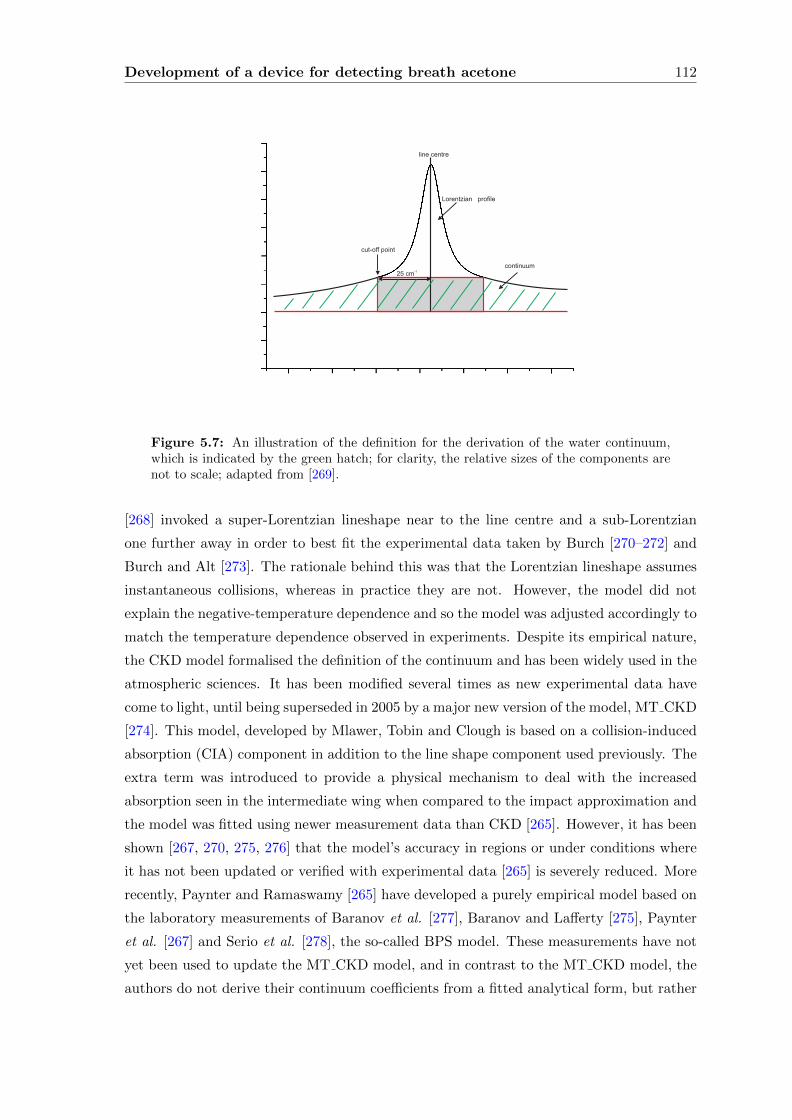
Development of a device for detecting breath acetone 112
25 cm-1
line centre
Lorentzian profile
cut-off point
continuum
Figure 5.7: An illustration of the definition for the derivation of the water continuum,which is indicated by the green hatch; for clarity, the relative sizes of the components arenot to scale; adapted from [269].
[268] invoked a super-Lorentzian lineshape near to the line centre and a sub-Lorentzian
one further away in order to best fit the experimental data taken by Burch [270–272] and
Burch and Alt [273]. The rationale behind this was that the Lorentzian lineshape assumes
instantaneous collisions, whereas in practice they are not. However, the model did not
explain the negative-temperature dependence and so the model was adjusted accordingly to
match the temperature dependence observed in experiments. Despite its empirical nature,
the CKD model formalised the definition of the continuum and has been widely used in the
atmospheric sciences. It has been modified several times as new experimental data have
come to light, until being superseded in 2005 by a major new version of the model, MT CKD
[274]. This model, developed by Mlawer, Tobin and Clough is based on a collision-induced
absorption (CIA) component in addition to the line shape component used previously. The
extra term was introduced to provide a physical mechanism to deal with the increased
absorption seen in the intermediate wing when compared to the impact approximation and
the model was fitted using newer measurement data than CKD [265]. However, it has been
shown [267, 270, 275, 276] that the model’s accuracy in regions or under conditions where
it has not been updated or verified with experimental data [265] is severely reduced. More
recently, Paynter and Ramaswamy [265] have developed a purely empirical model based on
the laboratory measurements of Baranov et al. [277], Baranov and Lafferty [275], Paynter
et al. [267] and Serio et al. [278], the so-called BPS model. These measurements have not
yet been used to update the MT CKD model, and in contrast to the MT CKD model, the
authors do not derive their continuum coefficients from a fitted analytical form, but rather
Development of a device for detecting breath acetone 113
purely from measurements, which also allows uncertainty parameters to be added to the
model.
Driven by the desire to formulate a more theoretical basing for the far-wing description of
the continuum, a number of theories were developed [279–284]. These centred on the use
of a quasi-state approximation, which assumes that the duration of collisional processes
is infinite in comparison with the time frame of interest [284, 285], to derive the absorp-
tion line shapes. Ma and Tipping have demonstrated that their model fits experimental
data in the MIR very well [284] and that it describes the negative temperature dependence
seen experimentally. However, it does underestimate the absorption seen within bands, for
which two explanations are proposed: one, that in the regime where the duration of the
collisional processes are short in comparison to the time of interest, the quasistatic approx-
imation breaks down and the original impact approximation becomes valid, (resulting in
a Lorentzian line shape at the line centres) but in the intermediate region, where the two
times are comparable, neither line shape can be applied; or two, a secondary mechanism
is producing absorption near the line centres. With the former, a near-wing modification,
combining both the far-wings and impact lineshapes, could be the solution but there is
currently no theoretical basis with which to do so accurately [285]. The second was not
favoured by the authors in a follow-up paper (Leforestier et al. [286]) who concluded, based
on calculations on the temperature dependence of far-wing line shapes (800 - 1150 cm−1)
[285], CIA (< 1150 cm−1) and dimer absorption (< 600 cm−1), that the contributions from
CIA were negligible in the frequency region investigated and that dimer absorption only
becomes important in the microwave and submillimetre regimes.
However, the notion of a secondary mechanism responsible for elements of the continuum
absorption has found increasing popularity recently, most notably with Ptashnik and co-
workers [264, 287, 288]. Following theoretical studies on the water dimer by a number of
authors [289–292], the positions and strengths of the bands of the water dimer absorptions
have been computed. However, the rotational structure of the bands has not been directly
calculated, so assumptions about the widths and shapes of the bands have to be made, in-
troducing a significant level of uncertainty: the band centres of the dimer absorption tend
to overlap with those of the monomer, so in order to determine whether the continuum ob-
served experimentally in the window regions is due to a degree of dimer contribution, these
parameters need to be known. However, these calculations demonstrated that although the
dimer absorption has a continuum nature, it also possesses broad spectral features near
band centres, a result that was highlighted by Ptashnik et al. [287] and exploited in their
study of 2004. Whilst the authors admit that uncertainties in the derived would-be dimer
absorption can arise from the subtraction of the monomer absorption from the measured
continuum (given the requirement of a good knowledge of the monomer spectrum), their
analysis of the temperature dependence of the residuals allowed a clear distinction to be
Development of a device for detecting breath acetone 114
made between the dimer and monomer contributions [266]. The results produced spectral
features that agreed reasonably well with the theoretical spectra [290, 293], as did a further
study in 2007 [276] and Ptashnik reviewed earlier measurements that could also be ar-
gued to demonstrate dimer absorption [288]. The new experimental data also highlighted
broad spectral features that could not be explained by the dimer absorption alone and
Ptashnik et al. [264] have recently suggested that these features could be due to shorter-
lived quasi-bound dimers which were not included in the original theoretical framework.
Whilst free pair states account for CIA, where the absorptions are caused by the short-
lived collision-induced dipole moment that occurs during single approach collisions, and
true bound dimers occur at the other extreme at low temperatures, quasi-bound dimers
are formed when there is a temporary stabilisation of a pair from a multiple approach
pair collision. Here the absorption arises from the temporary redistribution of part of the
translational energy of the collisional monomers to rotational energy [264]. Calculations by
Vigasin [294–296] and Epifanov and Vigasin [297] have indicated that these quasi-bound
dimers have equal importance in atmospheric conditions and a simplified calculation by
Ptashnik [264] has suggested that these extra features could be explained by quasi-bound
dimers.
The physical origin of the water continuum is a contentious issue and as of yet there is no
conclusive answer. Despite this, what is certain is that there is a greater level of absorption
due to water than can be explained due to the impact approximation of the water monomer
lines alone (i.e. a Lorentzian profile); whether this is because theoretical lineshapes are yet
to fully describe the whole absorption feature of a water monomer line (centre, near-wing
and far-wing regimes), or because extra absorption mechanisms are also involved, is still to
be resolved.
It is clear, however, that its presence will pose a problem, adding to the absorption level
recorded by the device. In order to determine an estimate for the influence of the water
continuum at 1688.45 nm, a series of measurements on laboratory air were undertaken. The
relative humidity of the laboratory air was determined by a humidity gauge, which also
monitored the room temperature and both were noted for each sample analysed. Various
pressures of laboratory air were fed into the cavity cell and the absorption signal recorded
each time. The I0 measurements were provided by samples of laboratory air, at a pressure
matching that of the I measurement, which had passed through some molecular sieve to
remove the water vapour. Using the pressure, temperature and humidity recorded, a value
for the water vapour pressure within each sample was determined and plotted against the
subsequent absorption level measured, as illustrated in Figure 5.8a. Figure 5.8b illustrates
the absorption level predicted for the same region using simulations based on the HITRAN
database [251], and it is clear that a greater level of absorption is seen experimentally than
would otherwise be expected, which is consistent with the presence of the water continuum.
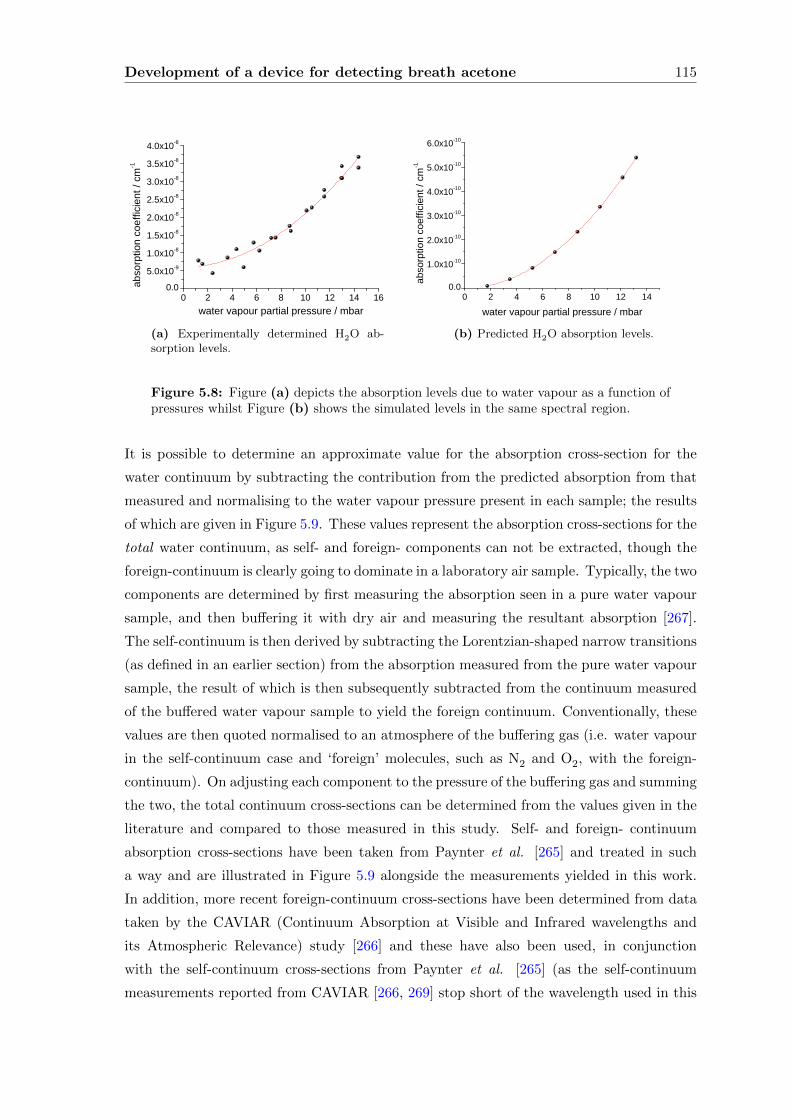
Development of a device for detecting breath acetone 115
0 2 4 6 8 1 0 1 2 1 4 1 60 . 0
5 . 0 x 1 0 - 91 . 0 x 1 0 - 81 . 5 x 1 0 - 82 . 0 x 1 0 - 82 . 5 x 1 0 - 83 . 0 x 1 0 - 83 . 5 x 1 0 - 84 . 0 x 1 0 - 8
abso
rption
coeff
icient
/ cm-1
w a t e r v a p o u r p a r t i a l p r e s s u r e / m b a r(a) Experimentally determined H2O ab-sorption levels.
0 2 4 6 8 1 0 1 2 1 40 . 0
1 . 0 x 1 0 - 1 0
2 . 0 x 1 0 - 1 0
3 . 0 x 1 0 - 1 0
4 . 0 x 1 0 - 1 0
5 . 0 x 1 0 - 1 0
6 . 0 x 1 0 - 1 0
abso
rption
coeff
icient
/ cm-1
w a t e r v a p o u r p a r t i a l p r e s s u r e / m b a r(b) Predicted H2O absorption levels.
Figure 5.8: Figure (a) depicts the absorption levels due to water vapour as a function ofpressures whilst Figure (b) shows the simulated levels in the same spectral region.
It is possible to determine an approximate value for the absorption cross-section for the
water continuum by subtracting the contribution from the predicted absorption from that
measured and normalising to the water vapour pressure present in each sample; the results
of which are given in Figure 5.9. These values represent the absorption cross-sections for the
total water continuum, as self- and foreign- components can not be extracted, though the
foreign-continuum is clearly going to dominate in a laboratory air sample. Typically, the two
components are determined by first measuring the absorption seen in a pure water vapour
sample, and then buffering it with dry air and measuring the resultant absorption [267].
The self-continuum is then derived by subtracting the Lorentzian-shaped narrow transitions
(as defined in an earlier section) from the absorption measured from the pure water vapour
sample, the result of which is then subsequently subtracted from the continuum measured
of the buffered water vapour sample to yield the foreign continuum. Conventionally, these
values are then quoted normalised to an atmosphere of the buffering gas (i.e. water vapour
in the self-continuum case and ‘foreign’ molecules, such as N2 and O2, with the foreign-
continuum). On adjusting each component to the pressure of the buffering gas and summing
the two, the total continuum cross-sections can be determined from the values given in the
literature and compared to those measured in this study. Self- and foreign- continuum
absorption cross-sections have been taken from Paynter et al. [265] and treated in such
a way and are illustrated in Figure 5.9 alongside the measurements yielded in this work.
In addition, more recent foreign-continuum cross-sections have been determined from data
taken by the CAVIAR (Continuum Absorption at Visible and Infrared wavelengths and
its Atmospheric Relevance) study [266] and these have also been used, in conjunction
with the self-continuum cross-sections from Paynter et al. [265] (as the self-continuum
measurements reported from CAVIAR [266, 269] stop short of the wavelength used in this
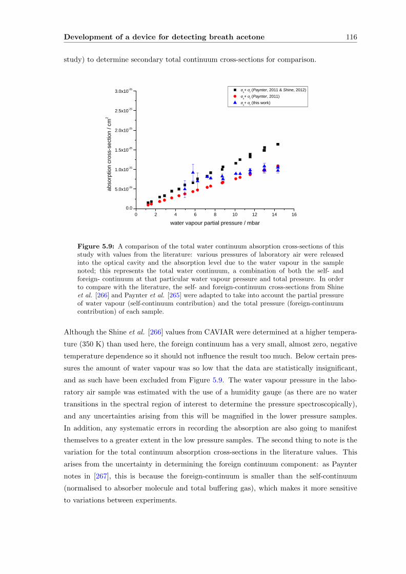
Development of a device for detecting breath acetone 116
study) to determine secondary total continuum cross-sections for comparison.
0 2 4 6 8 1 0 1 2 1 4 1 60 . 0
5 . 0 x 1 0 - 2 6
1 . 0 x 1 0 - 2 5
1 . 5 x 1 0 - 2 5
2 . 0 x 1 0 - 2 5
2 . 5 x 1 0 - 2 5
3 . 0 x 1 0 - 2 5 σs + σf ( P a y n t e r , 2 0 1 1 & S h i n e , 2 0 1 2 ) σs + σf ( P a y n t e r , 2 0 1 1 ) σs + σf ( t h i s w o r k )
abso
rption
cros
s-sec
tion /
cm2
w a t e r v a p o u r p a r t i a l p r e s s u r e / m b a r
Figure 5.9: A comparison of the total water continuum absorption cross-sections of thisstudy with values from the literature: various pressures of laboratory air were releasedinto the optical cavity and the absorption level due to the water vapour in the samplenoted; this represents the total water continuum, a combination of both the self- andforeign- continuum at that particular water vapour pressure and total pressure. In orderto compare with the literature, the self- and foreign-continuum cross-sections from Shineet al. [266] and Paynter et al. [265] were adapted to take into account the partial pressureof water vapour (self-continuum contribution) and the total pressure (foreign-continuumcontribution) of each sample.
Although the Shine et al. [266] values from CAVIAR were determined at a higher tempera-
ture (350 K) than used here, the foreign continuum has a very small, almost zero, negative
temperature dependence so it should not influence the result too much. Below certain pres-
sures the amount of water vapour was so low that the data are statistically insignificant,
and as such have been excluded from Figure 5.9. The water vapour pressure in the labo-
ratory air sample was estimated with the use of a humidity gauge (as there are no water
transitions in the spectral region of interest to determine the pressure spectroscopically),
and any uncertainties arising from this will be magnified in the lower pressure samples.
In addition, any systematic errors in recording the absorption are also going to manifest
themselves to a greater extent in the low pressure samples. The second thing to note is the
variation for the total continuum absorption cross-sections in the literature values. This
arises from the uncertainty in determining the foreign continuum component: as Paynter
notes in [267], this is because the foreign-continuum is smaller than the self-continuum
(normalised to absorber molecule and total buffering gas), which makes it more sensitive
to variations between experiments.
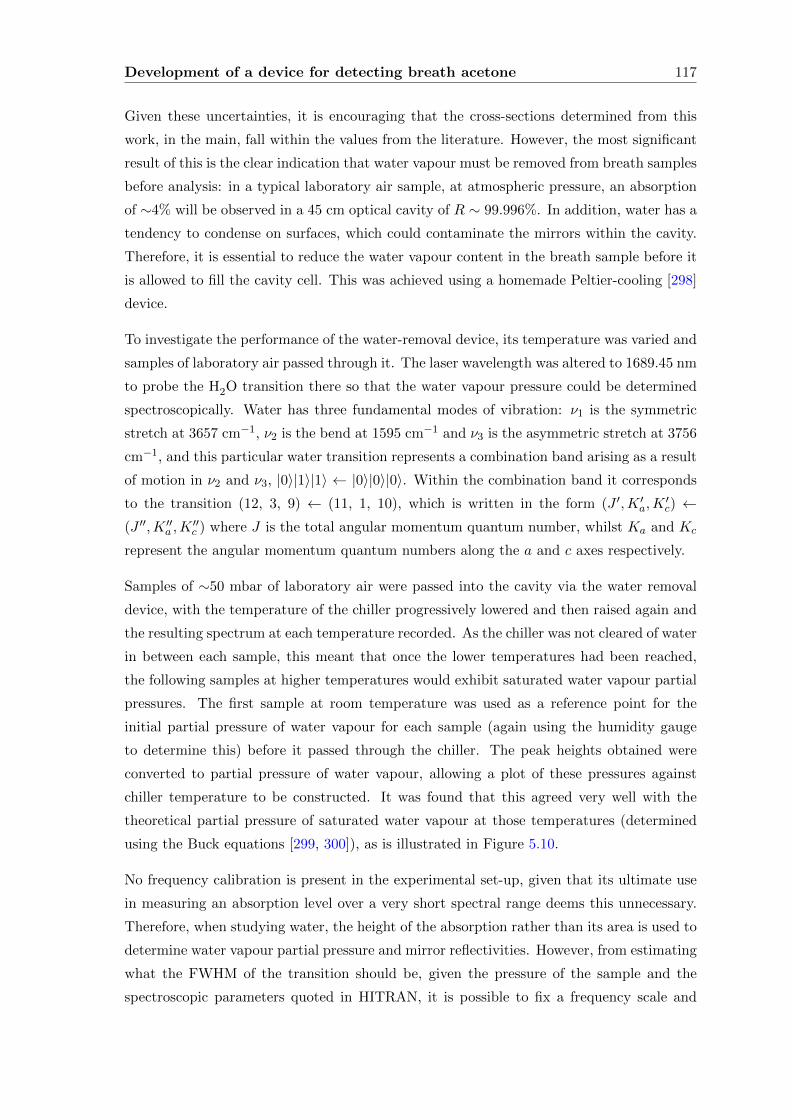
Development of a device for detecting breath acetone 117
Given these uncertainties, it is encouraging that the cross-sections determined from this
work, in the main, fall within the values from the literature. However, the most significant
result of this is the clear indication that water vapour must be removed from breath samples
before analysis: in a typical laboratory air sample, at atmospheric pressure, an absorption
of ∼4% will be observed in a 45 cm optical cavity of R ∼ 99.996%. In addition, water has a
tendency to condense on surfaces, which could contaminate the mirrors within the cavity.
Therefore, it is essential to reduce the water vapour content in the breath sample before it
is allowed to fill the cavity cell. This was achieved using a homemade Peltier-cooling [298]
device.
To investigate the performance of the water-removal device, its temperature was varied and
samples of laboratory air passed through it. The laser wavelength was altered to 1689.45 nm
to probe the H2O transition there so that the water vapour pressure could be determined
spectroscopically. Water has three fundamental modes of vibration: ν1 is the symmetric
stretch at 3657 cm−1, ν2 is the bend at 1595 cm−1 and ν3 is the asymmetric stretch at 3756
cm−1, and this particular water transition represents a combination band arising as a result
of motion in ν2 and ν3, |0〉|1〉|1〉 ← |0〉|0〉|0〉. Within the combination band it corresponds
to the transition (12, 3, 9) ← (11, 1, 10), which is written in the form (J ′,K ′a,K′c) ←
(J ′′,K ′′a ,K′′c ) where J is the total angular momentum quantum number, whilst Ka and Kc
represent the angular momentum quantum numbers along the a and c axes respectively.
Samples of ∼50 mbar of laboratory air were passed into the cavity via the water removal
device, with the temperature of the chiller progressively lowered and then raised again and
the resulting spectrum at each temperature recorded. As the chiller was not cleared of water
in between each sample, this meant that once the lower temperatures had been reached,
the following samples at higher temperatures would exhibit saturated water vapour partial
pressures. The first sample at room temperature was used as a reference point for the
initial partial pressure of water vapour for each sample (again using the humidity gauge
to determine this) before it passed through the chiller. The peak heights obtained were
converted to partial pressure of water vapour, allowing a plot of these pressures against
chiller temperature to be constructed. It was found that this agreed very well with the
theoretical partial pressure of saturated water vapour at those temperatures (determined
using the Buck equations [299, 300]), as is illustrated in Figure 5.10.
No frequency calibration is present in the experimental set-up, given that its ultimate use
in measuring an absorption level over a very short spectral range deems this unnecessary.
Therefore, when studying water, the height of the absorption rather than its area is used to
determine water vapour partial pressure and mirror reflectivities. However, from estimating
what the FWHM of the transition should be, given the pressure of the sample and the
spectroscopic parameters quoted in HITRAN, it is possible to fix a frequency scale and
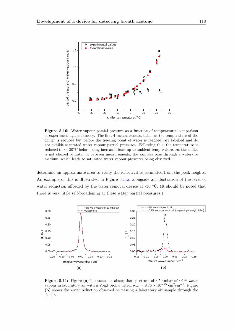
Development of a device for detecting breath acetone 118
- 4 0 - 3 0 - 2 0 - 1 0 0 1 0 2 0 3 0
0 . 0
0 . 5
1 . 0
1 . 5 e x p e r i m e n t a l v a l u e s t h e o r e t i c a l v a l u e s
partia
l pres
sure
of wa
ter va
pour
/ mba
r
c h i l l e r t e m p e r a t u r e / o C
1234
Figure 5.10: Water vapour partial pressure as a function of temperature: comparisonof experiment against theory. The first 4 measurements, taken as the temperature of thechiller is reduced but before the freezing point of water is reached, are labelled and donot exhibit saturated water vapour partial pressures. Following this, the temperature isreduced to ∼ -30C before being increased back up to ambient temperature. As the chilleris not cleared of water in between measurements, the samples pass through a water/icemedium, which leads to saturated water vapour pressures being observed.
determine an approximate area to verify the reflectivities estimated from the peak heights.
An example of this is illustrated in Figure 5.11a, alongside an illustration of the level of
water reduction afforded by the water removal device at -30 C. (It should be noted that
there is very little self-broadening at these water partial pressures.)
- 0 . 1 5 - 0 . 1 0 - 0 . 0 5 0 . 0 0 0 . 0 5 0 . 1 0 0 . 1 50 . 0 0
0 . 0 5
0 . 1 0
0 . 1 5
0 . 2 0
0 . 2 5
0 . 3 0 ~ 1 % w a t e r v a p o u r i n 5 0 m b a r a i r V o i g t p r o f i l e
[I 0-I] / I
r e l a t i v e w a v e n u m b e r / c m - 1
(a)
- 0 . 1 5 - 0 . 1 0 - 0 . 0 5 0 . 0 0 0 . 0 5 0 . 1 0 0 . 1 50 . 0 0
0 . 0 5
0 . 1 0
0 . 1 5
0 . 2 0
0 . 2 5
0 . 3 0
[I 0-I] / I
r e l a t i v e w a v e n u m b e r / c m - 1
~ 1 % w a t e r v a p o u r i n a i r ~ 0 . 1 % w a t e r v a p o u r i n a i r ( o n p a s s i n g t h r o u g h c h i l l e r )
(b)
Figure 5.11: Figure (a) illustrates an absorption spectrum of ∼50 mbar of ∼1% watervapour in laboratory air with a Voigt profile fitted; σint = 8.75 × 10⁻²⁵ cm2cm−1. Figure(b) shows the water reduction observed on passing a laboratory air sample through thechiller.
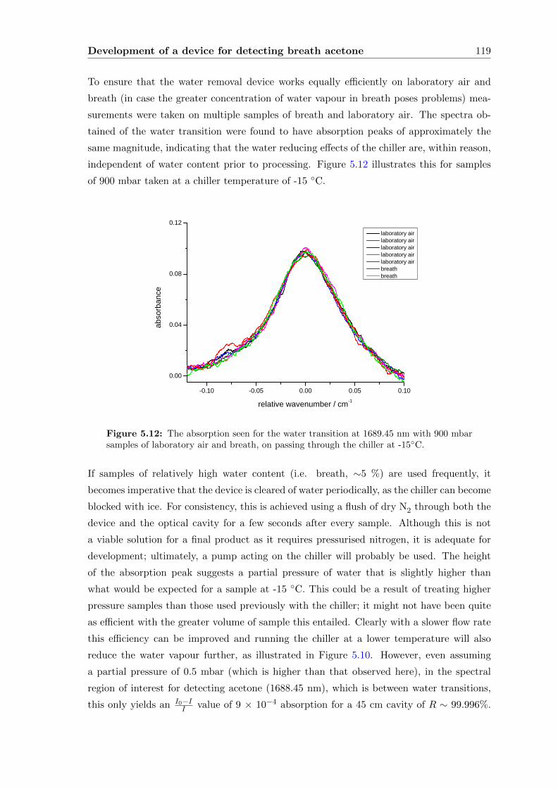
Development of a device for detecting breath acetone 119
To ensure that the water removal device works equally efficiently on laboratory air and
breath (in case the greater concentration of water vapour in breath poses problems) mea-
surements were taken on multiple samples of breath and laboratory air. The spectra ob-
tained of the water transition were found to have absorption peaks of approximately the
same magnitude, indicating that the water reducing effects of the chiller are, within reason,
independent of water content prior to processing. Figure 5.12 illustrates this for samples
of 900 mbar taken at a chiller temperature of -15 C.
- 0 . 1 0 - 0 . 0 5 0 . 0 0 0 . 0 5 0 . 1 00 . 0 0
0 . 0 4
0 . 0 8
0 . 1 2
abso
rbanc
e
l a b o r a t o r y a i r l a b o r a t o r y a i r l a b o r a t o r y a i r l a b o r a t o r y a i r l a b o r a t o r y a i r b r e a t h b r e a t h
r e l a t i v e w a v e n u m b e r / c m - 1
Figure 5.12: The absorption seen for the water transition at 1689.45 nm with 900 mbarsamples of laboratory air and breath, on passing through the chiller at -15C.
If samples of relatively high water content (i.e. breath, ∼5 %) are used frequently, it
becomes imperative that the device is cleared of water periodically, as the chiller can become
blocked with ice. For consistency, this is achieved using a flush of dry N2 through both the
device and the optical cavity for a few seconds after every sample. Although this is not
a viable solution for a final product as it requires pressurised nitrogen, it is adequate for
development; ultimately, a pump acting on the chiller will probably be used. The height
of the absorption peak suggests a partial pressure of water that is slightly higher than
what would be expected for a sample at -15 C. This could be a result of treating higher
pressure samples than those used previously with the chiller; it might not have been quite
as efficient with the greater volume of sample this entailed. Clearly with a slower flow rate
this efficiency can be improved and running the chiller at a lower temperature will also
reduce the water vapour further, as illustrated in Figure 5.10. However, even assuming
a partial pressure of 0.5 mbar (which is higher than that observed here), in the spectral
region of interest for detecting acetone (1688.45 nm), which is between water transitions,
this only yields an I0−II value of 9 × 10⁻⁴ absorption for a 45 cm cavity of R ∼ 99.996%.
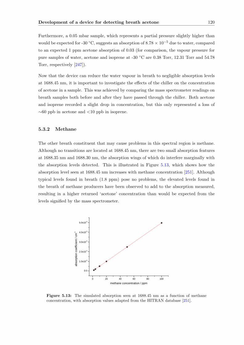
Development of a device for detecting breath acetone 120
Furthermore, a 0.05 mbar sample, which represents a partial pressure slightly higher than
would be expected for -30 C, suggests an absorption of 8.78 × 10⁻⁵ due to water, compared
to an expected 1 ppm acetone absorption of 0.03 (for comparison, the vapour pressure for
pure samples of water, acetone and isoprene at -30 C are 0.38 Torr, 12.31 Torr and 54.78
Torr, respectively [247]).
Now that the device can reduce the water vapour in breath to negligible absorption levels
at 1688.45 nm, it is important to investigate the effects of the chiller on the concentration
of acetone in a sample. This was achieved by comparing the mass spectrometer readings on
breath samples both before and after they have passed through the chiller. Both acetone
and isoprene recorded a slight drop in concentration, but this only represented a loss of
∼60 ppb in acetone and <10 ppb in isoprene.
5.3.2 Methane
The other breath constituent that may cause problems in this spectral region is methane.
Although no transitions are located at 1688.45 nm, there are two small absorption features
at 1688.35 nm and 1688.30 nm, the absorption wings of which do interfere marginally with
the absorption levels detected. This is illustrated in Figure 5.13, which shows how the
absorption level seen at 1688.45 nm increases with methane concentration [251]. Although
typical levels found in breath (1.8 ppm) pose no problems, the elevated levels found in
the breath of methane producers have been observed to add to the absorption measured,
resulting in a higher returned ‘acetone’ concentration than would be expected from the
levels signified by the mass spectrometer.
0 2 0 4 0 6 0 8 0 1 0 0
0 . 0
1 . 0 x 1 0 - 9
2 . 0 x 1 0 - 9
3 . 0 x 1 0 - 9
4 . 0 x 1 0 - 9
5 . 0 x 1 0 - 9
abso
rption
coeff
icient
/ cm-1
m e t h a n e c o n c e n t r a t i o n / p p m
Figure 5.13: The simulated absorption seen at 1688.45 nm as a function of methaneconcentration, with absorption values adapted from the HITRAN database [251].
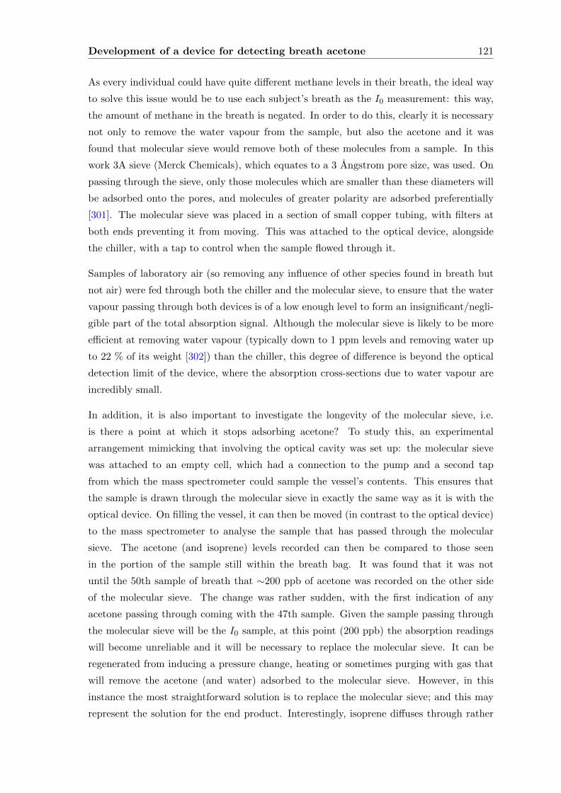
Development of a device for detecting breath acetone 121
As every individual could have quite different methane levels in their breath, the ideal way
to solve this issue would be to use each subject’s breath as the I0 measurement: this way,
the amount of methane in the breath is negated. In order to do this, clearly it is necessary
not only to remove the water vapour from the sample, but also the acetone and it was
found that molecular sieve would remove both of these molecules from a sample. In this
work 3A sieve (Merck Chemicals), which equates to a 3 Angstrom pore size, was used. On
passing through the sieve, only those molecules which are smaller than these diameters will
be adsorbed onto the pores, and molecules of greater polarity are adsorbed preferentially
[301]. The molecular sieve was placed in a section of small copper tubing, with filters at
both ends preventing it from moving. This was attached to the optical device, alongside
the chiller, with a tap to control when the sample flowed through it.
Samples of laboratory air (so removing any influence of other species found in breath but
not air) were fed through both the chiller and the molecular sieve, to ensure that the water
vapour passing through both devices is of a low enough level to form an insignificant/negli-
gible part of the total absorption signal. Although the molecular sieve is likely to be more
efficient at removing water vapour (typically down to 1 ppm levels and removing water up
to 22 % of its weight [302]) than the chiller, this degree of difference is beyond the optical
detection limit of the device, where the absorption cross-sections due to water vapour are
incredibly small.
In addition, it is also important to investigate the longevity of the molecular sieve, i.e.
is there a point at which it stops adsorbing acetone? To study this, an experimental
arrangement mimicking that involving the optical cavity was set up: the molecular sieve
was attached to an empty cell, which had a connection to the pump and a second tap
from which the mass spectrometer could sample the vessel’s contents. This ensures that
the sample is drawn through the molecular sieve in exactly the same way as it is with the
optical device. On filling the vessel, it can then be moved (in contrast to the optical device)
to the mass spectrometer to analyse the sample that has passed through the molecular
sieve. The acetone (and isoprene) levels recorded can then be compared to those seen
in the portion of the sample still within the breath bag. It was found that it was not
until the 50th sample of breath that ∼200 ppb of acetone was recorded on the other side
of the molecular sieve. The change was rather sudden, with the first indication of any
acetone passing through coming with the 47th sample. Given the sample passing through
the molecular sieve will be the I0 sample, at this point (200 ppb) the absorption readings
will become unreliable and it will be necessary to replace the molecular sieve. It can be
regenerated from inducing a pressure change, heating or sometimes purging with gas that
will remove the acetone (and water) adsorbed to the molecular sieve. However, in this
instance the most straightforward solution is to replace the molecular sieve; and this may
represent the solution for the end product. Interestingly, isoprene diffuses through rather
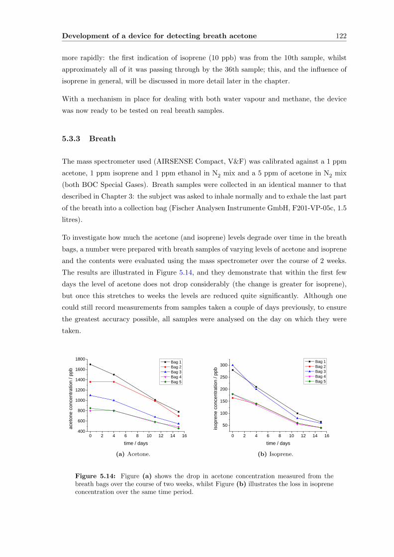
Development of a device for detecting breath acetone 122
more rapidly: the first indication of isoprene (10 ppb) was from the 10th sample, whilst
approximately all of it was passing through by the 36th sample; this, and the influence of
isoprene in general, will be discussed in more detail later in the chapter.
With a mechanism in place for dealing with both water vapour and methane, the device
was now ready to be tested on real breath samples.
5.3.3 Breath
The mass spectrometer used (AIRSENSE Compact, V&F) was calibrated against a 1 ppm
acetone, 1 ppm isoprene and 1 ppm ethanol in N2 mix and a 5 ppm of acetone in N2 mix
(both BOC Special Gases). Breath samples were collected in an identical manner to that
described in Chapter 3: the subject was asked to inhale normally and to exhale the last part
of the breath into a collection bag (Fischer Analysen Instrumente GmbH, F201-VP-05c, 1.5
litres).
To investigate how much the acetone (and isoprene) levels degrade over time in the breath
bags, a number were prepared with breath samples of varying levels of acetone and isoprene
and the contents were evaluated using the mass spectrometer over the course of 2 weeks.
The results are illustrated in Figure 5.14, and they demonstrate that within the first few
days the level of acetone does not drop considerably (the change is greater for isoprene),
but once this stretches to weeks the levels are reduced quite significantly. Although one
could still record measurements from samples taken a couple of days previously, to ensure
the greatest accuracy possible, all samples were analysed on the day on which they were
taken.
0 2 4 6 8 1 0 1 2 1 4 1 64 0 06 0 08 0 0
1 0 0 01 2 0 01 4 0 01 6 0 01 8 0 0 B a g 1
B a g 2 B a g 3 B a g 4 B a g 5
aceto
ne co
ncen
tratio
n / pp
b
t i m e / d a y s(a) Acetone.
0 2 4 6 8 1 0 1 2 1 4 1 65 0
1 0 0
1 5 0
2 0 0
2 5 0
3 0 0 B a g 1 B a g 2 B a g 3 B a g 4 B a g 5
isopre
ne co
ncen
tratio
n / pp
b
t i m e / d a y s(b) Isoprene.
Figure 5.14: Figure (a) shows the drop in acetone concentration measured from thebreath bags over the course of two weeks, whilst Figure (b) illustrates the loss in isopreneconcentration over the same time period.
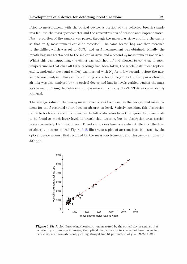
Development of a device for detecting breath acetone 123
Prior to measurement with the optical device, a portion of the collected breath sample
was fed into the mass spectrometer and the concentrations of acetone and isoprene noted.
Next, a portion of the sample was passed through the molecular sieve and into the cavity
so that an I0 measurement could be recorded. The same breath bag was then attached
to the chiller, which was set to -30C, and an I measurement was obtained. Finally, the
breath bag was reattached to the molecular sieve and a second I0 measurement was taken.
Whilst this was happening, the chiller was switched off and allowed to come up to room
temperature so that once all three readings had been taken, the whole instrument (optical
cavity, molecular sieve and chiller) was flushed with N2 for a few seconds before the next
sample was analysed. For calibration purposes, a breath bag full of the 5 ppm acetone in
air mix was also analysed by the optical device and had its levels verified against the mass
spectrometer. Using the calibrated mix, a mirror reflectivity of ∼99.996% was consistently
returned.
The average value of the two I0 measurements was then used as the background measure-
ment for the I recorded to produce an absorption level. Strictly speaking, this absorption
is due to both acetone and isoprene, as the latter also absorbs in this region. Isoprene tends
to be found at much lower levels in breath than acetone, but its absorption cross-section
is approximately 1.5 times larger. Therefore, it does have a significant effect on the level
of absorption seen: indeed Figure 5.15 illustrates a plot of acetone level indicated by the
optical device against that recorded by the mass spectrometer, and this yields an offset of
329 ppb.
0 1 0 0 0 2 0 0 0 3 0 0 0 4 0 0 0 5 0 0 0 6 0 0 00
1 0 0 0
2 0 0 0
3 0 0 0
4 0 0 0
5 0 0 0
6 0 0 0
optica
l instr
umen
t read
ing / p
pb
m a s s s p e c t r o m e t e r r e a d i n g / p p b
Figure 5.15: A plot illustrating the absorption measured by the optical device against thatrecorded by a mass spectrometer; the optical device data points have not been correctedfor the isoprene contributions, yielding straight line fit parameters of y = 0.922x+ 329.
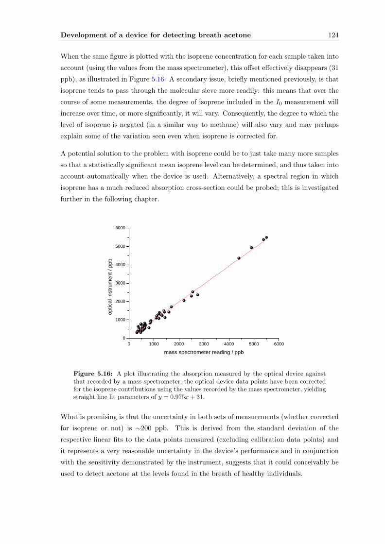
Development of a device for detecting breath acetone 124
When the same figure is plotted with the isoprene concentration for each sample taken into
account (using the values from the mass spectrometer), this offset effectively disappears (31
ppb), as illustrated in Figure 5.16. A secondary issue, briefly mentioned previously, is that
isoprene tends to pass through the molecular sieve more readily: this means that over the
course of some measurements, the degree of isoprene included in the I0 measurement will
increase over time, or more significantly, it will vary. Consequently, the degree to which the
level of isoprene is negated (in a similar way to methane) will also vary and may perhaps
explain some of the variation seen even when isoprene is corrected for.
A potential solution to the problem with isoprene could be to just take many more samples
so that a statistically significant mean isoprene level can be determined, and thus taken into
account automatically when the device is used. Alternatively, a spectral region in which
isoprene has a much reduced absorption cross-section could be probed; this is investigated
further in the following chapter.
0 1 0 0 0 2 0 0 0 3 0 0 0 4 0 0 0 5 0 0 0 6 0 0 00
1 0 0 0
2 0 0 0
3 0 0 0
4 0 0 0
5 0 0 0
6 0 0 0
optica
l instr
umen
t / pp
b
m a s s s p e c t r o m e t e r r e a d i n g / p p b
Figure 5.16: A plot illustrating the absorption measured by the optical device againstthat recorded by a mass spectrometer; the optical device data points have been correctedfor the isoprene contributions using the values recorded by the mass spectrometer, yieldingstraight line fit parameters of y = 0.975x+ 31.
What is promising is that the uncertainty in both sets of measurements (whether corrected
for isoprene or not) is ∼200 ppb. This is derived from the standard deviation of the
respective linear fits to the data points measured (excluding calibration data points) and
it represents a very reasonable uncertainty in the device’s performance and in conjunction
with the sensitivity demonstrated by the instrument, suggests that it could conceivably be
used to detect acetone at the levels found in the breath of healthy individuals.
Development of a device for detecting breath acetone 125
5.4 Conclusions
This chapter has provided a clear demonstration of the viability of laser-based CEAS for
the detection of broadband absorbers, where care must be taken to account for all possible
sources of absorption level change. This has been found particularly important in breath
where there is a large quantity of water, which provides a continuum absorption over a
very broad spectral region. A unique solution has been found here by removing water
and also using breath samples to generate their own background measurement, which has
allowed breath acetone levels to be measured within an uncertainty of 200 ppb. One way to
circumvent, or at least reduce, the problems associated with interfering species is to move
to a spectral region where their absorption is less significant and the acetone absorption
cross-sections are larger, a possibility which is explored in the following chapter.
Chapter 6
Detection of Acetone in the
Mid-Infrared
6.1 Introduction
The work carried out previously in this thesis has focused solely on the use of near-infrared
radiation sources, primarily because these are readily available, relatively cheap (the excep-
tion being the SC source), robust and reliable thanks to their use in the telecommunications
industry. However, in terms of molecular spectroscopy, the mid-infrared (MIR) is a far more
desirable region to probe as moving from the weak overtone and combination bands of the
near-infrared (NIR) to the fundamental transitions in the MIR allows access to transitions
whose absorption cross-sections are often at least fifty times larger, providing the potential
for greater detection sensitivities. This enhancement in σ(ν) on moving from the NIR to
the MIR is illustrated in Figure 6.1 for acetone. Traditionally, the MIR spectral region
has been probed using Pb-salt diode lasers, in addition to CO and CO2 gas lasers. More
recently, non-linear optics-based techniques have been used to generate MIR radiation from
NIR sources; a brief overview of these MIR sources is presented in Appendix A.
The advent of the quantum cascade laser (QCL), a relatively high power and widely tun-
able source in the MIR with inherent low bandwidth, offers the exciting prospect of achiev-
ing greater levels of sensitivity at very high resolution for trace gas detection. QCLs are
potentially available over a broad wavelength range (3 - 250 µm, although they are not
commercial available for all wavelengths within this range), with the particular QCL used
in the present studies operating near 8 µm over a quoted region of 1215 - 1223 cm−1. As
will be discussed at length later, this region is an ideal one in which to probe the spec-
troscopy of acetone. Initial studies will revolve around direct absorption measurements,
utilising the high resolution of the laser to probe the rotational structure of acetone, before
126
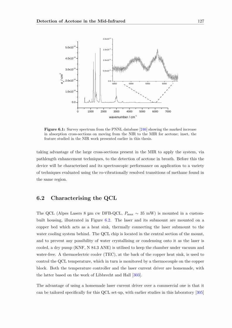
Detection of Acetone in the Mid-Infrared 127
0 1 0 0 0 2 0 0 0 3 0 0 0 4 0 0 0 5 0 0 0 6 0 0 0 7 0 0 0
0 . 0
1 . 0 x 1 0 - 1 9
2 . 0 x 1 0 - 1 9
3 . 0 x 1 0 - 1 9
4 . 0 x 1 0 - 1 9
5 . 0 x 1 0 - 1 9
5 8 5 0 5 9 0 0 5 9 5 0 6 0 0 00 . 0
5 . 0 x 1 0 - 2 2
1 . 0 x 1 0 - 2 1
1 . 5 x 1 0 - 2 1
2 . 0 x 1 0 - 2 1
σ p / cm2
w a v e n u m b e r / c m - 1
Figure 6.1: Survey spectrum from the PNNL database [246] showing the marked increasein absorption cross-sections on moving from the NIR to the MIR for acetone; inset, thefeature studied in the NIR work presented earlier in this thesis.
taking advantage of the large cross-sections present in the MIR to apply the system, via
pathlength enhancement techniques, to the detection of acetone in breath. Before this the
device will be characterised and its spectroscopic performance on application to a variety
of techniques evaluated using the ro-vibrationally resolved transitions of methane found in
the same region.
6.2 Characterising the QCL
The QCL (Alpes Lasers 8 µm cw DFB-QCL, Pmax ∼ 35 mW) is mounted in a custom-
built housing, illustrated in Figure 6.2. The laser and its submount are mounted on a
copper bed which acts as a heat sink, thermally connecting the laser submount to the
water cooling system behind. The QCL chip is located in the central section of the mount,
and to prevent any possibility of water crystallising or condensing onto it as the laser is
cooled, a dry pump (KNF, N 84.3 ANE) is utilised to keep the chamber under vacuum and
water-free. A thermoelectric cooler (TEC), at the back of the copper heat sink, is used to
control the QCL temperature, which in turn is monitored by a thermocouple on the copper
block. Both the temperature controller and the laser current driver are homemade, with
the latter based on the work of Libbrecht and Hall [303].
The advantage of using a homemade laser current driver over a commercial one is that it
can be tailored specifically for this QCL set-up, with earlier studies in this laboratory [305]
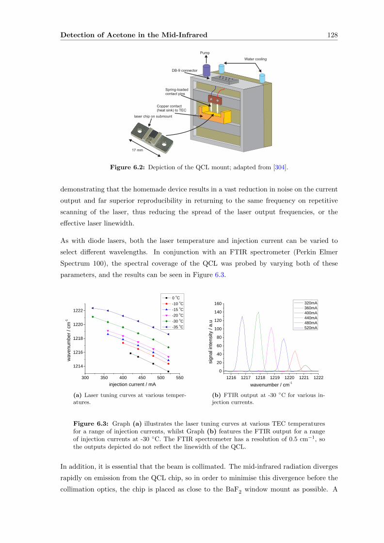
Detection of Acetone in the Mid-Infrared 128
Figure 6.2: Depiction of the QCL mount; adapted from [304].
demonstrating that the homemade device results in a vast reduction in noise on the current
output and far superior reproducibility in returning to the same frequency on repetitive
scanning of the laser, thus reducing the spread of the laser output frequencies, or the
effective laser linewidth.
As with diode lasers, both the laser temperature and injection current can be varied to
select different wavelengths. In conjunction with an FTIR spectrometer (Perkin Elmer
Spectrum 100), the spectral coverage of the QCL was probed by varying both of these
parameters, and the results can be seen in Figure 6.3.
3 0 0 3 5 0 4 0 0 4 5 0 5 0 0 5 5 0
1 2 1 4
1 2 1 6
1 2 1 8
1 2 2 0
1 2 2 2
wave
numb
er / c
m-1
i n j e c t i o n c u r r e n t / m A
0 o C - 1 0 o C - 1 5 o C - 2 0 o C - 3 0 o C - 3 5 o C
(a) Laser tuning curves at various temper-atures.
1 2 1 6 1 2 1 7 1 2 1 8 1 2 1 9 1 2 2 0 1 2 2 1 1 2 2 20
2 04 06 08 0
1 0 01 2 01 4 01 6 0
signa
l inten
sity / a
.u
w a v e n u m b e r / c m - 1
3 2 0 m A 3 6 0 m A 4 0 0 m A 4 4 0 m A 4 8 0 m A 5 2 0 m A
(b) FTIR output at -30 C for various in-jection currents.
Figure 6.3: Graph (a) illustrates the laser tuning curves at various TEC temperaturesfor a range of injection currents, whilst Graph (b) features the FTIR output for a rangeof injection currents at -30 C. The FTIR spectrometer has a resolution of 0.5 cm−1, sothe outputs depicted do not reflect the linewidth of the QCL.
In addition, it is essential that the beam is collimated. The mid-infrared radiation diverges
rapidly on emission from the QCL chip, so in order to minimise this divergence before the
collimation optics, the chip is placed as close to the BaF2 window mount as possible. A
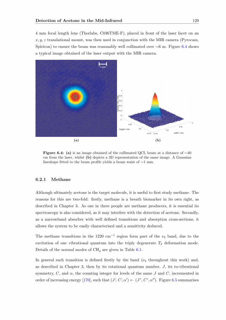
Detection of Acetone in the Mid-Infrared 129
4 mm focal length lens (Thorlabs, C036TME-F), placed in front of the laser facet on an
x, y, z translational mount, was then used in conjunction with the MIR camera (Pyrocam,
Spiricon) to ensure the beam was reasonably well collimated over ∼6 m. Figure 6.4 shows
a typical image obtained of the laser output with the MIR camera.
(a) (b)
Figure 6.4: (a) is an image obtained of the collimated QCL beam at a distance of ∼40cm from the laser, whilst (b) depicts a 3D representation of the same image. A Gaussianlineshape fitted to the beam profile yields a beam waist of ∼1 mm.
6.2.1 Methane
Although ultimately acetone is the target molecule, it is useful to first study methane. The
reasons for this are two-fold: firstly, methane is a breath biomarker in its own right, as
described in Chapter 3. As one in three people are methane producers, it is essential its
spectroscopy is also considered, as it may interfere with the detection of acetone. Secondly,
as a narrowband absorber with well defined transitions and absorption cross-sections, it
allows the system to be easily characterised and a sensitivity deduced.
The methane transitions in the 1220 cm−1 region form part of the ν4 band, due to the
excitation of one vibrational quantum into the triply degenerate T2 deformation mode.
Details of the normal modes of CH4 are given in Table 6.1.
In general each transition is defined firstly by the band (ν4 throughout this work) and,
as described in Chapter 3, then by its rotational quantum number, J , its ro-vibrational
symmetry, C, and α, the counting integer for levels of the same J and C, incremented in
order of increasing energy [170], such that (J’,C’, α′)← (J”,C”, α′′). Figure 6.5 summarises
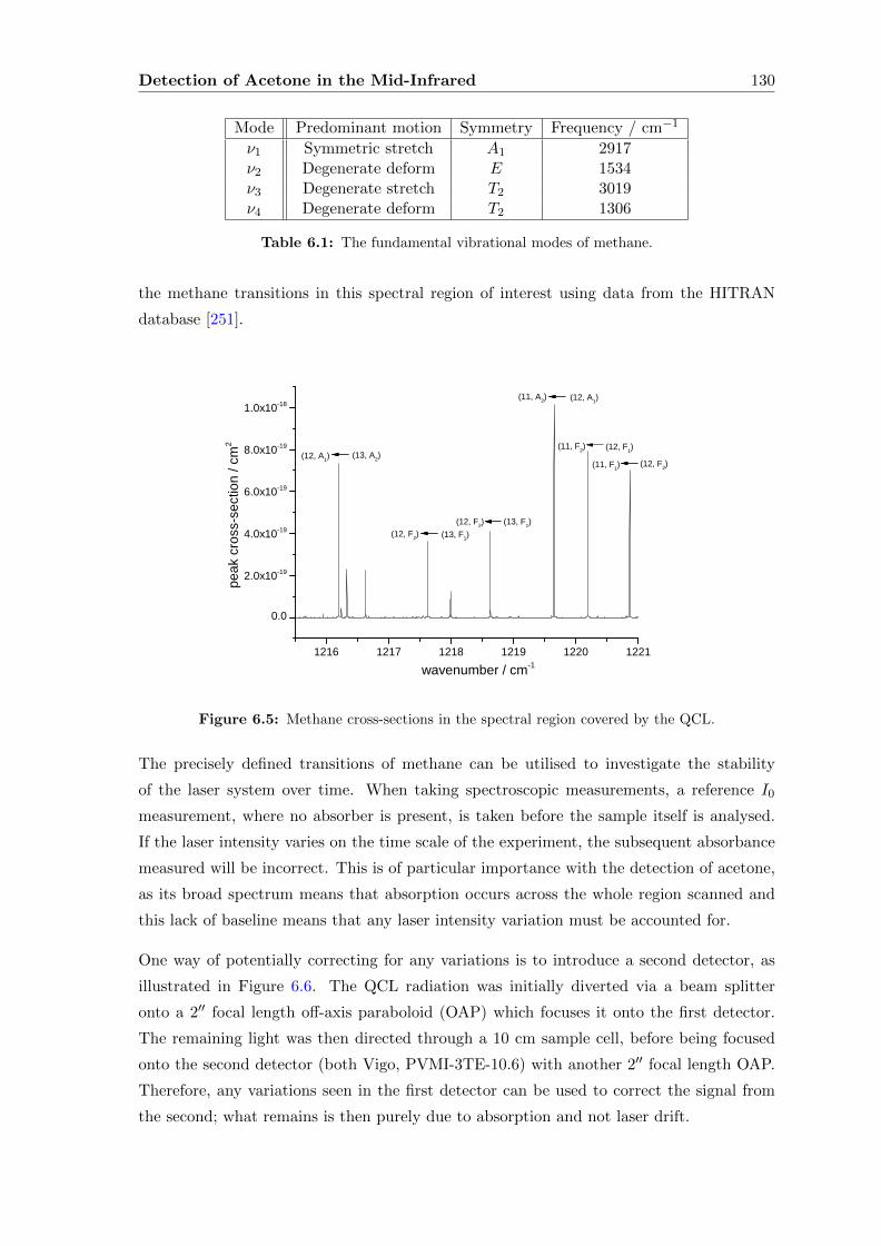
Detection of Acetone in the Mid-Infrared 130
Mode Predominant motion Symmetry Frequency / cm−1
ν1 Symmetric stretch A1 2917ν2 Degenerate deform E 1534ν3 Degenerate stretch T2 3019ν4 Degenerate deform T2 1306
Table 6.1: The fundamental vibrational modes of methane.
the methane transitions in this spectral region of interest using data from the HITRAN
database [251].
1 2 1 6 1 2 1 7 1 2 1 8 1 2 1 9 1 2 2 0 1 2 2 1
0 . 0
2 . 0 x 1 0 - 1 9
4 . 0 x 1 0 - 1 9
6 . 0 x 1 0 - 1 9
8 . 0 x 1 0 - 1 9
1 . 0 x 1 0 - 1 8
peak
cros
s-sec
tion /
cm2
w a v e n u m b e r / c m - 1
( 1 1 , F 2 ) ( 1 2 , F 1 )( 1 2 , A 1 ) ( 1 3 , A 2 )
( 1 2 , F 2 ) ( 1 3 , F 1 )( 1 2 , F 2 ) ( 1 3 , F 1 )
( 1 1 , A 2 ) ( 1 2 , A 1 )
( 1 1 , F 1 ) ( 1 2 , F 2 )
Figure 6.5: Methane cross-sections in the spectral region covered by the QCL.
The precisely defined transitions of methane can be utilised to investigate the stability
of the laser system over time. When taking spectroscopic measurements, a reference I0
measurement, where no absorber is present, is taken before the sample itself is analysed.
If the laser intensity varies on the time scale of the experiment, the subsequent absorbance
measured will be incorrect. This is of particular importance with the detection of acetone,
as its broad spectrum means that absorption occurs across the whole region scanned and
this lack of baseline means that any laser intensity variation must be accounted for.
One way of potentially correcting for any variations is to introduce a second detector, as
illustrated in Figure 6.6. The QCL radiation was initially diverted via a beam splitter
onto a 2′′ focal length off-axis paraboloid (OAP) which focuses it onto the first detector.
The remaining light was then directed through a 10 cm sample cell, before being focused
onto the second detector (both Vigo, PVMI-3TE-10.6) with another 2′′ focal length OAP.
Therefore, any variations seen in the first detector can be used to correct the signal from
the second; what remains is then purely due to absorption and not laser drift.
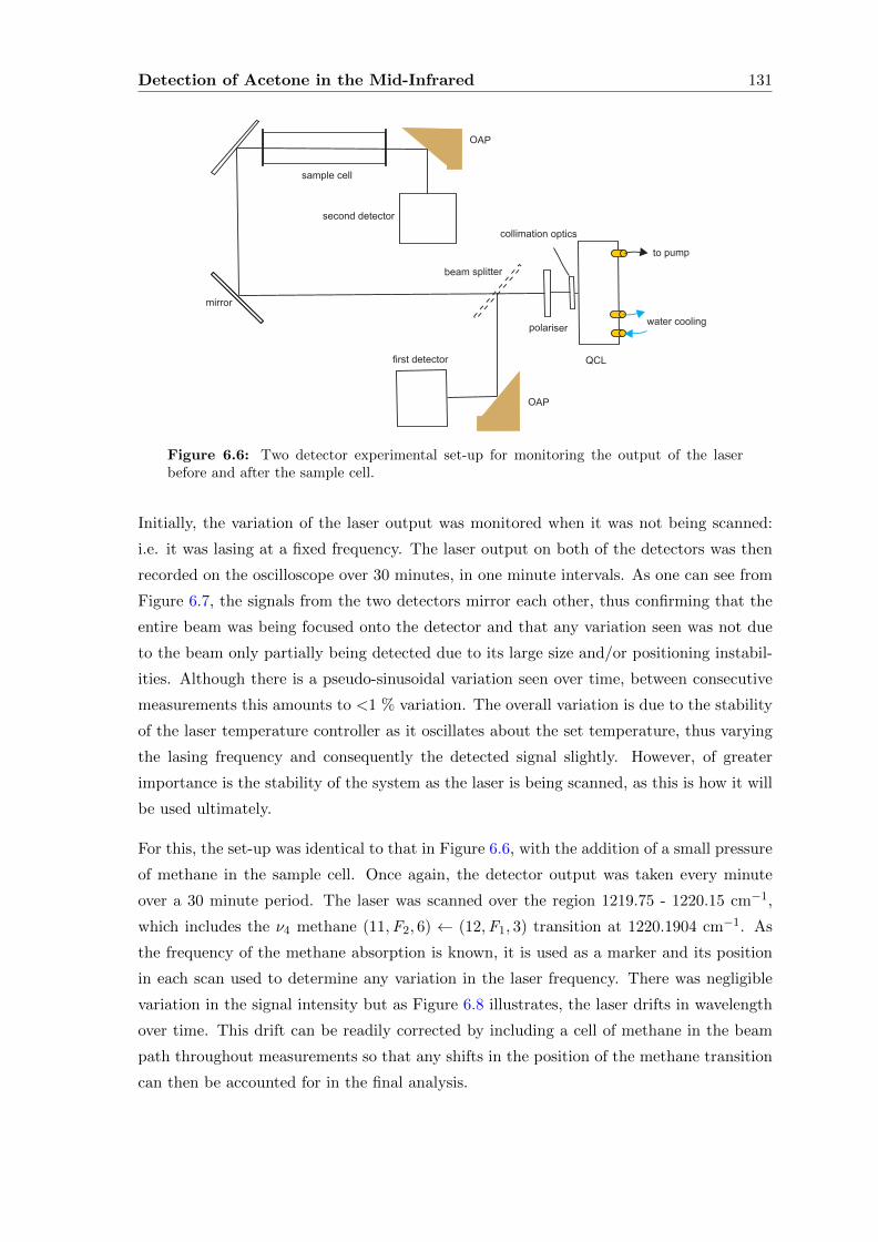
Detection of Acetone in the Mid-Infrared 131
Figure 6.6: Two detector experimental set-up for monitoring the output of the laserbefore and after the sample cell.
Initially, the variation of the laser output was monitored when it was not being scanned:
i.e. it was lasing at a fixed frequency. The laser output on both of the detectors was then
recorded on the oscilloscope over 30 minutes, in one minute intervals. As one can see from
Figure 6.7, the signals from the two detectors mirror each other, thus confirming that the
entire beam was being focused onto the detector and that any variation seen was not due
to the beam only partially being detected due to its large size and/or positioning instabil-
ities. Although there is a pseudo-sinusoidal variation seen over time, between consecutive
measurements this amounts to <1 % variation. The overall variation is due to the stability
of the laser temperature controller as it oscillates about the set temperature, thus varying
the lasing frequency and consequently the detected signal slightly. However, of greater
importance is the stability of the system as the laser is being scanned, as this is how it will
be used ultimately.
For this, the set-up was identical to that in Figure 6.6, with the addition of a small pressure
of methane in the sample cell. Once again, the detector output was taken every minute
over a 30 minute period. The laser was scanned over the region 1219.75 - 1220.15 cm−1,
which includes the ν4 methane (11,F2, 6) ← (12,F1, 3) transition at 1220.1904 cm−1. As
the frequency of the methane absorption is known, it is used as a marker and its position
in each scan used to determine any variation in the laser frequency. There was negligible
variation in the signal intensity but as Figure 6.8 illustrates, the laser drifts in wavelength
over time. This drift can be readily corrected by including a cell of methane in the beam
path throughout measurements so that any shifts in the position of the methane transition
can then be accounted for in the final analysis.
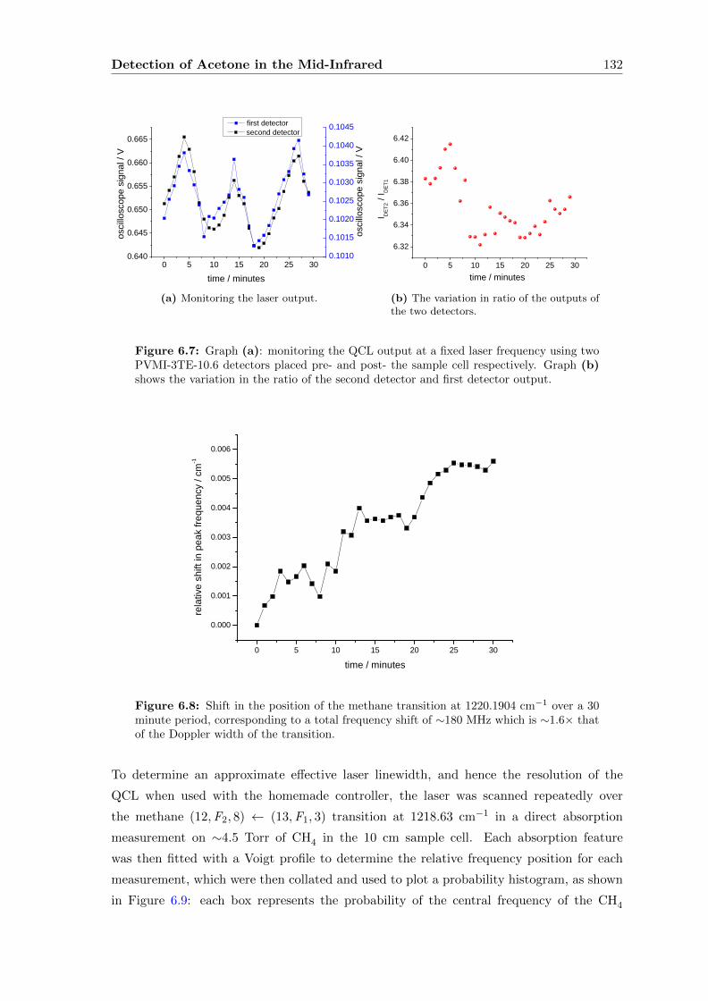
Detection of Acetone in the Mid-Infrared 132
0 5 1 0 1 5 2 0 2 5 3 00 . 6 4 0
0 . 6 4 5
0 . 6 5 0
0 . 6 5 5
0 . 6 6 0
0 . 6 6 5os
cillos
cope
signa
l / V
t i m e / m i n u t e s
s e c o n d d e t e c t o r
0 . 1 0 1 00 . 1 0 1 50 . 1 0 2 00 . 1 0 2 50 . 1 0 3 00 . 1 0 3 50 . 1 0 4 00 . 1 0 4 5
oscill
osco
pe sig
nal /
V
f i r s t d e t e c t o r
(a) Monitoring the laser output.
0 5 1 0 1 5 2 0 2 5 3 06 . 3 2
6 . 3 4
6 . 3 6
6 . 3 8
6 . 4 0
6 . 4 2
I DET2
/ IDE
T1
t i m e / m i n u t e s(b) The variation in ratio of the outputs ofthe two detectors.
Figure 6.7: Graph (a): monitoring the QCL output at a fixed laser frequency using twoPVMI-3TE-10.6 detectors placed pre- and post- the sample cell respectively. Graph (b)shows the variation in the ratio of the second detector and first detector output.
0 5 1 0 1 5 2 0 2 5 3 0
0 . 0 0 0
0 . 0 0 1
0 . 0 0 2
0 . 0 0 3
0 . 0 0 4
0 . 0 0 5
0 . 0 0 6
relati
ve sh
ift in
peak
frequ
ency
/ cm-1
t i m e / m i n u t e s
Figure 6.8: Shift in the position of the methane transition at 1220.1904 cm−1 over a 30minute period, corresponding to a total frequency shift of ∼180 MHz which is ∼1.6× thatof the Doppler width of the transition.
To determine an approximate effective laser linewidth, and hence the resolution of the
QCL when used with the homemade controller, the laser was scanned repeatedly over
the methane (12,F2, 8) ← (13,F1, 3) transition at 1218.63 cm−1 in a direct absorption
measurement on ∼4.5 Torr of CH4 in the 10 cm sample cell. Each absorption feature
was then fitted with a Voigt profile to determine the relative frequency position for each
measurement, which were then collated and used to plot a probability histogram, as shown
in Figure 6.9: each box represents the probability of the central frequency of the CH4
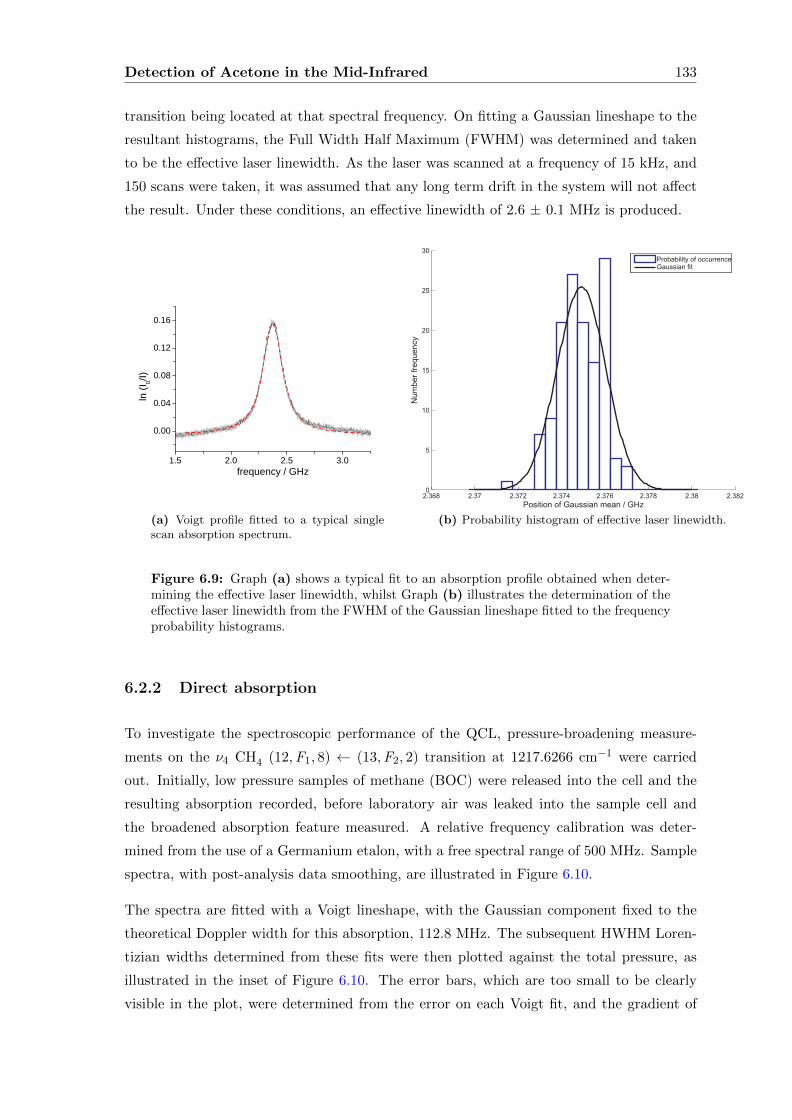
Detection of Acetone in the Mid-Infrared 133
transition being located at that spectral frequency. On fitting a Gaussian lineshape to the
resultant histograms, the Full Width Half Maximum (FWHM) was determined and taken
to be the effective laser linewidth. As the laser was scanned at a frequency of 15 kHz, and
150 scans were taken, it was assumed that any long term drift in the system will not affect
the result. Under these conditions, an effective linewidth of 2.6 ± 0.1 MHz is produced.
1 . 5 2 . 0 2 . 5 3 . 0
0 . 0 0
0 . 0 4
0 . 0 8
0 . 1 2
0 . 1 6
ln (I 0/I)
f r e q u e n c y / G H z
(a) Voigt profile fitted to a typical singlescan absorption spectrum.
(b) Probability histogram of effective laser linewidth.
Figure 6.9: Graph (a) shows a typical fit to an absorption profile obtained when deter-mining the effective laser linewidth, whilst Graph (b) illustrates the determination of theeffective laser linewidth from the FWHM of the Gaussian lineshape fitted to the frequencyprobability histograms.
6.2.2 Direct absorption
To investigate the spectroscopic performance of the QCL, pressure-broadening measure-
ments on the ν4 CH4 (12,F1, 8) ← (13,F2, 2) transition at 1217.6266 cm−1 were carried
out. Initially, low pressure samples of methane (BOC) were released into the cell and the
resulting absorption recorded, before laboratory air was leaked into the sample cell and
the broadened absorption feature measured. A relative frequency calibration was deter-
mined from the use of a Germanium etalon, with a free spectral range of 500 MHz. Sample
spectra, with post-analysis data smoothing, are illustrated in Figure 6.10.
The spectra are fitted with a Voigt lineshape, with the Gaussian component fixed to the
theoretical Doppler width for this absorption, 112.8 MHz. The subsequent HWHM Loren-
tizian widths determined from these fits were then plotted against the total pressure, as
illustrated in the inset of Figure 6.10. The error bars, which are too small to be clearly
visible in the plot, were determined from the error on each Voigt fit, and the gradient of
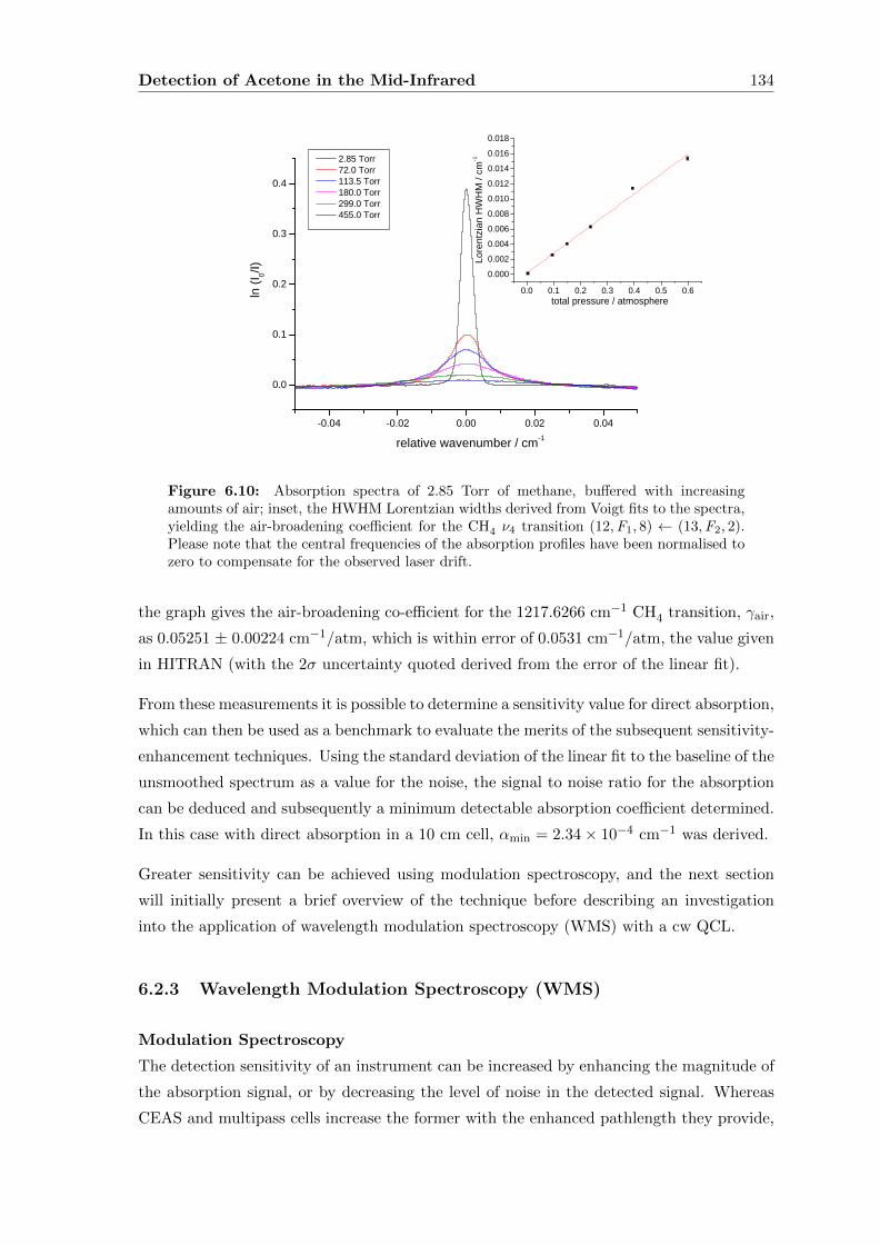
Detection of Acetone in the Mid-Infrared 134
- 0 . 0 4 - 0 . 0 2 0 . 0 0 0 . 0 2 0 . 0 4
0 . 0
0 . 1
0 . 2
0 . 3
0 . 4
0 . 0 0 . 1 0 . 2 0 . 3 0 . 4 0 . 5 0 . 60 . 0 0 00 . 0 0 20 . 0 0 40 . 0 0 60 . 0 0 80 . 0 1 00 . 0 1 20 . 0 1 40 . 0 1 60 . 0 1 8
t o t a l p r e s s u r e / a t m o s p h e r e
Loren
tzian
HWH
M / c
m-1
r e l a t i v e w a v e n u m b e r / c m - 1
ln (I 0/I)
2 . 8 5 T o r r 7 2 . 0 T o r r 1 1 3 . 5 T o r r 1 8 0 . 0 T o r r 2 9 9 . 0 T o r r 4 5 5 . 0 T o r r
Figure 6.10: Absorption spectra of 2.85 Torr of methane, buffered with increasingamounts of air; inset, the HWHM Lorentzian widths derived from Voigt fits to the spectra,yielding the air-broadening coefficient for the CH4 ν4 transition (12,F1, 8) ← (13,F2, 2).Please note that the central frequencies of the absorption profiles have been normalised tozero to compensate for the observed laser drift.
the graph gives the air-broadening co-efficient for the 1217.6266 cm−1 CH4 transition, γair,
as 0.05251 ± 0.00224 cm−1/atm, which is within error of 0.0531 cm−1/atm, the value given
in HITRAN (with the 2σ uncertainty quoted derived from the error of the linear fit).
From these measurements it is possible to determine a sensitivity value for direct absorption,
which can then be used as a benchmark to evaluate the merits of the subsequent sensitivity-
enhancement techniques. Using the standard deviation of the linear fit to the baseline of the
unsmoothed spectrum as a value for the noise, the signal to noise ratio for the absorption
can be deduced and subsequently a minimum detectable absorption coefficient determined.
In this case with direct absorption in a 10 cm cell, αmin = 2.34× 10⁻⁴ cm−1 was derived.
Greater sensitivity can be achieved using modulation spectroscopy, and the next section
will initially present a brief overview of the technique before describing an investigation
into the application of wavelength modulation spectroscopy (WMS) with a cw QCL.
6.2.3 Wavelength Modulation Spectroscopy (WMS)
Modulation Spectroscopy
The detection sensitivity of an instrument can be increased by enhancing the magnitude of
the absorption signal, or by decreasing the level of noise in the detected signal. Whereas
CEAS and multipass cells increase the former with the enhanced pathlength they provide,
Detection of Acetone in the Mid-Infrared 135
wavelength modulation spectroscopy (WMS) (developed first [306, 307]), and the related
technique, frequency modulation spectroscopy (FMS) [308], improve the detection limit by
reducing the noise in the absorption signal. Both techniques involve the application of a
high frequency modulation on top of the relatively low frequency applied to the laser to
scan its frequency over the absorption feature of interest. The detected signal then varies
at the modulation frequency applied, which must then be demodulated at a harmonic of
that modulation frequency to obtain the absorption feature. This demodulation is achieved
using phase sensitive detection provided by a lock-in amplifier, which is capable of filtering
out the components of the signal which are not at the same frequency and phase of the
modulation originally applied to the laser.
As discussed in Chapter 2, there are three major noise sources: shot noise, white noise and
external noise sources. The contributions from the latter are broadly categorised as 1/f
noise and are signal-dependent. Therefore, by moving to a higher frequency regime, 1/f
noise is necessarily reduced, though the degree to which the sensitivity is improved with
respect to direct absorption is dependent on the relative contributions of the different noise
sources.
Whether the modulation spectroscopy is classified as WMS or FMS depends entirely on
the relative frequency of the modulation applied compared to the linewidth (∆ν) of the
spectral feature of interest. With WMS, the modulation frequency is much smaller than
∆ν and tends to be in the kHz range, whilst the FMS modulation frequencies are much
larger than the spectral linewidth, and occur in the MHz/GHz regime [309]. One might
expect, therefore, that FMS will reduce the noise contribution further, but this is not
always found to be the case as the higher frequency regime also requires detectors with
faster response times and these higher bandwidth detectors often result in higher levels
of white noise. Therefore, it is often preferable to take advantage of the less complicated
electronics required for WMS, and this is the technique utilised here.
WMS Theory
The instantaneous frequency of laser light when a modulation is applied can be described
with the following equation:
ω(t) = ω0 + am cos(ωmt) (6.1)
where ω0 is the unmodulated centre frequency of the laser light, am is the amplitude of the
modulation and ωm is the modulation frequency. From this, the time-varying intensity of
the modulated light, I(ω0, t), can be described as a cosine Fourier series, as it is a periodic,
even function:
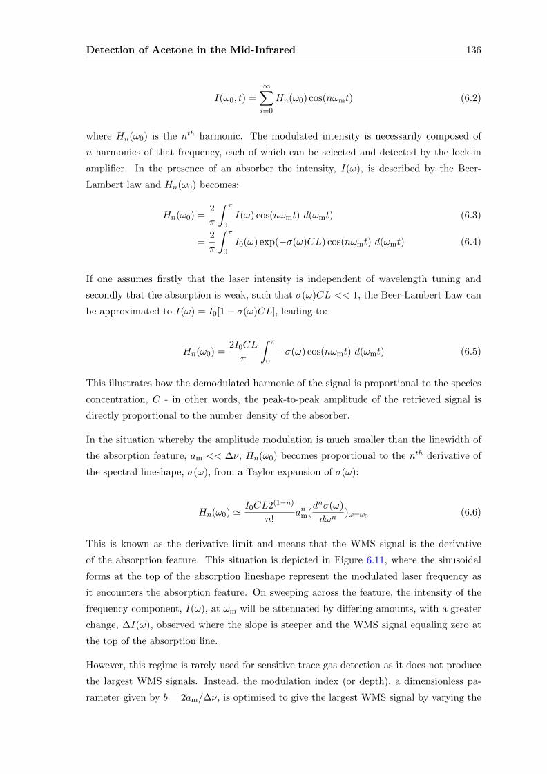
Detection of Acetone in the Mid-Infrared 136
I(ω0, t) =
∞∑i=0
Hn(ω0) cos(nωmt) (6.2)
where Hn(ω0) is the nth harmonic. The modulated intensity is necessarily composed of
n harmonics of that frequency, each of which can be selected and detected by the lock-in
amplifier. In the presence of an absorber the intensity, I(ω), is described by the Beer-
Lambert law and Hn(ω0) becomes:
Hn(ω0) =2
π
∫ π
0I(ω) cos(nωmt) d(ωmt) (6.3)
=2
π
∫ π
0I0(ω) exp(−σ(ω)CL) cos(nωmt) d(ωmt) (6.4)
If one assumes firstly that the laser intensity is independent of wavelength tuning and
secondly that the absorption is weak, such that σ(ω)CL << 1, the Beer-Lambert Law can
be approximated to I(ω) = I0[1− σ(ω)CL], leading to:
Hn(ω0) =2I0CL
π
∫ π
0−σ(ω) cos(nωmt) d(ωmt) (6.5)
This illustrates how the demodulated harmonic of the signal is proportional to the species
concentration, C - in other words, the peak-to-peak amplitude of the retrieved signal is
directly proportional to the number density of the absorber.
In the situation whereby the amplitude modulation is much smaller than the linewidth of
the absorption feature, am << ∆ν, Hn(ω0) becomes proportional to the nth derivative of
the spectral lineshape, σ(ω), from a Taylor expansion of σ(ω):
Hn(ω0) ' I0CL2(1−n)
n!anm(
dnσ(ω)
dωn)ω=ω0 (6.6)
This is known as the derivative limit and means that the WMS signal is the derivative
of the absorption feature. This situation is depicted in Figure 6.11, where the sinusoidal
forms at the top of the absorption lineshape represent the modulated laser frequency as
it encounters the absorption feature. On sweeping across the feature, the intensity of the
frequency component, I(ω), at ωm will be attenuated by differing amounts, with a greater
change, ∆I(ω), observed where the slope is steeper and the WMS signal equaling zero at
the top of the absorption line.
However, this regime is rarely used for sensitive trace gas detection as it does not produce
the largest WMS signals. Instead, the modulation index (or depth), a dimensionless pa-
rameter given by b = 2am/∆ν, is optimised to give the largest WMS signal by varying the
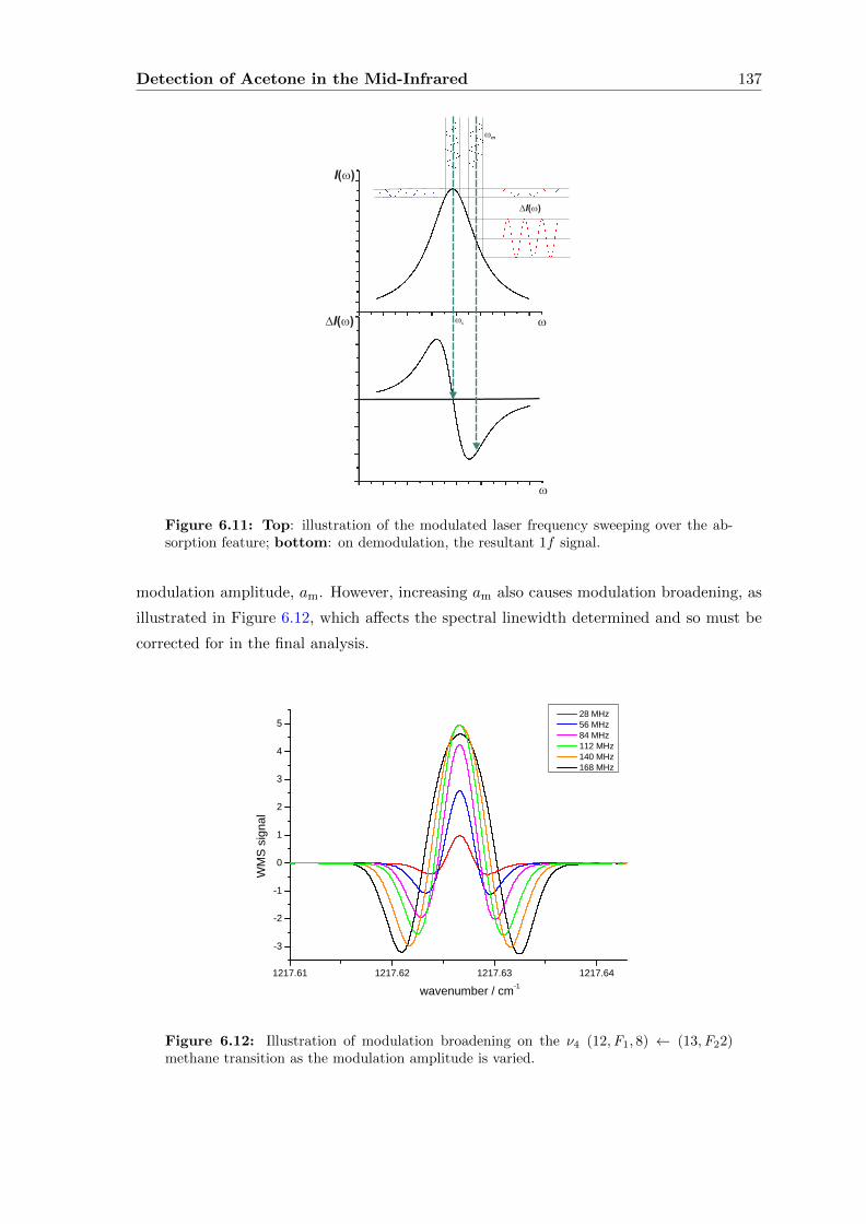
Detection of Acetone in the Mid-Infrared 137
Figure 6.11: Top: illustration of the modulated laser frequency sweeping over the ab-sorption feature; bottom: on demodulation, the resultant 1f signal.
modulation amplitude, am. However, increasing am also causes modulation broadening, as
illustrated in Figure 6.12, which affects the spectral linewidth determined and so must be
corrected for in the final analysis.
1 2 1 7 . 6 1 1 2 1 7 . 6 2 1 2 1 7 . 6 3 1 2 1 7 . 6 4
- 3
- 2
- 1
0
1
2
3
4
5
WMS s
ignal
w a v e n u m b e r / c m - 1
2 8 M H z 5 6 M H z 8 4 M H z 1 1 2 M H z 1 4 0 M H z 1 6 8 M H z
Figure 6.12: Illustration of modulation broadening on the ν4 (12,F1, 8) ← (13,F22)methane transition as the modulation amplitude is varied.
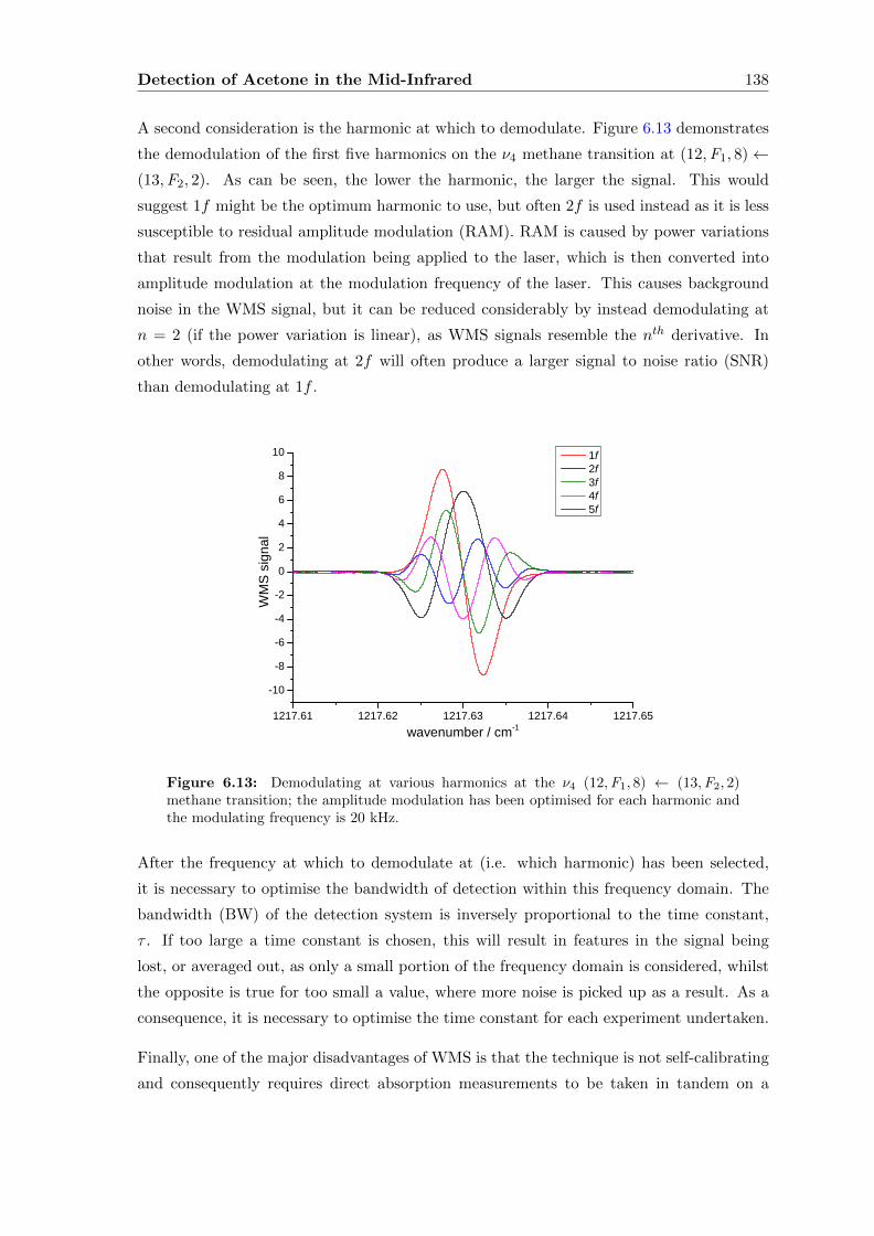
Detection of Acetone in the Mid-Infrared 138
A second consideration is the harmonic at which to demodulate. Figure 6.13 demonstrates
the demodulation of the first five harmonics on the ν4 methane transition at (12,F1, 8)←(13,F2, 2). As can be seen, the lower the harmonic, the larger the signal. This would
suggest 1f might be the optimum harmonic to use, but often 2f is used instead as it is less
susceptible to residual amplitude modulation (RAM). RAM is caused by power variations
that result from the modulation being applied to the laser, which is then converted into
amplitude modulation at the modulation frequency of the laser. This causes background
noise in the WMS signal, but it can be reduced considerably by instead demodulating at
n = 2 (if the power variation is linear), as WMS signals resemble the nth derivative. In
other words, demodulating at 2f will often produce a larger signal to noise ratio (SNR)
than demodulating at 1f .
1 2 1 7 . 6 1 1 2 1 7 . 6 2 1 2 1 7 . 6 3 1 2 1 7 . 6 4 1 2 1 7 . 6 5- 1 0
- 8- 6- 4- 202468
1 0
WMS s
ignal
w a v e n u m b e r / c m - 1
1 f 2 f 3 f 4 f 5 f
Figure 6.13: Demodulating at various harmonics at the ν4 (12,F1, 8) ← (13,F2, 2)methane transition; the amplitude modulation has been optimised for each harmonic andthe modulating frequency is 20 kHz.
After the frequency at which to demodulate at (i.e. which harmonic) has been selected,
it is necessary to optimise the bandwidth of detection within this frequency domain. The
bandwidth (BW) of the detection system is inversely proportional to the time constant,
τ . If too large a time constant is chosen, this will result in features in the signal being
lost, or averaged out, as only a small portion of the frequency domain is considered, whilst
the opposite is true for too small a value, where more noise is picked up as a result. As a
consequence, it is necessary to optimise the time constant for each experiment undertaken.
Finally, one of the major disadvantages of WMS is that the technique is not self-calibrating
and consequently requires direct absorption measurements to be taken in tandem on a
Detection of Acetone in the Mid-Infrared 139
strong absorption line to provide an absolute calibration for the technique. Alternative, self-
calibrating, methods have been proposed and demonstrated, most notably by Henningsen
and Simonsen [310] and Duffin, McGettick et al. [311–313], but both impose restrictions on
the flexibility of the technique: the former developed algorithms to determine the molecular
species density but the method requires the frequency tuning of the laser to be accurately
known and can only be applied to the second harmonic detection of isolated absorption
lines; whilst the latter, which utilises the RAM signal from a 1f trace for self-calibration,
dictates the use of a large absorption in the derivative limit. Within a laboratory setting,
such self-calibration methods are unnecessary and therefore are not employed in this work.
Experimental
The experimental set-up for WMS was identical to that utilised with direct absorption,
the only change was the introduction of a lock-in amplifier to provide the modulation
applied to the laser. A sample of 1.6 Torr of CH4 was fed into the glass cell and to find
the optimum value of the modulation amplitude (am) for the ν4 (12,F1, 8) ← (13,F2, 2)
methane transition, the modulation voltage was incrementally increased and the resulting
magnitude of the 1f and 2f peak-to-peak signals noted. Plotting the WMS signal against
the applied voltage, as in Figure 6.14, clearly shows the plateau at which point modulation
broadening dominates and increasing the voltage no longer causes an increase in the peak-
to-peak signal. For 1f , this optimum applied voltage was found to be 26 mV, whilst for 2f
it was 44 mV. These optimum WMS signals are then utilised to determine the linewidth
of the absorption feature under these conditions. As a low pressure of gas was used in this
analysis, we can assume that negligible pressure broadening takes place and thus a Gaussian
lineshape is expected. Work by Silver [314] has shown that the optimum modulation index,
b, for a Gaussian lineshape is 2.1 for the second harmonic and 1.6 for the first. Using this,
and the Doppler linewidth of the methane transition as determined from Figure 6.14b and
6.14d, the optimum modulation amplitudes were determined to be 100.4 MHz and 123.4
MHz for 1f and 2f respectively. In addition, signal to noise ratios were determined for
both the optimum 1f and 2f WMS measurements, and it was found that the 2f harmonic
produced a slightly higher SNR, 225 versus 200, and was thus used exclusively in the
following experiments.
As previously mentioned, it is necessary to take a direct absorption measurement alongside
a WMS measurement, in order to calibrate the technique. Therefore, initially a pressure of
0.27 Torr of methane was released into the cell and the (12,F1, 8) ← (13,F2, 2) transition
at 1217.6266 cm−1 was first probed with no high frequency modulation applied to the laser.
This allowed the exact methane concentration to be determined from the integrated area of
the recorded transition, before the WMS measurement was taken and the resultant peak-
to-peak amplitude attributed to the known pressure of methane in the cell. Sequential
amounts of methane were then removed from the cell and WMS measurements taken until
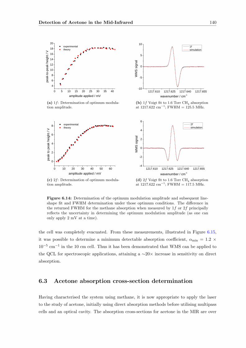
Detection of Acetone in the Mid-Infrared 140
0 5 1 0 1 5 2 0 2 5 3 0 3 5 4 0468
1 01 21 41 61 82 0
e x p e r i m e n t a l t h e o r y
peak
-to-pe
ak he
ight /
V
a m p l i t u d e a p p l i e d / m V(a) 1f : Determination of optimum modula-tion amplitude.
1 2 1 7 . 6 1 0 1 2 1 7 . 6 2 5 1 2 1 7 . 6 4 0 1 2 1 7 . 6 5 5- 1 0
- 5
0
5
1 0
WMS s
ignal
w a v e n u m b e r / c m - 1
1 f s i m u l a t i o n
(b) 1f Voigt fit to 1.6 Torr CH4 absorptionat 1217.622 cm−1; FWHM = 125.5 MHz.
0 1 0 2 0 3 0 4 0 5 0 6 0
0
2
4
6
8 e x p e r i m e n t a l t h e o r y
peak
to pe
ak he
ight /
V
a m p l i t u d e a p p l i e d / m V(c) 2f : Determination of optimum modula-tion amplitude.
1 2 1 7 . 6 1 0 1 2 1 7 . 6 2 5 1 2 1 7 . 6 4 0 1 2 1 7 . 6 5 5- 4
- 2
0
2
4
6
WMS s
ignal
w a v e n u m b e r / c m - 1
2 f s i m u l a t i o n
(d) 2f Voigt fit to 1.6 Torr CH4 absorptionat 1217.622 cm−1; FWHM = 117.5 MHz.
Figure 6.14: Determination of the optimum modulation amplitude and subsequent line-shape fit and FWHM determination under those optimum conditions. The difference inthe returned FWHM for the methane absorption when measured by 1f or 2f principallyreflects the uncertainty in determining the optimum modulation amplitude (as one canonly apply 2 mV at a time).
the cell was completely evacuated. From these measurements, illustrated in Figure 6.15,
it was possible to determine a minimum detectable absorption coefficient, αmin = 1.2 ×10⁻⁵ cm−1 in the 10 cm cell. Thus it has been demonstrated that WMS can be applied to
the QCL for spectroscopic applications, attaining a ∼20× increase in sensitivity on direct
absorption.
6.3 Acetone absorption cross-section determination
Having characterised the system using methane, it is now appropriate to apply the laser
to the study of acetone, initially using direct absorption methods before utilising multipass
cells and an optical cavity. The absorption cross-sections for acetone in the MIR are over
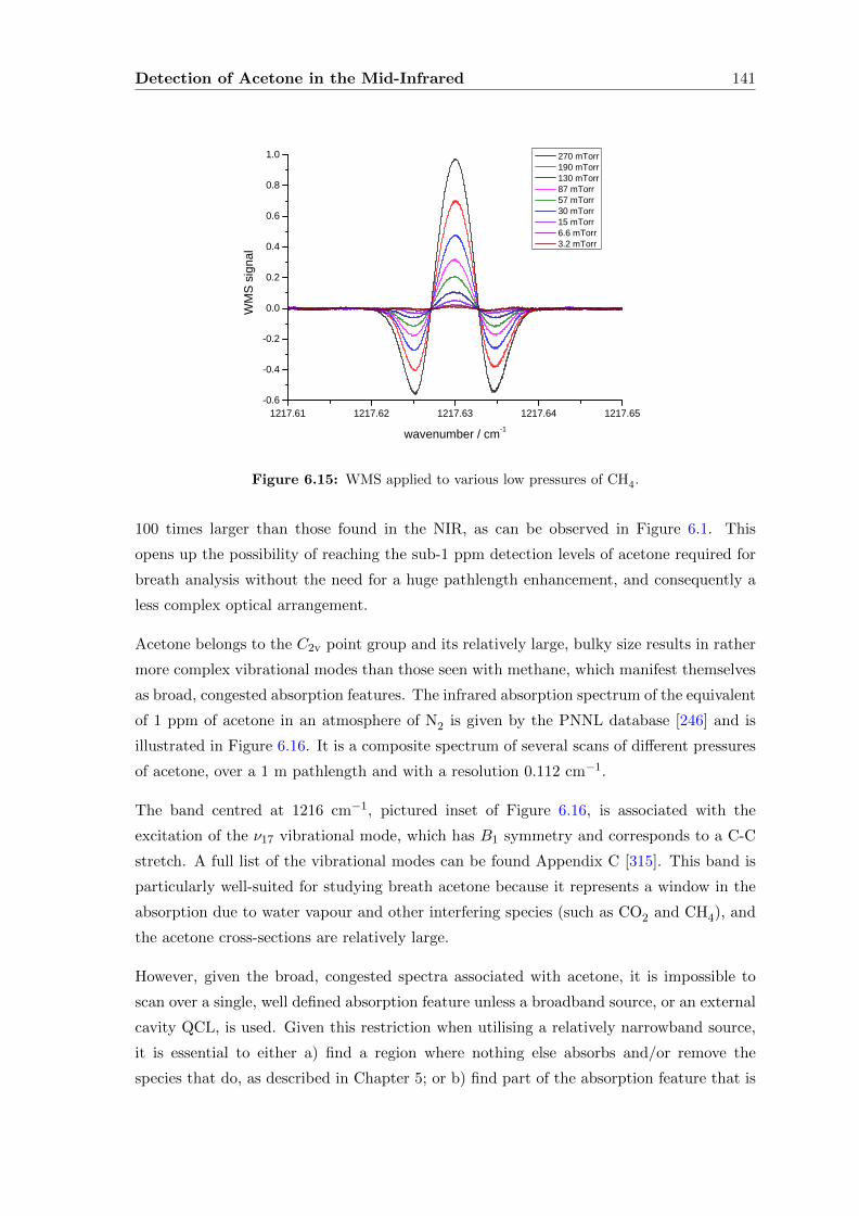
Detection of Acetone in the Mid-Infrared 141
1 2 1 7 . 6 1 1 2 1 7 . 6 2 1 2 1 7 . 6 3 1 2 1 7 . 6 4 1 2 1 7 . 6 5- 0 . 6
- 0 . 4
- 0 . 2
0 . 0
0 . 2
0 . 4
0 . 6
0 . 8
1 . 0
WMS s
ignal
w a v e n u m b e r / c m - 1
2 7 0 m T o r r 1 9 0 m T o r r 1 3 0 m T o r r 8 7 m T o r r 5 7 m T o r r 3 0 m T o r r 1 5 m T o r r 6 . 6 m T o r r 3 . 2 m T o r r
Figure 6.15: WMS applied to various low pressures of CH4.
100 times larger than those found in the NIR, as can be observed in Figure 6.1. This
opens up the possibility of reaching the sub-1 ppm detection levels of acetone required for
breath analysis without the need for a huge pathlength enhancement, and consequently a
less complex optical arrangement.
Acetone belongs to the C2v point group and its relatively large, bulky size results in rather
more complex vibrational modes than those seen with methane, which manifest themselves
as broad, congested absorption features. The infrared absorption spectrum of the equivalent
of 1 ppm of acetone in an atmosphere of N2 is given by the PNNL database [246] and is
illustrated in Figure 6.16. It is a composite spectrum of several scans of different pressures
of acetone, over a 1 m pathlength and with a resolution 0.112 cm−1.
The band centred at 1216 cm−1, pictured inset of Figure 6.16, is associated with the
excitation of the ν17 vibrational mode, which has B1 symmetry and corresponds to a C-C
stretch. A full list of the vibrational modes can be found Appendix C [315]. This band is
particularly well-suited for studying breath acetone because it represents a window in the
absorption due to water vapour and other interfering species (such as CO2 and CH4), and
the acetone cross-sections are relatively large.
However, given the broad, congested spectra associated with acetone, it is impossible to
scan over a single, well defined absorption feature unless a broadband source, or an external
cavity QCL, is used. Given this restriction when utilising a relatively narrowband source,
it is essential to either a) find a region where nothing else absorbs and/or remove the
species that do, as described in Chapter 5; or b) find part of the absorption feature that is
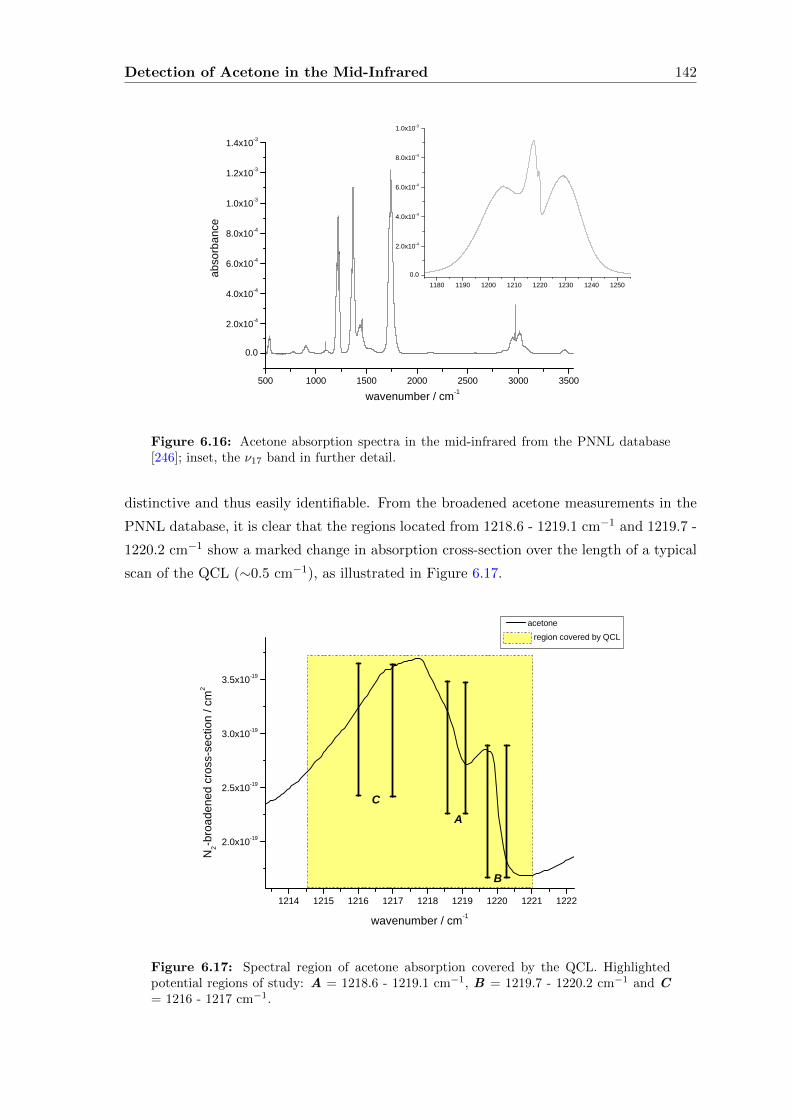
Detection of Acetone in the Mid-Infrared 142
5 0 0 1 0 0 0 1 5 0 0 2 0 0 0 2 5 0 0 3 0 0 0 3 5 0 0
0 . 0
2 . 0 x 1 0 - 4
4 . 0 x 1 0 - 4
6 . 0 x 1 0 - 4
8 . 0 x 1 0 - 4
1 . 0 x 1 0 - 3
1 . 2 x 1 0 - 3
1 . 4 x 1 0 - 3
1 1 8 0 1 1 9 0 1 2 0 0 1 2 1 0 1 2 2 0 1 2 3 0 1 2 4 0 1 2 5 00 . 0
2 . 0 x 1 0 - 4
4 . 0 x 1 0 - 4
6 . 0 x 1 0 - 4
8 . 0 x 1 0 - 4
1 . 0 x 1 0 - 3
w a v e n u m b e r / c m - 1
abso
rbanc
e
Figure 6.16: Acetone absorption spectra in the mid-infrared from the PNNL database[246]; inset, the ν17 band in further detail.
distinctive and thus easily identifiable. From the broadened acetone measurements in the
PNNL database, it is clear that the regions located from 1218.6 - 1219.1 cm−1 and 1219.7 -
1220.2 cm−1 show a marked change in absorption cross-section over the length of a typical
scan of the QCL (∼0.5 cm−1), as illustrated in Figure 6.17.
1 2 1 4 1 2 1 5 1 2 1 6 1 2 1 7 1 2 1 8 1 2 1 9 1 2 2 0 1 2 2 1 1 2 2 2
2 . 0 x 1 0 - 1 9
2 . 5 x 1 0 - 1 9
3 . 0 x 1 0 - 1 9
3 . 5 x 1 0 - 1 9
A
B
N 2-broa
dene
d cros
s-sec
tion /
cm2
w a v e n u m b e r / c m - 1
a c e t o n e r e g i o n c o v e r e d b y Q C L
C
Figure 6.17: Spectral region of acetone absorption covered by the QCL. Highlightedpotential regions of study: A = 1218.6 - 1219.1 cm−1, B = 1219.7 - 1220.2 cm−1 and C= 1216 - 1217 cm−1.
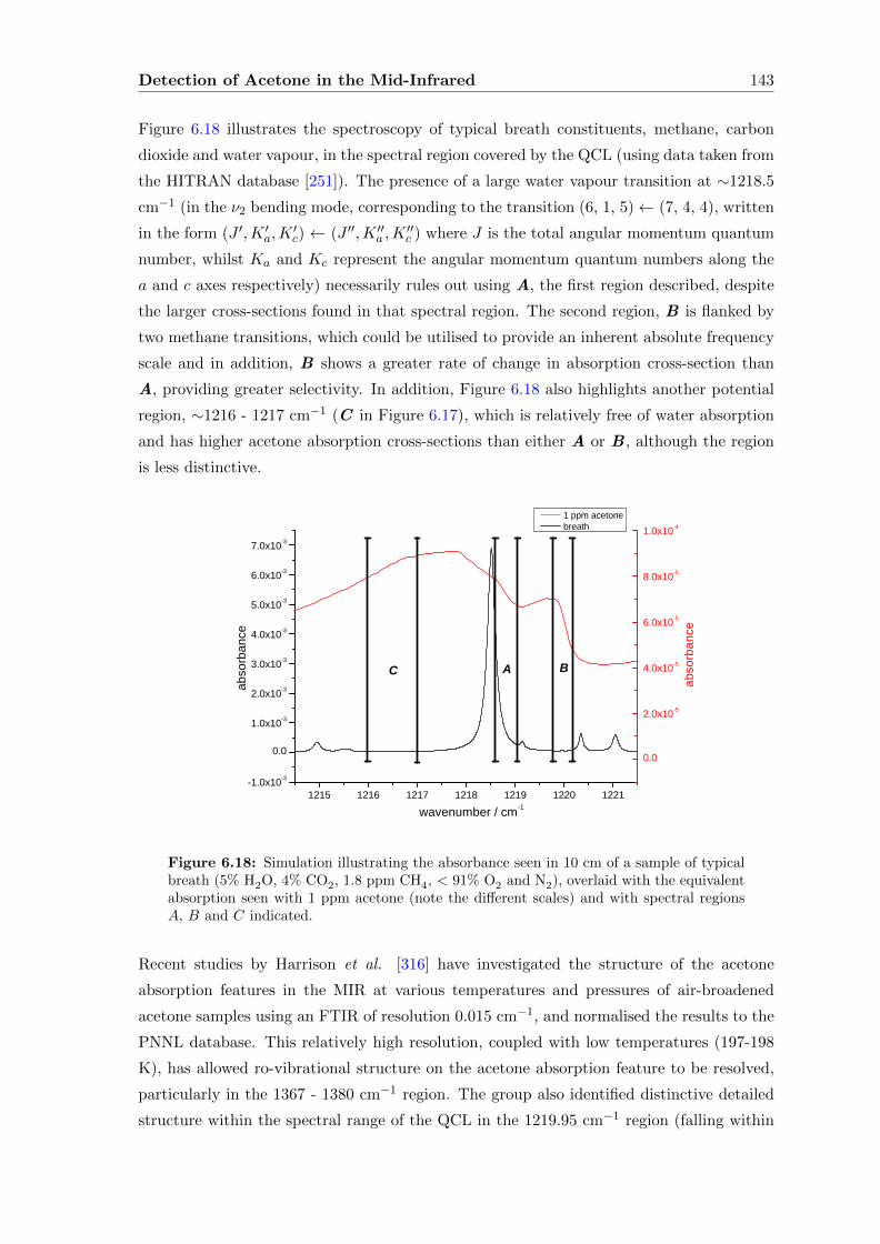
Detection of Acetone in the Mid-Infrared 143
Figure 6.18 illustrates the spectroscopy of typical breath constituents, methane, carbon
dioxide and water vapour, in the spectral region covered by the QCL (using data taken from
the HITRAN database [251]). The presence of a large water vapour transition at ∼1218.5
cm−1 (in the ν2 bending mode, corresponding to the transition (6, 1, 5)← (7, 4, 4), written
in the form (J ′,K ′a,K′c) ← (J ′′,K ′′a ,K
′′c ) where J is the total angular momentum quantum
number, whilst Ka and Kc represent the angular momentum quantum numbers along the
a and c axes respectively) necessarily rules out using A, the first region described, despite
the larger cross-sections found in that spectral region. The second region, B is flanked by
two methane transitions, which could be utilised to provide an inherent absolute frequency
scale and in addition, B shows a greater rate of change in absorption cross-section than
A, providing greater selectivity. In addition, Figure 6.18 also highlights another potential
region, ∼1216 - 1217 cm−1 (C in Figure 6.17), which is relatively free of water absorption
and has higher acetone absorption cross-sections than either A or B , although the region
is less distinctive.
1 2 1 5 1 2 1 6 1 2 1 7 1 2 1 8 1 2 1 9 1 2 2 0 1 2 2 1- 1 . 0 x 1 0 - 3
0 . 0
1 . 0 x 1 0 - 3
2 . 0 x 1 0 - 3
3 . 0 x 1 0 - 3
4 . 0 x 1 0 - 3
5 . 0 x 1 0 - 3
6 . 0 x 1 0 - 3
7 . 0 x 1 0 - 3
abso
rbanc
e
w a v e n u m b e r / c m - 1
1 p p m a c e t o n e b r e a t h
0 . 0
2 . 0 x 1 0 - 5
4 . 0 x 1 0 - 5
6 . 0 x 1 0 - 5
8 . 0 x 1 0 - 5
1 . 0 x 1 0 - 4
abso
rbanc
eC A B
Figure 6.18: Simulation illustrating the absorbance seen in 10 cm of a sample of typicalbreath (5% H2O, 4% CO2, 1.8 ppm CH4, < 91% O2 and N2), overlaid with the equivalentabsorption seen with 1 ppm acetone (note the different scales) and with spectral regionsA, B and C indicated.
Recent studies by Harrison et al. [316] have investigated the structure of the acetone
absorption features in the MIR at various temperatures and pressures of air-broadened
acetone samples using an FTIR of resolution 0.015 cm−1, and normalised the results to the
PNNL database. This relatively high resolution, coupled with low temperatures (197-198
K), has allowed ro-vibrational structure on the acetone absorption feature to be resolved,
particularly in the 1367 - 1380 cm−1 region. The group also identified distinctive detailed
structure within the spectral range of the QCL in the 1219.95 cm−1 region (falling within
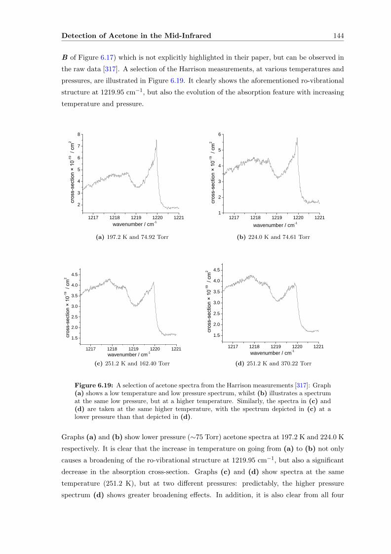
Detection of Acetone in the Mid-Infrared 144
B of Figure 6.17) which is not explicitly highlighted in their paper, but can be observed in
the raw data [317]. A selection of the Harrison measurements, at various temperatures and
pressures, are illustrated in Figure 6.19. It clearly shows the aforementioned ro-vibrational
structure at 1219.95 cm−1, but also the evolution of the absorption feature with increasing
temperature and pressure.
1 2 1 7 1 2 1 8 1 2 1 9 1 2 2 0 1 2 2 1
2345678
w a v e n u m b e r / c m - 1
(a) 197.2 K and 74.92 Torr
1 2 1 7 1 2 1 8 1 2 1 9 1 2 2 0 1 2 2 11
2
3
4
5
6
w a v e n u m b e r / c m - 1
(b) 224.0 K and 74.61 Torr
1 2 1 7 1 2 1 8 1 2 1 9 1 2 2 0 1 2 2 11 . 52 . 02 . 53 . 03 . 54 . 04 . 5
w a v e n u m b e r / c m - 1
(c) 251.2 K and 162.40 Torr
1 2 1 7 1 2 1 8 1 2 1 9 1 2 2 0 1 2 2 11 . 52 . 02 . 53 . 03 . 54 . 04 . 5
w a v e n u m b e r / c m - 1
(d) 251.2 K and 370.22 Torr
Figure 6.19: A selection of acetone spectra from the Harrison measurements [317]: Graph(a) shows a low temperature and low pressure spectrum, whilst (b) illustrates a spectrumat the same low pressure, but at a higher temperature. Similarly, the spectra in (c) and(d) are taken at the same higher temperature, with the spectrum depicted in (c) at alower pressure than that depicted in (d).
Graphs (a) and (b) show lower pressure (∼75 Torr) acetone spectra at 197.2 K and 224.0 K
respectively. It is clear that the increase in temperature on going from (a) to (b) not only
causes a broadening of the ro-vibrational structure at 1219.95 cm−1, but also a significant
decrease in the absorption cross-section. Graphs (c) and (d) show spectra at the same
temperature (251.2 K), but at two different pressures: predictably, the higher pressure
spectrum (d) shows greater broadening effects. In addition, it is also clear from all four
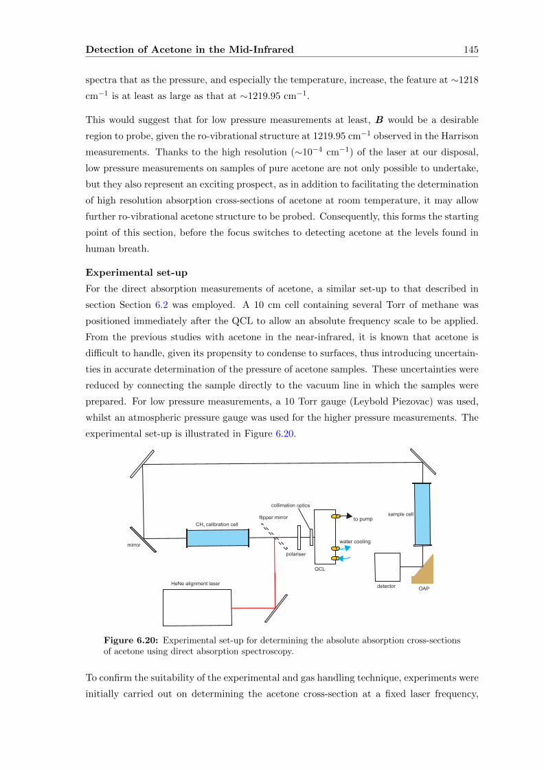
Detection of Acetone in the Mid-Infrared 145
spectra that as the pressure, and especially the temperature, increase, the feature at ∼1218
cm−1 is at least as large as that at ∼1219.95 cm−1.
This would suggest that for low pressure measurements at least, B would be a desirable
region to probe, given the ro-vibrational structure at 1219.95 cm−1 observed in the Harrison
measurements. Thanks to the high resolution (∼10−4 cm−1) of the laser at our disposal,
low pressure measurements on samples of pure acetone are not only possible to undertake,
but they also represent an exciting prospect, as in addition to facilitating the determination
of high resolution absorption cross-sections of acetone at room temperature, it may allow
further ro-vibrational acetone structure to be probed. Consequently, this forms the starting
point of this section, before the focus switches to detecting acetone at the levels found in
human breath.
Experimental set-up
For the direct absorption measurements of acetone, a similar set-up to that described in
section Section 6.2 was employed. A 10 cm cell containing several Torr of methane was
positioned immediately after the QCL to allow an absolute frequency scale to be applied.
From the previous studies with acetone in the near-infrared, it is known that acetone is
difficult to handle, given its propensity to condense to surfaces, thus introducing uncertain-
ties in accurate determination of the pressure of acetone samples. These uncertainties were
reduced by connecting the sample directly to the vacuum line in which the samples were
prepared. For low pressure measurements, a 10 Torr gauge (Leybold Piezovac) was used,
whilst an atmospheric pressure gauge was used for the higher pressure measurements. The
experimental set-up is illustrated in Figure 6.20.
Figure 6.20: Experimental set-up for determining the absolute absorption cross-sectionsof acetone using direct absorption spectroscopy.
To confirm the suitability of the experimental and gas handling technique, experiments were
initially carried out on determining the acetone cross-section at a fixed laser frequency,
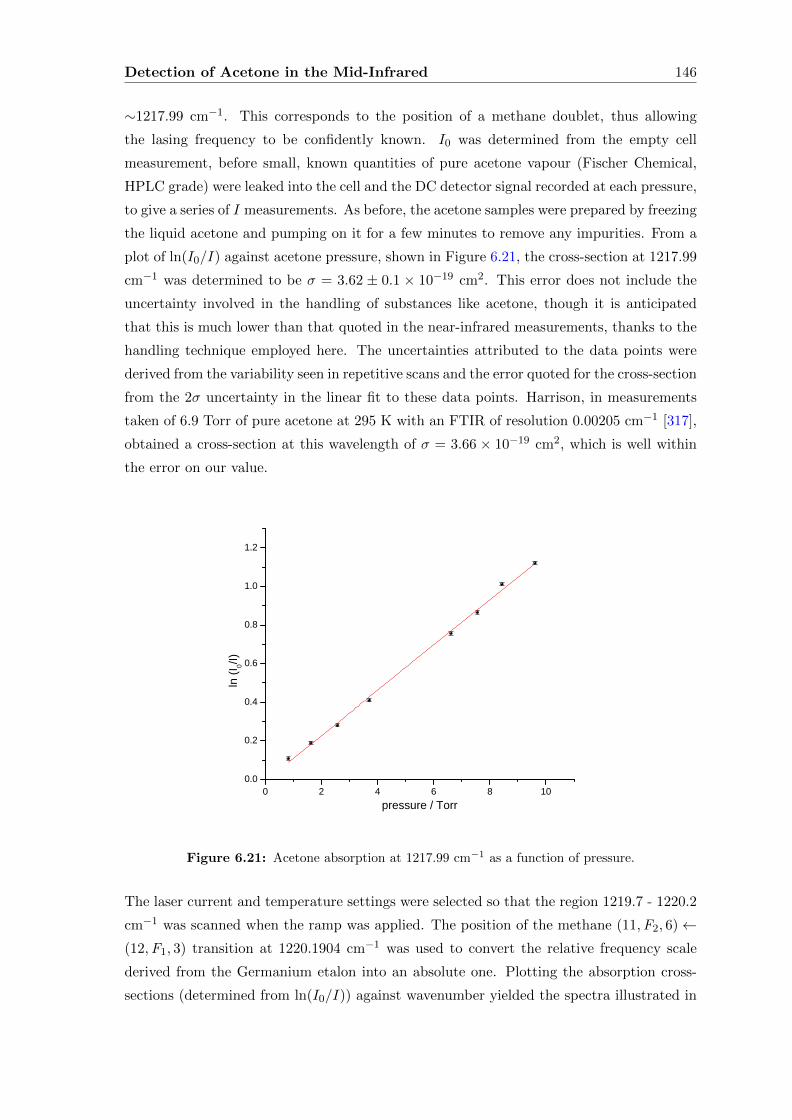
Detection of Acetone in the Mid-Infrared 146
∼1217.99 cm−1. This corresponds to the position of a methane doublet, thus allowing
the lasing frequency to be confidently known. I0 was determined from the empty cell
measurement, before small, known quantities of pure acetone vapour (Fischer Chemical,
HPLC grade) were leaked into the cell and the DC detector signal recorded at each pressure,
to give a series of I measurements. As before, the acetone samples were prepared by freezing
the liquid acetone and pumping on it for a few minutes to remove any impurities. From a
plot of ln(I0/I) against acetone pressure, shown in Figure 6.21, the cross-section at 1217.99
cm−1 was determined to be σ = 3.62 ± 0.1 × 10⁻¹⁹ cm2. This error does not include the
uncertainty involved in the handling of substances like acetone, though it is anticipated
that this is much lower than that quoted in the near-infrared measurements, thanks to the
handling technique employed here. The uncertainties attributed to the data points were
derived from the variability seen in repetitive scans and the error quoted for the cross-section
from the 2σ uncertainty in the linear fit to these data points. Harrison, in measurements
taken of 6.9 Torr of pure acetone at 295 K with an FTIR of resolution 0.00205 cm−1 [317],
obtained a cross-section at this wavelength of σ = 3.66 × 10⁻¹⁹ cm2, which is well within
the error on our value.
0 2 4 6 8 1 00 . 0
0 . 2
0 . 4
0 . 6
0 . 8
1 . 0
1 . 2
ln (I 0/I)
p r e s s u r e / T o r r
Figure 6.21: Acetone absorption at 1217.99 cm−1 as a function of pressure.
The laser current and temperature settings were selected so that the region 1219.7 - 1220.2
cm−1 was scanned when the ramp was applied. The position of the methane (11,F2, 6)←(12,F1, 3) transition at 1220.1904 cm−1 was used to convert the relative frequency scale
derived from the Germanium etalon into an absolute one. Plotting the absorption cross-
sections (determined from ln(I0/I)) against wavenumber yielded the spectra illustrated in

Detection of Acetone in the Mid-Infrared 147
Figure 6.22a.
These initial measurements, taken at 2 Torr, 4 Torr, 6 Torr and 8 Torr, illustrate the
presence of detailed structure, not visible in the broadened measurements from the PNNL
database, or the room temperature pressure-broadened measurements of Harrison et al
[316]. Low temperature studies from the same work highlighted the presence of rotational
structure in acetone spectra under those conditions, but these results demonstrate that the
structure can be resolved at room temperature with pure acetone samples. Most satisfying
is the fact that further experiments conducted latterly by Harrison and co-workers at room
temperature on low pressure (6.9 Torr) pure acetone samples produced cross-sections [317]
that match very well with the results from this study, as illustrated in Figure 6.22b.
1 2 1 9 . 7 1 2 1 9 . 8 1 2 1 9 . 9 1 2 2 0 . 0 1 2 2 0 . 12 . 0 x 1 0 - 1 9
2 . 5 x 1 0 - 1 9
3 . 0 x 1 0 - 1 9
3 . 5 x 1 0 - 1 9
4 . 0 x 1 0 - 1 9
cross-
sectio
n / cm
2
w a v e n u m b e r / c m - 1
2 . 0 6 T o r r 4 . 0 4 T o r r 6 . 1 8 T o r r 8 . 1 0 T o r r
(a)
1 2 1 9 . 6 1 2 1 9 . 7 1 2 1 9 . 8 1 2 1 9 . 9 1 2 2 0 . 0 1 2 2 0 . 12 . 4 x 1 0 - 1 9
2 . 6 x 1 0 - 1 9
2 . 8 x 1 0 - 1 9
3 . 0 x 1 0 - 1 9
3 . 2 x 1 0 - 1 9
3 . 4 x 1 0 - 1 9
3 . 6 x 1 0 - 1 9cro
ss-se
ction /
cm2
w a v e n u m b e r / c m - 1
H a r r i s o n e t a l . t h i s s t u d y
(b)
Figure 6.22: (a) shows the measured absorption cross-sections of acetone at low pres-sures, whilst (b) demonstrates the excellent agreement observed in the cross-sections mea-sured in this study with those of Harrison [317] for ∼6-7 Torr of acetone at 296 K.
The lowest pressure data from Figure 6.22a suggests that further ro-vibrational structure,
in addition to the two features observed at ∼1219.96 cm−1 and ∼1219.90 cm−1, may be
discernible at lower pressures. A series of low pressure measurements were recorded and the
results are illustrated in Figure 6.23, clearly showing the presence of rotational structure. At
these low pressures, self-broadening is reduced and in conjunction with the high resolution
QCL, detailed rotational structure can be observed. With increasing pressure, the rotational
structure starts to broaden out until the regime is reached where only the two familiar
features at ∼1219.95 cm−1 are seen.
Following this, a series of measurements were undertaken at various different laser currents,
so that a region spanning from 1218.6 - 1220.4 cm−1 was probed. Each sub-region was
selected in such a way that there was sufficient overlap with the adjacent sections and that
a methane transition of known frequency was within each sub-region, so that a continuous
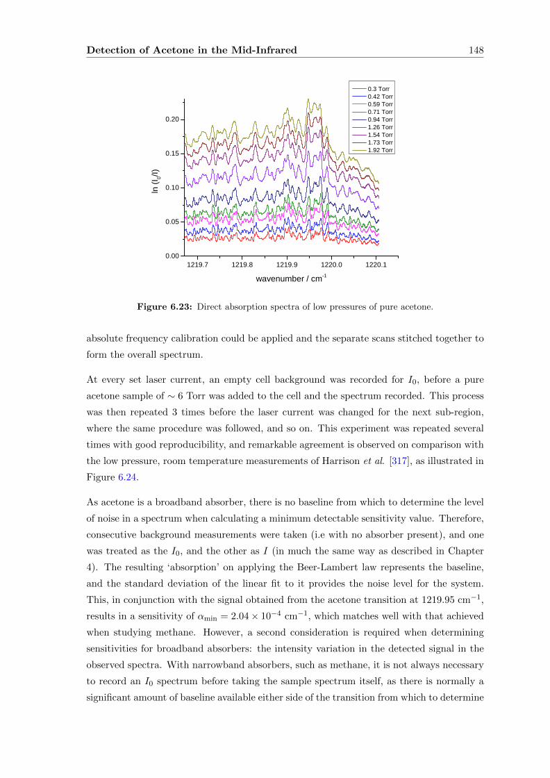
Detection of Acetone in the Mid-Infrared 148
1 2 1 9 . 7 1 2 1 9 . 8 1 2 1 9 . 9 1 2 2 0 . 0 1 2 2 0 . 10 . 0 0
0 . 0 5
0 . 1 0
0 . 1 5
0 . 2 0
ln (I 0/I)
w a v e n u m b e r / c m - 1
0 . 3 T o r r 0 . 4 2 T o r r 0 . 5 9 T o r r 0 . 7 1 T o r r 0 . 9 4 T o r r 1 . 2 6 T o r r 1 . 5 4 T o r r 1 . 7 3 T o r r 1 . 9 2 T o r r
Figure 6.23: Direct absorption spectra of low pressures of pure acetone.
absolute frequency calibration could be applied and the separate scans stitched together to
form the overall spectrum.
At every set laser current, an empty cell background was recorded for I0, before a pure
acetone sample of ∼ 6 Torr was added to the cell and the spectrum recorded. This process
was then repeated 3 times before the laser current was changed for the next sub-region,
where the same procedure was followed, and so on. This experiment was repeated several
times with good reproducibility, and remarkable agreement is observed on comparison with
the low pressure, room temperature measurements of Harrison et al. [317], as illustrated in
Figure 6.24.
As acetone is a broadband absorber, there is no baseline from which to determine the level
of noise in a spectrum when calculating a minimum detectable sensitivity value. Therefore,
consecutive background measurements were taken (i.e with no absorber present), and one
was treated as the I0, and the other as I (in much the same way as described in Chapter
4). The resulting ‘absorption’ on applying the Beer-Lambert law represents the baseline,
and the standard deviation of the linear fit to it provides the noise level for the system.
This, in conjunction with the signal obtained from the acetone transition at 1219.95 cm−1,
results in a sensitivity of αmin = 2.04× 10⁻⁴ cm−1, which matches well with that achieved
when studying methane. However, a second consideration is required when determining
sensitivities for broadband absorbers: the intensity variation in the detected signal in the
observed spectra. With narrowband absorbers, such as methane, it is not always necessary
to record an I0 spectrum before taking the sample spectrum itself, as there is normally a
significant amount of baseline available either side of the transition from which to determine
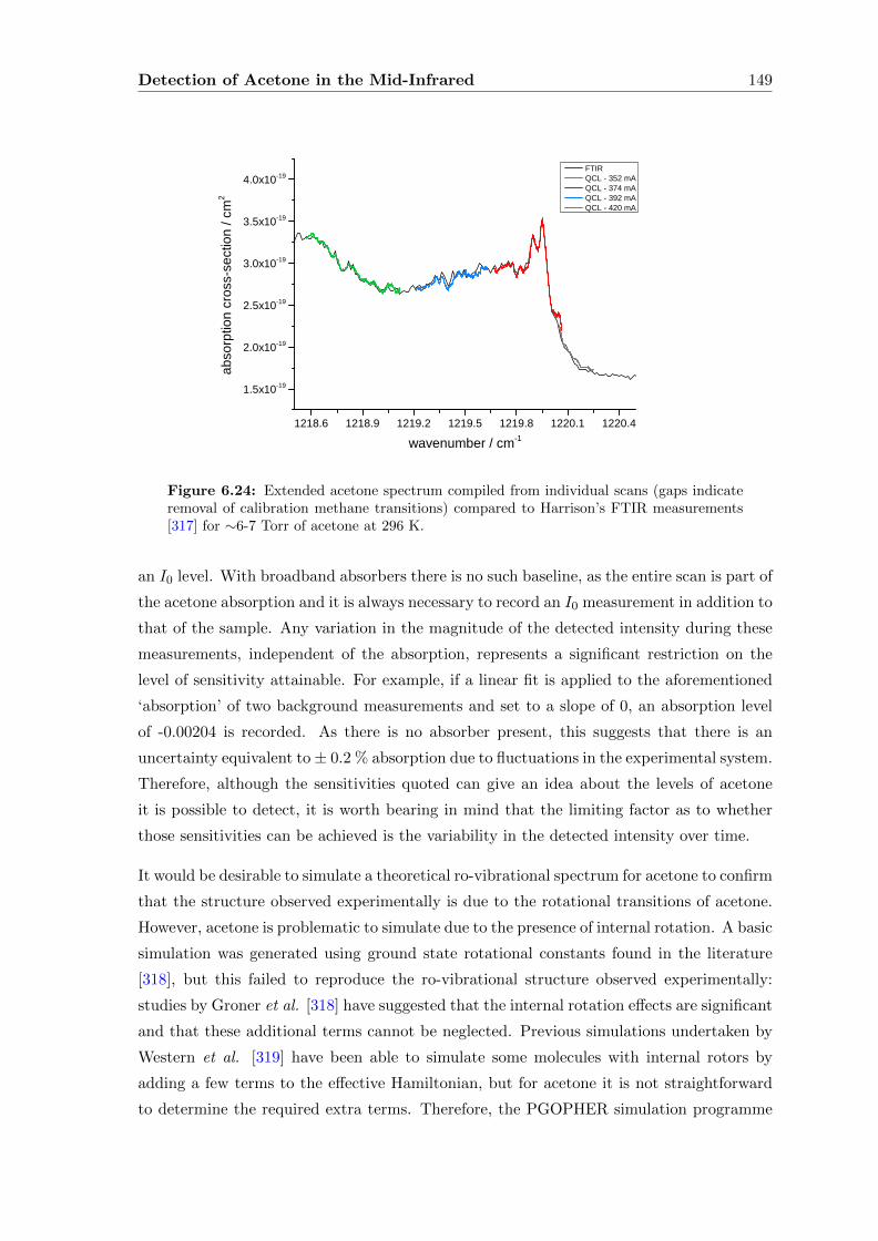
Detection of Acetone in the Mid-Infrared 149
1 2 1 8 . 6 1 2 1 8 . 9 1 2 1 9 . 2 1 2 1 9 . 5 1 2 1 9 . 8 1 2 2 0 . 1 1 2 2 0 . 4
1 . 5 x 1 0 - 1 9
2 . 0 x 1 0 - 1 9
2 . 5 x 1 0 - 1 9
3 . 0 x 1 0 - 1 9
3 . 5 x 1 0 - 1 9
4 . 0 x 1 0 - 1 9
abso
rption
cros
s-sec
tion /
cm2
w a v e n u m b e r / c m - 1
F T I R Q C L - 3 5 2 m A Q C L - 3 7 4 m A Q C L - 3 9 2 m A Q C L - 4 2 0 m A
Figure 6.24: Extended acetone spectrum compiled from individual scans (gaps indicateremoval of calibration methane transitions) compared to Harrison’s FTIR measurements[317] for ∼6-7 Torr of acetone at 296 K.
an I0 level. With broadband absorbers there is no such baseline, as the entire scan is part of
the acetone absorption and it is always necessary to record an I0 measurement in addition to
that of the sample. Any variation in the magnitude of the detected intensity during these
measurements, independent of the absorption, represents a significant restriction on the
level of sensitivity attainable. For example, if a linear fit is applied to the aforementioned
‘absorption’ of two background measurements and set to a slope of 0, an absorption level
of -0.00204 is recorded. As there is no absorber present, this suggests that there is an
uncertainty equivalent to± 0.2 % absorption due to fluctuations in the experimental system.
Therefore, although the sensitivities quoted can give an idea about the levels of acetone
it is possible to detect, it is worth bearing in mind that the limiting factor as to whether
those sensitivities can be achieved is the variability in the detected intensity over time.
It would be desirable to simulate a theoretical ro-vibrational spectrum for acetone to confirm
that the structure observed experimentally is due to the rotational transitions of acetone.
However, acetone is problematic to simulate due to the presence of internal rotation. A basic
simulation was generated using ground state rotational constants found in the literature
[318], but this failed to reproduce the ro-vibrational structure observed experimentally:
studies by Groner et al. [318] have suggested that the internal rotation effects are significant
and that these additional terms cannot be neglected. Previous simulations undertaken by
Western et al. [319] have been able to simulate some molecules with internal rotors by
adding a few terms to the effective Hamiltonian, but for acetone it is not straightforward
to determine the required extra terms. Therefore, the PGOPHER simulation programme
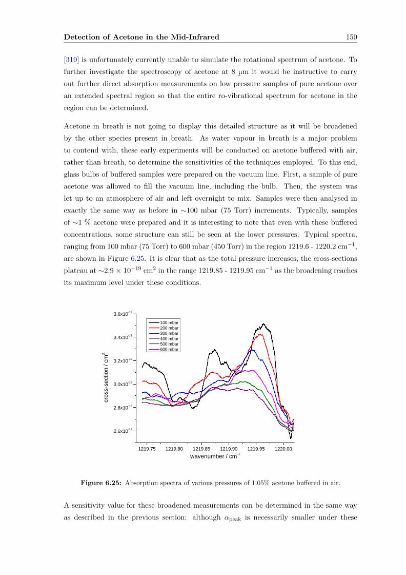
Detection of Acetone in the Mid-Infrared 150
[319] is unfortunately currently unable to simulate the rotational spectrum of acetone. To
further investigate the spectroscopy of acetone at 8 µm it would be instructive to carry
out further direct absorption measurements on low pressure samples of pure acetone over
an extended spectral region so that the entire ro-vibrational spectrum for acetone in the
region can be determined.
Acetone in breath is not going to display this detailed structure as it will be broadened
by the other species present in breath. As water vapour in breath is a major problem
to contend with, these early experiments will be conducted on acetone buffered with air,
rather than breath, to determine the sensitivities of the techniques employed. To this end,
glass bulbs of buffered samples were prepared on the vacuum line. First, a sample of pure
acetone was allowed to fill the vacuum line, including the bulb. Then, the system was
let up to an atmosphere of air and left overnight to mix. Samples were then analysed in
exactly the same way as before in ∼100 mbar (75 Torr) increments. Typically, samples
of ∼1 % acetone were prepared and it is interesting to note that even with these buffered
concentrations, some structure can still be seen at the lower pressures. Typical spectra,
ranging from 100 mbar (75 Torr) to 600 mbar (450 Torr) in the region 1219.6 - 1220.2 cm−1,
are shown in Figure 6.25. It is clear that as the total pressure increases, the cross-sections
plateau at ∼2.9 × 10⁻¹⁹ cm2 in the range 1219.85 - 1219.95 cm−1 as the broadening reaches
its maximum level under these conditions.
1 2 1 9 . 7 5 1 2 1 9 . 8 0 1 2 1 9 . 8 5 1 2 1 9 . 9 0 1 2 1 9 . 9 5 1 2 2 0 . 0 0
2 . 6 x 1 0 - 1 9
2 . 8 x 1 0 - 1 9
3 . 0 x 1 0 - 1 9
3 . 2 x 1 0 - 1 9
3 . 4 x 1 0 - 1 9
3 . 6 x 1 0 - 1 9
cross-
sectio
n / cm
2
w a v e n u m b e r / c m - 1
1 0 0 m b a r 2 0 0 m b a r 3 0 0 m b a r 4 0 0 m b a r 5 0 0 m b a r 6 0 0 m b a r
Figure 6.25: Absorption spectra of various pressures of 1.05% acetone buffered in air.
A sensitivity value for these broadened measurements can be determined in the same way
as described in the previous section: although αpeak is necessarily smaller under these
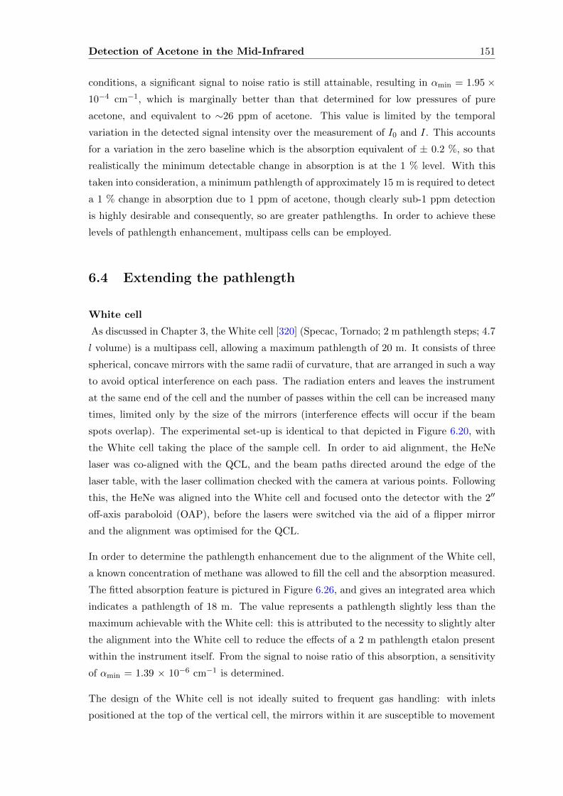
Detection of Acetone in the Mid-Infrared 151
conditions, a significant signal to noise ratio is still attainable, resulting in αmin = 1.95 ×10⁻⁴ cm−1, which is marginally better than that determined for low pressures of pure
acetone, and equivalent to ∼26 ppm of acetone. This value is limited by the temporal
variation in the detected signal intensity over the measurement of I0 and I. This accounts
for a variation in the zero baseline which is the absorption equivalent of ± 0.2 %, so that
realistically the minimum detectable change in absorption is at the 1 % level. With this
taken into consideration, a minimum pathlength of approximately 15 m is required to detect
a 1 % change in absorption due to 1 ppm of acetone, though clearly sub-1 ppm detection
is highly desirable and consequently, so are greater pathlengths. In order to achieve these
levels of pathlength enhancement, multipass cells can be employed.
6.4 Extending the pathlength
White cell
As discussed in Chapter 3, the White cell [320] (Specac, Tornado; 2 m pathlength steps; 4.7
l volume) is a multipass cell, allowing a maximum pathlength of 20 m. It consists of three
spherical, concave mirrors with the same radii of curvature, that are arranged in such a way
to avoid optical interference on each pass. The radiation enters and leaves the instrument
at the same end of the cell and the number of passes within the cell can be increased many
times, limited only by the size of the mirrors (interference effects will occur if the beam
spots overlap). The experimental set-up is identical to that depicted in Figure 6.20, with
the White cell taking the place of the sample cell. In order to aid alignment, the HeNe
laser was co-aligned with the QCL, and the beam paths directed around the edge of the
laser table, with the laser collimation checked with the camera at various points. Following
this, the HeNe was aligned into the White cell and focused onto the detector with the 2′′
off-axis paraboloid (OAP), before the lasers were switched via the aid of a flipper mirror
and the alignment was optimised for the QCL.
In order to determine the pathlength enhancement due to the alignment of the White cell,
a known concentration of methane was allowed to fill the cell and the absorption measured.
The fitted absorption feature is pictured in Figure 6.26, and gives an integrated area which
indicates a pathlength of 18 m. The value represents a pathlength slightly less than the
maximum achievable with the White cell: this is attributed to the necessity to slightly alter
the alignment into the White cell to reduce the effects of a 2 m pathlength etalon present
within the instrument itself. From the signal to noise ratio of this absorption, a sensitivity
of αmin = 1.39 × 10⁻⁶ cm−1 is determined.
The design of the White cell is not ideally suited to frequent gas handling: with inlets
positioned at the top of the vertical cell, the mirrors within it are susceptible to movement
Detection of Acetone in the Mid-Infrared 152
- 0 . 0 1 5 - 0 . 0 1 0 - 0 . 0 0 5 0 . 0 0 0 0 . 0 0 5 0 . 0 1 00 . 0
0 . 1
0 . 2
0 . 3
0 . 4
abso
rbanc
e
r e l a t i v e w a v e n u m b e r / c m - 1
3 . 4 T o r r C H 4 V o i g t f i t t o d a t a
Figure 6.26: Voigt fit to the methane (11,F2, 16)← (12,F1, 8) hot band (2 ← 1) transi-tion at 1218.7398 cm−1.
on addition or removal of gaseous samples, and as a result there can be some variability in
measurements of identical samples. Repeated measurements with nitrogen demonstrated
that careful manipulation of the gas inlet taps could significantly reduce the variability seen
due to the release of gas into the system (<1% in successive identical samples), and that
it was the evacuation of the cell that was the main culprit responsible for the change in
alignment. For this reason, when measurements were taken on acetone, an initial empty
cell was used as the background measurement (I0), before consecutive samples of acetone
were leaked into the cell. Given the increased pathlength available with the White cell, a
calibrated 25 ppm acetone in air mix (BOC Special Gases) was used and samples ranging
from 100 mbar to 900 mbar were analysed. However, it was noted that the White cell
etalon, which had been reduced by altering the entrance alignment, periodically came back
into prominence when filling the cell and pumping down on it. As a result, data taken still
exhibit etalon structure to a greater or lesser degree, so it was also necessary to apply a
Fourier Transform filter on the spectra to remove the effect analytically, the results from
which are illustrated in Figure 6.27.
From this, the absorption levels at 1219.925 cm−1 for each data set were determined and
plotted against total pressure of the acetone mix, resulting in Figure 6.28. The error bars are
derived from the variation observed in the absorption of samples of the same concentration.
The gradient of the plot in Figure 6.28, (σL/ kT ), indicates a cross-section of acetone at
this wavelength of σpeak = 2.78 ± 0.03 × 10⁻¹⁹ cm2, which agrees well with that quoted in
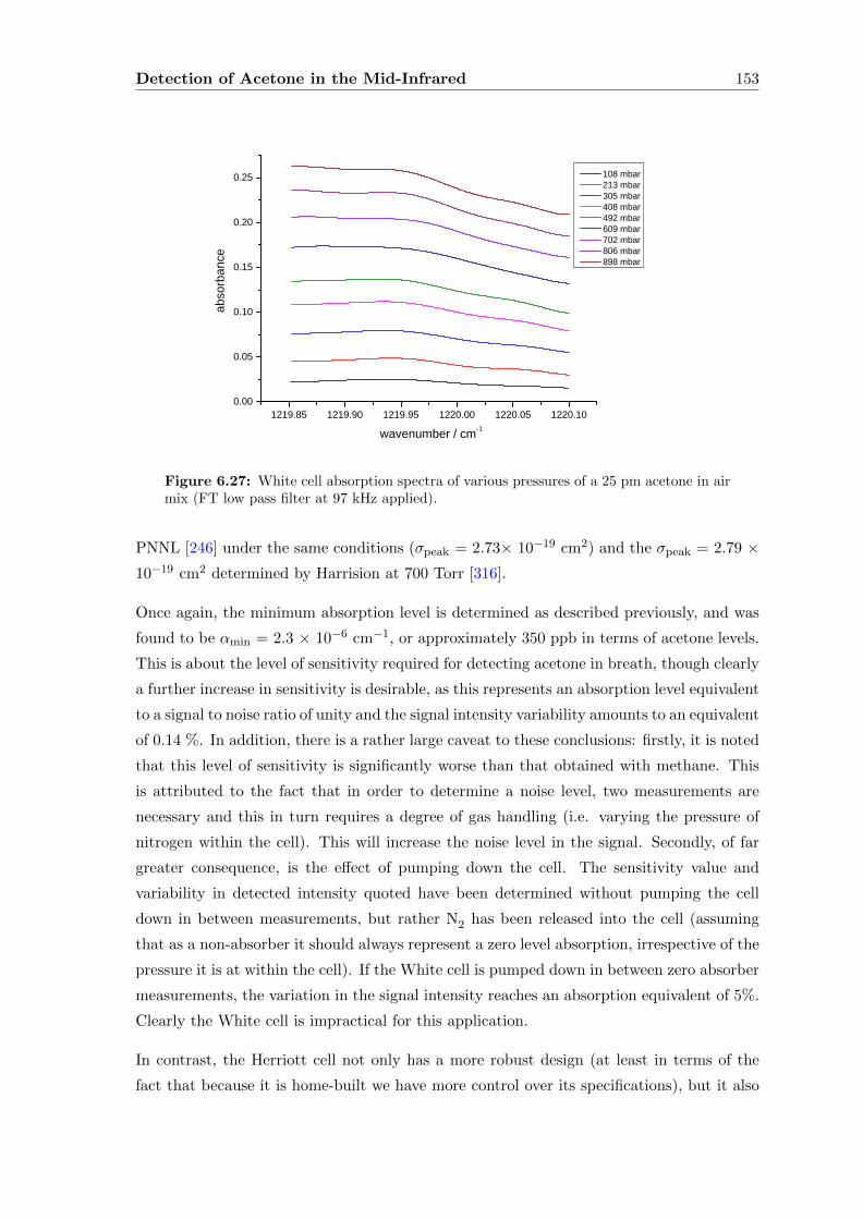
Detection of Acetone in the Mid-Infrared 153
1 2 1 9 . 8 5 1 2 1 9 . 9 0 1 2 1 9 . 9 5 1 2 2 0 . 0 0 1 2 2 0 . 0 5 1 2 2 0 . 1 00 . 0 0
0 . 0 5
0 . 1 0
0 . 1 5
0 . 2 0
0 . 2 5
abso
rbanc
e
w a v e n u m b e r / c m - 1
1 0 8 m b a r 2 1 3 m b a r 3 0 5 m b a r 4 0 8 m b a r 4 9 2 m b a r 6 0 9 m b a r 7 0 2 m b a r 8 0 6 m b a r 8 9 8 m b a r
Figure 6.27: White cell absorption spectra of various pressures of a 25 pm acetone in airmix (FT low pass filter at 97 kHz applied).
PNNL [246] under the same conditions (σpeak = 2.73× 10⁻¹⁹ cm2) and the σpeak = 2.79 ×10⁻¹⁹ cm2 determined by Harrision at 700 Torr [316].
Once again, the minimum absorption level is determined as described previously, and was
found to be αmin = 2.3 × 10⁻⁶ cm−1, or approximately 350 ppb in terms of acetone levels.
This is about the level of sensitivity required for detecting acetone in breath, though clearly
a further increase in sensitivity is desirable, as this represents an absorption level equivalent
to a signal to noise ratio of unity and the signal intensity variability amounts to an equivalent
of 0.14 %. In addition, there is a rather large caveat to these conclusions: firstly, it is noted
that this level of sensitivity is significantly worse than that obtained with methane. This
is attributed to the fact that in order to determine a noise level, two measurements are
necessary and this in turn requires a degree of gas handling (i.e. varying the pressure of
nitrogen within the cell). This will increase the noise level in the signal. Secondly, of far
greater consequence, is the effect of pumping down the cell. The sensitivity value and
variability in detected intensity quoted have been determined without pumping the cell
down in between measurements, but rather N2 has been released into the cell (assuming
that as a non-absorber it should always represent a zero level absorption, irrespective of the
pressure it is at within the cell). If the White cell is pumped down in between zero absorber
measurements, the variation in the signal intensity reaches an absorption equivalent of 5%.
Clearly the White cell is impractical for this application.
In contrast, the Herriott cell not only has a more robust design (at least in terms of the
fact that because it is home-built we have more control over its specifications), but it also
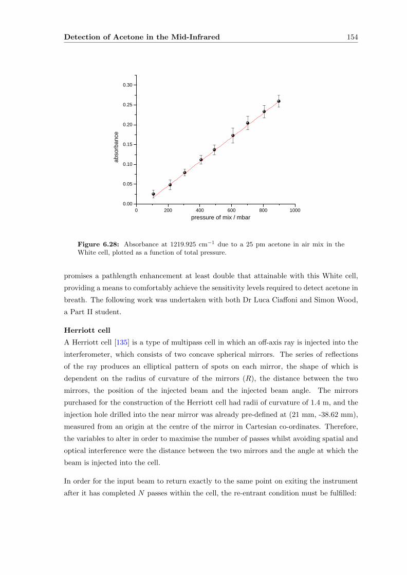
Detection of Acetone in the Mid-Infrared 154
0 2 0 0 4 0 0 6 0 0 8 0 0 1 0 0 00 . 0 0
0 . 0 5
0 . 1 0
0 . 1 5
0 . 2 0
0 . 2 5
0 . 3 0
abso
rbanc
e
p r e s s u r e o f m i x / m b a r
Figure 6.28: Absorbance at 1219.925 cm−1 due to a 25 pm acetone in air mix in theWhite cell, plotted as a function of total pressure.
promises a pathlength enhancement at least double that attainable with this White cell,
providing a means to comfortably achieve the sensitivity levels required to detect acetone in
breath. The following work was undertaken with both Dr Luca Ciaffoni and Simon Wood,
a Part II student.
Herriott cell
A Herriott cell [135] is a type of multipass cell in which an off-axis ray is injected into the
interferometer, which consists of two concave spherical mirrors. The series of reflections
of the ray produces an elliptical pattern of spots on each mirror, the shape of which is
dependent on the radius of curvature of the mirrors (R), the distance between the two
mirrors, the position of the injected beam and the injected beam angle. The mirrors
purchased for the construction of the Herriott cell had radii of curvature of 1.4 m, and the
injection hole drilled into the near mirror was already pre-defined at (21 mm, -38.62 mm),
measured from an origin at the centre of the mirror in Cartesian co-ordinates. Therefore,
the variables to alter in order to maximise the number of passes whilst avoiding spatial and
optical interference were the distance between the two mirrors and the angle at which the
beam is injected into the cell.
In order for the input beam to return exactly to the same point on exiting the instrument
after it has completed N passes within the cell, the re-entrant condition must be fulfilled:
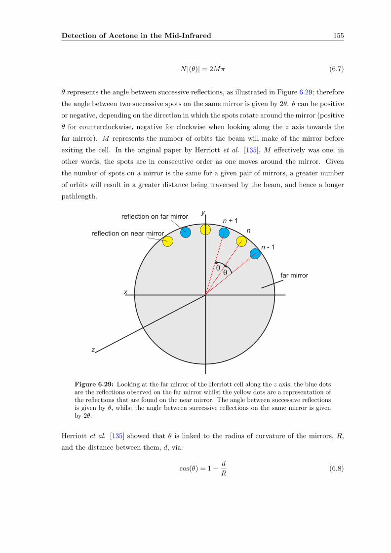
Detection of Acetone in the Mid-Infrared 155
N |(θ)| = 2Mπ (6.7)
θ represents the angle between successive reflections, as illustrated in Figure 6.29; therefore
the angle between two successive spots on the same mirror is given by 2θ. θ can be positive
or negative, depending on the direction in which the spots rotate around the mirror (positive
θ for counterclockwise, negative for clockwise when looking along the z axis towards the
far mirror). M represents the number of orbits the beam will make of the mirror before
exiting the cell. In the original paper by Herriott et al. [135], M effectively was one; in
other words, the spots are in consecutive order as one moves around the mirror. Given
the number of spots on a mirror is the same for a given pair of mirrors, a greater number
of orbits will result in a greater distance being traversed by the beam, and hence a longer
pathlength.
Figure 6.29: Looking at the far mirror of the Herriott cell along the z axis; the blue dotsare the reflections observed on the far mirror whilst the yellow dots are a representation ofthe reflections that are found on the near mirror. The angle between successive reflectionsis given by θ, whilst the angle between successive reflections on the same mirror is givenby 2θ.
Herriott et al. [135] showed that θ is linked to the radius of curvature of the mirrors, R,
and the distance between them, d, via:
cos(θ) = 1− d
R(6.8)
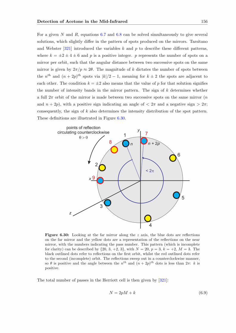
Detection of Acetone in the Mid-Infrared 156
For a given N and R, equations 6.7 and 6.8 can be solved simultaneously to give several
solutions, which slightly differ in the pattern of spots produced on the mirrors. Tarsitano
and Webster [321] introduced the variables k and p to describe these different patterns,
where k = ±2 ± 4 ± 6 and p is a positive integer. p represents the number of spots on a
mirror per orbit, such that the angular distance between two successive spots on the same
mirror is given by 2π/p ≈ 2θ. The magnitude of k dictates the number of spots between
the nth and (n + 2p)th spots via |k|/2 − 1, meaning for k ± 2 the spots are adjacent to
each other. The condition k = ±2 also means that the value of p for that solution signifies
the number of intensity bands in the mirror pattern. The sign of k determines whether
a full 2π orbit of the mirror is made between two successive spots on the same mirror (n
and n + 2p), with a positive sign indicating an angle of < 2π and a negative sign > 2π;
consequently, the sign of k also determines the intensity distribution of the spot pattern.
These definitions are illustrated in Figure 6.30.
Figure 6.30: Looking at the far mirror along the z axis, the blue dots are reflectionson the far mirror and the yellow dots are a representation of the reflections on the nearmirror, with the numbers indicating the pass number. This pattern (which is incompletefor clarity) can be described by 20, 3, +2, 3, with N = 20, p = 3, k = +2, M = 3. Theblack outlined dots refer to reflections on the first orbit, whilst the red outlined dots referto the second (incomplete) orbit. The reflections sweep out in a counterclockwise manner,so θ is positive and the angle between the nth and (n + 2p)th dots is less than 2π: k ispositive.
The total number of passes in the Herriott cell is then given by [321]:
N = 2pM + k (6.9)
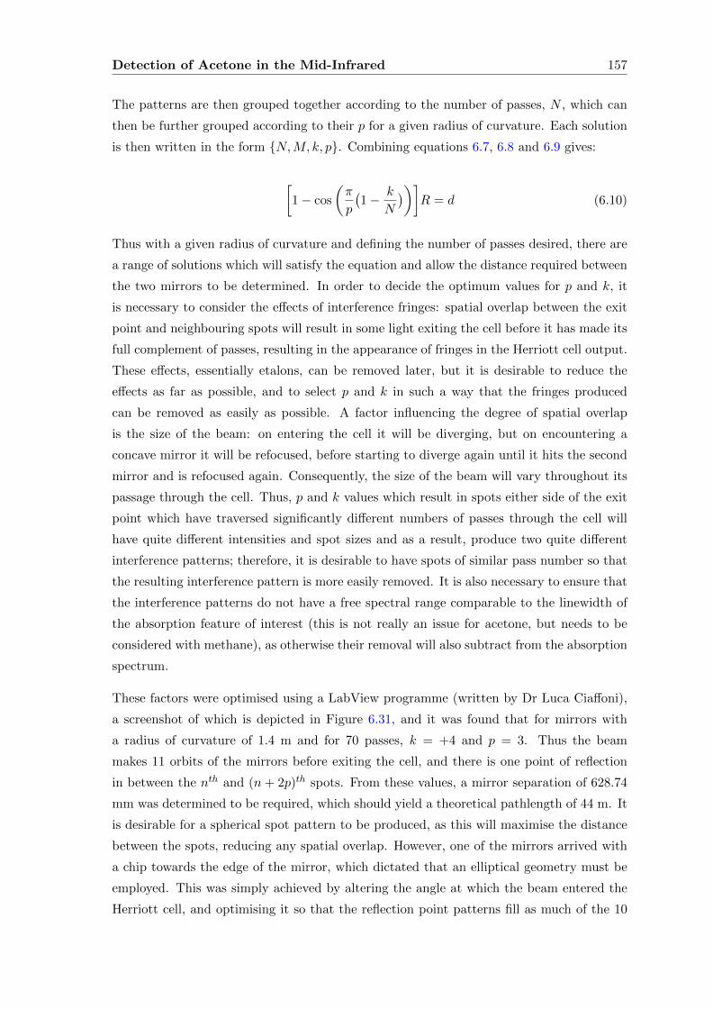
Detection of Acetone in the Mid-Infrared 157
The patterns are then grouped together according to the number of passes, N , which can
then be further grouped according to their p for a given radius of curvature. Each solution
is then written in the form N,M, k, p. Combining equations 6.7, 6.8 and 6.9 gives:
[1− cos
(π
p
(1− k
N
))]R = d (6.10)
Thus with a given radius of curvature and defining the number of passes desired, there are
a range of solutions which will satisfy the equation and allow the distance required between
the two mirrors to be determined. In order to decide the optimum values for p and k, it
is necessary to consider the effects of interference fringes: spatial overlap between the exit
point and neighbouring spots will result in some light exiting the cell before it has made its
full complement of passes, resulting in the appearance of fringes in the Herriott cell output.
These effects, essentially etalons, can be removed later, but it is desirable to reduce the
effects as far as possible, and to select p and k in such a way that the fringes produced
can be removed as easily as possible. A factor influencing the degree of spatial overlap
is the size of the beam: on entering the cell it will be diverging, but on encountering a
concave mirror it will be refocused, before starting to diverge again until it hits the second
mirror and is refocused again. Consequently, the size of the beam will vary throughout its
passage through the cell. Thus, p and k values which result in spots either side of the exit
point which have traversed significantly different numbers of passes through the cell will
have quite different intensities and spot sizes and as a result, produce two quite different
interference patterns; therefore, it is desirable to have spots of similar pass number so that
the resulting interference pattern is more easily removed. It is also necessary to ensure that
the interference patterns do not have a free spectral range comparable to the linewidth of
the absorption feature of interest (this is not really an issue for acetone, but needs to be
considered with methane), as otherwise their removal will also subtract from the absorption
spectrum.
These factors were optimised using a LabView programme (written by Dr Luca Ciaffoni),
a screenshot of which is depicted in Figure 6.31, and it was found that for mirrors with
a radius of curvature of 1.4 m and for 70 passes, k = +4 and p = 3. Thus the beam
makes 11 orbits of the mirrors before exiting the cell, and there is one point of reflection
in between the nth and (n+ 2p)th spots. From these values, a mirror separation of 628.74
mm was determined to be required, which should yield a theoretical pathlength of 44 m. It
is desirable for a spherical spot pattern to be produced, as this will maximise the distance
between the spots, reducing any spatial overlap. However, one of the mirrors arrived with
a chip towards the edge of the mirror, which dictated that an elliptical geometry must be
employed. This was simply achieved by altering the angle at which the beam entered the
Herriott cell, and optimising it so that the reflection point patterns fill as much of the 10
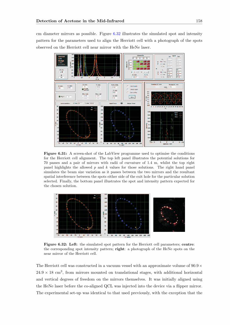
Detection of Acetone in the Mid-Infrared 158
cm diameter mirrors as possible. Figure 6.32 illustrates the simulated spot and intensity
pattern for the parameters used to align the Herriott cell with a photograph of the spots
observed on the Herriott cell near mirror with the HeNe laser.
Figure 6.31: A screen-shot of the LabView programme used to optimise the conditionsfor the Herriott cell alignment. The top left panel illustrates the potential solutions for70 passes and a pair of mirrors with radii of curvature of 1.4 m, whilst the top rightpanel highlights the allowed p and k values for those solutions. The right hand panelsimulates the beam size variation as it passes between the two mirrors and the resultantspatial interference between the spots either side of the exit hole for the particular solutionselected. Finally, the bottom panel illustrates the spot and intensity pattern expected forthe chosen solution.
Figure 6.32: Left: the simulated spot pattern for the Herriott cell parameters; centre:the corresponding spot intensity pattern; right: a photograph of the HeNe spots on thenear mirror of the Herriott cell.
The Herriott cell was constructed in a vacuum vessel with an approximate volume of 90.9×24.9 × 18 cm3, from mirrors mounted on translational stages, with additional horizontal
and vertical degrees of freedom on the mirrors themselves. It was initially aligned using
the HeNe laser before the co-aligned QCL was injected into the device via a flipper mirror.
The experimental set-up was identical to that used previously, with the exception that the
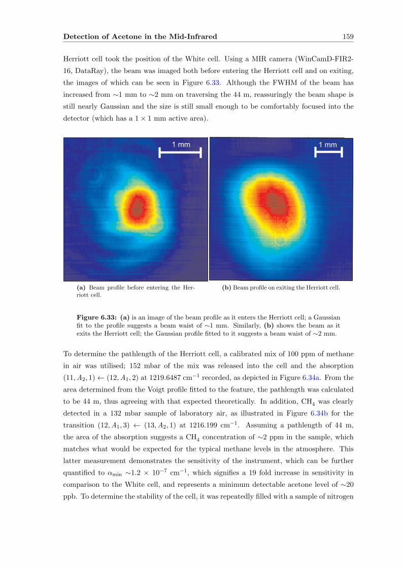
Detection of Acetone in the Mid-Infrared 159
Herriott cell took the position of the White cell. Using a MIR camera (WinCamD-FIR2-
16, DataRay), the beam was imaged both before entering the Herriott cell and on exiting,
the images of which can be seen in Figure 6.33. Although the FWHM of the beam has
increased from ∼1 mm to ∼2 mm on traversing the 44 m, reassuringly the beam shape is
still nearly Gaussian and the size is still small enough to be comfortably focused into the
detector (which has a 1× 1 mm active area).
(a) Beam profile before entering the Her-riott cell.
(b) Beam profile on exiting the Herriott cell.
Figure 6.33: (a) is an image of the beam profile as it enters the Herriott cell; a Gaussianfit to the profile suggests a beam waist of ∼1 mm. Similarly, (b) shows the beam as itexits the Herriott cell; the Gaussian profile fitted to it suggests a beam waist of ∼2 mm.
To determine the pathlength of the Herriott cell, a calibrated mix of 100 ppm of methane
in air was utilised; 152 mbar of the mix was released into the cell and the absorption
(11,A2, 1)← (12,A1, 2) at 1219.6487 cm−1 recorded, as depicted in Figure 6.34a. From the
area determined from the Voigt profile fitted to the feature, the pathlength was calculated
to be 44 m, thus agreeing with that expected theoretically. In addition, CH4 was clearly
detected in a 132 mbar sample of laboratory air, as illustrated in Figure 6.34b for the
transition (12,A1, 3) ← (13,A2, 1) at 1216.199 cm−1. Assuming a pathlength of 44 m,
the area of the absorption suggests a CH4 concentration of ∼2 ppm in the sample, which
matches what would be expected for the typical methane levels in the atmosphere. This
latter measurement demonstrates the sensitivity of the instrument, which can be further
quantified to αmin ∼1.2 × 10⁻⁷ cm−1, which signifies a 19 fold increase in sensitivity in
comparison to the White cell, and represents a minimum detectable acetone level of ∼20
ppb. To determine the stability of the cell, it was repeatedly filled with a sample of nitrogen
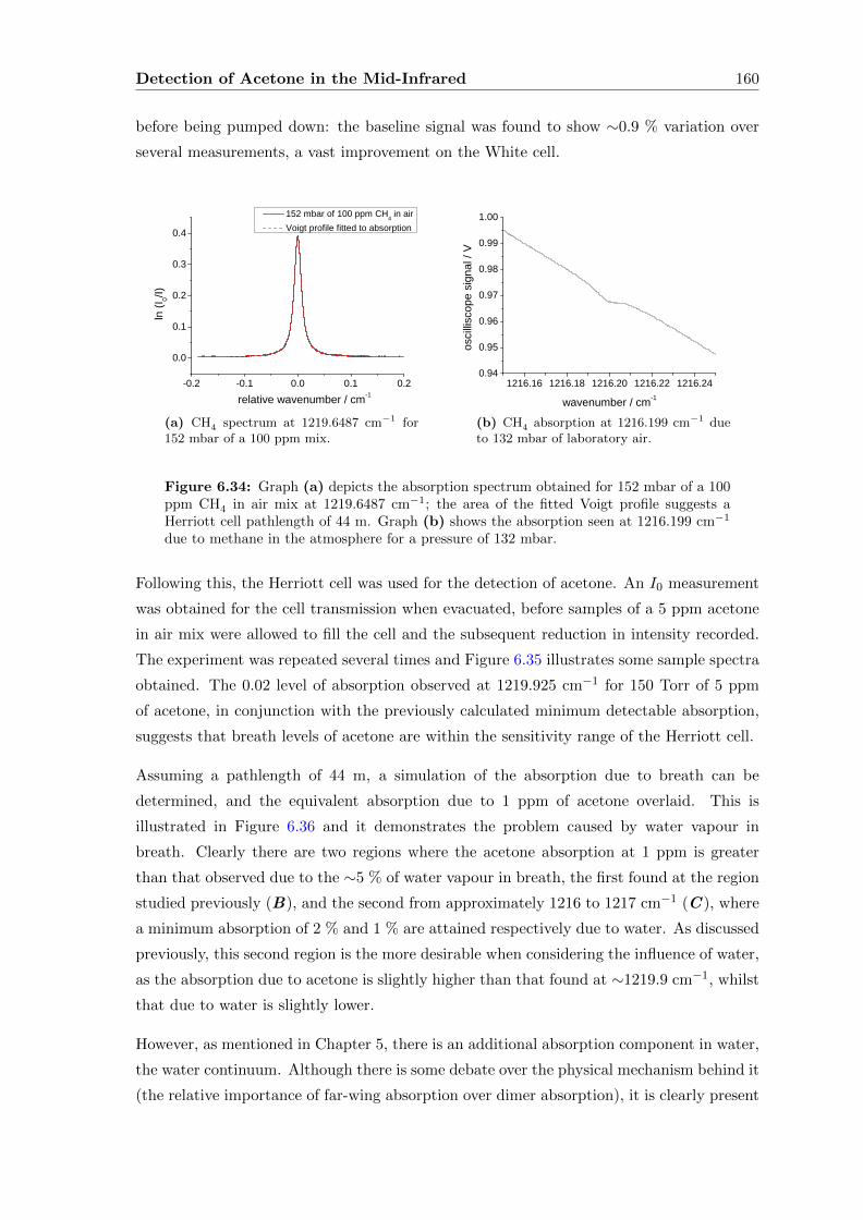
Detection of Acetone in the Mid-Infrared 160
before being pumped down: the baseline signal was found to show ∼0.9 % variation over
several measurements, a vast improvement on the White cell.
- 0 . 2 - 0 . 1 0 . 0 0 . 1 0 . 2
0 . 0
0 . 1
0 . 2
0 . 3
0 . 4
ln (I 0/I)
r e l a t i v e w a v e n u m b e r / c m - 1
1 5 2 m b a r o f 1 0 0 p p m C H 4 i n a i r V o i g t p r o f i l e f i t t e d t o a b s o r p t i o n
(a) CH4 spectrum at 1219.6487 cm−1 for152 mbar of a 100 ppm mix.
1 2 1 6 . 1 6 1 2 1 6 . 1 8 1 2 1 6 . 2 0 1 2 1 6 . 2 2 1 2 1 6 . 2 40 . 9 4
0 . 9 5
0 . 9 6
0 . 9 7
0 . 9 8
0 . 9 9
1 . 0 0
oscill
iscop
e sign
al / V
w a v e n u m b e r / c m - 1
(b) CH4 absorption at 1216.199 cm−1 dueto 132 mbar of laboratory air.
Figure 6.34: Graph (a) depicts the absorption spectrum obtained for 152 mbar of a 100ppm CH4 in air mix at 1219.6487 cm−1; the area of the fitted Voigt profile suggests aHerriott cell pathlength of 44 m. Graph (b) shows the absorption seen at 1216.199 cm−1
due to methane in the atmosphere for a pressure of 132 mbar.
Following this, the Herriott cell was used for the detection of acetone. An I0 measurement
was obtained for the cell transmission when evacuated, before samples of a 5 ppm acetone
in air mix were allowed to fill the cell and the subsequent reduction in intensity recorded.
The experiment was repeated several times and Figure 6.35 illustrates some sample spectra
obtained. The 0.02 level of absorption observed at 1219.925 cm−1 for 150 Torr of 5 ppm
of acetone, in conjunction with the previously calculated minimum detectable absorption,
suggests that breath levels of acetone are within the sensitivity range of the Herriott cell.
Assuming a pathlength of 44 m, a simulation of the absorption due to breath can be
determined, and the equivalent absorption due to 1 ppm of acetone overlaid. This is
illustrated in Figure 6.36 and it demonstrates the problem caused by water vapour in
breath. Clearly there are two regions where the acetone absorption at 1 ppm is greater
than that observed due to the ∼5 % of water vapour in breath, the first found at the region
studied previously (B), and the second from approximately 1216 to 1217 cm−1 (C ), where
a minimum absorption of 2 % and 1 % are attained respectively due to water. As discussed
previously, this second region is the more desirable when considering the influence of water,
as the absorption due to acetone is slightly higher than that found at ∼1219.9 cm−1, whilst
that due to water is slightly lower.
However, as mentioned in Chapter 5, there is an additional absorption component in water,
the water continuum. Although there is some debate over the physical mechanism behind it
(the relative importance of far-wing absorption over dimer absorption), it is clearly present
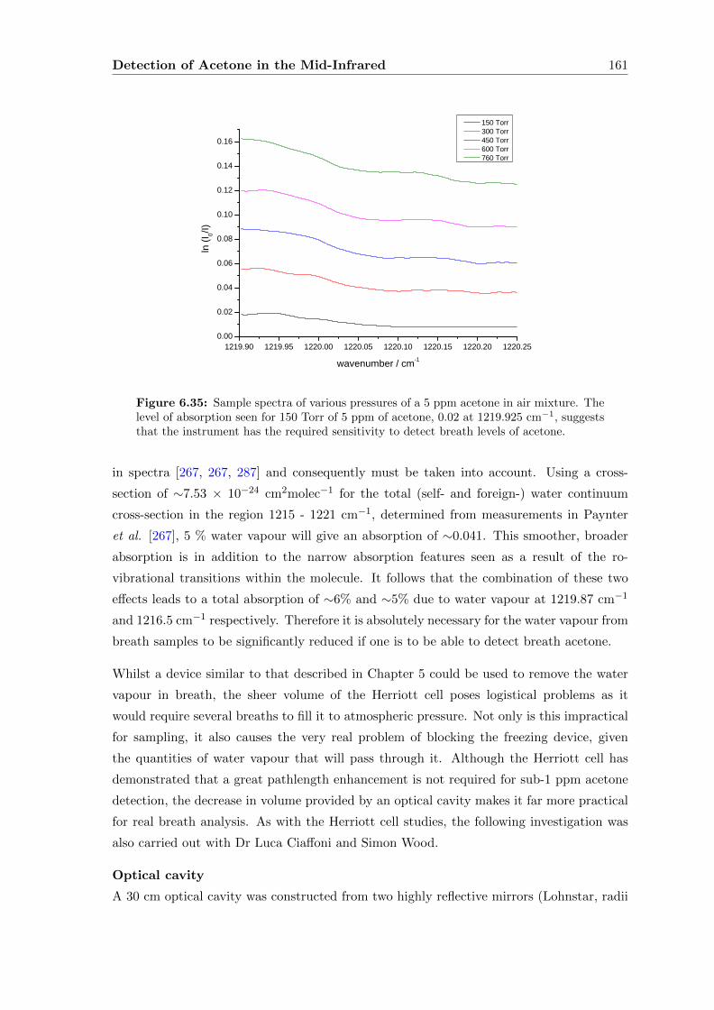
Detection of Acetone in the Mid-Infrared 161
1 2 1 9 . 9 0 1 2 1 9 . 9 5 1 2 2 0 . 0 0 1 2 2 0 . 0 5 1 2 2 0 . 1 0 1 2 2 0 . 1 5 1 2 2 0 . 2 0 1 2 2 0 . 2 50 . 0 0
0 . 0 2
0 . 0 4
0 . 0 6
0 . 0 8
0 . 1 0
0 . 1 2
0 . 1 4
0 . 1 6
ln (I 0/I)
w a v e n u m b e r / c m - 1
1 5 0 T o r r 3 0 0 T o r r 4 5 0 T o r r 6 0 0 T o r r 7 6 0 T o r r
Figure 6.35: Sample spectra of various pressures of a 5 ppm acetone in air mixture. Thelevel of absorption seen for 150 Torr of 5 ppm of acetone, 0.02 at 1219.925 cm−1, suggeststhat the instrument has the required sensitivity to detect breath levels of acetone.
in spectra [267, 267, 287] and consequently must be taken into account. Using a cross-
section of ∼7.53 × 10⁻²⁴ cm2molec−1 for the total (self- and foreign-) water continuum
cross-section in the region 1215 - 1221 cm−1, determined from measurements in Paynter
et al. [267], 5 % water vapour will give an absorption of ∼0.041. This smoother, broader
absorption is in addition to the narrow absorption features seen as a result of the ro-
vibrational transitions within the molecule. It follows that the combination of these two
effects leads to a total absorption of ∼6% and ∼5% due to water vapour at 1219.87 cm−1
and 1216.5 cm−1 respectively. Therefore it is absolutely necessary for the water vapour from
breath samples to be significantly reduced if one is to be able to detect breath acetone.
Whilst a device similar to that described in Chapter 5 could be used to remove the water
vapour in breath, the sheer volume of the Herriott cell poses logistical problems as it
would require several breaths to fill it to atmospheric pressure. Not only is this impractical
for sampling, it also causes the very real problem of blocking the freezing device, given
the quantities of water vapour that will pass through it. Although the Herriott cell has
demonstrated that a great pathlength enhancement is not required for sub-1 ppm acetone
detection, the decrease in volume provided by an optical cavity makes it far more practical
for real breath analysis. As with the Herriott cell studies, the following investigation was
also carried out with Dr Luca Ciaffoni and Simon Wood.
Optical cavity
A 30 cm optical cavity was constructed from two highly reflective mirrors (Lohnstar, radii
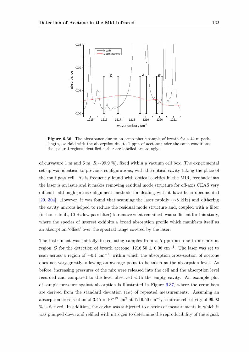
Detection of Acetone in the Mid-Infrared 162
1 2 1 5 1 2 1 6 1 2 1 7 1 2 1 8 1 2 1 9 1 2 2 0 1 2 2 10 . 0 0
0 . 0 5
0 . 1 0
0 . 1 5
BAC
b r e a t h 1 p p m a c e t o n e
abso
rbanc
e
w a v e n u m b e r / c m - 1
Figure 6.36: The absorbance due to an atmospheric sample of breath for a 44 m path-length, overlaid with the absorption due to 1 ppm of acetone under the same conditions;the spectral regions identified earlier are labelled accordingly.
of curvature 1 m and 5 m, R ∼99.9 %), fixed within a vacuum cell box. The experimental
set-up was identical to previous configurations, with the optical cavity taking the place of
the multipass cell. As is frequently found with optical cavities in the MIR, feedback into
the laser is an issue and it makes removing residual mode structure for off-axis CEAS very
difficult, although precise alignment methods for dealing with it have been documented
[29, 304]. However, it was found that scanning the laser rapidly (∼8 kHz) and dithering
the cavity mirrors helped to reduce the residual mode structure and, coupled with a filter
(in-house built, 10 Hz low pass filter) to remove what remained, was sufficient for this study,
where the species of interest exhibits a broad absorption profile which manifests itself as
an absorption ‘offset’ over the spectral range covered by the laser.
The instrument was initially tested using samples from a 5 ppm acetone in air mix at
region C for the detection of breath acetone, 1216.50 ± 0.06 cm−1. The laser was set to
scan across a region of ∼0.1 cm−1, within which the absorption cross-section of acetone
does not vary greatly, allowing an average point to be taken as the absorption level. As
before, increasing pressures of the mix were released into the cell and the absorption level
recorded and compared to the level observed with the empty cavity. An example plot
of sample pressure against absorption is illustrated in Figure 6.37, where the error bars
are derived from the standard deviation (1σ) of repeated measurements. Assuming an
absorption cross-section of 3.45 × 10⁻¹⁹ cm2 at 1216.50 cm−1, a mirror reflectivity of 99.92
% is derived. In addition, the cavity was subjected to a series of measurements in which it
was pumped down and refilled with nitrogen to determine the reproducibility of the signal.
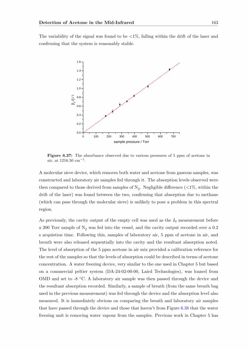
Detection of Acetone in the Mid-Infrared 163
The variability of the signal was found to be <1%, falling within the drift of the laser and
confirming that the system is reasonably stable.
0 1 0 0 2 0 0 3 0 0 4 0 0 5 0 0 6 0 0 7 0 00 . 0
0 . 2
0 . 4
0 . 6
0 . 8
1 . 0
1 . 2
1 . 4
1 . 6
[I 0-I] / I
s a m p l e p r e s s u r e / T o r r
Figure 6.37: The absorbance observed due to various pressures of 5 ppm of acetone inair, at 1216.50 cm−1.
A molecular sieve device, which removes both water and acetone from gaseous samples, was
constructed and laboratory air samples fed through it. The absorption levels observed were
then compared to those derived from samples of N2. Negligible difference (<1%, within the
drift of the laser) was found between the two, confirming that absorption due to methane
(which can pass through the molecular sieve) is unlikely to pose a problem in this spectral
region.
As previously, the cavity output of the empty cell was used as the I0 measurement before
a 200 Torr sample of N2 was fed into the vessel, and the cavity output recorded over a 0.2
s acquistion time. Following this, samples of laboratory air, 5 ppm of acetone in air, and
breath were also released sequentially into the cavity and the resultant absorption noted.
The level of absorption of the 5 ppm acetone in air mix provided a calibration reference for
the rest of the samples so that the levels of absorption could be described in terms of acetone
concentration. A water freezing device, very similar to the one used in Chapter 5 but based
on a commercial peltier system (DA-24-02-00-00, Laird Technologies), was loaned from
OMD and set to -8 C. A laboratory air sample was then passed through the device and
the resultant absorption recorded. Similarly, a sample of breath (from the same breath bag
used in the previous measurement) was fed through the device and the absorption level also
measured. It is immediately obvious on comparing the breath and laboratory air samples
that have passed through the device and those that haven’t from Figure 6.38 that the water
freezing unit is removing water vapour from the samples. Previous work in Chapter 5 has
Detection of Acetone in the Mid-Infrared 164
demonstrated that the levels of acetone are more-or-less unaffected on passing through
the chiller at these temperatures, so the reduction in absorption can be attributed to the
removal of water. Therefore, the absorbance that is recorded from the breath sample that
has passed through the water freezing device is very likely to be solely due to the acetone
present in that breath sample, and was measured at 480 ppb. The residual breath in the
bag from which the breath samples were taken was then cross-checked against the reading
from the mass spectrometer used in Chapter 5 and reassuringly found to contain acetone
levels (460 ppb) which were well within the uncertainty of the measurement carried out
using the optical device, as can be seen in Figure 6.38. The error bars depicted on the
plot are derived from the standard deviation (1σ) of repeat measurements taken of each
condition (in the case of breath, the samples are taken from the same breath bag), and
suggest a precision of 170 ppb in the sub-second response time. Similar measurements at
1215.60 cm−1 where the interference from H2O absorption is greater also return consistent
values of the acetone concentration after the breath has been pre-treated in the water-
removal device before being released into the cell, with 590 ppb recorded by the optical
device and 620 ppb by the mass spectrometer, as depicted in Figure 6.38b. The reduction
in absorption due to water being removed from the sample is approximately the same in
both the laboratory air and breath samples: this is believed to be due to the fact that
the breath sample within the bag is at a lower temperature than when it first leaves the
mouth, this drop in temperature lowers the saturated water vapour pressure in the breath
sample; in addition, the humidity of the laboratory air was very high on the day of the
measurements which leads to a situation where the reduction in water vapour in the breath
sample is equal to (or just greater than, with the uncertainty in the measurements taken
into account) the reduction observed in the laboratory air sample.
Although these represent only very initial measurements on determining breath acetone
with a MIR optical cavity, the system does seem to show promise and could be pursued and
tested against further breath samples. In addition, the experimental set up could be refined
to produce more accurate and sensitive results by dealing with the optical feedback better,
such as aligning it using the methods described in [29, 304], using a more mechanically stable
laser mount and placing the optical cavity in a bellow-type system (as used in Chapter 3)
or a fixed mirror cell (as in Chapter 5).
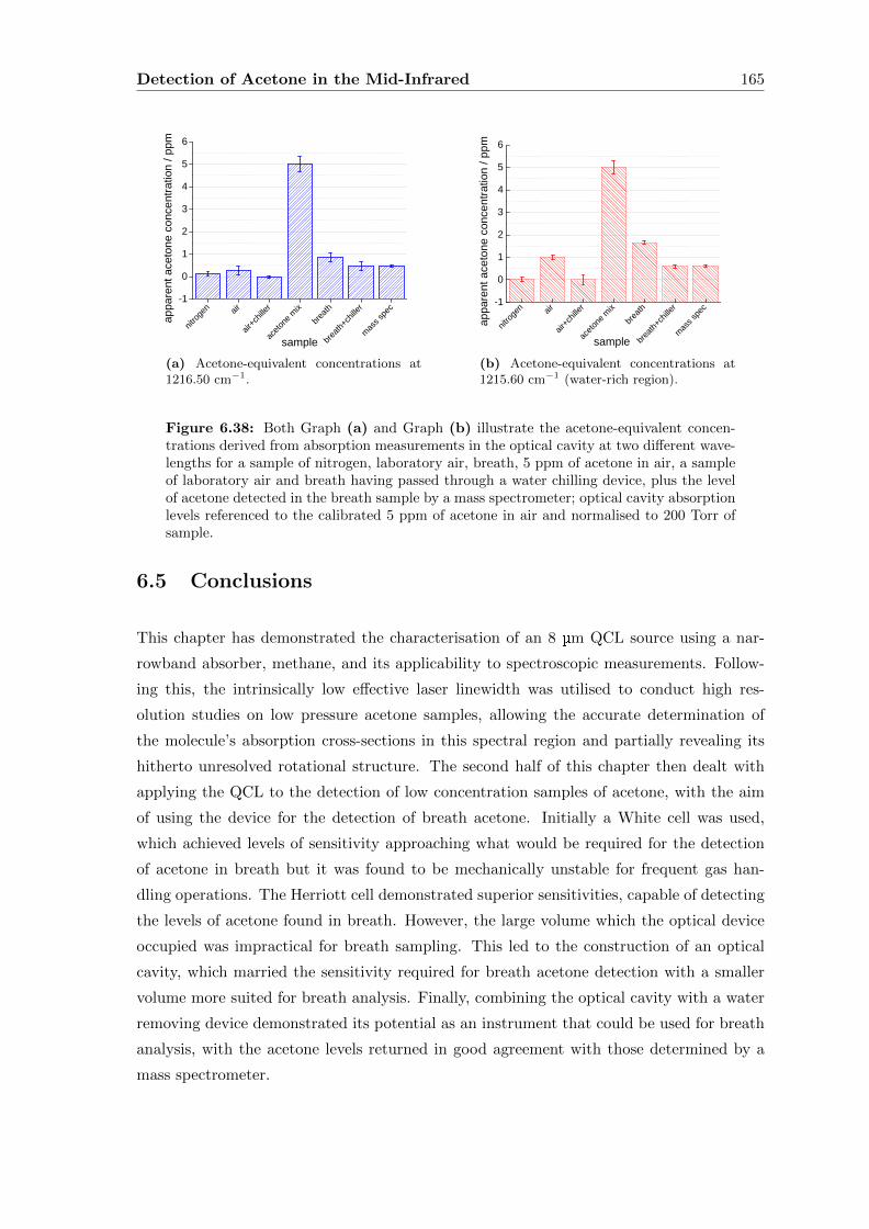
Detection of Acetone in the Mid-Infrared 165
n i t r og e n a i r
a i r +c h i l
l e r
a c et o n e
m i xb r e a
t h
b r e at h + c
h i l l er
m a s s s p e
c- 10123456
appa
rent a
ceton
e con
centr
ation
/ ppm
s a m p l e(a) Acetone-equivalent concentrations at1216.50 cm−1.
n i t r og e n a i r
a i r +c h i l
l e r
a c et o n e
m i xb r e a
t h
b r e at h + c
h i l l er
m a s s s p e
c- 10123456
appa
rent a
ceton
e con
centr
ation
/ ppm
s a m p l e(b) Acetone-equivalent concentrations at1215.60 cm−1 (water-rich region).
Figure 6.38: Both Graph (a) and Graph (b) illustrate the acetone-equivalent concen-trations derived from absorption measurements in the optical cavity at two different wave-lengths for a sample of nitrogen, laboratory air, breath, 5 ppm of acetone in air, a sampleof laboratory air and breath having passed through a water chilling device, plus the levelof acetone detected in the breath sample by a mass spectrometer; optical cavity absorptionlevels referenced to the calibrated 5 ppm of acetone in air and normalised to 200 Torr ofsample.
6.5 Conclusions
This chapter has demonstrated the characterisation of an 8 µm QCL source using a nar-
rowband absorber, methane, and its applicability to spectroscopic measurements. Follow-
ing this, the intrinsically low effective laser linewidth was utilised to conduct high res-
olution studies on low pressure acetone samples, allowing the accurate determination of
the molecule’s absorption cross-sections in this spectral region and partially revealing its
hitherto unresolved rotational structure. The second half of this chapter then dealt with
applying the QCL to the detection of low concentration samples of acetone, with the aim
of using the device for the detection of breath acetone. Initially a White cell was used,
which achieved levels of sensitivity approaching what would be required for the detection
of acetone in breath but it was found to be mechanically unstable for frequent gas han-
dling operations. The Herriott cell demonstrated superior sensitivities, capable of detecting
the levels of acetone found in breath. However, the large volume which the optical device
occupied was impractical for breath sampling. This led to the construction of an optical
cavity, which married the sensitivity required for breath acetone detection with a smaller
volume more suited for breath analysis. Finally, combining the optical cavity with a water
removing device demonstrated its potential as an instrument that could be used for breath
analysis, with the acetone levels returned in good agreement with those determined by a
mass spectrometer.
Detection of Acetone in the Mid-Infrared 166
Although only a few samples have been tested with the device, these early results do look
very promising and suggest that the MIR cavity constructed could be used for the detection
of breath acetone. Spectral interference appears to be less of a problem in the 8 µm spectral
region than in the NIR, making gas handling more straightforward, as there is no need for
molecular sieve and -8 C was found to be sufficient for removing water vapour to levels be-
low the detection limit of the spectrometer. In addition, thanks to the larger cross-sections
accessible with the QCL, a significant pathlength enhancement is not necessary to attain
the levels of sensitivity required for detecting breath acetone; indeed, a Herriott cell with
a smaller volume than that used here (perhaps using astigmatic mirrors) might represent
a more suitable solution for detecting breath acetone given the relatively more straight-
forward optical arrangement. However, the bulky water-cooling system currently required
for the laser renders the QCL-based system unsuitable at this stage for use outside of the
laboratory. The following and final chapter will look at potential future developments in
this field, including some initial results from a preliminary investigation into the possibility
of a UV LED-based system for the detection of acetone, which could represent a way in
which to combine the compactness of the NIR diode laser device with large cross-sections
and the attractive possibility of very limited spectral interference from other species.
Chapter 7
Future Directions and Conclusions
This thesis has centred on the development of absorption spectroscopy-based technologies
which have the potential to be applied to the diagnostics of breath analysis. The majority of
this work has concentrated on the detection of acetone, a molecule strongly linked with the
diabetic condition as a result of the utilisation of fat deposits as a primary energy source.
However, acetone is a broadband absorber, which means that a broadband source is required
to probe an entire absorption feature, providing the necessary selectivity to identify the
molecule, as described in Chapter 4. The necessity for a bulky and expensive spectrometer
within the detection system makes this difficult to be developed into a portable, bench-
top device, although miniaturised, low resolution, spectrometers are available [322] and
potentially offer a solution to this problem. If, instead, a narrowband diode laser is used to
probe a broadband absorber such as acetone, all other interferents must be removed from
the sample under analysis, or their influence negated. This was the technique employed in
Chapter 5, where a NIR diode laser-based optical cavity device was developed. A spectral
region where there were relatively few competing absorbing species was selected, and those
that remained were either removed to a level below the detection limit of the spectrometer
(water) or their presence was negated by using the breath sample of the individual to also
provide the background measurement (methane). Similarly, the optical cavity constructed
in Chapter 6 employed a water freezing device to remove the effects of water vapour from
breath samples, and the larger cross-sections accessible in the MIR by the quantum cascade
laser (QCL) ensured that a relatively low pathlength enhancement was sufficient to detect
acetone at the levels found in breath. However, this arrangement required the use of a cw
QCL: the MIR technology would have to markedly reduce in cost before it could realistically
be used outside of the laboratory for breath analysing purposes on a large scale.
One potential solution could lie in the use of an ultra-violet light emitting diode (UV
LED). Not only are these devices compact and relatively cheap in comparison to QCL
167
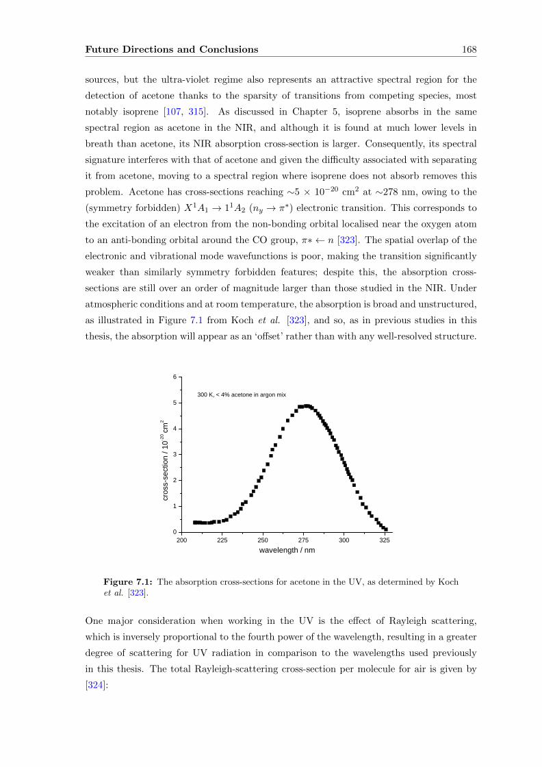
Future Directions and Conclusions 168
sources, but the ultra-violet regime also represents an attractive spectral region for the
detection of acetone thanks to the sparsity of transitions from competing species, most
notably isoprene [107, 315]. As discussed in Chapter 5, isoprene absorbs in the same
spectral region as acetone in the NIR, and although it is found at much lower levels in
breath than acetone, its NIR absorption cross-section is larger. Consequently, its spectral
signature interferes with that of acetone and given the difficulty associated with separating
it from acetone, moving to a spectral region where isoprene does not absorb removes this
problem. Acetone has cross-sections reaching ∼5 × 10⁻²⁰ cm2 at ∼278 nm, owing to the
(symmetry forbidden) X1A1 → 11A2 (ny → π∗) electronic transition. This corresponds to
the excitation of an electron from the non-bonding orbital localised near the oxygen atom
to an anti-bonding orbital around the CO group, π∗ ← n [323]. The spatial overlap of the
electronic and vibrational mode wavefunctions is poor, making the transition significantly
weaker than similarly symmetry forbidden features; despite this, the absorption cross-
sections are still over an order of magnitude larger than those studied in the NIR. Under
atmospheric conditions and at room temperature, the absorption is broad and unstructured,
as illustrated in Figure 7.1 from Koch et al. [323], and so, as in previous studies in this
thesis, the absorption will appear as an ‘offset’ rather than with any well-resolved structure.
2 0 0 2 2 5 2 5 0 2 7 5 3 0 0 3 2 50
1
2
3
4
5
6
cross-
sectio
n / 10
-20 cm
2
w a v e l e n g t h / n m
3 0 0 K , < 4 % a c e t o n e i n a r g o n m i x
Figure 7.1: The absorption cross-sections for acetone in the UV, as determined by Kochet al. [323].
One major consideration when working in the UV is the effect of Rayleigh scattering,
which is inversely proportional to the fourth power of the wavelength, resulting in a greater
degree of scattering for UV radiation in comparison to the wavelengths used previously
in this thesis. The total Rayleigh-scattering cross-section per molecule for air is given by
[324]:
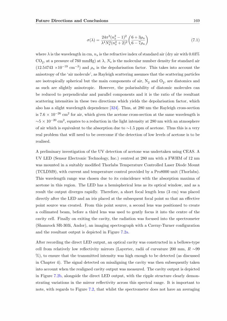
Future Directions and Conclusions 169
σ(λ) =24π3(n2
s − 1)2
λ4N2s (n2
s + 2)2
(6 + 3ρn6− 7ρn
)(7.1)
where λ is the wavelength in cm, ns is the refractive index of standard air (dry air with 0.03%
CO2, at a pressure of 760 mmHg) at λ, Ns is the molecular number density for standard air
(12.54743 ×10⁻¹⁹ cm−3) and ρn is the depolarisation factor. This takes into account the
anisotropy of the ‘air molecule’, as Rayleigh scattering assumes that the scattering particles
are isotropically spherical but the main components of air, N2 and O2, are diatomics and
as such are slightly anisotropic. However, the polarisability of diatomic molecules can
be reduced to perpendicular and parallel components and it is the ratio of the resultant
scattering intensities in these two directions which yields the depolarisation factor, which
also has a slight wavelength dependence [324]. Thus, at 280 nm the Rayleigh cross-section
is 7.6 × 10⁻²⁶ cm2 for air, which given the acetone cross-section at the same wavelength is
∼5 × 10⁻²⁰ cm2, equates to a reduction in the light intensity at 280 nm with an atmosphere
of air which is equivalent to the absorption due to ∼1.5 ppm of acetone. Thus this is a very
real problem that will need to be overcome if the detection of low levels of acetone is to be
realised.
A preliminary investigation of the UV detection of acetone was undertaken using CEAS. A
UV LED (Sensor Electronic Technology, Inc.) centred at 280 nm with a FWHM of 12 nm
was mounted in a suitably modified Thorlabs Temperature Controlled Laser Diode Mount
(TCLDM9), with current and temperature control provided by a Pro8000 unit (Thorlabs).
This wavelength range was chosen due to its coincidence with the absorption maxima of
acetone in this region. The LED has a hemispherical lens as its optical window, and as a
result the output diverges rapidly. Therefore, a short focal length lens (3 cm) was placed
directly after the LED and an iris placed at the subsequent focal point so that an effective
point source was created. From this point source, a second lens was positioned to create
a collimated beam, before a third lens was used to gently focus it into the centre of the
cavity cell. Finally on exiting the cavity, the radiation was focused into the spectrometer
(Shamrock SR-303i, Andor), an imaging spectrograph with a Czerny-Turner configuration
and the resultant output is depicted in Figure 7.2a.
After recording the direct LED output, an optical cavity was constructed in a bellows-type
cell from relatively low reflectivity mirrors (Layertec, radii of curvature 200 mm, R ∼99
%), to ensure that the transmitted intensity was high enough to be detected (as discussed
in Chapter 4). The signal detected on misaligning the cavity was then subsequently taken
into account when the realigned cavity output was measured. The cavity output is depicted
in Figure 7.2b, alongside the direct LED output, with the ripple structure clearly demon-
strating variations in the mirror reflectivity across this spectral range. It is important to
note, with regards to Figure 7.2, that whilst the spectrometer does not have an averaging
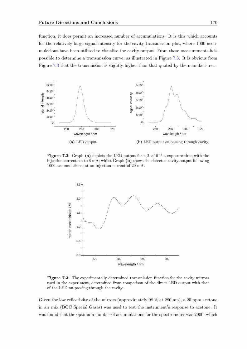
Future Directions and Conclusions 170
function, it does permit an increased number of accumulations. It is this which accounts
for the relatively large signal intensity for the cavity transmission plot, where 1000 accu-
mulations have been utilised to visualise the cavity output. From these measurements it is
possible to determine a transmission curve, as illustrated in Figure 7.3. It is obvious from
Figure 7.3 that the transmission is slightly higher than that quoted by the manufacturer.
2 6 0 2 8 0 3 0 0 3 2 00
1 x 1 0 4
2 x 1 0 4
3 x 1 0 4
4 x 1 0 4
5 x 1 0 4
6 x 1 0 4
signa
l inten
sity
w a v e l e n g t h / n m(a) LED output.
2 6 0 2 8 0 3 0 0 3 2 00
1 x 1 0 4
2 x 1 0 4
3 x 1 0 4
4 x 1 0 4
5 x 1 0 4
signa
l inten
sityw a v e l e n g t h / n m
(b) LED output on passing through cavity.
Figure 7.2: Graph (a) depicts the LED output for a 2 ×10⁻⁵ s exposure time with theinjection current set to 8 mA; whilst Graph (b) shows the detected cavity output following1000 accumulations, at an injection current of 20 mA.
2 7 0 2 8 0 2 9 0 3 0 00 . 0
0 . 5
1 . 0
1 . 5
2 . 0
2 . 5
mirro
r tran
smiss
ion / %
w a v e l e n g t h / n m
Figure 7.3: The experimentally determined transmission function for the cavity mirrorsused in the experiment, determined from comparison of the direct LED output with thatof the LED on passing through the cavity.
Given the low reflectivity of the mirrors (approximately 98 % at 280 nm), a 25 ppm acetone
in air mix (BOC Special Gases) was used to test the instrument’s response to acetone. It
was found that the optimum number of accumulations for the spectrometer was 2000, which
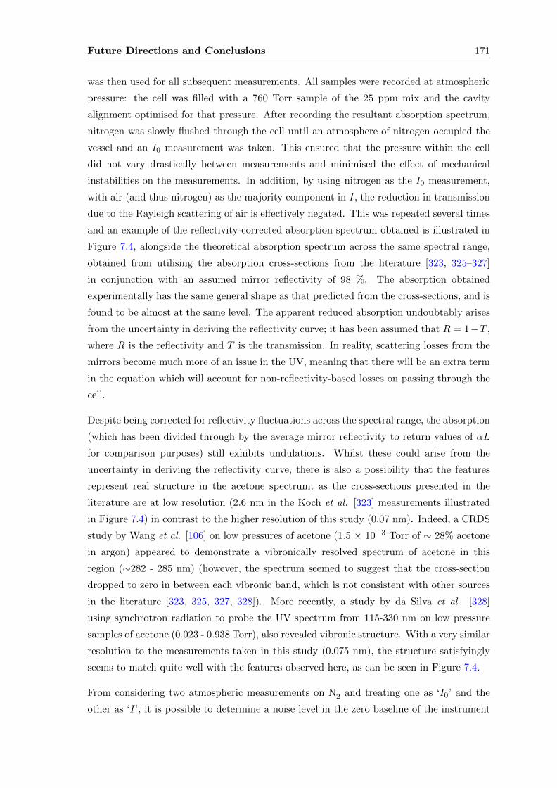
Future Directions and Conclusions 171
was then used for all subsequent measurements. All samples were recorded at atmospheric
pressure: the cell was filled with a 760 Torr sample of the 25 ppm mix and the cavity
alignment optimised for that pressure. After recording the resultant absorption spectrum,
nitrogen was slowly flushed through the cell until an atmosphere of nitrogen occupied the
vessel and an I0 measurement was taken. This ensured that the pressure within the cell
did not vary drastically between measurements and minimised the effect of mechanical
instabilities on the measurements. In addition, by using nitrogen as the I0 measurement,
with air (and thus nitrogen) as the majority component in I, the reduction in transmission
due to the Rayleigh scattering of air is effectively negated. This was repeated several times
and an example of the reflectivity-corrected absorption spectrum obtained is illustrated in
Figure 7.4, alongside the theoretical absorption spectrum across the same spectral range,
obtained from utilising the absorption cross-sections from the literature [323, 325–327]
in conjunction with an assumed mirror reflectivity of 98 %. The absorption obtained
experimentally has the same general shape as that predicted from the cross-sections, and is
found to be almost at the same level. The apparent reduced absorption undoubtably arises
from the uncertainty in deriving the reflectivity curve; it has been assumed that R = 1−T ,
where R is the reflectivity and T is the transmission. In reality, scattering losses from the
mirrors become much more of an issue in the UV, meaning that there will be an extra term
in the equation which will account for non-reflectivity-based losses on passing through the
cell.
Despite being corrected for reflectivity fluctuations across the spectral range, the absorption
(which has been divided through by the average mirror reflectivity to return values of αL
for comparison purposes) still exhibits undulations. Whilst these could arise from the
uncertainty in deriving the reflectivity curve, there is also a possibility that the features
represent real structure in the acetone spectrum, as the cross-sections presented in the
literature are at low resolution (2.6 nm in the Koch et al. [323] measurements illustrated
in Figure 7.4) in contrast to the higher resolution of this study (0.07 nm). Indeed, a CRDS
study by Wang et al. [106] on low pressures of acetone (1.5 × 10⁻³ Torr of ∼ 28% acetone
in argon) appeared to demonstrate a vibronically resolved spectrum of acetone in this
region (∼282 - 285 nm) (however, the spectrum seemed to suggest that the cross-section
dropped to zero in between each vibronic band, which is not consistent with other sources
in the literature [323, 325, 327, 328]). More recently, a study by da Silva et al. [328]
using synchrotron radiation to probe the UV spectrum from 115-330 nm on low pressure
samples of acetone (0.023 - 0.938 Torr), also revealed vibronic structure. With a very similar
resolution to the measurements taken in this study (0.075 nm), the structure satisfyingly
seems to match quite well with the features observed here, as can be seen in Figure 7.4.
From considering two atmospheric measurements on N2 and treating one as ‘I0’ and the
other as ‘I’, it is possible to determine a noise level in the zero baseline of the instrument
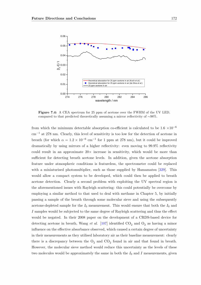
Future Directions and Conclusions 172
2 7 4 2 7 6 2 7 8 2 8 0 2 8 2 2 8 4 2 8 60 . 0 0
0 . 0 1
0 . 0 2
0 . 0 3
0 . 0 4
0 . 0 5
0 . 0 6
[I 0-I] / I
w a v e l e n g t h / n m
t h e o r e t i c a l a b s o r p t i o n f o r 2 5 p p m a c e t o n e i n a i r ( K o c h e t a l . ) t h e o r e t i c a l a b s o r p t i o n f o r 2 5 p p m a c e t o n e i n a i r ( d a S i l v a e t a l . ) 2 5 p p m a c e t o n e i n a i r
Figure 7.4: A CEA spectrum for 25 ppm of acetone over the FWHM of the UV LED,compared to that predicted theoretically assuming a mirror reflectivity of ∼98%.
from which the minimum detectable absorption co-efficient is calculated to be 1.6 ×10⁻⁶
cm−1 at 278 nm. Clearly, this level of sensitivity is too low for the detection of acetone in
breath (for which α = 1.2 × 10⁻⁶ cm−1 for 1 ppm at 278 nm), but it could be improved
dramatically by using mirrors of a higher reflectivity: even moving to 99.9% reflectivity
could result in an approximate 20× increase in sensitivity, which would be more than
sufficient for detecting breath acetone levels. In addition, given the acetone absorption
feature under atmospheric conditions is featureless, the spectrometer could be replaced
with a miniaturised photomultiplier, such as those supplied by Hamamatsu [329]. This
would allow a compact system to be developed, which could then be applied to breath
acetone detection. Clearly a second problem with exploiting the UV spectral region is
the aforementioned issues with Rayleigh scattering: this could potentially be overcome by
employing a similar method to that used to deal with methane in Chapter 5, by initially
passing a sample of the breath through some molecular sieve and using the subsequently
acetone-depleted sample for the I0 measurement. This would ensure that both the I0 and
I samples would be subjected to the same degree of Rayleigh scattering and thus the effect
would be negated. In their 2008 paper on the development of a CRDS-based device for
detecting acetone in breath, Wang et al. [107] identified CO2 and O2 as having a minor
influence on the effective absorbance observed, which caused a certain degree of uncertainty
in their measurements as they utilised laboratory air as their baseline measurement: clearly
there is a discrepancy between the O2 and CO2 found in air and that found in breath.
However, the molecular sieve method would reduce this uncertainty as the levels of these
two molecules would be approximately the same in both the I0 and I measurements, given
Future Directions and Conclusions 173
they originated from the same breath sample. Similarly, ozone is known to have a cross-
section 70 times larger than that of acetone at 280 nm, and even taking into account its
lower concentration (typically 50 ppb in air), it still poses a significant source of interference
(with an absorption level ratio of 3.38:1 for 50 ppb ozone to 1 ppm acetone) [330]. However,
it too can be taken into consideration by using the molecular sieve, ensuring the levels are
approximately the same in both background and sample measurements, or, if necessary, it
can be filtered out chemically [331, 332]. Thus, this represents a potential future direction
in the application of absorption spectroscopy to breath analysis, and in particular to the
detection of breath acetone.
Whilst the link between elevated levels of acetone in breath and diabetes is often quoted, it
is more accurately merely an indication that the body is predominantly using fat deposits as
a source of energy. Therefore, in addition to the potential application to diabetes diagnosis,
there is the significant weight-loss market that could benefit from a device that is able to
monitor breath acetone, particularly if it reduced to a hand-held size. Higher levels of
acetone in breath are a direct result of fat-burning: thus, a subject could blow into the
breath analysing device prior to exercise and then periodically breathe into it to monitor
their fat-burning efforts.
The field of breath analysis itself is still very much in its infancy with regards to its
widespread use in diagnostics, and the application of absorption spectroscopy to it even
more so, but it is a rapidly expanding field, with increasing numbers of studies investigat-
ing the possibilities of the non-invasive diagnosis of diseases it provides. This thesis has
sought to apply cavity enhanced absorption spectroscopy, in particular, to the application
of breath analysis. Chapter 3 began with a simple CEAS system using a DFB diode laser
to measure the levels of breath methane in a sample of 48 people. As a relatively straight-
forward molecule to detect given its narrow absorption features, and its significance as a
breath biomarker in its own right, methane was an ideal molecule to start with. This was
followed by the first demonstration of the application of a DS-DBR laser to cavity enhanced
spectroscopy. This laser exhibits a wide tunability, making it an ideal source for monitor-
ing multiple absorption transitions, which were demonstrated on another molecule found
in breath, CO2, illustrating its applicability in measuring CO2 isotope ratios for the urea
breath test. In Chapter 4 the focus shifted to detecting broadband absorbing molecules,
butadiene, acetone and isoprene, in the near-infrared. This involved the development of a
series of broadband cavity enhanced absorption (BB-CEAS) spectrometers, utilising both
SLED and SC sources. Two SLED devices were coupled together to provide a 200 nm spec-
tral range, which was used to demonstrate the possibility of monitoring multiple species
using BB-CEAS detection. Hitherto undetermined absorption cross-sections were deduced
for butadiene, acetone and isoprene over the 1.6 - 1.7 µm spectral range, before cavity
enhanced techniques were utilised to achieve respective noise-equivalent sensitivities of 200
Future Directions and Conclusions 174
ppb, 400 ppb and 200 ppb for the three molecules respectively (with the SC source). This
study helped to provide a basis for the development of a table-top breath acetone detecting
device in work carried out at Oxford Medical Diagnostics Ltd. A combination of molecular
sieve and a peltier-based chilling device were used to prepare the breath samples for analy-
sis in the optical cavity. The levels of acetone determined by the optical cavity were found
to agree with those measured by a mass spectrometer within an uncertainty of 200 ppb,
adding confidence to the suitability of the device for measuring breath acetone. Chapter 6
saw the introduction of a cw QCL, which allowed the fundamental transitions of acetone
at 8 µm to be probed. Utilising the narrow linewidth of the laser, high resolution mea-
surements on low pressure, pure acetone samples were conducted and rotational structure
discerned. Following this, the sensitivity of the system was incrementally increased using
a White cell, Herriott cell and finally a cavity. Exploiting the small volume provided by
the cavity, breath samples were analysed for acetone having first passed through another
chilling device to remove the water vapour, and the levels deduced once again corroborated
with those measured by the mass spectrometer on the same samples. Finally, an initial
investigation into the detection of acetone in the UV has been presented in this chapter as
a potential future direction for breath acetone detection.
Appendix A
Radiation Sources in the
Mid-Infrared
MIR radiation can be accessed in a number of ways, and these are summarised in Figure
A.1. Radiation with λ > 5 µm has traditionally be available via CO and CO2 lasers,
and the spectrally wide-ranging lead-salt solid state lasers. The gas lasers offer low laser
linewidth, coupled with a high power, but are restricted in their spectral coverage and
poor tunability. Limited by the position of their respective vibrational transitions, CO
lasers cover the region 5 - 6 µm, whilst the CO2 lasers emit from 9.2 - 10.8 µm. Pb-salt
lasers, on the other hand, allow a much broader coverage, from 3 - 30 µm [333], and also
offer narrow laser linewidth as they are essentially another type of diode laser, resulting
in their use in numerous gas detection systems [76, 334, 335]. However, they are limited
by a low power output and their need to be cryogenically cooled, which restricts their
use in any potential portable gas analyser. In the sub-5 µm regime, the use of non-linear
optical processes to convert NIR radiation into MIR radiation come to the fore. Difference
frequency generation (DFG) typically uses a non-linear crystal, such as periodically-poled
lithium niobate (PPLN), to combine two initial frequencies, ω1 and ω2, to produce a third,
ω1 − ω2 = ω3. The radiation has to be phase-matched in order to preferentially select
DFG over the other non-linear processes occurring within the crystal, and although this
allows the generation of a narrow laser linewidth, it also results in a very low power output
when used with cw sources (in the order of µW) as the conversion efficiency in the crystal
is low. The power conversion can be improved if a waveguide architecture is used. In
theory, as there is a degree of tunability with both of the input frequencies, this method
allows a wide range of resultant frequencies to be accessible. However, in practice the
necessity of fulfilling the phase-matching requirement restricts the tunability of the device,
as the refractive indices of the crystal must also be tuned with the changing difference
frequency, and this is achieved by varying the temperature of the crystal, which in turn
175
Appendix B. Radiation Sources in the Mid-Infrared 176
must be operated at a moderate temperature. DFG-based sources have been applied to
many spectroscopic applications, including a device for monitoring multiple trace gas species
[336, 337], measuring benzene concentrations [338] and notably in the field of breath analysis
by Sigrist et al. [339], who applied a DFG system to the monitoring of carbon isotope ratios
and to the detection of methylamines in breath. In addition, recent studies by Whittaker et
al. [340] have demonstrated the use of a DS-DBR laser within a DFG system, which offers
wide tunability in the MIR, coupled with narrow linewidth, for the high resolution detection
of broadband absorbers. Optical Parametric Oscillators (OPO) also exploit non-linear optic
effects to generate MIR. In this case, the non-linear crystal (also typically LiNbO3 [341–
343]) is placed within an optical cavity and the pump laser frequency ω3 is used to generate
radiation at ω1 + ω2, the signal and idler frequencies, respectively. The devices can either
be singly resonant, where the signal frequency is resonant with the cavity; doubly resonant,
where the idler frequency is also in resonance (though these are difficult to construct) and
in special cases even triply resonant, where all three frequencies resonate with the cavity
[333]. Thanks to the presence of the cavity, this process generates a lot more power (in
the order of several Watts) than DFG-based systems, but the bandwidth of the radiation
is typically greater than 3 GHz, making it unsuitable for high resolution studies (though it
could be applied to broadband absorbers where resolution is less important). In addition,
non-linear techniques are generally restricted to generating radiation in the 3-5 µm region
due to the non-linear optics that are available commercially, although the generation of
longer wavelength radiation using non-linear effects has been demonstrated using AgGaSe2
(∼7.2 µm) [344], ZnGeP2 (3.8 µm and 4.65 µm) [345] and GaSe (11.8 - 16.1 µm [346]; 8.8
- 15 µm [347]; and 8 - 19 µm, used for the detection of acetylene [348]) as the birefringent
bulk crystal materials, whilst Lee et al. used AgGaS2 in a dual-resonator scheme to access 9
- 11 µm [349]. 8 µm radiation, representing the region of study in Chapter 6, was generated
via non-linear means by Levi et al., who utilised orientation-patterned GaAs to produce
the desired idler radiation on combining lasers at 1.3 and 1.55 µm [350].
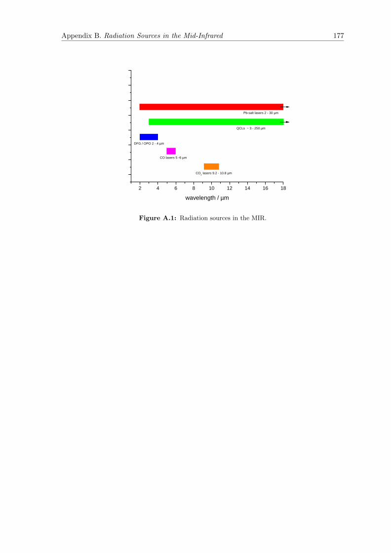
Appendix B. Radiation Sources in the Mid-Infrared 177
2 4 6 8 1 0 1 2 1 4 1 6 1 8
Q C L s ~ 3 - 2 5 0 µ m
D F G / O P O 2 - 4 µ m
C O 2 l a s e r s 9 . 2 - 1 0 . 8 µ m
C O l a s e r s 5 - 6 µ m
w a v e l e n g t h / µm
P b - s a l t l a s e r s 2 - 3 0 µ m
Figure A.1: Radiation sources in the MIR.
Appendix B
Characterisation of the DS-DBR
laser
The work described in this Appendix is based on the DS-DBR characterisation reported in
[193], carried out primarily by Dr Luca Ciaffoni and Kim Whittaker.
In order to investigate fully the effects of changing the relative amplitudes of the current
ramps applied to the front, rear and phase sections of the device, a 4 m multipass cell
was filled with 85 Torr of CO2 and the transmission spectra from both the cell and the
spectrum analyser were recorded for each tuning setting. When just the rear current is
scanned across its whole range, only a small fraction of the total spectral region is effectively
accessed by the laser (4.65 cm−1 out of 32 cm−1), due to the occurrence of multiple mode
hops. In contrast, when a current ramp is injected into the phase section only, mode hops
occur far less frequently as it is effectively exploiting the maximum tunability of one of the
longitudinal cavity modes. As illustrated in Figure B.1, this results in a larger accessible
region of a narrower spectral window (3.3 cm−1 out of 5 cm−1). When ramps are applied to
both the rear and the phase sections, intermediate responses are observed, also illustrated
in Figure B.1. An example of the CO2 spectra obtained under such conditions, where both
the rear and phase sections have a current modulation applied, is shown in Figure B.2. It is
immediately obvious from the spectrum analyser trace in this figure that the tuning rates
during each mode hop-free section vary.
Figure B.3 further illustrates the tuning characteristics of a DS-DBR and depicts the bound-
aries between adjacent longitudinal modes (given by the dotted lines) for a typical super-
mode. This figure has been adapted from Ward et al. [189], with the tuning paths used
to drive the laser in Figure B.1 depicted within the rear current (ir) and phase current
(ip) plane. Each tuning path used stays within one supermode and is continuous in the
178
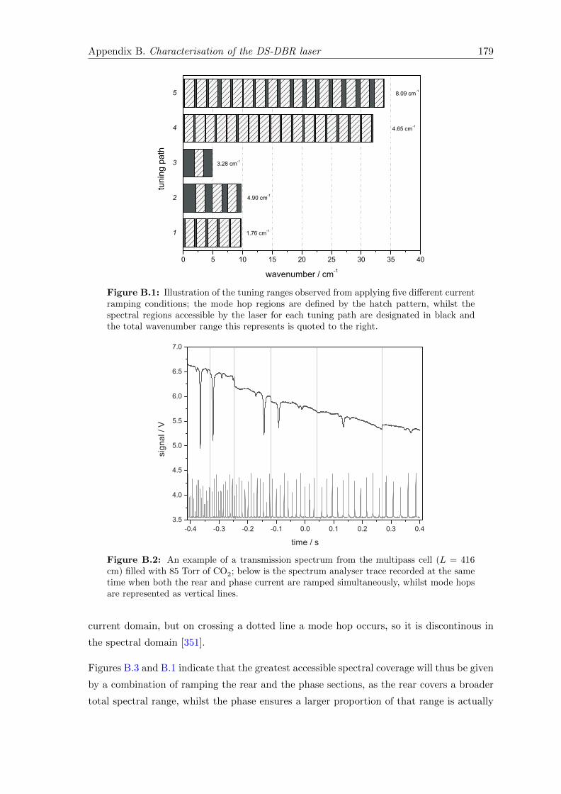
Appendix B. Characterisation of the DS-DBR laser 179
Figure B.1: Illustration of the tuning ranges observed from applying five different currentramping conditions; the mode hop regions are defined by the hatch pattern, whilst thespectral regions accessible by the laser for each tuning path are designated in black andthe total wavenumber range this represents is quoted to the right.
Figure B.2: An example of a transmission spectrum from the multipass cell (L = 416cm) filled with 85 Torr of CO2; below is the spectrum analyser trace recorded at the sametime when both the rear and phase current are ramped simultaneously, whilst mode hopsare represented as vertical lines.
current domain, but on crossing a dotted line a mode hop occurs, so it is discontinous in
the spectral domain [351].
Figures B.3 and B.1 indicate that the greatest accessible spectral coverage will thus be given
by a combination of ramping the rear and the phase sections, as the rear covers a broader
total spectral range, whilst the phase ensures a larger proportion of that range is actually
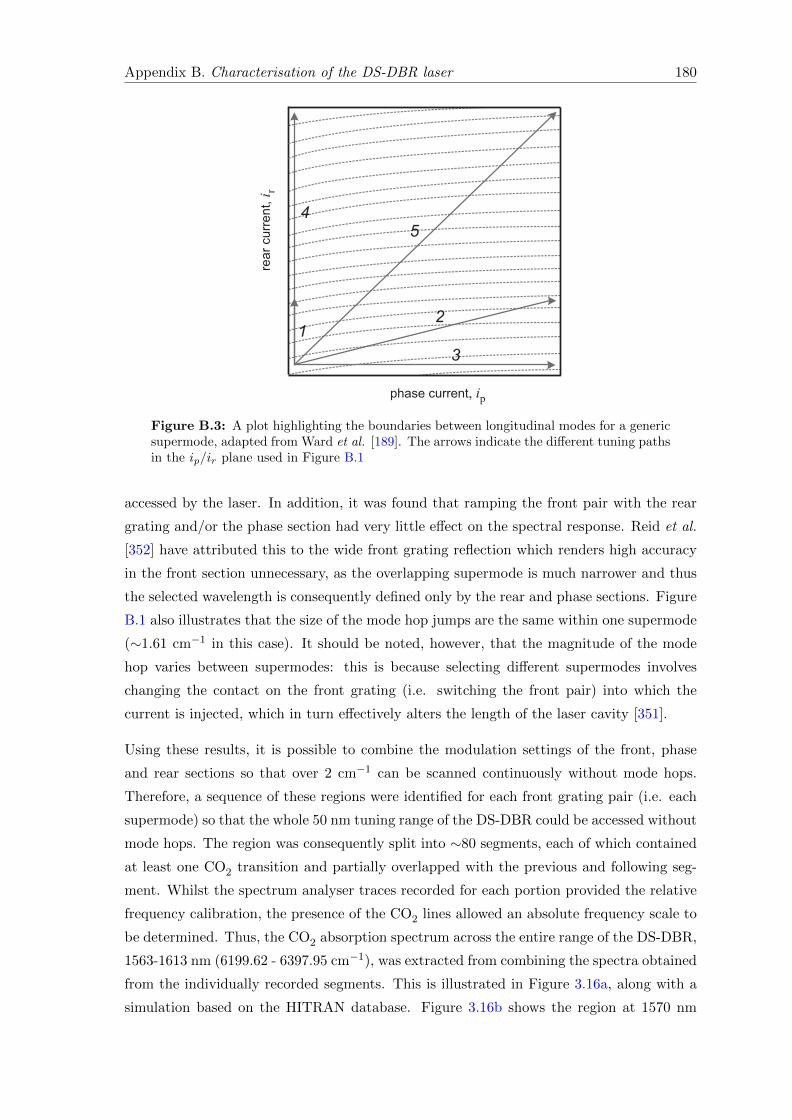
Appendix B. Characterisation of the DS-DBR laser 180
Figure B.3: A plot highlighting the boundaries between longitudinal modes for a genericsupermode, adapted from Ward et al. [189]. The arrows indicate the different tuning pathsin the ip/ir plane used in Figure B.1
accessed by the laser. In addition, it was found that ramping the front pair with the rear
grating and/or the phase section had very little effect on the spectral response. Reid et al.
[352] have attributed this to the wide front grating reflection which renders high accuracy
in the front section unnecessary, as the overlapping supermode is much narrower and thus
the selected wavelength is consequently defined only by the rear and phase sections. Figure
B.1 also illustrates that the size of the mode hop jumps are the same within one supermode
(∼1.61 cm−1 in this case). It should be noted, however, that the magnitude of the mode
hop varies between supermodes: this is because selecting different supermodes involves
changing the contact on the front grating (i.e. switching the front pair) into which the
current is injected, which in turn effectively alters the length of the laser cavity [351].
Using these results, it is possible to combine the modulation settings of the front, phase
and rear sections so that over 2 cm−1 can be scanned continuously without mode hops.
Therefore, a sequence of these regions were identified for each front grating pair (i.e. each
supermode) so that the whole 50 nm tuning range of the DS-DBR could be accessed without
mode hops. The region was consequently split into ∼80 segments, each of which contained
at least one CO2 transition and partially overlapped with the previous and following seg-
ment. Whilst the spectrum analyser traces recorded for each portion provided the relative
frequency calibration, the presence of the CO2 lines allowed an absolute frequency scale to
be determined. Thus, the CO2 absorption spectrum across the entire range of the DS-DBR,
1563-1613 nm (6199.62 - 6397.95 cm−1), was extracted from combining the spectra obtained
from the individually recorded segments. This is illustrated in Figure 3.16a, along with a
simulation based on the HITRAN database. Figure 3.16b shows the region at 1570 nm

Appendix B. Characterisation of the DS-DBR laser 181
(6369.42 cm−1) expanded and the number of experimental points reduced for clarity, with
the best fitting Voigt profiles superimposed. The Gaussian contribution to the Voigt profile
was fixed to the theoretical Doppler width (0.0119 cm−1) and the Lorentzian contributions
subsequently deduced were found to be within 2 % of the values quoted in the HITRAN
database [171].
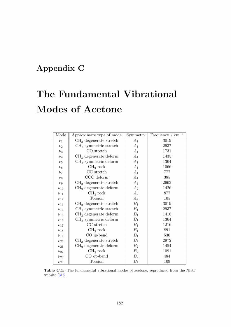
Appendix C
The Fundamental Vibrational
Modes of Acetone
Mode Approximate type of mode Symmetry Frequency / cm−1
ν1 CH3 degenerate stretch A1 3019ν2 CH3 symmetric stretch A1 2937ν3 CO stretch A1 1731ν4 CH3 degenerate deform A1 1435ν5 CH3 symmetric deform A1 1364ν6 CH3 rock A1 1066ν7 CC stretch A1 777ν8 CCC deform A1 385ν9 CH3 degenerate stretch A2 2963ν10 CH3 degenerate deform A2 1426ν11 CH3 rock A2 877ν12 Torsion A2 105ν13 CH3 degenerate stretch B1 3019ν14 CH3 symmetric stretch B1 2937ν15 CH3 degenerate deform B1 1410ν16 CH3 symmetric deform B1 1364ν17 CC stretch B1 1216ν18 CH3 rock B1 891ν19 CO ip-bend B1 530ν20 CH3 degenerate stretch B2 2972ν21 CH3 degenerate deform B2 1454ν22 CH3 rock B2 1091ν23 CO op-bend B2 484ν24 Torsion B2 109
Table C.1: The fundamental vibrational modes of acetone, reproduced from the NISTwebsite [315].
182
References
[1] T. H. Risby and F. K. Tittel. “Current status of midinfrared quantum and interband
cascade lasers for clinical breath analysis”. Optical Engineering, 49, 111123 (2010).
http://dx.doi.org/10.1117/1.3498768
[2] W. Miekisch, J. K. Schubert and G. F. E. Noeldge-Schomburg. “Diagnostic poten-
tial of breath analysis–focus on volatile organic compounds.” Clinica Chimica Acta;
International Journal of Clinical Chemistry, 347, 25–39 (2004).
http://dx.doi.org/10.1016/j.cccn.2004.04.023
[3] J. Rollo. “Cases of the Diabetes Mellitus. . . ”. Printed by T. Gillet for C. Dilly, in
the Poultry, Second Edition, London (1798).
[4] A. Manolis. “The diagnostic potential of breath analysis.” Clinical Chemistry, 29,
5–15 (1983).
http://www.clinchem.org/content/29/1/5.short
[5] L. Pauling and A. Robinson. “Quantitative analysis of urine vapor and breath by gas-
liquid partition chromatography”. Proceedings of the National Academy of Sciences
of the United States of America, 68, 2374–2376 (1971).
http://www.pnas.org/content/68/10/2374.short
[6] C. Wang and P. Sahay. “Breath Analysis Using Laser Spectroscopic Techniques:
Breath Biomarkers, Spectral Fingerprints, and Detection Limits”. Sensors, 9, 8230–
8262 (2009).
http://dx.doi.org/10.3390/s91008230
[7] P. Malfertheiner, F. Megraud, C. O’Morain, F. Bazzoli, E. El-Omar, D. Graham,
R. Hunt, T. Rokkas, N. Vakil and E. J. Kuipers. “Current concepts in the management
of Helicobacter pylori infection: the Maastricht III Consensus Report.” Gut, 56, 772–
81 (2007).
http://dx.doi.org/10.1136/gut.2006.101634
183

References 184
[8] W. D. Chey and B. C. Y. Wong. “American College of Gastroenterology guideline
on the management of Helicobacter pylori infection.” The American Journal of Gas-
troenterology, 102, 1808–25 (2007).
http://dx.doi.org/10.1111/j.1572-0241.2007.01393.x
[9] D. Y. Graham, P. D. Klein, D. J. Evans, D. G. Evans, L. C. Alpert, A. R. Opekun
and T. W. Boutton. “Camplobacter pylori detected noninvasively by the 13C-urea
breath test”. The Lancet, pp. 1174–1177 (1987).
[10] B. Marshall, R. McCullum and R. Guerrant. Helicobacter Pylori in Peptic Ulceration
and Gastritis. Blackwell Scientific Publications (1991).
[11] M. M. Walker, L. Teare and C. McNulty. “Gastric cancer and Helicobacter pylori:
the bug, the host or the environment?” Postgraduate Medical Journal, 84, 169–70
(2008).
http://dx.doi.org/10.1136/pgmj.2008.068346
[12] V. Savarino, S. Vigneri and G. Celle. “The 13C urea breath test in the diagnosis of
Helicobacter pylori infection.” Gut, 45 Suppl 1, I18–22 (1999).
http://www.pubmedcentral.nih.gov/articlerender.fcgi?artid=
1766662&tool=pmcentrez&rendertype=abstract
[13] V. Kasyutich, P. Martin and R. Holdsworth. “An off-axis cavity-enhanced absorption
spectrometer at 1605 nm for the 12CO2/13CO2 measurement”. Applied Physics B,
85, 413–420 (2006).
http://dx.doi.org/10.1007/s00340-006-2312-0
[14] C. Wang, N. Srivastava, B. Jones and R. Reese. “A novel multiple species ringdown
spectrometer for in situ measurements of methane, carbon dioxide, and carbon iso-
tope”. Applied Physics B, 92, 259–270 (2008).
http://dx.doi.org/10.1007/s00340-008-3077-4
[15] P. Klein. “13C breath tests: visions and realities”. The Journal of Nutrition, pp.
1637–1642 (2001).
http://jn.nutrition.org/content/131/5/1637S.short
[16] K. J. Goodman and J. T. Brenna. “High sensitivity tracer detection using high-
precision gas chromatography-combustion isotope ratio mass spectrometry and highly
enriched [U-13C]-labeled precursors.” Analytical Chemistry, 64, 1088–95 (1992).
http://www.ncbi.nlm.nih.gov/pubmed/1609955
[17] B. S. Sheu, S. C. Lee, H. B. Yang, H. W. Wu, C. S. Wu, X. Z. Lin and J. J. Wu.
“Lower-dose 13C-urea breath test to detect Helicobacter pylori infection - comparison
http://www.pubmedcentral.nih.gov/articlerender.fcgi?artid=1766662&tool=pmcentrez&rendertype=abstract
References 185
between infrared spectrometer and mass spectrometry analysis.” Alimentary Phar-
macology and Therapeutics, 14, 1359–63 (2000).
http://www.ncbi.nlm.nih.gov/pubmed/11012483
[18] E. R. Crosson, K. N. Ricci, B. a. Richman, F. C. Chilese, T. G. Owano, R. a. Proven-
cal, M. W. Todd, J. Glasser, A. a. Kachanov, B. a. Paldus, T. G. Spence and R. N.
Zare. “Stable isotope ratios using cavity ring-down spectroscopy: determination of
13C/12C for carbon dioxide in human breath.” Analytical Chemistry, 74, 2003–7
(2002).
http://www.ncbi.nlm.nih.gov/pubmed/12033299
[19] J. B. McManus, M. S. Zahniser, D. D. Nelson, L. R. Williams and C. E. Kolb.
“Infrared laser spectrometer with balanced absorption for measurement of isotopic
ratios of carbon gases.” Spectrochimica Acta. Part A, Molecular and Biomolecular
Spectroscopy, 58, 2465–79 (2002).
http://www.ncbi.nlm.nih.gov/pubmed/12353697
[20] ATS/EPS. “ATS/ERS recommendations for standardized procedures for the online
and offline measurement of exhaled lower respiratory nitric oxide and nasal nitric
oxide, 2005.” American Journal of Respiratory and Critical Care Medicine, 171,
912–30 (2005).
http://dx.doi.org/10.1164/rccm.200406-710ST
[21] FDA. “Class II Special Controls Guidance Document: Breath Nitric Oxide Test
System”. Technical report, U.S. Food and Drug Administration (2003).
[22] S. Kharitonov, D. Yates, R. Robbins and P. Barnes. “Increased nitric oxide in exhaled
air of asthmatic patients”. The Lancet, pp. 133–135 (1994).
http://www.sciencedirect.com/science/article/pii/S0140673694909318
[23] A. Smith, J. Cowan and K. Brassett. “Exhaled Nitric Oxide”. American Journal of
Respiratory and Critical Care Medicine, 172, 453–459 (2005).
http://ajrccm.atsjournals.org/content/172/4/453.short
[24] M. W. H. Pijnenburg and J. C. De Jongste. “Exhaled nitric oxide in childhood
asthma: a review.” Clinical and Experimental Allergy : Journal of the British Society
for Allergy and Clinical Immunology, 38, 246–59 (2008).
http://dx.doi.org/10.1111/j.1365-2222.2007.02897.x
[25] S. Moncada. “Nitric oxide gas: mediator, modulator, and pathophysiologic entity”.
The Journal of Laboratory and Clinical Medicine, 120, 187–91 (1992).
[26] C. Brindicci, K. Ito, P. J. Barnes and S. a. Kharitonov. “Effect of an Inducible Nitric
Oxide Synthase Inhibitor on Differential Flow-Exhaled Nitric Oxide in Asthmatic
References 186
Patients and Healthy Volunteers”. Chest, 132, 581–588 (2007).
http://dx.doi.org/10.1378/chest.06-3046
[27] M. Fleischer, E. Simon, E. Rumpel, H. Ulmer, M. Harbeck, M. Wandel, C. Fietzek,
U. Weimar and H. Meixner. “Detection of volatile compounds correlated to human
diseases through breath analysis with chemical sensors”. Sensors and Actuators B:
Chemical, 83, 245–249 (2002).
http://dx.doi.org/10.1016/S0925-4005(01)01056-5
[28] M. R. McCurdy, Y. Bakhirkin, G. Wysocki, R. Lewicki and F. K. Tittel. “Recent
advances of laser-spectroscopy-based techniques for applications in breath analysis.”
Journal of Breath Research, 1, 014001 (2007).
http://dx.doi.org/10.1088/1752-7155/1/1/014001
[29] Y. Bakhirkin, A. Kosterev, C. Roller, R. F. Curl and F. K. Tittel. “Mid-Infrared
Quantum Cascade Laser Based Off-Axis Integrated Cavity Output Spectroscopy for
Biogenic Nitric Oxide Detection”. Applied Optics, 43, 2257 (2004).
http://dx.doi.org/10.1364/AO.43.002257
[30] A. Kosterev, A. Malinovsky, F. Tittel, C. Gmachl, F. Capasso, D. L. Sivco, J. N.
Baillargeon, A. L. Hutchinson and A. Y. Cho. “Cavity ringdown spectroscopic detec-
tion of nitric oxide with a continuous-wave quantum-cascade laser”. Applied Optics,
40 (2001).
http://www.opticsinfobase.org/abstract.cfm?id=65460
[31] C. Roller, K. Namjou, J. D. Jeffers, M. Camp, A. Mock, P. J. McCann and J. Grego.
“Nitric Oxide Breath Testing by Tunable-Diode Laser Absorption Spectroscopy: Ap-
plication in Monitoring Respiratory Inflammation”. Applied Optics, 41, 6018 (2002).
http://dx.doi.org/10.1364/AO.41.006018
[32] B. W. M. Moeskops, S. M. Cristescu and F. J. M. Harren. “Sub-part-per-billion mon-
itoring of nitric oxide by use of wavelength modulation spectroscopy in combination
with a thermoelectrically cooled, continuous-wave quantum cascade laser”. Optics
Letters, 31, 823 (2006).
http://dx.doi.org/10.1364/OL.31.000823
[33] M. R. McCurdy, Y. Bakhirkin, G. Wysocki and F. K. Tittel. “Performance of an
exhaled nitric oxide and carbon dioxide sensor using quantum cascade laser-based
integrated cavity output spectroscopy.” Journal of Biomedical Optics, 12, 034034
(2007).
http://dx.doi.org/10.1117/1.2747608
References 187
[34] D. Hernandez, S. Addou, D. Lee, C. Orengo, E. a. Shephard and I. R. Phillips.
“Trimethylaminuria and a human FMO3 mutation database”. Human Mutation, 22,
209–213 (2003).
http://dx.doi.org/10.1002/humu.10252
[35] M. L. Simenhoff, J. F. Burke, J. J. Saukkonen, A. T. Ordinario and R. Doty. “Bio-
chemical profile of uremic breath.” The New England Journal of Medicine, 297,
132–135 (1977).
[36] S. C. Mitchell and A. Q. Zhang. “Methylamine in human urine”. Clinica Chimica
Acta, 312, 107–114 (2001).
http://dx.doi.org/10.1016/S0009-8981(01)00608-8
[37] J. King, P. Mochalski, A. Kupferthaler, K. Unterkofler, H. Koc, W. Filipiak, S. Teschl,
H. Hinterhuber and A. Amann. “Dynamic profiles of volatile organic compounds in
exhaled breath as determined by a coupled PTR-MS/GC-MS study.” Physiological
Measurement, 31, 1169–84 (2010).
http://dx.doi.org/10.1088/0967-3334/31/9/008
[38] B. G. Stone, T. J. Besse, W. C. Duane, C. D. Evans and E. G. DeMaster. “Effect of
regulating cholesterol biosynthesis on breath isoprene excretion in men”. Lipids, 28,
705–708 (1993).
http://dx.doi.org/10.1007/BF02535990
[39] T. H. Risby. “Volatile organic compounds as markers in normal and diseased states”.
In N. Marczin and M. Yacoub, editors, “Disease Markers in Exhaled Breath: Basic
Mechanisms and Clinical Applications”, pp. 113–122 (2002).
[40] E. Deneris and R. Stein. “Acid-catalyzed formation of isoprene from a mevalonate-
derived product using a rat liver cytosolic fraction.” Journal of Biological Chemistry,
260, 1382–1385 (1985).
http://www.jbc.org/content/260/3/1382.short
[41] A. Cailleux and P. Allain. “Isoprene and sleep”. Life Sciences, 44, 1877–1880 (1989).
http://www.sciencedirect.com/science/article/pii/0024320589903068
[42] T. Risby and S. Sehnert. “Clinical Application of Breath Biomarkers of Oxidative
Stress Status”. Free Radical Biology and Medicine, 27, 1182–1192 (1999).
[43] S. Chen, L. Zieve and V. Mahadevan. “Mercaptans and dimethyl sulfide in the breath
of patients with cirrhosis of the liver. Effect of feeding methionine”. J Lab Clin Med.,
75, 628–35 (1970).

References 188
[44] M. Phillips. “Detection of Lung Cancer With Volatile Markers in the Breath”. Chest,
123, 2115–2123 (2003).
http://dx.doi.org/10.1378/chest.123.6.2115
[45] M. Phillips and M. Sabas. “Increased pentane and carbon disulfide in the breath of
patients with schizophrenia.” Journal of clinical pathology, pp. 861–864 (1993).
http://jcp.bmj.com/content/46/9/861.short
[46] F. Kneepkens and G. Lepage. “The potential of the hydrocarbon breath test as
a measure of lipid peroxidation”. Free Radical Biology and Medicine, 17, 127–160
(1994).
http://www.sciencedirect.com/science/article/pii/0891584994901104
[47] M. R. Ras, F. Borrull and R. M. Marce. “Sampling and preconcentration techniques
for determination of volatile organic compounds in air samples”. Trends in Analytical
Chemistry, 28, 347–361 (2009).
http://dx.doi.org/10.1016/j.trac.2008.10.009
[48] A. Hryniuk and B. M. Ross. “Detection of acetone and isoprene in human breath using
a combination of thermal desorption and selected ion flow tube mass spectrometry”.
International Journal of Mass Spectrometry, 285, 26–30 (2009).
http://dx.doi.org/10.1016/j.ijms.2009.02.027
[49] D. Smith and P. Spanel. “Ambient analysis of trace compounds in gaseous media by
SIFT-MS”. The Analyst, 136, 2009 (2011).
http://dx.doi.org/10.1039/c1an15082k
[50] R. S. Blake, P. S. Monks and A. M. Ellis. “Proton-transfer reaction mass spectrom-
etry.” Chemical Reviews, 109, 861–96 (2009).
http://dx.doi.org/10.1021/cr800364q
[51] B. Moser, F. Bodrogi, G. Eibl, M. Lechner, J. Rieder and P. Lirk. “Mass spectromet-
ric profile of exhaled breath–field study by PTR-MS.” Respiratory Physiology and
Neurobiology, 145, 295–300 (2005).
http://dx.doi.org/10.1016/j.resp.2004.02.002
[52] P. Spanel and D. Smith. “Selected ion flow tube mass spectrometry for on-line trace
gas analysis in biology and medicine.” European Journal of Mass Spectrometry, 13,
77–82 (2007).
http://dx.doi.org/10.1255/ejms.843
[53] C. Di Natale, A. Macagnano, E. Martinelli, R. Paolesse, G. D’Arcangelo, C. Roscioni,
A. Finazzi-Agro and A. D’Amico. “Lung cancer identification by the analysis of breath
References 189
by means of an array of non-selective gas sensors”. Biosensors and Bioelectronics,
18, 1209–1218 (2003).
http://dx.doi.org/10.1016/S0956-5663(03)00086-1
[54] M. Righettoni, A. Tricoli and S. E. Pratsinis. “Si:WO(3) Sensors for highly selective
detection of acetone for easy diagnosis of diabetes by breath analysis.” Analytical
Chemistry, 82, 3581–7 (2010).
http://dx.doi.org/10.1021/ac902695n
[55] M. Murtz. “Breath Diagnostics Using Laser Spectroscopy”. Optics and Photonics
News, 16, 30–35 (2005).
http://dx.doi.org/10.1364/OPN.16.1.000030
[56] K. Heinrich, T. Fritsch, P. Hering and M. Murtz. “Infrared laser-spectroscopic anal-
ysis of 14NO and 15NO in human breath”. Applied Physics B, 95, 281–286 (2009).
http://dx.doi.org/10.1007/s00340-009-3423-1
[57] L. Menzel, A. Kosterev, R. Curl, F. Tittel, C. Gmachl, F. Capasso, D. Sivco, J. Bail-
largeon, A. Hutchinson, A. Cho and W. Urban. “Spectroscopic detection of biological
NO with a quantum cascade laser”. Applied Physics B, 72, 859–863 (2001).
http://dx.doi.org/10.1007/s003400100562
[58] K. Namjou, C. B. Roller and G. McMillen. “Breath-Analysis Using Mid-Infrared
Tunable Laser Spectroscopy”. 2007 IEEE Sensors, pp. 1337–1340 (2007).
http://dx.doi.org/10.1109/ICSENS.2007.4388658
[59] M. B. Esler, D. W. Griffith, S. R. Wilson and L. P. Steele. “Precision trace gas
analysis by FT-IR spectroscopy. 2. The 13C/12C isotope ratio of CO2.” Analytical
Chemistry, 72, 216–21 (2000).
http://www.ncbi.nlm.nih.gov/pubmed/10655656
[60] M. Wolff, M. Germer, H. G. Groninga and H. Harde. “Photoacoustic CO2 sensor
based on a DFB diode laser at 2.7µm”. The European Physical Journal Special
Topics, 153, 409–413 (2008).
http://dx.doi.org/10.1140/epjst/e2008-00473-9
[61] D. E. Cooper, R. U. Martinelli, C. B. Carlisle, H. Riris, D. B. Bour and R. J. Menna.
“Measurement of 12CO2:13CO2 ratios for medical diagnostics with 1.6 µm distributed-
feedback semiconductor diode lasers”. Applied Optics, 32, 6727–6731 (1993).
[62] D. Weidmann, G. Wysocki, C. Oppenheimer and F. Tittel. “Development of a com-
pact quantum cascade laser spectrometer for field measurements of CO2 isotopes”.
Applied Physics B, 80, 255–260 (2004).
http://dx.doi.org/10.1007/s00340-004-1639-7
References 190
[63] M. Erdelyi, D. Richter and F. Tittel. “13CO2 / 12CO2 isotopic ratio measurements
using a difference frequency-based sensor operating at 4.35 µm”. Applied Physics B:
Lasers and Optics, 75, 289–295 (2002).
http://dx.doi.org/10.1007/s00340-002-0960-2
[64] K. Uehara, K. Yamamoto, T. Kikugawa and N. Yoshida. “Isotope analysis of envi-
ronmental substances by a new laser-spectroscopic method utilizing different path-
lengths”. Sensors and Actuators B: Chemical, 74, 173–178 (2001).
http://dx.doi.org/10.1016/S0925-4005(00)00729-2
[65] R. N. Zare, D. S. Kuramoto, C. Haase, S. M. Tan, E. R. Crosson and N. M. R.
Saad. “High-precision optical measurements of isotope ratios in organic compounds
at 13C/12C isotope ratios in organic compounds at natural abundance”. Proceedings
of the National Academy of Sciences of the United States of America, 106 (2009).
[66] D. Marinov and J. Rey. “Spectroscopic investigation of methylated amines by a
cavity-ringdown-based spectrometer”. Applied Optics, 46, 3981–3986 (2007).
http://www.opticsinfobase.org/abstract.cfm?&id=138445
[67] D. Marinov, J. Rey and M. W. Sigrist. “Mid-infrared spectroscopic investigation of
methylamines by a continuous-wave system”. Applied Optics, 47, 1956–1962 (2008).
http://dx.doi.org/http://dx.doi.org/10.1364/AO.47.001956
[68] J. Manne, O. Sukhorukov, W. Jager and J. Tulip. “Pulsed quantum cascade laser-
based cavity ring-down spectroscopy for ammonia detection in breath”. Applied Op-
tics, pp. 5–7 (2006).
[69] H. Dahnke, D. Kleine and P. Hering. “Real-time monitoring of ethane in human
breath using mid-infrared cavity leak-out spectroscopy”. Applied Physics B, 975,
971–975 (2001).
[70] G. von Basum, H. Dahnke, D. Halmer, P. Hering and M. Murtz. “Online recording
of ethane traces in human breath via infrared laser spectroscopy.” Journal of Applied
Physiology, 95, 2583–90 (2003).
http://dx.doi.org/10.1152/japplphysiol.00542.2003
[71] G. von Basum, D. Halmer, P. Hering, M. Murtz, S. Schiller, F. Muller, A. Popp
and F. Kuhnemann. “Parts per trillion sensitivity for ethane in air with an optical
parametric oscillator cavity leak-out spectrometer.” Optics Letters, 29, 797–9 (2004).
http://www.ncbi.nlm.nih.gov/pubmed/15119381
References 191
[72] S. Studer, J. Orens, I. Rosas and J. Krishnan. “Patterns and significance of exhaled-
breath biomarkers in lung transplant recipients with acute allograft rejection”. Jour-
nal of Heart and Lung Transplantation, 20, 1158–1166 (2001).
http://dx.doi.org/10.1016/S1053-2498(01)00343-6
[73] C. Roller, A. Kosterev, F. K. Tittel, K. Uehara, C. Gmachl and D. L. Sivco. “Carbonyl
sulfide detection with a thermoelectrically cooled midinfrared quantum cascade laser”.
Optics Letters, 28, 2052 (2003).
http://dx.doi.org/10.1364/OL.28.002052
[74] D. Halmer, G. V. Basum and P. Hering. “Mid-infrared cavity leak-out spectroscopy
for ultrasensitive detection of carbonyl sulfide”. Optics Letters, 30, 2314–2316 (2005).
http://www.opticsinfobase.org/abstract.cfm?id=85023
[75] G. Wysocki, M. McCurdy, S. So, D. Weidmann, C. Roller, R. F. Curl and F. K.
Tittel. “Pulsed Quantum-Cascade Laser-Based Sensor for Trace-Gas Detection of
Carbonyl Sulfide”. Applied Optics, 43, 6040 (2004).
http://dx.doi.org/10.1364/AO.43.006040
[76] K. Moskalenko, A. Nadezhdinskii and I. Adamovskaya. “Human breath trace gas
content study by tunable diode laser spectroscopy technique”. Infrared Physics and
Technology, 37, 181–192 (1996).
http://www.sciencedirect.com/science/article/pii/1350449595000976
[77] M. J. Thorpe, D. Balslev-Clausen, M. S. Kirchner and J. Ye. “Cavity-enhanced
optical frequency comb spectroscopy: application to human breath analysis”. Optics
Express, 16, 2387–2397 (2008).
http://dx.doi.org/10.1364/OE.16.002387
[78] G. Freund and R. L. Weinsier. “Standardized ketosis in man following medium chain
triglyceride ingestion.” Metabolism: Clinical and Experimental, 15, 980–91 (1966).
http://www.ncbi.nlm.nih.gov/pubmed/5922367
[79] G. Koorevaar and G. van Stekelenburg. “Mammalian Acetoacetate Decarboxylase
Activity”. Clinica Chimica Acta, 71, 173–183 (1976).
[80] A. S. Rudenski, D. R. Matthews and J. C. Levy. “Understanding ‘Insulin Resistance’:
Both Glucose Resistance and Insulin Resistance Are Required to Model Human Di-
abetes”. Metabolism, 40, 908–917 (1991).
[81] C. R. Kahn. “Insulin Resistance: A Common Feature of Diabetes Mellitus”. N Engl
J Med, 315, 252–254 (1986).
[82] W. Petters. “Untersuchungen uber die Honigharnruhr”. Vjschr. Prakt. Heilk. (1857).

References 192
[83] H. Scott-Wilson. “A method for estimating acetone in animal liquids”. The Journal
of Physiology (1911).
http://jp.physoc.org/content/42/5-6/444.full.pdf
[84] W. Marriott. “The Blood in Acidosis from the Quantitative Standpoint”. Journal of
Biological Chemistry (1914).
http://www.jbc.org/content/18/3/507.short
[85] F. Otto, F. Denis and M. Boston. “Turbidity Methods for the Determination of
Acetone, Acetoacetic Acid and β-oxybutyric Acid in Urine”. J. Biol. Chem (1914).
[86] O. Folin and W. Denis. “On starvation and obesity, with special reference to acidosis”.
Journal of Biological Chemistry (1915).
http://www.jbc.org/content/21/1/183.short
[87] E. Widmark. “Studies in the Acetone Concentration in Blood, Urine, and Alveolar
Air. III: The Elimination of Acetone through the Lungs”. Biochemical Journal (1920).
http://www.ncbi.nlm.nih.gov/pmc/articles/PMC1263892/
[88] R. Hubbard. “Determination of acetone in expired air”. J. Biol. Chem, pp. 57–65
(1920).
http://scholar.google.com/scholar?hl=en&btnG=Search&q=intitle:
Determination+of+acetone+in+expired+air#0
[89] R. Stewart and E. Boettner. “Rapid Infra-Red Determination of Acetone in the Blood
and the Exhaled Air of Diabetic Patients”. Nature (1961).
http://www.nature.com/nature/journal/v191/n4792/abs/1911008a0.html
[90] G. Rooth and S. Ostenson. “Acetone in alveolar air, and the control of diabetes.”
Lancet, pp. 1102–1105 (1966).
http://www.ncbi.nlm.nih.gov/pubmed/4162529
[91] C. Tassopoulos and D. Barnett. “Breath-acetone and blood-sugar measurements in
diabetes”. The Lancet, 1282, 1282–1286 (1969).
http://www.sciencedirect.com/science/article/pii/S0140673669922223
[92] O. Crofford, R. Mallard, R. Winton, N. Rogers, J. Jackson and U. Keller. “Acetone
in breath and blood.” Transcripts of the American Clinical and Climatological Asso-
ciation, 88, 128–139 (1977).
http://www.ncbi.nlm.nih.gov/pmc/articles/PMC2441399/
[93] H. Shamoon. “The Effect of Intensive Treatment of Diabetes on the Development and
Progression of Long-Term Complications in Insulin-Dependent Diabetes Mellitus”. N.
England Journal of Medicine, 329, 977 (1993).
References 193
[94] C. Turner, C. Walton, S. Hoashi and M. Evans. “Breath acetone concentration
decreases with blood glucose concentration in type I diabetes mellitus patients during
hypoglycaemic clamps.” Journal of Breath Research, 3, 046004 (2009).
http://dx.doi.org/10.1088/1752-7155/3/4/046004
[95] T. D. C. Minh, S. R. Oliver, J. Ngo, R. Flores, J. Midyett, S. Meinardi, M. K. Carlson,
F. S. Rowland, D. R. Blake and P. R. Galassetti. “Noninvasive measurement of plasma
glucose from exhaled breath in healthy and type 1 diabetic subjects.” American
Journal of Physiology. Endocrinology and Metabolism, 300, E1166–75 (2011).
http://dx.doi.org/10.1152/ajpendo.00634.2010
[96] P. R. Galassetti, B. Novak, D. Nemet, C. Rose-Gottron, D. M. Cooper, S. Meinardi,
R. Newcomb, F. Zaldivar and D. R. Blake. “Breath ethanol and acetone as indicators
of serum glucose levels: an initial report.” Diabetes Technology and Therapeutics, 7,
115–23 (2005).
http://dx.doi.org/10.1089/dia.2005.7.115
[97] C. Wang, A. Mbi and M. Shepherd. “A Study on Breath Acetone in Diabetic Patients
Using a Cavity Ringdown Breath Analyzer: Exploring Correlations of Breath Acetone
With Blood Glucose and Glycohemoglobin A1C”. IEEE Sensors Journal, 10, 54–63
(2010).
http://dx.doi.org/10.1109/JSEN.2009.2035730
[98] P. Spanel, K. Dryahina, A. Rejskova, T. W. E. Chippendale and D. Smith. “Breath
acetone concentration; biological variability and the influence of diet.” Physiological
Measurement, 32, N23–31 (2011).
http://dx.doi.org/10.1088/0967-3334/32/8/N01
[99] P. Spanel and D. Smith. “Volatile compounds in health and disease.” Current Opinion
in Clinical Nutrition and Metabolic Care, 14, 455–60 (2011).
http://dx.doi.org/10.1097/MCO.0b013e3283490280
[100] D. Smith, P. Spanel, A. A. Fryer, F. Hanna and G. A. Ferns. “Can volatile compounds
in exhaled breath be used to monitor control in diabetes mellitus?” Journal of Breath
Research, 5, 022001 (2011).
http://dx.doi.org/10.1088/1752-7155/5/2/022001
[101] T. D. C. Minh, D. R. Blake and P. R. Galassetti. “The clinical potential of exhaled
breath analysis for diabetes mellitus.” Diabetes Research and Clinical Practice, pp.
1–11 (2012).
http://dx.doi.org/10.1016/j.diabres.2012.02.006
References 194
[102] B. Landini. “Breath Acetone Concentration Measured Using a Palm-Size Enzymatic
Sensor System”. Sensors Journal, IEEE, 9, 1802–1807 (2009).
http://ieeexplore.ieee.org/xpls/abs_all.jsp?arnumber=5291937
[103] PositiveID. “http://www.positiveidcorp.com/”.
[104] Y. Bakhirkin, A. A. Kosterev, T. Day, M. Pushkarsky and F. Tittel. “Tunable
mid-IR external cavity quantum cascade laser based spectroscopic sensor for acetone
detection”. In “SPIE Optics East”, (2007).
[105] C. Wang and A. Mbi. “A new acetone detection device using cavity ringdown spec-
troscopy at 266 nm: evaluation of the instrument performance using acetone sample
solutions”. Measurement Science and Technology, 18, 2731–2741 (2007).
http://dx.doi.org/10.1088/0957-0233/18/8/051
[106] C. Wang, S. T. Scherrer and D. Hossain. “Measurements of cavity ringdown spec-
troscopy of acetone in the ultraviolet and near-infrared spectral regions: potential for
development of a breath analyzer.” Applied Spectroscopy, 58, 784–91 (2004).
http://dx.doi.org/10.1366/0003702041389193
[107] C. Wang and A. B. Surampudi. “An acetone breath analyzer using cavity ringdown
spectroscopy: an initial test with human subjects under various situations”. Mea-
surement Science and Technology, 19, 105604 (2008).
http://dx.doi.org/10.1088/0957-0233/19/10/105604
[108] P. Atkins and R. Friedman. Molecular Quantum Mechanics. Oxford University Press
(2003).
[109] D. Swinehart. “The Beer-Lambert law”. Journal of Chemical Education, 39, 333
(1962).
http://dx.doi.org/10.1021/ed039p333
[110] W. Demtroder. Laser Spectroscopy. Springer-Verlag, third edition (2003).
[111] R. Dicke. “The effect of collisions upon the Doppler width of spectral lines”. Physical
Review, 89, 472–473 (1953).
http://adsabs.harvard.edu/abs/1953PhRv...89..472D
[112] J. Ye and J. L. Hall. “Ultrasensitive detections in atomic and molecular physics :
demonstration in molecular overtone spectroscopy”. J. Opt. Soc. Am. B, 15, 6–15
(1998).
[113] C. Davis. Lasers and Electro-Optics: Fundamentals and Engineering. Cambridge
University Press (1996).
References 195
[114] H.-P. Dorn, R. Neuroth and A. Hofzumahaus. “Investigation of OH absorption cross
sections of rotational transitions in the A2Σ+, ν ′ = 0 ← X2Π, ν ′′ = 0 band under
atmospheric conditions: Implications for tropospheric long-path absorption measure-
ments”. Journal of Geophysical Research, 100, 7397–7409 (1995).
[115] M. Mazurenka, A. J. Orr-Ewing, R. Peverall and G. A. D. Ritchie. “Cavity ring-down
and cavity enhanced spectroscopy using diode lasers”. Annual Reports Section ‘C’
(Physical Chemistry), 101, 100 (2005).
http://dx.doi.org/10.1039/b408909j
[116] A. Yariv and P. Yeh. Photonics: Optical electronics in modern communications.
Oxford University Press (2006).
[117] O. Svelto. Principles of Lasers. Plenum Press (1998).
[118] I. Vurgaftman, W. W. Bewley, C. L. Canedy, C. S. Kim, M. Kim, J. Ryan Lindle,
C. D. Merritt, J. Abell and J. R. Meyer. “Mid-IR Type-II Interband Cascade Lasers”.
IEEE Journal of Selected Topics in Quantum Electronics, 17, 1435–1444 (2011).
http://dx.doi.org/10.1109/JSTQE.2011.2114331
[119] J. Faist, F. Capasso, D. L. Sivco, C. Sirtori, A. L. Hutchinson and A. Y. Cho. “Quan-
tum Cascade Laser”. Science, 264, 553–556 (1994).
[120] R. F. Curl, F. Capasso, C. Gmachl, A. A. Kosterev, B. McManus, R. Lewicki,
M. Pusharsky, G. Wysocki and F. K. Tittel. “Quantum cascade lasers in chemi-
cal physics”. Chemical Physics Letters, 487, 1–18 (2010).
http://dx.doi.org/10.1016/j.cplett.2009.12.073
[121] R. Kazarinov and R. Suris. “Possibility of amplification of electromagnetic waves
in a semiconductor with a superlattice”. Fizika i Tekhnika Poluprovodnikov (Soviet
Physics - Semiconductors), 5, 797–800 (1971).
[122] G. Duxbury, N. Langford, M. T. McCulloch and S. Wright. “Quantum cascade
semiconductor infrared and far-infrared lasers: from trace gas sensing to non-linear
optics.” Chemical Society reviews, 34, 921–34 (2005).
http://dx.doi.org/10.1039/b400914m
[123] A. Hugi, R. Terazzi, Y. Bonetti, A. Wittmann, M. Fischer, M. Beck, J. Faist and
E. Gini. “External cavity quantum cascade laser tunable from 7.6 to 11.4µm”. Applied
Physics Letters, 95, 061103 (2009).
http://dx.doi.org/10.1063/1.3193539
[124] G. Wysocki, R. Lewicki, R. Curl, F. Tittel, L. Diehl, F. Capasso, M. Troccoli,
G. Hofler, D. Bour, S. Corzine, R. Maulini, M. Giovannini and J. Faist. “Widely

References 196
tunable mode-hop free external cavity quantum cascade lasers for high resolution
spectroscopy and chemical sensing”. Applied Physics B, 92, 305–311 (2008).
http://dx.doi.org/10.1007/s00340-008-3047-x
[125] C. Gmachl, D. L. Sivco, J. N. Baillargeon, A. L. Hutchinson and F. Capasso. “Quan-
tum cascade lasers with a heterogeneous cascade : Two-wavelength operation”. Ap-
plied Physics Letters, 572, 10–13 (2001).
http://dx.doi.org/10.1063/1.1383806
[126] B. G. Lee, M. A. Belkin, C. Pflugl, L. Diehl, H. A. Zhang, R. M. Audet, J. Macarthur,
D. P. Bour, S. W. Corzine, G. E. Hofler and F. Capasso. “DFB Quantum Cascade
Laser Arrays”. IEEE Journal of Quantum Electronics, 45, 554–565 (2009).
[127] F. Capasso. “High-performance midinfrared quantum cascade lasers”. Optical Engi-
neering, 49, 111102 (2010).
http://dx.doi.org/10.1117/1.3505844
[128] V. Shidlovski. “Superluminescent Diodes . Short overview of device operation prin-
ciples and performance parameters.” Technical report (2004).
[129] G. Alphonse, D. Gilbert, M. Harvey and M. Ettenberg. “High-power superlumines-
cent diodes”. IEEE Journal of Quantum Electronics, 24, 2454–2457 (1988).
http://dx.doi.org/10.1109/3.14376
[130] R. Alfano. “Observation of self-phase modulation and small-scale filaments in crystals
and glasses”. Physical Review Letters, 24 (1970).
http://link.aps.org/doi/10.1103/PhysRevLett.24.592
[131] G. New. Introduction to Nonlinear Optics. Cambridge (2011).
[132] J. M. Dudley and S. Coen. “Supercontinuum generation in photonic crystal fiber”.
Reviews of Modern Physics, 78, 1135–1184 (2006).
http://dx.doi.org/10.1103/RevModPhys.78.1135
[133] R. R. Alfano, editor. The Supercontinuum Laser Source: Fundamentals With Updated
References. Springer, 2nd edition (2006).
[134] J. Hult, R. S. Watt and C. F. Kaminski. “High bandwidth absorption spectroscopy
with a dispersed supercontinuum source.” Optics Express, 15, 11385–95 (2007).
http://www.ncbi.nlm.nih.gov/pubmed/19547496
[135] D. Herriott, H. Kogelnik and R. Kompfner. “Off-Axis Paths in Spherical Mirror
Interferometers”. Applied Optics, 3, 523 (1964).
http://dx.doi.org/10.1364/AO.3.000523
References 197
[136] R. Engeln and G. Berden. Cavity Ring-Down Spectrocopy: Techniques and Applica-
tions. Wiley (2009).
[137] H. Kogelnik and T. Li. “Laser beams and resonators”. Proceedings of the IEEE, 54
(1966).
http://ieeexplore.ieee.org/xpls/abs_all.jsp?arnumber=1447049
[138] A. E. Siegman. Lasers. Oxford University Press (1986).
[139] J. Morville, S. Kassi, M. Chenevier and D. Romanini. “Fast, low-noise, mode-by-
mode, cavity-enhanced absorption spectroscopy by diode-laser self-locking”. Applied
Physics B, 80, 1027–1038 (2005).
http://dx.doi.org/10.1007/s00340-005-1828-z
[140] A. OKeefe and D. a. G. Deacon. “Cavity ring-down optical spectrometer for absorp-
tion measurements using pulsed laser sources”. Review of Scientific Instruments, 59,
2544 (1988).
http://dx.doi.org/10.1063/1.1139895
[141] A. O’Keefe. “Integrated cavity output analysis of ultra-weak absorption”. Chemical
Physics Letters, pp. 331–336 (1998).
http://www.sciencedirect.com/science/article/pii/S0009261498007854
[142] R. Engeln, G. Berden, R. Peeters and G. Meijer. “Cavity enhanced absorption and
cavity enhanced magnetic rotation spectroscopy”. Review of Scientific Instruments,
69, 3763 (1998).
http://dx.doi.org/10.1063/1.1149176
[143] D. Romanini and K. K. Lehmann. “Ring-down cavity absorption spectroscopy of the
very weak HCN overtone bands with six, seven, and eight stretching quanta”. The
Journal of Chemical Physics, 99, 6287 (1993).
http://dx.doi.org/10.1063/1.465866
[144] A. O’Keefe and J. Scherer. “CW integrated cavity output spectroscopy”. Chemical
Physics Letters, pp. 343–349 (1999).
http://www.sciencedirect.com/science/article/pii/S0009261499005473
[145] B. Bakowski, L. Corner, G. Hancock, R. Kotchie, R. Peverall and G. Ritchie. “Cavity-
enhanced absorption spectroscopy with a rapidly swept diode laser”. Applied Physics
B: Lasers and Optics, 75, 745–750 (2002).
http://dx.doi.org/10.1007/s00340-002-1026-1

References 198
[146] J. B. Paul, L. Lapson and J. G. Anderson. “Ultrasensitive absorption spectroscopy
with a high-finesse optical cavity and off-axis alignment.” Applied Optics, 40, 4904–
10 (2001).
http://www.ncbi.nlm.nih.gov/pubmed/18360533
[147] D. Baer, J. Paul, M. Gupta and a. O’Keefe. “Sensitive absorption measurements in the
near-infrared region using off-axis integrated-cavity-output spectroscopy”. Applied
Physics B: Lasers and Optics, 75, 261–265 (2002).
http://dx.doi.org/10.1007/s00340-002-0971-z
[148] J. Fernandes, T. M. Wolever and A. Venketeshwer Rao. “Interrelationships between
age, total dietary fiber intake and breath methane in humans”. Nutrition Research,
20, 929–940 (2000).
[149] H. Y. Clark, L. Corner, W. Denzer, G. Hancock, A. Hutchinson, M. Islam, R. Peverall
and G. A. D. Ritchie. “Difference frequency generation in periodically poled lithium
niobate and its use in the detection of atmospheric methane”. Chemical Physics
Letters, 399, 102–108 (2004).
http://dx.doi.org/10.1016/j.cplett.2004.09.146
[150] E. Conway De Macario and A. J. L. Macario. “Methanogenic archaea in health
and disease: a novel paradigm of microbial pathogenesis.” International Journal of
Medical Microbiology, 299, 99–108 (2009).
http://www.ncbi.nlm.nih.gov/pubmed/18757236
[151] P. Eckburg and P. Lepp. “Archaea and their potential role in human disease”. Infec-
tion and Immunity, 71 (2003).
http://dx.doi.org/10.1128/IAI.71.2.591
[152] R. Hanson and T. Hanson. “Methanotrophic bacteria.” Microbiological Reviews, 60
(1996).
http://mmbr.asm.org/content/60/2/439.short
[153] Y. Peled, D. Weinberg, A. Hallak and T. Gilat. “Factors affecting methane produc-
tion in humans. Gastrointestinal diseases and alterations of colonic flora.” Digestive
diseases and sciences, 32, 267–71 (1987).
http://www.ncbi.nlm.nih.gov/pubmed/3816480
[154] M. Di Stefano and G. Corazza. “Role of hydrogen and methane breath testing in
gastrointestinal diseases”. Digestive and Liver Disease Supplements, 3, 40–43 (2009).
http://dx.doi.org/10.1016/S1594-5804(09)60018-8
References 199
[155] R. J. Saad and W. D. Chey. “Breath tests for gastrointestinal disease: the real deal
or just a lot of hot air?” Gastroenterology, 133, 1763–6 (2007).
http://dx.doi.org/10.1053/j.gastro.2007.10.059
[156] A. Eisenmann, A. Amann, M. Said, B. Datta and M. Ledochowski. “Implementation
and interpretation of hydrogen breath tests”. J. Breath Res., 2 (2008).
http://dx.doi.org/10.1088/1752-7155/2/4/046002
[157] L. Le Marchand, L. R. Wilkens, P. Harwood and R. V. Cooney. “Use of breath
hydrogen and methane as markers of colonic fermentation in epidemiologic studies:
circadian patterns of excretion.” Environmental Health Perspectives, 98, 199–202
(1992).
http://www.pubmedcentral.nih.gov/articlerender.fcgi?artid=
1519616&tool=pmcentrez&rendertype=abstract
[158] E. Zuccato, M. Andreoletti, A. Bozzani, F. Marcucci, P. Velio, P. Bianchi and
E. Mussini. “Respiratory excretion of hydrogen and methane in Italian subjects
after ingestion of lactose and milk.” European Journal of Clinical Investigation, 13,
261–266 (1983).
[159] R. Tormo, A. Bertaccini, M. Conde, D. Infante and I. Cura. “Methane and hydrogen
exhalation in normal children and in lactose malabsorption.” Early Human Develop-
ment, 65 Suppl, S165–72 (2001).
http://www.ncbi.nlm.nih.gov/pubmed/11755048
[160] J. P. Waud, S. B. Matthews and A. K. Campbell. “Measurement of breath hydro-
gen and methane, together with lactase genotype, defines the current best practice
for investigation of lactose sensitivity”. Annals of Clinical Biochemistry, 45, 50–58
(2008).
http://dx.doi.org/10.1258/acb.2007.007147
[161] T. M. Kajs, J. A. Fitzgerald, R. Y. Buckner, G. A. Coyle, B. S. Stinson, J. G. Morel
and M. D. Levitt. “Influence of a methanogenic flora on the breath H2 and symptom
response to ingestion of sorbitol or oat fiber.” American Journal of Gastroenterology,
92, 89–94 (1997).
[162] S. Rao, A. Attaluri, L. Anderson and P. Stumbo. “Fructose : Evaluation by Breath
Testing”. Clinics in Gastroenterology, 5, 959–963 (2008).
[163] G. R. Corazza, a. Strocchi, R. Rossi, D. Sirola and G. Gasbarrini. “Sorbitol
malabsorption in normal volunteers and in patients with coeliac disease.” Gut, 29,
44–8 (1988).
http://www.pubmedcentral.nih.gov/articlerender.fcgi?artid=1519616&tool=pmcentrez&rendertype=abstract
References 200
http://www.pubmedcentral.nih.gov/articlerender.fcgi?artid=
1433267&tool=pmcentrez&rendertype=abstract
[164] A. Gasbarrini, E. C. Lauritano, M. Gabrielli, E. Scarpellini, A. Lupascu, V. Ojetti
and G. Gasbarrini. “Small intestinal bacterial overgrowth: diagnosis and treatment.”
Digestive Diseases (Basel, Switzerland), 25, 237–40 (2007).
http://dx.doi.org/10.1159/000103892
[165] I. Posserud, P.-O. Stotzer, E. S. Bjornsson, H. Abrahamsson and M. Simren. “Small
intestinal bacterial overgrowth in patients with irritable bowel syndrome.” Gut, 56,
802–8 (2007).
http://dx.doi.org/10.1136/gut.2006.108712
[166] R. Khoshini, S.-C. Dai, S. Lezcano and M. Pimentel. “A systematic review of diagnos-
tic tests for small intestinal bacterial overgrowth.” Digestive Diseases and Sciences,
53, 1443–1454 (2008).
http://www.ncbi.nlm.nih.gov/pubmed/17990113
[167] L. Hwang, K. Low, R. Khoshini, G. Melmed, A. Sahakian, M. Makhani, V. Pokkunuri
and M. Pimentel. “Evaluating breath methane as a diagnostic test for constipation-
predominant IBS.” Digestive Diseases and Sciences, 55, 398–403 (2010).
http://www.ncbi.nlm.nih.gov/pubmed/19294509
[168] H. Zhang, J. K. DiBaise, A. Zuccolo, D. Kudrna, M. Braidotti, Y. Yu,
P. Parameswaran, M. D. Crowell, R. Wing, B. E. Rittmann and R. Krajmalnik-
Brown. “Human gut microbiota in obesity and after gastric bypass.” Proceedings
of the National Academy of Sciences of the United States of America, 106, 2365–70
(2009).
http://dx.doi.org/10.1073/pnas.0812600106
[169] F. Armougom, M. Henry, B. Vialettes, D. Raccah and D. Raoult. “Monitoring bacte-
rial community of human gut microbiota reveals an increase in Lactobacillus in obese
patients and Methanogens in anorexic patients.” PLOS one, 4, e7125 (2009).
http://dx.doi.org/10.1371/journal.pone.0007125
[170] L. Brown, D. Chris Benner, J. Champion, V. Devi, L. Fejard, R. Gamache, T. Gabard,
J. Hilico, B. Lavorel, M. Loete, G. Mellau, a. Nikitin, a.S. Pine, a. Predoi-Cross,
C. Rinsland, O. Robert, R. Sams, M. Smith, S. Tashkun and V. Tyuterev. “Methane
line parameters in HITRAN”. Journal of Quantitative Spectroscopy and Radiative
Transfer, 82, 219–238 (2003).
http://dx.doi.org/10.1016/S0022-4073(03)00155-9
http://www.pubmedcentral.nih.gov/articlerender.fcgi?artid=1433267&tool=pmcentrez&rendertype=abstract

References 201
[171] L. S. Rothman, I. E. Gordon, A. Barbe, D. C. Benner, P. F. Bernath, M. Birk,
V. Boudon, L. R. Brown, A. Campargue, J. Champion, K. Chance, L. H. Coudert,
V. Dana, V. M. Devi, S. Fally, J. Flaud, R. R. Gamache, A. Goldman, D. Jacquemart,
I. Kleiner, N. Lacome, W. J. Lafferty, J. Mandin, S. T. Massie, S. N. Mikhailenko,
C. E. Miller, N. Moazzen-ahmadi, O. V. Naumenko, A. V. Nikitin, J. Orphal, V. I.
Perevalov, A. Perrin, A. Predoi-cross, C. P. Rinsland, M. Rotger, S. A. Tashkun,
J. Tennyson, R. A. Toth, A. C. Vandaele and J. V. Auwera. “The HITRAN 2008
molecular spectroscopic database”. Journal of Quantitative Spectroscopy and Radia-
tive Transfer, 110, 533–572 (2009).
http://dx.doi.org/10.1016/j.jqsrt.2009.02.013
[172] J. Bond and R. Engel. “Factors influencing pulmonary methane excretion in man”.
The Journal of Experimental Medicine, 133, 572–588 (1971).
http://jem.rupress.org/content/133/3/572.abstract
[173] P. Pitt, K. M. de Bruijn, M. F. Beeching, E. Goldberg and L. M. Blendis. “Studies
on breath methane: the effect of ethnic origins and lactulose.” Gut, 21, 951–4 (1980).
http://www.pubmedcentral.nih.gov/articlerender.fcgi?artid=
1419292&tool=pmcentrez&rendertype=abstract
[174] L. McKay and M. Eastwood. “Methane excretion in man–a study of breath, flatus,
and faeces.” Gut, pp. 69–74 (1985).
http://gut.bmj.com/content/26/1/69.abstract
[175] A. Bjørneklett, O. Fausa and T. Midtvedt. “Bacterial overgrowth in jejunal and ileal
disease”. Scand J Gastroenterol., 18, 289–98 (1983).
[176] T. D. Bolin, J. R. Genge, V. M. Duncombe, Soe-Aung and Myo-Khin. “Patterns of
methane production in a Burmese (Myanmar) population.” Journal of Gastroenterol-
ogy and Hepatology, 11, 71–76 (1996).
[177] J. Fernandes, T. M. Wolever and A. V. Rao. “Increased serum cholesterol in healthy
human methane producers is confounded by age.” The Journal of Nutrition, 128,
1349–1354 (1998).
[178] M. D. Levitt, C. Ellis and J. Furne. “Influence of method of alveolar air collection on
results of breath tests.” Digestive Diseases and Sciences, 43, 1938–1945 (1998).
[179] L. Coldren. “Monolithic tunable diode lasers”. Selected Topics in Quantum Electron-
ics, IEEE, 6, 988–999 (2000).
http://ieeexplore.ieee.org/xpls/abs_all.jsp?arnumber=902147
http://www.pubmedcentral.nih.gov/articlerender.fcgi?artid=1419292&tool=pmcentrez&rendertype=abstract
References 202
[180] M. Lackner, M. Schwarzott, F. Winter, B. Kogel, S. Jatta, H. Halbritter and P. Meiss-
ner. “CO and CO2 spectroscopy using a 60 nm broadband tunable MEMS-VCSEL
at ∼ 1.55 µm”. Optics Letters, 31, 3170–3172 (2006).
[181] A. Q. Liu and X. M. Zhang. “A review of MEMS external-cavity tunable lasers”.
Journal of Micromechanics and Microengineering, 17, R1–R13 (2007).
http://dx.doi.org/10.1088/0960-1317/17/1/R01
[182] N. Whitbread. “Widely tunable lasers: the digital supermode DBR”. The 16th
Annual Meeting of the IEEE Lasers and Electro-Optics Society, 2003. LEOS 2003.,
1, 634–635.
http://dx.doi.org/10.1109/LEOS.2003.1252960
[183] A. J. Ward, N. D. Whitbread, P. J. Williams, A. K. Wood and M. J. Wale. “Extending
the tuning range of DS-DBR lasers”. 2008 IEEE 21st International Semiconductor
Laser Conference, pp. 147–148 (2008).
http://dx.doi.org/10.1109/ISLC.2008.4636052
[184] G. Busico, N. Whitbread and P. Williams. “A widely tunable digital supermode DBR
laser with high SMSR”. Quantum Electronics, 44, 3–4 (2002).
http://ieeexplore.ieee.org/xpls/abs_all.jsp?arnumber=1600971
[185] M. Lewander, A. Fried, P. Weibring, D. Richter, S. Spuler and L. Rippe. “Fast and
sensitive time-multiplexed gas sensing of multiple lines using a miniature telecom
diode laser between 1529 nm and 1565 nm”. Applied Physics B, 104, 715–723 (2011).
http://dx.doi.org/10.1007/s00340-011-4587-z
[186] V. Weldon, D. McInerney, R. Phelan and M. Lynch. “Characteristics of several NIR
tuneable diode lasers for spectroscopic based gas sensing: A comparison”. Spec-
troscopy, 63, 1013–1020 (2006).
http://dx.doi.org/10.1016/j.saa.2005.10.051
[187] R. Phelan, M. Lynch, J. F. Donegan and V. Weldon. “Simultaneous multispecies
gas sensing by use of a sampled grating distributed Bragg reflector and modulated
grating Y laser diode.” Applied Optics, 44, 5824–31 (2005).
http://www.ncbi.nlm.nih.gov/pubmed/16201449
[188] A. Ward, G. Busico, N. Whitbread, L. Ponnampalam, J. Duck and D. Robbins.
“Linewidth in Widely Tunable Digital Supermode Distributed Bragg Reflector Lasers:
Comparison Between Theory and Measurement”. IEEE Journal of Quantum Elec-
tronics, 42, 1122–1127 (2006).
http://dx.doi.org/10.1109/JQE.2006.882559
References 203
[189] A. Ward, D. Robbins, G. Busico, E. Barton, L. Ponnampalam, J. Duck, N. Whit-
bread, P. Williams, D. Reid, A. Carter and M. Wale. “Widely tunable DS-DBR laser
with monolithically integrated SOA: design and performance”. IEEE Journal of Se-
lected Topics in Quantum Electronics, 11, 149–156 (2005).
http://dx.doi.org/10.1109/JSTQE.2004.841698
[190] G. Sarlet, G. Morthier and R. Baets. “Optimization of multiple exposure gratings
for widely tunable lasers”. Photonics, 11, 21–23 (1999).
http://ieeexplore.ieee.org/xpls/abs_all.jsp?arnumber=736377
[191] A. Ward, D. Robbins and D. Reid. “Realization of phase grating comb reflectors and
their application to widely tunable DBR lasers”. IEEE Photonics Technology Letters,
16, 2427–2429 (2004).
http://ieeexplore.ieee.org/xpls/abs_all.jsp?arnumber=1344056
[192] L. Ponnampalam, N. Whitbread, R. Barlow, G. Busico, a.J. Ward, J. Duck and
D. Robbins. “Dynamically Controlled Channel-to-Channel Switching in a Full-Band
DS-DBR Laser”. IEEE Journal of Quantum Electronics, 42, 223–230 (2006).
http://dx.doi.org/10.1109/JQE.2005.863700
[193] L. Ciaffoni, G. Hancock, P. Hurst, M. Kingston, C. E. Langley, R. Peverall, G. A. D.
Ritchie and K. E. Whittaker. “Demonstration of a widely tunable digital supermode
distributed Bragg reflector laser as a versatile source for near-infrared spectroscopy”.
Applied Physics B (2012).
http://dx.doi.org/10.1007/s00340-011-4869-5
[194] H. Margenau. “Pressure Shift and Broadening of Spectral Lines”. Physical Review,
40, 387 (1932).
http://prola.aps.org/abstract/PR/v40/i3/p387_1
[195] P. R. Bevington. Data Reduction and Error Analysis for the Physical Sciences.
McGraw-Hill (1969).
[196] L. Ciaffoni. Laser Spectroscopy for the Detection of Volatile Sulfur-containing Com-
pounds in Breath. Ph.D. thesis, University of Oxford (2010).
[197] P. Bergamaschi, M. Schupp and G. W. Harris. “High-precision direct measurements of13CH4/12CH4 and 12CH3D/12CH4 ratios in atmospheric methane sources by means
of a long-path tunable diode laser absorption spectrometer.” Applied Optics, 33,
7704–16 (1994).
http://www.ncbi.nlm.nih.gov/pubmed/20962979

References 204
[198] S. M. Ball and R. L. Jones. “Broad-band cavity ring-down spectroscopy.” Chemical
Reviews, 103, 5239–62 (2003).
http://dx.doi.org/10.1021/cr020523k
[199] J. T. Hodges, J. P. Looney and R. D. van Zee. “Response of a ring-down cavity to
an arbitrary excitation”. The Journal of Chemical Physics, 105, 10278 (1996).
http://dx.doi.org/10.1063/1.472956
[200] P. Zalicki and R. Zare. “Cavity ring-down spectroscopy for quantitative absorption
measurements”. Journal of Chemical Physics, 102, 2708–2717 (1995).
http://scholar.google.com/scholar?hl=en&btnG=Search&q=intitle:Cavity+
ring-down+spectroscopy+for+quantitative+absorption+measurements#0
[201] R. T. Jongma, M. G. H. Boogaarts, I. Holleman and G. Meijer. “Trace gas detection
with cavity ring down spectroscopy”. Review of Scientific Instruments, 66, 2821
(1995).
http://dx.doi.org/10.1063/1.1145562
[202] R. Engeln and G. Meijer. “A Fourier transform cavity ring down spectrometer”.
Review of Scientific Instruments, 67, 2708 (1996).
http://dx.doi.org/10.1063/1.1147092
[203] E. Hamers, D. Schram and R. Engeln. “Fourier transform phase shift cavity ring
down spectroscopy”. Chemical Physics Letters, 365, 237–243 (2002).
http://dx.doi.org/10.1016/S0009-2614(02)01457-4
[204] E. R. Crosson, P. Haar, G. A. Marcus, H. A. Schwettman, B. A. Paldus, T. G. Spence
and R. N. Zare. “Pulse-stacked cavity ring-down spectroscopy”. Review of scientific,
70, 4–10 (1999).
http://dx.doi.org/10.1063/1.1149533
[205] G. Marcus and H. A. Schwettman. “Cavity ringdown spectroscopy of thin films in
the mid-infrared.” Applied Optics, 41, 5167–71 (2002).
http://www.ncbi.nlm.nih.gov/pubmed/12206228
[206] A. Czyzewski, S. Chudzynski, K. Ernst, G. Karasinski, L. Kilianek, A. Pietruczuk,
W. Skubiszak, T. Stacewicz, K. Stelmaszczyk, B. Kock and P. Rairoux. “Cavity
ring-down spectrography”. Optics Communications, 191, 271–275 (2001).
[207] J. Scherer. “Ringdown spectral photography”. Chemical Physics Letters, pp. 143–153
(1998).
http://dx.doi.org/10.1016/S0009-2614(98)00653-8
References 205
[208] J. J. Scherer, J. B. Paul, H. Jiao and A. O’Keefe. “Broadband ringdown spectral
photography.” Applied Optics, 40, 6725–32 (2001).
http://www.ncbi.nlm.nih.gov/pubmed/18364983
[209] S. M. Ball, I. M. Povey, E. G. Norton and R. L. Jones. “Broadband cavity ringdown
spectroscopy of the NO3 radical”. Chemical Physics Letters, 342, 113–120 (2001).
http://dx.doi.org/10.1016/S0009-2614(01)00573-5
[210] M. Bitter, S. M. Ball, I. M. Povey and R. L. Jones. “A broadband cavity ringdown
spectrometer for in-situ measurements of atmospheric trace gases”. Atmospheric
Chemistry and Physics, 5, 2547–2560 (2005).
http://dx.doi.org/10.5194/acp-5-2547-2005
[211] S. E. Fiedler, A. Hese and A. A. Ruth. “Incoherent broad-band cavity-enhanced
absorption spectroscopy”. Chemical Physics Letters, 371, 284–294 (2003).
http://dx.doi.org/10.1016/S0009-2614(03)00263-X
[212] S. E. Fiedler, G. Hoheisel, A. A. Ruth and A. Hese. “Incoherent broad-band cavity-
enhanced absorption spectroscopy of azulene in a supersonic jet”. Chemical Physics
Letters, 382, 447–453 (2003).
http://dx.doi.org/10.1016/j.cplett.2003.10.075
[213] A. A. Ruth, J. Orphal and S. E. Fiedler. “Fourier-transform cavity-enhanced absorp-
tion spectroscopy using an incoherent broadband light source.” Applied Optics, 46,
3611–6 (2007).
http://www.ncbi.nlm.nih.gov/pubmed/17514323
[214] D. Venables, T. Gherman and J. Orphal. “High sensitivity in situ monitoring of NO3
in an atmospheric simulation chamber using incoherent broadband cavity-enhanced
absorption spectroscopy”. Environmental Science and Technology, 40, 6758–6763
(2006).
http://pubs.acs.org/doi/abs/10.1021/es061076j
[215] J. Orphal and A. A. Ruth. “High-resolution Fourier-transform cavity-enhanced
absorption spectroscopy in the near-infrared using an incoherent broad-band light
source”. Optics Express, 16, 1595–1599 (2008).
[216] S. Vaughan, T. Gherman, A. A. Ruth and J. Orphal. “Incoherent broad-band cavity-
enhanced absorption spectroscopy of the marine boundary layer species I2, IO and
OIO.” Physical Chemistry Chemical Physics : PCCP, 10, 4471–7 (2008).
http://dx.doi.org/10.1039/b802618a
[217] A. Ruth, R. Varma and D. Venables. “A novel and sensitive in situ instrument
using incoherent broadband cavity-enhanced absorption spectroscopy for trace gas
References 206
measurements”. In “EGU General Assembly 2009, held 19-24 April, 2009”, volume 11,
p. 12954 (2009).
http://adsabs.harvard.edu/abs/2009EGUGA..1112954R
[218] S. M. Ball, J. M. Langridge and R. L. Jones. “Broadband cavity enhanced absorption
spectroscopy using light emitting diodes”. Chemical Physics Letters, 398, 68–74
(2004).
http://dx.doi.org/10.1016/j.cplett.2004.08.144
[219] J. M. Langridge, S. M. Ball and R. L. Jones. “A compact broadband cavity en-
hanced absorption spectrometer for detection of atmospheric NO2 using light emit-
ting diodes.” The Analyst, 131, 916–22 (2006).
http://dx.doi.org/10.1039/b605636a
[220] J. M. Langridge, S. M. Ball, A. J. L. Shillings and R. L. Jones. “A broadband
absorption spectrometer using light emitting diodes for ultrasensitive, in situ trace
gas detection.” The Review of Scientific Instruments, 79, 123110 (2008).
http://dx.doi.org/10.1063/1.3046282
[221] T. Wu, W. Zhao, W. Chen, W. Zhang and X. Gao. “Incoherent broadband cavity
enhanced absorption spectroscopy for in situ measurements of NO2 with a blue light
emitting diode”. Applied Physics B, 94, 85–94 (2008).
http://dx.doi.org/10.1007/s00340-008-3308-8
[222] T. Wu, W. Chen, E. Fertein, F. Cazier, D. Dewaele and X. Gao. “Development of
an open-path incoherent broadband cavity-enhanced spectroscopy based instrument
for simultaneous measurement of HONO and NO2 in ambient air”. Applied Physics
B, 106, 501–509 (2011).
http://dx.doi.org/10.1007/s00340-011-4818-3
[223] M. Triki, P. Cermak, G. Mejean and D. Romanini. “Cavity-enhanced absorption
spectroscopy with a red LED source for NOx trace analysis”. Applied Physics B, 91,
195–201 (2008).
http://dx.doi.org/10.1007/s00340-008-2958-x
[224] I. Ventrillard-Courtillot, E. Sciamma OBrien, S. Kassi, G. Mejean and D. Romanini.
“Incoherent broad-band cavity-enhanced absorption spectroscopy for simultaneous
trace measurements of NO2 and NO3 with a LED source”. Applied Physics B, 101,
661–669 (2010).
http://dx.doi.org/10.1007/s00340-010-4253-x
References 207
[225] J. M. Langridge, T. Laurila, R. S. Watt, R. L. Jones, C. F. Kaminski and J. Hult.
“Cavity enhanced absorption spectroscopy of multiple trace gas species using a su-
percontinuum radiation source.” Optics Express, 16, 10178–88 (2008).
http://www.ncbi.nlm.nih.gov/pubmed/18607425
[226] R. S. Watt, T. Laurila, C. F. Kaminski and J. Hult. “Cavity enhanced spectroscopy
of high-temperature H2O in the near-infrared using a supercontinuum light source.”
Applied Spectroscopy, 63, 1389–95 (2009).
http://dx.doi.org/10.1366/000370209790108987
[227] P. S. Johnston and K. K. Lehmann. “Cavity enhanced absorption spectroscopy using
a broadband prism cavity and a supercontinuum source.” Optics Express, 16, 15013–
23 (2008).
http://www.ncbi.nlm.nih.gov/pubmed/18795038
[228] S. R. T. Neil, C. M. Rushworth, C. Vallance and S. R. Mackenzie. “Broadband
cavity-enhanced absorption spectroscopy for real time, in situ spectral analysis of
microfluidic droplets.” Lab on a Chip, 11, 3953–5 (2011).
http://dx.doi.org/10.1039/c1lc20854c
[229] S.-S. Kiwanuka, T. Laurila and C. F. Kaminski. “Sensitive method for the kinetic
measurement of trace species in liquids using cavity enhanced absorption spectroscopy
with broad bandwidth supercontinuum radiation.” Analytical Chemistry, 82, 7498–
501 (2010).
http://dx.doi.org/10.1021/ac1012255
[230] L. N. Seetohul, Z. Ali and M. Islam. “Liquid-phase broadband cavity enhanced
absorption spectroscopy (BBCEAS) studies in a 20 cm cell.” The Analyst, 134,
1887–95 (2009).
http://dx.doi.org/10.1039/b907316g
[231] L. N. Seetohul, Z. Ali and M. Islam. “Broadband cavity enhanced absorption spec-
troscopy as a detector for HPLC.” Analytical Chemistry, 81, 4106–12 (2009).
http://dx.doi.org/10.1021/ac9004106
[232] S. E. Fiedler, A. Hese and A. A. Ruth. “Incoherent broad-band cavity-enhanced
absorption spectroscopy of liquids”. Review of Scientific Instruments, 76, 023107
(2005).
http://dx.doi.org/10.1063/1.1841872
[233] M. Schnippering, P. R. Unwin, J. Hult, T. Laurila, C. F. Kaminski, J. M. Langridge,
R. L. Jones, M. Mazurenka and S. R. Mackenzie. “Evanescent wave broadband cavity
enhanced absorption spectroscopy using supercontinuum radiation: A new probe of
References 208
electrochemical processes”. Electrochemistry Communications, 10, 1827–1830 (2008).
http://dx.doi.org/10.1016/j.elecom.2008.09.014
[234] L. van der Sneppen, G. Hancock, C. Kaminski, T. Laurila, S. R. Mackenzie, S. R. T.
Neil, R. Peverall, G. A. D. Ritchie, M. Schnippering and P. R. Unwin. “Following
interfacial kinetics in real time using broadband evanescent wave cavity-enhanced
absorption spectroscopy: a comparison of light-emitting diodes and supercontinuum
sources.” The Analyst, 135, 133–9 (2010).
http://dx.doi.org/10.1039/b916712a
[235] A. A. Ruth and K. T. Lynch. “Incoherent broadband cavity-enhanced total internal
reflection spectroscopy of surface-adsorbed metallo-porphyrins.” Physical Chemistry
Chemical Physics : PCCP, 10, 7098–108 (2008).
http://dx.doi.org/10.1039/b809591d
[236] T. Gherman, S. Kassi, a. Campargue and D. Romanini. “Overtone spectroscopy
in the blue region by cavity-enhanced absorption spectroscopy with a mode-locked
femtosecond laser: application to acetylene”. Chemical Physics Letters, 383, 353–358
(2004).
http://dx.doi.org/10.1016/j.cplett.2003.10.148
[237] C. Gohle, B. Stein, A. Schliesser, T. Udem and T. Hansch. “Frequency Comb Vernier
Spectroscopy for Broadband, High-Resolution, High-Sensitivity Absorption and Dis-
persion Spectra”. Physical Review Letters, 99, 1–4 (2007).
http://dx.doi.org/10.1103/PhysRevLett.99.263902
[238] M. Thorpe and J. Ye. “Cavity-enhanced direct frequency comb spectroscopy”. Applied
Physics B, 91, 397–414 (2008).
http://dx.doi.org/10.1007/s00340-008-3019-1
[239] B. Bernhardt, A. Ozawa, P. Jacquet, M. Jacquey, Y. Kobayashi, T. Udem,
R. Holzwarth, G. Guelachvili, T. W. Hansch and N. Picque. “Cavity-enhanced dual-
comb spectroscopy”. Nature Photonics, 4, 2009–2011 (2009).
http://dx.doi.org/10.1038/NPHOTON.2009.217
[240] H. G. Kjaergaard, D. M. Turnbull and B. R. Henry. “Intensities of CH- and CD-
stretching overtones in 1,3-butadiene and 1,3-butadiene-d6”. The Journal of Chemical
Physics, 99, 9438 (1993).
http://dx.doi.org/10.1063/1.465478
[241] H. Kjaergaard and B. Henry. “Intensities in local mode overtone spectra of dimethyl
ether and acetone”. The Journal of Chemical Physics, 94, 5844–5854 (1991).
http://dx.doi.org/10.1063/1.460468
References 209
[242] S. E. Fiedler, A. Hese and U. Heitmann. “Influence of the cavity parameters on the
output intensity in incoherent broadband cavity-enhanced absorption spectroscopy.”
The Review of Scientific Instruments, 78, 073104 (2007).
http://dx.doi.org/10.1063/1.2752608
[243] K. K. Lehmann and D. Romanini. “The superposition principle and cavity ring-down
spectroscopy”. The Journal of Chemical Physics, 105, 10263 (1996).
http://dx.doi.org/10.1063/1.472955
[244] E. Hecht. Optics. Addison-Wesley, second edition (1987).
[245] P. Atkins and J. de Paula. Atkins’ Physical Chemistry. Oxford University Press
(2002).
[246] “http://www.pnl.gov/ - Pacific Northwest National Laboratory (PNNL) database”.
[247] R. C. Weast, editor. Handbook of Chemistry and Physics. CRC Press, 55th edition.
[248] P. Cias, C. Wang and T. Dibble. “Absorption cross-sections of the C-H overtone of
volatile organic compounds: 2 methyl-1,3-butadiene (isoprene), 1,3-butadiene, and
2,3-dimethyl-1,3-butadiene”. Appl Spectroscopy, 61, 230–6 (2007).
[249] L. Chen, M. C. Y. Huang, C. F. R. Mateus, C. J. Chang-Hasnain and Y. Suzuki.
“Fabrication and design of an integrable subwavelength ultrabroadband dielectric
mirror”. Applied Physics Letters, 88, 031102 (2006).
http://dx.doi.org/10.1063/1.2164920
[250] K. K. Lehmann, P. S. Johnston and P. Rabinowitz. “Brewster angle prism retrore-
flectors for cavity enhanced spectroscopy.” Applied Optics, 48, 2966–78 (2009).
http://www.ncbi.nlm.nih.gov/pubmed/19488107
[251] L. Rothman, D. Jacquemart, a. Barbe, D. Chrisbenner, M. Birk, L. Brown, M. Car-
leer, C. Chackerianjr, K. Chance and L. Coudert. “The 2004 molecular spectroscopic
database”. Journal of Quantitative Spectroscopy and Radiative Transfer, 96, 139–204
(2005).
http://dx.doi.org/10.1016/j.jqsrt.2004.10.008
[252] W. Denzer, M. L. Hamilton, G. Hancock, M. Islam, C. E. Langley, R. Peverall and
G. A. D. Ritchie. “Near-infrared broad-band cavity enhanced absorption spectroscopy
using a superluminescent light emitting diode.” The Analyst, 134, 2220–3 (2009).
http://dx.doi.org/10.1039/b916807a
[253] E. Radziemska. “Effect of temperature on dark current characteristics of silicon solar
cells and diodes”. International Journal of Energy Research, 30, 127–134 (2006).
http://dx.doi.org/10.1002/er.1113
References 210
[254] A. Dempster. “A new method of positive ray analysis”. Physical Review (1918).
http://masspec.scripps.edu/mshistory/timeline/time_pdf/1917_
DempsterAJ.pdf
[255] T. D. Mark and G. H. Dunn. Electron Impact Ionization. Springer-Verlag (1985).
[256] W. Lindinger, J. Hirber and H. Paretzke. “An ion/molecule-reaction mass spectrom-
eter used for on-line trace gas analysis”. International Journal of Mass Spectrometry
and Ion Processes, 129, 79–88 (1993).
http://www.sciencedirect.com/science/article/pii/016811769387031M
[257] E. de Hoffmann and V. Stroobant. Mass Spectrometry: Principles and Applications.
John Wiley and Sons, Ltd. (2003).
[258] “http://www.files.chem.vt.edu/chem-ed/ms/quadrupo.html/”.
[259] J. Tyndall. “The Bakerian Lecture: On the Absorption and Radiation of Heat by
Gases and Vapours, and on the Physical Connexion of Radiation, Absorption, and
Conduction”. Philosophical Transactions of the Royal Society of London, 151, 1–36
(1861).
http://dx.doi.org/10.1098/rstl.1861.0001
[260] G. Hettner. “Uber das ultrarote Absorptionsspekrum des Wasserdampfes”. Ann.
Phys., 360, 476–496 (1913).
http://dx.doi.org/doi:10.1002/andp.19183600603
[261] W. M. Elsasser. “New values for the infrared absorption coefficient of atmospheric
water vapor”. Monthly Weather Review, 66, 175–178 (1938).
[262] W. M. Elsasser. “Note on Atmospheric Absorption Caused by the Rotational Water
Band”. Phys. Rev., 53, 768 (1938).
http://dx.doi.org/doi:10.1103/PhysRev.53.768
[263] W. M. Elsasser. “Far Infrared Absorption of Atmospheric Water Vapor”. The Astro-
physical Journal, 87, 497–507 (1938).
[264] I. Ptashnik, K. Shine and a.a. Vigasin. “Water vapour self-continuum and water
dimers: 1. Analysis of recent work”. Journal of Quantitative Spectroscopy and Ra-
diative Transfer, pp. 1–18 (2011).
http://dx.doi.org/10.1016/j.jqsrt.2011.01.012
[265] D. J. Paynter and V. Ramaswamy. “An assessment of recent water vapor continuum
measurements upon longwave and shortwave radiative transfer”. Journal of Geophys-
ical Research, 116, 1–13 (2011).
http://dx.doi.org/10.1029/2010JD015505

References 211
[266] K. P. Shine, I. V. Ptashnik and G. Radel. “The Water Vapour Continuum: Brief
History and Recent Developments”. Surveys in Geophysics (2012).
http://dx.doi.org/10.1007/s10712-011-9170-y
[267] D. J. Paynter, I. V. Ptashnik, K. P. Shine, K. M. Smith, R. McPheat and R. G.
Williams. “Laboratory measurements of the water vapor continuum in the 1200 -
8000 cm−1 region between 293 K and 351 K”. Journal of Geophysical Research, 114,
1–23 (2009).
http://dx.doi.org/10.1029/2008JD011355
[268] S. Clough and F. Kneizys. “Line shape and the water vapor continuum”. Atmospheric
Research, 23, 229–241 (1989).
http://www.sciencedirect.com/science/article/pii/0169809589900203
[269] I. V. Ptashnik, R. a. McPheat, K. P. Shine, K. M. Smith and R. G. Williams. “Water
vapor self-continuum absorption in near-infrared windows derived from laboratory
measurements”. Journal of Geophysical Research, 116, 1–16 (2011).
http://dx.doi.org/10.1029/2011JD015603
[270] D. E. Burch. “Absorption by H2O in narrow windows between 3000 - 4200 cm−1”.
Technical report, Air Force Geophys. Lab., Hanscom Air Force Base, Mass. (1985).
[271] D. E. Burch. “Continuum absorption by atmospheric H2O”. Proc. Soc. Photo Opt.
Instrum. Eng., 277, 28–39 (1981).
[272] D. E. Burch. “Continuum absorption by H2O”. Technical report, Air Force Geophys.
Lab., Hanscom Air Force Base, Mass. (1982).
[273] D. E. Burch and R. L. Alt. “Continuum absorption by H2O in the 700 - 1200 cm−1
and 2400 - 2800 cm−1 windows”. Technical report, Air Force Geophys. Lab., Hanscom
Air Force Base, Mass. (1984).
[274] S. Clough, M. Shephard, E. Mlawer, J. Delamere, M. Iacono, K. Cady-Pereira,
S. Boukabara and P. Brown. “Atmospheric radiative transfer modeling: a summary
of the AER codes”. Journal of Quantitative Spectroscopy and Radiative Transfer, 91,
233–244 (2005).
http://dx.doi.org/10.1016/j.jqsrt.2004.05.058
[275] Y. Baranov and W. Lafferty. “The water-vapor continuum and selective absorption
in the 3 -5 µm spectral region at temperatures from 311 to 363 K”. Journal of
Quantitative Spectroscopy and Radiative Transfer, 112, 1304–1313 (2011).
http://dx.doi.org/10.1016/j.jqsrt.2011.01.024
References 212
[276] D. J. Paynter, I. V. Ptashnik, K. P. Shine and K. M. Smith. “Pure water vapor
continuum measurements between 3100 and 4400 cm−1: Evidence for water dimer
absorption in near atmospheric conditions”. Geophysical Research Letters, 34, 2–6
(2007).
http://dx.doi.org/10.1029/2007GL029259
[277] Y. Baranov, W. Lafferty, Q. Ma and R. Tipping. “Water-vapor continuum absorption
in the 800 - 1250 cm−1 spectral region at temperatures from 311 to 363 K”. Journal
of Quantitative Spectroscopy and Radiative Transfer, 109, 2291–2302 (2008).
http://dx.doi.org/10.1016/j.jqsrt.2008.03.004
[278] F. Esposito, G. Grieco, G. Masiello, G. Pavese, R. Restieri, C. Serio and V. Cuomo.
“Intercomparison of line-parameter spectroscopic databases using downwelling spec-
tral radiance”. Quarterly Journal of the Royal Meteorological Society, 133, 191–202
(2007).
http://dx.doi.org/10.1002/qj.131
[279] U. Fano. “Pressure broadening as a prototype of relaxation”. Physical Review, 955
(1963).
http://prola.aps.org/abstract/PR/v131/i1/p259_1
[280] Q. Ma and R. H. Tipping. “A far wing line shape theory and its application to
the water continuum absorption in the infrared region”. The Journal of Chemical
Physics, 95, 6290 (1991).
http://dx.doi.org/10.1063/1.461549
[281] P. W. Rosenkranz. “Pressure broadening of rotational bands. I. A statistical theory”.
The Journal of Chemical Physics, 83, 6139 (1985).
http://dx.doi.org/10.1063/1.449607
[282] Q. Ma and R. H. Tipping. “A far wing line shape theory and its application to the
foreign-broadened water continuum absorption”. The Journal of Chemical Physics,
97, 818 (1992).
http://dx.doi.org/10.1063/1.463184
[283] P. W. Rosenkranz. “Pressure broadening of rotational bands. II. Water vapor from
300 to 1100 cm−1”. The Journal of Chemical Physics, 87, 163 (1987).
http://dx.doi.org/10.1063/1.453739
[284] R. Tipping and Q. Ma. “Theory of the water vapor continuum and validations”.
Atmospheric Research, 36, 69–94 (1995).
http://dx.doi.org/10.1016/0169-8095(94)00028-C
References 213
[285] Q. Ma, R. H. Tipping and C. Leforestier. “Temperature dependences of mechanisms
responsible for the water-vapor continuum absorption. I. Far wings of allowed lines.”
The Journal of Chemical Physics, 128, 124313 (2008).
http://dx.doi.org/10.1063/1.2839604
[286] C. Leforestier, R. H. Tipping and Q. Ma. “Temperature dependences of mecha-
nisms responsible for the water-vapor continuum absorption. II. Dimers and collision-
induced absorption.” The Journal of Chemical Physics, 132, 164302 (2010).
http://dx.doi.org/10.1063/1.3384653
[287] I. V. Ptashnik, K. M. Smith, K. P. Shine and D. a. Newnham. “Laboratory measure-
ments of water vapour continuum absorption in spectral region 5000 - 5600 cm−1:
Evidence for water dimers”. Quarterly Journal of the Royal Meteorological Society,
130, 2391–2408 (2004).
http://dx.doi.org/10.1256/qj.03.178
[288] I. V. Ptashnik. “Evidence for the contribution of water dimers to the near-IR water
vapour self-continuum”. Journal of Quantitative Spectroscopy and Radiative Transfer,
109, 831–852 (2008).
http://dx.doi.org/10.1016/j.jqsrt.2007.09.004
[289] H. Kjaergaard and T. Robinson. “Complexes of importance to the absorption of solar
radiation”. The Journal of Physical Chemistry A, pp. 10680–10686 (2003).
http://pubs.acs.org/doi/abs/10.1021/jp035098t
[290] D. P. Schofield and H. G. Kjaergaard. “Calculated OH-stretching and HOH-bending
vibrational transitions in the water dimer”. Physical Chemistry Chemical Physics, 5,
3100 (2003).
http://dx.doi.org/10.1039/b304952c
[291] H. G. Kjaergaard, A. L. Garden, G. M. Chaban, R. B. Gerber, D. a. Matthews
and J. F. Stanton. “Calculation of vibrational transition frequencies and intensities
in water dimer: comparison of different vibrational approaches.” The Journal of
Physical Chemistry A, 112, 4324–35 (2008).
http://dx.doi.org/10.1021/jp710066f
[292] V. Vaida, J. S. Daniel, H. G. Kjaergaard, L. M. Goss and a. F. Tuck. “Atmospheric
absorption of near infrared and visible solar radiation by the hydrogen bonded wa-
ter dimer”. Quarterly Journal of the Royal Meteorological Society, 127, 1627–1643
(2001).
http://dx.doi.org/10.1002/qj.49712757509

References 214
[293] A. L. Garden, L. Halonen and H. G. Kjaergaard. “Calculated band profiles of the
OH-stretching transitions in water dimer.” The Journal of Physical Chemistry A,
112, 7439–47 (2008).
http://dx.doi.org/10.1021/jp802001g
[294] A. Vigasin. “On the spectroscopic manifestations of weakly bound complexes in
rarefied gases”. Chemical Physics Letters, pp. 85–88 (1985).
http://www.sciencedirect.com/science/article/pii/0009261485804103
[295] A. Vigasin. “Bound, metastable and free states of bimolecular complexes”. Infrared
Physics, 32, 461–470 (1991).
http://dx.doi.org/10.1016/0020-0891(91)90135-3
[296] A. A. Vigasin. “On the possibility to quantify contributions from true bound and
metastable pairs to infrared absorption in pressurised water vapour”. Molecular
Physics, 108, 2309–2313 (2010).
http://dx.doi.org/10.1080/00268971003781563
[297] S. Epifanov and A. Vigasin. “Subdivision of phase space for anisotropically interacting
water molecules”. Molecular Physics, pp. 37–41 (1997).
http://www.tandfonline.com/doi/abs/10.1080/002689797172912
[298] J. C. A. Peltier. “Nouvelles experiences sur la caloricite des courants electriques”.
Annales de Chimie, 56, 371–386 (1834).
[299] A. Buck. “New equations for computing vapor pressure and enhancement factor.”
Journal of Applied Meteorology (1981).
http://www.public.iastate.edu/$\sim$bkh/teaching/505/arden_buck_sat.
[300] “http://www.respirometry.org/calculator/water-vapor-calculators”.
[301] “http://www.molecular-sieves.com/”.
[302] “http://www.molecularsieve.org/”.
[303] K. Libbrecht. “A lownoise highspeed diode laser current controller”. Review of
Scientific Instruments, 64, 2133–2135 (1993).
http://ieeexplore.ieee.org/xpls/abs_all.jsp?arnumber=4991156
[304] B. Cummings. Applications of infrared laser spectroscopy to breath analysis. Ph.D.
thesis, University of Oxford (2011).
[305] A. G. V. Bergin. “Private communication”.
References 215
[306] J. Reid, J. Shewchun, B. K. Garside and E. a. Ballik. “High sensitivity pollution
detection employing tunable diode lasers.” Applied Optics, 17, 300–7 (1978).
http://www.ncbi.nlm.nih.gov/pubmed/20174400
[307] J. Reid, B. K. Garside, J. Shewchun, M. El-Sherbiny and E. a. Ballik. “High sensitiv-
ity point monitoring of atmospheric gases employing tunable diode lasers.” Applied
Optics, 17, 1806–10 (1978).
http://www.ncbi.nlm.nih.gov/pubmed/20198072
[308] G. Hall and S. North. “Transient laser frequency modulation spectroscopy”. Annual
Review of Physical Chemistry (2000).
http://www.annualreviews.org/doi/pdf/10.1146/annurev.physchem.51.1.243
[309] J. M. Supplee, E. a. Whittaker and W. Lenth. “Theoretical description of frequency
modulation and wavelength modulation spectroscopy.” Applied Optics, 33, 6294–302
(1994).
http://www.ncbi.nlm.nih.gov/pubmed/20941160
[310] J. Henningsen and H. Simonsen. “Quantitative wavelength-modulation spectroscopy
without certified gas mixtures”. Applied Physics B: Lasers and Optics, 70, 627–633
(2000).
http://dx.doi.org/10.1007/s003400050871
[311] K. Duffin, A. McGettrick and W. Johnstone. “Tunable diode-laser spectroscopy with
wavelength modulation: a calibration-free approach to the recovery of absolute gas
absorption line shapes”. Journal of Lightwave Technology, 25, 3114–3125 (2007).
http://ieeexplore.ieee.org/xpls/abs_all.jsp?arnumber=4346610
[312] A. McGettrick, W. Johnstone, R. Cunningham and J. Black. “Tunable Diode Laser
Spectroscopy With Wavelength Modulation: Calibration-Free Measurement of Gas
Compositions at Elevated Temperatures and Varying Pressure”. Journal of Lightwave
Technology, 27, 3150–3161 (2009).
http://dx.doi.org/10.1109/JLT.2008.2008729
[313] A. McGettrick, K. Duffin and W. Johnstone. “Tunable diode laser spectroscopy
with wavelength modulation: A phasor decomposition method for calibration-free
measurements of gas concentration and pressure”. Journal of Lightwave, 26, 432–440
(2008).
http://www.opticsinfobase.org/abstract.cfm?&id=156049
[314] J. A. Silver. “Frequency-modulation spectroscopy for trace species detection: theory
and comparison among experimental methods”. Applied Optics, 31, 4927 (1992).
http://www.ncbi.nlm.nih.gov/pubmed/20733651
References 216
[315] “http://webbook.nist.gov/chemistry/”.
[316] J. J. Harrison, N. Humpage, N. D. Allen, A. M. Waterfall, P. F. Bernath and J. J.
Remedios. “Mid-infrared absorption cross sections for acetone (propanone)”. Journal
of Quantitative Spectroscopy and Radiative Transfer, 112, 457–464 (2011).
http://dx.doi.org/10.1016/j.jqsrt.2010.09.002
[317] J. Harrison. “Private communication”.
[318] P. Groner, S. Albert and E. Herbst. “Acetone: Laboratory assignments and predic-
tions through 620 GHz for the vibrational-torsional ground state”. The Astrophysical
Journal Supplement Series, 2, 145–151 (2002).
http://iopscience.iop.org/0067-0049/142/1/145
[319] C. Western. “Private communication”.
[320] J. White. “Long optical paths of large aperture”. J. Opt. Soc. Am, 338, 1–4 (1942).
http://www.irgas.com/IRGAS/techpapers/white_cell_design.pdf
[321] C. G. Tarsitano and C. R. Webster. “Multilaser Herriott cell for planetary tunable
laser spectrometers.” Applied Optics, 46, 6923–35 (2007).
http://www.ncbi.nlm.nih.gov/pubmed/17906720
[322] Hamamatsu. “http://sales.hamamatsu.com/en/products/solid-state-division/mini-
spectrometers.php”.
[323] J. D. Koch, J. Gronki and R. K. Hanson. “Measurements of near-UV absorption
spectra of acetone and 3-pentanone at high temperatures”. Helvetica Physica Acta,
109, 2037–2044 (2008).
http://dx.doi.org/10.1016/j.jqsrt.2008.02.010
[324] A. Bucholtz. “Rayleigh-scattering calculations for the terrestrial atmosphere”. Ap-
plied Optics, 34, 2765–2773 (1995).
http://www.opticsinfobase.org/abstract.cfm?id=45679
[325] R. D. Martinez, A. A. Buitrago, N. O. E. L. W. Howell and C. H. Hearn. “The
Near UV Absorption Spectra of Several Aliphatic Aldehydes and Ketones at 300 K”.
Atmospheric Environment, 26 (1992).
[326] M. Thurber. Acetone Laser-Induced Fluorescence for Temperature and Multiparame-
ter Imaging in Gaseous Flows. Ph.D. thesis (1999).
[327] A. J. Hynes, E. A. Kenyon, A. J. Pounds and P. H. Wine. “Temperature dependent
absorption cross-sections for acetone and n-butanone - implications for atmospheric
lifetimes”. Spectrochimica Acta, 48, 1235–1242 (1992).
References 217
[328] F. F. D. Silva, M. Nobre, A. Fernandes, R. Antunes, D. Almeida, G. Garcia, N. J.
Mason and P. Limao Vieira. “Spectroscopic studies of ketones as a marker for patients
with diabetes”. Journal of Physics: Conference Series, 101, 012011 (2008).
http://dx.doi.org/10.1088/1742-6596/101/1/012011
[329] Hamamatsu. “http://sales.hamamatsu.com/en/products/electron-tube-
division/detectors/photomultiplier-tubes.php?src=hp”.
[330] D. Daumont, J. Brion and J. Charbonnier. “Ozone UV spectroscopy I: Absorption
cross-sections at room temperature”. Journal of Atmospheric Chemistry, 15, 145–155
(1992).
http://www.springerlink.com/index/t6g4472v74607759.pdf
[331] GEW. “http://www.gewuv.com/en-UK/content/ozone-filter”.
[332] Trustifiltor. “http://www.trustifiltor.com/productlist.asp?ArticleID=64”.
[333] F. K. Tittel, D. Richter and A. Fried. “Mid-Infrared Laser Applications in Spec-
troscopy”. Quantum, 516, 445–516 (2003).
http://www.springerlink.com/index/t014012097214l11.pdf
[334] A. Fried. “Tunable diode laser measurements of formaldehyde during the TOPSE
2000 study: Distributions, trends, and model comparisons”. Journal of Geophysical
Research, 108 (2003).
http://dx.doi.org/10.1029/2002JD002208
[335] K. D. Skeldon, G. M. Gibson, C. a. Wyse, L. C. McMillan, S. D. Monk, C. Longbot-
tom and M. J. Padgett. “Development of high-resolution real-time sub-ppb ethane
spectroscopy and some pilot studies in life science.” Applied Optics, 44, 4712–21
(2005).
http://www.ncbi.nlm.nih.gov/pubmed/16075884
[336] D. G. Lancaster, D. Richter and F. K. Tittel. “Portable fiber-coupled diode-laser-
based sensor for multiple trace gas detection.” Applied Physics. B, Lasers and Optics,
69, 459–65 (1999).
http://www.ncbi.nlm.nih.gov/pubmed/11542659
[337] D. Richter, D. G. Lancaster and F. K. Tittel. “Development of an automated diode-
laser-based multicomponent gas sensor.” Applied Optics, 39, 4444–50 (2000).
http://www.ncbi.nlm.nih.gov/pubmed/11543548
[338] W. Chen, F. Cazier, F. Tittel and D. Boucher. “Measurements of benzene concen-
tration by difference-frequency laser absorption spectroscopy.” Applied Optics, 39,
References 218
6238–42 (2000).
http://www.ncbi.nlm.nih.gov/pubmed/18354632
[339] M. Sigrist, R. Bartlome, D. Marinov, J. Rey, D. Vogler and H. Wachter. “Trace
gas monitoring with infrared laser-based detection schemes”. Applied Physics B, 90,
289–300 (2007).
http://dx.doi.org/10.1007/s00340-007-2875-4
[340] K. Whittaker, L. Ciaffoni, G. Hancock and M. Islam. “Combining a DS-DBR laser
with QPM-DFG for mid-infrared spectroscopy”. Applied Physics B (2012).
http://dx.doi.org/10.1007/s00340-012-5071-0
[341] M. a. Arbore and M. M. Fejer. “Singly resonant optical parametric oscillation in
periodically poled lithium niobate waveguides.” Optics letters, 22, 151–3 (1997).
http://www.ncbi.nlm.nih.gov/pubmed/18183132
[342] L. E. Myers, R. C. Eckardt, M. M. Fejer, R. L. Byer and W. R. Bosenberg. “Multigrat-
ing quasi-phase-matched optical parametric oscillator in periodically poled LiNbO3.”
Optics Letters, 21, 591–3 (1996).
http://www.ncbi.nlm.nih.gov/pubmed/19876093
[343] W. R. Bosenberg, A. Drobshoff, J. I. Alexander, L. E. Myers and R. L. Byer.
“Continuous-wave singly resonant optical parametric oscillator based on periodically
poled LiNbO3.” Optics Letters, 21, 713–5 (1996).
http://www.ncbi.nlm.nih.gov/pubmed/19876134
[344] B. Sumpf, D. Rehle, T. Kelz and H. Kronfeldt. “A tunable diode-laser spectrometer
for the MIR region near 7.2 µm applying difference-frequency generation in AgGaSe2”.
Applied Physics B: Lasers and Optics, 373, 369–373 (1998).
[345] P. Budni, L. Pomeranz, M. Lemons and C. Miller. “Efficient mid-infrared laser using
1.9 µm-pumped Ho : YAG and ZnGeP2 optical parametric oscillators”. JOSA B, 17,
723–728 (2000).
http://www.opticsinfobase.org/abstract.cfm?&id=216
[346] R. S. Putnam and D. G. Lancaster. “Continuous-wave laser spectrometer automat-
ically aligned and continuously tuned from 11.8 to 16.1 µm by use of generation in
GaSe”. Applied Optics, 38 (1999).
[347] W. Eckhoff, R. Putnam, S. Wang and R. Curl. “A continuously tunable long-
wavelength cw IR source for high-resolution spectroscopy and trace-gas detection”.
Applied Physics B, 441, 437–441 (1996).
http://www.springerlink.com/index/92RPH96L9RT418H8.pdf
References 219
[348] W. Chen and G. Mouret. “Difference-frequency laser spectroscopy detection of acety-
lene trace constituent”. Applied Physics B: Lasers and Optics, 378, 375–378 (1998).
http://www.springerlink.com/index/8505YXC17CBNK7B8.pdf
[349] D. Lee, T. Kaing and J. Zondy. “An all-diode-laser-based, dual-cavity AgGaS2 cw
difference-frequency source for the 9 - 1 µm range”. Applied Physics B: Lasers and
Optics, 367, 363–367 (1998).
[350] O. Levi, T. Pinguet, T. Skauli and L. Eyres. “Difference frequency generation of 8
µm radiation in orientation-patterned GaAs”. Optics Letters, 27, 2091–2093 (2002).
http://www.opticsinfobase.org/abstract.cfm?id=70610
[351] N. Caponio, M. Goano and I. Maio. “Analysis and design criteria of three-section
DBR tunable lasers”. IEEE Journal on Selected Areas in Communications, 8 (1990).
http://ieeexplore.ieee.org/xpls/abs_all.jsp?arnumber=57827
[352] D. Robbins, D. Reid and A. Ward. “A novel broadband DBR laser for DWDM
networks with simplified quasi-digital wavelength selection”. Optical Fiber, pp. 4–6
(2002).
http://www.opticsinfobase.org/abstract.cfm?URI=OFC-2002-ThV5