Development of patient specificcardiovascular models predicting dynamicsin response to orthostatic stress challenges

Johnny T. Ottesen, Vera Novak, Mette S. Olufsen

Department of Science, Systems and Models

Roskilde University,

4000 Roskilde, Denmark

Division of Gerontology

Beth Israel Deaconess Medical School and Harvard University

Boston, MA 02215

Center for Research in Scientific Computing and Department of Mathematics

North Carolina State University, Raleigh, NC 27695

June 26, 2009

1

AbstractPhysiological realistic models of the controlled cardiovascular system

are constructed and validated against clinical data. Special attention is paidto the control of blood pressure, cerebral blood flow velocity, and heartrate during postural challenges, including sit-to-stand and head-up tilt. Thisstudy describes development of patient specific models, andhow sensitivityanalysis and nonlinear optimization methods can be used to predict patientspecific characteristics when analyzed using experimentaldata. Finally, wediscuss how a given model can be used to understand physiological changesbetween groups of individuals and how to use modeling to identify biomark-ers.

1 Introduction

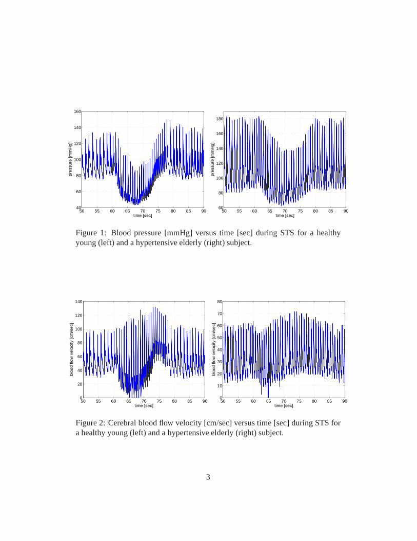
This manuscript summarizes a series of cardiovascular control models predictingbaroreflex and cerebral autonomic regulation of blood flow and pressure duringorthostatic postural challenges including sitting to standing (STS) and head-up tilt(HUT) [24, 25, 26, 27, 28, 29, 30, 18, 19, 20, 21, 22, 5, 2]. During these chal-lenges gravity pools blood from the upper to the lower body. As a result venousreturn is reduced, leading to a decrease in cardiac stroke volume, a decline inupper body arterial blood pressure (see Fig. 1), an increasein lower body arte-rial pressure, and an immediate decrease of blood flow to the brain (see Fig. 2).These changes are rapidly counteracted by short-term feedback control mecha-nisms working to reestablish blood flow and pressure. The main short-term feed-back mechanisms involved are autonomic regulation (mainlybaroreceptor feed-back control) and cerebral autoregulation. The barorecepter system controls bloodpressure by regulating heart rate (see Fig. 3), vascular tone (resistance and com-pliance), and cardiac contractility in response to changesin blood pressure, whilecerebral autoregulation controls cerebral blood flow by regulating cerebrovascu-lar tone (resistance and compliance). These control mechanisms are complex andinteract in ways that are not yet fully understood. Furthermore, it is believed thattheir functions are compromized by aging and disease. For example, mean bloodflow velocity and pressure show similar dynamics for healthyyoung and hyper-tensive elderly subjects, while the pulse velocity (the width - the systolic minusthe diastolic value for each pulse wave) in response to standing up is increased forhealthy young subjects but not for hypertensive elderly subjects (compare Figs. 1and 2). It is likely that this widening of the pulse wave (or lack thereof) is aresponse to changes in the feedback control.

2

50 55 60 65 70 75 80 85 9040

60

80

100

120

140

160

time [sec]

pres

sure

[mm

Hg]

50 55 60 65 70 75 80 85 9060

80

100

120

140

160

180

time [sec]pr

essu

re [m

mH

g]

Figure 1: Blood pressure [mmHg] versus time [sec] during STSfor a healthyyoung (left) and a hypertensive elderly (right) subject.

50 55 60 65 70 75 80 85 900

20

40

60

80

100

120

140

time [sec]

bloo

d flo

w v

eloc

ity [c

m/s

ec]

50 55 60 65 70 75 80 85 900

10

20

30

40

50

60

70

80

time [sec]

bloo

d flo

w v

eloc

ity [c

m/s

ec]

Figure 2: Cerebral blood flow velocity [cm/sec] versus time [sec] during STS fora healthy young (left) and a hypertensive elderly (right) subject.

3

50 60 70 80 9040

50

60

70

80

90

100

time [sec]

HR

[b

pm

]

Model

Data

baseline

firing

Vestibulo-

sympathetic

activation parasympathetic

withdrawal

sympathetic

activation

standing

relaxation

initial blood

pressure decrease

50 60 70 80 9040

50

60

70

80

90

100

time [sec]H

R [bpm

]

Model

Data

baseline

firing

initial blood

presure decrease

parasympathetic

withdrawal

sympathetic

activation

Vestibulo-

sympathetic

activationrelaxation

standing

50 60 70 80 9040

50

60

70

80

90

100

time [sec]

HR

[b

pm

]

Model

Data

baseline

firing

initial blood

pressure decrease

Vestibulo-

sympathetic

activation

parasympathetic

withdrawal

sympathetic

activation

relaxation

standing

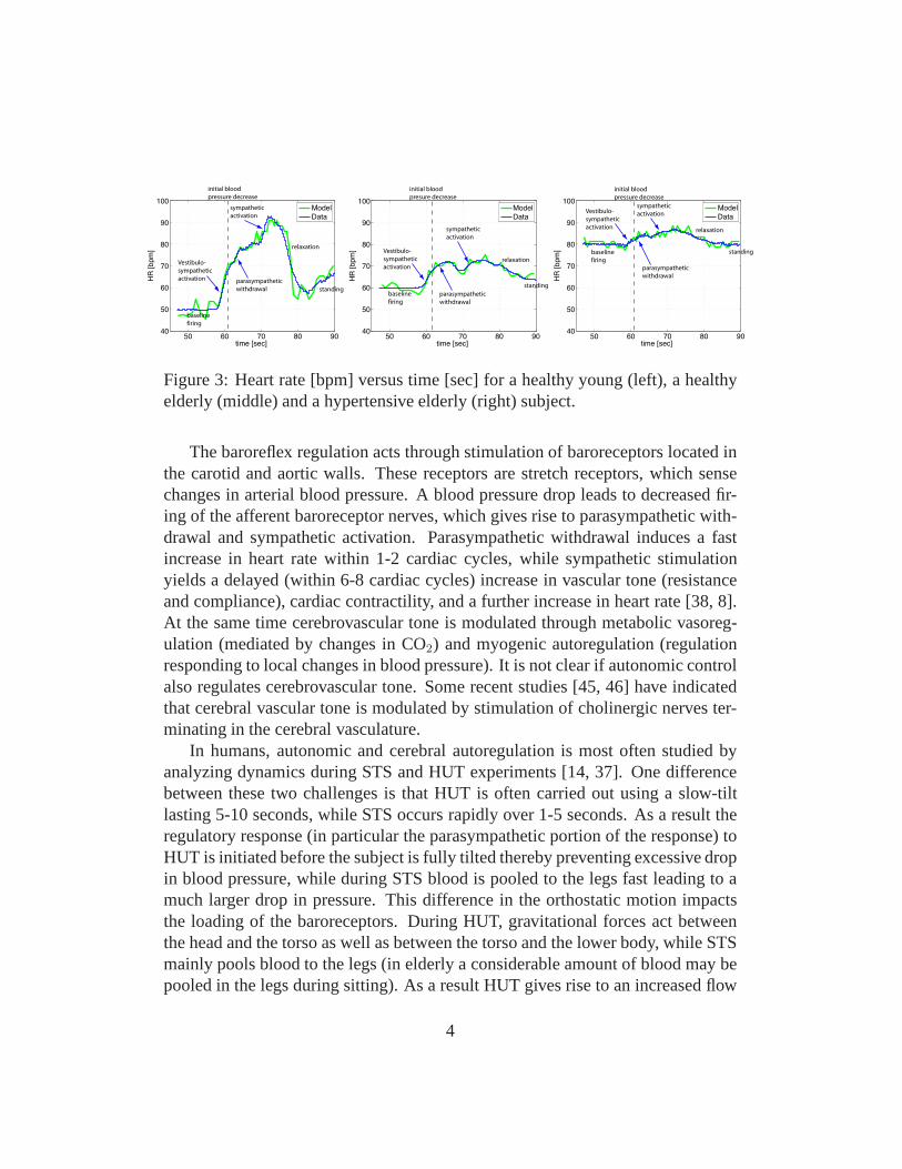
Figure 3: Heart rate [bpm] versus time [sec] for a healthy young (left), a healthyelderly (middle) and a hypertensive elderly (right) subject.

The baroreflex regulation acts through stimulation of baroreceptors located inthe carotid and aortic walls. These receptors are stretch receptors, which sensechanges in arterial blood pressure. A blood pressure drop leads to decreased fir-ing of the afferent baroreceptor nerves, which gives rise toparasympathetic with-drawal and sympathetic activation. Parasympathetic withdrawal induces a fastincrease in heart rate within 1-2 cardiac cycles, while sympathetic stimulationyields a delayed (within 6-8 cardiac cycles) increase in vascular tone (resistanceand compliance), cardiac contractility, and a further increase in heart rate [38, 8].At the same time cerebrovascular tone is modulated through metabolic vasoreg-ulation (mediated by changes in CO2) and myogenic autoregulation (regulationresponding to local changes in blood pressure). It is not clear if autonomic controlalso regulates cerebrovascular tone. Some recent studies [45, 46] have indicatedthat cerebral vascular tone is modulated by stimulation of cholinergic nerves ter-minating in the cerebral vasculature.

In humans, autonomic and cerebral autoregulation is most often studied byanalyzing dynamics during STS and HUT experiments [14, 37].One differencebetween these two challenges is that HUT is often carried outusing a slow-tiltlasting 5-10 seconds, while STS occurs rapidly over 1-5 seconds. As a result theregulatory response (in particular the parasympathetic portion of the response) toHUT is initiated before the subject is fully tilted thereby preventing excessive dropin blood pressure, while during STS blood is pooled to the legs fast leading to amuch larger drop in pressure. This difference in the orthostatic motion impactsthe loading of the baroreceptors. During HUT, gravitational forces act betweenthe head and the torso as well as between the torso and the lower body, while STSmainly pools blood to the legs (in elderly a considerable amount of blood may bepooled in the legs during sitting). As a result HUT gives riseto an increased flow

4

from the brain to the heart, which for a period of time may increase right atrialpressure stimulating pulmonary baroreceptors, which has potential to lower heartrate. During STS, there is no hydrostatic change between various regions in uppercorpus, thus all pooling of blood will be in the legs. Therefore this motion doesnot give rise to the immediate decrease in heart rate upon standing.

Another difference is that HUT is almost entirely passive, while STS requiremuscle contraction in the legs activating muscle sympathetic nerves (MSNA),which may increase heart rate before the observed drop in blood pressure. Otherexplanation for the initial increase in heart rate include stimulation by the vestibu-lar system, and/or by central command.

During HUT and STS experiments typical cardiovascular measurements in-clude: arterial blood pressure, heart rate, and cerebral blood fow velocity mea-sured using Transcranial Doppler ultrasound. These measurements are then usedto assess short term autonomic (baroreflex) and cerebral autoregulation. Mostcommon data analysis methods use some form of linear response models. Forexample, baroreflex sensitivity [36, 9] is often assessed using spectral transferfunctions relating changes in systolic blood pressure to interbeat intervals. Prob-lems with this method is two-fold; first the method is linear,second it is limitedto analysis of the relationships between two signals. Another limitation is thatthese methods lack the ability to predict how changes in neural responses interactto maintain arterial blood pressure.

In this manuscript we discuss alternative approaches basedon nonlinear dy-namic mathematical models. Two models will be discussed in detail: an openloop model developed to predict STS and HUT regulation of heart rate and aclosed loop model developed to predict blood flow and blood pressure baroreflexand cerebral autoregulation during STS. The heart rate model has been discussedin [24, 25, 17, 21, 22] and closed loop model has been discussed in [30, 18, 19,20, 6, 31, 5]. Both models were developed to analyze patient specific data, i.e.,our goal was to develop models that allow prediction of dynamic quantities in-cluding cerebral blood flow velocity, arterial blood pressure, and heart rate. Todo so, we estimated a set of nominal parameters for each subject using allometricscaling laws and anthropometric data (height, weight, age gender). Using thesenominal values patient specific values were obtained by predicting a subset ofparameters minimizing (in a reliable way) the difference between computed andmeasured values of the observed quantities. The subset of parameters identifiedusing optimization have potential to function as biomarkers, which can reveal sig-nificant differences between healthy and diseased subjects(or even within a groupof subjects). Not all optimized parameters will be different between groups, but

5

those that do have potential to serve as biomarkers characterizing varying statesof diseases. Finally, we show dynamics observed during longer time scales (> 35min) for a subject who experienced syncope. Note, at the onset of syncope bloodpressure and heart rate decreases rapidly. We show (see Fig.15) that our modelis able predict a similar behavior for a suitable choice of parameters, i.e., whensaturation in the vascular tone is reached.

2 Methods

2.1 Experimental design

The results reviewed used STS and HUT data from a number of healthy, hyper-tensive, and elderly subjects. The healthy young and elderly subjects where nottreated for any systemic disease and the hypertensive elderly subjects were diag-nosed and treated for hypertension but had no history of morethan one episode ofsyncope. Subjects with a history of diabetes, stroke and brain injury, renal liverand other systemic disorder were excluded. Instrumentation for all studies wasdone using similar protocols. Heart rate is measured using athree-lead electrocar-diogram (ECG) (SpaceLab Medical Inc., Issaquah, WA). A transcranial Dopplersystem (MultiDop X4, DWL Neuroscan Inc. Sterling VA) was used to obtain con-tinuous measurements of blood flow velocity in the middle cerebral artery. Thedata was acquired by insonating the artery through the temporal windows using a2-MHz pulsed Doppler probe. The probe was positioned to record the maximalflow velocities and stabilized using a three-dimensional head frame positioningsystem. A photoplethysmographic device mounted on the middle finger of thenon-dominant hand was used to obtain non-invasive beat-to-beat blood pressure(Finapres device, Ohmeda Monitoring Systems, Englewood, Colorado). To elim-inate effects of gravity, the hand was held at the level of theright atrium andsupported by a sling. All physiological signals were digitized at 500 Hz usingLabview NINDAQ software (National Instruments, Austin, TX) and stored foroffline analysis. Before data were analyzed they were down-sampled to 50 Hz.

• STS protocol: After instrumentation, subjects sat in a straight-backed chairwith their legs elevated at 90◦ in front of them. After five minutes of stablerecordings, the subjects were asked to stand up. Standing was defined as themoment both feet touched the floor, recorded by a force platform.

• HUT protocol: The subjects rested on their back in the supineposition for

6

10 minutes. After resting in this position, the table was then tilted to 70◦ for10 minutes.

• Syncope protocol: Using the HUT protocol described above the subjectswere tilted to 70◦ from supine to upright position and then kept uprightuntil presyncope (>35 min) at this time the subjects were returned to supineposition, and the subjects regained consciousness immediately

The STS and the open loop model data analyzed were collected from Lewis A.Lipsitz and Vera Novaks laboratories at Hebrew Senior Life and at the Beth IsraelDeaconess Medical Center, Boston, MA. All subjects provided informed consentapproved by the Institutional Review Board at Hebrew SeniorLife and at theBeth Israel Deaconess Medical Center. HUT data used for the syncope study wasobtained by Jesper Mehlsen, Medical Director, Department of Physiology andNuclear Medicine, Frederiksberg Hospital, University of Copenhagen, Denmark.

2.2 Modeling strategy

The following protocol provides an outline of the methodology that has guidedour work with the development of patient specific models.

• Data, knowledge and structure: Development of reliable patient specificphysiological models require detailed knowledge of the underlying biologi-cal system combined with a clear definition of the outcomes that the modelis supposed to predict or prescribe. Sufficient insight intoboth the physiol-ogy and available modeling techniques is crucial. In this spirit, structuresin the data analyzed in this study were revealed using standard statisticaltools combined with nonlinear optimization. Results of these analysis leadto knowledge of the system revealed through collaboration between math-ematicians and physicians. Other methodologies that can beused for ana-lyzing the structure of the system include filtering and generalized principalcomponent analysis.

• Canonical models: The level of details incorporated in the models reflectthe system analyzed. In order to identify and estimate patient specific pa-rameters in an effective and reliable way the number of parameters has tobe kept as low as possible so all unimportant elements are excluded (theprinciple of parsimony). The models will be based on first principles (e.g.,

7

conservation laws) whenever possible and the parameters shall have a phys-iological interpretation. Such models are denoted canonical models. Themodels discussed in this review were developed to study patient specificshort-term regulation of heart rate, blood pressure, and cerebral blood flowvelocity during STS and HUT. The models were formulated as dynamicalsystems. Steady state analysis of the model equations were considered. Af-terward models were used for analysis of baseline dynamic behavior andlater coupled with control models allowing prediction of dynamics duringthe orthostatic challenges (STS and HUT).

• Parameter identification and estimation: The main goal withthe modelspresented here [27, 28, 30, 21, 20, 22, 3, 31, 5, 2] was to identify biomarkers(model parameters) that allow the models to display the dynamic behaviorobserved in the data. Estimation of these quantities requires solution ofan inverse problem, where a set of parameters is estimated that minimizethe error between measured and computed quantities. For example, in theopen loop heart rate model, a set of parameters minimizing the least squareserror between computed and measured values of heart rate wasidentified,and in the closed loop model we minimized the least squares error betweencomputed and measured values of blood flow velocity and arterial bloodpressure.

For a given model and a given set of data, it is likely that the model is in-sensitive to a subset of the model parameters, i.e., changesin that subset ofparameters has a negligible impact on the solution. This setof parametersis called insensitive, and such parameters cannot be estimated via solutionto the inverse problem. Second, among the subset of parameters that aresensitive it is likely that parameters are correlated. For example, two resis-tors in series could both be sensitive, but it is not possibleto identify bothresistors separately, knowing only the total potential drop and current, e.g.,RT = R1 + R2 = 5 have indefinitely many solutions forR1 andR2. Thelatter problem is addressed in some of our recent studies [31, 5] using atechnique called subset selection. Once a set of sensitive uncorrelated pa-rameters have been identified and estimated, statistical methods should beinvoked to compare parameters within and between groups of individuals.In the models [17, 21, 31] we used analysis of variance (ANOVA) to show ifthe limited set of model parameters vary between healthy young and healthyelderly subjects. To understand patient specific behavior,model parametersand initial conditions (considered as a special kind of parameters) were es-

8

timated using literature data coupled with anthropometric(height, weight,age, gender) information, allometric scaling relations, as well as mean andsteady state values extracted from the data.

• Optimization algorithms: To perform the required parameter estimationsnon-linear optimization algorithms was used. Two methods were used, gra-dient free methods: the Nelder-Mead method (a simplex method) [18, 20,21, 22], genetic algorithms [7], and implicit filtering [7];and gradient-basedmethods: Newtons method and the Levenberg-Marquardt method [31, 5].The advantage of gradient-based methods is that sensitivities are computedas part of the optimization. A disadvantage of these methodsis that theODEs should be differentiated with respect to each of the parameters. Othermethods that have received much attention recently includeKalman filter-ing [3], particle filters, functional differential analysis, and sequential MonteCarlo (SMC) methods.

• Validation of models: The process of solving the inverse problem estimat-ing parameters that allow the models to predict data is one aspect of modelvalidation, but this type of analysis should be combined with more generalvalidation methods. For example, once a set of parameters have been esti-mated using one dataset, the models should be validated using other datasetsnot used for the parameter estimation. However, this type ofvalidation oftencannot be used for biological systems where inter and intra variations withinand between groups of individuals are large. One way to validate such mod-els is to use K-fold cross-validation [13] where a subset within one data-setis used for prediction of model parameters, while the remaining data areused for validation. Other validation methodologies include model reduc-tion (discussed in [6]) and analysis of sub-mechanisms. Common for allof these validation methods is that if a model fails to be validated it shouldbe adjusted. This process of iterative model development often generatesimportant new insights into the underlying physiology [12,1, 40, 30].

• Biomarkers: Patient specific model parameters estimated using reliable op-timization techniques from well-validated models have potential to be usedas biomarkers. This requires that confidence intervals for each identified pa-rameters are small and that some certainty is achieved that the optimized pa-rameters are not a result of optimization methods terminating at some localminimum. This type of methodology using models to estimate biomarkers

9

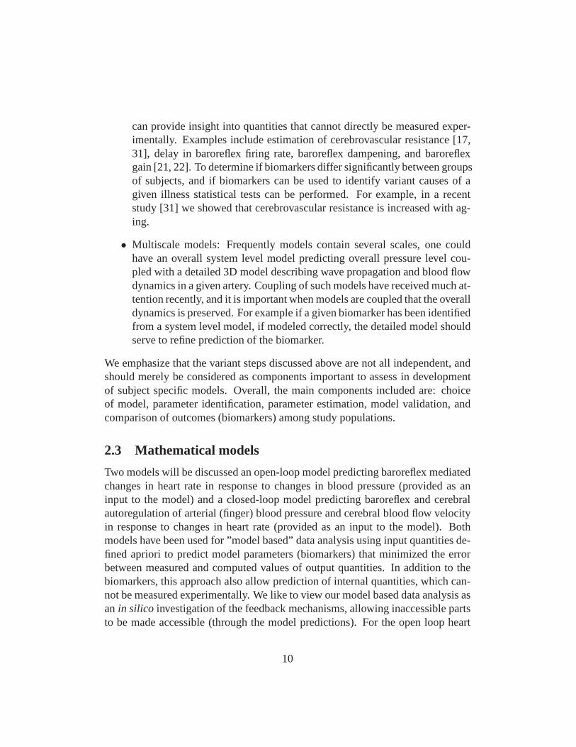
can provide insight into quantities that cannot directly bemeasured exper-imentally. Examples include estimation of cerebrovascular resistance [17,31], delay in baroreflex firing rate, baroreflex dampening, and baroreflexgain [21, 22]. To determine if biomarkers differ significantly between groupsof subjects, and if biomarkers can be used to identify variant causes of agiven illness statistical tests can be performed. For example, in a recentstudy [31] we showed that cerebrovascular resistance is increased with ag-ing.

• Multiscale models: Frequently models contain several scales, one couldhave an overall system level model predicting overall pressure level cou-pled with a detailed 3D model describing wave propagation and blood flowdynamics in a given artery. Coupling of such models have received much at-tention recently, and it is important when models are coupled that the overalldynamics is preserved. For example if a given biomarker has been identifiedfrom a system level model, if modeled correctly, the detailed model shouldserve to refine prediction of the biomarker.

We emphasize that the variant steps discussed above are not all independent, andshould merely be considered as components important to assess in developmentof subject specific models. Overall, the main components included are: choiceof model, parameter identification, parameter estimation,model validation, andcomparison of outcomes (biomarkers) among study populations.

2.3 Mathematical models

Two models will be discussed an open-loop model predicting baroreflex mediatedchanges in heart rate in response to changes in blood pressure (provided as aninput to the model) and a closed-loop model predicting baroreflex and cerebralautoregulation of arterial (finger) blood pressure and cerebral blood flow velocityin response to changes in heart rate (provided as an input to the model). Bothmodels have been used for ”model based” data analysis using input quantities de-fined apriori to predict model parameters (biomarkers) thatminimized the errorbetween measured and computed values of output quantities.In addition to thebiomarkers, this approach also allow prediction of internal quantities, which can-not be measured experimentally. We like to view our model based data analysis asan in silico investigation of the feedback mechanisms, allowing inaccessible partsto be made accessible (through the model predictions). For the open loop heart

10

rate model, we used blood pressure data as an input to predictheart rate and thelinks made visible through the model include baroreflex firing rate, sympatheticand parasympathetic tone, and concentrations of acetylcholine and noradrenaline,and for the closed loop model quantities predicted include cerebrovascular resis-tance, cerebral and systemic blood pressure. These model based quantities can beused to form hypotheses for how these ”invisible” quantities may vary, and withmore experiments, it may be possible to validate the varioussub-models. Thus,with sufficient validation, we may view the model together with the outcomes asa method that can provide insight into an individuals control system like a fin-gerprint. Such biomarkers have potential to be relevant fortreatment of severaldiseases such as hypertension, see [20, 18].

2.3.1 Open loop model

The overall function of the baroreceptor feedback mechanism is known. However,the underlying biochemical mechanistic processes are not fully understood and aredifficult to investigate in-vivo. In the studies summarizedhere we used STS andHUT experiments to investigate the short-term baroreceptor feedback regulationof heart rate, detailed description of the model can be foundin [24, 25, 30, 21, 22].To investigate baroreflex regulation of heart rate we developed the model shownin Fig. 4. This model uses blood pressure as an input to predict heart rate usingthe following five steps:

• Mean blood pressure is used to predict afferent baroreflex firing rate.

• Sympathetic and parasympathetic outflows are computed fromthe barore-flex firing rate combined with stimulation by muscle sympathetic nerves,the vestibular system, and from central command.

• Concentrations of acetylcholine and noradrenaline are computed as func-tions of the sympathetic and parasympathetic outflow.

• Heart rate potential is computed from chemical concentrations.

• Heart rate is predicted from the heart rate potential.

The baroreflex model uses weighted mean blood pressure as an input to predictthe afferent firing rate using a nonlinear differential equation of the form

dni

dt= ki

dp

dt

n(M − n)

(M/2)2− ni

τi, i = S, I, L (1)

n = nS + nI + nL + N,

11

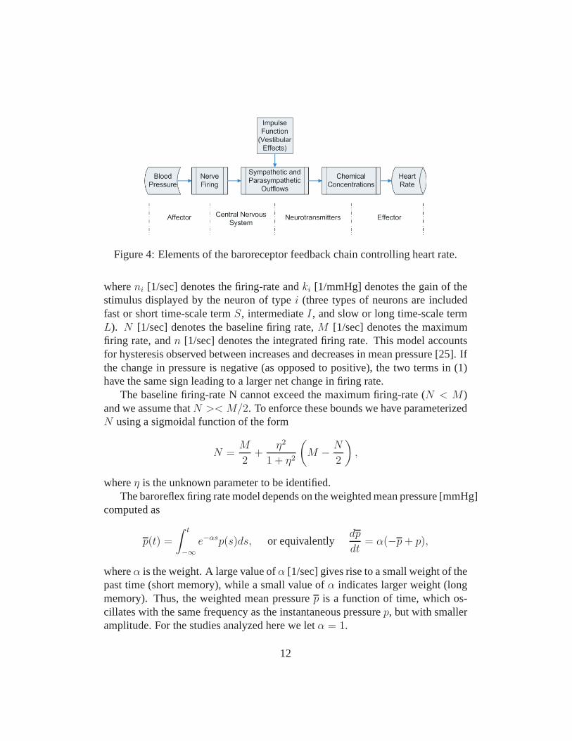
Figure 4: Elements of the baroreceptor feedback chain controlling heart rate.

whereni [1/sec] denotes the firing-rate andki [1/mmHg] denotes the gain of thestimulus displayed by the neuron of typei (three types of neurons are includedfast or short time-scale termS, intermediateI, and slow or long time-scale termL). N [1/sec] denotes the baseline firing rate,M [1/sec] denotes the maximumfiring rate, andn [1/sec] denotes the integrated firing rate. This model accountsfor hysteresis observed between increases and decreases inmean pressure [25]. Ifthe change in pressure is negative (as opposed to positive),the two terms in (1)have the same sign leading to a larger net change in firing rate.

The baseline firing-rate N cannot exceed the maximum firing-rate (N < M)and we assume thatN >< M/2. To enforce these bounds we have parameterizedN using a sigmoidal function of the form

N =M

2+

η2

1 + η2

(M − N

2

),

whereη is the unknown parameter to be identified.The baroreflex firing rate model depends on the weighted mean pressure [mmHg]

computed as

p(t) =

∫ t

−∞

e−αsp(s)ds, or equivalentlydp

dt= α(−p + p),

whereα is the weight. A large value ofα [1/sec] gives rise to a small weight of thepast time (short memory), while a small value ofα indicates larger weight (longmemory). Thus, the weighted mean pressurep is a function of time, which os-cillates with the same frequency as the instantaneous pressurep, but with smalleramplitude. For the studies analyzed here we letα = 1.

12

The afferent firing raten is used for prediction of sympatheticTsym and parasym-patheticTpar outflows. Parasympathetic outflow is proportional to the firing rate,while the sympathetic outflow is inversely proportional to the firing rate and isdampened (with rateβ) by the parasympathetic outflow. In addition, sympatheticoutflow is modulated through activation via central command, the vestibular sys-tem, and via MSNA. The latter is lumped into the contributionu(t) defined usingan impulse function. Thus,

Tpar =n(t)

M, Tsym =

1 − n(t − τd)/N + u(t)

1 + βTpar

, where

u(t) = − (b(t − tm))2 + u0, b =

√4u0

t2per

, and tm = tst +tper

2,

whereτd [sec] denotes the delay of the sympathetic response,u0 (dimensionless),tst [sec], andtper [sec] denote the magnitude and timing of the MSNA/centralcommand/vestibular stimulation.

Using the sympathetic and parasympathetic outflows, nondimensionalized con-centrations of acetylcholineCach and noradrenalineCnor were computed using thefirst order equation

dCi

dt=

−Ci + Tj

τi, i = nor, ach and j = sym, par. (2)

Parameters in this equation include characteristic time scales for noradrenalineand acetylcholine,τnor andτach [sec ]. In this equation we have lumped the longchain of biochemical reactions into a first order reaction equation and taken theaccumulated release timesτi to be equal to the average clearance and consumptiontime for the respective substances.

The heart rate potentialφ [beats] was computed using an integrate and firemodel of the form

dφ

dt= H0 (1 + MSCnor − MP Cach) ,

whereH0 denotes intrinsic heart rate, which we predicted as a function of age(H0 = 118.1 − 0.57 × age [10, 23]). The remaining parametersMS andMP

represent the strength of the response to changes in the concentrations. To boundheart rate within physiological values, we constrainedMS andMP in the interval[0,1]. This was done by introducing the parametersζS andζP that fulfill

MS =ζ2S

1 + ζ2S

and MS =ζ2P

1 + ζ2P

.

13

Whenφ reaches 1 it is reset to 0, and heart rate is computed as inverse of theintervalφ = 0 to φ = 1, i.e.,

HR = 1/(tφ=1 − tφ=0).

summary this model can be written on the form

dx

dt= f(x, ξ(t), p(t); θ), (3)

x = {ni, Cach, Cnor, φ} , i = S, I, L

θ = {ki, τi, M, η, τd, β, tst, tper, u0, τach, τnor, ζS, ζP} , i = S, I, L

ξ = {n, Tsym, Tpar} ,

wherex(t) denotes the states,ξ(t) the auxiliary equations,p(t) denotes the meanpressure (input from data), andθ denotes the model parameters.

This model is validated against heart rate, i.e., with this model we seek toidentify a set of parametersθ that minimize the least squares error

J = rTr, where r = |yc − yd| . (4)

The outputy is the heart rate, i.e.,yc = HRc = f(x, θ) denotes computed valuesof heart rate andyd = HRd denote the heart rate data.

2.3.2 Closed loop model

The model discussed above, predicted regulation of heart rate as a function ofblood pressure. However, data analyzed also include measurements of cerebralblood flow velocity. Therefore, in another series of studies[18, 20, 22, 31, 5] wedeveloped a closed loop model predicting autonomic (baroreflex mediated) andcerebral autoregulation of arterial blood pressure and cerebral blood flow velocityusing heart rate as an input. The most general form of the closed loop model isshown in Fig. 3. This model includes the systemic circulation, including the leftheart (the atria and the ventricle) the aorta and vena cava, arteries and veins in theupper and lower torso as well as arteries and veins in the legs.

The dotted lines on the figure indicate the diaphragm movement during respi-ration: the movement of the diaphragm change the trunk pressure and the trans-mural pressure of the vessels in the chest region. To model this we let

pext(t) =Au

2

(cos

(2πt

Tinsp

)− 1

)+ Bu, (5)

14

whereAl is the amplitude,Bl the base level value, andTinsp is the duration ofinspiration. Similarly organs below the diaphragm, e.g. the liver, experienceschanges in transmural pressure. However, the later blood pressure change is phaseshifted by 180 degrees compared to that in the chest region. This is imposed tothe model by allowing the exterior pressurepext below diaphragm to vary as

pext(t) =Al

2

(cos

(2πt

Tinsp

)− 1

)+ Bl, (6)

where similar to the model discussed aobveAl is the amplitude,Bl the base levelvalue, andTinsp is the duration of inspiration. To shift the two signals by 180◦ wechanged the sign ofAu andAI .

Finally, the period after inspiration has ended and during expiration we letpext(t) = Bl. Typically, the length of the respiration cycle isTresp = 8/3Tinsp.

In fact, this frequency and the depth of respiration are controlled. However, forthe studies analyzed here, the subjects were asked to breathe to a metronome at auniform depth, thus the model proposed above is adequate. Ifone has airflow data,it is possible to model exterior pressure directly as a function of airflow velocity,this approach was used in [4].

The closed loop model consists of three pars: A cardiovascular model predict-ing arterial blood flow and pressure in the various compartments; an autonomicregulation model predicting control of vascular tone (resistance and compliance),heart rate and cardiac contractility; and a cerebral autoregulation model predictingcerebrovascular resistance.

Cardiovascular ModelEach compartment in this model consists of a collection of arteries and veins ofsame caliber all with approximately the same pressure. Exceptions are the twocompartments representing the left ventricle and atrium. Flow in this model iscomputed using an analogy to an electrical network with resistors and capaci-tors. Using this terminology, flow between compartments areanalogous to cur-rent, pressure of each compartment is analogous to voltage,and compliance ofeach compartment is analogous to capacitance, while the resistance is the samein both formulations. Following this analogy the volume of each compartment isrelated to the pressure according to

V − Vunstr = C(p − pext), (7)

whereV [ml] is the total volume of the compartment,Vunstr [ml] is the unstressedvolume,C [ml/mmHg] is the compliance,p [mmHg] is the blood pressure, and

15

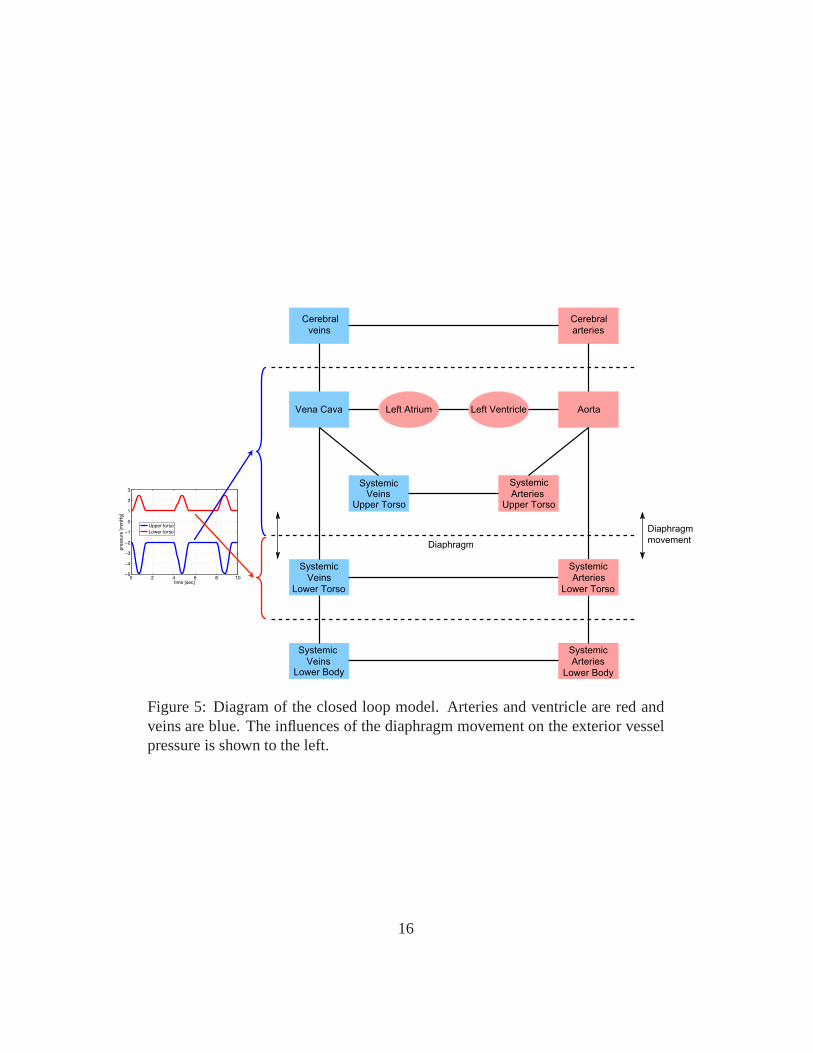
CerebralCerebral

veins

Vena Cava left Atrium

Upper TorsoVeins

Systemic

Systemic

Lower Torso

Veins

Systemic

VeinsLower Body

Systemic

ArteriesUpper Torso

Lower Torso

Arteries

Systemic

Systemic

Arteries

Lower Body

Left Ventricle Aorta

arteries

0 2 4 6 8 10−5

−4

−3

−2

−1

0

1

2

3

time [sec]

pre

ssure

[m

mH

g]

Upper torso

Lower torso Diaphragm

movement

Cerebral

Left Atrium

Diaphragm

Figure 5: Diagram of the closed loop model. Arteries and ventricle are red andveins are blue. The influences of the diaphragm movement on the exterior vesselpressure is shown to the left.

16

pext [mmHg] is the pressure of the tissue immediately outside thecompartmentwhich changes due to change in postural position or due to respiration. For com-partments in the legs and brain we assumed that the external pressurepext is con-stant, while for the compartments in the upper and lower torso the external pres-sure is modulated by movement of the diaphragm. Flow betweencompartmentsare computed using Ohms law which state that

q =pin − pout

R, (8)

whereq [ml/sec] denote the flow,pin andpout [mmHg] are the pressures of the twocompartments, andR [ml/sec mmHg] is the resistance to flow. Differentiating (7)gives

dV

dt= C

d(p − pext)

dt+ (p − pext)

dC

dt,

and using (8) we get

Cdp

dt= C

dpext

dt− (p − pext)

dC

dt+ qin − qout.

A differential equation of this form can be derived for all arterial and venouscompartments. Note, for steady state simulations we assumed thatpext = 0 andC is constant. In general,pext should be modulated with respiration (e.g., assuggested in (5) and (6) andC should be controlled, or as discussed in severalstudies by Ursino et al. [41, 42, 43] it may be appropriate to model C using anonlinear function of the stressed volume.

For compartments representing the left heart (the left and right atrium) twodifferent models have been analyzed. One model proposed by Ottesen [28] uses ageneralized activation function to predict the pressure inthe heart compartments;the other is a simple elastance model. The advantage of the elastance model is thatit contains only 4 parameters, while the more accurate modelby Ottesen contain14 parameters. The Ottesen model predicts the left heart pressure as

plh = a (V (t) − b)2 + (c(t)V (t) − d) f(t)/f(tp), (9)

f(t) =

pp

t(β − t)m

nnmm(β/(m + n)m+n0 ≤ t ≤ β

0 β ≤ t ≤ Ti

, (10)

wherea [mmHg/ml2] is related to the elastance during relaxation,b [ml] repre-sents the volume at zero diastolic pressure,c(t) [mmHg/ml] represents contractil-ity (note during steady statec is constant), andd [mmHg] is related to the volume-independent component of the developed pressure. In the activation functionf , Ti

17

[sec] denotes the length of the ith cardiac cycle,β [sec] denotes the onset of relax-ation,n andm characterize the contraction and relaxation phases andpp [mmHg]is the peak value of the activation. The ability to vary heartrate is included inthe pressure equation by scaling the timetp [sec] and peak valuespp of the ac-tivation functionf , for details see [28]. An advantage of this model is that theejection effect is easily incorporated, i.e., the fact thatdynamical changes in ven-tricular volume due to ejection of blood affect the ventricular contractility. Thusthe model is suitable when varying afterloads are considered. The correspondingelastance model is given by

plh = E(t)(V (t) − Vd), (11)

E(t) =

(EM − Em)

(1 − cos

(πt

TM

))0 ≤ t ≤ TM

(EM − Em)

(cos

(π(t − TM)

TR

))TM ≤ t ≤ TM + TR

0 TM + TR ≤ t ≤ Ti

,(12)

whereVd [ml] denote the volume at zero end-systolic pressure. In theelastancefunctionE, TM andTR [sec] denote the time for maximum (systolic) elastance(TM ) and the remaining time to relaxation (TR) and EM and Em [mmHg/ml]denotes the maximal (systolic,EM ) and minimal (Em) diastolic elastance. Thismodel accounts for varying heart rate by defining scaled parametersTMf = TM/Ti

andTRf = TR/Ti. As beforeTi [sec] denotes the length of the current cardiaccycle. For either of the two models, a differential equationfor the heart compart-ments can be obtained from conservation of volume, i.e., we let

dV

dt= qin − qout,

where as before the flows are computed using Ohms law. It should be noted, thatboth the atrium and the ventricle are modeled using the same type of equations,but that parameters for the two heart chambers vary. Finally, the left ventriclecannot function without heart valves. In all studies summarized here, we used timevarying resistances to represent the valves. These are defined such that a closedvalve is represented by a high resistanceRvalve,c and an open valve is representedby a very low resistanceRvalve,o. This can be done by defining valve resistancesas

Rvalve = min(Rvalve,o − e−k(pin−pout), Rvalve,c

),

wherek [1/mmHg] is a rate constant denoting the time it takes for thevalve toclose.

18

Similar to the open loop model, the closed loop steady state model (i.e., noparameters are controlledC, R, c are constant parameters) shown in Fig. 3 can berepresented by a system of differential equations of the form coupled with a set ofauxiliary equations

dx

dt= f(x, ξ(t), Ti; θ), (13)

x = {pi, pi,c, pi,ut, pi,lt, pi,l, Vla, Vlv} , i = a, v

θ = {R, C, a, b, c, d, n, m, Tmf , TMf , EM , Em, Ti} ,

ξ = {Rvalve, f, E, plv, pla} ,

wherex(t) denotes the states,ξ(t) denotes the auxiliary equations,Ti denote thelength of each cardiac cycle (input from data), andθ denote the model parameters.

This model is validated using measurements of heart rate (input), arterial bloodpressure and blood flow velocity, i.e., with this model we seek to estimate a set ofparametresθ that minimize the least squares error

J = rTr, where r = |yc − yd| . (14)

The outputy is a vector concatenating blood pressure and blood flow velocity, i.e.,yc = {pc(t1), pc(t2), ..., pc(tN), vc(t1), vc(t2), ..., vc(tN)} = f(x, θ) denotes com-puted values andyd = {pc(t1), pc(t2), ..., pc(tN ), vc(t1), vc(t2), ..., vc(tN )} denotethe corresponding data.

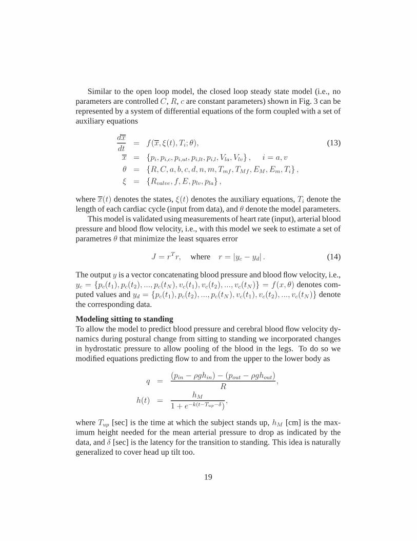
Modeling sitting to standingTo allow the model to predict blood pressure and cerebral blood flow velocity dy-namics during postural change from sitting to standing we incorporated changesin hydrostatic pressure to allow pooling of the blood in the legs. To do so wemodified equations predicting flow to and from the upper to thelower body as

q =(pin − ρghin) − (pout − ρghout)

R,

h(t) =hM

1 + e−k(t−Tup−δ),

whereTup [sec] is the time at which the subject stands up,hM [cm] is the max-imum height needed for the mean arterial pressure to drop as indicated by thedata, andδ [sec] is the latency for the transition to standing. This idea is naturallygeneralized to cover head up tilt too.

19

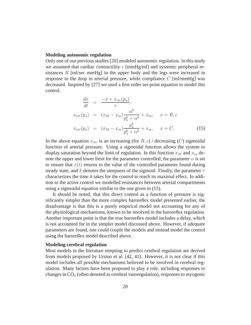
Modeling autonomic regulationOnly one of our previous studies [20] modeled autonomic regulation. In this studywe assumed that cardiac contractilityc [mmHg/ml] and systemic peripheral re-sistancesR [ml/sec mmHg] in the upper body and the legs were increased inresponse to the drop in arterial pressure, while complianceC [ml/mmHg] wasdecreased. Inspired by [27] we used a first order set-point equation to model thiscontrol.

dx

dt=

−x + xctr(pa)

τ,

xctr(pa) = (xM − xm)αk

pka + αk

+ xm, x = R, c

xctr(pa) = (xM − xm)pk

a

pka + αk

+ xm, x = C. (15)

In the above equationxctr is an increasing (forR, c) / decreasing (C) sigmoidalfunction of arterial pressure. Using a sigmoidal function allows the system todisplay saturation beyond the limit of regulation. In this functionxM andxm de-note the upper and lower limit for the parameter controlled,the parameterα is setto ensure thatx(t) returns to the value of the controlled parameter found duringsteady state, andk denotes the steepness of the sigmoid. Finally, the parameter τcharacterizes the time it takes for the control to reach its maximal effect. In addi-tion to the active control we modelled resistances between arterial compartmentsusing a sigmoidal equation similar to the one given in (15).

It should be noted, that this direct control as a function of pressure is sig-nificantly simpler than the more complex baroreflex model presented earlier, thedisadvantage is that this is a purely empirical model not accounting for any ofthe physiological mechanisms, known to be involved in the baroreflex regulation.Another important point is that the true baroreflex model includes a delay, whichis not accounted for in the simpler model discussed above. However, if adequateparameters are found, one could couple the models and instead model the controlusing the baroreflex model described above.

Modeling cerebral regulationMost models in the literature tempting to predict cerebral regulation are derivedfrom models proposed by Ursino et al. [42, 41]. However, it isnot clear if thismodel includes all possible mechanisms believed to be involved in cerebral reg-ulation. Many factors have been proposed to play a role, including responses tochanges in CO2 (often denoted as cerebral vasoregulation), responses to myogenic

20

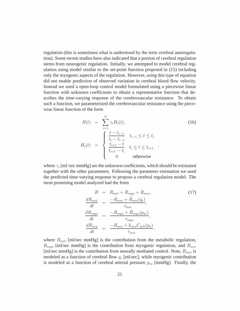
regulation (this is sometimes what is understood by the termcerebral autoregula-tion). Some recent studies have also indicated that a portion of cerebral regulationstems from neurogenic regulation. Initially, we attemptedto model cerebral reg-ulation using model similar to the set-point function proposed in (15) includingonly the myogenic aspects of the regulation. However, usingthis type of equationdid not enable prediction of observed variation in cerebralblood flow velocity.Instead we used a open-loop control model formulated using apiecewise linearfunction with unknown coefficients to obtain a representative function that de-scribes the time-varying response of the cerebrovascular resistance. To obtainsuch a function, we parameterized the cerebrovascular resistance using the piece-wise linear function of the form

R(t) =N∑

i=1

γiHi(t), (16)

Hi(t) =

t − ti−1

ti − ti−1

ti−1 ≤ t ≤ ti

ti+1 − t

ti+1 − titi ≤ t ≤ ti+1

0 otherwise

,

whereγi [ml /sec mmHg] are the unknown coefficients, which should be estimatedtogether with the other parameters. Following the parameter estimation we usedthe predicted time-varying response to propose a cerebral regulation model. Themost promising model analyzed had the form

R = Rmet + Rmyo + Rneu, (17)

dRmet

dt=

−Rmet + Rmet(qc)

τmet

,

dRmyo

dt=

−Rmyo + Rmyo(pac)

τmyo,

dRneu

dt=

−Rneu + kneuCach(pa)

τneu,

whereRmet [ml/sec mmHg] is the contribution from the metabolic regulation,Rmyo [ml/sec mmHg] is the contribution from myogenic regulation, andRneu

[ml/sec mmHg] is the contribution from neurally mediated control. Note,Rmet ismodeled as a function of cerebral flowqc [ml/sec], while myogenic contributionis modeled as a function of cerebral arterial pressurepca [mmHg]. Finally, the

21

0 10 20 30 40 500

1

2

3

4

5

6

7

time [sec]

Rc [

mm

Hg

se

c/c

m3]

Figure 6: Cerebrovascular resistance predicted using a piecewise linear function(16) (blue) versus the control function (red) proposed in (17).

neurogenic contribution is modeled as a function of arterial pressurepa [mmHg].It is believed that a potential neurogenic contribution to cerebral vasoregulation isboth cholinergic and adrenergic in nature. Therefore we letthe set-point equationuse concentration of acetylcholineCach (dimensionless). The concentration ofacetylcholine was computed similar to the open loop heart rate model, see equa-tion (2). For the metabolic and myogenic contributions the control functionsRwere sigmoidal functions similar to the one given in (15). Results of the two con-trol models (17) and (16) are shown in Fig. 4. It should be noted that if we omittedany part of the proposed control function we were not able to reproduce the dy-namic found from the piecewise linear function. One thing should be kept in mindis that both the spline model (16) and the differential equations model (17) has 26parameters. Ideally, it would be better if the cerebral regulation model containedfewer parameters.

2.4 Parameter estimation and model validation

Many real life processes and systems can be modeled using non-linear ODE’s orPDE’s. A frequent difficulty in biomedical applications is that the model equationsoften have a large number of unknown parameters. For some systems it is possibleto determine model parameters directly from the experimentally setup. However,in many cases it is difficult or even impossible to measure biomarkers, while otherquantities can be measured. For example, during the STS and HUT experiments,

22

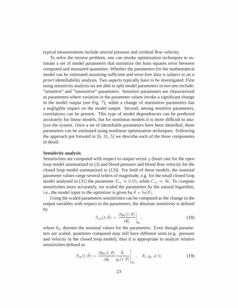
typical measurements include arterial pressure and cerebral flow velocity.To solve the inverse problem, one can invoke optimization techniques to es-

timate a set of model parameters that minimize the least squares error betweencomputed and measured quantities. Whether the parameters for the mathematicalmodel can be estimated assuming sufficient and error-free data is subject to anapriori identifiability analysis. Two aspects typically have to be investigated: Firstusing sensitivity analysis we are able to split model parameters in two sets include:”sensitive” and ”insensitive” parameters. Sensitive parameters are characterizedas parameters where variation in the parameter values invoke a significant changein the model output (see Fig. 7), while a change of insensitive parameters hasa negligible impact on the model output. Second, among sensitive parameters,correlations can be present. This type of model dependencies can be predictedaccurately for linear models, but for nonlinear models it ismore difficult to ana-lyze the system. Once a set of identifiable parameters have been identified, theseparameters can be estimated using nonlinear optimization techniques. Followingthe approach put forward in [6, 31, 5] we describe each of the three componentsin detail.

Sensitivity analysisSensitivities are computed with respect to output vectory (heart rate for the openloop model summarized in (3) and blood pressure and blood flowvelocity for theclosed loop model summarized in (13)). For both of these models, the nominalparameter values range several orders of magnitude, e.g. for the small closed loopmodel analyzed in [31] the parameterEm ≈ 0.05, while Cvs ≈ 36. To computesensitivities more accurately, we scaled the parameters bythe natural logarithm,i.e., the model input to the optimizer is given byθ = ln(θ).

Using the scaled parameters sensitivities can be computed as the change in theoutput variables with respect to the parameters, the absolute sensitivity is definedby

Si,k(t, θ) =∂yk(t, θ)

∂θi

∣∣∣∣θ0

, (18)

whereθ0, denotes the nominal values for the parameters. Even thoughparame-ters are scaled, quantities compared may still have different units (e.g. pressureand velocity in the closed loop model), thus it is appropriate to analyze relativesensitivities defined as

Sik(t, θ) =∂yk(t, θ)

∂θi

θi

yk(t, θ)

∣∣∣∣∣θ0

, θi, yk 6= 0, (19)

23

Note, for the open loop modelSi,k is computed with respect to one output, heartrate, while for the closed loop model both pressure and velocity are concatenatedtogether to provide one long output vector of length2N , thus the length ofSi,k is2N . As discussed in [6, 4] the sensitivities can either be foundusing automaticdifferentiation, by setting up a set of analytical equations, or using finite differ-ences. The finite difference approximation of the sensitivities is less accurate,but for most practical applications including those studied here, finite differenceapproximations provides sufficient accuracy. This should seen in the light of thehigh likelihood of introducing errors in analytical sensitivity calculations, in par-ticular for models that has many parameters, e.g., if a modelhas two outputs and21 parameters the system2 × 21 = 42 sensitivity equations should be derived.An alternative approach is to use automatic differentiation to derive sensitivityequations, but these methods are computationally ineffective in particular if thedifferential equations are solved using Matlab. More efficient packages exist in Cand Fortran, but these have not been analyzed for this study.

Using finite differences, the derivatives in the sensitivity equations can becomputed using the forward difference approximation

∂yk

∂θi

≈ yk(t, θ + hei) − yk(t, θ)

h,

where

ei =

[

0 . . . 0i

1 0 . . . 0

]T

is the unit vector in thei’th component direction.To rank the parameters from the most to the least sensitive, we used a scaled

2-norm to get the total sensitivity,Si, to thei’th parameter

Si =

(1

2N

2N∑

j=1

S2i,k

)1/2

.

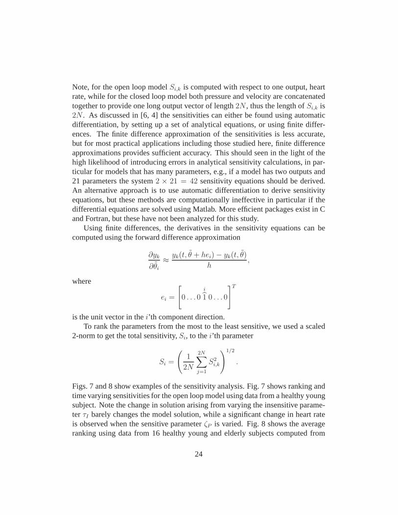
Figs. 7 and 8 show examples of the sensitivity analysis. Fig.7 shows ranking andtime varying sensitivities for the open loop model using data from a healthy youngsubject. Note the change in solution arising from varying the insensitive parame-ter τI barely changes the model solution, while a significant change in heart rateis observed when the sensitive parameterζP is varied. Fig. 8 shows the averageranking using data from 16 healthy young and elderly subjects computed from

24

the closed loop model. The specific closed loop model used forthese calcula-tions included 4 vascular and one ventricular compartments, the model had 21parameters.

It should be noted that the classical sensitivity analysis described above is alocal analysis, and thus sensitivities depend on the valuesof the parameters. Inthis study the goal is to use sensitivity analysis to rank parameters in order ofsensitivity and use this ranking in conjunction with results from subset selectionto identify a set of parameters that can be estimated for all subjects. This is doneprior to actual parameter estimations, thus the sensitivity ranking was computedusing nominal parameter values.

In summary, results from the sensitivity analysis showed that both models in-clude both sensitive and insensitive parameters. Sensitive parameters can often beestimated using optimization techniques, while insensitive parameters are difficultto estimate since a small change in the parameter value givesrise to a small changein the solution. This can become problematic when models areused to extract bi-ological information from estimated parameter values as done in the studies sum-marized here. However, it should be noted that identifiability is a mathematicalnotion. For biological implications the precise values of parameters are not alwaysimportant as long as they have certain characteristics, e.g., like being positive. Analternative method is to use generalized sensitivity analysis, which provide moreinsight into the dynamics of the model.

Subset selectionSubset selection can be approached using a number of methodsas describedin [32]. Below we outline the method used in [31]. In this study subset selec-tion analyzes the Jacobian matrix (r′ = dr/dθ) computed from the residual vectorr (see equations (3) and (13)). The entry at rowi and columnj of the Jacobianis ∂ri/∂θj . The Jacobian, singular value decompositionr′ = UΣV T is used toobtain a numerical rank forr′. This numerical rank is then used to determineρparameters that can be identified given the model outputy defined in (3) and (13).QR decomposition is used to determine theρ identifiable parameters to which oursystem is sensitive asa group. This differs from sensitivity analysis, which findsparameters to which our system isindividuallysensitive. To estimate the numberof uncorrelated parameters we used an error estimate in our computation of the Ja-cobian as a lower bound on acceptable singular values. For example, in the studiesanalyzed here we used Matlabs differential equations solver ODE15S with an ab-solute error tolerance of10−6, i.e., the error of the numerical model solution is oforder10−6 and the error in the Jacobian matrix is approximately

√10−6 = 10−3.

25

0.0

0.1

0.2

0.3

0.4

0.5

0.6

0.7

0.8

0 10 20 30 40 50

0

0.1

0.2

0.3

0.4

0.5

0.6

time [sec]

sensitiv

ity

ζP

kS

τI

0 10 20 30 40 500.95

1

1.05

1.1

1.15

1.2

1.25

1.3

1.35

time [sec]

HR

[beats

/s]

HR

New HR

0 10 20 30 40 500.95

1

1.05

1.1

1.15

1.2

1.25

1.3

1.35

time [sec]

HR

[beats

/s]

HR

New HR

0 10 20 30 40 500.95

1

1.05

1.1

1.15

1.2

1.25

1.3

1.35

time [sec]

HR

[beats

/s]

HR

New HR

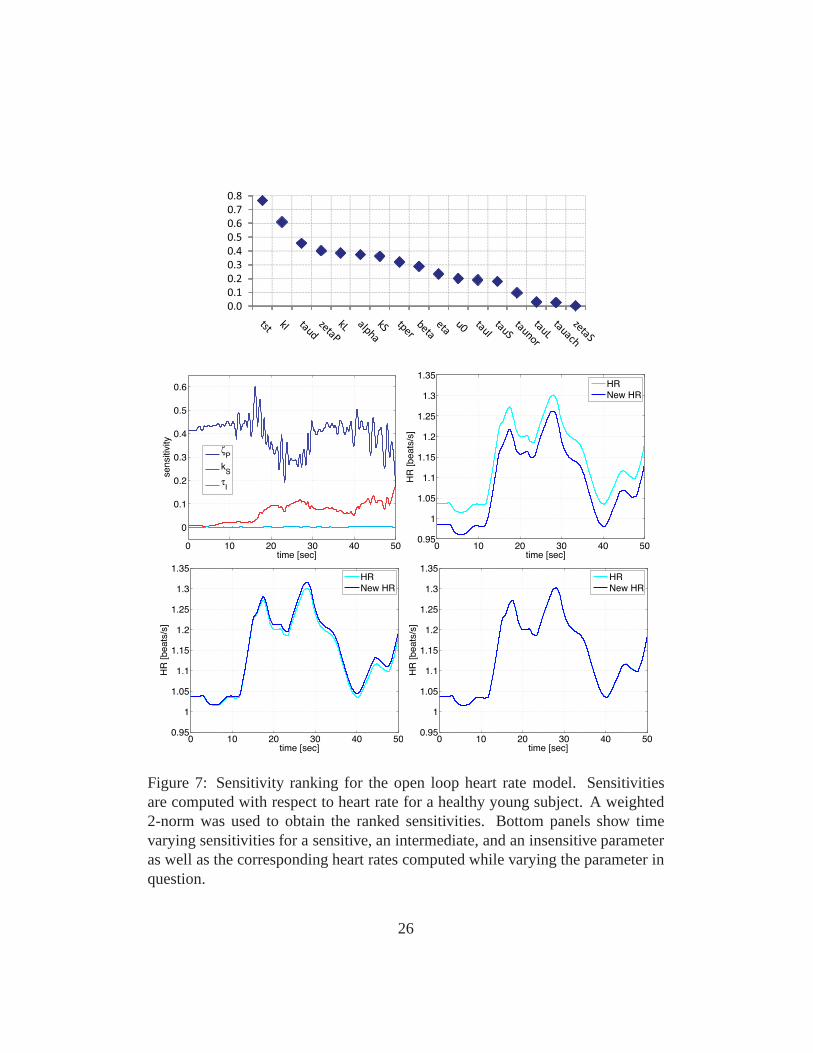
Figure 7: Sensitivity ranking for the open loop heart rate model. Sensitivitiesare computed with respect to heart rate for a healthy young subject. A weighted2-norm was used to obtain the ranked sensitivities. Bottom panels show timevarying sensitivities for a sensitive, an intermediate, and an insensitive parameteras well as the corresponding heart rates computed while varying the parameter inquestion.

26

0.0

0.2

0.4

0.6

0.8

1.0

1.2

1.4

1.6

1.8

2.0

Rc A

cEm

Rm

v,o

Cvs

TMf

Rs

EM Tr

fCas

Rvc

Cac

Rac

Rav,o

Cvc

Figure 8: Sensitivity ranking for a 5 compartment (systemicarteries and veins,cerebral arteries and veins, and the left ventricle) closedloop model. Sensitivitiesare computed with respect to arterial pressure and cerebralblood flow velocity.A weighted 2-norm was used to obtain an average sensitivity over the entire timeseries.

Consequently, singular values should not be smaller than10−3. Since the errorof the Jacobian is an approximation, the smallest singular value that we acceptis 10−2. Once the number of identifiable parameters has been determined, wefind the most dominant parameters by performing a QR decomposition with col-umn pivoting on the most dominant right singular vectors. The process beginsby choosing the most sensitive parameter in a way similar butnot identical tothe sensitivity analysis of the previous section, the column with largest 2-norm ischosen. The algorithm chooses additional parameters in a way that keeps the con-dition number of the chosen columns small. Below we summarize subset selectionmethod as an algorithm.

Subset selection algorithm:

1. Given an initial parameter estimate,θ0, compute the Jacobian,r′(θ0) andthe singular value decompositionr′ = UΣV T , whereΣ is a diagonal ma-trix containing the singular values ofr′ in decreasing order, andV is anorthogonal matrix of right singular vectors.

2. Determineρ, the numerical rank ofr′. This can be done by determining a

27

smallest allowable singular value.

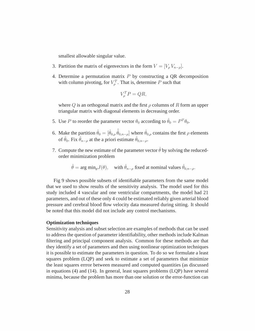
3. Partition the matrix of eigenvectors in the formV = [Vρ Vn−ρ].

4. Determine a permutation matrixP by constructing a QR decompositionwith column pivoting, forV T

ρ . That is, determineP such that

V Tρ P = QR,

whereQ is an orthogonal matrix and the firstρ columns ofR form an uppertriangular matrix with diagonal elements in decreasing order.

5. UseP to reorder the parameter vectorθ0 according toθ0 = P T θ0.

6. Make the partitionθ0 = [θ0,ρˆθ0,n−ρ] whereθ0,ρ contains the firstρ elements

of θ0. Fix θn−ρ at the a priori estimateθ0,n−ρ.

7. Compute the new estimate of the parameter vectorθ by solving the reduced-order minimization problem

θ = arg minθJ(θ), with θn−ρ fixed at nominal valuesθ0,n−ρ.

Fig 9 shows possible subsets of identifiable parameters fromthe same modelthat we used to show results of the sensitivity analysis. Themodel used for thisstudy included 4 vascular and one ventricular compartments, the model had 21parameters, and out of these only 4 could be estimated reliably given arterial bloodpressure and cerebral blood flow velocity data measured during sitting. It shouldbe noted that this model did not include any control mechanisms.

Optimization techniquesSensitivity analysis and subset selection are examples of methods that can be usedto address the question of parameter identifiability, othermethods include Kalmanfiltering and principal component analysis. Common for these methods are thatthey identify a set of parameters and then using nonlinear optimization techniquesit is possible to estimate the parameters in question. To do so we formulate a leastsquares problem (LQP) and seek to estimate a set of parameters that minimizethe least squares errror between measured and computed quantities (as discussedin equations (4) and (14). In general, least squares problems (LQP) have severalminima, because the problem has more than one solution or theerror-function can

28

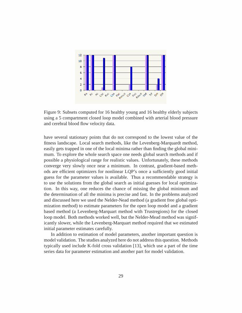
Figure 9: Subsets computed for 16 healthy young and 16 healthy elderly subjectsusing a 5 compartment closed loop model combined with arterial blood pressureand cerebral blood flow velocity data.

have several stationary points that do not correspond to thelowest value of thefitness landscape. Local search methods, like the Levenberg-Marquardt method,easily gets trapped in one of the local minima rather than finding the global mini-mum. To explore the whole search space one needs global search methods and ifpossible a physiological range for realistic values. Unfortunately, these methodsconverge very slowly once near a minimum. In contrast, gradient-based meth-ods are efficient optimizers for nonlinear LQP’s once a sufficiently good initialguess for the parameter values is available. Thus a recommendable strategy isto use the solutions from the global search as initial guesses for local optimiza-tion. In this way, one reduces the chance of missing the global minimum andthe determination of all the minima is precise and fast. In the problems analyzedand discussed here we used the Nelder-Nead method (a gradient free global opti-mization method) to estimate parameters for the open loop model and a gradientbased method (a Levenberg-Marquart method with Trustregions) for the closedloop model. Both methods worked well, but the Nelder-Mead method was signif-icantly slower, while the Levenberg-Marquart method required that we estimatedinitial parameter estimates carefully.

In addition to estimation of model parameters, another important question ismodel validation. The studies analyzed here do not address this question. Methodstypically used include K-fold cross validation [13], whichuse a part of the timeseries data for parameter estimation and another part for model validation.

29

3 Discussion

Below we summarize and discuss result reported in [24, 25, 30, 18, 19, 20, 21,22, 6, 31, 5]. We divide the presentation into three subsections; open loop model,closed loop model, and syncope.

3.1 Open Loop model

Results with the open loop model have been reported in [24, 25, 21, 22, 7] re-sults were obtained with the STS and HUT protocol. In [21] we analyzed STSdata from three groups of subjects including healthy young,healthy elderly, andhypertensive elderly healthy young subjects, and in [22] weanalyzed both STSand HUT data from five young subjects. For both studies all model parameterswere predicted using the Nelder-Mead optimization method.Results showed thatstandard deviations were typically high, however, for bothstudies we were ableto detect interesting differences between the groups of subjects. In [21] (results

50 60 70 80 90 100 110 120 130 140

40

50

60

70

80

90

100

110

120

p [mmHg]

n [1/s

ec]

50 60 70 80 90 100 110 120 130 140

40

50

60

70

80

90

100

110

120

p [mmHg]

n [1/s

ec]

50 60 70 80 90 100 110 120 130 140

40

50

60

70

80

90

100

110

120

p [mmHg]

n [1/s

ec]

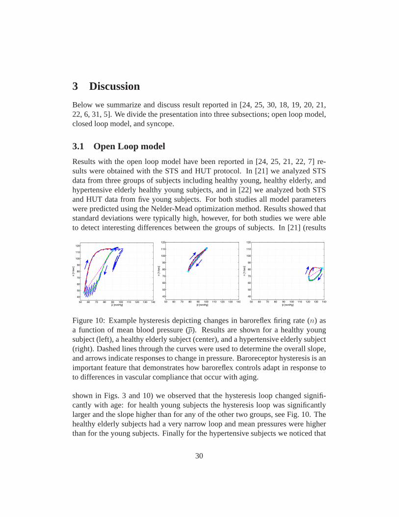
Figure 10: Example hysteresis depicting changes in baroreflex firing rate (n) asa function of mean blood pressure (p). Results are shown for a healthy youngsubject (left), a healthy elderly subject (center), and a hypertensive elderly subject(right). Dashed lines through the curves were used to determine the overall slope,and arrows indicate responses to change in pressure. Baroreceptor hysteresis is animportant feature that demonstrates how baroreflex controls adapt in response toto differences in vascular compliance that occur with aging.

shown in Figs. 3 and 10) we observed that the hysteresis loop changed signifi-cantly with age: for health young subjects the hysteresis loop was significantlylarger and the slope higher than for any of the other two groups, see Fig. 10. Thehealthy elderly subjects had a very narrow loop and mean pressures were higherthan for the young subjects. Finally for the hypertensive subjects we noticed that

30

for most subjects the hysteresis loop was not closed, indicating that within thetimeframe included in the experiments the pressure does notreturn to the valueobtained during sitting. This may indicate that part of the regulation is not work-ing as expected. In addition, comparison of parameters between groups revealedthat parameterskI , kL, β, τd, τach, andMP changed significantly between groups.These results were obtained using ANOVA analysis using 20 data sets for eachgroup. Data from 10 subjects (2 experiments per subject) were analyzed. It shouldbe noted that these results were obtained without any applying any model and pa-rameter reduction techniques. Seen from a physiological point of view observingdifferences in the given parameters are reasonable, reduction in kI andkL indicatethat with age and hypertension, the firing rate sensitivity to changes in pressure isreduced, increase ofβ andτd, indicate that with age and hypertension, the delayin onset of sympathetic response is increased and that parasympathetic dampen-ing of the sympathetic response is attenuated, finallyτach increase with age, butdecrease with hypertension. An age related increase inτach suggests that withage it takes longer for the parasympathetic response to reach its maximum effect,while the decrease with hypertension, may be compensating for the fact that thevessels are significantly stiffer. FinallyMP is increased with both age and hy-pertension indicating that parasympathetic regulation plays a more important rolethan subsequent sympathetic stimulation of heart rate.

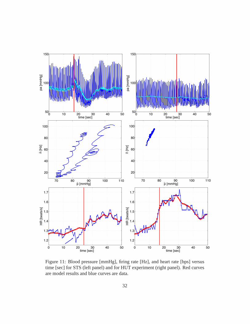
Results from [22] (see Fig. 11 ) showed that there were significant differencesbetween results from the STS and HUT procedures. Comparing the two testsshowed a much larger increase in heart rate during HUT than during STS anda more significant drop in blood pressure during STS than during HUT, leadingto more pronounced changes in firing rate and sympathetic/parasympathetic tone.Another noticeable difference is the change in the area of the hysteresis loop:the loop is significantly wider during STS than during HUT. Finally, we noticedthat during HUT heart rate decrease during the initial preparation to tilt (beforeany blood pressure drop was observed), while during STS heart rate increasedbefore the subject changed posture (the latter observationwas also found in ourfirst study [21]. This initial drop in heart rate is associated with a slight increasein blood pressure (compare panels A and E). This may be due to ashort increasein venous return due to hydrostatic pressure difference imposed between the heartand the head. On the other hand the increase in heart rate immediately beforestanding may, as explained earlier, be due to vestibular andmuscle sympatheticactivation.

In addition to analysis of the results, in [21] we used sensitivity analysis (seeFigs. 7 and 8) to rank model parameters from the most to the least sensitive. Re-

31

0 10 20 30 40 5050

100

150

time [sec]

pa [m

mH

g]

0 10 20 30 40 5050

100

150

time [sec]

pa [m

mH

g]

70 80 90 100 110

20

40

60

80

100

p [mmHg]

n [H

z]

70 80 90 100 110

20

40

60

80

100

p [mmHg]

n [H

z]

0 10 20 30 40 50

1.2

1.3

1.4

1.5

1.6

1.7

time [sec]

HR

[beats

/s]

0 10 20 30 40 50

1.2

1.3

1.4

1.5

1.6

1.7

time [sec]

HR

[beats

/s]

Figure 11: Blood pressure [mmHg], firing rate [Hz], and heartrate [bps] versustime [sec] for STS (left panel) and for HUT experiment (rightpanel). Red curvesare model results and blue curves are data.

32

sults of this analysis showed that some parameters are very insensitive includingτI , kI , ζS, andτach. Results varying a sensitive parameter, an intermediate pa-rameter and an insensitive parameter are showed together with the ranking. Oneaspect not done for this study is to analyze if any of the sensitive parameters arecorrelated, more analysis is needed to investigate potential correlations. Such cor-relations are likely to exist, some initial attempts to study those have been doneby Fowler [7] comparing results obtained with Nelder-Mead with both implicitfiltering and using a genetic algorithm to optimize model parameters.

3.2 Closed Loop model

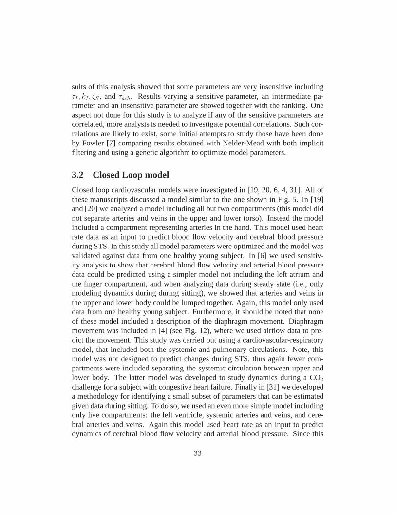
Closed loop cardiovascular models were investigated in [19, 20, 6, 4, 31]. All ofthese manuscripts discussed a model similar to the one shownin Fig. 5. In [19]and [20] we analyzed a model including all but two compartments (this model didnot separate arteries and veins in the upper and lower torso). Instead the modelincluded a compartment representing arteries in the hand. This model used heartrate data as an input to predict blood flow velocity and cerebral blood pressureduring STS. In this study all model parameters were optimized and the model wasvalidated against data from one healthy young subject. In [6] we used sensitiv-ity analysis to show that cerebral blood flow velocity and arterial blood pressuredata could be predicted using a simpler model not including the left atrium andthe finger compartment, and when analyzing data during steady state (i.e., onlymodeling dynamics during during sitting), we showed that arteries and veins inthe upper and lower body could be lumped together. Again, this model only useddata from one healthy young subject. Furthermore, it shouldbe noted that noneof these model included a description of the diaphragm movement. Diaphragmmovement was included in [4] (see Fig. 12), where we used airflow data to pre-dict the movement. This study was carried out using a cardiovascular-respiratorymodel, that included both the systemic and pulmonary circulations. Note, thismodel was not designed to predict changes during STS, thus again fewer com-partments were included separating the systemic circulation between upper andlower body. The latter model was developed to study dynamicsduring a CO2

challenge for a subject with congestive heart failure. Finally in [31] we developeda methodology for identifying a small subset of parameters that can be estimatedgiven data during sitting. To do so, we used an even more simple model includingonly five compartments: the left ventricle, systemic arteries and veins, and cere-bral arteries and veins. Again this model used heart rate as an input to predictdynamics of cerebral blood flow velocity and arterial blood pressure. Since this

33

440 460 480 500 52065

70

75

80

85

90

95

100

105

110

115

time [sec]

pa [m

mH

g]

440 460 480 500 520

35

40

45

50

55

60

time [sec]

vc [c

m/s

ec]

Figure 12: Model generated arterial pressure (top panel) and cerebral blood ve-locity (lower panel) when respiratory effects are included. The resulting curvesare realistic and in accordance with measurements

model was significantly simpler, and because we used subset selection, we wereable to predict dynamics for two groups of subjects including 16 healthy youngsubjects and 16 healthy elderly subjects. Results of this comparison showed thatboth cerebral resistance and compliance were modulated by aging. Results alsoshowed that the total resistance was increased and thatTM , f time for systolicpressure was increased.

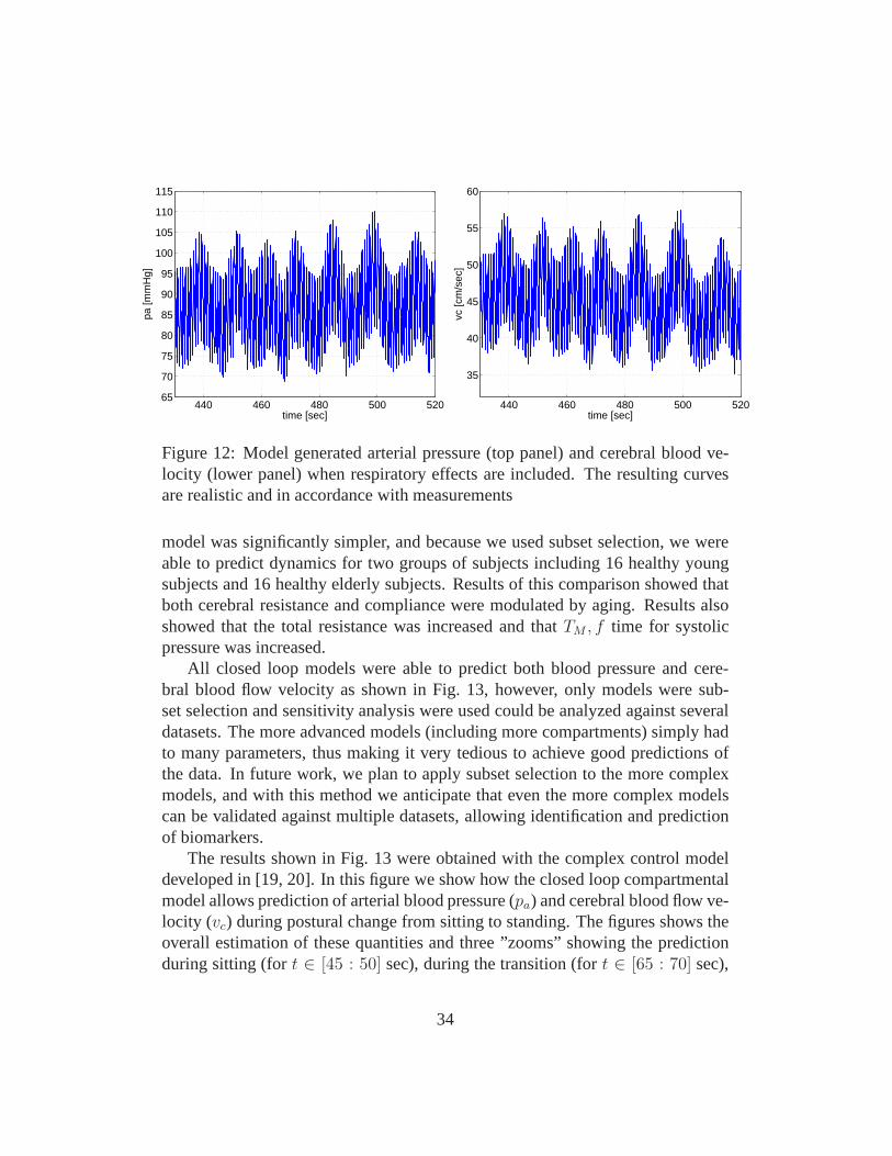
All closed loop models were able to predict both blood pressure and cere-bral blood flow velocity as shown in Fig. 13, however, only models were sub-set selection and sensitivity analysis were used could be analyzed against severaldatasets. The more advanced models (including more compartments) simply hadto many parameters, thus making it very tedious to achieve good predictions ofthe data. In future work, we plan to apply subset selection tothe more complexmodels, and with this method we anticipate that even the morecomplex modelscan be validated against multiple datasets, allowing identification and predictionof biomarkers.

The results shown in Fig. 13 were obtained with the complex control modeldeveloped in [19, 20]. In this figure we show how the closed loop compartmentalmodel allows prediction of arterial blood pressure (pa) and cerebral blood flow ve-locity (vc) during postural change from sitting to standing. The figures shows theoverall estimation of these quantities and three ”zooms” showing the predictionduring sitting (fort ∈ [45 : 50] sec), during the transition (fort ∈ [65 : 70] sec),

34

40 50 60 70 80 900

50

100

150

200

pa

[m

mH

g]

40 50 60 70 80 90−50

0

50

100

150

time [sec]

vc [

cm

/s]

45 46 47 48 49 50

50

100

150

pa

[m

mH

g]

45 46 47 48 49 50

0

50

100

time [sec]

vc [

cm

/s]

65 66 67 68 69 70

50

100

150

pa

[m

mH

g]

65 66 67 68 69 70

0

50

100

time [sec]

vc [

cm

/s]

80 81 82 83 84 85

50

100

150

pa

[m

mH

g]

80 81 82 83 84 85

0

50

100

time [sec]

vc [

cm

/s]

Figure 13: Pressure [mmHg] (top panel) and flow velocity [cm/sec] (bottom pan-nel) for STS with respiratory mechanical effect included.

and during standing (fort ∈ [80 : 85] sec). Note, while the model was able topredict the amplitude and approximate shape of the waveform, this type of modelcannot predict the wave reflections observed in the data. To predict these, it isnecessary to use a fluid dynamics model, that more realistically allows modelingof the wave propagation.

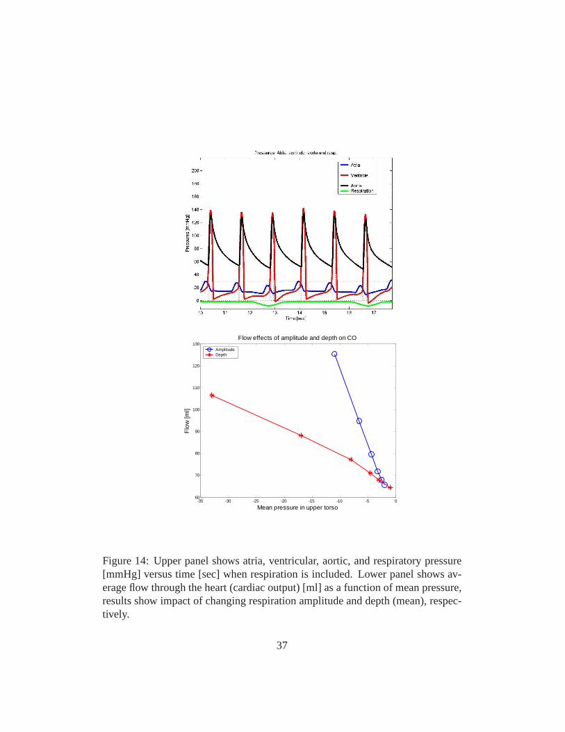
Another important aim with these models is to analyze internal dynamics ofthe states not measured. Results of this analysis is shown inFig. 14. The firstfigure shows prediction of arterial blood pressure and cerebral blood flow velocitymodeling the movement of the diaphragm as a function of measured airflow ve-locity. This result was obtained using a more elaborate closed loop compartmentalmodel accounting for both vascular movement of blood and respiratory dynamics

35

of CO2 and O2, this model is described in [5, 4]. The second figure (Fig. 14)showsnot only effect on arterial pressure but on the internal states as well. It should benoted that respiration also affects the overall flow distribution and favors somebraches at the expense of others and moreover Starlings law of the heart followsas a result. Furthermore, including mechanical coupling with respiration also af-fect model parameter values. Especially, parameters related to the ventricles andthe control mechanisms are sensitive to effect of respiration. Surprisingly the im-pact of mechanical movement giving rise to respiration is somehow strong as seein Fig. 14, where the movement of the diaphragm during respiration is seen to besignificant.

3.3 Syncope

Control mechanisms of the cardiovascular system play an important role in adap-tation to postural changes during everyday activities. Syncope (meaning a pausein music) is the medical term for temporary loss of consciousness or fainting.Syncope is a common and significant medical problem that accounts for 3-6%of emergency rooms visits and hospital admissions every year and in some casesmay hallmark a significant underlying morbidity. Syncope ismultifactorial andcan be triggered from many different inputs into the centraland peripheral auto-nomic systems. It often manifest as an abrupt loss of muscle tone with/withoutfalling accompanied by a decline in blood pressure, blood flow to the brain, andheart rate, the latter may even lead to temporary cardiac arrest. This presentationmay have clinical prodromes and changes in autonomic nervous system firing forminutes before the actual loss of consciousness occurs. Syncope is considered tobe a reflex mechanism, protecting the vital organs (mainly the brain) from lack ofperfusion.

It should be noted that the term syncope is related to a broad range of prob-lems, and mechanisms related to triggering of syncope are mulifcatorial and dif-ferent mechanisms can present in the same patients on various occasion not wellunderstood. The most common type of syncope is neurally mediated syncope,which is characterized by peripheral vasodilation and a decrease in blood pressure(hypotension) along with a slowing of heart rate (bradycardia) or increasing heartrate (tachycardia). The result is temporary insufficient blood flow to the brain.The event is usually initiated by a withdrawal of peripheralsympathetic tone inupright posture, releases of vasoconstriction or active vasodilatation, accompa-nied by a decline in blood pressure. Cardioacceleration andcentral vasodilatationare compensatory mechanisms that may fail if blood pressuredeclines further.

36

-35 -30 -25 -20 -15 -10 -5 060

70

80

90

100

110

120

130

Mean pressure in upper torso

Flo

w [m

l]

Flow effects of amplitude and depth on CO

AmplitudeDepth

Figure 14: Upper panel shows atria, ventricular, aortic, and respiratory pressure[mmHg] versus time [sec] when respiration is included. Lower panel shows av-erage flow through the heart (cardiac output) [ml] as a function of mean pressure,results show impact of changing respiration amplitude and depth (mean), respec-tively.

37

Bradycardia or slow heart rate typically occurs later when blood pressure falls be-low certain threshold. In the model of HUT syncope appear approximately after30 minutes as a sudden incident as a result of a crash in the control system wherethe effect of the controls saturates.

In the example discussed here the reduction in flow is initiated by the suddendrop in blood pressure observed during HUT, followed by compromised auto-nomic and cerebral autoregulation. In contrast to the heartrate regulation a uni-fying description of pressure changes shows that multiple simultaneous controlmechanisms may be important in order to understand the experiments.

There are many reasons to use the model to analyze questions related to syn-cope, most importantly, it is not well know what mechanisms triggers syncope.A number of theories put forward to explain the phenomena [15]. How each ofthese theories impact pressure, flow, and HR dynamics could be studied using theproposed models.

To model dynamics during syncope we used the model illustrated in Fig. 5modified to include intermediate control mechanisms essential for describing dy-namics of HUT experiments over longer time scales (> 35 min). To do so it isimportant to account for dynamics of the venous pump, functioning to preventpooling of flow in the extremities due to effects of gravity. This type of dynamicswas not included in the original closed loop model, which wasdeveloped to studydynamics over a short time scale (< 2 min). To model this we included a fluid shiftcompartment at the level of the legs. Through this compartment fluid was continu-ously transfered from the cardiovascular system to the extravascular environment.Consequently, during regulation, a combination of controlmechanisms includingarterial resistance and venous compliance regulation, fluid shift and dead volumesare regulated in this study. In addition, we incorporated a slight tension of thediaphragm The resulting model nicely describes the HUT experiments as shownin Fig. 15. In particular notice, how well the model reproduce data. The crashhappens in the model when the arterial compliance regulation reach its saturation.Thus the heart rate cannot manage to regulate the system alone, venous returndeclines and the system breaks down resulting in syncope.

4 Conclusion

Above we have discussed a number of methodologies that can beused to developpatient specific models that allow prediction of arterial blood pressure, cerebralblood flow velocity, and heart rate during STS and HUT. Two model approaches

38

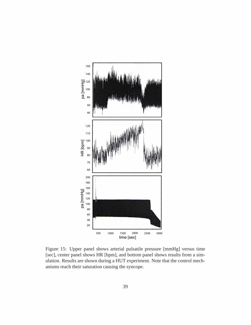
60

60

70

160

140

120

100

80

120

80

90

100

110

500 1000 2000 2500 30001500

40

40

20

60

80

100

120

140

160

180

200

pa [m

mH

g]

pa [m

mH

g]

HR

[bpm

]

time [sec]

Figure 15: Upper panel shows arterial pulsatile pressure [mmHg] versus time[sec], center panel shows HR [bpm], and bottom panel shows results from a sim-ulation. Results are shown during a HUT experiment. Note that the control mech-anisms reach their saturation causing the syncope.

39

were discussed open-loop models that use blood pressure as an input to predictheart rate, and a closed loop model that allow prediction of both blood pressureand blood flow velocity. We showed how these models could be used to predictpatient specific data by solving the inverse problem estimating a set of modelparameters that allow prediction of patient specific dynamics. Two analysis tec-niques were investigated, and prove to be essential to obtain good results: sen-sitivity analysis, which allow us to rank model parameters from the most to theleast sensitive, and subset selection, which allow us to identify correlation amongmodel parameters. The sensitivity ranking can be used to identify insensitive pa-rameters that cannot be estimated given data, and allowed usto identify essentialcomponents of the model. Subset selection allowed us to predict a subset of un-correlated parameters among the sensitive parameters, which can be reliably beestimated using the available data. Finally, we show how these models can beused to model clinical events (syncope), and using this example, we have shownthat this type of modeling approach has potential to be used for better understand-ing of underlying mechanisms triggering syncope. Another important outcome isthat the type of models developed here allow prediction of internal states, whichcannot be measured experimentally.

However, the models themselves have a number of limitations. First, the spar-sity of data used for prediction of dynamics in the closed loop models discussedabove, is probably the main limitation is obtaining good patient specific models.As discussed earlier, only 4-6 parameters can be estimated reliably given thesedata. Another limitation, not of the models, but of the patient specific analysis isthat without measurements of cardiac output it is difficult to get flow distributionscorrect. Many different estimates of cardiac output can be distributed to obtain thecorrect arterial pressure and cerebral blood flow velocity,and as discussed in [31],the models analyzed here typically underestimates cardiacoutput. Consequently,one important suggestion we can put forward for researchersinterested in usingthe proposed modeling tools discussed here is to incorporate some measurementsof cardiac output.

Another important lesson we learned (discussed in [6]), is that for any givenapplication, it is essential to include as few compartmentsas necessary to modelthe proposed dynamics, and then be conservative in reducingthe number of pa-rameters estimated to predict patient specific dynamics.

Finally, if one is interested in studying dynamics of the wave form, the ODEcompartmental models should be coupled with a fluid dynamicsmodel allowingaccurate prediction of the reflected waves.

40

5 Acknowledgements

The authors wish to thank graduate students involved with this project includ-ing Laura Ellwein, Dept of Biomedical Engineering, Marquette University, ScottPope, SAS Corp, Raleigh, NC, April Alston, Dept of Math, NCSU, and numer-ous undergraduate students participating in research and REU program at NCSU.Furhtermore, authors would like to thank Hien Tran and Tim Kelley, Departmentof mathematics, NCSU. The work by M.S. Olufsen was supportedin part by NSF-DMS grant # 0616597 and NSF-OISE grant# 0437037. V. Novak, director of theSAFE Laboratory at BIMDC was supported by NIH-NIA Harvard Older Ameri-can Independence Center 2P60 AG08812-11A1, Core B.

References

[1] Allen L.J.S. An Introduction to Mathematical Biology.Pearson Education,Up Sadddle River, NJ, 2003.

[2] Danielsen M.Modeling of feedback mechanisms which control the heart func-tion in a view to an implementation in cardiovascular models. PhD Thesis,Roskilde University, Denmark. Text No 358, 1998.

[3] DeVault K., Gremaud P., Zhao P., Vernieres G., Novak V., and Olufsen M.S.Blood flow in the circle of Willis: Modeling and calibration.SIAM J MultiscaleAnal Simul, 7:888–909, 2008.

[4] Ellwein L.M. Cardiovascular and Respiratory Regulation, Modeling and Pa-rameter Estimation.. PhD Thesis, Applied Mathematics, NC State University,Raleigh, NC. 2009.

[5] Ellwein L.M., Pope S.R., Xie A., Batzel J.J., Kelley C.T., and Olufsen M.S.Modeling cardiovascular and respiratory dynamics in congestive heart failure.Submitted, 2009.

[6] Ellwein L.M., Tran H.T., Zapata C., Novak V., and OlufsenM.S. Sensitivityanalysis and model assessment: Mathematical models for arterial blood flowand blood pressure.J Cardiovasc Eng, 8:94–108, 2008.

[7] Fowler K.R., Gray G.A., and Olufsen M.S. Modeling heart rate regulation -Part II: Parameter identification.J Cardiovasc Eng, 8:109–119, 2008.

41

[8] Guyton A.C. and Hall J.E.Textbook of medical physiology.WB Saunders,Philadelphia, PE, 9th ed, 1996.

[9] Johnson P., Shore A., Potter J.F., Panerai R.B., and James M. Baroreflex sen-sitivity measured by spectral and sequence analysis in cerebrovascular disease- methodological considerationsClin Auton Res, 16: 270–275, 2006.

[10] Jose A. and Collison D. The normal range and determinants of the intrinsicheart rate in man.Cardiovasc Res, 4: 160–167, 1970.

[11] Kaufmann H., Biaggioni I., Voustianiouk A., Diedrich A., Costa F.,Clarke R., Gizzi M., Raphan T., and Cohen B. Vestibular control of sympa-thetic activity: An otolith-sympathetic relfex in humans.Exp Brain Res, 143:463–469, 2002.

[12] Kyrylov V., Severyanova L.A., and Vieira A. Modeling Robust OscillatoryBehaviour of the Hypothalamic-Pituitary-Adrenal Axis.IEEE Trans BiomedEng, 52:1977–1983, 2005.

[13] Liang K.H., Krus D.J., and Webb J.M. K-fold crossvalidation in canonicalanalysis.Multivariate Behavioral Resarch, 30:539–546, 1995.

[14] Low P.A. and Bannister R.G. Multiple System Atrophy andPure AutonomicFailure. In: Low P.A.(eds).Clinical Autonomic Disorders.Lippincott-RavenPublishers, Philadelphia, PE, pp. 555–575, 1997.

[15] Mosqueda-Garcia R., Furlan R., Tank J., and Fernandez-Violante R. The elu-sive pathophysiology of neurally mediated syncope.Circulation, 102: 2898–2906, 2000.

[16] Olufsen M.S. Structured tree outflow condition for blood flow in larger sys-temic arteries.Am J Physiol, 276:H257–H268, 1999.

[17] Olufsen M.S., Nadim A., and Lipsitz L.A. Dynamics of cerebral bloodflow regulation explained using a lumped parameter model.Am J Physiol,282:R611–R622, 2002.

[18] Olufsen M.S. and Nadim A. On deriving lumped models for blood flow andpressure in the systemic arteries.Math Biosci Eng, 1:61–80, 2004.

42

[19] Olufsen M.S., Tran H.T., and Ottesen J.T. Modeling cerebral blood flow con-trol during posture change from sitting to standing.Cardiovasc Eng, 4(1):47–58, 2004.

[20] Olufsen M.S., Ottesen J.T., Tran H.T., Ellwein L.M., Lipsitz L.A., and No-vak V. Blood pressure and blood flow variation during postural change from sit-ting to standing: model development and validation.J Appl Physiol, 99:1523–1537, 2005.

[21] Olufsen M.S., Tran H.T., Ottesen J.T., Lipsitz L.A., and Novak V. Model-ing baroreflex regulation of heart rate during orthostatic stress.Am J Physiol,291:R1355–R1368, 2006.

[22] Olufsen M.S., Alston A.V., Tran H.T., Ottesen J.T., andNovak V. Modelingheart rate regulation, Part I: Sit-to-stand versus head-uptilt. J Cardiovasc Eng,8:73–87, 2008.

[23] Opthof T. The normal range and determinants of the intrinsic heart rate inman.Cardiovasc Res, 45:173–176, 2000.

[24] Ottesen J.T. Modeling of the baroreflex-feedback mechanism with time-delay.J Math Biol, 36:41–63, 1997.

[25] Ottesen J.T. Nonlinearity of baroreceptor nerves.Surv Math Ind, 7:187–201,1997.

[26] Ottesen J.T. General Compartmental Models of the Cardiovascular Systemin Mathematical Modelling in Medicine.IOS press, Amsterdam, pp. 121–138,2000.

[27] Ottesen J.T. Modeling the dynamical baroreflex-feedback control. MathComp Mod, 31:167–173, 2000.

[28] Ottesen J.T. and Danielsen M. Modeling ventricular contraction with heartrate changes.J Theor Biol, 222:337–346, 2003.

[29] Ottesen J.T. Valveless pumping in a fluid-filled closed elastic tube-system:one-dimensional theory with experimental validation.J Math Bioll, 46:309–332, 2003.

[30] Ottesen J.T., Olufsen M.S., and Larsen J. Applied mathematical models inhuman physiology.SIAM, Philadelphia, PA, 2004.

43

[31] Pope S., Ellwein L.M., Zapata C.L., Novak V., Kelley C.T., andOlufsen M.S. Estimation and identification of parameters ina lumped cere-brovascular model.Math Biosci Engl, 6:93–115, 2009.

[32] Pope S.R.Parameter identification in lumped compartment Cardiorespira-tory models. PhD Thesis, Applied Mathematics, NC State University, Raleigh,NC. 2009.

[33] Ray C. Interaction of the vestibular system and baroreflexes on sympatheticnerve activity in humans.Am J Physiol, 279:H2399–H2404, 2000.

[34] Ray C. and Monahan K. The vestibulosympathetic reflex inhumans: Neu-ral interactions between cardiovascular reflexes.Clin and Exp Pharmaco andPhysiol, 29: 98–102, 2002.

[35] Ray C. and Carter J. Vestibular activation of sympathetic nerve activity.ActaPhysiol Scand, 177: 313–319, 2003.

[36] Robbe H.W.J., Mulder L.J.M., Ruddel H., Langewitz W.A., Weldman J.B.P.,Mulder G. Assessment of baroreceptor reflex sensitivity by means of spectralanalysis.Hypertension, 10: 538–543, 1987.

[37] Robertson D., Low P.A., and Polinsky R.J.Primer on the autonomic nervoussystem.Academic Press, Boston, MA, 2nd ed, 2005.

[38] Smith J.J. and Kampine J.T.Circulatory physiology, the essentials. Williamsand Wilkins, Baltimore, MD, 3rd ed, 1990.

[39] Steele B., Olufsen M.S., and Taylor C. Fractal network model for simulatingabdominal and lower extremity blood flow during rest and exercise conditions.Comp Meth Biomech Biomed Eng, 10:39–51, 2007.

[40] Strogatz S.H.Nonlinear Dynamics and Chaos.Perseus Books Publishing,LLC, 1994.

[41] Ursino M. and Lodi C.A. A simple mathematical model of the interactionbetween intracranial pressure and cerebral hemodynamics.J Appl Physiol,82:1256–1269, 1997.

[42] Ursino M. and Magosso E. Short-term autonomic control of cardiovascu-lar function: a mini-review with the help of mathematical models. J IntegrNeurosci, 2:219–247, 2003.

44

[43] Ursino M. and Magosso E. Short-term autonomic control of the cardio-respiratory system: a summary with the help of a comprehensive mathematicalmodel. IEEE Eng MEd Biol Soc, 1:354–358, 2006.

[44] Wilson T.D., Cotter L.A., Draper J.A., Misra S.P., RiceC.D., Cass S.P., andYates B.J. Vestibular inputs elicit patterned changes in limb blood flow inconscious cats.J Physiol, 575: 671–684, 2006.

[45] Zhang R., Zuckerman J.H., Iwasaki K., Wilson T.E., Crandall C.G., andLevine B.D. Autonomic Neural Control of Dynamic Cerebral Autoregulationin Humans.Circulation, 106:1814–1820, 2002.

[46] Zhang R. and Levine B.D. Autonomic Ganglionic BlockadeDoes Not Pre-vent Reduction in Cerebral Blood Flow Velocity During Orthostasis in Hu-mans.Stroke, 38:1238–1244, 2007.

45