Development of New Decline Model for Shale Oil Reserves
80
-
Upload
khangminh22 -
Category
Documents
-
view
3 -
download
0
Transcript of Development of New Decline Model for Shale Oil Reserves


c© Copyright by Samit Shah 2013All Rights Reserved

Development of New Decline Model for Shale OilReserves
A Thesis
Presented to
the Faculty of the Department of Chemical Engineering
University of Houston
In Partial Fulfillment
of the Requirements for the Degree
Master of Science
in Petroleum Engineering
by
Samit Shah
August 2013

Development of New Decline Model for Shale OilReserves
Samit Shah
Approved:Chair of the CommitteeWilliam John Lee, ProfessorPetroleum Engineering
Committee Members:Thomas Holley,ProfessorPetroleum Engineering
Michael Myers,ProfessorPetroleum Engineering
Guan Qin,ProfessorPetroleum Engineering
Suresh K. Khator, Associate DeanCullen College of Engineering
Michael Harold, Department ChairChemical Engineering

Acknowledgements
I would like to take this opportunity to offer my heartfelt thanks to all those
who made my stay as a graduate student very enjoyable and who made this work
possible. I owe my deepest gratitude to my advisor, Dr. William John Lee for
giving me the opportunity to pursue my thesis under his esteemed guidance. His
mentoring, sustained encouragement, enthusiasm for discovery and vision for
future research have made my graduate study a rewarding experience. He has
always been willing and kind enough to help me every time I knock on his door
with questions, academic or personal. His timely inputs improved the quality of
my research and helped me immensely in keeping track of my progress. I would
like to express my gratitude to Dr. Thomas Holley, Dr. Michael Myers, and Dr.
Guan Qin for taking time out of their schedules to be on my defense committee.
Special thanks to Eshwar Yenigalla for being a good friend and colleague for his
support in helping me verify my data and supplying the required information,
along with guiding me throughout the project.
My thanks are given to my friends and colleagues who have contributed to
making my life at University of Houston enjoyable. I would like to thank all my
lab mates for their constant support. No acknowledgements could possibly be
complete without thanking my parents and sister whose affection and support
were driving forces behind all my endeavors.
v

Development of New Decline Model for Shale OilReserves
An Abstract
of a
Thesis
Presented to
the Faculty of the Department of Chemical Engineering
University of Houston
In Partial Fulfillment
of the Requirements for the Degree
Master of Science
in Petroleum Engineering
by
Samit Shah
August 2013

Abstract
This thesis provides a new methodology to forecast ultimate recovery, based
on more reliable production forecast for shale oil wells using historical produc-
tion data. Compared to available decline curve methods including Arps (AIME:
160, 228-247), Valko (SPE 134231) and Duong (SPE 137748), this method is more
accurate and more conservative.
Production forecasts play a vital role in determining the value of oil or gas
wells, and improved accuracy enhances management decisions on field develop-
ment. The new, more accurate method was verified using both field data and
numerical simulations. This method can potentially be used in most shale reser-
voirs producing single-phase liquid.
vii

Table of Contents
Acknowledgements . . . . . . . . . . . . . . . . . . . . . . . . . . . . . . . . . . v
Abstract . . . . . . . . . . . . . . . . . . . . . . . . . . . . . . . . . . . . . . . . . vii
Table of Contents . . . . . . . . . . . . . . . . . . . . . . . . . . . . . . . . . . . viii
List of Figures . . . . . . . . . . . . . . . . . . . . . . . . . . . . . . . . . . . . . xi
List of Tables . . . . . . . . . . . . . . . . . . . . . . . . . . . . . . . . . . . . . . xiv
Chapter 1 Introduction . . . . . . . . . . . . . . . . . . . . . . . . . . . . . . . 1
Chapter 2 Decline Curve Analysis . . . . . . . . . . . . . . . . . . . . . . . . 4
Chapter 3 Arps Decline Model . . . . . . . . . . . . . . . . . . . . . . . . . . 5
Chapter 4 Stretched Exponential Production Decline . . . . . . . . . . . . . . 7
Chapter 5 Duong′s Production Decline . . . . . . . . . . . . . . . . . . . . . . 9
Chapter 6 Comparison of methods . . . . . . . . . . . . . . . . . . . . . . . . 11
Chapter 7 New Method . . . . . . . . . . . . . . . . . . . . . . . . . . . . . . . 12
Chapter 8 Field Examples . . . . . . . . . . . . . . . . . . . . . . . . . . . . . 14
8.1 Example 1 . . . . . . . . . . . . . . . . . . . . . . . . . . . . . . . . . . 14
8.1.1 Arps Hyperbolic Model . . . . . . . . . . . . . . . . . . . . . . 15
8.1.2 SEPD . . . . . . . . . . . . . . . . . . . . . . . . . . . . . . . . . 17
8.1.3 Duong Model . . . . . . . . . . . . . . . . . . . . . . . . . . . . 18
8.1.4 Arps+Arps . . . . . . . . . . . . . . . . . . . . . . . . . . . . . . 20
8.1.5 SEPD+Arps . . . . . . . . . . . . . . . . . . . . . . . . . . . . . 20
8.1.6 Duong +Arps . . . . . . . . . . . . . . . . . . . . . . . . . . . . 21
8.1.7 Summary of methods . . . . . . . . . . . . . . . . . . . . . . . 22
8.2 Example 2 . . . . . . . . . . . . . . . . . . . . . . . . . . . . . . . . . . 24
8.2.1 Arps Hyperbolic Model . . . . . . . . . . . . . . . . . . . . . . 24
8.2.2 SEPD . . . . . . . . . . . . . . . . . . . . . . . . . . . . . . . . . 26
8.2.3 Duong Model . . . . . . . . . . . . . . . . . . . . . . . . . . . . 27
8.2.4 Arps+Arps . . . . . . . . . . . . . . . . . . . . . . . . . . . . . . 29
viii

8.2.5 SEPD+Arps . . . . . . . . . . . . . . . . . . . . . . . . . . . . . 29
8.2.6 Duong +Arps . . . . . . . . . . . . . . . . . . . . . . . . . . . . 30
8.2.7 Summary of methods . . . . . . . . . . . . . . . . . . . . . . . 31
Chapter 9 Simulated Examples . . . . . . . . . . . . . . . . . . . . . . . . . . 33
9.1 Simulated data of 20 months . . . . . . . . . . . . . . . . . . . . . . . 33
9.1.1 Arps Hyperbolic Model . . . . . . . . . . . . . . . . . . . . . . 34
9.1.2 SEPD . . . . . . . . . . . . . . . . . . . . . . . . . . . . . . . . . 36
9.1.3 Duong Model . . . . . . . . . . . . . . . . . . . . . . . . . . . . 37
9.1.4 Arps+Arps . . . . . . . . . . . . . . . . . . . . . . . . . . . . . . 39
9.1.5 SEPD+Arps . . . . . . . . . . . . . . . . . . . . . . . . . . . . . 39
9.1.6 Duong +Arps . . . . . . . . . . . . . . . . . . . . . . . . . . . . 40
9.1.7 Summary of results to simulated example . . . . . . . . . . . 41
9.2 Simulated rates of 50 months . . . . . . . . . . . . . . . . . . . . . . . 43
9.2.1 Arps Hyperbolic Model . . . . . . . . . . . . . . . . . . . . . . 43
9.2.2 SEPD . . . . . . . . . . . . . . . . . . . . . . . . . . . . . . . . . 45
9.2.3 Duong Model . . . . . . . . . . . . . . . . . . . . . . . . . . . . 46
9.2.4 Arps+Arps . . . . . . . . . . . . . . . . . . . . . . . . . . . . . . 48
9.2.5 SEPD+Arps . . . . . . . . . . . . . . . . . . . . . . . . . . . . . 48
9.2.6 Duong +Arps . . . . . . . . . . . . . . . . . . . . . . . . . . . . 49
9.2.7 Summary of methods . . . . . . . . . . . . . . . . . . . . . . . 50
9.3 Simulated rates of 100 months . . . . . . . . . . . . . . . . . . . . . . . 52
9.3.1 Arps Hyperbolic Model . . . . . . . . . . . . . . . . . . . . . . 52
9.3.2 SEPD . . . . . . . . . . . . . . . . . . . . . . . . . . . . . . . . . 54
9.3.3 Duong Model . . . . . . . . . . . . . . . . . . . . . . . . . . . . 55
9.3.4 Arps+Arps . . . . . . . . . . . . . . . . . . . . . . . . . . . . . . 57
9.3.5 SEPD+Arps . . . . . . . . . . . . . . . . . . . . . . . . . . . . . 57
9.3.6 Duong +Arps . . . . . . . . . . . . . . . . . . . . . . . . . . . . 58
ix

9.3.7 Summary of methods . . . . . . . . . . . . . . . . . . . . . . . 59
9.3.8 Comparision of Sepd + Arps . . . . . . . . . . . . . . . . . . . 61
Chapter 10 Conclusions . . . . . . . . . . . . . . . . . . . . . . . . . . . . . . . 62
References . . . . . . . . . . . . . . . . . . . . . . . . . . . . . . . . . . . . . . . 63
x

List of Figures
Figure 1.1 EIA assessments of technically recoverable shale oil in the USA. 1
Figure 1.2 Shale oil production in the USA and in the rest of the world. . . 2
Figure 1.3 Million barrels of oil produced per day from 2010 to 2040, globally. 3
Figure 3.1 Rate vs time variation with respect to b. . . . . . . . . . . . . . . . 6
Figure 8.1 Rate vs material balance time for field example 1. . . . . . . . . . 15
Figure 8.2 Ratio of rate to cumulative production vs time for field example 1. 16
Figure 8.3 Cumulative production vs time for field example 1. . . . . . . . . 16
Figure 8.4 Rate vs time for field example 1. . . . . . . . . . . . . . . . . . . . 17
Figure 8.5 Cumulative Production vs time for field example 1. . . . . . . . . 18
Figure 8.6 Ratio of rate to cumulative production vs time for field example 1. 19
Figure 8.7 Rate vs dimensionless time for field example 1. . . . . . . . . . . 19
Figure 8.8 Cumulative Production vs time for field example 1. . . . . . . . . 20
Figure 8.9 Cumulative Production vs time for field example 1. . . . . . . . . 21
Figure 8.10 Cumulative Production vs time for field example 1. . . . . . . . . 22
Figure 8.11 Cumulative Production vs time, all methods for field example 1. 23
Figure 8.12 Rate vs material balance time for field example 2. . . . . . . . . . 24
Figure 8.13 Ratio of rate to cumulative production vs time for field example 2. 25
Figure 8.14 Cumulative production vs time for field example 2. . . . . . . . . 25
Figure 8.15 Rate vs time for field example 2. . . . . . . . . . . . . . . . . . . . 26
Figure 8.16 Cumulative production vs time for field example 2. . . . . . . . . 27
Figure 8.17 Ratio of rate to cumulative production vs time for field example 2. 28
Figure 8.18 Rate vs dimensionless time for field example 2. . . . . . . . . . . 28
Figure 8.19 Cumulative production vs time for field example 2. . . . . . . . . 29
Figure 8.20 Cumulative production vs time for field example 2. . . . . . . . . 30
Figure 8.21 Cumulative production vs time for field example 2. . . . . . . . . 31
Figure 8.22 Cumulative production vs time, all methods for field example 2. 32
xi

Figure 9.1 Rate vs material balance time for 20 months data. . . . . . . . . . 34
Figure 9.2 Ratio of rate to cumulative production vs time for 20 months data. 35
Figure 9.3 Cumulative production vs time for 20 months data. . . . . . . . . 35
Figure 9.4 Rate vs time for 20 months data. . . . . . . . . . . . . . . . . . . . 36
Figure 9.5 Cumulative production vs time for 20 months data. . . . . . . . . 37
Figure 9.6 Ratio of rate to cumulative production vs time for 20 months data. 38
Figure 9.7 Rate vs dimensionless time for 20 months data. . . . . . . . . . . 38
Figure 9.8 Cumulative production vs time for 20 months data. . . . . . . . . 39
Figure 9.9 Cumulative production vs time for 20 months data. . . . . . . . . 40
Figure 9.10 Cumulative production vs time for 20 months data. . . . . . . . . 41
Figure 9.11 Cumulative Production vs time, all methods for 20 months data. 42
Figure 9.12 Rate vs material balance time for 50 months data. . . . . . . . . . 43
Figure 9.13 Ratio of rate to cumulative production vs time for 50 months data. 44
Figure 9.14 Cumulative production vs time for 50 months data. . . . . . . . . 44
Figure 9.15 Rate vs time for 50 months data. . . . . . . . . . . . . . . . . . . . 45
Figure 9.16 Cumulative production vs time for 50 months data. . . . . . . . . 46
Figure 9.17 Ratio of rate to cumulative production vs time for 50 months data. 47
Figure 9.18 Rate vs dimensionless time for 50 months data. . . . . . . . . . . 47
Figure 9.19 Cumulative production vs time for 50 months data. . . . . . . . . 48
Figure 9.20 Cumulative production vs time for 50 months data. . . . . . . . . 49
Figure 9.21 Cumulative production vs time for 50 months data. . . . . . . . . 50
Figure 9.22 Cumulative production vs time, all methods for 50 months data. 51
Figure 9.23 Rate vs material balance time for 100 months data. . . . . . . . . 52
Figure 9.24 Ratio of rate to cumulative production vs time for 100 months
data. . . . . . . . . . . . . . . . . . . . . . . . . . . . . . . . . . . . 53
Figure 9.25 Cumulative production vs time for 100 months data. . . . . . . . 53
Figure 9.26 Rate vs Time for 100 months data. . . . . . . . . . . . . . . . . . . 54
xii

Figure 9.27 Cumulative production vs time for 100 months data. . . . . . . . 55
Figure 9.28 Ratio of rate to cumulative production vs time for 100 months
data. . . . . . . . . . . . . . . . . . . . . . . . . . . . . . . . . . . . 56
Figure 9.29 Rate vs dimensionless time for 100 months data. . . . . . . . . . . 56
Figure 9.30 Cumulative production vs time for 100 months data. . . . . . . . 57
Figure 9.31 Cumulative production vs time for 100 months data. . . . . . . . 58
Figure 9.32 Cumulative production vs time for 100 months data. . . . . . . . 59
Figure 9.33 Cumulative production vs time, all methods for 100 months data. 60
xiii

List of Tables
Table 8.1 Comparision for all methods, example 1 . . . . . . . . . . . . . . . 23
Table 8.2 Comparision for all methods, example 2 . . . . . . . . . . . . . . . 32
Table 9.1 Comparision for all methods, 20 months of simulated data . . . . 42
Table 9.2 Comparision for all methods, 50 months of simulated data . . . . 51
Table 9.3 Comparision for all methods,100 months of simulated data . . . . 60
Table 9.4 Comparision of SEPD + Arps method . . . . . . . . . . . . . . . . 61
xiv
Chapter 1 Introduction
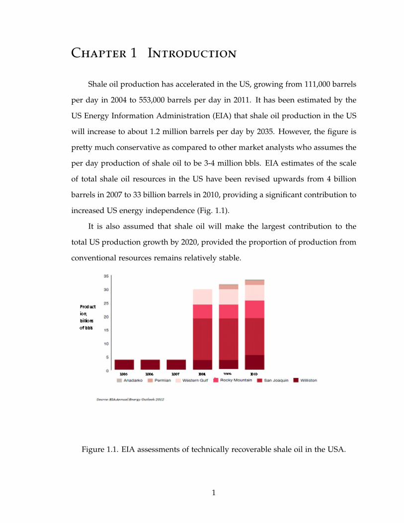
Shale oil production has accelerated in the US, growing from 111,000 barrels
per day in 2004 to 553,000 barrels per day in 2011. It has been estimated by the
US Energy Information Administration (EIA) that shale oil production in the US
will increase to about 1.2 million barrels per day by 2035. However, the figure is
pretty much conservative as compared to other market analysts who assumes the
per day production of shale oil to be 3-4 million bbls. EIA estimates of the scale
of total shale oil resources in the US have been revised upwards from 4 billion
barrels in 2007 to 33 billion barrels in 2010, providing a significant contribution to
increased US energy independence (Fig. 1.1).
It is also assumed that shale oil will make the largest contribution to the
total US production growth by 2020, provided the proportion of production from
conventional resources remains relatively stable.
Figure 1.1. EIA assessments of technically recoverable shale oil in the USA.
1

Figure 1.2. Shale oil production in the USA and in the rest of the world.
Though large amount of resources have been discovered globally, the de-
velopment of shale oil is still at an early stage outside the USA. Global shale
oil resources are estimated at between 330 billion and 1,465 billion barrels. In-
vestments have already begun to characterize, quantify and develop shale oil
resources outside the US. Since the beginning of 2012, there have been a num-
ber of announcements made regarding the discovery of shale oil resources. The
exploration and production of shale oil has also been encouraged.
As shown in figure Fig. 1.3, global shale oil production has the potential to
rise to up to 14 million barrels of oil per day by 2035, amounting to 12 % of total
oil supply at that date (using EIA projections for production other than shale oil).
The investment decisions for unconventional resources depend to a great ex-
tent on the ability to accurately forecast ultimate recovery. Conventional methods
for forecasting ultimate recovery have generally been a great success for conven-
2

tional resources. However, estimating reserves in unconventional reservoirs with
low permeability is problematic due to the longer transient flow periods. These
unconventional wells frequently have bi-linear and linear flow regimes that were
absent in traditional wells and these new flow regimes may dominate the pro-
duction cycle (Freeborn and Russel, 2012).The common industry practice is to use
Arps′ empirical rate decline models, but these equations are applicable only dur-
ing boundary-dominated flow. Using Arps′ relation for unconventional resources
can result in significant overestimation of reserves. Recent methods proposed to
estimate reserves in unconventional resources include the Stretched Exponential
decline model and the Duong model. Each of these methods also has its own
shortcomings.
Figure 1.3. Million barrels of oil produced per day from 2010 to 2040, globally.
3

Chapter 2 Decline Curve Analysis
Production decline curve analysis is one of the oldest methods for predicting
oil or gas reserves. Decline curve analysis (DCA) is a means of predicting the
future production of oil or gas from a well or series of wells, based on extrapola-
tion of production history. They play a vital role in determining the value of oil
or gas wells. If the conditions affecting the rate of production are not changed,
the curve will furnish useful knowledge as to the future production of the well.
With this knowledge the value of a property may be judged, and proper economic
analysis can be made. DCA is one of the most common methods for forecasting
of oil and gas production. The main advantage of decline curve analysis is that,
it uses historical data which is usually very easy to obtain. The results of de-
cline curve are simple plots and easy to visualize, analyze and understand. To
date various methods have been developed for decline curve analysis of which
the most common include Arps, Duong and Stretched Exponential Production
decline methods.
4

Chapter 3 Arps Decline Model
Arps decline curve analysis has been broadly used to estimate reserves since
1940s. It is still arguably the major technology to estimate EUR. Arps decline
curves are of three basic types: exponential (b = 0), hyperbolic (0 < b < 1), and
harmonic (b = 1). The Arps equations are shown below:
Exponential Decline,
qt = qiexp [−Dt] , (3.1)
Hyperbolic Decline
qt =
[qi
(1 + bDit)1/b
], (3.2)
Harmonic Decline
qt =
[qi
(1 + bt)
], (3.3)
where qt represents production rate at time t, qi represents stabilized rate at t =
0, Di is the decline rate which is constant for exponential decline, more generally,
Diis the decline rate at flow rate qi, b is Arps decline constant.
Arps derived hyperbolic decline model based on the emperical observation
that the decline parameter b is usually constant for most of the wells. The ex-
ponential decline model is the special case with b=0. Arps equations are valid
only for wells in boundary dominated flow. Unconventional wells, which have
permeabilities in the range of micro to nano Darcies, have long duration of tran-
sient flow in which b varies (decreases) significantly with time. In horizontal
wells with multifracturing completed in unconventional (low permeability) reser-
voirs, multiple flow regimes may persist for as long as a decade before reservoir
boundary dominates flow. During transient flow period, analysis of production
indicates that production decline can be adequately represented using values of
5

Arps decline constant, b, greater than one, although b decreases with time (Lee
and Sidle,2010).
Figure 3.1. Rate vs time variation with respect to b.
Forecasting of wells that have long transient flow periods, using a constant b
obtained from the early transient flow, over predicts well performance (kurtoglu
et al,2011). Fetkovich et al. (1987) have argued that such anomalous behavior,
i.e. values of (b > 1) arises when data from the transient flow regime are used to
fit the model that is actually appropriate only during Boundary Dominated Flow
(BDF).
The decline exponent must be within the range (0 < b < 1) range to apply
the Arps curves correctly. The harmonic case (b=1) should be used only with
reservation because a forward prediction could result in an infinite cumulative
recovery estimate.
6

Chapter 4 Stretched Exponential
Production Decline
To avoid the uncertainty associated with long term reserve estimates from
the Arps model, Valko (Valko, 2009) proposed a new method the Stretched Ex-
ponential Production Decline. This equation normally tends to fit all the data
and it can also handle high initial rates followed by a rapid decline, which are
common for wells with multi-stage fracturing. As it tends to fit most of the data,
the more historical data, more accurate will be the EUR. Compared to the Arps
hyperbolic model, SEPD has a most significant advantage: EUR is bounded for
any individual well. The SEPD can be applied using the following equations:
qt = qiexp[(− t
τ
)n], (4.1)
Q =[−qiτ
n
] [Γ(
1n
)− Γ
(1n
),(
tτ
)n], (4.2)
r21 =
[Γ(
1n
)− Γ
(1n
),(23.5
τ
)n]
[Γ(
1n
)− Γ
(1n
),(
11.5τ
)n] , (4.3)
r31 =
[Γ(
1n
)− Γ
(1n
),(35.5
τ
)n]
[Γ(
1n
)− Γ
(1n
),(
11.5τ
)n] , (4.4)
where qt is the time-varying production rate, qi is the initial production rate, Q is
the cumulative production, n is the exponent parameter for SEPD model, τ is a
characteristic time parameter, r21 is the ratio of two year production to one year
production; and r31 is the ratio of three year production to one year production.
The stretched exponential production decline (SEPD) model acknowledges
the heterogeneity of a reservoir in that the actual production decline is determined
7

by a great number of contributing volumes individually in exponential decay,
but with a specific distribution of characteristic time constants (Valko and Lee,
2010). SEPD appear to fit field data from various shale plays quite well, thereby
providing an effective alternative to Arps model (Lee, 2012). It predicts a lower
EUR that would be obtained from extrapolation of Transient flow regime without
the transition to exponential decline, as in the case of Arps.
But this method has some serious shortcomings. The equations are very com-
plex and difficult to solve. It relies on complete and incomplete gamma function,
for which computer codes are required.The application of this method requires a
relatively long production history of the well. Though this equation always ob-
tains a solution, the solutions ability to predict EUR may be too poor or of lesser
quality.
8

Chapter 5 Duong′s Production Decline
Duong′s method was empirically derived based on a long-term linear flow
in a large number of wells in tight and shale gas reservoirs (Duong, 2011). "A log-
log plot of rate over cumulative production vs. time is observed to fit a straight
line in most unconventional reservoir cases studied. The slope and intercept are
related to reservoir rock characteristics, fracture stimulation practice, operational
conditions and possibly liquids content" (Duong, 2011). Duong′s equations are
described below,
qt = q1t−n, (5.1)
Qqt
=
[1a
]tm, (5.2)
tD = t−mexp[
a1−m
(t1−m − 1)], (5.3)
qt = qitD + qin f , (5.4)
where qt represents production rate at time t, q1 represents stabilized rate at t
= 1,a and m are emperical constants, tD is dimensionless time, Q is cumulative
porduction and qin f is the intercept of the plot of qt vs. tD
The Duong equation differs from the previously mentioned methods due
to the simplicity and ease with which the equation is solved. This method is
easy and simple to use for predicting future rate and EUR. The equation can be
solved in a simple spreadsheet. This equation was formulated for the use for
unconventional resources.
Duong equations can be solved in just two steps: the first step is plotting ratio
of production rate, q, and cumulative production, Q, vs.t on log - log coordinates.
9

The parameters a and m can be obtained from intercept and slope respectively.
The second step is to plot dimensionless time vs rate, to solve for q1 and qin f .
However, the derivation of equation 5.4 does not include qin f , so the trend line
should be obtained in such a way so as to force the qin f to be zero.
Duong′s method appears to fit production data from both vertical and hor-
izontal wells. The EUR is not based on the traditional concept of drainage area
(BDF) but on the constraints of the latest trends with both time and economic rate
limits (Duong, 2011).
The Duong equation models transient flow, so it assumes prolonged produc-
tion within this flow regime. Duong model is suitable for a single flow regime but
currently has not been proved and is questionable for wells with transitions from
linear to boundary-dominated flow (Freeborn and Russell, 2012). The equation is
useful only for a transient flow regime and maybe a poor estimator of EUR. But it
gives accurate estimates so long as the transient flow regime persists. In addition,
the solution is quite sensitive to small variations in data.
10

Chapter 6 Comparison of methods
Arps is the most common method used in the industry currently. It pro-
duces accurate results for conventional resources, which have limited duration
transient flow regimes. Most of the data for wells in conventional resources are
in the boundary dominated flow regime. But because the transient flow regime
may last for more than a decade in unconventional resources, there came a need
to formulate new methods. The Arps model doesn′t work well in the transient
regime as the b value is usually greater than one, i.e., super hyperbolic, and de-
crease with time. In addition, production continues for infinitely long. However,
Arps is still used as a complement to the other methods.
SEPD and Duong were developed to overcome the problem that develops
when the transient flow regime lasts for a long time. SEPD always provides a so-
lution. The solution of SEPD requires specialised software or complex computer
code. The Duong method is easy to understand and visualize. It can be applied
using a simple spreadsheet. But this equation is valid for a single transient flow
regime only. It is neither expected to work across flow regimes nor to predict
accurately outside the flow regime being analyzed.
When historical field data is long enough to include a moderate to large
amount of boundary dominated flow data, then it may be preferable to use the
Arps models rather than using the SEPD equations (Freeboen and Russell, 2012)
In summary, SEPD and Duong fail to perform in BDF and Arps fail to pro-
vide accurate results if a long transient flow regime is present.
11

Chapter 7 New Method
As stated above, Arps is inaccurate in the transient flow regime, Duong is
inaccurate in boundary dominated flow (BDF). Hence there is a need to develop
a new decline model or a new method to predict more accurately the recovery in
unconventional resources. The new method is basically the combination of above
mentioned methods. As SEPD and Duong model the transient flow regime well
and Arps are widely used for BDF regime, the new method combines the two
methods to achieve our objectives and eliminate the shortcomings.
First we plot rate (or normalised rate) vs material balance time (or time) to
identify the flow regimes in well history and the current flow regime. Material
balance Time (MBT) is the ratio of cumulative production to the production rate.
Then we try to match the given data with the methods stated above and calculate
the parameters from rate vs time plots. If the data has not reached the BDF
the onset of BDF is unknown. The b value in Arps decline model decreases
during a long transient flow period. So Kurtoglu et al. (Kurtoglu et al., 2011)
suggested using Arps standard decline rate equation until the decline rate reaches
a minimum decline and thereafter, use the exponential decline equation with
decline exponent equal to terminal decline. In an analogous way, we assume in
our new method that BDF will start when the terminal decline rate is 5 percent
per annum .When D reaches the Dmin, we switch from the transient model to
the Arps model. At the time of switch to Arps, the value of b is assumed to be
0.3, typical for a solution drive reservoir (Fetkovich, 1980). If we know the time of
BDF onset from the rate vs MBT plot, we use the time for switch and select the b
value such that BDF data is matched. The EUR from the new method is the result
of combination of two models: one for transient flow and the other Arps, which
is currently the most accurate method to model boundary dominated flow. Thus
12
there are basically three new methods: 1) super Hyperbolic combined with Arps;
2) SEPD combined with Arps; and 3) Duong combined with Arps. Using the
field rate data and simulated rates data, we calculate the EUR using six methods
discussed above and determine the most appropriate method. Also we will match
the output from the above method to analytically simulated rates generated with
Fekete Harmony software.
13

Chapter 8 Field Examples
Two field examples and one simulated example are presented from uncon-
ventional shale oil reservoirs to provide a comparative assessment of various
decline curve analysis models, and to quantify the uncertainty associated with
30-year EUR estimates. These examples will be analyzed using the six decline
curve analysis models described earlier, viz., Arps Hyperbolic model, Stretched
Exponential Production Decline Model (SEPD), Duong model and the combined
models, Arps + Arps, SEPD + Arps and Duong + Arps.
8.1 Example 1
The first example is from the Elm Coulee Field in Richland County, Montana
well Anna 2-3h. Five years of production history are available. Fig. 8.1, a plot
of production rate, q, vs Material Balance Time, MBT, shows that a slope of -1
indicating BDF, starts from MBT 90, which is equivalent to the actual time of 45.5
months.
14

Figure 8.1. Rate vs material balance time for field example 1.
8.1.1 Arps Hyperbolic Model
For the Arps model, first we plot the ratio of observed production rate, q,
and cumulative production, Q, to estimate the decline exponent, b, and the ini-
tial decline rate, Di. The resulting fit is shown in Fig. 8.2. The resulting best fit
parameters are b =1.16 and Di = 0.198 1/d. Then we plot the production time,
t, and cumulative production, Q, as shown in Fig. 8.3. The best fit to the above
curve provides an estimate of the third parameter, qi, the initial production rate.
The resulting best fit parameter is qi = 9710 bbls/month. Using these fitted pa-
rameters, the 30-year cumulative production (30-year EUR), Q30, is estimated to
be 257,000 bbls.
15

Figure 8.2. Ratio of rate to cumulative production vs time for field example 1.
Figure 8.3. Cumulative production vs time for field example 1.
16

8.1.2 SEPD
For the Stretched Exponential Production Decline, the equations for r21 and
r31, i.e., the ratio of two year production to one year production and the ratio of
three year production to one year production respectively, are used to estimate the
characteristic time parameter, τ, and the parameter n. The equations were solved
using the VB code in excel. The resulting best fit parameters are τ = 1.2 months
and n = 0.32. Then we plot the production time, t, and cumulative production,
Q, as shown in Fig. 8.5. The best fit to the above curve gives the answer of the
third parameter, qi, the initial production rate. The resulting best fit parameter
is qi = 25,312 bbls/month. Using these fitted parameters, the 30-year cumulative
production (30-year EUR), Q,30, is estimated to be 200,000 bbls.
Figure 8.4. Rate vs time for field example 1.
17

Figure 8.5. Cumulative Production vs time for field example 1.
8.1.3 Duong Model
For the Duong model, the first step is to plot the ratio of production rate,
q, and cumulative production, Q, vs. production time, to estimate the intercept,
a, and the slope, m Fig. 8.6. The resulting best fit parameters are a = 1.597 1/d
and m = -1.409. Then we plot the dimensionless time, tD, and the production rate
as shown in Fig. 8.7. The intercept Qin f is forced to zero. The resulting best fit
parameter, based on Fig. 8.7, is q1 = 9,200 bbls/month. Using these parameters,
the 30-year cumulative production (30-year EUR), Q30, is estimated to be 200,000
bbls.
18

Figure 8.6. Ratio of rate to cumulative production vs time for field example 1.
Figure 8.7. Rate vs dimensionless time for field example 1.
19

8.1.4 Arps+Arps
This is a new method in which Arps super hyperbolic is combined with hy-
perbolic decline (b<1). At 45.5 months (or when the slope of MBT vs rate becomes
1), we change from the decline exponent b=1.2 to b=0.3. Because insufficient BDF
data is available, b= 0.3 has been selected (typically for solution gas drive oil
reservoirs). Arps hyperbolic initial decline is 0.017 d−1 and initial rate or the rate
of switch from Arps super hyperbolic to hyperbolic is 1,187 bbl/month. Using
these fitted parameters, the 30-year cumulative production (30-year EUR), Q30, is
estimated to be 209,000 bbls.
Figure 8.8. Cumulative Production vs time for field example 1.
8.1.5 SEPD+Arps
This is a new method in which Stretched Exponential Production decline is
combined with hyperbolic decline (b<1). At 45.5 months (or when the slope of
20

MBT vs rate becomes 1), we change from from SEPD to Arps hyperbolic decline.
Because insufficient BDF data is available, b= 0.3 has been selected (typically for
solution gas drive oil reservoirs). Arps hyperbolic initial decline is 0.023 d−1 and
initial rate or the rate of switch from SEPD to hyperbolic is 1031.2 bbl/month.
Using these parameters, the 30-year cumulative production (30-year EUR), Q30,
is estimated to be 186,000 bbls.
Figure 8.9. Cumulative Production vs time for field example 1.
8.1.6 Duong +Arps
This is a new method in which Duong is combined with hyperbolic decline
(b<1). At 45.5 months (or when the slope of MBT vs rate becomes 1), we change
from from Duong to Arps hyperbolic decline. Because insufficient BDF data is
available, b= 0.3 has been selected (typically for solution gas drive oil reservoirs).
Arps hyperbolic initial decline is 0.024 d−1 and initial rate or the rate of switch
21

from Duong to hyperbolic is 1,080 bbl/month. Using these parameters, 30-year
cumulative production (30-year EUR), Q30, is estimated to be 186,000 bbls.
Figure 8.10. Cumulative Production vs time for field example 1.
8.1.7 Summary of methods
Fig. 8.11 below shows the aggregation of 30 year forecasts from all the six
models discussed above. Arps hyperbolic model gives the most optimistic projec-
tion, while the new developed method SEPD + Arps gives the most conservative
projection.Table 8.1 shows the summary of the EUR projection for all the six mod-
els.
22

Figure 8.11. Cumulative Production vs time, all methods for field example 1.
Table 8.1. Comparision for all methods, example 1
Methods EUR (Mbbls)
Arps 257
SEPD 200
Duong 200
Arps + Arps 209
SEPD + Arps 186
Duong + arps 186
23

8.2 Example 2
This example is of the Woodford Field in Carter County in Oklahama. The
well name is Nickel Hill 1h-36. About six years of production data was available.
But after 3 years, the well was stimulated. So the available production data for
decline analysis was about 3 years. As seen in the Fig. 8.12, of production rate, q,
vs Material Balance Time, MBT, we can see that a slope of -1 starts from the MBT
60, which is equivalent to the actual time of 25.5 months.
Figure 8.12. Rate vs material balance time for field example 2.
8.2.1 Arps Hyperbolic Model
For the Arps model, first we plot the ratio of observed production rate, q,
and cumulative production, Q, to estimate the decline exponent, b, and the initial
decline rate, Di. The resulting fit is shown in Fig. 8.13.The resulting best fit pa-
rameters are b =1.11 and Di = 0.3 1/d. Then we plot the production time, t, and
cumulative production, Q, as shown in Fig. 8.14. The best fit to the above curve
provides an estimate of the third parameter, qi, the initial production rate. The
24

resulting best fit parameter is qi = 9,710 bbls/month. Using these parameters, the
30-year cumulative production (30-year EUR), Q30, is estimated to be 91,900 bbls.
Figure 8.13. Ratio of rate to cumulative production vs time for field example 2.
Figure 8.14. Cumulative production vs time for field example 2.
25

8.2.2 SEPD
For the Stretched Exponential Production Decline, the equations for r21 and
r31, i.e., the ratio of two year production to one year production and the ratio of
three year production to one year production respectively, are used to estimate the
characteristic time parameter, τ, and the parameter n. The equations were solved
using the VB code in excel. The resulting best fit parameters are τ = 1 months
and n = 0.34. Then we plot the production time, t, and cumulative production, Q,
as shown in Fig. 8.16. The best fit to the above curve gives the answer of the third
parameter, qi, the initial production rate. The resulting best fit parameter is qi =
11,774 bbls/month. Using these parameters, the 30-year cumulative production
(30-year EUR), Q,30, is estimated to be 64,300 bbls.
Figure 8.15. Rate vs time for field example 2.
26

Figure 8.16. Cumulative production vs time for field example 2.
8.2.3 Duong Model
For the Duong model, the first step is to plot the ratio of production rate, q,
and cumulative production, Q, vs. production time, to estimate the intercept, a,
and the slope, m Fig. 8.17. The resulting best fit parameters are a =1.7 1/d and
m = -1.34. Then we plot the dimensionless time, tD, and the production rate as
shown in Fig. 8.18. The intercept Qin f is forced to zero. The resulting best fit
parameter, based on Fig. 8.18, is q1 = 2,200 bbls/month. Using these parameters,
the 30-year cumulative production (30-year EUR), Q30, is estimated to be 97,100
bbls.
27
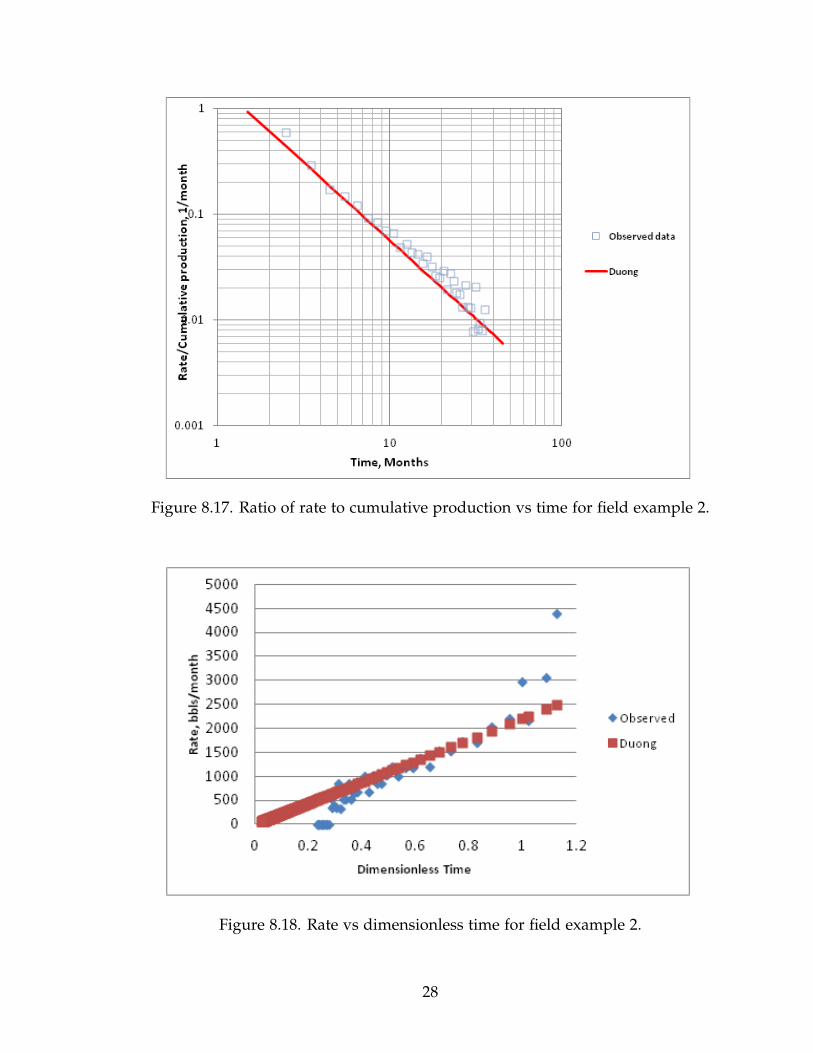
Figure 8.17. Ratio of rate to cumulative production vs time for field example 2.
Figure 8.18. Rate vs dimensionless time for field example 2.
28

8.2.4 Arps+Arps
This is a new method in which Arps super hyperbolic is combined with
hyperbolic decline (b<1). At 25.5 months (or when the slope of MBT vs rate
becomes 1), we change from the decline exponent b=1.11 to b=0.3. Because insuf-
ficient BDF data is available, b= 0.3 has been selected (typically for solution gas
drive oil reservoirs). Arps hyperbolic initial decline is 0.032 d−1 and initial rate or
the rate of switch from Arps super hyperbolic to hyperbolic is 658.4 bbl/month.
Using these parameters, the 30-year cumulative production (30-year EUR), Q30,
is estimated to be 66,000 bbls.
Figure 8.19. Cumulative production vs time for field example 2.
8.2.5 SEPD+Arps
This is a new method in whichStretched Exponential Production decline is
combined with hyperbolic decline (b<1). At 25.5 months (or when the slope of
MBT vs rate becomes 1), we change from from SEPD to Arps hyperbolic decline.
29

Because insufficient BDF data is available, b= 0.3 has been selected (typically
for solution gas drive oil reservoirs). Arps hyperbolic initial decline is 0.04 d−1
and initial rate or the rate of switch from SEPD to hyperbolic is 582 bbl/month.
Using these parameters, the 30-year cumulative production (30-year EUR), Q30,
is estimated to be 58,700 bbls.
Figure 8.20. Cumulative production vs time for field example 2.
8.2.6 Duong +Arps
This is a new method in which Duong is combined with hyperbolic decline
(b<1). At 25.5 months (or when the slope of MBT vs rate becomes 1), we change
from from Duong to Arps hyperbolic decline. Because insufficient BDF data is
available, b= 0.3 has been selected (typically for solution gas drive oil reservoirs).
Arps hyperbolic initial decline is 0.03 d−1 and initial rate or the rate of switch
from Duong to hyperbolic is 794 bbl/month. Using these parameters, 30-year
cumulative production (30-year EUR), Q30, is estimated to be 72,400 bbls.
30

Figure 8.21. Cumulative production vs time for field example 2.
8.2.7 Summary of methods
Fig. 8.22 below shows the aggregation of 30 year forecasts from all the six
models discussed above. Arps hyperbolic model gives the most optimistic projec-
tion, while the new developed method SEPD + Arps gives the most conservative
projection.Table 8.2 shows the summary of the EUR projection for all the six mod-
els.
31

Figure 8.22. Cumulative production vs time, all methods for field example 2.
Table 8.2. Comparision for all methods, example 2
Methods EUR (Mbbls)
Arps 91.9
SEPD 68.3
Duong 97.
Arps + Arps 66
SEPD + Arps 58.7
Duong + arps 72.4
32

Chapter 9 Simulated Examples
Simulated rates were obtained using numerical simulation and multiphase
flow in Fekete Harmony software. Numerical models solve the nonlinear partial-
differential equations (PDE′s) describing fluid flow through porous media with
numerical methods. Numerical methods are the process of discretizing the PDE′s
into algebraic equations and solving those algebraic equations to obtain the so-
lutions. These solutions that represent the reservoir behavior are the values of
pressure and phase saturation at discrete points in the reservoir and at discrete
times. The initial gas saturation was assumed to be 0. The simulation was ac-
cessed three times at 20, 50 and 100 months to provide a comparative assessment
of various decline curve analysis models, and to quantify the uncertainty asso-
ciated with 25 year EUR estimates. These examples were analyzed using the
six decline curve analysis models described earlier, viz., Arps Hyperbolic model,
Stretched Exponential Production Decline Model (SEPD), Duong model and the
combination of above mentioned models namely, Arps + Arps, SEPD + Arps and
Duong + Arps.
9.1 Simulated data of 20 months
From the simulation, rates for the first 20 months were selected to perform
the decline curve analysis. As seen in the Fig. 9.1, of production rate, q, vs Mate-
rial Balance Time, MBT, we can see that Boundary Dominated Flow hasn′t been
reached.
33

Figure 9.1. Rate vs material balance time for 20 months data.
9.1.1 Arps Hyperbolic Model
For the Arps model, first we plot the ratio of observed production rate, q,
and cumulative production, Q, to estimate the decline exponent, b, and the initial
decline rate, Di. The resulting fit is shown in Fig. 9.2. The resulting best fit
parameters are b =1.8 and Di = 3 1/d. Then we plot the production time, t, and
cumulative production, Q, as shown in Fig. 9.3. The best fit gives an estimate of
the third parameter, qi, the initial production rate. The resulting best fit parameter
is qi = 60000 bbls/month. Using these fitted parameters, the 30-year cumulative
production (30-year EUR), Q30, is estimated to be 639,000 bbls.
34

Figure 9.2. Ratio of rate to cumulative production vs time for 20 months data.
Figure 9.3. Cumulative production vs time for 20 months data.
35

9.1.2 SEPD
For the Stretched Exponential Decline model, the equations for r21 and r31,
i.e., the ratio of two year production to one year production and the ratio of three
year production to one year production respectively, are used to estimate the char-
acteristic time parameter, τ, and the parameter, n. As the available data was not
enough instead of 1, 2 and 3 years; 0.5, 1 and 1.5 years were used. The equations
were solved using the VB code in excel. The resulting best fit parameters are τ
= 0.12 months and n = 0.218. Then we plot the production time, t, and cumu-
lative production, Q, as shown in Fig. 9.5. The best fit gives an estimate of the
third parameter, qi, the initial production rate. The resulting best fit parameter
is qi = 95000 bbls/month. Using these fitted parameters the 30-year cumulative
production (30-year EUR), Q30, is estimated to be 487,000 bbls.
Figure 9.4. Rate vs time for 20 months data.
36

Figure 9.5. Cumulative production vs time for 20 months data.
9.1.3 Duong Model
For the Duong model, the first step is to plot the ratio of production rate, q,
and cumulative production, Q, to the production time, to estimate the intercept
constant, a, and the slope parameter, m Fig. 9.6. The resulting best fit parameters
are a = 0.735 1/d and m = -1.124. Then we plot the dimensionless time, tD, and
the production rate as shown in Fig. 9.7. The intercept Qin f is forced to zero. The
resulting best fit parameter, based on Fig. 9.7, is qi = 22,000 bbls/month. Using
these fitted parameters, the 30-year cumulative production (30-year EUR), Q30, is
estimated to be 582,000 bbls.
37

Figure 9.6. Ratio of rate to cumulative production vs time for 20 months data.
Figure 9.7. Rate vs dimensionless time for 20 months data.
38

9.1.4 Arps+Arps
As the BDF is not seen (or the slope of MBT vs rate has not yet become 1),
we select time to BDF when the terminal decline is 5 % per annum. At the time
of switch, b= 0.3 has been selected (typically for solution gas drive oil reservoirs).
Arps hyperbolic initial decline at the time of switch is 0.0084 d−1 and initial rate or
the rate of switch from Arps super hyperbolic to hyperbolic is 2,280 bbl/month.
Using these parameters, the 30-year cumulative production (30-year EUR), Q30,
is estimated to be 581,000 bbls.
Figure 9.8. Cumulative production vs time for 20 months data.
9.1.5 SEPD+Arps
As the BDF is not seen (or the slope of MBT vs rate has not yet become 1),
we select time to BDF when the terminal decline is 5 % per annum. At the time
of switch, b= 0.3 has been selected (typically for solution gas drive oil reservoirs).
Arps hyperbolic initial decline at the time of switch is 0.013 d−1 and initial rate
39

or the rate of switch from SEPD to hyperbolic is 1,800 bbl/month. Using these
parameters, the 30-year cumulative production (30-year EUR), Q30, is estimated
to be 454,000 bbls.
Figure 9.9. Cumulative production vs time for 20 months data.
9.1.6 Duong +Arps
As the BDF is not seen (or the slope of MBT vs rate has not yet become 1),
we select time to BDF when the terminal decline is 5 % per annum. At the time
of switch, b= 0.3 has been selected (typically for solution gas drive oil reservoirs).
Arps hyperbolic initial decline at the time of switch is 0.01 d−1 and initial rate
or the rate of switch from Duong to hyperbolic is 2,160 bbl/month. Using these
parameters, 30-year cumulative production (30-year EUR), Q30, is estimated to be
527,000 bbls.
40

Figure 9.10. Cumulative production vs time for 20 months data.
9.1.7 Summary of results to simulated example
Fig. 9.11 below shows the aggregation of 30 year forecast of all the six mod-
els discussed above. Arps hyperbolic model gives the most optimistic projection,
while the new developed method SEPD + Arps gives the most conservative pro-
jection. Table 9.1 shows the summary of the EUR projection for all the six models.
41

Figure 9.11. Cumulative Production vs time, all methods for 20 months data.
Table 9.1. Comparision for all methods, 20 months of simulated data
Methods EUR (Mbbls) percentage error
Arps 639 +47
SEPD 487 +12
Duong 582 +33.6
Arps + Arps 581 +33.3
SEPD + Arps 454 +4.2
Duong + arps 527 +21
Simulated 436 0
42

9.2 Simulated rates of 50 months
From the simulated data the data of first 50 months was selected to perform
the decline curve analysis. As seen in the Fig. 9.12, of production rate, q, vs
Material Balance Time, MBT, we can see that Boundary Dominated Flow hasn′t
been reached.
Figure 9.12. Rate vs material balance time for 50 months data.
9.2.1 Arps Hyperbolic Model
Arps Hyperbolic Model: For the Arps model, first we plot the ratio of ob-
served production rate, q, and cumulative production, Q, to estimate the de-
cline exponent, b, and the initial decline rate, Di. The resulting fit is shown in
Fig. 9.13.The resulting best fit parameters are b = 1.5 and Di = 2 1/d. Then we
plot the production time, t, and cumulative production, Q, as shown in Fig. 9.14.
The best fit gives an estimate of the third parameter, qi, the initial production
rate. The resulting best fit parameter is qi = 63,000 bbls/month. Using these fitted
parameters, the 30-year cumulative production (30-year EUR), Q, 30, is estimated
43

to be 603.000 bbls.
Figure 9.13. Ratio of rate to cumulative production vs time for 50 months data.
Figure 9.14. Cumulative production vs time for 50 months data.
44

9.2.2 SEPD
For the Stretched Exponential Decline model, the equations for r21 and r31,
i.e., the ratio of two year production to one year production and the ratio of three
year production to one year production respectively, are used to estimate the
characteristic time parameter, τ, and the parameter, n. The equations were solved
using the VB code in excel. The resulting best fit parameters are τ = 1 months and
n = 0.293. Then we plot the production time, t, and cumulative production, Q, as
shown in Fig. 9.16. The best fit gives an estimate of the third parameter, qi, the
initial production rate. The resulting best fit parameter is qi = 51,500 bbls/month.
Using these fitted parameters the 30-year cumulative production (30-year EUR),
Q30, is estimated to be 454,000 bbls.
Figure 9.15. Rate vs time for 50 months data.
45

Figure 9.16. Cumulative production vs time for 50 months data.
9.2.3 Duong Model
For the Duong model, the first step is to plot the ratio of production rate, q,
and cumulative production, Q, to the production time, to estimate the intercept
constant, a, and the slope parameter, m Fig. 9.17. The resulting best fit parameters
are a =0.731 1/d and m = -1.119. Then we plot the dimensionless time, tD, and
the production rate as shown in Fig. 9.18. The intercept Qin f is forced to zero. The
resulting best fit parameter, based on Fig. 9.18, is qi = 21,500 bbls/month. Using
these fitted parameters, the 30-year cumulative production (30-year EUR), Q30, is
estimated to be 545,000 bbls.
46

Figure 9.17. Ratio of rate to cumulative production vs time for 50 months data.
Figure 9.18. Rate vs dimensionless time for 50 months data.
47

9.2.4 Arps+Arps
As the BDF is not seen (or the slope of MBT vs rate has not yet become 1),
we select time to BDF when the terminal decline is 5 % per annum. At the time of
switch, b = 0.3 has been selected (typically for solution gas drive oil reservoirs).
Arps hyperbolic initial decline at the time of switch is 0.0084 d−1 and initial rate or
the rate of switch from Arps super hyperbolic to hyperbolic is 1,634 bbl/month.
Using these parameters, the 30-year cumulative production (30-year EUR), Q30,
is estimated to be 528,000 bbls.
Figure 9.19. Cumulative production vs time for 50 months data.
9.2.5 SEPD+Arps
As the BDF is not seen (or the slope of MBT vs rate has not yet become 1),
we select time to BDF when the terminal decline is 5 % per annum. At the time
of switch, b= 0.3 has been selected (typically for solution gas drive oil reservoirs).
Arps hyperbolic initial decline at the time of switch is 0.013 d−1 and initial rate
48

or the rate of switch from SEPD to hyperbolic is 1,400 bbl/month. Using these
parameters, the 30-year cumulative production (30-year EUR), Q30, is estimated
to be 438,000 bbls.
Figure 9.20. Cumulative production vs time for 50 months data.
9.2.6 Duong +Arps
As the BDF is not seen (or the slope of MBT vs rate has not yet become 1),
we select time to BDF when the terminal decline is 5 % per annum. At the time of
switch, b = 0.3 has been selected (typically for solution gas drive oil reservoirs).
Arps hyperbolic initial decline at the time of switch is 0.0086 d−1 and initial rate
or the rate of switch from Duong to hyperbolic is 1,930 bbl/month. Using these
parameters, 30-year cumulative production (30-year EUR), Q30, is estimated to be
505,000 bbls.
49

Figure 9.21. Cumulative production vs time for 50 months data.
9.2.7 Summary of methods
Fig. 9.22 below shows the aggregation of 30 year forecast of all the six mod-
els discussed above. Arps hyperbolic model gives the most optimistic projection,
while the new developed method SEPD + Arps gives the most conservative pro-
jection. Table 9.2 shows the summary of the EUR projection for all the six models.
50

Figure 9.22. Cumulative production vs time, all methods for 50 months data.
Table 9.2. Comparision for all methods, 50 months of simulated data
Methods EUR (Mbbls) percentage error
Arps 603 +38.5
SEPD 454 +4.2
Duong 545 +25.1
Arps + Arps 528 +21.1
SEPD + Arps 438 +0.5
Duong + arps 505 +15.9
Simulated 436 0
51

9.3 Simulated rates of 100 months
From the simulated data, the data of first 100 months was selected to perform
the decline curve analysis. As seen in the Fig. 9.23, of production rate, q, vs
Material Balance Time, MBT, we can see that Boundary Dominated Flow starts
after 60.5 months or can say 200 MBT.
Figure 9.23. Rate vs material balance time for 100 months data.
9.3.1 Arps Hyperbolic Model
For the Arps model, first we plot the ratio of observed production rate, q,
and cumulative production, Q, to estimate the decline exponent, b, and the initial
decline rate, Di. The resulting fit is shown in Fig. 9.24. The resulting best fit
parameters are b =1.7 and Di = 2 1/d. Then we plot the production time, t, and
cumulative production, Q, as shown in Fig. 9.25. The best fit gives an estimate of
the third parameter, qi, the initial production rate. The resulting best fit parameter
is qi = 50,000 bbls/month. Using these fitted parameters, the 30-year cumulative
production (30-year EUR), Q30, is estimated to be 580,000 bbls.
52

Figure 9.24. Ratio of rate to cumulative production vs time for 100 months data.
Figure 9.25. Cumulative production vs time for 100 months data.
53

9.3.2 SEPD
For the Stretched Exponential Decline model, the equations for r21 and r31,
i.e., the ratio of two year production to one year production and the ratio of three
year production to one year production respectively, are used to estimate the
characteristic time parameter, τ, and the parameter, n. The equations were solved
using the VB code in excel. The resulting best fit parameters are τ = 0.7 months
and n = 0.28. Then we plot the production time, t, and cumulative production, Q,
as shown in Fig. 9.27. The best fit gives an estimate of the third parameter, qi, the
initial production rate. The resulting best fit parameter is qi = 60,000 bbls/month.
Using these fitted parameters the 30-year cumulative production (30-year EUR),
Q30, is estimated to be 454,000 bbls.
Figure 9.26. Rate vs Time for 100 months data.
54

Figure 9.27. Cumulative production vs time for 100 months data.
9.3.3 Duong Model
For the Duong model, the first step is to plot the ratio of production rate, q,
and cumulative production, Q, to the production time, to estimate the intercept
constant, a, and the slope parameter, m Fig. 9.28. The resulting best fit parameters
are a = 0.874 1/d and m = -1.194. Then we plot the dimensionless time, tD, and
the production rate as shown in Fig. 9.29. The intercept Qin f is forced to zero. The
resulting best fit parameter, based on Fig. 9.29, is q1 = 22,500 bbls/month. Using
these fitted parameters, the 30-year cumulative production (30-year EUR), Q30, is
estimated to be 509,000 bbls.
55

Figure 9.28. Ratio of rate to cumulative production vs time for 100 months data.
Figure 9.29. Rate vs dimensionless time for 100 months data.
56

9.3.4 Arps+Arps
At 60.5 months (or when the slope of MBT vs rate becomes 1), we change
from the decline exponent b=1.11 to b=0.36, the best fit to the BDF data. Arps
hyperbolic initial decline at the time of switch is 0.032 d−1 and initial rate or
the rate of switch from Arps super hyperbolic to hyperbolic is 658.4 bbl/month.
Using these parameters, the 30-year cumulative production (30-year EUR), Q30,
is estimated to be 507,000 bbls.
Figure 9.30. Cumulative production vs time for 100 months data.
9.3.5 SEPD+Arps
At 60.5 months (or when the slope of MBT vs rate becomes 1), we change
from the decline exponent b=1.11 to b=0.36, the best fit to the BDF data. Arps
hyperbolic initial decline at the time of switch is 0.04 d−1 and initial rate or the
rate of switch from SEPD to hyperbolic is 582 bbl/month. Using these parameters,
the 30-year cumulative production (30-year EUR), Q30, is estimated to be 435,000
57

bbls.
Figure 9.31. Cumulative production vs time for 100 months data.
9.3.6 Duong +Arps
At 60.5 months (or when the slope of MBT vs rate becomes 1), we change
from the decline exponent b=1.11 to b=0.36, the best fit to the BDF data. Arps
hyperbolic initial decline at the time of switch is 0.03 d−1 and initial rate or the rate
of switch from Duong to hyperbolic is 794 bbl/month. Using these parameters,
30-year cumulative production (30-year EUR), Q30, is estimated to be 460,000
bbls.
58

Figure 9.32. Cumulative production vs time for 100 months data.
9.3.7 Summary of methods
Fig. 9.33 below shows the aggregation of 30 year forecast of all the six mod-
els discussed above. Arps hyperbolic model gives the most optimistic projection,
while the new developed method SEPD + Arps gives the most conservative pro-
jection. Table 9.3 shows the summary of the EUR projection for all the six models.
59

Figure 9.33. Cumulative production vs time, all methods for 100 months data.
Table 9.3. Comparision for all methods,100 months of simulated data
Methods EUR (Mbbls) percentage error
Arps 580 +33.2
SEPD 454 +4.1
Duong 509 +16.84
Arps + Arps 507 +16.43
SEPD + Arps 435 -0.26
Duong + arps 460 +5.45
Simulated 436 0
60

9.3.8 Comparision of Sepd + Arps
Table 9.4 shows the comparision of the Sepd + Arps with the simulated data
when different months of data were used. Even if the data of 20 months was used,
Sepd + Arps gives us the error of just 5 percent and as the number of months of
data used are increaded to 100 than the error is reduced to mere 0.25 percent. So
by far Sepd + Arps gives the most reliable answer.
Table 9.4. Comparision of SEPD + Arps method
Time EUR (Mbbls) percentage error
20 months 454.048 -4.18
50 months 437.972 -0.49
100 months 434.702 0.26
simulated 435.841 0
61

Chapter 10 Conclusions
From the analysis made from the field examples and the simulation, we can
conclude that:
1) SEPD + Arps gives the most conservative results of all the methods.
2) If enough data is not available then also SEPD + Arps gives the most reliable
and accurate results.
3) SEPD + Arps can work without enough Boundary Dominated Flow data avail-
able.
4) If we switch to Boundary Dominated flow equal to when the decline rate
reaches 5 % per annum, we are close to the exact results.
62

References
Arps, J.J.: Analysis of Decline Curves, Published in Petroleum Transactions,
AIME, 160(1945):228-247.
Can, B. and Kabir, C.S., Probabilistic Performance for Unconventional
Reservois with Stretched Exponential model, SPE 143666 presented at the
SPE North American Unconventional Gas Conference and Exhibition, The
Woodlands, Texas,14-16 June 2011.
Duong, A.N. An Unconventional rate Decline Approach for Tight and
Fracture-Dominated Gas Wells, CSUG/SPE 137748 presented at the Canadian
Unconventional Resources and International Petroleum Conference, Calgary,
Canada, 19-21 October 2010.
Fetkovich, M.J., 1980. Decline Curve Analysis Using Type Curves. SPE
Journal of Petroleum Technology 32(6):1065-1077.
Fetkovich, M.J. , Fetkovich, E.J., and Fetkovich, M.D., Useful Concepts
for Declin-Curve Forecasting, Reserve Estimation, and Analysis, SPEFE
(February 1996) 13-22.
Freeborn, R. and Russell, B., 2012. How To Apply Stretched Exponen-
tial Equations to Reserve Evaluation. Paper SPE-162631-MS presented at the
SPE Hydrocarbon Economics and Evaluation Symposium. Calgary, Alberta,
Canada, 24-25 September 2012.
63

Ilk, D., Rushing, J.A., and Blasingame, T.A., Exponential vs Hyperbolic
Decline in Tight Gas Sands-Understanding the Origin and Implications for
Reserve Estimates Using Arps Decline curves, SPE 116731 presented at SPE
Annual Technical Conference and Exhibition, Denverm Colorado, USA, 21-24
September, 2008.
Kanfar, M.S. , Wattenbarger, R.A. , Comparison of Empirical Decline
Curve Methods for Shale Wells, SPE 162648 presented at SPE Canadian
Unconventional Resources Conference held in Calgary, Alberta, Canada, 30
October-1 November, 2012.
Kurtoglu, B., Cox, S.A., and Kazemi, H., 2011. Evaluation of Long-Term
Performance of Oil Wells in Elm Coulee Field. Paper SPE-149273-MS pre-
sented at the Canadian Unconventional Resources Conference. Alberta,
Canada, 15-17 November 2011.
Lee, W.J. and Sidle, R.E., 2010. Gas Reserves Estimation in Resource
Plays. Paper SPE 130102 presented at the 2010 SPE Unconventional Reservoir
Conference, Pittsburgh, PA, USA, 23-25 February.
Lee, W.J., 2012, Estimating Reserves in unconventionalResources, Un-
published SPE Webinar Notes, 23 February.
Mishra, S., A New Approach to Reserves Estimation in Shale Gas Reservoirs
Using Multiple Decline Curve Analysis Models. SPE 1611092 presented at
SPE Easten Regional Meeting held in Lexington, Kentucky, USA, 3-5 October,
2012.
64

Pwc.2013. Shale Oil: The next energy revolution. http :
//www.pwc.com/enGX/gx/oil − gas − energy/publications/pd f s/pwc −
shale− oil.pd f (downloaded 5 May, 2013).
Valko, P.P., Assigning Value to stimulation in the barnett Shale: A si-
multaneous Analysis of 7000 Plus Productio Histories and Well Completion
records, SPE 119369 presented at 2009 SPE Hydraulic Fracturing Technology
Conference, The Woodlands, Texas, 19-21 January 2009.
Valko, P.P. and Lee, W.J., 2010. A Better Way To Forecast Production
From Unconventional Gas Wells. Paper SPE-134231-MS presented at the SPE
Annual Technical Conference and Exhibition. Florence, Italy, 19-22 September
2010.
65