Traffic Collision Analysis Models: Review and Empirical Evaluation
Upload
khangminh22Category
view
0download
0
1
Cha
pter
7Development of Empirical Models
From Process Data• In some situations it is not feasible to develop a theoretical
(physically-based model) due to:1. Lack of information2. Model complexity3. Engineering effort required.
• An attractive alternative: Develop an empirical dynamic model from input-output data.
• Advantage: less effort is required
• Disadvantage: the model is only valid (at best) for the range of data used in its development.
i.e., empirical models usually don’t extrapolate very well.

2
Simple Linear Regression: Steady-State Model• As an illustrative example, consider a simple linear model
between an output variable y and input variable u,
where and are the unknown model parameters to be estimated and ε is a random error.
• Predictions of y can be made from the regression model,
Cha
pter
7
y
1 2β β εy u= + +
1β 2β
1 2ˆ ˆˆ β β (7-3)y u= +
where and denote the estimated values of β1 and β2, and denotes the predicted value of y.
1β 2β
1 2β β ε (7-1)i i iY u= + +
• Let Y denote the measured value of y. Each pair of (ui, Yi) observations satisfies:

3
( )221 1 2
1 1ε β β (7-2)
N N
i ii i
S Y u= =
= = − −∑ ∑
• The least squares method is widely used to calculate the values of β1 and β2 that minimize the sum of the squares of the errors S for an arbitrary number of data points, N:
• Replace the unknown values of β1 and β2 in (7-2) by their estimates. Then using (7-3), S can be written as:
2
1
where the -th residual, , is defined as,ˆ (7 4)
N
ii
i
i i i
S e
i ee Y y
==
− −
∑
The Least Squares ApproachC
hapt
er 7

4
• The least squares solution that minimizes the sum of squared errors, S, is given by:
( )1 2β (7-5)uu y uy u
uu u
S S S S
NS S
−=
−
( )2 2β (7-6)uy u y
uu u
NS S S
NS S
−=
−
where:
2
1 1
N N
u i uu ii i
S u S u= =
∆ ∆∑ ∑1 1
N N
y i uy i ii i
S Y S u Y= =
∆ ∆∑ ∑
The Least Squares Approach (continued)C
hapt
er 7

5
Cha
pter
7
• Least squares estimation can be extended to more generalmodels with:
1. More than one input or output variable.
2. Functionals of the input variables u, such as poly-nomials and exponentials, as long as the unknown parameters appear linearly.
• A general nonlinear steady-state model which is linear in the parameters has the form,
1β ε (7-7)
p
j jj
y X=
= +∑
Extensions of the Least Squares Approach
where each Xj is a nonlinear function of u.

6
Cha
pter
7The sum of the squares function analogous to (7-2) is
2
1 1β (7-8)
pN
i j iji j
S Y X= =
= −
∑ ∑
which can be written as,
( ) ( ) (7-9)TS = −β βY - X Y X
where the superscript T denotes the matrix transpose and:
1 1β
βn p
Y
Y
= =
βY
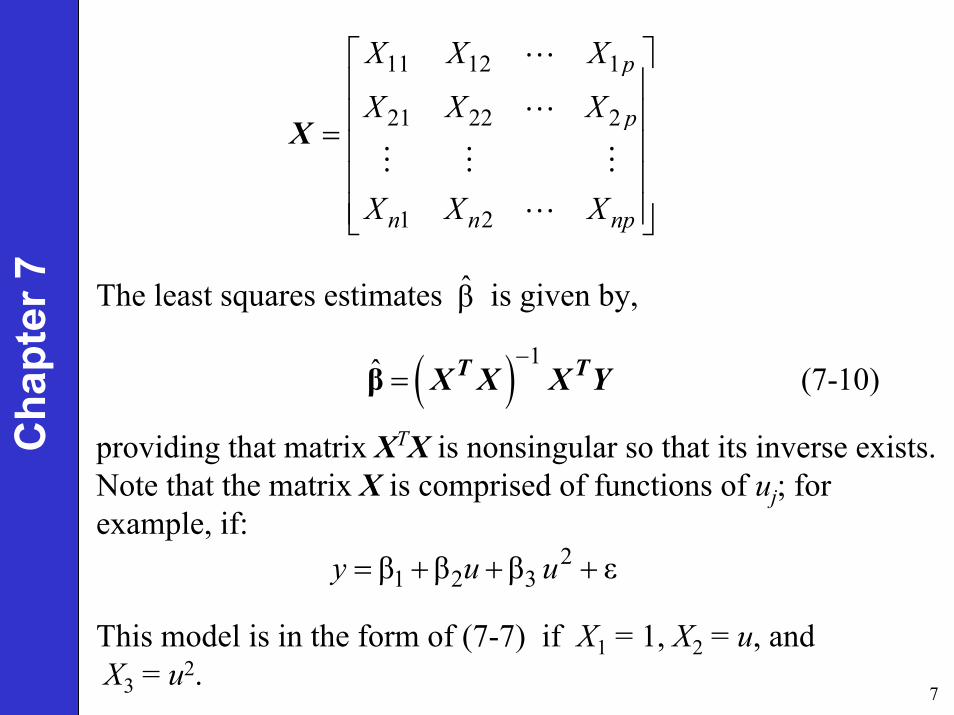
7
11 12 1
21 22 2
1 2
p
p
n n np
X X X
X X X
X X X
=
X
Cha
pter
7 The least squares estimates is given by,β
( ) 1ˆ (7-10)−
=β T TX X X Y
providing that matrix XTX is nonsingular so that its inverse exists. Note that the matrix X is comprised of functions of uj; for example, if:
21 2 3β β β εy u u= + + +
This model is in the form of (7-7) if X1 = 1, X2 = u, andX3 = u2.

8
Cha
pter
7
• Simple transfer function models can be obtained graphically from step response data.
• A plot of the output response of a process to a step change in input is sometimes referred to as a process reaction curve.
• If the process of interest can be approximated by a first- or second-order linear model, the model parameters can be obtained by inspection of the process reaction curve.
• The response of a first-order model, Y(s)/U(s)=K/(τs+1), to a step change of magnitude M is:
( ) /(1 ) (5-18)ty t KM e τ−= −
Fitting First and Second-Order Models Using Step Tests

9
Cha
pter
7 0
1 (7-15)τt
d ydt KM =
=
• The initial slope is given by:
• The gain can be calculated from the steady-state changesin u and y:
where ∆ is the steady-state change in .
y yKu M
y y
∆ ∆= =
∆

10
Cha
pter
7
Figure 7.3 Step response of a first-order system and graphical constructions used to estimate the time constant, τ.

11
First-Order Plus Time Delay Model-θ
( )τ 1Ke sG s
s=
+
For this FOPTD model, we note the following charac-teristics of its step response:
Cha
pter
7
1. The response attains 63.2% of its final responseat time, t = τ+θ.
2. The line drawn tangent to the response atmaximum slope (t = θ) intersects the y/KM=1line at (t = τ + θ ).
3. The step response is essentially complete at t=5τ. In other words, the settling time is ts=5τ.

12
Cha
pter
7
Figure 7.5 Graphical analysis of the process reaction curve to obtain parameters of a first-order plus time delay model.

13
There are two generally accepted graphical techniques for determining model parameters τ, θ, and K.
Method 1: Slope-intercept methodFirst, a slope is drawn through the inflection point of the process reaction curve in Fig. 7.5. Then τ and θ are determined by inspection.
Alternatively, τ can be found from the time that the normalized response is 63.2% complete or from determination of the settling time, ts. Then set τ=ts/5.
Cha
pter
7
Method 2. Sundaresan and Krishnaswamy’s Method
This method avoids use of the point of inflection construction entirely to estimate the time delay.

14
Cha
pter
7
• They proposed that two times, t1 and t2, be estimated from a step response curve, corresponding to the 35.3% and 85.3% response times, respectively.
• The time delay and time constant are then estimated from the following equations:
( )1 2
2 1
θ 1.3 0.29(7-19)
τ 0.67t t
t t= −= −
• These values of θ and τ approximately minimize the difference between the measured response and the model, based on a correlation for many data sets.
Sundaresan and Krishnaswamy’s Method

15
Cha
pter
7
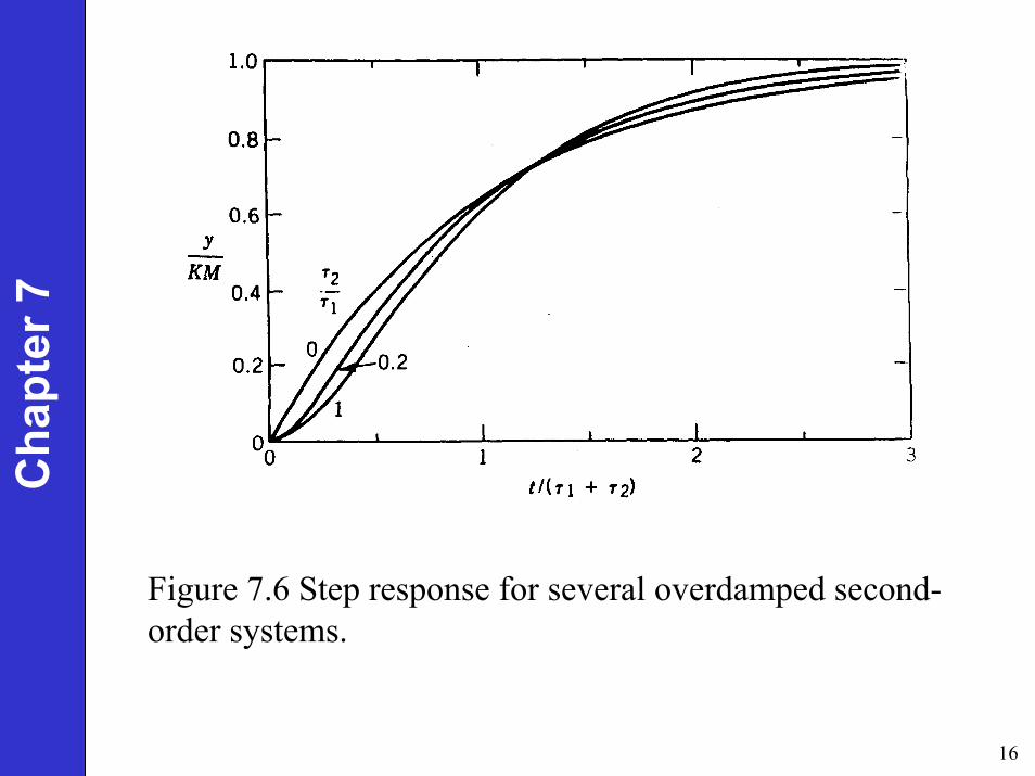
• In general, a better approximation to an experimental step response can be obtained by fitting a second-order model to the data.
• Figure 7.6 shows the range of shapes that can occur for the step response model,
( ) ( )( )1 2(5-39)
τ 1 τ 1KG s
s s=
+ +
• Figure 7.6 includes two limiting cases: , where the system becomes first order, and , the critically damped case.
• The larger of the two time constants, , is called the dominant time constant.
2 1τ / τ 0=2 1τ / τ 1=
1τ
Estimating Second-order Model Parameters Using Graphical Analysis
16
Cha
pter
7
Figure 7.6 Step response for several overdamped second-order systems.

17
1. Determine t20 and t60 from the step response.
2. Find ζ and t60/τ from Fig. 7.7.
3. Find t60/τ from Fig. 7.7 and then
t60 is known).
Cha
pter
7
• Assumed model:
( )θ
2 2τ 2ζτ 1
sKeG ss s
−=
+ +
• Procedure:
Smith’s Method
calculate τ (since

18
Cha
pter
7

19
Cha
pter
7Fitting an Integrator Model
to Step Response Data
In Chapter 5 we considered the response of a first-order process to a step change in input of magnitude M:
( ) ( )/ τ1 M 1 (5-18)ty t K e−= −
For short times, t < τ, the exponential term can be approximated by
/ τ 1τ
t te− ≈ −
so that the approximate response is:
( )1MM 1 1 (7-22)
τ τt Ky t K t ≈ − − =

20
Cha
pter
7is virtually indistinguishable from the step response of the integrating element
( ) 22 (7-23)KG s
s=
In the time domain, the step response of an integrator is
( )2 2 (7-24)y t K Mt=
Hence an approximate way of modeling a first-order process is to find the single parameter
2 (7-25)τKK =
that matches the early ramp-like response to a step change in input.

21
Cha
pter
7If the original process transfer function contains a time delay (cf. Eq. 7-16), the approximate short-term response to a step input of magnitude M would be
( ) ( ) ( )θ θKMy t t S tt
= − −
where S(t-θ) denotes a delayed unit step function that starts at t=θ.

22
Cha
pter
7
Figure 7.10. Comparison of step responses for a FOPTD model (solid line) and the approximate integrator plus time delay model (dashed line).

23
Cha
pter
7Development of Discrete-Time
Dynamic Models• A digital computer by its very nature deals internally with
discrete-time data or numerical values of functions at equally spaced intervals determined by the sampling period.
• Thus, discrete-time models such as difference equations are widely used in computer control applications.
• One way a continuous-time dynamic model can be converted to discrete-time form is by employing a finite difference approximation.
• Consider a nonlinear differential equation,
( ) ( ), (7-26)dy t
f y udt
=
where y is the output variable and u is the input variable.

24
Cha
pter
7• This equation can be numerically integrated (though with some
error) by introducing a finite difference approximation for the derivative.
• For example, the first-order, backward difference approximation to the derivative at is
where is the integration interval specified by the user andy(k) denotes the value of y(t) at . Substituting Eq. 7-26 into (7-27) and evaluating f (y, u) at the previous values of y and u (i.e., y(k – 1) and u(k – 1)) gives:
( ) ( )1(7-27)
y k y kdydt t
− −≅
∆
t k t= ∆
t∆t k t= ∆
( ) ( ) ( ) ( )( )( ) ( ) ( ) ( )( )
11 , 1 (7-28)
1 1 , 1 (7-29)
y k y kf y k u k
ty k y k tf y k u k
− −≅ − −
∆= − + ∆ − −

25
Cha
pter
7Second-Order Difference
Equation Models
( ) ( ) ( ) ( ) ( )1 2 1 21 2 1 2 (7-36)y k a y k a y k b u k b u k= − + − + − + −
• Parameters in a discrete-time model can be estimated directly from input-output data based on linear regression.
• This approach is an example of system identification (Ljung, 1999).
• As a specific example, consider the second-order difference equation in (7-36). It can be used to predict y(k) from data available at time (k – 1) and (k – 2) .
• In developing a discrete-time model, model parameters a1, a2, b1, and b2 are considered to be unknown.
t∆ t∆

26
( ) ( )( ) ( )
1 1 2 2 3 1 4 2
1 2
3 4
β , β , β , β1 , 2 ,
1 , 2
a a b bX y k X y k
X u k X u k
− −
− −
2
1 1β (7-8)
pN
i j iji j
S Y X= =
= −
∑ ∑
• This model can be expressed in the standard form of Eq. 7-7,
1β ε (7-7)
p
j jj
y X=
= +∑
• The parameters are estimated by minimizing a least squares error criterion:
by defining:
Cha
pter
7

27
Equivalently, S can be expressed as,
( ) ( ) (7-9)TS = −β βY - X Y X
where the superscript T denotes the matrix transpose and:
Cha
pter
7
1 1β
βn p
Y
Y
= =
βY
The least squares solution of (7-9) is:
( ) 1ˆ (7-10)−
=β T TX X X Y
Copyright © 2022 FDOKUMEN