i

Development of an External Ultrasonic Sensor Technique to Measure Interface

Conditions in Metal Rolling

Adeyemi Gbenga Joshua

The Department of Mechanical Engineering

This dissertation is submitted for the degree of Doctor of

Philosophy

December 2017

ii

Abstract

Metal rolling is by friction which develops at metal-to-roll interfaces during the rolling

process. But, friction at the metal-to-roll interface during the metal rolling process can cause

roll surface damage if not controlled. Over time, friction results in downtime and repair of

the mill. Therefore, lubrication is essential to control the metal-to-roll interface coefficient of

friction. It is important to understand the conditions at the metal-to-roll interface to

minimize energy loss and improve the strip surface finish.

In this work, a new method for measurement of metal-to-roll interface conditions, based on

the reflection of ultrasound, is evaluated during the cold metal rolling operation. The

method is a pitch-catch sensor layout arrangement. Here, a piezoelectric element generates

an ultrasonic pulse which is transmitted to the metal-to-roll contact interface. This method

is non-invasive to both roll and strip during the process.

The wave reflection from the metal-to-roll interface is received by a second transducer. The

amplitude of the reflected waves is processed in the frequency domain. The reflection

coefficient values are used to study the metal-to-roll interface conditions at different rolling

parameters like, roll speeds and rolling loads. The results show that the reflection coefficient

increases with increasing roll speed. This is because of reduction in the roll-bite contact area

or increase in the frictional resistance of interface during the roll speed increment. However,

the reflection coefficient decreases with increasing rolling load due to either increase in the

roll-bite contact area or pressure.

The reflection coefficient determines the oil film thickness formation at the metal-to-roll

interface. In-addition, the Time-of-Flight of the reflected wave obtained from this technique

is used to estimate strip thickness and roll-bite length during the rolling process. The oil film

thickness in the range of 1.25µm to 3.05µm was measured during the rolling process. The

film thickness increases with increasing roll speed and reduces with increasing rolling load.

The roll-bite value of 5.5mm was measured during the process.

The results from this study show that this ultrasonic technique can measure the metal-to-

roll interface conditions (roll-bite, oil film and strip thickness) during the rolling process. This

ultrasonic technique has the advantage of minor roll modification. Additionally, the

iii

experimental roll condition values obtained from the ultrasonic reflection method agree

with theoretical values. The technique shows promising results as a research tool, and with

further development, could be used for lubricant monitoring. Also, it can be utilized in the

control system of a working mill for reduction of friction losses in the metal rolling process.

iv

Acknowledgements

Praises to Almighty God for his abundant grace, blesses, wisdom, knowledge and

understanding given to me to finish the research.

I would like to thank the encouragement, inspiration, and support provided by my

supervisors throughout the duration of this project. I appreciate my first supervisor, Doctor

Christophe Pinna for his assistance, advice, and support from the beginning of this project.

Special thanks go to Professor Rob Dwyer-Joyce for his patience and invaluable help

throughout of this program; I appreciate all his invested time and ideas in the supervision of

my thesis and for his readiness for scientific discussion. Thanks also to Doctor Matt Marshall

for his input and good scientific advice that are for the benefit of this project. I am very

grateful to David Butcher for his technical assistance and the nice time we were working

together.

Much gratitude to the Tertiary Education Trust Fund (TETFund), Nigeria for their financial

assistance and providing the scholarship scheme that funded my PhD; this program would

not have been possible without their support. I also wish to appreciate the Ekiti State

University Management Members for their financial assistance, encouragement and for the

opportunity given to me to do my PhD in one of the world renowned universities. Many

thanks go to the staff of the Faculty of Engineering, Ekiti State University, particularly the

Department of Mechanical Engineering, for their understanding during the program. I would

like to thank Professor S. B. Adeyemo and Professor Aribisala Olugbenga James for their

advice during the period of this project.

Millions of thanks go to my family, mainly my wife Feyisayo Kemisola Adeyemi and my

children, for their understanding, help, and patience, for the period of being away from

them. Thanks to my friend and my brother Doctor Temitope Stephen for his assistance at

the early stage and throughout this project. My thanks also go to Sia Kemoh and her children

for their moral support all the time during this study.

I would also like to acknowledge the Leonardo Centre for Tribology Group for the excellent

working atmosphere and for their useful suggestions at various stages of this project

provided. I would like to thank Robin Mills, Andy Hunter, Xiangwei Li, and Thomas Holdich

v

for their hospitality and for providing useful attentions, discussions, and suggestions

throughout this project. I also thank the English Language Teaching Centre, University of

Sheffield for helping improve my writing.

Finally, I would like to appreciate my friends, both home and abroad; Ogunjemilusi D.K.,

Omojola Jola, and Peter for their support throughout this program. Many thanks to my

colleagues from Nigeria in University of Sheffield: Benjamin Oluwadare David Akindele,

Julius Abere, Alhaji Lawal Abdulqadir, Ayotunde Ojo, and Oku Nyong for their support and

assistance during this work.

vi

Contents

Abstract...................................................................................................................................... ii

Acknowledgements .................................................................................................................. iv

List of Figures ....................................................................................................................... xiii

List of Tables ........................................................................................................................ xxi

Nomenclature ..................................................................................................................... xxii

Chapter 1 Introduction .............................................................................................................. 1

1.1 Statement of the Problem .......................................................................................... 1

1.2 Aim and Objectives ..................................................................................................... 3

1.3 Thesis Layout ............................................................................................................... 3

1.4 Contribution to Knowledge ......................................................................................... 5

Chapter 2 Metal Rolling Background ..................................................................................... 6

2.0 Introduction .................................................................................................................... 7

2.1 Metal Forming Processes ............................................................................................ 7

2.1.1 Metal Rolling Process .......................................................................................... 8

2.1.2 Rolling Mill Design ............................................................................................... 8

2.1.2.1 Types of Rolling Mills ........................................................................................ 9

2.1.2.2 Two-High Rolling Mill ........................................................................................ 9

2.1.2.3 Three-High Rolling Mill ................................................................................... 10

2.1.2.4 Four-High Rolling Mill ..................................................................................... 10

2.1.2.5 Cluster Mill ...................................................................................................... 10

2.1.2.6 Tandem Rolling Mill ........................................................................................ 11

2.1.3 Types of Metal Rolling ....................................................................................... 11

2.1.3.1 By Geometry of the Material .......................................................................... 11

2.1.3.2 Material Working Temperature ...................................................................... 12

2.2 Mechanics of Metal Rolling ...................................................................................... 13

vii

2.2.1 Calculation of the Neutral Plane........................................................................ 13

2.2.2 Determination of Roll Pressure and Torque in Metal Rolling ........................... 15

2.2.3 Determination of Roll Deflection....................................................................... 17

2.3 Friction in Metal Rolling ............................................................................................ 18

2.3.1 Measurement of Friction ................................................................................... 19

2.3.1.1 Direct Measurement System .......................................................................... 20

2.3.1.2 Indirect Measurement System ....................................................................... 22

2.4 Metal Rolling Lubricant ............................................................................................. 27

2.4.1 Lubricant Properties .......................................................................................... 29

2.4.1.1 Viscosity .......................................................................................................... 30

2.4.1.2 Bulk modulus................................................................................................... 31

2.4.2 Analysis of Different Lubrication Zones in Cold Metal Rolling .......................... 34

2.4.2.1 Inlet Zone ........................................................................................................ 35

2.4.2.2 Work Zone ....................................................................................................... 35

2.4.2.3 Outlet Zone ..................................................................................................... 36

2.5 Numerical Modelling of Oil Film Formation in Cold Rolling ..................................... 36

2.6 Experimental Measurement of Oil Film Thickness in Metal Rolling ......................... 38

2.6.1 Wiping Off Method ............................................................................................ 38

2.6.2 Oil Drop on the Strip’s Surface Technique ........................................................ 39

2.6.3 Valley Integration Method ................................................................................ 40

2.6.4 Internal Ultrasonic Reflection Measuring Technique ........................................ 44

2.7 Limitation of the Experimental Measurement Methods .......................................... 46

2.8 Conclusion ................................................................................................................. 47

Chapter 3 Ultrasonic Background ............................................................................................ 48

3.0 Introduction .................................................................................................................. 49

3.1 Generating Ultrasonic Wave ..................................................................................... 49

viii

3.1.1 Ultrasonic Transducer ........................................................................................ 50

3.2 Fundamentals of Sound Waves ................................................................................ 52

3.2.1 Wave Propagation ............................................................................................. 52

3.2.2 Wave Mode ....................................................................................................... 53

3.2.2.1 Longitudinal Wave .......................................................................................... 53

3.2.2.2 Shear Wave ..................................................................................................... 54

3.2.3 Ultrasound and Material Properties Relationship............................................. 54

3.2.3.1 Speed of Sound ............................................................................................... 54

3.2.4 Fundamental Terminology of Ultrasonic Pulse ................................................. 55

3.2.4.1 Frequency and Bandwidths ............................................................................ 55

3.2.5 Acoustic Impedance of Materials ...................................................................... 56

3.2.6 Law of Reflection ............................................................................................... 57

3.2.7 Attenuation ........................................................................................................ 58

3.2.7.1 Absorption ...................................................................................................... 59

3.2.7.2 Scattering ........................................................................................................ 59

3.2.8 Pulser /Receiver and Digitiser Unit .................................................................... 59

3.2.9 Pulse Capturing Techniques .............................................................................. 61

3.2.9.1 Pulse-echo technique...................................................................................... 62

3.2.9.2 Pitch-catch Technique ..................................................................................... 62

3.3 Reflection of Sound at an Interface .......................................................................... 63

3.3.1 Perfect Interface ................................................................................................ 64

3.3.2 Dry and Rough Surface Contact ......................................................................... 65

3.3.3 Oil Interface ....................................................................................................... 66

3.3.4 Mixed Lubrication Interface .............................................................................. 66

3.4 Conclusion ................................................................................................................. 68

Chapter 4 Application of Ultrasonic Transmission Method to a Roll Model .......................... 69

ix

4.0 Introduction .................................................................................................................. 70

4.1 Normal Incidence Sensor Carrier Approach ............................................................. 70

4.1.1 Basic Concept ..................................................................................................... 70

4.1.2 Experimental Method and Ultrasonic Apparatus .............................................. 72

4.1.2.1 Transducer design ........................................................................................... 72

4.1.2.2 Model Roll and Loading Frame ....................................................................... 73

4.1.3 Data Acquisition and Processing ....................................................................... 75

4.1.4 Signal Processing ............................................................................................... 76

4.2 Experimental Results ................................................................................................ 76

4.2.1 Longitudinal Waves ........................................................................................... 76

4.2.1.1 Effect of Loads on the Reflection Signal at the Back Surface Model Roll ....... 78

4.2.2 Shear Waves ...................................................................................................... 81

4.3 Oblique Reflection Approach .................................................................................... 81

4.3.1 Basic Concept ..................................................................................................... 81

4.3.2 Experimental Procedure .................................................................................... 82

4.3.2.1 Ultrasonic apparatus Data Acquisition process .............................................. 83

4.3.3 Experimental results .......................................................................................... 84

4.3.3.1 Ultrasonic Signal Transmission Process in the Model roll .............................. 84

4.4 Discussion.................................................................................................................. 86

4.5 Conclusion ................................................................................................................. 87

Chapter 5 Implementation of Ultrasonic Sensors on a Pilot Mill ............................................ 89

5.0 Introduction .................................................................................................................. 90

5.1 Experimental Apparatus ........................................................................................... 90

5.1.1 The Pilot Mill ...................................................................................................... 90

5.1.2 Modification of the Roll ..................................................................................... 92

5.1.3 Transducer Layout ............................................................................................. 93

x

5.1.4 Instrumentation Equipment .............................................................................. 95

5.1.5 Metal Strip Specimens and Rolling Lubricant .................................................... 96

5.2 Experiment on a Stationary Strip .............................................................................. 96

5.2.1 Test Procedure ................................................................................................... 96

5.2.2 Signal Processing ............................................................................................... 97

5.2.3 Reflection of Signal from the Strip Back Surface ............................................... 98

5.2.4 Strip Thickness Calculation ................................................................................ 99

5.3 Experiment during Rolling ...................................................................................... 101

5.3.1 Basic Concept ................................................................................................... 101

5.3.2 Signal Processing ............................................................................................. 102

5.3.3 Experimental Procedure .................................................................................. 102

5.3.4 Recorded Waveform ........................................................................................ 103

5.3.4.1 The Nature of the Time-of-Flight Variation along the Roll-Bite ...................107

5.3.5 Effect of Loads on the Wave Reflection from the Back Surface of the Strip... 109

5.3.6 Calculation of Strip Thickness .......................................................................... 112

5.3.7 Determination of the Strip Thickness using th Strip-To-Roll Interface Profile .. 116

5.3.8 Determination of the Roll-Bite Length ............................................................ 119

5.4 Comparison with the Literature .............................................................................. 121

5.5 Conclusion ............................................................................................................... 124

Chapter 6 Modelling of Normal and Oblique Reflection at an interface .............................. 125

6.0 Introduction ................................................................................................................ 126

6.1 Relationship for Oblique Reflection and Transmission .......................................... 126

6.1.1 Effects of Media Properties on the Mode of Wave Reflection and Transmission 127

6.2 Propagation of Oblique Incidence Wave through an Embedded Layer ................. 129

6.3 Modelling of a Steel-Oil-Steel Interface .................................................................. 135

6.3.1 Modelling Parameters ..................................................................................... 136

xi

6.3.2 Modelling Procedure ....................................................................................... 136

6.3.3 Modelling Results ............................................................................................ 137

6.3.4 Comparison of Model Results with the Literature .......................................... 141

6.4 Experimental Validation .......................................................................................... 143

6.4.1 Experimental Set-up ........................................................................................ 143

6.4.2 Test Procedure ................................................................................................. 144

6.4.3 Signal Processing ............................................................................................. 144

6.4.4 Experimental Results ....................................................................................... 147

6.4.5 Comparison of Experimental Results with Model Results .............................. 151

6.4.5.1 Determination of Percentage Error from Obtained Values ..........................153

6.5 Conclusion ............................................................................................................... 154

Chapter 7 Measurement of oil film thickness during the rolling process ............................. 155

7.0 Introduction ................................................................................................................ 156

7.1 Basic Concept .......................................................................................................... 156

7.1.1 Determination of Reflection Coefficient ......................................................... 156

7.2 Experimental Approach .......................................................................................... 156

7.2.1 Rolling Mill ....................................................................................................... 157

7.2.2 Material and Lubricant .................................................................................... 157

7.2.3 Procedure ........................................................................................................ 158

7.3 Signal Processing ..................................................................................................... 159

7.4 Results ..................................................................................................................... 160

7.4.1 Reflection Coefficient, Stiffness and Film Thickness ....................................... 160

7.4.1.1 Determination of Reflection Coefficient .......................................................164

7.4.1.2 Determination of Stiffness ............................................................................166

7.4.1.3 Determination of Oil Film Thickness .............................................................167

7.4.1.4 Determination of Oil Film Thickness with Pulse-Echo Technique ................168

xii

7.4.2 Effect of Applied Rolling Loads on Oil Film Thickness Formation ................... 172

7.4.1 The Investigation of Roll Speed on the Oil Film Thickness Formation ............ 180

7.4.1.1 The 19mm/sec and 26mm/sec Roll Speeds at 40kN Rolling Load ...............180

7.4.1.2 The 19mm/sec and 26 mm/Sec Roll Speed at 70kN Rolling Load ................186

7.5 Comparison with the literature .............................................................................. 193

7.6 Conclusion ............................................................................................................... 196

Chapter 8 Conclusions and Recommendations ..................................................................... 197

8.0 Novelty of the Work ................................................................................................... 197

8.1 Development of External Sensor Arrangement ...................................................... 197

8.1.1 Implementation of the Technique ................................................................... 198

8.1.2 Analysis of the Oblique Reflection Technique ................................................. 199

8.1.3 Application of the Chosen Technique ............................................................. 200

8.2 Recommendations for Further Work...................................................................... 202

References ......................................................................................................................... 204

xiii

List of Figures

Figure 2-1: Groups of metal forming process ............................................................................. 7

Figure 2-2: Schematic diagram of the strip rolling process ........................................................ 8

Figure 2-3: Configuration of (a) Two-High (b) Three-High (c) Four-High (d) Cluster (e) Tandem

rolling mills.................................................................................................................................. 9

Figure 2-4: Samples of (a) shape and (b) sheet or plate metal rolling [11] .............................. 12

Figure 2-5: Neutral plane at metal-to-roll interface ................................................................. 14

Figure 2-6: Rolling force and applied torque during cold rolling ............................................. 16

Figure 2-7: Schematic diagram of the deformed roll. .............................................................. 18

Figure 2-8: Schematic diagram of roll with mark layout technique [35] ................................. 23

Figure 2-9: Imprint lines after rolling process .......................................................................... 23

Figure 2-10: schematic diagram of a Laser Doppler measuring method [5] ............................ 24

Figure 2-11 Schematic diagram of two contact surfaces ......................................................... 28

Figure 2-12: Functions of the lubricant [39] ............................................................................. 28

Figure 2-13: Illustration of viscosity with piston and cylinder ................................................. 30

Figure 2-14: Determination of the value of bulk modulus of applied oil [45] ......................... 33

Figure 2-15: Schematic diagram of different rolling zones ...................................................... 34

Figure 2-16: Schematic diagram of the roll bite separated by the oil film thickness [21] ....... 37

Figure 2-17: Schematic diagram of roll surface roughness sample ......................................... 40

Figure 2-18: Oil film thickness obtained from different methods [64] .................................... 42

Figure 2-19: Oil film thickness results obtained from above mentioned techniques [57] ...... 43

Figure 2-20: Roll with insert sensors [66] ................................................................................. 45

Figure 3-1: Acoustic sound ranges and frequency values ........................................................ 49

Figure 3-2: Tree diagram shows types of ultrasonic transducers ............................................ 50

Figure 3-3: Standard/commercial transducer [70] ................................................................... 50

Figure 3-4: Standard/commercial direct contact transducer ................................................... 51

Figure 3-5: Standard/commercial immersion transducer ........................................................ 52

Figure 3-6: Typical piezoelectric element sizes ........................................................................ 52

Figure 3-7: Schematic diagram of a model of an elastic body ................................................. 53

Figure 3-8: Schematic diagram of longitudinal wave ............................................................... 53

Figure 3-9: Schematic diagram of shear wave ......................................................................... 54

xiv

Figure 3-10: Schematic diagram of ultrasonic waveform in time domains [74] ...................... 55

Figure 3-11: Schematic diagram of ultrasonic bandwidth in frequency domains [75] ............ 56

Figure 3-12: Diagram of the incidence and reflected rays ....................................................... 57

Figure 3-13: Ultrasonic wave attenuation within the medium ................................................ 58

Figure 3-14: Schematic diagram of FMS ultrasonic equipment ............................................... 60

Figure 3-15: Line arrangement of ultrasonic pulsing and receiving apparatus ....................... 60

Figure 3-16: Schematic diagram of the pulse-echo signal transmitted layout ........................ 62

Figure 3-17: Pulse and catch technique with transducer in opposite arrangement ................ 63

Figure 3-18: Pulse and catch technique with transducer arrangement edges ........................ 63

Figure 3-19: Tribology interface of perfect contact (a) similar media, (b) dissimilar media.... 64

Figure 3-20: Tribology interface of (a) dry contact (b) wet contact (c) mixed lubrication

interface (d) thick oil film contact (e) spring model representation [44] ................................ 65

Figure 4-1: Sensor carrier ......................................................................................................... 70

Figure 4-2: Sensor carrier with sensor ...................................................................................... 71

Figure 4-3: Sensor carrier coupled with a roll for signal processing ........................................ 71

Figure 4-4: Inbuilt and modified piezoelectric element ........................................................... 72

Figure 4-5: Instrumented sensor carrier .................................................................................. 73

Figure 4-6: Model roll ............................................................................................................... 73

Figure 4-7: Model roll with sensor carrier ................................................................................ 74

Figure 4-8: Model roll with loading frame................................................................................ 74

Figure 4-9: Schematic diagram of the ultrasonic apparatus .................................................... 75

Figure 4-10: Ultrasonic apparatus with the loading frame ...................................................... 76

Figure 4-11: Transmitted signals within the sensor carrier and back surface of the roll mode

.................................................................................................................................................. 77

Figure 4-12: Reflected longitudinal wave graph from the back surface of the model roll ...... 77

Figure 4-13: Reflected longitudinal wave graph at 5KN load ................................................... 79

Figure 4-14: Reflected longitudinal wave graph at 10KN load ................................................. 79

Figure 4-15: Reflected longitudinal wave graph at 15KN load ................................................. 79

Figure 4-16: Reflected longitudinal wave graph at 20 KN load ................................................ 80

Figure 4-17: Reflection of the shear signal sent through the carrier at various loading ......... 81

Figure 4-18: Schematic diagram of the oblique incidence and reflected rays ......................... 82

Figure 4-19: Model roll without sensor carrier ........................................................................ 82

xv

Figure 4-20: Ultrasonic apparatus with the model roll ............................................................ 83

Figure 4-21: Reflection of the longitudinal wave sensor with pitch-catch method at unloaded

state .......................................................................................................................................... 84

Figure 4-22: Reflection of the shear wave sensor with pitch-catch method at unloaded state

.................................................................................................................................................. 85

Figure 5-1: Pilot mill used for the work .................................................................................... 90

Figure 5-2: Sketch of (a) front (b) side view of the pilot mill employed .................................. 91

Figure 5-3: Sketch of the metal roll .......................................................................................... 92

Figure 5-4: Roll photograph indicating the edge machined at an angle .................................. 93

Figure 5-5: Arrangement of the sensors on the roll surface .................................................... 93

Figure 5-6: Schematic component diagram for the ultrasonic data acquisition system ......... 95

Figure 5-7: Manual feeding of the strip into the pilot rolling mill ............................................ 97

Figure 5-8: Reflection of the longitudinal wave from the strip surface ................................... 98

Figure 5-9: Sketch of roll and strip engagement ...................................................................... 98

Figure 5-10: Sketch of signal transmission between rolls and strip interface ......................... 99

Figure 5-11: Trigometic ratio diagram to calculate the strip thickness .................................100

Figure 5-12: (a) Side and (b) front view when the sensor is over the roll-strip contact ........101

Figure 5-13: (a) Side and (b) front view when the sensor is away from the roll-strip contact

................................................................................................................................................102

Figure 5-14: Reflected signal obtained when the sensor is out of strip-to-roll contact ........103

Figure 5-15: Reflected signal obtained when the sensor is in contact with strip-to-roll

interface ..................................................................................................................................104

Figure 5-16: Amplitudes of the wave reflection received front and back surfaces of the rolled

strip .........................................................................................................................................105

Figure 5-17: Sample of ultrasonic data extracted for the determination of strip thickness; (a)

stream of processed reflected data for one complete strip rolling; (b) sub-section of data

when a sensor approaches the strip position; (c) single extracted reflected data from the

front and back surfaces of the strip. ......................................................................................106

Figure 5-18:Experimental and stimulation, various Time-of-Flight along the roll-bite [90] ..107

Figure 5-19: Wave amplitude against frequency ...................................................................108

Figure 5-20: Reflection coefficient against Time-of-Flight .....................................................109

Figure 5-21: Wave reflection of the transmitted signal through the roll ...............................110

xvi

Figure 5-22: Effects of the applied loads on the reflected signal from back surface of the strip

................................................................................................................................................111

Figure 5-23: Sketch of signal transmission between rolls and strip interface under various

applied loads ...........................................................................................................................113

Figure 5-24: Trigometic ratio diagram to calculate the strip thickness under the various load

applied ....................................................................................................................................114

Figure 5-25: Strip thickness values obtained by the ultrasonic measurement technique .....115

Figure 5-26: Strip thickness values obtained the by ultrasonic and manual measurement

techniques ..............................................................................................................................115

Figure 5-27: Front page of the software used to extract the wave reflected data................116

Figure 5-28: Wave reflection obtained between the rolled strip and roll .............................117

Figure 5-29: Time-of-Flight difference and pulse number between the rolled strip and roll 117

Figure 5-30: Experimental determination of strip thickness ..................................................118

Figure 5-31: Roll-bite length between the strip-to-roll interface ..........................................119

Figure 5-32: Comparison of roll-bite length values ................................................................120

Figure 5-33: Wave reflection obtained between the rolled strip and roll surface [92] .........121

Figure 5-34: Strip thickness against the roll-bite length [90] .................................................123

Figure 6-1: Longitudinal and shear wave interaction with a solid-to-solid interface ...........126

Figure 6-2 (a – d): Interaction waves with different interfaces [77] ......................................128

Figure 6-3: Transmission of an incidence longitudinal wave through the embedded layer [98]

................................................................................................................................................129

Figure 6-4: Interaction and the signal mode conversion within the embedded layer ...........130

Figure 6-5: Reflection coefficient from steel-oil-steel interface under the various angles of

incidences ...............................................................................................................................137

Figure 6-6: Reflection coefficients obtained from modelling under 2.32𝝁𝒎 oil film thickness

................................................................................................................................................138

Figure 6-7: Reflection coefficients obtained from modelling under 1.27μm oil film thickness

................................................................................................................................................139

Figure 6-8: Change in reflection coefficient with angles against the oil film thicknesses .....140

Figure 6-9: Reflection coefficient obtained at various angles of incidence under experiment

[97] ..........................................................................................................................................141

xvii

Figure 6-10:: Reflection coefficient obtained at various angles of incidence under

stimulation [99] ......................................................................................................................141

Figure 6-11: Longitudinal reflection coefficient against the angle of the incidence wave [97]

................................................................................................................................................142

Figure 6-12: Rolls and the sensor layout arrangement ..........................................................143

Figure 6-13: Entire ultrasonic reflected data extracted during the metal rolling operation .144

Figure 6-14: Longitudinal signal transmission at strip-to-roll interface during the rolling

process ....................................................................................................................................145

Figure 6-15: Wave amplitude spectrum of the pulse-echo values as load is increased .......145

Figure 6-16: Wave amplitude spectrum of the pitch-catch values as load is increased ........146

Figure 6-17: Longitudinal reflection coefficient against the frequencies with pulse-echo

technique ................................................................................................................................146

Figure 6-18: Longitudinal reflection coefficient against the frequencies with pitch-catch

technique ................................................................................................................................147

Figure 6-19: Flow chart of shown the step of obtaining the modelling reflection coefficient

................................................................................................................................................148

Figure 6-20: Reflection coefficient obtained from both applied measurement techniques .148

Figure 6-21: Stiffness obtained from both applied measurement techniques ......................149

Figure 6-22: Reflection coefficient against frequency with stiffness values under the 70kN

rolling load ..............................................................................................................................150

Figure 6-23: Reflection coefficient against the frequency with stiffness values under the

90kN rolling load .....................................................................................................................150

Figure 6-24: Reflection coefficient values obtained from modelling under 2.32𝝁𝒎 oil film

thickness .................................................................................................................................151

Figure 6-25: Reflection coefficient values obtained from modelling under 1.27𝝁𝒎 oil film

thickness .................................................................................................................................152

Figure 7-1: Load cell location (Scale: 1:15) .............................................................................157

Figure 7-2: Bulk Modulus for Gerolub 5525 at various temperatures and pressures [66] ....158

Figure 7-3: Processed reflected signal obtained from metal-to-roll interface during the rolling

operation ................................................................................................................................161

Figure 7-4: The reflected amplitude value against Frequency of the longitudinal wave sensor

................................................................................................................................................162

xviii

Figure 7-5: The reflected amplitude value against Frequency of the shear sensor ...............162

Figure 7-6: Longitudinal wave reflection coefficient against the frequency .........................163

Figure 7-7: Shear wave reflection coefficient against the frequency ....................................163

Figure 7-8: Variation of the longitudinal reflection coefficient signal sensor along the roll bite

................................................................................................................................................165

Figure 7-9: Roll-bite value obtained from mentioning techniques ........................................165

Figure 7-10: Variation of the shear reflection coefficient signal sensor along the roll bite ..166

Figure 7-11: Normal stiffness obtained along the roll-bite during the rolling process ..........167

Figure 7-12: Tangential stiffness obtained along the roll-bite during the rolling process .....167

Figure 7-13: Oil film thickness obtained at the roll-bite during the rolling operation ...........168

Figure 7-14: Longitudinal reflection coefficient obtained from the pulse-echo measurement

technique ................................................................................................................................168

Figure 7-15: Shear reflection coefficient obtained from the pulse-echo measurement

technique ................................................................................................................................169

Figure 7-16: Normal stiffness value obtained from the pulse-echo measurement technique

................................................................................................................................................169

Figure 7-17: Tangential stiffness value obtained from the pulse-echo measurement

technique ................................................................................................................................170

Figure 7-18: Oil film thickness value obtained from the pulse-echo measurement technique

................................................................................................................................................170

Figure 7-19: Oil film thickness obtained from both measurement techniques .....................171

Figure 7-20: Experimental and theoretical oil film thickness obtained during the metal rolling

process ....................................................................................................................................172

Figure 7-21: Amplitude of longitudinal sensor reflected wave at various loadings ..............173

Figure 7-22: Amplitude of shear sensor reflected wave at various loadings .........................173

Figure 7-23: Reflection coefficient of the longitudinal wave sensor along the roll-bite during

................................................................................................................................................174

Figure 7-24: Reflection coefficient of the shear wave sensor along the roll-bite during ......174

Figure 7-25: The reflection coefficient of longitudinal wave sensor against deformation loads

................................................................................................................................................175

Figure 7-26: The reflection coefficient of shear wave sensor against deformation loads .....175

xix

Figure 7-27: Normal stiffness obtained from the longitudinal wave sensor at the roll – bite

................................................................................................................................................176

Figure 7-28: Tangential stiffness obtained from shear wave sensor at the roll - bite ..........176

Figure 7-29: Normal stiffness and applied deformation load relationship ............................177

Figure 7-30: Tangential stiffness and applied deformation load relationship .......................177

Figure 7-31: Oil film thickness formed at the roll - bite during the rolling process. ..............178

Figure 7-32: Oil film against the loads applied .......................................................................178

Figure 7-33: Theoretical and experimental oil film thicknesses obtained under the various

rolling loads ............................................................................................................................179

Figure 7-34: Amplitude of longitudinal reflected wave at 40kN applied rolling load ............181

Figure 7-35: Amplitude of shear reflected wave at 40kN applied rolling load ......................181

Figure 7-36: Reflection coefficient of the reflected wave at 40kN applied rolling load ........182

Figure 7-37: Reflection coefficient of the reflected wave at 40kN applied rolling load ........182

Figure 7-38: Reflection coefficient of the reflected wave along the roll-bite at 40kN rolling

load .........................................................................................................................................183

Figure 7-39: Reflection coefficient of the reflected wave along the roll-bite at 40kN rolling

load .........................................................................................................................................184

Figure 7-40: Normal stiffness of the reflected wave along the roll-bite at 40kN applied rolling

load .........................................................................................................................................184

Figure 7-41: Tangential stiffness of the reflected wave along the roll-bite at 40kN applied

rolling load ..............................................................................................................................185

Figure 7-42: Oil film thickness obtained at roll-bite during the rolling process .....................185

Figure 7-43: Theoretical and experimental oil film thickness obtained at 40kN rolling load 186

Figure 7-44: Amplitude of longitudinal reflected wave at 70kN applied rolling load ............187

Figure 7-45: Amplitude of shear reflected wave at 70kN applied rolling load ......................187

Figure 7-46: Reflection coefficients among the various roll speeds at 70kN rolling load ......188

Figure 7-47: Reflection coefficients among the various roll speeds at 70kN rolling load ......188

Figure 7-48: Reflection coefficients obtained along roll-bite at various roll speeds at 70kN

load .........................................................................................................................................189

Figure 7-49: Reflection coefficients obtained along roll-bite at various roll speeds at 70kN

load .........................................................................................................................................189

Figure 7-50: Stiffness obtained at the roll-bite, under the various roll speeds at 70kN load 190

xx

Figure 7-51: Stiffness obtained at the roll - bite, under the various roll speeds at 70kN load

................................................................................................................................................190

Figure 7-52: Oil film thickness at roll-bite during the various roll speeds at 70kN rolling load

................................................................................................................................................191

Figure 7-53: Experimental and theoretical oil film thickness obtained at various roll speeds

under 70kN load .....................................................................................................................191

Figure 7-54: Experimental oil film thickness obtained at various roll speeds under 40kN and

70kNplied loads ......................................................................................................................192

Figure 7-55: Oil film thickness obtained by the internal ultrasonic sensor layout arrangement

[66] ..........................................................................................................................................194

xxi

List of Tables

Table 2-1: Advantages and disadvantages of hot rolling process ............................................ 12

Table 2-2: Advantages and disadvantages of the cold rolling process .................................... 13

Table 2-3: Values of the parameters (K and n) for different materials at room temperature

[17] ............................................................................................................................................ 17

Table 2-4: Coefficient of friction measurement reviewed techniques .................................... 26

Table 2-5: Oil film measurement techniques reviewed with the names of authors ............... 46

Table 4-1: Reflected amplitude values from the model rolls diameter ................................... 80

Table 4-2: Properties of the sent longitudinal wave ................................................................ 84

Table 4-3: Properties of the sent shear wave .......................................................................... 85

Table 5-1: Specific values of the parameters employed in the experiment ............................ 92

Table 5-2: Chemical composition of the specimen .................................................................. 96

Table 5-3: Oil and steel properties used for the experimental work [28, 66] .......................... 96

Table 5-4: Property values obtained from the reflected signal at static position .................101

Table 5-5: Values of the waves reflected parameters obtained from the back surface of the

strip .........................................................................................................................................112

Table 5-6: Strip thicknesses obtained from different measurement techniques ..................118

Table 6-1: Experimental reflection and stiffness value obtained...........................................149

Table 6-2: Reflection coefficient obtained during both applied process techniques ............152

Table 6-3: Reflection coefficient percentage error obtained from both employed techniques

................................................................................................................................................153

Table 7-1: Properties values used during the experiment .....................................................159

Table 7-2: Lambda ratio value obtained during the experiment ...........................................180

Table 7-3: Applied techniques with their rolling conditions observed ..................................193

xxii

Nomenclature

Symbols Meaning

Units

𝐹𝑁 Applied load N

Viscosity Pas

𝑉𝑟 Roll speed m/sec

𝑅𝑜 Roll radius m/sec

ℎ𝑜 Inlet oil film thickness µm

𝑡𝑜 , 𝑡𝑓 Initial and finial strip thickness mm

𝜇 Coefficient of friction -

𝜏 Shear stress N/m2

Ultrasonic frequency MHz

R Reflection coefficient -

K Stiffness GPa/µm

𝜔 Angular frequency rad/sec

Z Acoustic impendence kg/m2s

𝛽 Bulk of modulus GPa

ToF Time-of-flight µsec

𝜌 Density kg/m3

C Speed of sound m/Sec

E Young’s modulus Pa

𝐴𝑂 Amplitude of signal mV

𝐿𝑂 Roll length mm

Sin𝜃𝑟 Reflection angle Degree

Sin𝜃𝑖 Incidence angle Degree

𝐶𝐼 Speed of sound of material 1 m/sec

𝐶𝑟 Speed of sound of material 2 m/sec

𝑑𝑐 Diameter of the piezo-element mm

𝑣 Poisson’s ratio -

R’ Roll deflection mm

xxiii

𝜎 Stress N/m2

𝜸 Viscosity pressure coefficient GPa-1

P Contact pressure Pa

𝜎 ∗ Lambda ratio -

𝑉𝑂 Initial strip speed mm/sec

𝑉𝑓 Initial strip speed mm/sec

𝐹𝑟 Frictional force N

𝐹𝑦 Normal load N

𝐹𝑡 Tangential force N

𝑙𝑃 Length of contact mm

𝑏𝑂 Initial strip breath mm

𝑏𝑓 Final strip breath mm

T Torque kw

𝜀 Strain mµ

𝛼 Contact angle Degree

𝜃 Neutral angle Degree

𝑅𝑞1 Quadratic roughness of the strip mµ

𝑅𝑞2 Quadratic roughness of the roll mµ

1

Chapter 1

Introduction

Metal forming is a tribological procedure that consists of reducing a metal thickness to a

particular required level. Metal forming includes various metal reducing processes such as

rolling of metal, metal extrusion, tube and wire drawing processes [1]. Metal rolling is one of

the most valuable metals manufacturing processes and it plays a significant role in the

modern world. The production of sheet metal from the slab is often done by metal rolling

processes [2]. In 2015, it was reported that the production of steel increased from 189 to

1665 million tonnes between 1950 and 2014. It was stated that 50% of steel production is

consumed annually by the housing and construction sectors. It was also projected that the

demand for steel will be 1.5 times higher than the present requirement in the year 2050 as a

result of population growth [3].

Metal rolling is used by many industrial sectors for goods’ production globally [4]. Previous

research studies have been conducted to measure the oil film thickness within the metal-to-

roll interface during the cold metal rolling process. However, there is significant paucity in

the development of measurement techniques in metal rolling processes. The remainder of

this chapter states the problem on which this thesis focuses, in addition to outlining the aim

and research objectives together with an overview of the thesis layout. It concludes with a

discussion of knowledge gaps, which the research study expects to fill.

1.1 Statement of the Problem

This research addresses the planning and process of improving metal forming operations to

deliver excellent products. The research concentrates on cold metal rolling and its

operational process only. During cold metal rolling, the friction force that develops at the

metal-to-roll contact, grasps and drags the strip through the roll-bite. Therefore, the rapid

changes of friction value at the roll-bite have a significant effect on the metal rolling process.

Yingian [5] noted that for a successful rolling operation, the friction force of the roll-bite

must not be less than one half value of the roll contact angle. He also explained that there

2

must not be an excessive increase of the friction force at the metal-to-roll interface, to avoid

increases in the roll force. Furthermore, the friction force must be sufficient to maintain

good rolling process efficiency [6, 7]. In the past two decades, investigation of friction at the

roll-bite has been paid more attention by other scholars due to its importance in steel

production processes.

The metal forming industry has long been known for cutting-edge research on the steel

rolling process. Additionally, the continual upgrade of measurement techniques has

stimulated operational performance. Despite the economic importance of the metal forming

industry, literature reviews have not highlighted any improvement in film thickness

measurement at the roll-bite through the ultrasonic measuring technique. Lubricants are

applied to separate the roll and workpiece surfaces by the fluid film formed at their interface

during the rolling process. The thickness of the oil formed at the metal-to-roll interface

provides control information on friction conditions during the rolling process.

The coefficient of friction value of the roll and a strip surface depends on the quantity of oil

that is drawn into the roll-bite, together with rolling conditions. Metal cold rolling generally

takes place within a mixed lubrication regime. As such, there will be a formation of

pressurized oil thickness within the roll-to-strip interface to separate them. If the lubricant

thickness within the interface is known, then the friction force is easily determined.

However, an oil film at the roll-bite is needed to control the friction strength at the metal-to-

roll interface. This will be required to reduce the amount of energy wasted during the metal

rolling process. Therefore, a good quality of surface finish product will be obtained [6, 8].

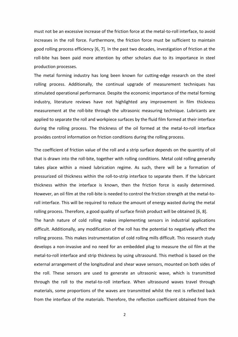
The harsh nature of cold rolling makes implementing sensors in industrial applications

difficult. Additionally, any modification of the roll has the potential to negatively affect the

rolling process. This makes instrumentation of cold rolling mills difficult. This research study

develops a non-invasive and no need for an embedded plug to measure the oil film at the

metal-to-roll interface and strip thickness by using ultrasound. This method is based on the

external arrangement of the longitudinal and shear wave sensors, mounted on both sides of

the roll. These sensors are used to generate an ultrasonic wave, which is transmitted

through the roll to the metal-to-roll interface. When ultrasound waves travel through

materials, some proportions of the waves are transmitted whilst the rest is reflected back

from the interface of the materials. Therefore, the reflection coefficient obtained from the

3

reflected wave can be used to monitor the roll-bite and to measure the film thickness at the

metal-to-roll interface during the rolling process

1.2 Aim and Objectives

The aim of this study is to develop a non-invasive and non-damaging ultrasonic method to

measure deformation and interface conditions in metal rolling. This technique is based on

rigorous analysis of the reflection coefficient of the ultrasonic signal obtained from the

surfaces of the rolled material and the rolling parameters employed.

To achieve this aim, the following objectives are considered:

To investigate the approaches for ultrasonic measurement that does not require

major modification of the mill roll.

To build the new external ultrasonic measuring device with longitudinal and shear

wave sensors on the roll.

To apply a mathematical model of the oblique reflection of the ultrasonic signals to

study the roll-to-strip interface;

To measure the strip thickness at both stationary and dynamic modes;

To measure the oil film thickness at the roll-bite interface during the cold metal

rolling process with the new device mentioned above;

To investigate the effect of rolling parameters (rolling load and roll speed) on the

formation of oil film thickness at the roll-bite surfaces during the cold rolling process.

To measure the roll-bite length during the rolling process

1.3 Thesis Layout

The chapters of this thesis follow a logical sequence to reflect the overall aim of the project.

Chapter 1 describes the problem, states the aim of the project and provides an outline of its

research objectives. The thesis layout and the knowledge gaps which this research study

seeks to fill are explained in the first chapter.

Chapter 2 briefly introduces the basics of metal forming such as bulk and sheet metal

forming processes. Additionally, the chapter focuses on the analyses of metal rolling

processes together with their diverse properties. The methods of measuring the friction

4

force of the roll-bite during the cold metal rolling are illustrated. The lubricant effects on the

coefficient of friction at the metal-to-roll interface during the metal cold rolling process are

also discussed. Similarly, the lubricant properties and oil film thickness formation at the

metal-to-metal interface during the cold metal rolling are reviewed. Finally, the chapter

examines the limitations of existing experimental procedures for determining the oil film

thicknesses during cold metal rolling. The measurement of oil film thickness with an internal

ultrasonic technique at the roll-bite during the rolling process is also discussed.

Chapter 3 offers a comprehensive review of the ultrasonic principles in engineering

applications, modes of wave propagation and types of ultrasonic wave propagation.

Additionally, reflection capturing techniques are discussed within this chapter. The

measurement of oil film thickness with ultrasonic methods in the mixed lubrication regime is

reviewed.

Chapter 4 describes the justification of the optimum external ultrasonic sensor arrangement,

carried out with the oblique and normal incidence reflection layouts to study the metal-to-

roll interface. Shear and longitudinal wave sensors were used to perform various tests with

both of the aforementioned ultrasonically measured techniques in this section. The results

obtained from each technique are analysed.

Chapter 5 elucidates the implementation procedure of the ultrasonic reflection layout

method on a pilot mill metal roll, discovered as an optimum arrangement in Chapter 4. Strip

thickness measurement was carried out both in stationary and dynamic (rolling) positions.

Chapter 6 describes the modelling and experimental procedure of the reflection coefficients

from the two measuring techniques discussed in Chapter 4. The reflection coefficient and

the stiffnesses obtained from the modelling and experimental processes of both measuring

techniques are evaluated using a comparative analytical technique. This is done to validate

the calculating parameters employed in the oblique reflection measuring method before

applying to the measurement film thickness in Chapter 7.

Chapter 7 describes the measurement of oil film thickness at the metal-to-roll interface.

Additionally, the measurement of oil film thicknesses has been conducted under different

applied deformation loads. The effects of roll speed on the oil film thickness formation

5

during the rolling operation is also investigated and explained in this chapter. All these

research activities were successfully conducted following the validation of the measurement

technique undertaken in Chapter 6.

Chapter 8 discusses the overall implications of the research project, draws some important

conclusions and details suggestions for future studies.

1.4 Contribution to Knowledge

The novelty of the research within this thesis is developing and implementing a new

experimental procedure with an external sensor arrangement on a pilot mill to measure

metal-to-roll interface conditions during the cold metal rolling. The oblique reflection

measurement technique based on active piezoelectric sensors has been mounted on the roll

and fixed to the pilot mill. Therefore, the following points can be drawn as its contribution to

knowledge:

Design and implementation of ultrasonic oblique reflection measurement layout

technique on a pilot mill;

Reflection coefficient at metal-to-roll interface having been tested with models

developed by Pialucha [9] at 0o and 19o angles of incidence. The measured reflection

coefficient was validated by the experimental result;

The designed layout technique was used to measure oil film thickness at roll-bite,

and the experiment was conducted under two different rolling loads and roll speed

respectively. The experimental oil film thickness values obtained were used to verify

the mixed lubrication regime at roll-bite at various applied loads;

The layout was used to measure the roll-bite length at the strip-to-roll interface;

This layout was also used to measure strip thicknesses at both stationary and

dynamic modes.

6

Chapter 2

Metal Rolling Background

This chapter introduces the basics of metal forming and the current methods of measuring

friction force of the roll-bite during cold metal rolling. The lubricant and other rolling

parameters’ effect on the coefficient friction at the metal-to-roll interface during metal cold

rolling process are discussed. The chapter also explains the measurement of oil film

thickness with an internal ultrasonic technique at the roll-bite during a rolling process. The

chapter concludes by discussing the limitations of existing experimental procedures for

determining the ultrasonic instrumentation during cold metal rolling.

.

7

2.0 Introduction

2.1 Metal Forming Processes

Metal forming is a tribological procedure that involves transforming the solid material

(metal) from one shape into another. The transformation process can either be the

reduction in thickness, shape or both in the material. Metal forming is a wide-ranging metal

deformation processing that includes various metal manufacturing processes. It is

characterized by the plastic deformation of the involved material into a required shape or

size. Metal forming can be classified into two broad groups as shown in Figure 2-1; bulk-

forming processes and sheet-forming processes [10].

Figure 2-1: Groups of metal forming process

The classification of the metal forming process is based on the working surface area to the

volume ratio of the material involved. With bulk forming, the contact tools have a low

surface covered area compared with the volume of the work done on the material involved.

Sheet metal forming is the opposite, being processed with the larger surface area contact of

the tools to the small volume of the material.

8

2.1.1 Metal Rolling Process

Metal rolling is a tribological process consisting of the continuous squeeze of a flat metal to

reduce its cross section to the required level. This process is one of the most valuable metal

manufacturing techniques in the modern world [11].

In the metal rolling process, the surfaces of the rolling material and the rolls are usually in

contact, and friction between them has an important influence on the operation [12]. During

the rolling process, the frictional force that develops at the metal-to-roll contact grips and

keeps dragging the strip through the roll-bite, as shown in Figure 2-2.

Figure 2-2: Schematic diagram of the strip rolling process

The strip with a large thickness enters the roll gap at the entrance plane of the roll contact.

The strip passes through the roll gap and leaves the outlet zone with a reduced thickness

strip (Figure 2-2). However, these rapid changes in friction value at the roll bite have a

serious effect on the metal rolling process and friction force effects have great significance

throughout deformation processes.

2.1.2 Rolling Mill Design

A rolling mill is a machine that consists of a set of rolls mounted on casings established as a

stand for the rolls. The stands are constituted to produce different kinds of mill layouts for

9

particular functions, by removing and replacing the rolls. Additionally, rolling mill consists of

an adjusting screw to control the roll gap, a pair of the rolls, and a pair of stand that fixed

with roll. It also consists of housing, bearing, motor, gear box, connecting shaft, switch

buttons, and speed control.

2.1.2.1 Types of Rolling Mills

There are many common types of rolling mill arrangements available in industry, which are

selected based on the size of the material, type of rolling (hot or cold) and mechanical

property of the material (hardness). Common types of rolling mills are shown in Figure 2-3

(a- e) [10, 13]

Figure 2-3: Configuration of (a) Two-High (b) Three-High (c) Four-High (d) Cluster (e) Tandem rolling mills

2.1.2.2 Two-High Rolling Mill

The two-high rolling mill consists of a pair of horizontal rolls arranged one above the other,

as shown in Figure 2-3a. The metal reduction takes place by feeding the material into the

gap between the adjacent rolls, as indicated above. The two adjacent rolls of the mill rotate

(a) (b)

(c)

(d) (e)

10

in the forward direction (non-reversing), while some are capable of turning backward and

forward (reversing).

2.1.2.3 Three-High Rolling Mill

The three adjacent rolls are arranged vertically, one above the other, in the three-high

rolling mill, as indicated in Figure 2-3b. This mill consists of three different rolls (upper,

middle and lower) driven by different electric motors. These rolls are arranged so that a

series of metal reductions can take place without the need to change the direction of the

rotating rolls. During the rolling process, steel is rolled backward between the middle and

bottom rolls and forward between the middle and top rolls respectively. The directions of

rotation of the rolls in three-high mills are not reversed as in the two-high rolling mill. The

three-high rolls rotates in both directions continuously, as demonstrated by the dotted line

in Figure 2-3b.

2.1.2.4 Four-High Rolling Mill

Figure 2-3c shows the arrangement of the four-high rolling mill. This contains two small-

diameter rolls that are reinforced by another two backup larger-diameter rolls. The two

small-diameter rolls are less strong and rigid compared with backup rolls during the metal

rolling process. They are called work rolls in this roll arrangement. These two small rolls are

used to reduce metal deflection during the rolling process. The two large-diameter rolls are

used to give support to the work rolls during the rolling process. Four-high stands can work

in both directions. The metal can be passed backward and forward between the same rolls,

as illustrated in a two-high mill.

2.1.2.5 Cluster Mill

The cluster mill (Figure 2-3d) consists of small diameter work rolls supported by two or more

backing rolls. The two pairs of backup rolls, which are much larger and stronger than the

working rolls are placed on the two small operating work rolls to prevent their alteration

during the rolling process. This type of roll arrangement allows the smaller working rolls to

be used perfectly despite their low strength and rigidity.

11

2.1.2.6 Tandem Rolling Mill

This is an arrangement of the rolls in a sequential series of stands with different rolling gaps

for metal reduction, as shown in Figure 2-3 (e). The tandem rolling mill consists of a

continuous long bar mill of several independent roll stands. Each roll stand has its own

motor, the speed of which can be easily changed independently of the others.

This type of mill is differentiated by the different sizes of the roll gaps, which start from the

largest to the smallest roll gap respectively. It operates in a continuous manner as shown in

Figure 2-3 (e). However, as the rolling of the metal continues, the mechanical properties of

the material are changed. This change occurs sequentially along the process by decreasing

metal diameters, increasing surface hardness and decreasing yield strength.

2.1.3 Types of Metal Rolling

Metal rolling process can be classified into two broad categories by the metal geometry or

the actual working temperature.

2.1.3.1 By Geometry of the Material

This is the process by which the rolling of the metal is classified in accordance with its

profile, such as a flat and curved shape. Shape metal rolling, is a bulk metal forming

operation where the high thickness metal square cross-section will be formed into a shape,

such as an I-beam, as indicated in Figure 2-4a. While the flat metal rolling is the process of

reducing the rectangular thickness cross-section of metal into sheet or plate, as shown in

Figure 2-4b. In flat metal rolling, the final product is either called a strip, with a thickness less

than 5mm, or plate when the thickness exceeds 5mm. It belongs to the sheet metal forming

group.

12

Figure 2-4: Samples of (a) shape and (b) sheet or plate metal rolling [11]

2.1.3.2 Material Working Temperature

The difference between hot and cold rolling depends on the working temperature of the

material. If this is above its recrystallization temperature, the process is called hot rolling.

Rolling of the metal from room temperature up to recrystallization temperature is referred

to as cold rolling. Recrystallization temperature is the temperature at which distorted grains

of the crystal structure are replaced by a new grain. The recrystallization temperature varies

with the properties of the material.

2.1.3.2.1 Hot Rolling

This is the process of rolling metal through the elastic to a plastic state above the material

recrystallization temperature. It is most commonly used when a large percentage of the

metal deformation is required. The advantages and disadvantages of this process are listed

in Table 2-1.

Table 2-1: Advantages and disadvantages of hot rolling process

Advantages Disadvantages

No stain hardening of the working material during the process.

The phase of the material changes in the process.

Brittle material can be easily worked on without distortion.

Poor surface finish due to the formation of scale on the material surface.

Little rolling force is required. Difficulties in achieving accurate dimensions of the product after the operation.

Low rolling capacity of the pilot mill is needed.

Hard to operate due to the high heat involved.

Holes, porosity, and cracks within the working material are welded together during the operation.

Deterioration of the metal roll life span.

(a) (b)

13

2.1.3.2.2 Cold Rolling

This is the process of rolling metal to a plastic state, below the crystallization temperature.

Cold rolling is suitable for the production of finished sheet and plate standard. Table 2-2

shows the advantages and disadvantages of the cold rolling process.

Table 2-2: Advantages and disadvantages of the cold rolling process

Advantages Disadvantages

Improves the material strength and hardness. High rolling force required.

No changes of phase involved. High rolling pilot mill capacity is needed.

Good product surface finishing. Lack of good control of the frictional force that can increase the damage of roll and product surfaces

No decarburization or oxidation of the material properties.

2.2 Mechanics of Metal Rolling

2.2.1 Calculation of the Neutral Plane

During the metal rolling process, each metal roll is powered by a motor connected through

the shaft. The relative velocity of the roll and the strip changes with the aid of the connected

motor during the rolling process. The schematic diagram of the rolls at neutral mode is

shown in Figure 2-5. Therefore, the neutral plane is a middle point between the entry and

exit zone where the strip parameters (speed and rolling force) are equal to the roll

parameters (speed and the friction force) [14]. These parameters are acting opposites of

each other, as shown in Figure 2-5.

14

Figure 2-5: Neutral plane at metal-to-roll interface

The location of the neutral angle indicated in Figure 2-5 is defined as [5] :

𝜃 =𝛼

2−

1

𝜇

𝛼2

2 2-1

While 𝛼 is the roll contact angle, the roll radius and metal-to-roll contact length (Fig. 2-5)

relations are expressed as follows:

𝑆𝑖𝑛 𝛼 =𝑙𝑝

𝑅𝑜 2-2

𝑅𝑜 is the radius of the roll, while 𝑙𝑝 is length of contact of the roll-to-metal interface and

defined [12] as:

𝑙𝑝 = √𝑅𝑜∆𝑡 2-3

∆𝑡 is changes in strip thickness during the rolling process (i.e. 𝑡𝑜 − 𝑡𝑓), 𝑡𝑜 and 𝑡𝑓 are initial

and final strip thicknesses.

Therefore, 𝑆𝑖𝑛 𝛼 =√𝑅𝑜∆𝑡

𝑅𝑜 , and it simplified and redefined as follows:

15

sin 𝛼 =√∆𝑡

𝑅𝑜 2-4

Therefore, if √∆𝑡

𝑅𝑜 is substituted for 𝛼 in equation 2-1, then the neutral angle (Figure 2-5) can

be obtained in terms of the rolling parameters if the coefficient of friction is given as:

𝜃 = √∆𝑡

4𝑅𝑜−

1

𝜇

∆𝑡

4𝑅𝑜 2-5

Moreover, 𝜇 is coefficient of friction develops at metal-to-roll interface during the rolling

process and is expressed [5] as follows:

𝜇 = 𝐹𝑟

𝐹𝑁 2-6

𝐹𝑁 is the rolling force while the 𝐹𝑟 is the friction force respectively.

2.2.2 Determination of Roll Pressure and Torque in Metal Rolling

The approximate mechanical analysis of the strip rolling process has been discussed in

Section 2.2.1. The deformation zone in the cold metal rolling process is very complex and

broad, during which the material usually undergoes strain hardness as it is out of the rolls.

The deformation of the roll geometry zone was analysed by equation 2-7 to obtain the

rolling force under the following assumptions [15]:

That the material undergoes strain plane process;

That the width of the material remains the same;

That the friction coefficient is constant along the roll-bite length;

That the materials undergo plastic deformation.

The direction of the rolling force and applied torque along the roll-bite during the strip

deformation is shown in Figure 2-6.

16

Figure 2-6: Rolling force and applied torque during cold rolling

Rolling forces are applied in both directions to reduce the material’s thickness. This required

rolling force is estimated [16] as follows:

𝐹𝑁 = 1.2𝑙𝑝𝑏𝑜𝑌𝑎𝑣𝑔 2-7

𝐹𝑁 is rolling force, 𝑏𝑜 = is the strip’s width. 𝑙𝑝 is the roll-bite length has been defined in

equation 2-3 as follows:

𝑙𝑝 = √𝑅𝑜∆𝑡

𝑌𝑎𝑣𝑔 = is an average true stress of the material and is expressed as follows:

𝑌𝑎𝑣𝑔 = 𝐾 𝑒𝑛

1+𝑛 2-8

While K and n are the strength coefficient and strain hardness exponent respectively. These

are constant properties to calculate the average stress of the rolling material during the

deformation processing. The K and n values rolling materials are shown in Table 2-3.

17

Table 2-3: Values of the parameters (K and n) for different materials at room temperature [17]

Materials K (MPa) n

Aluminium

1100-O 180 0.20

2024-T 690 0.16

6061-O 205 0.20

6061-T6 410 0.05

7075-O 400 0.17

Brass

70 -30, annealed 900 0.49

85-15, cold-rolled 580 0.34

Cobalt-based alloy, heat-treated

2070 0.50

Copper, annealed 315 0.54

Steel

Low-C annealed 530 0.26

4135 annealed 1015 0.17

4135 cold-rolled 1100 0.14

4340 annealed 640 0.15

304 stainless, annealed 1275 0.45

410 stainless, annealed 960 0.10

With the knowledge of the rolling load, the required rolling power can be calculated as

follows:

Power = 𝐹𝑁𝑙𝑝

2

2𝜋𝑁

60000 2-9

While the N is angular roll speed (rpm) and the unit of the power is defined as Kw [13].

2.2.3 Determination of Roll Deflection

During the metal rolling process, the forces generated are transmitted to the strip through

the roll. The rolls tend to bend along the contact length, which leads to the separation of the

roll and strip interface during the rolling process. This separation is caused by the reactions

between the strip and roll. Therefore, the rolls flatten at the contact, as shown in Figure 2-7

leading to the increased radius curvature of the roll from 𝑅𝑜 to 𝑅′𝑜. The metal roll deflection

is due to the elastic behaviour of the rolls during the rolling process as shown in Figure 2.7.

18

Figure 2-7: Schematic diagram of the deformed roll.

This is due to the increased reduction of the roll radius during the elastic behavior of the roll

when it engages with the strip during the deformation process. The roll flatness' is defined

[15] as:

𝑅′𝑜 = 𝑅𝑜 [1 + 𝐶𝐹𝑁

(∆𝑡)] 2-10

𝑅′𝑜 is deformed roll radius, 𝑅𝑜 is non-deformed roll radius, 𝐹𝑁 is rolling force and ∆𝑡 is

changes in strip thickness. While C is the constant parameter of the rolling material that is

defined as:

𝐶 = 16(1−𝑣2)

𝜋𝐸= 2.16 × 10−11Pa−1 2-11

𝑣 Is the steel Poisson’s ratio, while 𝐸 is the steel Youngs modulus respectively.

2.3 Friction in Metal Rolling

Friction force developed during the metal cold rolling process has been problematic. This is

due to the high resistance load and more power being required in the rolling process,

leading to heat generation at the roll-bite. Therefore, the proper lubricant film thickness at

the roll-bite, during the rolling process, is necessary for the separation of the interface [18].

The damaging consequences of the friction force of the roll-bite during metal rolling have

long been recognized. Research [5, 19, 20] has clearly shown that the friction force plays a

significant role in the resultant thickness of various strips subjected to different

experimental investigations. The friction force developed at the metal-to-roll interface

contributes to the high level of coefficient of friction at the interface during the process. This

19

is caused by the contact peaks form the two surfaces. The low coefficient friction contact

takes place due to the hydrodynamic pressure of the oil at asperities valleys of the surfaces

[21, 22]. The asperity flattening process depends on the loads on the asperity tops and in the

valleys. Other rolling parameters, such as rolling speed, material hardness and the

geometrical conditions of the strip and roll (roll diameter, strip thickness and reduction), are

also essential.

In metal deformation theory and practice, the coefficient of friction and resistance to

deformation in the roll-bite process has been considered. The coefficient of friction at the

roll-bite has been shown to depend on the condition of rolls and strip surfaces, the viscosity

and volume of lubricant used [23].

2.3.1 Measurement of Friction

In metal rolling, friction is associated with high pressures, and develops naturally during the

deformation process. In addition, frictional stress and normal pressure go together at the

metal-to-roll interface during the rolling process. Due to the harsh environment at the

interface, it has been problematic to determine the correct value of normal pressure and

friction during the metal rolling process [24]. Friction force has been one of the major

factors influencing the accuracy of the coefficient of friction in cold rolling. The coefficient of

friction at the roll - bite is defined as the ratio of the interface frictional stress to the normal

pressure. Therefore, the coefficient of friction at the roll-to-metal interface is determined by

the amount of normal pressure and frictional stress developed during the deformation

process. The developed coefficient of friction contributes to the surface quality of the

product generated during the rolling process. Therefore, the actual correct value of the

friction force to determine the accurate value of the coefficient of friction at the roll-bite is

essential. The coefficient of friction is necessary for cold metal rolling process. Its excess

developing at the roll-bite during the rolling process has been the most significant problem

with the rolling process. However, the nature of friction at the metal-to-roll interface is not

yet understood.

Different measures have been adopted by researchers to determine the value of normal

pressure and friction force required for the metal rolling process [25]. These include direct

and indirect frictional force measurement systems during the rolling process. In the direct

20

system, a pin is inserted radially in the work roll of a rolling mill, which has been pressed

down upon a load cell mounted within the roll [26]. The indirect method is the process of

measuring the required parameters to determine interface coefficient of friction at the roll-

bite, with the aid of other measurement techniques such as strip making and the Laser

Doppler method [19].

2.3.1.1 Direct Measurement System

The direct measurement method in metal rolling was the process of inserting a sensor on

the work roll [26] for the measurement of normal and friction forces at the interface

between roll and strip. This sensor consisted of a pin mounted directly on a load cell before

being fixed into the body of the roll. The displacement of the pin plunger by the normal

pressure developed at the roll-to-metal interface was displayed by the load cell monitor

device and recorded for further uses. The disadvantage of this device was that it could not

measure frictional forces.

The technique saw additional development into another sensor by Rooyen and Backofen

[27]. This consisted of two pins mounted within the holes of the work roll. The first pin was

radially inserted, the second inserted at an angle to the first. Both forces acting along the

axis of each pin were measured by the strain gauge mounted on each pin during the rolling

process. The radial pin measured the normal pressure while the oblique pin measured both

normal and frictional forces. The value of the coefficient of frictions at the roll interface was

calculated by the ratio of the forces and radial directions. This coefficient of friction at the

roll-to-metal value was obtained with the following formula:

𝜇 = (𝑃1

𝑃2− 1) 𝑡𝑎𝑛 ∅ 2-12

While 𝑃1, is normal pressure and 𝑃2, is an oblique pressure pin.

Lenard [28], furthered this technique, by varying the location angles of the pins on the roll.

The major disadvantage of this design is the traces of the pin marks on the surface of the

rolled strip and the pin bending as it slides across the strip surface during the rolling process.

MacGregor and Palme [29] designed a cantilever pin sensor due to the disadvantage of the

technique developed by Siebel and Lueg. This sensor was successfully used to measure

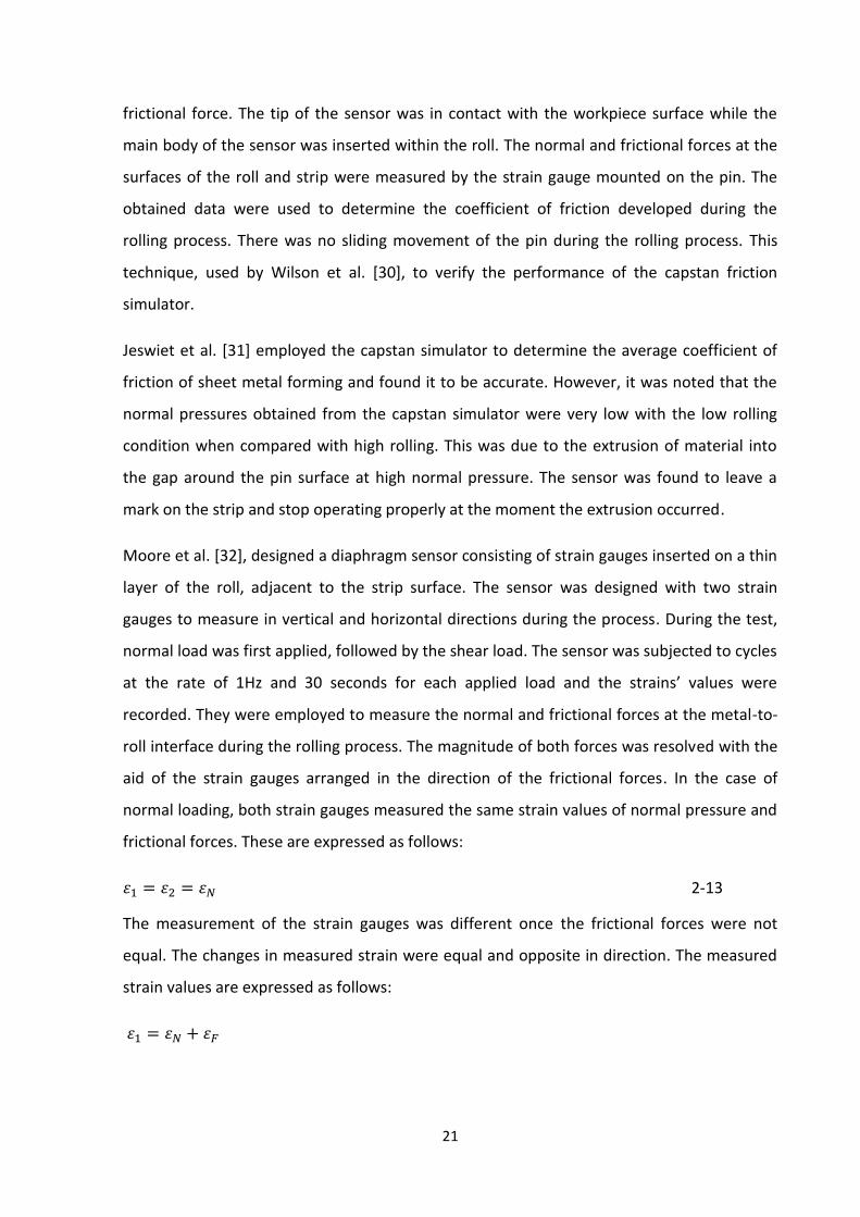
21

frictional force. The tip of the sensor was in contact with the workpiece surface while the

main body of the sensor was inserted within the roll. The normal and frictional forces at the

surfaces of the roll and strip were measured by the strain gauge mounted on the pin. The

obtained data were used to determine the coefficient of friction developed during the

rolling process. There was no sliding movement of the pin during the rolling process. This

technique, used by Wilson et al. [30], to verify the performance of the capstan friction

simulator.

Jeswiet et al. [31] employed the capstan simulator to determine the average coefficient of

friction of sheet metal forming and found it to be accurate. However, it was noted that the

normal pressures obtained from the capstan simulator were very low with the low rolling

condition when compared with high rolling. This was due to the extrusion of material into

the gap around the pin surface at high normal pressure. The sensor was found to leave a

mark on the strip and stop operating properly at the moment the extrusion occurred.

Moore et al. [32], designed a diaphragm sensor consisting of strain gauges inserted on a thin

layer of the roll, adjacent to the strip surface. The sensor was designed with two strain

gauges to measure in vertical and horizontal directions during the process. During the test,

normal load was first applied, followed by the shear load. The sensor was subjected to cycles

at the rate of 1Hz and 30 seconds for each applied load and the strains’ values were

recorded. They were employed to measure the normal and frictional forces at the metal-to-

roll interface during the rolling process. The magnitude of both forces was resolved with the

aid of the strain gauges arranged in the direction of the frictional forces. In the case of

normal loading, both strain gauges measured the same strain values of normal pressure and

frictional forces. These are expressed as follows:

𝜀1 = 𝜀2 = 𝜀𝑁 2-13

The measurement of the strain gauges was different once the frictional forces were not

equal. The changes in measured strain were equal and opposite in direction. The measured

strain values are expressed as follows:

𝜀1 = 𝜀𝑁 + 𝜀𝐹

22

𝜀2 = 𝜀𝑁 − 𝜀𝐹 2-14

𝜀1 and 𝜀2 are normal and frictional forces while the 𝜀𝑁 and 𝜀𝐹 are the strain of normal and

frictional force readings. This sensor was used to eliminate the strip extrusion problem that

occurred due to the gap around the surface of the pin inside the sensor. However, the

results obtained showed the same trend as another method but it was difficult to identify

the normal pressure from the frictional stress. Furthermore the thin layer surface of the

sensor collapsed when high loads were applied.

Yajure [33], developed a sealed cantilever pin to avoid the extrusion of the strip into the gap

around the sensor tip surface during the rolling process. This device was installed 1.5 mm

below the surface of the roll, it consists of a square pin was inserted into a round hole of a

square post; large clearance was made around the pin for the purpose of high rolling

pressure. Collapse of the die around the tip was still experienced during the rolling process.

However, the device gave a clear signal during the rolling process.

Henningsen et al. [34], designed a portal frame sensor device that contained two strain

gauges mounted on to the two vertical beams of the frame. These strain gauges measure

deflections of the two beams separated during the rolling process. The signals obtained from

these two strain gauges were used to show the value of frictional force in the rolling

direction.

This sensor was used successfully to conduct various tests on a pilot mill during the metal

rolling process. The sensor is strong and can withstand the high pressure that occurs during

the rolling process. However, the device is not capable of measuring the frictional force in

the transverse rolling direction. Additionally, it had the imprinted mark of the pin left on the

surface of the material after the rolling.

2.3.1.2 Indirect Measurement System

An indirect method for the coefficient of friction is the process of determining the

coefficients of friction through the value of the parameters obtained from the measurement

techniques employed. The most common techniques for the measurement of these

parameters are strip mark and Laser Doppler methods.

23

The strip mark layout technique is the process of measuring the forward slip movement of

the strip in respect of the roll rotation. Both roll and strip will rotate simultaneously, then

the mark on the roll will be imprinted on the surface of the strip during the rolling process.

Lenard [25] employed this technique to obtain the parameters for the determination of

coefficient of friction at the roll-bite during the cold rolling process. Figure 2-8 shows the line

𝑙1 sited between marks A and B within the roll surface. The machine was operated and the

strip passed through the roll gap. The line 𝑙2 was 𝑙1 noted to have duplicated onto the

surface of the rolled strip after the rolling operation.

Figure 2-8: Schematic diagram of roll with mark layout technique [35]

Figure 2-9 shows the line 𝑙2 on the strip surface, which was the imprinted of the mark 𝑙1,

that had initially been printed onto the surface of the roll before the strip was rolled.

Figure 2-9: Imprint lines after rolling process

24

This mark illustrates the elongation length of the strip that underwent the rolling process.

These two marks were used to determine the average forward slip of the rolled material and

were expressed as follows:

𝑆𝑓 =(𝑙2−𝑙1)

𝑙1 2-15

while 𝑆𝑓, is the forward slip to be calculated, 𝑙1 is the distance between the scratched lines

on the roll’s circumference. The 𝑙2 is the distance of the imprinted lines on the strip’s surface

after one revolution turn of the roll. The coefficient of friction can finally be calculated from

the forward slip values obtained in equation 2-15 with the combination of equations in 2-16

shown below.

𝜇 = 𝑡𝑜−𝑡𝑓

2√𝑅′(𝑡𝑜−𝑡𝑓)−4√𝑆𝑓𝑅′𝑡𝑓

2-16

The value for the variable 𝑅′ the roll deflection has been already defined in equation 2-10.

Therefore, Lenard concluded that the coefficient of friction obtained was decreasing as the

rolling speed increased, which was almost of the same trend as the theoretical prediction.

Liu [5], employed Laser Doppler probes to obtain both roll and strip velocity during the

metal rolling process for the determination of the coefficient of friction at the roll-bite

during the rolling process. As shown in Figure 2-10, one Laser probe was mounted in the

front of the upper roll to measure the roll speed and another was sited on one side of the

pilot mill to detect the speed of the strip.

Figure 2-10: schematic diagram of a Laser Doppler measuring method [5]

25

The forward slip value obtained is proportional to the difference of the existing strip velocity

𝑉2, and rolls velocity 𝑈𝑟. The strip and the rolls velocities are related as:

𝑆𝑓 =𝑉2−𝑈𝑟

𝑈𝑟 2-17

The value of the coefficient of friction at the roll-bite was calculated from the forward slip

values obtained in equation 2-16 with the combination of equations 2-17 respectively. The

value of the coefficient of friction obtained was almost the same trend as per the theoretical

prediction.

The summary of the coefficient of friction measurement techniques reviewed with the years

of the research and name of the authors, are presented in Table 2-4.

26

Table 2-4: Coefficient of friction measurement reviewed techniques

Authors/Date Method Limitation of method

Lueg, E.S. (1933) [26] Sensor pin Not able to measure

frictional force

Rooyen Backonfen (1957) [30]

Two sensor

pins at angle

Traces of the pins mark the

surface of measured material.

Lenard, J.G (2000) [28] Two sensors

pins at various angles

Traces of the pins mark the

surface of measured material

MacGregor and Palme (1948) [29]

Cantilever pin

sensor

Traces of the pins mark the

surface of measured material

Jeswiet et al (2001) [31] Capstan

simulator

device

Extrusion of the strip into the

gap around the sensor tip

surface

Moore et al (2002) [32] Diaphragm

sensor device

Collapsing of the thin layer of

the sensor.

Yajure et al (2002) [33] Sealed

cantilever pin

device

Collapsing of the thin layer of

the sensor.

Henningsen et al (2006) [34] Portal frame

sensor

Not capable of measurement

of frictional force in the

transverse rolling direction

Furthermore, all the results reported from the various experimental procedures for the

measurement of the coefficient of friction reviewed above section are reliable. Although,

these techniques are good and straightforward to understand, none have links with the

application of the ultrasonic measuring technique either directly or indirectly for the

measurement of the coefficient of friction and its variables. Additionally, these are invasive

methods requiring embedded plugs in the roll, which is dangerous for both roll and strip

surfaces during the rolling process. The extrusion of the material into the gap around the

surface pin during the rolling process is another problem of these techniques. Finally, the

27

surface of the sensor installed into a roll does collapse at high pressure during the rolling

process, due to the thin layer of the sensor on the roll body during the installation [36].

2.4 Metal Rolling Lubricant

In the metal rolling process, the lubricant is the fluid substance applied to separate the roll

from the metal surface during the rolling operation. Lubrication is the process or method of

applying the lubricant to the rolling surface and has a significant influence on the roll

durability and its load capacity. In the metal forming process an emulsion is usually applied

to avoid direct contact of roll and strip and to reduce damage to the strip surface.

Additionally, the oil cools the roll-bite, protects strip and roll from corrosion and maintains

the interface temperature from surface damage [37]. If the lubricant film fails, the friction

force at metal-to-roll can increase and damage the interface.

In addition, the oil film thickness, formed in the two contact zones, is sustained by the oil

pressure developed within the roll and strip together with the strip contacts of the two

bodies. This is referred to as the mixed lubrication regime where the two surfaces are

partially separated by asperity contact of materials and pressurised lubrication oil within the

surface valleys. Lubrication is very important in controlling the surface interactions between

the rolls and the strip during the rolling process. The tool (roll) and the workpiece (strip)

surface interaction at the wet interface is shown in Figure 2-11 (a). The two surfaces consist

of a major contact and a minor contact of the asperity of both surfaces. Furthermore, minor-

pores are created by the valleys on both surfaces and a convex hull, which develops as a

result of the pressure on both surfaces. These minor pores fill with oil during the rolling

operation. The closest contact with the asperities of the two surfaces is presented in Figure

2-11 (b).

28

Figure 2-11 Schematic diagram of two contact surfaces

This interaction needs four conditions to be satisfied in order to create an adequate

lubricated contact. First, enough lubricant must be made available at the entry zone of the

roll-bite. The lubricant must then be entrapped, that is, the oil droplets must be captured

and drawn into the metal-to-roll contact zone. The emulsion must be spread through the

contact uniformly and cover the contact surfaces of the two materials. Finally, the lubricant

must then flow through the work to the exit zone [38]. Some of the primary functions of the

lubricant at the metal-to-roll interface during the rolling operation are itemised and shown

in Figure 2-12.

Figure 2-12: Functions of the lubricant [39]

(a)

29

The applied lubricant during the cold rolling of steel strip, needs to have the above detailed

functional properties, in order to create good lubricating conditions, and acceptable surfaces

with efficient cooling during the rolling interaction (Figure 2-11).

The film thickness of the lubricant formed at the roll to metal contact interface depends on

the lubricant’s physical properties such as density and viscosity. Furthermore, rolling speed,

load, and roll-to-metal interface roughness are important in determining the amount of the

lubricant film thickness formed during the rolling process. The quality of the product surface

and the roll-to-metal surface protection from wear depends on the integrity and thickness of

the lubricant formed at the roll-bite [23].

Azushima [40], investigated the effects of rolling speed on the formation of coefficient of

friction during the rolling process. His results show that the higher the rolling speed, the

lower the rolling pressure, and the thicker the film of oil formed at the roll-to-metal

interface. This is due to the increasing frictional resistance within the layer of lubricant that

causes an increase in the separation of the interface in order to accommodate more oil.

Similarly, Button [41], explains the variation of pressure and the formation of oil film

thicknesses at the inlet and work zone during the cold rolling of an aluminium strip. The

result shows that these differences are also strongly influenced by the rolling conditions

such as the lubricant viscosity and percentage reduction of the strip in the value of the

formed coefficient of friction.

2.4.1 Lubricant Properties

In metal rolling, lubricant properties have a significant effect on performance during the

rolling process. As previously explained, a lubricant with good properties is expected to

provide a small separation at the metal-to-roll interface during the rolling to avoid the total

direct contact of the surfaces. In addition, this provides support for enough coefficient of

friction for a smooth rolling process [42]. The good performance of the lubricant functions,

listed in Figure 2-12, all depend on the properties of the lubricant applied. Furthermore, the

oil film thickness obtained at the roll-bite during the rolling operation depends on lubricant

properties (density, bulk modulus and viscosity), the rolls and strip geometric features, and

30

some of the rolling conditions (load and speed). The lubricating properties that are relevant

for the fluid used in this research are itemized and explained in sub-sections 2.4.1.1 below.

2.4.1.1 Viscosity

Viscosity is a lubricant property having a significant effect on the lubricant’s internal

resistance to flow. Generally, viscosity is necessary for the lubrication and a suitable amount

is required for the best performance of the oil. The first explanation of viscosity was given by

Isaac Newton in relation to the combination of piston and oil and closed cylinder, as shown

in Figure 2-13.

𝐶𝑟 is the radial clearance between the piston and the cylinder, 𝐿 and 𝐷 are the piston length

and diameter, 𝑥 is the distance moved by the piston while 𝐹 is the force applied to the

piston. The force applied to cause the relative motion of the piston was measured by the

fluid resistance to shear, which is directly proportional to the contact area and to the

velocity of the piston [43]. It is also indirectly proportional to the oil film thickness.

Therefore,

𝐹 =𝜋𝐷𝐿𝜇

𝐶𝑟

𝜕𝑥

𝜕𝑡 2-18

𝜇 is oil viscosity, 𝜋𝐷𝐿 (𝐴) is the contact area. Normally, the lubricant film is expected to be

thick enough and be able to separate the metal-to-roll interface, but not so thick to the

extent of creating additional force (𝐹) to overcome the shear rate of the lubricant during the

rolling process [44].

𝐷 𝐿

𝐶𝑟

𝐹

𝑥

Cylinder Piston

Figure 2-13: Illustration of viscosity with piston and cylinder

31

2.4.1.1.1 Types of Viscosity

The lubricant viscosity is classified according to its measurement technique, which are

Dynamic (Absolute) Viscosity and Kinematic Viscosity.

2.4.1.1.1.1 Dynamic (Absolute) Viscosity

Dynamic Viscosity is defined as the measurement of resistance of the fluid to flow under the

deformation or applied load. This viscosity is defined by [45] as:

𝜂 = 𝐹𝑟𝐴𝑉𝑜ℎ𝑚

= 𝜏

𝛾 2-19

while τ and γ denote shear stress and shear strain rate. 𝐹𝑟 and 𝐴 are the friction force and

the lubricated contact area. Finally, 𝑉𝑜 and ℎ𝑚 are surface velocity and film thickness

respectively. This dynamic viscosity is normally measured in Centipoise (cP). 1 cP = mPa.s.

2.4.1.1.1.2 Kinematic Viscosity

Kinematic Viscosity is generally known as the measurement of the resistance of a fluid to

flow under the forces of gravity. It is also defined as the ratio of the dynamic viscosity to its

density and expressed as follows:

𝜂𝑘 =𝜂

𝜌 2-20

While 𝜌 is the density of the fluid and 𝜂 is the dynamic viscosity respectively. This type of

viscosity is mostly quoted in data sheets at 40°C and 100°C; it is generally measured in

centistokes unit (mm2/s in SI unit). In addition, temperature and pressure have a major

effect on lubricant viscosity properties, but this effect will be discussed within the bulk

modulus oil property section.

2.4.1.2 Bulk modulus

The bulk modulus is a property of fluids which expresses the change in volume of the fluid

due to the external pressure applied [46]. The numerical change in the volume of fluid

during the applied external force depends on the operation conditions, the amount of air

present in the system and how the pressure is applied. Therefore, the following operating

conditions: oil pressure and temperature, closeness and the rigidity of the surfaces and the

32

content of air at the interface, influence the change in the bulk modulus of the fluid during

the operation [47].

To understand the meaning of the bulk modulus of fluid and how it was derived the

equation of state for fluids must be known. This is defined as a function relating density,

pressure and temperature of a fluid together. Due to the small change in fluid density to the

change of pressure and temperature, these three variables can be approximately related

using Taylor’s series [43]. Therefore,

𝜌 = 𝜌𝑂 + (𝜕𝜌

𝜕𝑃)𝑇(𝑃 − 𝑃𝑂) + (

𝜕𝜌

𝜕𝑇)𝑃(𝑇 − 𝑇𝑂) 2-21

While equation 2-21 is simplified further for clarification and re-defined as follows:

𝜌 = 𝜌𝑜 [1 +1

𝛽(𝑃 − 𝑃𝑂) − 𝛼(𝑇 − 𝑇𝑂)] 2-22

𝜌, 𝑃 and 𝑇 are the initial fluid density, pressure and temperature while 𝜌𝑜, 𝑃𝑂 and 𝑇𝑂 are

final fluid density, pressure and temperature respectively.

Also,

𝛽 = 𝜌𝑜 (𝜕𝑃

𝜕𝜌)𝑇

2-23

And

𝛼 = −1

𝜌𝑂(𝜕𝜌

𝜕𝑇)𝑃

2-24

As shown in equation 2-23, the density increases as the pressure increases with the

decrease in temperature. This is because the density is mass divided by volume. 𝛽 and 𝛼 were

re-defined in terms of volume and expressed as follows:

𝛽 = −𝑉𝑜 (𝜕𝑃

𝜕𝑉)𝑇

2-25

𝛼 =1

𝑉𝑜(𝜕𝑉

𝜕𝑇)𝑃

2-26

While 𝑉 and 𝑉𝑜 are the total and the initial volume of the fluid, 𝛽 is the change in pressure

divided by the change in volume at a constant temperature and is known as bulk modulus of

33

the fluid. 𝛼 is referred to as the cubical expansion coefficient, which is the fractional change

in volume due to a change in temperature.

There are various types of bulk modulus, which are only specific to their own applicable

conditions. These have been widely used in textbooks:

Isothermal secant bulk modulus

Isothermal tangent bulk modulus

Furthermore, Figure 2-14 shows the relationship between the change in fluid pressure and

the change in volume of the fluid at a constant temperature. The above mentioned types of

the bulk modulus are indicated in Figure 2-14 below, but are fully explained in the next sub-

sections.

Figure 2-14: Determination of the value of bulk modulus of applied oil [45]

2.4.1.2.1 Isothermal Secant Bulk Modulus

Isothermal secant bulk modulus is expressed as product of the original volume 𝑉𝑂 and the

slope of the line drawn from the original to any specified point on the plot of the pressure

versus specific volume. This method is suitable for large pressure changes. This is referred to

as the isothermal secant bulk modulus if the process undergoes a change in pressure at a

constant temperature. The above expression is defined as follows [46]:

𝐵𝑠 = 𝑉𝑂 (𝑃2−𝑃1

𝑉1−𝑉2) 2-27

34

Therefore, 𝐵𝑠 is the isothermal secant bulk modulus, 𝑃1 is the final fluid pressure, 𝑃2 Is the

initial fluid pressure, 𝑉1 and , 𝑉2 are the initial and final volumes of the fluid value while the

𝑉 is original fluid volume [48]

2.4.1.2.2 Isothermal Tangent Bulk Modulus

The tangent bulk modulus is expressed by the pressure to volume differential as shown in

equation 2-28. It is generally defined as the product of fluid volume and the partial

derivative of fluid pressure with respect to volume at constant temperature. The isothermal

tangent bulk modulus is defined by the following expression [49]:

𝐵𝑇 = 𝑉 (𝜕𝑃

𝜕𝑉) 2-28

𝐵𝑇 is the isothermal tangent bulk modulus, 𝑉𝑜 is the initial volume value, 𝜕𝑃 is the change of

the external pressure, 𝜕𝑉 is the change of the fluid volume

2.4.2 Analysis of Different Lubrication Zones in Cold Metal Rolling

Figure 2-5 shows a schematic illustration of the metal cold rolling process. The strip

dimension is reduced in thickness from 𝑡𝑜 to 𝑡𝑓 by the radius 𝑅𝑜 of the roll during the rolling

process. As shown in Figure 2-15, the roll-bite is divided into three zones: inlet, work and

outlet zone.

Figure 2-15: Schematic diagram of different rolling zones

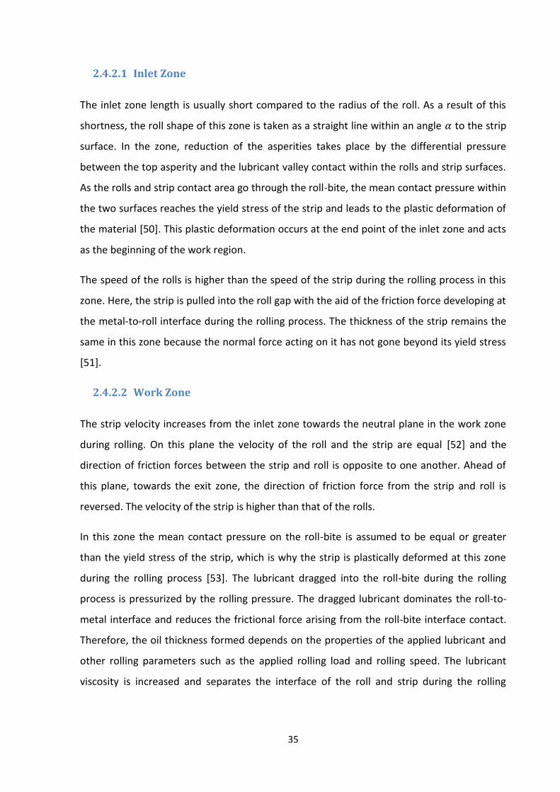
35

2.4.2.1 Inlet Zone

The inlet zone length is usually short compared to the radius of the roll. As a result of this

shortness, the roll shape of this zone is taken as a straight line within an angle 𝛼 to the strip

surface. In the zone, reduction of the asperities takes place by the differential pressure

between the top asperity and the lubricant valley contact within the rolls and strip surfaces.

As the rolls and strip contact area go through the roll-bite, the mean contact pressure within

the two surfaces reaches the yield stress of the strip and leads to the plastic deformation of

the material [50]. This plastic deformation occurs at the end point of the inlet zone and acts

as the beginning of the work region.

The speed of the rolls is higher than the speed of the strip during the rolling process in this

zone. Here, the strip is pulled into the roll gap with the aid of the friction force developing at

the metal-to-roll interface during the rolling process. The thickness of the strip remains the

same in this zone because the normal force acting on it has not gone beyond its yield stress

[51].

2.4.2.2 Work Zone

The strip velocity increases from the inlet zone towards the neutral plane in the work zone

during rolling. On this plane the velocity of the roll and the strip are equal [52] and the

direction of friction forces between the strip and roll is opposite to one another. Ahead of

this plane, towards the exit zone, the direction of friction force from the strip and roll is

reversed. The velocity of the strip is higher than that of the rolls.

In this zone the mean contact pressure on the roll-bite is assumed to be equal or greater

than the yield stress of the strip, which is why the strip is plastically deformed at this zone

during the rolling process [53]. The lubricant dragged into the roll-bite during the rolling

process is pressurized by the rolling pressure. The dragged lubricant dominates the roll-to-

metal interface and reduces the frictional force arising from the roll-bite interface contact.

Therefore, the oil thickness formed depends on the properties of the applied lubricant and

other rolling parameters such as the applied rolling load and rolling speed. The lubricant

viscosity is increased and separates the interface of the roll and strip during the rolling

36

process. This is due to the variation of the pressure developed and the dissipation of the

heat generated from the oil at the asperity contact of the rolls and strip surfaces [54].

2.4.2.3 Outlet Zone

The outlet zone is the last zone along the roll-bite, shown in Figure 2-15. The lubricant

thickness of this zone is slightly reduced compared to the inlet zone and its pressure drops

to the ambient level. The strip becomes rigid immediately after the work zone due to the

recovery of the plastic flow of rolled material. In this zone, the strip moves faster than the

roll.

2.5 Numerical Modelling of Oil Film Formation in Cold Rolling

Figure 2-16 shows the roll-bite interface separated by the film thickness of the lubricant

applied during the rolling process. Sutcliffe [55] explains that the inlet region cannot be

treated independently of the work zone and the exit area. The oil film thickness determined

in the inlet region can be assumed to be the same as at the work zone. Therefore, the

elongation of the strip through the bite will tend to reduce the oil thickness in the entry

region towards the work zone. The amount of lubricant at the roll-bite contact surface area

(Figure 2-16) during the metal rolling has been predicted by various researchers [56-58].

Their predictions during the rolling operation were based on modelling approaches relating

to the speed of the roll, the yield stress and initial thickness of the rolling material.

37

Figure 2-16: Schematic diagram of the roll bite separated by the oil film thickness [21]

Wilson and Walowit [59] applied Reynolds equation to predict the oil thickness at the roll-

bite during metal rolling operation. This Reynolds equation is stated as follows:

ℎ𝑜 = 3𝜂𝑜𝛾(𝑉𝑜+𝑈𝑟)𝑅

′

𝐿[1−𝑒𝑥𝑝(−𝛾𝜎𝑦)] 2-29

Where, 𝜂𝑜, is the dynamic viscosity of the used lubricant and 𝛾 is the pressure viscosity. The

R’ is the radius of the deflected roll, 𝑈𝑟 is the roll surface velocity, 𝑉𝑜 is the entry velocity of

the strip and the𝐿, is the projected contact length while 𝜎𝑦 is the average yield strength of

the strip.

The oil viscosity pressure coefficient of friction at the roll-bite is given as:

𝛾 = (0.6 + 0.965 log10 𝜂𝑜) × 10−8 2-30

Therefore, if the thickness of the oil film is reduced, the asperities perforate through the

lubricant. As the viscosity of the oil or the relative speed is increased, mixed lubrication is

achieved, which leads to oil pockets and asperity contact. The oil film thickness is

determined in the lubricating regime by comparing it with the asperity heights of the rolls

and the rolled metal [60]. This ratio is defined as:

38

Ʌ = ℎ𝑚𝑖𝑛

√𝑅𝑞12 + 𝑅𝑞2

2 2-31

Where ℎ𝑚𝑖𝑛, is the minimum film thickness obtained from the roll-bite, 𝑅𝑞1 and 𝑅𝑞2 are the

surface roughness values of the strip and roll surfaces respectively. Then the proportions of

film thickness for the corresponding lubrication regimes are roughly estimated at [28, 61]:

• Boundary lubrication, Λ< 1

• Mixed lubrication, 1 <Λ< 5

• Hydrodynamic lubrication, 5 <Λ< 100

2.6 Experimental Measurement of Oil Film Thickness in Metal Rolling

A series of film thickness measurement techniques have been developed by various scholars

such as:

The wiping off method;

The oil drop on the surface of the strip;

The valley interrogation method;

The internal ultrasonic reflection measuring technique.

The aim of this section is to consider the experimental determination of oil film thickness

measurement at the metal-to-roll interface with the above mentioned techniques and to

compare them with the external ultrasonic layout that is the focus of this thesis.

2.6.1 Wiping Off Method

Whetzel and Rodman [62], explained the measurement of the oil film thickness by wiping off

the adhered lubricant from the strip after the rolling process. The lubricant had been

obtained by dipping it into the solvent after the rolling then allowing the adhered oil to

dissolve into the solvent. The solvent was allowed to vaporize and the volume of remaining

lubricant was measured.

Therefore, the oil film thickness at the inlet of the metal-to-roll interface denoted by ℎ𝑜, was

obtained from the weight and the density of the remaining oil and the oil-covered area. The

inlet oil film thickness ℎ𝑜, is expressed as:

39

𝑣𝑜𝑙𝑢𝑚𝑒 =𝑀𝑎𝑠𝑠

𝐷𝑒𝑛𝑠𝑖𝑡𝑦

While the, 𝑉𝑜𝑙𝑢𝑚𝑒 = 𝐴𝑟𝑒𝑎 × ℎ𝑜

ℎ𝑜 =𝑉𝑜𝑙𝑢𝑚𝑒

𝐴𝑟𝑒𝑎 2-32

The inlet oil film thickness (ℎ𝑜) at the roll-bite interface was obtained with this technique.

The thickness of 0.1 µm was obtained from the rolls and the strip in the entrance zone. The

value was found to concur with the theoretical values obtained from the literature section of

the paper.

2.6.2 Oil Drop on the Strip’s Surface Technique

Katayama [63], developed the method introduced by Whetzel and Rodman [62] for further

determination of oil film thickness on the roll-bite during the metal cold rolling. The

experiment began by cleaning the rolls and strip surfaces with solvent, and small amount oil

was dropped on the surface of the strip. The weight of the oil was obtained by subtracting

the weight of the metal from the total weight of the strip and oil. The final strip weight

reduction was measured by the chemical weight balance, instead of dissolving the adhered

lubricant, by dropping the rolled strip in the solvent.

The area of the oil spot spread was traced and measured with a planimeter. This area was

clearly visible and different from the unlubricated region. The oil film thickness at the inlet of

the metal-to-roll interface denoted by ℎ𝑜, was obtained from the weight and the density of

the dropped oil and the oil-covered area. The oil film thickness was also determined by

equation 2-32 shown in Section 2.6.1.

40

2.6.3 Valley Integration Method

Azushima [64] measured the oil film thickness at the roll-bite with the aid of the relationship

between the strip and roll asperities being crushed after a rolling process. The roll surface

was sandpapered with 400 emery paper and cleaned with benzene before the rolling

process of the materials. The maximum roughness value of the roll and strip were measured,

before and after the material was rolled. The sample profile of the rough surface of the roll

and the strip is shown in Figure 2-17.

Figure 2-17: Schematic diagram of roll surface roughness sample

The roughness height at the surface of the roll was denoted as ℎ while the surface of the

strip is assumed to be flat before rolling, as shown Figure 2-17. The applied oil flowed across

the roll surface and occupied the strip surface roughness space imprinted by the roll during

the deformation process. The average thickness of this oil within the surface of the strip and

roll after the rolling process was used to determine the oil film thickness at the metal–to-roll

interface during the rolling process [64] and was expressed as follows:

ℎ𝑜 =1

2(𝑅

𝑞1 + 𝑅𝑞2) 2-33

While the 𝑅𝑞1 and 𝑅𝑞2 are the roughness values of the roll and the strip and ℎ𝑜 is the film

thickness at the inlet of the metal-to-roll interface respectively. The outlet film thickness was

obtained at the roll-bite with the aid of the inlet oil film thickness value ( ℎ𝑜) in relation to

the outlet strip and roll speeds respectively. Therefore, the oil film thickness of the outlet

zone was denoted as ℎ1, and is expressed as follows:

ℎ1 = ℎ𝑜𝑈𝑜+𝑈𝑟

𝑈𝑓+𝑈𝑟 2-34

The ℎ1 and ℎ𝑜 are film thicknesses at the work and inlet zones, 𝑈𝑜 and 𝑈𝑓 are the inlet and

outlet strip speed while 𝑈𝑟 denotes the roll speed. The mean value of 0.4 µm was obtained

41

at 4m/min rolling speed and increased to 4µm at 850m/min rolling speed. In accordance

with Whetzel and Rodman [62], the results obtained are also in good agreement with the

results from their literature review.

Sutcliffe [55], estimates the inlet film thickness at the roll-bite based on the first method

described by Azushima [64]. The profile roughness value of the roll and strip were measured

with the profilometer and converted to a digital value with the aid of a data logger. The inlet

oil film thickness value ( ℎ𝑜) at the roll-bite was determined and used to estimate the outlet

film thickness in relation to the outlet strip and roll speeds respectively. The percentage

reduction of the strip was also considered and the relationship of these parameters is

expressed as follows:

𝑈𝑓 = 𝑈𝑟𝑡𝑓

𝑡𝑜 2-35

Continuity of the mass flowrate of the fluid was considered; therefore the outlet film

thickness ℎ1 at the roll-bite is expressed as follows:

ℎ1𝑈𝑟 =ℎ𝑜(𝑈𝑓+𝑈𝑟)

2 2-36

And

ℎ1

ℎ𝑜=

(1+𝑡𝑜

𝑡𝑓⁄ )

2 2-37

𝑈𝑓 and 𝑈𝑟 are the outlet strip and roll speed respectively while, ℎ1 and ℎ𝑜 are the outlet

and inlet film thickness.

The results obtained by this technique were compared with those from the oil drop method

is and are presented in Figure 2-18.

42

Figure 2-18: Oil film thickness obtained from different methods [64]

There is good agreement between the results obtained from both techniques. As shown (Fig.

2-18) they have the same trend.

Cuperus [57], explained the uses of a Rautaruuki meter for the measurement of oil film

thickness at the strip surface. This is an infrared measuring device used to measure the oil

film thickness during the metal rolling process. The outcome performance of the meter

depends on the strip roughness and the lubricant properties. The strip surface was cleaned

with the solvent, then the zero oil film thickness of 10 different points on the strip surface

were captured and the average of the zero signals was recorded. Next, the oil was dropped

onto various places on the surface of the strip. The measured oil film thickness was

compared with the obtained from the oil dropping technique.

In addition, Cuperus also reviewed the measuring techniques listed above and improved the

modes of applying lubricant into the roll-bite during the rolling process. A special piece of

apparatus was designed to continuously drop the oil during the rolling process, instead of

the manual oil drop method previously employed. These methods were undertaken

separately to conduct experiments with the aid of two rolls. The rolls were prepared with

the different values of surface roughness respectively. The results obtained from these

techniques were prepared and are shown in Figures 2-19.

43

Figure 2-19: Oil film thickness results obtained from above mentioned techniques [57]

As shown in the figures above, the results obtained from these techniques are in good

agreement since their results follow the same trend.

Azushima and Inagaki [65], employed the numerical method of the starvation model to

calculate the inlet oil film thickness in cold sheet rolling. The method is based on the

relationship between material surface brightness and thickness of the applied oil. The oil

droplet-in-water emulsion was used as a lubricant during the experiment. The experiment

was conducted with 0.4mm thickness, 30mm wide and 300mm length of the sheet metal

and coil rolling. The emulsion was prepared in different beakers, one having 10% and

another 20% of the polyoxyethylene alkyl ether in the same volume of water. The surfaces

of the roll and the workpiece were cleaned with benzene before the experiments. The 15%

of the sheet metal reduction was obtained by rolling at a 30 m/min rolling speed. The

surface brightness of the material was measured at five different locations on the surface of

44

the rolled sheet, with a brightness meter, after the experiment. The inlet oil film thickness at

the roll-bite was calculated with the aid of the oil and the surface brightness relationship

and expressed as follows:

𝐺𝑠 = 335𝑙𝑛 − ℎ𝑜26.65 2-38

𝐺𝑠 is the surface brightness of the rolled sheet while the ℎ𝑜 is the inlet oil film thickness.

The values of the inlet oil film thickness of 0.097µm (10% emulsion) and 0.129 µm (20%

emulsion) were obtained from the sheet metal and roll interface. The values of 0.270µm

(10% emulsion) and 0.0.324µm (20% emulsion) were also obtained from the coil to roll

interface respectively.

Azushima and Inagaki [40], reviewed and adjusted the 2009 technique with the application

of the same materials and procedure. The modification of the technique was due to the

inaccuracy of the calculation of inlet oil film thickness of the coil rolling during the rolling

process. The oil film plate on the roll and a strip surface was considered to determine the

inlet oil film thickness for the coil rolling. This technique was re-expressed as follows:

𝐺𝑠 = −6.65 − 335 ln (ℎ𝑜) 2-39

The values of inlet oil film thickness obtained were improved from 0.097µm to 0.192µm

(10% emulsion) and from 0.129 µm to 0.301µm (20% emulsion) for the sheet metal. While

the values of inlet oil film thickness for coil rolling improved from 0.270µm (10% emulsion)

to 1.197µm and 0.0.324µm to 2.058µm (20% emulsion).

2.6.4 Internal Ultrasonic Reflection Measuring Technique

Dwyer-Joyce and Hunter [66] used ultrasonic reflection sensors internally installed in the

roll, as shown in Figure 2-20, to measure the film thickness of the lubricant at the metal-to-

roll interface during the cold metal rolling process.

45

Figure 2-20: Roll with insert sensors [66]

The sensors were mounted in the radial holes drilled facing outwards from the roll so that

the transmitted signal would be apparent to the roll-bite. This experiment was carried out

with a pair of 108mm roll diameter of high rolling mills. The initial thickness of the metal

strip was taken and lubricant was applied to both sides of the strip. Finally, it was manually

fed into the rolling gap of the mill during the rolling process [66].

The electrical pulse was generated and sent from the pulser/receiver unit to the sensors to

the metal-to-roll interface with the ultrasonic equipment. The reflected signals from the roll-

bite surface were captured and stored for further analysis. The reflection coefficient of the

reference and reflected signal captured from the roll-bite surface was calculated by dividing

the reflected FFT by a reference FFT signal. The obtained reflection coefficient was used to

calculate the oil film thickness at meta-to-roll interface with the of the spring model.

The summary of the oil film thickness measurement techniques reviewed, with research

year and authors’ names, is presented in Table 2-5. The disadvantages of these techniques

are explained in Section 2.7.

46

Table 2-5: Oil film measurement techniques reviewed with the names of authors

Authors/Date Method

Whetzel and Rodman (1956) [62] Wiping off method

Katayama (1967) [63] Oil drop on the surface of the strip

Azushima (1978) [64] Valley Integration Method

Cuperus (1998) [57] Rautaruuki meter

Azushima and Inagaki (2009) [65] Numerical method of the

starvation model

Azushima and Inagaki (2011) [40] Numerical method of the

starvation model

Dwyer-Joyce and Hunter [66] Internal ultrasonic reflection

measuring technique

2.7 Limitation of the Experimental Measurement Methods

The above reviewed experimental methods are straightforward and require little knowledge

to conduct. They also appear to give reliable and promising experimental results. However,

none of the experimental procedures were conducted with the application of the ultrasonic

technique in any form. Moreover, most of the results obtained were from the inlet zone of

the roll-bite, while the oil film thickness obtained at the work zone was based on the inlet

film thickness. Furthermore, all of these methods based their lubrication on a small amount

of oil volume, which means the techniques usually give rise to oil starvation at an inlet

region of the roll-bite during the rolling process [40]. Therefore, these techniques are only

meant for experimental purposes and cannot be implemented for large industrial projects.

In addition, the internal ultrasonic measuring technique employed by Dwyer-Joyce and

Hunter [66] is more reliable and feasible for oil film thickness measurement than the above

mentioned methods. The oil film thickness obtained crossed the roll-bite with this technique

according to the report from the scholars. However, the internal ultrasonic technique

installation is expensive and complex to build. It also requires significant roll modification.

47

Furthermore, the plug used to insert the sensor also caused some marks on the surface of

the strip during the rolling process. This is acceptable for research, but unacceptable for

production.

2.8 Conclusion

Various methods adopted by scholars to determine the value of the friction force have been

reviewed. Furthermore, several experimental methods to measure oil film thickness during

cold rolling have been discussed. The benefits and the contributions of the methods have

been analysed, with limitations also discussed. The measurement of the oil film thickness

using an internal ultrasonic technique was also examined.

It is important to develop a new measurement technique to measure the oil film thickness at

the metal-to-roll interface, in order to overcome the limitations of the measurement

techniques mentioned above. An external ultrasonic sensor layout that is the target of this

research has not been applied to the measurement of oil film so far. Dwyer-Joyce and

Hunter [66] made use of an internal ultrasonic arrangement and the limitations of this

technique have been considered above. This new design will provide solutions to all these

shortcomings of the internal ultrasonic and other approaches mentioned above. The

method only requires a minor modification of the roll, and does not cause any marks on the

surface of the strip during the rolling process. The technique is non-invasive and non-

destructive. It is not complex, very cheaper and easier to install more than the internal

ultrasonic measurement method.

48

Chapter 3

Ultrasonic Background

This chapter describes the fundamentals and principles of the interaction of ultrasonic

waves with boundaries between different media in terms of the acoustic impedance. As

explained in this chapter, the response of an ultrasonic wave at a boundary is determined by

the acoustic impedance mismatch, the stiffness of the surfaces and the frequency of the

sensor used. Determination of a film thickness at the interface of two materials by the

ultrasonic spring model is also reviewed.

49

3.0 Introduction

Ultrasound is the propagation of waves in a frequency range of above 20 kHz , where the

frequency is conventionally considered to be inaudible to human hearing. The ultrasound

wave travels from one material to another due to the mechanical deformation of the

medium. The energy transmitted is in an orderly movement as kinetic energy within the

particles of the medium moves. The energy propagates due to electrostatic bonds of the

particles that react like a spring. This stiffness of the bond permits the particles to rebound

and re-collide with each other and causes the displacement of the adjacent particles. The

disturbances and movement of the particles are transmitted to the next one step by step

within the medium and the waves propagate continuously through the medium [67].

Ultrasonic techniques have been applied to measurement, monitoring and non-destructive

mechanical testing in engineering and other fields such as medicine, construction and

materials since the late 1990s. It is a non-intrusive and non-harmful method that always

measures the ideal properties of the material interface [68]. Figure 3-1 shows the various

types of ultrasound by the frequency range.

Figure 3-1: Acoustic sound ranges and frequency values

The first range, from 0 - 20Hz, is known as infra-sound. This is followed by the acoustic

sounds in the frequency range of 20 Hz - 20 kHz. Finally, ultrasound is the last frequency

ranging from 20 kHz to 200 MHz. Therefore, frequency is the number of the completed

cycles of the sound of a wave per unit time and is measured in cycle per seconds (cps) or

Hertz (Hz).

3.1 Generating Ultrasonic Wave

Ultrasonic waves are generated with the aid of the different components that combine to

form an ultrasonic unit. The ultrasonic unit consists of transducers, a pulser and digitizer

unit. The details of these components are fully discussed in Sections 3.1.1 and 3.1.2.

50

3.1.1 Ultrasonic Transducer

The transducer is a device that converts an electrical pulse generated from a pulser /

receiver unit into a mechanical vibration. It also converts the returned mechanical vibration

from the tested materials into electrical energy during the ultrasonic measuring process.

Types of the transducer are shown in the tree diagram (Figure 3-2).

Figure 3-3 shows a schematic diagram of a commercial transducer [69]. The components of

the sensor shown in Figure 3-3 are important to illustrate how the parts are arranged and

interrelate.

Figure 3-3: Standard/commercial transducer [70]

Figure 3-2: Tree diagram shows types of ultrasonic transducers

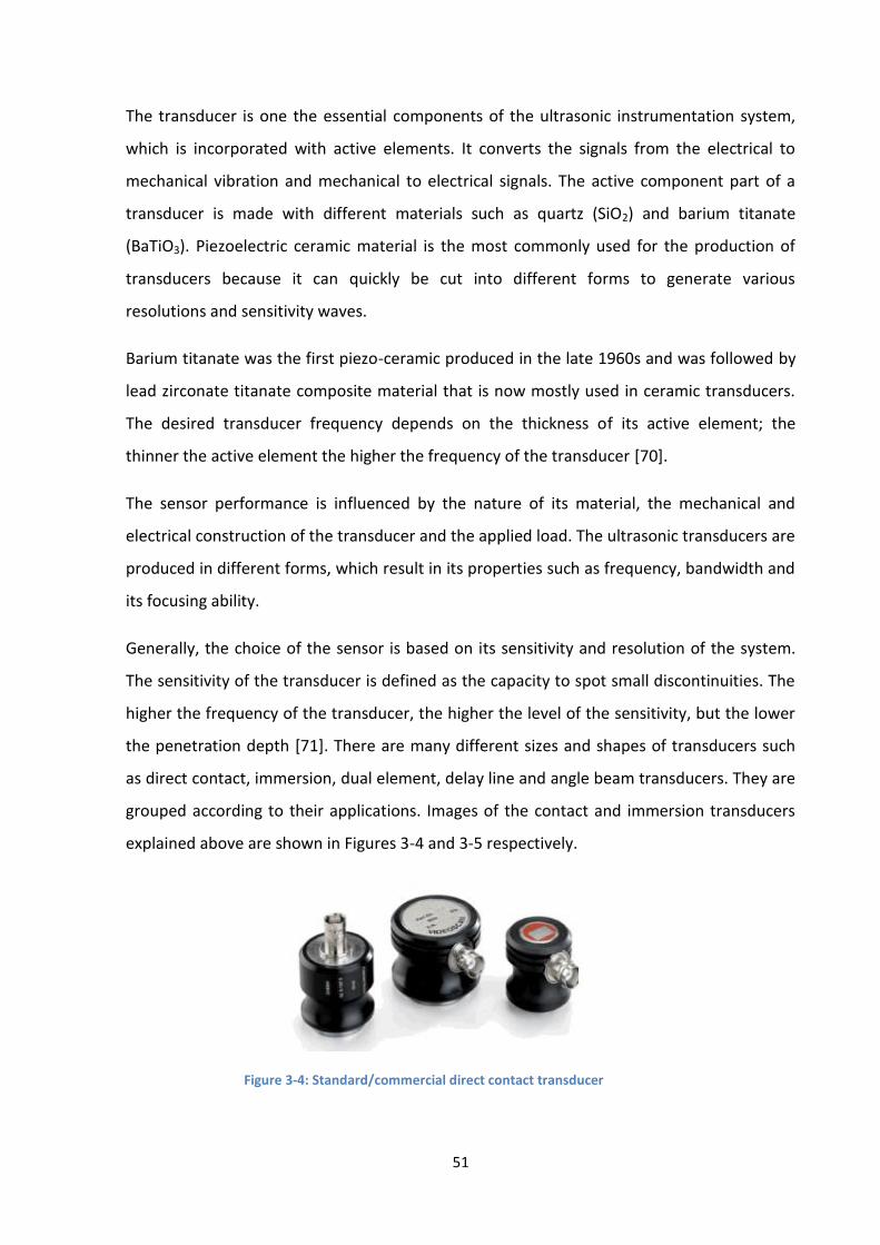
51

The transducer is one the essential components of the ultrasonic instrumentation system,

which is incorporated with active elements. It converts the signals from the electrical to

mechanical vibration and mechanical to electrical signals. The active component part of a

transducer is made with different materials such as quartz (SiO2) and barium titanate

(BaTiO3). Piezoelectric ceramic material is the most commonly used for the production of

transducers because it can quickly be cut into different forms to generate various

resolutions and sensitivity waves.

Barium titanate was the first piezo-ceramic produced in the late 1960s and was followed by

lead zirconate titanate composite material that is now mostly used in ceramic transducers.

The desired transducer frequency depends on the thickness of its active element; the

thinner the active element the higher the frequency of the transducer [70].

The sensor performance is influenced by the nature of its material, the mechanical and

electrical construction of the transducer and the applied load. The ultrasonic transducers are

produced in different forms, which result in its properties such as frequency, bandwidth and

its focusing ability.

Generally, the choice of the sensor is based on its sensitivity and resolution of the system.

The sensitivity of the transducer is defined as the capacity to spot small discontinuities. The

higher the frequency of the transducer, the higher the level of the sensitivity, but the lower

the penetration depth [71]. There are many different sizes and shapes of transducers such

as direct contact, immersion, dual element, delay line and angle beam transducers. They are

grouped according to their applications. Images of the contact and immersion transducers

explained above are shown in Figures 3-4 and 3-5 respectively.

Figure 3-4: Standard/commercial direct contact transducer

52

Figure 3-5: Standard/commercial immersion transducer

Images of the different sizes of the piezoelectric element described above as an active

element (Fig. 3-3) of commercial transducer are shown in Figure 3-6.

Figure 3-6: Typical piezoelectric element sizes

The piezoelectric element contains two different poles (positive and negative) to connect

with the positive and negative poles of the cable during ultrasonic wave transmission. It has

the same operating principle as the commercial transducer for the generating, sending and

capturing of the reflected data during the ultrasonic signal transmission process. For this

reason, it is generally used as an alternative to the commercial transducer. A piezoelectric

element is very cheap compared with the commercial transducer and is easy to cut into

different sizes and shapes.

3.2 Fundamentals of Sound Waves

3.2.1 Wave Propagation

The energy of wave propagation occurs through the transmission of kinetic energy from

particle to particle of the host medium due to the electrostatic interaction between particle

bonds (Figure 3-7). Elastic wave propagation is the process by which the wave transmits

within the medium. This occurs due to the conversion of the electrical pulse into mechanical

energy from the transducer.

Positive pole

Negative pole

53

Moreover, if the particles of the medium are compressed or in tension beyond the medium’s

elastic limit, the force is transmitted to the adjacent particles according to the stiffness of

the bonds. This force causes the adjacent particles of the medium to move and set other

particles to oscillate continuously.

Figure 3-7: Schematic diagram of a model of an elastic body

Since the bonds between the particles are guided with the spring during the oscillations, as

indicated in Figure 3-2 above, the rate of propagation of elastic wave transmission through

the medium depends upon the material and the phase in which it exists. For the wave to be

elastic, the initial and final locations of the particles must be identical following its passage.

This is the situation for Non Destructive Test (NDT) applications [72].

3.2.2 Wave Mode

The propagation of sound waves can be in a longitudinal or shear in a bulk wave

transmission, depending on the direction of the movement of the particles. These types of

sound waves are fully discussed in Sections 3.2.2.1 and 3.2.2.2 respectively.

3.2.2.1 Longitudinal Wave

A longitudinal wave is one produced by the compression force of the host medium in which

the particle vibration occurs in the same direction as the propagation wave. The compressed

and stretched movement of the elastic bands within the particles are shown in Figure 3-8.

Figure 3-8: Schematic diagram of longitudinal wave

54

The longitudinal wave can also be generated in both liquid and solid media due to its ability

to travel through the atomic structure during the compression and the refraction movement

of the media.

3.2.2.2 Shear Wave

Ultrasonic shear waves are transverse waves in that their particle travel perpendicular or at

right angles to the wave propagation direction as shown in Figure 3-9.

Figure 3-9: Schematic diagram of shear wave

Shear waves propagate efficiently through solid acoustic material. They are not propagated

into liquid or gaseous materials. The shear waves are relatively weak compared with

longitudinal ones. Shear waves are usually generated by the conversion of the longitudinal

wave when it strikes the medium at an angle [72].

3.2.3 Ultrasound and Material Properties Relationship

The stiffness behaviour and damping properties of a given material can determine how a

wave will propagate. The stiffness behaviour affects the wave speed of ultrasound, while the

signal energy absorption and a reduction in amplitude of the waveform depend on the

material particles’ interactions and distance from the source. Therefore, material properties’

effects in relation to ultrasound behaviours are outlined in the following subsection.

3.2.3.1 Speed of Sound

The rate of propagated sound waves depends on the properties of the material because the

sound wave travels at a different speed in a material. Sound wave propagation depends on

the density of a host material, being a primary function of the mass and volume occupied by

the particles. It also depends on elastic forces within the particles of a medium that is

55

controlled by the amount of elastic constants such as, bulk modulus, shear modulus or the

Young Modulus of the medium. The sound wave moves rapidly in the solid medium

compared to a gaseous medium due to the compact ability of the material particles in solid

form [73]. The propagation of sound waves in a material at a given time is defined as a

product of frequency and wavelength. It is expressed as follows:

𝑐 = 𝑓 3-1

While c is the speed of sound, and it is measured in m/s2, f is the frequency of the sound

wave and it is measured in (Hz) and,, is the wavelength and it is measured as (m).

3.2.4 Fundamental Terminology of Ultrasonic Pulse

The terminology used to describe the ultrasound generated pulse is briefly described with

the full details of the captured and processed signal description.

3.2.4.1 Frequency and Bandwidths

When the ultrasonic transducer is executed with an electric pulse, it becomes deformed and

sets up a vibration that travels a number of cycles through the elastic medium, such as a

liquid or a solid form. The decay of the transducer oscillation depends on its level of coupling

and the damping ratio.

Figure 3-10: Schematic diagram of ultrasonic waveform in time domains [74]

56

Figure 3-10 shows the ultrasonic pulse waveform in the time domain. The peak-to-peak

value of the signal indicates the strength of the computed signal. The transformation of the

time domain of captured signal into the frequency domain provides the amplitude range,

categorizing the frequencies of the transducer used, as shown in Figure 3-11.

Figure 3-11: Schematic diagram of ultrasonic bandwidth in frequency domains [75]

Figure 3-11 shows the excitation of a transducer within the complete frequency a signal

containing a range of frequencies is called a bandwidth. The bandwidth of the signal shows

the range of useful frequencies and is typically set in terms of a proportion of the centre

frequency.

3.2.5 Acoustic Impedance of Materials

Acoustic impedance is a material’s ability to transmit ultrasound transmission from one

material to another. The acoustic impedance property of the material is very useful in

assessing ultrasound behaves at the interface of two different types of material. It is also

reliable when estimating the acoustic transmission and the reflection at the interface of two

different materials with various impedances [76]. Finally, it is a crucial consideration in the

transducer design. The acoustic impedance of a material is a product of density of the

particular host medium and wave speed that travel through it, and it is calculated as follows:

𝑧 = 𝜌𝑐 3-2

The unit of Rayl (Pa.s/m3) or Kgm-2× 106.

Bandwidth

57

The transmission of signals across two materials boundaries depends on the nature of the

bond of the materials interface and the acoustic impedance similarities of the materials. The

difference in acoustic properties of the two materials is usually referred to as the impedance

mismatch of the material.

3.2.6 Law of Reflection

Reflection is the diversion of an incidence ray direction when it hits the interface of the

medium at an angle and is reflected at the same incidence angle, as indicated in Figure 3-7.

Therefore, the Law of Reflection states that on a smooth surface, the angle at which an

incidence wave hits the surface is equal to the angle at which it is reflected [77]. As

illustrated (Figure 3-7) the incidence wave OP (𝑣1) strikes the interface of the specimen at

an angle 𝜃1 at point O, and the reflected OQ (𝑣2) of the incidence ray at an angle 𝜃2. This is

achieved with the aid of an imaginary line at point O, perpendicular to the interface of the

specimen and is known as normal to the interface. The angle of incidence 𝜃1 is the same as

the angle of reflection 𝜃2. Therefore, the Law of Reflection is stated as follows:

𝜃1 = 𝜃2 3-3

Figure 3-12: Diagram of the incidence and reflected rays

As shown in the figure above, the ultrasonic wave is reflected at the boundaries where there

is a difference in acoustic impedances of the material involved. The reflection and

transmission of the sent ultrasonic are calculated with the aid of the equation 3-3.

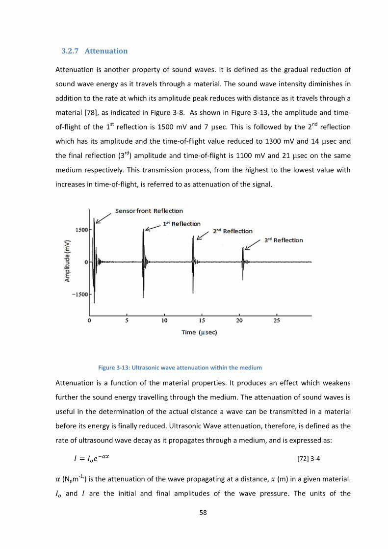
58

3.2.7 Attenuation

Attenuation is another property of sound waves. It is defined as the gradual reduction of

sound wave energy as it travels through a material. The sound wave intensity diminishes in

addition to the rate at which its amplitude peak reduces with distance as it travels through a

material [78], as indicated in Figure 3-8. As shown in Figure 3-13, the amplitude and time-

of-flight of the 1st reflection is 1500 mV and 7 µsec. This is followed by the 2nd reflection

which has its amplitude and the time-of-flight value reduced to 1300 mV and 14 µsec and

the final reflection (3rd) amplitude and time-of-flight is 1100 mV and 21 µsec on the same

medium respectively. This transmission process, from the highest to the lowest value with

increases in time-of-flight, is referred to as attenuation of the signal.

Figure 3-13: Ultrasonic wave attenuation within the medium

Attenuation is a function of the material properties. It produces an effect which weakens

further the sound energy travelling through the medium. The attenuation of sound waves is

useful in the determination of the actual distance a wave can be transmitted in a material

before its energy is finally reduced. Ultrasonic Wave attenuation, therefore, is defined as the

rate of ultrasound wave decay as it propagates through a medium, and is expressed as:

𝐼 = 𝐼𝑜𝑒−𝛼𝑥 [72] 3-4

𝛼 (Npm-1,) is the attenuation of the wave propagating at a distance, 𝑥 (m) in a given material.

𝐼𝑜 and 𝐼 are the initial and final amplitudes of the wave pressure. The units of the

59

attenuation coefficient are in Nepers per meter and can be converted to decibels per meter

by dividing by 0.1151 [77]. The causes of the wave energy reduction during the ultrasonic

transmission are categorized as follows: scattering and absorption.

3.2.7.1 Absorption

Absorbed ultrasound is one of the effects responsible for the attenuation of the signal

during its propagation through the material. It is the process by which the sound wave

energy is converted to other forms of energy, thereby creating a reduction in strength as it

travels through the material. Moreover, it usually turns into heat energy due to hysteretic

losses in the metal bonding as a result of the particles vibrating at their positions. The rate of

attenuation of the signal by absorption effect depends on the signal’s frequency. The higher

its frequency, the more the vibration of the material’s particles, and the higher the

absorption rate of the ultrasound energy.

3.2.7.2 Scattering

Scattering is the flection of sound waves in many different angles on the medium’s surface

due to its irregularity. Scattering is one of the factors which can cause the sound wave

energy reduction. This is due to the loss of the energy concentration by reflections of the

waves in many different directions. The change of direction of the sound wave occurs due to

the presence of discontinuities in the material’s body and its non-homogeneous nature. If

the discontinuities of the medium are larger than the wavelength of the ultrasound

transmitted wave, it will scatter more and reduce its penetrability energy.

3.2.8 Pulser /Receiver and Digitiser Unit

Ultrasonic waves were generated using a Film Measurement System (FMS) which consists of

pulser and receiver unit as shown in Figure 3-14.

60

Figure 3-14: Schematic diagram of FMS ultrasonic equipment

This machine was built by Tribosonic/NDT Solutions Ltd purposely to generate, capture and

process the reflection of the transmitted signal during the ultrasonic applications.

Figure 3-15 shows the typical line arrangement of the apparatus for the generation and

processing of ultrasonic waves that are in oblique form. The configuration consists of a

computer to display, control and monitor the wave properties. The apparatus contains an

ultrasonic pulser/ receiver unit (UPR) which was used to generate a series of short duration

voltage pulses to excite the piezoelectric transducer. The transducer is driven by the

pulser/receiver unit, while both the pulser and digitiser are controlled by a PC.

Figure 3-15: Line arrangement of ultrasonic pulsing and receiving apparatus

Amplifier

Reflected wave

Control Unit (Laptop)

UPR

Digitiser

Sensor (Receiver)

Incidence wave

Boundary Layer

Sensor (Pulser)

61

The PC sends a controlled signal that triggers the pulser unit of the UPR to generate a high-

frequency voltage pulse. The voltage pulse actuates the piezoelectric plate of the

transducer, which converts the electrical excitations to ultrasonic signals, and these are

consequently emitted through the medium to the targeted contact interface. The reflected

ultrasonic signals from the interface strike the piezoelectric plate which then converts the

motion of the ultrasound wave to a high-frequency voltage. The high-frequency voltage was

then passed to the amplifier unit which amplifies the voltage signals before passing them to

the receiver unit for onward transfer to the digitizer. The function of the digitizer is to

convert the analog signals obtained from the receiver to digital form. The digitizer provides a

wide range of bandwidths, sampling rates as well as dynamic range so that the signal

frequency matches the broad spectrum of the ultrasonic measurement needs. For the

present studies, the reflections were sampled at a resolution of 12 bits and at a rate of 100

million samples/second. The PC displays both the emitted and reflected signals.

3.2.9 Pulse Capturing Techniques

Reflected ultrasonic waves can be obtained either by pulse-echo or pitch-catch techniques,

depending on the number and the position of the transducer used. In the pulse-echo

method, a single sensor is used for both transmitting and receiving the ultrasonic signal,

whereas in the pitch and catch, two transducers are used to send and receive the signal.

62

3.2.9.1 Pulse-echo technique

In the pulse-echo technique, the signal transmits through the specimen until it is reflected

back at the interface of the sample to the same transducer as is illustrated in Figure 3-16.

Figure 3-16: Schematic diagram of the pulse-echo signal transmitted layout

Figure 3-16 shows the signal transmitted from the sensor into the test material (MT). The

two reflection signals appear as displayed in the ultrasonic graph shown above. The first

reflected signal at the probe face is the initial pulse signal from the probe. The second

reflected signal is from the material back face that is the echo of the transmitted signal from

the back wall of the material. The distance (MT1) is the distance between the reflection from

the sensor face and material back face, which represents the thickness of the used material.

3.2.9.2 Pitch-catch Technique

The pulser generates an electrical pulse electrifying a transducer and converting the

electrical pulse input into mechanical energy, producing an ultrasonic wave. The wave

transmits through the specimen until it is received on the other side of the material of the

second transducer that acts as a receiver. Two sensors are also involved in the transmission

of the signals in this technique while the mode of the sensor arrangement is based on Snell’s

Principle (Section 3.2.6). This principle states that the ratio of the angle of incidence and the

reflection waves is equal to the ratio of the velocities of incidence and reflection of the

waves that pass through the medium [79].

63

The transducers for the pitch and catch technique can be arranged in the opposite direction

to each other, as shown in Figure 3-17. The incidence wave was transmitted perpendicular

to the interface of the specimen and caught by a different second transducer acting as a

receiver.

In- addition, the pitch-catch technique can be the mode of transmission of wave at an angle

through the same material from one side to the other of the material, as shown in Figure 3-

18.

Figure 3-18: Pulse and catch technique with transducer arrangement edges

The configuration of the pitch and catch arrangements shown in Figures 3-17 and 3-18

depend on the area of application, but they both transmit and receive the wave reflection by

using different sensors.

3.3 Reflection of Sound at an Interface

When an ultrasonic wave strikes an interface between two different materials that are

entirely bonded together, part of its energy is propagated in the second medium, while the

remaining energy is reflected back to the initial medium. The total amounts of the energy

transmitted to the second material and quantities of the reflected back wave to the first

Figure 3-17: Pulse and catch technique with transducer in opposite arrangement

Pulser Transducer

Receiver Transducer

Incidence wave

Specimen

Incidence wave

Specimen Interface

Reflected wave

64

material depend on the acoustic impedance of the two materials. Furthermore, the involved

media’s interface is never perfectly smooth and thus always affects the transmission of the

signal to the second media [80].

3.3.1 Perfect Interface

When an incidence ultrasonic wave is normal to the perfect boundary of the two materials,

the proportion of the amplitude of the reflected wave pressure (𝐴1) to the amplitude of the

incidence wave pressure (𝐴2) is known as the reflection coefficient and is expressed as:

𝑅 =𝐴1

𝐴2⁄ 3-5

However, the reflection of the wave depends on the properties of the materials and the

boundary condition of the two materials. If the materials are different, as shown in Figure 3-

18 (a), under the perfect interface, part of the incidence wave is transmitted and part of the

wave reflected (Fig. 3-19 (a)).

The quantity of this reflected wave depends on the acoustic properties of the two materials,

respectively. Therefore the reflection coefficient of the ultrasonic wave of the reflected

signal is obtained by the following equation:

𝑅 = 𝑍2−𝑍1

𝑍2+𝑍1 3-6

Additionally, if the wave is transmitted through the same materials at a perfect boundary,

then the entire incidence wave is transmitted to the second material without any reflection,

Figure 3-19: Tribology interface of perfect contact (a) similar media, (b) dissimilar media

𝐼

𝑇

𝐼 𝑅

𝑇

Steel

Aluminiu

(a) (b)

65

as shown in Figure 3-19 (b). According to equation 3-6, the reflection coefficient of the

reflected wave is zero.

3.3.2 Dry and Rough Surface Contact

When an ultrasonic incidence wave hits the rough and dry interface of two different solid

materials, its reaction can be seen as in Figure 3-20 (a).

Figure 3-20: Tribology interface of (a) dry contact (b) wet contact (c) mixed lubrication interface (d) thick oil film contact (e) spring model representation [44]

As previously stated, the proportion of the amplitudes of the incidence and reflected wave,

known as the reflection coefficient, depends on the stiffness of the interface of the two

bodies involved. Kendall and Tabor [81] explained that, when the wavelength of the

ultrasonic wave sent is larger than the size of the asperity contact, then the reflection of the

wave from the interface of the used media is a function of the material interface stiffness.

Therefore, the value of the reflection coefficient at the rough surface is obtained with the

aid of the quasi-static spring model and expressed as follows:

𝑅 = 𝑍2−𝑍1+ί𝜔(𝑍1𝑍2/𝐾)

𝑍2+𝑍1+ί𝜔(𝑍1𝑍2/𝐾) 3-7

[82][82][82][82][82][82][82][82]

While the reflection coefficient for the similar media is:

66

𝑅 =1

√1+(2𝐾 𝜔𝑧′⁄ )2 3-8

Because of the same acoustic properties of the materials (𝑧1 = 𝑧2 = 𝑧′)

Where 𝑧1, and 𝑧2, refer to as the acoustic impedance of the material while 𝜔 is an angular

frequency of the wave and is expressed as:

𝜔 = 2𝜋𝑓 3-9

While 𝐾𝑎, is the stiffness of the dry contact and is expressed as:

𝐾𝑎 = −𝑑𝑝

𝑑𝑢⁄ 3-10

𝐾𝑎 is the stiffness of the rough contact area, and is expressed as the change in nominal

contact pressure 𝑝, is required to cause the unit approach of the average lines of the

medium surfaces. While u, is the mean separation lines of the two contacting surfaces. The

stiffness of the contact area depend on the load applied; the higher the weight of the

applied load, the greater the contact and stiffness in the area.

3.3.3 Oil Interface

If the lubricant is then introduced into the rough surface, as indicated in Figure 3-20 (b), an

ultrasonic wave will also be reflected in the front face of the layer and some on the back

face. For the thick lubricant layers’, the reflected pulses will be separated, and it will be

possible to distinguish the reflections in the time domain (Fig.3-20(d)). If the oil film

thickness is slight, the reflected pulses closed together and behave as a single layer (Fig. 3-

20(e)). The spring model approach used for the rough surface contact can also be applied to

the measurement of the lubricant film’s pressurised liquid stiffness 𝐾𝑙 as a function of the

bulk modulus (𝐵) between the two infinite flat half spaces of the fluid and its thickness (h),

as shown in the equation below:

𝐾𝑙 = B h⁄ 3-11

3.3.4 Mixed Lubrication Interface

The mixed lubrication interface consists of both liquid and solid contacts, as indicated in

Figure 3-20 (c). As the asperity contact is crushed down by the materials, it leads to the

67

reduction of the oil film thickness and the solid contact becomes more significant as shown

in Figure 3-20 (c). Therefore, the total stiffness 𝐾𝑡, at the interface is as a result of the

asperity stiffness contact 𝐾𝑎, and the pressurized liquid stiffness 𝐾𝑙 acting in a parallel form,

as indicated in Figure 3-20 (e), is expressed as:

𝐾𝑡= 𝐾𝑎 + 𝐾𝑙 3-12

Due to the response of the sensors to the stiffness layers, the shear sensor has good

responses to dry contact while the longitudinal sensor has effective responses to both wet

and dry layers in the mixed interface respectively. Therefore, the reflection coefficient for

the dry contact (asperities) will be obtained by the shear wave and reflection coefficients for

the wet contact from the longitudinal wave as expressed in equation 3-6 above. The

stiffness value for the dry (solid) contact 𝐾𝑎, obtained from equation 3-10, is expressed as

follows:

𝐾𝑎 =𝜔𝑧

2√

1

𝑅12− 1 3-13

𝑅1 is the reflection coefficient of asperity contact obtained by shear sensor (if

R1 is equal to 1 it means no asperity contact, but if 𝑅1, is less than 1 it means there is

asperity contact). Additionally, the stiffness value for wet contact 𝐾𝑙, obtained from

equation 3-11, is expressed as follows:

𝐾𝑙 =𝑤𝑧

2√

1

𝑅22− 1 3-14

𝑅2 is the reflection coefficient of the wet contact obtained by longitudinal sensor.

The interface has both solid and liquid stiffness. Therefore, the normal stiffness denoted by

𝐾𝜎 is measured with a longitudinal wave while shear stiffness denoted by 𝐾𝜏 is also

measured with shear wave. Both normal and shear stiffnesses are sum of their respective

solid and liquid parts of the interface, expressed as:

𝐾𝜎 = 𝐾𝜎𝑎 + 𝐾𝜎𝑙 3-15 (a)

𝐾𝜏 = 𝐾𝜏𝑎 + 𝐾𝜏𝑙 3-15 (b)

𝐾𝜎𝑙 and 𝐾𝜎𝑎 are liquid and solid normal stiffness while 𝐾𝜏𝑎 and 𝐾𝜏𝑙 are solid and liquid

tangential stiffness. Since liquid does not support shear load, the liquid tangential stiffness

of 𝐾𝜏𝑙 from the equation above will become zero (then 𝐾𝜏 is equal to 𝐾𝜏𝑎) [32]. Then the

longitudinal signal captured the total normal stiffness at the rolling bite interface. Therefore,

68

the lubricant stiffness is calculated by taking the dry stiffness value from the overall stiffness.

This is done by the equivalent ratio of shear stiffness and average stiffness to the Poisson's

ratio of the used material, and is expressed by the equation below:

𝐾𝜏𝑎

𝐾𝜎𝑎=

2(1−𝑣)

2(2−𝑣) 3-16

While the value of liquid normal stiffness 𝐾𝜎𝑙 is obtained from the equation 3-15 (a) above.

Therefore, the oil film thickness was calculated by the liquid normal stiffness with the aid of

the spring model, as expressed in the equation below:

𝐾𝜎𝑙 =𝐵

ℎ 3-17

while 𝐵 is the bulk of the modulus of the applied oil and ℎ is the thickness value of the

applied lubricant at the interface of the roll and the metal during the mixed lubricant regime

[44, 82-86].

3.4 Conclusion

The basic theory of ultrasound and its properties have been discussed in this chapter. This

theory has been used to explain how ultrasonic waves are transmitted and reflected during

their propagation through the medium. Additionally, generating ultrasonic wave

components, the transducers, and pulser and digitizer unit, have been fully explained. Pulse

capturing techniques have also been included in this section.

Finally, the reflection of sound waves from complete or perfect, rough, oil and mixed

interfaces during the ultrasonic wave transmission have been fully analysed.

69

Chapter 4

Application of Ultrasonic Transmission Method to a Roll Model

This chapter describes two different configurations of separate experiments of normal and

oblique incidence reflection, to study the metal-to-roll interface. A basic knowledge of

ultrasonic approaches, illustrated in Chapter 3, has been used to design the sensor

arrangement. The aim of these experiments was to determine the optimum ultrasonic

sensor arrangement to study the metal-to-roll interface with minimal modification of the

roll. Shear and longitudinal transducers were used to perform various tests in both

configurations. The implementation of the chosen technique to study the roll surface

conditions in Chapter 5 is based on the approach developed in this section.

70

4.0 Introduction

This non-destructive oil film thickness measurement technique has attempted to further

develop the use of an external ultrasonic sensor to avoid all the challenges from the internal

roll embedded sensor approach explained in Section 2.6.4. This chapter analyses two

common conventional ultrasonic transmission modes with two different layouts of wave

propagation. One mode consists of a metal block as a carrier of a longitudinal wave sensor

for normal incidence pulse-echo design. The other consists of two longitudinal wave sensors

externally mounted on the roll at an angle in a pitch-catch arrangement. The reflection of

the sent signals for both layouts was captured and recorded for further processing. The

pitch-catch transmission method was found suitable for this work due to the outcome of the

experiments. The details of each test are explained in the remainder of this chapter.

4.1 Normal Incidence Sensor Carrier Approach

4.1.1 Basic Concept

The sensor carrier shown in Figure 4-1 was designed and manufactured from a 130mm by

65mm rectangular mild steel block.

Figure 4-1: Sensor carrier

The carrier was constructed with a 110mm internal diameter to accommodate the roll of

108mm diameter during the signal transmission process. The difference of 2mm radial was

set-up between the roll and the sensor carrier to avoid direct contact during the rolling

process. This radial clearance between the roll and the sensor’s carrier was also made to

accommodate the coupling gel for the proper transmission of the ultrasonic signal.

71

Figure 4-2 shows how the sensor carrier generated incidence signal hits the sensor carrier

interface and is reflected back. This reflected wave is captured by the same sensor for

further analysis.

Figure 4-2: Sensor carrier with sensor

The coupling of the sensor carrier with a roll and the signal transmission process during the

experimental work is shown in Figure 4-3. However, as illustrated in Figure 4-3 the meeting

points of the sensor carrier and model roll were sub-grouped into two different interfaces.

The first interface, at the top of the roll, is referred to as the sensor carrier-to-roll interface,

and the second interface is at the bottom of the roll interface. Part of the generated signal is

reflected from the first interface while the rest of the signal is transmitted through the roll.

Almost all the signal transmitted through the model roll is reflected back at the second

interface due to the discontinuity of the interface. However, this arrangement results in

energy loss of sent signals at both interfaces before capturing back at the sensor mounted

on carrier.

Figure 4-3: Sensor carrier coupled with a roll for signal processing

Sensor

Sensor carrier

1st Interface

2nd Interface

Model roll

72

4.1.2 Experimental Method and Ultrasonic Apparatus

4.1.2.1 Transducer design

The piezoelectric elements were made from lead-zirconate-titanate due to its high

sensitivity and excellent thermal stability of high operating temperatures. The longitudinal

and shear piezoelectric elements, with a central frequency of 10MHz and 5MHz respectively,

were used for the experiment for the provision of good penetration of signal into the metal-

to-roll interface with clear and distinct reflected signals during the investigation. The

piezoelectric element had a thickness of 0.2mm and a diameter of 7.0mm. The sensors were

modified to form narrow strips of 2mm to improve the resolution, as shown in Figure 4.4.

Figure 4-4: Inbuilt and modified piezoelectric element

The modification was done with the aid of two razor blades bonded together and separated

by a suitable dimension for the space required within the two bonded edges. The cutting

device was simultaneously used to remove the two ’wings’ of the sensor, which left the

central element strip.

The surface of the sensors was typically covered with gold or silver for the provision of a thin

film layer for a more robust connection with the electrical wire during the soldering process.

The transducers were bonded to the test specimen with M-Bond 610 onto the carrier

surface, as shown in Figure 4-5. The carrier was put into the oven and heated to 1000C

adhesive curing temperature for 5 hours. The carrier with attached sensors was cured to

remove the trapped air bubbles of the adhesive and also for the proper bonding of the

sensor to the carrier surface. The material was allowed to cool in the oven to room

temperature to avoid the re-contraction of the sensor.

73

Figure 4-5: Instrumented sensor carrier

The cable was connected from the top of the element without disrupting the bond to the

carrier surface (Fig. 4-5). The attached sensor layer was covered with epoxy to protect the

sensor from rough handling during the investigation. The thinly cut elements were found to

be more challenging to bond to the surface of a specimen and difficult to solder during the

roll instrumentation.

4.1.2.2 Model Roll and Loading Frame

The metal-model roll used for the experiment was manufactured to 110 mm length by

110mm diameter with EN301 mild steel, as shown in Figure 4-6.

Figure 4-6: Model roll

74

Figure 4-7 shows the arrangement of the sensor carrier and the model roll before they were

fixed into the hydraulic jack.

Figure 4-7: Model roll with sensor carrier

The experiments started by recording the reflected signal without any load on the carrier, as

shown in Figure 4-8, as the reference signal. The model roll was inserted within the loading

frame of the hydraulic jack shown in Figure 4-8.

Figure 4-8: Model roll with loading frame

The jack was slightly raised against the model and loading structure to where line contact

was established. The load was subsequently increased to 5kN, and the reflection of the

75

ultrasonic signal sent through the sensor at this weight was captured and recorded. This

procedure was repeated as the pressures increased at 5kN intervals up to 20kN.

4.1.3 Data Acquisition and Processing

Figure 4.9 shows the schematic layout of the ultrasonic apparatus connected to the model

roll with the sensor carrier. The apparatus consisted of a pulser-receiver unit, digitizer and a

data acquisition unit. An industrial computer system contained all these components as PCI

(peripheral component interconnect) cards, and was used to conduct this experiment.

Figure 4-9: Schematic diagram of the ultrasonic apparatus

The industrial computer system used in this study was controlled with the aid of the

ultrasonic pulsing hardware unit referred to as a Film Measurement System (FMS) from

Tribosonics Ltd. This unit was used to generate, capture, display and record the ultrasonic

signals during the transmission process. The ultrasonic pulse receiver unit is the main

measurement unit. It generates and receives pulses from a medium through the transducer.

The output signal of 25V with duration of 100ns was used. Then the ultrasonic pulse

Digitizer

Ultrasonic

pulser/receiver

unit

Data acquisition and

Processing

Industrial Computer

System

Film M

easurem

ent

System (FM

S)

76

propagated through the carrier was almost reflected at the discontinuing layer of the

medium and received back by the same transducer. This signal processing and the display of

the results were carried out using software written in the LabVIEW program installed on the

PC. The ultrasonic reflected waves from the contact surface for each load were recorded and

studied further.

4.1.4 Signal Processing

Figure 4-10 shows the arrangement of the ultrasonic equipment (FMS) used to generate

wave and the employed hydraulic jack for the experiment.

Figure 4-10: Ultrasonic apparatus with the loading frame

Part of the generated signals were transmitted through the roll and reflected back to the

surface of the roll (2nd interface) while part were reflected at the carrier surface (1st

interface) respectively (Fig.4-3). The signal processing was repeated for the number of loads

applied during the experiment. The reflection of the transmitted signals was captured and

stored with the aid of the ultrasonic apparatus (Fig. 4-10). The ultrasonic reflections

obtained from the contact surface of the model for each applied load were converted to the

time domain. This was done with the LabVIEW program installed on the personal computer.

4.2 Experimental Results

4.2.1 Longitudinal Waves

Figure 4-11a shows the transmitted signal process within the sensor and carrier surfaces

when the carrier was not loaded against the roll while Figure 4-11b shows the transmitted

signal when the carrier was loaded against the model roll. Part of the generated signal was

77

reflected at the carrier-to-roll surface while the remaining wave was transmitted through

the roll and reflected at its back surface respectively.

Figure 4-11: Transmitted signals within the sensor carrier and back surface of the roll mode

The waveform of the reflected waves formed from the sensor carrier and the back surface

of the model roll during the signal transmission process is shown in Figure 4-12.

Figure 4-12: Reflected longitudinal wave graph from the back surface of the model roll

-3000

-2000

-1000

0

1000

2000

3000

0 10 20 30 40 50 60

Am

plit

ud

e (

mv)

Time (µsec)

1st, 2nd and 3rd reflection (Group A)

Reflection A

4threflection

(a)

(b)

Reflection B

Sensor pulse

78

As shown in the Figure 4-11, the first waveforms of various reflections (group A) from the

surface of the sensor carrier. The 1st reflection was from the surface of the carrier while the

2nd and 3rd waveforms were the re-bounced of the reflected signal from the same surface

respectively. This was due to the discontinuity at the surface of the carrier. The interval

between the two consecutive waveforms of the reflected signal is referred to as the

ultrasonic Time-of-Flight (ToF). The ToF of the 1st reflection, which was the initial waveform

at the surface of the sensor carrier, was 3.75 𝜇𝑠𝑒𝑐. This value was read directly from the

graph after the initial sensor pulse value and it compared with the actual thickness of the

sensor carrier surface. The ToF of the 2nd and 3rd reflections were increased at an almost

constant value of 3.75 𝜇𝑠𝑒𝑐 because the wave was re-bounced within the same thickness of

the sensor carrier.

Reflection B was from the back surface of the model roll, indicated as a 4th reflection in

Figure 4-11(b). The ToF of the reflected signal from the back surface of the model roll was

located at 40.95 𝜇𝑠𝑒𝑐 from the graph. This value corresponded to the diameter of the model

roll and the thickness of the sensor carried employed.

4.2.1.1 Effect of Loads on the Reflection Signal at the Back Surface Model Roll

This section focuses on discussion of the resolution and strength of the signal reflected from

the back surface of the model roll. The effect of applied loads on the reflected signal

obtained at the back surface of the model roll (Fig. 4-12) was separated and studied for this

purpose. Figures 4-13 to 4-16, show the response of this wave reflection according to the

values of load applied. The same range of 39 to 43 µsec was selected at the horizontal axis,

while the effects of the loads were studied with the value of the amplitude in the vertical

axis respectively. It was observed from these graphs that the values of amplitude increase as

the loads applied increase.

79

Figure 4-13: Reflected longitudinal wave graph at 5KN load

Figure 4-14: Reflected longitudinal wave graph at 10KN load

Figure 4-15: Reflected longitudinal wave graph at 15KN load

-200

-150

-100

-50

0

50

100

150

200

39 40 41 42 43A

mp

litu

de

(m

V)

Time (µsec)

-300

-200

-100

0

100

200

300

39 40 41 42 43

Am

plit

ud

e (

mV

)

Time (µsec)

-900

-700

-500

-300

-100

100

300

500

700

900

39 40 41 42 43

Am

plit

ud

e (

mV

)

Time (µsec)

80

Figure 4-16: Reflected longitudinal wave graph at 20 KN load

The corresponding value of the wave reflected amplitude at the back surface of the 110 mm

model roll diameters for the various applied are shown in Table 4-1.

Table 4-1: Reflected amplitude values from the model rolls diameter

Load

(kN)

110mm thickness (Amplitude value)

(mV)

5 76

10 208

15 720

20 755

The results clearly show that the applied rolling load has a significant effect on the energy of

the wave reflection of the transmitted signal. The higher the rolling load, the higher the

wave reflection from the back surface of the model. As shown (Figures 4-13 to 4-16), the

amplitude value of the reflected wave was observed to increase as the applied load

increased. This is due to greater closeness of the carrier-to-roll model surface contact (1st

interface in Fig.4-3) that increased the energy of the transmitted signal through the model

roll. The higher the applied load, the greater the closeness of the interface, then the higher

the energy of the transmitted signal and the higher the amplitude of the reflected wave at

the back of the roll. This means that high loads will be required before high strength signal

energy can be transmitted through the roll.

-900

-700

-500

-300

-100

100

300

500

700

900

39 40 41 42 43A

mp

litu

de

(m

V)

Time (µsec)

81

4.2.2 Shear Waves

The same experiment was repeated with the application of shear waves and the 110mm

diameter of model roll. Shear sensor was also tested with the same procedure employed for

the longitudinal sensor. This was due to the important nature of the shear sensor to confirm

the present of the solid contact at the metal-to-roll interface during the rolling process. The

obtained wave reflection data was processed and is presented in Figure 4-17. None of the

wave reflections were seen at the expected location on the back surface of the model roll

after the analysis.

Figure 4-17: Reflection of the shear signal sent through the carrier at various loading

The noise ratio of the sent signal was observed instead of the wave reflection when the

voltage of the ultrasonic equipment increased from 25V to 60V during the processing.

Additionally, the shear sensor negative responses was due to the reaction of the coupling gel

used to couple the carrier with the model roll. Longitudinal waves were able to be

transmitted from one medium to another with the presence of liquid while the shear wave

attenuated very fast and diminished in the gel layer between the carrier and roll model. This

is the reason why the shear wave did not reflect back on the surface of the model roll as

shown (Fig. 4-17).

4.3 Oblique Reflection Approach

4.3.1 Basic Concept

Figure 4-18 shows the design of the pitch-catch ultrasonic transmission technique that was

used to generate and transmit signals in the model roll with the transducers at the both

sides.

-3000

-2000

-1000

0

1000

2000

3000

0 10 20 30 40 50 60 70 80

Am

plit

ud

e (

mv)

Time (µsec)

Noise of the signal

82

Figure 4-18: Schematic diagram of the oblique incidence and reflected rays

The ultrasonic wave hits the interface of the material at an inclined angle, and its reflection

was captured at the other side of the roll, at the same angle of incidence. The incidence and

reflected waves are denoted by 𝑣1 and 𝑣2 the angle of incidence and reflected are denoted

by 𝜃1 and 𝜃2 respectively.

4.3.2 Experimental Procedure

Figure 4-19 shows the model roll after the material has been cut into the required angles at

both sides. The model roll interface was prepared for mixed lubrication purposes; therefore

a pair of longitudinal and shear transducers were attached to both side angles of the model

roll.

Figure 4-19: Model roll without sensor carrier

The experiment was conducted without applying any loads nor any carrier to the model roll

during the process. The ultrasonic signal was generated and transmitted through the model

83

roll with the aid of the ultrasonic equipment. Refer to Sections 3.2.2 and 4.1.3 for details of

the FMS and the software used.

4.3.2.1 Ultrasonic apparatus Data Acquisition process

The schematic diagram of the different combination of ultrasonic equipment units and

model roll is shown in Figure 4-20. The layout consists of pulse-receiver transducers, a

digitizer, an ultrasonic sensor and the model roll. The ultrasonic apparatus and model roll

communicated through the pulser and receiver transducers during measurement. The data

acquisition process used to obtain the ultrasonic wave reflection in Section 4.1.3 was also

employed in this section. The only difference is that the oblique reflection technique was

used in this section, which involved the application of the two separated transducers.

Figure 4-20: Ultrasonic apparatus with the model roll

The transmission methods of the generated and sent signals through the model during the

investigation are illustrated in Figure 4-20. The incidence wave hits the back surface of the

model roll and is reflected back at the same angle of incidence. This reflection was captured

by the receiver transducer and processed using LabVIEW software installed on the PC. This

84

procedure was used to process both the longitudinal and shear wave employed during the

experiment.

4.3.3 Experimental results

4.3.3.1 Ultrasonic Signal Transmission Process in the Model roll

Figure 4-21 shows the amplitude of the longitudinal wave reflection obtained from the back

surface of the model roll. This procedure was done in the time domain using LabView on the

PC. The Time-of-Flight (37.4µsec) of the wave reflection from the initial pulse at the surface

of the sensor corresponded to the thickness of the used model roll. The higher value of the

amplitude of the wave reflection of 1872 mV was obtained from the model roll without any

load applied.

Figure 4-21: Reflection of the longitudinal wave sensor with pitch-catch method at unloaded state

The properties of the reflection obtained at the longitudinal wave sensor are shown in Table

4-2.

Table 4-2: Properties of the sent longitudinal wave

Load (𝐤𝐍) Time-of-Flight (µ𝐬𝐞𝐜 ) Amplitude (𝐦𝐕)

0.0 37.4 1872

Given the discussion in Chapter 2, that the metal-to-roll interface generally undergoes mixed

lubrication (solid and liquid contact) during the rolling process, the aim of this experiment

was to study an ultrasonic signal energy transmitted through the model roll thickness and to

study the wave reflection from its back surface. Therefore, shear and longitudinal sensors

-2500

-2000

-1500

-1000

-500

0

500

1000

1500

2000

2500

0 10 20 30 40 50 60

Am

plit

ud

e (

mv)

Time (µsec)

85

were used to study the model roll interface respectively. The longitudinal wave was aimed

to study whatever might happen in the roll liquid and solid contact interface while the shear

wave was aimed to study whatever might happen in solid contact during the rolling

experiment. Installation of the roll onto the pilot mill and using it to deform the strip was

one of the objectives of this project.

Therefore, shear transducer was mounted and used to send signals and its reflection

obtained was processed and presented in Figure 4-23. The Time-of-Flight of the reflection

was obtained as 70.61 µsec. Larger Time-of-Flight was observed from the reflection of the

shear wave (Fig. 4-22). This is due to the low speed of 3190 m/sec of the shear wave during

its transmission process through the model roll. The Time-of-Flight of the wave

corresponded to the thickness of the model roll. In addition, the 1797 mV amplitude value of

the shear wave reflection from the back surface was also recorded.

Figure 4-22: Reflection of the shear wave sensor with pitch-catch method at unloaded state

Table 4-3 shows the properties of the reflected shear wave obtained during the process.

Table 4-3: Properties of the sent shear wave

Load (𝐤𝐍) Time-of-Flight (µ𝐬𝐞𝐜 ) Amplitude (𝐦𝐕)

0.0 70.61 1797

-2500

-2000

-1500

-1000

-500

0

500

1000

1500

2000

2500

0 20 40 60 80 100

Am

plit

ud

e (m

v)

Time (µsec)

86

4.4 Discussion

The purpose of these experiments was to determine which of the two techniques described

above provide the better external ultrasonic layout technique for understanding the model

roll contact surface conditions. A high energy of the received ultrasonic reflection was

observed with the oblique reflection technique at free load. This resulted in a very high

signal-to-noise ratio achieved from both sensors applied through the layout configuration.

The technique was able to capture a received signal from the back surface of the model roll

with amplitude of 1872mV and 1797mV against a noise level for both longitudinal and shear

wave sensors. Background noise was of order of 30mV for both signals (Figs 4-21 and 4-22).

This gives a signal-to-noise ratio (SNR) for the reflection from the top surface in the range of

60.4:1 (longitudinal signal) and 59.9:1 for the shear sensor. The high signal-to-noise ratio is

necessary in order to extract useful information to detect and locate size of the interface

conditions during the metal rolling process.

Additionally, the sensors were able to transmit with high signal-to-noise level due to the

direct attachment of the transducer to the model roll surface (Fig. 4-19) and that led to the

lack of interface between the sensor and the model roll. This resulted in little or no energy

loss during the transmission and that is the reason a large value of high signal-to-noise was

also able to be achieved from longitudinal (Fig. 4-21) and shear (Fig. 4-22) sensors.

The ultrasonic reflections obtained from the back surface of the model roll with the second

layout configuration (normal pulsing technique) increased when the applied loads were

increased, which is related to the closeness of the carrier-to-roll interface during the

experiment. This technique was performed below expectation due to a low signal level

observed as the load applied to the model roll through the jack. The minimum reflected

signal level received was increased as the applied load increased. Compared with the

oblique reflection technique (free load), the amplitude value of 76mV with background noise

of 33mV was recorded for the 5kN applied load (Fig. 4-13). This gives a signal-to-noise ratio

range of 2:1. In ultrasonic testing, it is very important to put the level of the signal-to-noise

ratio of the obtained reflected wave into consideration for better performance of the

system. The higher the signal-to-noise ratio, the better the performance.

87

The disadvantage of the pulse-echo technique is that, a very long data capture time would

be required on account of the delays due to the additional sensor carrier involved before

installing onto the roll for signal transmission (Fig. 4-11).

In this layout, high quantity of signal-to-noise level of ultrasonic reflection observed at the

carrier-to-model roll interface (Fig. 4-12) caused a reduction in the signal transmitted energy

through the model roll. This was due to the discontinuity of the carrier surface to the model

roll and absorption of the wave from the applied coolant gel to the carrier-to-model

interface during the process.

In addition, it is not possible to view the shear wave reflected in the far side of the roll at the

expected location (Fig. 4-17), due to the reason that signal received from shear sensor has

low amplitude. The reduction in amplitude was partially caused by the losses of shear wave

energy into the coupling gel applied to the carrier-to-model roll interface. The amplitude of

the reflected signal from the back surface of the model roll was smaller than the amplitude

of the noise. The signal-to-noise was less than 1:1, and the noise was totally masked the

shear wave reflected signal. This was undesirable, because the reflected signal of the shear

wave was not located at the expected point. The limitation of the pulse-echo technique in

this configuration relates to the requirement for gel or liquid couplant as shear sensor

cannot be used to obtain the required sufficient signal-to-noise ratio required.

4.5 Conclusion

This chapter has presented two experimental layouts to the model roll. The aim has been to

ascertain the best external sensor layout arrangement for the ultrasonic transmission

method to study the metal-to-roll interface conditions. This investigation was carried out

with the sensor mounted on a sensor carrier and the transducer mounted on the model roll

in a pitch-catch arrangement. However, when comparing data obtained from similar signal

processing applied to both techniques, oblique reflection approach has been found to be

significantly more sensitive in studying the metal-to-roll interface. The following conclusions

can thus be drawn:

This study has shown the ability to use the ultrasonic reflection to investigate and

monitor the model roll interface conditions;

The experimental findings in this study show that the oblique reflection arrangement

was better than the normal pulsing layout. This result may be explained by the strong

88

signal-to-noise level of transmitting wave through the model roll that produced the

highest amplitude wave reflection at the back surface of the model roll;

The results show shear sensors cannot be used with the carrier configuration. This

may be explained by the lack of interface between the shear sensor and the model

roll that prevented the linkage of the signal during the transmission process. Due to

this almost all the ultrasonic energy was reflected back from the back surface of the

sensor carrier.

89

Chapter 5

Implementation of Ultrasonic Sensors on a Pilot Mill

This chapter describes the implementation of the pitch-catch technique on a pilot mill. The

technique was used to measure the strip thicknesses statically on the mill and during rolling.

The experimental results obtained from this technique were compared with independently

measured values and the differences were studied.

90

5.0 Introduction

This chapter discusses the design and machining of a metal roll from a pilot mill to install an

ultrasonic sensor; the instrumentation is also described. The ultrasonic approaches

described in Chapter 4 have been used to study the application of Time-of-Flight of the

reflected ultrasonic signal obtained from the roll back surface. The thickness of the strip was

also determined using the Time-of-Flight of the reflected wave obtained from the front of

metal roll and back surfaces of the metal rolled. This was done at both statically on the mill

and during rolling. The value of the strip thickness obtained was compared with the

measured value using a micrometre screw gauge.

5.1 Experimental Apparatus

5.1.1 The Pilot Mill

Figures 5-1 and 5-2 show the picture and the sketch of the pilot mill employed in this metal

rolling experiment.

Figure 5-1: Pilot mill used for the work

This machine is a two roll mill type, with the upper and lower cylindrical rolls rotating in

opposite directions. The average surface roughness of the roll was measured as Rq= 0.7µm

with the aid of a Veeco Dektak 150 profilometer roughness measurement machine. The

surface hardness of the metal roll was also determined as 750HV with the aid of the Vickers

hardness machine. Figure 5-2a and 5-2b shows the front and side of the pilot mill

respectively.

91

Figure 5-2: Sketch of (a) front (b) side view of the pilot mill employed

The mill consisted of two load cells mounted between the upper roll machine frames of the

machine. One of the load cells is shown (Fig. 5-2b) while the remaining one is located on the

other side of the machine. The machine contained screw adjustment rods on both stand

sides of the machine frame to regulate the rolling force by screwing up and down. Roll

spacing and adjustment was set manually using the adjustment wheel mechanism of the

machine. Two slip rings were installed on both ends of the top link shaft of the machine roll.

The speed of the machine was controlled via the control unit panel mounted on it to count

the rate of passage of the gear teeth through the shaft linked with the upper roll. This rolling

speed was monitored and measured with the machine speed panel, allowing the selection of

various rolling speeds of the machine during the metal deformation process. The

specification parameters of the pilot mill employed during the experiment are listed in Table

5-1.

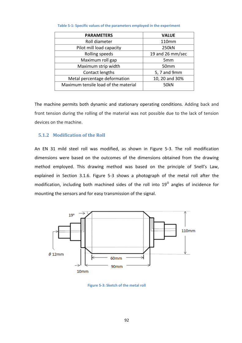
92

Table 5-1: Specific values of the parameters employed in the experiment

PARAMETERS VALUE

Roll diameter 110mm

Pilot mill load capacity 250kN

Rolling speeds 19 and 26 mm/sec

Maximum roll gap 5mm

Maximum strip width 50mm

Contact lengths 5, 7 and 9mm

Metal percentage deformation 10, 20 and 30%

Maximum tensile load of the material 50kN

The machine permits both dynamic and stationary operating conditions. Adding back and

front tension during the rolling of the material was not possible due to the lack of tension

devices on the machine.

5.1.2 Modification of the Roll

An EN 31 mild steel roll was modified, as shown in Figure 5-3. The roll modification

dimensions were based on the outcomes of the dimensions obtained from the drawing

method employed. This drawing method was based on the principle of Snell’s Law,

explained in Section 3.1.6. Figure 5-3 shows a photograph of the metal roll after the

modification, including both machined sides of the roll into 19O angles of incidence for

mounting the sensors and for easy transmission of the signal.

Figure 5-3: Sketch of the metal roll

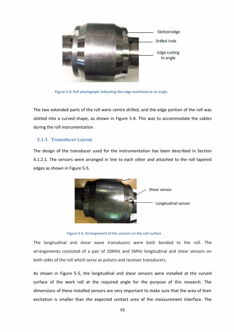
93

Figure 5-4: Roll photograph indicating the edge machined at an angle

The two extended parts of the roll were centre drilled, and the edge portion of the roll was

slotted into a curved shape, as shown in Figure 5-4. This was to accommodate the cables

during the roll instrumentation.

5.1.3 Transducer Layout

The design of the transducer used for the instrumentation has been described in Section

4.1.2.1. The sensors were arranged in line to each other and attached to the roll tapered

edges as shown in Figure 5-5.

Figure 5-5: Arrangement of the sensors on the roll surface

The longitudinal and shear wave transducers were both bonded to the roll. The

arrangements consisted of a pair of 10MHz and 5MHz longitudinal and shear sensors on

both sides of the roll which serve as pulsers and receiver transducers.

As shown in Figure 5-5, the longitudinal and shear sensors were installed at the curved

surface of the work roll at the required angle for the purpose of this research. The

dimensions of these installed sensors are very important to make sure that the area of their

excitation is smaller than the expected contact area of the measurement interface. The

Longitudinal sensor

Shear sensor

94

resolution of the ultrasonic measurement is defined by the ultrasonic beam width. A smaller

beam width results in higher resolution. For accurate measurement of the contact, the beam

width needs to be smaller than the contact width. Due to the geometry of both the work roll

and strip, a line contact is expected to form between the two, and thus contact length will

be much larger than the width. Due to this, the beam width would be definitely smaller than

the contact length for the entire applied load. In this research, 7mm x 2mm of the

piezoelectric element sensors were used.

In order to estimate the beam width, the flat transducer equation 5-1 stated below was

applied:

𝐵𝐷 = 0.2568 (𝐷) ∗ 𝑆𝐹 [87, 88] 5-1

while 𝐵𝐷 is the beam diameter, 𝐷 (7mm) element diameter and 𝑆𝐹 is normalized focal

length, which is the 1 for the flat transducer [87] . Therefore, the expected beam width of

the reflected signal from metal-to-roll interface was calculated as 1.8mm, this value was

obtained with the aid of equation 5-1.

Based on the comparison of beam diameter value obtained above, the expected interface

line contact of 3.7mm obtained in equation 2-3 (at a minimum of 5% metal reduction), and

high signal-to-noise of the applied technique (Section 4-4), it can be concluded that the

ultrasonic element installed is capable of studying the metal-to-roll interface conditions

during the metal rolling process without too much blurring of the obtained data.

95

5.1.4 Instrumentation Equipment

The complete sketch of the ultrasonic experimental layout with the external sensor

arrangement is shown in Figure 5-6. As indicated, the cables soldered with the sensors on

both sides of the roll were linked with the pulser/receiver unit through the slip rings.

Figure 5-6: Schematic component diagram for the ultrasonic data acquisition system

These sensors were bonded to both sides of the roll, as shown in Figure 5-5. M-Bond 610

adhesive was used to attach the sensors to the roll surface before being clamped together

for maximum pressure at the bonding interface. The clamped roll was placed inside an oven

and was cured at approximately 140oC for 5 hours. It was allowed to cool naturally in the

oven to avoid uneven cooling of the sensor-to-roll interface. The connecting cable was

soldered onto the sensors then coated with an epoxy for protection and to safeguard the

cables during the rolling process.

As previously explained, the voltage generated from the pulser/receiver unit is transmitted

to the transducer (pulser), which converts the electrical energy to mechanical energy and

produces ultrasonic signals (sound waves with high frequency). The ultrasonic signal is

generated by the transducer due to the vibration of the mechanical energy that is obtained

during the conversion. The signals were transmitted through the metal roll, reflected back

on the back surface of the roll and consequently captured by the receiver. The reflected

signals were received and converted back to voltage by a transducer (receiver). The voltage

was then transmitted back to the pulser/receiver unit before being passed to the digitizer,

where the reflections were digitized and finally displayed on the computer. This whole

process of generation and acquisition of signals was configured and controlled using a

LabVIEW program.

96

5.1.5 Metal Strip Specimens and Rolling Lubricant

Steel grade EN24, with the chemical composition (from the manufacturer) shown in Table 5-

2, was used as a specimen during the investigation. This steel was selected because of its

low carbon content and therefore its relatively low tensile strength generating a rolling load

below the maximum load capacity of the mill [89].

Table 5-2: Chemical composition of the specimen

Carbon Silicon Manganese Chromium Vanadium Tungsten

0.9 – 1.05 % 0.15 – 0.35 % 1.0 – 1.25 % 0.05 - 0.7% 0.05 – 0.15 % 0.05 – 0.70%

The low carbon steel specimen was cut into a cross-sectional dimension of 5mm thickness,

50mm width, and length of 250mm. The average surface roughness of the strip specimen

was measured with a Veeco Dektak 150 profilometer as 0.9µm. The strip surface hardness

was determined as 270HV with Vickers hardness machine.

Gerolub 5525 lubricant was applied with a hand brush onto the strip surfaces before being

fed into the roll gap during the rolling operation. This oil was chosen based on its high

viscosity that allowed thick film formations at relatively high rolling loads and low rolling

speeds. The properties of the oil and steel adopted for the experiment are shown in Table 5-

3.

Table 5-3: Oil and steel properties used for the experimental work [28, 66]

Gerolub 5525 lubricant oil

Density 810.2 (kg/m3)

Dynamic viscosity @ 25oC 65 (Pas)

Pressure viscosity coefficient

1.77 x10-8 (P-1a)

Bulk modulus 1.5 (GPa)

Steel (Roll)

Density 7800.0 (kg/m3)

Longitudinal velocity 5900.0 (m/s)

5.2 Experiment on a Stationary Strip

5.2.1 Test Procedure

A series of percentage metal deformations were made with the application of various loads

applied through the roll to the strip when stationary. The lubricant was applied to both sides

of the strip using a hand brush, and it was manually fed into the rolling gap of the mill, as

97

shown in Figure 5-7. The strip was dragged into the roll gap due to the friction force that

developed along the interface. The machine was stopped when the strip had been partially

rolled. The roll was set in such a way that the signal sent was able to transmit onto the strip

front and be reflected on the back surface of the strip. The initial and final thickness values

of the strips were measured and recorded with the micrometre screw gauge before and

after the process.

Figure 5-7: Manual feeding of the strip into the pilot rolling mill

The ultrasonic equipment (FMS) was set to pulse voltage of 25 volts, 1000Hz pulsing rate,

and gain adjusted for each sensor before the commencement of the signal transmission

process. The FMS digitiser runs at 100MHz sample frequency and has a vertical resolution of

12bits. The ultrasonic signal was sent to the interface. Therefore, a portion of the signal was

reflected back at the interface of the two materials, while the remainder of the signal was

transmitted through the strip and reflected from the strip back surface. The wave reflection

was adjusted and amplified by the customized pulser and receiver digitizer card that had

been built and installed on the FMS computer by the Tribosonics Company. The digitizer unit

was controlled using the LabVIEW program during the data capture process. The adjusted

reflected wave from the back surface of the strip, appeared in the time domain and was

captured and stored for further use.

5.2.2 Signal Processing

The reflected signals at the surfaces of the strip at stationary were captured by the LabVIEW

acquisition program on the PC. These reflected signals were processed in the Time domain.

As stated, the Time-of-Flight of the wave reflection corresponded to the thickness of the

transmitted medium, therefore the Time-of-Flight obtained was used to calculate the strip

thickness rolled during the operation.

Upper Instrumented roll

Strip

98

5.2.3 Reflection of Signal from the Strip Back Surface

The processed wave reflections of the generated signal sent through the roll to the strip

interface are shown in Figure 5-8. The reflected signal amplitude values were plotted against

the Time-of-Flight of the reflection signal obtained from the front and back surfaces of the

strip respectively.

Figure 5-8: Reflection of the longitudinal wave from the strip surface

The path of the reflected signal obtained from front and back surfaces of the strip, shown in

Figure 5-9, are illustrated in Figure 5-8. Waveform B was the reflected wave from the front

surface of the strip (point B) while waveform C was the reflection of the wave transmitted

from the back surface of the strip (point C) (Fig. 5-9).

Figure 5-9: Sketch of roll and strip engagement

-3000

-2500

-2000

-1500

-1000

-500

0

500

1000

1500

2000

2500

0.7 5.7 10.7 15.7 20.7 25.7 30.7 35.7 40.7

Am

plit

ud

e (

mV

)

Time (µsec)

Point G

Waveform (B)

Waveform (C)

∆𝑡𝑅 ∆𝑡𝑆

E

C (Back surface of the strip)

(Front surface of the strip) B

B1

99

The Time-of-Flight of the reflected signal, that is, the distance between points B and G (Fig.

5-9) was denoted as ∆𝑡𝑅 (Fig.5-8). While the Time-of-Flight of the wave reflection obtained

from the back surface of the strip, that is the vertical distance between point B1 and C (Fig.

5-9) was also denoted as ∆𝑡𝑆 (Fig.5-8).

5.2.4 Strip Thickness Calculation

Figure 5-10 shows the sketch of the signal transmission process from roll to strip and back to

roll when the sensor was facing the contact interface.

The diverged incidence beams (𝑣1 and 𝑣11) from sensor A (pulser) hit the back surfaces of

the roll and strip at angles 𝜃1 and 𝜃1′ respectively and the wave reflections denoted as 𝑣2

and 𝑣21 are bounced from the back surfaces of the roll and strip at angles 𝜃2 and 𝜃2′

respectively which are then received by the sensor G (receiver). The transmission

arrangements of the incidence and reflected beams illustrated in Figure 5-10 above show

clearly the signals transmitted through the strip which has allowed for determination of the

rolled strip thickness during the metal rolling process. Figure 5-11 is the triangle block

extracted from the signal transmission sketch, shown in Figure 5-10, for the determination

of the strip thickness employed. Line BC represents the actual strip thickness (𝑡𝑓) value while

line CB1 (Fig.5-11) is the path length of the wave reflection from the back surface of the

strip.

Figure 5-10: Sketch of signal transmission between rolls and strip interface

D

C

Strip back surface

Strip front surface

E G

Roll

Strip

A

B1

100

The thickness of the strip along /B1C/ was firstly calculated with the obtained Time-of-Flight

of the wave reflection from its back surface with the ultrasonic equation expressed as

follows:

/B1C/ = ∆𝑡𝑆 . 𝐶

2 5-2

While 𝑐 is the speed of the sound in the strip.

Then, the actual value thickness of the strip /BC/ was finally calculated by mathematical

manipulation of the obtained value of /B1C/ with the trigonometric ratio principle expressed

as follows:

cos 𝜃2 =/𝐵𝐶/

/𝐵1𝐶/ 5-3

cos 𝜃2 is the angle of the incidence wave that has been proved to be equal to the angle of

the reflected wave (Section 3.1.6). The angle of 19o was employed as the incidence angle in

this research. Therefore, /BC/ was the final value of the strip thickness obtained during the

rolling process.

The properties of the wave reflection data obtained from the strip and roll surfaces,

including the obtained strip thickness, were recorded in Table 5-4. The value of the strip

thickness employed was also measured with a micrometre screw gauge before the

experiment was conducted and recorded.

B1B

C

𝑡𝑓 𝜃2

Figure 5-11: Trigometic ratio diagram to calculate the strip thickness

101

Table 5-4: Property values obtained from the reflected signal at static position

Time-of-Flight (µsec)

1.78

Speed of the sound in strip ‘’ c’’

(m/sec)

5900

Angle of reflection (Degree)

19

Length ‘’/B1C/ ‘’(mm) 5.25

Experimental thickness ‘’ /BC/’’(mm)

4.86

Measured strip thickness (mm)

5.0

The strip values obtained from both measuring techniques were found to have slight

differences of 0.14mm from each other (Table 5-4).

5.3 Experiment during Rolling

This section describes the detailed study to determine the strip thickness during the metal

rolling process. The ultrasonic oblique reflection signal approach described in Chapter 4 was

used for this operation.

5.3.1 Basic Concept

The measurement technique proven to be the optimum in Chapter 4 is applied to a rolling

mill in this section. The sensor will rotate with the roll. When the sensors are over the strip

(Fig. 5-12) ultrasonic signal will pass through the roll-strip contact and be reflected from the

back of the strip.

Figure 5-12: (a) Side and (b) front view when the sensor is over the roll-strip contact

Section A-A’’

102

Figure 5-13 shows the position of the sensors when rotating away from the strip-to-roll

contact. The wave will be completely reflected from the roll-air interface.

Figure 5-13: (a) Side and (b) front view when the sensor is away from the roll-strip contact

5.3.2 Signal Processing

During the dynamic operation of the rolling process, ultrasonic reflected signals are

continuously captured from the surfaces of the strip as the roll rotates for a specific

duration. Therefore, a large quantity of the reflected signal is generated, captured and

digitized at this specified period, which is difficult to process in real-time. In order not to lose

information during the process, the acquired data was streamed directly to the hard disk of

the computer and stored in binary form for further processing. The stored reflected data

along with reference data can then be processed using another in-house written LabVIEW

program.

5.3.3 Experimental Procedure

The strip thicknesses were measured with a Vernier caliper both before and after each

rolling operation. Trial and error was needed in adjusting the gap width screw, due to not

having a roll gap measuring device. This was done to achieve the required strip thickness

and desired percentage metal reduction during the rolling process. However, due to the low

speed and high rolling load, the rolling metal experiences a deformation leading to mixed

contact within the strip and roll surface. The ultrasonic equipment was set to the same value

of pulse voltage and pulsing rate mentioned in Section 5.2.1. The captured window was

delayed by 39.5 µsec from the initial pulse. Therefore the Time-of-Flight is the reflection

time plus the delay. The equipment measurement scale was ranged from 0.0 to 5.4µsec

before the commencement of the signal transmission process, and the equipment was runs

at 100MHz sample frequency with vertical resolution of 12bits as mentioned earlier. The

(a) (b)

Section A-A’’

103

generated signal was transmitted through the metal roll continuously to the strip during the

rolling operation and the wave reflected at the strip back surface. This reflection was

captured, analysed and the result obtained (Time-of-Flight) was used to calculate the strip

thickness and the roll-bite contact length. The experimental details of the process are fully

explained below.

5.3.4 Recorded Waveform

Figure 5-14 shows the waveforms of the wave reflection from the back surface of the roll

when the sensor is away from the strip contact (Fig. 5-13).

Figure 5-14: Reflected signal obtained when the sensor is out of strip-to-roll contact

The 1st reflection is the waveform of the reflected signal obtained from the back surface of

the roll, while the 2nd reflection is the waveform of the bounced back echo of the 1st

reflection. The positive amplitude of both waveforms are almost the same (1275 mV for the

1st reflection and 1273 mV for the 2nd) as almost all the reflected wave was bounced back.

Figure 5-15, also shows the waveforms of the reflected wave obtained when the sensing

face was in contact with the strip surface (Fig. 5-12).

-2000

-1500

-1000

-500

0

500

1000

1500

0 2 4 6 8 10 12 14 16

Am

plit

ud

e (

mV

)

Time (µsec)

1st Reflection 2nd Reflection

104

Figure 5-15: Reflected signal obtained when the sensor is in contact with strip-to-roll interface

The 1st waveform was the reflection of the reflected wave from the back surface of the roll,

while the 2nd reflection was the waveform from the reflected signal back surface of the strip.

The 2nd reflected waveform had the smallest value of amplitude (80mV) compared with the

amplitude value of the 1st waveform (1028 mV).

The amplitude value of the 1st reflection, when the sensor was out of the roll-to-strip

contact (Fig. 5-14), was a higher value of 1275 mV compared with the amplitude value of the

1st reflection 1028 mV when the sensor was in contact with the roll-to-strip interface. The

reduction in the amplitude value of the 1st waveform reflection (Figure 5-15) was due to part

of the waves having been transmitted while part were reflected back from the back surface

of the roll. The Time-of-Flight of the reflected signal obtained from both metal roll and rolled

strip back surface were donate as ∆𝑡𝑅 and ∆𝑡𝑆 respectively.

As shown in Figure 5-15, the rolled strip thickness was able to be determined due to the

better reflected signal received from front and back surfaces of the strip during the rolling

process. The peak to peak amplitude of both front (left-hand side) and back (right-hand side)

pulses shown in Figure 5-16, was plotted against the pulse number for both front and back

surfaces from Figure 5-15.

-1500

-1000

-500

0

500

1000

1500

0 1 2 3 4 5 6

Am

plit

ud

e (

mV

)

Time (µsec)

1st Reflection

(Waveform A)

2nd Reflection

(Waveform B)

∆𝑡𝑅 ∆𝑡𝑆

105

Figure 5-16: Amplitudes of the wave reflection received front and back surfaces of the rolled strip

As can be seen from Figure 5-16, the amplitude of the reflected signal from the front surface

of the strip was of acceptable magnitude while the amplitude of the reflected signal from

the back surface of the strip is moderate. This shows signal amplitude for both reflections is

sufficient to calculate an accurate measurement of strip thickness during the rolling process.

The raw reflected data obtained during the rolling operation contained both reference and

reflected wave data obtained during the metal rolling operation. The process of separating

the reflected signal from the metal-to-roll interface from the obtained data is shown in

Figure 5-17 (a-c).

0

50

100

150

200

250

300

350

400

450

500

0

500

1000

1500

2000

2500

3000

0 200 400 600 800 1000 1200 1400 1600

Pea

k to

Pea

k A

mp

litu

de

(mV

)

Pea

k to

Pea

k A

mp

litu

de

(mV

)

Pulse Number

Front Interface (Axis 1) Back of Strip Interface (Axis 2)

106

Figure 5-17: Sample of ultrasonic data extracted for the determination of strip thickness; (a) stream of processed reflected data for one complete strip rolling; (b) sub-section of data when a sensor approaches the strip position; (c) single extracted reflected data from the front and back surfaces of the strip.

Figure 5-17 (a) shows the raw data obtained from the metal and roll surfaces during the

rolling process. These series of reflections are from both metal-to-air and metal-to-roll

contact interfaces during a full metal rolling operation with the normal rolling load of 70kN.

These reflections were captured, processed and stored for further use.

Figure 5-17 (b) shows another sub-set of a series of the reflected data obtained from the

first processed data (Figure 5-17 (a)). This is a series of the generated reflected signal from

the sensor to the roll the moment the strip is within the sensor’s view during the

(a)

(c)

(b)

107

deformation process (Figure 5-12 (a)). The dotted lines in Figure 5-17 (a) show the sensor

reflection signal from the roll-to-strip interface when the sensor surface focuses on the

compression of the strip and roll contact. The effect of the strip deformation by the rolling

passage obviously cleared on the amplitude of the reflected signals (Figure 5-17 (b)).

Therefore, when the sensors move away from the strip, then the amplitude of the reflected

ultrasound wave from the metal-to-air interface (Figure 5-13) was restored back to the

original value. The reduction in the value of the amplitude varied slightly as the attached

sensors’ focus moves towards and away from the strip during the rolling process.

Furthermore, Figure 5-17 (c) shows the actual required reflected data indicating the changes

in Time-of-Flight of the reflection between the strip front and back surfaces, which was used

to calculate the strip thickness.

5.3.4.1 The Nature of the Time-of-Flight Variation along the Roll-Bite

Smooth curves for processed Time-of-Flight variation of the reflected signal as shown in

Figure 5-18 are expected along the metal-to-roll interface whenever the sensor surface is in

contact with the strip during the rolling process as discussed in Carretta et al. [90].

Figure 5-18:Experimental and stimulation, various Time-of-Flight along the roll-bite [90]

108

Figure 5-18 shows that the experimental data varies from the expected shape. The reflected

signal at the contact interface of the rolling process is complex and the causes for the

variation are not well understood in the literature. Carretta et al. [90], explained that the

fringe pattern observed in Figure 5-18 can sometimes be observed instead of the smooth

curve graph. As discussed in the paper, this was due to the interference of the transmitted

signal as the signals hit the contact interface at slightly different times and the bounce back.

The same effect was also reported during the measurement of rolling bearing contact by

Howard [91].

The shape of Time-of-Flight variation observed along the metal-to-roll interface in this

research is in double-dip pattern (Fig. 5-17) which was different from the Time-of-Flight

variation observed by Carretta et al. [90] and Howard [91]. This difference may be due to the

distance of the sensor to the contact interface, the number of the sensor involved and the

signal pulsing technique. The main point however is that the smooth curve graph shown in

Figure 5-18 was not achieved and the reason for this effect remains an open question.

The data shown in Figure 5-19 is a sample of the processed data obtained from the metal-to-

roll interface which includes both reference and reflected signals captured in terms of Time-

of-Flight along the roll-bite during the rolling process. The set of the data was processed

with the aid of an FFT LabView program so as to separate the reference from the reflected

signal in the frequency domain.

Figure 5-19: Wave amplitude against frequency

0

5

10

15

20

25

30

35

40

0 5 10 15 20

Am

plit

ud

e (

mV

)

Frequency (MHz)

Reference signal

Reflected Signal

B

A 𝑓𝑐

109

As shown in the Figure 5-19, point A is the reference peak amplitude value (34.0mV), point B

is the reflected peak amplitude value (21.8mV), while 𝑓𝑐 is the centre frequency (8.9MHz).

The reflection coefficient obtained from the diagram is 0.64 using equation 3-5.

Figure 5-20 shows the reflected signal captured and processed using the LabVIEW program

at various positions across the roll-bite during the metal rolling process. The figure shows

the double-dip pattern described earlier.

The reflection coefficient at the centre of the roll-bite was selected as this occurs between

the dips at a point of no-interference. In Figure 5-20, a reflection coefficient of 0.64 was

obtained at a peak amplitude value for the centre of the roll-bite, which was the same with

the reflection coefficient value obtained from the frequency domain shown in Figure 5-19.

Therefore, the entire reflection coefficient values utilised in this research was obtained by

the technique explained and shown in Figure 5-20.

5.3.5 Effect of Loads on the Wave Reflection from the Back Surface of the Strip

Figure 5-21 shows the processed reflected signal obtained from the strip surfaces at each

applied load. Waveforms A and B, shown in Figure 5-15, are the wave reflections from the

front and back surfaces of the strip. The quality of the reflected waveform mainly depends

on the strip thickness and the applied load. The strip thickness is determined with the

0.3

0.4

0.5

0.6

0.7

0.8

0.9

1

1.1

0 0.05 0.1 0.15 0.2 0.25 0.3 0.35

Re

fle

ctio

n c

oe

ffic

ien

t

Time (µsec)

0.64

Figure 5-20: Reflection coefficient against Time-of-Flight

110

mathematical manipulation of the Time-of-Flight (t) between waveform signals A and B

and the speed of the sound of the strip.

The Time-of-Flight (horizontal distance from the left edge of the graph) between the two

waveforms (Figure 5-21) and depends on the rolling gap (vertical distance between the two

adjacent rolls). The roll gap is usually controlled by the load applied through the screw

stands of the milling machine. Moreover, the greater the applied load the less the roll gap

distance and the smaller the strip thickness. Therefore, the Time-of-Flight of the reflected

signal from the back surface of the strip reduces.

Figure 5-21: Wave reflection of the transmitted signal through the roll

Figure 5-21 shows the effects of applied loads on the reflected signal from the back surface

of the strip. These waveforms were arranged on the same axis for ease of studying the effect

of loads on the wave reflection from the back surface of the strip.

Furthermore, as the strip loaded during the rolling process, the wave path length of the

reflected wave reduces. Also, the speed of the ultrasound in the stressed material increases,

which leads to a reduction in ToF from waveform 1 to waveform 3. Hence, the energy of the

wave reflected reduces due to wave transmission and dispersion at the metal-to-roll

interface. This leads to the reduction in reflected wave amplitude value and the wave path

length as is shown in Figure 5-21.

-1300

-800

-300

200

700

1200

0.8 1.3 1.8 2.3 2.8

Am

plit

ud

e (

mV

)

Time (µsec)

Wave reflection at 40kN

Wave reflection at 70kN

Wave reflection at 90kN

∆𝑡𝑠1

Waveforms A

Waveform 2

Waveform 1 Waveform 3

∆𝑡𝑠2

∆𝑡𝑠3

Reflection from

strip Front surface

Reflection from

strip back surface

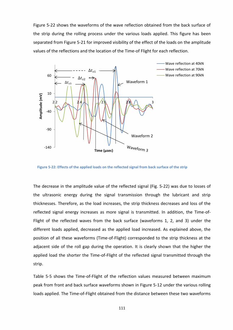
111

Figure 5-22 shows the waveforms of the wave reflection obtained from the back surface of

the strip during the rolling process under the various loads applied. This figure has been

separated from Figure 5-21 for improved visibility of the effect of the loads on the amplitude

values of the reflections and the location of the Time-of Flight for each reflection.

Figure 5-22: Effects of the applied loads on the reflected signal from back surface of the strip

The decrease in the amplitude value of the reflected signal (Fig. 5-22) was due to losses of

the ultrasonic energy during the signal transmission through the lubricant and strip

thicknesses. Therefore, as the load increases, the strip thickness decreases and loss of the

reflected signal energy increases as more signal is transmitted. In addition, the Time-of-

Flight of the reflected waves from the back surface (waveforms 1, 2, and 3) under the

different loads applied, decreased as the applied load increased. As explained above, the

position of all these waveforms (Time-of-Flight) corresponded to the strip thickness at the

adjacent side of the roll gap during the operation. It is clearly shown that the higher the

applied load the shorter the Time-of-Flight of the reflected signal transmitted through the

strip.

Table 5-5 shows the Time-of-Flight of the reflection values measured between maximum

peak from front and back surface waveforms shown in Figure 5-12 under the various rolling

loads applied. The Time-of-Flight obtained from the distance between these two waveforms

-140

-90

-40

10

60

2.2 2.4 2.6 2.8 3

Am

plit

ud

e (

mV

)

Time (µsec)

Wave reflection at 40kN

Wave reflection at 70kN

Wave reflection at 90kN∆𝑡𝑠1

∆𝑡𝑠2 ∆𝑡𝑠3

Waveform 2

Waveform 1

112

was used to determine the strip thickness during the rolling operation. This is due to the fact

that they are the most visible and formed in the same side of the graph.

Table 5-5: Values of the waves reflected parameters obtained from the back surface of the strip

Load (KN)

Percentage reduction

(%)

Waveform of the

rolled strip

Different of Time-of-Flight ‘’∆𝒕𝒔’’

(µsec)

Amplitude Value (mV)

40 8.4 1 1.58 85

70 14.4 2 1.45 53

90 24.0 3 1.34 36

Consequently, this measurement technique was utilised in order to obtain the Time-of-Flight

value between the two waveforms which was then used to calculate the rolled strip

thickness during the metal rolling operation that explained in Section 5.3.6 below.

5.3.6 Calculation of Strip Thickness

Figure 5-23 shows the illustration of wave reflections (Fig. 5-22) from the back surface of the

strip during the rolling process under the various applied loads when the sensors are in

contact with the roll and strip interfaces. The wave reflected Time-of-Flight graphs (Figs. 5-

21 and 22) represent the reflections from different back surfaces of the strip in accordance

with their thickness during the rolling process. From Figure 5-23 below, the 1st interface

represented the strip front surface (1st thickness) during the first loading (40 kN), while the

2nd and 3rd interfaces represented the strip front surfaces during the second (70 kN) and

third (90 kN) loading respectively.

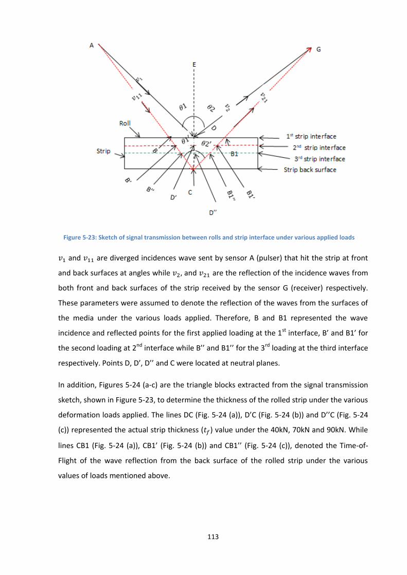
113

𝑣1 and 𝑣11 are diverged incidences wave sent by sensor A (pulser) that hit the strip at front

and back surfaces at angles while 𝑣2, and 𝑣21 are the reflection of the incidence waves from

both front and back surfaces of the strip received by the sensor G (receiver) respectively.

These parameters were assumed to denote the reflection of the waves from the surfaces of

the media under the various loads applied. Therefore, B and B1 represented the wave

incidence and reflected points for the first applied loading at the 1st interface, B’ and B1’ for

the second loading at 2nd interface while B’’ and B1’’ for the 3rd loading at the third interface

respectively. Points D, D’, D’’ and C were located at neutral planes.

In addition, Figures 5-24 (a-c) are the triangle blocks extracted from the signal transmission

sketch, shown in Figure 5-23, to determine the thickness of the rolled strip under the various

deformation loads applied. The lines DC (Fig. 5-24 (a)), D’C (Fig. 5-24 (b)) and D’’C (Fig. 5-24

(c)) represented the actual strip thickness (𝑡𝑓) value under the 40kN, 70kN and 90kN. While

lines CB1 (Fig. 5-24 (a)), CB1’ (Fig. 5-24 (b)) and CB1’’ (Fig. 5-24 (c)), denoted the Time-of-

Flight of the wave reflection from the back surface of the rolled strip under the various

values of loads mentioned above.

Figure 5-23: Sketch of signal transmission between rolls and strip interface under various applied loads

114

The properties of the wave reflection data obtained from the strip and roll surfaces, under

the various loads applied, are shown in Table 5-5. These properties were used with the

properties of the transducers employed to determine the value of the rolled strip thickness

under the various applied loads.

The thickness of the strip along the path length of the signal transmission (lines CB1, CB1’

and CB1’’ in Fig. 5-23) was firstly calculated with the obtained Time-of-Flight of the wave

reflection from its back surface for the applied loads with equation 5-1.

Then, the actual value thickness of the strip was finally obtained by mathematical

manipulation of the obtained value of the first of the strip thickness with the trigonometric

ratio principle expressed in equation 5-3.

An angle of 19o was employed as the incidence angle in this research. The final value of the

strip thickness obtained during the rolling process was calculated with the individual applied

load and is presented in Figure 5-25. The value of the rolled strip thicknesses obtained were

plotted against the Time-of-Flight and applied loads. Figure 5-25 shows the decrease in the

strip thickness value with increases of applied loads. It also shows the related decreased

Time-of-Flight of the reflected wave from the back of the strip.

B1 D

C

𝑡𝑓1

𝜃2 B1’ D’

C

𝑡𝑓2

𝜃2 B1’’ D’’

C

𝑡𝑓3

𝜃2

(a) (b) (c)

Figure 5-24: Trigometic ratio diagram to calculate the strip thickness under the various load applied

115

Figure 5-25: Strip thickness values obtained by the ultrasonic measurement technique

Figure 5-26 shows the relationship between the ultrasonic measured rolled strip thickness

and the applied loads. The strip thicknesses obtained by ultrasonic measuring techniques

were slightly different from those measured values achieved with a Vernier calliper. The

difference between strip thicknesses obtained from the ultrasonic oblique reflection and the

other obtained by the Vernier calliper measuring device after the process is shown in Figure

5-26.

Figure 5-26: Strip thickness values obtained the by ultrasonic and manual measurement techniques

Furthermore, the small differences in strip thickness measured value (Figure 5-26) between

the ultrasound and the manual (Vernier calliper) measurement methods, may have been

due to either human error or device error. An imperfectly smooth surface may also cause a

problem on the strip. This method is also suitable to determine the strip thickness during the

3.6

3.7

3.8

3.9

4

4.1

4.2

4.3

4.4

4.5

1.58 1.45 1.34

40 70 90

Stri

p t

hic

kne

ss (

mm

)

Time (µsec) / Load (kN)

0

0.5

1

1.5

2

2.5

3

3.5

4

4.5

5

40 70 90

Stri

p t

hic

knss

(m

m)

Load (kN)

Experimental value (mm)

Measured value (mm)

116

rolling process once the ultrasonic reflection Time-of-Flight of the transmitted signal is

known.

5.3.7 Determination of the Strip Thickness using th Strip-To-Roll Interface Profile

Figure 5-27 shows the front page of the software written in NI LabVIEW used for the analysis

of the reflected data obtained from the roll-to-strip interface profile during the rolling

process.

Figure 5-27: Front page of the software used to extract the wave reflected data

The page consists of four different windows and some dialog boxes. The 1st window shows

the raw data from which the Time-of-Flight between the waves reflected from the strip-to-

roll interface and the back surface of the strip during the rolling process.

Figure 5-28 shows the waveform of the roll-to-strip interface and strip back surface

reflections imported from the 1st window.

117

Figure 5-28: Wave reflection obtained between the rolled strip and roll

As shown from Figure 5-28, 1st waveform is the wave reflection obtained from the strip-to-

roll interface while 2nd waveform is the reflection obtained from the back surface of the

strip.

The strip profile reflection data program from the 3th window is plotted in terms of Time-of-

Flight against pulsing number as shown in Figure 5-29.

Figure 5-29: Time-of-Flight difference and pulse number between the rolled strip and roll

-1.5

-1

-0.5

0

0.5

1

1.5

100 150 200 250 300 350

Am

plit

ud

e (

mV

)

Time (10ns)

1st waveform

2nd waveform

105

110

115

120

125

130

135

140

145

150

480 530 580 630 680 730 780 830 880

Ch

ange

in T

ime

-of-

Flig

ht

(10

ns)

Pulse Number

118

The strip thickness was determined with the aid of the extracted data shown in the figure

above. This was done by mathematical manipulation of the obtained change of Time-of-

Flight data into strip thickness with the aid of equations 5-2 and 5-3. The distance across the

roll-bite is obtained by dividing the pulse number by the pulse rate (1000/sec) and

multiplying by the roll speed (26mm/sec) and is presented in Figure 5-30 below.

Figure 5-30: Experimental determination of strip thickness

The initial strip thickness was located on the graph at a point where the curve line started

while the final strip thickness was sited where the graph curve line remain constant. The

determination of the strip thickness explained in this section show the full picture of the

strip thickness from the initial to final thicknesses. This is useful for extracting further details

on the rolled strip such as, change-in-strip thickness and percentage metal thickness

deformation, which is not possible by the method employed in Section 5.3.6.

Finally, the dimensions of the strip thicknesses were measured with a micrometre before

and after metal rolling and compared with the experimental value in Table 5-6.

Table 5-6: Strip thicknesses obtained from different measurement techniques

Parameters Ultrasonic measured values (mm)

Vernier calliper measured values (mm)

Initial strip thickness 4.28 4.50

Final strip thickness 3.40 3.78

3.1

3.3

3.5

3.7

3.9

4.1

4.3

4.5

0.1 1.1 2.1 3.1 4.1 5.1 6.1 7.1 8.1

Stri

p t

hic

kne

ss (

mm

)

Distance in rolling direction (mm)

Initial strip thickness value

Final strip thickness value

119

The experimental values obtained had a difference of 0.22mm from the initial and 0.38mm

from the measured values. This may have been a speed of sound value, caliper accuracy and

elastic and plastic deformation of the strip during the rolling process.

5.3.8 Determination of the Roll-Bite Length

As explained in chapter 2, the roll-bite is simply the distance between the entry and exit

zone of the of the metal-to-strip interface. Therefore, Figure 5-29 shown in Section 5.3.7 was

reproduced as Figure 2-31 due to the reason that it was already used to calculate the

distance across roll-bite contact length. This was used as information to determine the roll-

bite experimentally. Rolling time can be converted to contact length via the rolling speed as

no roll skidding was observed during the metal roll process, possibly due to the low rolling

speed, the small percentage value of the metal reduction and the moderate thickness

(5mm) value of the strip applied during the operation.

Figure 5-31: Roll-bite length between the strip-to-roll interface

The roll-bite length was sited along the curve line of the graph for the reasons stated in

Section 5.3.7. The value of 5.59mm was obtained as the roll-bite length from the distance

between the initial (0.51mm) and final (6.1mm) points sited along the curve line in the graph

(Figure 5-32). The theoretical approach for the roll-bite length was discussed in Section 2.2.;

this principle was used to calculate the roll-bite length theoretically with equation 2.3., and

3.1

3.3

3.5

3.7

3.9

4.1

4.3

4.5

0.1 1.1 2.1 3.1 4.1 5.1 6.1 7.1 8.1

Stri

p t

hic

kne

ss (

mm

)

Distance in rolling direction (mm)

Roll-bite length

120

the measured strip data stated in Table 5-6. In Section 5.3.7., a value of 6.29mm was

obtained and these two results were compared with the aid of Figure 5-32.

Figure 5-32: Comparison of roll-bite length values

Although, they are differ by 0.7mm, the causes of the difference may be due to assumptions

made during the formulation of the theoretical background of the approach. It had been

assumed that the roll should be perfectly curved, which is not possible during the rolling

process.

After the expected ultrasonic sensor beam size at the metal-to-roll interface was estimated

in Section 5.1.3, it was discovered that the line contact of metal-to-roll interface is large

enough to accommodate the transmitted ultrasonic signal with minor blurring that may be

developed the process without significant effect on the obtained data. Due to the fact that

the small diameter of the sensor produces the small size of the beam width that interacts

with the interface during the experiment, this minimized the error that may occur during the

measurement. The smaller the diameter of the sensor the more the sensitivity and the

lesser measurement error obtained. The experimental contact length obtained is 5.59mm

compared to the 1.79mm ultrasonic beams width estimated. Therefore, little or no error is

expected due to the fact that the ultrasonic beam width point will always be at the centre of

the interface for every rolling operation.

0

1

2

3

4

5

6

7

Experimental roll-bite length value

(mm)

Theoretical roll-bitelength value (mm)

Series1 5.59 6.29

Len

gth

(m

m)

121

5.4 Comparison with the Literature

Carretta et al in [92] applied the same ultrasonic technique (pulse-echo) with internal

sensors fitted in the work roll to determine the rolled strip thickness and roll-bite length

during the metal rolling process. They explained that the experiment was performed using

an industrial rolling mill with 387mm roll diameter, 22.5m/min (375mm/s) roll speed and

2.8mm thickness, 100mm width and 490m length of IF steel. In-addition, it was reported

that the investigation was conducted for 30% metal reduction as well as application of

ultrasonic shear signal of 3252m/s propagation speed in the rolling material. Figure 5-33

shows the wave reflections obtained from the front (roll interface) and back surfaces of the

strip during the rolling process. The time difference between the rolled strip front and back

surfaces waveform is equivalent to the rolled strip thickness.

Figure 5-33: Wave reflection obtained between the rolled strip and roll surface [92]

As can be seen from the figure above, the value of 2.11mm (1.3µsec) rolled strip thickness is

obtained using the time-of-reflection method. This compares well to the expected exit strip

thickness of 2.14mm, with a 1.42% error.

As demonstrated in this chapter, an oblique reflection technique was employed to measure

the rolled strip thickness and roll-bite length during the metal rolling process in this

research. The experiment was conducted using pilot rolling mill at 26mm/s roll speed with

14.4% (0.72mm) metal reduction for 5mm thickness of mild steel. The details of the rolling

material as well as pilot mill used are shown in Table 5-1.

122

Despite the difference in the sensor configurations, percentage metal reduction and roll

speed, the wave reflections obtained in this research when the sensor surfaces are in

contact with the metal-to-roll interface show similar trend with those obtained in Carretta et

al. [92] (Figs. 5-15 and 5-33).

The comparison of the strip thickness results of the proposed approach in this research with

those of the theoretical calculations has been discussed extensively in Section 5.3.6. As can

be seen from Section 5.3.6 (that shows oblique and caliper values for the various applied

rolling load/percentage metal reductions), the technique employed in this research is

accurate with only minor difference of 0.24 (6%) between the rolled strip thickness value

and the rolled strip thickness value obtained with the caliper (for 70kN rolling load/14.4%

metal reduction). The error in both this work and reported in literature [92] are both low,

6% and 1.42% respectively. These errors are by a number of factors. Firstly, a tabulated

value for the speed of sound (5900m/s) was used in this research, this may differ slightly

from the actual speed of sound in the applied strip. Secondly, in this work a longitudinal

sensor was used. This has a shorter Time-of-Flight than the shear waves used by Carretta et

al. [92], due to the higher speed of sound. Therefore, any error in the ToF measured will

have larger error on the thickness measurement.

As already mentioned, Carretta et al. [92] applied modelling and experimental procedure to

measure the roll-bite length during the metal rolling with the rolling parameter conditions

stated above. The obtained experimental data and simulation value were used to plot the

strip thickness against the roll-bite length as shown in Figure 5-34.

123

Figure 5-34: Strip thickness against the roll-bite length [90]

As can be seen in the figure above, the obtained results (Figure 5-34), shows a similar trend

with the strip thickness against roll-bite length obtained in this research (Fig. 5-31), despite

the difference of the rolling parameters condition involved. The results obtained from this

proposed approach have been extensively discussed and compared with the theoretical

calculations value of roll-bite length obtained in Section 5.3.8.

The contact length measured by Carretta et al. [92] was 13.24mm, whereas the theoretical

value for these rolling conditions is 11.146mm. This gives an error of 15.8%. A relatively

minor difference of 0.7mm (12% error) was observed between this research value and the

theoretical value. The reason for the variation of the theoretical value and the value of this

research has been discussed in Section 5.3.8. Similar magnitude of errors is seen in both

works with the results in this work showing less error. There may be some error selecting

the entry and exit points of the roll-bite. Additionally, the theoretical values assume a

perfect condition. This is not practically possible.

Detailed comparative studies were carried out between the obtained data from Carretta et

al. [92] as well as those of theoretical and direct measurements via the measuring device on

strip thickness and roll-bite length values. Similar trends were observed in these

comparative studies. In particular, it is shown that the two techniques (external and internal

ultrasonic sensor layout methods) correspond to one another which implies the reliability of

124

the measurement system. The external ultrasonic technique employed by this research

looks more accurate, due to the minor percentage variation of a roll-bite length and strip

thickness obtained compared with the roll-bite length obtained by theoretical approach.

Although, it is difficult to compare the accuracy of the values obtained in [92] with the

values obtained by this research; due to the difference of the rolling parameter conditions

applied by both approaches.

This external sensor layout configuration used in this research has been applied to study the

roll gaps conditions and this arrangement does not result in markings on the rolled product

surface under large contact pressure when compared with the existing techniques. As such,

the experimental methodology is suitable for real-time measurements in the roll-bite of an

industrial mill.

5.5 Conclusion

This chapter has described the design and construction procedure for the development of a

new external ultrasonic experimental technique for studying metal-to-roll interface

conditions. These arrangements have been implemented on the pilot rolling mill and tested

using two experiments (stationary and dynamic) conditions. The following conclusions are

drawn:

The instrumented roll was successfully installed and implemented onto the pilot roll

mill,

The strip thicknesses at both stationary and at rolling conditions were able to be

determined using the reflected wave obtained from the strip back surface,

The effect of the loads on the ultrasonic wave reflection from the back surface of the

strip and strip thickness was successfully viewed and studied,

The length of the roll-bite value was experimentally determined and compared with

the calculated values,

Strip thickness profile across roll-bite was observed.

125

Chapter 6

Modelling of Normal and Oblique

Reflection at an interface

This chapter describes and compares the obtained sound wave reflection coefficient at an

interface between two media with pulse-echo and pitch-catch ultrasonic measurement

techniques by modelling and experimental processes. Modelling of the incidence angle at 0o

and 19o was carried out with matrix techniques for multi-layered inspection theory. The

experimental part of the study was carried out on a pilot metal rolling mill, with an

instrumented upper roll, equipped with piezoelectric elements at 0o to the roll surface for

pulse-echo and 19o for pitch-catch measurement techniques.

126

6.0 Introduction

The aim of this section is to create a model of the oblique reflection process and compare

with the experimental reflection of an ultrasonic signal transmitted to the interface of thin

fluid contact at different incidence angles. The use of ultrasonic oblique reflection methods

for measurement is quite challenging due to its layout arrangement.

Some researchers [93-98] have used normal and oblique ultrasonic pulsing techniques, and

compared the reflection coefficient obtained from the two. They have mostly concluded

that minor differences are observed in their reflection coefficient values, up to 22.50 of

incidence angles. The reflection coefficient obtained between the model and experiment

approach shows that the oblique reflection ultrasonic technique may play an important role

in the determination of the roll interface conditions during the metal rolling process.

6.1 Relationship for Oblique Reflection and Transmission

The oblique transmission and reflection of longitudinal and shear incidence waves at a solid-

to-solid interface is shown schematically in Figure 6-1.

Figure 6-1: Longitudinal and shear wave interaction with a solid-to-solid interface

Where; 𝐼𝑑 is a longitudinal incidence wave and 𝜃𝑖 is the angle of incidence. As shown in the

figures above, 𝐴𝑅𝐿, 𝐴𝑅𝑆, 𝐴𝑇𝐿, and 𝐴𝑇𝑆 are the reflected longitudinal, reflected shear,

transmitted longitudinal and shear transmitted waves respectively, while 𝜃𝑠1 and 𝜃𝑑1, 𝜃𝑑2

and 𝜃𝑠2 are angles of reflection and transmission of each wave. When a longitudinal wave

hits the perfectly bonded interface of the two materials, at any angle 𝜃𝑖 (either longitudinal

(a) (b)

127

or shear) some portion of the wave is reflected at the same angle with reflected angle 𝜃𝑑1

for the longitudinal wave (Figure 6-1 (a)) and 𝜃𝑠1 for the shear wave (Figure 6-1 (b)). The

remainder of the wave that is transmitted into the second material and divided into two

parts; longitudinal with an angle of 𝜃𝑑2 and shear with an angle of 𝜃𝑠2. This kind of wave

mode conversion takes place for both longitudinal and shear waves when crossing from one

boundary to another. The angles of reflection and refraction of the transmitted waves

depend on the acoustic properties of the materials, the angle of incidence and the nature of

the interface (either liquid or gas).

The angles of reflection and refraction of the transmitted signals can easily be determined

by Snell’s Law, once the incidence angle and speed of sound in the material are known [98].

The relationship between the incidence and reflected angles at the materials interface

shown Figure 6-1 and the speed of sound traveling in them during the process are expressed

as follows:

sin𝜃𝑖

𝐶𝐼𝑑=

sin𝜃𝑑𝐼

𝐶𝑅𝐿=

sin𝜃𝑠𝐼

𝐶𝑅𝑆=

sin𝜃𝑑2

𝐶𝑇𝐿=

sin𝜃𝑠2

𝐶𝑇𝑆 6-1

In acoustic analysis, the speed of sound 𝑐 and the wave-number 𝑘 relationship is expressed

as follows:

𝑐 =𝜔

𝑘 6-2

Substituting equation 6-2 into equation 6-1, gives:

𝑘𝐼𝑑 sin 𝜃𝑖 = 𝑘𝑅𝐿 sin 𝜃𝑑𝐼 = 𝑘𝑅𝑆 sin 𝜃𝑠𝐼 = 𝑘𝑇𝐿 sin 𝜃𝑑2 = 𝑘𝑇𝑆 sin 𝜃𝑠2 6-3

Reflection and transmission of oblique incidences can now be considered, once Snell’s Law is

understood [99].

6.1.1 Effects of Media Properties on the Mode of Wave Reflection and

Transmission

Figures 6-2 (a-d) show the reflection of the incident wave as it hits different types of

interface. Figure 6-2 (a) shows the reflection of the longitudinal signal from a fluid to a

vacuum interface. The entire incidence signal is reflected at the same angle (𝜃𝑖 = 𝜃𝑟). The

reason is that sound waves correspond to a mechanical energy that only transmits through

128

the media. This phenomenon occurs for both shear and longitudinal waves because neither

can transmit through a vacuum.

However, the shear signal is attenuated faster in a fluid medium than a longitudinal signal.

This is the reason why the generation of the shear signal conversion on the opposite side is

not possible in a liquid medium, unlike in a solid to vacuum interface, as shown in Figure 6-2

(c). In Figure 6-2 (b), which is the fluid-to-fluid interface, the angle of reflection and the

transmission of the longitudinal wave are obtained based on Snell’s Law. The reflected and

transmitted modes of longitudinal wave (𝐼𝑑) are shown in different media in Figure 6-2a and

6-2b, which is not possible for the shear wave (𝐼𝑠). This is due to the fact that both gases and

liquids are not capable of transmitting the shear wave. Therefore, the shear wave can only

penetrate through the solid material during the signal transmission process [77]. The

reflection of the longitudinal and shear waves occurred as shown in Figure 6-2 (c and d)

respectively; because they are slowly attenuated in solid media. The transmission and mode

of the shear and longitudinal signals conversion with the media are shown in Figure 6-1 (a

and b).

Figure 6-2 (a – d): Interaction waves with different interfaces [77]

(a) (b)

(c) (d)

129

6.2 Propagation of Oblique Incidence Wave through an Embedded

Layer

The characteristics of the reflection and transmission of an oblique longitudinal incidence

wave within a thin layer of fluid are shown in Figure 6-3. The layer is considered as a

microscopic interface with effective properties dependent on the interface structure [9]. The

angles of reflection and transmission indicated are derived from equation 6-1. Their

relationship is shown in equation 6-3 in Section 6.1, above.

Figure 6-3: Transmission of an incidence longitudinal wave through the embedded layer [98]

The wave reflections and interactions within the interfaces of the embedded liquid layer of

the solid-to-solid contact (semi-infinite media), shown in Figure 6-3, are presented in Figure

6-4. In this figure, the interface between the two solid media considered as a single layer.

The particle velocities (or displacements) and stresses on the upper and lower interfaces

between the layer can be related to each other with the aid of a transfer matrix expressed as

follows:

{

𝜎𝑧𝑧𝜎𝑧𝑥𝑤𝑢

} = [𝑀] {

𝜎𝑧𝑧𝜎𝑧𝑥𝑤𝑢

} [95, 96] 6-4

t

b

130

[M] is 4 X 4 matrix. The subscripts b and t denote the bottom and top layers, while 𝜎𝑧𝑧 and

𝜎𝑧𝑥 are the normal and tangential stresses. Also, 𝑤 and 𝑢 are the vertical and horizontal

displacements. While the elements of the matrix 𝑀 depends on the layer property. Equation

6-4 can be regarded as the boundary condition, which relates the stress and particle

displacement between the top and the bottom layered interfaces.

Figure 6-4: Interaction and the signal mode conversion within the embedded layer

Once the longitudinal wave strikes interface 1 (bottom of layer 1) at an angle, the

transmitted and reflected waves produce a unique stress and displacement on both sides of

the layer [100]. The amplitudes of the reflected and transmitted waves may be found by

using the matrix Equation 6-4. The deflections of the longitudinal and shear wave are given

by Pilarski [94]:

131

1. For the horizontal displacement,

𝑢𝐿+ = 𝐴𝐿

+ sin 𝜃𝑑2𝑒(𝑖𝑘𝐿 cos𝜃𝑑2𝑍) 6-5

𝑢𝑇+ = −𝐴𝑇

+ cos 𝜃𝑠2𝑒(𝑖𝑘𝑆 cos𝜃𝑠2𝑍) 6-6

𝑢𝐿− = 𝐴𝐿

− sin 𝜃𝑑1𝑒(−𝑖𝑘𝐿 cos𝜃𝑑1𝑍) 6-7

𝑢𝑇− = 𝐴𝑇

− cos 𝜃𝑠1𝑒(−𝑖𝑘𝑆 cos𝜃𝑠1𝑍) 6-8

2. For the vertical displacement,

𝑤𝐿+ = 𝐴𝐿

+ cos 𝜃𝑑2𝑒(𝑖𝑘𝐿 cos𝜃𝑑2𝑍) 6-9

𝑤𝑇+ = 𝐴𝑇

+ sin 𝜃𝑠2𝑒(𝑖𝑘𝑆 cos𝜃𝑠2𝑍) 6-10

𝑤𝐿− = −𝐴𝐿

− cos 𝜃𝑑1𝑒(−𝑖𝑘𝐿 cos𝜃𝑠1𝑍) 6-11

𝑤𝑇− = 𝐴𝑇

− sin 𝜃𝑠1𝑒(−𝑖𝑘𝑆 cos𝜃𝑑1𝑍) 6-12

The 𝑢 and 𝑤 in the x and z axes are presented the displacement vectors of the longitudinal

and shear waves in the upper and lower parts of the layer boundaries. The value of 𝑣 was

set to zero, because the structure is assumed to be in two dimensions and the y coordinate

axis is implicit and is omitted in the mathematical expression. The superscripts (+) and (-)

indicate the up and down movements of the wave at the layer interface respectively. While

z is distance in the direction of wave propagation and 𝐴𝐿 and 𝐴𝑇 are the amplitudes of the

displacement waves. In addition, 𝑘𝐿 and 𝑘𝑆 are longitudinal and shear wave numbers and

expressed as follows:

𝑘𝐿 = 𝜔

𝐶𝐿 and 𝑘𝑆 =

𝜔

𝐶𝑆 6-13

while 𝐶𝐿 and 𝑐𝑆 are the velocities of longitudinal and shear waves in the infinite isotropic

medium. Normal and tangential stresses can be determined at any point within the isotropic

and homogeneous boundary layers with the stress and strain relations:

𝜎𝑖𝑗 = ʎ𝑖𝑗𝜀𝑘𝑘 + 2𝜇𝜀𝑖𝑗 6-14

The relationships between the Lame constants (ʎ + 𝜇), density and velocities of longitudinal

and shear waves shown in equations 6-15 and 6-16 below can used to calculate the stresses

and displacement components in both x and z axes respectively. The relationships are

expressed as follows:

132

𝜎𝑥𝑥 = ʎ𝜕𝑢𝑧

𝜕𝑧+ (ʎ + 2µ)

𝜕𝑢𝑥

𝜕𝑥 6-15

and

𝜎𝑧𝑥 = 𝜇(𝜕𝑢𝑥

𝜕𝑧 +𝜕𝑢𝑧

𝜕𝑥) 6-16

while

𝜇 = ρ𝑐𝑆2 6-17

and

ʎ + 2𝜇 = ρ𝑐𝐿2 6-18

The normal and tangential stresses and displacements at the material boundaries can be

determined by the relationships 6-5 to 6-18. These serve as the foundation for the analyses

in subsequent sections.

As previously explained, the oblique longitudinal or shear wave reflection coefficient at an

interface can be obtained with a transfer matrix approach [95, 96]. This can be done by

relating the stresses and displacement components at the top face with those at the

bottom. The bottom layer is denoted as k-th while the top layer is denoted as k+1. For the

boundary conditions, the continuity of the normal and tangential stresses and displacements

between the top and bottom faces are satisfied and expressed by the following matrix

equation:

133

[𝑀𝑘,𝑏]

{

𝐴𝑅𝐿,𝑘𝐴𝑅𝑆,𝑘𝐴𝑇𝐿,𝑘𝐴𝑇𝑆,𝑘}

= {

𝜎𝑧𝑧𝜎𝑧𝑥𝑤𝑢

} 6-19

[𝑀𝑘+1,𝑡]

{

𝐴𝑅𝐿,𝑘+1𝐴𝑅𝑆,𝑘+1𝐴𝑇𝐿,𝑘+1𝐴𝑇𝑆,𝑘+1}

= {

𝜎𝑧𝑧𝜎𝑧𝑥𝑤𝑢

} 6-20

[𝑀𝑘,𝑏]

{

𝐴𝑅𝐿,𝑘𝐴𝑅𝑆,𝑘𝐴𝑇𝐿,𝑘𝐴𝑇𝑆,𝑘}

= {

𝜎𝑧𝑧𝜎𝑧𝑥𝑤𝑢

} =

{

𝐴𝑅𝐿,𝑘+1𝐴𝑅𝑆,𝑘+1𝐴𝑇𝐿,𝑘+1𝐴𝑇𝑆,𝑘+1}

= {

𝜎𝑧𝑧𝜎𝑧𝑥𝑤𝑢

} 6-21

For the solid-oil-solid system, equation 6-21 is chosen according to the generalised multi-

layered system. Therefore, the relationship of interface 1 and interface 2 in Figure 6-4 is

expressed as follows:

[𝑀1,𝑏]

{

𝐴𝑅𝐿,1𝐴𝑅𝑆,1𝐴𝑇𝐿,1𝐴𝑇𝑆,1}

=[𝑀2,𝑡]

{

𝐴𝑅𝐿,2𝐴𝑅𝑆,2𝐴𝑇𝐿,2𝐴𝑇𝑆,2}

6-22

[𝑀2,𝑏]

{

𝐴𝑅𝐿,2𝐴𝑅𝑆,2𝐴𝑇𝐿,2𝐴𝑇𝑆,2}

=[𝑀3,𝑡]

{

𝐴𝑅𝐿,3𝐴𝑅𝑆,3𝐴𝑇𝐿,3𝐴𝑇𝑆,3}

6-23

The problem is solved by assembling equations 6-19 and 6-20 and presented as follows:

b

t

b

t

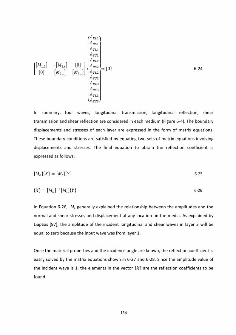
134

[[𝑀1,𝑏] −[𝑀2,𝑡] [0]

[0] [𝑀2,𝑡] [𝑀3,𝑡]]

{

𝐴𝑅𝐿1𝐴𝑅𝑆1𝐴𝑇𝐿1𝐴𝑇𝑆1𝐴𝑅𝐿2𝐴𝑅𝑆2𝐴𝑇𝐿2𝐴𝑇𝑆2𝐴𝑅𝐿3𝐴𝑅𝑆3𝐴𝑇𝐿3𝐴𝑇𝑆3}

= {0} 6-24

In summary, four waves, longitudinal transmission, longitudinal reflection, shear

transmission and shear reflection are considered in each medium (Figure 6-4). The boundary

displacements and stresses of each layer are expressed in the form of matrix equations.

These boundary conditions are satisfied by equating two sets of matrix equations involving

displacements and stresses. The final equation to obtain the reflection coefficient is

expressed as follows:

[𝑀𝑏]{𝑋} = [𝑀𝑡]{𝑌} 6-25

{𝑋} = [𝑀𝑏]−1[𝑀𝑡]{𝑌} 6-26

In Equation 6-26, 𝑀𝑖 generally explained the relationship between the amplitudes and the

normal and shear stresses and displacement at any location on the media. As explained by

Liaptsis [97], the amplitude of the incident longitudinal and shear waves in layer 3 will be

equal to zero because the input wave was from layer 1.

Once the material properties and the incidence angle are known, the reflection coefficient is

easily solved by the matrix equations shown in 6-27 and 6-28. Since the amplitude value of

the incident wave is 1, the elements in the vector {𝑋} are the reflection coefficients to be

found.

135

[𝑀𝑏] =

[

𝑖𝜔𝜌1𝛼1𝜓1/𝑔𝑙1 2𝑖𝜔𝜌

1𝑠𝛽

1

2𝜉1/𝑔

𝑠1−𝑖𝜔𝜌

2𝛼2𝜓2/𝑔𝑙2 2𝑖𝜔𝜌

2𝑠𝛽

2

2𝜉2/𝑔

𝑠2

−2𝑖𝜔𝜌1𝑠𝛽

1

2𝛾1/𝑔

𝑙1𝑖𝜔𝜌

1𝛽1

2𝜓1/𝑔

𝑠1−2𝑖𝜔𝜌

2𝑠𝛽

2

2𝛾2/𝑔

𝑙2−𝑖𝜔𝜌

2𝛽2

2𝜓2/𝑔

𝑠2

𝛼1𝑠/𝑔𝑙1 −𝜉1/𝑔

𝑠1−𝛼2𝑠𝑔𝑙2 −𝜉

2𝑔𝑠2

−𝛾1/𝑔

𝑙1−𝛽

1𝑠/𝑔

𝑠1−𝛾

2𝑔𝑙2

𝛽2𝑠𝑔

𝑠2 ]

6-27

[𝑀𝑡] =

[

𝑖𝜔𝜌2𝛼2𝜓2/𝑔𝑙2 2𝑖𝜔𝜌

2𝑠𝛽

2

2𝜉2/𝑔

𝑠2−𝑖𝜔𝜌

1𝛼1𝜓1/𝑔𝑙1 2𝑖𝜔𝜌

1𝑠𝛽

1

2𝜉1/𝑔

𝑠1

−2𝑖𝜔𝜌2𝑠𝛽

2

2𝛾2/𝑔

𝑙2𝑖𝜔𝜌

2𝛽2

2𝜓2/𝑔

𝑠2−2𝑖𝜔𝜌

1𝑠𝛽

1

2𝛾1/𝑔

𝑙1−𝑖𝜔𝜌

1𝛽1

2𝜓1/𝑔

𝑠1

𝛼2𝑠/𝑔𝑙2 −𝜉2/𝑔

𝑠2−𝛼1𝑠𝑔𝑙1 −𝜉

1𝑔𝑠1

−𝛾2/𝑔

𝑙2−𝛽

2𝑠/𝑔

𝑠2−𝛾

1𝑔𝑙1

𝛽1𝑠𝑔

𝑠1 ]

6-28

Vector {𝑌} = {

0010

} for longitudinal incident wave.

While the matrix symbol parameters defined as follows:

𝑠 =sin𝜃𝐼𝐿

𝛼 = sin𝜃𝐼𝑆

𝛽 6-29

𝛾 = √1 − 𝛼2𝑆2 6-30

𝜉 = √1 − 𝛽2𝑆2 6-31

𝜓 = 1 − 2𝛽2𝑆2 6-32

𝑔𝑙 = 𝑒𝑥𝑝 (𝑖𝜔𝛾𝑦

𝛼) 6-33

𝑔𝑠 = 𝑒𝑥𝑝 (𝑖𝜔𝜉𝑦

𝛽) 6-34

Matrices [𝑀𝑏] and [𝑀𝑡] are employed in equations 6-27 and 6-28 to determine the

reflection coefficient matrices {𝑋} as shown in Appendix 1.

6.3 Modelling of a Steel-Oil-Steel Interface

Computer simulations of the reflection coefficient of the incident wave were conducted at

two different load levels from an interface of two media with the various ultrasonic sensor

layout arrangements described in Chapter 4. This was done to study the effect of the

incident angles in ultrasound wave propagation at the interface of two similar media.

The interface between two solids with a thin liquid layer at the middle is very complicated.

For instance, the formation of a thin interface layer when two solids are bonded together

either with a thin layer of another material, e.g., glue or oil, depending on the properties of

136

this layer. The boundary between the two solids may behave as slip, perfect, or neither. Its

state has a significant effect on the wave reflection and mechanical behaviour of the

interface [101].

Rokhlin and Wang [102], classified a solid-oil-solid interface into two classes, namely rigid

and slip interfaces. These classes depend on the interface thickness layer, hence slip in solid-

oil-solid can be achieved if the interface layer is a thin ideal liquid. One can assume that a

liquid will behave in the interface as an ideal if the thickness of the layer is significantly large

enough to separate the interface.

However, if the lubricant layer is very thin then this will not be sufficient to separate the

media interface. Therefore the interface consists of isolated asperity contacts surrounded by

the gaps filled with liquid and is referred to as mixed contact interface.

In this work, modelling developed by Pialucha [9] has been considered as the best software

to investigate the effect of sound wave reflection from solid-oil-solid contact interface at the

0o and 19o angles of incidence the process. This is due to the relevance of the software

application to the present research.

6.3.1 Modelling Parameters

The properties of oil and steel adopted for the modelling are shown in Table 5-3 in Section

5.1.5. Together with the experimental values of embedded oil film thickness 2.32𝜇𝑚 and

1.27𝜇𝑚 obtained under the rolling loads of 60kN and 90kN with the 26mm/sec roll speed.

Frequencies of 0 to 10 MHz were used because the modelling will be validated with the

transducer of the same frequency. This modelling was carried out with the solid-oil-solid

interface of the same acoustic impedance properties.

6.3.2 Modelling Procedure

As stated above, the mathematical analysis of the modelling was conducted in the MATLAB

R2010b version scripts written by Li [99] with the Pialucha [9] method. The method was

used by Pialucha to evaluate the ultrasonic oblique reflection coefficient incidence for non-

destructive characterization of the adherent / adhesive interface of bonded joints. The

ultrasonic sensor was mounted at an inclined angle, operating in a pitch-catch orientation.

The experimental value of the reflection coefficient obtained was found to be within 5 % of

the predicted value [9].

137

This script was modified into the 19o angle of incidence and the properties of the tested

materials were changed to suit this study. This modified script is shown in Appendix A (Angle

Frequency vs Coeff.m). The simulations were run for longitudinal waves between the

incidence angles of 0o and 19o. The reflection coefficients of the signals obtained from the

modelling were stored for further studies.

6.3.3 Modelling Results

Figure 6-5 shows the variation of the longitudinal reflection coefficient obtained from a

steel-oil-steel interface with different angle of incidence during the modelling process.

Figure 6-5: Reflection coefficient from steel-oil-steel interface under the various angles of incidences

As can be seen from the figures above, it is noted that the angle of incidence wave has little

significant effect on reflection coefficient to much extent as the maximum variations occur

at normal incidence of about 9% up to 19o of an incidence angle. As previously discussed,

this as also been proved and authenticated by another researcher (Section 6.0).

Figures 6-6 and 6-7 show the reflection coefficient at 0o and 19o angle of incidences under

the variable values of the oil film thicknesses as a function of frequency. This was done to

investigate the effect of the incidence angle on the reflection coefficient at the interface for

the specific angles illustrated in Figure 6-5 above. The blue dotted line (Figs. 6-6 and 6-7)

indicates the reflection coefficient from the pulse-echo ultrasonic technique (0o angle of

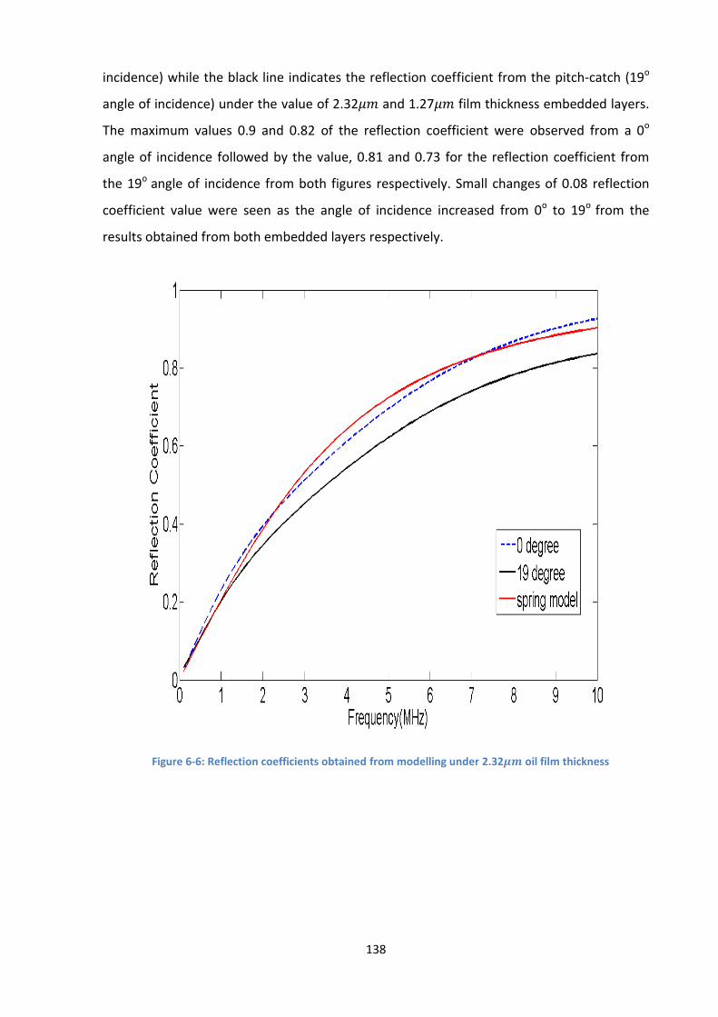
138

incidence) while the black line indicates the reflection coefficient from the pitch-catch (19o

angle of incidence) under the value of 2.32𝜇𝑚 and 1.27𝜇𝑚 film thickness embedded layers.

The maximum values 0.9 and 0.82 of the reflection coefficient were observed from a 0o

angle of incidence followed by the value, 0.81 and 0.73 for the reflection coefficient from

the 19o angle of incidence from both figures respectively. Small changes of 0.08 reflection

coefficient value were seen as the angle of incidence increased from 0o to 19o from the

results obtained from both embedded layers respectively.

Figure 6-6: Reflection coefficients obtained from modelling under 2.32𝝁𝒎 oil film thickness

139

Figure 6-7: Reflection coefficients obtained from modelling under 1.27μm oil film thickness

Additionally, the oil film thicknesses (interface layers) applied during the modelling was used

to determine the surface stiffness with the aid of bulk modulus property as expressed in

equation 3-11. The stiffness values obtained were used in the spring model equation 3-8 to

determine the reflection coefficient values for the frequency range 0 to 10MHz. These

reflection coefficient values obtained were plotted against the frequency for the differing

values of the layer (oil film thicknesses) applied for the modelling (Figs. 6-6 and 6-7). This

was done to check if the modelling was conducted in the spring model regime.

As shown in Figures 6-6 and 6-7, the graphs obtained with the aid of the spring model

equation are indicated by the red lines. This shows that the modelling was conducted within

the spring model regime. This was due to the fact that the graphs obtained from modelling

in normal pulsing technique and the graph obtained using the spring model were almost the

same with approximately equal reflection coefficient values at frequency of 10MHz which

was the sensor frequency.

140

Furthermore, Figure 6-8, was used to illustrate the relationship between the changes in

reflection coefficient with angle of incidence wave in respect to the oil film thicknesses.

Figure 6-8: Change in reflection coefficient with angles against the oil film thicknesses

The normal stiffness value of the applied longitudinal sensor with the pulse-echo technique

(0 degree) was calculated. This was done by the mathematical manipulation of the

experimental oil film thickness obtained from the pitch-catch technique with the bulk

modulus value of the applied lubricant as shown in equation 3-11. The obtained normal

stiffness value was employed to determine the pulse-echo technique reflection coefficient

values using spring model equation 3-8. The ratios of the reflection coefficient of both

techniques were calculated against the oil film thickness obtained during the process. This

graph was plotted with the ratio of the reflection coefficient obtained at 10MHz for 0 degree

(pulse-echo) and 19 degree (pitch-catch) of angle of incidence with respect to the value of

the obtained oil film thickness (interface layers). As can be seen from the graph, oil film

thickness has only a minor effect on ratio of the reflection coefficient value to changes to

the angles of incidence. This is shown by the slight changes of horizontal line drawn for the

ratio of the reflection coefficients obtained at angles 0 and 19 degrees for the two values of

the oil film thickness layer applied. The constant ratio of 𝑅0 𝑅19⁄ regardless of the film

thickness means that no adjustment needs to be made for different film thickness. This

makes practical implementation easier.

0.2

0.4

0.6

0.8

1

1.2

1.4

1.6

1.8

2

1.1 1.3 1.5 1.7 1.9 2.1 2.3 2.5 2.7 2.9 3.1

R0

/R1

9

Oil film (µm)

141

6.3.4 Comparison of Model Results with the Literature

The longitudinal reflection coefficient values obtained at the experimental and simulation of

paraffinic oil and polyphenol ether at various wave incidence angles by Xiangwei [99] are

shown in Figure 6-9 and 6-10 respectively. These results show the same trend with the

longitudinal reflection coefficient values obtained from both modelling and experimental

processes applied in the chapter.

Figure 6-9: Reflection coefficient obtained at various angles of incidence under experiment [97]

Figure 6-10:: Reflection coefficient obtained at various angles of incidence under stimulation [99]

142

As can be seen from the figures above, the reflection coefficient were observed to have little

effect on incidence angles up to 19o, likewise in the obtained model results shown in Figure

6-5 respectively. The largest effect of incidence angle was observed from 25o upward on the

reflection coefficient as indicated from the model results and from the literature results.

Liaptsis [97] also observed a decrease in the longitudinal wave reflection coefficients values

for a steel-to-steel contact with a small quantity of oil at their interface and increases of the

incidence wave angles at a surface difference stiffness ratio value, as shown in Figure 6-11.

This shows the same trend as the longitudinal reflection coefficient value obtained from the

modelling process of the reflection coefficient against angles of incidence shown in Figures

6-5.

Figure 6-11: Longitudinal reflection coefficient against the angle of the incidence wave [97]

The change in the reflection coefficient value of the wave is due to the increase in the path

length that the signal travels during the transmission process. The higher the angle of the

incident wave the larger the path length and the lower the reflection coefficient value of the

wave obtained.

Furthermore, Chen et al. [103] also proved from their findings that the reflection coefficient

of the longitudinal wave decreased with increasing frequency value when the wave

incidence angle was more than the 30o. Pilarski [94] explained that the sensitivity of the

interface weakness detection achieved by introduction of the oblique incidence technique

without the necessity of high frequency. Nam et al. [98] concluded that the longitudinal

143

reflection coefficients obtained at a 22.5o angle of incidence are similar to those obtained at

a normal incidence longitudinal wave. They stated that the characteristics of the reflection

coefficient at this oblique incidence angle 22.5o are mainly influenced by the normal

interface stiffness.

6.4 Experimental Validation

6.4.1 Experimental Set-up

The roll was instrumented with 10 MHz and 5 MHz central frequencies of longitudinal and

shears sensors for resonance transmission of the signal. As shown in Figure 6-12, the

sketched layout arrangement consists of mounting sensors centrally and at both edges of

the roll.

Figure 6-12: Rolls and the sensor layout arrangement

Four sensors (two longitudinal and two shear) were mounted on both sides of the upper roll.

The first pair of sensors on the right side of the roll is longitudinal and shear sensors, which

act as pulsers to generate signals during the transmission process. This was followed by

another pair of sensors (longitudinal and shear) on the left side of the roll, acting as

receivers for the reflected signal from the metal-to-roll interface (thin layer) during the

operation. The sensors were mounted in accordance with the transmission angles of

incidence 𝜃. The remaining two sensors (shear and longitudinal) were arranged on the top

surface of the roll for the normal ultrasonic transmission technique (pulse–echo) as shown in

Fig. 6-12.

144

6.4.2 Test Procedure

This experiment was conducted using a 5 mm thick, 25 mm wide and 250 mm length of strip.

The strip was manually loaded between the rolls of the pilot rolling machine (Fig. 5-8) after

the lubricant was applied to the surface of the strip. This experiment was conducted during

the metal rolling process under the rolling loads of 70kN and 90kN for each operation

respectively. Ultrasonic signals were sent through the roll to the metal-roll-interface during

the rolling process. The ultrasonic reflected signals were continuously captured from the

surfaces of the strip as the roll rotates for a specific duration. A large quantity of the

reflected signal was captured and digitized. The acquired data was streamed directly to the

hard disk of the computer and stored in binary form for further processing. This was done to

prevent loss of information during the process.

6.4.3 Signal Processing

The reflected and reference data that was stored together during the rolling process was

processed using a LabVIEW acquisition program on the PC as shown Figure 6-13.

Figure 6-13: Entire ultrasonic reflected data extracted during the metal rolling operation

The above data (Figure 6-13) was also processed further with the aid of LabVIEW on a PC to

separate the reference (reflected signal from metal-to-air interface) and reflected wave

(reflected signal from metal-to-roll interface) from the raw data. The two reflected values

were in terms of the amplitude value and frequency domain. Reflection coefficient of the

longitudinal wave sent from the metal-to-roll interface was obtained by dividing the

reflected peak amplitude value with the reference peak amplitude value respectively. This

reflection coefficient value was used further to calculate the stiffness value at the metal-to-

roll interface during the rolling process.

Reference data Reflected data

Time (µsec)

145

The various reflection coefficients obtained along the roll-bite with Time-of-Flight are shown

in Figure 6-14. The centre value of this figure was used as the reflection coefficient of the

reflected signal obtained from the metal-roll interface.

Figure 6-14: Longitudinal signal transmission at strip-to-roll interface during the rolling process

The obtained reflected signal was processed in the frequency domain in terms of the

reference and reflected amplitude values. As previously explained this is done in the easy

calculation of the reflection coefficient of the transmitted signal using the reflected and

reference amplitude value ratio. The data obtained under the applied rolling loads from

both techniques are presented in terms of the frequency domain in Figures 6-15 and 6-16

respectively. These (Figure 6-15 and 6-16) show decreases in the amplitude of the reflected

signal as the applied load increases for both applied approaches.

Figure 6-15: Wave amplitude spectrum of the pulse-echo values as load is increased

0.4

0.5

0.6

0.7

0.8

0.9

1

1.1

1.2

1.3

0 0.1 0.2 0.3 0.4 0.5

Re

fle

ctio

n c

oe

ffic

ien

t

Time (µsec)

Reflection coefficient

0

5

10

15

20

25

30

35

40

45

50

0 5 10 15 20

Am

plit

ud

e (

mV

)

Frequency (MHz)

Reference signal

Reflected signal at 70kN

Reflected signal at 90kN

146

Figure 6-16: Wave amplitude spectrum of the pitch-catch values as load is increased

Figure 6-17 and 6-18 show reflection coefficients against frequency results from pulse-echo

and pitch-catch ultrasonic transmission techniques obtained during the metal rolling

process. Results are shown for frequencies lying within the bandwidth of each reference

spectrum, as shown in Figures 6-15 and 6-16.

Figure 6-17: Longitudinal reflection coefficient against the frequencies with pulse-echo technique

As shown in Figure 6-17, the experimental reflection coefficients across the bandwidth of

the sensor through the pulse-echo technique were observed to be frequency dependent.

0

5

10

15

20

25

30

35

40

0 5 10 15 20

Am

plit

ud

e (

mV

)

Frequency (MHz)

Reference signal

Reflected signal at 70kN

Reflected signal at 90kN

0

0.2

0.4

0.6

0.8

1

1.2

4 5 6 7 8 9

Re

fle

ctio

n c

oe

ffic

ien

t

Frequency (MHz)

Reflection coefficient of the reflected signal at 70kN

Reflection coefficient of the reflected signal at 90kN

147

The reflection coefficient from the metal-to-roll interface was found to increase as the

frequency increases for both applied rolling loads. This implies a good agreement with the

spring model prediction indicated with a red line in Figures 6-6 and 6-7.

Figure 6-18: Longitudinal reflection coefficient against the frequencies with pitch-catch technique

Figure 6-18, shows the variation of the experimental longitudinal reflection coefficient with

frequency for 70kN and 90kN applied rolling loads. The reflection coefficient appears to

decrease over the bandwidth of the sensor (4–10MHz), which is poor agreement with the

spring model predictions as shown in Figures 6-6 and 6-7. The reason for this disagreement

is not clear, but the disagreement is consistent and was seen across all results. Liaptsis [97],

explained that this poor agreement was due to the increase of the angle orientation of the

sensor that leads to the divergent beam in the steel that can result in reflection from more

than the centre region of the interface contact.

6.4.4 Experimental Results

The experimental reflection coefficient values obtained from Section 6.4.1., were utilised for

calculating the interface stiffness values obtained from both techniques (pitch-catch and

pulse-echo). These stiffness values were used to determine the oil film thicknesses formed.

The obtained oil film thickness values were then utilised to model thickness layers between

the two surfaces to obtain the model reflection coefficient values.

0

0.2

0.4

0.6

0.8

1

1.2

1.4

1.6

1.8

4 5 6 7 8 9 10

refl

ect

ion

co

eff

icie

nt

Frequency (MHz)

Reflection coefficient of the reflected wave at 70kN

Reflection coefficient of the reflected wave at 90kN

148

Figure 6-19, illustrates the process of obtaining modelled reflection coefficient from the

experimental reflection coefficient. The obtained reflection coefficients from the two

techniques under the modelling and experimental procedure are shown in Figure 6-20.

Figure 6-20: Reflection coefficient obtained from both applied measurement techniques

The reflection coefficients from both techniques were found to decrease as the applied load

increases. The reason for this has been already mentioned above.

0

0.1

0.2

0.3

0.4

0.5

0.6

0.7

0.8

0.9

1

70 90

Re

fle

ctio

n c

oe

ffic

en

t

load (kN)

Obtained value from 0 degree angle of incidence.

Obtained value from 19 degree angle of incidence.

Figure 6-19: Flow chart of shown the step of obtaining the modelling reflection coefficient

Experimental

Ref. coeff.

Experimental Stiffness

Experimental Oil film

Modelling

Layers thickness

Modelling

Ref. coeff.

Equations 3-13 and 3-14

Equation 3-17

149

The normal stiffness’s of this interface was calculated using the equation 3-13 in Section

3.3.4, with the aid of the reflection coefficient values obtained above. The obtained stiffness

from these techniques under the applied rolling load is shown in Figure 6-21.

Figure 6-21: Stiffness obtained from both applied measurement techniques

The reflection coefficient and the normal stiffness values obtained during the experiments

conducted under the applied rolling loads that were presented in Figures 6-20 and 6-21 are

summarized and shown in Table 6-1 below.

Table 6-1: Experimental reflection and stiffness value obtained

Load case Reflection coefficient value obtained Stiffness values obtained

(kN) 0o incidence angle

19o incidence angle

0o incidence angle

(GPa/µm)

19o incidence angle

(GPa/µm) 70 0.82 0.77 0.82 0.98

90 0.64 0.62 1.32 1.49

Figures 6-22 and 6-23 show the reflection coefficient values obtained by equation 3-5

against frequency as the stiffness of the interface at the different angles of incidence used

under the two applied load during the metal rolling process.

0

0.2

0.4

0.6

0.8

1

1.2

1.4

1.6

70 90

No

rmal

sti

ffn

ess

(G

Pa/

µm

)

Load (kN)

Obtained value at 0 degreeangle of incidence

Obtained value at 19 degreeangle of incidence

150

Figure 6-22: Reflection coefficient against frequency with stiffness values under the 70kN rolling load

Figure 6-23: Reflection coefficient against the frequency with stiffness values under the 90kN rolling load

As can be seen from the figures above, the longitudinal reflection coefficient for steel-oil-

steel interface at 19 and 0 degree angle of incidence was plotted as a function of frequency

0

0.1

0.2

0.3

0.4

0.5

0.6

0.7

0.8

0.9

1

0 2 4 6 8 10 12

Re

fle

ctio

n c

oe

ffic

ien

t

Frequency (MHz)

Stiffness of 0.98 (GPa/um) obtainedat 19 (degree) angle of incidence

Stiffness of 0.82 (GPa/um) obtainedat 0 (degree) angle of incidence.

0

0.1

0.2

0.3

0.4

0.5

0.6

0.7

0.8

0 2 4 6 8 10 12

Re

fle

ctio

n c

oe

ffic

ien

t

Frequency (MHz)

Stiffness of 1.49 (GPa/um) obtained at 19(degree) angle of incidence

Stiffness of 1.32 (GPa/um) obtained at 0(degree) angle of incidence

151

for various stiffness values. The higher stiffness values are recorded from the 19o angle of

incidence for both figures, followed by the stiffness value obtained by the 0o angle of

incidence. It can be seen that the angle of incidence showed some degree of effect on the

experimental stiffness value obtained from steel-oil-steel interface. This is due to the double

effect expressed on reflection coefficient value from the spring model used to calculate the

stiffness from the oblique approached. The spring model is generally authenticated for the

normal pulsing technique, but it was used to calculate the stiffness from the data obtained

by the pitch-catch technique. This was due to the small variation observed from the

reflection coefficient of a sound wave between the 0o and 19o angles of incidence.

Additionally, this variation has been proved to be insignificant by some authors as stated

earlier in Section 6.0. Some authors proved that oblique reflection ultrasonic transmission

techniques are the best way to study the sensitivity interface of the two materials with low

frequency and the appropriate angle of incidence sound wave [93, 94, 101]. Therefore, the

difference in the stiffness observed between the two configurations under the applied

rolling loads is still negligible and proved to be within the expected range of error.

6.4.5 Comparison of Experimental Results with Model Results

Figures 6-24 and 6-25 show the comparison between the reflection coefficient of the

incident wave obtained from the experiments and the modelling for both the pulse-echo

and pitch-catch measurement techniques with 2.32µm and 1.27µm oil film thickness

embedded layer. This was calculated ultrasonically using oblique reflection technique.

Figure 6-24: Reflection coefficient values obtained from modelling under 2.32𝝁𝒎 oil film thickness

0

0.1

0.2

0.3

0.4

0.5

0.6

0.7

0.8

0.9

1

Normal Pulsing ObliqueReflection

Re

fle

ctio

n c

oe

ffic

ien

t

Experimental value

Modelling value

152

Figure 6-25: Reflection coefficient values obtained from modelling under 1.27𝝁𝒎 oil film thickness

Table 6-2, shows the obtained reflection coefficient value from the various angles of the

incidence applied from both experimental and modelling under the difference value of the

embedded layers (oil film thickness).

Table 6-2: Reflection coefficient obtained during both applied process techniques

Reflection coefficient obtained

Experimental results Modelling results

Oil film thickness (µm)

0o angle of incidence

19o angle of incidence

0o angle of incidence

19o angle of incidence

2.32 0.82 0.77 0.9 0.82

1.27 0.64 0.62 0.81 0.73

As can be seen, the highest values of the reflection coefficients were obtained from the

modelling process and decrease as the oil film thickness (embedded layer) decreases.

However, the difference of the reflection coefficients between the two measurement

techniques employed is negligible due to their small value. Additionally, the reflection

coefficient obtained from the processes is of the same trend, that they decreased by the

decreased value of the embedded layer of the interface. Due to more contact of the

asperities of both surfaces that developed at the metal-to-roll interface through the

reduction of the embedded layer (oil film thickness) that promotes more signal transmission

and reduces the reflected wave amplitude value during the rolling process. Once the

0

0.1

0.2

0.3

0.4

0.5

0.6

0.7

0.8

0.9

1

Normal Pulsing ObliqueReflection.

Re

fle

ctio

n c

oe

ffic

ien

t

Experimental value

Modelling value

153

reflected amplitude value reduced compared with the reference amplitude value, then the

reflection coefficient value obtained will reduce.

6.4.5.1 Determination of Percentage Error from Obtained Values

The percentage error of the reflection coefficient values from both processes under the

different measurement technique applied were determined by relating the reflection

coefficient and the angle of incidence waves values with the expression shown below:

%𝐸 =𝑅𝜃𝑜−𝑅𝜃𝑖

𝑅𝜃𝑜 6-35

Where:

𝑅𝜃𝑜 Is the reflection coefficient value obtained at normal pulsing (0o) measurement

technique and 𝑅𝜃𝑖 is the reflection coefficient obtained at oblique pulsing (19o)

measurement technique.

The percentage error of the reflection coefficients were obtained from normal pulsing and

oblique reflection measurement techniques for both modelling and experimental processes

(Figures 6-24 and 6-25) with the aid of equation 6-35. Therefore, the percentage error of the

reflection coefficients obtained under the differentiating value of 2.32µm and 1.27µm the

applied embedded thickness layers are shown in Table 6-3 below.

Table 6-3: Reflection coefficient percentage error obtained from both employed techniques

Difference in reflection coefficient obtained from both configurations

Embedded layer thickness

(m)

Experimental values %

Modelling values %

2.32 6.4 8.8

1.27 3.1 9.8

As can be seen from the above table, the percentage errors obtained from the reflection

coefficient at experimental values were very small compared with the error recorded from

the modelling. Various values for the reflection coefficient were obtained from both

ultrasonic techniques under the different approaches above mentioned. The best result of

reflection coefficient was achieved at both ultrasonic techniques from the experimental

procedure due to the lower value of the percentage error obtained under the two different

values of embedded layers employed. This shows the reliability of the oblique reflection

measurement techniques for the studies of the metal-to-roll interface as proposed.

154

Therefore, the effect of angle of incidence wave on ultrasonic reflection coefficient in this

research is negligible.

6.5 Conclusion

The model of Pialucha [9] was used and simulations were conducted for the solid-oil-solid

case to study the effect of the incidence angle on the longitudinal wave reflection

coefficient. Experimental tests were carried out to validate the results of the model using

pulse-echo and pitch-catch measurement techniques under two different embedded

thickness layers. This leads to the notion that the expression for reflected coefficient

obtained is correct. This also illustrates the validity of the use of the ultrasound normal

pulsing technique at this recommended angle of incident. The following can thus be

concluded:

This study has shown the ability to use the ultrasonic reflection to study the effect of

the angle of incidence wave on the reflection coefficient of the obtained reflected

wave;

The reflection coefficient value obtained from normal and oblique ultrasonic

transmission methods are slightly different from each other under the same

experimental conditions;

Higher percentage errors were recorded from the reflection coefficient obtained at

modelling process;

The stiffness value obtained from both normal and oblique ultrasonic transmission

techniques is a little different of 16% (at 70kN) and 7% (at 90kN) from each other;

This study has shown that the modelling was running in the spring model regime;

This study has proven that the reflection coefficient obtained from the interface

layers is only minimally affected by the incident angle.

155

Chapter 7

Measurement of oil film thickness during the

rolling process

This chapter presents the results obtained from the application of the external ultrasonic

sensor technique for the measurement of metal and roll lubrication condition interface

during cold rolling. This method was used to measure the formation of oil film thickness

under various rolling loads and speeds. The investigations were achieved using the reflection

coefficient at the roll-bite interface during the rolling operation. The effects of the

parameters mentioned above on the formation of oil film thicknesses are fully discussed in

the remainder of this chapter.

156

7.0 Introduction

A plethora of techniques exist for calculating the oil film thickness in cold metal rolling

operations. Some are based on the prediction of the oil film obtained at the roll-bite inlet

zone to calculate the oil film formation at metal-to-roll contact (section 2.6). Only a handful

of methods exist to measure oil film thickness in the working zone during metal rolling. The

ultrasonic method developed by Dwyer-Joyce and Hunter [66] which involves applying

internal insert sensors to measure oil film thickness across the roll-bite can pose great

difficulties, as explained in Section 2.7. The focus of this study was to measure the oil film

across the roll-bite without any assumption of other zones with the aid of the oblique

reflection ultrasonic technique. In this section, the oil film thickness was determined by

oblique reflection technique (pitch-catch) and included the investigation of the rolling

parameters on the oil film thickness sections (Sections 7.4.2 and 7.4.3). Normal pulsing

technique (pulse-echo) was also applied in Section 7.4.1.4 to determine the oil film

thickness. This was done to validate the results obtained with oblique technique 7.4.1.3.

7.1 Basic Concept

7.1.1 Determination of Reflection Coefficient

Experimentally, the oil film reflection coefficient was obtained by dividing the peak

amplitude values of the wave reflections from the oil layer at the metal-to-roll interface

(Figure 5-14) and the metal-to-air interface (Figure 5-13). This is because the entire

transmitted signal from the metal-to-air interface is small, due to the low value of the

acoustic impedance of the air. Hence, the reflection coefficient of the ultrasonic signal was

determined with the aid of Equation 3-11. The value of the obtained reflection coefficient

was applied to properties of the oil and the strip to determine the oil film thickness at the

roll–bite surfaces with the aid of the stated spring model (Equation 3-16).

7.2 Experimental Approach

The test device implemented in this section was similar to the one described in Section

5.1.1. This process is also briefly discussed with the details of the experimental procedure

used and the materials employed in Section 7.3.2.

157

7.2.1 Rolling Mill

The oil film measurement was conducted with the aid of the rolling mill that was already

discussed in section 5.2.1. The roll speeds of the machine were limited to 19 and 26 mm/sec

due to the short length of the strip (250 mm) and for safe operation of the mill. The two

upper parts of the roll were fixed with two load-cells to measure force development at the

roll-bite surface during the rolling operation. These two load-cells were located between the

mill screw and top part of roll bearing host as shown in Figure 7-1.

Figure 7-1: Load cell location (Scale: 1:15)

There was no provision to give both entry and exit tension on the strip to enhance the

operation during the rolling process. The vertical position of the mill can be adjusted to the

required rolling gap through the adjuster screw wheel of the machine that is shown in Figure

5-2. This was to ensure the correct rolling gap during the rolling operation.

7.2.2 Material and Lubricant

The rolls and strip (mild steel) material employed in the research study have been fully

described in sections 5.1.2 and 5.1.5. Two sets of different dimensions of the strip were used

for the experiment. The first set had a 5mm thickness, 50mm width, and 250mm length. The

second set had a 4mm thickness, 40mm wide and 250mm long. Both materials were low

carbon steel with the same chemical composition. Gerolub 5525 lubricant was used during

the experimental process and its properties are shown in Table 5-3, Section 5.1.5.

Generally, the thickness of the applied lubricant obtained at the metal-to-roll interface

depends on the oil stiffness and its bulk modulus property. The bulk modulus of the oil value

depends on pressure and temperature of the metal-to-roll interface respectively. Therefore,

the applied lubricant will draw in and fill the pockets between the asperity contacts during

Load cell

158

the rolling process. It is assumed that the lubricant can freely flow between the valleys due

to the random distribution of the surface which means that the oil is under ambient

atmospheric pressure [90].

Figure 7-2: Bulk Modulus for Gerolub 5525 at various temperatures and pressures [66]

The Bulk modulus value of the oil used in this research was calibrated against pressure and

temperature by Dwyer-Joyce and Hunter [66] as shown in Figure 7-2. This was used to

estimate the thickness of the lubricant at the roll-bite during cold metal rolling.

7.2.3 Procedure

The strips were manually fed into the mill roll gap at a roll speed of 26mm/Sec, before being

dragged by the rolls during the rolling process, after the application of the Gerolub 5525

lubricant oils under 40kN rolling load. This was done due to the high load experienced by the

strip at the beginning of the rolling operation. The value of the applied rolling loads was

monitored and measured with the load cells positioned within the machine frame shown in

Figure 7-1. The instrumentation settings applied in Section 5.3.3., were also followed for the

159

two sensors used. The ultrasonic signals were sent using both pitch-catch and pulse-echo

techniques at the same time. The reflections obtained from the strip-to-roll interface during

the experiment were captured and processed with the aid of LabView. The processed data

were used to calculate the oil film formed at the strip-to-roll interface during the

experiment.

The experiment was repeated for different rolling loads of 40kN, 70kN and 90kN and also for

two different speed values, 19 mm/sec and 26mm/sec separately. The reflections of the

signal sent during the process were captured, processed and used to study the effect of

rolling loads and roll speeds on the oil film thickness formation. The parameter values and

material properties used during this experimental process are listed in Table 7-1.

Table 7-1: Properties values used during the experiment

Parameters Values

Roll radius 55mm

Strip dimensions 5mmx 50mm x250mm

Initial strip thickness 5.0mm

Final strip thickness 4.52mm

Metal reduction 0.48mm

Rolling load 40kN

Roll speed 19.0mm/sec

Strip speed 18.4mm/sec

Steel yield stress 250MPa

Quadratic roughness of the strip 0.9µm

Quadratic roughness of the roll 0.7µm

7.3 Signal Processing

As previously explained in section 5.3.2, the receiver sensor picked up several reflections

from the metal-to-air (reference signal) and metal-to-roll (reflected signal) interfaces during

the rolling process respectively. The raw data obtained during the rolling process (both

reference and reflected signal) were saved on a single file and processed further with the aid

of the LabView program into time-of-flight domain. This was done to identify the reference

160

signal from reflected signals as shown in Figure 7-3 (a). This data (Figure 7-3 (a)) was

processed further to separate the reference signal from the reflected signal and presented

in terms of Time-of-Flight as shown in Figure 7-3 (b). The data obtained in Figure 7-3 (b) was

processed into the frequency domain and shows the reference and reflected signals

amplitude values (Figure 7-3 (c). Finally, the reflection coefficient of the reflected signal was

obtained by dividing the amplitude value of the reflected signal with the amplitude value

reference signal with equation 3-11. In addition the various reflection coefficients of the

reflected signal along the roll-bite were obtained in terms of Time-of-Flight from the raw

data as shown in Figure 7-3 (a) with the aid of the LabView program. This process can also

be used to obtain the reflection coefficient for the applying sensor during the rolling

process. The liquid and solid stiffness value of the strip and roll surfaces were calculated

with the longitudinal wave reflection coefficient obtained. The solid stiffness of the surfaces

was calculated by the reflection coefficient obtained from the shear wave sensor. The liquid

stiffness was obtained by subtracting the solid stiffness obtained from the total (solid and

liquid) stiffness’s determined by the longitudinal sensor. The oil film was finally determined

by dividing the bulk modulus of the oil with the liquid stiffness obtained. This process is fully

discussed in Section 7.4.

7.4 Results

7.4.1 Reflection Coefficient, Stiffness and Film Thickness

Figure 7-3 (a) shows the processed ultrasonic data (reference and reflected) obtained from

the strip and roll surfaces during the metal rolling process. The signal process procedure of

this reflected data obtained during this experiment has already been explained in section 7.3

above.

161

Figure 7-3: Processed reflected signal obtained from metal-to-roll interface during the rolling operation

The reflection coefficient of the transmitted signal is calculated by dividing the value of the

reflected signal with reference signal values (Equation 3-11).

Figures 7-4 and 7-5 show the amplitude of the reference and reflected longitudinal and

shear signals obtained from the strip and roll surface at roll speed of 19mm/Sec with

Gerolub 5525 lubricant oils under 40kN rolling load. The graph was obtained from the

reflected data captured after the rolling process and processed with the aid of the Labview

program installed on the PC.

(a)

(b) (c)

Time (µsec)

162

Figure 7-4: The reflected amplitude value against Frequency of the longitudinal wave sensor

The reference signal is of maximum amplitude when the sensor is out of contact with the

strip. This amplitude value of the signal dropped immediately when the strip engaged with

the sensing face under the rolling load during the cold metal rolling process (Figure 7-4). This

is due to the deformation of the asperity contact of the strip and roll surfaces [104], where

some of the energy is transmitted through the metal-to-roll interface during the rolling

process.

Figure 7-5: The reflected amplitude value against Frequency of the shear sensor

0

5

10

15

20

25

30

0 5 10 15 20

Am

plit

ud

e (

mV

)

Frequency (MHz)

Reference signal

Reflected signal at 40kN load

0

5

10

15

20

25

30

35

40

0 5 10 15 20

Am

plit

ud

e (

mV

)

Frequency (MHz)

Reference signal

Reflected signal at 40kN load

163

Figures 7-6 and 7-7 show reflection coefficient against frequency results obtained from

pitch-catch ultrasonic transmission techniques using longitudinal and shear sensors during

the metal rolling process at the centre of the roll-bite. Results are shown for frequencies

lying within the bandwidth of each reference spectrum of Figures 7-4 and 7-5.

Figure 7-6: Longitudinal wave reflection coefficient against the frequency

Figure 7-7: Shear wave reflection coefficient against the frequency

As can be seen from the figure above, there is a poor agreement between experimental

coefficient reflections across the bandwidth of both sensors used, compared with the spring

model predictions shown in Figures 6-6 and 6-7. A possible reason given by Liaptsis [97] has

0

0.2

0.4

0.6

0.8

1

1.2

1.4

4 5 6 7 8 9 10

Re

fle

ctio

n c

oe

ffic

ien

t

Frequency (MHz)

0

0.2

0.4

0.6

0.8

1

1.2

1.4

1.6

1.8

2

4 4.5 5 5.5 6 6.5 7 7.5 8

Re

fle

ctio

n C

oe

ffic

ien

t

Frequency (MHz)

164

been previously discussed in Section 6.4.3., although this trend is noticed across all results,

and the reason for this poor agreement requires further analysis.

7.4.1.1 Determination of Reflection Coefficient

As explained in Section 3.3.3, the reflection coefficient was the proportion ratio of the peak

amplitude value of the reflected wave to the peak amplitude value of the reference wave at

8.9MHz and 6.2MHz centre frequency for longitudinal and shear sensor waves respectively.

The reflection coefficient of the signal was obtained by dividing the FFT of the measurement

signal (reflected from the metal-to-roll interface) by the FFT of the reference signal

(reflected from the metal-to-air interface). The values of 0.73 and 0.74 were obtained as the

reflection coefficient for the Longitudinal and shear wave sensors respectively.

Usually, the longitudinal wave reference data should be captured from metal-to-air interface

condition so that sensor surface is not in contact with oil; but this is always difficult during

the experimental processing. Therefore, the reflection coefficient of roll-to-air and roll-to-oil

was calculated in an ideal situation with the aid of equation 3-4 in section 3.3.1 to

compensate for the losses of the longitudinal wave energy before the signal transmission

process. The 0.9998 and 0.936 reflection coefficient values were obtained for metal-to-air

and metal-to-oil interfaces respectively; giving a proportional value of 1.068. This value was

acquired by dividing the obtained metal-to-air reflection coefficient value by the reflection

coefficient of the metal-to-oil value. In this project, longitudinal reference number was

multiplied by this value (1.068) before using it to calculate the reflection coefficient of the

obtained wave reflected data. This only applies to the longitudinal wave reflection because

oil does not have a significant effect on the shear wave during the transmission process.

Figures 7-8 shows the variable values of the longitudinal wave reflection coefficients

obtained along the roll-bite during the metal rolling process. The longitudinal wave

reflection coefficient obtained from the Figure 7-8 should be close to 1.0 at inlet zone, when

the roll is not engaged with the strip, but it was less than one due to the reason given above.

As the sensor surface on the roll and strip come into contacts, the contact reflection

coefficient reduces. The reason for this reduction in the reflection coefficient is the increase

in the metal-to-roll interface contact area during the rolling process. As the contact area

increases, transmission of waves through the interface increases resulting in lower reflection

coefficient value. Hence, the longitudinal reflection coefficient value of 0.72 was obtained as

165

shown in Figure 7-8 (from the maximum amplitude value of the frequency of the ultrasonic

sensor applied Figure 7-4).

Figure 7-8: Variation of the longitudinal reflection coefficient signal sensor along the roll bite

The horizontal distance between the entry and exist points (experimental roll-bite length)

was determined using the change of Time-of-Flight with the pulse number of the varying

positions of the longitudinal reflected signal along the roll-bite (Fig. 7-8) during the metal

rolling process. The obtained data was processed using the LabView program as explained in

Section 5.3.8. The distance value of 3.7mm obtained as entry to exit was demonstrated as

shown in the figure above. The expected theoretical value of the roll-bite length (5mm) was

obtained with the same procedure discussed in Section 5.3.8. The experimental and

theoretical values of the roll-bite length obtained are presented in Figure 7-9.

Figure 7-9: Roll-bite value obtained from mentioning techniques

0.4

0.5

0.6

0.7

0.8

0.9

1

1.5 2 2.5 3 3.5 4 4.5 5 5.5 6

Lon

g. W

ave

re

fle

ctio

n

coe

ffic

en

t

Distance across roll-bite (mm)

0

0.5

1

1.5

2

2.5

3

3.5

4

4.5

5

Experimental value Theoretical value

Ro

ll-b

ite

len

gth

(m

m)

Techniques

Roll- bite length from ToF (3.7mm)

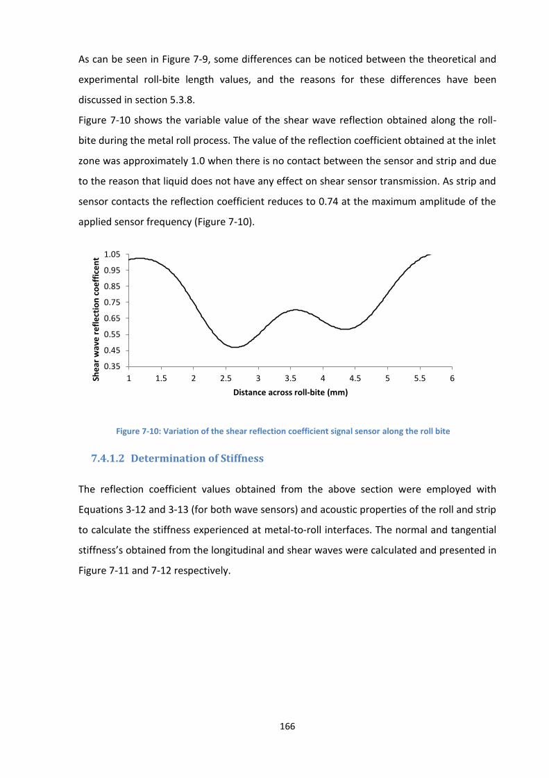
166

As can be seen in Figure 7-9, some differences can be noticed between the theoretical and

experimental roll-bite length values, and the reasons for these differences have been

discussed in section 5.3.8.

Figure 7-10 shows the variable value of the shear wave reflection obtained along the roll-

bite during the metal roll process. The value of the reflection coefficient obtained at the inlet

zone was approximately 1.0 when there is no contact between the sensor and strip and due

to the reason that liquid does not have any effect on shear sensor transmission. As strip and

sensor contacts the reflection coefficient reduces to 0.74 at the maximum amplitude of the

applied sensor frequency (Figure 7-10).

Figure 7-10: Variation of the shear reflection coefficient signal sensor along the roll bite

7.4.1.2 Determination of Stiffness

The reflection coefficient values obtained from the above section were employed with

Equations 3-12 and 3-13 (for both wave sensors) and acoustic properties of the roll and strip

to calculate the stiffness experienced at metal-to-roll interfaces. The normal and tangential

stiffness’s obtained from the longitudinal and shear waves were calculated and presented in

Figure 7-11 and 7-12 respectively.

0.35

0.45

0.55

0.65

0.75

0.85

0.95

1.05

1 1.5 2 2.5 3 3.5 4 4.5 5 5.5 6She

ar w

ave

re

fle

ctio

n c

oe

ffic

en

t

Distance across roll-bite (mm)

167

Figure 7-11: Normal stiffness obtained along the roll-bite during the rolling process

Figure 7-12: Tangential stiffness obtained along the roll-bite during the rolling process

The normal stiffness of 1.21GPa/µm and 0.36GPa/µm for the tangential stiffness values

were selected at the centre frequency, the same to the frequency where the reflection

coefficient used for the calculation was obtained.

7.4.1.3 Determination of Oil Film Thickness

As previously explained in section 3.3.4, the oil film thickness value was calculated using the

normal and tangential stiffness obtained from the reflected data of the transmitted signal

after the rolling process. The longitudinal normal stiffness contained stiffness’s from both

liquid and solid contacts while the shear stiffness contained only stiffness from solid contact

and this was expressed in equations 3-14 (a and b) in Section 3.3.4 [66]. Since liquid does not

support shear force, then Liquid shear stiffness in equation 3-14 (b) was equivalent to zero

and the shear stiffness obtained by the shear sensor was equivalent to solid shear stiffness

contact. Therefore the normal stiffness at liquid contact was obtained by equating the ratio

shear stiffness at solid contact and normal stiffness at the solid contact to the Poisson’s ratio

0.5

0.7

0.9

1.1

1.3

1.5

1.7

1.9

2.1

2.3

2.5

2 2.5 3 3.5 4 4.5 5 5.5 6

No

rmal

sti

ffn

ess

(G

Pa/

µm

)

Distance across roll-bite (mm)

0.20.25

0.30.35

0.40.45

0.50.55

0.60.65

0.7

1.5 2.5 3.5 4.5 5.5 6.5

Tan

gen

tial

sti

ffn

ess

(G

Pa/

µm

)

Distance across roll-bite (mm)

168

of the used material with the aid of equation 3-15. The oil film thickness at strip-to-roll

interface was obtained with the aid of normal stiffness at liquid contact; the oil film

thickness and Bulk modulus of the oil are expressed in equation 3-16. The oil film thickness

obtained is presented in Figure 7-13.

Figure 7-13: Oil film thickness obtained at the roll-bite during the rolling operation

7.4.1.4 Determination of Oil Film Thickness with Pulse-Echo Technique

Figures 7-14 and 7-15 show the longitudinal and shear reflection coefficients obtained from

the pulse-echo measurement technique.

Figure 7-14: Longitudinal reflection coefficient obtained from the pulse-echo measurement technique

0

0.5

1

1.5

2

2.5

3

3.5

4

2.6 3.1 3.6 4.1 4.6 5.1

Oil

film

th

ickn

ess

(µ

m)

Distance across roll-bite (mm)

0.2

0.3

0.4

0.5

0.6

0.7

0.8

0.9

1

1.1

2 2.5 3 3.5 4

Lon

g. R

efl

ect

ion

co

eff

icie

nt

Distance across roll-bite (mm)

169

Figure 7-15: Shear reflection coefficient obtained from the pulse-echo measurement technique

These values were obtained with the same approach used to determine the longitudinal and

shear reflection coefficient from the data obtained using the pitch-catch technique in

Section 7.4.1.1. The reflection coefficients obtained from this technique are of higher value

than the reflection coefficients obtained from the pitch-catch technique.

Figures 7-16 and 7-17 show the normal and tangential stiffness obtained from the

longitudinal and shear wave reflection data under the pulse-echo approach during the metal

rolling process.

Figure 7-16: Normal stiffness value obtained from the pulse-echo measurement technique

0.4

0.5

0.6

0.7

0.8

0.9

1

1.1

1.2

2 2.5 3 3.5 4

She

ar r

efl

ect

ion

co

eff

icie

nt

Distance across roll-bite (mm)

0

0.5

1

1.5

2

2.5

2 2.5 3 3.5 4

No

rmal

sti

ffn

ess

(G

Pa/

µm

)

Distance across roll-bite (mm)

170

Figure 7-17: Tangential stiffness value obtained from the pulse-echo measurement technique

Both stiffness values were calculated from the reflections obtained from the sensor using

the same approach applied to the data obtained using the pitch-catch technique in Section

7.4.1.2. The normal and tangential stiffness obtained from the pulse-echo technique are of

lower values compared with both the stiffness values obtained from pitch-catch technique

due to the higher value of the reflection coefficient obtained from the pulse-echo

measurement above.

Figure 7-18 shows the various oil film thicknesses obtained across the roll-bite using the

pulse-echo technique. These values were obtained with the same mathematical

manipulation used to obtain the oil film from the pitch-catch measurement technique in

Section 7.4.1.3.

Figure 7-18: Oil film thickness value obtained from the pulse-echo measurement technique

0

0.01

0.02

0.03

0.04

0.05

0.06

0.07

2 2.5 3 3.5 4

Tan

gen

tial

sti

ffn

ess

(G

Pa/

µm

)

Distance across roll-bite (mm)

0

0.5

1

1.5

2

2.5

3

3.5

2 2.5 3 3.5 4

Oil

film

th

ickn

ess

(µ

m)

Distance across roll-bite (mm)

171

Figure 7-19 shows the various oil film thicknesses obtained along roll-bite length contact

from both pitch-catch and pulse-echo measurement techniques under the same metal

rolling conditions.

Figure 7-19: Oil film thickness obtained from both measurement techniques

As can be seen from the figure above, the value of the oil film thickness observed t the

centre of the roll-bite using the pulse-echo technique (2.32µm) is a slightly higher than the

oil film thickness obtained from the pitch-catch (2.07µm) measurement technique. A 7.7%

higher value for oil film thickness was reported using the pulse-echo technique compared to

the pitch-catch technique.

The theoretical oil film thickness at the metal-to-roll interface was calculated using equation

2-29 in Section 2-5 with material property's itemized in Tables 5-3 and 7-1 and contact

length from equation 2-3. The theoretical oil film thickness obtained was assumed to be

constant across the roll-bite. The experimental and the theoretical values of oil film

thickness obtained are presented in Figure 7-20.

0

0.5

1

1.5

2

2.5

3

3.5

4

0.5 1 1.5 2 2.5

Oil

film

th

ickn

ess

(µ

m)

Distance across roll-bite (mm)

Oil film thickness obtained from pitch-catch technique

Oil film thickness obtained from pulse-echo technique

172

Figure 7-20: Experimental and theoretical oil film thickness obtained during the metal rolling process

As shown in Figure 7-20, there is a marginal difference between the two experimental oil

film thicknesses obtained and the theoretical result. This may be because the equation was

derived to calculate the oil film thickness at inlet section while the experimental results

show the oil film thickness at the work zone. For this reason it is expected that the

theoretical approach will report a higher value for film thickness, and this is what is

observed.

Finally, the Lambda ratio of the lubrication system was calculated using equation 2-31 in

Section 2-5 and Lambda ratio 1.8 was obtained from the oil film thickness obtained under

the pitch-catch measurement technique. The value was calculated using the experimental oil

film thickness obtained and roughness values of the strip and roll measured before the

experiment (0.87µm). The lubrication system was classified as mixed lubrication regime

since the oil film thickness value was greater than the roughness value of the surfaces.

7.4.2 Effect of Applied Rolling Loads on Oil Film Thickness Formation

Figures 7-21 and 7-22 show the reflected data obtained from longitudinal and shear wave

sensors from the different applied loads. Increasing the applied load reduces the amplitude

of the reflected signals. The reason for this reduction in the amplitude value of the reflected

wave was the increase in the metal-to-roll contact area that increases with the increase of

the rolling load. Hence, the rate of the signal transmitted through the interface increased;

0

0.5

1

1.5

2

2.5

3

Pitch-catch Pulse-echo Theoreticalapproach

Series1 2.07 2.32 2.62

Oil

film

th

ickn

ess

(u

m)

173

therefore, the low value in the amplitude wave reflection was recorded. Additionally,

reduction in reflected wave amplitude during the metal rolling was due to the increment in

rolling load that increased the contact area of metal-to-roll interface. Hence, as the loads on

the rolled metal increase, the metal-to-roll contact interface increases and more waves are

transmitted to the strip. Due to this, a reduction in the amplitude value of the reflected

waves was recorded. Figures 7-21 (for longitudinal) and Figure 7-22 (for shear) shows the

reduction in wave reflected amplitude values against the frequency of the applied sensors in

terms of the rolling loads applied.

Figure 7-21: Amplitude of longitudinal sensor reflected wave at various loadings

Figure 7-22: Amplitude of shear sensor reflected wave at various loadings

0

5

10

15

20

25

30

0 5 10 15 20

Am

plit

ud

e (

mV

)

Frequency (MHz)

Reference signal

Reflected signal at 40kN rolling load

Reflected signal at 70kN rolling load

Reflected signal at 90kN rolling load

0

5

10

15

20

25

30

35

40

0 5 10 15 20

Am

plit

ud

e (

mV

)

Frequency (MHz)

Reference signal

Reflected signal at 40kN rolling load

Reflected signal at 70kN rolling load

Reflected signal at 90kN rolling load

174

Therefore, the greater the applied load, the more the contact of the interface length and

greater reduction in the amplitude value of the reflected waves. The reflection coefficient of

the reflected data obtained at each load applied during the experiment was calculated as

explained in Section 7.4.1.1, above.

Figures 7-23 and 7-24 show the various reflection coefficients obtained from metal-to-roll

interface during the metal rolling operation with longitudinal and shear wave sensors. It is

noted that the reflection coefficient amplitude has some fringes when the roller entered or

departed from the sensor active measurement zone. The amplitude of the reflection

coefficient reduced to a minimum level at metal-to-roll contact interface. That is, when the

rolled strip is underneath the sensor, at the distance of 3.7mm to 6.9mm, for the rolling

loads applied. The Longitudinal and shear wave reflection coefficient values obtained were

reduced from 0.87 to 0.54 and 0.93 to 0.72 as the applied rolling loads increased from 40kN

to 90 kN respectively.

Figure 7-23: Reflection coefficient of the longitudinal wave sensor along the roll-bite during

Figure 7-24: Reflection coefficient of the shear wave sensor along the roll-bite during

0.4

0.5

0.6

0.7

0.8

0.9

1

1.1

2.8 3.8 4.8 5.8 6.8 7.8

Lon

g. w

ave

re

fle

ctio

n

coe

ffic

ien

t

Distance across roll-bite (mm)

Reflection coefficient at 40kN rolling load

Reflection coefficient at 70kN rolling load

Reflection coefficient at 90kN rolling load

0.5

0.6

0.7

0.8

0.9

1

1.1

1.2

2.8 3.8 4.8 5.8 6.8 7.8

she

ar w

ave

re

fle

ctio

n

coe

ffic

ien

t

Distance across roll-bite (mm)

Reflection coefficient at 40kN rolling loadReflection coefficient at 70kN rolling loadReflection coefficient at 90kN rolling load

175

The overlapping signals can be seen to contain some shoulders during application of the

rolling loads at 3.3mm (right hand side) and 7.2mm (left hand side) along the roll-bite length

in Figures 7-23 and 7-24 respectively. Additionally, the obtained reflected signals change at

the shoulder as can be seen in the graphs with respect to the loads. The reason for the

reaction of the signals to load increment at these points is not well understood. However,

the center values of the graph are the main focus of this is research and these centre values

conform adequately to changes in the applied rolling loads.

The reflection coefficients from the applied sensors against the loads during the cold metal

rolling are processed by the same method explained in Section 7.4.1.1, and obtained results

are shown in Figures 7-25 and 7-26.

Figure 7-25: The reflection coefficient of longitudinal wave sensor against deformation loads

Figure 7-26: The reflection coefficient of shear wave sensor against deformation loads

0.4

0.5

0.6

0.7

0.8

0.9

35 45 55 65 75 85 95

Lon

g. W

ave

re

fle

ctio

n

coe

ffic

ien

t

Load (kN)

0.65

0.7

0.75

0.8

0.85

0.9

0.95

35 45 55 65 75 85 95

She

ar w

ave

re

fle

ctio

n c

oe

fici

en

t

load (kN)

176

As explained in the previous section, the more the rolling load increase, the more the plastic

and elastic deformation at strip-to-roll interface increases. Hence the greater transmission

of signals from the roll to strip and the less reflected signal obtained during the rolling

process. It can also be observed that there is a decrease in the values at the tail end due to

the high rolling load applied, which leads to low reflection coefficient value (Figure 7-25).

This gradual tailing-off is due to the large signals transmitted to the strip during the rolling

operation.

Furthermore, the experimental values of the longitudinal and shear stiffness at the metal-to-

roll interface were calculated with the same approach employed in Section 7.4.1.2, and the

obtained results are presented in Figures 7-27 and 7-28 respectively.

Figure 7-27: Normal stiffness obtained from the longitudinal wave sensor at the roll – bite

Figure 7-28: Tangential stiffness obtained from shear wave sensor at the roll - bite

0.3

0.8

1.3

1.8

2.3

2.8

3.5 4.5 5.5 6.5 7.5

No

rmal

sti

ffn

ess

(G

Pa/

µm

)

Distance across roll-bite (mm)

Normal stiffness obtained at 40kN rolling load

Normal stiffness obtained at 70kN rolling load

Normal stiffness obtained at 90kN rolling load

0

0.05

0.1

0.15

0.2

0.25

0.3

0.35

0.4

0.45

0.5

3.2 4.2 5.2 6.2 7.2

Tan

gen

tial

sti

ffn

ess

(GP

a/µ

m)

Distance across roll-bite (mm)

Tangential stiffness obtained at 40kN rolling load

Tangential stiffness obtained at 70kN rolling load

Tangential stiffness obtained at 90kN rolling load

177

Figures 7-29 and 7-30, show the values of the normal and tangential stiffness plotted against

the loads applied respectively.

Figure 7-29: Normal stiffness and applied deformation load relationship

Figure 7-30: Tangential stiffness and applied deformation load relationship

The normal and tangential stiffness’s were found to be in an approximately linear

relationship with the applied loads during the rolling process. That is, the stiffness value

0.6

0.8

1

1.2

1.4

1.6

1.8

2

35 45 55 65 75 85 95

No

rmal

sti

ffn

ess

(G

Pa/

µm

)

Load (kN)

0.1

0.15

0.2

0.25

0.3

0.35

35 45 55 65 75 85 95

Tan

gen

tial

sti

ffn

ess

(G

Pa/

µm

)

Load (kN)

178

increases as the applied rolling load increases due to increased closeness of the gap in the

contact interface area of the metal-to-roll during the increment of the applied load.

The normal and tangential stiffness value obtained were used with the method employed in

Section 7.4.1.3, to determine the oil film thickness formed at the metal-to-roll interface

under the various loads applied and presented in Figure 7-31.

Figure 7-31: Oil film thickness formed at the roll - bite during the rolling process.

The oil film values obtained were plotted against the loads applied during the rolling process

and is shown in Figure 7-32.

Figure 7-32: Oil film against the loads applied

0

0.5

1

1.5

2

2.5

3

3.5

4

4.2 4.7 5.2 5.7 6.2 6.7

Oil

film

th

ickn

ess

(µ

m)

Distance across roll-bite (mm)

Oil film thickness obtained at 40kN rolling load

Oil film thickness obtained at 70kN rolling load

Oil film thickness obtained at 90kN rolling load

1.2

1.4

1.6

1.8

2

2.2

2.4

2.6

2.8

3

35 45 55 65 75 85 95

Oil

film

th

ickn

ess

(µ

m)

Load (kN)

179

It is clearly shown in Figure 7-32 that as the applied rolling loads increase, oil film thickness

at the strip-to-roll interface gradually decreases. This is because the increase in the applied

loads causes an increase in the contact at the metal-to-roll interface. In addition, this leads

to the reduction in the volume of the oil that is drawn into the roll surface and causes a

decrease in the thickness of the oil at the strip-to-roll interface during the process.

Furthermore, the oil thickness was theoretically calculated as explained before in Section

7.4.1.3, with the values of 0.48mm, 0.72mm and 1.2mm metal reduction observed under

the rolling loads applied. The difference between the theoretical and experimental oil

thickness obtained are presented in Figure 7-33.

Figure 7-33: Theoretical and experimental oil film thicknesses obtained under the various rolling loads

As shown in Figure 7-33, there is little variation between the theoretical and the

experimental value of the oil film thickness presented. This may be due to the effect of the

lubricating oil properties which can be varied from the ideal properties used for the

prediction formulae. Additionally, the oil film thickness values obtained from the theoretical

approach are the oil film at the inlet zone while experimental values are from the work zone

respectively. However, both values obtained from the two methods are reasonably close

within ranges of accuracy. There ranges are, 12.6% for 40kN, 6.0% for 70kN and 7.0% for

90kN.

Finally, lambda ratio of the lubrication system was calculated as explained Section 7.4.1.3,

last paragraph and presented in Table 7-2.

40kN 70kN 90kN

Experimental value (um) 2.84 2.32 1.27

Theoretical value (um) 3.2 2.46 1.36

0

0.5

1

1.5

2

2.5

3

3.5

Oil

film

th

ickn

ess

(µ

m)

180

Table 7-2: Lambda ratio value obtained during the experiment

Loads

(kN)

Lambda

ratio

Lubrication

regime

40 2.47 Mixed

70 2.02 Mixed

90 1.10 Mixed

As can be seen, the various loads applied for the different metal reduction processes during

the rolling operation are operating within the mixed lubrication regime.

7.4.1 The Investigation of Roll Speed on the Oil Film Thickness Formation

The effect of roll speeds was investigated on the formation of oil film thickness under

various rolling loads with the aid of the ultrasonic reflection measuring technique in this

section. The experiments were conducted using two different values of roll speeds (19 and

26 mm/sec) under the 40kN and 70kN rolling loads respectively. The captured data from the

reflected waves were used to calculate the thickness of the oil film at roll-bite during the

rolling process.

7.4.1.1 The 19mm/sec and 26mm/sec Roll Speeds at 40kN Rolling Load

The reflected wave data received from the metal-to-roll interface during the application of

the same rolling load (40kN) to 19mm/sec and 26mm/sec roll speeds were analyzed and

presented in Figures 7-28 and 7-29 respectively. As explained in Section 7.4.2, pressure on

the metal-to-roll interface increases with increasing rolling load while it decreases with

increasing rolling speed. This can be seen clearly from the increasing of the wave reflected

amplitude obtained at various speeds under the same rolling load (Figures 7-34 and 7-35).

These Figures show the increasing of the amplitude value of the reflected wave with the

increasing of applied roll speed and this was due to the increases of the lubrication

resistance during the rolling process. This increase of the roll speed also caused the

increasing frictional resistance within the layer of oil and separated the strip-to-roll interface

during the rolling process [105]. Additionally, an increase in roller speed also increases the

volume of oil drawn into the contact surface and reduces the contact length of the two

surfaces. Therefore, the higher the rolls speed, the higher the amplitude value of the

181

reflected wave. This was experienced from the two applied sensors under the same applied

rolling loads.

Figure 7-34: Amplitude of longitudinal reflected wave at 40kN applied rolling load

Figure 7-35: Amplitude of shear reflected wave at 40kN applied rolling load

As previously explained and calculated in Section 7.4.1.1, the reflection coefficients of the

reflected signal was obtained by dividing the amplitude of the reflected signal by the

0

5

10

15

20

25

30

0 5 10 15 20

Am

plit

ud

e (

mV

)

Frequency (MHz)

Reference signal

Reflected signal @ 19mm/sec roll speed

Reflected signal @ 26mm/sec roll speed

0

5

10

15

20

25

30

35

40

0 5 10 15

Am

plit

ud

e (

mV

)

Frequency (MHz)

Reference signal

Reflected signal @19mm/sec roll speed

Reflected signal @26mm/sec roll speed

182

amplitude of the reference signal. The reflection coefficient obtained from the reflected

data captured by these roll speeds was compared with the aid of the Figures 7-36 and 7-37

Figure 7-36: Reflection coefficient of the reflected wave at 40kN applied rolling load

Figure 7-37: Reflection coefficient of the reflected wave at 40kN applied rolling load

0

0.1

0.2

0.3

0.4

0.5

0.6

0.7

0.8

19mm/sec rollspeed

26mm/sec rollspeed

Series1 0.65 0.8

Lon

g. w

ave

re

fle

ctio

n c

oe

ffic

ien

t

0

0.1

0.2

0.3

0.4

0.5

0.6

0.7

0.8

0.9

1

19mm/sec roll speed 26mm/sec roll speed

Series1 0.73 0.93

She

ar w

ave

re

fle

ctio

n c

oe

ffic

ien

t

183

As can be seen from these Figures, as the roll speeds increased the longitudinal and shear

reflection coefficient values of the reflected waves obtained increased under the same

rolling load. The reason for this is explained in more detail below.

Furthermore, the various longitudinal reflection coefficient values obtained along the roll-

bite are shown in Figure7-38 while the shear reflection coefficient obtained is also shown in

Figure 7-39 respectively. The higher the roll speed the more lubricant is penetrated into the

interface, then the lesser the contact length due to the separation of the interface by the

penetrated oil. Additionally, the reduction in the surface asperity contact was experienced

and less wave transmission occurred and the high reflection coefficient value was recorded.

As shown in Figure 7-38, the longitudinal reflection value at 19mm/sec is 0.67, while it

increased to 0.83 at 26mm/sec roll speed. Also, Figure 7-38 shows the increases of shear

reflection coefficient from 0.64 at 19mm/sec to 0.85 at 26mm/sec roll speed. In addition,

the increase of the roll speed has a significant effect on the roll-bite contact length as shown

in the figures. This was due to more volume of the lubricant flowing into the metal-to-roll

interface and causing the separation of the interface thereby creating more film thickness

along the roll-bite. The higher the separation of the contact surface, the lesser the roll-bite

length obtained.

Figure 7-38: Reflection coefficient of the reflected wave along the roll-bite at 40kN rolling load

0.35

0.45

0.55

0.65

0.75

0.85

0.95

1.05

1.15

5.3 6.3 7.3 8.3 9.3 10.3 11.3

Lon

g. w

ave

re

fle

ctio

n c

oe

ffic

en

t

Distance across roll-bite (mm)

Reflection coefficent of the reflected wave @ 19mm/sec roll speed

Reflection coefficent of the reflected wave @ 26mm/sec roll speed

4.10mm

3.19mm

184

Figure 7-39: Reflection coefficient of the reflected wave along the roll-bite at 40kN rolling load

As shown in Figures 7-38 and 7-39, the length of the roll–bite was located in the middle of

these figures as previously explained in Section 7.4.1.1. The length of the roll-bite obtained

at 19mm/sec was larger than the length of the roll-bite achieved at the 26mm/Sec under the

same rolling load. This was due to the reason explained above.

In addition, the normal and tangential stiffness values of the strip-to-roll interface were

calculated with the same approach explained in Section 7.4.1.2. This was done for the

reflected data obtained for both the 19mm/sec and 26mm/sec roll speeds under the same

applied rolling load of 40kN and the obtained results are presented in Figures 7-40 and 7-41.

Figure 7-40: Normal stiffness of the reflected wave along the roll-bite at 40kN applied rolling load

0.35

0.45

0.55

0.65

0.75

0.85

0.95

1.05

1.15

4.8 5.8 6.8 7.8 8.8 9.8 10.8

She

ar w

ave

re

fle

ctio

n c

oe

ffic

en

t

Distance across roll-bite (mm)

Reflection of the reflected wave @ 19mm/sec roll speed

Reflection of the reflected wave @ 26mm/sec roll speed

-0.5

0

0.5

1

1.5

2

2.5

3

5.8 6.8 7.8 8.8 9.8

No

rmal

sti

ffn

ess

(G

Pa/

µm

)

Distance across roll-bite (mm)

Normal stiffness obtained @ 19mm/secroll speed

Normal stiffness obtained @ 26mm/secroll speed

4.10mm

3.17mm

185

Figure 7-41: Tangential stiffness of the reflected wave along the roll-bite at 40kN applied rolling load

The values of both stiffness’s obtained at the applied sensors under the same rolling load are

reduced as the roll speed increased, due to the reason already explained above.

Finally, the oil film thickness formed at metal-to-roll interface was calculated with the same

methods explained in Section 7.4.1.3, under various roll speeds and presented in Figure 7-

42.

Figure 7-42: Oil film thickness obtained at roll-bite during the rolling process

0

0.1

0.2

0.3

0.4

0.5

0.6

0.7

0.8

0.9

5.8 6.8 7.8 8.8 9.8

Tan

gen

tial

sit

ffn

ess

(G

Pa/

µm

)

Distance across roll-bite (mm)

Tangential stiffness obtained @ 19mm/sec roll speed

Tangential stiffness obtained @ 26mm/sec roll speed

0

0.5

1

1.5

2

2.5

3

3.5

4

4.5

5

6.7 7.2 7.7 8.2 8.7 9.2

Oil

film

th

ickn

ess

(µ

m)

Distance across roll-bite (mm)

Oil film thickness obtained @ 19mm/sec roll speed

Oil film thickness obtained @ 26mm/sec roll speed

186

The difference of the oil film thickness obtained from the roll speed applied during the metal

rolling process is obvious as shown in the figure above due to the reason explained earlier.

The higher the roll speed, the higher the oil film thickness obtained.

Finally, the theoretical oil film thickness was calculated with the same approach used in

Section 7.4.1.3, and the obtained results were compared with the experimental value and

are presented in Figure 7-43.

Figure 7-43: Theoretical and experimental oil film thickness obtained at 40kN rolling load

As can be seen from Figure 7-43, the oil film thickness obtained from both the theoretical

and experimental values is of the same trend. That is, the value of oil thickness increases

with the increase of the roll speed. Although, the theoretical oil thickness value obtained at

lower speed was higher than the experimental value, due to the reason mentioned earlier in

Section 7.4.1.3, but they both followed the same incremental trend of the subsequent

increase in roll speed.

7.4.1.2 The 19mm/sec and 26 mm/Sec Roll Speed at 70kN Rolling Load

As explained in Section 7.4.3, the effect of 19mm/sec and 26mm/sec roll speeds on film

thickness under the same 40 kN rolling load were studied. The results obtained from these

conditions were analysed and presented in the above section. These loads were increased to

187

70kN under the 19mm/Sec and 26mm/sec roll speeds and their effect on the oil film

thickness was studied in this section.

The behavioural trend of the increased amplitude was observed with 70kN applied rolling

load, as compared to 40kN rolling load in Section 7.4.3.1. However, some level of marginal

difference in their values occurred. In the 70kN rolling load the amplitude value of the

reflected signal increases from 19mV to 23mV (Figures 7-44) and 26mV to 32mV (Figure 7-

45) for longitudinal and shear wave sensors from the 19mm/sec to 26mm/sec roll speeds,

while the amplitude value of the reflected signal increases from 17mV to 21mV and 25mv to

31mV for both longitudinal and shear wave sensors under same mentioned roll speeds of

40kN applied rolling load.

Figure 7-44: Amplitude of longitudinal reflected wave at 70kN applied rolling load

Figure 7-45: Amplitude of shear reflected wave at 70kN applied rolling load

0

5

10

15

20

25

30

0 20 40 60 80 100

Am

plit

ud

e (

mV

)

Frequency (MHz)

Reference signal

Reflected signal at 19mm/sec roll speed

Reflected signal at 26mm/sec roll speed

0

5

10

15

20

25

30

35

40

0 5 10 15 20

Am

plit

ud

e (

mV

)

Frequency (MHz)

Reference signalReflected signal at 19mm/sec roll speedReflected signal at 26mm/sec roll speed

188

The reflection coefficient of the wave reflected during the rolling processes was calculated

for both applied sensors by the same method applied in section 7.4.1.1. The obtained values

of the reflection coefficient from both sensor waves employed at the various roll speeds

under the same rolling load were presented in Figures 7-46 and 7-47.

Figure 7-46: Reflection coefficients among the various roll speeds at 70kN rolling load

Figure 7-47: Reflection coefficients among the various roll speeds at 70kN rolling load

0

0.1

0.2

0.3

0.4

0.5

0.6

0.7

0.8

0.9

19mm/sec roll speed 26mm/sec roll speed

Series1 0.72 0.89

Lon

g. w

ave

re

fle

ctio

n c

oe

ffic

ien

t

0

0.1

0.2

0.3

0.4

0.5

0.6

0.7

0.8

0.9

1

19mm/sec roll speed 26mm/sec roll speed

Series1 0.74 0.94

She

ar w

ave

re

fle

ctio

n c

oe

ffic

ien

t

189

As indicated in the above figures, the values of the reflection coefficients of the waves were

found to increase as the roll speed increased under the same rolling load.

Additionally, the various reflection coefficient value along the roll-bite were extracted with

the aid of the LabVIEW program in terms of Time-of-Flight in the roll-to-metal interface for

both roll speeds and the same rolling load applied. The obtained Time-of-Flight was used

with the roll speed employed to determine the roll-bite length with the aid of the ToF

ultrasonic formulae for both sensor waves employed and presented in Figures 7-48 and 7-

49.

Figure 7-48: Reflection coefficients obtained along roll-bite at various roll speeds at 70kN load

Figure 7-49: Reflection coefficients obtained along roll-bite at various roll speeds at 70kN load

0.35

0.45

0.55

0.65

0.75

0.85

0.95

1.05

5 7 9 11

Lon

g. w

ave

re

fle

ctio

n c

oe

ffic

en

t

Distance across roll-bite (mm)

Reflection coefficent at 19mm/sec roll speed

Reflection coefficent at 26mm/sec roll speed

0.4

0.5

0.6

0.7

0.8

0.9

1

1.1

1.2

4 6 8 10 12

She

ar w

ave

re

fle

ctio

n c

oe

ffic

en

t

distance across roll-bite (mm)

Reflection coefficent of reflected wave at 19mm/sec roll speed

Reflection coefficent of reflected wave at 26mm/sec roll speed

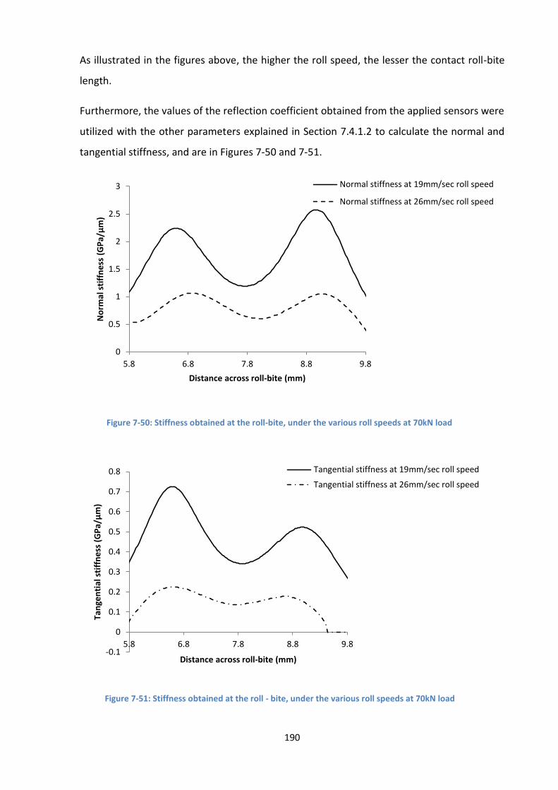
190

As illustrated in the figures above, the higher the roll speed, the lesser the contact roll-bite

length.

Furthermore, the values of the reflection coefficient obtained from the applied sensors were

utilized with the other parameters explained in Section 7.4.1.2 to calculate the normal and

tangential stiffness, and are in Figures 7-50 and 7-51.

Figure 7-50: Stiffness obtained at the roll-bite, under the various roll speeds at 70kN load

Figure 7-51: Stiffness obtained at the roll - bite, under the various roll speeds at 70kN load

0

0.5

1

1.5

2

2.5

3

5.8 6.8 7.8 8.8 9.8

No

rmal

sti

ffn

ess

(G

Pa/

µm

)

Distance across roll-bite (mm)

Normal stiffness at 19mm/sec roll speed

Normal stiffness at 26mm/sec roll speed

-0.1

0

0.1

0.2

0.3

0.4

0.5

0.6

0.7

0.8

5.8 6.8 7.8 8.8 9.8

Tan

gen

tial

sti

ffn

ess

(G

Pa/

µm

)

Distance across roll-bite (mm)

Tangential stiffness at 19mm/sec roll speed

Tangential stiffness at 26mm/sec roll speed

191

As shown in the figures above, the values of both normal and tangential stiffness are

reduced as the applied roll speed increased under the same 70kN of the rolling load.

The film that was obtained under the same applied rolling load with various roll speeds were

calculated with the same procedure applied in Section 7.4.1.3. The oil film thickness values

obtained from these various roll speeds are presented in Figure 7-52.

Figure 7-52: Oil film thickness at roll-bite during the various roll speeds at 70kN rolling load

The theoretical oil film thickness computation employed in Section 7.4.1.3 was used in this

section and the theoretical results obtained were compared with the experimental values

and presented in Figure 7-53.

Figure 7-53: Experimental and theoretical oil film thickness obtained at various roll speeds under 70kN load

0

0.5

1

1.5

2

2.5

3

3.5

4

5.8 6.8 7.8 8.8

Oil

film

th

ickn

ess

(µm

)

Distance across roll-bite (mm)

Oil film thickness obtained @ 19mm/sec roll speed

Oil film thickness obtained @ 26mm/sec roll speed

192

As it can be seen in the figure above, the experimental and the theoretical oil film thickness

values have the same response to the increment of the roll speed under the same rolling

load applied. The theoretical oil film thicknesses obtained were found at the higher values of

the graph due to the reason explained in Section 7.4.1.3.

Finally, Figure 7-54, shows the combination of the obtained results from 19mm/sec and

26mm/sec under the rolling loads of 40kN and 70kN for the comparison of the acquired oil

film thickness values.

Figure 7-54: Experimental oil film thickness obtained at various roll speeds under 40kN and 70kNplied loads

It is clearly shown in Figure 7-54 that the oil film thickness obtained from the various applied

roll speeds is different under the same rolling loads applied to them during the rolling

process. As explained in the previously, an increase in roll speed permits more volume of

lubricant oil to be drawn into the metal-to-roll interface. This causes a separation of the

interface and causes the reduction of the contact length of the roll-bite. This leads to the

increase in of the oil film thickness at the roll - bite. As it can be seen in the above figure, the

higher the roll speed, the higher the thickness of the oil film on roll-bite.

Furthermore, as previously discussed in Section 7.4.1, low reflection coefficient means that

high pressure was applied to the metal-to-roll interface. As the rolling load increases, the

pressure on the metal-to-roll interface increases, while it decreases with increasing roll

speed. This can be seen clearly from Figure 7-54 where at low rolling load, the pressure is

1

1.5

2

2.5

3

3.5

18 20 22 24 26 28

Oil

film

th

ickn

ess

(µ

m)

Speed roll (mm/sec)

Oil film thickness obtained at 40kN rolling load

Oil film thickness obtained at 70kN rolling load

193

low and thus the lubricant penetrates more to the interface and results in high oil film

thickness value. At high rolling load the lubricant has less chance to penetrate to the metal-

to-roll interface due to the high pressure on their surfaces caused by the plastic and elastic

deformation of the asperity contact. Thus a low value of the oil film thickness is recorded at

the same roll speed due to the high rolling load involved. That explains the variation in the

oil film thickness values obtained at the same roll speed under different applied rolling

loads. The value of 3.05µm oil film thickness was obtained at 26mm/sec roll speed under the

40kN rolling load while 2.4µm was also obtained under the same roll speed but with 70kN

rolling load. Therefore, both rolling load and roll speed have a significant effect on the

formation of oil film thickness at the roll - bite during metal rolling operation.

7.5 Comparison with the literature

Dwyer-Joyce and Hunter [66] applied internal ultrasonic sensors fitted in the work roll to

measure the oil film thickness formed between the roll and strip interface during the metal

rolling operation. As discussed in their study, the experiment was conducted with Gerolub

lubricating oil, which is also the lubricating oil employed for conducting the experiments in

our research.

Table 7-3, includes the experimental rolling conditions and oil film thickness values obtained

from theoretical calculations, from the proposed method developed in this research with

experimental procedure explained in Section 7.2.3, as well as those obtained from Dwyer-

Joyce and Hunter [66].

Table 7-3: Applied techniques with their rolling conditions observed

Techniques Experimental Conditions Oil film thickness (µm)

Hunter [66]

387mm roll diameter, 1666.7mm/s roll speed,

2.8mm strip thickness, 100mm strip width,

490mm strip length, 10% metal reduction,

0.77µm and 1.88µm roll and strip roughness

value.

1.72

Pitch-catch Shown in Table 7-1 2.07

Theory (Equation 2-29)

Shown in Tables 5-3 and 7-1 2.63

194

Dwyer-Joyce and Hunter [66] carried out the investigation with an industrial rolling mill and

IF steel described in Section 5.4. for rolling conditions listed in Table 7-3. The variation of the

experimental oil film thickness obtained along the roll-bite distance with the Dwyer-Joyce

and Hunter [66] approach is shown in Figure 7-55.

Figure 7-55: Oil film thickness obtained by the internal ultrasonic sensor layout arrangement [66]

As can be seen from Figure 7-55, the variation of the oil film thickness against distance

across the roll-bite has the same trend as that obtained with the applied technique in this

research shown in Figure 7-13. Both results show a clear double dip, despite the fact that

there is a difference in the rolling parameter conditions involved. The comparison between

the oil film thickness obtained from this research and the theoretical value is shown in

Figure 7-20 of Section 7.4.1.4. The reasons for the differences are also discussed.

As can be seen from the comparison Table 7-3, there is a difference of 16% between the oil

film thickness obtained from this research and the oil film value measured by Dwyer-Joyce

and Hunter [66]. The differences observed between the two experimental results above are

due to the variation in the rolling parameter conditions used during the investigation as

shown in Table 7-3.

Furthermore, the higher value of oil film thickness obtained in this research may also have

been due to the fact that a pilot mill which operated under lower rolling load was employed

in this research; this contrasts with the industrial mill operated under higher rolling load

used by Dwyer-Joyce and Hunter [66]. The higher the rolling load, the lower the oil film

thickness obtained.

0

1

2

3

4

5

-5 -3 -1 1 3 5

Oil

film

th

ickn

ess

(µ

m)

Distance from centre of roll-bite (mm)

10% metal reductionwith 100m/min

195

The results strongly imply the measurement reliability of the system: the oil film thickness

obtained from both techniques only differed slightly; and both revealed similar double-dip

shapes on the graphs. The external ultrasonic technique employed by this research is

accurate enough with only a minor deviation in the oil film thickness obtained using the

experimental approach when compared with the theoretical approach. It is, however,

difficult to compare the accuracy of the oil film thickness values obtained in [66] with the

values obtained in our research because of the difference in the rolling parameter

conditions.

It can be concluded that the order of magnitude indicates that the oil film thickness

obtained in this research work conforms to expectations from the literature. Additionally,

the values of oil film thickness obtained are in the same range as those obtained with other

experimental measurement techniques reviewed in the literature and shown in Table 2-5,

Section 2.6.4. Finally, the experimental results obtained are in good agreement with the

results obtained from the theoretical predictions shown in Figure 7-20.

Furthermore, when the film thickness values obtained for various ranges of applied loads

and roll speeds were compared with the results obtained from the literature [65, 106], it can

be observed that the film thickness was dependent on the sliding speed at the contact. This

showed good agreement with the results obtained in the investigation reported in [65, 106],

which studied the effect of load and roll speed on the formation of an oil film at metal-to-

roll interface. In particular, as the roll speed increased, more oil was trapped by the work roll

which then flowed into the interface space during the rotation of the work rolls. Because of

this, the oil film thickness of the lubricating oil applied also increased at the metal-to-roll

interface during the rolling process (Figure 7-54). Additionally, as the applied rolling loads

increased, the film thickness obtained at the metal-to-roll interface decreased (Figure 7-31).

Therefore, the comparison of the results obtained from this layout with the results obtained

from the theoretical predictions as well as the those from the literature with different

measurement techniques have shown that the proposed technique is indeed a promising

measurement approach. As explained above, this external sensor layout configuration used

in this research has shown that this arrangement does not result in markings on the rolled

product surface under large contact pressure when compared with the existing techniques.

As such, the experimental methodology is suitable for real-time measurements of oil film

thickness in metal-to-roll interface in industrial mills.

196

7.6 Conclusion

This study was set up to measure the oil film thickness and monitor the effect of rolling

parameters on the formation of oil film thickness at the metal-to-roll interface during the

rolling process. The measurement was done with the aid of a novel oblique ultrasonic

technique. As previously explained, the ultrasonic sensors were located on both sides of the

roll at an angle to each other. The sound waves were allowed to propagate through the roll

and reflected at metal-to-roll interface during the rolling process. The reflections of the

waves were processed and used for the film thickness calculation during the rolling

operation. This process of capturing the wave reflection was used to conduct experiments

with different rolling conditions. The reflection coefficients of the reflected wave processed

were recorded for further uses. The following deductions are drawn from the experiments

conducted and reported in this chapter:

This study has shown the ability to use the ultrasonic reflection to measure the oil

film thickness at metal-to-roll interface during the metal rolling process;

The results in this chapter indicate that the oil film thickness formation is varied

under applied rolling loads;

This study indicates that roll speeds have a significant effect on the formation of oil

film thickness at metal-to-roll interface during the rolling process;

The oil film measurement was carried out without any damage of the roll and strip

surfaces;

Good correlation between normal and oblique oil film thicknesses was obtained.

197

Chapter 8

Conclusions and Recommendations

8.0 Novelty of the Work

This study has clearly demonstrated the feasibility of using non-invasive sensors on rolling

mills, not only for research purpose, but more importantly, the solution found can be

reliably transferred to industry.

Although previous work showed that ultrasonic sensors could be embedded into a roll, there

were clear limitations, which have been overcome in this work. Rolls only require minor

modifications in areas not affecting the rolling process of the strip, especially the surface

integrity of the rolled material. Holes drilled into the roll could also affect its integrity with

fatigue cracks potentially developing over time. Collapse of the embedded plug is not a

problem anymore, with sensors easily and securely mounted onto the roll.

The proposed solution makes use of a pitch-catch ultrasonic measurement technique, as

opposed to a pulse-echo method, with a new experimental procedure which has been

successfully developed and implemented. Results in terms of interface conditions (oil film

thickness, roll bite length and strip thickness) measurements have been verified against

theoretical predictions as well as with the pulse-echo technique (for oil film thickness) to

demonstrate the robustness of the new procedure.

8.1 Development of External Sensor Arrangement

Metal forming is one of the backbones of many metal industrial developments. Metal

forming plays a major part in the provision of employment and development of numerous

steel companies that directly and indirectly depend on it. It is therefore pertinent that metal

forming analytics and procedure receives attention from the research and development

community. Metal rolling is one the major metal forming processes, is the process of

reducing the metal thickness through the gap between the two adjacent rolls. This is due to

the coefficient friction which develops between the rolls and metal surfaces. Several

attempts by different scholars have been made to measure the coefficient of friction at the

roll-bite. The excess of the friction experienced at the metal-to-roll interface has a significant

198

harmful side effect on both roll and rolling metal surfaces. It is also a problem if it is not high

enough because the metal will be slippery at roll-bite during the rolling process. Therefore,

for the purpose of surface cooling and controlling of the friction at the metal-to-roll

interface a lubricant is introduced. The oil thickness of this interface is necessary to achieve

the required friction.

8.1.1 Implementation of the Technique

The measurement of the oil film thickness at the metal-to-roll interface is needed to control

the friction strength at the metal-to-roll interface and also to reduce the amount of energy

wasted during the metal rolling process [18]. This has been a problem due to the harsh

nature of cold rolling that makes implementing sensors in industrial applications difficult [5].

Additionally, the negative effect of roll modification on the potential of the rolling process

makes instrumentation of cold rolling mills difficult.

In this research, two non-invasive methods, with no need to insert a sensor plug into the roll

to measure the oil film and strip thickness at the metal-to-roll interface were developed and

studied (Chapter 4). The two methods were based on the external arrangement of the

longitudinal and shear wave sensors. In the first method, sensors were mounted on the

sensor carrier before coupling with gel into the model roll and its signal transmission was

based on the pulse-echo technique. The signals generated from the sensor were transmitted

through the sensor carrier and model roll before reflecting from the back surface of the

model roll and received by the same sensor. In the second method, the signal transmission

process was based on the pitch-catch technique. The sensors were mounted on both sides

of the roll at an angle to each other; one of the sensors acts as a pulser while the other one

acts like a receiver. The signals generated from the pulser were transmitted through the

model roll and reflected back from its surface before being captured by the receiver sensor

on the other side of the model roll. The wave reflection obtained from both approaches was

studied.

The first method with the sensor carrier was found to perform below expectations due to

the interfaces between the sensor carrier and model roll before reaching the back of the

model roll (Figure 4-3). In addition, the amplitude of the reflected signal was smaller than

the amplitude of the noise obtained on the back surface of the 110mm roll model with the

high value of the pressure applied during the signal transmission process (Figure 4-12). The

199

signal-to-noise ratio was less than 1:1 and the noise totally masked by the shear wave

reflection. The technique is a highly attenuated process with high signal energy loss during

the transmission operation. Furthermore, the rapid attenuation of the shear wave within the

coupling gel at the sensor carrier to model roll interface is another challenge that affects the

transmission of the shear waves throughout the sensor carrier to the model roll. Shear

waves only propagate very well in an acoustic solid material, while it was not effectively

propagated in a liquid or gas medium. Therefore, with the high 20kN pressure applied during

this investigation, no reflected wave was received from the back surface of the employed

roll model (Figure 4-17).

The second method, which is pitch-catch, was concluded to be the best transmission process

technique because a high energy of the reflected signal was received at the back surface of

the model roll with little or no pressure applied during the signal transmission (Figure 4-21).

This resulted in a high signal-to-noise ratio achieved from both sensors applied through the

layout configuration. The process is a less attenuated signal transmission operation.

Additionally, in this technique the sensor was mounted directly on the model roll without

any interface (Figure 4-18), which was easier for the shear wave to transmit through the roll

model (Figure 4-22).

Finally, the oblique reflection technique was selected out of the two mentioned techniques

due to the explanation given above. The technique was installed into the pilot roll mill and

tested (Chapter 5). The Time-of-Flight of the reflected wave obtained through this

technique, was used to determine the strip thickness in both stationary (Figure 5-9) and

dynamic (Figure 5-16) modes. It also studied the effect of loads on the Time-of-flight of

ultrasonic reflection at the back of the strip during the rolling operation (Figures 5-22 and 5-

23). Finally, it was applied to measure the roll-bite length during the metal rolling process

(Figure 5-32).

8.1.2 Analysis of the Oblique Reflection Technique

This technique was modelled and analysed with the aid of MatLab scripts written by Li [99]

that were modified to suit the purpose of this project. The aim is to compare the reflection

coefficients obtained from the ultrasonic signal sent at different incidence angles. The

simulations were run for longitudinal waves at incidence angles of 0o and 19o for two

different values of rolling loads.

200

The maximum reflection coefficient value of 0.9 was obtained from the embedded layer at

0o angles of incidence (Figure 6-6). This is followed by reflection coefficient values of 0.82

obtained at 19o angle incidences at the same 2.32m and 1.27m embedded thickness

layers. Minor changes in the reflection coefficient values of 0.08 were clearly shown as the

angle of the incidences as it increased from 0o to 19o respectively.

The experimental validation of this analysis was conducted by transmitting the incidence

waves at 19o with pitch-catch and pulse-echo (0o of incidence angle) techniques in a dynamic

mode. The investigations were conducted under 70kN and 90kN applied rolling load. The

reflected wave of the sent signal at this condition was captured, processed and studied.

A little difference was observed between the reflection coefficient of the reflected signal

and the stiffness values obtained from both techniques under the same applied loads

respectively. The difference in the results obtained from both techniques is negligible,

because they are small values. Due to this reason, pulse-echo mathematical computation

approaches were employed to calculate the pitch-catch technique. Also, based on the

outcome and the recommendation of a researcher that has already worked on similar

research, the longitudinal reflection coefficients obtained at a 19o angle of incidence wave

are similar to those obtained at a normal incidence longitudinal wave [98].

8.1.3 Application of the Chosen Technique

Finally, this technique was applied during the cold metal rolling process to measure and

study the effect of rolling parameters on the formation of oil film thickness at the metal-to-

roll interface.

The followings are the main findings drawn:

The thicknesses of the rolled strip were successfully measured with dynamic position.

The three differences of the strip samples were rolled from the initial thickness of

5mm value in and 4.40mm, 4.04mm and 3.71mm experimental values while the

obtained measured values are 4.52mm, 4.28mm and 3.80mm. The accuracy of the

measured values of the three samples are; 2.7%, 5.9% and 1.39%, which shows a

good agreement with standard measuring devices (Fig. 5-27).

The technique was applied to the measurement of the roll-bite length during the

metal rolling process. The value of the 5.59mm was experimentally obtained while

201

the computed value was 6.29mm. The accuracy of the obtained value compared with

the mathematical prediction value is 12.5%, shows the validity of the technique for

the measurement of the roll-bite during the metal rolling process (Fig. 5-33).

It was apparent from the experimental results obtained that the angle of incidence

has a minor effect on the stiffness’s value obtained from both ultrasonic

measurement techniques. These were in good agreement with that seen from

scholars during their investigations.

The difference in reflection coefficients obtained from the modelling of angles of

incidence is more noticeable than the experimental value. The reasons for these

differences were not clear.

The oil film thicknesses at the metal-to-roll interface were successfully measured at

the metal-to-roll interface during the metal rolling process. The value of 2.07µm was

experimentally obtained while the theoretical value was 2.62µm, but with good

correlation between normal and oblique oil film thickness (2.32µm) was obtained.

Also, this result was about the same trend with the result obtained by Dwyer-Joyce

and Hunter [66]. These points proved the accuracy of the technique for the

measurement of oil film thickness.

The effect of rolling loads on oil film thickness formation was also successfully

studied with this technique and a positive reaction was obtained. Three different

values of the rolling load values were employed during the investigation with the

same roll speed. The oil film thickness value of 2.84µm was obtained at 40kN, which

was reduced to 2.32µm at 70kN and finally reduced to 1.27µm at 90kN applied

rolling loads respectively. The theoretical values of oil film obtained in these loads

are: 3.2µm, 2.46µm and 1.36µm which are close to the experiments values. It proved

the authentication of the ultrasonic oblique reflection coefficient as the best method

to study the metal-to-roll interface conditions.

The effects of roll speeds on the oil film thickness were also examined under the two

various rolling loads during the metal rolling process. It was observed that the higher

the roll speed, the higher the oil film thickness obtained. The value of oil film

thickness obtained at 19mm/sec at 40kN was 1.79µm which increased to 3.05µm at

26mm/sec under the same roll load. Likewise, the 1.25 µm oil film obtained at

19mm/sec under 70kN rolling load was increased to 2.48µm at 26mm/sec roll speed.

These oil film thicknesses that were obtained are close to the oil film thicknesses

202

obtained theoretically, which shows that the technique is suitable to study the roll

speed effect on the oil film thickness formation.

8.2 Recommendations for Further Work

In this thesis, a non-invarse ultrasonic technique based on the reflection of ultrasound from

the external ultrasonic sensor arrangement was developed for measuring at the metal-roll-

interface during rolling conditions. The technique shows significant promise as an efficient

method to study the metal-to-roll interface during the cold metal rolling process. The

following further work set out in this section could be of help to improve and build more

confidence in the present possibility of the new experimental layout.

The outcomes of this study have shown a number of important implications for

future practice in industry. The advantage of this research technique is that it

provides some evidence of useful measurement parameters at the metal-to-roll

interface during cold metal rolling. Therefore, it could be developed further by

avoiding the mounting of the sensor direct on the roll to reduce the risk of roll

modification. The water based coupling method can be applied; this will give room

for continuous measurement during the rolling process. But this could only apply to

longitudinal sensors for the measurement of strip thickness only.

This technique was used to study the small roll diameter interface. This research

should be developed further and implemented onto a larger roll and tested. This

could be done whilst increasing the applied ultrasonic equipment voltage to avoid

signal attenuation that might be caused due to the long part transmission of the

signal.

It was observed in the modelling section of the work that the frequency values have

a significant effect on the value of the reflection coefficient at the angle of the

incidence applied. Thus, a 2MHz and 3MHz sensor was recommended to be used,

and their effect on the angle of incidence transmission signal studied. Drinkwater

[97] explained that the reflection coefficient obtained from angle incidence of 0o and

45o are almost the same at 2MHz and 3MHz applied sensor.

Further experimental investigation is needed by applying this technique to estimate

the deflection of the roll during the rolling process.

203

The study should be repeated using other external sensor, such as EMAT and laser

ultrasound to investigate the metal-to-roll interface conditions during the rolling

process.

204

References

[1] Valiev, R. Z., Estrin, Y., Horita, Z., Langdon, T. G., Zechetbauer, M. J., & Zhu,

Y. T., Producing bulk ultrafine-grained materials by severe plastic deformation.

Journal of the Minerals, Metals and Materials Society, 2006; 58(4):33-39.

[2] Schey, J.A., Metal deformation processes/friction and lubrication, I.L. Iit Research

Inst Chicago, Editor 1970.

[3] Morfeldt, J., W. Nijs, and S. Silveira, The impact of climate targets on future steel

production–an analysis based on a global energy system model. Journal of Cleaner

Production, 2015;103:469-482.

[4] Kleiner, M., M. Geiger, and A. Klaus., Manufacturing of light weight components

by metal forming. CIRP Annals-Manufacturing Technology, 2003;52.(2): 521-542.

[5] Liu, Y., Friction at strip-roll interface in cold rolling. Doctoral Thesis, University of

Wollongong, 2002.

[6] Le, H.R. and M.P.F. Sutcliffe, Measurements of friction in strip drawing under thin

film lubrication. Tribology International, 2002; 35(2):123-128.

[7] Huart, S., Dubar, M., Deltombe, R., Dubois, A., & Dubar, L., Asperity

deformation, lubricant trapping and iron fines formation mechanism in cold rolling

processes. Wear, 2004; 257(5):471-480.

[8] Dieter, G. E., and Bacon, D. J., Mechanical Metallurgy. Vol.3. New York: McGraw-

Hill, 1986.

[9] Pialucha, T.P., The Reflection Coefficient from Interface Layers in NDT of Adhesive

Joints, Doctoral Thesis, University of London, 1992.

[10] Roberts, W. L. Cold rolling of steel. New York: McGraw Dekker, 1978.

[11] Altan, T., S.-I. Oh, and G. Gegel, Metal forming fundamentals and applications.

American Society for Metals, 1983:353.

[12] Liu, Y. J., Tieu, A. K., Wang, D. D., & Yuen, W. Y. D. Friction measurement in

cold rolling. Journal of Materials Processing Technology, 2001;111(1):142-145.

[13] Beddoes, J. and M. Bibby, Principles of metal manufacturing processes Butterworth-

Heinemann, 1999.

[14] Ďurovský, F., L. Zboray, and Ž. Ferková, Computation of rolling stand parameters

by genetic algorithm. Acta Polytechnica Hungarica, 2008;5(2):14.

[15] Yun, I., W. Wilson, and K. Ehmann, Review of chatter studies in cold rolling.

International Journal of Machine Tools and Manufacture, 1998;38(12): 1499-1530.

205

[16] Louaisil, K., Dubar, M., Deltombe, R., Dubois, A., & Dubar, L., Analysis of

interface temperature, forward slip and lubricant influence on friction and wear in cold

rolling. Wear, 2009;266(1):119-128.

[17] Pietrzyk, M., Kusiak, J., Majta, J., Hartley, P., Lin, J., & Mori, K. Proceedings of

the 12th International Conference on Metal Forming Akademia Gorniczo-Hutnicza,

Krakow, Poland.2008.

[18] Le, H. R. and M.P.F. Sutcliffe, The effect of surface deformation on lubrication and

oxide-scale fracture in cold metal rolling. Metallurgical and Materials Transactions B,

2004;35(5):919-928.

[19] Tieu, A.K. and Y.J. Liu, Friction variation in the cold-rolling process. Tribology

International, 2004;37(2):177-183.

[20] Nilsson, M., Tribology in Metal Working, Doctoral Thesis, Uppsala University, 2012.

[21] Atkins, A.G., Hydrodynamic lubrication in cold rolling. International Journal of

Mechanical Sciences, 1974;16(1):1-19.

[22] Šamánek, O., M. Zimmerman, P. Svoboda, & Vrbka, M., Influence of surface

texturing on lubricant film formation and surface fatigue. Engineering Mechanics,

2010;17(1):27-36.

[23] Stephenson, D.A., Friction in cold strip rolling. Wear, 1983;92(2):293-311.

[24] Henningsen, P., M. Arentoft, and J. Jeswiet, Methods and Devices Used to Measure

Friction in Rolling. Proceedings of the Institution of Mechanical Engineers, Part B:

Journal of Engineering Manufacture, 2006;220(1):49-57.

[25] Lenard, J. and L. Lai-Seng, Study of friction in cold strip rolling. Journal of

Engineering Materials and Technology, 1984;106:139-146.

[26] Siebel, E. and W. Lueg, Investigations into the distribution of pressure at the surface

of the Materials in contact with the Rolls. Mitt. K. W. 1933;15:1-14.

[27] Van Rooyen, G.T. and Backofen, W.A., Friction in cold rolling. Journal of the iron

and steel Institue, 1957;186:235-244.

[28] Lenard, J. G., Altan, B., Bay, D., Geiger, K., Kopp, L., Schey, S., & Shaw, S,

Tribology in metal rolling keynote presentation forming group F. CIRP Annals-

Manufacturing Technology, 2000;49(2):567-590.

[29] MacGregor, C. and R. Palm, Contact Stresses in the Rolling Metals. Journal of

Applied Mechanics-Transactions of the ASME 1948;15(3):297-302.

[30] Wilson, W.R., H.G. Malkani, and P.K. Saha, Boundary friction measurements

using a new sheet metal forming simulator. Proc. NAMRC XIX, 1991:37-42.

206

[31] Jeswiet, J., P. Wild, and H. Sefton, A friction sensor for a sheet metal forming

simulator. Transactions-North American Manufacturing Research Institution of SME,

2001:29-34.

[32] Moore, T., M. Shalaby, and J. Jeswiet, An Embedded Friction Sensor Based on a

Strain-Gauged Diaphragm. Journal of Manufacturing Science and Engineering.2002;

124:523-527.

[33] Yajure, E.,. Master's Thesis, Queen's University, Kingston, Ontario, Canada, 2002.

[34] Henningsen, P., M. Arentoft, and T. Wanheim, Measurements of normal and

frictional forces in a rolling process. Proceedings of the Institution of Mechanical

Engineers, Part B: Journal of Engineering Manufacture, 2006. 220(1): p. 59-64.

[35] Xie, H. B., K. Manabe, and Z. Y. Jiang. A Novel Approach to Investigate Surface

Roughness Evolution in Asymmetric Rolling Based on Three Dimensional Real

Surface. Finite Elements in Analysis and Design, 2013;74:1-8.

[36] Shalaby, M., Novel Friction Sensors for Bulk and Sheet Metal Forming. Library and

Archives Canada Bibliothèque et Archives Canada. 2005.

[37] Fudanoki, F., Araki, J., Inoue, S., & Yanai, K., Development of model for

formation of surface properties in cold rolling of stainless steels and application to the

actual mill. Nippon Steel Technical Report, 2010.

[38] Dick, K. and J.G. Lenard, The effect of roll roughness and lubricant viscosity on the

loads on the mill during cold rolling of steel strips. Journal of Materials Processing

Technology, 2005;168(1):16-24.

[39] Hružík, L., Vašina, M., & Bureček, A., Evaluation of bulk modulus of oil system

with hydraulic line. In EPJ Web of Conferences. 2013;45:01041.

[40] Azushima, A., S. Inagaki, and H. Ohta, Plating Out Oil Film Thickness on Roll and

Workpiece During Cold Rolling with O/W Emulsion. Tribology Transactions,

2011;54(2):275-281.

[41] Button, S. T., Numerical and experimental analysis of lubrication in strip cold

rolling. Journal of the Brazilian Society of Mechanical Sciences and Engineering,

2011;33(2):189-196.

[42] Lin, H.-S., N. Marsault, and W.R.D. Wilson, A Mixed Lubrication Model for Cold

Strip Rolling—-Part I: Theoretical. Tribology Transactions, 1998;41(3):317-326.

[43] Merritt, H.E., Hydraulic control systems. John Wiley & Sons. 1967

[44] Dwyer-Joyce, R.S., B.W. Drinkwater, and Donohoe, C.J., The measurement of

lubricant-film thickness using ultrasound. Proceedings of the Royal Society A:

Mathematical, Physical and Engineering Sciences, 2003;459(2032):957-976.

207

[45] Hamrock, B.J. and Anderson, W.J. NASA Reference Publication 1105. Rolling-

element bearings, 1983.

[46] Cho, B.-H., H.-W. Lee, and J.-S. Oh, Estimation technique of air content in

automatic transmission fluid by measuring effective bulk modulus. Int. J. Automot.

Technol, 2002;3(2):57-61.

[47] Gholizadeh, H., Modeling and experimental evaluation of the effective bulk modulus

for a mixture of hydraulic oil and air, Doctoral Thesis, University of Saskatchewan

2013.

[48] Hayward, A., How to measure the isothermal compressibility of liquids accurately.

Journal of Physics D: Applied Physics, 1971;4(7):938.

[49] Wilson, D. and C. Bolze, Isothermal Bulk Modulus of Selected Fluids to 700 F and

10,000 psig. Journal of Basic Engineering, 1964:463-467.

[50] Wilson, W. and L. Murch, Refined Model for the Hydrodynamic Lubrication of

Strip Rolling. J. Lubric. Technol.(Trans. ASME, F), 1976;98(3):426-432.

[51] Fleck, N. and K. Johnson, Towards a new theory of cold rolling thin foil.

International Journal of Mechanical Sciences, 1987;29(7):507-524.

[52] Jiang, Z., A. Tieu, and X. Zhang, Finite element modelling of mixed film lubrication

in cold strip rolling. Journal of Materials Processing Technology, 2004;151(1):242-

247.

[53] Montmitonnet, P., Hot and cold strip rolling processes. Computer methods in applied

mechanics and engineering, 2006;195(48):6604-6625.

[54] Button, S.T., Numerical and experimental analysis of lubrication in strip cold rolling.

Journal of the Brazilian Society of Mechanical Sciences and Engineering,

2011;33(2):189-196.

[55] Sutcliffe, M. P. F., & Johnson, K. L., Lubrication in cold strip rolling in the

‘mixed’regime. Proceedings of the Institution of Mechanical Engineers, Part B:

Journal of Engineering Manufacture, 1990;204(4):249-261.

[56] Sutcliffe, M P. F., Experimental measurements of lubricant film thickness in cold

strip rolling. Proceedings of the Institution of Mechanical Engineers, Part B: Journal

of Engineering Manufacture, 1990;204(4):263-273.

[57] Cuperus, R., W. ten Napel, W. Neumann, and Smits, R. P. J. M., Measurements of

Film Thickness and Friction in Cold Rolling. Tribology at Work: Proceedings of the

5th International Tribology Conference in Australia, Brisbane 6-9 December 1998.

[58] Saniei, M. and M. Salimi, Development of a mixed film lubrication model in cold

rolling. Journal of Materials Processing Technology, 2006;177(1):575-581.

208

[59] Wilson, W. and Walowit J., An isothermal hydrodynamic lubrication theory for strip

rolling with front and back tension. In Tribology Convention. 1971:169-172.

[60] Lenard, J. G. Metal Forming Science and Practice: A State-of-the-Art Volume in

Honour of Professor JA Schey's 80th Birthday. Elsevier, 2002.

[61] Lenard, J.G., Primer on flat rolling. Newnes, 2013.

[62] Whetzel, J. C., & Rodman, S. Improved lubrication in cold strip rolling. Iron Steel

Eng, 1959; 36:123-132.

[63] Katayama, Y., Status of Research on Refining, Analysis, Testing and Products.

Bulletin of The Japan Petroleum Institute, 1967;9:122-128.

[64] Azushima, A., Determination of oil film thickness in rolling from the relationship

Between Surface Roughness of Strip and Roll: Investigation into Friction and

Lubrication in Cold Rolling. Bulletin of JSME, 1978;21(159):1402-1407.

[65] Azushima, A. and S. Inagaki, Measurement and analysis of inlet oil film thickness in

cold sheet rolling with oil-in-water emulsion. Tribology Transactions, 2009;52(4):

427-434.

[66] Dwyer-Joyce, R. S., and A. K. Hunter., A novel sensor for lubrication and contact

measurement in metal rolling. In 5th World Tribology Congress, WTC 2013, vol. 4,

pp. 3048-3051.

[67] Rose, J.L., Ultrasonic waves in solid media. Cambridge university press, 2004.

[68] Blitz, J. and G. Simpson, Ultrasonic methods of non-destructive testing. Vol. 2,

Springer Science & Business Media, 1995.

[69] Gasni D., Ultrasonic Reflection for Measurement of Oil Film Thickness and Contact

between Dissimilar Material. Doctoral Thesis, University of Sheffield, 2012.

[70] Miclea C., Tanasoiu C., Amarande L., Miclea C., Plavitu C., Cioangher M.,

Trupina L., and David C., Effect of Temperature on the Main Piezoelectric

Parameters of a Soft PZT Ceramic, Romanian Journal of Information Science and

Technology, 2007, vol. 10, pp. 243-50.

[71] Park J. and Mackay S., Practical data acquisition for instrumentation and control

systems: Newnes, 2003.

[72] Krautkrämer, J. and H. Krautkrämer, Ultrasonic testing of materials: Springer-

Verlag (4th Edition), 1990.

[73] Schmerr Jr, L.W., Fundamentals of ultrasonic nondestructive evaluation: a modeling

approach. Springer Science & Business Media, 2013.

209

[74] Mills, R., Ultrasonic measurement of lubricant films generated at the piston-cylinder

interface of internal combustion engines. Doctoral Thesis, university of Sheffield.

2012.

[75] Zhang, J., B.W. Drinkwater, and R.S. Dwyer-Joyce, Ultrasonic oil-film thickness

measurement: An angular spectrum approach to assess performance limits. The

Journal of the Acoustical Society of America, 2007;121(5):2612.

[76] Yao, C. and C. Wu, A study of contact interface and wear diagnosis for hand taps

using ultrasonic method. Applied Acoustics, 2014;85:46-56.

[77] Cheeke, J.D.N., Fundamentals and applications of ultrasonic waves. CRC press,

2012.

[78] Allegra, J. and S. Hawley, Attenuation of sound in suspensions and emulsions:

theory and experiments. The Journal of the Acoustical Society of America,

1972;51(5B):1545-1564.

[79] Adler, L., Rokhlin, S. I., Mattei, C., Blaho, G., & Xie, Q., Angle Beam Ultrasonic

Spectroscopy System for Quantitative Inspection of Adhesive Bonds, in Review of

Progress in Quantitative Nondestructive Evaluation, Springer. 1999:1553-1559.

[80] Geng, T., Meng, Q., Chen, Z. & Wang, P., Ultrasonic monitoring of lubricating

conditions of hydrodynamic bearing. in Journal of Physics: Conference Series. 2011.

[81] Kendall, K. and D. Tabor. An ultrasonic study of the area of contact between

stationary and sliding surfaces. in Proceedings of the Royal Society of London A:

Mathematical, Physical and Engineering Sciences. The Royal Society, 1971.

[82] Vail, J. R., Mills, R. S., Stephen, J. T., Marshall, M. B., & Dwyer-Joyce, R. S., An

ultrasonic method for measuring fluid penetration rate into threaded contacts.

Tribology International, 2013;67:21-26.

[83] Kasolang, S., Ahmed, D. I., Dwyer-Joyce, R. S., & Yousif, B. F., Performance

analysis of journal bearings using ultrasonic reflection. Tribology International,

2013;64(0):78-84.

[84] Dwyer-Joyce, R.S., B.W. Drinkwater, and A.M. Quinn, The Use of Ultrasound in

the Investigation of Rough Surface Interfaces. Journal of Tribology, 20011;123(1):8.

[85] Dwyer-Joyce, R., T. Reddyhoff, and J. Zhu, Ultrasonic measurement for film

thickness and solid contact in elastohydrodynamic lubrication. Journal of Tribology,

2011;133(3):031501.

[86] Dwyer-Joyce, R.S., T. Reddyhoff, and B.W. Drinkwater, Operating Limits for

Acoustic Measurement of Rolling Bearing Oil Film Thickness. Tribology

Transactions, 2004;47(3):366-375.

210

[87] Ginzel E., Beam Width Analysis, NDT. net, vol. Vol.6 No 9, 2001.

[88] OLYMPUS, Ultrasonic Transducers Technical Notes, 2006.

[89] Okamoto S., Toyama M., And Inoue T., Effects of Carbon Content, Rolling

Condition and Cooling Rate on the Mechanical Properties of As-rolled High-strength

Low Alloy Steel, Transactions of the Iron and Steel Institute of Japan, 1987, vol. 27,

pp. 474-477,.

[90] Carretta, Y., Hunter, A., Boman, R., Ponthot J.-P., Legrand, N., Laugier M., and.

Dwyer-Joyce R. S., Ultrasonic roll bite measurements in cold rolling–Roll stress and

deformation, Journal of Materials Processing Technology, 2017.

[91] Howard, T. P., Development of a Novel Bearing Concept for Improved Wind

Turbine Gearbox Reliability, Doctoral Thesis, University of Sheffield, 2016.

[92] Carretta, Y., Hunter, A., Boman, R., Ponthot J.-P., Legrand, N., Laugier M., and.

Dwyer-Joyce R. S., Ultrasonic roll bite measurements in cold rolling: Contact length

and strip thickness, Proceeding of the Institution of Mechanical Engineers, Part:

Journal of Engineering Tribology, p. 1350650117712314, 2017.

[93] Pilarski, A. and J. Rose, Ultrasonic oblique incidence for improved sensitivity in

interface weakness determination. NDT International, 1988;21(4):241-246.

[94] Pilarski, A., J. Rose, and K. Balasubramaniam. The angular and frequency

characteristics of reflectivity from a solid layer embedded between two solids with

imperfect boundary conditions. The Journal of the Acoustical Society of

America 1990;87(2):532-542.

[95] Pialucha, T., M. Lowe, and P. Cawley, Validity of different models of interfaces in

adhesion and diffusion bonded joints, in Review of Progress in Quantitative

Nondestructive Evaluation. Springer. 1993:1547-1554.

[96] Lowe, M.J., Matrix techniques for modeling ultrasonic waves in multilayered media.

IEEE transactions on ultrasonics, ferroelectrics, and frequency control,

1995;42(4):525-542.

[97] Liaptsis, D., B.W. Drinkwater, and R. Thomas, The interaction of oblique

incidence ultrasound with rough, partially contacting interfaces. Nondestructive

Testing and Evaluation, 2006;21(3-4):109-121.

[98] Nam, T., Lee, T., Kim, C., Jhang, K. Y., & Kim, N., Harmonic generation of an

obliquely incident ultrasonic wave in solid–solid contact interfaces. Ultrasonics,

2012;52(6):778-783.

[99] LI, X., Development of an Ultrasonic Method to Measure Viscosity in a Bearing

Contact. Master's Thesis, Imperial College London, 2013.

211

[100] Sharma, K. and R.R. Bhargava, Propagation of thermoelastic plane waves at an

imperfect boundary of thermal conducting viscous liquid/generalized thermoelastic

solid. Afrika Matematika, 2014:1-22.

[101] Rokhlin, S. and D. Marom, Study of adhesive bonds using low‐frequency

obliquely incident ultrasonic waves. The Journal of the Acoustical Society of

America, 1986;80(2):585-590.

[102] Rokhlin, S. and Y. Wang, Analysis of boundary conditions for elastic wave

interaction with an interface between two solids. The Journal of the Acoustical

Society of America, 1991;89(2):503-515.

[103] Chen, J., H. Chen, and E. Pan, Reflection and transmission coefficients of plane

waves in magnetoelectroelastic layered structures. Journal of Vibration and Acoustics,

2008;130(3):031002.

[104] Thomas, R., B.W. Drinkwater, and D. Liaptsis, The reflection of ultrasound from

partially contacting rough surfaces. The Journal of the Acoustical Society of America,

2005;117(2):638-645.

[105] Lenard, J.G., Tribology in Metal Rolling Keynote Presentation Forming Group F.

CIRP Annals - Manufacturing Technology, 2000. 49(2): p. 567-590.

[106] Thompson, P. M., Jones Jr, W. R., Jansen, M. J., & Prahl, J. M., The effect of

sliding speed on film thickness and pressure supporting ability of a point contact

under zero entrainment velocity conditions. 2000.

212

APPENDIX 1

MATLAB scripts Adopted to investigate and display the effect of wave incidence angle on the

reflection coefficient at an interface.

% solid-layer-solid with Global Matrix Technique -- XL % matrix from Palucha' PhD paper % layer 1 steel, layer 2 viscous fluid, layer 3 steel % longitudinal incident waves at angle

clear all

% layer thickness h = 2.32e-6; % m

% layer 1 properties % steel cl1=5900; % m/s cs1=3235; % m/s d1=8700; % kg/m3 alpha1=cl1; beta1=cs1;

% layer 2 properties % honey d2=870.1;% kg/m3 K2=1.5e9; %Pa (bulk of modulus eta2=70.0; %Pas (viscosity)

% layer 3 properties % steel cl3=5900; cs3=3235; d3=8700; alpha3=cl3; beta3=cs3;

f = 0.1:0.1:10; angle = 0:1:30; [X,Y] = meshgrid(f, angle); fTemp = X(:); angleTemp = Y(:);

% Z = X .* exp(-X.^2 - Y.^2); % surf(X,Y,Z)

count=1;

for i=1:length(fTemp); % MHz

f = fTemp(i); angleDeg = angleTemp(i);

omega=2*pi*f*10^6;

cl2=(K2/d2)^0.5; kappal2=(4*pi*omega*eta2)/(3*K2); alpha2=cl2/(1+1i*kappal2/(2*pi)); %complex longitudinal velocity cs2=(2* omega*eta2/d2)^0.5; kappas2=2*pi;

213

beta2=cs2/(1+1i*kappas2/(2*pi)); %complex shear velocity

%angleDeg = 10; aIL=angleDeg*pi/180; sinIL = sin(aIL);

s = aIL/alpha1; % snell constant

% layer 1 matrix element x21=108; % coordinate in layer 1 A1 =(1-alpha1^2*s^2)^0.5; B1 = (1-beta1^2*s^2)^0.5; C1 = 1-2*beta1^2*s^2; gl1 = exp((1i*omega*A1*x21)/alpha1); gs1 = exp((1i*omega*B1*x21)/beta1);

% layer 2 matrix elment x22=h; A2 =(1-alpha2^2*s^2)^0.5; B2 = (1-beta2^2*s^2)^0.5; C2 = 1-2*beta2^2*s^2; gl2 = exp((1i*omega*A2*x22)/alpha2); gs2 = exp((1i*omega*B2*x22)/beta2);

% layer 3 matrix element x23=108; % coordinate in layer 1 A3 =(1-alpha3^2*s^2)^0.5; B3 = (1-beta3^2*s^2)^0.5; C3 = 1-2*beta3^2*s^2; gl3 = exp((1i*omega*A3*x23)/alpha3); gs3 = exp((1i*omega*B3*x23)/beta3);

% Matrix M1 bottom M1b=[1i*omega*d1*alpha1*C1,2i*omega*d1*s*beta1^2*B1,

1i*omega*d1*alpha1*C1*gl1, -2i*omega*d1*s*beta1^2*B1*gs1; -2i*omega*d1*s*beta1^2*A1,

1i*omega*d1*beta1*C1,2i*omega*d1*s*beta1^2*A1*gl1,

1i*omega*d1*beta1*C1*gs1; alpha1*s, -B1, alpha1*s*gl1, B1*gs1; -A1, -beta1*s, A1*gl1, -beta1*s*gs1];

% Matrix M2 top M2t=[1i*omega*d2*alpha2*C2*gl2,2i*omega*d2*s*beta2^2*B2*gs2,

1i*omega*d2*alpha2*C2, -2i*omega*d2*s*beta2^2*B2; -2i*omega*d2*s*beta2^2*A2*gl2,

1i*omega*d2*beta2*C2*gs2,2i*omega*d2*s*beta2^2*A2, 1i*omega*d2*beta2*C2; alpha2*s*gl2, -B2*gs2, alpha2*s, B2; -A2*gl2, -beta2*s*gs2, A2, -beta2*s];

% Matrix M2 bottom M2b=[1i*omega*d2*alpha2*C2,2i*omega*d2*s*beta2^2*B2,

1i*omega*d2*alpha2*C2*gl2, -2i*omega*d2*s*beta2^2*B2*gs2; -2i*omega*d2*s*beta2^2*A2,

1i*omega*d2*beta2*C2,2i*omega*d2*s*beta2^2*A2*gl2,

1i*omega*d2*beta2*C2*gs2; alpha2*s, -B2, alpha2*s*gl2, B2*gs2; -A2, -beta2*s, A2*gl2, -beta2*s*gs2];

% Matrix M3 top M3t=[1i*omega*d3*alpha3*C3*gl3,2i*omega*d3*s*beta3^2*B3*gs3,

1i*omega*d3*alpha3*C3, -2i*omega*d3*s*beta3^2*B3;

214

-2i*omega*d3*s*beta3^2*A3*gl3,

1i*omega*d3*beta3*C3*gs3,2i*omega*d3*s*beta3^2*A3, 1i*omega*d3*beta3*C3; alpha3*s*gl3, -B3*gs3, alpha3*s, B3; -A3*gl3, -beta3*s*gs3, A3, -beta3*s];

%[L]{x}=[R]{y} L =[M1b(1,1),M1b(1,2), -M2t(1,1), -M2t(1,2), -M2t(1,3), -M2t(1,4), 0,

0; M1b(2,1),M1b(2,2), -M2t(2,1), -M2t(2,2), -M2t(2,3), -M2t(2,4), 0,

0; M1b(3,1),M1b(3,2), -M2t(3,1), -M2t(3,2), -M2t(3,3), -M2t(3,4), 0,

0; M1b(4,1),M1b(4,2), -M2t(4,1), -M2t(4,2), -M2t(4,3), -M2t(4,4), 0,

0; 0, 0, M2b(1,1), M2b(1,2), M2b(1,3), M2b(1,4), -M3t(1,3), -M3t(1,4); 0, 0, M2b(2,1), M2b(2,2), M2b(2,3), M2b(2,4), -M3t(2,3), -M3t(2,4); 0, 0, M2b(3,1), M2b(3,2), M2b(3,3), M2b(3,4), -M3t(3,3), -M3t(3,4); 0, 0, M2b(4,1), M2b(4,2), M2b(4,3), M2b(4,4), -M3t(4,3), -

M3t(4,4)];

R =[-M1b(1,3), -M1b(1,4), 0, 0, 0, 0, 0, 0; -M1b(2,3), -M1b(2,4), 0, 0, 0, 0, 0, 0; -M1b(3,3), -M1b(3,4), 0, 0, 0, 0, 0, 0; -M1b(4,3), -M1b(4,4), 0, 0, 0, 0, 0, 0; 0, 0, 0, 0, 0, 0, M3t(1,1), M3t(1,2); 0, 0, 0, 0, 0, 0, M3t(2,1), M3t(2,2); 0, 0, 0, 0, 0, 0, M3t(3,1), M3t(3,2); 0, 0, 0, 0, 0, 0, M3t(4,1), M3t(4,2)];

y = [1; 0; 0; 0; 0; 0; 0; 0];

Ry = R*y;

x = L\Ry;

Rrl(count)=x(1,1); Rrs(count)=x(2,1); Rtl(count)=x(7,1); Rts(count)=x(8,1);

Rrlamp(count)=(real(Rrl(count))^2+imag(Rrl(count))^2)^0.5; Rrsamp(count)=(real(Rrs(count))^2+imag(Rrs(count))^2)^0.5; Rtlamp(count)=(real(Rtl(count))^2+imag(Rtl(count))^2)^0.5; Rtsamp(count)=(real(Rts(count))^2+imag(Rts(count))^2)^0.5;

freq(count)=f; count=count+1; end

N = size(X,1); M = size(X,2);

%Rrsamp2 = Rrsamp'; %Rrsamp3 = reshape(Rrsamp2,N,M);

Rrlamp2 = Rrlamp'; Rrlamp3 = reshape(Rrlamp2,N,M);

%2D

215

%% %surf(X,Y, Rrlamp3) angles = [0;19]; colors = {'b--';'k'; 'r'; 'b-.';'k-.';'r-.'; 'b--';'k--'}; for i = 1:length(angles) angleTemp=angles+1;

plot(X(angleTemp(i),:),Rrlamp3(angleTemp(i),:),colors{i},'linewidth',1.5) hold on

end

xlabel('Frequency(MHz)','fontsize',20) ylabel('Reflection Coefficient','fontsize',20) set(gca, 'fontsize',20) %ylabel('angle')

% z= 46.0*10^6; B=1.5*10^9;

K = B/h; w = 2*pi*fTemp*10^6;

R = 1./sqrt(1+(2.*K./(z.*w)).^2); plot(fTemp,R, '-r','linewidth',1.5)

hold off

%legend([num2str(angles); 'f'], 'location', 'southeast') legend(num2str(angles(1)), num2str(angles(2)), 'spring model' )