Development of an electric vehicle for

autonomous use on a New Zealand dairy farm

Timothy Clarrie Petterson

A thesis submitted in partial fulfilment of the requirements for the degree of

Master of Engineering

in Mechanical Engineering

University of Canterbury

February 28th 2020

i

Abstract

With the increasing cost of employment and difficulty finding suitably skilled workers, autonomous

vehicles are being implemented as a solution across a number of industries. On New Zealand dairy farms,

simplistic tasks such as transporting feed and supplies, mowing, spraying and pasture measurement could

easily be completed by a small autonomous vehicle. Pasture measurement is particularly important to

maximize the farm’s productivity, but is often neglected as it consumes a significant quantity of time.

Consequently, there is real demand for an autonomous vehicle to complete these tasks.

Ideally, this autonomous vehicle would be electric due to the reduced environmental impact, coupled with

lower running costs, higher reliability and ease of control when compared to internal combustion (IC)

equivalents. However, the major factors limiting the implementation of electric vehicles (EVs) in

agriculture is their significantly smaller range (travel distance on one charge) and higher purchase price.

For it to be worthwhile to utilize an EV to complete these autonomous tasks, it must produce a similar range

when compared to an IC equivalent at a competitive price. It was identified during the EV’s development

that producing the desired range was going to be very difficult due to the expensive nature of lightweight

batteries limiting battery capacity.

An EV was developed, similar in size to a typical IC quad, which focused on maximizing its efficiency and

minimizing vehicle weight and cost, whilst remaining a capable off-road vehicle. The developed EV was

significantly lighter than similar sized off-road EVs, with suspension, traction and steering characteristics

that matched or exceeded the performance of IC equivalents. This means that a very capable off-road EV

can be developed. The developed EV produced a maximum powertrain efficiency of 84%. However, even

with this high efficiency, further work had to be completed to maximize range within the limited battery

capacity.

Due to the off-road environment and low operational speed of the EV, motion and rolling resistance are the

only significant forces constantly opposing the EV’s motion. Motion resistance was investigated and it was

determined that vehicle design and tyre selection had a major influence on the resistive forces experienced.

A further study into rolling resistance was conducted, were it was found little was known about rolling

resistance of small all-terrain vehicles (ATVs). Experiments were conducted and rolling resistance data was

collected for seven ATV tyres. The obtained data confirmed and established relationships between rolling

resistance, tyre properties, and operational and environmental conditions. It was determined that tyre

selection has a major influence on the forces opposing the EV’s motion and, consequently, had a significant

effect on the developed EV’s range.

ii

The developed EV produced a significantly larger range (travel distance on one charge) than similar sized

off-road EVs despite its much smaller battery capacity. This was due to the significant reduction of rolling

and motion resistance through appropriate tyre selection and vehicle design. The developed EV was

competitive with an IC equivalent, producing a 20km lower range at approximately the same vehicle price.

With further developments in battery technology and the reduction of battery prices, the developed EV will

be able to match or exceed the range of IC equivalents to produce a more commercially viable autonomous

vehicle.

iii

Deputy Vice-Chancellor’s Office Postgraduate Research Office

Co-Authorship Form - Masters

This form is to accompany the submission of any thesis that contains research reported in co-authored work that has been published, accepted for publication, or submitted for publication. A copy of this form should be included for each co-authored work that is included in the thesis. Completed forms should be included at the front (after the thesis abstract) of each copy of the thesis submitted for examination and library deposit.

Please indicate the chapter/section/pages of this thesis that are extracted from co-authored work and provide details of the publication or submission from the extract comes:

Chapter 4 – accepted for publication

Petterson, Timothy Clarrie & Gooch, Shayne Douglas. 2020, ROLLING RESISTANCE OF ATV TYRES IN AGRICULTURE, Design2020 16th International Design Conference, May 18-21 2020, Croatia

Please detail the nature and extent (%) of contribution by the candidate:

90% contribution by candidate

Certification by Co-authors: If there is more than one co-author then a single co-author can sign on behalf of all The undersigned certifies that: The above statement correctly reflects the nature and extent of the Masters candidate’s

contribution to this co-authored work In cases where the candidate was the lead author of the co-authored work he or she wrote the text

Name: Shayne Gooch Signature: Shayne Gooch Date: 25/02/20

iv

Acknowledgements

Firstly, I would like to thank my friends and family who have supported me throughout both my

undergraduate and postgraduate studies. Your support and encouragement has been invaluable and greatly

appreciated. Special thanks must go to my parents for their unwavering support and my partner, who has

encouraged and tolerated me throughout this journey. Thank you.

I would also like to acknowledge and thank my supervisor, Associate Professor Shayne Gooch for his

guidance, mechanical engineering expertise and support throughout this project.

Finally, thank you to all the people who have helped me throughout my studies and have contributed to my

project. From the mechanical engineering technicians, to the friends who have lent me equipment and Mike,

who allowed me to utilize his dairy farm for testing.

v

Table of Contents

Abstract….. ................................................................................................................ i

Acknowledgements ................................................................................................... iv

Table of Contents ...................................................................................................... v

List of Figures ......................................................................................................... ix

List of Tables .......................................................................................................... xiv

Nomenclature ......................................................................................................... xvi

Chapter 1 Introduction ............................................................................................ 1

1.1 Motivation .................................................................................................................................... 1

1.1.1 EVs in agricultural .................................................................................................................... 2

1.1.2 Dairy farm demand ................................................................................................................... 4

1.2 Thesis Scope and Research Objective ....................................................................................... 6

1.3 Thesis Structure .......................................................................................................................... 7

Chapter 2 Design of the EV .................................................................................... 8

2.1 Introduction ................................................................................................................................. 8

2.2 Task Clarification ....................................................................................................................... 8

2.3 Design Requirement Specification ............................................................................................. 9

2.4 Operating Environment ........................................................................................................... 11

2.5 Overall Vehicle Design.............................................................................................................. 14

2.6 Establishing Vehicle Subsystems ............................................................................................. 17

2.7 Drive System .............................................................................................................................. 18

2.7.1 Tyres vs tracks ........................................................................................................................ 18

2.7.2 Number of wheels ................................................................................................................... 20

2.7.3 Tyre selection .......................................................................................................................... 20

2.8 Powertrain ................................................................................................................................. 22

2.8.1 Proposed concepts ................................................................................................................... 22

2.8.2 Chosen concept ....................................................................................................................... 30

vi

2.8.3 Power and torque calculations ................................................................................................ 33

2.8.4 Front powertrain design .......................................................................................................... 39

2.8.5 Rear powertrain design ........................................................................................................... 47

2.8.6 Issues affecting the viability of the powertrain ....................................................................... 54

2.8.7 Overall powertrain characteristics........................................................................................... 55

2.8.8 Brakes ..................................................................................................................................... 57

2.9 Suspension ................................................................................................................................. 66

2.9.1 Suspension terminology and properties .................................................................................. 66

2.9.2 Proposed concepts ................................................................................................................... 70

2.9.3 Chosen concept ....................................................................................................................... 74

2.9.4 Front suspension design .......................................................................................................... 75

2.9.5 Rear suspension design ........................................................................................................... 89

2.9.6 Vehicle roll and roll gradient .................................................................................................. 93

2.9.7 A-arm and upright design ....................................................................................................... 96

2.9.8 A-arm analysis and lateral load transfer ................................................................................ 100

2.9.9 Trailing arm design ............................................................................................................... 105

2.9.10 Rear trailing arm analysis ..................................................................................................... 106

2.9.11 Overall suspension properties ............................................................................................... 109

2.10 Steering .................................................................................................................................... 110

2.10.1 Directional stability ............................................................................................................... 110

2.10.2 Ackermann steering .............................................................................................................. 110

2.10.3 Proposed concepts ................................................................................................................. 112

2.10.4 Chosen concept ..................................................................................................................... 116

2.10.5 Steering arm design ............................................................................................................... 116

2.10.6 Turning radius ....................................................................................................................... 119

2.10.7 Bump steer and roll steer ...................................................................................................... 121

2.10.8 Static steering torque ............................................................................................................. 125

2.10.9 Steering rack and motor selection ......................................................................................... 127

2.10.10 Tie rod analysis ............................................................................................................. 129

2.10.11 Overall steering properties ............................................................................................ 131

2.11 Chassis/Body ............................................................................................................................ 132

2.11.1 Proposed concepts ................................................................................................................. 133

2.11.2 Chosen concept ..................................................................................................................... 135

2.11.3 Vehicle layout ....................................................................................................................... 136

2.11.4 Material selection .................................................................................................................. 137

vii

2.11.5 Chassis design ....................................................................................................................... 140

2.11.6 Analysis ................................................................................................................................. 141

2.11.7 Overall chassis properties ..................................................................................................... 144

2.12 Battery System ........................................................................................................................ 144

2.12.1 Types of suitable batteries ..................................................................................................... 145

2.12.2 Battery selection and issues with available batteries ............................................................ 146

2.12.3 Battery box design ................................................................................................................ 150

2.12.4 Conclusion ............................................................................................................................ 151

2.13 Vehicle Design Summary........................................................................................................ 152

2.14 Conclusion ............................................................................................................................... 154

Chapter 3 Motion Resistance ..............................................................................155

3.1 Introduction ............................................................................................................................. 155

3.2 Soils and Soil Measurement ................................................................................................... 156

3.2.1 Soil classification .................................................................................................................. 156

3.2.2 Soil measurement .................................................................................................................. 157

3.3 Motion Resistance Components ............................................................................................. 158

3.3.1 Compaction, sinkage and velocity effects ............................................................................. 158

3.3.2 Tyre deformation................................................................................................................... 161

3.3.3 Slip sinkage ........................................................................................................................... 161

3.3.4 Bulldozing ............................................................................................................................. 162

3.3.5 Multi-pass ............................................................................................................................. 162

3.3.6 Drive wheels ......................................................................................................................... 163

3.4 Motion Resistance Models ...................................................................................................... 165

3.4.1 Bekker motion resistance model ........................................................................................... 165

3.4.2 Description of motion resistance model used ....................................................................... 168

3.4.3 Motion resistance model ....................................................................................................... 170

3.4.4 Motion resistance predictions ............................................................................................... 170

3.4.5 Discussion ............................................................................................................................. 175

3.5 Traction .................................................................................................................................... 177

3.5.1 Traction and drawbar pull predictions .................................................................................. 179

3.5.2 Discussion ............................................................................................................................. 180

3.6 Conclusion ............................................................................................................................... 182

viii

Chapter 4 Rolling Resistance ..............................................................................184

4.1 Introduction ............................................................................................................................. 184

4.2 Background and Motivation .................................................................................................. 185

4.3 Factors Affecting Rolling Resistance ..................................................................................... 185

4.3.1 Tyre factors ........................................................................................................................... 186

4.3.2 Operating conditions ............................................................................................................. 189

4.3.3 Environmental conditions ..................................................................................................... 190

4.4 Previous Studies ...................................................................................................................... 191

4.5 General Rolling Resistance Equation .................................................................................... 191

4.6 Analytical Models .................................................................................................................... 191

4.7 Rolling Resistance Data Collection ........................................................................................ 192

4.7.1 Test rig and testing environment ........................................................................................... 192

4.7.2 Testing variations and data processing ................................................................................. 194

4.8 Results ...................................................................................................................................... 195

4.9 Discussion................................................................................................................................. 198

4.9.1 Observed trends..................................................................................................................... 199

4.10 Conclusion ............................................................................................................................... 202

Chapter 5 Discussion ...........................................................................................204

5.1 Introduction ............................................................................................................................. 204

5.2 Tyre Selection .......................................................................................................................... 204

5.3 Range Prediction ..................................................................................................................... 208

5.4 Commercial Viability .............................................................................................................. 210

5.4.1 EV comparison ...................................................................................................................... 210

5.4.2 IC vehicle comparison .......................................................................................................... 211

Chapter 6 Conclusion ..........................................................................................215

References.. ...........................................................................................................217

A. Parts List ...........................................................................................................224

ix

List of Figures

Figure 1.1: 2008 Tesla Roadster ................................................................................................................... 1

Figure 1.2: 2019 Nissan Leaf ........................................................................................................................ 1

Figure 1.3: Polaris Ranger EV side-by-side .................................................................................................. 3

Figure 1.4: John Deere Gator TE 4x2 Electric .............................................................................................. 3

Figure 1.5: UBCO 2x2 utility bike................................................................................................................ 3

Figure 1.6: Eco Charger Eliminator 4x4 quad .............................................................................................. 3

Figure 1.7: C-Dax pasture meter ................................................................................................................... 4

Figure 2.1: Satellite image of a Canterbury dairy farm .............................................................................. 12

Figure 2.2: Laneway covered in thin layer of mud ..................................................................................... 13

Figure 2.3: Pugged up paddock and rut left behind from the centre pivot irrigator .................................... 13

Figure 2.4: Typical paddock condition post grazing ................................................................................... 13

Figure 2.5: Worked up gateway entrance ................................................................................................... 13

Figure 2.6: High traffic area of a paddock which was used to feed out ...................................................... 13

Figure 2.7: Typical paddock condition prior to grazing ............................................................................. 13

Figure 2.8: Quad used on a NZ dairy farm ................................................................................................. 14

Figure 2.9: Tape/bungee gate typically used on a dairy farm ..................................................................... 14

Figure 2.10: Bungee gateway ..................................................................................................................... 14

Figure 2.11: Approach, break-over and departure angles (NZTA, 2020) ................................................... 16

Figure 2.12: Subsystems of the developed EV ........................................................................................... 17

Figure 2.13: Pressure distribution of large agricultural tyres and tracks (Graden, 2018) ........................... 19

Figure 2.14: Typical brushed PMDC motor ............................................................................................... 24

Figure 2.15: PMSM/BLDC motor (inner rotor) .......................................................................................... 24

Figure 2.16: Squirrel cage induction motor ................................................................................................ 25

Figure 2.17: Switch reluctance motors ....................................................................................................... 25

Figure 2.18: QS motor 1000 - 3000W (QSMotor, 2019) ............................................................................ 31

Figure 2.19: Free body diagram of the EV ................................................................................................. 34

Figure 2.20: Power and torque requirements for steady motion across flat a dairy farm ........................... 36

Figure 2.21: EV's maximum power requirements on varying gradients ..................................................... 37

Figure 2.22: Torque requirements as a function of slope ............................................................................ 37

Figure 2.23: Power and torque requirements for the EV transporting a 100kg payload and towing a 150kg

trailer up a 15o slope.................................................................................................................................... 38

Figure 2.24: Honda TRX350 front differential and CV schematics ........................................................... 40

x

Figure 2.25: Price comparison of the electric motors investigated ............................................................. 41

Figure 2.26: Weight comparison of electric motors.................................................................................... 41

Figure 2.27: 3kW BLDC Golden motor (Golden Motor, 2019b) ............................................................... 42

Figure 2.28: Power and efficiency curves of the selected BLDC motor..................................................... 43

Figure 2.29: Torque and efficiency curves of the selected BLDC motor ................................................... 44

Figure 2.30: Selected planetary gearbox (Apex Dynamics, 2019) ............................................................. 46

Figure 2.31: Total efficiency of the front powertrain and the power available at the wheels ..................... 47

Figure 2.32: Honda TRX300 Sportrax rear axle and bearing carrier assemblies........................................ 48

Figure 2.33: Two-stage chain drive mechanism ......................................................................................... 50

Figure 2.34: Spur gear and chain drive two-stage reduction system .......................................................... 50

Figure 2.35: Total efficiency of the rear powertrain and the power available at the wheels ...................... 53

Figure 2.36: The EV’s efficiency and power curves compared to required power for two situations ........ 55

Figure 2.37: The EV's torque and efficiency curves compared to required torque for two situations ........ 56

Figure 2.38: Free body diagram of EV under braking ................................................................................ 60

Figure 2.39: Tektro 180mm brake rotor ...................................................................................................... 63

Figure 2.40: Shimano disc brake caliper ..................................................................................................... 63

Figure 2.41: Selected tension spring ........................................................................................................... 65

Figure 2.42: Selected servomotor ............................................................................................................... 65

Figure 2.43: Front brake assembly .............................................................................................................. 65

Figure 2.44: Rear brake assembly ............................................................................................................... 65

Figure 2.45: Front brake assembly .............................................................................................................. 65

Figure 2.46: Positive caster and mechanical trail (Milliken & Milliken, 1995) ......................................... 68

Figure 2.47: Kingpin axis and scrub radius schematic (Milliken & Milliken, 1995) ................................. 69

Figure 2.48: Ball joint locations for the front wheel ................................................................................... 78

Figure 2.49: Instant centre locations for differently angled control arms (Hamb, 2018)............................ 79

Figure 2.50: Front suspension instant centres and roll centre ..................................................................... 80

Figure 2.51: Caster and trail ........................................................................................................................ 81

Figure 2.52: Front suspension wheel recession........................................................................................... 82

Figure 2.53: Front suspension packaging, front view ................................................................................. 83

Figure 2.54: Front suspension packaging, top view .................................................................................... 83

Figure 2.55: Front wheel travel horizontal .................................................................................................. 84

Figure 2.56: Front view of the EV’s suspension at full bump (LHS) and full droop (RHS) ...................... 85

Figure 2.57: Undamped vehicle response to hitting a bump with a higher rear ride frequency (Giaraffa,

2017) ........................................................................................................................................................... 86

Figure 2.58: Quarter car suspension model ................................................................................................ 86

Figure 2.59: Camber gain through wheel travel.......................................................................................... 88

xi

Figure 2.60: Toe change through wheel travel ........................................................................................... 88

Figure 2.61: Rear suspension wheel recession ............................................................................................ 90

Figure 2.62: Rear suspension side view ...................................................................................................... 91

Figure 2.63: The EV's rear trailing suspension ........................................................................................... 91

Figure 2.64: Rear wheel travel .................................................................................................................... 91

Figure 2.65: The EV's roll centre and CoG ................................................................................................. 94

Figure 2.66: Front lower A-arm, left-hand side .......................................................................................... 98

Figure 2.67: Front upper A-arm, left-hand side .......................................................................................... 98

Figure 2.68: Front upright, left-hand side ................................................................................................... 99

Figure 2.69: Upper and lower ball joint orientations .................................................................................. 99

Figure 2.70: Free body diagram of lower control arm .............................................................................. 101

Figure 2.71: Stress analysis of the lower control arm under maximum vertical loading conditions ........ 101

Figure 2.72: Stress analysis of the lower control arm under a vertical impact load ................................. 102

Figure 2.73: Free body diagram of lateral loads acting on the EV’s front wheel ..................................... 103

Figure 2.74: Stress analysis of the lower control arm under maximum lateral loading ............................ 103

Figure 2.75: Stress analysis of the upper control arm under maximum lateral loading ............................ 104

Figure 2.76: Stress analysis of the lower control arm under a frontal impact load ................................... 104

Figure 2.77: Stress analysis of the upper control arm under a frontal impact load ................................... 105

Figure 2.78: Rear trailing arm ................................................................................................................... 106

Figure 2.79: Rear trailing arm free body diagram..................................................................................... 107

Figure 2.80: Bending forces acting on the trailing arm ............................................................................ 107

Figure 2.81: Free body diagram of the rear trailing arm under maximum lateral loading ........................ 108

Figure 2.82: Front wheel Ackermann steering (Jazar, 2008) .................................................................... 111

Figure 2.83: Prefect Ackermann steering ................................................................................................. 111

Figure 2.84: Pitman arm rotation causing the tie rods to travel unequal distances ................................... 113

Figure 2.85: Trapezoidal steering system (Jazar, 2008) ........................................................................... 117

Figure 2.86: Left upright with steering arm .............................................................................................. 118

Figure 2.87: Outer wheel angle against inner wheel angle ....................................................................... 119

Figure 2.88: The developed EV's turning radius at full lock .................................................................... 120

Figure 2.89: Tie rod length determination, front view .............................................................................. 122

Figure 2.90: EV's instant centres and tie rod geometry ............................................................................ 122

Figure 2.91: Tie rod assembly................................................................................................................... 123

Figure 2.92: The developed EV's bump steer ........................................................................................... 124

Figure 2.93: The developed EV's roll steer ............................................................................................... 124

Figure 2.94: Required steering force ......................................................................................................... 127

Figure 2.95: Centre link rack and pinion steering system ......................................................................... 127

xii

Figure 2.96: Selected rack and pinion, front view .................................................................................... 128

Figure 2.97: Selected rack and pinion, rear view ...................................................................................... 128

Figure 2.98: 200W worm drive motor from Motion Dynamics ................................................................ 129

Figure 2.99: Free body diagram of frontal impact load ............................................................................ 130

Figure 2.100: Buckling end conditions (Budynas et al., 2015) ................................................................. 130

Figure 2.101: Vehicle layout, top view ..................................................................................................... 137

Figure 2.102: The EV's space frame chassis ............................................................................................. 140

Figure 2.103: Stress analysis of the chassis under maximum static loading conditions ........................... 141

Figure 2.104: Stress analysis of the chassis under vertical impact loading applied through the front

suspension ................................................................................................................................................. 142

Figure 2.105: Stress analysis of the chassis under vertical impact loading applied through the rear

suspension ................................................................................................................................................. 142

Figure 2.106: Stress analysis of the chassis under torsional loading produced by a vertical impact force

applied to one front coil-over mount ......................................................................................................... 143

Figure 2.107: Stress analysis of the chassis from the moment induced at the rear trailing arms pick-up points

due to maximum cornering conditions ...................................................................................................... 144

Figure 2.108: Specific energy and price comparison between lithium batteries ...................................... 148

Figure 2.109: Energy density and price comparison between lithium batteries ....................................... 148

Figure 2.110: Battery box design .............................................................................................................. 151

Figure 2.111: Battery box showing welded aluminium 'T' extrudes ......................................................... 151

Figure 2.112: Solidworks model of the developed EV, front view .......................................................... 153

Figure 3.1: Soil particle size classification (R Young, 2012) ................................................................... 156

Figure 3.2: Bevameter schematic (M. G. Bekker, 1969) .......................................................................... 158

Figure 3.3: Drawbar pull of two axle vehicles in loam soil (Holm, 1969) ............................................... 164

Figure 3.4: Pneumatic tyre in soft terrain (M. G. Bekker, 1960) .............................................................. 166

Figure 3.5: A mineral terrain's response to repetitive loading (J.Y. Wong, 1989) ................................... 169

Figure 3.6: Compaction resistance for varying contact patch widths ....................................................... 172

Figure 3.7: Tyre sinkage against varying contact patch widths ................................................................ 172

Figure 3.8: Total motion resistance of a four-wheeled vehicle ................................................................. 173

Figure 3.9: Motion resistance as a function of slippage for a four-wheeled vehicle using 24x8" tyres ... 174

Figure 3.10: Sinkage for a four-wheeled vehicle using 24x8" tyres ......................................................... 174

Figure 3.11: Predicted traction for the developed EV............................................................................... 179

Figure 3.12: Predicted drawbar pull of the developed EV ........................................................................ 180

Figure 4.1: Rolling resistance comparison between radial and bias-ply car tyres (GmbH, 1986) ............ 187

Figure 4.2: Tyre diameter's influence on rolling resistance (J. Y. Wong, 1993) ...................................... 188

xiii

Figure 4.3: Comparison of rolling resistance coefficients to inflation pressure across different terrains (Cole,

1972) ......................................................................................................................................................... 190

Figure 4.4: Towed test rig ......................................................................................................................... 193

Figure 4.5: Testing route on dairy farm .................................................................................................... 194

Figure 4.6: Rolling resistance force against normal load for ‘Tyre 1’ (19x7") ......................................... 196

Figure 4.7: Rolling resistance force against normal load for ‘Tyre 2’ (22x11") ....................................... 196

Figure 4.8: Rolling resistance coefficients of the seven tyres across the five terrain and speed combinations

.................................................................................................................................................................. 197

Figure 4.9: Relationship between inflation pressure and rolling resistance for 22x11 ATV tyres ........... 198

Figure 5.1: Maxxis Bighorn 2.0 Radial tyres 24x8R12 ............................................................................ 207

Figure 5.2: Small electric off-road vehicle range and price ratio comparison .......................................... 210

Figure 5.3: Comparison of the developed EV to IC equivalents .............................................................. 212

xiv

List of Tables

Table 2.1: Design requirement specification for developed EV ................................................................... 9

Table 2.2: Powertrain design requirements ................................................................................................. 23

Table 2.3: Powertrain concepts ................................................................................................................... 30

Table 2.4: Parameters used in power and torque calculations .................................................................... 36

Table 2.5: Power and torque requirements ................................................................................................. 39

Table 2.6: 3kW BLDC Golden motor specifications (Golden Motor, 2019b) ........................................... 43

Table 2.7: Apex planetary gearbox specifications (Apex Dynamics, 2019) ............................................... 46

Table 2.8: Sprocket and chain sizes for the rear drivetrain ......................................................................... 52

Table 2.9: Overall powertrain properties .................................................................................................... 57

Table 2.10: Brake concepts ......................................................................................................................... 58

Table 2.11: Dynamic loads and required braking forces ............................................................................ 62

Table 2.12: Total required braking torque for the EV ................................................................................ 63

Table 2.13: Calculation results from Equations 2.35 to 2.37 ...................................................................... 64

Table 2.14: Suspension design requirement specifications ......................................................................... 71

Table 2.15: Suspension systems considered in the development of the EV ............................................... 73

Table 2.16: Double A-arm coil-over locations ........................................................................................... 76

Table 2.17: Results from spring stiffness calculations................................................................................ 87

Table 2.18: Spring stiffness calculations results for the rear suspension .................................................... 92

Table 2.19: Vehicle roll gradient and roll rates .......................................................................................... 94

Table 2.20: Front suspension off-the-shelf component list ......................................................................... 97

Table 2.21: Trailing arm dimensions and forces ....................................................................................... 107

Table 2.22: Overall suspension properties ................................................................................................ 109

Table 2.23: Steering design requirements ................................................................................................. 112

Table 2.24: Steering system concepts ....................................................................................................... 115

Table 2.25: Inputs for determining Ackermann angle .............................................................................. 118

Table 2.26: The EV's turning circle and steering parameters ................................................................... 121

Table 2.27: Static steering torque calculations ......................................................................................... 126

Table 2.28: Selected steering rack properties and steering ratio (Dan's Pefromance Parts, 2018) ........... 128

Table 2.29: Buckling calculations ............................................................................................................. 131

Table 2.30: Overall steering properties ..................................................................................................... 132

Table 2.31: Chassis evaluation criteria ..................................................................................................... 133

Table 2.32: Chassis concepts .................................................................................................................... 135

xv

Table 2.33: Mechanical properties of potential chassis materials (Callister, 2007) ................................. 138

Table 2.34: Properties of the three batteries (Beck, 2019; Mobbs, nd)..................................................... 146

Table 2.35: Specifications of the selected battery module (GWL Power, 2020) ...................................... 149

Table 2.36: Overall properties of the developed EV................................................................................. 153

Table 3.1: Terrain values used in predictions (J.Y. Wong, 1989; J. Y. Wong, 1993) .............................. 171

Table 4.1: Details of the seven ATV tyres used in the experiment ........................................................... 195

Table 4.2: Rolling resistance coefficients for the seven tyres tested ........................................................ 197

xvi

Nomenclature

Algebraic symbols

𝐴 Area (m2)

𝐴𝑦 Lateral acceleration (ms-2)

𝑎 Acceleration (ms-2)

𝑏 Width of contact patch (m)

𝑏1 Distance between the CoG and front axle (m)

𝑏𝑡 Unloaded tyre section width (m)

𝐶 Centre-to-centre distance (m)

𝐶𝑐𝑟 Critical damping (Nsm-1)

𝐶𝐷 Drag coefficient

𝑐 Coefficient of cohesion

𝑐1 Distance between the CoG and rear axle (m)

𝐷 Diameter (m)

𝐸 Young’s modulus (GPa)

𝑒𝑚 Acceleration of drivetrain components

𝐹 Force (N)

𝐹𝑎 Acceleration force (N)

𝐹𝑐 Centripetal force (N)

𝐹𝐷 Aerodynamic drag force (N)

𝐹𝑁 Normal force (N)

𝐹𝑜𝑆 Factor of safety

𝐹𝑟𝑒𝑠 Total resistive force (N)

xvii

𝐹𝑅𝑅 Rolling resistance force (N)

𝐹𝑆 Grade/slope resistance force (N)

𝑓 Frequency (Hz)

𝐺𝑅 Gear ratio

𝑔 Acceleration due to gravity (ms-2)

ℎ CoG height (m)

ℎ𝑡 Tyre cross-section height (m)

𝐼 Inertia (kgm2)

𝑖 Slip (%)

𝐾 Shear deformation modulus (m)

𝐾𝑠 Spring rate (stiffness) (Nm-1)

𝐾𝑠𝑠 Slip-sinkage coefficient

𝐾𝑡 Tyre rate (stiffness) (Nm-1)

𝐾𝑤 Wheel rate (stiffness) (Nm-1)

𝐾∅ Roll rate (Nm/o)

𝑘𝑐 Soil parameter (kN/mn+1)

𝑘𝑒 Tyre construction parameter

𝑘𝑢 Repetitive loading gradient

𝑘∅ Soil parameter (kN/mn+2)

𝐿 Length (m)

𝑙 Length of contact patch (m)

𝑀 Bending moment (Nm)

𝑀𝑅 Motion ratio

𝑚 Mass (kg)

𝑚𝑠 Sprung mass (kg)

xviii

𝑁 Number

𝑛 Soil parameter

𝑃 Power (W)

𝑝 Pressure (Pa)

𝑝𝑐 Carcass pressure (Pa)

𝑝𝑔 Ground pressure (Pa)

𝑝𝑖 Inflation pressure (Pa)

𝑅𝑐 Compaction resistance (N)

𝑟 Radius (m)

𝑇 Torque (Nm)

𝑡 Track width (m)

𝑣 Velocity (ms-1)

𝑊 Load (N)

𝑊𝑠 Safe load (N)

𝑧 Sinkage (m)

Greek symbols

𝛼 Angular acceleration (rads-2)

𝛽 Steering arm angle (o)

𝛾𝑠 Soil density (kgm-3)

𝛿 Steering angle (o)

𝛿𝑡 Tyre deflection (m)

𝜖 Rolling resistance parameter

𝜂 Efficiency

𝜃 Slope (o)

𝜇𝑟𝑟 Rolling resistance coefficient

xix

𝜇 Coefficient of friction

𝜌 Density (kgm-3)

𝜎 Stress (MPa)

𝜎𝑦 Yield stress (MPa)

𝜏 Shear stress (Nm-2)

∅ Angle of friction (o)

∅𝑟 𝐴𝑦⁄ Roll gradient (o/g)

𝜔 Angular velocity (rads-1)

1

Chapter 1

Introduction

1.1 Motivation

As the world looks to reduce its environmental impact, electric vehicles (EVs) are being developed as a

replacement for combustion vehicles on our roads. The environmental benefits, coupled with lower running

costs, reduced noise emissions and government incentives, have resulted in their rapid increase in popularity

across the globe. The EV first took off in 2008 with the release of the Tesla Roadster (Figure 1.1). It was

the first highway-capable, mass-produced EV, capable of producing a range of over 320km (US Department

of Energy, 2015). Further advancements in battery technology and the development of a charging

infrastructure resulted in major car manufacturers introducing electric models into their vehicle fleets. The

Nissan Leaf (Figure 1.2), initially released in 2010, was one of the first highway-capable EVs to be sold in

large quantities. It was targeted at the typical commuter market as it produced a reasonable range of between

120-160km (today’s range is 243km) and was much more affordable (NZ$60,000) than the Tesla (Nissan,

2019). Today, over 400,000 Nissan Leafs have been sold globally, making it the world’s best-selling EV

(Nissan, 2019). To date, nearly all major car manufactures are producing EV, including Toyota, Audi,

BMW, Honda, Hyundai, Nissan and Renault.

Figure 1.1: 2008 Tesla Roadster

Figure 1.2: 2019 Nissan Leaf

One of the major reasons EVs are becoming much more common on our roads is the reduced environmental

impact. In New Zealand, more than 80% of our electricity is generated from renewable sources, with enough

generation capacity to allow every light vehicle to be replaced by an EV (Ministry of Transport, 2019). This

2

means that EVs in New Zealand produce 80% less CO2 emissions than an equivalent petrol vehicle and

60% fewer CO2 emissions across the lifecycle of the vehicle (Ministry of Transport, 2019). Utilizing EVs

exclusively would mean no tailpipe emissions, reduced air pollution and reduced smog in large cities.

The other major reason EVs are becoming more popular is their reduced running costs. Battery EVs are

significantly cheaper to run than internal combustion (IC) vehicles. Charging an EV in New Zealand is the

equivalent of paying only 30 cents per litre in fuel, just 15% of the cost of a petrol equivalent (Energywise

NZ, 2019). The average EV driver also saves $600 per year on road user charges (Energywise NZ, 2019).

These reduced running costs quickly offset the higher price tag of EVs. The simplicity and compactness of

the electric motor means there are far fewer parts used than on an IC vehicle; 90% less moving parts when

compared to an IC engine (Pulse Energy, 2018). This significantly reduces maintenance costs (no engine

oil change, air or fuel filter changes, longer brake life etc.) and improves the reliability of the vehicle.

Many governments have also introduced incentives to encourage the purchase of EVs and reduce the initial

higher purchase price. For example, the US government is giving out federal income tax credits worth up

to US$7,500 depending on the model and battery capacity of the EV (US Department of Energy, 2020).

The New Zealand government has also made EVs exempt from road user chargers (Ministry of Transport,

2019). EVs are exceptionally quiet and provide very good torque, meaning they produce great acceleration.

The number of EVs in New Zealand has tripled in the past two years, with 15,500 registered EVs, currently

on our roads (Hayward, 2019). The sale of road EVs is predicted to reach 28% of annual vehicle sales by

2030 in the New Zealand (New Zealand Goverment, 2015). Globally, EVs are predicted to make up 35%

of new car sales by 2040 (BloombergNEF, 2016), demonstrating the switch to EVs is well underway. With

improvements in battery technology and the limited supply of fossil fuels, EVs are the future of

transportation.

1.1.1 EVs in agricultural

EVs have also made their way into the agricultural sector and off-road environments. They are becoming

increasingly important in agriculture as people look to purchase environmental friendly and sustainable

equipment and produce. In a study completed in 2014, 66% of the respondents said they were willing to

pay more for produce that was produced in a sustainable manner (Nielsen, 2015). The reduced running

costs and reduced maintenance are major reasons EVs are being developed to replace traditional IC

equipment. Major agricultural manufacturers, including John Deere and Fendt, have developed large

electric tractors, while many other companies have developed smaller off-road EVs to replace traditional

IC all-terrain vehicles (ATVs). These smaller agricultural vehicles include the Polaris Ranger EV, the John

Deere Gator, UBCO 2x2 and the Eco Charger quad, shown in Figures 1.3 to 1.6.

3

Figure 1.3: Polaris Ranger EV side-by-side

Figure 1.4: John Deere Gator TE 4x2 Electric

Figure 1.5: UBCO 2x2 utility bike

Figure 1.6: Eco Charger Eliminator 4x4 quad

Both Polaris and John Deere are major manufacturers of utility-sized vehicles in the agricultural sector.

Many other side-by-side EVs have been developed, which are similar in size to the Ranger and Gator

(Figures 1.3 and 1.4). The UBCO bike was developed in New Zealand and was first presented at the

National Fieldays in 2014. The company has drastically grown since, expanding globally into the US and

Australian markets (UBCO, 2019). Another small off-road EV developed in New Zealand is the E3, which

is a three-wheeled ATV similar in size to a typical side-by-side. The Eco Charger quad, shown in Figure

1.6 was developed in the United Kingdom and is one of the few electric, full-sized quads available today.

These small off-road EVs are becoming more popular and common across New Zealand farms. The running

cost savings are a major drawcard, with the average annual running cost of an IC quad of approximately

NZ$4,000, compared to a similar sized EV costing approximately NZ$300 per year to charge (SwitchEV,

2019). The EVs are also much more reliable due to their lower part count and, if brushless motors are

utilized, there will be even fewer parts that wear out. This produces a more reliable vehicle requiring

significantly less maintenance. This will maximize operational time, increasing farm productivity. The

simple, compact design of EVs also allows more vehicle space to be allocated to performing useful work

such as transporting people or supplies. The quietness of EVs is also important around livestock meaning

less stress for animals. The reduced noise is also beneficial to the driver’s hearing. EV’s do not produce

4

any emissions during operation, reducing their environmental footprint and making them ideal for use in

enclosed spaces, such as greenhouses or places with limited ventilation. The high torque output and easy

motor control makes them ideal for towing or transporting heavy loads and ascending steep slopes.

However, like road EVs, the major factors hindering their use in agriculture is their significant cost and low

range in comparison to IC equivalents. Most of these small off-road EVs only have a range of between 24

– 75km (E3 Si3 and Polaris Ranger EV, respectively) while IC equivalents are producing ranges of

approximately 200km. This is particularly worrying on large farms, where sections of the farm are a

significant distance from the charging station. Most of the small off-road EVs also cost approximately twice

as much as their IC equivalents. For example, the Eco Charger quad (Figure 1.6) retails for NZ$29,300

while an equivalent Honda TRX500 only costs $15,200. The Honda produces a range of approximately

211km (Pearce, 2008) while the Eco Charger manages just 48km (Eco Charger, 2019), less than a quarter

of the Honda’s range.

1.1.2 Dairy farm demand

Dairy is New Zealand’s number one export earner, worth more than $14 billion per year (MPI, 2019). There

is 11,590 dairy herds, consisting of 4.99 million dairy cows across 8,380 farms, covering a total land area

of 1.76 million hectares (DairyNZ, 2019). The operation of a dairy farm consists of a variety of tasks,

ranging from milking to feeding out to constructing new fences. More simplistic tasks include mowing,

spraying, transporting feed and supplies around the farm, and pasture measurement.

Pasture measurement and monitoring is crucial on a dairy farm as it provides the farm owner with vital

information for making feed decisions. It allows the optimization of the dairy farm by matching pasture

availability with herd demand to optimize herd rotation across the paddocks and identify deficit or surplus

feed supply (DairyNZ, 2020). Accurately allocating pasture is crucial in the peak growing season to achieve

milk production goals and avoid consequences such as permanent damage to grass growth. Pasture

measurement is typically done by either a manual measurement, calibrated eye assessment or by sensors

attached to a quad bike such as the C-Dax pasture meter, as shown in Figure 1.7 (DairyNZ, 2020).

Figure 1.7: C-Dax pasture meter

5

Pasture measurement is quite time intensive, requiring farm workers to drive around their paddocks

collecting data. In periods when the farm is busy, pasture measurement is often neglected as it is seen to be

less important than other tasks. Consequently, less time is generally allocated to pasture measurement,

resulting in a less than optimal utilization of grass and supplements (hay, silage, palm kernel). If pasture

could be consistently monitored, it would greatly increase the productivity of the farm. Speaking with one

particular Canterbury dairy farmer, he confirmed that if he could consistently monitor his pasture, he could

increase the productivity of his farm by $60,000 per year.

With the large number of New Zealand dairy farms, there is a real need for these simplistic tasks to be

completed in a cost-effective manner, as such, an autonomous vehicle would be the perfect solution. The

transportation of feed, supplies and equipment around a dairy farm can be easily completed by a capable

autonomous vehicle similar in size to a conventional quad or side-by-side. Utilizing an autonomous vehicle

to carry out pasture measurement will provide the farm with consistent pasture measurement data, allowing

the optimization of the dairy herd’s rotation. Other simple tasks, such as spraying and mowing can also be

easily completed by an autonomous vehicle, making it the ideal choice to maximize the productivity of the

farm. Utilizing an autonomous vehicle will leave farm workers available to complete the more complex

tasks. Utilizing such a vehicle would also reduce staff requirements, allowing the farm to operate with less

staff, saving on employment costs as well as mitigating the need to find suitably skilled dairy farm workers.

Therefore, utilizing an autonomous vehicle will save a significant amount of operational time, provide

consistent pasture measurements to optimize herd rotation and would allow the farm to operate more

productively.

Autonomous vehicles have already made their way into agriculture. They have generally been developed

to complete specific tasks. Khosro-Anjom (2014), Celen (2015) and Jensen (2007) designed purpose built,

small crop vehicles. Khosro-Anjom’s strawberry robot was built purely to transport a tray of strawberries

and assess the workers posture whilst picking, whereas Celen’s robot was designed to be used for spraying

or fertilizing crops. Jensen’s API robot was designed to monitor crops and weeds, as well as performing

precision spraying of weeds. All three vehicles were based off a simplistic electrically powered design.

Transporting fruit around orchards has also been a key area autonomous vehicles are being developed for,

as during picking season there is quite often labour shortages and employing extra staff is quite costly

(Ministry of Agriculture and Forestry, 2008). Hamner (2010) focused on modifying a Toro electric

workman (similar to the gator in Figure 1.4) to transport people and fruit around the orchard, while

Yunxiang (2013; 2017) developed a structure designed to transport the large apple crates around an orchard.

Honda is also developing a small, electric, autonomous, off-road platform (called the 3E-D18) based off

the design of a typical quad. It is still in the development stage, with the intention of being used across a

number of industries to perform a wide variety of tasks.

6

Most of these autonomous platforms are EVs because EVs are easy to control autonomously. Combustion

engines are more complicated than electric motors and require additional sensors and actuators in order to

control them. Most of these autonomous EVs are also small in comparison to typical farm machinery,

mainly due to safety concerns (Celen & Onler, 2015), cost, complexity, and reduced effects on the

environment, such as soil compaction (Pedersen & Jensen, 2007; Sánchez-Hermosilla, Rodríguez,

González, Guzmán, & Berenguel, 2010).

1.2 Thesis Scope and Research Objective

It has been established that there is a real need for a small autonomous vehicle to complete simplistic tasks

such as pasture measurement and transportation of feed and supplies around a New Zealand dairy farm.

The market for such a vehicle in New Zealand is quite large due to the approximate 8,380 dairy farms

currently in operation (DairyNZ, 2019). Ideally, an EV would be used as they are much environmentally

friendly, have lower running costs, are more reliable and require less maintenance than IC equivalents. This

will reduce downtime and maximize the farm’s productivity. Their quietness around livestock will also

minimize the vehicle’s effect on livestock well-being. The ease of control of EVs is another key reason they

are desired over an IC equivalent for autonomous operation.

The initial scope of the project was to design and manufacture a small autonomous EV to complete the

desired tasks on a New Zealand dairy farm. The design’s focus was on developing an EV that was capable

in off-road environments so that it could complete its desired tasks and meet the design specifications whilst

producing a large range. The EV was to incorporate a previously developed autonomous control system,

therefore, the control and electrical system design were outside of the project’s scope. However, the

developed EV needed to make autonomous control as easy as possible through selection of components

and the design of the subsystems.

As the desired tasks could be completed either by a typical IC vehicle or an EV, it had to be commercially

viable to choose an EV. This meant the cost of the developed EV had to be competitive with an IC

equivalent. The EV’s cost relates to its component cost, excluding manufacturing costs and profit margins.

This is because if an IC equivalent was used (quad or side-by-side), it would require an extensive redesign

to make it suitable for autonomous operation and to meet the design specifications. Therefore, the purchase

price of a similar IC vehicle is effectively a component price as well.

During the development of the EV, it was discovered that achieving the desired range would be difficult to

achieve on a single charge whilst remaining within the vehicle cost constraint. Producing an EV with a

similar price to an IC equivalent limited battery capacity, significantly reducing the EV’s range. Combining

these two factors meant that the developed EV’s ratio of vehicle price to range had to be competitive with

an equivalent IC vehicle’s ratio. This meant the project’s focus shifted to maximizing the developed EV’s

7

range at a similar market price to an IC equivalent. It was determined that this could be achieved by

maximizing powertrain efficiency and by minimizing the forces opposing the EV’s motion. This in turn led

to an investigation into tyre to soil interactions to determine how motion and rolling resistance could be

minimized. Therefore, the research objective was to determine how the design of the vehicle and the

selection of tyres could maximize the developed EV’s range and commercial viability.

As discussed previously, vehicle range and excessive purchase price are the major limiting factors for small

off-road EV’s. It is the main reason why they are not more prevalent on New Zealand farms. It was also the

reason an existing small off-road EV would not be suitable for this autonomous application. Their limited

range and excessive purchase price meant that an IC equivalent would produce a much more commercially

viable vehicle. The developed EV presented in this thesis focuses on minimizing the forces opposing its

motion with an aim to obtain a large range within a limited battery capacity.

1.3 Thesis Structure

Chapter 2 of the thesis presents the design of a capable, efficient, off-road EV to perform the desired tasks,

whilst establishing key issues affecting its commercial viability. It also outlines operating conditions on a

typical New Zealand dairy farm to show the environment the EV must be able to operate in.

Chapter 3 presents an investigation into the motion resistance of the developed EV in deformable terrain.

It looks at the tyre-soil interaction to determine how motion resistance can be minimized, whilst traction is

maximized.

Chapter 4 investigates the developed EV’s motion resistance on firm ground, commonly called rolling

resistance, to determine how it can be minimized. This chapter presents experimental data and findings,

crucial for the commercial viability of the developed EV.

Chapter 5 discusses the developed EV’s range and commercial viability when compared to current, small

off-road EVs and IC equivalents.

Chapter 6 will presents the conclusions from the thesis.

8

Chapter 2

Design of the EV

2.1 Introduction

The purpose of this chapter is to discuss the small off-road EV that has been developed with an aim to

perform various tasks autonomously on a New Zealand dairy farm. This chapter will establish issues that

could potentially affect the viability of small off-road EVs. It will present a design which will focus on

maximizing the efficiency of the vehicle whilst simultaneously meeting relevant design specifications. The

operating environment, vehicle subsystem design and final design will be discussed in the following

sections.

2.2 Task Clarification

There is a demand for an ATV sized, i.e. 4x4 quad bike or side-by-side, autonomous vehicle to complete

simplistic tasks on a New Zealand dairy farm. These tasks could include pasture measurement (crucial in

the optimisation of a dairy farm), mowing, spraying and transporting a payload for one point to another.

This could also include tasks such as transporting feed to stock or moving supplies and equipment around

a farm. The vehicle needs to be capable of continuous operation for a full day, with charging taking place

overnight. This means vehicle range is a high priority.

An EV is desirable to complete these tasks as opposed to an IC vehicle due to its reduced environmental

impact, lower running costs, higher reliability, reduced noise emissions (important around livestock), as

well as the ease of autonomous control an EV gives, and reduced maintenance.

Problem Statement: Can a small off-road EV be developed that is commercially viable and market

competitive when compared to an IC equivalent? This relates to the performance, and in particular, the

range of the vehicle, and the associated vehicle cost (total component cost). Combining these two factors

gives a ratio comparing the range to vehicle price ($/km figure).

9

2.3 Design Requirement Specification

The main design requirements focus on constraining the vehicle cost whilst maximising the range and

performance of the EV. The design requirement specification for the small, off-road EV is shown in Table

2.1. The specification list ensures that the final design is suitable for its intended application, and allows

the requirements to be categorized as either a demand or wish.

Table 2.1: Design requirement specification for developed EV

Demand/

Wish Small Off-road EV Requirements

Functional Requirements

Performance

D Maximum speed: 20kmhr-1 = 5.56ms-1 (forward)

D Maximum speed: 12kmhr-1 = 3.3ms-1 (reverse)

W Range: 200km

D Acceleration: 1ms-2

D Deceleration: < -1ms-2

D Turning circle radius: 3m maximum

W Towing capacity: 150kg

W Payload capacity: half of vehicle mass

Vehicle Dimensions

D Maximum length: 2200mm

D Maximum width: 1050mm

D Vehicle height should be minimized due to of tape gate height constraints (lowest gates

are typically 0.6m high)

Operating Conditions

D Needs to be able to traverse typical NZ dairy farm year round

D Can be operated in all typical weather conditions

D Fully operational in a muddy, dirty environment

D All components need to be simple and robust due to the harsh environment and potential

overloading situations

Vehicle Attachments

D Crash protection: front and rear bars required

D Conventional towbar and 50mm towball required

D Physical interfaces for mounting equipment on both sides and top of the vehicle

10

D Space provided to mount GPS and communications antennae to the top of the vehicle (>

100mm square)

D Suitable space for mounting autonomous navigation hardware (LIDAR or similar)

Tele-Operation

D Vehicle needs to be tele-operated by something equivalent in size to a PS3 joystick

D The vehicle should provide secure on-board storage of the tele-operation device

Autonomous Systems

D Steering and motor interfaces are required

D Steering requires physical limit stops and limit switches

D Utilize existing autonomous technology

D Flexibility in space claim for control electronics hardware (electronic hardware will be

changed over time)

W Control electronics need to be accessed in power-up and operational state

Safety Requirements

D Must be stable on rolling dairy country

D Three two-pole NO/NC emergency stop switches; one rear and one each side of the

vehicle

D Compliant with NZS/AS and/or EN/SAE standards for EVs of relevant voltage and

power ratings

D Integrate multi-coloured LED status lighting - communicating the vehicle status with

nearby workers

D Vehicle lighting required

D Turning indicators are required to communicate intent when changing direction or

moving off

D Remote control override of autonomous vehicle

W Allow for collision detection and avoidance systems

Economic Requirements

D Vehicle component cost (excluding autonomous control systems, navigation hardware,

vehicle sensors, actuators and controllers) needs to be competitive with a petrol powered

quad: approximately $13,000

Quality Requirements

W Design life for vehicle excluding batteries >10 years

D Vehicle to be fully tested in agricultural environment prior to release

D All manufactured components to comply with specified tolerances

11

Manufacturing Requirements

W Simple design of components to allow for cost-effective manufacturing methods to be

utilized

D Parts are to be easily assembled and disassembled using basic tools

W Vehicle components and consumables must be easily sourced and readily available

W Components of existing ATVs should be utilized

Ergonomic Requirements

D The vehicle must be easy to control and allow for the integration of autonomous

technology into the vehicle

D Charging must be simple and able to be completed via a standard wall socket and a fast

charge system

D Panels of the vehicles must be easily removable for servicing and replacing parts

Ecological Requirements

D All control systems and batteries need to be fully sealed to protect them from the outside

environment

D Electric motors and actuators need to be protected from the environment

W Able to be cleaned by water blasting: IP66 rated

Life Cycle Requirements

W Vehicle parts and consumables are readily available

W Constructed using recyclable materials

2.4 Operating Environment

The EV is being developed for use on a typical New Zealand dairy farm, which largely consist of flat or

rolling country. A dairy farm is typically laid out as an array on paddocks, each of which is connected via

a network of laneways to/from a central milking shed. Figure 2.1 shows the layout of a Canterbury dairy

farm.

12

Figure 2.1: Satellite image of a Canterbury dairy farm

Ground conditions change throughout the year, with firm soils experienced during summer and deformable

soils experienced in winter. Generally, laneways are firmer than paddocks but are often covered in mud

during winter due to increased rain. Vehicles or livestock also deposit mud on laneways when leaving

paddocks. High traffic areas such as gateways, water toughs and feed out areas get worked up and muddy,

and are therefore more susceptible to damage. Paddock surfaces vary throughout the year, becoming

rougher when damp from the pugging of cow hooves and ruts created by centre pivot irrigators and tractors.

If the pugged ground is not smoothed out by summer, it will set and develop into a hard, rough surface.

Dairy farms generally consist of flat or rolling country to maximize farm productivity (DairyNZ, 2019).

Rolling country is categorized by a slope of between 8o to 15o (Newsome, Wilde, & Willoughby, 2008).

Therefore the develop EV must be capable of ascending a 15o slope (26% gradient) fully loaded. However,

the EV was designed to be capable of ascending slopes of 25o (42% gradient), to ensure it could traverse

the vast majority of terrains typical of a dairy farm. A 25o slope is considered moderately steep country,

which are far less common on New Zealand dairy farms (Newsome et al., 2008). Figures 2.2 – 2.7 show a

Canterbury dairy farm during a moderate winter.

13

Figure 2.2: Laneway covered in thin layer of mud

Figure 2.3: Pugged up paddock and rut left behind

from the centre pivot irrigator

Figure 2.4: Typical paddock condition post grazing

Figure 2.5: Worked up gateway entrance

Figure 2.6: High traffic area of a paddock which

was used to feed out

Figure 2.7: Typical paddock condition prior to

grazing

Due to the nature of the dairy environment, vehicles are typically covered in a thick layer of mud and cow

manure (Figure 2.8) which is highly corrosive. The control systems, motors and batteries must be protected

from the outside environment to ensure the long-term reliability of the vehicle and to reduce maintenance

costs. The vehicle height restriction is due to the type of gates typically used on a dairy farm. These gates

14

generally consist of an electrified single bungee, tape or wire (sometimes two are used) spanning the

gateway at a height ranging from 0.6 – 0.9m. Figures 2.9 and 2.10 show a typical dairy farm tape gates.

Figure 2.8: Quad used on a NZ dairy farm

Figure 2.9: Tape/bungee gate typically used on a dairy

farm

Figure 2.10: Bungee gateway

The operating environment and tasks to be completed have a significant effect on the design of the EV. The

vehicle must be able to operate in the described environment to be a viable replacement for conventional

IC ATVs. This means the off-road performance must be similar or superior to conventional ATVs. This

will influence parameters such as traction systems, component layout, suspension and chassis design.

2.5 Overall Vehicle Design

The design was based on keeping the vehicle as simple as possible whilst still meeting all the design

specifications. The EV needs to be easy to manufacture and prototype, whereby components of the vehicle

are able to be easily changed or modified to allow for future development of the vehicle itself. As mentioned

previously, it was identified that a key issue faced was the desired range of the vehicle. This meant not only

focusing on the efficiency of the powertrain and drive system, but also investigating the effects that the

other subsystems have on the vehicles overall efficiency.

Since the EV will be carrying out tasks autonomously, it must be able to complete these tasks without the

assistance of a human operator. This correlates to its ability to traverse challenging agricultural terrain

15

without becoming incapacitated or incapable of progressing with the task. The EV will be used as an

autonomous vehicle and therefore does not have the knowledge or driving skill of a typical agricultural

worker. Unlike the autonomous EV, a human operator can accurately assess the terrain in front of the

vehicle and can choose a route that will reduce the likelihood of becoming immobilized. A human operator

can also recognize when the vehicle is coming into difficulty, and can change his position on the vehicle or

driving style to get out of that situation. An autonomous vehicle only has a GPS mapped route and sensors

to avoid obstacles in its path, but it cannot assess the terrain underneath the vehicle or address traction

issues as it comes. The vehicle therefore needs to be well equipped for the environment. It should be able

to drive straight through a challenging section of terrain such as a bog or those shown in Figures 2.2 – 2.7,

without becoming immobilized.

Determining the most suitable vehicle size was based on the tasks it must be able to complete. The length

and width of a typical quad is similar to the maximum dimensions outlined in the design requirements. The

EV was designed close to these maximum dimensions so that it could complete the same specified tasks

whilst traversing the challenging agricultural environment. If a smaller vehicle were used (i.e. similar to the

size of a child’s quad), it would struggle to complete the desired tasks and carry the required maximum

payload. The smaller sized wheels and minimal ground clearance would make it more susceptible to

becoming incapacitated. A wider vehicle track and width is desirable due the increased stability of operation

on rolling country. A wider track will reduce the likelihood of the vehicle rolling and allow it to carry a

payload on top of itself much more safely that a vehicle with a narrow track (Milliken & Milliken, 1995).

The vehicle’s length and wheelbase is dependent on the required space to carry batteries and other vehicle

components. A longer vehicle allows larger tyres or tracks to be fitted, which increases ground clearance

and consequently reduces the risk of becoming ‘bellied’. A longer wheelbase provides superior towing

performance than a short wheelbase, as the longer wheelbase minimizes the effect of the additional weight

of the trailer causing the front wheels of the tow vehicle to lift. This provides the front wheels with more

traction, producing a responsive (steering wheels still support a significant portion of the vehicle’s weight)

and safer vehicle. However, a short wheelbase reduces the cost and mass of the vehicle as the chassis and

body are shorter. The smaller overall vehicle mass is a major advantage; it will improve range, reduce its

impact on the terrain and grass, and improve its off-road capabilities. A shorter wheelbase also provides

greater manoeuvrability, a small turning radius and reduces the likelihood of becoming stuck when there is

a sudden gradient change (i.e. entering a ditch) due to the superior break-over angle (Figure 2.11 shows

how the break-over angle is determined). Therefore, the length of the vehicle was minimized only to the

point where it can house all necessary vehicle components but can still provide satisfactory towing

capability.

The height of the vehicle needs to be as low as practically possible due to both the need for the vehicle to

drive underneath a standard dairy farm tape gate (electrified) and to reduce the vehicle’s centre of gravity,

16

to improve stability and handling. However, the vehicle must maintain a reasonable amount of ground

clearance so that it does not get stuck in standard wheel ruts, boggy gateways, centre pivot tracks or sudden

gradient changes typical of a dairy farm in New Zealand. The height of the vehicle is strongly influenced

by the tyres or tracks selected.

The layout of the vehicle and the location of components was optimized so that the majority of the available

space was utilized, whilst allowing the vehicle to be fully functional. At the front of the vehicle, room is

allocated for the sensors, navigation and collision avoidance hardware, allowing it full vision in front of the

vehicle. The battery units make up a significant portion of the vehicle’s mass. These batteries are centrally

located low in the vehicle, lowering its centre of gravity (CoG) and providing an equal weight distribution

between the front and rear of the vehicle. The vehicle’s CoG needs to be low as this will improve the

vehicle’s stability, which is essential on rolling country. A low CoG greatly increases the force required for

the vehicle to either roll over its front or roll to the side during cornering or traversing rolling country

(Milliken & Milliken, 1995). Equal weight distribution between the front and rear axles is desired so that

equal normal forces act on both sets of wheels, providing equal traction and motion resistance to all wheels.

Good approach and departure angles are important for off-road vehicles, as they help the vehicle to

overcome sudden gradient changes. Good approach and departure angles generally mean the wheels

protrude just past the front and rear of the vehicle making them the first and last point of contact. If the

body or chassis significantly protrudes past the front tyres, the nose of the vehicle may wedge itself into a

ditch or may not be able to climb over a hump due to its poor approach angle. Figure 2.11 shows the

approach, break-over and departure angles of a typical SUV. As shown in Figure 2.11 the body protrudes

past the front and rear wheels, significantly reducing the vehicle’s approach and departure angles. Figure

2.11 also shows that a long wheelbase and a reduced ground clearance will reduce the break-over angle,

increasing the likelihood of the vehicle become immobilized due to a sudden gradient change.

Figure 2.11: Approach, break-over and departure angles (NZTA, 2020)

17

As discussed previously, the major factor that influences the EV’s usefulness on a farm is its range. To

optimize range, the forces opposing the vehicles motion must be minimized. There are four main forces

opposing the EVs motion. These forces are motion resistance (typically called rolling resistance on firm

ground), aerodynamic drag, acceleration force and grade resistance (acting whilst the vehicle is traveling

up inclined planes). Due to the low speeds (maximum speed of 20kmhr-1) and the relatively small frontal

area of the vehicle, aerodynamic drag is very small and so has a very minor effect on the EV’s motion when

compared to the other resistive forces. The other three forces are all influenced by the vehicle’s mass. The

relationship between mass and these resistive forces are proportional, i.e. if the vehicle’s mass was halved,

the force opposing its motion would also be halved. Due to this proportional relationship, the EV’s design

was focused on minimizing mass as much as possible. This strongly influenced the selection of vehicle

components, particularly batteries. The reduced vehicle weight in turn meant that motor size could be

reduced due to lower power requirements, further reducing vehicle mass and improving vehicle

performance.

2.6 Establishing Vehicle Subsystems

The vehicle design was broken down into subsystems typical of a standard vehicle. This allowed each

subsystem to be focused on separately, addressing its specific design requirements to create a solution

focused on the optimizing the vehicle’s efficiency, range and commercial viability whilst maintaining its

off-road and task capabilities. Figure 2.12 presents the seven subsystems of the vehicle.

Figure 2.12: Subsystems of the developed EV

Although the developed EV will be used as an autonomous vehicle, the focus of the project was on

developing an efficient, commercially viable, and capable off-road EV. The developed EV presented in this

chapter is then compared to IC equivalents to evaluate its commercial viability and answer the research

question outlined in section 2.2. Therefore, the autonomous control and electrical systems were not

developed, as their design is not within the project’s scope. The design of the remaining subsystems outlined

in Figure 2.12 have a significant influence on the overall viability, and off-road capability of the EV.

Therefore, their design will be discussed in depth. However, the selection of vehicle components and the

design of the subsystems was also based on reducing the complexity of the control system, allowing for

18

easier autonomous control. As the overall commercial viability of the EV relates to the vehicle price,

components in the electrical and control system such as lights, control boards, the house battery (what

powers the control system), safety switches, etc., were included in the total vehicle price and total vehicle

weight presented at the end of this chapter.

2.7 Drive System

The drive system is crucial for the performance and off-road abilities of the developed EV. The drive system

provides the vehicle with traction and generates resistance between the terrain and vehicle. Therefore, it is

crucial to select a drive system that produces minimal resistance in both firm and soft terrains, whilst still

providing the EV with adequate traction. Reducing these resistive forces will lead to a much more efficient

and commercially viable EV. This section discusses the vehicle’s traction system and the reasoning behind

the selection of a four wheeled vehicle design.

2.7.1 Tyres vs tracks

Off-road vehicles are generally propelled by either wheels or tracks. The selection of the drive system is

largely determined by typical operating conditions and with a view to maximize efficiency. Tracks provide

superior traction in soft wet soils and snow due to their larger contact patch. The large contact patch also

allows tracks to traverse rough terrain, providing a smoother motion for the vehicle and reducing the depth

of ruts created due to their superior contact area. However, tyres provide a smoother and more efficient ride

on hard surfaces. The inflation pressure of tyres can also be significantly reduced to increase their contact

patch and provide adequate traction in most soil conditions. Both tyres and tracks would be able to propel

the EV across a typical New Zealand dairy farm, however tyres are more versatile, allowing them to operate

both on and off-road.

A major reason wheels were chosen for the EV was due to their reduced weight and superior efficiency. A

track system is significantly heavier than tyres, due to numerous components and the long rubber track. The

additional weight of the track system will severely affect the range of the EV. Tractive efficiency is higher

for track systems than for tyres due to their large contact patch; being most efficient at 0-3% slip whereas

tyres are most efficient at 5-9% slip (Harris, 2018). However, the higher tractive efficiency of tracks does

not produce a higher overall efficiency than a wheel equivalent. The lower overall efficiency of tracks is

due to the larger number of components absorbing more energy, and the higher rolling resistance

experienced on medium to firm terrain; up to 55% more (Graden, 2018). For large agricultural tractors, of

the power transmitted by the engine, only 70% is utilized by the tracks, whereas tyres will utilize up to

90%. Pneumatic tyres transmit up to 29% more power to the ground and are far better at overcoming rolling

resistance (Graden, 2018). As discussed previously, vehicle mass must be minimized and efficiency

maximized to produce a viable EV. These are two major reasons why tyres were selected over tracks.

19

The vehicle design is also constrained by cost influencing the design towards simple solutions. Tracks are

complex systems and their large component list produces much higher costs than a similar tyre system. For

example, a pair of tracks designed for Polaris side-by-sides retails for USD $5000 (Polaris, 2019), compared

to the tyres they typically use at USD $153 (Maxxis, 2019). They are expensive to maintain and replace,

and cannot be easily repaired (i.e. a tyre can be easily changed, whereas a track is much more difficult).

Tyres do not have moving parts, whereas tracks do. Moving parts produce wear and depending on the

working environment, this wear can rapidly increase. With no moving parts in a tyre system, the likelihood

of components becoming damaged is reduced and so provides a more reliable drive system. The suspension

for a tracked vehicle is also much more complicated to design and is crucial for keeping the tracks in contact

with the ground. Tyres are available in a vast variety of sizes, constructions and designs, allowing a tyre to

be selected for the intended application. This allows tyres to be easily changed to suit different terrain and

soil conditions. Rubber tracks have a limited variation, making them potentially unsuitable in various

situations. The complexity, high maintenance, limited variety and excessive cost are contributing factors in

the decision to use tyres for the developed EV.

Although the developed EV is lighter than a conventional ATV, its impact on vegetation and soil was also

considered for the drive system’s selection. Contact pressure and subsequently the soil impact was another

reason tyres were chosen. Tracks have a larger contact patch than tyres, which provides them with superior

floatation, resulting in shallower ruts in soft soils; while this is beneficial, tracks provide a very non-uniform

pressure distribution due to their small rigid idlers and drive wheels. These create pressure spikes of up to

50% higher than a similar tyre (Graden, 2018). In moist soils, the soil is damaged by these high contact

pressures resulting in deeper compaction. Tyres, on the other hand, have a relatively even pressure

distribution, resulting in a uniform contact pressure. The even pressure distribution minimizes deep soil

damage. Figure 2.13 compares a track system to equivalent tyres used on a large agricultural tractor.

Figure 2.13: Pressure distribution of large agricultural tyres and tracks (Graden, 2018)

20

Power requirements of a wheeled vehicle are less than a tracked equivalent. This is partly due to the reduced

weight of tyres, but also due to the smaller inertia in the drive system. Tracks have a large number of parts

and a large rubber track that must rotate. This greatly increases the torque requirements and hence the size

of the drive motors, adding additional weight and cost to the EV. Steering of a tracked vehicle would also

be difficult to control autonomously and the skid steering would result in damage to the grass and soil.

Tyres are easier to manoeuvre and require less power to drive, thus providing a better drive system for the

EV.

2.7.2 Number of wheels

The number of wheels was assessed according to the following criteria; off-road capabilities, cost,

simplicity and efficiency. A two-wheel vehicle would be inherently unstable at low speeds and would

require a complex control system to keep it upright. A larger six-wheel vehicle was also considered, which

would provide great traction, but required many components, significantly increasing the complexity,

weight and cost of the EV. This quickly led to either a three- or a four-wheeled vehicle being proposed.

The three-wheel design consisted of two front wheels and one rear wheel. The three-wheel design was

simpler than the four-wheel design, with the reduced number of components also reducing its cost.

However, due to the agricultural environment and the tasks that the EV would be performing, the four-

wheel system is a superior design. It provides four contact areas as opposed to three, providing more traction

in deformable soils (J. Y. Wong, 1993) and better stability on rolling country (Saeedi & Kazemi, 2013),

thus reducing the chance of the vehicle rolling or becoming immobilized. The motion resistance in soft

soils is also reduced in the four-wheel design, where the rear wheels will run in the ruts created by the front

wheels (Holm, 1969). Vehicle weight is spread across four wheels as opposed to three. This reduces soil

compaction, further reducing motion resistance and with the rear tyres following in the tracks of the front

tyres, the work done to compact and bulldoze soft soils is completed largely by the front two tyres (Lyasko,

2010a). Whereas for the three-wheel design, all three tyres would have to bulldoze and compact the soil in

front of them, producing a higher motion resistance and a decreased overall vehicle efficiency as well as

producing an extra track of damage to pasture. Towing capabilities of the four-wheel design are superior

due to higher traction and the drawbar load being spread across two wheels, as opposed to only a single one

in the three-wheel design. The superior off-road and task capabilities along with the reduced motion

resistance were the key reasons a four-wheeled vehicle was selected.

2.7.3 Tyre selection

During the development of the EV, it was determined that motion resistance played a major role in its

performance and range. Motion resistance is the only force consistently opposing the vehicle’s motion from

the moment it begins to move, resulting in significant energy losses due to the deformation of tyre and

21

terrain. However, due to the complex nature of tyres and ground interactions, motion resistance for small

off-road tyres has been difficult to quantify. In order to develop a commercially viable EV, its motion

resistance had to be minimized so that the vehicle’s overall efficiency and range could be maximized. The

relationships between motion resistance, tyre properties, and operating and environmental conditions were

investigated and are discussed in depth in Chapter 3. Through the investigation into motion resistance, it

was found that the energy lost to tyre deformation and recovery (called rolling resistance) of ATV tyres

was largely unknown. For the majority of the EV’s operation, it will be driving on firm to medium soils

where no appreciable sinkage occurs. This means that the motion resistance experienced will be purely due

to the tyre deformation. It was found that a very limited amount of data was available for rolling resistance

of ATV tyres in an agricultural environment. This meant it was impossible to accurately determine how

much rolling resistance the EV was going to experience. The lack of data also meant that rolling resistance

relationships of road tyres could not be confirmed or quantified as to their magnitude for ATV tyres in an

agricultural environment. Due to the lack of data for ATV tyres, experiments were completed, with rolling

resistance data obtained for various ATV tyres. The effects of ATV tyre properties, operating and

environmental conditions were investigated. This information is presented in Chapter 4, and allowed the

selection of an efficient ATV tyre, which significantly reduced motion resistance.

For the EV to perform capably on a dairy farm, the tyres must provide sufficient traction and ground

clearance. Ground clearance is typically determined by tyre diameter. The larger the diameter, the higher

the chassis and suspension components will sit. Increased ground clearance will improve the vehicles off-

road capabilities, as it will reduce the chance of the vehicle becoming immobilized due to deep wheel ruts,

sudden gradient changes, boggy gateways and rough paddocks. Greater ground clearance will also reduce

the vehicle’s resistance when driving through a bog as most of the components will be above the bog. The

increased height will also raise important components, such as motors, hubs and gearboxes, reducing their

exposure to mud and water, thus extending their life and reducing maintenance. A larger diameter tyre will

roll over obstacles such as rocks or small protrusions with more ease than a smaller tyre. Steyn and Warnich

(2014) compared the distance travelled by a bicycle fitted with 26 and 29 inch diameter tyres once they

encountered a 100mm rock in a coast down test. It was found that the bicycle tyre with a diameter of 26

inches stopped, on average, a distance of 10% shorter than a bicycle with 29 inch tyres. The larger diameter

tyre conserved a larger portion on its momentum due to its longer leverage. Tyres must also have a suitable

tread pattern to obtain traction. Dairy farm ground conditions change throughout the year, with firm soils

experienced in summer and softer soils in winter. Different tyres were selected to suit different ground

conditions, which provided the EV with sufficient traction whilst minimizing its motion resistance. In

summer, a general all-terrain tyre would be used, due to it smoother and shallower tread pattern producing

less rolling resistance. While in winter, a tyre with deeper and wider spaced tread would be utilized to

provide sufficient traction in soft soils. The wider tread pattern allows mud to clear the tread, preventing

the tyre from clogging up. Another important consideration for tyre selection was the vehicle height

22

limitation (due to tape gate constraints) and the additional torque required to turn larger tyres. Although a

larger tyre would improve off-road capabilities, the additional power requirements would increase the size

of drive motors and overall vehicle mass (from both tyres and motors), negatively affecting the EVs design

objective. The selection of the EV’s tyres was based on the findings of the motion resistance and rolling

resistance studies, presented in Chapters 3 and 4 respectively. The final tyre selection will be discussed in

Chapter 5.

2.8 Powertrain

The overall efficiency, viability and range of the EV is highly dependent upon the powertrain’s efficiency.

Therefore, the focus of the powertrain was to maximize its efficiency whilst still producing a viable, cost

effective design. Maximizing powertrain efficiency was focused on selecting motors with high efficiencies

and minimizing the number of components in the drivetrain. The powertrain also had to provide enough

power so that the EV can perform all of its tasks and traverse steep slopes. The selection of motor size was

crucial for the development of an efficient EV. If the selected motors were too small, the EV would not be

able to perform the functions that it was designed to do, rendering it useless. If the motors were oversized,

the larger motors would add unnecessary weight to the EV, increasing its motion resistance and reducing

its range and commercial viability. As minimizing the vehicle’s total mass is a focus of the EV’s design, a

lighter powertrain with minimal components is desired. The powertrain also needed to be simple, cost-

effective and easy to implement. The purpose of this section is to establish an efficient powertrain design

for the four-wheeled EV. This section will discuss the selection of components, the arrangement of those

components and the overall performance of the powertrain. It will also establish current issues associated

with electric motors used for this application.

2.8.1 Proposed concepts

In an IC vehicle, there is typically one motor, a gearbox, a transfer case and differentials to supply power

to the wheels. The development of compact electric motors has allowed many different powertrain

arrangements to be used on various EVs to suit their individual needs. In addition to the multiple drivetrain

arrangements, there are a number of different types of electric motors available, which have different

characteristics. The type of motor used and the drivetrain arrangement is based on the operating

environment, vehicle size and available technology.

The different types of electric motors that are used for traction applications were investigated along with

possible powertrain arrangements. The types of electric motors that could be used on the EV and viable

powertrain arrangements are presented in the following sections. The powertrain design was focused on

maximizing its efficiency, however the selected powertrain also had to be cost-effective and lightweight to

ensure the EV was commercially viable. The powertrain design was evaluated against key design

23

specifications outlined in Table 2.2. These design specifications were based on making the EV efficient,

lightweight, easy to control autonomously, while meeting the original design specifications outlined in

Table 2.1. An important consideration in the powertrain selection was the protection of the electric motors

from the extreme dairy farm environment. The motors would need to either have a high ingress protection

(IP) rating or be located such that they could be protected from the muddy and wet environment. The

powertrain design influenced the suspension, chassis and steering design. These subsystems were designed

together to ensure they were compatible and worked effectively together.

Table 2.2: Powertrain design requirements

Design Requirements Importance

High efficiency High

Minimal powertrain components High

Provides sufficient power so that the EV can perform its tasks High

Good off-road capabilities High

Can handle the extreme dairy farm environment (robust and reliable) High

Simple and easy to implement Medium

Cost-effective High

Compatible with other subsystems High

Lightweight High

Electric motor comparison and selection

Electric motors are generally categorized by how the rotating magnetic field is produced. This is done by

either using an alternating current (AC) or a mechanical commutator. They are further categorized by the

type of stator or rotor used. Electric motors used for traction applications are typically either permanent

magnet DC motors (PMDC), permanent magnet synchronous motors (PMSM), induction motors (IM) or

switched reluctance motors (SRM) (Ehsani, Gao, & Gay, 2003). These four motors are displayed in the

morphological matrix in Table 2.3. The selection of motor type was influenced heavily by the availability

of low power output motors (1 – 10kw), motor efficiency, cost and controllability.

DC motors were the most widely used traction motor in the early 1900s (Karthik, 2019), due to their simple

speed control and ability to withstand a sudden load increase. In PMDC motors, the stator uses permanent

magnets to set up a stationary magnetic field. Current is then passed through the commutator to the rotor to

create a torque and consequently, rotation. The commutator consists of a set of brushes, which contact the

conductors on the rotor to provide conduction to each rotor winding during rotation. Figure 2.14 shows a

PMDC motor. This motor is quite simple and therefore, inexpensive and reasonably common. It is easy to

control due to the mechanical commutator however, this commutator also reduces the motor’s efficiency

24

and reliability. As the brushes wear over time, a build-up of carbon dust is produced, which can lead to

electrical faults (Widmer, Martin, & Kimiabeigi, 2015). This motor also requires more maintenance than

alternatives due to brush wear and has a shorter lifespan. The efficiency of a PMDC is typically around 85-

90% (Hooper, 2011).

Figure 2.14: Typical brushed PMDC motor

Figure 2.15: PMSM/BLDC motor (inner rotor)

Permanent magnet synchronous motors (PMSM) are also commonly called brushless DC (BLDC) motors.

The term used depends on the control system, where PMSM use a sinusoidal drive and BLDC use a

trapezoidal control. A PMSM/BLDC motor consists of a rotor with multiple permanent magnets and a stator

with windings, which produces a rotating magnetic field that the rotor follows. Figure 2.15 shows a PMSM.

These motors have very high efficiencies up to 96% (Bogue, 2017). They are very compact when compared

to the other traction motors as they produce a very strong magnetic field within a very small volume. They

also have very high torque densities (Ehsani et al., 2003). Motor control is more complex than a brushed

PMDC motor, but also much simpler than induction motors. They are generally more expensive, due to the

high-strength rare earth magnets used. The other major disadvantage of a PMSM is that the motors will

‘cog’ when they are under no load, due to the permanent magnetic field. Cogging occurs when the motor

is under no load and it produces a fluctuating torque as it rotates. PMSM or BLDC motors are very

commonly used for traction applications and are currently used on EVs such as the Nissan Leaf, Toyota

Prius and Ford Focus Electric.

AC induction motors operate by using a wound stator with a rotating magnetic field to induce electrical

currents in the motor’s rotor (typically called a squirrel cage). The induced electrical current produces a

magnetic field in the rotor that resists relative movement between the stator and rotor fields causing the

rotor to rotate with the stator field. Figure 2.16 shows an induction motor. A major advantage of an

induction motor is that the magnetic field is adjustable, so that optimal torque and performance can be

achieved at all speeds. As they do not use rare earth metals, they are also cheaper than PMSMs. They

produce no cogging torque, as there is no permanent magnetic field. However, they incur losses in their

rotor conductors that are two to three times higher than BLDC motors. This results in reduced efficiency of

approximately 90% (Widmer et al., 2015). Induction motors are also heavier and require much more space

25

than BLDC motors. They require a very complex control system (inverter). Induction motors are very

common in industrial applications as they are driven off three phase power. They are also well known to be

used in EVs developed by Tesla.

Figure 2.16: Squirrel cage induction motor

Figure 2.17: Switch reluctance motors

Switched or variable reluctance motors operate by using magnetic reluctance to produce torque. The rotor

consists of a piece of laminated steel, which aligns itself with a pair of stator windings as they are energized

as seen in Figure 2.17. These motors are very simple, robust, and cost-effective. There is a lack of

commercial availability of these motors as they have a low efficiency (<90%), and produce high torque

ripples and noise when compared to other motors (Hooper, 2011; Widmer et al., 2015).

It was decided to utilize PMSM/BLDC motors for the EV as they produce the highest efficiency, which is

crucial for the viability of the EV. They are very compact, lightweight and easier to control than the

alternatives. Utilizing a compact motor means that hub motors could potentially be used and space

requirements are reduced, minimizing chassis size and mass. Utilizing lightweight motors will be beneficial

to the EV’s range as well. There is also a large selection of BLDC motors available within the desired power

output range. This selection of BLDC motors provides options for cost-effective motors with desirable

efficiency and power characteristics. Most of the available BLDC motors include compatible inverters that

are manufactured alongside the motor, allowing the motors to be easily controlled. The high torque density

of BLDC motors make them ideal for off-road use. As no mechanical commutator is used, they are very

reliable and require minimal maintenance.

A brushed DC motor was not selected as it has a much lower efficiency and requires a lot more maintenance

to ensure that it functions correctly. An induction motor was not chosen, as it requires a much more complex

control system, has a much larger space requirement and a larger mass. This would influence the EV’s

design significantly, as the chassis would have to be made larger to accommodate the motors and the

additional weight will reduce the EV’s range. Switch reluctance motors were not used as they have a low

efficiency, large mass and are not commercially available in the power range required.

26

Drivetrain arrangements

The key focus of the drivetrain design was to optimize its efficiency subject to fixed constraints on cost and

complexity. To optimize efficiency, the number of drivetrain components should be minimized. This is

because the total drivetrain efficiency is the efficiency of each component multiplied together. Therefore,

to reduce energy loss, both the number of drivetrain components should be minimized and the efficiency

of each component maximized. A reduced number of components also simplifies the design and generally

reduces the EV’s cost. The viability of various drivetrain arrangements were investigated and are shown in

Table 2.3.

The four-wheeled EV could utilize as little as one or as many as four motors to propel itself, as shown in

the morphology matrix (Table 2.3, row 2). In a conventional IC engine ATV, a single motor is used to

provide power to all four wheels. The developed EV could have been powered by a single motor, but would

then have to utilize a similar drivetrain arrangement to that of a conventional ATV. This single motor

drivetrain arrangement was disregarded due to its large number of components, and consequently the

associated higher complexity and inefficiency. A single motor arrangement would also require additional

space in the main body of the EV, causing packaging issues. The EV needed to be as lightweight as possible,

and the additional chassis space required for the single motor arrangement would mean a larger chassis and

body would be required, adding weight to the EV, reducing its range. The additional weight of a transfer

case and gearbox was also be detrimental to the EV’s range.

As a single motor arrangement (solution 4B, Table 2.3) would not be suitable for the EV, the powertrain

was split into front and rear sections. For the front drivetrain, four possible arrangements were proposed.

The first solution, (solution 1C, Table 2.3), uses a single motor which provides power to a planetary gearbox

that has two output shafts. Constant velocity joints (CVs) would then transfer the power from the gearbox

to the wheels. Due to the design of the planetary gearhead, both output shafts would be forced to rotate at

the same speed, effectively acting like a ‘locked’ differential. This has both positive and negative effects

for the EV. As the EV will be operated in a challenging agricultural environment, a locked differential will

increase its off-road capabilities as it helps to maintain traction. For example, if one of the front wheels

loses contact will the ground or loses traction, the other wheel will continue to rotate at the same speed,

providing traction to propel the vehicle forward. If an open differential were used in this scenario, all motor

torque would be sent to the wheel with the least amount of traction, meaning that the wheel with grip will

not be rotating, causing the vehicle to become immobilized. The major drawback of a locked differential,

especially when one is used on the front wheels, is that it greatly reduces the vehicle’s manoeuvrability.

When a vehicle turns a corner the inside wheel travels a shorter distance than the outside wheel, therefore

the two wheels must rotate at different angular velocities. A locked front differential forces both wheels to

rotate at the same angular velocity, causing tyre slip and energy loss during turning, greatly reducing

manoeuvrability. A locked front differential design is rarely used full-time on an off-road vehicle due to

27

manoeuvrability issues. However, many quads and side-by-sides utilize a locking differential, whereby the

differential lock can be engaged and disengaged, providing the best features of both options. This drivetrain

design requires a number of components, however, planetary gearboxes are very efficient so the additional

drivetrain components should not influence the overall efficiency significantly. The design also requires

the motor and gearbox to be located inside the chassis, requiring additional space. Although this is not ideal,

it will allow a better performing suspension to be developed, as there are fewer packaging issues inside the

front hubs. The design also minimizes unsprung mass, which allows the tyres to follow the terrain surface,

maximizing traction and improving ride quality.

The second front drivetrain option (solution 2C, Table 2.3), is very similar to the first except that it uses an

open differential instead of a locked planetary gearbox. An open front differential is very common on small

off-road vehicles such as quads and side-by-sides as well as larger vehicles, such as tractors and 4WD

passenger vehicles (utes, SUVs). The open differential allows the two front wheels to rotate at different

angular velocities. During turning, this allows the inside wheel to rotate at a slower rate than the outside

wheel, reducing tyre slip and the vehicle’s turning circle. This system allows the vehicle to be very

manoeuvrable, but also reduces it’s off-road capabilities as discussed previously. The drivetrain design has

advantages of low unsprung mass and good efficiency as they have few components and good compatibility

with the suspension and steering systems. However, it is not as compact and simple as other drivetrain

arrangements that were proposed.

A front hub motor or a hub motor in combination with a planetary gearbox was also proposed (solution 3C,

Table 2.3). This concept consist of a single hub motor per wheel. The use of a planetary gearbox would be

conditional on the speed range at which the motor is most efficient. Many EVs today utilize hub motors.

The main reasons for doing this is that it simplifies the drivetrain and provides a very compact drive system

that sits inside the hub. This leaves a large amount of space in the body of the vehicle unoccupied where a

normal engine would sit. This will allow the chassis to be minimized, reducing the EV’s size and mass,

increasing its range and overall efficiency. Hub motors package very well inside the wheel, producing a

compact solution. They provide direct drive to the individual wheel. This greatly improves the efficiency

of the drivetrain, as there is minimal power losses as there are no drive shafts, differentials, or CVs to rotate.

The issues with using hub motors in off-road vehicles are that they are very exposed to the harsh

environment, they significantly increase unsprung mass (which is highly undesired), and produce

compatibility issues with the suspension and steering systems. As the motors will be mounted inside the

wheel hub, they will be exposed to a lot of water, mud and cow manure. Therefore, they will need a high

IP rating of at least 65 (protected from water jets and are dust tight). An even higher IP rating would be

required if the motors were submerged, which is likely to occur in winter. A high IP rating significantly

increases the cost of the motor and means the available motor range is very limited. The compatibility of

hub motors and suspension systems is also more complex. In road vehicles, the amount of suspension and

28

wheel travel is quite small. However, in an off-road vehicle, wheel travel is very important, as discussed in

the Suspension section. This increased suspension travel can cause interference issues between suspension

components and the motors, significantly increasing the complexity of the suspension design and reducing

the EV’s off-road capabilities.

The final drivetrain arrangement proposed (solution 4C, Table 2.3) for the front of the EV was a motor and

planetary gearbox mounted inboard to power each front wheel individually. This system consists of a motor,

right-angled planetary gearhead and CV to provide power to the wheels. This concept mounts the motors

inside the chassis, protecting them from the harsh environment, meaning additional chassis space is

required. A larger, wider chassis will increase the EV’s weight, reducing its range and limiting the length

of the front suspension control arms. This will lead to a smaller amount of suspension travel, limiting its

off-road capabilities. This design will provide good efficiency due to the limited number of components,

although it will have a lower efficiency than a hub motor. Using two right-angled planetary gearheads will

also significantly increase the cost of the EV as the gearheads would have to handle high torques due to the

gear ratio reduction. Using individual motors for the front wheels also increases the complexity of vehicle

control. If the same power input was provided to both motors, the front axle will act as a “locked”

differential where both wheels would be forced to rotate at the same angular velocity. This will greatly

reduce the EV’s manoeuvrability. Therefore, a complex control system would have to be developed to

control the individual speeds of the motors during turning to ensure the EV is manoeuvrable.

Four viable rear drivetrain arrangements were proposed. The first (solution 1D, Table 2.3), consists of a

single rear motor providing power to an open differential, which transfers power to the wheels. An open

rear differential is common on cheaper ATV models. The open rear differential will allow the EV to have

a good manoeuvrability, however, as the rear wheels are not used to steer the vehicle, its effect on

manoeuvrability is much smaller than an open front differential. Consequently, the reduced off-road

capabilities of an open rear differential are a major disadvantage. The efficiency of the system is good, as

there are few components and it will be compatible with most suspension systems. It requires additional

chassis space and is not as compact or simple as other concepts. However, the drivetrain arrangement allows

the motor to be mounted inside the chassis, protecting it from the harsh environment, meaning that it will

not require a high IP rating, increasing the motor selection range and reducing the drivetrain’s cost. The

second arrangement (solution 2D, Table 2.3) is very similar and has the same characteristics to the previous

concept except that it uses a locked rear differential instead of an open one. The major advantage of a locked

rear differential is its superior traction and off-road abilities when compared to an open differential. It will

have a slightly larger turning circle than solution 1D, but increased traction of the rear wheels are of much

higher importance. A locked rear differential is commonly used in quads, side-by-sides and other off-road

vehicles, drastically improving their traction off-road.

29

A chain drive system (solution 3D, Table 2.3) was also proposed for the rear wheels. It consists of a single,

exposed axle that connects both wheels together, a bearing carrier and a chain drive connected to a drive

motor. The chain drive system is commonly used on sport ATVs and quads. Using a single axle to connect

the two wheels together will mean both wheels are forced to rotate at the same angular velocity, meaning

the rear wheels will act as a “locked” differential, providing very good off-road abilities. The chain drive

system mounts the motor away from the wheels, protecting it from mud, water and cow manure. This

drivetrain arrangement will influence suspension design as both wheels are connected together by a solid

axle and therefore both wheels are forced to move together. The chassis will also have to be modified to

encompass the motor being mounted away from the wheels. The design will limit ground clearance at the

rear of the EV, as the bearing carrier will be fixed at wheel centre height. Therefore, to provide sufficient

ground clearance at the rear, large diameter tyres will have to be used. The chain drive mechanism has a

higher efficiency than a differential. The design is also relatively simple and easy to implement, reducing

the build cost. The bearing carrier assembly is also much lighter than a differential, minimizing vehicle

weight.

The final concept proposed for the rear drivetrain (solution 4D, Table 2.3) is the same hub motor

arrangement that was proposed for the front drive train (solution 3C, Table 2.3). It has the same

characteristics as previously discussed. As this concept uses multiple motors and gearboxes, it will be more

expensive than the other three proposed concepts and requires additional electrical and control system

design.

30

Table 2.3: Powertrain concepts

Morphological Matrix – Powertrain

Solution 1 2 3 4

A

Motor type

Brushed DC Motor Brushless DC Motor Induction Motor Reluctance Motor

B

Drivetrain

arrangeme

nts

One motor/axle Hub motors front

and rear motor

Hub motor each

wheel

Single motor

C

Front

drivetrain

Planetary gear drive

locked axle

Open front

differential

Hub gearbox and

motor/ hub motor

Inboard mounted

motor, gearbox

D

Rear

drivetrain

Open differential

Locked differential

Chain drive

Hub motor

2.8.2 Chosen concept

The EV will be powered by two brushless electric motors; one for the front wheels and one for the rear

wheels as shown in Table 2.3, solution 1B. The front drivetrain will utilize a differential and CVs to transmit

power to the wheels. The single front motor and differential combination was selected due to its simplicity,

high efficiency, reliability and robustness. The front differential will improve the manoeuvrability of the

EV whilst also working very well with the suspension design to produce a very capable off-road vehicle

with good suspension characteristics. This drivetrain arrangement has more components than alternatives

31

but it is also the cheapest option due to the expensive nature of high torque planetary gearboxes. Mounting

the electric motor inside the chassis protects it from the harsh dairy farm environment and, therefore, motor

selection is not restricted by high IP ratings, allowing a more efficient and inexpensive motor to be selected.

This will help to make the EV more commercially viable. Protecting the motor by mounting it inside the

chassis also significantly improves the EV’s reliability and allows it to be used in all seasons on the dairy

farm.

In the conceptual development phase of the EV, hub motors in the front wheels was originally thought to

be desirable. Further investigation into this concept determined that using hubs motors was not viable. This

was largely due to the small selection of low output motors (1 – 3kW) potentially suited for the EV.

Standalone hub motors, where the wheel bolts directly to the hub motor, such as the QS Motor shown in

Figure 2.18, were typically only designed for road going EVs.

Figure 2.18: QS motor 1000 - 3000W (QSMotor, 2019)

This meant the hub motors were designed to be efficient at typical road speeds (50 - 80kmhr-1). At the low

speeds the EV will be operating (10 - 20kmhr-1), these motors produced an efficiency of 30 – 60%, which

is far too low for the development of commercially viable EV. These motors also have low IP ratings,

typically up to IP 54 (QSMotor, 2019). Therefore, their reliability and robustness in an off-road

environment would be very poor, and they would be prone to failure once exposed to the harsh environment

of a dairy farm. The weight of these hub motors (18.5kg each equating to 37kg for the front powertrain) is

significantly heavier than the single motor and front differential system selected (18kg for the front

powertrain). Greatly reducing the range and overall efficiency of the EV.

Using an electric motor in combination with a planetary gearbox for a hub motor was also thoroughly

investigated. The planetary gearbox could reduce the speed at which the motor was most efficient (3000-

6000rpm) to the typical operating speed of the EV (100 -200rpm), producing an efficient powertrain.

However, the main reason this design was not utilized on the EV is the excessive length of the motor-

gearbox arrangement. Due to the large gear reduction required, a two-stage planetary gearhead would have

to be used, making the whole assembly between 300-350mm long. This excessive length would cause major

32

issues with the suspension design and would interfere with the control arms during both wheel travel and

steering of the front wheels. This concept is completely incompatible with the suspension and, therefore,

cannot be used. If this hub motor-gearbox arrangement were to be used the EV would have a poor front

suspension, severely limiting its off-road capabilities. The large unsprung mass of both hub motor

arrangements would also be detrimental to the EV’s ride and traction abilities. Hub motors were also not

selected due to the additional motor control complexity, their exposure to the dairy farm environment, and

the expensive planetary gearboxes that would have to be used. The required planetary gearboxes are very

expensive ($2500 - $3000 per gearbox) due to the large torque produced by the gear reduction and the large

radial loads applied to the output shaft by the weight of the EV. Using a hub motor would also reduce the

robustness of the EV as sudden impact loads will be applied to the wheels by rough terrain. These high

impact loads will be passed directly to the hub motor or planetary gearbox causing them to fail and require

expensive repair work. By using the selected front differential design, the impact loads experienced by the

wheels will not be transmitted to the motor. Instead, they will be absorbed by the suspension components,

which are designed to handle high impact loads and are much cheaper to replace if they do fail.

A locked front axle was not chosen as greatly reduces vehicle manoeuvrability. The front wheels of the EV

are used for steering, therefore it is very important that the inside and outside wheels can rotate at different

angular velocities. A locked front axle would also require a larger steering input on firm ground as the

friction between the tyres and ground would be significant. This reduces the amount of tyre slip and

produces a much larger turning radius and applies significant loads to the steering mechanism. The reduced

traction of the open differential system across challenging terrain can be mitigated by designing a good

suspension system that allows the wheels to maintain contact with the terrain. This will allow both wheels

to provide similar traction. The inboard mounted gearbox and motor concept was also unsuitable due to the

expensive nature of using two two-stage planetary gearboxes, making the EV commercially unviable. The

increased chassis width required for this design would also be detrimental to suspension travel. The width

of the EV is limited as stated in the design specifications, therefore a wider chassis will mean smaller control

arms have to be used. This will reduce wheel travel and, therefore, reduce the EV’s off-road abilities.

The rear drivetrain will utilize a chain drive and solid axle system to transmit the power from the rear motor

to the rear wheels. The single rear motor and chain drive system was selected due to its simplicity, high

efficiency, robustness and good traction abilities. The chain drive mechanism will improve the EV’s off-

road capabilities by ensuring both rear wheels are always rotating at the same angular velocity. This

drivetrain arrangement does limit the EV’s ground clearance but this limitation can be minimized by using

larger diameter tyres. This drivetrain arrangement is one of the most efficient proposed, minimizing energy

losses between the motor and the wheels. It is also one of the more inexpensive rear drivetrain options. It

is lighter than the alternatives due to the use of a bearing carrier instead of a differential and is more

affordable than hub motors. The electric motor will be mounted away from the rear wheels, protecting it

33

from the harsh dairy environment and allowing a greater selection of inexpensive and high efficiency

motors. A chain drive mechanism is very simple and robust, making it ideal for use in an off-road

environment.

The open and locked rear differential drivetrains were not used due to the higher mass of a differential

negatively influencing the EV’s range. They are also not as efficient as a chain drive system, and have a

larger inertia, requiring more torque and power to accelerate them. The chain drive system is also much

simpler than using a differential. An open differential was not selected due to its reduced off-road abilities

when one wheel loses traction. As discussed previously, hub motors were not selected as they are

susceptible to damage from both the environment and impact loads. They are also expensive, heavy, bulky

and not reliable for use on a dairy farm.

2.8.3 Power and torque calculations

Accurately determining the power and torque requirements is crucial for the development of a commercially

viable EV. The EV must have enough power to perform the tasks it was designed to complete, whilst also

maximizing its range through minimizing vehicle and powertrain mass. If oversized motors were used,

unnecessary extra weight would be added to the vehicle, increasing its rolling resistance and power

consumption on both flat and steep terrain. The increased cost of larger motors in combination with higher

rolling resistance will reduce the EV’s commercial viability. Using undersized components would under

power the vehicle making it unable to perform the tasks that it was designed to complete. Therefore, it was

crucial that the power requirements were defined for the EV.

Accurately defining the EV’s power requirements was initially very challenging, as one of the main forces

opposing the EV’s motion, -motion resistance-, could not be accurately determined. As the majority of the

EV’s operation will be on ground surfaces where no appreciable sinkage occurs, the motion resistance

consists of energy lost to tyre deformation and the interaction with the terrain (ground firmness and

vegetation cover). This is called rolling resistance, where the tyre and terrain deformation is typically

represented by a coefficient (H. Bauer, Cypra, Beer, & Bauer, 1996). This initially presented a significant

problem due to the lack of rolling resistance data available for ATV tyres in off-road conditions. Studies

by Steyn and Warnich (2014), and Holloway et al. (1989) provided some useful information about similar

sized ATV tyres. However, the environments in which the tyres operated were vastly different to that of a

typical New Zealand dairy farm. Therefore, it was essential that the rolling resistance of ATV tyres was

investigated to both minimize and accurately define it for the developed EV. A rolling resistance

investigation was conducted and is presented in Chapter 4, where seven ATV tyres were tested on a New

Zealand dairy farm. This study defined their rolling resistance and assisted in the selection of a low rolling

resistance tyre for the EV. Selecting a low rolling resistance tyre maximized the EV’s range, efficiency,

34

and commercial viability. The rolling resistance data collected and presented in Chapter 4 was used to

accurately determine the EV’s power requirements and ensure traction motors of the correct size were used.

Similar small, electric, off-road vehicles such as quads and side-by-sides have varying sized motors based

on their application, price and weight. The power to weight ratio of most of these EVs varies from

0.01kW/kg to 0.04kW/kg. IC quads and side-by-sides typically have a higher power to weight ratio, as the

additional weight of the EV’s battery packs is detrimental to their ratio. IC combustion ATVs typically

have a power to weight ratio of between 0.02kW/kg to 0.16kW/kg (HondaPro, 2017).

The power requirements of the EV were determined by calculating the magnitude of the forces opposing

the vehicles motion. Figure 2.19 shows a simple free body diagram of these forces acting on the vehicle.

Figure 2.19: Free body diagram of the EV

The four main opposing forces, as discussed earlier are; rolling resistance, grade resistance, acceleration

and aerodynamic drag. The magnitude of these four forces was determined by Equations 2.1 - 2.4,

respectively.

𝐹𝑅𝑅 = 𝜇𝑟𝑟(𝑚𝑔) cos 𝜃 (2.1)

𝐹𝑆 = (𝑚𝑔) sin 𝜃 (2.2)

𝐹𝑎 = 𝑚𝑎𝑒𝑚 (2.3)

𝐹𝑑𝑟𝑎𝑔 =

1

2𝜌𝐶𝐷𝐴𝑣2

(2.4)

Where 𝑣 is the vehicle’s relative velocity with respect to the wind (𝑣 = wind velocity + vehicle velocity)

and 𝑒𝑚 accounts for the acceleration of drivetrain components. The total force resisting the EV’s motion

can be described by Equation 2.5.

35

𝐹𝑡𝑜𝑡 = 𝐹𝑅𝑅 + 𝐹𝑆 + 𝐹𝑎 + 𝐹𝑑𝑟𝑎𝑔 (2.5)

The required power to travel at a velocity 𝑣, is,

𝑃 =

𝐹𝑡𝑜𝑡𝑣

𝜂

(2.6)

Equation 2.6 determines the required power the traction motors must produce (at their output shaft), given

a set of operational parameters and a drivetrain efficiency 𝜂. This is the power required purely by the

traction motors and does not include the power required to run the control system or steering motor. The

torque requirements were also calculated. Equation 2.7 determines the torque based on the power

requirements and rotational velocity (load torque).

𝑇 =

𝑃

𝜔

(2.7)

Where 𝜔 is found by,

𝜔 =𝑣

𝑟

(2.8)

The torque required to accelerate the wheels is determined by,

𝑇 = 𝐼𝑤 ∗ 𝛼 (2.9)

Where 𝐼𝑤 is the inertia of the wheel and 𝛼 is the angular acceleration. As the wheel was assumed to be a

solid cylinder its inertia can be determined by,

𝐼𝑤 =

1

2𝑚𝑤ℎ𝑒𝑒𝑙𝑟2

(2.10)

The power and torque requirements were determined for the EV across a number of operational conditions.

The parameters used in the power and torque calculations are presented in Table 2.4. The rolling resistance

coefficient was determined for the EV’s selected tyre in long grass from Chapter 4. The EV’s mass is

approximately 200kg and the drivetrain efficiency was estimated to be 90% (the actual drivetrain efficiency

was calculated to be slightly higher than this value, however this value provided a good approximation).

The required maximum acceleration of the EV as outlined in the design specification is 1ms-2 and an 𝑒𝑚

value of 1.1 was used due to the reduced number of drivetrain components. Typically, this value is between

1.05 and 1.4 to account for the acceleration of the drivetrain components. A conservative drag coefficient

was used based on the EV having similar aerodynamics to a cube. It was assumed that a 20kmhr-1 head

acted against the EV, however, due to the low vehicle speeds, drag has very little effect on the power

requirements.

36

Table 2.4: Parameters used in power and torque calculations

Property Unit Value

𝜇𝑟𝑟 0.04

𝑚 (kg) 200

𝑔 (ms-2) 9.81

𝑒𝑚 1.1

𝑎 (ms-2) 1

𝜌 (kgm-3) 1.2

𝐶𝐷 0.8

𝐴 (m2) 0.32

𝑣𝑤𝑖𝑛𝑑 (ms-1) 5.56

𝜂 0.9

𝑚𝑤ℎ𝑒𝑒𝑙 (kg) 12

𝑟 (m) 0.29

Figure 2.20 shows the EV’s power and torque requirements for steady state motion (no acceleration) across

flat dairy farm terrain at varying velocities. The only resistive forces acting on the EV in this situation are

rolling resistance and drag.

Figure 2.20: Power and torque requirements for steady motion across flat a dairy farm

24

25

26

27

28

29

30

31

32

0

0.1

0.2

0.3

0.4

0.5

0.6

0.7

0.1 2 4 6 8 10 12 14 16 18 20

To

rque

(Nm

)

Po

wer

(kW

)

Vehicle speed (kmhr-1)

Power and torque for steady motion across flat terrain

Power

Torque

37

Figures 2.21 and 2.22 show the required power and torque at varying gradients. In these calculations, the

EV was at maximum acceleration and rolling resistance and drag were acting against the vehicle’s motion

as before. The torque required at the different operating speeds was very similar as torque is dependent

upon the applied force, not velocity. Therefore, Figure 2.22 only shows the torque curves at two velocities.

Figure 2.21: EV's maximum power requirements on varying gradients

Figure 2.22: Torque requirements as a function of slope

0

1

2

3

4

5

6

7

8

0 2 4 6 8 10 12 14 16 18 20

Po

wer

req

uir

ed (

kW

)

Vehicle speed (kmhr-1)

Power requirements on varying gradients

0 degrees

5 degrees

10 degrees

15 degrees

20 degrees

25 degrees

0

50

100

150

200

250

300

350

400

0 5 10 15 20 25

To

rque

(Nm

)

Gradient (o)

Torque requirements for varying gradients

10km/hr

20km/hr

38

It can be seen from Figure 2.20 – 2.22 that the maximum power and torque occurs at the EV’s maximum

speed of 20kmhr-1. The maximum power and torque required for steady motion across flat terrain was

determined to be 0.6kW and 31.4Nm, respectively. The slope of typical New Zealand dairy farm rarely

exceeds 15o. However, to ensure the EV will be capable across the vast majority of dairy farm terrains, the

EV should be capable of traversing a 25o (42% gradient) slope. At this gradient, the EV will require a

maximum total power of 7.08kW and a torque of 370Nm at its maximum speed. It can be seen in Figure

2.21 that an increase in slope from 0o to 10o will require twice the power ascend. This clearly demonstrates

that the importance of minimizing vehicle mass as mass is proportional to rolling resistance, gradient

resistance and acceleration force. Therefore minimizing mass will reduce power requirements and motor

size, increasing the viability of the EV.

The additional power required to carry a payload and tow a trailer was also determined. Figure 2.23 shows

the power and torque required to propel the fully loaded EV up a 15o slope while towing a trailer. The

maximum payload and towing capacity, as outlined in the design specification, was 100kg and 150kg,

respectively.

Figure 2.23: Power and torque requirements for the EV transporting a 100kg payload and towing a 150kg

trailer up a 15o slope

The required power and torque the EV must produce for the varying conditions are outlined in Table 2.5.

426

427

428

429

430

431

432

0

1

2

3

4

5

6

7

8

9

0 2 4 6 8 10 12 14 16 18 20

To

rque

(Nm

)

Po

wer

(kW

)

Vehicle speed (kmhr-1)

Fully loaded EV traversing 15o slope

Power

Torque

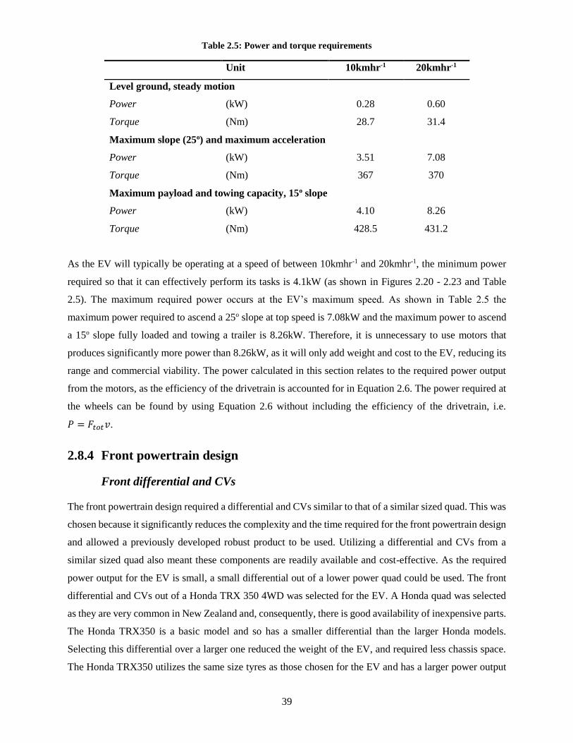
39

Table 2.5: Power and torque requirements

Unit 10kmhr-1 20kmhr-1

Level ground, steady motion

Power (kW) 0.28 0.60

Torque (Nm) 28.7 31.4

Maximum slope (25o) and maximum acceleration

Power (kW) 3.51 7.08

Torque (Nm) 367 370

Maximum payload and towing capacity, 15o slope

Power (kW) 4.10 8.26

Torque (Nm) 428.5 431.2

As the EV will typically be operating at a speed of between 10kmhr-1 and 20kmhr-1, the minimum power

required so that it can effectively perform its tasks is 4.1kW (as shown in Figures 2.20 - 2.23 and Table

2.5). The maximum required power occurs at the EV’s maximum speed. As shown in Table 2.5 the

maximum power required to ascend a 25o slope at top speed is 7.08kW and the maximum power to ascend

a 15o slope fully loaded and towing a trailer is 8.26kW. Therefore, it is unnecessary to use motors that

produces significantly more power than 8.26kW, as it will only add weight and cost to the EV, reducing its

range and commercial viability. The power calculated in this section relates to the required power output

from the motors, as the efficiency of the drivetrain is accounted for in Equation 2.6. The power required at

the wheels can be found by using Equation 2.6 without including the efficiency of the drivetrain, i.e.

𝑃 = 𝐹𝑡𝑜𝑡𝑣.

2.8.4 Front powertrain design

Front differential and CVs

The front powertrain design required a differential and CVs similar to that of a similar sized quad. This was

chosen because it significantly reduces the complexity and the time required for the front powertrain design

and allowed a previously developed robust product to be used. Utilizing a differential and CVs from a

similar sized quad also meant these components are readily available and cost-effective. As the required

power output for the EV is small, a small differential out of a lower power quad could be used. The front

differential and CVs out of a Honda TRX 350 4WD was selected for the EV. A Honda quad was selected

as they are very common in New Zealand and, consequently, there is good availability of inexpensive parts.

The Honda TRX350 is a basic model and so has a smaller differential than the larger Honda models.

Selecting this differential over a larger one reduced the weight of the EV, and required less chassis space.

The Honda TRX350 utilizes the same size tyres as those chosen for the EV and has a larger power output

40

and gross weight, meaning the differential and CVs will produce a robust and reliable front drivetrain for

the EV. It was also decided to utilize the hubs, seals and wheel bearings from the Honda TRX350 as well

to simplify the design and reduce manufacturing time and cost. Figure 2.24 shows a schematic of the Honda

TRX350 differential and CV assemblies.

Figure 2.24: Honda TRX350 front differential and CV schematics

Motor selection

As determined previously, it was desired to use BLDC motors on the EV as they are very efficient, compact,

lightweight, readily available and easy to control. As two motors were used on the EV, the power required

per motor was half of the value determined in the power calculation section. This meant a minimum power

of 2kW was required per motor, with between 3kW to 4.5kW preferred so that the EV could traverse steeper

slopes at higher speeds. A number of available electric motors were investigated to compare their efficiency,

weight, cost and power output. The motor selection was based on these properties as well as their

availability, how easy they would be to implement, and ease of communication with the manufacturing

company. As the front motor is mounted inside the chassis, its IP rating is not a major concern. The cost of

various electric motors was compared relative to their power output as shown in Figure 2.25. Motor weight

was also compared to power output in Figure 2.26.

41

Figure 2.25: Price comparison of the electric motors investigated

Figure 2.26: Weight comparison of electric motors

A 3kW, BLDC, air-cooled Golden motor was chosen for the front powertrain. It is represented in Figures

2.25 and 2.26 as the orange markers and was selected for a number of reasons. The motor matches the EV’s

power requirements very well. This motor has a rated power output of 3kW and peak power output of 4kW,

0

500

1000

1500

2000

2500

0 1 2 3 4 5 6 7 8 9 10

Co

st (

NZ

D)

Power (kW)

Price comparsion of available electric motors

0

5

10

15

20

25

0 1 2 3 4 5 6 7 8 9 10

Wei

ght

(kg)

Power (kW)

Weight comparsion of available electric motors

42

providing the EV with enough power so that it can perform all of its tasks and traverse steep slopes, without

being oversized. It has a high efficiency (85 – 91%) across a large rpm range (2000rpm) (Golden Motor,

2019b). This is very important as it will allow the EV to be efficient at a board range of operating speeds,

and therefore will not limit the EV to a narrow operating range. Most of the BLDC motors investigated had

a similar efficiency to the Golden motor but not across such a large rpm range. The BLDC motor also

operated at a lower rpm range when compared to the alternatives. This will mean a smaller gear reduction

will be required, resulting in a smaller and lighter gearbox. As seen in Figure 2.25, the Golden motor is the

cheapest motor that was investigated within the EV’s power requirements (2 - 4.5kW). This means it is the

best value for money motor that was researched and will minimize the cost of the powertrain. Another key

reason the Golden motor was selected was that the University had previously used this motor on other small

EV projects and had found it very easy to implement and it had performed reliably. Motors produced by

this company have been used extensively in small EVs, gaining them a good reputation for a high quality

product. This motor is readily available and inexpensive, and the company is easy to communicate with.

The selected motor has a reasonable power to weight ratio, as seen in Figure 2.26. Lighter motors could

have been used, however they were more expensive and operated at a much higher rpm than the Golden

motor, meaning that larger, more expensive gearboxes would have to be used.

The selected motor is the air-cooled variant of the 3kW Golden motor range. The air-cooled version was

selected over the water-cooled version, as it reduced the complexity, weight and space requirements of the

powertrain. The water-cooled version weighs more and also requires a heat exchanger and water pump to

ensure it does not over heat, further adding weight to the EV. The 3kW motor operates at a voltage of 48V,

which is compatible with the operating voltage of the EV. A motor controller (inverter) can also be

purchased from the Golden motor company designed specifically for the 3kW BLDC motor. This makes

the controllability of the motor easy and simplistic as a custom inverter is not required. This motor controller

has a mass of 1.9kg and is much more cost-effective than manufacturing a custom one. The specifications

of the chosen motor is shown in Table 2.6, and the motor is shown in Figure 2.27.

Figure 2.27: 3kW BLDC Golden motor (Golden Motor, 2019b)

43

Table 2.6: 3kW BLDC Golden motor specifications (Golden Motor, 2019b)

Model: HPM3000B – 3kW BLDC Motor

Operating voltage 48V

Rated power 3kW

Peak power 4kW

Speed 2000 – 4500rpm

Rated torque 10Nm

Peak torque 25Nm

Efficiency >90%

Weight 7.3kg (air-cooled)

The power and efficiency, and the torque and efficiency curves for the selected motor are shown in Figures

2.28 and 2.29, respectively.

Figure 2.28: Power and efficiency curves of the selected BLDC motor

0

500

1000

1500

2000

2500

3000

3500

4000

4500

0

10

20

30

40

50

60

70

80

90

100

1250 1750 2250 2750 3250 3750 4250 4750

Po

wer

outp

ut

(W)

Eff

icie

ncy

(%

)

Motor speed (rpm)

3kW BLDC Golden motor power and efficiency

Efficiency

power

44

Figure 2.29: Torque and efficiency curves of the selected BLDC motor

From Figures 2.28 and 2.29, it can be seen that the motor is most efficient (approximately 90%) between

3200rpm and 4200rpm. It also has an efficiency of at least 85% from 2200 rpm to 3200rpm. As this is the

most efficient operating range for the selected motor, the design of the front drivetrain needs to place this

high efficiency range inside the typical operating speed range of the EV. Power output and torque drastically

reduce after 4000rpm, with poor efficiency and low power and torque outputs when motor speed increases

past 4350rpm.

The EV will typically be operated in a speed range of between 10kmhr-1 and 20kmhr-1, with its maximum

speed being 20kmhr-1. Using the selected 24-inch diameter tyre, which has a rolling radius of 290mm (due

to low inflation pressure and the applied normal load), the revolutions per minute of the wheels be can be

determined by,

𝑟𝑝𝑚 =

𝑣 ∗ 60

2𝜋𝑟

(2.11)

From Equation 2.11, the typical operating range of EV (10-20kmhr-1) is between 91.5rpm and 182.9rpm.

Therefore, a gear reduction of approximately 23 is required to place the highest motor efficiency and highest

power output range at a vehicle speed of between 10 – 20kmhr-1. The front differential selected has a gear

ratio of 3.77, typical of most ATV differentials. Consequently, the front powertrain will need a further gear

reduction to place the high efficiency range inside the vehicle operating range.

0

5

10

15

20

25

0

10

20

30

40

50

60

70

80

90

100

1250 1750 2250 2750 3250 3750 4250 4750

To

rque

(Nm

)

Eff

icie

ncy

(%

)

Motor speed (rpm)

3kW BLDC Golden motor torque and efficiency

Efficiency

Torque

45

This is a major problem for electric motors that are used for low speed traction applications. All BLDC

motors operate efficiently at high speeds and very inefficiently at low speeds. The selected Golden motor

operates efficiently at a lower rpm range than similar motors, which was one of the reasons it was selected.

Electric motors used for low speed traction applications need a significant gear reduction so that their high

efficiency can be utilized. Typically, a planetary gearbox is used to provide this gear reduction. Planetary

gearboxes are very expensive, significantly reducing the commercial viability of the EV. For example, the

Golden motor selected for the EV retails for NZ$340 (Golden Motor, 2019b), while a compatible, single

stage, planetary gearbox retails for NZ$1620 (Linear Motion, 2019). Planetary gearboxes are expensive as

they are designed to withstand high torque outputs produced by the gear reduction. Using another

component in the powertrain also reduces the overall efficiency of the drivetrain and adds weight to the

vehicle, further hindering its range.

Gear ratio and planetary gearbox selected

A planetary gearbox with a gear ratio of six was selected for the front powertrain. This produced a final

gear reduction for the front drivetrain of 22.62.

𝐺𝑅𝑡𝑜𝑡 = 𝐺𝑅𝑑𝑖𝑓𝑓 ∗ 𝐺𝑅𝑔𝑏 (2.12)

This gear ratio was close to the desired gear ratio and placed the high efficiency range (85-91%) of the

motor at a vehicle speed of between 10 and 20kmhr-1, producing an efficient powertrain. It also meant the

motor is producing approximately 3.5kW at its maximum speed, allowing the EV to traverse a 25o slope at

top speed (Figure 2.21). If a planetary gearbox with a gear ratio of five were used, it would place the high

efficiency range above the maximum speed of the EV, producing an inefficient powertrain. If a gearbox

with a ratio of seven were used, the EV would not be able to reach its top speed and would have insufficient

power above 15kmhr-1, reducing the EV’s abilities to perform its desired tasks.

An Apex planetary gearbox was selected for the EV, as shown in Figure 2.30. It is very efficient, compact

and is compatible with the Golden motor. Its specifications are shown in Table 2.7. As there is negligible

radial and axial loads acting on the gearbox, the sizing of the gearbox was based solely on the nominal

torque. This is the safe operating torque the gearbox can transmit for a continuous period. The 3kW motor

used has a maximum torque of 25Nm. With a planetary gearbox ratio of six, this produces a maximum

output torque of 150Nm. The nominal torque of the selected gearbox was 150Nm and therefore, is strong

enough to cope with the torque output of the motor without being oversized. The selected gearbox is made

from stainless steel and has a high IP rating, which will ensure it is robust and reliable for use in the harsh

dairy farm environment.

46

Figure 2.30: Selected planetary gearbox (Apex Dynamics, 2019)

Table 2.7: Apex planetary gearbox specifications (Apex Dynamics, 2019)

AB090-006 Apex Planetary Gearhead

Nominal output torque (Nm) 150

Nominal input speed (rpm) 4000

Max input speed (rpm) 8000

Max radial load (N) 3250

Max axial load (N) 1625

Efficiency (%) 97

Weight (kg) 3.7

IP rating 65

Front drivetrain characteristics

To determine the power available at the wheels and the overall front powertrain efficiency, the efficiency

of the differential and CVs must be determined. The efficiency of a differential can be determined by,

𝜂𝑑𝑖𝑓𝑓 = 𝜂𝑏𝑒𝑎𝑟𝑖𝑛𝑔𝑁𝑏𝑒𝑎𝑟𝑖𝑛𝑔 ∗ 𝜂𝑔𝑒𝑎𝑟𝑚𝑒𝑠ℎ (2.13)

The efficiency of the ball bearings and the spiral gear mesh is 0.99 and 0.96, respectively (X-Engineer,

2020). As there are three bearings in the differential, this produces an efficiency of 0.931. The efficiency

of a CV can be determined by the type of joints it uses. The efficiency of the CVs used on the EV is 0.99

(X-Engineer, 2020). The overall front drivetrain efficiency can be determined by,

𝜂𝑑𝑟𝑣 = 𝜂𝑔𝑏 ∗ 𝜂𝑑𝑖𝑓𝑓 ∗ 𝜂𝑐𝑣 (2.14)

This gives the front drivetrain an overall efficiency of 89.4%. Equation 2.14 illustrates why the number of

drivetrain components needs to be minimized. If the EV did not require a planetary gearbox, the overall

front drivetrain efficiency would increase to 92.2%, improving the EV’s range and commercially viability.

47

The power and efficiency curves for the entire front powertrain are shown in Figure 2.31. The power

presented here is the power available at the wheels, not the output power from the motor. The efficiency

represents the total efficiency (𝜂𝑚𝑜𝑡𝑜𝑟 ∗ 𝜂𝑑𝑟𝑣) for the front powertrain.

Figure 2.31: Total efficiency of the front powertrain and the power available at the wheels

As seen in Figure 2.31, the front powertrain is very efficient (75 – 82%) from approximately 10 to

20kmhr-1. This is highly desired for the EV as this is its typical operating range. Maximum efficiency occurs

at 19.5kmhr-1 and has a value of 82.3%. Across this operating range, the maximum power output is quite

high, meaning that the EV will be able to complete its desired tasks and traverse steep terrain. The maximum

power available at the wheels (3.7kW) occurs at 19kmhr-1, -very close to the EV’s top speed-, where the

maximum required power occurs.

2.8.5 Rear powertrain design

Rear axle and bearing carrier

A chain drive mechanism was selected for the rear powertrain, which included a bearing carrier and rear

axle assembly. The rear drivetrain was designed using parts from an existing, similar sized quad because it

reduces the complexity and time required for the rear drivetrain design, allowing a previously developed,

robust product to be used. It would be significantly more expensive and time consuming to design and

0

500

1000

1500

2000

2500

3000

3500

4000

30

40

50

60

70

80

90

6 8 10 12 14 16 18 20 22

Po

wer

(W

)

To

tal

Eff

icie

ncy

(%

)

Velocity (kmhr-1)

Total efficiency of the front powertrain

Efficiency

Power available at the wheels

48

manufacture a custom rear axle and bearing carrier assembly. Utilizing a bearing carrier and axle from a

similar sized quad also meant these components are readily available and cost-effective. As consumable

parts such as bearings and seals will also be readily available and inexpensive, maintenance will be much

easier and less time consuming. A solid rear axle assembly is typically used on 2WD sport ATVs. As the

power output from the rear electric motor is small in comparison to typical quads, a bearing carrier assembly

from a lower powered quad could be used. The bearing carrier and rear axle assembly from a Honda

TRX300 Sportrax was used on the EV. A Honda model was chosen as this meant that the components used

on the front and rear drivetrains can be sourced from the same place. A different model of Honda had to be

used as the Sportrax is rear wheel drive only and does not have a front differential. The Honda TRX350

quad uses a rear differential instead of a bearing carrier and solid axle assembly. The Honda TRX300

Sportrax is a basic model and so the bearing carrier and axle is smaller and lighter, reducing the weight and

unsprung mass of the EV. The Sportrax has a larger power output and gross vehicle weight than the EV,

meaning the bearing carrier and rear axle will produce a robust and reliable rear drivetrain for the EV. The

larger vehicle mass of the Sportrax also means the rear axles will easily support the mass of the EV and

will not bend when the EV is fully loaded. It was also decided to utilize the hubs, seals and wheel bearings

from the Sportrax to simplify the design and reduce manufacturing time and cost. Figure 2.32 shows a

schematic of the Honda TRX300 Sportrax’s rear axle and bearing carrier assemblies.

Figure 2.32: Honda TRX300 Sportrax rear axle and bearing carrier assemblies

Motor selection

The rear powertrain utilizes the same 3kW Golden motor that was used in the front powertrain. Its

specifications and performance curves are shown in Table 2.6 and Figures 2.28 and 2.29, respectively. As

discussed previously, this motor is a very good fit for the developed EV. The benefits of this motor are

discussed in the ‘Front Powertrain Design’ section. An additional benefit of using the same motors for the

front and rear of the EV is that it simplifies the EV’s controllability and means that both motors are sourced

from one place, simplifying manufacturing. As both traction motors are the same, they can be supplied with

49

the same input, easily controlling their speed. Utilizing the same motors for both powertrains will mean

they have the same performance and power curves, resulting in an even 50:50 power distribution between

the front and rear wheels across all speeds.

Drivetrain and gear ratio selection

Ideally, the gear ratios of the front and rear powertrains would be the same. This would make the vehicle

very simple and easy to control. Different gear ratios could be used, but it would require a more complex

control system to ensure the front wheels and rear wheels rotated at the same angular velocity. If different

gear ratios were used and both motors were supplied with the same input, the front and rear wheels would

rotate at different speeds, producing slip, resulting in wasted of energy and reduced efficiency.

The gear ratio used by the front powertrain placed the Golden motor’s most efficient operating speeds in

the typical operating velocity (10-20kmhr-1) of the EV, as shown in Figure 2.31. This gear ratio produced

very desirable efficiency and power curves for the front powertrain. Therefore, the rear drivetrain will

utilize the same gear ratio meaning the control required for the traction motors is simplified.

A chain drive mechanism consists of driving and driven sprockets. As the rear powertrain requires a gear

reduction of 22.62, the driving sprocket must be smaller than the driven sprocket. This causes the driven

sprocket to rotate at a slower speed. The gear ratio of a chain or gear drive mechanism can be determined

by,

𝐺𝑅 =

𝐷𝑑𝑟𝑖𝑣𝑒𝑛

𝐷𝑑𝑟𝑖𝑣𝑖𝑛𝑔=

𝑁𝑑𝑟𝑖𝑣𝑒𝑛

𝑁𝑑𝑟𝑖𝑣𝑖𝑛𝑔

(2.15)

Therefore, to maximize the gear ratio, the driving sprocket needs to be as small as possible. However, the

number of teeth on the driving sprocket should not be reduced below 13. If the number of teeth is reduced

past this point, excessive wear (on the chain and sprocket) and larger speed variations will occur due to the

vertical motion of the chain as it enters the sprocket (Budynas, Nisbett, & Shigley, 2015). This will reduce

the reliability and longevity of the EV and will cause the rear wheels to continuously accelerate and

deaccelerate, producing slip as the front wheels will be rotating at a constant speed. This would drastically

reduce the EV’s efficiency. Using the gear ratio found in Equation 2.15 and a 13-tooth driving sprocket,

the size of the driven sprocket can be determined. For the desired gear ratio, the driven sprocket that is

mounted to the rear axle needs to have 294 teeth. This correlates to a sprocket diameter of approximately

1200mm. This size sprocket is completely unfeasible as the rear wheels have a diameter of 580mm, less

than half the size of this sprocket. Therefore, a two-stage gear reduction is required.

Three possible ways to achieve this gear reduction were investigated. The first of which was a two-stage

chain drive mechanism, similar to what is shown in Figure 2.33. The electric motor will drive an

intermediate shaft, which will then drive the rear axle. Due to the minimum number of teeth the driving

50

sprocket can have, the driven sprockets will need to have diameters of 250mm. This diameter is still

excessive and will significantly reduce the EV’s ground clearance and off-road abilities. As the sprockets

are low hanging, they would also be prone to damage. The packaging of such a system within the small EV

would also be difficult due to both height and length restrictions. Therefore, a two-stage chain drive

mechanism was not suitable for the EV.

Figure 2.33: Two-stage chain drive mechanism

Figure 2.34: Spur gear and chain drive two-stage

reduction system

The use of a spur gear reduction was also investigated. The electric motor will drive a small pinion gear,

which, in turn, drives a larger spur gear. The spur gear is mounted on a connecting shaft to a chain drive

mechanism that rotates the rear axle. Figure 2.34 shows a similar chain drive, spur gear mechanism, except

the motor is driving the sprocket not the pinion gear. This system is much more compact than the two-

stage chain mechanism, with the spur gear assembly requiring minimal space. However, for the spur gears

to safely transmit the torque produced, they would need to be 20mm wide. For the required gear reduction

to be achieved, the driven spur gear would be 200mm in diameter. This would produce a very heavy

assembly which is detrimental to the EV. The spur gear assembly would need custom made housing so that

the gears can be lubricated and protected from the environment. This adds more weight to the EV and

requires significantly more design and manufacturing time, producing an expensive gear reduction system.

Therefore, this reduction system was also not suitable for the EV.

The final gear reduction system investigated consisted of mounting a small planetary gearbox to the traction

motor. The small chain drive sprocket is mounted to the output shaft of the planetary gearhead, which drives

the rear axle. This design is very compact and simple. Although the planetary gearbox is expensive, it would

still be cheaper than a custom-made spur gear assembly. As it is compact, the motor and gearbox assembly

will easily fit within the length and height limitations (determined by suspension and chassis design). The

weight of this system is significantly less than using a spur gear system and provides more ground clearance

than the two-stage chain-drive mechanism. It will also be very quick to assemble during manufacturing.

Therefore, a planetary gearbox in conjunction with the chain drive mechanism will be used on the EV.

The planetary gearbox used is the same one as was used in the front powertrain. This was done to keep the

powertrain simple. As both gearboxes are the same, they can be interchanged and both motors will rotate

51

at the same rpm for a given vehicle speed, simplifying motor control. The Apex planetary gearbox

specifications are shown in Table 2.7. As there is minimal radial loads (only a small force applied by chain

tension) and negligible axial load, this gearbox will provide a reliable, strong reduction mechanism.

Chain drive sizing and calculations

As the selected planetary gearbox has a gear ratio of six, the gear ratio of the chain-drive mechanism must

be 3.77 to ensure the rear drivetrain has the same gear ratio as the front drivetrain. To minimize sprocket

size and therefore maximize ground clearance of the rear axle, the driving sprocket needs to be as small as

possible. As discussed previously, the smallest number of teeth allowed before excessive wear and

significant speed variations occurs is 13. The speed variation due to the number of teeth on the driving

sprocket is called the choral speed variation and can be determined by,

Δ𝑉

𝑉=

𝑣𝑚𝑎𝑥 − 𝑣𝑚𝑖𝑛

𝑉=

𝜋

𝑁[

1

sin(180 𝑁)⁄−

1

tan(180 𝑁)⁄]

(2.16)

The speed variation of the 13-tooth sprocket is 2.9%, which is small enough to have negligible effect on

the EV’s motion. Using Equation 2.15, the number of teeth on the driven sprocket was determined to be

49. This procures a total rear drivetrain gear ratio of 22.62.

A 420 chain size was used on the EV. It has pitch of 12.7mm and a width of 7.94mm. This chain size is

typically used on small dirt bikes and kids ATVs (Motor-chains, 2016). This chain size was selected as it

has a small pitch, allowing the sprockets to have smaller diameters, which improves the ground clearance

below the rear axle and reduces the EV’s weight. The strength of this chain was calculated to ensure it

would be strong enough for the EV. Shigley (2015) states that roller chains seldom fail due to lack of tensile

strength, but often fail due to a large amount of service hours. Failure typically occurs due to wear on the

roller pins or fatigue in the roller surface. The fatigue strength of the link-plates governs the chain’s capacity

at low speeds (Budynas et al., 2015). For a single-strand chain, the nominal power limited by link-plate is

determined by Equation 2.17. Equation 2.18 shows the nominal power the chain can support when it is

roller-limited.

𝐻1 = 0.004𝑁11.08𝑛1

0.9𝑝(3−0.07𝑝) (2.17)

𝐻2 =

1000𝐾𝑟𝑁11.5𝑝0.8

𝑛11.5

(2.18)

Where 𝑁1 is the small sprocket’s number of teeth, 𝑝 is the chain pitch (inch), 𝐾𝑟 is 17 for a 420 chain and

H in the allowable horsepower. The values for 𝐻1 and 𝐻2 were determined to be 14.3hp and 27.6hp,

52

respectively. As these power values are greater than the output power from the motor, the 420 chain is

strong enough to be used on the EV.

The length of the chain was determined next. It is preferred to have an even number of pitches in the chain

and an odd number of teeth on the driving sprocket so that a special chain link is not required. It was decided

to use a 420 chain with 72 pitches, so the rear motor assembly is placed in a desirable place on the EV’s

rear suspension. The corresponding distance between the centres of the two sprockets was determined by,

𝐶 =𝑝

4[−𝐴 + √𝐴2 − 8 (

𝑁2 − 𝑁1

2𝜋)

2

]

(2.19)

Where A is,

𝐴 =

𝑁1 + 𝑁2

2−

𝐿

𝑝

(2.20)

The centre-to-centre distance and sprocket sizes is shown in Table 2.8.

Table 2.8: Sprocket and chain sizes for the rear drivetrain

Unit Value

Driving Sprocket

N1 13

Diameter (mm) 53

Driven Sprocket

N2 49

Diameter (mm) 198

420 Chain size

Pitch, p (mm) 12.7

Width (mm) 7.94

Length (mm) 914.4

Centre-to-centre distance (mm) 249.7

Rear drivetrain efficiency and performance

To determine the power available at the wheels and the overall EV efficiency, the efficiency of the rear

drivetrain must be determined. The efficiency of the rear drivetrain is a function of the planetary gearbox

efficiency, the chain drive efficiency and the efficiency of the ball bearings in the bearing carrier. It can be

calculated using Equation 2.21.

53

The efficiency of a chain drive system is 0.98 (Warner, 2017) and there are two ball bearings in the bearing

carrier assembly that have an efficiency of 0.99 each (X-Engineer, 2020). This gives a rear drivetrain

efficiency of 93.2%. The rear drivetrain is 3.8% more efficient than the front drivetrain because it utilized

a chain drive mechanism instead of a differential. It would have been even more efficient if a planetary

gearbox were not used. The power and efficiency curves for the entire rear powertrain are shown in Figure

2.35. The power presented here is the power available at the wheels, not the output power from the motor.

The efficiency represents the total efficiency (𝜂𝑚𝑜𝑡𝑜𝑟 ∗ 𝜂𝑑𝑟𝑣) for the rear powertrain.

Figure 2.35: Total efficiency of the rear powertrain and the power available at the wheels

Figure 2.35 shows that the rear powertrain follows the same curves as the front powertrain (Figure 2.31),

except they are shifted vertically up by a small margin. They follow the same path as both powertrains

utilize the same motor and the same gear ratio, with the only difference being that the rear drivetrain is

slightly more efficient, thus shifting the curve upwards. The rear powertrain is very efficient (80 – 85%)

across the EV’s typical operating speeds, with its maximum efficiency occurring at 19.5kmhr-1 (85.7%).

0

500

1000

1500

2000

2500

3000

3500

4000

4500

40

45

50

55

60

65

70

75

80

85

90

6 8 10 12 14 16 18 20 22P

ow

er (

W)

To

tal

Eff

icie

ncy

(%

)

Velocity (kmhr-1)

Total efficiency of the rear powertrain

Efficiency

Power available at the wheels

𝜂𝑑𝑟𝑣 = 𝜂𝑔𝑏 ∗ 𝜂𝑐ℎ𝑎𝑖𝑛 ∗ 𝜂𝑏𝑒𝑎𝑟𝑖𝑛𝑔𝑁𝑏𝑒𝑎𝑟𝑖𝑛𝑔 (2.21)

54

2.8.6 Issues affecting the viability of the powertrain

The major issue that effects the viability of the powertrain is the large gear reduction that is required to

fully utilize the efficiency of the electric motors. All BLDC traction motors operate efficiently at high

speeds and inefficiently at low speeds (Yedamale, 2003). Therefore, when electric motors are used for low-

speed traction applications in conjunction with larger tyres, a two-stage gear reduction is generally required.

As discussed previously, the large gear reduction will optimize the efficiency of the powertrain by placing

the efficient motor speed in the typical operating velocity range of the vehicle. However, as a two-stage

gear reduction is required, connecting the motor directly to the differential or chain drive mechanism will

not provide the necessary reduction alone. Further reduction is required. For this second gear reduction

stage, a planetary gearbox is typically used, as was the case for the EV. Planetary gearboxes are very

expensive, significantly reducing the commercial viability of the EV. The single-stage planetary gearboxes

used on the EV retail for NZ$1620 each (Linear Motion, 2019). Purchasing the gearboxes alone will account

for over 25% of the EV’s cost. Other disadvantages of having to utilize a planetary gearbox is the reduced

drivetrain efficiency, as there is now more components in the drivetrain and the additional weight of the

gearbox reduces the EV’s range. Ideally, electric motors would be developed to be efficient at low speeds

(400 - 800rpm), such that only a single-stage gear reduction is required. This would allow the electric motor

to be connected directly to the differential or chain drive, eliminating the need for a planetary gearbox. This

would significantly improve the commercial viability of the EV as the vehicle cost would be significantly

reduced and the efficiency of the drivetrain would increase along with the EV’s range.

Another limitation that influenced the design of the EV was the low IP ratings of electric traction motors.

During the motor selection process, many suitably sized motors (1-10kW) were investigated. The majority

of these motors had an IP rating of 54 or less. The few that had higher ratings (IP64 and IP65) were

unsuitable due to small efficiency ranges and low power outputs. Even with an IP rating of 65, the motors

could not be submerged. On a dairy farm in winter, it is common to have deep pools of water in gate

entrances meaning that hub motors would likely become partially submerged. This would lead to motor

malfunctions and an unreliable powertrain. This ultimately means that the motors would have to be mounted

inside the chassis so that they are protected from the dairy farm environment.

As discussed during the motor selection, the 3kW Golden motor was not the lightest motor (7.3kg) available

within the required power output range. Ideally, a lighter motor would have been chosen as this would

increase the EV’s range and viability. However, the lighter motors investigated were very expensive and

operated at much higher speeds than the selected motor. This meant that, ultimately these motors were

unsuitable for the EV.

55

2.8.7 Overall powertrain characteristics

The EV’s powertrain design was focused on maximizing efficiency, creating sufficient power to perform

all of its desired tasks, and producing a cost-effective, robust and reliable system. The power and torque

available at the wheels and the total efficiency of the EV’s powertrain were computed and compared to the

required power and torque outputs in extreme loading cases, as investigated in the power and torque

calculations section. Figure 2.36 shows the power and efficiency curves for the entire vehicle and Figure

2.37 shows the torque produced by the powertrain. The power presented here is the power available at the

wheels, not the output power from the motor. The efficiency represents the total efficiency for the entire

powertrain (front and rear). Both power and torque outputs were compared to the required outputs for the

EV to traverse a 25o slope and transport a combined payload of 250kg up a 15o slope.

Figure 2.36: The EV’s efficiency and power curves compared to required power for two situations

0

10

20

30

40

50

60

70

80

90

0

1

2

3

4

5

6

7

8

6 8 10 12 14 16 18 20 22E

ffic

iency

(%

)

Po

wer

(kW

)

Velocity (kmhr-1)

Overall EV power and efficiency curves

Power available at the wheels

Power required, 25 degree slope

Power required, 250kg payload, 15 degree slope

Efficiency

56

Figure 2.37: The EV's torque and efficiency curves compared to required torque for two situations

As shown in Figures 2.36 and 2.37, the EV will be most efficient when it is traveling within its typical

operating speed range of 10-20kmhr-1 (78 - 84%). The typical efficiency of road going EVs is 80% (Bloom,

2013), so the developed powertrain has a similar efficiency to road going EVs. Maximum efficiency occurs

at 19.9kmhr-1 and has a value of 84%. The developed powertrain is very efficient and so will greatly

improve the EV’s commercial viability and range. As seen in Figure 2.36, the available power at the wheels

is larger than the required power for the two extreme loading cases investigated, up to a speed of

approximately 19.5kmhr-1. The EV will not be able to travel faster than this speed under these loading

situations as the required power is greater than the EV’s power output. As the EV’s maximum speed is

limited to 20kmhr-1, this will have minimal affect on the EV. The maximum power available at the wheels

(7.48kW) occurs at 19kmhr-1. Figure 2.37 shows that the torque output of the EV is significantly larger than

the required torque at low speeds and is sufficient up to a speed of 19.5kmhr-1. As the EV has more power

and torque than required for these extreme loading scenarios, it will be able to perform all tasks as required.

The developed powertrain is simple and utilizes components from existing quads to produce a cost-effective

and easily manufacturable powertrain. The powertrain design also minimized weight by selecting

lightweight components. A locked rear axle was utilized, which will significantly improve the EV’s off-

road capabilities and help it to maintain traction on soft and uneven terrain. The powertrain design places

the electric motors inside the chassis, protecting them from the harsh dairy farm environment and ultimately

improving the reliability of the powertrain. The overall properties of the powertrain are shown in Table 2.9.

0

10

20

30

40

50

60

70

80

90

0

100

200

300

400

500

600

700

800

900

1000

6 8 10 12 14 16 18 20 22

Eff

icie

ncy

(%

)

To

rque

(Nm

)

Velocity (kmhr-1)

Overall EV torque and efficiency curves

Torque output

Required torque, 25 degree slope

Required torque, 250kg payload, 15 degree slope

Efficiency

57

Utilizing high efficiency motors with a large efficiency range meant that the developed powertrain would

maximize vehicle range, essential in developing a viable EV.

Table 2.9: Overall powertrain properties

Property Value

Gear ratio 22.62

Overall Drivetrain Efficiency 91.3%

Motors 2x 3kW BLDC Motor (4kW peak)

Overall Powertrain Efficiency (10 – 20kmhr-1) 78 – 84%

Maximum Efficiency 84% at 19.5kmhr-1

Maximum Power available at the wheels 7.48kW

Maximum Torque 860Nm

2.8.8 Brakes

The key criteria for the EV’s brake system was that a fail-safe actuation, whereby if power were lost to the

EV, the brakes would engage. This is to maximize safety in cases where the vehicle is parked on a slope or

suddenly loses power. This would mean that if the EV was switched off, the batteries were disconnected,

or the batteries were completed discharged, the brakes would be applied. The brakes also needed to meet

the required deceleration specification, outlined in Table 2.1. The required deceleration (1ms-2) is low as

the EV will only move at slow speeds (20kmhr-1) and is relatively lightweight. Therefore, a simple, cost-

effective braking system was desired. The brake system needed to be robust and reliable, as it would be

exposed to a lot of mud, water and manure.

Concepts

Due to the low deceleration required, the proposed concepts were evaluated largely by their simplicity, cost,

reliability and robustness in the dairy farm environment. The brakes must also be compatible with the

selected suspension design and should be lightweight.

Fail safe brakes are typically engaged by a mechanical mechanism and disengaged by supplying power to

an actuator, motor or electromagnet which separates the frictional surfaces. Three viable concepts were

proposed for the EV. The first (solution 1, Table 2.10) is a typical, electric, fail-safe brake. It utilizes an

electromagnetic coil to disengage the brake and compression springs to engage the brake. When power is

supplied to the electromagnetic coil, it creates a magnetic field that pulls an armature across a small air gap,

compressing multiple springs in the brake housing. With the armature pulled into the brake housing, the

brake rotor is free to rotate. When power is removed from the brake, the springs press the armature against

the rotor, sandwiching it between two frictional surfaces, creating a braking torque. These types of brakes

58

are typically used on machines in industry. They provide a robust braking system with more than enough

braking torque to meet the EV’s design specifications, but are bulky and heavy. As they are quite bulky,

the suspension design will be more complex as packaging the brake and maintaining desirable suspension

geometry will be difficult. They are also expensive and the electromagnetic consumes a lot of power,

reducing the battery capacity available for the EV’s traction motors.

The second concept (solution 2, Table 2.10) is a typical hydraulic disc brake system utilized on similar

sized quads. It consists of brake rotors, calipers, brake lines and a master cylinder. The brakes will be

applied by a heavy compression spring pressing against a lever mechanism to actuate the master cylinder.

They will be disengaged by a linear actuator pressing on the same lever. Hydraulic disc brakes are

commonly used in the majority of both on- and off-road vehicles due to their superior braking torque. This

design will provide good braking performance and will be compatible with the suspension design. However,

it has a larger number of components and requires a reasonable amount of chassis space to house the master

cylinder, linear actuator and lever mechanism. It is lighter than the electric, fail-safe brake and consumes

considerably less power. The autonomous control of this system will be more complex than the alternatives

as it will require feedback from a brake pressure sensor and linear actuator position.

The final concept proposed (solution 3, Table 2.10) is a cable actuated disc bake. It is a very simple braking

system consisting of brake rotors, calipers and an actuation method. Instead of using a cable to rotate the

brake arm, it was proposed to use a tension spring. The spring is mounted directly to the caliper arm and

will always act to engage the brake. The brake will be disengaged by a small servomotor pulling against

the spring. Cable disc brakes are commonly used on bicycles and other small-wheeled vehicles such as

scooters. This concept is very simple and cost-effective but does not provide the braking performance of a

hydraulic system. It requires minimal space, ensuring compatibility with the suspension, while being

lightweight and easy to control. As there are few components and is mechanically actuated, it is a robust

and reliable system. Additionally, only a small amount of power is required to disengage the brakes.

Table 2.10: Brake concepts

Morphological Matrix – Brake system

Solution 1 Solution 2 Solution 3

Electric fail-safe brake

Hydraulic disc brake system

Cable actuated disc brake

59

Selected concept

The EV will utilize the cable actuated disc brakes that are commonly used on mountain bikes. This concept

uses a tension spring instead of a cable to engage the brakes. This produces a mechanical fail-safe actuation

method, as required for the brake system. The cable brake design was selected as it is very simple, compact,

lightweight and cost-effective. It will also provide a robust and reliable braking system for the EV in a dairy

farm environment. This design is also compatible with the suspension, making it easy to package inside the

rim and mount to the upright. As the required deceleration (1ms-2) is small and the EV is relatively

lightweight, this type of disc brake could be used as it will provide enough braking torque to meet the design

specification.

The electric fail-safe brake was not selected as it is heavy, bulky, expensive, and the electromagnet

consumes a lot of power. This would reduce the EV’s range and increase its cost, reducing its commercial

viability. The bulky brake would also produce a less desirable suspension geometry as it would limit the

placement of suspension pick-up points and would require an increased kingpin angle, which is undesired

(as discussed in the suspension section). Even though a hydraulic disc brake system will produce superior

braking performance when compared to the selected design, it is more complex, expensive and has a larger

number of components requiring more chassis space. The control system required for the hydraulic brake

system is also more complex than the selected design.

Longitudinal load transfer

Longitudinal load transfer occurs as a result of acceleration or deceleration forces. During braking,

deceleration occurs, causing a longitudinal load transfer to the front wheels. This compresses the front

suspension, as the front wheels will have more ‘weight’ on them. Assuming an equal weight distribution, -

left to right-, longitudinal load transfer is a function of wheelbase, vehicle mass, the vehicle’s CoG and

acceleration. The normal force due to longitudinal load transfer, supported by the front and rear wheels, are

shown in Equations 2.22 and 2.23, respectively. The normal force 𝐹𝑧, represented in these equations is per

wheel (total axle load is 2𝐹𝑧).

𝐹𝑧𝑓 =

1

2𝑚𝑔

𝑐1

𝐿−

1

2𝑚𝑎𝑥

ℎ

𝐿

(2.22)

𝐹𝑧𝑟 =

1

2𝑚𝑔

𝑏1

𝐿+

1

2𝑚𝑎𝑥

ℎ

𝐿

(2.23)

Where 𝑏1 relates to the distance between the CoG and the front axle, 𝑐1 is the distance between the CoG

and the rear axle, ℎ is the height of the CoG above the ground and 𝐿 is the vehicle’s wheelbase.

60

Required braking torque

Deceleration force, due to braking, is a function of deceleration and vehicle mass. It is represented by,

𝐹𝑑𝑒𝑐𝑒𝑙 = 𝑚𝑎𝑥 (2.24)

For the 200kg EV, the required deceleration is 1ms-2, which gives a required braking force of 200N for the

entire vehicle. As longitudinal load transfer will occur, there will be a larger normal load supported by the

front axle, as determined by Equation 2.22. Therefore, the front wheels will have to provide a larger braking

effort than the rear wheels.

Equation 2.24 determined that the required braking force for the EV was 200N. This is the required force

on flat, level ground. The maximum braking effort the EV will have to provide occurs at a deceleration

of1ms-2 going down the steepest slope it is expected to encounter (25o). This situation is represented by the

free body diagram in Figure 2.38. It was assumed that motion resistance and drag were very small in

comparison to the required braking effort, so their influence on decelerating the EV was not included.

Figure 2.38: Free body diagram of EV under braking

The dynamic normal loads supported by the front and rear wheels (𝐹𝑧𝑓 and 𝐹𝑧𝑟) due to braking down the

slope must be determined. The sum of the moments about the front wheel’s contact patch was taken to

determine the normal load supported by the rear wheels.

𝐹𝑧𝑟 =𝑚

𝐿[𝑏1𝑔 cos 𝜃 − 𝑔ℎ sin 𝜃 − 𝑎𝑥ℎ] (2.25)

If the normal force supported by the rear axle is zero or negative it will mean the rear wheels have lost

contact with the ground and the vehicle has rolled over its front wheels. This occurs when the moment

61

produced by the force applied longitudinally at the vehicles CoG is large enough to overcome the normal

load. The sum of the forces in the z direction were then computed to give the normal force supported by

the front wheels.

𝐹𝑧𝑓 = 𝑚𝑔 cos 𝜃 − 𝐹𝑧𝑟 (2.26)

The total normal load supported by the slope is determined by Equation 2.27 and the gravity force pulling

the vehicle down the slope can be determined by Equation 2.28

𝐹𝑧𝑡𝑜𝑡 = 𝑚𝑔 cos 𝜃 (2.27)

𝐹𝑥𝑠𝑙𝑜𝑝𝑒 = 𝑚𝑔 sin 𝜃 (2.28)

The dynamic load distribution can now be determined by,

% 𝑙𝑜𝑎𝑑𝑓𝑟𝑜𝑛𝑡 =

𝐹𝑧𝑓

𝐹𝑧𝑡𝑜𝑡

(2.29)

% 𝑙𝑜𝑎𝑑𝑟𝑒𝑎𝑟 =

𝐹𝑧𝑟

𝐹𝑧𝑡𝑜𝑡

(2.30)

The total required braking force can be determined by,

𝐹𝑏𝑟𝑎𝑘𝑒,𝑡𝑜𝑡 = 𝐹𝑥𝑠𝑙𝑜𝑝𝑒 + 𝐹𝑑𝑒𝑐𝑒𝑙 (2.31)

The required braking force for the front and rear wheels can be determined by Equation 2.32. The braking

torque is determined by the tyre’s diameter.

𝐹𝑏𝑟𝑎𝑘𝑒 = 𝐹𝑏𝑟𝑎𝑘𝑒,𝑡𝑜𝑡 ∗ % 𝑙𝑜𝑎𝑑 (2.32)

𝑇𝑏𝑟𝑎𝑘𝑒 = 𝐹𝑏𝑟𝑎𝑘𝑒 ∗

𝐷

2

(2.33)

The results from Equations 2.26 – 2.33 are shown in Table 2.11. The EV has a mass of 200kg, a wheelbase

of 1250mm, CoG height of 320mm and it is assumed to have a 50:50 weight distribution.

62

Table 2.11: Dynamic loads and required braking forces

Parameter Unit Value

𝐹𝑧𝑟 (both wheels) (N) 625.6

𝐹𝑧𝑓 (both wheels) (N) 1152.6

𝐹𝑧𝑡𝑜𝑡 (N) 1778.2

𝑙𝑜𝑎𝑑 𝑑𝑖𝑠𝑡𝑟𝑖𝑏𝑢𝑡𝑖𝑜𝑛𝑓𝑟𝑜𝑛𝑡 64.8%

𝑙𝑜𝑎𝑑 𝑑𝑖𝑠𝑡𝑟𝑖𝑏𝑢𝑡𝑖𝑜𝑛𝑟𝑒𝑎𝑟 35.2%

𝐹𝑥𝑠𝑙𝑜𝑝𝑒 (N) 829.2

𝐹𝑑𝑒𝑐𝑒𝑙 (N) 200

𝐹𝑏𝑟𝑎𝑘𝑒,𝑡𝑜𝑡 (N) 1029.2

𝐹𝑏𝑟𝑎𝑘𝑒,𝑓𝑟𝑜𝑛𝑡 𝑎𝑥𝑙𝑒 (N) 667.1

𝐹𝑏𝑟𝑎𝑘𝑒,𝑟𝑒𝑎𝑟 𝑎𝑥𝑙𝑒 (N) 362.1

𝑇𝑏𝑟𝑎𝑘𝑒,𝑓𝑟𝑜𝑛𝑡 𝑎𝑥𝑙𝑒 (Nm) 193.4

𝑇𝑏𝑟𝑎𝑘𝑒,𝑟𝑒𝑎𝑟 𝑎𝑥𝑙𝑒 (Nm) 105

Another important consideration during braking is the inertia of the wheels and drivetrain. Additional

braking torque is required to stop all rotating parts of the vehicle’s drivetrain. The braking torque required

to slow these rotating components must be included in the total braking torque. The torque required to slow

these components can be determined by Equation 2.9, where the angular deceleration is determined by

Equation 2.34.

𝛼 =𝑎𝑥

𝑟

(2.34)

The tyres and axles can be modelled as a solid cylinder and their inertia determined by Equation 2.10. The

sum of the inertias of the drivetrain components is then multiplied by the angular deceleration to give the

torque required to decelerate the wheels and drivetrain components.

It was decided to utilize two front disc brakes and one rear disc brake on the EV, as the front wheels will

provide the majority of the braking force. The front brakes will be connected to the front hubs, located

inside the rim, while the rear brake will be connected to the bearing carrier housing. As the front axle will

utilize two brakes, the required braking torque per front brake will be half of the torque presented in Table

2.11. The inertia torque of the front and rear drivetrains are presented in Table 2.12, along with the total

braking torque required for the front and rear brakes (including the inertia torque).

63

Table 2.12: Total required braking torque for the EV

Required braking torque Unit Value

𝑇𝑖𝑛𝑒𝑟𝑡𝑖𝑎,

1

2 𝑓𝑟𝑜𝑛𝑡 𝑑𝑟𝑖𝑣𝑒𝑡𝑟𝑎𝑖𝑛

(Nm) 1.4

𝑇𝑖𝑛𝑒𝑟𝑡𝑖𝑎,𝑟𝑒𝑎𝑟 𝑑𝑟𝑖𝑣𝑒𝑡𝑟𝑎𝑖𝑛 (Nm) 3.1

𝑇𝑏𝑟𝑎𝑘𝑒 𝑡𝑜𝑡,𝑓𝑟𝑜𝑛𝑡 𝑤ℎ𝑒𝑒𝑙 (Nm) 98.1

𝑇𝑏𝑟𝑎𝑘𝑒 𝑡𝑜𝑡,𝑟𝑒𝑎𝑟 𝑎𝑥𝑙𝑒 (Nm) 108.1

Brake design

The pervious section determined the required brake torque. To minimize the required braking force for the

given braking torque, the rotor diameter should be maximized. This places the caliper further away from

the axis of rotation, producing a larger moment arm. It was decided to use a 180mm rotor. This was the

largest rotor that could be used before interference issues occurred between the caliper and the rim. The

required braking force that is generated at the caliper can be determined by,

𝐹𝑏 = 2 ∗

𝑇𝑏𝑟𝑎𝑘𝑒 𝑡𝑜𝑡

𝑑

(2.35)

Where 𝑑 is the rotor diameter. The required caliper clamping force is determined by,

𝐹𝑐𝑙𝑎𝑚𝑝 =

𝐹𝑏

2𝜇

(2.36)

Where 𝜇 is the coefficient of friction between the rotor and brake pads. It typically has a value of 0.4

(Twiflex, nd). This friction coefficient was assumed for the EV. The selected brake rotor and caliper are

shown in Figures 2.39 and 2.40, respectively.

Figure 2.39: Tektro 180mm brake rotor

Figure 2.40: Shimano disc brake caliper

64

The mechanical advantage of the selected caliper needed to be determined. It was found that rotating the

caliper arm by 45o produced a brake pad movement of 1mm. The mechanical advantage of the brake was

increased by replacing the factory caliper arm with a custom 60mm long arm (pivot point to spring pick-up

point). The longer arm meant that the end of the arm travelled a further distance to close the caliper than

the short, factory arm. Consequently, the longer arm produces a larger mechanical advantage, so less spring

force is required to produce the desired clamping force. The 60mm long arm travelled a distance of 45mm

for a 45o rotation, producing a mechanical advantage of 45 (45mm of arm movement equals 1mm of brake

pad movement). The required spring force can be determined by,

𝐹𝑟𝑒𝑞 𝑠𝑝𝑟𝑖𝑛𝑔 =

𝐹𝑐𝑙𝑎𝑚𝑝

𝑚𝑒𝑐ℎ𝑎𝑛𝑖𝑐𝑎𝑙 𝑎𝑑𝑣𝑎𝑛𝑡𝑎𝑔𝑒

(2.37)

The required caliper clamping and spring force for the front and rear brakes are shown in Table 2.13.

Table 2.13: Calculation results from Equations 2.35 to 2.37

Braking force Unit Value

𝐹𝑏,𝑓𝑟𝑜𝑛𝑡 𝑤ℎ𝑒𝑒𝑙 (N) 1090.3

𝐹𝑏,𝑟𝑒𝑎𝑟 𝑎𝑥𝑙𝑒 (N) 1201.6

𝐹𝑐𝑙𝑎𝑚𝑝,𝑓𝑟𝑜𝑛𝑡 𝑤ℎ𝑒𝑒𝑙 (N) 1362.9

𝐹𝑐𝑙𝑎𝑚𝑝,𝑟𝑒𝑎𝑟 𝑎𝑥𝑙𝑒 (N) 1502

𝐹𝑟𝑒𝑞 𝑠𝑝𝑟𝑖𝑛𝑔 𝑓𝑟𝑜𝑛𝑡 (N) 30.3

𝐹𝑟𝑒𝑞 𝑠𝑝𝑟𝑖𝑛𝑔 𝑟𝑒𝑎𝑟 (N) 33.4

The required caliper braking and clamping forces determined for the EV decelerating at 1ms-2 down a 25o

slope can easily be achieved by the selected mountain bike rotor and brake caliper. Oertel, Neuburger, and

Sabo (2010) tested cable actuated, mountain bike, disc brakes and determined that they could produce

clamping forces up to 5kN, which is more than 3 times what is required for the EV. Therefore, the selected

brake design will be able to provide the required braking force subject to the selection of tension spring.

The spring must provide at least 33.4N of force perpendicular to the caliper arm in order to achieve the

desired deceleration. It must also have an extension of at least 45mm. The selected spring (Figure 2.41)

has an initial tension of 74N, a spring rate of 0.46N/mm, free length of 87.7mm and a maximum extended

length of 224.7mm. As the caliper arm will rotate upwards to disengage the brake, the spring will no longer

be acting perpendicular to the arm. The component of the spring force that is acting perpendicular to the

arm can be determined by,

𝐹𝑠 𝑝𝑝𝑑 = 𝐹𝑠 cos 𝜑 (2.38)

65

Where 𝜑 is the angle of the caliper arm. The maximum rotation of the caliper arm is 45o, which correlates

to a perpendicular spring force of 73N, more than twice that which is required. Therefore, this spring will

be able to provide the necessary force to decelerate the EV quicker than 1ms-2 going down a 25o degree

slope, meeting the design specification. To disengage the brake and extend the spring, a servomotor was

chosen as they are simple, cheap and easy to control. The selected servomotor is shown in Figure 2.42.

Figure 2.41: Selected tension spring

Figure 2.42: Selected servomotor

A mountain bike brake cable was used to connect the servomotor to the caliper arm. The cable was run

around a small pulley so the servomotor would pull the caliper arm at nearly a perpendicular angle, as seen

in Figure 2.43. A 25mm long arm was fitted to the servomotor providing a straight-line cable distance of

50mm, which is enough to fully open the brake caliper. The maximum force the spring applies is 78.6N

(10mm of pretension on the spring). This correlates to a required servo torque of 1.97Nm, which is less

than the servomotor’s maximum torque (2.26Nm). Therefore, the selected servomotor will be able to

disengage the brakes and is small and waterproof, so can be mounted inside the wheel rim on top of the

upright as shown in Figure 2.43. It only requires a small amount of power (17W maximum) and can run off

the EV’s house battery. Therefore, the battery capacity available to the traction motors, and consequently

the EV’s range, will not be affected. Figures 2.43 and 2.45 show the Solidworks model of the front brake

design. Figure 2.44 shows the rear brake design and how it mounts to the trailing arm. The developed

braking system for the EV is simple, cost-effective, lightweight and robust. The fail-safe spring system

engages the brakes when power is removed from the servomotors. The braking system produces enough

braking torque to decelerate the EV when it is going down a 25o slope, meeting the design specification.

Figure 2.43: Front brake

assembly

Figure 2.44: Rear brake assembly

Figure 2.45: Front brake

assembly

66

2.9 Suspension

Suspension is crucial in an off-road vehicle. A good suspension system will allow the vehicle to effectively

transfer the power expelled at the wheels to the terrain thus maximizing traction. It also defines a vehicle’s

handling, stability, ground clearance, roll centre and off-road capabilities. Consequently, a poorly designed

suspension system will significantly hinder the performance and capabilities of a vehicle. For the developed

EV, the suspension design was focused on providing good off-road capabilities in order to traverse the

challenging dairy farm environment. Factors such as maintaining traction and maximizing vehicle

efficiency by conserving vehicle momentum in the presence of sudden terrain irregularities (such as wheel

ruts or rough surfaces) were taken into account. The EV’s suspension must also be affordable and easily

manufacturable. As minimizing the vehicle’s total mass is a focus of the EV’s design, a lighter suspension

with minimal components is also preferred. The purpose of this section is to present a suspension system

that will address these design requirements to produce a suspension which will improve both the EV’s off-

road capabilities and it’s overall efficiency and range.

The effect of suspension on vehicle momentum and range was investigated. Steyn and Warnich (2014)

presented a study into whether the presence of suspension would affect range. A variety of hard-tail

mountain bikes (front suspension, no rear suspension) and full suspension mountain bikes (front and rear

suspension) were tested on road, gravel, grass, sand and over a 100mm high rock. The rolling resistance for

both suspension types was similar on all surfaces with the exception of the 100mm rock. The effect of

suspension on the vehicle’s range on a nice, uniform surface is minimal. However, when an obstacle, such

as the 100mm rock, is in the path of the wheel, the effect of suspension becomes clear. The full suspension

mountain bikes travelled 5-10% further than the hard-tail mountain bikes after hitting the 100mm rock in

coast-down tests. The full suspension mountain bikes were able to maintain more of their momentum after

hitting the obstacle due to the rear suspension being able to move up and over of the rock. Since the

suspension flexed to absorb the rock, the tyres did not deform to the same extent, reducing its energy loss.

The EV will be used on a dairy farm where obstacles such as rocks, ruts and holes will likely be present.

By designing the vehicle with a reasonable suspension system, the presence of these small obstacles will

have a minimal effect on its momentum, reducing battery consumption, ultimately leading to a greater

range.

2.9.1 Suspension terminology and properties

Vehicle roll and roll rate

Body roll is caused by the centripetal force encountered when turning. It causes the chassis to lean,

compressing the outside suspension and extending the inside. A vehicle’s roll is determined by the locations

of its CoG and roll centre. The roll centre is the point at which cornering (lateral) forces act on the vehicle.

67

Suspension geometry dictates where the roll centre is located. The amount of roll a vehicle will experience

is determined by the magnitude of force applied at the roll centre, the distance between the roll centre and

CoG, and the vehicle’s roll stiffness. The roll rate is a measure of chassis stiffness during roll (Milliken &

Milliken, 1995). To minimize roll, the suspension should be designed to place the roll centre as close to its

CoG as possible, thus minimizing the moment arm. If the roll centre were at the same point as the CoG, the

vehicle’s body would not roll. Stiffer springs, a wider wheel track and anti-roll bars can also be used to

reduce roll.

Ground clearance

For off-road vehicles, ground clearance is essential, as a larger clearance will allow the vehicle to traverse

terrain that is more challenging. Unfortunately, a lower CoG is desired to improve vehicle stability on steep

terrain and improve handling characteristics. For the developed EV, as ground clearance is of higher

importance, a compromise on CoG height was made. This will improve the EV’s off-road capabilities,

reduce the amount of resistance experienced in deformable terrain, and lift important electrical controls and

motors out of muddy environments.

Camber

Camber is a measure of the wheel angle in relation to the vertical plane when viewed from the front of the

vehicle. It can be positive, negative or zero. Positive camber is where the tyre is leaning away from the

vehicle. Negative camber occurs when tyre is leaning in towards the vehicle (Dixon & Engineers, 1996).

Both positive and negative camber cause the tyre to wear unevenly and can result in a reduced contact patch

area, reducing traction. However, negative camber can improve cornering performance due to the higher

wheel load experienced by the outer corner (due to lateral load transfer). For off-road vehicles, it is preferred

to have zero to slightly negative camber. This allows the entire tyre tread to be in contact with the ground,

providing good traction and even tyre wear. Having a slightly negative camber will apply a slight load on

the steering assembly, which takes up any slackness in worn joints, reducing any slop in the steering. It

should be noted that for an independent suspension, as the wheel moves through its vertical travel, the

camber will change. This can be minimized through correct sizing of A-arms.

Toe

Toe-in occurs when the front of the tyres are angled in towards the centreline of the car when viewed from

above. Contrastingly, toe-out occurs when the front of the tyres are angled away from the car’s centreline.

Toe-in is sometimes used in rear-wheel drive cars as it aids in cornering. Toe-out is typically used in front-

wheel drive cars as the force applied during acceleration causes the front wheels to straighten out. For a

four-wheel drive, off-road vehicle, it is desirable to have zero toe (Milliken & Milliken, 1995). This reduces

tyre wear and conserves more energy.

68

Caster and trail

Caster is very important for vehicle steering stability. It is a measure of the steering axis’ tilted angle when

the tyre is viewed from the side. Positive castor is achieved when the upper ball joint is behind the lower

one. Figure 2.46 shows a tyre with positive caster. Positive caster places the steering axis in front of the

contact patch, producing mechanical trail. The contact point between the tyre and ground is behind the

steering axis, which produces a torque on the steering axis causing it to steer straight. A higher positive

caster angle will increase this aligning torque, improving the vehicle’s steering stability (Milliken &

Milliken, 1995). However, too much caster will require a much larger steering input making it harder for

the vehicle to turn. Negative caster places the steering axis behind the contact point, causing the vehicle to

become unstable. Caster also effects the amount of camber change during steering. The majority of vehicles

have positive caster. For an off-road vehicle of similar size to the developed EV, caster should be

approximately 5o to provide steering stability and allow the tyres to be turned without excessive force

(University of San Diego, 2017b).

Caster angle also affects camber gain. It produces favourable camber gain causing the outside wheel to

produce negative camber in cornering and the inside wheel to produce positive camber, effectively leaning

the tyres into the corner, improving cornering abilities.

Figure 2.46: Positive caster and mechanical trail (Milliken & Milliken, 1995)

Kingpin inclination angle & scrub radius

When a tyre is viewed from the front, the kingpin inclination angle is the angle between the vertical plane

and the kingpin axis (also called the steering axis), defined by the upper and lower ball joints. The wheel

rotates about this axis. The kingpin angle affects vehicle steering. The higher the angle, the more the car is

lifted when it is steered. Therefore, once the steering input is removed the vehicle’s weight returns the

69

wheels back centre. Spindle length also affects the amount the car is lifted. Camber is a function of kingpin

angle. If a vehicle has zero caster, and the kingpin angle is increased, the outside wheel will produce positive

camber if turned. This is highly undesirable due to the reduced grip experienced. Caster adds negative

camber to the outside wheel, counteracting the kingpin angle’s influence (Milliken & Milliken, 1995).

Therefore, it is preferable to have a small kingpin angle to reduce both the effects of losing camber while

turning and the force required to turn the wheels. Some kingpin angle is preferable to help return the wheels

to centre and improve steering stability. It is desirable to have between 10o to 15o of kingpin angle in a

small off-road vehicle (University of San Diego, 2017a).

The subsequent distance between the kingpin axis and the centre of tyre at the contact patch is called the

scrub radius. Figure 2.47 shows the kingpin axis and a negative scrub radius. The scrub radius creates a

lever arm through which all the braking and tractive forces act on the steering axis. The smaller the scrub

radius, the smaller the braking force acting on the steering. A smaller scrub radius makes it easier to handle

the vehicle when moving slowly and means the wheels do not have to go through a large arc to turn. Zero

scrub radius is not desired as, in stationary conditions, the contact patch must be spun in place which

requires a lot more effort. Under hard braking, this causes the suspension to become skittish due to the

varying torque applied. A negative scrub radius is commonly used on road cars as it causes the wheels to

toe-in under braking which is more stable. Most ATVs have positive scrub radius where the kingpin axis

intersects the contact patch on the inside half of the tyre. Increasing the kingpin inclination angle will reduce

the scrub radius. Therefore, there is a compromise between desired kingpin angle and scrub radius. Ideally,

the scrub radius for an off-road ATV should be kept within 25mm (University of San Diego, 2017a).

Figure 2.47: Kingpin axis and scrub radius schematic (Milliken & Milliken, 1995)

70

Jounce and droop travel

Jounce, also known as bump, is the term used to express the compression of the suspension. The amount of

jounce travel is the amount of upward travel available from ride height. Conversely, droop describes the

extension of the suspension and is the amount of downward travel available from ride height.

Spring rate & wheel rate and motion ratio

The spring rate is a measure of spring stiffness. The wheel rate is the effective spring rate of the suspension

when the force is applied at the wheel. A progressive wheel rate can be developed when suspension

geometry is used to produce an increasing wheel rate during bump. It is beneficial to have a progressive

wheel rate as it will reduce the chance of the suspension completely compressing and hitting its bump stops

(University of San Diego, 2017c). The motion ratio is the ratio between spring and wheel travel. For the

developed EV it is preferable to have a high motion ratio as this will reduce the bending forces experienced

in the suspension arms.

2.9.2 Proposed concepts

There are many different suspension systems used in off-road vehicles. The type of suspension is usually

based on the operating environment, vehicle size and load capacity. For smaller, off-road vehicles, such as

quads and side-by-sides, independent or dependent (solid axle) suspension systems are typically used. An

independent suspension allows each wheel to move separately from each other. In a dependent suspension

system, the vertical motion of one wheel influences the motion of the other wheel that is on the same axle.

For example, if one wheel is forced upwards due to travelling over a bump, the second wheel will be forced

down. A vehicle’s front and rear suspension are generally different due to different functional and

performance requirements. The front suspension must also incorporate steering which must be considered

in the suspension selection.

Viable suspension systems for the front and the rear of the EV were investigated. The systems presented in

the following paragraphs are the most suitable for the EV considering its size and operating environment.

The viable suspension systems were evaluated against the key design specifications outlined in Table 2.14.

These design specifications were based on making the EV capable off-road, conserving vehicle momentum

and meeting the original design specifications outlined in Table 2.1. The suspension design was

significantly influenced by the powertrain and driveline design. The two subsystems must work effectively

together therefore, the selected suspension system had to be compatible with the powertrain.

71

Table 2.14: Suspension design requirement specifications

Evaluation criteria Importance

Robust and reliable High

Good suspension travel, similar to equivalent quads High

Good ground clearance High

Compact – height restrictions Medium

Simple and easy to manufacture Medium

Can produce recession to aid in travel across bumpy terrain High

Compatible with powertrain design High

Lightweight High

Minimal/controlled camber change during steering and suspension travel Medium

Three viable concepts were proposed for the EV’s front suspension. The first of which (solution 1, Table

2.15) is the double A-arm suspension system. It is an independent suspension which consists of upper and

lower A-arms, a coil-over shock and an upright. This suspension design is extensively used in both on- and

off-road vehicles. Quads and side-by-sides commonly utilize this suspension due to the large wheel travel

it can produce and desirable camber change over this wheel travel. Its design is more complex than

alternatives, however it does produce a compact package. It allows for more control over camber and toe

settings and allows the roll centre to be improved. In cornering, the suspension will also produce a small

amount of negative camber on the outside wheels which improves its cornering abilities. Double A-arm

suspension also has a lower total mass and unsprung mass than alternatives. A lower unsprung mass is

advantageous as it allows the wheel to follow variations in the terrain more easily to improve the ride

quality.

The MacPherson strut (solution 2, Table 2.15) is another independent suspension system. It is similar to a

double A-arm suspension and is commonly used on cars and some off-road vehicles as a cost-effective

solution. It consists of a lower arm, an upright and a coil-over shock. It has been used on a number of side-

by-sides to reduce their complexity and cost. This design also allows plenty of clearance for the CVs. A

major disadvantage of the MacPherson strut is the high vertical assembly. This means the chassis and body

will have to accommodate the additional height. Its camber change is also much smaller than the double A-

arms during cornering, limiting vehicle control.

The solid axle (solution 3, Table 2.15) is a three-link with a track bar design. However, for this part of the

conceptual design, all solid axle designs are combined and represented as solution 3. The solid axle design

presented here consists of a large diff and axle housing with axles running inside, coil springs, shocks and

multiple connecting arms. Front solid axles are typically used on heavy off-road vehicles. They are

72

commonly used in four-wheel-drive vehicles (2-3ton) and larger off-road vehicles such as tractors and

trucks. The major advantage of this suspension is its robustness and strength. It is a dependent suspension

system which can be both an advantage and a disadvantage. The design is heavy and consequently, there is

a large unsprung mass. It also has various components and will require significant manufacturing time to

make the axle housings.

Four viable concepts were proposed for the rear suspension. Solution 1 (Table 2.15), is a double A-arm

design with toe-link. This design is the same as the double A-arm design proposed for the front suspension

with the addition of a toe-link. The toe-link is added as the rear wheels are not going to be used to steer. H-

arms could also be used in place of A-arms and a toe link. This design has the same advantages relating to

camber and roll centre control, as well as good wheel travel and compactness. It is commonly used in side-

by-side UTVs and in more expensive quads.

The trailing arm suspension (solution 2, Table 2.15) is a dependent suspension. This system consists of a

trailing arm, a coil-over shock, and a bearing carrier which a solid axle runs through to connect the wheels.

The trailing arm connects to the chassis and pivots in an arc to provide good wheel travel and recession.

This design is simple, robust, reliable and cost-effective. The only major disadvantage is that both rear

wheels are forced to move together. Consequently, if one wheel rolls over a bump, the whole rear axle will

compress. Due to this design, the entire load is carried by the one member, meaning that it must be designed

robustly. This design also means there is no camber change during wheel travel, no toe change and the roll

centre is located along the ground.

The final concepts (solutions 3 and 4, Table 2.15) are types of independent, trailing arm suspensions. Unlike

the previous suspension, the motion of one wheel does not affect the other. They both consist of two trailing

arms with separate coil-over shocks. A rear differential (mounted to the chassis), with CVs or universal

joints must be used due to the independent wheel motion. Their unsprung mass is low due to the diff being

mounted to the chassis. Both systems are commonly used on quads and side-by-sides due to their simplicity

and cost. A pure, trailing arm suspension (solution 3, Table 2.15) has the same characteristics as solution

2. Camber and toe do not change during vertical motion and, consequently, its roll centre is located along

the ground. A semi-trailing arm has its bushing axis angled towards the chassis’ centreline. This allows the

roll centre to be lifted to the desired position, reducing roll. However, the angled bushing axis causes camber

change to be constant with wheel travel and will cause toe-in in both bump and droop (Milliken & Milliken,

1995). Generally, we want the opposite of this in a good suspension.

Trailing arm suspension designs were not considered to be viable options for the front suspension due to

their design requiring the chassis to protrude extensively in front of the axle. This would cause poor off-

road capabilities due to a poor approach angle and would cause the vehicle to become unstable and difficult

73

to handle due to the poor weight distribution produced. It would also add unnecessary size and weight to

the vehicle, which would be detrimental to the EVs efficiency and range.

Table 2.15: Suspension systems considered in the development of the EV

Morphological Matrix – Suspension systems

Solution Front Suspension Rear Suspension

1

Double A-arm (wishbone)

Double A-arm with toe link (or H-arms)

2

MacPherson strut

Trailing arm – Dependent swing arm

3

Solid axle

Trailing arm – Independent

4

Semi-trailing arm

74

2.9.3 Chosen concept

The EV will incorporate double A-arms as its front suspension (solution 1, Table 2.15). The double A-arm

design was selected due to its large wheel travel, good camber control, low sprung mass and compactness.

It also provides the additional advantages of controlling the roll centre to improve handling and lower mass

to improve the EV’s range. Double A-arm suspension is very common in quads and side-by-sides due to

these desirable characteristics. It is the most complex front suspension option, however, the alternatives

were not suitable based on the design requirements outlined in Table 2.15. The EV’s front drivetrain is also

compatible with this suspension, allowing the differential to be mounted to the chassis, with CVs

transferring power to the wheels.

The Macpherson strut was not chosen due to its tall vertical assembly. The developed EV needs to be as

short as possible to both lower its CoG and to allow it to enter paddocks under electrical tape that may be

across their gateways. Solid axle suspension was also unsuitable due to its significant weight and large

manufacturing requirements. The additional weight would be detrimental to the EV’s range and the large

unsprung mass would produce a poor ride which could reduce the life and accuracy of the on-board

electronics. The chassis would also have to be raised and modified to ensure the solid axle would fit and

provide enough clearance on full bump. The EV’s ground clearance would also be reduced as the solid axle

hangs lower than both double A-arm and MacPherson strut designs.

A trailing arm (solution 2, Table 2.15) will be used as the EV’s rear suspension. The trailing arm design

was chosen in conjunction with the EV’s rear drivetrain. It will be beneficial to have a permanently locked

rear axle to improve the EV’s capabilities across challenging terrain. A locked rear axle would ensure that

if one rear wheel lost contact will the ground, the other would continue to turn. A locked differential could

have been used with the other three concepts to produce the same result however, a chain drive will

maximize driveline efficiency and reduce weight (no differential). One of the key design specifications was

simplicity. A double A-arm with a toe link is very complex and is not required for good rear suspension

travel. It would have also been incompatible with the selected drivetrain. Both independent trailing arm

solutions (3 and 4), were not chosen due to their incompatibility with the selected chain drive mechanism

as well as the undesirable toe and camber characteristics produced by the semi-trailing. The selected trailing

arm was chosen due to its simplicity, inexpensiveness and compatibility with the drivetrain design. It will

provide sufficient wheel travel and recession. The main drawback of this design is the dependent movement

of the rear wheels. However, the locked axle will mitigate most of the traction that will be lost in undulating

terrain and the independent front suspension will allow the EV to articulate enough across rough terrain.

The roll centre will be located along the ground at the rear axle. Although, this is not desirable as the

maximum speed and acceleration of the EV are quite low. Therefore, the cornering forces will also be low

so a low roll centre at the rear axle will not be a problem.

75

2.9.4 Front suspension design

Packaging

The first task in designing the EV’s front suspension was establishing what the packaging requirements

were. For the front suspension to be designed, the tyre, rim, brakes and track width needed to be defined.

The track width was made as large as possible, while still meeting the design requirements and ensuring it

was compatible with the selected front differential and CVs. A larger track width improves the EV’s roll

stiffness and its stability on rolling country. A larger wheel track has the added benefit of utilizing longer

A-arms, although the length of the A-arms was limited by the CVs. Longer A-arms will increase the amount

of wheel travel, improving the EV’s off-road capabilities. The tyre and rim selection was based on the

motion resistance investigation in Chapter 3 and the rolling resistance study in Chapter 4. It was determined

that a 24x8R12 tyre would be used. A large diameter rim with a positive offset was chosen to allow the

upper and lower ball joints to be located inside the rim whilst still providing desirable suspension geometry.

This allowed the suspension to compact, reducing weight and vehicle height. The rim diameter had to be

large enough for the brake caliper and rotor to fit inside. A positive offset rim was also utilized as this

allowed the suspension to package inside the rim, allowing the kingpin inclination angle to be reduced

whilst maintaining a small quantity of scrub. The location of the brake rotor is the farthest outboard location

that the lower ball joint can be placed. A positive offset rim also allows the wheel bearings to be located as

close to the tyre’s centreline as possible. This will reduce loading on them, increasing their lifespan. The

rim used with the selected low rolling resistance tyre, was a 12x7” rim a 5+2 positive offset. A larger offset

rim would be preferred, however, ATV rims are not commonly produced with a higher offset than what

was used.

Another important packaging consideration is the CVs used to drive the front wheels. The suspension must

move without interfering with the CV, wheel or chassis. Therefore, there must be adequate space between

the upper and lower control arms and sufficient clearance between all components during wheel travel. The

design of the A-arms also must not interfere with the tyre during turning.

The coil-over spring’s location must be determined prior to developing the suspension geometry. For a

double A-arm suspension, there are typically three places where the coil-over could be located, shown in

Table 2.16.

76

Table 2.16: Double A-arm coil-over locations

Lower A-arm pickup Upper A-arm pickup Mounted inboard

The developed EV will mount the coil-over to the lower A-arm. This will keep the vehicle’s height as small

as possible, allowing it to travel underneath dairy farm tape gates and reduces the size and weight of the

chassis. The lower A-arm will therefore support the majority of the wheel load and must be designed

accordingly. Due to the small load applied to the upper-arm, it can be made with a lighter gauge tube,

reducing unsprung mass.

The upper A-arm pickup was not selected as it would make the suspension package significantly taller,

exceeding the EV’s height restrictions. The chassis would also have to be made taller to accommodate the

higher pickup point, adding weight to the vehicle. The advantage of mounting the coil-over to the upper

arm is that it makes the design much simpler. Mounting to the lower arm causes clearance issues between

the CVs and coil-over which must be overcome. The majority of the wheel load will be supported by the

upper arm, however, the lower A-arm needs to be designed with heavier gauge tube to ensure it can handle

any knocks or collisions it may have with obstacles such as rocks and dirt mounds.

Mounting the coil-over inside the chassis was not chosen due the additional design complexity of the

pushrod and bell housing and the space limitations with the chassis. The EV’s chassis will be narrow at the

front to allow the A-arm to be as long as possible to provide good wheel travel, which is critical for an off-

road vehicle.

Key considerations

To obtain a significant amount of wheel travel, the A-arms must be long. With the wheel track set, this was

achieved by pushing the ball joint pick-up points as far into the rim as possible and by reducing the chassis

width. However, chassis width constrained by housing powertrain components such as the differential and

traction motor. The EV’s chassis width was reduced to allow for the longest A-arms possible and thus

maximize wheel travel. Longer A-arms also reduce camber change during travel.

Camber change will occur during wheel travel. If both the upper and lower control arms were the same

length, the camber versus wheel travel curve would be a straight line. However, if a longer lower arm and

77

shorter upper arm were used, the wheel will progressively develop negative camber in bump and minimal

camber change in droop. This is desirable as it will improve cornering performance and maintain traction

in droop. Unequal arm lengths will also ensure the roll centre maintains a consistent distance away from

the CoG during wheel travel. This will mean the vehicle will handle in the same manner no matter what

state the suspension is in. The EV will utilize a long lower A-arm and a short upper A-arm.

A-arm width is also an important consideration. The A-arms must carry the vertical load of the vehicle, the

lateral load during cornering and the frontal load caused by vehicle motion, braking and hitting obstacles.

Therefore, they must be wide enough to withstand these frontal loads. A narrow A-arm would have a much

higher bending stress than a wide A-arm in this situation. However, excessive width can reduce the amount

the wheel can turn, reducing vehicle manoeuvrability. The EV will utilize arms that are wide enough to

safely carry the frontal loads but also not so wide that they interfere with the wheel during turning.

Lowering the amount of unsprung weight is beneficial to both the EV’s range and its ride quality. The

unsprung mass consists of the tyre, rim, upright, hub, brakes and half of all the connecting components (A-

arms, tie rods, CVs, coil-over etc.) (Milliken & Milliken, 1995). A large unsprung mass will travel straight

ahead when the terrain surface drops away, reducing wheel traction and causing a larger impact when it

comes back into contact with the road surface. It will also cause the vehicle to launch upwards if it hits a

bump. Ideally, there would be no unsprung mass so that the tyre would follow the terrain surface perfectly.

Reducing unsprung mass is therefore important to maintain traction and improve ride quality.

The EV’s suspension design consisted of many compromises based on performance and functionality. The

design was an iterate process. Various geometries were proposed and then tested to see how they performed

and whether there were any clearance issues with other components. The geometry was then refined to

produce the final design illustrated in the following sections. The initial front suspension geometry was

tested using free online 2D suspension software. Once it was performing desirably, SolidWorks was used

to model it in 3D. This allowed the complete suspension to be modelled accurately. The suspension

performance was then evaluated in OptimumKinematics.

Ball joint locations

Once the packaging of the wheel and brake components was defined, the pickup points for the upper and

lower ball joints were determined. The lower ball joint needs to be as close to the brake disc as possible.

This will reduce the required kingpin angle to achieve the desired scrub radius. A small kingpin angle is

desired due to its detrimental effects on camber and steering input. A kingpin angle between 10o-15o and a

scrub radius on 25mm or less is desired for the small off-road EV. The lower ball joint should be placed as

low as possible inside the rim to minimize the lateral forces it will experience during cornering. However,

the lowered ball joint will reduce the EV’s ground clearance, greatly inhibiting its off-road capabilities.

Therefore, the lower ball joint is fixed just below the hub. The lower A-arm carries the majority of the

78

lateral forces during cornering. With the lower ball joint’s location determined, the upper ball joint’s

location was determined by the kingpin angle. The upper ball joint needs to be as far away from the lower

ball as possible to reduce the lateral forces acting on both A-arms during cornering. This means it should

either be pushed as high as possible inside the rim (called the short knuckle) or placed above the tyre (tall

knuckle). A tall knuckle will reduce the lateral forces on both arms, allowing a small kingpin angle to be

achieved whilst keeping a desired scrub radius. A tall knuckle was not used on the EV due to the added size

and weight of the knuckle, the vehicle height restriction and the limitation of not being able to change tyre

size. Tyre diameter and width cannot be changed without increasing spindle length and, therefore,

producing a larger scrub radius. Due to the large ATV rim diameter chosen, the short knuckle was selected

as it still produces good suspension geometry and reduces unsprung mass and vehicle height. The EV’s

final ball joint locations are shown in Figure 2.48. The kingpin angle and scrub radius were determined to

be 10.3o and 14.4mm, respectively. They are shown as the blue dashed lines in Figure 2.48. This kingpin

angle will provide good steering stability, minimize the detrimental camber effects and reduce the amount

of force required to turn the wheels. The small, positive scrub radius will minimize the braking and

acceleration forces acting on the vehicle’s steering and also allow the wheel to turn through a small arc,

improving manoeuvrability. At ride height, the vehicle will have no camber and no toe.

Figure 2.48: Ball joint locations for the front wheel

79

Roll centre

When the vehicle is viewed from the front, the roll centre is found by projecting a line from the centre of

the tyre’s contact patch to the suspension’s instant centre. The instant centre is the location at which the

planes of the lower and upper control arms intersect. It is the point at which the suspension geometry and

wheel rotate about (Milliken & Milliken, 1995). Figure 2.49 shows the roll centres and instant centres

(called the reaction point) of three different A-arm designs.

Figure 2.49: Instant centre locations for differently angled control arms (Hamb, 2018)

Figure 2.49 clearly shows that the A-arm’s mounting points on the chassis must be less than the distance

between the ball joints (at the wheel) to produce a roll centre that is higher than the ground. If the arms are

parallel, the instant centres will be at infinity and, therefore, the roll centre will be located along the ground.

This type of A-arm arrangement will also result in siginificant bump and roll steer (as discussed in the

steering section) as the instant centres are at infinity, making the vehicle difficult to control. If the A-arms

are angled away from each other, the roll centre will be located under the ground. This would make the

vehicle unstable in cornering and on slopes due to the large lever arm between the roll centre and CoG.

Therefore, to produce a roll centre which is close to the CoG, the A-arms must be angled towards each

other. Ideally, the instant centres want to be as wide as possible to raise the roll centre and minimise the

amount of camber change that occurs during wheel travel (wider instant centres result in the wheels going

through a larger arc during their travel). When raising the roll centre, it is also important to consider the

effect of jacking. If the roll centre is above ground level, the lateral forces acting on the tyre can generate a

80

moment, forcing the tyres to tuck under themselves, producing positive camber and resulting in a loss of

traction. This effect can cause serious issues in cornering situations. Therefore, the design needs to create

a roll centre high enough to minimise the roll moment arm, but not so high that jacking occurs. The roll

centre and instant centres for the front suspension are shown in Figure 2.50. The front roll centre is 133mm

above ground level. The location of the upper arm’s inboard mounting point when veiwed in 2D from the

front was determined by the effects it had on camber change, and the relative movement between the roll

centre and CoG during suspension travel. The arm length chosen produced favourable camber change

(negative camber in bump, minimal change in droop) and keeps the roll centre lever arm constant

throughout suspension travel.

Figure 2.50: Front suspension instant centres and roll centre

Caster

The desired caster for the EV was 5o. This would provide sufficient mechanical trail to ensure steering

stability and counteract the undesirable camber change that the kingpin angle causes. If more caster was

used, the force required to turn the wheels would become excessive. The caster was set by aligning the

upper ball joint behind and lower joint ball when the vehicle is viewed from the side. The final caster was

set to 5.1o. Figure 2.51 shows the EV’s steering axis when viewed from the side.

81

Figure 2.51: Caster and trail

Recession

Longitudinal recession occurs when the suspension system is compressed and the wheel moves upwards

and backwards in an arc. For an A-arm suspension, both arms would need to be angled backwards for this

to occur. If they were parallel to the ground, the wheel would only move vertically during jounce and droop.

If the arms were angled forward, the wheel would move both forwards and upwards in compression; this is

known as precession. The major problem with angling the a-arms forward or keeping them parallel is that,

if the wheel encounters an obstacle that applies a force which is perpendicular to the wheel’s travel, the

suspension will lock out. This will cause a significant loss of vehicle momentum and, therefore, reduce the

EV’s range and apply a significant impact load to the vehicle. If recession is used in the suspension design,

it will allow the tyre more time to move backwards and up over the obstacle, conserving more momentum.

The slower rate at which the obstacle is encountered will also lessen frontal or longitudinal tyre impact

forces. Recession will conserve more of the EV’s momentum across bumpy terrain, increasing its range

and significantly reducing the likelihood of the suspension locking out.

The issue with designing a front suspension that uses recession is that under braking it will dive. During

braking, there is a longitudinal load transfer to the front axle. If the front axle is designed to have recession,

this load transfer will cause the front suspension to compress and, therefore, dive. To prevent diving from

occurring, precession would have to be used as the wheel travel is opposite to the applied load. However,

the EV is only travelling at low speeds, hence only a low deceleration is required. This means that even if

recession were used, the diving experienced would be small. Therefore, it is much more beneficial to use

82

recession in the EV’s suspension design to conserve momentum, extend vehicle range and reduce impact

loads on the EV. Most ATVs have a recession angle of between 5o and 15o (University of San Diego,

2017c). The recession angle of the upper A-arm should be slightly steeper than the lower arm so that an

instant centre is produced and the wheel travels in an arc. For the developed EV, the recession angle was

set to 15o and 17o for the lower A-arm and upper A-arm, respectively. These angles were chosen as they

allowed the wheel to move sufficiently backwards in bump whilst still maintaining good vertical wheel

travel. Figure 2.52 shows the recession angles and the wheel path in jounce and droop.

Figure 2.52: Front suspension wheel recession

Motion ratio and wheel travel

Motion ratio is the ratio of wheel travel to spring travel as shown in Equation 2.39. It needs to be maximized.

This means the coil-over shock must be placed as close to the lower ball joint as possible. By positioning

the coil-over here, bending stresses experienced by the lower A-arm are reduced, allowing it to be made of

a lighter gauge tube. It also reduces the load that the coil-over spring must carry, reducing the cost and

weight of the coil-over spring.

𝑀𝑅 =

𝑆𝑝𝑟𝑖𝑛𝑔 𝑡𝑟𝑎𝑣𝑒𝑙

𝑊ℎ𝑒𝑒𝑙 𝑡𝑟𝑎𝑣𝑒𝑙

(2.39)

It was chosen to place the coil-over on the lower control arm to keep the EV within the vehicle height

restriction. This added significant complexity to the suspension design as the coil-over must not interfere

83

with the CV and the upper A-arm throughout wheel travel. Sufficient clearance was achieved by positioning

the bottom coil-over mount forward onto the leading section of the lower A-arm. The coil-over shock was

then tilted towards the chassis and the upper control arm was adjusted to a large “U” shape to provide

sufficient clearance throughout wheel travel. It was disadvantageous to place the coil-over shock on a large

angle as this would reduce the motion ratio and cause the lower control arm and spring to support a larger

load. A rising wheel rate was also desired as it would increase the spring stiffness during bump. This is

achieved by increasing the motion ratio during compression by angling the coil-over towards the chassis at

ride height. As the suspension compresses, the angle between the coil-over and lower A-arm tends toward

90o, increasing the motion ratio. This is preferable as it will reduce the likelihood of the suspension

bottoming out and getting damaged. Figures 2.53 and 2.54 show the packaging of the front suspension.

Figure 2.53: Front suspension packaging, front

view

Figure 2.54: Front suspension packaging, top view

The coil-over was mounted at an angle of 25o from the vertical when viewed from the front. The location

of the coil-over and its angle meant that the front suspension had a motion ratio of 0.69 at ride height,

increasing to 0.79 at full bump. Figure 2.55 shows front wheel travel with respect to coil-over length.

84

Figure 2.55: Front wheel travel horizontal

The coil-cover selection for the front suspension was based on providing sufficient travel and ensuring the

EV height restriction was not exceeded. This resulted in the chosen coil-over having a 9.5” compressed

length and an extended length of 15”, as seen in Figures 2.53 and 2.54. In Figure 2.55, the wheel travel is

presented as positive when the suspension is in jounce and negative when it is in droop. It can be seen in

Figure 2.55 that the recession angles used in the EV’s design cause the wheel to move backwards

approximately 30mm during compression from ride height. The total wheel travel and the vertical wheel

travel are very similar with the maximum droop and jounce being 120mm and 95mm, respectively. The

total wheel travel, therefore, is 215mm. This is slightly larger than equivalent quads (Honda, 2019; Suzuki,

2019). The larger wheel travel will significantly improve the EV’s off-road capabilities and provide a

smoother ride across undulating terrain with the added recession helping to conserve momentum. Figure

2.56 shows the EV’s front suspension at full bump and full droop. It illustrates that there is minimal toe and

camber change at full droop and a small amount of negative camber at full bump, as desired. This will be

discussed in the following sections.

-150

-100

-50

0

50

100

150

240 260 280 300 320 340 360 380 400

Whee

l T

ravel

(m

m)

Shock Open Centres (mm)

Front suspension wheel travel

Vertical wheel travel

Horizontal wheel travel

Total wheel travel

85

Figure 2.56: Front view of the EV’s suspension at full bump (LHS) and full droop (RHS)

Ground clearance has been a very important factor in the suspension design. It was the reason for placing

the lower ball joint as high as possible and the reason the lower A-arm were angled upwards to connect

with the chassis. This can be seen in Figure 2.53. Angling the lower A-arm up like this lifted the chassis

and body of the EV to provide a front ground clearance of 281mm using 24-inch tyres. This ground

clearance is slightly better than equivalent quads and side-by-sides (Honda, 2019; Suzuki, 2019).

Ride frequency and spring stiffness

Determining the desired ride frequency is the first step in determining what coil-over spring stiffness should

be used. The ride frequency is the natural frequency of the body (undamped). In racecars, a high ride

frequency (3-5Hz) is desired to reduce suspension travel and increase spring stiffness to allow for lower

ride heights and better cornering abilities (Giaraffa, 2017). A low ride frequency is desired for the developed

EV to produce a softer suspension and more wheel travel, allowing the wheels to follow the terrain more

effectively.

Front and rear ride frequencies are typically different. This is due to the pitching that occurs when a vehicle

hits a bump. There is a time delay between when the front wheels hit the bump and when the rear wheels

hit it. For an undamped car with the same front and rear ride frequencies, this will cause the vehicle to pitch

continuously. To reduce pitching when a vehicle hits a bump, the rear ride frequency is typically 10-20%

higher than the front (Giaraffa, 2017). This allows the rear to “catch up” with the front. Figure 2.57 shows

the response of an undamped vehicle with a higher rear frequency. This will minimize the body pitch

induced by hitting bumps.

86

Figure 2.57: Undamped vehicle response to hitting a bump with a higher rear ride frequency (Giaraffa, 2017)

The front and rear ride frequencies were chosen to be 0.9Hz and 1.1Hz respectively. These values are

typical for family cars and off-road vehicles that produce large amounts of suspension travel (Giaraffa,

2017). With ride frequency and motion ratio determined, the spring and wheel stiffness can be calculated.

The quarter car suspension model represents the suspension of one wheel. It is shown in Figure 2.58.

Figure 2.58: Quarter car suspension model

The natural frequency of the sprung system is represented by,

𝑓 =1

2𝜋√

𝐾

𝑚

(2.40)

The spring rate, 𝐾𝑠, is relative to the wheel rate, 𝐾𝑤, by the motion ratio,

𝐾𝑤 = 𝐾𝑠𝑀𝑅2 (2.41)

87

By including the tyre’s spring rate, Equation 2.40 becomes,

𝑓 =1

2𝜋√

(𝐾𝑤𝐾𝑡)/(𝐾𝑤 + 𝐾𝑡)

𝑚𝑠

(2.42)

Equation 2.42 can then be rearranged to give the spring rate for the desired ride frequency.

𝐾𝑠 =

4𝑚𝑠𝜋2𝐾𝑡𝑓2

𝑀𝑅2(𝐾𝑡 − 4𝑚𝑠𝜋2𝑓2)

(2.43)

Equations 2.43 and 2.41 were used to determine the EV’s front spring stiffness and wheel stiffness. The

EV’s total mass is approximately 200kg. The spring stiffness was calculated with an additional payload

mass of 50kg. Due to the 50:50 weight distribution, the total mass per wheel (unsprung + sprung) was

62.5kg. The resulting spring stiffness and wheel stiffness for the front suspension are shown in Table 2.17.

The tyre spring stiffness for an ATV tyre is 36100N/m (Holloway et al., 1989).

Table 2.17: Results from spring stiffness calculations

Parameter Unit Value

Unsprung mass (kg) 12

Sprung mass (kg) 50.5

Motion ratio 0.69

Front ride frequency (Hz) 0.9

Tyre spring stiffness (N/m) 36100

Spring stiffness (or rate) (N/m) 3550

Wheel stiffness (or rate) (N/m) 1690

Damping

Damping in an important consideration as an undamped system will oscillate for a long period of time. As

the damping ratio is increased, overshoot and oscillations are reduced. Critical damping occurs when there

is no overshoot with the fastest response time. If the system is overdamped, it will take a long time for it to

return to steady state. Ideally, the system will be critically damped. However, to avoid over-damping at

lighter loads, some degree of underdamping is usually used (Giaraffa, 2013). The critical damping of the

system can be found by,

𝐶𝑐𝑟 = 2√𝐾𝑤𝑚𝑠 (2.44)

The critical damping for the front suspension was found to be 584Ns/m. Ideally, the damping used should

be less than this value. For the EV carrying a 50kg payload, the damping ratio was set to 0.7, which relates

to approximately 410Ns/m.

88

Front suspension performance

The front suspension design was tested in a suspension kinematic software called OptimumKinematics.

This allowed the final design to be analysed throughout the wheel’s motion to determine their effects on

camber and toe. Figures 2.59 and 2.60 show the camber gain and toe change through wheel travel,

respectively.

Figure 2.59: Camber gain through wheel travel

Figure 2.60: Toe change through wheel travel

89

Figure 2.59 shows desirable camber change throughout the wheel’s motion. As the suspension compresses

(represented as negative values on the graph), wheel camber becomes negative, reaching an angle of -2.5o

at 70mm of bump. This is highly desirable due to the increasing cornering abilities as discussed previously.

In droop, the camber becomes slightly positive. Although this is not desirable, the induced positive camber

is very small and will have very little effect on traction. The change in toe through wheel travel is very

small, with a maximum toe of -1.4o produced at full bump. This value of toe will have very little effect on

steering as it is very small. The EV’s bump steer and roll steer were also analysed and are presented in the

steering section. The EV’s front suspension design provides good geometry, producing a large wheel travel

and ground clearance whilst still producing desirable chamber and toe.

2.9.5 Rear suspension design

As the rear wheels are not used to steer the EV, the design of the rear suspension was much simpler than

the front. The selected trailing arm concept further simplifies the design. The solid rear axle and pure trailing

arm design means that the camber and toe remain constant throughout wheel travel. These values are both

fixed at zero degrees. Therefore, no positive or negative camber can be developed during wheel travel. This

means that there will not be a loss of traction during droop but the rear wheels will not corner as well as the

front wheels (as no negative camber is produced). Zero toe is also desired for the rear axle as it is not used

to steer the EV.

Due to the pure trailing arm design, the rear suspension’s instant centres are at infinity and, therefore, its

roll centre is located along the ground surface. The bearing carrier and solid rear axle selected in the

powertrain section meant only the trailing arm needed to be designed. The design of the trailing arm was

focused on producing wheel travel comparable to other quads and providing recession. As discussed in the

front suspension section, recession is highly desired for the EV, as it will help it to climb over obstacles and

conserve momentum. Another advantage of a rear suspension using recession is the anti-squat developed.

During acceleration, there is a longitudinal load transfer to the rear axle causing the vehicle to pitch

backwards (front lifts up, rear suspension compresses). If the rear suspension is designed to have recession,

it will resist the pitching moment, causing the chassis to remain level, keeping any navigation systems level

during acceleration.

Recession and packaging

For recession to be achieved, the trailing arm must angle down from the chassis to the rear axle. A larger

angle will result in a larger longitudinal distance that the rear wheels will travel during bump. This means

the chassis mounting points must be higher than the tyre radius to achieve recession during jounce. To

maximize wheel, travel the trailing arm should be as long as possible. A long trailing arm produces more

wheel travel than a short arm for the same angle travelled. Therefore, the length of the trailing arm was

maximized.

90

Packaging issues were the main limiting factor effecting both the amount of wheel travel and recession.

The length of the chassis was to be kept as short as possible to reduce weight, hence, increasing vehicle

range. Reduced chassis length will improve the EV’s manoeuvrability and off-road capabilities. This

produced a constraint on the trailing arm length, as it could not be extended past the battery packs on the

chassis. The chain drive system and electric motor will also mounted on the trailing arm, providing an

additional packaging challenge. For the developed EV, the angle of the rear-trailing arm was set to 11.5o

from the horizontal. This angle was chosen due to the packaging constraints of having the rear motor fixed

to the trailing arm and the height limitations of the EV. This angle allowed the rear axle to move backwards

during bump whilst still maintaining sufficient vertical wheel travel. Figure 2.61 shows the rear

suspension’s wheel path in jounce and droop.

Figure 2.61: Rear suspension wheel recession

Motion ratio and wheel travel

As the rear suspension consists of a single trailing arm, only one coil-over is required. Having one rear coil-

over reduces the vehicle’s mass and cost. As in the front suspension, motion ratio should be maximized.

This meant the coil-over was placed as close to the rear axle and bearing carrier as possible. By positioning

the coil-over here, bending stresses experienced in the trailing arm were significantly reduced, meaning that

it could be made of lighter, smaller steel sections. It also reduces the load the coil-over spring must carry,

reducing its mass and cost as well.

The coil-over will be angled slightly towards the front of the EV. As discussed previously, this will slightly

reduce the motion ratio. However, by doing this, a progressive wheel rate is developed. The effective spring

stiffness will increase during jounce as the angle between the coil-over and trailing arm tends toward 90o,

91

increasing the motion ratio. This is preferable as it will reduce the likelihood of the suspension bottoming

out, resulting in damage. Figures 2.62 and 2.63 shows the packaging of the rear suspension.

Figure 2.62: Rear suspension side view

Figure 2.63: The EV's rear trailing suspension

The rear coil-over was mounted at an angle of 7o from the vertical as shown in Figure 2.62. Due to the EV’s

height restrictions, a smaller coil-over has to be used. The reduced trailing arm length, due to chassis size

requirements, and shorter coil-over limited the amount of wheel travel the rear suspension could produce.

The location of the coil-over meant the rear suspension had a motion ratio of 0.83 at ride height, increasing

to 0.88 at full bump. Figure 2.64 shows rear wheel travel with respect to the coil-over length

Figure 2.64: Rear wheel travel

-80

-60

-40

-20

0

20

40

60

80

170 190 210 230 250 270 290

Whee

l T

ravel

(m

m)

Shock Open Centers (mm)

Rear suspension wheel travel

Vertical wheel travel

Horizontal wheel travel

Total wheel travel

92

Figure 2.64 shows that the rear suspension design produces approximately 10mm of backwards movement

during bump. The amount of recession was limited by the angle at which the trailing arm was mounted. If

it was mounted at a steeper angle, more longitudinal wheel movement could be achieved in bump. However,

packaging constraints limited this angle. The front suspension produces approximately three times as much

backward wheel movement in bump. The maximum droop and jounce produced by the trailing arm

suspension were 75mm and 60mm respectively, producing a total wheel travel of 135mm. This value of

wheel travel is slightly smaller than similar ATVS with a rear trailing arm suspension (ATV.com, 2020).

The ground clearance at the rear of the vehicle was dictated by tyre size and the decision to use a solid rear

axle. Using a solid rear axle with a bearing carrier means that the bottom of the bearing carrier is the first

component that will interfere with the terrain. The only way to increase ground clearance at the rear would

be to use a larger diameter tyre which would lift the whole rear axle assembly upwards. The selected tyres

for the EV are 24 inches in diameter. This means that the ground clearance at the rear of the EV was fixed

at 230mm. This ground clearance is higher than similar solid axle quads (ATV.com, 2020), due to the larger

tyre size used on the EV.

Ride frequency, spring stiffness and damping

Ride frequency and spring stiffness were discussed in the front suspension design. It was determined that

the desired ride frequency for the rear suspension was 1.1Hz. This frequency combined with a lower front

suspension frequency will limit the amount of pitching that will occur when the EV hits bumps or wheel

ruts. With the ride frequency and motion ratio determined, the wheel and spring stiffness were determined

using Equations 2.43 and 2.41. The EV’s total mass is approximately 200kg. The spring stiffness of the

single coil-over was calculated with an additional vehicle payload mass of 50kg. Due to the 50:50 weight

distribution, the total supported by the rear trailing arm and single coil-over (unsprung and sprung) was

125kg. The resulting spring stiffness and wheel stiffness for the rear suspension are shown in Table 2.18.

The tyre spring stiffness for an ATV tyre is 36100N/m (Holloway et al., 1989).

Table 2.18: Spring stiffness calculations results for the rear suspension

Parameter Unit Value

Unsprung mass (kg) 32

Sprung mass (kg) 93

Motion ratio 0.83

Rear ride frequency (Hz) 1.1

Spring stiffness (or rate) (N/m) 7350

Axle stiffness (two wheels) (N/m) 5060

Wheel stiffness (or rate) (N/m) 2530

93

The unsprung mass of the rear suspension is higher than the front due to the solid rear axle and bearing

carrier being considered as part of the unsprung mass. Also, with the rear drive motor sitting on the trailing

arm, part of its mass contributes to the higher unsprung mass. Although a higher unsprung mass is not

desired, the simplistic design and good traction properties produced due to the rear axle being ‘locked’ are

the main reasons why it was used instead of alternatives.

The critical damping of the rear axle was found to be 1371Ns/m using Equation 2.44. It was determined

that the damping used should be less than this value to prevent over-damping at lighter loads. For the EV

carrying a 50kg payload, the damping ratio was set to 0.7, which relates to approximately 960Ns/m.

2.9.6 Vehicle roll and roll gradient

Vehicle roll is caused by the centripetal force encountered when turning. As discussed in the suspension

terminology section, it can be reduced be placing the roll centre closer to the CoG, thus reducing the moment

arm through which the lateral force acts on the vehicle. With the front and rear roll centres and wheel rates

determined, the EV’s roll gradient and roll rate can be calculated. The roll rate is the moment resisting body

roll per degree of body roll (Milliken & Milliken, 1995). It is measured in Newton-meters per degree of

roll. Roll gradients are expressed as degrees of body roll per g (9.81ms-2) of lateral acceleration (∅𝑟/𝐴𝑦).

For a high performing race cars this value will be very low, 0.2 – 0.7 deg/g. For the developed EV, it is

expected to be much higher due to the lower ride frequency selected. The EV’s roll gradient can be

calculated using Equation 2.45. The following calculations do not account for roll due to tyres.

∅𝑟

𝐴𝑦=

𝑊 ∗ ℎ

𝐾∅𝐹 + 𝐾∅𝑅

(2.45)

Where 𝐾∅𝐹 and 𝐾∅𝑅 are the front and rear roll rates respectively, W is the vehicle weight (N) and H is the

distance between the CoG and the roll centre. The individual front and rear roll rates (Nm/deg) can be

calculated using Equation 2.46 and 2.47 respectively.

𝐾∅𝐹 =

𝜋(𝑡𝑓2)𝐾𝐿𝐹𝐾𝑅𝐹

180(𝐾𝐿𝐹 + 𝐾𝑅𝐹)

(2.46)

𝐾∅𝑅 =

𝜋(𝑡𝑟2)𝐾𝐿𝑅𝐾𝑅𝑅

180(𝐾𝐿𝑅 + 𝐾𝑅𝑅)

(2.47)

Where 𝑡 is the track width and 𝐾 is the wheel rate. The EV’s mean roll centre must be determined for the

calculation of its roll gradient. Figure 2.65 shows the EV’s roll centres and its CoG.

94

Figure 2.65: The EV's roll centre and CoG

Where the mean roll centre is determined by,

𝑅𝐶𝑚𝑒𝑎𝑛 =

𝑚𝑠𝑓𝑟𝑜𝑛𝑡 ∗ ℎ𝑓 + 𝑚𝑠𝑟𝑒𝑎𝑟 ∗ ℎ𝑟

𝑚𝑠𝑓𝑟𝑜𝑛𝑡 + 𝑚𝑠𝑟𝑒𝑎𝑟

(2.48)

Using Equations 2.45 – 2.48 (Giaraffa, 2018) the roll rate and roll gradient for the 200kg EV was

determined. These values are shown in Table 2.19.

Table 2.19: Vehicle roll gradient and roll rates

Unit Front Suspension Rear Suspension

Wheel rate (N/m) 1690 2530

Track width (m) 0.850 0.850

Roll centre height (m) 0.133 0

Roll rate (Nm/deg) 10.66 15.95

Total vehicle properties

CoG height (m) 0.32

Mean roll centre (m) 0.07

h (m) 0.25

Roll gradient (deg/g) 18.4

The final roll gradient of the EV is quite high. This is due to the low roll centre height produced by the rear

trailing arm design and the low ride frequency selected for the EV. The low ride frequency was chosen as

it produces a higher amount of wheel travel, allowing the wheels to follow the terrain more effectively, thus

providing more traction and better off-road performance than a stiffer suspension. Consequently, the low

ride frequency produce low spring and wheel rates, ultimately leading to lower roll rates for the front and

rear suspension. The EV’s roll gradient could be reduced by adding stiffer springs or anti-roll bars.

95

However, doing these things would reduce wheel travel and, ultimately, reduce its off-road capabilities. As

discussed previously, to reduce the roll gradient and maintain the same ride frequency and the same amount

of wheel travel, the EV’s CoG should be lowered or the roll centre raised. The developed EV has optimized

both of these factors. The CoG height was reduced by placing heavy components such as differentials,

motors and batteries as low as possible without negatively influencing ground clearance. The roll centre of

the front suspension was lifted as much as possible without causing undesired camber changes and ground

clearance reductions. The rear trailing arm suspension produces a very low roll centre. A different

suspension system would have lifted the rear roll centre, however, this would have produced a more

complex and expensive vehicle and would have meant that the desired rear drive system could not be used.

The effect of the EV’s high roll gradient was investigated to determine whether it would cause excessive

roll. The maximum lateral force the EV will experience occurs at its maximum speed of 20kmhr-1 whilst it

is turning a sharp corner. It is assumed that the vehicle is in steady state while turning the corner of constant

radius, 𝑟. The radius of the smallest corner the EV can turn at its maximum speed is determined by the

maximum frictional force the terrain can provide (Blundell & Harty, 2015).

𝐹𝑦 = 𝜇𝑦𝐹𝑁 (2.49)

The force due to centripetal acceleration is represented as,

𝐹𝑐 =

𝑚𝑣2

𝑟

(2.50)

By equating the centripetal force to the maximum force the terrain can provide without sliding occurring,

(𝐹𝑦 = 𝐹𝑐), Equations 2.49 and 2.50 can be rearranged to give the smallest radius the EV can turn at

maximum speed,

𝑟 =

𝑣2

𝜇𝑔

(2.51)

With the corner radius determined, the maximum lateral acceleration that the EV will experience can be

determined by,

𝐴𝑦 =𝑣2

𝑟

(2.52)

It was assumed that the maximum coefficient of friction the dairy farm environment could provide was

0.65, which was in moist soil that allowed the tyres to sink about 50mm (Noon, 1994). This coefficient,

combined with the EV’s maximum speed, produced a cornering radius of 4.84m. The maximum lateral

acceleration of the EV was then determined to be 6.38ms-2 or 0.65g. The lateral acceleration was then

multiplied by the EVs roll gradient to give a maximum body roll of 12o. This body roll is not excessive for

96

an off-road EV. The EV will not roll during its maximum lateral acceleration as the roll centre will remain

below the CoG. Therefore, despite the EV having a high roll gradient, it will remain stable in cornering due

to its low operational speeds. This means the negative effects of the rear-trailing arm’s roll centre do not

limit the EV’s cornering stability.

2.9.7 A-arm and upright design

Material and component selection

The design of the front A-arms and uprights was focused on keeping them simple and easy to manufacture.

One of the first key considerations was material selection. There is a large range of materials from which

the A-arms could be manufactured. Material selection was based on manufacturability, strength, durability,

cost and mass. Therefore, it was chosen to use AS/NZS1163 C350, commonly called mild steel. It has yield

and tensile strengths of 350MPa and 430MPa respectively (New Zealand Steel, 2015). Alternatives such as

ASIS 4130 (chromoly) could have been used which would have slightly reduced A-arm weight due to its

higher yield and tensile strengths allowing it to be made out of thinner walled tube. However, the additional

complexity required to manufacture the A-arms (TIG welding and preheating) as well a much higher

material cost meant that mild steel was a better option. Mild steel is readily available, easy to manufacture

(can be welded a lot quicker with a MIG welder and requires no preheating) and is inexpensive, whilst still

producing a reasonable tensile stress and plastic region. A plastic region is desired as it can be identified

that a part is failing before it fractures and breaks.

The EV’s front A-arms and uprights utilize many consumable components from an existing ATV quad.

This was chosen because it significantly reduces the complexity of the EV and therefore the amount of

design. Utilizing these off-the-shelf components also meant that they are readily available and inexpensive.

It is more cost-effective to utilize these existing components as manufacturing them on a small scale would

prove to be very costly and time consuming. Using off-the-shelf consumable components such as bushes,

ball joint and wheel bearings, means that the EV’s maintenance can be completed easily and quickly as all

these components are readily available. The required off-the-shelf components for the front suspension are

listed in Table 2.20.

97

Table 2.20: Front suspension off-the-shelf component list

Component Quantity

A-arm bushes 8

Lower ball joint 2

Upper ball joint 2

Ball joint circlips 4

Front wheel bearings (30x50x20) 2

Inner dust seal 2

Outer dust seal 2

Internal circlip 2

Front hubs 2

Wheel studs & nuts 8

Hub washer 2

Hub nut 2

As discussed in the powertrain section, the EV will use the front differential, CVs and hubs out of a Honda

TRX350 4WD quad. Therefore, it was decided to use all the components in Table 2.20 from the same

Honda TRX350, simplifying where the EV’s components are sourced from.

Front control arms

The lower A-arm absorbs the majority of the forces that the front suspension encounters. The coil-over

location means that the lower A-arms support the vehicle’s sprung mass. The lower A-arms also experience

more lateral forces from cornering and more longitudinal forces experienced by braking, accelerating and

impacts, than the upper A-arms. Therefore, it was decided to make the lower control arm from a larger tube

than the upper control arm. The lower A-arms were constructed from extra light 20 nominal bore tube,

which has an outside diameter of 26.9mm and a wall thickness of 2mm. The bushes selected previously

determined the tube size required for the chassis mounting points. The shape of the lower A-arm was heavily

influenced by the packaging of the coil-over and CV. There had to be sufficient clearance to allow the wheel

to turn completely throughout the entire wheel travel. Its width needed to be maximized to reduce the

bending stress that would occur from longitudinal (frontal impact) forces. The EV’s lower A-arm (left-hand

side) is shown in Figure 2.66.

98

Figure 2.66: Front lower A-arm, left-hand side

The upper A-arm has smaller forces acting on it, therefore, it was constructed from smaller tube to reduce

its mass. The upper A-arms were made from light 15 nominal bore tube with an outside diameter of 21.3mm

and a wall thickness of 2mm. Its shape was also heavily influenced by packaging. Its design must allow the

coil-over to move through its entire travel without interfering with the control arm. This produced the A-

arm shape as shown in Figure 2.67.

Figure 2.67: Front upper A-arm, left-hand side

Both A-arms are a simplistic with the tube sections located in one plane to reduce manufacturing complexity

and time. The tube sections can be CNC bent and the steel plates will be laser cut to ensure accuracy.

99

Upright

The upright is designed to be made from the same grade of material as the A-arms (AS/NZS1163 C350

steel). It could have been made from a lighter material such as 6061 aluminium. As 6061 aluminium has a

reduced tensile strength of 150MPa, the upright would have to be made thicker to produce the same strength

as a steel upright, but it would ultimately produce a lighter upright than a mild steel equivalent. The

increased size of an aluminium upright may have caused packaging issues as available space inside the rim

is limited. Using aluminium would increase manufacturing complexity, as AC TIG welding would be

required and the distortion of aluminium from the welding process could cause issues with ensuring the

suspension geometry is kept correct. Other higher tensile grade materials could be used, but their significant

cost and complex manufacturing processes are why they were not chosen. The uprights used on the EV

utilize mild steel as it is readily available, cheap and easy to manufacture, whilst still providing good

mechanical properties.

The designed upright is to be manufactured in sections. The central section where the bearings and CV sit

will be turned down to the correct dimensions on a lathe, whilst the rest of the upright will be CNC laser

cut and welded together to ensure the suspension pick-up points are kept in the correct positions. Figure

2.68 shows the left-hand side upright with upper and lower ball joint, tie rod and brake caliper mounting.

The orientation of the upper and lower ball joints was chosen based minimizing the forces applied to the

A-arms and ensuring that the control arms could be easily disconnected from the upright. The final

orientation of the ball joints is shown Figure 2.69, where both upper and lower arms and ball joints can be

easily be remove from the upright.

Figure 2.68: Front upright, left-hand side

Figure 2.69: Upper and lower ball joint orientations

100

2.9.8 A-arm analysis and lateral load transfer

The strength of the control arms were analysed to ensure that they would not fail under the designated

loading conditions. The EV’s mass is approximately 200kg with a 50:50 weight distribution (longitudinally

and laterally). If a 100kg payload is added the maximum load each wheel must support in static conditions

is 75kg. Four maximum loading scenarios are presented where the control arms were analysed to determine

the induced stress and their respective factor of safety. The four loading conditions are:

1. Maximum vertical loading. This occurs when the maximum payload mass (100kg) is added to the

EV and lateral load transfer occurs. During cornering lateral load transfer will occur, whereby the

outside wheel supports a larger portion of the vehicle’s mass and therefore induces more bending

in the lower control arm.

2. Vertical impact loading. This occurs when the fully loaded EV drives off a raised ledge and lands

solely on its front wheels.

3. Lateral loading during cornering will induce axial loads through the control arms. This occurs at

maximum lateral acceleration.

4. Frontal impact loading. This occurs when the front wheels collide will an obstacle such as a rock

or deep wheel rut.

Maximum vertical loading

When the EV travels around a corner, centripetal acceleration causes a lateral load transfer. Load is

transferred from the inside wheels to the outside wheels causing the outside suspension to compress. This

change in load can be determined by,

Δ𝑊 =

𝑚𝐴𝑦ℎ𝐶𝑜𝐺

𝑡

(2.53)

Where ℎ𝐶𝑜𝐺 is the CoG height and lateral acceleration, 𝐴𝑦, can be calculated by Equation 2.52. For the

developed EV it was determined previously that its maximum lateral acceleration is 6.38ms-2. Assuming a

vehicle and payload mass of 300kg, the maximum lateral load transfer that will occur is 720.6N or 73.45kg.

Under these conditions the outside front and rear wheels will have to support a load of 111.7kg (1096N)

each, while the inside wheels will only be supporting a load of 38.3kg. The vertical load is supported purely

by the lower control arm. Figure 2.70 shows the free body diagram of the lower control arm with the applied

vertical load.

101

Figure 2.70: Free body diagram of lower control arm

The lower control arm was analysed in Solidworks FEA to determine the stress induced from this vertical

loading situation, due to lateral load transfer. Figure 2.71 shows the results of the FEA stress analysis on

the lower control arm.

Figure 2.71: Stress analysis of the lower control arm under maximum vertical loading conditions

Figure 2.71 shows an exaggerated deflection of the arm from the implied load. The control arm was

constrained at the suspension pick-up points and at the ball joint, with a force of 1.6kN applied to the coil-

over mount (𝐹𝑠 = 𝑀𝑅 ∗ 𝐹𝑤ℎ𝑒𝑒𝑙). The maximum induced stress was 12.6MPa. This correlates to a factor of

safety of 27.8 as calculated by Equation 2.54. This means that the A-arm will not fail under these conditions.

𝐹𝑜𝑆 = 𝜎𝑦

𝜎

(2.54)

Vertical impact loading

Vertical impact loading occurs when the vehicle losses contact with the ground and then lands heavily. For

the scenario analysed, the EV (300kg total mass) was driven off a raised ledge with a height of 0.5m. This

causes the EV to accelerate downwards at 9.81ms-2, producing a velocity of 3.13ms-1 when the front wheels

encounter the ground. It was assumed the vertical force was absorbed purely by the front suspension. This

102

produces a total vertical impact force of 6.84kN, assuming the vehicle came to a stop within its 215mm of

wheel travel. This is when the coil-over will hit its bump stops and act like a rigid member. This impact

load will be implied solely to the lower control arms as the upper control arms do not carry any vertical

load. Figure 2.72 shows the stress analysis of the lower control arm.

Figure 2.72: Stress analysis of the lower control arm under a vertical impact load

The control arm was constrained at the suspension pick-up points and fixed at the coil-over mounting point

as the coil-over will act as a solid member when the suspension bottoms out. The vertical impact force was

applied to the ball joint pick-up point as seen in Figure 2.72. For the investigated vertical impact load the

maximum induced stress was 312.7MPa correlating to a 1.12 factor of safety. This means the lower control

arm will not yield under the applied vertical load.

Lateral loading

During cornering a lateral force acts at the tyre’s contact patch. This force is transmitted through the tyre to

the control arms. The maximum lateral force the EV will experience was calculated using Equation 2.50

and found to be 1914N, equating to 478.5N per wheel. Figure 2.73 shows a free body diagram of the front

suspension under lateral loading. It was assumed the coil-over did not carry any lateral load.

103

Figure 2.73: Free body diagram of lateral loads acting on the EV’s front wheel

The force in the lower control arm was found by taking the sum of the moments about point “A” and then

reducing the equation to give Equation 2.55. The sum of the moments about point “B” was also taken to

give the force in the upper control arm (Equation 2.56).

𝐹𝐿 =

𝐹𝑦(𝐿1 + 𝐿2)

cos 𝛼 ∗ 𝐿3 + sin 𝛼 ∗ 𝑥1

(2.55)

𝐹𝑈 =

𝐹𝑦 ∗ 𝐿1

𝑥2 sin 𝜃 − 𝐿4 cos 𝜃

(2.56)

Solving Equations 2.55 and 2.56 produced compression force of 1027N in the lower control arm and a

tension force of 508N in the upper control arm. These forces were applied to the control arms and analysed

in Solidworks FEA. Figure 2.74 show the lower control arm with a 1027N compressive force applied and

Figure 2.75 shows the upper control arm with a 508N tensile force applied.

Figure 2.74: Stress analysis of the lower control arm under maximum lateral loading

104

Figure 2.75: Stress analysis of the upper control arm under maximum lateral loading

Both control arms were constrained at the chassis mounting points and the force applied to the ball joint

pick-up point. The maximum stress induced in the lower and upper control arm were 26.7MPa and 11MPa

respectively. Producing factors of safety of 13.1 and 31.8 respectively. Both control arms will safely

withstand the maximum lateral loading condition.

Frontal impact loading

For this scenario it was assumed the EV was traveling at top speed (5.56ms-1) when it accounted an obstacle

causing it to come to a complete stop within 1m. The impact would take place only on one front tyre. This

would produce a deceleration of 15.4ms-2, producing a total impact force of 4.6kN imparted to one tyre. It

was assumed that the impact was shared equally between the upper and lower control arms. The FEA

analysis of the lower and upper control arms is shown in Figures 2.76 and 2.77 respectively.

Figure 2.76: Stress analysis of the lower control arm under a frontal impact load

105

Figure 2.77: Stress analysis of the upper control arm under a frontal impact load

Both control arms were constrained at the chassis mounting points and the force applied horizontally to the

ball joint pick-up point. The maximum stress induced in the lower and upper control arms was 142.5MPa

and 234.9MPa respectively. Producing factors of safety of 2.5 and 1.5 respectively. Both control arms will

safely withstand this frontal impact load.

2.9.9 Trailing arm design

As in the design of the front control arms, the rear trailing arm’s design was focused on producing a simple,

easy to manufacture, cost-effective component. The material selected was the same grade of steel used by

the front control arms because of its manufacturability, cost and availability. As discussed previously, other

materials could have been used which would have reduced its weight but at the cost of manufacturability

and price. The weight savings produced by using a lighter or higher strength material such as aluminium

6061 or chromoly AISI 4130 would be small in comparison to the total mass of the vehicle. The current

mild steel trailing trail weighs approximately 2.3kg. So if chromoly were used, its higher yield strength

(435MPa) would allow the trailing arm’s mass to be reduced to 1.85kg, producing a weight saving of only

450g. Although it is very important to minimize the EV’s mass, the additional cost and complexity of using

chromoly meant that it was not worthwhile.

As discussed in the powertrain section, the rear drive system will utilize the complete axle and bearing

carrier assembly from a Honda TRX300 Sportrax. Therefore, the only consumable components the rear

suspension has is the trailing arm and coil-over bushes. The trailing arm will utilize bushes from a Honda

TRX300 Sportrax. These bushes are readily available and inexpensive, reducing the complexity and

manufacturing time of the trailing arm and allowing maintenance to be completed quickly and easily.

The trailing arm design was very simple with a rectangular shape chosen to reduce complexity and

manufacturing time. It consists of two main runners and two cross-braces as shown in Figure 2.78. The

106

main runners are constructed from 50x25x2mm rectangular hollow section (RHS). It was chosen to use this

size of RHS as it provides very good strength in bending from the vertical direction while remaining

lightweight. The lateral forces acting on the rear trailing arm are much smaller than the vertical forces,

therefore the RHS was orientated so that the vertical load produced bending about its strong axis. The

placement of the coil-over meant that the bending experienced in the control arm was greatly reduced. This

meant the small, lightweight steel section used could support the vertical load without failing. The rear

cross-brace was also constructed from 50x25x2mm RHS due to the large vertical force applied to the centre

of it by the coil-over. The connection of the trailing arm to the bearing carrier was lowered, whereby the

bearing carrier was mounted high on the trailing arm (as seen in Figure 2.78). This was done to allow extra

height for the rear coil-over and thus allow the wheel travel of rear axle to be increased.

Figure 2.78: Rear trailing arm

2.9.10 Rear trailing arm analysis

The strength of the trailing arm was analysed to ensure that they would not fail under typical loading

conditions. The trailing arm will experience vertical and lateral loading during typical operation. The EV’s

total mass is 300kg (including the maximum payload) with a 50:50 load distribution, means that the vertical

load supported by the trailing arm is 150kg (1471N). As the rear axle is following the front axle it is not

expected to experience a high frontal impact load, therefore this will not be presented here. The two

scenarios that were investigated are the maximum vertical loading and the maximum lateral loading cases.

Maximum vertical loading

Maximum vertical loading will occur during acceleration. This will produce a longitudinal load transfer as

discussed in the powertrain section. For the EV, its maximum acceleration is limited to 1ms-2. This produces

a longitudinal load transfer of 76.8N to the rear axle. Due to the simple design of the rear trailing arm it can

be analysed by hand calculations. Figure 2.79 shows the free body diagram under vertical loading.

107

Figure 2.79: Rear trailing arm free body diagram

The spring force was found by taking the moments about point A. The rear trailing arm dimensions and

forces are shown in Table 2.21. Dimension L1 is measured from the centre of the rear wheels.

Table 2.21: Trailing arm dimensions and forces

Variable Unit Value

L1 (mm) 414.3

L2 (mm) 346

𝜃 (o) 7

α (o) 11.5

Fwheel (N) 1547.8

Fspring (N) 1915

The spring force applied to the trailing arm can be simplified and presented as just the vertical component

as this is what produces bending in the arm. Figure 2.80 shows the trailing arm being represented as a beam

with a pin and roller support. The vertical component of the spring force was calculated to be 1816N, which

is spread across two 50x25x2mm RHS members. This means the load applied to each section of RHS is

908N.

Figure 2.80: Bending forces acting on the trailing arm

108

The bending moment induced was calculated to be 51.6Nm. The resulting bending stress was calculated

by,

𝜎 =

𝑀𝑐

𝐼

(2.57)

Where c is distance between the bending axis and the outermost part of the steel section and I is the moment

of inertia of the RHS (0.0838 x 10-6m4). The bending stress in each 50x25x2mm RHS member was

calculated to be 15.4MPa. This produced a 22.7 factor of safety.

This high factor of safety means that the trailing arm will not fail in bending when the maximum operational

load is implied to it. It suggests that the trailing arm could be made out of smaller, lighter, steel sections.

However, the larger steel section provides additional strength in case a vertical impact load is experienced.

For example, if the EV (300kg) drove off a raised ledge or obstacle and then landed only on its rear wheels

the applied vertical force would be much larger than what was calculated previously. If the ledge’s height

were 0.5m tall, the EV would be accelerating at 9.81ms-2 downwards when the rear wheels encountered the

ground. This produces vertical force on the rear wheels of 14.7kN, assuming that it came to a stop within

100mm of wheel travel. The corresponding force transmitted by the coil-over to the trailing arm due to it

hitting its bump stops is 15.5kN. This equates to 7.75kN being applied to each longitudinal trailing arm

member. Following the same procedure as before, the bending stress experienced in the trailing arm was

determined to be 107.4MPa. This produces a factor of safety of 3.25. Therefore, the trailing arm will be

able to handle the maximum operational vertical loading condition, as well as high impact vertical loading.

Maximum lateral loading

Maximum lateral loading will occur during cornering. As discussed previously this force has a magnitude

of 478.5N per wheel. The trailing arm under lateral loading can be represented as a cantilever beam. Figure

2.81 shows the free body diagram per longitudinal member.

Figure 2.81: Free body diagram of the rear trailing arm under maximum lateral loading

The resulting maximum bending moment was calculated to be 198Nm and is located at point A. This high

bending moment is produced due to the long lever arm at which the lateral force acts. This loading condition

causes bending to occur about the RHS’s weaker axis, which has a lower moment inertia of 0.0281 x 10-

6m4. The bending stress was calculated using Equation 2.57 to be 88MPa, producing a factor of safety of

3.97.

109

2.9.11 Overall suspension properties

The EV’s suspension design was focused on providing good off-road abilities, maintaining traction and

maximizing vehicle efficiency by conserving momentum and reducing weight. The designed suspension

provided good ground clearance, wheel travel and recession whilst minimizing undesirable effects such as,

positive camber change, toe change, large kingpin angles and a large scrub radius. The suspension is

compact allowing the EV to meet its size constraints and its mass was minimized whilst still producing an

easily manufacturable, cost-effective and strong suspension. The overall suspension properties are shown

in Table 2.22. The suspension was designed using a 24x8” ATV tyre, with a rolling radius of 290mm to

account for the low tyre inflation pressure and applied load. The developed suspension will conserve vehicle

momentum and provide the EV with good off-road capabilities, essential for an autonomous vehicle.

Table 2.22: Overall suspension properties

Property Unit

Front Suspension Rear Suspension

Kingpin inclination angle (o) 10.3

Scrub radius (mm) 14.4

Camber (o) 0

Toe (o) 0

Caster (o) 5.1

Trail (mm) 25

Roll centre height (mm) 133 0

Track width (mm) 850 850

MR (ride height)

0.69 0.83

MR (Full bump)

0.79 0.88

Maximum droop (mm) 120 75

Maximum jounce (mm) 95 60

Total wheel travel (mm) 215 135

Ground clearance (mm) 281 230

Ride frequency (Hz) 0.9 1.1

Spring stiffness (or rate) (N/m) 3550 7350

Wheel stiffness (or rate) (N/m) 1690 2530

Damping (Ns/m) 410 960

Total vehicle properties

CoG height (m) 0.32

Mean roll centre (m) 0.07

Roll gradient (deg/g) 18.4

110

2.10 Steering

A steering system’s objective is to provide directional control to the vehicle. A good steering system is

crucial for autonomous and remotely controlled vehicles to provide predictable and consistent handling.

The steering system must have a quick response time to allow it to be easily controlled. One of the key

design specifications was producing a vehicle that has a high manoeuvrability. A high manoeuvrability will

allow the EV to easily navigate around obstacles and through gateways. The EV’s steering must also cope

with rough terrain and minimize the affects of the rough terrain on the vehicle’s heading. Correct steering

geometry is required to both minimize the EV’s turning circle and reduce energy loss during turning due to

tyre slip. The EV’s steering was designed in parallel with the front suspension, to ensure there were no

compatibility issues and that the response of the suspension had minimal effect on steering. The purpose of

this section is to present a steering system that will address these design requirements to produce good

steering control and a high manoeuvrability.

2.10.1 Directional stability

The effect of kingpin inclination angle and caster on steering was discussed in the suspension section. The

larger the kingpin angle is, the more the vehicle is lifted when it is steered. This means that the vehicles

weight will return the wheels back to centre. It was desired to keep this angle small to reduce positive

camber gains and reduce the amount of force required to turn the wheels. The final kingpin angle used on

the EV was 10.3o, which centres the wheels and provide good directional stability at low speeds.

Caster is also very important to vehicle steering stability. Positive caster, like kingpin inclination, causes

the wheel to rise and fall with steering. This produces an aligning torque, returning the wheels to centre and

sets up a mechanical trail. Its affect is more pronounced than the kingpin angle at higher speeds (Milliken

& Milliken, 1995). The caster used on the developed EV was 5.1o, which will produce directionally stability

whilst not requiring excessive input force to turn the wheels.

2.10.2 Ackermann steering

As it was very important to have a manoeuvrable vehicle, Ackermann steering had to be used to minimize

the amount of tyre slippage, scrub and energy loss that occurs during turning. Ackermann steering was

developed to prevent tyre slip when a vehicle turns a corner at low speeds. For vehicles that experience low

lateral acceleration, such as the developed EV, Ackermann steering should be used. At higher lateral

accelerations, tyres operate at significant slip angles and the loads on the inside wheels are much less than

the outside wheels. In these situations, parallel or reverse Ackermann is often used, which is common in

race cars (Milliken & Milliken, 1995). Most cars today have between 40-80% Ackermann steering (Dixon

& Engineers, 1996).

111

Ackerman steering allows the front wheels to turn on different radii about a single point. The centre of the

turn is found by the intersection of the axes running perpendicular to all wheels, as shown in Figure 2.82.

For positive Ackermann, as seen in Figure 2.82, the toe angle of the inside front wheel is greater than the

outside front wheel. The difference between these two angles is called the Ackermann angle. The different

angles allow the inside wheel to turn on a tighter radius than the outside wheel, minimizing slippage and

tyre scrub.

Figure 2.82: Front wheel Ackermann steering (Jazar, 2008)

The Ackermann condition is achieved when the inside and outside wheels turn a corner slip free and is

represented by,

cot 𝛿𝑜 − cot 𝛿𝑖 =

𝑡

𝑙

(2.58)

In prefect Ackermann steering, the kingpins and the steering arm pivot points lie of a straight line directed

through the centre of the rear axle, as shown in Figure 2.83.

Figure 2.83: Prefect Ackermann steering

For prefect Ackermann to occur, all axes running perpendicular to the wheels will converge to a single

point, for any steering angle. There are no four-bar steering mechanisms that can produce prefect Ackerman

112

steering, however, multi-bar linkages can be designed to work close to the ideal condition (Jazar, 2008).

The percentage of Ackermann steering achieved can be calculated by,

𝐴𝑐𝑘𝑒𝑟𝑚𝑎𝑛𝑛 𝑓𝑟𝑎𝑐𝑡𝑖𝑜𝑛 =

𝛿𝑜,𝑎𝑐𝑡𝑢𝑎𝑙 − 𝛿

𝛿𝑜,𝑖𝑑𝑒𝑎𝑙 − 𝛿× 100%

(2.59)

Where 𝛿 is the cot-average of 𝛿𝑜 and 𝛿𝑖. For the developed EV, Ackerman geometry was used to increase

its manoeuvrability at low speeds and reduce energy loss to slippage. The locked rear axle selected for the

EV will reduce its manoeuvrability and increase its turning circle. The locked rear axle forces both rear

wheels to rotate at the same angular velocity. As the EV goes around a corner, the outside wheel will travel

a larger distance than the inside wheel. Due to the equal rotation of both wheels, the inside wheel must slip

to allow the outside wheel to travel a further distance.

2.10.3 Proposed concepts

Many different steering systems exist. The type of system used is highly dependent on the vehicle and

application. Most cars and SUVs use either a power steering box, pitman arm and drag link arrangement or

a rack and pinion system. The EV is a much smaller, off-road vehicle with tight space constraints. Similar

sized off-road ATVs utilize pitman arm or rack and pinion systems. Viable steering systems for the EV

were proposed. The steering systems presented in the following paragraphs are the most suitable for the

EV, due to its size and operating environment. The viable steering systems were evaluated against key

design specifications as outlined in Table 2.23. These design specifications were based on producing a

vehicle with good manoeuvrability and control. Vehicle manoeuvrability relates to the range of motion the

wheels can rotate and the turning circle size. The steering design was influenced by the suspension design,

particularly the upright and placement of control arms. The two subsystems must work effectively together;

therefore, the selected steering system had to be compatible with the front suspension.

Table 2.23: Steering design requirements

Evaluation Criteria Importance

Robust and reliable – able to handle rough terrain High

High manoeuvrability High

Minimal losses to slip High

Compactness – space limitations Medium

Simple and easy to manufacture Medium

Has a good response time and predictable handling High

Compatible with suspension design High

Lightweight Medium

113

Four viable steering systems were proposed. The first of which is a basic pitman arm arrangement (solution

1A, Table 2.24). Pitman arm steering is commonly used on quads, go-karts and other small vehicles. It

consists of a pitman arm and two tie rod linkages. When the pitman arm is rotated, it pushes or pulls the tie

rods that are connected to the wheels causing the vehicle to turn. This steering system is very simple and

easy to manufacture. It is particularly suited to small vehicles as they have a reduced front axle weight,

allowing the driver to turn the wheels without any assistance. Due to its simplistic design it is also compact,

lightweight and cost-effective. The only major disadvantages of the pitman arm design is that it has a

reduced manoeuvrability and controllability when compared to alternatives. This is due to the poor

Ackermann geometry produced during turning. The tie rod pick-up points are offset from the centre of the

pitman arm and as the arm rotates the tie rod that is being pulled will travel a larger lateral distance than

the tie rod that is being pushed, as seen in Figure 2.84. This causes the outside wheel to turn on a much

shallower angle than what is required to produce prefect Ackermann steering. The outside wheel will travel

though a much larger radius than what is desired, producing excessive tyre slip and scrub and resulting in

poor manoeuvrability and a large turning circle. The rotation of the pitman arm means that the tie rods will

move varying lateral distances per degree of pitman arm rotation. This would make autonomous control

difficult as the vehicle’s handling and steering would be difficult to predict.

Figure 2.84: Pitman arm rotation causing the tie rods to travel unequal distances

A rack and pinion steering system is very common in cars and small passenger vehicles (solution 2A, Table

2.24). It is also extensively used in small off-road vehicles such as side-by-sides and buggies. It consists of

a rack, pinion gear and tie rod linkages. The driver turns the steering wheel, which rotates the pinion gear

causing the rack, which is connected to the tie rods, to slide laterally. It is a simple design yet is more

114

expensive than the previous pitman arm design. The motion of the rack produces very good Ackermann

geometry as both tie rods move laterally by the same amount. This produces good manoeuvrability and a

small turning circle. The good steering geometry reduces slippage and scrub during turning, conserving

energy. The equal lateral movement of the tie rods means the steering can be easily predicted and controlled

autonomously. The solution is also compact, compatible with the suspension design and very robust.

However, it is slightly heavier than the pitman arm design.

Due the electric and autonomous nature of the EV, it was proposed to use a linear actuator on a guide rail

(solution 3A, Table 2.24). Either a standard linear actuator could be used in conjunction with a guide rail

or a tracked linear actuator. The ends of the actuator would be connected to the tie rods. This would produce

a lateral motion very similar to a rack and pinion system. This system would produce good manoeuvrability

and reduce tyre slippage and scrub. As the linear actuator produces all of the steering movement, no

additional motor will be required unlike the other concepts. This produces a simple and compact steering

solution. Linear actuators can be easily controlled however, their travel speed is slow compared to the other

concepts and consequently will produce a slow steering response. The rough terrain experienced in an off-

road environment imparts impact forces to the steering system. These forces will be directly transmitted to

the actuator, which could cause damage and affect the EV’s heading.

The final steering system proposed for the EV (solution 4A, Table 2.24) is a parallelogram steering system

that is typically used on heavy vehicles, such as trucks and buses, but is also utilized by four-wheel-drive

SUVs. The system consists of tie rods, a centre link, a pitman arm and idler arm. During turning the pitman

arm is rotated causing the centre link and tie rods to move, producing wheel rotation. Unlike the solution

1A, this steering system uses an idler arm to control the centre link so that both tie rods move by the same

amount. This design produces reasonable manoeuvrability, but is less than the rack and pinion system. It

will provide consistent handling and a good response time, making it suitable for autonomous control. The

design requires additional space to mount the idler arm and so the packaging of this design is more difficult

that the other concepts. The additional components also increase the system’s weight and complexity. The

design is very robust and reliable, and so will be able to handle the rough terrain of a dairy farm.

The EV’s steering will utilize Ackermann geometry to minimize its turning radius and reduce tyre slip and

scrub. As demonstrated in Figure 2.83, the steering arms must be angled to point towards the centre of the

rear differential. As such, there is two possible steering arrangements that can be used. The first (solution

1B, Table 2.24) is a front steering Ackermann system, where the steering rack is located in front of the front

axle. This means that the steering arms angle out towards the tyres. This system can produce good

Ackermann geometry, but is limited by interference with the wheels and brakes. Using front steering also

requires the chassis to be extended past the front suspension to house the steering rack. Rear steer (solution

2B, Table 2.24), locates the steering rack behind the front axle. This means the steering arms are angled

away from the tyres, providing additional room for the packaging of the front uprights. Locating the rack

115

behind the front axle also allows the chassis to be shortened, reducing vehicle weight and providing a more

compact solution.

Table 2.24: Steering system concepts

Morphological Matrix – Steering systems

Solution Steering System (A) Ackermann Geometry (B)

1

Pitman arm

Front steer

2

Rack and pinion

Rear steer

3

Linear actuator

4

Parallelogram steering

116

2.10.4 Chosen concept

The EV will utilize a rack and pinion steering system (solution 2A, Table 2.24). A rack and pinion system

was selected due to its high manoeuvrability (good Ackermann geometry can be achieved with it) and

precise motion. It also provides additional advantages of being compact, simplistic and robust. Rack and

pinion steering is common in side-by-sides and ATVs due to these desirable characteristics. The EV’s front

suspension is compatible with this steering system and the predictable steering and quick response time of

a rack and pinion system will make autonomous control easier.

A single pitman arm is a simpler and more cost-effective solution than the rack and pinion system, however,

the poor manoeuvrability produced by its unequal tie rod motion meant that it was unsuitable. The

difference in tie rod movement greatly affect the angle at which the wheels should be pointed during turning

to minimize slip, turning radius and energy loss. This would present numerous problems when trying to

control the EV either remotely or autonomously. A linear actuator was not selected due to its slow response

time, which will inhibit the EV’s controllability. The linear actuator would also be susceptible to damage

from sudden impact forces imparted when traversing rough terrain. Parallelogram steering was not selected

due to its increased complexity and the large number of components. The high component count will

increase vehicle weight and require additional space for the mounting of the pitman and idler arms. The

additional weight would be detrimental to the EV’s range and the chassis would need to be modified to

accommodate the idler and pitman arms.

Rear Ackermann steering was selected, as it will provide good manoeuvrability and reduces energy loss

due to tyre slip and scrub. Using a front steering system would increase the complexity of the EV, as

packaging of the front steering arm inside the rim would be challenging and would interfere with suspension

components. This means that it is not compatible with the front suspension design. Rear steering provides

a more compact solution and reduces chassis length. By reducing chassis length, the EV’s total mass will

be reduced, which will improve its range and efficiency. The shortened front section of chassis will also

increase the EVs approach angle, improving its off-road abilities.

2.10.5 Steering arm design

The steering arm design was based on determining the length and angle at which it should be aligned to

minimize the EV’s turning radius whilst producing a good steering response. The EV’s rear Ackermann

steering can be represented as a trapezoid as shown in Figure 2.85.

117

Figure 2.85: Trapezoidal steering system (Jazar, 2008)

The steering arm’s length, d, was determined first. This arm length determines the steering response time

and how much force is required to turn the wheels. A short arm will turn the wheels quickly as less steering

rack travel is required per degree of wheel rotation. A long arm will require a larger rack and more rotations

of the pinion gear to turn the wheels by the same amount as a short arm. However, an arm that is too short

will be difficult to control as a small turn of the pinion gear will produce a large turn of the wheels, greatly

reducing the accuracy and handling of the EV. Therefore, an arm length that is not too long, but is also not

too short is required to produce a quick and controllable steering response.

The length of the arm also influences the force required to turn the wheels. The amount of torque required

to turn the wheels is equal to the length of the steering arm multiplied by the input force. Therefore, if the

length of the steering arm is increased, the required input force will be reduced. Consequently, a short

steering arm will required a larger force to turn the wheels. In the EV’s case, this will correlate to a larger

steering motor, which will add weight to the vehicle and consume more energy from the batteries, reducing

the EV’s range and efficiency. A smaller steering arm will also require larger tie rods to withstand the

higher buckling forces. To minimize the required steering force and motor size, a longer arm should be

used. Another important consideration in determining the arm length was the packaging of the upright

inside the rim and the placement of tie rods to ensure there was no interference with the front differential.

The steering arm cannot interfere with any of the suspension components or the wheels during suspension

travel and turning.

Most small off-road vehicles such as quads and side-by-sides use a steering arm length of between 75mm

to 110mm. It was decided to use a steering arm length of 100mm. This length will provide a reasonable

steering response during turning and will minimize the required input force. This will reduce the size of the

steering motor and tie rods, thus minimizing the EV’s mass and improving its range. This length also

allowed the steering arm to be packaged nicely inside the rim. The steering arm was placed high on the

118

upright to allow the steering rack to sit above the front differential and provide clearance with the

suspension control arms. Mounting the steering arm high on the upright also improved the EV’s ground

clearance. If it were mounted low, ground clearance would be reduced and the tie rods would be exposed

and more likely to incur damage. The steering arm on the left upright is shown in Figure 2.86.

Figure 2.86: Left upright with steering arm

With the steering arm length determined the angle 𝛽 (Figure 2.85), that produces the best Ackermann

geometry could be determined. The EV’s rack and pinion steering can be approximated as a trapezoidal

steering mechanism as shown in Figure 2.85. For a trapezoidal steering mechanism, the relationship

between the inner and outer steering angles (Jazar, 2008) is,

sin(𝛽 + 𝛿𝑖) + sin(𝛽 − 𝛿𝑜)

=𝑡

𝑑+ √(

𝑡

𝑑− 2 sin 𝛽)

2

− (cos(𝛽 − 𝛿𝑜) − cos(𝛽 + 𝛿𝑖))2

(2.60)

To determine the steering arm angle that produces the highest Ackermann fraction, varying arm angles (𝛽)

ranging from 15o to 30o were run through Equation 2.60, in EES software to calculate the outside wheel

angle (𝛿𝑜) for a given inside wheel angle (𝛿𝑖). The produced curves (Figure 2.87) were a function of only

the arm angle (𝛽) and were compared to the ideal Ackermann condition (Equation 2.58). Table 2.25 shows

the inputs used in the computation.

Table 2.25: Inputs for determining Ackermann angle

Parameter Unit Value

Track (mm) 850

Wheelbase (mm) 1250

Steering arm length (mm) 100

119

Figure 2.87: Outer wheel angle against inner wheel angle

The results of the ESS computation (Figure 2.87), show that a steering arm angle of 28o produced the closest

agreement with the perfect Ackermann condition across an inside wheel angle range of 0o to 35o. The

maximum inside wheel angle that the EV can turn is 40o. At this maximum angle, a steering arm angle of

25o would produce better Ackerman geometry. However, it was decided to use a steering arm angle of 28o

as this angle produced the highest Ackermann percentage at a larger range of turning angles.

2.10.6 Turning radius

The EV’s minimum turning radius will occur at full steering lock. This is when the inside wheel is turned

as far as it can go. Figure 2.88 shows the EV at full lock (40o). The axes running perpendicular to the wheels

do not converge at a single point. This is because the selected steering arm angle produced a smaller outside

wheel angle than required as seen in Figure 2.87. This means the outside wheel’s turning radius is larger

than what it should be for perfect Ackermann. As the axes do not converge to a single point, a small amount

of slippage will occur at full lock.

120

Figure 2.88: The developed EV's turning radius at full lock

The EV’s minimum turning radius was determined by,

𝑅 = √𝑎2

2 + 𝑙2 cot2 𝛿 (2.61)

Where 𝑎2 is the distance between the rear axle and the CoG, and 𝛿 is the cot-average found by,

cot 𝛿 =

cot 𝛿𝑜 + cot 𝛿𝑖

2

(2.62)

The EV’s minimum turning radius was calculated along with the ideal outside wheel angle (Equation 2.58)

and the resulting Ackermann percentage (Equation 2.59). Table 2.26 presents the EV’s minimum turning

circle and its Ackermann percentage at full lock and half lock (𝛿𝑖 = 20o).

121

Table 2.26: The EV's turning circle and steering parameters

Parameter Unit Value

Track (mm) 850

Wheelbase (mm) 1250

a2 (mm) 625

Steering arm Length (mm) 100

Steering arm angle, 𝛽 (o) 28

Full lock

Inner wheel angle, 𝛿𝑖 (o) 40

Outer wheel angle, 𝛿𝑜 (o) 28

𝛿 (o) 33.06

Turning radius (m) 2.02

𝛿𝑜,𝑖𝑑𝑒𝑎𝑙 (o) 28.11

Ackermann percentage 102.2

Half lock

Inner wheel angle, 𝛿𝑖 (o) 20

Outer wheel angle, 𝛿𝑜 (o) 16.4

𝛿 (o) 18.03

Turning radius (m) 3.9

𝛿𝑜,𝑖𝑑𝑒𝑎𝑙 (o) 16.3

Ackermann percentage 94

The minimum turning radius produced by the EV’s steering system was 2.02m as shown in Table 2.26.

This turning radius is considerably less than the limit outlined in the design specification (3m) and superior

to equivalent quads (PolarisATV, 2009). The EV’s Ackermann geometry is very good, with high

percentages achieved at both half and full lock. This means minimal tyre slip will occur when the EV turns

a corner, reducing energy loss and improving manoeuvrability.

2.10.7 Bump steer and roll steer

Bump steer is a measure of toe angle gain or loss when vehicle goes into bump and droop. If the steering

geometry is not set up correctly, significant bump steer will occur when the vehicle drives over an obstacle

causing the tyres to either toe in or toe out. This will cause the vehicle to steer in an undesired direction

during suspension travel. Likewise, roll steer occurs when the vehicle goes into roll causing the outside

suspension to compress as the inside suspension extends. This can cause the vehicle to change steering

direction (toe change occurs). Both bump and roll steer are very undesirable as they will cause the vehicle

122

will steer in an unintended direction, making the vehicle difficult to handle and control. With most types of

steering and suspension geometry some steer with suspension travel is inevitable (Milliken & Milliken,

1995).

Both bump and roll steer are a function steering and suspension geometry. As discussed in the suspension

section, all suspensions have instant centres about which the suspension rotates. Therefore, to minimize

bump and roll steer the tie rods must be pointed at the suspension’s instant centres (IC) so that both the

steering and suspension rotate about the same point. If the tie rods are not directed at the suspension’s

instant centre, the vehicle will steer during wheel travel, as the two systems are rotating about different

centres. Tie rod length must also be determined to minimize bump and roll steer. If the tie rod is too short

or too long then during wheel travel it will not continue to point at the suspension’s instant centre resulting

in toe change. Therefore, tie rod length is dependent upon the location of the steering arm on the upright,

the suspension’s instant centres and the lengths of the control arms. With the steering arm fixed to the

upright, a line can be drawn to the suspension’s instant centre from the tie rod pick-up point on the steering

arm (tie rod axis). The distance between the suspension’s inner mounting plane and ball joint plane along

the tie rod axis, is the length the tie rod must be so that it can follow the suspension’s instant centre

throughout wheel travel. This will significantly reduce bump and roll steer. Figures 2.89 and 2.90 shows

the EV’s steering and suspension geometry that minimized bump and roll steer.

Figure 2.89: Tie rod length determination, front view

Figure 2.90: EV's instant centres and tie rod geometry

123

The tie rod can lie anywhere along the tie rod axis so long as its length remains the same length as

determined in Figures 2.89 and 2.90. Due to the length and angle of the steering arm determined previously,

the EV’s tie rod will connect to the upright inside the ball joint plane (tie rod pick-up point, Figure 2.89).

This will push other tie rod pick-up point inside the chassis. With the tie rod length and angle determined,

the steering rack location is fixed. For the developed EV the steering rack was fixed behind and above the

front differential, with the tie rods orientated perpendicular to the chassis (top view) when the wheels were

pointed straight ahead. The tie rods used were made out of the same grade of steel (AS/NZS1163 C350)

and the same diameter as those used on Honda TRX350 and TX420 quads. The final tie rod length (distance

between pick-up point centres) that minimizes bump steer was found to be 264mm. The EV’s tie rod

assembly is shown in Figure 2.91. The EV will utilize tie rod ends from a Honda TRX350, which will mean

all the factory components used on the front half of the EV will be sourced from the same quad. This makes

the manufacturing and maintenance of the EV simple and easy.

Figure 2.91: Tie rod assembly

The EV’s front suspension and steering was analysed in OptimumKinematics to determine the bump and

roll steer for the final design. The EV’s toe response to bump and roll is shown in Figures 2.92 and 2.93

respectively.

124

Figure 2.92: The developed EV's bump steer

Figure 2.93: The developed EV's roll steer

Figure 2.92 shows the amount of toe change throughout the EV’s front wheel travel (bump steer). The

maximum toe out (0.9o) occurs at maximum bump (represented as negative values). Maximum toe in (0.23o)

occurs at approximately 65mm of droop. Figure 2.93 shows that the maximum toe in on the front left wheel

during roll occurs at 9o of body roll and produces 0.23o of toe in. Both of these results show that there is

insignificant toe change during wheel travel and body roll. The developed steering works well with the

125

suspension design to produce good directional stability and minimize any suspension effects on the

vehicle’s steering. Consequently, bump steer and roll steer will very little effect on the EV’s steering. The

developed EV will steer in the desired direction and so will be easier to control autonomously.

2.10.8 Static steering torque

The EV’s steering motor needed to be accurately sized, such that it could produce enough torque to turn

the wheels in all conditions. Selecting a motor that does not provide enough torque to turn the wheels will

render the EV useless, while over sizing the motor will add extra weight and cost to the EV reducing

commercial viability. Therefore, it was crucial to calculate the maximum steering torque in order to size

the steering motor. The maximum steering torque occurs when the EV is stationary on a high frictional

surface, such as concrete. When the EV is moving the required steering input is reduced as it does not have

to scrub the tyre’s contact patch around underneath itself. The required steering torque in stationary

conditions consists of two parts; tyre-contact patch sliding torque and gravity aligning torque. The tyre-

contact patch sliding torque is the torque required to physically scrub the tyre contact patch around the

kingpin or steering axis. In dynamic conditions, this torque is much smaller than in stationary conditions.

The gravity aligning torque is the torque required to lift the tyre due to the caster and kingpin inclination

angles, discussed previously. Two different models were used to calculate the static steering torque. The

first was presented by Dixon and Engineers (1996), which is an empirical equation that gives a reasonable

estimate of the static steering torque provided that the kingpin axis is not too far away from the centre of

the tyre’s contact patch.

𝑇𝑡𝑦𝑟𝑒 =

𝜇𝐹𝑁1.5

3𝑝𝑖0.5

(2.63)

Where 𝐹𝑁 is the normal force per wheel. The second model was presented by Ma et al. (2016) who provided

a separate model for the tyre-patch sliding torque and the gravity aligning torque, where the total static

turning torque is the sum of these two torques. The tyre sliding torque is based on the contact patch pressure

distribution and the distance between the kingpin axis and the tyre’s contact patch centre (Equation 2.64).

The gravity aligning torque is a function of the caster, kingpin inclination and turn angles (Equation 2.65).

𝑇𝑠𝑙𝑖𝑑𝑒 =

𝜇6𝐹𝑁

𝑎3𝑏∫ ∫ (

𝑎

2− 𝑥) (

𝑎

2+ 𝑥) √(𝑒𝑥 − 𝑥)2 + (𝑒𝑦 − 𝑦)

2𝑑𝑥𝑑𝑦

𝑦1

𝑦0

𝑥1

𝑥0

(2.64)

𝑇𝑔𝑟𝑎𝑣𝑖𝑡𝑦 = 𝐹𝑁(𝑟𝑠 + 𝑟𝑑𝑦𝑛 ∗ tan 𝜎𝑐) cos 𝜎𝑐 sin 𝜎𝑐 cos 𝛾 sin 𝛿 (2.65)

Where a and b are the contact patch length and width respectively, 𝑒𝑥 is the mechanical trail and 𝑒𝑦 is the

scrub radius. The static steering torque to turn the inside wheel to 40o was calculated for both models and

126

is presented in Table 2.27. It was assumed the EV was fully loaded with a 100kg payload. Therefore, the

total mass supported by each wheel will be 75kg. It was assumed the coefficient of friction was 1, which is

the static friction between a tyre and concrete. This is the highest static friction the EV will encounter.

Table 2.27: Static steering torque calculations

Parameter Unit Value

Normal force (per wheel) (N) 735.8

Inflation pressure (5psi) (N/m2) 34474

Coefficient of friction

1

a (mm) 150

b (mm) 100

𝑒𝑥 (mm) 25

𝑒𝑦 (mm) 14.4

Caster (o) 5.1

Kingpin angle (o) 10.3

𝛿 (o) 40

Dixon Equation

Static steering torque (Nm) 19.5

Ma et al. Equation

Tyre-sliding torque (Nm) 34.7

Gravity aligning torque (Nm) 16.3

Total static steering torque (Nm) 51

It was decided to use Ma et al. (2016) model to predict the maximum static steering torque as it accounts

for the effects of caster, kingpin inclination angle and scrub radius and so will be more accurate that the

generic empirical equation used by Dixon (1996). As shown in Table 2.27, the maximum steering torque

the EV will have to provide is 51Nm for the inside wheel and 46.6Nm for the outside wheel (which will

only turn 28o due to the Ackermann geometry). The required force from the steering rack can be calculated

by dividing the torque by the longitudinal length of the steering arm, which is 89mm for the 100mm long

arm, as shown in Figure 2.94. The total force the steering rack needs to provide to turn the front wheels to

full lock on concrete is 1097N (573N for the inside wheel and 523.6N for the outside wheel).

127

Figure 2.94: Required steering force

2.10.9 Steering rack and motor selection

To minimize bump and roll steer tie rod length was fixed, as previously described. This length in

combination with the upright and steering arm design meant that the inboard pick-up points for the tie rods

were close together (76mm). For the EV to achieve its turning radius of 2.02m it required 85mm of rack

travel. As the distance between the tie rod pick-up points is smaller than the required rack travel, a

conventional rack and pinion system as shown in Table 2.24 could not be used. Instead, a rack and pinion

centre link was used, as shown in Figure 2.95.

Figure 2.95: Centre link rack and pinion steering system

The selected rack and pinion system is shown in Figures 2.96 and 2.97. It was designed for off-road buggies,

so is suitable for use on the EV. It has a rack travel of 89mm which is larger than the required travel. Its

dimensions are shown in Table 2.28. Using an existing rack and pinion system reduced the complexity and

design time of the EV’s steering. The cost to manufacture a custom rack and pinion system is also higher

than purchasing an off-the-shelf product, therefore it was a better option to utilize a suitable rack.

128

Figure 2.96: Selected rack and pinion, front view

Figure 2.97: Selected rack and pinion, rear view

The pinion size was calculated from the rack travel and pinion rotation.

𝐷𝑝𝑖𝑛𝑖𝑜𝑛 =

𝑟𝑎𝑐𝑘 𝑡𝑟𝑎𝑣𝑒𝑙

𝑝𝑖𝑛𝑖𝑜𝑛 𝑟𝑜𝑡𝑎𝑡𝑖𝑜𝑛𝑠 ∗ 𝜋

(2.66)

The rack and pinion’s steering ratio was determined by how many degrees of rotation the pinion turned in

order to achieve a certain wheel rotation. The results are shown in Table 2.28.

Table 2.28: Selected steering rack properties and steering ratio (Dan's Pefromance Parts, 2018)

Parameter Unit Value

Length (mm) 270

Width (mm) 57

Height (mm) 67

Rack Travel (mm) 89

Pinion rotations for full travel

1.25

Pinion diameter (mm) 22.7

Steering ratio

5.6:1

The maximum force the steering rack must produce to turn the wheels to full lock under static conditions

with a 100kg payload was determined to be 1097N. The required motor torque can be determined by,

𝑇𝑚𝑜𝑡𝑜𝑟 = 𝐹𝑠𝑡𝑒𝑒𝑟,𝑚𝑎𝑥 ∗ 𝑟𝑝𝑖𝑛𝑖𝑜𝑛 (2.67)

The required motor torque was found to be 12.4Nm. It was decided to use a small electric motor with a

worm gearbox. The worm gearbox allows the motor to be smaller (due to the gear reduction), reducing the

EV’s mass and producing a more compact package. A major advantage of using a worm gearbox is that it

has a very low reverse efficiency (Milliken & Milliken, 1995). This means torque about the kingpin axes

cannot drive the worm gearbox. This feature is highly desired for the autonomous EV, as rough terrain will

not be able to turn the wheels and cause the vehicle to steer off course. This will make the EV easier to

control and will require minimal course correction software. The worm gearbox also protects the motor

129

from becoming overloaded by the forces applied to the steering mechanism in rough terrain. The selected

worm drive motor was a 200W 24V motor from Motion Dynamics, as shown in Figure 2.98.

Figure 2.98: 200W worm drive motor from Motion Dynamics

This motor produces a maximum torque of 20Nm at between 150-180rpm and an optimal torque of 12.5Nm.

The motor torque is larger than the maximum required torque and therefore, this motor will be able to steer

the EV under any condition. As the EV is designed to operate at 48V, a reducer will be used to drop the

voltage down to 24V for this motor. The small compact nature of the motor means that it will package

nicely inside the chassis. Steering response time is important for the controllability and manoeuvrability of

the EV. The selected worm drive motor produces its maximum torque at 3600rpm, which relates to the

gearbox’s output shaft speed of 180rpm (3 revolutions per second). As the steering rack only requires 0.625

of a pinion revolution to turn the wheels from centre to full lock, the response time can be found by,

𝑡𝑖𝑚𝑒 =

𝑟𝑒𝑣𝑜𝑙𝑢𝑡𝑖𝑜𝑛𝑠 𝑡𝑜 𝑓𝑢𝑙𝑙 𝑙𝑜𝑐𝑘

𝐺𝑒𝑎𝑟𝑏𝑜𝑥 𝑠𝑝𝑒𝑒𝑑

(2.68)

This gives a steering response time of 0.2s to get the wheels from pointed straight ahead to full lock, or 0.4s

to get from full lock to full lock. This is a very good response time and means that the EV will be very

manoeuvrable and easy to control.

2.10.10 Tie rod analysis

The strength of the tie rods was analysed to ensure they did not fail when a high frontal impact load is

applied to them. It was found in the suspension analysis that a frontal impact load of 4.6kN occurs when

the EV is travelling at 20kmhr-1 and collides with an obstacle causing it to stop within 1m. The free body

diagram of this situation is shown in Figure 2.99.

130

Figure 2.99: Free body diagram of frontal impact load

The frontal impact (4.6kN) will cause a moment about the steering axis, which will apply a force to the tie

rod in magnitude of 744.3N. Where 𝑥1 is the longitudinal length of the steering arm (89mm).

𝐹𝑡𝑖𝑒 𝑟𝑜𝑑 = 𝐹𝑖𝑚𝑝𝑎𝑐𝑡 ∗𝑟𝑠𝑐𝑟𝑢𝑏

𝑥1

(2.69)

This force will induce buckling in the tie rod. The critical buckling force can be determined by Equation

2.70 and Figure 2.100.

Figure 2.100: Buckling end conditions (Budynas et al., 2015)

131

𝑃𝑐𝑟 =

𝐶𝜋2𝐸𝐼

𝑙2

(2.70)

Where,

𝐼 =

𝜋(𝐷4 − 𝑑4)

64

(2.71)

The tie rods are represented as a pinned-pinned connection resulting in a C value of one. The tie rods are

made of C350 mild steel tube with a diameter of 12mm and a wall thickness of 2mm. The tie rod’s critical

buckling load and equation inputs are shown in Table 2.29.

Table 2.29: Buckling calculations

Parameter Unit Value

Young’s modulus, E (GPa) 210

Outside diameter, D (mm) 12

Inside diameter, d (mm) 8

Tie rod length, l (mm) 264

End conditions, C 1

Critical buckling load (kN) 24.3

The critical buckling load was found to be 24.3kN, which means the tie rods have a factor of safety of 32.6

in buckling. Therefore, the applied frontal impact load will not induce buckling in the tie rods. The applied

impact load was then reversed (load applied to the rear of the tyre in the case of the EV reserving). This

induces a tensile load in the tie rod. The induced stress can be found from Equation 2.72.

𝜎 =

4 ∗ 𝐹𝑡𝑖𝑒 𝑟𝑜𝑑

𝜋(𝐷2 − 𝑑2)

(2.72)

The tensile stress was calculated to be 11.85MPa, which relates to a factor of safety of 29.5. The analysis

of the tie rods have shown that they will not fail in the high impact loading conditions investigated.

2.10.11 Overall steering properties

The EV’s steering design was focused on providing good manoeuvrability, controllability, predictable

handling and a robust design that can handle the rough terrain experienced on a dairy farm. Ackermann

geometry was used to minimize the EV’s turning circle and the energy lost to tyre slip and scrub. The

designed steering produced good wheel rotation and a small turning radius. The effects of bump and roll

steer were minimized, such that they will have little to no impact on the EV’s steering. The selected centre

link rack and pinion system and worm drive motor will provide very quick response times and predicable

handling. The selected motor will be able to rotate the front wheels to full lock on concrete when it is

132

stationary. The steering package is compact, allowing it to sit within the chassis and is lightweight, helping

to increase the EV’s range. The steering system utilizes readily available components and is strong enough

to handle high impact loads. The overall steering properties are shown in Table 2.30. The developed steering

will reduce energy losses to tyre slip during turning and provide the EV with a strong controllable steering,

essential for an autonomous vehicle.

Table 2.30: Overall steering properties

Property Unit Value

Steering arm length (mm) 100

Steering arm angle, 𝛽 (o) 28

Full Lock

Turning circle radius (mm) 2.02

Inner wheel angle, 𝛿𝑖 (o) 40

Outer wheel angle, 𝛿𝑜 (o) 28

Ackermann percentage (%) 102.2

Total static steering torque (both front wheels) (Nm) 97.6

Pinion diameter (mm) 22.7

Steering ratio 5.6:1

Required rack travel (mm) 85

Response time (full lock to full lock) (s) 0.4

Steering motor torque (Nm) 20

2.11 Chassis/Body

The purpose of a chassis is to support the vehicle’s components and hold up under static and dynamic loads

without excessive distortion or deflection. In an off-road environment, the chassis will be subject to impact

loads due to the rough, irregular terrain. It must be robust so that it can cope with these conditions. The

developed chassis has to be compatible with the selected powertrain, suspension and steering systems. The

selected powertrain requires the front traction and steering motors to be housed inside the chassis to protect

them from the dairy farm environment. The suspension also requires specific mounting points for its control

arms and coil-overs. Range is a function of the resistive forces opposing the EV’s motion and to ensure the

EV has a competitive range, these forces must be minimized. One way of doing this is by reducing the EV’s

weight. The chassis will contribute to a reasonable portion of the EV’s weight so the developed chassis

mass must be minimised. The selected chassis must also be cost-effective. This relates to an easily

manufacturable, simple chassis design made from inexpensive materials. The purpose of this section is to

133

present a chassis that will address these design requirements to produce a simple, robust and viable chassis

design.

2.11.1 Proposed concepts

Production vehicles are manufactured with a variety of chassis, ranging from simple ladder frames through

to monocoque construction. The type of chassis used depends on the application, load-carrying

requirements and the other subsystem designs (suspension, powertrain). Viable chassis for the EV were

proposed based on their suitability for use on a small, off-road vehicle. The viable chassis concepts were

evaluated against the key design criteria outlined in Table 2.31. The evaluation criteria were based on

improving the commercial viability of the EV and producing an easily manufacturable, robust chassis.

Table 2.31: Chassis evaluation criteria

Evaluation criteria Importance

Lightweight High

Simplistic High

Compatible with suspension, powertrain and steering systems High

Compact – height and length restrictions Medium

Easy to manufacture Medium

Robust and reliable – can handle impact loads from the rough terrain High

Cost-effective Medium

The first concept (solution 1, Table 2.32) is a typical ladder frame design. It consists of two steel sections

running the length of the vehicle with cross members utilized to tie the chassis together and to mount vehicle

components such as the engine, gearbox and body. They are typically used on trucks, load carrying vehicles

and passenger vehicles such as utes and 4WD SUVs. The two longitudinal sections tend to have a large

cross-sectional height, making the chassis strong in vertically loading (bending). The design is simple and

strong in vertical loading situations, however, it does not have a very good torsional stiffness. The ladder

frame design means that the EV’s body must sit above it, which will increase the CoG height (desirable for

stability and handling reasons) and may exceed the height restrictions. The design is very simple, easy to

manufacture and cost-effective. The front suspension design will mean additional framework will be

required at the front of the EV to incorporate the suspension pick-up points. The simple ladder frame will

be heavier than the alternatives as a separate body is required which requires structural integrity.

The second concept (solution 2, Table 2.32) is a space frame design that utilizes varying tube sizes. It is a

three dimensional chassis which connects to the suspension pick-up points and motor mounts. Unlike the

ladder frame, vehicle components sit inside the chassis and, therefore, the body consists of simple

lightweight panels that wrap around the outside of the frame. This means it is generally lighter than the

134

ladder chassis as the body panels have no structural function. The space frame design makes use of triangles

to maximize rigidity and minimize weight, providing good torsional and bending stiffness. Space frames

are commonly used on custom-built vehicles such as race cars, off-road buggies and small off-road vehicles.

Side-by-sides utilize a combination of a space and ladder frame designs while quads typically utilize a space

frame design. The spaceframe design is lightweight and compact, and is made to suit the suspension and

powertrain design. It is also robust and strong. However, it is more complex than a simple ladder frame

design and will require more time to manufacture and, therefore, will be more expensive.

A long slim member (solution 3, Table 3.32) was also proposed for the chassis. This design is very simple

as it consists of one member that could be either welded or bolted together. The other subsystems (batteries,

suspension, steering etc.) connect to the outside of the member producing a modular vehicle. The design

will have a good bending stiffness but a reduced torsional stiffness when compared to the space frame. It

will be easy to manufacture and is inexpensive. The only major drawback of the design is that it is not

perfectly compatible with the front powertrain or the suspension. The front powertrain requires the electric

motor and differential to sit inside the chassis and the suspension requires five pickup points per side. For

this chassis design to be used, it would need a large cross sectional area and removable panels to house the

motor and differential, resulting in a heavy and more complex chassis.

The final concept proposed (solution 4, Table 3.32) is a monocoque chassis. The monocoque design

integrates the body as part of the chassis. As the body and chassis are one component, there is no internal

load-carrying frame. It is typically used on aircraft, some road vehicles and racecars. It provides a good

strength to weight ratio and will be compatible with the suspension and powertrain designs. It does not have

any joints so stress is distributed throughout the structure, reducing localized stress. This means monocoque

chassis generally are lighter than a typical ladder or space frame chassis. However, the design of a

monocoque chassis is complex and manufacturing is much more time-consuming and expensive than the

other proposed concepts as it generally requires moulds to be made.

135

Table 2.32: Chassis concepts

Morphological Matrix – Chassis

Solution 1: Ladder Frame

Solution 2: Space Frame

Solution 3: Single long slim chassis member

Solution 4: Monocoque Chassis

2.11.2 Chosen concept

The space frame design (solution 2, Table 2.32) was selected for the EV as it provides good torsional and

bending stiffness, is relatively lightweight, and can be easily designed to suit the selected suspension and

powertrain designs. A simple space frame design with thin body panels will minimize the EV’s weight,

improving its range, while also providing a cost-effective and manufacturable solution. It will provide a

robust and reliable platform for the EV and will be able to absorb impact loads experienced in rough terrain.

The space frame design also produces a very compact solution, allowing components to be mounted inside

it, protecting crucial components such as motors, inverters and control systems from the harsh dairy farm

environment. The compact nature of the design will allow the chassis size to be minimized, further reducing

vehicle mass.

Although the ladder frame is simpler than the space frame design, it was not selected as it will be much

heavier. Its reduced torsional stiffness would also mean that it would have to use larger and heavier

longitudinal sections to ensure it would not twist excessively when crossing undulating terrain. Its effect

on lifting the CoG will also be detrimental to the EV’s stability on rolling country and during cornering.

136

The long slim member was not selected as it not compatible with the selected suspension and powertrain

designs. It would require a significant amount of design work to ensure the subsystems will work together.

The resulting additional mass would also be detrimental to the EV’s viability. The monocoque chassis is

the lightest concept proposed but was not selected due to its complexity and expensive manufacturing

process. The additional cost of manufacturing a monocoque chassis that is suitable for a dairy farm

environment would make the EV unviable.

2.11.3 Vehicle layout

The layout of components was designed to lower the CoG and provide equal weight distribution both

laterally and longitudinally. A lower CoG was desired as it improved the EV’s stability, reduced lateral and

longitudinal load transfer and, consequently, body roll and pitching. The EV’s low CoG was achieved by

mounting the heavy powertrain components and battery packs as low as possible. The traction motors,

gearboxes and front differential were mounted to the bottom chassis member, while the battery packs were

placed on either side of the chassis. The obvious constraint on the CoG’s height was the required ground

clearance. Ground clearance needed to be maximized to produce a capable off-road vehicle. The obtained

ground clearance was outlined in the suspension design.

An equal longitudinal and lateral weight distribution was desired so that both sets of wheels obtained the

same amount of traction and that the normal load is shared equally across all tyres and suspension control

arms. An equal longitudinal load distribution will minimize the difference in the normal loads supported

by the front and rear wheels under braking and acceleration. Offsetting the weight to the rear will improve

cornering abilities during braking but reduce the vehicle’s ability to steer under acceleration. Likewise, if

the front wheels are loaded more than the rear wheels, under braking, the rear wheels will contribute a

minimal amount of braking force. Therefore, a 50:50 distribution will provide a compromise between the

two. An even weight distribution will also reduce the motion resistance of the EV in soft terrain, as

discussed in Chapter 3. An equal lateral load distribution ensures that the EV handles and performs

consistently. An equal load distribution was achieved by placing the batteries at the centre of the vehicle

(longitudinally) and either side of the chassis. The longitudinal placement of the front traction motor,

inverters and house battery were also manipulated to produce an approximately 50:50 weight distribution.

As the main batteries are located in the middle of the EV, it was decided to utilize detachable battery packs.

This provided the advantage of reduced chassis width (and mass) and improves the functionality of the EV

as the batteries can be quickly and easily swapped over in the field. This will mean that the EV can be

continuously operated as the batteries can be charged off the vehicle. It also produces more of a modular

vehicle, whereby if a larger battery capacity were desired, it could easily be interchanged with the selected

battery capacity.

137

As one of the key design specifications for the chassis was to minimize mass, the size was reduced as much

as possible whilst maintaining enough strength to handle extreme loading conditions. The EV’s chassis will

utilize a narrow space frame design with detachable battery packs. A narrow chassis was selected to reduce

mass, manufacturing time, complexity and material cost. The minimum chassis width was dependent on

the motor and gearbox used for the front powertrain and the front suspension pick-up points. The selected

Golden motor had a diameter of 182mm and has to be mounted inside the chassis to protect it from mud

and water. Utilizing a narrow space frame with detachable battery packs makes the chassis design simpler

and greatly reduces manufacturing complexity. Chassis length was also minimized to reduce mass and

improve the EV’s off-road abilities by producing desirable approach and departure angles. It was

constrained by the EV wheelbase and battery pack size. Chassis height was determined by the battery pack

height and the suspension pick-up points. Figure 2.101 shows a top view of the EV, displaying the

distribution of components and the narrow space frame chassis.

Figure 2.101: Vehicle layout, top view

2.11.4 Material selection

The weight of the space frame is heavily influenced by material selection. While making the chassis out of

a lightweight material is highly desirable, it must be easy to manufacture and cost-effective. There is a large

range of materials from which the chassis could be made from. Space frames are typically manufactured

out of either mild steel (AS/NZS1163 C350) or chromoly (AISI 4130). Aluminium 6061-T6 was also

investigated to see whether it would be a suitable match for the EV. Aluminium 6061-T6 is one of the

strongest grades of aluminium available. The mechanical properties of these three materials are shown in

Table 2.33.

138

Table 2.33: Mechanical properties of potential chassis materials (Callister, 2007)

Property Unit

AS1163

C350

Chromoly

AISI4130

Aluminium

6061-T6

Density (gcm-3) 7.85 7.85 2.7

Yield stress (MPa) 350 435 276

Ultimate tensile stress (MPa) 430 670 310

Young’s Modulus (GPa) 210 210 69

The strength to weight ratio is very important for the chassis. Table 2.33 shows that aluminium 6061-T6

has a good strength and a very low density, seemly making it the perfect choice for a lightweight chassis.

However, this grade of aluminium requires T6 heat treatment for it to exhibit its high yield and tensile

strengths. This means that after welding, it must be heat treated and aged correctly. This adds significant

complexity and time (up to 20 hours to quench and age correctly) to the manufacturing process, making it

much more difficult and expensive to manufacture. The additional time and expertise required to age and

heat treat aluminium will add significant cost to the chassis fabrication. Aluminium also has to be AC TIG

welded which is much slower than MIG welding, and the distortion of aluminium from welding will cause

issues with ensuring the suspension geometry and mounting points were kept in the correct position.

Another drawback of using aluminium is that it has a lower elastic modulus (Young’s modulus) than mild

steel and chromoly. This will mean additional struts and braces would have to be used to stiffen the chassis

to match a mild steel or chromoly one. This adds more manufacturing time, cost and complexity. It would

also have to be made out of slightly larger tube than the other two steels due to its lower yield stress, but

would still produce the lightest chassis. As the EV needs to have a life of at least 10 years, fatigue should

also be considered in the material selection for the chassis. Aluminium does not have an endurance limit,

therefore, after a repeated number of load cycles it will eventually fail. How quickly it fails is dependent

on the magnitude of the load. In an off-road environment, the terrain will impart a lot of vibration and

impact loads to the chassis, so the chassis must be able to endure a large number of load cycles. This grade

of aluminium is also very expensive and, consequently, its availability is limited.

As seen in Table 2.33, AS/NZS1163 C350, commonly called mild steel, has a good yield strength and a

higher Young’s modulus than aluminium. This will mean that it will produce a stiffer chassis and therefore

will require less bracing and a reduced manufacturing time. Of the three materials presented here, it will

produce the heaviest chassis due to its high density and lower yield strength than chromoly. However, it is

advantageous in that it is inexpensive and readily available. It is also easy to manufacture and weld as it

does not require any pre- or post-heat treatment or ageing. This will save a significant amount of

manufacturing time and cost, simplifying fabrication. It will also mean that the EV can easily and

inexpensively be repaired if it is damaged. Contrastingly, if either of the other two materials were used,

they would have to be professionally repaired with correct heat-treatment to ensure their structural integrity

139

is maintained. This will be expensive and will result in the EV being unoperational for a longer time. Mild

steel can easily and quickly be welded with a MIG welder which will further reduce manufacturing time

and complexity. Unlike aluminium, steel does have an endurance limit. This is the stress level steel can

withstand for an infinite number of load cycles, producing a more durable and long-lasting chassis. Mild

steel has a reasonable plastic region whereby it can be identified that it is failing before it breaks, allowing

it to be repaired prior to a major fracture.

The final material proposed for the chassis was AISI 4130 steel, commonly called chromoly. It has very

good mechanical properties with the exception of density. However, the higher yield and tensile strengths

of chromoly mean that smaller tube sections can be used to achieve the same strength as a mild steel

equivalent. This ultimately results in a lighter chassis as desired. The major disadvantages of using

chromoly include the complex and time consuming manufacturing process and how expensive it is to

purchase. It is also not readily available and generally has to be ordered, resulting in increased lead times.

Chromoly also requires a pre- and post-heat treatment during the welding process. During welding, a heat

affect zone (HAZ) is created. If proper pre-heat and post-heat treatment is not completed, cracking will

occur in the coarse-grained region of the HAZ. The post-heat treatment is required to relieve stresses in the

weld. If these treatments are not completed, the chassis’ structural integrity will be greatly reduced. This

also means that the frame cannot easily be repaired as it will require proper heat treatment, resulting in an

expensive repair and longer downtimes. Chromoly must be TIG welded which is a lot more time consuming

than MIG welding. As with mild steel, chromoly has an endurance limit and so it will produce a durable

and long-lasting chassis.

Of the three materials proposed, the chassis will be fabricated from mild steel (AS1163 C350). This is

because it is cost-effective, readily available, durable and the easiest to manufacture. It does not require any

heat treatment or ageing and can be welded using a MIG welder, significantly reducing manufacturing

complexity, time and cost. It can also be easily and quickly repaired, minimizing downtime. It produces the

desirable mechanical properties of good yield strength, stiffness and good plastic region. It is also durable

and ductile so the steel chassis tubes can be bent to the correct shape and the material will stretch prior to

failure instead of cracking. The only major disadvantage of utilizing mild steel is the additional weight it

will add to the EV. This additional mass will be offset by the reduced cost to purchase materials and

manufacture the frame, producing a more commercially viable product than the other two materials. The

final mass of the mild steel chassis was determined to be 20.5kg. If chromoly were used this would have

resulted in a weight saving of approximately 3-5kg. Although weight saving is desired, this only equates to

1.5-2.5% of the EV’s mass, so will have a very minor effect of the EV’s range.

As the commercial viability of the EV is based on its range and cost, the weight savings and, consequently,

the increased range an aluminium or chromoly chassis would produce, is not enough to offset their high

cost and difficulty to manufacture. Using aluminium and chromoly would produce a significantly more

140

expensive chassis due to the high material price and long, complex manufacturing process. The low lifespan

and durability of aluminium also means that it would not be a suitable option for the EV’s chassis.

2.11.5 Chassis design

As discussed previously, the chassis was designed to minimize its dimensions and connect to all of the

suspension pick-up points. It also has to house important components and not interfere with the steering or

powertrain. The chassis design was also focused on minimizing bending stress, induced by the suspension

pick-up points. As the coil-overs support the majority of the EV’s mass, the front coil-over mounts were

located at the corner of the frame to minimize bending stress. Unfortunately, the single rear coil-over could

not be mounted at an intersection of frame members, therefore, it will induce some bending and twisting in

the connecting member. However, this member is relatively short and will be gusseted to minimize the

induced bending and torsional stresses. The lateral forces induced by cornering that are transmitted through

the front A-arms will produce a lateral compression in the chassis. Cross members were added to connect

the front pick-up points to minimize the deflection of these mounting points under lateral loading. The

chassis design makes use of triangles to maximize rigidity and minimize mass. Utilizing triangles also

minimizes bending in the frame, placing members under either tension or compression.

The chassis is constructed from a combination of extra light 25 nominal bore tube and extra light 20 nominal

bore tube. They have outside diameters of 33.7mm and 26.9mm respectively. Both have a wall thickness

of 2mm. The tube will be CNC bent and the mounting brackets will be CNC laser cut to ensure dimensional

accuracy. The frame would then be tacked together and welded out, preferably with a MIG welder, although

a TIG welder could also be used. Figure 2.102 shows the EV’s chassis.

Figure 2.102: The EV's space frame chassis

In Figure 2.102, the long mounts at the centre and on either side of the chassis are the mounts/guides for

the detachable battery packs. The centre section of the space frame, from the front suspension points to the

trailing arm mounting points, will be full enclosed. This will protect the motors and control systems from

141

the dairy farm environment. Thin, lightweight (0.9mm) aluminium panels will be used to enclose the EV,

as the panels have no structural function so only need to be watertight.

2.11.6 Analysis

The strength of the chassis was analysed to ensure it would not fail under the designated loading conditions.

Various chassis design iterations were completed to produce the final chassis design which is strong enough

to withstand typical and impact loading conditions, whilst its mass was reduced as much as possible. The

final mass of the chassis, including all the mounting points, was determined to be 20.5kg. The EV’s mass

is approximately 200kg with an even weight distribution. With the maximum payload added to the chassis

(100kg), the total mass supported by the chassis is 244kg, as the total mass of the unsprung components

(tyres, suspension components, etc.) is 56kg. Three maximum loading scenarios were investigated where

the chassis was analysed to determine the induced stress and factors of safety. The three loading conditions

are static vertical loading, vertical impact loading and torsional loading.

Static vertical loading

The maximum static load the chassis needs to support is the EV’s sprung mass plus an additional 100kg

payload. As stated previously, this equates to a total mass of 244kg. The chassis’ strength was analysed in

Solidworks FEA to determine the induced stresses within the frame. The 244kg (2.39kN) load was applied

uniformly to the central section of the chassis. Figure 2.103 shows the results of the FEA stress analysis.

Figure 2.103: Stress analysis of the chassis under maximum static loading conditions

Figure 2.103 shows an exaggerated deflection of the chassis from the applied load. The chassis was

constrained at the three coil-over pick-up points, as these three points carry the EV’s sprung mass. The

maximum induced stress was 23MPa, producing a factor of safety of 15.2. This means that the chassis will

not fail under these conditions.

142

Vertical impact loading

As discussed in the suspension analysis, vertical impact loading will occur when the EV drives off a ledge

and lands heavily. It was previously determined that if the fully loaded EV (300kg) drove off a 500mm tall

ledge and landed solely on its front wheels, a total impact force of 6.84kN would be applied through the

coil-overs to the chassis. Figure 2.104 shows this vertical impact implied purely to the front suspension

coil-over mounts.

Figure 2.104: Stress analysis of the chassis under vertical impact loading applied through the front

suspension

The chassis was constrained at the rear suspension pick-up point, with the vertical impact load shared evenly

by both front suspension coil-over mounts. The maximum induced stress was determined to be 263MPa,

producing a factor of safety of 1.33. The vertical impact load was then applied to the single rear coil-over

mount. As determined in the suspension analysis, for the same vertical drop of 500mm, if the 300kg EV

lands purely on its rear wheels, a vertical impact force of 15.5kN is applied through the rear suspension’s

coil-over. This higher impact force is due to the shorter wheel travel of the rear wheels, resulting in the

chassis coming to a complete stop within a shorter distance due to the suspension hitting its bump stops.

Figure 2.105 shows this situation.

Figure 2.105: Stress analysis of the chassis under vertical impact loading applied through the rear suspension

143

The chassis was constrained at the front coil-over and lower control arm mounts with the impact load

applied to the rear coil-over mount. This induced a maximum stress of 320MPa, producing a factor of safety

of 1.1. Although both of these factors of safety are lower than desired, the chassis will be able to withstand

these impact loading conditions. Additional bracing could be added around the high stress area to reduce

the induced stress.

Torsional loading

Torsional loading, or the twisting of the chassis, will occur when the EV is traveling around a corner (due

to lateral load transfer, or induced forces from control arms), when it is crossing undulating terrain and

when a vertical impact load is experienced purely by one wheel. The EV’s maximum lateral load transfer

and associated forces on the suspension control arms were determined in the suspension analysis. For the

front suspension, the resulting twisting of the chassis is less than what occurs when a vertical impact force

is implied to one wheel. Therefore, the front suspension’s lateral load transfer analysis will not be presented

here. Instead, the vertical impact force applied to the front suspension when the EV drives off a 500mm

raised ledge will be applied purely to one front wheel. As stated previously, this relates to a total force of

6.84kN being applied to one front coil-over mount as seen in Figure 2.106.

Figure 2.106: Stress analysis of the chassis under torsional loading produced by a vertical impact force

applied to one front coil-over mount

The chassis was constrained at the rear suspension pick-up points, with the 6.84kN impact force applied to

one front coil-over mount. As seen in Figure 2.106, the applied load result is a twisting of the chassis. The

maximum induced stress was 283.4MPa, producing a factor of safety of 1.24. The design of the single, rear

trailing arm suspension produces a maximum bending moment at its pick-up points under maximum

cornering conditions. The maximum bending moment was determined to be 198Nm per pick-up point, as

discussed in the suspension analysis. A moment of 198Nm was applied to each trailing arm pick-up point,

as shown in Figure 2.107.

144

Figure 2.107: Stress analysis of the chassis from the moment induced at the rear trailing arms pick-up points

due to maximum cornering conditions

The chassis was constrained at the front suspension’s control arm mounting points. This produced a

maximum induced stress of 89MPa and a factor of safety of 3.9. Both of these maximum torsional loading

cases show that the chassis will be able to withstand the applied forces.

2.11.7 Overall chassis properties

The EV’s chassis design was focused on producing a lightweight, simple, cost-effective and easily

manufacturable chassis that is capable of handling extreme impact and torsional loads. A space frame

design was used due to its high strength to weight ratio and ease of manufacture. The designed chassis is

simple, utilizing standard AS1163 C350 steel tubing to produce an inexpensive, robust chassis. Although

the selected grade of steel produced the worst strength to weight ratio out of the three materials investigated,

it was the right choice to maximize the commercial viability of the EV due to its good mechanical

properties, inexpensive nature and ease of manufacture. The weight of the chassis was minimized through

using varying tube sizes and utilizing triangles to minimize the induced stress from high impact loads. The

chassis design is compatible with the suspension, steering and powertrain subsystems, providing protection

from the dairy farm environment for the electric motors and control systems.

2.12 Battery System

The overall viability and range of the EV is heavily dependent on battery selection. The type of battery and

the capacity selected has a major influence on the EV’s weight and price. The battery pack will contribute

to a significant portion of the EV’s mass which will strongly influence the forces opposing its motion,

particularly motion resistance. Battery capacity will also strongly influence the EV’s range so greater

capacity would be desired. However, the additional cost and weight of a larger battery capacity will limit

145

the viability of the EV. Today, there are typically three types of batteries used in EVs that would be suitable

for use in the off-road EV; lead-acid, lithium iron phosphate and lithium ion 18650 cells. Other types of

batteries such as nickel metal hydride are also used in vehicles but are much less common due to low

discharge efficiencies and, consequently, limited availability. The purpose of this section is to select a

battery that offers the best compromise between cost, weight and capacity to maximize the commercial

viability of the EV. This section will also discuss a major issue influencing the viability of the EV.

2.12.1 Types of suitable batteries

Lead-acid batteries are one of the earliest developed types of rechargeable battery. They are very common

and are typically used as starter and accessory batteries for combustion vehicles. They are also commonly

used as traction batteries in golf carts. Then tend to be utilized when a lot of power is required and weight

is not important, making them ideal for power storage and stationary equipment (Electropaedia, 2005).

They are inexpensive, have a high output capability and are readily available. They are a robust battery

capable of tolerating abuse. They are also readily available in a number of sizes and capacities. However,

their useable battery capacity decreases rapidly under high power demands and is also less than lithium ion

equivalents (Pinnangudi, Kuykendal, & Bhadra, 2017). A major disadvantage of lead-acid batteries is that

they are extremely heavy and are bulky, resulting in a low specific energy (Wh/kg) and a low energy density

(Wh/L). They also have a shorter lifespan compared to lithium-ion batteries, however, they can easily be

recycled.

Lithium iron phosphate (LiFePO4) is a type of rechargeable lithium-ion battery. They are commonly used

in EVs, bicycles, scooters and other small transportation devices. They are much lighter and more compact

than lead-acid, thus they have a much higher specific energy and energy density. As weight is an important

factor in the range of an EVs, these batteries are more suitable for traction applications that lead-acid

batteries. However, they are more expensive. LiFePO4 batteries have an additional advantage of having a

constant discharge voltage. This means the battery cells will maintain their voltage of 3.2V during

discharge, delivering nearly full power until they run flat. Because LiFePO4 batteries typically have a

nominal output of 3.2V, exactly 15 packs will be required to provide the 48V required to operate the EV.

The LiFePO4 chemistry also produces a longer lifespan and a slower decline of energy density than other

lithium-ion batteries. Their lifespan can be up to five times longer than lead-acid batteries (Golden Motor,

2019a). Another advantage of using LiFePO4 is that they are thermally and chemically stable, improving

the safety of the vehicle. This battery is incombustible during both rapid charging and discharging, and

when short circuits occur. They can also handle high temperatures with minimal degradation (Beck, 2019).

Although they are expensive, they are cheaper than 18650 cells due to the lower cost of raw materials.

Lithium-ion 18650 batteries are expensive, lightweight and rechargeable. They are commonly used in

lightweight applications such as phone and laptop batteries. They are also commonly used in road going

146

EVs such as Teslas and electric racecars. As they are lightweight, they have the highest specific energy of

all production batteries. They are also very compact, producing a high energy density. They have a nominal

voltage of 3.6V, meaning that 14 modules would be required to produce 50.4V to power the EV. However,

they have a lower discharge rate than lithium iron phosphate batteries, meaning that the maximum current

they can provide is reduced which could limit the power produced by the traction motors. The higher energy

density of the 18650 cells makes them much more unstable, especially in higher operating temperatures.

They heat up faster during charging and thermal runaway can occur (Beck, 2019). Li-ion 18650 are also

much more hazardous during disposal and have a shorter lifespan than LiFePO4. Both LiFePO4 and Lithium

18650 have a long shelf life, meaning they can be stored for long periods and retain characteristics similar

to the time of manufacture.

Table 2.34 compares the characteristics of the three batteries. The specific energy is a comparison of the

battery’s energy to its mass, and the energy density is a comparison between its energy and size (volume).

The usable capacity of a battery is always less than its stated capacity. If the batteries are discharged beyond

this point, permanent damage will occur, resulting in a need to replace the batteries. For lead-acid batteries,

this value is typically 50%, while lithium ion batteries can be discharged up to 80% without permanent

damage occurring (Marsh, 2019; Rushworth, 2015; Taylor-Parker, 2018).

Table 2.34: Properties of the three batteries (Beck, 2019; Mobbs, nd)

Property Unit Lead-acid LiFePO4 Li-ion 18650

Specific Energy Wh/kg 10 - 40 90 - 120 160 - 220

Energy Density Wh/L 80 180 400

Usable Capacity (%) 50 80 80

Lifespan cycles 200 - 300 1000 - 10000 500 - 1000

2.12.2 Battery selection and issues with available batteries

The decision of what batteries would be used on the EV came down to a choice between lithium iron

phosphate and lithium-ion 18650. Lead-acid was not a viable option for the EV due to its low specific

energy and low energy density. For example, if four 12V, 100Ah lead-acid batteries were used (48V and

4800Wh total), this would produce a battery pack weight of approximately 102kg. This mass is more than

double that of an equivalent LiFePO4 pack and more than four times as heavy as an 18650 pack. This would

add significant mass to the EV, greatly reducing its efficiency and range. Vehicle components such as

motors, control arms, coil-overs and the chassis would also have to be upgraded to withstand the additional

weight, further increasing the cost and mass of the vehicle. Lead-acid’s lower usable battery capacity also

significantly limits its use in an EV as a larger capacity would be required to provide the same amount of

usable energy as a smaller capacity lithium-ion battery pack. The additional space required by the larger

147

batteries would also be detrimental to the EV. This would mean the chassis would have to be extended to

incorporate the larger batteries, reducing the EV’s off-road abilities and manoeuvrability, and adding further

weight to the EV.

The range and commercial viability of the EV is strongly dependent on minimizing the forces that oppose

its motion. Vehicle weight has a proportional effect on the resistive forces, particularly rolling resistance

and grade resistance. As the batteries will contribute to a significant portion of the EV’s weight, lightweight

batteries are highly desired. This means that ideally, lithium 18650 cells would be used on the EV. They

have a very high specific energy (very lightweight) and very high energy density (very compact), which

would greatly reduce the EV’s mass and allow the chassis to be shortened. These factors will further reduce

mass and improve vehicle performance. Unfortunately, they are also extremely expensive, which is one of

the reasons they are not extensively used in small transportation devices (bicycles, electric scooters etc.).

This is a major issue influencing the viability of the developed EV and other small off-road vehicles. The

cost of utilizing these lightweight batteries will make the EV significantly more expensive than an IC

competitor, rendering the vehicle unviable. While utilizing heavier LiFePO4 batteries will increase the

forces opposing the EV’s motion and reduce vehicle range. Due to the excessive cost of 18650 batteries

(approximately 2.5 – 3.5 times as expensive as LiFePO4 batteries, as shown in Figures 2.108 and 2.109),

they could not be used on the EV. This meant a compromise had to be made, where the heavier, but less

expensive LiFePO4 batteries had to be used. This will reduce the EV’s range but means that it is within the

cost constraint as outlined in the design specification. The cheaper batteries will also produce a higher ratio

of range to vehicle price, as desired for a commercially viable EV.

Commercially available lithium-ion battery modules were investigated to compare their cost, weight and

size. A battery pack is generally formed by connecting multiple modules in series or parallel. Battery

modules consist of individual cells that are joined in either series or parallel. Battery modules were selected

for the EV as they vastly simplify the construction of the battery pack, producing a robust and reliable

product that can be assembled in a matter of hours, as opposed to the weeks required to individually connect

every cell together. Figure 2.108 and 2.109 show a comparison between lithium iron phosphate and lithium

ion 18650 batteries.

148

Figure 2.108: Specific energy and price comparison between lithium batteries

Figure 2.109: Energy density and price comparison between lithium batteries

Figure 2.108 and 2.109 illustrate that the specific energies and energy densities of 18650 cells are superior

to LiFePO4 batteries. As discussed earlier, this will mean that, for the same capacity, an 18650-battery pack

will be half the weight of a LiFePO4 pack. However, their expensive nature meant they could not be used

0

0.5

1

1.5

2

2.5

0 50 100 150 200 250

NZ

D/W

h

Specific energy (Wh/kg)

Specific energy and cost comparsion of batteries

Li-ion 18650

LiFePO4

Selected battery, LiFePO4

0

0.5

1

1.5

2

2.5

0 50 100 150 200 250 300 350 400 450

Co

st p

er W

h (

NZ

D/W

h)

Energy density (Wh/L)

Energy density and cost comparsion of batteries

Li-ion 18650

LiFePO4

Selected battery, LiFePO4

149

on the EV. Therefore, the most suitable LiFePO4 battery was selected as represented by the grey marker in

Figures 2.108 and 2.109. It has the highest specific energy and energy density of the LiFePO4 batteries

investigated. This means it will produce the lightest and most compact battery pack out of the LiFePO4

batteries investigated. The selected battery is also one of the more inexpensive options presented,

minimizing battery cost and maximizing the EV’s ratio of range to vehicle price. It is approximately 2.3

times cheaper than the most inexpensive 18650-battery module investigated. The selected LiFePO4 battery

is a 100Ah modules from GWL Power and its specifications are shown in Table 2.35.

Table 2.35: Specifications of the selected battery module (GWL Power, 2020)

SP-LFP100AHA - Lithium Cell LiFePO4 (3.2V/100Ah)

Weight (kg) 3.1

Height (mm) 221

Width (mm) 142

Depth (mm) 61

Nominal voltage (V) 3.2

Capacity (Ah) 100

Max discharge current (A) 300

Optimal discharge current (A) 33

Max charging current (A) 200

Optimal charging current (A) 33

Cost (NZD) 175

As the module voltage is 3.2V, 15 modules will be required to make the 48V battery pack required by the

EV. This produces a total battery capacity of 4.8kWh, corresponding to a total battery pack cost and weight

of NZ$2625 and 46.5kg respectively. This means that the battery packs will account for nearly a quarter of

the EV’s mass. If lithium ion 18650 cells were used to produce the same capacity, they would weigh 29.4kg

and cost nearly NZ$7000 (Energus, 2020). The resulting ratio of range to vehicle cost would be significantly

lower than the LiFePO4 batteries, producing a much less commercially viable vehicle (a much higher

vehicle cost per kilometre of range). However, if the cost of these lightweight batteries were reduced to a

similar price as the LiFePO4 batteries, a much more viable EV could be presented.

LiFePO4 modules are more readily available than Li-ion 18650 modules as shown by the quantity of data

points in Figures 2.108 and 2.109. This provides a much larger selection range, allowing a cost-effective

battery with good properties to be selected. Another advantage of using LiFePO4 batteries are that they have

a long lifespan and degrade at a slow rate. They last up to five times longer than lithium 18650 cells, making

the EV more cost-effective in the long term as well. They are also thermally and chemically stable and

robust, producing a safer autonomous vehicle. Their constant discharge voltage will mean they will be able

150

to supply the motors with maximum current throughout their discharge cycle. The maximum discharge

current of the selected batteries is 300A, which is larger than the maximum current required by the two

traction motors (189A total). This means the batteries are easily capable of suppling the motors with the

required power.

The selected battery capacity (100Ah, 4800Wh) was, again, a function of price, and the resulting ratio

between range and vehicle cost. A larger battery capacity was desired as it would produce a larger range

and a better ratio of range to vehicle cost. However, the additional cost of lightweight batteries would

produce an EV that was far more expensive than an IC equivalent, exceeding the cost constraint outlined

in the design specification. The additional mass of the larger battery capacity would also increase the

magnitude of the forces opposing the EV’s motion. It was found that if the EV’s battery capacity was

doubled, the resulting range would only increase by 70% due to the larger rolling resistance experienced.

The additional weight would mean the EV would consume significantly more energy when climbing slopes.

The selected battery capacity provides enough energy to produce a sufficient range and a reasonable ratio

between range and vehicle price while meeting the cost constraint imposed to ensure it is competitive with

an IC equivalent.

The battery pack will need a battery management system (BMS), terminal connectors, single cells per

module and fuses. The BMS and single cells monitor the voltage and temperature of the battery cells. This

will keep the battery voltage within the specified limits and will control the charging, discharging and

balancing of the battery modules. This will protect them from over discharging and overcharging,

preventing damage from occurring to the batteries. Keeping the batteries within the operating temperature

limits also prevents permanent damage from occurring and ensures the EV’s safety. The BMS (BMS123

Smart), single cells, connectors and fuses were selected from GWL Power as they were compatible with the

selected batteries and are reasonably cost-effective.

2.12.3 Battery box design

As discussed in the chassis section, the EV will utilize detachable battery boxes to allow the batteries to be

easily and quickly exchanged in the field to minimize downtime. This will also futureproof the EV as larger

capacity batteries can be easily installed if desired. The size of the battery boxes is directly related to the

selected batteries. Their size was minimized to reduce mass, but were large enough to incorporate the

selected battery modules with additional padding to absorb any vibration transmitted through the frame. As

each battery box will only support approximately 25kg, they are made from aluminium 5005. Aluminium

5005 will provide a lightweight, strong and relatively inexpensive battery box. This particular grade of

aluminium does not require any heat treatment so manufacturing is reasonably simple. As seen in Figures

2.110 and 2.111, the design consists of an exoskeleton and a watertight internal box. An exoskeleton was

used to minimize weight, providing the load carrying sides of the box with extra support as the non-load

151

carrying sides did not require any bracing. The box itself only had to be watertight so uses thinner

aluminium sheet (1mm) and an upwards lip on the box to prevent water from running inside. The

exoskeleton is made from 3mm aluminium plate, resulting in a total battery box weight of 2.7kg. The

detachable battery box mechanism consists of a standard and readily available aluminium ‘T’ extrusion and

a standard RHS 50x20x1.6mm mild steel section. A small slot is cut into the RHS to allow the ‘T’ extrude

to slide inside it. The RHS guide is welded to the space frame, as seen in Figure 2.102. The ‘T’ extrude is

welded to the back of the battery box, as seen in Figure 2.111. A spring loaded lock pin is used to lock the

battery boxes in place, producing a simple, quick and cost-effective detachable mechanism.

Figure 2.110: Battery box design

Figure 2.111: Battery box showing welded

aluminium 'T' extrudes

2.12.4 Conclusion

The EV’s battery system centred around selecting a type of battery and a capacity that offered the best

compromise between cost and weight. The selected battery will maximize the ratio between range and

vehicle price, whilst ensuring the EV remains within the cost constraint. Ideally, lithium 18650 batteries

would have been used due to their far superior specific energy, but they were far too expensive to use in a

viable off-road EV. Likewise, the additional cost of utilizing a larger capacity battery pack would also

significantly reduce the commercially viability of the EV. The expensive nature of lightweight batteries is

a major limiting factor affecting the commercial viability of the EV. A final battery pack consisting of

100Ah LiFePO4 modules offered the best compromise, producing a battery capacity of 4800Wh.

152

2.13 Vehicle Design Summary

The developed EV presented in this chapter was focused on producing a commercially viable, efficient and

capable off-road EV that meets the design specifications outlined in Table 2.1. As the operating

environment is very challenging, a good suspension, steering and powertrain system had to be developed

to ensure the EV would be capable of traversing challenging terrain and completing its tasks. ATV tyres

were used to provide the EV with traction and ground clearance, and to maximize its efficiency and range.

Tyre selection will be discussed in Chapter 5. The powertrain utilizes two Golden motors (8kW peak power

output) to separately power the front and rear drivetrains. The front and rear drivetrains consist of a

differential and CVs, and a chain drive and solid axle system respectively. This produced a very efficient

powertrain with good traction capabilities. The design of the suspension was focused on conserving vehicle

momentum when crossing rough terrain and providing the EV with good off-road abilities. This is crucial

for its usefulness and ability to perform tasks in the challenging dairy farm environment. It consists of a

double A-arm front suspension and a rear trailing arm design. The steering design was focused on producing

a highly manoeuvrable and easy to control system. It utilizes rear-steer Ackermann geometry and a centre

link rack and pinion system. A space frame chassis was utilized to protect the electric motors and electrical

equipment whilst producing a cost-effective, easily manufacturable and robust chassis. The shortened

chassis and placement of tyres resulted in the EV having 90o approach and departure angles and a 41.2o

break-over angle, meaning that sudden gradient changes will not limit the EV’s motion. Detachable

LiFePO4 battery packs were utilized to maximize the commercial viability of the EV with the current

available battery technology and future proof the vehicle.

The EV’s complete parts list is shown in Appendix A. This provides a detailed list of all the components

used in the developed EV and their associated weight and price. The total EV weight was calculated to be

198kg. The final vehicle price was approximately NZ$12,800. This price meets the design specification.

Price-wise, the developed EV is competitive with an IC equivalent as it has a very similar price. However,

determining the commercial viability of the EV will be a function of this vehicle’s price and its obtained

range. The commercial viability of the EV will be addressed in Chapter 5. The overall vehicle properties

are shown in Table 2.36. Figure 2.112 show the Solidworks model of the developed EV.

153

Table 2.36: Overall properties of the developed EV

Overall Vehicle Properties

Total cost NZD $12,800

Total weight (kg) 198

Height (mm) 580

Length (mm) 1830

Width (mm) 1050

Wheelbase (mm) 1250

Track (mm) 850

Ground clearance (mm) 230

Approach angle (o) 90

Departure angle (o) 90

Break-over angle (o) 41.2

Maximum motor power output (kW) 8.1

Maximum power available at the wheels (kW) 7.48

Maximum efficiency

84% at 19.5kmhr-1

Overall powertrain efficiency (10 – 20kmhr-1) 78 – 84%

Figure 2.112: Solidworks model of the developed EV, front view

154

2.14 Conclusion

This chapter has presented the design of a small off-road EV capable of traversing challenging dairy farm

environments to complete the tasks outlined at the beginning of this chapter. The focus of the design has

been on maximizing the commercial viability of the EV and producing a very capable, small, off-road EV.

Battery capacity and powertrain efficiency were maximized whilst minimizing vehicle cost and

manufacturing complexity. Consequently, the design of the EV also focused on minimizing weight to

reduce the forces opposing its motion.

The presented design offers a good compromise between vehicle cost, range and efficiency. It has been

illustrated that the high speeds at which electric motors are most efficient make the powertrain more

expensive for low speed applications. This is because a large two-stage gear reduction is required to utilize

the motor’s high efficiency. Consequently, the significant additional cost of utilizing planetary gearboxes

has limited the commercial viability of the EV and has reduced the ratio between range and vehicle price.

However, if planetary gearboxes were not utilized, an inefficient EV would have been developed, producing

a less commercially viable vehicle. If efficient low speed electric motors were developed, commercial

viability of the EV would be improved. This would allow additional battery capacity to be added whilst

staying within the price limitation, producing a larger ratio between vehicle range and price.

The other major limiting factor influencing the commercial viability of the EV was the selection of batteries

and the selected battery capacity. Ideally, additional lightweight batteries would have been used to produce

a larger range. However, the additional cost of a larger capacity battery pack or utilizing lighter batteries

would have produced a commercially unviable EV. The selected capacity and type of batteries used offered

the best compromise between price and vehicle range.

The developed EV presented in this chapter focused on maximizing the efficiency of the powertrain and

conserving vehicle momentum and energy whilst traversing challenging terrain. However, to make the EV

viable, its range must be maximized. As the total range of the vehicle is strongly dependent on the forces

opposing its motion, these forces had to be minimized. During the development of the EV, it was determined

that motion resistance has a significant influence on the EV’s range and power requirements. It is the only

resistive force constantly opposing the vehicle’s motion from the moment it begins to move. Therefore,

motion resistance must be minimized to improve the commercial viability of the EV. Chapter 3 presents an

investigation into the motion resistance of ATV tyres in off-road environments. The findings from Chapter

3 aided in the selection of an efficient tyre and strongly influenced the design of the EV presented in this

Chapter.

155

Chapter 3

Motion Resistance

3.1 Introduction

The agricultural environment the EV will be operating in presents its own unique challenges. The terrain

presents a significant challenge to both vehicle mobility and vehicle efficiency. As shown in Chapter 2, the

ground conditions in winter become very poor, presenting significant obstacles for ground vehicles. Terrain

properties affect vehicle motion with soft soils and deformable ground producing additional resistance and

reducing traction capabilities. The interaction between tyre and terrain was investigated as it was essential

to both minimize energy losses and provide sufficient traction so that the EV could perform its desired

tasks.

Terrain on a dairy farm will likely range from firm soils to deformable sand and soft mud, which behave

and interact differently with the vehicle. Understanding vehicle and terrain interaction is important to ensure

the design objectives are met and motion resistance is minimized. Motion resistance can be broken into two

components; internal and external resistance. Internal resistance largely relates to the energy consumed by

tyre deformation and recovery. On firm surfaces, where no appreciable soil deformation occurs, motion

resistance only consists of internal resistance and energy losses due to the terrain surface, i.e. vegetation

cover, roughness etc. (J. Y. Wong, 1993).

External motion resistance comprises of forces created by soil deformation which do not produce thrust

(M. G. Bekker, 1960). Significant soil deformation is caused when the normal load exceeds the soil’s

bearing capacity. Soil compaction greatly influences the resistance acting on the vehicle along with

velocity, tyre deformation, slip sinkage and bulldozing. This chapter will discuss these opposing factors

and briefly present models that have been developed to predict their magnitude. A suitable model for the

developed EV is compiled along with motion resistance and traction predictions in deformable ground. The

purpose of this chapter is to address the EV’s motion resistance and determine how it can be minimized to

produce a more commercially viable EV.

156

3.2 Soils and Soil Measurement

3.2.1 Soil classification

The agricultural environment the EV will be operating in will largely consist of medium to firm soils such

as those investigated in Chapter 4. However, through certain sections of dairy farms, particularly gateways,

feed-out areas and troughs, the soil becomes soft and deformable due to the large quantity of traffic. The

type of soil and its moisture content has a significant effect on its mechanical properties, plasticity and

stability. There are many methods of classifying soils, however, for engineering purposes the classification

is largely based on grain size and its consistency (Raymond Young, Fattah, & Skiadas, 1984). Larger

particles, such as sand and gravel, determine many of the soil’s mechanical properties, while the fine

particles, such as clays, control the physical-chemical properties. The quantities of coarse and fine particles

and their distribution within the soil dictate the soil’s strength and compressibility. Figure 3.1 displays the

size classifications of soils used by various organizations.

Figure 3.1: Soil particle size classification (R Young, 2012)

Currently, only approximate tyre-soil models exist which do not consider the dynamic processes involved.

These models are valid as the time factor is not critical due to the short period of time (seconds), that wheel

forces act upon the ground. This is sufficient time to conclude that these forces are not dynamic but also

short enough for soil consolidation to be considered negligible (M. G. Bekker, 1960). It is therefore assumed

that the physical properties of soils are considered constants described as friction and cohesion (M. G.

Bekker, 1960). Cohesive or plastic soils are typically very fine sized moist particles, such as clay. Cohesive

soils bind together through the capillary action of moisture films and other complicated phenomena. The

157

cohesive forces stick the particles together irrespective of the pressure they exert on each other. The

coefficient of cohesion is described by the variable c.

Frictional soils interact quite differently, with their strength depending on the applied normal load. Dry

sand is a frictional soil which has a much larger grain size than clay. If no load is applied to frictional soils,

the individual grains move easily against each other. However, when the grains are pressed together (for

instance when a load is applied), friction develops between them, restricting their motion and hence

providing strength. Frictional soils are expressed by Φ, the angle of friction. Most soils are a combination

of both cohesive and frictional grains. The composition of cohesive and frictional particles will greatly

influence the traction and motion resistance of a vehicle and will therefore influence the design of the EV.

3.2.2 Soil measurement

The study, measurement and characterization of terrain in relation to its mechanical properties used for

vehicle mobility are very complex. There has been no universally accepted method to date (J.Y. Wong,

1989). Three main techniques are currently used to measure and characterize terrain in vehicle mobility

predictions; the cone penetrometer, the bevameter and civil engineering lab testing.

Developed during World War 2, the cone penetrometer technique was used to assess whether it was safe to

cross various terrain. The hand-held device consisted of a rod with a cone attached to its base and a dial to

measure the force required to push the cone into the soil. The cone was pushed in at a certain rate and to

varying depths. The force per unit area of the cone base was determined and was called the cone index. The

cone index combines the compressive and shear characteristics of the terrain. It was found, through studies

outlined by J.Y. Wong (1989), that the cone penetrometer technique provided inaccurate readings in

frictional soils such as sand.

The bevameter technique developed by Bekker is based on loading the terrain in a similar way to which a

vehicle does. The bevameter technique comprises of a penetration test and a shear test. The penetration test

determines the pressure sinkage relationship of the soil by pressing a flat plate, similar in size to the contact

patch of the vehicle’s tyres or tracks, into the ground whilst measuring the applied force and sinkage. The

motion resistance due to soil compaction can then be predicted. The shear test involves pressing a circular

disc with grousers into the soil and measuring the torque required to rotate it and shear the soil. This

information is used to predict the shear stress distribution of the soil at the surface. Figure 3.2 shows a

schematic of the bevameter. The bevameter provides the closest simulation of vehicle loading conditions

and, therefore, is commonly used to measure these parameters (J.Y. Wong, 1989).

158

Figure 3.2: Bevameter schematic (M. G. Bekker, 1969)

The third technique used to measure soil characteristics for vehicle mobility applications, involves

collecting soil samples and taking them to a lab to be tested as is done in civil engineering. Tests will

generally provide soil properties such as density, shear strength, shear modulus, etc. However, taking

measurements in the field is preferred as it provides data when the soil is in its natural state, removing the

risk of modifying soil properties during sampling or testing. It is also faster and less expensive to perform

measurements in the field.

3.3 Motion Resistance Components

3.3.1 Compaction, sinkage and velocity effects

Compaction resistance is the phenomenon that occurs when the soil’s bearing capacity cannot support the

normal load applied to it by the wheel or track of a vehicle. This results in sinkage of the wheel or track,

where the wheel must then compact the soil in front of it to move forward. This process consumes a

significant amount of energy resulting in reduced vehicle range and efficiency, a loss of thrust, and the

potential for the vehicle to become immobilised. To reduce wheel sinkage in soft soils the vehicle’s mass

must be minimized. This has been a major focus of the vehicle design discussed in Chapter 2 as it has a

significant affect on the EVs motion resistance. It also has a proportional relationship to the vehicle’s power

requirements when climbing a gradient. Another way to reduce sinkage and compaction resistance is to

increase the contact patch of the tyre and therefore decrease its ground pressure. This can be done either by

increasing the tyre size (diameter and width) or by decreasing the inflation pressure.

Another possible solution to reduce motion resistance is to utilize tyres that provide enough floatation to

make vehicle sinkage negligible. Studies conducted by Terzaghi (1944) and M. Bekker (1951) produced a

159

model which determined the safe load, Ws, of a rectangular loaded area that soil can support based on soil

parameters, c and Φ.

𝑊𝑠 = 𝐴 (𝑐𝑁𝑐 + 𝛾𝑧𝑁𝑞 +1

2𝑦𝑏𝑁𝛾) (3.1)

Where 𝑁𝑐 , 𝑁𝑞 and 𝑁𝛾 are dependent on the angle of friction ∅ (M. Bekker, 1951), A is the contact area

(𝐴 = 𝑏𝑙) and b is the width. This equation can be reduced further to determine the safe workload that a

purely frictional (Equation 3.2) and a purely cohesive (Equation 3.3) soil can support.

𝑊𝑠 =1

2𝐴𝑏𝛾𝑁𝛾 (3.2)

𝑊𝑠 = 𝐴𝑐𝑁𝑐 (3.3)

Equation 3.2 clearly shows that, to increase the load capacity frictional soil (dry sand) can support, the

contact patch width should be maximized as it enters the equation at a higher power than the contact patch

length. Thus, in sandy soils, if two tyres with the same contact patch area were compared, one with a longer,

narrower contact patch and the other with a shorter, wider area, the wider tyre would support a larger load

before sinkage occurred. However, in a purely cohesive soil (Equation 3.3) the contact patch width and

length have an equal effect on the load the soil can support. These equations illustrate that vehicle floatation

cannot be determined by ground pressure alone as width plays an important role in frictional soils. As most

soils contain both frictional and cohesive particles, a wider tyre would produce better floatation than a

narrower tyre in most situations.

As discussed earlier, soil conditions around high traffic areas of a dairy farm become very soft. It would be

unfeasible to use a tyre or track system large enough to provide enough floatation for compaction not to

occur. Therefore, the effect of tyre properties during compaction is of higher importance than their ability

to maintain floatation. Bekker (1960) developed a model to predict sinkage based on models developed by

Bernstein, Goriatchkin and those used in civil engineering soil mechanics. The developed pressure-sinkage

relationship is,

𝑝 = (𝑘𝑐

𝑏+ 𝑘∅) 𝑧𝑛 (3.4)

Where p is pressure, 𝑘𝑐, 𝑘∅ and n are soil parameters related to its frictional and cohesive properties.

Equation 3.4 has been extensively validated with data (M. G. Bekker, 1960) and is used for predicting

ground deformation due to sinkage. Variables 𝑘𝑐 and 𝑘∅ are independent of the size and shape of the loading

area in homogeneous soil. Equation 3.4 can be rearranged to give sinkage, z, with the pressure substituted

with load and area values.

160

𝑧 = [𝑊

𝑏𝑙(𝑘𝑐𝑏

+𝑘∅)]

1

𝑛

(3.5)

Equation 3.5 demonstrates that reducing the ground pressure by increasing the contact patch area will, in

turn, reduce the sinkage and, consequently, the tyre’s motion resistance. The length of the contact patch (l)

enters this equation at a higher power than width (b). This means an increase in contact patch length and

tyre diameter is much more beneficial than an increase in width. Therefore, to minimize sinkage and

compaction, the tyre diameter should be increased while the tyre width is limited. As floatation will not

always be possible on a dairy farm, tyre selection will prioritize greater tyre diameter over greater width

reducing its motion resistance in soft soils.

The type of ground pressure distribution also affects the compaction experienced. For most pneumatic tyre

motion resistance models, it is assumed that there is a uniform pressure distribution at the contact patch to

reduce computation complexity. Some tyre shapes, particularly ones with a rounder tread pattern (high tread

in the centre tapering to the sides), will produce a much higher and non-uniform pressure distribution (M.

G. Bekker, 1962). A tyre with a rectangular, flat tread pattern will produce a more uniform pressure

distribution, reducing sinkage. Consequently, a tyre designed for hard surfaces will perform poorly in soft

ground unless it is deflated sufficiently to produce a uniform pressure distribution. The tyres used on the

EV will have a more rectangular tread shape to reduce the EV’s motion resistance and provide more

traction.

Vehicle velocity also influences sinkage and compaction resistance. In soft soils with high porosity, an

increase in velocity reduces soil compaction (Bolling, 1985). Carman (2002) found that a velocity increase

from 0.8ms-1 to 1.4ms-1 reduced sinkage by 6% for the two tyres tested in clay loam soil. A higher velocity

decreases the contact duration between the tyre and soil, reducing sinkage. Pope (1969) adapted Reece’s

pressure-sinkage equations to account for the different sinkage rates produced at different velocities. Pope

(1971) compared his model to experimental data collected for small rigid wheels. The model showed

reasonable agreement with the data and showed a decrease in motion resistance with an increase in velocity.

However, the speeds tested at were very low (0.01ms-1 to 0.08ms-1) and the effect of velocity on sinkage

rates at higher speeds was not investigated by Pope. Grahn (1991) modified Bekker’s pressure-sinkage

equation (Equation 3.4) to account for the penetration velocity of a rigid wheel or track in sandy loam soil.

It was found that for the same sinkage of a wheel, the soil would support a higher wheel load when driving

at a higher speed. Grahn also determined that the greatest reduction in motion resistance caused by sinkage

occurred when vehicle velocity was increased from 0kmhr-1 to 5kmhr-1. However, a further increase of

velocity up to 15kmhr-1 only slightly reduced sinkage. Although velocity effects are small and may become

insignificant as velocity increases to above 5kmhr-1, these studies suggest it would be beneficial to operate

the EV at a faster speed through softer soil conditions as it will reduce sinkage and motion resistance.

161

3.3.2 Tyre deformation

As a tyre rotates, energy is consumed due to the repeated deformation and recovery. Some of the energy

stored during deformation is recovered once the load is removed while the rest is converted to heat. This

produces a hysteresis cycle and a significant energy loss (Transportation Research Board, 2006). It is crucial

that a tyre with a low energy loss is selected to minimize the EV’s motion resistance and maximize its range

and commercial viability as environmental conditions are outside our control. Therefore, the relationships

between tyre properties and energy loss must be investigated further to ensure a tyre with minimal energy

losses is selected.

The dairy farm environment largely consists of medium to firm soils throughout the year. The exception

being in winter and through high traffic areas, such as gateways and around toughs, where soil conditions

become softer and sinkage occurs. As the vast majority of the EV’s operation will be on medium to firm

ground where no appreciable soil deformation occurs, tyre deformation and the interaction between tyre

and the terrain’s surface (including vegetation cover) will be the only source of energy loss during motion

on flat ground. Therefore, it must be investigated further to accurately define how much energy is consumed

and how the energy losses can be minimized. The interaction between the terrain surface and tyre produces

an energy loss due to tyre deformation commonly called rolling resistance.

Few studies have been conducted which investigate the rolling resistance of ATV tyres. With minimal data

available to accurately define rolling resistance of ATV tyres, the EV’s power requirements will be very

poorly defined. As rolling resistance will largely be the sole component of motion resistance for the EV, it

needs to be accurately defined for the correct sizing of traction motors and powertrain components. The

EV’s range and commercial viability will also be determined by the rolling resistance opposing its motion,

as will be covered in Chapter 4.

The energy losses due to repeated tyre deformation and recovery is an important factor to include when

determining motion resistance of tyres in soft soils. Depending on the amount of sinkage occurring, tyre

deformation will either play a minor or major role in the total energy loss. It is generally assumed in the

prediction of motion resistance that the tyre’s internal resistance (rolling resistance) is the same on hard

surfaces as it is in soft surfaces (M. G. Bekker, 1960; J. Y. Wong, 1993). Therefore, it is assumed the rolling

resistance of a tyre on a hard surface (caused by tyre and operational factors) is the same when in soft

terrain. This resistive force is then added to the other opposing forces that make up the tyre’s total motion

resistance.

3.3.3 Slip sinkage

Slip sinkage is the increase in vehicle motion resistance and sinkage due to the production of slip. Slip

sinkage occurs in deformable soils where the driving wheels dig in and shear the top layer of soil. The tyre

162

horizontally displaces the soil resulting in additional sinkage. The amount of energy lost due to slip sinkage

can be estimated by calculating the volume of soil per time unit that is displaced by the tread of the tyre.

Slip sinkage only occurs for driving wheels as towed wheels do not produce any slip. Driving wheels must

produce slip to obtain traction. The amount of slip required to produce adequate traction depends largely

on the contact patch dimensions, normal load and soil conditions. As the normal load and soil conditions

cannot be changed for the developed EV, the contact patch area should be optimized. Bekker (1960) and

Wong (1993) discuss the benefits of a longer patch. Bekker compared two tyres, which had the same contact

patch area, with different widths and lengths. The tyre with the longer contact patch produced a much higher

tractive efficiency as it produced the most thrust at a much smaller amount of slippage. Therefore, it is

desirable to use a larger diameter tyre to minimize the amount of energy lost to slip-sinkage in order to

maintain sufficient traction.

3.3.4 Bulldozing

Bulldozing occurs when the tyre can be seen pushing a substantial mass of soil in front of itself. Bulldozing

resistance is very challenging to handle and predict as it is difficult to differentiate from compaction. It has

been determined that excessively wide tyres are particularly prone to producing significant bulldozing

resistance in loose soils (M. G. Bekker, 1960). Bulldozing resistance is often neglected in motion resistance

predictions as it is negligible in most situations. Driving wheels do not experience as much bulldozing

resistance as towed wheels due to their rotation forcing the soil down underneath the tyre rather than

pushing it forward. Wong (1984) covers a model developed by Bekker and Wong to predict bulldozing

resistance. He states it is highly dependent on assuming whether the soil is in local or general shear failure

and therefore can produce highly inaccurate predictions. Although bulldozing resistance will be neglected

in the EV’s motion resistance prediction, it does demonstrate that narrower tyres produce less bulldozing

resistance than wider tyres.

3.3.5 Multi-pass

The multi-pass effect occurs when two or more wheels run in the same wheel rut. The leading wheel

deforms and compacts the soil which causes the rear wheel to experience different soil conditions. This

produces a different tractive performance and a reduced motion resistance for the rear wheels. Holm (1969)

investigated the effects of multi-pass behaviour in loam soil with varying moisture contents. He found that

the motion resistance of the second wheel was approximately half that of the first wheel. The drawbar pull

(total motion resistance subtracted from the tractive effort) was significantly higher for the second tyre due

to the pre-compacted soil producing half of the motion resistance of the first pass and significantly more

traction. This resulted in a greater efficiency in the rear wheels. Lyasko (2010a) found a similar trend. The

effects of multi-pass on the rear wheels motion resistance is very difficult to predict due to the change of

soil parameters. The change in soil parameters must be measured once the front wheels have crossed the

163

ground so that the compaction of the following tyre can be predicted. Holm (1969) provided a brief

summary for multi-pass theories but none of these have been validated.

The reduced motion resistance and improved traction of the rear wheels due to the multi-pass effect was an

important factor which affected the design of the developed EV. As discussed in Chapter 2, the three-wheel

vehicle design was rejected due to the extra motion resistance three wheel ruts would produce. The

developed EV has the same wheels front and rear and the same wheel track width, allowing the rear wheels

to run in the ruts created by the front wheels. This significantly reduces the EV’s motion resistance in soft

soils as the rear wheels will not complete much compaction work. As slip-sinkage has a proportional affect

to compaction, the minimal compaction work done by the rear wheels will further reduce motion resistance.

This is why the same sized tyres were used on all four wheels of the EV.

3.3.6 Drive wheels

For off-road vehicles to fully utilize their available power, the total vehicle weight must be used to create

traction. This means all wheels should be driven. This is particularly important over soft terrain. The

advantages of a four-wheel drive vehicle over a two-wheel drive vehicle in loose soil also extends to the

reduction of motion resistance. W Söhne (1968) and Holm (1969) investigated the effects of motion

resistance and drawbar pull for two axle vehicles. Söhne (1968) compared the performance of a four-wheel

drive and a rear-wheel drive tractor on a dry loam and a wet clayey loam field. He found the drawbar pull

and tractive efficiency of the four-wheel drive tractor to be 20% higher on dry loam and 44% higher on wet

clayey loam than an equivalent rear-wheel drive tractor (at the same slip). Holm (1969) compared front,

rear and four-wheel drive systems in loam soil with a 19.5% moisture content. Figure 3.3 shows his results.

164

Figure 3.3: Drawbar pull of two axle vehicles in loam soil (Holm, 1969)

Figure 3.3 clearly shows the four-wheel drive vehicle has more than three times the drawbar pull of the

two-wheel drive systems. The higher drawbar pull is caused by the increased traction provided by the

second set of driving wheels as well as a lower motion resistance due to the multi-pass effect. This is a key

reason why the developed EV utilizes a four-wheel drive system. The four-wheel drive system will provide

significantly more traction and drawbar pull, increasing the EV’s off-road capabilities. The rotation

produced by the driven wheels pushes the soil down in front them to aid in reducing its motion resistance.

It can also be seen that a front-wheel drive vehicle produces more drawbar pull than a rear-wheel drive

vehicle in soft soils. This is because the front wheels do significantly more work compacting the soil in

front of them than the rear wheels. The rotating motion of driven front wheels aids in reducing motion

resistance. Whereas a rear-wheel drive vehicle pushes the front wheels forward so soil compaction

consumes more energy and produces more bulldozing resistance. This results in a smaller drawbar pull.

The developed EV has a four-wheel drive system to provide sufficient drawbar pull and traction in soft

soils. The four-wheel drive system also reduces the EV’s motion resistance as the rotating motion of the

driven wheels reduces bulldozing resistance and minimizes the amount of slip required to obtain sufficient

traction. With reduced slippage, more of the EV’s energy will be converted into translational moment,

improving the EV’s efficiency across soft terrain.

165

3.4 Motion Resistance Models

Tyre and ground interaction has attracted considerable interest since World War II (J. Y. Wong, 1993). Its

importance was initially based on determining whether a particular vehicle could traverse a section of

terrain based on soil measurements taken in the field. U.S Army Waterways Experiment station (WES)

developed various empirical models based solely on experimentation to provide military personnel with the

tools to quickly assess terrain trafficability and provide a simple “go/no go” decision for their vehicles (J.

Wong, 1984). These empirical models developed by WES use the cone penetrometer technique to assess

the soil. The WES models were developed for army vehicles and focus heavily on large vehicle tyres

carrying heavy loads. Wismer and Luth (1974) and Sprawka (2012) discuss some of these models. They

are only valid for a very specific situation and, therefore, cannot be used in any other situation.

Consequently, these empirical models are not suitable for predicting the motion resistance of ATV tyres in

soft terrain. Semi-empirical and theoretical models have also been proposed, which provide predictions for

a boarder range of tyres, loading and terrain conditions than purely empirical models.

Bekker’s (1960) pressure-sinkage relationship has been widely accepted in soil-vehicle mechanics (J. Y.

Wong, 1993). It is used as the basis of almost all semi-empirical models used in terramechanics. The

pressure-sinkage relationship (Equation 3.4) is determined by the Bevameter technique, with the soil

parameter values of 𝑘𝑐 and 𝑘∅ dependent on the exponent n collected. Reece (1965) proposed a modified

pressure-sinkage relationship suggesting Bekker’s model could be improved upon by utilizing soil

parameters that were dimensionless and therefore independent of n. Reece’s equation is,

𝑝 = (𝑐𝑘𝑐′ + 𝛾𝑠𝑏𝑘∅

′ ) (𝑧

𝑏)

𝑛 (3.6)

Where 𝛾𝑠 is the soil’s density, c is cohesion and 𝑘𝑐′ , 𝑘∅

′ , 𝑛 are soil parameters. Reece’s pressure-sinkage

relationship has been validated with numerous experiments (J. Y. Wong, 1993) and has formed the basis of

some developed motion resistance models (Pope, 1969). Further adaptations to Bekker’s pressure-sinkage

relationship have been developed to improve its accuracy for different loading distribution shapes.

However, Bekker’s model will be utilized for the prediction of the EV’s motion resistance from compaction

as it has been investigated thoroughly and is generally accepted to provide a good prediction of sinkage (J.

Y. Wong, 1993).

3.4.1 Bekker motion resistance model

Through the use of Bekker’s pressure-sinkage relationship, the energy consumed due to compaction can be

predicted. Although the ATV tyres used on the EV are pneumatic, the motion resistance of a rigid wheel

over soft terrain is still of importance as soft terrain can allow the tyre to remain round enough to be

modelled as a rigid wheel.

166

The sinkage prediction of a rigid wheel is based on the assumption that the terrain reaction is purely radial

and equal to the normal pressure beneath a plate at the same depth. Motion resistance of a rigid wheel

(Equation 3.7) due to compaction is determined by calculating the vertical work done to make a wheel rut

of depth z and width 𝑏𝑡𝑟.

𝑅𝑐 =1

(3 − 𝑛)2𝑛+22𝑛+1(𝑛 + 1)𝑏𝑡𝑟

1/(2𝑛+1)(𝑘𝑐/𝑏 + 𝑘∅)

12𝑛+1

[3𝑊

√𝐷]

2𝑛+22𝑛+1

(3.7)

For the vast majority of the EV’s operation, its tyres will behave like typical pneumatic tyres (a large flat

contact patch) due to its low inflation pressures (3 - 10psi). Therefore, its motion resistance needs to be

modelled as such. Figure 3.4 shows a pneumatic tyre in soft terrain. A section of the tyre’s circumference

is flattened (l1) where its contact pressure will be equal to the sum of the inflation pressure, pi, and tyre

carcass pressure, pc (a measure of the tyre’s stiffness at zero inflation pressure). It is assumed that section

l1 supports the entire load while section l2 remains round.

Figure 3.4: Pneumatic tyre in soft terrain (M. G. Bekker, 1960)

It is assumed that ground pressure is equal to the carcass and inflation pressures. The work done to make a

wheel rut of width b and depth z can be expressed using the pressure-sinkage relationship for a flat plate.

Equation 3.8 shows the motion resistance (due to compaction alone) for a pneumatic tyre operating in the

elastic mode.

𝑅𝑐 =𝑏(𝑝𝑖 + 𝑝𝑐)

𝑛+1𝑛

(𝑛 + 1)(𝑘𝑐/𝑏 + 𝑘∅)1/𝑛

(3.8)

It should be mentioned that the dimension b relates to the smaller dimension of the contact patch, so for

excessively wide tyres the length of the contact patch should be used for b. In practice, the carcass stiffness

167

represented as a pressure is difficult to determine as it changes with load and inflation pressure. Therefore,

Bekker has proposed to use the average ground pressure on a hard surface to represent 𝑝𝑖 + 𝑝𝑐 (J. Y. Wong,

1993). Generalized deflection charts are available for some off-road tyres (produced by their

manufacturers), whereby you can determine the average ground pressure for a certain load and inflation

pressure. However, for most ATV tyres, these charts do not exist and the contact patch area must be

measured.

The motion resistance model 3.8 assumes all the vehicle weight is supported by section l1 and assumes

section l2 does no work. In reality, section l2 will support some load and complete some work, so section l2

should be modelled as a rigid wheel. This leads to a complex problem where it is extremely difficult to

determine how much load each section supports. It has been proven that the assumption that the entire load

is supported by the flat tyre portion is valid for a first-order analysis (M. G. Bekker, 1960). In Equation 3.8,

the deflected tyre shape is only an approximation. It is assumed to be flat when generally this section of the

tyre will deflect gradually. The contact patch is also assumed to have a uniform pressure distribution.

Although this is not entirely correct, most tyres do have a reasonably uniform pressure distribution.

However, the influence of deep tread will produce higher localized pressure in firmer soils. Currently, the

contact patch (section l1) is assumed to be rectangular. An improvement could be made by modelling the

contact patch shape as an ellipse as this a more representative shape.

As discussed above, the tyre may behave as a rigid wheel if terrain conditions are soft enough. Therefore,

it is important to predict what mode of operation the tyre will take. If the ground pressure, pg, is less than

the inflation and carcass pressure (𝑝𝑔 < 𝑝𝑖 + 𝑝𝑐), then the tyre will remain round and will act like a rigid

wheel. Determining this critical pressure between the two modes of operation is achieved by substituting

the sinkage equation for a rigid wheel into Bekker’s pressure-sinkage equation (Equation 3.4) to give,

𝑝𝑔 = [𝑘𝑐

𝑏+ 𝑘∅]

1/(2𝑛+1)

[3𝑊

(3 − 𝑛)𝑏√𝐷]

2𝑛2𝑛+1

(3.9)

If the critical pressure, pg, calculated by Equation 3.9 is smaller than the sum of the inflation and carcass

pressures, the tyre will remain round and should be modelled as a rigid wheel (J.Y. Wong, 1989). If the

critical pressure is larger than the carcass and inflation pressures then the tyre is operating in the elastic

mode.

Bekker’s motion resistance models do have limitations whereby if certain parameters are exceeded then the

model will produce very inaccurate results. In Bekker’s derivation of his rigid wheel motion resistance

model, he only took the first two terms in the integration of the normal pressure acting on the wheel’s

circumference. As a result, motion resistance Equation 3.7 (for rigid wheels) only works well when the

exponent of deformation, n, is less than or equal to 1.3. Beyond that, the error in the computation of sinkage

168

depth increases rapidly. However, for most of the data collected on soils, the value of n is generally lower

than 1.3. Bekker also pointed out that Equation 3.7 is only valid for wheels larger than 50cm in diameter

and for moderate sinkages (𝑧 ≤ 𝐷/6) (J. Y. Wong, 1993). Meirion-Griffith and Spenko (2011) developed

and then validated a modified Bekker pressure-sinkage model for wheels smaller than 50cm in diameter.

Their model included the effect of wheel diameter as the flat plate assumption used by Bekker was

insufficient at small wheel diameters. This model is not applicable to the EV as the tyres used will be larger

than 50cm in diameter and therefore this issue is not relevant. Both models (3.7 and 3.8) are designed to

predict the motion resistance of a towed wheel. The proposed EV will have all its wheels driven so this

factor must be accounted for. In general, the motion resistance of a driven wheel needs to include the slip-

sinkage effect.

3.4.2 Description of motion resistance model used

The motion resistance models (3.7 and 3.8) are based only on the work done to compact the soil and,

therefore, neglect other resistive factors such as those described in section 3.3. To provide a more accurate

prediction of the EV’s motion resistance, these other factors must be included. A model developed by

Harnisch et al. (2005) called AS2TM utilizes Bekker’s pressure-sinkage relationship to predict compaction

as well as accounting for other resistive factors in its motion resistance prediction. These factors include

the elastic deformation of the tyre, slip sinkage, the multi-pass effect and the influence of tyre tread. The

AS2TM model, however, has not been documented much in vehicle predictions as it requires test data for

the tyre moving in the soil for the tuning of parameters. This was demonstrated by Bauer et al. (2005) where

test data from a wheel in the soil bin had to be utilized to tune the model. Harnisch et al. (2005) went on to

point out that Bekker’s approach is generally accepted and is the basis of the majority of tyre-soil models.

As there is no accessible data available for the motion resistance of ATV tyres in soft terrain, this model

could not be used. Instead, a combination of models and data collected in Chapter 4 will be used to predict

the EV’s motion resistance.

The compaction resistance for the EV will be determined via Bekker’s motion resistance model for a

pneumatic tyre (Equation 3.8). In this motion resistance prediction, it will be assumed that the tyre operates

in the elastic mode due to the low operational inflation pressures (5psi). However, this will be confirmed

using Equation 3.9 for the soil parameters used.

The influence of velocity on motion resistance was investigated in a previous section and it was concluded

that a higher velocity would reduce compaction and therefore motion resistance. However, this effect is

quite small when velocities are larger than 5kmhr-1 (Grahn, 1991). Therefore, velocity effects will not be

included in the EV’s motion resistance prediction as it will be travelling faster than 5kmhr-1 so velocity

effects on compaction will be negligible.

169

The internal work spent on the deformation of the tyre will be accounted for by the assumption that this

work is equal to the rolling resistance of the tyre on a hard surface (M. G. Bekker, 1960; J. Y. Wong, 1993).

Analytical models were initially used to predict this energy loss, however with the completion of the rolling

resistance experiment (Chapter 4), its data provided a much more accurate representation of the energy lost

to tyre deformation. Therefore, the rolling resistance data collected for the tyres traveling along a hard-

packed laneway will provide the most accurate prediction of the energy loss due to tyre hysteresis.

Bulldozing resistance will be assumed negligible in this prediction as the tyres used are not excessively

wide so bulldozing resistance will be small in comparison to compaction. The driving wheels will also

produce less bulldozing resistance due to their rotation forcing the soil down rather than pushing it forward.

The slip sinkage effect must be included in the motion resistance prediction. It can cause large discrepancies

between predicted and measured motion resistance if unaccounted for. Lyasko (2010b) developed a slip

sinkage model where its coefficient, Kss, is multiplied by the compaction resistance.

𝐾𝑠𝑠 =

1 + 𝑖

1 − 0.5𝑖

(3.10)

Where 𝑖 is the slip of the wheel measured from zero to one. When no slip occurs, 𝑖 = 0 so the slip

coefficient, Kss, will equal one. Lyasko (2010b) used multiple data sets to validate his model which found

good agreement for the slip range investigated (0-33% slip).

The effect of repetitive loading or the multi-pass effect also needs to be considered. As discussed previously,

the terrains response to repetitive loading must be measured to predict the motion resistance of subsequent

wheels. Wong (1989) shows in Figure 3.5 the typical response of soils under repetitive loading.

Figure 3.5: A mineral terrain's response to repetitive loading (J.Y. Wong, 1989)

170

The increase in pressure during the first loading cycle (OA) causes a linear increase in sinkage. The terrain

is then unloaded from point A to point B. It can be seen in Figure 3.5 that, with the removal of the normal

load, the depth of the wheel rut also slightly decreases. The load is then reapplied at point B and follows

the same path as the unloading cycle back to point A, causing a small amount of compaction. When the

reapplied load exceeds the previous normal pressure (point A), additional sinkage will occur (point C).

Wong (1984) described both unloading (AB) and reloading (BA) cycles using Equation 3.11 which uses

Bekker’s pressure-sinkage relationship.

𝑝 = 𝑝𝑢 − 𝑘𝑢(𝑧𝑢 − 𝑧) (3.11)

Where 𝑘𝑢 is the slope of line AB and 𝑝𝑢 and 𝑧𝑢 are the pressure and sinkage when unloading begins (point

A). The variable 𝑘𝑢 must be determined experimentally for each soil condition. It can be determined that if

the front and rear tyres are identical and the vehicle’s load distribution is 50:50, as is assumed for the EV,

the ground pressure will be the same for both front and rear tyres. This means that under repetitive loading,

the rear tyre will only compact the soil from point B to point A, producing no additional compaction than

the leading tyre. The work done by the rear wheel to compact the soil from B to A will be dependent on the

elasticity of the soil. For a typical mineral soil, as shown in Figure 3.5, typical of a dairy farm, this quantity

of work is small in comparison to the compaction work done by the leading tyre. Therefore, for the EV’s

motion resistance prediction, the compaction work done by the rear tyre will be neglected. The developed

EV is designed with an even (50:50) load distribution to minimize the compaction work done during

repetitive loading. If the EV had an uneven load distribution, one set of wheels would produce additional

compaction, increasing the EV’s total motion resistance in soft soils.

3.4.3 Motion resistance model

The final model used to predict the EV’s motion resistance is presented in Equation 3.12. It uses Bekker’s

pressure-sinkage relationship to account for the work done by a pneumatic tyre to compact the terrain. It

also accounts for the energy lost due to tyre deformation by utilizing the rolling resistance data collected

for ATV tyres in Chapter 4. Slip-sinkage is accounted for by using Lyasko (2010b) research. The multi-

pass effect is accounted for by assuming the compaction work done by the rear wheels is negligible.

𝑅𝑡𝑜𝑡 =𝑏(𝑝𝑖 + 𝑝𝑐)

𝑛+1𝑛

(𝑛 + 1)(𝑘𝑐/𝑏 + 𝑘∅)1/𝑛∗ 𝐾𝑠𝑠 + 𝜇𝑟𝑟𝑚𝑔

(3.12)

3.4.4 Motion resistance predictions

The motion resistance and traction predictions in this chapter relate to the EV’s motion resistance in

deformable soils. This motion resistance will be significantly more than its typical motion resistance, which

just consists of tyre deformation and surface interactions (rolling resistance, presented in the following

171

chapter). These motion resistance predictions were important to ensure the EV will not become immobilized

in soft soil conditions typical of high traffic areas such as gateways and troughs.

For the motion resistance predictions, data collected in Chapter 4 will be utilized along with soil parameters

provided by Wong (1989; 1993), shown in Table 3.1. The soil parameters selected in Table 3.1 were chosen

to represent a variety of softer soil conditions which may be encountered on a New Zealand dairy farm.

Table 3.1: Terrain values used in predictions (J.Y. Wong, 1989; J. Y. Wong, 1993)

Terrain Moisture

Content (%)

n kc

(kN/mn+1)

kΦ

(kN/mn+2)

c

kPa

Φ

deg

K

(cm)

Upland Sandy

Loam

51 1.1 74.6 2080 3.3 33.7o 9.3

North Gower

Clayey Loam

52 0.85 6.8 1134 6.1 26.6o 4.5

Dry Sand 0 1.1 0.95 1528.43 1.04 28o 1.14

The effect of contact patch width and length was investigated first. The compaction resistance was

calculated individually (using Equations 3.7 and 3.8) as it was desired to isolate this factor. Using the soil

parameters in Table 3.1, the compaction resistance and sinkage were calculated for a constant contact patch

area and pressure. The applied normal load was 50kg as this is the approximate load carried per wheel of

the developed EV. A tyre diameter of 0.6m was used, as this is approximately the diameter of the tyre that

the EV will utilize. A constant contact patch area of 100cm2 was assumed as this produced a ground pressure

of 49kPa or 7.1psi. As the tyre’s inflation pressure will be 5psi, this ground pressure value is realistic as the

carcass can provide a stiffness equivalent in pressure to 2.1psi. This stiffness was later verified through the

measurement of contact patch areas under a 50kg normal load. The width (and consequently the length) of

the contact patch was varied for the constant loading conditions and is shown in Figure 3.6. The critical

pressure was calculated for each combination of width and soil condition. The tyre behaved as a pneumatic

wheel (Equation 3.8) for all prediction points, except the last point in dry sand where the rigid wheel model

was used. It should be noted that the compaction resistance calculated in Figure 3.6 is for one wheel only.

172

Figure 3.6: Compaction resistance for varying contact patch widths

The power required to overcome the compaction resistance in Figure 3.6 can easily be determined by

multiplying the resistive force by vehicle velocity. The sinkage was also determined using Equation 3.5.

These results are shown in Figure 3.7.

Figure 3.7: Tyre sinkage against varying contact patch widths

0

20

40

60

80

100

120

0 0.02 0.04 0.06 0.08 0.1 0.12

Co

mp

acti

on r

esis

tance

(N

)

Contact patch width (m)

Compaction resistance for varying contact patch widths

Upland Sandy Loam

North Gower Clayey Loam

Dry Sand

0

5

10

15

20

25

30

35

40

45

50

0 0.02 0.04 0.06 0.08 0.1 0.12

Sin

kag

e (m

m)

Contact patch width (m)

Tyre sinkage against contact patch width

Upland Sandy Loam

North Gower Clayey Loam

Dry Sand

173

The total motion resistance (Equation 3.12) was then computed for three tyres in clayey loam and dry sand.

Upland sandy loam and clayey loam produced very similar results, therefore it was decided to only present

one of them. The three tyres used in the motion resistance prediction are 22x11”, 24x8” and 27x9” tyres,

where the 22x11” and 27x9” tyres are the same as those used in the rolling resistance testing in Chapter 4.

Contact patch measurements were taken for these tyres at varying loads to determine their ground pressure

and motion resistance for different normal loads. A constant inflation pressure of 5psi was used. Figure 3.8

shows the total motion resistance of a four-wheeled EV (motion resistance of all four wheels) in the two

soil conditions against increasing vehicle mass. The total motion resistance was predicted using Equation

3.12 where it was assumed the rear tyres did not produce compaction as they are the same size as the front

tyres and the load distribution was 50:50. All tyres produced a ground pressure that was less than the critical

ground pressure and therefore could be modelled as a pneumatic tyre.

Figure 3.8: Total motion resistance of a four-wheeled vehicle

The motion resistance at varying degrees of slippage was then predicted for a constant normal load of

200kg. The total motion resistance and sinkage for the 200kg four-wheeled vehicle using 24x8” tyres is

shown in Figures 3.9 and 3.10 respectively.

0

200

400

600

800

1000

1200

0 100 200 300 400 500 600

To

tal

Mo

tio

n R

esis

tance

(N

)

Vehicle mass (kg)

Motion resistance of three ATV tyres

22x11 Clayey Loam

24x8 Clayey Loam

27x9 Clayey Loam

22x11 Dry Sand

24x8 Dry Sand

27x9 Dry Sand

174

Figure 3.9: Motion resistance as a function of slippage for a four-wheeled vehicle using 24x8" tyres

Figure 3.10: Sinkage for a four-wheeled vehicle using 24x8" tyres

80

100

120

140

160

180

200

220

240

0 0.05 0.1 0.15 0.2 0.25 0.3 0.35

To

tal

Mo

tio

n R

esis

tance

(N

)

Slip

Motion resistance vs slip for 24x8" tyre

Upland Sandy Loam

Clayey Loam

Dry Sand

0

10

20

30

40

50

60

0 0.05 0.1 0.15 0.2 0.25 0.3 0.35

Sin

kag

e (m

m)

Slip

Sinakge due to slip

Upland Sandy Loam

Clayey Loam

Dry Sand

175

3.4.5 Discussion

The effect of contact patch width on compaction resistance is demonstrated in Figure 3.6. It can be seen

that, for an identical contact patch area and normal load, the wider is it, the greater the compaction

resistance. This is despite similar sinkage depths of the various contact patch widths. The larger compaction

resistance experienced by the wider tyre is due to the additional work it must do to compact the soil. The

work done is determined by the width and depth of the wheel rut created. As the contact patch and ground

pressure is the same, the sinkage shown in Figure 3.7 is very similar. This means rut width is the only thing

that changes considerably. As a result, a wider tyre must do more work to compact a wider channel of soil

than the narrower tyre. It can also been seen in Equation 3.7 (compaction resistance of a rigid wheel) that

wheel diameter, D, enters the equation at a higher power than wheel width. Therefore, for a tyre which is

modelled as a rigid wheel due to soft soil conditions, it would be more effective to increase the wheel

diameter and hence contact patch length to reduce resistance due to compaction. Although some of the

contact patch dimensions used in Figure 3.6 are unrealistic (for example b=10mm, l=1000mm), it does

illustrate the relationship between tyre width and compaction resistance. It can be seen that an aspect ratio

reduction from 8:3 to 1:1 will double the compaction resistance. These relationships help to select the tyres

that minimize compaction resistance for the EV to the greatest degree.

Another interesting observation is that in certain soil conditions, if the contact patch width is increased

(same length) resulting in a lower ground pressure and less sinkage, the compaction resistance can increase.

This is due to the magnitude of work the tyre must do to produce a wider wheel rut being greater than the

work required to make a deeper rut. If subsurface crossing is going to occur, as is the case for most dairy

farms in winter, excessive tyre width will be detrimental to vehicle performance. Consequently, tyre width

should be limited with tyre diameter being maximized instead.

Figure 3.8 shows the predicted motion resistance of a four-wheeled vehicle with varying mass using three

different sets of tyres. It can be seen that the 24x8” tyres produce the least amount of motion resistance in

both soil conditions. This is due to its minimal losses from tyre hysteresis (as discovered in Chapter 4), its

low ground pressure and the shape of its contact patch. It had a long, narrow contact patch with an aspect

ratio of 2:1. As discussed previously, a longer contact patch is more beneficial than a wide one in reducing

motion resistance. The 22x11” tyre produced a very similar ground pressure (and therefore contact patch

area) as the 24x8” tyre, however its contact patch width and length were nearly identical sizes, producing

an aspect ratio of approximately 1:1. This meant the tyre would sink to the same depth as the 24x8” tyre

but would have to compact a wider channel of soil to do so, consequently producing a larger motion

resistance. The 27x9” tyre produced the highest motion resistance in both soil conditions. It has a much

higher rolling resistance value (tyre hysteresis loss) than the other two tyres. This higher energy loss due to

tyre hysteresis coupled with its higher ground pressure meant that its motion resistance was significantly

higher. The 27x9” tyre produced a much smaller contact patch that the other tyres, producing the higher

176

ground pressure. As the inflation pressure of all tyres were kept the same, the higher ground pressure is due

to a higher carcass stiffness. The aspect ratio of its contact patch was 2:1; the same aspect ratio as the 24x8”

tyre. However, due to its higher ground pressure, a higher sinkage was produced and therefore a larger

motion resistance. Of the three tyres used in the motion resistance predictions, the 24x8” tyre produces the

least amount of motion resistance for a four-wheeled vehicle.

The effect of slip on motion resistance was then investigated for the developed 200kg EV using 24x8” tyres.

Figure 3.9 shows an approximately linear relationship between slip and motion resistance produced by the

model shown in Equation 3.12. The effect of slip on total motion resistance is dependent on the amount of

compaction resistance and sinkage produced (Figure 3.10). If compaction is small, such as in upland sandy

loam soil, increasing the slip from 0% to 30% will only increase motion resistance by 25%. If compaction

is larger, the effect of slip also increases. For example, in dry sand, if slip was increased from 0% to 30%,

the total motion resistance increases by 33%. Therefore, to minimize the energy lost to the slip-sinkage

effect, the compaction resistance and the amount of slip should be minimized ( a larger diameter tyre used).

The effects of tyre deformation and hysteresis on total motion resistance are very dependent on soil

conditions and the amount of compaction occurring. In very soft soils, the compaction resistance and slip-

sinkage produced will be much higher than the energy losses due to tyre deformation. In this situation, the

energy losses due to tyre deformation could be neglected. However, in the soil conditions investigated, tyre

deformation plays a significant role in the vehicle’s total motion resistance and cannot be neglected. In the

clayey loam soil, the energy lost to tyre deformation makes up between 30-40% of the total motion

resistance for all three tyres investigated in Figure 3.8. In dry sand, it accounts for between 25-35% of the

total motion resistance. Therefore, it is crucial to include the energy lost due to tyre deformation in the

vehicle’s motion resistance prediction. As tyre deformation and energy losses are a function of tyre

properties and operational conditions, the investigation into these relationships presented in Chapter 4 is

crucial for the minimization of motion resistance in deformable soils. Minimizing the EV’s motion

resistance in deformable soils will improve its ability to traverse soft terrain and will conserve energy,

producing a larger range.

The model used allowed us to predict the EV’s total motion resistance in some deformable soils. This

allowed us to determine the energy loss that would occur in these soil conditions and to determine how

much traction is required to traverse these soils. The model used has several assumptions which may affect

its accuracy. The compaction model developed by Bekker assumed only the flat portion of the tyre produced

compaction and that the contact patch was rectangular with a uniform pressure distribution. These

assumptions are not entirely correct however they are valid for a first-order analysis (M. G. Bekker, 1960).

The prediction model also assumed that the rear tyres would produce no compaction resistance due to the

same wheel size and an equal load distribution being used. The rear wheels will produce some compaction

through terrain rebound, although the amount will be much smaller than the front wheels. Bulldozing and

177

velocity affects were also neglected in the model due to the small wheel width and minimal effects of

velocity at higher speeds. Improvements to the prediction could include modelling the tyre’s contact patch

as an ellipse, accounting for the compaction produced by the rear tyres and including any bulldozing or

velocity effects. By introducing a more elaborate model to account for these issues, more accurate results

could be obtained. However, it may not be worthwhile due to the soil parameters inevitably varying even

within a very small area which may cause larger errors than those produced in these predictions.

The motion resistance investigation and the model used to predict the EV’s motion resistance in deformable

soils established key features of both the vehicle design and the tyre selection. It was shown that, for the

same contact patch area and ground pressure, it was much more beneficial to have a larger contact patch

length than width and so a larger diameter tyre should be used as opposed to a short wide one. A lower

ground pressure will also greatly reduce motion resistance due to the lower sinkage experienced. For a set

normal load, this can be achieved by increasing the contact patch area (length or width). This can be done

by reducing the inflation pressure or selecting a tyre with a smaller carcass stiffness, allowing it to deform

more. As the inflation pressure for the EV will be chosen for which the least amount of rolling resistance

is produced across its typical terrain, the carcass stiffness is the only factor that will change the contact

patch area for a set normal load. The 27x9” tyre in this study produced a much smaller contact patch due

to its higher carcass stiffness and therefore produced the most compaction resistance of the three tyres

investigated. A smaller carcass stiffness is therefore desired to minimize compaction and the total motion

resistance. The developed EV uses the same tyres on the front and rear axles to minimize the compaction

produced.

Further work should include collecting motion resistance data for the selected ATV tyre in various

deformable soils typical of New Zealand dairy farms. This data would allow the motion resistance and

traction of the EV to be accurately determined and compared to the model presented here. This would

provide important information to evaluate the vehicle’s power consumption and mobility in soft terrain.

3.5 Traction

The developed EV can move across soft terrain if it develops traction that is greater than its motion

resistance. If the developed traction is less than its motion resistance, the vehicle will become immobilized.

Across firm soils, the EV’s motion resistance will be much smaller than in soft soils, therefore if the EV’s

traction is sufficient to overcome its motion resistance in soft soils, it can be safely be assumed that its

traction will also be sufficient in firm terrain. The drawbar pull of a vehicle, is the amount of force available

at the drawbar to pull a load (J. Y. Wong, 1993). It is equal to the sum of the resistive forces acting against

the vehicle subtracted from its tractive force.

178

𝐹𝑑𝑟𝑎𝑤𝑏𝑎𝑟 = 𝐹𝑡𝑟𝑎𝑐 − ∑ 𝐹𝑅𝑒𝑠 (3.13)

Soil shear failure underneath the tyres limits its traction in soft conditions. The maximum soil shear stress

can be determined by the Coulomb rule (M. G. Bekker, 1960).

𝜏𝑚𝑎𝑥 = 𝑐 + 𝑝 tan ∅ (3.14)

Therefore, the maximum tractive force than can be produced by the shearing of the terrain can be

determined by the contact patch area and soil shear strength.

𝐹𝑚𝑎𝑥 = 𝐴𝑐 + 𝑊 tan ∅ (3.15)

It can be seen from Equation 3.15 that if the soil consists largely of cohesive, clayey particles (Φ=0), a

higher vehicle mass will not produce more traction. Consequently, the additional mass will produce a much

higher motion resistance and, therefore, the net drawbar pull of the heavier vehicle will be less. In highly

cohesive soils, the size of the contact patch is the main factor influencing traction. Therefore, a larger

contact patch area will produce a higher tractive force and also a lower motion resistance, resulting in a

higher drawbar pull. Conversely, if the soil consists of mainly friction, sandy particles (c = 0), vehicle mass

heavily influences traction. A heavy vehicle will therefore produce more traction than a lighter vehicle, but

it will also have a higher motion resistance, especially if it cannot produce enough floatation to remain on

the soil’s surface. The effect on total drawbar pull would have to be determined based on the soil conditions.

Usually in agriculture where drawbar pull is of high importance (tractors), a combination of a larger contact

patch area and larger mass are used to produce more traction. This is typically achieved by using larger

diameter tyres filled with water and additional weights added to the tractor. For the developed EV,

minimizing the total resistive forces acting on the EV is of higher importance than drawbar pull, so vehicle

mass must be minimized. As most agricultural soils consist of both frictional and cohesive particles, contact

patch area must be maximized to produce sufficient traction. This will mean larger tyres and lower inflation

pressures will be used. This was also a key reason why a four-wheeled EV was selected over a three-

wheeled EV in the conceptual design phase. The additional contact patch area of the fourth tyre greatly

improves the EV’s traction and net drawbar pull, producing a more capable off-road vehicle that can

perform more work (climb a slope, tow a trailer, etc.).

Equation 3.15 predicts the maximum traction that can be produced at the optimal slip value in a particular

set of soil conditions. However, is more desirable to determine the tractive effort produced over a range of

slip values. For a pneumatic tyre operating in the elastic mode, its contact patch is assumed to be flat with

a uniform pressure. Bekker (1983) proposed a tyre’s thrust-slip relationship be treated as a rigid track,

179

which assumed all the traction is provided by the flat portion of the tyres contact patch. The traction

produced by a pneumatic tyre operating in the elastic mode can be determined by,

𝐹𝑡𝑟𝑎𝑐 = (𝐴𝑐 + 𝑊 tan ∅) [1 −

𝐾

𝑖𝑙(1 − 𝑒−𝑖𝑙/𝐾)]

(3.16)

From Equation 3.16 (J. Y. Wong, 1993), it can be seen that a longer contact patch length will produce

maximum thrust at a lower slip. For example, if two tyres with the same contact patch area and normal load

were compared, the one that is twice as long and half as wide as the other will produce maximum traction

at half the slip as the short, wide one. This means a narrower, larger diameter tyre will produce a larger

thrust at a lower slippage than a wide tyre (assuming equal contact area) and therefore less energy will be

wasted due to tyre slippage, reducing motion resistance and improving vehicle efficiency.

3.5.1 Traction and drawbar pull predictions

The tractive effort for the developed EV was predicted using Equation 3.16 and the soil properties listed in

Table 3.1. It was assumed that the vehicle’s mass was 200kg. The total traction of the whole vehicle was

calculated for slip ranging from 1% to 100%, shown in Figure 3.11.

Figure 3.11: Predicted traction for the developed EV

0

200

400

600

800

1000

1200

1400

0 0.1 0.2 0.3 0.4 0.5 0.6 0.7 0.8 0.9 1

Tra

ctiv

e E

ffo

rt (

N)

Slip

Traction-slip relationship for developed EV

Upland Sandy Loam

Clayey Loam

Dry Sand

180

The EV’s drawbar pull was then calculated using Equation 3.13 and the motion resistance calculated in the

previous section. The results in the three different soil conditions are shown in Figure 3.12.

Figure 3.12: Predicted drawbar pull of the developed EV

3.5.2 Discussion

The traction prediction used in this chapter assumes that only the flat portion of the tyre (section l1 in Figure

3.4) produces traction. It neglects the traction produced by section l2 which can be significant if the tyre

only has a short length of flat contact patch, as is the case in very soft soil conditions. By including the

traction provided by the curved section of the tyre, the accuracy of the EV’s drawbar pull prediction could

be improved. The effect of tread pattern, depth and spacing is generalized in this prediction. Depending on

soil conditions, tyre tread will have varying influences on traction. Another improvement to the traction

prediction could be made by including the effect of tread design and depth. Aggressive tread design and

depth will produce additional traction in moist, cohesive soils. However, Bekker (1960) shows the effect

of tread in sandy conditions is minimal with bald tyres producing just as much traction as tyres with full

tread. It was found during the rolling resistance investigation in Chapter 4 that deep treaded, wide lug spaced

tyres produced a higher rolling resistance. Therefore, it would be much more desirable to use a less

aggressive tyre if the soil conditions are more frictional than cohesive as a shallow tread will provide equal

traction when compared to a deep tread.

-100

0

100

200

300

400

500

600

700

800

900

0 0.05 0.1 0.15 0.2 0.25 0.3 0.35

Dra

wb

ar P

ull

(N

)

Slip

Drawbar pull vs slip

Upland Sandy Loam

Clayey Loam

Dry Sand

181

Figure 3.11 shows the relationship between slip and traction for the EV in three soil conditions. All three

soil conditions show that, as slip increases, so does the tractive effort. Generally, there is steep rise in

traction at low slip values, with traction plateauing off or reducing at higher slip percentages. Dry sand

provides the most traction at lower slip values due to its low shear deformation modulus. Which means

that, at a slip of 10%, the EV can produce twice as much thrust in dry sand than it can in both sandy loam

and clayey loam.

As discussed earlier, for the same contact patch area, a long narrow area will produce more traction at a

lower slippage. This will conserve energy, and reduce motion resistance and damage to the terrain. The

lower amount of slip required to produce adequate traction (to overcome motion resistance) will also reduce

rut depth. A decrease in rut depth will reduce the likelihood of the vehicle becoming bellied and

immobilized. When a vehicle becomes bellied, the terrain partially or fully supports the chassis or

suspension components directly, leading to a decrease in load carried by the tyres and a consequent

reduction in traction. A wider tyre would need to slip more to produce the same thrust, greatly reducing its

efficiency and increasing its rut depth. To produce the most traction, tracks should be used due to their very

long contact patch. However, as discussed in Chapter 2, the combined efficiency of a tracked system is

much lower than a tyre system and so was not used for the EV. A longer contact patch correlates to a larger

diameter tyre. This tyre design will reduce motion resistance and rut depth. Therefore, the drawbar pull of

the developed EV will be much greater if large diameter tyres are used. This can result in a larger towing

capacity or an increased gradient capability.

The EV’s drawbar pull, as shown in Figure 3.12, is negative for low slip values. This is because the motion

resistance is larger than the tractive effort meaning that the vehicle is immobilized. The EV must produce

enough slip to overcome its motion resistance. In dry sand, this value is very low, only requiring 1.5% slip

to overcome its motion resistance. In clayey loam and upland sandy loam, the slip required to overcome

motion resistance is 3% and 5% respectively. The motion resistance of the EV is significantly higher in dry

sand than the other two soil conditions. However its traction is also much higher in dry sand and, thus, a

higher drawbar pull is achieved in dry sand.

The traction and drawbar pull calculated in Figures 3.11 and 3.12 is for motion along flat, horizontal ground.

The drawbar pull is essentially the extra thrust the vehicle can produce to either ascend a slope, tow or carry

a load. Consequently, at a slip of 20%, the 200kg EV can traverse a slope of 21o in dry sand, but only a

slope of 8o in upland sandy loam. This demonstrates the influence soil conditions have on traction and

drawbar pull.

As discussed previously, further work should involve the testing of the selected ATV tyre in deformable

soils typical of a New Zealand dairy farm to accurately determine the tractive effort it can produce. The

182

influence of tread depth and design on traction for ATV tyres should also be investigated to find a design

that produces good traction in soft soils, but not at the expense of producing a high rolling resistance.

3.6 Conclusion

This chapter has presented an investigation into the motion resistance and traction of the developed EV. As

the focus of the developed EV is to maximize its commercial viability and range, the effect of various tyre

parameters and vehicle elements that minimize motion resistance were of high importance. The total motion

resistance and traction of the EV in soft soils was predicted (using 24x8” tyres) to ensure the EV was able

to traverse soft, deformable terrain encountered during winter and around high traffic areas. It was found

that:

1. A larger diameter, narrow tyre will reduce compaction and therefore motion resistance in

subsurface crossing when compared to a small diameter, wide tyre with the same contact patch

area. Wide tyres are only suitable for surface crossing as their excessive width produces additional

compaction and bulldozing resistance in soft terrain.

2. A reduced tyre carcass stiffness will reduce ground pressure and compaction, and therefore motion

resistance.

3. A larger diameter tyre will produce a higher tractive effort at a lower slip angle than a smaller

diameter tyre. This will further reduce motion resistance as the slip-sinkage effect will be

minimized.

4. It has been determined that a larger diameter, narrower tyre will be used on the EV in deformable

soils as it minimizes motion resistance and produces more traction at lower slip percentages. This

will maximize the EVs efficiency and commercial viability.

5. Even in soft soils where reasonable sinkage occurs, tyre deformation contributes to a significant

portion of motion resistance.

6. A four-wheeled EV with equal wheel track and tyre size will produce less motion resistance and

more traction than a three-wheeled equivalent.

7. A four-wheel drive vehicle has a much lower motion resistance and a much higher drawbar pull

than a similar two-wheel drive vehicle.

8. The EV’s total motion resistance at a slip of 15% was 123N, 127N and 181N in upland sandy loam,

clayey loam and dry sand respectively.

9. The EV had to produce at least 5%, 3% and 1.5% slip to overcome motion resistance in upland

sandy loam, clayey loam and dry sand respectively.

10. The vehicles traction using 24x8” tyres is sufficient to overcome motion resistance in the soft

terrains investigated. The resultant drawbar pull means that, in these soft conditions at a slip of

20%, the EV can ascend a slope of 21o in dry sand.

183

The motion resistance investigation and predictions presented in this chapter established how motion

resistance could be minimized in soft, deformable soils. However, for the majority of the year, the dairy

farm environment consists of medium to firm ground. Therefore, the EV will spend the vast majority of its

time operating in these soil conditions where no appreciable sinkage occurs. As discussed in the ‘Tyre

deformation’ section, energy loss (motion resistance) will be solely due to tyre deformation and the

interaction with the terrain’s surface, commonly called rolling resistance. As rolling resistance will be the

only force constantly opposing the EV’s motion, it had to be defined and minimized to improve the

commercial viability of the EV and allow for the accurate sizing of powertrain components. As modifying

the terrain and operating environment to minimize rolling resistance is outside the control of the EV design,

an appropriate tyre had to be selected that minimized rolling resistance in the EV’s typical operating

environment. This meant that the interaction between the dairy farm terrain and ATV tyres had to be

investigated to determine the influence that tyre properties had on rolling resistance. In the motion

resistance predictions, it was determined that tyre deformation also contributes to a significant amount of

energy loss in deformable soils. Therefore, it was crucial that tyre properties and operational conditions

were investigated further to establish relationships with rolling resistance in a typical dairy farm

environment to allow the selection of a low rolling resistance tyre. This investigation is presented in Chapter

4.

184

Chapter 4

Rolling Resistance

4.1 Introduction

One of the major issues in developing an off-road EV is maximizing the ratio of vehicle range to retail

price. The cost of providing additional lightweight batteries is beyond that of an IC competitor for the same

vehicle range. IC ATVs have a superior range when compared to current electric ATVs, despite the

inefficiencies of the combustion cycle. One way to improve efficiency and maximize range is to minimize

the forces opposing the vehicle’s motion. Of the four main opposing forces, motion resistance is the only

force constantly present throughout the vehicles motion. As the vast majority of the EV’s operation will be

firm soils (no appreciable soil deformation occurs), rolling resistance is the only component of motion

resistance that is present. Rolling resistance results in significant energy losses due to the deformation of

the tyres and their interaction with the terrain. It was determined early on in the development of the EV that

rolling resistance was a major factor influencing its range and commercial viability. However, due to the

complex nature of tyres and ground conditions, rolling resistance for small off-road tyres has been difficult

to quantify. It needed to be accurately determined in order to size powertrain components and minimized

as much as possible to make the EV competitive with an IC equivalent.

Chapter 3 presented a motion resistance and drawbar pull prediction in soft soils. This prediction utilized

the rolling resistance data that is presented in this chapter. It was found that even in soft, deformable soils,

the energy losses due to tyre hysteresis contributed to a significant portion of the total motion resistance.

Therefore, a low rolling resistance tyre will also significantly reduce motion resistance in deformable soils.

As tyre selection is a key factor within the control of the vehicle design, a low rolling resistance tyre needs

to be selected to minimize rolling and motion resistance to maximize the EV’s commercial viability. The

influence of operational conditions such as normal load and inflation pressure also needs to be investigated

on firm soils to determine how they can be modified to further reduce rolling resistance.

This chapter presents new data for rolling resistance of ATV tyres in an agricultural environment. This

information is important due to the limited amount of existing rolling resistance data available for ATV

tyres. With sales of EV road vehicles predicted to reach 28% of annual vehicle sales by 2030 in New

Zealand (New Zealand Goverment, 2015), it can be expected that the demand for off-road EVs will also

185

increase. A competitive and cost-effective EV cannot be developed without defining and minimising rolling

resistance.

4.2 Background and Motivation

Rolling resistance has a significant effect on vehicle motion especially when operating off-road. Although

there is sufficient research into rolling resistance of tyres on hard surfaces (i.e. roads), there are few off-

road studies and even less data is available for ATV tyre rolling resistance. ATV tyres are unique due to

their size, design, operating environment and inflation pressure (typically 3 – 7psi). This lack of data makes

it very difficult to determine the power and battery requirements of a small off-road EV. Using oversized

components such as batteries and motors adds unnecessary extra weight to the vehicle, increases rolling

resistance and reduces commercial viability. Using undersized components would under power the vehicle,

making it unable to perform the functions it was designed to do. Therefore, it is crucial that rolling resistance

is defined for the chosen tyres.

EVs have limited battery capacity. To maximize the vehicle’s range, the stored energy in the battery must

be used as efficiently as possible. In this chapter, we will investigate the parameters that are associated with

energy loss due to rolling resistance to determine how rolling resistance can be minimised to improve the

developed EV’s efficiency, range and commercial viability. Reducing rolling resistance allowed the

implementation of smaller and lighter motors into the proposed EV, reducing vehicle cost and weight,

further reducing rolling resistance.

Various analytical models have been developed to predict rolling resistance however none have been

validated for ATV tyres operating in a dairy farm environment. Two suitable models will be compared to

the collected experimental data to determine their accuracy for predicting ATV tyre rolling resistance.

4.3 Factors Affecting Rolling Resistance

For off-road, zero gradient vehicle motion, rolling resistance is the only significant force opposing the

vehicle’s motion. The interaction between tyre and ground causes a loss in energy as both tyre and ground

are deformed. There are multiple mechanisms responsible for rolling resistance on medium to hard soil.

These include energy loss due to the deflection of the tyre carcass and tread while rolling, scrubbing and

tyre slip at the contact patch, deformation of the ground, and air drag both inside and outside of the tyre

(Gillespie, 1992; J. Y. Wong, 1993). A hysteresis is developed within the tyre due to repeated deformation

and recovery. The overall rolling resistance is dependent on tyre properties, operating parameters and

terrain conditions.

186

4.3.1 Tyre factors

As a tyre rotates, energy is consumed due to repeated deformation and recovery. The majority of this energy

loss is caused by the viscoelastic behaviour of the rubber compound. Some of the energy stored is recovered

once the load is removed while the rest is converted to heat. This loss is known as hysteresis (Transportation

Research Board, 2006). J. Y. Wong (1993) shows that, for a tyre travelling between 128-152kmhr-1 on a

road, 90-95% of the tyre energy loss is from hysteresis in the tyre. For a tyre that is travelling a lot slower,

hysteresis losses will make up a larger percentage of the total energy lost due to lower aerodynamic drag

acting on the perimeter.

Tyre construction has a significant effect on tyre performance, life expectancy and rolling resistance. Its

carcass is the most important structural element and is typically designed using a bias-ply, radial or bias-

belted construction. The bias-ply design has cords that extend diagonally across the carcass from side to

side at an angle of approximately 40o. A bias-ply tyre has at least 2 plies with the cords running in opposite

directions, forming a diamond-shaped pattern (J. Y. Wong, 1993). During rotation, the diagonal plies flex,

rub and elongate, producing a wiping motion between the tread and the ground. Consequently, the tyres

wear faster and produce a higher rolling resistance. Radial tyres have cord layers extending radial across

the carcass (running perpendicular to the crown) with belts fixed on top of the cords. Flexing of the carcass

under rotation produces minimal relative movement of the belt cords, greatly reducing deformation and

wiping of the tread at the contact patch (J. Y. Wong, 1993). Kurjenluoma et al. (2009) and Transportation

Research Board (2006) found that the coefficient of rolling resistance was 20-25% lower for radial than for

bias-ply tyres on arable clay soil and paved roads. The lower rolling resistance, longer tread life, better

control and higher top speed are why radial tyres are predominantly used on cars. Bias-ply tyres provide

better grip and clean out in rough terrain as their design allows the entire tyre body to flex, so are typically

used in low speed off-road applications. Figure 4.1 shows a comparison of the rolling resistance of the two

tyre constructions. In between these two constructions is the bias-belted tyre. It is similar to the bias-ply

design except there are belts built into the tread and the cords are made of materials with a higher elastic

modulus.

187

Figure 4.1: Rolling resistance comparison between radial and bias-ply car tyres (GmbH, 1986)

The rubber used in tyres exhibits viscoelastic properties which results in a loss of energy as the tyre is

deformed and then recovered. The amount of energy loss during this process is dependent on the type and

quantities of the rubber formulation. An obvious solution to reduce the tyre’s rolling resistance would be

to reduce the amount of hysteretic material used in its construction. However, in certain areas of the tyre,

particularly its tread, a rubber with higher hysteretic properties is required to provide good traction,

especially in wet conditions. Gillespie (1992) found that the rolling resistance of a production car tyre was

20% less than a similar high-hysteresis tyre. Synthetic rubber generally has a larger rolling resistance than

natural rubber. Butyl rubber compounds have an even higher rolling resistance of up to 1.35 times that of

natural rubber (Hunt, Walter, & Hall, 1977). However, synthetic rubber compounds are more common than

natural rubber due to their reduced cost, extended life and grip in wet conditions. An increased number of

carcass plies and thicker sidewalls and tread will increase rolling resistance as more energy is required to

deform the tyre. However, increased ply count and tread depth will improve the tyre’s puncture resistance

and improve traction which are both essential in off-road conditions.

Tyre temperature affects the inflation pressure, the stiffness and the rubber compound’s hysteresis. As a

tyre warms up, its pressure increases and there is a subsequent decrease in material hysteresis. Janssen

(1980) found that rolling resistance for a car tyre was approximately halved when its shoulder temperature

was increased from -10oC to 40oC. An off-road tyre would rarely reach this temperature, however it

illustrates that the warmer the tyre is, the more efficient the vehicle will be. This implies that long,

continuous trips would be more efficient than short, stop-start trips.

The size of the tyre also influences its rolling resistance. This effect is often negligible on hard surfaces,

such as concrete, but in off-road terrain it is more pronounced. Steyn and Warnich (2014), Walter Söhne

(1969) and M. G. Bekker (1962) found that at the same inflation pressure, large diameter tyres produce less

188

rolling resistance than smaller diameter tyres. Both tyre sizes deformed by the same amount (same pressure

and load) but the tyre deformation in the smaller tyre is proportionally greater thus absorbing more of the

wheel’s rotational energy. The larger diameter tyre required less energy to overcome the tyre bulge at the

contact patch due to the longer leverage provided by its greater diameter. The larger diameter also allows

it to roll more easily across uneven terrain. Figure 4.2 shows that as the diameter of the tyre increases, its

rolling resistance decreases.

Figure 4.2: Tyre diameter's influence on rolling resistance (J. Y. Wong, 1993)

Söhne (1969) and M. G. Bekker (1962) also investigated the effect the width of an agricultural tyre has on

its rolling resistance. If a wide tyre and a narrow tyre were placed under the same load and inflation pressure,

the area of the contact patch would be the same. A narrow tyre has a long, slim contact path, whereas a

wide tyre has a short, wide contact patch. Excessive length of the contact patch is detrimental to tyre

rotation. A longer contact patch results in more tyre deformation in the direction of travel, causing the tyre’s

sidewalls to deflect more. The wider tyre deforms less in the rolling direction and maintains more energy.

However, M. G. Bekker (1962) found that the diameter has a much stronger influence than width, which

has little affect if the diameter is large.

ATV tyres are designed to be robust and provide excellent traction with little concern for rolling resistance.

Steyn and Warnich (2014) tested different mountain bike tread patterns and concluded that a smooth tread

pattern rolls better than an open tread pattern. Tall lugs and wide lug spacing increases rolling resistance

due to the roughness of the tyre surface. The tyre’s tread is typically a high hysteresis rubber compound.

As it wears down, the tyre’s mass and the amount of energy lost to hysteresis reduces. On average, rolling

resistance decreases by 20% across the life of the tyre (Transportation Research Board, 2006; Wong, 1993).

189

4.3.2 Operating conditions

The normal load in conjunction with inflation pressure has a significant effect on the rolling resistance of a

tyre. For a set inflation pressure, an increase in normal load will increase the deflection in the sidewalls.

The enlarged deformation increases the hysteresis experienced by the tyre, resulting in larger energy losses.

For passenger vehicles, the relationship between sidewall deflection due to load and rolling resistance is

approximately linear and, therefore, an increase in load typically results in a proportional increase in rolling

resistance (Gharibkhani, Mardani, & Vesali, 2012; Transportation Research Board, 2006). This linear

relationship allows the other influencing factors to be grouped and represented as a single coefficient which

is multiplied by the normal load to find the rolling resistance for a certain set of parameters. The

proportional relationship outlines the significant influence vehicle mass has on rolling resistance and

demonstrates that it should be minimized in the design of an efficient EV, as shown in Chapter 2.

Inflation pressure influences the stiffness of the tyre and ground conditions dictate what inflation pressure

will produce the least amount of rolling resistance. On hard surfaces, a higher inflation pressure will

generally produce less tyre deformation and reduce the energy loss. However, if a high inflation pressure

were used on a soft soil, the tyre would experience a higher motion resistance than if a low inflation pressure

was used. This is due to the increased ground penetration work caused by the smaller contact patch. The

lower inflation pressure produces a larger contact patch due to the large deformation of the sidewalls. This

decreases ground deformation but will also increase the energy lost to tyre deformation. McAllister (1983),

Elwaleed et al. (2006) and Kurjenluoma et al. (2009) all found through testing of agricultural tyres that a

lower inflation pressure reduced the rolling resistance of the tyres in soft soil conditions. However,

Elwaleed et al. (2006) did find that if the pressure was lowered too much, the rolling resistance increased

greatly. Therefore, for a certain set of ground, loading and tyre variables, there will be an optimal inflation

pressure that minimises rolling resistance. Figure 4.3 displays a general relationship between a tyre and

different ground conditions.

190

Figure 4.3: Comparison of rolling resistance coefficients to inflation pressure across different terrains (Cole,

1972)

Increased velocity affects rolling resistance due to the increased work in deforming the tyre and the

development of vibrations (Wong, 1993). This effect on a car tyre is displayed in Figure 4.1. Velocity has

little effect at low speeds typically experienced with ATV tyres. Both Holloway et al. (1989) and Taghavifar

and Mardani (2013) found that velocity did not have any effect on rolling resistance at the speeds of 16kmhr-

1 and 32kmhr-1 and 0.7, 1.4 and 2ms-1. However, Gillespie (1992) states that the influence of velocity

becomes more noticeable when the inflation pressure is low.

4.3.3 Environmental conditions

The firmness of the ground has a significant effect on motion resistance. Soft soils (e.g. sand) produce much

higher resistive forces than hard surfaces (e.g. concrete). This relationship is displayed in Figure 4.3 for a

car tyre. On hard surfaces, the main loss of energy is due to the deformation of the tyre. On soft surfaces,

sinkage occurs and a volume of soil is displaced within the contact patch as the wheel rotates and the vehicle

moves forward. Shear displacement or slip also occurs as the tyre obtains traction on the soft surface,

resulting in further energy loss. Motion resistance models for tyres in soft soils have been developed and

were discussed in Chapter 3. This chapter focuses on rolling resistance on firm soils typical of the majority

of the EV’s operation, i.e. conditions with no noticeable sinkage.

The ground surface also plays an important role in rolling resistance. A rough surface will result in higher

tyre deformation in localised areas, leading to rolling resistance increases of up to 33% (a car tyre on coarse

seal-coated asphalt when compared to new concrete) (J. Y. Wong, 1993). Surface roughness is generally

broken into two components; macrotexture and microtexture. Macrotexture relates more to larger changes

in the surface such as corrugations or bumps and microtexture relates to the harshness in the surface

191

(fractions of a millimetre). Tyres driven on rough macrotexture or microtexture will experience more

deformation and suffer larger energy losses than those driven on smooth surfaces (Transportation Research

Board, 2006).

4.4 Previous Studies

As mentioned previously, there has been minimal data collected for rolling resistance of ATV tyres in off-

road conditions. Holloway et al. (1989) investigated the rolling resistance of towed 22x11R8 and 21x7R10

ATV tyres on hard packed clay. This yielded a variety of rolling resistance coefficients ranging from 0.05

to 0.09. It was also concluded that the rolling resistance coefficient was independent of the normal load.

Tyres have greatly developed since 1989 with both construction and design changing and thus their

properties and rolling resistance will have also changed. The hard packed clay does not represent a dairy

farm environment very well as a dairy farm has long and short grass with moist soils underneath. The

influence of other rolling resistance factors were also not accounted for in this study. Lever et al. (2006)

conducted tests on a 500mm diameter ATV tyre driven on snow-covered frozen ground with 2-10cm of

light fresh snow on top. The rolling resistance coefficient for the driven tyre was found to be 0.08. The

environment tested by Lever et al. was vastly different to typical conditions encountered on a typical dairy

farm in New Zealand.

4.5 General Rolling Resistance Equation

It is widely accepted that the rolling resistance of a pneumatic tyre is proportional to the normal ground

load (H. Bauer et al., 1996). Equation 4.1 shows its general form.

𝐹𝑅𝑅 = 𝜇𝐹𝑁 (4.1)

Where FN is the normal ground load and µ is the coefficient of rolling resistance for a given combination of

tyre properties, operational factors and environmental conditions. The coefficients are well known for most

road tyres but largely unknown for ATV tyres in off-road environments.

4.6 Analytical Models

Various analytical models have been developed to predict the rolling resistance of off-road tyres on hard

surfaces such as concrete. These models predict only the rolling resistance produced due to hysteresis losses

and consequently neglect losses due to terrain interaction. Typically, the surfaces of New Zealand dairy

farms are not rigid like concrete, and therefore these models will not accurately predict the EV’s rolling

resistance across the majority of its surfaces. However, they may be able to estimate the rolling resistance

experienced on hard packed laneways. These models have been based off a combination of experimental

192

results and established relationships. Both models that are presented here are based upon the relationship

between tyre deflection and rolling resistance and collected experimental data. Bekker and Semonin (1975)

proposed the following model to predict the energy loss due to tyre deformation,

𝐹𝑅𝑅 = [3.581𝑏𝐷2𝑝𝑔𝜖(0.0349𝛼 − sin 2𝛼)]/𝛼(𝐷 − 2𝛿𝑡) (4.2)

Where 𝑝𝑔 is the average ground pressure and parameters α and ϵ are calculated by Equations 4.3 and 4.4

respectively.

𝛼 = cos−1 [

𝐷 − 2𝛿𝑡

𝐷]

(4.3)

𝜖 = 1 − exp (−

𝑘𝑒𝛿𝑡

ℎ)

(4.4)

The variable 𝑘𝑒 is related to the tyre construction. It takes a value of 15 for bias-ply tyres and 7 for radial

tyres. Ageikin (1991) presents a different model to predict the rolling resistance coefficient on hard ground,

𝜇𝑟𝑟 =

1.75𝑝𝑐𝛿𝑡(𝑏𝑡2 + 1.5ℎ𝑡

2)(𝑏𝑡 − 0.3𝛿𝑡)

𝑊𝑏𝑡2ℎ𝑡

(4.5)

Similar to Bekker and Semonin’s model, Equation 4.5 is also based upon the deflection of the tyre and its

geometric properties. Lyasko (2010b) found a good agreement between Equation 4.5 and rolling resistance

data obtained for an 18.4R38 tractor tyre on concrete. Although these models were developed for rigid

surfaces, they may be useful in predicting the EV’s rolling resistance on hard packed laneways. Both models

were compared to the experimental data collected in the following sections to determine their validity for

ATV tyres.

4.7 Rolling Resistance Data Collection

4.7.1 Test rig and testing environment

A test rig (Figure 4.4) was designed and manufactured by myself at the University of Canterbury. The test

rig consisted of a simple, welded A-frame that was towed behind a vehicle which allowed the tyres, normal

load and inflation pressure to be changed easily in the field. A 200kg load cell was placed between the front

of the frame and the trailer coupling. Two vertical pipes held gym weights directly above the wheel axle

centre, so that the full weight load contributes to the normal tyre force, i.e. not supported by the trailer

coupling. The test rig’s axles were turned down to the correct diameter to suit the pillow block bearings and

the wheel mounting flanges were then TIG welded to the axle. The wheels were set to zero camber and

aligned parallel to each other. The test rig’s wheel track was smaller than that of the tow vehicle. The normal

193

load from the bare frame supported purely by the two wheels was measured to be 19.7kg. The force from

the load cell was measured in parallel with the test rig’s velocity. A Hall Effect sensor measured the wheel's

angular velocity. The linear vehicle velocity was calculated using the rolling radius of the tyres. It was

assumed no slip occurred as the wheels were towed not driven.

Figure 4.4: Towed test rig

The test rig was towed around a path set up on a dairy farm in Canterbury, New Zealand. It consisted of

short grass (10-70mm tall), long grass (200-250mm tall) and a hard packed laneway. The surfaces were

considered relatively flat and smooth. These are the three typical surfaces the EV will likely be operating

on and therefore the EV’s power requirements are a function of the rolling resistance produced by these

surfaces. The rolling resistance of the EV also needs to be minimized in relation to these surfaces. This will

strongly influence the inflation pressure used on the developed EV. Testing took place in the last week of

September 2018. The weather remained consistently fine over the week of testing, with no significant rain.

The ground conditions were firm with no sinkage experienced by either the tow vehicle or the test rig,

typical of a New Zealand dairy farm. The soil type in this area is a silt loam soil. Grass cover was consistent

across the test route. Figure 4.5 shows the testing environment, the path and the speed (10 or 20kmhr-1) that

the test rig travelled.

194

Figure 4.5: Testing route on dairy farm

4.7.2 Testing variations and data processing

Seven different pairs of ATV tyres were tested. Table 4.1 shows the tyres tested with their relevant

information. The normal load was adjusted by adding gym weights to the test rig as show in Figure 4.4.

Five normal loads were tested on the seven tyres which ranged from 19.7kg (bare test rig) to 229.7 kg, plus

the mass of the tyres themselves. Tyre mass obviously changed with the different sized tyres. All tyres

operated at 5psi, except tyre number two whose inflation pressure was adjusted from 2psi to 11psi.

LABVIEW was used to measure and collect the data at a rate of 50Hz. As shown in Figure 4.5, each run

collected five sets of data for the different combinations of variables (load, inflation pressure, tyre, terrain

and speed). Five runs of the same combination of variables were completed with the average rolling

resistance force along with its associated maximum absolute error calculated.

195

Table 4.1: Details of the seven ATV tyres used in the experiment

Tyre Number 1 2 3 4 5 6 7

Tyres at same

relative scale

Size (in) 19x7R8 22x11R8

23x8R11 24x10R11 25x8R12 25x13R9 27x9R14

Brand & Model Dunlop

KT945

Bushmate

P323

Dunlop

KT576

Duro

Buffalo

Dunlop

KT402

Cheng

ShinC828

STI XT

Outback

Tread depth (mm) 5 6 1 9.5 1 7.5 15

Diameter (mm) 467 520 565 578 618 622 655

Construction Bias-ply Bias-ply Bias-ply Bias-ply Bias-ply Bias-ply Bias-ply

Ply Rating 2 6 4 4 4 4 6

Mass (kg) 5.9 9.1 10 13 12 18 17.7

4.8 Results

Figures 4.6 and 4.7 display the rolling resistance force against normal load (tyre mass inclusive) for the

19x7 and 22x11 tyres respectively. The seven different lines represent the measured terrain and speed

combinations as well as the two rolling resistance predictions developed by Bekker and Semonin (1975)

(Equation 4.2) and Ageikin (1991) (Equation 4.5).

196

Figure 4.6: Rolling resistance force against normal load for ‘Tyre 1’ (19x7")

Figure 4.7: Rolling resistance force against normal load for ‘Tyre 2’ (22x11")

0

50

100

150

200

250

300

350

0 500 1000 1500 2000 2500

Ro

llin

g R

esis

tance

(N

)

Normal load supported by two tyres (N)

Normal load vs rolling resistance for 19x7 ATV tyre

Short Grass 10km/hr

Short Grass 20km/hr

Long Grass 10km/hr

Long Grass 20km/hr

Laneway 20km/hr

Bekker/Semonin

Ageikin

0

50

100

150

200

250

300

0 500 1000 1500 2000 2500

Ro

llin

g R

esis

tance

(N

)

Normal load supported by two tyres (N)

Normal load vs rolling resistance for 22x11 ATV tyre

Short Grass 10km/hr

Short Grass 20km/hr

Long Grass 10km/hr

Long Grass 20km/hr

Laneway 20km/hr

Bekker/Semonin

Ageikin

197

All seven tyres produced similar linear patterns as displayed in Figures 4.6 and 4.7. As the normal load

increased, the rolling resistance also increased at a proportional rate. Due to this relationship the following

graphs are presented in terms of rolling resistance coefficients where the rolling resistance force is divided

by the normal load. Figure 4.8 compares the rolling resistance coefficients of the seven tyres. These rolling

resistance coefficients with their associated uncertainties are shown in Table 4.2.

Figure 4.8: Rolling resistance coefficients of the seven tyres across the five terrain and speed combinations

Table 4.2: Rolling resistance coefficients for the seven tyres tested

Tyre 1 2 3 4 5 6 7

Short Grass 10kmhr-1 0.08 0.05 0.065 0.040 0.05 0.063 0.07

Short Grass 20kmhr-1 0.09 0.07 0.07 0.05 0.06 0.07 0.08

Long Grass 10kmhr-1 0.08 0.05 0.06 0.04 0.05 0.06 0.067

Long Grass 20kmhr-1 0.11 0.08 0.08 0.06 0.08 0.08 0.09

Laneway 20kmhr-1 0.08 0.05 0.041 0.029 0.04 0.051 0.069

Uncertainties (±)

Short Grass 10kmhr-1 0.01 0.01 0.009 0.006 0.02 0.006 0.01

Short Grass 20kmhr-1 0.02 0.02 0.01 0.01 0.02 0.01 0.03

Long Grass 10kmhr-1 0.01 0.02 0.01 0.02 0.02 0.01 0.008

Long Grass 20kmhr-1 0.02 0.01 0.02 0.01 0.01 0.02 0.02

Laneway 20kmhr-1 0.01 0.02 0.006 0.006 0.02 0.009 0.009

0.01

0.03

0.05

0.07

0.09

0.11

0.13

0 1 2 3 4 5 6 7 8

Ro

llin

g R

esis

tance

Co

effi

cien

t

Tyre Number (increasing with tyre diameter)

Rolling resistance coefficient comparsion of the seven tyres tested

Short Grass 10km/hr

Short Grass 20km/hr

Long Grass 10km/hr

Long Grass 20km/hr

Laneway 20km/hr

198

The uncertainties presented in Table 4.2 and Figures 4.6 – 4.8 show the maximum and minimum values

obtained for the rolling resistance coefficients and forces. Figure 4.9 displays the relationship between

inflation pressure and rolling resistance for the 22x11 ATV tyre. A total normal load of 157.9kg (tyre mass

inclusive) was kept constant across the different inflation pressures.

Figure 4.9: Relationship between inflation pressure and rolling resistance for 22x11 ATV tyres

4.9 Discussion

The main purpose of this study was to define and minimise the rolling resistant force for ATV tyres used

in off-road or agricultural environments. Table 4.2 shows the rolling resistance coefficients for all the tyres

tested. With these coefficients determined, a lower rolling resistant tyre can be selected and the power and

torque requirements can be accurately calculated for the EV. This study allowed for the correct sizing of

motors and drivetrain components for the EV developed in Chapter 2. This information will also be

particularly useful for other small off-road EVs. Choosing a tyre with lower rolling resistance will result in

lower energy loss and allows for smaller, lighter powertrain components to be used. This in turn reduces

the vehicle’s weight and its rolling resistance. The battery capacity can also be optimized and the range

accurately determined producing a superior, commercially viable, off-road EV.

0.02

0.03

0.04

0.05

0.06

0.07

0.08

0.09

0.1

0.11

0 2 4 6 8 10 12

Ro

llin

g C

oef

fici

ent

Inflation Pressure (psi)

Inflation pressure vs rolling resistance coefficient for 22x11 ATV

tyre

Short Grass 10km/hr

Short Grass 20km/hr

Long Grass 10km/hr

Long Grass 20km/hr

Laneway 20km/hr

199

The results of this study were found to be consistent with those reported earlier in the literature. The

coefficient of rolling resistance measured for the 22x11 inch tyre (tyre 2) was between 0.05 and 0.08. These

results are similar to those reported by Holloway et al. (1989) for a similar size tyre with similar design

features and construction (bias-ply). Lever et al. (2006) reported a coefficient of rolling resistance of 0.08

for a 500mm diameter ATV tyre on snow-covered frozen ground. This result is similar to the coefficient of

rolling resistance measured for the 19x7" tyre (0.08 ± 0.01) tested in both long and short grass which has a

similar diameter of 467mm.

The rolling resistance data collected was for towed tyres. A driven wheel will produce slightly different

values of rolling resistance due to the production of slip. However, since the testing was carried out on firm

ground and not deformable terrain, the difference between driven and towed rolling resistance is negligible.

The test rig was towed around the path displayed in Figure 4.4. This meant that the grass was repeatedly

squashed due to the large quantity of runs completed. This may have slightly influenced the data. The

rolling resistance measured for the lightest load (just the test frame) was higher than expected. This was

due to the towed test frame bouncing due to the lack of weight. Consequently, this data was removed from

the calculation of the rolling resistance coefficients as displayed in Table 4.2 and Figure 4.8.

4.9.1 Observed trends

As seen in Figures 4.6 and 4.7, the rolling resistance data follows a linear pattern where the rolling resistance

is proportional to the normal load. This study has verified that the rolling resistance is proportional to the

normal load for the ATV tyre sample tested. Therefore, the coefficient of rolling resistance must account

for all the operational, environmental and tyre factors. These factors have varying influences on rolling

resistance and the complex behaviour of the tyre and ground interaction means that this coefficient often

has to be determined experimentally. This proportional relationship also signifies the importance of

minimising vehicle weight to reduce rolling resistance.

The two models used to predict rolling resistance of the 19x7” and 22x11” tyres showed varied results for

the different tyres. Both models greatly under estimated the rolling resistance at the two lighter loads (bare

test rig and 60kg added). However, in Figure 4.6, Bekker and Semonin’s model showed good agreement

with the measured rolling resistance for the three heavier normal loads on the hard packed laneway, while

Ageikin’s model predicted a rolling resistance that was approximately half of that which was measured.

For the 22x11” tyre, Bekker and Semonin’s model grossly over estimated the rolling resistance for all

normal loads except the bare test rig. Ageikin’s model significantly under estimated the rolling resistance

for the lighter two normal loads, however it did predict a rolling resistance that was similar for the three

heavier normal loads whilst travelling on the laneway. In general, Bekker and Semonin’s model predicts a

rolling resistance that was approximately twice as much as Ageikin’s model. The comparison of these two

models to measured data shows that neither model is suitable to predict the rolling resistance of ATV tyres.

200

It shows that the prediction results are very tyre dependent and cannot accurately predict the rolling

resistance at lighter normal loads. ATV tyres are unique due to their low operating inflation pressures. The

low pressure and subsequent tyre deflection may have been the reason these two models failed to accurately

predict rolling resistance. Both models were developed to model the rolling resistance of off-road tyres on

hard, rigid surfaces (concrete) which are uncommon in an agricultural environment. As such, their

usefulness is also limited. The complicated tyre-ground interaction varies for different tyres so to accurately

predict the rolling resistance of ATV tyres, the rolling resistance coefficient must be determined

experimentally.

All the tyres tested were of bias-ply construction despite radial tyres having lower values of rolling

resistance. Bias-ply tyres dominate the ATV market due to their superior traction abilities and durability.

The bias-ply construction allows the whole tyre to flex allowing the tyre to conform to the terrain and

produce better grip and cleanout than a radial equivalent. However, for the EV application where efficiency

is the major focus, a radial tyre would be selected. It has been found that bias-ply tyres produce 20% more

rolling resistance than their radial equivalents (Kurjenluoma et al., 2009) so it would be easy to determine

the rolling resistance of radial ATV tyres based off the data collected.

This study did not allow certain tyre properties to be isolated and compared directly to each other. This was

largely due to the lack of resources and time available to complete testing. However, Figure 4.8 compares

the rolling resistance of the seven tyres to each other. It can be seen that as the tyre diameter increases (from

tyre one to four), the rolling resistance coefficient decreases from 0.08 to 0.04 (short grass 10kmhr-1). These

four tyres have similar properties other than their change in diameter. This observed trend agrees with

previous research. Tyre five has similar rolling resistant coefficients to tyre four, however, tyres six and

seven have much higher values. Tyre six is significantly wider than the other tyres. This factor combined

with its bias-ply construction is responsible for its higher rolling resistance. The extra width, bias-ply

construction and small rim means that the cord lengths are very long, producing a greater wiping motion

and a larger hysteresis cycle. The firm soil conditions meant no sinkage occurred, negating the floatation

benefit of wider tyres. As discussed previously, wide tyres reduce rolling resistance when the diameter is

small, however once the tyre diameter increases to a sufficient size, the increased width does not reduce

rolling resistance. As discussed in Chapter 3, wide tyres also produce significantly more motion resistance

in soft soils as well. Tyre seven produced high rolling resistance values despite it having the largest diameter

of the tyres tested. The reason for this high value is both the tread pattern and the tread depth. The tread

depth (15mm) was more than double that of the majority of the other tyres. This tread height coupled with

the very wide aggressive tread pattern and firm ground conditions produced a rough rolling motion. It had

the effect of driving across corrugations on a gravel road. As discussed previously, rough terrain, or in this

case rough tread, significantly increases the rolling resistance of a tyre.

201

The proportional relationship between normal load and rolling resistance means that the additional weight

of larger tyres will have a negative impact on the EV’s rolling resistance and total efficiency. However, the

significantly reduced rolling resistance coefficients of larger diameter tyres means their additional mass is

quickly offset by their ability to conserve energy. For example, if a 150kg (plus tyre mass) four-wheeled

vehicle were operating in short grass, even with the additional mass of the larger 24x10” tyres, the vehicle’s

rolling resistance will be 42% less than if the 19x7” tyres were used.

The effect of velocity on rolling resistance was shown to be important at the two speeds that were tested. It

can be seen in the results that both the rolling resistance values for short and long grass at 20kmhr-1 were

higher than their respective values at 10kmhr-1. This disagrees with the studies completed by Holloway et

al. (1989) and Taghavifar and Mardani (2013) who state that velocity has little effect on rolling resistance

at low speeds. At higher speeds, it has been well documented that velocity influences rolling resistance due

to increased vibration and flexing of the tyre. Gillespie (1992) states the effect of velocity is small at low

speeds, however when inflation pressure is low, the influence of speed becomes more pronounced. The

tyres were inflated to 5psi and so this low pressure would explain why the velocity effect was noticeable at

10kmhr-1 and 20kmhr-1. Ground conditions also affected the rolling resistance. Of the three terrain

conditions measured at 20kmhr-1, the laneway produced the least amount of rolling resistance followed by

the short then long grass. The laneway was clearly the smoothest and most compacted soil condition so it

was expected it would produce the least resistance. Longer grass slightly influenced the rolling resistance

due to the increased amount of vegetation the tyres had to push through.

The inflation pressures for the 22x11 tyre were varied from 2psi to 11psi as shown in Figure 4.9. The normal

load acting on the tyres was kept constant at 157.9kg (tyre mass inclusive). All terrain and speed

combinations followed the same trend with the rolling resistance reducing consistently from 2psi to 8psi

and then slightly rising. The magnitude of rolling resistance halved from 2psi to 8psi across all terrain and

speed combinations. This produced a coefficient of 0.040 ± 0.008 at 8psi on short grass (10kmhr-1). There

is clearly an optimal inflation pressure that produces the least amount of rolling resistance. Each tyre has a

different set of properties and therefore different characteristics. An optimal inflation pressure that

minimizes rolling resistance will be specific to not only the tyre design and construction, but also the

environment and operating conditions. These factors determine how much the tyre and the ground deform.

The inflation pressure can easily be adjusted to minimize energy loss due to the deformation of the tyre and

ground. Therefore, this parameter should be tuned specifically to the developed EV and environment.

202

4.10 Conclusion

This chapter has presented a study into rolling resistance of ATV tyres in an agricultural environment. A

test rig was fabricated and towed behind a vehicle. The rolling resistance force was measured by a load cell

in conjunction with the test rigs velocity. Seven different ATV tyres ranging from 460 to 655mm in diameter

were tested to determine their rolling resistance across various normal loads, terrains, inflation pressures

and velocities. It was found that:

1. This study had verified that the normal load on ATV tyres is proportional to the rolling

resistance for the ATV tyre sample tested;

2. Rolling resistance for the ATV tyres tested could not be accurately predicted using models

developed by Bekker and Semonin (1975), and Ageikin (1991);

3. Coefficients of rolling resistance have been defined for a range of operational, environmental,

and tyre property combinations. These environmental conditions (short, long grass and

laneways) are representative of conditions the EV will experience for the majority of its

operation on a New Zealand dairy farm;

4. The rolling resistance coefficients for the tested ATV tyres ranged from 0.029 to 0.11. The

lowest rolling resistance was found to be in the 24x10 tyre. It had a coefficient of 0.04 at a

speed of 10kmhr-1 (grass) and 0.06 at 20kmhr-1 (long grass);

5. The diameter of ATV tyres has a significant influence on the rolling resistance. The 19x7 tyre

produced nearly twice as much rolling resistance as the 24x10 tyre;

6. Significant tyre width and wide spaced, deep tread were found to have detrimental effects on

rolling resistance even when the tyre's diameter is large;

7. Increased velocity at low speeds produces more rolling resistance. This affect is noticeable

even at the EV’s low operational speeds of 10kmhr-1 and 20kmhr-1 due to low inflation

pressure;

8. Inflation pressure plays an important role in rolling resistance. There is an optimal inflation

pressure for a certain tyre, terrain, loading and speed combination. For the 22x11 tyre tested,

this optimal pressure was 8psi which produced a rolling resistance coefficient of 0.04 (10kmhr-

1 short grass).

Further work should involve the isolation of properties for ATV tyres so that each individual property can

be quantified to determine its value in minimizing rolling resistance. From our observations, the main

properties of interest are: outside diameter, overall tread width and tread type/depth. It is recommended that

a comparison be made using the same tyre size with varying tread depths and patterns. The results of the

study would allow the recommendation of the best tyre size and type for specific normal loads and ground

conditions. Tyre width should also be studied with the diameter and type of tyre fixed while varying the

203

width to quantify the relationship between width and rolling resistance. The use of radial tyres in small off-

road vehicles is desired due to their lower rolling resistance. Therefore, testing of radial tyres should also

be completed to accurately determine their energy consumption.

This study provided vital information pertinent to the EV’s powertrain design in Chapter 2. Without this

study, the motor power and torque requirements would not have been accurately determined. This study

also provided significant insight into the influence and magnitude of ATV tyre properties on rolling

resistance. This was crucial in reducing the EV’s rolling resistance and hence increasing its overall

efficiency and range. The results of this study are a major factor in making the developed EV more

competitive and commercially viable compared to an IC equivalent. The findings from this chapter dictated

the tyre selection and strongly influenced the range and commercial viability of the EV as discussed in

Chapter 5.

204

Chapter 5

Discussion

5.1 Introduction

The purpose of this chapter is to assess the overall commercial viability of the developed EV. Chapter 2

presented the design of an efficient, capable, off-road EV, with a focus on maximizing the commercial

viability of the EV through an efficient and cost-effective design. It was determined that the forces opposing

the EV’s motion had to be minimized to improve its range and commercial viability. Therefore, an

investigation into motion resistance was carried out to determine how these resistive forces could be

minimized through vehicle design and tyre selection. As the vast majority of the EV’s operation will be on

medium to firm soils with grass cover, its motion resistance will consist of tyre deformation and their

interaction with this surface (rolling resistance). Subsequently, a study into the rolling resistance of ATV

tyres in a dairy farm environment was conducted. The findings of these studies and their subsequent

influence on tyre selection will be discussed to establish what type of tyre will minimize the EV’s motion

resistance in both soft and firm terrain, whilst providing enough traction to traverse the dairy farm

environment. The predicted range and commercial viability (ratio between vehicle cost and range) will be

determined for the developed EV. The resulting ratio is compared to current electric and IC ATVs (quads)

to determine the commercial viability of the developed EV.

5.2 Tyre Selection

As a typical New Zealand dairy consists largely of firm to medium soils, rolling resistance is the only major

force constantly opposing the EV’s motion. Therefore, it was crucial for the commercial viability of the

developed EV to minimize rolling resistance. It was found in Chapter 4 that the type and size of tyre used

has a significant impact on rolling resistance. It was also determined that if the wrong tyre is selected for

the EV, rolling resistance could more than double, effectively halving the EV’s range. Tyre size and

stiffness also has a significant effect on the EV’s motion resistance and traction in deformable terrain. This

section will define the best tyre to minimize the EV’s rolling and motion resistance whilst providing

sufficient traction.

Tyre construction has a major influence on rolling resistance. The study presented in Chapter 4 only utilized

bias-ply tyres, due to availability, as they are much more common in ATV applications. Bias-ply tyres are

205

typically used in ATV applications due to their superior clean out abilities and ability to conform to the

terrain, providing better traction. As a result, they dominate the ATV tyre market. However, a number of

manufacturers have been developing radial ATV tyres, which will produce a much lower rolling resistance

than bias-ply equivalents. It has been found that bias-ply tyres produce 20% more rolling resistance than

their radial equivalents (Kurjenluoma et al., 2009). Therefore, a radial ATV tyre should be used on the EV

to minimize its rolling resistance. Radial tyres also provide the additional benefits of longer tread life and

better handling characteristics. As the amount of energy lost to tyre deformation is a function of the quantity

of rubber deformed, the thickness of the tyre’s sidewalls and ply count should be minimised. However, an

increased ply count will improve puncture resistance and tyre longevity. A higher ply count will also mean

the tyre can support a larger load (Maxxis Tyres, 2017). The availability of radial tyres also means very

low ply count options are not readily available. A lower ply count also correlates to a lighter tyre, further

reducing vehicle weight, unsprung mass and rolling resistance. Therefore, a ply count of either four or six

is desired to minimise rolling resistance and provide a robust and reliable tyre. The influence of carcass

stiffness on motion resistance was discussed in Chapter 3. It was found that the 27x9” tyre had a much

smaller contact patch and a larger ground pressure due to a higher carcass stiffness than the other measured

tyres. The higher carcass stiffness produced a larger sinkage and consequently a larger motion resistance in

soft soils. Therefore, a lower carcass stiffness is also desired to increase the tyre’s contact patch. This

generally correlates to a reduced sidewall thickness and ply count.

It was found in both Chapters 3 and 4 that tyre diameter and width had a significant effect on rolling and

motion resistance. In Chapter 4, the effect of increasing tyre diameter from 19 inches to 24 inches halved

the rolling resistance, while utilizing an excessively wide tyre like the 25x13 inch Cheng Shin tyre was

detrimental to rolling resistance as the long cord lengths and large quantity of rubber produced a large

hysteresis cycle. Chapter 3 also showed that it was much more beneficial to utilize a large diameter,

narrower tyre to reduce compaction resistance and consequently minimize energy losses in soft terrain. It

was also shown that a large diameter tyre obtains more traction at a lower slip percentage than a wide tyre

with the same contact patch area. This means less energy will be wasted to obtain sufficient traction when

a large diameter tyre is used. A wide tyre produces larger compaction and bulldozing resistance due to the

additional width of the tyre performing more work on the terrain. Therefore, it was desired to use a 24x8

inch tyre on the EV. This diameter produced the lowest rolling resistance of the tyres tested in Chapter 4

and meets the height constraint imposed by the tape gates. It will also provide very good traction properties

due to its long contact patch and provides the EV with very good ground clearance, as discussed in Chapter

2. The large diameter and narrow width also reduces compaction and bulldozing resistance in soft soils. At

this tyre diameter, the smallest width available in ATV tyres is 8 inches. If a smaller width were desired,

the diameter would have to be reduced, producing more rolling resistance. Therefore, a tyre width of 8

inches was selected.

206

It was found in Chapter 4 that large tread depth and an aggressive, wide spaced tread pattern produced a

significant amount of rolling resistance despite the large tyre diameter. The wide tread pattern and large

tread depth produced a rough rolling motion, significantly increasing rolling resistance. This means that the

EV should utilize a tyre with a shallow tread depth (5 - 10mm) and a less aggressive tread pattern.

Consequently, an all-terrain ATV tyre will provide the best compromise between providing enough traction

for the EV to perform in challenging terrain and minimizing rolling resistance. This type of tyre would be

ideal for minimising rolling resistance when ground conditions are reasonable (spring, summer and

autumn). However, soil conditions are much softer in winter and appreciable sinkage occurs. This could

mean that the traction provided by the shallower tread pattern may not be enough to overcome motion

resistance. A deeper, wide spaced tread pattern may be required to provide the EV with sufficient traction.

Therefore, the EV should utilize two sets of tyres, one for soft soil conditions (winter) and one for typical

soil conditions where no appreciable sinkage occurs. This could be two different types of tyres (mud tyre

and all-terrain tyre) or the same type of tyre with two different tread depths. Due to the limited availability

of radial ATV tyres, it would best to utilize the same all-terrain tyre with varying tread depths. This provides

the additional benefit of reducing tyre replacement costs; once the tread on the winter tyres is worn down,

they can then be used as the EV’s standard operational tyres. This will both minimise rolling resistance and

make the most out of the tyres.

As discussed in Chapter 4, the inflation pressure which minimizes rolling resistance is dependent on not

just the tyre properties, but the operational and environmental conditions. In soft, deformable soils, inflation

pressure needs to be reduced as compaction is a function of ground pressure. A larger contact patch will

produce less compaction as the weight is spread across a larger area. A larger contact patch will also reduce

the required tyre slippage to produce sufficient traction, conserving more energy. Luckily, ATV tyres are

designed to operate at very low inflation pressures, allowing their pressure to be safely reduced to very low

levels. However, as the EV will be travelling on medium to firm soils for the majority of its operation, its

inflation pressure will be based on the pressure at which the lowest rolling resistance occurs. As investigated

in Chapter 4, the inflation pressure that minimised the rolling resistance of the 22x11 inch tyre was 8psi for

the New Zealand dairy farm conditions. There will be a similar optimal inflation pressure that will exist for

the selected tyre. This value will need to be determined experimentally, as in Chapter 4. A tyre with a

rectangular shaped cross-section is also desired. The rectangular shape produces a more even pressure

distribution, reducing sinkage and motion resistance in soft soils as well as maximising traction.

With the desired tyre characteristics determined that will produce the least amount of motion and rolling

resistance whilst providing the EV with sufficient traction, a Maxxis Bighorn 2.0 Radial tyre was selected.

The selected tyre is shown in Figure 5.1.

207

Figure 5.1: Maxxis Bighorn 2.0 Radial tyres 24x8R12

The Maxxis Bighorn 2.0 Radial is an all-terrain ATV tyre. The tread pattern is less aggressive than most

ATV tyres and it utilizes a smaller tread block than other all-terrain tyres. This reduces rotational mass, and

produces a much smoother rolling motion, minimising rolling resistance. The slimmer tread block and

shorter tread depth means that they are one of the lightest radial, all-terrain tyres available, weighing only

7.35kg each. This will further reduce rolling resistance and improve the EV’s range and commercial

viability. The tread pattern also provides very good traction on a number of surfaces, with the non-

directional tread pattern producing good grip in rocky, sandy and muddy terrains (Mudthrowers, 2020).

As the name implies, the tyre consists of the radial construction desired to minimise rolling resistance,

improve ride quality and tyre longevity. They are manufactured in the desired size, 24x8 inch, with a 12x7

inch rim. They have a 6-ply rating so will be robust but will also have lower energy losses when compared

to higher ply rating tyres. They have a 140kg load rating (Maxxis Tyres, 2017) so will comfortably support

the EV when it is fully loaded.

As discussed previously, the EV should utilize two sets of tyres depending on ground conditions. The

selected Maxxis Bighorn tyres have a tread depth of 18mm when they are new, so will be very capable and

will provide sufficient traction in muddy terrain. Utilizing a worn set of these tyres (approximately 5 -

10mm tread depth) would minimize rolling resistance during the EV’s typical operation on firm soils. The

alternative to using a worn set of these tyres would be to utilize a turf tyre as the EVs standard operating

tyre. A turf tyre (typically used on golf courses etc.) is designed with a very smooth tread pattern so that it

does not damage the terrain surface. While this would minimise rolling resistance, it would produce a

vehicle that is incompetent off-road. The EV would very easily become immobilized if any deformable soil

208

were encountered. Therefore, it is a better option for the EV to utilize half worn, all-terrain tyres during its

typically operation. This also provides the additional benefit of saving money on tyre replacement costs.

A Maxxis tyre was chosen as they are readily available in New Zealand and have a good reputation for

producing quality tyres across a wide range of vehicles. In the ATV tyre market, they are well recognised

as a leading tyre manufacturer producing quality products which Polaris, TGB, Kymco and Yamaha have

chosen to use as original equipment on their production side-by-sides and quads (Maxxis, 2020).

The selected 24x8R12 tyre influenced the suspension and steering design presented in Chapter 2. The large

rim size allowed the packaging of the upper and lower ball joints inside the rim producing a desirable king

pin angle and scrub radius. This produced favourable suspension geometry and improved steering stability

while reducing the force required to turn the wheels. The offset rim also located the wheel bearings very

close to the wheels centreline, minimizing the loading on them. The larger tyre diameter provided the EV

with ground clearance slightly larger than IC equivalents. This will greatly improve the EV’s off-road

abilities and reduce the likelihood immobilization.

5.3 Range Prediction

The EV developed in Chapter 2 utilized a 4.8kWh LiFePO4 battery pack. As discussed in the battery section,

LiFePO4 batteries can be discharged to 80% of their battery capacity without permanent damage occurring

(Marsh, 2019; Rushworth, 2015). This means the EV’s useable battery capacity is 3.84kWh. With the total

vehicle mass determined (198kg) in Chapter 2 and the rolling resistance of ATV tyres determined in Chapter

4, the forces opposing the EV’s motion can be accurately calculated to determine the EV’s range.

For the EV’s range prediction, it was assumed the vehicle is travelling along horizontal (no gradient change)

ground typical of a New Zealand dairy farm. As the vast majority of the EV’s operation will be on medium

to firm ground (no sinkage) with grass cover, the rolling resistance data collected in Chapter 4 will provide

an accurate representation of the motion resistance force opposing the EV’s motion during its typical

operation. It was assumed that the EV’s typical operation would consist of travel in short grass (45% of the

time), long grass (45%) and along laneways (10%). As a 24x8 inch radial ATV tyre was selected for the

EV, the data collected for the bias-ply, 24-inch tyre in combination with the findings of Kurjenluoma et al.

(2009) (radial tyres produce 20% less rolling resistance than bias-ply equivalents) will produce an accurate

estimate of the EV’s rolling resistance coefficient. It was found in Chapter 4 that all the ATV tyres tested

produced a higher rolling resistance at higher speeds. The effect of velocity on the grass-covered terrain

caused a rolling resistance increase of between 20 – 50% at 20kmhr-1 as opposed to 10kmhr-1. Therefore,

for the range prediction the EV will be travelling at 10kmhr-1. These factors produced a total rolling

resistance coefficient of 0.031 for the EV travelling across typical dairy farm terrain.

209

As it is assumed that the EV is travelling along level terrain at a constant speed, the only other force

opposing the EV’s motion is aerodynamic drag. As the speed the EV is travelling is very slow, it will have

minimal effect on the total force opposing the EV’s motion. It was assumed that the EV was driving into a

constant 20kmhr-1 head wind. This produced a drag force of 10.7N (Equation 2.4). The design of the EV’s

powertrain meant that the EV was very efficient in its typical operating speed range (10 – 20kmhr-1),

producing an overall powertrain efficiency of 79% at 10kmhr-1. This efficiency is less than its maximum

(84%) occurring at 19.5kmhr-1. Despite the slightly lower powertrain efficiency at 10kmhr-1, the additional

rolling resistance force at higher speeds meant that a higher range would be produced at 10kmhr-1.

The total power consumed by this steady state motion across typical dairy farm terrain was calculated by

Equation 2.6 to be 250.2W (0.2502kW). The EV’s usable battery capacity (3.84kWh) is then divided by

the calculated power consumption to give the run time of the EV,

𝑅𝑢𝑛𝑡𝑖𝑚𝑒 =

𝑈𝑠𝑎𝑏𝑙𝑒 𝑏𝑎𝑡𝑡𝑒𝑟𝑦 𝑐𝑎𝑝𝑎𝑐𝑖𝑡𝑦

𝑃

(5.1)

Equation 5.1 produced a runtime of 15.3 hours for the EV. At a vehicle velocity of 10kmhr-1, this produces

a range of 153km. With the vehicle price determined in Chapter 2 to be NZ$12,800, the resulting ratio of

vehicle price to range is $83.45 per kilometre of range. This calculated range and ratio will determine the

commercial viability of the EV. This will be addressed in the next section.

This range prediction is reasonably accurate as it is based off experimental data collected in Chapter 4.

Obviously, it is conditional on steady state motion (no acceleration and deceleration) and traversing level

ground. This prediction assumes all the usable battery capacity is consumed solely by the traction motors.

It does not include any effects of regenerative braking or account for any of the power consumed by the

steering motor. However, these factors will likely cancel each other out to produce a range similar to what

is calculated here. The EV’s control system, electronics and brakes will be powered by a separate house

battery and therefore they will not consume any energy from the main battery packs.

It was decided to include a range prediction of the EV operating in the same conditions as described

previously, with the inclusion of the EV ascending a 26% grade (15o slope) for 10% of its run time. This

produced a run time of 9 hours at 10kmhr-1, producing a range of 90km. This range is still very good for an

off-road EV. The two predicted ranges of the EV will be compared to similar off-road EVs in the following

section.

210

5.4 Commercial Viability

5.4.1 EV comparison

The developed EV was compared to existing, small, off-road EVs to compare their ranges and the ratio

between vehicle price and range. Figure 5.2 shows the results.

Figure 5.2: Small electric off-road vehicle range and price ratio comparison

As mentioned previously, EVs have made their way into the off-road and agricultural markets with a

number of companies producing small off-road EVs. The vehicles presented in Figure 5.2 are a good

representation of similar sized, EVs. However, full size electric quads are limited with only a few options

available from Ecocharger E-ATV. The three-wheeled EVs, called the E3, are developed and manufactured

in New Zealand. The side-by-side market has a few more options available, with at least four different

manufacturers producing capable vehicles. These include the major ATV and agricultural manufactures

Polaris and John Deere. The Ezraider vehicle is a small, lightweight and powerful (up to 18kW) 4WD

platform which the rider stands on, much like a scooter. The Alke vehicles are small 2WD vehicles similar

in size to side-by-sides with a longer wheelbase and tray.

It can be seen from Figure 5.2 that the developed EV produces a far superior range than the other EVs.

Even with the addition of a 26% gradient for 10% of the EV’s run time (climbed a 15o slope for 55 minutes),

0

100

200

300

400

500

600

700

800

900

0 20 40 60 80 100 120 140 160

Rat

io o

f veh

icle

pri

ce t

o r

ange

(NZ

$/k

m)

Range (km)

Small electric off-road vehicle comparison

Quads

3-Wheeler

Side-by-sides

Ezradier

Alke vehicles

Devloped EV (flat terrain)

Developed EV (26% gradient)

211

the developed EV produces a range exceeding the other off-road EVs. This is purely because the forces

opposing the developed EV’s motion have been minimized as much as possible. This was achieved by

selecting an efficient, low rolling resistance tyre, maximizing powertrain efficiency and minimizing vehicle

mass. The other investigated EV’s had weights ranging from 326kg to 935kg, with the exception of the

Ezraiders. This additional weight is hugely detrimental to rolling resistance, grade resistance and,

consequently, their range. Their selected tyres looked to be of a bias-ply construction, excessively wide or

utilized deep, wide spaced tread which further increased rolling resistance. Most of these EVs also utilized

a larger battery capacity than the developed EV, ranging from 6kWh to 10kWh. This means that even with

the developed EV’s smaller battery capacity (4.8kWh) it managed to produce a range more than double that

of its nearest competitor. The two three-wheeler EVs with the lowest ranges and the Ezraiders utilized

smaller battery packs (approximately 3kWh) which also contributed to their small range and high price to

range ratios.

It can also be seem from Figure 5.2 that the developed EV has a much better ratio of vehicle price to range

(lower $/km figure) than the other EVs. Although this does provide a useful comparison in relation to the

developed EV’s commercial viability, it is not a fair comparison. This is because the EV’s presented in

Figure 5.2 have been designed for a different application (driven by people) and the price used represents

their purchase price. Whereas the developed EV has been designed as an autonomous vehicle and its price

is a component price and so does not include manufacturing costs and profit margins. However, even if the

EV’s price were to double its long range would still produce a vehicle price to range ratio less than that of

the other EV’s. This means that the developed EV is more commercially viable than the currently available

small, electric, off-road vehicles. This is largely due to the minimization of the forces opposing its motion

(lightweight vehicle and efficient tyre) producing a large range.

5.4.2 IC vehicle comparison

The developed EV produced overall vehicle dimensions and off-road/task abilities that were similar to a

typical entry model, full-size, petrol quad. Therefore, the developed EV’s range and commercial viability

will be compared to similar sized IC quads. Unlike EVs, manufacturers of IC ATVs very rarely state vehicle

range or fuel economy (no fuel economy or range figures were found from the manufacturers). This makes

the comparison between the developed EV and an IC equivalent difficult.

However, studies have been conducted which investigated the fuel economy of various ATVs. Pearce

(2008) investigated the fuel economy of a number of quads including a Honda TRX500FM and Polaris

Sportsman 500, both of which are four-wheel drive. Durbin et al. (2004) presented a study which collected

data from 39 ATVs (quads) including their travelled distance and the associated fuel consumption across a

variety of terrains. These terrains included open dessert, dirt tracks and sand dunes. He found the ATVs

were most efficient across open desert terrain producing an average fuel economy of approximately 12.75

212

kilometres per litre. The findings of this study are fairly generic to all ATVs. For an IC vehicle, the fuel

consumption is heavily dependent on the driving style, terrain, vehicle weight, tyre selection and engine

size. Therefore, the fuel economy will differ across each combination of vehicle design, terrain and driving

style. However, due to the limited amount of ATV fuel economy information available, the generic findings

of Durbin (2004) will be used for the range predictions of two quads; Suzuki KingQuad 400 and Yamaha

Grizzly 350 4WD. These two quads were selected as they are both entry-level, four-wheel drive quads in

the same price range as the developed EV. It was assumed these quads had a fuel economy of 12.75km/L

(Durbin et al., 2004) across typical dairy farm terrain. Pearce (2008) found the fuel economies of the Honda

and Polaris quads across typical farm terrain to be 13.65km/L and 10.6km/L, respectively. The range of the

four IC quads was computed by multiplying their respective fuel tank size with their associated fuel

economy. Their associated purchase price (Honda, 2020; Polaris NZ, 2020; Suzuki NZ, 2020) was then

found to calculate their ratio of vehicle price to range. The results are shown in Figure 5.3.

Figure 5.3: Comparison of the developed EV to IC equivalents

As can be seen in Figure 5.3, the developed EV has a smaller range (12% to 38% smaller) and,

consequently, a higher ratio of vehicle price to range (15% to 25% higher) than the equivalent IC quads

presented here. The price of the four quads presented in Figure 5.3 ranged from $11,500 to $15,200, with

an average price of $13,400 which is slightly more expensive than the developed EV ($12,800). Therefore,

the developed EV is competitive but not as commercially viable as an IC equivalent. However, the

developed EV is not far off producing a similar range to the petrol quads presented here (only 20km),

meaning that the developed EV is very close to producing a similar or better ratio of vehicle price to range.

0

10

20

30

40

50

60

70

80

90

140 150 160 170 180 190 200 210 220

Rat

io o

f veh

icle

pri

ce t

o r

ange

(NZ

$/k

m)

Range (km)

Comparison of developed EV to IC equivalents

Honda TRX500

Suzuki KingQuad 400

Yamaha Grizzly 350 4WD

Polaris Sportsman 500

Developed EV

213

The developed off-road EV maximized powertrain efficiency and minimized rolling and motion resistance

to produce a more efficient and energy conserving off-road vehicle than IC equivalents. However, its

commercial viability was significantly hindered by the expensive nature of lightweight batteries. The

expensive batteries meant a smaller battery capacity had to be used on the EV to remain within the cost

constraint imposed to place the EV in the same price range as similar IC quads. This ultimately resulted in

a smaller range and a higher price to range ratio than similar IC quads. The poor efficiency of BLDC motors

at low speeds meant planetary gearboxes had to be used to maximize the efficiency of the powertrain. This

added significant cost to the EV which imposed a tighter cost constraint on the battery capacity, further

limiting the battery size and range. However, utilizing these gearboxes produced a maximum powertrain

efficiency of 84%. Whereas IC vehicles are typically only between 13% to 20% efficient (Transportation

Research Board, 2006). This means that only 13-20% of the fuel’s energy is converted into useful work to

propel the vehicle. The developed EV is more than four times as efficient as IC equivalents but the major

limiting factor in EVs is the much lower energy density of batteries when compared to fuel. This means a

larger battery capacity is required to produce the same range as an IC equivalent.

As discussed in Chapter 2, the developed EV utilizes detachable battery packs. Therefore, when future

battery developments occur, the battery packs can easily be exchanged for a higher capacity or lighter

battery pack to match or exceed the range of an IC equivalent. Both traction motors and planetary gearboxes

can also be easily exchanged if efficient, low speed electric motors are developed as the current motors

have minimal effect on the EV’s suspension, steering and chassis designs. The detachable battery

mechanism means that the developed EV can exceed the range of IC equivalents by utilizing additional

battery packs through a manual or automatic exchange mechanism. This would also allow the EV to operate

continuously, maximizing its value to the dairy farm. If the EV’s battery capacity were doubled (200Ah),

it would produce a much better ratio of vehicle price to range, $59/km, which is lower than IC equivalents

presented in Figure 5.3. However, this would produce an EV that significantly exceeds the vehicle cost

constraint. The resulting range would be 261km, only a 70% increase for twice the battery capacity. This

is due to the additional weight producing a larger rolling resistance. Therefore, it would be much more

effective to utilize two smaller battery packs (100Ah, as the EV is designed with) and an exchange system,

to produce a larger total range of 306km. Utilizing two battery packs would also reduce charging times and

replacement costs, and if one battery pack becomes damaged or fails it can be exchanged with the second

pack, minimizing downtime.

Although the developed EV is not as commercially viable (has a higher $/km figure) as an IC equivalent,

the additional advantages of using an EV make it much more suitable for use as an off-road autonomous

vehicle. These advantages include the significant running cost savings (over $4000 cheaper to run per year

(SwitchEV, 2019)), reduced environmental impact, simplicity, higher reliability, reduced noise emissions

(very important around livestock), reduced maintenance and downtime, and they are much easier to control

214

autonomously. The design of the developed EV also places its high efficiency, power and torque range in

the typical operating speeds that the autonomous vehicle will be travelling at to complete its tasks. An IC

equivalent is designed to operate at much higher speeds, resulting in low torque, power and efficiency at

the desired operating speeds. These factors make the developed EV a competitive option to complete

autonomous work on a dairy farm despite the slightly higher ratio of vehicle price to range. Its higher cost

should quickly be offset within the first year of operation due to the significant fuel savings of using an EV.

Although the EV was developed to perform tasks on a typical New Zealand dairy farm, it could easily be

used across a wide variety of environments. Ranging from autonomous work transporting fruit around

orchards to performing tasks on remote high country stations where fuel supply is limited and an EV

charged by a solar power system would be a useful option. It could also be used across a number of sectors

(forestry, mining, horticulture, agricultural) to perform simplistic tasks, saving a significant amount of

labour cost. As shown in Figure 5.2, the developed EV has produced a significant range improvement when

compared to existing small off-road EVs. This significant range improvement is due to the minimisation of

the main forces opposing the EV’s motion; rolling and motion resistance. This was achieved through tyre

selection, vehicle design and a focus of minimizing vehicle weight. The developed EV is very close to

producing a similar price to range ratio to IC equivalents and with developments in battery technology, the

developed EV will likely produce a larger range than IC equivalents. It has been shown that for an off-road

EV to be competitive with an IC equivalent, it is crucial that rolling resistance and motion resistance are

minimized.

215

Chapter 6

Conclusion

The design of an efficient off-road EV was presented in Chapter 2. This design focused on maximizing the

range of the EV within the price constraint imposed by an equivalent IC vehicle. The developed EV

produced a high efficiency in the typical operating speed range, whilst producing enough power and torque

to ensure it could complete the desired tasks around a typical New Zealand dairy farm. Suspension, steering

and chassis systems were developed that matched or exceeded the performance of equivalent IC vehicles

to produce a capable off-road vehicle well suited to complete the desired tasks autonomously. Vehicle

weight was minimized to reduce the resistive forces opposing the EV’s motion, while ensuring the vehicle

would still be simple and easy to manufacture. The vehicle price limitation constrained battery selection

due to the expensive nature of lightweight batteries. This limited battery capacity leading to an investigation

into minimizing rolling and motion resistance.

In an off-road environment, it was determined that rolling and motion resistance contribute to a significant

portion of the total forces opposing vehicle motion. Consequently, the range of an EV is heavily dependent

on the magnitude of these forces. As the environment cannot generally be modified to minimize these

resistances, the design of the vehicle and the selection of tyres focused on minimizing rolling and motion

resistance. The operating conditions (vehicle velocity and inflation pressure) should also be adjusted to

further minimize rolling resistance. It has been shown that when the design of the EV focuses on minimizing

these opposing forces, a much larger range can be achieved with a smaller battery capacity. This, in turn,

meant the developed EV presented in this thesis was competitive with IC equivalents. The results of the

investigation also marked a significant improvement in vehicle range and price when compared to similar

sized, off-road EVs. The developed EV produced a range that was more than twice that of the nearest small

off-road EV, with less than half of the battery capacity. Therefore, for off-road EVs to become more

commercially viable, their design needs to focus on minimizing these resistive forces and maximizing

powertrain efficiency within their typical operating speed.

The developed EV was designed in such a way that further electric motor and battery developments can be

easily integrated into the vehicle. When these developments occur or battery prices are reduced (allowing

additional capacity to be added), the developed EV will produce a larger range and become a more

commercially viable vehicle than an IC equivalent. Even though the current design has a slightly higher

ratio of vehicle price to range, the developed EV is a much better option than an IC vehicle to complete the

216

desired tasks autonomously. The EV is advantageous due to its lower running costs, reduced maintenance,

higher reliability and reduced environmental impact.

The rolling and motion resistance findings presented in this thesis are not just limited to EVs but can be

applied to any off-road vehicle utilizing ATV tyres. This will allow for the selection of an efficient, low

rolling resistance tyre suitable for a variety of ground conditions, maximising range. The rolling resistance

data collected in Chapter 4 can also be used in the development of any small off-road vehicle. This would

quantify the rolling resistance force to aid in motor sizing and selection.

Future work should include the manufacture of the developed EV and the implementation of an autonomous

control system. This would allow the total cost of the prototype to be determined and validate the range

predictions presented in this thesis. Further ATV tyre testing is also recommended for radial tyres and the

further isolation of tyre properties to determine their individual effect on rolling resistance. ATV tyre testing

in deformable grounds would also be beneficial to validate the proposed model and quantify the effect of

ATV tyre tread in deformable terrains.

217

References

Ageikin, S. (1991). Off-the-road Mobility of Automobiles.

Apex Dynamics. (2019). High Precision Planetary Gearbox AB/ABR Series

ATV.com. (2020). 2005 Honda TRX™ 300EX. Retrieved from

https://www.atv.com/specs/honda/sport/2005/trx-tm/300ex/detail.html

Bauer, H., Cypra, A., Beer, A., & Bauer, H. (1996). Bosch automotive handbook. Warrendale,

Penn.: SAE.

Bauer, R., Leung, W., & Barfoot, T. (2005). Experimental and simulation results of wheel-soil

interaction for planetary rovers. Paper presented at the 2005 IEEE/RSJ international

conference on intelligent robots and systems.

Beck, A. (2019). Lithium Iron Phosphate vs. Lithium-ion: Differences and Advantages. Retrieved

from https://blog.epectec.com/lithium-iron-phosphate-vs-lithium-ion-differences-and-

advantages

Bekker, M. (1951). An Introduction to Research on Vehicle Mobility.

Bekker, M., G,, & Semonin, E., V, . (1975). Motion Resistance of Pneumatic Tires. Journal of

Automotive Engineering, 6(2).

Bekker, M. G. (1960). Off-The-Road Locomotion: The University of Michigan Press.

Bekker, M. G. (1962). Theory of land Locomotion. United States of America.

Bekker, M. G. (1969). Introduction to Terrain-Vehicle Systems. Part I: The Terrain. Part II: The

Vehicle: MICHIGAN UNIV ANN ARBOR.

Bekker, M. G. (1983). Prediction of Design and Performance Parameters in Agro-forestry

Vehicles: Methods, Tests, and Numerical Examples (Vol. 22880): National Research

Council of Canada.

Bloom, M. (2013). Electric Vehicles and the Brushless DC Motor. Retrieved from

http://buildipedia.com/aec-pros/design-news/the-brushless-dc-motor-and-its-use-in-

electric-cars

BloombergNEF. (2016). Electric vehicles to be 35% of global new car sales by 2040. Retrieved

from https://about.bnef.com/blog/electric-vehicles-to-be-35-of-global-new-car-sales-by-

2040/

Blundell, M., & Harty, D. (2015). Chapter 5 - Tyre Characteristics and Modelling. In Butterworth-

Heinemann (Ed.), The Multibody Systems Approach to Vehicle Dynamics (Second Edition)

(pp. 335-450).

Bogue, J. (2017). The Battle of the Motors-Induction vs. DC Brushless. Tech Directions, 76(7),

15.

Bolling, I. H. (1985). How to predict soil compaction from agricultural tires. Journal of

Terramechanics, 22(4), 205-223.

Budynas, R. G., Nisbett, J. K., & Shigley, J. E. (2015). Shigley's mechanical engineering design

(Tenth ed.). New York, NY: McGraw-Hill Education.

Callister, W. D. (2007). Materials science and engineering: an introduction (7th ed.). New York:

John Wiley & Sons.

Carman, K. (2002). Compaction characteristics of towed wheels on clay loam in a soil bin. Soil

and Tillage Research, 65(1), 37-43.

218

Celen, I. H., & Onler, E. (2015). A Design of an Autonomous Agricultural Robot to Navigate

between Rows. International Conference of Electrical, Automation and Mechanical

Engineering, 349-352.

Cole, D. (1972). Elementary Vehicle Dynamics, Course Notes in the Mechanical Engineering, The

University of Michigan. Ann Arbor, MI.

DairyNZ. (2019). QuickStats about dairying – NEW ZEALAND. Retrieved from

https://www.dairynz.co.nz/media/5791052/quickstats-about-dairying-new-zealand-

2019.pdf

DairyNZ. (2020). Pasture assessment Retrieved from https://www.dairynz.co.nz/feed/pasture-

management/assessing-and-allocating-pasture/pasture-assessment/

Dan's Pefromance Parts. (2018). Latest Rage 425153: Center Load Rack & Pinion Retrieved2019,

from https://www.dansperformanceparts.com/sand/sand-steering/rack-pinions/latest-rage-

425153-center-load-rack-pinion-each.html

Dixon, J. C., & Engineers, S. o. A. (1996). Tires, suspension, and handling.

Durbin, T. D., Smith, M. R., Wilson, R. D., & Rhee, S. H. (2004). In-use activity measurements

for off-road motorcycles and all-terrain vehicles. Transportation Research Part D:

Transport and Environment, 9(3), 209-219.

Eco Charger. (2019). EC Tech Sheet (Eliminator II). Retrieved from

https://ecochargerquads.com/assets/pdfs/2018/EC-Tech-Sheet-Eliminator.pdf

Ehsani, M., Gao, Y., & Gay, S. (2003). Characterization of electric motor drives for traction

applications. Paper presented at the IECON'03. 29th Annual Conference of the IEEE

Industrial Electronics Society (IEEE Cat. No. 03CH37468).

Electropaedia. (2005). Lead Acid Batteries. Retrieved2019, from

https://www.mpoweruk.com/leadacid.htm

Elwaleed, A., Yahya, A., Zohadie, M., Ahmad, D., & Kheiralla, A. (2006). Effect of inflation

pressure on motion resistance ratio of a high-lug agricultural tyre. Journal of

Terramechanics, 43(2), 69-84.

Energus. (2020). Li2x10p25RT: Li-ion building block with temp. sensor 3.6V 50Ah 15C.

Retrieved 20/01/20, from https://www.energusps.com/shop/product/li2x10p25rt-li-ion-

building-block-with-temp-sensor-3-6v-50ah-15c-280?category=3

Energywise NZ. (2019). Why buy an EV? Retrieved 20/02/20, from

https://www.energywise.govt.nz/on-the-road/electric-vehicles/why-buy-an-ev/

Gharibkhani, M., Mardani, A., & Vesali, F. (2012). Determination of wheel-soil rolling resistance

of agricultural tire. Australian Journal of Agricultural Engineering, 3(1), 6.

Giaraffa, M. (2013). Tech Tip: Springs & Dampers, Part Three. Retrieved from

https://www.yumpu.com/en/document/read/5350360/tech-tip-springs-dampers-part-three-

optimumg

Giaraffa, M. (2017). Tech tip: Springs & dampers, part one. Optimum G: Technical Papers.

Giaraffa, M. (2018). Tech Tip: Springs & Dampers, Part Two. Retrieved from

https://optimumg.com/springs-dampers-part-two/

Gillespie, T. (1992). Fundamentals of Vehicle Dynamics.

GmbH, R. B. (1986). Automotive Handbook (2nd ed.). Germany.

Golden Motor. (2019a). High Quality Lithium Battery Packs for EVs. Retrieved2019, from

https://www.goldenmotor.com/

Golden Motor. (2019b). Powerful, Efficient and Reliable BLDC Motors. Retrieved2019, from

https://www.goldenmotor.com/

Graden, D. (2018). Ag Tracks vs Tires: Manufacturer's Answer. Ag Tire Answers. Retrieved

Grahn, M. (1991). Prediction of sinkage and rolling resistance for off-the-road vehicles

considering penetration velocity. Journal of Terramechanics, 28(4), 339-347.

219

GWL Power. (2020). SP-LFP100AHA - Lithium Cell LiFePO4 (3.2V/100Ah). Retrieved

20/01/20, from https://www.ev-power.eu/LiFePO4-small-cells/SP-LFP100AHA-

Lithium-Cell-LiFePO4-3-2V-100Ah.html#tab1

Hamb. (2018). Another control arm question. Retrieved2019, from

https://www.jalopyjournal.com/forum/threads/another-control-arm-question.1093426/

Hamner, B., Singh, S., & Bergerman, M. (2010). Improving Orchard Efficiency with Autonomous

Utility Vehicles. ASABE Annual International Meeting Presentation.

Harnisch, C., Lach, B., Jakobs, R., Troulis, M., & Nehls, O. (2005). A new tyre–soil interaction

model for vehicle simulation on deformable ground. Vehicle system dynamics, 43(sup1),

384-394.

Harris, B. J. (2018). Ag Tracks vs Tires: Manufacturer's Answer. Ag Tire Answers. Retrieved from

https://agtiretalk.com/ag-tracks-vs-tires-manufacturers-answer/

Hayward, M. (2019, 15/08/2019). Electric vehicles on NZ roads nearly triple in two years. Stuff.

Retrieved from https://www.stuff.co.nz/motoring/115016941/electric-vehicles-on-nz-

roads-nearly-triple-in-two-years

Holloway, D., Wilson, W., & Drach, T. (1989). Examination of ATV Tire Forces Generated on

Clay, Crass, and Sand Surfaces. SAE transactions, 1064-1075.

Holm, I. (1969). Multi-pass behaviour of pneumatic tires. Journal of Terramechanics, 6(3), 47-71.

Honda. (2019). Honda Foreman TRX500 Specifications. Retrieved 25/01/2020, from

https://www.honda.co.uk/atv/models/trx500-foreman/specifications.html

Honda. (2020). Honda TRX500FM6. Retrieved 18/02/2020, from

http://www.hastingshonda.co.nz/motorcycles/trx500fm6/

HondaPro. (2017). 2017 ATV Models HP & TQ / Weight & Performance Comparison Review

with Power-to-Weight Ratio Ratings. Retrieved from

https://www.hondaprokevin.com/2017-honda-atv-horsepower-rating-chart-utility-4x4-

race-sport-quad-2x4-four-wheeler

Hooper, I. F. (2011). Development of in-wheel motor systems for formula sae electric vehicles,

University of Western Australia).

Hunt, J., Walter, J., & Hall, G. (1977). The effect of tread polymer variations on radial tire rolling

resistance. Paper presented at the Society of Automotive Engineers, Special Publications,

P-74, Tire Rolling Losses and Fuel Economy—An R&D Planning Workshop.

Janssen, M., & Hall, G. (1980). Effect of ambient temperature on radial tire rolling resistance. SAE

transactions, 576-580.

Jazar, R. N. (2008). Steering Dynamics. In Vehicle Dynamics: Theory and Application (pp. 379-

454). Boston, MA: Springer US.

Karthik, S. H. (2019). Types of Motors used in Electric Vehicles. Retrieved from

https://circuitdigest.com/article/different-types-of-motors-used-in-electric-vehicles-ev

Khosro-Anjom, F., Rehal, R. S., Fathallah, F. A., Wilken, K. D., & Vougioukas, S. G. (2014).

Sensor-based Stooped Work Monitoring in Robotaided Strawberry Harvesting.

CSBE/ASABE Joint Meeting Presentation.

Kurjenluoma, J., Alakukku, L., & Ahokas, J. (2009). Rolling resistance and rut formation by

implement tyres on tilled clay soil. Journal of Terramechanics, 46(6), 267-275.

Lever, J., Ray, L., Streeter, A., & Price, A. (2006). Solar power for an Antarctic rover.

Hydrological Processes: An International Journal, 20(4), 629-644.

Linear Motion. (2019). Planetary Gearheads. Retrieved from

http://www.linearmotion.co.nz/wawcs0145137/idDetails=181/PLANETARY-

GEARHEADS.html

Lyasko, M. (2010a). Multi-pass effect on off-road vehicle tractive performance. Journal of

Terramechanics, 47(5), 275-294.

220

Lyasko, M. (2010b). Slip sinkage effect in soil–vehicle mechanics. Journal of Terramechanics,

47(1), 21-31.

Ma, B., Yang, Y., Liu, Y., Ji, X., & Zheng, H. (2016). Analysis of vehicle static steering torque

based on tire–road contact patch sliding model and variable transmission ratio. Advances

in Mechanical Engineering, 8(9), 1687814016668765.

Marsh, J. (2019). Lithium-ion vs. lead acid batteries. Retrieved from

https://news.energysage.com/lithium-ion-vs-lead-acid-batteries/

Maxxis. (2019). Zilla AT25X10.00-12 6PR. Retrieved2019, from https://shop.maxxis.com/c/atv-

moto_atv-utv-

sxs_zilla?action_type=switch_product&selected_cat_keys=1094046.1185433.1185209.0.

0&selected_product=bb6c54d1264d6f7c7876177420e50ed8&redirected_post=1

Maxxis. (2020). Bighorn Radial. Retrieved 18/02/2020, from

https://www.maxxis.co.uk/catalog/tyre-16-32-bighorn-radial#

Maxxis Tyres. (2017). Tyre Catalogue

McAllister, M. (1983). Reduction in the rolling resistance of tyres for trailed agricultural

machinery. Journal of agricultural engineering research, 28(2), 127-137.

Meirion-Griffith, G., & Spenko, M. (2011). A modified pressure–sinkage model for small, rigid

wheels on deformable terrains. Journal of Terramechanics, 48(2), 149-155.

Milliken, W. F., & Milliken, D. L. (1995). Race car vehicle dynamics (Vol. 400): Society of

Automotive Engineers Warrendale, PA.

Ministry of Agriculture and Forestry. (2008). Horticulture and Arable Monitoring Report.

Wellington, New Zealand,: MAF Policy.

Ministry of Transport. (2019). Electric Vehicles. Retrieved 20/02/20, from

https://www.transport.govt.nz/multi-modal/climatechange/electric-vehicles/#top

Mobbs, M. (nd). Lead acid vs. lithium-ion battery comparison. Retrieved from

https://static1.squarespace.com/static/55d039b5e4b061baebe46d36/t/56284a92e4b0629ae

dbb0874/1445481106401/Fact+sheet_Lead+acid+vs+lithium+ion.pdf

Motor-chains. (2016). Useful chain size information, application information. Retrieved2019,

from http://www.moto-chains.com/site/898528/page/578189

MPI. (2019). Dairy. Retrieved 20/02/20, from https://www.mpi.govt.nz/exporting/food/dairy/

Mudthrowers. (2020). Maxxis Bighorn Radial 2.0. Retrieved 18/02/2020, from

https://www.mudthrowers.com/inc/sdetail/62/19828

New Zealand Goverment. (2015). Projections of Electric Vehicle Fleet Size. New Zealand:

Ministry of Business, Innovation & Employment.

New Zealand Steel. (2015). Data Sheet, Circular Hollow Sections. Auckland, New Zealand:

Retrieved from

https://www.nzsteel.co.nz/assets/media/136588/PP%20Hollow%20Sections%20Circular

%20Hollow%20Sections.pdf

Newsome, P. F. J., Wilde, R. H., & Willoughby, E. J. (2008). LAND RESOURCE INFORMATION

SYSTEM SPATIAL DATA LAYERS.Landcare Research New Zealand Ltd.

Nielsen. (2015). The Sustainability Imperative

Nissan. (2019). New Nissan Leaf. Retrieved 19/02/20, from https://www.nissan.co.nz/cars-

vehicles/all-new-

leaf/overview?gclsrc=aw.ds&gclid=Cj0KCQiAs67yBRC7ARIsAF49CdUSsTe-

UFriUMsvo983m-

no2NbdmRiB5Lwr7lfQUgejfu3Dh8q2hnUaAnNkEALw_wcB&gclsrc=aw.ds

Noon, R. K. (1994). Engineering analysis of vehicular accidents: CRC Press.

221

NZTA. (2020). 38 Class MC vehicle definition. Retrieved from

https://vehicleinspection.nzta.govt.nz/virms/entry-certification/technical-bulletins/class-

mc-vehicle-definition

Oertel, C., Neuburger, H., & Sabo, A. (2010). Construction of a test bench for bicycle rim and disc

brakes. Procedia Engineering, 2(2), 2943-2948.

Pearce, A. (2008). Six ATVs put to the test. Retrieved from

https://www.fwi.co.uk/machinery/atvs/six-atvs-put-to-the-test

Pedersen, M. H., & Jensen, J. L. (2007). Autonomous Agricultural Robot (Masters, Aalborg

University).

Pinnangudi, B., Kuykendal, M., & Bhadra, S. (2017). 4 - Smart Grid Energy Storage. In B. W.

D’Andrade (Ed.), Academic Press (pp. 93-135): Academic Press.

Polaris. (2019). Prospector Pro® Tracks. Retrieved2019, from https://rzr.polaris.com/en-

us/shop/accessories/tracks/2880758/

Polaris NZ. (2020). Polaris Sportsman 570 Heavy Duty EPS. Retrieved 18/02/20, from

https://www.polarisnewzealand.com/special-

offers/?gclid=Cj0KCQiAkKnyBRDwARIsALtxe7iVJH-

DbUHxKQdrLkkZJUozAJcI5MIYMhvZ3w5psRuPnFPsLmoH3ZIaAqhdEALw_wcB

PolarisATV. (2009). Turning Radius information. Retrieved2019, from

https://www.polarisatvforums.com/threads/turning-radius-info-wanted.1381/

Pope, R. (1969). The effect of sinkage rate on pressure sinkage relationships and rolling resistance

in real and artificial clays. Journal of Terramechanics, 6(4), 31-38.

Pope, R. (1971). The effect of wheel speed on rolling resistance. Journal of Terramechanics, 8(1),

51-58.

Pulse Energy. (2018). 6 Things You Need To Know About Electric Vehicles. Retrieved 20/02/20,

from https://www.pulseenergy.co.nz/our-blog/6-things-you-need-to-know-about-electric-

vehicles/

QSMotor. (2019). 2018 popular QSMOTOR 1000W - 3000W 205 Electric wheel hub motor for

electric mini car. Retrieved2019, from

http://www.cnqsmotor.com/en/article_read/2018%20popular%20QSMOTOR%201000W

%20-

%203000W%20205%20Electric%20wheel%20hub%20motor%20for%20electric%20min

i%20car/565.html

Reece, A. R. (1965). Principles of soil-vehicle mechanics. Proceedings of the Institution of

Mechanical Engineers: Automobile Division, 180(1), 45-66.

Rushworth, J. (2015, 30/03/2015). Batteries: Lithium-ion vs AGM. Retrieved from

https://www.victronenergy.com/blog/2015/03/30/batteries-lithium-ion-vs-agm/

Saeedi, M., & Kazemi, R. (2013). Stability of three-wheeled vehicles with and without control

system.

Sánchez-Hermosilla, J., Rodríguez, F., González, R., Guzmán, J. L., & Berenguel, M. (2010). A

mechatronic description of an autonomous mobile robot for agricultural tasks in

greenhouses. Mobile Robots Navigation.

Söhne, W. (1968). Four-wheel drive or rear-wheel drive for high power farm tractors. Journal of

Terramechanics, 5(3), 9-28.

Söhne, W. (1969). Agricultural engineering and terramechanics. Journal of Terramechanics, 6(4),

9-30.

Sprawka, P. (2012). The methods of evaluation the mobility of off-road vehicles. Paper presented

at the Solid State Phenomena.

222

Steyn, W., & Warnich, J. (2014, 01/01). Comparison of tyre rolling resistance for different

mountain bike tyre diameters and surface conditions. South African Journal for Research

in Sport, Physical Education and Recreation, 36, 179-193.

Suzuki. (2019). KingQuad 500 Power Steer. Retrieved 25/01/2020, from

https://www.suzuki.co.nz/Farm-ATV/Model/lt-a500xp-kingquad-500-power-steer/farm-

atv

Suzuki NZ. (2020). LT-F400F KingQuad 400 Manual. Retrieved 18/02/20, from

https://suzuki.co.nz/Farm-ATV/Model/lt-f400f-kingquad-400-manual/farm-atv

SwitchEV. (2019). e3 ATV electric farm vehicle.

Taghavifar, H., & Mardani, A. (2013). Investigating the effect of velocity, inflation pressure, and

vertical load on rolling resistance of a radial ply tire. Journal of Terramechanics, 50(2),

99-106.

Taylor-Parker, P. (2018, 23/10/2018). Lead-Acid vs Lithium Batteries: Which are the best for

solar? Retrieved from https://www.wholesalesolar.com/blog/lead-acid-vs-lithium-

batteries/

Terzaghi, K. (1944). Theoretical soil mechanics. Chapman And Hali, Limited John Wiler And

Sons. Inc, New York.

Transportation Research Board. (2006). Tires and Passenger Vehicle Fuel Economy. Washington,

D.C.: National Research Council.

Twiflex. (nd). Braking Calculations. Retrieved from https://www.twiflex.com/braking-

calculations

UBCO. (2019). Our Story. Retrieved 20/02/20, from https://www.ubcobikes.com/our-story/

University of San Diego. (2017a). Vehicle Dynamics #3c: double A-arm design, packaging,

bending, chassis design review. Retrieved from

https://www.youtube.com/watch?v=_Gr2znAM8EU&t=1227s

University of San Diego. (2017b). Vehicle Dynamics Lecture #2a: basic terms, steering, tires, roll

center. Retrieved from https://www.youtube.com/watch?v=TzUNlFlIYq0

University of San Diego. (2017c). Vehicle Dynamics Lecture #2b: roll center, anti dive & squat,

motion ratio, unsprung weight. Retrieved from

https://www.youtube.com/watch?v=jijrhTDQdQI

US Department of Energy. (2015). Timeline: History of the Electric Car. Retrieved 19/02/20, from

https://www.energy.gov/timeline/timeline-history-electric-car

US Department of Energy. (2020). Federal Tax Credits for All-Electric and Plug-in Hybrid

Vehicles. Retrieved 20/02/20, from https://www.fueleconomy.gov/feg/taxevb.shtml

Warner, J. (2017). A Look at Belt, Chain and Gear Drive Technology. Retrieved from

https://www.powertransmission.com/blog/a-look-at-belt-chain-and-gear-drive-

technology/

Widmer, J. D., Martin, R., & Kimiabeigi, M. (2015). Electric vehicle traction motors without rare

earth magnets. Sustainable Materials and Technologies, 3, 7-13.

Wismer, R., & Luth, H. (1974). Off-road traction prediction for wheeled vehicles. Transactions of

the ASAE, 17(1), 8-0010.

Wong, J. (1984). On the study of wheel-soil interaction. Journal of Terramechanics, 21(2), 117-

131.

Wong, J. Y. (1989). Terramechanics and Off-Road Vehicles Amsterdam, The Netherlands:

Elesvier.

Wong, J. Y. (1993). Theory of Ground Vehicles (Second ed.).

X-Engineer. (2020). Drivetrain losses (efficiency). Retrieved from x-engineer.org website:

https://x-engineer.org/automotive-engineering/drivetrain/transmissions/drivetrain-losses-

efficiency/

223

Ye, Y., He, L., Zhou, J., Zhang, Q., & Lewis, K. (2013). A Remotely Controlled Bin-Dog for

Transferring

Bins in Orchard Environments. ASABE Annual International Meeting Paper.

Ye, Y., Wang, Z., Jones, D., He, L., E., T. M., Hollinger, G. A., & Zhang, Q. (2017). Bin-Dog: A

Robotic Platform for Bin Management in Orchards. Robotics and Mechatronics for

agriculture, 6.

Yedamale, P. (2003). Brushless DC (BLDC) motor fundamentals. Microchip Technology Inc, 20,

3-15.

Young, R. (2012). Soil properties and behaviour (Vol. 5): Elsevier.

Young, R., Fattah, E., & Skiadas, N. (1984). Vehicle Traction Mechanics Amsterdam, The

Netherlands: Elsevier.

224

A. Parts List

Subsystem Component Description Size (mm) Weight (kg) Price (NZD)

Electric Motor Golden Motor HPM3000B

air/cool

180OD x 110 7.3 338.00$

Motor controller (inverter) VEC200 170L 120W 50H 1.9 315.00$

Planetary Gearbox AB090 Gear ratio 6 105.5L 90H 90W 3.7 1,620.00$

Front Differential (GR=3.77) Honda TRX 350 parts 3.5 80.00$

Front CV assembly - Right Honda TRX 350 parts 1.5 80.00$

Front CV assembly - Left Honda TRX 350 parts 1.5 80.00$

Upright RHS Custom, Mild Steel 165H x 147W x 135D 1.2 30.00$

Upright LHS Custom, Mild Steel 165H x 147W x 135D 1.2 30.00$

Front wheel bearings x2 Honda TRX 350 parts fully

sealed Angular bearings

30x50x20 126.00$

Inner dust seal x2 Honda TRX 350 parts 40x58x9 19.00$

Outer dust seal x2 Honda TRX 350 parts 38x50x7 20.00$

Internal Circlip Honda TRX 350 parts 50mm 5.00$

Front hubs x2 Honda TRX 420 parts stud pattern 4x 110PCD

Wheel studs & nuts x 8 Honda TRX 350 parts M10x1.25 40mm

Hub washer x2 Honda TRX 350 parts M16

Hub nut x2 Honda TRX 350 parts M16

Split pin x2 Honda TRX 350 parts 3mm x30mm

Front Tyres x2 24X8X12 6PR Maxxis

Bighorn 2.0

24x8 R12 290.00$

Front Rims x2 Steel Rim, Black R12 x 7 , 5+2 160.00$

Front brake caliper x2 Shimano M375 disc brake

caliper

0.3 80.00$

Brake discs x2 Tektro Disc Rotors 180mm diameter 0.3 70.00$

Brake servo motors x2 Turnigy TGY-WP23

Waterproof

41x20x39 0.048 120.00$

Brake springs x2 RS PRO Steel Extension

Spring

87.7mm x 17mm 0.05 11.40$

Brake cable x2 Shimano Brake Cable Inner

MTB SS

1.6x2050mm 0.05 8.50$

Electric Motor Golden Motor HPM3000B

air/cool

180OD x 110 7.3 338.00$

Motor controller VEC200 170L 120W 50H 1.9 315.00$

Planetary Gearbox AB090 Gear ratio 6 105.5L 90H 90W 3.7 1,620.00$

Drive spocket 13 tooth 1/2inch pitch 420

chain

PD 53mm, 13 tooth 0.25 10.00$

Axle spocket 49 tooth 1/2 inch pitch 420

cgain

PD 198mm, 49 tooth 0.75 65.00$

Chain 420 chain. 72 pitches long pitch=0.5" W=6.35mm 0.52 75.00$

Bearing carrier assembly Honda TRX300 300X parts 225.00$

Rear axle Honda TRX300 300X parts 125.00$

Brake disc flange Honda TRX300 300X parts 85.00$

Powertrain &

Drive system

Front

Rear

2

24

7.2

60.00$

225

Brake disc Tektro Disc Rotors 180mm OD 0.15 35.00$

Brake caliper Shimano M375 disc brake

caliper

0.15 40.00$

Brake servo motor Turnigy TGY-WP23

Waterproof

41x20x39 0.024 60.00$

Brake springs RS PRO Steel Extension

Spring

87.7mm x 17mm 0.025 5.70$

Brake cable Shimano Brake Cable Inner

MTB SS

1.6x2050mm 0.025

O rings x2 Honda TRX300 300X parts 39.7x1.3 7.00$

Rear axle bolt Honda TRX300 300X parts 34.00$

Rear axle Nut Honda TRX300 300X parts 4.00$

Rear axle Nut Honda TRX300 300X parts 12.00$

Circlip Honda TRX300 300X parts 40mm 3.70$

Circlip Honda TRX300 300X parts 37mm 35.00$

Rear hubs x2 Honda TRX300 300X parts 4 x PCD110mm 330.00$

Wheel studs & nuts x 8 Honda TRX300 300X parts M10x1.25 40mm

Hub nuts x2 Honda TRX300 300X parts Castle M18 16.50$

Split pin x2 Honda TRX300 300X parts 4x 30mm 2.00$

Rear Tyres x2 24X8X12 6PR Maxxis

Bighorn 2.0

24x8 R12 290.00$

Rear Rims x2 Steel Rim, Black R12 x 7 , 5+2 160.00$

Suspension Front

LCA x2 MS tube = 1300mm total

length

OD 26.9 x 2mm 2.4 10.00$

UCA x2 MS tube = 910mm total length OD 21.3 x 2mm 1.4 5.00$

Coilover shocks x2 15" extended 9.5" compressed 4 420.00$

A-arm bushes x8 Honda TRX 350 parts 0.4 50.00$

Shock bushes x4 Should come with Shocks

Upper & Lower ball joints &

nuts

Honda TRX 350 parts 32mm 82.00$

Ball joint-Circlips x4 Honda TRX 350 parts 32mm 4.00$

Rear

Rear coil-over shock 11" extended to 7.5"

compressed

2 240.00$

Rear trailing arm assembly

with brake caliper & motor

mounting

MS RHS, Custom 50x25x2mm 2.5 20.00$

Trailing arm bushes Honda TRX300 300X parts 0.15 35.00$

Chassis/body Space frame Tube MS 33.7mm OD x 2mm

Space frame Tube MS 26.9mm OD x 2mm

Mounting brackets LCA SHS MS, 115mm x2 long 50x50x3mm 2.00$

Mounting brackets UCA SHS MS, 220mm x2 long 50x50x3mm 4.00$

Mounting points -shocks MS 4mm thick

12V battery mounts Equal angle MS, 800mm long 20x20x3 1.00$

Towbar MS 10mm thick 10.00$

Towball 50mm 19.00$

Front bar Tube MS 31.8mm OD x 2mm 1.8 16.00$

Rear Powertrain Continued

20.5

3

24

0.5

90.00$

226

Vehicle Lid Aluminium 1mm 885x380mm = 0.34m^2 0.8

End Body Panel Aluminium 1mm 280x195mm = 0.055m^2 0.13

Main Body panel Aluminium 1mm 925x650mm = 0.6m^2 1.4

Battery pack guides/mounts

x4

RHS MS guides with middle

cut out

50x20x1.6mm, L=230mm 1.5 3.00$

Battery pack locking bolt/pin

x4

Spring loaded locking

pin/Index bolt

654-202P M10 0.1 40.00$

Steering Tierod Ball joints RH thread

x2

Honda TRX 350 parts 23.00$

Tierod Ball joints LH thread

x2

Honda TRX 350 parts 23.00$

Tierods x2 Custom size OD 12mm x2.5mm 0.15 5.00$

Centre link Rack & pinion Dan's Performance Parts

425153

270x57x67mm 1.5 145.00$

Steering motor & worm

gearbox

24V, 200W, 20Nm DC 236x122x77 2.5 107.00$

Physical steering stops M8 cap screws

Limit switches Limit Switch ME-8108 0.09 10.00$

Batteries SP-LFP100AHA - Lithium

Cell

LiFePO4 (3.2V/100Ah) x15 221x142x61 per module 46.5 $ 2,625.00

Battery Management system BMS123 Smart  0.34 388.00$

Single cell modules x11 BMS123 Smart - Single Cell

Module

280.00$

Terminal Connectors x14 For SP-LFP100AHA 42.00$

Battery boxes x2 Ali sheet metal box with

external ali frame

1mm sheet, 3mm frame

Battery box connecting

mechanism

Aliuminum "T" extrude

UA3071

20x20x6mm

12V battery to run control

system

 LiFePO4 (12V/20Ah) 181x167x77 3.4 115.00$

Controller box (all controller

systems and remote control)

Sealed Plastic box, to fit

within chassis

1 20.00$

Main control board Teensy - arduino 0.1 30.00$

Fuse 48V main fuse 200A

Fuse 24V fuse 16A

Fuse BMS 12V x3 3A

Fuse Charger 5V

Relay lights x4 5V/24V 3.40$

Relay precharge 5V/48V 50.00$

Relay ready 5V/12V 3.40$

48V to 24V reducer 0.4 162.48$

Emergency stops x3 35.00$

Contactor 200A 43.00$

Lights red, green, white,

yellow

0.5 12.00$

Chassis/body Continued

0.2

45.00$

45.00$

110.00$

0.2

Control and

Electrical

system

1

5.4

0.35