Development of a water vapor isotope ratio infrared ...
204
HAL Id: tel-01369376 https://tel.archives-ouvertes.fr/tel-01369376 Submitted on 20 Sep 2016 HAL is a multi-disciplinary open access archive for the deposit and dissemination of sci- entific research documents, whether they are pub- lished or not. The documents may come from teaching and research institutions in France or abroad, or from public or private research centers. L’archive ouverte pluridisciplinaire HAL, est destinée au dépôt et à la diffusion de documents scientifiques de niveau recherche, publiés ou non, émanant des établissements d’enseignement et de recherche français ou étrangers, des laboratoires publics ou privés. Development of a water vapor isotope ratio infrared spectrometer and application to measure atmospheric water in Antarctica Janek Landsberg To cite this version: Janek Landsberg. Development of a water vapor isotope ratio infrared spectrometer and application to measure atmospheric water in Antarctica. Physics [physics]. Université de Grenoble; Rijksuniversiteit te Groningen (Groningen, Nederland), 2014. English. NNT : 2014GRENY052. tel-01369376
-
Upload
khangminh22 -
Category
Documents
-
view
3 -
download
0
Transcript of Development of a water vapor isotope ratio infrared ...

HAL Id: tel-01369376https://tel.archives-ouvertes.fr/tel-01369376
Submitted on 20 Sep 2016
HAL is a multi-disciplinary open accessarchive for the deposit and dissemination of sci-entific research documents, whether they are pub-lished or not. The documents may come fromteaching and research institutions in France orabroad, or from public or private research centers.
L’archive ouverte pluridisciplinaire HAL, estdestinée au dépôt et à la diffusion de documentsscientifiques de niveau recherche, publiés ou non,émanant des établissements d’enseignement et derecherche français ou étrangers, des laboratoirespublics ou privés.
Development of a water vapor isotope ratio infraredspectrometer and application to measure atmospheric
water in AntarcticaJanek Landsberg
To cite this version:Janek Landsberg. Development of a water vapor isotope ratio infrared spectrometer and application tomeasure atmospheric water in Antarctica. Physics [physics]. Université de Grenoble; Rijksuniversiteitte Groningen (Groningen, Nederland), 2014. English. �NNT : 2014GRENY052�. �tel-01369376�

THÈSE
Pour obtenir le grade de
DOCTEUR DE L'UNIVERSITÉ DE GRENOBLE
préparée dans le cadre d'une cotutelle entre
l'Université de Grenoble et le Rijksuniversiteit Groningen
Spécialité : Physique appliquée
Arrêté ministériel : 7 août 2006
Présentée par
Janek Landsberg
Thèse dirigée par Prof. Dr. Erik Kerstel, LIPhy, UJF Grenoble
et Prof. Dr. Harro Meijer, CIO, Rijksuniversiteit Groningen
et codirigée par Dr. Daniele Romanini, LIPhy, UJF Grenoble
préparée au sein du Laboratoire interdisciplinaire de Physique
dans le cadre de l' Ecole Doctorale de Physique, Grenoble
Developpement d'un spectromètre laserOF-CEAS pour les mésures des isotopesde la vapeur d'eau aux concentrations del'eau basses
Thèse soutenue publiquement le 12 décembre 2014 devant le jury composé
de :
Prof. Dr. Erik Kerstel, Directeur de thèse
Prof. Dr. Harro Meijer, Directeur de thèse
Dr. Daniele Romanini, Co-directeur de thèse
Dr. Amaelle Landais, Rapporteur
Prof. Dr. Thomas Leisner, Rapporteur
Prof. Dr. Thomas Röckmann, Examinateur
Prof. Dr. Howard Levinsky, Examinateur
Dr. Harald Saatho�, Examinateur
Prof. Dr. Ton Schoot-Uiterkamp, Examinateur


Development of an OF-CEAS laser spectrometer for water vapor isotope measurements
at low water concentrations
Felix Janek Landsberg
A Université de Grenoble I and Rijksuniversiteit Groningen double degree PhD thesis


Development of an OF-CEAS
laser spectrometer
for water vapor isotope
measurements at low waterconcentration
A PhD thesis completed in a co-tutelle arrangement
between the J. Fourier University (Grenoble I)
and the University of Groningen
Felix Janek Landsberg

Book cover: Meike Kloster-Landsberg and Felix Janek Landsberg:
Background photo: view from the slope of Jutulhogget near Troll station, Antarctica
Front (left to right): H216O behavior during an ice cloud formation in the AIDA cloud chamber,
the interior of the OF-CEAS instrument SIRI,
droplet formation on the tip of a syringe
Back (left to right): An electronic card of the OF-CEAS instrument,
Troll station, main building,
bubbler calibration set-up
ISBN (E-book): 978-90-367-7447-5
ISBN (book): 978-90-367-7448-2
Published by SmartPrinting solutions - http://sps-print.eu - Gouda, The Netherlands
The work presented in this thesis received support from:
Netherlands Organization for Scienti�c Research (NWO) under project number
NAAP 851.20.0045
University of Grenoble installation funding E. Kerstel
Additional funding from RUG resources
NSF, DFG GEPRIS and EUROCHAMP-2 (ISOCLOUD campaign)
Norwegian Polar Institute (logistics Troll campaign)

Development of an OF-CEAS laser
spectrometer for water vapor
isotope measurements
at low water concentration
PhD thesis
to obtain the degree of PhD at theUniversity of Groningenon the authority of the
Rector Magni�cus Prof. E. Sterkenand in accordance with
the decision by the College of Deans.
This thesis will be defended in public on
Friday 12 December 2014 at 09.00 hours
by
Felix Janek Landsberg
born on 27 May 1982in Freiburg im Breisgau, Germany

Supervisors
Prof. H.A.J. Meijer
Prof. E.R.T. Kerstel
Co-supervisor
Dr. D. Romanini
Assessment committee
Prof. J.-F. Doussin
Prof. M.A. Herber
Prof. E. Lacot
Prof. T. Leisner
ISBN: 978-90-367-7448-2

Acknowledgments
The dissertation presented in the following would not have been possible without the scienti�c,
personal and �nancial support of quite a number of people and organizations, whom I would
like to thank especially in the following.
First of all, I want to thank my supervisor in Grenoble, Erik Kerstel, for his strong support, his
good ideas and helpful propositions throughout the years of this thesis.
Many thanks also to Daniele Romanini, my co-supervisor, who always had valuable comments
and a helpful hand, especially concerning all problems related to the OF-CEAS technique.
I also would like to thank my supervisor in Groningen, Harro Meijer, who supported me - due
to the fact that I spent the majority of my thesis in Grenoble - often per distance and via e-mail
and always showed a great interest in the advancement of my thesis.
Un très grand merci à Samir Kassi, qui m'a aidé beaucoup avec une multitude des problèmes
et modi�cations concernant le logiciel LabView pour faire tourner les instruments et avec des
problèmes concernant l'instrument OF-CEAS. Je voudrais aussi remercier Thibault Desbois,
qui m'a aidé beaucoup, spécialement au début de ma thèse en m'introduisant dans la technique
OF-CEAS et en me forçant de faire cet introduction en Français, cela m'a beaucoup aidé á
améliorer mon Français!
Je voudrais aussi remercier Serge Béguier, qui m'a assisté avec les problèmes informatiques et
qui a fait plusieurs logiciels indispensables dans LabView et merci aussi á Jean-Luc Martin qui
m'a aidé patiemment avec des problèmes électroniques. Merci aussi à mes co-doctorants Marine
Favier et Mathieu Casado, qui ont pris le relais avec les instruments developpés dans cette thèse,
qui se sont occupés des expériences dans les dernières semaines de ma thése et qui ont pris soin
que les instruments seront utiliser dans le futur. Bernard Chelli Ponce de Leon et Michel Thijs,
qui ont fait des stages avec moi, m'ont aidé avec des traveaux dans le laboratoire et Bernard
aussi pendant une campagne de mesure à Créteil, merci beaucoup aussi pour cela.
Je voudrais aussi dire merci à tout l'àtelier méchanique au LIPhy, qui m'a aidé beaucoup avec la
fabrication des pièces méchaniques compliqués et souvent avec des conseils quand j'ai fabriqué
vii

des pièces moi-meme.
Merci aussi à tout l'équipe LAsers, Molécules et Environnement (LAME) du LIPhy pour l'intégration
chaleureux dans l'équipe et beaucoup des discussions fructueux.
I would also like to thank the IMK-AAF group of the Karlsruhe Institute of Technology for
their support during four measurement campaigns at the AIDA cloud chamber in Karlsruhe.
Especially thanks to Harald Saatho�, Ottmar Moehler and Naruki Hiranuma for a very friendly
and valuable collaboration and many good ideas concerning our joint experiments. A special
thanks to Jan Habig, former PhD student in the IMK-AAF group, with whom I spent numerous
weeks of shared work, both in Grenoble and Karlsruhe and had many fruitful discussions.
A great thanks also to Liz Moyer, Eric Stutz, Kara Lamb, Lazlo Sarkozy and Ben Clouser from
the Department of Geophysical Science of the University of Chicago for the good collaboration
during the measurement campaigns in Karlsruhe, thanks a lot Kara for the modelling and data,
Eric for the joint work with our calibration systems, both in Karlsruhe and Grenoble and Liz
for very helpful comments.
Thank you to Benjamin Kühnreich, Steven Wagner and Volker Ebert for the joint work at the
AIDA cloud chamber and particularly thanks to Benjamin for several stimulating and helpful
discussions, both during the campaigns and afterwards.
Je voudrais aussi remercier Amaelle Landais, Olivier Cattani et Fréderic Prie du Laboratoire
des Sciences du Climat et de l'Environnement (LSCE) á Gif-sur-Yvette pour la collaboration.
Olivier m'a donné des conseils indispensables sur le developpement du système de calibration
et m'a généreusement prêté un système de calibration pour la campagne de mesure en Antarc-
tique. Merci beaucoup à Amaelle et Fréderic pour la campagne de mesure conjoint á Créteil et
les discussions scienti�ques avant et après.
Tusen takk also to the Norwegian Polar Institute, without whom the measurement campaign to
Antarctica would never have been possible. I would especially like to thank Elisabeth Isaksson
and Kim Holmén for the pre-organization and Ken Pederson and Per Erik Hanevold for the help
during my stay at Troll station. In this context, I also would like to thank Chris Lunder from the
Norwegian Institute for Air research (NILU), who generously provided me with environmental
data for the measurement period at Troll.
For the �nancial support, I would like to thank the Netherlands Organisation for Scienti�c Re-
search (NWO) for the funding of three years of my PhD thesis in the framework of a NAAP
project, including the measurement campaign to Troll and various scienti�c instrumentation.
Thanks also to the University UJF of Grenoble I for the funding of scienti�c equipment under
the Kerstel installation grant and the Rijksuniversiteit Groningen for the �nancing of an addi-
tional year of my thesis. Concerning the ISOCLOUD campaign, I am thankful to have indirectly
participated of the NSF and DFG GEPRIS funding as well as of EUROCHAMP-2 funding for
the travel expenses.
Apart from the scienti�c and �nancial support, I would like to thank a number of additional peo-
ple for their personal support during the time of my thesis. A very great thank you to my wife
viii

Meike Kloster-Landsberg, who supported me in every way during my entire thesis and without
whom many parts would have been much more di�cult or even impossible. I also would like to
thank my family and Meike's family for their support during all this time and their sympathy
in all aspects.
Finalement, je voudrais aussi remercier Mustapha Bouali et l'ensemble vocal de Grenoble, avec
qui j'ai passé beaucoup de temps très agréable pendant mon temps à Grenoble, à la fois musi-
calement et personnellement. La musique m'a ressourcé chaque fois.
ix


Summary
In recent years, the measurement of water isotopologues has become increasingly important for
atmospheric research. Due to the in�uence of climatic conditions on the isotope ratios, the
isotopic composition of water stored in the ice in Antarctica and the Arctic can be used as
paleothermometers to reconstruct past climate changes [1]. The measurement of changes of the
isotopic composition of water vapor in the atmosphere can be used to study the global hydrolocal
hydrologic cycle [2] and to re�ne atmospheric circulation models [3].
Whereas the conventional method for water isotope measurements, Isotope Ratio Mass Spec-
trometry (IRMS), is not adapted for in-situ continuous measurements of water vapor isotopes,
the recent development of laser spectrometers o�ers a comparably easy and robust method to
conduct in-the-�eld research with good time resolution [4�7]. However, until now, most optical
instruments require relative high humidity levels with water concentrations of at least several
1000 ppmv, which excludes measurements in some of the most interesting regions for water
isotope research, such as the upper atmosphere and the central regions of Antarctica.
In this work, we present a novel infrared laser spectrometer based on Optical Feedback
Cavity Enhanced Absorption spectroscopy (OF-CEAS), speci�cally designed to measure the
four isotopologues H216O, H2
18O, H217O and HD 16O under very dry conditions, at water
concentrations of some hundred to only tens of ppmv. The instrument developed during this
thesis shows a much higher measurement stability over time compared to previous OF-CEAS
instruments with optimum integration times of up to several hours and a very long e�ective path
length of more than 30 km. At water concentrations around 80 ppmv, a precision of 0.8h, 0.1h
and 0.2h for δ2H, δ18O and δ17O respectively could be achieved with an integration time of 30
min and of 12h, 1.1h and 3.2h with 4s averaging. At the optimum water concentration of
approx. 650 ppmv, the precision for δ2H, δ18O and δ17O is 0.28h, 0.02h and 0.07h respectively,
with averaging times of 30 to 60 min.
An investigation of the overall performance of the instrument is presented and we speci�cally
discuss the problem of a dependence of the isotope measurements on the water concentration at
xi

Summary
which a measurement is carried out. As main source of the concentration dependence, pattern
noise is identi�ed and a detailed analysis of the noise sources is given.
Furthermore, a new calibration system for water vapor isotope measurements, the Syringe
Nanoliter Injection Calibration System (SNICS), is introduced, which was developed in the
framework of this thesis to o�er a more reliable and stable means for the calibration of water
vapor isotope measurements. This calibration system is based on the continuous injection of
water into an evaporation chamber with two nanoliter syringe pumps and is able to generate
standard water vapor in a range of 5 to 15 000 ppmv. A model simulation of the water injection
is presented and shows a good agreement with experimental results.
Subsequently, a �rst employment of the OF-CEAS spectrometer at the Norwegian research
station of Troll in Antarctica is discussed. Data from a three-week period from February and
March 2011, during which the spectrometer continuously measured water vapor isotopologues
in the atmosphere at the research station, is shown and problems and possibilities are discussed.
Finally, the Isocloud project, an international project to study (super)saturation e�ects at the
AIDA cloud chamber of the Karlsruhe Institute Technology in Germany, is introduced, in which
we participated with both the spectrometer and the calibration instrument. Experimental data
of the four measurement campaigns is presented, preliminary results are discussed. We conclude
with a discussion of the optimum measurement protocol and give an outlook for the future.
xii

Résumé
Au cours de ces dernières annés, la mesure des isotopologues de l'eau est devenue de plus
en plus importante dans le domaine des sciences de l'atmosphère. La composition isotopique
de l'eau conservée dans la glace en Antarctique et en Arctique peut être utilisée comme un
paléothermomètre permettant de comprendre les changements passés du climat [1] du fait de
l'in�uence des conditions climatiques sur les rapports isotopiques. La mesure des variations de
la composition isotopique de la vapeur d'eau dans l'atmosphère peut servir à étudier le cycle
hydrologique global de la terre [2] et à ra�ner les modèles de circulations atmosphériques [3].
La Spectrométrie de Masse des Rapports Isotopiques (plus souvent connu par son acronyme
anglais IRMS), qui est la méthode conventionnelle pour la mesure des isotopes de l'eau, n'est
pas adaptée aux mesures en continu et in-situ des isotopes de vapeur d'eau. C'est grâce au
développement récent des spectromètres laser, qu'il existe maintenant une méthode simple et
robuste pour e�ectuer des recherches sur le terrain avec une bonne résolution temporelle [4�
7]. Cependant, jusqu'à présent la plupart des instruments optiques usuels exigent des niveaux
d'humidité relativement élevés avec des concentrations d'eau supérieures à 1000 ppmv, ce qui
exclut les mesures dans certaines des régions les plus intéressantes pour l'étude des variations
isotopiques dans l'eau, telles comme les couches élevées de l'atmosphère ou les régions centrales
de l'Antarctique.
Ce travail à pour but d'introduire un nouveau spectromètre laser infrarouge basé sur la tech-
nique d'Optical Feedback Cavity Enhanced Absorption spectroscopy (OF-CEAS). Il a été conçu
spécialement pour la mesure des quatre isotopologues H216O, H2
18O, H217O et HD 16O dans
un environnement sec avec des concentrations d'eau de quelques centaines à seulement quelques
dizaines de ppmv. L'instrument développé dans le cadre de cette thèse montre une stabilité
de mesure supérieure aux instruments OF-CEAS précédents, avec des temps d'intégration opti-
maux pouvant aller jusqu'à plusieurs heures et une longueur de trajet optique e�ective de plus
de 30 km. Pour des concentrations d'eau d'environ 80 ppmv , une précision de 0.8h, 0.1h et
0.2h a été atteinte respectivement pour δ2H, δ18O et pour δ17O avec un temps d'intégration de
xiii

Résumé
30 minutes et de 12h, 1.1h and 3.2h avec une moyenne e�ectuée sur 4s. Pour la concentration
d'eau optimale de 650 ppmv, la précision pour δ2H, δ18O et δ17O est de 0.28h, 0.02h et de
0.07h, avec une durée d'accumulation de 30 à 60 minutes.
La performance globale de l'instrument est analysée et le problème de la dépendance des
mesures isotopiques vis-à-vis de la concentration d'eau avec laquelle l'expérience est e�ectuée
est étudié en détail. La présence d'un motif �xe spectral est identi�ée comme étant la source prin-
cipale de bruit et est analysée en détail. En outre, un nouveau système de calibration pour des
mesures d'isotopes de vapeur d'eau, le Syringe Nanoliter Injection Calibration System (SNICS),
est présenté. Ce système a été développé dans le cadre de cette thèse a�n de disposer d'un moyen
�able et stable pour la calibration des mesures des variations isotopiques de la vapeur d'eau. Le
système de calibration est basé sur l'injection continue d'eau dans une chambre d'évaporation
avec deux pousse-seringues au nanolitre. Il est capable de générer une vapeur d'eau standard
entre 5 et 15000 ppmv. Une simulation modélisée de l'injection d'eau, qui est en bon accord avec
les expériences, est présentée. Ensuite une première utilisation du spectromètre OF-CEAS dans
la station de recherche norvégienne (Troll) en Antarctique est exposée en détail. Les données
enregistrées pendant une période de trois semaines de Février à Mars 2011 sont présentées et
discutées, en particulier celles relatives aux problèmes de calibration rencontrés avec un système
de calibration rudimentaire construit sur place. Pendant cette période le spectromètre a mesuré
en continu les isotopologues de vapeur d'eau dans l'atmosphère sur le site de la station. Pour
conclure, nous présentons le projet Isocloud, un projet international ayant pour but d'étudier
des e�ets de (super)saturation en utilisant la chambre à nuages AIDA du Karlsruhe Institute
of Technology en Allemagne. Notre spectromètre et le système de calibration faisaient partie
de ce projet. Les données expérimentales de quatre campagnes de mesure sont présentées et
des résultats préliminaires sont discutés. Nous concluons en présentant un protocole optimal de
mesure optimal ainsi que par une discussion des perspectives pour le futur.
xiv

Samenvatting
De bepaling van de isotopensamenstelling van waterdamp heeft zich in de afgelopen jaren on-
twikkeld tot een steeds belangrijker analytisch instrument in atmosferisch onderzoek. De invloed
van klimaatfactoren op de isotoopverhoudingen maakt dat de isotopensamenstelling van water
opgeslagen in Antarctisch en Arctisch gletsjerijs gebruikt kan worden als een paleo-thermometer
in de reconstructie van klimaatveranderingen in het verleden [1]. De isotoopverhoudingen in
waterdamp in de atmosfeer levert informatie over de (zoet-) water kringloop [2] en is een be-
langrijk gegeven voor de verdere ontwikkeling van atmosferische circulatie modellen [3]. Daar
waar de conventionele meetmethode voor de bepaling van isotoopverhoudingen, Isotopen Ratio
Massa Spectrometrie (IRMS), niet geschikt is voor �in-situ� bepaling van isotoopverhoudingen
in waterdamp, bieden recente methoden gebaseerd op laser spectrometrie de mogelijkheid om
op relatief eenvoudige en robuuste instrumentatie te bouwen voor meting in het veld met hoge
tijdsresolutie [4�7]. Echter, de meeste van deze optische instrumenten vereisen een relatief hoge
luchtvochtigheid met water concentraties van tenminste enkele duizenden ppmv (volumeconcen-
tratie in delen per miljoen), waardoor metingen in enkele van de meest interessante regio's op
aarde, zoals in de hogere atmosferische lagen of in centraal Antarctica, onmogelijk zijn. Dit proef-
schrift beschrijft de ontwikkeling van een innovatieve infrarood laser spectrometer welke gebruik
maakt van de methode van Optical Feedback Cavity Enhanced Absorption Spectroscopy (OF-
CEAS) voor de kwantitatieve bepaling van de vier waterisotopologen H216O, H2
18O, H217O
en HD 16O in zeer droge lucht bij waterconcentraties van enkele honderden tot slechts tientallen
ppmv's. Het door ons ontwikkelde instrument, vergeleken met eerdere OF-CEAS instrumenten,
wordt gekenmerkt door een veel langere meetstabiliteit in de tijd met een optimale middel-
ingstijd tot enkele uren en een grote gevoeligheid ten gevolge van de extreem lange optische
weglengte van ruim 30 km. Bij een waterconcentratie van 80 ppmv is de meetprecisie 0.8h,
0.1h en 0.2h voor d2H, d18O en d17O, respectievelijk, bij middeling over 30 min, en 12h,
1.1h en 3.2h bij middeling over 4 s. Bij de optimale waterconcentratie van ongeveer 650 ppmv
is de precisie voor δ2H, δ18O en δ17O, respectievelijk, gelijk aan 0.28h, 0.02h en 0.07h bij
xv

Samenvatting
middeling over 30 tot 60 min. We presenteren een algemene karakterisering van het instru-
ment, alsook een gedetailleerde beschrijving van de afhankelijkheid van de isotopenmetingen
van de waterconcentratie bij welke de metingen worden uitgevoerd. Als belangrijkste oorzaak
van deze concentratieafhankelijkheid wijzen we naar het gestructureerde karakter van de instru-
mentele ruis op de achtergrond (basislijn) van het waterspectrum welke gebruikt wordt voor
de bepaling van de isotopenverhoudingen. Het e�ect van dit `patroonruis' op de metingen is
verder onderzocht. Teneinde de spectrometer te kunnen kalibreren is een luchtstroom met een
stabiele waterconcentratie en isotopensamenstelling vereist. Omdat bekende methoden voor de
productie van een dergelijke vochtige luchtstroom niet voldoende betrouwbaar en stabiel bleken
te zijn bij de door ons gewenste lage waterconcentraties, is in het kader van dit proefschrift een
alternatief instrument ontwikkeld genaamd SNICS (voor Syringe Nanoliter Injection Calibra-
tion System). Dit systeem is gebaseerd op twee commerciële nanoliter spuitspompen teneinde
waterconcentraties van 5 tot 15 000 ppmv te kunnen genereren met een zo laag mogelijke con-
sumptie van de vaak kostbare water isotopen standaarden. Een simpel model geeft een goede
kwantitatieve beschrijving van geïnduceerde veranderingen in zowel concentratie als isotopen-
verhoudingen. Vervolgens wordt een uitgebreide beschrijving gegeven van de eerste toepassing
van de spectrometer in Antarctica, op het Noors station Troll, waarbij data van een periode van
3 weken in februari en maart van 2011 worden gepresenteerd. Tot slot bespreken we de deelname
van de spectrometer en zijn kalibratie apparatuur aan het internationale project ISOCLOUD
ter bestudering van (super) saturatie e�ecten tijdens wolkvorming in de AIDA simulatiekamer
van het Karlsruhe Institute of Technology. We laten experimentele data van 4 meetcampagnes
en de eerste resultaten zien. We besluiten met een bespreking van de optimale meetstrategie en
geven een blik op de toekomst.
xvi

Contents
Introduction 1
1 Isotope terminology 3
1.1 Saturation water vapor pressure . . . . . . . . . . . . . . . . . . . . . . . . . . . . 3
1.2 Isotopes . . . . . . . . . . . . . . . . . . . . . . . . . . . . . . . . . . . . . . . . . 4
1.2.1 Isotope ratios . . . . . . . . . . . . . . . . . . . . . . . . . . . . . . . . . . 4
1.2.2 Fractionation . . . . . . . . . . . . . . . . . . . . . . . . . . . . . . . . . . 6
1.2.3 Delta values as proxies . . . . . . . . . . . . . . . . . . . . . . . . . . . . . 9
2 Measurement of isotopes 13
2.1 Mass spectrometry . . . . . . . . . . . . . . . . . . . . . . . . . . . . . . . . . . . 13
2.2 The optical alternative: Stable Isotope Ratio Infrared Spectroscopy . . . . . . . . 14
2.3 Optical Spectroscopy Techniques . . . . . . . . . . . . . . . . . . . . . . . . . . . 16
2.4 State-of-the-art . . . . . . . . . . . . . . . . . . . . . . . . . . . . . . . . . . . . . 21
2.5 Optical feedback cavity enhanced absorption spectroscopy (OF-CEAS) . . . . . . 23
2.6 Absorption scale linearity . . . . . . . . . . . . . . . . . . . . . . . . . . . . . . . 26
3 OCEAS instrument design 29
3.1 Optical Layout . . . . . . . . . . . . . . . . . . . . . . . . . . . . . . . . . . . . . 29
3.2 Mechanical layout . . . . . . . . . . . . . . . . . . . . . . . . . . . . . . . . . . . 30
3.3 Flow system . . . . . . . . . . . . . . . . . . . . . . . . . . . . . . . . . . . . . . . 30
3.4 Data acquisition and storage . . . . . . . . . . . . . . . . . . . . . . . . . . . . . 31
3.5 System control and house keeping . . . . . . . . . . . . . . . . . . . . . . . . . . . 31
3.6 Choice of spectral ranges . . . . . . . . . . . . . . . . . . . . . . . . . . . . . . . . 32

xviii Contents
4 Data analysis procedures 37
4.1 Analysis of experimental spectra . . . . . . . . . . . . . . . . . . . . . . . . . . . 39
4.2 Precision . . . . . . . . . . . . . . . . . . . . . . . . . . . . . . . . . . . . . . . . . 39
4.3 Noise analysis . . . . . . . . . . . . . . . . . . . . . . . . . . . . . . . . . . . . . . 43
4.4 Photodetector linearity . . . . . . . . . . . . . . . . . . . . . . . . . . . . . . . . . 46
4.5 Power saturation . . . . . . . . . . . . . . . . . . . . . . . . . . . . . . . . . . . . 49
4.6 Matrix e�ects . . . . . . . . . . . . . . . . . . . . . . . . . . . . . . . . . . . . . . 52
4.7 Conclusion . . . . . . . . . . . . . . . . . . . . . . . . . . . . . . . . . . . . . . . 55
5 Data Corrections and Calibration 57
5.1 Calibration strategy . . . . . . . . . . . . . . . . . . . . . . . . . . . . . . . . . . 61
5.1.1 Concentration dependence in other spectral ranges . . . . . . . . . . . . . 71
6 Calibration instruments 73
6.1 Microdrop injector . . . . . . . . . . . . . . . . . . . . . . . . . . . . . . . . . . . 76
6.2 Syringe Nanoliter Injection Calibration System . . . . . . . . . . . . . . . . . . . 77
6.2.1 Modeling of the syringe injection . . . . . . . . . . . . . . . . . . . . . . . 78
6.2.2 Comparison with experimental data . . . . . . . . . . . . . . . . . . . . . 81
6.2.3 Calibration with two syringe pumps . . . . . . . . . . . . . . . . . . . . . 82
7 Water vapor isotopologues in Antarctica 87
7.1 The Antarctic spectrometer design . . . . . . . . . . . . . . . . . . . . . . . . . . 87
7.2 Local set-up . . . . . . . . . . . . . . . . . . . . . . . . . . . . . . . . . . . . . . . 89
7.3 Calibration procedure . . . . . . . . . . . . . . . . . . . . . . . . . . . . . . . . . 90
7.3.1 Syringe pump calibration . . . . . . . . . . . . . . . . . . . . . . . . . . . 90
7.3.2 Bubbler . . . . . . . . . . . . . . . . . . . . . . . . . . . . . . . . . . . . . 93
7.3.3 Calibration measurements at Troll Station . . . . . . . . . . . . . . . . . . 96
7.4 Measurement . . . . . . . . . . . . . . . . . . . . . . . . . . . . . . . . . . . . . . 100
7.4.1 Backtrajectories . . . . . . . . . . . . . . . . . . . . . . . . . . . . . . . . 102
7.5 Conclusion . . . . . . . . . . . . . . . . . . . . . . . . . . . . . . . . . . . . . . . 102
8 Water isotope fractionation in simulated ice clouds 111
8.1 General set-up . . . . . . . . . . . . . . . . . . . . . . . . . . . . . . . . . . . . . 113
8.1.1 Isocloud OF-CEAS . . . . . . . . . . . . . . . . . . . . . . . . . . . . . . . 116
8.2 Pumped Counter�ow Virtual Impactor (PCVI) . . . . . . . . . . . . . . . . . . . 118
8.3 Calibration of total water and isotope ratios . . . . . . . . . . . . . . . . . . . . . 119
8.3.1 Calibration of OF-CEAS . . . . . . . . . . . . . . . . . . . . . . . . . . . 119
8.3.2 Calibration of in situ measured HDO/H2_16O ratios for CHI-WIS . . . . 121
8.4 Typical expansion experiment . . . . . . . . . . . . . . . . . . . . . . . . . . . . . 123
8.4.1 Comparison of total water measurement of APeT/MBW and Rewas/SIRI 127

Contents xix
8.4.2 Ice phase measurements . . . . . . . . . . . . . . . . . . . . . . . . . . . . 131
8.5 Modeling of �uxes in the AIDA chamber . . . . . . . . . . . . . . . . . . . . . . . 134
8.6 Summary of Isocloud . . . . . . . . . . . . . . . . . . . . . . . . . . . . . . . . . . 138
Conclusion and outlook 141
Bibliography 162
Nomenclature 164
A Isotope standards used in this work 165
B Modeling of SNICS injection 167
C Optics Letter 173


Introduction
Atmospheric water vapor is the most important greenhouse gas and responsible for approxi-
mately 60% of the natural greenhouse e�ect [8]. The spatial distribution of water vapor and the
partitioning between vapor and liquid phase play an important role in the radiative balance of
the atmosphere [9, 10]. Phase transitions between vapor and liquid or solid phase are determin-
ing cloud formation and precipitation, and present the basic mechanism of atmospheric energy
transport.
The relative abundances of the di�erent stable isotopologues of water are sensitive to the condi-
tions at which phase changes, and evaporation and condensation in particular, take place. The
isotopic composition of precipitation at higher latitudes is related to air temperature [11�13].
Because of this, water isotopic ratios o�er a unique possibility to study processes that would
otherwise remain hidden. Water isotopic ratios can be used as tracers of the atmospheric water
cycle [14] and for the study of convective processes in the atmosphere [15�18]. Due to the in�u-
ence of climatic conditions on the isotope ratios, the isotopic composition of water stored in the
ice in Antarctica and the Arctic can be used to reconstruct past climate changes [1, 19, 20].
Conventionally, isotope ratio measurements are conducted by means of Isotope-Ratio Mass Spec-
trometry (IRMS) . Because of elaborate and time consuming preparation of the samples and
the impossibility of in-situ measurements (cf. also 2.1), optical spectroscopy is increasingly used
as alternative, especially when continuous and in-�eld measurements are required. In recent
years, diverse laser spectrometers based on di�erent optical techniques have been introduced
(e.g. the references [4�7, 10], as well as section 2.4 of this thesis for a more detailed discussion)
and successfully applied. However, to the best of our knowledge, so far no instrument has been
able to measure isotope ratios in very dry conditions (< 50 ppmv) encountered in the upper
atmosphere, with a su�ciently high precision to resolve microphysical processes responsible for
some of the most interesting mechanisms in Earths atmosphere, such as supersaturation.
This thesis was initiated in the framework of the Dutch National AntArctic Research Program
(NAAP) and funded to a large extend by the Netherlands Organization for Scienti�c Research

2 Introduction
(NWO). Additional funding was given by the the Integration of European Simulation Cham-
bers for Investigating Atmospheric Processes (EUROCHAMP-2). Local funding was generously
provided by the Université Joseph Fourier (UJF). The goal was to develop a novel infrared
laser spectrometer to measure stable water isotopes and the subsequent application to climate
research, speci�cally by measuring water vapor isotopes in the Antarctic atmosphere.
After a �rst measurement campaign to Antarctica, an additional focus was set on the develop-
ment of a robust and reliable calibration set-up for very low water concentration calibrations
of isotopic measurements. Increased attention was also given to a more in-depth study of noise
characteristics of the spectrometer itself. Furthermore, the application of the instrument was
expanded to study mechanisms encountered in the atmosphere. These investigations were car-
ried out at the cloud chamber AIDA in Karlsruhe, Germany in the framework of the so-called
Isocloud project.
In chapter 1, a general introduction to the terminology of water vapor isotopologues is given,
explaining the underlying mechanisms and principles. In chapter 2, we give an overview of the
traditional and recent methods used to study water vapor isotopologues and in chapter 3, the
principles and layout of the laser spectrometer developed in this thesis are explained.
Chapter 4 explains how the data recorded with the laser spectrometer is analyzed and converted
to concentration and isotope ratio values. Furthermore, the precision and accuracy of the instru-
ment are discussed. A procedure for the calibration of the data is introduced in chapter 5. In
chapter 6, di�erent calibration instruments are introduced that were used and partly developed
during the thesis to put the isotopic measurements on an absolute scale.
In chapters 7 and 8, we �nally present the application of the laser spectrometer to di�erent
scienti�c questions. In chapter 7 the study of atmospheric moisture in Antarctica at the Norwe-
gian research station Troll is presented and in chapter 8, the investigation of ice cloud formation
in stratospheric air that was done in the framework of the Isocloud project in the atmospheric
climate chamber AIDA in Karlsruhe, Germany.

Chapter 1
Isotope terminology
1.1 Saturation water vapor pressure
In a mixture of di�erent gases, each speci�c component behaves as if it would alone occupythe entire volume �lled by the mixture. Because of this, not the total pressure but the partialpressure of each component is determining if a molecule is present at a certain temperature inpurely gaseous form or partially as a condensate. The partial pressure above which condensationsets in, is called the saturation pressure.In the case of water, the relation between saturation pressure and temperature has been inves-tigated by several groups and di�erent expressions have been established. Because of di�erentheat capacity and molar volume, the saturation pressure of water above ice and above waterat the same temperature are di�erent and independent relations have to be used for the twocases. The most commonly used relations are the equations of Go� [21, 22]. More recently, aformulation based on an integration of the Clapeyron equation was established by Murphy andKoop [23]:
pwater = exp (54.842763− 6763.22/T− 4.210 ln(T) + 0.000367T
+tanh[0.0415(T− 218.8)](53.878− 1331.22/T
−9.44523 ln(T) + 0.014025T)) (1.1)
pice = exp(9.550426− 5723.265/T+ 3.53068 ln(T)− 0.00728332T) (1.2)
with T in Kelvin and p in pascal. The equation for saturation pressure above water is valid for
123 < T < 332 K and the equation for ice for T > 110 K.
If the partial pressure of water is higher than the saturation pressure, this is called supersatura-
tion. The phenomena of supersaturation is quite common in the absence of nucleation centers
(e.g. aerosols) on which the vapor can condense or freeze out, but has also been observed when
nucleation centers are present (discussed in more detail in chapter 8). The saturation parameter
S =pH2O
psaturation(1.3)
is used to express the degree of saturation, with supersaturation for S > 1.

4 1. Isotope terminology
1.2 Isotopes
Atoms consist of a nucleus surrounded by electrons. The nucleus is composed by protons and
neutrons. The protons are positively charged and determine by their number (the atomic num-
ber), which chemical element the atom belongs to. The neutrons carry no electric charge and
determine along with the protons, which have approximately the same mass, the mass of an
atom. The sum of the number of protons (Z) and neutrons (N) in a nucleus is the nuclear mass
number:
A = Z +N (1.4)
The common notation to describe a speci�c nucleus of element X is:
AZXN
Two atoms of the same element (same number of protons) but a di�erent number of neutrons,
are called isotopes. Many elements have two or more stable and naturally occurring isotopes.
Apart from stable isotopes, some elements also have unstable (radioactive) isotopes that only
have a small chance of natural occurrence.
In the case of hydrogen, two stable isotopes exist: 1H and 21H1 (also called deuterium). A third
isotope 32H2 (tritium) is radioactive. Oxygen has three stable isotopes, the most abundant 16O
and two rare isotopes, 18O and 17O.
In the case of molecules with di�erent isotopic composition, one di�erentiates between iso-
topomers and isotopologues. Isotopomers have the same number of each isotopic atom but
di�er in their position. The term is a contraction of 'isotopic isomer' [24]. Isotopologues are
molecular entities that di�er only in isotopic composition (number of isotopic substitutions) [24],
e.g. H216O, HD 16O, H2
18O and H217O.
1.2.1 Isotope ratios
Isotope abundances are generally reported as ratio of the less abundant isotope and the most
abundant isotope:
R =abundance of rare isotope
abundance of abundant isotope(1.5)
The isotope ratio normally has a superscript before the ratio symbol R to indicate which isotope
is considered [25]. For example:
2R(H2O) =[HD16O]
2[H162 O]
(1.6)

1.2. Isotopes 5
The factor 2 in the denominator accounts for the two equivalent positions of the hydrogen atom
in the water molecule.
It is common to report isotope ratios not in absolute numbers but in respect to a reference
sample or standard. One of the reasons for this is that the absolute ratios are in general less
relevant than changes in the ratios because of phase transitions or molecular changes. Another
reason is that most of the instruments capable to measure isotope abundances are not suitable
to measure absolute ratios but rely on the comparison with a reference sample [25].
As the change of the isotope ratios during the transitions is often very small, the change of the
isotope ratio of a sample A is normally reported relative to the ratio of a reference sample r as
a permil deviation:
δA/r =RARr− 1 (×103h) (1.7)
In the case of water, the standards used as international references, are Vienna Standard Mean
Ocean Water (VSMOW) and Standard Light Antarctic Precipitation (SLAP) [26]. The absolute
isotope ratios for VSMOW have been determined to:
2H/1H : (155.75± 0.08) · 10−6 [27]18O/16O : (2005.20± 0.45) · 10−6 [28]17O/16O : (379.9± 0.8) · 10−6 [29]
(1.8)
The absolute isotope ratios for SLAP have only been measured with a comparable precision for2H/1H [27]:
2H/1H = (89.12± 0.07) · 10−6
and have been calculated for 18O/16O based on the isotope ratio relative to VSMOW [30, 31]:
18O/16O = (1893.91± 0.45)
As the water standards VSMOW and SLAP are nearly depleted, two new international stan-
dards, VSMOW2 and SLAP2 have been provided by the Hydrology Laboratory of the Interna-
tional Atomic Energy Agency (IAEA) in Vienna. δ2H for VSMOW2 and δ18O for VSMOW2
and SLAP2 are, within the measurement precision, identical to those of VSMOW and SLAP,
respectively. However, δ2H = −427.5 ± 0.3h for SLAP2 and thus measurably di�erent from
δ2H = −428h of SLAP [26, 30].

6 1. Isotope terminology
1.2.2 Fractionation
Because of the di�erences in mass and size of the atomic nuclei of two isotopes of the same
element, two isotopologues have slightly di�erent physical and chemical properties. Because of
the higher mass, a heavier isotopologue has a lower mobility than a lighter one. This leads to
a lower di�usion velocity of the heavier isotopologues as well as a smaller chemical reactivity,
which depends signi�cantly on the collision frequency with other molecules [25]. In addition, the
heavier molecules often have a higher binding energy than the lighter ones because of a larger
atomic diameter.
Because of the di�erent properties of the isotopes, the isotope ratios can change during a chem-
ical reaction or a phase transition. As an example, during evaporation of water, the most
abundant and light isotopologue H162 O preferentially evaporates, resulting in isotope ratios that
are lower in the vapor phase compared to that in the liquid source water.
The di�erence in the isotopic composition of two compounds in equilibrium (A ⇔ B) or be-
fore and after a physical or chemical transition (A → B) can be described with the isotope
fractionation factor, which is de�ned as:
αA(B) = αB/A =RBRA
(1.9)
As the change of the isotope ratios is often very small (α ≈ 1), one often uses the fractionation
instead, which is de�ned as ε = αBA − 1 (normally reported in permil).
In general, we distinguish between two kinds of fractionation, equilibrium fractionation and
kinetic fractionation.
Equilibrium fractionation describes the di�erence in isotope ratios between two states that are
in thermal equilibrium, i.e. in a system with no net �uxes. It can be shown [32, 33] that the
fractionation factors of two molecules can be related to the ratio of the respective partition
functions, a detailed discussion is however beyond the scope of this work.
In the case of water, the equilibrium fractionation factors are only dependent on temperature
and not on pressure. For the phase change ice to vapor, the most commonly used equation for
δ2H was determined by Merlivat [34] in 1967 and is valid for −40 °C ≤ T ≤ 0 °C:
lnαice−vapor(2H/1H) = −9.45 · 10−2 +
16289
T2 (1.10)
with T in Kelvin. For the phase change between liquid and gas phase water for δ2H, and for
both phase changes, ice-vapor and liquid-vapor for δ18O, the generally used equations were

1.2. Isotopes 7
formulated by Majoube [35, 36]:
lnαliquid−vapor(2H/1H) = −52.612 · 10−3 − 76.248
T+
24.844 · 103
T2 (1.11)
lnαice−vapor(18O/16O) = −28.224 · 10−3 +
11.839
T(1.12)
lnαliquid−vapor(18O/16O) = −2.06667 · 10−3 − 0.4156
T+
1.137 · 103
T2 (1.13)
with T in Kelvin. These equations are valid for −34 °C ≤ T ≤ 0 °C for αice−vapor(18O/16O)
and 0.75 °C ≤ T ≤ 91.6 °C for the phase change liquid-vapor.
Kinetic fractionation on the other hand describes an irreversible process, with a removal of
molecules from the vapor phase e.g. because of di�usion. If one assumes that molecules are
removed due to di�usion from the boundary layer between liquid and vapor phase, the kinetic
fractionation factor can be expressed as [32, 37, 38]:
αkin =RwRe
=αdiffαeq(1− h)
1− αeqh(Rv/Rw)(1.14)
with αeq the equilibrium fractionation factor, h the relative humidity, Rv the isotope ratio of the
vapor, Rw the isotope ratio of the liquid and αdiff the di�usion fractionation factor accounting
for di�erences in the di�usivities of the di�erent isotopologues, with e.g. α18Odiff :
α18diff =
(DH
2
16O
DH2
18O
)n
with DH2
16O and DH2
18O the molecular di�usivity of H216O and H2
18O, respectively. The
exponent n depends on the ratio of turbulent to moelcular di�usion and is one if for no turbu-
lences.
In the case of ice crystal formation in clouds, supersaturation can often be encountered, which
also results in non-equilibrium conditions with kinetic fractionation (cf. also chapter 8). Jouzel
and Merlivat [39] attribute this to the fact that the crystallization is di�usion limited, which
means that crystallization occurs relatively fast but new water molecules have to be �re-supplied�
to the crystallization zone by di�usion, which means that the crystallization zone is more de-
pleted in the heavier HD 16O, H218O and H2
17O molecules, which condense resultingly more
slowly. As a consequence, the vapor becomes more enriched in the heavier isotopologues com-
pared to the equilibrium case. The e�ective fractionation in this case can be described as [39]:
αk =S
αeD/D′(S − 1) + 1(1.15)

8 1. Isotope terminology
with S the saturation parameter (equation (1.3)) and D/D′ the ratio of the di�usion coe�cient
of the abundant isotopologue over that of the rare water isotopologue. Based on [40], this leads
to
αk(δ2H) ≈ S
1.0251αe(S − 1) + 1(1.16)
αk(δ18O) ≈ S
1.0285αe(S − 1) + 1(1.17)
(1.18)
Alternatively, the kinetic fractionation in this case can be described with [39]:
αkin =αeqαdiff (S − 1) + 1
S(1.19)
with the de�nition of the parameters as above. This equation clearly shows the e�ect of the
supersaturation and the di�usivities of the di�erent isotopologues on the relation of kinetic and
equilibrium fractionation.
Fractionation that occurs in an open system with an immediate removal of evaporated water,
is described by the so-called Rayleigh fractionation. It is generally encountered when a dry gas
�ux removes the water vapor from the evaporation zone. Because of the continuous removal of
a larger fraction of lighter isotopologues, the δ value of the remaining liquid becomes increas-
ingly enriched and consequently the δ value of the vapor. The principle of this fractionation is
demonstrated in �gure 1.1, which is based on a similar �gure from [25]. Let N be the number
of the most abundant isotopic molecules, which is approximately equal to the total number of
molecues, and R the isotope ratio of rare to abundant isotopologue. The number of the rare
isotopic molecule is thus Nrare = R ·N . At each time step, −dN molecules are evaporated from
the liquid volume. If we neglect the the number of other rare isotopic molecules, which is true
to a good approximation, we can write the mass balance of the rare isotopologue as:
R
1 +RN =
R+ dR
1 +R+ dR(N + dN)− αeqR
1 + αRdN (1.20)
Because of the small abundance of the rare isotopologue, we can approximate the total num-
ber of molecules with the number of the most abundant isotopic molecule. We thus equal all
denominators with 1 +R. Equation 1.20 then becomes
RN = (R+ dR)(N + dN)− αRdN (1.21)
If we now neglect the product of the di�erentials, dRdN ≈ 0, we can separate the two variables
and integrate the equation with the boundary condition R = R0 for N = N0. This leads to
R
R0=
N
N0
α−1
(1.22)

1.2. Isotopes 9
with R0 the original isotopic composition of the liquid and N0 the initial total number of
molecules in the liquid.
In �gure 1.2, the increasing enrichment of the liquid due to continuous removal of isotopically
lighter water vapor is shown for a typical case for δ2H.
Figure 1.1: Schematics of the Rayleigh process, with N the number of the most abundantisotopic molecule, R the isotope ratio of the liquid and α the fractionation factor between liquidand vapor phase.
Figure 1.2: During the evaporation process, the liquid becomes increasingly enriched in theheavier isotopes as lighter isotopes evaporate preferentially and the isotope ratio increases (blackline). Consequently, the average isotope ratio of the fraction that was already evaporated (inred), increases until it logically matches the initial isotope ratio of the liquid when all water isevaporated.
These di�erent fractionation processes give a �rst idea, how natural occuring transitions
behave and can be described mathematically. Of course more complex fractionation processes
can occur, with a composition of the di�erent fractionation mechanisms described above or with
additional sources and sinks of water vapor, requiring more intricate and detailed models.
1.2.3 Delta values as proxies
Because of the dependence of fractionation processes on climatic conditions such as temperature
and humidity levels, the delta values can be used as proxies of weather and climate changes.
While δ2H and δ18O can be used as proxies of past temperature changes [41], the two parameters

10 1. Isotope terminology
can be combined in the so-called deuterium excess parameter (d-excess), de�ned as [14]:
d-excess = δ2H − 8× δ18O (1.23)
The d-excess provides additional information on variations of past temperature and evaporative
conditions [42, 43] and is a�ected by relative humidity.
Additional information can also be captured by the 17O-excess, which combines δ17O and δ18O
in the following manner [44]:
17O-excess = ln(1 + δ17O)− 0.528 ln(1 + δ18O) (1.24)
The variation in 17O-excess in water is relatively independent of temperature and is mainly
dependent on kinetic fractionation e�ects [45]. It is therefore a strong indicator of the relative
humidity in the source region, where water was evaporated [45, 46]. Whereas d-excess measure-
ments have been routinely carried out since several years (see e.g. [1, 43, 47], the measurement
of 17O-excess has only recently gained increased attention. This is mainly due to the fact that
very precise measurements are required (17O-excess is generally expressed in per meg), which
had not been possible until recently [48, 49].
Risi et al. [3] present a comparison of an isotopic general circulation model (LMDZ) with
measurements of d-excess and 17O−excess in di�erent meteoric water samples, water vapor at
Southern Ocean transects and polar ice cores. Whereas the model behavior agrees relatively
well for δ2H for di�erences between the last glacial maximum (LGM) and the present day dis-
tribution in Antarctica, the model is not yet well adapted to re�ect the behavior 17O-excess.
The authors ascribe this mainly to the fact that the integration of 17O-excess into the models
remains still di�cult because of missing experimental data. In addition, they point out that17O-excess seems to be more sensitive to a large range of parameters than d-excess, including
mixing along distillation trajectories.
Measurements of 17O-excess in ice cores from various sites in Antarctica [50, 51] show that the
evolution of 17O−excess is largely dependent on the location. Whereas a relatively large increase
of 20 ppm in 17O−excess can be observed in ice from the last deglaciation at the inner conti-
nental site of Vostok, it remains almost constant at the coastal site of Talos Dome. Whereas
Winkler et al. [50] attribute this to a larger in�uence of oceanic moisture source regions on the
ice at coastal Antarctic sites, Schoenemann et al. [51] propose kinetic isotope e�ects during snow
formation under supersaturated conditions as the principal reason. Because of presumably large
in�uences of local e�ects on 17O−excess in continental Antarctic ice, Winkler et al. [50] propose
to rather use 17O−excess in coastal East Antarctic ice cores as a proxy for relative humidity.
Based on a comparison of d-excess, δ18O and δ2H measurements with environmental parameters
such as temperature and pressure from a 1.5 year period at the Bermuda Islands, Steen-Larsen
et al. [52] show that the largest in�uence on d-excess can e�ectively be allocated to relative
humidity. Contrary to previous assumptions, they didn't observe an impact of wind speed on

1.2. Isotopes 11
d-excess, but observed a strong correlation with wind direction, which might be due to di�erent
source regions of the water vapor.
Due to the improved precision of recent laser spectrometers, d-excess and 17O−excess measure-
ments become increasingly important and feasible, and a better understanding of the complex
mechanisms governing these second-order parameters is only a question of time, when more ex-
perimental data sets from various places on Earth will help to re�ne the theoretical description.


Chapter 2
Measurement of isotopes
2.1 Mass spectrometry
For more than 50 years, Isotope Ratio Mass Spectrometry (IRMS) has been the conventional
method to measure isotope ratios. Current IRMS instrumentation o�ers not only very high
precision measurements, but also a relatively high throughput of samples.
Unfortunately, this technique has several disadvantages that make measurements of condens-
able gases or highly adsorbing molecules such as water very di�cult. In the case of water
vapor isotopes, the measurement can not be done directly on the water molecules, but has to
be preceded by a chemical transfer of the isotope in question to a molecule that can be ana-
lyzed directly. In the case of 18O, the transfer is typically done between H2O and CO2 in an
equilibrium process involving the bicarbonate reaction, which normally requires several hours
to reach equilibrium [53]. An accurate measurement of 17O in H2O by the CO2 equilibration
method is practically impossible because 17O 12C 16O appears in the same mass channel as the
more abundant 16O 13C 16O. Accurate measurements of 17O and 18O can be made following the
method of Barkan and Luz[44]. Instead of CO2, CoF3 is used as reagent to �uorinate water
samples enabling the determination of δ18O, as well as δ17O, by IRMS on O2. In the case of2H, di�erent methods exist, including the reduction to hydrogen gas at an elevated temperature
with a suitable reducing agent [54�56] and on-line pyrolysis of water in combination with a
continuous-�ow IRMS [57, 58].
Most of these techniques require a very accurate temperature regulation and relatively large sam-
ple quantities (typically 4-5 mL)[53], which are not always available. In addition, the chemical
transfer is usually very time consuming and thus makes real-time analysis practically impossible.
Moreover, since the 18O and 2H isotopic ratio determinations are not carried out simultaneously
on the same sample, one risks to introduce uncorrelated errors in the two measurements.
In the case of water vapor isotope measurements, an additional drawback of IRMS is that the
vapor �rst has to be collected in the form of liquid water or ice, which can for example be
done via cryogenic trapping[59] or with a molecular sieve [60]. However, apart from the risk to
change the isotope ratios during the trapping or recovery of the water, this also seriously limits
the temporal resolution and renders monitoring of fast isotope changes virtually impossible.

14 2. Measurement of isotopes
2.2 The optical alternative: Stable Isotope Ratio Infrared
Spectroscopy
An alternative for the measurement of water vapor isotope ratios is o�ered by di�erent optical
measurement techniques. In the near- and mid-infrared region of the electro-magnetic spectrum,
the di�erent water isotopes show a number of highly characteristic rotational-vibrational tran-
sitions (�gure 2.1). If the vapor and total pressure are su�ciently low, the individual molecular
transitions can be easily resolved and attributed to a speci�c water isotopologue.
Figure 2.1: Simulated absorption spectrum of water in the infrared, based on the HITRAN2012database [61]. The width of the individual ro-vibrational transitions are too small to be visibleon this scale.
The simplest method to analyze a gas sample, is direct absorption spectroscopy. A light
beam with intensity I0 and frequency ν0 that passes through an absorption cell of length l, �lled
with an absorbing medium of concentration c experiences an attenuation of the intensity due to
light absorption by the gas molecules. This attenuation is described by the Lambert-Beer Law,
which is valid in the linear absorption regime:
I = I0 exp(−α(ν)l) (2.1)
The dimension of I and I0 is power per unit area. The frequency dependent absorption coe�cient
α(ν) can be calculated by
α(ν) = σ(ν)n (2.2)
with n the molecular number density and σ(ν) the molecular cross section, which depends on
the frequency ν through the line pro�le function g(ν − ν0):
σ = Sg(ν − ν0) (2.3)

2.2. The optical alternative: Stable Isotope Ratio Infrared Spectroscopy 15
Combining equations 2.2 and 2.3 we get:
α(ν) l = S g(ν − ν0) n l (2.4)
The line pro�le function g(ν − ν0) depends on pressure and temperature and is normalized:∫∞−∞ g(ν)dν = 1. The line strength S of the absorption transition is an important spectroscopic
property of the absorbing species. S depends on the transition dipole moment, which is a purely
molecular property, and on the number of molecules in the lower level of the transition, which
can be described by the Boltzmann distribution. It is thus also dependent on the temperature,
which strongly in�uences the population distribution over the rotational levels of the ground
vibrational state. For a given transition, the temperature dependence can be described by the
following equation [62]:
S(T ) = S(T0) · Q(T0)
Q(T )· e
E′′kT
eE′′kT0
· 1− e−E′−E′′kT
1− e−E′−E′′kT0
(2.5)
with S(T0) the line strength at reference temperature T0 [Kelvin], and E′′ and E′ the lower
and upper state energy, respectively. k is Boltzmann's constant and Q(T ) the ro-vibrational
partition function of the molecule, which can be approximated by a temperature dependent
third order polynomial [63]. The penultimate term accounts for the ratio of Boltzmann popu-
lations, whereas the last term describes the e�ect of stimulated emission, which in the infrared
can usually be neglected. Equation 2.5 assumes a static gas cell with constant number density.
At constant pressure instead of constant volume, the right hand side of equation (2.5) has to be
extended with the term T0/T , which is proportional to the number density. This is the usual
case for the spectrometer of this thesis, in which the gas �ows through the gas cell at a constant
pressure.
Depending on how the absorption coe�cient is de�ned, the line strength S is expressed in dif-
ferent units. A convenient choice, and the one used for the HITRAN database, is to express the
line strength S in cm/molecule, the number density in molecules/cm3, the optical path length
in cm, and the width of the optical transition in wavenumbers (cm-1).
Although the absorption of light by a molecule happens at well de�ned frequencies, the
absorption is not in�nitely narrow but takes place in a frequency range around these central
frequencies due to di�erent broadening mechanisms. This results in a line shape of each spectral
line, which is described by the above mentioned line pro�le function g(ν − ν0) and takes into
account di�erent physical phenomena that contribute to the spectral broadening.

16 2. Measurement of isotopes
2.3 Optical Spectroscopy Techniques
Di�erent optical techniques have been developed for spectroscopic measurements, of which we
will introduce some of the most important in the following.
A technique that exploits the Beer-Lambert law, is direct absorption spectroscopy [5, 7, 64�66],
also termed Tunable Diode Laser Absorption Spectroscopy (TDLAS) when the laser in question
is either a lead-salt or a semiconductor diode laser. In order to increase the sensitivity of this
method, while maintaining a small footprint of the spectrometer, the optical path can be folded
between two refocusing mirrors, creating a multiple-pass cell (MPC). Di�erent con�gurations
have been developed over the years, the most common of which are the White cell [67, 68] and the
Herriot cell [5, 64, 69]. The wavelength of the laser is tuned over one or several absorption lines
by a change of the laser current so that their absorption pro�le can be measured by registering
a decrease in the transmitted light level.
An alternative spectroscopic method o�ering much larger e�ective path lengths is Cavity Ring
Down Spectroscopy (CRDS), which is based on the measurement of the decay rate of light
injected into an optical cavity formed by two or more high re�ectivity mirrors. In the following,
we give a short and simpli�ed introduction to CRDS, a more detailed and re�ned picture can
be found for example in [70, 71].
When light is injected into the cavity, it travels back and forth between the mirrors. At each
re�ection on one of the cavity mirrors, the intensity of the light splits into three parts. The largest
part is re�ected back into the cavity, which is expressed with the Re�ectance R of the mirrors
(present-day cavity mirrors typically have values of R > 0.99). Another part is transmitted
through the mirror, described by the Transmittance T and the remaining part is lost due to
absorptions and scattering in the mirror itself (the Loss L). Because of energy conservation, the
relation between R, T and L is:
R + T + L = 1 (2.6)
The intensity of the light transmitted through the optical cavity can be measured with a pho-
todetector behind one of the cavity mirrors. If the light injection is interrupted, either because
a pulsed laser is used or because of an interruption of a continuous wave (CW) light source, the
transmitted light intensity shows an exponential behavior:
I(t) = I0e− tτ
The so-called Ring-Down (RD) time τ does not depend on the amplitude of the light pulse and
is thus not a�ected by intensity �uctuations of the light source. In the following we will give a
simplistic description of the CRDS in the so-called broad-band or ballistic approach. Later we
will correct the results obtained in this manner such that they can be applied to our case of CW
narrow-band excitation of the cavity. A more complete description can be found in [71]. After

2.3. Optical Spectroscopy Techniques 17
Figure 2.2: Ping-pong or ballistic model of pulsed CRDS: a short laser pulse is injected intoa cavity. At each re�ection, only a portion of the light is re�ected, while another portion istransmitted and a part is lost due to absorption in the sample cell and in the mirror. Thisleads to an exponential decrease of the transmitted signal, measured by a photodiode behindthe cavity (�gure based on a graph from [72])
a �rst passage through the cavity, the initial intensity Iin is attenuated to:
I0 = T2e−αlIin (2.7)
with α the absorption coe�cient of the absorbing medium in the cavity. After n round trips,
the intensity measured by a photodetector can be calculated with:
I(t) = I0e−2n(− lnR+αl) (2.8)
We can now replace the discrete number of passes n by the time the light spends in the resonator,
t = 2 · l · n/c, which brings equation 2.8 to a continuous form:
Ird = I0 exp
(ct
l(− lnR + α)
)(2.9)
The decay time constant (ring-down time) can be written as:
τ =1
c(− lnR+ αl)(2.10)
When an absorber is present in the measurement cell, the decay rate of the light intensity is
increased and the ring-down time decreases. The measurement of the ring-down can be converted
into an absorption coe�cient by subtracting the ring-down rate of the empty cavity from the
ring-down rate of the cavity with an absorbing sample:
α =1
c
(1
τ− 1
τ0
)(2.11)

18 2. Measurement of isotopes
where τ0 is the ring-down time for the empty cavity.
An important measure of the performance of an optical spectrometer is the minimum absorption,
which can be measured. In CRDS instruments, this is determined with:
αmin =1
c
(1
τ0 −∆tmin− 1
τ0
)≈ ∆τmin
cτ20
(2.12)
with ∆τmin the minimum measurable di�erence between τ and τ0.
As indicator of the absorption measuring performance of an instrument, one generally states the
Noise-Equivalent Absorption (NEA) [73], which is the minimum detectable absorption coe�cient
that can be distinguished from empty cavity losses during a one second measurement interval
with 1 sigma uncertainty, per square root of the data-acquisition rate f :
NEA =
(1
f
)1/2∆τmincτ2
0
(2.13)
In the case where white noise dominates the measurement statistics, which is generally the case
for short acquisition times, the noise decreases with the inverse square root of time. This is the
reason for the dependency on the square root of the data-acquisition rate in equation (2.13).
In addition to the behavior of the intensity with time, we also have to consider the relation of
intensity and frequency encountered in optical spectrometers. In a cavity with two mirrors with
same re�ectivity R, the intensity of the transmitted radiation can be calculated with the Airy
formula, when excitation of other transverse modes than TEM00 is ignored (see e.g. [74]):
IT (ν) = I0(ν)(1− R)2
(1− R)2 + 4R sin2(Φ/2)(2.14)
with ν the input frequency of the radiation and Φ the phase di�erence between two successively
re�ected partial waves inside the cavity, which is Φ = 4lπνc . The Airy formulas are calculated
by taking the wave-like nature of light into account and interferences are considered as a given
light wave propagates back and forth inside of a cavity.
The transmitted intensity is maximum when the denominator of equation (2.14) is minimum,
which is the case when the sine is zero. This is the case for
2π
clν = mπ (2.15)
and
νm = mc
2l= m∆νl (2.16)
∆νl is the frequency interval between two resonances and is called Free Spectral Range (FSR).
It depends on the distance l between the mirrors.

2.3. Optical Spectroscopy Techniques 19
Because of this behavior, an optical cavity works as a �lter with maxima only for frequencies,
which ful�ll the condition from equation (2.16).
For each frequency that follows equation (2.16), the length of a round trip of the light in the
cavity corresponds to a multiple of the wavelength, corresponding to a longitudinal mode of the
optical cavity. This relation ensures constructive interference of a re�ected light wave when it
overlaps with itself after a full round trip in the cavity. Apart from these longitudinal modes
with nodes only in axial direction, there are also modes with nodes in x- and y-dimension
(in Cartesian coordinates) and radial dimension (cylindrical coordinates), respectively. The
collectivity of modes is called Transverse Electromagnetic Modes (TEMmnq) , with subscripts
m, n, and q for the number of nodes in the respective dimensions (q is the longitudinal number
of modes and often omitted). An example of di�erent TE-modes is shown in �gure 2.3.
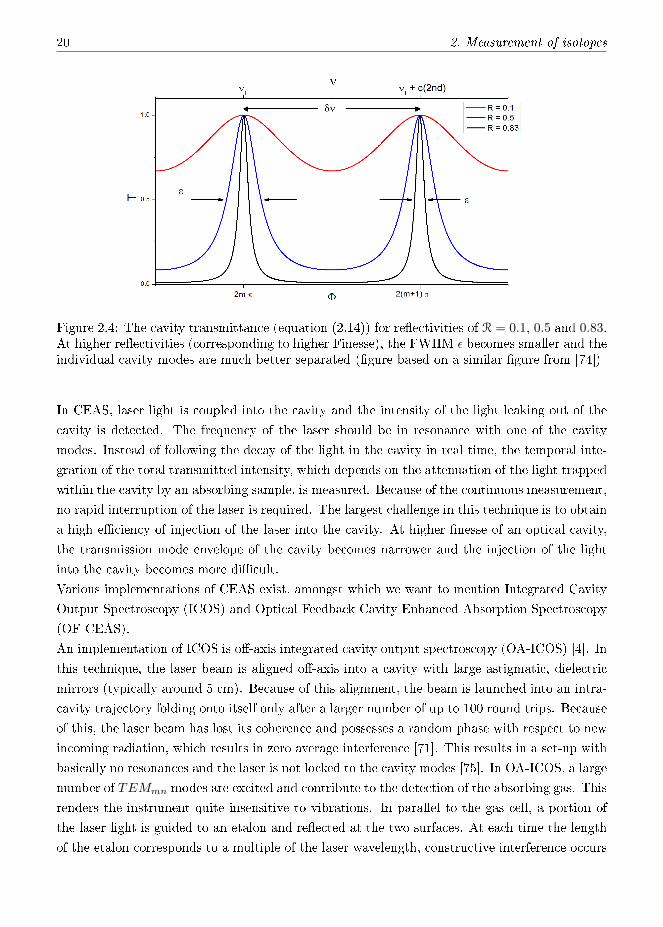
Figure 2.3: Schematic representation of the electric �eld distribution for the vertical polarizationcase in the xy-plane in the resonator in cylindrical coordinates, �gure from [74])
The Full Width Half Maximum (FWHM) of the resonance given in equation (2.14), is [71]:
∆νc =c
2πl
1− R√R
(2.17)
The width of a cavity mode thus depends on the mirror re�ectivity and on the cavity length l.
The ratio of the FSR and the width of a cavity mode is de�ned as the Finesse F :
F =∆νFSR
∆νc=
π√R
1− R(2.18)
Note that this formulation is true for a linear, but not a V-shaped cavity, where the equation
has to be modi�ed. It is an indicator of how well separated and narrow the cavity modes are.
A graph showing the transmittance for di�erent re�ectivities R (based on a �gure from [74]) is
shown in �gure 2.4. With increasing re�ectivity, the cavity modes become increasingly narrow.
Instead of measurements of the ring-down time for the determination of the absorption coe�-
cients, it is also possible to consider steady state conditions with a continuous light injection.
This leads to Cavity Enhanced Absorption Spectroscopy (CEAS) techniques.
20 2. Measurement of isotopes
Figure 2.4: The cavity transmittance (equation (2.14)) for re�ectivities of R = 0.1, 0.5 and 0.83.At higher re�ectivities (corresponding to higher Finesse), the FWHM ε becomes smaller and theindividual cavity modes are much better separated (�gure based on a similar �gure from [74])
In CEAS, laser light is coupled into the cavity and the intensity of the light leaking out of the
cavity is detected. The frequency of the laser should be in resonance with one of the cavity
modes. Instead of following the decay of the light in the cavity in real time, the temporal inte-
gration of the total transmitted intensity, which depends on the attenuation of the light trapped
within the cavity by an absorbing sample, is measured. Because of the continuous measurement,
no rapid interruption of the laser is required. The largest challenge in this technique is to obtain
a high e�ciency of injection of the laser into the cavity. At higher �nesse of an optical cavity,
the transmission mode envelope of the cavity becomes narrower and the injection of the light
into the cavity becomes more di�cult.
Various implementations of CEAS exist, amongst which we want to mention Integrated Cavity
Output Spectroscopy (ICOS) and Optical Feedback Cavity Enhanced Absorption Spectroscopy
(OF-CEAS).
An implementation of ICOS is o�-axis integrated cavity output spectroscopy (OA-ICOS) [4]. In
this technique, the laser beam is aligned o�-axis into a cavity with large astigmatic, dielectric
mirrors (typically around 5 cm). Because of this alignment, the beam is launched into an intra-
cavity trajectory folding onto itself only after a larger number of up to 100 round trips. Because
of this, the laser beam has lost its coherence and possesses a random phase with respect to new
incoming radiation, which results in zero average interference [71]. This results in a set-up with
basically no resonances and the laser is not locked to the cavity modes [75]. In OA-ICOS, a large
number of TEMmn modes are excited and contribute to the detection of the absorbing gas. This
renders the instrument quite insensitive to vibrations. In parallel to the gas cell, a portion of
the laser light is guided to an etalon and re�ected at the two surfaces. At each time the length
of the etalon corresponds to a multiple of the laser wavelength, constructive interference occurs

2.4. State-of-the-art 21
and a photodiode measuring the etalon re�ections records a maximum in the intensity. In this
way, a frequency comb is generated and can be used to determine the tuning rate of the laser.
A drawback of this technique is that due to the large number of re�ections at the cavity mirrors,
the transmission through the cavity is extremely reduced and a laser with relatively high output
power and very sensitive detectors - often cooled to low temperatures - have to be employed.
In addition, because of the relatively large mirrors, the sample volume is at least one order of
magnitude larger than in CEAS techniques using on-axis cavity injection.
In the OF-CEAS technique, a portion of the light inside the cavity is sent back to the laser source
and e�ciently couples the laser frequency to one of the modes of the cavity. This technique is
used for the instrument developed in this thesis and will be explained in more detail in section
2.5.
2.4 State-of-the-art
In recent years, several optical instruments based on the spectroscopic techniques described
above, have been introduced for the measurement of water vapor isotope ratios.
A direct absorption spectrometer was introduced by Kerstel et al. [64] as early as 1999 (after
a development phase that had started in 1995). It measured the isotopic composition of water
using a Color Center Laser (or Farbe Center Laser, FCL) around 3662 cm-1 (2.73 µm) and at
an e�ective path length of approx. 20 m in a spherical mirror Herriot MPC with a base-length
of 43 cm. Their instrument was used for the determination of the isotopic composition of liquid
water samples. A 10 µl water sample was introduced into an evacuated gas cell and measured
in parallel to a reference cell containing an isotope standard. At partial pressures around 13
mbar, precisions of 0.7, 0.3 and 0.5h were reached for δ2H, δ17O and δ18O, respectively, for an
average over 15 laser scans, corresponding to approx. 30 min total measurement time.
Webster et al. [5, 76] reported measurements of the water isotopic composition in the upper tro-
posphere lower stratosphere (UTLS) with a TDL spectrometer called ALIAS, which is equipped
with an MPC and a quantum cascade laser (QCL) emitting at 6.7 µm. At water concentrations
around 80 ppmv, they report uncertainties for the delta values of approximately 50h over a
pressure range of 75 - 300 mbar.
A TDLAS using a LN2-cooled lead-salt laser, commercialized by Campbell Scienti�c Inc., was
used by Lee and co-workers [65, 66], to measure atmospheric water vapor isotopologues at 6.7
µm with a precision of 2h for δ2H and 0.12h for δ18O, with 1 h averages at 5600 ppmv, and
1.1h and 0.07h at 15,000 ppmv for δ2H and δ18O respectively.
More recently, an MPC equipped direct absorption spectrometer, measuring at 2.66µm was
described by Dyro� et al. [7]. This instrument uses 2f wavelength modulation and on-board
calibration to two isotope standards to arrive at an accuracy of 2h for δ2H and δ18O at a water
concentration of 600 ppmv. At 100ppmv, a detection limit of 4.5h and 1.2h for δ2H and δ18O,

22 2. Measurement of isotopes
respectively was reported for 60s averaging.
An instrument based on a QCL-equipped OA-ICOS was described by Sayres et al. and success-
fully employed for isotope measurements in the upper troposphere and lower stratosphere [10].
Their instrument achieved a precision of 0.14 ppmv for the H2O concentration, whereas at a
water concentration of 5 ppmv a precision of 50h and 30h for δ2H and δ18O, respectively, was
demonstrated.
OA-ICOS is also used in the commercial instruments of Los Gatos Research (LGR). The LGR
instruments �rst became commercially available in 2006. Newer versions of the instrument have
been presented and discussed by di�erent research groups [48, 77, 78]. Aemisegger et al. [78]
report a precision of 0.02h with 7 min averaging for δ2H and of 0.01h for δ18O with 30 min
averaging with a later version of the Water Vapor Isotope Analyzer (WVIA-EP) at water con-
centrations around 15,700 ppmv. For measurements including δ17O, Berman et al. [48] state for
the Triple Isotope Water Analyzer (TIWA-45EP) a combined precision and accuracy of 0.07h
and 0.03h for δ18O and δ17O, respectively, in a water concentration range of 2 − 4.5 × 10¹⁶
molecules/cm3 (17,500 to 40,000 ppmv), for measurements averaged over four separate injec-
tions of liquid water samples.
A particularity of the Picarro WS-CRDS spectrometer is that it uses a three-mirror ring cavity.
The calibration of the frequency scale requires the use of a custom made wavelength monitor
[79]. For one of the later versions of the Picarro instruments, the L2130-i, Aemisegger et al. [78]
report at 15,700 ppmv a precision of 0.02h with 170 min averaging for δ2H and 0.006h with
100 min averaging for δ18O. With 5 s averaging, the reported precision is 0.83h and 0.22h for
δ2H and δ18O, respectively.
More recently, Steig et al. [49] presented a modi�cation of the Picarro instrument (model L2140-
i), which was speci�cally designed to measure ∆17O with high precision. It uses two lasers to
measure δ18O and δ17O at 7193 cm−1 and reaches precisions of 0.015h for both δ18O and δ17O
and of 0.01h for ∆17O, with 1200 s averaging at water concentrations around 20,000 ppmv.
Although several of the above described techniques demonstrate very good performance with
high stability and precision, none of the instruments, with the exception of the Harvard ICOS
[10] and the ALIAS instrument [5], is well adapted to measure water isotopologues with su�-
ciently high precision under very dry conditions with H2O < 1000 ppmv. Because of a large
volume (around 1m3) and large mass, the Harvard ICOS is, however, not particularly well-suited
for wider spread use.
In order to be able to measure under very dry conditions, one could decrease the noise level, which
is for example done in modulation techniques such as noise immune cavity enhanced optical het-
erodyne molecular spectroscopy (NICE-OHMS), which was most pro�tably used in Lamb-Dip
experiments [80]. However, this technique is very complex and not suitable for Doppler-limited
spectroscopy.
Another possibility would be to use stronger ro-vibrational transitions, which can be found in

2.5. Optical feedback cavity enhanced absorption spectroscopy (OF-CEAS) 23
the mid-infrared region at 2.7 µm and 6.7 µm. This is done in the Harvard ICOS instrument
[10], the ALIAS instrument [76] and as well in the ISOCLOUD in-situ isotope instruments (see
chapter 8). In the case of H2O, the gain is approximately one order of magnitude, and is o�set
by less sensitive MIR detectors and mirrors with lower re�ectivity, resulting in higher noise level
and/or shorter e�ective path lengths.
Finally, a viable alternative solution is to increase the e�ective absorption path length, which
can be achieved by the use of higher re�ectivity coatings on the cavity mirrors of a CRDS or
CEAS system.
2.5 Optical feedback cavity enhanced absorption spectroscopy
(OF-CEAS)
Most of the previously described cavity enhanced absorption spectroscopy techniques su�er from
ine�cient and noisy cavity injection due to changes in the laser frequency and linewidth, which
is in general much larger than the width of a single cavity mode. As mentioned above, this
becomes a major problem when using very high �nesse cavities, in which the coupling is even
more di�cult because of the correspondingly narrower cavity mode width.
In the case of OF-CEAS, a portion of the light (optical feedback) travelling inside the cavity
is send back to the laser source, which results in a coupling of the laser to one of the cavity
modes, which in turn leads to a narrowing of the laser line width to below that of the cavity
mode transmission [81].
Figure 2.5: Schematics of a typical OF-CEAS set-up with a V-shaped cavity (�gure from [82]
A schematic of a typical OF-CEAS set-up with a V-shaped cavity is shown in �gure 2.5.
The light from a diode laser is injected into a V-shaped cavity via a set of di�erent optical com-
ponents. The V-shape of the cavity e�ciently avoids that a direct re�ection from the folding

24 2. Measurement of isotopes
mirror at the apex of the cavity (labeledMa) is sent back to the laser and ensures that only light
re�ected at mirror M1 inside the cavity returns as optical feedback (OF) to the laser. A pho-
todetector (PD) with a beamsplitter (BS) is used to monitor the injected laser intensity, whereas
a signal detector behind the cavity measures the cavity output. An attenuator (A), e.g. a lin-
ear polarizer, between the cavity and the laser is used to adjust the level of feedback to the laser.
As the laser is scanned over a frequency range, it is slowed down due to the optical feedback
and stays longer at the successive cavity frequencies (cf. �gure 2.6). At higher feedback levels,
the laser couples stronger to the cavity frequencies and the resident time for each frequency is
extended.
Figure 2.6: Figure from [82]. Frequency of the diode laser coupled by optical feedback to theV-shaped cavity, as a function of free running laser frequency, during the passage through acavity mode for two di�erent levels of feedback (solid and dotted lines for weak and strongfeedback levels, respectively). The linear dashed line indicates the free running laser frequency,which is directly proportional to the laser current. Arrows in the plot indicate the path of thecoupled laser frequency (α → β → γ → δ when the laser current is tuned and emphasize thelonger residence time at the respective cavity frequency
The distance between the laser and the cavity equals L2, the length of the second cavity
arm. This ensures that constructive interference inside the laser cavity is obtained for all cavity
modes, as the distance corresponds to an integer multiple of one-half the wavelength irrespective
of the exact wavelength value (a detailed derivation can be found in [81]). To compensate for
instabilities in the laser-cavity distance and cavity length due to temperature and mechanical
variations or disturbances, a mirror between laser and cavity is mounted on a piezo element,
controlled by a feedback loop. The error signal for the feedback loop is obtained by analysis of
the symmetry of the transmission pro�les of the cavity modes.
For the con�guration described here above and used in our spectrometer, in which the laser to
cavity distance equals L2, modes for which the cavity round trip is an even or odd multiple
of one-half of the wavelength (from now on simply called even and odd modes), experience a

2.5. Optical feedback cavity enhanced absorption spectroscopy (OF-CEAS) 25
slightly di�erent re�ection coe�cient at the folding mirror, which results in a small di�erence in
the ring-down time associated with the odd and even modes [81, 82]. However, this di�erence
can easily be corrected for in the data analysis, as the di�erence remains constant over the small
tuning range of the laser wavelength.
An OF-CEAS spectrum is �nally recorded by determining the maxima of successive TEM0,0
cavity mode pro�les in the raw OF-CEAS signal (cf. �gure 2.7) and normalizing them with the
signal of the reference detector. At the end of each laser scan, the laser is interrupted for a little
more than the duration of one cavity mode to measure a ring-down on one cavity mode. These
RD measurements are used to calibrate the transmission signal and to convert the spectra to
absorption units, based on the (approximated) relation:
√Hk
τk=
√Hm
τm(2.19)
with the cavity modes k andm, τk the ring-down time of mode k, and Hk the measured intensity
ratio at mode k. A derivation of this relation can be found in [81]. This approximation is very
good under typical CEAS conditions, and even in the limit of relatively strong absorption. In
(a) (b)
Figure 2.7: Exemplary OF-CEAS signal, a) signal over the entire laser scan b) at the end of eachscan the laser is interrupted to record a RD event to convert the recorded spectra to absorptionscale
table 2.1, the most important characteristic dimensions like the FSR and Finesse are compared
for a linear cavity and a V-shaped cavity.

26 2. Measurement of isotopes
Linear Cavity V-shaped cavity
FSR c/(2L) c/2(L1 + L2)
ring-down time emptycavity τ0 =
L/c1−R τ0 =
L1+L2
2c(1−R)
ring-down time withabsorber τ = −L/c
1−R+αLτ = L1+L2
2c(1−R+α(L1+L2))
Finesse πR
1−√R
πR1−R2
max. transmission forlossless cavity ≈ 1
(1+LT
)2≈ 1
41
(1+LT
)2
H(α→ 0,L + T � 1)
Table 2.1: FSR, ring-down time, Finesse and maximal transmission for linear and V-shapedcavity as a function of re�ectivity R, transmittance T, and the length of the cavity arm(s) L(linear cavity), and L1 and L2 (V-shaped cavity), respectively. c is the speed of light.
2.6 Absorption scale linearity
As mentioned above, in direct absorption techniques, the molecular absorption coe�cient α is
obtained in a very straightforward manner from the Lambert-Beer-Bouguer law:
α = −1
lln
(ItI0
)with It the transmitted intensity, I0 the incoming light intensity and l the e�ective path length.
In the case of OF-CEAS, the relation between molecular absorption and intensity is more com-
plicated. As described in detail in [6, 81] and brie�y summarized in the following, the relation
between α and the transmitted intensity in OF-CEAS allows the measurement of isotope ratios
over a much larger concentration range than in direct absorption spectroscopy.
In the case of a V-shaped cavity with cavity arm lengths l1 and l2, �lled with an absorber with
absorption coe�cient αm = α(ωm) at the center of a cavity mode, the cavity transmission is
described with an Airy-shaped transfer function whose maximum at frequency ωm is given by
[82]:
Hmax(αm) =
[T exp(−αml1/2)
1− R2 exp(−αm(l1 + l2))
]2
(2.20)
The e�ective mirror transmission and re�ectivity coe�cients T and R are T = (TaT1)1/2 and
R = (Ra)1/2(R1R2)1/4 with the subscript a indicating the folding (apex) mirror and 1 and 2 the
mirrors at the end of the two cavity arms (the transmitted intensity is calculated for mirror 1).

2.6. Absorption scale linearity 27
In general, all three mirrors are from the same batch and are virtually identical. As the angle
between the two cavity arms is very small, the re�ectivity is practically the same as for normal
incidence and the re�ection and transmission coe�cients can be considered equal for the three
mirrors.
Equation 2.20 is valid for cavity injections by a perfectly monochromatic �eld slowly passing
through resonance. This is generally true in the case of OF-CEAS, as the laser tuning is
su�ciently slow to assure full cavity buildup during frequency locking by optical feedback,
which also results in a laser line width narrowing to well below the cavity mode width.
Because of conservation of energy, the e�ective mirror losses due to absorption and scattering
are given by L = 1−R−T. With this, it is easy to show with equation 2.20 that the maximum
transmission for a completely lossless cavity (α = 0 and L = 0) reaches 25%:
H(α← 0, L + T � 1) ≈ 1
4
1
(1 + LT
)2(2.21)
Equation 2.20 is derived by squaring the sum of the amplitudes of the �eld transmitted through
the mirror at the end of one cavity arm and not by summing the square of the amplitudes [82].
The summation of the intensities would not account for the resonance e�ect in OF-CEAS and
is only valid in the case of a broadband incoherent source. This would result in substantially
lower transmission of only T/4.
If we approximate exp(−αml1) ≈ 1 in the numerator, it is possible to invert equation 2.20,
following the derivation presented in [6] and [81]:
αm =1
l1 + l2
[2 ln(R)− ln
(1− T√
Hmax
)](2.22)
We further make the assumption T/√Hmax � 1, which is in general true as T is typically
smaller than 100 ppm and very large absorptions are avoided, such that Hmax > 1%. With this,
we can write
αk ≈2
l1 + l2ln(R) +
T
(l1 + l2)√Hmax(k)
(2.23)
If we write ln(R) ≈ 1− R = T + L, it becomes evident that the �rst term on the right hand of
equation (2.23) is −γ0, the loss per unit length for the empty cavity. We can than write:
γkc
= αk −2
l1 + l2ln(R) = αk +
γ0
c≈ T
(l1 + l2)√Hmax(k)
(2.24)
The total loss coe�cient γk can be determined experimentally by �tting exp(−γkt) to a ring-
down event, which can be produced by an abrupt interruption of the laser once the maximum
injection for mode k has been reached. The CEAS spectrum can then be obtained in abso-
lute absorption units, apart from an o�set due to the empty cavity losses (γ0), by calculating

28 2. Measurement of isotopes
1/√Hmax(m) for all modes m and then multiplying by the factor (γk/c)
√Hmax(k) determined
by the ring-down measurement at mode k. It should be underlined that the absorption-scale
calibration procedure can also be performed in the presence of intracavity absorption. The cali-
bration of CEAS measurements in absolute absorption units does not require a measurement of
the ring-down time for an empty cavity. An investigation of the accuracy of the normalization
is discussed in detail in [81].
For a typical OF-CEAS cavity with ring-down time of 20 µs, the relative error due to the nor-
malization procedure is smaller than 100 ppm for cavity transmissions larger than 10% of the
maximum value (H > 0.1). This would correspond to an absorption coe�cient of 4× 10⁻⁶/cm
or, considering a typical noise level of 4× 10⁻¹⁰/cm, to a dynamic range of four decades. For a
higher �nesse cavity such as the one used in our spectrometer, the accuracy of the normaliza-
tion is even better. For cavity transmissions larger than 5%, the relative error for a cavity with
ring-down times of 130 µs would be smaller than 50 ppm.

Chapter 3
OCEAS instrument design
In this chapter, the OF-CEAS laser spectrometer, SIRI (Spectromètre Infrarouge des Rapports
Isotopiques), developed within the framework of this thesis, is described. A �rst OF-CEAS
spectrometer for water vapor isotope measurements was introduced by Kerstel et al. in 2006 [6],
an improved version was described by Iannone et al. in 2009 [83]. With the novel spectrometer
SIRI, we speci�cally aimed for an instrument able to measure water vapor isotopes in very dry
conditions with water concentrations well below 500 ppmv as encountered in Antarctica and
the upper atmosphere. This requires an instrument with much higher sensitivity and stability
and could be achieved with the design detailed in the following. In addition, we refer to our
publication in Optics Letters [84], which can be found in appendix C. Please note that for the
purpose of the Optics Letter publication, the instrument developed in this work and referred to
as SIRI throughout this entire thesis was named HiFi (for High Finesse Spectrometer) to o�er
a more international name.
3.1 Optical Layout
The laser source used in the laser spectrometer SIRI is, as in the predecessor IRIS, a distributed
feedback (DFB) diode laser (obtained from either LaserComponents or Nanoplus) with a typ-
ical maximal output power of 10mW. For the di�erent spectral regions (discussed in detail in
section 3.6), various lasers were used.
The cavity mirrors (from Layertec GmbH) have a radius of 1 m and a wedge of 1°. With an
empty cavity, these mirrors yield a ring-down time of 150 µs (at 7184 cm−1, which is more than
a factor seven higher than in previous instruments and requires an even more precise alignment
of the optical set-up. The ring-down time corresponds to a re�ectivity of 99.9989% (1-R=11
ppm) and leads to a cavity with a �nesse of approx. 144,000 (a standard linear cavity of the
same external length using the same mirrors would have F ≈ 288, 000). This high �nesse results
in an e�ective path length of nearly 45 km and is necessary to be sensitive enough to measure
at very low water concentrations.
Instead of using very high re�ectivity mirrors, it would have been possible to change from the
near-infrared into the mid-infrared (MIR) at 2.7 µm, which would have resulted in transitions
that are approx. a factor 10 stronger. However, apart from the currently still lower re�ectivities

30 3. OCEAS instrument design
of mirrors for the MIR, this would also have required the use of less sensitive photodetectors.
The gain of stronger transitions would thus have been canceled out or even overcompensated by
these disadvantages.
In our instrument, the photodetectors are InGaAs detectors (Hamamatsu) wired in the back
of the detector, which reduces the risk of optical fringes induced by parasitic re�ections on the
wires.
To correct the measurements for water absorption occurring outside of the gas cell, the path
lengths outside the cavity for reference and signal photodiode were matched. This becomes
especially important when the sample measured in the gas cell is much drier than the ambient
air.
3.2 Mechanical layout
The instrument is mounted in a thermally insulated aluminum casing, which has a volume of
approx. 45 l and a weight of 25 kg and is thus easily transportable. The core of the spectrometer
is an additionally insulated triangular base mounted on four metallic springs on which the optical
set-up is installed. The V-shaped cavity consists of two arms of 50 cm under an angle of 0.94°.
Other than previous versions, the gas cell is other than in previous versions now machined from
a single stainless steel bloc, which reduces the risk of leaks.
3.3 Flow system
An important factor in�uencing the response time of an instrument, is the so-called memory
e�ect. Due to for example adsorption of water to the walls of tubing and cavity of the instrument
or small dead volumes that are not e�ciently exchanged with new gas, the time response of an
optical spectrometer can sometimes be in the order of several minutes.
To reduce the memory of our system, the electropolished stainless steel of the gas cell is now
additionally coated with a �uoroaliphatic polymer (Cytonix FluoroPel 800A).
Because of the very low water concentrations, special attention was paid to the gas inlet system
to reduce memory e�ects. All inlet tubing is coated O'Brian tubing, and a Siltek treated inlet
�lter (Restek) is used to protect the system against contamination from larger particles. The
pressure is regulated to 35 mbar by a Siltek treated pressure controller (Bronkhorst) at a �ow
rate of approx. 150 sccm. The gas cell has channels with a diameter of 5 mm, which results in
a volume of 18.6 ccm and therefore in a gas exchange time of only 0.18 s.
During in �eld deployment of the instrument, additional O'Brien tubing is used for the inlet and
is temperature stabilized to approximately 50°C with an auto-regulating heating band (Horst).

3.4. Data acquisition and storage 31
3.4 Data acquisition and storage
The entire instrument is controlled by a C program on a ARM9-based micro-controller (AT-
MEL), which is also used for the data acquisition in combination with a analog/digital converter.
Communication with the ARM9 is established via an Ethernet connection with a Labview (Na-
tional Instruments) based program, which is also used to control the instrument. Data analysis
is done on-line with the same Labview program in combination with a C based analysis program
incorporating the Minuit library of CERN [85]. The signal of the two photodiodes is digitized
by a 16 bit A/D converter with 60 000 points per channel. Due to the high ring-down times,
which result in very long residence times for each single mode in the cavity, a scanning frequency
of 1.96 spectra per second was chosen, corresponding to approximately 3.5 ms per single mode.
The scanning frequency is thus a factor three smaller than in the predecessor IRIS. However,
instead of one ring-down event per second, the laser is now interrupted for approximately 3.5
ms (400 data points) at the end of each scan. Housekeeping data such as cavity temperature
and pressure are recorded with 12 bit and averaged over 10 consecutive acquisitions before being
written to �le.
3.5 System control and house keeping
A large improvement has been made in the temperature stability of the system compared to
previous versions. Whereas IRIS was stabilized to 35.5 ± 0.5°C by an on/o� regulation, the
temperature of the instrument is now regulated in a two step system to 45°C with mK-precision
and a drift of less than 0.5 mK over 200 min (see �gure 3.1).. The air temperature in the entire
instrument is regulated to 38 ± 0.1 °C with a PID regulated TEC (Supercool) in combination
with two mixing fans. Furthermore, the temperature of the optical triangle is stabilized at
45 °C with additional heating bands , which are regulated with a PID loop via a pulse width
modulation (PWM). The temperature sensor used for the regulation is a very low drift Pt1000,
which is read out with 16 bit resolution.
To avoid additional electronic heat in the insulated box due to the power supply, the instrument
is powered by a commercially available 220W single output desktop power supply. Because of two
additional Pt1000 temperature sensors that are freely suspended in the inlet and outlet stream
of the cavity, it is also possible to correct measurements for �uctuations of the gas temperature.
This becomes especially important if atmospheric measurements with large variations of the air
temperature (e.g. day-night cycle) shall be done. Due to the di�erent temperature dependency
of the single absorption lines, this can become crucial when isotope ratios should be determined
with high accuracy. The pressure in the cavity is stable within the microbar level (better than
10 µbar) for several hours (cf. �gure 3.1b).

32 3. OCEAS instrument design
(a) (b)
Figure 3.1: Allan variances of temperature and pressure in the instrument. The sensors usedfor the Allan variances are independent sensors and not used for the regulation. The stabilityof the cell temperature is better than 1 mK, the maximum at 1 s is due to the read-out of thesensor. The pressure is regulated with a precision of better than 10 µbar over a time of 3.6 h
3.6 Choice of spectral ranges
Depending on the speci�c requirements of the measurements, di�erent spectral regions in the
near infra-red were selected for the measurements. For most of the measurements, a spectral
region around 7184 cm−1 was chosen that was also used in previous instruments [6, 83] and is
also used by commercial instruments [78, 86]. As can be seen in an exemplary spectra in this
region (�gure 3.2), this region is suited for measurements of all of the four isotopologues H162 O,
HD 16O, H218O and H2
17O. Because of a relatively large number of additional weak absorption
Figure 3.2: Simulated spectrum at 7184cm−1, 1 ppmv H216O, spectral information from the
Hitran database [61]

3.6. Choice of spectral ranges 33
lines and several methane absorption lines in this spectral region, the analysis of the spectral
data is more di�cult than in other spectral regions.
An alternative, for measurements in which H217O is of no or little interest, is the spectral re-
gion around 7200 cm−1 in which the absorption lines of the three isotopologues H162 O, HD 16O
and H218O are better separated (�gure 3.3). This region, which we used for some of our mea-
surements, is also the region of choice of the most common version of the instruments of Los
Gatos Research Inc. [78]. For measurements at very low water concentrations (< 40 ppmv),
Figure 3.3: Simulation of a spectrum at 7200cm−1 and 1 ppmv H216O; spectral information
from the Hitran database [61]
we chose an alternative spectral region around 7286 cm−1 (cf. �gure 3.5), which includes an
H218O absorption line that is nearly a factor 4 stronger and an H16
2 O line that is more than
a factor 50 stronger than in the above mentioned regions. In addition, the region around 7286
cm−1 enables the measurement of δ2H with spectral lines of H216O and HD 16O at 7280 cm−1.
With the available laser (Nanoplus GmbH), the two region could be reached by selecting the
appropriate temperature of the laser chip. In table 3.1, the wavenumber, intensity and tem-
perature dependence of the line strength for the principal absorption lines [61] is shown for the
di�erent spectral regions used in our measurements. For the spectral region around 7286 cm−1,
the change of the wavelength region additionally results in an increase of the ring-down time of
the instrument due to a higher re�ectivity of the cavity mirrors (cf. �gure 3.4). With ring-down
times of up to 180 µs, this con�guration results in a signi�cantly increased sensitivity in the low
water vapor concentration range (see chapter 8).
This spectral range was not used in our instrument but we adapted a di�erent OF-CEAS spec-
trometer that was initially built in our laboratory by J. Habig of the Karlsruhe Institute of
Technology [87].

34 3. OCEAS instrument design
Figure 3.4: The re�ectivity of our cavity mirrors vs. the wavenumber (measurements by S. Kassi,LIPhy, UJF). The re�ectivity is higher for the region 7286 cm−1 proposed for measurements ofδ18O at very low water concentrations compared to the spectral regions used before.
isotopologue wavenumber intensity temperature dependence[cm−1] [cm−1/(molecule× cm−2)] %/°C
H216O 7183.6858 3.67× 10⁻²⁴ 0.0593
H218O 7183.5892 4.54× 10⁻²⁴ 0.133
H217O 7183.7355 1.16× 10⁻²⁴ -0.688
HD 16O 7183.9728 3.385× 10⁻²⁵ -0.609
H216O 7200.1338 3.268× 10⁻²⁴ -0.398
H218O 7199.9613 4.434× 10⁻²⁴ -0.0365
HD 16O 7200.3024 3.514× 10⁻²⁵ -0.155
H216O 7286.0508 2.049× 10⁻²² -0.244
H218O 7285.7703 3.442× 10⁻²³ -0.709
H216O 7280.4842 2.735× 10⁻²³ -0.103
HD 16O 7280.5569 7.383× 10⁻²⁵ -0.787
Table 3.1: Principal absorption lines in the investigated spectral regions [61]

3.6. Choice of spectral ranges 35
(a)
(b)
Figure 3.5: Simulation of spectra at a) 7286 cm−1 and b) 7280 cm−1, respectively. Spectralinformation from the Hitran database [61].


Chapter 4
Data analysis procedures
To retrieve concentrations and isotope ratios from a measurement, a theoretical model is gen-
erally �t to the experimental spectra. For the synthetic spectra, di�erent models can be used,
that take di�erent factors responsible for line broadening into account.
If the pressure of the gas sample is very low (p ≤ 0.5 mbar), the line width of the spectral lines
is dominated by the Doppler line width. It takes into account the e�ect that the frequency at
which a molecule with a velocity component along the trajectory of the light beam absorbs and
emits electromagnetic radiation is slightly shifted. As the velocity of the molecules in a gas is
due to thermal motion, this change in the absorption frequency leads to a Gaussian line shape
[88]:
I(ν) = I0 exp
[−(
2 ln(2)(ν − ν0)
γD
)](4.1)
with γD the FWHM of the Gaussian function:
γD =ν0
c(8kBT ln(2)/m)1/2 (4.2)
with ν0 the center frequency of the absorption in Hz, c the speed of light, kB Boltzmann's con-
stant, T the temperature in Kelvin and m the mass of the molecule in kg.
At higher pressures, the collision between molecules in the gas can lead to a reduction of the
lifetime of the molecule's upper energy state, which according to Heisenberg's uncertainty prin-
ciple leads to an increased linewidth. The line shape in this case is described by a Lorentzian
function [89]:
I(ν) = I02πγC
(ν − ν0)2 + (πγC)2(4.3)
(4.4)
with γC the FWHM of the Lorentz function. At higher pressures (p ≥ 1000 mbar), the collisional
broadening is the dominant mechanism and the pro�le can be described relatively well by a
purely Lorentzian line shape [90]. At intermediate pressure (0.5 mbar ≤ p ≤ 1000 mbar), the
line shape is often approximated with the Voigt pro�le, which is a convolution of a Gaussian

38 4. Data analysis procedures
and a Lorentzian pro�le. The normalized Voigt pro�le can be written as [91]:
ΓV (ν) =γC
π3/2γ2D
∫ +∞
−∞
e−y2(
ν−ν0γD− y)2
+(γCγD
)2 dy (4.5)
and has in a �rst approximation a FWHM γV of [92]:
γV ≈ 0.5346γC +√
0.2166γ2C + γ2
D (4.6)
However, the Voigt pro�le is only an approximation, as it does not take into account further
mechanisms that in�uence the line shape of a spectral lines. In reality, the Doppler pro�le of
the spectral lines is narrowed because of collisions between the active molecules and molecules
in the bu�er gas, which result in a reduced free path length (to below the wavelength of the
infrared radiation) and consequently in a smaller velocity of the molecules.
Two di�erent models have been developed to take this narrowing, the so-called Dicke e�ect, into
account. The Rautian and Sobel'man model (in the following Rautian pro�le)[93] and the model
of Galatry (Galatry pro�le)[94]. These two models take into account the Doppler broadening,
the Dicke narrowing and the collisional broadening. Whereas the Galatry model assumes that
the mass of the active molecule is much heavier than the mass of the molecules of the carrier gas
(and consequently many collisions are required to induce a notable velocity change), the model
of Rautian and Sobel'man supposes the contrary, namely that the perturber is much heavier
than the active molecule (and a single collision su�ces) [90, 93, 94].
As in our case, the active molecule is in general lighter than the carrier gas molecules, we will
focus here on the Rautian pro�le. This pro�le can be expressed as [90]:
γR(γD, γC , z) =1
γD√π<[
W (γD, γC + z)
1−√πzW (γD, γC + z)
](4.7)
with
W (γD, γC , z) =i
π
∫ ∞−∞
e−t2
(ν−ν0γD+ i( γCγD + z)− t√
ln(2))dt (4.8)
and the narrowing parameter z:
z =βCγD
(4.9)
with βC the coe�cient of collisional narrowing (given in cm−1).

4.1. Analysis of experimental spectra 39
4.1 Analysis of experimental spectra
For the analysis of our experimental spectra, a simulated spectrum based on the Rautian line
pro�le is �t to the experimental data. The line positions of the di�erent absorption lines were
taken from determinations with high sensitivity CW-Cavity Ring Down Spectroscopy done by
Leshchishina et al. [95] and the frequency scale of the measured spectrum was scaled linearly
to match this theoretical spectrum, e�ectively determining the FSR of our OF-CEAS cavity.
The Gaussian line widths (Doppler broadening) were calculated for the di�erent isotopologues
based on the gas cell temperature and then �xed for all spectra. Lorentzian widths (pressure
broadening) and the Dicke parameters (motional narrowing) were �t once over an exemplary
measurement and kept constant throughout the measurements. The relative intensities of di�er-
ent absorption lines from the same isotopologue were �xed, thus yielding only one free parameter
for intensity per isotopologue. Note that of di�erent temperature dependencies of the strengths
of di�erent absorption lines, this grouping should only be done with a very good temperature
stabilization, which is present in our spectrometer. In addition to the group intensities for each
isotopologue, an additional parameter accounts for a possible mode shift of the entire spectra,
which can occur due to small temperature �uctuations of the gas or gas cell temperature. To
take into account additional absorption lines of methane in the same spectral region, these lines
were introduced as an additional species in the model spectrum, with an additional �tted group
intensity parameter. The absorption frequencies of methane were taken from measurements of
Campargue et al. [96], whereas we determined the relative intensities and Lorentzian line widths
of the strongest methane absorption lines in a measurement on a diluted methane sample. The
methane absorption does not play an important role for higher water concentrations but be-
comes an important factor at lower water concentrations (500 ppmv and below). The baseline
is �t with neighboring strong water absorption lines outside the measurement range, and an
additional third order polynomial.
The quality of the �t, and consequentially an important factor of the instrumental performance,
is determined by the residual on the �t. Throughout the water concentration range, in which
we can measure with SIRI, the RMS of the residual on the �t is below 8 × 10⁻¹¹ cm−1 (at
2 Hz measurements). At water concentrations below 500 ppmv, the NEAS of the instrument
is typically around 6 × 10⁻¹¹ cm−1Hz−1/2, which is an improvement by a factor of almost 7
compared to the predecessor instrument IRIS.
4.2 Precision
In the case of an absolutely stable system, the precision of the measurements would continu-
ously improve with increasing integration time. However, in the real world instrument stability
is limited, for example because of temperature or pressure drift or mechanical disturbances.

40 4. Data analysis procedures
Figure 4.1: A single experimental spectrum, recorded in 0.51 s at 500 ppmv H2O. The RMS ofthe residual (bottom panel), is 8× 10⁻¹¹ cm−1
Because of these drifts, longer averaging is only bene�cial up to the level where instrumental
drift becomes noticeable.
The optimum integration time can be e�ectively determined with an Allan-Werle-plot. The
Allan-Werle-plot was �rst introduced to the �eld of laser-based trace gas detection to reveal low
frequency drift phenomena [97] and later adapted to characterize instrumental stability [98]. To
determine the stability of SIRI and its level of precision, long time measurements at di�erent
water concentrations were made. A gas bottle was �lled with a mixture of dry synthetic air and
a calculated amount of a local water standard to a given water concentration. This standard gas
bottle was then connected to the OF-CEAS instrument for long time (> 8h) stability measure-
ments. This measurement was repeated with di�erent water concentrations in the range from
20 ppmv to 1500 ppmv. Measurements with a bottle �lled with a standard water gas mixture is
a well adapted approach for long term stability measurements as it o�ers a very stable moist air
supply and is very easy to use. Most importantly, Kerstel et al. [6] showed that fractionation in
the bottle can be neglected under the conditions encountered in our experiments, with partial
pressures well below saturation.
Figure 4.2 shows Allan-Werle plots for the isotope ratios of the three isotopologues HDO, H217O
and H218O from measurements at di�erent water concentrations that were done with standard
gas bottles as described above.
In the case of δ2H, the best precision σopt = 0.12h is reached in τopt = 36.4 min and at a water
concentration of 1500 ppmv. For δ18O the optimum integration time is also τopt = 36 min,

4.2. Precision 41
but the best precision is at H2O= 600 ppmv and for δ17O the best results are achieved with
τopt = 70 min at 1500 ppmv and σopt = 0.064h. Because of fast natural isotope variations, it
is not always possible to integrate the measurements for more than 30 min. Because of this, the
precision that can be achieved in shorter time is also a very important measure. In table 4.1,
the precisions at the di�erent water concentration measurements shown in �gure 4.2, are given
for T = 4 s (8 data points) averaging and for the Allan optimum integration time Topt. With 4 s
averaging, the time resolution is still su�cient to study fast isotopic processes, but the precision
is nearly a factor of three better than for non-averaged (0.5 s) measurements. As can be seen in
(a) (b)
(c)
Figure 4.2: Allan deviation for the three isotopes
�gure 4.3, the precision of the measurements in a water concentration range from 200ppmv to
2000ppmv remains approximately the same for all three isotopologues. For δ2H, the precision
is always better than 0.8h, for δ17O better than 0.15h and for δ18O better than 0.1h. A de-
tailed discussion of the precision of our instrument can be found in [84], which is included in the
appendix of this thesis. In the letter, the instrument is named HiFi (High Finesse Instrument)
to avoid confusion with the name of the previous instrument IRIS.

42 4. Data analysis procedures
Figure 4.3: Minimum Allan deviation vs. H2O
Table 4.1: Measurement Precision as a Function of the Water Mixing Ratio for Di�erent Aver-aging Times
σ(2H) σ(2H) σ(18O) σ(18O) σ(17O) σ(17O)H2O (4 s) (Topt) (4 s) (Topt) (4 s) (Topt)[ppmv] [h] [h] [h] [h] [h] [h]
20 54 5 4.4 0.5 12 1.180 12 0.8 1.1 0.1 3.2 0.2190 5.5 0.6 0.5 0.07 1.4 0.19420 2.7 0.5 0.27 0.05 0.7 0.16610 1.7 0.5 0.18 0.02 0.4 0.1770 1.1 0.28 0.18 0.04 0.3 0.071470 0.7 0.12 0.17 0.05 0.22 0.07

4.3. Noise analysis 43
4.3 Noise analysis
To estimate the performance of the �tting routine used to analyze our data and to investigate
factors that can in�uence the analysis of the data, synthetic spectra were generated with a
Labview based simulation program. For the simulation, the C-based routine that is also used
for the �tting analysis of the data was incorporated into the Labview program. All generated
spectra were simulated with a Rautian line pro�le. Gaussian and Lorentzian widths as well as
the Dicke parameter were set to the average values that were obtained from �ts to experimental
spectra. The relative intensities of the di�erent lines of the same isotopologue were �xed.
To simulate changes in the water concentration only, the intensities of all spectral lines of
water were equally scaled. The baseline of the simulated spectra consists of a second order
polynomial, superimposed with Gaussian white noise. To compare synthetic and experimental
data, simulations were done with Gaussian noise of the same size as the �t residual of the
experimental spectra and the intensity of the spectral lines was also matched.
In �gure 4.4, the Allan-Werle plot of an experimental run at 80 ppmv H2O with a residual of
7.1 · 10−11 cm−1 is shown together with that of synthetic data simulating the same conditions.
Surprisingly, the experimental data yield an Allan deviation that is more than two times lower
than of the synthetic data. A histogram over the residuals of 30 subsequent spectra of the
measurement used for the Allan-Werle plot (�gure 4.5) shows that the experimental noise is
indeed Gaussian distributed, as would be expected for uncorrelated, normally distributed white
noise.
With pure white noise, averaging of several spectra reduces the residual of the �t (σavg) with
the square root of the number of averaged spectra (N):
σavg = σ0 ·1√N
Whereas the simulated data follows the 1/√N behavior, the residual of the �t to the experimen-
tal data clearly does not tend towards zero, but instead levels o� at a value of about 6 · 10−11
cm−1 (�gure 4.6). Clearly, a large fraction of the noise is not susceptible to averaging. Indeed,
if we compare the �t residual of a single spectrum with that of the �t to the average of �ve
or twenty spectra (�gure 4.7), we see that the structure of the residual remains very similar,
independent of the number of averaged spectra. This means that a large fraction of the noise in
our measurements is not fast changing white noise but slowly varying structured noise, possibly
caused by multiple, weak optical fringes [98].
Larger fringes are typically caused by parasitic re�ections of the laser beam and can be ef-
�ciently reduced by catching these re�ections with optical traps or improvements in the optical
alignment, which was e�ciently done in our set-up. Smaller fringes, e.g. due to backscattering
on the optical surfaces in the beam path, are primarily due to scattering of light on the optical
elements in the beam path and are virtually impossible to remove [99]. This structured noise

44 4. Data analysis procedures
(a) (b)
(c)
Figure 4.4: Allan-Werle plot of a measurement at 80ppmv compared to a simulated measure-ment at the same water concentration for a) δ2H b) δ18O and c) δ17O. Both, simulated andexperimental spectra have a RMS deviation of 7× 10⁻¹¹cm−1/s on the �t.
Figure 4.5: A histogram over the residuals of 30 subsequent spectra shows that the noise isfollowing a Gaussian distribution (in black)

4.3. Noise analysis 45
Figure 4.6: The residual of the spectral �t vs. the number of spectra averaged (in black). Inred, the behavior for random white noise is depicted. When averaging over several spectra, theresidual of the �t does decreases much slower than for random white noise.
Figure 4.7: Comparison of the �t residual without averaging (second panel, in black), with theresiduals of a �t to a spectrum averaged over 5 (third panel, in blue) and 20 individual spec-tra, respectively (bottom panel, in red). The shape of the residual remains nearly unchanged,independently of the number of averages. The noise pattern is thus not random white noise butsystematic time-invariant noise.

46 4. Data analysis procedures
is highly correlated between subsequent spectra and results in a smaller variation of the �t on
a short time scale than the fast changing white noise. Because of this, the Allan-Werle plot
for the experimental data starts at much lower values than the corresponding plot for synthetic
data with the same level of (fast changing white) noise. To take the more stable noise source
in the generation of synthetic spectra into account, an additional Gaussian distributed noise
is added once to the baseline of the synthetic spectra and kept constant throughout the entire
simulation. By changing the relative amount of the structured noise to the entire noise level, it
is thus possible to adapt the simulation to the measurements and to estimate the contribution
and in�uence of structured noise on the real measurements.
With an increasing contribution of time-invariant noise to the total noise of the simulation, the
standard deviation of the delta values decreases and can be matched to the real measurement.
With an RMS of the structured noise that is 1.5 times the RMS of the fast changing white
noise, the simulated Allan-Werle plot is in very good agreement with the experimental data (cf.
�gure 4.8). Of course, for longer integration times, the synthetic Allan deviation continues to
decrease, whereas the precision of the real measurement is limited by instrumental drift and
increases again. The RMS of time-invariant noise was set to 6 × 10⁻¹¹ cm−1 and the RMS of
variable noise to 4 × 10⁻¹¹ cm−1. For the summation of these two independent noise distribu-
tions, the quadrature of the two sources has to be added, resulting in an overall RMS of the
residual of σtot =√
62 + 42 cm−1 = 7.2 cm−1 and a contribution of the structured noise to the
overall noise, which is 6 cm−1/7.2 cm−1 ≈ 83%.
In �gure 4.9, the RMS of the residual versus the number of averaged residuals is shown
just as in �gure 4.6, but this time including the corresponding behavior for the synthetic data
with 83% structured noise. The RMS of the simulation with structured noise is slightly larger
than for the experimental data but perfectly reproduces the behavior for di�erent averaging.
Because of the large contribution of slowly changing structured noise in the measurements, the
�uctuations between subsequent spectra is smaller than would be expected from the residual on
the �ts. In fact, the (short) time precision that can be achieved in the measurements would be
equal to the precision of measurements with the white noise component only. The structured
noise, which remains virtually constant, permanently biases the model �t to the spectrum and
is therefore re�ected in the accuracy of the measurement and not the precision.
4.4 Photodetector linearity
A possible problem that is well known in spectroscopic studies is photo detector non-linearity
[100, 101], that is, the signal voltage has a nonlinear dependency on the incident power. A
non-linearity would have large e�ects on our measurements, as a change of the emitted laser
power would result in an apparent change of the water concentration and of the apparent isotope
ratios, as was shown by Kerstel et al. [102].

4.4. Photodetector linearity 47
(a) (b)
(c)
Figure 4.8: The Allan-Werle plot of �gure 4.4 now including the deviation for a simulation with60% structured noise and the same overall noise level. Whereas the simulation with randomwhite noise only shows much larger deviations than the experiment, the simulation with 60%structured noise perfectly matches the experimental data.

48 4. Data analysis procedures
Figure 4.9: The residual of the spectral �t vs. the number of spectra averaged (in black). Inred, the behavior for random white noise is depicted. When averaging over several spectra, theresidual of the �t does decreases much slower than for random white noise.
One possibility to check for a non-linearity of the photo detectors is to measure a constant
sample with the spectrometer and change only the laser power. If the detectors show a non-
linear behavior, this would result in a change of the measured concentrations, since the baseline
of the measurement (corresponding to a high detector signal) and the peaks of the absorption
lines (corresponding to low detector signal), would be a�ected di�erently by the change of
the laser power, provided that the absorption is relatively strong. In addition, the reference
channel may be a�ected because of the change in laser power with detuning of the laser. In
our case, however, this change is approximately 20% over the span of one spectrum, whereas
the absorption depth of the stronger line(s) in the spectrum can be well over 50%, depending
of course on the water concentration. However, a change of the laser power in our instrument
can not be done by computer and would require to open the instrument to make the necessary
changes to the laser current driver. This would also lead to a perturbation of the instrument
stability, in particular of the temperature stabilization, which could in its turn introduce changes
or instabilities in the measurements.
Because of this we examined a possible non-linearity of the detectors on several ring-down
events, which are performed at the end of each laser scan to scale the absorption spectra (see
also chapter 3). When the laser is interrupted at the end of a scan, the light intensity normally
decays exponentially.. This ringdown event is carried out in a spectral region with little or no
gas absorption in order to avoid possible line saturation e�ects (see paragraph 4.5) and because
in this case the ringdown time is long, and can thus be measured more accurately. Now, if the
output voltage of the photo detectors has a non-linear component, the measured decay will not
be purely exponential.
The dependency of the signal voltage of the detectors on the incident light intensity including a

4.5. Power saturation 49
non-linear component can be described by the following relation:
V (t) = V0 + I(t) + εI(t)2
With I(t) = I0 +A exp(t−t0τ
)this leads to:
V (t) = V0 + I0 + εI20 +A(1 + 2εI0) exp
(− t− t0
τ
)+ ε exp
(−2(t− t0)
τ
)= V ′0 +A′ exp
(− t− t0
τ
)+ ε exp
(−2(t− t0)
τ
)(4.10)
In �gure 4.10, a typical ring-down event recorded at the end of each laser scan, is shown. For
the non-linearity check, we averaged over 30 subsequent ring-down events to further reduce the
noise on the measurement. In �gure 4.10a, the �t of an ordinary exponential decay and the
residual of this �t are shown. The reduced chi-square of the �t is χ2red = 8.8 × 10⁻⁹ and gives
a ring-down time of τ = 119.25± 0.01 µs. The residual of the �t is uniform and does not show
any deviations during the ring-down event.
In �gure 4.10b, the same ring-down event �t with an additional quadratic term (equation 4.10)
is given, assuming a non-linearity of the photo detectors. The �t has a reduced chi-square of
χ2red = 8.1× 10⁻⁹ and results in a ring-down time of τ = 119.41± 0.03 µs. The coe�cient of the
non-linearity term ε = (−1.8± 6.0)× 10−3 and thus is equal to zero within the error limits. In
both �gures, the ring-down event is shown on a logarithmic vertical scale. The curve deviates
from a straight line for lower signals because of the non-zero background signal of the photo
detector. As an ordinary exponential function matches the ring-down event very well and the
additional quadratic term is within the error equal to zero, it can be concluded that the photo
detectors show a non-linearity that is well below the measurement precision of the instrument,
and the concentration and isotope ratio measurements are not a�ected.
4.5 Power saturation
Measurements with the OF-CEAS technique rely on the linear dependence of the absorbed
power on the incident laser intensity. However, if the population density of the absorbing level
is noticeably diminished due to the absorption of laser radiation, saturation of the transition
can occur and the relation of absorbed power and incident intensity is no longer purely linear.
Saturation of a transition is reached when the depletion of a level due to relaxation becomes
comparable to the absorption induced population of the same level, that is, the number of
molecules that are excited from the ground state to an upper state is comparable to the number
of molecules that go back to the ground level [74]. A larger laser power leads to a stronger
depletion of the ground level of a transition, whereas a larger number of molecules in the gas
cell (higher pressure) results in collision induced relaxation of the upper level. The intensity at

50 4. Data analysis procedures
(a)
(b)
Figure 4.10: An average of 30 ring-down events, �t with a) an ordinary exponential decay andb) assuming a non-linearity of the photo detectors. Note that the ring-down signal deviatesfrom a straight line in the logarithmic plot at the end of the measurement. This is due to thedetector background, which is larger than zero.

4.5. Power saturation 51
which saturation of a transition occurs can be calculated with [103]
Is =ch
3
Γ2k3
A(4.11)
with c: speed of light, h: Planck constant, A: the Einstein coe�cient of the transition, k: the
wave vector and Γ the full width at half maximum (FWHM) of a transition, which takes in
the Voigt pro�le also into account the e�ect of collisional relaxation. The dependence of the
saturation intensity on the pressure in the gas cell is taken into account via the FWHM of the
absorption line, which is larger for higher pressure and approaches the Doppler FWHM for very
low pressures.
To investigate if saturation of one or several absorption lines occurs in our instrument, we analyze
ring-down events measured at the central frequency of the absorption lines of the investigated
wavelength region. As observed by Romanini et al. [104] and Giusfredi et al. [103], a ring-down
is no longer single exponential, when saturation of a transition occurs as the degree of saturation
diminishes with diminishing intra-cavity intensity and the intensity ultimately becomes smaller
than the saturation intensity of equation (4.11). The Einstein coe�cients of the transitions
investigated in our OF-CEAS spectrometer are shown in table 4.2. As a larger Einstein coe�cient
corresponds to a lower saturation intensity (equation (4.11)), the absorption line of H182 O at
7183.5859 cm-1, which has the largest Einstein coe�cient, would be the �rst absorption line
a�ected by saturation e�ects. To estimate if power saturation occurs in our measurements,
isotopologue wavenumber [cm�1] Einstein coe�cient [s�1]H162 O 7183.685800 0.0566
H182 O 7183.585780 23.12
H172 O 7183.735450 11.53
HD16O 7183.972790 1.853
H162 O 7200.133840 0.0094
H182 O 7199.961310 5.52
HD16O 7200.302440 11.48
Table 4.2: Einstein coe�cients of the transitions investigated in SIRI (from [61])
we compare the intracavity intensity Ic with the saturation intensity (equation (4.11)). The
intracavity intensity can be calculated with
Ic = (F
π· I0) · η (4.12)
with F the cavity �nesse, I0 the intensity of the injected light and η the portion of I0 injected
into the TEM00 modes. The intensity of the laser is in our case approx. 2 · 10−3 W/cm−2
and the injection e�ciency into the TEM00 modes around 20%. With a �nesse of 288,000 (cf.
section 3.1), this leads to Ic = 1.833 · 106 kg/s3.
For the saturation intensity (equation (4.11)), we need to know the FWHM of the transition,

52 4. Data analysis procedures
which we can obtain from our �t model to the experimental data. For the H218O absorption at
k = 7183.58578 cm−1, the Gaussian FWHM is 615 MHz and the Lorentzian FWHM approx. 98
MHz. We approximate the FWHM with the Gaussian linewidth, thus underestimating the sat-
uration intensity. With this and the Einstein coe�cient from table 4.2, the saturation intensity
is Is = 8.087× 10⁸ kg/s3, which is more than a factor 440 larger than the intracavity intensity.
In our measurements, power absorption can thus be neglected.
For an additional experimental veri�cation, we also investigate if power saturation occurs by
looking at ring-down events performed directly on an absorption line. As mentioned above,
power saturation would result in ring-down curves that are no longer single exponential. Un-
fortunately, it was not possible to study the saturation e�ects on this line as no laser for this
wavelength region was available at the time of these measurements (nor could it be purchased
and delivered fast enough). Instead, the saturation was investigated on the HD16O absorption
at 7200.3024 cm−1. This line has an Einstein coe�cient that is half as large as that of the
H218O line. However, the absorption for this line is more than a factor 15 weaker, which means
that the ring-down time is longer and can be measured more precisely.
For the study of saturation e�ects, the pressure in the cavity was reduced to 2.7 mbar. This
reduces the density of molecules in the cavity and therefore also the relaxation of excited lev-
els due to collision with other molecules, e�ectively lowering the saturation intensity level (cf.
equation (4.11)).
To determine the ring-down more precisely, instead of one single ring-down measurement, 30
subsequent ring-down events were averaged. The averaged measurement is shown in �gure 4.11
on a logarithmic scale together with a single exponential �t. The �t gives a ring-down time
of τ = 141.01 ± 0.1 µs and has χ2red = 1.3 × 10⁻⁸. In the �t residual, a larger deviation is
visible for the beginning of the ring-down measurement, which could be an indication of possi-
ble saturation e�ects. However, this larger residual is also visible for ring-down measurements
performed on the baseline (cf. �gure 4.10), where power saturation can not occur. In addition,
the calculation of the saturation intensity for the HD 16O absorption line for a pressure of 2.7
mbar gives Is = 8.627 · 108 kg/s3 and a ratio of saturation intensity and intracavity intensity
of Is/Ic = 470. Therefore, we can conclude that no saturation of the transitions occur in our
measurements, which are done at a pressure of 35 mbar, which further increases the saturation
intensities for the di�erent transitions.
4.6 Matrix e�ects
Apart from gas pressure and temperature, the line pro�les of the spectral lines also depend on
the bu�er gas used in the experiment. As explained above, the collisions between the molecules
of interest and the carrier gas lead to a pressure broadening of the absorption line, which is
described by the Lorentzian line width. However, this broadening is not only dependent on
pressure but also on which gas is used as carrier, as the interactions are di�erent for di�erent

4.6. Matrix e�ects 53
(a) (b)
Figure 4.11: A ring-down measurement on the absorption line of HD16O at 7200.3024 cm-1 (a),�t with a single exponential decay function (b) The residual on the �t shows a small deviationin the beginning of the ring-down, which can also be found in ring-down events performed onthe baseline of the spectrum.
molecules.
This becomes important if di�erent carrier gases are to be used in the experiments. The
Lorentzian widths of the spectral lines depend on the bu�er gas that is used and a di�erent
parameter �le for the spectral �t has to be used for each of the gases. Because of this, di�erent
carrier gases for calibration and measurement have to be avoided, and if possible precisely the
same relative abundances of di�erent molecules should be used.
Two measurements under exactly the same conditions but with di�erent carrier gases are shown
Figure 4.12: Comparison of two experimental spectra measured at the same conditions but withdi�erent carrier gases. In black a measurement in air is shown and in red, a measurement innitrogen. The di�erence between the two spectra is given in green (right scale).
in �gure 4.12. For the two measurements, synthetic air (20% oxygen, 80% nitrogen), and pure

54 4. Data analysis procedures
nitrogen, respectively were used as carrier gases.
The di�erence of the line widths in di�erent carrier gases is due to di�erences in the relaxation
of the excited states due to di�erent collisional rates. To estimate the di�erent line widths, we
make the (simplistic) assumption that the di�erent collisional widths are only due to di�erences
of the mean free path lengths (MFP) for the two matrices, which determine the collisional rate.
The MFP can be calculated using the molecular diameter [105]:
l =kBT√2πd2p
(4.13)
with kB Boltzmann's constant, T the temperature in Kelvin, d the diameter of the gas molecules
in meters and p the pressure in Pascals. The MFP di�erence is thus determined by the square
of the di�erent molecular diameters. The molecular diameters of Nitrogen and Oxygen are 370
pm and 358 pm, respectively. For the conditions in our experiments (35 mbar, 45 °C), this leads
to MFP lengths of 2.06 µm and 2.2 µm for N2 and O2, respectively. For synthetic air with 20%
oxygen and 80% nitrogen, the MFP is of the same ratio, which results in an MFP of 2.09 µm.
The collisional rate in the carrier gas and therefore also the Lorentzian width of the spectral
lines is proportional to the inverse of the MFP. The Lorentzian line widths for N2 should thus
be approx. 1.5% larger than for synthetic air.
A more detailed study by Moretti et al.[106] reveals that for a more complete picture, other
properties, like the di�erent rotational states have to be taken into account as well. The au-
thors propose that the di�erent collisional rates are likely due to di�erent quadrupole moments,
which play an important role in the dipole-quadrupole interaction occurring during the collision
between H2O and N2 or O2. For the H218O line at 7183.59 cm−1 in our spectrum, they report
a collisional broadening coe�cient of 2.26(1) MHz/Torr in N2, and of 0.99(4) MHz/Torr in O2,
which leads to a broadening coe�cient of 1.99(2) MHz/Torr in synthetic air and an approx.
11% larger Lorentzian line width in N2 compared to air.
In �gure 4.12, two spectra from measurements with a lower �nesse instrument of the same sam-
ple at [H2O]≈ 5900 ppmv, is shown for measurements with the two di�erent carrier gases. As
can be seen in the di�erence between the spectra in synthetic air and the spectra in nitrogen,
the di�erence between the two spectra more negative at the wings of the absorption lines and
positive for the line maxima (most visible for the two strongest lines). This indicates that the
line widths are a bit larger for the nitrogen bu�er gas than for synthetic air. In addition, the
di�erence shows a negative slope and is more negative for larger mode numbers. This is due
to a very strong H162 O absorption line, which is in close proximity to the end of the measured
spectral region (corresponding to approx. mode 220). Because of the stronger broadening in
nitrogen, the wing of this absorption line also has a larger in�uence in nitrogen than in air. A �t
to the absorption lines with �xed Gaussian line widths and free Lorentzian line width indicates
Lorentzian line widths that are approx. 4.5% larger for N2 than for synthetic air, which is in
relative good agreement with the value given by Moretti et al.[106], especially regarding the fact

4.7. Conclusion 55
that we use a Rautian line pro�le, whereas Moretti et al. assume a Voigt pro�le of the line.
It is di�cult to estimate the error that would be made in the isotope determination, if di�er-
ent carrier gases would be used for calibration and measurement or if a parameter �le with
Lorentzian widths for another matrix is used. Erroneous line widths are partly compensated by
other parameters in the spectral �t, which makes a simple estimate of the error impossible. In
addition, we found that di�erent carrier gases can also result in a change of the concentration
dependence of the isotope ratios. In conclusion, the use of di�erent gas matrices should be
avoided and if possible, desiccated sample air instead of synthetic air should be used for cali-
brations. Due to measurements at very low water concentrations, this was not always possible
in our measurements, as most desiccants do not permit to dry air to concentrations below 100
ppmv. Instead, we had to use dry synthetic air. However, the error made because of di�erent
molecular composition is in this case negligible. Earth's atmosphere consists of 78.08% N2,
20.95% O2 and 0.97% trace gases and water [107]. The synthetic air is speci�ed with 20 ± 1%
O2 and 80 ± 1% N2. The line width di�erence because of di�erences of the gas matrix is thus
smaller than 0.07% and does not result in visible changes of the residual in our measurements.
4.7 Conclusion
With SIRI, the NEAS at water concentrations below 500 ppmv is typically 6·10−11 cm−1 Hz−1/2,
an improvement by a factor of almost 7 compared to the previous instrument IRIS, which is
equal to the ratio of the �nesses.
Due to the new temperature regulation, the cavity temperature is stabilized at 45°C with a drift
smaller than 0.5 mK over 3.6 h. Over the same time, the drift in cavity pressure is smaller
than 10 µbar. This increased stability results in optimum integration times of up to 70 min (for
longer integration times drift degrades the precision), compared to longest optimum integration
times of approx. 5 min in IRIS.
In conclusion, the new instrument achieves similar or better results in terms of measurement
precision compared to our previous OF-CEAS water isotope spectrometer, as well as compared to
most commercial water vapor spectrometers but at a water concentration that is approximately
an order of magnitude lower. The NEAS of 5.7×10⁻¹¹ cm−1 Hz−1/2 (or 5.4×10⁻¹² cm−1 Hz−1/2
when normalized per spectral element) is among the lowest values reported for near-infrared
CEAS so far, with the exception of NICE-OHMS (with its much smaller tuning range) and the
lowest for CEAS with a base length below 50 cm.
The improved stability time can be used to increase the precision on a single measurement
before drift starts dominating the noise. It also enables longer uninterrupted recording before
recalibration needs to be carried out [98].


Chapter 5
Data Corrections and Calibration
As described in chapter 1, the measurement of isotope ratios is never a measurement of absolute
values but always done relative to well-known calibration standards. The recommended proce-
dure of the International Atomic Energy Agency (IAEA) to calibrate isotope measurements is
to measure two isotope standards and make a linear correction of the measured isotope delta
values [26, 108]:
δ(cal)s = δ
(t)1 +
(δ(m)s − δ(m)
1
)× f (5.1)
with
f =(δ
(t)2 − δ
(t)1
)/(δ
(m)2 − δ(m)
1
)(5.2)
with 1, 2 and s for isotope standard 1 and 2, and the unknown sample, respectively, and the su-
perscripts (m), (cal) and (t) indicating measured, calibrated and true isotope delta (determined
independently, e.g. by IRMS measurements).
In many optical spectrometers, however, the isotope ratios of the same sample, measured at
di�erent concentrations, are dependent on the concentration at which they are measured [109�
113]. Although the measurement should result in the same isotope ratio, independent of the
concentration at which it was measured, this is often not the case and an additional correction
of the isotope measurements for the concentration has to be made.
The reason for the concentration dependence of the isotope ratios is not always evident and
often has di�erent reasons in di�erent instruments. Early measurements with the color center
laser, dual gas cell, liquid water isotope ratio spectrometer developed in the mid-90's at the uni-
versity of Groningen required a correction for the di�erence in the amount of water injected into
the reference and sample gas cells. This e�ect was understood as due to a di�erential pressure
broadening between the sample and reference cells, and could be quantitatively described with
a simple model [64].
Tuzson et al. [109] propose amongst other things instrumental non-linearity, non-unity gain
factors and potential cross-coupling e�ects as potential reasons. Cross-coupling between di�er-
ent spectral lines in the measurement because of overlapping wings of the absorption lines, can
be very pronounced in spectra with many di�erent absorption lines, where the separation of
the individual lines is not always straightforward. Additional sources can be uncertainties in

58 5. Data Corrections and Calibration
the spectral baseline and the tails of very strong absorption lines that are close to the spectral
window used for the measurements.
In the case of our instrument, strong H216O absorption lines close to the spectral region used
Figure 5.1: Water (blue) and methane (green) spectra measured at 7184 cm−1. The measure-ment of H2O was done at 350 ppmv and the CH4 measurement at an enhanced concentration ofapprox. 1700 ppmv to localize additional methane absorption lines in the spectral range mea-sured with our instrument. To improve the result of our data �tting, the di�erent absorptionlines were included into the model spectra �t to our data. At natural abundance (< 2 ppmv)the methane peaks are generally not visible in the spectrum.
for the measurements are taken into account in the model spectra �t to the experimental data.
Furthermore, additional measurements in the spectral region were made on Methane samples at
an enhanced concentration of approx. 1700 ppmv, to take weaker Methane absorption lines into
account as well (cf. �gure 5.1). These absorption lines are at natural abundances (< 2 ppmv)
generally hidden in the water absorption spectra. After careful generation of the model spectra
and di�erent �t approaches, we found that the main source for the remaining concentration
dependence of the isotope ratios is structured and time-invariant noise in the measurement,
discussed in more detail in section 4.3.
In �gure 5.2, the isotope ratio measurements as a function of the water concentration are shown
for two synthetic data sets, which were simulated as described in section 4.3. Both simulations
were done with an RMS of the residual of 7.8×10⁻¹¹cm−1 and the concentration of the di�erent
isotopes was varied by changing the amplitudes of the individual spectral lines. The relative
change of all amplitudes was identical, such that the isotope ratios should remain constant.
In one simulation, the noise was Gaussian white noise only, which was recalculated with a
fresh start of the random number generator for each spectrum. In the other simulation, 83%
was time-invariant structured noise as previously observed in the measurements. Whereas the
isotope ratios in the measurement with white noise only (�gure 5.2, in red) show almost no
variation with changing water concentration, the measurement with structured noise (in black),
shows a strong dependence of the isotope ratios on the water concentration. At very low water

59
(a) (b)
(c)
Figure 5.2: Comparison of the isotope ratios of two synthetic data sets with varying waterconcentrations. a) δ2H, b) δ18O and c) δ17O. In the case of pure white noise (in red), theisotope ratios show essentially no dependence on the water concentration in the measurement.In a measurement with 83% structured noise (in black, see also section 4.3), the concentrationdependence becomes very pronounced for all three isotopologues.

60 5. Data Corrections and Calibration
concentrations, the absorption lines become weaker and the in�uence of the structured noise on
the measurement becomes even more pronounced. Because of this, the isotope ratios show very
large deviations for lower water concentrations and almost no deviation for larger concentra-
tions.
(a) (b)
(c)
Figure 5.3: Comparison of six simulations with 60% (randomly generated) structured noise.The pattern of the structured noise has a large in�uence on the concentration dependence ofthe isotope ratio. Between di�erent simulations, the concentration dependence even changes thesign because of the di�erence in the structured noise.
In �gure 5.3, the isotope deltas from the �t of six di�erent simulations with varying water
concentrations are shown. The simulations were all done with 60% structured noise and were
identical apart from the structured noise, which was each time randomly generated Gaussian
distributed noise. The di�erence in structured noise results in changes of the concentration
dependence of the isotope ratios and can even lead to a change of the sign of the dependency
between di�erent simulations. If the pattern of structured noise changes, the concentration de-
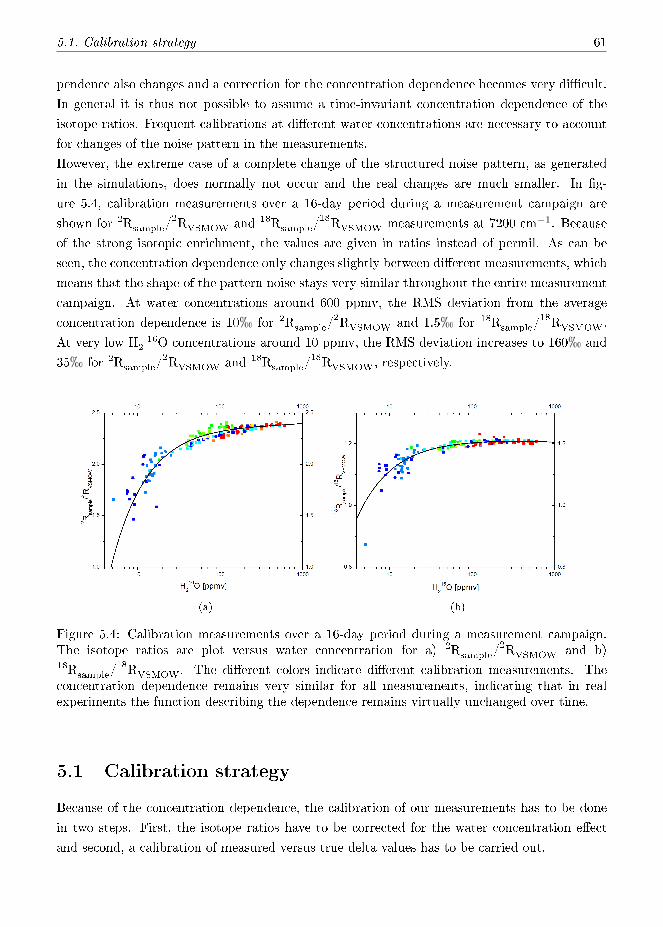
5.1. Calibration strategy 61
pendence also changes and a correction for the concentration dependence becomes very di�cult.
In general it is thus not possible to assume a time-invariant concentration dependence of the
isotope ratios. Frequent calibrations at di�erent water concentrations are necessary to account
for changes of the noise pattern in the measurements.
However, the extreme case of a complete change of the structured noise pattern, as generated
in the simulations, does normally not occur and the real changes are much smaller. In �g-
ure 5.4, calibration measurements over a 16-day period during a measurement campaign are
shown for 2Rsample/2RVSMOW and 18Rsample/
18RVSMOW measurements at 7200 cm−1. Because
of the strong isotopic enrichment, the values are given in ratios instead of permil. As can be
seen, the concentration dependence only changes slightly between di�erent measurements, which
means that the shape of the pattern noise stays very similar throughout the entire measurement
campaign. At water concentrations around 600 ppmv, the RMS deviation from the average
concentration dependence is 10h for 2Rsample/2RVSMOW and 1.5h for 18Rsample/
18RVSMOW.
At very low H216O concentrations around 10 ppmv, the RMS deviation increases to 160h and
35h for 2Rsample/2RVSMOW and 18Rsample/
18RVSMOW, respectively.
(a) (b)
Figure 5.4: Calibration measurements over a 16-day period during a measurement campaign.The isotope ratios are plot versus water concentration for a) 2Rsample/
2RVSMOW and b)18Rsample/
18RVSMOW. The di�erent colors indicate di�erent calibration measurements. Theconcentration dependence remains very similar for all measurements, indicating that in realexperiments the function describing the dependence remains virtually unchanged over time.
5.1 Calibration strategy
Because of the concentration dependence, the calibration of our measurements has to be done
in two steps. First, the isotope ratios have to be corrected for the water concentration e�ect
and second, a calibration of measured versus true delta values has to be carried out.

62 5. Data Corrections and Calibration
In the following, our calibration strategy is illustrated on a set of three isotope measurements
done at 7184 cm−1. First, a measurement of the isotope standard GS48 was done using the
SNICS calibrated water vapor generator (see section 6.2) at di�erent water concentration steps.
Subsequently, a measurement with varying water concentration of the standard GS22 was done,
which serves here as our �unknown� water sample. Finally, a measurement of GS50 as second
calibration standard was done at di�erent water concentrations. This sequence enables us to
calibrate the measured values for the �unknown� GS22 sample on the isotopic scale de�ned by
the local standard materials GS48 and GS50, whose isotopic compositions bracket that of GS22.
This is thus similar to the IAEA-recommended procedure for calibration to the VSMOW-SLAP
scale (see beginning of this chapter).
Over each concentration step of the measurements, the average of the water concentration and
the isotope ratios was calculated. As an example, we show the measurement of GS22 in �gure 5.5
for (a) water concentration and (b) isotope deltas. For each concentration step, unstable periods
were excluded. The light gray boxes in the �gure indicate the sections over which averages were
calculated.
(a) (b)
Figure 5.5: Measurement of water concentration variation of the standard GS22 generatedwith SNICS. The light gray boxes indicate sections over which averages were calculated for thecalibration.
In �gure 5.6, the average delta values are plot against the water concentration for (a) δ2H,
(b) δ18O and (c) δ17O, clearly showing the dependency on the amount of water in the measure-
ments. Whereas the relation is almost linear for larger water concentrations, it is non-linear for
concentrations below 150 ppmv.
We found that the concentration dependence is best described with a linear term in combination
with a hyperbola:
δ([H216O]) = δ0 +m× [H2
16O] +b
[H216O]
(5.3)

5.1. Calibration strategy 63
(a) (b)
(c)
Figure 5.6: Delta values averaged over each concentration step of the two calibration mea-surements with GS48 and GS50 (data not shown) and the measurement of GS22 (�gure 5.5).For higher water concentrations, the relation between water concentration and delta values ispractically linear whereas it is strongly non-linear for lower abundances. The two calibrationmeasurements are �t with a combination of hyperbola and line (black and red line). The �tresults are given in table 5.1

64 5. Data Corrections and Calibration
For each isotopologue, the function of equation (5.3) is �t independently to the two calibration
measurements of GS48 and GS50. The data is weighted with the standard error of the data
points. The �t is shown in �gure 5.6, the resulting parameters are given in table 5.1. The
Standard Isotope δ0 b m
GS48δ2H −58± 5 3619± 459 −0.02± 0.01δ18O −12± 2 −416± 125 0.021± 0.004δ17O −9± 3 −1302± 248 0.018± 0.007
GS50δ2H −282± 7 7489± 504 0± 0.02δ18O −38.8± 0.8 −529± 64 0.01± 0.002δ17O −24± 2 −1069± 145 0.013± 0.005
Table 5.1: Fit parameters of the function on the concentration dependence for all three isotopedeltas for the standards GS48 and GS50
parameters of the function are di�erent for the two isotope standards, which is not surprising as
the error that is made in the estimation of the concentration of the di�erent isotopes is larger for
weaker absorption lines and thus more pronounced for stronger depleted isotope standards. This
is especially pronounced for δ2H, where the �t on GS50 indicates a much stronger non-linear
concentration dependence than for GS48. Whereas the di�erence in the relative abundance
between the two standards is smaller than 3% for H218O and smaller than 2% for H2
17O, it
is larger than 24% for δ2H (cf. table A.A.1). For δ18O and δ17O, the di�erence in the �t
parameters is smaller than the uncertainty on the parameters and one globally valid function
could be assumed to correct the concentration dependence.
The concentration dependence of an unknown sample is determined from the concentration
dependence determined in the two calibration measurements. We assume that the function for
the sample measurement can be determined as a linear combination of the parameters δ0, b and
m of the �t functions determined in the calibration measurements. The relative contribution of
the two results is determined by the di�erence in the delta values of the two standards and the
unknown sample. For the parameter b, this is for example:
bs = b1 + (b2 − b1)× δs − δ1δ2 − δ1
(5.4)
with subscripts 1, 2 and s indicating standard 1 and 2 and sample, respectively and δ and b the
isotope delta and parameter b of the same isotopologue. As the concentration dependence is
much less pronounced for higher water concentrations, we propose to use the isotope deltas at
the highest available water concentration in the measurements.
In our case, the highest concentration at which the two standards and the sample were measured
is 400 ppmv. The three delta values at 400 ppmv in the three measurements are given in table
5.2. The linear combination of the concentration dependency functions of the two calibration
measurements results in correction functions for the sample measurement with parameters δ0, b
and m as shown in table 5.3. The concentration dependence calculated from the linear combi-

5.1. Calibration strategy 65
isotope GS48 sample (GS22) GS50δ2H [h] -57.3 -117.7 -261.3δ18O [h] -4.6 -17.0 -35.9δ17O [h] -2.8 -7.5 -19.8
Table 5.2: The measured delta values for the two calibration measurements of GS48 and GS50and the sample measurement (GS22) at the highest water concentration in the measurements(400 ppmv).
Isotope δ0 b mδ2H −124± 6 4765± 472 −0.01± 0.01δ18O −23± 1 −461± 101 0.017± 0.003δ17O −13± 3 −1238± 219 0.017± 0.006
Table 5.3: Correcting function for the concentration dependence for the sample measurement(GS22) originating from a linear combination of the functions from the two calibration measure-ments
nation of the calibration is shown together with the averaged isotope measurements of �gure 5.6
in �gure 5.7. In light red, the error on the correction based on the uncertainty of the parameters
is given. The adjustment function for the sample measurement calculated from a linear com-
bination of the correction functions for the two calibration measurements agrees well with the
measurement at di�erent water concentrations of the isotope deltas for the sample measurement
of GS22. With the functions describing the concentration dependency of the delta values for
the two water standards (equation (5.3) and table 5.2) and the sample (table 5.3), the isotope
measurements can be corrected for variations of the water concentrations. This correction is
done by subtracting the linear and hyperbolic concentration dependence from the measured
delta values:
δcorr. = δmeas. −b
H162 O
−m×H162 O (5.5)
The adjusted isotope ratios are shown in �gure 5.8 for all three isotopologues. The correction
results in delta values that show no longer a dependency on the water concentration. For
very low water concentrations (< 50 ppmv), the correction is more problematic due to the
large deviation from a linear dependency and shows larger uncertainties. The horizontal lines
in the plots indicate the average delta values calculated over all water concentrations of the
measurements, excluding concentrations below 50 ppmv because of the larger uncertainties.
The averaged measured delta values for the three measurements along with the real deltas
are shown in table 5.4. After the correction of the concentration dependency, a calibration of
measured versus true delta values can be done, assuming a linear relation between true and
measured deltas (cf. equations 5.1 and 5.2).
In �gure 5.9, a plot of real versus measured delta values is shown for δ2H, δ18O and δ17O

66 5. Data Corrections and Calibration
(a) (b)
(c)
Figure 5.7: The adjustment function for the unknown sample (here GS22) determined from alinear combination of the adjustment functions from the calibrations for a) δ2H, b) δ18O andc) δ17O. The light red area indicates the uncertainty of the function based on the standarddeviation of the �t parameters. The adjustment function agrees well with the concentrationdependency of the sample measurement.
GS48 GS50 GS22δ2H true −43.3± 0.3 −276.7± 0.3 −113.5± 0.3δ2H meas. −57.4± 0.8 −281.5± 1.2 −124.2± 1.2δ18O true −6.52± 0.03 −35.01± 0.03 −15.29± 0.03δ18O meas. −12.0± 0.3 −38.6± 0.2 −21.8± 0.9δ17O true −3.45± 0.02 −18.64± 0.02 −8.1± 0.02δ17O meas. −8.4± 0.4 −23.8± 0.3 −11.3± 1.1
Table 5.4: Correcting function for the concentration dependence for the sample measurement(GS22) resulting from a linear combination of the functions from the two calibration measure-ments

5.1. Calibration strategy 67
(a) (b)
(c)
Figure 5.8: The averaged delta values from the two calibration and the sample measurementcorrected for the concentration dependency. a) δ2H b) δ18O and c) δ17O. The horizontal linesindicate the average delta values calculated for all measurement points with H2
16O > 50 ppmv.Lower water concentrations are excluded because of much higher uncertainties due to the largecontribution of the non-linearity in the concentration dependence function

68 5. Data Corrections and Calibration
along with the linear calibration function. The delta values are also plot for GS22, the sample
measurement, to show the quality of the concentration correction and calibration procedure.
Within the error on the calibrated deltas, they agree well with the true values.
For the calibration of our measurements, this results in:
(a) (b)
(c)
Figure 5.9: Plot of the measured delta value corrected for the water concentration dependenceagainst the true delta value for a) δ2H, b) δ18O and c) δ17O for the two calibration measurementswith GS48 and GS50, averaged over all concentration steps above 50 ppmv. The error barsrepresent the 1-sigma standard deviation of the measured values. The GS22 value agrees for allthree isotopes with the value given by the GS48-GS50 calibration lines.
δ2H
(c)= 16.5 + 1.0415× δ2H(m)
(5.6)
δ18O
(c)= 6.3 + 1.07153× δ18O(m)
(5.7)
δ17O
(c)= 4.9 + 0.9889× δ17O(m)
(5.8)
with superscripts (c) and (m) for calibrated and measured values, respectively. The calibrated
delta values, corrected for the concentration dependence, are shown in �gure 5.10, with horizontal

5.1. Calibration strategy 69
lines indicating the true delta values of the respective isotope standards. Within the errors, the
calibrated delta values agree well with the true values.
To better appreciate the accuracy of the calibration, the RMS deviation from the true value as
(a) (b)
(c)
Figure 5.10: Calibrated delta values of the measurements, corrected for the concentration de-pendence, against the measured water concentration. The horizontal lines indicate the trueisotopic composition of the di�erent water standards.
a function of the water concentration is shown in �gure 5.11. For water concentrations larger
than 50 ppmv, the standard deviation is smaller than 10h, 4h and 5h, for δ2H, δ18O and
δ17O, respectively. For concentrations below 50 ppmv, the error increases because of the large
non-linearity in the concentration dependence. For higher concentrations, the concentration
dependence is less pronounced (cf. �gure 5.4) and the error stays below the errors calculated
here.

70 5. Data Corrections and Calibration
(a) (b)
(c)
Figure 5.11: RMS deviation from the true value as function of the water concentration for the(a) δ2H, (b) δ18O, and (c) δ17O isotope ratios.

5.1. Calibration strategy 71
5.1.1 Concentration dependence in other spectral ranges
In the spectral range at 7200 cm−1, with absorption lines of H216O, HD 16O and H2
18O, the
concentration dependence of the delta values is also best described with equation (5.5). An
ensemble of di�erent calibration measurements at 7200 cm−1 averaged for each concentration
step, is shown in �gure 5.12 in a log-lin-plot. The non-linearity is comparable to that observed
in the 7184 cm−1 region. A strongly enriched isotope standard (BEW2) was used. The change
of the spectral region from 7184 cm−1 to 7200 cm−1, which has better separated absorption
lines, does not reduce the concentration dependency of the measurements. This might be an
indication that the major source of the concentration dependence are strong absorptions outside
the recorded spectral window, which dominate the baseline shape and can be found in both of
the spectral regions.
In �gure 5.13a, a plot of 2Rsample/2RVSMOW versus the water concentration is shown for
(a) (b)
Figure 5.12: Set of a) δ2H and b) δ18O averaged over di�erent water concentration steps frommeasurements at 7200 cm−1. The di�erent colors indicate di�erent calibration measurements.As at 7184 cm−1, the concentration dependence is best described with equation (5.5).
measurements at 7280 cm−1. The water concentration dependency is less pronounced in this
spectral region and can be approximated with a linear function. At any given concentration,
the spread in the measurements is larger than the correction that would be applied.
Figure 5.13b shows 18Rsample/18RVSMOW versus H216O for measurements at 7286 cm−1. As
explained above, this spectral range is well suited to low water concentration measurements
(section 3.6) and in fact no measurements above 50 ppmv were possible due to saturation of
the absorption signal on the strong transitions in this region.. A possible water concentration
dependence is smaller than the measurement error at any given water concentration and can
thus be safely neglected.

72 5. Data Corrections and Calibration
(a) (b)
Figure 5.13: Average a) 2Rsample/2RVSMOW, measured at 7280 cm−1 and b)18Rsample/18RVSMOW, measured at 7286 cm−1 for di�erent water concentration steps.The di�erent colors indicate di�erent calibration measurements. At 7280 cm−1, the concen-tration dependence of 2Rsample/2RVSMOW can be approximated with a linear relation. Formeasurements at 7286 cm−1, a possible concentration dependence of 18Rsample/18RVSMOW issmaller than the uncertainty at one concentration and no correction is applied.

Chapter 6
Calibration instruments
The measurement of isotope ratios is never an absolute measurement but is always done in
comparison with measurements of known samples, called isotope standards. These additional
calibration measurements are necessary to correct for instrumental artifacts like non-linearity
or a dependence of the isotope ratios on the concentration at which they are measured [114]. In
addition, small changes of temperature and pressure inside the absorption cell can in�uence the
measurement and lead to a change in the measured isotopic composition.
Depending on instrument stability and the dependency of the isotope ratios on the concentra-
tion, a protocol with frequent calibration measurements of di�erent isotope standards measured
at one or di�erent concentrations has to be established.
For these measurements, well determined isotope standards have to be used to enable an inter-
comparison of the measurements made with di�erent instruments and to calibrate the values to
the scale determined by VSMOW and SLAP (see section 1.2.1). Normally, the measurements
calibrated with respect to laboratory standards, which in turn have been calibrated by IRMS
with respect to the international standard materials VSMOW and SLAP.
Generally, these standards are distributed and stored as liquid water, whereas the optical spec-
trometers analyze vapor phase water. Therefore, a procedure is required to transform liquid
water standards into water vapor without changing the isotopic composition, or alternatively
with a change of the isotopic composition that can be determined independently of the spec-
trometer. If the liquid water is evaporated only partially, fractionation of the isotopes occurs
and the isotopic composition in the vapor phase water no longer corresponds to the composition
of the liquid water. In addition, one would like to vary the amount of water in the gas phase to
be able to make isotope measurements at di�erent concentrations and study the e�ect of these
changes on the isotope ratios.
Not least because of the increased importance of optical spectrometers, a number of di�erent
calibration instruments has been developed. Several groups [65, 115, 116] propose to use a Dew
Point Generator (DPG) to inject small amounts of water into a dry air stream and calculate the
isotope ratios based on Rayleigh distillation curves. However, in these calibrations, the tempera-
ture has to be measured very precisely to determine the occurring fractionation and with smaller
water reservoirs, the liquid water becomes increasingly enriched in the heavier isotopologues. In
addition, these calibrations often require long time to stabilize and equilibrate and are typically
done for 12 to 24h. An alternative way for the measurement of di�erent liquid samples is the

74 6. Calibration instruments
injection of a small amount of liquid water into a heated chamber and to measure the pulse of
the evaporation [117]. In combination with an autosampler, this procedure is well adapted to
automatically measure larger numbers of liquid water samples. However, for continuous mea-
surements of vapor phase water and small amounts of water, this method is not well suited.
Another possibility is to simply �ll a pressurized tank with a mixture of a water standard and
dry air, as was demonstrated in our group [6]. This works well as long as the dew point temper-
ature of the water in the tank is lower than ambient air temperature. A drawback is that the
isotopic composition could be a�ected by surface e�ects inside the tank. Iannone in his PhD
work [118] established that with selected tanks that were previously conditioned with isotopi-
cally the same water, the isotopic fractionation was smaller than the measurement precision.
The remaining drawbacks then are that the isotope range that can be covered is limited, that
the water concentration is not easily varied, that the tank preparation is time consuming, and
�nally that the tank is big and heavy.
Alternatively, Iannone et al. [119] and later Sturm and Knohl [120] demonstrated the successful
implementation of a Microdrop calibration system. With a piezoelectric micrdroplet generator,
sub-microliter volumes of water are injected into a dry air stream. Because of the small volume,
the water is immediately evaporated and no fractionation occurs. With an unheated evapora-
tion chamber, this method can be used to generate water concentrations between 12 and 3500
ppmv. The Microdrop calibration system, which was also used for measurements of this thesis,
is described in more detail in section 6.1.
A calibration instrument, developed by Lee and co-workers [65, 66], allows for a more easily
adjusted water concentration. This device, called a dripper by the authors, uses a syringe pump
to continuously inject water with a syringe pump into a heated evaporation chamber and trans-
ported to the spectrometer by a dry air stream. By changing the water injection rates between
1 and 12 µl/min, the water concentration can be varied between 800 and 30,000 ppmv.
Similar devices were built by Gkinis et al.[121] and Tremoy, Cattani et al. [122]. In the latter
devices, a stream of liquid water of approximately 0.5 µl/min is generated with a syringe pump.
From the main sample line, a small fraction is split-o� and directed through a fused silica cap-
illary towards a hot oven, stabilized at 170°C with a PID-controlled heater. The capillary has
an inner diameter of 100 µm, which imposes a back pressure and e�ciently reduces the water
injection into the evaporation chamber. Through the chamber, a dry air �ow is guided and
transports the water vapor to the spectrometer. Whereas the calibration device of Gkinis et al.
works reliable between 17,000 and 22,000 ppm, the instrument of Tremoy, Cattani et al. was
tested between 2000 and 30,000 ppmv. After an adaption to lower water concentrations, this
set-up was also employed in our measurements (see chapter 7).
A very robust system that has seen wide-spread use and convinces because of its simplicity is the
so-called bubbler [37, 52, 123�127]. A dry nitrogen or air �ow is guided through a larger volume
(typically several liters) of liquid water, often through a di�usor to create smaller gas bubbles.
While the bubbles rise through the water column, the gas inside the bubble becomes saturated

75
in water. The temperature inside the water container is stabilized and monitored. Because
of this, it is possible to calculate the isotope ratios in the water vapor, assuming equilibrium
fractionation during the phase change (section 1.2.2,[35, 36]). To vary the water concentration,
the saturated gas �ow is subsequently combined with a variable dry gas �ow. As long as a large
liquid water volume is used, the increasing enrichment of the liquid phase is often negligible and
well below the measurement precision. However, it also means that large amounts of standard
water have to be used. In addition, an additional error is introduced because of the indirect
determination of the isotopic composition of the vapor phase based on the assumption of equi-
librium fractionation.
Apart from calibration systems developed by individual groups, there are also commercial ver-
sions available. The Standard Delivery Module (SDM) in combination with a Vaporizer (Picarro
Inc.) is based on two syringe pumps injecting a small continuous water �ow into an evaporation
chamber, heated to 140 °C [78, 122, 128], through which a dry air stream is guided. Due to the
high temperature in the injection chamber, water is evaporated at the meniscus of the needle
and after a short equilibration time, the isotope ratio of the vapor phase equals that of the
liquid standard water. Because of the two syringe pumps, automatized calibrations with two
standards can be performed. Another method is used by the Water Vapor Isotope Standard
Source (WVISS, Los Gatos Research)[114]. In this device a nebulizer aspirates liquid water from
a 0.5 l water reservoir and injects small water droplets into an evaporation chamber, heated to
80 °C. Following the evaporation, the humid air is mixed with a variable dry air �ow. With an
injection rate of 50µl/min H2O and an additional dry air �ow of up to 5 l/min, concentrations
between 2500 and 25,000 ppm can be achieved[114].
Recently, Gkinis et al. introduced an ultrasonic concentric nebulizer, which has been used for
the isotopic analysis and calibration of ice cores [129].
Several of the above mentioned calibration set-ups proved to work reliably and generate water
vapor at di�erent concentrations without fractionation. However, to the best of our knowledge,
no reliable and robust option exists for the calibration at water concentrations below 500 ppmv.
Some of the instruments could potentially be adapted to produce lower water concentration by
an increase of the air �ow through the evaporation chamber, or by subsequent dilution of the
humidi�ed air stream with dry air (see also the calibration discussion in chapter 7). This, how-
ever, results in a large consumption of costly and often limited standard water, and/or requires
a large amount of air dried to a level that is not easily obtained in an on-line drying technique
(e.g., using Drierite�). In addition, the air �ow can not be greatly increased as this would result
in turbulent �ow, which reduces or destroys the stability of the injection. Also, with an air �ow
rate of 5 standard liters per minute (slm), the water injection would still need to be lower than
2 µl/min to reach a water mixing ratio lower than 500 ppmv..

76 6. Calibration instruments
6.1 Microdrop injector
An instrument that allows the generation of very low water concentrations is the microdrop
generator [130], which was �rst introduced for water vapor measurements by Iannone et al. in
2007 [131] and was later also used by other groups [120, 123]. With their microdrop generator,
Iannone et al. [119] were able to generate water mixing ratios ranging from 12 to 7600 ppmv
using a commercial piezo-electric droplet generator (Microdrop GmbH, model MD-K-130) to
generate subnanoliter water droplets injected into a stream of dry synthetic air or nitrogen.
Due to the small size of the water droplets, evaporation is immediate and no fractionation
occurs. The microdispenser technology used for the generation of microdroplets is based on
the same principle as common inkjet printer nozzles [132, 133]. Around a glass capillary with
inner diameter 30 µm, a piezo ceramic tube is mounted. When a voltage pulse is applied to the
piezoelectric component, the capillary tube is contracted and the liquid inside is ejected as a
droplet. For the generation of a droplet, the contraction of the glass capillary has to generate
su�cient inertia to overcome surface tension and viscous forces. By changing the pulse width
and intensity, it is possible to adjust to a speci�c droplet size. The pulse frequency determines
the number of droplets per time and therefore the water concentration. A series of photographs
showing the generation of a water droplet is shown in �gure 6.1, taken from [119]. In the middle
of the droplet generator, the glass capillary can be seen. In the third image, the ejection of the
droplet is shown, which is followed by a retraction of the remaining water back into the capillary.
Figure 6.1: Generation of a microdrop with the piezo injector. In the third image, the dropletis ejected and the remaining water column retracts back into the glass capillary.

6.2. Syringe Nanoliter Injection Calibration System 77
6.2 Syringe Nanoliter Injection Calibration System
Because the existing calibration instruments were not adapted to generate water concentrations
as low as several tens of ppmv and the failing of the microdrop generator during the preparation
of our Troll measurement campaign (see chapter 7), an alternative calibration system, the Sy-
ringe Nanoliter Injection Calibration System (SNICS), based on very low injection rate syringe
pumps was developed in the framework of this thesis. It was developed to o�er a more robust
and fully automatized method to regularly calibrate water vapor isotope ratio measurements at
low volume mixing ratio (vmr) with liquid water standards. An additional goal was to waste as
little standard water as possible, thus requiring water injection rates as low as several tens of nl
per minute to match the optimal concentration range of our OF-CEAS spectrometer.
A schematic of the calibration instrument is shown in �gure 6.2a. At the core of SNICS are
two high precision syringe pumps (Harvard Apparatus) that can inject two di�erent standard
waters into separate evaporation chambers 6.2b. A dry carrier gas is connected to both of the
injection chambers. Because of two upstream installed mass �ow controllers (MFC, Bronkhorst),
the �ow rate through each of the chambers can be individually adjusted. Behind each evap-
oration chamber, an electronic three-way-valve is connected, which allows to select, which of
the two evaporation lines is connected to the OF-CEAS spectrometer. Typically, one of the
two injection lines ("measurement line") is connected to the OF-CEAS spectrometer, whereas
the other one ("waste line") is connected to a supplementary vacuum pump. In front of the
outlet to the OF-CEAS spectrometer, an upstream pressure regulator (Bronkhorst) has been
installed, behind which a vacuum pump is connected. This enables setting the gas �ow rate in
the measurement line independently of the �ow rate through the spectrometer and to stabilize
the pressure in the measurement line. The di�erence between incoming and outgoing �ow is
automatically compensated by an additional �ow to the vacuum pump.
To provide stable conditions also in the waste line, a proportional valve with an additional
vacuum pump downstream, is connected to the other exit of the two three-way-valves. With
this valve, the pressure in the waste line is typically adjusted to the same pressure as in the
measurement line.
Because of the two independent lines, it is for example possible to initialize a stable injection of
two di�erent standards at the same time and to quickly switch between the two standards by
simply changing which of the evaporation chambers is connected to the spectrometer. Alterna-
tively, it is also possible to inject the same water standard in both lines but at di�erent water
concentrations to investigate water concentration dependencies.
An additional three-way-valve at the outlet to the spectrometer allows to also connect a sam-
ple gas and to quickly change between calibration and measurement. To increase the stability
of the device, the entire calibration set-up is mounted into a thermally insulated 19 inch box,
which is stabilized in temperature with a PID regulated peltier in combination with two mixing
fans (Laird Technology, Supercool). In addition, this makes the calibration set-up easily trans-

78 6. Calibration instruments
portable. The read-out of �ow and pressure as well as the control of �ow, pressure and electronic
valves is done via two data acquisition cards (National Instruments, Measurement Computing).
The syringe pumps are connected to a computer through a built-in USB port.
For the combined read-out and control of all components of the calibration set-up, we developed
a new Labview program. This program allows to run fully automatized calibration cycles with
changes in gas �ow and water injection rates as well as changes between the two injection lines.
(a)
(b)
Figure 6.2: Schematics of SNICS (a) and the �ow chambers in which the water is evaporated(b)
6.2.1 Modeling of the syringe injection
In �gure 6.3, the tip of a syringe needle with a water droplet during a stable calibration run
is shown. The water exiting at the tip of the syringe needle does not immediately evaporate
upon injection from the standard reservoir inside the syringe but builds a droplet from which

6.2. Syringe Nanoliter Injection Calibration System 79
evaporation occurs. To good approximation the evaporation rate will be proportional to the
exposed surface area of the droplet. Therefore, initially the evaporation rate is smaller than
the supply rate of water from the reservoir through the needle (Hamilton Company�, gauge 26,
internal diameter = 0.464 mm) and the droplet will grow in size. Steady-state will be reached
when the evaporation rate equals to water supply rate. In the following paragraphs we will
derive equations describing the dynamics of the droplet and its isotopic composition.
We assume the droplet on the syringe needle from which water is evaporated to be a spherical
cap (cf. �gure B.1a) with volume Vdrop. The evaporation from a droplet inevitably results in
isotope fractionation between this volume and gas phase water. However, as the syringe injection
gives a constant supply to the droplet, always yielding the same isotope ratio, in steady state
conditions, this leads to an equilibrium with an enriched water droplet such that the liquid-
vapor fractionation renders the isotopic composition of the vapor phase equal to that of the
water supplied from the syringe, as will be shown below.
As evaporation occurs at the surface layer of the droplet only, the surface will be strongest
Figure 6.3: Image of the syringe needle tip with a droplet during a calibration run
enriched in the heavier isotopes with a gradient of the isotope ratio perpendicular to the surface,
which is determined by the di�usivity of the heavier isotopes. The inhomogeneity of the water
droplet in the di�erent isotopes can be estimated by the average distance a (heavy) water
molecule has traveled in the droplet due to di�usion. The di�usion length L can be calculated
with [134]:
L = 2√Dt
withD the di�usion coe�cient and t time. The di�usion coe�cients of HDO and H218O in water
have been measured to be 2.34 · 10−9 m2/s and 2.66 · 10−9 m2/s, respectively [135], yielding the
di�usion lengths for 1s of 110 µm and 117 µm. They are thus of the same order of magnitude
as the radius of the droplet and we can make the assumption that the entire droplet and not
just a surface layer is becoming enriched in the heavier isotopes.
Because of injection rates as low as 100 nl/min, the di�usion velocity is comparable, but opposite

80 6. Calibration instruments
in sign, to the velocity of the water �ux injected with the syringe. We thus have to determine
if the di�usion is large enough to change the isotopic composition in the syringe itself. The
syringe needle, which is generally used for the calibrations, is a 26 gauge needle with 51 mm
length (Hamilton) and 464 µm inner diameter. The speed of the �ux inside the needle at 100
nl/min is thus
vflux =100 nl/minAneedle
= 12 µm/s
with Aneedle the internal cross section of the needle. To calculate the penetration depth in the
needle of the di�using heavier isotopologues, we equate the di�usion length and the distance
crossed of the injection �ow
2√Dt = t · vflux
which leads for H218O to
t =4D
v2= 74 s
The penetration depth inside the needle is thus
Lneedle = t · vflux = 0.9 mm (6.1)
This corresponds to an enriched volume of 114.57 nl inside the needle. With a total length of
51 mm of the needle, this is however less than 2% of the needle length. We thus conclude that
the isotope ratio in the syringe volume itself is not changed.
Instead of an isotope ratio gradient inside the droplet, we assume an enriched surface layer
volume and a core volume with the isotope ratio of the water standard (�gure 6.4). This means
that the syringe calibration system is built of three di�erent water volumes:
1) the syringe reservoir with constant isotope ratio R0 of the given water standard and a �ow
rate Φ0(t), which is determined by the injection speed of the syringe pump.
2) the core volume of the droplet, which has a time dependent volume VC(t) and constant isotope
ratio RC(t) = R0.
3) The surface layer of the droplet with volume VS(t) and isotope ratio RS(t), which is in�uenced
by the evaporation from the surface layer and a continuous supply of the isotope standard
from the core volume VC . For the surface volume, we assume a constant thickness d, which
is determined by the di�usion of water molecules in the surface layer. For small d, we can
approximate VC to be the surface area AS multiplied with the thickness of the layer:
VS(t) = AS(t) ∗ d (6.2)

6.2. Syringe Nanoliter Injection Calibration System 81
Alternatively to the volume of equation (6.2), the volume can be taken equal to the entire droplet
volume, which would be the limiting case for large di�usion coe�cients with a su�ciently high
�ow speed in the needle to avoid back di�usion into the syringe reservoir.
(a)
Figure 6.4: Modelling approach for the water injection with SNICS. Water from the syringereservoir is injected into a core volume Vc with identical isotopic composition. From the corevolume, the water is transported to an enriched surface volume Vs with isotopic compositionRs(t).
A detailed discussion of the model can be found in chapter B, here we only present the
results. Based on our modelling approach, the isotope ratio of the enriched surface layer can be
calculated by
RS(t) =ψ(t)
1 + ψ(t)(6.3)
and the isotope ratio of the vapor phase with
Re(t) = RS(t) · αV (6.4)
6.2.2 Comparison with experimental data
In the following, we will now compare the results of the theoretical model described above, with
real experimental data.
Other than the model, the experimental data is smoothed because the response time of the
OF-CEAS spectrometer. To include this response into our model, we �lter the model output by
a double-exponential time response. The two time constants of the exponential were determined
in transition experiments with the real instrument and were set to τ1 = 30 s and τ2 = 300 s.
In addition, the two exponential functions were weighed di�erently, with a ten times larger
amplitude of the fast time response.

82 6. Calibration instruments
6.2.3 Calibration with two syringe pumps
The use of two di�erent injection lines o�ers the possibility to quickly change between two
di�erent water standards or between di�erent concentrations of the same water standard without
the penalty of an additional time delay because of the time required to reach a new steady state
of the injection module. In �gure 6.5, a measurement with regular changes between the two
injection lines is shown. One syringe pump was used to inject a slightly depleted standard
(GS48), whereas the other syringe was �lled with a strongly enriched standard (BEW2).
Figure 6.5: Measurement using the two separate injection lines in SNICS. One syringe injecteda slightly depleted water standard (GS48), whereas the other syringe was �lled with BEW2,a strongly enriched standard. Using the two di�erent lines, it is possible to make much fasterchanges of water concentration or water standard than would be possible with only one syringepump
In �gure 6.6, a calibration run with the 100-µl syringe under constant conditions is shown.
The water injection rate was set to 150 nl/min and the air �ow rate to 300 sccm, resulting in
a mean water concentration of around 660 ppmv. Whereas the isotope ratios are very stable
throughout the calibration run, an oscillation with amplitude 2.2 ppmv, thus 0.33% of the
water concentration, can be observed in the water concentration measurement. A Fast Fourier
Transform (FFT) of the water concentration measurement yields an oscillation period of 424 s.
With an injection rate of 150 nl/min, this corresponds to an injected volume of 1.06 µl. Taking
the inner diameter of 1.46 mm of the syringe into account, this corresponds to a distance of
633 µm covered by the plunger of the syringe during one oscillation. This value matches very
well the distance of 635 µm that is speci�ed for one full revision of the lead screw of the syringe
pump [136]. The oscillation is thus caused by inhomogeneities of the turning of the lead screw
of the syringe pump. It is also present with the second syringe pump and changes its period and
amplitude if a smaller or larger syringe is used. In the isotope ratios of the same measurement,
this oscillation is not visible and neither is it in the FFT of the isotope ratios. In general, the
oscillations of the water concentration are small enough to not a�ect the isotope ratios. In cases,

6.2. Syringe Nanoliter Injection Calibration System 83
where it is visible in the isotope ratios (e.g. when a larger syringe is used), averaging of the
isotope ratio over the entire oscillation period is recommended.
(a) (b)
Figure 6.6: Calibration run for one water concentration, with 150 nl/min water injection andan air �ow rate of 300 sccm. (a) Water concentration and isotope ratios during the entirecalibration run. The water concentration shows an oscillation, which is caused by a variationof the injection rate due to the syringe pump (b) FFT of the water concentration, yielding anamplitude of 2.2 ppmv and a frequency of 2.357× 10⁻³Hz of the oscillation, leading to a periodof 424 s which corresponds exactly to the period of revolution of the lead screw of the syringepump. The amplitude of the oscillation is thus smaller than 1% of the total water concentration.
In �gure 6.7, a calibration run with a constant air �ow of 180 sccm and water injection
rates between 10 and 130 nl/min is shown. In �gure 6.7a, the non-averaged water concentration
measurement is shown together with the water concentration calculated from water injection
and air �ow rates. The light gray curve shows the entire measurement data whereas the black
indicates the data used to average over each concentration step. In the raw data, four sudden
drops in the water concentration are visible. These disruptions are due to the formation of
air bubbles at the connection from syringe to needle and which disturb because of their larger
compressibility. The formation of air bubbles can be avoided following a more careful syringe
�lling procedure, in which the syringe is �lled with a small disposable syringe from the back and
the plunger is inserted only afterward. In �gure 6.7b, the average water concentration of each
injection step has been plot against the calculated water concentration. The relation between
calculated and measured water concentration is perfectly linear. The intercept of 10 ppmv is
due to residual water in the carrier gas, whereas the slope of 1.029 probably originates from
uncertainties in both the Hitran parameters for the intensities of the absorption lines (for the
H216O line at 7183.6858 cm−1, the uncertainty is 5 - 10% [61, 137]) and the uncertainties in the
air �ow measurement (0.6%, [138]) and the water injection rate (0.35%, [139]).
As mentioned in the model of the syringe injection (section 6.2.1), the very low water injec-
tion rates used with SNICS result in injection velocities that are of the same order of magnitude
as the di�usion velocities of the molecules. Based on the estimate given above, the di�usion
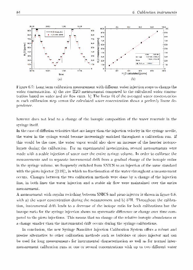
84 6. Calibration instruments
(a) (b)
Figure 6.7: Long term calibration measurement with di�erent water injection steps to change thewater concentration. a) the raw H2O measurement compared to the calculated water concen-tration based on water and air �ow rates. b) The linear �t of the averaged water concentrationat each calibration step versus the calculated water concentration shows a perfectly linear de-pendence.
however does not lead to a change of the isotopic composition of the water reservoir in the
syringe itself.
In the case of di�usion velocities that are larger than the injection velocity in the syringe needle,
the water in the syringe would become increasingly enriched throughout a calibration run. If
this would be the case, the water vapor would also show an increase of the heavier isotopo-
logues during the calibration. For an experimental investigation, several measurements were
made with a stable injection of water over the entire syringe volume. In order to calibrate the
measurements and to separate instrumental drift from a gradual change of the isotopic ratios
in the syringe volume, we frequently switched from SNICS to an injection of the same standard
with the piezo injector ([119]), in which no fractionation of the water throughout a measurement
occurs. Changes between the two calibration methods were done by a change of the injection
line, in both lines the water injection and a stable air �ow were maintained over the entire
measurement.
A measurement with regular switching between SNICS and piezo injector is shown in �gure 6.8,
with a) the water concentration during the measurement and b) δ2H. Throughout the calibra-
tion, instrumental drift leads to a decrease of the isotope ratio for both calibrations but the
isotope ratio for the syringe injection shows no systematic di�erence or change over time com-
pared to the piezo injections. This means that no change of the relative isotopic abundances or
a change smaller than the instrumental drift occurs during the syringe calibrations.
In conclusion, the new Syringe Nanoliter Injection Calibration System o�ers a robust and
precise alternative to other calibration methods such as bubblers or piezo injector and can
be used for long measurements for instrumental characterization as well as for normal inter-
measurement calibration runs at one or several concentrations with up to two di�erent water

6.2. Syringe Nanoliter Injection Calibration System 85
(a) (b)
Figure 6.8: A calibration run with regular changes between injection of the same water standardby piezo injector and SNICS.
standards. The buildup of a water droplet and the time until equilibrium with stable isotope
ratios can take several minutes. As soon as equilibrium is reached, the isotope ratio in the vapor
phase is identical to the isotope ratio of the water standard and no fractionation inside the
syringe reservoir occurs due to di�usion. By changing between two di�erent syringe injection
lines, faster changes between di�erent concentrations or standards is possible. In the current
set-up, operator invention is still required to re�ll the syringes. However, we plan to remedy this
drawback by equipping the system with a system with a 3-way liquid �ow valve immediately
following the syringe, either directing the syringe output towards the needle, or enabling the
syringe to be re�lled from a closed standard water reservoir. The re�lling is possible with the
syringe pump model used in SNICS, which o�ers a withdraw mode.


Chapter 7
Water vapor isotopologues in Antarctica
In the context of a globally warming climate it is crucial to study the climate variability in the
past and to understand the underlying mechanisms [140]. Precipitation deposited on the polar
ice caps provides a means to retrieve information on temperature changes (through the paleo-
temperature dependence of the isotopic composition of the ice) and atmospheric composition
(of gas stored in bubbles in the ice) on time scales from one to almost one million years, with
sub-annual resolution in the most recent centuries [141]. However, it is now widely recognized
that the calibration of the paleo-thermometer is highly problematic. For this reason attempts
to model the global water cycle, including the isotope signals, are ongoing with the aim of
providing a more physical basis of the isotope - temperature relation. Currently, there is a large
divergence in the results obtained by di�erent modeling strategies. The missing link in these
model studies is their forcing by experimental data on the pre-deposition isotopic composition
of the vapor phase compartment of the hydrological cycle. We propose to measure the isotopic
composition of moisture carried towards and deposited on Antarctica, in order to constrain the
numerical models. For these reasons we have developed the OF-CEAS spectrometer described
in this thesis and measured water vapor isotopologues in Antarctic air. The instrument was
�rst operated at the Antarctic Research station Troll, to continuously measure in-situ the three
stable isotope ratios of atmospheric water vapor.
The Norwegian Research station of Troll is located in Queen Maud Land, Antarctica (72°01'S,
2°32'E, 1275 m a.s.l.) at approximately 220 km from the Antarctic coast. Troll station is one
of the few stations located at the slope of the Antarctic ice sheet, which is exposed to varying
in�uence from the Antarctic plateau and the Southern Ocean [142]. Because of this it is ideally
suited to study the transportation of humid air from the ocean to the Antarctic plateau as well
as continental transportation of atmospheric moisture.
The main complex of the research station is built on ground rock, whereas the air �eld is located
on the blue ice at approximately 7 km from the main station (cf. �gure 7.1).
7.1 The Antarctic spectrometer design
During the Antarctic campaign, the instrument was measuring at 7184 cm−1, allowing simulta-
neous measurements of H162 O, HD16O, H2
18O and H217O. The general design of the instrument

88 7. Water vapor isotopologues in Antarctica
Figure 7.1: The location of Troll research station. The main complex of the station is placedon submontane rock, whereas the air �eld is 7 km from the main station on the blue ice (mapprovided by the Norwegian Polar Institute)
is as described in chapter 3. However, some di�erences will be discussed in the following.
During the measurement campaign, the instrument was powered by two internal switching
power supplies (Mean Well RD-125 and TDK Lambda LS75), providing 5V and 24V and 15V,
respectively. Instead of a Bronkhorst �ow controller (cf. chapter 3), the pressure inside the
instrument was stabilized with an adjustable vacuum pump at the exit of the instrument (KNF
84.4ANDCB), controlled with a PID loop regulating the cavity pressure. The �ow was regulated
with a sonic nozzle at the inlet of the instrument. The sonic nozzle is basically a tube which has
on the upstream side a convergent cross section and a smooth rounded outlet section with a small
opening in the center through which the �ow has to pass. Because of this restriction, the �ow is
accelerated to supersonic speed in the opening and the �ow rate through the nozzle becomes a
linear function of the inlet pressure and independent of the downstream pressure [143], as long
as the downstream pressure is signi�cantly smaller than the inlet pressure (pin > 1.4 × pout).With an inner diameter of the nozzle of 100 µm and atmospheric pressure at the inlet, the �ow
was regulated to 110 sccm during the campaign.
A photograph of the Antarctic OF-CEAS set-up is shown in �gure 7.2 with the beam path
indicated in yellow and some of the optical elements highlighted in red. The ring-down time,
which was in a later version of the instrument increased to up to 150 µs for this wavelength
region, was limited to 80 µs because of the lower re�ectivity of the mirrors that were used.

7.2. Local set-up 89
Figure 7.2: The OF-CEAS spectrometer design used during the Antarctic mission. In yellow,the beam path is indicated.
7.2 Local set-up
Because of the requirement of a su�cient power supply and an insulated measurement container,
we were bound to install our measurement set-up in the close vicinity to the main complex of
the station. To be the least in�uenced by emissions of the station itself, the spectrometer was
installed in a small insulated container approximately 200 m from the main building and situated
at the border of the station arrangement (see �gure 7.3). The measurement inlet tubing was
directed in west-north-west direction. Whereas in the winter half-year, winds are most of the
time coming from North-East and East-South-East, the wind direction in the summer months
is more �uctuating, but with a median around 30° [142]. In �gure 7.4, a polar diagram of wind
at Troll Station during the measuring period in January and February 2011 is shown, the data
was provided by the Norwegian Institute for Air Research (NILU). Approximately 40% of the
time, the wind was coming from a corridor of 22.5° to 135°, corresponding to the direction of
main buildings of the station. Another 40% of the time, wind was coming from South and West
(157.5° to 337.5°), and 20% of the time from North, which is the direction of minor station
buildings. To avoid contamination of the collected air sample by the operation of the research
station, it would have been better to measure at a larger distance of the station buildings.
Unfortunately, because of the necessity of a power source and local infrastructure, neither this
nor a measurement location to the north east of the station was possible.

90 7. Water vapor isotopologues in Antarctica
Figure 7.3: Photography of the arrangement of Troll station, with an arrow indicating thecontainer used for our set-up throughout the measurement campaign. On the bottom of the�gure, a compass has been added to indicate cardinal directions.
The spectrometer was installed on a table inside the container, which had a size of approxi-
mately 2 x 2.5 x 2 m and a volume of 10 m3. The inlet tubing was a Silcotek treated stainless
steel tubing connected to the outside via a venting slot in the wall of the container. To avoid
freezing or clogging of the tube, it was constantly heated to approx. 50°C with a self-regulating
heating band (Horst GmbH) and thermally insulated. To avoid snow entering directly into the
inlet tubing, a small plastic cover was mounted around the inlet (�gure 7.5).
Because of the small size of the measurement container, solar heating during day time in com-
bination with the heat generated by the electronics, in particular by the heating band and the
heating of the calibration device (see section 7.3.1), led to an increased temperature of up to
30°C in the room. Together with the heat generated by the internal power supply of the OF-
CEAS spectrometer, this led to problems in the temperature stabilization of the spectrometer
itself, which could not be su�ciently cooled. This problem was largely solved by installing an
air fan in front of one of the venting slits of the container, which decreased the temperature in
the container to below 20°C. In addition, the temperature inside the spectrometer was increased
from 35°C to 40°C to increase the di�erence to room temperature.
7.3 Calibration procedure
7.3.1 Syringe pump calibration
Because of pre-campaign problems with a proper functioning of the piezo injector (section 6.1,
[119]), an alternative calibration method was used during the campaign in Antarctica. For the

7.3. Calibration procedure 91
Figure 7.4: Polar diagram of wind at Troll Station during the measuring period in Januaryand February 2011. The wind was often coming from North-East with interim winds fromSouth-West.
campaign, a syringe pump based calibration system, developed by Olivier Cattani from the
Laboratoire des Sciences du Climat et de l'Environnement (LSCE) was employed.
A schematics of this system is shown in �gure 7.6. On the syringe pump (Legato 100, kdSci-
enti�c), a 60 mL syringe is injecting close to the minimum injection rate of the pump (typically
13.3 µL/min). The water is pushed through 1/16 inch PEEK tubing and split into two streams
to reduce the rate that is injected into the evaporation chamber. Part of the injected water is
send to a waste bin, whereas the other portion is injected via a heated capillary (100 µm inner
diameter, approx. 10 cm length) into a glass chamber (150 ccm) that is heated to 140°C. Because
of complete evaporation of the injected water at the tip of the capillary, no fractionation occurs.
An adjustable dry gas �ow, either dry synthetic air from a bottle or ambient air, dried within a
cartridge with a desiccant (Drierite), is connected to the injection chamber. The air �ow through
the glass chamber is maintained by the spectrometer itself in combination with an additional
pump with a �ow regulator connected in parallel. The adjustable �ow to the secondary pump
also o�ers a further possibility to regulate the water concentration in the calibration system
more precisely. Typically, the total gas �ow through the evaporation chamber is set to 2 l/min.
This calibration system was designed to work with commercially available spectrometers,
which typically measure several 10,000 ppmv and more than 50% of the injected water is sent

92 7. Water vapor isotopologues in Antarctica
Figure 7.5: The inlet for atmospheric air during the measurement campaign. The coated tubingwas heated to 50°C and thermally insulated. A plastic cover around the inlet avoided perturba-tions because of snow fall
Figure 7.6: The LSCE calibration system, based on a syringe pump
to the evaporation chamber. As our OF-CEAS spectrometer measures in a range of 200 ppmv
< H2O < 4000 ppmv, the water injection rate has to be reduced much further. With an air
�ow rate of 2 slm, a water concentration of 1000 ppmv corresponds to an injection rate of 1.5
µL/min, thus only 11% of the total water injection rate, whereas the remainder has to be send
to the waste line.
During prior test measurements in the lab, the LSCE calibration system worked quite reli-
able and showed only small �uctuations of the water concentration during the calibration runs.
However, during �eld employment, the calibration turned out to be very sensitive to small
changes in the conditions in the measurement container. The adjustment of the water �ow
fraction to the waste, which is the most sensitive part of this calibration system, proved to be
nearly impossible in the �eld. Even a small change of the height of the end of the waste tubing,
which results in a small pressure change in the tubing, led to a large disturbance of the water
concentration. In addition, the fact that the temperature in the measurement container could
not be stabilized led to further instabilities.

7.3. Calibration procedure 93
As mentioned above, the calibration system was designed to provide much higher water con-
centrations than measured with our spectrometer and the need to drastically reduce the water
injection rates resulted in a much larger sensitivity of the system stability to the change of any
one parameter. Because of the large sensitivity of the calibration system to the exact settings,
it had to be precisely set before each calibration run and often became unstable after some
minutes of relatively stable water injection.
In �gure 7.7, two exemplary calibration runs with the syringe injection system during the Antarc-
tic mission are shown. In �gure 7.7a, a calibration with the Groningen standard GS48 is shown
and in 7.7b, a calibration with the standard GS22. Although the water concentrations were
relatively stable (amplitude of oscillations on H2O < 100 ppmv), strong variations and periodic
oscillations of the delta values are apparent. These oscillations are due to the formation of
small water droplets on the tip of the capillary, which occurred probably because of pressure
�uctuations inside the evaporation chamber, induced by a variation of the air �ow through the
chamber. Because of larger fractionation factors and a stronger memory e�ect, they are more
pronounced in δ2H than in δ18O.
(a) Calibration with GS48 (b) Calibration with GS22
Figure 7.7: Exemplary relatively stable calibration with the syringe calibration system used inTroll
7.3.2 Bubbler
Because of the high sensitivity and instability of the syringe calibration system during the
campaign, we eventually decided to knock together a bubbler as a simpler and more robust
alternative calibration system. As explained in chapter 6, the principle of the bubbler is based
on the saturation of an initially dry gas �ow guided as bubbles through a volume of liquid water.
Due to a relatively large transit time (several seconds), the gas bubbles get saturated in water
and an equilibrium between liquid water and gas phase water can be assumed. The temperature

94 7. Water vapor isotopologues in Antarctica
of the water column was measured, such that the corresponding water saturation vapor pressure
[23] and equilibrium fraction factor [36] could be determined. The �rst gives the water mixing
ratio when combined with the measured pressure above the water column, whereas the second
quantity gives the vapor phase isotopic ratio when combined with the liquid phase isotopic ratio.
For this reason, samples of the water inside the bubbler were taken at the beginning, as well as
at the end of the experiment and analyzed by IRMS.
As the bubbler used here, had to be assembled in the �eld, it is a relatively simple version
compared to other implementations [37, 52, 123�127].
A schematics is shown in �gure 7.8. The inlet pressure of the bubbler was regulated with a combo
Figure 7.8: Schematics of the Bubbler calibration system used during the Antarctic campaign
pressure regulator (VICI Valco Instruments Co. Inc.) to approx. 1.5 bar. The regulation of
the dry air �ow and the �ow through the water, was done with two manual proportional valves
and the �ow was measured with two electronic �ow meters (Honeywell 3300). The downstream
pressure was measured with an electronic pressure meter (Honeywell) and read-out with an
electronic DAQ card (National Instruments USB6009).
The bubbler was built from an empty Drierite cartridge �lled with local water melted from the
ice layer surrounding the research station. The temperature of the bubbler was measured with
an electrically isolated NTC thermistor (BetaTHERM Sensors) inside the water reservoir. The
read-out, by measuring the voltage (supplied by the DAQ card) over a 10kΩ resistance connected
in parallel to the thermistor, yielded a precision of 3 mK and accuracy 0.2 K.
The entire �ow through the bubbler system was guided to the OF-CEAS instrument. Because
of this, a change of the water concentration made an adaption of both the dry air �ow rate and
the �ow rate through the bubbler necessary to again match the �ow of the spectrometer.
As only one water was available in su�cient quantities to �ll a bubbler for the calibration, it was
not possible to do a two-standard calibration and apply a linear correction of the delta values
as recommended e.g. by the International Atomic Energy Agency [26]. Instead, only a scaling
factor was calculated to correct the measured delta values from the calibrations and yield the

7.3. Calibration procedure 95
real values. This factor was calculated from the isotope ratios:
fcor. =Rreal
Rmeas ×RV SMOW(7.1)
with Rreal the real isotope ratio, RV SMOW the isotope ratio of VSMOW, and Rmeas the mea-
sured isotope ratio.
Whereas the �rst calibrations with the bubbler were done at one water concentration only, all
later calibrations were done at three di�erent water concentrations to take a possible water
concentration dependence of the isotope ratios into account (cf. chapter 5).
Because of the fractionation between liquid and gas phase water, the reservoir becomes increas-
ingly enriched in the heavier isotopologues. Consequently, this enrichment has to be taken into
account for the calibration measurements. To evaluate if the enrichment in our case has to be
accounted for, we make an estimate of the enrichment throughout the campaign.
The bubbler reservoir was �lled with approx. 0.57 l H2O. Over the entire measurement period,
a �ow through the bubbler volume was maintained for a total of 91 h and interrupted, when no
calibration measurements were done. During this time, the average water concentration gener-
ated by the bubbler was 1814 ppmv, which corresponds at a gas �ow rate of 100 sccm to a water
injection rate of 145.8 nl/min. The amount of water evaporated over the entire measurement
period is thus 91 h · 145.8 nl/min = 0.8 ml.
For the average water temperature of 16.85 °C in the bubbler, the fractionation factor for δ2H
and δ18O (ratio of isotopic composition in vapor and liquid phase) are calculated to be 0.945,
and 0.99 respectively [144].
We can thus calculate the increasing enrichment of the liquid water reservoir assuming Rayleigh
Fractionation (cf. section 1.2.2,[145]):
R
R0= fα−1 =
[0.55− 0.8 · 10−3
0.55
]α−1
(7.2)
For δ2H, this leads to 1− RR0
= −0.08h and for δ18O to 1− RR0
= −0.01h, indicating that the
change in the isotope ratios of the reservoir water is smaller than the measurement precision, if
one assumes that the isotopic composition of the bubbler water is equal to VSMOW and R0 = 1.
As the water is collected in Antarctica, it is depleted in the heavier isotopes and the di�erence
is even smaller.
An independent measurement of the reservoir water by IRMS, done by H. Jansen of the Cen-
ter for Isotope Research in Groningen on a sample of pre-campaign and post-campaign water,
shows indeed no di�erence in the isotope ratios of the two water samples. This measurement
yielded δ2H= −348.6h and δ18O= −43.57h for the pre-campaign water and δ2H= −348.6h
and δ18O= −43.52h for the post-campaign water, con�rming the above estimate to within the
measurement accuracies (resp. 0.3h and 0.1h for δ2H and δ18O). Consequently, no correction
for this e�ect was required.

96 7. Water vapor isotopologues in Antarctica
The isotope abundances in the water vapor were calculated assuming equilibrium fractionation
between liquid and gas phase with the fractionation factors based on the formulation of Horita
and Wesolowski [144] and using the water temperature measurement. The average water tem-
perature inside the bubbler was 16.8± 1.5°C, which corresponds to delta values of -401.4h and
-53.08h for δ2H, and δ18O, respectively. The maximum water temperature during the measure-
ment campaign was 20°C and the minimum 11.8°C, corresponding to variations of the isotope
abundance in the vapor phase water in a range of δDmax − δDmin = −399.3 + 404.9h = 5.6h
and δ18Omax − δ18Omin = −52.81 + 53.53h = 0.72h. Throughout an individual calibration
run, the change of the water temperature was maximal much smaller, and always less than 2
°C.
7.3.3 Calibration measurements at Troll Station
Because of the temperature sensor mounted in the gas stream inside the cavity (cf. section 3.5),
the gas �ow temperature is recorded. During the measurement campaign, the gas temperature
inside the cavity was on average equal to 39.0 °C, with a six-σ variation of 12.3 °C (see �gure 7.9).
The cavity temperature was 40.2°C with a six-σ variation of 4.8 °C. The quite high variation of
the cavity temperature is partly due to problems with the read-out of the temperature sensor,
which led to a partial erroneous read-out of the temperature (the spikes observed in �gure 7.9).
The real cavity temperature is thus more stable than the �gure of 4.8 °C suggests, with actual
variations limited to less than 0.9 °C.
The large variations of the gas �ow temperature are strongly correlated with external conditions
Figure 7.9: The cavity and gas temperature inside the instrument for the measurement periodin Antarctica. The gas temperature is much more sensitive to external in�uences than thetemperature of the large cavity.
like ambient air temperature and wind speed. This is probably related to insu�cient thermal in-
sulation of the inlet tubing, which resulted in larger variations in the self-regulated heating of the
tubing and subsequently in stronger �uctuations of the gas temperature. Because of the large

7.3. Calibration procedure 97
gas temperature variations, all measurements have been post-corrected for the (�Boltzmann-
�)variation of the absorption line strengths induced by the temperature changes. In �gure 7.10,
an example of the e�ect of the gas temperature correction is shown for δ17O, for which the tem-
perature dependence is strongest (cf. table 3.1). In �gure 7.10a the uncorrected and corrected
measurements are compared for a single calibration run and in �gure 7.10b, all calibrations over
an 11-day period are shown for δ17O. In both cases, the correction clearly results in a decrease
in the delta value variation and underlines the importance of this correction.
(a) (b)
Figure 7.10: Correction of the isotope measurements, exemplarily shown for δ17O. In a) thecorrection is shown on an individual calibration run and in b) the correction for the entiremeasurement period is shown, both showing the strong e�ect of the gas temperature on theisotope ratios.
In �gure 7.11, an exemplary calibration measurement is shown. Each calibration was done
for approximately one hour and consisted of three concentration steps. Calibrations were done
once in the morning (around 7:30 am) and once in the evening (around 7:30 pm). In �gure
7.12, the isotope deltas for all calibration measurements during the Troll mission from 08-02 till
18-02 (11 days) are shown, averaged over each stable concentration step and corrected for the
temperature dependent fractionation inside the bubbler.
The total variation of the delta values in the calibrations for the entire measurement period,
after correction for gas temperature variations, is 25h for δ2H, 14.5h for δ17O and 8.7h for
δ18O. These relatively large di�erences are mainly due to instrumental drift, induced by temper-
ature instabilities inside the measurement container. Another reason is a water concentration
dependence of the isotope ratios that is visible for all three isotopologues (see also chapter 5).
The behavior of δ2H and δ17O with the water concentration changes between di�erent calibra-
tion runs and sometimes its slope even changes sign. We suppose that the changing behavior
of this dependency is a result of residual optical fringes with a structure that changes on the
time scale of the measurements (approx. 1 day) that interfere with the absorption spectra and
introduce deviations (see chapter 4 for a more detailed discussion). As the change of the con-

98 7. Water vapor isotopologues in Antarctica
(a)
Figure 7.11: Exemplary calibration measurement with the bubbler
centration dependence between two calibration measurements proved impossible to predict, we
decided not to attempt a correction of δ2H and δ17O.
For δ18O (�gure 7.12b), the water concentration dependence of the delta values reproduces be-
tween the di�erent calibration runs. Because in general only three di�erent water concentration
steps were made per calibration, it would not be advisable to �t the concentration dependency of
δ18O with a higher order polynomial. We thus assume a linear dependency, which is determined
with a �t to the ensemble of the calibration steps of all calibrations. We assume that the slope
is constant for all calibration runs and thus �t a single global slope to all runs simultaneously.
A linear �t to δ18O yields a slope of (2.3± 0.2× 10⁻³)h/ppmv (�gure 7.13a). In �gure 7.13b,
δ18O of all calibration runs, corrected for the concentration dependence, is shown.
To estimate the instrumental drift throughout the measurement campaign, the average delta
values for the concentration step closest to 1000 ppmv of all calibration runs are compared in
�gure 7.13. With an average time between two calibrations of 12.45h, the average di�erence
between two calibration runs is 7.2h for δ2H, 0.6h for δ18O and 4.7h for δ17O.
To estimate the uncertainty introduced in the measurements because of the concentration
dependence, we take the average isotope ratios for all concentration steps and determine for each
calibration run the di�erence between maximum and minimum isotope ratio for the two isotopo-
logues. The average di�erence of the isotope values in a single calibration run is 7.4h, 5h and
4.5h for δ2H, δ18O, and δ17O respectively, with an average di�erence in water concentration of
2300 ppmv. When δ18O is corrected for the concentration dependence with a linear dependency

7.3. Calibration procedure 99
(a) (b)
(c)
Figure 7.12: Average delta values over all calibration steps of the Bubbler calibrations from08-02 till 18-02-2011, a) δ2H, b) δ18O and c) δ17O.
as described above, the average di�erence in δ18O decreases to 1.9h. As the calibration runs
always lasted more than one hour, these estimates also include a drift over the calibration run
and will in reality be slightly smaller.
The large drifts in the delta values throughout the measurement campaign probably originate
in instabilities in the OF-CEAS spectrometer during the campaign. As mentioned above, the
temperature regulation of the spectrometer proved to be di�cult because of too much heat
generated by the electronics in the container and inside the instrument itself. The installation
of a fan and the increased temperature in the spectrometer did improve the stability but also
resulted in relatively large changes in the room temperature of up to 15 °C. As the continuous
operation of the fan would have decreased the temperature too much, it could only be powered
from time to time.
To calibrate the measurements, the average delta values were calculated for each calibration
and the delta values of each measurement were scaled with the average factor from the two
embracing calibrations.
Because of the relatively large uncertainties in the delta values, the δ17O-excess, which is calcu-

100 7. Water vapor isotopologues in Antarctica
(a) Linear �t to correct for the concentration depen-dence of δ18O. The individual calibrations have beenshifted as described in the text to be able to �t theconcentration dependence of the ensemble of all cal-ibration
(b) δ18O of the calibrations during the Antarcticamission, linearly corrected for the concentration de-pendence
Figure 7.13: Estimation of the instrumental drift resulting in changes of the delta values betweendi�erent calibration runs. For each calibration, the average delta values for the concentrationstep closest to 1000 ppmv is shown.s
lated with δ17O-excess= ln(1 + δ17O) − 0.528 ln(1 + δ18O)[44] and is usually given in per meg
variation, is not reliable.
Because of its high uncertainty, δ17O, which is generally only shown in combination and com-
parison with δ18O in the form of δ17O-excess, is not further considered.
7.4 Measurement
During some episodes of the measurements, the air �ow temperature inside the cavity changed
quite dramatically due to external in�uences. In �gure 7.14, the gas temperature inside the
cavity, measured inside the gas �ow (section 3.5), is shown for a two day section, together with
the temperature of the cavity, the temperature of the ambient air and the wind speed. Whereas

7.4. Measurement 101
the cavity temperature stays relatively stable throughout the measurement, the gas temperature
shows variations of more than 4°C, which are clearly correlated with the wind speed. These vari-
ations are surprisingly strong, if one takes into account that the air is guided through more than
�ve meters of temperature stabilized 1/4 inch stainless steel tubing and additionally through a
�lter and 50 cm of 1/8 inch stainless steel tubing, mounted inside the temperature stabilized
instrument itself.
These strong variations strongly underline the importance of independent gas temperature sen-
sors inside laser spectrometers comparable to ours, to be able to correct for line strength changes
due to variations in the gas temperature.
The water concentration and isotope ratio measurements shown in the following have therefore
been corrected for the changes in the gas �ow temperature, based on the temperature coe�cients
of the di�erent absorption lines.
The water concentration and isotope ratios were quasi-continuously measured for a period
of 11 days in February 2011, with small interruptions for calibration runs and smaller adaptions
of the laser spectrometer. The water concentration, δ2H and δ18O measurement for this period
are shown in �gure 7.15 together with an air temperature measurement, friendly provided by
C. Lunder from the Norwegian Institute for air research (NILU) .
Occasionally during the measurement period, the temperature approached highs close to 0 °C,
which together with strong solar radiation, resulted in water concentrations of more than 4000
ppmv, which is close to the maximum our laser spectrometer could measure. In addition, the
relatively mild temperatures resulted in sublimation and melting of the ice around the research
station (see �gure 7.17), and led temporarily to a strong component in the measured water vapor
coming from local water instead of water vapor transported to Antarctica.
Because of the limitation imposed by a calibration procedure involving only one water stan-
dard, and the above mentioned drift and water concentration dependency, the delta values
calibrated against the bubbler measurements exhibit a relatively large uncertainty.
Drift and water concentration dependency led to an δ2H accuracy of approx. 12h, and an
accuracy of 4.4h for δ18O. Because of this, a profound study and interpretation of the observed
isotope ratio variations during the measurement period is not very useful.
However, because some atmospheric events were associated with very large changes in the iso-
topic ratios, which certainly are larger than the uncertainty of the measurements, it is still
possible to examine if a correlation with atmospheric variations, especially in the source region,
exist.
In �gure 7.18, a measurement section of two days shows the water concentration, the delta values
and the 2H-excess. In addition, the air temperature and the wind speed, measured by NILU in
a measurement container at 1309 m a.s.l., thus 34 m above the main building of the station and
at a distance of approximately 200 m [142], is shown. Until approximately 11:00h on 16-02-2011

102 7. Water vapor isotopologues in Antarctica
(10.46 on the time scale given in the �gure), the isotope ratios are relatively stable, with δ2H
around -320h and δ18O around -45h. At 11:00h, both δ2H and δ18O show a rapid increase,
δ2H up to -280h and δ18O to -32h. At the same time the D-excess decreases. A decrease in
the air temperature took place approximately one hour before the change of the isotope ratios
and seems thus not be directly correlated with the change of the isotopic composition. However,
a strong increase in wind speed seems to be strongly correlated with the change of D-excess.
At approximately 18:00 on the same day, the wind speed decreases, whereas δ2H and D-excess
show a much slower transition and the transition for δ18O happens around 3 hours later at
approximately 21:00.
In addition to these strong changes, a temporary change of the wind direction that goes along
with an increase of wind speed and occurred at T=11.15, directly translates into an increase
of all isotope ratios and thus indicates a relatively large in�uence of the wind direction on the
relative isotope abundances.
7.4.1 Backtrajectories
To determine if the observed change of the isotopic composition at 11:00 am on 16-02-2011
and the change back to the previous composition at approximately 18:00h for D-excess and
21:00h for δ18O on the same day are related to a change of the source region of the atmospheric
moisture, back trajectories were calculated with the online available Hybrid Single Particle La-
grangian Integrated Trajectory Model (HYSPLIT) of the National Oceanic and Atmospheric
Administration (NOAA) [146, 147] using the Global Data Assimilation System (GDAS) meteo-
rology archive. A set of back trajectories for the same time frame as the experimental data in
�gure 7.18, is shown in �gure 7.19. For a better overview, the most important characteristics of
each calculated back trajectory are given in table 7.1.
The strong transitions in the isotope ratios observed with our spectrometer, do not seem to be
correlated with changes of the source region of the humid air, nor with the altitude of the air.
Most of the time, the air stream is mainly passing over land and coming from altitudes around
1000 m above ground level. The rapid changes in the isotopic composition of the atmospheric
moisture at Troll station seems thus to be more correlated with local conditions, such as wind
speed and local re-evaporation.
7.5 Conclusion
The measurement campaign at Troll station showed that our laser spectrometer reliably mea-
sures water concentration and the two isotope ratios δ2H and δ18O with very good precision.
Because of problems with the on-site calibration of the isotope ratios, the accuracy of the col-
lected data is unfortunately not su�cient to draw detailed conclusions about atmospheric water

7.5. Conclusion 103
Table 7.1: Back trajectories for Troll station for 16-02-2011, simulated with the HYSPLIT modelof NOAA [146, 147]
time [hh:mm] source region altitude of source [m]
04:00 land 128506:00 land 79208:00 land 76310:00 land 92712:00 land 87114:00 land 77316:00 land 73718:00 sea 77320:00 land 87722:00 land 106924:00 sea 626:00 sea 0
vapor transportation or to re�ne atmospheric circulation models. The water concentrations
encountered during the measurements are well above the minimal concentrations that our in-
strument can measured with good precision, partially they were nearly too high.
A comparison of the isotopic measurements with back trajectory models revealed no correlation
between the source region of the air mass and our isotopic measurements. A strong relation
between the local wind speed and the isotope ratios of ambient air indicates that local phe-
nomena probably govern the local water vapor composition. A possible explanation could be
for example the strong eddy winds on the mountain range that resulted temporarily in wind
speeds of more than 22 m/s during our measurement campaign. Furthermore, the strong solar
radiation and high temperatures temporarily lead to strong evaporation of the local snow and
strongly in�uenced and sometimes even governed the isotopic composition of the atmospheric
water vapor.
In order to analyze atmospheric water transportation processes and to help to re�ne the theo-
retical modeling of these processes, we propose to conduct further measurement campaigns on
the Antarctic high plateau, for example at the French Italian research station Dome Concordia.
This station is located at (75°06'S, 123°21'E) at an altitude of 3,233 m a.s.l. [19, 148] The
mean annual temperature of -49.8°C (measured in 2009) corresponds at an average pressure of
644.4 mbar [149] to a saturation water concentration of approximately 63 ppmv. In the summer
months December and January, the temperature reaches values of up to -25°C and thus water
concentrations of several hundreds of ppmv.
Our OF-CEAS spectrometer would thus be almost perfectly adapted to measure water vapor
isotopologues in the harsh environment of the Antarctic high plateau. Because of the location
on the high plateau, less eddy winds coming from inland regions are to expected and because
of the cold temperatures, melting and evaporation of local water is less likely to in�uence the
104 7. Water vapor isotopologues in Antarctica
composition of atmospheric moisture.
The occasionally large drifts of the instrument, caused mainly by temperature regulation prob-
lems and manifesting in relatively large di�erences in the isotope ratios between di�erent cali-
bration runs, were e�ciently reduced with further improvements of the laser spectrometer after
the measurement campaign. The operation temperature was further increased to 45°C and the
internal power supply was replaced with an external one to reduce heat production inside the
thermally insulated instrument.
Because of the di�culties encountered with the Piezo injector before the campaign and with the
two other calibration systems in-the-�eld, a new and more robust system based on high-precision
syringe pumps (section 6.2) was developed and o�ers a more reliable and automatized way to
perform isotope calibrations during future measurement campaigns.

7.5. Conclusion 105
(a)
Figure 7.14: The gas �ow temperature inside the OF-CEAS spectrometer was in�uenced byrapid changes in the ambient conditions. Apart from changes in the ambient air temperature,strong winds around the research station resulted in a large change of the air sample temperature.Other then the wind speed, the wind direction had no direct in�uence on the temperature. Thedata were post-corrected for the temperature variations.

106 7. Water vapor isotopologues in Antarctica
(a)
Figure 7.15: Quasi-continuous water concentration measurement at Troll Station during 11days in February 2011. Interruptions are due to calibration runs with the bubbler and minormodi�cations of the OF-CEAS spectrometer. In the top panel, the water concentration is shown,in the second panel δ2H and δ18O. The third panel shows wind speed and wind direction andthe bottom panel the ambient air temperature.

7.5. Conclusion 107
(a)
Figure 7.16: Zoom into an apparent spike in �gure 7.15. The transition is relatively slow andlasts for more than 25 minutes, showing that the data is real and not an experimental artifact.
(a)
Figure 7.17: Continuously warm temperatures and strong solar radiation temporarily lead to astrong melting of the ice layer around Troll station, which resulted in higher water concentrationsin the ambient air and a large contribution of local water vapor to the isotope ratios measuredby our spectrometer

108 7. Water vapor isotopologues in Antarctica
(a)
Figure 7.18: Section of two days (16-02 to 18-02) from the measurement at Troll Station inFebruary 2011

7.5. Conclusion 109
(a)
Figure 7.19: Back trajectories for Troll station for 16-02-2011, calculated with the HYSPLITmodel of NOAA


Chapter 8
Water isotope fractionation in simulated ice clouds
Various measurements carried out in the coldest regions of the atmosphere revealed the oc-
currence of super-saturation (partial pressure of water above the saturation pressure) in the
presence of ice crystals in the upper troposphere [150].
Super-saturation is a well-known phenomenon in the absence of nucleation centers. However,
it can also occur in the presence of foreign nuclei that initiate heterogeneous freezing, or even
in the presence of ice crystals. Two hypotheses have been forwarded to explain the latter case.
The �rst hypothesis is known as di�usion-limited super-saturation [151], while the second
hypothesis is that of equilibrium-limited crystallization [152]. As these two mechanisms would
leave a very distinct signature on the isotopic composition of the ice crystals and the atmo-
spheric water vapor, measurements of the isotopic ratios can be exploited to determine their
relative importance. A schematic representation of the two proposed mechanisms is given in
�gure 8.1. In the di�usion-limited case, crystallization, e�ectively reducing supersaturation to
saturation, is limited by the di�usion time of the water molecules to the nuclei with heavier
water isotopologues di�using more slowly. This induces a negative gradient in the isotope abun-
dances in the direction of the ice crystals. However, as the probability of adsorption is higher
for heavier isotopologues, the crystals are still enriched in the heavier isotopes. At the same
time, the relative humidity decreases in close proximity to the ice nuclei, as neighboring water
molecules freeze out faster than new molecules can be replenished by di�usion.
The second possible mechanism, equilibrium-limited crystallization, assumes that the absorption
capacity of the ice crystals is the limiting factor for the decrease of the degree of super-saturation.
In this case, the di�erent di�usion rates of the isotopologues do not a�ect the isotopic abun-
dances in the ice crystal. Consequently, the heavier isotopologues would be more abundant in
the crystals than in the case of di�usion-limited crystallization and neither isotope ratio nor
relative humidity, would change in the proximity of the ice nuclei. By measuring the di�erent
water isotopologues separately in the gas phase, in ice crystals, and in the total water content
in the ice cloud chamber, we aimed to investigate, which of the above mentioned mechanisms is
primarily responsible for the super-saturation e�ects observed in the upper troposphere and to
experimentally determine fractionation factors at very low temperatures.
Because of the di�cult accessibility and very low water concentrations (< 10 ppmv), mea-
surements to investigate these mechanisms in situ are until now to the best of our knowledge
not feasible. The AIDA cloud simulation chamber at the Karlsruhe Institute of Technology,

112 8. Water isotope fractionation in simulated ice clouds
(a)
Figure 8.1: a) Di�usion-limited and b) equilibrium limited Fractionation can produce the samesupersaturation. Due to di�erent reasons for the supersaturation (see text), they produce dis-tinct isotope signals, which can be used to determine, which mechanism is responsible. In thelower panel, the relative humidity in close proximity to the ice crystal is given in green and δDin red. Figure from E.J.Moyer [153]
Germany (KIT) was ideally suited for this study, as it enables producing the right conditions for
super-saturation to occur during an expansion-driven cloud formation, and being equipped as
it is with extractive sample ports and two in-situ long-path length optical absorption gas cells
of the White design.
Ice cloud formation and the possible mechanisms were studied in the framework of the Iso-
cloud project, an international collaboration funded by the National Science Foundation (http:
//www.nsf.gov/), the Deutsche Forschungsgesellschaft (http://www.dfg.de) and Eurochamp-
2 (http://www.eurochamp.org) between the group of E. Moyer of the Department of Geophys-
ical Sciences of the University of Chicago (UoC), the Institute for Meteorology and Climate
Research Atmospheric Research of the KIT, the group of V. Ebert of the Center of Smart In-
terfaces, Technische Universität Darmstadt (TUD) and Physikalisch Technische Bundesanstalt
(PTB) in Braunschweig, Germany and the LIPhy of the University of Grenoble as adjoint part-
ner.

8.1. General set-up 113
Gas phase water and isotopic composition was measured with two in-situ TDLAS spectrometers.
The UoC developed a system that measured H162 O and HDO at 2.65 µm (CHI-WIS) and the
University of Darmstadt/PTB/KIT groups contributed with a similar instrument, called Isotope
AIDA-PCI-in-cloud-TDL (ISO-APicT), described in detail in the dissertation of Jan C. Habig
[87]), that measured H162 O and H18
2 O at 2.64µm. Both of these instruments will also be discussed
in more detail in the PhD theses of K. Lamb (University of Chicago) and B. Kühnreich (Univer-
sität Darmstadt/PTB Braunschweig). We participated with the OF-CEAS spectrometer (SIRI)
and the syringe calibration system developed in the framework of this thesis and supported the
KIT with the operation of their OF-CEAS spectrometer (Resonatorverstärktes Wasserdampf
Absorptions Spektrometer, Rewas-Iso), which was also built in Grenoble and which is based on
our own spectrometer.
To measure the isotopic composition of the ice crystals, one of the OF-CEAS spectrometers
was connected behind a pumped counter-�ow virtual impactor (PCVI) [154] that separates ice
particles larger than a set cut-o� size from the gas �ow. The PCVI is described in more detail
in section 8.2. The second OF-CEAS spectrometer was directly connected to the cloud chamber
and measured via an extractive heated tubing the isotopic composition of total water.
In addition to these four instruments, the already existent AIDA PCI extractive TDL (APeT)
and a frost point mirror (MBW) measured total water concentration via an extractive line and
a single pass in-situ TDL (SP-APicT) additionally measured the water concentration in the
gas phase. A schematic representation of the experimental set-up is shown in �gure 8.2, a list
of the di�erent instruments deployed during the Isocloud campaign and their most important
characteristics are given in table 8.1.
8.1 General set-up
The AIDA cloud chamber is made of aluminum, has a diameter of 4 m and a height of 7.5 m
with a volume of 84.5 m3 and an inner surface of 103 m2. A vacuum pump is connected to the
top of the cloud chamber and is used to rapidly decrease the pressure in the chamber, which
leads to an adiabatic expansion and thus a cooling of the contained air. At the bottom of the
chamber, a fan is installed to homogenize the air inside the chamber. Close to the ground level,
the PCVI is connected via an extractive tubing, behind which one of the OF-CEAS spectrom-
eters was installed. The second OF-CEAS spectrometer was connected to Silcotek coatet 1/4
inch stainless steel tubing heated to 35 °C, that was installed approximately 135 cm above the
base of the chamber. At a distance of 13 cm from the chamber walls, air was extracted through
the tubing with a �ow rate of 130 sccm. It would have been best, to connect this second OF-
CEAS spectrometer at the same location at which the other extractive instruments measuring
absolute water, were connected and at the same level of the chamber as the in situ instruments.
Unfortunately, because of limitations of the local availability, this was not possible. Initially, the
spectrometer was connected close to the top of the AIDA chamber, however this did not work

114 8. Water isotope fractionation in simulated ice clouds
Table
8.1:Alist
ofthe
di�erent
instruments
deployedduring
theIsocloud
campaigns.
Group
Instrument
Wavelength
Measured
Measured
name
regionIsotop
ologuesphase
UoC
CHI-W
IS2.65
µmH216O
andHD
16O
gasphase
(insitu)
KIT,TUD/P
TB
Iso-APicT
2.64µm
H216O
andH218O
gasphase
(insitu)
KIT
Rew
as-Iso1.39
µm(Isocloud
1-3)
H216O
,HD
16O
,H218O
,H217O
totalwater
1.37µm
(Isocloud4)
H216O
andHD
16O
or(extractive)
H216O
andH218O
LIPhy
SIRI
1.392µm
(Isocloud1-3)
H216O
,HD
16O
,H218O
,H217O
mostly
icephase
1.389µm
(Isocloud4)
H216O
,HD
16O
,H218O
(behind
PCVI)
KIT
SP-APicT
1.37µm
H216O
gasphase
(insitu)
KIT
APeT
1.37µm
H216O
totalwater
(extractive)KIT
MBW
notapplicable
totalwater
totalwater
(extractive)

8.1. General set-up 115
well because of disturbances of the measurements due to strong vibrations of the metal frame
on which the instrument had to be installed. Because of this, a location close to the bottom of
the chamber, which provided more mechanical stability, was chosen.
At a height of approx. 4 m, two white cells are installed into which the two TDL spectrometers
of the UoC and PTB/KIT groups were coupled. The PTB/KIT instrument, Isotope AIDA-
PCI-in-cloud-TDL (ISO-APicT), a change between two di�erent lasers was made possible to
integrate the already existent facility TDL hygrometer APicT [155], which previously measured
gas phase water on the same beam path of the White cell. An additional single pass TDL
spectrometer (SP-APicT) was connected to the chamber at the same level as the other TDL
spectrometers to independently measure the water concentration in gas phase.
In addition to the OF-CEAS spectrometer, total water concentration in the cloud chamber
was measured by an extractive TLD spectrometer, AIDA PCI extractive TDL (APeT) and a
chilled-mirror frost point hygrometer (MBW 373LX) [155] connected to the same heated extrac-
tive line either on the third level of the cloud chamber (approx. 6 m height) or on the second
level (approx. 4.5 m height). The Isocloud project comprised four measurement campaigns that
(a)
Figure 8.2: Experimental set-up at the AIDA cloud chamber during the Isocloud measurementcampaigns, schematics by H. Saatho� (KIT). The OF-CEAS instrument behind the PCVI wastypically SIRI.
were conducted in April 2012, June 2012, October 2012 and March 2013. The two OF-CEAS
116 8. Water isotope fractionation in simulated ice clouds
spectrometers were in a very similar con�guration for the �rst three campaigns and measuring
at 1.392 µm, the wavelength region that was also used during the mission to Antarctica (cf.
7. For the last campaign, the KIT OF-CEAS spectrometer was adapted to be able to measure
the H182 O/H16
2 O ratio in very dry air as encountered in the stratosphere. These adaptions are
described in more detail in section 8.1.1.
As the �rst two campaigns served mainly as trial campaigns to test the di�erent optical instru-
ments and to reveal where modi�cations and adaptions were necessary, the data presented in
the following is from the last two measurement campaigns, Isocloud3 and Isocloud4.
8.1.1 Isocloud OF-CEAS
Whereas the con�guration of our OF-CEAS spectrometer was very similar to the one also used
for the Antarctic mission, several modi�cations were made between the campaigns to adapt the
instrument to the very demanding conditions that were encountered during the measurements.
As a decrease of the inlet pressure, as experienced by the spectrometer during the cloud simula-
tion experiments would result in a changing �ow with an ultrasonic nozzle, this �ow restriction
was completely removed from the instrument. In addition, the variable-speed pump, which was
used to regulate the cavity pressure, proved to be too weak to provide a su�cient �ow at the
lower pressures. Because of this, a Restek coated Bronkhorst pressure regulator was installed
upstream of the cavity and the variable-speed pump was replaced with an ordinary and larger
membrane pump (KNF N813.5 ANE). With this modi�cation, the �ow through the instrument
could be increased to 150 sccm and be kept constant, even as the inlet pressure descended to
below 100 mbar.
For the last measurement campaign (Isocloud4), we replaced the laser in Rewas-Iso with a laser
operating between 7278 and 7290 cm−1. As mentioned in section 3.6, the absorption line of
H216O is more than a factor 50, and the H2
18O line nearly a factor 4 stronger at 7286 cm−1
compared to the lines in the spectral regions at 7184 and 7200 cm−1. Because of this, the
concentration range of the modi�ed instrument in which sub-permil precision for δ18O can be
achieved is signi�cantly reduced to 1 ppmv < H2O < 60 ppmv. In addition to the measurement
of δ18O, a spectral region around 7280 cm−1 allows the measurement of δ2H. Since, at natural
abundance, in this region the HD 16O line is about 40 times weaker than the major isotopologue
line, it is especially appropriate for measurements of samples strongly enriched in HD 16O, as
were generated during the Isocloud campaigns. Two experimental spectra for the wavelength
region at 7286 cm−1 and 7280 cm−1 are shown along with a �t to the data in �gure 8.3. The
spectrum of �gure 8.3a was recorded at a water concentration of 23 ppmv and the spectrum of
�gure 8.3b at 90 ppmv.

8.1. General set-up 117
(a)
(b)
Figure 8.3: Experimental spectra measured with Rewas-Iso in the new wavelength range at a)7286 cm−1 and b) 7280 cm−1.

118 8. Water isotope fractionation in simulated ice clouds
In �gure 8.4, the Allan-Werle plot is shown for measurements of δ18O at three di�erent
concentrations. At 16 ppmv, at the optimum integration time of 3740 s, a precision of 0.17h is
obtained. With 1 s averaging, the precision is 4h at 16 ppmv and 15h at 5 ppmv.
Figure 8.4: Allan deviation plot for Rewas-Iso in the H182 O wavelength region. At H2O = 16
ppmv, and an optimum integration time of 3740 s, the precision is 0.17 h
8.2 Pumped Counter�ow Virtual Impactor (PCVI)
As a detailed discussion of the functioning of the PCVI would go well beyond the scope of this
work, it is only brie�y introduced here. A more thorough description can be found in [156�158].
In �gure 8.5, a schematic representation of the PCVI is shown (from [158]). A sample �ow
(fs) including particles - in our case the air from the cloud chamber - is drawn into the virtual
impactor by a vacuum pump (indicated as pump �ow in the �gure). Supplemental counter�ow
(fcf ) of a particle-free gas, typically a dry synthetic air stream, is sustained to intertially remove
smaller particles from the �ow through the PCVI. Only particles above a certain mass and,
because of same densities, above a certain size (the so-called cut size or cut-o� size) traverse the
counter�ow because of their larger inertia and are separated from the bulk part of the sample
�ow. The particle-free counter�ow consists of a fraction (the e�ective counter�ow fecf ) that is
evacuated by the connected pump and another fraction (fof ) that serves as carrier gas for the
separated particles in the output �ow (fcf = fecf + fof ).
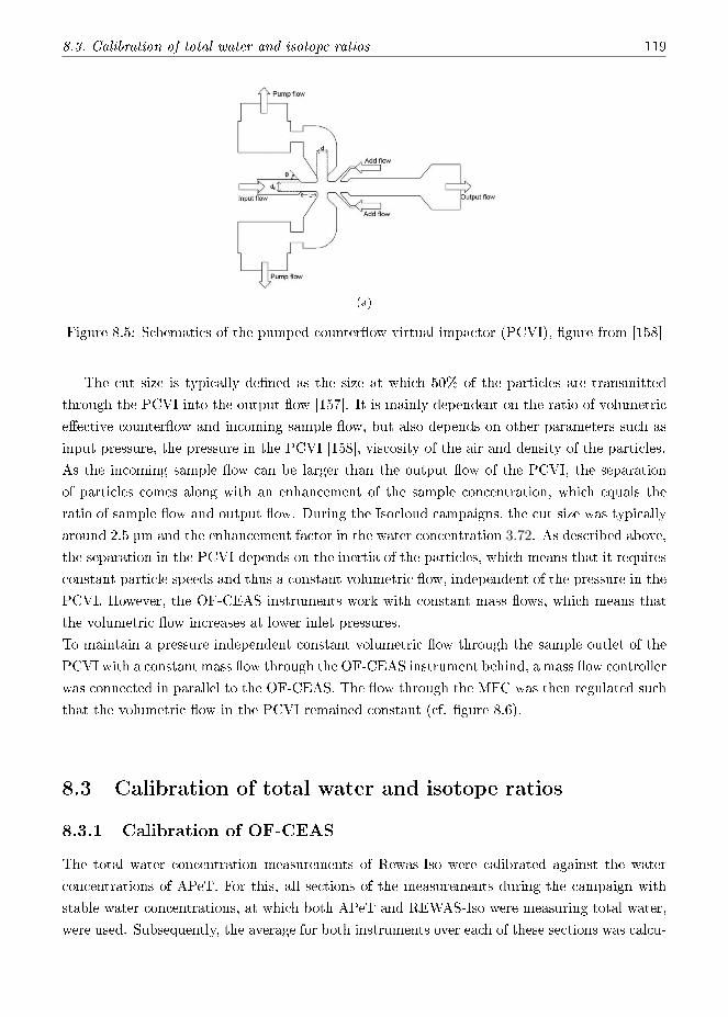
8.3. Calibration of total water and isotope ratios 119
(a)
Figure 8.5: Schematics of the pumped counter�ow virtual impactor (PCVI), �gure from [158]
The cut size is typically de�ned as the size at which 50% of the particles are transmitted
through the PCVI into the output �ow [157]. It is mainly dependent on the ratio of volumetric
e�ective counter�ow and incoming sample �ow, but also depends on other parameters such as
input pressure, the pressure in the PCVI [158], viscosity of the air and density of the particles.
As the incoming sample �ow can be larger than the output �ow of the PCVI, the separation
of particles comes along with an enhancement of the sample concentration, which equals the
ratio of sample �ow and output �ow. During the Isocloud campaigns, the cut size was typically
around 2.5 µm and the enhancement factor in the water concentration 3.72. As described above,
the separation in the PCVI depends on the inertia of the particles, which means that it requires
constant particle speeds and thus a constant volumetric �ow, independent of the pressure in the
PCVI. However, the OF-CEAS instruments work with constant mass �ows, which means that
the volumetric �ow increases at lower inlet pressures.
To maintain a pressure independent constant volumetric �ow through the sample outlet of the
PCVI with a constant mass �ow through the OF-CEAS instrument behind, a mass �ow controller
was connected in parallel to the OF-CEAS. The �ow through the MFC was then regulated such
that the volumetric �ow in the PCVI remained constant (cf. �gure 8.6).
8.3 Calibration of total water and isotope ratios
8.3.1 Calibration of OF-CEAS
The total water concentration measurements of Rewas-Iso were calibrated against the water
concentrations of APeT. For this, all sections of the measurements during the campaign with
stable water concentrations, at which both APeT and REWAS-Iso were measuring total water,
were used. Subsequently, the average for both instruments over each of these sections was calcu-

120 8. Water isotope fractionation in simulated ice clouds
(a)
Figure 8.6: The volumetric �ows at the sample outlet of the PCVI during an expansion experi-ment. As the mass �ow through the OF-CEAS instrument stays constant, the volumetric �owincreases with lower pressures. To sustain a constant total mass �ow at the sample outlet, anMFC with a pump is connected in parallel to the OF-CEAS and the �ow is decreased with lowerpressure. Lower panel shows the pressure and temperature in the AIDA chamber for a typicalexpansion experiment.
lated. As REWAS-Iso was measuring in four di�erent wavelength regions during the campaign
(cf. 8.1.1), four di�erent datasets were thus constructed.
As an example, in �gure 8.7, the H2O calibration is shown for the H218O wavelength region at
7286 cm−1. A linear function was �t to the plot of the water concentration measured by Rewas
vs. that measured by APeT and yielded an intercept of 0.1±0.07 ppmv and a slope of 0.76±0.01.
The large di�erence with unity is due to an initially erroneous conversion factor from line pro�le
to concentration in the �t �le of the OF-CEAS spectrometer. The water concentrations of SIRI
were not calibrated in Isocloud4 as SIRI was connected almost always behind the PCVI and no
direct comparison could be made. Since SIRI measured in a same wavelength range that had
been calibrated previously, this was also not necessary.
The isotope ratio measurements of Rewas-Iso and SIRI were calibrated with SNICS at least
twice a day, once before the experiment in the morning and once after the experiment in the
evening. Because of the limited time available for the calibrations, we decided to focus the cali-
bration on the correction of the water concentration dependency and only one isotope standard
was used for measurements at di�erent water concentrations. In the case of SIRI, the concen-
tration dependency was determined for a combination of the two calibrations before and after
the measurement (cf. 5.1) and was used for the correction of the measurements. The variation
between the two calibration measurements was in general comparable to the variation of mea-
surement steps in the individual calibrations. For concentrations above 40 ppmv, the standard

8.3. Calibration of total water and isotope ratios 121
(a)
Figure 8.7: Calibration of the H2O measurement of Rewas-Iso vs. APeT. For the calibration, allsections with stable conditions in the Isocloud4 measurements were identi�ed and the averageof H16
2 O for APeT and Rewas-Iso were calculated and plotted against each other. The standarddeviation on the measurement is smaller than the size of the data points.
deviation of the correction function is 18h for δ2H and 2.1h for δ18O, for concentrations below
this, the standard deviation becomes signi�cantly larger because of the strong non-linearity of
the concentration dependence.
8.3.2 Calibration of in situ measured HDO/H2
16O ratios for CHI-WIS
For the Chicago-built in-situ TDLS water spectrometer CHI-WIS, the experimentally deter-
mined value of the deuterium isotope ratio
2R̃ =[HD 16O]sample/[H2
16O]sample[HD 16O]VSMOW/[H2
16O]VSMOW
was calibrated against the (calibrated) R of Rewas-Iso. Analog to the calibration of the water
concentration for Rewas-Iso, all sections of the data with stable H2O and R2H were identi�ed
over the entire measurement period. As Rewas-Iso was not always measuring HDO, only those
experiments were considered, in which an HDO measurement was available for both instruments.
As all stable sections were used, the data include measurements at di�erent pressures and before
and after expansion experiments.
Di�erent calibration strategies were studied in order to calibrate the isotope ratio [HDO]/[H162 O]
of CHI-WIS (in the followingRCHIWIS) with the calibrated measurements of Rewas-Iso. Amongst
others, a separate calibration of [H162 O] and [HDO] was tried. However, the best result is achieved

122 8. Water isotope fractionation in simulated ice clouds
when a correction is applied to the isotope ratio directly, assuming a quadratic relation between
RCHIWIS and RRewas. The �t was weighted using the standard deviations of the Rewas-Iso data
points only (ωi = 1σ2i), considering that the error on the Rewas data is typically of the same size
as and occasionally up to 4 times larger than that of CHI-WIS data (cf. �gure 8.8). The �t
(a)
Figure 8.8: The deuterium isotope ratio measurements (12 in total) of Rewas-Iso plotted againstthose of CHI-Wis. The error bars represent 1σ standard deviations. A quadratic function was �tto the data to correct the CHI-Wis measurement with the calibrated measurement of Rewas-Iso.
gives the following relation:
RRewas = −4 + 1.27 ·RCHIWIS + 0.11 · (RCHIWIS − 12)2 (8.1)
The residual of the �t indicates a di�erence of several hundred permil between the isotope ratios
of CHI-WIS and Rewas-Iso after the calibration. This is because data from the entire Isocloud4
campaign was used for the calibration �t. Because of the small amount of stable measurement
sections that could be compared, only a limited amount of data points was available and it
was not possible to make one separate calibration for each measurement day. This means that
the drift of the two instruments is also included in the �t and adds to the uncertainties. In
addition, Rewas-Iso features a large uncertainty on the isotope ratios at very low (< 5 ppmv)
water concentrations.
In �gure 8.9, the e�ect of the R2H calibration is exemplary shown for one experiment. In
�gure 8.9 a), the uncalibrated isotope ratio is shown for CHI-WIS and in b) the calibrated data.
Although one calibration was done for the entire measurement campaign, the calibrated data
agree within less than 100 permil, which is much smaller than the isotopic changes observed in

8.4. Typical expansion experiment 123
(a) (b)
Figure 8.9: Isotope ratio measurement (HDO/H162 O) of CHI-WIS and Rewas-Iso during the
Isocloud4 campaign. a) CHI-WIS is not calibrated for drift. A di�erence of nearly 500h canbe seen in the stable sections in the beginning and the end of the experiment, where bothinstruments should agree b) CHI-WIS data calibrated against Rewas-Iso measurements for theentire measurement campaign. The two instruments agree better than 100h, which is muchsmaller than the overall change in the isotope ratios and corresponds to a relative error on theratio R of approx. 1%.
the measurements, and corresponds to a relative measurement accuracy of 1% on the (enriched)
deuterium ratio.
8.4 Typical expansion experiment
For the Isocloud campaigns, a standard experimental protocol was established to study ice cloud
formation processes. At the beginning of a measurement day, water was added to the chamber
air until the partial pressure was close to saturation pressure [23]. This water was strongly
doped with HDO (2R = 10 to 20) to enhance the otherwise relatively weak HDO signal.
An experimental run was started when the air in the cloud chamber was homogeneously mixed
and the water concentration as well as the isotopic composition were stable.
For each expansion experiment, the pressure inside the chamber was decreased by evacuating
chamber air with the vacuum pump connected to the top of the cloud chamber (cf. �gure 8.10).
Pressure drops were either from 300 mbar to 230 mbar, 230 mbar to 170 mbar or 300 mbar to
170 mbar, and took a few minutes to achieve.. The decrease of the pressure inside the chamber
lead to an adiabatic cooling of typically 5-7 K of the chamber air.
As the partial pressure of water was close to saturation before the experiment, this decrease in
temperature leads to supersaturation in the chamber air and, in the presence of ice-condensation
nuclei, subsequently to the formation of an ice cloud.
As ice-condensation nuclei, di�erent types of aerosol particles were used, amongst others Arizona
Test Dust (ATD) and Sulfuric Acid (H2SO4). The degree of supersaturation that is reached

124 8. Water isotope fractionation in simulated ice clouds
during an expansion experiment, as well as size and amount of formed ice can be in�uenced by
the selection of a speci�c aerosol and the amount of aerosol particles that are added [159].
Throughout the measurement campaigns, expansion experiments with ice cloud formation were
carried out at di�erent initial chamber temperatures ranging from -40°C to -85°C, corresponding
to water saturation vapor pressures of 12.8 Pa down to 0.024 Pa [23].
A typical expansion experiment is shown in �gure 8.10. As discussed above, the three in-
struments SP-APicT, Chi-WIS and Iso-APicT measure in-situ gas phase water, in the case of
Chi-WIS also including HDO, and for Iso-APicT including H218O.
In the upper panel of �gure 8.10, the di�erent water concentration measurements are shown.
MBW and APeT as well as Rewas-Iso measure total water via two di�erent extractive lines, in
the case of Rewas-Iso together with one (H218O or HDO; Isocloud4) or three (HD 16O,H2
18O
and H217O; Isocloud3) of the rare water isotopologues. SIRI was connected behind the PCVI
and measured ice phase water including the three rare isotopologues. The enhancement in
the water concentration that occurs in the PCVI (discussed in section 8.2), was corrected for.
Furthermore, the water concentrations corresponding to saturation vapor pressure is shown.
When the vacuum pump is turned on, the pressure starts to decrease with approx. 0.22 mbar/s.
At the same time, the air temperature decreases in less than 6 min more than 8.5°C (lower
panel in �gure 8.10). The decrease of air temperature also results in a decrease in saturation
water vapor pressure. When a critical supersaturation is reached, water vapor starts to form
ice particles on the present nuclei. The ice formation can be seen in an increase in total water
(APeT, MBW and Rewas) and a decrease in water vapor (APicT and CHIWIS) in the upper
panel of �gure 8.10.
In the center panel, the isotope ratio HDO/H162 O measurement for gas phase (CHI-WIS), total
water (Rewas-Iso) and in the PCVI ice (SIRI) is shown. In the isotopic composition (center panel
of �gure 8.10), the crystallization results in a decrease of the isotope ratio HDO/H182 O in gas
phase water as the heavier isotopologues preferentially crystallize. The measurement of Rewas-
Iso shows that total water becomes increasingly enriched during the ice cloud formation. If the
water concentration and isotopic composition would change only due to the removal of chamber
air by the vacuum pump, the isotope ratio in total water would remain relatively constant as all
isotopes are practically removed homogeneously. The strong increase of the total water isotope
ratio indicates a water �ux from the chamber walls, with a strong isotopic enrichment compared
to the chamber air.
The measurement of SIRI behind the PCVI shows an increase of the relative abundance of
HDO in the ice phase, which is expected because of preferential crystallization of the heavier
isotopologues. The isotope ratio does not decrease to the initial value of the carrier gas but
remains highly elevated (2R > 10). This is due to wall-adsorption that leads to a large memory
e�ect at very low water concentrations. As the carrier gas is very dry, adsorbed HDO molecules
on the walls are not e�ciently replaced by H162 O but only slowly released, leading to the high

8.4. Typical expansion experiment 125
(a)
Figure 8.10: Upper panel: The di�erent measurements of vapor phase, total water and ice phasebehind the PCVI and the ice water content calculated as the di�erence of APeT and APicTmeasurement. The orange dashed line indicates the concentration corresponding to saturationwater vapor pressure. Center panel: HD16O/H16
2 O for total water (Rewas-Iso), gas phase water(CHI-WIS) and behind the PCVI (SIRI). Lower panel: chamber pressure (in blue) and chamberair temperature (in red)

126 8. Water isotope fractionation in simulated ice clouds
(a)
Figure 8.11: δ18O measurement of the ice behind the PCVI during the experiment shown in�gure 8.10. In the beginning of the ice formation, δ18O/H16
2 O increases approx. 50h. Duringthe experiment, the change is smaller than the noise level.
isotope ratio values.
In �gure 8.11, the ice phase δ18O measurement of SIRI behind the PCVI is shown. To guide
the eye, a smoothed curve with a Median �ltering over 60 points (40 s) at a time is shown in
red. In light blue, the corresponding H162 O measurement is given. For this experiment, no total
water δ18O measurement is available, as Rewas-Iso was measuring HDO and H162 O only. The
Iso-APicT gas phase measurement of H162 O and H18
2 O is still being analyzed by our colleagues
at Darmstadt university and not yet available at the time of this writing.
When the �rst ice arrives behind the PCVI, 18R increases by approx. 50h from 1.15 to 1.2.
During the approx. 16 min of the ice cloud expansion (from 13:57 h till 14:11 h), the change of
the isotope ratio is within the noise band of the measurement and no trend can be identi�ed. The
initial increase in 18R is probably due to a higher relative abundance of the heavier isotopologues
in the water vapor inside the chamber compared to the dry synthetic air. As isotopic changes in
the case of δ18O are very small, possible changes could unfortunately not be resolved with our
OF-CEAS spectrometer at the water concentrations measured during the Isocloud campaigns.
In addition, the separation of the ice particles in the PCVI leads to a further smoothing of
the signal, which makes the temporal resolution of the ice formation even more di�cult. The
strongest enrichment, which can be found in newly formed ice particles, can not be measured
with the PCVI, as these particles are too small to be separated. During crystal growth, the ice
becomes isotopically lighter due to a depletion of the gas phase in the heavier isotopologues.

8.4. Typical expansion experiment 127
8.4.1 Comparison of total water measurement of APeT/MBW and
Rewas/SIRI
In �gure 8.10, a signi�cant di�erence between the total water measurement of APeT and MBW
on one side and REWAS-Iso on the other side can be seen. Whereas the three H2O measure-
ments show di�erences smaller than 1 ppmv for the stable region before and after the pressure
decrease, the measurement of REWAS-Iso indicates a more rapid and stronger increase in con-
centration than the two other instruments. This di�erence can be observed in practically all
of the measurements, with REWAS-Iso always showing a stronger and faster response to the
pressure decrease than APeT and MBW. In fact, the measurements of REWAS-Iso appear to
be driven more directly by the pumping-induced pressure change.
A possible explanation for the di�erences between the total water concentrations measured
by APeT and MBW on one extractive line compared to the water concentration measured by
Rewas-Iso on another extractive line could be that the measurement of one or several of the
instruments was a�ected by the temperature or pressure changes during an expansion exper-
iment, either directly or because these introduced systematic errors in the instruments. It is
also important to notice that REWAS-Iso is measuring with constant pressure and temperature
inside the instrument, whereas APeT and MBW measure water number density at changing
pressure and temperature, which in the case of APeT requires corrections for decreasing total
air number density and increasing number density due to a drop of the temperature.
Systematic errors because of temperature or pressure changes would be obvious if the two instru-
ments on the same extraction line would show di�erent readings. However, the measurements
of APeT and MBW, which were always connected to the same extraction line, are in relatively
good agreement throughout the expansion experiments, especially as far as the overall shape of
the water concentration changes is concerned. Furthermore, APeT and MBW also agreed with
other instruments sampling at di�erent positions of AIDA (also including level 1) during the
intercomparison measurements of the AquaVIT campaigns 1 and 2 [155]. At the same time,
the water concentration measured by Rewas-Iso and SIRI agree, when connected to the same
extraction line. Figure 8.12 shows an example of the good agreement between APeT and MBW
and between Rewas-Iso and SIRI for one experiment. This makes it highly unlikely that the
problem is related to measurement problems with one of the instruments.
Furthermore, APeT measures the water concentration optically and MBW via a dew point
mirror, thus by two very di�erent techniques, and a common error between these two instruments
can practically be excluded. In the case of Rewas-Iso and SIRI, both instruments measure the
water concentration by the OF-CEAS technique. However, both instruments are measuring in
di�erent spectral regions with di�erent temperature dependencies of the investigated absorption
lines. In addition, both instruments are stabilized in cavity temperature, pressure and �ow rate,
which makes them virtually insusceptible to pressure and temperature changes in the AIDA
chamber. Finally, the characteristics of the water concentration change measured by Rewas-Iso

128 8. Water isotope fractionation in simulated ice clouds
during an expansion experiment does not change between the di�erent spectral regions for HDO
and H218O in which it was measuring during Isocloud4.
Therefore, the di�erences in the water concentrations have to be real, either because of in-
Figure 8.12: During the expansion experiments, the water concentration measured by (a) APeTand MBW are in good agreement, as are the measurements by Rewas-Iso and SIRI (b)
homogeneities in the cloud chamber itself or because of problems inside the extractive tubing.
Because of the limited size of the cloud chamber, there is permanently an exchange of water in-
side the chamber with water on the chamber wall. Whereas this exchange reaches an equilibrium
under stable conditions, an increased addition of water from the walls can be observed during
the expansion experiments. In addition, a boundary layer close to the chamber wall is strongly
in�uenced by the temperature of the chamber wall, which stays relatively constant during the
pump-down experiments, in contrast to the gas temperature in the chamber. The extractive
tubing through which Rewas-Iso was measuring during the campaigns samples the chamber air
at a distance of 13 cm from the chamber wall, in contrast to the tubing of APeT and MBW,
which extracts air at a distance of 30 to 40 cm from the wall.
Due to the smaller distance from the wall, the measurement of Rewas-Iso could thus be more
a�ected by �uxes coming from the walls than that of the other two instruments. However, �ow
simulations of the conditions encountered in the AIDA chamber during evacuation and under
stable conditions show that this is not the reason. This is also con�rmed by the observed radial
temperature pro�le in the chamber. In �gure 8.13a, the horizontal gas temperature pro�le in-
side the chamber in proximity to the chamber wall is shown for the expansion 14 of 14-03-2013.
Whereas the sensors at a distance of up to 30 mm from the wall show temperature readings
that are very close to the wall temperature, the sensor at 100 mm is in good agreement with the
mean gas temperature in the chamber. The chamber air appears to be already homogeneously
mixed at this distance and the in�uence of a direct �ux from the wall seem to be very small.
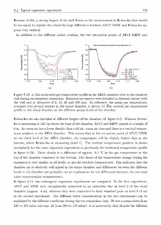
8.4. Typical expansion experiment 129
Because of this, a strong impact of the wall �uxes on the measurement in Rewas-Iso that would
be necessary to explain the relatively large di�erences between APeT/MBW and Rewas-Iso ap-
pears very unlikely.
In addition to the di�erent radial position, the two extraction points of APeT/MBW and
(a) (b)
Figure 8.13: a) The horizontal gas temperature pro�le in the AIDA chamber close to the chamberwall during an exemplary expansion. Temperature sensors were installed in thermal contact withthe wall and at distances of 3, 10, 30 and 100 mm. As reference, the mean gas temperature,averaged over several sensors in the entire chamber is shown, b) The vertical gas temperaturepro�le in the cloud chamber at the di�erent access levels of the chamber
Rewas-Iso are also installed at di�erent heights of the chamber (cf. �gure 8.2). Whereas Rewas-
Iso is measuring at 135 cm above the base of the chamber, APeT and MBW sample at a height of
6 m. As warm air has a lower density than cold air, warm air rises and there is a vertical temper-
ature gradient in the AIDA chamber. This means that at the extraction point of APeT/MBW
on the third level of the AIDA chamber, the temperature will be slightly higher than at the
bottom, where Rewas-Iso is measuring (level 1). The vertical temperature gradient is shown
exemplarily for the same expansion experiment as previously the horizontal temperature pro�le
in �gure 8.13b. There clearly is a di�erence of approx. 0.5 °C in the gas temperature at the
top of the chamber compared to the bottom. The shape of the temperature change during the
expansion is very similar on all levels, as are the absolute temperatures. This indicates that the
chamber air is relatively well mixed in the entire chamber and di�erences between the di�erent
levels in the chamber are probably not an explanation for the di�erences between the two total
water concentration measurements.
In �gure 8.14, two subsequent expansion experiments are compared. In the �rst experiment,
APeT and MBW were exceptionally connected to an extractive line on level 2 of the cloud
chamber (approx. 4 m), whereas they were connected to their standard port on level 3 (6 m)
in the second experiment. The di�erent water concentrations in the two experiments can be
explained by the di�erent conditions during the two expansions (exp. 20 was a pump-down from
230 to 170 mbar and exp. 21 from 300 to 170 mbar). It is noteworthy that despite the di�erent

130 8. Water isotope fractionation in simulated ice clouds
extraction ports, the overall shape of the water concentration measurement by APeT is identical
between the two di�erent sampling heights. This indicates that the di�erent shape of the water
concentration measurements of APeT/MBW and Rewas-Iso is not due to a di�erent sampling
height.
Figure 8.14: Comparison of two subsequent expansion experiments, in exp. 20 APeT and MBWwere sampling at 4 m height and in exp. 21 at 6 m. Because of di�erent measurement conditions,the water concentrations are not equal but the shape is identical for both measurement heights
Finally, the ridges inside the cloud chamber that improve its mechanical strength, could
hamper a good mixing of the air closer to the walls. The ridges extend approximately 10 cm
into the chamber, which is nearly the same distance at which Rewas-Iso is measuring. However,
this hypothesis was excluded in an extensive chamber and instrumental intercomparison study
(AquaVIT-1) done in the AIDA simulation chamber by Fahey et al. [160]. For experimental
conditions similar to the conditions encountered during the Isocloud campaigns, they found that
mixing ratio gradients are virtually non-existent.
CFD simulations and simultaneous measurements at various AIDA positions during the in-
tercomparison campaigns AquaVIT 1 and 2 support our arguments against all of the above-
mentioned hypotheses [161]. After excluding almost all possible chamber related reasons for the
observed discrepancies, the cause may rather be related to the sampling system with a rather
small �ow of 150 sccm. The di�erence in the total water measurement of REWAS and APeT is
well correlated with the pressure change and relaxes at constant pressure. Therefore, problems
with the �ow controller system or a dynamic leak seem possible causes for the observation.
Despite numerous leak tests and other investigations, neither of these last two hypotheses could
be con�rmed. However, until now no �ow simulations in the chamber were done for isotope
changes and a problem due to incomplete mixing of the chamber air remains a possibility as
well. The true cause of the discrepancy between the instruments on the lower and higher air
extraction lines could thus not yet be revealed and remains speculation.

8.4. Typical expansion experiment 131
8.4.2 Ice phase measurements
In �gure 8.15, the water concentration measurement of two expansions is shown (top panel)
together with the particle density measured with two optical particle counters (OPC, WELAS
2100, second panel). The particle density is with approx. 500 cm−3 higher in �gure 8.15b than
in �gure 8.15a (100 cm−3), the water concentration is the opposite. Lower ice nuclei number
concentrations at higher water concentrations allow the formation of fewer but larger ice crystals
(about 100 µm) in experiment 8.15a compared to about 50 µm in experiment �gure 8.15b.
Because of the larger particle sizes, the ice crystals grow more quickly to beyond the cuto� size
of the PCVI and are thus sublimated in the sample air arriving in the OF-CEAS spectrometer.
In the case of experiment 8 of �gure 8.15a, the water concentration behind the PCVI contin-
ues to increase for approx. 70 s after the start of the experiment, whereas in experiment 15
(�gure 8.15b), it takes approx. 40 s longer for ice crystals to be detectable by the OF-CEAS
instrument. Note that this di�erence in ice crystal size is also visible in the onset behavior of
the two di�erent optical particle counters which have di�erent lower detection limits.
In �gure 8.16, an expansion experiment at -60°C is shown. In the top panel, the water
concentration measurements with an initial water vapor concentration of 40 ppmv are shown.
The center panel shows the ratio HDO/H162 O in the vapor phase, total water in the gas phase,
as well as in the ice phase as measured behind the PCVI. Due to heavier wall ice that is released
during the pressure decrease, the HD 16O/H216O ratio increased from 10.6 to 11.1 during the
experiment. The isotope ratio measured by SIRI behind the PCVI increases in the beginning of
the experiment (until 11:05 h), then decreases for approximately one minute, before it increases
again, to level o� at a higher than before the expansion, due to the above discussed wall-induced
memory e�ect for HDO. The one-minute long decrease of the HDO/H162 O ratio can be observed
in several of the experiments (e.g. also in �gure 8.10).
This dip in the isotope ratio is probably due to the increasing in�uence of wall ice throughout
the expansion experiment. In the beginning, the ice is becoming progressively enriched because
of a preferential crystallization of the heavier isotopologues. As the vapor phase becomes more
depleted in the rare isotopologues, more H162 O molecules crystallize and the isotope ratio of the
ice decreases slightly. Because of highly enriched water coming from the walls, the total water
isotope ratio increases again and as this water freezes, consequently also the isotope ratio of the
ice crystals, leading to the observed behavior with a dip in the isotope ratio in the beginning of
the experiment.
Figure 8.17 shows a measurement, in which Rewas-Iso was connected behind the PCVI. In
addition to the expansion experiment, the AIDA air before and after the pump-down has been
measured with Rewas-Iso directly connected to the AIDA chamber via heated tubing. These two
data sets serve as an additional calibration of the measurement and allow comparing directly
the isotopic compositions through the PCVI and inside the chamber air.
In the top panels of �gure 8.17, the water concentration measurements are shown with a back-

132 8. Water isotope fractionation in simulated ice clouds
(a) (b)
Figure 8.15: Two cloud expansion measurements (a) starting at -50 °C and with 100particles/cm−3 and (b) starting at -60 °C and with 500 particles/cm−3. Top panel: H2O ingas phase, in the ice behind the PCVI and in total water. Second panel: Measurement of twoOPCs (Welas and Welas2) of the particle density in the cloud chamber. Third panel: Themaximal particle size in a) is nearly 100 µm compared to around 50 µm in b). Bottom panel:Pressure and air temperature during the experiment

8.4. Typical expansion experiment 133
Figure 8.16: Expansion at -60°C. Top panel: Measurement of gas phase, total water and icebehind the PCVI. Center panel: HDO/H16
2 O in gas phase, total water and ice. In the ice phasewater, a small dip in the isotope ratio can be observed shortly after the beginning of the icecloud measurement, which is probably related to the water dynamics in the cloud chamber.Bottom panel: Pressure and air temperature during the experiment
ground measurement before (left panel) and after the expansion (right panel). In the center
panels, the corresponding δ18O measurements of background and expansion are given and in
the bottom panel, pressure and temperature during the expansion.
For a �rst estimate of the fractionation factor in the experiment, we assume a constant frac-
tionation factor and only a transition from the vapor phase to ice, thus a Rayleigh fractionation
process with one sink. We can then calculate the fractionation factor with the following formula
(cf. 1.2.2 and [145]):
R
R0=
(N
N0
)α−1
(8.2)
with R and R0 the current and initial isotope ratio and N and N0 the current and initial water
concentration, respectively. The δ18O values are 3.5 ± 0.8h and 3.1 ± 0.7h for the chamber
air before and after the expansion, respectively and 10.6 ± 1.8h for the ice phase behind the
PCVI. The water concentration before the ice cloud formation was 8.12 ± 0.05 ppmv and the
lowest water concentration during the expansion (measured with APicT) 5.65± 0.07 ppmv. For
the fractionation coe�cient α, we then get 18α = 1.018± 0.014.
This is only a �rst estimate, as no additional sinks and sources for water, such as the chamber

134 8. Water isotope fractionation in simulated ice clouds
wall were taken into account. In addition, the measurement behind the PCVI risks to be biased
as only ice crystals of a certain size can be measured. Even with the improved detection limit in
Rewas-Iso of approx. 4h in δ18O at water concentrations around 20 ppmv, the standard error
made in the calculation of the fractionation factor (0.014) relatively high. A better estimation
of the fractionation factors can be obtained by the comparison of in-situ measurements of the
gas phase (ISO-APicT and CHI-WIS) with measurements of the total water (APeT, MBW and
Rewas-Iso). In addition, a more complete model of the water �uxes in the cloud chamber has
to be developed, as was done by Kara Lamb of the University of Chicago as part of her PhD
thesis. A brief introduction of this model will be given in the next section, for more details we
refer to the PhD thesis of K. Lamb and [162].
Figure 8.17: Expansion at very low water concentration. Top panel: water concentration mea-surement during the experiment (middle) and background measurements before (left) and after(right) the expansion. Middle panel: corresponding δ18O measurements of background andexpansions. Bottom panel: pressure and temperature during the expansion
8.5 Modeling of �uxes in the AIDA chamber
As the ice cloud formation experiments are done in a �nite volume, we have to take into account
interactions of the gas inside the chamber with the chamber wall and the removal of air from
the chamber during the experiments.

8.5. Modeling of �uxes in the AIDA chamber 135
Figure 8.18: Schematics of the water and isotope �uxes included in the model
Figure 8.18 gives a schematics of the water �uxes that are simulated in the model. Three
di�erent �uxes of H2O are assumed:
1) A reduction of [H2O]total in the chamber because of the decrease in pressure:
∆ [H2O]pump = [H2O] · dNN
(8.3)
= [H2O] ·(
(p+ ∆p)T
p(T + ∆T )− 1
)(8.4)
As the chamber air is constantly stirred by a mixing fan, we assume a homogenous isotopic
distribution throughout the chamber, and :
Rpump = R(t) (8.5)
2) An exchange between vapor and ice phase due to crystallization and sublimation
∆ [H2O]ice = [H2O]total − [H2O]gas (8.6)

136 8. Water isotope fractionation in simulated ice clouds
As total water the measurement of APeT is used and for water vapor the data from APicT.
For the crystallization, Rayleigh distillation is assumed with (cf. section 1.2.2)
dR
R= (α− 1)
dN
N(8.7)
As the gas temperature change during an experiment is typically of the order of only 4°C to
5°C during an ice cloud formation, a linear dependence of the fractionation factor α on the
temperature can be assumed:
α = a0 + a1T (8.8)
The o�set a0 is a free parameter in the �t and the slope a1 is derived from the temperature
dependence of the fractionation factor as described by Merlivat and Nief ([34], equation (1.10)).
The result is however insensitive to whether the formulation of Merlivat and Nief is used or the
formulation by Ellehøj [163].
α can be separated into kinetic and equilibrium fractionation (section 1.2.2,[39],[46]):
with α = αeq · αk (8.9)
and αK =S
1 + αeqDD′ (S − 1)
(8.10)
and the the equilibrium fractionation factor can subsequently be determined based on equations
8.8 and 8.10. The water that sublimates from ice to vapor is assumed to have the same isotope
ratio it froze at.
3) A �ux of [H2O] from wall ice into the chamber air:
∆ [H2O]wall = ∆ [H2O]total −∆ [H2O]pump (8.11)
As the fraction of ice coming from the wall is much smaller than the total amount of wall ice, the
isotopic composition of the wall ice can be assumed to be constant throughout an experiment.
In addition, the change of the wall temperature is very small during the adiabatic expansions.
Because of this, we can assume that the isotope ratio of the ice coming from the wall is practically
constant:
Rv,wall = const. (8.12)
The parameter Rv,wall is �tted. A list of all input data and parameters used in the model is
shown in table 8.2.

8.5. Modeling of �uxes in the AIDA chamber 137
Table 8.2: Input data and parameters used in the isotope �ux model
parameter determination∆[H2O]total measured by APeT/MBW/Rewas-Iso∆[H2O]gas measured by APicT/SP-APicT/ISO-APicT∆[H2O]pump = [H2O] · (p+∆p)T
p(T+∆T ) − 1
∆[H2O]ice = [H2O]total − [H2O]gas∆[H2O]wall = ∆[H2O]total −∆[H2O]pumpR(t)gas measured by CHI-WIS/ISO-APicTR(t)total measured by REWAS-IsoRv,wall const., free �t parameterRpump = R(t)gasRice = α(T ) · αgasα(T ) = α0 + α1Tα0 const., free �t parameterα1 based on [34] or [163]
The ice, pumping, and wall �ux components are determined for one second time intervals
by interpolated data sets. The model is adapted to the experimental data with a Levenberg-
Marquardt least squares �t.
In �gure 8.19, the isotopic ratio measured by CHI-WIS is shown for a typical expansion
experiment, along with the model �t (top panel). In the middle panel, the di�erent water �uxes
assumed in the model (see above) are given, showing the removal of chamber air as negative
�ux and a positive �ux coming from the walls. The �ux between vapor and ice is positive
in the beginning, indicating a transition from vapor to ice phase when the air temperature
decreases and water vapor saturation is reached. When the temperature increases at the end
of the experiment, the vapor-ice �ux is negative, representing the transition from ice phase to
water vapor.
In the bottom panel, water concentrations measured by APeT and APicT are shown along
with chamber pressure and air temperature, showing the typical behavior during the expansion
experiments as described above.
Based on the model, equilibrium fractionation factors have been derived from the �t for a
series of Isocloud experiments at di�erent temperatures. The fractionation factors are shown in
�gure 8.20 and compared with previous results by other groups ([34, 127, 164�168]). The tem-
perature dependence of fractionation factors derived from our experiments agree with previous
investigations. The recent proposition of higher fractionation factors at temperatures below 250
K [127] is not con�rmed.

138 8. Water isotope fractionation in simulated ice clouds
Figure 8.19: Figure from [162], Top panel: The isotopic ratio measured by CHI-WIS, alongwith the model �t. Middle panel: Model �uxes between ice and vapor (green), from the walls(black) and due to the removal of chamber air by the pump (blue). Bottom panel: Total andvapor phase water concentrations measured by APeT (blue) and APicT (green). In dashed redchamber air temperature and in dashed black pressure.
8.6 Summary of Isocloud
Although it was not yet possible to determine, which of the two mechanisms, di�usion-limited
fractionation or equilibrium fractionation, is responsible for the supersaturation observed in
the upper atmosphere, the Isocloud project yielded very promising results. It was possible to
establish a measurement protocol to e�ciently measure ice cloud formation at temperatures
as low as -80°C in vapor phase, total water and ice phase simultaneously. Because of the
isotope calibration of the external OF-CEAS spectrometers, we could calibrate the internal
TDL spectrometers and reduce the relative error to < 1% on a very large isotopic enrichment.
The ice phase was successfully measured with the OF-CEAS instruments behind the PCVI and
a �rst comparison of the isotope ratios in all three phases could be done. Rewas-Iso could be
successfully adapted to measure δ18O with four times higher precision than before and at water
concentrations as low as a few ppmv.
Because of unde�ned problems in the connection of Rewas-Iso to the AIDA cloud chamber,
the total water measurement is unfortunately only partly exploitable and has to be treated
carefully. If the observed di�erences between Rewas-Iso and APeT are due to �uxes from the
chamber walls that are captured by Rewas-Iso due to the closer proximity to the walls, these
measurements could for example be used to test the validity of the above described modeling
approach of wall �uxes and could even be used to re�ne the model. At the time of this writing,

8.6. Summary of Isocloud 139
Figure 8.20: Figure from Kara D. Lamb, UoC: Comparison of the temperature dependence offractionation factors derived from the (isotope) �ux model in the AIDA chamber with previouslypublished results. Pink dots represent fractionation factors inferred from ISOCLOUD measure-ments. Previously experimental results are shown with data as symbols and modeling resultsas lines (solid for experimental ranges and dashed for extrapolations). Our results agree withprevious published data but not with the recently proposed increase of equilibrium fractionationfactors for water vapor over ice.
this was however work in progress and could not be included.
The mechanisms for supersaturation could not clearly be identi�ed because of limitations in
the experimental set-up. Most importantly, the uncertainty in the total water measurement
because of problems in the Rewas-Iso sample line make a precise determination of the isotopic
composition of total water impossible. In addition, the measurement of ice phase water behind
the PCVI only re�ects a portion of the total ice phase. Due to the inevitable cut-o� size
of separated particles, smaller ice crystals are lost and are not detectable. Therefore, it is
not possible to accurately determine the di�erence between the isotopic composition of gas
phase water and ice phase water that would be necessary to further investigate the two possible
explanations of supersaturation.
To overcome these limitations, for a next cloud campaign, several improvements could be made
and would lead to an even better result and better intercomparibility of the di�erent instruments.
Rewas-Iso should be connected to the same outlet as the other two total water measurements,
MBW and APeT, in order to eliminate any uncertainty concerning the sampling location and
transfer of the sample through the extraction tubing. Regular measurements should be done
at stable conditions inside the cloud chamber to calibrate the internal isotope measurements
against the external (and previously calibrated) OF-CEAS spectrometers. The wavelength range
of SIRI should be changed to the same range as Rewas-Iso, which is especially important for
lower temperatures with very low water concentrations.
Finally, regular calibrations of the OF-CEAS spectrometers with the Syringe Nanoliter Injection

140 8. Water isotope fractionation in simulated ice clouds
Calibration System should be made with two enriched standards approximately matching the
isotopic composition inside the cloud chamber. This way, an additional uncertainty because of
di�erent isotopic composition of calibration and real measurements, can be eliminated.

Conclusion
In the framework of this thesis, we developed an OF-CEAS spectrometer that shows signi�cantly
better performance and stability than previous instruments based on the same technique. At
water concentrations around 80 ppmv, the precision was 0.8h, 0.1h and 0.2h for δ2H, δ18O
and δ17O, respectively with optimum averaging time (about 30 min). With 4s averaging, the
precision is 12h, 1.1h and 3.2h. In the optimum measurement range of the instrument at
water concentrations around 650 ppmv, precisions of 0.28h, 0.02h and 0.07h can be achieved
with averaging times of 30 to 60 min.
As limiting factor of the accuracy, a strong concentration dependence of the isotope ratio mea-
surements was identi�ed. Due to thorough investigations and optimization of the analysis pro-
cedure, the main source of this dependency was identi�ed to be constant pattern noise in the
measurements, which propagates in the isotope ratios and becomes especially prominent at low
absorptions, corresponding to lower water concentrations. By comparing the experimental data
with synthetic absorption spectra, we could conclude that approx. 83% of the baseline noise
is due to slowly changing structured noise. The structured noise is assumed to originate from
residual backscattering on multiple optical surfaces in the beam path and could not (yet) be
removed.
We therefore propose a calibration strategy with two isotope standards. One standard should be
measured at four di�erent water concentrations before the measurement, with each step main-
tained for 30 min to determine the concentration dependence. In addition, the second standard
should be measured at one water concentration to adapt the isotope scale, which is a much
smaller correction than the correction for the concentration dependence. After the measure-
ment, the second water standard should be measured at four di�erent water concentrations and
the �rst standard at only one concentration. This way, the correction function for the unknown
sample can subsequently calculated as a linear combination of the individual functions of the
two standards and possible drift can be corrected for by the additional one-concentration mea-
surements of the other standard, respectively. In this way, calibration measurements are done
142 Conclusion
for approximately �ve hours per day and measurements of unknown samples can be done for
approximately the same time between the two 2.5 h calibrations. If the water concentration
only shows small variations during a measurement (no variations of more than 200 ppmv and
no water concentrations below 80 ppmv), the number of concentration steps could be reduced
to three or even two steps, thus shortening the time needed for calibration.
With the in this thesis established calibration and correction protocol, the demonstrated accu-
racy of the measurements for water concentrations above 80 ppmv is better than 10h for δ2H,
4h for δ18O and 5h for δ17O. The time between the two calibrations should be su�ciently
short to reduce additional uncertainties due to drift of the instrument. Based on the drift anal-
ysis with Allan-Werle plots, we recommend to run calibrations approximately every 6h.
If measurements should be done at lower water concentrations, the error made in the correction
strongly increases due to an inverse dependency of the isotope ratios on the water concentration,
which becomes very large for drier gas samples. At 50 ppmv, the accuracy is approx. 35h, 8h
and 10h for δ2H, δ18O and δ17O, respectively.
For measurements of δ18O at water concentrations as low as 5 ppmv, we successfully demon-
strated the application of a modi�ed OF-CEAS spectrometer, measuring at 7286 cm-1. With
this modi�ed instrument, a precision better than 0.2h was demonstrated for δ18O at water con-
centrations below 20 ppmv. In addition, due to much stronger absorption coe�cients, the water
concentration dependency of the isotope measurements are much smaller than in measurements
at 7184 cm-1 and 7200 cm-1.
As a novel calibration instrument, the Syringe Nanoliter Injection Calibration System (SNICS)
was developed and used for calibration measurements in the lab and during several measurement
campaigns at the AIDA cloud chamber in Karlsruhe. A theoretical model was established to
better explain the operation of the syringe injection system and showed good agreement with
the experimental results. In parallel measurements of SNICS and a microdrop injector, we could
show that no fractionation occurs in the water inside the syringe itself and that the new system
is well adapted for calibration measurements at water concentrations as low as several tens of
ppmv.
Finally, the OF-CEAS spectrometer was successfully operated during measurement campaigns
in Antarctica and at the cloud simulation chamber in Karlsruhe, Germany. Due to di�culties
with the calibration in Antarctica, this data could not be fully exploited. However, due to its
proper functioning under harsh conditions, we were able to show the promising perspective of
using optical spectrometers for isotope measurements in the coldest region of the planet. With
the cloud chamber experiments, we were able to show that the OF-CEAS technique is, after
proper adaptions, capable to measure water isotope ratios even at water concentrations as low
as several ppm and could thus also be successfully used for atmospheric studies, for example in
the stratosphere.
In the near future, more experimental investigations will be done in order to reduce the water
concentration dependence of the OF-CEAS spectrometer, which is at the moment the limiting

143
factor for a higher precision and accuracy of the measurements. One possibility that is going to
be studied is the removal of the additional reference photo diode and to extract this information
from the measurement of the signal photodiode. In this way, optical elements in the beam path
such as the beam splitter, a lens in front of the reference photo diode and the photo diode itself
could be removed, which would eliminate parasitic re�ections and possible optical fringes in the
measurements and could result in a reduced concentration dependence.
As it was shown in the framework of this thesis, the novel OF-CEAS spectrometer is well adapted
to measure at very low water concentrations. The instrument can with proper calibration be
used for measurements under extreme conditions as for example encountered in continental
Antarctica. Next winter, it will probably be part of an upcoming measurement campaign at the
French Italian Antarctic research station of Dome Concordia (75°06'S - 123°21'E). This campaign
will be done in the framework of the European Research Council (ERC) Starting Grant project
COMBINISO of A. Landais of Laboratoire des Sciences du Climat et de l'Environnement. At
Dome Concordia, the mean air temperature is around -50.8°C [148], which corresponds at a
mean pressure of around 650 mbar to water mixing ratios as low as 60 ppmv [169]. The cal-
ibration device, SNICS, can be used not only to calibrate the OF-CEAS instrument but also
other, e.g. commercially available, instruments. It is also going to be used for the upcoming
measurements at Dome Concordia.
The objective of these measurements and the ERC COMBINISO project in general is to estab-
lish a better description of the links between climate, hydrological cycle and stratospheric inputs
over the last 100 years in Antarctica. For a correct use of water isotopes, it is important to better
understand the relation between physical properties such as temperature and relative humidity
and the fractionation factors. First measurements in a cloud chamber have thus been done
to investigate kinetic fractionation factors during solid condensation at low temperature [170].
Further investigations will be done to determine water fractionation coe�cients. These can be
used to improve the description of cloud microphysics in isotopic models and will thus lead to a
better understanding of isotope records in polar ice cores. To accomplish the goal of even more
stable water vapor isotope measurements, a new water vapor isotope spectrometer based on the
technique of Optical Feedback Frequency Stabilized Cavity Ring-Down Spectroscopy (OFFS-
CRDS)[171] is currently being developed in this project to measure all three of the water vapor
isotopes, δ18O, δ17O and δ2H, and will be employed together with our OF-CEAS spectrometer.


Bibliography
[1] Jouzel, J ; Masson-Delmotte, V ; Cattani, O ; Dreyfus, G ; Falourd, S ; Hoff-
mann, G ; Minster, B ; Nouet, J ; Barnola, J M. ; Chappellaz, J ; Fischer, H ;
Gallet, J C. ; Johnsen, S ; Leuenberger, M ; Loulergue, L ; Luethi, D ; Oerter,
H ; Parrenin, F ; Raisbeck, G ; Raynaud, D ; Schilt, A ; Schwander, J ; Selmo, E
; Souchez, R ; Spahni, R ; Stauffer, B ; Steffensen, J P. ; Stenni, B ; Stocker,
T F. ; Tison, J L. ; Werner, M ; Wolff, E W.: Orbital and millennial Antarctic
climate variability over the past 800,000 years. In: Science (New York, N.Y.) 317 (2007),
No. 5839, 793�6
[2] Hoffmann, G ; Werner, M ; Heimann, M: The water isotope module of the ECHAM
atmospheric general circulation model: a study on timescales from days to several years.
In: J. Geophys. Res. 103 (1998), No. D14, P. 16871�16896
[3] Risi, C. ; Landais, A. ; Winkler, R. ; Vimeux, F.: What controls the spatio-temporal
distribution of D-excess and 17O-excess in precipitation? A general circulation model
study. In: Climate of the Past Discussions 8 (2012), No. 6, 5493�5543
[4] Baer, D.S. ; Paul, J.B. ; Gupta, M. ; O'Keefe, a.: Sensitive absorption measure-
ments in the near-infrared region using o�-axis integrated-cavity-output spectroscopy. In:
Applied Physics B: Lasers and Optics 75 (2002), No. 2-3, 261�265
[5] Webster, Christopher R. ; Heymsfield, Andrew J.: Water isotope ratios D/H,
18O/16O, 17O/16O in and out of clouds map dehydration pathways. In: Science (New
York, N.Y.) 302 (2003), No. 5651, 1742�5
[6] Kerstel, E.R.T. ; Iannone, R.Q. ; Chenevier, M ; Kassi, S ; Jost, H.-J. ; Romanini,
D: A water isotope (2H, 17O, and 18O) spectrometer based on optical feedback cavity-
enhanced absorption for in situ airborne applications. In: Applied Physics B 85 (2006),
No. 2-3, 397�406

146 BIBLIOGRAPHY
[7] Dyroff, C. ; Fütterer, D. ; Zahn, A.: Compact diode-laser spectrometer ISOWAT for
highly sensitive airborne measurements of water-isotope ratios. In: Applied Physics B 98
(2010), No. 2-3, 537�548
[8] Rozanski, K.: 18. Isotopes in atmospheric moisture. In: Aggarwal, Pradeep K. (Edt.)
; Gat, Joel R. (Edt.) ; Froehlich, Klaus F. (Edt.): Isotopes in the Water Cycle - Past,
Present and Future of a Developing Science. 2005, Chapter 18. Isotop, P. 291�301
[9] Solomon, Susan: Stratospheric ozone depletion: A review of concepts and history. In:
Reviews of Geophysics 37 (1999), No. 3, 275
[10] Sayres, David S. ; Moyer, E J. ; Hanisco, T F. ; St Clair, J M. ; Keutsch, F N.
; O'Brien, A ; Allen, N T. ; Lapson, L ; Demusz, J N. ; Rivero, M ; Martin, T ;
Greenberg, M ; Tuozzolo, C ; Engel, G S. ; Kroll, J H. ; Paul, J B. ; Anderson,
J G.: A new cavity based absorption instrument for detection of water isotopologues in
the upper troposphere and lower stratosphere. In: The Review of scienti�c instruments
80 (2009), No. 4, 044102
[11] Dansgaard, W: The abundance of 18O in atmospheric water and water vapour. In:
Tellus 5 (1953), No. 4, P. 461�469
[12] Epstein, S ; Mayeda, T: Variation of O18 content of waters from natural sources. In:
Geochimica et Cosmochimica Acta 4 (1953), No. 5, 213�224
[13] Craig, H: Isotopic Variations in Meteoric Waters. In: Science (New York, N.Y.) 133
(1961), No. 3465, 1702�3
[14] Dansgaard, W: Stable isotopes in precipitation. In: Tellus 16 (1964), No. 4, 436�468
[15] Jouzel, J. ; Merlivat, L. ; Roth, E.: Isotopic study of hail. In: Journal of Geophysical
Research 80 (1975), No. 36, 5015�5030
[16] Risi, Camille ; Bony, Sandrine ; Vimeux, Francoise ; Descroix, Luc ; Ibrahim,
Boubacar ; Lebreton, Eric ; Mamadou, Ibrahim ; Sultan, Benjamin: What controls
the isotopic composition of the African monsoon precipitation? Insights from event-based
precipitation collected during the 2006 AMMA �eld campaign. In: Geophysical Research
Letters 35 (2008), No. 24, L24808
[17] Lee, Jung-Eun ; Pierrehumbert, Raymond ; Swann, Abigail ; Lintner, Benjamin R.:
Sensitivity of stable water isotopic values to convective parameterization schemes. In:
Geophysical Research Letters 36 (2009), No. 23, L23801
[18] Kurita, Naoyuki ; Noone, David ; Risi, Camille ; Schmidt, Gavin A. ; Yamada, Hi-
royuki ; Yoneyama, Kunio: Intraseasonal isotopic variation associated with the Madden-
Julian Oscillation. In: Journal of Geophysical Research: Atmospheres 116 (2011), No.
D24

BIBLIOGRAPHY 147
[19] Augustin, Laurent ; Barbante, Carlo ; Barnes, Piers R F. ; Barnola, Jean M. ;
Bigler, Matthias ; Castellano, Emiliano ; Cattani, Olivier ; Chappellaz, Jerome
; Dahl-Jensen, Dorthe ; Delmonte, Barbara ; Dreyfus, Gabrielle ; Durand, Gael ;
Falourd, Sonia ; Fischer, Hubertus ; Flückiger, Jacqueline ; Hansson, Margareta E.
; Huybrechts, Philippe ; Jugie, Gérard ; Johnsen, Sigfus J. ; Jouzel, Jean ; Kauf-
mann, Patrik ; Kipfstuhl, Josef ; Lambert, Fabrice ; Lipenkov, Vladimir Y. ; Littot,
Geneviève C ; Longinelli, Antonio ; Lorrain, Reginald ; Maggi, Valter ; Masson-
Delmotte, Valerie ; Miller, Heinz ; Mulvaney, Robert ; Oerlemans, Johannes ;
Oerter, Hans ; Orombelli, Giuseppe ; Parrenin, Frederic ; Peel, David a. ; Pe-
tit, Jean-Robert ; Raynaud, Dominique ; Ritz, Catherine ; Ruth, Urs ; Schwander,
Jakob ; Siegenthaler, Urs ; Souchez, Roland ; Stauffer, Bernhard ; Steffensen,
Jorgen P. ; Stenni, Barbara ; Stocker, Thomas F. ; Tabacco, Ignazio E. ; Udisti,
Roberto ; Van De Wal, Roderik S W. ; Van Den Broeke, Michiel ; Weiss, Jerome
; Wilhelms, Frank ; Winther, Jan-Gunnar ; Wolff, Eric W. ; Zucchelli, Mario ;
Members, Epica C.: Eight glacial cycles from an Antarctic ice core. In: Nature 429
(2004), No. 6992, 623�628
[20] Masson-Delmotte, V. ; Hou, S. ; Ekaykin, A. ; Jouzel, J. ; Aristarain, A. ;
Bernardo, R. T. ; Bromwich, D. ; Cattani, O. ; Delmotte, M. ; Falourd, S. ;
Frezzotti, M. ; Gallée, H. ; Genoni, L. ; Isaksson, E. ; Landais, A. ; Helsen,
M. M. ; Hoffmann, G. ; Lopez, J. ; Morgan, V. ; Motoyama, H. ; Noone, D. ;
Oerter, H. ; Petit, J. R. ; Royer, A. ; Uemura, R. ; Schmidt, G. A. ; Schlosser, E.
; Simões, J. C. ; Steig, E. J. ; Stenni, B. ; Stievenard, M. ; Broeke, M. R. d. ; Wal,
R. S. W. d. ; Berg, W. J. d. ; Vimeux, F. ; White, J. W. C.: A Review of Antarctic
Surface Snow Isotopic Composition: Observations, Atmospheric Circulation, and Isotopic
Modeling*. In: Journal of Climate 21 (2008), No. 13, 3359�3387
[21] Goff, J. A.: Saturation pressure of water on the new kelvin scale. In: Trans. Am. Soc.
Heating Air-Cond. Eng. 63 (1957), P. 347�354
[22] Goff, J. A.: Saturation pressure of water on the new Kelvin scale. In Humidity and
moisture: Measurement and control in science and industry. Reinhold Publishing, New
York, USA, 1965
[23] Murphy, D. M. ; Koop, T.: Review of the vapour pressures of ice and supercooled water
for atmospheric applications. In: Quarterly Journal of the Royal Meteorological Society
131 (2005), No. 608, 1539�1565
[24] McNaught, A. D. ; Wilkinson, A.: Compendium of Chemical Terminology, 2nd ed.
"The Gold Book". 2nd. Oxford : Blackwell Scienti�c Publications, 1997
[25] Mook, Willem G.: Lecture Notes on Stable Isotope Hydrology. Internatio. 2001. � 57 �
60 P.
148 BIBLIOGRAPHY
[26] International Atomic Energy Agency: Reference Sheet for International Measure-
ment Standards / IAEA. 2009 (May). � Scienti�c report. � 5 P.
[27] De Wit, J.C. ; Straaten, C.M. van d. ; Mook, W.G: Determination of the Absolute
Hydrogen Isotopic Ratio of VSMOW and SLAP. In: Geostandards Newsletter 4 (1980),
No. 1, P. 33�36
[28] Baertschi, P.: Absolute 18O Content of Standard Mean Ocean Water. In: Earth and
Planetary Science Letters 31 (1976), P. 341�344
[29] Li, W. ; Ni, B. ; Jin, D. ; Chang, T.L: Measurement of the Absolute Abundance of
Oxygen-17 in VSMOW. In: Chinese Science Bulletin 33 (1988), P. 1610�1613
[30] Wise, S.A. ; Watters, R.L.: Report of Investigation Reference Materials 8535, 8536,
8537 / National Institute of Standards & Technology. 2005. � Scienti�c report
[31] Gonfiantini, R. ; Rozanski, K. ; Stichler, W.: Intercalibration of Environmental
Isotope Measurements: The Program of the International Atomic Energy Agency. In:
Radiocarbon 32 (1990), No. 3, P. 369�374
[32] Criss, R. E.: Principles of Stable Isotope Distribution. Oxford University Press, USA,
1999
[33] Chacko, T. ; Cole, D. ; Horita, J.: Equilibrium oxygen, hydrogen and carbon iso-
tope fractionation factors applicable to geologic systems. In: Reviews in Mineralogy and
Geochemistry 43 (2001), P. 1�81
[34] Merlivat, L ; Nief, G: Fractionnement isotopique lors des changements d'état solide-
vapeur et liquide-vapeur de l'eau à des températures inférieures à 0°C. In: Tellus 19
(1967), No. 1, 122�127
[35] Majoube, M.: Fractionnement en 18O entre la glace et la vapeur d'eau. In: J. Chim.
Phys. 68 (1971), P. 625�636
[36] Majoube, M.: Fractionnement en Oxygène 18 et en Deutérium entre l'eau et sa vapeur.
In: J. Chim. Phys. 10 (1971), P. 1423�1436
[37] Cappa, Christopher D.: Isotopic fractionation of water during evaporation. In: Journal
of Geophysical Research 108 (2003), No. D16, 4525
[38] Luz, Boaz ; Barkan, Eugeni ; Yam, Ruth ; Shemesh, Aldo: Fractionation of oxygen
and hydrogen isotopes in evaporating water. In: Geochimica et Cosmochimica Acta 73
(2009), No. 22, 6697�6703

BIBLIOGRAPHY 149
[39] Jouzel, Jean ; Merlivat, Liliane: Deuterium and oxygen 18 in precipitation: Modeling
of the isotopic e�ects during snow formation. In: Journal of Geophysical Research: . . . 89
(1984), No. D7, 11749
[40] Merlivat, Liliane: Molecular di�usivities of H216O, HD16O, and H218O in gases. In:
The Journal of Chemical Physics 69 (1978), No. 6, 2864
[41] Lorius, C. ; Merlivat, L. ; Hagemann, R.: Variation in the mean deuterium content
of precipitations in Antarctica. In: Journal of Geophysical Research 74 (1969), No. 28,
7027�7031
[42] Jouzel, Jean ; Merlivat, Liliane ; Lorius, Claude: Deuterium excess in an East
Antarctic ice core suggests higher relative humidity at the oceanic surface during the last
glacial maximum. In: Nature 299 (1982), No. 5885, 688�691
[43] Vimeux, F ; Masson, V ; Jouzel, J ; Stievenard, M ; Petit, JR: Glacial-interglacial
changes in ocean surface conditions in the southern hemisphere. In: NATURE 398 (1999),
No. 6726, 410�413
[44] Barkan, Eugeni ; Luz, Boaz: High precision measurements of 17O/16O and 18O/16O
ratios in H2O. In: Rapid communications in mass spectrometry : RCM 19 (2005), No.
24, 3737�42
[45] Barkan, Eugeni ; Luz, Boaz: Di�usivity fractionations of H2(16)O/H2(17)O and
H2(16)O/H2(18)O in air and their implications for isotope hydrology. In: Rapid com-
munications in mass spectrometry : RCM 21 (2007), No. 18, 2999�3005
[46] Landais, Amaelle ; Barkan, Eugeni ; Luz, Boaz: Record of δ 18 O and 17 O-excess in
ice from Vostok Antarctica during the last 150,000 years. In: Geophysical Research Letters
35 (2008), No. 2, L02709
[47] Gat, J. R. ; Matsui, E.: Atmospheric water balance in the Amazon basin: An isotopic
evapotranspiration model. In: Journal of Geophysical Research 96 (1991), No. D7, 13179
[48] Berman, Elena S F. ; Levin, Naomi E. ; Landais, Amaelle ; Li, Shuning ; Owano,
Thomas: Measurement of δ18O, δ17O, and 17O-excess in water by o�-axis integrated
cavity output spectroscopy and isotope ratio mass spectrometry. In: Analytical chemistry
85 (2013), No. 21, 10392�8
[49] Steig, E. J. ; Gkinis, V. ; Schauer, a. J. ; Schoenemann, S. W. ; Samek, K. ;
Hoffnagle, J. ; Dennis, K. J. ; Tan, S. M.: Calibrated high-precision 17Oexcess
measurements using laser-current tuned cavity ring-down spectroscopy. In: Atmospheric
Measurement Techniques Discussions 6 (2013), No. 6, 10191�10229

150 BIBLIOGRAPHY
[50] Winkler, R. ; Landais, A. ; Sodemann, H. ; Dümbgen, L. ; Prié, F. ; Masson-
Delmotte, V. ; Stenni, B. ; Jouzel, J.: Deglaciation records of 17O-excess in East
Antarctica: reliable reconstruction of oceanic relative humidity from coastal sites. In:
Climate of the Past Discussions 7 (2011), No. 3, 1845�1886
[51] Schoenemann, Spruce W. ; Steig, Eric J. ; Ding, Qinghua ; Markle, Bradley R. ;
Schauer, Andrew J.: Triple water-isotopologue record from WAIS Divide, Antarctica:
Controls on glacial-interglacial changes in 17-O(excess) of precipitation. In: Journal of
Geophysical Research: Atmospheres 119 (2014), No. 14, 8741�8763
[52] Steen-Larsen, H. C. ; Sveinbjörnsdottir, a. E. ; Peters, a. J. ;Masson-Delmotte,
V. ; Guishard, M. P. ; Hsiao, G. ; Jouzel, J. ; Noone, D. ; Warren, J. K. ; White,
J. W. C.: Climatic controls on water vapor deuterium excess in the marine boundary
layer of the North Atlantic based on 500 days of in situ, continuous measurements. In:
Atmospheric Chemistry and Physics Discussions 14 (2014), No. 2, 2363�2401
[53] Kerstel, E R T. ; Meijer, H A J.: Optical Isotope Ratio Measurements in Hydrology
(Chapter 9). In: Aggarwal, P.K. (Edt.) ; Gat, J. (Edt.) ; Froehlich, K. (Edt.):
Isotopes in the Water Cycle: past, present and future of a developing science. 2005, P.
109�123
[54] J. Bigeleisen ; M.J., Perlman ; H., Prosser: Conversion of hydrogenic materials for
hydrogen to isotopic analysis. In: Anal. Chem1 24 (1952), P. 1356�1357
[55] Gehre, M. ; Höfling, R. ; Kowski, P.: Sample preparation device for quantitative
hydrogen isotope analysis using chromiun metal. In: Anal. Chem. 68 (1996), P. 4414
[56] Socki, R.A. ; Romanek, C.S. ; Gibson, E.K: On-line technique for measuring stable
oxygen and hydrogen isotopes from microliter quantities of water. In: Anal. Chem.1 71
(1999), P. 2250�2253
[57] Begley, I.S. ; Scrimgeour, C.M.: High-precision d2H and d18O measurement for
water and volatile organic compounds by continuous-�ow pyrolysis isotope ratio mass
spectrometry. In: Anal. Chem. 69 (1997), P. 1530�1535
[58] Phillips, A. ; Fourel, F. ; Morrison, J.: Oxygen-deuterium isotopic measurements
using a variety of pyrolysis methods � IRMS continuous-�ow techniques. In: Isotopes
in Environ. Health Stud. 36 (2000), P. 347
[59] Helliker, Brent R. ; Roden, John S. ; Cook, Craig ; Ehleringer, James R.: A rapid
and precise method for sampling and determining the oxygen isotope ratio of atmospheric
water vapor. In: Rapid communications in mass spectrometry : RCM 16 (2002), No. 10,
929�32

BIBLIOGRAPHY 151
[60] Han, L-F ; Gröning, M ; Aggarwal, P. ; Helliker, B.R.: Reliable determination of
oxygen and hydrogen isotope ratios in atmospheric water vapour adsorbed on 3A molecular
sieve. In: Rapid Communications in Mass Spectrometry 20 (2006), No. 23, 3612�3618
[61] Rothman, L.S. ; Gordon, I.E. ; Babikov, Y. ; Barbe, A. ; Chris Benner, D. ;
Bernath, P.F. ; Birk, M. ; Bizzocchi, L. ; Boudon, V. ; Brown, L.R. ; Campargue,
A. ; Chance, K. ; Cohen, E.A. ; Coudert, L.H. ; Devi, V.M. ; Drouin, B.J. ; Fayt,
A. ; Flaud, J.-M. ; Gamache, R.R. ; Harrison, J.J. ; Hartmann, J.-M. ; Hill, C.
; Hodges, J.T. ; Jacquemart, D. ; Jolly, A. ; Lamouroux, J. ; Le Roy, R.J. ; Li,
G. ; Long, D.a. ; Lyulin, O.M. ; Mackie, C.J. ; Massie, S.T. ; Mikhailenko, S. ;
Müller, H.S.P. ; Naumenko, O.V. ; Nikitin, A.V. ; Orphal, J. ; Perevalov, V. ;
Perrin, A. ; Polovtseva, E.R. ; Richard, C. ; Smith, M.a.H. ; Starikova, E. ; Sung,
K. ; Tashkun, S. ; Tennyson, J. ; Toon, G.C. ; Tyuterev, Vl.G. ; Wagner, G.: The
HITRAN2012 molecular spectroscopic database. In: Journal of Quantitative Spectroscopy
and Radiative Transfer (2013)
[62] Chapter IsotopeRat. In:Kerstel, E R T.: Handbook of Stable Isotope Analytical Tech-
niques. Bd. 1. Elsevier, 2004, P. 759�787
[63] Rothman, L. S. ; Rinsland, C. P. ; Goldman, A. ; Massie, S. T. ; Edwards, D. P.
; Flaud, J. M. ; Perrin, A. ; Camy-Peyret, C. ; Dana, V. ; Mandin, J. Y. ;
Schroeder, J. ; McCann, A. ; Gamache, R. R. ; Wattson, R. B. ; Yoshino, K.
; Chance, K. V. ; Jucks, K. W. ; Brown, L. R. ; Nemtchinov, V. ; Varanasi,
P.: THE HITRAN MOLECULAR SPECTROSCOPIC DATABASE AND HAWKS (HI-
TRAN ATMOSPHERIC WORKSTATION): 1996 EDITION (Reprint from J Quant Spec-
trosc Radiat Transfer, vol 60, pg 665-710, 1998). In: JOURNAL OF QUANTITATIVE
SPECTROSCOPY & RADIATIVE TRANSFER 111 (2010), No. 11, 1568�1613
[64] Kerstel, E R T. ; Trigt, R van ; Dam, N ; J Reuss ; Meijer, H A J.: Simultaneous
determination of the 2H/1H, 17O/16O, and 18O/16O isotope abundance ratios in water
by means of laser spectrometry. In: Anal. Chem. 71 (1999), No. 23, P. 5297�5303
[65] Lee, X ; Sargent, S: In Situ Measurement of the Water Vapor 18 O/16 O Isotope Ratio
for Atmospheric and Ecological Applications. In: Journal of Atmospheric & . . . (2005),
No. 1999, 555�566
[66] Wen, Xue-Fa ; Sun, Xiao-Min ; Zhang, Shi-Chun ; Yu, Gui-Rui ; Sargent, Steve D. ;
Lee, Xuhui: Continuous measurement of water vapor D/H and 18O/16O isotope ratios
in the atmosphere. In: Journal of Hydrology 349 (2008), No. 3-4, 489�500
[67] Lübken, Franz-Josef ; Dingler, Florian ; Lucke, Henrich von ; Anders, Joachim ;
Riedel, Wolfgang J. ; Wolf, Helmut: MASERATI: a RocketBorne Tunable Diode Laser
Absorption Spectrometer. In: Applied Optics 38 (1999), No. 25, 5338

152 BIBLIOGRAPHY
[68] Buchholz, B. ; Kühnreich, B. ; Smit, H. G. J. ; Ebert, V.: Validation of an ex-
tractive, airborne, compact TDL spectrometer for atmospheric humidity sensing by blind
intercomparison. In: Applied Physics B 110 (2012), No. 2, P. 249�262
[69] Gurlit, W ; Zimmermann, R ; Giesemann, C ; Fernholz, T ; Ebert, V ; Wolfrum,
J ; Platt, U ; Burrows, JP: Lightweight diode laser spectrometer CHILD (Compact
High-altitude In-situ Laser Diode) for balloonborne measurements of water vapor and
methane. In: APPLIED OPTICS 44 (2005), No. 1, 91�102
[70] Huang, Haifeng ; Lehmann, Kevin K.: Sensitivity limits of continuous wave cavity
ring-down spectroscopy. In: The journal of physical chemistry. A 117 (2013), No. 50,
13399�411
[71] Romanini, D ; Ventrillard, I ;Méjean, G ;Morville, J ; Kerstel, E: Introduction
to cavity enhanced absorption spectroscopy 1 Introduction. Version: 2014. http://dx.
doi.org/10.1007/978-3-642-40003-2_1. In: Gagliardi, G. (Edt.) ; Loock, H.-P.
(Edt.): Cavity-Enhanced Spectroscopy and Sensing (Vol. 179). Springer Berlin Heidelberg,
2014. � DOI 10.1007/978�3�642�40003�2_1, P. 1�51
[72] Paldus B. A. ; Zare R. N.: Absorption Spectroscopies: From Early Begin-
nings to Cavity-Ringdown Spectroscopy. Version: 1999. http://dx.doi.org/10.1021/
bk-1999-0720. In: Busch, Kenneth W. (Edt.) ; Busch, Marianna A. (Edt.): Cavity-
Ringdown Spectroscopy Bd. 720. Washington, DC : American Chemical Society, 1999. �
DOI 10.1021/bk�1999�0720. � ISBN 0�8412�3600�3, 49�70
[73] Zee, Roger D. ; Hodges, Joseph T. ; Looney, J. P.: Pulsed, Single-Mode Cavity
Ringdown Spectroscopy. In: Applied Optics 38 (1999), No. 18, 3951
[74] Demtröder, Wolfgang: Laser Spectroscopy: Vol. 1: Basic Principles. Bd. 9. Springer-
Verlag, 2007. � ISBN 354073418X
[75] Paul, J B. ; Lapson, L ; Anderson, J G.: Ultrasensitive absorption spectroscopy with
a high-�nesse optical cavity and o�-axis alignment. In: Applied optics 40 (2001), No. 27,
4904�10
[76] WEBSTER, CR ; MAY, RD ; TRIMBLE, CA ; CHAVE, RG ; KENDALL, J:
AIRCRAFT (ER-2) LASER INFRARED-ABSORPTION SPECTROMETER (ALIAS)
FOR IN-SITU STRATOSPHERIC MEASUREMENTS OF HCL, N2O, CH4, NO2, AND
HNO3. In: APPLIED OPTICS 33 (1994), No. 3, 454�472
[77] Sturm, C ; Zhang, Q ; Noone, D: An introduction to stable water isotopes in climate
models: bene�ts of forward proxy modelling for paleoclimatology. In: Climate of the Past
6 (2010), No. 1, 115�129

BIBLIOGRAPHY 153
[78] Aemisegger, F. ; Sturm, P. ; Graf, P. ; Sodemann, H. ; Pfahl, S. ; Knohl, A. ;
Wernli, H.: Measuring variations of d18O and d2H in atmospheric water vapour using
laser spectroscopy: an instrument characterisation study. In: Atmos. Meas. Tech. 5 (2012),
No. 7, 1491�1511
[79] Crosson, E.R.: A cavity ring-down analyzer for measuring atmospheric levels of methane,
carbon dioxide, and water vapor. In: Applied Physics B 92 (2008), No. 3, 403�408
[80] Ye, Jun ; Ma, LS ; Hall, JL: Ultrasensitive detections in atomic and molecular physics:
demonstration in molecular overtone spectroscopy. In: JOSA B 15 (1998), No. 1, 6�15
[81] Morville, Jérôme ; Romanini, Daniele ; Kerstel, Erik: Cavity Enhanced Absorp-
tion Spectroscopy with Optical Feedback. Version: 2014. http://dx.doi.org/10.1007/
978-3-642-40003-2_5. In: Gagliardi, G. (Edt.) ; Loock, H.-P. (Edt.): Cavity En-
hanced Spectroscopy and Sensing (Vol. 179). Springer Berlin Heidelberg, 2014. � DOI
10.1007/978�3�642�40003�2_5, Chapter 13, P. 163�207
[82] Morville, J. ; Kassi, S. ; Chenevier, M. ; Romanini, D.: Fast, low-noise, mode-
by-mode, cavity-enhanced absorption spectroscopy by diode-laser self-locking. In: Appl.
Phys. B 80 (2005), No. 8, 1027�1038
[83] Iannone, Rosario Q. ; Kassi, Samir ; Jost, Hans-Jürg H.-J. ; Chenevier, Marc ; Ro-
manini, Daniele ; Meijer, Harro A J. ; Dhaniyala, Suresh ; Snels, Marcel ; Kerstel,
Erik R T.: Development and airborne operation of a compact water isotope ratio infrared
spectrometer. In: Isotopes Environ Health Stud. 45 (2009), No. 4, 303�20
[84] Landsberg, J ; Romanini, D ; Kerstel, E: Very high �nesse optical-feedback cavity-
enhanced absorption spectrometer for low concentration water vapor isotope analyses. In:
Optics letters 39 (2014), No. 7, 1795�8
[85] James, F. ; Roos, M.: Minuit - a system for function minimization and analysis of the
parameter errors and correlations. In: Computer Physics Communications 10 (1975), No.
6, 343�367
[86] Brand, W A. ; Geilmann, H ; Crosson, E R. ; ; Rella, C W.: Cavity ring-down
spectroscopy versus high-temperature conversion isotope ratio mass spectrometry and a
case study on 25 à2H and à18O of pure water samples and alcohol/water mixtures. In:
Rapid Communications in Mass Spectrometry 23 (2009), P. 1879�1884
[87] Habig, Jan C.: Bestimmung von Wasserdampfpartialdrücken und Wasserisotopenverhält-
nissen mittels resonatorverstärkter Absorptionsspektroskopie - Entwicklung von Software
und Spektrometer sowie die Anwendung für die Atmosphärenforschung, Karlsruhe Insti-
tute of Technology / University of Heidelberg, Diss., 2013

154 BIBLIOGRAPHY
[88] Demtröder, Wolfgang: 7. Emission und Absorption elektromagnetischer Strahlung
durch Atome. In: Exerimentalphysik 3 - Atome, Moleküle und Festkörper. 2005, P.
231�238
[89] Tittel, Frank K. ; Richter, Dirk ; Fried, Alan: Mid-Infrared Laser Applications
in Spectroscopy. Version: 2003. http://dx.doi.org/10.1007/3-540-36491-9. In:
Sorokina, Irina T. (Edt.) ; Vodopyanov, Konstantin L. (Edt.): Solid-State Mid-Infrared
Laser Sources Bd. 89. Berlin, Heidelberg : Springer Berlin Heidelberg, 2003. � DOI
10.1007/3�540�36491�9. � ISBN 978�3�540�00621�3, 458�529
[90] Lepère, Muriel: Line pro�le study with tunable diode laser spectrometers. In: Spec-
trochimica acta. Part A, Molecular and biomolecular spectroscopy 60 (2004), No. 14, 3249�
58
[91] Huang, Xianglei ; Yung, YL: A common misunderstanding about the Voigt line pro�le.
In: Journal of the atmospheric sciences 61 (2004), No. 13, 1630�1632
[92] Olivero, JJ ; Longbothum, RL: Empirical �ts to the Voigt line width: a brief review.
In: Journal of Quantitative Spectroscopy and . . . 17 (1977), 233�236
[93] Rautian, S.G. ; Sobel'man, I.I.: The e�ect of collisions on the doppler broadening of
spectral lines. In: Sov. Phys. Usp. Engl. Transl. 9 (1967), P. 701�716
[94] Galatry, L: Simultaneous e�ect of Doppler and foreign gas broadening on spectral lines.
In: Physical Review 122 (1961), No. 4, P. 1218
[95] Leshchishina, O. ; Mikhailenko, S. ; Mondelain, D. ; Kassi, S. ; Campargue, A.:
CRDS of water vapor at 0.1Torr between 6886 and 7406cm-1. In: Journal of Quantitative
Spectroscopy and Radiative Transfer 113 (2012), No. 17, 2155�2166
[96] Campargue, A. ; Leshchishina, O. ; Wang, L. ; Mondelain, D. ; Kassi, S. ; Nikitin,
A.V.: Re�nements of the WKMC empirical line lists (5852-7919cm-1) for methane between
80K and 296K. In: Journal of Quantitative Spectroscopy and Radiative Transfer 113
(2012), No. 15, 1855�1873
[97] Allan, D.W.: STATISTICS OF ATOMIC FREQUENCY STANDARDS. 54 (1966), No.
2
[98] Werle, P: Accuracy and precision of laser spectrometers for trace gas sensing in the
presence of optical fringes and atmospheric turbulence. In: Applied Physics B - Lasers
and Optics 102 (2010), P. 313�329
[99] Romanini, D. ; Chenevier, M. ; Kassi, S. ; Schmidt, M. ; Valant, C. ; Ramonet,
M. ; Lopez, J. ; Jost, H.-J.: Optical-feedback cavity-enhanced absorption: a compact

BIBLIOGRAPHY 155
spectrometer for real-time measurement of atmospheric methane. In: Appl. Phys. B 83
(2006), No. 4, 659�667
[100] Nelson, D D. ; McManus, J B. ; Urbanski, S ; Herndon, S ; Zahniser, M S.: High
precision measurements of atmospheric nitrous oxide and methane using thermoelectrically
cooled mid-infrared quantum cascade lasers and detectors
[101] Gagliardi, G. ; Castrillo, a. ; Iannone, R.Q. ; Kerstel, E.R.T. ; Gianfrani, L.:
High-precision determination of the 13CO2/12CO2 isotope ratio using a portable 2.008-
?m diode-laser spectrometer. In: Applied Physics B: Lasers and Optics 77 (2003), No. 1,
119�124
[102] Kerstel, E R T. ; Gianfrani, L: Advances in laser-based isotope ratio measurements:
Selected applications. In: Appl. Phys. B (2008)
[103] Giusfredi, G. ; Bartalini, S. ; Borri, S. ; Cancio, P. ; Galli, I. ; Mazzotti, D. ; De
Natale, P.: Saturated-Absorption Cavity Ring-Down Spectroscopy. In: Physical Review
Letters 104 (2010), No. 11, 110801
[104] Romanini, D ;Dupré, P ; Jost, R: Non-linear e�ects by continuous wave cavity ringdown
spectroscopy in jet-cooled NO 2. In: Vibrational spectroscopy 19 (1999), No. 2, 93�106
[105] Nave, Carl R.: HyperPhysics. http://hyperphysics.phy-astr.gsu.edu/hbase/
kinetic/menfre.html. Version: 2001
[106] Moretti, L ; Sasso, A ; Gianfrani, L ; Ciurylo, R: Collisional-Broadened and Dicke-
Narrowed Lineshapes of H2_16O and H2_18O Transitions at 1.39 um. In: Journal of
molecular spectroscopy 205 (2001), No. 1, 20�27
[107] Williams, David R.: NASA - Earth Fact Sheet. http://nssdc.gsfc.nasa.gov/
planetary/factsheet/earthfact.html. Version: 2013
[108] R., Gon�antini: The delta-notation and the mass-spectrometric measurement techniques.
In: R., Gat J. (Edt.) ; Gonfiantini, R. (Edt.): Stable Isotope Hydrology, Deuterium and
Oxygen-18 in the Water Cycle. Technical. Vienna : IAEA, 1981, Chapter 4, P. 35�84
[109] Tuzson, B ;Mohn, J ; Zeeman, M J. ; Werner, R A. ; Eugster, W ; Zahniser, M S.
; Nelson, D D. ;McManus, J B. ; Emmenegger, L: High precision and continuous �eld
measurements of delta C-13 and delta O-18 in carbon dioxide with a cryogen-free QCLAS.
In: APPLIED PHYSICS B-LASERS AND OPTICS 92 (2008), No. 3, P. 451�458
[110] Wen, X.-F. ; Meng, Y. ; Zhang, X.-Y. ; Sun, X.-M. ; Lee, X.: Evaluating calibration
strategies for isotope ratio infrared spectroscopy for atmospheric 13CO2/12CO2 measure-
ment. In: Atmospheric Measurement Techniques Discussions 6 (2013), No. 1, 795�823

156 BIBLIOGRAPHY
[111] Schmidt, Markus ; Maseyk, Kadmiel ; Lett, Céline ; Biron, Philippe ; Richard,
Patricia ; Bariac, Thierry ; Seibt, Ulli: Concentration e�ects on laser-based del O-18
and del H-2 measurements and implications for the calibration of vapour measurements
with liquid standards. In: Rapid Communications in Mass Spectrometry 24 (2010), No.
24, P. 3553�3561
[112] Aemisegger, F. ; Pfahl, S. ; Sodemann, H. ; Lehner, I. ; Seneviratne, S. I. ;
Wernli, H.: Deuterium excess as a proxy for continental moisture recycling and plant
transpiration. In: Atmospheric Chemistry and Physics 13 (2013), No. 11, 29721�29784
[113] Lis, G ; Wassenaar, L I. ; Hendry, M J.: High-precision laser spectroscopy D/H and
18O/16O measurements of microliter natural water samples. In: Analytical chemistry 80
(2008), No. 1, 287�93
[114] Kurita, N. ; Newman, B. D. ; Araguas-Araguas, L. J. ; Aggarwal, P.: Evaluation of
continuous water vapor δD and δ18O measurements by o�-axis integrated cavity output
spectroscopy. In: Atmospheric Measurement Techniques Discussions 5 (2012), No. 2,
2821�2855
[115] Franz, Peter ; Röckmann, Thomas: A new continuous �ow isotope ratio mass spectrom-
etry system for the analysis of delta2H, delta17O and delta18O of small (120 microg) water
samples in atmospheric applications. In: Rapid communications in mass spectrometry :
RCM 18 (2004), No. 13, 1429�35
[116] Wang, Lixin ; Caylor, Kelly K. ; Dragoni, Danilo: On the calibration of continuous,
high-precision d18O and d2H measurements using an o�-axis integrated cavity output
spectrometer. In: Rapid Communications in Mass Spectrometry 23 (2009), No. 4, P.
530�536
[117] Gupta, Priya ; Noone, David ; Galewsky, Joseph ; Sweeney, Colm ; Vaughn,
Bruce H.: Demonstration of high-precision continuous measurements of water vapor iso-
topologues in laboratory and remote �eld deployments using wavelength-scanned cavity
ring-down spectroscopy ( WS-CRDS ) technology. In: . . . in mass spectrometry (2009),
2534�2542
[118] Iannone, Rosario Q.: Development of a near-infrared Optical Feedback Cavity Enhanced
Absorption Spectrometer (OF-CEAS) for atmospheric water vapor isotope ratio measure-
ments, Rijksuniversiteit Groningen, Diss., 2009
[119] Iannone, Rosario Q. ; Romanini, Daniele ; Kassi, Samir ; Meijer, Harro a. J. ; Ker-
stel, Erik R. T.: A Microdrop Generator for the Calibration of a Water Vapor Isotope
Ratio Spectrometer. Journal of Atmospheric and Oceanic Technology. In: J Atmos Ocean
Technol 26 (2009), No. 7, 1275�1288

BIBLIOGRAPHY 157
[120] Sturm, P ;Knohl, A: Water vapor δ2H and δ18O measurements using o�-axis integrated
cavity output spectroscopy. In: AMT 3 (2009), P. 67�77
[121] Gkinis, Vasileios ; Popp, Trevor J. ; Johnsen, Sigfus J. ; Blunier, Thomas: A continu-
ous stream �ash evaporator for the calibration of an IR cavity ring-down spectrometer for
the isotopic analysis of water. In: Isotopes in environmental and health studies 46 (2010),
No. 4, 463�75
[122] Tremoy, Guillaume ; Vimeux, Françoise ; Cattani, Olivier ; Mayaki, Salla ; Souley,
Ide ; Favreau, Guillaume: Measurements of water vapor isotope ratios with wavelength-
scanned cavity ring-down spectroscopy technology: new insights and important caveats
for deuterium excess measurements in tropical areas in comparison with isotope-ratio mass
spectrometry. In: Rapid communications in mass spectrometry : RCM 25 (2011), No. 23,
3469�80
[123] Clair, J M S. ; Hanisco, T F. ; Weinstock, E M. ; Moyer, E J. ; Sayres, D S. ;
Keutsch, F N. ; Kroll, J H. ; Demusz, J N. ; Allen, N T. ; Smith, J B. ; J. R.
Spackman ; Anderson, J G. ; St Clair, J M. ; Spackman, J R.: A new photolysis
laser-induced �uorescence instrument for the detection of H2O and HDO in the lower
stratosphere. In: The Review of scienti�c instruments 79 (2008), No. 6, 064101
[124] Iannone, Rosario Q. ; Romanini, Daniele ; Cattani, Olivier ; Meijer, Harro a. J. ;
Kerstel, Erik R. T.: Water isotope ratio ( δ 2 H and δ 18 O) measurements in atmo-
spheric moisture using an optical feedback cavity enhanced absorption laser spectrometer.
In: Journal of Geophysical Research 115 (2010), No. D10, D10111
[125] Johnson, L R. ; Sharp, Z D. ; Galewsky, J ; Strong, M ; Van Pelt, a D. ; Dong, F ;
Noone, D: Hydrogen isotope correction for laser instrument measurement bias at low wa-
ter vapor concentration using conventional isotope analyses: application to measurements
from Mauna Loa Observatory, Hawaii. In: Rapid communications in mass spectrometry :
RCM 25 (2011), No. 5, 608�16
[126] Wen, Xue-Fa ; Lee, Xuhui ; Sun, Xiao-Min ; Wang, Jian-Lin ; Tang, Ya-Kun ; Li,
Sheng-Gong ; Yu, Gui-Rui ; Haven, New: Intercomparison of Four Commercial Ana-
lyzers for Water Vapor Isotope Measurement. In: Journal of Atmospheric and Oceanic
Technology 29 (2012), No. 2, 235�247
[127] Ellehoj, M D. ; Steen-Larsen, H C. ; Johnsen, S J. ; Madsen, M B.: Ice-vapor
equilibrium fractionation factor of hydrogen and oxygen isotopes: experimental investiga-
tions and implications for stable water isotope studies. In: Rapid communications in mass
spectrometry : RCM 27 (2013), No. 19, 2149�58
[128] Picarro: High-Precision Vaporizer. http://www.picarro.com/products_solutions/
peripherals/high_precision_vaporizer. Version: 2014

158 BIBLIOGRAPHY
[129] Gkinis, Vasileios ; Morrie, Valerie ; Jones, Tyler ; Vaughn, Bruce ; White, James:
High resolution , high precision , simultaneous measurements of δD and δ18 O using a
CRDS analyzer with an ultrasonic nebulizer sample preparation module . 15 (2013)
[130] Lee, Eric R.: Microdrop Generation. Boca Raton, FL : CRC Press, 2003. � 272 P. �
ISBN 0�8493�1559�X
[131] Iannone, R. ; Romanini, D. ; Meijer, H. ; Kerstel, E.: Calibration of a diode
laser water isotope ratio spectrometer for in-situ measurements in the troposphere and
lower stratosphere : Using a piezo-injector to produce water with know concentration and
isotopic signature in the laboratory. In: Geophysical Research Abstracts (Vol. 9, p. 02398),
2007
[132] Gans, Berend-Jan de ; Schubert, Ulrich S.: Inkjet printing of well-de�ned polymer dots
and arrays. In: Langmuir : the ACS journal of surfaces and colloids 20 (2004), No. 18,
7789�93
[133] Meinhart, C.D. ; Zhang, H.: The �ow structure inside a microfabricated inkjet print-
head. In: Journal of Microelectromechanical Systems 9 (2000), No. 1, 67�75
[134] Bird, R.Byron ; Stewart, Warren E. ; Lightfoot, Edwin N.: Transport Phenomena
(Second Edition). John Wiley & sons, 2002
[135] Horita, J. ; Cole, D. R.: Stable isotope partitioning in aqueous and hydrothermal
systems to elevated temperatures. In: Palmer, D. A. (Edt.) ; Fernández-Prini, R.
(Edt.) ; Harvey, A. H. (Edt.): Aqueous systems at elevated temperatures and pressures:
Physical chemistry in water, steam and hydrothermal solutions. Elsevier, 2004, P. 277�319
[136] Harvard Apparatus: User's Manual - Pump 11 Pico Plus Elite. 2012. � Scienti�c
report. � 8 P.
[137] Rothman, L.S. ; Jacquemart, D. ; Barbe, A. ; Chris Benner, D. ; Birk, M. ; Brown,
L.R. ; Carleer, M.R. ; Chackerian, C. ; Chance, K. ; Coudert, L.H. ; Dana, V.
; Devi, V.M. ; Flaud, J.-M. ; Gamache, R.R. ; Goldman, A. ; Hartmann, J.-M. ;
Jucks, K.W. ; Maki, A.G. ; Mandin, J.-Y. ; Massie, S.T. ; Orphal, J. ; Perrin, A.
; Rinsland, C.P. ; Smith, M.A.H. ; Tennyson, J. ; Tolchenov, R.N. ; Toth, R.A.
; Vander Auwera, J. ; Varanasi, P. ; Wagner, G.: The HITRAN 2004 molecular
spectroscopic database. In: Journal of Quantitative Spectroscopy and Radiative Transfer
96 (2005), No. 2, 139�204
[138] Bronkhorst High-Tech B.V.: Datasheet F-201CV, Mass Flow Controller
for Gases. http://www.bronkhorst.com/files/downloads/datasheets/el-flow/
f-201cv.pdf. Version: 2014

BIBLIOGRAPHY 159
[139] Harvard Apparatus: Harvard Apparatus - Pico Plus Elite. http://www.
harvardapparatus.com/webapp/wcs/stores/servlet/product_11051_10001_64201_
-1_HAI_ProductDetail___#specificationstab. Version: 2014
[140] IPCC ; Solomon, S. (Edt.) ; Qin, D. (Edt.) ; Manning, M. (Edt.) ; Chen, Z. (Edt.) ;
Marquis, M. (Edt.) ; Averyt, K.B. (Edt.) ; Tignor, M. (Edt.) ; Miller, H.L. (Edt.):
Climate Change 2007: The Physical Science Basis. Contribution of Working Group I to the
Fourth Assessment Report of the Intergovernmental Panel on Climate Change. Cambridge,
United Kingdom and New York, NY, USA. : Cambridge University Press, 2007. � 996 P.
[141] Jouzel, J ; Masson-Delmotte, V: Paleoclimates: what do we learn from deep ice
cores? In: Wiley Interdisciplinary Reviews-Climate Change 1 (2010), No. 5, P. 654�669
[142] Hansen, G. ; Aspmo, K. ; Berg, T. ; Edvardsen, K. ; Fiebig, M. ; Kallenborn, R.
; Krognes, T. ; Lunder, C. ; Stebel, K. ; Schmidbauer, N. ; Solberg, S. ; Yttri,
K.E.: Atmospheric monitoring at the Norwegian Antarctic station Troll: measurement
programme and �rst results. In: Polar Research 28 (2009), No. 3, 353�363
[143] Trigas FI: No Title. http://www.trigasfi.de/pdf/Sonic-Nozzle-Brochure.pdf.
Version: 2014
[144] Horita, J ; Wesolowski, DJ J.: Liquid-vapor fractionation of oxygen and hydrogen
isotopes of water from the freezing to the critical temperature. In: GEOCHIMICA ET
COSMOCHIMICA ACTA 58 (1994), No. 16, 3425�3437
[145] Mook, Willem G.: V1 - Introduction - Theory , methods, review. In: Environmental
Isotopes in the Hydrological Cycle - Principles and Applications. International Atomic
Energy Agency and United Nations Educational, Scienti�c and Cultural Organization,
2001, P. 1�165
[146] Draxler, R.R. ; Rolph, G.D.: HYSPLIT (HYbrid Single-Particle Lagrangian Integrated
Trajectory) Model access via NOAA ARL READY Website. (http://ready.arl.noaa.
gov/HYSPLIT.php. Version: 2013
[147] Draxler, R.R. ; Hess, G.D.: An overview of the HYSPLIT_4 modeling system of
trajectories, dispersion, and deposition. In: Aust. Meteor. Mag. 47 (1998), P. 295�308
[148] Institut Polaire Francais - Dome Concordia. http://www.institut-polaire.fr/ipev/
bases_et_navires/station_concordia_dome_c
[149] Keller, Linda M. ; Lazzara, Matthew A. ; Thom, Jonathan E. ; Weidner, George A.
; Stearns, Charles R.: Antarctic Automatic Weather Station Data for the calendar year
2009. (2010)

160 BIBLIOGRAPHY
[150] Krämer, M ; Schiller, C ; Afchine, A ; Bauer, R ; Gensch, I ; Mangold, A ;
Schlicht, S ; Spelten, N ; Sitnikov, N ; Borrmann, S ; Reus, M de ; Spichtinger, P:
Ice supersaturations and cirrus cloud crystal numbers. In: ATMOSPHERIC CHEMISTRY
AND PHYSICS 9 (2009), P. 3505�3522
[151] Kärcher, B: Supersaturation, dehydration, and denitri�cation in Arctic cirrus. In:
ATMOSPHERIC CHEMISTRY AND PHYSICS 5 (2005), P. 1757�1772
[152] Korolev, Alexei V. ; Mazin, Ilia P.: Supersaturation of Water Vapor in Clouds. In:
Journal of Atmospheric Science 60 (2003), No. 24, P. 2957�2974
[153] Moyer, E.J.: International Collaboration in Chemistry: Improving understanding of ice
nucleation and growth inhibition mechanisms via new isotopic tracer studies in the AIDA
aerosol chamber. In: Application for a Research Grant: Project Description (2010)
[154] Gallavardin, S J. ; Froyd, K D. ; Lohmann, U ; Moehler, O ; Murphy, D M. ;
Cziczo, D J.: Single particle laser mass spectrometry applied to di�erential ice nucleation
experiments at the AIDA Chamber. In: Aerosol Science and Technology 42 (2008), P. 773�
791
[155] Fahey, D. W. ; Gao, R. S. ; Möhler, O.: Summary of the AquaVIT Water Vapor
Intercomparison : Static Experiments. 2009 (October). � Scienti�c report. � 102 P.
[156] Hiranuma, N. ; Kohn, M. ; Pekour, M. S. ; Nelson, D. a. ; Shilling, J. E. ; Cziczo,
D. J.: Droplet activation, separation, and compositional analysis: laboratory studies and
atmospheric measurements. In: Atmospheric Measurement Techniques 4 (2011), No. 10,
2333�2343
[157] Boulter, J E. ; Cziczo, D J. ;Middlebrook, A M. ; Thomson, D S. ;Murphy, D M.:
Design and Performance of a Pumped Counter�ow Virtual Impactor. In: Aerosol Science
and Technology 40 (2006), No. 11, P. 969�976
[158] Kulkarni, Gourihar ; Pekoura, Mikhail ; Afchineb, Armin ; Murphyc, Daniel M.
; Cziczoa, Daniel J. ; Pekour, Mikhail ; Afchine, Armin ; Murphy, Daniel M. ;
Cziczo, Daniel J.: Comparison of Experimental and Numerical Studies of the Performance
Characteristics of a Pumped Counter�ow Virtual Impactor. In: Aerosol Science and
Technology 45 (2011), No. 3, 382�392
[159] Möhler, O. ; Büttner, S. ; Linke, C. ; Schnaiter, M. ; Saathoff, H. ; Stetzer,
O. ; Wagner, R. ; Krämer, M. ; Mangold, A. ; Ebert, V. ; Schurath, U.: E�ect of
sulfuric acid coating on heterogeneous ice nucleation by soot aerosol particles. In: Journal
of Geophysical Research 110 (2005), No. D11, D11210

BIBLIOGRAPHY 161
[160] Fahey, D. W. ; Gao, R.-S. ; Möhler, O. ; Saathoff, H. ; Schiller, C. ; Ebert, V. ;
Krämer, M. ; Peter, T. ; Amarouche, N. ; Avallone, L. M. ; Bauer, R. ; Bozóki,
Z. ; Christensen, L. E. ; Davis, S. M. ; Durry, G. ; Dyroff, C. ; Herman, R. L. ;
Hunsmann, S. ; Khaykin, S. M. ; Mackrodt, P. ; Meyer, J. ; Smith, J. B. ; Spelten,
N. ; Troy, R. F. ; Vömel, H. ; Wagner, S. ; Wienhold, F. G.: The AquaVIT-1
intercomparison of atmospheric water vapor measurement techniques. In: Atmospheric
Measurement Techniques Discussions 7 (2014), No. 4, 3159�3251
[161] Saathoff, H.: No Title. 2013
[162] Lamb, Kara D. ; Clouser, Ben ; Sarkozy, Laszlo ; Stutz, Eric ; Kühnreich, Benjamin
; Landsberg, Janek ; Habig, Jan ; Hiranuma, Naruki ; Wagner, Steven ; Ebert,
Volker ; Kerstel, Erik ; Möhler, Ottmar ; Saathoff, Harald ; Moyer, Elisabeth:
Direct Measurements of Isotopic Fractionation Factors of Water Vapor over Ice for T <
235 K. In: Goldschmidt conference (2013)
[163] Ellehø j, Mads D.: Ice-vapor equilibrium fractionation factor, Niels Bohr Institute, Diss.,
2011
[164] Matsuo, Sadao ; Kuniyoshi, Hideko ; Miyake, Yasuo: Vapor pressure of ice containing
d2o. In: Science 145 (1964), No. 3639, P. 1454�1455
[165] Johansson, M. ; Holmberg., K. E.: Separation of heavy water in phase equilibria
involving pure water or salt-water systems. In: Acta Chemica Scandinavica 23 (1969), No.
3, P. 765
[166] Van Hook, W. Alexander V.: Vapor pressures of the isotopic waters and ices. In: The
Journal of Physical Chemistry 72 (1968), No. 4, P. 1234�1244
[167] Pupezin, Jovan D. ; Jakli, Gyorgy ; Jancso, Gabor ; Van Hook, W. A.: Vapor
pressure isotope efect in aqueous systems. i. water-water-d2 (-64.deg. to 100.deg.) and
BIBLIOGRAPHY 154 water-water18-0 (-17.deg. to 16.deg.). ice and liquid. ii. alkali metal
chloride solution in water and water-d2 (-5.deg. to 100.deg.). In: The Journal of Physical
Chemistry 76 (1972), No. 5, P. 743�762
[168] Méheut, Merlin ; Lazzeri, Michele ; Balan, Etienne ; Mauri, Francesco: Equilib-
rium isotopic fractionation in the kaolinite, quartz, water system: Prediction from �rst-
principles density-functional theory. In: Geochimica et Cosmochimica Acta 71 (2007), No.
13, P. 3170�3181
[169] Antarctic Meteorology Research at the University of Wisconsin-Madison (AMRC
& AWS). http://amrc.ssec.wisc.edu/data/view-data.php?action=list&product=
surface/plot. Version: 2014

162 BIBLIOGRAPHY
[170] Casado, Mathieu ; Cauquoin, Alexandre ; Landais, Amaelle ; Landsberg, Janek ;
Kerstel, Erik ; Doussin, Jean-François: Experimental determination for kinetic frac-
tionation during solide condensation at low temperature and theoretical framework. In:
Geophysical Research Abstracts, Vol. 16, 2014
[171] Burkart, Johannes ; Romanini, Daniele ; Kassi, Samir: Optical feedback stabilized
laser tuned by single-sideband modulation. In: Optics letters 38 (2013), No. 12, 2062�4
[172] Harris, J. W. ; Stocker, H.: Spherical Segment (Spherical Cap). In: Handbook of
Numerical Analysis. Special Volume: Foundations of Computational Mathematics. 1998,
P. 107
[173] Noone, D. ; Risi, C. ; Bailey, A. ; Berkelhammer, M. ; Brown, D. P. ; Buenning,
N. ; Gregory, S. ; Nusbaumer, J. ; Schneider, D. ; Sykes, J. ; Vanderwende, B. ;
Wong, J. ; Meillier, Y. ; Wolfe, D.: Determining water sources in the boundary layer
from tall tower pro�les of water vapor and surface water isotope ratios after a snowstorm
in Colorado. In: Atmospheric Chemistry and Physics 13 (2013), No. 3, 1607�1623
[174] Bolot, M. ; Legras, B. ; Moyer, E. J.: Modelling and interpreting the isotopic
composition of water vapour in convective updrafts. In: Atmospheric Chemistry and
Physics 13 (2013), No. 16, 7903�7935
[175] Moyer, E.J. ; Sayres, D.S. ; Engel, G.S. ; St. Clair, J.M. ; Keutsch, F.N. ; Allen,
N.T. ; Kroll, J.H. ; Anderson, J.G.: Design considerations in high-sensitivity o�-axis
integrated cavity output spectroscopy. In: Applied Physics B 92 (2008), No. 3, 467�474
[176] Romanini, D. ; Lehmann, K. K.: Ring-down cavity absorption spectroscopy of the very
weak HCN overtone bands with six, seven, and eight stretching quanta. In: The Journal
of Chemical Physics 99 (1993), No. 9, 6287
[177] Ehlers, Patrick ; Silander, Isak ; Wang, Junyang ; Axner, Ove: Fiber-laser-based
noise-immune cavity-enhanced optical heterodyne molecular spectrometry instrumenta-
tion for Doppler-broadened detection in the 10�â�'12â¿�â¿�cm�â�'1â¿�Hz�â�'1/2
region. In: Journal of the Optical Society of America B 29 (2012), No. 6, 1305
[178] Laurent, P ; Clairon, A ; Breant, C: Frequency noise analysis of optically self-locked
diode lasers. In: Quantum Electronics, IEEE . . . 25 (1989), No. 6
[179] Gianfrani, L ; Gagliardi, G ; Burgel, M van ; Kerstel, E R T.: Isotope analysis
of water by means of near-infrared dual-wavelength diode laser spectroscopy. In: Optics
Express 11 (2003), P. 1566�1576
Nomenclature
APeT AIDA PCI extractive TDL
CEAS Cavity Enhanced Absorption Spectroscopy
CRDS Cavity Ring Down Spectroscopy
CW Continuous Wave
FFT Fast Fourier Transform
FSR Free Spectral Range
FWHM Full Width Half Maximum
HYSPLIT Hybrid Single Particle Lagrangian Integrated Trajectory Model
IAEA International Atomic Energy Agency
ICOS Integrated Cavity Output Spectroscopy
IRMS Isotope-Ratio Mass Spectrometry
ISO-APicT Isotope AIDA-PCI-in-cloud-TDL
MFP Mean Free Path
NEA Noise-Equivalent Absorption
NILU Norwegian Institute for Air Research
OA-ICOS O�-axis Integrated Cavity Output Spectroscopy
OF-CEAS Optical Feedback Cavity Enhanced Absorption Spectroscopy
OFFS-CRDS Optical Feedback Frequency Stabilized Cavity Ring-Down Spectroscopy

164 Nomenclature
OPC Optical Particle Counter
QCL Quantum cascade laser
RD Ring-Down
RMS Root Mean Square
SIRI Spectromètre Infrarouge des Rapports Isotopiques
SLAP Standard Light Antarctic Precipitation
SNICS Syringe Nanoliter Injection Calibration System
standard liters per minute slm
TDLAS Tunable Diode Laser Absorption Spectroscopy
TEM Transverse Electromagnetic Mode
UTLS Upper Troposphere Lower Stratosphere
vmr Volume mixing ration
VSMOW Vienna Standard Mean Ocean Water

Appendix A
Isotope standards used in this work
Standard δ2H δ
18O δ17O
GS48 −43.3± 0.3h −6.52± 0.03h −3.45± 0.02hGS50 −276.7± 0.3h −35.01± 0.03h −18.64± 0.02hGS22 −113.5± 0.3h −15.29± 0.03h −8.1± 0.02hBEW1 880h 111.9h -BEW2 1374h 175.4h -
Table A.1: Isotope standards used in this work


Appendix B
Modeling of SNICS injection
Instead of an isotope ratio gradient inside the droplet, we assume an enriched surface layer
volume and a core volume with the isotope ratio of the water standard (�gure B.2). This means
that the syringe calibration system is built of three di�erent water volumes:
1) the syringe reservoir with constant isotope ratio R0 of the given water standard and a �ow
rate Φ0(t), which is determined by the injection speed of the syringe pump.
2) the core volume of the droplet, which has a time dependent volume VC(t) and constant isotope
ratio RC(t) = R0.
3) The surface layer of the droplet with volume VS(t) and isotope ratio RS(t), which is in�uenced
by the evaporation from the surface layer and a continuous supply of the isotope standard
from the core volume VC . For the surface volume, we assume a constant thickness d, which
is determined by the di�usion of water molecules in the surface layer. For small d, we can
approximate VC to be the surface area AS multiplied with the thickness of the layer:
VS(t) = AS(t) ∗ d (B.1)
(a) (b)
Figure B.1: Illustration of the dimensions of a droplet formed during water injection with SNICS.(a) The syringe needle has a diameter of 2r0 and the height of the droplet is h(t). (b) Quantitiesused to compute the volume of the droplet over time
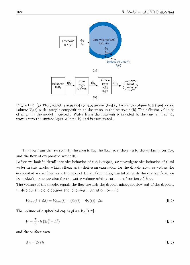
168 B. Modeling of SNICS injection
(a)
(b)
Figure B.2: (a) The droplet is assumed to have an enriched surface with volume Vs(t) and a corevolume Vc(t) with isotopic composition as the water in the reservoir (b) The di�erent volumesof water in the model approach. Water from the reservoir is injected to the core volume Vc,travels into the surface layer volume Vs and is evaporated.
The �ow from the reservoir to the core is Φ0, the �ow from the core to the surface layer ΦC ,
and the �ow of evaporated water Φe.
Before we look in detail into the behavior of the isotopes, we investigate the behavior of total
water in this model, which allows us to derive an expression for the droplet size, as well as the
evaporated water �ow, as a function of time. Combining the latter with the dry air �ow, we
then obtain an expression for the water volume mixing ratio as a function of time.
The volume of the droplet equals the �ow towards the droplet minus the �ow out of the droplet.
In discrete time one obtains the following integration formula:
Vdrop(t+ ∆t) = Vdrop(t) + (Φ0(t)− Φe(t)) ·∆t (B.2)
The volume of a spherical cap is given by [172]:
V =π
6· h(3r2
0 + h2)
(B.3)
and the surface area
AS = 2πrh (B.4)

169
for 0 ≤ h ≤ 2r
With r2 = r20 + r2
d and rd = r − h (cf. �gure B.1b), AS can also be written as
AS = π(r20 + h2
)(B.5)
We now want to express the cap height in terms of the droplet volume Vdrop. Rearranging
equation B.3, we can write
h3 + 3r20h−
6V
π= 0 (B.6)
We �nd three solutions of which only one is real:
h =α2 − 36 · r2
0
6 · α(B.7)
with
α := 6
3V
π+
(r60 + 9
(V
π
)2)1/2
1/3
We now assume that the evaporation rate Φe(t) is proportional to the (exposed) surface of the
water droplet:
Φe(t) := ke ·As(t) (B.8)
with ke a constant evaporation factor.
With this and the injection rate Φ0(t), the iteration step yields
Vdrop(t+ ∆t) = Vdrop(t) + (Φ0(t)− Φe(t)) ·∆t (B.9)
As(t+ ∆t) = π(r20 + h2 (Vdrop(t+ ∆t); r0)
)(B.10)
for the droplet volume and the exposed surface area of the droplet.
For the study of the isotopic behavior, we have to di�erentiate between the two volumes VC and
VS of the droplet. The change of the surface volume VS is determined by the �ow from the core
volume (ΦC) and the evaporation �ow Φe:
VS(t+ ∆t) = VS(t) + (ΦC(t)− Φe(t)) ·∆t (B.11)
The core volume is determined by the supply �ow from the syringe pump Φ0(t) and the �ow
ΦC(t) to the surface layer:
VC(t+ ∆t) = VC(t) + (Φ0 − ΦC) ·∆t (B.12)

170 B. Modeling of SNICS injection
Alternatively, we can also express VC(t) as the di�erence between the total droplet volume
Vdrop(t) and the surface layer volume VS(t):
VC(t) = Vdrop(t)− VS(t) (B.13)
∆VC(t) = ∆Vdrop(t)−∆VS(t) (B.14)
In a volume V with constant density, the isotope ratio can be calculated as
R =V ′′
V ′≈ V ′′
V − V ′′(B.15)
with V ′ indicating the volume of the most abundant and V ′′ the volume of a rare isotope. For
V ′′, this leads to
V ′′ = V · R
1 +R(B.16)
The rare isotope in the surface layer can thus be described by the following relation:
V ′′S (t+ ∆t) = VS(t+ ∆t) · RS(t+ ∆t)
1 +RS(t+ ∆t)(B.17)
which leads together with equation (B.11) to:
VS(t+ ∆t) · RS(t+ ∆t)
1 +RS(t+ ∆t)= VS(t)
RS(t)
1 +RS(t)+
[ΦC(t)
R0
1 +R0− Φ′′e (t)
]·∆t (B.18)
with
ΦC(t) = Φ0(t)− ∆VC(t)
∆t(B.19)
= Φ0(t)− ∆Vdrop(t)−∆VS(t)
∆t(B.20)
this gives
VS(t+ ∆t) ·RS(t+ ∆t)
1 +RS(t+ ∆t)= VS(t) ·
RS(t)
1 +RS(t)+
(∆VS(t)−∆Vdrop(t)
)(B.21)
·R0
1 +R0+
[Φ0(t)
R0
1 +R0− Φ′′e (t)
]∆t
Substituting ψ(t) := RS(t)1+RS(t) , we can write
ψ(t+∆t) =1
VS(t+ ∆t)·{VS(t)ψ(t) +
[∆VS(t)−∆Vdrop(t)
] R0
1 +R0+
[Φ0(t)
R0
1 +R0− Φ′′e (t)
]∆t
}(B.22)
Φ′′e (t) can be written as
Φ′′e (t) = Φe(t)RV SMOW (1 + δS) · αV
1 +RV SMOW (1 + δS) · αV(B.23)

171
Since RV SMOW � 1, we can approximate
1
1 +RV SMOW (1 + δS) · αV≈ 1
1 +RV SMOW (1 + δS)
Φ′′e (t) ≈ Φe(t)RV SMOW (1 + δS)
1 +RV SMOW (1 + δS)· αV
= Φe(t) · ψ(t) · αV (B.24)
Thus, we �nally get
ψ(t+ ∆t) =1
VS(t+ ∆t)·{VS(t)ψ(t) +
[∆VS(t)−∆Vdrop(t)
] R0
1 +R0(B.25)
+
[Φ0(t)
R0
1 +R0− Φe(t) · ψ(t) · αV
]∆t
}(B.26)
With eq. B.1, B.8-B.10, we can now calculate the isotope ratio in the surface layer and the
evaporated water. The isotope ratio of the enriched surface layer can be calculated by
RS(t) =ψ(t)
1 + ψ(t)(B.27)
and the isotope ratio of the vapor phase with
Re(t) = RS(t) · αV (B.28)


Appendix C
Very high �nesse optical-feedback cavity-enhanced
absorption spectrometer for low
concentration water vapor isotope analyses
Reproduction of an Optics Letter [84] in the formatting of the thesis.
http://www.opticsinfobase.org/ol/abstract.cfm?uri=ol-39-7-1795
© 2014 Optical Society of America. One print or electronic copy may be made for personal use only.
Systematic reproduction and distribution, duplication of any material in this chapter for a fee or for
commercial purposes, or modi�cations of the content of this chapter are prohibited.
J. Landsberg, D. Romanini, and E. Kerstel
So far, cavity-enhanced absorption spectroscopy (CEAS) has been based on optical cavities with a high �nesse
F that, however, has been limited by mirror re�ectivity and by cavity transmission considerations to a few
times 10,000. Here, we demonstrate a compact near-infrared optical-feedback CEAS instrument for water vapor
isotope ratio measurements, with F > 140, 000. We show that this very high �nesse can be e�ectively exploited
to improve the detection sensitivity to the full extent predicted by the increased e�ective path length to reach a
noise equivalent absorption sensitivity of 5.7× 10⁻¹¹cm−1 Hz−1/2 for a full spectrum registration (including
possible e�ects of interference fringes and �t model inadequacies).
In recent years, gas concentration and isotope ratio analyzers based on near-infrared, cavity-
enhanced absorption (CEAS; characterized by a measurement of the light intensity transmit-
ted by the cavity) or cavity ringdown spectroscopies (CRDS; characterized by a time-resolved
measurement of the light intensity decay) have experienced an increase in acceptance by the
scienti�c community [71]. Compared with their conventional mass spectrometer counterparts,
optical instruments are easier to handle and enable continuous and in situ measurements with
high temporal resolution. Arguably, water vapor isotope measurements have bene�ted the most,
as evidenced by, e.g., [10, 78, 173].
However, there is a number of applications for which higher detection sensitivity is impera-
tive. For example, some of the most interesting isotopic processes involving atmospheric water
occur at water abundances well below the range accessible with commonly available laser spec-
trometers. In the Antarctic atmosphere, water concentration does not normally exceed a few
hundred parts per million by volume (ppmv), whereas in the lower stratosphere it reaches lows
of just a few ppmv. Isotope studies in these environments are relevant for the validation of the

water isotope paleothermometer [77] and for the understanding of cirrus cloud formation and
troposphere-stratosphere exchanges [3, 174], respectively.
Until now, a small number of optical instruments have been developed with the aim to measure
in situ water isotopes with high precision at very low water abundances [5�7, 10, 83, 118, 175].
Unfortunately, resolving the details of isotope fractionation e�ects at these low water concen-
trations requires even higher levels of sensitivity and precision.
A standard quanti�cation of the sensitivity of an absorption spectrometer is given by the noise
equivalent absorption sensitivity (NEAS) [175, 176], which gives the minimum detectable ab-
sorption per unit path length normalized to the measurement rate MR (the inverse of the time
required to record a full spectrum). If δI represents the uncertainty (1σ) of the detected light
transmission of intensity I over an e�ective absorption path length Le� , the NEAS is given by
NEAS =δI
I
1
Le�
1√MR
(C.1)
One possible way to increase the sensitivity of a CEAS spectrometer is to combine it with a
high-frequency modulation technique in order to reduce δI. This is exploited in noise-immune
cavity-enhanced optical heterodyne molecular spectroscopy (NICE-OHMS) which, however, is
experimentally highly complex [80]. In addition, its full sensitivity potential has never been
approached in applications where complete Doppler-broadened rovibrational features need to
be recorded [177]. A compelling alternative is to �simply� increase Le� by increasing the �nesse
F of the optical cavity through the use of very high-re�ectivity mirror coatings. There are two
obvious disadvantages to this approach. First, the time required to reach the full build-up of
light intensity inside the cavity, as well as the subsequent decay of the light leaking out of the
cavity (τ), are also proportional to F. This increases the time required to record the spectrum,
thus lowering MR. Second, a higher �nesse tends to reduce the detected signal by reducing
the coupling e�ciency of the relatively broad laser emission (the free-running linewidth of a
DFB laser as used in this study is several MHz on a 1 s timescale) to the exceedingly nar-
row cavity mode width (∼ 1 kHz for the high-�nesse cavity). In addition, an increase of the
mirror re�ectivity is almost inevitably accompanied by a reduction of the mirror transmission
(as there is a technical lower limit to the losses caused by coating absorption and scattering)
which reduces the cavity throughput at resonance [71]. Thus, for �normal� CEAS or CRDS one
expects to gain sensitivity proportional to �nesse due to a cause of a lower cavity transmission,
either proportional to F, when the system is limited by detector noise, or by F in the case of
shot-noise limited detection. Longer averaging may compensate for slower spectrum acquisition.
However, the maximum averaging time is, in all practical situations, determined by variations
in environmental factors that limit the stability time of the spectrometer (Topt, as determined,
e.g., by the minimum in an Allan-Werle plot [98]). Beyond this time, drift will start degrading
the detection limit. Moreover, many systems are not limited by technical noise but rather by
optical interference fringes (�etaloning�) which may not be equally susceptible to averaging.

175
The e�ect of increasing F is quite di�erent in the case of optical-feedback cavity-enhanced ab-
sorption spectroscopy (OFCEAS), as this technique enables optimal and rapid coupling of the
laser radiation to the transmission modes of the high-�nesse cavity [81]. In fact, in this Letter
we demonstrate an OFCEAS spectrometer with F ≈ 144, 000. It realizes a high level of light
injection and cavity-throughput and a gain in sensitivity proportional to the �nesse for a given
measurement time. In addition, we were able to increase Topt compared to a previous lower
�nesse setup.
In order to record absorption spectra with the OFCEAS technique, a laser is approximately
mode-matched, then optically locked to successive longitudinal, TEM00 modes of a three-mirror
V-shaped cavity. This geometry returns a portion of the light resonating inside the cavity as
optical feedback to the laser source. At the same time, it avoids un�ltered feedback of the
direct re�ection from the input mirror, as described in, e.g., [81]. The aforementioned high
light throughput is predominantly due to a narrowing of the laser linewidth to below the cavity
transmission mode width (∼ FSR/F) [81, 82, 178]. Thus, OFCEAS, in contrast to other CEAS
or CRDS techniques, does not su�er from an inadequate light transmission at very high mirror
re�ectivity. In fact, no diminution of the light intensity after the cavity is observed, despite a
seven-fold augmentation of F.
The instrument presented in this Letter is compared to a previous instrument developed in our
group. This older instrument, called isotope ratio infrared spectrometer (IRIS) participated in
airborne campaigns to study the upper troposphere and lower stratosphere and is described in
detail in [6, 83, 118]. IRIS was equipped with high-re�ectivity mirrors resulting in a ring-down
time of τ0 = 21 µs and a NEAS of 4 × 10⁻¹⁰ cm−1 Hz−1/2. The new high-�nesse isotope ratio
instrument (�HiFI�) is equipped with mirrors of re�ectivity 99.9989% (1 - R = 11 ppm and
roughly equal losses and transmission; Layertec GmbH), resulting in τ0 = 150 µs. The �nesse of
a V-shaped cavity with arms of length L1 and L2 is given by F = πR/(1−R2) = πcτ0/(L1 +L2)
[82]. In this case, with L1 = L2 = 489 mm, F ≈ 144, 000 (a standard linear cavity of the same
external length using the same mirrors would have F = 288, 000, and twice as large FSR, for
the same ring-down time).
As IRIS, HiFI measures the four water vapor isotopologues H216O, H2
18O, H217O and HD 16O
in the spectral range near 7184 cm−1. A deliberate choice was made to work in the near-infrared
region of the spectrum, where state-of-the-art mirror coatings allow for a more than ten times
increase in �nesse compared to the mid-infrared (MIR) regions around 2.7 and 6.7 µm. The
associated longer Le� is expected to outweigh the roughly one order of magnitude higher ab-
sorption band strength in the MIR, without even considering the lower performance of MIR
detectors and other optical components.
Figure C.1 shows a typical HiFI spectrum. At water concentrations below 500 ppmv, the NEAS
is typically 6× 10⁻¹¹ cm−1 Hz−1/2, an improvement by a factor of almost 7 compared to IRIS
which is equal to the ratio of the �nesses. Clearly, the penalty of the slower scan rate is not as
severe as might have been expected, mostly because the scan time is still used e�ectively (see

176 C. Optics Letter
below) to better de�ne the cavity mode transmission maxima needed to calculate the absorption
spectrum. Thus, the product of the �rst and last factors in Eq. C.1 remains unchanged, and
the improvement in NEAS appears to be determined by the increase in Le�. Although in both
instruments no fringes are visible on the spectrum baseline, we cannot completely exclude that
part of the improvement is due to a reduction of the fringes underneath the noise structure.
It is noted that our NEAS values are based on the RMS noise of the �t residuals of a single
spectrum. Thus, they would also include possible e�ects of �t imperfections and fringes.
In the following, we brie�y discuss the improvements that were necessary to accommodate the
Figure C.1: Single spectrum recorded with HiFI at 500 ppmv H216O and a 2 Hz measurement
rate. The RMS of the residuals is 8× 10⁻¹¹ cm−1.
new ultrahigh-�nesse cavity and increase Topt, and we present our �rst results illustrating instru-
ment stability and performance. HiFI is mounted in a thermally insulated 19 in. rack housing.
The V-shaped cavity has an internal volume ∼25 mL that is electro-polished and coated with a
�uoroaliphatic polymer (Cytonix FluoroPel 800A). Air inside the instrument housing is venti-
lated and regulated to 38±0.1°C with a thermo-electric air-air heat exchanger (Supercool). The
temperature of the optical breadboard is stabilized at 45°C using adhesive heater tapes (Minco),
regulated with a proportional-integral-di�erential feedback-loop implemented in software. The
sample pressure inside the cavity is regulated to 35 mbar by a custom Siltek-treated (Restek)
pressure controller (Bronkhorst) at a �ow rate of 150 standard mL/min for a calculated gas ex-
change time of 0.35 s. Over a period of 3.6 h, the drift of the cavity temperature is smaller than
0.5 mK and the drift of the pressure smaller than 10 µbar, as measured with sensors not used in
the control loops. The signal and reference photodiode outputs are digitized by a 2 channel, 16
bit A/D converter with a record length of 60k points and 8 µs step size (125 kHz). Note that,
compared to the previous spectrometer, about 4 times as many datapoints are acquired per
spectral scan, while the detector bandwidth (48 kHz) is matched to the Nyquist limit associated
with the data acquisition rate, enabling an improved de�nition of the cavity transmission signal.
In view of the long cavity ring-down time, the scanning frequency is set to 2 spectra per second
(∼10 for IRIS) and the laser tuning speed to one cavity FSR (153.2 MHz) in 3.5 ms (∼0.5 ms

177
for IRIS [6]). A single spectrum spans about 110 successive cavity modes, corresponding to a
spectral window of 0.6 cm−1. At the end of each scan, the laser is interrupted for 3.2 ms in order
to record a ring-down event on the last cavity mode with a typical shot-to-shot RMS fractional
variation of 1.7× 10⁻⁴. This measurement allows for an absolute calibration of the absorption
scale [6, 81].
For the analysis, a spectrum composed of Rautian line pro�les [93] is �t to each individual
retrieved spectrum, and the isotope ratios are calculated using the integrated line intensities [6]
before being averaged. Absorption lines of methane in the same spectral region are introduced
in the �t since methane absorption becomes an important factor at water concentrations below
∼500 ppmv. The baseline is �t by two strong water absorption lines outside the measurement
range, which are grouped with the H216O lines inside the measurement range, and an additional
third-order polynomial.
To determine the precision of the isotope ratio measurements, a gas bottle was repeatedly
Figure C.2: Time series of H216O and its isotope ratios (two top panels) and the corresponding
Allan plots (bottom panel) for the selected data for H218O, H2
17O, and HD 16O, as well as thedeuterium- and 17O-excesses, as a function of averaging time T at a water mixing ratio of 20ppmv.
prepared with a mixture of dry synthetic air and a local water standard for di�erent water
concentrations. This standard gas bottle was then connected to the OF-CEAS instrument
for longterm stability measurements (>8 h). Previous studies comparing this method with a
microdroplet injector indicate that isotopic fractionation using a standard 50 L tank is unde-
tectable [118]. Figure C.2 shows an Allan-Werle plot of the H218O, H2
17O and HD 16O isotope
ratios from measurements at the lowest sample concentration of 20 ppmv. The �gure also in-
cludes the Allan deviations for the deuterium excess d = δ2H − 8 δ18O [14] and the 17O-excess
= ln(1 + δ17O)− 0.528 ln(1 + δ18O) [44] which, however, are practically indistinguishable from
the δ2H and δ17O Allan deviation curves, respectively.
Dependent on the water concentration, the optimum integration time for the isotope ratio de-
termination is up to ∼70 min. For longer integration times, drift degrades the precision. The

178 C. Optics Letter
stability of HiFI is thus much higher than that of IRIS, for which the longest optimum integra-
tion time was ∼5 min [118], mostly due to the better temperature stabilization (cf. chapter 3).
The best precision for δ2H and δ17O is obtained at around 1500 ppmv. For δ2H, 70 min averag-
ing gives a precision σ(2H) = 0.12h, while averaging of 3 min results in σ(17O) = 0.07h and
σ(18O) = 0.05h. However, the optimum for δ18O, with σ(18O) = 0.02h, is obtained at a lower
water concentration of ∼600 ppmv (in about 30 min). In fact, cavity transmission at the peak
of the H218O absorption line drops to 10% at 1500 ppmv, giving a signal-to-noise ratio far from
optimal.
In table C.1, the precisions at di�erent water concentrations are given for T = 4 s (8 data points)
averaging and for the Allan optimum σ(Topt). With 4 s averaging, the time resolution is still
su�cient to study fast isotopic processes, but the precision is nearly a factor of three better than
for nonaveraged (0.5 s) measurements.
In conclusion, the new instrument achieves similar or better results in terms of measurement
precision compared to our previous OFCEAS water isotope spectrometer, as well as compared to
most commercial water vapor spectrometers but at a water concentration that is approximately
an order of magnitude lower. The NEAS of 5.7×10⁻¹¹ cm−1 Hz−1/2 (or 5.4×10⁻¹² cm−1 Hz−1/2
when normalized per spectral element) is among the lowest values reported for near-infrared
CEAS so far, with the exception of NICE-OHMS (with its much smaller tuning range) and the
lowest for CEAS with a base length below 50 cm. Here, the instrument o�ers the possibility to
record useful isotopic signals in dry Antarctic or upper tropospheric air and eventually even in
stratospheric air. The improved stability time can be used to increase the precision on a sin-
gle measurement before drift starts dominating the noise. It also enables longer uninterrupted
recording before recalibration needs to be carried out [98].
The instrument is capable of even higher precision or higher sensitivity isotopic measurements,
σ(2H) σ(2H) σ(18O) σ(18O) σ(17O) σ(17O)H2
16O (4 s) (Topt) (4 s) (Topt) (4 s) (Topt)(ppmv) [h] [h] [h] [h] [h] [h]20 54 5 4.4 0.5 12 1.180 12 0.8 1.1 0.1 3.2 0.2190 5.5 0.6 0.5 0.07 1.4 0.19420 2.7 0.5 0.27 0.05 0.7 0.16610 1.7 0.5 0.18 0.02 0.4 0.1770 1.1 0.28 0.18 0.04 0.3 0.071470 0.7 0.12 0.17 0.05 0.22 0.07
Table C.1: Measurement Precision as a Function of the Water Mixing Ratio for Di�erent Aver-aging Times.
when only one or two isotopic ratios need to be determined. In a previously identi�ed range
around 7200 cm−1 [179], the spectral lines are better separated and the isotopologues, excluding
δ17O, can be measured with modestly better precision. Alternatively, we recently demonstrated

179
that near 7286 cm−1, δ18O can be measured almost one order of magnitude better with a min-
imal Allan deviation of 0.4% in 30 min at only 4 ppmv H216O (cf. chapter 8). By temperature
tuning of the same laser, it is also possible to measure δ2H at 7289 or 7280 cm−1, with a compa-
rable performance to what is shown here at 7184 cm−1. Finally, nearby H216O lines at 7299.43
and 7181.17 cm−1 may be used for water detection below 0.1 ppbv.
Especially in the case of a molecule in which a (anharmonic) hydrogen oscillator is excited, such
as water, our approach may avoid the need to use more complex MIR light sources and optics,
given that line strengths may di�er by only one order of magnitude, easily compensated by the
higher �nesse available in the NIR.