Development of a Micro-thermal Sensor Based on 3-omega ...

Development of a Micro-thermal Sensor Based on 3-omega Technique for Dynamic

Freezing Applications

A DISSERTATION

SUBMITTED TO THE FACULTY OF

UNIVERSITY OF MINNESOTA BY

Harishankar Natesan

IN PARTIAL FULFILLMENT OF THE REQUIREMENTS

FOR THE DEGREE OF

DOCTOR OF PHILOSOPHY

Advisor: John C. Bischof

March 2019

i

Acknowledgement

The completion of my doctoral thesis work would not have been possible without the support of a

number of people. First, I would like to express my sincere gratitude to my advisor, Professor John

Bischof, for his valuable guidance throughout this endeavor. Thank you for constantly motivating

and challenging me to be an independent, critical researcher. As I look back at my PhD studies, I

realize that I owe a large part of my success to you.

I would like to thank the Professors of my review committee, Prof. Chris Hogan, Prof. Xiaojia

Wang, and Prof. David Wood for their valuable guidance and support during my PhD studies. Next,

I would like to thank Prof. Chris Dames (University of California, Berkeley), Prof. John Rogers

(Northwestern University, Evanston), Prof. Jeunghwan Choi (East Carolina University,

Greenville), Prof. Limei Tian (Texas A&M University, College Station) for a wide variety of

technical and general direction over the years. Further, I would like to thank Dr. Sean Lubner,

Wyatt Hodges, Shaunak Phatak, Sriharsha Mushnoori, Dushyant Mehra, Michelle Ip, who offered

significant intellectual and experimental support at various points in my program.

I would like to thank Dr. Zhenpeng Qin, Dr. Michael Etheridge, Dr. Chunlan Jiang for their

mentoring and support especially at the beginning of my PhD studies. I would also like to thank

other past and current lab members of Bioheat and Mass Transfer Lab for their support and

friendship.

I would like to express my gratitude towards National Science Foundation (NSF/CBET #1236760),

Minnesota Partnership Grant and University of Minnesota Doctoral Dissertation Fellowship (2016-

17) for their financial support.

ii

Last, but certainly not least, I would like to thank my family and friends for supporting me. Thanks

to my parents for everything they have given me. Specifically, I would like to express my sincere

gratitude to my mother for her numerous sacrifices that enabled me to complete this thesis. Thanks

to my sisters Dr. Shanmugapriya and Dr. Lavanya for being a source of inspiration and offering

emotional support. Thanks to my friends for all the good times. Specifically, I would like to thank

Sid, Mullu, Pava, and Raja for I have learned a lot from them.

iii

Dedication

In memory of my dad.

iv

Abstract

Atrial Fibrillation (AF) is a major heart disease affecting millions of people every year. If

left untreated, AF can cause cardiovascular disease, stroke and even death. Cryoablation for

PV (Pulmonary Vein) isolation has been used for more than 10 years in AF treatment, which

involves freezing (< -60 0C) and subsequent scarring of PV using a cold balloon/ catheter

surface. Despite widespread and growing clinical use, the precise dosing and treatment times

for cryoablation can vary depending on cooling surface contact, tissue thickness, and freeze

completion through the wall. Without this knowledge, the treatment can be expected to

have diminishing efficacy and may contribute to collateral injury. For instance, under-

freezing may lead to inadequate treatment, while over-freezing can damage adjacent tissues

(esophagus, lung and nerves), thereby creating complications. Clearly, there is a need to

monitor this process to ensure complete treatment while avoiding complications.

Unfortunately, the approaches for monitoring cryotherapy in the treatment of other diseases

using clinical imaging cannot work for PV due to poor spatial resolution (mm). Thus, there

is a pressing need to improve monitoring of cryoablation of the PV to reproducibly supply

information on freezing within tissues at the millimeter to sub-millimeter level. Here then

we present a response to this need through development of a micro- thermal sensor based

on the “3ω” technique. We propose that a disposable thermal sensor based on 3ω

technology can be deployed on a balloon to measure tissue contact, thickness and the

initiation and completion of freezing in the PV all with an accuracy better than 1 mm.

The 3ω technique, on which the sensor is based, was originally developed for thin inorganic

materials. The technique was first modified for measurement of thermal conductivity of soft,

hydrated biological tissues. Using the new sensor, for the first time, we have measured the

v

thermal conductivity of thin porcine cardiac tissues in vitro addressing a major knowledge

gap to inform focal therapy modeling for atrial fibrillation. This information is critical for

successful treatment planning/prediction of therapy impact in the PV and surrounding

tissues.

Next, we show a dynamic use of the sensor for monitoring an idealized therapy in in vitro

thin tissues (≤ 2 mm). For this, we demonstrated the ability of the sensor (on a flat substrate)

to sense contact, flow, tissue thickness and freeze front in idealized systems. Specifically,

the sensor was used to sense contact with tissue vs. water, ice (frozen agargel) thickness,

and freeze initiation and completion. The success of this study suggests that integration of

“3ω” sensors onto cardiology probe surfaces (i.e. balloons or catheters) can monitor

cryoablation and by extension other PV focal therapies.

As a next step, we integrated these sensors onto cryoballoons using transfer printing

techniques. The 3ω sensor technology has traditionally been used for flat and rigid

substrates. Therefore, we modified the shape of the sensor from a linear to a serpentine

shape for integration onto balloon substrates. Next, using numerical analyses, we

investigated the ability of the modified sensor on a flat substrate to differentiate

measurements in limiting cases of ice, water and fat. These numerical results were then

complemented by experimentation by micro-patterning the serpentine sensor onto a flat

substrate and onto a flexible balloon. In both formats (flat and balloon) the serpentine sensor

was experimentally shown to: (1) identify tissue contact vs. fluid, (2) distinguish tissue

thickness in the 0.5 to 2 mm range, and (3) measure the initiation and completion of freezing

as previously reported for a linear sensor. This study demonstrates proof of principle that a

vi

serpentine 3ω sensor on a balloon can monitor tissue contact, thickness and phase change

which is relevant for cryo and other focal thermal treatments of PV to treat atrial fibrillation.

vii

Table of Contents

List of Tables ................................................................................................................................ xii

List of Figures .............................................................................................................................. xiv

0. Statement of Contributions ................................................................................................... 1

1. Multi-Scale Thermal Property Measurements for Biomedical Applications ................... 5

1.1. Introduction ........................................................................................................................... 5

1.2. Thermal Properties of Biomaterials ...................................................................................... 9

1.2.1. Thermal conductivity of biomaterials ............................................................................ 9

1.2.2. Calorimetric measurements of biomaterials................................................................. 10

1.3 Thermal Conductivity Measurement Techniques ................................................................ 12

1.3.1. Microscale thermal conductivity measurement techniques ......................................... 12

1.3.2. Nanoscale thermal conductivity measurement techniques........................................... 18

1.3.3. Applications for multiscale thermal conductivity measurement .................................. 24

1.4. Calorimetric Measurement Techniques .............................................................................. 27

1.4.1. Differential scanning calorimetry (DSC) ..................................................................... 28

1.4.2. Nanocalorimetry .......................................................................................................... 33

1.4.3. Applications for multiscale calorimetric measurements .............................................. 36

1.5. Conclusion .......................................................................................................................... 41

1.6. Specific Acknowledgements ............................................................................................... 42

2. Thermal Properties of Porcine and Human Biological Systems ...................................... 43

viii

2.1. Introduction ......................................................................................................................... 43

2.2. Thermal Properties .............................................................................................................. 46

2.2.1. Thermal conductivity measurement ............................................................................. 46

2.2.2. Specific heat capacity measurement ............................................................................ 49

2.3 Factors that Affect Thermal Property Values ...................................................................... 52

2.3.1. High Temperature Effects (37 °C – 100 °C): Protein Phase Change and Water Loss 52

2.3.2. Low temperature effects (37 °C – -196 °C): Water Phase change and Cryoprotectant

Effects .................................................................................................................................... 53

2.4. Modeling Case Study .......................................................................................................... 56

2.5. Thermal Properties Dataset Tables ..................................................................................... 60

2.6. Conclusion .......................................................................................................................... 66


3. A Micro-Thermal Sensor for Focal Therapy Applications .................................................. 68

3.1. Introduction ......................................................................................................................... 68

3.2. Methods .............................................................................................................................. 69

3.2.1. ‘Supported’ 3ω technique ............................................................................................ 69

3.2.2. Thermal conductivity measurement of thin cardiac tissues ......................................... 72

3.2.3. Sensing contact versus flow ......................................................................................... 73

3.2.4. Sensing tissue thickness ............................................................................................... 73

3.2.5. Sensing phase change .................................................................................................. 74

ix

3.3. Results ................................................................................................................................. 75

3.3.1. Thermal conductivity measurement of thin cardiac tissue ........................................... 75

3.3.2. Sensing contact ............................................................................................................ 76

3.3.3. Sensing tissue thickness ............................................................................................... 76

3.3.4. Sensing phase change .................................................................................................. 78

3.4. Discussion ........................................................................................................................... 79


SI 3.1. Supplementary Information- Construction of the Supported 3ω Sensor ........................ 82

SI 3.2. Supplementary Information- Theory behind Flow Rate Measurement .......................... 82

SI 3.2.1. Dependence of 3ω signal on flow direction ............................................................ 84

SI 3.3. Supplementary Information- Use of In-phase 3ω Signal (V3ω, Ip) to Sense Contact,

Thickness and Phase Change ..................................................................................................... 85

4. A Micro-Thermal Sensor for Cryoablation Balloons ........................................................... 86

4.1 Introduction .......................................................................................................................... 86

4.2 Methods ............................................................................................................................... 89

4.2.1. Numerical characterization of the serpentine 3ω sensor on a flat substrate ................. 89

4.2.2. Micro-thermal sensing using the serpentine sensor on a flat substrate ........................ 92

4.2.3. Micro-thermal sensing using serpentine sensors on a balloon substrate ...................... 94

4.3. Results and Discussion ....................................................................................................... 97

4.3.1. Numerical characterization of serpentine 3ω sensors on a flat substrate ..................... 97

x

4.3.2. Micro-thermal sensing using the serpentine sensor on a flat substrate ...................... 101

4.3.3. Integration of serpentine 3ω sensor onto a balloon .................................................... 102

4.3.4. Micro-thermal sensing using serpentine sensors on a balloon substrate .................... 102

4.4 Summary ............................................................................................................................ 103

4.5. Specific Acknowledgements ............................................................................................. 104

SI 4.1. Supplementary Information: Validation of the Numerical Model ............................... 105

SI 4.2. Supplementary Information: Error in Thermal Conductivity of Serpentine Sensors ... 106

5. Conclusion and Future Research Directions ....................................................................... 109

5.1 Conclusion ......................................................................................................................... 109

5.2. Future Research Direction: Perform Ex Vivo Testing of the 3ω Sensor in Porcine Heart

Lung Block .............................................................................................................................. 110

5.2.1. Experimental approach .............................................................................................. 110

5.2.2. Expected outcome ...................................................................................................... 110

6. Bibliography ........................................................................................................................... 111

Appendix A. Reusable Bi-Directional 3ω Sensor to Measure Thermal Conductivity of 100-

micron Thick Biological Tissues ............................................................................................... 150

A.1. Abstract ............................................................................................................................ 150

Appendix B. Biomaterial Scaffolds for Non-Invasive Focal Hyperthermia as a Potential

Tool to Ablate Metastatic Cancer Cells ................................................................................... 151

B.1 Abstract ............................................................................................................................. 151

xi

Appendix C. Measurement of Specific Heat and Crystallization in VS55, DP6 and M22

Cryoprotectant Systems with and without Sucrose. ............................................................... 152

C.1 Abstract ............................................................................................................................. 152

xii

List of Tables

Table 1.1. Overview of common bioheat transfer applications ....................................................... 6

Table 1.2. Overview of thermal conductivity ‘k’ measurement techniques .................................... 7

Table 1.3. Overview of calorimetric measurement techniques ........................................................ 9

Table 1.4. Micro-scale techniques for thermal conductivity measurement ................................... 14

Table 1.5. Nanoscale techniques for thermal conductivity measurement ...................................... 20

Table 1.6. Representative measurements in biomolecules using DSC .......................................... 31

Table 1.7. Representative list of nanocalorimeters both commercial and custom built at academic

institutions ...................................................................................................................................... 39

Table 2.1. Overview of common bioheat transfer applications ..................................................... 45

Table 2.2. Overview of ‘k’ measurement techniques .................................................................... 47

Table 2.3. Organization of thermal property datasets .................................................................... 57

Table 2.4. Thermal properties of porcine systems at sub-zero temperatures i ............................... 59

Table 2.5. Thermal properties of porcine systems at sub-zero temperatures ii .............................. 60

Table 2.6 Thermal properties of porcine systems at supra-zero temperatures ............................... 62

Table 2.7. Thermal properties of human systems at supra-zero temperatures i ............................. 63

Table 2.8. Thermal properties of human systems at supra-zero temperatures ii ............................ 64

Table 2.9. Thermal properties of cryoprotectants .......................................................................... 65

xiii

Table 2.10. Thermal properties of porcine liver treated with cryoprotectants ............................... 66

Table SI.3.1. Comparison of thermal conductivity measurement techniques ................................ 81

Table 4.1. Summary of measurement parameters used to record 3ω signal (V3ω, op) from the 3ω

sensor using a lock-in amplifier ................................................................................................... 103

xiv

List of Figures

Figure 1.1. Thermal conductivity measurement of biomaterials ..................................................... 8

Figure 1.2. Specific heat capacity measurement of biomaterials. .................................................. 11

Figure 1.3. Important phase change events on biomolecules with their corresponding latent heat13

Figure 1.4. 3ω method ................................................................................................................... 16

Figure 1.5. Optical techniques for thermal conductivity measurement ......................................... 17

Figure 1.6. Scanning thermal microscopy ..................................................................................... 21

Figure 1.7. Microscale k measurement opportunities .................................................................... 26

Figure 1.8. Example nanoscale thermal conductivity measurement opportunitiesrmal conductivity

at the surface. ................................................................................................................................. 28

Figure 1.9. Differential Scanning Calorimetry .............................................................................. 30

Figure 1.10. Nanocalorimetry ........................................................................................................ 32

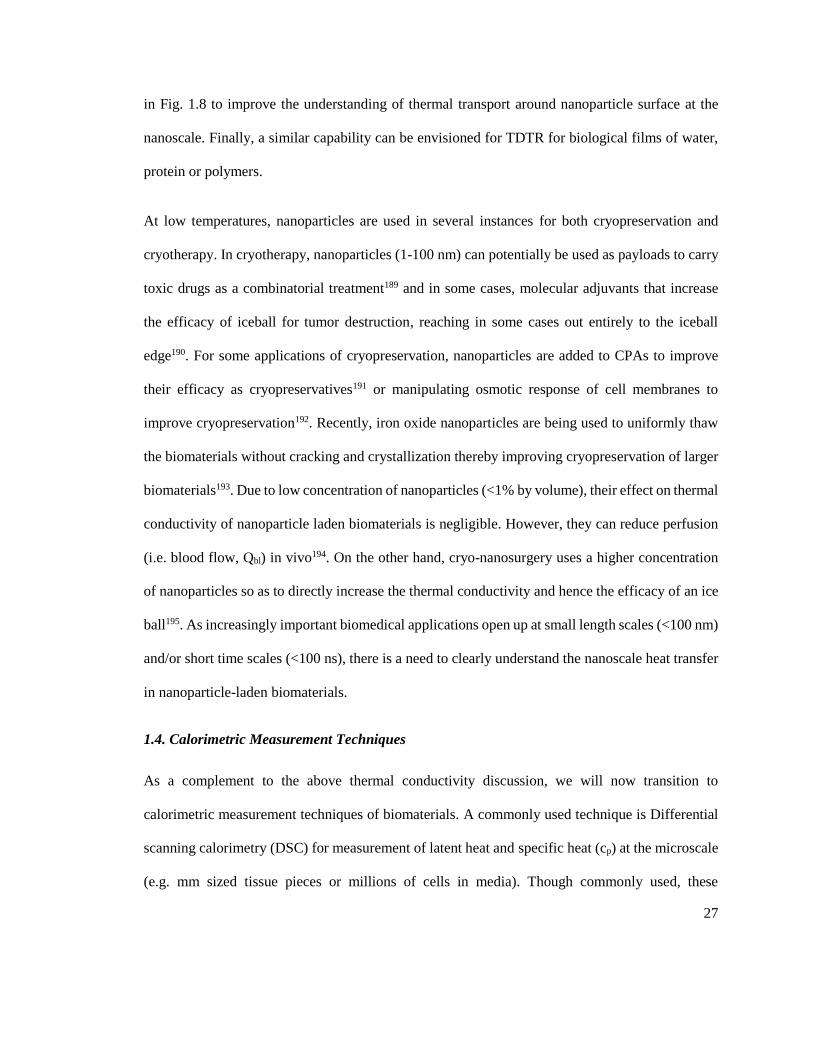
Figure 1.11. Examples of protein and lipid nano-calorimetric measurements ............................... 41

Figure 2.1. Schematic of most thermal conductivity measurement techniques ............................. 46

Figure 2.2. Thermal conductivity datasets in the suprazero range ................................................. 48

Figure 2.3. Thermal conductivity datasets in the sub-zero and cryogenic range ........................... 49

Figure 2.4. Specific heat capacity for biomaterials without cryoprotectants ................................. 50

Figure 2.5. Thermal conductivity datasets for porcine liver with and without cryoprotectants..... 51

xv

Figure 2.6. Specific heat capacity for porcine liver with and without cryoprotectants .................. 52

Figure 2.7. Thermal conductivity datasets for cryoprotectants ...................................................... 53

Figure 2.8. Thermal properties of water used for modeling case study ......................................... 54

Figure 2.9. Geometry in cylindrical co-ordinates for (a) cryopreservation, (b) cryosurgery ......... 55

Figure 2.10. Numerical simulation for cryopreservation ............................................................... 56

Figure 2.11. Numerical simulation for cryosurgery ....................................................................... 58

Figure 3.1 Concept of the supported 3ω method to measure thermal conductivity, ‘k’ of thin (>0.1

mm) tissues .................................................................................................................................... 70

Figure 3.2 Supported 3ω measurements of porcine PV, phrenic nerve and esophagus ................. 74

Figure 3.3 The measurement of flow vs. tissue contact by 3ω sensor ........................................... 75

Figure 3.4 The measurement of thickness by 3ω sensor ................................................................ 77

Figure 3.5 The measurement of phase change onset, completion and thaw by the 3ω sensor ...... 79

Figure SI.3.1. Use of in phase 3ω signal (V3ω, ip) to sense (a) contact, (b) thickness and (c) phase

change ............................................................................................................................................ 83

Figure 4.1. Development of micro-thermal 3ω sensors for monitoring balloon cryoablation in

pulmonary vein (PV)...................................................................................................................... 88

Figure 4.2 Finite element analysis of the serpentine sensor (L=0.5 mm, b= 5 μm, w= 180 μm) on

a flat substrate ................................................................................................................................ 97

file:///C:/Users/Harishankar/Google%20Drive%20(Not%20Syncing)/BHMT-%20Harishankar/Thesis/My%20thesis/Full%20thesis/Version%203/Thesis_Natesan%20(01.29.2019).docx%23_Toc536557872


xvi

Figure 4.3 Micro-thermal sensing using a serpentine shaped sensor (L= 0.5 mm, b= 5 μm, w= 180

μm, t= 100 nm) on a flat substrate ................................................................................................. 98

Figure 4.4. Micro-thermal sensing using serpentine shaped sensor (L= 0.5 mm, b= 5 μm, w= 180

μm, t= 100 nm) on a balloon substrate......................................................................................... 100

Figure SI.4.1. Validation of the numerical model…………………………………………. 106

Figure SI.4.2. Finite element analysis of the effect of heater line and substrate geometry on the

error in thermal conductivity ....................................................................................................... 107





1

0. Statement of Contributions

The thesis work consists of three stand-alone publications in the first three chapters, which have

been subjected to peer-review process, while Chapter 4 has been submitted for publication as well.

Chapter 1 is a review article that is authored by myself under the guidance of Dr. John Bischof.

This chapter discusses new measurement tools and opportunities for thermal conductivity and

specific heat capacity measurement of biological tissues at the micro and nanoscale.

Natesan, H., & Bischof, J. C. (2017). Multiscale thermal property measurements for biomedical

applications. ACS Biomaterials Science & Engineering, 3(11), 2669-2691.

Chapter 2 is a textbook chapter that is authored by Shaunak Phatak and myself under the guidance

of Dr. John Bischof. In this chapter, we have compiled thermal conductivity and specific heat

capacity values of human and porcine systems in the subzero and supra-zero temperature ranges

for the purposes of aiding the development of accurate models of conditions and pathologic

treatments involving bio-heat transfer mechanisms.

Phatak, S., Natesan, H., Choi, J., Sweet, R., & Bischof, J. (2017). Thermal Properties of Porcine

and Human Biological Systems. Handbook of Thermal Science and Engineering, Kulacki, F.

(Eds.), Springer 1-26.

Chapter 3 is a technical article that showed thermal conductivity measurements of porcine thin

cardiac tissues for the first time using 3ω technique. Further, we demonstrate that a micro-thermal

sensor based on the 3ω technique can sense tissue contact, thickness and phase change in vitro

under idealized conditions in 0.5 to 2 mm thick tissues relevant to cryoablation of the pulmonary

vein (PV). This article is authored by myself and Dr. John Bischof with assistance of Wyatt

Hodges, Dr. Sean Lubner, Dr. Jeunghwan Choi and Dr. Chris Dames. I, Dr. Jeunghwan Choi and

2

Dr. John Bischof contributed to the conception and design of the experiment to measure thermal

conductivity, sense contact and thickness. Wyatt Hodges, Dr. Sean Lubner and Dr. Chris Dames

contributed to the conception and carried out experiments to sense phase change. Wyatt Hodges

and Chris Dames carried out the theoretical comparison for thickness and phase change

experiments.

Natesan, H., Hodges, W., Choi, J., Lubner, S., Dames, C., & Bischof, J. (2016). A micro-thermal

sensor for focal therapy applications. Scientific reports, 6, 21395.

Chapter 4 is a technical article that focuses on modifying the micro-thermal sensor from a linear

format to a serpentine format for integration onto a flexible balloon. Next, using numerical

analyses, the ability of the modified sensor on a flat substrate was studied to differentiate

measurements in limiting cases of ice, water and fat. These numerical results were then

complemented by experimentation by micro-patterning the serpentine sensor onto a flat substrate

and onto a flexible balloon. In both formats (flat and balloon) the serpentine sensor was

experimentally shown to: (1) identify tissue contact vs. fluid, (2) distinguish tissue thickness in the

0.5 to 2 mm range, and (3) measure the initiation and completion of freezing as previously reported

for a linear sensor. The numerical analysis and experimentation were performed by me. These

sensors were integrated onto balloons by Dr. Limei Tian and Dr. John Rogers. The article was

written by me under the guidance of Dr. John Bischof with assistance on sensor fabrication sections

from Dr. Tian and Dr. Rogers.

Natesan, H., Tian, L., Rogers, J., & Bischof, J. In submission to Journal for Biomechanical

Engineering

3

Chapter 5 consists of conclusion and future research directions for this thesis work authored by

me under the guidance of Dr. John Bischof.

Appendix A is a technical article that discusses about the adaptation of the 3 method—widely

used for rigid, inorganic solids—into a reusable sensor to measure k of soft biological samples, two

orders of magnitude thinner than conventional tissue characterization methods. Analytical and

numerical studies quantify the error of the commonly used “boundary mismatch approximation”

of the bi-directional 3ω geometry, confirm that the generalized slope method is exact in the low-

frequency limit, and bound its error for finite frequencies. Dr. Sean Lubner authored the manuscript

under the guidance of Dr. Chris Dames with assistance from Dr. Jeunghwan Choi, Geoff

Wehmeyer, Bastian Waag, Vivek Mishra, myself, and Dr. John Bischof. I confirmed the results of

thermal conductivity of mouse liver using a second 3ω instrument that I built at Bioheat and Mass

Transfer Lab at the University of Minnesota.

Lubner, S. D., Choi, J., Wehmeyer, G., Waag, B., Mishra, V., Natesan, H., Bischof, J., & Dames,

C. (2015). Reusable bi-directional 3 ω sensor to measure thermal conductivity of 100-μ m thick

biological tissues. Review of Scientific Instruments, 86(1), 014905.

Appendix B is a technical article that shows microporous poly (ε-caprolactone) biomaterials could

be used to attract metastasizing breast cancer cells in vivo early in tumor progression. In order to

enhance the therapeutic potential of these scaffolds, they were modified such that infiltrating cells

could be eliminated with non-invasive focal hyperthermia. My contribution was to measure thermal

conductivity and specific heat capacity of the scaffolds infiltrated with cells post-harvest. I also

assisted in the writing sections on thermal property measurement of this manuscript.

4

Pelaez, F., Manuchehrabadi, N., Roy, P., Natesan, H., Wang, Y., Racila, E., ...,Bischof, J., &

Azarin, S. M. (2018). Biomaterial scaffolds for non-invasive focal hyperthermia as a potential tool

to ablate metastatic cancer cells. Biomaterials, 166, 27-37.

Appendix C is a technical article that is not directly related to my thesis work. Using DSC, the

specific heat capacity of five CPAs was measured. cp was measured in the minimal and maximal

cases of crystallization for VS55 and DP6 to understand their crystallization behavior. This chapter

was authored by Shaunak Phatak with assistance from myself, Dr. Jeunghwan Choi, Dr. Kelvin

Brockbank under the guidance of Dr. John Bischof. The experimentation and modeling work was

led by Shaunak Phatak with assistance from myself.

Phatak, S., Natesan, H., Choi, J., Brockbank, K. G., & Bischof, J. C. (2018). Measurement of

Specific Heat and Crystallization in VS55, DP6, and M22 Cryoprotectant Systems With and

Without Sucrose. Biopreservation and biobanking, 16(4), 270-277.

5

1. Multi-Scale Thermal Property Measurements for Biomedical Applications

The following chapter has been reproduced with permission from “Natesan, H., & Bischof, J. C.

(2017). Multiscale thermal property measurements for biomedical applications. ACS Biomaterials

Science & Engineering, 3(11), 2669-2691” Copyright 2017 American Chemical Society

1.1. Introduction

Bioheat transfer based innovations in health care include applications such as focal treatments for

cancer and cardiovascular disease and the preservation of tissues and organs for transplantation. As

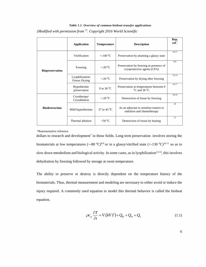
outlined in Table 1.1, biodestruction, (commonly known as focal or thermal therapy) and

biopreservation comprise the two main applications of bioheat transfer. Thermal therapy refers to

the application of heat or cold to destroy tumors and other diseased systems in the body1. Recently,

there has been a major drive towards use of thermal therapy to ablate thin tissues (<5 mm thick)

for cardiovascular and other diseases. For instance, Medtronic has received FDA approval for

ArcticFrontTM cryoballoons, which cryoablate pulmonary veins (< 2mm thick) for the treatment of

atrial fibrillation, and work is underway to establish renal and hepatic arteries as targets for thermal

treatment of hypertension and diabetes, respectively2-4.

Biopreservation refers to the preservation of biomaterials (Table 1.1) to increase their shelf lives

for tissue and organ transplant (i.e. regenerative medicine), in vitro fertilization, germplasm

preservation of endangered species and food science. Biopreservation, which involves cooling

biomaterials to very low temperatures (<-80 0C) in the presence of cryoprotective agents (CPAs) at

specific rates to slow down all biological activity, is important for successful organ banking5. At

least 1 in 5 patients die waiting for an organ transplant, making it one of the most pressing medical

problems of the 21st century6. In fact, The White House has called for “new breakthroughs treating

cancer and ending the wait for organ transplants” and has directed hundreds of millions of federal

6

dollars to research and development7 in those fields. Long term preservation involves storing the

biomaterials at low temperatures (~-80 0C)8-9 or in a glassy/vitrified state (<-130 0C)10-11 so as to

slow down metabolism and biological activity. In some cases, as in lyophilization12-14, this involves

dehydration by freezing followed by storage at room temperature.

The ability to preserve or destroy is directly dependent on the temperature history of the

biomaterials. Thus, thermal measurement and modeling are necessary to either avoid or induce the

injury required. A commonly used equation to model this thermal behavior is called the bioheat

equation,

smblp QQQTkt

Tc

. (1.1)

Table 1.1. Overview of common bioheat transfer applications

(Modified with permission from 15. Copyright 2016 World Scientific

Application Temperature Description

Rep.

ref.*

Biopreservation

Vitrification <-140 0C Preservation by attaining a glassy state

10-11

Freezing <-20 0C Preservation by freezing in presence of

cryoprotective agents (CPA)

8-9

Lyophilization/

Freeze Drying <-20 0C Preservation by drying after freezing

12-14

Hypothermic

preservation 0 to 36 0C Preservation at temperatures between 0

0C and 36 0C

16-17

Biodestruction

Cryotherapy/

Cryoablation <-20 0C Destruction of tissue by freezing

18-19

Mild hyperthermia 37 to 43 0C As an adjuvant to sensitize tumors to

radiation and chemotherapy

20

Thermal ablation >50 0C Destruction of tissue by heating

21

*Representative reference

7

where thermophysical properties of biomaterials such as density (ρ), specific heat capacity (cp) and

thermal conductivity (k) can be experimentally measured, usually in vitro to avoid the interference

of perfusion with the measurement. Qbl is the blood perfusion term, which reduces the efficacy of

thermal therapies by acting as a heat sink. For cryoablation, the biomaterials will have two phases:

frozen and unfrozen, and Qbl would be absent in the frozen regime. For cryopreservation, Qbl would

always be absent as the tissues would already have been removed from the body. Heat source term

(Qs) refers to the endothermic/ exothermic heat release from several phase change events generally

associated with water, but to a lesser extent proteins and lipids in the biomaterial. Qs and Qbl are

typically large compared to metabolic heat generation (Qm) and hence Qm is sometimes neglected61.

Thus, measurement of thermal properties (k, Cp), latent heat and phase change temperatures is

necessary for a complete understanding of the heat transport in biomaterials. In this review paper,

we will first define and discuss thermal property measurements of biomaterials. Next, we will

Table 1.2. Overview of thermal conductivity ‘k’ measurement techniques

Biomaterial k measurement Length Scale Rep. Ref.

Macroscale aSteady state

techniques

> 2 mm 22-24,25

bTransient

techniques

26-28 29-30 31-36 37-39 40-44

Thin Tissue

scale

Supported 3ω 10 μm- 2 mm

45-47

Laser flash 48-50

Cellular scale

Supported 3ω 1- 100 μm 43, 51-52

cTDTR 100 nm- 1 μm 53-54

dSThM Spatial: 50-500 nm

Vertical: 1-10 nm

55-56

Molecular scale TDTR 50 - 100 nm 53-54

eTAM 1-20 nm 57-60

aSteady state techniques include: guarded hot plate22-24, radial heat flow25 bTransient techniques include: thermal comparator26-28, heated thermocouple29-30, transient hot wire31-36, transient

thermistor probe37-39, pulsed decay40-44 cTDTR- Time Domain Thermoreflectance dSThM- Scanning Thermal Microscopy eTAM- Transient Absorption Method

8

explain various micro and nanoscale measurement techniques which currently define the limits of

these measurement techniques. Finally, we will discuss various opportunities that are driving the

need for new micro and nanoscale measurements.

(a) (b)

(c) (d)

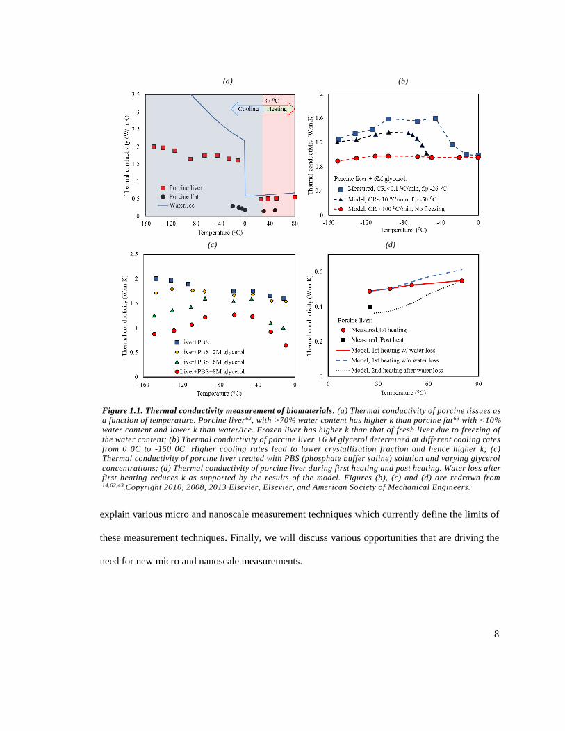
Figure 1.1. Thermal conductivity measurement of biomaterials. (a) Thermal conductivity of porcine tissues as

a function of temperature. Porcine liver62, with >70% water content has higher k than porcine fat63 with <10%

water content and lower k than water/ice. Frozen liver has higher k than that of fresh liver due to freezing of

the water content; (b) Thermal conductivity of porcine liver +6 M glycerol determined at different cooling rates

from 0 0C to -150 0C. Higher cooling rates lead to lower crystallization fraction and hence higher k; (c)

Thermal conductivity of porcine liver treated with PBS (phosphate buffer saline) solution and varying glycerol

concentrations; (d) Thermal conductivity of porcine liver during first heating and post heating. Water loss after

first heating reduces k as supported by the results of the model. Figures (b), (c) and (d) are redrawn from 14,62,43

.Copyright 2010, 2008, 2013 Elsevier, Elsevier, and American Society of Mechanical Engineers. .

9

1.2. Thermal Properties of Biomaterials

The thermal properties of a biomaterial refer to its thermal conductivity and calorimetric parameters

such as specific heat capacity, latent heat and phase change temperature of various internal

molecular events. Portions of this review were significantly modified and refined from a larger

chapter on thermal conductivity written by the authors15.

1.2.1. Thermal conductivity of biomaterials

Thermal conductivity (k) is an important property of biomaterials that determines its ability to

transfer heat. Using Fourier’s law, k can be expressed as, k = - Q/∇T, where Q is heat flux (W/m2)

and ∇T is temperature gradient (K/m). A common technique to determine k is to apply a known

heat flux followed by measuring the resulting temperature gradient in the biomaterial. Though

Fourier’s law can break down at small length and time scales, it is generally valid for biomaterials15.

Historically, thermal conductivity measurement of biomaterials began with refrigerated foods. In

such cases, k of biomaterials was either directly measured22-23, 73-74 or predicted using models

developed based on weight averaging of the composition75-78. The pursuit of thermal conductivity

measurement of macroscale biomaterials has led to several bulk methods, which have been

reviewed in detail elsewhere14. These techniques cannot be used for thin tissues or cellular systems

(1 μm - 2 mm) due to the inherent limitation of using larger probes (>1 mm). Further, these

Table 1.3. Overview of calorimetric measurement techniques

Bio-material Calorimetric

measurement

Typical

sample size

Temperature scan rate

(0 C/min)

Rep.

Ref.

Tissue scale *DSC 1-10 μL <750 62

Cellular scale *DSC 1-10 μL <750 64

Nanocalorimetry 0.5- 1 nL <1,000 65-66

Molecular scale Nanocalorimetry 1-100 pL <10,000,000 67-72

*DSC- Differential Scanning Calorimetry

10

measurements and models do not take into account the temperature dependence of k especially for

temperatures < -40 0C and > 40 0C14, 79. Finally, k of biomaterials is measured under quasi

equilibrium, which cannot be applied to non-equilibrium situations like cryopreservation, where

the biomaterial often undergoes supercooling, vitrification, and/or devitrification80. For instance, a

biomaterial subjected to higher cooling rates would more likely possess lower crystal fractions. In

this case, a lower fraction of crystals would reduce k closer to that of water and a larger fraction of

crystals would increase its k value closer to that of ice in a cooling rate dependent manner. Recently,

a number of studies have been able to account for this by making non-equilibrium measurements

of k as a function of both temperature and thermal history (eg. cooling rate)14, 35-36, 80. As shown in

Fig. 1.1, the value of k for a typical biomaterial is influenced by composition (water, protein, and

lipids), phase (water vs ice), non-equilibrium conditions (cooling rate), additive concentration (e.g.

CPAs), and water loss at suprazero temperatures. Several thermal conductivity measurement

techniques listed in Table 1.2 will be reviewed in Section 1.3.

1.2.2. Calorimetric measurements of biomaterials

Calorimetric measurement broadly includes the measurement of specific heat capacity, latent heat

during phase change and phase change temperature in biomaterials. These parameters can be used

to study the kinetics and the thermodynamics of phase change events that in some sense are a

quantitative metric of the injury process. Similar to k, specific heat capacity (cp) of biomaterials

with and without CPAs need to be measured and they typically follow the trends at suprazero and

subzero temperatures as shown in Fig 1.2.

Next, latent heat is another important parameter in calorimetric measurements. For instance, water,

protein, lipids, DNA and RNA are building blocks of biomaterials. Any change to their phase or

native state can result in direct biological injury. For instance, at sub-physiological temperatures in

11

cryobiology, water-ice phase change is one of the most important events linked to cell injury (Fig.

1.3). At slower cooling rates (<10 0C/min in fibroblasts), water leaves the cell due to osmotic

imbalance resulting in cellular dehydration82. At high cooling rates (>60 0C/min in fibroblasts),

water can supercool and often result in intracellular ice formation (IIF)83. Importantly, these

biophysical responses are highly dependent on the size and type of cell9 and the attachment state

which enhances both IIF and water transport84-88. Further, at supraphysiological temperatures

(a)

(b) (c)

Figure 1.2. Specific heat capacity measurement of biomaterials.(a) Specific heat capacity of porcine liver in

PBS 14 (b) Specific heat capacity of porcine liver in PBS with and without glycerol solutions during heating

from -150 0C to 25 0C at 5 0C/min; Temperature regions corresponding to glass transition (T g) and melting

peaks (Tm) are denoted by dotted lines; (c) Apparent specific heat capacity of porcine liver during heating

from 20 0C to 85 0C. Apparent cp term includes latent heat and sensible heat. In 1 st heating, protein denatures

irreversibly releasing latent heat. During 2nd heating, cp does not show latent heat release for T>40 0C. cp 1st

and 2n heating samples are measured using DSC inside a closed pan. Pre- heated samples are first heated in

ambience and then measured using DSC. Thus, they have lower cp due to water loss from evaporation. Figures

(b, c) are redrawn from 43, 81. Copyright 2013 Elsevier and American Society of Mechanical Engineers

12

during focal thermal therapies, lipids undergo melting, inducing hyperpermeability of membranes

and protein denaturation, both of which have been linked to the injury process89,64. Based on such

overwhelming evidence, it is clear that these phase change events are critical determinants of either

life or death after temperature changes. Calorimetric measurement of such events is an important

step towards understanding and improving bioheat transfer processes. Several measurement

techniques are outlined in Table 1.3.

1.3 Thermal Conductivity Measurement Techniques

1.3.1. Microscale thermal conductivity measurement techniques

Commonly used 3ω and laser flash methods for inorganic materials, introduced in Table 1.4, are

now techniques that can be adapted for measuring thermal conductivity of thin tissues and systems.

i. 3ω method

For the past three decades, the 3ω method has been a popular and effective tool in measuring

thermal conductivity of thin inorganic materials such as amorphous solids47, multilayered films90-

92 with anisotropy93-94, suspended wires 95 and even liquids96-98. The principle of this technique,

originally developed by Cahill is illustrated in Fig. 1.4 (a). The measurement comprises a long, thin

metallic heater line (1 to 3 mm long, 10 to 100 μm wide, <100 nm thick) microfabricated onto a

sample of interest. By applying alternating current (I0sin (ωt)), the heater line is electrically heated

with a DC and an AC component, QAC=Qo.sin (2ωt). At the heater line, these components of Joule

heating produce a temperature response with a corresponding DC and ‘2ω’ AC component. The

AC temperature oscillations propagates and decays radially away from the heater resembling a

semi-cylinder with a radius of penetration depth (D/2ω)0.5, where D is the thermal diffusivity. The

length of the semi-cylindrical region affected by the temperature oscillations of the heater line is

approximately the length of the heater line as well. Importantly, the magnitude of the temperature

13

oscillations at the heater strip is inversely proportional to k of this semi-cylindrical region in the

substrate. These oscillations containing information of k, subsequently cause the electrical

resistance (R) of the heater line to fluctuate at ‘2ω’. Finally, when multiplied by the 1ω current, this

2ω resistance fluctuation causes a voltage oscillation across the heater at the 3rd harmonic, giving

this method its name. This method can be defined a quasi-steady state technique as the AC

temperature fluctuations (2ω) achieve a repetitive steady state for long time scales typically

involved in the measurement (>>1/2ω).

The equation between thermal conductivity and the 3ω voltage can be derived based on a one

dimensional heat transfer model where a semi-infinite solid is heated at the surface with an

infinitely thin periodic heat source47.

kin phase = [V

1ω 3

4πlR2

dR

dT]

d ln(ω)

dV3ω,in phase (1.2)

In Eqn. (1.2), R and dR/dT are obtained by calibrating the sensor to establish the R vs T relationship.

By sweeping the heater electrical frequency ‘ω’ and measuring the resulting in phase 3ω voltage,

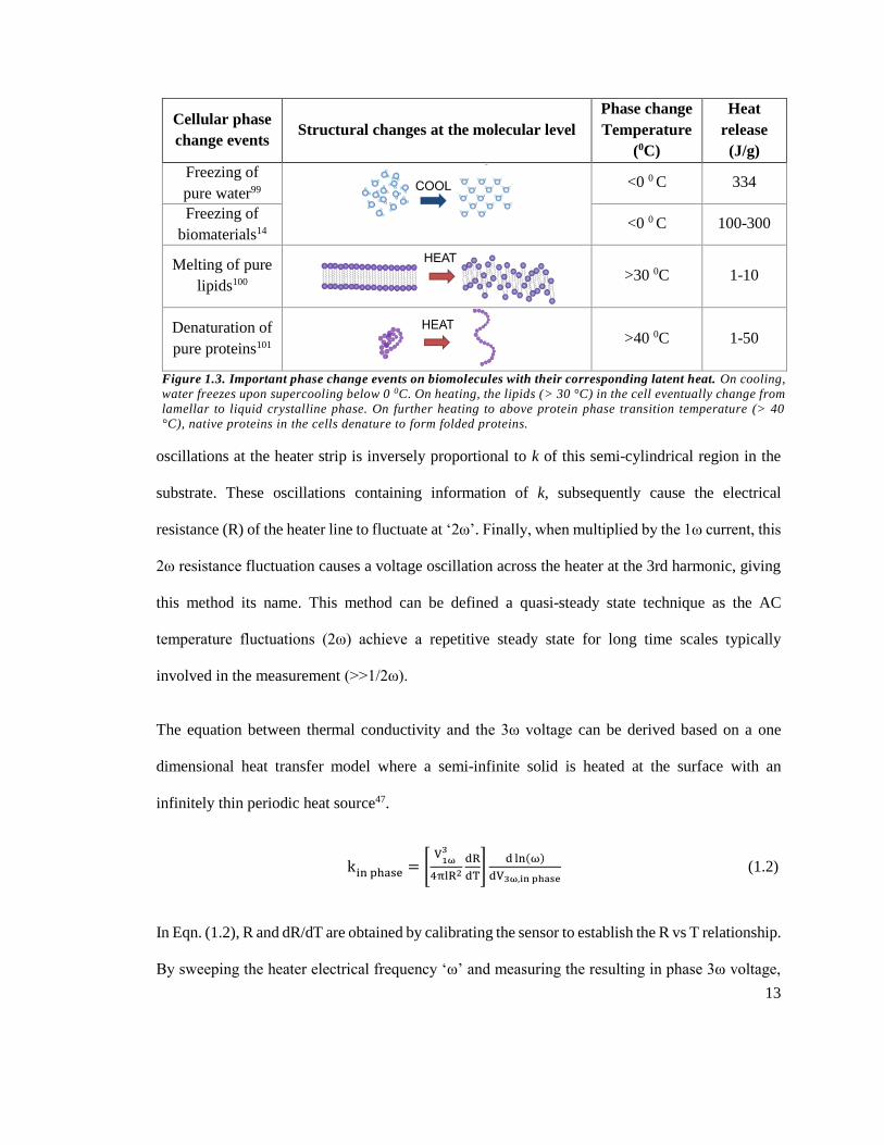
Cellular phase

change events Structural changes at the molecular level

Phase change

Temperature

(0C)

Heat

release

(J/g)

Freezing of

pure water99

<0 0 C 334

Freezing of

biomaterials14 <0 0 C 100-300

Melting of pure

lipids100

>30 0C 1-10

Denaturation of

pure proteins101

>40 0C 1-50

Figure 1.3. Important phase change events on biomolecules with their corresponding latent heat. On cooling,

water freezes upon supercooling below 0 0C. On heating, the lipids (> 30 °C) in the cell eventually change from

lamellar to liquid crystalline phase. On further heating to above protein phase transition temperature (> 40

°C), native proteins in the cells denature to form folded proteins.

14

the slope (dV3ω, in phase/d(ln ω)) can be experimentally determined and substituted in Eqn. (1.2).

Hence this method is known as the slope method and offers several advantages. For instance, this

technique is robust against contact resistance between the heater and the substrate. In addition,

surface parasitic heat loss is negligible as the temperature oscillations are small (0.1- 1 0C) and

localized within the substrate.

Recently, a new “supported” 3ω method (Fig. 1.4 (b)) has been developed. Instead of deploying

the 3ω line on the substrate to be tested, the line is created on a separate substrate that is then

brought into contact with the tissue. Thus, the temperature oscillations in this case would represent

a cylinder, with each half being in the substrate and the tissue. This method allowed for the first-

time the thermal conductivity measurements in thin porcine cardiac tissues45, 103 (Fig. 1.4 (c)),

biological solutions104, and single cells105. The accuracy of this technique for fresh tissues/water is

6%-7% and for frozen tissues/ ice is 2%-545. Further, as the tradition 3ω has been used to measure

composite inorganic materials91, 106, the same should be possible with supported 3ω method for

composite tissues. A major issue during measurement of wet biological tissues and cells is water

layer(s) and/or evaporation from the sample. A thin layer of water could form between the sample

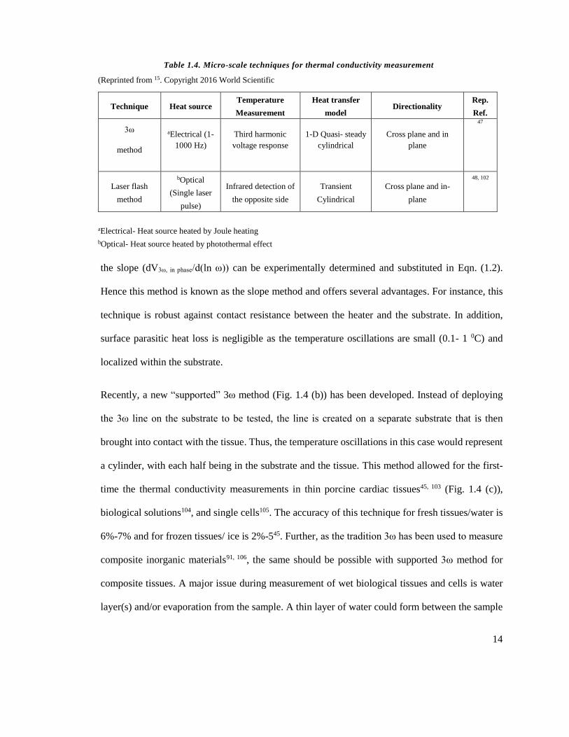
Table 1.4. Micro-scale techniques for thermal conductivity measurement

(Reprinted from 15. Copyright 2016 World Scientific

Technique Heat source Temperature

Measurement

Heat transfer

model Directionality

Rep.

Ref.

3ω

method

aElectrical (1-

1000 Hz)

Third harmonic

voltage response

1-D Quasi- steady

cylindrical

Cross plane and in

plane

47

Laser flash

method

bOptical

(Single laser

pulse)

Infrared detection of

the opposite side

Transient

Cylindrical

Cross plane and in-

plane

48, 102

aElectrical- Heat source heated by Joule heating

bOptical- Heat source heated by photothermal effect

15

and the sensor, which could result in overestimation of the k of the sample. Next, evaporation of

water content in the biomaterial cools the sample (evaporation is endothermic), acting as a heat

sink, results in a higher apparent k. Hence, it is necessary to monitor evaporation and/or water loss

for accurate measurement in thin systems.

ii. Laser flash method

One of the earliest noncontact optical thermal conductivity techniques48 is the laser flash method

which can potentially be modified for use with biomaterials. As an established, ASTM standardized

technique107, scientists have used it extensively with thin films such as polymers (14- 250 µm thick)

108-109, carbon nanotubes (0.6-1.4 mm thick)110, glass111, metals (18 μm -1 mm thick)112-114, materials

with anisotropy113, wood115, and even liquids50, 116 at both low (T > -268 0C)117 and high

temperatures112 (>1000 0C). Further, it has been used to measure interfacial contact resistance118-

120. The principle of operation is depicted in Fig. 1.5 (a). It is a transient technique, where the heat

source is a short duration laser pulse. This approximates an instantaneous heat source heating one

side of a sample. The thermal energy diffuses across the sample resulting in a temperature rise on

the opposite side, usually measured by a thermocouple or an infrared thermometer. From the

transient temperature rise, thermal diffusivity (⍺=k/ ρc) of the sample can be determined by

applying a suitable thermal transport model. In contrast to 3ω technique, thermal conductivity is

only indirectly determined from ⍺ if ρ and c are known. For instance, based on the one dimensional

Cartesian developed by Parker and his co-workers48, an expression for ⍺ and ρc is shown in the

following equations,

𝛼 =0.48𝐿2

𝜋2𝑡1/2 (1.3)

where L is the sample thickness (m) and 𝑡1/2 is time for the back surface to reach half the maximum

temperature rise (s), and

16

𝜌𝑐 =𝑄

𝐿𝑇𝑚 (1.4)

where 𝑇𝑚 is maximum temperature rise at the rear surface (K). Using ⍺ and ρc from Eqns. (1.3)

and (1.4), thermal conductivity of the sample can be determined. An important error from this

model arises from assuming the sample to be a black body, which absorbs all incoming radiation.

This error can be minimized by applying a layer of black coating over the sample surface122. Other

errors include the uncertainty in sample thickness, parasitic heat loss, finite pulse duration and

multi-dimensional heat flow. The uncertainty of this technique is ±3-5%123.

(a)

(b)

(c) (d)

Figure 1.4. 3ω method. (a) Principle of operation of the 3ω method (I- current, R- electrical resistance, Q-

Joule heating, T- temperature,αT- temperature coefficient of resistance), (b) Side view of supported 3ω method

with steps involved in thermal conductivity measurement; (c) Supported 3ω measurements of porcine PV, and

(d) esophagus. Measurements are the average ± standard deviation of N = 5 samples and validated using ice

measurements (black points). The black and yellow trend-line data are k values of water, ice and fat from

literature121. Figure (a) is reprinted and redrawn from 46Figures (b), (c) are reprinted from 45, 103. Copyright

2015 and 2016 American Institute of Physics and Nature

17

For applications with thin biological tissues (< 2 mm), this technique would face limitations from

evaporative heat and water loss from the wet sample as also seen in 3ω method. Tada and co-

workers addressed this limitation by encapsulating the liquid sample (~1 mm) between two thin

metal disks held together by capillary force. As one of the metal disks is heated, heat diffuses from

the disk through the liquid sample to the other side introducing the issue of contact resistance

between the disk and the sample. Laser flash technique has been successfully used to measure the

thermal conductivity of water50, molten salt125 and human tooth (1.2- 1.5 mm thick)126.

(a) (b) (c)

(d) (e) (f)

Figure 1.5. Optical techniques for thermal conductivity measurement. (a) Laser flash method, (b) Time-

Domain Thermoreflectance Method; (c) Transient absorption method. Inset showing the heating of an

individual gold nanorod with a coating (green color) heated by the pump beam; (d) Thermal conductivity

measurement of thin protein films using TDTR. (e) Plot of transient absorption signal vs. time; (f) Thermal

conductance and volumetric specific heat of CTAB coated on the gold nanorod surface. Figure from (d)

reprinted from reference 124. Figures (a) is modified from15 and (e) and (f) are reprinted from 58. Copyrights

2014, 2016, 2013 American Chemical Society, World Scientific and American Chemical Society

18

1.3.2. Nanoscale thermal conductivity measurement techniques

Nanoscale thermal conductivity measurement techniques are advanced state of the art techniques

developed for small length (1 nm-1 μm) and time scales (100 ps- 10 ns). A representative list is

shown in Table 1.5, and discussed in the following sections.

i. Time domain thermoreflectance (TDTR) method

TDTR is a noninvasive optical technique that has been used to measure thermal conductivity of

thin films53, 127-128 with directionality129-133 and composite layers54; and microscale liquid droplets134

and thermal conductance across solid-solid interfaces135, solid-liquid interfaces136 across self-

assembled monolayers of molecular chains137 and even chemical bonds138. The technique uses a

pump probe setup as shown in Fig 1.5 (b). A pump beam (spot size- 10-20 μm) produces ultrashort

train of pulses (~100 fs) rapidly heating the sample surface. The surface subsequently cools down

after each pulse at a specific rate depending on the thermal conductivity of the sample. This surface

temperature drop changes the optical reflectance of the sample surface (thermoreflectance). After

a suitable time delay (< 100 ps), the probe beam irradiates the surface and its reflection is detected

by an optical sensor. By monitoring the change in reflectance, the optical sensor measures the

temperature change and ultimately the thermal conductivity using a suitable thermal transport

model. A simple one-dimensional Cartesian model can be approximated if penetration depth is

smaller than the pump beam spot size (~10 μm-100 μm)53-54, 127, 134. In the case of biomaterials,

penetration depth (√𝛼𝑡) at ultrashort time scales (~100-1000 ps) corresponds to 100-600 nm in

biomaterials.

For samples with poor thermoreflectance coefficient, a thin metallic transducer (e.g. gold, 50-100

nm thick) can be used as shown in Fig. 1.5 (b). TDTR has been used to measure thermal

conductivity of thin protein films124 (Fig. 1.5 (d)). The measurement accuracy is ~7% at probe beam

19

sampling frequency of 10 MHz139. A major source of uncertainty arises from the thickness and

thermoreflectance behavior of the transducer. The transducer thickness can be reduced by the use

of recently developed and highly sensitive transducer based on TR-MOKE (Time resolved

Magneto Optical Kerr effect). In TR MOKE, the transducer is magnetic, whose highly sensitive

temperature response to laser heat energy is measured based on thermo-magnetic and magneto-

optical effects133, 140-141. TDTR faces several limitations in nanoscale bioheat transfer applications.

First, the transducers generally have a weak but linear relationship between the optical reflectance

and temperature. Hence, a temperature rise of the order of 10 0C is necessary for measurable change

in the output signal142, which is significantly higher than other techniques such as 3ω method

(temperature rise~0.1- 10C46). Next, due to limitations with thin film geometry, thermal transport

around nanoparticles in suspended medium cannot be measured.

A variation of TDTR is possible if the pump beam is modulated at a frequency ‘ω’ resulting in a

periodic heat source. This technique, which has been used to measure thermal conductivity of

materials such as thin metal films (20-100 nm thick)143 with anisotropy, multilayer structures144,

carbon nanotubes145 and thermal conductance at the interface146 , is referred to as frequency domain

thermoreflectance method (FDTR)147. As the name implies, the change of the measuring parameter

i.e., thermoreflectance of the transducer with pump beam frequency (100 kHz- 200 MHz) is fitted

to an analytical model to determine k. As it relies of frequency change of the pump beam, the

mechanical delay stage for probe beam is not needed reducing the complexity of the experimental

setup. Further, the thermal penetration depth (2⍺/ω)0.5 can easily be controlled by changing the

modulated frequency of the pump beam. Also, this technique can simultaneously measure k and cp

and measure interface conductance if the thermal diffusivity is at least 3x10-6 m2/s147. However,

20

thermal diffusivity of biomaterials is usually less than 2 x10-6 m2/s. A disadvantage of this

technique is that it has poor sensitivity for in plane thermal conductivity147.

ii. Transient absorption method (TAM)

Similar to TDTR, TAM is also a pump-probe technique developed in the last decade to measure

thermal conductivity of nanoparticle (NP) coating (1- 10 nm) and thermal conductance at the

interface around nanoparticles in the suspended state. Metallic NP such as gold are the transducers

of thermal energy through photo-thermal effect148. On laser irradiation, free electrons of the NP are

excited to oscillate with a frequency depending on NP geometry and material. Surface plasmon

resonance (SPR) occurs when the incident light frequency matches with the natural frequency of

the free electrons. SPR significantly increases the absorbance of the nanoparticles. Following this

absorption, several events ensue: (i) electron-electron coupling in the nanoparticle within 1 ps,

followed by electron-phonon coupling for energy transfer from electron to the NP lattice over 1-10

Table 1.5. Nanoscale techniques for thermal conductivity measurement

(Reprinted from 15. Copyright 2016 World Scientific)

Technique Heat source Temperature

measurement

Heat transfer

model

Directional

ity Rep. Ref

Time domain

thermoreflectance

(TDTR) microscopy

aOptical –

Laser (> 1

MHz pulsed)

Using surface

reflectivity

dependence on

temperature

Transient

In- plane

and cross

plane

53-54

Transient Absorption

Method (TAM)

aOptical –

Laser (> 1

MHz pulsed)

Using Transmitted

signal to measure

absorbance

Transient Spherical

radial 57-60

Scanning Thermal

Microscopy

(SThM)

bElectrical Thermocouple,

thermistor or RTD

Quasi- steady

model

Spherical

radial 55-56

aOptical- Heat source heated by photothermal effect bElectrical- Heat source heated by Joule heating

21

ps, (ii) thermal equilibration of the phonons across the particle, and the excitement of acoustic mode

vibrations which cause oscillations in the measured signal at < 300 ps, and (iii) the diffusion regime,

in which the NP lattice dissipates heat into the surroundings (hundreds of ps to a few ns). Therefore,

nanoparticles act as transducers of laser thermal energy.

For temperature measurement, this technique relies on the relationship between temperature and

optical absorption of the nanoparticles instead of reflectance as in TDTR. The experimental setup

is illustrated in Fig. 1.5 (c)59-60, 150. As a femtosecond pump beam heats the NPs, it is cooled by the

surrounding medium. The subsequent temperature drop at short time scales (<1000 ps) changes the

optical absorbance (∆Abs) of the NPs. After a time delay, the probe beam shoots an ultrashort pulse

(a)

(b) (c) (d)

Figure 1.6. Scanning thermal microscopy. (a) Schematic with the inset showing the heat transfer mechanism

between the heated tip and the sample. (b) Optical Transmission image; (c) Topography; (d) Thermal image

of nucleus of HeLa cells attached to a glass substrate undergoing mitosis. Figures (a ) and (b-d) reprinted from 15,149. Copyright 2016, 2003 World Scientific and Elsevier

22

through the nanoparticle solution. The change in the transmitted signal is monitored by a photo-

detector. If the scattered signal is minimum, ∆Abs can be determined from the transmitted signal.

Thus, transient ∆Abs behavior as shown in Fig. 1.5 (f) contains information about the temperature

response of the NPs. However, the behavior of ∆Abs at short time scales (<500 ps) is dominated by

photo-thermal events such as phonon-electron coupling (<10 ps) and acoustic phonon vibrations

(<100 - 500 ps) within the nanoparticle. Only above 500 ps, ∆Abs represents the thermal dissipation

from the hot nanoparticles to the surrounding medium. For time scale < 1000 ps, the penetration

depth is of the order of 1-20 nm from the surface of the NP. Interestingly, this is of the same order

as that of the NP coating thicknesses used in many biomedical applications. Therefore, thermal

properties of the nanoparticle interface and coatings could be determined from ∆Abs in the diffusion

regime (500-1000 ps). A main drawback is that only certain nanoparticles with minimum scattering

and maximum absorption qualify as suitable transducer for this technique. For instance, gold

nanorods can be used with near infrared Ti-sapphire laser as they have minimum scattering and

maximum absorption in the near infrared frequency regime (700-1000 nm). In addition, TEM relies

on several characterization steps such as UV-vis absorption spectrometer, transmission electron

microscopy, ζ-potential and dynamic light scattering measurements before measuring thermal

properties. Nevertheless, TEM have been used to successfully measure the thermal properties (k,

cp) of the coatings such as CTAB and PEG (Fig. 1.5 (f))57-58. In some cases, the nanoparticles have

also been immobilized on a quartz support and immersed in organic solvents to measure thermal

conductance at the nanorod - fluid interface150. Therefore, TAM offers unique opportunities to

address some unanswered questions about thermal transport around the nanoparticles at small time

(<1000 ps) and length scales (1-20 nm)151

Several optical techniques such as laser flash method, TDTR and TAM have been discussed in the

previous sections (Fig. 1.5). Apart from these techniques, there are other optical techniques such

23

as thermal lens microscopy152 and photoluminescence153 based methods used for measuring thermal

conductivity and/or thermal diffusivity of biological cells. Though optical techniques are non-

invasive and non-contact, the spatial resolution is limited by the diffraction limit of optics (~300

nm). Thus, SThM discussed in the next section accounts for this drawback by using a physical

probe as detailed in the next section.

iii. Scanning thermal microscopy (SThM) method

SThM uses a nanoscale heated probe to qualitatively measure thermal conductivity56, 154-158 or

temperature55, 159-161 on the sample surface or its sub-surface162-164 in the range of hundreds of nm

to µm range. The probe (~100 nm) can be microfabricated to simultaneously act as a heater and a

thermometer165. The schematic of SThM is shown in Fig. 1.6. The probe is attached to a cantilever,

while the sample sits on a stage. A mirror attached to a cantilever reflects light onto a photodiode

to inform the vertical and horizontal movement of the probe. As the probe scans the surface, the

sample surface displaces the probe depending on its topography. Meanwhile, the stage moves the

sample to maintain constant gap between the probe and the sample surface. During the scan, a

constant current heats the probe, while the sample surface cools it resulting in temperature decay

(Fig. 1.6 (a-inset))56. This transient temperature change of the probe is monitored to qualitatively

determine thermal conductivity of the sample near the surface.

This method has been used to probe inorganic nanomaterials such as carbon nanotubes166 and

polyethylene nanofibers167 with a spatial resolution as small as 50 nm. SThM has been used directly

on biomaterials, generating thermal images such as those inside of living HeLa tumour cells as

shown in Fig. 1.6149. This suggests, for instance, that SThM may one day be able to directly

measure the intracellular activity of different organelles or compartments of living cells. This

technique can also measure phase change temperature at a single location162, 168-172.

24

Despite the possibility of in situ thermal imaging of biomaterials by SThM, there are also several

limitations. For instance, an important drawback is that it offers only qualitative measurements of

thermal conductivity. As the thermal transport mechanism between the hot probe and the sample is

complex and not fully understood (Fig. 1.6 (a-inset))165, 173-175, proper heat transfer models and

calibration techniques are still under development. Another drawback is that the temperature

measurement is significantly affected by the surface roughness. For instance, topography and

thermal imaging in HeLa cells appear highly correlated in Fig. 1.6 (b). If these limitations are

overcome, this system is an excellent tool to physically probe thermal conductivity of sub-

nanoscale intracellular components such as cytoplasm, nucleus, cell membranes in the presence of

additives (i.e. chemical and NPs) and/or phase change (i.e. crystals).

1.3.3. Applications for multiscale thermal conductivity measurement

i. Thin tissue and cellular scale applications (10 nm- 2mm)

A recent review on the measurement of thermal properties of large tissues (>2 mm thick) and organs

sheds light on lack of similar measurements in thin tissues (< 2 mm) and cells (<100 μm) in

literature14, 52, 176. Further, thermal property measurement of thin, anisotropic and/or composite

structures such as in Fig. 1.7 (a) remain largely unexplored. However, anisotropy in larger muscle

tissues have been studied in the past as shown in Fig. 1.7 (b). During freezing, the presence of ice

crystals significantly impact the thermal conductivity depending on its direction, fraction and

morphology. First, crystal growth occurs in the direction of the temperature gradient thereby

artificially introducing anisotropy in thermal conductivity. Directional crystal growth is commonly

observed during cryoablation of tissues. Next, crystallized fraction is determined by the cooling

rate as described in Section 1.2, which in turn affects the k to a large extent. Finally, the ice crystal

morphology depends on the freeze front being planar, dendritic or epitaxial. One instrument, the

25

directional solidification stage, has been developed to study such crystal growth morphology177.

This stage, also known as the Bridgeman technique, achieves anisotropic crystal growth by moving

the sample at a given speed from a warm to a cold block with a temperature gradient of over 20

0C/mm. In solutions, the phase front develops from planar into dendritic structure (Fig. 1.7 (c). The

space between the dendrites, which can be 10’s μm, is occupied by an unfrozen region, which on

further cooling becomes a eutectic mixture. The resulting ice crystal morphology would be

alternating layers of ice and eutectic mixture (Fig. 1.7 (c)), resulting in an anisotropic, composite

thermal conductivity. On freezing complex biological organs, ice crystals follow the open fluidic

pathways for crystal growth such as vasculature extracellular spaces in liver and other organs178-179.

It is unclear what the implications of this anisotropy are on frozen tissues during cryotherapy as it

is largely unstudied. On the other hand, freezing during cryopreservation involves the random

nucleation of small ice crystals. After nucleation, the ice crystals grow in random directions as

shown in Fig. 1.7 (d) diminishing the issue of anisotropy180.

In the case of cryopreservation, there is a need to study the influence of thermal history on thermal

properties of thin tissues (eg. arteries)181-182. Specifically, vitrification often fails from crack

formation and crystallization. The presence of ice crystals changes thermal property changes by 50

– 100% in crystallized vs. non-crystallized biomaterials as shown in Figs. 1 and 2. In the case of

cracks, the ensuing voids would be expected to change the k value. Due to lack of microscale

thermal conductivity measurement techniques, these areas of interest remain largely unexplored.

Nevertheless, 3ω technique and laser flash method as discussed in Section 1.3 offer excellent

opportunities to measure thermal properties of anisotropic, composite, and thin tissues and cells.

26

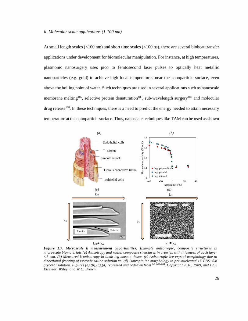
ii. Molecular scale applications (1-100 nm)

At small length scales (<100 nm) and short time scales (<100 ns), there are several bioheat transfer

applications under development for biomolecular manipulation. For instance, at high temperatures,

plasmonic nanosurgery uses pico to femtosecond laser pulses to optically heat metallic

nanoparticles (e.g. gold) to achieve high local temperatures near the nanoparticle surface, even

above the boiling point of water. Such techniques are used in several applications such as nanoscale

membrane melting185, selective protein denaturation186, sub-wavelength surgery187 and molecular

drug release188. In these techniques, there is a need to predict the energy needed to attain necessary

temperature at the nanoparticle surface. Thus, nanoscale techniques like TAM can be used as shown

(a) (b)

(c) (d)

Figure 1.7. Microscale k measurement opportunities. Example anisotropic, composite structures in

microscale biomaterials (a) Anisotropy and radial composite structures in arteries with thickness of each layer

<1 mm. (b) Measured k anisotropy in lamb leg muscle tissue. (c) Anisotropic ice crystal morphology due to

directional freezing of isotonic saline solution vs. (d) Isotropic ice morphology in pre -nucleated 1X PBS+6M

glycerol solution. Figures (a),(b),(c),(d) reprinted and redrawn from 14, 183-184. Copyright 2010, 1989, and 1993

Elsevier, Wiley, and W.C. Brown

27

in Fig. 1.8 to improve the understanding of thermal transport around nanoparticle surface at the

nanoscale. Finally, a similar capability can be envisioned for TDTR for biological films of water,

protein or polymers.

At low temperatures, nanoparticles are used in several instances for both cryopreservation and

cryotherapy. In cryotherapy, nanoparticles (1-100 nm) can potentially be used as payloads to carry

toxic drugs as a combinatorial treatment189 and in some cases, molecular adjuvants that increase

the efficacy of iceball for tumor destruction, reaching in some cases out entirely to the iceball

edge190. For some applications of cryopreservation, nanoparticles are added to CPAs to improve

their efficacy as cryopreservatives191 or manipulating osmotic response of cell membranes to

improve cryopreservation192. Recently, iron oxide nanoparticles are being used to uniformly thaw

the biomaterials without cracking and crystallization thereby improving cryopreservation of larger

biomaterials193. Due to low concentration of nanoparticles (<1% by volume), their effect on thermal

conductivity of nanoparticle laden biomaterials is negligible. However, they can reduce perfusion

(i.e. blood flow, Qbl) in vivo194. On the other hand, cryo-nanosurgery uses a higher concentration

of nanoparticles so as to directly increase the thermal conductivity and hence the efficacy of an ice

ball195. As increasingly important biomedical applications open up at small length scales (<100 nm)

and/or short time scales (<100 ns), there is a need to clearly understand the nanoscale heat transfer

in nanoparticle-laden biomaterials.

1.4. Calorimetric Measurement Techniques

As a complement to the above thermal conductivity discussion, we will now transition to

calorimetric measurement techniques of biomaterials. A commonly used technique is Differential

scanning calorimetry (DSC) for measurement of latent heat and specific heat (cp) at the microscale

(e.g. mm sized tissue pieces or millions of cells in media). Though commonly used, these

28

instruments have several limitations such as low temperature scanning rates (<750 0C/min) and

large sample weight (> 1 mg). This has led to the development of Nanocalorimetry on a silicon-

based membrane for small sample weight (as low as 10 ng), thereby allowing large heating rates

(~107 0C/min). Nanocalorimetry can be ideal for applications at the cellular, sub-cellular and

molecular levels, allowing a broad range of phase change behavior in biomedical applications to

be measured.

(a) (b)

(c) (d)

Figure 1.8. Example nanoscale thermal conductivity measurement opportunities. (a) Schematic of TAM

probing gold nanorod (GNR) surface up to 20 nm. (b) Heating of GNR melting ice to water 196. Measured thermal

conductivity will change from that of ice to water on heating. (c) Heating of protein coating resulting in

denaturation surrounding the GNP surface197. Measured thermal conductivity will change from that of fully

deployed native proteins to denatured proteins; (c) Measurement of molecular release event through monitoring

of thermal conductivity at the surface188.

29

1.4.1. Differential scanning calorimetry (DSC)

The first calorimeter was built by a French Scientist Antoine Lavoisier in 1780 to measure the heat

production of a guinea pig198. In the last two centuries, calorimetry has come a long way from

measurement of heat release/absorption of an animal to micro and nanoscale measurements of cells

and macromolecules. Differential Scanning Calorimetry (DSC) is a type of calorimetry that is used

to measure the enthalpy, specific heat capacity and latent heat of wide variety of materials with

small sample mass (~3 to 100 mg) over wide temperature ranges (-180 0C to >750 0C). In the last

five decades, it has been widely used for understanding the thermodynamics and kinetics of the

phase change of water, protein and lipids in biomolecules as listed in Table 1.6. A typical DSC set-

up consists of a furnace loaded with two pans or crucibles. One of these is filled with the sample,

while the other is usually empty to subtract background heat flow from the crucible and other

artifacts. The DSC measures the difference in heat flow between the sample and the reference pans

during heating, cooling or at an isothermal temperature. The resulting differential heat flow, (mW)

‘ɸsample’, is plotted as a function of temperature (0C) or time (s). Then, ∆h (∆H/m) and cp (Cp/m)

can be determined using the following equations,

2

1

.1

T

T

sampledT

dT

dt

dt

d

mh

(1.5)

dT

dt

dt

d

mc

sample

p .1

(1.6)

30

Based on heating technique, DSC can be divided into two basic types: the standard DSC with linear

heating and the modulated DSC with modulated heating. The standard DSC allows the sample and

the reference to be heated by a linear temperature program. There are two types of standard DSC:

Heat flux DSC (HF DSC) and power compensated DSC. Heat flux DSC was developed by Privalov

et al, in 1964199. In this type of DSC, the sample and the reference are heated in a single furnace

and the temperatures are measured using thermocouples (Fig. 1.9 (a)). Difference in heat release/

absorption between the sample and the reference will result in a difference in temperature between

the sample and the reference (∆T)200-202. The main advantage of this type of design is the simplicity

of construction. However, the sample and the reference being loaded in the same furnace makes it

less accurate (2% vs 0.2% for Power compensated (PC) DSC) for calorimetric measurements and

(a) (b)

Figure 1.9. Differential Scanning Calorimetry. (a) Schematic of HF DSC. Inset showing a typical DTA

thermogram during a first order phase change. (b) PC DSC with a second feedback loop. Inset showing a typical

DSC thermogram during a first order phase change.

31

achieve lower scan rates (<250 0C/min vs >500 0C/min than PC DSC). Power compensated DSC

was developed by O’ Neill et al (Fig. 1.9 (b))203-204. This technique has two identical furnaces: one

for the sample and the other for reference. Each furnace has a heater and a platinum resistance

temperature sensor. The furnaces are made of platinum iridium alloy. The main difference between

HF DSC and PC DSC is the control loop. HF DSC supplies equal amounts of heat flow to both the

sample and the reference and uses ∆T to determine ɸm (ɸs-ɸr). In contrast, the PF DSC supplies

differential heat flow to the sample and the reference such that ∆T becomes 0 0C. Thus, the

differential heat flow, ɸm is obtained directly, improving the accuracy and sensitivity.

M-DSC has the capability to simultaneously measure Cp and heat flow from a kinetically controlled

process (e.g. phase change)208. It uses two simultaneous heating rates: a sinusoidal heating rate

modulated over the linear heating rate. The linear component provides information of irreversible

heat flow (e.g. crystallization) similar to that of standard DSC, while the modulated component

allows the reversible heat flow measurement of the sample (e.g. Cp). One application of M-DSC is

to measure specific heat capacity overlapping another kinetic process such as crystallization in a

polymer (poly(ethylene terephthalate))208.

Table 1.6. Representative measurements in biomolecules using DSC

Type Sample Measured

Parameters Size Max. Scan

rate

Rep.

Ref

Proteins

Ribonuclease, lysozyme,

chymotrypsin, cytochrome c and

myoglobin

∆H, Cp(T),

Tm

1.33 mL (conc –

0.05-0.5 %) 1 0C/min

101

Proteins in AT-1 cells Cpex(T), Tm 40 µL (conc - 76

µg/µL) 50 0C/min

121, 205

Lipids

Dipalmitoyl phosphatidylcholine

(DPPC) liposomes. Cpex(T), Tm NA 10 0C/min

206

Fatty tissues Cp(T), Tm 20 µL 1.3 0C/min 207

*Cp(T)- specific heat capacity, Tm- phase change temperature, ∆H- latent heat during phase change

32

In the past, certain calorimeters were designed to directly measure metabolic heat release in

organisms and even cells. For instance, these calorimeters were used to study metabolism in

mammalian sperm cells209-210, T-lymphoma cells211, blood mononuclear cells212 and organisms such

as Leishmania amazonensis parasites213, thermotolerant Bacillus214. They have similar sensitivity

(millijoule) to that of current DSCs.

Open type

(a) (b)

Closed type

(c)

.

Figure 1.10. Nanocalorimetry. (a) Cross-sectional schematics of the open type differential nanocalorimeter is

shown. (b) Top view of the circled region in (a) is shown. The left side is the sample area and the right side is

the reference area. The calorimeter studies the heat of reaction between two liquid materials (i.e. two blue

circles on each side) merged using electrostatic merging and mixing mechanism. (c) Device schematic (cross -

sectional view) of closed type parylene-polymer-based microfluidic absolute nanocalorimeters. The parylene

membrane is suspended and thermally isolated by vacuum. Figures reprinted from 215, 30. Copyright 2009 and

2004 National academy of Sciences of the United States

33

1.4.2. Nanocalorimetry

Nanocalorimetry is a new type of calorimetry that was developed to work with samples that are

three orders of magnitude smaller than those with a typical DSC (mass~ ng and down to picoliter

volumes). These devices are typically highly responsive (μs- ms), sensitive (~1 nJ/K), and can

achieve a high heating rate of ~107 0C/min. These devices allow unprecedented calorimetric

measurements for biomaterials if properly protected from evaporation. The basic construction of

the device depends on the sample, application and purpose of the experiment. A typical

nanocalorimeter is constructed on a thin film silicon-based membrane (as shown in Fig. 1.10(a)).

A heater line and a temperature sensor are microfabricated on top of the membrane in a chamber.

The heater is excited by an electric current heating the sample, and the resulting temperature is

measured by a temperature sensor with a resolution of the order of ~ μK to mK. The heating could

be either continuous14, 30, 65, 215-218 or modulated by an alternating current219-222. The sensitivity of

this instrument depends on the thermal conductivity (k) and heat capacity (Cp) of the structural

body as explained later.

There are several methods to measure temperature in a nanocalorimetric chamber. The most

commonly used method is thermopile65, 223-224. The thermopile is really several thermocouples

connected in series to improve temperature sensitivity (10μK), with the sensitivity being

proportional to the number of thermocouples. Thermistors can also be used to measure temperature

with similar sensitivity215, 225. The thermal time constant of typical thermistors (characteristic length

scale ~mm) are, in most cases, approximately several seconds. For calorimetric applications,

thermistor time constant have been reduced to <100ms by reducing the characteristic length of the

thermistor element to <250 μm226. However, they need external electric power for operation. In

other words, electric current should be passed through the thermistor to measure change in

34

resistance, which can produce Joule heating and interfere with the existing heat flow in the

system227. Another commonly used temperature measurement is the resistance thermometer. The

principle of operation is same as that of thermistors. However, the advantage is that they have lower

resistance than thermistors, resulting in lower Joule heating. Platinum is an example material used

for this purpose228. Both the resistance thermometer and thermistors need calibration that involve

the assignment of temperatures to resistance of temperature sensors. For this purpose, the

nanocalorimeters are isolated inside a furnace for several hours to bring the entire system to a steady

state temperature while simultaneously measuring the resistance. However, for use at high

temperatures (>600 K), the furnace-based calibration results in large thermal gradient within the

calorimeter. This gradient can be as large as 40 K, introducing a significant error in calibration. So

pyrometers have been used to identify the temperature at the sensor for calibration at high

temperatures (573 K to 873 K)229.

The sample can be fed to the chamber using micro-fluidics or syringe pumps depending on the

chamber type. The chamber can be open or closed depending on the application. If the chamber is

open, the sample is placed by micropipette or inkjet printing, although this approach suffers from

parasitic heat loss and sample evaporation; thus, it is most suitable for solid materials (Table 1.7).

If the chamber is closed with a layer on top as shown in Fig. 1.10 (b) (i.e. with PDMS), the sample

is supplied by microfluidic channels. However, the added layers of materials comprising these

channels increases the thermal mass of the system. Unfortunately, a high thermal mass (k.Cp) leads

to high thermal time constant, resulting in lower sensitivity. This effect can be minimized by proper

selection of materials with minimum heat capacity and thermal conductance. If the thermal mass is

increased, the heat flow from the sample is absorbed by the material, thus reducing the sensitivity.

Lee et al have developed a nanocalorimeter with a closed chamber using parylene with low thermal

mass and vacuum separators to reduce thermal conductance and improve resolution by at least a

35

factor of magnitude compared to other closed type devices30. The calorimeter built from parylene

has a time constant of ~1.3 s30, whereas the one built from higher thermal mass PMMA has a time

constant of ~12 s65. In another non biological example, the thermal mass of the nanocalorimeters

have been reduced by an alternate design, where the heaters and thermometers are integrated onto

a suspended beam of SiNx230-231

or NbNx substrate232 and temperature is measured using a resistance

thermometer230, 233 or bi-material cantilever231 (10-50 μK). These calorimeters have achieved an

impressive picowatt resolution (<1 pW) and millisecond time constant (<100 ms)230-234. Further,

these calorimeters use modulated heating scheme with high frequencies as they improve signal-

noise ratio by reducing 1/f noise caused by thermal drift233. A disadvantage of suspended

nanocalorimeters is their extremely sensitivity to small vibration, which require high vacuum (<10-

4 Torr). Further, the sample loading onto these nanocalorimeters is currently only possible by direct

microfabrication of the sample onto the sensor. Thus, while these nanocalorimeters represent state-

of-the art sensitivity, their application to bioengineering problems remain uncertain and untried at

this point. Perhaps with the use of 3D printing and/or cryogenic preparations there will be an

opportunity to use these sensors, similar to previous cryo SEM or cryo TEM preparations, at low

pressures on frozen hydrated samples235.

Several nanocalorimeters that have been developed in labs or commercially are listed in Table 1.7

Nanocalorimeters have been developed to operate over a wide temperature range (-1000C to 7000

C). Nanocalorimeters have been constructed to make both absolute30, 65, 215 and differential heat

measurements236. In addition to the list in Table 1.7, Xensor Integration, a manufacturer has been

building nanocalorimeters chips for use at 800 0C, 1300 0C and in liquids. In fact, the Mettler Toledo

Flash DSC 1 uses the sensors from Xensor (www.xensor.nl).

36

1.4.3. Applications for multiscale calorimetric measurements

Nanocalorimeters require very small sample volumes and have fast response and high resolution.

Further, they are expected to become even more sensitive with the improvement of their fluid-

handling capability and temperature measurement. Currently, they are several major application

areas opening up for nanocalorimetry: (a) cryobiology, (b) high-throughput calorimetry for the drug

industry, (c) protein conformational studies, (d) label-free biochemical sensing, and (e) monitoring

of cells.

i. Cryobiology

For cryopreservation, biomaterials freeze at low temperatures, damaging cells in several ways9.

Hence, cryoprotective agents (CPAs) are added to biomaterials to avoid freezing the water content.

One approach is to use high concentration CPA (>2M) to achieve vitrification at achievable

cooling/warming rates (< 100 0C/min) in clinical settings. However, this approach is highly toxic

and hence remains unsuccessful. On the other hand, low concentration CPAs (<2M) are minimally

toxic but have been estimated to need ultrarapid cooling (~104 0C/min) and warming rates (> 104

0C/min) for successful vitrification. With recent developments in cryopreservation approaches,

ultrarapid cooling rates (~104 0C/min) are achievable in microscale (<100 μm) biomaterials237-240.

In fact, Jin et al have successfully cryopreserved mouse oocytes by achieving ultrarapid warming

rates and CPAs at low molarity (2M)241. Further development of successful use of CPAs requires

improved understanding and implementation of vitrification and warming in these small systems.

One important uncertainty is the crystallization and vitrification behaviour of low concentration

CPAs (<2M). For instance, the critical cooling rate – the minimum rate required to achieve

vitrification – has never been measured for low concentration CPAs (<2M)242. Several estimates

are available in literature, often contradicting each other by at least an order of magnitude. Thus,

37

we need an accurate, quantitative technique that can achieve high heating rates to understand the

thermodynamics and kinetics of phase change events of low concentration CPAs. In fact,

nanocalorimetry has been used at ultrafast heating rates to study glass transition and crystallization

in polymers71, 243-246, perhaps pointing the way for potential use in cryobiology.

ii. High-throughput calorimetry

An important advantage of nanocalorimeters is the ability to use them in a high throughput mode.

This can be useful for quality control in the drug discovery industry, where enthalpy can give

insight into ligand binding and the sample availability and measurement times are small. In

principle, all nanocalorimeters can be operated in parallel to increase their measurement

throughput. The main issue is fluid-handling. As previously mentioned, fluid delivery for open-

chamber nanocalorimetry systems can lead to error from evaporation. One solution to this is to use

large sample volumes (~250 nL) with electrostatic droplet merging techniques70, 215. One such

device that does this consists of electrostatic drop merging, magnetic mixing with thermistor

sensors, which enable high-throughput heat-of-reaction measurements (96 measurements in

parallel) with 250 nL samples. For closed-chamber types, substantial heat loss and inaccuracy of

the sample injection volume have been issues. In theory, the system could be multiplexed without

much complication, but this has not been attempted as far as we know. However, Lerchner and his

co-workers achieved high throughput in closed-type nanocalorimeter using segmented flow

construction. In this case, the sample, usually a solid or aggregate, is carried by carrier fluids to the

measurement chambers247. Interested readers are directed to a detailed review on this topic248.

iii. Protein conformational studies

In the pharmaceutical industry, proteins are often studied to understand their stability against

aggregation during lyophilization, shipping and storage249-251. Proteins undergo weak glass

38

transitions, which are difficult to measure using conventional DSC252. Thus, nanocalorimetry is

critical in making these measurements with high sensitivity253-254. During nanoparticle-based

hyperthermia, nanoparticles are often functionalized with protein receptors for increased stability

to reach the target255. The conformational behavior of proteins attached to nanoparticles has not

been extensively studied in the literature186. Nanocalorimeters can be particularly advantageous as

the small sample volume requirement enables the measurement of a scarce sample, such as proteins

produced by the subpopulation of a heterogeneous cell culture. Several groups have demonstrated

the use of nanocalorimeters with 10-μg biological samples228, 256-258. For instance, Wang et al used

a nanocalorimeter with 50 nW sensitivity to measure protein denaturation of small volumes (~1 μl)

with proteins such as lysozyme at concentrations of ~3 to 20 mg/ml PBS solution (Fig. 1.11 (a, b)).

This technique has also been used to measure hydration and dehydration of lipids which occur at

millisecond time scales67. Fig. 1.11 (c) shows the heating of dehydrated DPPC for several cycles

with the time interval being 300 ms between each cycle. The first cycle shows a peak at ~64.3 0C,

which shows tightly held water release, indicating that it is impossible to achieve a truly dry state.

The next cycles do not have a peak at low temperatures, indicating the dry state of lipids.

iv. Biochemical sensing

Nanocalorimeters can be used to sense heat of reaction in enzymes, antibodies, DNA, cells, and

many other micro/nanoscale biomaterials. There are several ways to transport the biomolecules to

the chamber. A simple technique is to supply both the substrate and the enzyme to the chamber,

where they mix by diffusion217, 259-260. This method, however, requires rather large amounts of

enzyme solution for detection (~10-20μL). Another way to transport a small sample is with

microbeads. The enzymes can be immobilized on microbeads and loaded into a chamber or directly

deposited in the chamber to detect substrates216, 225, 261-262. Similarly, antibodies or DNA can be used

39

for calorimetric sensing and DNA “thermosequencing”263. For instance, Ahmad et al used

nanocalorimeters to detect biotin in the sample using a microbead coated with streptavidin receptor

(Fig. 1.11 (d))69. The binding event produces a heat release enthalpy, ∆H of ~107 kJ/mol biotin

(~438 nJ/ng biotin) for a volume flow rate (V) of 20 μL/min with a concentration (Cbiotin) of 50

μmol/L. The heat rate from the reactions can be calculated as

P=V. ∆H. Cbiotin (1.7)

For this case, P is ~1.78 μW which is greater than the noise equivalent power (NEP) of the

instrument at 20 nW. Owing to low NEP, the instrument can measure extremely small biotin

concentrations of 1 μmol/L of phosphate buffer for a flow rate of 20 μL/min as per Eqn. (1.7). Thus,

the signal- noise ratio and sensitivity of the thermopile (temperature sensor) largely determines the

limit of detection. Further, microbeads also help improve the signal-noise ratio by having a larger

surface area and localizing the heat generation in the chamber. This phenomenon increases the heat

Table 1.7. Representative list of nanocalorimeters both commercial and custom built at academic institutions

(Reprinted and updated from the reference 243. Copyright 2012 Wiley.)

Chamber

type

Chamber

volume

(nL)

Sample delivery Power

resolution

(nW)

Energy

resolution

(nJ)

Reference

Closed 3.5 Microfluidics 4.2 10 30

Closed 800 Syringe pump 50 5000 216

Closed 15 Syringe pump 300 105 43, 217

Closed 6000 Syringe pump 30 1000 65

Open 500 Electrostatic merging 50 750 215

Open 0.75 Micropipette 13 100 218

Open 0.05 Inkjet head 150 500 264

Open 50 Micropipette 22 132 265

Open 560 ng Electrospray NA NA 67

Open 100 ng- 10 μg Micropipette <500 NA 266 (Mettler

Toledo- Flash

DSC)

40

of reaction at the nanocalorimetric sensor above the limit of instrument detection. Thus,

nanocalorimeters can provide real-time, label-free sensing for long-term use without sensor

element fouling. In comparison, use of open type stagnant droplet arrangements provided limit of

detection of 8μmol/L with a smaller sample volume of 250 nL whose noise equivalent power was

50 nW215.

v. Monitoring of cells

Nanocalorimeters have been used for monitoring the metabolism of various cell types, such as

bacteria68, 267, mammalian cells268-269 and single zebrafish embryos65. The monitoring of cellular

metabolic changes as a form of released heat can give an important insight into the dynamics of the

underlying biological processes. The microfluidic capability can provide a controllable

environment for various cell types, and calorimetric measurement is label-free and nondestructive

and can be used with other analysis methods. Such studies have shown the possibility of using

nanocalorimeters to monitor the effect of stimuli such as antibiotics68, 267 and hormones268-269 on

metabolic rate. For instance, Lerchner and his co-workers have investigated the susceptibility of

methicillin-resistant Staphylococcus aureus (MRSA) to the use of antibiotic cefotoxin. Fig. 1.11

(e) shows the signal change, which represents the heat flow from the bacteria i.e., metabolism. As

the antibiotics are growth inhibitors, the metabolic heat rate decreases if the bacteria is sensitive to

the antibiotics. Also, the signal change from the S. aures bacteria on exposure to bacteriophage (a

virus that infects and kills bacteria) was more than 90% whereas that of E. Coli, which is resistant

to bacteriophage, did not change68. Thus, nanocalorimeters can be used to study the efficacy of

antibiotics and bacteriophages against bacteria. Further, the growth of suspended bacteria267 and

biofilms270 can also be observed and measured within nanocalorimeters. Thus, the nanocalorimeter

has great potential as an analytical tool for measuring cellular metabolism.

41

1.5. Conclusion

Bioheat applications at the nanoscale and microscale are driving the need for thermal conductivity

and calorimetric measurement at new dimensional and temporal scales. In this review, we have

(a) (b)

(c) (d)

(e)

Figure 1.11. Examples of protein and lipid nano-calorimetric measurements. (a) Denaturation of lysozyme

(Concentrations: 20 mg/ml,5 mg/mL; scanning rate: 5 0C/min); (b) Calculated differential heat capacity versus

chamber temperature. (c) Phase transition of DPPC in dry state in dry nitrogen, the interval time betwe en

cycles is 300 ms. (d) Peak area and Peak height from measuring binding effects between biotin (concentration -

50 μmolL-1) and streptavidin receptor. (e) Metabolic heat release from a bacterial suspension with typical

shapes of signals from zero measurements (A) and those with bacterial suspension (B). The signal shift ∆U is

a measure of the metabolic heat rate. Figures reprinted from 236,67,68-69. Copyright 2014, 2011, 2010, 2006

Wiley, Springer, Elsevier and IEEE

42

discussed new measurement tools and opportunities to make these measurements. . For instance,

we first reviewed several thermal conductivity measurement techniques that can be adopted at

multiple scales and thermal regimes. We then focused on calorimetric measurement of biomaterials

such as DSC at the microscale (e.g. tissues and millions of cells in media) and nanocalorimetry at

the nanoscale (e.g. cells and biomolecules). Together this serves as an overview of measurement

of thermal conductivity, latent heat and specific heat in the cryogenic (< -40 °C) and hyperthermic

(> 400C) regimes where water, protein and lipid phase changes occur correlate to injury. In short,

these new thermal measurement tools and opportunities serve to increase our understanding and

prediction of injury or preservation processes in bioheat transfer applications.

1.6. Specific Acknowledgements

The authors gratefully acknowledge financial support from Minnesota Partnership grant and a

Doctoral Degree Fellowship from the University of Minnesota.

43

2. Thermal Properties of Porcine and Human Biological Systems

This chapter appeared in the following publication:

Phatak, S., Natesan, H., Choi, J., Sweet, R., & Bischof, J. (2017). Thermal Properties of Porcine

and Human Biological Systems. Handbook of Thermal Science and Engineering, Kulacki, F.

(Eds.), Springer 1-26.

2.1. Introduction

Bioheat transfer, a key component in the field of thermal medicine, has traditionally been important

to understand for the purpose of two main areas: thermal therapies and bio- or cryopreservation.

Thermal therapy is the application of hot or cold temperatures to destroy undesirable tissues, such

as tumors within the body1, 20. Cryopreservation is the preservation of biomaterials for a number of

applications, such as organ transplantation, in vitro fertilization, and food preservation, through

cooling systems to very low temperatures (<-80°C) to arrest biological activity8. Cryopreservation

can be achieved by slow freezing where addition of cryoprotectants such as glycerol and Dimethyl

sulfoxide (DMSO) avoids intracellular ice formation or by fast cooling techniques that result in

vitrification or glass formation due to the presence of cryoprotectants. Successful organ banking

through cryopreservation would increase the number of possible transplantations; currently 1 in 5

patients die due to lack of an availability of viable organs5. More information regarding these

applications can be found in the references provided in Table 2.1. More recently, interest in the

thermal properties of human tissues has increased for the purpose of the development of predictive

models for training and assessment of skills related to thermally related interventions and

conditions.

44

For all applications of bioheat transfer, the temperature excursions of the biomaterials can be

correlated to the injury that may occur in the system271. Thus, thermal modeling is necessary to

predict the thermal history and hence the injury, since it may not be always possible to measure

temperature experimentally. Hence, analytical or numerical models become valuable in order to

study the process. In cryopreservation, knowledge about thermal history and cooling rates will help

in understanding the phases through which a particular system passes, i.e. liquid, crystal and

glassy/vitreous states. The cooling and heating rates encountered in these systems can help define

whether a system will pass through these various phases. Temperature gradients experienced due

to fast cooling required for vitrification also affect stress development in the sample and can cause

cracking. For more information on these topics, please see 10, 14, 272. In the case of cryosurgery,

thermal history again would be an indicator of destruction of the tissue or tumor in the biological

system. Mechanisms believed to cause damage include direct cell injury, vascular injury and

immunological injury. These injuries depend upon the cooling and thawing rates, the minimum end

temperatures and the hold times at these temperatures. As an example, tumor destruction is

associated with a minimum lethal temperature. A heat transfer model can help understand these

temperature distributions and cooling and heating rates, so as to correlate with actual experimental

results273-274. The interested reader is directed to 18-19, 275 for more details regarding the injury

mechanisms associated with cryosurgery. During thermal therapy, heating results in water loss and

protein denaturation. These events lead to reduction in the thermal conductivity and specific heat

capacity of the system of interest. Thus, temperature dependent thermal properties are needed when

used in a model, as these directly will affect the thermal histories. For more information regarding

the effects of higher temperatures on thermal properties, please refer to 276.

Heat transfer in biological systems is a complex process influenced by a variety of mechanisms:

for example, conduction within tissues; convection as well as perfusion due to blood circulation;

45

metabolic heat generation; heat exchange between different blood vessels and also

thermoregulation effects including shivering; and vasodilation. An example is the classic Pennes’

Bioheat Equation39, 277,

𝜌𝐶𝑝𝜕𝑇

𝜕𝑡=

𝜕

𝜕𝑥(𝑘

𝜕𝑇

𝜕𝑥) + �̇�𝑚 + �̇�𝑝 (2.1)

where 𝜌, 𝐶𝑝, 𝑇, 𝑘 𝑎𝑛𝑑 �̇�𝑚 are the tissue density, specific heat capacity, temperature, thermal

conductivity and metabolic heat generation per unit volume. Energy exchange between blood and

tissue is denoted by the perfusion term �̇�𝑝 given as follows,

�̇�𝑝 = 𝜔𝜌𝑏𝐶𝑝𝑏(𝑇𝑎 − 𝑇) (2.2)

Table 2.1. Overview of common bioheat transfer applications

Application Temperature Definition Rep. ref.*

Biopreservation

Vitrification <-140 °C Preservation by attaining a

glassy state 10-11

Freezing <-20 °C Preservation by freezing in

presence of cryoprotectants 9, 23, 26, 278

Lyophilization/

Freeze Drying <-20 °C

Preservation by drying after

freezing 12-13, 26

Hypothermic

preservation 0 to 37 °C Preservation at temperatures

between 0 0C and 37 0C 16-17, 35

Biodestruction

Cryotherapy/

Cryoablation <-20 °C Destruction of tissue by

freezing 18-19

Mild

hyperthermia 37 to 45 °C

As an adjuvant to sensitize

tumors to radiation and

chemotherapy

20, 42

Thermal ablation >50 °C Destruction of tissue by heating

21, 279

*Representative reference. Table 2.1 has been reproduced from 279.

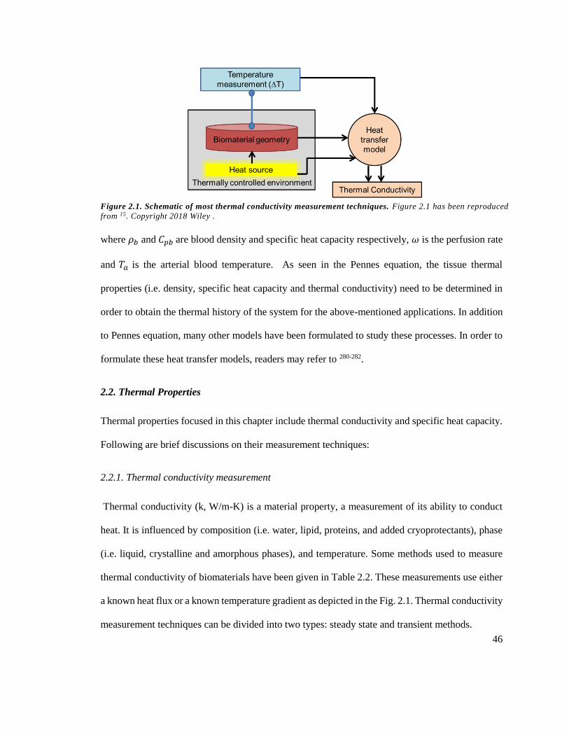
46

where 𝜌𝑏 and 𝐶𝑝𝑏 are blood density and specific heat capacity respectively, 𝜔 is the perfusion rate

and 𝑇𝑎 is the arterial blood temperature. As seen in the Pennes equation, the tissue thermal

properties (i.e. density, specific heat capacity and thermal conductivity) need to be determined in

order to obtain the thermal history of the system for the above-mentioned applications. In addition

to Pennes equation, many other models have been formulated to study these processes. In order to

formulate these heat transfer models, readers may refer to 280-282.

2.2. Thermal Properties

Thermal properties focused in this chapter include thermal conductivity and specific heat capacity.

Following are brief discussions on their measurement techniques:

2.2.1. Thermal conductivity measurement

Thermal conductivity (k, W/m-K) is a material property, a measurement of its ability to conduct

heat. It is influenced by composition (i.e. water, lipid, proteins, and added cryoprotectants), phase

(i.e. liquid, crystalline and amorphous phases), and temperature. Some methods used to measure

thermal conductivity of biomaterials have been given in Table 2.2. These measurements use either

a known heat flux or a known temperature gradient as depicted in the Fig. 2.1. Thermal conductivity

measurement techniques can be divided into two types: steady state and transient methods.

Figure 2.1. Schematic of most thermal conductivity measurement techniques. Figure 2.1 has been reproduced

from 15. Copyright 2018 Wiley .

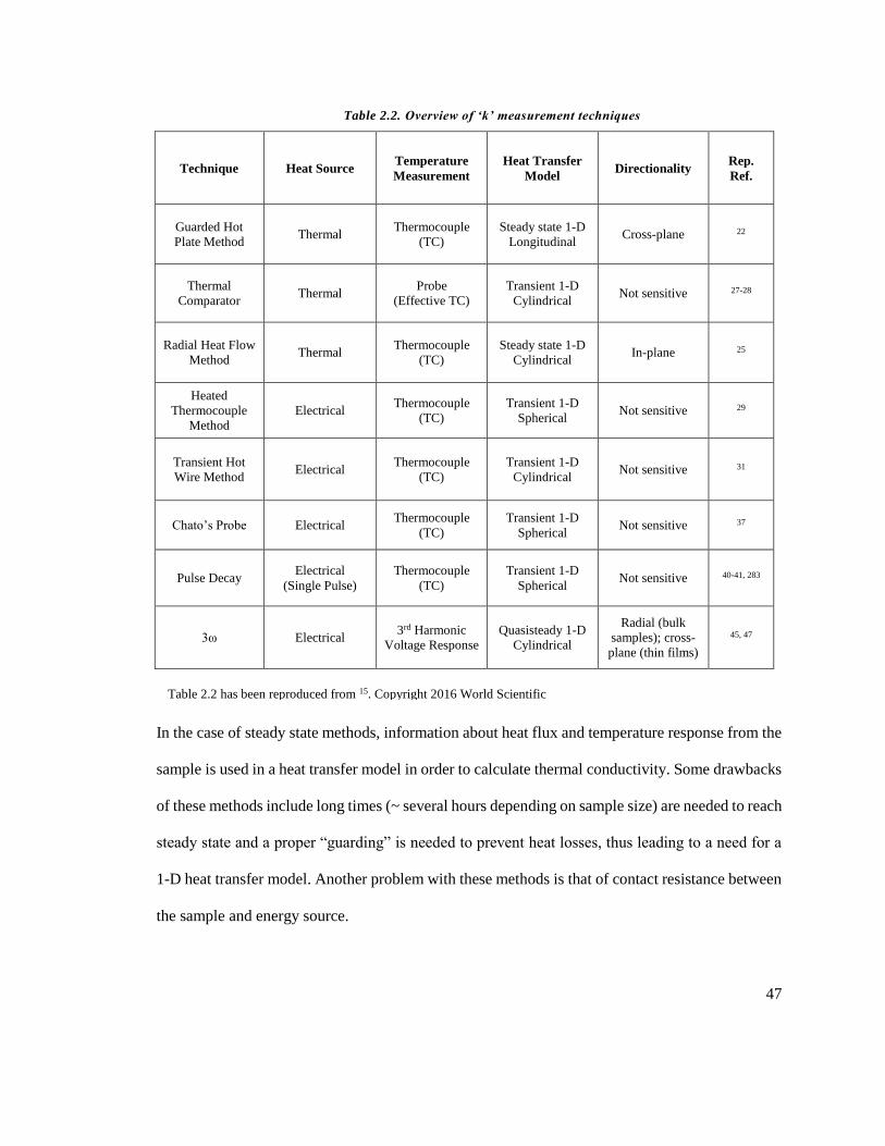
47

In the case of steady state methods, information about heat flux and temperature response from the

sample is used in a heat transfer model in order to calculate thermal conductivity. Some drawbacks

of these methods include long times (~ several hours depending on sample size) are needed to reach

steady state and a proper “guarding” is needed to prevent heat losses, thus leading to a need for a

1-D heat transfer model. Another problem with these methods is that of contact resistance between

the sample and energy source.

Table 2.2. Overview of ‘k’ measurement techniques

Technique Heat Source Temperature

Measurement

Heat Transfer

Model Directionality

Rep.

Ref.

Guarded Hot

Plate Method Thermal

Thermocouple

(TC)

Steady state 1-D

Longitudinal Cross-plane 22

Thermal

Comparator Thermal

Probe

(Effective TC)

Transient 1-D

Cylindrical Not sensitive 27-28

Radial Heat Flow

Method Thermal

Thermocouple

(TC)

Steady state 1-D

Cylindrical In-plane 25

Heated

Thermocouple

Method

Electrical Thermocouple

(TC)

Transient 1-D

Spherical Not sensitive 29

Transient Hot

Wire Method Electrical Thermocouple

(TC)

Transient 1-D

Cylindrical Not sensitive 31

Chato’s Probe Electrical Thermocouple

(TC)

Transient 1-D

Spherical Not sensitive 37

Pulse Decay Electrical

(Single Pulse)

Thermocouple

(TC)

Transient 1-D

Spherical Not sensitive 40-41, 283

3ω Electrical 3rd Harmonic

Voltage Response

Quasisteady 1-D

Cylindrical

Radial (bulk

samples); cross-

plane (thin films)

45, 47

Table 2.2 has been reproduced from 15. Copyright 2016 World Scientific

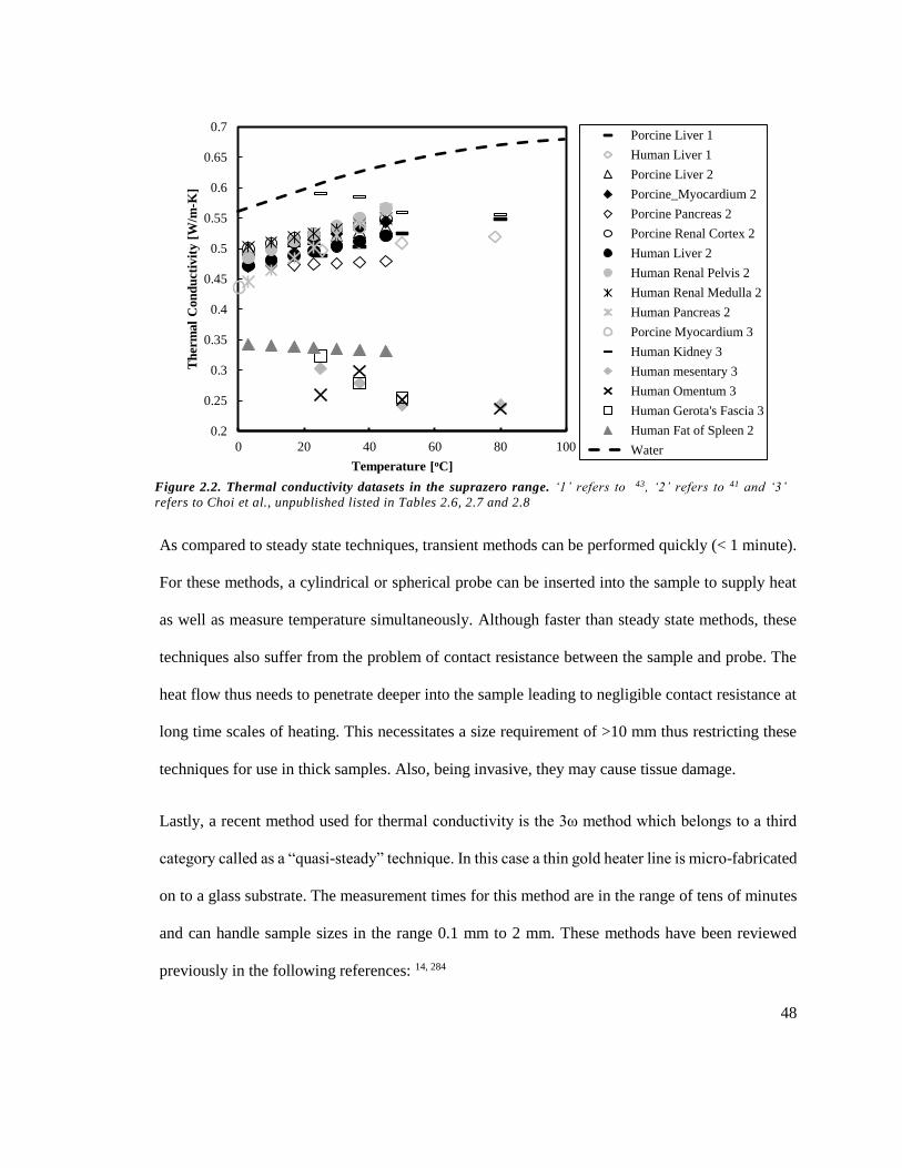
48

As compared to steady state techniques, transient methods can be performed quickly (< 1 minute).

For these methods, a cylindrical or spherical probe can be inserted into the sample to supply heat

as well as measure temperature simultaneously. Although faster than steady state methods, these

techniques also suffer from the problem of contact resistance between the sample and probe. The

heat flow thus needs to penetrate deeper into the sample leading to negligible contact resistance at

long time scales of heating. This necessitates a size requirement of >10 mm thus restricting these

techniques for use in thick samples. Also, being invasive, they may cause tissue damage.

Lastly, a recent method used for thermal conductivity is the 3ω method which belongs to a third

category called as a “quasi-steady” technique. In this case a thin gold heater line is micro-fabricated

on to a glass substrate. The measurement times for this method are in the range of tens of minutes

and can handle sample sizes in the range 0.1 mm to 2 mm. These methods have been reviewed

previously in the following references: 14, 284

Figure 2.2. Thermal conductivity datasets in the suprazero range. ‘1’ refers to 43, ‘2’ refers to 41 and ‘3’

refers to Choi et al., unpublished listed in Tables 2.6, 2.7 and 2.8

0.2

0.25

0.3

0.35

0.4

0.45

0.5

0.55

0.6

0.65

0.7

0 20 40 60 80 100

Th

erm

al

Con

du

ctiv

ity

[W

/m-K

]

Temperature [oC]

Porcine Liver 1

Human Liver 1

Porcine Liver 2

Porcine_Myocardium 2

Porcine Pancreas 2

Porcine Renal Cortex 2

Human Liver 2

Human Renal Pelvis 2

Human Renal Medulla 2

Human Pancreas 2

Porcine Myocardium 3

Human Kidney 3

Human mesentary 3

Human Omentum 3

Human Gerota's Fascia 3

Human Fat of Spleen 2

Water

49

2.2.2. Specific heat capacity measurement

Specific heat capacity (Cp, J/g-°C) is a material property that denotes the amount of heat that should

be transferred to a material to raise its temperature by unit temperature (e.g. degree Celsius). In the

case of biomaterials, it is important to measure their Cp as a function of temperature. For example,

in a wide temperature range (say -150 °C to 20 °C), cryoprotectants pass through different states,

such as liquid, ice and vitrified (amorphous), with each of these phases having a different Cp, thus

necessitating temperature dependent properties. The most common technique used to measure Cp

is differential scanning calorimetry (DSC). DSC is capable of measuring Cp as well as latent heat

of relatively small sample sizes (~3-100 mg) over a wide temperature range of -180°C to 750°C279.

The technique measures the difference in the heat flow rate to the sample and reference pans while

maintaining the same temperature program285. The reference sample has known thermal properties.

This difference in heat flow can then be plotted as function of temperature or time. Using this

measured differential heat flow(∅𝑠𝑎𝑚𝑝𝑙𝑒) , the Cp can then be calculated as follows:

Figure 2.3. Thermal conductivity datasets in the sub-zero and cryogenic range (datasets have been listed

in Tables 2.4 and 2.5).

- - -

0

1

2

3

-150 -100 -50 0 50

Th

erm

al

Co

nd

uct

ivit

y [

W/m

-K]

Temperature [0C]

Porcine Liver

Porcine Pulmonary

VeinPorcine Esophagus

Porcine Phrenic Nerve

Porcine Myocardium

Porcine Fat

Porcine Perpendicular

to FiberPorcine Parallel to

FiberPorcine Leg

Porcine Neck

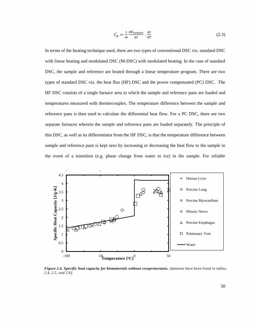
50

𝐶𝑝 =1

𝑚

𝑑∅𝑠𝑎𝑚𝑝𝑙𝑒

𝑑𝑡 .

𝑑𝑡

𝑑𝑇 (2.3)

In terms of the heating technique used, there are two types of conventional DSC viz. standard DSC

with linear heating and modulated DSC (M-DSC) with modulated heating. In the case of standard

DSC, the sample and reference are heated through a linear temperature program. There are two

types of standard DSC viz. the heat flux (HF) DSC and the power compensated (PC) DSC. The

HF DSC consists of a single furnace area in which the sample and reference pans are loaded and

temperatures measured with thermocouples. The temperature difference between the sample and

reference pans is then used to calculate the differential heat flow. For a PC DSC, there are two

separate furnaces wherein the sample and reference pans are loaded separately. The principle of

this DSC, as well as its differentiator from the HF DSC, is that the temperature difference between

sample and reference pans is kept zero by increasing or decreasing the heat flow to the sample in

the event of a transition (e.g. phase change from water to ice) in the sample. For reliable

Figure 2.4. Specific heat capacity for biomaterials without cryoprotectants. (datasets have been listed in tables.

2.4, 2.5, and 2.6).

- -

0

0.5

1

1.5

2

2.5

3

3.5

4

4.5

-100 -50 0 50

Sp

ecif

ic H

eat

Ca

pa

city

[J

/g-K

]

Temperature [oC]

Human Liver

Porcine Lung

Porcine Myocardium

Phrenic Nerve

Porcine Esophagus

Pulmonary Vein

Water

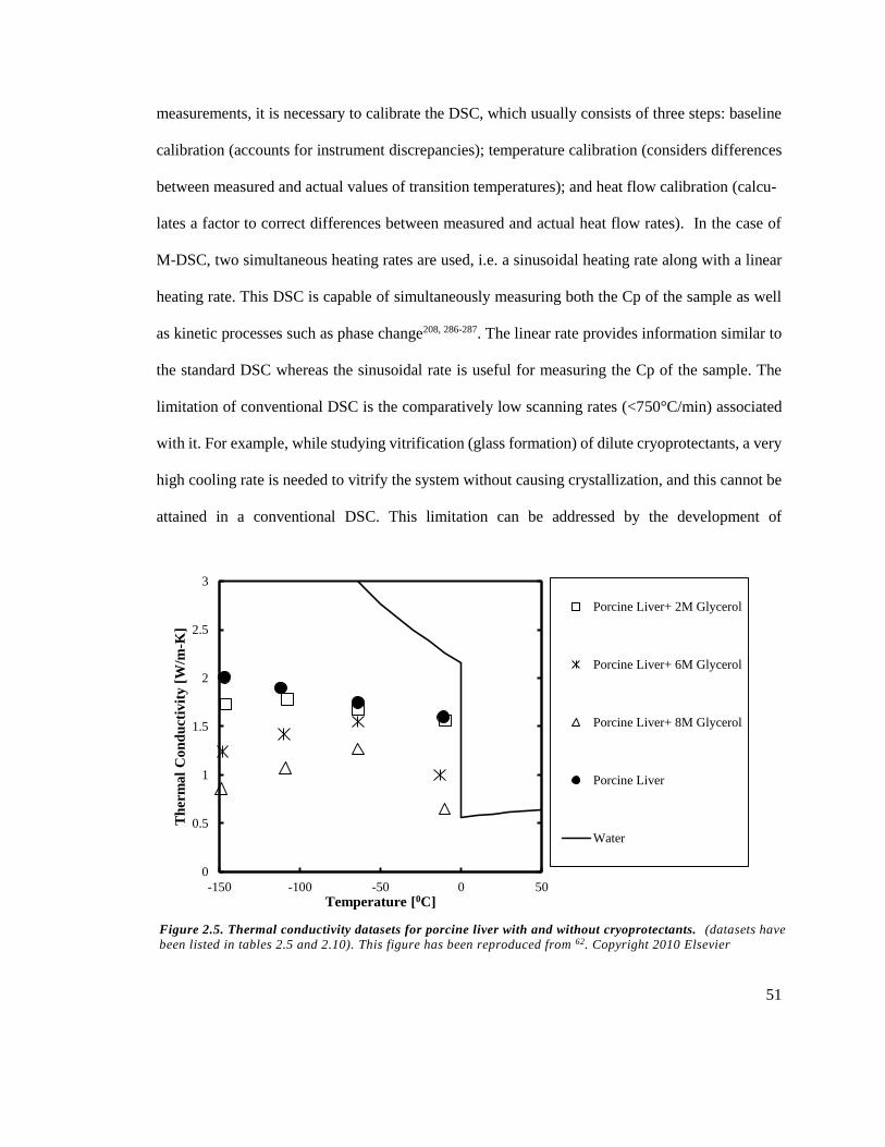
51

measurements, it is necessary to calibrate the DSC, which usually consists of three steps: baseline

calibration (accounts for instrument discrepancies); temperature calibration (considers differences

between measured and actual values of transition temperatures); and heat flow calibration (calcu-

lates a factor to correct differences between measured and actual heat flow rates). In the case of

M-DSC, two simultaneous heating rates are used, i.e. a sinusoidal heating rate along with a linear

heating rate. This DSC is capable of simultaneously measuring both the Cp of the sample as well

as kinetic processes such as phase change208, 286-287. The linear rate provides information similar to

the standard DSC whereas the sinusoidal rate is useful for measuring the Cp of the sample. The

limitation of conventional DSC is the comparatively low scanning rates (<750°C/min) associated

with it. For example, while studying vitrification (glass formation) of dilute cryoprotectants, a very

high cooling rate is needed to vitrify the system without causing crystallization, and this cannot be

attained in a conventional DSC. This limitation can be addressed by the development of

Figure 2.5. Thermal conductivity datasets for porcine liver with and without cryoprotectants. (datasets have

been listed in tables 2.5 and 2.10). This figure has been reproduced from 62. Copyright 2010 Elsevier

0

0.5

1

1.5

2

2.5

3

-150 -100 -50 0 50

Th

erm

al

Co

nd

uct

ivit

y [

W/m

-K]

Temperature [0C]

Porcine Liver+ 2M Glycerol



Porcine Liver

Water

52

nanocalorimetry67 on a silicon-based membrane that can work with a very small sample weight (~

10 ng), which leads to the possibility of very high heating or cooling rates (~107 °C/min).

2.3 Factors That Affect Thermal Property Values

The focus of this chapter is on organizing literature data for thermal conductivity and specific heat

capacity of human and porcine systems in the cryogenic, subzero and suprazero temperature ranges.

All the data provided here has resulted from actual measurements presented in primary research

papers. Apart from primary papers, there are some databases available such as the one by IT'IS

Foundation associated with ETH Zurich288. In addition there are reviews on this topic such as73, 289-

290. Blood perfusion results have not been taken into account in the data presented in this chapter.

The interested reader may refer to31, 284, 291-293 for details regarding perfusion associated

measurements. Some factors that influence the thermal properties of biomaterials are discussed

below:

2.3.1. High temperature effects (37 °C – 100 °C): Protein phase change and water loss

In the case of high temperatures, the values of thermal properties generally rise from 0 °C up to

roughly 45 °C where protein denaturation and water loss can play a role. After 45 °C there is much

Figure 2.6. Specific heat capacity for porcine liver with and without cryoprotectants. (datasets have been

listed in tables 2.5 and 2.10). This figure has been reproduced from 62. Copyright Elsevier 2010

0

0.5

1

1.5

2

2.5

3

3.5

4

4.5

-150 -100 -50 0 50

Sp

ecif

ic H

eat

Ca

pa

city

[J

/g-K

]

Temperature [oC]

Porcine Liver

Porcine Liver+ 2M

Glycerol

Porcine Liver+6M

Glycerol

Porcine Liver+ 8M

Glycerol

Water

Glass

Transition

53

less data, although it would appear that water loss plays a more prominent role as compared to

protein denaturation resulting in lower values of ‘k’ and ‘Cp’. This drop in thermal conductivity

can be seen in Fig. 2.2 above for human kidney, mesentery, omentum and gerota’s fascia. The

lower ‘k’ values for mesentery, gerota’s fascia, omentum are due to a higher fat content in these

systems. Similarly, human fat of spleen also exhibits lower ‘k’ values due to the presence of fat in

the system. Protein denaturation occurs as a heat absorption event over a finite temperature range.

The interested reader can refer to 31, 43, 294 for more details regarding these high temperature effects.

2.3.2. Low temperature effects (37 °C – -196 °C): Water phase change and cryoprotectant effects

Thermal properties of biomaterials at low temperatures are affected by two factors: phase change

(water to ice) and the presence of cryoprotectants. Freezing or crystallization of water to ice results

in an increase in thermal conductivity values at subzero temperatures as ice has a higher thermal

conductivity compared to water. This general trend of increasing values of thermal conductivity

can be observed in Fig. 2.3 above for various biomaterials. In contrast, specific heat capacity values

Figure 2.7. Thermal conductivity datasets for cryoprotectants (datasets have been listed in table. 2.9)

0

0.5

1

1.5

2

2.5

3

-150 -100 -50 0 50

Th

erm

al

Con

du

ctiv

ity

[W

/m-K

]

Temperature [0C]

2M Glycerol

6M Glycerol

2M DMSO

6M DMSO

10M DMSO

DP6 Euro Collins Solution

US Gel

Water

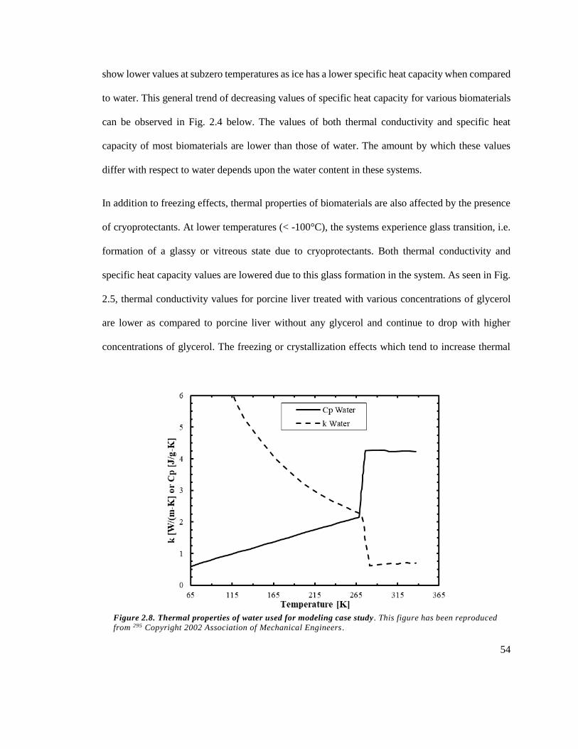
54

show lower values at subzero temperatures as ice has a lower specific heat capacity when compared

to water. This general trend of decreasing values of specific heat capacity for various biomaterials

can be observed in Fig. 2.4 below. The values of both thermal conductivity and specific heat

capacity of most biomaterials are lower than those of water. The amount by which these values

differ with respect to water depends upon the water content in these systems.

In addition to freezing effects, thermal properties of biomaterials are also affected by the presence

of cryoprotectants. At lower temperatures (< -100°C), the systems experience glass transition, i.e.

formation of a glassy or vitreous state due to cryoprotectants. Both thermal conductivity and

specific heat capacity values are lowered due to this glass formation in the system. As seen in Fig.

2.5, thermal conductivity values for porcine liver treated with various concentrations of glycerol

are lower as compared to porcine liver without any glycerol and continue to drop with higher

concentrations of glycerol. The freezing or crystallization effects which tend to increase thermal

Figure 2.8. Thermal properties of water used for modeling case study. This figure has been reproduced

from 295 Copyright 2002 Association of Mechanical Engineers.

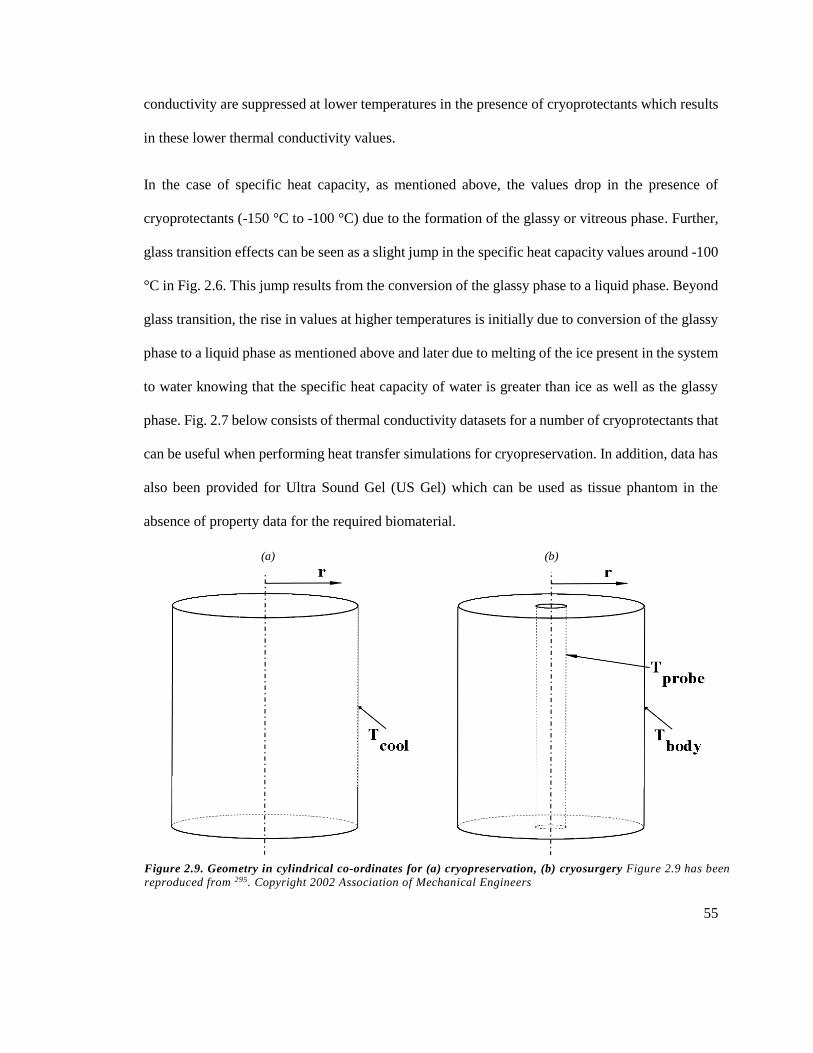
55

conductivity are suppressed at lower temperatures in the presence of cryoprotectants which results

in these lower thermal conductivity values.

In the case of specific heat capacity, as mentioned above, the values drop in the presence of

cryoprotectants (-150 °C to -100 °C) due to the formation of the glassy or vitreous phase. Further,

glass transition effects can be seen as a slight jump in the specific heat capacity values around -100

°C in Fig. 2.6. This jump results from the conversion of the glassy phase to a liquid phase. Beyond

glass transition, the rise in values at higher temperatures is initially due to conversion of the glassy

phase to a liquid phase as mentioned above and later due to melting of the ice present in the system

to water knowing that the specific heat capacity of water is greater than ice as well as the glassy

phase. Fig. 2.7 below consists of thermal conductivity datasets for a number of cryoprotectants that

can be useful when performing heat transfer simulations for cryopreservation. In addition, data has

also been provided for Ultra Sound Gel (US Gel) which can be used as tissue phantom in the

absence of property data for the required biomaterial.

(a) (b)

Figure 2.9. Geometry in cylindrical co-ordinates for (a) cryopreservation, (b) cryosurgery Figure 2.9 has been

reproduced from 295. Copyright 2002 Association of Mechanical Engineers

56

The general trends seen in Fig. 2.7 are same as those observed in the case of porcine liver treated

with glycerol in Fig. 2.5. The thermal conductivity values increase at lower temperatures due to

ice formation whereas the presence of the glassy phase due to cryoprotectants at temperatures < -

100 °C results in lower or constant thermal conductivity values. Also, as the concentration of

cryoprotectants increases, the thermal conductivity values are lowered as the ice formation is

suppressed by the glassy phase. These trends can be seen in Fig. 2.7 for DMSO and glycerol. The

interested reader is directed to 36, 44, 81 for more discussion regarding low temperature and

cryoprotectants related ‘k’ and ‘Cp’ measurements.

2.4. Modeling Case Study

This section provides an example from 295 showing the importance of temperature dependent

properties for numerical predictions of heat transfer applied for cryopreservation and cryosurgery.

A numerical technique known as the Enthalpy method has been used to solve the heat transfer with

phase change problem for cryopreservation and cryosurgery. The governing equation for this

method296 is given as follows:

(a) (b)

Figure 2.10. Numerical simulation for cryopreservation. (a) Phase front propagation (Lines with symbols

denote temperature dependent properties) (b) Thermal history for a cylinder (Lines with symbols denote

temperature dependent properties). Figures 2.10 (a) & b have been reproduced from 295. Copyright 2002

Association of Mechanical Enigneers

0

0.02

0.04

0.06

0.08

0 600 1200 1800 2400

Dis

tan

ce [

m]

Time [s]

CartesianCylindricalSphericalCartesian (T)Cylindrical (T)Spherical (T)

-

-

-

-150

-100

-50

0

50

0 500 1000 1500 2000

Tem

per

atu

re [

°C]

Time [s]

r=0 cm

r=2 cm

r=4 cm

r=6 cm

57

𝜌𝜕𝐻(𝑇)

𝜕𝑡= ∇ ∙ (𝑘∇𝑇) + 𝑔(𝑇) (2.4)

where 𝜌, 𝐻, 𝑇, 𝑡, 𝑘 𝑎𝑛𝑑 𝑔(𝑇) are density, enthalpy, temperature, time, thermal conductivity and

heat generation per unit volume.

Eqn. (2.4) is a modified version of the transient heat equation where enthalpy and temperature are

dependent variables. In other techniques used for solving phase change, such as source tracking

method, two equations are needed to solve for the frozen and unfrozen region. In addition, an

energy balance equation is included to track the interface between these two regions. The advantage

of the enthalpy method over such methods is that a single equation in terms of enthalpy is used to

solve for both regions and thus no tracking equation is needed. In the case of pure materials like

water, phase change happens at a single temperature whereas for biomaterials, phase change occurs

over a temperature range called a mushy zone. The enthalpy method can be used to solve for both

these materials.

For information regarding this method and its applicability to cryosurgery and cryopreservation,

readers may refer to 14, 274, 297. Constant as well as temperature dependent thermal properties of

water have been used in these analyses.

Table 2.3. Organization of thermal property datasets

Table Number Description

4 & 5 Porcine Systems at subzero temperatures I and II

6 Porcine Systems at suprazero temperatures

7 & 8 Human Systems at suprazero temperatures I and II

9 Cryoprotectants

10 Porcine liver treated with cryoprotectants

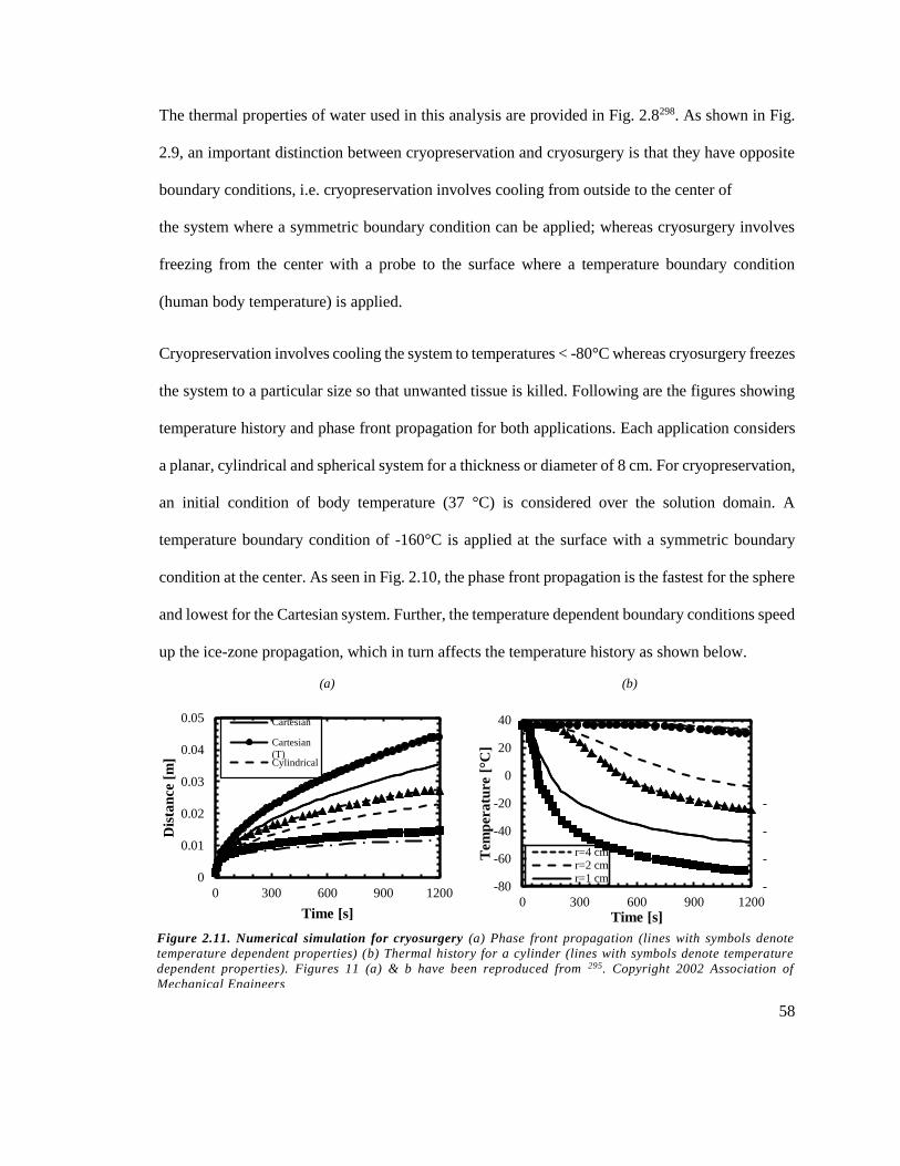
58

The thermal properties of water used in this analysis are provided in Fig. 2.8298. As shown in Fig.

2.9, an important distinction between cryopreservation and cryosurgery is that they have opposite

boundary conditions, i.e. cryopreservation involves cooling from outside to the center of

the system where a symmetric boundary condition can be applied; whereas cryosurgery involves

freezing from the center with a probe to the surface where a temperature boundary condition

(human body temperature) is applied.

Cryopreservation involves cooling the system to temperatures < -80°C whereas cryosurgery freezes

the system to a particular size so that unwanted tissue is killed. Following are the figures showing

temperature history and phase front propagation for both applications. Each application considers

a planar, cylindrical and spherical system for a thickness or diameter of 8 cm. For cryopreservation,

an initial condition of body temperature (37 °C) is considered over the solution domain. A

temperature boundary condition of -160°C is applied at the surface with a symmetric boundary

condition at the center. As seen in Fig. 2.10, the phase front propagation is the fastest for the sphere

and lowest for the Cartesian system. Further, the temperature dependent boundary conditions speed

up the ice-zone propagation, which in turn affects the temperature history as shown below.

(a) (b)

Figure 2.11. Numerical simulation for cryosurgery (a) Phase front propagation (lines with symbols denote

temperature dependent properties) (b) Thermal history for a cylinder (lines with symbols denote temperature

dependent properties). Figures 11 (a) & b have been reproduced from 295. Copyright 2002 Association of

Mechanical Engineers

0

0.01

0.02

0.03

0.04

0.05

0 300 600 900 1200

Dis

tan

ce [

m]

Time [s]

Cartesian

Cartesian

(T)Cylindrical

-

-

-

-

-80

-60

-40

-20

0

20

40

0 300 600 900 1200

Tem

per

atu

re [

°C]

Time [s]

r=4 cmr=2 cmr=1 cm

59

In the case of cryosurgery, a temperature boundary condition of -160°C (applied by a cryoprobe)

is considered at a radius of 1.5 mm for the radial systems or at one of the surfaces (0 mm) for the

Cartesian system. The second boundary condition considers a domain large enough to assume semi-

infinite conditions (assuming the system is at body temperature). The same thermal properties as

cryopreservation are used in this analysis. As seen from the results in Fig. 2.11, the phase front

propagates fastest for the Cartesian system and slowest for the sphere. As seen before, this

propagation is faster when temperature dependent properties are used. The interested reader may

refer to 295 for more information regarding this analysis.

Table 2.4. Thermal properties of porcine systems at sub-zero temperatures- i

System Type

Thermal

Conductivity

[W/mK]

Specific Heat

Capacity

[J/gK]

Reference

Pulmonary Vein

0.57(35.9°C) 3.34(39°C)

‘k’— 103

‘Cp’— Unpublished,

BHMT, UMN

0.47(14.42°C) 3.27(5°C)

1.14(-13.77°C) 2.82(1°C)

1.44(-30.9°C) 1.87(-34°C)

— 1.74(-46°C)

— 1.49(-72°C)

— 1.38(-84°C)

Esophagus

0.55(35.58°C) 3.49(39°C)

0.48(13.99°C) 3.39(9°C)

1.61(-17.43°C) 1.92(-30°C)

1.84(-36.95°C) 1.63(-52°C)

— 1.43(-74°C)

— 1.29(-86°C)

Phrenic Nerve

0.45(35.53°C) 3.57(33°C)

0.5(14.01°C) 3.47(13°C)

1.29(-14.01°C) 2.44(-18°C)

1.84(-34.18°C) 1.83(-30°C)

— 1.7(-44°C)

— 1.5(-66°C)

— 1.35(-90°C)

BHMT, UMN: Bioheat & Mass Transfer Lab, University of Minnesota

n: Number of repetitions

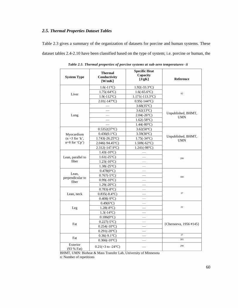
60

2.5. Thermal Properties Dataset Tables

Table 2.3 gives a summary of the organization of datasets for porcine and human systems. These

dataset tables 2.4-2.10 have been classified based on the type of system; i.e. porcine or human, the

Table 2.5. Thermal properties of porcine systems at sub-zero temperatures- ii

System Type

Thermal

Conductivity

[W/mK]

Specific Heat

Capacity

[J/gK]

Reference

Liver

1.6(-11°C) 1.92(-33.3°C)

62 1.75(-64°C) 1.6(-65.6°C)

1.9(-112°C) 1.171(-113.3°C)

2.01(-147°C) 0.95(-144°C)

Lung

— 3.68(35°C)

Unpublished, BHMT,

UMN

— 3.62(13°C)

— 2.04(-26°C)

— 1.62(-58°C)

— 1.44(-80°C)

Myocardium

(n =3 for ‘k’,

n=8 for ‘Cp’)

0.5352(37°C) 3.62(50°C)

Unpublished, BHMT,

UMN

0.436(0.1°C) 3.59(30°C)

1.743(-26.25°C) 1.75(-34°C)

2.046(-94.45°C) 1.508(-62°C)

2.312(-147.9°C) 1.241(-98°C)

Lean, parallel to

fiber

1.43(-10°C) —

299 1.61(-25°C) —

1.23(-10°C) —

1.38(-25°C) —

Lean,

perpendicular to

fiber

0.478(0°C) —

300 0.767(-5°C) —

0.99(-10°C) —

1.29(-20°C) —

Lean, neck

0.783(-8°C) — 37 0.835(-8.4°C) —

0.408(-9°C) —

Leg

0.49(6°C) — 22 1.28(-8°C) —

1.3(-14°C) —

Fat

0.186(0°C) —

{Cherneeva, 1956 #145} 0.227(-5°C) —

0.254(-10°C) —

0.291(-20°C) —

Fat 0.36(-9.1°C) — 37

0.366(-10°C) — 301

Exterior

(93 % Fat) 0.21(+3 to -24°C) — 299



61

temperature range considered; i.e. subzero or suprazero, thermal properties of cryoprotectants and

effect of cryoprotectants on porcine liver.

For porcine liver in Table 2.6 from 43, specific heat data between 31°C-85°C is not directly added

as there is an endothermic heat release associated with protein denaturation in that range. The

specific heat capacity available in that range is apparent specific heat and not sensible specific heat

capacity. The interested reader may refer to 43 for more details. The thermal conductivity

measurements for porcine and human systems from 41 were carried out at temperatures 3, 10, 17,

23, 37 and 45 °C. Linear regression fit constants were provided to be used in the following formula

to calculate thermal conductivity:

𝑘 = 𝑘0 + 𝑘1𝑇 (2.5)

Where 𝑘0 [𝑊

𝑚𝐾] and 𝑘1 [

𝑊

𝑚𝐾2] are regression fit constants and 𝑇 is the temperature in °C.

Thermal conductivity values have been calculated using the above formula for temperatures 10, 23,

37 and 45 °C.

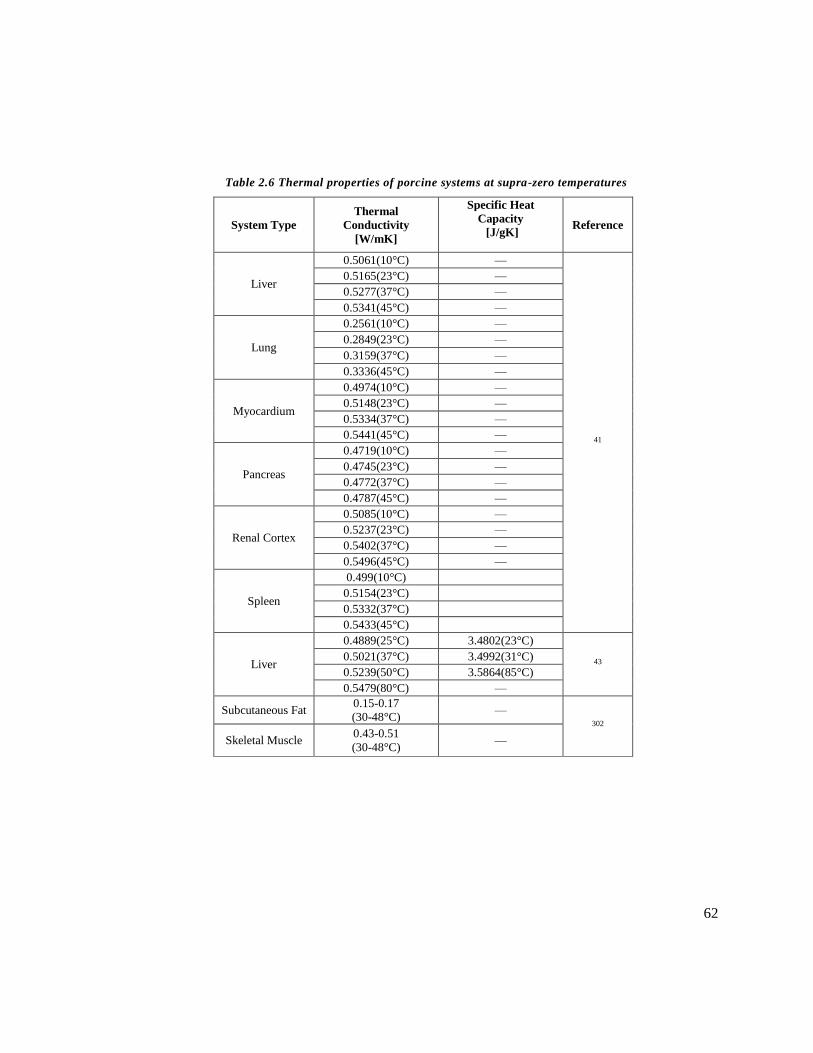
62

Table 2.6 Thermal properties of porcine systems at supra-zero temperatures

System Type

Thermal

Conductivity

[W/mK]

Specific Heat

Capacity

[J/gK]

Reference

Liver

0.5061(10°C) —

41

0.5165(23°C) —

0.5277(37°C) —

0.5341(45°C) —

Lung

0.2561(10°C) —

0.2849(23°C) —

0.3159(37°C) —

0.3336(45°C) —

Myocardium

0.4974(10°C) —

0.5148(23°C) —

0.5334(37°C) —

0.5441(45°C) —

Pancreas

0.4719(10°C) —

0.4745(23°C) —

0.4772(37°C) —

0.4787(45°C) —

Renal Cortex

0.5085(10°C) —

0.5237(23°C) —

0.5402(37°C) —

0.5496(45°C) —

Spleen

0.499(10°C)

0.5154(23°C)

0.5332(37°C)

0.5433(45°C)

Liver

0.4889(25°C) 3.4802(23°C)

43 0.5021(37°C) 3.4992(31°C)

0.5239(50°C) 3.5864(85°C)

0.5479(80°C) —

Subcutaneous Fat 0.15-0.17

(30-48°C) —

302

Skeletal Muscle 0.43-0.51

(30-48°C) —

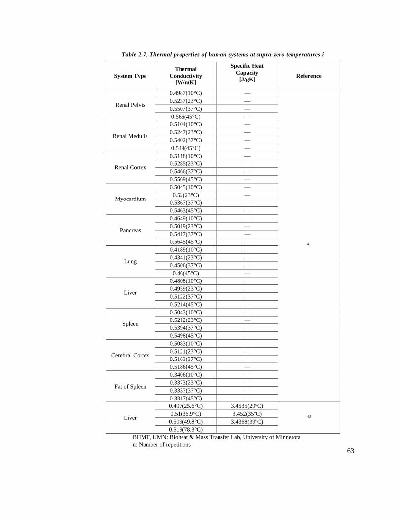
63

Table 2.7. Thermal properties of human systems at supra-zero temperatures i

System Type

Thermal

Conductivity

[W/mK]

Specific Heat

Capacity

[J/gK]

Reference

Renal Pelvis

0.4987(10°C) —

41

0.5237(23°C) —

0.5507(37°C) —

0.566(45°C) —

Renal Medulla

0.5104(10°C) —

0.5247(23°C) —

0.5402(37°C) —

0.549(45°C) —

Renal Cortex

0.5118(10°C) —

0.5285(23°C) —

0.5466(37°C) —

0.5569(45°C) —

Myocardium

0.5045(10°C) —

0.52(23°C) —

0.5367(37°C) —

0.5463(45°C) —

Pancreas

0.4649(10°C) —

0.5019(23°C) —

0.5417(37°C) —

0.5645(45°C) —

Lung

0.4189(10°C) —

0.4341(23°C) —

0.4506(37°C) —

0.46(45°C) —

Liver

0.4808(10°C) —

0.4959(23°C) —

0.5122(37°C) —

0.5214(45°C) —

Spleen

0.5043(10°C) —

0.5212(23°C) —

0.5394(37°C) —

0.5498(45°C) —

Cerebral Cortex

0.5083(10°C) —

0.5121(23°C) —

0.5163(37°C) —

0.5186(45°C) —

Fat of Spleen

0.3406(10°C) —

0.3373(23°C) —

0.3337(37°C) —

0.3317(45°C) —

Liver

0.497(25.6°C) 3.4535(29°C)

43 0.51(36.9°C) 3.452(35°C)

0.509(49.8°C) 3.4368(39°C)

0.519(78.3°C) —



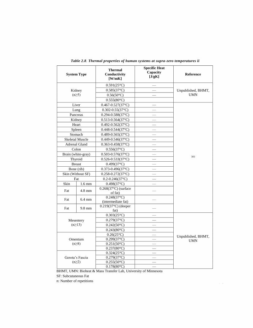
64

Table 2.8. Thermal properties of human systems at supra-zero temperatures ii

System Type

Thermal

Conductivity

[W/mK]

Specific Heat

Capacity

[J/gK]

Reference

Kidney

(n≥5)

0.591(25°C) —

Unpublished, BHMT,

UMN

0.585(37°C) —

0.56(50°C) —

0.555(80°C)

Liver 0.467-0.527(37°C) —

303

Lung 0.302-0.55(37°C) —

Pancreas 0.294-0.588(37°C) —

Kidney 0.513-0.564(37°C) —

Heart 0.492-0.562(37°C) —

Spleen 0.448-0.544(37°C) —

Stomach 0.489-0.565(37°C) —

Skeletal Muscle 0.449-0.546(37°C) —

Adrenal Gland 0.363-0.458(37°C) —

Colon 0.556(37°C) —

Brain (white-gray) 0.503-0.576(37°C) —

Thyroid 0.526-0.533(37°C) —

Breast 0.499(37°C) —

Bone (rib) 0.373-0.496(37°C) —

Skin (Without SF) 0.258-0.272(37°C) —

Fat 0.2-0.246(37°C) —

Skin 1.6 mm 0.498(37°C) —

Fat 4.8 mm 0.268(37°C) (surface

of fat) —

Fat 6.4 mm 0.248(37°C)

(intermediate fat) —

Fat 9.8 mm 0.219(37°C) (deeper

fat) —

Mesentery

(n≥13)

0.303(25°C) —

Unpublished, BHMT,

UMN

0.279(37°C) —

0.242(50°C) —

0.243(80°C) —

Omentum

(n≥8)

0.26(25°C) —

0.299(37°C) —

0.251(50°C) —

0.237(80°C) —

Gerota’s Fascia

(n≥2)

0.324(25°C) —

0.279(37°C) —

0.255(50°C) —

0.178(80°C) —


SF: Subcutaneous Fat


65

Table 2.9. Thermal properties of cryoprotectants

System Type

Thermal

Conductivity

[W/mK]

Specific Heat

Capacity

[J/gK]

Reference

US Gel

(Tissue Phantom)

0.52(38°C) 3.7(39°C)

274

0.47(-2°C) 3.84(10°C)

1.71(-45°C) 2.06(-50°C)

2.3(-85°C) 1.45(-100°C)

2.28(-125°C) 0.94(-149°C)

2M Glycerol

Solution

1.61(-27°C) 3.781(-5°C)

14

1.96(-64°C) 1.712(-73°C)

2.15(-108°C) 1.206(-110°C)

2.25(-147°C) 0.903(-148°C)

6M Glycerol

Solution

0.82(-28°C) 2.984(-20°C)

1.27(-65°C) 1.996(-73°C)

1.05(-108°C) 1.114(-110°C)

0.97(-147°C) 0.834(-148°C)

2M DMSO Solution

1.443(-20°C) —

35

1.69(-60°C) —

1.933(-100°C) —

2.203(-140°C) —

6M DMSO Solution

0.378(-20°C) —

0.592(-60°C) —

0.721(-100°C) —

0.773(-140°C) —

10M DMSO Solution

0.28(-20°C) —

0.27(-60°C) —

0.264(-100°C) —

0.253(-140°C) —

DP6 in EC Solution

(cryoprotectant)

0.317(-20°C) —

36 0.53(-40°C) —

0.356(-70°C) —

0.35(-140°C) —

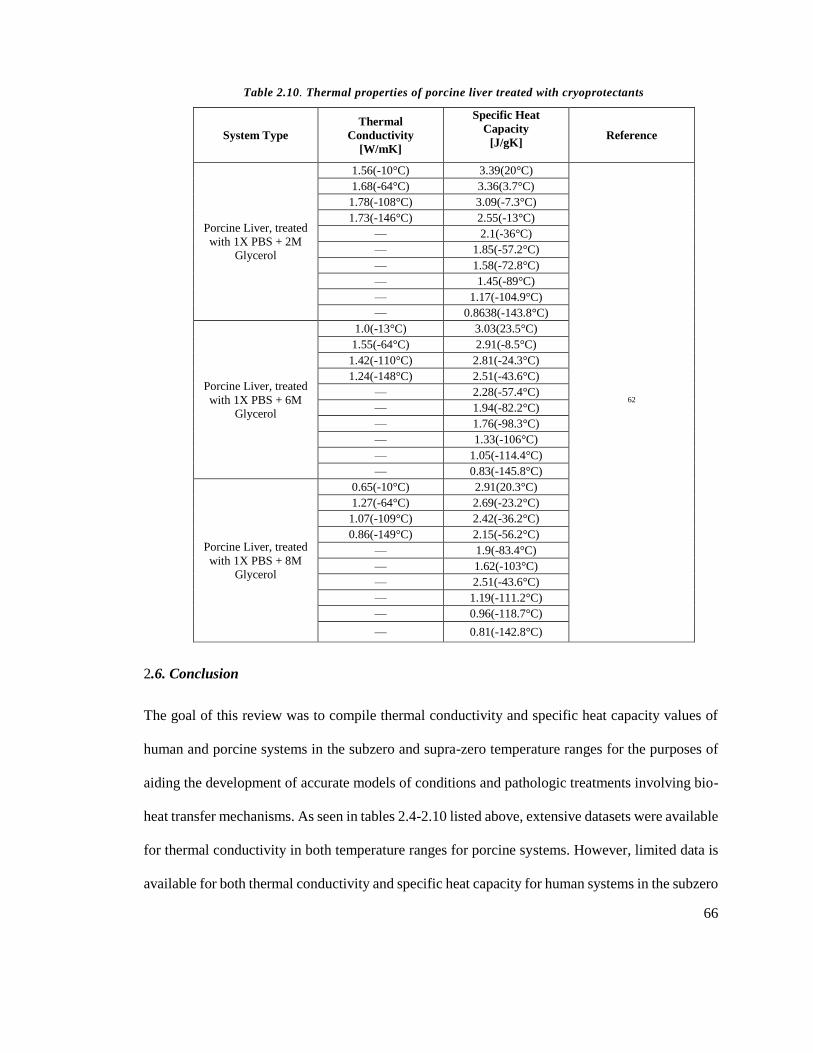
66

2.6. Conclusion

The goal of this review was to compile thermal conductivity and specific heat capacity values of

human and porcine systems in the subzero and supra-zero temperature ranges for the purposes of

aiding the development of accurate models of conditions and pathologic treatments involving bio-

heat transfer mechanisms. As seen in tables 2.4-2.10 listed above, extensive datasets were available

for thermal conductivity in both temperature ranges for porcine systems. However, limited data is

available for both thermal conductivity and specific heat capacity for human systems in the subzero

Table 2.10. Thermal properties of porcine liver treated with cryoprotectants

System Type

Thermal

Conductivity

[W/mK]

Specific Heat

Capacity

[J/gK]

Reference

Porcine Liver, treated

with 1X PBS + 2M

Glycerol

1.56(-10°C) 3.39(20°C)

62

1.68(-64°C) 3.36(3.7°C)

1.78(-108°C) 3.09(-7.3°C)

1.73(-146°C) 2.55(-13°C)

— 2.1(-36°C)

— 1.85(-57.2°C)

— 1.58(-72.8°C)

— 1.45(-89°C)

— 1.17(-104.9°C)

— 0.8638(-143.8°C)


with 1X PBS + 6M

Glycerol

1.0(-13°C) 3.03(23.5°C)

1.55(-64°C) 2.91(-8.5°C)

1.42(-110°C) 2.81(-24.3°C)

1.24(-148°C) 2.51(-43.6°C)

— 2.28(-57.4°C)

— 1.94(-82.2°C)

— 1.76(-98.3°C)

— 1.33(-106°C)

— 1.05(-114.4°C)

— 0.83(-145.8°C)


with 1X PBS + 8M

Glycerol

0.65(-10°C) 2.91(20.3°C)

1.27(-64°C) 2.69(-23.2°C)

1.07(-109°C) 2.42(-36.2°C)

0.86(-149°C) 2.15(-56.2°C)

— 1.9(-83.4°C)

— 1.62(-103°C)

— 2.51(-43.6°C)

— 1.19(-111.2°C)

— 0.96(-118.7°C)

— 0.81(-142.8°C)

67

temperature range. Another area where there is limited data available is the effect of cryoprotectants

on biomaterials. As was seen in Figs. 2.5 and 2.6 for porcine liver, thermal properties of

biomaterials are affected by the presence of cryoprotectants due to the presence of a vitreous or

amorphous phase in addition to crystallization. Future thermal property measurements can be

conducted by incorporating these changes to get a more accurate behavior to be applied in a model.

As seen in the modeling case studies section, the importance of temperature dependent properties

versus constant properties is reflected from the significant differences in the thermal histories for

planar, cylindrical and spherical systems using water properties. Similar analyses can be performed

by considering thermal properties of other biomaterials presented in this chapter.


Acknowledgments Funding for this work was provided by the Center for Research in Education

and Simulation Technologies at the University of Minnesota and the National Science Foundation

(Award Number CBET 1236760).

68

3. A Micro-Thermal Sensor for Focal Therapy Applications

The following chapter appeared in publication:

Natesan, H., & Bischof, J. C. (2017). Multiscale thermal property measurements for biomedical

applications. ACS Biomaterials Science & Engineering, 3(11), 2669-2691.

3.1. Introduction

Focal energy based therapies have a long use in the treatment of cancer, cardiovascular and neural

disease1, 19, 271. As the technique evolves, there are increasingly thin and complex tissue anatomies

where focal therapies and freezing are being applied that require sub mm monitoring accuracy to

avoid debilitating side effects. For instance, cryogenic approaches to treatment of atrial fibrillation

are increasingly being used in the pulmonary vein (PV) which is only 1 – 2 mm thick304-307. This

treatment in thin PV often suffers from over and under-freezing suggesting a need for better

monitoring. Unfortunately, traditional clinical imaging has difficulty monitoring at or below the

mm scale, which is of the order of thickness of the PV itself. For this reason it is not surprising

that in a pilot computed tomography (CT) study, we were unable to visualize the PV or the freezing

process within it308. So, despite the past successes of clinical image guidance for cryoablation in

cm sized tissues309-311, clinical imaging alone lacks the spatial resolution to successfully monitor

freezing in the PV or other thin tissue structures (1-2 mm thick).

Thus, there is an urgent need to monitor tissue contact, thickness and freeze completion during

treatment which relatively low-resolution clinical imaging cannot provide at the millimeter to sub

millimeter scale. Here we provide evidence that a future solution could involve a micro- thermal

sensor based on the “3ω” technique of thermal conductivity measurement (Fig. 3.1)47. The sensor

comprises a thin metallic heater line, typically made of gold, and deposited on a flat glass substrate

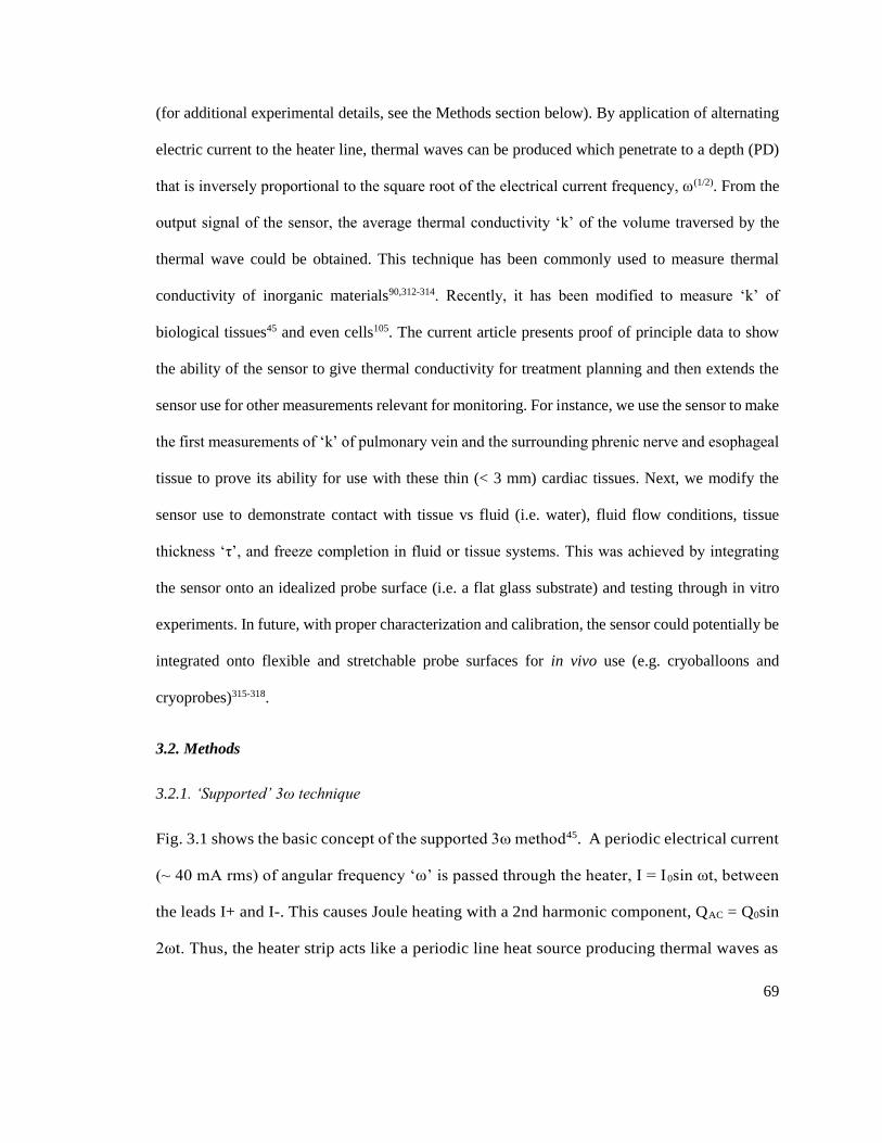
69

(for additional experimental details, see the Methods section below). By application of alternating

electric current to the heater line, thermal waves can be produced which penetrate to a depth (PD)

that is inversely proportional to the square root of the electrical current frequency, ω(1/2). From the

output signal of the sensor, the average thermal conductivity ‘k’ of the volume traversed by the

thermal wave could be obtained. This technique has been commonly used to measure thermal

conductivity of inorganic materials90,312-314. Recently, it has been modified to measure ‘k’ of

biological tissues45 and even cells105. The current article presents proof of principle data to show

the ability of the sensor to give thermal conductivity for treatment planning and then extends the

sensor use for other measurements relevant for monitoring. For instance, we use the sensor to make

the first measurements of ‘k’ of pulmonary vein and the surrounding phrenic nerve and esophageal

tissue to prove its ability for use with these thin (< 3 mm) cardiac tissues. Next, we modify the

sensor use to demonstrate contact with tissue vs fluid (i.e. water), fluid flow conditions, tissue

thickness ‘τ’, and freeze completion in fluid or tissue systems. This was achieved by integrating

the sensor onto an idealized probe surface (i.e. a flat glass substrate) and testing through in vitro

experiments. In future, with proper characterization and calibration, the sensor could potentially be

integrated onto flexible and stretchable probe surfaces for in vivo use (e.g. cryoballoons and

cryoprobes)315-318.

3.2. Methods

3.2.1. ‘Supported’ 3ω technique

Fig. 3.1 shows the basic concept of the supported 3ω method45. A periodic electrical current

(~ 40 mA rms) of angular frequency ‘ω’ is passed through the heater, I = I0sin ωt, between

the leads I+ and I-. This causes Joule heating with a 2nd harmonic component, QAC = Q0sin

2ωt. Thus, the heater strip acts like a periodic line heat source producing thermal waves as

70

shown in Fig. 3.1 (b, d). The exact analytical solution to this conduction problem is well

known45, 47, 319. Thermal waves propagate and decay radially away from the heater and PD

can be calculated using Eqn. (3.1)

)2).(2(

DPD (3.1)

where D - thermal diffusivity (m2/s), 2ω- frequency of Joule heating (Hz). The temperature

rise of the heater strip due to Joule heating is inversely proportional to the effective ‘k’ of

the system, oscillates at 2ω, and is typically kept smaller than 1 K rms. Subsequently, the

temperature oscillation causes the heater’s electrical resistance ‘R’ to also fluctuate at 2ω.

Finally, when multiplied by the 1ω current, this 2ω resistance fluctuation causes a

(a) (b) (c)

(d) (e) (f)

Figure 3.1 Concept of the supported 3ω method to measure thermal conductivity, ‘k’ of thin (>0.1 mm)

tissues. (a) Supported 3ω sensor comprises a metal heater line with typical dimensions of b = 30 to 80 μm

wide, L= 1.5 to 2.5 mm long, ~200 nm thick, microfabricated onto a glass substrate and coated with a dielectric

layer45. (b) Side view (xy plane) of the sensor showing calibration to determine ksub. (c) Tissue is placed on top

of the sensor to measure its k. (d) Side view (xy plane) showing thermal waves penetrating into the tissue and

the substrate. (e, f) Data from measuring k of ~1 mm thick frozen agargel at -25 0C with air as a backside

boundary condition of the sample. (e) Third harmonic voltage slope (dV3ω, ip /dω) and (f) V3ω, op as a function

of frequency of driving current ‘ω’; ip is the “in phase” component of the signal, and op is the “out of phase”

component. Zones (i) and (iii) refer to the frequency range where the assumptions of Eqns (3.3) and (3.4) are

not satisfied. Zone (ii) refers to the range where the assumptions of semi-infinite solid and 1D heat source are

satisfied.

71

component of voltage across the heater to oscillate at the 3rd harmonic. Thus, the resulting

3ω voltage (~10s to 100s of μV), measured between the leads V+ and V- using a lock in

amplifier, results in ktotal, which contains information about the known ‘k’ of the substrate,

‘ksub’, and the unknown ‘k’ of the sample, ‘ksample’. A lock in amplifier is needed to extract

3ω signals of low magnitude from the noisy environment. To determine k sample of a

biological tissue, the sample is placed on top of the sensor as in Fig. 3.1 (c, d). The effective

thermal conductivity, ‘ktotal’, measured from the 3ω voltage, satisfies Eqn. (3.2) (< 1 %

error)45 with ksub known from calibration,

subsampletotal kkk (3.2)

Next is the determination of ‘ktotal’ from the 3ω voltage, which comprises two components

- in phase and out of phase. ktotal can be determined from either of these components as

shown in Eqns. (3.3) and (3.4).

ip

totaldV

d

L

IRk

,3

32 ln

4

(3.3)

op

totalLV

IRk

,3

32

8

(3.4)

where ⍺ - temperature coefficient of resistance (1/0C), L- Length of the heater line (m), V3ω,

ip - in-phase component, and V3ω, op - the out of phase component of the 3ω output voltage

(V). Eqns. (3.3) and (3.4) can only be applied in a certain frequency range where their

assumptions are satisfied.47 The first assumption is that the substrate and the sample are

semi-infinite, (τsub/PD > 5 and τsample/PD > 5 for 1% error)91, which bounds the frequency

(∝1/ PD2) in the lower limit. The next assumption is that the heater is a one dimensional

72

cylindrical heat source (PD/b > 5 for 1% error)91 bounding the frequency in the upper limit.

For instance, a representative sensor (L= 2 mm, b=30 μm) was used to measure the ‘k’ of 1

mm thick frozen agargel at -25 0C. In this case, PD should be between 0.08 mm (PD/b > 5)

to 0.2 mm (τsample/PD>5), which corresponds to a frequency ‘ω’ range of 2 to 20 Hz (D ice

/(2•PD2) from Eqn. (3.1)). The raw data in Fig. 3.1 (e) shows that V3ω, ip is linearly

proportional to ln (ω) in zone (ii), thus satisfying the assumptions of Eqn. (3.3). The varying

slope in the zone (i) indicates that the assumption of semi-infinite solid is violated, while

the variation in zone (iii) indicates that the assumption of 1D heat source is violated.

Similarly, V3ω, op is independent of frequency in zone (ii), thus satisfying the same

assumptions in Eqn. (3.4). Thus, the average slope value (dV3ω, ip/dω) and the average V3ω,

op in zone (ii) is used in Eqns. (3.3) and (3.4). For traditional 3ω k measurements, the k

determined from (dV3ω, ip/dω) is the value commonly reported in the literature47, 320 as the

slope is independent of contact resistance between the heater line and the sample.312

Importantly, both V3ω, op and V3ω, ip can be used to sense contact, thickness, and phase

change. However, V3ω, ip requires multiple frequencies for thickness measurement and thus

longer times making it less attractive for our intended use (See SI).

3.2.2. Thermal conductivity measurement of thin cardiac tissues

The construction of the sensor is explained in SI 1. Porcine PV, esophagus and phrenic nerve

were obtained from sacrificed animals from other IACUC approved studies, immersed in

phosphate buffered saline (PBS) and stored in a 4 0C refrigerator62. During measurement,

the tissue was sliced into approximately 2 mm long samples and placed on the heater line.

To avoid dehydration and/or evaporation of water content in the tissue, the sample was

encapsulated on the sides and at the top by agar gel (0.5 % by weight agarose powder

73

dissolved in water at 65 0C and solidified overnight in a 4 0C refrigerator). The sample- agar

gel complex is then covered by a plastic wrap to isolate the sample from evaporative cooling

and sublimation which interfere with a consistent and correct measurement45. Importantly,

in this system, water evaporation or ice sublimation from the tissue was negligible (weight

change< 5%) during the measurement in Fig. 3.2. Finally, all measurements were made

within 24 hours after tissue host sacrifice to avoid significant changes in water content43.

3.2.3. Sensing contact versus flow

Our experimental setup consists of a supported 3ω sensor (L=2.5 mm, b=50 μm) and a

variable speed peristaltic pump (Cole-Parmer Masterflex®). A velocity range of 10 to 60

cm/s was chosen to mimic blood velocity in cardiac vessels. For sensing tissue contact, PV

was manually placed on top of the sensor, thereby blocking the water flow. The sensor

recorded the V3ω, op (∝1/ k) at fixed frequency of 10.1 Hz (constant PD) and input RMS

current of 30 mA. A lock-in time constant of 1 s was selected as a compromise between

measurement noise and time response of the measurement system. The chosen frequency is

a typical value used to measure ‘k’ of biological tissues (> 0.1 mm thick) with temperature

above 00C (see zone (ii) of Fig. 3.1 (e, f)).

3.2.4. Sensing tissue thickness

Agargel (0.5% weight of agarose in water) was placed on the sensor (L=2 mm, b=30 μm)

and immediately frozen to -25 0C in a cryofreezer (Planer Kryo 10 Series III). Next, for an

input RMS current of 20 mA, V3ω, op was recorded as a function of frequency at a fixed

temperature of -25 0C on the sensor surface. First, the backside boundary condition was

changed to be thermally insulated (plastic, k~ 0.2 W/m.K) vs isothermal (Copper, k~385

W/m.K) at -25 0C for constant sample thickness (~0.5 mm). Next, the thickness of frozen

74

agargel was changed from ~0.48 mm to ~1.98 mm while keeping the backside boundary

condition as air (kair~ 0.02 W/m.K) at -55 0C321.

3.2.5. Sensing phase change

Deionized water was pipetted onto the sensor (L=1.5 mm, b= 80 µm). The dielectric layer caused

the water to bead instead of spread, with the water droplet having an approximate spherical diameter

of 2 mm. The temperature was lowered from 20 0C to -10 0C, allowing the water droplet to

completely freeze into ice. After allowing the freezing event to complete, and the voltage to

(a)

(b) (c)

Figure 3.2 Supported 3ω measurements of porcine PV, phrenic nerve and esophagus. Measurements are the

average ± standard deviation of N = 5 samples and validated using ice measurements (black points). The

difference in k between frozen and unfrozen tissue is roughly a factor of 2. The black and yellow trend -line data

are k values of water, ice and fat from literature121

75

stabilize, the temperature was increased back to 20 0C. Completion of freezing and thawing events

were verified by visual inspection during the experiment. A measurement frequency of 1.03 Hz

was used, having PD in deionized water of 0.46 mm with a lock-in time constant of 1 s. This

experimental procedure was repeated on a mouse liver sample (thickness~3 mm) to confirm the

behavior in biological tissues.

3.3. Results

3.3.1. Thermal conductivity measurement of thin cardiac tissue

(a) (b) (c)

(d) (e) (f )

Figure 3.3 The measurement of flow vs. tissue contact by 3ω sensor. Plots in (a-c) show three cases with the

schematic inset (x-y plane) for the events: (a) water at rest; (b) water flowing; and (c) tissue in contact with 3ω

sensor. Red dots represent the beginning of these events. In all cases the resulting V 3ω, op measured from a

representative experiment is shown on the y-axis in µV showing that the signal of flowing water < water at rest

< bio-tissue using dashed lines of data as visual guides. In the bottom row (d – f), graphics in (d) show a water

flowing past the sensor at an azimuthal angle ‘φ’ and polar angle ‘ϴ’. Further, (e) shows V3ω, op correlates with

flow rate for φ=900, ϴ=00, while (f) shows V3ω, op correlates with a variable ‘φ’, under fixed ‘ϴ’ of 00 and flow

rate of 20 cm/s (with some oscillations between 60 s and 120 s due to transient behavior of the pump). Data in

(e) and (f) were obtained with a different input current of 30 mA. Data in (e) is the average ± standard deviation

of N=5 samples. Horizontal error bars are less than 5%.

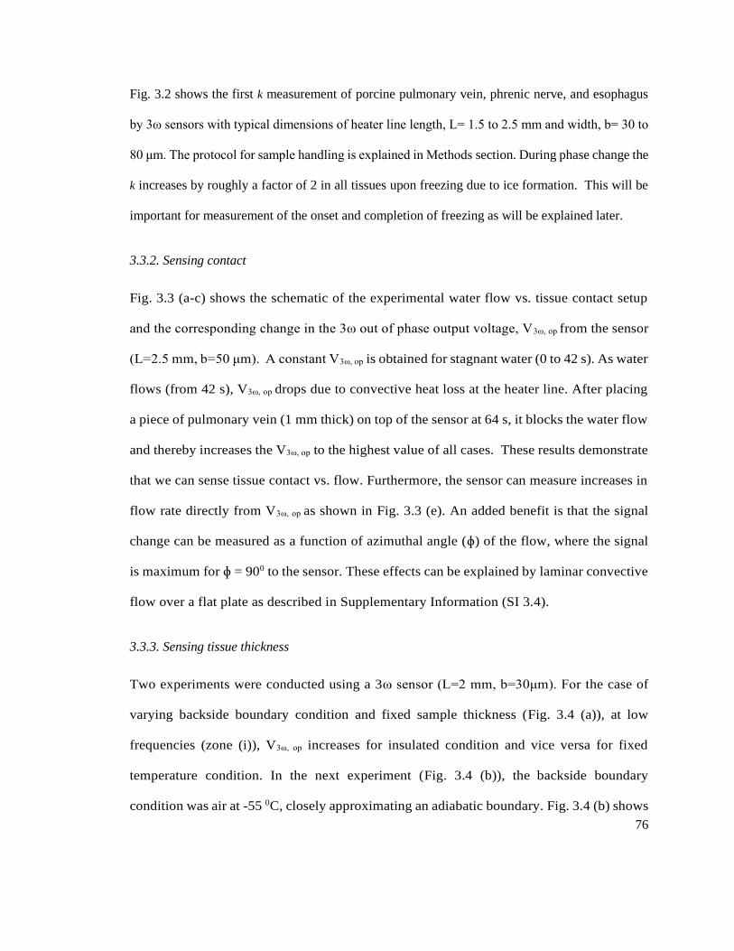
76

Fig. 3.2 shows the first k measurement of porcine pulmonary vein, phrenic nerve, and esophagus

by 3ω sensors with typical dimensions of heater line length, L= 1.5 to 2.5 mm and width, b= 30 to

80 μm. The protocol for sample handling is explained in Methods section. During phase change the

k increases by roughly a factor of 2 in all tissues upon freezing due to ice formation. This will be

important for measurement of the onset and completion of freezing as will be explained later.

3.3.2. Sensing contact

Fig. 3.3 (a-c) shows the schematic of the experimental water flow vs. tissue contact setup

and the corresponding change in the 3ω out of phase output voltage, V3ω, op from the sensor

(L=2.5 mm, b=50 μm). A constant V3ω, op is obtained for stagnant water (0 to 42 s). As water

flows (from 42 s), V3ω, op drops due to convective heat loss at the heater line. After placing

a piece of pulmonary vein (1 mm thick) on top of the sensor at 64 s, it blocks the water flow

and thereby increases the V3ω, op to the highest value of all cases. These results demonstrate

that we can sense tissue contact vs. flow. Furthermore, the sensor can measure increases in

flow rate directly from V3ω, op as shown in Fig. 3.3 (e). An added benefit is that the signal

change can be measured as a function of azimuthal angle (ɸ) of the flow, where the signal

is maximum for ɸ = 900 to the sensor. These effects can be explained by laminar convective

flow over a flat plate as described in Supplementary Information (SI 3.4).

3.3.3. Sensing tissue thickness

Two experiments were conducted using a 3ω sensor (L=2 mm, b=30μm). For the case of

varying backside boundary condition and fixed sample thickness (Fig. 3.4 (a)), at low

frequencies (zone (i)), V3ω, op increases for insulated condition and vice versa for fixed

temperature condition. In the next experiment (Fig. 3.4 (b)), the backside boundary

condition was air at -55 0C, closely approximating an adiabatic boundary. Fig. 3.4 (b) shows

77

V3ω, op to be independent of thickness in the zone (ii) where the frequency is high enough

for the thermal penetration depth (PD) to be within the sample. Below a characteristic

frequency (zone (i)), the measurements become very sensitive to the backside boundary

condition, leading to an abrupt increase in V3ω, op as a function of the thickness. This

thickness dependence can also be appreciated by plotting V3ω, op at a single low frequency

such as 0.1 Hz as shown in Fig. 3.4 (b-inset). The PD of thermal waves can be calculated

by PD=(D/2.ω)0.5, where D is thermal diffusivity (m2/s)). At 0.1 Hz, the PD into the frozen

agargel is ~1 mm. A comparison of an idealized theoretical calculation45, 91 with the

experiment shows that the experimental measurements are consistent with the model trends,

and suggest that with proper calibration can be used to measure thickness.

(a) (b)

Figure 3.4 The measurement of thickness by 3ω sensor. (a) Plot shows a representative experiment of V3ω, op

shown in y-axis, where at low frequencies in zone (i), it depends on backside boundary for fixed sample thickness

( 0.5 mm). Blue circle data represents the case where backside of the sample is low k plastic (quasi -adiabatic)

and red triangle data represents the case where backside is high k copper at fixed temperature (quasi -

isothermal). Inset schematic shows the comparison between PD and for zones (i) and (ii). (b) Plot shows a

representative experiment where V3ω, op at low frequencies in zone (i) depends on sample thickness for a fixed

backside boundary condition of air. Ice of known thickness (as noted inside figure) is placed on the surface of

the sensor at -250C. Backside boundary condition is air at -550C. Inset shows plot of V3ω, op at 0.1 Hz vs thickness

of the sample ‘ ’. Data is the average ± standard deviation of N=3 samples.

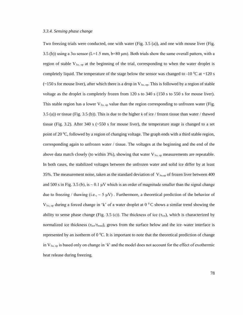
78

3.3.4. Sensing phase change

Two freezing trials were conducted, one with water (Fig. 3.5 (a)), and one with mouse liver (Fig.

3.5 (b)) using a 3ω sensor (L=1.5 mm, b=80 μm). Both trials show the same overall pattern, with a

region of stable V3ω, op at the beginning of the trial, corresponding to when the water droplet is

completely liquid. The temperature of the stage below the sensor was changed to -10 0C at ~120 s

(~150 s for mouse liver), after which there is a drop in V3ω, op. This is followed by a region of stable

voltage as the droplet is completely frozen from 120 s to 340 s (150 s to 550 s for mouse liver).

This stable region has a lower V3ω, op value than the region corresponding to unfrozen water (Fig.

3.5 (a)) or tissue (Fig. 3.5 (b)). This is due to the higher k of ice / frozen tissue than water / thawed

tissue (Fig. 3.2). After 340 s (~550 s for mouse liver), the temperature stage is changed to a set

point of 20 0C, followed by a region of changing voltage. The graph ends with a third stable region,

corresponding again to unfrozen water / tissue. The voltages at the beginning and the end of the

above data match closely (to within 3%), showing that water V3ω, op measurements are repeatable.

In both cases, the stabilized voltages between the unfrozen water and solid ice differ by at least

35%. The measurement noise, taken as the standard deviation of V3ω,op of frozen liver between 400

and 500 s in Fig. 3.5 (b), is ~ 0.1 μV which is an order of magnitude smaller than the signal change

due to freezing / thawing (i.e., ~ 5 μV) . Furthermore, a theoretical prediction of the behavior of

V3ω, op during a forced change in ‘k’ of a water droplet at 0 0 C shows a similar trend showing the

ability to sense phase change (Fig. 3.5 (c)). The thickness of ice (τice), which is characterized by

normalized ice thickness (τice/τtotal), grows from the surface below and the ice–water interface is

represented by an isotherm of 0 0C. It is important to note that the theoretical prediction of change

in V3ω, op is based only on change in ‘k’ and the model does not account for the effect of exothermic

heat release during freezing.

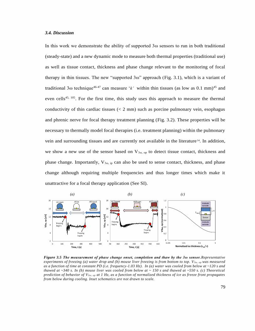
79

3.4. Discussion

In this work we demonstrate the ability of supported 3ω sensors to run in both traditional

(steady-state) and a new dynamic mode to measure both thermal properties (traditional use)

as well as tissue contact, thickness and phase change relevant to the monitoring of focal

therapy in thin tissues. The new “supported 3ω” approach (Fig. 3.1), which is a variant of

traditional 3ω technique46-47 can measure ‘k’ within thin tissues (as low as 0.1 mm)45 and

even cells45, 105. For the first time, this study uses this approach to measure the thermal

conductivity of thin cardiac tissues (< 2 mm) such as porcine pulmonary vein, esophagus

and phrenic nerve for focal therapy treatment planning (Fig. 3.2). These properties will be

necessary to thermally model focal therapies (i.e. treatment planning) within the pulmonary

vein and surrounding tissues and are currently not available in the literature14. In addition,

we show a new use of the sensor based on V3ω, op to detect tissue contact, thickness and

phase change. Importantly, V3ω, ip can also be used to sense contact, thickness, and phase

change although requiring multiple frequencies and thus longer times which make it

unattractive for a focal therapy application (See SI).

(a) (b) (c)

Figure 3.5 The measurement of phase change onset, completion and thaw by the 3ω sensor.Representative

experiments of freezing (a) water drop and (b) mouse liver freezing is from bottom to top. V3ω, op was measured

as a function of time at constant PD (i.e. frequency-1.03 Hz). In (a) water was cooled from below at ~120 s and

thawed at ~340 s. In (b) mouse liver was cooled from below at ~ 150 s and thawed at ~550 s. (c) Theoretical

prediction of behavior of V3ω, op at 1 Hz, as a function of normalized thickness of ice as freeze front propagates

from below during cooling. Inset schematics are not drawn to scale.

80

Fig. 3.3 shows the new ability of the sensor to detect contact with tissue vs fluid (i.e. water)

with different ‘k’. The response time is typically ~15 s as shown in Fig. 3.3(a-c). Further,

by calibrating the reduction in V3ω, op one can also sense different fluid flow rates (as shown

in Fig. 3.3 (e)). Once in contact with the tissue, the sensor can be used to measure the

thickness of the pulmonary vein (or other thin luminal structure in contact). Thickness

measurements exploit the low frequency (PD sample thickness) regime in zone (i) of Figs.

3.1 (e, f) and 3.4 (a). Thus, the frequency of the electric current can be reduced such that the

PD of the thermal wave is comparable to the thickness of the sample. At this point, the signal

becomes sensitive to the backside boundary condition as shown in Fig. 3.4 (a) zone (i). Fig.

3.4 (b) inset shows that V3ω, op increases with thickness at lower frequencies, showing an

increased sensitivity to the backside boundary condition (in this case air) as PD increases.

However, there is a discrepancy in magnitude between the theory45, 91 and experiment

despite a similar trend. This difference could be attributed to the complex construction of

the sensor (i.e. multi-layered geometry) as compared to the theoretical model. In the

experiments, the sensor has a second glass substrate (~1 mm thick) as a physical support,

attached with polyimide adhesive (~100 μm thick). Furthermore, the sensor is placed on top

of a temperature control stage (~ 2 mm from the heater line). In addition, there are copper

wires and epoxy bonds connecting the heater line to the electronics. This complicates the

thermal model, especially at lower frequencies where the relatively long time constants

allow deeper PD from this multi-layered sensor geometry. In contrast, theory assumes a

simpler, more idealized sensor geometry as depicted in Figs. 3.1 (a-d) and 3.4 (a- inset).

Despite these differences, a consistent trend between the theory and the experiment provides

a qualitative proof that the sensor can measure thickness, and absolute agreement can be

explored further in the future.

81

Next, the sensor can be used to sense the phase change in the tissue (Fig. 3.5). During freezing, the

change in ‘ksample’ between frozen and thawed tissue (Fig. 3.2) leads to a change in the V3ω, op, and

an inverse behavior during thawing. In addition, theoretical predictions in Fig. 3.5 (c) show that

V3ω, op is a function of ice thickness as the ice front propagates away from the sensor.

An important aspect of sensing is the need to minimize measurement time, which increases as

sensor frequency decreases (i.e., PD increases). Thus, the sensor would require long electronic time

constants, especially for several mm thickness measurements to obtain a stable signal. The longest

electronic time constant used in this article is 10 s at ~0.1 Hz. In comparison, cryotherapy of PV

typically lasts ~120 s304 and clinical imaging techniques have temporal resolution of < 1 s307, 322-330.

Further reduction in the time of measurement and possibly multiplexing at a variety of frequencies

remain interesting and important future improvements for this measurement.

Table SI.3.1. Comparison of thermal conductivity measurement techniques

Measurement

Characteristics

Current

techniques*

Traditional 3ω Supported 3ω

Can measure sizes < 1

mm

Compensates for

Parasitic Heat Loss

Compensates for

Contact Resistance

(only for in –phase)

(only for in –phase)

Use in Biomaterials

Reuse possible

Avoids

Microfabrication

(necessary for every

sample)

(necessary for one

sensor only)

*The ‘Current Techniques’ refers to a representative sample of techniques (Guarded Hot

plate, Embedded Thermistor, Cut bar) (Reproduced from Lubner et al IMECE 2012 with

Copyright (2012) Permission from ASME)176

82


This work was supported in part by NSF (CBET Grant # 1236760), Medtronic Inc. and NSF

Graduate Research Fellowship (Grant # 1106400). We would like to thank Visible Heart

Lab at University of Minnesota (UMN) for supplying biological tissues and Minnesota

Nanofabrication Centre for providing access to microfabrication facilities.

SI 3.1. Supplementary Information: Construction of the Supported 3ω Sensor

The advantage of supported 3ω sensors is summarized in Table SI.3.1. Using standard

photolithography and liftoff microfabrication techniques, a gold heater line, with typical

dimensions of 30 μm wide, 1 to 3 mm long, and 200 nm thick is deposited on a glass substrate (1

mm thick amorphous SiO2). A 5 nm thick Chromium adhesion layer holds the gold heater line and

glass together. The heater lines are connected to the signal processing unit and a lock in amplifier

(SR 830, SRS, Sunnyvale CA) using copper wires. As the soft, hydrated biological tissue is weakly

electrically conducting, a thin dielectric film is incorporated between the heater and the sample to

prevent electrical cross-talk, after connecting the wires to the heater line. This was achieved by

dissolving polystyrene pellets in toluene at a concentration of 15 mg/mL. A few drops of the

solution were dropped directly on top of the sensor, which was then held vertical to allow excess

solution to run off. The toluene evaporates in 5 to 10 seconds leaving a thin continuous layer (~

1μm) of polystyrene dielectric layer (Fig. 3.1 (a, b)).

SI 3.2. Supplementary Information: Theory behind Flow Rate Measurement

The theory behind flow rate measurement is that the electrical power input to the heater is

lost as heat by conduction to the substrate below and convection to the flowing water above

the sensor as given by Eqn. (SI.3.1).

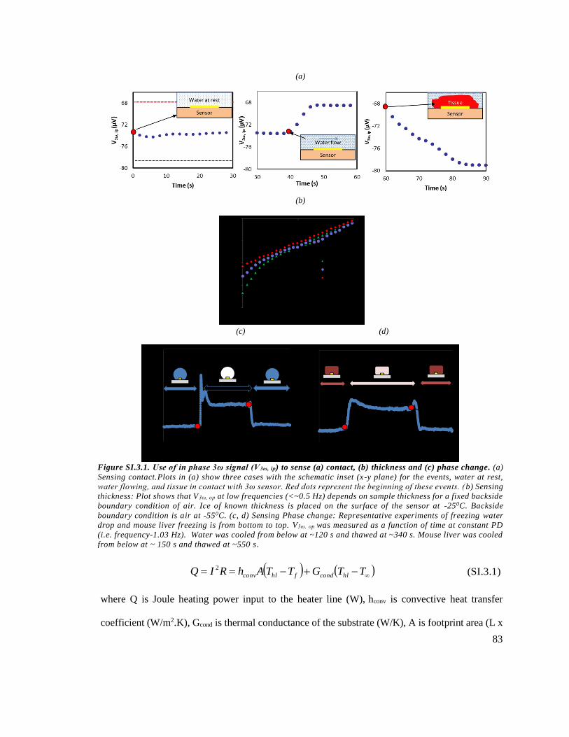
83

TTGTTAhRIQ hlcondfhlconv

2 (SI.3.1)

where Q is Joule heating power input to the heater line (W), hconv is convective heat transfer

coefficient (W/m2.K), Gcond is thermal conductance of the substrate (W/K), A is footprint area (L x

(a)

(b)

(c) (d)

Figure SI.3.1. Use of in phase 3ω signal (V3ω, ip) to sense (a) contact, (b) thickness and (c) phase change. (a)

Sensing contact.Plots in (a) show three cases with the schematic inset (x-y plane) for the events, water at rest,

water flowing, and tissue in contact with 3ω sensor. Red dots represent the beginning of these events. (b) Sensing

thickness: Plot shows that V3ω, op at low frequencies (<~0.5 Hz) depends on sample thickness for a fixed backside

boundary condition of air. Ice of known thickness is placed on the surface of the sensor at -250C. Backside

boundary condition is air at -550C. (c, d) Sensing Phase change: Representative experiments of freezing water

drop and mouse liver freezing is from bottom to top. V3ω, op was measured as a function of time at constant PD

(i.e. frequency-1.03 Hz). Water was cooled from below at ~120 s and thawed at ~340 s. Mouse liver was cooled

from below at ~ 150 s and thawed at ~550 s.

84

b) of the heater line (m2), Thl is temperature of the heater line (K), Tf is temperature of the fluid (K),

and T∞ is ambient environment temperature (K). The variables in Eqn. (S1.3.1) can in general be

complex and time-dependent. If current ‘I’ and the substrate thermal conductance ‘Gcond’ are

maintained constant, then changes in convective heat loss (hconv) arising from changing the flow

will result in changes in the temperature at the heater (Thl). This will be reflected as changes in ‘R’,

and thus V3ω, op. Thus, the sensor can be used to sense flow rate in a similar fashion to other past

approaches such as hot wire anemometry331-332.

SI 3.2.1. Dependence of 3ω signal on flow direction

Fig. 3.3 (f) shows the signal change depends on the azimuthal angle (ɸ) of the flow direction.

These effects could be explained by laminar convective flow over a flat plate with an

unheated starting length, as shown in the Eqn. (SI.3.2)333

3

2

4

3

01

xx

kNu

x

kNuh water

xwaterx

conv

(SI.3.2)

where ‘x’ is the total distance travelled by water on the substrate. ‘ ’ is the unheated

starting length, referring to the distance travelled by water over unheated glass substrate and

‘x- ’ can be referred as the heated length. In the case of the sensor, heated length is a

function of flow angle ‘φ’. For φ=00, the heated length will be ‘L’, i.e., the thermal boundary

layer will develop over the length of the heater line ‘L’. In contrast, for φ=900, the heated

length ‘x’ is the width of the heater line ‘b’ plus the thermal penetration depth (PD). It is

known from Eqn. (SI.3.2) and the boundary layer theory that the average convection

coefficient (hconv) will decrease with increase in boundary layer thickness333. As (b+PD)<<L,

85

thermal boundary layer thickness will be small across the heater line. Thus, hconv will be

higher for the case φ=900, thus explaining the behavior in Fig. 3.3 (f).

SI 3.3. Supplementary Information: Use of In-phase 3ω Signal (V3ω, Ip) to Sense Contact,

Thickness and Phase Change

Fig. S1.3.1 shows the use of V3ω, ip to sense contact, thickness and phase change. The sensor is run

in “dynamic” mode (i.e. at a single frequency as a function of time) to sense contact (Fig. S1. 3.1

(a) and phase change (Fig. SI.3.1 (c)). The sensitivity and response time is similar to that of out-

phase signal discussed in the main paper. However, for thickness measurement (Fig. S1.3.1 (b)),

the backside boundary is sensed at a lower frequency (~0.5 Hz) for in phase signal. In comparison,

the backside boundary is sensed at a higher frequency (~0.7 Hz) for out of phase signal. Thus, out

of phase signal has the potential for faster measurement.

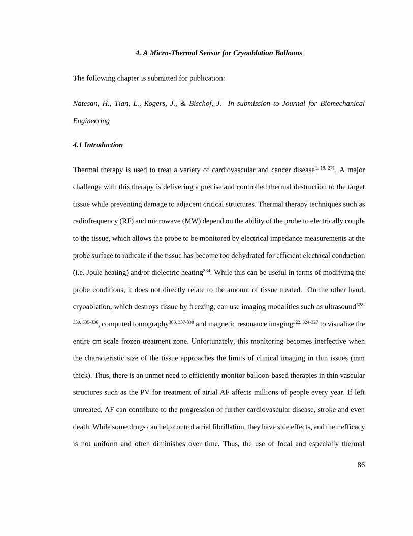
86

4. A Micro-Thermal Sensor for Cryoablation Balloons

The following chapter is submitted for publication:

Natesan, H., Tian, L., Rogers, J., & Bischof, J. In submission to Journal for Biomechanical

Engineering

4.1 Introduction

Thermal therapy is used to treat a variety of cardiovascular and cancer disease1, 19, 271. A major

challenge with this therapy is delivering a precise and controlled thermal destruction to the target

tissue while preventing damage to adjacent critical structures. Thermal therapy techniques such as

radiofrequency (RF) and microwave (MW) depend on the ability of the probe to electrically couple

to the tissue, which allows the probe to be monitored by electrical impedance measurements at the

probe surface to indicate if the tissue has become too dehydrated for efficient electrical conduction

(i.e. Joule heating) and/or dielectric heating334. While this can be useful in terms of modifying the

probe conditions, it does not directly relate to the amount of tissue treated. On the other hand,

cryoablation, which destroys tissue by freezing, can use imaging modalities such as ultrasound328-

330, 335-336, computed tomography308, 337-338 and magnetic resonance imaging322, 324-327 to visualize the

entire cm scale frozen treatment zone. Unfortunately, this monitoring becomes ineffective when

the characteristic size of the tissue approaches the limits of clinical imaging in thin issues (mm

thick). Thus, there is an unmet need to efficiently monitor balloon-based therapies in thin vascular

structures such as the PV for treatment of atrial AF affects millions of people every year. If left

untreated, AF can contribute to the progression of further cardiovascular disease, stroke and even

death. While some drugs can help control atrial fibrillation, they have side effects, and their efficacy

is not uniform and often diminishes over time. Thus, the use of focal and especially thermal

87

interventions to electrically isolate the pulmonary vein (PV) thereby avoiding drugs is considered

a milestone advancement in the treatment of AF304, 339. Specifically, thermal and cryoablation for

PV isolation has been used for more than 20 years and has become a standard of care for drug-

refractory paroxysmal atrial fibrillation305, 339-345. However, these treatments suffer from an inability

to image or monitor the thermal therapy, leading to cases of over- and under-treatment. Indeed,

over-treatment can lead to hemoptysis, esophageal freezing or phrenic nerve palsy343, 346-347, and

under-treatment requires repeat treatments348-349. Thus, as imaging cannot work on these thin mm-

sized tissues, alternatives are urgently needed to improve monitoring of balloon-based thermal and

focal therapy.

Monitoring at the surface of the probes can be achieved in a rudimentary way with thermocouples350

or more robustly using thermal conductivity changes with micro-sensors based on the 3ω

technique47 modified for thin biological systems45. Fig. 4.1 (a, left) shows our original published

embodiment of a 3ω sensor deposited on a flat substrate. This 3ω sensor can sense tissue or fluid

contact, flow, mm-scale tissue thickness, and the initiation and completion of freezing , and it can

be used to measure thermal conductivity (k) of thin (< 2 mm) biological tissues45, 103. It uses a sensor

made up of a long, thin gold heater line (3 mm X 20 μm X 100 nm) deposited on a glass substrate.

The biological tissue of interest is placed on top of the sensor such that it covers the heater line. An

alternating current of frequency ‘ω’ excites the heater line, producing temperature oscillations of

frequency ‘2ω’ that propagate into the sample and the substrate over a thermal penetration depth,

PD= (α/2ω)0.5, where ⍺ is thermal diffusivity (m2/s) and ω is the frequency of the applied electric

current (radians). The resulting third harmonic voltage across the heater line ‘3ω’ contains

information about the temperature oscillations at the heater line. The temperature oscillations at the

heater line can be used to calculate thermal conductivity of the sample with knowledge of the

thermal and electrical properties of the sensor47.

88

However, as cryoablation and other focal therapy in the PV is generally performed with balloons,

there is a further need to integrate 3ω sensors onto balloons to perform the same sensing and

monitoring functions. Recent advancements in flexible electronics now allow multiple types of

sensors including 3ω sensors to be attached to flexible, stretchable substrates315-318, 351-352. The

current collaborative effort now integrates 3ω sensors directly onto a balloon for monitoring

thermal therapy. Example designs that integrate electronic sensors onto balloons317-318, 352 and

(a)

(b) (c)

Figure 4.1. Development of micro-thermal 3ω sensors for monitoring balloon cryoablation in pulmonary

vein (PV).(a) Development of a micro-thermal sensor starting from a linear sensor (L= 2 mm, b= 20 μm) on

a flat substrate, to a serpentine sensor (L=0.5 mm, b= 5 μm, w= 180 μm). Finally, the serpentine sensor was

integrated onto a balloon for focal therapy applications. (b) Historical data for a linear sensor shows V 3ω,

op as a function of heater electrical frequency (ω/(2π)) where the sample is ice and the backside boundary is

air. Zone i refers to the frequency range where PD ~tsample . Zone iii refers to the range where PD ~theater;

Zone ii refers to the range where V3ω, op is neither affected by the heater line (PD>>theater) nor the backside

boundary condition (PD<< tsample). Inset schematic shows the comparison between PD and sample thickness,

, for Zones i, ii, and iii. (c) Historical data for a linear sensor shows V 3ω, op (y-axis) at low frequencies in

Zone i depends on a backside boundary for fixed sample thickness ( 0.5 mm). Blue circle data represent

the case where a backside of the sample is low k plastic (quasi-adiabatic), and red triangle data represents

the case where the backside is high k copper at fixed temperature (quasi -isothermal). Inset schematic shows

the comparison between PD and for Zones i and ii. Copyright pending for Fig. 4.1(b) and (c) from 103.

89

human skin316 have already been published. In the current work, we modify the linear 3ω sensor

design from a thin straight line to a serpentine shape to enable its integration onto a flexible,

stretchable balloon as shown in Fig. 4.1 (a). The serpentine shape minimizes local strains during

inflation and deflation of the balloon as previously reported for other sensors316-318, 351-352. Hence,

the modified sensor is first numerically analyzed using Finite Element Modeling on a flat substrate

to determine the ability to differentiate between ice, water and fat. Further, the sensor was

investigated for its ability to sense thickness and phase change for ice and water respectively. Next,

these results were confirmed experimentally to sense tissue contact, thickness and phase change.

Finally, we microfabricated the sensor onto a flexible, stretchable balloon using transfer printing

techniques (Fig. 4.1 (a))317. The sensor on a balloon was then tested to sense contact, thickness and

phase change for possible cryotherapy (or other thermal therapy) application.

4.2 Methods

4.2.1. Numerical characterization of the serpentine 3ω sensor on a flat substrate

i. Principle of 3ω sensor

The historical operation of the linear 3ω sensor is shown in Figs 1 (b) and (c). Fig. 4.1 (b) shows

an instance where the sensor was used to measure the thickness of ice (1 mm thick) with air as a

backside boundary condition. The plot shows the output signal (i.e., third harmonic voltage (V3ω,

op)) across the heater line measured as a function of frequency. The frequency range is divided into

three zones (see inset): Zone i refers to the lower frequency range where PD ~ tsample (sample

thickness) while Zone iii refers to the frequency range where PD ~ theater line (thickness of the heater

line). Zone ii refers to a specific frequency range where theater line >>PD <<tsample. This frequency

range is characterized by a constant V3ω, op avg, which is inversely proportional to effective thermal

90

conductivity of the region in the sample and the substrate traversed by the temperature oscillations

ktotal (W/m.k). In fact, it can be determined as shown in Eqn. (4.1):

𝑘𝑡𝑜𝑡𝑎𝑙 =𝛼𝑅2𝐼3

8𝐿𝑉3𝜔,𝑜𝑝 𝑎𝑣𝑔. , (4.1)

Where R and L are the resistance [Ω] and length of the heater line [L] respectively; I is the electric

current applied across the heater line [A]; and V3ω, op avg. is the resulting average third harmonic out-

of-phase voltage [V] measured from Zone ii of the frequency sweep. Finally, the thermal

conductivity of the sample can be determined from ktotal using Eqn. (4.2)45 if thermal conductivity

of the substrate ksub is known beforehand from calibration:

(4.2)

An important feature of the 3ω sensor is that the frequency-dependent measurement enables sub-

surface sensing of ksample based on the behavior of V3ω, op in Zone ii. In Zone i, where PD~tsample, the

behavior of V3ω, op becomes dependent, not only on ksample but also on tsample, and the backside

boundary condition of the sample320. This is shown using a representative experiment where the

sensor measured ice of 0.5 mm thickness with a varying backside boundary of quasi-thermal copper

vs. quasi-adiabatic plastic (see Fig. 4.1 (c)). Results for thicker ice (0.5- 2mm) with quasi-adiabatic

air as backside boundary conditions is shown in a previously reported work103. Using these

principles, the 3ω sensor on flat and balloon substrates has been used to sense contact with fluid

vs. tissue, thickness and freezing phase change.

ii. Numerical model of 3ω sensor

Mishra et al. developed a 2-D axisymmetric finite element model of a thin and infinitely long heater

line on a flat substrate353. We extend this model here into 3D for the heater line that is serpentine,

but still attached like the linear line onto a flat substrate. A commercially available COMSOL

subsampletotal kkk

91

package (Version 5.0) was used to simulate the sensor as a quasi-steady model with the governing

equation as shown below,

𝑘 [𝜕2𝑇

𝜕𝑥2 +𝜕2𝑇

𝜕𝑦2 +𝜕2𝑇

𝜕𝑧2] + 𝑃′𝑒𝑖2𝜔𝑡𝛿(𝑥, 𝑦, 𝑧) = 𝐶𝑇 (4.3)

where P’, T and C refer to the heater line power per unit length [W/m], average temperature

oscillations in the heater line [K], and volumetric heat capacity of the surrounding medium

(substrate/ sample) [J/m^3/K] respectively. The partial differential equation (PDE) in Eqn. (4.3) is

set up using coefficient form PDE module. Contact resistance between the heater line and the

substrate were assumed to be negligible45. The heater line was modeled as a heat source at the

surface of the heater line i.e., negligible thickness. The thickness is neglected as the PD (~10 μm at

100 Hz for water at 220C) >> heater line thickness (<100 nm) for frequencies of interest in

biologically relevant materials. The model was validated with closed form analytical solution for

linear sensor and also with experimental data for a serpentine heater line on a glass substrate as

shown in SI 4.1. Specifically, a gold serpentine sensor of dimensions b = 5 μm, w = 180 μm, and

L = 0.5 mm is modeled on a flat glass substrate of (length= 5 mm, width= 5 mm, thickness=1 mm).

The backside boundary condition for the experiment was air i.e., quasi- adiabatic which would

approximate the interior of an inflated balloon.

Using the numerical model, we first investigated the ability of the sensor to identify ice (k=2.45

W/m.K, ⍺=1.33E-6 m2/s), water (k=0.6 W/m.K, ⍺=1.43E-7 m2/s) and fat (k=0.2 W/m.K, ⍺=1.39E-

7 m2/s) at a frequency of 2 Hz, which is in the mid frequency range of Zone ii for all the three

samples. The heater line was modeled to be on a 2 mm thick glass substrate (k= 1.26 W/m.K;

⍺=6.6E-7 m2/s) and in contact with the sample of 2 mm thickness. Contact resistance between the

substrate, the heater line and the sample were assumed to be negligible. The backside of the sample

92

and the substrate were assumed to be under adiabatic conditions. The heater electrical power

applied to the heater line was assumed to be 5 mW, which is approximately equal to the heater

input power for the serpentine sensor used in this paper for an input current of ~10 mA. Next, the

ability of the serpentine sensor to measure thickness was investigated. For thickness, the sensor

was modeled to be in contact with ice with water or fat as backside boundary conditions in the

thickness range of 0.5- 2 mm range. The resulting V3ω, op is determined at 0.1 Hz and plotted as a

function of thickness of the sample. The frequency of 0.1 Hz is chosen as the PD (~0.33 mm in fat,

~0.34 mm in water, ~1.03 mm in ice) is comparable to the thickness of 0.5 – 2 mm for PV and lies

in Zone i (low frequency range).

Finally, we investigated the ability of the sensor to sense phase change from water to ice. This is

achieved by first modeling the serpentine sensor to be in contact with water with an adiabatic

backside boundary condition. Next, V3ω, op at 2 Hz is determined and plotted as a function of tice/twater

by changing the thickness of ice (i.e. ice front is advancing next to the sensor). The frequency of 2

Hz is chosen as the PD is ~0.074 mm for fat, ~0.075 mm for water, 0.23 mm for ice, which is an

order of magnitude less than the thickness of 2 mm that we wish to sense within PV and lies in

Zone ii of both ice and water.

4.2.2. Micro-thermal sensing using the serpentine sensor on a flat substrate

i. Construction of the serpentine sensor

A gold serpentine shaped heater line (L=0.5 mm, b=5 μm, w= 180 μm, t= 80 nm) is patterned onto

a 1 mm thick silica glass (amorphous SiO2) substrate using standard photolithography and lift off

techniques. A chromium layer (~5 nm thick) is used as an adhesion to bond gold line onto glass

substrate. A polystyrene dielectric layer (~1 μm thick) is deposited on top of the heater line. The

process is detailed elsewhere103. The glass substrate is attached on top of another silica glass

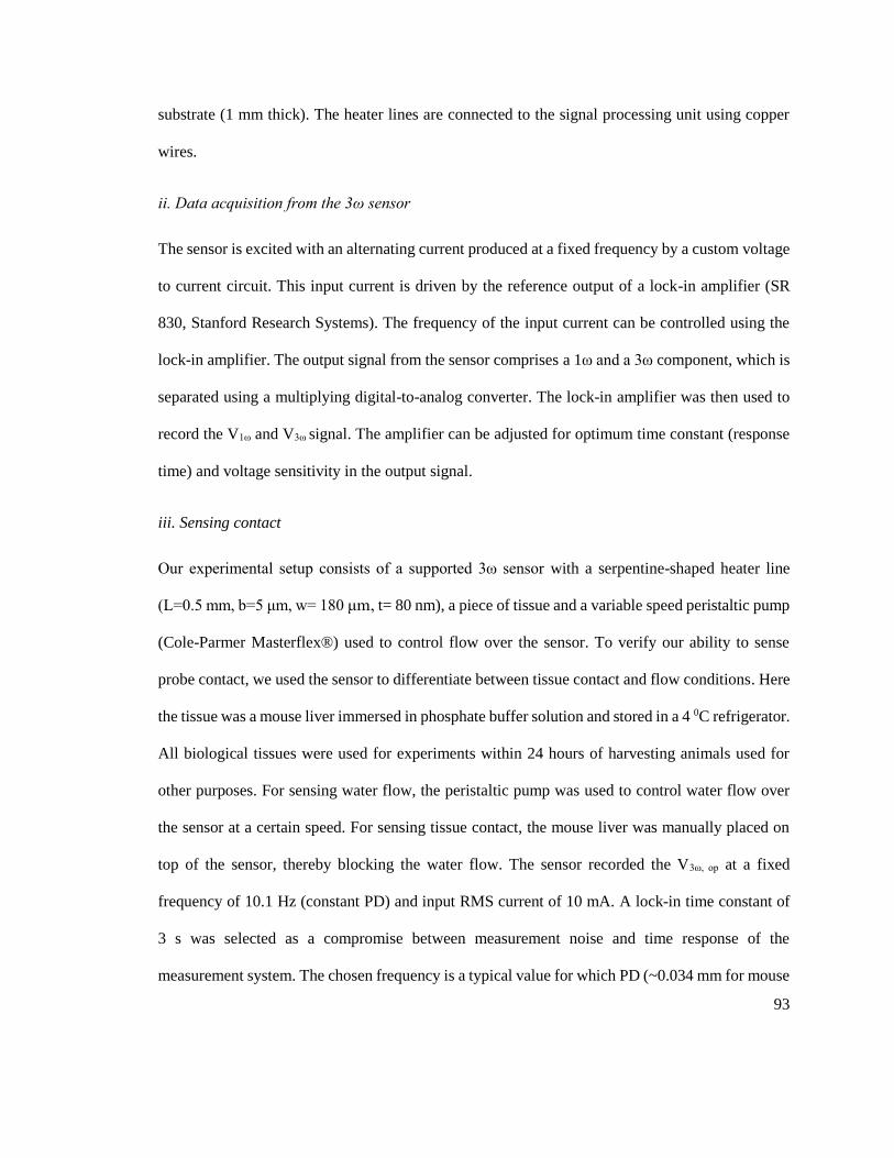
93

substrate (1 mm thick). The heater lines are connected to the signal processing unit using copper

wires.

ii. Data acquisition from the 3ω sensor

The sensor is excited with an alternating current produced at a fixed frequency by a custom voltage

to current circuit. This input current is driven by the reference output of a lock-in amplifier (SR

830, Stanford Research Systems). The frequency of the input current can be controlled using the

lock-in amplifier. The output signal from the sensor comprises a 1ω and a 3ω component, which is

separated using a multiplying digital-to-analog converter. The lock-in amplifier was then used to

record the V1ω and V3ω signal. The amplifier can be adjusted for optimum time constant (response

time) and voltage sensitivity in the output signal.

iii. Sensing contact

Our experimental setup consists of a supported 3ω sensor with a serpentine-shaped heater line

(L=0.5 mm, b=5 μm, w= 180 μm, t= 80 nm), a piece of tissue and a variable speed peristaltic pump

(Cole-Parmer Masterflex®) used to control flow over the sensor. To verify our ability to sense

probe contact, we used the sensor to differentiate between tissue contact and flow conditions. Here

the tissue was a mouse liver immersed in phosphate buffer solution and stored in a 4 0C refrigerator.

All biological tissues were used for experiments within 24 hours of harvesting animals used for

other purposes. For sensing water flow, the peristaltic pump was used to control water flow over

the sensor at a certain speed. For sensing tissue contact, the mouse liver was manually placed on

top of the sensor, thereby blocking the water flow. The sensor recorded the V3ω, op at a fixed

frequency of 10.1 Hz (constant PD) and input RMS current of 10 mA. A lock-in time constant of

3 s was selected as a compromise between measurement noise and time response of the

measurement system. The chosen frequency is a typical value for which PD (~0.034 mm for mouse

94

liver) << tsample (~2 mm).

iv. Sensing tissue thickness

Agargel (0.5% weight of agarose in water) was placed on the sensor and immediately frozen to -

25 0C using a cooler enclosed in a cryofreezer (Planer Kryo 10 Series III). For an input RMS current

of 10 mA, V3ω, op was recorded as a function of frequency (from 0.1 to 10 Hz) at a fixed temperature

of -25 0C on the sensor surface. The experiment was repeated for a different thickness (n = 3) of

frozen agargel (i.e., changed from ~0.5 mm to ~1.9 mm) while keeping the backside boundary

condition as air (kair~ 0.02 W/m.K) at -55 0C 321. The thermal convection effects of air can be

assumed negligible as the convection heat loss is <1% of the conduction heat flow from the heater

line if convection coefficient is assumed to be <25 W/m2.K320.

v. Sensing phase change

A 3 mm thick, several cm long mouse liver slice was placed on the sensor. The temperature was

lowered from 20 0C to -10 0C, allowing the tissue sample to become frozen. After allowing the

freezing event to complete and the voltage to stabilize, the temperature was increased back to 20

0C. Completion of freezing and thawing events were verified by visual inspection during the

experiment. An alternating current with an RMS of 10 mA at a frequency of 10.1 Hz, which is in

the Zone ii of the frequency sweep was applied across the sensor and the results were recorded with

a lock-in time constant of 3 s.

4.2.3. Micro-thermal sensing using serpentine sensors on a balloon substrate

i. Integration of serpentine 3ω sensor onto a balloon

The 3ω sensors were deposited on flexible balloons316-318, 352. Specifically, the 3ω sensors and

associated interconnects/contacts were microfabricated on silicon wafers using conventional

95

microfabrication techniques. An initial sacrificial layer of poly(methyl methacrylate) spun onto the

wafer allowed eventual release of the entire 3ω device from the wafer. Elastomeric transfer printing

techniques were then used to transfer the device from the wafer to a balloon surface. The device

contains gold lines, deposited by electron-beam evaporation and interconnects by

photolithography, fully encapsulated in thin layers of polyimide (spin cast). Careful design of the

polyimide geometries provided the required mechanical robustness (to withstand the pressure of

the balloon) as well as encapsulation from surrounding fluids as previously described for other

flexible electronic constructs315-318.

ii. Sensing contact

The following experiments were conducted using a 3ω sensor of serpentine shaped heater line

(L=0.5 mm, b=5 μm) integrated onto a balloon. To verify our ability to sense probe contact, we

used a sensor integrated onto a balloon to differentiate between contact with agargel and air. The

balloon was positioned a few mm away from the agargel (2 mm thick), which in turn was placed

on a copper plate at room temperature (~22 0C). The sensor recorded the V3ω, op at a fixed frequency

of 11.1 Hz (constant PD) and input RMS current of 6 mA. A lock-in time constant of 3 s was

selected as a compromise between measurement noise and time response of the measurement

system. The chosen frequency is a typical value for which PD (~0.032 mm for agargel) << tsample

(Zone ii) as the purpose is to sense the tissue that is in immediate contact with the sensor. The

balloon was moved so that the sensor came in contact with the agargel.

iii. Sensing tissue thickness

A copper plate was positioned inside a cryofreezer (Planer Kryo 10 Series III) equilibrated to -25

0C. Agargel (0.5% weight of agarose in water) was placed on the copper plate (5 mm thick) at -25

0C and immediately frozen. Next, for an input RMS current of 6 mA, V3ω, op was recorded at 0.1 Hz

96

at a fixed temperature of -25 0C on the sensor surface. Here, the chosen frequency is a typical

value for which PD ~ tsample as the purpose is to sense the backside of the sample in contact

with the sensor. The experiment was repeated for different thickness of frozen agargel (i.e.,

changed from ~0.5 mm to ~2.0 mm) while keeping the backside boundary condition as copper

(kcopper ~386 W/m.K)333.

iv. Sensing phase change

A 3 mm thick sample of agargel was placed on the copper plate at 20 0C. The sensor on the balloon

was brought in contact with the top surface of the agargel. The temperature of the copper plate was

lowered from 20 0C to -25 0C, freezing the agargel sample. After the cooling process is complete

and followed by voltage stabilization, the temperature was increased back to 20 0C. An alternating

current with an RMS of 6 mA at a frequency of 11.1 Hz, which is in the Zone ii of the frequency

sweep was applied across the sensor.

97

4.3. Results and Discussion

4.3.1. Numerical characterization of serpentine 3ω sensors on a flat substrate

The 3ω sensors had to be modified from a linear into a serpentine shape for deposition onto a

balloon substrate. However, the serpentine shape changes the behavior of sensor output signal, V3ω,

op as a function of frequency. So, a numerical model as shown in Fig. 4.2 (a) was created to confirm

(a) (b)

(c) (d)

Figure 4.2 Finite element analysis of the serpentine sensor (L=0.5 mm, b= 5 μm, w= 180 μm) on a flat substrate .

(a) 3D numerical discretization of the serpentine sensor on a flat 2 mm thick glass substrate. (b) Measurement

predictions of V3ω,op at 2 Hz for different samples of ice, water and fat in contact with the sensor. V 3ω,op is

normalized to the values of ice (c) Measurement predictions of V3ω,op at 0.1 Hz for varying sample thickness of ice

with water or fat on the backside. V3ω,op for each configuration is normalized to the values for samples at 2 mm

thickness (d) Measurement predictions of V3ω,op at 2 Hz for varying thickness of ice as ice front moves from the

sensor. V3ω,op is normalized to the PD in ice

98

the ability of the serpentine shaped sensor for micro-thermal sensing. First, the ability of the sensor

to differentiate between biologically relevant materials such as fat, water and ice is shown in Fig.

4.2 (b). Here, V3ω, op is determined for cases where the sample was in contact with fat, water and

ice. V3ω, op was normalized with V3ω, op obtained for ice (k=2.45 W/m.K). The value increases to

~2.3 for water with k=0.6 W/m.K and ~3.0 for fat with k=0.2 W/m.K. The reason V3ω, op increases

(a) (b)

(c) (d)

Figure 4.3 Micro-thermal sensing using a serpentine shaped sensor (L= 0.5 mm, b= 5 μm, w= 180 μm, t= 100

nm) on a flat substrate. (a) Serpentine-shaped sensor on a flat glass substrate (b) (Contact) Experimental

measurement of water vs. tissue contact; V3ω,op is measured at ω of 10.1 Hz. (c) (Thickness) Experimental

measurement of V3ω,op at 0.1 Hz for different thickness of frozen agargel at -25 0C (AVG ± STDEV of N = 3). Black

line shows the results from the numerical model. The backside boundary conditions are air and modeled as

adiabatic conditions. V3ω,op is normalized to tis value for 0.5 mm thick sample. Inset shows experimental

measurement of V3ω,op as a function of frequency for different sample thickness. (d) (Phase Change) Experimental

measurement of V3ω,op during mouse liver freezing at 10.1 Hz and normalized to its initial value at 0 s. Cooling

begins at ~30 s and thawing begins at ~140 s.

99

with drop in thermal conductivity could be explained by Eqns. (4.1) and (4.2). For the same sensor

(substrate and heater line geometry) and input electrical current, V3ω, op measured at a frequency in

Zone ii i.e. 2 Hz, is inversely proportional to thermal conductivity. Thus, if the sensor and input

current remain the same, the sensor can be used to sense contact with different materials through

V3ω, op.

Next, the ability of the sensor to sense thickness of materials such as water and ice with different

boundary conditions was modeled as shown in Fig. 4.2 (c). Here, V3ω, op is normalized for each case

with the value determined at 2 mm. For the case with ice as sample and fat as backside, normalized

V3ω, op increases to ~1.03 for 1.5 mm thick sample, ~1.15 for 1 mm thick sample, and finally ~1.50

for 0.5 mm thick sample. In contrast, for the case with water as backside boundary, the normalized

V3ω, op increases to ~1.01 for 1.5 mm thick sample, ~1.06 for 1 mm thick sample, and finally ~1.28

for 0.5 mm thick sample. If the noise in the signal is less than 1%, the sensor can be reliably used

to sense thickness even up to 2 mm for ice with fat as backside boundary.

Finally, the ability of the sensor to track ice thickness in water is shown in Fig. 4.2 (d). Here, the

sensor is modeled to be in contact with water while an ice front moves away from the sensor. It has

to be noted that latent heat was neglected for these simulations. V3ω, op is determined at 2 Hz as it is

in Zone ii and scales with tsample and is independent of backside boundary conditions. V3ω, op is

normalized to the PD in ice. As the thickness ratio (tice/PD) increases to 1.73, normalized V3ω, op

decreases to ~1 beyond which there is a plateau in the signal. This sharp drop in the signal is due

to the fact that the thermal conductivity of ice is at 2.45 W/m.K, which is ~4 times that of water at

0.6 W/m.K thereby confirming the ability of the sensor to measure a phase change event.

While the sensor operates as desired, the original ability of the 3ω sensor to measure ksample of

materials such as ice, water and fat using V3ω,op in Eqn. (4.1) will be degraded. More specifically,

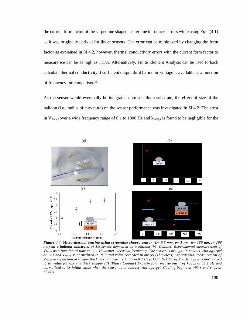
100

the current form factor of the serpentine shaped heater line introduces errors while using Eqn. (4.1)

as it was originally derived for linear sensors. The error can be minimized by changing the form

factor as explained in SI 4.2, however, thermal conductivity errors with the current form factor to

measure ice can be as high as 115%. Alternatively, Finite Element Analysis can be used to back

calculate thermal conductivity if sufficient output third harmonic voltage is available as a function

of frequency for comparison351.

As the sensor would eventually be integrated onto a balloon substrate, the effect of size of the

balloon (i.e., radius of curvature) on the sensor performance was investigated in SI.4.2. The error

in V3ω, op over a wide frequency range of 0.1 to 1000 Hz and ksample is found to be negligible for the

(a) (b)

(c) (d)

Figure 4.4. Micro-thermal sensing using serpentine shaped sensor (L= 0.5 mm, b= 5 μm, w= 180 μm, t= 100

nm) on a balloon substrate.(a) 3ω sensor deposited on a balloon (b) (Contact) Experimental measurement of

V3ω,op as a function of time at 11.1 Hz heater electrical frequency. The sensor is brought in contact with ag argel

at ~2 s and V3ω,op is normalized to its initial value recorded in air (c) (Thickness) Experimental measurement of

V3ω,op as a function of sample thickness ‘d’ measured at ω of 0.1 Hz (AVG ± STDEV of N = 3). V 3ω,op is normalized

to tis value for 0.5 mm thick sample (d) (Phase Change) Experimental measurement of V3ω,op at 11.1 Hz and

normalized to its initial value when the sensor is in contact with agargel. Cooling begins at ~90 s and ends at

~240 s.

101

current application, where the heater line on the balloon will bend around a radius equal to the

ostium of the pulmonary vein (~4 to 6 mm)354.

4.3.2. Micro-thermal sensing using the serpentine sensor on a flat substrate

After construction of the serpentine 3ω sensor on a flat, glass substrate as shown in Fig. 4.3 (a) a

number of specific experimental measurements were undertaken. First, we used the sensor to

differentiate between tissue contact and flow conditions as shown in Fig. 4.3 (b). Here the 3ω

voltage (V3ω, op) is shown to be constant as the water is at rest and then rises at ~28 s due to flow

and concomitant convective heat loss. At 50 s, the plot shows that placing a piece of low k tissue

(1 mm thick mouse liver) on top of the sensor replaces water flow with tissue contact thereby

increasing V3ω, op to the highest value of all cases. Fig. 4.3 (c) shows V3ω,op at 0.1 Hz as a function

of sample thickness normalized to its value for 0.5 mm thick sample. The black line represents the

results from numerical modeling of the sensor in contact with frozen agargel. The inset figure

shows normalized V3ω,op as a function of frequency for varying sample thickness. At high

frequencies, the thermal penetration depth (PD = (α/2ω)0.5) is small and stays within the sample as

depicted in the inset. However, at lower frequencies, the penetration depth can increase to become

comparable to the sample thickness. More specifically, the V3ω, op response at 0.1 Hz decreases

with increasing thickness (0.5 to 2 mm). Finally, the ability to sense phase change was verified by

monitoring V3ω, op during freezing and thawing of a mouse liver placed on top of the sensor as

shown in Fig. 4.3 (d). The temperature of the stage below the sensor was changed to -25 0C at ~30

s, after which there was a drop in V3ω, op. This drop corresponds to the jump in k for biological

tissues on freezing and is followed by a stable region where the sample is completely frozen. After

~140 s, the temperature of the stage is set to 15 0C, resulting in increase in V3ω, op.

102

4.3.3. Integration of serpentine 3ω sensor onto a balloon

Linear 3ω sensors (Fig. 4.1 (a)) have been used to sense contact with tissue vs water, thickness and

phase change103. However, this linear heater line sensor cannot be integrated onto a flexible,

stretchable substrate such as a cryoballoon as it fractures under the large deformations needed to

inflate the balloon. Hence, we modified the heater line into a serpentine shape that allows in- and

out-of-plane buckling motion under large deformations. Such 3ω sensors have been previously

developed to measure thermal conductivity on the surface of human skin351. The sensors shown in

Fig. 4.4 (a) involve a small Au heater with b= 5 μm, width w= 180 μm, and length L= 0.5 mm and

a similarly shaped pair of PI encapsulation layers with widths of 20 µm. An overall layout in the

form of a filamentary serpentine structure provides elastic stretchability of 54% and 71% in the

horizontal and vertical directions, respectively, as computed by numerical analysis with a threshold

for Au plastic deformation of 0.3%351

4.3.4. Micro-thermal sensing using serpentine sensors on a balloon substrate

In Fig. 4.4 (a), the serpentine sensor is deployed on a balloon to sense contact, thickness and phase

change. Fig. 4.4 (b) shows 3ω voltage at rest and then the response at ~ 2 s when it is brought in

contact with agargel (0.5% weight of agarose in water) which results in an immediate drop in V3ω,

op due to high k for agargel vs. air. Next, to verify our ability to measure thickness, we prepared

several samples of thin frozen agargel of varying thickness and recorded the 3ω signal at 0.1 Hz

(Fig. 4.4 (c)). V3ω, op at 0.1 Hz (which has a PD ~ 2 mm in ice) increases as a function of thickness

(0.5 to 2 mm). In contrast, V3ω, op at 0.1 Hz decreased with increase with thickness for the flat

substrate. This difference is due to the fact that the backside boundary condition for the balloon

experiments is highly conductive copper plate while that of flat substrate experiments is highly

insulating air (k= 0.02 W/m.K). Finally, we used the sensor to monitor freezing of agargel through

103

its effect on the 3ω voltage as shown in Fig. 4.4 (d). V3ω, op is normalized with respect to its initial

value where the agargel is not frozen. Here the temperature of the copper plate below the sample

was changed to -25 0C at ~90 s after which there was a drop in V3ω, op. This drop corresponds to the

jump in k for agargel on freezing and is followed by a region where the sample is completely frozen.

4.4 Summary

In summary, we have shown how to modify a linear 3ω sensor for use on a balloon using a

serpentine heater line and flexible electronic approaches (Fig. 4.1). First, we numerically studied

the behavior of the serpentine sensor on a flat substrate for different materials of varying thickness

(Fig. 4.2). Then, we explored the error introduced by curvature of the substrate (SI 4.2). Next, we

Table 4.1. Summary of measurement parameters used to record 3ω signal (V3ω, op) from the 3ω sensor using

a lock-in amplifier

Characteristics of the sensor Linear sensor on flat

substrate

Serpentine sensor on

flat substrate

Serpentine sensor

on balloon

Data discused Figure 3.2 and 3.3 from 103 Figure 4.3 Figure 4.4

Size of the heater line L= 2 mm, b= 20 μm, t=

100 nm

L= 0.5 mm, b= 5 μm,

w= 180 μm, t= 100 nm

L= 0.5 mm, b= 5

μm, w= 180 μm, t=

100 nm

Substrate Glass (~1 mm thick) Glass (~1 mm thick)

Polyurethane

balloon (~0.1 mm

thick)

Contact Measurement

Water vs. Mouse liver

tissue

Water vs. Mouse liver

tissue Air vs. Agargel

Response time^ 1 second 3 seconds 3 seconds

Thickness Measurement

Agargel: 0.5 – 2.0 mm

thick

Agargel: 0.5 – 1.9 mm

thick

Agargel: 0.5 – 2.0

mm thick

Waiting time^^ 15 minutes 15 minutes 15 minutes

Phase Measurement

Freezing and thawing of

mouse liver and agargel

Freezing and

thawing of mouse

liver

Freezing and

thawing of

agargel

Response time^ 1 second 3 seconds 3 seconds

^Response time (RT) refers to the time constant used for the lock-in amplifier during the measurement. ^^Waiting time

refers to the time waited before voltage stabilization (<1% noise), which was ~30*RT

104

show experimental measurements of serpentine sensors on flat substrates for sensing contact,

thickness and phase change within thin biological tissues at the limit of resolution of clinical

imaging, 0.5 – 2 mm (Fig. 4.3). Finally, we demonstrate experimental proof of principle that we

can integrate the sensor onto a balloon and make similar measurements (Fig. 4.4). A summary of

these experimental results is tabulated in Table 4.1. The response time refers to the parameter used

by the lock-in amplifier during the measurement. The response time for contact and phase change

measurement is on the order of 1-3 seconds, while the waiting time for thickness measurement was

15 minutes. As thickness measurements were made at a low frequency of 0.1 Hz, a long waiting

time was necessary to acquire a reliable signal. In future, the frequency of measurement could be

optimized in order to reduce the sampling time.

In addition to improving balloon-based thermal or focal treatment in PV as envisioned here, the

new thin, flexible sensor could be used on other probes or balloons for monitoring thermal (heat or

cold) focal therapy in peripheral artery disease, renal or hepatic artery treatments (hypertension and

diabetes) in the future. Conceivably these sensors can also be used on balloons using a non-thermal

ablation technique (such as irreversible electroporation) for accurate placement of electrodes to

achieve a desired ablation zone355-356.


Funding from a Minnesota Biotechnology Partnership grant, Doctoral Dissertation Fellowship

(2016/17), and the use of the Nano Center at University of Minnesota are gratefully acknowledged.

Inputs from Prof. Chris Dames and Wyatt Hodges from University of California on modeling of

the 3ω sensor are gratefully acknowledged.

105

SI 4.1. Supplementary Information: Validation of the Numerical Model

The numerical model was first validated through comparison with a closed form analytical solution

for a linear sensor(L=50 mm, b= 30 μm) on a flat substrate (k= 1 W/m.K, ⍺=1E-6 m2/s)91. The

deviation of V3ω, op of the FEM model from the analytical model is calculated as a function of

frequency and plotted as shown in Fig. SI.4.1 (a). It can be seen that the error decreases with

increase in frequency and is in general less than 2%.

Next, the numerical model for serpentine sensors is validated through comparison with

experimental measurement of the serpentine sensor on glass substrate. Using the numerical model,

temperature rise is determined as a function of frequency specifically at 4 values of 0.1, 1, 10, 100

Hz. V3ω, op is determined from the temperature rise using the Eqn. (SI.4.1)46, 312

V3ω,op = −1

2∗ αT ∗ I ∗ R ∗ Img(T) (SI.4.1)

where ⍺T- temperature coefficient of resistance (/0C), I- electrical input current (A), R- electrical

resistance (Ω), Img(T)- imaginary part of the complex temperature response determined from the

numerical model (0C). For an input current of ~10 mA, V3ω, op is determined for varying thermal

conductivity (k) and thermal diffusivity (⍺) of the substrate at four frequencies of 0.1 Hz, ~1 HZ,

~10 Hz, ~100 Hz and the resulting RMS deviation of the data from the model is calculated from

Eqn. (SI.4.2) for each case and plotted as shown in Fig. SI.4.1 (b).

𝐸𝑟𝑟𝑜𝑟 (%) = [1

4∑ (

𝑉3𝜔,𝑜𝑝,𝑐𝑎𝑙𝑐−𝑉3𝜔,𝑜𝑝,𝑚𝑒𝑎𝑠𝑢𝑟𝑒𝑑

𝑉3𝜔,𝑜𝑝,𝑚𝑒𝑎𝑠𝑢𝑟𝑒𝑑)

2

]

0.5

(SI.4.2)

The error is found to be minimal for k= 1.26±0.1 W/m.K, ⍺=6.6E-7±0.5E-7 m2/s (N=3), which is

close to the values in literature47.

106

SI 4.2. Supplementary Information: Error in Thermal Conductivity of Serpentine Sensors

In order to determine the error, a numerical model of the curved sensor was developed using

COMSOL to numerically determine V3ω, op as a function of frequency. Substituting the value in

Eqns. 4.1 and 4.2, numerically calculated thermal conductivity kcalc was determined and can be

compared to the thermal conductivity used in the model kactual to assess error. Then, the error can

be determined from using Eqn. (SI.4.3),

𝑘𝑒𝑟𝑟𝑜𝑟 (%) = 100 ∗ (𝑘𝑐𝑎𝑙𝑐−𝑘𝑎𝑐𝑡𝑢𝑎𝑙

𝑘𝑎𝑐𝑡𝑢𝑎𝑙) (SI.4.3)

First, the effect of form factor of the serpentine sensor on the kerror of the serpentine sensor on a flat

substrate is investigated. The form factor was changed by changing the aspect ratio of the heater

line. This was achieved by keeping the dimensions of the sensor such as L= 3 mm, b= 20 μm, t=

100 nm as constants while changing w. The heater line was modeled to be on a glass substrate (2

mm thick) and in contact with ice (2 mm thick). The backside boundary conditions of the sample

and the substrate were assumed to be adiabatic. Fig. SI.4.2 (a) shows that the error decreases with

increase in the aspect ratio (AR) of the heater line (L/w).

(a) (b)

Figure SI.4.1. Validation of the numerical model. (a) (Theoretical validation) Plot of error in imaginary part

of the complex temperature rise (Img (T)) determined from the numerical model in comparison with the closed

form analytical solution. A linear sensor (L=50 mm, b=30μm) is modeled to be on a glass substrate (k= 1

W/m.K, ⍺=1E-6 m2/s) and subjected to an input power of 5 W. (b) (Experimental validation) 3D plot of error

in calculating V3ω, op as a function of k and ⍺. A serpentine sensor (L=0.5 mm, b= 5 μm, w= 180 μm) is modeled

to be on a flat glass substrate (2 mm thick). The error is found to be minimal at % for k=1.26± 0.1 W/m.K ,

⍺=6.6E-7±0.5E-7 m2/s

107

Next, we investigated the effect of size of the balloon i.e., substrate curvature on the performance

of the sensor. This is achieved by determined error from Eqn. (SI.4.3) in measuring thermal

conductivity of ice for a linear sensor (L= 3 mm, b= 20 μm, t= 100 nm) on a curved substrate and

compared with that of the flat substrate. The reason for using a linear sensor for this particular case

is to simplify the numerical model and focus only on the effect of substrate curvature on the

behavior of the sensor. Further, the backside boundary condition is assumed adiabatic for both

cases. The error is determined as a function of the radius of the substrate (4 mm to 6 mm) as the

(a) (b)

(c)

Figure SI.4.2. Finite element analysis of the effect of heater line and substrate geometry on the error in

thermal conductivity. (a)Plot of kerror as a function of AR of the heater line (L= 3 mm, w= variable, b= 20 μm,

t= 100 nm). AR= inf represents the case where w=0 and hence a linear heater line (b) Plot of k error for a linear

sensor on a varying radius of the curved substrate (L= 3 mm, w=0 μm, b= 20 μm, t= 100 nm) with the sensor

parallel to the substrate. Inset shows the parallel orientation of the sensor. (c) Plot of k error for a linear sensor

on a varying radius of the curved substrate (L= 3 mm, w=0 μm, b= 20 μm, t= 100 nm) with the sensor

perpendicular to the substrate. The results are for two orientations of the linear sensor. Inset shows the

perpendicular orientation of the sensor. The curvature of the substrate introduces negligible error.

108

radius of PV ostium is the similar range. Fig. SI.4.2 (b, c) shows that there would be negligible

error introduced by the balloon substrate.

109

5. Conclusion and Future Research Directions

5.1 Conclusion

Bioheat applications at the microscale and nanoscale are driving the need for thermal conductivity

and calorimetric measurement at new dimensional and temporal scales. In the first chapter, we have

discussed new measurement tools and opportunities to make these measurements. This review

serves as an overview of measurement of thermal conductivity, latent heat and specific heat in the

cryogenic (< -40 °C) and hyperthermic (> 400C) regimes where water, protein and lipid phase

changes occur correlate to injury. In the second chapter, we have compiled thermal conductivity

and specific heat capacity values of human and porcine systems in the subzero and supra-zero

temperature ranges for the purposes of aiding the development of accurate models of conditions

and pathologic treatments involving bio-heat transfer mechanisms. In the third chapter, we have

used a new micro-thermal sensor based on 3ω technique to determine thermal conductivity of thin

cardiac tissues such as pulmonary vein, phrenic nerve and esophagus. Further, we performed proof

of concept experiments to sense tissue contact, thickness and freezing phase change. These

measurements could potentially be used for monitoring cryoablation of pulmonary vein for

treatment of atrial fibrillation. In the fourth chapter, we have we have shown how to modify a

linear 3ω sensor for use on a balloon using a serpentine heater line and flexible electronic

approaches. First, we numerically studied the behavior of the serpentine sensor on a flat substrate

for different materials of varying thickness. Then, we explored the error introduced by curvature of

the substrate. Next, we show experimental measurements of serpentine sensors on flat substrates

for sensing contact, thickness and phase change within thin biological tissues at the limit of

resolution of clinical imaging, 0.5 – 2 mm. Finally, we demonstrate experimental proof of principle

that we can integrate the sensor onto a balloon and make similar measurements.

110

5.2. Future Research Direction: Perform Ex Vivo Testing of the 3ω Sensor in Porcine Heart

Lung Block

Ex vivo testing of the balloons with sensors will be undertaken in a porcine heart lung block which

is sufficiently close to human to warrant careful ex vivo study.

5.2.1. Experimental approach

The sensor implemented balloons will be manufactured as in Chapter 4 and tested ex vivo on

porcine heart- lung blocks each containing four pulmonary vein (PV). To mimic extreme

conditions, 2 of the PVs in each heart lung block will be studied while being manipulated in air,

and then the other 2 while immersed in a 37 °C water bath with or without flow. Flow will be

induced through PV by a peristaltic pump to mimic blood flow during balloon seating. While no in

vivo studies are proposed, valuable data and iteration with ex vivo tissue will allow our

electrophysiologist to help us redesign the sensor array for later in vivo study. For each PV

experiment, we will measure: (1) balloon seating, (2) PV thickness, (3) presence of adjacent tissues

beyond PV, (4) initiation and completion of phase change.

5.2.2. Expected outcome

We expect that the sensors in contact and properly seated (visually) in the PV will read a

reproducible thermal conductivity that is higher than air, and lower than water. Further, we will use

the sensor to predict the thickness of the PV (confirmation with Thickness gauge) and we will use

this to guide the time of freezing during cryoablation. The intramural freezing completion will be

corroborated visually, and by direct temperature measurement from outside the PV.

111

6. Bibliography

1. Chu, K. F.; Dupuy, D. E., Thermal ablation of tumours: biological mechanisms and

advances in therapy. Nat Rev Cancer 2014, 14 (3), 199-208.

2. Piccini, J. P.; Daubert, J. P., Cryoablation of atrial fibrillation. J Interv Card Electrophysiol

2011, 32 (3), 233-242.

3. Thomas, G.; Shishehbor, M. H.; Bravo, E. L.; Nally, J. V., Renal denervation to treat

resistant hypertension: Guarded optimism. Cleveland Clinic Journal of Medicine 2012, 79 (7), 501-

510.

4. Gallagher, J. J.; Anderson, R. W.; Kasell, J.; Rice, J. R.; Pritchett, E. L.; Gault, H. J.;

Harrison, L.; Wallace, A. G., Cryoablation of drug-resistant ventricular tachycardia in a patient

with a variant of scleroderma. Circulation 1978, 57 (1), 190-197.

5. Lewis, J. K.; Bischof, J. C.; Braslavsky, I.; Brockbank, K. G. M.; Fahy, G. M.; Fuller, B.

J.; Rabin, Y.; Tocchio, A.; Woods, E. J.; Wowk, B. G.; Acker, J. P.; Giwa, S., The Grand

Challenges of Organ Banking: Proceedings from the first global summit on complex tissue

cryopreservation. Cryobiology 2016, 72 (2), 169-182.

6. OPTN: Organ Procurement and Transplantation Network - OPTN.

https://optn.transplant.hrsa.gov/

files/192/optn.transplant.hrsa.gov.html.

7. Saving Lives and Giving Hope by Reducing the Organ Waiting List.

https://www.whitehouse.gov/blog/2016/06/13/saving-lives-and-giving-hope-reducing-organ-

waiting-list

files/195/saving-lives-and-giving-hope-reducing-organ-waiting-list.html.

https://optn.transplant.hrsa.gov/

https://www.whitehouse.gov/blog/2016/06/13/saving-lives-and-giving-hope-reducing-organ-waiting-list

https://www.whitehouse.gov/blog/2016/06/13/saving-lives-and-giving-hope-reducing-organ-waiting-list

112

8. Karlsson, J. O. M.; Toner, M., Long-term storage of tissues by cryopreservation: critical

issues. Biomaterials 1996, 17 (3), 243-256.

9. Mazur, P., Freezing of living cells: mechanisms and implications. The American journal

of physiology 1984, 247 (3 Pt 1), C125-142.

10. Fahy, G. M.; MacFarlane, D. R.; Angell, C. A.; Meryman, H. T., Vitrification as an

approach to cryopreservation. Cryobiology 1984, 21, 407-426.

11. Song, Y. C.; Khirabadi, B. S.; Lightfoot, F.; Brockbank, K. G. M.; Taylor, M. J., Vitreous

cryopreservation maintains the function of vascular grafts. Nature Biotechnology 2000, 18, 296-

299.

12. Carpenter, J. F.; Pikal, M. J.; Chang, B. S.; Randolph, T. W., Rational Design of Stable

Lyophilized Protein Formulations: Some Practical Advice. Pharmaceutical Research 1997, 14 (8),

969-975.

13. Crowe, J. H.; Hoekstra, F. A.; Crowe, L. M., Anhydrobiosis. Annual Review of Physiology

1992, 54 (1), 579-599.

14. Choi, J.; Bischof, J. C., Review of biomaterial thermal property measurements in the

cryogenic regime and their use for prediction of equilibrium and non-equilibrium freezing

applications in cryobiology. Cryobiology 2010, 60 (1), 52-70.

15. Natesan, H.; Choi, J. H.; Lubner, S. D.; Dames, C.; Bischof, J., Multi-scale thermal

conductivity measurements for cryobiological applications. In Micro and Nanotechnology in

Cryomedicine: Implementation from Nano to Microscale, 1st ed.; World Scientific: 2016.

16. Steponkus, P. L., Advances in Low-Temperature Biology. Elsevier: 1996; p 337.

17. Belzer, F. O.; Southard, J. H., Principles of solid-organ preservation by cold storage.

Transplantation 1988, 45 (4), 673-676.

113

18. Gage, A. A.; Baust, J., Mechanisms of Tissue Injury in Cryosurgery. Cryobiology 1998,

37 (3), 171-186.

19. Hoffmann, N. E.; Bischof, J. C., The cryobiology of cryosurgical injury. Urology 2002, 60

(2, Supplement 1), 40-49.

20. Sapareto, S. A.; Dewey, W. C., Thermal dose determination in cancer therapy.

International Journal of Radiation Oncology*Biology*Physics 1984, 10 (6), 787-800.

21. O'Neal, D. P.; Hirsch, L. R.; Halas, N. J.; Payne, J. D.; West, J. L., Photo-thermal tumor

ablation in mice using near infrared-absorbing nanoparticles. Cancer letters 2004, 209 (2), 171-

176.

22. Hill, J. E.; Leitman, J. D.; Sunderland, J. E., Thermal Conductivity of Various Meats. Food

Technology 1967, 21 (1143), 91 - 96.

23. Poppendiek, H. F.; Randall, R.; Breeden, J. A.; Chambers, J. E.; Murphy, J. R., Thermal

conductivity measurements and predictions for biological fluids and tissues. Cryobiology 1967, 3

(4), 318-327.

24. Committee, E. Test Method for Evaluating the Resistance to Thermal Transmission of

Materials by the Guarded Heat Flow Meter Technique; ASTM International: 2011, 2011.

25. Glassbrenner, C. J.; Slack, G. A., Thermal Conductivity of Silicon and Germanium from

3°K to the Melting Point. Phys. Rev. 1964, 134 (4A), A1058-A1069.

26. Vachon, R. I.; Walker, F. J.; Walker, D. F.; Nix, G. H. In In vivo determination of thermal

conductivity of bone using the thermal comparator technique, 1967; 1967.

27. Morley, M. J., Thermal conductivities of muscles, fats and bones. International Journal of

Food Science & Technology 1966, 1 (4), 303-311.

28. Vendrik, A. J. H.; Vos, J. J., A method for the measurement of the thermal conductivity of

human skin. Journal of Applied Physiology 1957, 11 (2), 211-215.

114

29. Grayson, J., Internal Calorimetry in the Determination of Thermal Conductivity and Blood

Flow. Journal of Physiology 1952, 118, 54-72.

30. Lee, W.; Fon, W.; Axelrod, B. W.; Roukes, M. L., High-sensitivity microfluidic

calorimeters for biological and chemical applications. Proceedings of the National Academy of

Sciences of the United States of America 2009, 106 (36), 15225-30.

31. Bhattacharya, A.; Mahajan, R. L., Temperature dependence of thermal conductivity of

biological tissues. Physiol. Meas. 2003, 24 (3).

32. Blackwell, J. H., A Transient‐Flow Method for Determination of Thermal Constants of

Insulating Materials in Bulk Part I—Theory. Journal of Applied Physics 1954, 25 (2).

33. Andersson, P.; Backstrom, G., Thermal conductivity of solids under pressure by the

transient hot wire method. Review of Scientific Instruments 1976, 47 (2), 205-209.

34. Assael, M. J.; Chen, C. F.; Metaxa, I.; Wakeham, W. A., Thermal Conductivity of

Suspensions of Carbon Nanotubes in Water. International Journal of Thermophysics 2004, 25 (4),

971-985.

35. Ehrlich, L. E.; Feig, J. S. G.; Schiffres, S. N.; Malen, J. A.; Rabin, Y., Large Thermal

Conductivity Differences between the Crystalline and Vitrified States of DMSO with Applications

to Cryopreservation. PloS one 2015, 10 (5), e0125862.

36. Ehrlich, L. E.; Malen, J. A.; Rabin, Y., Thermal conductivity of the cryoprotective cocktail

DP6 in cryogenic temperatures, in the presence and absence of synthetic ice modulators.

Cryobiology 2016.

37. Chato, J. C. In A Method for the Measurement of the Thermal Properties of Biological

Materials, Symposium on Thermal Problems in Biotechnology, New York, The American Society

of Mechanical Engineers: New York, 1968; pp 16-25.

115

38. Chato, J. C., Measurement of thermal properties of growing tumors. Annals of the New

York Academy of Sciences 1980, 335 (1), 67-85.

39. Balasubramaniam, T. A.; Bowman, H. F., Thermal conductivity and thermal diffusivity of

biomaterials: a simultaneous measurement technique. Transactions of the ASME. Series K, Journal

of Biomechanical Engineering 1977, 99 (3), 148-54.

40. Chen, M. M.; Holmes, K. R.; Rupinskas, V., Pulse-decay method for measuring the thermal

conductivity of living tissues. Journal of Biomechanical Engineering 1981, 103, 253-260.

41. Valvano, J. W.; Cochran, J. R.; Diller, K. R., Thermal conductivity and diffusivity of

biomaterials measured with self-heated thermistors. International Journal of Thermophysics 1985,

6 (3), 301-311.

42. Patel, P. A.; Valvano, J. W.; Pearce, J. A.; Prahl, S. A.; Denham, C. R., A self-heated

thermistor technique to measure effective thermal properties from the tissue surface. Journal of

biomechanical engineering 1987, 109 (4).

43. Choi, J.; Morrissey, M.; Bischof, J., Thermal Processing of Biological Tissue at High

Temperatures: Impact of Protein Denaturation and Water Loss on the Thermal Properties of Human

and Porcine Liver in the Range 25–80 °C. Journal of Heat Transfer 2013, 135 (6), 061302.

44. Zhang, H.; Cheng, S.; He, L.; Zhang, A.; Zheng, Y.; Gao, D., Determination of thermal

conductivity of biomaterials in the temperature range 233-313K using a tiny detector made of a

self-heated thermistor. Cell Preservation Technology 2002, 1 (2), 141-147.

45. Lubner, S. D.; Choi, J.; Wehmeyer, G.; Waag, B.; Mishra, V.; Natesan, H.; Bischof, J. C.;

Dames, C., Reusable bi-directional 3ω sensor to measure thermal conductivity of 100-μm thick

biological tissues. Review of Scientific Instruments 2015, 86 (1).

46. Dames, C.; Chen, G., 1ω,2ω, and 3ω methods for measurements of thermal properties.

Review of Scientific Instruments 2005, 76 (12).

116

47. Cahill, D. G.; Pohl, R. O., Thermal conductivity of amorphous solids above the plateau.

Physical Review B (Condensed Matter) 1987, 35 (8), 4067-73.

48. Parker, W. J.; Jenkins, R. J.; Butler, C. P.; Abbott, G. L., Flash Method of Determining

Thermal Diffusivity, Heat Capacity, and Thermal Conductivity. Journal of Applied Physics 1961,

32 (9), 1679.

49. Cape, J. A.; Lehman, G. W., Temperature and Finite Pulse‐Time Effects in the Flash

Method for Measuring Thermal Diffusivity. Journal of Applied Physics 1963, 34 (7), 1909-1913.

50. Tada, Y.; Harada, M.; Tanigaki, M.; Eguchi, W., Laser flash method for measuring thermal

conductivity of liquids ;application to low thermal conductivity liquids. Review of Scientific

Instruments 1978, 49 (9), 1305-1314.

51. Park, B. K.; Yi, N.; Park, J.; Kim, Y.; Kim, D., Development of a thermal sensor to probe

cell viability and concentration in cell suspensions. AIP Advances 2014, 4 (4), 047120.

52. Park, B. K.; Woo, Y.; Jeong, D.; Park, J.; Choi, T.-Y.; Simmons, D. P.; Ha, J.; Kim, D.,

Thermal conductivity of biological cells at cellular level and correlation with disease state. Journal

of Applied Physics 2016, 119 (22), 224701.

53. Paddock, C. A.; Eesley, G. L., Transient thermoreflectance from thin metal films. Journal

of Applied Physics 1986, 60 (1), 285-290.

54. Cahill, D. G., Analysis of heat flow in layered structures for time-domain

thermoreflectance. Review of Scientific Instruments 2004, 75 (12), 5119-5122.

55. Majumdar, A.; Carrejo, J. P.; Lai, J., Thermal imaging using the atomic force microscope.

Applied Physics Letters 1993, 62 (20), 2501-2503.

56. Pylkki, R. J.; Moyer, P. J.; West, P. E., Scanning Near-Field Optical Microscopy and

Scanning Thermal Microscopy. Japanese Journal of Applied Physics 1994, 33 (Part 1, No. 6B),

3785-3790.

117

57. Wu, X.; Ni, Y.; Zhu, J.; Burrows, N. D.; Murphy, C. J.; Dumitrica, T.; Wang, X., Thermal

Transport across Surfactant Layers on Gold Nanorods in Aqueous Solution. ACS Appl. Mater.

Interfaces 2016, 8 (16), 10581-10589.

58. Huang, J.; Park, J.; Wang, W.; Murphy, C. J.; Cahill, D. G., Ultrafast Thermal Analysis of

Surface Functionalized Gold Nanorods in Aqueous Solution. ACS Nano 2013, 7 (1), 589-597.

59. Ge, Z.; Cahill, D. G.; Braun, P. V., AuPd Metal Nanoparticles as Probes of Nanoscale

Thermal Transport in Aqueous Solution. J. Phys. Chem. B 2004, 108 (49), 18870-18875.

60. Wilson, O. M.; Hu, X.; Cahill, D. G.; Braun, P. V., Colloidal metal particles as probes of

nanoscale thermal transport in fluids. Physical Review B 2002, 66 (22).

61. Bhowmick, S.; Bischof, J. C., Source terms in thermal therapy: a parametric study. ASME-

PUBLICATIONS-HTD 2000, 368, 161-170.

62. Choi, J. H.; Bischof, J. C., A quantitative analysis of the thermal properties of porcine liver

with glycerol at subzero and cryogenic temperatures. Cryobiology 2008, 57 (2), 79-83.

63. Cherneeva, L. I., Study of thermal properties of foods. Report of Vnikhi (Scientific

Research Institute of the Refrigeration Industry), Gostorgisdat, Moscow 1956.

64. Lepock, J. R., Cellular effects of hyperthermia: relevance to the minimum dose for thermal

damage. International journal of hyperthermia : the official journal of European Society for

Hyperthermic Oncology, North American Hyperthermia Group 2003, 19 (3), 252-66.

65. Lerchner, J.; Wolf, A.; Schneider, H. J.; Mertens, F.; Kessler, E.; Baier, V.; Funfak, A.;

Nietzsch, M.; Krügel, M., Nano-calorimetry of small-sized biological samples. Thermochimica

Acta 2008, 477 (1-2), 48-53.

66. Lerchner, J.; Maskow, T.; Wolf, G., Chip calorimetry and its use for biochemical and cell

biological investigations. Chemical Engineering and Processing: Process Intensification 2008, 47

(6), 991-999.

118

67. Yi, F.; Kim, I. K.; Li, S.; Lavan, D. A., Hydrated/Dehydrated Lipid Phase Transitions

Measured Using Nanocalorimetry. J Pharm Sci 2014, 103 (11), 3442-3447.

68. Lerchner, J.; Mueller-Hagen, D.; Roehr, H.; Wolf, A.; Mertens, F.; Mueller, R.; Witte, W.;

Klare, I., Chip-calorimetric evaluation of the efficacy of antibiotics and bacteriophages against

bacteria on a minute-timescale. Journal of Thermal Analysis and Calorimetry 2011, 104 (1), 31-

36.

69. Ahmad, L. M.; Towe, B.; Wolf, A.; Mertens, F.; Lerchner, J., Binding event measurement

using a chip calorimeter coupled to magnetic beads. Sensors and Actuators B: Chemical 2010, 145

(1), 239-245.

70. Recht, M. I.; Torres, F. E.; Bruyker, D. D.; Bell, A. G.; Klumpp, M.; Bruce, R. H.,

Measurement of enzyme kinetics and inhibitor constants using enthalpy arrays. Analytical

biochemistry 2009, 388 (2), 204-212.

71. Toda, A.; Androsch, R.; Schick, C., Insights into polymer crystallization and melting from

fast scanning chip calorimetry. Polymer 2016, 91, 239-263.

72. Minakov, A. A.; Schick, C., Ultrafast thermal processing and nanocalorimetry at heating

and cooling rates up to 1 MK/s. Review of Scientific Instruments 2007, 78 (7), 073902-073902.

73. Bowman, H. F.; Cravalho, E. G.; Woods, M., Theory, Measurement, and Application of

Thermal Properties of Biomaterials. Annual Review of Biophysics and Bioengineering 1975, 4 (1),

43-80.

74. Chato, J. C., Measurement of thermal properties of biological materials. Heat transfer in

medicine and biology 1985, 1, 167-173.

75. Eucken, A., Allgemeine Gesetzmäßigkeiten für das Wärmeleitvermögen verschiedener

Stoffarten und Aggregatzustände. Forsch Ing-Wes 1940, 11 (1), 6-20.

119

76. Kopelman, I. J., Transient Heat Transfer and Thermal Properties in Food Systems.

Michigan State University. Department of Food Science: 1966; p 270.

77. Levy, F. L., A modified Maxwell-Eucken equation for calculating the thermal conductivity

of two-component solutions or mixtures. International Journal of Refrigeration 1981, 4 (4), 223-

225.

78. Murakami, E. G.; Okos, M. R., Measurement and Prediction of Thermal Properties of

Foods. In Food Properties and Computer-Aided Engineering of Food Processing Systems, Singh,

R. P.; Medina, A. G., Eds. Springer Netherlands: 1989; pp 3-48.

79. Rabin, Y., The effect of temperature-dependent thermal conductivity in heat transfer

simulations of frozen biomaterials. Cryo Letters 2000, 21 (3), 163-170.

80. Han, B.; Bischof, J. C., Thermodynamic nonequilibrium phase change behavior and

thermal properties of biological solutins for cryobiology applications. Journal of Biomechanical

Engineering 2004, 126, 196-203.

81. Choi, J. H.; Bischof, J. C., A quantitative analysis on the thermal properties of phosphate

buffered saline with glycerol at subzero temperatures. International Journal of Heat and Mass

Transfer 2008, 51 (3-4), 640-649.

82. Mazur, P.; Leibo, S. P.; Chu, E. H., A two-factor hypothesis of freezing injury. Evidence

from Chinese hamster tissue-culture cells. Experimental Cell Research 1972, 71 (2), 345-55.

83. Toner, M.; Cravalho, E. G.; Karel, M., Thermodynamics and kinetics of intracellular ice

formation during freezing of biological cells. Journal of Applied Physics 1990, 67 (3), 1582-1593.

84. Choi, J.; Bischof, J. C., Cooling rate dependent biophysical and viability response shift

with attachment state in human dermal fibroblast cells. Cryobiology 2011, 63 (3), 285-291.

85. Acker, J. P.; McGann, L. E., Protective effect of intracellular ice during freezing?

Cryobiology 2003, 46 (2), 197-202.

120

86. Irimia, D.; Karlsson, J. O. M., Kinetics and Mechanism of Intercellular Ice Propagation in

a Micropatterned Tissue Construct. Biophysical journal 2002, 82 (4), 1858-1868.

87. Acker, J. P.; Larese, A.; Yang, H.; Petrenko, A.; McGann, L. E., Intracellular Ice Formation

Is Affected by Cell Interactions. Cryobiology 1999, 38 (4), 363-371.

88. Berger, W. K.; Uhrík, B., Freeze-induced shrinkage of individual cells and cell-to-cell

propagation of intracellular ice in cell chains from salivary glands. Experientia 1996, 52 (9), 843-

850.

89. Raphael, C. L.; Dajun, Z.; Hannig; Jurgen, Biophysical Injury Mechanisms in Electrical

Shock Trauma. Annual Review of Biomedical Engineering 2000, 2 (1), 477-509.

90. Cahill, D. G.; Katiyar, M.; Abelson, J. R., Thermal conductivity of a-Si: H thin films.

Physical Review B 1994, 50 (9).

91. Borca-Tasciuc, T.; Kumar, A. R.; Chen, G., Data reduction in 3omega method for thin-

film thermal conductivity determination. Review of Scientific Instruments 2001, 72 (4), 2139-2147.

92. Olson, B. W.; Graham, S.; Chen, K., A practical extension of the 3ω method to multilayer

structures. Review of Scientific Instruments 2005, 76 (5).

93. Kim, J. H.; Feldman, A.; Novotny, D., Application of the three omega thermal conductivity

measurement method to a film on a substrate of finite thickness. Journal of Applied Physics 1999,

86 (7), 3959-3963.

94. Tong, T.; Majumdar, A., Reexamining the 3-omega technique for thin film thermal

characterization. Review of Scientific Instruments 2006, 77 (10), 104902-104902-9.

95. Lu, L.; Yi, W.; Zhang, D. L., 3 w method for specific heat and thermal conductivity

measurements. Review of Scientific Instruments 2001, 72 (7), 2996-3003.

96. Choi, S. R.; Kim, D., Real-time thermal characterization of 12 nl fluid samples in a

microchannel. The Review of scientific instruments 2008, 79 (6), 064901.

121

97. Roy-Panzer, S.; Kodama, T.; Lingamneni, S.; Panzer, M. A.; Asheghi, M.; Goodson, K.

E., Thermal characterization and analysis of microliter liquid volumes using the three-omega

method. The Review of scientific instruments 2015, 86 (2), 024901.

98. Schiffres, S. N.; Malen, J. A., Improved 3-omega measurement of thermal conductivity in

liquid, gases, and powders using a metal-coated optical fiber. Review of Scientific Instruments 2011,

82 (6), 064903.

99. Hobbs, P. V., Ice physics. Oxford: Clarendon Press: New York, 1974; Vol. 1.

100. Caffrey, M., LIPIDAT A Database of Thermo Data and Association Information on Lipid.

CRC Press: 1993; p 356.

101. Privalov, P. L.; Khechinashvili, N. N., A thermodynamic approach to the problem of

stabilization of globular protein structure: a calorimetric study. Journal of molecular biology 1974,

86 (3), 665-684.

102. Ohta, H.; Shibata, H.; Waseda, Y., New attempt for measuring thermal diffusivity of thin

films by means of a laser flash method. Review of Scientific Instruments 1989, 60 (3), 317-321.

103. Natesan, H.; Hodges, W.; Choi, J.; Lubner, S.; Dames, C.; Bischof, J., A Micro-Thermal

Sensor for Focal Therapy Applications. Scientific Reports 2016, 6, 21395.

104. Park, B. K.; Yi, N.; Park, J.; Kim, D., Development of a microfabricated sensor to measure

thermal conductivity of picoliter scale liquid samples. The Review of scientific instruments 2012,

83 (10), 106102.

105. Park, B. K.; Yi, N.; Park, J.; Kim, D., Thermal conductivity of single biological cells and

relation with cell viability. Applied Physics Letters 2013, 102 (20).

106. Feldman, A., Algorithm for solutions of the thermal diffusion equation in a stratified

medium with a modulated heating source. High Temperatures - High Pressures 1999, 31 (3).

122

107. Committee, E. Test Method for Thermal Diffusivity by the Flash Method; ASTM

International: 2013, 2013.

108. Choy, C. L.; Leung, W. P.; Ng, Y. K., Thermal diffusivity of polymer films by the flash

radiometry method. Journal of Polymer Science Part B: Polymer Physics 1987, 25 (9), 1779-1799.

109. Nunes dos Santos, W.; Mummery, P.; Wallwork, A., Thermal diffusivity of polymers by

the laser flash technique. Polymer Testing 2005, 24 (5), 628-634.

110. Akoshima, M.; Hata, K.; Futaba, D. N.; Mizuno, K.; Baba, T.; Yumura, M., Thermal

Diffusivity of Single-Walled Carbon Nanotube Forest Measured by Laser Flash Method. Japanese

Journal of Applied Physics 2009, 48 (5S2), 05EC07.

111. Mehling, H.; Hautzinger, G.; Nilsson, O.; Fricke, J.; Hofmann, R.; Hahn, O., Thermal

Diffusivity of Semitransparent Materials Determined by the Laser-Flash Method Applying a New

Analytical Model. International Journal of Thermophysics 1998, 19 (3), 941-949.

112. Rudkin, R. L.; Jenkins, R. J.; Parker, W. J., Thermal Diffusivity Measurements on Metals

at High Temperatures. Review of Scientific Instruments 1962, 33 (1), 21-24.

113. Shibata, H.; Ohta, H.; Waseda, Y., New Laser-Flash Method for Measuring Thermal

Diffusivity of Isotropic and Anisotropic Thin Films. Materials Transactions, JIM 1991, 32 (9),

837-844.

114. Ohta, H.; Shibata, H.; Waseda, Y., New attempt for measuring thermal diffusivity of thin

films by means of a laser flash method. Review of Scientific Instruments 1989, 60 (3), 317-321.

115. Harada, T.; Hata, T.; Ishihara, S., Thermal constants of wood during the heating process

measured with the laser flash method. J Wood Sci 1998, 44 (6), 425-431.

116. Coquard, R.; Panel, B., Adaptation of the FLASH method to the measurement of the

thermal conductivity of liquids or pasty materials. International Journal of Thermal Sciences 2009,

48 (4), 747-760.

123

117. Kogure, Y.; Mugishima, Y.; Hiki, T., Low-Temperature Thermal Diffusivity Measurement

by Laser-Flash Method. J Phys Soc Jpn 1986, 55 (10), 3469-3478.

118. Milošević, N.; Raynaud, M.; Maglić, K., Estimation of thermal Contact Resistance

Between the Materials of Double-Layer Sample Using the Laser Flash Method. Inverse Probl Eng

2002, 10 (1), 85-103.

119. Campbell, R. C.; Smith, S. E.; Dietz, R. L. In Measurements of adhesive bondline effective

thermal conductivity and thermal resistance using the laser flash method, Fifteenth Annual IEEE

Semiconductor Thermal Measurement and Management Symposium (Cat. No.99CH36306),

1999/03//; 1999; pp 83-97.

120. Casalegno, V.; Vavassori, P.; Valle, M.; Ferraris, M.; Salvo, M.; Pintsuk, G., Measurement

of thermal properties of a ceramic/metal joint by laser flash method. J Nucl Mater 2010, 407 (2),

83-87.

121. Shitzer, A.; Becker, B. R.; Fricke, B. A., Thermal Properties of Foods. In Refrigeration,

2006 ASHRAE Handbook, S., O. M., Ed. ASHRAE: 2006; pp 9.1-9.31.

122. Akoshima, M.; Neda, M.; Baba, T., Quantitative evaluation of the Effect of Black-Coating

for Laser Flash Measurement. DEStech Publications, Inc: 2013; p 343.

123. Hay, B.; Filtz, J. R.; Hameury, J.; Rongione, L., Uncertainty of Thermal Diffusivity

Measurements by Laser Flash Method. International Journal of Thermophysics 2005, 26 (6), 1883-

1898.

124. Foley, B. M.; Gorham, C. S.; Duda, J. C.; Cheaito, R.; Szwejkowski, C. J.; Constantin, C.;

Kaehr, B.; Hopkins, P. E., Protein Thermal Conductivity Measured in the Solid State Reveals

Anharmonic Interactions of Vibrations in a Fractal Structure. J. Phys. Chem. Lett. 2014, 5 (7),

1077-1082.

124

125. Ohta, H.; Ogura, G.; Waseda, Y.; Suzuki, M., Thermal diffusivity measurements of molten

salts using a three layered cell by the laser flash method. Review of Scientific Instruments 1990, 61

(10), 2645-2649.

126. Panas, A. J.; Żmuda, S.; Terpiłowski, J.; Preiskorn, M., Investigation of the Thermal

Diffusivity of Human Tooth Hard Tissue. International Journal of Thermophysics 2003, 24 (3),

837-848.

127. Capinski, W., Thermal-conductivity measurements of GaAs/AlAs superlattices using a

picosecond optical pump-and-probe technique. Physical Review B 1999, 59 (12), 8105-8113.

128. Huxtable, S.; Cahill, D. G.; Fauconnier, V.; White, J. O.; Zhao, J.-C., Thermal conductivity

imaging at micrometre-scale resolution for combinatorial studies of materials. Nat Mater 2004, 3

(5), 298-301.

129. Wang, X.; Ho, V.; Segalman, R. A.; Cahill, D. G., Thermal Conductivity of High-Modulus

Polymer Fibers. Macromolecules 2013, 46 (12), 4937-4943.

130. Wang, X.; Liman, C. D.; Treat, N. D.; Chabinyc, M. L.; Cahill, D. G., Ultralow thermal

conductivity of fullerene derivatives. Physical Review B 2013, 88 (7).

131. Schmidt, A. J.; Chen, X.; Chen, G., Pulse accumulation, radial heat conduction, and

anisotropic thermal conductivity in pump-probe transient thermoreflectance. Review of Scientific

Instruments 2008, 79 (11).

132. Feser, J. P.; Cahill, D. G., Probing anisotropic heat transport using time-domain

thermoreflectance with offset laser spots. Review of Scientific Instruments 2012, 83 (10), 104901-

104901-7.

133. Zhu, J.; Park, H.; Chen, J.-Y.; Gu, X.; Zhang, H.; Karthikeyan, S.; Wendel, N.; Campbell,

S. A.; Dawber, M.; Du, X.; Li, M.; Wang, J.-P.; Yang, R.; Wang, X., Revealing the Origins of 3D

125

Anisotropic Thermal Conductivities of Black Phosphorus. Adv. Electron. Mater. 2016, 2 (5), n/a-

n/a.

134. Schmidt, A.; Chiesa, M.; Chen, X.; Chen, G., An optical pump-probe technique for

measuring the thermal conductivity of liquids. Review of Scientific Instruments 2008, 79 (6).

135. Costescu, R. M.; Wall, M. A.; Cahill, D. G., Thermal conductance of epitaxial interfaces.

Physical Review B 2003, 67 (5).

136. Ge, Z.; Cahill, D. G.; Braun, P. V., Thermal Conductance of Hydrophilic and Hydrophobic

Interfaces. Physical Review Letters 2006, 96 (18).

137. Wang, Z.; Carter, J. A.; Lagutchev, A.; Koh, Y. K.; Seong, N.-H.; Cahill, D. G.; Dlott, D.

D., Ultrafast Flash Thermal Conductance of Molecular Chains. Science 2007, 317 (5839), 787-790.

138. Losego, M. D.; Grady, M. E.; Sottos, N. R.; Cahill, D. G.; Braun, P. V., Effects of chemical

bonding on heat transport across interfaces. Nat Mater 2012, 11 (6), 502-506.

139. Koh, Y. K.; Singer, S. L.; Kim, W.; Zide, J. M. O.; Lu, H.; Cahill, D. G.; Majumdar, A.;

Gossard, A. C., Comparison of the 3omega method and time-domain thermoreflectance for

measurements of the cross-plane thermal conductivity of epitaxial semiconductors. Journal of

Applied Physics 2009, 105 (5), 054303-054303-7.

140. Chen, J.-Y.; Zhu, J.; Zhang, D.; Lattery, D. M.; Li, M.; Wang, J.-P.; Wang, X., Time-

Resolved Magneto-Optical Kerr Effect of Magnetic Thin Films for Ultrafast Thermal

Characterization. J. Phys. Chem. Lett. 2016, 7 (13), 2328-2332.

141. Liu, J.; Choi, G.-M.; Cahill, D. G., Measurement of the anisotropic thermal conductivity

of molybdenum disulfide by the time-resolved magneto-optic Kerr effect. Journal of Applied

Physics 2014, 116 (23), 233107.

142. Ujihara, K., Reflectivity of Metals at High Temperatures. Journal of Applied Physics 2003,

43 (5), 2376-2383.

126

143. Schmidt, A. J.; Cheaito, R.; Chiesa, M., Characterization of thin metal films via frequency-

domain thermoreflectance. Journal of Applied Physics 2010, 107 (2), 024908.

144. Yang, J.; Maragliano, C.; Schmidt, A. J., Thermal property microscopy with frequency

domain thermoreflectance. Review of Scientific Instruments 2013, 84 (10), 104904.

145. Gao, Y.; Marconnet, A. M.; Xiang, R.; Maruyama, S.; Goodson, K. E., Heat Capacity,

Thermal Conductivity, and Interface Resistance Extraction for Single-Walled Carbon Nanotube

Films Using Frequency-Domain Thermoreflectance. IEEE Transactions on Components,

Packaging and Manufacturing Technology 2013, 3 (9), 1524-1532.

146. Freedman, J. P.; Yu, X.; Davis, R. F.; Gellman, A. J.; Malen, J. A., Thermal interface

conductance across metal alloy\dielectric interfaces. Physical Review B 2016, 93 (3), 035309.

147. Schmidt, A. J.; Cheaito, R.; Chiesa, M., A frequency-domain thermoreflectance method

for the characterization of thermal properties. Review of Scientific Instruments 2009, 80 (9).

148. Qin, Z.; Bischof, J. C., Thermophysical and biological responses of gold nanoparticle laser

heating. Chemical Society reviews 2012, 41 (3), 1191-217.

149. Li, M. H.; Gianchandani, Y. B., Applications of a low contact force polyimide shank

bolometer probe for chemical and biological diagnostics. Sensors and Actuators A: Physical 2003,

104 (3), 236-245.

150. Park, J.; Huang, J.; Wang, W.; Murphy, C. J.; Cahill, D. G., Heat Transport between Au

Nanorods, Surrounding Liquids, and Solid Supports. J. Phys. Chem. C 2012, 116 (50), 26335-

26341.

151. Cahill, D. G.; Choi, G. M.; Park, J.; Huang, J.; Wang, W.; Wilson, R. Ultrafast Heat

Transfer in Nanoscale Materials.

127

152. Vasudevan, S.; Chen, G. C. K.; Andika, M., Application of thermal lens response to

monitor health status of red blood cells: A quantitative study of the cell death process by extracting

thermal diffusivity and size. Applied Physics Letters 2010, 96 (11), 113703.

153. ElAfandy, R. T.; AbuElela, A. F.; Mishra, P.; Janjua, B.; Oubei, H. M.; Büttner, U.; Majid,

M. A.; Ng, T. K.; Merzaban, J. S.; Ooi, B. S., Nanomembrane-Based, Thermal-Transport Biosensor

for Living Cells. Small 2016, n/a-n/a.

154. Nonnenmacher, M.; Wickramasinghe, H. K., Scanning probe microscopy of thermal

conductivity and subsurface properties. Applied Physics Letters 1992, 61 (2), 168-170.

155. Assael, M. J.; Chen, C. F.; Metaxa, I.; Wakeham, W. A., Thermal Conductivity of

Suspensions of Carbon Nanotubes in Water. International Journal of Thermophysics 2004, 25 (4),

971-985.

156. Gomès, S.; Newby, P.; Canut, B.; Termentzidis, K.; Marty, O.; Fréchette, L.; Chantrenne,

P.; Aimez, V.; Bluet, J.-M.; Lysenko, V., Characterization of the thermal conductivity of insulating

thin films by scanning thermal microscopy. Microelectronics Journal 2013, 44 (11), 1029-1034.

157. Florescu, D. I.; Mourokh, L. G.; Pollak, F. H.; Look, D. C.; Cantwell, G.; Li, X., High

spatial resolution thermal conductivity of bulk ZnO (0001). Journal of Applied Physics 2002, 91

(2), 890-892.

158. Gu, Y. Q.; Ruan, X. L.; Han, L.; Zhu, D. Z.; Sun, X. Y., Imaging of Thermal Conductivity

with Sub-Micrometer Resolution Using Scanning Thermal Microscopy. International Journal of

Thermophysics 2002, 23 (4), 1115-1124.

159. Williams, C. C.; Wickramasinghe, H. K., Photothermal Imaging with Sub-100-nm Spatial

Resolution. In Photoacoustic and Photothermal Phenomena, Hess, P. D. P.; Pelzl, P. D. J., Eds.

Springer Berlin Heidelberg: 1988; pp 364-369.

128

160. Kim, K.; Jeong, W.; Lee, W.; Reddy, P., Ultra-High Vacuum Scanning Thermal

Microscopy for Nanometer Resolution Quantitative Thermometry. ACS Nano 2012, 6 (5), 4248-

4257.

161. Lee, W.; Kim, K.; Jeong, W.; Zotti, L. A.; Pauly, F.; Cuevas, J. C.; Reddy, P., Heat

dissipation in atomic-scale junctions. Nature 2013, 498 (7453), 209-212.

162. Hammiche, A.; Hourston, D. J.; Pollock, H. M.; Reading, M.; Song, M., Scanning thermal

microscopy: Subsurface imaging, thermal mapping of polymer blends, and localized calorimetry.

Journal of Vacuum Science Technology B: Microelectronics and Nanometer Structures 1996, 14

(2), 1486-1491.

163. Hammiche, A.; Pollock, H. M.; Song, M.; Hourston, D. J., Sub-surface imaging by

scanning thermal microscopy. Meas Sci Technol 1996, 7 (2).

164. Hammiche, A.; Montagu-Pollock, H. M.; Reading, M.; Song, M. Method and apparatus

for performing localized thermal analysis and sub-surface imaging by scanning thermal

microscopy. 6,491,425, 2002/12//, 2002.

165. Luo, K.; Shi, Z.; Lai, J.; Majumdar, A., Nanofabrication of sensors on cantilever probe tips

for scanning multiprobe microscopy. Applied Physics Letters 1996, 68 (3), 325-327.

166. Shen, S.; Henry, A.; Tong, J.; Zheng, R.; Chen, G., Polyethylene nanofibres with very high

thermal conductivities. Nat Nano 2010, 5 (4), 251-255.

167. Shi, L.; Zhou, J.; Kim, P.; Bachtold, A.; Majumdar, A.; McEuen, P. L., Thermal probing

of energy dissipation in current-carrying carbon nanotubes. Journal of Applied Physics 2009, 105

(10).

168. Shnyrov, V. L.; Sanchez-Ruiz, J. M.; Boiko, B. N.; Zhadan, G. G.; Permyakov, E. A.,

Applications of scanning microcalorimetry in biophysics and biochemistry. Thermochimica acta

1997, 302 (1), 165-180.

129

169. Price, D. M.; Reading, M.; Hammiche, A.; Pollock, H. M., Micro-thermal analysis:

scanning thermal microscopy and localised thermal analysis. International journal of

pharmaceutics 1999, 192 (1), 85-96.

170. Craig, D. Q. M.; Kett, V. L.; Andrews, C. S.; Royall, P. G., Pharmaceutical applications of

micro-thermal analysis. J Pharm Sci 2002, 91 (5), 1201-1213.

171. Zhang, J.; Bunker, M.; Chen, X.; Parker, A. P.; Patel, N.; Roberts, C. J., Nanoscale thermal

analysis of pharmaceutical solid dispersions. International journal of pharmaceutics 2009, 380 (1-

2), 170-3.

172. Nikiforov, M. P.; Hohlbauch, S.; King, W. P.; Voïtchovsky, K.; Contera, S. A.; Jesse, S.;

Kalinin, S. V.; Proksch, R., Temperature-dependent phase transitions in zeptoliter volumes of a

complex biological membrane. Nanotechnology 2011, 22 (5).

173. Shi, L.; Majumdar, A., Thermal Transport Mechanisms at Nanoscale Point Contacts.

Journal of Heat Transfer 2001, 124 (2), 329-337.

174. Lefèvre, S.; Volz, S.; Chapuis, P.-O., Nanoscale heat transfer at contact between a hot tip

and a substrate. International Journal of Heat and Mass Transfer 2006, 49 (1–2), 251-258.

175. Park, K.; Cross, G. L.; Zhang, Z. M.; King, W. P., Experimental Investigation on the Heat

Transfer Between a Heated Microcantilever and a Substrate. Journal of Heat Transfer 2008, 130

(10), 102401-102401.

176. Lubner, S. D.; Choi, J.; Hasegawa, Y.; Fong, A.; Bischof, J. C.; Dames, C. In

Measurements of the Thermal Conductivity of Sub-Millimeter Biological Tissues, ASME 2012

International Mechanical Engineering Congress and Exposition, American Society of Mechanical

Engineers: 2012; pp 1397-1404.

177. Rubinsky, B.; Ikeda, M., A cryomicroscope using directional solidification for the

controlled freezing of biological material. Cryobiology 1985, 22 (1), 55-68.

130

178. Bischof, J.; Christov, K.; Rubinsky, B., A Morphological Study of Cooling Rate Response

in Normal and Neoplastic Human Liver Tissue: Cryosurgical Implications. Cryobiology 1993, 30

(5), 482-492.

179. Rubinsky, B.; Lee, C. Y.; Bastacky, J.; Onik, G., The process of freezing and the

mechanism of damage during hepatic cryosurgery. Cryobiology 1990, 27 (1), 85-97.

180. Hey, J.; MacFarlane, D., Crystallization of ice in aqueous solutions of glycerol and

dimethyl sulfoxide 2: ice crystal growth kinetics. Cryobiology 1998, 37 (2), 119-130.

181. Feig, J. S. G.; Solanki, P. K.; Eisenberg, D. P.; Rabin, Y., Polarized light scanning

cryomacroscopy, part II: Thermal modeling and analysis of experimental observations.

Cryobiology.

182. Feig, J. S. G.; Eisenberg, D. P.; Rabin, Y., Polarized light scanning cryomacroscopy, part

I: Experimental apparatus and observations of vitrification, crystallization, and photoelasticity

effects. Cryobiology.

183. Fox, S. I., Human Physiology. 4 ed.; Wm C Brown Publishers: Dubuque, IA, 1993.

184. Pham, Q. T.; Willix, J., Thermal Conductivity of Fresh Lamb Meat, Offals and Fat in the

Range -40 to +30oC: Measurements and Correlations. Journal of Food Science 1989, 54 (3), 508-

515.

185. Urban, A. S.; Fedoruk, M.; Horton, M. R.; Rädler, J. O.; Stefani, F. D.; Feldmann, J.,

Controlled nanometric phase transitions of phospholipid membranes by plasmonic heating of single

gold nanoparticles. Nano Lett. 2009, 9 (8), 2903-2908.

186. Huettmann, G.; Radt, B.; Serbin, J.; Birngruber, R. In Inactivation of proteins by

irradiation of gold nanoparticles with nano- and picosecond laser pulses, 2003; 2003; pp 88-95.

131

187. Csaki, A.; Garwe, F.; Steinbrück, A.; Maubach, G.; Festag, G.; Weise, A.; Riemann, I.;

König, K.; Fritzsche, W., A Parallel Approach for Subwavelength Molecular Surgery Using Gene-

Specific Positioned Metal Nanoparticles as Laser Light Antennas. Nano Lett. 2007, 7 (2), 247-253.

188. Poon, L.; Zandberg, W.; Hsiao, D.; Erno, Z.; Sen, D.; Gates, B. D.; Branda, N. R.,

Photothermal Release of Single-Stranded DNA from the Surface of Gold Nanoparticles Through

Controlled Denaturating and Au−S Bond Breaking. ACS Nano 2010, 4 (11), 6395-6403.

189. Rao, W.; Bellotti, A.; Littrup, P. J.; Yu, J.; Lu, X.; He, X., Nanoparticle-encapsulated

doxorubicin enhances cryoablation of cancer stem-like cells. Technology 2014, 02 (01), 28-35.

190. Goel, R.; Swanlund, D.; Coad, J.; Paciotti, G. F.; Bischof, J. C., TNF-alpha-based

accentuation in cryoinjury--dose, delivery, and response. Mol. Cancer Ther. 2007, 6 (7), 2039-

2047.

191. Han, X.; Ma, H. B.; Wilson, C.; Critser, J. K., Effects of nanoparticles on the nucleation

and devitrification temperatures of polyol cryoprotectant solutions. Microfluid Nanofluid 2008, 4

(4), 357-361.

192. Yue, C.; Zhao, G.; Yi, J.; Gao, C.; Shen, L.; Zhang, Y.; Wang, Z.; Liu, W., Effect of

hydroxyapatite nanoparticles on osmotic responses of pig iliac endothelial cells. Cryobiology 2014,

69 (2), 273-280.

193. Etheridge, M. L.; Xu, Y.; Rott, L.; Choi, J.; Glasmacher, B.; Bischof, J. C., RF heating of

magnetic nanoparticles improves the thawing of cryopreserved biomaterials. Technology 2014, 02

(03), 229-242.

194. Shenoi, M. M.; Iltis, I.; Choi, J.; Koonce, N. A.; Metzger, G. J.; Griffin, R. J.; Bischof, J.

C., Nanoparticle Delivered Vascular Disrupting Agents (VDAs): Use of TNF-Alpha Conjugated

Gold Nanoparticles for Multimodal Cancer Therapy. Mol. Pharmaceutics 2013, 10 (5), 1683-1694.

132

195. Liu, J.; Deng, Z.-S., Nano-Cryosurgery: Advances and Challenges. Journal of Nanoscience

and Nanotechnology 2009, 9 (8), 4521-4542.

196. Govorov, A. O.; Richardson, H. H., Generating heat with metal nanoparticles. Nano Today

2007, 2 (1), 30-38.

197. Huettmann, G.; Radt, B.; Serbin, J.; Birngruber, R. In Inactivation of proteins by

irradiation of gold nanoparticles with nano- and picosecond laser pulses, 2003; 2003; pp 88-95.

198. Buchholz, A. C.; Schoeller, D. A., Is a calorie a calorie? Am J Clin Nutr 2004, 79 (5), 899S-

906S.

199. Pl, P.; Ka, K.; Dr, M., Study of Heat Denaturation of DNA by Use of The Adiabatic

Microcalorimeter. Dokl Akad Nauk SSSR 1964, 156, 951-953.

200. Privalov, P. L.; Monaselidze, D. R.; Mrevlishvili, G. M.; Magaldadze, V. A., "

INTRAMOLECULAR" HEAT OF FUSION OF MACROMOLECULES. SOVIET PHYSICS

JETP 1965, 20 (6).

201. Beck, K.; Gill, S. J.; Downing, M., Heat of Transition of Ribonuclease A1. Journal of the

American Chemical Society 1965, 87 (4), 901-904.

202. Danforth, R.; Krakauer, H.; Sturtevant, J. M., Differential Calorimetry of Thermally

Induced Processes in Solution. Review of Scientific Instruments 1967, 38 (4).

203. Watson, E. S.; O'Neill, M. J.; Justin, J.; Brenner, N., A Differential Scanning Calorimeter

for Quantitative Differential Thermal Analysis. Analytical Chemistry 1964, 36 (7), 1233-1238.

204. O'Neill, M. J., The Analysis of a Temperature-Controlled Scanning Calorimeter. Analytical

Chemistry 1964, 36 (7), 1238-1245.

205. He, X.; Wolkers, W. F.; Crowe, J. H.; Swanlund, D. J.; Bischof, J. C., In Situ Thermal

Denaturation of Proteins in Dunning AT-1 Prostate Cancer Cells: Implication for Hyperthermic

Cell Injury. Annals of Biomedical Engineering 2004, 32 (10), 1384-1398.

133

206. Bronshteyn, V. L.; Steponkus, P. L., Calorimetric studies of freeze-induced dehydration of

phospholipids. Biophysical journal 1993, 65 (5), 1853-1865.

207. Morley, M. J.; Fursey, G. a. J., The apparent specific heat and enthalpy of fatty tissue during

cooling. International Journal of Food Science & Technology 1988, 23 (5), 467-477.

208. Reading, M.; Luget, A.; Wilson, R., Modulated differential scanning calorimetry.

Thermochimica Acta 1994, 238, 295-307.

209. Hammerstedt, R. H.; Lovrien, R. E., Calorimetric techniques for metabolic studies of cells

and organisms under normal conditions and stress. J. Exp. Zool. 1983, 228 (3), 459-469.

210. Antonelli, M. L.; Luciani, M.; Silvestroni, L., The microcalorimetric approach to human

sperm physiology. Thermochimica Acta 1991, 180, 107-115.

211. Nordmark, M. G.; Laynez, J.; Schön, A.; Suurkuusk, J.; Wadsö, I., Design and testing of a

new microcalorimetric vessel for use with living cellular systems and in titration experiments. J.

Biochem. Biophys. Methods 1984, 10 (3-4), 187-202.

212. Nogueira-Machado, J. A.; Mares-Guia, M. L.; Lima e Silva, F. C.; Magalhães, T. V. B.;

Chaves, M. M., Calorimetry: a highly sensitive technique for evaluating the effect of IL-2, IFN-γ

and IL-10 on the response of peripheral blood mononuclear cells. Thermochimica Acta 1999, 327

(1–2), 57-62.

213. Mares-Guia, M.; do Nascimento, V. V.; Lovrien, R.; Melo, M. N., Microcalorimetric

determination of glucose utilization by leishmania. Thermochimica Acta 1990, 172, 203-211.

214. Anderson, C. R.; Flickinger, M. C., Monitoring growth and acetic acid secretion by a

thermotolerantBacillus using conduction microcalorimetry. Journal of Industrial Microbiology

1993, 12 (2), 114-120.

134

215. Torres, F. E.; Kuhn, P.; De Bruyker, D.; Bell, A. G.; Wolkin, M. V.; Peeters, E.;

Williamson, J. R.; Anderson, G. B.; Schmitz, G. P.; Recht, M. I., Enthalpy arrays. Proceedings of

the National Academy of Sciences of the United States of America 2004, 101 (26), 9517-9522.

216. Wang, L.; Sipe, D. M.; Xu, Y.; Lin, Q., A MEMS Thermal Biosensor for Metabolic

Monitoring Applications. Journal of Microelectromechanical Systems 2008, 17 (2), 318-327.

217. Zhang, Y.; Tadigadapa, S., Calorimetric biosensors with integrated microfluidic channels.

Biosensors & bioelectronics 2004, 19 (12), 1733-43.

218. Johannessen, E. A.; Weaver, J. M. R.; Bourova, L.; Svoboda, P.; Cobbold, P. H.; Cooper,

J. M., Micromachined Nanocalorimetric Sensor for Ultra-Low-Volume Cell-Based Assays.

Analytical Chemistry 2002, 74 (9), 2190-2197.

219. Xiao, K.; Gregoire, J. M.; McCluskey, P. J.; Dale, D.; Vlassak, J. J., Scanning AC

nanocalorimetry combined with in-situ x-ray diffraction. Journal of Applied Physics 2013, 113

(24), 243501.

220. Lee, D.; Sim, G.-D.; Xiao, K.; Choi, Y. S.; Vlassak, J. J., Scanning AC nanocalorimetry

study of Zr/B reactive multilayers. Journal of Applied Physics 2013, 114 (21), 214902.

221. Sadat, S.; Chua, Y. J.; Lee, W.; Ganjeh, Y.; Kurabayashi, K.; Meyhofer, E.; Reddy, P.,

Room temperature picowatt-resolution calorimetry. Applied Physics Letters 2011, 99 (4), 043106.

222. Kearns, K. L.; Whitaker, K. R.; Ediger, M. D.; Huth, H.; Schick, C., Observation of low

heat capacities for vapor-deposited glasses of indomethacin as determined by AC nanocalorimetry.

The Journal of Chemical Physics 2010, 133 (1), 014702.

223. Lerchner, J.; Wolf, A.; Wolf, G., Recent Developments in Integrated Circuit Calorimetry.

Journal of Thermal Analysis and Calorimetry 1999, 57 (1), 241-251.

224. Merzlyakov, M., Integrated circuit thermopile as a new type of temperature modulated

calorimeter. Thermochimica Acta 2003, 403 (1), 65-81.

135

225. Xie, B.; Mecklenburg, M.; Danielsson, B.; Öhman, O.; Norlin, P.; Winquist, F.,

Development of an integrated thermal biosensor for the simultaneous determination of multiple

analytes. Analyst 1995, 120 (1), 155-160.

226. Berger, R. L.; Friauf, W. S.; Cascio, H. E., A Low-Noise Thermistor Bridge for Use in

Calorimetry. Clinical Chemistry 1974, 20 (8), 1009-1012.

227. Moffat, R. J.; Kim, J., Temperature and Heat Transfer Measurements. CRC Press: 2004;

p 2698.

228. Garden, J. L.; Chateau, E.; Chaussy, J., Highly sensitive ac nanocalorimeter for microliter-

scale liquids or biological samples. Applied Physics Letters 2004, 84 (18), 3597-3599.

229. Swaminathan, P.; Burke, B. G.; Holness, A. E.; Wilthan, B.; Hanssen, L.; Weihs, T. P.;

LaVan, D. A., Optical calibration for nanocalorimeter measurements. Thermochimica Acta 2011,

522 (1), 60-65.

230. Sadat, S.; Meyhofer, E.; Reddy, P., Resistance thermometry-based picowatt-resolution

heat-flow calorimeter. Applied Physics Letters 2013, 102 (16), 163110.

231. Sadat, S.; Chua, Y. J.; Lee, W.; Ganjeh, Y.; Kurabayashi, K.; Meyhofer, E.; Reddy, P.,

Room temperature picowatt-resolution calorimetry. Applied Physics Letters 2011, 99 (4), 043106.

232. Dechaumphai, E.; Chen, R., Sub-picowatt resolution calorimetry with niobium nitride thin-

film thermometer. Review of Scientific Instruments 2014, 85 (9), 094903.

233. Dechaumphai, E.; Chen, R., Sub-picowatt resolution calorimetry with niobium nitride thin-

film thermometer. Review of Scientific Instruments 2014, 85 (9), 094903.

234. Zheng, J.; Wingert, M. C.; Dechaumphai, E.; Chen, R., Sub-picowatt/kelvin resistive

thermometry for probing nanoscale thermal transport. Review of Scientific Instruments 2013, 84

(11), 114901.

136

235. Echlin, P., Low-Temperature Microscopy and Analysis. Springer Science & Business

Media: 2013; p 553.

236. Wang, L.; Lin, Q. In A MEMS Nanocalorimeter for Biomolecular Characterization, 2006;

2006; pp 349-352.

237. Kuwayama, M.; Vajta, G.; Kato, O.; Leibo, S. P., Highly efficient vitrification method for

cryopreservation of human oocytes. Reproductive BioMedicine Online 2005, 11 (3), 300-308.

238. Shi, M.; Ling, K.; Yong, K. W.; Li, Y.; Feng, S.; Zhang, X.; Pingguan-Murphy, B.; Lu, T.

J.; Xu, F., High-Throughput Non-Contact Vitrification of Cell-Laden Droplets Based on Cell

Printing. Scientific Reports 2015, 5.

239. Vajta, G.; Holm, P.; Kuwayama, M.; Booth, P. j.; Jacobsen, H.; Greve, T.; Callesen, H.,

Open pulled straw (OPS) vitrification: A new way to reduce cryoinjuries of bovine ova and

embryos. Mol. Reprod. Dev. 1998, 51 (1), 53-58.

240. Heo, Y. S.; Nagrath, S.; Moore, A. L.; Zeinali, M.; Irimia, D.; Stott, S. L.; Toth, T. L.;

Toner, M., "Universal" vitrification of cells by ultra-fast cooling. Technology 2015, 03 (01), 64-71.

241. Jin, B.; Kleinhans, F. W.; Mazur, P., Survivals of mouse oocytes approach 100% after

vitrification in 3-fold diluted media and ultra-rapid warming by an IR laser pulse. Cryobiology

2014, 68 (3), 419-430.

242. Hopkins, J. B.; Badeau, R.; Warkentin, M.; Thorne, R. E., Effect of common

cryoprotectants on critical warming rates and ice formation in aqueous solutions. Cryobiology

2012, 65 (3), 169-178.

243. Yi, F.; La Van, D. A., Nanoscale thermal analysis for nanomedicine by nanocalorimetry.

Wiley Interdisciplinary Reviews: Nanomedicine and Nanobiotechnology 2012, 4 (1), 31-41.

244. De Santis, F.; Adamovsky, S.; Titomanlio, G.; Schick, C., Scanning nanocalorimetry at

high cooling rate of isotactic polypropylene. Macromolecules 2006, 39 (7), 2562-2567.

137

245. Kearns, K. L.; Whitaker, K. R.; Ediger, M. D.; Huth, H.; Schick, C., Observation of low

heat capacities for vapor-deposited glasses of indomethacin as determined by AC nanocalorimetry.

Journal of Chemical Physics 2010, 133 (1), 014702-(10 pp.).

246. Ahrenberg, M.; Chua, Y. Z.; Whitaker, K. R.; Huth, H.; Ediger, M. D.; Schick, C., In situ

investigation of vapor-deposited glasses of toluene and ethylbenzene via alternating current chip-

nanocalorimetry. The Journal of chemical physics 2013, 138.

247. Wolf, A.; Hartmann, T.; Bertolini, M.; Schemberg, J.; Grodrian, A.; Lemke, K.; Förster,

T.; Kessler, E.; Hänschke, F.; Mertens, F.; Paus, R.; Lerchner, J., Toward high-throughput chip

calorimetry by use of segmented-flow technology. Thermochimica Acta 2015, 603, 172-183.

248. Torres, F. E.; Recht, M. I.; Coyle, J. E.; Bruce, R. H.; Williams, G., Higher throughput

calorimetry: opportunities, approaches and challenges. Current opinion in structural biology 2010,

20 (5), 598-605.

249. Pyne, A.; Chatterjee, K.; Suryanarayanan, R., Solute crystallization in mannitol–glycine

systems—implications on protein stabilization in freeze-dried formulations. J Pharm Sci 2003, 92

(11), 2272-2283.

250. Chi, E. Y.; Krishnan, S.; Randolph, T. W.; Carpenter, J. F., Physical Stability of Proteins

in Aqueous Solution: Mechanism and Driving Forces in Nonnative Protein Aggregation.

Pharmaceutical Research 2003, 20 (9), 1325-1336.

251. Carpenter, J. F.; Pikal, M. J.; Chang, B. S.; Randolph, T. W., Rational design of stable

lyophilized protein formulations: some practical advice. Pharmaceutical research 1997, 14 (8),

969-975.

252. Katayama, D. S.; Carpenter, J. F.; Manning, M. C.; Randolph, T. W.; Setlow, P.; Menard,

K. P., Characterization of amorphous solids with weak glass transitions using high ramp rate

differential scanning calorimetry. J Pharm Sci 2008, 97 (2), 1013-1024.

138

253. Svanidze, A. V.; Huth, H.; Lushnikov, S. G.; Schick, C., Study of phase transition in

tetragonal lysozyme crystals by AC-nanocalorimetry. Thermochimica Acta 2012, 544, 33-37.

254. WeiB, T.; Igel, G.; Urban, G. In Chip-Based Scanning Nano-Calorimeter for Protein

Stability Analysis in Biosensor Membranes, Solid-State Sensors, Actuators and Microsystems

Conference, 2007. TRANSDUCERS 2007. International, 2007/06//; 2007; pp 1761-1764.

255. Kim, B. Y. S.; Rutka, J. T.; Chan, W. C. W., Nanomedicine. New England Journal of

Medicine 2010, 363 (25), 2434-2443.

256. Svanidze, A. V.; Huth, H.; Lushnikov, S. G.; Kojima, S.; Schick, C., Phase transition in

tetragonal hen egg-white lysozyme crystals. Applied Physics Letters 2009, 95 (26).

257. Wang, L.; Wang, B.; Lin, Q., Demonstration of MEMS-based differential scanning

calorimetry for determining thermodynamic properties of biomolecules. Sensors and Actuators B:

Chemical 2008, 134 (2), 953-958.

258. Olson, E. A.; Efremov, M. Y.; Kwan, A. T.; Lai, S.; Petrova, V.; Schiettekatte, F.; Warren,

J. T.; Zhang, M.; Allen, L. H., Scanning calorimeter for nanoliter-scale liquid samples. Applied

Physics Letters 2000, 77 (17), 2671-2673.

259. Yoon, S.-I.; Park, S.-C.; Kim, Y.-J., A micromachined microcalorimeter with split-flow

microchannel for biochemical sensing applications. Sensors and Actuators B: Chemical 2008, 134

(1), 158-165.

260. Lerchner, J.; Wolf, A.; Wolf, G.; Baier, V.; Kessler, E.; Nietzsch, M.; Krügel, M., A new

micro-fluid chip calorimeter for biochemical applications. Thermochimica Acta 2006, 445 (2), 144-

150.

261. van Herwaarden, A. W.; Sarro, P. M.; Gardner, J. W.; Bataillard, P., Liquid and gas micro-

calorimeters for (bio)chemical measurements. Sensors and Actuators A: Physical 1994, 43 (1–3),

24-30.

139

262. Bataillard, P.; Steffgen, E.; Haemmerli, S.; Manz, A.; Widmer, H. M., An integrated silicon

thermopile as biosensor for the thermal monitoring of glucose, urea and penicillin. Biosensors and

Bioelectronics 1993, 8 (2), 89-98.

263. Esfandyarpour, H.; Zheng, B.; Pease, R. F. W.; Davis, R. W., Structural optimization for

heat detection of DNA thermosequencing platform using finite element analysis. Biomicrofluidics

2008, 2 (2), 024102.

264. Chancellor, E. B.; Wikswo, J. P.; Baudenbacher, F.; Radparvar, M.; Osterman, D., Heat

conduction calorimeter for massively parallel high throughput measurements with picoliter sample

volumes. Applied Physics Letters 2004, 85 (12), 2408.

265. Xu, J.; Reiserer, R.; Tellinghuisen, J.; Wikswo, J. P.; Baudenbacher, F. J., A

Microfabricated Nanocalorimeter: Design, Characterization, and Chemical Calibration. Analytical

Chemistry 2008, 80 (8), 2728-2733.

266. van Herwaarden, S.; Iervolino, E.; van Herwaarden, F.; Wijffels, T.; Leenaers, A.; Mathot,

V., Design, performance and analysis of thermal lag of the UFS1 twin-calorimeter chip for fast

scanning calorimetry using the Mettler-Toledo Flash DSC 1. Thermochimica Acta 2011, 522 (1–

2), 46-52.

267. Higuera-Guisset, J.; Rodríguez-Viejo, J.; Chacón, M.; Muñoz, F. J.; Vigués, N.; Mas, J.,

Calorimetry of microbial growth using a thermopile based microreactor. Thermochimica Acta

2005, 427 (1–2), 187-191.

268. Johannessen, E. A.; Weaver, J. M. R.; Bourova, L.; Svoboda, P.; Cobbold, P. H.; Cooper,

J. M., Micromachined Nanocalorimetric Sensor for Ultra-Low-Volume Cell-Based Assays.

Analytical Chemistry 2002, 74 (9), 2190-2197.

269. Verhaegen, K.; Baert, K.; Simaels, J.; Van Driessche, W., A high-throughput silicon

microphysiometer. Sensors and Actuators A: Physical 2000, 82 (1–3), 186-190.

140

270. Lerchner, J.; Wolf, A.; Buchholz, F.; Mertens, F.; Neu, T. R.; Harms, H.; Maskow, T.,

Miniaturized calorimetry — A new method for real-time biofilm activity analysis. Journal of

Microbiological Methods 2008, 74 (2–3), 74-81.

271. He, X.; Bischof, J. C., Quantification of temperature and injury response in thermal therapy

and cryosurgery. Crit. Rev. Biomed. Eng. 2003, 31 (5&6).

272. Rabin, Y.; Taylor, M. J.; Wolmark, N., Thermal expansion measurements of frozen

biological tissues at cryogenic temperatures. Journal of Biomechanical Engineering 1998, 120 (2),

259-266.

273. Rabin, Y.; Shitzer, A., Numerical solution of the multidimensional freezing problem during

cryosurgery. Journal of Biomechanical Engineering 1998, 120, 32-37.

274. Etheridge, M. L.; Choi, J.; Ramadhyani, S.; Bischof, J. C., Methods for Characterizing

Convective Cryoprobe Heat Transfer in Ultrasound Gel Phantoms. Journal of Biomechanical

Engineering 2013, 135 (2), 021002-021002.

275. Rubinsky, B., Cryosurgery. Annual Reviews of Biomedical Engineering 2000, 2, 157-187.

276. Rossmanna, C.; Haemmerich, D., Review of temperature dependence of thermal

properties, dielectric properties, and perfusion of biological tissues at hyperthermic and ablation

temperatures. Critical Reviews in Biomedical Engineering 2014, 42 (6), 467-492.

277. Pennes, H. H., Analysis of tissue and arterial blood temperatures in the resting human

forearm. Journal of Applied Physiology 1948, 1, 93-122.

278. Karlsson, J. O.; Toner, M., Long-term storage of tissues by cryopreservation: critical

issues. Biomaterials 1996, 17 (3), 243-256.

279. Natesan, H.; Bischof, J. C., Multi-Scale Thermal Property Measurements for Biomedical

Applications. ACS Biomater. Sci. Eng. 2016.

141

280. Charny, C. K., Mathematical models of bioheat transfer. Advances in heat transfer 1992,

22, 19-155.

281. Diller, K. R., Modeling of bioheat transfer processes at high and low temperatures.

Advances in heat transfer 1992, 22, 157-357.

282. Arkin, H.; Xu, L. X.; Holmes, K. R., Recent developments in modeling heat transfer in

blood perfused tissues. IEEE Transactions on Biomedical Engineering 1994, 41 (2), 97-107.

283. Baish, J., Microvascular Heat Transfer In Biomeidcal Engineering Handbook,2 2000; pp

98-1.

284. Diller, K. R.; Valvano, J. W.; Pearce, J. A., Bioheat transfer. In The CRC handbook of

thermal engineering, Kreith, F., Ed. 1999; pp 4114-4187.

285. Hohne, G.; Hemminger, W.; Flammersheim, H. J., Differential scanning calorimetry: an

introduction for practitioners. Springer: 1996.

286. Reading, M.; Hahn, B. K.; Crowe, B. S. Method and apparatus for modulated differential

analysis. 5224775, 1993/07/06/, 1993.

287. Marcus, S. M.; Reading, M. Method and apparatus for thermal conductivity measurements.

5335993, 1994/08/09/, 1994.

288. Hasgall, P. A.; Neufeld, E.; Gosselin, M. C.; Klingenböck, A.; Kuster, N., IT’IS Database

for thermal and electromagnetic parameters of biological tissues. 2015.

289. Yuan, S.; Diller, K. R., An optical differential scanning calorimeter cryomicroscope.

Journal of Microscopy 2005, 218 (2), 85-93.

290. Duck, F. A., Physical Properties of Tissues: A Comprehensive Reference Book. Academic

Press: 2013; p 357.

142

291. Yuan, D. Y.; Xu, L. X.; Zhu, L.; Holmes, K. R.; Valvano, J. W. In Perfusion And

Temperature Measurements In Hyperthermic Canine Prostates, Proceedings of the 17th Southern

Biomedical Engineering Conference, 1998/02//; 1998; pp 85-85.

292. Liu, J.; Xu, L. X., Estimation of blood perfusion using phase shift in temperature response

to sinusoidal heating at the skin surface. IEEE Transactions on Biomedical Engineering 1999, 46

(9), 1037-1043.

293. Valvano, J. W., Tissue Thermal Properties and Perfusion. 2010, 455-485.

294. Guntur, S. R.; Lee, K. I.; Paeng, D.-G.; Coleman, A. J.; Choi, M. J., Temperature-

Dependent Thermal Properties of ex Vivo Liver Undergoing Thermal Ablation. Ultrasound in

Medicine & Biology 2013, 39 (10), 1771-1784.

295. Han, B.; Bischof, J. C., Effect of Thermal Properties on Heat Transfer in Cryopreservation

and Cryosurgery. 2002, 7-15.

296. Ozisik, M. N., Heat conduction. 2 ed.; Wiley: New York, 1993.

297. Zhang, Y.; Tadigadapa, S., Thermal characterization of liquids and polymer thin films

using a microcalorimeter. Applied Physics Letters 2005, 86 (3), 034101.

298. Bald, W. B.; Fraser, J., Cryogenic surgery. Reports on Progress in Physics 1982, 45 (12),

1381-434.

299. Lentz, C. P., Thermal conductivity of meats, fats, gelatin gels and ice. Food Technol 1961,

15 (5), 243-247.

300. Cherneeva, L. I. Study of thermal properties of foods. In : Report of VNIKHI(Scientific

Research Institute of the Refrigeration Industry); Gostorgisdat, Moscow, 1956.

301. Moline, S. W., Thermal properties of foods at low temperatures. Journal of Food

Technology 1961, 15, 228-231.

143

302. Henriques, F. C.; Moritz, A. R., Studies of Thermal Injury- I. The Conduction of Heat to

and through Skin and the Temperatures Attained Therein. A Theoretical and an Experimental

Investigation. Am J Pathol 1947, 23 (4), 530-549.

303. Bowman, H. F., Heat Transfer and Thermal Dosimetry. Journal of Microwave Power 1981,

16 (2), 121-133.

304. Avitall, B.; Urboniene, D.; Rozmus, G.; Lafontaine, D.; Helms, R.; Urbonas, A., New

Cryotechnology for Electrical Isolation of the Pulmonary Veins. Journal of Cardiovascular

Electrophysiology 2003, 14 (3), 281-286.

305. Kojodjojo, P.; O'Neill, M. D.; Lim, P. B.; Malcolm-Lawes, L.; Whinnett, Z. I.; Salukhe, T.

V.; Linton, N. W.; Lefroy, D.; Mason, A.; Wright, I.; Peters, N. S.; Kanagaratnam, P.; Davies, D.

W., Pulmonary venous isolation by antral ablation with a large cryoballoon for treatment of

paroxysmal and persistent atrial fibrillation: medium-term outcomes and non-randomised

comparison with pulmonary venous isolation by radiofrequency ablation. Heart 2010, 96 (17),

1379-1384.

306. Van Belle, Y.; Janse, P.; Theuns, D.; Szili-Torok, T.; Jordaens, L., One year follow-up

after cryoballoon isolation of the pulmonary veins in patients with paroxysmal atrial fibrillation.

Europace: European Pacing, Arrhythmias, and Cardiac Electrophysiology: Journal of the

Working Groups on Cardiac Pacing, Arrhythmias, and Cardiac Cellular Electrophysiology of the

European Society of Cardiology 2008, 10 (11), 1271-1276.

307. Sarabanda, A. V.; Bunch, T. J.; Johnson, S. B.; Mahapatra, S.; Milton, M. A.; Leite, L. R.;

Bruce, G. K.; Packer, D. L., Efficacy and Safety of Circumferential Pulmonary Vein Isolation

Using a Novel Cryothermal Balloon Ablation System. Journal of the American College of

Cardiology 2005, 46 (10), 1902-1912.

144

308. Shenoi, M. M.; Zhang, X.; Venkatasubramanian, R. T.; Grassl, E. D.; George, L.;

Schmechel, S.; Coad, J. E.; Bischof, J. C., CT Visualization and Histopathological Assessment of

Cryoablation in Pulmonary Veins. 2009, 207-208.

309. Cabrera, J. A.; Sánchez-Quintana, D.; Farré, J.; Navarro, F.; Rubio, J. M.; Cabestrero, F.;

Anderson, R. H.; Ho, S. Y., Ultrasonic Characterization of the Pulmonary Venous Wall

Echographic and Histological Correlation. Circulation 2002, 106 (8), 968-973.

310. Kato, R.; Lickfett, L.; Meininger, G.; Dickfeld, T.; Wu, R.; Juang, G.; Angkeow, P.;

LaCorte, J.; Bluemke, D.; Berger, R.; Halperin, H. R.; Calkins, H., Pulmonary Vein Anatomy in

Patients Undergoing Catheter Ablation of Atrial Fibrillation Lessons Learned by Use of Magnetic

Resonance Imaging. Circulation 2003, 107 (15), 2004-2010.

311. Xia, F.; Mao, J.; Ding, J.; Yang, H., Observation of normal appearance and wall thickness

of esophagus on CT images. Eur J Radiol 2009, 72 (3), 406-411.

312. Cahill, D. G., Thermal conductivity measurement from 30 to 750 K: the 3ω method. Review

of Scientific Instruments 1990, 61 (2), 802-808.

313. Lee, S. M.; Cahill, D. G., Heat transport in thin dielectric films. Journal of Applied Physics

1997, 81 (6), 2590-2595.

314. Cahill, D. G.; Bullen, A.; Seung-Min, L., Interface thermal conductance and the thermal

conductivity of multilayer thin films. High Temperatures High Pressures 2000, 32 (2), 135-142.

315. Kim, D.-H.; Lu, N.; Ghaffari, R.; Kim, Y.-S.; Lee, S. P.; Xu, L.; Wu, J.; Kim, R.-H.; Song,

J.; Liu, Z.; Viventi, J.; de Graff, B.; Elolampi, B.; Mansour, M.; Slepian, M. J.; Hwang, S.; Moss,

J. D.; Won, S.-M.; Huang, Y.; Litt, B.; Rogers, J. A., Materials for multifunctional balloon catheters

with capabilities in cardiac electrophysiological mapping and ablation therapy. Nat Mater 2011, 10

(4), 316-323.

145

316. Webb, R. C.; Bonifas, A. P.; Behnaz, A.; Zhang, Y.; Yu, K. J.; Cheng, H.; Shi, M.; Bian,

Z.; Liu, Z.; Kim, Y.-S.; Yeo, W.-H.; Park, J. S.; Song, J.; Li, Y.; Huang, Y.; Gorbach, A. M.;

Rogers, J. A., Ultrathin conformal devices for precise and continuous thermal characterization of

human skin. Nat Mater 2013, 12 (11).

317. Klinker, L.; Lee, S.; Work, J.; Wright, J.; Ma, Y.; Ptaszek, L.; Webb, R. C.; Liu, C.; Sheth,

N.; Mansour, M.; Rogers, J. A.; Huang, Y.; Chen, H.; Ghaffari, R., Balloon catheters with

integrated stretchable electronics for electrical stimulation, ablation and blood flow monitoring.

Extreme Mechanics Letters 2015, 3, 45-54.

318. Lee, S. P.; Klinker, L. E.; Ptaszek, L.; Work, J.; Liu, C.; Quivara, F.; Webb, C.; Dagdeviren,

C.; Wright, J. A.; Ruskin, J. N.; Slepian, M.; Huang, Y.; Mansour, M.; Rogers, J. A.; Ghaffari, R.,

Catheter-Based Systems With Integrated Stretchable Sensors and Conductors in Cardiac

Electrophysiology. Proceedings of the IEEE 2015, 103 (4), 682-689.

319. Wang, H.; Sen, M., Analysis of the 3-omega method for thermal conductivity

measurement. International Journal of Heat and Mass Transfer 2009, 52 (7-8), 2102-2109.

320. Dames, C., Measuring the Thermal Conducitivity of Thin Films: 3 omega and Related

Electrothermal Methods. Annual Review of Heat Transfer 2013, 16 (1), 7-49.

321. Vargaftik, N. B., Handbook of Thermal Conductivity of Liquids and Gases. CRC Press:

1993; p 362.

322. Pease, G. R.; Wong, S. T. S.; Roos, M. S.; Rubinsky, B., Mr image-guided control of

cryosurgery. Journal of Magnetic Resonance Imaging 1995, 5 (6), 753-760.

323. Asirvatham, S. J.; Bruce, C. J.; Friedman, P. A., Advances in imaging for cardiac

electrophysiology : Coronary Artery Disease. Coronary Artery Diesease 2003, 14 (1), 3-13.

324. Butts, K.; Sinclair, J.; Daniel, B. L.; Wansapura, J.; Pauly, J. M., Temperature quantitation

and mapping of frozen tissue. Journal of Magnetic Resonance Imaging 2001, 13 (1), 99-104.

146

325. Daniel, B. L.; Butts, K.; Block, W. F., Magnetic resonance imaging of frozen tissues:

Temperature-dependent MR signal characteristics and relevance for MR monitoring of

cryosurgery. Magnetic Resonance in Medicine 1999, 41 (3), 627-630.

326. Gilbert, J. C.; Rubinsky, B.; Roos, M. S.; Wong, S. T. S.; Brennan, K. M., MRI-monitored

cryosurgery in the rabbit brain. Magnetic Resonance Imaging 1993, 11 (8), 1155-1164.

327. Wansapura, J. P.; Daniel, B. L.; Vigen, K. K.; Butts, K., In Vivo MR Thermometry of

Frozen Tissue Using R2* and Signal Intensity1. Acad. Radiol. 2005, 12 (9), 1080-1084.

328. Gilbert, J. C.; Onik, G. M.; Hoddick, W. K.; Rubinsky, B., Real time ultrasonic monitoring

of hepatic cryosurgery. Cryobiology 1985, 22 (4), 319-330.

329. Onik, G.; Cooper, C.; Goldberg, H. I.; Moss, A. A.; Rubinsky, B.; Christianson, M.,

Ultrasonic characteristics of frozen liver. Cryobiology 1984, 21 (3), 321-328.

330. Bruce, C. J.; Packer, D. L.; Seward, J. B., Intracardiac doppler hemodynamics and flow:

new vector, phased-array ultrasound-tipped catheter. American Journal of Cardiology 1999, 83

(10), 1509-1512.

331. Lomas, C. G., Fundamentals of Hot Wire Anemometry. Cambridge University Press: 2011;

p 225.

332. Bruun, H. H., Hot-Wire Anemometry: Principles and Signal Analysis. Meas Sci Technol

1996, 7 (10), null.

333. Incropera, F. P., Fundamentals of Heat and Mass Transfer. John Wiley & Sons: 2011; p

2249.

334. Andreano, A.; Brace, C. L., A Comparison of Direct Heating During Radiofrequency and

Microwave Ablation in Ex Vivo Liver. Cardiovasc Intervent Radiol 2013, 36 (2), 505-511.

147

335. Onik, G. M.; Cohen, J. K.; Reyes, G. D.; Rubinsky, B.; Chang, Z.; Baust, J., Transrectal

ultrasound-guided percutaneous radical cryosurgical ablation of the prostate. Cancer 1993, 72 (4),

1291-1299.

336. Onik, G.; Rubinsky, B.; Zemel, R.; Weaver, L.; Diamond, D.; Cobb, C.; Porterfield, B.,

Ultrasound-guided hepatic cryosurgery in the treatment of metastatic colon carcinoma. Preliminary

results. Cancer 1991, 67 (4), 901-907.

337. Sandison, G. A.; Loye, M. P.; Rewcastle, J. C.; Hahn, L. J.; Saliken, J. C.; McKinnon, J.

G.; Donnelly, B. J., X-ray CT monitoring of iceball growth and thermal distribution during

cryosurgery. Physics in Medicine and Biology 1998, 43 (11).

338. Schwartz, B. F.; Rewcastle, J. C.; Powell, T.; Whelan, C.; Manny Jr, T.; Vestal, J. C.,

Cryoablation of small peripheral renal masses: A retrospective analysis. Urology 2006, 68 (1,

Supplement), 14-18.

339. Haïssaguerre, M.; Gencel, L.; Fischer, B.; Le Métayer, P.; Poquet, F.; Marcus, F. I.;

Cleménty, J., Successful Catheter Ablation of Atrial Fibrillation. Journal of Cardiovascular

Electrophysiology 1994, 5 (12), 1045-1052.

340. Kuck, K.-H.; Fürnkranz, A., Cryoballoon Ablation of Atrial Fibrillation. Journal of

Cardiovascular Electrophysiology 2010, 21 (12), 1427-1431.

341. Haeusler, K. G.; Koch, L.; Ueberreiter, J.; Endres, M.; Schultheiss, H.-P.; Heuschmann, P.

U.; Schirdewan, A.; Fiebach, J. B., Stroke risk associated with balloon based catheter ablation for

atrial fibrillation: Rationale and design of the MACPAF Study. BMC Neurology 2010, 10 (1).

342. Reddy, V. Y.; Neuzil, P.; Themistoclakis, S.; Danik, S. B.; Bonso, A.; Rossillo, A.; Raviele,

A.; Schweikert, R.; Ernst, S.; Kuck, K.-H.; Natale, A., Visually-Guided Balloon Catheter Ablation

of Atrial Fibrillation Experimental Feasibility and First-in-Human Multicenter Clinical Outcome.

Circulation 2009, 120 (1), 12-20.

148

343. Doppalapudi, H.; Yamada, T.; Kay, G. N., Complications during catheter ablation of atrial

fibrillation: Identification and prevention. Heart Rhythm 2009, 6 (12, Supplement), S18-S25.

344. Calkins, H.; Reynolds, M. R.; Spector, P.; Sondhi, M.; Xu, Y.; Martin, A.; Williams, C. J.;

Sledge, I., Treatment of Atrial Fibrillation With Antiarrhythmic Drugs or Radiofrequency Ablation

Two Systematic Literature Reviews and Meta-Analyses. Circ Arrhythm Electrophysiol 2009, 2 (4),

349-361.

345. Haíssaguerre, M.; Jaís, P.; Shah, D. C.; Gencel, L.; Pradeau, V.; Garrigues, S.; Chouairi,

S.; Hocini, M.; Le Métayer, P.; Roudaut, R.; Clémenty, J., Right and Left Atrial Radiofrequency

Catheter Therapy of Paroxysmal Atrial Fibrillation. Journal of Cardiovascular Electrophysiology

1996, 7 (12), 1132-1144.

346. Malmborg, H.; Lönnerholm, S.; Blomström-Lundqvist, C., Acute and clinical effects of

cryoballoon pulmonary vein isolation in patients with symptomatic paroxysmal and persistent atrial

fibrillation. Europace 2008, 10 (11), 1277-1280.

347. Ahmed, H.; Neuzil, P.; d'Avila, A.; Cha, Y.-M.; Laragy, M.; Mares, K.; Brugge, W. R.;

Forcione, D. G.; Ruskin, J. N.; Packer, D. L.; Reddy, V. Y., The esophageal effects of cryoenergy

during cryoablation for atrial fibrillation. Heart Rhythm 2009, 6 (7), 962-969.

348. Kuck, K.-H.; Fürnkranz, A.; Chun, K. R. J.; Metzner, A.; Ouyang, F.; Schlüter, M.; Elvan,

A.; Lim, H. W.; Kueffer, F. J.; Arentz, T.; Albenque, J.-P.; Tondo, C.; Kühne, M.; Sticherling, C.;

Brugada, J., Cryoballoon or radiofrequency ablation for symptomatic paroxysmal atrial fibrillation:

reintervention, rehospitalization, and quality-of-life outcomes in the FIRE AND ICE trial. Eur

Heart J 2016, 37 (38), 2858-2865.

349. Packer, D. L.; Kowal, R. C.; Wheelan, K. R.; Irwin, J. M.; Champagne, J.; Guerra, P. G.;

Dubuc, M.; Reddy, V.; Nelson, L.; Holcomb, R. G.; Lehmann, J. W.; Ruskin, J. N.; Investigators,

S. A. F. C., Cryoballoon Ablation of Pulmonary Veins for Paroxysmal Atrial Fibrillation: First

149

Results of the North American Arctic Front (STOP AF) Pivotal Trial. Journal of the American

College of Cardiology 2013, 61 (16), 1713-1723.

350. Lalonde, J.-P.; Groves, R. E.; Laske, T. G.; Iaizzo, P. A.; Bischof, J. C. Feedback system

for cryoablation of cardiac tissue. US20150119868A1, 2015/04/30/, 2015.

351. Tian, L.; Li, Y.; Webb, R. C.; Krishnan, S.; Bian, Z.; Song, J.; Ning, X.; Crawford, K.;

Kurniawan, J.; Bonifas, A.; Ma, J.; Liu, Y.; Xie, X.; Chen, J.; Liu, Y.; Shi, Z.; Wu, T.; Ning, R.;

Li, D.; Sinha, S.; Cahill, D. G.; Huang, Y.; Rogers, J. A., Flexible and Stretchable 3ω Sensors for

Thermal Characterization of Human Skin. Advanced Functional Materials 2017, 27 (26), 1701282.

352. Webb, R. C.; Pielak, R. M.; Bastien, P.; Ayers, J.; Niittynen, J.; Kurniawan, J.; Manco, M.;

Lin, A.; Cho, N. H.; Malyrchuk, V.; Balooch, G.; Rogers, J. A., Thermal Transport Characteristics

of Human Skin Measured In Vivo Using Ultrathin Conformal Arrays of Thermal Sensors and

Actuators. PloS one 2015, 10 (2).

353. Mishra, V.; Hardin, C. L.; Garay, J. E.; Dames, C., A 3 omega method to measure an

arbitrary anisotropic thermal conductivity tensor. Review of Scientific Instruments 2015, 86 (5),

054902.

354. Kim, Y.-H.; Marom, E. M.; Herndon, J. E.; McAdams, H. P., Pulmonary vein diameter,

cross-sectional area, and shape: CT analysis. Radiology 2005, 235 (1), 43-49; discussion 49-50.

355. Davalos, R.; Rubinsky, B. Tissue ablation with irreversible electroporation. US8048067

B2, 2011/11/01/, 2011.

356. Sugrue, A.; Maor, E.; Ivorra, A.; Vaidya, V.; Witt, C.; Kapa, S.; Asirvatham, S.,

Irreversible electroporation for the treatment of cardiac arrhythmias. Expert Review of

Cardiovascular Therapy 2018, 16 (5), 349-360.

150

Appendix A. Reusable Bi-Directional 3ω Sensor to Measure Thermal Conductivity of 100-

micron Thick Biological Tissues


Lubner, S. D., Choi, J., Wehmeyer, G., Waag, B., Mishra, V., Natesan, H., Bischof, J., & Dames,

C. (2015). Reusable bi-directional 3 ω sensor to measure thermal conductivity of 100-μ m thick

biological tissues. Review of Scientific Instruments, 86(1), 014905.

A.1. Abstract

Accurate knowledge of the thermal conductivity (k) of biological tissues is important for

cryopreservation, thermal ablation, and cryosurgery. Here, we adapt the 3 method—widely used

for rigid, inorganic solids—as a reusable sensor to measure k of soft biological samples, two orders

of magnitude thinner than conventional tissue characterization methods. Analytical and numerical

studies quantify the error of the commonly used “boundary mismatch approximation” of the bi-

directional 3 geometry, confirm that the generalized slope method is exact in the low-frequency

limit, and bound its error for finite frequencies. The bi-directional 3 measurement device is

validated using control experiments to within 2% (liquid water, std. dev.) and 5% (ice).

Measurements of mouse liver cover a temperature range from -69 ºC to + 33 ºC. The liver results

are independent of sample thicknesses from 3 mm down to 100 m, and agree with available

literature for non-mouse liver to within the measurement scatter.

151

Appendix B. Biomaterial Scaffolds for Non-Invasive Focal Hyperthermia as a Potential Tool

to Ablate Metastatic Cancer Cells


Pelaez, F., Manuchehrabadi, N., Roy, P., Natesan, H., Wang, Y., Racila, E., ...,Bischof, J., &

Azarin, S. M. (2018). Biomaterial scaffolds for non-invasive focal hyperthermia as a potential tool

to ablate metastatic cancer cells. Biomaterials, 166, 27-37.

B.1 Abstract

Currently, there are very few therapeutic options for treatment of metastatic disease, as it often

remains undetected until the burden of disease is too high. Microporous poly(ε-caprolactone)

biomaterials have been shown to attract metastasizing breast cancer cells in vivo early in tumor

progression. In order to enhance the therapeutic potential of these scaffolds, they were modified

such that infiltrating cells could be eliminated with non-invasive focal hyperthermia. Metal disks

were incorporated into poly(ε-caprolactone) scaffolds to generate heat through electromagnetic

induction by an oscillating magnetic field within a radiofrequency coil. Heat generation was

modulated by varying the size of the metal disk, the strength of the magnetic field (at a fixed

frequency), or the type of metal. When implanted subcutaneously in mice, the modified scaffolds

were biocompatible and became properly integrated with the host tissue. Optimal parameters for in

vivo heating were identified through a combination of computational modeling and ex vivo

characterization to both predict and verify heat transfer dynamics and cell death kinetics during

inductive heating. In vivo inductive heating of implanted, tissue-laden composite scaffolds led to

tissue necrosis as seen by histological analysis. The ability to thermally ablate captured cells non-

invasively using biomaterial scaffolds has the potential to extend the application of focal thermal

therapies to disseminated cancers.

152

Appendix C. Measurement of Specific Heat and Crystallization in VS55, DP6 and M22

Cryoprotectant Systems with and without Sucrose.


Phatak, S., Natesan, H., Choi, J., Brockbank, K. G., & Bischof, J. C. (2018). Measurement of

Specific Heat and Crystallization in VS55, DP6, and M22 Cryoprotectant Systems With and

Without Sucrose. Biopreservation and biobanking, 16(4), 270-277.

C.1 Abstract

Cryopreservation represents one if not the only long-term option for tissue and perhaps future organ

banking. In one particular approach, cryopreservation is achieved by completely avoiding ice

formation (or crystallization) through a process called vitrification. This “ice-free” approach to

tissue banking requires a combination of high concentration cryoprotective additives such as M22

(9.4 M), VS55 (8.4 M) or DP6 (6 M) and sufficiently fast rates of cooling and warming to avoid

crystallization. In this paper we report the temperature-dependent specific heat capacity of the

above-mentioned cryoprotective additives in small volumes (10 mg sample pans) at rates of 5 and

10 °C/min using a commercially available DSC (TA Instruments Q1000), in the temperature range

of -150°C to 30°C. This data can be utilized in heat-transfer models to predict thermal histories in

a cryopreservation protocol. More specifically, the effects of temperature dependence of the

specific heat due to presence of three different phases (liquid, ice and vitreous phase) can

dramatically impact the thermal history and therefore the outcome of the cryopreservation

procedure. The crystallization potential of these CPAs was also investigated by studying cases of

maximal and minimal crystallization in VS55 and DP6, where M22 did not crystallize under any

rates tested. To further reduce crystallization in VS55 and DP6, a stabilizing sugar (sucrose) was

153

added in varying concentrations (0.15 M, 0.6 M) and shown to further reduce crystallization,

particularly in VS55, at modest rates of cooling (1, 5 and 10 °C/min).

Development of a Micro-thermal Sensor Based on 3-omega ...

Documents

Transcript of Development of a Micro-thermal Sensor Based on 3-omega ...