Development of a calibration procedure for gyroscopes ... - DIVA
105
Development of a calibration procedure for gyroscopes in CubeSat missions Daniel Royo Serrano Space Engineering, master's level (120 credits) 2021 Luleå University of Technology Department of Computer Science, Electrical and Space Engineering
-
Upload
khangminh22 -
Category
Documents
-
view
2 -
download
0
Transcript of Development of a calibration procedure for gyroscopes ... - DIVA
Development of a calibration procedure for
gyroscopes in CubeSat missions
Daniel Royo Serrano
Space Engineering, master's level (120 credits)
2021
Luleå University of Technology
Department of Computer Science, Electrical and Space Engineering

Abstract
CubeSat missions are becoming increasingly popular, and it is likely that they will continue to rise rapidly inpopularity for years to come. Usually, CubeSats present an ADCS system consisting of magnetometers, gyroscopeand sun sensors intended for attitude determination and magnetorquers, reaction wheels or other propulsive devicesmeant for attitude and orbit control. In this thesis, gyroscope calibration is considered. ADCS requirements areever more strict as CubeSat missions become more daring and used more extensively, and a simple procedure forcalibrating MEMS gyroscopes seems to not be found in the literature treating CubeSat missions. This can lead tosituations that could hinder or threaten the success of a given mission, as experienced in the SwissCube missionshows[1]. Therefore, this thesis aims to develop a simple and reliable calibration procedure for MEMS gyroscopesdrawing from existing literature. Both deterministic and non-deterministic errors will be considered, with particularattention being given to the effect that the temperature might have on the deterministic sources of error. Threedifferent temperature models are considered in this thesis: the ordinary least squares linear regression model, andthe linear and cubic interpolation spline models.
The calibration procedure will then be used to calibrate the L3GD20H tri-diagonal MEMS gyroscope intended to beused in the FORESAIL-1 CubeSat mission of the Finnish Centre of Excellence for Sustainable Space and intendedto be launched in 2021. The spacecraft for the mission if being built at Aalto University and the science payloadsare being developed by the University of Turku and the Finnish Meteorological Institute. The models derived willthen be validated with a different set of tests for the new L3GD20H gyroscope. The error of the uncorrected andcorrected outputs was measured in terms of mean absolute error, root mean square error and maximum absoluteerror. The results of the different calibration models are compared against each other and against the uncorrectedoutput. The gyroscope deterministic errors and thermal error models are found to be largely correctly derived, asthey succeed in lowering the error of the uncorrected output in most cases. The thermal calibration model thatfares better for the L3GD20H gyroscope output is the ordinarily linear regression model. Potential improvementson the work presented in this thesis are also discussed in the end.

Contents
Abstract
Acknowledgements
1 Introduction 11.1 Scope 11.2 Background 11.3 Objectives 11.4 Document Structure 1
2 Project Context and Theory 22.1 The FORESAIL-1 mission 22.2 Attitude Determination and Control of FORESAIL-1 22.3 Micro-electromechanical System Angular Rate Sensors 3
2.3.1 The L3GD20H 3-axis Gyroscope 42.3.2 MEMS Gyroscopes and Error Sources 52.3.3 Gyroscope Error Model 62.3.4 Gyroscope Bias 62.3.5 Gyroscope Scale Factor and Misalignment Errors 72.3.6 Thermal Calibration 72.3.7 Random Errors Estimation 7
2.4 Calibration methods 92.4.1 Ordinary Least Squares Regression Model 92.4.2 Mean Absolute Error, Root Mean Square Error and Maximum Absolute Error 92.4.3 Interpolation 10
2.5 Outliers 122.5.1 Tukey’s Method 13
3 Test Procedures and Data Collection 163.1 Test Procedures 16
3.1.1 Hardware and Test Setup 163.1.2 Software 173.1.3 Test Procedures 183.1.4 Test for Non-Deterministic Errors 22
3.2 Data Collection and Dataset Explanation 233.2.1 Data Collection 233.2.2 Outliers and Far-out Points 24
4 Results 304.1 Discussion of Test Results 30
4.1.1 Deterministic Errors 304.1.2 Thermal Drift in Bias 314.1.3 Thermal Drift in Scale Factor Error 394.1.4 Misalignment Error 464.1.5 Non-Deterministic Errors 47
4.2 Results Verification 494.2.1 Comparison between Uncalibrated Data, Linear and Cubic Spline Interpolation and OLS
Linear Regression Models 494.2.2 Comparison between Uncalibrated data, Linear Interpolation and OLS Linear Regression
Models 534.2.3 Comparison between Uncalibrated Data, Linear Interpolation and OLS Linear Regression
Models (Inclined) 564.2.4 Results Verification Summary 60
5 Conclusion 61

6 Future Work 62
A Scripts 67
B Error Tables 87

Acknowledgments
I would like to extend my most heartfelt feeling of gratitude to the professors that have supervised and guided thisthesis: Dr. Jaan Praks, Dr. Andris Slavinskis and Dr. Johnny Ejemalm. Dr. Jaan Praks and Dr. Andris Slavinskiswelcomed me in the Space Technology group at Aalto University and have provided invaluable help all throughoutthis project.A special thank you to Petri Niemela, the lead engineer of the Foresail-1 mission, for always having thetime to discuss my work and for answering any questions I had. I have learnt a lot from you.
I would also like to thank all the people I had the pleasure to work alongside at Aalto University during this project:Dr. Muhammad Rizwan Mughal, Bruce Clayhills, Bagus Riwanto, Nemanja Jovanovic, and Kiril Cheremetiev, forhaving lent me a hand whenever I needed and for making my hours at the laboratory more enjoyable; and MattiVaaja Mikko Simenius for all their help in the workshop.
I too would like to express my gratitude to fellow LTU alumni Kim Steele, Nehir Schmid and Mevine Staaden foralways having my back.
Last but not least, I would like to thank my family. I would not have been able to finish this thesis were it not foryour love and support. I love you Mum, Dad and Blanquita.
1 Introduction
1.1 Scope
This document is intended to be a report of the thesis work performed on gyroscopes of the Attitude Determinationand Control System (ADCS) system of the Foresail-1 (FS1) CubeSat. FS1 is a satellite mission of the FinnishCentre of Excellence for Sustainable Space, and its main payload is the Particle Telescope (PATE), developed bythe University of Turku[2]. The study was conducted at the Department of Electronics and Nanoengineering (ELE)of Aalto University in Jaan Praks’ group from April to October 2020[3].
1.2 Background
The CubeSat concept and program started in 1999 at SSDL (Space Systems Development Laboratory) of StanfordUniversity under the leadership of Robert J. Twiggs. CubeSats have a standardized dimension of one unit (or U)equal to 10 cm x 10 cm x 10 cm and typically weight less than 1.33 kg or 3 lbs per U.
Moreover, Commercial-Off-The-Shelf (COTS) components and technologies are used rather often, instead of devel-oping them specifically for each mission as traditional. This results in lower costs and shorter development scheduleswhen compared to typical historical satellite missions. This makes CubeSats the perfect choice for the demonstra-tion of spacecraft technologies; experiments with a low chance of success that cannot justify the economical cost ofa fully-fledged satellite mission or experiments might endanger the mission which would be unjustifiable in a moreexpensive mission. Other uses include Earth observation or amateur radio projects; recent years have also broughtmore daring missions, such as NASA’s MarCO CubeSats which by reaching Mars have paved the way for furtherCubeSat missions to the Moon, Mars and possibly other targets in the Solar System[4, 5, 6].
Since the CubeSat standard was introduced, it has been extensively used in academia-led missions. However, therapid technological advancements and decreasing costs have led to the emergence in the number of CubeSat missionsand it is not restricted to academia anymore. Indeed, since 2014 more than half of the new CubeSats in orbit pertainto commercial or amateur projects[7]. There is no apparent reason why this trend should reverse so in the comingyears the amount of CubeSat missions will most likely skyrocket.
Most of these missions have the same configuration for attitude determination; i.e. a combination of sun sensors,magnetometers and gyroscopes that tend to be COTS components. They must therefore be tested and calibratedprior to flight and, while the ADCS systems of CubeSat missions become more advanced and more precision isexpected from them, the same cannot be said for sensor validation and calibration procedures. Indeed, most effortis spent on thermal, power and communication subsystem testing and not as much on the ADCS system[1]. Thisthesis aims to help correct this shortcoming by focusing on gyroscope characterization for CubeSat missions.
1.3 Objectives
There are two main objectives for this report. The first is to develop a method to calibrate MicroelectromechanicalSystems (MEMS) gyroscopes that is replicable and easy to implement in future CubeSat missions. The second isto fit and compare different calibration models to the dataset obtained for the gyroscopes used in the FS1 missionand select the best option; model performance will be the foremost important factor, other factors such as ease ofcalculation and expected memory usage will also be taken into account.
1.4 Document Structure
This thesis is structured as follows: in Section 2 the Foresail-1 mission and in particular, the ADCS of said mission isdiscussed; a review of MEMS gyroscopes, their main sources of error and typical calibration procedures is included;and finally, a definition of outliers in a dataset is given, as well as common methods to identify these outliers.In Section 3 the test procedures and hardware and software used during the tests are discussed; then, the datacollection methods and datasets obtained during testing are explained; finally, the method for filtering outliers fromthe datasets is presented. In Section 4 first, the results of the calibration tests are presented; the error modelsobtained from those are then verified against a new set of data from different tests. Finally, in Section 5 theconclusions of this thesis are discussed and in Section 6 some ideas to verify, improve and expand this work arepresented.
1
2 Project Context and Theory
In this section will be discussed briefly the Foresail-1 mission and in particular the ADCS of said mission. Then abrief explanation of gyroscopes and in particular MEMS gyroscopes and the L3GD20H tri-axial gyroscope used inthe FS1 mission will follow. Upon that, the error model of the gyroscope and typical calibration procedures will bediscussed. Lastly, the concept of outliers in a dataset will be defined and typical methods of filtering said outlierswill be examined.
2.1 The FORESAIL-1 mission
Foresail-1 (FS1) is a CubeSat mission developed by the Finnish Centre of Excellence for Sustainable Space hostingtwo payloads; the satellite is being developed ad built at Aalto University in Finland and will host two payloads:the Particle TElescope (PATE) developed by the University of Turku and the Plasma Brake (PB) developed by theFinnish Meteorological Institute (FMI)[2, 3].
PATE is intended to measure the energy-dependent pitch angle spectra of the precipitating Rao-Blackwellised (RB)particles, and solar Energetic neutral atom (ENA) flux; FS1 would be the first nanosatellite mission to do so[3].
PATE will measure energetic electrons in the energy range 80–800 keV as well as H+ ions (protons) and neutralatoms in the energy range 0.3–10 MeV. The PB consists of a tether that will be deployed during the mission andis meant to lower the spacecraft’s altitude and thus sped up deorbiting. This would represent one solution to theissue of an ever increasing satellite population at Low Earth Orbit (LEO) and could be used in the future to furtherthe sustainability of space missions[3].
For more information regarding the FS1 mission please refer to [2, 3, 8] and the FS1 documentation[9].
2.2 Attitude Determination and Control of FORESAIL-1
The ADCS system is responsible for maintaining the desired attitude or orientation of the spacecraft through themission[10].
The ADCS system functions can be divided into:
• Attitude measurement.
• Attitude determination, which involves processing the data measured in the previous step in order to assessand predict respectfully the current and future attitude and position of the spacecraft.
• Attitude control by means of actuators (thrusters, momentum or reaction wheels, magnetorquers, etc).
The ADCS of FS-1 is only intended to service the needs of the science payloads, PATE and the PB. The requirementsthat these payload demand are rather demanding, so it is essential that the ADCS system and in particular thegyroscopes, which are the components relevant to this thesis, are as precise as possible.
In particular, FS1’s ADCS system’s is responsible for, among other things, to point solar arrays in the desiredmanner so that the spacecraft is sufficiently powered by the Sun; and ensure that the spacecraft follows the correctattitude modes to conduct the scientific operations of the mission.
Attitude measurement will be done by the L3GD20H 3-axis gyroscope and LIS3MDL 3-axis magnetometer, bothby STMicroelectronics; and in-house built sunsensors. Measuring the angular rate of the spacecraft accurately isof the utmost importance in order to achieve the desired attitude modes depending on the stage of the mission,and thus precise and properly calibrated gyroscopes are needed. Sun sensors are needed in order to achieve precisepointing control.
Attitude determination will be achieved using an Unscented Kalman Filter (UKF) that takes as an input all theinformation from the different sensors. A closed-loop feedback system ensures that the spacecraft attains the desiredattitude by applying torque through the magnetorquers as needed until the desired orientation is attained.
Attitude control will be performed using in-house built magnetorquers. They are built in the form of air coils sothat they can be integrated to the solar panels in the x- and y-axes. A small magnetorquer board will be placed onthe z-axis. Thus all axes will have two magnetorquers, which will be connected in parallel.
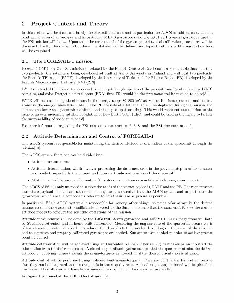
In Figure 1 is presented the ADCS block diagram[9].
2
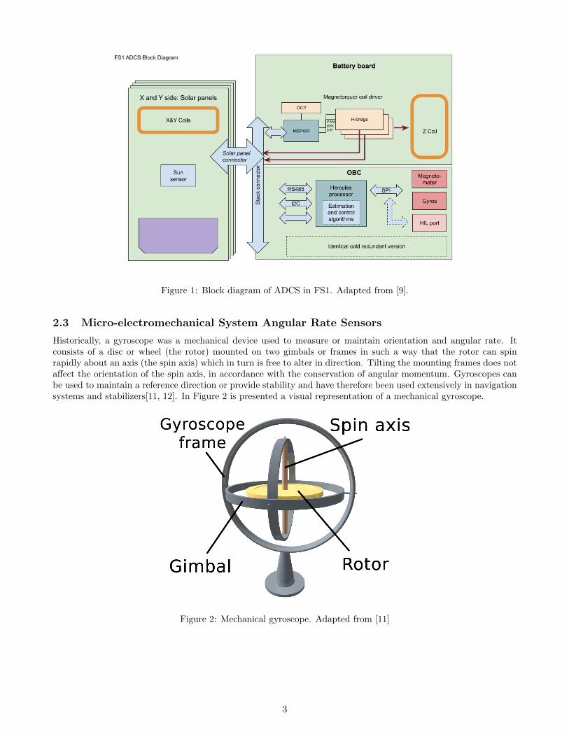
Figure 1: Block diagram of ADCS in FS1. Adapted from [9].
2.3 Micro-electromechanical System Angular Rate Sensors
Historically, a gyroscope was a mechanical device used to measure or maintain orientation and angular rate. Itconsists of a disc or wheel (the rotor) mounted on two gimbals or frames in such a way that the rotor can spinrapidly about an axis (the spin axis) which in turn is free to alter in direction. Tilting the mounting frames does notaffect the orientation of the spin axis, in accordance with the conservation of angular momentum. Gyroscopes canbe used to maintain a reference direction or provide stability and have therefore been used extensively in navigationsystems and stabilizers[11, 12]. In Figure 2 is presented a visual representation of a mechanical gyroscope.
Figure 2: Mechanical gyroscope. Adapted from [11]
3

Optical gyroscopes such as the Ring Laser Gyro (RLG) and Fibre Optic Gyro (FOG) started to appear in the1970s; they use the phase shift of light travelling in opposite directions around a fixed path length to detect angularvelocity. RLGs and FOGs provide a high accuracy but are also quite complex and thus rather large and costly[13].
Micro-electromechanical system (MEMS) gyroscopes belong to a type of gyroscope named the Vibrating StructureGyroscope (VSG), which started to appear in the 1980s. They make use of a vibrating structure to determine therate of rotation and do not need a point of reference.
The principal of operation is as follows: ”To use the Coriolis effect to detect angular rotation, a solid structure isforced to vibrate normally at its resonant frequency. This is achieved by applying an alternating voltage to theprimary electrodes. The vibration provides the structure with a linear velocity component. When the structure isrotated, the Coriolis forces cause the vibration motion of the structure to be coupled to another vibration mode orplane of the structure. The magnitude of this secondary vibration is proportional to the angular rate of turn.”[14]
In Figure 3a is presented a schematic of the motion of a gyroscope. The aforementioned Coriolis effect creates theCoriolis force of FC , the applied angular rate is represented by the blue arrow while ν stands for the vibration. InFigure 3b is presented a schematic of a MEMS gyroscope.
(a) Schematic of the motion of a vibratingring MEMS gyroscope. Adapted from [15]. (b) Schematic of a MEMS gyroscope. Adapted from [16]
Figure 3: Schematics of (a) the motion of a vibrating ring MEMS gyroscope and of (b) a MEMS gyroscope.
There are various types of VSGs, including but not limited to cylindrical resonator gyroscopes (CRG); tuningfork gyroscope (TFG); piezoelectric gyroscopes; and hemispherical resonator gyroscope (HRG)[17]. For a thoroughexplanation of the various types of VSGs please refer to [17]. MEMS gyroscopes use lithographically constructedversions of one or more of thee type of VSGs.
2.3.1 The L3GD20H 3-axis Gyroscope
The L3GD20H is a MEMS low-power three-axis angular rate sensor. It includes a sensing element and an ICinterface able to provide the measured angular rate to the external world through digital interface (I2C/SPI). Thesensing element is manufactured using a dedicated micromachining process developed by ST to produce inertialsensors and actuators on silicon wafers[18].
4
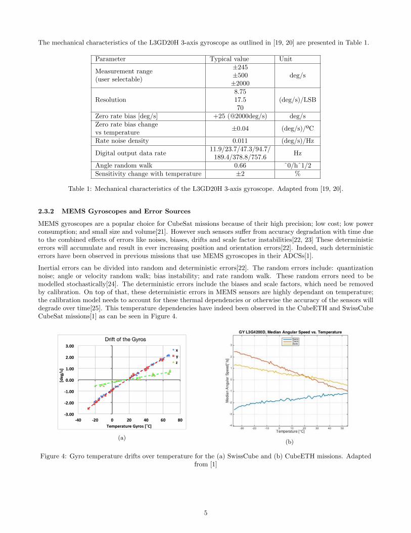
The mechanical characteristics of the L3GD20H 3-axis gyroscope as outlined in [19, 20] are presented in Table 1.
Parameter Typical value Unit
Measurement range(user selectable)
±245±500±2000
deg/s
Resolution8.7517.570
(deg/s)/LSB
Zero rate bias [deg/s] +25 (@2000deg/s) deg/sZero rate bias changevs temperature
±0.04 (deg/s)/ºC
Rate noise density 0.011 (deg/s)/Hz
Digital output data rate11.9/23.7/47.3/94.7/
189.4/378.8/757.6Hz
Angle random walk 0.66 ˆ0/hˆ1/2Sensitivity change with temperature ±2 %
Table 1: Mechanical characteristics of the L3GD20H 3-axis gyroscope. Adapted from [19, 20].
2.3.2 MEMS Gyroscopes and Error Sources
MEMS gyroscopes are a popular choice for CubeSat missions because of their high precision; low cost; low powerconsumption; and small size and volume[21]. However such sensors suffer from accuracy degradation with time dueto the combined effects of errors like noises, biases, drifts and scale factor instabilities[22, 23] These deterministicerrors will accumulate and result in ever increasing position and orientation errors[22]. Indeed, such deterministicerrors have been observed in previous missions that use MEMS gyroscopes in their ADCSs[1].
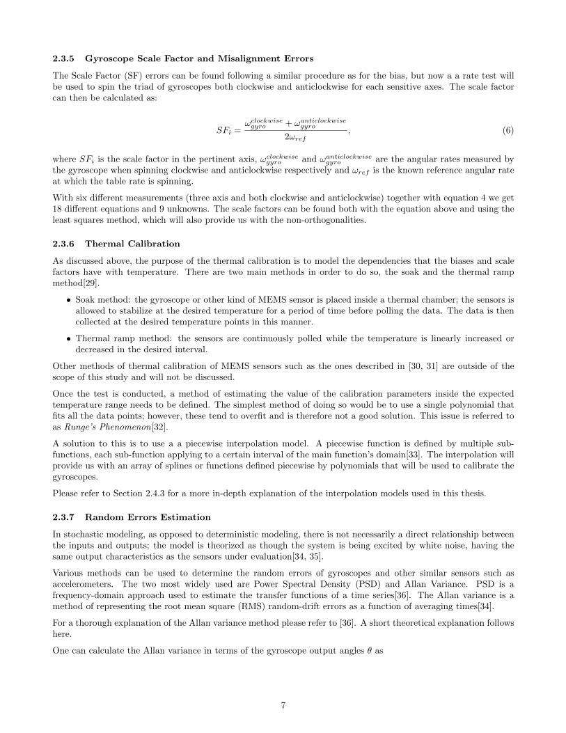
Inertial errors can be divided into random and deterministic errors[22]. The random errors include: quantizationnoise; angle or velocity random walk; bias instability; and rate random walk. These random errors need to bemodelled stochastically[24]. The deterministic errors include the biases and scale factors, which need be removedby calibration. On top of that, these deterministic errors in MEMS sensors are highly dependant on temperature;the calibration model needs to account for these thermal dependencies or otherwise the accuracy of the sensors willdegrade over time[25]. This temperature dependencies have indeed been observed in the CubeETH and SwissCubeCubeSat missions[1] as can be seen in Figure 4.
(a)(b)
Figure 4: Gyro temperature drifts over temperature for the (a) SwissCube and (b) CubeETH missions. Adaptedfrom [1]
5

2.3.3 Gyroscope Error Model
An ideal MEMS-gyroscope has no noise or offset, has perfect linearity and when subject to a known rotation willproduce a known output. However, real gyroscopes present the following deterministic errors:
• Bias or offset of the gyroscope reading with respect to the theoretical value it should present when not excited.This ”zero reading” drifts over time due to integration of inherent imperfections and noise within the device,which causes the bias[26].
• Scale factor error, describes how well the output of the sensors corresponds to the input[27]. Normallyexpressed in percentage terms or as a scale value.
• Non-orthogonalities, or axis-to-axis misalignment error, which describes how well the alignment of each gyro-scope axis fits into the ideal case of mutual orthogonality[28].
The output of a typical MEMS gyroscope can be expressed in function of the input angular velocity and thedeterministic error variables of the gyroscope as
ωgyros = Kg × ωinput +Bgyros, (1)
where ωgyros and ωinput are respectively the angular velocity as recorded by the gyroscopes and the real angularvelocity; Kg is the non-orthogonality error and scale factor matrix and Bgyros is the bias of the gyroscopes. Kg
presents the form
mx,x mx,y mx,z
my,x my,y my,z
mz,x mz,y mz,z
, (2)
being the mxx, my and mzz diagonal elements the scale factor errors and the mij non-diagonal elements thenon-orthogonalities. In matrix form equation 1 is
ωgyro,x
ωgyro,y
ωgyro,z
=
mx,x mx,y mx,z
my,x my,y my,z
mz,x mz,y mz,z
ωreal,x
ωreal,y
ωreal,z
+
bxbybz
, (3)
which can also be expressed as:
ωgyro,x
ωgyro,y
ωgyro,z
=
mx,x mx,y mx,z bxmy,x my,y my,z bymz,x mz,y mz,z bz
ωreal,x
ωreal,y
ωreal,z
1
. (4)
In order to solve this equation a combination of static and dynamic tests using a rate table will be performed. Thisprocedure is explained below.
2.3.4 Gyroscope Bias
In order to find the bias for each axis the triad of orthogonal gyroscopes are placed on a leveled surface with eachsensitive axis pointing alternatively up and down, which results in a total of six positions. The bias can then becalculated as[29]
bi =ωupgyro + ωdown
gyro
2, (5)
where bi is the bias in each axis, and ωupgyro and ωdown
gyro are the measured angular rates by the gyroscopes whenpointing alternatively upward and downwards.
6
2.3.5 Gyroscope Scale Factor and Misalignment Errors
The Scale Factor (SF) errors can be found following a similar procedure as for the bias, but now a a rate test willbe used to spin the triad of gyroscopes both clockwise and anticlockwise for each sensitive axes. The scale factorcan then be calculated as:
SFi =ωclockwisegyro + ωanticlockwise
gyro
2ωref, (6)
where SFi is the scale factor in the pertinent axis, ωclockwisegyro and ωanticlockwise
gyro are the angular rates measured bythe gyroscope when spinning clockwise and anticlockwise respectively and ωref is the known reference angular rateat which the table rate is spinning.
With six different measurements (three axis and both clockwise and anticlockwise) together with equation 4 we get18 different equations and 9 unknowns. The scale factors can be found both with the equation above and using theleast squares method, which will also provide us with the non-orthogonalities.
2.3.6 Thermal Calibration
As discussed above, the purpose of the thermal calibration is to model the dependencies that the biases and scalefactors have with temperature. There are two main methods in order to do so, the soak and the thermal rampmethod[29].
• Soak method: the gyroscope or other kind of MEMS sensor is placed inside a thermal chamber; the sensors isallowed to stabilize at the desired temperature for a period of time before polling the data. The data is thencollected at the desired temperature points in this manner.
• Thermal ramp method: the sensors are continuously polled while the temperature is linearly increased ordecreased in the desired interval.
Other methods of thermal calibration of MEMS sensors such as the ones described in [30, 31] are outside of thescope of this study and will not be discussed.
Once the test is conducted, a method of estimating the value of the calibration parameters inside the expectedtemperature range needs to be defined. The simplest method of doing so would be to use a single polynomial thatfits all the data points; however, these tend to overfit and is therefore not a good solution. This issue is referred toas Runge’s Phenomenon[32].
A solution to this is to use a a piecewise interpolation model. A piecewise function is defined by multiple sub-functions, each sub-function applying to a certain interval of the main function’s domain[33]. The interpolation willprovide us with an array of splines or functions defined piecewise by polynomials that will be used to calibrate thegyroscopes.
Please refer to Section 2.4.3 for a more in-depth explanation of the interpolation models used in this thesis.
2.3.7 Random Errors Estimation
In stochastic modeling, as opposed to deterministic modeling, there is not necessarily a direct relationship betweenthe inputs and outputs; the model is theorized as though the system is being excited by white noise, having thesame output characteristics as the sensors under evaluation[34, 35].
Various methods can be used to determine the random errors of gyroscopes and other similar sensors such asaccelerometers. The two most widely used are Power Spectral Density (PSD) and Allan Variance. PSD is afrequency-domain approach used to estimate the transfer functions of a time series[36]. The Allan variance is amethod of representing the root mean square (RMS) random-drift errors as a function of averaging times[34].
For a thorough explanation of the Allan variance method please refer to [36]. A short theoretical explanation followshere.
One can calculate the Allan variance in terms of the gyroscope output angles θ as
7
θ(t) =
∫ t
Ω(t)dt, (7)
being the angle measurements at t = kτ0(τ0, 2τ0, 3τ0...) where k ranges from 1 to N .
Once N values of θ have been computed, one ca then the Allan variance can be calculated as
θ2(T ) =1
2(N − 2n)
N−2n∑k=1
[θnext(T )− θk(T )]2, (8)
being θ2(τ) the Allan variance as a function of τ , N a number of consecutive data points, m the averaging factor,K a set of discrete values varying from 1 to N and τ = mτ0 the averaging time.
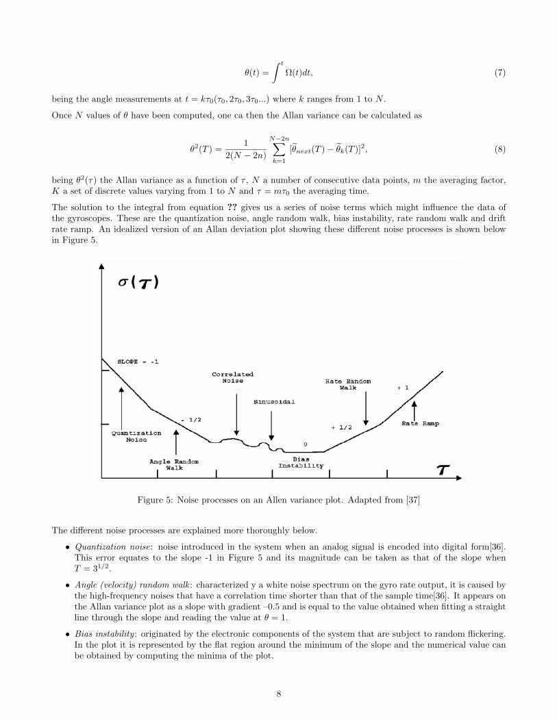
The solution to the integral from equation ?? gives us a series of noise terms which might influence the data ofthe gyroscopes. These are the quantization noise, angle random walk, bias instability, rate random walk and driftrate ramp. An idealized version of an Allan deviation plot showing these different noise processes is shown belowin Figure 5.
Figure 5: Noise processes on an Allen variance plot. Adapted from [37]
The different noise processes are explained more thoroughly below.
• Quantization noise: noise introduced in the system when an analog signal is encoded into digital form[36].This error equates to the slope -1 in Figure 5 and its magnitude can be taken as that of the slope whenT = 31/2.
• Angle (velocity) random walk : characterized y a white noise spectrum on the gyro rate output, it is caused bythe high-frequency noises that have a correlation time shorter than that of the sample time[36]. It appears onthe Allan variance plot as a slope with gradient –0.5 and is equal to the value obtained when fitting a straightline through the slope and reading the value at θ = 1.
• Bias instability : originated by the electronic components of the system that are subject to random flickering.In the plot it is represented by the flat region around the minimum of the slope and the numerical value canbe obtained by computing the minima of the plot.
8
• Rate random walk : this is a noise process of uncertain origin and represented by the slope +1/2 in thelogarithmic plot of the Allan variance. The numerical value can be found by reading the value of the plotwhen T = 3.
• Drift rate ramp: represents the rate at which the average changes. It is and represented by the slope +1 inthe logarithmic plot of the Allan variance. The numerical value can be found by reading the value of the plotwhen T = 21/2.
2.4 Calibration methods
2.4.1 Ordinary Least Squares Regression Model
Ordinary least squares (OLS) is a method of linear regression; linear regression establishes that between an inde-pendent variable x and a dependent variable y(x) exists the relation
y = b1x+ b0, (9)
being b1 also known as the coefficient and b0 the constant coefficient. OLS finds the values for b1, b0 such that thetotal sum of squares of the difference between the calculated and observed values of y is minimized[38]. Expressedin a formula that would be
S =
n∑i=1
(yi − y2i ) =
n∑i=1
(yi − b1x1 − b0)2 =
n∑i=1
(εi)2 = min, (10)
where yi and yi are the predicted and observed values of the dependant variable, εi is the error or residual and n isthe total number of observations[38].
In order to find the values of b1 and b0 that minimize S one can take a partial derivative of each coefficient andequate it to zero[38].
2.4.2 Mean Absolute Error, Root Mean Square Error and Maximum Absolute Error
Mean Absolute Error (MAE) and Root Mean Square Error (RMSE) are two of the most commonly used metricsthat characterize how well a model fits reality. Both measure the average magnitude of the error in a model, albeitin slightly different ways. MAE represents the average over the test sample of the absolute difference betweenpredicted and real value; all terms have equal weight[39]. It can be computed as
MAE =1
n
n∑i=1
|yi − yi|, (11)
RMS on the other hand is the square root of the average over the test sample of the squared difference betweenpredicted values and actual observations[39]. It can be computed as
RMSE =
√√√√ 1
n
n∑i=1
(yi − yi)2, (12)
RMSE gives a higher weighting to large errors, as the difference between predicted and actual observations aresquared before the average is taken. This means that RMSE should be the method used if large errors are undesir-able. However, the RMSE does not increase just with the variance of the errors. RMSE increases with the varianceof the frequency distribution of error magnitudes[39].
As RMSE is not as straightforward as MAE and has other implications other than quantifying the error in a model,MAE is a more clear measure in order to understand how well a model fits the data. However, since large errorsare to be avoided when calibrating the gyroscopes, RMSE will also be evaluated.
Something interesting to note is that RMSE will always be larger than MAE, or equal if all errors are of the samemagnitude[39].
9
In addition, since both RMSE and MAE are averages of the error across a population, it has been deemed interestingto add a measure of the possible magnitude of the error of a model. Computing the maximum absolute error in apopulation can give us this insight. Mathematically, it can be expresses as[40]:
MAX = max(|yi − yi|). (13)
In this report MAE, RMSE and MAX were computed using Python’s package scikit-learn[41].
2.4.3 Interpolation
Interpolation is a method by which the related known values are used to estimate the an unknown related valuelocated in the same range as the known values[42, 43].
Interpolation differs from other methods such as approximation and curve-fitting in that when using interpolationone forces the function to fit all data points. Interpolation is most appropriate when one intends to smooth outnoisy data and is not appropriate when the datasets present high variance[44].
The most known method for interpolating is a polynomial interpolation, by which a for a data set of n data pointsa unique polynomial of degree at most n-1 is derived. There are various method of polynomial interpolation, e.g.Monomial Basis, Lagrange Basis or Newton’s Basis. Polynomial interpolation however represents an importantdrawback; if the dataset has a non-negligible variance, it is likely that one need use a high degree polynomial tofit the data. This is likely to result in over-fitting, which occurs when the model predicts well not only the databut also its noise; one can refer to it as fitting the data ”too well”. It occurs if the model shows low bias and highvariance[44, 45].
A piecewise interpolating function or spline resolves this by breaking up the dataset in multiple ranges and applyinga different function of a low-degree polynomial to each range. This corrects for the possible over-fitting when usinglarge degree polynomials; splines are also not as adversely affected by outliers as they are defined locally ratherthan globally[44, 46].
The simplest spline would be one using linear functions; said linear interpolations states that if we know twoparameters p0 and p1 at temperatures t0 and t1 we can estimate the value of said parameter at another arbitrarytemperature t as
p(t) =t1 − tt1 − t0
p0 +t− t0t1 − t0
p1, (14)
where p(t) is the value of the parameter at the temperature t. However, they present a lack of smoothness at thebreakout points (points that mark the boundaries between intervals). This is so because at each breakout pointthe slope of the interpolating function is undefined. A common solution to this issue is to use a Cubic splineinterpolation, which uses third-degree polynomials as its piecewise functions. Then the interpolant is not onlycontinuously differentiable but also has a continuous second derivative[32].
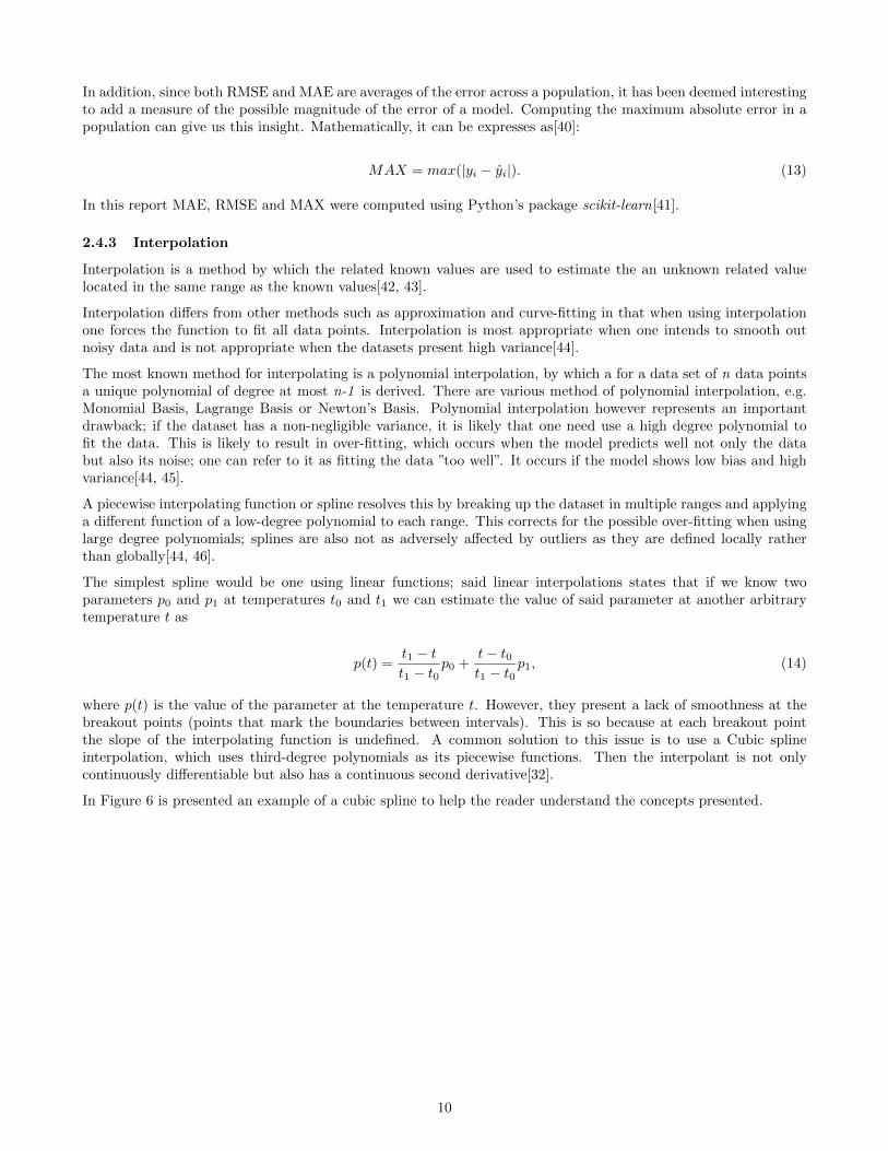
In Figure 6 is presented an example of a cubic spline to help the reader understand the concepts presented.
10
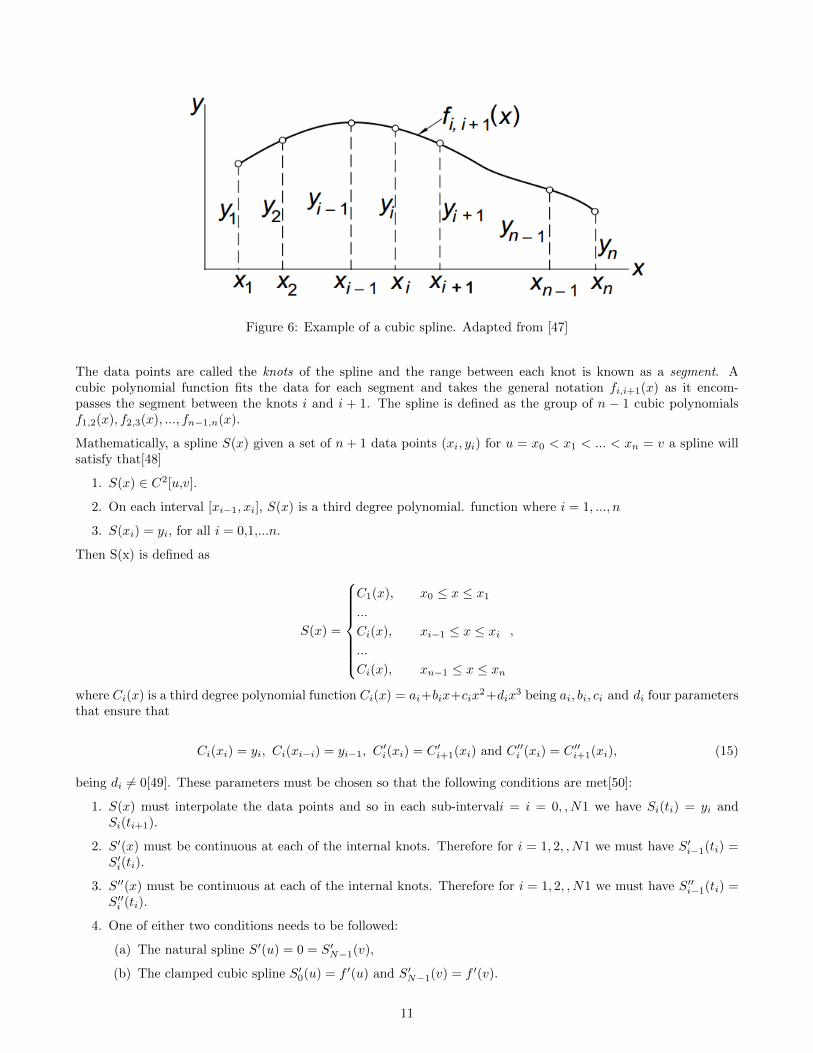
Figure 6: Example of a cubic spline. Adapted from [47]
The data points are called the knots of the spline and the range between each knot is known as a segment. Acubic polynomial function fits the data for each segment and takes the general notation fi,i+1(x) as it encom-passes the segment between the knots i and i + 1. The spline is defined as the group of n − 1 cubic polynomialsf1,2(x), f2,3(x), ..., fn−1,n(x).
Mathematically, a spline S(x) given a set of n+ 1 data points (xi, yi) for u = x0 < x1 < ... < xn = v a spline willsatisfy that[48]
1. S(x) ∈ C2[u,v].
2. On each interval [xi−1, xi], S(x) is a third degree polynomial. function where i = 1, ..., n
3. S(xi) = yi, for all i = 0,1,...n.
Then S(x) is defined as
S(x) =
C1(x), x0 ≤ x ≤ x1...
Ci(x), xi−1 ≤ x ≤ xi...
Ci(x), xn−1 ≤ x ≤ xn
,
where Ci(x) is a third degree polynomial function Ci(x) = ai+bix+cix2+dix
3 being ai, bi, ci and di four parametersthat ensure that
Ci(xi) = yi, Ci(xi−i) = yi−1, C′i(xi) = C ′i+1(xi) and C ′′i (xi) = C ′′i+1(xi), (15)
being di 6= 0[49]. These parameters must be chosen so that the following conditions are met[50]:
1. S(x) must interpolate the data points and so in each sub-intervali = i = 0, , N1 we have Si(ti) = yi andSi(ti+1).
2. S′(x) must be continuous at each of the internal knots. Therefore for i = 1, 2, , N1 we must have S′i−1(ti) =S′i(ti).
3. S′′(x) must be continuous at each of the internal knots. Therefore for i = 1, 2, , N1 we must have S′′i−1(ti) =S′′i (ti).
4. One of either two conditions needs to be followed:
(a) The natural spline S′(u) = 0 = S′N−1(v),
(b) The clamped cubic spline S′0(u) = f ′(u) and S′N−1(v) = f ′(v).
11

The clamped cubic spline gives more accurate approximation to the function f(x), but requires knowledge of thederivative at the endpoints[50]. It is therefore more common to use a natural cubic spline.
For an in-depth derivation of the algorithm followed to obtain a natural cubic spline from a dataset please refer to[50] or [51].
2.5 Outliers
In a data set, an outlier is defined as a data point which has an abnormally large or small value when comparedto the rest of the data set. As per [52], An outlying observation may be merely an extreme manifestation of therandom variability inherent in the data. ... On the other hand, an outlying observation may be the result of grossdeviation from prescribed experimental procedure or an error in calculating or recording the numerical value.
In the particular case of this mission, the presence of outliers in the data taken from the sensors might tell us thatthose sensors are faulty and are not fit to use in the mission. It is therefore of the utmost importance that thepresence of outliers be checked in all sensors that are due to be used so as not to possibly compromise the missionby using faulty devices.
Should there be an outlier population greater than for instance 5%, the first step would be to check for computationerrors and/or repeat the experiment. Should successive experiments show again an abnormally higher outlierpopulation and in the absence of another plausible explanation the device should be considered faulty and discarded.
There are various methods of detecting outliers in a population such as: the standard deviation (SD) method;the z-score and the modified z-score; Tukey’s fences or boxplot and the skewness adjusted boxplot developed byVanderviere and Huber [53];and the median and the MADe method, which uses the median and the Median AbsoluteDeviation (MAD)[54].
In order to select the most appropriate method one needs to analyse the data. In Figure 7 it is presented a flowchartintended to help choose the appropriate method.
12
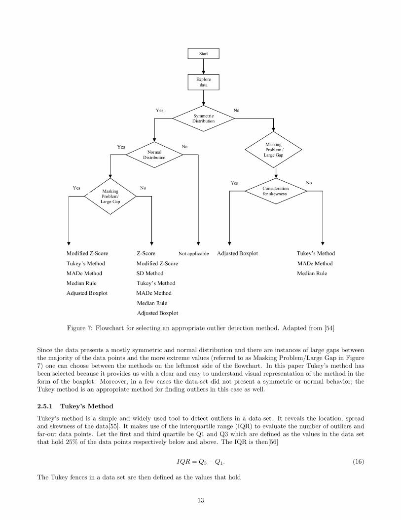
Figure 7: Flowchart for selecting an appropriate outlier detection method. Adapted from [54]
Since the data presents a mostly symmetric and normal distribution and there are instances of large gaps betweenthe majority of the data points and the more extreme values (referred to as Masking Problem/Large Gap in Figure7) one can choose between the methods on the leftmost side of the flowchart. In this paper Tukey’s method hasbeen selected because it provides us with a clear and easy to understand visual representation of the method in theform of the boxplot. Moreover, in a few cases the data-set did not present a symmetric or normal behavior; theTukey method is an appropriate method for finding outliers in this case as well.
2.5.1 Tukey’s Method
Tukey’s method is a simple and widely used tool to detect outliers in a data-set. It reveals the location, spreadand skewness of the data[55]. It makes use of the interquartile range (IQR) to evaluate the number of outliers andfar-out data points. Let the first and third quartile be Q1 and Q3 which are defined as the values in the data setthat hold 25% of the data points respectively below and above. The IQR is then[56]
IQR = Q3 −Q1. (16)
The Tukey fences in a data set are then defined as the values that hold
13
Lower Tukey Fence = Q1 − kIQR,
Upper Tukey Fence = Q3 + kIQR,(17)
where k is a constant to be defined by the user. Typically k is equal to either 1.5 or 3; when values are outsideof the Tukey fences defined when k = 1.5 these values are known as outlier and when k = 3 they are defined asfar-out [54].
In Figure 8 is presented an example of a box-plot and probability density function (PDF) of a Gaussian dataset.
Figure 8: Box-plot and PDF of a Gaussian dataset. Adapted from [57]
Aside from the parameters described before (IQR, Q1, Q3, median) the σ or standard deviation parameter is alsointroduced. The standard deviation σ measures the dispersion of a dataset relative to its mean; the higher thedeviation, the further the data points are from the mean and the more spread out they are. The standard deviationis computed as the square root of the variance σ2, which also measures how spread out the data points are fromthe mean. Mathematically[58, 59]:
σ =√σ2 =
n∑i=1
(xi − a)2
n. (18)
For a normally distributed dataset the first and third quartile equate to a standard deviation of -0.67 and 0.67respectively; the Tukey fences would be located at a standard deviation of -2.608 and 2.608.
In order to ascertain the shape and symmetry of the data a simple histogram plot with a kernel density estimate(KDE) will be used. A histogram is a graphical display of data; the data is divided into ranges or bins and shownas bars of different height according to the density or number of data points in each range. A KDE is anothermethod of visualizing the distribution of a data-set as the histogram; a KDE however represents the distribution asa continuous probability density curve[60].
14

Mathematically, for a dataset with an unknown density at any given point x, the kernel density function can beexpressed as:
fh(x) =1
n
n∑i=1
Kh(x− xi) =1
nh
n∑i=1
K(x− xih
), (19)
where K is the kernel function, generally smooth and symmetric such as a Gaussian and h > 0 is defined as thebandwith and is a smoothing parameter[61].
15

3 Test Procedures and Data Collection
In this section the test procedures and hardware and software used during the tests are discussed; then, the datacollection methods and datasets obtained during testing are explained; finally, the method for filtering outliers fromthe datasets is presented.
3.1 Test Procedures
In this section the test setup and hardware and software used during the tests will be presented. Then the proceduresfollowed during each test are attached in step-by-step tables.
3.1.1 Hardware and Test Setup
The tests were performed at Aalto University’s Department of Electronics and Nanoengineering (ELE) laboratorylocated at TUAS building (Maarintie 8) on August-September 2020. The list of hardware devices and software usedduring the test is presented below.
• On-board computer (OBC) printed circuit board (PCB), developed in house at Aalto University. The designis outlined in [62].
• Battery PCB, developed in house at Aalto University. The design is outlined in [63].
• HP EliteBook PC Notebook 850 G4 running the Ground Station (GS) software, which can be found at [64].
• Votsch VTM 7004 Climate chamber.
• AC1120S 1-axis rate table by Acutronic, mounted together with the Votsch’s VTM 7004. This table rate isintended to be used during development, production, in-process testing, calibration and final inspection ofinertial components, instrument and MEMS[65].
• The S700 Digital Servoamplifier by Kollmorgen.
• Code Composer Studio or CCS is a integrated development environment (IDE) developed by Texas Instru-ments (TI) that supports TI’s Microcontroller and Embedded Processors portfolio[66].
• Spectrum Digital XDS100v3 USB CJTAG/JTAG Emulator,used to debug TI’s MCU on the OBC PCB. [67]
• Direct Current (DC) Power Supply or Battery Bank. The Xtorm Power Bank Voyager 26.000, Model noXB303 was used in the tests.
• FTDI TTL Universal Asynchronous Receiver/Transmitter (UART) to Universal Serial Bus (USB) serial cableor similar to send and receive telecommands (TC) and telemetry (TM) from and to the PCB and GS.
• USB to RS232 interface cable to connect the S700 Servoamplifier to the computer.
• Makerbeam kit[68]
In Figure 9 are presented the OBC and battery PCB stack connected to the GS as during the tests.
16
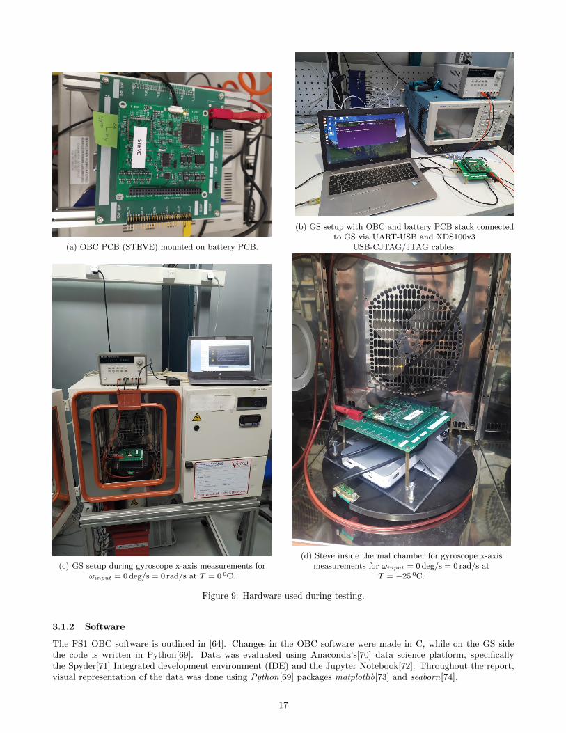
(a) OBC PCB (STEVE) mounted on battery PCB.
(b) GS setup with OBC and battery PCB stack connectedto GS via UART-USB and XDS100v3
USB-CJTAG/JTAG cables.
(c) GS setup during gyroscope x-axis measurements forωinput = 0deg/s = 0 rad/s at T = 0 ºC.
(d) Steve inside thermal chamber for gyroscope x-axismeasurements for ωinput = 0deg/s = 0 rad/s at
T = −25 ºC.
Figure 9: Hardware used during testing.
3.1.2 Software
The FS1 OBC software is outlined in [64]. Changes in the OBC software were made in C, while on the GS sidethe code is written in Python[69]. Data was evaluated using Anaconda’s[70] data science platform, specificallythe Spyder[71] Integrated development environment (IDE) and the Jupyter Notebook[72]. Throughout the report,visual representation of the data was done using Python[69] packages matplotlib[73] and seaborn[74].
17
3.1.3 Test Procedures
The procedures followed in the various tests performed to characterize and verify the error model of the L3GD20Hgyroscope are now presented. These procedures can provide a guideline to characterize other gyroscopes.
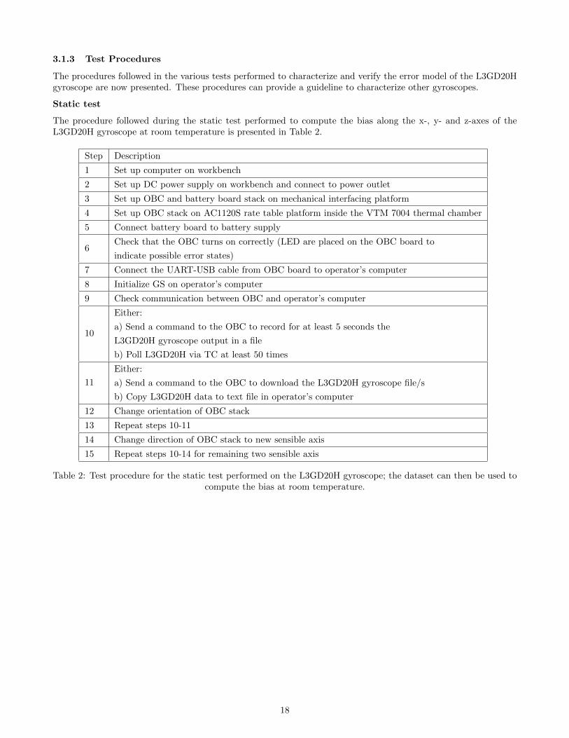
Static test
The procedure followed during the static test performed to compute the bias along the x-, y- and z-axes of theL3GD20H gyroscope at room temperature is presented in Table 2.
Step Description
1 Set up computer on workbench
2 Set up DC power supply on workbench and connect to power outlet
3 Set up OBC and battery board stack on mechanical interfacing platform
4 Set up OBC stack on AC1120S rate table platform inside the VTM 7004 thermal chamber
5 Connect battery board to battery supply
6Check that the OBC turns on correctly (LED are placed on the OBC board to
indicate possible error states)
7 Connect the UART-USB cable from OBC board to operator’s computer
8 Initialize GS on operator’s computer
9 Check communication between OBC and operator’s computer
10
Either:
a) Send a command to the OBC to record for at least 5 seconds the
L3GD20H gyroscope output in a file
b) Poll L3GD20H via TC at least 50 times
11
Either:
a) Send a command to the OBC to download the L3GD20H gyroscope file/s
b) Copy L3GD20H data to text file in operator’s computer
12 Change orientation of OBC stack
13 Repeat steps 10-11
14 Change direction of OBC stack to new sensible axis
15 Repeat steps 10-14 for remaining two sensible axis
Table 2: Test procedure for the static test performed on the L3GD20H gyroscope; the dataset can then be used tocompute the bias at room temperature.
18

Dynamic test
The procedure followed during the static test performed to compute the SF and misalignment errors for the x-, y-and z-axes of the L3GD20H gyroscope at room temperature is presented in Table 2.
Step Description
1 Set up computer on workbench
2 Set up DC power supply on workbench and connect to power outlet
3 Set up OBC and battery board stack on mechanical interfacing platform
4 Set up OBC stack on AC1120S rate table platform inside the VTM 7004 thermal chamber
5 Connect battery board to battery supply
6Check that the OBC turns on correctly (LED are placed on the OBC board to
indicate possible error states)
7 Connect the UART-USB cable from OBC board to operator’s computer
8 Initialize GS on operator’s computer
9 Check communication between OBC and operator’s computer
10 Connect S300 Servo Drive to operator’s computer via (check cable
11 Turn on S300 Servo Drive
12 Start S300 Servo Drive GUI on operator’s computer and connect to S300 Servo Drive
13Check that the AC1120S rate table is working properly sending a command to
activate rotation via the servo drive GUI
14Send a command to the angular rate to spin at pre-specified angular
velocity (30 degrees per second)
15
Either:
a) Send a command to the OBC to record for at least 5 seconds the
L3GD20H gyroscope output in a file
b) Poll L3GD20H via TC at least 50 times
16
Either:
a) Send a command to the OBC to download the L3GD20H gyroscope file/s
b) Copy L3GD20H data to text file in operator’s computer
17Send a command to the angular rate platform to in the opposite direction
as before (-30 degrees per second)
18 Repeat steps 15-16
19 Change direction of OBC stack to new sensible axis
20 Repeat steps 14-9 for remaining two sensible axis
Table 3: Test procedure for the static test performed on the L3GD20H gyroscope; the dataset can then be used tocompute the SF and misalignment errors at room temperature.
19
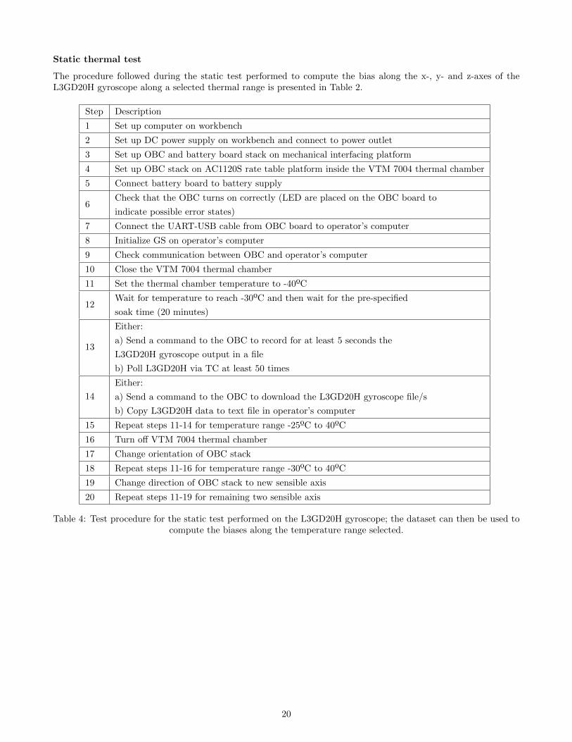
Static thermal test
The procedure followed during the static test performed to compute the bias along the x-, y- and z-axes of theL3GD20H gyroscope along a selected thermal range is presented in Table 2.
Step Description
1 Set up computer on workbench
2 Set up DC power supply on workbench and connect to power outlet
3 Set up OBC and battery board stack on mechanical interfacing platform
4 Set up OBC stack on AC1120S rate table platform inside the VTM 7004 thermal chamber
5 Connect battery board to battery supply
6Check that the OBC turns on correctly (LED are placed on the OBC board to
indicate possible error states)
7 Connect the UART-USB cable from OBC board to operator’s computer
8 Initialize GS on operator’s computer
9 Check communication between OBC and operator’s computer
10 Close the VTM 7004 thermal chamber
11 Set the thermal chamber temperature to -40ºC
12Wait for temperature to reach -30ºC and then wait for the pre-specified
soak time (20 minutes)
13
Either:
a) Send a command to the OBC to record for at least 5 seconds the
L3GD20H gyroscope output in a file
b) Poll L3GD20H via TC at least 50 times
14
Either:
a) Send a command to the OBC to download the L3GD20H gyroscope file/s
b) Copy L3GD20H data to text file in operator’s computer
15 Repeat steps 11-14 for temperature range -25ºC to 40ºC
16 Turn off VTM 7004 thermal chamber
17 Change orientation of OBC stack
18 Repeat steps 11-16 for temperature range -30ºC to 40ºC
19 Change direction of OBC stack to new sensible axis
20 Repeat steps 11-19 for remaining two sensible axis
Table 4: Test procedure for the static test performed on the L3GD20H gyroscope; the dataset can then be used tocompute the biases along the temperature range selected.
20
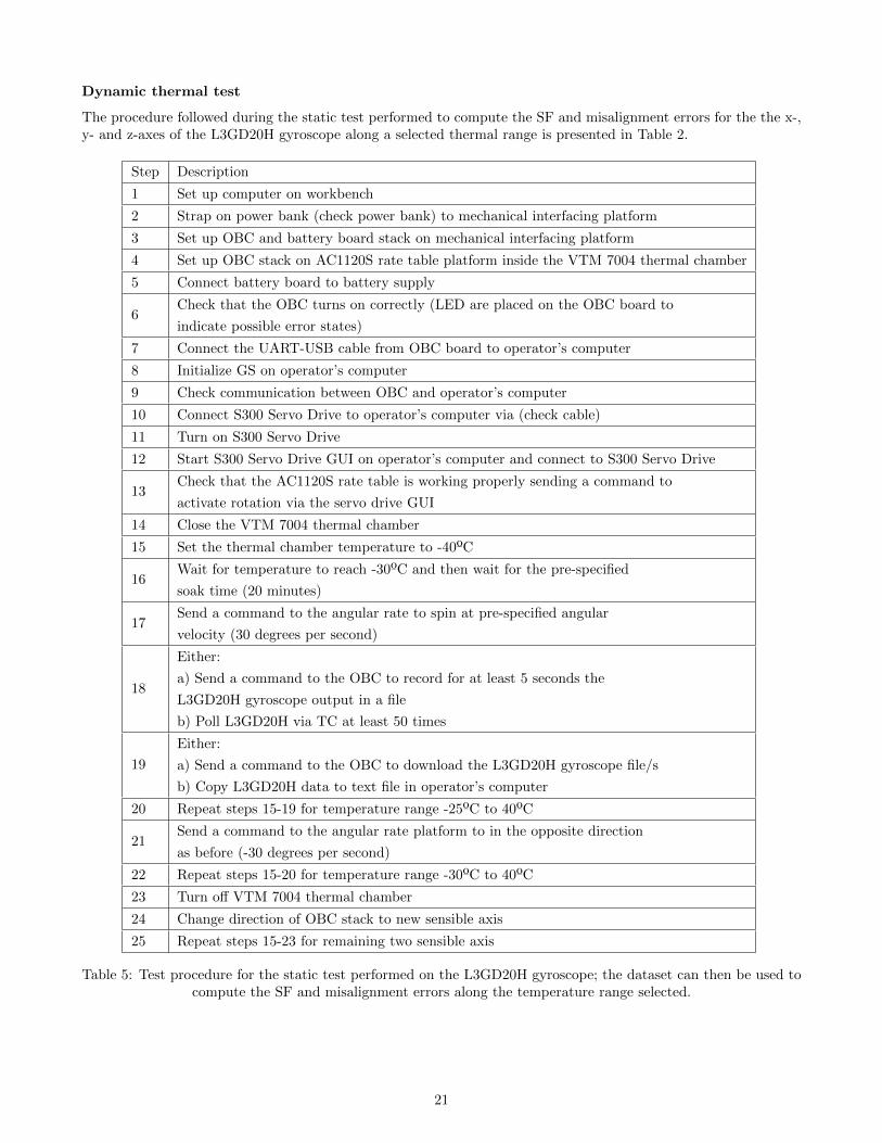
Dynamic thermal test
The procedure followed during the static test performed to compute the SF and misalignment errors for the the x-,y- and z-axes of the L3GD20H gyroscope along a selected thermal range is presented in Table 2.
Step Description
1 Set up computer on workbench
2 Strap on power bank (check power bank) to mechanical interfacing platform
3 Set up OBC and battery board stack on mechanical interfacing platform
4 Set up OBC stack on AC1120S rate table platform inside the VTM 7004 thermal chamber
5 Connect battery board to battery supply
6Check that the OBC turns on correctly (LED are placed on the OBC board to
indicate possible error states)
7 Connect the UART-USB cable from OBC board to operator’s computer
8 Initialize GS on operator’s computer
9 Check communication between OBC and operator’s computer
10 Connect S300 Servo Drive to operator’s computer via (check cable)
11 Turn on S300 Servo Drive
12 Start S300 Servo Drive GUI on operator’s computer and connect to S300 Servo Drive
13Check that the AC1120S rate table is working properly sending a command to
activate rotation via the servo drive GUI
14 Close the VTM 7004 thermal chamber
15 Set the thermal chamber temperature to -40ºC
16Wait for temperature to reach -30ºC and then wait for the pre-specified
soak time (20 minutes)
17Send a command to the angular rate to spin at pre-specified angular
velocity (30 degrees per second)
18
Either:
a) Send a command to the OBC to record for at least 5 seconds the
L3GD20H gyroscope output in a file
b) Poll L3GD20H via TC at least 50 times
19
Either:
a) Send a command to the OBC to download the L3GD20H gyroscope file/s
b) Copy L3GD20H data to text file in operator’s computer
20 Repeat steps 15-19 for temperature range -25ºC to 40ºC
21Send a command to the angular rate platform to in the opposite direction
as before (-30 degrees per second)
22 Repeat steps 15-20 for temperature range -30ºC to 40ºC
23 Turn off VTM 7004 thermal chamber
24 Change direction of OBC stack to new sensible axis
25 Repeat steps 15-23 for remaining two sensible axis
Table 5: Test procedure for the static test performed on the L3GD20H gyroscope; the dataset can then be used tocompute the SF and misalignment errors along the temperature range selected.
21
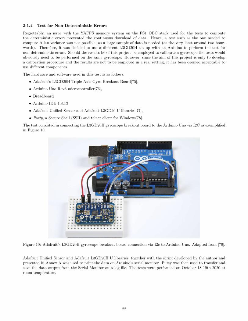
3.1.4 Test for Non-Deterministic Errors
Regrettably, an issue with the YAFFS memory system on the FS1 OBC stack used for the tests to computethe deterministic errors prevented the continuous download of data. Hence, a test such as the one needed tocompute Allan variance was not possible, as a large sample of data is needed (at the very least around two hoursworth). Therefore, it was decided to use a different L3GD20H set up with an Arduino to perform the test fornon-deterministic errors. Should the results be of this project be employed to calibrate a gyroscope the tests wouldobviously need to be performed on the same gyroscope. However, since the aim of this project is only to developa calibration procedure and the results are not to be employed in a real setting, it has been deemed acceptable touse different components.
The hardware and software used in this test is as follows:
• Adafruit’s L3GD20H Triple-Axis Gyro Breakout Board[75],
• Arduino Uno Rev3 microcontroller[76],
• Breadboard
• Arduino IDE 1.8.13
• Adafruit Unified Sensor and Adafruit L3GD20 U libraries[77],
• Putty, a Secure Shell (SSH) and telnet client for Windows[78].
The test consisted in connecting the L3GD20H gyroscope breakout board to the Arduino Uno via I2C as exemplifiedin Figure 10
Figure 10: Adafruit’s L3GD20H gyroscope breakout board connection via I2c to Arduino Uno. Adapted from [79].
Adafruit Unified Sensor and Adafruit L3GD20H U libraries, together with the script developed by the author andpresented in Annex A was used to print the data on Arduino’s serial monitor. Putty was then used to transfer andsave the data output from the Serial Monitor on a log file. The tests were performed on October 18-19th 2020 atroom temperature.
22
3.2 Data Collection and Dataset Explanation
In this section the methods for data collection and the different datasets obtained are discussed. An evaluation ofthe datasets follow, with special emphasis on the validity of the data collected as function of the number of outliersfound.
3.2.1 Data Collection
Data used for the development and verification of the calibration method was logged in two different ways; bystoring a file on the OBC flash memory, downloading it to the user’s computer and reading it; and by polling thesensors via the GS in the user’s computer.
The user sends a command to the OBC to record a certain data output, in this case the output of the L3GD20Hgyroscope, for a period of time. The file is stored in the flash memory and is accessible to any operator that connectsto the OBC. The files system used in the FS1 mission is an open-sourced file system called YAFFS (Yet AnotherFlash File System)[80]. For a comprehensive explanation of how YAFFS works please refer to [81]. In the case ofa gyroscope file the data recorded will include the output of the gyroscopes and the timestamp as measured sincethe OBC was turned on. The data is stored in binary form. The operator then sends a command to the OBC todownload the desired files. The files are stored as a byte-stream or octet stream, which is a sequence of bytes; eachbyte contains 8 bits. Since the bits can be encoded in multiple ways, the operator must know how the data is storedin order to retrieve it.
Once the files are downloaded a parser is used to decode the data. The parser used for this task makes use ofthe struct Python module, which interprets bytes as packed binary data. The module struct performs conversionsbetween Python values and C struct represented as Python bytes objects[82]. Since the C structure that the datawas stored in is known to the user, one can use the struct.unpack(format, buffer) (in which format refers to the Ctype and buffer to the memory array the data is stored in) function from the struct module in order to unpack thedata. The decoded data is then used in further calculations. Please refer to A for the code used in this process.
An alternate way of polling data from the sensors had to be found however, as bugs in the implementation of the filesystem and the file transfer system made the use of the first method sub-optimal at times. In this second methoda telecommand (TC) would be sent to the OBC by the user to read the angular rate as provided by the L3GD20Hgyroscope. The data would then be sent to the user as a telemetry (TM) package, the data being again in binaryform. The struct.unpack(format, buffer) function from the struct module is used once again to decode the data.The data can be read then in the command line running the GS software.
Dataset for thermal drift in bias - static thermal test
The dataset used for the derivation of the gyroscope bias include files recorded by either of the two methods describedin 3.2.1. The data was taken between the 22nd and the 23rd of September 2020 following the procedure describedin 4 and as such 90 files were obtained: 30 files for each axis, 15 files in either orientation (up or down) and onefile for each temperature break-point. The temperature ranged from −30°C to 40°C in increments of 5°C, resultingin 15 temperature breakpoints. At least 100 individual data points were taken for each temperature break-pointor file. A total of 9562 individual data points were recorded, 115 of those being classified as outliers. The meanof the data-set of each file was taken to perform calculations. However, as explained in 4.1.2 the data recorded forthe z-axis was discarded. It was replaced by a dataset recorded on the 29th of September 2020 and as previously itconsisted of 30 files, 15 in each orientation and each file containing at least 100 individual data points. In the end,9620 individual data points were taken.
Dataset for thermal drift in SF errors and non-orthogonalities - dynamic thermal test
The dataset used for the derivation of the gyroscope SF errors and non-orthogonalities include files recorded bythe second method as described in 3.2.1. The data was taken between the 25th and the 26th of September 2020following the procedure described in 5 and as such 90 files were obtained as before. The temperature ranged from-30ºC to 40ºC in increments of 5, resulting in 15 temperature breakpoints. Between 50 and 100 individual datapoints were taken for each temperature break-point or file. A total of 7552 individual data points were recorded,280 of those being classified as outliers and 15 as far-out points, which correspond to 3.14% and 0.20% of the totalpopulation respectively. Again, the mean of the data-set of each file was taken to perform calculations.
23
Datasets for verification
The first dataset used for the verification of the derived models include files by the second method as described in3.2.1. The data was taken on August 18th following the procedure described in 5, now for a temperature rangebetween −5°C and 25°C in 5°C increments. There were therefore seven breakpoints and a total of 42 different files.At least 50 relevant data points were taken for each axis and temperature after discarding for outliers. A total of5074 individual data points were recorded.
The second dataset used for the verification of the derived models include files by the second method as describedin 3.2.1. The data was taken between November 24th and 25th 2020 following the procedure described in 5, nowfor a temperature range between −8°C and 32°C in 4°C increments. There were therefore eleven breakpoints and atotal of 66 different files. At least 50 relevant data points were taken for each axis and temperature after discardingfor outliers. A total of 5567 individual data points were recorded.
The third dataset used for the verification of the derived models include files by the second method as described in3.2.1. The data was taken on November 25th 2020 following the procedure described in 5, now for a temperaturerange between −8°C and 32°C in 4°C increments. There were therefore eleven breakpoints and a total of 44 differentfiles. At least 50 relevant data points were taken for each axis and temperature after discarding for outliers. A totalof 3214 individual data points were recorded.
Datasets for Allan Deviation
Three different data sets were obtained in order to calculate the Allan deviation plots for the L3GD20H gyroscope.The output data rate of the gyroscope during testing was 100 Hz. Dataset 1 consisted of a total of 159674 individualdata points or 26.4 minutes worth of data. Dataset 2 and Dataset 3 consisted of 650866 and 658098 or around 108and 110 minutes worth of data respectively. The difference in the recording duration was only discovered whenanalyzing the data after the experiment and when the components were not available to the author anymore. Ideallyone would want to compare datasets of similar duration.
3.2.2 Outliers and Far-out Points
As described in Section 2.5 first a study of the presence of outliers in the datasets will be performed. The first stepis to decide which methodology for finding and classifying outliers should be implemented. This can be done byobserving the type of data-set available and using the flowchart presented in Figure 7 in Section 2.5.
The majority of data files present a symmetrical distribution and similar to a Gaussian, which is why taking themean of the dataset to perform calculations is acceptable. However, in some cases there are instances of largegaps between the majority of the data points and the more extreme values (referred to as Masking Problem/LargeGap in Figure 7). These extreme values need to be discarded so that the distribution of the data set will be moreGaussian-like and for the results not to be affected by outliers. There are three possible methods as per the Figure7 to detect outliers in a case such as ours, the Median Rule, and the Median Absolute Deviation (MADe) and theTukey’s methods.
In this report Tukey’s method has been decided upon, as it provides a simple and easy to understand visualrepresentation in the form of the boxplot.
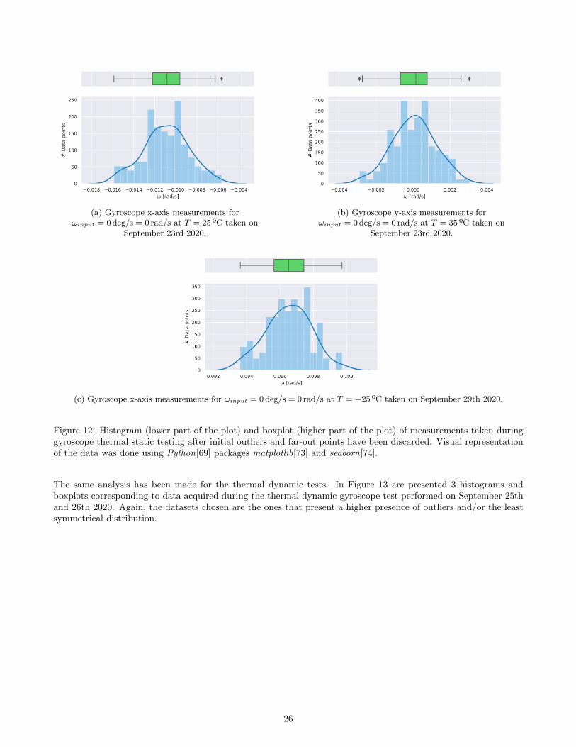
In Figure 11 are presented 3 histograms and boxplots corresponding to data acquired during the thermal staticgyroscope testing performed on September 23rd and 29th 2020. The datasets chosen are the ones that present ahigher presence of outliers and/or the least symmetrical distribution.
In the boxplot, the green body represents the IQR, being the left half the data population between the median orsecond quartile (Q2) and the lower quartile (Q1) and the right half between Q2 and the upper quartile (Q3); thewicks represent the data region encompassed by the Tukey fences when k = 1.5; and the individual data pointsoutside of the boxplot represent the outliers. In the histogram plot the bins represent the height of the bar representsthe frequency of each data region; the blue line represents a kernel density estimate (KDE), which is a means ofrepresenting the data using a continuous probability density curve[74].
24
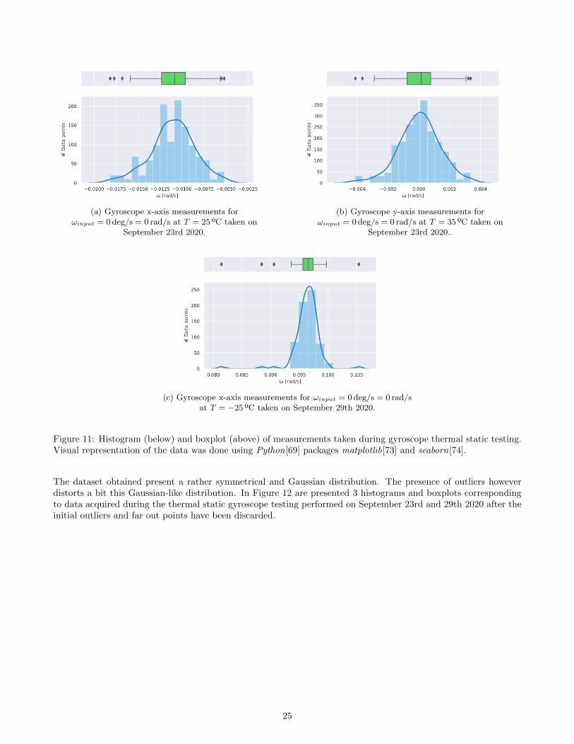
(a) Gyroscope x-axis measurements forωinput = 0deg/s = 0 rad/s at T = 25 ºC taken on
September 23rd 2020.
(b) Gyroscope y-axis measurements forωinput = 0deg/s = 0 rad/s at T = 35 ºC taken on
September 23rd 2020..
(c) Gyroscope x-axis measurements for ωinput = 0deg/s = 0 rad/sat T = −25 ºC taken on September 29th 2020.
Figure 11: Histogram (below) and boxplot (above) of measurements taken during gyroscope thermal static testing.Visual representation of the data was done using Python[69] packages matplotlib[73] and seaborn[74].
The dataset obtained present a rather symmetrical and Gaussian distribution. The presence of outliers howeverdistorts a bit this Gaussian-like distribution. In Figure 12 are presented 3 histograms and boxplots correspondingto data acquired during the thermal static gyroscope testing performed on September 23rd and 29th 2020 after theinitial outliers and far out points have been discarded.
25
(a) Gyroscope x-axis measurements forωinput = 0deg/s = 0 rad/s at T = 25 ºC taken on
September 23rd 2020.
(b) Gyroscope y-axis measurements forωinput = 0deg/s = 0 rad/s at T = 35 ºC taken on
September 23rd 2020.
(c) Gyroscope x-axis measurements for ωinput = 0deg/s = 0 rad/s at T = −25 ºC taken on September 29th 2020.
Figure 12: Histogram (lower part of the plot) and boxplot (higher part of the plot) of measurements taken duringgyroscope thermal static testing after initial outliers and far-out points have been discarded. Visual representationof the data was done using Python[69] packages matplotlib[73] and seaborn[74].
The same analysis has been made for the thermal dynamic tests. In Figure 13 are presented 3 histograms andboxplots corresponding to data acquired during the thermal dynamic gyroscope test performed on September 25thand 26th 2020. Again, the datasets chosen are the ones that present a higher presence of outliers and/or the leastsymmetrical distribution.
26
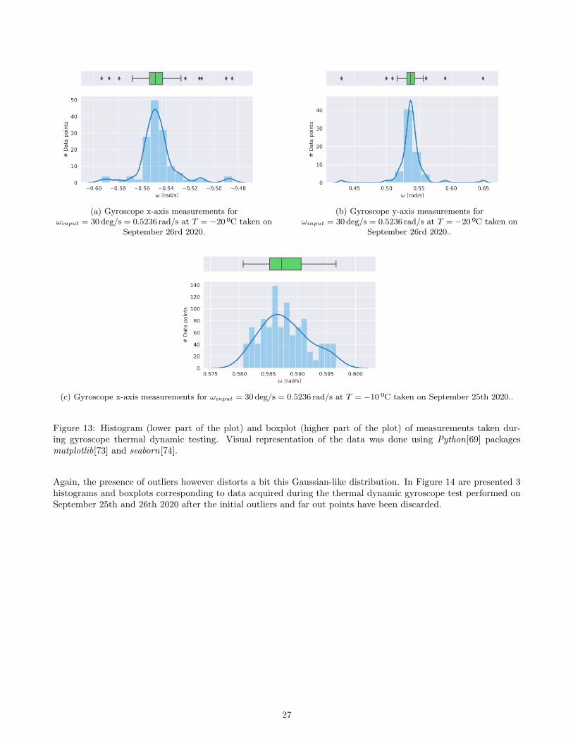
(a) Gyroscope x-axis measurements forωinput = 30deg/s = 0.5236 rad/s at T = −20 ºC taken on
September 26rd 2020.
(b) Gyroscope y-axis measurements forωinput = 30deg/s = 0.5236 rad/s at T = −20 ºC taken on
September 26rd 2020..
(c) Gyroscope x-axis measurements for ωinput = 30deg/s = 0.5236 rad/s at T = −10 ºC taken on September 25th 2020..
Figure 13: Histogram (lower part of the plot) and boxplot (higher part of the plot) of measurements taken dur-ing gyroscope thermal dynamic testing. Visual representation of the data was done using Python[69] packagesmatplotlib[73] and seaborn[74].
Again, the presence of outliers however distorts a bit this Gaussian-like distribution. In Figure 14 are presented 3histograms and boxplots corresponding to data acquired during the thermal dynamic gyroscope test performed onSeptember 25th and 26th 2020 after the initial outliers and far out points have been discarded.
27
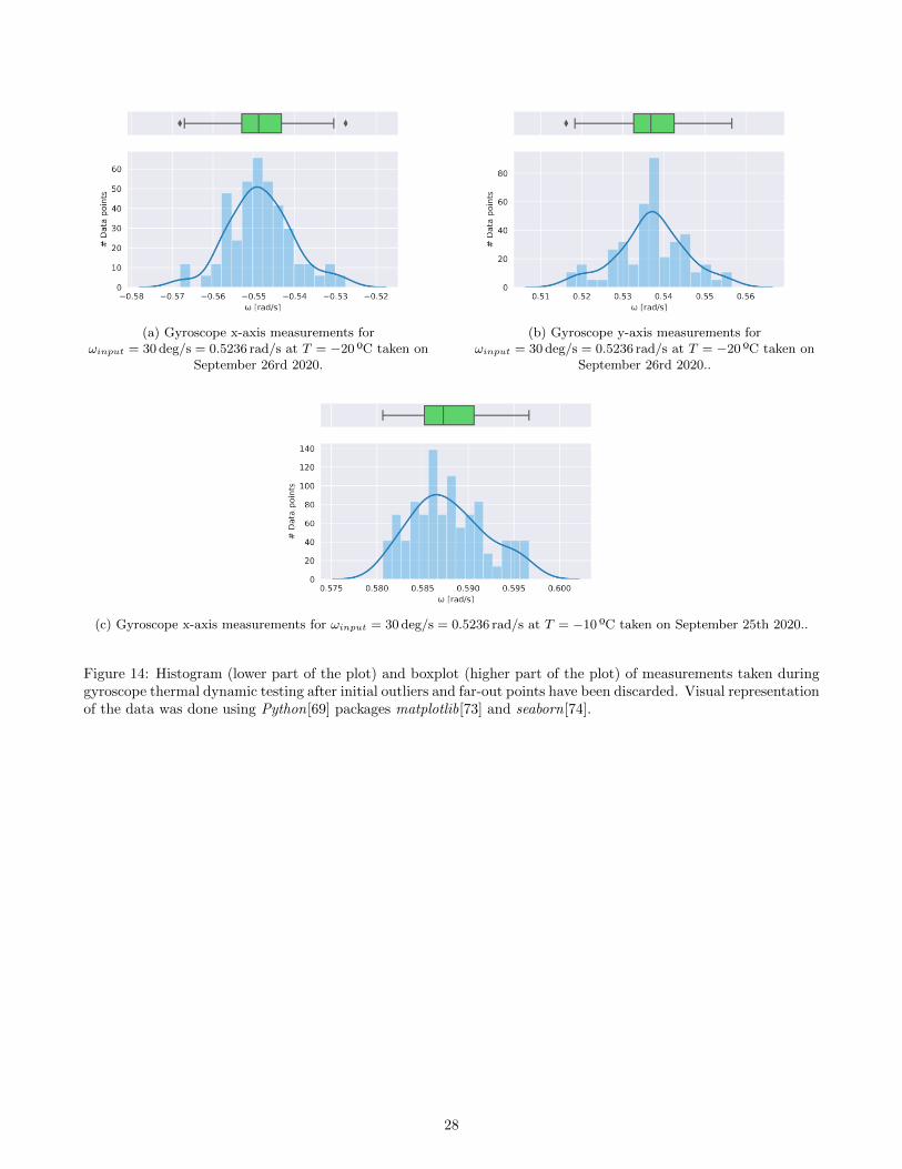
(a) Gyroscope x-axis measurements forωinput = 30deg/s = 0.5236 rad/s at T = −20 ºC taken on
September 26rd 2020.
(b) Gyroscope y-axis measurements forωinput = 30deg/s = 0.5236 rad/s at T = −20 ºC taken on
September 26rd 2020..
(c) Gyroscope x-axis measurements for ωinput = 30deg/s = 0.5236 rad/s at T = −10 ºC taken on September 25th 2020..
Figure 14: Histogram (lower part of the plot) and boxplot (higher part of the plot) of measurements taken duringgyroscope thermal dynamic testing after initial outliers and far-out points have been discarded. Visual representationof the data was done using Python[69] packages matplotlib[73] and seaborn[74].
28

In Table 6 is presented a summary of the number of data points, outliers and far-out points of the various datasetsrecorded to characterize the L3GD20H gyroscope.
Total data points[#]
Outliers[#]
Outliers[%]
Far-out points[#]
Far-out points[%]
Bias thermal drift 9620 105 1.09 1 0.01SF, misalignments and thermal drift 7567 237 3.13 15 0.19Verification dataset #1 5074 88 1.73 19 0.37Verification dataset #2 5567 152 2.73 1 0.02Verification dataset #3 3214 201 5.88 1 0.03
Table 6: Test procedure for the static test performed on the L3GD20H gyroscope; the dataset can then be used tocompute the SF and misalignment errors along the temperature range selected.
The number of outliers is generally rather low, the maximum being for the verification dataset from experimentnumber three in which the triad of gyroscopes was placed on a ramp in order to introduce a certain inclination. Itis likely that this is the cause of a greater number of outliers, as the make-shift ramps were not part of a levelledstructure. Aside from that dataset, the percentage of outliers is always around 3% or lower and the far-out pointsnever exceed 0.4%. The number of outliers and far-out points is low enough so that one can ascertain to a certaindegree that the gyroscopes are working properly and no major sources of error were present during the experiments.
Moreover, now that the outliers and far out points have been discarded, the distribution of the datasets more closelyresembles a Gaussian.
29
4 Results
In this section are presented the results of the tests and analysis of said results. First, the deterministic errorsand their relationship with temperature are presented. Then follows an evaluation of the thermal calibrationmodels considered in this thesis, namely the OLS linear regression and linear and cubic spline interpolation models.The non-deterministic errors are also discussed briefly. Then, the results for the deterministic errors and thermalcalibration models are verified.
4.1 Discussion of Test Results
In this section are presented the deterministic errors obtained in the tests, as well as the results as to their relationshipwith temperature. An evaluation of the different methods for thermal calibration follows, namely OLS linearregression and linear and cubic spline interpolation models. Lastly, the non-deterministic errors will be discussedbriefly.
4.1.1 Deterministic Errors
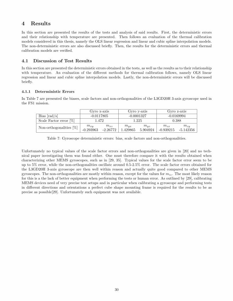
In Table 7 are presented the biases, scale factors and non-orthogonalities of the L3GD20H 3-axis gyroscope used inthe FS1 mission.
Gyro x-axis Gyro y-axis Gyro z-axisBias [rad/s] -0.0117805 -0.0001327 -0.0169994Scale Factor error [%] 1.472 1.225 0.388
Non-orthogonalities [%]mxy mxz myx myz mzx mzy
-0.293963 -2.26772 1.429865 5.904924 -0.939215 -5.142356
Table 7: Gyroscope deterministic errors: bias, scale factors and non-orthogonalities.
Unfortunately no typical values of the scale factor errors and non-orthogonalities are given in [20] and no tech-nical paper investigating them was found either. One must therefore compare it with the results obtained whencharacterizing other MEMS gyroscopes, such as in [29, 35]. Typical values for the scale factor error seem to beup to 5% error, while the non-orthogonalities oscillate around 0.5-2.5% error. The scale factor errors obtained forthe L3GD20H 3-axis gyroscope are then well within reason and actually quite good compared to other MEMSgyroscopes. The non-orthogonalities are mostly within reason, except for the values for miz. The most likely reasonfor this is a the lack of better equipment when performing the tests or human error. As outlined by [29], calibratingMEMS devices need of very precise test setups and in particular when calibrating a gyroscope and performing testsin different directions and orientations a perfect cube shape mounting frame is required for the results to be asprecise as possible[29]. Unfortunately such equipment was not available.
30
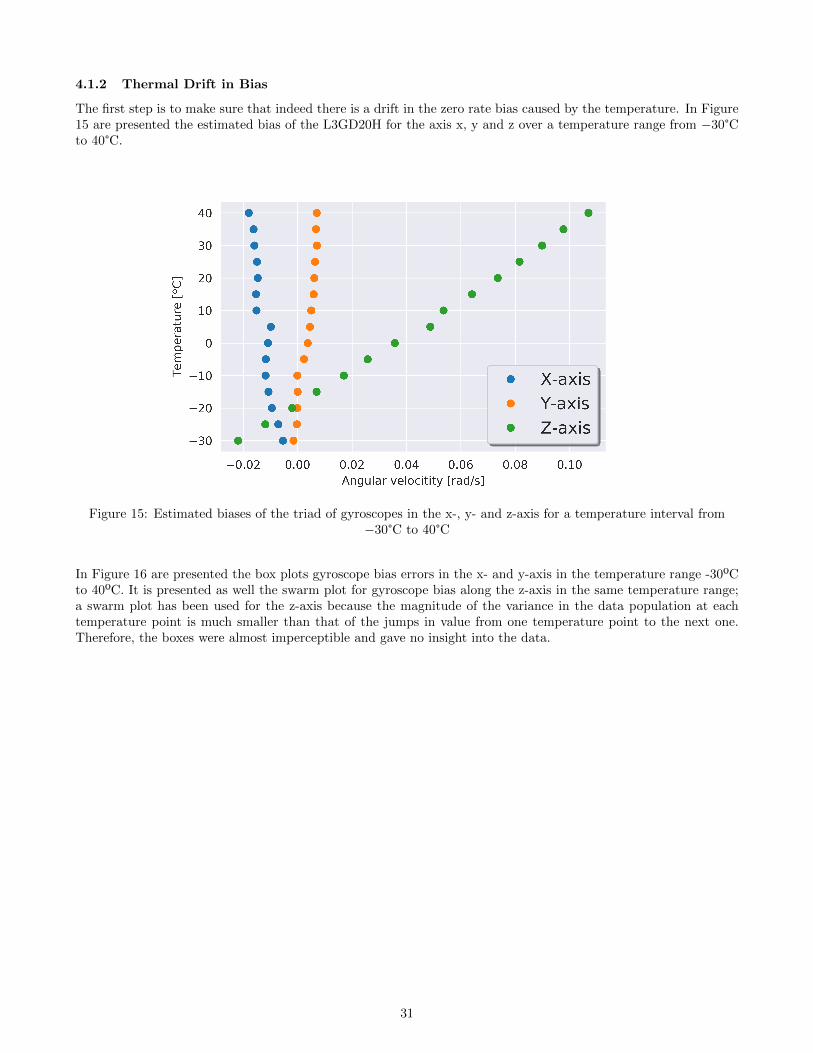
4.1.2 Thermal Drift in Bias
The first step is to make sure that indeed there is a drift in the zero rate bias caused by the temperature. In Figure15 are presented the estimated bias of the L3GD20H for the axis x, y and z over a temperature range from −30°Cto 40°C.
Figure 15: Estimated biases of the triad of gyroscopes in the x-, y- and z-axis for a temperature interval from−30°C to 40°C
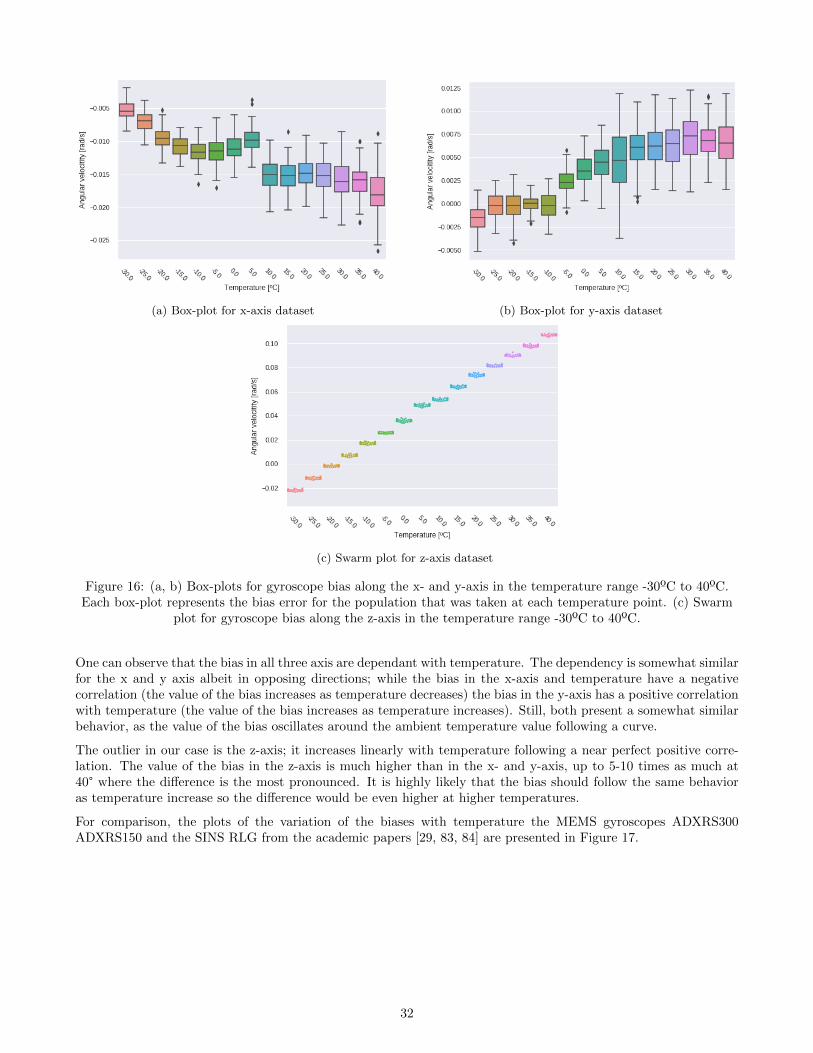
In Figure 16 are presented the box plots gyroscope bias errors in the x- and y-axis in the temperature range -30ºCto 40ºC. It is presented as well the swarm plot for gyroscope bias along the z-axis in the same temperature range;a swarm plot has been used for the z-axis because the magnitude of the variance in the data population at eachtemperature point is much smaller than that of the jumps in value from one temperature point to the next one.Therefore, the boxes were almost imperceptible and gave no insight into the data.
31
(a) Box-plot for x-axis dataset (b) Box-plot for y-axis dataset
(c) Swarm plot for z-axis dataset
Figure 16: (a, b) Box-plots for gyroscope bias along the x- and y-axis in the temperature range -30ºC to 40ºC.Each box-plot represents the bias error for the population that was taken at each temperature point. (c) Swarm
plot for gyroscope bias along the z-axis in the temperature range -30ºC to 40ºC.
One can observe that the bias in all three axis are dependant with temperature. The dependency is somewhat similarfor the x and y axis albeit in opposing directions; while the bias in the x-axis and temperature have a negativecorrelation (the value of the bias increases as temperature decreases) the bias in the y-axis has a positive correlationwith temperature (the value of the bias increases as temperature increases). Still, both present a somewhat similarbehavior, as the value of the bias oscillates around the ambient temperature value following a curve.
The outlier in our case is the z-axis; it increases linearly with temperature following a near perfect positive corre-lation. The value of the bias in the z-axis is much higher than in the x- and y-axis, up to 5-10 times as much at40° where the difference is the most pronounced. It is highly likely that the bias should follow the same behavioras temperature increase so the difference would be even higher at higher temperatures.
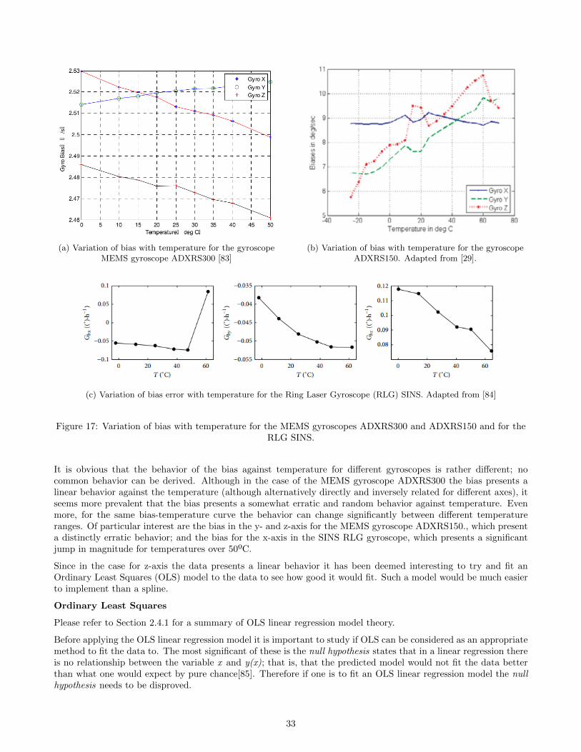
For comparison, the plots of the variation of the biases with temperature the MEMS gyroscopes ADXRS300ADXRS150 and the SINS RLG from the academic papers [29, 83, 84] are presented in Figure 17.
32
(a) Variation of bias with temperature for the gyroscopeMEMS gyroscope ADXRS300 [83]
(b) Variation of bias with temperature for the gyroscopeADXRS150. Adapted from [29].
(c) Variation of bias error with temperature for the Ring Laser Gyroscope (RLG) SINS. Adapted from [84]
Figure 17: Variation of bias with temperature for the MEMS gyroscopes ADXRS300 and ADXRS150 and for theRLG SINS.
It is obvious that the behavior of the bias against temperature for different gyroscopes is rather different; nocommon behavior can be derived. Although in the case of the MEMS gyroscope ADXRS300 the bias presents alinear behavior against the temperature (although alternatively directly and inversely related for different axes), itseems more prevalent that the bias presents a somewhat erratic and random behavior against temperature. Evenmore, for the same bias-temperature curve the behavior can change significantly between different temperatureranges. Of particular interest are the bias in the y- and z-axis for the MEMS gyroscope ADXRS150., which presenta distinctly erratic behavior; and the bias for the x-axis in the SINS RLG gyroscope, which presents a significantjump in magnitude for temperatures over 50ºC.
Since in the case for z-axis the data presents a linear behavior it has been deemed interesting to try and fit anOrdinary Least Squares (OLS) model to the data to see how good it would fit. Such a model would be much easierto implement than a spline.
Ordinary Least Squares
Please refer to Section 2.4.1 for a summary of OLS linear regression model theory.
Before applying the OLS linear regression model it is important to study if OLS can be considered as an appropriatemethod to fit the data to. The most significant of these is the null hypothesis states that in a linear regression thereis no relationship between the variable x and y(x); that is, that the predicted model would not fit the data betterthan what one would expect by pure chance[85]. Therefore if one is to fit an OLS linear regression model the nullhypothesis needs to be disproved.
33
The OLS linear regression model calculations have been conducted using the Python module, which also providesus with a series of classes and functions for conducting statistical tests, and statistical data exploration (that allowsone, among other things, to prove or disprove the null hypothesis) and for the estimation of many other differentstatistical models[86].
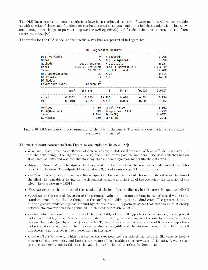
The results for the OLS model applied to the z-axis bias are presented in Figure 18:
Figure 18: OLS regression model summary for the bias in the z-axis. The analysis was made using Python’spackage statsmodels[86].
The most relevant parameters from Figure 18 are explained below[87, 88]:
• R-squared, also known as coefficient of determination; a statistical measure of how well the regression linefits the data being 1 the highest (i.e. best) and 0 the lowest possible numbers. The data collected has anR-squared of 0.998 and one can therefore say that a linear regression model fits the data well. .
• Adjusted R-squared, which adjusts the R-squared number based on the number of independent variablespresent in the data. The adjusted R-squared is 0.998 and again acceptable for our model.
• Coefficient in a typical y = mx + c linear equation the coefficient would be m and its value us the size ofthe effect that variable is having on the dependent variable and the sign of the coefficient the direction of theeffect. In this case m =0.0018
• Standard error, or the estimate of the standard deviation of the coefficient; in this case it is equal to 0.00002
• t-statistic, or the ratio of deviation of the estimated value of a parameter from its hypothesized value to itsstandard error. It can also be thought as the coefficient divided by its standard error. The greater the valueof t the greater evidence against the null hypothesis; the null hypothesis states that there is no relationshipbetween the two variables being studied. In this case t-statistic = 92.331
• p-value, which gives us an estimation of the probability of the null hypothesis being correct; t and p needto be evaluated together. A small p-value indicates a strong evidence against the null hypothesis and thusrenders the model (our hypothesis) acceptable. Typical threshold values are p-value of 0.05 for a hypothesisto be statistically significant. In this case p-value is negligible and therefore our assumption that the nullhypothesis is not correct is likely acceptable in this case.
• Omnibus/Prob(Omnibus), which is a test of the skewness and kurtosis of the residual. Skewness is itself ameasure of data symmetry and kurtosis a measure of the “peakiness” or curvature of the data. A value closeto 1 is considered good; in this case the value is over 9.440 and therefore far from ideal.
34
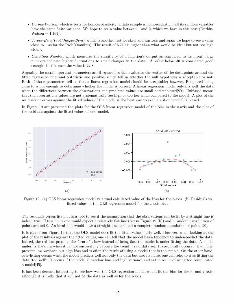
• Durbin-Watson, which is tests for homoscedasticity; a data sample is homoscedastic if all its random variableshave the same finite variance. We hope to see a value between 1 and 2, which we have in this case (Durbin-Watson = 1.161).
• Jarque-Bera/Prob(Jarque-Bera), which is another test for skew and kurtosis and again we hope to see a valueclose to 1 as for the Prob(Omnibus). The result of 5.719 is higher than what would be ideal but not too higheither.
• Condition Number, which measures the sensitivity of a function’s output as compared to its input; largenumbers indicate higher fluctuations to small changes in the data. A value below 30 is considered goodenough. In this case the value is 22.8
Arguably the most important parameters are R-squared, which evaluates the scatter of the data points around thefitted regression line; and t-statistic and p-value, which tell us whether the null hypothesis is acceptable or not.Both of those parameters tell us that a linear regression model should be acceptable; however, R-squared beingclose to is not enough to determine whether the model is correct. A linear regression model only fits well the datawhen the differences between the observations and predicted values are small and unbiased[89]. Unbiased meansthat the observations values are not systematically too high or too low when compared to the model. A plot of theresiduals or errors against the fitted values of the model is the best way to evaluate if our model is biased.
In Figure 19 are presented the plots for the OLS linear regression model of the bias in the z-axis and the plot ofthe residuals against the fitted values of said model.
(a) (b)
Figure 19: (a) OLS linear regression model vs actual calculated value of the bias for the z-axis. (b) Residuals vsfitted values of the OLS regression model for the z-axis bias.
The residuals versus fits plot is a tool to see if the assumption that the observations can be fit by a straight line isindeed true. If this holds one would expect a relatively flat line (red in Figure 19 (b)) and a random distribution ofpoints around 0. An ideal plot would have a straight line at 0 and a complete random population of points[90].
It is clear from Figure 19 that the OLS model does fit the fitted values fairly well. However, when looking at theplot of the residuals against the fitted values, one can tell that the model has a tendency to under-predict the data.Indeed, the red line presents the form of a bow instead of being flat; the model is under-fitting the data. A modelunderfits the data when it cannot successfully capture the trend if said data set. It specifically occurs if the modelpresents low variance but high bias and is often the result of using a model that is too simple. On the other hand,over-fitting occurs when the model predicts well not only the data but also its noise; one can refer to it as fitting thedata ”too well”. It occurs if the model shows low bias and high variance and is the result of using too complicateda model[45].
It has been deemed interesting to see how well the OLS regression model would fit the bias for the x- and y-axis,although it is likely that it will not fit the data as well as for the z-axis.
35
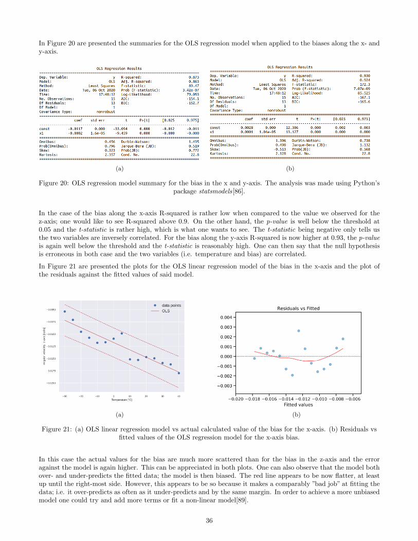
In Figure 20 are presented the summaries for the OLS regression model when applied to the biases along the x- andy-axis.
(a) (b)
Figure 20: OLS regression model summary for the bias in the x and y-axis. The analysis was made using Python’spackage statsmodels[86].
In the case of the bias along the x-axis R-squared is rather low when compared to the value we observed for thez-axis; one would like to see R-squared above 0.9. On the other hand, the p-value is well below the threshold at0.05 and the t-statistic is rather high, which is what one wants to see. The t-statistic being negative only tells usthe two variables are inversely correlated. For the bias along the y-axis R-squared is now higher at 0.93, the p-valueis again well below the threshold and the t-statistic is reasonably high. One can then say that the null hypothesisis erroneous in both case and the two variables (i.e. temperature and bias) are correlated.
In Figure 21 are presented the plots for the OLS linear regression model of the bias in the x-axis and the plot ofthe residuals against the fitted values of said model.
(a) (b)
Figure 21: (a) OLS linear regression model vs actual calculated value of the bias for the x-axis. (b) Residuals vsfitted values of the OLS regression model for the x-axis bias.
In this case the actual values for the bias are much more scattered than for the bias in the z-axis and the erroragainst the model is again higher. This can be appreciated in both plots. One can also observe that the model bothover- and under-predicts the fitted data; the model is then biased. The red line appears to be now flatter, at leastup until the right-most side. However, this appears to be so because it makes a comparably ”bad job” at fitting thedata; i.e. it over-predicts as often as it under-predicts and by the same margin. In order to achieve a more unbiasedmodel one could try and add more terms or fit a non-linear model[89].
36
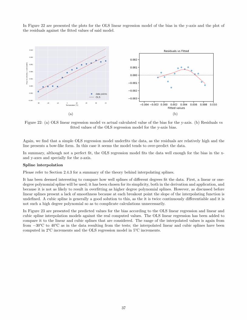
In Figure 22 are presented the plots for the OLS linear regression model of the bias in the y-axis and the plot ofthe residuals against the fitted values of said model.
(a) (b)
Figure 22: (a) OLS linear regression model vs actual calculated value of the bias for the y-axis. (b) Residuals vsfitted values of the OLS regression model for the y-axis bias.
Again, we find that a simple OLS regression model underfits the data, as the residuals are relatively high and theline presents a bow-like form. In this case it seems the model tends to over-predict the data.
In summary, although not a perfect fit, the OLS regression model fits the data well enough for the bias in the x-and y-axes and specially for the z-axis.
Spline interpolation
Please refer to Section 2.4.3 for a summary of the theory behind interpolating splines.
It has been deemed interesting to compare how well splines of different degrees fit the data. First, a linear or one-degree polynomial spline will be used; it has been chosen for its simplicity, both in the derivation and application, andbecause it is not as likely to result in overfitting as higher degree polynomial splines. However, as discussed beforelinear splines present a lack of smoothness because at each breakout point the slope of the interpolating function isundefined. A cubic spline is generally a good solution to this, as the it is twice continuously differentiable and it isnot such a high degree polynomial so as to complicate calculations unnecessarily.
In Figure 23 are presented the predicted values for the bias according to the OLS linear regression and linear andcubic spline interpolation models against the real computed values. The OLS linear regression has been added tocompare it to the linear and cubic splines that are considered. The range of the interpolated values is again fromfrom −30°C to 40°C as in the data resulting from the tests; the interpolated linear and cubic splines have beencomputed in 2°C increments and the OLS regression model in 5°C increments.
37
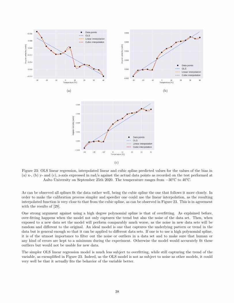
(a) (b)
(c)
Figure 23: OLS linear regression, interpolated linear and cubic spline predicted values for the values of the bias in(a) x-, (b) y- and (c), z-axis expressed in rad/s against the actual data points as recorded on the test performed at
Aalto University on September 25th 2020. The temperature ranges from −30°C to 40°C.
As can be observed all splines fit the data rather well, being the cubic spline the one that follows it more closely. Inorder to make the calibration process simpler and speedier one could use the linear interpolation, as the resultinginterpolated function is very close to that from the cubic spline, as can be observed in Figure 23. This is in agreementwith the results of [29].
One strong argument against using a high degree polynomial spline is that of overfitting. As explained before,over-fitting happens when the model not only captures the trend but also the noise of the data set. Then, whenexposed to a new data set the model will perform comparably much worse, as the noise in new data sets will berandom and different to the original. An ideal model is one that captures the underlying pattern or trend in thedata but is general enough so that it can be applied to different data sets. If one is to use a high polynomial spline,it is of the utmost importance to filter out the noise or outliers in a data set and to make sure that human orany kind of errors are kept to a minimum during the experiment. Otherwise the model would accurately fit theseoutliers but would not be usable for new data.
The simpler OLS linear regression model is much less subject to overfitting, while still capturing the trend of thevariable, as exemplified in Figure 23. Indeed, as the OLS model is not as subject to noise as other models, it couldvery well be that it actually fits the behavior of the variable better.
38
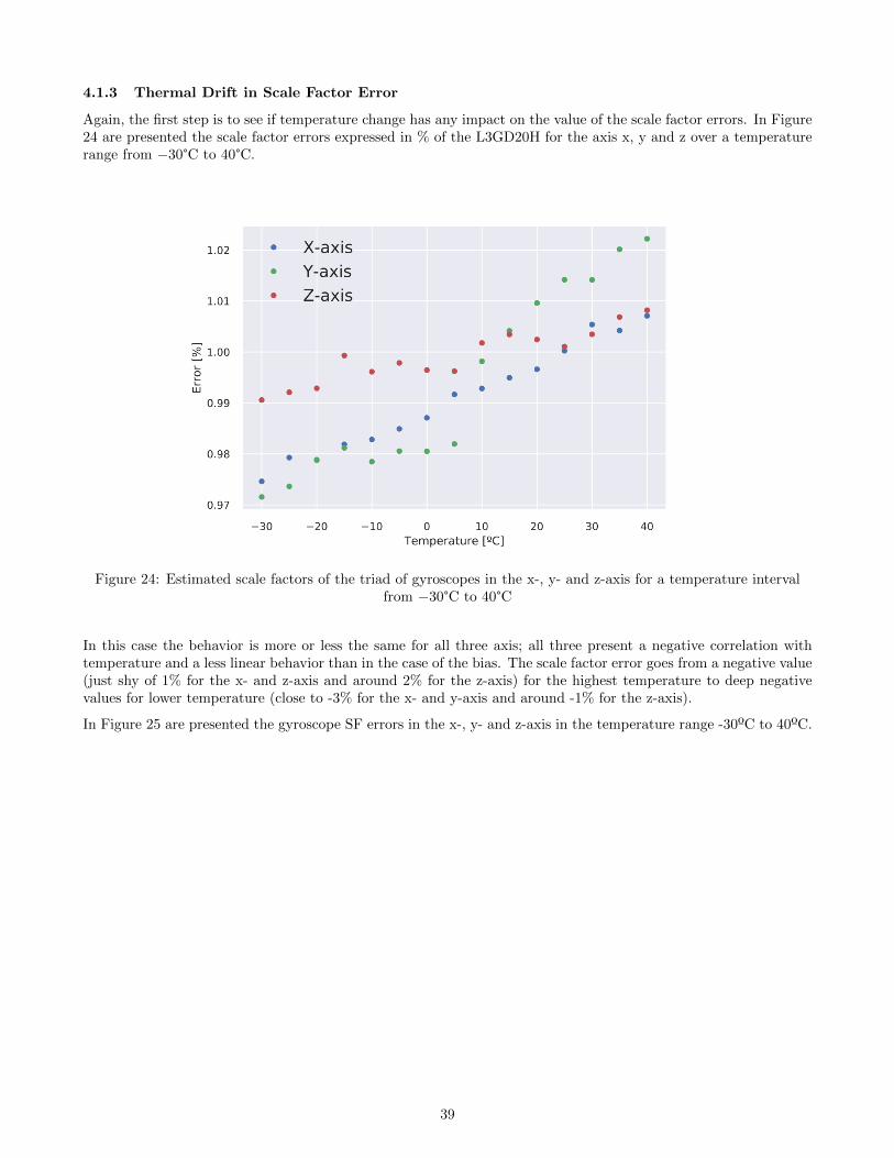
4.1.3 Thermal Drift in Scale Factor Error
Again, the first step is to see if temperature change has any impact on the value of the scale factor errors. In Figure24 are presented the scale factor errors expressed in % of the L3GD20H for the axis x, y and z over a temperaturerange from −30°C to 40°C.
Figure 24: Estimated scale factors of the triad of gyroscopes in the x-, y- and z-axis for a temperature intervalfrom −30°C to 40°C
In this case the behavior is more or less the same for all three axis; all three present a negative correlation withtemperature and a less linear behavior than in the case of the bias. The scale factor error goes from a negative value(just shy of 1% for the x- and z-axis and around 2% for the z-axis) for the highest temperature to deep negativevalues for lower temperature (close to -3% for the x- and y-axis and around -1% for the z-axis).
In Figure 25 are presented the gyroscope SF errors in the x-, y- and z-axis in the temperature range -30ºC to 40ºC.
39
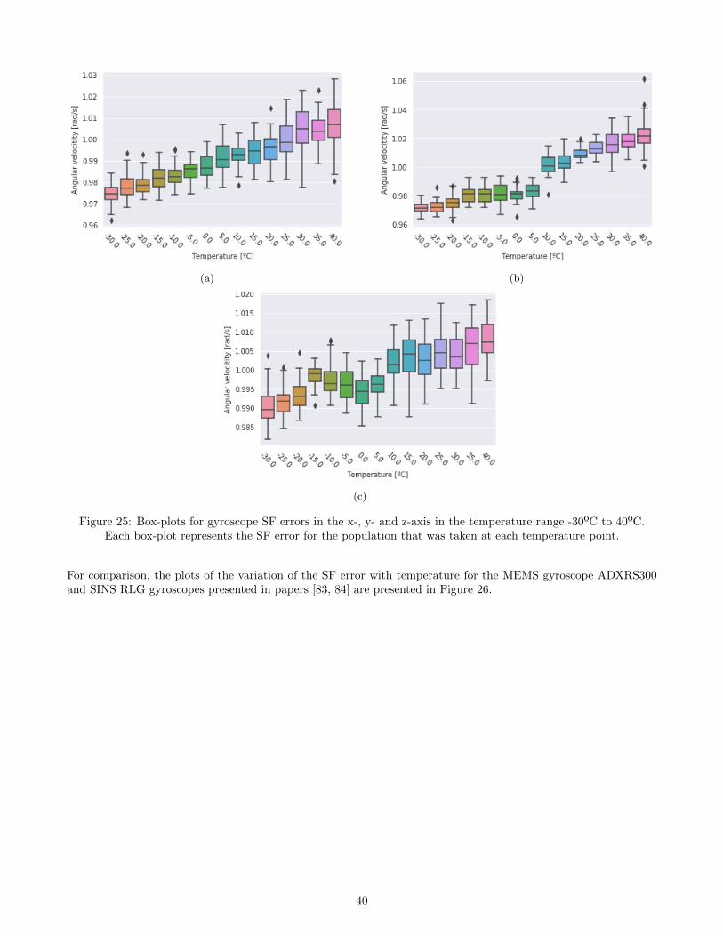
(a) (b)
(c)
Figure 25: Box-plots for gyroscope SF errors in the x-, y- and z-axis in the temperature range -30ºC to 40ºC.Each box-plot represents the SF error for the population that was taken at each temperature point.
For comparison, the plots of the variation of the SF error with temperature for the MEMS gyroscope ADXRS300and SINS RLG gyroscopes presented in papers [83, 84] are presented in Figure 26.
40
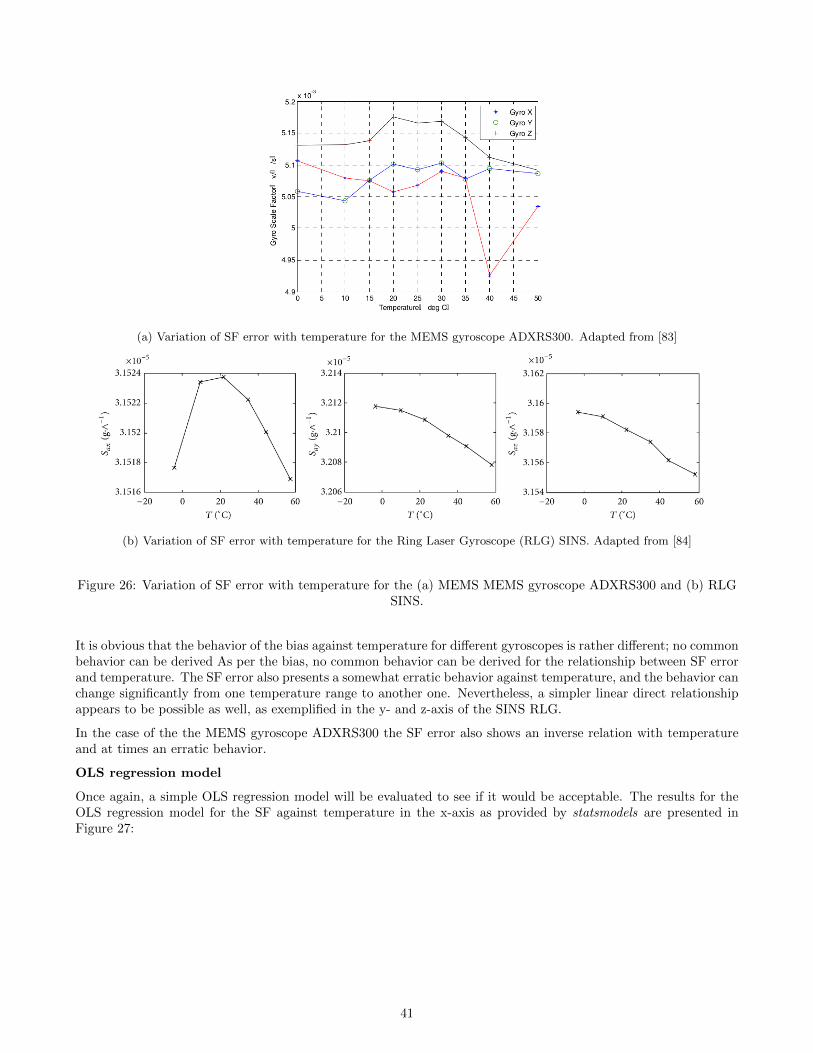
(a) Variation of SF error with temperature for the MEMS gyroscope ADXRS300. Adapted from [83]
(b) Variation of SF error with temperature for the Ring Laser Gyroscope (RLG) SINS. Adapted from [84]
Figure 26: Variation of SF error with temperature for the (a) MEMS MEMS gyroscope ADXRS300 and (b) RLGSINS.
It is obvious that the behavior of the bias against temperature for different gyroscopes is rather different; no commonbehavior can be derived As per the bias, no common behavior can be derived for the relationship between SF errorand temperature. The SF error also presents a somewhat erratic behavior against temperature, and the behavior canchange significantly from one temperature range to another one. Nevertheless, a simpler linear direct relationshipappears to be possible as well, as exemplified in the y- and z-axis of the SINS RLG.
In the case of the the MEMS gyroscope ADXRS300 the SF error also shows an inverse relation with temperatureand at times an erratic behavior.
OLS regression model
Once again, a simple OLS regression model will be evaluated to see if it would be acceptable. The results for theOLS regression model for the SF against temperature in the x-axis as provided by statsmodels are presented inFigure 27:
41
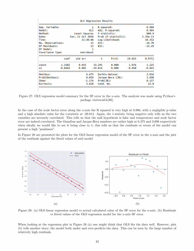
Figure 27: OLS regression model summary for the SF error in the x-axis. The analysis was made using Python’spackage statsmodels[86].
In the case of the scale factor error along the x-axis the R squared is very high at 0.986, with a negligible p-valueand a high absolute value for the t-statistic at -29.814. Again, the t-statistic being negative only tells us the twovariables are inversely correlated. This tells us that the null hypothesis is false and temperature and scale factorerror are indeed correlated. The Omnibus and Jarque-Bera numbers are rather high at 6.475 and 3.698 respectivelywhen ideally we would like to see it being close to 1; this tells us that the residuals or errors of the model canpresent a high ”peakiness”.
In Figure 28 are presented the plots for the OLS linear regression model of the SF error in the x-axis and the plotof the residuals against the fitted values of said model.
(a) (b)
Figure 28: (a) OLS linear regression model vs actual calculated value of the SF error for the x-axis. (b) Residualsvs fitted values of the OLS regression model for the x-axis SF error.
When looking at the regression plot in Figure 28 (a) one might think that OLS fits the data well. However, plot(b) tells another story; the model both under and over-predicts the data. This can be seen by the large number ofrelatively high residuals.
42
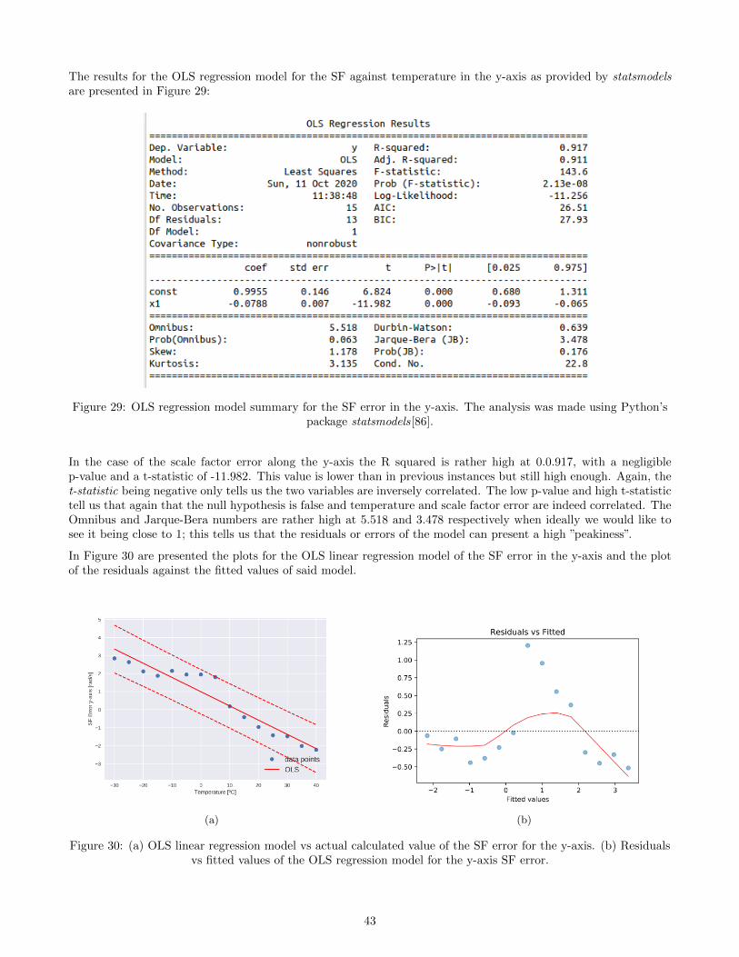
The results for the OLS regression model for the SF against temperature in the y-axis as provided by statsmodelsare presented in Figure 29:
Figure 29: OLS regression model summary for the SF error in the y-axis. The analysis was made using Python’spackage statsmodels[86].
In the case of the scale factor error along the y-axis the R squared is rather high at 0.0.917, with a negligiblep-value and a t-statistic of -11.982. This value is lower than in previous instances but still high enough. Again, thet-statistic being negative only tells us the two variables are inversely correlated. The low p-value and high t-statistictell us that again that the null hypothesis is false and temperature and scale factor error are indeed correlated. TheOmnibus and Jarque-Bera numbers are rather high at 5.518 and 3.478 respectively when ideally we would like tosee it being close to 1; this tells us that the residuals or errors of the model can present a high ”peakiness”.
In Figure 30 are presented the plots for the OLS linear regression model of the SF error in the y-axis and the plotof the residuals against the fitted values of said model.
(a) (b)
Figure 30: (a) OLS linear regression model vs actual calculated value of the SF error for the y-axis. (b) Residualsvs fitted values of the OLS regression model for the y-axis SF error.
43
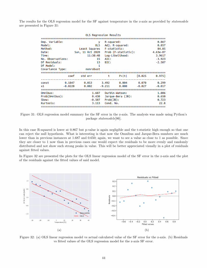
The results for the OLS regression model for the SF against temperature in the z-axis as provided by statsmodelsare presented in Figure 31:
Figure 31: OLS regression model summary for the SF error in the z-axis. The analysis was made using Python’spackage statsmodels[86].
In this case R-squared is lower at 0.867 but p-value is again negligible and the t-statistic high enough so that onecan reject the null hypothesis. What is interesting is that now the Omnibus and Jarque-Bera numbers are muchlower than in previous instances at 1.687 and 0.650; again, we want to see a value as close to 1 as possible. Sincethey are closer to 1 now than in previous cases one would expect the residuals to be more evenly and randomlydistributed and not show such strong peaks in value. This will be better appreciated visually in a plot of residualsagainst fitted values.
In Figure 32 are presented the plots for the OLS linear regression model of the SF error in the z-axis and the plotof the residuals against the fitted values of said model.
(a) (b)
Figure 32: (a) OLS linear regression model vs actual calculated value of the SF error for the z-axis. (b) Residualsvs fitted values of the OLS regression model for the z-axis SF error.
44
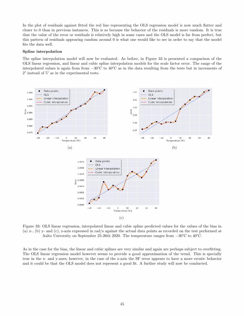
In the plot of residuals against fitted the red line representing the OLS regression model is now much flatter andcloser to 0 than in previous instances. This is so because the behavior of the residuals is more random. It is truethat the value of the error or residuals is relatively high in some cases and the OLS model is far from perfect, butthis pattern of residuals appearing random around 0 is what one would like to see in order to say that the modelfits the data well.
Spline interpolation
The spline interpolation model will now be evaluated. As before, in Figure 33 is presented a comparison of theOLS linear regression, and linear and cubic spline interpolation models for the scale factor error. The range of theinterpolated values is again from from −30°C to 40°C as in the data resulting from the tests but in increments of2° instead of 5° as in the experimental tests.
(a) (b)
(c)
Figure 33: OLS linear regression, interpolated linear and cubic spline predicted values for the values of the bias in(a) x-, (b) y- and (c), z-axis expressed in rad/s against the actual data points as recorded on the test performed at
Aalto University on September 25-26th 2020. The temperature ranges from −30°C to 40°C.
As in the case for the bias, the linear and cubic splines are very similar and again are perhaps subject to overfitting.The OLS linear regression model however seems to provide a good approximation of the trend. This is speciallytrue in the x- and y-axes; however, in the case of the z-axis the SF error appears to have a more erratic behaviorand it could be that the OLS model does not represent a good fit. A further study will now be conducted.
45
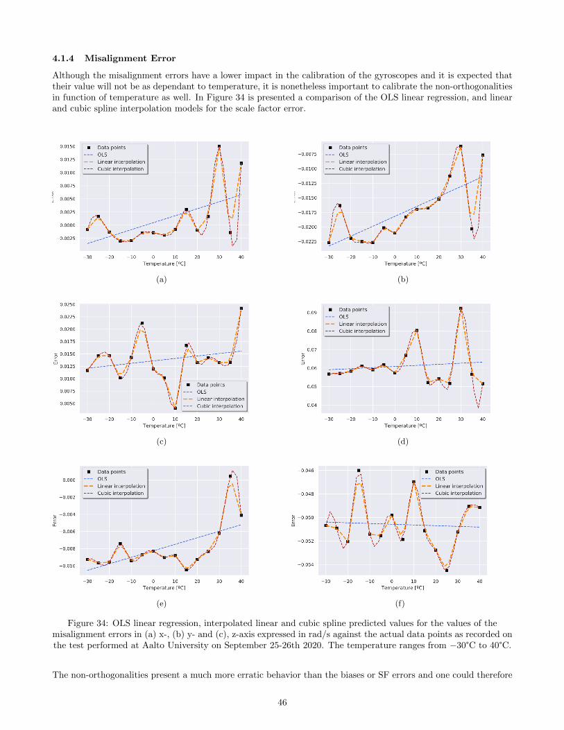
4.1.4 Misalignment Error
Although the misalignment errors have a lower impact in the calibration of the gyroscopes and it is expected thattheir value will not be as dependant to temperature, it is nonetheless important to calibrate the non-orthogonalitiesin function of temperature as well. In Figure 34 is presented a comparison of the OLS linear regression, and linearand cubic spline interpolation models for the scale factor error.
(a) (b)
(c) (d)
(e) (f)
Figure 34: OLS linear regression, interpolated linear and cubic spline predicted values for the values of themisalignment errors in (a) x-, (b) y- and (c), z-axis expressed in rad/s against the actual data points as recorded onthe test performed at Aalto University on September 25-26th 2020. The temperature ranges from −30°C to 40°C.
The non-orthogonalities present a much more erratic behavior than the biases or SF errors and one could therefore
46
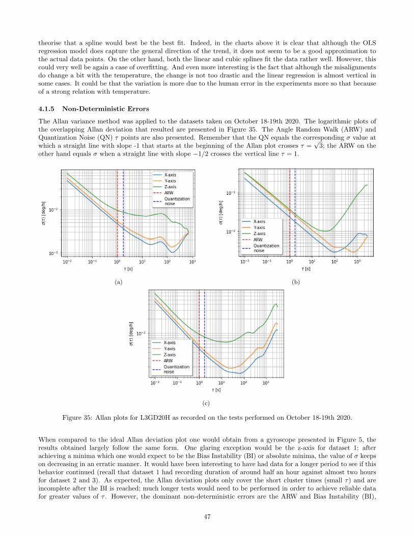
theorise that a spline would best be the best fit. Indeed, in the charts above it is clear that although the OLSregression model does capture the general direction of the trend, it does not seem to be a good approximation tothe actual data points. On the other hand, both the linear and cubic splines fit the data rather well. However, thiscould very well be again a case of overfitting. And even more interesting is the fact that although the misalignmentsdo change a bit with the temperature, the change is not too drastic and the linear regression is almost vertical insome cases. It could be that the variation is more due to the human error in the experiments more so that becauseof a strong relation with temperature.
4.1.5 Non-Deterministic Errors
The Allan variance method was applied to the datasets taken on October 18-19th 2020. The logarithmic plots ofthe overlapping Allan deviation that resulted are presented in Figure 35. The Angle Random Walk (ARW) andQuantization Noise (QN) τ points are also presented. Remember that the QN equals the corresponding σ value atwhich a straight line with slope -1 that starts at the beginning of the Allan plot crosses τ =
√3; the ARW on the
other hand equals σ when a straight line with slope −1/2 crosses the vertical line τ = 1.
(a) (b)
(c)
Figure 35: Allan plots for L3GD20H as recorded on the tests performed on October 18-19th 2020.
When compared to the ideal Allan deviation plot one would obtain from a gyroscope presented in Figure 5, theresults obtained largely follow the same form. One glaring exception would be the z-axis for dataset 1; afterachieving a minima which one would expect to be the Bias Instability (BI) or absolute minima, the value of σ keepson decreasing in an erratic manner. It would have been interesting to have had data for a longer period to see if thisbehavior continued (recall that dataset 1 had recording duration of around half an hour against almost two hoursfor dataset 2 and 3). As expected, the Allan deviation plots only cover the short cluster times (small τ) and areincomplete after the BI is reached; much longer tests would need to be performed in order to achieve reliable datafor greater values of τ . However, the dominant non-deterministic errors are the ARW and Bias Instability (BI),
47
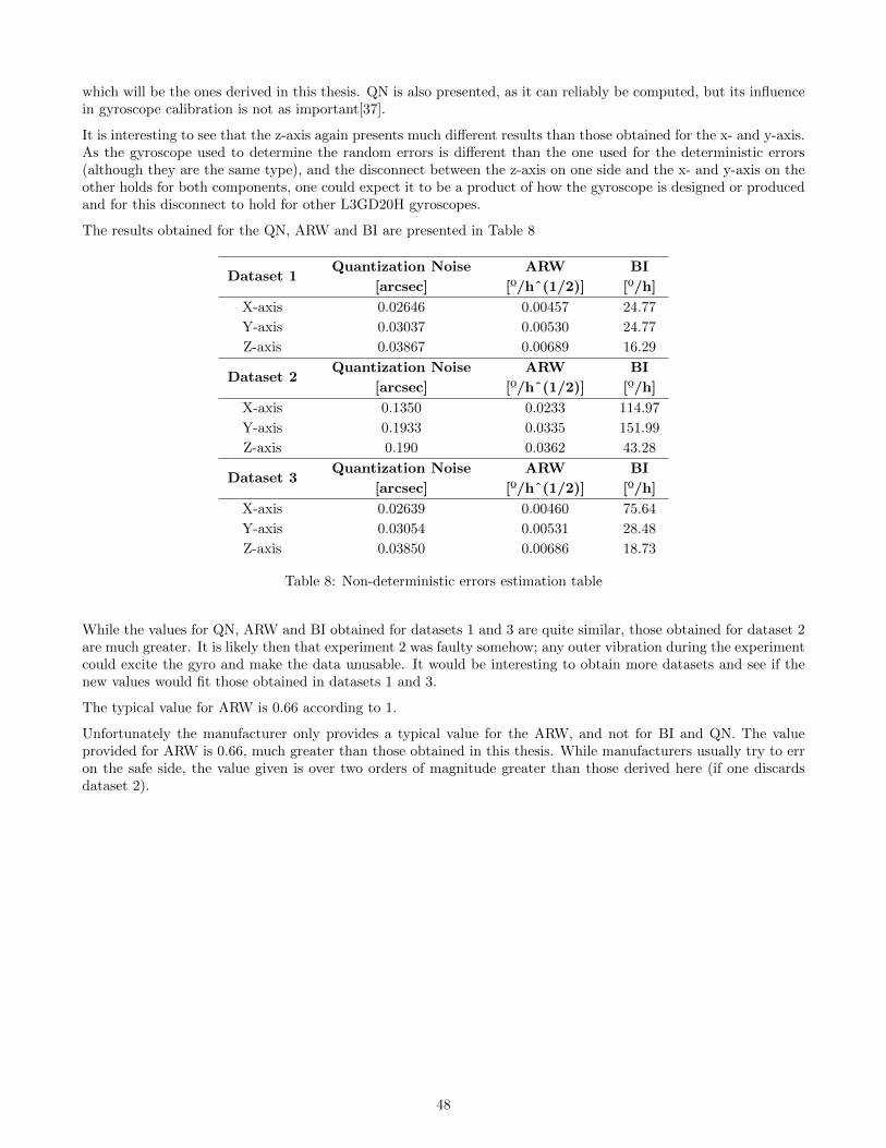
which will be the ones derived in this thesis. QN is also presented, as it can reliably be computed, but its influencein gyroscope calibration is not as important[37].
It is interesting to see that the z-axis again presents much different results than those obtained for the x- and y-axis.As the gyroscope used to determine the random errors is different than the one used for the deterministic errors(although they are the same type), and the disconnect between the z-axis on one side and the x- and y-axis on theother holds for both components, one could expect it to be a product of how the gyroscope is designed or producedand for this disconnect to hold for other L3GD20H gyroscopes.
The results obtained for the QN, ARW and BI are presented in Table 8
Dataset 1Quantization Noise
[arcsec]
ARW
[º/hˆ(1/2)]
BI
[º/h]
X-axis 0.02646 0.00457 24.77
Y-axis 0.03037 0.00530 24.77
Z-axis 0.03867 0.00689 16.29
Dataset 2Quantization Noise
[arcsec]
ARW
[º/hˆ(1/2)]
BI
[º/h]
X-axis 0.1350 0.0233 114.97
Y-axis 0.1933 0.0335 151.99
Z-axis 0.190 0.0362 43.28
Dataset 3Quantization Noise
[arcsec]
ARW
[º/hˆ(1/2)]
BI
[º/h]
X-axis 0.02639 0.00460 75.64
Y-axis 0.03054 0.00531 28.48
Z-axis 0.03850 0.00686 18.73
Table 8: Non-deterministic errors estimation table
While the values for QN, ARW and BI obtained for datasets 1 and 3 are quite similar, those obtained for dataset 2are much greater. It is likely then that experiment 2 was faulty somehow; any outer vibration during the experimentcould excite the gyro and make the data unusable. It would be interesting to obtain more datasets and see if thenew values would fit those obtained in datasets 1 and 3.
The typical value for ARW is 0.66 according to 1.
Unfortunately the manufacturer only provides a typical value for the ARW, and not for BI and QN. The valueprovided for ARW is 0.66, much greater than those obtained in this thesis. While manufacturers usually try to erron the safe side, the value given is over two orders of magnitude greater than those derived here (if one discardsdataset 2).
48
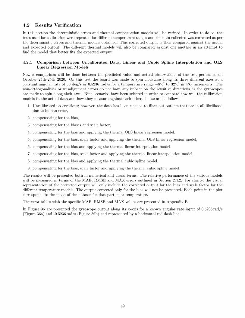
4.2 Results Verification
In this section the deterministic errors and thermal compensation models will be verified. In order to do so, thetests used for calibration were repeated for different temperature ranges and the data collected was corrected as perthe deterministic errors and thermal models obtained. This corrected output is then compared against the actualand expected output. The different thermal models will also be compared against one another in an attempt tofind the model that better fits the expected output.
4.2.1 Comparison between Uncalibrated Data, Linear and Cubic Spline Interpolation and OLSLinear Regression Models
Now a comparison will be done between the predicted value and actual observations of the test performed onOctober 24th-25th 2020. On this test the board was made to spin clockwise along its three different axes at aconstant angular rate of 30 deg/s or 0.5236 rad/s for a temperature range −8°C to 32°C in 4°C increments. Thenon-orthogonalities or misalignment errors do not have any impact on the sensitive directions as the gyroscopesare made to spin along their axes. Nine scenarios have been selected in order to compare how well the calibrationmodels fit the actual data and how they measure against each other. These are as follows:
1. Uncalibrated observations; however, the data has been cleaned to filter out outliers that are in all likelihooddue to human error,
2. compensating for the bias,
3. compensating for the biases and scale factor,
4. compensating for the bias and applying the thermal OLS linear regression model,
5. compensating for the bias, scale factor and applying the thermal OLS linear regression model,
6. compensating for the bias and applying the thermal linear interpolation model
7. compensating for the bias, scale factor and applying the thermal linear interpolation model,
8. compensating for the bias and applying the thermal cubic spline model,
9. compensating for the bias, scale factor and applying the thermal cubic spline model.
The results will be presented both in numerical and visual terms. The relative performance of the various modelswill be measured in terms of the MAE, RMSE and MAX errors outlined in Section 2.4.2. For clarity, the visualrepresentation of the corrected output will only include the corrected output for the bias and scale factor for thedifferent temperature models. The output corrected only for the bias will not be presented. Each point in the plotcorresponds to the mean of the dataset for that particular temperature.
The error tables with the specific MAE, RMSE and MAX values are presented in Appendix B.
In Figure 36 are presented the gyroscope output along its x-axis for a known angular rate input of 0.5236 rad/s(Figure 36a) and -0.5236 rad/s (Figure 36b) and represented by a horizontal red dash line.
49
(a) X-axis corrected and uncorrected output for angular rate 30 deg/s
(b) X-axis corrected and uncorrected output for angular rate -30 deg/s
Figure 36: Uncorrected and corrected gyroscope output for the x-axis for a known angular rate of 30 deg/s or0.5236 rad/s both anti- and clockwise along said x-axis for a temperature range −8°C to 32°C in 4°C increments..
The measurements were performed at Aalto University on October 24th 2020. The uncorrected outputcorresponds to the black squares; the output corrected for bias and SF error are the blue dots; the output
corrected for bias, SF error and applying the linear spline interpolation thermal model are the orange dots; theoutput corrected for bias, SF error and applying the cubic spline interpolation thermal model are the green dots;
and the output corrected for bias, SF error and applying the OLS linear regression thermal model are the red dots.
As exemplified in the plot above, the actual results obtained during measurement are far-off the actual angular rate.Interestingly, the uncorrected output does not show such a strong correlation when rotating in the clockwise but itdoes when rotating anticlockwise.
The anticlockwise output shows that it is essential to correct for the temperature, as the error would only growbigger for more extreme values. Correcting for the bias and SF error is not a viable solution, as the temperaturerelationship holds as seen in Figure 36b. Another interesting point is that the OLS presents a much more stableoutput without losing any accuracy against the interpolated models; in fact, it is more accurate, albeit marginally.
In Figure 37 are presented the gyroscope output along its x-axis for a known angular rate input of 0.5236 rad/s,represented by a horizontal red dash line.
50
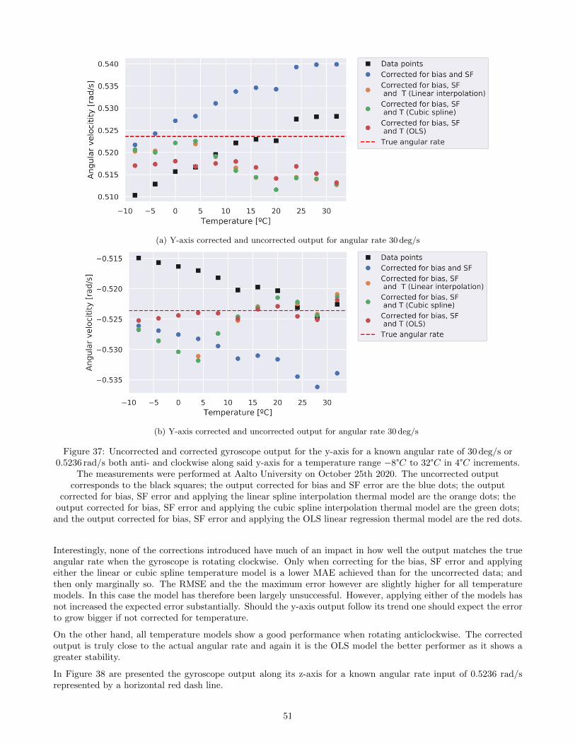
(a) Y-axis corrected and uncorrected output for angular rate 30 deg/s
(b) Y-axis corrected and uncorrected output for angular rate 30 deg/s
Figure 37: Uncorrected and corrected gyroscope output for the y-axis for a known angular rate of 30 deg/s or0.5236 rad/s both anti- and clockwise along said y-axis for a temperature range −8°C to 32°C in 4°C increments.
The measurements were performed at Aalto University on October 25th 2020. The uncorrected outputcorresponds to the black squares; the output corrected for bias and SF error are the blue dots; the output
corrected for bias, SF error and applying the linear spline interpolation thermal model are the orange dots; theoutput corrected for bias, SF error and applying the cubic spline interpolation thermal model are the green dots;
and the output corrected for bias, SF error and applying the OLS linear regression thermal model are the red dots.
Interestingly, none of the corrections introduced have much of an impact in how well the output matches the trueangular rate when the gyroscope is rotating clockwise. Only when correcting for the bias, SF error and applyingeither the linear or cubic spline temperature model is a lower MAE achieved than for the uncorrected data; andthen only marginally so. The RMSE and the the maximum error however are slightly higher for all temperaturemodels. In this case the model has therefore been largely unsuccessful. However, applying either of the models hasnot increased the expected error substantially. Should the y-axis output follow its trend one should expect the errorto grow bigger if not corrected for temperature.
On the other hand, all temperature models show a good performance when rotating anticlockwise. The correctedoutput is truly close to the actual angular rate and again it is the OLS model the better performer as it shows agreater stability.
In Figure 38 are presented the gyroscope output along its z-axis for a known angular rate input of 0.5236 rad/srepresented by a horizontal red dash line.
51
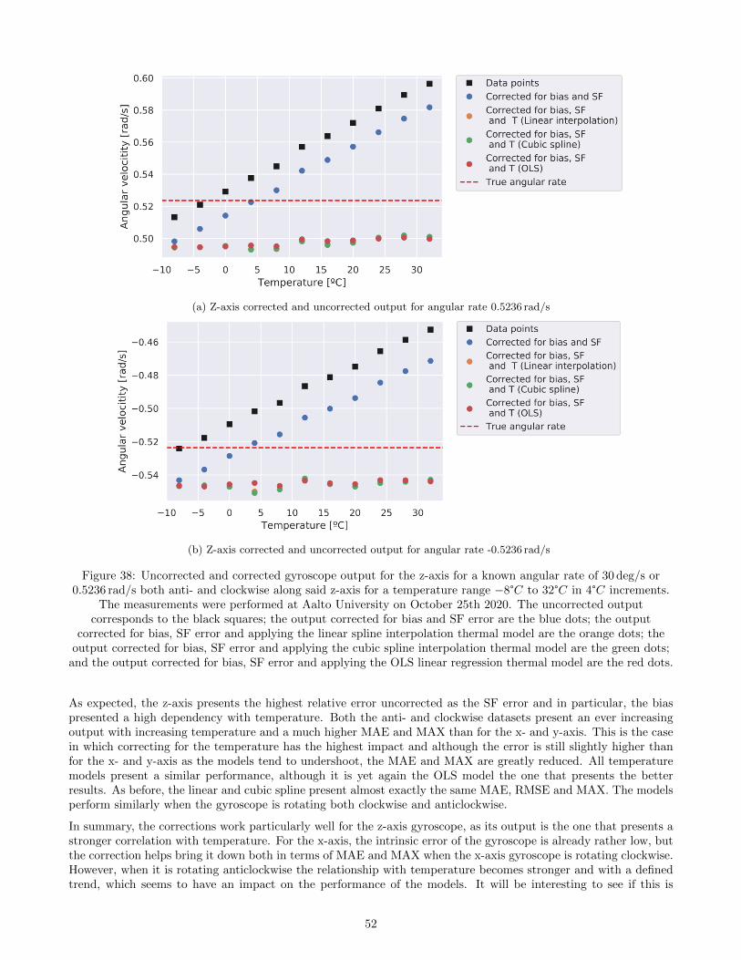
(a) Z-axis corrected and uncorrected output for angular rate 0.5236 rad/s
(b) Z-axis corrected and uncorrected output for angular rate -0.5236 rad/s
Figure 38: Uncorrected and corrected gyroscope output for the z-axis for a known angular rate of 30 deg/s or0.5236 rad/s both anti- and clockwise along said z-axis for a temperature range −8°C to 32°C in 4°C increments.
The measurements were performed at Aalto University on October 25th 2020. The uncorrected outputcorresponds to the black squares; the output corrected for bias and SF error are the blue dots; the output
corrected for bias, SF error and applying the linear spline interpolation thermal model are the orange dots; theoutput corrected for bias, SF error and applying the cubic spline interpolation thermal model are the green dots;
and the output corrected for bias, SF error and applying the OLS linear regression thermal model are the red dots.
As expected, the z-axis presents the highest relative error uncorrected as the SF error and in particular, the biaspresented a high dependency with temperature. Both the anti- and clockwise datasets present an ever increasingoutput with increasing temperature and a much higher MAE and MAX than for the x- and y-axis. This is the casein which correcting for the temperature has the highest impact and although the error is still slightly higher thanfor the x- and y-axis as the models tend to undershoot, the MAE and MAX are greatly reduced. All temperaturemodels present a similar performance, although it is yet again the OLS model the one that presents the betterresults. As before, the linear and cubic spline present almost exactly the same MAE, RMSE and MAX. The modelsperform similarly when the gyroscope is rotating both clockwise and anticlockwise.
In summary, the corrections work particularly well for the z-axis gyroscope, as its output is the one that presents astronger correlation with temperature. For the x-axis, the intrinsic error of the gyroscope is already rather low, butthe correction helps bring it down both in terms of MAE and MAX when the x-axis gyroscope is rotating clockwise.However, when it is rotating anticlockwise the relationship with temperature becomes stronger and with a definedtrend, which seems to have an impact on the performance of the models. It will be interesting to see if this is
52

repeated in further experiments. The y-axis gyroscope already presents a low error when uncorrected, and neitherof the models have much of an impact either in a positive or negative way.
When comparing the different temperature models, the OLS regression model has a clear edge over the splinemodels, although the difference in performance is not too great. Meanwhile, the linear interpolation model performsmarginally better than the cubic spline in most cases.
4.2.2 Comparison between Uncalibrated data, Linear Interpolation and OLS Linear RegressionModels
In order to corroborate the results obtained in the previous experiment, a new dataset was taken following the sameprocedure but for a different temperature range. On this test the board was made to spin clockwise along its threedifferent axes at a constant angular rate of 30 deg/s or 0.5236 rad/s for a temperature range −5°C to 25°C in 5°Cincrements. Again, the non-orthogonalities do not have an impact in this case and the output will not be correctedfor them. As the results for the linear and cubic spline interpolation are very similar and the linear interpolationwas marginally better in most cases, the cubic spline interpolation model will not be considered from now on. Sevenscenarios have been selected in order to compare how well the calibration model fits the actual data. These are asfollows:
1. Uncalibrated observations; however, the data has been cleaned to filter out outliers that are in all likelihooddue to human error,
2. compensating for the bias,
3. compensating for the bias and scale factor,
4. compensating for the bias and applying the thermal OLS linear regression model,
5. compensating for the bias, scale factor and applying the thermal OLS linear regression model,
6. compensating for the bias and applying the thermal linear interpolation model,
7. compensating for the bias, scale factor and applying the thermal linear interpolation model.
In Figure 39 are presented the gyroscope output along its x-axis for a known angular rate input of 0.5236 rad/srepresented by a horizontal red dash line.
53
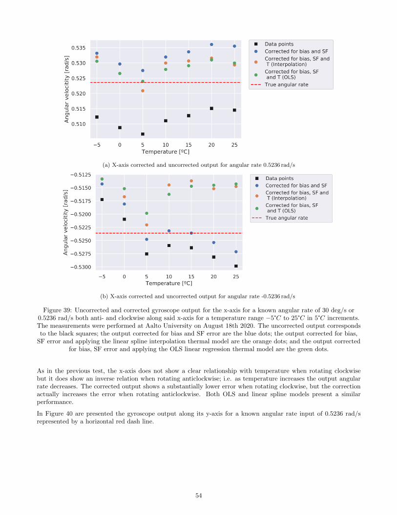
(a) X-axis corrected and uncorrected output for angular rate 0.5236 rad/s
(b) X-axis corrected and uncorrected output for angular rate -0.5236 rad/s
Figure 39: Uncorrected and corrected gyroscope output for the x-axis for a known angular rate of 30 deg/s or0.5236 rad/s both anti- and clockwise along said x-axis for a temperature range −5°C to 25°C in 5°C increments.The measurements were performed at Aalto University on August 18th 2020. The uncorrected output correspondsto the black squares; the output corrected for bias and SF error are the blue dots; the output corrected for bias,
SF error and applying the linear spline interpolation thermal model are the orange dots; and the output correctedfor bias, SF error and applying the OLS linear regression thermal model are the green dots.
As in the previous test, the x-axis does not show a clear relationship with temperature when rotating clockwisebut it does show an inverse relation when rotating anticlockwise; i.e. as temperature increases the output angularrate decreases. The corrected output shows a substantially lower error when rotating clockwise, but the correctionactually increases the error when rotating anticlockwise. Both OLS and linear spline models present a similarperformance.
In Figure 40 are presented the gyroscope output along its y-axis for a known angular rate input of 0.5236 rad/srepresented by a horizontal red dash line.
54
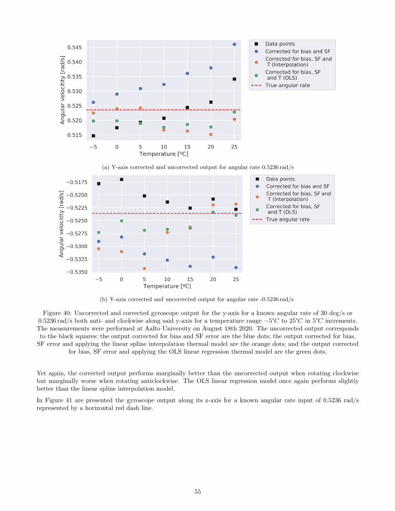
(a) Y-axis corrected and uncorrected output for angular rate 0.5236 rad/s
(b) Y-axis corrected and uncorrected output for angular rate -0.5236 rad/s
Figure 40: Uncorrected and corrected gyroscope output for the y-axis for a known angular rate of 30 deg/s or0.5236 rad/s both anti- and clockwise along said y-axis for a temperature range −5°C to 25°C in 5°C increments.The measurements were performed at Aalto University on August 18th 2020. The uncorrected output correspondsto the black squares; the output corrected for bias and SF error are the blue dots; the output corrected for bias,
SF error and applying the linear spline interpolation thermal model are the orange dots; and the output correctedfor bias, SF error and applying the OLS linear regression thermal model are the green dots.
Yet again, the corrected output performs marginally better than the uncorrected output when rotating clockwisebut marginally worse when rotating anticlockwise. The OLS linear regression model once again performs slightlybetter than the linear spline interpolation model.
In Figure 41 are presented the gyroscope output along its z-axis for a known angular rate input of 0.5236 rad/srepresented by a horizontal red dash line.
55
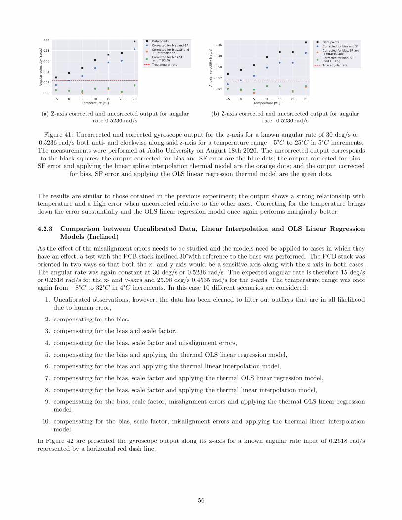
(a) Z-axis corrected and uncorrected output for angularrate 0.5236 rad/s
(b) Z-axis corrected and uncorrected output for angularrate -0.5236 rad/s
Figure 41: Uncorrected and corrected gyroscope output for the z-axis for a known angular rate of 30 deg/s or0.5236 rad/s both anti- and clockwise along said z-axis for a temperature range −5°C to 25°C in 5°C increments.The measurements were performed at Aalto University on August 18th 2020. The uncorrected output correspondsto the black squares; the output corrected for bias and SF error are the blue dots; the output corrected for bias,
SF error and applying the linear spline interpolation thermal model are the orange dots; and the output correctedfor bias, SF error and applying the OLS linear regression thermal model are the green dots.
The results are similar to those obtained in the previous experiment; the output shows a strong relationship withtemperature and a high error when uncorrected relative to the other axes. Correcting for the temperature bringsdown the error substantially and the OLS linear regression model once again performs marginally better.
4.2.3 Comparison between Uncalibrated Data, Linear Interpolation and OLS Linear RegressionModels (Inclined)
As the effect of the misalignment errors needs to be studied and the models need be applied to cases in which theyhave an effect, a test with the PCB stack inclined 30°with reference to the base was performed. The PCB stack wasoriented in two ways so that both the x- and y-axis would be a sensitive axis along with the z-axis in both cases.The angular rate was again constant at 30 deg/s or 0.5236 rad/s. The expected angular rate is therefore 15 deg/sor 0.2618 rad/s for the x- and y-axes and 25.98 deg/s 0.4535 rad/s for the z-axis. The temperature range was onceagain from −8°C to 32°C in 4°C increments. In this case 10 different scenarios are considered:
1. Uncalibrated observations; however, the data has been cleaned to filter out outliers that are in all likelihooddue to human error,
2. compensating for the bias,
3. compensating for the bias and scale factor,
4. compensating for the bias, scale factor and misalignment errors,
5. compensating for the bias and applying the thermal OLS linear regression model,
6. compensating for the bias and applying the thermal linear interpolation model,
7. compensating for the bias, scale factor and applying the thermal OLS linear regression model,
8. compensating for the bias, scale factor and applying the thermal linear interpolation model,
9. compensating for the bias, scale factor, misalignment errors and applying the thermal OLS linear regressionmodel,
10. compensating for the bias, scale factor, misalignment errors and applying the thermal linear interpolationmodel.
In Figure 42 are presented the gyroscope output along its z-axis for a known angular rate input of 0.2618 rad/srepresented by a horizontal red dash line.
56
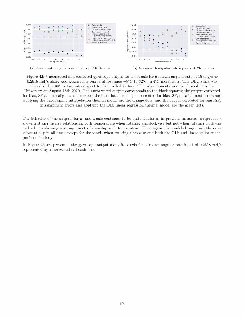
(a) X-axis with angular rate input of 0.2618 rad/s (b) X-axis with angular rate input of -0.2618 rad/s
Figure 42: Uncorrected and corrected gyroscope output for the x-axis for a known angular rate of 15 deg/s or0.2618 rad/s along said x-axis for a temperature range −8°C to 32°C in 4°C increments. The OBC stack was
placed with a 30° incline with respect to the levelled surface. The measurements were performed at AaltoUniversity on August 18th 2020. The uncorrected output corresponds to the black squares; the output corrected
for bias, SF and misalignment errors are the blue dots; the output corrected for bias, SF, misalignment errors andapplying the linear spline interpolation thermal model are the orange dots; and the output corrected for bias, SF,
misalignment errors and applying the OLS linear regression thermal model are the green dots.
The behavior of the outputs for x- and z-axis continues to be quite similar as in previous instances; output for xshows a strong inverse relationship with temperature when rotating anticlockwise but not when rotating clockwiseand z keeps showing a strong direct relationship with temperature. Once again, the models bring down the errorsubstantially in all cases except for the x-axis when rotating clockwise and both the OLS and linear spline modelperform similarly.
In Figure 43 are presented the gyroscope output along its z-axis for a known angular rate input of 0.2618 rad/srepresented by a horizontal red dash line.
57
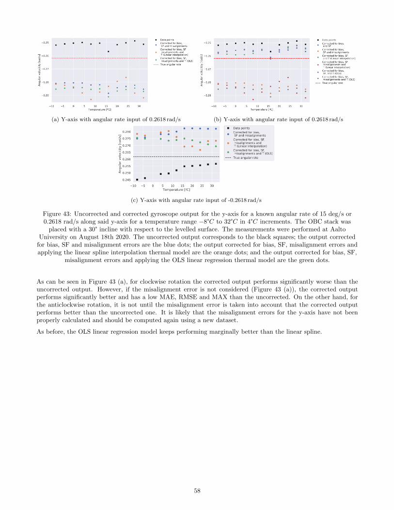
(a) Y-axis with angular rate input of 0.2618 rad/s (b) Y-axis with angular rate input of 0.2618 rad/s
(c) Y-axis with angular rate input of -0.2618 rad/s
Figure 43: Uncorrected and corrected gyroscope output for the y-axis for a known angular rate of 15 deg/s or0.2618 rad/s along said y-axis for a temperature range −8°C to 32°C in 4°C increments. The OBC stack was
placed with a 30° incline with respect to the levelled surface. The measurements were performed at AaltoUniversity on August 18th 2020. The uncorrected output corresponds to the black squares; the output corrected
for bias, SF and misalignment errors are the blue dots; the output corrected for bias, SF, misalignment errors andapplying the linear spline interpolation thermal model are the orange dots; and the output corrected for bias, SF,
misalignment errors and applying the OLS linear regression thermal model are the green dots.
As can be seen in Figure 43 (a), for clockwise rotation the corrected output performs significantly worse than theuncorrected output. However, if the misalignment error is not considered (Figure 43 (a)), the corrected outputperforms significantly better and has a low MAE, RMSE and MAX than the uncorrected. On the other hand, forthe anticlockwise rotation, it is not until the misalignment error is taken into account that the corrected outputperforms better than the uncorrected one. It is likely that the misalignment errors for the y-axis have not beenproperly calculated and should be computed again using a new dataset.
As before, the OLS linear regression model keeps performing marginally better than the linear spline.
58
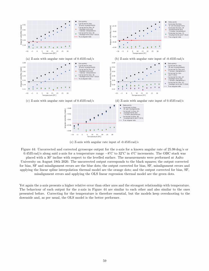
(a) Z-axis with angular rate input of 0.4535 rad/s (b) Z-axis with angular rate input of -0.4535 rad/s
(c) Z-axis with angular rate input of 0.4535 rad/s (d) Z-axis with angular rate input of 0.4535 rad/s
(e) Z-axis with angular rate input of -0.4535 rad/s
Figure 44: Uncorrected and corrected gyroscope output for the z-axis for a known angular rate of 25.98 deg/s or0.4535 rad/s along said z-axis for a temperature range −8°C to 32°C in 4°C increments. The OBC stack was
placed with a 30° incline with respect to the levelled surface. The measurements were performed at AaltoUniversity on August 18th 2020. The uncorrected output corresponds to the black squares; the output corrected
for bias, SF and misalignment errors are the blue dots; the output corrected for bias, SF, misalignment errors andapplying the linear spline interpolation thermal model are the orange dots; and the output corrected for bias, SF,
misalignment errors and applying the OLS linear regression thermal model are the green dots.
Yet again the z-axis presents a higher relative error than other axes and the strongest relationship with temperature.The behaviour of each output for the z-axis in Figure 44 are similar to each other and also similar to the onespresented before. Correcting for the temperature is therefore essential, but the models keep overshooting to thedownside and, as per usual, the OLS model is the better performer.
59
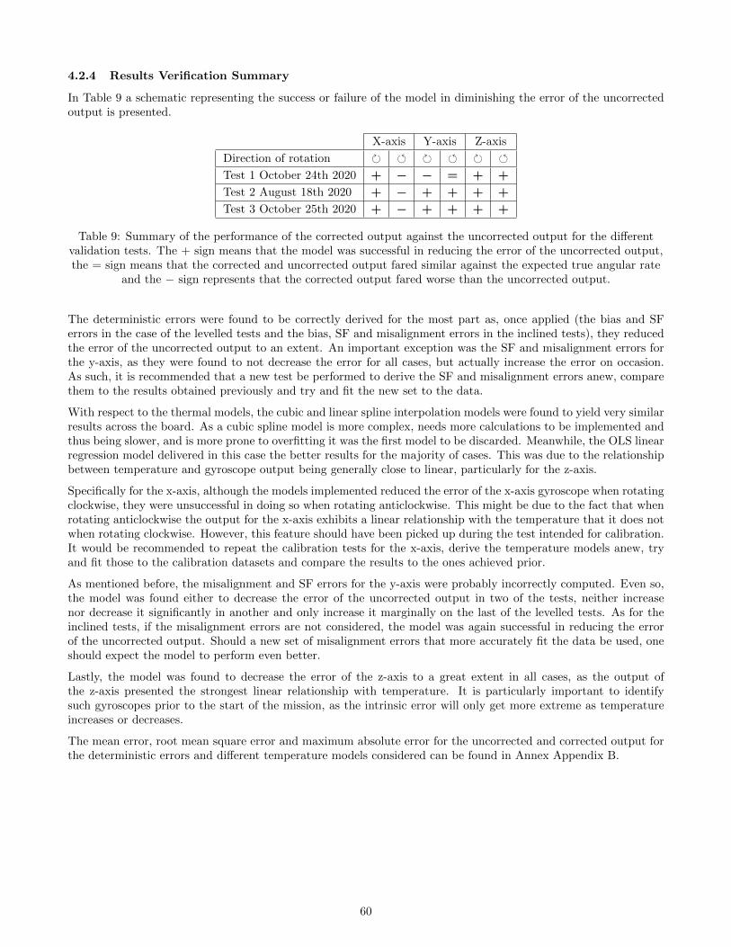
4.2.4 Results Verification Summary
In Table 9 a schematic representing the success or failure of the model in diminishing the error of the uncorrectedoutput is presented.
X-axis Y-axis Z-axis
Direction of rotation
Test 1 October 24th 2020 + − − = + +
Test 2 August 18th 2020 + − + + + +
Test 3 October 25th 2020 + − + + + +
Table 9: Summary of the performance of the corrected output against the uncorrected output for the differentvalidation tests. The + sign means that the model was successful in reducing the error of the uncorrected output,the = sign means that the corrected and uncorrected output fared similar against the expected true angular rate
and the − sign represents that the corrected output fared worse than the uncorrected output.
The deterministic errors were found to be correctly derived for the most part as, once applied (the bias and SFerrors in the case of the levelled tests and the bias, SF and misalignment errors in the inclined tests), they reducedthe error of the uncorrected output to an extent. An important exception was the SF and misalignment errors forthe y-axis, as they were found to not decrease the error for all cases, but actually increase the error on occasion.As such, it is recommended that a new test be performed to derive the SF and misalignment errors anew, comparethem to the results obtained previously and try and fit the new set to the data.
With respect to the thermal models, the cubic and linear spline interpolation models were found to yield very similarresults across the board. As a cubic spline model is more complex, needs more calculations to be implemented andthus being slower, and is more prone to overfitting it was the first model to be discarded. Meanwhile, the OLS linearregression model delivered in this case the better results for the majority of cases. This was due to the relationshipbetween temperature and gyroscope output being generally close to linear, particularly for the z-axis.
Specifically for the x-axis, although the models implemented reduced the error of the x-axis gyroscope when rotatingclockwise, they were unsuccessful in doing so when rotating anticlockwise. This might be due to the fact that whenrotating anticlockwise the output for the x-axis exhibits a linear relationship with the temperature that it does notwhen rotating clockwise. However, this feature should have been picked up during the test intended for calibration.It would be recommended to repeat the calibration tests for the x-axis, derive the temperature models anew, tryand fit those to the calibration datasets and compare the results to the ones achieved prior.
As mentioned before, the misalignment and SF errors for the y-axis were probably incorrectly computed. Even so,the model was found either to decrease the error of the uncorrected output in two of the tests, neither increasenor decrease it significantly in another and only increase it marginally on the last of the levelled tests. As for theinclined tests, if the misalignment errors are not considered, the model was again successful in reducing the errorof the uncorrected output. Should a new set of misalignment errors that more accurately fit the data be used, oneshould expect the model to perform even better.
Lastly, the model was found to decrease the error of the z-axis to a great extent in all cases, as the output ofthe z-axis presented the strongest linear relationship with temperature. It is particularly important to identifysuch gyroscopes prior to the start of the mission, as the intrinsic error will only get more extreme as temperatureincreases or decreases.
The mean error, root mean square error and maximum absolute error for the uncorrected and corrected output forthe deterministic errors and different temperature models considered can be found in Annex Appendix B.
60
5 Conclusion
The first objective of this thesis was to develop a MEMS gyroscope calibration procedure that could be implementedin future CubeSat missions. Such a procedure has been developed drawing particularly from the work on MEMSgyroscopes from [22, 29, 35], and the experience from previous CubeSat missions, in particular the CubETH andSwissCube. The deterministic sources of error have been taken into account, such as the bias, scale factor andmisalignment errors; a simple procedure to compensate for non-deterministic errors has also been implemented.Particular attention has been given to the effect of the temperature on the deterministic sources of error, as thisis an issue that is sometimes overlooked and could hinder a mission (as was the experience of the SwissCube team[91])
The thermal calibration procedure chosen for this thesis was the soak method, by which the components are placedin a thermal chamber at a constant temperature for an extended period of time before the measurements are taken.This is repeated for all relevant temperatures in the temperature range. This method was chosen over others forits reliability and simplicity, as the objective was to implement a method that could be easily replicable by otherteams in future missions.
The theory behind the procedure is laid out in Section 2.3 and the actual tests carried out that could be followedby future teams with the necessary adjustments are in Section 3.1.
The second objective of the thesis was to apply the test procedure to our test case, the L3GD20H 3-axis gyroscopefor the FS-1 mission. Two tests were carried out in order to compute the different sources of error, as explainedin Section 3.1. Three more tests were performed in order to validate the results obtained. The tests procedures,hardware and software used are explained in Section 3.1 and the resulting datasets in 3.2.
First, the Tukey method was followed to clean the datasets by identifying outliers and far-out points. The theoreticalexplanation for this method is given in Section 2.5 and the implementation can be found in Section 3.2.2. In the caseof the MEMS gyroscope L3GD20H, the output was found to follow a Gaussian-like, normal and mostly symmetricdistribution. Only a small percentage of outliers and far-out points were found for all datasets and thus it wasconsidered that there had not been any sources of major errors from either a malfunction in the gyroscopes orhuman error during the experiments.
As mentioned before, the deterministic sources of error and the temperature correction models were computed usingthe data from the first two tests. The temperature models considered in this thesis were the OLS linear regressionmodel, and the linear and cubic spline interpolation models. A brief theoretical explanation for the models canbe found in Section 2.4. Thus, the bias, SF and misalignment errors with their respective temperature correctedmodels were found, the derivation and results of those being in Section 4.1. Then, the models were validated againstthe uncorrected data and against each other using the data from three other tests.
The deterministic errors were found to be largely correctly derived, except for possibly the SF and misalignmenterrors for the y-axis. All other deterministic error sources were successful in reducing the error of the uncorrectedoutput if applied. The thermal calibration model decided upon in this thesis was the OLS linear regression model,not only because it was the better performer in the majority of the cases but also because it was the simplest of themodels considered and the least likely to be subject to over-fitting. The calibrating model applied was successful inreducing the error of the output in terms of mean absolute error, root mean square error and maximum absoluteerror or to not increase the error except for one case when the x-axis is rotating in the negative direction. It islikely that the temperature effect on the output was not properly calibrated for this case and a new calibration testshould be carried out. These results are discussed in Section 4.2.
Finally, the method outlined in this paper also allows the user to determine the random errors of a gyroscopeby applying the Allan variance operation to a segment of data and inspecting the resulting curve in the mannerdescribed in Section 2.3.7 and exemplified in Section 4.1.5.
In summary, the two objectives of the thesis have been largely met, although some improvements could be made.These will be discussed in Section 6.
61

6 Future Work
As mentioned previously, the gyroscopes calibrated in this study are not the ones that are meant to be employedin the FS-1 mission. However, since the same model is intended to be used, this study could serve as help for theFS-1 team to calibrate the triad of gyroscopes that will eventually fly in the mission. It will be interesting to see ifthe results obtained in such calibration are similar to those of this study. Should the gyroscopes used in this thesisbe re-purposed, it would be best to repeat the calibration procedure to try and replicate the results and especiallyto try and derive a temperature model for the x-axis that would correctly fit the output of said axis when rotatingin the negative direction and try and derive a new set of SF and misalignment errors for the y-axis.
Other methods of temperature gyroscope calibration such as the ones described in [30, 31] could also be employed; inthose papers relatively new, theoretically faster method for gyroscope temperature calibration is laid out. It wouldbe interesting to see if such methods yield similar results to the ones obtained via the traditional soak method.Another potential improvement regarding the temperature calibration if employing the soak method would be toleave the gyroscope at a stable temperature inside the thermal chamber for longer than the 25 minute periodemployed in this study; this could potentially yield more stable results.
Moreover, even though the OLS linear regression model was found to be the best solution, in this case, it is likelythat other models will perform better when calibrating other gyroscopes. Another improvement would be to tryand implement different temperature models to the ones presented in this thesis, especially considering the fact thatthe cubic spline model might be prone to overfitting in some cases.
Lastly, although special care was taken to not excite the gyroscope during the tests, it would have been better if amethod of shielding the gyroscope from outer vibrations had been derived. An interesting and simple idea wouldbe to place the gyroscope inside a vessel that floats in a container filled with water, as done in [92].
62
References
[1] S. Rossi, A. Ivanov, G. Faure, B. Geissman, J. Amiguet, R. Valceschini, M. Starein, R. Zufferey, and G. Burri,“Cubeth ADCS design, implementation and validation tests,” Proceedings of the International AstronauticalCongress, IAC, vol. 13, no. October, pp. 10665–10678, 2015.
[2] “Foresail-1 | Aalto University,” Jan 2020. [Online; accessed 30. Sep. 2020].
[3] M. Palmroth, J. Praks, R. Vainio, P. Janhunen, E. K. Kilpua, A. Afanasiev, M. Ala-Lahti, A. Alho,T. Asikainen, E. Asvestari, M. Battarbee, A. Binios, A. Bosser, T. Brito, M. Dubart, J. Envall, U. Ganse,N. Y. Ganushkina, H. George, J. Gieseler, S. Good, M. Grandin, S. Haslam, H. P. Hedman, H. Hietala, N. Jo-vanovic, S. Kakakhel, M. Kalliokoski, V. V. Kettunen, T. Koskela, E. Lumme, M. Meskanen, D. Morosan, M. R.Mughal, P. Niemela, S. Nyman, P. Oleynik, A. Osmane, E. Palmerio, J. Peltonen, Y. Pfau-Kempf, J. Plosila,J. Polkko, S. Poluianov, J. Pomoell, D. Price, A. Punkkinen, R. Punkkinen, B. Riwanto, L. Salomaa, A. Slavin-skis, T. Santti, J. Tammi, H. Tenhunen, P. Toivanen, J. Tuominen, L. Turc, E. Valtonen, P. Virtanen, andT. Westerlund, “FORESAIL-1 CubeSat Mission to Measure Radiation Belt Losses and Demonstrate Deorbit-ing,” Journal of Geophysical Research: Space Physics, vol. 124, no. 7, pp. 5783–5799, 2019.
[4] “CubeSat concept - eoPortal Directory - Satellite Missions,” Nov 2020. [Online; accessed 13. Nov. 2020].
[5] “JPL | Cubesat | MarCO,” Nov 2020. [Online; accessed 13. Nov. 2020].
[6] S. Stirone, “Space Is Very Big. Some of Its New Explorers Will Be Tiny.,” N.Y. Times, Mar 2019.
[7] “CubeSat Database - swartwout,” Sep 2020. [Online; accessed 30. Sep. 2020].
[8] I. Iakubivskyi, P. Janhunen, J. Praks, V. Allik, and M. Robert, “Coulomb Drag Propulsion experiments ofESTCube-2 and FORESAIL-1,” 2019.
[9] P. J. R. V. Jaan Praks, Petri Niemela, “Foresail-1 Experiment Interface Document, Aalto University, Foresailsatellite documentation repository,” 2020.
[10] P. Berlin, Satellite Platform Design. Lulea University of Technology, 6th edition ed., 2014.
[11] “Basics of Gyroscope,” Feb 2020. [Online; accessed 5. Oct. 2020].
[12] “Gyroscope | Definition of Gyroscope by Oxford Dictionary on Lexico.com also meaning of Gyroscope,” Oct2020. [Online; accessed 10. Oct. 2020].
[13] Thinkology, “Silicon Sensing | MEMS Gyroscopes,” Oct 2020. [Online; accessed 5. Oct. 2020].
[14] “Watson Industries,” Oct 2020. [Online; accessed 10. Oct. 2020].
[15] Techbriefs Media Group, “All-Silicon MEMS Inertial Sensing at Fiber Optic Gyro Performance Levels,” Nov2020. [Online; accessed 20. Nov. 2020].
[16] A. Darvishian, “Design and Analysis of Extremely Low-Noise MEMS Gyroscopes for Navigation,” PhD Thesis,2018.
[17] “An Overview of MEMS Inertial Sensing Technology,” Oct 2020. [Online; accessed 10. Oct. 2020].
[18] “L3GD20H - STMicroelectronics,” Oct 2020. [Online; accessed 7. Oct. 2020].
[19] R. Cechowicz, “Bias drift estimation for mems gyroscope used in inertial navigation,” Acta Mechanica etAutomatica, vol. 11, no. 2, pp. 104–110, 2017.
[20] D. Features, “Datasheet L3GD20H MEMS motion sensor: three-axis digital output gyroscope,”STMicroeletronics, no. March, pp. 1–52, 2013.
[21] “Introduction and application areas for MEMS,” Oct 2020. [Online; accessed 1. Oct. 2020].
63
[22] S. Nassar, X. Niu, P. Aggarwal, and N. El-Sheimy, “INS/GPS sensitivity analysis using different KalmanFilter approaches,” Proceedings of the Institute of Navigation, National Technical Meeting, vol. 2, no. January,pp. 993–1001, 2006.
[23] S. Godha, “Performance evaluation of low cost MEMS-based IMU integrated with GPS for land vehicle navi-gation application,” UCGE report, no. 20239, 2006.
[24] N. El-Sheimy, H. Hou, and X. Niu, “Analysis and modeling of inertial sensors using allan variance,” IEEETransactions on Instrumentation and Measurement, vol. 57, no. 1, pp. 140–149, 2008.
[25] K. Shcheglov, C. Evans, R. Gutierrez, and T. K. Tang, “Temperature dependent characteristics of the jpl siliconmems gyroscope,” in 2000 IEEE Aerospace Conference. Proceedings (Cat. No.00TH8484), vol. 1, pp. 403–411vol.1, 2000.
[26] “The Case of the Misguided Gyro | Analog Devices,” Oct 2020. [Online; accessed 5. Oct. 2020].
[27] H. Prescott and J. Ferguson, “Calibration of Deterministic IMU Errors,” pp. 1–38, 2015.
[28] “Orthogonal Perspectives | Analog Devices,” Oct 2020. [Online; accessed 5. Oct. 2020].
[29] P. Aggarwal, Z. Syed, X. Niu, and N. El-Sheimy, “A standard testing and calibration procedure for low costMEMS inertial sensors and units,” Journal of Navigation, vol. 61, no. 2, pp. 323–336, 2008.
[30] X. Niu, Y. Li, H. Zhang, Q. Wang, and Y. Ban, “Fast thermal calibration of low-grade inertial sensors andinertial measurement units,” Sensors (Switzerland), vol. 13, no. 9, pp. 12192–12217, 2013.
[31] H. Yang, B. Zhou, L. Wang, H. Xing, and R. Zhang, “A novel tri-axial MEMS gyroscope calibration methodover a full temperature range,” Sensors (Switzerland), vol. 18, no. 9, 2018.
[32] G. Ng, “Natural Cubic Splines Implementation with Python - eat-pred-love - Medium,” Medium, Mar 2020.
[33] “Piecewise Function Examples - Math Terms & Solutions - Maplesoft,” Oct 2020. [Online; accessed 1. Oct.2020].
[34] H. Hou, “Modeling inertial sensors errors using Allan variance,” 2004.
[35] P. Aggarwal, Z. Syed, X. Niu, N. El-Sheimy, D. C. Brown, Guo-Qing Wei, Song De Ma, B. K. Horn, G. E.Karras, D. Mavrommati, M. Pollefeys, R. Koch, L. V. Gool, Z. Zhang, F. Zhou, Y. Cui, H. Gao, and Y. Wang,“Cost-effective Testing and Calibration of Low Cost MEMS Sensors for Integrated Positioning, Navigation andMapping Systems,” Shaping the change xxiii FIG congress, pp. 1–9, 2006.
[36] N. El-Sheimy, H. Hou, and X. Niu, “Analysis and modeling of inertial sensors using allan variance,” IEEETransactions on Instrumentation and Measurement, vol. 57, no. 1, pp. 140–149, 2008.
[37] I. Freescale Semiconductor, “Allan Variance: Noise Analysis for Gyroscopes,” Freescale white paper, p. 9, 2015.
[38] “Ordinary Least Squares (OLS) using statsmodels - GeeksforGeeks,” Jul 2020. [Online; accessed 6. Oct. 2020].
[39] Jj, “MAE and RMSE — Which Metric is Better? - Human in a Machine World - Medium,” Medium, Jun 2018.
[40] R. P. North and D. M. Livingstone, “Comparison of linear and cubic spline methods of interpolating lake watercolumn profiles,” Limnology and Oceanography: Methods, vol. 11, no. APR, pp. 213–224, 2013.
[41] “scikit-learn: machine learning in Python — scikit-learn 0.23.2 documentation,” Oct 2020. [Online; accessed 9.Oct. 2020].
[42] “Interpolation,” Jun 2020. [Online; accessed 19. Oct. 2020].
[43] “Interpolation in Statistics: Definition, Formula & Example - Video & Lesson Transcript | Study.com,” Oct2020. [Online; accessed 19. Oct. 2020].
[44] L. A. Leal, “Numerical Interpolation: Natural Cubic Spline - Towards Data Science,” Medium, Sep 2020.
[45] “Machine Learning Lesson of the Day – Overfitting and Underfitting,” Mar 2014. [Online; accessed 13. Oct.2020].
64
[46] J. Voitle, “Natural and Clamped Cubic Spline Interpolation,” pp. 1–15, 2000.
[47] J. Kiusalaas, Numerical Methods in Engineering with MATLAB. USA: Cambridge University Press, 2005.
[48] “Cubic Spline Interpolation - Wikiversity,” Oct 2020. [Online; accessed 4. Oct. 2020].
[49] “Cubic Spline Interpolation,” Sep 2020. [Online; accessed 4. Oct. 2020].
[50] C. Spline, “Interpolation using Cubic Spline,” vol. 1, pp. 1–4.
[51] A. M. Kvarving, “Natural cubic splines,” Stata Journal, vol. 4, no. 22, 1995.
[52] F. E. Grubbs, “Procedures for detecting outlying observations in samples,” Technometrics, vol. 11, no. 1,pp. 1–21, 1969.
[53] E. Vandervieren and M. Hubert, “An adjusted boxplot for skewed distributions,” 01 2004.
[54] S. Seo and P. D. Gary M. Marsh, “A review and comparison of methods for detecting outliersin univariate datasets,” Department of Biostatistics, Graduate School of Public Health, pp. 1–53, 2006.
[55] I. Adil and A. Irshad, “A modified approach for detection of outliers,” Pakistan Journal of Statistics andOperation Research, vol. 11, 04 2015.
[56] “InterQuartile Range (IQR),” May 2016. [Online; accessed 3. Oct. 2020].
[57] M. Bergamasco, F. Della Rossa, and L. Piroddi, “Active noise control of impulsive noise with selective outlierelimination,” Proceedings of the American Control Conference, no. June 2013, pp. 4165–4170, 2013.
[58] M. Hargrave, “Standard Deviation Definition,” Investopedia, Sep 2020.
[59] “Using the Variance Equation,” Sep 2019. [Online; accessed 22. Oct. 2020].
[60] “pandas.DataFrame.plot.kde — pandas 1.1.4 documentation,” Oct 2020. [Online; accessed 18. Nov. 2020].
[61] C. Yen-Chi, “Lecture 6: Density Estimation: Histogram and Kernel Density Estimator,” pp. 1–11, 2018.
[62] “FS1 OBC Hardware Design,” Nov 2020. [Online; accessed 5. Nov. 2020].
[63] “FS1 EPS Battery Board Design,” Nov 2020. [Online; accessed 5. Nov. 2020].
[64] P. Niemela, “FS1 OBC Software Design, Aalto University, Foresail satellite documentation repository,” 2020.
[65] “1-Axis Rate Table Series AC1120 (customized) - ACUTRONIC / US,” Oct 2020. [Online; accessed 10. Oct.2020].
[66] “CCSTUDIO Code Composer Studio (CCS) Integrated Development Environment (IDE) | TI.com,” Oct 2020.[Online; accessed 10. Oct. 2020].
[67] “XDS100v3 USB CJTAG/JTAG Emulator,” Apr 2020. [Online; accessed 5. Nov. 2020].
[68] “MakerBeam - Think Build Enjoy,” Nov 2020. [Online; accessed 13. Nov. 2020].
[69] “Welcome to Python.org,” Oct 2020. [Online; accessed 3. Oct. 2020].
[70] “Anaconda | The World’s Most Popular Data Science Platform,” Oct 2020. [Online; accessed 9. Oct. 2020].
[71] S. Team, “Home — Spyder IDE,” Sep 2020. [Online; accessed 9. Oct. 2020].
[72] “Project Jupyter,” Oct 2020. [Online; accessed 9. Oct. 2020].
[73] “Matplotlib: Python plotting — Matplotlib 3.3.2 documentation,” Sep 2020. [Online; accessed 3. Oct. 2020].
[74] “seaborn: statistical data visualization — seaborn 0.11.0 documentation,” Sep 2020. [Online; accessed 3. Oct.2020].
[75] A. Industries, “L3GD20H Triple-Axis Gyro Breakout Board - L3GD20/L3G4200 Upgrade,” Dec 2020. [Online;accessed 2. Dec. 2020].
65

[76] “Arduino Uno Rev3 | Arduino Official Store,” Dec 2020. [Online; accessed 2. Dec. 2020].
[77] adafruit, “Adafruit L3GD20 U,” Dec 2020. [Online; accessed 2. Dec. 2020].
[78] “Download PuTTY - a free SSH and telnet client for Windows,” Apr 2018. [Online; accessed 2. Dec. 2020].
[79] B. Earl, “Adafruit Triple Axis Gyro Breakout,” Adafruit, Jan 2013.
[80] “A Robust Flash File System Since 2002 | Yaffs - A Flash File System for embedded use,” Feb 2020. [Online;accessed 18. Oct. 2020].
[81] C. Manning, “How YAFFS works,” Retrieved April, pp. 1–25, 2010.
[82] “struct — Interpret bytes as packed binary data — Python 3.9.0 documentation,” Oct 2020. [Online; accessed18. Oct. 2020].
[83] B. Fang, W. Chou, and L. Ding, “An optimal calibration method for a MEMS inertial measurement unit,”International Journal of Advanced Robotic Systems, vol. 11, no. 1, pp. 1–14, 2014.
[84] J. Li, Y. Ma, and C. Xiyuan, “Interpolation Compensation Method of Ring Laser Gyroscope Inertial NavigationSystem,” vol. 2013, 2013.
[85] “Multiple regression - Handbook of Biological Statistics,” Aug 2016. [Online; accessed 4. Nov. 2020].
[86] “Introduction — statsmodels,” Oct 2020. [Online; accessed 9. Oct. 2020].
[87] J. Yadav, “Statistics: How Should I interpret results of OLS? - Jyoti Yadav - Medium,” Medium, Aug 2019.
[88] “Interpreting Results from Linear Regression – Is the data appropriate? - Accelebrate,” Oct 2020. [Online;accessed 6. Oct. 2020].
[89] “How To Interpret R-squared in Regression Analysis - Statistics By Jim,” Jul 2020. [Online; accessed 9. Oct.2020].
[90] R. Alvarez, “Creating Diagnostic Plots in Python,” Jun 2019. [Online; accessed 13. Oct. 2020].
[91] S. Rossi, “CUBETH SENSOR CHARACTERIZATION : SENSOR ANALYSIS REQUIRED FOR A IAA-AAS-DyCoSS2-14-13-07 CUBETH SENSOR CHARAC TERIZATION : SENSOR A NALYSIS REQUIRED FORA CUBES AT MISSION,” no. April, 2016.
[92] L. Barreda Pupo,“Characterization of errors and noises in MEMS inertial sensors using Allan variance method,”2016.
66
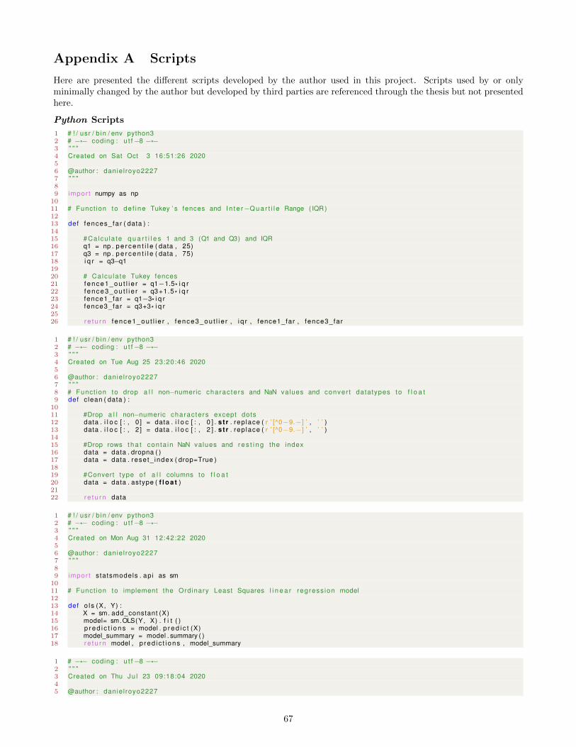
Appendix A Scripts
Here are presented the different scripts developed by the author used in this project. Scripts used by or onlyminimally changed by the author but developed by third parties are referenced through the thesis but not presentedhere.
Python Scripts
1 # ! / usr / b in / env python32 # −*− coding : u t f−8 −*−3 " " "4 Created on Sat Oct 3 16:51:26 202056 @author : danie l royo22277 " " "89 impor t numpy as np
1011 # Funct ion to de f ine Tukey ’ s fences and I n t e r−Q u a r t i l e Range ( IQR)1213 def fences_far ( data ) :1415 # Ca lcu la te q u a r t i l e s 1 and 3 (Q1 and Q3) and IQR16 q1 = np . p e r c e n t i l e ( data , 25)17 q3 = np . p e r c e n t i l e ( data , 75)18 i q r = q3−q11920 # Ca lcu la te Tukey fences21 f e n c e 1 _ o u t l i e r = q1−1.5* i q r22 f e n c e 3 _ o u t l i e r = q3+1.5* i q r23 fence1_far = q1−3* i q r24 fence3_far = q3+3* i q r2526 r e t u r n fence1_ou t l i e r , f ence3_ou t l i e r , i q r , fence1_far , fence3_far
1 # ! / usr / b in / env python32 # −*− coding : u t f−8 −*−3 " " "4 Created on Tue Aug 25 23:20:46 202056 @author : danie l royo22277 " " "8 # Funct ion to drop a l l non−numeric charac te rs and NaN values and conver t datatypes to f l o a t9 def clean ( data ) :
1011 #Drop a l l non−numeric charac te rs except dots12 data . i l o c [ : , 0 ] = data . i l o c [ : , 0 ] . st r . rep lace ( r ’ [^0−9.−] ’ , ’ ’ )13 data . i l o c [ : , 2 ] = data . i l o c [ : , 2 ] . st r . rep lace ( r ’ [^0−9.−] ’ , ’ ’ )1415 #Drop rows t h a t con ta in NaN values and r e s t i n g the index16 data = data . dropna ( )17 data = data . rese t_ index ( drop=True )1819 #Convert type of a l l columns to f l o a t20 data = data . astype ( f l o a t )2122 r e t u r n data
1 # ! / usr / b in / env python32 # −*− coding : u t f−8 −*−3 " " "4 Created on Mon Aug 31 12:42:22 202056 @author : danie l royo22277 " " "89 impor t statsmodels . ap i as sm
1011 # Funct ion to implement the Ordinary Least Squares l i n e a r regress ion model1213 def o l s (X, Y) :14 X = sm. add_constant (X)15 model= sm.OLS(Y, X) . f i t ( )16 p r e d i c t i o n s = model . p r e d i c t (X)17 model_summary = model . summary ( )18 r e t u r n model , p red i c t i ons , model_summary
1 # −*− coding : u t f−8 −*−2 " " "3 Created on Thu Ju l 23 09:18:04 202045 @author : danie l royo2227
67
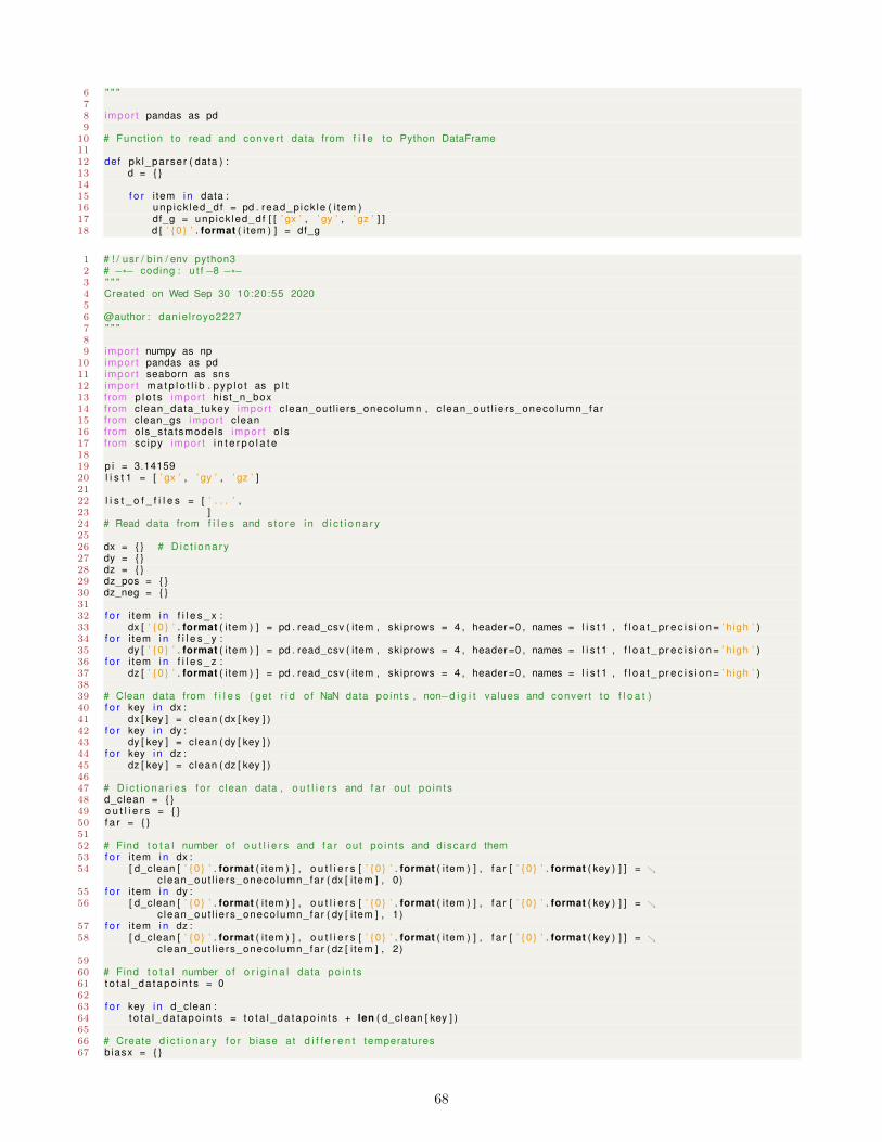
6 " " "78 impor t pandas as pd9
10 # Funct ion to read and conver t data from f i l e to Python DataFrame1112 def pk l_parser ( data ) :13 d = 1415 f o r i tem i n data :16 unp ick led_df = pd . read_p ick le ( i tem )17 df_g = unp ick led_df [ [ ’ gx ’ , ’ gy ’ , ’ gz ’ ] ]18 d [ ’ 0 ’ . format ( i tem ) ] = df_g
1 # ! / usr / b in / env python32 # −*− coding : u t f−8 −*−3 " " "4 Created on Wed Sep 30 10:20:55 202056 @author : danie l royo22277 " " "89 impor t numpy as np
10 impor t pandas as pd11 impor t seaborn as sns12 impor t m a t p l o t l i b . pyp lo t as p l t13 from p l o t s impor t h is t_n_box14 from clean_data_tukey impor t c lean_out l iers_onecolumn , c lean_out l ie rs_oneco lumn_far15 from clean_gs impor t c lean16 from ols_sta tsmodels impor t o l s17 from sc ipy impor t i n t e r p o l a t e1819 p i = 3.1415920 l i s t 1 = [ ’ gx ’ , ’ gy ’ , ’ gz ’ ]2122 l i s t _ o f _ f i l e s = [ ’ . . . ’ ,23 ]24 # Read data from f i l e s and s to re i n d i c t i o n a r y2526 dx = # D i c t i o n a r y27 dy = 28 dz = 29 dz_pos = 30 dz_neg = 3132 f o r i tem i n f i l e s _ x :33 dx [ ’ 0 ’ . format ( i tem ) ] = pd . read_csv ( item , skiprows = 4 , header =0 , names = l i s t 1 , f l o a t _ p r e c i s i o n = ’ high ’ )34 f o r i tem i n f i l e s _ y :35 dy [ ’ 0 ’ . format ( i tem ) ] = pd . read_csv ( item , skiprows = 4 , header =0 , names = l i s t 1 , f l o a t _ p r e c i s i o n = ’ high ’ )36 f o r i tem i n f i l e s _ z :37 dz [ ’ 0 ’ . format ( i tem ) ] = pd . read_csv ( item , skiprows = 4 , header =0 , names = l i s t 1 , f l o a t _ p r e c i s i o n = ’ high ’ )3839 # Clean data from f i l e s ( get r i d o f NaN data po in ts , non−d i g i t values and conver t to f l o a t )40 f o r key i n dx :41 dx [ key ] = clean ( dx [ key ] )42 f o r key i n dy :43 dy [ key ] = clean ( dy [ key ] )44 f o r key i n dz :45 dz [ key ] = clean ( dz [ key ] )4647 # D i c t i o n a r i e s f o r c lean data , o u t l i e r s and f a r out po in t s48 d_clean = 49 o u t l i e r s = 50 f a r = 5152 # Find t o t a l number o f o u t l i e r s and f a r out po in t s and d iscard them53 f o r i tem i n dx :54 [ d_clean [ ’ 0 ’ . format ( i tem ) ] , o u t l i e r s [ ’ 0 ’ . format ( i tem ) ] , f a r [ ’ 0 ’ . format ( key ) ] ] =
c lean_out l ie rs_oneco lumn_far ( dx [ i tem ] , 0)55 f o r i tem i n dy :56 [ d_clean [ ’ 0 ’ . format ( i tem ) ] , o u t l i e r s [ ’ 0 ’ . format ( i tem ) ] , f a r [ ’ 0 ’ . format ( key ) ] ] =
c lean_out l ie rs_oneco lumn_far ( dy [ i tem ] , 1)57 f o r i tem i n dz :58 [ d_clean [ ’ 0 ’ . format ( i tem ) ] , o u t l i e r s [ ’ 0 ’ . format ( i tem ) ] , f a r [ ’ 0 ’ . format ( key ) ] ] =
c lean_out l ie rs_oneco lumn_far ( dz [ i tem ] , 2)5960 # Find t o t a l number o f o r i g i n a l data po in t s61 t o t a l _ d a t a p o i n t s = 06263 f o r key i n d_clean :64 t o t a l _ d a t a p o i n t s = t o t a l _ d a t a p o i n t s + len ( d_clean [ key ] )6566 # Create d i c t i o n a r y f o r biase at d i f f e r e n t temperatures67 biasx =
68
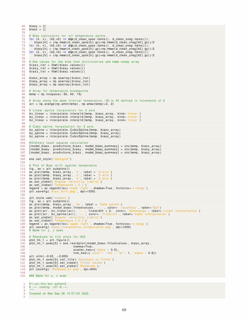
68 biasy = 69 biasz = 7071 # Bias c a l c u l a t i o n f o r a l l temperature po in t s72 f o r ( k , v ) , ( k2 , v2 ) i n zip ( d_clean_xpos . i tems ( ) , d_clean_xneg . i tems ( ) ) :73 biasx [ k ] = ( np . mean( d_clean_xpos [ k ] . gx ) +np . mean( d_clean_xneg [ k2 ] . gx ) ) /274 f o r ( k , v ) , ( k2 , v2 ) i n zip ( d_clean_ypos . i tems ( ) , d_clean_yneg . i tems ( ) ) :75 biasy [ k ] = ( np . mean( d_clean_ypos [ k ] . gy ) +np . mean( d_clean_yneg [ k2 ] . gy ) ) /276 f o r ( k , v ) , ( k2 , v2 ) i n zip ( d_clean_zpos . i tems ( ) , d_clean_zneg . i tems ( ) ) :77 biasz [ k ] = ( np . mean( d_clean_zpos [ k ] . gz ) +np . mean( d_clean_zneg [ k2 ] . gz ) ) /27879 # Get values f o r the b ias from d i c i t i o n a r i e s and make numpy ar ray80 b i a s x _ l i s t = l i s t ( b iasx . values ( ) )81 b i a s y _ l i s t = l i s t ( b iasy . values ( ) )82 b i a s z _ l i s t = l i s t ( b iasz . values ( ) )8384 b iasx_ar ray = np . asarray ( b i a s x _ l i s t )85 b iasy_ar ray = np . asarray ( b i a s y _ l i s t )86 b iasz_ar ray = np . asarray ( b i a s z _ l i s t )8788 # Array f o r temperature breakpo in ts89 temp = np . l i nspace (−30, 40 , 15)9091 # Array along the same i n t e r v a l temperature −30 to 40 def ined i n increments o f 292 a r r = np . arange ( np . amin ( temp ) , np . amax( temp ) +2 , 2)9394 # L inear s p l i n e i t e r p o l a t i o n f o r 3 ax is95 bx_ l i nea r = i n t e r p o l a t e . i n te rp1d ( temp , b iasx_array , k ind= ’ l i n e a r ’ )96 by_ l i nea r = i n t e r p o l a t e . i n te rp1d ( temp , b iasy_array , k ind= ’ l i n e a r ’ )97 bz_ l i nea r = i n t e r p o l a t e . i n te rp1d ( temp , b iasz_array , k ind= ’ l i n e a r ’ )9899 # Cubic s p l i n e i t e r p o l a t i o n f o r 3 ax is
100 bx_sp l ine = i n t e r p o l a t e . CubicSpl ine ( temp , b iasx_ar ray )101 by_sp l ine = i n t e r p o l a t e . CubicSpl ine ( temp , b iasy_ar ray )102 bz_sp l ine = i n t e r p o l a t e . CubicSpl ine ( temp , b iasz_ar ray )103104 #Ordinary l e a s t squares c a l c u l a t i o n105 [ model_biasx , p red i c t i ons_b iasx , model_biasx_summary ] = o ls ( temp , b iasx_ar ray )106 [ model_biasy , p red i c t i ons_b iasy , model_biasy_summary ] = o ls ( temp , b iasy_ar ray )107 [ model_biasz , p red i c t i ons_b iasz , model_biasz_summary ] = o ls ( temp , b iasz_ar ray )108109 sns . s e t _ s t y l e ( " da rkg r i d " )110111 # P lo t o f Bias d r i f t aga ins t temperature112 f i g , ax = p l t . subp lo ts ( )113 ax . p l o t ( temp , b iasx_array , ’ o ’ , l a b e l = ’X−ax is ’ )114 ax . p l o t ( temp , b iasy_array , ’ o ’ , l a b e l = ’Y−ax is ’ )115 ax . p l o t ( temp , b iasz_array , ’ o ’ , l a b e l = ’Z−ax is ’ )116 ax . se t_y labe l ( ’ Angular v e l o c i t i t y [ rad / s ] ’ )117 ax . se t_x labe l ( ’ Temperature [ C ] ’ )118 legend = ax . legend ( loc= ’ lower r i g h t ’ , shadow=True , f o n t s i z e = ’ x−l a rge ’ )119 p l t . save f ig ( ’ b i a s _ d r i f t . png ’ , dp i =1200)120121 p l t . s t y l e . use ( ’ seaborn ’ )122 f i g , ax = p l t . subp lo ts ( )123 ax . p l o t ( temp , b iasx_array , ’ ks ’ , l a b e l = ’ Data po in t s ’ )124 ax . p l o t ( temp , model_biasx . f i t t e d v a l u e s , ’−− ’ , co l o r = ’ r oya lb l ue ’ , l a b e l = "OLS" )125 ax . p l o t ( ar r , bx_ l i nea r ( a r r ) , ’−− ’ , l i n e w i d t h = 2 , co l o r = ’ darkorange ’ , l a b e l = ’ L inear i n t e r p o l a t i o n ’ )126 ax . p l o t ( ar r , bx_sp l ine ( a r r ) , ’−− ’ , co l o r = ’ f i r e b r i c k ’ , l a b e l = ’ Cubic i n t e r p o l a t i o n ’ )127 ax . se t_y labe l ( ’ Angular v e l o c i t i t y [ rad / s ] ’ )128 ax . se t_x labe l ( ’ Temperature [ C ] ’ )129 legend = ax . legend ( loc= ’ upper r i g h t ’ , shadow=True , f o n t s i z e = ’ x−l a rge ’ )130 p l t . save f ig ( ’ b iasx_ in te rpo la t ion_compar ison3 . png ’ , dp i =1200)131 # Same f o r y , z axes132133 # Residuals vs f i t s p l o t s f o r OLS134 plot_ lm_1 = p l t . f i g u r e ( )135 plot_ lm_1 . axes [ 0 ] = sns . r e s i d p l o t ( model_biasx . f i t t e d v a l u e s , b iasx_array ,136 lowess=True ,137 scat ter_kws = ’ alpha ’ : 0 . 5 ,138 l ine_kws = ’ co l o r ’ : ’ red ’ , ’ lw ’ : 1 , ’ alpha ’ : 0 . 8 )139 p l t . x l im (−0.02 , −0.005)140 plot_ lm_1 . axes [ 0 ] . s e t _ t i t l e ( ’ Residuals vs F i t t e d ’ )141 plot_ lm_1 . axes [ 0 ] . se t_x labe l ( ’ F i t t e d values ’ )142 plot_ lm_1 . axes [ 0 ] . se t_y labe l ( ’ Residuals ’ ) ;143 p l t . save f ig ( ’ res idua ls_bx . png ’ , dp i =800)144145 ### Same f o r y , z axes
1 # ! / usr / b in / env python32 # −*− coding : u t f−8 −*−3 " " "4 Created on Mon Sep 28 10:57:03 20205
69
6 @author : danie l royo22277 " " "89 impor t sys
10 impor t numpy as np11 impor t pandas as pd12 impor t seaborn as sns13 impor t m a t p l o t l i b . pyp lo t as p l t14 from p l o t s impor t h is t_n_box15 from clean_data_tukey impor t c lean_out l iers_onecolumn , c lean_out l ie rs_oneco lumn_far16 from clean_gs impor t c lean17 from pr i n t _va l ues impor t dump18 from statsmodels . sandbox . regress ion . predstd impor t w l s_p red i c t i on_s td19 from tukey_fence impor t fences20 from sc ipy impor t i n t e r p o l a t e21 from ols_sta tsmodels impor t o l s22 from gy ro_ tempe ra tu re_ca l i b ra t i on_ id l e_ tes t3 impor t *232425 # L i s t o f f i l e s f o r temperatures ranging from −30 C to +40 C when the FS−1 OBC board26 # i s made to sp in around i t s x d i r e c t i o n a t 30 deg / s both clock− and an t i c l ock−wise2728 l i s t _ o f _ f i l e s = [ ’ . . . ’ ,29 ]3031 # Impor t b ias f o r temperature range from ’ gy ro_ tempe ra tu re_ca l i b ra t i on_ id l e_ tes t3 ’ f i l e32 # and f i l l d i c t t i o n a r i e s w i th values3334 d_bx = 35 d_by = 36 d_bz = 3738 bx_array = biasx . values ( )39 by_array = biasy . values ( )40 bz_array = biasz . values ( )4142 d_bx = dict ( zip ( f i l es_xpos , bx_array ) )43 d_by = dict ( zip ( f i l es_ypos , by_array ) )44 d_bz = dict ( zip ( f i l es_zpos , bz_array ) )4546 # Read data from f i l e s and s to re i n d i c t i o n a r y47 # Clean data48 # Find o u t l i e r s and f a r out po in t s49 # (same code as i n prev ious s c r i p t s )5051 # True angular ra te i npu t52 p i = 3.1415953 omega = 30* p i /1805455 # Array o f temperature po in t s a t which measurements were taken56 temp = np . l i nspace (−30, 40 , 15)5758 # Array along the same i n t e r v a l temperature −30 to 40 def ined i n increments o f 259 a r r = np . arange ( np . amin ( temp ) , np . amax( temp ) +2 , 2)60 ar r2 = np . arange(−5, 30 , 5)616263 # D i c t i o n a r i e s f o r sca le f a c t o r s f o r a l l temperature po in t s64 SFx = 65 SFy = 66 SFz = 676869 # Scale f a c t o r c a l c u l a t i o n across a l l temperatures70 f o r ( k , v ) , ( k2 , v2 ) i n zip ( d_clean_xpos . i tems ( ) , d_clean_xneg . i tems ( ) ) :71 SFx [ k ] = ( np . mean( d_clean_xpos [ k ] . gx )−np . mean( d_clean_xneg [ k2 ] . gx ) ) / ( 2 * omega)7273 f o r ( k , v ) , ( k2 , v2 ) i n zip ( d_clean_ypos . i tems ( ) , d_clean_yneg . i tems ( ) ) :74 SFy [ k ] = ( np . mean( d_clean_ypos [ k ] . gy )−np . mean( d_clean_yneg [ k2 ] . gy ) ) / ( 2 * omega)7576 f o r ( k , v ) , ( k2 , v2 ) i n zip ( d_clean_zpos . i tems ( ) , d_clean_zneg . i tems ( ) ) :77 SFz [ k ] = ( np . mean( d_clean_zpos [ k ] . gz )−np . mean( d_clean_zneg [ k2 ] . gz ) ) / ( 2 * omega)7879 # Array f o r temperature breakpo in ts80 temp = np . l i nspace (−30, 40 , 15)8182 # PLot f o r sca le f a c t o r e r r o r aga ins t temperature (same f o r y− and z− axes )83 f i g , ax = p l t . subp lo ts ( )84 sns . boxp lo t ( data=SFx_nomean_df )85 ax . s e t _ x t i c k l a b e l s ( ax . g e t _ x t i c k l a b e l s ( ) , r o t a t i o n =−45)86 ax . se t_y labe l ( ’ Angular v e l o c i t i t y [ rad / s ] ’ )87 ax . se t_x labe l ( ’ Temperature [ C ] ’ )88 p l t . save f ig ( ’ s f x _ d r i f t _ b o x p l o t . png ’ , dp i =1200)89
70
90 # Take values from SF e r r o r d i c t i o n a r i e s and t rans form to numpy ar rays91 s f x _ l i s t = l i s t (SFx . values ( ) )92 s f y _ l i s t = l i s t (SFy . values ( ) )93 s f z _ l i s t = l i s t (SFz . values ( ) )94 s fx_ar ray = np . asarray ( s f x _ l i s t )95 s fy_ar ray = np . asarray ( s f y _ l i s t )96 s fz_ar ray = np . asarray ( s f z _ l i s t )9798 # P lo t o f SF i n th ree ax is f o r a l l temperature po in t s − d r i f t99 f i g , ax = p l t . subp lo ts ( )
100 ax . p l o t ( temp , s fx_ar ray , ’ o ’ , l a b e l = ’X−ax is ’ )101 ax . p l o t ( temp , s fy_ar ray , ’ o ’ , l a b e l = ’Y−ax is ’ )102 ax . p l o t ( temp , s fz_ar ray , ’ o ’ , l a b e l = ’Z−ax is ’ )103 ax . se t_y labe l ( ’ E r ro r [%] ’ )104 ax . se t_x labe l ( ’ Temperature [ C ] ’ )105 legend = ax . legend ( loc= ’ upper l e f t ’ , shadow=True , f o n t s i z e = ’ x−l a rge ’ )106 p l t . save f ig ( ’ s f _ d r i f t . png ’ , dp i =1200)107108 # L inear s p l i n e i n t e r p o l a t i o n o f sca le f a c t o r s109 s f x _ l i n e a r = i n t e r p o l a t e . i n te rp1d ( temp , s fx_ar ray , k ind= ’ l i n e a r ’ )110 s f y _ l i n e a r = i n t e r p o l a t e . i n te rp1d ( temp , s fy_ar ray , k ind= ’ l i n e a r ’ )111 s f z _ l i n e a r = i n t e r p o l a t e . i n te rp1d ( temp , s fz_ar ray , k ind= ’ l i n e a r ’ )112113 # Cubic s p l i n e i n t e r p o l a t i o n o f sca le f a c t o r s114 s f x _ s p l i n e = i n t e r p o l a t e . CubicSpl ine ( temp , s fx_a r ray )115 s f y _ s p l i n e = i n t e r p o l a t e . CubicSpl ine ( temp , s fy_a r ray )116 s f z _ s p l i n e = i n t e r p o l a t e . CubicSpl ine ( temp , s fz_a r ray )117118 # OLS l i n e a r regress ion model o f SF e r r o r119 [ model_sfx , p red i c t i ons_s f x , model_sfx_summary ] = o l s ( temp , s fx_ar ray )120 [ model_sfy , p red i c t i ons_s f y , model_sfy_summary ] = o l s ( temp , s fy_ar ray )121 [ model_sfz , p red i c t i ons_s f z , model_sfz_summary ] = o l s ( temp , s fz_ar ray )122123 sns . se t_con tex t ( " paper " )124125 f i g , ax = p l t . subp lo ts ( )126 ax . p l o t ( temp , s fx_ar ray , ’ ks ’ , l a b e l = ’ Data po in t s ’ )127 ax . p l o t ( temp , model_sfx . f i t t e d v a l u e s , ’−− ’ , co l o r = ’ r oya lb l ue ’ , l a b e l = "OLS" )128 ax . p l o t ( ar r , s f x _ l i n e a r ( a r r ) , ’−− ’ , l i n e w i d t h = 2 , co l o r = ’ darkorange ’ , l a b e l = ’ L inear i n t e r p o l a t i o n ’ )129 ax . p l o t ( ar r , s f x _ s p l i n e ( a r r ) , ’−− ’ , co l o r = ’ f i r e b r i c k ’ , l a b e l = ’ Cubic i n t e r p o l a t i o n ’ )130 ax . se t_y labe l ( ’ E r ro r ’ )131 ax . se t_x labe l ( ’ Temperature [ C ] ’ )132 legend = ax . legend ( loc= ’ upper l e f t ’ , shadow=True , f o n t s i z e = ’ l a rge ’ )133 p l t . save f ig ( ’ s f x _ i n t e r p o l a t i o n _ o l s . png ’ , dp i =1200)134135 plot_ lm_1 = p l t . f i g u r e ( )136 plot_ lm_1 . axes [ 0 ] = sns . r e s i d p l o t ( model_sfx . f i t t e d v a l u e s , s fx_ar ray ,137 lowess=True ,138 scat ter_kws = ’ alpha ’ : 0 . 5 ,139 l ine_kws = ’ co l o r ’ : ’ red ’ , ’ lw ’ : 1 , ’ alpha ’ : 0 . 8 )140 plot_ lm_1 . axes [ 0 ] . s e t _ t i t l e ( ’ Residuals vs F i t t e d ’ )141 plot_ lm_1 . axes [ 0 ] . se t_x labe l ( ’ F i t t e d values ’ )142 plot_ lm_1 . axes [ 0 ] . se t_y labe l ( ’ Residuals ’ ) ;143 p l t . save f ig ( ’ r e s i d u a l s _ s f x . png ’ , dp i =800)144145 # Biases from s t a t i c t e s t a t room temperature (T=20 C )146 b_gx = −0.011780544674184271147 b_gy = −0.00013268794108398639148 b_gz = 0.01699940100852356149150 # Apply l e a s t squares to f i n d SF and non−misal ignment e r r o r s151152 A = np . ar ray ( [ [ 1 , 0 , 0 , 0 , 0 , 0 , 0 , 0 , 0 ] ,153 [ 0 , 1 , 0 , 0 , 0 , 0 , 0 , 0 , 0 ] ,154 [ 0 , 0 , 1 , 0 , 0 , 0 , 0 , 0 , 0 ] ,155 [ 0 , 0 , 0 , 1 , 0 , 0 , 0 , 0 , 0 ] ,156 [ 0 , 0 , 0 , 0 , 1 , 0 , 0 , 0 , 0 ] ,157 [ 0 , 0 , 0 , 0 , 0 , 1 , 0 , 0 , 0 ] ,158 [ 0 , 0 , 0 , 0 , 0 , 0 , 1 , 0 , 0 ] ,159 [ 0 , 0 , 0 , 0 , 0 , 0 , 0 , 1 , 0 ] ,160 [ 0 , 0 , 0 , 0 , 0 , 0 , 0 , 0 , 1 ] ,161 [ 1 , 0 , 0 , 0 , 0 , 0 , 0 , 0 , 0 ] ,162 [ 0 , 1 , 0 , 0 , 0 , 0 , 0 , 0 , 0 ] ,163 [ 0 , 0 , 1 , 0 , 0 , 0 , 0 , 0 , 0 ] ,164 [ 0 , 0 , 0 , 1 , 0 , 0 , 0 , 0 , 0 ] ,165 [ 0 , 0 , 0 , 0 , 1 , 0 , 0 , 0 , 0 ] ,166 [ 0 , 0 , 0 , 0 , 0 , 1 , 0 , 0 , 0 ] ,167 [ 0 , 0 , 0 , 0 , 0 , 0 , 1 , 0 , 0 ] ,168 [ 0 , 0 , 0 , 0 , 0 , 0 , 0 , 1 , 0 ] ,169 [ 0 , 0 , 0 , 0 , 0 , 0 , 0 , 0 , 1 ] ] )170171 # Create empty d i c t i o n a r i e s f o r outputs from l e a s t squares so l ve r172 x = 173 r e s i du a l s =
71
174 rank = 175 s = 176177 # Find misal ignment e r r o r s f o r temperature range178 f o r ( k , v ) , ( k2 , v2 ) , ( k3 , v3 ) , ( k4 , v4 ) , ( k5 , v5 ) , ( k6 , v6 ) , ( k7 , v7 ) , \179 ( k8 , v8 ) , ( k9 , v9 ) i n zip ( d_clean_xpos . i tems ( ) , d_clean_xneg . i tems ( ) , d_clean_ypos . i tems ( ) , \180 d_clean_yneg . i tems ( ) , d_clean_zpos . i tems ( ) , d_clean_zneg . i tems ( ) , \181 d_bx . i tems ( ) , d_by . i tems ( ) , d_bz . i tems ( ) ) :182 B = np . ar ray ( [ ( np . mean( d_clean [ k ] . gx )−d_bx [ k7 ] ) / omega ,183 ( np . mean( d_clean [ k ] . gy )−d_by [ k8 ] ) / omega ,184 ( np . mean( d_clean [ k ] . gz )−d_bz [ k9 ] ) / omega ,185 ( np . mean( d_clean [ k3 ] . gx )−d_bx [ k7 ] ) / omega ,186 ( np . mean( d_clean [ k3 ] . gy )−d_by [ k8 ] ) / omega ,187 ( np . mean( d_clean [ k3 ] . gz )−d_bz [ k9 ] ) / omega ,188 ( np . mean( d_clean [ k5 ] . gx )−d_bx [ k7 ] ) / omega ,189 ( np . mean( d_clean [ k5 ] . gy )−d_by [ k8 ] ) / omega ,190 ( np . mean( d_clean [ k5 ] . gz )−d_bz [ k9 ] ) / omega ,191 ( np . mean( d_clean [ k2 ] . gx )−d_bx [ k7 ] ) /−omega ,192 ( np . mean( d_clean [ k2 ] . gy )−d_by [ k8 ] ) /−omega ,193 ( np . mean( d_clean [ k2 ] . gz )−d_bz [ k9 ] ) /−omega ,194 ( np . mean( d_clean [ k4 ] . gx )−d_bx [ k7 ] ) /−omega ,195 ( np . mean( d_clean [ k4 ] . gy )−d_by [ k8 ] ) /−omega ,196 ( np . mean( d_clean [ k4 ] . gz )−d_bz [ k9 ] ) /−omega ,197 ( np . mean( d_clean [ k6 ] . gx )−d_bx [ k7 ] ) /−omega ,198 ( np . mean( d_clean [ k6 ] . gy )−d_by [ k8 ] ) /−omega ,199 ( np . mean( d_clean [ k6 ] . gz )−d_bz [ k9 ] ) /−omega ] )200 x [ k ] , r e s i d ua l s [ k ] , rank [ k ] , s [ k ] = np . l i n a l g . l s t s q (A,B)201202 df_mis = pd . DataFrame ( x )203204 # Create numpy ar rays o f misal ignment e r r o r s from misal ignment DataFrame205 mxy_array = np . ar ray ( df_mis . i l o c [ 1 ] )206 mxz_array = np . ar ray ( df_mis . i l o c [ 2 ] )207 myx_array = np . ar ray ( df_mis . i l o c [ 3 ] )208 myz_array = np . ar ray ( df_mis . i l o c [ 5 ] )209 mzx_array = np . ar ray ( df_mis . i l o c [ 6 ] )210 mzy_array = np . ar ray ( df_mis . i l o c [ 7 ] )211212 # L inear s p l i n e i n t e r p o l a t i o n o f sca le f a c t o r s213 mxy_interp1 = i n t e r p o l a t e . i n te rp1d ( temp , mxy_array , k ind= ’ l i n e a r ’ )214 mxz_interp1 = i n t e r p o l a t e . i n te rp1d ( temp , mxz_array , k ind= ’ l i n e a r ’ )215 myx_interp1 = i n t e r p o l a t e . i n te rp1d ( temp , myx_array , k ind= ’ l i n e a r ’ )216 myz_interp1 = i n t e r p o l a t e . i n te rp1d ( temp , myz_array , k ind= ’ l i n e a r ’ )217 mzx_interp1 = i n t e r p o l a t e . i n te rp1d ( temp , mzx_array , k ind= ’ l i n e a r ’ )218 mzy_interp1 = i n t e r p o l a t e . i n te rp1d ( temp , mzy_array , k ind= ’ l i n e a r ’ )219220 # Cubic s p l i n e i n t e r p o l a t i o n o f sca le f a c t o r s221 mxy_spl ine = i n t e r p o l a t e . CubicSpl ine ( temp , mxy_array )222 mxz_spl ine = i n t e r p o l a t e . CubicSpl ine ( temp , mxz_array )223 myx_spl ine = i n t e r p o l a t e . CubicSpl ine ( temp , myx_array )224 myz_spl ine = i n t e r p o l a t e . CubicSpl ine ( temp , myz_array )225 mzx_spl ine = i n t e r p o l a t e . CubicSpl ine ( temp , mzx_array )226 mzy_spl ine = i n t e r p o l a t e . CubicSpl ine ( temp , mzy_array )227228 # OLS l i n e a r regress ion o f misal ignment e r r o r s229 [ model_mxy , predict ions_mxy , model_mxy_summary ] = o l s ( temp , mxy_array )230 [ model_mxz , predict ions_mxz , model_mxz_summary ] = o l s ( temp , mxz_array )231 [ model_myx , predict ions_myx , model_myx_summary ] = o l s ( temp , myx_array )232 [ model_myz , predict ions_myz , model_myz_summary ] = o l s ( temp , myz_array )233 [ model_mzx , predict ions_mzx , model_mzx_summary ] = o l s ( temp , mzx_array )234 [ model_mzy , predict ions_mzy , model_mzy_summary ] = o l s ( temp , mzy_array )235236 #PLOTS237 sns . se t_con tex t ( " paper " )238 p l t . t i g h t _ l a y o u t ( )239240 f i g , ax = p l t . subp lo ts ( )241 ax . p l o t ( temp , mxy_array , ’ ks ’ , l a b e l = ’ Data po in t s ’ )242 ax . p l o t ( temp , model_mxy . f i t t e d v a l u e s , ’−− ’ , co l o r = ’ r oya lb l ue ’ , l a b e l = "OLS" )243 ax . p l o t ( ar r , mxy_interp1 ( a r r ) , ’−− ’ , l i n e w i d t h = 2 , co l o r = ’ darkorange ’ , l a b e l = ’ L inear i n t e r p o l a t i o n ’ )244 ax . p l o t ( ar r , mxy_spl ine ( a r r ) , ’−− ’ , co l o r = ’ f i r e b r i c k ’ , l a b e l = ’ Cubic i n t e r p o l a t i o n ’ )245 ax . se t_y labe l ( ’ E r ro r ’ )246 ax . se t_x labe l ( ’ Temperature [ C ] ’ )247 legend = ax . legend ( loc= ’ upper l e f t ’ , shadow=True , f o n t s i z e = ’medium ’ )248 p l t . save f ig ( ’ mxy_ in te rpo la t i on_o ls_dynamic_ca l i b ra t i on . png ’ , dp i =1200)249250 # Same p l o t s t y l e f o r y− and z−values
1 # ! / usr / b in / env python32 # −*− coding : u t f−8 −*−3 " " "4 Created on Mon Oct 26 12:16:14 202056 @author : danie l royo2227
72
7 " " "89 impor t numpy as np
10 impor t pandas as pd11 impor t seaborn as sns12 impor t m a t p l o t l i b . pyp lo t as p l t13 from clean_data_tukey impor t c lean_out l iers_onecolumn , c lean_out l ie rs_oneco lumn_far14 from clean_gs impor t c lean15 impor t statsmodels . ap i as sm16 from gy ro_ tempe ra tu re_ca l i b ra t i on_ id l e_ tes t3 impor t *17 from gyro_ tempera ture_dynamic_ca l ib ra t ion_ tes t2 impor t *18 from sk learn . met r i cs impor t mean_absolute_error , mean_squared_error19 from ols_sta tsmodels impor t o l s20 from sc ipy impor t i n t e r p o l a t e2122 p i = 3.1415923 l i s t 1 = [ ’ gx ’ , ’ gy ’ , ’ gz ’ ]24 true_omega = 30* p i /180252627 l i s t _ o f _ f i l e s = [ ’ . . . ’ ,28 ]29 # Read data from f i l e s and s to re i n d i c t i o n a r y3031 d = # D i c t i o n a r y32 dx = # D i c t i o n a r y33 dy = 34 dz = 3536 f o r i tem i n f i l e s _ x :37 dx [ ’ 0 ’ . format ( i tem ) ] = pd . read_csv ( item , skiprows = 3 , header =0 , names = l i s t 1 , f l o a t _ p r e c i s i o n = ’ high ’ ,
er ro r_bad_ l ines=False )38 f o r i tem i n f i l e s _ y :39 dy [ ’ 0 ’ . format ( i tem ) ] = pd . read_csv ( item , skiprows = 3 , header =0 , names = l i s t 1 , f l o a t _ p r e c i s i o n = ’ high ’ ,
er ro r_bad_ l ines=False )40 f o r i tem i n f i l e s _ z :41 dz [ ’ 0 ’ . format ( i tem ) ] = pd . read_csv ( item , skiprows = 3 , header =0 , names = l i s t 1 , f l o a t _ p r e c i s i o n = ’ high ’ ,
er ro r_bad_ l ines=False )4243 # Clean data from f i l e s ( get r i d o f NaN data po in ts , non−d i g i t values and conver t to f l o a t )44 f o r key i n dx :45 dx [ key ] = clean ( dx [ key ] )46 f o r key i n dy :47 dy [ key ] = clean ( dy [ key ] )48 f o r key i n dz :49 dz [ key ] = clean ( dz [ key ] )5051 #Create d i c t i o n a r i e s f o r c lean data and # o u t l i e r s5253 d_clean = 54 dx_clean = 55 o u t l i e r s = 56 f a r = 575859 f o r i tem i n f i l e s x _ p o s :60 [ dx_clean [ ’ 0 ’ . format ( i tem ) ] , o u t l i e r s [ ’ 0 ’ . format ( i tem ) ] ] = c lean_out l iers_onecolumn ( dx [ i tem ] , 0)61 f o r i tem i n f i l e s y _ p o s :62 [ dy_clean [ ’ 0 ’ . format ( i tem ) ] , o u t l i e r s [ ’ 0 ’ . format ( i tem ) ] ] = c lean_out l iers_onecolumn ( dy [ i tem ] , 1)63 f o r i tem i n f i l e s z _ p o s :64 [ dz_clean [ ’ 0 ’ . format ( i tem ) ] , o u t l i e r s [ ’ 0 ’ . format ( i tem ) ] ] = c lean_out l iers_onecolumn ( dz [ i tem ] , 2)6566 f o r key i n d :67 t o t a l _ d a t a p o i n t s = t o t a l _ d a t a p o i n t s + len ( d [ key ] )6869 omega = 30* p i /180 # ac tua l angular v e l o c i t y o f the t u r n t a b l e7071 i = np . arange (−8 ,36 ,4)72 temp = i73 o = sm. add_constant ( i )7475 # Impor t b ias and scale f a c t o r i n t e r p o l a t e d values from c a l i b r a t i o n s c r i p t76 bx_ar ray_ l i nea r = bx_ l i nea r ( i )77 by_ar ray_ l i nea r = by_ l i nea r ( i )78 bz_ar ray_ l i nea r = bz_ l i nea r ( i )7980 s f x _ a r r a y _ l i n e a r = s f x _ l i n e a r ( i )81 s f y _ a r r a y _ l i n e a r = s f y _ l i n e a r ( i )82 s f z _ a r r a y _ l i n e a r = s f z _ l i n e a r ( i )8384 bx_array = bx_sp l ine ( i )85 by_array = by_sp l ine ( i )86 bz_array = bz_sp l ine ( i )87
73
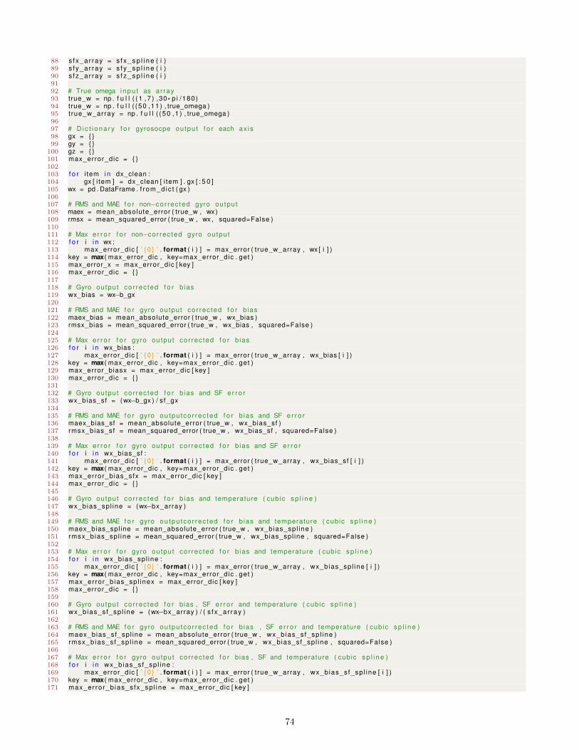
88 s fx_ar ray = s f x _ s p l i n e ( i )89 s fy_ar ray = s f y _ s p l i n e ( i )90 s fz_ar ray = s f z _ s p l i n e ( i )9192 # True omega inpu t as ar ray93 true_w = np . f u l l ( ( 1 , 7 ) ,30* p i /180)94 true_w = np . f u l l ( (50 ,11 ) , true_omega )95 t rue_w_array = np . f u l l ( ( 50 ,1 ) , true_omega )9697 # D i c t i o n a r y f o r gyrosocpe output f o r each ax is98 gx = 99 gy =
100 gz = 101 max_error_dic = 102103 f o r i tem i n dx_clean :104 gx [ i tem ] = dx_clean [ i tem ] . gx [ : 5 0 ]105 wx = pd . DataFrame . f rom_d ic t ( gx )106107 # RMS and MAE f o r non−cor rec ted gyro output108 maex = mean_absolute_error ( true_w , wx)109 rmsx = mean_squared_error ( true_w , wx , squared=False )110111 # Max e r r o r f o r non−cor rec ted gyro output112 f o r i i n wx :113 max_error_dic [ ’ 0 ’ . format ( i ) ] = max_error ( true_w_array , wx [ i ] )114 key = max( max_error_dic , key=max_error_dic . get )115 max_error_x = max_error_dic [ key ]116 max_error_dic = 117118 # Gyro output cor rec ted f o r b ias119 wx_bias = wx−b_gx120121 # RMS and MAE f o r gyro output cor rec ted f o r b ias122 maex_bias = mean_absolute_error ( true_w , wx_bias )123 rmsx_bias = mean_squared_error ( true_w , wx_bias , squared=False )124125 # Max e r r o r f o r gyro output cor rec ted f o r b ias126 f o r i i n wx_bias :127 max_error_dic [ ’ 0 ’ . format ( i ) ] = max_error ( true_w_array , wx_bias [ i ] )128 key = max( max_error_dic , key=max_error_dic . get )129 max_error_biasx = max_error_dic [ key ]130 max_error_dic = 131132 # Gyro output cor rec ted f o r b ias and SF e r r o r133 wx_bias_sf = (wx−b_gx ) / sf_gx134135 # RMS and MAE f o r gyro ou tpu tco r rec ted f o r b ias and SF e r r o r136 maex_bias_sf = mean_absolute_error ( true_w , wx_bias_sf )137 rmsx_bias_sf = mean_squared_error ( true_w , wx_bias_sf , squared=False )138139 # Max e r r o r f o r gyro output cor rec ted f o r b ias and SF e r r o r140 f o r i i n wx_bias_sf :141 max_error_dic [ ’ 0 ’ . format ( i ) ] = max_error ( true_w_array , wx_bias_sf [ i ] )142 key = max( max_error_dic , key=max_error_dic . get )143 max_error_bias_sfx = max_error_dic [ key ]144 max_error_dic = 145146 # Gyro output cor rec ted f o r b ias and temperature ( cubic s p l i n e )147 wx_bias_spl ine = (wx−bx_array )148149 # RMS and MAE f o r gyro ou tpu tco r rec ted f o r b ias and temperature ( cubic s p l i n e )150 maex_bias_spl ine = mean_absolute_error ( true_w , wx_bias_spl ine )151 rmsx_bias_spl ine = mean_squared_error ( true_w , wx_bias_spl ine , squared=False )152153 # Max e r r o r f o r gyro output cor rec ted f o r b ias and temperature ( cubic s p l i n e )154 f o r i i n wx_bias_spl ine :155 max_error_dic [ ’ 0 ’ . format ( i ) ] = max_error ( true_w_array , wx_bias_spl ine [ i ] )156 key = max( max_error_dic , key=max_error_dic . get )157 max_error_b ias_spl inex = max_error_dic [ key ]158 max_error_dic = 159160 # Gyro output cor rec ted f o r bias , SF e r r o r and temperature ( cubic s p l i n e )161 wx_bias_sf_sp l ine = (wx−bx_array ) / ( s f x_a r ray )162163 # RMS and MAE f o r gyro ou tpu tco r rec ted f o r b ias , SF e r r o r and temperature ( cubic s p l i n e )164 maex_bias_sf_spl ine = mean_absolute_error ( true_w , wx_bias_sf_sp l ine )165 rmsx_b ias_sf_sp l ine = mean_squared_error ( true_w , wx_bias_sf_spl ine , squared=False )166167 # Max e r r o r f o r gyro output cor rec ted f o r bias , SF and temperature ( cubic s p l i n e )168 f o r i i n wx_b ias_sf_sp l ine :169 max_error_dic [ ’ 0 ’ . format ( i ) ] = max_error ( true_w_array , wx_b ias_sf_sp l ine [ i ] )170 key = max( max_error_dic , key=max_error_dic . get )171 max_error_b ias_sfx_sp l ine = max_error_dic [ key ]
74

172 max_error_dic = 173174 # Gyro output cor rec ted f o r b ias and temperature ( l i n e a r i n t e r p o l a t i o n )175 wx_bias_interp1 = (wx−bx_ar ray_ l i nea r )176177 # RMS and MAE f o r gyro ou tpu tco r rec ted f o r b ias and temperature ( l i n e a r i n t e r p o l a t i o n )178 maex_bias_interp1 = mean_absolute_error ( true_w , wx_bias_interp1 )179 rmsx_bias_ in terp1 = mean_squared_error ( true_w , wx_bias_interp1 , squared=False )180181 # Max e r r o r f o r gyro output cor rec ted f o r b ias and temperature ( cubic s p l i n e )182 f o r i i n wx_bias_interp1 :183 max_error_dic [ ’ 0 ’ . format ( i ) ] = max_error ( true_w_array , wx_bias_interp1 [ i ] )184 key = max( max_error_dic , key=max_error_dic . get )185 max_error_b ias_ in terp1x = max_error_dic [ key ]186 max_error_dic = 187188 # Gyro output cor rec ted f o r bias , SF e r r o r and temperature ( l i n e a r i n t e r p o l a t i o n )189 wx_bias_sf_ in terp1 = (wx−bx_ar ray_ l i nea r ) / ( s f x _ a r r a y _ l i n e a r )190191 # RMS and MAE f o r gyro ou tpu tco r rec ted f o r b ias , SF e r r o r and temperature ( l i n e a r i n t e r p o l a t i o n )192 maex_bias_sf_ interp1 = mean_absolute_error ( true_w , wx_b ias_sf_ in terp1 )193 rmsx_b ias_s f_ in terp1 = mean_squared_error ( true_w , wx_bias_sf_ in terp1 , squared=False )194195 # Max e r r o r f o r gyro output cor rec ted f o r bias , SF and temperature ( l i n e a r i n t e r p o l a t i o n )196 f o r i i n wx_b ias_sf_ in terp1 :197 max_error_dic [ ’ 0 ’ . format ( i ) ] = max_error ( true_w_array , wx_b ias_sf_ in terp1 [ i ] )198 key = max( max_error_dic , key=max_error_dic . get )199 max_er ror_b ias_s fx_ in terp1 = max_error_dic [ key ]200 max_error_dic = 201202 # OLS l i n e a r regress ion p r e d i c t i o n o f b ias and SF e r r o r s f o r temperature range203 bx_array_ols = model_biasx . p r e d i c t ( o )204 s fx_a r ray_o ls = model_sfx . p r e d i c t ( o )205206 # Gyro output cor rec ted f o r b ias and temperature (OLS)207 wx_bias_ols = (wx−bx_array_ols )208209 # RMS and MAE f o r gyro ou tpu tco r rec ted f o r b ias and temperature (OLS)210 maex_bias_ols = mean_absolute_error ( true_w , wx_bias_ols )211 rmsx_bias_ols = mean_squared_error ( true_w , wx_bias_ols , squared=False )212213 # Max e r r o r f o r gyro output cor rec ted f o r b ias and temperature (OLS)214 f o r i i n wx_bias_ols :215 max_error_dic [ ’ 0 ’ . format ( i ) ] = max_error ( true_w_array , wx_bias_ols [ i ] )216 key = max( max_error_dic , key=max_error_dic . get )217 max_error_biasx_ols = max_error_dic [ key ]218 max_error_dic = 219220 # Gyro output cor rec ted f o r bias , SF e r r o r and temperature (OLS)221 wx_bias_sf_ols = (wx−bx_array_ols ) / ( s f x_a r ray_o ls )222223 # RMS and MAE f o r gyro ou tpu tco r rec ted f o r b ias , SF e r r o r and temperature224 maex_bias_sf_ols = mean_absolute_error ( true_w , wx_bias_sf_ols )225 rmsx_bias_sf_ols = mean_squared_error ( true_w , wx_bias_sf_ols , squared=False )226227 # Max e r r o r f o r gyro output cor rec ted f o r bias , SF and temperature (OLS)228 f o r i i n wx_bias_sf_ols :229 max_error_dic [ ’ 0 ’ . format ( i ) ] = max_error ( true_w_array , wx_bias_sf_ols [ i ] )230 key = max( max_error_dic , key=max_error_dic . get )231 max_error_b ia_sfsx_ols = max_error_dic [ key ]232 max_error_dic = 233234 # Turn omega inpu t and cor rec ted values to ar ray w i th s ize equal to t h a t o f temperature range235 wx = np . mean(wx)236 wx = np . reshape (wx , (11 , ) )237 wx_bias_sf = np . mean( wx_bias_sf )238 wx_bias_sf = np . reshape ( wx_bias_sf , ( 11 , ) )239 wx_bias_sf_ in terp1 = np . mean( wx_b ias_sf_ in terp1 )240 wx_bias_sf_ in terp1 = np . reshape ( wx_bias_sf_ in terp1 , (11 , ) )241 wx_bias_sf_sp l ine = np . mean( wx_bias_sf_sp l ine )242 wx_bias_sf_sp l ine = np . reshape ( wx_bias_sf_spl ine , (11 , ) )243 wx_bias_sf_ols = np . mean( wx_bias_sf_ols )244 wx_bias_sf_ols = np . reshape ( wx_bias_sf_ols , (11 , ) )245246 sns . set ( s t y l e =" da rkg r i d " )247 sns . se t_con tex t ( " notebook " )248249 f i g , ax = p l t . subp lo ts ( )250 ax . p l o t ( temp , wx , ’ ks ’ , l a b e l = ’ Data po in t s ’ )251 ax . p l o t ( temp , wx_bias_sf , ’ o ’ , l a b e l = ’ Corrected f o r b ias and SF ’ )252 ax . p l o t ( temp , wx_bias_sf_ in terp1 , ’ o ’ , l a b e l = ’ Corrected f o r bias , SF \ n and T ( L inear i n t e r p o l a t i o n ) ’ )253 ax . p l o t ( temp , wx_bias_sf_spl ine , ’ o ’ , l a b e l = ’ Corrected f o r bias , SF \ n and T ( Cubic s p l i n e ) ’ )254 ax . p l o t ( temp , wx_bias_sf_ols , ’ o ’ , l a b e l = ’ Corrected f o r bias , SF \ n and T (OLS) ’ )255 ax . se t_y labe l ( ’ Angular v e l o c i t i t y [ rad / s ] ’ )
75
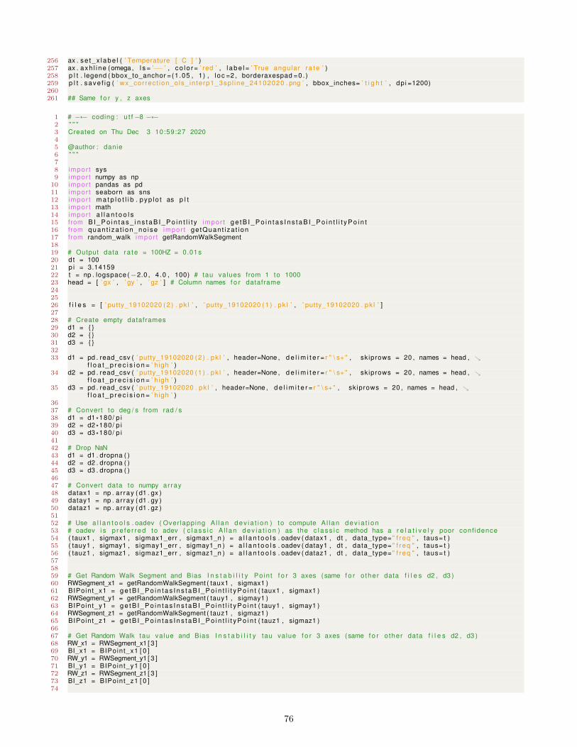
256 ax . se t_x labe l ( ’ Temperature [ C ] ’ )257 ax . axh l i ne (omega , l s = ’−− ’ , co l o r = ’ red ’ , l a b e l = ’ True angular ra te ’ )258 p l t . legend ( bbox_to_anchor =(1 .05 , 1) , l oc =2 , borderaxespad =0 . )259 p l t . save f ig ( ’ wx_correct ion_ols_ in terp1_3spl ine_24102020 . png ’ , bbox_inches= ’ t i g h t ’ , dp i =1200)260261 ## Same f o r y , z axes
1 # −*− coding : u t f−8 −*−2 " " "3 Created on Thu Dec 3 10:59:27 202045 @author : danie6 " " "78 impor t sys9 impor t numpy as np
10 impor t pandas as pd11 impor t seaborn as sns12 impor t m a t p l o t l i b . pyp lo t as p l t13 impor t math14 impor t a l l a n t o o l s15 from B I _ P o i n t a s _ i n s t a B I _ P o i n t l i t y impor t g e t B I _ P o i n t a s I n s t a B I _ P o i n t l i t y P o i n t16 from quan t i za t i on_no ise impor t ge tQuant i za t ion17 from random_walk impor t getRandomWalkSegment1819 # Output data ra te = 100HZ = 0.01 s20 dt = 10021 p i = 3.1415922 t = np . logspace (−2.0 , 4 .0 , 100) # tau values from 1 to 100023 head = [ ’ gx ’ , ’ gy ’ , ’ gz ’ ] # Column names f o r dataframe242526 f i l e s = [ ’ putty_19102020 ( 2 ) . pk l ’ , ’ putty_19102020 ( 1 ) . pk l ’ , ’ putty_19102020 . pk l ’ ]2728 # Create empty dataframes29 d1 = 30 d2 = 31 d3 = 3233 d1 = pd . read_csv ( ’ putty_19102020 ( 2 ) . pk l ’ , header=None , d e l i m i t e r = r " \ s+ " , skiprows = 20 , names = head ,
f l o a t _ p r e c i s i o n = ’ high ’ )34 d2 = pd . read_csv ( ’ putty_19102020 ( 1 ) . pk l ’ , header=None , d e l i m i t e r = r " \ s+ " , skiprows = 20 , names = head ,
f l o a t _ p r e c i s i o n = ’ high ’ )35 d3 = pd . read_csv ( ’ putty_19102020 . pk l ’ , header=None , d e l i m i t e r = r " \ s+ " , skiprows = 20 , names = head ,
f l o a t _ p r e c i s i o n = ’ high ’ )3637 # Convert to deg / s from rad / s38 d1 = d1 *180/ p i39 d2 = d2 *180/ p i40 d3 = d3 *180/ p i4142 # Drop NaN43 d1 = d1 . dropna ( )44 d2 = d2 . dropna ( )45 d3 = d3 . dropna ( )4647 # Convert data to numpy ar ray48 datax1 = np . ar ray ( d1 . gx )49 datay1 = np . ar ray ( d1 . gy )50 dataz1 = np . ar ray ( d1 . gz )5152 # Use a l l a n t o o l s . oadev ( Over lapping A l lan d e v i a t i o n ) to compute A l lan de v i a t i o n53 # oadev i s p re fe r red to adev ( c l a s s i c A l l an d e v i a t i o n ) as the c l a s s i c method has a r e l a t i v e l y poor conf idence54 ( taux1 , sigmax1 , sigmax1_err , sigmax1_n ) = a l l a n t o o l s . oadev ( datax1 , dt , data_type=" f r eq " , taus= t )55 ( tauy1 , sigmay1 , sigmay1_err , sigmay1_n ) = a l l a n t o o l s . oadev ( datay1 , dt , data_type=" f r eq " , taus= t )56 ( tauz1 , sigmaz1 , sigmaz1_err , sigmaz1_n ) = a l l a n t o o l s . oadev ( dataz1 , dt , data_type=" f r eq " , taus= t )575859 # Get Random Walk Segment and Bias I n s t a b i l i t y Po in t f o r 3 axes (same f o r o ther data f i l e s d2 , d3 )60 RWSegment_x1 = getRandomWalkSegment ( taux1 , sigmax1 )61 BIPoint_x1 = g e t B I _ P o i n t a s I n s t a B I _ P o i n t l i t y P o i n t ( taux1 , sigmax1 )62 RWSegment_y1 = getRandomWalkSegment ( tauy1 , sigmay1 )63 BIPoint_y1 = g e t B I _ P o i n t a s I n s t a B I _ P o i n t l i t y P o i n t ( tauy1 , sigmay1 )64 RWSegment_z1 = getRandomWalkSegment ( tauz1 , sigmaz1 )65 BIPoint_z1 = g e t B I _ P o i n t a s I n s t a B I _ P o i n t l i t y P o i n t ( tauz1 , sigmaz1 )6667 # Get Random Walk tau value and Bias I n s t a b i l i t y tau value f o r 3 axes (same f o r o ther data f i l e s d2 , d3 )68 RW_x1 = RWSegment_x1 [ 3 ]69 BI_x1 = BIPoint_x1 [ 0 ]70 RW_y1 = RWSegment_y1 [ 3 ]71 BI_y1 = BIPoint_y1 [ 0 ]72 RW_z1 = RWSegment_z1 [ 3 ]73 BI_z1 = BIPoint_z1 [ 0 ]74
76
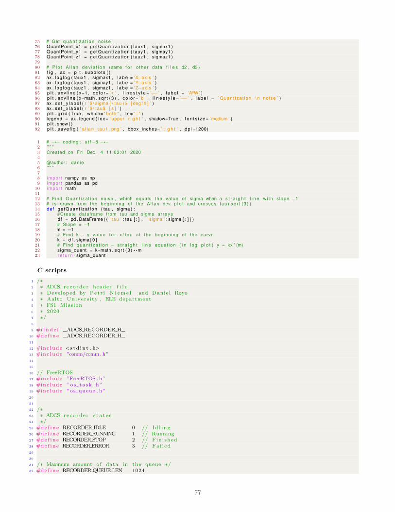
75 # Get quan t i za t i on noise76 QuantPoint_x1 = ge tQuant i za t ion ( taux1 , sigmax1 )77 QuantPoint_y1 = ge tQuant i za t ion ( tauy1 , sigmay1 )78 QuantPoint_z1 = ge tQuant i za t ion ( tauz1 , sigmaz1 )7980 # P lo t A l l an d e v i a t i on (same f o r o ther data f i l e s d2 , d3 )81 f i g , ax = p l t . subp lo ts ( )82 ax . l og log ( taux1 , sigmax1 , l a b e l = ’X−ax is ’ )83 ax . l og log ( tauy1 , sigmay1 , l a b e l = ’Y−ax is ’ )84 ax . l og log ( tauz1 , sigmaz1 , l a b e l = ’Z−ax is ’ )85 p l t . axv l i ne ( x=1 , co l o r = ’ r ’ , l i n e s t y l e = ’−− ’ , l a b e l = ’ARW’ )86 p l t . axv l i ne ( x=math . s q r t ( 3 ) , co l o r = ’ b ’ , l i n e s t y l e = ’−− ’ , l a b e l = ’ Quant iza t ion \ n noise ’ )87 ax . se t_y labe l ( r ’ $ \ sigma ( \ tau ) $ [ deg / h ] ’ )88 ax . se t_x labe l ( r ’ $ \ tau$ [ s ] ’ )89 p l t . g r i d ( True , which=" both " , l s = "−" )90 legend = ax . legend ( loc= ’ upper r i g h t ’ , shadow=True , f o n t s i z e = ’medium ’ )91 p l t . show ( )92 p l t . save f ig ( ’ a l l an_ tau1 . png ’ , bbox_inches= ’ t i g h t ’ , dp i =1200)
1 # −*− coding : u t f−8 −*−2 " " "3 Created on F r i Dec 4 11:03:01 202045 @author : danie6 " " "78 impor t numpy as np9 impor t pandas as pd
10 impor t math1112 # Find Quant iza t ion noise , which equals the value o f sigma when a s t r a i g h t l i n e w i th slope −113 # i s drawn from the beginning o f the A l lan dev p l o t and crosses tau ( s q r t ( 3 ) )14 def ge tQuant i za t ion ( tau , sigma ) :15 #Create dataframe from tau and sigma arrays16 df = pd . DataFrame ( ’ tau ’ : tau [ : ] , ’ sigma ’ : sigma [ : ] )17 # Slope = −118 m = −119 # Find k − y value f o r x / tau a t the beginning o f the curve20 k = df . sigma [ 0 ]21 # Find quan t i za t i on − s t r a i g h t l i n e equat ion ( i n log p l o t ) y = kx ^ (m)22 sigma_quant = k * math . s q r t ( 3 ) * *m23 r e t u r n sigma_quant
C scripts
1 /∗2 ∗ ADCS reco rde r header f i l e3 ∗ Developed by Pet r i N i em e l and Danie l Royo4 ∗ Aalto Univers i ty , ELE department5 ∗ FS1 Miss ion6 ∗ 20207 ∗/8
9 #i f n d e f ADCS RECORDER H10 #de f i n e ADCS RECORDER H11
12 #inc lude <s t d i n t . h>13 #inc lude ”comm/comm. h”14
15
16 // FreeRTOS17 #inc lude ”FreeRTOS . h”18 #inc lude ”o s t a sk . h”19 #inc lude ”os queue . h”20
21
22 /∗23 ∗ ADCS reco rde r s t a t e s24 ∗/25 #de f i n e RECORDER IDLE 0 // I d l i n g26 #de f i n e RECORDERRUNNING 1 // Running27 #de f i n e RECORDER STOP 2 // Fin i shed28 #de f i n e RECORDERERROR 3 // Fa i l ed29
30
31 /∗ Maximum amount o f data in the queue ∗/32 #de f i n e RECORDERQUEUE LEN 1024
77
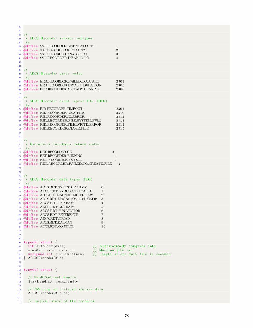
33
34
35 /∗36 ∗ ADCS Recorder s e r v i c e subtypes37 ∗/38 #de f i n e SST RECORDER GET STATUS TC 139 #de f i n e SST RECORDER STATUS TM 240 #de f i n e SST RECORDER ENABLE TC 341 #de f i n e SST RECORDER DISABLE TC 442
43
44 /∗45 ∗ ADCS Recorder e r r o r codes46 ∗/47 #de f i n e ERR RECORDER FAILED TO START 230148 #de f i n e ERR RECORDER INVALID DURATION 230549 #de f i n e ERR RECORDER ALREADYRUNNING 230850
51 /∗52 ∗ ADCS Recorder event r epor t IDs (RIDs )53 ∗/54 #de f i n e RID RECORDER TIMEOUT 230155 #de f i n e RID RECORDER NEW FILE 231056 #de f i n e RID RECORDER IO ERROR 231257 #de f i n e RID RECORDER FILE SYSTEM FULL 231358 #de f i n e RID RECORDER FILE WRITE ERROR 231459 #de f i n e RID RECORDER CLOSE FILE 231560
61
62 /∗63 ∗ Recorder ’ s f unc t i on s re turn codes64 ∗/65 #de f i n e RET RECORDEROK 066 #de f i n e RET RECORDER RUNNING −167 #de f i n e RET RECORDER FS FULL −168 #de f i n e RET RECORDER FAILED TO CREATE FILE −269
70
71 /∗72 ∗ ADCS Recorder data types (RDT)73 ∗/74 #de f i n e ADCS RDTGYROSCOPERAW 075 #de f i n e ADCS RDT GYROSCOPE CALIB 176 #de f i n e ADCSRDTMAGNETOMETERRAW 277 #de f i n e ADCS RDTMAGNETOMETER CALIB 378 #de f i n e ADCS RDT PSD RAW 479 #de f i n e ADCS RDT DSS RAW 580 #de f i n e ADCS RDT SUN VECTOR 681 #de f i n e ADCS RDT REFERENCE 782 #de f i n e ADCS RDT TRIAD 883 #de f i n e ADCS RDTKALMAN 984 #de f i n e ADCS RDT CONTROL 1085
86
87
88 typede f s t r u c t 89 i n t auto compress ; // Automatica l ly compress data90 u in t32 t max f i l e s i z e ; // Maximum f i l e s i z e91 unsigned i n t f i l e d u r a t i o n ; // Length o f one data f i l e in seconds92 ADCSRecorderCS t ;93
94
95 typede f s t r u c t 96
97 // FreeRTOS task handle98 TaskHandle t ta sk hand le ;99
100 // RAM copy o f c r i t i c a l s t o rage data101 ADCSRecorderCS t cs ;102
103 // Log i ca l s t a t e o f the r e co rde r
78
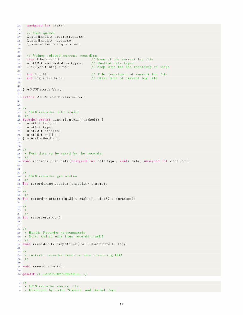
104 unsigned i n t s t a t e ;105
106 // Data queues107 QueueHandle t r eco rde r queue ;108 QueueHandle t tc queue ;109 QueueSetHandle t queue se t ;110
111
112 // Values r e l a t e d cur rent r e co rd ing113 char f i l ename [ 1 3 ] ; // Name o f the cur rent l og f i l e114 u in t32 t enab l ed data types ; // Enabled data types115 TickType t s top t ime ; // Stop time f o r the r e co rd ing in t i c k s116
117 i n t l o g f d ; // F i l e d e s c r i p t o r o f cur r ent l og f i l e118 i n t l o g s t a r t t im e ; // Star t time o f cur r ent l og f i l e119
120
121 ADCSRecorderVars t ;122
123 extern ADCSRecorderVars t∗ r e c ;124
125
126 /∗127 ∗ ADCS reco rde r f i l e header128 ∗/129 typede f s t r u c t a t t r i b u t e ( ( packed ) ) 130 u in t 8 t l ength ;131 u in t 8 t type ;132 u in t32 t seconds ;133 u in t16 t m i l l i s ;134 ADCSLogHeader t ;135
136
137 /∗138 ∗ Push data to be saved by the r e co rde r139 ∗/140 void reco rde r push data ( unsigned i n t data type , void ∗ data , unsigned i n t data l en ) ;141
142
143 /∗144 ∗ ADCS reco rde r get s t a tu s145 ∗/146 i n t r e c o r d e r g e t s t a t u s ( u in t16 t ∗ s t a tu s ) ;147
148 /∗149 ∗/150 i n t r e c o r d e r s t a r t ( u in t 32 t enabled , u in t 32 t durat ion ) ;151
152 /∗153 ∗154 ∗/155 i n t r e c o rd e r s t op ( ) ;156
157
158 /∗159 ∗ Handle Recorder telecommands160 ∗ Note : Cal l ed only from r e c o rd e r t a s k !161 ∗/162 void r e c o r d e r t c d i s p a t c h e r (PUS Telecommand t∗ tc ) ;163
164 /∗165 ∗ I n i t i a t e r e co rde r func t i on when i n i t i a t i n g OBC166 ∗/167
168 void r e c o r d e r i n i t ( ) ;169
170 #end i f /∗ ADCS RECORDER H ∗/
1 /∗2 ∗ ADCS reco rde r source f i l e3 ∗ Developed by Pet r i N i em e l and Danie l Royo
79
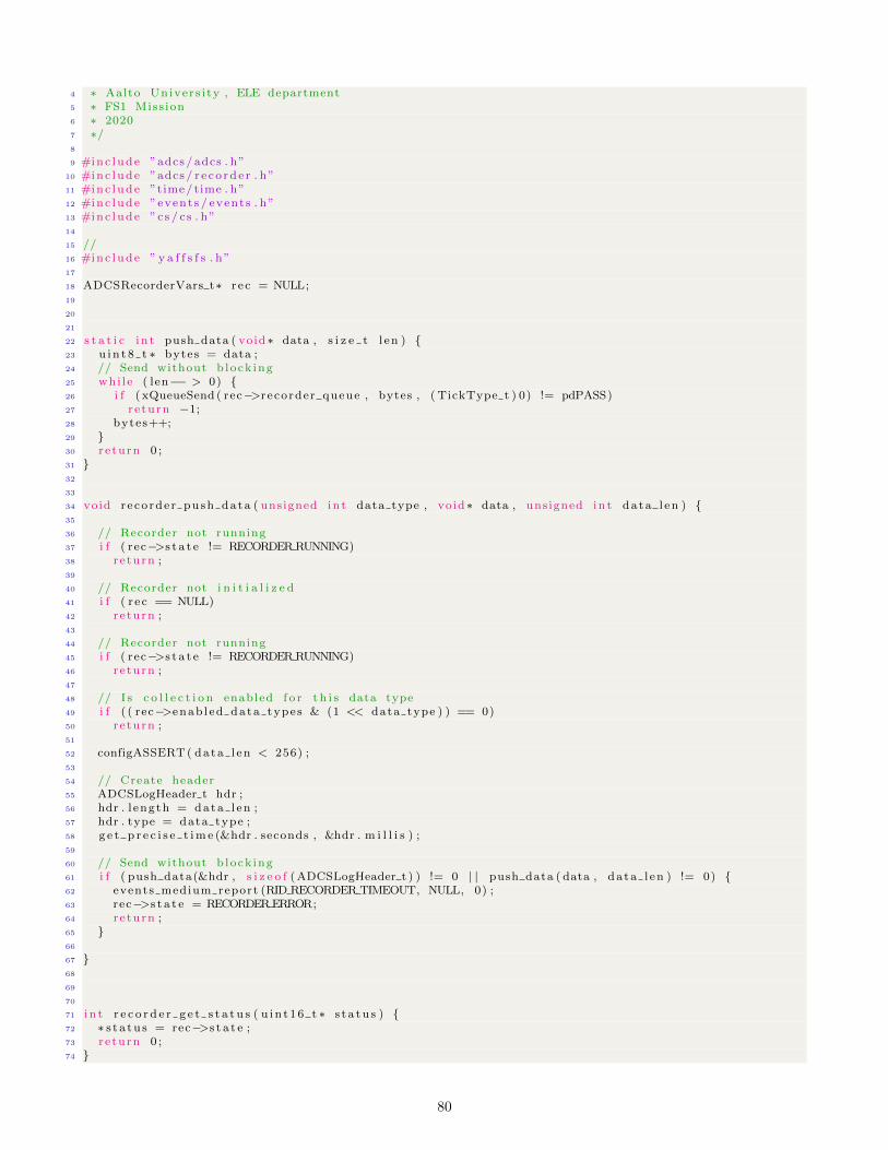
4 ∗ Aalto Univers i ty , ELE department5 ∗ FS1 Miss ion6 ∗ 20207 ∗/8
9 #inc lude ”adcs / adcs . h”10 #inc lude ”adcs / r e co rde r . h”11 #inc lude ”time/ time . h”12 #inc lude ”events / events . h”13 #inc lude ”cs / cs . h”14
15 //16 #inc lude ” y a f f s f s . h”17
18 ADCSRecorderVars t∗ r e c = NULL;19
20
21
22 s t a t i c i n t push data ( void ∗ data , s i z e t l en ) 23 u in t 8 t ∗ bytes = data ;24 // Send without b lock ing25 whi le ( len−− > 0) 26 i f ( xQueueSend ( rec−>recorder queue , bytes , ( TickType t ) 0) != pdPASS)27 r e turn −1;28 bytes++;29 30 r e turn 0 ;31 32
33
34 void reco rde r push data ( unsigned i n t data type , void ∗ data , unsigned i n t data l en ) 35
36 // Recorder not running37 i f ( rec−>s t a t e != RECORDERRUNNING)38 r e turn ;39
40 // Recorder not i n i t i a l i z e d41 i f ( r e c == NULL)42 r e turn ;43
44 // Recorder not running45 i f ( rec−>s t a t e != RECORDERRUNNING)46 r e turn ;47
48 // I s c o l l e c t i o n enabled f o r t h i s data type49 i f ( ( rec−>enab l ed data types & (1 << data type ) ) == 0)50 r e turn ;51
52 configASSERT( data l en < 256) ;53
54 // Create header55 ADCSLogHeader t hdr ;56 hdr . l ength = data l en ;57 hdr . type = data type ;58 g e t p r e c i s e t ime (&hdr . seconds , &hdr . m i l l i s ) ;59
60 // Send without b lock ing61 i f ( push data(&hdr , s i z e o f (ADCSLogHeader t ) ) != 0 | | push data ( data , da ta l en ) != 0) 62 events medium report (RID RECORDER TIMEOUT, NULL, 0) ;63 rec−>s t a t e = RECORDERERROR;64 r e turn ;65 66
67 68
69
70
71 i n t r e c o r d e r g e t s t a t u s ( u in t16 t ∗ s t a tu s ) 72 ∗ s t a tu s = rec−>s t a t e ;73 r e turn 0 ;74
80
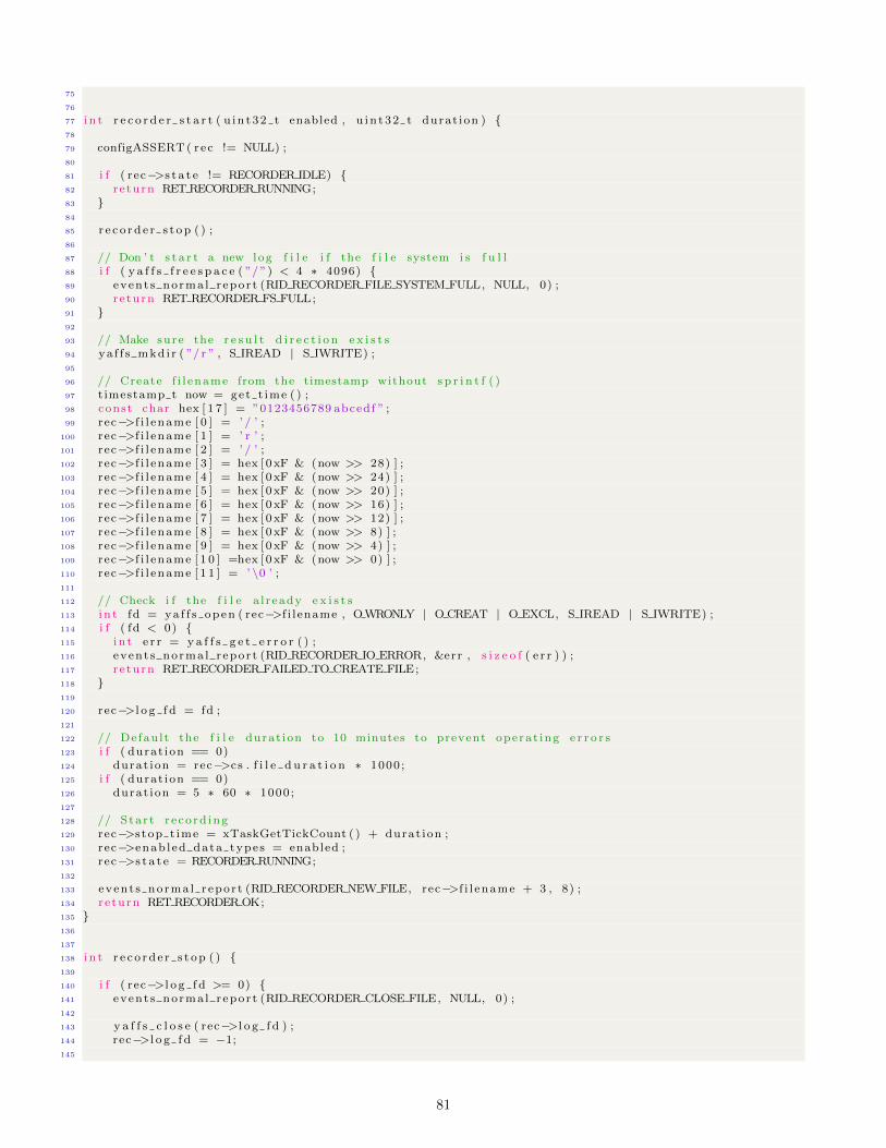
75
76
77 i n t r e c o r d e r s t a r t ( u in t 32 t enabled , u in t 32 t durat ion ) 78
79 configASSERT( rec != NULL) ;80
81 i f ( rec−>s t a t e != RECORDER IDLE) 82 r e turn RET RECORDER RUNNING;83 84
85 r e c o rd e r s t op ( ) ;86
87 // Don ’ t s t a r t a new log f i l e i f the f i l e system i s f u l l88 i f ( y a f f s f r e e s p a c e ( ”/ ”) < 4 ∗ 4096) 89 event s norma l r epor t (RID RECORDER FILE SYSTEM FULL, NULL, 0) ;90 r e turn RET RECORDER FS FULL;91 92
93 // Make sure the r e s u l t d i r e c t i o n e x i s t s94 ya f f s mkd i r ( ”/ r ” , S IREAD | S IWRITE) ;95
96 // Create f i l ename from the timestamp without s p r i n t f ( )97 t imestamp t now = get t ime ( ) ;98 const char hex [ 1 7 ] = ”0123456789 abcedf ” ;99 rec−>f i l ename [ 0 ] = ’ / ’ ;
100 rec−>f i l ename [ 1 ] = ’ r ’ ;101 rec−>f i l ename [ 2 ] = ’ / ’ ;102 rec−>f i l ename [ 3 ] = hex [ 0 xF & (now >> 28) ] ;103 rec−>f i l ename [ 4 ] = hex [ 0 xF & (now >> 24) ] ;104 rec−>f i l ename [ 5 ] = hex [ 0 xF & (now >> 20) ] ;105 rec−>f i l ename [ 6 ] = hex [ 0 xF & (now >> 16) ] ;106 rec−>f i l ename [ 7 ] = hex [ 0 xF & (now >> 12) ] ;107 rec−>f i l ename [ 8 ] = hex [ 0 xF & (now >> 8) ] ;108 rec−>f i l ename [ 9 ] = hex [ 0 xF & (now >> 4) ] ;109 rec−>f i l ename [ 1 0 ] =hex [ 0 xF & (now >> 0) ] ;110 rec−>f i l ename [ 1 1 ] = ’ \0 ’ ;111
112 // Check i f the f i l e a l r eady e x i s t s113 i n t fd = ya f f s open ( rec−>f i l ename , OWRONLY | O CREAT | O EXCL, S IREAD | S IWRITE) ;114 i f ( fd < 0) 115 i n t e r r = y a f f s g e t e r r o r ( ) ;116 event s norma l r epor t (RID RECORDER IO ERROR, &err , s i z e o f ( e r r ) ) ;117 r e turn RET RECORDER FAILED TO CREATE FILE;118 119
120 rec−>l o g f d = fd ;121
122 // Defau l t the f i l e durat ion to 10 minutes to prevent operat ing e r r o r s123 i f ( durat ion == 0)124 durat ion = rec−>cs . f i l e d u r a t i o n ∗ 1000 ;125 i f ( durat ion == 0)126 durat ion = 5 ∗ 60 ∗ 1000 ;127
128 // Star t r e co rd ing129 rec−>s top t ime = xTaskGetTickCount ( ) + durat ion ;130 rec−>enab l ed data types = enabled ;131 rec−>s t a t e = RECORDERRUNNING;132
133 event s norma l r epor t (RID RECORDER NEW FILE, rec−>f i l ename + 3 , 8) ;134 r e turn RET RECORDEROK;135 136
137
138 i n t r e c o rd e r s t op ( ) 139
140 i f ( rec−>l o g f d >= 0) 141 event s norma l r epor t (RID RECORDER CLOSE FILE, NULL, 0) ;142
143 y a f f s c l o s e ( rec−>l o g f d ) ;144 rec−>l o g f d = −1;145
81
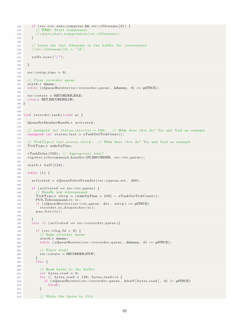
146 i f ( rec−>cs . auto compress && rec−>f i l ename [ 0 ] ) 147 // TODO: Star t compressor148 // cmprs s ta r t compres s i on ( rec−>f i l ename ) ;149 150
151 // Leave the l a s t f i l ename to the bu f f e r f o r convenience152 // rec−>f i l ename [ 0 ] = ’\0 ’ ;153
154 ya f f s s yn c ( ”/ ”) ;155
156 157
158 rec−>s top t ime = 0 ;159
160 // Clear r e co rde r queue161 u in t 8 t dummy;162 whi le ( xQueueReceive ( rec−>recorder queue , &dummy, 0) == pdTRUE) ;163
164 rec−>s t a t e = RECORDER IDLE;165 r e turn RET RECORDEROK;166 167
168
169 void r e c o rd e r t a s k ( void ∗ a ) 170
171 QueueSetMemberHandle t a c t i va t ed ;172
173 // unsigned i n t s t a t u s i n t e r v a l = 500 ; // What does t h i s do? Try and f i nd an example174 unsigned i n t s t a t u s l a s t = xTaskGetTickCount ( ) ;175
176 // TickType t l a s t s t a t u s c h e c k ; // What does t h i s do? Try and f i nd an example177 TickType t wakeUpTime ;178
179 vTaskDelay (500) ; // Appropriate time ?180 r eg i s t e r t e l e command hand l e r (ST RECORDER, rec−>tc queue ) ;181
182 u in t 8 t bu f f [ 1 2 8 ] ;183
184 whi le (1 ) 185
186 ac t i va t ed = xQueueSelectFromSet ( rec−>queue set , 200) ;187
188 i f ( a c t i va t ed == rec−>tc queue ) 189 // Handle new telecommand190 TickType t s l e e p = (wakeUpTime + 250) − xTaskGetTickCount ( ) ;191 PUS Telecommand t∗ tc ;192 i f ( xQueueReceive ( rec−>tc queue , &tc , s l e e p ) == pdTRUE)193 r e c o r d e r t c d i s p a t c h e r ( tc ) ;194 pu s f r e e ( tc ) ;195
196 197 e l s e i f ( a c t i va t ed == rec−>r eco rde r queue ) 198
199 i f ( rec−>l o g f d < 0) 200 // Some re co rde r queue201 u in t 8 t dummy;202 whi le ( xQueueReceive ( rec−>recorder queue , &dummy, 0) == pdTRUE) ;203
204 // Force stop !205 rec−>s t a t e = RECORDER STOP;206 207 e l s e 208
209 // Read bytes to the bu f f e r210 i n t byte s r ead = 0 ;211 f o r ( ; byte s r ead < 128 ; byte s r ead++) 212 i f ( xQueueReceive ( rec−>recorder queue , &bu f f [ byte s r ead ] , 0) != pdTRUE)213 break ;214 215
216 // Write the bytes to f i l e
82
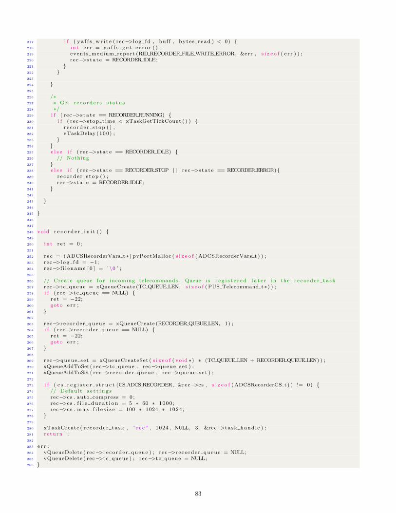
217 i f ( y a f f s w r i t e ( rec−>l o g fd , buf f , byte s r ead ) < 0) 218 i n t e r r = y a f f s g e t e r r o r ( ) ;219 events medium report (RID RECORDER FILE WRITE ERROR, &err , s i z e o f ( e r r ) ) ;220 rec−>s t a t e = RECORDER IDLE;221 222 223
224 225
226 /∗227 ∗ Get r e c o rd e r s s t a tu s228 ∗/229 i f ( rec−>s t a t e == RECORDERRUNNING) 230 i f ( rec−>s top t ime < xTaskGetTickCount ( ) ) 231 r e c o rd e r s t op ( ) ;232 vTaskDelay (100) ;233 234 235 e l s e i f ( rec−>s t a t e == RECORDER IDLE) 236 // Nothing237 238 e l s e i f ( rec−>s t a t e == RECORDER STOP | | rec−>s t a t e == RECORDERERROR) 239 r e c o rd e r s t op ( ) ;240 rec−>s t a t e = RECORDER IDLE;241 242
243 244
245 246
247
248 void r e c o r d e r i n i t ( ) 249
250 i n t r e t = 0 ;251
252 r e c = (ADCSRecorderVars t ∗) pvPortMalloc ( s i z e o f ( ADCSRecorderVars t ) ) ;253 rec−>l o g f d = −1;254 rec−>f i l ename [ 0 ] = ’ \0 ’ ;255
256 // Create queue f o r incoming telecommands . Queue i s r e g i s t e r e d l a t e r in the r e c o rd e r t a s k257 rec−>tc queue = xQueueCreate (TC QUEUE LEN, s i z e o f (PUS Telecommand t ∗) ) ;258 i f ( rec−>tc queue == NULL) 259 r e t = −22;260 goto e r r ;261 262
263 rec−>r eco rde r queue = xQueueCreate (RECORDER QUEUE LEN, 1) ;264 i f ( rec−>r eco rde r queue == NULL) 265 r e t = −22;266 goto e r r ;267 268
269 rec−>queue se t = xQueueCreateSet ( s i z e o f ( void ∗) ∗ (TC QUEUE LEN + RECORDERQUEUE LEN) ) ;270 xQueueAddToSet ( rec−>tc queue , rec−>queue se t ) ;271 xQueueAddToSet ( rec−>recorder queue , rec−>queue se t ) ;272
273 i f ( c s r e g i s t e r s t r u c t (CS ADCS RECORDER, &rec−>cs , s i z e o f (ADCSRecorderCS t ) ) != 0) 274 // Defau l t s e t t i n g s275 rec−>cs . auto compress = 0 ;276 rec−>cs . f i l e d u r a t i o n = 5 ∗ 60 ∗ 1000 ;277 rec−>cs . max f i l e s i z e = 100 ∗ 1024 ∗ 1024 ;278 279
280 xTaskCreate ( r e co rde r t a sk , ”r ec ” , 1024 , NULL, 3 , &rec−>ta sk hand le ) ;281 r e turn ;282
283 e r r :284 vQueueDelete ( rec−>r eco rde r queue ) ; rec−>r eco rde r queue = NULL;285 vQueueDelete ( rec−>tc queue ) ; rec−>tc queue = NULL;286
83
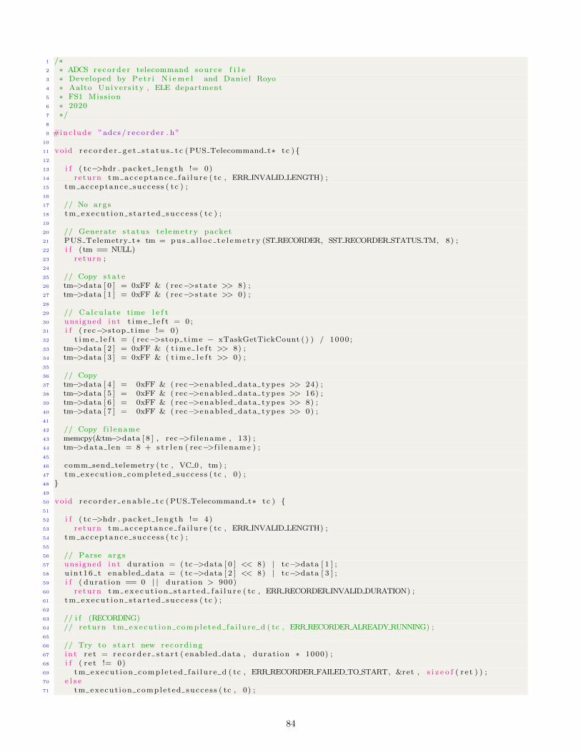
1 /∗2 ∗ ADCS reco rde r telecommand source f i l e3 ∗ Developed by Pet r i N i em e l and Danie l Royo4 ∗ Aalto Univers i ty , ELE department5 ∗ FS1 Miss ion6 ∗ 20207 ∗/8
9 #inc lude ”adcs / r e co rde r . h”10
11 void r e c o r d e r g e t s t a t u s t c (PUS Telecommand t∗ tc ) 12
13 i f ( tc−>hdr . packe t l eng th != 0)14 r e turn tm ac c ep t anc e f a i l u r e ( tc , ERR INVALID LENGTH) ;15 tm acceptance succe s s ( tc ) ;16
17 // No args18 tm exe cu t i on s t a r t ed su c c e s s ( tc ) ;19
20 // Generate s t a tu s te l emetry packet21 PUS Telemetry t∗ tm = pu s a l l o c t e l eme t r y (ST RECORDER, SST RECORDER STATUS TM, 8) ;22 i f (tm == NULL)23 r e turn ;24
25 // Copy s t a t e26 tm−>data [ 0 ] = 0xFF & ( rec−>s t a t e >> 8) ;27 tm−>data [ 1 ] = 0xFF & ( rec−>s t a t e >> 0) ;28
29 // Ca lcu la te time l e f t30 unsigned i n t t im e l e f t = 0 ;31 i f ( rec−>s top t ime != 0)32 t im e l e f t = ( rec−>s top t ime − xTaskGetTickCount ( ) ) / 1000 ;33 tm−>data [ 2 ] = 0xFF & ( t im e l e f t >> 8) ;34 tm−>data [ 3 ] = 0xFF & ( t im e l e f t >> 0) ;35
36 // Copy37 tm−>data [ 4 ] = 0xFF & ( rec−>enab l ed data types >> 24) ;38 tm−>data [ 5 ] = 0xFF & ( rec−>enab l ed data types >> 16) ;39 tm−>data [ 6 ] = 0xFF & ( rec−>enab l ed data types >> 8) ;40 tm−>data [ 7 ] = 0xFF & ( rec−>enab l ed data types >> 0) ;41
42 // Copy f i l ename43 memcpy(&tm−>data [ 8 ] , rec−>f i l ename , 13) ;44 tm−>data l en = 8 + s t r l e n ( rec−>f i l ename ) ;45
46 comm send telemetry ( tc , VC 0 , tm) ;47 tm execut ion comple ted succe s s ( tc , 0) ;48 49
50 void r e c o r d e r e n ab l e t c (PUS Telecommand t∗ tc ) 51
52 i f ( tc−>hdr . packe t l eng th != 4)53 r e turn tm ac c ep t anc e f a i l u r e ( tc , ERR INVALID LENGTH) ;54 tm acceptance succe s s ( tc ) ;55
56 // Parse args57 unsigned i n t durat ion = ( tc−>data [ 0 ] << 8) | tc−>data [ 1 ] ;58 u in t16 t enabled data = ( tc−>data [ 2 ] << 8) | tc−>data [ 3 ] ;59 i f ( durat ion == 0 | | durat ion > 900)60 r e turn tm ex e c u t i o n s t a r t e d f a i l u r e ( tc , ERR RECORDER INVALID DURATION) ;61 tm exe cu t i on s t a r t ed su c c e s s ( tc ) ;62
63 // i f (RECORDING)64 // re turn tm execu t i on comp l e t ed f a i l u r e d ( tc , ERR RECORDER ALREADYRUNNING) ;65
66 // Try to s t a r t new reco rd ing67 i n t r e t = r e c o r d e r s t a r t ( enabled data , durat ion ∗ 1000) ;68 i f ( r e t != 0)69 tm execu t i on comp l e t ed f a i l u r e d ( tc , ERR RECORDER FAILED TO START, &ret , s i z e o f ( r e t ) ) ;70 e l s e71 tm execut ion comple ted succe s s ( tc , 0) ;
84
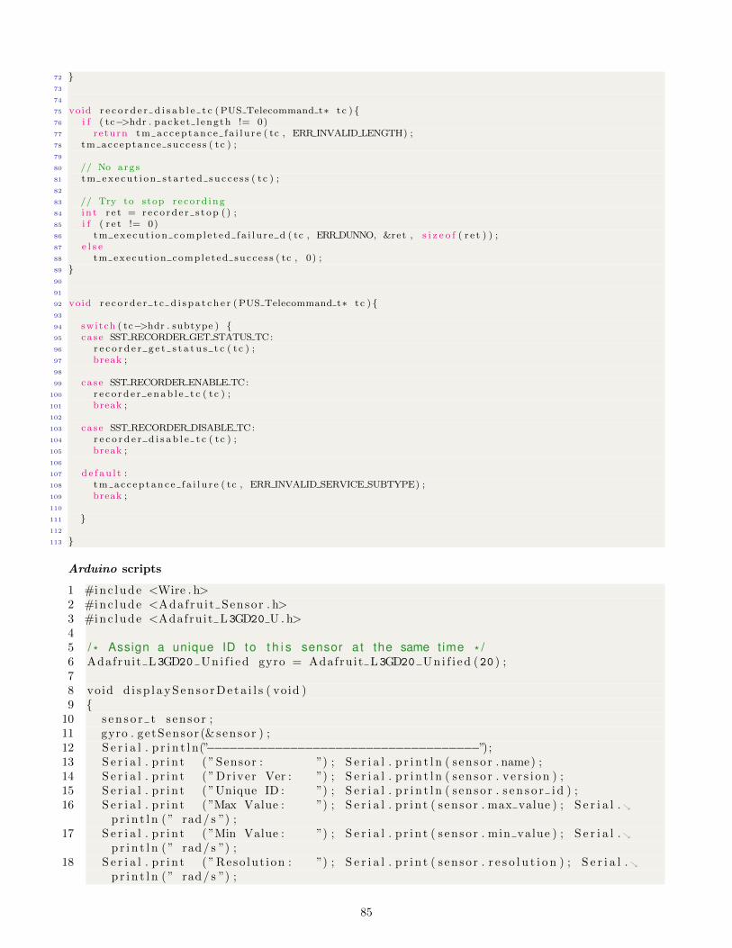
72 73
74
75 void r e c o r d e r d i s a b l e t c (PUS Telecommand t∗ tc ) 76 i f ( tc−>hdr . packe t l eng th != 0)77 r e turn tm ac c ep t anc e f a i l u r e ( tc , ERR INVALID LENGTH) ;78 tm acceptance succe s s ( tc ) ;79
80 // No args81 tm exe cu t i on s t a r t ed su c c e s s ( tc ) ;82
83 // Try to stop re co rd ing84 i n t r e t = r e c o rd e r s t op ( ) ;85 i f ( r e t != 0)86 tm execu t i on comp l e t ed f a i l u r e d ( tc , ERRDUNNO, &ret , s i z e o f ( r e t ) ) ;87 e l s e88 tm execut ion comple ted succe s s ( tc , 0) ;89 90
91
92 void r e c o r d e r t c d i s p a t c h e r (PUS Telecommand t∗ tc ) 93
94 switch ( tc−>hdr . subtype ) 95 case SST RECORDER GET STATUS TC:96 r e c o r d e r g e t s t a t u s t c ( tc ) ;97 break ;98
99 case SST RECORDER ENABLE TC:100 r e c o r d e r e n ab l e t c ( tc ) ;101 break ;102
103 case SST RECORDER DISABLE TC:104 r e c o r d e r d i s a b l e t c ( tc ) ;105 break ;106
107 de f au l t :108 tm ac c ep t anc e f a i l u r e ( tc , ERR INVALID SERVICE SUBTYPE) ;109 break ;110
111 112
113
Arduino scripts
1 #inc lude <Wire . h>2 #inc lude <Adaf ru i t Sensor . h>3 #inc lude <Adafruit L3GD20 U . h>45 / * Assign a unique ID to t h i s sensor a t the same t ime * /6 Adafru it L3GD20 Uni f i ed gyro = Adafruit L3GD20 Uni f i ed (20 ) ;78 void d i s p l a y S e n s o r D e t a i l s ( void )9
10 s e n s o r t s enso r ;11 gyro . getSensor (& senso r ) ;12 S e r i a l . p r i n t l n(”−−−−−−−−−−−−−−−−−−−−−−−−−−−−−−−−−−−−”);13 S e r i a l . p r i n t ( ”Sensor : ”) ; S e r i a l . p r i n t l n ( s enso r . name) ;14 S e r i a l . p r i n t ( ”Driver Ver : ”) ; S e r i a l . p r i n t l n ( s enso r . v e r s i o n ) ;15 S e r i a l . p r i n t ( ”Unique ID : ”) ; S e r i a l . p r i n t l n ( s enso r . s e n s o r i d ) ;16 S e r i a l . p r i n t ( ”Max Value : ”) ; S e r i a l . p r i n t ( s enso r . max value ) ; S e r i a l .
p r i n t l n ( ” rad/ s ”) ;17 S e r i a l . p r i n t ( ”Min Value : ”) ; S e r i a l . p r i n t ( s enso r . min value ) ; S e r i a l .
p r i n t l n ( ” rad/ s ”) ;18 S e r i a l . p r i n t ( ” Reso lut ion : ”) ; S e r i a l . p r i n t ( s enso r . r e s o l u t i o n ) ; S e r i a l .
p r i n t l n ( ” rad/ s ”) ;
85
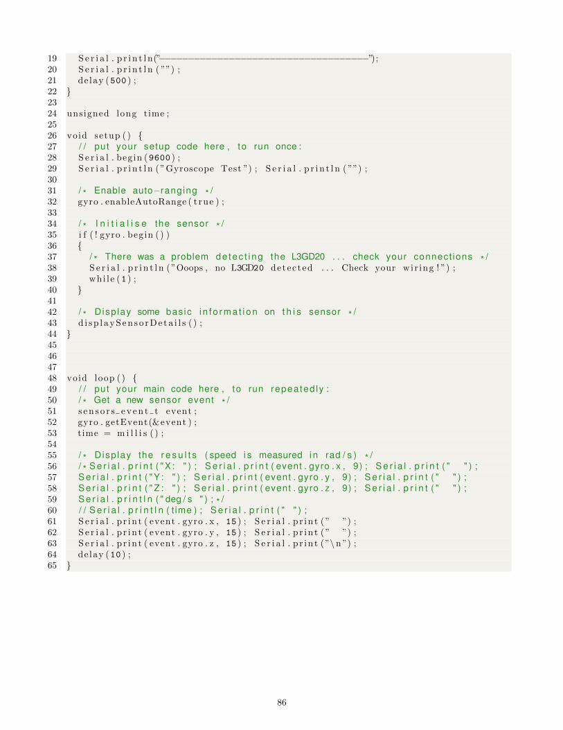
19 S e r i a l . p r i n t l n(”−−−−−−−−−−−−−−−−−−−−−−−−−−−−−−−−−−−−”);20 S e r i a l . p r i n t l n ( ””) ;21 de lay (500 ) ;22 2324 unsigned long time ;2526 void setup ( ) 27 / / put your setup code here , to run once :28 S e r i a l . begin (9600 ) ;29 S e r i a l . p r i n t l n ( ”Gyroscope Test ”) ; S e r i a l . p r i n t l n ( ””) ;3031 / * Enable auto−ranging * /32 gyro . enableAutoRange ( t rue ) ;3334 / * I n i t i a l i s e the sensor * /35 i f ( ! gyro . begin ( ) )36 37 / * There was a problem de tec t i ng the L3GD20 . . . check your connect ions * /38 S e r i a l . p r i n t l n ( ”Ooops , no L3GD20 detec ted . . . Check your wi r ing ! ”) ;39 whi l e (1 ) ;40 4142 / * D isp lay some basic i n f o rma t i on on t h i s sensor * /43 d i s p l a y S e n s o r D e t a i l s ( ) ;44 45464748 void loop ( ) 49 / / put your main code here , to run repeated ly :50 / * Get a new sensor event * /51 s e n s o r s e v e n t t event ;52 gyro . getEvent(&event ) ;53 time = m i l l i s ( ) ;5455 / * D isp lay the r e s u l t s ( speed i s measured i n rad / s ) * /56 / * S e r i a l . p r i n t ( "X : " ) ; S e r i a l . p r i n t ( event . gyro . x , 9) ; S e r i a l . p r i n t ( " " ) ;57 S e r i a l . p r i n t ( "Y : " ) ; S e r i a l . p r i n t ( event . gyro . y , 9) ; S e r i a l . p r i n t ( " " ) ;58 S e r i a l . p r i n t ( " Z : " ) ; S e r i a l . p r i n t ( event . gyro . z , 9) ; S e r i a l . p r i n t ( " " ) ;59 S e r i a l . p r i n t l n ( " deg / s " ) ; * /60 / / S e r i a l . p r i n t l n ( t ime ) ; S e r i a l . p r i n t ( " " ) ;61 S e r i a l . p r i n t ( event . gyro . x , 15 ) ; S e r i a l . p r i n t ( ” ”) ;62 S e r i a l . p r i n t ( event . gyro . y , 15 ) ; S e r i a l . p r i n t ( ” ”) ;63 S e r i a l . p r i n t ( event . gyro . z , 15 ) ; S e r i a l . p r i n t (”\n ”) ;64 de lay (10 ) ;65
86
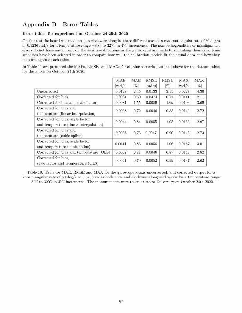
Appendix B Error Tables
Error tables for experiment on October 24-25th 2020
On this test the board was made to spin clockwise along its three different axes at a constant angular rate of 30 deg/sor 0.5236 rad/s for a temperature range −8°C to 32°C in 4°C increments. The non-orthogonalities or misalignmenterrors do not have any impact on the sensitive directions as the gyroscopes are made to spin along their axes. Ninescenarios have been selected in order to compare how well the calibration models fit the actual data and how theymeasure against each other.
In Table 11 are presented the MAEs, RMSEs and MAXs for all nine scenarios outlined above for the dataset takenfor the x-axis on October 24th 2020.
MAE
[rad/s]
MAE
[%]
RMSE
[rad/s]
RMSE
[%]
MAX
[rad/s]
MAX
[%]
Uncorrected 0.0128 2.45 0.0133 2.55 0.0228 4.36
Corrected for bias 0.0031 0.60 0.0374 0.71 0.0111 2.11
Corrected for bias and scale factor 0.0081 1.55 0.0089 1.69 0.0193 3.69
Corrected for bias and
temperature (linear interpolation)0.0038 0.72 0.0046 0.88 0.0143 2.72
Corrected for bias, scale factor
and temperature (linear interpolation)0.0044 0.84 0.0055 1.05 0.0156 2.97
Corrected for bias and
temperature (cubic spline)0.0038 0.73 0.0047 0.90 0.0143 2.73
Corrected for bias, scale factor
and temperature (cubic spline)0.0044 0.85 0.0056 1.06 0.0157 3.01
Corrected for bias and temperature (OLS) 0.0037 0.71 0.0046 0.87 0.0148 2.82
Corrected for bias,
scale factor and temperature (OLS)0.0041 0.79 0.0052 0.99 0.0137 2.62
Table 10: Table for MAE, RMSE and MAX for the gyroscope x-axis uncorrected, and corrected output for aknown angular rate of 30 deg/s or 0.5236 rad/s both anti- and clockwise along said x-axis for a temperature range−8°C to 32°C in 4°C increments. The measurements were taken at Aalto University on October 24th 2020.
87

MAE
[rad/s]
MAE
[%]
RMSE
[rad/s]
RMSE
[%]
MAX
[rad/s]
MAX
[%]
Uncorrected 0.0054 1.02 0.0065 1.25 0.017 3.25
Corrected for bias 0.0112 2.13 0.0127 2.43 0.0255 4.86
Corrected for bias and scale factor 0.0056 1.08 0.0069 1.32 0.0168 3.20
Corrected for bias, and
temperature (linear interpolation)0.0127 2.43 0.0137 2.63 0.0254 4.85
Corrected for bias,
scale factor and temperature (linear interpolation)0.0096 1.83 0.0102 1.95 0.0200 3.83
Corrected for bias, and
temperature (cubic interpolation)0.0127 2.43 0.0138 2.63 0.0255 4.87
Corrected for bias,
scale factor and temperature (cubic interpolation)0.0096 1.84 0.0103 1.97 0.0203 3.88
Corrected for bias, and temperature (OLS) 0.0127 2.43 0.0137 2.61 0.0242 4.62
Corrected for bias,
scale factor and temperature (OLS)0.0097 1.85 0.0103 1.96 0.0195 3.73
Table 11: Table for MAE, RMSE and MAX for the gyroscope x-axis uncorrected, and corrected output for aknown angular rate of -30 deg/s or -0.5236 rad/s both anti- and clockwise along said x-axis for a temperature
range −8°C to 32°C in 4°C increments. The measurements were taken at Aalto University on October 24th 2020.
In Table 13 are presented the MAE, RMSE and MAX for all nine scenarios outlined above for the dataset takenfor the y-axis on October 25th 2020.
MAE
[rad/s]
MAE
[%]
RMSE
[rad/s]
RMSE
[%]
MAX
[rad/s]
MAX
[%]
Uncorrected 0.0090 1.72 0.0110 2.10 0.0322 6.14
Corrected for bias 0.0090 1.71 0.0109 2.09 0.0320 6.12
Corrected for bias and scale factor 0.0105 2.00 0.0138 2.63 0.0439 8.38
Corrected for bias and
temperature (linear interpolation)0.0107 2.05 0.0125 2.39 0.0387 7.38
Corrected for bias, scale factor
and temperature (linear interpolation)0.0087 1.67 0.0115 2.20 0.0046 8.89
Corrected for bias and
temperature (cubic spline)0.0107 2.05 0.0125 2.39 0.0388 7.40
Corrected for bias, scale factor
and temperature (cubic spline)0.0087 1.67 0.0116 2.21 0.0464 8.86
Corrected for bias and temperature (OLS) 0.0104 1.99 0.0123 2.34 0.0389 7.43
Corrected for bias,
scale factor and temperature (OLS)0.0091 1.74 0.0114 2.18 0.046 8.81
Table 12: Table for MAE, RMSE and MAX for the gyroscope y-axis uncorrected, and corrected output for aknown angular rate of 30 deg/s or 0.5236 rad/s both anti- and clockwise along said y-axis for a temperature range−8°C to 32°C in 4°C increments. The measurements were taken at Aalto University on October 24th 2020.
88
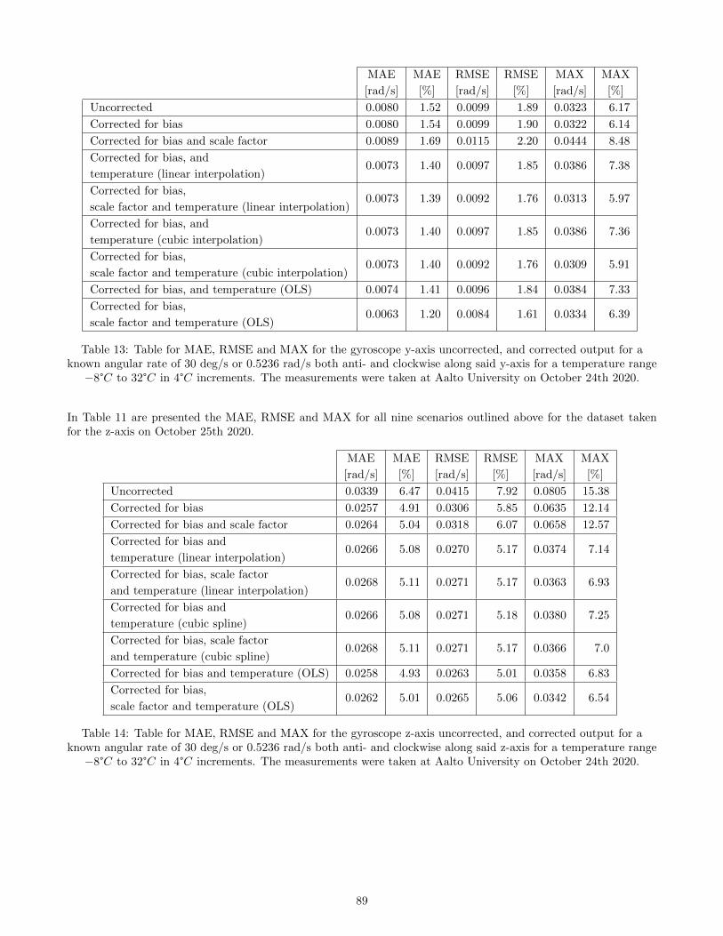
MAE
[rad/s]
MAE
[%]
RMSE
[rad/s]
RMSE
[%]
MAX
[rad/s]
MAX
[%]
Uncorrected 0.0080 1.52 0.0099 1.89 0.0323 6.17
Corrected for bias 0.0080 1.54 0.0099 1.90 0.0322 6.14
Corrected for bias and scale factor 0.0089 1.69 0.0115 2.20 0.0444 8.48
Corrected for bias, and
temperature (linear interpolation)0.0073 1.40 0.0097 1.85 0.0386 7.38
Corrected for bias,
scale factor and temperature (linear interpolation)0.0073 1.39 0.0092 1.76 0.0313 5.97
Corrected for bias, and
temperature (cubic interpolation)0.0073 1.40 0.0097 1.85 0.0386 7.36
Corrected for bias,
scale factor and temperature (cubic interpolation)0.0073 1.40 0.0092 1.76 0.0309 5.91
Corrected for bias, and temperature (OLS) 0.0074 1.41 0.0096 1.84 0.0384 7.33
Corrected for bias,
scale factor and temperature (OLS)0.0063 1.20 0.0084 1.61 0.0334 6.39
Table 13: Table for MAE, RMSE and MAX for the gyroscope y-axis uncorrected, and corrected output for aknown angular rate of 30 deg/s or 0.5236 rad/s both anti- and clockwise along said y-axis for a temperature range−8°C to 32°C in 4°C increments. The measurements were taken at Aalto University on October 24th 2020.
In Table 11 are presented the MAE, RMSE and MAX for all nine scenarios outlined above for the dataset takenfor the z-axis on October 25th 2020.
MAE
[rad/s]
MAE
[%]
RMSE
[rad/s]
RMSE
[%]
MAX
[rad/s]
MAX
[%]
Uncorrected 0.0339 6.47 0.0415 7.92 0.0805 15.38
Corrected for bias 0.0257 4.91 0.0306 5.85 0.0635 12.14
Corrected for bias and scale factor 0.0264 5.04 0.0318 6.07 0.0658 12.57
Corrected for bias and
temperature (linear interpolation)0.0266 5.08 0.0270 5.17 0.0374 7.14
Corrected for bias, scale factor
and temperature (linear interpolation)0.0268 5.11 0.0271 5.17 0.0363 6.93
Corrected for bias and
temperature (cubic spline)0.0266 5.08 0.0271 5.18 0.0380 7.25
Corrected for bias, scale factor
and temperature (cubic spline)0.0268 5.11 0.0271 5.17 0.0366 7.0
Corrected for bias and temperature (OLS) 0.0258 4.93 0.0263 5.01 0.0358 6.83
Corrected for bias,
scale factor and temperature (OLS)0.0262 5.01 0.0265 5.06 0.0342 6.54
Table 14: Table for MAE, RMSE and MAX for the gyroscope z-axis uncorrected, and corrected output for aknown angular rate of 30 deg/s or 0.5236 rad/s both anti- and clockwise along said z-axis for a temperature range−8°C to 32°C in 4°C increments. The measurements were taken at Aalto University on October 24th 2020.
89
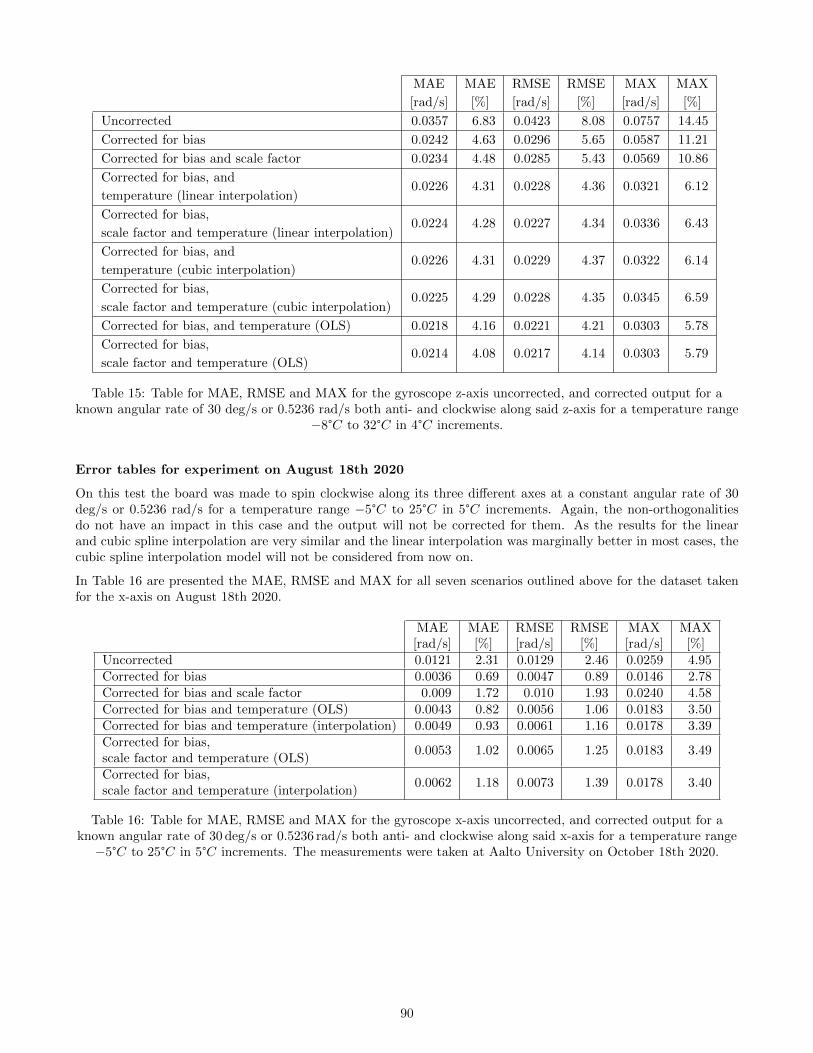
MAE
[rad/s]
MAE
[%]
RMSE
[rad/s]
RMSE
[%]
MAX
[rad/s]
MAX
[%]
Uncorrected 0.0357 6.83 0.0423 8.08 0.0757 14.45
Corrected for bias 0.0242 4.63 0.0296 5.65 0.0587 11.21
Corrected for bias and scale factor 0.0234 4.48 0.0285 5.43 0.0569 10.86
Corrected for bias, and
temperature (linear interpolation)0.0226 4.31 0.0228 4.36 0.0321 6.12
Corrected for bias,
scale factor and temperature (linear interpolation)0.0224 4.28 0.0227 4.34 0.0336 6.43
Corrected for bias, and
temperature (cubic interpolation)0.0226 4.31 0.0229 4.37 0.0322 6.14
Corrected for bias,
scale factor and temperature (cubic interpolation)0.0225 4.29 0.0228 4.35 0.0345 6.59
Corrected for bias, and temperature (OLS) 0.0218 4.16 0.0221 4.21 0.0303 5.78
Corrected for bias,
scale factor and temperature (OLS)0.0214 4.08 0.0217 4.14 0.0303 5.79
Table 15: Table for MAE, RMSE and MAX for the gyroscope z-axis uncorrected, and corrected output for aknown angular rate of 30 deg/s or 0.5236 rad/s both anti- and clockwise along said z-axis for a temperature range
−8°C to 32°C in 4°C increments.
Error tables for experiment on August 18th 2020
On this test the board was made to spin clockwise along its three different axes at a constant angular rate of 30deg/s or 0.5236 rad/s for a temperature range −5°C to 25°C in 5°C increments. Again, the non-orthogonalitiesdo not have an impact in this case and the output will not be corrected for them. As the results for the linearand cubic spline interpolation are very similar and the linear interpolation was marginally better in most cases, thecubic spline interpolation model will not be considered from now on.
In Table 16 are presented the MAE, RMSE and MAX for all seven scenarios outlined above for the dataset takenfor the x-axis on August 18th 2020.
MAE[rad/s]
MAE[%]
RMSE[rad/s]
RMSE[%]
MAX[rad/s]
MAX[%]
Uncorrected 0.0121 2.31 0.0129 2.46 0.0259 4.95Corrected for bias 0.0036 0.69 0.0047 0.89 0.0146 2.78Corrected for bias and scale factor 0.009 1.72 0.010 1.93 0.0240 4.58Corrected for bias and temperature (OLS) 0.0043 0.82 0.0056 1.06 0.0183 3.50Corrected for bias and temperature (interpolation) 0.0049 0.93 0.0061 1.16 0.0178 3.39Corrected for bias,scale factor and temperature (OLS)
0.0053 1.02 0.0065 1.25 0.0183 3.49
Corrected for bias,scale factor and temperature (interpolation)
0.0062 1.18 0.0073 1.39 0.0178 3.40
Table 16: Table for MAE, RMSE and MAX for the gyroscope x-axis uncorrected, and corrected output for aknown angular rate of 30 deg/s or 0.5236 rad/s both anti- and clockwise along said x-axis for a temperature range−5°C to 25°C in 5°C increments. The measurements were taken at Aalto University on October 18th 2020.
90
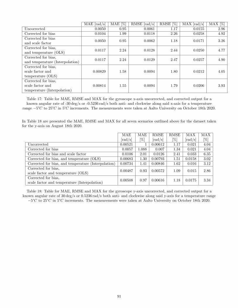
MAE [rad/s] MAE [%] RMSE [rad/s] RMSE [%] MAX [rad/s] MAX [%]Uncorrected 0.0050 0.95 0.0061 1.17 0.0155 2.96Corrected for bias 0.0104 1.99 0.0118 2.26 0.0258 4.92Corrected for biasand scale factor
0.0050 0.95 0.0062 1.18 0.0171 3.26
Corrected for bias,and temperature (OLS)
0.0117 2.24 0.0128 2.44 0.0250 4.77
Corrected for bias,and temperature (Interpolation)
0.0117 2.24 0.0129 2.47 0.0257 4.90
Corrected for bias,scale factor andtemperature (OLS)
0.00829 1.58 0.0094 1.80 0.0212 4.05
Corrected for bias,scale factor andtemperature (Interpolation)
0.00814 1.55 0.0094 1.79 0.0206 3.93
Table 17: Table for MAE, RMSE and MAX for the gyroscope x-axis uncorrected, and corrected output for aknown angular rate of -30 deg/s or -0.5236 rad/s both anti- and clockwise along said x-axis for a temperature
range −5°C to 25°C in 5°C increments. The measurements were taken at Aalto University on October 18th 2020.
In Table 18 are presented the MAE, RMSE and MAX for all seven scenarios outlined above for the dataset takenfor the y-axis on August 18th 2020.
MAE[rad/s]
MAE[%]
RMSE[rad/s]
RMSE[%]
MAX[rad/s]
MAX[%]
Uncorrected 0.00521 1 0.00612 1.17 0.021 4.04Corrected for bias 0.0057 1.088 0.007 1.34 0.021 4.04Corrected for bias and scale factor 0.0106 2.01 0.0126 2.41 0.033 6.35Corrected for bias, and temperature (OLS) 0.00683 1.30 0.00793 1.51 0.0158 3.02Corrected for bias, and temperature (Interpolation) 0.00734 1.41 0.00846 1.62 0.016 3.12Corrected for bias,scale factor and temperature (OLS)
0.00487 0.93 0.00572 1.09 0.015 2.86
Corrected for bias,scale factor and temperature (Interpolation)
0.00508 0.97 0.00616 1.18 0.0175 3.34
Table 18: Table for MAE, RMSE and MAX for the gyroscope y-axis uncorrected, and corrected output for aknown angular rate of 30 deg/s or 0.5236 rad/s both anti- and clockwise along said y-axis for a temperature range−5°C to 25°C in 5°C increments. The measurements were taken at Aalto University on October 18th 2020.
91
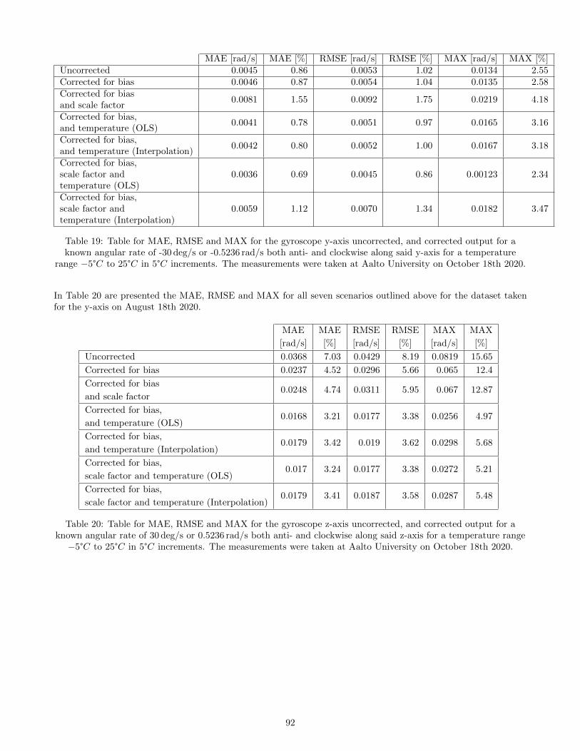
MAE [rad/s] MAE [%] RMSE [rad/s] RMSE [%] MAX [rad/s] MAX [%]Uncorrected 0.0045 0.86 0.0053 1.02 0.0134 2.55Corrected for bias 0.0046 0.87 0.0054 1.04 0.0135 2.58Corrected for biasand scale factor
0.0081 1.55 0.0092 1.75 0.0219 4.18
Corrected for bias,and temperature (OLS)
0.0041 0.78 0.0051 0.97 0.0165 3.16
Corrected for bias,and temperature (Interpolation)
0.0042 0.80 0.0052 1.00 0.0167 3.18
Corrected for bias,scale factor andtemperature (OLS)
0.0036 0.69 0.0045 0.86 0.00123 2.34
Corrected for bias,scale factor andtemperature (Interpolation)
0.0059 1.12 0.0070 1.34 0.0182 3.47
Table 19: Table for MAE, RMSE and MAX for the gyroscope y-axis uncorrected, and corrected output for aknown angular rate of -30 deg/s or -0.5236 rad/s both anti- and clockwise along said y-axis for a temperature
range −5°C to 25°C in 5°C increments. The measurements were taken at Aalto University on October 18th 2020.
In Table 20 are presented the MAE, RMSE and MAX for all seven scenarios outlined above for the dataset takenfor the y-axis on August 18th 2020.
MAE
[rad/s]
MAE
[%]
RMSE
[rad/s]
RMSE
[%]
MAX
[rad/s]
MAX
[%]
Uncorrected 0.0368 7.03 0.0429 8.19 0.0819 15.65
Corrected for bias 0.0237 4.52 0.0296 5.66 0.065 12.4
Corrected for bias
and scale factor0.0248 4.74 0.0311 5.95 0.067 12.87
Corrected for bias,
and temperature (OLS)0.0168 3.21 0.0177 3.38 0.0256 4.97
Corrected for bias,
and temperature (Interpolation)0.0179 3.42 0.019 3.62 0.0298 5.68
Corrected for bias,
scale factor and temperature (OLS)0.017 3.24 0.0177 3.38 0.0272 5.21
Corrected for bias,
scale factor and temperature (Interpolation)0.0179 3.41 0.0187 3.58 0.0287 5.48
Table 20: Table for MAE, RMSE and MAX for the gyroscope z-axis uncorrected, and corrected output for aknown angular rate of 30 deg/s or 0.5236 rad/s both anti- and clockwise along said z-axis for a temperature range−5°C to 25°C in 5°C increments. The measurements were taken at Aalto University on October 18th 2020.
92
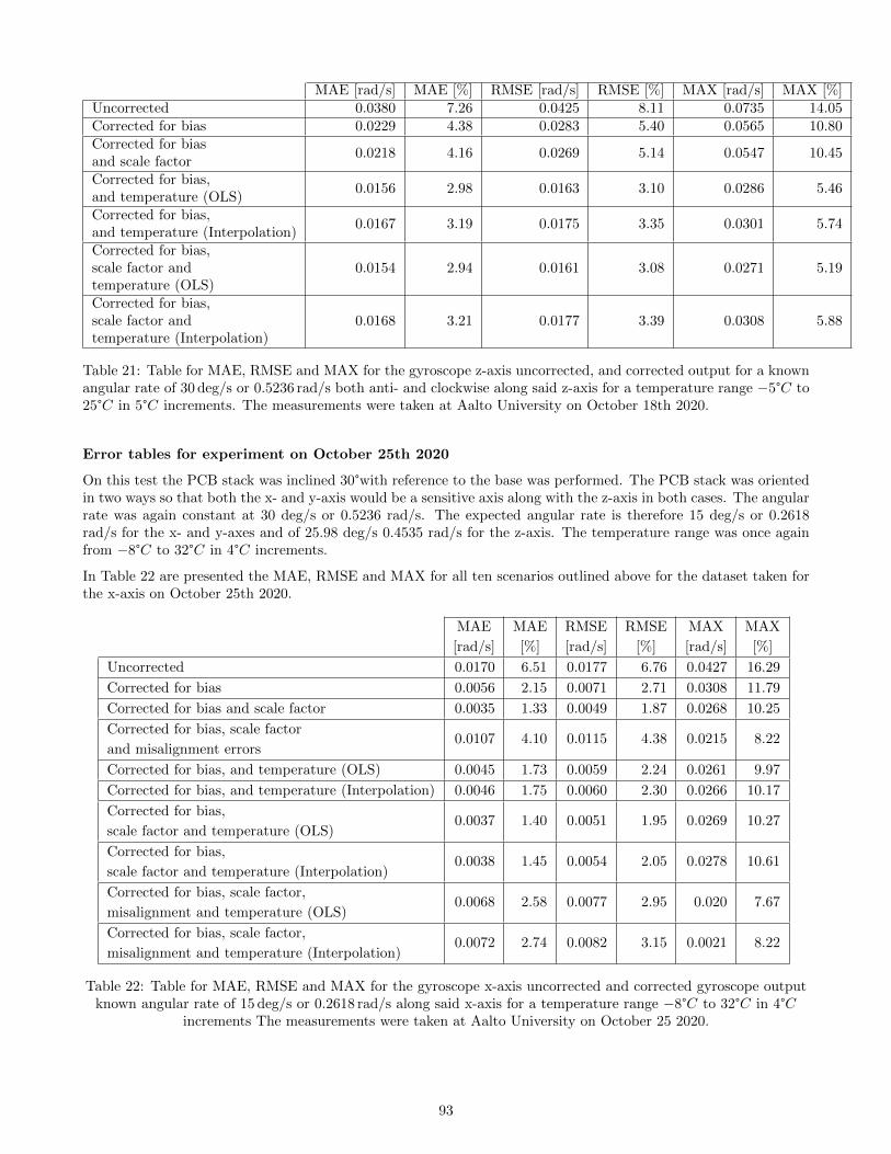
MAE [rad/s] MAE [%] RMSE [rad/s] RMSE [%] MAX [rad/s] MAX [%]Uncorrected 0.0380 7.26 0.0425 8.11 0.0735 14.05Corrected for bias 0.0229 4.38 0.0283 5.40 0.0565 10.80Corrected for biasand scale factor
0.0218 4.16 0.0269 5.14 0.0547 10.45
Corrected for bias,and temperature (OLS)
0.0156 2.98 0.0163 3.10 0.0286 5.46
Corrected for bias,and temperature (Interpolation)
0.0167 3.19 0.0175 3.35 0.0301 5.74
Corrected for bias,scale factor andtemperature (OLS)
0.0154 2.94 0.0161 3.08 0.0271 5.19
Corrected for bias,scale factor andtemperature (Interpolation)
0.0168 3.21 0.0177 3.39 0.0308 5.88
Table 21: Table for MAE, RMSE and MAX for the gyroscope z-axis uncorrected, and corrected output for a knownangular rate of 30 deg/s or 0.5236 rad/s both anti- and clockwise along said z-axis for a temperature range −5°C to25°C in 5°C increments. The measurements were taken at Aalto University on October 18th 2020.
Error tables for experiment on October 25th 2020
On this test the PCB stack was inclined 30°with reference to the base was performed. The PCB stack was orientedin two ways so that both the x- and y-axis would be a sensitive axis along with the z-axis in both cases. The angularrate was again constant at 30 deg/s or 0.5236 rad/s. The expected angular rate is therefore 15 deg/s or 0.2618rad/s for the x- and y-axes and of 25.98 deg/s 0.4535 rad/s for the z-axis. The temperature range was once againfrom −8°C to 32°C in 4°C increments.
In Table 22 are presented the MAE, RMSE and MAX for all ten scenarios outlined above for the dataset taken forthe x-axis on October 25th 2020.
MAE
[rad/s]
MAE
[%]
RMSE
[rad/s]
RMSE
[%]
MAX
[rad/s]
MAX
[%]
Uncorrected 0.0170 6.51 0.0177 6.76 0.0427 16.29
Corrected for bias 0.0056 2.15 0.0071 2.71 0.0308 11.79
Corrected for bias and scale factor 0.0035 1.33 0.0049 1.87 0.0268 10.25
Corrected for bias, scale factor
and misalignment errors0.0107 4.10 0.0115 4.38 0.0215 8.22
Corrected for bias, and temperature (OLS) 0.0045 1.73 0.0059 2.24 0.0261 9.97
Corrected for bias, and temperature (Interpolation) 0.0046 1.75 0.0060 2.30 0.0266 10.17
Corrected for bias,
scale factor and temperature (OLS)0.0037 1.40 0.0051 1.95 0.0269 10.27
Corrected for bias,
scale factor and temperature (Interpolation)0.0038 1.45 0.0054 2.05 0.0278 10.61
Corrected for bias, scale factor,
misalignment and temperature (OLS)0.0068 2.58 0.0077 2.95 0.020 7.67
Corrected for bias, scale factor,
misalignment and temperature (Interpolation)0.0072 2.74 0.0082 3.15 0.0021 8.22
Table 22: Table for MAE, RMSE and MAX for the gyroscope x-axis uncorrected and corrected gyroscope outputknown angular rate of 15 deg/s or 0.2618 rad/s along said x-axis for a temperature range −8°C to 32°C in 4°C
increments The measurements were taken at Aalto University on October 25 2020.
93
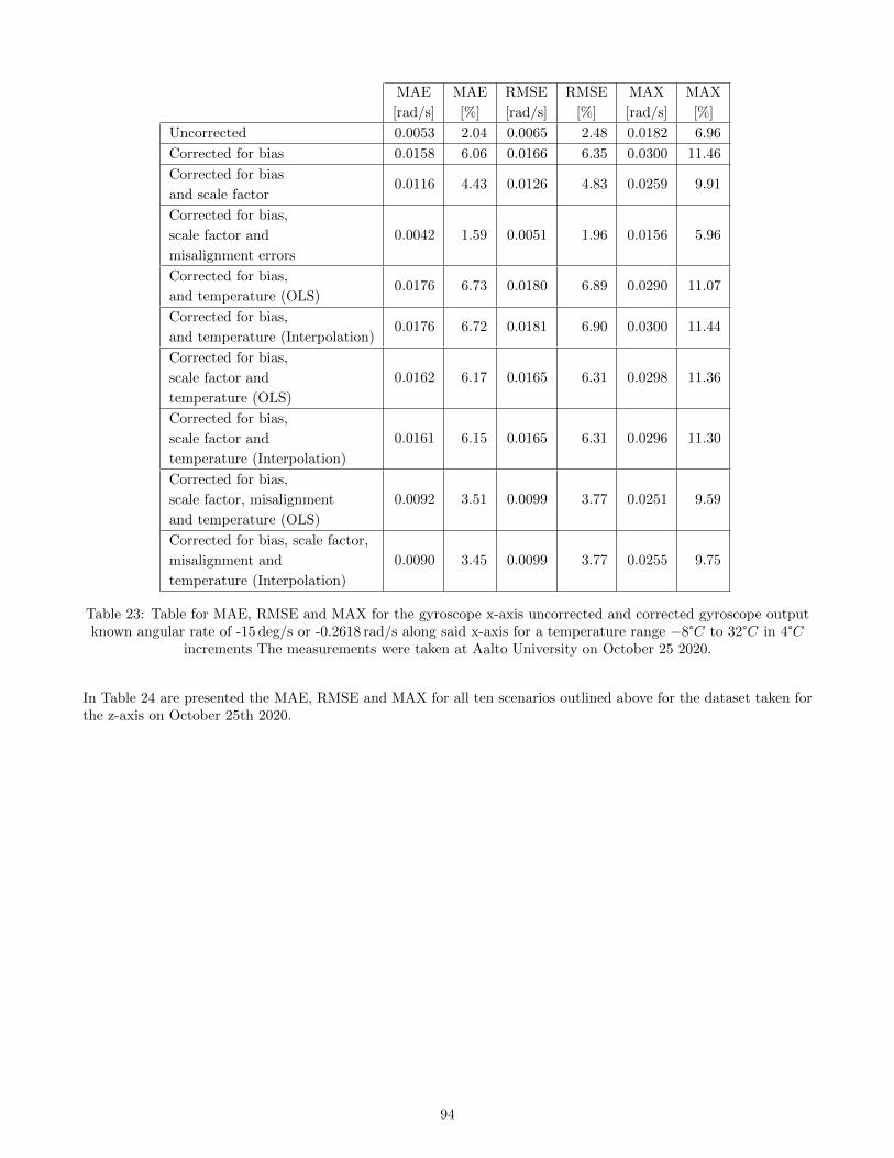
MAE
[rad/s]
MAE
[%]
RMSE
[rad/s]
RMSE
[%]
MAX
[rad/s]
MAX
[%]
Uncorrected 0.0053 2.04 0.0065 2.48 0.0182 6.96
Corrected for bias 0.0158 6.06 0.0166 6.35 0.0300 11.46
Corrected for bias
and scale factor0.0116 4.43 0.0126 4.83 0.0259 9.91
Corrected for bias,
scale factor and
misalignment errors
0.0042 1.59 0.0051 1.96 0.0156 5.96
Corrected for bias,
and temperature (OLS)0.0176 6.73 0.0180 6.89 0.0290 11.07
Corrected for bias,
and temperature (Interpolation)0.0176 6.72 0.0181 6.90 0.0300 11.44
Corrected for bias,
scale factor and
temperature (OLS)
0.0162 6.17 0.0165 6.31 0.0298 11.36
Corrected for bias,
scale factor and
temperature (Interpolation)
0.0161 6.15 0.0165 6.31 0.0296 11.30
Corrected for bias,
scale factor, misalignment
and temperature (OLS)
0.0092 3.51 0.0099 3.77 0.0251 9.59
Corrected for bias, scale factor,
misalignment and
temperature (Interpolation)
0.0090 3.45 0.0099 3.77 0.0255 9.75
Table 23: Table for MAE, RMSE and MAX for the gyroscope x-axis uncorrected and corrected gyroscope outputknown angular rate of -15 deg/s or -0.2618 rad/s along said x-axis for a temperature range −8°C to 32°C in 4°C
increments The measurements were taken at Aalto University on October 25 2020.
In Table 24 are presented the MAE, RMSE and MAX for all ten scenarios outlined above for the dataset taken forthe z-axis on October 25th 2020.
94
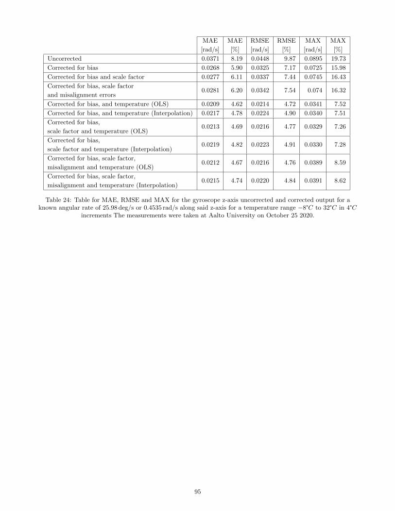
MAE
[rad/s]
MAE
[%]
RMSE
[rad/s]
RMSE
[%]
MAX
[rad/s]
MAX
[%]
Uncorrected 0.0371 8.19 0.0448 9.87 0.0895 19.73
Corrected for bias 0.0268 5.90 0.0325 7.17 0.0725 15.98
Corrected for bias and scale factor 0.0277 6.11 0.0337 7.44 0.0745 16.43
Corrected for bias, scale factor
and misalignment errors0.0281 6.20 0.0342 7.54 0.074 16.32
Corrected for bias, and temperature (OLS) 0.0209 4.62 0.0214 4.72 0.0341 7.52
Corrected for bias, and temperature (Interpolation) 0.0217 4.78 0.0224 4.90 0.0340 7.51
Corrected for bias,
scale factor and temperature (OLS)0.0213 4.69 0.0216 4.77 0.0329 7.26
Corrected for bias,
scale factor and temperature (Interpolation)0.0219 4.82 0.0223 4.91 0.0330 7.28
Corrected for bias, scale factor,
misalignment and temperature (OLS)0.0212 4.67 0.0216 4.76 0.0389 8.59
Corrected for bias, scale factor,
misalignment and temperature (Interpolation)0.0215 4.74 0.0220 4.84 0.0391 8.62
Table 24: Table for MAE, RMSE and MAX for the gyroscope z-axis uncorrected and corrected output for aknown angular rate of 25.98 deg/s or 0.4535 rad/s along said z-axis for a temperature range −8°C to 32°C in 4°C
increments The measurements were taken at Aalto University on October 25 2020.
95

MAE
[rad/s]
MAE
[%]
RMSE
[rad/s]
RMSE
[%]
MAX
[rad/s]
MAX
[%]
Uncorrected 0.0327 7.21 0.0391 8.62 0.0752 16.58
Corrected for bias 0.0225 4.96 0.0270 5.96 0.0582 12.83
Corrected for bias
and scale factor0.0219 4.83 0.0262 5.78 0.0566 12.49
Corrected for bias,
scale factor and
misalignment errors
0.0218 4.80 0.0260 5.73 0.0572 12.61
Corrected for bias,
and temperature (OLS)0.0253 5.57 0.0255 5.63 0.0367 8.09
Corrected for bias,
and temperature (Interpolation)0.0260 5.74 0.0263 5.80 0.0367 8.09
Corrected for bias,
scale factor and
temperature (OLS)
0.0249 5.49 0.0251 5.54 0.0345 7.61
Corrected for bias,
scale factor and
temperature (Interpolation)
0.0259 5.71 0.0262 5.77 0.0357 7.88
Corrected for bias,
scale factor, misalignment
and temperature (OLS)
0.0251 5.53 0.0254 5.59 0.0350 7.72
Corrected for bias, scale factor,
misalignment and
temperature (Interpolation)
0.0263 5.80 0.0266 5.87 0.0367 8.10
Table 25: Table for MAE, RMSE and MAX for the gyroscope z-axis uncorrected and corrected output for aknown angular rate of -25.98 deg/s or -0.4535 rad/s along said z-axis for a temperature range −8°C to 32°C in 4°C
increments The measurements were taken at Aalto University on October 25 2020.
In Table 26 are presented the MAE, RMSE and MAX for all ten scenarios outlined above for the dataset taken forthe y-axis on October 25th 2020.
96
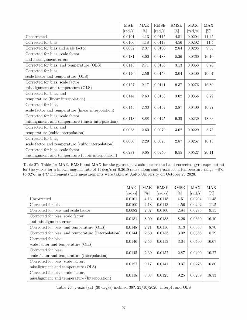
MAE
[rad/s]
MAE
[%]
RMSE
[rad/s]
RMSE
[%]
MAX
[rad/s]
MAX
[%]
Uncorrected 0.0101 4.13 0.0115 4.51 0.0294 11.45
Corrected for bias 0.0100 4.18 0.0113 4.56 0.0292 11.5
Corrected for bias and scale factor 0.0082 2.37 0.0100 2.84 0.0285 9.55
Corrected for bias, scale factor
and misalignment errors0.0181 8.00 0.0188 8.26 0.0360 16.10
Corrected for bias, and temperature (OLS) 0.0148 2.71 0.0156 3.13 0.0363 8.70
Corrected for bias,
scale factor and temperature (OLS)0.0146 2.56 0.0153 3.04 0.0400 10.07
Corrected for bias, scale factor,
misalignment and temperature (OLS)0.0127 9.17 0.0141 9.37 0.0276 16.80
Corrected for bias, and
temperature (linear interpolation)0.0144 2.60 0.0153 3.02 0.0366 8.79
Corrected for bias,
scale factor and temperature (linear interpolation)0.0145 2.30 0.0152 2.87 0.0400 10.27
Corrected for bias, scale factor,
misalignment and temperature (linear interpolation)0.0118 8.88 0.0125 9.25 0.0239 18.33
Corrected for bias, and
temperature (cubic interpolation)0.0068 2.60 0.0079 3.02 0.0229 8.75
Corrected for bias,
scale factor and temperature (cubic interpolation)0.0060 2.29 0.0075 2.87 0.0267 10.18
Corrected for bias, scale factor,
misalignment and temperature (cubic interpolation)0.0237 9.05 0.0250 9.55 0.0527 20.11
Table 27: Table for MAE, RMSE and MAX for the gyroscope z-axis uncorrected and corrected gyroscope outputfor the y-axis for a known angular rate of 15 deg/s or 0.2618 rad/s along said y-axis for a temperature range −8°Cto 32°C in 4°C increments The measurements were taken at Aalto University on October 25 2020.
MAE
[rad/s]
MAE
[%]
RMSE
[rad/s]
RMSE
[%]
MAX
[rad/s]
MAX
[%]
Uncorrected 0.0101 4.13 0.0115 4.51 0.0294 11.45
Corrected for bias 0.0100 4.18 0.0113 4.56 0.0292 11.5
Corrected for bias and scale factor 0.0082 2.37 0.0100 2.84 0.0285 9.55
Corrected for bias, scale factor
and misalignment errors0.0181 8.00 0.0188 8.26 0.0360 16.10
Corrected for bias, and temperature (OLS) 0.0148 2.71 0.0156 3.13 0.0363 8.70
Corrected for bias, and temperature (Interpolation) 0.0144 2.60 0.0153 3.02 0.0366 8.79
Corrected for bias,
scale factor and temperature (OLS)0.0146 2.56 0.0153 3.04 0.0400 10.07
Corrected for bias,
scale factor and temperature (Interpolation)0.0145 2.30 0.0152 2.87 0.0400 10.27
Corrected for bias, scale factor,
misalignment and temperature (OLS)0.0127 9.17 0.0141 9.37 0.0276 16.80
Corrected for bias, scale factor,
misalignment and temperature (Interpolation)0.0118 8.88 0.0125 9.25 0.0239 18.33
Table 26: y-axis (yz) (30 deg/s) inclined 30º, 25/10/2020: interp1, and OLS
97
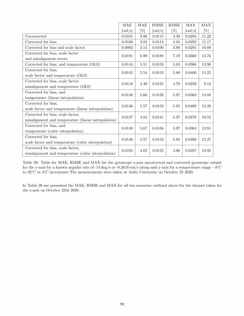
MAE
[rad/s]
MAE
[%]
RMSE
[rad/s]
RMSE
[%]
MAX
[rad/s]
MAX
[%]
Uncorrected 0.0101 3.86 0.0115 4.39 0.0294 11.22
Corrected for bias 0.0100 3.82 0.0114 4.34 0.0292 11.17
Corrected for bias and scale factor 0.0082 3.14 0.0100 3.80 0.0285 10.89
Corrected for bias, scale factor
and misalignment errors0.0181 6.90 0.0188 7.19 0.0360 13.76
Corrected for bias, and temperature (OLS) 0.0144 5.51 0.0153 5.83 0.0366 13.96
Corrected for bias,
scale factor and temperature (OLS)0.0145 5.54 0.0152 5.80 0.0400 15.25
Corrected for bias, scale factor,
misalignment and temperature (OLS)0.0118 4.49 0.0125 4.79 0.0239 9.12
Corrected for bias, and
temperature (linear interpolation)0.0148 5.66 0.0156 5.97 0.0363 13.88
Corrected for bias,
scale factor and temperature (linear interpolation)0.0146 5.57 0.0153 5.85 0.0400 15.28
Corrected for bias, scale factor,
misalignment and temperature (linear interpolation)0.0127 4.84 0.0141 5.37 0.0276 10.52
Corrected for bias, and
temperature (cubic interpolation)0.0148 5.67 0.0156 5.97 0.0364 13.91
Corrected for bias,
scale factor and temperature (cubic interpolation)0.0146 5.57 0.0153 5.85 0.0400 15.27
Corrected for bias, scale factor,
misalignment and temperature (cubic interpolation)0.0105 4.02 0.0122 4.66 0.0287 10.95
Table 28: Table for MAE, RMSE and MAX for the gyroscope z-axis uncorrected and corrected gyroscope outputfor the y-axis for a known angular rate of -15 deg/s or -0.2618 rad/s along said y-axis for a temperature range −8°Cto 32°C in 4°C increments The measurements were taken at Aalto University on October 25 2020.
In Table 26 are presented the MAE, RMSE and MAX for all ten scenarios outlined above for the dataset taken forthe z-axis on October 25th 2020.
98
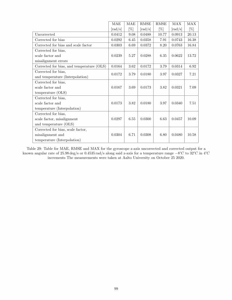
MAE
[rad/s]
MAE
[%]
RMSE
[rad/s]
RMSE
[%]
MAX
[rad/s]
MAX
[%]
Uncorrected 0.0412 9.08 0.0488 10.77 0.0913 20.13
Corrected for bias 0.0292 6.45 0.0358 7.91 0.0743 16.38
Corrected for bias and scale factor 0.0303 6.69 0.0372 8.20 0.0763 16.84
Corrected for bias,
scale factor and
misalignment errors
0.0239 5.27 0.0288 6.35 0.0622 13.72
Corrected for bias, and temperature (OLS) 0.0164 3.62 0.0172 3.79 0.0314 6.92
Corrected for bias,
and temperature (Interpolation)0.0172 3.79 0.0180 3.97 0.0327 7.21
Corrected for bias,
scale factor and
temperature (OLS)
0.0167 3.69 0.0173 3.82 0.0321 7.09
Corrected for bias,
scale factor and
temperature (Interpolation)
0.0173 3.82 0.0180 3.97 0.0340 7.51
Corrected for bias,
scale factor, misalignment
and temperature (OLS)
0.0297 6.55 0.0300 6.63 0.0457 10.09
Corrected for bias, scale factor,
misalignment and
temperature (Interpolation)
0.0304 6.71 0.0308 6.80 0.0480 10.58
Table 29: Table for MAE, RMSE and MAX for the gyroscope z-axis uncorrected and corrected output for aknown angular rate of 25.98 deg/s or 0.4535 rad/s along said z-axis for a temperature range −8°C to 32°C in 4°C
increments The measurements were taken at Aalto University on October 25 2020.
99
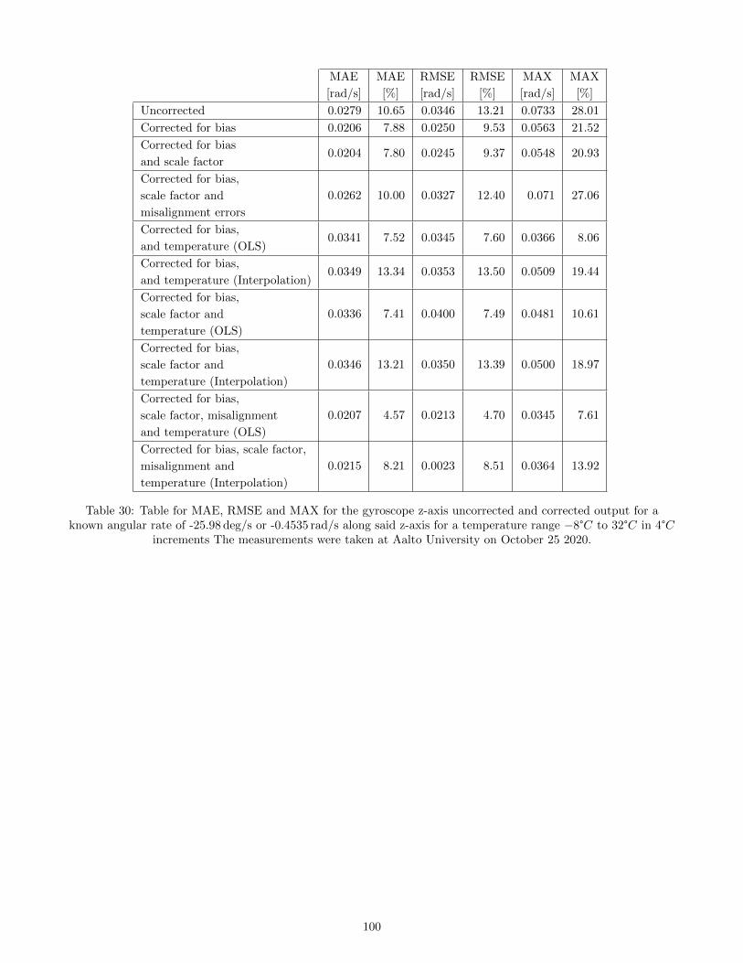
MAE
[rad/s]
MAE
[%]
RMSE
[rad/s]
RMSE
[%]
MAX
[rad/s]
MAX
[%]
Uncorrected 0.0279 10.65 0.0346 13.21 0.0733 28.01
Corrected for bias 0.0206 7.88 0.0250 9.53 0.0563 21.52
Corrected for bias
and scale factor0.0204 7.80 0.0245 9.37 0.0548 20.93
Corrected for bias,
scale factor and
misalignment errors
0.0262 10.00 0.0327 12.40 0.071 27.06
Corrected for bias,
and temperature (OLS)0.0341 7.52 0.0345 7.60 0.0366 8.06
Corrected for bias,
and temperature (Interpolation)0.0349 13.34 0.0353 13.50 0.0509 19.44
Corrected for bias,
scale factor and
temperature (OLS)
0.0336 7.41 0.0400 7.49 0.0481 10.61
Corrected for bias,
scale factor and
temperature (Interpolation)
0.0346 13.21 0.0350 13.39 0.0500 18.97
Corrected for bias,
scale factor, misalignment
and temperature (OLS)
0.0207 4.57 0.0213 4.70 0.0345 7.61
Corrected for bias, scale factor,
misalignment and
temperature (Interpolation)
0.0215 8.21 0.0023 8.51 0.0364 13.92
Table 30: Table for MAE, RMSE and MAX for the gyroscope z-axis uncorrected and corrected output for aknown angular rate of -25.98 deg/s or -0.4535 rad/s along said z-axis for a temperature range −8°C to 32°C in 4°C
increments The measurements were taken at Aalto University on October 25 2020.
100