Journal of Quantitative Analysis inSports

Volume 4, Issue 4 2008 Article 4

Determining Hall of Fame Status for MajorLeague Baseball Using an Artificial Neural

Network

William A. Young II∗ William S. Holland†

Gary R. Weckman‡

∗Ohio University, william.a.young.1@ohio.edu†Ohio University, william.s.holland.1@ohio.edu‡Ohio University, weckmang@ohio.edu

Copyright c©2008 The Berkeley Electronic Press. All rights reserved.

Determining Hall of Fame Status for MajorLeague Baseball Using an Artificial Neural

Network∗

William A. Young II, William S. Holland, and Gary R. Weckman

Abstract

Election into Major League Baseball’s (MLB) National Hall of Fame (HOF) often sparks de-bate among the fans, media, players, managers, and other members in the baseball community.Since the HOF members must be elected by a committee of baseball sportswriters and other en-tities, the prediction of a player’s inclusion in the HOF is not trivial to model. There has beena lack of research in predicting HOF status based on a player’s career statistics. Many modelsthat were found in a literature search use linear models, which do not provide robust solutions forclassification prediction in complex non-linear datasets. The multitude of possible combinationsof career statistics is better suited for a non-linear model, like artificial neural networks (ANN).The objective of this research is to create an ANN model which can be used to predict HOF statusfor MLB players based on their career offensive and defensive statistics as well as the number ofcareer end of the season awards. This research is limited to investigating players who are not pitch-ers. Another objective of this report is to give the audience of this particular journal an overviewof ANNs.

KEYWORDS: Major League Baseball, Hall of Fame, artificial neural networks

∗Department of Industrial and Systems Engineering, Ohio University, 270 Stocker Center, Athens,OH 45701, USA; (t) +1- 740-593-1539; (f) +1-740-593-0778.

1 Introduction Election into Major League Baseball’s (MLB) National Hall of Fame (HOF) often sparks debate among the fans, media, players, managers, and other members in the baseball community. Much of this debate stems from the fact that MLB does not have an elaborate set of rules based to enshrine players into their HOF. Various committees within MLB ultimately determine a player’s HOF status.

The Baseball Writers Association of America (BBWAA) meets each year to elect eligible players into the HOF. Writers must have 10 years of experience to be eligible to vote for MLB’s HOF. In certain cases, a writer can be nominated as honoraria members. Historically, the rules for the election process are divided into two forms of entry into the HOF. Applicants are voted in by either the BBWAA or the Veterans Committee. The Baseball Writers Association of America considers players who have played in at least 10 major league seasons and have been retired for at least five seaons (BBWAA, 2007). The Veterans Committee considers players whose careers ended no later than 21 seasons prior to the election year.

The BBWAA also has a set of guidelines that determines whether players are eligible to be inducted into the HOF. The conditions for an eligible candidate include MLB players who (BBWAA, 2007):

� were active beginning 20 years before and 5 years removed as a player prior to the annual election date

� has played in 10 championship seasons � are at least 5 years removed from being an active player, but are still

active in baseball in another capacity � have passed away, but have not met the condition of being 5 years

removed as an active player � are not on the HOF ineligible list

BBWAA requires a six-member committee called the BBWAA Screening Committee for the electoral process. Annually, the committee elects two members to a three-year term. The voters are instructed to vote based on a player’s career statistics, playing ability, integrity, sportsmanship, character, and contributions toward his team (BBWAA, 2007).

A player must receive seventy-five percent of the ballots to be inducted into the HOF. The Veterans Committee electorate consists of the living HOF members, which currently consists of 63 members. The committee must narrow a list of thirty players chosen by a separate committee down to 10 players. However, the Veterans Committee may only consider players whose careers began in 1943 or after. Thus, only two methods of induction exist; election by the

1

Young et al.: Determining HOF Status for MLB Using an Artificial Neural Network

Published by The Berkeley Electronic Press, 2008

BBWAA at least five and not twenty years after retirement and special election by the Veterans Committee more than twenty years after retirement. Without having expert knowledge of the game of baseball and its HOF, induction for players is highly debatable.

The hypothesis of this research is that HOF status can be predicted from a player’s career offensive and defensive statistics as well as the number of awards earned at the end of the season. Since there are no set-rules for a player’s induction, it is also hypothesized that an artificial neural network (ANN) is better suited for this type of problem than logistic regression (or linear based methods). For example, ANNs have historically outperformed their linear counterpart for classification (Schürmann, 1996), continuous (Kumar et al., 1995) and even temporal systems (Mozer, 1994). Classifying HOF status is non-trivial, since committee members use varying criteria in which they vote for enshrinement. Thus, the significance of this research is to determine if an ANN is capable of modeling human decisions. Having a quantifiable method should also reduce uncertainty of the nebulous process of inducting members into the HOF.

“Hall of Fame voting is tougher than most people realize because it's so hard to draw the line that separates Hall of Famers from the great players who fall into that close-but-not-quite department.” – Peter Gammons (Gammons and Stark, 2007)

Past research of modeling MLB’s HOF membership typically investigated if racial discrimination existed among voters (Jewell, 2003) (Findlay and Reid, 1997) (Desser, et al., 1999). These studies support that the presence of racial discrimination does not appear to be significant. Thus, for this research, race will not be used as an input parameter to the ANN model. Though the analysis of these models studied important issues related to society, they do little to investigate what attributes a player might posses that distinguishes him from non-HOF members.

The research presented in this article differs from past efforts in a few ways. Besides the exclusion of investigating racial discrimination, this article will make forecasts based on several future eligible players as well as players who are currently eligible for the HOF. Other research has specific agendas to reveal if certain voting behavior (or biasing) exists. This research aims to extract knowledge from the system model in terms of input behavior and it’s significance. Revealing this knowledge will allow for a better understanding of what voters look for when casting their ballots for HOF induction. Another distinction is the comprehensive set of input parameters that were used for the system model. Past models typically only use offensive statistics (and specific inputs related to race); however, this research will investigate a variety of

2

Journal of Quantitative Analysis in Sports, Vol. 4 [2008], Iss. 4, Art. 4

http://www.bepress.com/jqas/vol4/iss4/4

offensive and defensive statistics as well as post season awards for performance and character.

The objective of this paper aims to identify the significant attributes that result in classification of a HOF member. Identifying the significance and behavior of the input attributes will result in a better understanding of how HOF committee members are voting for the candidates. It will also illuminate reasons why certain players might have been overlooked in the past. It should be noted that the scope of this research is limited to investigating fielders (i.e. not pitchers or designated hitters). Pitchers were removed from this study because it is assumed that their HOF candidacy is determined by their pitching performance, rather than their offensive or defensive production. Players who played the majority of their games as a designated hitter were also removed because many of the defensive attributes used in the data mining method would not apply for these players. Thus, it was assumed that these players would skew the results.

Another objective of this report is to provide for the audience of this particular journal a brief (non-technical) overview of ANNs and their applications in sports. This particular objective was set because a search of literature involving ANN analysis in the journal was unsuccessful. The ANN discussion presents a brief overview of the historic, biological inspiration, topologies, and the experimental procedure required for to develop an ANN model. ANNs are stochastic non-linear machine learning models, where experience, patience, and a working knowledge of the relevant topics are required to develop a robust model. The review of ANN topics is meant to be non-technical, where complicated mathematical derivations are avoided, since many of the concepts relevant to ANNs are lost in mathematical formulation and jargon. This introduction will focus on a high-level discussion of a wide variety of ANN topics, without delving into specific topics, which would require mathematically intensive derivations to explain fully. Thus, readers are encouraged to pursue the cited references for more explicit details.

If the ANN model produces sufficient results in predicting the status of a player whose HOF status has been finalized, the model should be capable of accurately predicting a current player’s future HOF status. Thus, another objective is to forecast players who either met the requirement of having played in 10 championship seasons, or are currently being voted on by the HOF voting committee.

The results of the model can also be used to determine input significance. For example, how much more significance do voters place on offensive stats like home runs than defensive stats such as errors or other fielding statistics? Thus, an application of this quantitative method could be used when HOF committees select a ballot of players to be voted on each year.

3

Young et al.: Determining HOF Status for MLB Using an Artificial Neural Network

Published by The Berkeley Electronic Press, 2008

The following sections of this report are as follows; Section 2 is dedicated to a review of literature regarding models found in sports, an introduction to ANNs, and the use of ANNs in sports. Section 3 describes the methodology used to derive an MLB HOF ANN model Section 4 disseminates the results of the methodology and the benchmark methods. Finally, Section 5 concludes with a discussion about the quality of estimation and other relevant issues concerning the proposed methodology.

2 Literature Review Baseball has drastically changed in many aspects over the last century. For example, MLB has recently scheduled more games in a single season than historically in the past. Stadium dimensions have changed to promote better attendance from increased offensive production (Clapp and Hakes, 2005). The equipment has arguably increased in quality, resulting in “livelier” bats and balls. Sports medicine has improved greatly, resulting in fewer injuries and less rehabilitation time when players are injured. Expansion has increased the number of teams in the league, where some argue that the pitching talent is dispersed around the league causing inflated statistics (Quinn and Bursik, 2007). Another issue involves the recent release of the Mitchell Report (Mitchell, 2007). This report has enlightened the baseball community with a thorough investigation of the use of steroids and other performance enhancing drugs over the past several seasons with their players. Only time will tell if the allegations against the players named in the report will have an effect on their future HOF status. However, it possibly gives another reason MLB has experienced “inflated” statistics.

2.1 Predicting Systems in Sports

Many methodologies have been introduced into sports analysis. For example, Bayesian theory has been used to predict the outcomes of sporting events (Stern, 1991). Markov chains have been utilized to predict the final score of games (Glickman and Stern, 1998). Maximum likelihood estimates were constructed to determine a rating of sports teams (Harvill and Smith, 1980). Operations research has been used to determine strategies for calling time-outs in football games, which were based on making Type I (alpha) or Type II (beta) errors (Carter and Machol, 1971).

Many stochastic methods have been developed to describe a team ranking among other teams in a league. The most common approach to evaluate a team’s rating is to use least squares regression or related normal distribution theory (Glickman and Stern, 1998). These techniques often minimize the prediction error of the scores accumulated by teams in their seasons. These predictive models are

4

Journal of Quantitative Analysis in Sports, Vol. 4 [2008], Iss. 4, Art. 4

http://www.bepress.com/jqas/vol4/iss4/4

complicated by the fact that competitive sports leagues are often structured in such a way that teams do not face all other possible teams in the league. Therefore, the incomplete data poses a difficult problem when a ranking of a team is desired. When this type of problem occurs, network theory has been used to rate a team based on their league’s schedule (Park and Newman, 2005), where transitive relationships about the teams are used to determine rankings.

Optimization has also made its way into quantitative sports analysis. For example, Poisson regression models have been used to determine optimal betting strategies for sports gambling (Dixan and Coles, 1997). Recommender systems producing near-optimal starting line ups have also been found within baseball research (Bukiet et al., 1997). Another example of optimization strategies found in sports research includes determining player selections in a sport league’s draft (Fry et al., 2007).

Constructing a model to predict the status of a player to make the HOF has been given little attention. The prediction of HOF status has been examined using ordinary least-squares estimates and binary logistic estimates (Findlay and Reid, 2002). Each of these traditional methods is tested with two data forms: an average offensive performance and a career total offensive performance. An important aspect of this research is the fact that career statistics resulted in a more accurate model. Genetic algorithms, which are another biologically inspired form of machine learning, have been used to generate a set of rules to predict a player’s chances of being enshrined into the HOF (Cohen, 2004). This approach applies a type of global search heuristic, which looks for an optimal (or sub-optimal) solution through a series of mutating through generations of chromosomes. Though this research has resulted in suitable predicting accuracies, it does not offer an explanation or a quantification of the importance of input parameters.

2.2 Artificial Neural Networks

Artificial neural networks (ANNs) are mathematical models, which are biologically inspired to imitate the primitive cognitive functionality of the human brain. Initial efforts in ANN development have dated back to the early 1940s (McCulloch and Pitts, 1943). The model, which is associated with a subset of artificial intelligence called machine learning, is data-driven, and is capable of representing complex non-linear input and output relationships. It is for this reason that ANNs are known as universal approximators (Reed and Marks, 1998). More importantly, ANN provides a structured approach to determining a non-linear model. There are many scientific applications of ANNs, where the most common use is function approximations (Young et al., 2008) and classifications (Efraim et al., 2001).

5

Young et al.: Determining HOF Status for MLB Using an Artificial Neural Network

Published by The Berkeley Electronic Press, 2008

The mathematical representation of an ANN is inspired by the biological neuron. ANNs consist of several layers of interconnecting processing elements, which are called neurons. Neurons are implemented with an activation function,which control signals passing through the network. The human brain functions and processes information when it receives signals through synapses located around the dendrites. A basic sketch of the biological neural network model is shown below in Figure 1 (Neuralpower, 2007).

Figure 1: Biological Neuron

An artificial neuron is a single processing element in an ANN. This single unit is more commonly referred today as a perceptron unit. A single perceptron computes the output of the neuron by forming a linear combination of weights and real-valued input values, where this value is generally translated by a non-linear activation function. For example, the perceptron, shown in Figure 2, has a set of independent inputs (X1, X2, X3, and Xm or X), connection weights (W1, W2, W3, and Wm or W), bias (B), and an dependent variable (Y). For this neuron, the inputs are multiplied with the connection weights and summed together at the node. The bias is also added to this sum and the value is entered into an activation function (f(�(WTX+B)). The result of this activation function is then equal to the dependent variable. The weights are unknown and are set at small random values before training can occur, which will be discussed later. The weights represent the strength of the association between independent and dependent variables.

6

Journal of Quantitative Analysis in Sports, Vol. 4 [2008], Iss. 4, Art. 4

http://www.bepress.com/jqas/vol4/iss4/4

Figure 2: Artificial Neuron

Several common activation functions can be used for an artificial neuron. Some of the more common functions are found in Table 1. To determine which activation function produces the best results for the ANN requires a trial and error procedure, which is described later. However, the most commonly used activation functions are the linear, sigmoid, and hyperbolic tangent functions.

Table 1: Common Activation Functions

Activation Functions Definitions Range Linear x (-� , +�)

Sigmoid ��� � ���� (0, 1)

Hyperbolic �� � ������ ���� (-1, 1)

Exponential ��� (0, �)

Softmax ��� ��� (0, 1)

Unit Sum � ��� (0, 1)

Square root � (0, �) Sine Sin(x) (0, 1)

Ramp � �� � � ������ � � � ��� � � � � (-1, 1)

Step ��� � � ��� � � �� (0, 1)

The multilayer perceptron is the most common ANN topology used today. It consists of groups of neurons that are interconnected by weights. The weights of the network are found by a process called training. The interactions within the

7

Young et al.: Determining HOF Status for MLB Using an Artificial Neural Network

Published by The Berkeley Electronic Press, 2008

network can either act as excitation or inhibition signals, which are propagated through the network. Thus, the output of a single neuron in the first hidden layer, is used as an input for the second hidden layer neuron. An example of an MLP ANN is shown in Figure 3, where it is represented in terms of a Network Interpretation Diagram (Özesmi and Özesmi, 1999). For this example, weights that are excitation signals (or positive in value) are represented by solid lines, where line thickness is determined by the weight’s magnitude. Likewise, inhibitor signals (or negative in value) are represented by dashed lines.

Neurons are typically implemented with activation functions that are mathematically convenient for training algorithms. The network shown in Figure 3 is composed of four layers, with an assumed hyperbolic tangent activation function. The first layer of the network (from left to right) is the input layerfollowed by two hidden layers and finally an output layer. The layers are often called hidden, because they are not directly seen by the individual. For this reason, ANNs are often called “black-box” models, because the mechanism for the prediction is not transparent (Olden and Jackson, 2002).

Figure 3: Multi-Layered ANN

A variant of the MLP ANN is the Generalized Feed-Forward (GFF) ANN. For this model, extra weights are added in such a way that weights from a layer can bypass layers in the network in order to connect to other nodes. For example, if the MLP shown in Figure 3 were to be transformed into a GFF, existing weights would remain. Additional weights would then be added from each input in the input layer to each of the processing elements in the second hidden layer. Likewise, each of the nodes in the first hidden-layer would be connected with the

8

Journal of Quantitative Analysis in Sports, Vol. 4 [2008], Iss. 4, Art. 4

http://www.bepress.com/jqas/vol4/iss4/4

output layer. This type of ANN is also referred to as a fully connected network, since the additional weights are connected with every element of one layer. Other variants of this type of network exist, where the connection strategy is partially connected. However, these types of networks are less commonly used. There are several advantages to using an MLP. They have been used successfully in numerous applications, they are easy to use, and they can approximate any input/output map well. However, MLPs train very slowly and often require many networks to be tested in order to converge to a final solution. MLPs are guaranteed to solve the same problems that GFFs can. However, in practice, GFFs often solve the problems more efficiently, where less experimental time is required (Nelson & Illingworth, 1992).

There are two main learning paradigms used for creating ANN, which include supervised and unsupervised learning (Haykin, 1999). Supervised learning uses both the inputs and outputs to update the internal weights of the ANN. This process is sometimes called training “with a teacher.” Unsupervised ANNs differ because the internal weights of the ANN structure are only modified by input values. Thus, this technique is referred to as training “without a teacher.”

Training is an iterative process where the network’s weights are updated through a “learning” algorithm. Typically, weights are updated after the learning algorithm has seen all samples (or exemplars) from the training dataset. Once all samples are seen by the training algorithm, which is known as an epoch, the parameters are adjusted based on the observed error. The most widely used supervised training method is called back-propagation (Rumelhart and McClelland, 1986). Back-propagation refers to the direction in which the error is assigned to neurons during a repetitive training procedure in order to determine the network’s weights. In general, the back-propagation algorithm is performed when the network’s output is computed given an input vector with a known target value(actual output) and a set of randomly assigned weights for the network. In order to calculate the output of a neural network, every neuron’s output must be calculated and passed forward (or propagated) to the neurons in the following layers. The output value in the final layer is used to calculate the error in the network (target – output). Once the error is determined, the network’s total entropy is needed in order to assign “responsibility” of the error to the networks hidden-layer nodes. Computing cost functions for every neuron in the network using an application of the chain-rule is a fundamental process of back-propagation. This assignment of error to the network’s nodes is used to adjust the weights in such a way that neurons with the most attributed error are updated more aggressively than neurons with less error. The entropy of each hidden-layer node is necessary to make the weight adjustments for the network. The weight of the network is adjusted in a feed-forward manner, where for a given node, the output of that node is

9

Young et al.: Determining HOF Status for MLB Using an Artificial Neural Network

Published by The Berkeley Electronic Press, 2008

multiplied by a small learning rate, the connection weight to the next layer’s neuron, and the network’s total entropy. Once every weight is updated using the back-propagation scheme, the network is given another training sample (next input vector) to further define the weights of the network in order to minimize a certain cost function (i.e. mean squared or total sum of squares error). The process is repeated, until there is a small allowable error or the iterative algorithm has reached a predetermined stopping point (i.e. total number of training samples). A momentum term is often applied in the calculation of the weight update to speed up training efforts. For a more elaborate description of the training algorithms (and others mentioned in this article), please refer to the numerous publications dedicated to this particular topic (i.e. Haykin (1999)). There are several other algorithms used in practice, such as conjugate gradient, quick, and delta propagation, which are all considered first generation algorithms. A more sophisticated second generation learning approach is Levenberg-Marquardt (Levenberg, 1944), which generally produces better results than first order approaches but converges with fewer epochs and is more computationally intensive, (Marquardt, 1963). First ordered methods use local approximation of a surface performance slope of the cost function to determine which direction the weights should be updated to achieve minimization. Second ordered approaches attempt to determine the curvature instead of just the slope of the cost function. The Levenberg-Marquardt method combines the best features of the Gauss-Newton and the steepest-decent methods, but does not suffer from their limitations. Though the Levenberg-Marquardt is complex in its derivation, the basic strategy for updating the network’s weights is as follows. Using the randomly assigned weights of a network, the total sum of squares is calculated using all of the training samples. The Jacobian Matrix is then computed so that the incremental values for the weights can be determined. The sum of squares for all training samples is recomputed, and the process is repeated until the learning algorithm is terminated (i.e. small allowable error is reached or a max training time has occurred). Depending on properties of the Jacobian Matrix for this learning strategy, the Levenberg-Marquardt algorithm defaults closely to a gradient search method if the performance surface deviates from a “parabola-like” surface, which often occurs with non-linear neural computing (Bishop, 1995). Since the Levenberg- Marquardt learning algorithm is more robust to linear assumptions than back-propagation, it is a more sophisticated approach. It is also more likely that weights will be adjusted in such a way that a network will converge to a global optimum, rather than a local optimum.

Several factors determine whether the training process should be terminated. The first instance is whether the network’s performance has reached a certain pre-defined goal of a small allowable error. Since training is often a lengthy process

10

Journal of Quantitative Analysis in Sports, Vol. 4 [2008], Iss. 4, Art. 4

http://www.bepress.com/jqas/vol4/iss4/4

and it might not be possible to reach a specified error goal, the second instance for termination is if the training algorithm has reached a pre-determined number of epochs. A third reason training might be terminated is if the network’s performance does not change after a pre-defined number of epochs. Finally, the fourth instance for termination is if the cross-validation dataset’s network performance becomes increasingly worse, which is further explained below.

Parameter selection (i.e. number of neurons, number of layers, etc.) of an ANN is determined through an experimental procedure that requires an investigation based on trial-and-error. This is because of the random nature of initial weights and the varying complexity of datasets. For example, there are occasions when an ANN can have an insufficient number of neurons or even the situation where there are too many neurons in the network. Other issues can arise with learning rates that are used for training with momentum (Fausett, 1994). Sub-optimal rates can cause potential problems where weights are changed too frequently or not enough. Thus, experimentation is required because no standard methodologies exist to predetermine an optimal network structure.

The process of determining an ANN is iterative and is based on experimenting with differing ANN architectures. It is not always sufficient to train a single network because performances and associations will change based on initial conditions of the network. Therefore, several networks are often tested before determining the “best” ANN. Figure 14 is provided as a summary of the experimental procedure that should be applied when deriving an ANN. The information flow has three phases, which include data pre-processing, training, and testing. Each of these steps is discussed later in more detail. For this procedure, it is stromgly suggested that several (shown in the figure as N) ANNs be initialized and trained before making a decision on a final model. Since the weights of a network are small random values at the start of training, a network will most likely converge to different final values for the weights after training has occurred. ANNs are stochastic in nature, since multiple solutions can be formed depending on values of the weights found. Thus, when a network topology has been determined (i.e. number of nodes and hidden layers), the topology should be trained N times. This N should not be confused with the total number of iterations used when the training algorithm is invoked, which is known as an epoch. Thus, each iteration of N (shown as i in the figure below) will be randomly seeded with initial weight values, trained with a learning algorithm, and then an assessment of the N models should occur in order to select the best performing (and final) network.

11

Young et al.: Determining HOF Status for MLB Using an Artificial Neural Network

Published by The Berkeley Electronic Press, 2008

Figure 4: Procedural Flow for ANNs

The experimental procedure starts by data pre-processing. This procedure includes removing noisy or missing values, normalizing database attributes, translating symbolic to numeric data, and randomly partitioning the dataset into three subsets of data. The subsets of data include training, cross-validation, and testing. Cross-validation and database normalization is important because it promotes better generalization properties of final model (Principe et al., 2000). A topology for the network should be experimented with once data pre-processing has been completed. This procedure consists of determining the type of network (i.e. MLP, GFF, etc), number of hidden layers, the number of nodes in each layer, and type of activation functions used in each node. Though there is not a standard for the number of hidden layers a network should have, it is highly suggested that a network has at least two. This is because a multi-layered ANN is capable of solving non-trivial non-linear non-separable problems. To demonstrate this capability, the XOR problem will be discussed. In digital system design, three binary logical operators are commonly used, which include AND, OR, and XOX logic gates. Figure 5 shows a graph of the AND digital logic, where for the gate to pass a binary one (shown as diamonds),

12

Journal of Quantitative Analysis in Sports, Vol. 4 [2008], Iss. 4, Art. 4

http://www.bepress.com/jqas/vol4/iss4/4

both inputs (X1 and X2) must equal one. If any other combinations of the inputs are given, the logical gate will pass a zero (shown as circles). The logic for the OR gate is shown in Figure 6; however, binary ones are passed in all combinations of binary inputs, except when both are equal to zero. These two logical operators are examples of linearly separable problems, since the two classes (binary one and zero) can be correctly separated by a linear decision boundary (shown as a line in the graph). The decision boundary represents how classifications are made. Points above the boundary equate to one type of class, and points below the boundary represent another. A single ANN perception is guaranteed to solve linearly separable problems, which is stated in the Perception Learning Rule (Rosenblatt, 1958). The decision boundaries shown in the figures are arbitrarily drawn; other boundaries could solve this problem correctly.

Figure 5: AND Logic Figure 6: OR Logic

Another commonly used logical operator for digital systems is known as the XOR gate. Using this gate has many benefits to digital circuit design; however, discussing these benefits is beyond the scope of this paper. The XOR gate differs greatly to the AND and OR because it is a non-linear non-separable problem. The logic of this gate is graphically shown in Figure 7. A binary zero is passed through the gate when both the input values are equal. Likewise, a binary zero is passed when the input values differ. As stated earlier, an ANN with a single perception with linear threshold values is guaranteed to solve linear separable problems. The XOR problem cannot be solved with an ANN network with a single perceptron. Thus, no linear decision boundary can be drawn through the points where each binary classified correctly.

0.0

0.5

1.0

1.5

0.0 0.5 1.0 1.5

X2

X1

0.0

0.5

1.0

1.5

0 0.5 1 1.5

X2

X1

13

Young et al.: Determining HOF Status for MLB Using an Artificial Neural Network

Published by The Berkeley Electronic Press, 2008

Figure 7: XOR Logic

Though the single perception has limitations in solving non-linear non-separable problems, a multi-layered network of perceptrons can solve this type of problem. For the XOR problem, a network with a minimum of two hidden layers with a single processing element in each layer is needed to converge on a solution where each of the points is correctly classified. Since many classification problems are non-linear (i.e. predicting HOF status of MLB players) and cannot be separated by linear decision boundaries, multi-layered networks are preferred.

An important and often overlooked practice is the use of cross-validation data during the training phase (Vapnik, 1995). Cross-validation is used to determine the weights of a network that promote generalization. Utilizing cross-validation is a strategy to prevent over-fitting or memorization. This training concept is shown in Figure 8 (Almeida, 1999).

For example, the goal of training is to reduce a cost, which is often mean squared error (MSE) of the model. The cross-validation dataset is used during the training phase that is used to determine when the network’s weights should no longer be adjusted. This is depicted in Figure 8, where the performance is at a maximum for each dataset. Thus, if tuning does not cease at this point, the performance of the training data will continue to improve artificially, but the unseen cross-validation will worsen. This is because the ANN has a large degree of freedom, where weights can be fitted in a way that the total database used for training is memorized. Applying cross-validation avoids over-fitting (or memorization) and produces the “best” generalized network.

���

���

���

���

� ��� � �����

��

14

Journal of Quantitative Analysis in Sports, Vol. 4 [2008], Iss. 4, Art. 4

http://www.bepress.com/jqas/vol4/iss4/4

Figure 8: Stopping with Cross-validation

Finally, if termination occurs and the recursive process is complete after training N networks, the process should be repeated with a different network structure (i.e. different number of nodes or hidden layers) until the results and capabilities of the ANN become clear. Once a final ANN is validated, the network can be used to forecast other sample instances.

2.3 ANNs in Sports

Though ANNs have not been found in literature to model HOF status, they have been used in many other instances of sports research. This is because ANNs have the ability to model probabilistic datasets accurately. ANNs have been used to rank a team within a league. One such model was proposed in 1995 (Wilson, 1995). The initial effort was to limit the controversy over which team played in the NCAA National Championship. However, this effort was overlooked in favor of the Bowl Championship Series formula. Separate research accurately rated team strength based on four statistics in football found from an ANN (Purucker, 1996). The ranking problem is not only relevant to teams, but is also seen in rating or ranking individual players on a team. ANNs have been used to perform dimension reduction of an extremely large dataset in order to make individual ratings of rugby players in New Zealand (Bracewell et al., 2003). Like other methodologies found in sports research, ANNs have been used as a tool for optimization. For these systems, the ANN is relied upon to map independent inputs to dependent outputs efficiently, where the goal is to find the

15

Young et al.: Determining HOF Status for MLB Using an Artificial Neural Network

Published by The Berkeley Electronic Press, 2008

best set of possible choices out of several alternatives in order to maximize or minimize some performance metric. Once a model has been determined, various techniques can be used to determine the importance of input values. One of the most popular forms of this knowledge extraction technique is called sensitivity about the mean analysis. This technique determines the importance (or sensitivity) of the input parameters used in the model. Sensitive input parameters greatly change the output of a model even when they are varied slightly in their value. Insensitive inputs can be changed greatly without a significant change to the model’s response. Thus, knowing the significance of inputs for a particular model will allow decision makers to make better decisions, in order to optimize a system. This is because insensitive features can be overlooked for ones that are more sensitive. For example, to increase recruiting efforts made for elite swimmers, an ANN was used to identify key physiological parameters that promote better performance in individual swimming events (Roczniok et al., 2007). In terms of an optimization system, recruiters could use the results of the ANN to identify which athletes the organization would more preferably recruit. Thus, the knowledge obtained from mining the empirical data would allow an organization to overcome complexities of recruiting such as physical development that comes with aging. ANNs have also been used in an optimization tool designed to recommend an optimal bat weight for baseball players (Bahill and Freitas, 1995). For this study, ANNs were used as a critical part of the recommendation. The occurrence of missing values in a dataset hinders most data mining efforts. This is because standard statistical and machine learning methods do not tolerate the occurrence of missing values. Many values were missing in the database for the bat-weight problem. Discarding these samples with missing data would have drastically reduced the sample size for developing the model, which is not recommended. The important role of the ANN in this system was to estimate the value for this missing by using the partial (non-missing) information in the dataset. Once the missing values were imputed with an estimated value, individual models were created for the players’ and they were coupled with bat-ball physics collisions equations to suggest optimal bat weight for individual players based on their physical attributes.

The most common form of using ANN in sports research models is to predict the outcome of a sporting event. One predictive system forecasted the outcomes of rugby matches in the 2003 Rugby Union World Cup (O'Donoghue and Williams, 2004) at a high rate of success. Hybrid intelligent models have also been derived that use fuzzy logic with ANN tuning to predict American football matches accurately. Another application of ANN being used in sports was the development of a training aid for table tennis umpires (Wong, 2007). The sport of table tennis is

16

Journal of Quantitative Analysis in Sports, Vol. 4 [2008], Iss. 4, Art. 4

http://www.bepress.com/jqas/vol4/iss4/4

very fast, where umpires must make a decision on game play soon after it occurs. The goal of this system is to evaluate the decisions made by the umpires during the game. This type of system can be used to better train umpires judging the game, which ultimately can have ramifations as to the outcome of future matches.

It is clear from the survey, that ANNs are slowing emerging into the field of sports science and should increase in usage for the near future.

3 Methodology This section describes the methodology taken to model a player’s MLB HOF status by using career statistics from fielding, batting, and the performance and character awards a player has received in the off-season through an ANN. After the dataset is described in the following subsection, the data preprocessing technique, called k-means reduction, is discussed. Finally, the experimentation procedure to find the “best” ANN will be included in this section. The results of this methodology will be benchmarked against a logistic regression model. Specific results of these models will be disseminated in the next section of this report.

3.1 HOF Database

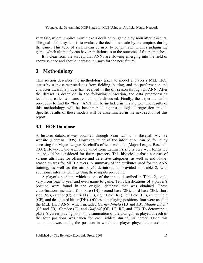
A historic database was obtained through Sean Lahman’s Baseball Archive website (Lahman, 1995). However, much of the information can be found by accessing the Major League Baseball’s official web site (Major League Baseball, 2007). However, the archive obtained from Lahman’s site is very well formatted and should be considered for future projects. This historic database consists of various attributes for offensive and defensive categories, as well as end-of-the-season awards for MLB players. A summary of the attributes used for the ANN training, as well as the attribute’s definition, is provided in Table 2, with additional information regarding these inputs preceding. A player’s position, which is one of the inputs described in Table 2, could vary from year to year and even game to game. Ten classifications of a player’s position were found in the original database that was obtained. These classifications included; first base (1B), second base (2B), third base (3B), short stop (SS), catcher (C), outfield (OF), right field (RF), left field (LF), center field (CF), and designated hitter (DH). Of these ten playing positions, four were used in the MLB HOF ANN, which included Corner Infield (1B and 3B), Middle Infield(SS and 2B), Catcher (C), and Outfield (OF, LF, RF, and CF). To determine a player’s career playing position, a summation of the total games played at each of the four positions was taken for each athlete during his career. Once this summation was made, the position in which the player played the maximum

17

Young et al.: Determining HOF Status for MLB Using an Artificial Neural Network

Published by The Berkeley Electronic Press, 2008

number of games was determined to be his career playing position. Since many of the attributes for the players used in the MLB HOF ANN involve fielding statistics, any player who was assigned with the designated hitter playing position was removed from the sample. Another reason to reduce the playing positions down to four was to promote network generalization by keeping the number of natural input clusters small. Thus, if many of the binary inputs were used to distinguish the playing position, the network’s performance would suffer.

Table 2: Historic MLB Career Dataset Summary Inputs Description Min. Avg. Max. Std. debut First year in MLB 1939 1967 1986 12 POS(Middle Infield) Second base or Shortstop 0 0.3 1 0.4 POS(Catcher) Catcher 0 0.1 1 0.2 POS(Outfield) Right field, Center field, or Leftfield 0 0.4 1 0.5 POS(Corner Infield) First base or Third base 0 0.3 1 0.4 G Games played 1783 2373 3308 328 AB At-bats 6187 8589 12364 1280 R Runs 769 1264 2174 278 H Hits 1626 2417 3771 442 2B Doubles 177 408 725 101 3B Triples 6 68 177 34 HR Home Runs 14 293 755 170 RBI Runs-batted-in 458 1218 2297 383 SB Stolen-bases 12 171 938 176 CS Caught stealing 8 78 307 51 BB Base-on-balls 375 973 2021 377 SO Strike outs 216 1167 2597 413 IBB intentional base-on-balls 15 112 293 61 HBP Hit-by-pitch 9 50 198 32 SH Sacrifice hit 0 50 214 51 SF Sacrifice fly 18 76 128 26 GIDP Grounded into double play 62 199 350 62 PO Put outs 1555 6010 21265 4061 A Assists 60 2792 8375 2673 E Errors 41 187 388 94 DP Double Plays 8 659 2034 592 PB Passed Balls 0 7 182 28 Performance Awards Recognition for on-the-field play 0 6 20 5 Character Awards Recognition for Personality, Service, etc. 0 1 3 1

Two award categories were used for the MLB HOF ANN, which included a category for performance and one for character. Both Performance and Character Award inputs are calculated to be the sum of the respective award received by a player during his career. Short descriptions and the classifications of each award used in this study are shown in Table 3.

18

Journal of Quantitative Analysis in Sports, Vol. 4 [2008], Iss. 4, Art. 4

http://www.bepress.com/jqas/vol4/iss4/4

Table 3: Individual Major League Baseball Awards

Name Description Performance

Award Character Award

ALCS MVP Player who most contributes to his team's success in the American League Championship Series

X

AS MVP Player who most contributes to his team's success in the All-Star Game X

Babe Ruth Award

Player with the best performance in the World Series X

Branch Rickey Award

Player in recognition of their exceptional community service X

Gold Glove Best fielder at a position X

Hank Aaron Award Best offensive performer X

Hutch Award Player who best exemplifies the fighting spirit and competitive desire to win X

Lou Gehrig Memorial Award

Players who best exemplify character and integrity both on and off the field X

Major League Player of the Year

Player who has the most outstanding season regardless of position or league X

MVP Player who most contributes to his team's success in the season X

NLCS MVP Player who most contributes to his team's success in the National League Championship Series

X

Roberto Clemente Award Player in recognition of his charitable activities X

Rookie of the Year Best first year player X

Silver Slugger Best offensive player at each position X

Triple Crown Seasonal leader in homeruns, runs batted in, and batting average X

WS MVP Player who most contributes to his team's success in the World Series X

3.2 Data Preprocessing

The original database was reduced in sample size by several conditions that were pre-determined to avoid potential problems. The initial conditions (or rules) for player removal are shown in Table 4. The first rule was to allow only non-pitchers in the database. The second was to eliminate all players who were classified as

19

Young et al.: Determining HOF Status for MLB Using an Artificial Neural Network

Published by The Berkeley Electronic Press, 2008

designated hitters for their career. The third condition is that a player must have played in 10 Major League Championship seasons to be eligible for HOF candidacy, which adhere to the BBWAA rules (Baseball Writers Association of America, 2007). Another condition was to remove players that are at least five years removed from playing, since there has not been a final determination on their induction to the HOF. Likewise, players were removed from the databases that currently are still eligible for candidacy, because their HOF status has yet to be defined. Finally, players were eliminated from the research if they did not finish their careers before 1960.

In many instances of ANN research, analyses are hampered by insufficient sample sizes in databases (Bui, 2004). From the dataset collected, the probability of a given player (who is not a pitcher) reaching the HOF is roughly 1% for all players who ever played in MLB. The probability only increases to a chance of 4.8% for players who are eligible to be selected into the HOF. Thus, the ANN is asked to classify correctly a very small portion of the represented data, which causes problems in determining the parameters of the ANN. This type of problem is known as an imbalanced dataset.

Table 4: Conditions for Training (Cross-validation) Dataset

Condition Description

1 Position must NOT be a pitcher

2 Position must NOT be designated hitter

3 Must have played in 10 seasons

4 Must be 5 years removed from MLB by 2006

5 Must not be current candidates

6 Must have finished their career after 1960

An imbalanced dataset causes an ANN to classify the data into the majority class, which in this case are non-HOF members. In order to encourage the ANN to train effectively, the dataset was further reduced in order to lessen the disparity between non-HOF and HOF proportions. Few techniques exist in research to deal with imbalanced data. Duplicating sample instances that are underrepresented offers one possible solution to improve the accuracy of classification prediction (DeRouin et al., 1991). Another possibility is to create artificially data in the training data sets (Guo and Viktor, 2004). However, this research implements a method to correct the imbalance dataset problem using k-means clustering.

20

Journal of Quantitative Analysis in Sports, Vol. 4 [2008], Iss. 4, Art. 4

http://www.bepress.com/jqas/vol4/iss4/4

3.3 k-means Reduction

K-means is an unsupervised learning algorithm, which clusters data into similar groups. When the integer k is assumed, the goal of this algorithm is to determine kcenters (centroids), which represent the classification of a given sample. The centroids are initially placed as far away from one another. Once these centers are positioned, each sample is associated with the nearest centroid. The centroids are finalized when the algorithm locates positions that minimize an objective function, which is often the sum of the squared error of the distance between a database and the data point’s center cluster. The one downfall of this method is that there is no general theoretical solution as to the number of k, which is optimal for a given dataset. The use of k-means has been applied to databases in order to increase the predicting accuracy of an ANN by reducing the number of samples in a dataset, which decreases the computational complexity for training (Faraoun and Boukelif, 2005). Faraoun and Boukelif eliminated samples in a dataset by maximizing covered regions in N-dimensional space based on the distance from a sample and the center of its centroid. In order to reject a sample from the dataset, the distance must be larger than a minimum distance, which was determined experimentally. For the research presented in this paper, the role of k-means is similar to the intent of Faraoun and Boukelif’s research. The goal for this research is to remove samples from the majority class (i.e. non-HOF), while keeping members of the inferior class (i.e. HOF) (Cohen, et al., 2006). With this strategy, the goal is to maximize the covering region of players who are similar to HOF members in N-dimensional space to balance the dataset. Once k has been assumed and the associations have been made, samples classified into centroids without HOF members are removed. This process is repeated until there are only centroids classified with at least one member in the HOF class. For this procedure, k should be small. If k is too large, it is possible that the once initial inferior class would become the dominant class, which is not desired. Thus, applying the iterative process with a small k value will converge to a balanced dataset slowly, but the ill effects of “over” balancing are avoided. If an iterative step is performed where removing clusters would result in the inferior class (i.e. HOF) becoming the dominant class, the k-means balancing procedure should be stopped at that point. An example of using k-means to reduce and balance a sample dataset is shown below in Figure 9. For this example, k is equal to three. Centroids 1 and 2 both contain HOF and non-HOF members. No samples from either of these clusters would be removed in order to balance the dataset initially. However, Centroid 3 only contains non-HOF classifications, which are all of the inferior class type. Thus, all of the samples found in this cluster would be removed. Initially, the

21

Young et al.: Determining HOF Status for MLB Using an Artificial Neural Network

Published by The Berkeley Electronic Press, 2008

dataset contained 227 samples, where 22% of the samples were of the inferior class. Removing 98 samples resulted in a total sample size of 129. Therefore, applying this balancing procedure resulted in 48% of the sample population being HOF members. The new database is more balanced which will allow data mining algorithms to be used to better distinguish between the two classifications.

Figure 9: K-means Balancing

After reducing the dataset with the criterion found in Table 4, the k-means balancing procedure was performed with 10 clusters. Table 5 provides a summary of non-HOF and HOF members of the centroids (or clusters) found from the initial k-means analysis. Centroids not containing HOF members (3, 6, 7, 8, and 10) were removed from the dataset. After this reduction, the process is repeated on the remaining dataset. This breakdown is found in Table 6, where the next set of clusters was removed (2, 5, 7, and 9).

Centroid 1: Non HOFCentroid 1: HOFCentroid 2: Non HOFCentroid 2: HOFCentroid 3: Non HOF

22

Journal of Quantitative Analysis in Sports, Vol. 4 [2008], Iss. 4, Art. 4

http://www.bepress.com/jqas/vol4/iss4/4

Table 5: 1st Iteration Table 6: 2nd Iteration

Centroid non-HOF HOF Total 1 73 5 78 2 4 18 22 3 99 0 99 4 144 1 145 5 32 18 50 6 93 0 93 7 128 0 128 8 61 0 61 9 42 1 43 10 133 0 133 Total 809 43 852 Percentage 95% 5%

Centroid non-HOF HOF Total 1 3 17 20 2 42 0 42 3 45 2 47 4 19 12 31 5 55 0 55 6 16 9 25 7 65 0 65 8 9 2 11 9 31 0 31 10 10 1 11 Total 295 43 338 Percentage 87% 13%

The k-means process is repeated to check if any new clusters will result in a cluster that does not contain HOF members. Table 7 and Table 8 show the results of the k-means balancing procedure for the third and fourth iteration respectively.

Table 7: 3rd Iteration Table 8: 4th Iteration

Centroid non-HOF HOF Total 1 3 12 15 2 26 0 26 3 16 8 24 4 2 2 4 5 10 0 10 6 17 4 21 7 3 8 11 8 1 4 5 9 11 4 15 10 13 1 14 Total 102 43 145 Percentage 70% 30%

Centroid non-HOF HOF Total 1 3 12 15 2 16 7 23 3 2 2 4 4 3 7 10 5 11 4 15 6 2 6 8 7 14 0 14 8 1 2 3 9 0 2 2 10 14 1 15 Total 66 43 109 Percentage 61% 39%

The fifth and final iteration of the balancing procedure is shown in Table 9. The entire balancing process reduced the original dataset to 89% of its original sample size. This resulted in a HOF representation from 5% to 45%, where the disproportion between HOF members to non-HOF players is vastly improved.

23

Young et al.: Determining HOF Status for MLB Using an Artificial Neural Network

Published by The Berkeley Electronic Press, 2008

Table 9: 5th (Final) Iteration

Centroid non-HOF HOF Total 1 7 1 8 2 5 2 7 3 3 4 7 4 2 7 9 5 9 5 14 6 0 3 3 7 1 1 2 8 3 3 6 9 10 11 21 10 12 6 18 Total 52 43 95 Percentage 55% 45%

3.4 MLB HOF ANN

After the k-means balancing has been executed using the original imbalanced dataset, the ANN experimental procedure is performed. The balanced dataset (described in Table 9) was divided randomly into three subsets of data, which was used for training, cross-validation, and testing. The percentage breakdown of this data was 60%, 20%, and 20% respectively. A considerable amount of experimentation is needed to determine the “best” classification network. The results of each experimental procedure will not be discussed in detail for brevity. However, several networks were tested, which varied in network topologies, number of hidden layers, number of processing elements, activation function types, and learning algorithms. A summary of the accuracies found in Table 10.

24

Journal of Quantitative Analysis in Sports, Vol. 4 [2008], Iss. 4, Art. 4

http://www.bepress.com/jqas/vol4/iss4/4

Table 10: Experimental ANN Summary T

rial

Top

olog

y

#of H

idde

n L

ayer

s

Net

wor

k A

ctiv

atio

n Fu

nctio

ns

Lea

rnin

g M

etho

d

Tra

inin

g %

Cor

rect

Cro

ss-

Val

idat

ion

%C

orre

ct

Tes

ting

%C

orre

ct

All

%C

orre

ct

1 GFF 20 Sigmoid Conjugant Gradient 91% 84% 79% 87% 2 GFF 4 Sigmoid Conjugant Gradient 93% 84% 79% 88% 4 MLP 3 Tanh Momentum 93% 84% 79% 88% 3 GFF 4-4 Tanh Levenberg-Marquardt 100% 79% 68% 89% 5 MLP 50-10-5 Tanh Levenberg-Marquardt 98% 96% 71% 90% 6 MLP 14 Tanh Momentum 71% 92% 100% 90% 7 GFF 10-5 Sigmoid Conjugant Gradient 71% 92% 100% 90% 8 GFF 5-2 Sigmoid Conjugant Gradient 93% 87% 84% 91% 9 GFF 5-5 Sigmoid Levenberg-Marquardt 98% 95% 68% 92% 10 MLP 10-5 Sigmoid Momentum 100% 92% 79% 93% 11 GFF 4-4-4 Tanh Conjugant Gradient 100% 100% 75% 94% 12 GFF 50-30-10 Sigmoid Momentum 100% 100% 75% 94% 13 GFF 4-4-4 Tanh Conjugant Gradient 100% 92% 83% 94% 14 GFF 75-25-5 Tanh Conjugant Gradient 96% 96% 88% 94% 15 GFF 5-10-5 Tanh Conjugant Gradient 100% 100% 79% 95% 16 GFF 64-5 Sigmoid Momentum 100% 100% 79% 95% 17 MLP 55-5-4 Tanh Conjugant Gradient 100% 96% 83% 95% 18 MLP 85-10-5 Tanh Conjugant Gradient 100% 96% 83% 95% 19 GFF 7-10-6 Tanh Levenberg-Marquardt 100% 96% 83% 95% 20 MLP 16-4 Tanh Levenberg-Marquardt 100% 100% 89% 95% 21 MLP 94-30-10 Sigmoid Levenberg-Marquardt 100% 96% 88% 96% 22 GFF 150-20 Tanh Momentum 100% 96% 88% 96% 23 MLP 32-4-4 Tanh Levenberg-Marquardt 100% 100% 89% 96% 24 MLP 80-40 Tanh Conjugant Gradient 100% 100% 89% 98% 25 MLP 20-5 Tanh Conjugant Gradient 100% 100% 89% 98%

A generalized form of the “best” network found in the experimental process is shown in Figure 10. The input layer consists of a player’s batting, fielding, and awards statistics. The network in this figure is a multi-layered perceptron (MLP) ANN that consists of two hidden layers, where the first layer has 20 processing elements and the second hidden-layer has 5. Each of the MLP’s hidden layer nodes implements a hyperbolic tangent activation function as shown in the figure. The final output layer implements a linear function, which is considered a good practice for predicting future observations (Principe et al., 2000).

25

Young et al.: Determining HOF Status for MLB Using an Artificial Neural Network

Published by The Berkeley Electronic Press, 2008

Figure 10: Generalized MLB HOF ANN

4 Results The following section presents the results of the benchmark method (binary logistic regression) as well as specific details for the MLB HOF ANN. After assessing the model’s performance on the three subsets of data, a sensitivity analysis is carried out to determine key input parameters of the model. After identifying significant input parameters, the ANN model is used to predict two additional player groups not found in the training, cross-validation, or testing datasets. These players were either retired and are still being voted on by the HOF Committee or are players who are not yet eligible for HOF induction.

4.1 Logistic Regression

Logistical regression is a popular choice when modeling binary variables because it has been proven to result in fewer classification errors than other statistical methods such as discriminate analysis (Fienberg, 1987). This is because discriminate analysis has many assumptions based on normal distributions and ideal covariance matrices (Press and Wilson, 1978). Many studies using discriminate analysis rely on an assumption of multivariate normality; however, qualitative attributes, such as a player’s position, can potentially violate these

26

Journal of Quantitative Analysis in Sports, Vol. 4 [2008], Iss. 4, Art. 4

http://www.bepress.com/jqas/vol4/iss4/4

assumptions. Thus, logistical regression will be used to benchmark the MLB HOF ANN derived in this study. Binary (binomial) logistic regression is a form of regression where the dependent value being modeled is dichotomous, where the independent values can be of any form. The model predicts a probability of an event or classification occurring along a logistical (or sigmoid) curve. An iterative reweighted least squares algorithm can used to obtain the maximum likelihood estimates, which are used to determine the intercept and factors of the model (McCullagh and Nelder, 1992). The functional form of logistic regression is very similar to an ANN with one hidden layer that contains one logistical sigmoid processing element. The only difference between the two models is how the weights are derived. In both models, a weighted sum is taken of the input parameters and the coefficients, an intercept (bias) is added to this sum, and then placed in an activation function (sigmoid).

The results of applying logistic regression is shown in Table 11, where Inducted(Y) represents a HOF member and Inducted(N) represents a player who was not elected into the HOF. The table shows the results in confusion matrix form, where the top section is read as actual, and the side heading are read as estimates. Therefore, the values along the diagonal part of the matrix are forecasted correctly and the values not in the diagonal are misclassified. The results of the logistic model produce an overall accuracy of 100% for the training data, which is shown in Table 11. However, the model was applied to the cross-validation and testing datasets and the accuracy was significantly lower with an overall accuracy of 79%. This suggests that the statistical model was not able to generalize the system adequately.

Table 11: a) Training b) Cross-validation and Testing Logistic Performances Training Output / Desired

Inducted (N)

Inducted (Y)

C-V & Testing Output / Desired

Inducted (N)

Inducted (Y)

Inducted (N) 33 0 Inducted

(N) 13 3

Inducted (Y) 0 23 Inducted

(Y) 5 17

%Correct 100% 100% %Correct 72% 85%

4.2 Artificial Neural Network

The network that produced the highest accuracy (as indicated in Table 10) was a MLP ANN with two hidden layers. Levenberg-Marquardt learning algorithm was used to determine the network weights. This algorithm was given a maximum

27

Young et al.: Determining HOF Status for MLB Using an Artificial Neural Network

Published by The Berkeley Electronic Press, 2008

epoch number of 5000, but the learning stopped around 200. A summary of training procedure is shown in Figure 11.

Figure 11: Average MSE for Final MLB HOF ANN The training data set and cross-validation data sets were tested to determine the accuracy of the adaptive learning process. The resulting test yielded the data given in Table 12a) for the training data set and Table 12b) for the cross-validation and testing set. This table shows 95% accuracies in predicting Inducted(Y) for both the training, cross-validation and testing data sets.

Table 12: a) Training b) Cross-validation & Testing ANN Performances

Training Output / Desired

Inducted (N)

Inducted (Y)

C-V & Testing Output / Desired

Inducted (N)

Inducted (Y)

Inducted (N) 33 0 Inducted

(N) 17 1

Inducted (Y) 0 23 Inducted

(Y) 1 19

%Correct 100% 100% %Correct 95% 95% Table 13 shows the predicting accuracies using the entire dataset for the logistic regression and ANN models. The results show about a 6% increased predicting accuracy using the ANN over the regression model.

0

0.2

0.4

0.6

0.8

1

1 100 199 298 397 496 595 694 793 892 991

Aver

age

MSE

Epoch

TrainingCross Validation

28

Journal of Quantitative Analysis in Sports, Vol. 4 [2008], Iss. 4, Art. 4

http://www.bepress.com/jqas/vol4/iss4/4

Table 13: a) L

All Data Output / Desired

Inducte(N)

Inducted (N) 46

Inducted (Y) 5

%Correct 93% 4.3 Sensitivity Anal

Sensitivity analysis quanmodel. Figure 12 shows when compared to the omean and 50 steps-per-sinsight as to why a cerAccording to the sensitivPos(Outfield), Pos(CornSacrifice Flies, and Char

Figure 12: In

0.000.050.100.150.200.250.300.35

debu

tPO

S(M

iddl

e In

field

)PO

S(C

atch

er)

POS(

Out

field

)PO

S(C

orne

r Inf

ield

) G

Sens

itivi

tyLogistic Regression and b) ANN Performances

ed Inducted (Y)

All Data Output / Desired

Inducted (N)

3 Inducted (N) 50

40 Inducted (Y) 1

90% %Correct 98%

lysis

ntifies the relative importance of input parame the relative importance that the input parame

output estimation using ±1 standard deviation side. The more sensitive inputs can be used tortain player should or should not be a HOF vity analysis, the eight most sensitive variablesner Infield), debut, H, Performance Awardsracter Awards.

nput Sensitivity Analysis for MLB HOF ANN

GA

B R H 2B 3B HR

RB

ISB C

SB

B SO IBB

HB

PSH SF

GID

PPO A ED

PPB

Input Name

Inducted(N)Inducted(Y)

Inducted (Y)

1

42

98%

eters in a eters have about the o provide member.

s include; s, Errors,

PBPe

rfor

man

ce A

war

dsC

hara

cter

Aw

ards

29

Young et al.: Determining HOF Status for MLB Using an Artificial Neural Network

Published by The Berkeley Electronic Press, 2008

Two of the eight most influential input variables indicate a player’s position. These unary-encoded values are believed to represent the differences in which the voters hold playing positions to when voting on HOF candidacy. For example, voters will typically have evaluated an Outfielder’s offensive production more stringently than Catchers or Middle-infielders. However, these same voters might place more importance for the defensive categories for Catchers and Middle-infielders. Since the ANN uses all of the inputs for the evaluation, the position inputs act as binary discriminators in the model. Thus, the weights associated with these input values attempt to explain the differences in how the voters evaluate one’s HOF candidacy. The remainder of the inputs used in the model have continuous or integer values (i.e. not binary). Therefore, when the sensitivity results are obtained for these non-binary values, each of the playing positions is held to their mean (0.5). The remainder of the sensitivity analysis attempts to explain voting behavior for an “average” player. The most sensitive input that does not explain a player’s playing position is debut. The significance of this attribute is not surprising; due in part to the reasons why MLB has experienced “inflated” statistics over the past few decades. When debut is varied by ±1 standard deviations from the mean, the results show an intersecting point around 1962 in Figure 14. Thus, an average player before this year is more likely to be a HOF member than after this point. The change in this probability could be thought of as a rate that inflated statistics have on HOF candidacy. Thus, present players must obtain higher offensive, defensive, and awards benchmarks than players in the past to become a member of the HOF.

Figure 13: Sensitivity Analysis for Awards

0

0.2

0.4

0.6

0.8

1

1950 1956 1962 1968 1974 1980 1986

Out

put(

s)

Varied Input debut

Inducted(N)Inducted(Y)

30

Journal of Quantitative Analysis in Sports, Vol. 4 [2008], Iss. 4, Art. 4

http://www.bepress.com/jqas/vol4/iss4/4

Table 14 is provided to reiterate the non-linear time component variable (debut) of the ANN. For example, Jose Canseco’s career started in 1985. Mr. Canseco significantly lacked the adequate career statistics to make the HOF according to the voting results in the 2007 election (NBHOF, 2007) and the forecast made from the ANN. However, if Canseco’s debut year could hypothetically be changed, there should be a point in which his career attributes would warrant his enshrinement into the HOF. For example, Table 14 shows the prediction when only his debut year was varied from 1944 to 1949. This table shows that if Mr. Canseco’s debut year were 1946 instead of 1985, he would be enshrined into HOF.

Table 14: Jose Canseco Output(s) for Varied Debut Year

Start Year Position Inducted(N) Inducted(Y)1949 Outfield 0.65 0.35 1948 Outfield 0.60 0.4 1947 Outfield 0.54 0.46 1946 Outfield 0.48 0.52 1945 Outfield 0.42 0.58 1944 Outfield 0.36 0.64

Figure 14 shows the sensitivity results of hits (H), which has an intersecting point around 2,600 career hits. Thus, a player significantly increases their chances of HOF induction after this point. This figure also implies that a player can almost certainly be enshrined in the HOF after reaching the 3,000 career hit plateau.

Figure 14: Sensitivity Analysis for Hits The sensitivity results for a varied Performance Award value is shown in

0.0

0.2

0.4

0.6

0.8

1.0

1800 2000 2200 2400 2600 2800 3000

Out

put(

s)

Varied Input H

Inducted(N)Inducted(Y)

31

Young et al.: Determining HOF Status for MLB Using an Artificial Neural Network

Published by The Berkeley Electronic Press, 2008

Figure 15. The point at which Induction(Y) and Induction(N) met is around nine awards.

Figure 15: Sensitivity Analysis for Performance Awards

The sensitivity result for Error is shown in Figure 16. This figure shows that a player will decrease his chances of becoming a member of the HOF with each error he makes on the field. The intersecting point, which occurs at an output probability of 0.5, is around 130 errors. Thus, if a player is able to keep his error total down below this value, his chances of reaching the HOF is high.

Figure 16: Sensitivity Analysis for Errors

0

0.2

0.4

0.6

0.8

1

0 2 4 6 8 10 12

Out

put(

s)

Varied Input Performance Awards

Inducted(N)Inducted(Y)

0

0.2

0.4

0.6

0.8

1

75 125 175 225 275 325

Out

put(

s)

Varied Input E

Inducted(N)Inducted(Y)

32

Journal of Quantitative Analysis in Sports, Vol. 4 [2008], Iss. 4, Art. 4

http://www.bepress.com/jqas/vol4/iss4/4

4.4 Correlation Matrix

Another common issue with machine learning models is correlated data. The occurrence of heavily correlated data can cause an increase in the amount of time and experimental work needed to create a good model. All of the input values were used to calculate the correlations values. Table 15 shows the correlation values of inputs that have strong associations with other input values. For a parameter to appear in this table, a correlation must be greater than 0.75 or less than -0.75.

MI C OF G AB R H 2B HR RBI A E PB

MI 1.0 C -0.1 1.0 O -0.5 -0.2 1.0 G -0.1 0.0 0.1 1.0 AB -0.1 -0.1 0.1 0.9 1.0 R -0.2 -0.1 0.3 0.8 0.8 1.0 H -0.2 -0.1 0.2 0.8 0.9 0.8 1.0 2B -0.2 0.0 0.2 0.7 0.8 0.7 0.8 1.0 HR -0.6 0.1 0.3 0.4 0.3 0.5 0.3 0.4 1.0 RBI -0.6 0.1 0.3 0.6 0.5 0.6 0.5 0.7 0.9 1.0 A 0.8 -0.2 -0.8 0.0 0.0 -0.2 -0.1 -0.2 -0.5 -0.5 1.0 E 0.5 -0.1 -0.8 0.1 0.1 -0.1 -0.1 -0.1 -0.3 -0.3 0.8 1.0 PB -0.2 0.9 -0.2 0.0 -0.1 -0.1 -0.1 0.0 0.0 0.1 -0.2 -0.1 1.0

Table 15: Partial Correlation Matrix of Input Parameters

4.5 Retired Player Forecasts

Two misclassifications were made in the testing dataset. These errors are shown in Table 16, where the name of the player who was misclassified as well as the predicted values for Inducted (N) and Inducted(Y) is provided. A “delta” value is also shown in this table. This value attempts to quantify the certainty of the predicted classification by taking the difference of Induction (Y) and Induction (N). Thus, this measurement gives an indication how far the estimate of induction and exclusion is from one another. Therefore, the lower the delta value is, the less certainty should be placed on ANN prediction. Likewise, the higher the delta value is, the more significance should be placed on the estimate. There were two different types of errors found in the testing dataset. The first type of error is when a player has been denied status into the HOF, but the ANN

33

Young et al.: Determining HOF Status for MLB Using an Artificial Neural Network

Published by The Berkeley Electronic Press, 2008

predicted his enshrinement. The second error occurred when the ANN did not predict induction into the HOF, but was voted in by the HOF committee. The actual voting percentages on these players are shown in the following table (NBHOF, 2007).

Table 16: ANN Forecasts for Retired Players

Name Start Year Position Inducted

(N) Inducted (Y) Delta

Last Year Voted

%Voting

Garvey, Steve 1969 Corner

Infield 0.01 0.99 0.98 2007 21%

Aparicio, Luis 1956 Middle

Infield 0.81 0.19 -0.62 1984 85%

Steve Garvey received considerably less than the necessary votes required for HOF membership; however, a further investigation of his career statistics might explain why this misclassification occurred. Table 17 is provided to compare Garvey’s career with other players who were inducted into the HOF at the Corner Infield position as well as a player that most resembled his career statistics in terms of N-dimensional space using the k-means centroid analysis.

Table 17: Garvey vs. HOF and Perez

Group/Player Ind.(Y) debut H PA E SF CA Garvey, Steve 0 1969 2599 9 130 90 2 Avg. HOF 1 1964 2653 7 251 93 1 Perez, Tony 1 1964 2732 1 240 106 1

%of Avg. HOF N/A 0.3% -2.1% 27.8% -92.7% -2.9% 58.3% %of Tony Perez N/A 0.3% -5.1% 88.9% -84.6% -17.8% 50.0%

The number of Hits a player has over his career is one of the most sensitive input attribute to the model. For this attribute, Garvey trails in the number of hits for an average HOF Corner Infielder. He also has less total career hits than Toney Perez, which was the player “closest” to Garvey according to the k-means analysis. The differences between attributes seem small when compared to other HOF members; however, Garvey’s performance in two other highly sensitive input attribute might suggest that he should have been inducted into the HOF. Garvey compiled nine Performance Awards over his career, which included All-Star MVP (2), Gold Glove (4), League MVP (1), and NLCS MVP (2). According to the sensitivity analysis shown in Figure 15, a player considerably

34

Journal of Quantitative Analysis in Sports, Vol. 4 [2008], Iss. 4, Art. 4

http://www.bepress.com/jqas/vol4/iss4/4

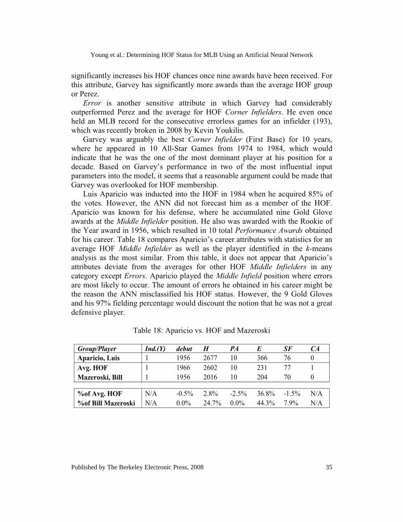
significantly increases his HOF chances once nine awards have been received. For this attribute, Garvey has significantly more awards than the average HOF group or Perez. Error is another sensitive attribute in which Garvey had considerably outperformed Perez and the average for HOF Corner Infielders. He even once held an MLB record for the consecutive errorless games for an infielder (193), which was recently broken in 2008 by Kevin Youkilis. Garvey was arguably the best Corner Infielder (First Base) for 10 years, where he appeared in 10 All-Star Games from 1974 to 1984, which would indicate that he was the one of the most dominant player at his position for a decade. Based on Garvey’s performance in two of the most influential input parameters into the model, it seems that a reasonable argument could be made that Garvey was overlooked for HOF membership. Luis Aparicio was inducted into the HOF in 1984 when he acquired 85% of the votes. However, the ANN did not forecast him as a member of the HOF. Aparicio was known for his defense, where he accumulated nine Gold Glove awards at the Middle Infielder position. He also was awarded with the Rookie of the Year award in 1956, which resulted in 10 total Performance Awards obtained for his career. Table 18 compares Aparicio’s career attributes with statistics for an average HOF Middle Infielder as well as the player identified in the k-means analysis as the most similar. From this table, it does not appear that Aparicio’s attributes deviate from the averages for other HOF Middle Infielders in any category except Errors. Aparicio played the Middle Infield position where errors are most likely to occur. The amount of errors he obtained in his career might be the reason the ANN misclassified his HOF status. However, the 9 Gold Gloves and his 97% fielding percentage would discount the notion that he was not a great defensive player.

Table 18: Aparicio vs. HOF and Mazeroski Group/Player Ind.(Y) debut H PA E SF CA Aparicio, Luis 1 1956 2677 10 366 76 0 Avg. HOF 1 1966 2602 10 231 77 1 Mazeroski, Bill 1 1956 2016 10 204 70 0

%of Avg. HOF N/A -0.5% 2.8% -2.5% 36.8% -1.5% N/A %of Bill Mazeroski N/A 0.0% 24.7% 0.0% 44.3% 7.9% N/A

35

Young et al.: Determining HOF Status for MLB Using an Artificial Neural Network

Published by The Berkeley Electronic Press, 2008

4.6 Recently Retired Player Forecasts

The players found in Table 19 are players that are recently retired, have been removed from active playing status for at least 5 years, but are still being voted on by the HOF committee. Therefore, since no determination was made on these players’s HOF status, they were excluded from the training, cross-validation, and testing datasets.

Table 19: ANN Forecasts for Recently Retired Player

Name Start Year Position Ind. (N) Ind. (Y) Delta

Last Year Voted

%Voting

Hernandez, Keith 1974

Corner Infield 0.01 0.99 0.98 2004 43%

Mattingly, Don 1982

Corner Infield 0.03 0.97 0.95 2008 16%

In terms of Performance Awards, Hernandez has had an exemplary career. Hernandez collected 11 consecutive Gold Glove Awards at first base. He is also a five-time All-Star selection with one NL MVP (1979) Award. Hernandez played in seven seasons where his batting average was over 0.300 and finished his career with a 0.296 average. There were only two seasons where Hernandez finished a season as the league’s leader in any offensive category. Aside from defensive awards that Hernandez received, his career performance in offensive categories do not compare to other HOF members that played at the Corner Infield position. In comparison to these players, Table 20 shows that Hernandez had less Hits and Sacrifice Flies, which are correlated with one’s ability to drive in runs. Voters for the HOF might have overlooked his defensive play at the Corner Infield position and determined that his career offensive attributes were not sufficient to be enshrined. Thus, the misclassification might have occurred due to the extremely high number of (defensive) Performance Awards Hernandez obtained.

Table 20: Hernandez vs. HOF

Group/Player Ind. (Y) debut H PA E SF CA Avg. HOF 1 1964 2653 7 251 93 1 Hernandez, Keith 0 1974 2182 14 115 71 0

%of Avg. HOF N/A 0.5% -21.6% 53.6% -117.8% -30.4% N/A

36

Journal of Quantitative Analysis in Sports, Vol. 4 [2008], Iss. 4, Art. 4

http://www.bepress.com/jqas/vol4/iss4/4

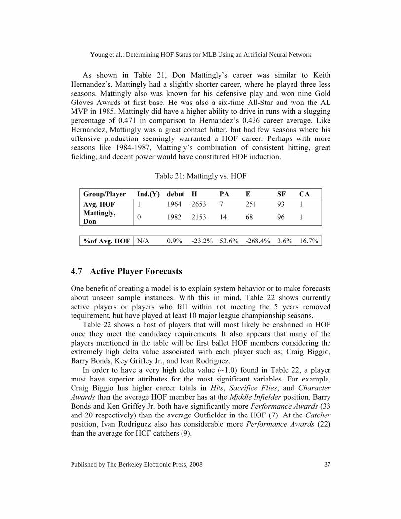
As shown in Table 21, Don Mattingly’s career was similar to Keith Hernandez’s. Mattingly had a slightly shorter career, where he played three less seasons. Mattingly also was known for his defensive play and won nine Gold Gloves Awards at first base. He was also a six-time All-Star and won the AL MVP in 1985. Mattingly did have a higher ability to drive in runs with a slugging percentage of 0.471 in comparison to Hernandez’s 0.436 career average. Like Hernandez, Mattingly was a great contact hitter, but had few seasons where his offensive production seemingly warranted a HOF career. Perhaps with more seasons like 1984-1987, Mattingly’s combination of consistent hitting, great fielding, and decent power would have constituted HOF induction.

Table 21: Mattingly vs. HOF

Group/Player Ind.(Y) debut H PA E SF CA Avg. HOF 1 1964 2653 7 251 93 1 Mattingly, Don 0 1982 2153 14 68 96 1

%of Avg. HOF N/A 0.9% -23.2% 53.6% -268.4% 3.6% 16.7%

4.7 Active Player Forecasts

One benefit of creating a model is to explain system behavior or to make forecasts about unseen sample instances. With this in mind, Table 22 shows currently active players or players who fall within not meeting the 5 years removed requirement, but have played at least 10 major league championship seasons.

Table 22 shows a host of players that will most likely be enshrined in HOF once they meet the candidacy requirements. It also appears that many of the players mentioned in the table will be first ballet HOF members considering the extremely high delta value associated with each player such as; Craig Biggio, Barry Bonds, Key Griffey Jr., and Ivan Rodriguez.

In order to have a very high delta value (~1.0) found in Table 22, a player must have superior attributes for the most significant variables. For example, Craig Biggio has higher career totals in Hits, Sacrifice Flies, and Character Awards than the average HOF member has at the Middle Infielder position. Barry Bonds and Ken Griffey Jr. both have significantly more Performance Awards (33 and 20 respectively) than the average Outfielder in the HOF (7). At the Catcherposition, Ivan Rodriguez also has considerable more Performance Awards (22) than the average for HOF catchers (9).

37

Young et al.: Determining HOF Status for MLB Using an Artificial Neural Network

Published by The Berkeley Electronic Press, 2008

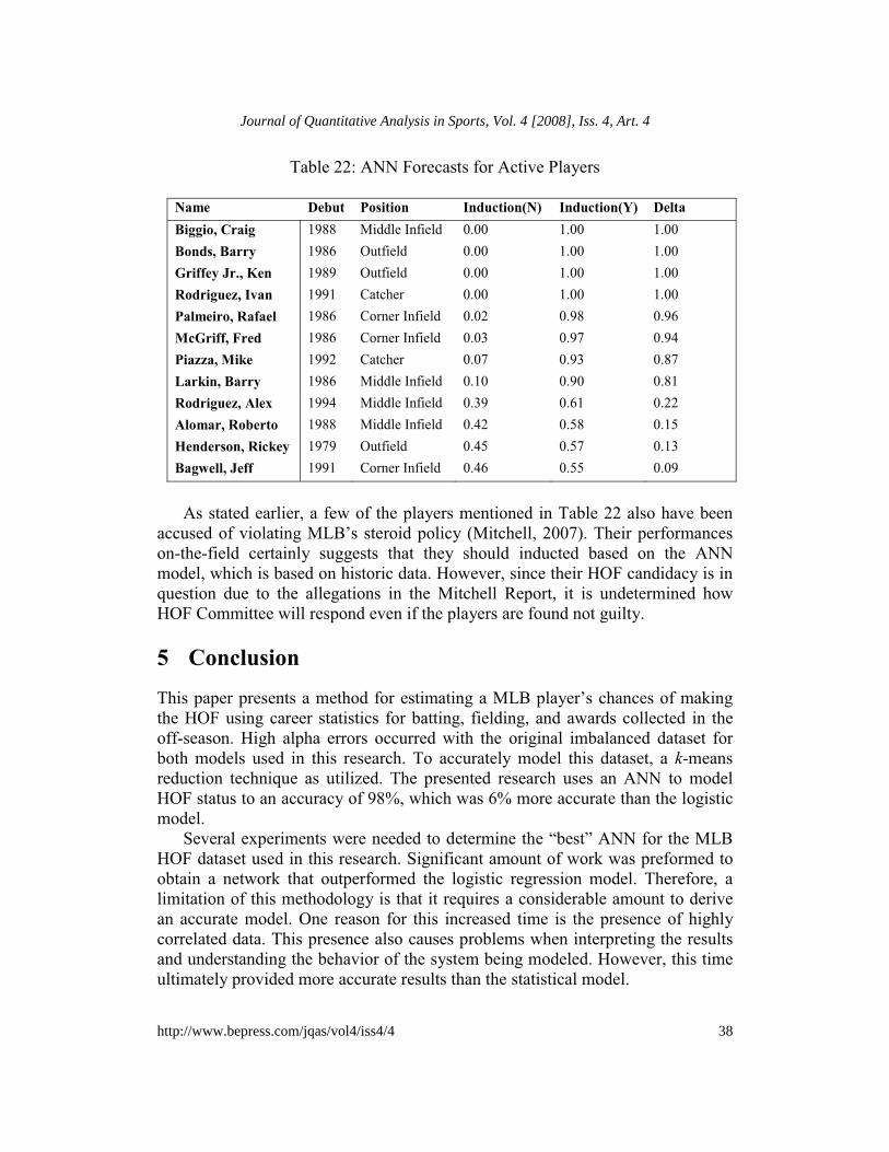
Table 22: ANN Forecasts for Active Players Name Debut Position Induction(N) Induction(Y) Delta Biggio, Craig 1988 Middle Infield 0.00 1.00 1.00 Bonds, Barry 1986 Outfield 0.00 1.00 1.00 Griffey Jr., Ken 1989 Outfield 0.00 1.00 1.00 Rodriguez, Ivan 1991 Catcher 0.00 1.00 1.00 Palmeiro, Rafael 1986 Corner Infield 0.02 0.98 0.96 McGriff, Fred 1986 Corner Infield 0.03 0.97 0.94 Piazza, Mike 1992 Catcher 0.07 0.93 0.87 Larkin, Barry 1986 Middle Infield 0.10 0.90 0.81 Rodriguez, Alex 1994 Middle Infield 0.39 0.61 0.22 Alomar, Roberto 1988 Middle Infield 0.42 0.58 0.15 Henderson, Rickey 1979 Outfield 0.45 0.57 0.13 Bagwell, Jeff 1991 Corner Infield 0.46 0.55 0.09

As stated earlier, a few of the players mentioned in Table 22 also have been

accused of violating MLB’s steroid policy (Mitchell, 2007). Their performances on-the-field certainly suggests that they should inducted based on the ANN model, which is based on historic data. However, since their HOF candidacy is in question due to the allegations in the Mitchell Report, it is undetermined how HOF Committee will respond even if the players are found not guilty. 5 Conclusion This paper presents a method for estimating a MLB player’s chances of making the HOF using career statistics for batting, fielding, and awards collected in the off-season. High alpha errors occurred with the original imbalanced dataset for both models used in this research. To accurately model this dataset, a k-means reduction technique as utilized. The presented research uses an ANN to model HOF status to an accuracy of 98%, which was 6% more accurate than the logistic model. Several experiments were needed to determine the “best” ANN for the MLB HOF dataset used in this research. Significant amount of work was preformed to obtain a network that outperformed the logistic regression model. Therefore, a limitation of this methodology is that it requires a considerable amount to derive an accurate model. One reason for this increased time is the presence of highly correlated data. This presence also causes problems when interpreting the results and understanding the behavior of the system being modeled. However, this time ultimately provided more accurate results than the statistical model.

38

Journal of Quantitative Analysis in Sports, Vol. 4 [2008], Iss. 4, Art. 4

http://www.bepress.com/jqas/vol4/iss4/4

Incorporating sensitivity about the mean analysis is useful when trying to understand voting behavior of the HOF committee. It is also used to provide insight as to why some players might have been misclassified by the model. In terms of this research, the most sensitive attributes were Pos(Outfield), Pos(Corner Infield), debut, H, Performance Awards, Errors, Sacrifice Flies, and Character Awards. When using these results, it appears that the HOF committee does not have a tendency to enshrine players who are solely recognized for their defensive playing abilities. However, these misclassified players also have a tendency to receive many performance-based awards like Golden Gloves. The abundance of these awards might have biased the ANN in predicting these players into the HOF. Another objective for this paper was to provide readers of this journal with an overview of ANNs. A broad discussion was made about the history, topologies, training issues, and methods employed to increase predicting accuracies for ANNs. Though limitations were noted for ANNs, they are slowly being utilized in many complex-modeling environments, where increased accuracies from standard statistical methods are being reported. Thus, it appears that ANNs will emerge in complex modeling problems such as quantitative methods in sports.

References

Bahill, A. T., Freitas, M. M., (1995), Two Methods for Recommending Bat Weights. Annals of Biomedical Engineering , 23 (4), 436-444.

Baseball Writers' Association of America. (2007). BBWAA Rules for Election to the Hall of Fame. Retrieved 2007, from The National Baseball Hall of Fame and Museum: http://web.baseballhalloffame.org/hofers/bbwaa.jsp

BBWAA. (2007). Retrieved 12 17, 2007, from National Baseball Hall of Fame and Museum: http://web.baseballhalloffame.org/hofers/bbwaa.jsp

Bishoop, C. (1995). Neural Networks for Pattern Recongnition, Oxford University Press, USA.

Bracewell, P., Meyer, D., and Ganesh, S. (2003). Creating and Monitoring Meaningful Individual Rugby Ratings. Research Letters in the Information and Mathematical Sciences , 4, 19-22.

Bui, T. D. (2004). Neural network analysis of sparse datasets: An application to the fracture system in folds of the Lisburne formation, Northeastern Alaska.

39

Young et al.: Determining HOF Status for MLB Using an Artificial Neural Network

Published by The Berkeley Electronic Press, 2008

Ph.D. Dissertation, Texas A&M University, Department of Petroleum Engineering, College Station, Texas.

Bukiet, B., Harold, E., and Palacios, J. (1997). A Markov Chain Approach to Baseball. Operations Research , 45, 14–23.

Carter, V., and Machol, R. (1971). Operations research on football. Operations Research , 19, 541-545.

Clapp, C., and Hakes, J. (2005). How long a honeymoon? The effect of new stadiums on attendance in Major League Baseball. Journal of Sports Economics , 6 (3), 237-263.

Cohen, G., et al. (2006). Learning from Imbalanced Data in Surveillance of Nosocomial Infection, Artificial Intelligence in Medicine, 37, 7–18.

Cohen, D. A. (2004). EA-lect: An Evolutionary Algorithm for Constructing Logical Rules to Predict Election into Cooperstown. Congress on Evolutionary Computation, 2, pp. 1354-1361. Portland, OR, USA.

DeRouin, E., Brown, J., Beck, H., Fausett, L., and Schneider, M. (1991). Neural Network Training on Unequally Represented Classes. In C. H. Dagli, S. R. Kumara, and Y. C. Shin, Intelligent Engineering Systems Through Artificial Neural Networks (pp. 135-141). New York: ASME Press.

Desser, A., Monks, J., and Robinson, M. (1999). Baseball Hall of Fame Voting: A Test of the Customer Discrimination Hypothesis. Social Science Quarterly80, 591-603.

Dixan, M., and Coles, S. (1997). Modeling association football scores and inefficiencies in the football betting market. Applied Statistics , 46 (2), 265–280.

Efraim, T., Jay, E. A., Liang, T. P., and McCarthy, R. V. (2001). Decision support systems and intelligent systems. Upper Saddle River, NK: Prentice Hall.

Faraoun, K. M., and Boukelif, A. (2005). Neural Networks Learning Improvement using the K-Means Clustering Algorithm to Detect Network Intrusions. International Journal of Computational Intelligence , 3 (2), 161-168.

40

Journal of Quantitative Analysis in Sports, Vol. 4 [2008], Iss. 4, Art. 4

http://www.bepress.com/jqas/vol4/iss4/4

Fausett, L. (1994). Fundamentals of Neural Networks. Prentice Hall.

Fienberg, S.E. (1987). The Analysis of Cross-Classified Categorical Data. The MIT Press.

Findlay, D.W., and Reid, C.E. (1997). Voting Behavior, Discrimination, and the National Baseball Hall of Fame. Economic Inquiry, 35, 562-578.

Findlay, D. W., and Reid, C. E. (2002). A Comparison of Two Voting Models to Forecast Election into the National Baseball Hall of Fame. Managerial and Decision Economics , 23, 99-113.

Fry, M. J., Lundberg, A. W., and Ohlmann, J. W. (2007). A Player Selection Heuristic for a Sports League Draft. Journal of Quantitative Analysis in Sports , 3 (2), 1-35.

Gammons, P., and Stark, J. (2007, December 29). ESPN 2008 Hall of Fame.Retrieved March 10, 2008, from ESPN: http://sports.espn.go.com/mlb/hof08/news/story?id=3169953

Glickman, M., and Stern, H. (1998). A state-space model for National Football League scores. Journal of the American Statistical Association , 93, 25-35.

Guo, H., and Viktor, H. L. (2004). Learning from imbalanced data sets with boosting and data generation: the DataBoost-IM approach. Newsletter of the ACM Special Interest Group on Knowledge Discovery and Data Mining. 6, pp. 30-39. ACM.

Harvill, D., and Smith, M. (1980). Predictions for National Football League Games with Linear Model Methodology. Journal of the American Statistical Association , 75, 516-524.

Haykin, S. (1999). Neural Networks: A Comprehensive Foundation. Prentice Hall.

Jewell, R. T., (2003). Voting for the Baseball Hall of Fame: The Effect of Race on Election Date. Industrial Relations, 42, 87-100.

Kumar, A., Rao, V. R., and Soni, H. (1995). An empirical comparison of neural network and logistic regression models. Marketing Letters , 6 (4), 251-263.

41

Young et al.: Determining HOF Status for MLB Using an Artificial Neural Network

Published by The Berkeley Electronic Press, 2008

Lahman, S. (1995). Download Database. Retrieved 2007, from Baseball Archive: http://baseball1.com

Levenberg, K. (1944). A Method for the Solution of Certain Non-Linear Problems in Least Squares. The Quarterly of Applied Mathematics , 2, 164–168.

Major League Baseball. (2007). Historical Player Stats. Retrieved 2007, from The Official Site of Major League Baseball: http://mlb.mlb.com/stats/historical/player_stats.jsp

Marquardt, D. (1963). An Algorithm for Least-Squares Estimation of Nonlinear Parameters. SIAM Journal on Applied Mathematics , 11, 431–441.

McCullagh, P. and Nelder, J.A. (1992). Generalized Linear Model. Chapman & Hall.

McCulloch, W., and Pitts, W. (1943). A Logical Calculus of the Ideas Immanent

in Nervous Activity. Bulletin of Mathematical Biophysics , 5, 115-133.

Mitchell, G. J. (2007). Report to the Commissioner of Baseball of an Independent Investigation into the Illegal use of Steroids and Other Performance Enhancing Substances by Players in Major League Baseball. Office of the Commissioner of Baseball.

Mozer, M. (1994). Neural net architectures for temporal sequence processing. In A. Weigend, and N. A. Gershenfeld, Time Series Prediction: Forecasting the Future and Understanding the Past (pp. 243-264). Reading, MA : Addison-Wesley.

NBHOF. (2007, 12 17). History. Retrieved 12 17, 2007, from National Baseball Hall of Fame and Museum: http://web.baseballhalloffame.org/museum/history.jsp

Nelson M. M., Illingworth W. W., (1992). A Practical Guide to Neural Nets. 4th ed. Reading, MA: Addison-Wesley Publishing Company.

Neuralpower. (n.d.). Neuralpower Technology. Retrieved 2008, from http://www.neuralpower.com/images/tecnology/figure1.gif

42

Journal of Quantitative Analysis in Sports, Vol. 4 [2008], Iss. 4, Art. 4

http://www.bepress.com/jqas/vol4/iss4/4

O'Donoghue, P., and Williams, J. (2004). An Evaluation of Human and Computer-Based Predictions of the 2003 Rugby Union World Cup. International Journal of Computer Science in Sport , 3 (1), 5-22.

Olden, J. D., and Jackson, D. A. (2002). Illuminating the ‘‘black box’’: a randomization approach for understanding variable contributions in artificial neural networks. Ecological Modelling , 154, 135–150.

Özesmi, S., and Özesmi, U. (1999). An artificial neural network approach to spatial habitat modeling with interspecific interaction. Ecological Modeling , 116, 15–31.

Park, J., and Newman, M. (2005). A networked-based ranking system of US college foorball. Jouran of Statistical Mechanics: Theory and Experiment , 10, 10-14.

Press, S.J., and Wilson, S. (1978). Choosing Between Logistic Regression and Discriminant Analysis, Journal of the American Statistical Association, 73, 699-705.

Principe, J. C., Euliano, N. R., and Lefebvre, W. C. (2000). Neural and adaptive systems: Fundamentals through simulations. John Wiley and Sons.

Purucker, M. (1996). Neural network quarterbacking. IEEE Potentials , 15 (3), 9–15.

Quinn, K. G., and Bursik, P. B. (2007). Growing and Moving the Game: Effects of MLB Expansion and Team Relocation 1950-2004. Journal of Quantitative Analysis in Sports , 3 (2), 1-30.

Reed, R. D., and Marks, R. J. (1998). Neural smithing: Supervised learning in feedforward artificial neural networks. Cambridge, MA: MIT Press.

Roczniok, R., Rygula, I., and Kwasniewska, A. (2007). The Use of Kohonen’s Neural Networks in the Recruitment Process for Sport Swimming. Journal of Human Kinetics , 17, 75-88.

Rosenblatt, Frank. (1958). The perceptron: a probabilistic model for information storage. Psychological Review, 65, 386-408.

43

Young et al.: Determining HOF Status for MLB Using an Artificial Neural Network

Published by The Berkeley Electronic Press, 2008

Rumelhart, D., and McClelland, J. (1986). Parallel Distributed Processing.Cambridge, MA: MIT Press, .

Schürmann, J. (1996). Pattern Classification: A Unified View of Statistical and Neural Approaches. Wiley-Interscience.

Stern, H. (1991). On probability of winning a football game. American Statistician , 45, 179–183.

Vapnik, V. N. (1995). The nature of statistical learning theory. New York: Springer-Verlag.

Wilson, R. L. (1995). Ranking College Football Teams: A Neural Network Approach. Interfaces , 25 (4), 44-59.

Wong, P. K. (2007). Developing an Intelligent Assistant for Table Tennis Umpires. First Asia International Conference on Modelling & Simulation (AMS '07), (pp. 340-345). Phuket, Thailand.

Young, W., Weckman, G., and Brown, M. (2008). Artificial Neural Networks for Knowledge Extraction of Concrete Shear Strength Prediction. International Journal of Industrial Engineering , 15 (1).

Zhou, Y. O., He, D. X., and Nong, Z. (2005). Application of Functional Network to Solving Classification Problems. Proceedings of the World Academy of Science, Engineering and Technology , 7, 390-393.

44

Journal of Quantitative Analysis in Sports, Vol. 4 [2008], Iss. 4, Art. 4

http://www.bepress.com/jqas/vol4/iss4/4