determination of thermal conductivity for adobe (clay soil ...

[Singh et. al., Vol.7 (Iss.3): March 2019] ISSN- 2350-0530(O), ISSN- 2394-3629(P)

DOI: https://doi.org/10.29121/granthaalayah.v7.i3.2019.979

Http://www.granthaalayah.com ©International Journal of Research - GRANTHAALAYAH [335]

Science

DETERMINATION OF THERMAL CONDUCTIVITY FOR ADOBE

(CLAY SOIL) MIXED WITH DIFFERENT PROPORTIONS OF QUARTZ

(SHARP SAND)

S. K Singh1, Ngaram S. M.2, Wante H. P.31 Department of Physics, Adamawa State University Mubi, Adamawa State, Nigeria.

2, 3 Department of Science Laboratory Technology (Physics Unit), Federal Polytechnic Mubi,

Adamawa State, Nigeria.

Abstract

This research investigated the thermal conductivity of Adobe mixed with Quartz in view of their

availability usage as building materials. The thermal conductivities of disc made from Adobe-

Quartz chippings were determined. The values of the thermal conductivities obtained were

between 0.6Wm-1k-1and 0.9Wm-1k-1, these values could be used to identify Adobe/Quartz as

one of the engineering materials used in building construction. Adobe/Quartz was prepared in discs

form of the same diameters and thicknesses and was also compressed under the same pressure of

15 atmospheres (100: 0, 95: 5and 80: 20). The average values of the thermal conductivities were

between 0.07Wm-1Ҡ-1 and 0.93Wm-1Ҡ-1, for sample contained the proportion of (80:20) and

the sample of ratio (95:5). MATLAB 7.0 and EXCEL software were used in the various

computations, especially in determining dT/dt, Root mean square error (RMSE), Curve fittings

parameter and the correlation coefficient, R2. An average correlation coefficient of 0.78 was

existed between Adobe-Quartz ratio and thermal conductivity. The equation, y = -0.11x2 + 0.01x

+ 1.03 is the general equation that can be used for the prediction of average thermal conductivity at various ratios. Where y is the average thermal conductivity and x here signifies the ratios. This also indicates that compacted Adobe-Quartz of low density will be a suitable thermal insulator when used as aggregates in walls.

Keywords: Thermal Conductivity; Adobe; Quartz; Lee Disc and Resistivity.

Cite This Article: S. K Singh, Ngaram S. M., and Wante H. P. (2019). “DETERMINATION OF

THERMAL CONDUCTIVITY FOR ADOBE (CLAY SOIL) MIXED WITH DIFFERENT

PROPORTIONS OF QUARTZ (SHARP SAND).” International Journal of Research -

Granthaalayah, 7(3), 335-345. https://doi.org/10.29121/granthaalayah.v7.i3.2019.979.

1. Introduction

Thermal conductivity is a measure of a material ability to transport heat energy. It is an intrinsic

property of any material. It is defined as the quantity of heat energy transmitted per unit distance

per unit temperature change over that distance in the direction of heat transfer. It is highly

http://www.granthaalayah.com/

http://www.granthaalayah.com


https://crossmark.crossref.org/dialog/?doi=https://doi.org/10.29121/granthaalayah.v7.i3.2019.979&domain=pdf&date_stamp=2019-03-31


DOI: 10.5281/zenodo.2636862


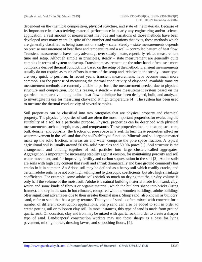
dependent on the chemical composition, physical structure, and state of the materials. Because of

its importance in characterizing material performance in nearly any engineering and/or science

application, a vast amount of measurement methods and variations of those methods have been

developed over many years. In spite of the number and variations that exits, these methods which

are generally classified as being transient or steady – state. Steady – state measurements depends

on precise measurement of heat flow and temperature and a well – controlled pattern of heat flow.

Transient measurements have many advantage over steady – state, especially related measurement

time and setup. Although simple in principles, steady – state measurement are generally quite

complex in terms of system and setup. Transient measurement, on the other hand, often use a more

complexly derived thermal conductivity based on the setup of the method. Transient measurements

usually do not require as much efforts in terms of the setup and, relative to the steady – state type,

are very quick to perform. In recent years, transient measurements have become much more

common. For the purpose of measuring the thermal conductivity of clay-sand, available transient

measurement methods are currently unable to perform the measurement needed due to physical

structure and composition. For this reason, a steady – state measurement system based on the

guarded – comparative – longitudinal heat flow technique has been designed, built, and analyzed

to investigate its use for measuring clay-sand at high temperature [4]. The system has been used

to measure the thermal conductivity of several samples.

Soil properties can be classified into two categories that are physical property and chemical

property. The physical properties of soil are often the most important properties for evaluating the

suitability of a soil for a particular purpose. Physical properties can be described with physical

measurements such as length, mass, and temperature. These properties include texture, structure,

bulk density, and porosity, the fraction of pore space in a soil. In turn these properties affect air

water movement in the soil, and thus the soil’s ability to function. Minerals and soil organic matter

make up the solid fraction, whereas air and water comprise the pore space fraction. A typical

agricultural soil is usually around 50.0% solid particles and 50.0% pores [1]. Soil structure is the

arrangement and binding together of soil particles into large cluster, called aggregates.

Aggregation is important for increasing stability against erosion, for maintaining porosity and soil

water movement, and for improving fertility and carbon sequestration in the soil [3]. Adobe soils

are soils with high clay content that swell and shrink dramatically and bare ground commonly has

cracks in it in summer. An Adobe soil may be defined as a heavy soil which readily cracks, and

certain adobe soils have not only high wilting and hygroscopic coefficients, but also high shrinkage

coefficients. For example, some adobe soils shrink so much on drying that the air-dry volume is

only half the volume of the moist soil. Adobe is a natural building material made from sand, clay,

water, and some kinds of fibrous or organic material, which the builders shape into bricks (using

frames), and dry in the sun. In hot climates, compared with the wooden buildings, adobe buildings

offer significant advantages due to their greater thermal mass. Sharp sand, also known as builders’

sand, refer to sand that has a gritty texture. This type of sand is often mixed with concrete for a

number of different construction applications. Sharp sand can also be added to soil in order to

create potting soil or to loosen clay soil. In most instances, this type of sand is made from ground

quartz rock. On occasion, clay and iron may be mixed with quartz rock in order to create a sharper

type of sand. Landscapers’ construction workers may use these sharps as a base for lying

pavement, mixing mortar, dressing lawns, and smoothing floors, [4].



DOI: 10.5281/zenodo.2636862


This paper was aimed at determining the thermal conductivity for adobe (clay) mixed with Quartz

(sand) using Lees Disc method.

2. Materials and Methods

Design Method

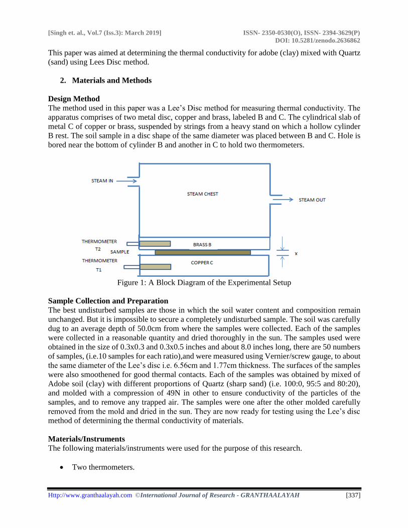
The method used in this paper was a Lee’s Disc method for measuring thermal conductivity. The

apparatus comprises of two metal disc, copper and brass, labeled B and C. The cylindrical slab of

metal C of copper or brass, suspended by strings from a heavy stand on which a hollow cylinder

B rest. The soil sample in a disc shape of the same diameter was placed between B and C. Hole is

bored near the bottom of cylinder B and another in C to hold two thermometers.

Figure 1: A Block Diagram of the Experimental Setup

Sample Collection and Preparation

The best undisturbed samples are those in which the soil water content and composition remain

unchanged. But it is impossible to secure a completely undisturbed sample. The soil was carefully

dug to an average depth of 50.0cm from where the samples were collected. Each of the samples

were collected in a reasonable quantity and dried thoroughly in the sun. The samples used were

obtained in the size of 0.3x0.3 and 0.3x0.5 inches and about 8.0 inches long, there are 50 numbers

of samples, (i.e.10 samples for each ratio),and were measured using Vernier/screw gauge, to about

the same diameter of the Lee’s disc i.e. 6.56cm and 1.77cm thickness. The surfaces of the samples

were also smoothened for good thermal contacts. Each of the samples was obtained by mixed of

Adobe soil (clay) with different proportions of Quartz (sharp sand) (i.e. 100:0, 95:5 and 80:20),

and molded with a compression of 49N in other to ensure conductivity of the particles of the

samples, and to remove any trapped air. The samples were one after the other molded carefully

removed from the mold and dried in the sun. They are now ready for testing using the Lee’s disc

method of determining the thermal conductivity of materials.

Materials/Instruments

The following materials/instruments were used for the purpose of this research.

• Two thermometers.



DOI: 10.5281/zenodo.2636862


• Stop clock.

• Weighing balance.

• Special clamp stand.

• Boiler

• Heater

• Vanier/Screw gauge

• Mold, and

• Lee’s disc apparatus

Procedure for Determining the Thermal Conductivity of the Sample (Adobe/Quartz)

The block diagram is shown in Fig.1. A steam was passed through the cylinder B from a steam

boiler and the temperature indicated by two thermometers, T1 and T2 as Ө1 and Ө2 were recorded

when the steady state temperature has been reached. Cylinder B was now removed, C is still

suspended. Heat C directly by the steam chamber, until T2 records the temperature up to 100C

higher than that recorded in the steady state. Removed the steam chamber and wait for 2-3 minutes,

so that heat is uniformly distributed over the disc and placed the insulating material on C. Start

recording the temperature at interval of 30seconds is taking, using stop clock, continue till the

temperature falls by 100C below the steady state temperature from T1. The samples were prepared

by mixed of Adobe (clay) with different proportions of Quartz (sharp sand) (100:0, 95:5and 80:20),

and then cut into proper shapes and sizes for thermal conductivity measurements.

3. Results and Discussion

The amount or quantity of heat, q, which is transmitted per second through a soil sample whose

thickness is x, can be determined by means of Fourier’s Law.

H = rate of flow of heat

Ҡ = coefficient of thermal conductivity

A = cross sectional area of heat transfer

T1 = temperature at lower disc

T2 = temperature at upper disc

The manner of obtaining T1 and T2, the temperature of two points, merits some explanation. From

steady state temperature readings, an average value was determined and used in calculations. The

value of Ҡ was calculated from the temperature readings of both the upper and lower disc

respectively. The result of this study is discussed using the variation of ratio of Adobe (clay soil)

and Quartz (sand soil). Based on this variation, the following are the outcome of the research.

Results of the Variation of Ratio 95:5 Adobes (Clay) to Quartz (Sand)

This sample 1 contained ninety five percent Adobe (clay) and five percent Quartz (sand).

The Time-temperature data obtained by recording the temperature at interval of 30.0 seconds,

continued until the temperature falls by 100C below the steady state temperature from T1.



DOI: 10.5281/zenodo.2636862


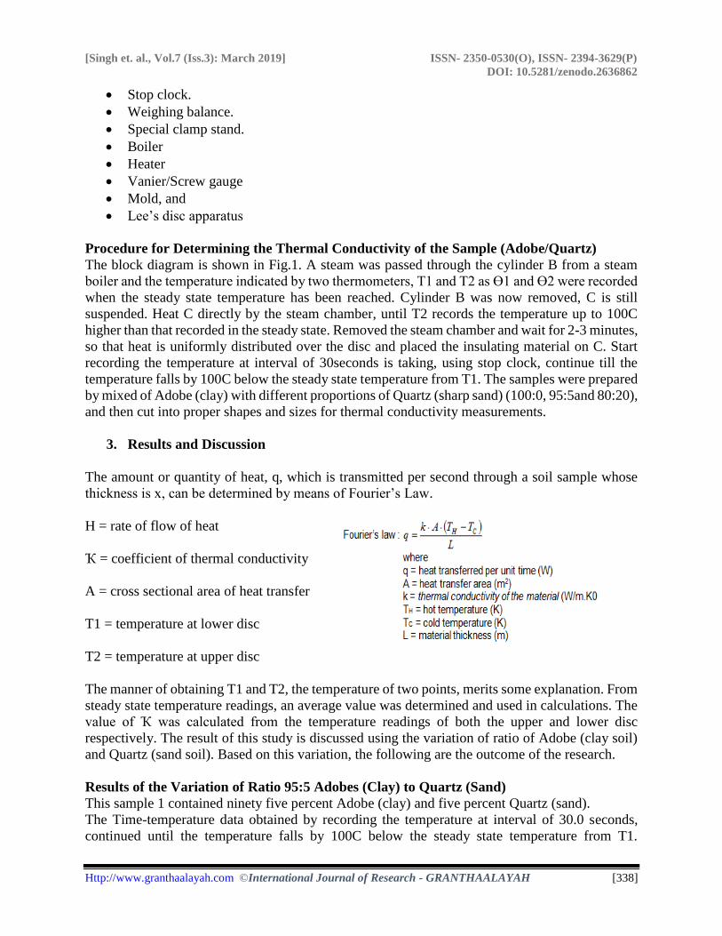
Observed that (sample e) has the highest temperature of 83.80C at 0.0 second while (sample b) has

lowest temperature of 45.50C at 1130 seconds.

Figure 2: The cooling curve for sample 1 (95:5)

The figure (2), gives the cooling rate with temperature of ten samples a-j, each of which having

the same size but molded in different mold. It can be seen that (sample b) has the lowest thermal

conductivity of 0.5330Wm-1k-1 and the highest thermal conductivity of 1.3476 Wm-1k-1 for

(sample h). This implies that sample b, produces the best result because of the lowest thermal

conductivity which result in the high thermal resistivity that favors it as interior building materials

for naturally cooled design in tropical region.

The figure (3), gives the cooling rate with temperature of ten samples a-j, each of which having

the same size but molded in different mold. It can be seen that (sample b) has the lowest thermal


(sample a). This implies that sample b, produces the best result because of the lowest thermal

conductivity which result in the high thermal resistivity that favors it as interior building materials


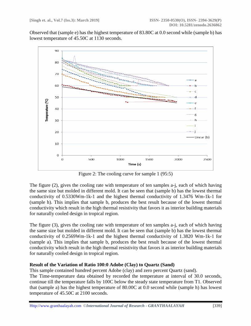
Result of the Variation of Ratio 100:0 Adobe (Clay) to Quartz (Sand)

This sample contained hundred percent Adobe (clay) and zero percent Quartz (sand).

The Time-temperature data obtained by recorded the temperature at interval of 30.0 seconds,

continue till the temperature falls by 100C below the steady state temperature from T1. Observed

that (sample a) has the highest temperature of 80.00C at 0.0 second while (sample h) has lowest

temperature of 45.50C at 2100 seconds.



DOI: 10.5281/zenodo.2636862


Figure 3: The cooling curve for sample 2 (100:0)

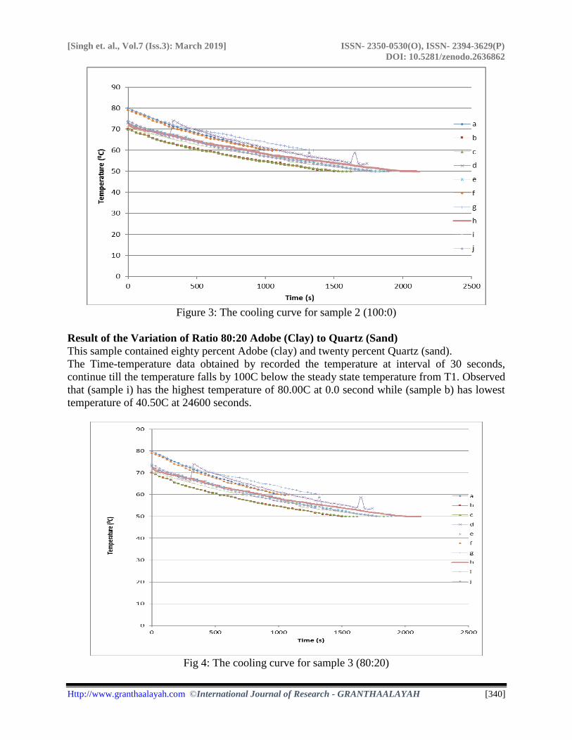
Result of the Variation of Ratio 80:20 Adobe (Clay) to Quartz (Sand)

This sample contained eighty percent Adobe (clay) and twenty percent Quartz (sand).

The Time-temperature data obtained by recorded the temperature at interval of 30 seconds,

continue till the temperature falls by 100C below the steady state temperature from T1. Observed

that (sample i) has the highest temperature of 80.00C at 0.0 second while (sample b) has lowest

temperature of 40.50C at 24600 seconds.

Fig 4: The cooling curve for sample 3 (80:20)



DOI: 10.5281/zenodo.2636862


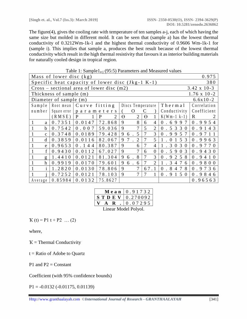
The figure(4), gives the cooling rate with temperature of ten samples a-j, each of which having the

same size but molded in different mold. It can be seen that (sample a) has the lowest thermal


(sample i). This implies that sample a, produces the best result because of the lowest thermal

conductivity which result in the high thermal resistivity that favours it as interior building materials


Table 1: Sample1a-j (95:5) Parameters and Measured values

M as s o f l o w e r d i s c ( k g ) 0 . 9 7 5

S p e c i f i c h e a t c a p a c i t y o f l o w e r d i s c ( J k g - 1 K - 1 ) 3 8 0

Cross – sectional area of lower disc (m2) 3.42 x 10-3

Thickness of sample (m) 1.76 x 10 -2

Diameter of sample (m) 6.6x10 -2

S a m p l e

n u m b e r

R o o t m e a n

S q u a r e e r r o r

( R M S E )

C u r v e f i t t i n g

p a r a m e t e r s

D i s c s T e m p e r a t u r e

( O C )

T h e r m a l

C o n d u c t i v i t y

K ( W m - 1 k - 1 )

C o r r e l a t i o n

C o e f f i c i e n t

R 2 P 1 P 2 Ө 2 Ө 1

1 a 0 . 7 3 5 1 0 . 0 1 4 7 7 2 . 8 6 8 9 8 6 4 0 . 6 9 9 7 0 . 9 9 5 4

1 b 0 . 7 5 4 2 0 . 0 0 7 5 9 . 0 3 6 9 7 5 2 0 . 5 3 3 0 0 . 9 1 4 3

1 c 0 . 3 7 4 8 0 . 0 1 8 9 7 9 . 4 2 8 9 6 . 5 7 3 0 . 9 9 5 7 0 . 9 7 1 1

1 d 0 . 3 8 5 9 0 . 0 1 1 6 8 2 . 0 6 7 9 7 . 2 7 5 1 . 0 1 5 3 0 . 9 9 6 3

1 e 0 . 9 6 5 3 0 . 1 4 4 8 0 . 3 8 7 9 6 7 4 1 . 3 0 3 0 0 . 9 7 7 0

1 f 0 . 9 4 3 0 0 . 0 1 1 2 6 7 . 0 2 7 9 7 6 0 0 . 5 9 0 3 0 . 9 4 3 0

1 g 1 . 4 4 1 0 0 . 0 1 2 1 8 1 . 3 0 4 9 6 . 8 7 3 0 . 9 2 5 8 0 . 9 4 1 0

1 h 0 . 9 9 1 9 0 . 0 1 7 0 7 9 . 6 0 1 9 6 . 6 7 2 1 . 3 4 7 6 0 . 9 8 0 0

1 i 1 . 2 8 2 0 0 . 0 1 3 0 7 8 . 8 0 6 9 7 6 7 . 1 0 . 8 4 7 8 0 . 9 7 3 6

1 j 0 . 7 2 5 2 0 . 0 1 2 1 7 8 . 1 0 3 9 7 7 1 0 . 9 1 5 0 0 . 9 8 4 6

A v e r a g e 0 . 8 5 9 8 4 0 . 0 1 3 2 7 5 . 8 6 2 7 0 . 9 6 5 6 3

M e a n 0 . 9 1 7 3 2

S T D E V 0 . 2 7 0 0 9 2

V A R . 0 . 0 7 2 9 5

Linear Model Polyol.

Ҡ (t) = P1 t + P2 … (2)

where,

Ҡ = Thermal Conductivity

t = Ratio of Adobe to Quartz

P1 and P2 = Constant

Coefficient (with 95% confidence bounds)

P1 = -0.0132 (-0.01175, 0.01139)



DOI: 10.5281/zenodo.2636862


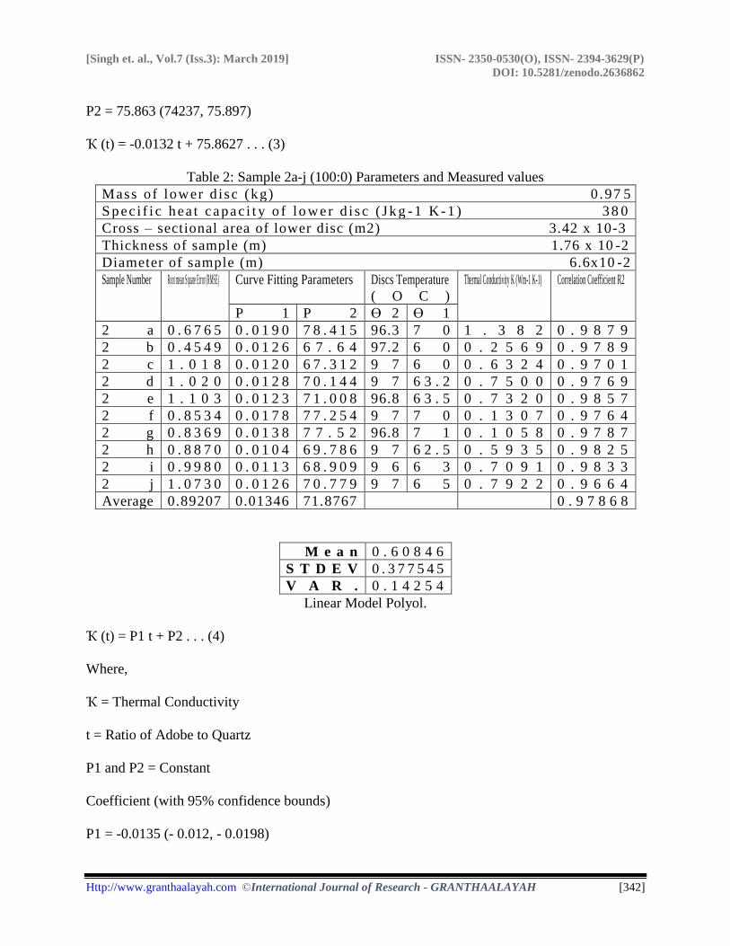
P2 = 75.863 (74237, 75.897)

Ҡ (t) = -0.0132 t + 75.8627 . . . (3)

Table 2: Sample 2a-j (100:0) Parameters and Measured values

Mass of lower d i sc (kg) 0 .97 5

S p ec i f i c h ea t c apac i t y o f l o w er d i s c ( Jk g - 1 K- 1 ) 3 8 0

Cross – sectional area of lower disc (m2) 3.42 x 10-3



Sample Number Root mean Square Error (RMSE) Curve Fitting Parameters Discs Temperature

( O C )

Thermal Conductivity K (Wm-1 K-1) Correlation Coefficient R2

P 1 P 2 Ө 2 Ө 1

2 a 0 . 6 7 6 5 0 . 0 1 9 0 7 8 . 4 1 5 96.3 7 0 1 . 3 8 2 0 . 9 8 7 9

2 b 0 . 4 5 4 9 0 . 0 1 2 6 6 7 . 6 4 97.2 6 0 0 . 2 5 6 9 0 . 9 7 8 9

2 c 1 . 0 1 8 0 . 0 1 2 0 6 7 . 3 1 2 9 7 6 0 0 . 6 3 2 4 0 . 9 7 0 1

2 d 1 . 0 2 0 0 . 0 1 2 8 7 0 . 1 4 4 9 7 6 3 . 2 0 . 7 5 0 0 0 . 9 7 6 9

2 e 1 . 1 0 3 0 . 0 1 2 3 7 1 . 0 0 8 96.8 6 3 . 5 0 . 7 3 2 0 0 . 9 8 5 7

2 f 0 . 8 5 3 4 0 . 0 1 7 8 7 7 . 2 5 4 9 7 7 0 0 . 1 3 0 7 0 . 9 7 6 4

2 g 0 . 8 3 6 9 0 . 0 1 3 8 7 7 . 5 2 96.8 7 1 0 . 1 0 5 8 0 . 9 7 8 7

2 h 0 . 8 8 7 0 0 . 0 1 0 4 6 9 . 7 8 6 9 7 6 2 . 5 0 . 5 9 3 5 0 . 9 8 2 5

2 i 0 . 9 9 8 0 0 . 0 1 1 3 6 8 . 9 0 9 9 6 6 3 0 . 7 0 9 1 0 . 9 8 3 3

2 j 1 . 0 7 3 0 0 . 0 1 2 6 7 0 . 7 7 9 9 7 6 5 0 . 7 9 2 2 0 . 9 6 6 4

Average 0.89207 0.01346 71.8767 0 . 9 7 8 6 8

M e a n 0 . 6 0 8 4 6

S T D E V 0 . 3 7 7 5 4 5

V A R . 0 . 1 4 2 5 4

Linear Model Polyol.

Ҡ (t) = P1 t + P2 . . . (4)

Where,





P1 = -0.0135 (- 0.012, - 0.0198)



DOI: 10.5281/zenodo.2636862


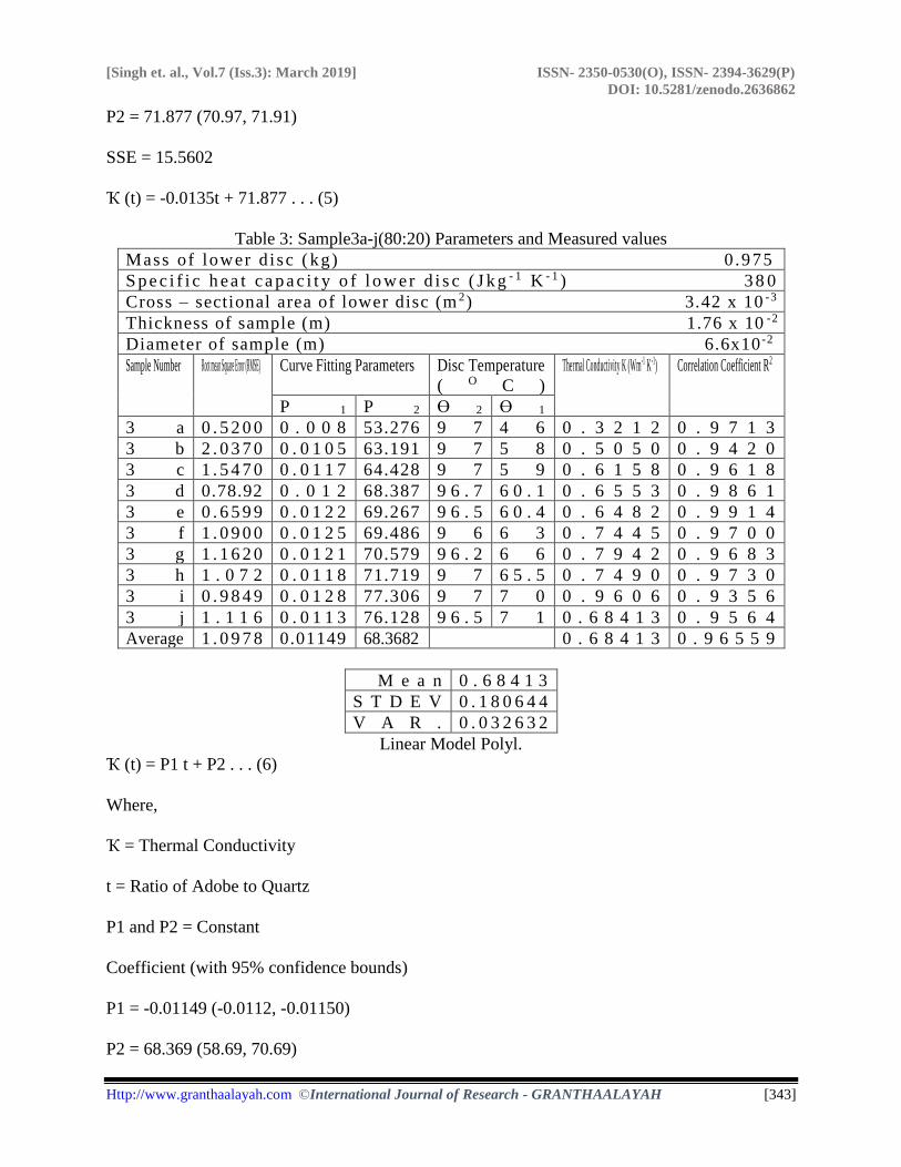
P2 = 71.877 (70.97, 71.91)

SSE = 15.5602

Ҡ (t) = -0.0135t + 71.877 . . . (5)

Table 3: Sample3a-j(80:20) Parameters and Measured values

Mass of lower d i sc ( kg) 0 .975

S p e c i f i c h ea t c a p a c i t y o f l o w er d i s c ( J k g - 1 K - 1 ) 3 8 0

Cross – sectional area of lower disc (m 2) 3.42 x 10 -3



Sample Number Root mean Square Error (RMSE) Curve Fitting Parameters Disc Temperature

( O C )

Thermal Conductivity K (Wm-1 K-1) Correlation Coefficient R2

P 1 P 2 Ө 2 Ө 1

3 a 0 . 5 2 0 0 0 . 0 0 8 53.276 9 7 4 6 0 . 3 2 1 2 0 . 9 7 1 3

3 b 2 . 0 3 7 0 0 . 0 1 0 5 63.191 9 7 5 8 0 . 5 0 5 0 0 . 9 4 2 0

3 c 1 . 5 4 7 0 0 . 0 1 1 7 64.428 9 7 5 9 0 . 6 1 5 8 0 . 9 6 1 8

3 d 0.78.92 0 . 0 1 2 68.387 9 6 . 7 6 0 . 1 0 . 6 5 5 3 0 . 9 8 6 1

3 e 0 . 6 5 9 9 0 . 0 1 2 2 69.267 9 6 . 5 6 0 . 4 0 . 6 4 8 2 0 . 9 9 1 4

3 f 1 . 0 9 0 0 0 . 0 1 2 5 69.486 9 6 6 3 0 . 7 4 4 5 0 . 9 7 0 0

3 g 1 . 1 6 2 0 0 . 0 1 2 1 70.579 9 6 . 2 6 6 0 . 7 9 4 2 0 . 9 6 8 3

3 h 1 . 0 7 2 0 . 0 1 1 8 71.719 9 7 6 5 . 5 0 . 7 4 9 0 0 . 9 7 3 0

3 i 0 . 9 8 4 9 0 . 0 1 2 8 77.306 9 7 7 0 0 . 9 6 0 6 0 . 9 3 5 6

3 j 1 . 1 1 6 0 . 0 1 1 3 76.128 9 6 . 5 7 1 0 . 6 8 4 1 3 0 . 9 5 6 4

Average 1 . 0 9 7 8 0.01149 68.3682 0 . 6 8 4 1 3 0 . 9 6 5 5 9

M e a n 0 . 6 8 4 1 3

S T D E V 0 . 1 8 0 6 4 4

V A R . 0 . 0 3 2 6 3 2

Linear Model Polyl.

Ҡ (t) = P1 t + P2 . . . (6)

Where,





P1 = -0.01149 (-0.0112, -0.01150)

P2 = 68.369 (58.69, 70.69)



DOI: 10.5281/zenodo.2636862


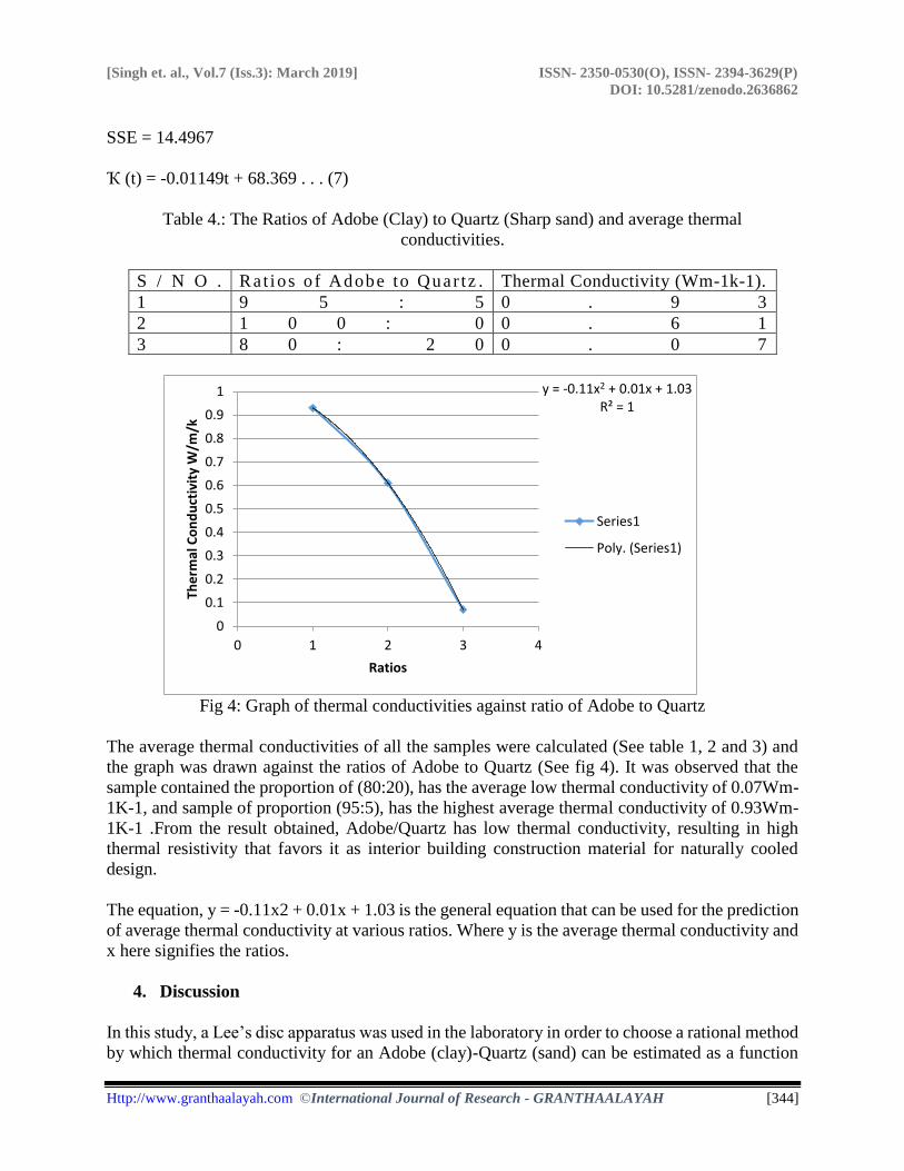
SSE = 14.4967

Ҡ (t) = -0.01149t + 68.369 . . . (7)

Table 4.: The Ratios of Adobe (Clay) to Quartz (Sharp sand) and average thermal

conductivities.

S / N O . Ra t ios o f Adobe to Quar tz . Thermal Conductivity (Wm-1k-1).

1 9 5 : 5 0 . 9 3

2 1 0 0 : 0 0 . 6 1

3 8 0 : 2 0 0 . 0 7

Fig 4: Graph of thermal conductivities against ratio of Adobe to Quartz

The average thermal conductivities of all the samples were calculated (See table 1, 2 and 3) and

the graph was drawn against the ratios of Adobe to Quartz (See fig 4). It was observed that the

sample contained the proportion of (80:20), has the average low thermal conductivity of 0.07Wm-

1K-1, and sample of proportion (95:5), has the highest average thermal conductivity of 0.93Wm-

1K-1 .From the result obtained, Adobe/Quartz has low thermal conductivity, resulting in high

thermal resistivity that favors it as interior building construction material for naturally cooled

design.

The equation, y = -0.11x2 + 0.01x + 1.03 is the general equation that can be used for the prediction

of average thermal conductivity at various ratios. Where y is the average thermal conductivity and

x here signifies the ratios.

4. Discussion

In this study, a Lee’s disc apparatus was used in the laboratory in order to choose a rational method

by which thermal conductivity for an Adobe (clay)-Quartz (sand) can be estimated as a function

y = -0.11x2 + 0.01x + 1.03R² = 1

0

0.1

0.2

0.3

0.4

0.5

0.6

0.7

0.8

0.9

1

0 1 2 3 4

The

rmal

Co

nd

uct

ivit

y W

/m/k

Ratios

Series1

Poly. (Series1)



DOI: 10.5281/zenodo.2636862


of Adobe-Quartz ratios. Looking at the result of the thermal conductivities, which were calculated,

(see table, 1, 2 and 3), there is a strong variation in the thermal conductivities of the samples. It

was observed that sample1 (Adobe 95, Quartz 5 i.e. 95:5), has the highest thermal conductivity of

0.9173wm-1k-1, while sample5 (Adobe 90, Quartz 10 i.e. 100:0), has the least thermal

conductivity of 0.60846wm-1k-1. And the average thermal conductivity of all the samples were

also calculated, the sample contained the proportion of (80:20), has the average lowest thermal

conductivity of 0.07Wm-1K-1, and sample of proportion (95:5), has the average highest thermal

conductivity of 0.93Wm-1K-1.Thermal conductivity varies principally with particles size

distribution of soil, bulk density and the water content, the greater the bulk densityand the higher

water content, the greater will be the thermal conductivity. The situation increases the effective

inter-particles thermal contact within the soil [5]. The equation,y = -0.11x2 + 0.01x + 1.03 is the

general equation that can be used for the prediction of average thermal conductivity at various

ratios. Where y is the average thermal conductivity and x here signifies the samples ratio.

The varying temperature regime within the soil effectively arises as consequences of soil surface

temperature variation. The basic pattern of this variation is imposed by insulation and the way in

which the net radiation of the soil surface separated by different layers. Soils in compacted

condition have a greater thermal conductivity than the soil in a loose condition. Many processes

occurring in the soil are greatly influenced by temperature. Kersten’s thermal conductivity values

were 0.9987, 0.9946, and 1.243wm-1k-1 compared to thermal conductivities of 0.6841, 0.6084

and 0.9173wm-1k-1 obtained in this study for temperature variation. In general, values obtained

by [2] and [6] are higher than that obtained from the experiments described in this study. One

explanation for these large differences could be because of using different procedure for measuring

thermal properties.

References

[1] Brady and Weil, “Thermal properties of soil Adobe samples for a passively cooled”.

16(4).2002

[2] Kersten, M.S. “Thermal properties of soils.”University of Minnesota Institute of Technology

Engineering Experiment station, 11(21),1949.

[3] Nicholas, K.A, Wright S. F, Liebig, M A and Pikul Jr.J.L Functional Significance of glomalin to

soil fertility. Proceedings from the Great Plains Soil Fertility Conference Proceedings.Denver, CO,

March 2-4, 2004.

[4] Pillai, C; and George; A. “An improve comparative thermal conductivity of highly Radioactive

specimens.” Proc. International thermal conductivity conference 22, T.W. Tong, Ed. Techomic

Publishing Company.1991.

[5] Rooyen V, Winterkorn. “Physical and Mechanical properties of particles” World Academy of

Science, Engineering and Technology, 64,2010.

[6] Salomone, L.A., Kovacs, W.D., “Thermal properties of soils,” Bulletin 28, Engineering

Experiment Station, University of Minnesota, Minneapolis, Minn., 1949.

*Corresponding author.

E-mail address: snghshvkmr@ yahoo.co.in


determination of thermal conductivity for adobe (clay soil ...

Documents

Transcript of determination of thermal conductivity for adobe (clay soil ...