steel melting arc furnace transformer equipment ... - PDF Images
Upload
independentCategory
view
3download
0
Pergamon Specfmhrmrcn Act@, Vol 49B. Nos 12-14. pp, 1385-1410, 1994
Copyright 0 1994 Elsev~er Science Ltd Printed m Great Bntain. All nghts reserved
0584-8547#94 s7 al t .cm
058&8547(94)ooo67-0
Detection of trace amounts of Ni by laser-induced fluorescence in graphite furnace with intensified charge coupled device*
ALEXANDER MARUNKOV, NIKOLAI CHEKALIN
V. I. Vernadsky Institute of Geochemistry and Analytical Chemistry, Kosygin Str. 19, Moscow 117975, Russia
JONAS ENGER
The Analytical Laser Spectroscopy Group, Department of Physics, Chalmers University of Technology, S-412 96 Goteborg, Sweden
and
OVE AXNER~
Department of Physics, Umea University, S-901 87 Umea, Sweden
(Received 29 April 1994; accepted 9 July 1994)
Abstract-A laser-induced fluorescence in graphite furnace (LIF-GF) set-up has been equipped with an intensified CCD detector (ICCD) that enables simultaneous multichannel detection of large wavelength regions. The main advantages of such a system in comparison with conventional photomultiplier detection are: simultaneous detection of several fluorescence wavelengths for easy characterization of excitation and fluorescence spectra and for an increase of the absolute sensitivity and spectral selectivity; simultaneous monitoring of background signals, such as those due to matrix interferences, blackbody radiation and scattered laser light; decrease of the susceptibility to radio-frequency pick-ups emitted from the pump laser due to the delayed read-out procedure; time-resolved studies of fluorescence spectra for improved elemental selectivity or for studies of atomization processes, and a possibility to perform two-dimensional imaging of height distributions of atomization and, in combination with an imaging spectrometer, diffusion processes in the furnace. The first work on LIF-GF with ICCD detection has been performed on Ni. The most sensitive and versatile excitation and detection wavelengths have been identified. Detection limits in water solutions by the LIF-GF technique have been improved by two orders of magnitude and are found to be 0.015 pg with ICCD and 0.01 pg using a photomultiplier at the most sensitive excitation and detection wavelengths. Nickel in @ml concentrations has been detected in aqueous standard reference samples with sodium concentrations ranging from &ml to % (rivetine water and estuarine water) with good accuracy and precision. The Ni contents of standard riverine and estuarine water were determined to 1.00 * 0.11 and 0.75 ? 0.07 @ml, respectively. The certified concentrations are 1.03 -t 0.10 and 0.743 + 0.078 @ml.
1. INTRODUCTION
IN THE continuous search for new powerful analytical techniques for detection of trace elements at ultra-low concentrations, i.e. at or below pg/ml, ppt, or 1 : 10” concentrations, or in ultra-small amounts, i.e. in fg amounts, i.e. 10-15-10-12 g, laser- based spectroscopic techniques have emerged as useful tools during the last decade. Among these types of techniques, laser-induced fluorescence in graphite furnace (LIF-GF), also often referred to as laser-excited atomic fluorescence spectrometry with electro thermal atomizer (ETA-LEAFS), has shown to be particularly useful owing to qualities such as low detection limits, good selectivity and satisfactory accuracy and precision. The LIF-GF technique is a successful and powerful combination of the analytical performance of the graphite furnace as an atomizer with the high sensitivity of the laser-induced fluorescence technique for detection of atoms. The good qualities
* This paper was published in the Special Honor Issue of Spectrochimica Acta Part B, dedicated to J. D. Winefordner.
t Author to whom all correspondence should be addressed.
1385
1386 A. ~~ARUNKOV et al.
of the technique has been demonstrated during recent years by a number of publications [l-13]. In addition, the LIF-GF technique has been thoroughly reviewed and discussed by, for example, BUTCHER et al. [14], OMENETTO et al. [15] and SJ~STR~M [16].
A typical experimental set-up for LIF-GF consists of a laser system tuned to suitable excitation wavelength(s), a graphite furnace, together with a detection-and-recording system. The detection system often consists of a monochromator, or occasionally narrow-banded optical filters, tuned to an appropriate detection wavelength and a photomultiplier (PMT). The use of PMTs for detection of the emitted fluorescence has been prevalent primarily due to their high quantum efficiencies, around lo-25% for most wavelengths, low price, and ease of use. The fluorescence detection is therefore most often performed using one single transition wavelength, or occasionally a few, all covered by the finite bandwidth of the spectrometer system, typically in the order of a nanometre.
However, when atoms with complicated electronic structure are being analysed, such as V, Cr, Mn, Fe, Co, Ni etc, it is not, a priori, obvious which pair of excitation- and-detection wavelengths is the most useful, versatile, or sensitive. A thorough investigation of the sensitivity as well as vulnerability to matrix interferences (i.e. selectivity) blackbody radiation and scattered laser light for each combination of excitation and detection wavelengths can in many cases, therefore, be very cumbersome to perform. Hence, a substantial improvement of the experimental set-up could result from the use of a multichannel detector for the emitted fluorescence.
An intensified CCD detector (ICCD) has several advantages over a photomultiplier. First, owing to its ability to detect several wavelengths simultaneously, it can be used for fast and convenient investigations of the fluorescence spectra from atoms so as to find the most sensitive excitation-and-detection wavelength combination. This is of great importance when elements with complex atomic structure are being analysed, as was discussed above. Second, it can also be used to increase the absolute sensitivity of the LIF-GF technique as compared to photomultiplier detection by allowing simultaneous detection of the fluorescence at several wavelengths. Third, the use of ICCD detection for investigation of background signals from matrix interferences, blackbody radiation and scattered laser light, both at and around the wavelength of detection, is also very important, especially when samples with high concentrations of matrices are being analysed. This leads to an improved spectral selectivity. Fourth, owing to the delayed reading of the ICCD detector (delayed in time with respect to the laser pulse), it has a rather high immunity from radio-frequency pick-ups emitted from the pump laser, which often influence measurements when PMTs are being used. Fifth, by storing a number of consecutive fluorescence spectra within one furnace firing, the final fluorescence spectrum can be time-resolved in such a way that the time dependence (i.e. the atomization behaviour) of the analytical signal can be studied with respect to those of possible spectral interferences from matrix constituents in the sample. Such knowledge can, in turn, lead to improved conditions, both regarding finding the optimum furnace heating program for a given sample as well as allowing for an improved selectivity by a discrimination of the detected signals not only in wavelength, but rather in a combined wavelength-and-time space. Sixth, and finally, a two-dimensional ICCD detector can be used together with an imaging spectrometer for height distribution studies of atomization and diffusion processes in the graphite furnace.
The most important disadvantages of the ICCD detector are the following ones: first, a somewhat lower sensitivity as compared to a PMT, resulting from a lower quantum efficiency of the photocathode (often around or below 10%); second, a high price (several tens of thousands of U.S.$); third, a limited read-out rate (around or parts of Hz for a full two-dimensional read-out, or up to 200 Hz for binned read- outs); and fourth, it produces a huge number of data, which necessitates the use of computers with large data storage capabilities.
The present paper is a first report on the use of a two-dimensional ICCD detector for monitoring of the fluorescence in an LIF-GF set-up. In this pilot study, the
Trace Ni by LIF-GF with a CCD 1387
usefulness of the LIF-GF-ICCD system was studied in the analysis of Ni as it has a complex electronic structure with a large number of possible combinations of excitation and detection wavelengths. In addition, Ni needs a high atomization temperature, which often gives rise to substantial amounts of blackbody radiation over large parts of the wavelength region. Finally, Ni has also been found to be of interest in environmental and toxicological studies [ 17-271.
Nickel has previously been detected using the LIF-GF technique by FALK et al. [6]. They obtained a detection limit of 1 pg in aqueous solutions. A number of other fluorescence techniques, e.g. in flames or plasmas with laser or hollow cathode excitations, have also been used with varying success. A large number of fluorescence works have been compiled by SMITH et al. [28].
Detection of Ni in trace amounts by conventional techniques, as for example electrothermal atomization coupled with atomic absorption (ETAAS), in a variety of samples, such as aqueous solutions, blood, serum, and urine, has been achieved by a number of authors. A good compilation of some 80 references of work done in this field prior to 1988 can be found in Ref. [29]. Other more recent compilations of detection of traces of Ni in a variety of samples can be found in the yearly Atomic Spectrometry Updates published in the Journal of Analytical Atomic Spectrometry [30-411.
It has been found that, when detecting Ni at ng/ml concentrations in biological samples, the ETAAS technique is in many cases to be preferred in comparison with the normally more sensitive inductively coupled plasma mass-spectrometer technique (ICP-MS) owing to interferences from oxides of Ca at all of the Ni isotope masses
WI. Nickel in biological samples has been extensively studied by, for example, NIXON et
al. [42]. The authors were able to detect Ni in serum using the Zeeman-corrected ETAAS technique down to sub-ng/ml concentrations. They reached a very low detection limit (0.06 ng/ml, using 100 ~1 aliquots). This was sufficient, although sometimes marginally so, in order to determine the natural concentrations of Ni in human serum (0.14 +- 0.09 @ml).
However, even if these types of demonstrations are impressive, one can clearly see the continuous need for more and more sensitive techniques for detection of traces. Such needs prompted the present work concerned with improving the versatility, sensitivity as well as selectivity of the LIF-GF technique by incorporating a modern multichannel ICCD detection system. Hence, this work is the first in a series concerned with improved detection of traces at sub-ng/ml concentrations or sub-pg amounts of various elements in a variety of samples. This first work is concerned with a thorough study of Ni in aqueous solutions and in standard reference samples with concentrations of salt in the percent range.
A description of the experimental set-up follows in Section 2. Section 3 is concerned with a discussion of suitable excitation and detection wavelengths for Ni. Section 4 demonstrates the usefulness of ICCD detection coupled to the LIF-GF technique by a display of some fluorescence spectra that could be used for a compilation of the strongest LIF-GF excitation-and-detection wavelength combinations of Ni. Finally, a comparison of the detection limits, sensitivity and usefulness of an ICCD detector for LIF-GF with those of a photomultiplier is made. The same section also encompasses measurements of ng/ml concentrations of Ni in aqueous standard reference samples with seven orders of magnitude higher concentrations of Na.
2. EXPERIMENTAL ARRANGEMENT
The general principles and typical experimental set-ups for the LIF-GF technique have been described in detail in the literature previously [14, 161. The experimental set-up used in the authors’ laboratory has also been described [43, 441. The experimental set-up used in this work, however, differs from the ones used before in that use is made of a non-dispersive light collection system based upon a spherical mirror instead of a set of lenses for collection of

1388 A. MARUNKOV et al.
Graphite Furnace
Tube
cup
Fig. 1. The experimental set-up for the LIF-GF technique with ICCD detection.
fluorescence light and an ICCD system for detection of emitted fluorescence light. Thus chromatic aberrations in the system are eliminated. The experimental set-up is schematically shown in Fig. 1. In summary, the basic concepts of the experimental arrangement of the LIF-GF technique used in this experiment is as follows.
The laser light used for excitation of the Ni atoms was produced by an excimer laesr system, consisting of a pump laser run with XeCl at 308 nm (Lambda Physik, LPX 210i) together with a dye laser (Lambda Physik, FL 3002). The dye used was Coumarin 47, generating light around 450 nm, which in turn was frequency doubled in a BBO crystal. Typical UV pulse energies were in the lo-100 pJ range, depending on the type of application. The length of the dye laser pulses was approximately 20 ns.
The furnace was a spatially and temporally isothermal two-step integrated cuvette graphite furnace designed by FRECH and coworkers [45, 461. The temperatures of the cup and the tube can be controlled and adjusted separately for optimum conditions by detection of the blackbody radiation emitted from the tube and cup through optical fibres by photodiodes. The photodiode signals were fed to two separate temperature regulating systems, one for the cup and one for the tube. Separate temperature calibrations of the tube and cup were done by a pyrometer (Maurer Spectral, TMR 32) in the temperature region of 1100-3100 K. The temperature distribution in the tube was very homogeneous owing to the design of the furnace [47]. In addition, a very good temperature stability from one firing to another (within a few degrees) and very smooth temperature calibration curves vs photodiode voltage were obtained. These features make the furnace very suitable for detection of non-volatile elements as well as for diagnostic purposes.
The fluorescence light was collected by an optical system consisting of two mirrors. The emitted light was first collected by a flat mirror in a front-surface illumination mode with a 3 mm hole drilled at a 45” angle through which the laser beam can enter into the furnace. This was done to ensure the best possible light collection efficiency [7, 14, 481. The diameter of the laser beam in the furnace was approximately 2 mm. The fluorescence light was focused onto the entrance slit of the spectrometer (Jobin Yvon, HR 250) by a large aluminium-coated spherical mirror with a diameter of 100 mm and a focal length of 160 mm. In order to avoid saturation of the detector neutral density quartz filters for detection of light in the UV region or a solar blind filter (SB-300-F, CORION, Holliston, MA, U.S.A.), when detection was performed close to the visible part of the spectrum, were used. The solar blind filter also served as a means to reduce the background originating as a result of blackbody radiation from the graphite furnace. The spectrometer was equipped with interchangeable turrets, each holding two gratings. Four different gratings were available (two holographic ones with 2400 and 1200 grooves mm, respectively, and two ruled ones with 600 and 150 grooves mm, respectively). The
Trace Ni by LIF-GF with a CCD 1389
dispersion of the spectrometer was 3 run/mm at 500 nm using a grating with a groove density of 1200 grooves mm. With a detector resolution of 3-4 CCD pixels, this corresponds to a maximum resolution of 200-250 pm for this particular grating when using a small entrance slit.
The spectrometer was equipped with dual entrance as well as exit ports and two swing-away mirrors. In this experiment, only one entrance port was used. The dual exit ports with corresponding swing-away mirror enabled the use of two different detectors. An ordinary PMT was placed at one exit (Hamamatsu, R2027), while a UV-sensitive ICCD detector system (Spectroscopy Instruments, ICCD 576S/RBT) was mounted at the other exit port.
The PMT was in this experiment only used in order to obtain comparative figures-of-merit for the two detectors (sensitivity, tolerance to pick-ups of noise and background signals as well as the overall versatility, all influencing the final detection limits). The output of the PMT was amplified in a fast (200 MHz) preamplifier (LeCroy WlOO BTB; input resistance 50 R, voltage amplification 10). A boxcar module (Stanford Research System, SR-250) was used for gated detection of the output signal from the preamplifier. The PMT data were gathered and stored in a PC-type lab-computer equipped with a 12-bit A/D converter card using a home-made data collection program written in Turbo Pascal.
The detector unit in the ICCD detector was placed at the output focal plane of the spectrometer and consists of a UV-sensitive, gateable intensifier and a CCD detector. The intensifier was coupled to the CCD detector by means of a fibre-optical bundle. The CCD chip was of Thomson-type and has 578 by 384 pixels, each with a size of 0.023 by 0.023 mm. The CCD detector was cooled to -35°C (precision thermostatted within O.Ol’C) in order to reduce thermally produced charges. The ICCD detector was used with the shorter side along the horizontal plane of the spectrometer in order to make fast read-outs possible. Read-out rates above 100 Hz are only possible with the CCD running in binned mode with this orientation.
The combined system of lasers and detectors was triggered by a pulse generator (Stanford Research Systems, DG 535 ), synchronous with the 50 Hz power line in order to reduce any fluctuations of the signals as well as the background from the heating current of the furnace. The boxcar was triggered from scattered laser light by a photodiode placed in close proximity to the pump laser. This reduced any form of jitter in the gating of the boxcar with respect to the fluorescence signal. When the ICCD system was used, however, the high voltage pulse generator for the intensifier (Spectroscopy Instrument, FG-100) could not be triggered in the same way since it has an internal delay between trigger and high voltage output which is at least 30 ns. Therefore, the ICCD detector system had to be triggered electronically from the high-power supply unit of the excimer laser. Normally, the excimer laser can be stabilized against long-term drifts to within a fraction of its pulse length (? 2-3 ns) by an electronic trigger-regulating unit (Lambda Physik, LPA-97). However, due to repeated malfunctioning of this system, no regulation of the triggering of the excimer lasers could be used in this work. Therefore, a relatively long gating of the ICCD intensifier (200 ns) had to be used in order to ensure a satisfactory long-term stability in the overlap between the detector gate and the fluorescence light. Such a long gate can, however, allow excess amounts of blackbody radiation to be detected which could affect the overall performance of the system.
In order to minimize laser light scattering a number of precautions were taken. Apertures were placed in front of the furnace, scattering protection screens were inserted at suitable positions and a laser beam dump made of black fabric was placed 3 metres behind the furnace. Finally, the quartz windows, sealing the graphite tube from ambient air, were removed in order to reduce scattered laser light and fluorescence from the windows. The last action had no discernible effect upon the atomization of the Ni samples but could possibly reduce the lifetime of the tube.
3. EXPERIMENTAL PROCEDURES
3.1. The graphite furnace Nickel is an element that requires a high temperature for efficient atomization [49]. The exact
degree of atomization of Ni in a graphite furnace is, however, difficult to estimate properly since the atomization process has been found to depend on the type of sample investigated as well as its major constituents. Possible atomization processes of Ni in various matrices have been reviewed and discussed by FRECH et al. [50]. It has been found, for example, that minute amounts of chloride, as exist in large concentrations in sea-water, may cause severe interference effects due to the build-up of NiCl already at 2400 K [51-531. This interference decreases with increased temperature, although it cannot be fully eliminated even if the temperature is increased
1390 A. MARUNKOV et al.
to 3000 K [SO]. SLAVIN and MANNING found that this type of interference could be somewhat reduced by using a L’vov platform together with magnesium nitrate as modifier [54].
Hence, when Ni is detected in chloride matrices in a graphite furnace, the temperature must be raised close to its maximum attainable value, i.e. around 3000 K, in order to obtain a high and reproducible degree of atomization. Such high atomization temperatures will, however, put large demands on the detection system since significant amounts of blackbody radiation are emitted from the furnace at these high temperatures.
The atomization temperatures of the cup and tube and the delay between the start of the heating cycles were therefore carefully optimized so as to give a good vaporization and atomization of the sample with the least possible wear of the graphite material.
It was established experimentally that the fluorescence signal from Ni increased with a cup temperature up to approximately 3000 K for a pure aqueous Ni solution with no matrix modifier used. The dependence of the signal on the tube temperature was rather weak. For a high cup temperature (3000 K), the fluorescence signal increased with tube temperature up to approximately 2200 K and levelled off thereafter. The working temperature for the tube was therefore chosen as 2300 K. This finding indicates that the atomization of Ni mainly occurs directly in the cup and that molecular formation in the tube is rather insignificant. The use of a relatively low tube temperature significantly reduced the amount of blackbody radiation in the proximity of the interaction region, thereby reducing the background.
The tube was heated for 7 s while the cup was heated for a maximum of 5 s during each atomization in order to avoid any excess wear of the graphite cup and tube that easily occurs with the use of high temperatures. The delay between the beginning of tube and cup heating cycles was approximately 2 s. Under these conditions, a Ni signal could be seen for approximately 4 s for low Ni concentrations (I 10 pg). For higher Ni concentrations, the signal lasted up to 7 s. In order to minimize the risk of any carry-over of sample from one atomization cycle to the following, every second heating cycle was performed without sample. Data acquisition started 1 s prior to tube heating.
Pure Ar was fed into the atomizer volume with a flow rate of 1-2 Vmin during the heating and atomization stages. The flow rate was significantly increased (about one order of magnitude) immediately after the atomization stage in order to prevent penetration of atmospheric air into the hot atomizer since the furnace was being run without quartz windows at the light entrance and exit ports in order to minimize scattered laser light.
3.2. Sample preparation and measurements procedure The Ni standard reference solutions were prepared by appropriate dilution of a 1000 &ml
stock solution in chloride form using deionized water (18 M&cm conductance obtained from a Milli-Q system, Millipore, MA, U.S.A.). All solutions were acidified with HNOs to 0.02 M. All chemicals used were of analytical grade.
The standard reference materials (riverine water, SLRS-2, and estuarine water, SLEW-l) were gathered and prepared for analysis at the Division of Chemistry of the National Research Council, Ottawa, Canada. Small volumes of the samples were poured into 20 ml beakers and analysed immediately with no additional pretreatment. A micropipette (Oxford Laboratories International Corporation) was used to deposit a 5 ~1 aliquot of the working solution into the cup through a dosing hole into the graphite tube. After drying the water solution at a temperature of 90°C for 30 s, the cup and tube were taken up to working temperatures with a fast (2600 K/s) heating rate. No ashing stage was used.
The repetition rate of the laser rate was 50 Hz. For each laser shot, a binned one-dimensional spectrum (384 pixels wide) from the ICCD was transferred to the PC. The data acquisition time was 10 s. Hence, 500 spectra were stored for each furnace heating. Consequently, with a fluorescence signal duration of 4-7 s, approximately 200-350 of these spectra carry the analytical signal. All 500 curves have, however, full information about the ICCD background level and noise, blackbody radiation, scattered laser light and their wavelength dependencies. Such information is of importance for accurate post-processing of the data, as will be discussed in detail below.
3.3. Choice of excitation wavelengths Nickel is an element with ten valence electrons forming singlet, triplet, quintet and septet
states. There are two low-lying triplet and one singlet configurations below 5000 cm-’ in Ni in which a vast majority of all the atoms are found under thermal conditions, namely a 3d8 4s’ 3F state (with three fine structure levels, 3F4, 3F3, and 3F2, at 0, 1332 and 2217 cm-‘, respectively);
Trace Ni by LIF-GF with a CCD 1391
0
Ni
Fig. 2. A simplified energy level diagram of Ni. The pertinent wavelength regions for excitation and fluorescence between various states within the four groups of states are indicated.
a 3d9 4s 3D state (with the fine structure levels 3D3, 3D2, and 3D1, at 205, 880 and 1713 cm-‘, respectively); and a 38 4s lD2 state (at 3410 cm-‘). (See Fig. 2.)
At a temperature of 3000 K the thermal degree of population of these seven low-lying levels are as follows: approximately 36% of all atoms are in the 3F4 state at 0 cm-‘; 25% are in the 3D3 state at 205 cm-‘; 13% are in the 3F3 state at 1332 cm-‘; and 12% are in the 3D2 state at 880 cm-‘. Each of the remainder has less than 10% of all atoms.
Hence, in order to excite as many atoms as possible, the excitation should start, if possible, from either of the 3F4 or the 3D3 states. However, when selecting the most useful excitation and detection transitions, one has also to take into account the access of suitable excitation transitions, both regarding accessible wavelengths and the highest possible transition probabilities.
Focusing upon excitations from the six low-lying even-parity triplet states (i.e. the 3ds 4s’ 3F and 3d9 4s 3D states) one finds that the only accessible excited states are grouped into two different regions--one group consisting of 3d9 4p 3P, 3D, and 3F states and 3d8 4s4p 3D, ‘F, and 3G states in the 28 000-35 000 cm-’ region; the other consisting of 3d8 &4p 3P, 3D, 3F, and 3G states in the 42000-48000 cm-’ region. This is schematically displayed in Fig. 2.
In order to excite atoms from low-lying states to the first set of odd parity levels, i.e. in the 28000-35 000 cm-’ region, excitation wavelengths in the range between 294 and 373 nm are needed. This also implies that the fluorescence wavelengths are restricted to the same wavelength region. However, in order to reduce the influence of blackbody radiation from the hot furnace, fluorescence detection should preferably be performed as far down in the UV region as possible, preferably below 300 nm. Therefore, the interest was primarily focused upon the other group of excited levels, i.e. those in the 44000-48000 cm-’ region.
The levels in this region can be reached by excitation light in the 220-248 nm range. Fluorescence originating from this set of states can be monitored either in the same wavelength region, i.e. in the 220-248 nm range, or in the 314-376 nm range, i.e. to a rather high-lying odd parity 3d8 4s2 3P state around 15 000 cm- ‘. Indirect fluorescence, from the lower group of excited atoms, i.e. in the 28000-35000 cm-’ region, back to the lower even parity levels, can in some cases also be of interest with this type of excitation scheme. All these possible fluorescence wavelengths are depicted schematically in Fig. 2.
After a careful examination and consideration of suitable excitation and detection transitions it was decided that the excitation should primarily be done in the 220-248 nm region. Within this region, there are a number of strong transitions around 230 nm that are very suitable for fluorescence detection, i.e. with gA factors around 10 x lo8 I-Ix (where g is the degeneracy of
1392 A. MARUNKOV et al.
226.5 226.0 225.5 225.0 Wavelength (nm)
224.5 224.0
Fig. 3. A one-step LEI spectrum from 10 &ml of Ni in an acetylene/air flame in the wavelength region 226.25-224.25 nm.
the upper state and A the Einstein A-coefficient for spontaneous the 220-230 nm region was found suitable and examined closer.
4. RESULTS AND DISCUSSIONS
emission) [55, 561. Therefore,
Several investigations of the detectability of Ni using the new LIF-GF-ICCD technique have been performed.
4.1. A comparison of various excitation schemes of Ni In order to find suitable excitation wavelengths in the 220-230 nm region, for which
very little transition probability data exists in the literature, a number of one-step laser-enhanced ionization (LEI) spectra from Ni aspirated into an air/acetylene flame were obtained in this wavelength region. The experimental set-up is identical to that used in Ref. [44] and is therefore not described in detail here.
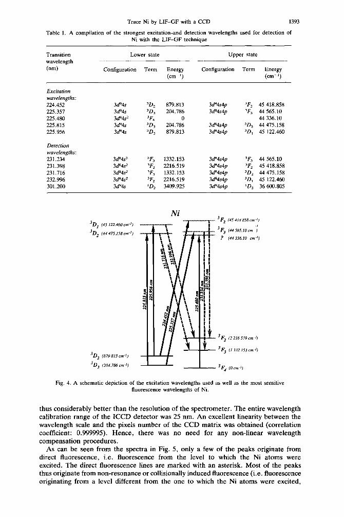
First, a typical LEI spectrum of Ni in an acetylene/air flame in the 224.25-226.25 nm wavelength region is shown in Fig. 3. From such spectra, five strong transitions were chosen as suitable candidates for LIF-GF. Fluorescence detection at several wavelengths in primarily two different wavelength regions around 230 nm and around 300 nm were then compared for these five strong excitation wavelengths using the LIF-GF-ICCD technique. This procedure could thus eliminate any possible extraordinary strong LEI signals originating from a combined excitation-and-photoionization process. Information about the strongest fluorescence lines in these regions is given in Table 1 and Fig. 4.
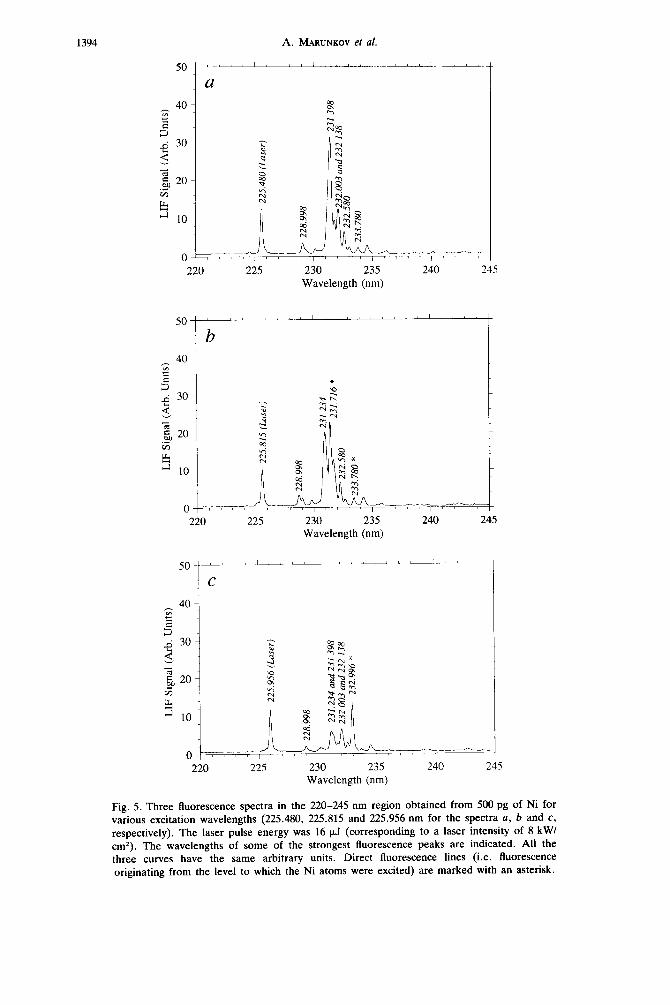
Some typical LIF-GF-ICCD fluorescence spectra are shown in Fig. 5. The figure shows three fluorescence spectra from the 220-245 nm region for different excitation wavelengths (225.480, 225.815 and 225.956 nm). The curves correspond to 500 pg of Ni (in order to clearly show all Ni fluorescence peaks) and were taken using laser pulse energies of 12-20 +l (roughly corresponding to irradiances of 6-10 kW/cm2). Each presented spectrum has been constructed by summing all 500 individual fluorescence spectra taken during one furnace firing.
Each spectrum consists of a number of peaks that all originate from Ni. It was found that the peak position reproducibility between consecutive furnace firings was very good, in general 51 pixel. This corresponds to a wavelength reproducibility of roughly +0.05 nm. Owing to this good reproducibility, an accurate wavelength calibration of the CCD pixel scale could be done. Therefore, prior to all measurements, the full CCD wavelength scale was calibrated using scattered light from the laser beams positioned in wavelength on various Ni transitions measured by the LEI technique, i.e. from spectra similar to that displayed in Fig. 3. The accuracy of the laser wavelength determination using the LEI technique was approximately k-1 pm,
Trace Ni by LIF-GF with a CCD 1393
Table 1. A compilation of the strongest excitation.and detection wavelengths used for detection of Ni with the LIF-GF technique
Transition wavelength
(nm)
Lower state Upper state
Configuration Term Energy Configuration Term Energy (cm-‘) (cm-i)
Excitation wavelengths: 224.452 225.357 225.480 225.815 225.956
3d94s 3D, 879.813 3@4s4p % 45 418.858 3d94s jD3 204.786 3d”4s4p % 44 565.10 3d84s= 3F4 0 44 336.10 3d94s 3D, 204.786 3d84s4p 3D, 44 475.158 3a94s 3D* 879.813 3d84s4p 3D, 45 122.460
Detection wavelengths : 231.234 231.398 231.716 232.996 301.200
3@4s2 ‘F3 1332.153 3d84s4p 3F3 44 565.10 3ds4sz ‘F2 2216.519 3@4s4p 3F* 45 418.858 3d84s* ‘& 1332.153 3d84s4p 3D, 44 475.158 3ds4st 3F* 2216.519 3d”4s4p 3D, 45 122.460 3d94s ‘D, 3409.925 3ds4s4p ‘D, 36 600.805
Ni
3D, (45 122.460cd)
3D2 (44 475.158cm.‘)
3D2 (879813cd)
3D3 (204.786 cm-‘)
‘F, (45 418 858 cm.‘)
‘F3 i44565.1Ocm y
? (44336.10 cm-‘)
‘Fz (2216519cd)
3F3 (I 332 153cm-‘J
3 F4 10 cm-‘)
Fig. 4. A schematic depiction of the excitation wavelengths used as well as the most sensitive fluorescence wavelengths of Ni.
thus considerably better than the resolution of the spectrometer. The entire wavelength calibration range of the ICCD detector was 25 nm. An excellent linearity between the wavelength scale and the pixels number of the CCD matrix was obtained (correlation coefficient: 0.999995). Hence, there was no need for any non-linear wavelength compensation procedures.
As can be seen from the spectra in Fig. 5, only a few of the peaks originate from direct fluorescence, i.e. fluorescence from the level to which the Ni atoms were excited. The direct fluorescence lines are marked with an asterisk. Most of the peaks thus originate from non-resonance or collisionally induced fluorescence (i.e. fluorescence originating from a level different from the one to which the Ni atoms were excited,
1394
220 225 230 235 240 24s
Wavelength (nm)
220 225 230 235 240 245
220 225 230 235 Wavelength (nm)
240 245
Fig. 5. Three fluorescence spectra in the 220-245 nm region obtained from 500 pg of Ni for various excitation wavelengths (225.480, 225.815 and 225.956 nm for the spectra a, b and c, respectively). The laser pulse energy was 16 p.l (corresponding to a laser intensity of 8 kW/ cmZ). The wavelengths of some of the strongest fluorescence peaks are indicated. All the three curves have the same arbitrary units. Direct fluorescence lines (i.e. fluorescence originating from the level to which the Ni atoms were excited) are marked with an asterisk.
Trace Ni by LIF-GF with a CCD 1395
Table 2. A compilation of the strongest excitation-and-detection schemes for LIF-GF-ICCD detection of Ni in various wavelength regions
Excitation-and-detection A exclfatl0” scheme (nm)
A Ruorersnce (nm)
Signal* (arbitrary units)
1 224.452 231.398 78 2 224.452 301.200 19 3 225.357 231.234 100 4 225.357 301.200 20 5 225.480 231.398 43 6 225.480 301.200 9 7 225.815 231.716 84 8 225.815 301.200 16 9 225.956 232.996 23
10 225.956 301.200 10
* All data were measured using 5 pg of Ni. The signals have been resealed so that the strongest one gives 100 arbitrary units.
populated by collisions with buffer gas species). As can be seen, the direct fluorescence lines are not always the strongest ones. This makes an a priori estimate of the strongest combination of excitation and detection wavelength difficult. This demonstrates the usefulness of an ICCD detector for monitoring of fluorescence from a LIF-GF set-
up* The relative sensitivities of a variety of excitation-and-detection schemes of Ni using
the LIF-GF-ICCD technique were determined. The most sensitive excitation-and- detection schemes for each of the five excitation wavelength are presented in Table 2. All measurements were performed using 5 pg of Ni in deionized water. As can be seen from the table, there are three excitation-and-detection schemes with fluorescence detection around 231 nm that have significantly higher sensitivities than the others, i.e. number 1, 3 and 7 (with relative sensitivities of 78, 100 and 84, respectively). Among these three schemes it was soon found that numbers 3 and 7, despite their high sensitivity, were less suitable for detection of Ni in samples with moderate-to- high concentrations of Na due to a yet unidentified strong background interference from Na. Therefore, further interest was directed at scheme number 1, which thus showed considerably smaller interference from high concentrations of Na.
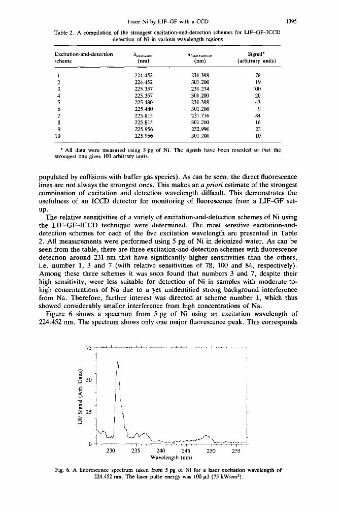
Figure 6 shows a spectrum from 5 pg of Ni using an excitation wavelength of 224.452 nm. The spectrum shows only one major fluorescence peak. This corresponds
0 ” I r x 5 I r 7 I ” ” I, 1 I, c 8, , 1 230 235 240 245 250 255
Wavelength (nm)
Fig. 6. A fluorescence spectrum taken from 5 pg of Ni for a laser excitation wavelength of 224.452 nm. The laser pulse energy was 100 CLJ (75 kW/cm*).
1396 A. MARUNKOV et al.
0 295 300 305 310 315 3
Wavelength (nm)
Fig. 7. A fluorescence spectrum in the 295-320 nm region obtained from 500 pg of Ni for a laser excitation wavelength of 224.452 nm. The laser pulse energy was 20 111 (10 kW/cm2).
to the excitation-and-detection scheme number 1. In this figure the grating in the spectrometer was adjusted in such a way that the laser excitation wavelength (224.452 nm) was positioned just outside the detection region. It is reassuring to see that the amount of scattered laser light is sufficiently low, just a few nanometres from the excitation wavelength so as not to give any substantial interferences for 5 pg of Ni at the selected detection wavelengths.
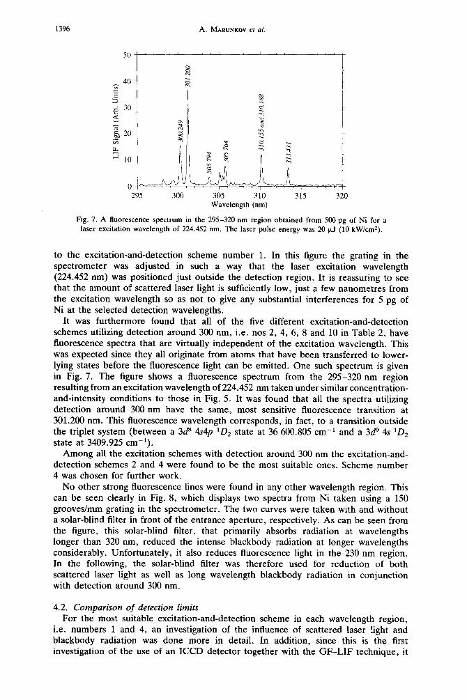
It was furthermore found that all of the five different excitation-and-detection schemes utilizing detection around 300 nm, i.e. nos 2, 4, 6, 8 and 10 in Table 2, have fluorescence spectra that are virtually independent of the excitation wavelength. This was expected since they all originate from atoms that have been transferred to lower- lying states before the fluorescence light can be emitted. One such spectrum is given in Fig. 7. The figure shows a fluorescence spectrum from the 295-320 nm region resulting from an excitation wavelength of 224.452 nm taken under similar concentration- and-intensity conditions to those in Fig. 5. It was found that all the spectra utilizing detection around 300 nm have the same, most sensitive fluorescence transition at 301.200 nm. This fluorescence wavelength corresponds, in fact, to a transition outside the triplet system (between a 3d8 4s4p lD2 state at 36 600.805 cm-’ and a 3d9 4s lD2 state at 3409.925 cm-l).
Among all the excitation schemes with detection around 300 nm the excitation-and- detection schemes 2 and 4 were found to be the most suitable ones. Scheme number 4 was chosen for further work.
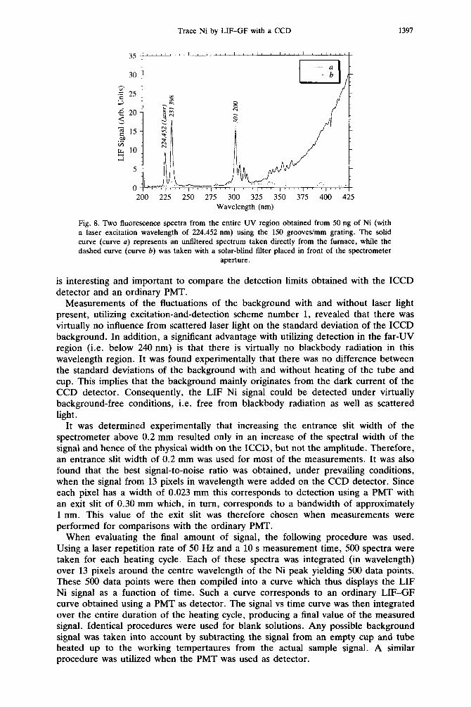
No other strong fluorescence lines were found in any other wavelength region. This can be seen clearly in Fig. 8, which displays two spectra from Ni taken using a 150 grooves/mm grating in the spectrometer. The two curves were taken with and without a solar-blind filter in front of the entrance aperture, respectively. As can be seen from the figure, this solar-blind filter, that primarily absorbs radiation at wavelengths longer than 320 nm, reduced the intense blackbody radiation at longer wavelengths considerably. Unfortunately, it also reduces fluorescence light in the 230 nm region. In the following, the solar-blind filter was therefore used for reduction of both scattered laser light as well as long wavelength blackbody radiation in conjunction with detection around 300 nm.
4.2. Comparison of detection limits For the most suitable excitation-and-detection scheme in each wavelength region,
i.e. numbers 1 and 4, an investigation of the influence of scattered laser !ight and blackbody radiation was done more in detail. In addition, since this is the first investigation of the use of an ICCD detector together with the GF-LIF technique, it
Trace Ni by LIF-GF with a CCD 1397
200 225 250 275 300 325 350 375 400 425 Wavelength (nm)
Fig. 8. Two fluorescence spectra from the entire UV region obtained from 50 ng of Ni (with a laser excitation wavelength of 224.452 nm) using the 150 grooves/mm grating. The solid curve (curve a) represents an unfiltered spectrum taken directly from the furnace, while the dashed curve (curve b) was taken with a solar-blind filter placed in front of the spectrometer
aperture.
is interesting and important to compare the detection limits obtained with the ICCD detector and an ordinary PMT.
Measurements of the fluctuations of the background with and without laser light present, utilizing excitation-and-detection scheme number 1, revealed that there was virtually no influence from scattered laser light on the standard deviation of the ICCD background. In addition, a significant advantage with utilizing detection in the far-UV region (i.e. below 240 nm) is that there is virtually no blackbody radiation in this wavelength region. It was found experimentally that there was no difference between the standard deviations of the background with and without heating of the tube and cup. This implies that the background mainly originates from the dark current of the CCD detector. Consequently, the LIF Ni signal could be detected under virtually background-free conditions, i.e. free from blackbody radiation as well as scattered light.
It was determined experimentally that increasing the entrance slit width of the spectrometer above 0.2 mm resulted only in an increase of the spectral width of the signal and hence of the physical width on the ICCD, but not the amplitude. Therefore, an entrance slit width of 0.2 mm was used for most of the measurements. It was also found that the best signal-to-noise ratio was obtained, under prevailing conditions, when the signal from 13 pixels in wavelength were added on the CCD detector. Since each pixel has a width of 0.023 mm this corresponds to detection using a PMT with an exit slit of 0.30 mm which, in turn, corresponds to a bandwidth of approximately 1 nm. This value of the exit slit was therefore chosen when measurements were performed for comparisons with the ordinary PMT.
When evaluating the final amount of signal, the following procedure was used. Using a laser repetition rate of 50 Hz and a 10 s measurement time, 500 spectra were taken for each heating cycle. Each of these spectra was integrated (in wavelength) over 13 pixels around the centre wavelength of the Ni peak yielding 500 data points. These 500 data points were then compiled into a curve which thus displays the LIF Ni signal as a function of time. Such a curve corresponds to an ordinary LIF-GF curve obtained using a PMT as detector. The signal vs time curve was then integrated over the entire duration of the heating cycle, producing a final value of the measured signal. Identical procedures were used for blank solutions. Any possible background signal was taken into account by subtracting the signal from an empty cup and tube heated up to the working tempertaures from the actual sample signal. A similar procedure was utilized when the PMT was used as detector.
1398 A. MARUNKOV et al.
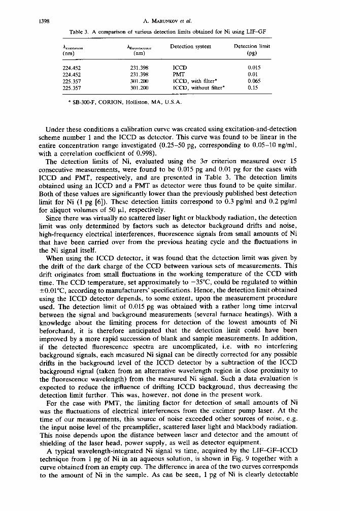
Table 3. A comparison of various detection limits obtained for Ni using LIF-GF
A fluorescence Detection system Detection limit
(nm) (P&
224.452 231.398 ICCD 0.015 224.452 231.398 PMT 0.01 225.357 301.200 ICCD, with filter* 0.065 225.357 301.200 ICCD, without filter* 0.15
* SB300-F, CORION, Holliston, MA, U.S.A.
Under these conditions a calibration curve was created using excitation-and-detection scheme number 1 and the ICCD as detector. This curve was found to be linear in the entire concentration range investigated (0.25-50 pg, corresponding to 0.05-10 @ml, with a correlation coefficient of 0.998).
The detection limits of Ni, evaluated using the 3a criterion measured over 15 consecutive measurements, were found to be 0.015 pg and 0.01 pg for the cases with ICCD and PMT, respectively, and are presented in Table 3. The detection limits obtained using an ICCD and a PMT as detector were thus found to be quite similar. Both of these values are significantly lower than the previously published best detection limit for Ni (1 pg [6]). These detection limits correspond to 0.3 pg/ml and 0.2 pg/ml for aliquot volumes of 50 ~1, respectively.
Since there was virtually no scattered laser light or blackbody radiation, the detection limit was only determined by factors such as detector background drifts and noise, high-frequency electrical interferences, fluorescence signals from small amounts of Ni that have been carried over from the previous heating cycle and the fluctuations in the Ni signal itself.
When using the ICCD detector, it was found that the detection limit was given by the drift of the dark charge of the CCD between various sets of measurements. This drift originates from small fluctuations in the working temperature of the CCD with time. The CCD temperature, set approximately to -35°C could be regulated to within *O.Ol”C, according to manufacturers’ specifications. Hence, the detection limit obtained using the ICCD detector depends, to some extent, upon the measurement procedure used. The detection limit of 0.015 pg was obtained with a rather long time interval between the signal and background measurements (several furnace heatings). With a knowledge about the limiting process for detection of the lowest amounts of Ni beforehand, it is therefore anticipated that the detection limit could have been improved by a more rapid succession of blank and sample measurements. In addition, if the detected fluorescence spectra are uncomplicated, i.e. with no interfering background signals, each measured Ni signal can be directly corrected for any possible drifts in the background level of the ICCD detector by a subtraction of the ICCD background signal (taken from an alternative wavelength region in close proximity to the fluorescence wavelength) from the measured Ni signal. Such a data evaluation is expected to reduce the influence of drifting ICCD background, thus decreasing the detection limit further. This was, however, not done in the present work.
For the case with PMT, the limiting factor for detection of small amounts of Ni was the fluctuations of electrical interferences from the excimer pump laser. At the time of our measurements, this source of noise exceeded other sources of noise, e.g. the input noise level of the preamplifier, scattered laser light and blackbody radiation. This noise depends upon the distance between laser and detector and the amount of shielding of the laser head, power supply, as well as detector equipment.
A typical wavelength-integrated Ni signal vs time, acquired by the LIF-GF-ICCD technique from 1 pg of Ni in an aqueous solution, is shown in Fig. 9 together with a curve obtained from an empty cup. The difference in area of the two curves corresponds to the amount of Ni in the sample. As can be seen, 1 pg of Ni is clearly detectable
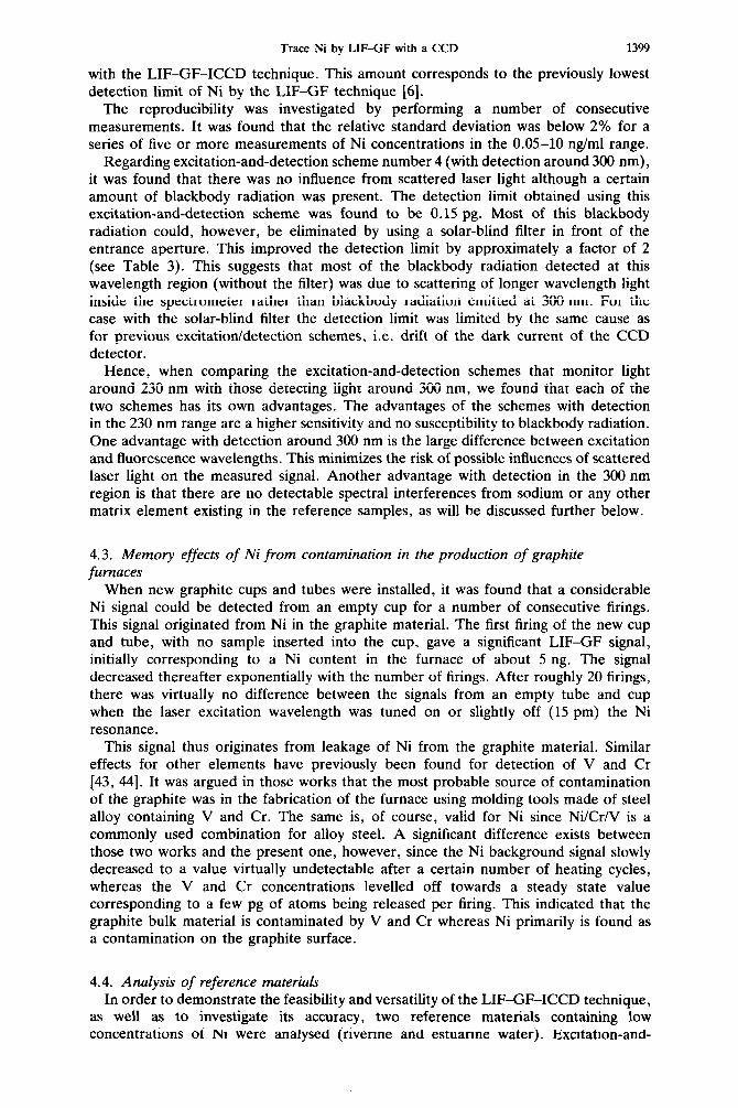
Trace Ni by LIF-GF with a CCD 1399
with the LIF-GF-ICCD technique. This amount corresponds to the previously lowest detection limit of Ni by the LIF-GF technique [6].
The reproducibility was investigated by performing a number of consecutive measurements. It was found that the relative standard deviation was below 2% for a series of five or more measurements of Ni concentrations in the 0.05-10 ng/ml range.
Regarding excitation-and-detection scheme number 4 (with detection around 300 nm), it was found that there was no influence from scattered laser light although a certain amount of blackbody radiation was present. The detection limit obtained using this excitation-and-detection scheme was found to be 0.15 pg. Most of this blackbody radiation could, however, be eliminated by using a solar-blind filter in front of the entrance aperture. This improved the detection limit by approximately a factor of 2 (see Table 3). This suggests that most of the blackbody radiation detected at this wavelength region (without the filter) was due to scattering of longer wavelength light inside the spectrometer rather than blackbody radiation emitted at 300 nm. For the case with the solar-blind filter the detection limit was limited by the same cause as for previous excitation/detection schemes, i.e. drift of the dark current of the CCD detector.
Hence, when comparing the excitation-and-detection schemes that monitor light around 230 nm with those detecting light around 300 nm, we found that each of the two schemes has its own advantages. The advantages of the schemes with detection in the 230 nm range are a higher sensitivity and no susceptibility to blackbody radiation. One advantage with detection around 300 nm is the large difference between excitation and fluorescence wavelengths. This minimizes the risk of possible influences of scattered laser light on the measured signal. Another advantage with detection in the 300 nm region is that there are no detectable spectral interferences from sodium or any other matrix element existing in the reference samples, as will be discussed further below.
4.3. Memory effects of Ni from contamination in the production of graphite furnaces
When new graphite cups and tubes were installed, it was found that a considerable Ni signal could be detected from an empty cup for a number of consecutive firings. This signal originated from Ni in the graphite material. The first firing of the new cup and tube, with no sample inserted into the cup, gave a significant LIF-GF signal, initially corresponding to a Ni content in the furnace of about 5 ng. The signal decreased thereafter exponentially with the number of firings. After roughly 20 firings, there was virtually no difference between the signals from an empty tube and cup when the laser excitation wavelength was tuned on or slightly off (15 pm) the Ni resonance.
This signal thus originates from leakage of Ni from the graphite material. Similar effects for other elements have previously been found for detection of V and Cr [43, 441. It was argued in those works that the most probable source of contamination of the graphite was in the fabrication of the furnace using molding tools made of steel alloy containing V and Cr. The same is, of course, valid for Ni since Ni/Cr/V is a commonly used combination for alloy steel. A significant difference exists between those two works and the present one, however, since the Ni background signal slowly decreased to a value virtually undetectable after a certain number of heating cycles, whereas the V and Cr concentrations levelled off towards a steady state value corresponding to a few pg of atoms being released per firing. This indicated that the graphite bulk material is contaminated by V and Cr whereas Ni primarily is found as a contamination on the graphite surface.
4.4. Analysis of reference materials In order to demonstrate the feasibility and versatility of the LIF-GF-ICCD technique,
as well as to investigate its accuracy, two reference materials containing low concentrations of Ni were analysed (riverine and estuarine water). Excitation-and-
1400 A. MARUNKOV et al.
IpgofNi
0 1 2 3 4 5 6 7 8 9 IO Time (s)
Fig. 9. LIF-GF-ICCD signals from 1 pg of Ni (curve a) and from deionized water (curve b)
during one heating cycle. The laser pulse energy was 100 CLJ (corresponding to a laser intensity
of 50 kW/cm*).
detection scheme number 1 was used. No chemical or thermal pretreatments were used for the analysis presented below.
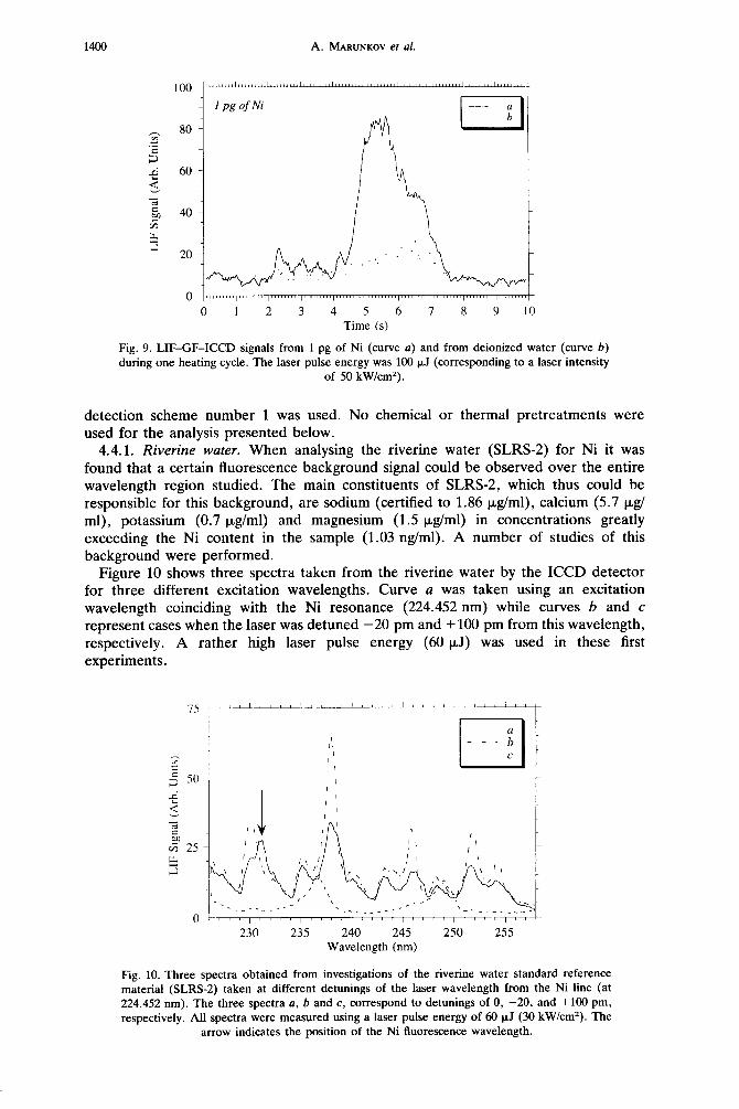
4.4.1. Riverine water. When analysing the riverine water (SLRS-2) for Ni it was found that a certain fluorescence background signal could be observed over the entire wavelength region studied. The main constituents of SLRS-2, which thus could be responsible for this background, are sodium (certified to 1.86 pg/ml), calcium (5.7 l.~g/ ml), potassium (0.7 ug/ml) and magnesium (1.5 kg/ml) in concentrations greatly exceeding the Ni content in the sample (1.03 @ml). A number of studies of this background were performed.
Figure 10 shows three spectra taken from the riverine water by the ICCD detector for three different excitation wavelengths. Curve a was taken using an excitation wavelength coinciding with the Ni resonance (224.452 nm) while curves b and c represent cases when the laser was detuned -20 pm and + 100 pm from this wavelength, respectively. A rather high laser pulse energy (60 u,J) was used in these first experiments.
r--r-l b
230 235 240 245 250 255 Wavelength (nm)
Fig. 10. Three spectra obtained from investigations of the riverine water standard reference material (SLRS-2) taken at different detunings of the laser wavelength from the Ni line (at
224.452 nm). The three spectra a, b and c, correspond to detunings of 0, -20, and +lOO pm,
respectively. All spectra were measured using a laser pulse energy of 60 CJ (30 kW/cm*). The
arrow indicates the position of the Ni fluorescence wavelength.

Trace Ni by LIF-GF with a CCD 1401
As can be seen from a comparison between the three curves, both the shape and the magnitude of the background fluorescence spectra varied significantly with laser excitation wavelength. The rather structured shape of the two spectra taken at 224.452 and 224.432 nm (curves a and b, respectively) are completely missing in curve c in which the background is rather smooth with only a few broad and widely separated peaks. In addition, the Ni fluorescence peak is virtually indistinguishable from the structured background under these conditions (the position of the Ni peak is marked with an arrow in the figure). The fact that the structure as well as the magnitude of the background varied significantly even for small changes in the excitation wavelength made it difficult to perform background correction in a proper way. Despite this, a rather satisfactory determination of the Ni content of this standard reference sample could be done using the following procedure.
First, the actual “excitation” width of the Ni resonance was determined from investigations of the Ni signal vs excitation wavelength using a pure Ni standard solution. It was found that the Ni signal decreased two orders of magnitude when the laser excitation wavelength was detuned -7.5 pm and +15 pm from resonance, respectively. The asymmetry of this interval has to do with the fact that the strong excitation line at 224.452 nm is flanked by a considerably weaker yet unidentified line in Ni (clearly seen in Fig. 3). A measure of the Ni content of the riverine sample was then calculated as the difference between the fluorescence signal obtained with the laser excitation wavelength on the Ni resonance and the mean of the two fluorescence signals obtained with the laser excitation wavelength detuned -7.5 pm and +15 pm, respectively.
It was found that this background correction procedure could not itself, under prevailing conditions, eliminate all this structured background due to the strong variation of the background with excitation wavelength. An evaluation of the Ni content of the riverine sample in this way gave a concentration of 2.67 + 0.16 ng/ml (0.16 represents here the standard deviation of five consecutive measurements). This value is considerably higher than the certified Ni concentration of 1.03 + 0.10 @ml. Thus, a more efficient background elimination procedure had to be found. A study of the influence of laser power upon the signal-to-background ratio was therefore performed.
It was found that the Ni transition was rather strongly saturated at most of the intensities used. Hence, by reducing the laser intensity the signal-to-background ratio could be improved considerably. The above-mentioned background correction procedure was then repeated for a number of different laser intensities. As the laser pulse energy was attenuated 8, 19 and 35 times (down to roughly 2 CIJ), it was found that the Ni content of the sample decreased with decreasing intensity. Ni concentrations of 1.60 ? 0.13, 1.22 + 0.11 and 1.09 + 0.11 rig/ml, respectively, resulted.
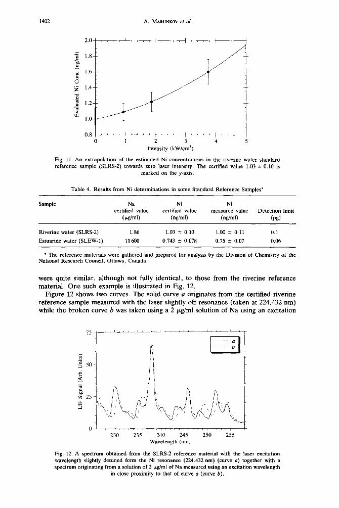
It was now possible to improve on the accuracy of the determination of Ni in this reference material by extrapolating the estimated Ni content of the sample towards zero intensity for which the background will be fully eliminated. Such an extrapolation, made by a second order polynomial fit, is shown in Fig. 11. The extrapolated value amounts to 1.00 ? 0.11 rig/ml (the intercept between the fit and the y-axis). This value is overlapping with the certified value of 1.03 2 0.10 rig/ml to a large degree. The certified value is marked along the y-axis in the figure. The values obtained are collected in Table 4.
In order to understand what matrix component (or components) that causes the background signals shown in Fig. 10, spectra from all the major constituents (i.e. Ca, K, Mg, Na) were investigated separately by introducing standard solutions of each of these elements in concentrations corresponding to those we have in the reference material into the atomizer. It was found that all these elements gave different types of background spectra when being excited with laser light in the 224-225 nm region. It was found, however, that the background spectra from Na were considerably stronger (5-10 times) than those from the other elements and that they spectrally
1402 A. ~~ARUNK~V et a/.
0.8 L-+--+--+----t- 0 1 2 3 4 5
Intensity (kW/cm’)
Fig. 11. An extrapolation of the estimated Ni concentrations in the riverine water standard reference sample (SLRS-2) towards zero laser intensity. The certified value 1.03 + 0.10 is
marked on the y-axis.
Table 4. Results from Ni determinations in some Standard Reference Samples*
Sample Na Ni certified value certified value
( pg/ml) (ng/ml)
Ni measured value
(@ml)
Detection limit
(pg)
Riverine water (SLRS-2) 1.86 1.03 -c 0.10 1.00 ?z 0.11 0.1
Estuarine water (SLEW-l) 11600 0.743 2 0.078 0.75 2 0.07 0.06
* The reference materials were gathered and prepared for analysis by the Division of Chemistry of the National Research Council, Ottawa, Canada.
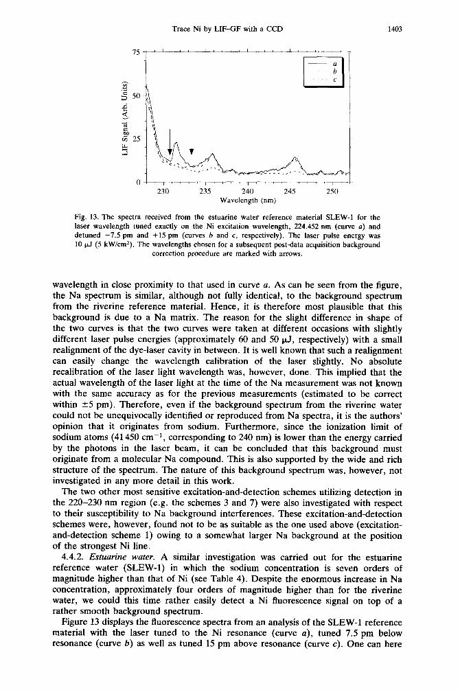
were quite similar, although not fully identical, to those from the riverine reference material. One such example is illustrated in Fig. 12.
Figure 12 shows two curves. The solid curve a originates from the certified riverine reference sample measured with the laser slightly off resonance (taken at 224.432 nm) while the broken curve b was taken using a 2 kg/ml solution of Na using an excitation
75 ” ” ” ” ” ” ” ” ” ” ” ” “““‘I
230 235 240 245 250 255 Wavelength (nm)
i
T
Fig. 12. A spectrum obtained from the SLRS-2 reference material with the laser excitation wavelength slightly detuned form the Ni resonance (224.432 nm) (curve a) together with a spectrum originating from a solution of 2 &ml of Na measured using an excitation wavelength
in close proximity to that of curve a (curve b).
Trace Ni by LIF-GF with a CCD 1403
01 i’, 7’ I 1 c t I-1 ” _7Tc 230 235 240 245 250
Wavelength (nm)
Fig. 13. The spectra received from the estuarine water reference material SLEW-l for the laser wavelength tuned exactly on the Ni excitation wavelength, 224.452 nm (curve a) and detuned -7.5 pm and +15 pm (curves b and c, respectively). The laser pulse energy was 10 pJ (5 kW/cmz). The wavelengths chosen for a subsequent post-data acquisition background
correction procedure are marked with arrows.
wavelength in close proximity to that used in curve a. As can be seen from the figure, the Na spectrum is similar, although not fully identical, to the background spectrum from the riverine reference material. Hence, it is therefore most plausible that this background is due to a Na matrix. The reason for the slight difference in shape of the two curves is that the two curves were taken at different occasions with slightly different laser pulse energies (approximately 60 and 50 rJ, respectively) with a small realignment of the dye-laser cavity in between. It is well known that such a realignment can easily change the wavelength calibration of the laser slightly. No absolute recalibration of the laser light wavelength was, however, done. This implied that the actual wavelength of the laser light at the time of the Na measurement was not known with the same accuracy as for the previous measurements (estimated to be correct within ?5 pm). Therefore, even if the background spectrum from the riverine water could not be unequivocally identified or reproduced from Na spectra, it is the authors’ opinion that it originates from sodium. Furthermore, since the ionization limit of sodium atoms (41450 cm-‘, corresponding to 240 nm) is lower than the energy carried by the photons in the laser beam, it can be concluded that this background must originate from a molecular Na compound. This is also supported by the wide and rich structure of the spectrum. The nature of this background spectrum was, however, not investigated in any more detail in this work.
The two other most sensitive excitation-and-detection schemes utilizing detection in the 220-230 nm region (e.g. the schemes 3 and 7) were also investigated with respect to their susceptibility to Na background interferences. These excitation-and-detection schemes were, however, found not to be as suitable as the one used above (excitation- and-detection scheme 1) owing to a somewhat larger Na background at the position of the strongest Ni line.
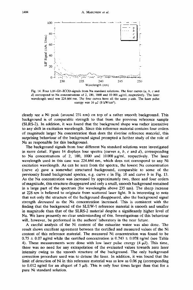
4.4.2. Estuarine water. A similar investigation was carried out for the estuarine reference water (SLEW-l) in which the sodium concentration is seven orders of magnitude higher than that of Ni (see Table 4). Despite the enormous increase in Na concentration, approximately four orders of magnitude higher than for the riverine water, we could this time rather easily detect a Ni fluorescence signal on top of a rather smooth background spectrum.
Figure 13 displays the fluorescence spectra from an analysis of the SLEW-l reference material with the laser tuned to the Ni resonance (curve a), tuned 7.5 pm below resonance (curve 6) as well as tuned 15 pm above resonance (curve c). One can here
1404 A. MARUNKOV et al.
230 235 240 245 250 Wavelength (nm)
Fig. 14. Four LIF-GF-ICCD-signals from Na standard solutions. The four curves (a, b, c and d) correspond to Na concentrations of 2, 100, 1000 and 10 000 &ml, respectively. The laser wavelength used was 224.664 nm. The four curves have all the same y-axis. The laser pulse
energy was 16 CLJ (8 kW/cm*).
clearly see a Ni peak (around 231 nm) on top of a rather smooth background. This background is of comparable strength to that from the previous reference sample (SLRS-2). In addition, it was found that the background shape was rather insensitive to any shift in excitation wavelength. Since this reference material contains four orders of magnitude larger Na concentration than does the riverine reference material, this surprising behaviour of the background signal prompted a further study of the role of Na as responsible for this background.
The background signals from four different Na standard solutions were investigated in more detail. Figure 14 displays four spectra (curves a, b, c and d), corresponding to Na concentrations of 2, 100, 1000 and 10000 pg/ml, respectively. The laser wavelength used in this case was 224.664 nm, which does not correspond to any Ni excitation wavelength. As can be seen from the spectra, the lowest Na concentration (curve a) gave a somewhat structured background, comparable to some of the previously found background spectra, e.g. curve c in Fig. 10 and curve b in Fig. 13. As the Na concentration was increased by approximately two, three and four orders of magnitude, this structure disappeared and only a small, smooth background remained in a large part of the spectrum (for wavelengths above 235 nm). The sharp increase at 228 nm is believed to originate from scattered laser light. It is interesting to note that not only the structure of the background disappeared, also the background signal strength decreased as the Na concentration increased. This is consistent with the finding that the background of the SLEW-l reference material is smooth and smaller in magnitude than that of the SLRS-2 material despite a significantly higher level of Na. We have presently no clear understanding of this. Investigations of this behaviour will, however, be performed in the authors’ laboratory in the near future.
A careful analysis of the Ni content of the estuarine water was also done. The result shows excellent agreement between the certified and measured values of the Ni content of this reference material. The measured Ni concentration was found to be 0.75 f 0.07 ng/ml while the certified concentration is 0.743 -+ 0.078 ng/ml (see Table 4). These measurements were done with low laser pulse energy (4 t.J). This time, there was no need for any extrapolation of the evaluated values towards zero laser intensity owing to the smooth structure of the background. The only background correction procedure used was to detune the laser. In addition, it was found that the limit of detection of Ni in this reference material was as low as 0.06 pg (corresponding to 0.012 ng/ml for an aliquot of 5 ~1). This is only four times larger than that for a pure Ni standard solution.
Trace Ni by LIF-GF with a CCD 1405
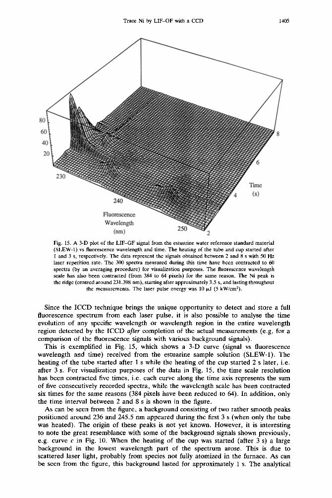
Fig. 15. A 3-D plot of the LIF-GF signal from the estuarine water reference standard material (SLEW-l) vs fluorescence wavelength and time. The heating of the tube and cup started after 1 and 3 s, respectively. The data represent the signals obtained between 2 and 8 s with 50 Hz laser repetition rate. The 300 spectra measured during this time have been contracted to 60 spectra (by an averaging procedure) for visualization purposes. The fluorescence wavelength scale has also been contracted (from 384 to 64 pixels) for the same reason. The Ni peak is the ridge (centred around 231.398 nm), starting after approximately 3.5 s, and lasting throughout
the measurements. The laser pulse energy was 10 CJ (5 kW/cm2).
Since the ICCD technique brings the unique opportunity to detect and store a full fluorescence spectrum from each laser pulse, it is also possible to analyse the time evolution of any specific wavelength or wavelength region in the entire wavelength region detected by the ICCD after completion of the actual measurements (e.g. for a comparison of the fluorescence signals with various background signals).
This is exemplified in Fig. 15, which shows a 3-D curve (signal vs fluorescence wavelength and time) received from the estuarine sample solution (SLEW-l). The heating of the tube started after 1 s while the heating of the cup started 2 s later, i.e. after 3 s. For visualization purposes of the data in Fig. 15, the time scale resolution has been contracted five times, i.e. each curve along the time axis represents the sum of five consecutively recorded spectra, while the wavelength scale has been contracted six times for the same reasons (384 pixels have been reduced to 64). In addition, only the time interval between 2 and 8 s is shown in the figure.
As can be seen from the figure, a background consisting of two rather smooth peaks positioned around 236 and 245.5 nm appeared during the first 3 s (when only the tube was heated). The origin of these peaks is not yet known. However, it is interesting to note the great resemblance with some of the background signals shown previously, e.g. curve c in Fig. 10. When the heating of the cup was started (after 3 s) a large background in the lowest wavelength part of the spectrum arose. This is due to scattered laser light, probably from species not fully atomized in the furnace. As can be seen from the figure, this background lasted for approximately 1 s. The analytical
1406 A. MARUNKOV et al.
Ni signal from 0.75 ng/ml of Ni in the estuarine water starts to appear (at 231.2 nm) after approximately 3.5 s. Consequently, from an analysis of the curve shown, one can conclude that the Ni signal arises primarily at times later than those for most of the background signal. This suggests that the signal-to-background can be improved by a proper discrimination of the emitted fluorescence light not only in wavelength but also in time. In addition, these findings suggest that parts of the scattered laser light background also could be reduced by a proper choice of ashing procedure. No such attempts were however done in the present study.. Hence, this type of 3-D LIF fluorescence information is also very useful in order to find the most suitable heating program for analysis of various samples with complicated matrices.
One possible post-data acquisition procedure for efficient reduction and extraction of relevant information from such a 3-D curve could be as follows. From previous investigations of the Ni signal vs fluorescence wavelength in pure Ni standard solutions (e.g. Fig. 6) and in estuarine sample solutions (e.g. curve a in Fig. 13) suitable positions for a measurement of the background signal level near the Ni fluorescence line at 231.398 nm were identified. Such positions are marked by arrows in Fig. 13.
Wavelength-integrated curves (as a function of time) of the detected LIF signals around the Ni fluorescence wavelength as well as around the two background detecting wavelengths were then created. Such curves, obtained from the set of data presented in Fig. 15, are presented in Fig. 16. Curve 1 in Fig. 16(a) has been obtained by an averaging of the original set of data over the wavelength region 230.86-231.96 nm. This curve corresponds to what would be detected by a PMT using an ordinary LIF-GF set-up. The curves 1 and 2 in Fig. 16(b) have been obtained by averaging the data over the wavelength regions just outside the Ni fluorescence peak, i.e. 230.35-230.70 nm and 233.15-233.50 nm, respectively. Curve 2 in Fig. 16(a), finally, has been constructed by a subtraction of the mean of the curves in Fig. 16(b) from curve 1 in Fig. 16(a) so as to compensate for a large part of the existing background interferences. Curve 2 in Fig. 16(a) thus corresponds to a background-corrected LIF-GF vs time curve.
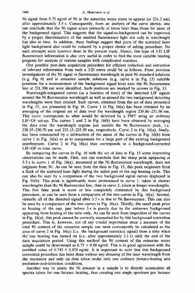
By comparing the curves in Fig. 16 with the set of data in Fig. 15 some interesting observations can be made. First, one can conclude that the sharp peak apeparing at 3.3 s in curve 1 of Fig. 16(a), measured at the Ni fluorescence wavelength, does not originate from Ni. As can be seen from the data in Fig. 15, this peak originates from a flank of the scattered laser light during the initial part of the cup heating cycle. This can also be seen by a comparison of the two background signal curves displayed in Fig. 16(b). This peak is significantly more pronounced in curve 1, taken at shorter wavelengths than the Ni fluorescence line, than in curve 2, taken at longer wavelengths. This first false peak is more or less completely eliminated by this background procedure, as can be seen from a comparison of the two curves in Fig. 16(a). Second, virtually all of the detected signal after 3.5 s is due to Ni fluorescence. This can also be seen by a comparison of the two curves in Fig. 16(a). Thirdly, the small peak prior to heating of the cup, just before 3 s is purely due to the unknown background appearing from heating of the tube only. As can be seen from inspection of the curves in Fig. 16(a), this peak cannot be correctly accounted for by this background correction procedure. This is, however, not of any crucial importance since a measure of the total Ni content of the estuarine sample can most conveniently be calculated as the area of curve 2 in Fig. 16(a) (i.e. the background corrected signal) from a time when the’ cup heating was turned on (i.e. after approximately 3.1 s) until the end of the data acquisition period. Using this method the Ni content of the estuarine water sample could be determined as 0.73 f 0.08 ng/ml. This is in good agreement with the certified value of 0.743 f 0.078 rig/ml. It is important to note that this background correction procedure has been done without any defuning of the laser wavelength from the resonance and only on data taken under only one ordinary furnace-heating and excitation-and-detection conditions.
Another way to assess the Ni amount in a sample is to directly accumulate all spectra taken for one furnace heating, thus creating one single spectrum per furnace
Trace Ni by LIF-GF with a CCD 1407
800 t--y1
3 600 .g 3
$ 400
7 5 2 200
=i
0 12 3 4 5 6 7 8 9 Time (s)
0 I 2 3 4 5 6 7 8 9 IO Time (s)
Fig. 16. LIF-GF signal curves obtained using the data presented in Fig. 15. Curve 1 in (a) has been obtained by an integration of the original set of data over the wavelength region 230.86-231.96 nm (corresponding to 16 pixels on the CCD around the Ni fluorescence wavelength at 231.398 nm). Curves I and 2 in (b) have been obtained by integration of the data over the wavelength regions just outside the Ni fluorescence peak, i.e. 230.35-230.70 nm and 233.15-233.50 nm, respectively (both curves integrated over 5 pixels). Curve 2 in (a), finally, has been constructed by subtraction of the mean of the curves in (b) from curve I in
(a) so as to compensate for background interferences.
heating cycle (as for example curve a in Fig. 13). By detuning the laser, curves similar to curves b and c in Fig. 13 can be produced. By then subtracting the mean of the two fluorescence spectra taken with the laser wavelengths slightly detuned from resonance from that obtained when the laser wavelength was tuned to the Ni resonance, a background corrected curve can be created. By a subsequent integration measurement of the remaining Ni peak, the Ni content can be assessed. Using such a procedure the Ni content of the estuarine sample solution was determined to 0.71 + 0.08 ng ml. Despite the less sophisticated background correction procedure, this value still compares rather well with the previous data (0.75 + 0.07 @ml) as well as the certified value (0.743 _t 0.078 @ml).
Finally, there are also other procedures that can be used for even more efficient corrections of background signals, e.g. by fitting curves to background signals and to combine laser detuned spectra with spectra taken at resonance in a more efficient way. All such procedures will, however, be more time consuming. Their usefulness depends to a large extent on the type of background in each specific case.
1408 A. MARUNKOV et al.
5. CONCLUSIONS
A laser-induced fluorescence in graphite furnace (LIF-GF) set-up has been equipped with an intensified CCD detector (ICCD). This brings many new important features to the LIF-GF technique. The main advantage with a LIF-GF-ICCD system in comparison with conventional photomultiplier detection is that it enables a simultaneous multichannel detection of large wavelength regions. This property gives the LIF-GF technique the following very important qualities:
(i) it vouches for an easy characterization of fluorescence spectra so as to find the most sensitive excitation-and-detection wavelength combinations from elements with complex atomic structure;
(ii) it makes it possible to increase the absolute sensitivity and spectral selectivity of the LIF-GF technique by a detection of several fluorescence wavelengths simultaneously;
(iii) it gives possibilities to study the entire wavelength dependence of various background signals, e.g. matrix interferences, blackbody radiation and scattered laser light. This is of importance when samples with high concentrations of concomitant elements are to be analysed; and
(iv) it gives possibilities to measure the content of an element and efficiently correct for any spectral background in a sample with large amounts of matrices during only one furnace heating cycle and without any need for detuning of the laser wavelength.
In addition, since a full, 1-D fluorescence wavelength spectrum can be stored for each laser pulse, it becomes possible to analyse the time evolution of any specific fluorescence line or group of lines in the entire wavelength region detected by the ICCD. This implies that the time dependence of the analytical signal can be studied with respect to those of possible spectral interferences from matrix constituents in the sample. This is of importance for finding the most suitable furnace heating program for a given sample as well as allowing for an improved selectivity by a discrimination of the detected signals not only in wavelength, but rather in a combined wavelength- and-time space. An additional advantage is that the LIF-GF-ICCD technique shows a reduced susceptibility to radio-frequency pick-ups emitted from the pump laser. This comes from the fact that the ICCD is being read out at a time after the firing of the laser. Finally, the ICCD detector permits the possibility of performing the 2-D imaging of height distributions of atomization and diffusion processes in the furnace in combination with an imaging spectrometer.
The first work with the LIF-GF-ICCD technique was performed on Ni. The most sensitive and versatile excitation-and-detection wavelengths have been identified. Detection limits for Ni in water solutions by the LIF-GF technique have been improved by two orders of magnitude and were found to be 0.015 pg with ICCD and 0.01 pg using a PMT at the most sensitive excitation-and detection wavelength.
Nickel in ng/ml concentrations has also been detected in aqueous standard reference samples with sodium concentrations ranging from kg/ml to % (riverine and estuarine water) with good accuracy and precision. The Ni content of the riverine water (SLRS- 2) was determined to 1 .OO + 0.11 rig/ml. The certified concentration was 1.03 f 0.10 ngl ml. The Ni content of the estuarine water (SLEW-l) was determined to 0.75 + 0.07 ng/ ml while the certified concentration was 0.743 + 0.078 ng/ml.
The detection limit of Ni in estuarine water was estimated to be 0.06 pg (corresponding to 0.012 ng/ml for an aliquot of 5 ul), i.e. only four times higher than in pure Ni standard solutions (0.015 pg). The use of the ICCD detector for characterization of fluorescence background from the major matrix elements (Ca, K, Mg and Na) was also investigated. A variety of methods and procedures useful for efficient background correction using the LIF-GF-ICCD technique have been demonstrated and discussed- methods and procedures that are not possible to use in any of the so-far more commonly used furnace-based techniques, e.g. ordinary LIF-GF and AAS. A substantial improvement of the qualities of an ordinary LIF-GF set-up, primarily
Trace Ni by LIF-GF with a CCD 1409
regarding improved species selectivity, has thus resulted by using an ICCD detector together with the LIF-GF technique.
Acknowledgements-The authors would like to acknowledge the Royal Swedish Academy of Sciences, the Swedish Natural Science Research Council and the Swedish Council for Planning and Coordination of Research for generous financial support. In addition, the authors are also grateful to PETER LJUNGBERG for his invaluable help with preparing Fig. 15 and for critical comments on the manuscript.
REFERENCES
[l] M. A. Bolshov, A. V. Zybin, V. G. Koloshnikov and M.V. Vasnetsov, Spectrochim. Acta XiB, 345 (1981).
[2] M. A. Bolshov, A. V. Zybin and I. I. Smirenkina, Spectrochim. Acta 36B, 1143 (1981). [3] A. W. Miziolek and R. J. Willis, Opt. Lett. 6, 528 (1981). [4] F. R. Preli, J. P. Dougherty and R. G. Michel, Anal. Chem. 59, 1784 (1987). [S] J. P. Dougherty, F. R. Preli, J. T. McCaffrey, M. D. Seltzer and R. G. Michel, J. Anal. At. Spectrom.
2, 429 (1987). [6] H. Falk, H. J. Paetzold, K. P. Schmidt and J. Tilch, Spectrochim. Acta 44B, 1101 (1988). [7] N. Omenetto, P. Cavalli, M. Broglia, P. Qi and G. Rossi, J. Anal. At. Spectrom. 3, 231 (1988). [S] M. Leong, J. Vera, B. W. Smith, N. Omenetto and J. D. Winefordner, Anal. Chem. 60, 1605 (1988).
[9] J. P. Dougherty, J. A. Costello and R. G. Michel, Anal. Chem. 60, 336 (1988). [lo] J. A. Vera, C. L. Stevenson, B. W. Smith, N. Omenetto and J. D. Winefordner, J. Anal. At. Spectrom.
4, 619 (1989). [ll] B. Remy, I. Verhaeghe and P. Mauchien, Appl. Spectrosc. 44, 1633 (1990). [12] D. J. Butcher, R. L. Irwin, J. Takahashi, G. Su, G.-T. Wei and R. G. Michel, Appl. Spectrosc. 44,
1521 (1990). [13] Z. Liang, R. F. Lonardo and R. G. Michel, Spectrochim. Acta 48B, 7 (1993). [14] D. J. Butcher, J. P. Dougherty, F. R. Preli, A. P. Walton, G.-T. Wei, R. L. Irwin, and R. G. Michel,
J. Anal. At. Spectrom. 3, 1059 (1988). [15] N. Omenetto, B. W. Smith and J. D. Winefordner, Spectrochim. Acta 43B, 1111 (1988). [16] S. Sjostrom, Spectrochim. Acta Rev. 13, 407 (1990). [17] F. W. Sunderman, M. C. Crisostomo, M. C. Reid, S. M. Hopfer and S. Nomoto, Ann. Clin. Lab.
Sci. 14, 232 (1984). [18] F. S. Wei and W. Q. Qu, Anal. Lett. 17, 1607 (1984). [19] C. N. Leach, J.V. Linden, S. M. Hopfer, M. C. Crisostomo and F. W. Sunderman, Clin. Chem. 31,
556 (1985). [20] J. R. Andersen, B. Gammelgaard and S. Reimert, Analyst 111, 721 (1986). [21] M. R. Wills, C. S. Brown, R. L. Bertholf, R. Ross and J. Savory, Clin. Chim. Acta 145, 193 (1985).
[22] M. Drazniowsky, I. S. Parkinson, M. K. Ward, S. M. Channon and D. N. Kerr, Clin. Chim. Acta
145, 219 (1985). [23] A. Kumar, M. Z. Hasan and B. T. Deshmukh, Indian J. Pure Appl. Phys. 24, 594 (1986). [24] S. M. Hopfer, J. W. Linen, W. N. Rezuke, J. E. O’Brien, L. Smith, F. Watters and F. W. Sunderman,
Res. Commun. Chem. Pharmacol. 55, 101 (1987). [25] K. P. Schmidt and H. Falk, Spectrochim. Acta 42B, 431 (1987). [26] J. M. Benson, A. F. Eidson, R. L. Hanson, R. F. Henderson and C. H. Hobbs, J. Appl. Toxicol. 9,
219 (1989). [27] J. H. Raithel, F. Henning and K. H. Schaller, J. Environ. Pathol. Toxicol. Oncol. 9, 115 (1989). [28] B. W. Smith, M. R. Glick, K. N. Spears and J. D. Winefordner, Appl. Spectrosc. 43, 376 (1989). [29] A. Varma, CRC Handbook of Furnace Atomic Spectroscopy, p. 245. CRC Press Inc., Boca Raton,
FL (1990). [30] M. S. Cresser, J. Armstrong, J. Dean, M. H. Ramsey and M. Cave, J. Anal. At. Spectrom. 6, 1R
(1991). [31] S. Branch, H. M. Crews, D. J. Halls and A. Taylor, J. Anal. At. Spectrom. 6, 69R (1991). [32] J. Marshall, J. Carroll and J. S. Crighton, J. Anal. At. Spectrom. 6, 283R (1991). [33] M. S. Cresser, J. Armstrong, J. Dean, P. Watkins and M. Cave, J. Anal. At. Spectrom. 7, 1R (1992). [34] A. Taylor, S. Branch, H. M. Crews and D. J. Halls, J. Anal. At. Spectrom. 7, 67R (1992). [35] J. Marshall, J. Carroll, J. S. Crighton and C. L. R. Barnard, J. Anal. At. Spectrom. 7, 349R (1992). [36] M. S. Cresser, J. Armstrong, J. Cook, J. Dean, P. Watkins and M. Cave, J. Anal. At. Spectrom. 8
1R (1993). [37] A. Taylor, S. Branch, H. M. Crews and D. J. Halls, J. Anal. At. Spectrom. 8, 79R (1993). [38] J. Marshall, J. Carroll, J. S. Crighton and C. L.R. Barnard, J. Anal. At. Spectrom. 8, 337R (1993). [39] S. J. Hill, J. B. Dawson, W. J. Price, I. L. Shuttler and J. F. Tyson, J. Anal. At. Spectrom. 6, 187R
(1991) [40] S. J. Hill, J. B. Dawson, W. J. Price, I. L. Shuttler and J. F. Tyson, J. Anal. At. Spectrom. 7, 215R
(1992). [41] S. J. Hill, J. B. Dawson, W. J. Price, I. L. Shuttler and J.F. Tyson, J. Anal. At. Spectrom. 8, 197R
(1993).

1410 A. MARUNKOV et al.
[42] D. E. Nixon, T. P. Moyer, D. P. Squillance and J. T. McCarthy, Analyst 114, 1671 (1989). (431 S. SjiistrBm, 0. Axner and M. Norberg, J. Anal. At. Spectrom. 8, 375 (1993). [44] 0. Axner and H. Rubinsztein-Dunlop, Appl. Opt. 32, 867 (1993).
[45] E. Lundberg, D. C. Baxter and W. Frech, 1. Anal. At. Spectrom. 1, 105 (1986). [46] E. Lundberg, W. Frech and J. M. Harnly, J. Anal. At. Speckom. 3, 1115 (1988). [47] E. Lundberg, W. Frech, D. C. Baxter and A. Cedergren, Specrrochim. Acra 43B, 451 (1988). [48] G.-T. Wei, J. P. Dougherty, F. R. Preli Jr and R. G. Michel, J. Anal. At Specrrom. 5, 249 (1990). [49] K. R. Sperling, Spectrochim. Acta 39B, 371 (1984). [50] W. Frech, E. Lundberg and A. Cedergren, Prog. Anal. AI. Specrrosc. 8, 257 (1985).
[51] E. J. Czobik and J. P. Matousek, Anal. Chem. 50, 2 (1978). [52] R. Cruz and J. C. van Loon, Anal. Chim. Acfa 72, 231 (1974).
(531 K. Julshamm, At. Absorpt. Newsl. 16, 149 (1977). [54] W. Siavin and D. C. Manning, Prog. Anal. At. Spectrosc. 5, 243 (1982). [55] C. H. Corliss and W. R. Bozman, Experimental Transilion Probabilities for Spectral Lines of Seventy
Elements, NBS Monograph 53, U.S. Government Printing Office, Washington, DC (1962). [56] J. Reader, C. H. Corliss, W. L. Wiese and G. A. Martin, Wavelength and Transition Probabilities for
Atom and Atomic Zons, NSRDS-NBS 68, Washington, DC (1980).
Copyright © 2022 FDOKUMEN