ORIGINAL RESEARCH PAPER

Detection of fluvial sand systems using seismic attributesand continuous wavelet transform spectral decomposition: casestudy from the Gulf of Thailand

Mirza Naseer Ahmad • Philip Rowell •

Suchada Sriburee

Received: 29 July 2013 / Accepted: 24 January 2014

� Springer Science+Business Media Dordrecht 2014

Abstract Fluvial sands host excellent oil and gas reser-

voirs in various fields throughout the world. However, the

lateral heterogeneity of reservoir properties within these

reservoirs can be significant and determining the distribu-

tion of good reservoirs is a challenge. This study attempts

to predict sand distribution within fluvial depositional

systems by applying the Continuous Wavelet Transfor-

mation technique of spectral decomposition along with full

spectrum seismic attributes, to a 3D seismic data set in the

Pattani Basin, Gulf of Thailand. Full spectrum seismic

attributes such as root mean square and coherency help to

effectively map fluvial systems down to certain depth

below which imaging is difficult in the intervals of interest

in this study. However, continuous wavelet transform used

in conjunction with other attributes by applying visualiza-

tion techniques of transparency and RGB can be used at

greater depths to extract from 3D seismic data useful

information of fluvial depositional elements. This work-

flow may help to identify different reservoir compartments

within the fluvial systems of the Gulf of Thailand.

Keywords Gulf of Thailand � CWT spectral

decomposition � Fluvial systems

Introduction

Mapping of sub-surface sand bodies associated with fluvial

systems is one of the key issues for oil and gas exploration

in the Gulf of Thailand. These fluvial sand systems contain

a series of sand point bar and overbank deposits inter-

spersed with mud-filled abandonment channels and the

sand bodies are generally restricted laterally and vertically.

The implication for reservoir characterization of these

depositional systems due to this complex geometry is that

the point bar sand accumulations that form the main res-

ervoirs can be highly compartmentalized as a result of

crosscutting mud-filled channels. Therefore, delineation of

point bar and channel geometries has important conse-

quences for hydrocarbon exploration and development.

This study attempts to define sand body geometries by

using the continuous wavelet transform (CWT) spectral

decomposition technique and seismic attributes on a seis-

mic data set from the Pattani Basin within the Gulf of

Thailand (Fig. 1). Previously in the same area the discrete

Fourier transform spectral decomposition technique was

used to identify relatively thick sand bodies (Ahmad and

Rowell 2012). However, the CWT technique theoretically

has the ability to provide better resolution as it does not

require pre-selecting a window length and does not have

fixed time–frequency resolution (Sinha et al. 2005). The

workflow suggested in this study may be useful to improve

the resolution and detection of new stratigraphic and

structural traps in the interval of interest in the area.

Geology of the area

The Gulf of Thailand lies on the southern margin of the

Eurasian Plate covering an area of about 270,000 km2. The

basins in the Gulf of Thailand are divided into two parts by

the north–south trending Ko Kra Ridge (Fig. 1). This ridge

separates the comparatively larger Pattani, Malay and

Khmer Basins to the east from the narrower and more

elongate basins to the west (Racey 2011). Extensional

M. N. Ahmad (&) � P. Rowell � S. Sriburee

Petroleum Geoscience Program, Chulalongkorn University,

Bangkok, Thailand

e-mail: naseerrb3@yahoo.com

123

Mar Geophys Res

DOI 10.1007/s11001-014-9213-0

basins of the Gulf of Thailand are considered to have been

initiated by the collision of the Indian Plate with the Eur-

asian Plate and generally these rift basins have a typical

half-graben dominant rifting style (Morley et al. 2011). The

general strike of regional basin bounding faults is north–

south. Some faults trending oblique to the regional north–

south faults are also observed. These faults have been

interpreted as transfer zones/graben shifts influenced by

oblique pre-existing fabrics (Morley et al. 2004). The

timing of formation of different structures within the dif-

ferent basins of the Gulf of Thailand is regionally variable.

The basins to the east of the Ko Kra Ridge are dominated

by ?Eocene–Oligocene syn-rift structures followed by very

rapid Miocene-Recent post-rift subsidence, whereas the

basins to the west of the Ko Kra Ridge are characterized by

Late Oligocene to Mid-Miocene rifting and Late Miocene-

Pliocene post-rift subsidence (Morley and Racey 2011). A

schematic cross-section across the Pattani Basin is shown

in Fig. 2.

The study area within the Pattani Basin contains more

than 7,600 m in thickness of predominantly non-marine,

fluvial-deltaic sediments and has been sub-divided strati-

graphically into five sequences (Morley and Racey 2011).

These depositional sequences evolve from lacustrine and

alluvial dominant syn-rift sediments in the Eocene–Oligo-

cene to post-rift fluvial-dominant sediments in the Early to

Middle Miocene, to marginal marine dominant sedimen-

tation in the Late Miocene to the Recent. Figure 3 shows a

typical well log from the Pattani Basin with an interpre-

tation of the different depositional environments encoun-

tered in the interval of interest. These depositional

environment interpretations are supported by seismic

images in the basin. Shallow seismic time and horizon

slices show evidence of a general N–S trend of the fluvial

systems within the Pattani Basin (Fig. 4a. Within these

fluvial systems complex superimposed geometries of

channels and point bars are common (Fig. 4b, c). Pay

sands, which are predominantly gas-saturated, are mostly

encountered in the post-rift section within mainly thin

fluvial sands. The depth of these gas pay zones ranges from

1,500–2,600 m in the study area. The sand porosities in the

shallow part (\1,200 m depth) are reported to be in the

range of 13–30 %, whereas porosity decreases drastically

to a range of 1–15 % at 2,400 m. This drastic decline may

be related to rapid onset of digenesis associated with high

geothermal gradients (Racey 2011). The source rock

Fig. 1 Location map of the

study area in the Gulf of

Thailand. The area is composed

of north–south trending basins

(yellow color polygons). The

Pattani Basin study area is

highlighted

Mar Geophys Res

123

Fig

.2

Sch

emat

icE

ast–

Wes

tcr

oss

-sec

tio

nac

ross

the

Pat

tan

iB

asin

(mo

difi

edaf

ter

Mo

rley

and

Rac

ey2

01

1)

Mar Geophys Res

123

intervals are lacustrine shales and coals in the syn-rift

Oligocene sequence and coals within the Lower to Middle

Miocene. The basin-bounding faults of the Pattani Basin

were active throughout most of the basin’s history and

most likely acted as conduits for vertical hydrocarbon

migration.

Methodology

Synthetic seismograms were generated for key wells to link

logs (in depth domain) to time domain seismic data and to

observe the seismic character of sands within the area. The

synthetic seismograms were created by using the extracted

wavelet at well locations. Well to seismic ties were per-

formed by establishing correlation between the seismic and

synthetic seismograms by adjusting T-D functions through

stretch and squeeze.

The zone of interest is defined from 1,300 to 2,600 m,

which includes fluvial sand reservoirs of Early to Middle

Miocene. Three key horizons (H1, H2 and H3) were

mapped throughout the 3D full stack seismic data volume

and interpolated to obtain continuous horizon surfaces for

extracting various seismic attributes (Fig. 5). In order to

map in detail the vertical changes in sand distribution and

seismic geomorphology some additional horizon slices

Fig. 3 Typical well log from the Gulf of Thailand along with interpreted depositional environments. This representive well log has been

extracted from an extensive database of over 100 wells within the interval of interest in the central Pattani Basin

Mar Geophys Res

123

were selected with reference to these three interpreted

horizons (red horizons; Fig. 5). These interpreted horizons

(H1, H2, and H3) were projected at different levels through

the seismic data for detection of meaningful sand distri-

bution patterns. For example, H1-300 and H3-160 horizon

slices are approximately 300 and 160 ms shallower than

the H1 and H3 horizons respectively. Similarly, horizon

slices sand1 and sand2 are selected with respect to Horizon

H2. Figure 6 shows a typical seismic section within the

study area with typical discontinuous reflection packages,

consistent with a fluvial dominant depositional systems

interpretation. There are also many faults as well within the

section so discontinuities are even more exaggerated by the

structural complexities in many parts of the basin. It is

extremely difficult to interpret chrono-startigraphic sur-

faces in this type of depositional environment. Therefore

phantom horizons are interpreted which are parallel to

structure. We used these pseudo-chronostratigraphic sur-

faces as guides to extract time equivalent depositional

system geometries using variable time extraction windows.

Spectral decomposition is a tool for better imaging and

mapping temporal bed thickness using 3D seismic data

(Partyka et al. 1999) and it aids in seismic interpretation by

analyzing the variation of amplitude spectra. There is a

variety of spectral decompositions methods. Each method

has its own advantages and disadvantages and different

applications require different methods (Castagana 2006). In

this study, we applied CWT transforms on full stack seis-

mic data to check the frequency response of fluvial sand

systems and calculated iso-frequency volumes using the

CWT technique. RGB visualization techniques were also

applied to multiple iso-frequency volumes. RGB spectral

decomposition volumes have been documented to have the

capability of extracting geological information that would

Fig. 4 a Shallow seismic horizon slice shows the typical geometry of

fluvial systems within the Gulf of Thailand. The dominant trend of the

fluvial systems are N–S. b A zoomed in portion of a seismic horizon

slice showing a fluvial system with a complex superimposed

geometry of channels and point bars. c A vertical seismic section

along the marked red line in b

Mar Geophys Res

123

be otherwise inaccessible by other methods (Henderson

et al. 2007).

In order to understand the relationship between bright

amplitudes at specific frequencies and thicknesses of sand

bodies, synthetic models of different thicknesses of sand were

analyzed. Three-layered models which consist of a sand layer

encased between two shale layers were prepared. The sand

thicknesses were set at 6, 10, 20, 25, 30, 40 and 50 m. The

acoustic impedances used for these three layers were taken

from nearby well data. Synthetic seismograms for each model

were generated using wavelet extracted from the seismic data

within the zone of interest along the wellbore. The velocity

and density of the sand layer used in the model are 2,750 m/s

and 2.15 g/cc whereas velocity and density of shale layers

used was 3,100 m/s and 2.49 g/cc. These synthetic seismo-

grams were spectrally decomposed using CWT for different

frequencies, and frequencies showing maximum amplitude

for specific sand thickness were noted and plotted against the

sand layer thickness to establish a relationship between fre-

quency and layer thickness.

Fig. 5 Vertical seismic section

with three interpreted horizons

(H1, H2 and H3). The red

horizon slices were generated

with reference to these

interpreted horizons

Fig. 6 Typical seismic section

in the study area

Mar Geophys Res

123

Fig. 7 Synthetic to seismic tie

in one of the representative

wells

Fig. 8 a Extracted wavelet used for synthetic generation in time series. b Frequency spectra of extracted wavelet

Mar Geophys Res

123

In addition to spectral decomposition, we also calculated

seismic coherence. Seismic coherency is a measure of trace-

to-trace similarity or continuity of seismic waveform in a

specified window. In this study each point in the 3D seismic

volume was compared with the waveform of 12 adjacent

traces over a short vertical window of 9 ms. Coherency may

be helpful to detect sands associated with fluvial systems

(Peyton et al. 1998). The root mean square (RMS) attribute

was also calculated over selected windowed intervals of

10–20 ms tied to key horizon slices. RMS is a statistical

measure of amplitude variation within a defined window and

is a useful attribute when values run through the positive and

negative domain like seismic. RMS emphasizes the varia-

tions in the acoustic impedance over the selected windowed

interval which can provide useful information for the map-

ping of the fluvial sands. We use the RMS attribute because

sands are typically represented as trough/peak pairs and as

the interpreted horizons and slices are not exactly chrono-

stratigraphic surfaces the RMS attribute calculated over a

selected window may provide more useful information for

the detection of sand distribution. The sand bodies associated

with the fluvial systems were mapped by applying different

Fig. 9 Synthetic seismogram

along with GR log and acoustic

impedance. Sands generally

show low acoustic impedance

and the top sand reflector

correlates to a negative

amplitude on the synthetic

seismogram

Mar Geophys Res

123

Fig. 10 Cross-plot of sand

thickness versus maximum

amplitude response at CWT

frequencies. Thick sand beds

give maximum amplitude at low

frequencies while thinner sand

beds show maximum amplitude

response at high frequencies.

These results are based on

synthetic model data

Fig. 11 CWT spectral decomposition along a representative well

section at a 20 Hz, b 30 Hz, c 40 Hz and d 45 Hz. Thick sands show

bright amplitudes at low frequencies whereas thin sands show bright

amplitude at higher frequencies (c and d) such as above the H1

marker. The yellow curve is GR (increasing towards right) while the

red curve is a gas pay flag

Mar Geophys Res

123

3D visualization techniques, such as transparency which

combined calculated attributes from spectral decomposition

with seismic coherency and RGB blending of different

frequencies.

Results and discussion

Synthetic seismogram

The seismic data is of normal polarity with an increase in

acoustic impedance being represented by a peak. The

synthetic seismograms of four key wells in the study area

Fig. 12 Cross-plot of sand net to gross and average amplitude at

20 Hz within the zone of interest (H1 to H2). Average amplitude

increases as sand ratio increases. This cross-plot is based on real

seismic data. Sand net to gross was calculated from well data

Fig. 13 Average amplitude map between H1 to H2 interval at 20 Hz

CWT spectral decomposition along with representative seismic cross-

sections through key wells. High average amplitudes are observed

within the zone of interest for thick sands and gas-saturated sands. No

gas zone was encountered between H1 and H2 at Well-03 and Well-

04 and the average amplitude is low. The yellow curve represents GR

while the red flagrepresents gas pay zones

Mar Geophys Res

123

show a reasonable correlation to the seismic data (Fig. 7)

using the extracted wavelet shown in both the time and

frequency domains in Fig. 8. Sands have relatively low

acoustic impedance and the top sand reflectors generally

show negative amplitudes on the synthetic seismogram

(Fig. 9).

Response of spectral decomposition to thickness

variation of sands

According to the spectral decomposition of synthetic

models (Fig. 10) as the thickness of the sand bed decreases,

we observe the maximum seismic amplitude response at

higher frequencies. This frequency-thickness relationship

can help us to identify particular frequencies for specific

sand thicknesses e.g. to explore 40 m thick sand bed we

need to analyze the 15 Hz iso-frequency volume. The thin

sands which are less than 20 m thick indicate maximum

amplitude at 40 Hz which is due to the limitation of fre-

quency bandwidth of the extracted wavelet used. The

amplitude spectrum of this wavelet drops drastically

between 40 and 50 Hz (Fig. 8). It is important to realize

that these observations are for a simple three-layered model

and results may vary to some degree in real data because

multiple closely spaced sand beds separated by thin shales

are common in the interval of interest. This may produce

anomalous amplitudes at different frequencies due to

Fig. 14 Comparison of RMS attribute maps extracted at a the shallow H1-300 horizon slice and b a deeper horizon slice at H3-160. The RMS

attribute window is 20 ms

Fig. 15 A coherence horizon slice in the H1 to H2 interval. The

cross-sections are location of vertical seismic sections view in

Figs. 16, 17 and 18. Blue numbers are measured width of low

coherency mud-filled channels are highlighted by arrows

Mar Geophys Res

123

interference effect of different sand reflectors. However

this modeling does suggest that bright amplitudes at low

frequencies (*20 Hz) may indicate thick sands in the

range of 30–35 m.

Amplitude spectra outputs using the CWT on the real

dataset along a representative well show that the seismic

response is significantly different for different sand thick-

nesses. Thick sands show bright amplitudes at 20 Hz

(Fig. 11a) whereas higher frequency components show low

amplitude at the same thick sand intervals within the well

(Fig. 11b, c, d). A thin sand just above the H1 horizon has

low amplitudes at 20 and 30 Hz but brightens up consid-

erably at higher frequencies (Fig. 11 c, d).

As the sands within the zone of interest are restricted in

distribution due to their fluvial nature it is meaningful to be

able to predict thick sand zones within this interval. We

analyzed the relationship between amplitudes at 20 Hz

which are indicative of thick sand bodies with respect to sand

net to gross in the interval between the two interpreted

horizons (H1 and H2) using the real seismic dataset. The

average amplitude at 20 Hz increases as the sand percentage

increases between the two horizons at well locations

Fig. 16 The vertical seismic section A-A’ of Fig. 15. Red number is width of the mud filled channel. Channel location is highlighted

Fig. 17 The vertical seismic section B-B’ of Fig. 15. Red number is width of the mud-filled channel. Channel location is highlighted

Mar Geophys Res

123

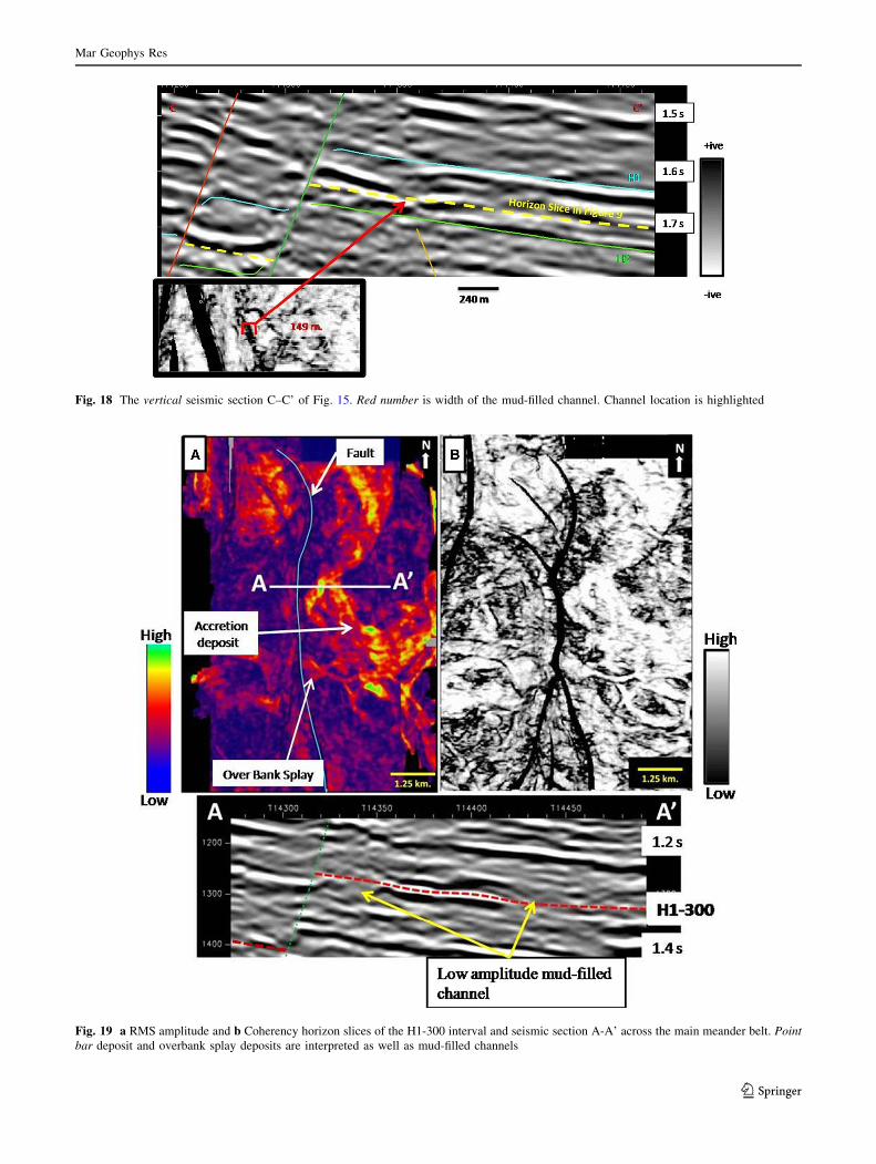
Fig. 18 The vertical seismic section C–C’ of Fig. 15. Red number is width of the mud-filled channel. Channel location is highlighted

Fig. 19 a RMS amplitude and b Coherency horizon slices of the H1-300 interval and seismic section A-A’ across the main meander belt. Point

bar deposit and overbank splay deposits are interpreted as well as mud-filled channels

Mar Geophys Res

123

(Fig. 12). An average amplitude map of the 20 Hz frequency

data within the zone of interest also verifies that brighter

amplitudes represent thick sand zones at well locations

(Fig. 13). At the Well-01 and -02 locations bright amplitudes

correlate with thick sands encountered in these wells within

the H1 to H2 interval whereas low amplitudes are observed at

the Well-03 and -04 locations that have relatively thin sands

within the same interval (Fig. 13). The average amplitude is

also affected by the presence of hydrocarbons. Note that the

N–S trending high amplitude channel belt has even higher

amplitudes at the Well-01 and -02 locations due to gas effect.

This effect will be documented in a future study. In summary,

a comparison of amplitude variations at low frequencies with

well data proves that high amplitudes can be correlated with

prospective zones.

RMS analysis

RMS attribute analysis can be a useful method to delineate

sand body geometries. However, it requires a good acoustic

contrast between sand and shale and is therefore quite

depth dependent. For example, RMS analysis using a

Fig. 20 a Amplitude extraction from CWT at 20 Hz and b Coherency

horizon slice of Sand1. A representative seismic section through

Well-01 shows a strong amplitude at well location which correlates to

a thick sand on the log data. The marked red horizon slice is out of the

picture on the downthrown side of the fault

Mar Geophys Res

123

shallow horizon slice (H1-300) shows a very good image of

sands associated with a meander belt whereas at deeper

horizons (H3-160) the image is not of good enough defi-

nition to map the sand systems accurately (Fig. 14).

Seismic coherence analysis

Coherence slices within the H1 to H2 interval show nar-

row, low coherence, sinuous features associated with broad

white belts of high coherence (Fig. 15). The associated

vertical sections across the dark sinuous features reveal that

they may be channels (Figs. 16, 17, 18). These channel

geometries correlate with a low amplitude seismic response

and based on synthetic modeling, are interpreted as mud-

filled. On the other hand, high-coherence, broad, white

features on the coherence slice represent strong negative

amplitudes on the vertical seismic sections. These negative

amplitudes are associated with sands confirmed at drilled

well locations. Based on their geometries on the coherence

slice and vertical seismic sections these are interpreted as

sands associated with point bar deposits.

Seismic geomorphology and mapping of sands

Bright negative amplitudes are observed on the vertical

seismic sections which are interpreted to represent sands

which can often be vertically quite closely spaced. Multiple

horizon slices were thus selected in the zone of interest in

order to understand the vertical variations in sand distri-

bution patterns by observing different seismic attributes,

coherence and various CWT spectral components. The

focus is on presenting mostly 20 Hz CWT results, as this

low frequency best indicates thick sands. Key horizon sli-

ces shown in Fig. 5 are discussed below.

Horizon slice H1-300

This is the shallowest horizon slice that was imaged for

sand distribution analyses. This horizon slice shows most

clearly the prominent image of fluvial systems on the

RMS calculated horizon slice. However, below this depth

the RMS attribute alone does not yield as clear an image.

The horizon slice of both RMS and coherence shows a

well developed NW–SE oriented meander belt of high

sinuosity (Fig. 19). The RMS amplitude extractions are

high associated with point bar sand deposits within the

meander belt. The meander belt width is approximately

3.2 km whereas the width of the mud-filled channels

observed on the vertical seismic section and coherency

horizon slice are quite narrow. Overbank splay-like fea-

tures are also observed in the central part of the slice at

the outer channel bend. These deposits can form at the

outer channel bend where flow momentum causes the

flow to breach the adjacent area (Posamentier and Kolla

2003).

Horizon slice sand 1

This horizon slice below H1 is within the zone of hydro-

carbon bearing reservoirs. The features observed on a

horizon slice from the 20 Hz CWT iso-frequency volume

and coherency volumes indicate low sinuosity features as

compared to the shallower horizon slice (Figs. 20, 21). The

meander belt is also narrower and the associated low

amplitude channels are of width in the range of

150–200 m. Well-01 encountered blocky sands in the

interval which corresponds to this horizon slice. An overlay

of the coherency horizon slice on the 20 Hz CWT spectral

decomposition horizon slice shows that some sand bodies

are cut across by the low amplitude mud-filled channels

(Fig. 21).

Horizon slice sand 2

The general trend of sand bodies in this deeper horizon

slice is north–south (Fig. 22a). The meander belt is about

200–500 m wide. The GR pattern is blocky and the

thickness of the sand observed at the Well-01 location in

the interval corresponding to this horizon slice is in the

range of 31 m. Lateral migration of sand bodies can be

Fig. 21 Overlay of a 50 % transparent coherency slice on the 20 Hz

CWT spectral decomposition horizon slice of sand1. A number of sand

bodies are seen to be cut across by low amplitude mud-filled channels

Mar Geophys Res

123

Fig. 22 a Amplitude extraction

of CWT at 20 Hz and

b Coherency horizon slice of

Sand 2. c Overlay of 50 %

transparent coherency slice on

20 Hz CWT spectral

decomposition horizon slice.

Different sand bodies are cut

across by low amplitude mud-

filled channels

Mar Geophys Res

123

seen on the vertical seismic section (Fig. 22). An overlay

of the coherency on the 20 Hz CWT spectral decomposi-

tion horizon slice shows different sand bodies separated by

low amplitude mud-filled channels (Fig. 22c). Faults

appear to dissect sand bodies also.

Horizon slice H3-160

The quality of images at this deepest horizon slice are not

as good as compared with other slices and it is difficult to

interpret meander belt geometry on either the coherency or

the CWT horizon slices (Fig. 23a, b). The reason for this

low quality imaging may be related to the thickness of the

sand bodies at this depth. The best image is observed on an

RGB blended horizon slice using three different frequen-

cies (Fig. 23c). Thick point bar sands and cross-cutting

mud-filled channels can be observed on this blended

horizon slice. The observed sand thickness within Well-05

where it intersects this horizon slice is about 9 m and low

amplitudes are observed at the well location.

Comparison of different attributes

Horizon based extractions of the RMS attribute and

seismic coherency effectively delineate different ele-

ments of the fluvial systems at shallow depths in the study

area (Fig. 24), but at deeper levels these two attributes

have limited discrimination capability for different ele-

ments of the fluvial systems (Fig. 25). This may be due to

lack of amplitude contrast between mud- filled channels

and the associated sandy point bars (Henderson et al.

2007). Rock physics analysis has also revealed that below

certain depths, the acoustic impedance contrast between

shale and sand is minimal (Ahmad and Rowell 2013).

However, horizon based map extractions from CWT

spectral decomposition volumes do provide better

Fig. 23 a Amplitude extraction of CWT at 40 Hz and b Coherency horizon slice of H3-160. c Horizon slice of RGB blending for three

frequencies at 20 Hz, 30 Hz and 40 Hz

Mar Geophys Res

123

imaging of sand depositional systems at greater depths

(Fig. 23a). Moreover, RGB blending of different fre-

quency horizon slices further improves the resolution of

depositional geometry and morphology of these

subsurface fluvial systems (Fig. 23c). This comparison

between maps of full stack seismic attributes (RMS and

seismic coherence) and maps produced using CWT and

RGB techniques highlights the value of CWT and RGB

Fig. 24 a RMS attribute map at H1-300 horizon slice. b Coherency horizon slice at H1-300 horizon slice. At this shallow level, full spectrum

seismic attributes effectively map fluvial depositional system elements in the area

Fig. 25 a RMS attribute map at H3-160 horizon slice. b Coherency horizon slice at H3-160 horizon slice. At this deeper level, full spectrum

seismic attributes cannot effectively map fluvial depositional system elements in the area

Mar Geophys Res

123

visualization for delineation of different fluvial elements

at deeper levels.

Conclusions

In this study, we extracted various seismic attributes from

the seismic data to image the fluvial depositional systems

within the Pattani Basin of the Gulf Thailand. Full spec-

trum seismic attributes such as RMS and seismic coherence

can only successfully map fluvial systems at shallow

depths. Below a certain depth full spectrum seismic attri-

butes have limited capability of identification of different

fluvial elements. The results reveal that CWT and RGB

visualization of multiple frequencies can be successfully

used to detect fluvial systems at deeper levels that are not

recognized by full spectrum seismic attributes. Therefore,

CWT techniques may be useful in the planning of wells for

field development in the study area.

Acknowledgments We thank Fugro-Jason for providing an aca-

demic license of their Continuous Wavelet Transform spectral

decomposition module which was used in this research. Landmark is

also acknowledged for providing academic licenses of GeoProbe,

PowerView and SeisWorks for the present research. We also thank

management of Chevron Thailand Exploration and Production, Ltd.

for permission to publish this paper.

References

Ahmad MN, Rowell P (2012) Application of spectral decomposition

and seismic attributes to understand the structure and distribution

of sand reservoirs within tertiary rift basins of the Gulf of

Thailand. Lead Edge 31:630–634

Ahmad MN, Rowell P (2013) Mapping of fluvial sand systems using

rock physics analysis and simultaneous inversion for density:

case study from the Gulf of Thailand. First Break 3:49–54

Castagana JP (2006) Comparison of spectral decomposition methods.

First Break 24:75–79

Henderson J, Purves SJ, Leppard C (2007) Automated delineation of

geological elements from 3D seismic data through analysis of

multichannel, volumetric spectral decomposition data. First

Break 25:87–93

Morley CK, Racey A (2011) Tertiary stratigraphy. In: Ridd MF,

Barber AJ (eds) The geology of Thailand. The Geological

Society, London, pp 223–271

Morley CK, Haranya C, Phoosongsee W, Kornsawn A, Wonganan N

(2004) Activation of rift oblique and rift parallel pre-existing

fabrics during extension and their effect on deformation style;

examples from rifts of Thailand. J Struct Geol 26:1803–1829

Morley CK, Charusiri P, Watkinson IM (2011) Structure geology of

Thailand during the Cenozoic. In: Ridd MF, Barber AJ (eds) The

geology of Thailand. The Geological Society, London,

pp 274–334

Partyka G, Gridley J, Lopez (1999) Interpretational applications of

spectral decomposition in reservoir characterization. Lead Edge

18:353–360

Peyton L, Bottjer R, Partyka G (1998) Interpretation of incised alleys

using new 3-D seismic techniques: a case history using spectral

decomposition and coherency. Lead Edge 17:1294–1298

Posamentier HW, Kolla V (2003) Seismic geomorphology and

stratigraphy of depositional elements in deep-water settings.

J Sediment Res 73:367–388

Racey A (2011) Petroleum geology. In: Barber AJ, Ridd MF (eds)

The geology of Thailand. The Geological Society, London,

pp 351–392

Sinha S, Routh PS, Anno PD, Castagana JP (2005) Spectral

decomposition of seismic data with continuous-wavelet trans-

form. Geophysics 70:P19–P25

Mar Geophys Res

123