Détection de l'endommagement dans un composite tissé ...
317
HAL Id: tel-01932575 https://pastel.archives-ouvertes.fr/tel-01932575 Submitted on 23 Nov 2018 HAL is a multi-disciplinary open access archive for the deposit and dissemination of sci- entific research documents, whether they are pub- lished or not. The documents may come from teaching and research institutions in France or abroad, or from public or private research centers. L’archive ouverte pluridisciplinaire HAL, est destinée au dépôt et à la diffusion de documents scientifiques de niveau recherche, publiés ou non, émanant des établissements d’enseignement et de recherche français ou étrangers, des laboratoires publics ou privés. Détection de l’endommagement dans un composite tissé PA66,6/Fibres de verre à l’aide de techniques ultrasonores en vue d’une prédiction de la durabilité de pièces automobiles Pascal Pomarede To cite this version: Pascal Pomarede. Détection de l’endommagement dans un composite tissé PA66,6/Fibres de verre à l’aide de techniques ultrasonores en vue d’une prédiction de la durabilité de pièces automobiles. Mécanique des matériaux [physics.class-ph]. Ecole nationale supérieure d’arts et métiers - ENSAM, 2018. Français. NNT : 2018ENAM0024. tel-01932575
-
Upload
khangminh22 -
Category
Documents
-
view
0 -
download
0
Transcript of Détection de l'endommagement dans un composite tissé ...
HAL Id: tel-01932575https://pastel.archives-ouvertes.fr/tel-01932575
Submitted on 23 Nov 2018
HAL is a multi-disciplinary open accessarchive for the deposit and dissemination of sci-entific research documents, whether they are pub-lished or not. The documents may come fromteaching and research institutions in France orabroad, or from public or private research centers.
L’archive ouverte pluridisciplinaire HAL, estdestinée au dépôt et à la diffusion de documentsscientifiques de niveau recherche, publiés ou non,émanant des établissements d’enseignement et derecherche français ou étrangers, des laboratoirespublics ou privés.
Détection de l’endommagement dans un composite tisséPA66,6/Fibres de verre à l’aide de techniques
ultrasonores en vue d’une prédiction de la durabilité depièces automobiles
Pascal Pomarede
To cite this version:Pascal Pomarede. Détection de l’endommagement dans un composite tissé PA66,6/Fibres de verreà l’aide de techniques ultrasonores en vue d’une prédiction de la durabilité de pièces automobiles.Mécanique des matériaux [physics.class-ph]. Ecole nationale supérieure d’arts et métiers - ENSAM,2018. Français. �NNT : 2018ENAM0024�. �tel-01932575�
N°: 2009 ENAM XXXX
Arts et Métiers ParisTech - Campus de Metz Laboratoire d’Etude des Microstructures et Mécanique des Matériaux (LEM3)
2018-ENAM-0024
École doctorale n° 432 : Sciences des Métiers de l’ingénieur
présentée et soutenue publiquement par
Pascal POMAREDE
le 18 Mai 2018
Damage detection in PA 66/6|Glass woven fabric composite material using
ultrasonic techniques towards durability prediction of automotive parts
Doctorat ParisTech
T H È S E
pour obtenir le grade de docteur délivré par
l’École Nationale Supérieure d'Arts et Métiers
Spécialité “ Mécanique et Matériaux ”
Directeur de thèse : Fodil MERAGHNI
Co-encadrement de la thèse : Nico F. DECLERCQ
T
H
È
S
E
Jury
M. Christ GLORIEUX, Professeur, Department of Physics and Astronomy, KU Leuven Président - Rapporteur
M. Ahmad OSMAN, Professeur, Fraunhofer IZFP, HTW des Saarlandes Rapporteur
Mme Nathalie GODIN, Maitre de conférences, Mateis, INSA Lyon Examinateur
Mme Lynda CHEHAMI, Maitre de conférences, UVHC, Université de Valenciennes Examinateur
M. Fodil MERAGHNI, Professeur, LEM3, Arts et Métiers ParisTech - Metz Examinateur
M. Nico F. DECLERCQ, Professeur, LUNE, Georgia Tech Lorraine Examinateur
M. Stéphane DELALANDE, Docteur, PSA Group– Centre Technique Vélizy Examinateur


Remerciements
Ce sujet s’est déroulé dans le cadre de l’Open Lab Materials & Processes mené par
le Groupe PSA que je tiens à remercier pour avoir proposé ce sujet de thèse et pour son
financement. Un grand merci à Mr Stéphane Delalande, mon contact privilégié avec le
groupe PSA, qui a toujours montré un grand intérêt pour ce projet. Ses retours et
discussion ont toujours été d’une grande aide.
Mes remerciements vont à présent à mes deux encadrants de thèse, MM Fodil
Meraghni et Nico F. Declercq. Merci à eux pour leur disponibilité et leur soutien durant
ces trois (et un peu plus) années même durant les moments de doute. Je tiens à les
remercier pour leur écoute et leur investissement sur ce projet qui a permis l’étude de
nombreuses méthodes (notamment de Contrôle Non Destructif); ce qui a participé
grandement à l’enrichissement de ce sujet de thèse auquel je tiens énergiquement à les
associer. Je vous remercie finalement pour les nombreux échanges, scientifique ou non,
que nous avons eu durant ces années.
Je souhaite remercier les membres de mon jury de thèse, tout d’abord Mr Christ
Glorieux, qui a accepté de présider ce jury, ainsi que Mmes Lynda Chehami et Nathalie
Godin et Mr Ahmad Osman pour les discussions enrichissantes durant la soutenance de
thèse.
Ces travaux ont été réalisé conjointement au laboratoire LEM3 du campus Arts et
Metiers ParisTech de Metz et au laboratoire LUNE (Laboratory for Ultrasonic
Nondestructive Evaluation), UMI 2958, de Georgia Tech Lorraine. Je tiens donc à
remercier leurs équipes respectives pour leur accueil durant ce projet.
Tout d’abord merci, merci à l’équipe de Georgia Tech Lorraine que j’ai eu la chance
de côtoyer. Patrick Guillaume., Olivier Konne. pour leur support technique à Georgia
Tech Lorraine. Je remercie toute l’équipe TeraHertz (Junliang Dong (DR.!), Alexandre
Locquet, David S. Citrin) avec laquelle une forte collaboration a été possible. Merci à
Lynda et Esam qui ont été d’un grand soutien (moral et scientifique) durant leurs post-
docs au labo LUNE.

Je remercie également toute l’équipe du LEM3. Laurent (continue d’écouter et de
propager du bon son !!) et Patrick pour leur GRANDE aide durant les essais et leur
bonne humeur communicative.
Merci à tous les doctorants (maintenant docteurs) de l’équipe au LEM3 pour tous les
bons moments passés ensemble, au labo mais aussi à la ville: Francis A., Dimitris C.,
Marie, Nicolas. Merci aussi à Sebastian, Akbar, Boris, Georgina, Aziz « T’a pas encore
fini? », Pierre, Gael, Sylvain, Dominique. Merci aux petits (?) derniers El Hadi, Paul(s)
D. et L. (Nord et Sud).
Merci à Nada et Soraya pour leur soutien jusque durant la dernière ligne droite et
grâce à qui un « certain bureau » a continué à être « régulièrement transformé en salle
de pause ».
Je n’oublie pas Clément « CND » et Francis P. qui ont formé avec moi la team des
« trois mousquetaires » qui a commencé leurs thèses en même temps. J’ai pu affronter
grâce à eux ces trois années avec succès et je rejoins enfin avec eux le cercle des
docteurs. Je me permets d’ajouter Kevin (d’Artagnan ?) à cette team, lui qui nous a
supporté aussi longtemps que nos encadrants. Merci pour tes conseils et ton
enthousiasme.
Je remercie aussi tous mes amis, Bob leur sera éternellement reconnaissant ;-)
Merci enfin à ma famille pour leur soutien sans faille sans lequel je ne serais pas là
où je suis aujourd’hui.
Contents
i
Contents
Contents ..................................................................................................... i
List of figures .......................................................................................... vi
List of tables ......................................................................................... xxv
Part I : Résumé étendu en Français ...................................................... 1
1) Introduction générale ....................................................................... 3
2) Présentation du composite tissé de l’étude : Un polyamide 66/6
renforcé par des fibres de verre tissées ....................................................... 5
a) La matrice polyamide 66/6 ............................................................................... 6
b) Le renfort en fibres de verres tissées ................................................................ 7
3) Caractérisation du comportement mécanique du composite
étudié lors de sollicitations monotone et cyclique en traction................... 8
4) Etude des mécanismes d’endommagement : analyses
quantitatives et qualitatives........................................................................ 14
5) Méthodes ultrasonores de Contrôle Non Destructif (CND) ....... 18
a) Détermination du tenseur de rigidité par mesure des vitesses de propagation
ultrasonore ..................................................................................................................... 19
b) Mesures par ondes de Lamb guidées .............................................................. 24
6) Validation sur échantillon impacté par poids tombant .............. 31
7) Conclusion générale et perspectives ............................................. 41
Contents
ii
Part II: Damage detection in PA 66/6|Glass woven fabric composite
material using ultrasonic techniques towards durability prediction of
automotive parts .................................................................................... 45
I) Introduction .................................................................................. 46
1) Context ............................................................................................. 46
2) Objectives and research orientations ........................................... 50
II) Description of the studied composite material: Woven glass
reinforced polyamide 66/6 .................................................................... 53
1) Overview of composite material .................................................... 55
a) Matrix Parts .................................................................................................... 55
b) Reinforcements ............................................................................................... 56
2) Components of the studied composite material ........................... 57
a) Glass fibers ..................................................................................................... 58
b) Polyamide 66/6 matrix ................................................................................... 64
c) Properties of the composite material .............................................................. 70
3) Conclusion ....................................................................................... 73
III) Characterization of the mechanical behavior of the studied
composite material under monotonic and cyclic loading .................. 75
1) Description of the experimental procedure ................................. 76
2) Monotonic tensile test for the 0° configuration ........................... 79
3) Monotonic tensile test for the 45° configuration ......................... 82
4) Incremental cyclic tensile test ........................................................ 88

Contents
iii
5) Conclusion ....................................................................................... 92
IV) Damage mechanisms investigation: quantitative and qualitative
analysis ................................................................................................... 95
1) Optical microscopy analysis of undamaged composite............... 97
2) Damage initiation ............................................................................ 99
3) Fractography analysis .................................................................. 102
4) X-ray tomography analysis .......................................................... 104
a) 0° oriented - Undamaged sample ................................................................. 108
b) 0° oriented - Damaged sample ..................................................................... 111
c) 45° oriented – Damaged sample ................................................................... 113
d) Void volume fraction evolution .................................................................... 116
5) Conclusion ..................................................................................... 117
V) Non Destructive Evaluation (NDE) methods based on ultrasound
119
1) Review of ultrasonic method of Non Destructive Evaluation
(NDE) of damage ....................................................................................... 122
a) Ultrasonic imaging techniques: transmission and reflection ........................ 122
b) Multi angle ultrasonic investigation of material ........................................... 125
c) Guided waves based testing methods ........................................................... 139
d) Nonlinear acoustic method ........................................................................... 146
e) Coda waves in Non-Destructive Testing ...................................................... 154
f) Synthesis of the Non Destructive Evaluation method review ...................... 159

Contents
iv
2) Ultrasonic C-scan in transmission .............................................. 160
3) Stiffness tensor components determination ............................... 161
a) Description of the experimental procedure and first analysis ...................... 162
b) Experimental results: 0° configuration after tensile test ............................... 180
c) Experimental results: 45° configuration after tensile test ............................. 184
d) Proposed damage indicators ......................................................................... 190
4) Guided Lamb waves ..................................................................... 195
a) Preliminary investigation on an aluminum plate .......................................... 196
b) Investigations of the woven glass fiber reinforced polyamide 66/6 samples
damaged by tension ..................................................................................................... 199
5) Conclusion ..................................................................................... 215
VI) Validation on samples impacted by drop weight .................... 219
1) Drop weight impact tests ............................................................. 221
2) X-Ray tomography investigations of the impacted plates ........ 225
3) Ultrasonic C-scan results ............................................................. 226
4) Validation of the ultrasonic based damage indicators .............. 232
a) Ultrasonic measurement of stiffness components on the impacted plates ... 232
b) Guided waves based approach ...................................................................... 235
5) Conclusion ..................................................................................... 239
VII) Concluding remarks and further works .................................. 243
1) Concluding remarks ..................................................................... 243
2) Further works ............................................................................... 246
Contents
v
VIII) References ................................................................................... 247
IX) Appendix ..................................................................................... 257
1) Appendix 1: Damage investigation using nonlinear acoustic
methods on different woven fiber reinforced composite materials ...... 257
a) Nonlinear Wave Modulation Spectroscopy (NWMS) method..................... 259
b) Resonance frequency shift study .................................................................. 265
c) Nonlinear Resonant Ultrasound Spectroscopy (NRUS) ............................... 267
d) Conclusion .................................................................................................... 269
2) Appendix 2: Damage investigation using Coda Waves
Interferometry (CWI) technique on a woven carbon fibers reinforced
composite material .................................................................................... 270
a) Presentation of the investigated composite material .................................... 270
b) Experimental set-up ...................................................................................... 271
c) Conclusion .................................................................................................... 280

List of figures
vi
List of figures
Figure 1 : Procédé de moulage par thermo-compression pour la fabrication des composites
de série Vizilon (Source: DuPont) .......................................................................................... 5
Figure 2 : Courbe contrainte/déformation, en traction à 23°C, pour un Polyamide 66/6
(Ultramid® C3U de BASF) sec (vert) et après conditionnement 50% HR (rouge)
[http://iwww.plasticsportal.com/] ........................................................................................... 7
Figure 3 : Position des éprouvettes orientées à 0° et 45° par rapport au sens chaine
(direction du sens de l‟écoulement) pour la plaque en composite. ......................................... 9
Figure 4 : Réponses contrainte/déformation obtenues par corrélation d‟image (Gauche) et
extensomètre (Droite) sur trois échantillons dans la configuration 0°. ................................ 10
Figure 5 : Réponses contrainte/déformation obtenues par corrélation d‟image (Gauche) et
extensomètre (Droite) sur trois échantillons dans la configuration 45°. .............................. 10
Figure 6 : (a) Champs de déformation ε11 pour un échantillon dans la configuration 0°. (b)
Champs de déformation ε22 pour un échantillon dans la configuration 45°. Les deux champs
sont calculés peu avant la ruine. ........................................................................................... 12
Figure 7 : Mesure des modules E0 et En sur une courbe charge/décharge............................ 13
Figure 8 : Comparaison de l‟évolution de la réduction du module d‟Young lors d‟essais
cycliques incrémentaux en traction pour des échantillons dans la configuration 0° et 45°. 13
Figure 9: Images MEB lors d‟essais de traction in-situ pour différents niveaux de
changements appliqués suivant l‟axe des fibres ................................................................... 15
Figure 10 : Courbes contrainte/déformation typiques du polyamide 66/6 renforcé de fibres
de verre tissées dans la configuration 0° et 45°. Les cercles rouges indiquent le niveau de

List of figures
vii
contrainte et de déformation pour lesquels les essais de traction (réalisés sur différents
échantillons) ont été interompus comme resumé dans le Tableau 3. ................................... 15
Figure 11 : Récapitulatif des mécanismes d‟endommagement et leurs tailles caractéristiques
associées pour les échantillons dans la configuration 0° and 45° ........................................ 17
Figure 12 : Evolution de la fraction volumique de vides obtenue par tomographie aux
rayons X pour des échantillons précédemment endommagées suivant les valeurs de
chargement en traction.......................................................................................................... 18
Figure 13 : Essai C-scans préliminaires sur le composite polyamide 66/6 renforcé avec des
fibres de verre tissée chargé en traction à différents niveaux. (a): Echantillons en
configuration 0°; (b): Echantillons en configuration 45°. Pour ces derniers,de large zones
d‟endommagement sont clairement visible. ......................................................................... 19
Figure 14 : Schéma représentatif des différents plans de propagation des ondes de volume
(a) Plans de propagation pour la configuration 0° (b) Plans de propagation pour la
configuration 45° .................................................................................................................. 20
Figure 15 : Evolution de sept des constantes de rigidité en fonction du chargement, pour
différents échantillons orientés à 0°. .................................................................................... 22
Figure 16 : Evolution de onze des constantes de rigidité en fonction du chargement pour
différents échantillons orientés à 45°. .................................................................................. 23
Figure 17 : Evolution des différents indicateurs d‟endommagement utilisés jusqu‟ici. a)
Fractions volumiques de vides obtenues par tomographie à rayons X. b) Réduction du
module élastique. c) Norme de Frobenius du tenseur de rigidité obtenue par mesure
ultrasonore. d) Déphasage des signaux ultrasonores utilisé pour le calcul du tenseur de
rigidité ................................................................................................................................... 24
Figure 18 : Montage expérimental pour la mesure des modes d‟ondes guidées .................. 25
List of figures
viii
Figure 19 : Spectrogramme d‟un signal transmis dans un échantillon dans (a) la
configuration 0° et (b) la configuration 45 ° avec le signal temporel correspondant .......... 26
Figure 20 : Transformée de Fourier 2D pour un échantillon intact dans la configuration 0°
avec les modes S0, A0, S1 et A1. Le tenseur de rigidité obtenu par homogénéisation
périodique a été utilisé pour les modes en lignes continues. Le tenseur obtenu par mesures
ultrasonores, a lui été utilisé pour celles en lignes discontinues. ......................................... 26
Figure 21 : Transformée de Fourier 2D pour un échantillon intact dans la configuration 45°
avec les modes S0, A0, S1 and A1. Le tenseur de rigidité obtenu par homogénéisation
périodique a été utilisé pour les modes en lignes continues. Le tenseur obtenu par mesures
ultrasonores, a lui été utilisé pour celles en lignes discontinues. ......................................... 27
Figure 22 : Deux signaux transmis avec un exemple de mesure des vitesses de (a) groupe et
de (b) phase. .......................................................................................................................... 28
Figure 23 : Courbes de dispersion des vitesses de phase en fonction de la fréquence pour
des échantillons dans (a) la configuration 0° et (b) la configuration 45°. La matrice de
rigidité, obtenue par homogénéisation périodique, a été utilisée pour les modes représentés
par la moyenne des lignes continues. Alors que la matrice de rigidité obtenue par
acquisitions ultrasonores a été utilisée pour les lignes discontinues. ................................... 29
Figure 24 : Comparaison entre les évolutions des deux indicateurs d‟endommagement
considérés (a) DI3 et (b) DI4 pour les deux orientations d‟échantillon considérées. ............ 31
Figure 25 : (a) Coubes force/temps, (b) courbes déplacement/temps et (c) courbes
énergie/temps pour les quatre énergies de poids tombant considérées. Le capteur de
déplacement sature pour une hauteur de chute de 2.00 M.................................................... 33
Figure 26 : Faces non-impactée des plaques pour des énergies d‟impact de (a) 10 J, (b) 15 J,
(c) 17.5 J, et (d) 20 J. ............................................................................................................ 34
List of figures
ix
Figure 27 : C-scans ultrasonore en transmission obtenue avec un transducteur de 10 MHz
pour les plaques impactée à des niveaux d‟énergies de (a) 10, (b) 15, (c) 17.5 et (d) 20 J . 35
Figure 28 : (a) Carte des temps d‟arrivés du premier pic positif de la plaque impactée à 20
J. L‟indentation permanente est colorée en rouge (b) Zoom sur un des B-scans de la plaque
impactée à 20 J. .................................................................................................................... 35
Figure 29 : Evolution des neuf composantes du tenseur de rigidité du matériau composite
testé en fonction de l‟énergie d‟impact................................................................................. 38
Figure 30 : (a) Evolution de la norme de Frobenius du tenseur de rigidité obtenu par
mesures ultrasonores et (b) evolution du déphasage avec l‟énergie d‟impact ..................... 39
Figure 31 : Résultat de la corrélation croisé effectué sur les quatre plaques impactées ....... 40
Figure 32 : (a) Evolution du maximum de coefficient de corrélation avec la position des
transducteurs. (b) Evolution du décalage temporelle avec la position des transducteurs. Les
mesures sont faites sur la plaque impactée à 20 J................................................................. 41
Figure 33 : Required reduction of C02 emission for large scale produced cars in different
countries over years [Groupe PSA] ...................................................................................... 47
Figure 34 : Forecast volumes of advanced composites components in the automotive
industry [Composites, Forecasts and Consulting] ................................................................ 48
Figure 35 : Representation of the different textile fabrics used in the composite industry
[114] ..................................................................................................................................... 60
Figure 36 : Meshing of a 2/2 twill weave fabric [115] (Courtesy of Francis Praud) ........... 61
Figure 37 : Schematic representation of the differents woven armor classicaly used in
composites material [15] ...................................................................................................... 62
Figure 38 : Damage mechanisms in a woven composite loaded in tension along the fibers
axis [18] ................................................................................................................................ 63
List of figures
x
Figure 39 : Fibers rotations during tensile tests on samples oriented at 45° from the warp
direction [116] ...................................................................................................................... 64
Figure 40 : Post failure damage mechanisms after tensile tests on samples oriented at 45°
from the warp direction [116] ............................................................................................... 64
Figure 41 : Stress/strain curve, in tension at 23°C, for a Polyamide 66/6 (Ultramid® C3U
from BASF) dry (Green ) and after conditionning 50% RH (Red)
[http://iwww.plasticsportal.com/] ......................................................................................... 66
Figure 42 : Moisture absorption function of time for different polyamide and different
thickness when conditioning in “atmosphere 23” conditions. The moisture equilibrium for a
polyamide 66 (Ultramid A) by BASF is reached around 2.5% [22]..................................... 67
Figure 43 : Young‟s modulus of classical polymers as function of their temperature and
crystallinity [117] ................................................................................................................. 69
Figure 44 : Evolution of the vitreous transition temperature Tg with the relative humidity
(Courtesy of Solvay). ............................................................................................................ 69
Figure 45 : Compression molding process for a composite of the Vizilon series (Source:
DuPont) ................................................................................................................................. 70
Figure 46 : (a) RVE of the material and (b) 3D representation of the 2/2 twill weave fabric
of the VizilonTM SB63G1-T1.5-S3 obtained by X-ray tomography .................................... 71
Figure 47: Comparison of the ratio rigidity/formability (Left) and weighted strength/
weighted modulus (right) of the studied composite material with others classically used
material: (Source: DuPont) ................................................................................................... 72
Figure 48 : Position of the samples oriented at 0° and 45° from warp direction (mold flow
direction) on the composite plate. The direction “1” is the loading direction in tension. .... 77

List of figures
xi
Figure 49 : Experimental set-up of the tensile test with all the displacement measurement
sensors .................................................................................................................................. 78
Figure 50 : Stress/Strain curves for one of the samples with fibers oriented at 0° with the
four displacement sensors considered .................................................................................. 79
Figure 51 : 0° oriented samples after tensile test until failure .............................................. 80
Figure 52 : Stress/Strain curve obtained with DIC (Left) and Extensometer (Right) for the
three tested samples oriented at 0° from fiber's axis ............................................................ 80
Figure 53 : Nonlinearity point on the stress-strain curve from DIC acquisitions................. 81
Figure 54 : a): ε11 strain field during tensile tests right before failure. b) : sample right after
failure .................................................................................................................................... 82
Figure 55 : 45° oriented sample after tensile test until failure.............................................. 83
Figure 56 : Stress/Strain curves for the 45° orientation for the entire displacement sensor
considered (Here the sample was not solicited until breakage)............................................ 83
Figure 57 : Stress/Strain curve obtained with DIC (a) and Extensometer (b) for the three
tested samples oriented at 45° from fiber's axis ................................................................... 84
Figure 58 : ε22 strain field at the (a) beginning (b) middle (c) end of the test for a sample in
the 45° configuration during a tensile test ............................................................................ 85
Figure 59 : Tested sample in the 45° configuration just before failure (Left) and after failure
(Right) from a tensile test ..................................................................................................... 86
Figure 60 : ε11 (Left) and ε12 (Right) strain field for the 45° configuration during a tensile
test ......................................................................................................................................... 87
Figure 61 : Comparison between the behavior in the 0° configuration and the 45°
configuration. Displacement measured with Digital Image Correlation .............................. 87
List of figures
xii
Figure 62 : Monotonic tensile test and incremental (20 MPa) cyclic test for the 0°
configuration ......................................................................................................................... 88
Figure 63: Monotonic tensile test and incremental (20 MPa) cyclic test for the 45°
configuration ......................................................................................................................... 89
Figure 64 : Measurement of the E0 and En moduli on a loading unloading curve ............... 90
Figure 65 : Evolution of damage function of the maximal stress of the cycle for a 0° (Left)
and 45° (Right) oriented sample ........................................................................................... 91
Figure 66 : Comparison of the Young modulus reduction during incremental cyclic test for
0° and 45° oriented samples ................................................................................................. 92
Figure 67: Microstructure observation via optical microscope of the polyamide 66/6
reinforced with woven glass fibers. (a) and (b) depict respectively 0° and 45°
configurations. (c) is a magnification on a sample in the 0° configuration .......................... 98
Figure 68 : a) Crack visible in transversal yarns, b) Micro porosities in the 45°
configurations c) Micro porosities in the 0° configurations. ................................................ 99
Figure 69 : Transversal yarns during SEM in-situ tensile test for different applied force . 101
Figure 70 : Fiber/matrix deboning obtained with SEM ...................................................... 101
Figure 71 : Rupture mechanisms observed for samples oriented along the fiber axis ....... 103
Figure 72 : Rupture mechanisms observed for samples oriented at 45° from fiber axis .... 103
Figure 73 : Principle of the X-Ray tomography techniques [http://www.techmaxasia.com]
............................................................................................................................................ 105
Figure 74 : Slices of an undamaged sample; Top: Raw image, Middle: After a Median
filter, Bottom: After a Median filter + a Despeckle filter ................................................... 106

List of figures
xiii
Figure 75 : Schematic representation of the observed area on a polyamide 6,6 /Woven glass
fiber samples and the associated 3D reconstruction ........................................................... 107
Figure 76 : Typical stress/strain curve of the PA66/6 reinforced with woven glass fiber in
the 0° and 45° configurations. The red circles show schematicaly the strain and stress levels
where the different tensile tests (performed on several specimens) have been interrupted as
summarized in Table 12. Ultrasonic measurements and X-ray tomography investigations
are then performed on those specimens .............................................................................. 107
Figure 77 : Transversal (Weft) yarns measurement on a slice of an undamaged sample
obtained via X-Ray tomography ........................................................................................ 109
Figure 78 : Slices of the undamaged sample oriented along the fiber axis in different
directions before 3D reconstruction ................................................................................... 109
Figure 79 : Three dimensional reconstruction of undamaged samples, in the 0° and 45°
configuration, with initial porosity (Yellow) ...................................................................... 110
Figure 80 : mCT-3D reconstructions of composite samples in the 0° configuration
respectively (a) before and (b) after tensile loading at a stress level of 92.6 %σUTS0°. ... 112
Figure 81 : Slices of the sample loaded at 300 MPa in tension along the warp axis before
3D reconstruction ............................................................................................................... 112
Figure 82 : Damage mechanisms observed in woven composite sample loaded in tension at
45° from the warps axis. ..................................................................................................... 114
Figure 83 : Pseudo-delamination in a woven composite sample loaded in tension at 45°
from the warps axis at a stress level of 120MPa. ............................................................... 114
Figure 84 : mCT-3D reconstructions of composite samples in the 45° configuration
respectively (a) before and (b) after tensil loading at a stress level of 91.6 %σUTS0°. ..... 115
List of figures
xiv
Figure 85 : Summary of the damage mechanisms and their associated typical scale for both
0° and 45° oriented samples. .............................................................................................. 116
Figure 86 : Void volume fraction evolution obtained with X-ray tomography on previously
damaged samples with respect to the tensile loading values. ............................................. 117
Figure 87 : Left: Ultrasonic Pulse Echo (UPE); Right: Ultrasonic in transmission (UPV)
[Krautkramer NDT Ultrasonic Systems] ............................................................................ 123
Figure 88 : Examples of C-scan with 12 slices cut on top of each other of a fiber reinforced
composites materials damaged by impact [49]................................................................... 124
Figure 89 : Slowness curve of the different waves mode that propagate inside a carbon-
epoxide composite sample immersed in water [118] ......................................................... 128
Figure 90 : Schematic representation of the wave mode conversion principle propagating in
a plane of symmetry [www.olympus-ims.com] ................................................................. 129
Figure 91 : Schematic representation of the principle of time of flight measurement of the
stiffness components measurement in immersion .............................................................. 130
Figure 92 : Schematic representation of the wave velocity measurement method in
immersion [Inspired from perso.univ-lemans.fr ] .............................................................. 132
Figure 93 : Figure of the three planes used to compute the nine rigidity constants of an
orthotropic material [51] ..................................................................................................... 133
Figure 94 : Left: Polar scan with two transducers in transmission mode [62]; Right: Polar
scan with an acoustic mirror [39] ....................................................................................... 136
Figure 95 : Left: Pulsed polar scan on a satin weave carbon fabric/PPS laminate [67];
Right: Pole figure for an aluminum sample [119] .............................................................. 137
Figure 96 : Carbon/Epoxy [0°2,90°2] sample; a) : microscope observation of the surface of
the sample; b) Double transmitted signal; c) Backscattered signal [67] ............................ 138

List of figures
xv
Figure 97 : Carbon/Epoxy UD sample; a) : microscope observation of the surface of the
sample; b) Double transmitted signal; c) Backscattered signal [67] .................................. 138
Figure 98 : Backscattered signal on Glass/Epoxy [-45°,+45°]s ; a) :Undamaged; b) Loaded
in shear stress at 42.5 MPa [60] .......................................................................................... 139
Figure 99 : Left :Signal of Lamb waves from numerical results with a S0 and A0 mode
visible [120] ....................................................................................................................... 140
Figure 100 : Typical phase velocity dispersion curves for aluminum ................................ 141
Figure 101 : Decomposition of a Lamb waves signal in A0 and S0 modes [121] ............. 144
Figure 102 : Results of a 2D-FFT in the wavenumber-frequency domain [72] ................. 144
Figure 103 : Schematic representation of the considered aluminum sample with a notch
type defect. a) Top observation, b) Side observation, c) Side observation + ultrasonic
wave‟s propagation through the sample (Based on [77]) ................................................... 145
Figure 104 : Side observation of the sample + ultrasonic wave‟s propagation through the
sample. 2D Fourier transform results for the incident, reflected and transmitted wave with
the theoretical dispersion curves. (Based on [77]) ............................................................ 145
Figure 105 : Schematic representation of the different Nonlinear Elastic Waves
Spectroscopy (NEWS) with references for each of them ................................................... 148
Figure 106 : Schematic spectrum that can be obtain with the NRUS method for an
undamaged (left) and damaged (right) sample [83] ........................................................... 149
Figure 107 : Schematic representation of the principle of the NWMS technique: spectral
analysis of the nonlinear acoustic response of a damaged sample caused by apparition of
harmonics and sidebands (Based on [108]) ........................................................................ 151
Figure 108 : Numerical results obtained after identification of the attenuation model
parameters for concrete ...................................................................................................... 154
List of figures
xvi
Figure 109 : Schematic representation of the different wave propagation regime [122] ... 155
Figure 110 : Signal waveforms collected on a CRFP composite before (h0) and after (h1)
an increase of temperature [96] .......................................................................................... 156
Figure 111 : Preliminary C-scan results on 2/2 twill weave fabric reinforced polyamide
composite previously loaded in tension with different amplitude. (a): Samples in 0°
configuration ; (b): Samples in 45° configuration. For the latter, besides the large damage
zones, one can easily distinguish the 45° orientation of the yarns. .................................... 161
Figure 112 : Schematic representation of the different propagation planes of ultrasonic
waves. (a) Propagation planes in the 0° configuration, (b) Propagation planes in the 45°
configuration. ...................................................................................................................... 162
Figure 113 : LUNE lab's 5 axis ultrasonic robot from Inspection Technology .................. 163
Figure 114 : Emitted pulse shape (Left) and spectrum (Right) for a 2.25MHz centered
frequency transducer; The experimentally mesured central frequency is about 2.1 MHz . 163
Figure 115 : Response signal of a wave traveling in water (without the sample) .............. 164
Figure 116 : Schematic representation of the two planes of interest. The plane 1-3 on the
left and 2-3 on the right ...................................................................................................... 164
Figure 117 : Transmitted signal (left) and associated spectral response (Right) propagated
in an undamaged sample for incidence angle of 0° and 13°. Information for a signal
propagated only in water was added for comparison purpose ........................................... 166
Figure 118 : Experimental set-up for measurement in the plane 1-2 ................................. 167
Figure 119 : Relative difference between the velocities values obtains with two considered
calculation method .............................................................................................................. 170

List of figures
xvii
Figure 120 : Comparison of numerically and experimentally determined propagation wave
velocities in the plane (1-3). The experimental values are represented by points whereas
numerical values are represented in continuous line. ......................................................... 171
Figure 121 : Comparison of numerically and experimentally determined propagation wave
velocities in the plane (2-3). The experimental values are represented by points whereas
numerical values are represented in continuous line. ......................................................... 171
Figure 122 : Dispersion curves computed with the Disperse software for guided wave
propagation in a 1.53mm thick studied composite along the fibers direction. (a) Phase
Velocities, (b): Group Velocities. ....................................................................................... 172
Figure 123 : Comparison between experimental and numerical phase velocities for different
propagation direction in the 1-2 plane. ............................................................................... 173
Figure 124 : Time of flight of longitudinal wave (Left) and transversal wave (Right) for all
the chosen incidence angles ................................................................................................ 179
Figure 125 : Stress/strain curve for a tensile test on a 0° oriented sample. The red circles
indicate the chosen loading for the five tested samples...................................................... 181
Figure 126 : Evolution of seven of the stiffness components with the increase of the loading
for different 0° oriented sample .......................................................................................... 182
Figure 127 : Stiffness curves for two samples oriented at 0° from the fiber's axis. An
undamaged sample and a sample loaded in tension at 300 MPa ........................................ 183
Figure 128 : Schematic representation of the different propagation planes of ultrasonic
waves. For samples in the 0° configurations, the planes 1-3 and 1-2 were used. For the
samples in the 45° configuration, the plane X1-3 and 1-2 were used. ................................ 185
Figure 129 : Stress/strain curve for a tensile test on a 45° oriented sample. The red circles
indicate the chosen loading for the three tested .................................................................. 185

List of figures
xviii
Figure 130 : Evolution of eleven of the rigidity constants with the increase of the loading
for different 45° oriented sample with a third order interpolation ..................................... 186
Figure 131 : Stiffness curves for two samples oriented at 45° from the fiber's axis. An
undamaged sample and a sample loaded in tension at 120MPa ......................................... 188
Figure 132 : Damage evolution with stress level of samples oriented at 0° and 45° obtained
via ultrasonic measurements .............................................................................................. 190
Figure 133 : Evolution of the maximal amplitude for sample in the (a) 0° configuration and
(b) 45° configuration. Evolution of the frequency shift for sample in the (c) 0°
configuration and (d) 45° configuration. ............................................................................ 191
Figure 134 : Evolution of the Frobenius norm of the stiffness matrix for the two
configurations of samples (a): 0° and (b) 45° configuration. In (c) both configurations are
plotted for comparison purpose. ......................................................................................... 193
Figure 135 : Phase shift indicators evolution with increasing tensile stress for samples
oriented at 0° and 45° (Resp; Left and Right) and for the two tested principal plane 1-2, 1-3
and the average on the two plane (Resp: a, b and c) .......................................................... 194
Figure 136 : Evolution of the void volume fraction evolution measured with X-ray
tomography; Signal phase shase shift measured with an ultrasonic method and the elastic
modulus loss measured during incremental cycling tensile tests ....................................... 195
Figure 137 : Investigated aluminum plate. Several defects are appearing in the plate, mostly
holes of different diameter. A large notch is also visible ................................................... 197
Figure 138 : Transmitted signal for different defects and a reference case when a burst of a)
500KHz and b) 1MHz is emitted ........................................................................................ 198
Figure 139 : Experimental set-up of the guided waves experiment ................................... 200
List of figures
xix
Figure 140 : 2D Fast Fourier Transform for the undamaged specimen in the 0°
configuration for mode S0, A0, S1 and A1. The stiffness matrix obtained by periodic
homogenization was used for the modes represented by mean of continuous lines. Whereas
the matrix obtained by ultrasonic acquisitions was used for the ones plotted in dashed lines.
............................................................................................................................................ 201
Figure 141 : Two transmitted signals with an example of (a) group and (b) phase velocity
measurement ....................................................................................................................... 202
Figure 142 : Distance/time evolution obtained for the undamaged samples oriented at 0°
used in order to calculate the phase velocity ...................................................................... 203
Figure 143 : Phase velocity/Frequency dispersion curves for sample in the 0° configuration.
The stiffness matrix obtained by periodic homogenization was used for the modes
represented by mean of continuous lines. Whereas the matrix obtained by ultrasonic
acquisitions was used for the ones plotted in dashed lines. ................................................ 204
Figure 144 : 2D Fast Fourier Transform for the undamaged specimen in the 45°
configuration for mode S0, A0, S1 and A1. The stiffness matrix obtained by periodic
homogenization was used for the modes represented by mean of continuous lines. Whereas
the matrix obtained by ultrasonic acquisitions was used for the ones plotted in dashed lines.
............................................................................................................................................ 205
Figure 145 : Phase velocity/Frequency dispersion curves for sample in the 45°
configuration. The stiffness matrix obtained by periodic homogenization was used for the
modes represented by mean of continuous lines. Whereas the matrix obtained by ultrasonic
acquisitions was used for the ones plotted in dashed lines. ................................................ 205
Figure 146 : a) Complete experimental set-up used to measure the top and bottom signals
from a transmitted Lamb waves. b) Zoom in on the transducers holder system ............... 206
Figure 147 : 2D Fast Fourier Transform for (a) the signal recorded on the top surface in the
0° configuration and (b) the signal recorded on the bottom surface in the 0° configuration.
List of figures
xx
2D Fourier transform for (c) the signal recorded on the top surface in the 45° configuration
and (d) the signal recorded on the bottom surface in the 45° configuration. ..................... 207
Figure 148 : Typical signals measured on top and bottom surface of sample in the (a) 0°
configuration and (b) 45° configuration ............................................................................. 208
Figure 149 : Spectrogramme d‟un signal transmis dans un échantillon dans (a) la
configuration 0° et (b) la configuration 45 ° avec le signal temporel correspondant ........ 209
Figure 150 : 2D Fast Fourier Transform for the samples, in the 0° configuration, loaded in
tension at a) 150, b) 200, c) 250 and d) 300MPa................................................................ 210
Figure 151 : 2D Fast Fourier Transform for the samples, in the 45° configuration, a)
undamaged and loaded in tension at b) 40, c) 80 and d) 120MPa. ..................................... 211
Figure 152 : Time signal of guided waves propagation inside an undamaged and a highly
damage sample for a): Sample oriented at 0° from the yarns direction; b): Sample oriented
at 45° from the yarns direction ........................................................................................... 212
Figure 153 : Evolution the damage indicators DI3 for the samples oriented at 0° and 45° in
respectively a) and b). ......................................................................................................... 214
Figure 154 : Comparison of the evolution of the two considered damage indicator, DI3 in
(a) and DI4 in (b), for the two considered samples' orientation .......................................... 215
Figure 155 : Drop weigh test machine installation of LAMPA at ENSAM Angers campus
............................................................................................................................................ 222
Figure 156 : (a) Force time curves, (b) displacement time curves and (c) Energy time curves
for the four considered drop weight energies. The displacement sensor saturates during the
20 J impact test. .................................................................................................................. 223
Figure 157 : Visual observation of the plates on the impacted side for an impact energy of
(a) 10, (b) 15, (c) 17.5 and (d) 20 J ..................................................................................... 224

List of figures
xxi
Figure 158 : Visual observation of the damage in the plates on the opposite of the impacted
side for an impact of (a) 10, (b) 15, (c) 17.5 and (d) 20 J................................................... 224
Figure 159 : X-ray tomography observations performed on the impacted at an energy level
of 17.5 J .............................................................................................................................. 225
Figure 160 : X-ray tomography observations performed on the sample impacted at an
energy level of 20 J ............................................................................................................. 226
Figure 161 : Ultrasonic C-scan in transmission on specimens prior impact tests with some
visible defects ..................................................................................................................... 227
Figure 162 : Ultrasonic C-scan imaging in transmission with 10 MHz transducers for the
plates impacted at an energy level of (a) 10, (b) 15, (c) 17.5 and (d) 20 J ......................... 228
Figure 163 : Ultrasonic C-scan imaging in transmission with 5 MHz transducers for the
plates impacted for an impact of (a) 10, (b) 15, (c) 17.5 and (d) 20 J ................................ 228
Figure 164 : Ultrasonic imaging in reflection of the plate impacted at 20 J. Impacted side
(Left) and the opposite one (Right). B-scan in the X and Y directions for both side. ........ 229
Figure 165 : Impact damage tolerance and permanent indentation concept [123] ............. 230
Figure 166 : (a) Times of arrival map for the first peak in the plate impacted at 20 J. The
permanent indentation is highlighted in red (b) Zoom in on one of the b-scan from Figure
164. ..................................................................................................................................... 231
Figure 167 : Evolution of the nine stiffness components of the tested composite material
when increasing drop weight energy .................................................................................. 233
Figure 168 : (a) Evolution of the Frobenius norm of the stiffness tensor obtained by
ultrasound method and (b) evolution of the phase shift indicator with the impact energy 234

List of figures
xxii
Figure 169 : (a) Transmitted guided wave signals measured on the plates impacted at
different energy levels. (b) Cross-correlation results obtained on the plates impacted at
different energy levels with considering the plate impacted at 10 J as a reference ............ 236
Figure 170 : Schematic representation of the experimental set-up for the guided waves
investigations of the plate ................................................................................................... 237
Figure 171 : (a) Evolution of the maximum correlation coefficient with the transducers
position. (b) Evolution of the time lag with the transducers position ................................ 238
Figure 172 : Example of three typical L-scans obtained from the plate impacted at 20 J . 239
Figure 173 : Photo of the sample of each selected woven composite materials. ............... 258
Figure 174 : Experimental set-up. The differents components are labeled and the path's
signal is shown by yellow arrows ....................................................................................... 260
Figure 175 : Spectrum response of an undamaged woven glass fiber reinforced vinylester
composite sample excited by 10 kHz and 13 kHz. Markers use to define the “background
function” are plotted in green ............................................................................................. 261
Figure 176 : Spectrum response of an undamaged woven glass fiber reinforced vinylester
composite sample excited by 10 kHz and 13 kHz. The background function has been
subtract and the identified peak are marked in red ............................................................. 262
Figure 177 : Frequency response of the vinylester/glass composite submitted to different
loading value. The input frequencies are indicate by the green arrow ............................... 263
Figure 178 : Frequency response of the epoxy matrix sample submitted to a tensile loading
value of 250 MPa ................................................................................................................ 263
Figure 179 : Standard measure of the nonlinear transmission behavior of the epoxy matrix
samples under excitation of 11 kHz and 14 kHz including the plot of a cubic regression. 264

List of figures
xxiii
Figure 180 : TDFD parameter function of the loading value for a) Vinylester, b) epoxy and
c) polyamide 6.6/6 matrix based woven glass fiber reinforced composites ....................... 265
Figure 181 : Frequency response of the undamaged vinylester matrix based sample (In
blue) and the 400MPa previously loaded in tension vinylester matrix based sample (in
green) for a white noise as input signal .............................................................................. 266
Figure 182 : Normalized frequency shift evolution function of the tensile loading level for
the woven glass fiber reinforced and a) Vinylester based samples, b) Epoxy based samples,
c) Polyamide 6.6/6 based samples ...................................................................................... 267
Figure 183 : Spectrum of the epoxy matrix sample damaged by a tensile stress of 400 MPa
and excited by white noise under a stepwise increase of the excitation‟s power for the a)
Vinylester samples, b) Epoxy samples, c) Polyamide 66 samples ..................................... 268
Figure 184 : a) Schematic representation and b) photography of the four points bending
setup .................................................................................................................................... 272
Figure 185 : Force displacement curve for the 12mm and 9mm four points bending tests 272
Figure 186 : Evolution of damage, calculated as the reduction of the bending modulus, with
increasing the magnitude of the 4 points bending applied displacement ........................... 273
Figure 187 : a) Complete experimental set-up for the ultrasonic signal recording. b) Zoom
in on one of the tested sample with indication of transducers position. ............................. 274
Figure 188 : Signal waveform recorded (in red continuous line) before any loading and (in
dashed black line) after 3mm of four points bending applied. ........................................... 275
Figure 189 : a) Normalized cross-correlation coefficient between the sample loaded (200-
1200N) and the sample before loading. b) Normalized cross-correlation coefficient for the
reference sample between different moment and the first signal record for this sample. c)
Time shift between the sample loaded (200-1200N) and the sample before loading. d) Time
List of figures
xxiv
shift coefficient for the reference sample between different moment and the first signal
record for this sample ......................................................................................................... 277
Figure 190 : Variation of δV/V over the whole recorded signals for the sample 1 (in dashed
red line) and the sample 2 (in continuous black line) ......................................................... 279
Figure 191 : Relative velocity changes (dashed line) and the normalized bending modulus
evolution (continuous line) obtained for different loading values ..................................... 280

List of tables
xxv
List of tables
Table 1 : Mechanical properties of the most used fibers in composite materials [15]. EL, ET:
Respectively longitudinal and transverse Young modulus; σrL, εrL: Respectively stress and
strain to failure. ..................................................................................................................... 57
Table 2 : Comparison of various types of glass fiber by mass ratio of the different
components ........................................................................................................................... 59
Table 3 : Mechanical properties of various types of glass fibers ......................................... 59
Table 4 : Typical properties of polyamide 66/6. The values with a ”*” correspond to a
conditioned PA66/6 (Source: www.matweb.com) ............................................................... 65
Table 5 : Properties of the Vizilon SN63G1-T1.5-S3 (Source: DuPont) ............................. 72
Table 6 : Summary of the results for tensile tests on samples oriented along the fiber‟s axis
.............................................................................................................................................. 82
Table 7 : Summary of the results for tensile test on samples oriented at 45° from fiber‟s axis
.............................................................................................................................................. 84
Table 8 : Elastic modulus and associated damage for each cycle for the sample oriented at
45° from fiber‟s axis ............................................................................................................. 90
Table 9 : Elastic modulus and associated damage for each cycle for samples oriented at
along the fiber‟s axis............................................................................................................. 91
Table 10 : Polishing procedure ............................................................................................. 97
Table 11: X-ray tomography acquisition parameters ......................................................... 106
Table 12 : Samples and their defined tensile loading for 0° and 45° oriented samples ..... 108
List of tables
xxvi
Table 13 : Volume fraction of the matrix and fiber on the undamaged sample the 0°
configuration ....................................................................................................................... 110
Table 14 : Volume fraction of the matrix, fiber and void on the undamaged samples in the
0° configuration .................................................................................................................. 111
Table 15 : Relation the nonlinear parameter with the sidebands amplitude and relation of
the sidebands frequencies with the input frequencies ........................................................ 151
Table 16 : Numerical stiffness components for the 0° and 45° configurations obtained by
periodic homogenization courtesy of Francis Praud .......................................................... 168
Table 17: Average relative difference between the two computational methods of the wave
mode velocities ................................................................................................................... 169
Table 18 : Identified stiffness components for different orthotropic stiffness tensor as initial
guess of the solution. 239 velocity values are used as an input.......................................... 175
Table 19 : Identified stiffness components for different isotropic stiffness tensor as initial
guess of the solution. 239 velocity values are used as an input.......................................... 176
Table 20 : Identified stiffness components for different orthotropic stiffness tensor as initial
guess of the solution. 77 velocity values are used as an input............................................ 177
Table 21 : Identified stiffness components for different isotropic stiffness tensor as initial
guess of the solution. 77 velocity values are used as an input............................................ 177
Table 22 : Identified stiffness components with different level of perturbation on the
simulated input velocity values .......................................................................................... 179
Table 23 : Stiffness constants of the studied composite material obtained with numerical
periodic homogenization method and obtained with the experimental ultrasonic method for
0° and 45° fibers orientation. The confidence interval of each identified stiffness constants
is indicated under parenthesis ............................................................................................. 180

List of tables
xxvii
Table 24 : Stiffness components of the studied composite material with an ultrasonic
method for various values of loading in tension for samples in the 0° configuration ........ 182
Table 25 : Rigidity constants of the studied composite material with an ultrasonic method
for various values of loading in tension for a 45° fiber orientation .................................... 187
Table 26 : Maximum amplitude for two fixed angles for all the loading value used ......... 192
Table 27 : List of defects on the investigated plate and their respective dimensions the
reference signal energy measured using a 500 KHz signal and a 1MHz signal is
respectively of 0.006 V2.s
-1 and 0.104 V
2.s
-1. ..................................................................... 199
Table 28 : Values of the two proposed damage indicators for the two considered sample‟
orientations ......................................................................................................................... 213
Table 29 : Stress level of each sample considered for the experimental set-up using guided
waves .................................................................................................................................. 214
Table 30 : Drop height and impact energies of the four impacted composite plates. The
displacement sensor saturates during the test. The values with (*) must be considered with
caution because of the displacement sensor saturation noticed during some impact tests . 222
Table 31 : Permanent indentation size measured using ultrasonic C-scan method in
reflection ............................................................................................................................. 231
Table 32: Time lag obtained with cross correlation with the 10 J impacted plate considered
as a reference ...................................................................................................................... 236
Table 33 : Materials tested and loading value used on the different sample ...................... 258
Table 34 : Displacement and loading values for monotonic four points bending loading . 271

List of tables
xxviii
Part I : Résumé étendu en Français
1
Part I : Résumé étendu en Français

Part I : Résumé étendu en Français
2
Sommaire
1) Introduction générale ....................................................................... 3
2) Présentation du composite tissé de l’étude : Un polyamide 66/6
renforcé par des fibres de verre tissées ....................................................... 5
a) La matrice polyamide 66/6 ............................................................................... 6
b) Le renfort en fibres de verres tissées ................................................................ 7
3) Caractérisation du comportement mécanique du composite
étudié lors de sollicitations monotone et cyclique en traction................... 8
4) Etude des mécanismes d’endommagement : analyses
quantitatives et qualitatives........................................................................ 14
5) Méthodes ultrasonores de Contrôle Non Destructif (CND) ....... 18
a) Détermination du tenseur de rigidité par mesure des vitesses de propagation
ultrasonore ..................................................................................................................... 19
b) Mesures par ondes de Lamb guidées .............................................................. 24
6) Validation sur échantillon impacté par poids tombant .............. 31
7) Conclusion générale et perspectives ............................................. 41

Part I : Résumé étendu en Français
3
1) Introduction générale
Durant ces dernières années, un effort de plus en plus important a été effectué par les
constructeurs automobiles afin de réduire le poids total de leurs véhicules de série. Ceci
s‟explique par le durcissement de plus en plus important, notamment en Europe, des
normes sur les émissions de CO2. Différentes solutions sont envisagées par les
constructeurs automobiles afin d‟atteindre ces seuils. Sachant que d‟après des données des
fabricants d‟équipements d‟origine, plus d‟1/3 de la consommation de carburant d‟un
véhicule peut être imputé à sa masse, la réduction de cette dernière est une priorité de
nombreux constructeurs automobiles. Les matériaux composites ont rapidement été
considérés comme étant une solution adaptée au vu de leur ratio densité/rigidité très
intéressant.
Les parties principales du véhicule visant à être remplacées par des matériaux
composites peuvent être séparées en deux. Premièrement, celles près du moteur qui vont
devoir résister à de hautes températures ; ensuite, celles qui servent à renforcer les
performances structurelles du véhicule. Pour ce deuxième cas, on peut noter une étude
réalisée par DuPont de Nemours et le groupe PSA visant à remplacer des poutres de
protection antichoc métalliques par un équivalent en polyamide 66/6 renforcé de fibres de
verre tissées (série VizilonTM). Ils ont montrés que leur solution permettait une réduction de
40% de la masse par rapport au matériau métallique. De plus, le composite peut également
absorber plus d‟énergie lors d‟impacts.
Cependant, l‟utilisation de ces matériaux pour la conception de véhicules de grande
série peut entrainer l‟apparition d‟endommagement durant le procédé de fabrication.
Conséquemment, une solution de contrôle non destructif (CND) est nécessaire afin de
contrôler la qualité des pièces après production. Cette méthode devrait également permettre
un contrôle local du véhicule lors d‟évènements inattendus tel qu‟un choc à faible vitesse.
Les méthodes basées sur les ultrasons ont pour avantages de pouvoir être implantées à un
cout relativement peu élevé par rapport à d‟autres techniques de CND. De plus, elles
peuvent être utilisées sans risque pour la santé de la personne en charge du contrôle, par
Part I : Résumé étendu en Français
4
rapport notamment aux rayons X. Enfin, étant présent dans l‟industrie depuis longtemps,
les méthodes basées sur les ultrasons sont nombreuses et assez bien documentées. En
conséquence, ce sont ces méthodes qui ont été choisies pour étudier l‟endommagement des
pièces automobiles en matériaux composite.
Cependant, avant d‟étudier différentes méthodes de CND, le comportement mécanique
et l‟endommagement induit doivent être caractérisés. Pour cela, différents types de
sollicitations mécaniques doivent être considérés. Des cas de chargement en traction et
d‟impacts à basse vitesse seront donc discutés.
Le matériau au centre de l‟étude est le polyamide 66/6 renforcé par trois plis de fibres
de verre tissées. Ce composite est développé par DuPont de Nemours et sa conception a été
optimisée en partenariat avec le groupe PSA. Plus généralement, ce sujet s‟inscrit dans le
cadre de l‟Open Lab PSA « Materials and Processes » financé par le groupe PSA. Celui-ci
implique également trois partenaires académiques : les Arts et Métiers ParisTech, l‟UMI
Georgia Tech-CNRS (UMI 2958) tous deux basés à Metz et le Luxembourg Institute of
Science and Technology (LIST). Le présent sujet a été réalisé principalement au sein des
laboratoires LEM3-UMR CNRS 7239 et LUNE (Laboratory for Ultrasonic Nondestructive
Evaluation), respectivement basés sur le campus ENSAM-Arts et Métiers le campus de
Georgia Tech Lorraine, tous deux à Metz. La proximité de ces deux laboratoires a permis
une interaction forte avec ces deux établissements.
Ce rapport est organisé ainsi :
- La présentation du matériau composite et des composants dont il est constitué
- La caractérisation de la réponse macroscopique du composite lors de chargements
en traction suivant l‟axe des fibres et hors axes (45°) des fibres
- L‟étude à l‟échelle microscopique des mécanismes d‟endommagement induits par
ces chargements en traction

Part I : Résumé étendu en Français
5
- L‟utilisation de deux méthodes ultrasonores d‟évaluation de l‟endommagement : la
détermination du tenseur de rigidité par mesure de vitesses de phase; et l‟analyse
des ondes guidées transmises dans le matériau endommagé.
- Validation des méthodes de Contrôle Non Destructif (CND) sur des échantillons
impactés par poids tombant
2) Présentation du composite tissé de l’étude : Un polyamide
66/6 renforcé par des fibres de verre tissées
Le composite sélectionné pour cette étude est un polyamide 66/6 renforcé par trois plis
de fibres tissées suivant un motif sergé 2,2. Ce matériau est produit par DuPont de Nemours
par thermo-compression pour l‟industrie automobile. Le procédé de fabrication est résumé
sur la Figure 1. Des informations additionnelles sur le composite sont indiquées dans le
Tableau 1. Comme mentionné précédemment, ce composite a été sélectionné pour
remplacer des matériaux métalliques servant de pièces structurelles sur les voitures de
grande série. Les propriétés visées sont essentiellement une bonne résistance à des
sollicitations en fatigue ainsi que lors d‟impact. La matrice et le type de renforts ont été
sélectionnés afin de satisfaire ces exigences.
Figure 1 : Procédé de moulage par thermo-compression pour la fabrication des
composites de série Vizilon (Source: DuPont)
Part I : Résumé étendu en Français
6
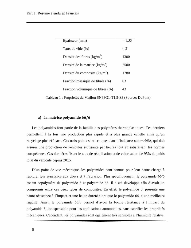
Tableau 1 : Propriétés du Vizilon SN63G1-T1.5-S3 (Source: DuPont)
a) La matrice polyamide 66/6
Les polyamides font partie de la famille des polymères thermoplastiques. Ces derniers
permettent à la fois une production plus rapide et à plus grande échelle ainsi qu‟un
recyclage plus efficace. Ces trois points sont critiques dans l‟industrie automobile, qui doit
assurer une production de véhicules suffisante par heures tout en satisfaisant les normes
européennes. Ces dernières fixent le taux de réutilisation et de valorisation de 95% du poids
total du véhicule depuis 2015.
D‟un point de vue mécanique, les polyamides sont connus pour leur haute charge à
rupture, leur résistance aux chocs et à l‟abrasion. Plus spécifiquement, le polyamide 66/6
est un copolymère de polyamide 6 et polyamide 66. Il a été développé afin d‟avoir un
compromis entre ces deux types de composites. En effet, le polyamide 6, présente une
haute résistance à l‟impact et une haute dureté alors que le polyamide 66, a une meilleure
rigidité. Ainsi, le polyamide 66/6 permet d‟avoir la bonne résistance à l‟impact du
polyamide 6, indispensable pour les applications automobiles, sans sacrifier les propriétés
mécaniques. Cependant, les polyamides sont également très sensibles à l‟humidité relative.
Epaisseur (mm) ≈ 1,53
Taux de vide (%) < 2
Densité des fibres (kg/m3) 1300
Densité de la matrice (kg/m3) 2500
Densité du composite (kg/m3) 1780
Fraction massique de fibres (%) 63
Fraction volumique de fibres (%) 43

Part I : Résumé étendu en Français
7
En effet, la réaction des liaisons hydrogènes avec l‟eau va entrainer leur affaiblissement ce
qui a un impact direct sur les propriétés mécaniques du polyamide. Plus précisément,
lorsque le taux d‟humidité relative augmente, leur module élastique a tendance à diminuer
et leur ductilité à augmenter. L‟influence de l‟humidité relative sur le comportement est sur
la Figure 2.
b) Le renfort en fibres de verres tissées
Les renforts tissés sont constitués de torons de fibres entremêlées suivant un motif
choisi afin de constituer une structure complexe. Les torons dans la direction principale du
tissage sont nommés torons du sens chaîne, alors que ceux perpendiculaires à cette
direction sont nommés torons du sens chaine.
L‟un des avantages notable du renfort tissé est de limiter la propagation de délaminage
[1]. Ce type d‟endommagement est l‟un des mécanismes les plus critiques, pouvant de plus
apparaitre lors de sollicitations par impact. Ce choix de renfort peut donc augmenter la
durée de vie du composite de manière significative après un choc à basse vélocité
imprévus. Par ailleurs, le renfort tissé va également permettre, contrairement à un renfort
Figure 2 : Courbe contrainte/déformation, en traction à 23°C, pour un Polyamide 66/6
(Ultramid® C3U de BASF) sec (vert) et après conditionnement 50% HR (rouge)
[http://iwww.plasticsportal.com/]

Part I : Résumé étendu en Français
8
unidirectionnel, un meilleur équilibre des propriétés mécaniques dans le plan du renfort.
Néanmoins, ce type de renfort va entrainer une diminution, par rapport au renfort
unidirectionnel, de la résistance maximale ainsi que du module élastique lors de
sollicitation suivant l‟axe des fibres [2], [3].
Les composites utilisant ce type de renfort sont connus pour voir apparaitre des
mécanismes d‟endommagements très spécifiques aux types de sollicitations considérés.
Une étude des mécanismes susceptibles d‟apparaitre lors de sollicitions en traction,
compression et flexion, menée par Karakaya et al. [2] a mis en avant l‟influence du type de
sollicitation. Des échantillons orientés suivant le sens chaine ou orientés à 45° de celui-ci
ont été considérés; ceux-ci étant évidemment les cas critiques lors de sollicitation en
traction dans le plan du composite. Ces mécanismes seront discutés plus en détail, pour le
composite de l‟étude, dans la partie dédiée à son étude microscopique pour le cas de la
sollicitation en traction d‟échantillons orientés suivant le sens chaine et orientés à 45° de
celui-ci.
3) Caractérisation du comportement mécanique du composite
étudié lors de sollicitations monotone et cyclique en traction
Cette partie est dédiée à l‟étude de la réponse mécanique du composite polyamide
66/6|fibres de verre tissées lors de sollicitations en traction monotone et cyclique. Deux
configurations d‟échantillons ont été considérées. Pour la première configuration les
échantillons sont orientés suivant le sens chaine et pour la seconde les échantillons sont
orientés à 45° du sens chaine. Les éprouvettes sont des rectangles de 150 x 45 x 1.5 mm
découpés par jet d‟eau. Les deux configurations d‟échantillons sont représentées sur la
Figure 3.
Avant les essais, les éprouvettes sont conditionnées dans une étuve humide Memmert
HCP256 à une humidité relative de 50 % et une température de 70°C. Une humidité
relative de 50 % pour les essais sur les matériaux sensibles aux RH est privilégiée par les
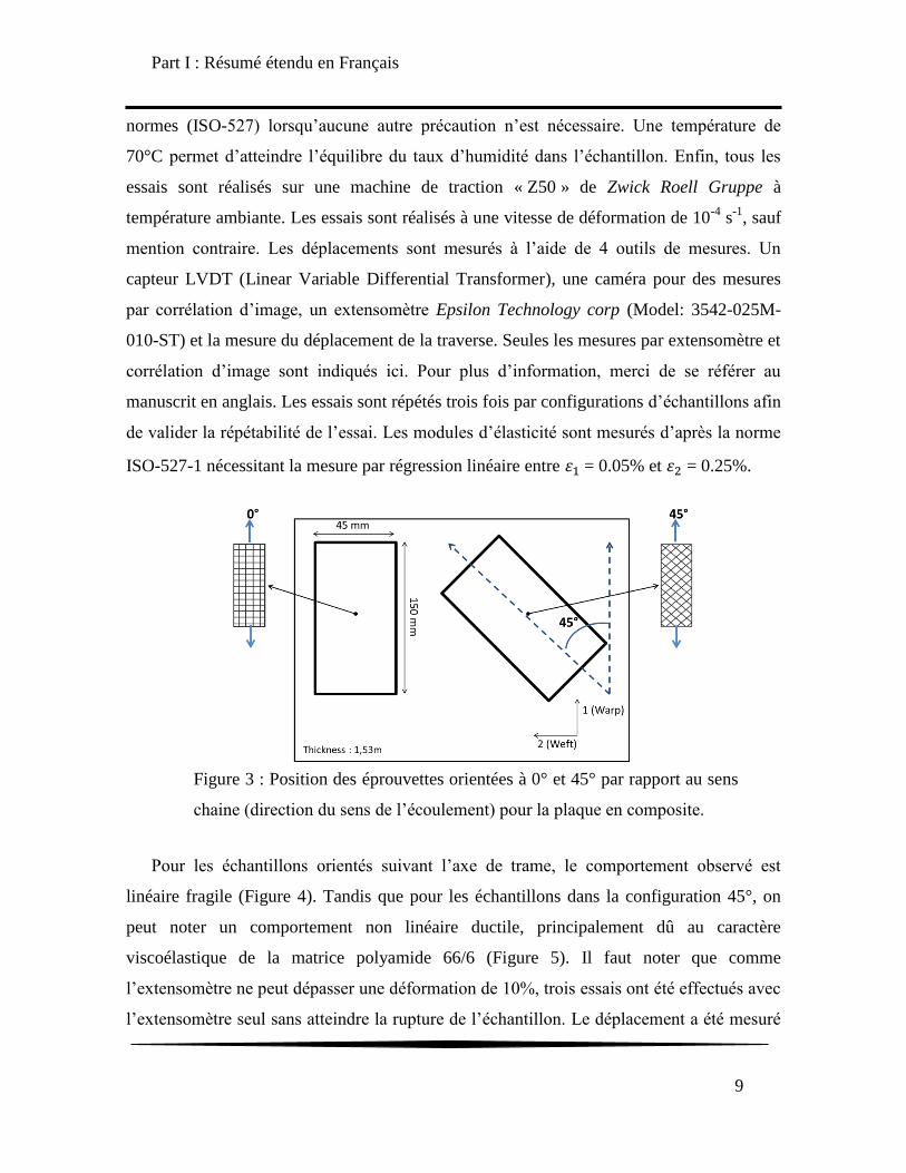
Part I : Résumé étendu en Français
9
normes (ISO-527) lorsqu‟aucune autre précaution n‟est nécessaire. Une température de
70°C permet d‟atteindre l‟équilibre du taux d‟humidité dans l‟échantillon. Enfin, tous les
essais sont réalisés sur une machine de traction « Z50 » de Zwick Roell Gruppe à
température ambiante. Les essais sont réalisés à une vitesse de déformation de 10-4
s-1
, sauf
mention contraire. Les déplacements sont mesurés à l‟aide de 4 outils de mesures. Un
capteur LVDT (Linear Variable Differential Transformer), une caméra pour des mesures
par corrélation d‟image, un extensomètre Epsilon Technology corp (Model: 3542-025M-
010-ST) et la mesure du déplacement de la traverse. Seules les mesures par extensomètre et
corrélation d‟image sont indiqués ici. Pour plus d‟information, merci de se référer au
manuscrit en anglais. Les essais sont répétés trois fois par configurations d‟échantillons afin
de valider la répétabilité de l‟essai. Les modules d‟élasticité sont mesurés d‟après la norme
ISO-527-1 nécessitant la mesure par régression linéaire entre = 0.05% et = 0.25%.
Pour les échantillons orientés suivant l‟axe de trame, le comportement observé est
linéaire fragile (Figure 4). Tandis que pour les échantillons dans la configuration 45°, on
peut noter un comportement non linéaire ductile, principalement dû au caractère
viscoélastique de la matrice polyamide 66/6 (Figure 5). Il faut noter que comme
l‟extensomètre ne peut dépasser une déformation de 10%, trois essais ont été effectués avec
l‟extensomètre seul sans atteindre la rupture de l‟échantillon. Le déplacement a été mesuré
Figure 3 : Position des éprouvettes orientées à 0° et 45° par rapport au sens
chaine (direction du sens de l‟écoulement) pour la plaque en composite.
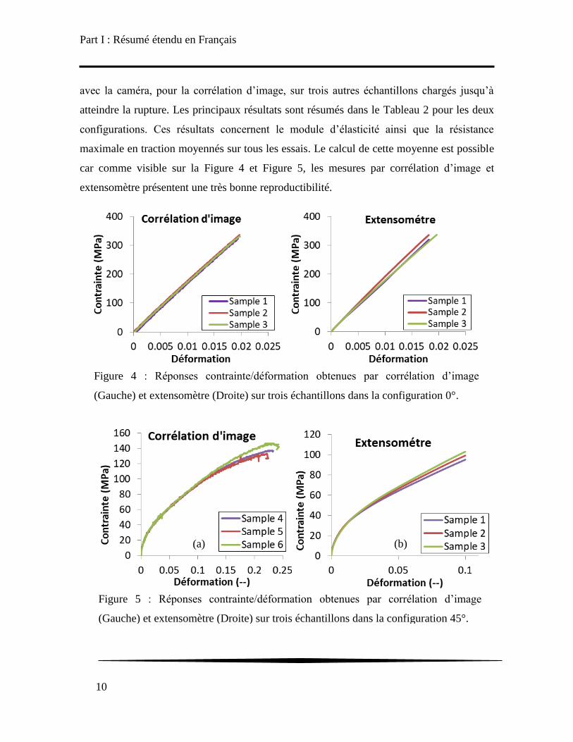
Part I : Résumé étendu en Français
10
avec la caméra, pour la corrélation d‟image, sur trois autres échantillons chargés jusqu‟à
atteindre la rupture. Les principaux résultats sont résumés dans le Tableau 2 pour les deux
configurations. Ces résultats concernent le module d‟élasticité ainsi que la résistance
maximale en traction moyennés sur tous les essais. Le calcul de cette moyenne est possible
car comme visible sur la Figure 4 et Figure 5, les mesures par corrélation d‟image et
extensomètre présentent une très bonne reproductibilité.
Figure 5 : Réponses contrainte/déformation obtenues par corrélation d‟image
(Gauche) et extensomètre (Droite) sur trois échantillons dans la configuration 45°.
(a) (b)
Figure 4 : Réponses contrainte/déformation obtenues par corrélation d‟image
(Gauche) et extensomètre (Droite) sur trois échantillons dans la configuration 0°.
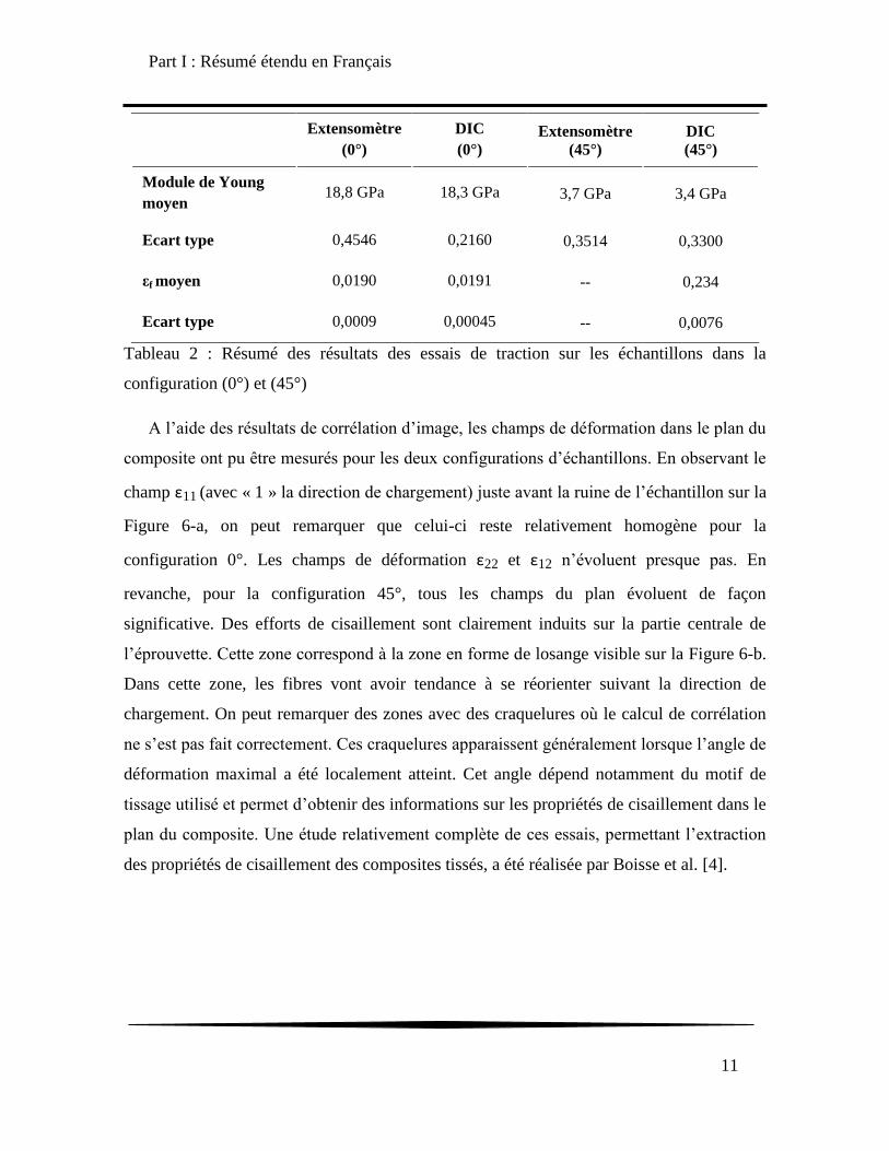
Part I : Résumé étendu en Français
11
Extensomètre
(0°)
DIC
(0°) Extensomètre
(45°) DIC (45°)
Module de Young
moyen 18,8 GPa 18,3 GPa 3,7 GPa 3,4 GPa
Ecart type 0,4546 0,2160 0,3514 0,3300
εf moyen 0,0190 0,0191 -- 0,234
Ecart type 0,0009 0,00045 -- 0,0076
Tableau 2 : Résumé des résultats des essais de traction sur les échantillons dans la
configuration (0°) et (45°)
A l‟aide des résultats de corrélation d‟image, les champs de déformation dans le plan du
composite ont pu être mesurés pour les deux configurations d‟échantillons. En observant le
champ ε11 (avec « 1 » la direction de chargement) juste avant la ruine de l‟échantillon sur la
Figure 6-a, on peut remarquer que celui-ci reste relativement homogène pour la
configuration 0°. Les champs de déformation ε22 et ε12 n‟évoluent presque pas. En
revanche, pour la configuration 45°, tous les champs du plan évoluent de façon
significative. Des efforts de cisaillement sont clairement induits sur la partie centrale de
l‟éprouvette. Cette zone correspond à la zone en forme de losange visible sur la Figure 6-b.
Dans cette zone, les fibres vont avoir tendance à se réorienter suivant la direction de
chargement. On peut remarquer des zones avec des craquelures où le calcul de corrélation
ne s‟est pas fait correctement. Ces craquelures apparaissent généralement lorsque l‟angle de
déformation maximal a été localement atteint. Cet angle dépend notamment du motif de
tissage utilisé et permet d‟obtenir des informations sur les propriétés de cisaillement dans le
plan du composite. Une étude relativement complète de ces essais, permettant l‟extraction
des propriétés de cisaillement des composites tissés, a été réalisée par Boisse et al. [4].
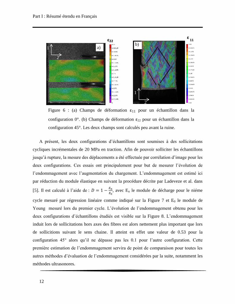
Part I : Résumé étendu en Français
12
A présent, les deux configurations d‟échantillons sont soumises à des sollicitations
cycliques incrémentales de 20 MPa en traction. Afin de pouvoir solliciter les échantillons
jusqu‟à rupture, la mesure des déplacements a été effectuée par corrélation d‟image pour les
deux configurations. Ces essais ont principalement pour but de mesurer l‟évolution de
l‟endommagement avec l‟augmentation du chargement. L‟endommagement est estimé ici
par réduction du module élastique en suivant la procédure décrite par Ladeveze et al. dans
[5]. Il est calculé à l‟aide de :
, avec En le module de décharge pour le niéme
cycle mesuré par régression linéaire comme indiqué sur la Figure 7 et E0 le module de
Young mesuré lors du premier cycle. L‟évolution de l‟endommagement obtenu pour les
deux configurations d‟échantillons étudiés est visible sur la Figure 8. L‟endommagement
induit lors de sollicitations hors axes des fibres est alors nettement plus important que lors
de sollicitions suivant le sens chaine. Il atteint en effet une valeur de 0.53 pour la
configuration 45° alors qu‟il ne dépasse pas les 0.1 pour l‟autre configuration. Cette
première estimation de l‟endommagement servira de point de comparaison pour toutes les
autres méthodes d‟évaluation de l‟endommagement considérées par la suite, notamment les
méthodes ultrasonores.
Figure 6 : (a) Champs de déformation ε11 pour un échantillon dans la
configuration 0°. (b) Champs de déformation ε22 pour un échantillon dans la
configuration 45°. Les deux champs sont calculés peu avant la ruine.
a)
ε22 ε
11
b) 1
2
1
2
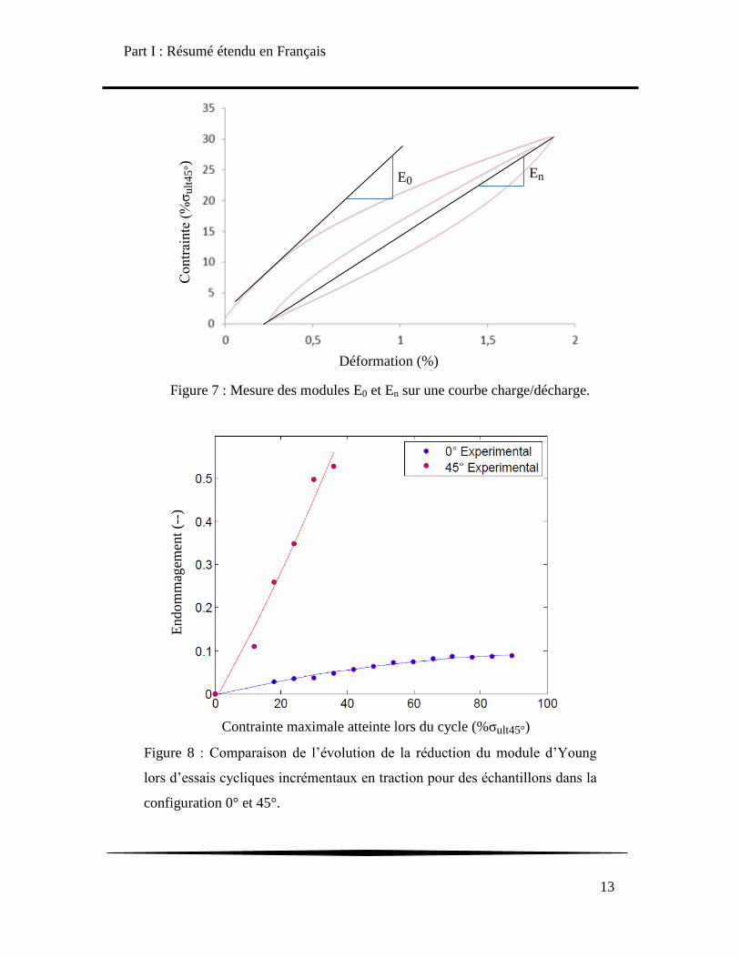
Part I : Résumé étendu en Français
13
E0 En
Figure 7 : Mesure des modules E0 et En sur une courbe charge/décharge.
Déformation (%)
Contr
ainte
(%
ζu
lt4
5°)
Figure 8 : Comparaison de l‟évolution de la réduction du module d‟Young
lors d‟essais cycliques incrémentaux en traction pour des échantillons dans la
configuration 0° et 45°.
Endom
mag
emen
t (-
-)
Contrainte maximale atteinte lors du cycle (%ζult45°)
Part I : Résumé étendu en Français
14
4) Etude des mécanismes d’endommagement : analyses
quantitatives et qualitatives
Comme évoqué précédemment, plusieurs mécanismes d‟endommagement sont
susceptibles d‟apparaitre sur les composites tissés. Ils vont de plus être extrêmement
dépendants du type de sollicitation que la pièce est susceptible de rencontrer durant sa vie
en service. Afin de caractériser efficacement l‟endommagement du polyamide 66/6
renforcé de fibres de verre tissées, il est nécessaire de considérer différents cas de
sollicitation mécanique. Ici nous considérons le cas de chargement en traction pour les deux
configurations d‟échantillons évoquées précédemment.
Pour ces deux cas de chargements, le premier mécanisme d‟endommagement observé
sera la décohésion fibre/matrice. Ce dernier a été mis en avant lors d‟essais de traction in-
situ au Microscope Electronique à Balayage (MEB). On peut voir sur la Figure 9-c que ce
dernier s‟est initié pour des valeurs de chargement entre 66 N et 120 N. Cette décohésion
fibres/matrice va ensuite se propager sous forme de fissure suivant la direction transverse à
la direction de chargement.
Les autres mécanismes d‟endommagement sont analysés à l‟aide d‟un tomographe à
rayon X EasyTom (Nano) conçu par RX solutions. Des échantillons orientés à 0° et 45° du
sens chaine, préalablement chargés en traction à des niveaux de contrainte définis, sont tous
observés. Un échantillon resté intact est également observé pour chaque configuration. Au
total 6 échantillons dans la configuration 0° et 4 échantillons dans la configuration 45° sont
considérés. Pour information, ces échantillons seront également considérés pour les parties
suivantes. Les valeurs de chargements sont indiquées par des cercles rouges sur la Figure
10 et résumées dans le Tableau 3.

Part I : Résumé étendu en Français
15
Figure 10 : Courbes contrainte/déformation typiques du polyamide 66/6 renforcé de
fibres de verre tissées dans la configuration 0° et 45°. Les cercles rouges indiquent le
niveau de contrainte et de déformation pour lesquels les essais de traction (réalisés sur
différents échantillons) ont été interompus comme resumé dans le Tableau 3.
for both orientation
()
c) 120N: 15.7MPa
d) 240N: 31.4MPa e) Final step (435N: 56.8MPa)
a) 0N
Figure 9: Images MEB lors d‟essais de traction in-situ pour
différents niveaux de changements appliqués suivant l‟axe des fibres
b) 66N: 8.2MPa

Part I : Résumé étendu en Français
16
Echantillon 1 2 3 4 5 6
Configuration 0° 0° 0° 0° 0° 0°
Chargement
normalisé
0
°
30,8
°
46,3
°
61,7
°
77,2
°
92,6
°
Déformation 0 0,005 0,007 0,010 0,013 0,016
Echantillon 7 8 9 10
Configuration 45° 45° 45° 45°
Chargement
normalisé
0
°
30,5
°
61,1
°
91,6
°
Déformation 0 0,021 0,083 0,162
Tableau 3 : Echantillons observés et leurs chargements fixés associés
Les mécanismes d‟endommagement observés sont résumés sur la Figure 11 pour les
deux orientations d‟échantillons. Pour ceux orientés suivant le sens chaine, on remarque
que le nombre de fissures transverses augmente avec le chargement. Des zones de vides au
bord des torons transverses sont également clairement visibles. Pour les valeurs de
chargement les plus importantes, le sens de propagation des fissures transverses peuvent
bifurquer et se mettre à longer les torons longitudinaux. Cela se produit généralement une
fois que la fissure transverse s‟est propagée jusqu‟au bout du toron transverse. Il requiert
alors généralement moins d‟énergie à la fissure de bifurquer plutôt que de continuer et de
casser les fibres du toron longitudinal. On appelle ce mécanisme le méta-délaminage.
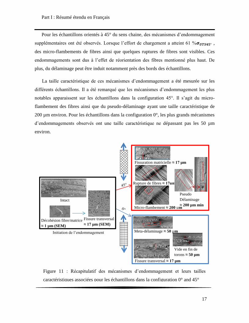
Part I : Résumé étendu en Français
17
Pour les échantillons orientés à 45° du sens chaine, des mécanismes d‟endommagement
supplémentaires ont été observés. Lorsque l‟effort de chargement a atteint 61 % ° ,
des micro-flambements de fibres ainsi que quelques ruptures de fibres sont visibles. Ces
endommagements sont dus à l‟effet de réorientation des fibres mentionné plus haut. De
plus, du délaminage peut être induit notamment près des bords des échantillons.
La taille caractéristique de ces mécanismes d‟endommagement a été mesurée sur les
différents échantillons. Il a été remarqué que les mécanismes d‟endommagement les plus
notables apparaissent sur les échantillons dans la configuration 45°. Il s‟agit du micro-
flambement des fibres ainsi que du pseudo-délaminage ayant une taille caractéristique de
200 µm environ. Pour les échantillons dans la configuration 0°, les plus grands mécanismes
d‟endommagements observés ont une taille caractéristique ne dépassant pas les 50 µm
environ.
Rupture de fibres ≈ 17um
Micro-flambement ≈ 200 µm
Fissuration matricielle ≈ 17 µm
Pseudo
Délaminage
≈ 200 µm min
Meta-délaminage ≈ 50 µm
Fissure transversal
≈ 17 µm (SEM) Décohésion fibre/matrice
≈ 1 µm (SEM)
Initiation de l‟endommagement
Intact
Vide en fin de
torons ≈ 50 µm
Fissure transversal ≈ 17 µm
Figure 11 : Récapitulatif des mécanismes d‟endommagement et leurs tailles
caractéristiques associées pour les échantillons dans la configuration 0° and 45°
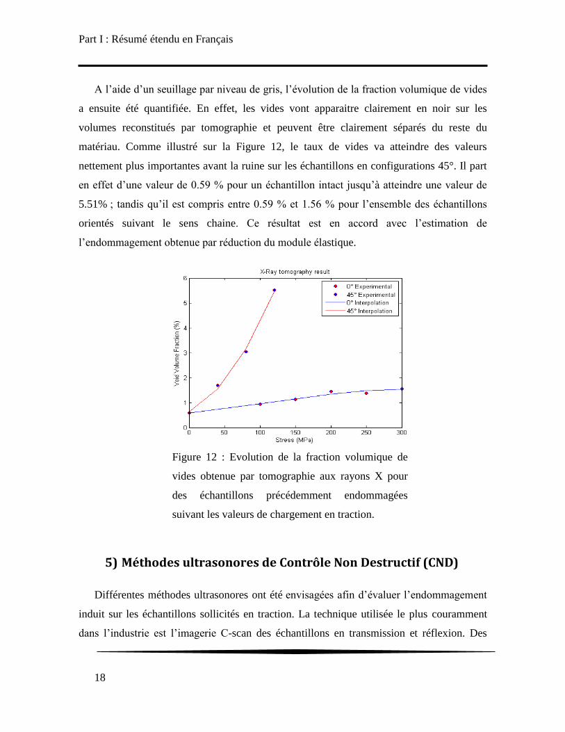
Part I : Résumé étendu en Français
18
A l‟aide d‟un seuillage par niveau de gris, l‟évolution de la fraction volumique de vides
a ensuite été quantifiée. En effet, les vides vont apparaitre clairement en noir sur les
volumes reconstitués par tomographie et peuvent être clairement séparés du reste du
matériau. Comme illustré sur la Figure 12, le taux de vides va atteindre des valeurs
nettement plus importantes avant la ruine sur les échantillons en configurations 45°. Il part
en effet d‟une valeur de 0.59 % pour un échantillon intact jusqu‟à atteindre une valeur de
5.51% ; tandis qu‟il est compris entre 0.59 % et 1.56 % pour l‟ensemble des échantillons
orientés suivant le sens chaine. Ce résultat est en accord avec l‟estimation de
l‟endommagement obtenue par réduction du module élastique.
5) Méthodes ultrasonores de Contrôle Non Destructif (CND)
Différentes méthodes ultrasonores ont été envisagées afin d‟évaluer l‟endommagement
induit sur les échantillons sollicités en traction. La technique utilisée le plus couramment
dans l‟industrie est l‟imagerie C-scan des échantillons en transmission et réflexion. Des
Figure 12 : Evolution de la fraction volumique de
vides obtenue par tomographie aux rayons X pour
des échantillons précédemment endommagées
suivant les valeurs de chargement en traction.

Part I : Résumé étendu en Français
19
essais ont été effectués sur les échantillons dans la configuration 0° et 45° observés par
tomographie à rayon X. Mais aucun endommagement n‟a pu être clairement détecté sur les
échantillons dans la configuration 0° comme montré sur la Figure 13-a. Comme vu
précédemment, les endommagements ici vont être de taille caractéristique très faible dans
cette configuration. En revanche, pour l‟autre configuration, des zones d‟endommagement
très nettes ont pu être imagées. Elles ont été comparées avec la tomographie à rayon X et
correspondent en fait à des flambements de fibres ainsi qu‟à du délaminage local. D‟autres
méthodes ont été alors envisagées pour évaluer l‟importance des microfissurations induites
sur les échantillons dans la configuration 0°.
a) Détermination du tenseur de rigidité par mesure des vitesses de
propagation ultrasonore
Cette première méthode vise à obtenir le tenseur de rigidité d‟un matériau en mesurant
la vitesse de propagation des ondes de volume dans différentes directions et pour différents
plans du matériau. En effet, la vitesse de propagation des ondes de volume dans une
direction donnée est reliée au tenseur de rigidité Cijkl par l‟équation de Christoffel :
0. Les vitesses mesurées sont ensuite utilisées dans un
Fibers buckling
Local
delamination
Figure 13 : Essai C-scans préliminaires sur le composite polyamide 66/6 renforcé avec
des fibres de verre tissée chargé en traction à différents niveaux. (a): Echantillons en
configuration 0°; (b): Echantillons en configuration 45°. Pour ces derniers,de large zones
d‟endommagement sont clairement visible.
b)
a)

Part I : Résumé étendu en Français
20
algorithme d‟optimisation qui permettra d‟avoir les différentes composantes du tenseur.
Tous les composites préalablement chargés en traction ont été analysés à l‟aide de cette
méthode. Le composite étudié ayant un comportement élastique orthotrope, neuf
composantes sont nécessaires pour obtenir un tenseur de rigidité complet. Des mesures
dans les trois plans principaux du composite sont alors nécessaires. Ce sont les plans 1-2, 1-
3 et 2-3 visibles sur la Figure 14. Cependant, dans notre cas, l‟épaisseur du composite est
trop faible les ondes se propageant dans le plan 1-2 ne seront donc pas des ondes de
volumes mais des ondes guidées. Ces ondes guidées sont reliées aux propriétés de rigidité
par d‟autres systèmes d‟équation. En conséquence, les mesures réalisées dans les plans 1-3
et 2-3 prennent en compte la propagation des ondes de volume sont liées à Cijkl par
l‟équation de Christoffel alors que les mesures dans le plan 1-2 sont reliées à Cijkl par des
équations plus complexes. Ceci est pris en compte lors du calcul du tenseur de rigidité par
optimisation.
Des essais sur des échantillons non endommagés orientés suivant 0° et à 45° du sens
chaine ont été réalisés. Des mesures dans les trois plans principaux ont pu être effectuées.
Afin d‟initialiser l‟algorithme, une première estimation du tenseur de rigidité est réalisée
par homogénéisation périodique avec l‟aide de Francis Praud. Les tenseurs obtenus avec
optimisation sont indiqués avec les deux premières estimations dans le Tableau 4.
Figure 14 : Schéma représentatif des différents plans de propagation des ondes de
volume (a) Plans de propagation pour la configuration 0° (b) Plans de propagation
pour la configuration 45°
a) b)

Part I : Résumé étendu en Français
21
C11 C12 C13 C22 C23 C33 C44 C55 C66
Numérique
0°
20 2,1 1,5 20 1,5 4,5 2,3 1,3 1,3
Expérimentale 22,16
(0,2)
2,6
(0,15)
1,48
(0,76)
21,75
(0,08)
1,45
(0,17)
4,13
(0,07)
2,33
(0,09)
1,61
(0,21)
1,42
(0,12)
Numérique
45°
13,35 8,75 1,5 13,35 1,5 4,5 8,95 1,3 1,3
Expérimentale 14,6
(0,43)
6,0
(0,29)
1,5
(0,645)
13,5
(0,184)
1,4
(0,223)
4,2
(0,248)
6,7
(0,118)
1,7
(0,237)
1,6
(0,31)
Tableau 4 : Tenseurs de rigidité obtenus pour le matériau composite étudié par
homogénéisation périodique analytique et mesure ultrasonore pour les configurations 0° et
45°. L‟intervalle de confiance pour chaque composante est indiqué entre parenthèse.
Les différents échantillons endommagés sont ensuite analysés à l‟aide de la même
méthode. Cependant, à cause de la petite largeur de l‟éprouvette, des mesures seulement
suivant dans les plans 1-2 et 1-3 ont pu être effectués. Cela entraine que seuls 7 des 9
composantes du tenseur de rigidité ont pu être obtenus. Pour le composite orienté à 45° du
sens chaine, le plan 1-3 n‟est plus un plan principal. Lorsque l‟échantillon est sollicité en
traction, la symétrie d‟élasticité va être perdue à cause du mode de propagation des fissures
pour cette configuration. Nous devons alors considérer 13 composantes de rigidité pour
correctement prévoir l‟évolution du comportement du composite. Les composantes C56,
C14, C24 et C13 sont alors ajoutées. On peut noter sur la Figure 15 que lorsque les
échantillons dans la configuration 0° sont sollicités en traction, ce sont principalement les
composantes fonctions de la direction de chargement qui vont diminuer, c‟est-à-dire C11,
C12, C13. Une relative diminution de C55 est également notable. En revanche, les autres
composantes évoluent peu avec le niveau de chargement en traction.
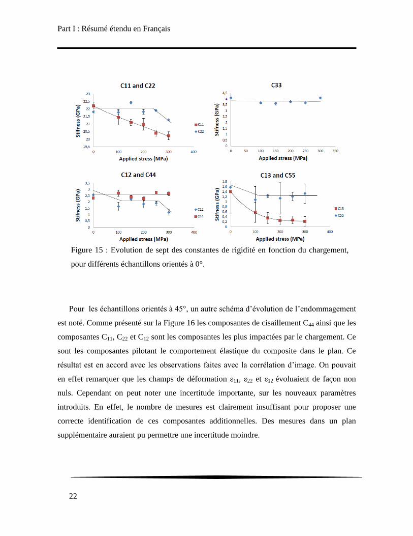
Part I : Résumé étendu en Français
22
Pour les échantillons orientés à 45°, un autre schéma d‟évolution de l‟endommagement
est noté. Comme présenté sur la Figure 16 les composantes de cisaillement C44 ainsi que les
composantes C11, C22 et C12 sont les composantes les plus impactées par le chargement. Ce
sont les composantes pilotant le comportement élastique du composite dans le plan. Ce
résultat est en accord avec les observations faites avec la corrélation d‟image. On pouvait
en effet remarquer que les champs de déformation ε11, ε22 et ε12 évoluaient de façon non
nuls. Cependant on peut noter une incertitude importante, sur les nouveaux paramètres
introduits. En effet, le nombre de mesures est clairement insuffisant pour proposer une
correcte identification de ces composantes additionnelles. Des mesures dans un plan
supplémentaire auraient pu permettre une incertitude moindre.
Figure 15 : Evolution de sept des constantes de rigidité en fonction du chargement,
pour différents échantillons orientés à 0°.

Part I : Résumé étendu en Français
23
Ensuite, deux indicateurs d‟endommagement ont été proposés. Le premier est basé sur
le calcul de la norme du tenseur de rigidité obtenu par mesures ultrasonores ; tandis que le
deuxième est basé sur le calcul du déphasage du signal pour toutes les directions de
propagation considérées. La prise en compte de mesures à différents angles d‟incidence
permet d‟évaluer l‟évolution anisotrope de l‟endommagement. L‟évolution de ces
indicateurs est tracée respectivement sur la Figure 17-c et Figure 17-d. Ces derniers
retranscrivent une évolution plus importante de l‟endommagement pour la configuration
45° que pour la configuration 0°. Ce qui est en accord avec l‟estimation de
l‟endommagement obtenue lors des essais de traction et de tomographie à rayon X.
Cependant, la différence d‟évolution de l‟endommagement entre les deux configurations
Figure 16 : Evolution de onze des constantes de rigidité en fonction du
chargement pour différents échantillons orientés à 45°.
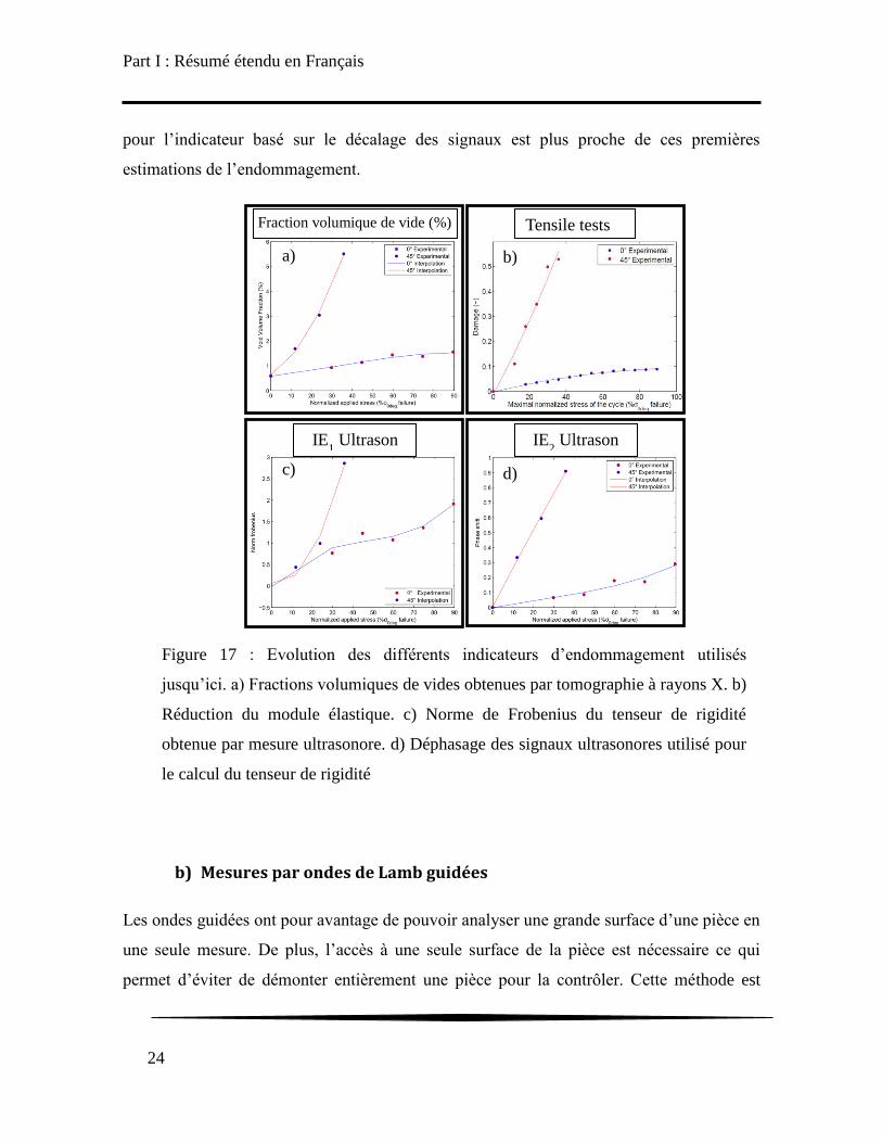
Part I : Résumé étendu en Français
24
pour l‟indicateur basé sur le décalage des signaux est plus proche de ces premières
estimations de l‟endommagement.
b) Mesures par ondes de Lamb guidées
Les ondes guidées ont pour avantage de pouvoir analyser une grande surface d‟une pièce en
une seule mesure. De plus, l‟accès à une seule surface de la pièce est nécessaire ce qui
permet d‟éviter de démonter entièrement une pièce pour la contrôler. Cette méthode est
Figure 17 : Evolution des différents indicateurs d‟endommagement utilisés
jusqu‟ici. a) Fractions volumiques de vides obtenues par tomographie à rayons X. b)
Réduction du module élastique. c) Norme de Frobenius du tenseur de rigidité
obtenue par mesure ultrasonore. d) Déphasage des signaux ultrasonores utilisé pour
le calcul du tenseur de rigidité
IE1 Ultrason
Fraction volumique de vide (%)
Tensile tests
IE2 Ultrason
a) b)
c) d)
0°

Part I : Résumé étendu en Français
25
plus simple à mettre en place que la méthode décrite précédemment. Deux transducteurs
sont utilisés en transmission, l‟émetteur est fixé alors que le receveur est attaché au bras
d‟un robot afin de contrôler son déplacement. Un burst de 5 cycles de sinus à 500 KHz est
généré par l‟émetteur. La distance entre les deux transducteurs variera entre 4.25 et 7.25
cm. Des signaux sont alors enregistrés tous les 0.5 cm. Le montage expérimental est
renseigné sur la Figure 18.
Des échantillons intacts de référence sont analysés en premier lieu afin de déterminer
quels modes se propagent suivant la configuration. Une analyse des spectrogrammes des
différents signaux enregistrés sur les deux configurations d‟échantillons a tout d‟abord été
menée. On peut remarquer, sur la Figure 19-a, qu‟un seul mode semble se propager dans
l‟échantillon dans la configuration 0°, il apparait pour une fréquence de 500 KHz. En
revanche, deux modes sont observables sur les spectrogrammes des échantillons dans la
configuration 45° en Figure 19-b. Ils apparaissent respectivement pour une fréquence de
500 KHz et 250 KHz.
Ensuite, une transformée de Fourier 2D est appliquée sur les signaux obtenus pour les
deux échantillons non endommagés. Cette transformée s‟effectue à la fois dans le domaine
temporel et dans le domaine spatial. Les figures résultantes sont donc affichées dans un
graphe fréquence (MHz)/nombre d‟onde (mm-1
) pour respectivement l‟échantillon dans la
configuration 0° (Figure 20) et 45° (Figure 21). Deux ensembles de modes obtenus à l‟aide
du logiciel Disperse, en utilisant deux tenseurs d‟élasticité différents, ont été considérés.
Ainsi, pour les modes en ligne continue, le tenseur utilisé a été calculé par homogénéisation
périodique avec l‟aide de Francis Praud. Pour les modes en ligne pointillé, le tenseur utilisé
X
Z
Receiver Emitter
Figure 18 : Montage expérimental pour la mesure des modes d‟ondes guidées

Part I : Résumé étendu en Français
26
est celui obtenu par mesure ultrasonore à l‟aide de la méthode présentée dans la section
précédente.
Figure 20 : Transformée de Fourier 2D pour un échantillon intact dans la configuration
0° avec les modes S0, A0, S1 et A1. Le tenseur de rigidité obtenu par homogénéisation
périodique a été utilisé pour les modes en lignes continues. Le tenseur obtenu par
mesures ultrasonores, a lui été utilisé pour celles en lignes discontinues.
Figure 19 : Spectrogramme d‟un signal transmis dans un échantillon dans (a) la
configuration 0° et (b) la configuration 45 ° avec le signal temporel correspondant
S1
(a) (b)
A0
S1
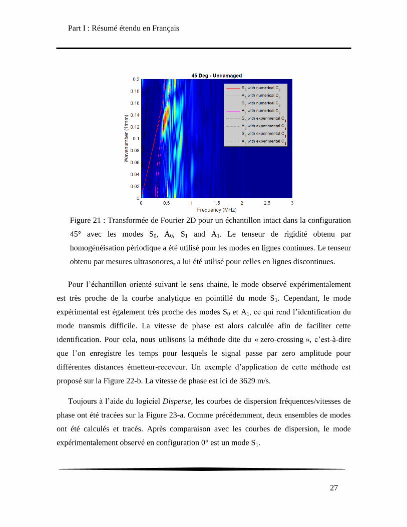
Part I : Résumé étendu en Français
27
Pour l‟échantillon orienté suivant le sens chaine, le mode observé expérimentalement
est très proche de la courbe analytique en pointillé du mode S1. Cependant, le mode
expérimental est également très proche des modes S0 et A1, ce qui rend l‟identification du
mode transmis difficile. La vitesse de phase est alors calculée afin de faciliter cette
identification. Pour cela, nous utilisons la méthode dite du « zero-crossing », c‟est-à-dire
que l‟on enregistre les temps pour lesquels le signal passe par zero amplitude pour
différentes distances émetteur-receveur. Un exemple d‟application de cette méthode est
proposé sur la Figure 22-b. La vitesse de phase est ici de 3629 m/s.
Toujours à l‟aide du logiciel Disperse, les courbes de dispersion fréquences/vitesses de
phase ont été tracées sur la Figure 23-a. Comme précédemment, deux ensembles de modes
ont été calculés et tracés. Après comparaison avec les courbes de dispersion, le mode
expérimentalement observé en configuration 0° est un mode S1.
Figure 21 : Transformée de Fourier 2D pour un échantillon intact dans la configuration
45° avec les modes S0, A0, S1 and A1. Le tenseur de rigidité obtenu par
homogénéisation périodique a été utilisé pour les modes en lignes continues. Le tenseur
obtenu par mesures ultrasonores, a lui été utilisé pour celles en lignes discontinues.

Part I : Résumé étendu en Français
28
Pour l‟échantillon en configuration 45°, le mode expérimental apparait entre les modes
analytiques A1 et S1. La vitesse de phase a ensuite été évaluée à 3272 m/s en se servant de
la même méthode que celle citée précédemment. Après comparaison avec les courbes de
dispersion numérique, il reste difficile de déterminer le mode avec certitude. Afin de lever
cette indétermination, un montage permettant de mesurer le signal arrivant sur la surface
inférieure et supérieure de la plaque est mis en place. On s‟attend à ce que les signaux
mesurés au même endroit sur chaque surface soit en phase, pour un mode symétrique, et en
déphasage pour un mode antisymétrique. Il a été observé que pour les deux configurations
étudiées, le décalage temporel entre les signaux mesurés sur chacune des faces est très
faible. En conséquence, nous faisons l‟hypothèse que les modes observés sur les deux
configurations sont de même nature. Au vu des informations recueillies jusqu‟à présent, les
deux modes sont donc des modes S1.
Figure 22 : Deux signaux transmis avec un exemple de mesure des vitesses de (a)
groupe et de (b) phase.
(a) (b)

Part I : Résumé étendu en Français
29
Figure 23 : Courbes de dispersion des vitesses de phase en fonction de la fréquence
pour des échantillons dans (a) la configuration 0° et (b) la configuration 45°. La
matrice de rigidité, obtenue par homogénéisation périodique, a été utilisée pour les
modes représentés par la moyenne des lignes continues. Alors que la matrice de
rigidité obtenue par acquisitions ultrasonores a été utilisée pour les lignes discontinues.
(a)
(b)
Part I : Résumé étendu en Français
30
Les échantillons endommagés, et étudiés dans les sections précédentes sont ensuite
également analysés par ondes guidées suivant la même procédure. L‟objectif étant de voir
si les endommagements apparaissant dans ces échantillons entraînent un changement dans
les modes transmis. Seulement, aucun changement de modes n‟a été noté, pour les deux
configurations d‟échantillons, quel que soit le niveau de chargement considéré. Une autre
approche a ensuite été considérée pour évaluer le niveau d‟endommagement par ondes
guidées. Pour cela, deux autres indicateurs d‟endommagement ont été proposés. Le premier
prend en compte la moyenne, sur toutes les distances émetteur-receveur considérées, de
l‟amplitude maximale du signal. Le second est calculé de façon équivalente, mais en
prenant en compte l‟intégralité du signal au lieu de l‟amplitude maximale de celui-ci. Ils
sont calculés ainsi :
∑
∑ ∫
L‟évolution de ces deux indicateurs est tracée sur la Figure 24 pour les deux
configurations d‟échantillon. Le premier de ces deux indicateurs ne semble pas
correctement détecter l‟évolution de l‟endommagement. Particulièrement pour les
échantillons dans la configuration 0°. En effet, de 150 MPa à 250 MPa, l‟indicateur décroit
de façon continue, ce qui n‟est pas en accord avec ce qui été observé dans les sections
précédentes. De la même façon, on peut noter que pour l‟autre configuration d‟échantillon,
une décroissance de l‟indicateur se produit entre 0 et 40 MPa. L‟évolution du second
indicateur semble être plus en accord avec les autres indicateurs d‟endommagement étudiés
jusqu‟ici. C‟est-à-dire une évolution de l‟endommagement avec le niveau de chargement,
mais également un niveau d‟endommagement maximal atteint plus important pour les
échantillons dans la configuration 45°.

Part I : Résumé étendu en Français
31
6) Validation sur échantillon impacté par poids tombant
Dans l‟industrie automobile, les structures sont dimensionnées en vue de résister le plus
possible à des impacts. Cependant, pour la plupart des matériaux composites renforcés par
des fibres continues, un impact peut entrainer, même pour des énergies d‟impact faibles,
l‟apparition et la propagation de délaminages. Ce dernier peut entrainer une ruine
catastrophique et inattendue de la pièce en composite. Le renfort tissé a pour avantage de
réduire la propagation de délaminage, cependant ce type de ruine est toujours possible. Il
est donc critique de connaitre le comportement de la pièce lors d‟un impact imprévu, mais
également de connaitre la capacité des différentes méthodes de contrôle ultrasonore à
détecter et quantifier l‟endommagement induit par impact.
Cette section est donc dédiée à la validation des méthodes ultrasonores sur structure
impactée. Quatre éprouvettes normalisées de 100 x 150 x 1.53 mm ont été impactées à
l‟aide d‟une machine de chute au laboratoire LAMPA d‟Angers grâce à l‟aide du
professeur Laurent Guillaumat. Un impacteur de 16 mm de diamètre et de 1.02 kg a été
utilisé. Les énergies d‟impact ont été choisies afin de rester dans le domaine des
endommagements à peine visibles ou Barely Visible Impact Damage en anglais (BVID).
L‟énergie d‟impact réel et l‟énergie absorbée ont été calculées grâce aux courbes
Figure 24 : Comparaison entre les évolutions des deux indicateurs
d‟endommagement considérés (a) DI3 et (b) DI4 pour les deux orientations
d‟échantillon considérées.
a) b)
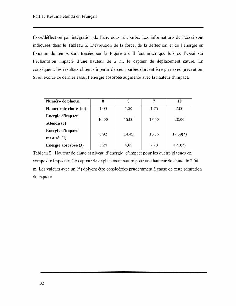
Part I : Résumé étendu en Français
32
force/déflection par intégration de l‟aire sous la courbe. Les informations de l‟essai sont
indiquées dans le Tableau 5. L‟évolution de la force, de la déflection et de l‟énergie en
fonction du temps sont tracées sur la Figure 25. Il faut noter que lors de l‟essai sur
l‟échantillon impacté d‟une hauteur de 2 m, le capteur de déplacement sature. En
conséquent, les résultats obtenus à partir de ces courbes doivent être pris avec précaution.
Si on exclue ce dernier essai, l‟énergie absorbée augmente avec la hauteur d‟impact.
Numéro de plaque 8 9 7 10
Hauteur de chute (m) 1,00 1,50 1,75 2,00
Energie d’impact
attendu (J) 10,00 15,00 17,50 20,00
Energie d’impact
mesuré (J) 8,92 14,45 16,36 17,59(*)
Energie absorbée (J) 3,24 6,65 7,73 4,48(*)
Tableau 5 : Hauteur de chute et niveau d‟énergie d‟impact pour les quatre plaques en
composite impactée. Le capteur de déplacement sature pour une hauteur de chute de 2,00
m. Les valeurs avec un (*) doivent être considérées prudemment à cause de cette saturation
du capteur
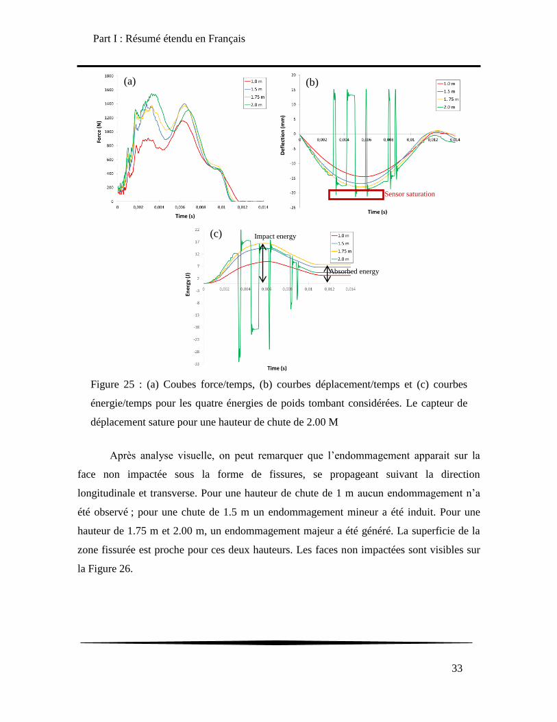
Part I : Résumé étendu en Français
33
Après analyse visuelle, on peut remarquer que l‟endommagement apparait sur la
face non impactée sous la forme de fissures, se propageant suivant la direction
longitudinale et transverse. Pour une hauteur de chute de 1 m aucun endommagement n‟a
été observé ; pour une chute de 1.5 m un endommagement mineur a été induit. Pour une
hauteur de 1.75 m et 2.00 m, un endommagement majeur a été généré. La superficie de la
zone fissurée est proche pour ces deux hauteurs. Les faces non impactées sont visibles sur
la Figure 26.
Figure 25 : (a) Coubes force/temps, (b) courbes déplacement/temps et (c) courbes
énergie/temps pour les quatre énergies de poids tombant considérées. Le capteur de
déplacement sature pour une hauteur de chute de 2.00 M
(a) (b)
(c) Impact energy
Absorbed energy
Sensor saturation

Part I : Résumé étendu en Français
34
Les quatre plaques ont ensuite été analysées par tomographie à rayon X suivant une
procédure équivalente à celle décrite dans la section 4). Cette étude a permis de valider les
observations visuelles en termes d‟ampleur de l‟endommagement induit par l‟impact.
Une étude par C-scan ultrasonores en immersion est enfin effectuée sur chacune des
plaques. Des essais en réflexion et transmission avec des transducteurs de 10 MHz ont été
réalisés. Avec les essais en transmission une zone d‟atténuation d‟amplitude, correspondant
à une zone endommagée, a été imagée sur toutes les plaques sauf celles impactées à 10 J.
Les quatre images sont visibles sur la Figure 27. Ensuite, les essais C-scan en réflexion ont
permis de caractériser la taille de l‟indentation permanente induite par l‟impact sur la face
impactée. Les indentations permanentes sont souvent utilisées pour estimer la gravité d‟un
endommagement dû à un impact, particulièrement lorsque l‟accès à la face non impactée
n‟est pas possible. La surface de l‟indentation est mesurée grâce aux C-scans représentant
le temps d‟arrivée du premier pic positif. De plus, comme illustré sur les B-scans de la
Figure 28, la profondeur de la déformation permanente est également discernable et peut
être mesurée en prenant en compte la vitesse de propagation de l‟onde ultrasonore dans
Figure 26 : Faces non-impactée des plaques pour des énergies d‟impact
de (a) 10 J, (b) 15 J, (c) 17.5 J, et (d) 20 J.
(a) (b)
(c) (d)

Part I : Résumé étendu en Français
35
l‟eau. Les dimensions des indentations permanentes mesurées sont renseignées dans le
Tableau 6 pour chacune des plaques étudiées.
Figure 28 : (a) Carte des temps d‟arrivés du premier pic positif de la plaque
impactée à 20 J. L‟indentation permanente est colorée en rouge (b) Zoom sur un
des B-scans de la plaque impactée à 20 J.
115.68 µs
115.73 µs
0.0739 mm
Figure 27 : C-scans ultrasonore en transmission obtenue avec un transducteur de 10
MHz pour les plaques impactée à des niveaux d‟énergies de (a) 10, (b) 15, (c) 17.5 et
(d) 20 J
(a) (b)
(c) (d)
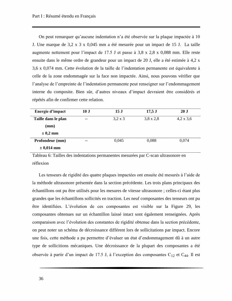
Part I : Résumé étendu en Français
36
On peut remarquer qu‟aucune indentation n‟a été observée sur la plaque impactée à 10
J. Une marque de 3,2 x 3 x 0,045 mm a été mesurée pour un impact de 15 J. La taille
augmente nettement pour l‟impact de 17.5 J et passe à 3,8 x 2,8 x 0,088 mm. Elle reste
ensuite dans le même ordre de grandeur pour un impact de 20 J, elle a été estimée à 4,2 x
3,6 x 0,074 mm. Cette évolution de la taille de l‟indentation permanente est équivalente à
celle de la zone endommagée sur la face non impactée. Ainsi, nous pouvons vérifier que
l‟analyse de l‟empreinte de l‟indentation permanente peut renseigner sur l‟endommagement
interne du composite. Bien sûr, d‟autres niveaux d‟impact devraient être considérés et
répétés afin de confirmer cette relation.
Energie d’impact 10 J 15 J 17,5 J 20 J
Taille dans le plan
(mm)
± 0,2 mm
-- 3,2 x 3 3,8 x 2,8 4,2 x 3,6
Profondeur (mm)
± 0,014 mm
-- 0,045 0,088 0,074
Tableau 6: Tailles des indentations permanentes mesurées par C-scan ultrasonore en
réflexion
Les tenseurs de rigidité des quatre plaques impactées ont ensuite été mesurés à l‟aide de
la méthode ultrasonore présentée dans la section précédente. Les trois plans principaux des
échantillons ont pu être utilisés pour les mesures de vitesse ultrasonore ; celles-ci étant plus
grandes que les échantillons sollicités en traction. Les neuf composantes des tenseurs ont pu
être identifiées. L‟évolution de ces composantes est visible sur la Figure 29, les
composantes obtenues sur un échantillon laissé intact sont également renseignées. Après
comparaison avec l‟évolution des constantes de rigidité obtenue dans la section précédente,
on peut noter un schéma de décroissance différent lors de sollicitations par impact. Encore
une fois, cette méthode a pu permettre d‟évaluer un état d‟endommagement dû à un autre
type de sollicitions mécaniques. Une décroissance de la plupart des composantes a été
observée à partir d‟un impact de 17.5 J, à l‟exception des composantes C12 et C44. Il est

Part I : Résumé étendu en Français
37
cependant difficile de conclure sur la détectabilité de l‟endommagement induit par l‟impact
de 10 J ou 15 J. En effet, seulement les composantes C11 et C22, ainsi que C13 dans une
moindre mesure, décroissent pour un impact de 15 J. Encore une fois, il faudrait considérer
d‟autres énergies d‟impact autour de 10 – 15 J afin de connaitre le seuil de détectabilité de
cette méthode.
Afin de finaliser la validation de cette méthode de détection, les indicateurs
d‟endommagement utilisés précédemment sont calculés pour toutes les éprouvettes
impactées. Pour rappel, le premier indicateur est calculé comme la norme de Frobenius du
tenseur de rigidité calculé par mesure ultrasonore des vitesses de propagation. Le second est
la moyenne de tous les déphasages entre le signal se propageant dans un échantillon
endommagé et le signal se propageant dans un échantillon intact. Ils sont encore une fois
nommés DI1 et DI2 par la suite. Leur évolution en fonction de l‟énergie d‟impact est visible
sur la Figure 30. On peut noter que les deux indicateurs augmentent avec l‟énergie d‟impact
de façon similaire. Une augmentation est discernable à partir de 15 J, la valeur des deux
indicateurs continue d‟augmenter nettement pour 17.5 J, puis une augmentation plus
importante est notable pour 20 J. Ces observations sont en corrélation avec les résultats
obtenus par tomographie à rayons X en terme de gravité de la zone endommagée. En effet,
aucun d‟endommagement n‟a été observé pour une énergie d‟impact de 10 J tandis qu‟une
fissure mineure est apparue pour une énergie d‟impact de 15 J et enfin une large zone
d‟endommagement comparable s‟est développée pour 17,5 J et 20 J.

Part I : Résumé étendu en Français
38
Figure 29 : Evolution des neuf composantes du tenseur de rigidité du matériau
composite testé en fonction de l‟énergie d‟impact.
Damage evolution of 0° and 45° finer oriented sample obtained via
ultrasonic measurements
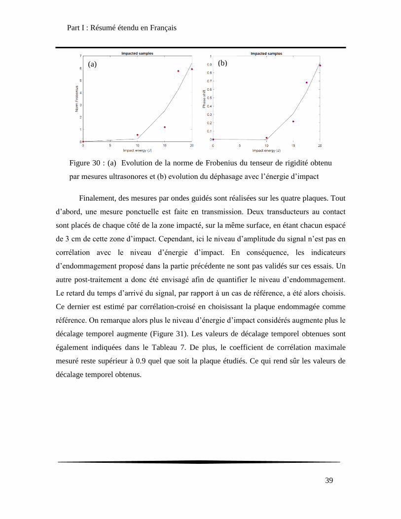
Part I : Résumé étendu en Français
39
Finalement, des mesures par ondes guidés sont réalisées sur les quatre plaques. Tout
d‟abord, une mesure ponctuelle est faite en transmission. Deux transducteurs au contact
sont placés de chaque côté de la zone impacté, sur la même surface, en étant chacun espacé
de 3 cm de cette zone d‟impact. Cependant, ici le niveau d‟amplitude du signal n‟est pas en
corrélation avec le niveau d‟énergie d‟impact. En conséquence, les indicateurs
d‟endommagement proposé dans la partie précédente ne sont pas validés sur ces essais. Un
autre post-traitement a donc été envisagé afin de quantifier le niveau d‟endommagement.
Le retard du temps d‟arrivé du signal, par rapport à un cas de référence, a été alors choisis.
Ce dernier est estimé par corrélation-croisé en choisissant la plaque endommagée comme
référence. On remarque alors plus le niveau d‟énergie d‟impact considérés augmente plus le
décalage temporel augmente (Figure 31). Les valeurs de décalage temporel obtenues sont
également indiquées dans le Tableau 7. De plus, le coefficient de corrélation maximale
mesuré reste supérieur à 0.9 quel que soit la plaque étudiés. Ce qui rend sûr les valeurs de
décalage temporel obtenus.
Figure 30 : (a) Evolution de la norme de Frobenius du tenseur de rigidité obtenu
par mesures ultrasonores et (b) evolution du déphasage avec l‟énergie d‟impact
(a) (b)

Part I : Résumé étendu en Français
40
10 J 15 J 17.5 J 20 J
0 1.12e-7 1.92e-7 3.20e-7
Tableau 7 : Décalage temporel mesuré par corrélation croisé sur des signaux mesuré
ponctuellement sur les quatre plaques impactées
Afin de valider cette observation, un autre montage expérimentale est mis en place afin
d‟effectuer cette mesure ponctuelle sur tout l‟échantillon. Ainsi, les transducteurs restent
séparés de 6 cm mais vont parcourir solidairement une longueur de 70 mm. Seule la plaque
impactée à 20 J a été étudiée ici. De la même façon, le coefficient de corrélation ainsi que la
valeur de décalage temporel sont estimés pour chaque point de mesure sur la plaque. Les
courbes représentant l‟évolution du coefficient de corrélation et du décalage temporel en
fonction de la position sur la plaque est respectivement tracé sur Figure 171-a et Figure
171-b. Six mesures ont été effectuées afin d‟éprouver la répétabilité du montage
expérimentale. On peut noter qu‟à l‟exception d‟une mesure (en jaune) toutes les autres
mesures présentent des valeurs de coefficient de corrélation au-dessus de 0.9. Ensuite,
encore une fois à l‟exception d‟une mesure (en jaune), une augmentation nette du décalage
temporelle est notable autour de -25 mm. Ce qui correspond à l‟endroit où le composite a
été impacté. Cependant, il faut noter d‟importante variation dans les profils de décalage
Figure 31 : Résultat de la corrélation croisé effectué sur les quatre
plaques impactées
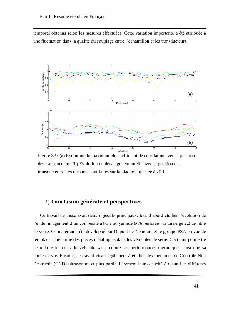
Part I : Résumé étendu en Français
41
temporel obtenus selon les mesures effectuées. Cette variation importante a été attribuée à
une fluctuation dans la qualité du couplage entre l‟échantillon et les transducteurs.
7) Conclusion générale et perspectives
Ce travail de thèse avait deux objectifs principaux, tout d‟abord étudier l‟évolution de
l‟endommagement d‟un composite à base polyamide 66/6 renforcé par un sergé 2,2 de fibre
de verre. Ce matériau a été développé par Dupont de Nemours et le groupe PSA en vue de
remplacer une partie des pièces métalliques dans les véhicules de série. Ceci doit permettre
de réduire le poids du véhicule sans réduire ses performances mécaniques ainsi que sa
durée de vie. Ensuite, ce travail visait également à étudier des méthodes de Contrôle Non
Destructif (CND) ultrasonore et plus particulièrement leur capacité à quantifier différents
Figure 32 : (a) Evolution du maximum de coefficient de corrélation avec la position
des transducteurs. (b) Evolution du décalage temporelle avec la position des
transducteurs. Les mesures sont faites sur la plaque impactée à 20 J
(a)
(b)
Part I : Résumé étendu en Français
42
états d‟endommagement induit sur des matériaux composite. Ainsi, différentes méthodes de
CND ont été étudiées sur des matériaux préalablement endommagés via différents types de
sollicitions mécaniques.
Dans un premier temps, le comportement mécanique et les modes d‟endommagement
lors de sollicitations en traction quasi-statique sont étudiés. Deux orientations d‟échantillon
ont été considérées : suivant les fibres du sens chaine et orientées à 45° du sens chaine. A
l‟échelle macroscopique, on note deux réponses bien distinctes. Pour la configuration 0°,
une réponse contrainte/déformation linéaire fragile avec un endommagement induit limité.
Tandis que pour la configuration 45°, on note une réponse non linéaire ductile avec une
augmentation nette de l‟endommagement. L‟évolution de l‟endommagement a été ici
estimée par réduction du module élastique. Les champs de déformation, obtenus par
corrélation d‟image, montrent de plus que pour la configuration 0° la sollicitation en
traction entraine majoritairement une déformation uniforme suivant la direction de
chargement. Pour la configuration 45°, on observe d‟abord également une augmentation
progressive de la déformation suivant l‟axe de chargement puis un couplage entre le
cisaillement plan et la traction. Cette réponse est en fait induite par un effet de réorientation
des fibres le long de la direction de chargement. Cette différence de réponse mécanique
entraîne également différents mécanismes de rupture. C‟est-à-dire une fissure droite et net
pour les échantillons en configuration 0° et une fissure en escalier avec du délaminage
visible sur les tranches des échantillons en configuration 45°.
Les mécanismes d‟endommagement entrainant la ruine ont ensuite été étudiés à
l‟échelle microscopique. L‟initiation de l‟endommagement par décohésion fibre/matrice a
été tout d‟abord observée lors d‟essais de traction in-situ au Microscope Electronique à
Balayage (MEB). Les autres mécanismes ont dû être observés au tomographe à rayons X
suite à différentes difficultés lors des essais MEB. Des échantillons en configuration 0° et
45° ont été observés. Un schéma d‟endommagement différent a été noté pour chacune des
configurations. Pour la configuration 0°, des mécanismes d‟endommagement
principalement de faible taille caractéristique ont été observés. En revanche pour

Part I : Résumé étendu en Français
43
l‟orientation 45°, on a pu noter des endommagements de grandes tailles, principalement du
flambage de fibres et du pseudo-délaminage. Cette différence de mécanismes entraine une
évolution de l‟endommagement global distincte. Cette dernière a été estimée par mesure du
taux volumique de vides sur les reconstructions 3D des échantillons endommagés. Son
évolution en fonction du chargement appliqué présente une évolution similaire à celle de la
réduction du module élastique.
Différentes méthodes de Contrôle Non Destructif (CND) basées sur les ultrasons ont
ensuite été étudiées. Tout d‟abord, des C-scans ultrasonores d‟échantillons en configuration
0° et 45° ont été faits. Les échantillons ont été préalablement endommagés en traction à
différents niveaux de chargement. Seuls les endommagements macroscopiques apparaissant
sur les échantillons en configuration 45° ont pu être imagés. La méthode de calcul des
constantes de rigidité par mesure des vitesses de phase a alors été considérée. Grace à cette
méthode, l‟évolution anisotrope de l‟endommagement, après chargement en traction, a pu
être observée. Cette évolution est par ailleurs très dissemblable pour les deux
configurations et est en accord avec l‟évolution des champs de déformation mesurée par
corrélation d‟image. C‟est-à-dire une décroissance des composantes de rigidité dépendant
de la direction de chargement pour la configuration 0° et une décroissance de tous les
composantes du plan du tissage, y compris le cisaillement plan, pour la configuration 45°.
Deux indicateurs d‟endommagement basés sur les mesures précédentes ont par la suite été
proposés. Le premier est la norme de Frobenius du tenseur de rigidité obtenu et le deuxième
est la moyenne, sur tous les plan principaux utilisés, du déphase du signal mesuré par
rapport à un signal obtenu sur un matériau sain. Leur évolution, surtout pour le deuxième,
est proche de ce qui a été observé grâce aux essais de tomographie et de traction. Les ondes
guidées ont ensuite été utilisées pour inspecter les mêmes échantillons. Les modes transmis
ont tout d‟abord été analysés pour différents cas d‟endommagement, mais aucun
changement dans la nature des modes transmis n‟a été observé quel que soit le niveau de
chargement et la configuration des échantillons. D‟autres indicateurs ont alors été proposés
comme l‟énergie du signal transmis. L‟évolution de ce dernier est bien en accord avec les
autres méthodes d‟estimation de l‟endommagement utilisées jusqu‟ici et indique une
Part I : Résumé étendu en Français
44
évolution plus importante de l‟endommagement avant la ruine pour un échantillon en
configuration 45° que pour l‟autre configuration.
Enfin, une étude de validation des méthodes proposées grâce à des essais d‟impact par
poids tombant sur des échantillons est proposée. Différents niveaux d‟impact ont été
utilisés tout en essayant de rester dans le domaine des endommagements à peine visibles. Il
a été montré, par observation visuelle et tomographie à rayon X, que l‟endommagement
induit augmente avec l‟énergie d‟impact. L‟indentation permanente a été mesurée par
pulse-écho ultrasonore sur les quatre plaques. Sa taille augmente également avec l‟énergie
d‟impact ce qui en fait également un bon indicateur de l‟endommagement interne induit. La
méthode de mesure du tenseur de rigidité a pu détecter une évolution de l‟endommagement
dès 17.5 J. A partir de ce niveau d‟énergie, l‟ensemble des composantes diminue, à
l‟exception de C12 et C44, avec l‟augmentation du niveau d‟énergie. L‟indicateur
d‟endommagement du déphasage augmente lui de façon nette dès 15 J. Enfin, comme
l‟indicateur d‟endommagement basé sur l‟amplitude du signal transmis n‟a pas pu
caractériser l‟endommagement induit par impact, une autre méthode de traitement a été
considérée. Le décalage temporel a alors été estimé par corrélation croisée et a montré une
évolution fonction de l‟énergie d‟impact. La localisation de l‟endommagement a pu être
détectée lors de scan effectué sur toute une plaque. Cependant, le montage expérimental,
dans son état actuel, présente de larges variations dans les mesures effectuées. Ces
variations sont actuellement attribuées à une mauvaise qualité de couplage entre les
transducteurs et l‟échantillon.
Part II: Damage detection in PA 66/6|Glass woven fabric composite material using
ultrasonic techniques towards durability prediction of automotive parts
45
Part II: Damage detection in PA 66/6|Glass woven
fabric composite material using ultrasonic
techniques towards durability prediction of
automotive parts
I) Introduction
46
I) Introduction
Contents
1) Context ............................................................................................. 46
2) Objectives and research orientations ........................................... 50
1) Context
During the last decades, interests and resource efficiency granted to C02 reduction in
automotive vehicle via mass reduction have considerably increased. This is easily explained
by the rise of more and more stringent European requirements about car‟s greenhouse gas
emission. Indeed, the European Union required the new average passenger cars to emit less
than 130 g C02/km in 2015 and less than 95 g C02/km by 2020. Automotive industries in
the United States as well as in China also have their own C02 emission requirement (Figure
33). This makes the car light weighting an international concern which actually involves
many industries and research unit. In addition, data from automotive Original Equipment
Manufacturers (OEM) shows that “more than 1/3 of the fuel consumption in a fossil fuel-
powered vehicle is dependent on mass” [6].
Because of their low density and their relatively high mechanical properties (compared
to metallic parts usually used in the automotive industry), polymer based composite
material has been quickly considered as a really remarkable solution for the light weighting
of next generation cars. The weight percent of plastic materials in large series cars is about
15-20 % nowadays. This percent has slowly increased since the 60‟s, where it reached 6%,
and stabilize around 15-20% since the 2000‟s [7], [8]. However, because of the previously
discussed new European requirements, this percent is set to grow during the next ten years.

I) Introduction
47
Specialists in the French automotive field claim that it will reach 30% before 2020 [9],
[10].
As a consequence, all the forecasts predict a continuation in the growth of composites
parts in the automotive industry (As shown in Figure 34). Two main parts on the vehicle
were investigated, the one near the motor that need to withstand high temperature and the
one that meant to be used to increase the vehicle‟s structural performance. As an example,
DuPont De Nemours and Groupe PSA manufactured a side-intrusion beam using VizilonTM
woven glass fiber composite in 2013. They showed that a reduction of 40% of weight was
achieved in comparison with the ultra-high strength steel previously used. They also
showed that DuPont‟s composite manages to absorb more energy than metals in case of
impact. The resistance of automotive part submitted to crash events is of course a key point
in the design of automotive structure [6]. Their higher fatigue resistance properties
compared to traditional metallic materials is also one of the major reasons of the use of
composite materials for structural parts in the automotive industries.
Figure 33 : Required reduction of C02 emission for large scale
produced cars in different countries over years [Groupe PSA]
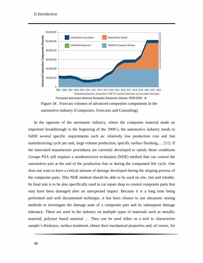
I) Introduction
48
In the opposite of the aeronautic industry, where the composite material made an
important breakthrough in the beginning of the 2000‟s, the automotive industry needs to
fulfill several specific requirements such as: relatively low production cost and fast
manufacturing cycle per unit, large volume production, specific surface finishing,… [11]. If
the innovated manufacture procedures are currently developed to satisfy those conditions
Groupe PSA still requires a nondestructive evaluation (NDE) method that can control the
automotive part at the end of the production line or during the component life cycle. One
does not want to have a critical amount of damage developed during the shaping process of
the composite parts. This NDE method should be able to be used on site, fast and reliable.
Its final aim is to be also specifically used in car repair shop to control composite parts that
may have been damaged after an unexpected impact. Because it is a long time being
performed and well documented technique, it has been chosen to use ultrasonic testing
methods to investigate the damage state of a composite part and its subsequent damage
tolerance. These are used in the industry on multiple types of materials such as metallic
material, polymer based material … They can be used either as a tool to characterize
sample‟s thickness, surface treatment, obtain their mechanical properties and, of course, for
Figure 34 : Forecast volumes of advanced composites components in the
automotive industry [Composites, Forecasts and Consulting]
I) Introduction
49
characterizing defects and induced damage in materials [12]–[14]. As a consequence of this
large application range, there is a lot of NDE techniques based on ultrasound that are
investigated in the literature, as it will be discussed in detail in the literature review of the
manuscript. They also have the advantages of being relatively inexpensive and easy to set-
up on site or being portable.
The study will focus on a thermoplastic matrix based glass fibers reinforced composite
produced by DuPont De Nemours meant to be used for structural application. Specifically,
it is a polyamide 66/6 based composite reinforced with woven glass fibers. This material is
named VizilonTM SB63G1-T1.5-S3 by their manufacturers. Preliminary works have been
performed in 2012 by members of the OpenLab “Materials and Processes”. It was shown
that ultrasonic imaging methods can detect large damage appearance induced in this woven
composite. However, it was not possible to image the early stages of damage evolution and
accumulation.
The present research is taking place in the framework of the OpenLab PSA “Materials
and Processes” and was funded by Groupe PSA. This OpenLab involves three academic
partners: Arts et Métiers ParisTech, The UMI Georgia Tech-CNRS (UMI 2958) located in
Metz and the Luxembourg Institute of Science and Technology (LIST). The letter of intent
has been signed by all the partners on May 19th
of 2011. The objectives of these OpenLabs
is to allow Groupe PSA “to remain on the leading edge of automotive products and
services” and “to strengthen its scientific partnerships with the world‟s most advanced
scientific key Labs”. More specifically, the present thesis subject is a partnership between
Georgia Tech Lorraine, les ENSAM-Arts et Métiers ParisTech and Groupe PSA. The
research was undertaken in the LEM3-UMR CNRS 7239 and the LUNE laboratories,
respectively located in the ENSAM-Arts et Métiers campus and the Georgia Tech Lorraine
campus both in Metz.

I) Introduction
50
2) Objectives and research orientations
In 2013, first investigations underwent in the framework of the OpenLab Materials and
processes on VizilonTM SB63G1-T1.5-S3 showed that critical damage can be detected in
this composite material. However, the final goal of Groupe PSA is to develop a NDE
ultrasonic tool to detect and quantify damage of automotive parts. With this tool a
technician should be able to determine if the parts can still be used or if they need to be
replaced or repaired. In order to achieve this objective, different damage indicators based
on the ultrasonic measurement have to be developed and validated on damaged structure.
Then, various fatigue tests can be performed on either the structural parts or a car prototype
in order to predict the performance and durability of those structures.
However, before developing this NDE tool, one needs to compile a lot of information
on the damage development scheme of the polyamide 66/6 based composite reinforced by
woven glass fabrics. Data on damage mechanisms, their chronology of appearance, the
influence of the loading nature and path, etc are required. Its mechanical behavior and the
related damage effects should also be completely known. Two sample configurations,
which are oriented at 0° and 45° from the warp direction, were chosen to be considered for
the present study. They obviously are the limiting case of the composite mechanical
behavior under tension. Solicitations under low velocity impact were also taken into
account because they are considered as event that an automotive part is more likely to
undergo during its life in service.
All the samples were investigated after various mechanical solicitations with optical
microscopy, Scanning Electronic Microscopy (SEM), X-ray tomography and ultrasonic
methods. The ultrasonic apparatuses are actually located at the LUNE laboratory of
Georgia Tech Lorraine whereas all the other apparatus are in the LEM3 laboratories in the
ENSAM-Arts et Métiers ParisTech campus of Metz. In order to know their sensitivity to
detect damage, several ultrasonic NDT methods were investigated during this project.
Indeed, the present project is close to a scoping study, from the ultrasonic point of view.
I) Introduction
51
After a review of the investigated ultrasonic based NDE methods some of them were
chosen, based on their respective advantages and accordance with the considered composite
material.
The present manuscript will be organized according to the following structures:
The chapter II) will be focused on the description of the VizilonTM SB63G1-T1.5-S3
and its constituents based on the information given by the manufacturer DuPont de
Nemours. Firstly, it will be reminded what a composite material is; then the different types
of matrix and reinforcement are quickly described. A particular attention will be, of course,
given to the woven fabric architecture. Then, more specific information will be given on the
polyamide 66/6 and the woven E-glass fiber reinforcement that constitute the studied
composite itself.
In the chapter III), the different mechanical tests performed on the DuPont‟s composite
material are described and analyzed in terms of damage and stiffness reduction. These
include monotonic and cyclic incremental tensile tests performed on both 0° and 45°
configurations. An expected difference in the stress/strain response was observed between
the two samples orientations. This was confirmed by measurements of the elastic modulus‟
evolution during the incremental cyclic tensile tests.
The chapter IV) is devoted to the study of the microstructure of the polyamide 66/6
composite reinforced with woven glass fibers. The global microstructure was first
investigated with optical microscope. Then undamaged and damaged samples were
analyzed with Scanning Electronic Microscopy (SEM) and X-ray tomography. The
different damage mechanisms, that may appear, were observed for both sample
configurations. Then, the void volume fraction evolution, as a function of tensile loadings
level, is measured by images analysis using the grey level thresholding on the X-ray
tomography results for both orientations.
Afterwards, the different samples loaded in tension are analyzed with ultrasonic
techniques in chapter V). A literature review, dedicated to the ultrasonic NDE methods to

I) Introduction
52
investigate damage, is proposed in the first subsection. There is a growing interest for most
of those methods in the field of polymer based composite materials. In a second subsection
it is showed that the classical C-scan methods are not suitable for damage quantification, at
the microscale, in the studied composite material. Other techniques were then successfully
used on stepwise damaged composites samples. First of all the measurement of stiffness
components via ultrasonic transmitted signal is performed. This was successfully used on
the samples previously analyzed with X-Ray tomography. Its can give useful information to
understand how damage mechanisms occur and alter the stiffness properties of the material.
Based on this measurement, a first damage indicator was proposed based on the phase shift
at various incidence angles. Then, guided waves investigations were considered for a next
subsection. This method was also proved to be effective to detect increasing states of
damage. From those experimental results, a second damage indicator that considers the
signal energy was proposed.
Finally, the validation of the proposed NDT ultrasonic based methods on composite
specimens impacted at different energy level is proposed in chapter VI). The samples were
analyzed by X-ray tomography in order to observe the induced damage mechanisms as well
as the extent of the damaged areas. The ultrasonic C-scan was then performed, both in
reflection and transmission, and useful information was collected. The measurement of
stiffness components and guided waves was finally used on those samples in a similar
manner as in the previous chapter.
The investigations of two others NDT methods based on ultrasound are presented in
two appendixes at the end of the manuscript. Since they are worth mentioning, but are not
as much in connection with the main study of this research than the other presented
investigations, they are proposed in the appendix section. The first appendix is dedicated to
the investigation of non-linear ultrasonic methods of damage evaluation whereas the second
appendix is dealing with the use of the coda part (or later arrival part) of the signal to
quantify the growth of induced damage. Both methods were presented in the literature
review dedicated to ultrasonic based NDE method that can be found in chapter V).
II) Description of the studied composite material: Woven glass reinforced polyamide
66/6
53
II) Description of the studied composite material:
Woven glass reinforced polyamide 66/6
Contents
1) Overview of composite material .................................................... 55
a) Matrix Parts .................................................................................................... 55
b) Reinforcements ............................................................................................... 56
2) Components of the studied composite material ........................... 57
a) Glass fibers ..................................................................................................... 58
Woven fabric reinforcements .............................................................................. 60
b) Polyamide 66/6 matrix ................................................................................... 64
Sensitivity to moisture absorption ...................................................................... 65
Sensitivity to temperature ................................................................................... 68
c) Properties of the composite material .............................................................. 70
3) Conclusion ....................................................................................... 73
The main aim of this first chapter is to introduce the VizilonTM SB63G1-T1.5-S3,
produced by DuPont, which is studied in this thesis manuscript. This composite material is
a polyamide 66/6 reinforce by woven glass fibers. First, the advantages of the composite
material and its specificities are briefly reminded. Then, a focus on woven composite
material and its associated damage mechanisms is proposed. The different components of
the composite material chosen by Groupe PSA are then introduced in two further
subsections. A discussion on the influence of temperature and moisture content on a
polyamide matrix is also going to be proposed. In addition, the final subsection is mostly

II) Description of the studied composite material: Woven glass reinforced polyamide
66/6
54
dealing with specific information on the studied composite material. Most of these
technical data were given by the material‟s manufacturer DuPont.
II) Description of the studied composite material: Woven glass reinforced polyamide
66/6
55
1) Overview of composite material
A composite material is made of two or more different constituents that are “mixed”
together; the latters can be separate in three categories:
- A matrix, which holds the different parts together and allow the composite to be
shaped. It also transfers the mechanical loading to the reinforcement parts.
- Reinforcements, which add rigidity and limit crack propagation in the composite
material.
- Additives are often added to the matrix part to enhance its properties, whether in
terms of electrical/thermal conductivity or stiffness. This eases a reduction in the
composite‟s cost by lowering the volume fraction of reinforcement without
decreasing its mechanical properties.
The two first mentioned types of constituents will be discussed in the following
sections.
a) Matrix Parts
Three classes of matrix can be easily distinguished: Ceramic Matrix Composites
(CMC), Metal Matrix Composite (MMC), Organic/Polymer matrix composites. The first
two are considered for high temperature application. If the composite will not be submitted
to a temperature higher than 300°C during its lifespan of service, the organic matrix
composites can be used. They are polymer based matrix and are the most used class of
composites in the industry. They are usually considered for low cost parts at high-volume
production manufacturing. The material studied in the present manuscript is based on an
organic matrix (Polyamide 66/6). Therefore, this class will be highlighted in the present
section. The polymer matrices can be split in two families: thermosetting matrix and
thermoplastic matrix.
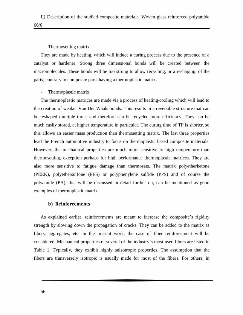
II) Description of the studied composite material: Woven glass reinforced polyamide
66/6
56
- Thermosetting matrix
They are made by heating, which will induce a curing process due to the presence of a
catalyst or hardener. Strong three dimensional bonds will be created between the
macromolecules. These bonds will be too strong to allow recycling, or a reshaping, of the
parts, contrary to composite parts having a thermoplastic matrix.
- Thermoplastic matrix
The thermoplastic matrices are made via a process of heating/cooling which will lead to
the creation of weaker Van Der Waals bonds. This results in a reversible structure that can
be reshaped multiple times and therefore can be recycled more efficiency. They can be
much easily stored, at higher temperature in particular. The curing time of TP is shorter, so
this allows an easier mass production than thermosetting matrix. The last three properties
lead the French automotive industry to focus on thermoplastic based composite materials.
However, the mechanical properties are much more sensitive to high temperature than
thermosetting, exception perhaps for high performance thermoplastic matrices. They are
also more sensitive to fatigue damage than thermosets. The matrix polyetherketone
(PEEK), polyethersulfone (PES) or polyphenylene sulfide (PPS) and of course the
polyamide (PA), that will be discussed in detail further on, can be mentioned as good
examples of thermoplastic matrix.
b) Reinforcements
As explained earlier, reinforcements are meant to increase the composite‟s rigidity
strength by slowing down the propagation of cracks. They can be added to the matrix as
fibers, aggregates, etc. In the present work, the case of fiber reinforcement will be
considered. Mechanical properties of several of the industry‟s most used fibers are listed in
Table 1. Typically, they exhibit highly anisotropic properties. The assumption that the
fibers are transversely isotropic is usually made for most of the fibers. For others, in

II) Description of the studied composite material: Woven glass reinforced polyamide
66/6
57
particular for glass fibers, an isotropic structure is assumed. Whenever available in Table 1,
the transverse modulus has been estimated by indirect measurement techniques.
Fiber EL ET σrL εrL
Polyaramide HM 120 2,5 2900 1,9
Polyamide 6,6 HT 6 960 20
Carbone HT 230 6 3500 1,5
Glass E (Standard) 73 68 2500 3,5
Glass R
(High performance) 86 3300 3,5
Table 1 : Mechanical properties of the most used fibers in composite materials [15]. EL,
ET: Respectively longitudinal and transverse Young modulus; σrL, εrL: Respectively stress
and strain to failure.
Fiber reinforcements can be used as small fibers or continuous fibers in the composite
material. In the latter case, their length is equivalent to that of the plate. They can be
arranged along a unique direction (unidirectional composite), as a woven plain fabric or
randomly oriented. This choice is normally made while considering the final application of
the composite, its expected solicitations in service, its required shape and the expected
performance.
2) Components of the studied composite material
As aforementioned in this chapter, the studied composite material is a polyamide 66/6
based composite reinforced with a 2/2 twill weave glass fiber fabric. The different
constituents of the composite will now be introduced. In addition, the properties of the
composite itself, the VizilonTM SB63G1-T1.5-S3, will be discussed.

II) Description of the studied composite material: Woven glass reinforced polyamide
66/6
58
a) Glass fibers
Various types of glass fibers exist in the industry. One can distinguish A, C, D, E, R, S,
etc -glass fibers, among others. Each of these types of glass fibers has its own composition
and mechanical, electrical, chemical, etc…, properties. The Table 2 gives the compositions
of several of the most used types of glass fibers; whereas the Table 3 gives their mechanical
properties. In the studied composite material, the reinforcement is made by E-glass fiber,
which is the most commonly used glass fiber in the industry. This is due to its reasonable
cost of production and to its satisfactory mechanical properties. The “E” stand for
“Electrical-application”, this type of glass fiber is indeed very poor in alkali metals in
contrast with the A-glass fiber. Now, the woven fabric is considered and the benefit of this
arrangement over unidirectional is explained.

II) Description of the studied composite material: Woven glass reinforced polyamide
66/6
59
E-glass w/Boron
E-glass w/o
Boron ECR-glass S-2 glass R-glass Quartz
SiO2 52-56% 59% 54-62% 64-66% 60-64% 99.9999%
Al2O3 12-16% 12.1-13.2% 9-15% 24-26% 17-24% -
B2O3 5-10% - - - - -
CaO 16-25% 22-23% 17-25% - 5-11% -
MgO 0-5% 3.1-3.4% 0-5% 8-12% 6-12% -
ZnO - - 2.9% - - -
Na2O 0-1% 0.6-0.6% 1.0% 0-0.1% 0-2% -
K2O trace 0-0.2% 0.2% - 0-2% -
TiO2 0.2-0.5% 0.5-1.5% 2.5% - - -
Zr2O3 - - - 0-1% - -
Li2O - - - - - -
Fe2O3 0.2-0.4% 0.2% 0.1% 0-0.1% - -
F2 0.2-0.7% 0-0.1% trace - - -
E-glass R-glass HS2,HS4 T-glass S-1 S-2
Tensile strength (GPa) 1.9-2.5 3.1-3.4 3.1-4.0 4.0-4.2 3.8-4.1 4.3-4.6
Tensile modulus (GPa) 69-80 86-89 82-90 84 85-87 88-91
Table 2 : Comparison of various types of glass fiber by mass ratio of the
different components
(Source: www.Compositesworld.com)
Table 3 : Mechanical properties of various types of glass fibers
(Source: www.compositeswolrd.com)
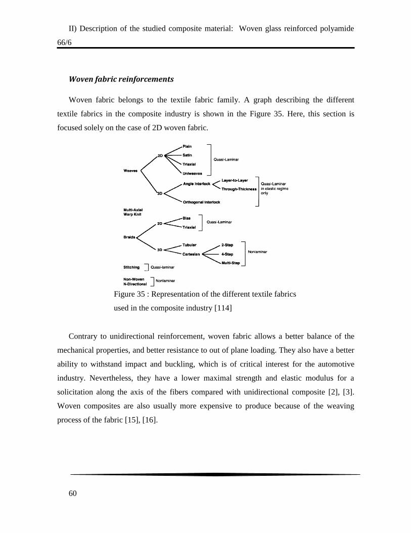
II) Description of the studied composite material: Woven glass reinforced polyamide
66/6
60
Woven fabric reinforcements
Woven fabric belongs to the textile fabric family. A graph describing the different
textile fabrics in the composite industry is shown in the Figure 35. Here, this section is
focused solely on the case of 2D woven fabric.
Contrary to unidirectional reinforcement, woven fabric allows a better balance of the
mechanical properties, and better resistance to out of plane loading. They also have a better
ability to withstand impact and buckling, which is of critical interest for the automotive
industry. Nevertheless, they have a lower maximal strength and elastic modulus for a
solicitation along the axis of the fibers compared with unidirectional composite [2], [3].
Woven composites are also usually more expensive to produce because of the weaving
process of the fabric [15], [16].
Figure 35 : Representation of the different textile fabrics
used in the composite industry [114]
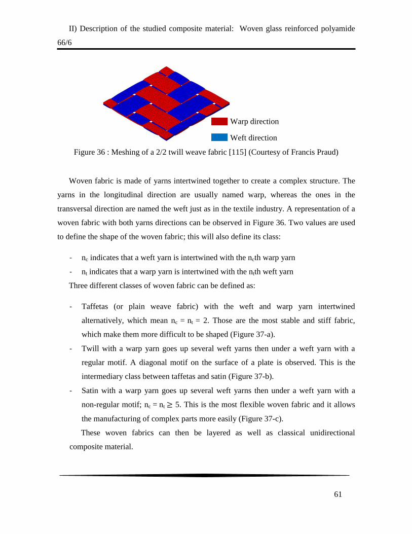
II) Description of the studied composite material: Woven glass reinforced polyamide
66/6
61
Woven fabric is made of yarns intertwined together to create a complex structure. The
yarns in the longitudinal direction are usually named warp, whereas the ones in the
transversal direction are named the weft just as in the textile industry. A representation of a
woven fabric with both yarns directions can be observed in Figure 36. Two values are used
to define the shape of the woven fabric; this will also define its class:
- nc indicates that a weft yarn is intertwined with the ncth warp yarn
- nt indicates that a warp yarn is intertwined with the ntth weft yarn
Three different classes of woven fabric can be defined as:
- Taffetas (or plain weave fabric) with the weft and warp yarn intertwined
alternatively, which mean nc = nt = 2. Those are the most stable and stiff fabric,
which make them more difficult to be shaped (Figure 37-a).
- Twill with a warp yarn goes up several weft yarns then under a weft yarn with a
regular motif. A diagonal motif on the surface of a plate is observed. This is the
intermediary class between taffetas and satin (Figure 37-b).
- Satin with a warp yarn goes up several weft yarns then under a weft yarn with a
non-regular motif; nc = nt 5. This is the most flexible woven fabric and it allows
the manufacturing of complex parts more easily (Figure 37-c).
These woven fabrics can then be layered as well as classical unidirectional
composite material.
Figure 36 : Meshing of a 2/2 twill weave fabric [115] (Courtesy of Francis Praud)
Weft direction
Warp direction
II) Description of the studied composite material: Woven glass reinforced polyamide
66/6
62
Compared to a unidirectional reinforcement, the woven reinforcement will suffer a
specific damage scheme with specific damage mechanisms. Those mechanisms are
classically distinguished into three classes that represent each damage scale:
- Macroscopic scale : Delamination
- Mesoscopic scale : Intra-warp cracks, fiber breakage
- Microscopic scale : inter-warp cracks, Fiber/Matrix debonding
The intra-warp cracks can appear in two configurations. First, transversal cracks can
appear parallel to the warp axis along his thickness. Second, longitudinal cracks can appear
parallel to the warp axis but along the fabric plane. Karakaya et al. [2], among others, show
that these damage mechanisms will be different considering the solicitations and the
orientation of the fibers. Tension, bending and compression loading were considered on
samples oriented along the warp direction and a 45° direction from the warp axis. Further
details about the related damage mechanisms and mechanical behavior can be found in the
work by Karakaya [2]. In order to show the change in damage scheme induced by different
solicitations, tensile loading at 0° and 45° from the warp directions will now be briefly
discussed.
Figure 37 : Schematic representation of the differents woven
armor classicaly used in composites material [15]
Taffeta
nc=nt=2
2/2 twill
nc=nt=3
5-harness satin
nc=nt=5 (b)
(b)
(c) (a)

II) Description of the studied composite material: Woven glass reinforced polyamide
66/6
63
For 0° orientations, fiber/matrix debonding can first be observed. Transversal cracks in
the yarns then propagate along the debonded area. When the cracks reach the end of
transversal yarns, a deviation of the cracks may occur and induce a longitudinal
yarns/matrix debonding. This mechanisms is often named “meta-delamination” [17] and
can be observed in Figure 38-a. The failure of the composite is then caused by longitudinal
yarn breakage as visible in Figure 38-b. A pull-out of the fibers can consequently be
observed [18].
For 45° orientations, the ductility of the matrix will induce a reorientation of the fibers
in the loading direction as illustrated in Figure 39. This phenomenon is induced by
plasticization of the matrix near the intertwined area of yarns and is even more pronounced
with the matrix‟s ductility, temperature and loading velocity [19], [20]. When plastic
deformation is no longer possible in the matrix nor the interphase, micro-cracks then appear
in the matrix, and propagate along the fibers [20], [21]. This will generally induce
delamination in the composite material. Then, shear band localization can be generated and
will propagate along the fibers. In the end, the fibers break prior to the final failure of the
composite. As shown in Figure 40, the post-failure samples submitted to tensile tests in the
45° orientations may exhibit large amount of delamination.
Figure 38 : Damage mechanisms in a woven composite loaded in tension
along the fibers axis [18]
Fibers breakage in a longitudinal yarn Transversal cracks and associated yarns/matrix debonding
Transversal cracks and associated yarns/matrix debonding
(a) (b)

II) Description of the studied composite material: Woven glass reinforced polyamide
66/6
64
During their life cycle, composite parts can be submitted to various solicitations along
various orientations. So, it is important to analyze the behavior of the woven composite
under these various load cases when the introduction of those materials is considered for a
new application.
b) Polyamide 66/6 matrix
Polyamide polymers in general are known for their high strength, abrasion resistance,
and resilience. They are however also very sensitive to humidity. The polyamide 66/6 is a
copolymer based on polyamide 66 that was developed to obtain a compromise between the
polyamide 66 and the polyamide 6.
The polyamide 66 is a thermoplastic polymer made of repeated amid chains. It was first
produced by DuPont De Nemours in 1935 and then sold as a textile fiber in 1938 (and
called Nylon). The polyamide 6, later developed in 1938 by Paul Schlack at IG Farben, has
a higher resistance to impact and toughness, but lower stiffness properties compared to
Figure 40 : Post failure damage mechanisms
after tensile tests on samples oriented at 45°
from the warp direction [116]
Figure 39 : Fibers rotations during
tensile tests on samples oriented at 45°
from the warp direction [116]
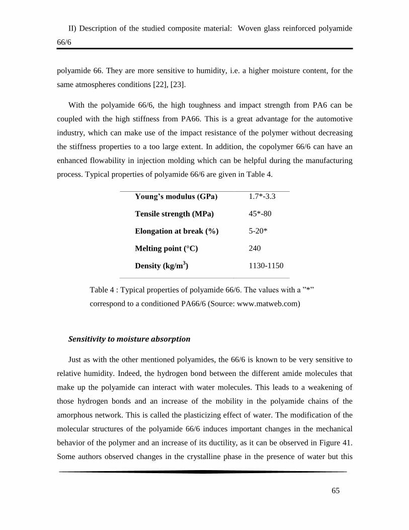
II) Description of the studied composite material: Woven glass reinforced polyamide
66/6
65
polyamide 66. They are more sensitive to humidity, i.e. a higher moisture content, for the
same atmospheres conditions [22], [23].
With the polyamide 66/6, the high toughness and impact strength from PA6 can be
coupled with the high stiffness from PA66. This is a great advantage for the automotive
industry, which can make use of the impact resistance of the polymer without decreasing
the stiffness properties to a too large extent. In addition, the copolymer 66/6 can have an
enhanced flowability in injection molding which can be helpful during the manufacturing
process. Typical properties of polyamide 66/6 are given in Table 4.
Sensitivity to moisture absorption
Just as with the other mentioned polyamides, the 66/6 is known to be very sensitive to
relative humidity. Indeed, the hydrogen bond between the different amide molecules that
make up the polyamide can interact with water molecules. This leads to a weakening of
those hydrogen bonds and an increase of the mobility in the polyamide chains of the
amorphous network. This is called the plasticizing effect of water. The modification of the
molecular structures of the polyamide 66/6 induces important changes in the mechanical
behavior of the polymer and an increase of its ductility, as it can be observed in Figure 41.
Some authors observed changes in the crystalline phase in the presence of water but this
Young’s modulus (GPa) 1.7*-3.3
Tensile strength (MPa) 45*-80
Elongation at break (%) 5-20*
Melting point (°C) 240
Density (kg/m3) 1130-1150
Table 4 : Typical properties of polyamide 66/6. The values with a ”*”
correspond to a conditioned PA66/6 (Source: www.matweb.com)

II) Description of the studied composite material: Woven glass reinforced polyamide
66/6
66
phenomenon is not clearly understood; nevertheless it remains as a minor effect. The
transition temperature will also be affected by the moisture content and will decrease with
an increase of the moisture content [24]. When the structure is in service for a relatively
long time, the absorbed moisture of the polyamide will not remain as initially, i.e. under
dry-as-molded conditions. The mechanical characterization of those materials is therefore,
normally, performed in “atmosphere 23” conditions in order to reflect the real material
behavior in service. This annotation means 23°C and 50% of relative humidity. However,
the moisture absorption rate can be very low at 23°C/50% RH and it can take months to
reach moisture equilibrium (Figure 42). As an example, it could take more than a year for a
4 mm thick PA66 if those conditioning conditions are considered [25]. Therefore, it is
recommended to condition the sample by considered higher temperature and/or relative
humidity before storing the sample in “atmosphere 23” condition. A brief comparison of
different standard procedures, as well as useful literature references, can be found in [25].
Figure 41 : Stress/strain curve, in tension at 23°C, for a Polyamide 66/6
(Ultramid® C3U from BASF) dry (Green ) and after conditionning 50% RH (Red)
[http://iwww.plasticsportal.com/]

II) Description of the studied composite material: Woven glass reinforced polyamide
66/6
67
In the end, the influence of moisture absorption will have a direct effect on the damage
mechanisms that can be induced in the reinforced polyamide composite. As an example, the
study of Arif et al. [26] on polyamide 66 reinforced with short glass fiber can be mentioned.
Their investigation leads to two main results: in one hand, the moisture content will not
induce the apparition of pre-damage in the composite. In the other hand damage
mechanisms for 0% conditioning conditions and for 50/100% conditioning conditions will
be different:
For 0% of relative humidity, the damage mechanisms are:
- Fiber matrix debonding near the end of the fiber
- Brittle matrix cracking and cavitation
- Fiber breakages
- Total failure
For the 50/100 % of relative humidity, the damage mechanisms are :
- Fiber matrix debonding near the end of the fiber
Figure 42 : Moisture absorption function of time for different polyamide and
different thickness when conditioning in “atmosphere 23” conditions. The moisture
equilibrium for a polyamide 66 (Ultramid A) by BASF is reached around 2.5% [22]
II) Description of the studied composite material: Woven glass reinforced polyamide
66/6
68
- Local deformation of the matrix near the debonding area
- Ductile matrix cracking (With high matrix deformation bands for the 100%)
- Total failure
Sensitivity to temperature
The polyamide 66/6 is a semi-crystalline polymer, i.e. it has a crystalline and an
amorphous phase. The percentage of crystalline phase will differ for each polymer, for
example, polyamide 6 and polyamide 66 will have a typical crystalline rate of 35–45%
[27]. It can be noted that the mix of polyamide monomers to obtain polyamide copolymers
usually leads to a decrease of the crystalline rate. For a semi-crystalline polymer, two
important temperatures can be distinguished: the melting point Tm and, in addition to fully
amorphous polymer, a vitreous transition temperature Tg. As for moisture, an increase of
temperature will lead to an increase of the polymer ductility and a decrease of its strength.
In the Figure 43, one can clearly see that when the Young‟s modulus decrease when
increasing the temperature, with an important drop at transition temperature. Those are also
caused by an increase of the mobility of chains from the amorphous network. This increase
is caused by a breakage of some weak links [28]. In addition to moisture, the temperature
will have a plasticizing effect on the crystalline phase. If on the other hand the temperature
decreases, the intra-lamellar slip will be reduced and the density of stored energy will
increase. This will induce a localization of deformation and a more brittle global behavior
[29].

II) Description of the studied composite material: Woven glass reinforced polyamide
66/6
69
Some studies focused on the specific case of the combined influence of temperature and
moisture on the mechanical response. It was observed and discussed in [25], on a
polyamide 6, that the combination of both conditions does not necessarily increases the
Figure 43 : Young‟s modulus of classical polymers as function of their
temperature and crystallinity [117]
1: Glassy state
2: Rubbery state
3: Viscous state
Figure 44 : Evolution of the vitreous transition temperature Tg with
the relative humidity (Courtesy of Solvay).
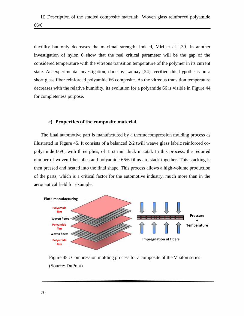
II) Description of the studied composite material: Woven glass reinforced polyamide
66/6
70
ductility but only decreases the maximal strength. Indeed, Miri et al. [30] in another
investigation of nylon 6 show that the real critical parameter will be the gap of the
considered temperature with the vitreous transition temperature of the polymer in its current
state. An experimental investigation, done by Launay [24], verified this hypothesis on a
short glass fiber reinforced polyamide 66 composite. As the vitreous transition temperature
decreases with the relative humidity, its evolution for a polyamide 66 is visible in Figure 44
for completeness purpose.
c) Properties of the composite material
The final automotive part is manufactured by a thermocompression molding process as
illustrated in Figure 45. It consists of a balanced 2/2 twill weave glass fabric reinforced co-
polyamide 66/6, with three plies, of 1.53 mm thick in total. In this process, the required
number of woven fiber plies and polyamide 66/6 films are stack together. This stacking is
then pressed and heated into the final shape. This process allows a high-volume production
of the parts, which is a critical factor for the automotive industry, much more than in the
aeronautical field for example.
Figure 45 : Compression molding process for a composite of the Vizilon series
(Source: DuPont)
Plate manufacturing
Pressure +
Temperature
Polyamide film
Woven fibers
Polyamide film
Woven fibers
Impregnation of fibers Polyamide film
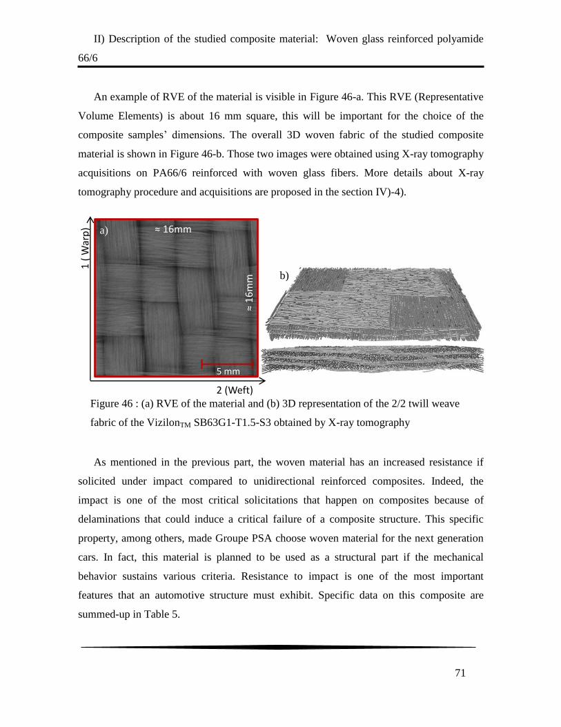
II) Description of the studied composite material: Woven glass reinforced polyamide
66/6
71
An example of RVE of the material is visible in Figure 46-a. This RVE (Representative
Volume Elements) is about 16 mm square, this will be important for the choice of the
composite samples‟ dimensions. The overall 3D woven fabric of the studied composite
material is shown in Figure 46-b. Those two images were obtained using X-ray tomography
acquisitions on PA66/6 reinforced with woven glass fibers. More details about X-ray
tomography procedure and acquisitions are proposed in the section IV)-4).
As mentioned in the previous part, the woven material has an increased resistance if
solicited under impact compared to unidirectional reinforced composites. Indeed, the
impact is one of the most critical solicitations that happen on composites because of
delaminations that could induce a critical failure of a composite structure. This specific
property, among others, made Groupe PSA choose woven material for the next generation
cars. In fact, this material is planned to be used as a structural part if the mechanical
behavior sustains various criteria. Resistance to impact is one of the most important
features that an automotive structure must exhibit. Specific data on this composite are
summed-up in Table 5.
Figure 46 : (a) RVE of the material and (b) 3D representation of the 2/2 twill weave
fabric of the VizilonTM SB63G1-T1.5-S3 obtained by X-ray tomography
b)
5 mm
1 (
War
p)
2 (Weft)
≈ 16mm
≈ 1
6m
m
a)
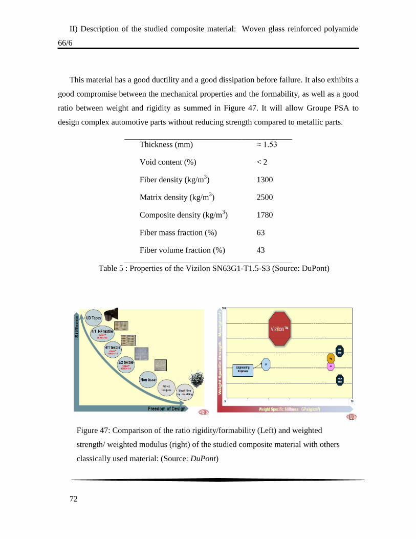
II) Description of the studied composite material: Woven glass reinforced polyamide
66/6
72
This material has a good ductility and a good dissipation before failure. It also exhibits a
good compromise between the mechanical properties and the formability, as well as a good
ratio between weight and rigidity as summed in Figure 47. It will allow Groupe PSA to
design complex automotive parts without reducing strength compared to metallic parts.
Table 5 : Properties of the Vizilon SN63G1-T1.5-S3 (Source: DuPont)
Thickness (mm) ≈ 1.53
Void content (%) < 2
Fiber density (kg/m3) 1300
Matrix density (kg/m3) 2500
Composite density (kg/m3) 1780
Fiber mass fraction (%) 63
Fiber volume fraction (%) 43
Figure 47: Comparison of the ratio rigidity/formability (Left) and weighted
strength/ weighted modulus (right) of the studied composite material with others
classically used material: (Source: DuPont)

II) Description of the studied composite material: Woven glass reinforced polyamide
66/6
73
3) Conclusion
For the automotive industry the introduction of a thermoplastic composite reinforced
with woven fibers has several advantages. First, the thermoplastic matrix allows both a
faster and larger scale manufacturing and easier recycling. In addition, the specific
polyamide 66/6 matrix is known to have an important impact resistance and good
mechanical properties. Second, the woven reinforcement is known for a larger resistance to
impact and delamination. Since the automotive part used to contribute to the vehicle‟s
structural solidity, it must also be able to withstand non-negligible impact solicitations; this
choice of constituents is very appealing for structural applications. However, the polyamide
matrix used in the VizilonTM SB63G1-T1.5-S3 is very sensitive to the water uptake. The
moisture content will have a direct effect on the development of damage and hence on the
mechanical response. In addition, the woven reinforced composite has particular damage
schemes, compared to unidirectional reinforced composites, which are influence by the
type of solicitation. Therefore, it is important to consider several typical solicitations to
characterize the studied composite material behavior and the different associated damage
mechanisms. In the end this will permit to test NDE methods on various damage
mechanisms. Indeed, since this composite material is planned to be used as a structural part,
it may undergo various solicitations during its service life.

II) Description of the studied composite material: Woven glass reinforced polyamide
66/6
74

III) Characterization of the mechanical behavior of the studied composite material under
monotonic and cyclic loading
75
III) Characterization of the mechanical behavior of the
studied composite material under monotonic and
cyclic loading
Contents
1) Description of the experimental procedure ................................. 76
2) Monotonic tensile test for the 0° configuration ........................... 79
3) Monotonic tensile test for the 45° configuration ......................... 82
4) Incremental cyclic tensile test ........................................................ 88
5) Conclusion ....................................................................................... 92
Various mechanical tests were performed on the studied composite material to identify
its macroscopic mechanical behavior. In the first section, all the information about the
tensile tests procedure is described. Then, monotonic tensile tests are performed in order to
determine the main mechanical properties, namely: Young modulus, the ultimate strength,
the strain to failure etc. Those tests are done on samples oriented at both 0° and 45° from
the warp direction. Indeed, as mentioned in the previous chapter, the two orientations are
critical cases for tensile test solicitations that, as it is shown, lead to two very different
stress/strain responses. Then, incremental cyclic tests are carried out on the two
configurations of sample. The evolution of damage, for increasing stress values, is then
estimated based on the elastic modulus reduction.
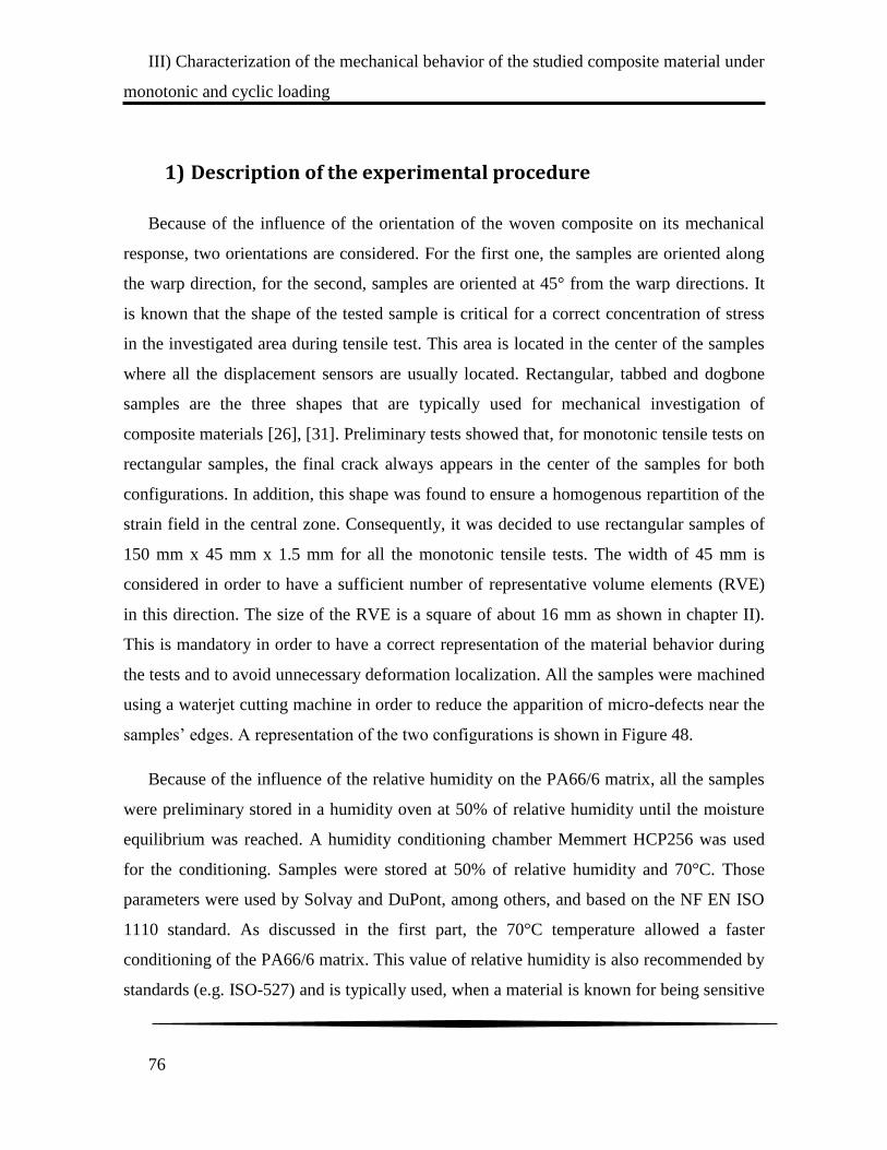
III) Characterization of the mechanical behavior of the studied composite material under
monotonic and cyclic loading
76
1) Description of the experimental procedure
Because of the influence of the orientation of the woven composite on its mechanical
response, two orientations are considered. For the first one, the samples are oriented along
the warp direction, for the second, samples are oriented at 45° from the warp directions. It
is known that the shape of the tested sample is critical for a correct concentration of stress
in the investigated area during tensile test. This area is located in the center of the samples
where all the displacement sensors are usually located. Rectangular, tabbed and dogbone
samples are the three shapes that are typically used for mechanical investigation of
composite materials [26], [31]. Preliminary tests showed that, for monotonic tensile tests on
rectangular samples, the final crack always appears in the center of the samples for both
configurations. In addition, this shape was found to ensure a homogenous repartition of the
strain field in the central zone. Consequently, it was decided to use rectangular samples of
150 mm x 45 mm x 1.5 mm for all the monotonic tensile tests. The width of 45 mm is
considered in order to have a sufficient number of representative volume elements (RVE)
in this direction. The size of the RVE is a square of about 16 mm as shown in chapter II).
This is mandatory in order to have a correct representation of the material behavior during
the tests and to avoid unnecessary deformation localization. All the samples were machined
using a waterjet cutting machine in order to reduce the apparition of micro-defects near the
samples‟ edges. A representation of the two configurations is shown in Figure 48.
Because of the influence of the relative humidity on the PA66/6 matrix, all the samples
were preliminary stored in a humidity oven at 50% of relative humidity until the moisture
equilibrium was reached. A humidity conditioning chamber Memmert HCP256 was used
for the conditioning. Samples were stored at 50% of relative humidity and 70°C. Those
parameters were used by Solvay and DuPont, among others, and based on the NF EN ISO
1110 standard. As discussed in the first part, the 70°C temperature allowed a faster
conditioning of the PA66/6 matrix. This value of relative humidity is also recommended by
standards (e.g. ISO-527) and is typically used, when a material is known for being sensitive

III) Characterization of the mechanical behavior of the studied composite material under
monotonic and cyclic loading
77
to relative humidity, except when specific recommendations is required, as was discussed
in a previous chapter. The weights of the samples were measured before the conditioning
and every two days after storing the samples in the humidity chamber. The moisture
equilibrium is considered as reached when the measured weight hardly changes (less than
5%) for three consecutive measurements.
All the monotonic tensile tests and incremental cyclic tensile tests, described in this
section, were done at ambient temperature, with a tensile test machine “Z050”
manufactured by Zwick Roell Gruppe compliant with the norm ISO 5893. Except when
mentioned, the tensile tests were performed at a constant strain rate of 10-4
s-1
. An initial
gauge length of 65 mm was considered for all tensile tests.
In order to validate the tensile test procedure, various displacement sensors were used
for the first tests:
- A Linear Variable Displacement Transformer (LVDT),
- A video camera for Digital Image Correlation (DIC) technique,
Figure 48 : Position of the samples oriented at 0° and 45° from
warp direction (mold flow direction) on the composite plate. The
direction “1” is the loading direction in tension.
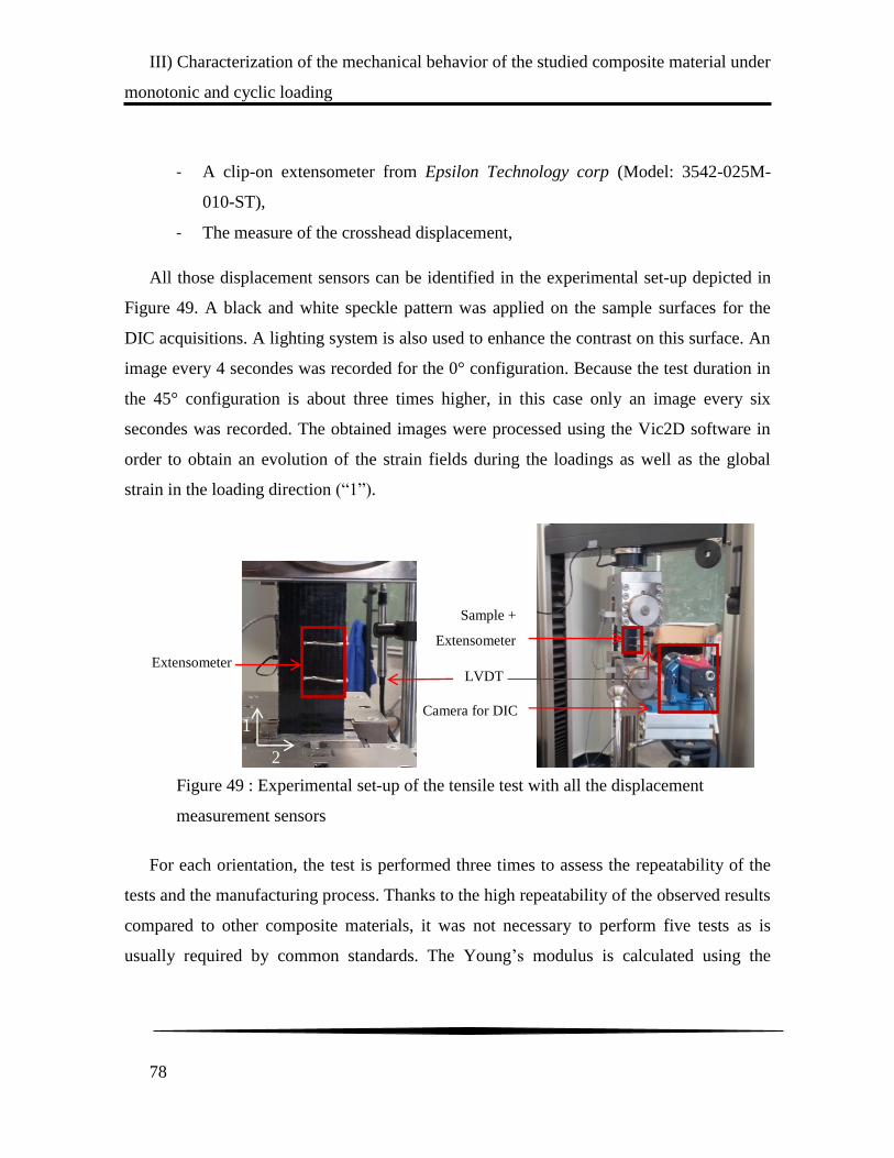
III) Characterization of the mechanical behavior of the studied composite material under
monotonic and cyclic loading
78
- A clip-on extensometer from Epsilon Technology corp (Model: 3542-025M-
010-ST),
- The measure of the crosshead displacement,
All those displacement sensors can be identified in the experimental set-up depicted in
Figure 49. A black and white speckle pattern was applied on the sample surfaces for the
DIC acquisitions. A lighting system is also used to enhance the contrast on this surface. An
image every 4 secondes was recorded for the 0° configuration. Because the test duration in
the 45° configuration is about three times higher, in this case only an image every six
secondes was recorded. The obtained images were processed using the Vic2D software in
order to obtain an evolution of the strain fields during the loadings as well as the global
strain in the loading direction (“1”).
For each orientation, the test is performed three times to assess the repeatability of the
tests and the manufacturing process. Thanks to the high repeatability of the observed results
compared to other composite materials, it was not necessary to perform five tests as is
usually required by common standards. The Young‟s modulus is calculated using the
Sample +
Extensometer
Camera for DIC
Extensometer LVDT
Figure 49 : Experimental set-up of the tensile test with all the displacement
measurement sensors
1
2
III) Characterization of the mechanical behavior of the studied composite material under
monotonic and cyclic loading
79
standard ISO-527-1, which recommends calculation of the elastic modulus by linear
regression between = 0.05% and = 0.25%.
2) Monotonic tensile test for the 0° configuration
The stress/train curves for the different displacement sensors are plotted in Figure 50.
For the samples oriented at 0° from fiber‟s axis, one can clearly see a correlation between
the extensometer measurement and the DIC method and between the crosshead
displacement and the LVDT separately, what is quite expected. Indeed the LVDT is fixed
to the jaws and follow their displacement and the extensometer is fixed close to the
mapping area that was used for the DIC method.
It was chosen to consider as relevant, information that is measured by the extensometer
and the DIC, because the other two sensors appear to include, in the obtained results, the
response of the jaws. The extensometer and the DIC only measure the response of the
material. As mentioned in the procedure‟s section, only three samples were tested because
Figure 50 : Stress/Strain curves for one of the samples with fibers oriented at 0°
with the four displacement sensors considered
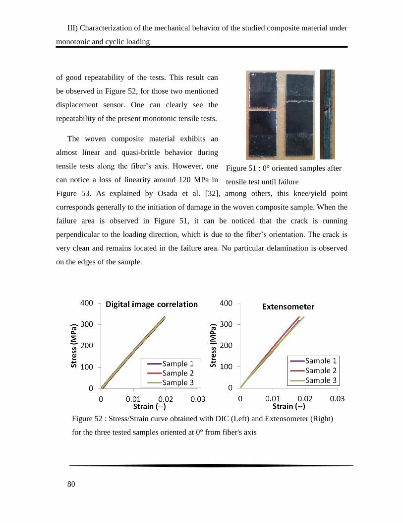
III) Characterization of the mechanical behavior of the studied composite material under
monotonic and cyclic loading
80
of good repeatability of the tests. This result can
be observed in Figure 52, for those two mentioned
displacement sensor. One can clearly see the
repeatability of the present monotonic tensile tests.
The woven composite material exhibits an
almost linear and quasi-brittle behavior during
tensile tests along the fiber‟s axis. However, one
can notice a loss of linearity around 120 MPa in
Figure 53. As explained by Osada et al. [32], among others, this knee/yield point
corresponds generally to the initiation of damage in the woven composite sample. When the
failure area is observed in Figure 51, it can be noticed that the crack is running
perpendicular to the loading direction, which is due to the fiber‟s orientation. The crack is
very clean and remains located in the failure area. No particular delamination is observed
on the edges of the sample.
Figure 52 : Stress/Strain curve obtained with DIC (Left) and Extensometer (Right)
for the three tested samples oriented at 0° from fiber's axis
Figure 51 : 0° oriented samples after
tensile test until failure
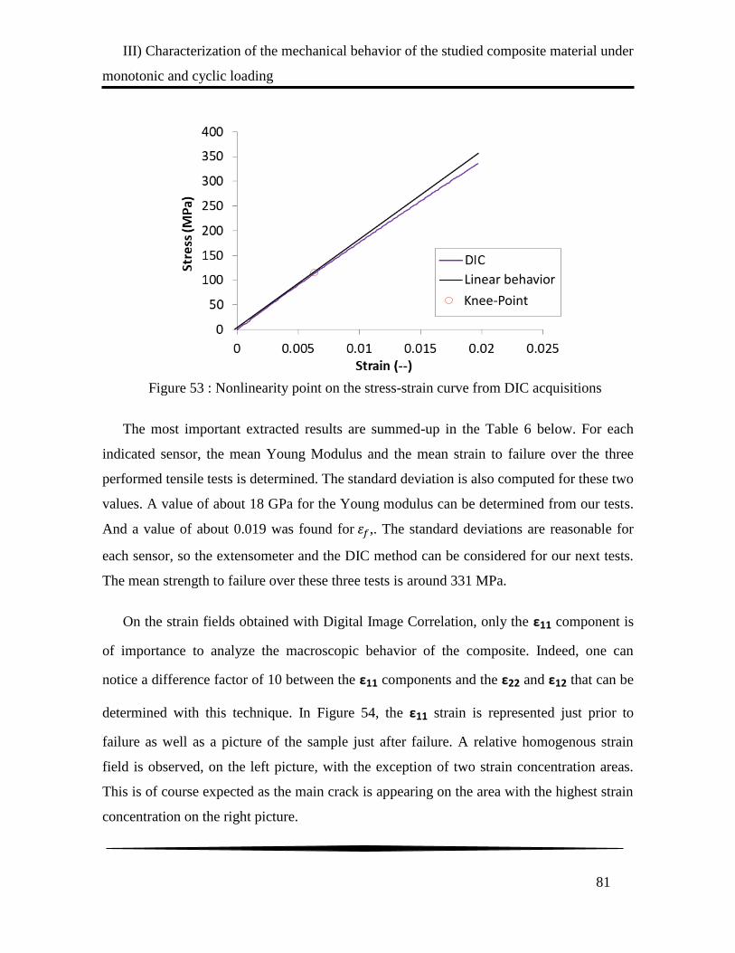
III) Characterization of the mechanical behavior of the studied composite material under
monotonic and cyclic loading
81
The most important extracted results are summed-up in the Table 6 below. For each
indicated sensor, the mean Young Modulus and the mean strain to failure over the three
performed tensile tests is determined. The standard deviation is also computed for these two
values. A value of about 18 GPa for the Young modulus can be determined from our tests.
And a value of about 0.019 was found for ,. The standard deviations are reasonable for
each sensor, so the extensometer and the DIC method can be considered for our next tests.
The mean strength to failure over these three tests is around 331 MPa.
On the strain fields obtained with Digital Image Correlation, only the ε11 component is
of importance to analyze the macroscopic behavior of the composite. Indeed, one can
notice a difference factor of 10 between the ε11 components and the ε22 and ε12 that can be
determined with this technique. In Figure 54, the ε11 strain is represented just prior to
failure as well as a picture of the sample just after failure. A relative homogenous strain
field is observed, on the left picture, with the exception of two strain concentration areas.
This is of course expected as the main crack is appearing on the area with the highest strain
concentration on the right picture.
Linear behavior
Knee-Point
Figure 53 : Nonlinearity point on the stress-strain curve from DIC acquisitions
. . . . .
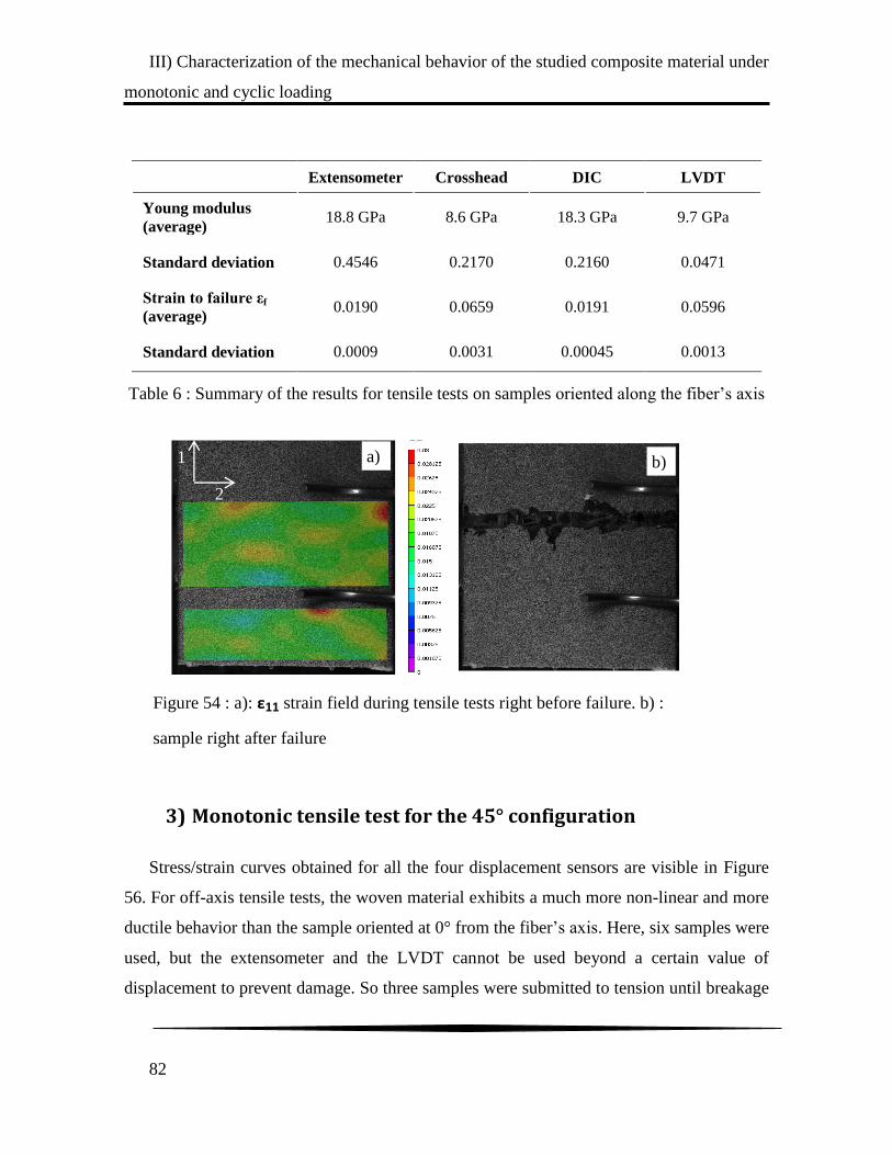
III) Characterization of the mechanical behavior of the studied composite material under
monotonic and cyclic loading
82
Extensometer Crosshead DIC LVDT
Young modulus
(average) 18.8 GPa 8.6 GPa 18.3 GPa 9.7 GPa
Standard deviation 0.4546 0.2170 0.2160 0.0471
Strain to failure εf
(average) 0.0190 0.0659 0.0191 0.0596
Standard deviation 0.0009 0.0031 0.00045 0.0013
3) Monotonic tensile test for the 45° configuration
Stress/strain curves obtained for all the four displacement sensors are visible in Figure
56. For off-axis tensile tests, the woven material exhibits a much more non-linear and more
ductile behavior than the sample oriented at 0° from the fiber‟s axis. Here, six samples were
used, but the extensometer and the LVDT cannot be used beyond a certain value of
displacement to prevent damage. So three samples were submitted to tension until breakage
Figure 54 : a): ε11 strain field during tensile tests right before failure. b) :
sample right after failure
ε11
1
2
a) b)
Table 6 : Summary of the results for tensile tests on samples oriented along the fiber‟s axis

III) Characterization of the mechanical behavior of the studied composite material under
monotonic and cyclic loading
83
but only the measurement of the crosshead and resulting from the DIC can be obtained. The
resulting stress/strain curves are plotted in Figure 57-
a. The other three samples did not exceed 10% of
strain; therefore in this case all sensors were used. The
stress/strain curves obtained from the extensometer
are plotted in Figure 57-b. For the 45° configuration,
the same observation can be made from the
correlation between the different displacement
sensors.
When the failure area visible in Figure 55 is
observed, it can be noted that the crack is running at 45° of the loading direction, which is
induced by the fabric orientation. The main crack is propagating in stairs shape; lots of
delamination can be observed on the side of the sample relatively close to the failure zone.
0
10
20
30
40
50
60
70
80
90
100
0 0.05 0.1 0.15 0.2
Stre
ss (
MP
a)
Strain (--)
ExtensometerCross barDICLVDT
Figure 56 : Stress/Strain curves for the 45° orientation for the entire
displacement sensor considered (Here the sample was not solicited until
Crosshead
. . . .
Figure 55 : 45° oriented sample
after tensile test until failure

III) Characterization of the mechanical behavior of the studied composite material under
monotonic and cyclic loading
84
As in the previous subsection, the most important results are summed up in the Table 7.
The Young modulus is about 3.5 GPa and the strain to failure εf is about 0.23. The
deviation for this test is higher when considering the value of Young‟s modulus. The mean
strength to failure is about 134 MPa.
Extensometer Crosshead DIC LVDT
Young modulus
(average) 3.7 GPa 3.5 GPa 3.4 GPa 3.3 GPa
Standard
deviation 0.3514 0.2625 0.3300 0.6481
Strain to failure εf
(average) -- 0.225 0.234 --
Standard
deviation -- 0.0052 0.0076 --
Figure 57 : Stress/Strain curve obtained with DIC (a) and Extensometer
(b) for the three tested samples oriented at 45° from fiber's axis
(a)
(a)
(b)
. . . . . . .
Table 7 : Summary of the results for tensile test on samples oriented at 45°
from fiber‟s axis
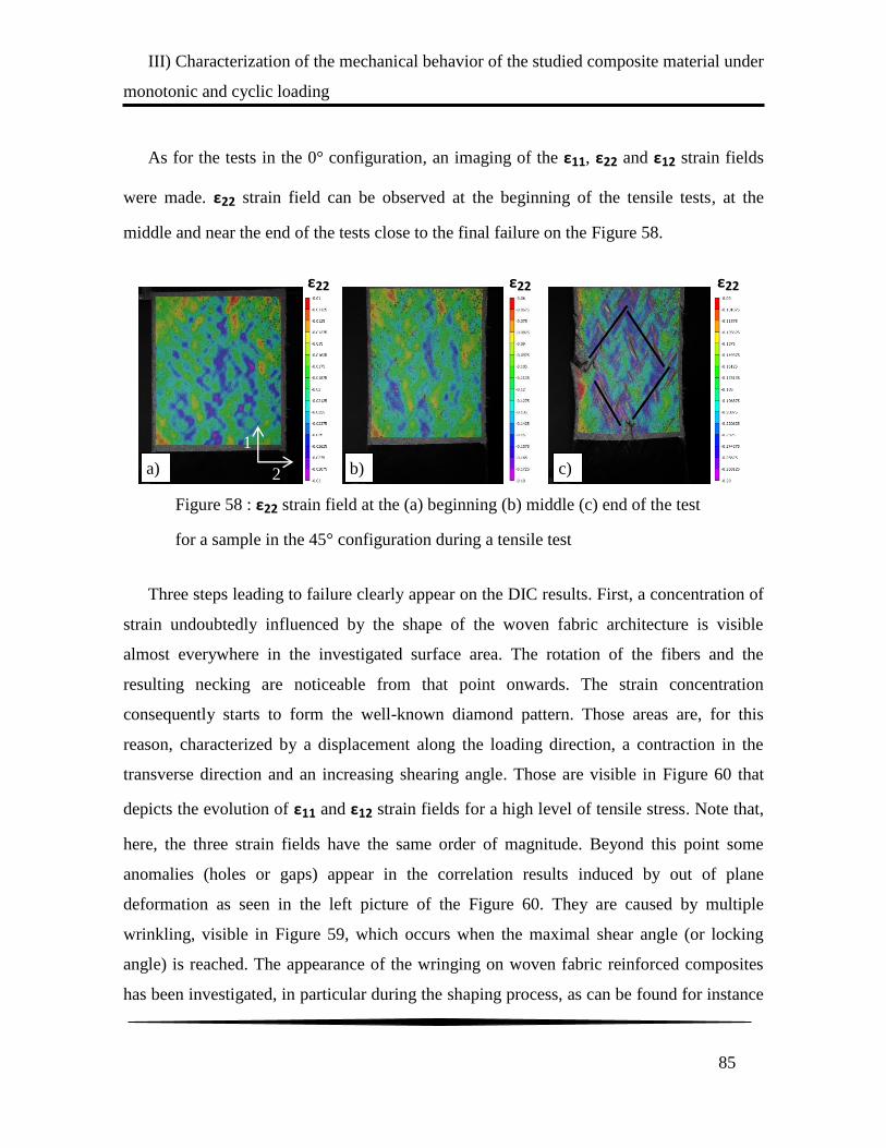
III) Characterization of the mechanical behavior of the studied composite material under
monotonic and cyclic loading
85
As for the tests in the 0° configuration, an imaging of the ε11, ε22 and ε12 strain fields
were made. ε22 strain field can be observed at the beginning of the tensile tests, at the
middle and near the end of the tests close to the final failure on the Figure 58.
Three steps leading to failure clearly appear on the DIC results. First, a concentration of
strain undoubtedly influenced by the shape of the woven fabric architecture is visible
almost everywhere in the investigated surface area. The rotation of the fibers and the
resulting necking are noticeable from that point onwards. The strain concentration
consequently starts to form the well-known diamond pattern. Those areas are, for this
reason, characterized by a displacement along the loading direction, a contraction in the
transverse direction and an increasing shearing angle. Those are visible in Figure 60 that
depicts the evolution of ε11 and ε12 strain fields for a high level of tensile stress. Note that,
here, the three strain fields have the same order of magnitude. Beyond this point some
anomalies (holes or gaps) appear in the correlation results induced by out of plane
deformation as seen in the left picture of the Figure 60. They are caused by multiple
wrinkling, visible in Figure 59, which occurs when the maximal shear angle (or locking
angle) is reached. The appearance of the wringing on woven fabric reinforced composites
has been investigated, in particular during the shaping process, as can be found for instance
Figure 58 : ε22 strain field at the (a) beginning (b) middle (c) end of the test
for a sample in the 45° configuration during a tensile test
ε22
Exx
ε22
Exx
ε22
Exx
a)
a)
b)
b)
c)
1
2

III) Characterization of the mechanical behavior of the studied composite material under
monotonic and cyclic loading
86
in [33]. The strain scheme, which is more complex than in the 0° configuration, explains
why the tensile test in 45° configuration (or bias-extension test) is still extensively
investigated. In addition, this is one of the easiest experiments that can provide information
on in-plane shear properties of a given woven reinforced composite. A recent review of the
bias-extension test as well as some known experimental and numerical issues that may be
undergone with the test, and may lead to unprecise results, can be found in [4].
As a reminder, Figure 61 depicts the stress/strain curve for the two chosen
configurations (0° and 45°). The selected configurations made the difference in mechanical
behavior very obvious, which is why they have been chosen for the present study. Indeed,
they lead to very distinct microstructural behavior, i.e. brittle for the 0° and mostly ductile
for the 45°. In addition, the 45° case induces high shearing effect during the tensile loading.
Figure 59 : Tested sample in the 45° configuration just before
failure (Left) and after failure (Right) from a tensile test

III) Characterization of the mechanical behavior of the studied composite material under
monotonic and cyclic loading
87
Figure 60 : ε11 (Left) and ε12 (Right) strain field for the 45°
configuration during a tensile test
ε11 ε12
1
2
Figure 61 : Comparison between the behavior in the 0° configuration and the
45° configuration. Displacement measured with Digital Image Correlation
Elastic Modulus: 18.3 GPa
Elastic Modulus: 3.4 GPa
. . . . .
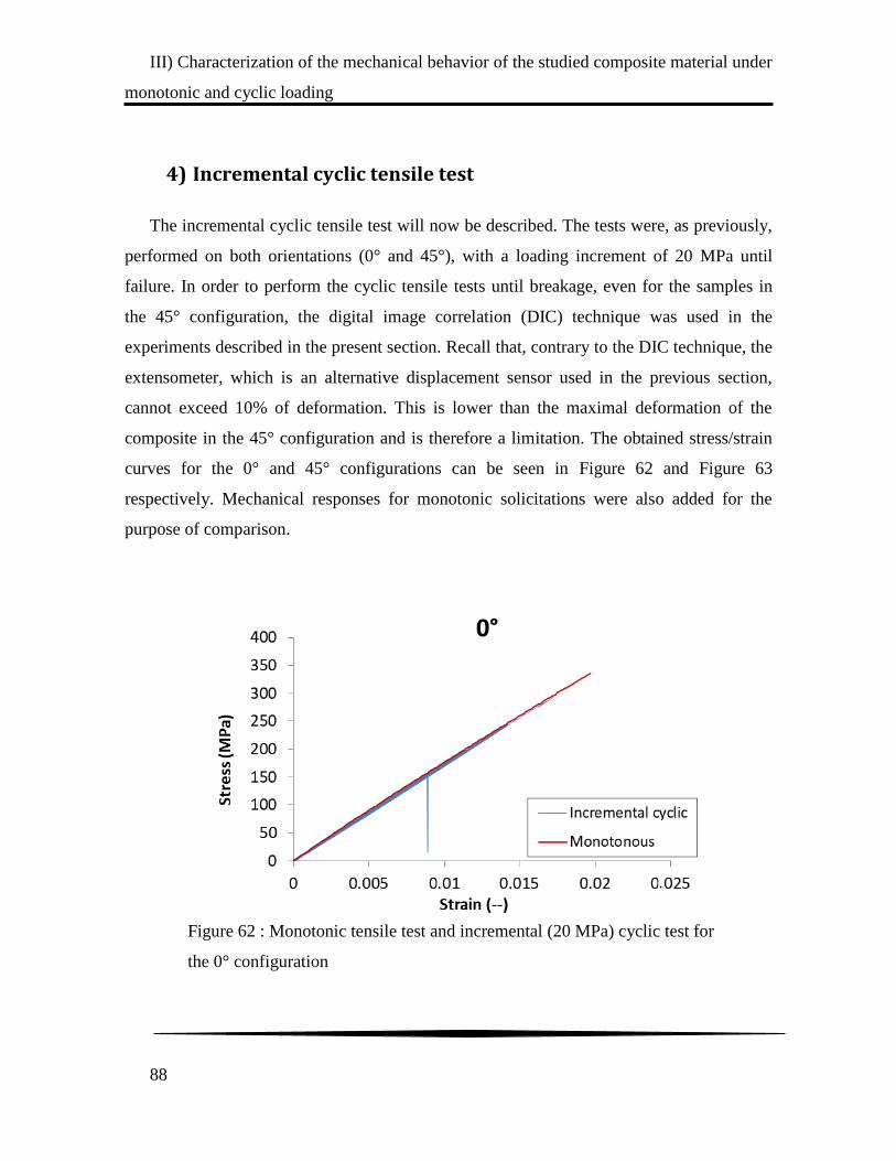
III) Characterization of the mechanical behavior of the studied composite material under
monotonic and cyclic loading
88
4) Incremental cyclic tensile test
The incremental cyclic tensile test will now be described. The tests were, as previously,
performed on both orientations (0° and 45°), with a loading increment of 20 MPa until
failure. In order to perform the cyclic tensile tests until breakage, even for the samples in
the 45° configuration, the digital image correlation (DIC) technique was used in the
experiments described in the present section. Recall that, contrary to the DIC technique, the
extensometer, which is an alternative displacement sensor used in the previous section,
cannot exceed 10% of deformation. This is lower than the maximal deformation of the
composite in the 45° configuration and is therefore a limitation. The obtained stress/strain
curves for the 0° and 45° configurations can be seen in Figure 62 and Figure 63
respectively. Mechanical responses for monotonic solicitations were also added for the
purpose of comparison.
Figure 62 : Monotonic tensile test and incremental (20 MPa) cyclic test for
the 0° configuration
. . . . .
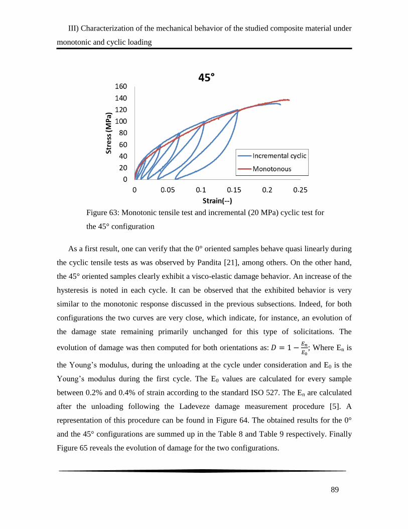
III) Characterization of the mechanical behavior of the studied composite material under
monotonic and cyclic loading
89
As a first result, one can verify that the 0° oriented samples behave quasi linearly during
the cyclic tensile tests as was observed by Pandita [21], among others. On the other hand,
the 45° oriented samples clearly exhibit a visco-elastic damage behavior. An increase of the
hysteresis is noted in each cycle. It can be observed that the exhibited behavior is very
similar to the monotonic response discussed in the previous subsections. Indeed, for both
configurations the two curves are very close, which indicate, for instance, an evolution of
the damage state remaining primarily unchanged for this type of solicitations. The
evolution of damage was then computed for both orientations as:
; Where En is
the Young‟s modulus, during the unloading at the cycle under consideration and E0 is the
Young‟s modulus during the first cycle. The E0 values are calculated for every sample
between 0.2% and 0.4% of strain according to the standard ISO 527. The En are calculated
after the unloading following the Ladeveze damage measurement procedure [5]. A
representation of this procedure can be found in Figure 64. The obtained results for the 0°
and the 45° configurations are summed up in the Table 8 and Table 9 respectively. Finally
Figure 65 reveals the evolution of damage for the two configurations.
Figure 63: Monotonic tensile test and incremental (20 MPa) cyclic test for
the 45° configuration
. . . . .

III) Characterization of the mechanical behavior of the studied composite material under
monotonic and cyclic loading
90
Maximal
stress (MPa) 0 40 60 80 100 120
Modulus
(GPa) 3.2 2.84 2.36 2.08 1.6 1.50
Damage (-) 0 0.11 0.26 0.35 0.5 0.53
En
E0
. .
Figure 64 : Measurement of the E0 and En moduli on a loading unloading curve
Table 8 : Elastic modulus and associated damage for each cycle for the
sample oriented at 45° from fiber‟s axis

III) Characterization of the mechanical behavior of the studied composite material under
monotonic and cyclic loading
91
Maximal
stress (MPa) 0 40 60 80 100 120 140 160 180 200 220 240 260 280
Modulus
(GPa) 20.98 20.39 20.26 20.20 20.00 19.80 19.64 19.47 19.42 19.29 19.17 19.18 19.19 19.13
Damage (-) 0 0.028 0.034 0.037 0.046 0.056 0.064 0.071 0.074 0.080 0.086 0.085 0.087 0.088
The cyclic tensile behavior of the studied PA66/6 reinforced with woven glass fibers is
anisotropic. For the samples in the 45° configuration, damage almost reaches a value of
0.53 close to the final failure. However, for the 0° case, it only goes up to 0.1 when close to
the final failure.
Figure 65 : Evolution of damage function of the maximal stress of the cycle for
a 0° (Left) and 45° (Right) oriented sample
Table 9 : Elastic modulus and associated damage for each cycle for samples oriented at along the
fiber‟s axis
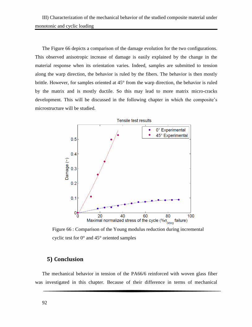
III) Characterization of the mechanical behavior of the studied composite material under
monotonic and cyclic loading
92
The Figure 66 depicts a comparison of the damage evolution for the two configurations.
This observed anisotropic increase of damage is easily explained by the change in the
material response when its orientation varies. Indeed, samples are submitted to tension
along the warp direction, the behavior is ruled by the fibers. The behavior is then mostly
brittle. However, for samples oriented at 45° from the warp direction, the behavior is ruled
by the matrix and is mostly ductile. So this may lead to more matrix micro-cracks
development. This will be discussed in the following chapter in which the composite‟s
microstructure will be studied.
5) Conclusion
The mechanical behavior in tension of the PA66/6 reinforced with woven glass fiber
was investigated in this chapter. Because of their difference in terms of mechanical
Figure 66 : Comparison of the Young modulus reduction during incremental
cyclic test for 0° and 45° oriented samples

III) Characterization of the mechanical behavior of the studied composite material under
monotonic and cyclic loading
93
response two configurations were studied. The first one with the warp yarns oriented along
the loading direction and the second with those yarns oriented at 45° from the loading
direction. The behavior in the first configuration is more linear and brittle whereas it
appears more nonlinear and ductile for the 45° configurations. Digital Image Correlation
(DIC) results indicate, for the latter, the presence of shear strain in the woven fabric during
the loading, as well as fiber re-orientation along the direction of the loading. For the 0°
configurations the strain field evolution is mostly governed by elongation along the loading
direction (Eyy). The damage growth was then estimated by elastic modulus reduction
during incremental tensile tests. The results indicate a higher increase of damage for the 45°
configurations. Clearly, different samples need investigation at a microscale in order to
identify the related damage mechanisms for each considered samples configurations.

III) Characterization of the mechanical behavior of the studied composite material under
monotonic and cyclic loading
94
IV) Damage mechanisms investigation: quantitative and qualitative analysis
95
IV) Damage mechanisms investigation: quantitative and
qualitative analysis
Contents
1) Optical microscopy analysis of undamaged composite............... 97
2) Damage initiation ............................................................................ 99
3) Fractography analysis .................................................................. 102
4) X-ray tomography analysis .......................................................... 104
a) 0° oriented - Undamaged sample ................................................................. 108
b) 0° oriented - Damaged sample ..................................................................... 111
c) 45° oriented – Damaged sample ................................................................... 113
d) Void volume fraction evolution .................................................................... 116
5) Conclusion ..................................................................................... 117
In the previous chapter, the polyamide 66/6 reinforced by woven glass fibers was
investigated at the macroscale; its microstructure is now studied in this chapter. Optical
microscopy, Scanning Electron Microscopy (SEM) and X-ray tomography, are used to
analyze the composite material at the microscale. An optical microscope is first used to
roughly analyze the microstructure of the undamaged composite samples oriented at 0°
(warp) and 45° from the warp direction. The presence of initial damage is also investigated.
The initiation of damage is then identified with SEM in-situ tensile tests in the 0°
configurations exclusively. The different rupture patterns that may appear on the two
considered orientations after the failure of the composite are then observed with a SEM.
The last and main subsection of this chapter is dedicated to X-ray tomography analysis.
Undamaged samples are first investigated for the purpose of a reference state, and then

IV) Damage mechanisms investigation: quantitative and qualitative analysis
96
composite samples, preliminary loaded in tension at stepwise increasing loading values are
analyzed. This allows us to identify the different damage mechanisms and their associated
scales. A measurement of the evolution of the void volume fraction is also performed by
using a grey level threshold. Both along axis (0°) and off axis (45°) oriented composites
specimens are tested as in the previous chapter.
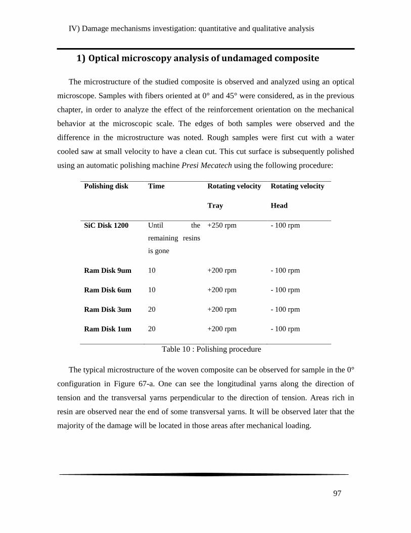
IV) Damage mechanisms investigation: quantitative and qualitative analysis
97
1) Optical microscopy analysis of undamaged composite
The microstructure of the studied composite is observed and analyzed using an optical
microscope. Samples with fibers oriented at 0° and 45° were considered, as in the previous
chapter, in order to analyze the effect of the reinforcement orientation on the mechanical
behavior at the microscopic scale. The edges of both samples were observed and the
difference in the microstructure was noted. Rough samples were first cut with a water
cooled saw at small velocity to have a clean cut. This cut surface is subsequently polished
using an automatic polishing machine Presi Mecatech using the following procedure:
Polishing disk Time Rotating velocity
Tray
Rotating velocity
Head
SiC Disk 1200 Until the
remaining resins
is gone
+250 rpm - 100 rpm
Ram Disk 9um 10 +200 rpm - 100 rpm
Ram Disk 6um 10 +200 rpm - 100 rpm
Ram Disk 3um 20 +200 rpm - 100 rpm
Ram Disk 1um 20 +200 rpm - 100 rpm
Table 10 : Polishing procedure
The typical microstructure of the woven composite can be observed for sample in the 0°
configuration in Figure 67-a. One can see the longitudinal yarns along the direction of
tension and the transversal yarns perpendicular to the direction of tension. Areas rich in
resin are observed near the end of some transversal yarns. It will be observed later that the
majority of the damage will be located in those areas after mechanical loading.
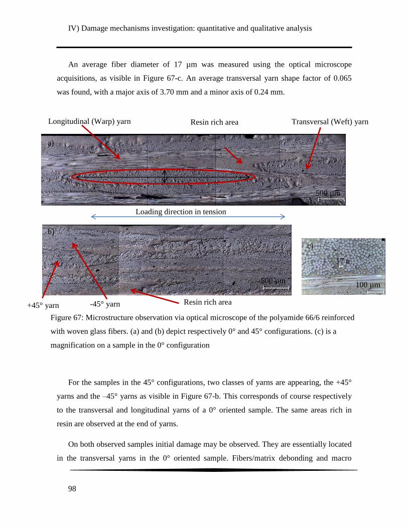
IV) Damage mechanisms investigation: quantitative and qualitative analysis
98
An average fiber diameter of 17 µm was measured using the optical microscope
acquisitions, as visible in Figure 67-c. An average transversal yarn shape factor of 0.065
was found, with a major axis of 3.70 mm and a minor axis of 0.24 mm.
For the samples in the 45° configurations, two classes of yarns are appearing, the +45°
yarns and the –45° yarns as visible in Figure 67-b. This corresponds of course respectively
to the transversal and longitudinal yarns of a 0° oriented sample. The same areas rich in
resin are observed at the end of yarns.
On both observed samples initial damage may be observed. They are essentially located
in the transversal yarns in the 0° oriented sample. Fibers/matrix debonding and macro
Figure 67: Microstructure observation via optical microscope of the polyamide 66/6 reinforced
with woven glass fibers. (a) and (b) depict respectively 0° and 45° configurations. (c) is a
magnification on a sample in the 0° configuration
Loading direction in tension
Loading direction in tension
+45° yarn -45° yarn
500 µm
Resin rich area
100 µm
17 u
500 µm
Longitudinal (Warp) yarn
Transversal (Weft) yarn
Resin rich area
b)
a)
c)

IV) Damage mechanisms investigation: quantitative and qualitative analysis
99
porosities are the most apparent defects (Figure 68-b and c). Some cracks are also noticed
but are very rare in the initial state (Figure 68-a). Some initial defects can be observed in
the longitudinal yarns but they may be difficult to quantify because of fibers removal
during the samples polishing. Indeed, because of their low diameter, the longitudinal fibers
can be easily damaged and even debonded from the matrix during this process. In the 45°
oriented sample, the initial damage is essentially located inside the yarns. The rich resin
area seems to remain undamaged.
More information on the initial amount of damage inside the composite is given in the
subsection dedicated to X-ray tomography.
2) Damage initiation
The damage initiation and the first appearing damage mechanisms is investigated in this
subsection. Scanning Electronic Microscopy (SEM) in-situ tensile tests along the fiber axis
were considered. The samples were first cut in 50 mm x 5 mm x 1.53 mm rectangular
shape. This geometry is adopted because of the tensile tests machine limitations. However,
because of the chosen sample‟s dimension, the mentioned results should be considered with
caution. Indeed, in order to have a homogenized stress concentration, the sample should
Figure 68 : a) Crack visible in transversal yarns, b) Micro porosities in the 45°
configurations c) Micro porosities in the 0° configurations.
All pictures were taken in the initial state prior to any mechanical loading
a)
a)
b)
b)
c)
c)

IV) Damage mechanisms investigation: quantitative and qualitative analysis
100
contain more than one RVE of the microstructure. The RVE adopted here is a square of 16
mm x 16 mm, but the tested sample is only 5mm width. The samples were then polished
using the procedure described in the previous subsection. A coating of gold/palladium is
then applied on the samples, in order to increase the imaging quality because of their
limited conductivity. Pictures are then taken for different loading values: 120 N, 240 N and
435 N. The microscopic observations are given in Figure 69. Some damage is visible in
Figure 69-a before the loading test and is caused mostly by the cutting process and
polishing. Knowledge of the reference state is therefore essential in order to avoid wrong
assumptions concerning the location and the stress level corresponding to damage
initiation. During this experiment, the first apparition of damage was noted starting between
66 N and 120 N, it consists mostly of fiber/matrix debonding in the transversal yarns
(Figure 70). The debonding in the samples becomes gradually more important and some
cracks begin to appear due to damage propagating along the debonding area (Figure 69-d)
between 120 N and 240 N. The loading test continues until 435 N with the accumulation of
debonding and cracks in transversal yarns. Nevertheless, the process cannot continue
further an applied load beyond 435 N because of breakage of the sample inside the jaws.
Because the other appearing damage mechanisms can be more easily observed than
fiber/matrix deboning when using X-ray tomography the rest of the damage mechanisms
characterization will be performed with this X-ray technique. Though, an observation,
using SEM, of fracture surfaces is still proposed in the following subsection.

IV) Damage mechanisms investigation: quantitative and qualitative analysis
101
Figure 70 : Fiber/matrix deboning obtained with SEM
c) 120N: 15.7MPa
d) 240N: 31.4MPa e) Final step (435N: 56.8MPa)
a) 0N
Figure 69 : Transversal yarns during SEM in-situ tensile test for different
applied force
b) 66N: 8.2MPa

IV) Damage mechanisms investigation: quantitative and qualitative analysis
102
3) Fractography analysis
In order to identify the different rupture mechanisms, it has been decided to use
fractography of the samples subjected to tensile test until breakage. Composites with fibers
at 0° and composites with fibers at 45° with respect to the direction of tension load are
examined. The technique can provide a first clear idea about the different mechanisms that
lead to failure.
- 0° orientation:
In Figure 71 are represented the different observed rupture mechanism for samples in
the 0° configuration. As main mechanisms, cracks in the matrix and also fiber/matrix
deboning can be seen in Figure 71-a and b. As observed in Figure 71-c, fiber breakage in
the transversal yarns can propagate all along the yarn and leads to a longitudinal
fiber/matrix deboning. The mechanism which causes the final failure of the composite is of
course longitudinal fibers breakage, visible in Figure 71-d. A pull-out phenomenon can be
observed right after the failure as well (Figure 71-f). This indicates a relatively weak
fiber/matrix interface.
- 45° orientation:
Fractography images of the samples in the 45° configurations can be found in Figure
72. As shown for the 0° configurations, matrix cracking is observed (Figure 72-b). Some
pseudo-delamination can also be noticed in Figure 72-d. The final failure of the composite
is again caused by fiber breakage Figure 72-a. Fiber pull-out was observed, in Figure 72-c,
to a higher extent than in the 0° configuration. This observation can be explained by the
plasticization in the matrix induced by fibers reorientations that could weaken the
fibers/matrix interface.
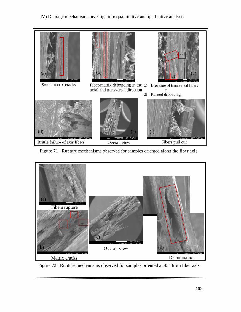
IV) Damage mechanisms investigation: quantitative and qualitative analysis
103
Overall view
Fiber/matrix debonding in the
axial and transversal direction
Some matrix cracks 1) Breakage of transversal fibers
+
2) Related debonding
1)
2)
Brittle failure of axis fibers Fibers pull out
Figure 71 : Rupture mechanisms observed for samples oriented along the fiber axis
(a) (b) (c)
(d) (e) (f)
Delamination
Fibers rupture
Matrix cracks
Figure 72 : Rupture mechanisms observed for samples oriented at 45° from fiber axis
Overall view (d) (b)
(c)
(a)

IV) Damage mechanisms investigation: quantitative and qualitative analysis
104
With these observations, a number of failure mechanisms can be identified on the two
studied orientations. Nevertheless, it is of interest to know the order of appearance of the
different mechanisms when a sample is submitted to tension. A more accurate estimation of
the typical extent and importance of the observed mechanisms are also necessary for what
follows in this thesis. In addition, in order to characterize the sensitivity of a Non
Destructive Evaluation method, one of the first tests is to verify the size of the smallest
detectable defects, which corresponds to the resolution of the detection technique. X-ray
tomography observation will be presented in the next subsection to answer those specific
questions.
4) X-ray tomography analysis
An X-ray tomography (EasyTom (Nano) from RX solutions) was used to perform a 3D
non-destructive analysis. A representation of the basic principle of micro-tomography is
shown in Figure 73. X-rays are beamed through the tested sample for different angular
positions with respect to a flat panel detector. Images are recorded as a grey level map
which is a function of the absorption of X-rays by the material. The X-Act software is then
used to make a 3D reconstruction of the tested sample. Then, various image processing
filters are applied, using the Avizo software, on the reconstruction to get rid of noise in the
images. First, a median filter is used on the raw images to reduce the major contribution of
noise. A despeckle filter is finally applied on the filter images to remove most of the
remaining interference noise. The contribution of the two filters can be seen in Figure 74.
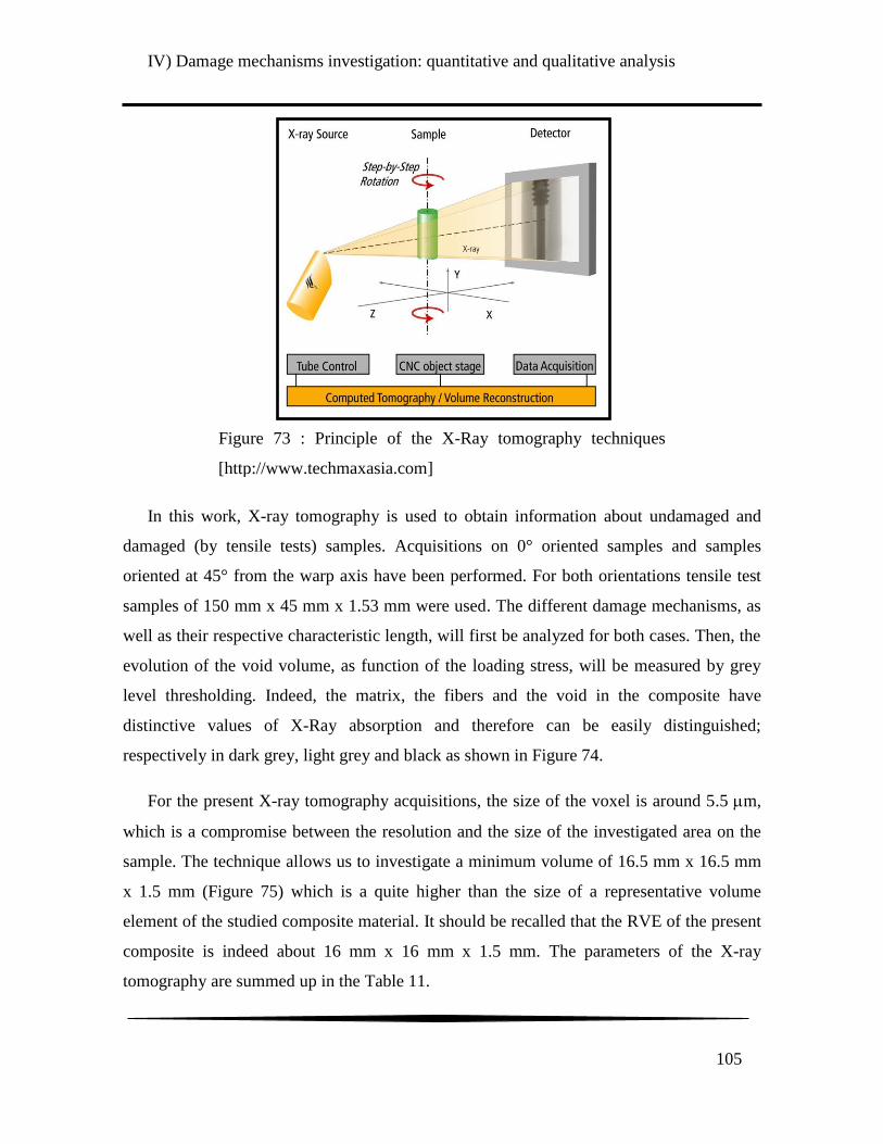
IV) Damage mechanisms investigation: quantitative and qualitative analysis
105
In this work, X-ray tomography is used to obtain information about undamaged and
damaged (by tensile tests) samples. Acquisitions on 0° oriented samples and samples
oriented at 45° from the warp axis have been performed. For both orientations tensile test
samples of 150 mm x 45 mm x 1.53 mm were used. The different damage mechanisms, as
well as their respective characteristic length, will first be analyzed for both cases. Then, the
evolution of the void volume, as function of the loading stress, will be measured by grey
level thresholding. Indeed, the matrix, the fibers and the void in the composite have
distinctive values of X-Ray absorption and therefore can be easily distinguished;
respectively in dark grey, light grey and black as shown in Figure 74.
For the present X-ray tomography acquisitions, the size of the voxel is around 5.5 m,
which is a compromise between the resolution and the size of the investigated area on the
sample. The technique allows us to investigate a minimum volume of 16.5 mm x 16.5 mm
x 1.5 mm (Figure 75) which is a quite higher than the size of a representative volume
element of the studied composite material. It should be recalled that the RVE of the present
composite is indeed about 16 mm x 16 mm x 1.5 mm. The parameters of the X-ray
tomography are summed up in the Table 11.
Figure 73 : Principle of the X-Ray tomography techniques
[http://www.techmaxasia.com]
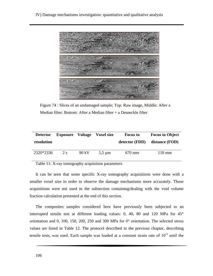
IV) Damage mechanisms investigation: quantitative and qualitative analysis
106
Detector
resolution
Exposure Voltage Voxel size Focus to
detector (FDD)
Focus to Object
distance (FOD)
2320*2336 2 s 90 kV 5,5 µm 670 mm 110 mm
Table 11: X-ray tomography acquisition parameters
It can be seen that some specific X-ray tomography acquisitions were done with a
smaller voxel size in order to observe the damage mechanisms more accurately. Those
acquisitions were not used in the subsection containing/dealing with the void volume
fraction calculation presented at the end of this section.
The composites samples considered here have previously been subjected to an
interrupted tensile test at different loading values: 0, 40, 80 and 120 MPa for 45°
orientation and 0, 100, 150, 200, 250 and 300 MPa for 0° orientation. The selected stress
values are listed in Table 12. The protocol described in the previous chapter, describing
tensile tests, was used. Each sample was loaded at a constant strain rate of 10-3
until the
Figure 74 : Slices of an undamaged sample; Top: Raw image, Middle: After a
Median filter, Bottom: After a Median filter + a Despeckle filter

IV) Damage mechanisms investigation: quantitative and qualitative analysis
107
defined tensile loading value was reached. They were then unloaded at the same constant
strain rate. The chosen loading values are indicated on stress/strain curves previously
obtained with tensile test until failure, with red circles in Figure 76.
1 (Warp)
2 (Weft) 3
16.5 mm
16.5 mm
Observed
area
45 mm
150 m
m
Figure 75 : Schematic representation of the observed area on a polyamide
6,6 /Woven glass fiber samples and the associated 3D reconstruction
3D reconstruction of an
undamaged sample oriented
Figure 76 : Typical stress/strain curve of the PA66/6 reinforced with woven glass fiber
in the 0° and 45° configurations. The red circles show schematicaly the strain and stress
levels where the different tensile tests (performed on several specimens) have been
interrupted as summarized in Table 12. Ultrasonic measurements and X-ray tomography
investigations are then performed on those specimens
0
50
100
150
200
250
300
350
400
0 0.1 0.2 0.3
Stre
ss (
MP
a)
Strain
0°
45°
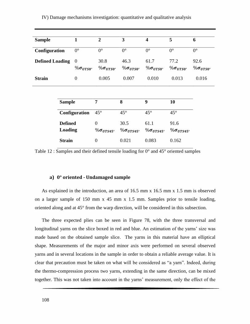
IV) Damage mechanisms investigation: quantitative and qualitative analysis
108
Sample 1 2 3 4 5 6
Configuration 0° 0° 0° 0° 0° 0°
Defined Loading 0
°
30.8
°
46.3
°
61.7
°
77.2
°
92.6
°
Strain 0 0.005 0.007 0.010 0.013 0.016
Sample 7 8 9 10
Configuration 45° 45° 45° 45°
Defined
Loading
0
°
30.5
°
61.1
°
91.6
°
Strain 0 0.021 0.083 0.162
Table 12 : Samples and their defined tensile loading for 0° and 45° oriented samples
a) 0° oriented - Undamaged sample
As explained in the introduction, an area of 16.5 mm x 16.5 mm x 1.5 mm is observed
on a larger sample of 150 mm x 45 mm x 1.5 mm. Samples prior to tensile loading,
oriented along and at 45° from the warp direction, will be considered in this subsection.
The three expected plies can be seen in Figure 78, with the three transversal and
longitudinal yarns on the slice boxed in red and blue. An estimation of the yarns‟ size was
made based on the obtained sample slice. The yarns in this material have an elliptical
shape. Measurements of the major and minor axis were performed on several observed
yarns and in several locations in the sample in order to obtain a reliable average value. It is
clear that precaution must be taken on what will be considered as “a yarn”. Indeed, during
the thermo-compression process two yarns, extending in the same direction, can be mixed
together. This was not taken into account in the yarns‟ measurement, only the effect of the

IV) Damage mechanisms investigation: quantitative and qualitative analysis
109
thermo-compression on a sole yarn was considered. Since a 3D representation of the
sample is obtained, one can easily follow the propagation of a yarn in the whole
reconstructed volume to be sure that only one yarn was measured. All of this can be seen in
Figure 77.
As a result, it appears that the average yarns are ellipses with a minor axis of 0.22 mm
and a major axis of 3.6 mm in the weft direction; their minor axis is 0.24 mm and their
major axis 3.6 mm in the warp direction. The values are close to those measured on the
image obtained with optical microscopy. They will be used in the following chapter to
Figure 78 : Slices of the undamaged sample oriented along the fiber axis in
different directions before 3D reconstruction
Figure 77 : Transversal (Weft) yarns measurement on a slice of an undamaged sample
obtained via X-Ray tomography
Several yarns mixed together

IV) Damage mechanisms investigation: quantitative and qualitative analysis
110
determine the stiffness matrix of the
composite material using a periodic
homogenization theory.
As mentioned in the introduction,
information about the different material
present in the tested sample can be
extracted from the X-ray tomography
acquisitions. Indeed, because of the
significantly different X-ray absorption
properties of the different constituents of
the composite material, estimation of the
volume fraction can be performed by grey level thresholding.
First, two constituents, i.e. the fiber and the matrix, are considered for the grey level
thresholding. The following first estimation of the volume fraction of each material was
obtained. Let‟s recall that a value of 43% of fiber faction volume was indicated in the data
sheet of the composite handed by DuPont, as mentioned in the part II. The measured value
of fiber volume fraction is very close to the given value (Table 13).
Matrix volume fraction Fiber volume fraction
57.4 % 42.6 %
Then, the void is considered as a third constituents and a second grey level thresholding
is applied on the undamaged sample. Results are summarized in Table 14. Indeed, as it can
be seen in Figure 78, Figure 77 and Figure 79 initial porosities are present in the sample
before mechanical solicitation. The porosities appear mostly in the weft yarns near the
Table 13 : Volume fraction of the matrix and fiber on the
undamaged sample the 0° configuration
Figure 79 : Three dimensional reconstruction
of undamaged samples, in the 0° and 45°
configuration, with initial porosity (Yellow)
0°
45°

IV) Damage mechanisms investigation: quantitative and qualitative analysis
111
yarns‟ extremity or close to areas where yarns are mixed together during the thermo-
compression process.
The fiber volume fraction remains close to the 43% given by DuPont. The measured
volume fraction of void is around 0.6% before any mechanical solicitations. Note that in
their data sheet, considering the PA 66/6 reinforced with woven glass fibers, DuPont
specified that the volume fraction of void is lower than 2%. This is verified on the
undamaged samples that have been tested.
Void volume fraction Matrix volume fraction Fiber volume fraction
0.6 % 56.9 % 42.5 %
Table 14 : Volume fraction of the matrix, fiber and void on the undamaged samples in the
0° configuration
b) 0° oriented - Damaged sample
Most of the analysis is done on a sample loaded in tension at 300 MPa along the fiber.
A triple constituent grey level thresholding is performed as above. A clear increase of the
void area is shown in Figure 80 along the transversal direction (direction of the weft yarn).
All the damage mechanisms that were observed are visible in Figure 81. An increase of the
number of cracks can be seen on the observed sample compared to the non-loaded
composite sample. The main damage mechanisms detected are cracks at the end of yarns,
but transversal cracks can also be seen. Some longitudinal cracks appeared as well, but only
in the samples loaded at 300 MPa (Figure 81-a). Those are cracks that start from a
transversal yarn end and propagate along the nearest longitudinal yarn. This is often called
pseudo-delamination in the literature. Nevertheless, it should be expected that some cracks
close when the tension on the sample is released. Hence, the number of effective cracks can
actually be higher in reality.
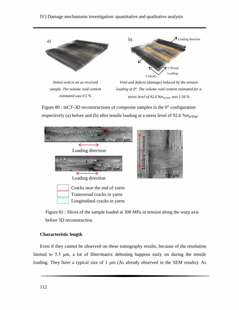
IV) Damage mechanisms investigation: quantitative and qualitative analysis
112
Characteristic length
Even if they cannot be observed on these tomography results, because of the resolution
limited to 5.5 μm, a lot of fiber/matrix deboning happens early on during the tensile
loading. They have a typical size of 1 μm (As already observed in the SEM results). As
Figure 80 : mCT-3D reconstructions of composite samples in the 0° configuration
respectively (a) before and (b) after tensile loading at a stress level of 92.6 %σUTS °
Void and defects (damage) induced by the tension
loading at 0°. The volume void content estimated for a
stress level of 92.6 %𝜎𝑈𝑇𝑆0° was 1.56 %
Initial void in an as received
sample. The volume void content
estimated was 0.5 %
a) b)
1 (Warp)
Loading
direction 2 (Weft)
Loading direction
Figure 81 : Slices of the sample loaded at 300 MPa in tension along the warp axis
before 3D reconstruction
Loading direction
290 μm
Loading direction
280 μm
220 μm
Load
ing d
irec
tion
Cracks near the end of yarns
Transversal cracks in yarns
Longitudinal cracks in yarns
a)
b)
c)
IV) Damage mechanisms investigation: quantitative and qualitative analysis
113
previously stated the most important damage mechanisms for a woven composite loaded in
tension along the axis of the fiber are transversal cracks in the matrix. They have a typical
size of 10 μm. The cracks appear as a result of multiple fiber/matrix deboning, locally, in a
yarn. They can either grow along the transversal yarns and get stopped by the longitudinal
one or propagate along the longitudinal yarn if enough energy is . They can grow all along
the transversal yarns, where they are then temporally stopped by the longitudinal yarns.
Two damage mechanisms can appear at this stage: pseudo-delamination and fiber breakage.
The latter, which is causing the ultimate failure of the composites, has a typical extent of 17
μm (which is the size of the fibers). The pseudo-delamination is a bifurcation of the
transversal cracks in the longitudinal direction. The crack then follows the longitudinal
yarns. This mechanism has a typical size of 50 µm.
c) 45° oriented – Damaged sample
For the samples oriented at 45° from the fiber axis many other damage mechanisms can
be seen in comparison with the previous samples configuration. Indeed, cracks near the end
of yarns as well as cracks inside yarns were noticed, just as in the case of samples oriented
along the fibers‟ axis (Figure 82-a and b). However, in addition, fibers breakage (Figure 82-
c) and local fiber micro buckling (Figure 82-d) were noticed. These two mechanisms
appeared with an onset of 80 MPa loading of the sample, which is significantly early
compared with the final stage of sample failure.
The fiber micro buckling is caused by the reorientation of fibers during the loading test.
Indeed, as the load increases the angle between the fibers tend to decrease. Then, when the
tension is interrupted, the fibers must return to their original place, which is impossible
because of the section reduction caused by the Poisson effect. The effect of fiber
reorientation during off-axis loading has also been observed by Vieille and al. [19], among
others. The mentioned damage mechanisms can be observed in Figure 82. Pseudo-
delamination, visible in Figure 83, may also appear locally beyond a stress level of 100
MPa for a loading at 45° from the warp direction. Note that pseudo delamination appears
inside a yarns and that delamination appears between two woven fabrics. Finally, it is worth
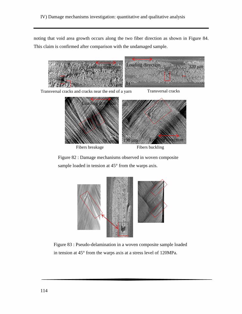
IV) Damage mechanisms investigation: quantitative and qualitative analysis
114
noting that void area growth occurs along the two fiber direction as shown in Figure 84.
This claim is confirmed after comparison with the undamaged sample.
Figure 83 : Pseudo-delamination in a woven composite sample loaded
in tension at 45° from the warps axis at a stress level of 120MPa.
Transversal cracks
Loading direction 320 μm
Transversal cracks and cracks near the end of a yarn
Loading direction
255 μm
Fibers breakage
Loading direction
70 μm Loading direction 190 μm
Fibers buckling
Figure 82 : Damage mechanisms observed in woven composite
sample loaded in tension at 45° from the warps axis.
a) b)
d)
c)

IV) Damage mechanisms investigation: quantitative and qualitative analysis
115
Characteristic length
As for the samples oriented along the fiber axis, the fiber/matrix deboning, transversal
cracks and cracks near the yarns‟ end have a characteristic length of respectively 1 μm, 20
μm and 50 μm. The fiber breakages have a characteristic length of 17 μm. The pseudo-
delamination and fibers micro buckling both have a characteristic length of 200 μm which
is the largest of the damage mechanisms observed in this woven composite material. The
important size of the micro-buckling is explained by the fact that the buckling of numerous
fibers is induced which causes local micro-cracks around the fibers. As will be seen in
what‟s next, the last two mechanisms are the only ones visible by C-scan imaging. A
summary of all the discussed damage mechanisms, for both 0° and 45° configuration, is
presented in Figure 85.
Voids and defects (damage) induced by the tension
loading at 45°. The volume void content estimated
for a stress level of 91.6 % 0° was 5.51 %
Initial void in an as received
sample. The initial volume void
content estimated was 0.6 %
Figure 84 : mCT-3D reconstructions of composite samples in the 45°
configuration respectively (a) before and (b) after tensil loading at a stress
level of 91.6 %σUTS °.
a)
a)
b)
b) 1 (Warp)
1 (Warp)
2 (Weft)
2 (Weft)
Loading direction
Loading direction
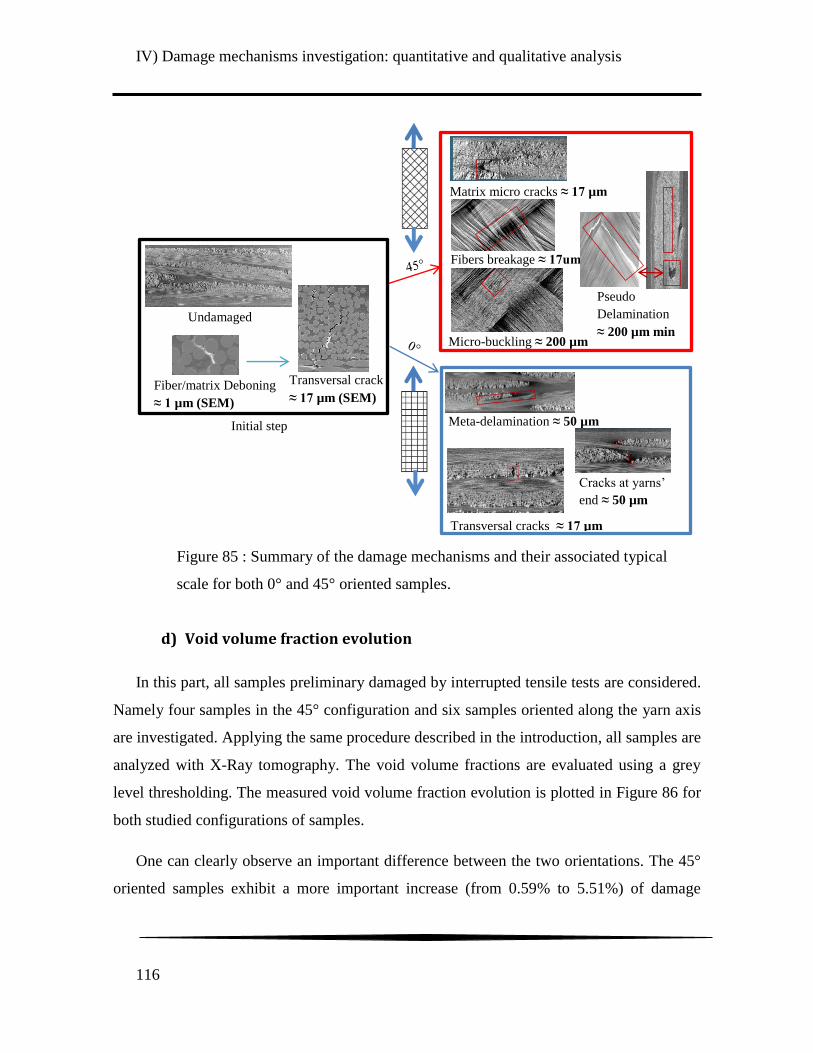
IV) Damage mechanisms investigation: quantitative and qualitative analysis
116
d) Void volume fraction evolution
In this part, all samples preliminary damaged by interrupted tensile tests are considered.
Namely four samples in the 45° configuration and six samples oriented along the yarn axis
are investigated. Applying the same procedure described in the introduction, all samples are
analyzed with X-Ray tomography. The void volume fractions are evaluated using a grey
level thresholding. The measured void volume fraction evolution is plotted in Figure 86 for
both studied configurations of samples.
One can clearly observe an important difference between the two orientations. The 45°
oriented samples exhibit a more important increase (from 0.59% to 5.51%) of damage
Fibers breakage ≈ 17um
Micro-buckling ≈ 200 µm
Matrix micro cracks ≈ 17 µm
Pseudo
Delamination
≈ 200 µm min
Meta-delamination ≈ 50 µm
Transversal crack
≈ 17 µm (SEM) Fiber/matrix Deboning
≈ 1 µm (SEM)
Initial step
Undamaged
Cracks at yarns‟
end ≈ 50 µm
Transversal cracks ≈ 17 µm
Figure 85 : Summary of the damage mechanisms and their associated typical
scale for both 0° and 45° oriented samples.
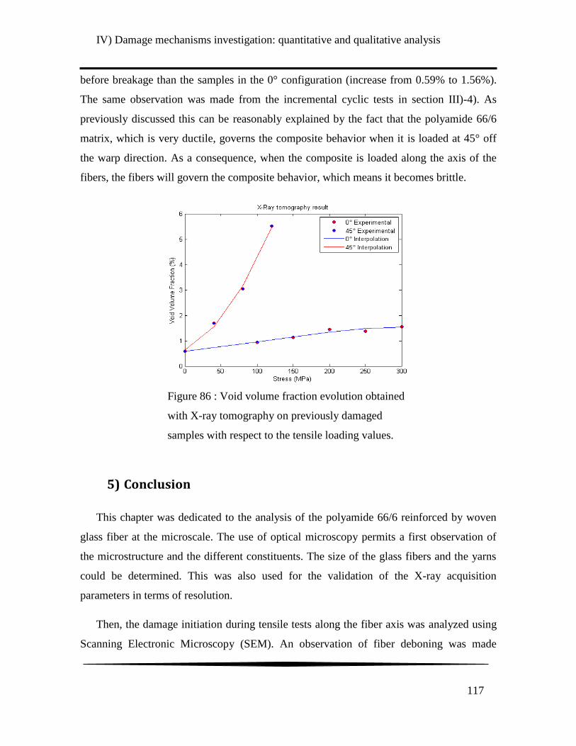
IV) Damage mechanisms investigation: quantitative and qualitative analysis
117
before breakage than the samples in the 0° configuration (increase from 0.59% to 1.56%).
The same observation was made from the incremental cyclic tests in section III)-4). As
previously discussed this can be reasonably explained by the fact that the polyamide 66/6
matrix, which is very ductile, governs the composite behavior when it is loaded at 45° off
the warp direction. As a consequence, when the composite is loaded along the axis of the
fibers, the fibers will govern the composite behavior, which means it becomes brittle.
5) Conclusion
This chapter was dedicated to the analysis of the polyamide 66/6 reinforced by woven
glass fiber at the microscale. The use of optical microscopy permits a first observation of
the microstructure and the different constituents. The size of the glass fibers and the yarns
could be determined. This was also used for the validation of the X-ray acquisition
parameters in terms of resolution.
Then, the damage initiation during tensile tests along the fiber axis was analyzed using
Scanning Electronic Microscopy (SEM). An observation of fiber deboning was made
Figure 86 : Void volume fraction evolution obtained
with X-ray tomography on previously damaged
samples with respect to the tensile loading values.
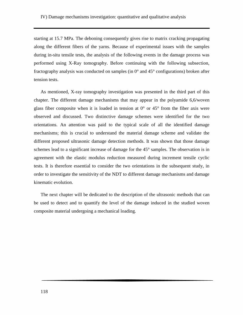
IV) Damage mechanisms investigation: quantitative and qualitative analysis
118
starting at 15.7 MPa. The deboning consequently gives rise to matrix cracking propagating
along the different fibers of the yarns. Because of experimental issues with the samples
during in-situ tensile tests, the analysis of the following events in the damage process was
performed using X-Ray tomography. Before continuing with the following subsection,
fractography analysis was conducted on samples (in 0° and 45° configurations) broken after
tension tests.
As mentioned, X-ray tomography investigation was presented in the third part of this
chapter. The different damage mechanisms that may appear in the polyamide 6,6/woven
glass fiber composite when it is loaded in tension at 0° or 45° from the fiber axis were
observed and discussed. Two distinctive damage schemes were identified for the two
orientations. An attention was paid to the typical scale of all the identified damage
mechanisms; this is crucial to understand the material damage scheme and validate the
different proposed ultrasonic damage detection methods. It was shown that those damage
schemes lead to a significant increase of damage for the 45° samples. The observation is in
agreement with the elastic modulus reduction measured during increment tensile cyclic
tests. It is therefore essential to consider the two orientations in the subsequent study, in
order to investigate the sensitivity of the NDT to different damage mechanisms and damage
kinematic evolution.
The next chapter will be dedicated to the description of the ultrasonic methods that can
be used to detect and to quantify the level of the damage induced in the studied woven
composite material undergoing a mechanical loading.
V) Non Destructive Evaluation (NDE) methods based on ultrasound
119
V) Non Destructive Evaluation (NDE) methods based on
ultrasound
Contents
1) Review of ultrasonic method of Non Destructive Evaluation
(NDE) of damage ....................................................................................... 122
a) Ultrasonic imaging techniques: transmission and reflection ........................ 122
b) Multi angle ultrasonic investigation of material ........................................... 125
Phase velocities measurement toward stiffness tensor calculation ................... 125
Polar scan method ............................................................................................. 135
c) Guided waves based testing methods ........................................................... 139
d) Nonlinear acoustic method ........................................................................... 146
Nonlinear Resonant Ultrasound Spectroscopy (NRUS) ................................... 148
Nonlinear Wave Modulation Spectroscopy (NWMS) ...................................... 150
Nonlinear Reverberation Spectroscopy (NRS) ................................................. 153
e) Coda waves in Non-Destructive Testing ...................................................... 154
f) Synthesis of the Non Destructive Evaluation method review ...................... 159
2) Ultrasonic C-scan in transmission .............................................. 160
3) Stiffness tensor components determination ............................... 161
a) Description of the experimental procedure and first analysis ...................... 162
Preliminary remarks and first results on undamaged samples .......................... 162
Experimental procedure for the plane 1-3 and 2-3 ........................................... 164
Experimental procedure for the plane 1-2 ........................................................ 166
Preliminary analysis on undamaged samples ................................................... 167

V) Non Destructive Evaluation (NDE) methods based on ultrasound
120
Investigation of the optimization algorithm robustness to input parameters .... 173
b) Experimental results: 0° configuration after tensile test ............................... 180
c) Experimental results: 45° configuration after tensile test ............................. 184
d) Proposed damage indicators ......................................................................... 190
4) Guided Lamb waves ..................................................................... 195
a) Preliminary investigation on an aluminum plate .......................................... 196
b) Investigations of the woven glass fiber reinforced polyamide 66/6 samples
damaged by tension ..................................................................................................... 199
Analysis of dispersion curves/Lamb waves modes .......................................... 200
Analysis of signals measured on top/bottom surface of the specimen ............. 206
Investigation of damaged samples .................................................................... 209
Investigation of proposed damage indicators ................................................... 211
5) Conclusion ..................................................................................... 215
The objective of this chapter is to present several Non Destructive Evaluation (NDE)
techniques based on ultrasonic wave propagation in solid media in order to compare their
respective advantages and limitations. The different considered NDE techniques are applied
to the polyamide 66/6 reinforced by woven glass fibers damaged samples presented on the
previous chapters. The X-ray tomography investigation, from chapter IV), is used as a
reference to validate the results from ultrasonic investigation.
In a first section, different ultrasonic NDE techniques are presented with an emphasis
on the techniques considered for this project. The majority of those techniques have
attracted notable interest by research teams in NDE. Their application on polymer based
composites reinforced with fibers is more specifically detailed. All the samples introduced
in chapter IV) were analyzed by ultrasonic C-scan, which is described in the second
V) Non Destructive Evaluation (NDE) methods based on ultrasound
121
section. In the third section, the stiffness components measurement by an ultrasonic
immersion method and the obtained results is detailed. The method was used on the
samples in the 0° and 45° configurations. The evolution, with damage, of the stiffness
components identified is then analyzed with regards of the loading level used to introduce
an increasing amount of damage. Two damage indicators, based on those results, are then
proposed and their relevance is discussed. In a forth section, guided waves were used to
evaluate damage. First, an investigation of the transmitted mode for different damage state
level is proposed. Then, the evolution of the transmitted signal energy is proposed as
another damage indicator. The sensitivity of the different indicators introduced in this
chapter is finally discussed.
It is worth mentioning that, in addition to the experimental results discussed in this
chapter, investigations on nonlinear acoustics techniques and coda wave interferometry are
proposed in the appendix of this manuscript.
V) Non Destructive Evaluation (NDE) methods based on ultrasound
122
1) Review of ultrasonic method of Non Destructive Evaluation
(NDE) of damage
Ultrasonic based NDE methods are frequently used to control damage because of
various advantages such as their simplicity of implementation and great flexibility. Indeed,
ultrasonics can, if needed, be used with only one transducer, e.g. when access to the two
sides of a structure is not possible. The method can be used manually in-situ on complex
structures with little equipment without reducing efficiency to a significant degree. So,
ultrasonic techniques are used either to control structural parts, right after manufacturing
and in service, or to validate an assembly [34], [35] for example. On the specific case of
composite material, ultrasonic is known to be very effective to detect the most critical
damage mechanism in composite material which is the delamination [36]–[38]. In addition,
the ultrasonic method can be implemented at a relatively low cost, because of their constant
evolution, and does not cause potential health problems like X-ray related techniques for
example. This explains why many methods, based on the propagation of ultrasonic waves
in material, were developed both in the academic field and in the industry. However, as it
was shown in the previous chapter, the damage that can be generated inside the structure
can be of very small scale. It may be difficult to detect it with classical industrial imaging
technique. Consequently, in this section a review of some ultrasonic methods, that are
currently investigated to evaluate damage on material, is proposed. Their application on
composite materials will be more specifically discussed.
a) Ultrasonic imaging techniques: transmission and reflection
This class is one of the oldest, and furthermore the most used, of the ultrasonic NDE
techniques in the industry. The principle is to scan the whole surface of the structure point
by point and to record the ultrasonic signals for each of those points. Information such as
the damping (attenuation in amplitude), the velocity, Time of Flight (ToF), etc is then
extracted from the acquired signals. The measure can be made on contact or in immersion
in water. Two main techniques can be distinguished: the Ultrasonic Pulse Velocity (UPV),
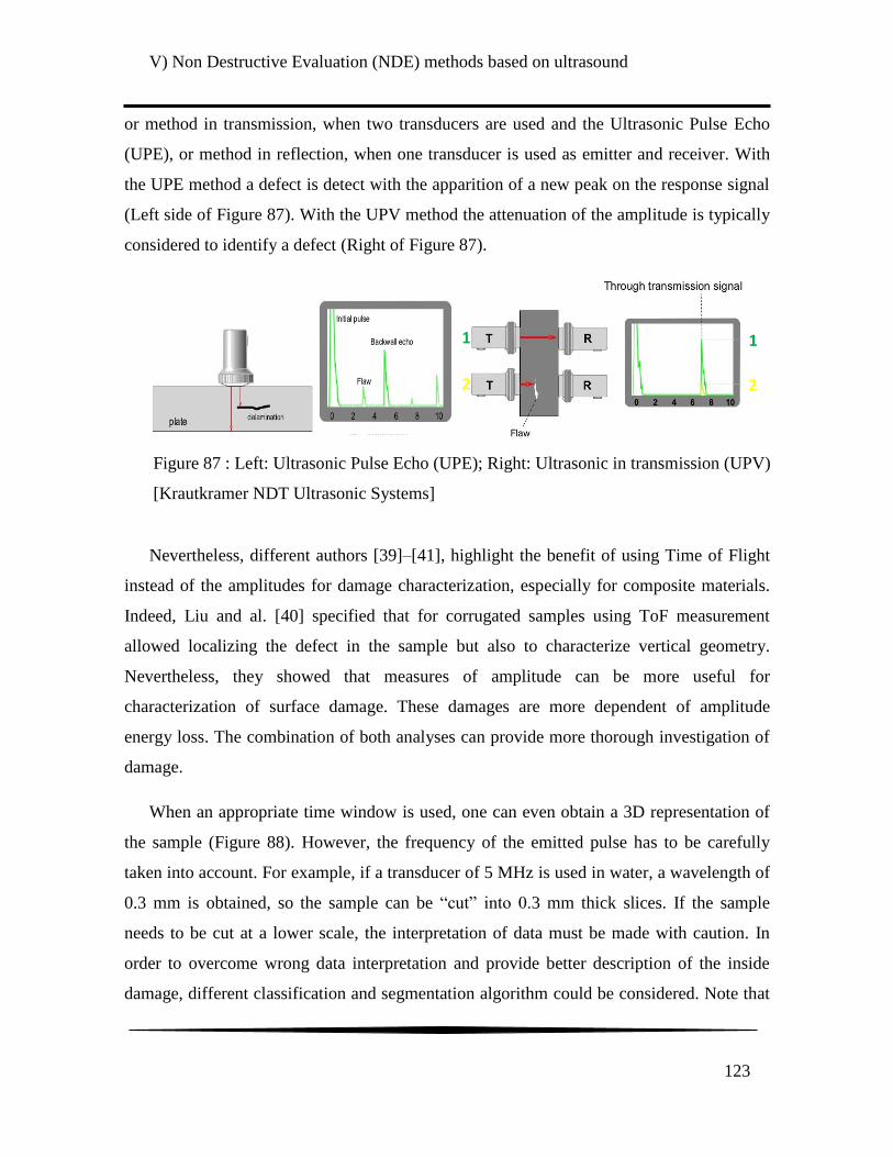
V) Non Destructive Evaluation (NDE) methods based on ultrasound
123
or method in transmission, when two transducers are used and the Ultrasonic Pulse Echo
(UPE), or method in reflection, when one transducer is used as emitter and receiver. With
the UPE method a defect is detect with the apparition of a new peak on the response signal
(Left side of Figure 87). With the UPV method the attenuation of the amplitude is typically
considered to identify a defect (Right of Figure 87).
Nevertheless, different authors [39]–[41], highlight the benefit of using Time of Flight
instead of the amplitudes for damage characterization, especially for composite materials.
Indeed, Liu and al. [40] specified that for corrugated samples using ToF measurement
allowed localizing the defect in the sample but also to characterize vertical geometry.
Nevertheless, they showed that measures of amplitude can be more useful for
characterization of surface damage. These damages are more dependent of amplitude
energy loss. The combination of both analyses can provide more thorough investigation of
damage.
When an appropriate time window is used, one can even obtain a 3D representation of
the sample (Figure 88). However, the frequency of the emitted pulse has to be carefully
taken into account. For example, if a transducer of 5 MHz is used in water, a wavelength of
0.3 mm is obtained, so the sample can be “cut” into 0.3 mm thick slices. If the sample
needs to be cut at a lower scale, the interpretation of data must be made with caution. In
order to overcome wrong data interpretation and provide better description of the inside
damage, different classification and segmentation algorithm could be considered. Note that
Figure 87 : Left: Ultrasonic Pulse Echo (UPE); Right: Ultrasonic in transmission (UPV)
[Krautkramer NDT Ultrasonic Systems]
1
2
1
2

V) Non Destructive Evaluation (NDE) methods based on ultrasound
124
ultrasound imaging is often considered as one of the more difficult imaging-techniques to
segment [42].
Many studies dealing with the comparison of ultrasonics with other NDE methods are
worth mentioning. As an example, Pastor, Garnier and al. [38], [43] propose a comparison
of ultrasonic contact testing with infrared (IR) testing. The major advantage of IR is its
faster time of control (50 times faster than US). It manages also to detect a defect in a
geometric discontinuity region of a sample, which the US testing is not capable of in the
report. However, the IR testing had difficulties to detect defects smaller than 6 mm and
does not detect an intentionally inserted peel ply. US testing was able to image those
defects more efficiently because they appear on flat composite samples. On the other hands,
the TeraHertz imaging techniques has proved to be more effective to detect even smaller
defects than ultrasound but is slower to process [44]–[46] and does not work for certain
materials. It is indeed worth mentioning that, because of its high conductivity, it is very
arduous to performed TeraHertz investigation in depth of carbon fibers reinforced
composites [47]. The defects that can be detected are typically located on the surface or in
the first ply, even though some recent researches performed by Dong et al. in Georgia Tech
Lorraine tried to overcome this issue. This investigation was performed in collaboration
Figure 88 : Examples of C-scan with 12 slices cut on top of each other
of a fiber reinforced composites materials damaged by impact [49]

V) Non Destructive Evaluation (NDE) methods based on ultrasound
125
with the LEM3 from Metz, which investigated the carbon fibers reinforced composite
specimen by means of X-ray tomography in order to provide a validation of the TeraHertz
results. A collaborative paper has consequently been submitted for publication.
b) Multi angle ultrasonic investigation of material
Phase velocities measurement toward stiffness tensor calculation
In order to fully characterize the material, Markham [48] presents a method to
determine all the stiffness components of a material based on ultrasonic measurements. He
applied the method first on a transversely isotropic composite. The method was also
successfully used to measure the change in stiffness on composite submitted to different
levels of impact [49], [50] and tensile test [51], [52] for example.
The main principle of this method is to measure the velocity of wave propagation at
different incidence angles along different principal planes. It can be shown that the velocity
of wave propagations trough a solid media is function of the rigidity of the sample. To
comply with the laws of physics, three equations must be combined.
First the equation of motion:
(V.1)
With : the stress tensor, : the displacement vector, : the material‟s density
Then, one takes into account the generalized Hooke‟s law, for linear elastic behavior:
(V.2)
With : the fourth order stiffness tensor and : the strain tensor
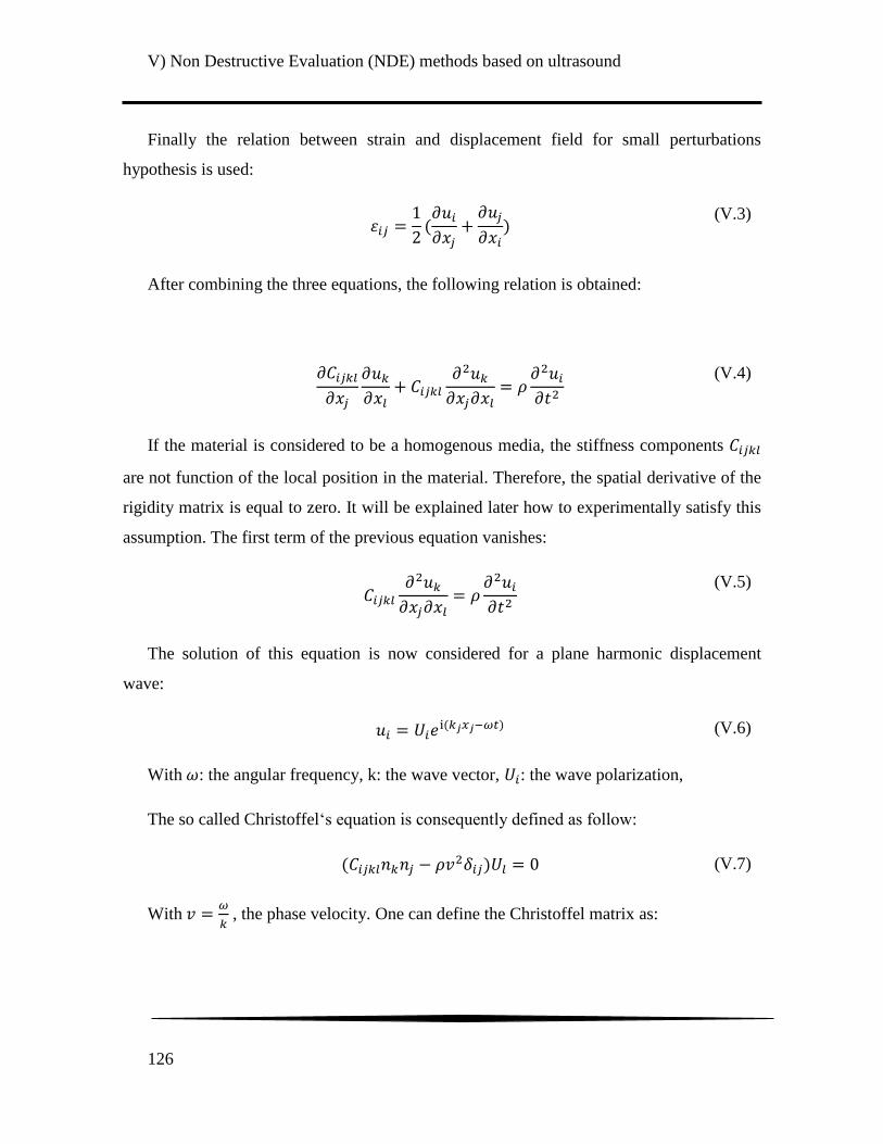
V) Non Destructive Evaluation (NDE) methods based on ultrasound
126
Finally the relation between strain and displacement field for small perturbations
hypothesis is used:
(V.3)
After combining the three equations, the following relation is obtained:
(V.4)
If the material is considered to be a homogenous media, the stiffness components
are not function of the local position in the material. Therefore, the spatial derivative of the
rigidity matrix is equal to zero. It will be explained later how to experimentally satisfy this
assumption. The first term of the previous equation vanishes:
(V.5)
The solution of this equation is now considered for a plane harmonic displacement
wave:
(V.6)
With : the angular frequency, k: the wave vector, : the wave polarization,
The so called Christoffel„s equation is consequently defined as follow:
0 (V.7)
With
, the phase velocity. One can define the Christoffel matrix as:
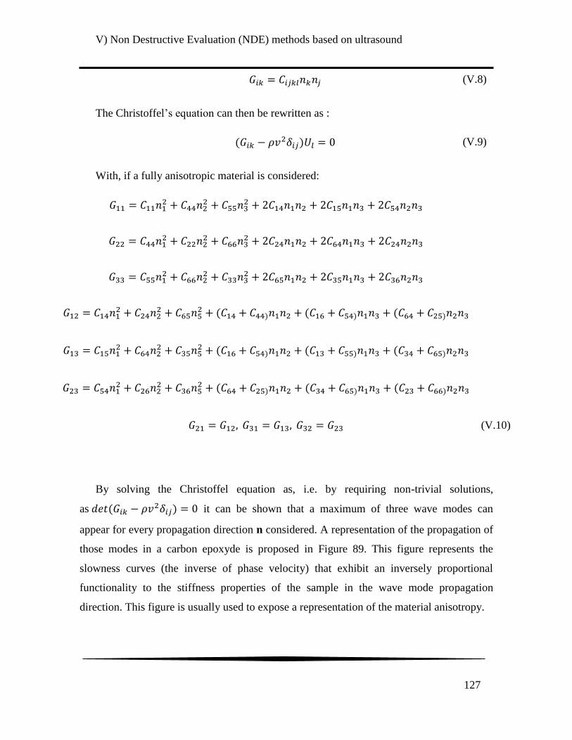
V) Non Destructive Evaluation (NDE) methods based on ultrasound
127
(V.8)
The Christoffel‟s equation can then be rewritten as :
0 (V.9)
With, if a fully anisotropic material is considered:
(V.10)
By solving the Christoffel equation as, i.e. by requiring non-trivial solutions,
as 0 it can be shown that a maximum of three wave modes can
appear for every propagation direction n considered. A representation of the propagation of
those modes in a carbon epoxyde is proposed in Figure 89. This figure represents the
slowness curves (the inverse of phase velocity) that exhibit an inversely proportional
functionality to the stiffness properties of the sample in the wave mode propagation
direction. This figure is usually used to expose a representation of the material anisotropy.
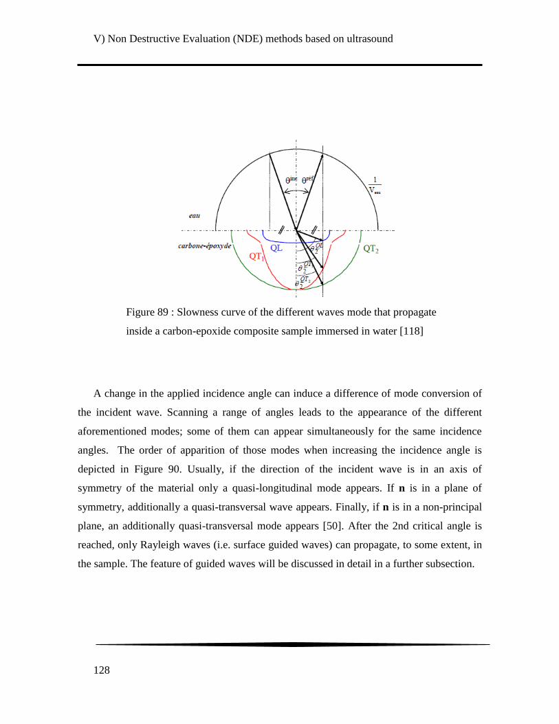
V) Non Destructive Evaluation (NDE) methods based on ultrasound
128
A change in the applied incidence angle can induce a difference of mode conversion of
the incident wave. Scanning a range of angles leads to the appearance of the different
aforementioned modes; some of them can appear simultaneously for the same incidence
angles. The order of apparition of those modes when increasing the incidence angle is
depicted in Figure 90. Usually, if the direction of the incident wave is in an axis of
symmetry of the material only a quasi-longitudinal mode appears. If n is in a plane of
symmetry, additionally a quasi-transversal wave appears. Finally, if n is in a non-principal
plane, an additionally quasi-transversal mode appears [50]. After the 2nd critical angle is
reached, only Rayleigh waves (i.e. surface guided waves) can propagate, to some extent, in
the sample. The feature of guided waves will be discussed in detail in a further subsection.
Figure 89 : Slowness curve of the different waves mode that propagate
inside a carbon-epoxide composite sample immersed in water [118]
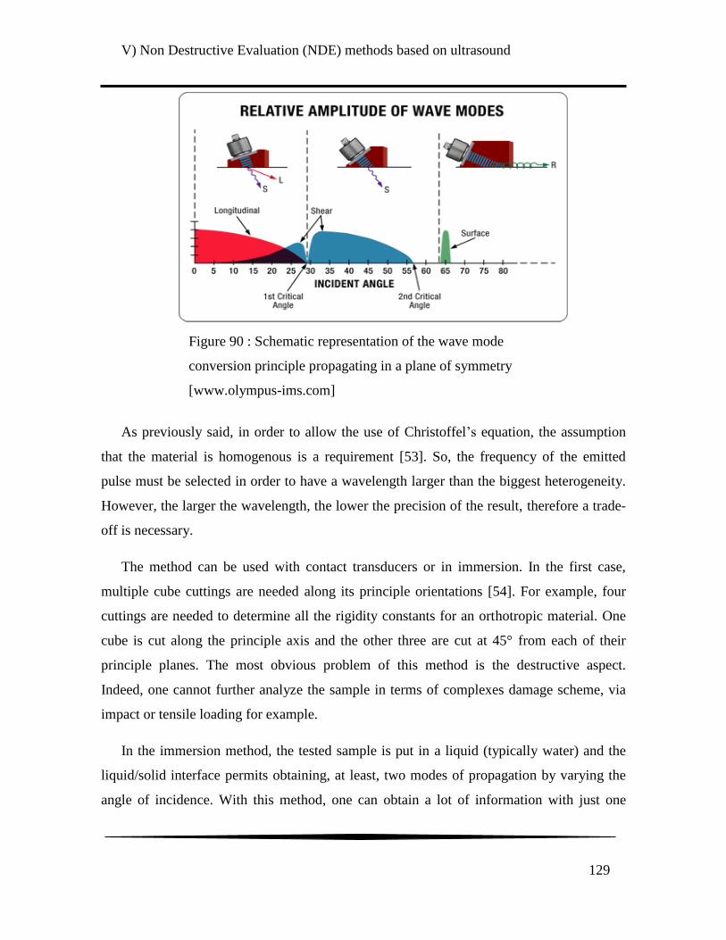
V) Non Destructive Evaluation (NDE) methods based on ultrasound
129
As previously said, in order to allow the use of Christoffel‟s equation, the assumption
that the material is homogenous is a requirement [53]. So, the frequency of the emitted
pulse must be selected in order to have a wavelength larger than the biggest heterogeneity.
However, the larger the wavelength, the lower the precision of the result, therefore a trade-
off is necessary.
The method can be used with contact transducers or in immersion. In the first case,
multiple cube cuttings are needed along its principle orientations [54]. For example, four
cuttings are needed to determine all the rigidity constants for an orthotropic material. One
cube is cut along the principle axis and the other three are cut at 45° from each of their
principle planes. The most obvious problem of this method is the destructive aspect.
Indeed, one cannot further analyze the sample in terms of complexes damage scheme, via
impact or tensile loading for example.
In the immersion method, the tested sample is put in a liquid (typically water) and the
liquid/solid interface permits obtaining, at least, two modes of propagation by varying the
angle of incidence. With this method, one can obtain a lot of information with just one
Figure 90 : Schematic representation of the wave mode
conversion principle propagating in a plane of symmetry
[www.olympus-ims.com]
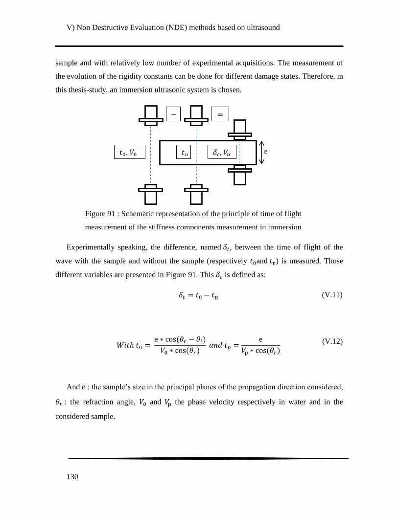
V) Non Destructive Evaluation (NDE) methods based on ultrasound
130
sample and with relatively low number of experimental acquisitions. The measurement of
the evolution of the rigidity constants can be done for different damage states. Therefore, in
this thesis-study, an immersion ultrasonic system is chosen.
Experimentally speaking, the difference, named , between the time of flight of the
wave with the sample and without the sample (respectively and ) is measured. Those
different variables are presented in Figure 91. This is defined as:
(V.11)
(V.12)
And : the sample‟s size in the principal planes of the propagation direction considered,
: the refraction angle, and the phase velocity respectively in water and in the
considered sample.
𝛿𝑡, 𝑉𝑝 e 𝑡𝑝 𝑡 , 𝑉
Figure 91 : Schematic representation of the principle of time of flight
measurement of the stiffness components measurement in immersion

V) Non Destructive Evaluation (NDE) methods based on ultrasound
131
(V.13)
(V.14)
(V.15)
(V.16)
In order to get rid of the in equation (V.16), Snell‟s law is applied:
V
V
(V.17)
Eventually, the refraction angle and the velocity of propagation of the wave in the
material (named ) can be calculated with the following equations:
(V.18)
(V.19)

V) Non Destructive Evaluation (NDE) methods based on ultrasound
132
It was shown that the ToF measured with this technique corresponds to the group
velocity of the transmitted wave, which is in general different from the phase velocity. This
is because the energy flux vector does not coincide necessarily with the wave normal in
anisotropic material with oblique incidence. It was later proven, in [55] among others, that
for all considered directions and in generally anisotropic materials, the measured ToF is
equivalent to a phase delay. Indeed, changes in velocities and travelling paths compensate
each other, making it physically correct to use the measured to estimate phase velocity.
This proof will not be detailed here can be found in [56] for example.
In order to extract the full stiffness tensor of a fully anisotropic material (triclinic),
measurement in three orthogonal planes of the three waves modes are really advised [57].
Otherwise, large errors in the stiffness components identification may be induced. A lot of
experimental measurements are required for similar reason. When an orthotropic material is
considered, measurements in three orthogonal planes of the sample are still necessary. But
less experimental values are needed and measurement of the three wave modes is not
mandatory. Usually, the planes 1-3, 2-3 and 1-2 are used. Indeed, with measurement in the
plane 1-3 the components , , , can be determined, measurement in the plane
Figure 92 : Schematic representation of the wave velocity measurement
method in immersion [Inspired from perso.univ-lemans.fr ]

V) Non Destructive Evaluation (NDE) methods based on ultrasound
133
2-3 allow to determine , , , and with measurement in the plane 1-3 one can
determine the components , , , . This is summarized in Figure 93.
Some authors [51]–[53] highlight the fact that measurement along the 1-2 plane can be
difficult because of the low thickness of a composite material and the possible involvement
of guided propagation. So they only used the plane 1-2 and 1-3, which leads to obtaining
seven out of nine stiffness constants. There are authors who consider out of plane
measurement, usually 45°, in order to obtain the remaining constants. However, Hufenbach
[51] precise that out of plane measurement can lead to important wave deviation and false
results. So he prefers to consider only in-plane measurement and compute seven rigidity
constants.
After the experimental acquisition, the stiffness can consequently be determined by
solving the inverse problem of the Christoffel equation. This is typically performed via an
optimization approache. Usually, a Levenberg-Marquardt algorithm is use to minimize the
square deviation between the analytical and experimental velocities. This optimization
problem is set as:
Figure 93 : Figure of the three planes used to compute the nine
rigidity constants of an orthotropic material [51]

V) Non Destructive Evaluation (NDE) methods based on ultrasound
134
( ) ∑
(V.20)
The numerical velocities are determined by solving the Christoffel equation for a given
set of .
Some authors consider a genetic algorithm to solve this problems [58]. This can allow a
lower number of experimental data and is less sensitive to the initialization values.
However, it requires more time to converge to an optimization solution. Deterministic
algorithms, as the Levenberg-Marquardt algorithm, converge more easily and quickly but
can lead to stability issues with the algorithm. They are very sensitive to the initial guess, if
this guess is too far from the best solution one can find a local minimum instead of the
global minimum. As a consequence, in order to initialize the algorithm, a good first
estimation of the value of is required.
The values of identified stiffness components will be dependent on this initial guess but
also on the number of experimental velocities considered and the number of principal
planes investigated. Therefore, it is necessary to estimate a confidence interval, ci(i), for
each component of the identified stiffness matrix. It was proposed by Audoin and al. [59] to
use the covariance matrix ϕ to obtain statistical information of the deviation from the
analytical solutions of the Christoffel equation for each stiffness component. This
covariance matrix is calculated as
〖 〗
(V.21)
with:
the Jacobian matrix, r is the vector of the residual values i.e. the
functional evaluated with the identified solution, n is the number of experimental velocities,
m the number of stiffness parameters to identified.

V) Non Destructive Evaluation (NDE) methods based on ultrasound
135
The values of confidence interval can then be extracted from the diagonal terms of the
covariance matrix.
√ (V.22)
The ultrasonic C-scan, discussed earlier, can give some information about the damage:
its location and its size (if the latter is comparable with the wavelength). But it remains
difficult to have a good quantification of the damage severity. Recall that increasing
damage on a sample induces a decrease of the Young‟s modulus. This effect can be clearly
seen on stress/strain curves of fatigue tests. So the method can be used to compute the
stiffness components at several moments of the damage life of the material and to observe
their evolutions. This could provide very useful information about the anisotropic
properties of the material that could be linked to the microstructure of the tested specimen.
The modification of the anisotropy during the damage evolution can be verify and used to
developed material damage behavior model.
Polar scan method
The method proposed by Markham requires some long post-processing before having
information on the tested sample. Plus, it may be difficult for use in practice because the
sample needs to be perfectly aligned in the path of the two transducers. So, another
technique, named Polar Scan, was earlier developed to determine the damage with more
ease in the composite with an experimental method rather similar [39], [60], [61].
Indeed, with the Polar Scan method a scan of a specific point in the sample is made for
all accessible oblique angles of incidence. These angles are usually named ψ and are
obtained together with the polar coordinate (θ, ϕ). During the experiment, a pulse wave is
emitted and travels through the sample a first time, is then reflected by an acoustic mirror to
travel through the sample a second time. This is called the double transmission mode (Right
of the Figure 94). For each polar angle, the amplitude is recorded. The acoustic mirror
facilitates the technique as normally a sound beam is deviated due to internal scattering and

V) Non Destructive Evaluation (NDE) methods based on ultrasound
136
might miss a transducer placed on the opposite side in reception mode. By having a wide
mirror reflecting sound back into the sample sound is actually re-collimated to reach the
transducer again which now acts as receiver. A more classical method does not use an
acoustic mirror but a second transducer that is used as a receiver as visible on the left of the
Figure 94.
The frequency must be low enough for the composite to be considered as a homogenous
material (no fiber detection, no initially present porosity …). As the previous method,
information on a homogenized material is obtained. The chosen frequency will be function
of the material and his thickness [62]. The amplitudes measured are then plotted on a figure
pole. Most of the authors call the resulting figure a local fingerprint of the sample. It was
actually shown by numerous authors, [39], [60], [62], that the polar scan method is very
useful to determine the fiber direction, the stacking sequence, and the rigidity.
Qualitatively, one can see the symmetry of the rigidity very effectively [39]. Polar scan
results for an orthotropic material and an isotropic material are respectively plotted on the
left and right of the Figure 95 as example.
Figure 94 : Left: Polar scan with two transducers in transmission mode [62];
Right: Polar scan with an acoustic mirror [39]
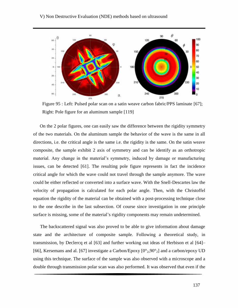
V) Non Destructive Evaluation (NDE) methods based on ultrasound
137
On the 2 polar figures, one can easily saw the difference between the rigidity symmetry
of the two materials. On the aluminum sample the behavior of the wave is the same in all
directions, i.e. the critical angle is the same i.e. the rigidity is the same. On the satin weave
composite, the sample exhibit 2 axis of symmetry and can be identify as an orthotropic
material. Any change in the material‟s symmetry, induced by damage or manufacturing
issues, can be detected [61]. The resulting pole figure represents in fact the incidence
critical angle for which the wave could not travel through the sample anymore. The wave
could be either reflected or converted into a surface wave. With the Snell-Descartes law the
velocity of propagation is calculated for each polar angle. Then, with the Christoffel
equation the rigidity of the material can be obtained with a post-processing technique close
to the one describe in the last subsection. Of course since investigation in one principle
surface is missing, some of the material‟s rigidity components may remain undetermined.
The backscattered signal was also proved to be able to give information about damage
state and the architecture of composite sample. Following a theoretical study, in
transmission, by Declercq et al [63] and further working out ideas of Herbison et al [64]–
[66], Kersemans and al. [67] investigate a Carbon/Epoxy [0°2,90°2] and a carbon/epoxy UD
using this technique. The surface of the sample was also observed with a microscope and a
double through transmission polar scan was also performed. It was observed that even if the
Figure 95 : Left: Pulsed polar scan on a satin weave carbon fabric/PPS laminate [67];
Right: Pole figure for an aluminum sample [119]

V) Non Destructive Evaluation (NDE) methods based on ultrasound
138
ultrasonically detected mechanical behavior of those two composites is different (Figure 96
b) and Figure 97 b)), the backscattered signal remains unchanged and is in correlation with
the observed surface. Indeed, symmetry axis at 0°, 90° (in green) and 30°,150° (in red),
detected with the backscattered signal were observed on both samples‟ surface. They also
investigated Glass/Epoxy [-45°,+45°]s samples before and after shearing loading. On the
undamaged sample the expected fiber‟s orientation were observed with the backscattered
signal (Figure 98). On the damaged sample the same symmetry axis could be observed but
with a higher amplitude. They recall that for this mechanical solicitation; cracks following
the fiber‟s axis are very expected. Therefore, they state that this technique could be used to
estimate the amount of micros-cracks in the material at least on the surface.
Figure 96 : Carbon/Epoxy [0°2,90°2] sample; a) : microscope observation of the
surface of the sample; b) Double transmitted signal; c) Backscattered signal [67]
Figure 97 : Carbon/Epoxy UD sample; a) : microscope observation of the surface of
the sample; b) Double transmitted signal; c) Backscattered signal [67]
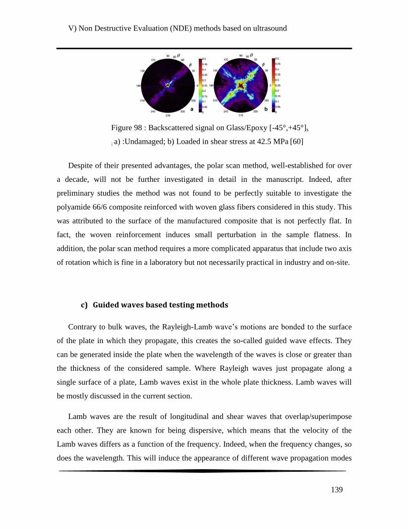
V) Non Destructive Evaluation (NDE) methods based on ultrasound
139
Despite of their presented advantages, the polar scan method, well-established for over
a decade, will not be further investigated in detail in the manuscript. Indeed, after
preliminary studies the method was not found to be perfectly suitable to investigate the
polyamide 66/6 composite reinforced with woven glass fibers considered in this study. This
was attributed to the surface of the manufactured composite that is not perfectly flat. In
fact, the woven reinforcement induces small perturbation in the sample flatness. In
addition, the polar scan method requires a more complicated apparatus that include two axis
of rotation which is fine in a laboratory but not necessarily practical in industry and on-site.
c) Guided waves based testing methods
Contrary to bulk waves, the Rayleigh-Lamb wave‟s motions are bonded to the surface
of the plate in which they propagate, this creates the so-called guided wave effects. They
can be generated inside the plate when the wavelength of the waves is close or greater than
the thickness of the considered sample. Where Rayleigh waves just propagate along a
single surface of a plate, Lamb waves exist in the whole plate thickness. Lamb waves will
be mostly discussed in the current section.
Lamb waves are the result of longitudinal and shear waves that overlap/superimpose
each other. They are known for being dispersive, which means that the velocity of the
Lamb waves differs as a function of the frequency. Indeed, when the frequency changes, so
does the wavelength. This will induce the appearance of different wave propagation modes
Figure 98 : Backscattered signal on Glass/Epoxy [-45°,+45°]s
; a) :Undamaged; b) Loaded in shear stress at 42.5 MPa [60]

V) Non Destructive Evaluation (NDE) methods based on ultrasound
140
that can be classified as symmetric or antisymmetric modes. Several of these modes may
appear at the same time (Left of Figure 99) but with a different velocity of propagation. The
representation of the velocity of the different propagating Lamb wave modes as function of
frequency is called “dispersions curves”. An example of dispersion curves is shown in
Figure 100 for aluminum. Dispersion curves are determined by the material characteristics
and plate thickness. For an isotropic material, a Lamb mode can be formulated by the
characteristic equations as follows [68]:
(V.23)
(V.24)
With:
,
, and
, and where, h, k, w, cL, cT, and cp are
respectively the plate thickness, the wavenumber, the wave circular frequency, the
longitudinal and transverse modes velocities and the phase velocity.
Figure 99 : Left :Signal of Lamb waves from numerical results with a S0 and
A0 mode visible [120]
Right : Schematic representation of symmetric and antisymmetric Lamb
waves mode [37]

V) Non Destructive Evaluation (NDE) methods based on ultrasound
141
For propagation in an anisotropic medium, the equations are more complicated. Further
in the manuscript, guided wave propagation along off-principle planes will be considered.
For this reason, the necessary guided wave equations are required for a monoclinic stiffness
tensor. The latter is obtained with a rotation along the axis 3 at a chosen angle of the
orthotropic stiffness matrix. The wave equations are given by:
(V.25)
(V.26)
Figure 100 : Typical phase velocity dispersion curves for aluminum
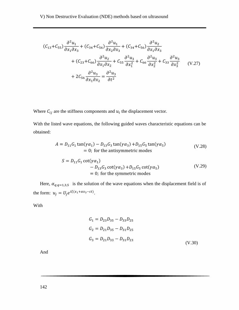
V) Non Destructive Evaluation (NDE) methods based on ultrasound
142
(V.27)
Where are the stiffness components and the displacement vector.
With the listed wave equations, the following guided waves characteristic equations can be
obtained:
0 (V.28)
0
(V.29)
Here, is the solution of the wave equations when the displacement field is of
the form: .
With
(V.30)
And

V) Non Destructive Evaluation (NDE) methods based on ultrasound
143
(V.31)
The amplitude ratio and are given by:
(V.32)
For more details about the guided waves characteristic equations we refer to the book of
Nayfeh [69].
Lamb waves are frequently used in the industry to characterize material properties [70],
[71], to detect damage in a structure and to locate and to quantify these defects. These
waves also have the ability to travel relatively long distances and are therefore frequently
used on-site to detect damage in pipelines, for example [36], [37]. They do not require a
point by point acquisition, contrary to a C-scan, since all the required information can be
obtained via B-scan-like acquisitions. Thanks to Lamb waves, in the industry a single
measurement may be sufficient to detect damage. Since it requires access to one side of the
sample it is also easier to be used on-site. The simplest application of Lamb waves is to
check for generated echoes when damage is encountered.
Nevertheless, many authors [72]–[74] also highlight the strength of an analysis of the
dispersions effects of the Lamb waves modes to detect damage. A frequency domain
processing is classically done to obtain Lamb wave velocities. Nevertheless, this can be
easily performed only when a single wave mode is appearing on the temporal response, or
when the different waves are clearly distinguished from each other; clearly not the case in
the Figure 101. In the case when multiple Lamb wave modes are detected, a 2D Fourier
transform (in time and space) must be applied on the signals [72], [75]. The results are then
typically plotted as function of the frequency and the wavenumber. The results typically
show distinguishable line patterns, called dispersion curves (Figure 102). The curves can be
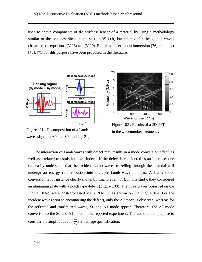
V) Non Destructive Evaluation (NDE) methods based on ultrasound
144
used to obtain components of the stiffness tensor of a material by using a methodology
similar to the one described in the section V).1).b) but adapted for the guided waves
characteristic equations (V.28) and (V.29). Experiment sets-up in immersion [76] or contact
[70], [71] for this purpose have been proposed in the literature.
The interaction of Lamb waves with defect may results in a mode conversion effect, as
well as a related transmission loss. Indeed, if the defect is considered as an interface, one
can easily understand that the incident Lamb waves travelling through the material will
undergo an energy re-distribution into multiple Lamb wave‟s modes. A Lamb mode
conversion is for instance clearly shown by Imano et al. [77]. In this study, they considered
an aluminum plate with a notch type defect (Figure 103). The three waves observed on the
Figure 103-c, were post-processed via a 2D-FFT as shown on the Figure 104. For the
incident wave (prior to encountering the defect), only the A0 mode is observed, whereas for
the reflected and transmitted waves, S0 and A1 mode appear. Therefore, the A0 mode
converts into the S0 and A1 mode in the reported experiment. The authors then propose to
consider the amplitude ratio
for damage quantification.
Figure 102 : Results of a 2D-FFT
in the wavenumber-frequency Figure 101 : Decomposition of a Lamb
waves signal in A0 and S0 modes [121]

V) Non Destructive Evaluation (NDE) methods based on ultrasound
145
Incident wave
Reflected wave
Transmitted wave
Incident wave
Reflected wave
Transmitted wave
b)
a)
c)
Figure 103 : Schematic representation of the considered aluminum sample with a
notch type defect. a) Top observation, b) Side observation, c) Side observation +
ultrasonic wave‟s propagation through the sample (Based on [77])
Figure 104 : Side observation of the sample + ultrasonic wave‟s propagation
through the sample. 2D Fourier transform results for the incident, reflected
and transmitted wave with the theoretical dispersion curves. (Based on [77])
Incident wave
Reflected wave
Transmitted wave

V) Non Destructive Evaluation (NDE) methods based on ultrasound
146
d) Nonlinear acoustic method
Recently, various experimental researches have been reported on nonlinear acoustic
methods and what they can provide to estimate the global damage state of a material [78]–
[83]. It was shown that the nonlinearity of the acoustic response increases with increasing
damage. Typically, a nonlinear effect will be earlier detected during the degradation of a
material than classical linear responses linked to wave velocity, ultrasonic amplitude,
rigidity constant, … [83], [84]. The term Nonlinear Elastic Waves Spectroscopy (NEWS) is
usually used to name all those methods. As expected with the name of the method, the
objective is to investigate the frequency response obtained after a Fourier transform. The
acoustic response of the sample can be recorded with a loudspeaker or a laser vibrometer.
In his paper Rabe insists on the fact that a laser vibrometer will be much more accurate
[80]. The recent literature focuses mostly on applications for composite material (concrete
or polymer based composites). Nevertheless the method was also used for characterizing
for example the increase of stiffness of metallic alloys by heating treatment [78].
Ostragradsky and Johnson in [85] propose a description of classical nonlinear acoustics that
they extend to the study of nonlinear elasticity of rocks and their modeling. The last part of
this paper is dedicated to the application of nondestructive evaluation (NDE) of materials.
A complementary review of the seminal researched on classical and “non-classical
nonlinear acoustics from the 1950‟s onwards, can be found in the work of Nizhni Novgorod
[86].
If the higher order terms are added into the isotropic elastic equation, a nonlinear
description of the elasticity, taking into account hysteresis can be expressed as:
∫ (V.33)
(V.34)
V) Non Destructive Evaluation (NDE) methods based on ultrasound
147
With the linear elastic modulus, and the 2nd and 3st order nonlinear parameter,
the material hysteresis parameter.
Numerous nonlinear acoustic techniques have been developed to measure the
material‟s nonlinearity. Among them two main categories were particularly discussed in the
literature : The Nonlinear Wave Modulation Spectroscopy (NWMS) and Nonlinear
Resonant Ultrasound Spectroscopy (NRUS) [84]. Another category can be found in the
literature : Nonlinear Reverberation Spectroscopy (NRS) [87]. All of these methods can be
used in continuous wave mode or in impact mode. In the first case, solicitation is performed
using harmonic waves. In the second case, the sample is submitted to an impact
investigation. The advantage of using the impact mode is that for a single test, numerous
resonance frequencies will be solicited simultaneously [82], [84], [88], which makes the
experiment faster. However it has also been shown that the measured resonance frequencies
are not perfectly linked to the true physical amplitude in the sample. Because of dynamic
effects occuring in the signal, such as a reverberation effect, the real physical amplitude can
be hidden when the Fourier transform is applied [82]. Those three NEWS methods will be
described in detail further in this section. A graph recalling the three main NEWS methods,
with associated references, is seen in Figure 105.
The two first mentioned methods, NRUS and NWMS were investigated in continuous
wave mode for three different materials, including the polyamide 66/6 reinforced by woven
glass fibers, during the research project discussed in this manuscript. Because a significant
share of this work is applied to samples other than this polyamide 66/6 based composite
material and because this technique did not successfully evaluated damage in this material,
the investigation was not added to the main body of this thesis manuscript but rather in the
appendix section 1).
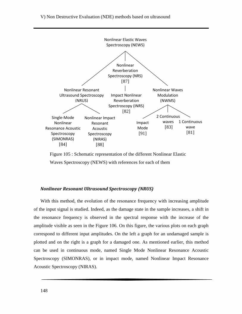
V) Non Destructive Evaluation (NDE) methods based on ultrasound
148
Nonlinear Resonant Ultrasound Spectroscopy (NRUS)
With this method, the evolution of the resonance frequency with increasing amplitude
of the input signal is studied. Indeed, as the damage state in the sample increases, a shift in
the resonance frequency is observed in the spectral response with the increase of the
amplitude visible as seen in the Figure 106. On this figure, the various plots on each graph
correspond to different input amplitudes. On the left a graph for an undamaged sample is
plotted and on the right is a graph for a damaged one. As mentioned earlier, this method
can be used in continuous mode, named Single Mode Nonlinear Resonance Acoustic
Spectroscopy (SIMONRAS), or in impact mode, named Nonlinear Impact Resonance
Acoustic Spectroscopy (NIRAS).
Figure 105 : Schematic representation of the different Nonlinear Elastic
Waves Spectroscopy (NEWS) with references for each of them
Nonlinear Elastic Waves Spectroscopy (NEWS)
Nonlinear Resonant Ultrasound Spectroscopy
(NRUS)
Single-Mode Nonlinear
Resonance Acoustic Spectroscopy (SIMONRAS)
[84]
Nonlinear Impact Resonant Acoustic
Spectroscopy (NIRAS)
[88]
Nonlinear Reverberation
Spectroscopy (NRS)
[87]
Impact Nonlinear Reverberation
Spectroscopy (INRS)
[82]
Nonlinear Waves Modulation
(NWMS)
2 Continuous waves
[83]
Impact Mode
[91]
1 Continuous wave
[81]

V) Non Destructive Evaluation (NDE) methods based on ultrasound
149
It can be shown that the slope of the resonance frequency shift is a function of , the
hysteresis parameter [89]. If the equation of described earlier is inserted into the
wave equation with and equal to zero and if the nonlinear contribution to the wave
solution is computed one can find three relations:
(V.35)
a linear decrease of the resonance frequency for increasing strain levels
(V.36)
a quadratic amplitude dependence of the third harmonic the amplitude of the
fundamental/resonance frequency, and
(V.37)
a linear increase of the modal damping ratio (decrease of the quality factor Q) with the
increase of the amplitude, where all the coefficients are function of the parameter. In
other words, any change of the coefficient induces a change in the parameter. The first
relation is considered for this Nonlinear Resonant Ultrasound Spectroscopy method.
Figure 106 : Schematic spectrum that can be obtain with the NRUS method
for an undamaged (left) and damaged (right) sample [83]

V) Non Destructive Evaluation (NDE) methods based on ultrasound
150
Nonlinear Wave Modulation Spectroscopy (NWMS)
The other of the two mainly used nonlinear acoustic methods is the so-called Nonlinear
Wave Modulation Spectroscopy. As with the previous method, the NWMS has been used
in impact mode (for example : [84], [90]) and continuous mode (for example : [83], [91]).
The same observation can be made for the benefits and disadvantages of both methods.
Here, the sample is submitted to either two continuous waves, in continuous mode, or one
continuous wave and an impact solicitation in impact mode. One of the waves should have
a low frequency and the other one a higher frequency. It is often considered that the
difference of the two input signals‟ frequency should be lower than the lowest selected
frequency. In impact mode, the impact hammer is used to cover the lower frequency.
Aymerich and all [92] used a flexural vibration wave to cover this lower frequency.
When the sample is undamaged, one should observe only peaks that correspond to the
input frequency, with of course a decrease of the amplitude. However, when the sample is
damaged, various other peaks will appear on the spectrum (Figure 107). They correspond to
harmonics of the input frequencies and appear at values of n* fi, with n: an integer.
Modulation between the input frequencies also appear at values of f1 +/- n*f2, they are
called sidebands: The amplitude of these new peaks should increase with an increase of the
damage in the sample. Specifically, the sidebands‟ amplitudes can be related to the
nonlinear parameter , , [91] :
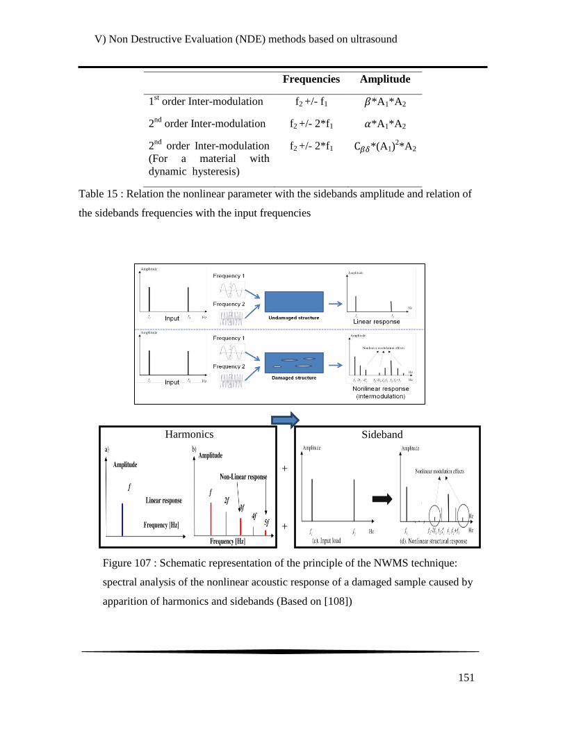
V) Non Destructive Evaluation (NDE) methods based on ultrasound
151
Frequencies Amplitude
1st order Inter-modulation f2 +/- f1 *A1*A2
2nd
order Inter-modulation f2 +/- 2*f1 *A1*A2
2nd
order Inter-modulation
(For a material with
dynamic hysteresis)
f2 +/- 2*f1 *(A1)2*A2
Table 15 : Relation the nonlinear parameter with the sidebands amplitude and relation of
the sidebands frequencies with the input frequencies
+
+
Harmonics Sideband
Figure 107 : Schematic representation of the principle of the NWMS technique:
spectral analysis of the nonlinear acoustic response of a damaged sample caused by
apparition of harmonics and sidebands (Based on [108])
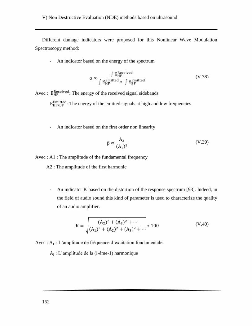
V) Non Destructive Evaluation (NDE) methods based on ultrasound
152
Different damage indicators were proposed for this Nonlinear Wave Modulation
Spectroscopy method:
- An indicator based on the energy of the spectrum
∫
∫ ∫
(V.38)
Avec : : The energy of the received signal sidebands
: The energy of the emitted signals at high and low frequencies.
- An indicator based on the first order non linearity
(V.39)
Avec : A1 : The amplitude of the fundamental frequency
A2 : The amplitude of the first harmonic
- An indicator K based on the distortion of the response spectrum [93]. Indeed, in
the field of audio sound this kind of parameter is used to characterize the quality
of an audio amplifier.
√
00 (V.40)
Avec : : L‟amplitude de fréquence d‟excitation fondamentale
: L‟amplitude de la (i-éme-1) harmonique
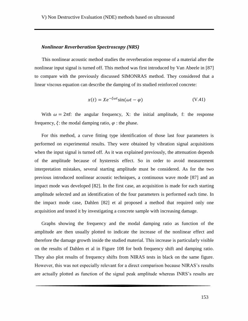
V) Non Destructive Evaluation (NDE) methods based on ultrasound
153
Nonlinear Reverberation Spectroscopy (NRS)
This nonlinear acoustic method studies the reverberation response of a material after the
nonlinear input signal is turned off. This method was first introduced by Van Abeele in [87]
to compare with the previously discussed SIMONRAS method. They considered that a
linear viscous equation can describe the damping of its studied reinforced concrete:
(V.41)
With : the angular frequency, X: the initial amplitude, f: the response
frequency, : the modal damping ratio, : the phase.
For this method, a curve fitting type identification of those last four parameters is
performed on experimental results. They were obtained by vibration signal acquisitions
when the input signal is turned off. As it was explained previously, the attenuation depends
of the amplitude because of hysteresis effect. So in order to avoid measurement
interpretation mistakes, several starting amplitude must be considered. As for the two
previous introduced nonlinear acoustic techniques, a continuous wave mode [87] and an
impact mode was developed [82]. In the first case, an acquisition is made for each starting
amplitude selected and an identification of the four parameters is performed each time. In
the impact mode case, Dahlen [82] et al proposed a method that required only one
acquisition and tested it by investigating a concrete sample with increasing damage.
Graphs showing the frequency and the modal damping ratio as function of the
amplitude are then usually plotted to indicate the increase of the nonlinear effect and
therefore the damage growth inside the studied material. This increase is particularly visible
on the results of Dahlen et al in Figure 108 for both frequency shift and damping ratio.
They also plot results of frequency shifts from NIRAS tests in black on the same figure.
However, this was not especially relevant for a direct comparison because NIRAS‟s results
are actually plotted as function of the signal peak amplitude whereas INRS‟s results are

V) Non Destructive Evaluation (NDE) methods based on ultrasound
154
plotted as function of the acceleration in the z-direction previously computed in COMSOL
and matching the experimental set-up. However, they show that both methods detect an
increase in the damage state.
e) Coda waves in Non-Destructive Testing
The investigation of Coda Waves appeared earlier in the field of seismology, they refer
to the late arrivals of a response signal. They are the result of multiple wave scattering and
act as a fingerprint of the heterogeneity of a seismic wave. As an example, the wave
attenuation induced by the scattering process, in addition to the initial absorption effect, has
been studied. A review of those studies can be found in [94].
This technique was later considered for nondestructive evaluation of materials,
especially of concrete structures. It was extensively demonstrated that the waves are very
Figure 108 : Numerical results obtained after identification of the attenuation model
parameters for concrete
Left : Normalized frequency versus amplitude for samples damaged at different level
+ results from NIRAS tests performed on the same material, Right : Normalized
Modal Damping Ratio versus amplitude for samples damaged at different level [82]

V) Non Destructive Evaluation (NDE) methods based on ultrasound
155
sensitive to the weakest change in the material microstructure, such as micro-cracks [95],
thermal changes [96], etc . A particular attention must be paid to the input frequency.
Indeed, the mesoscopic range of ultrasonic wavelength or the multiple scattering regimes
must be considered in order to have a fully reproducible Coda waves propagation (Figure
109). In this regime, the wavelength of the input signal is shorter than the smallest
heterogeneity in the considered material. In concrete, this heterogeneity is assumed to be
around one centimeter, therefore a frequency range of 150 kHz to 1 MHz is typically
considered.
In composite materials however, the considered heterogeneity could be that of full yarns
or at a smaller scale the fibers themselves. They have a characteristic size respectively of
0.5 mm and 15 µm, which corresponds to frequencies of 7 MHz and 250 MHz. Because of
the attenuation effect it is hard to consider very high frequencies in composite materials.
However, papers publish by Livings and al. [96], [97] demonstrate that the acoustic
signature of the material is sensitive to small changes in the material for a 1 MHz input
emission. One of the major current issues is the lack of sufficiently accurate theoretical
work or comparative data. Indeed, the application of the coda wave technique in polymer-
based composites is a recent development.
During this research project, coda wave interferometry has been investigated on a
woven carbon fiber reinforced polyphenylene sulfide based composite material. Carbon
fiber reinforced composite samples were preferred over glass fiber reinforced ones because
Figure 109 : Schematic representation of the
different wave propagation regime [122]

V) Non Destructive Evaluation (NDE) methods based on ultrasound
156
of the lower ultrasonic wave attenuation [98]. One of the objectives of this research project
is to investigate several ultrasonic NDE methods on composite materials and to try to
compare pros and cons. As a consequence, a discussion of this investigation is added in the
appendix section 2).
Because Coda waves involve waves that have been scattered multiple times in the
structure, the investigation mostly focuses on the late arrival signal, retarded with respect to
the initial received signal. As it can be seen on the Figure 110 no difference between the
early wave packets of a reference signal and a disturbed one can be observed. However,
there appears a phase shift for late wave packets. The main purpose of a Coda wave
interferometry study is to measure, based on the observed phase shift, a the relative velocity
change induced by a change in the heterogeneity of a material. In order to extract this
information, four main waveform comparison techniques can be used. A comparison of
those four techniques can be found in [99] and are briefly mentioned below.
Figure 110 : Signal waveforms collected on a CRFP composite before (h0) and
after (h1) an increase of temperature [96]

V) Non Destructive Evaluation (NDE) methods based on ultrasound
157
- The moving window cross-correlation technique
Both the reference signal (without damage) and the perturbed signal (with damage) are
cut in time window of length 2* . The perturbed signal is then shifted by a value . The
correlation coefficient R is computed for every considered and for every window.
∑
√∑
√∑
(V.42)
The value for which the R coefficient is the highest, frequently named , is then
stored for every window. If the change in the signal is only due to small perturbations, such
as temperature or minor damage, the evolution of the velocity is constant, as if it‟s due to a
stiffness reduction. This means that is equal to a constant α. It can also be shown that
if dv<<v, one can obtain . Since , represents actually dt, α can be
measured by plotting function of the central time of the corresponding window. Then
by applying a linear regression on this plot, the α‟s value is directly obtained. Of course,
this implies a small perturbation in the signal.
- The moving window cross-spectrum technique
For this technique, the analysis is performed in the frequency domain. First, the cross
spectrum between the windowed reference signal, y, and the windowed disturbed one, x, is
calculated with:
(V.43)

V) Non Destructive Evaluation (NDE) methods based on ultrasound
158
With, X and Y the Fourier transform of respectively x and y and * indicate the complex
conjugate
The phase spectrum of the cross spectrum is then calculated. The time delay can then
be obtained by fitting a line to the phase spectrum.
- The stretching technique
As the name implies, the signal waveform is here stretched by a stretching
coefficient . Indeed, a uniform velocity change in a waveform induces a change
closer to a compression or stretching of a signal. This technique could therefore give more
stable and accurate results. The stretched signal is calculated as:
(V.44)
The correlation coefficient is then calculated with:
∑
√∑ √∑
(V.45)
- The moving window stretching technique
This technique is similar to the stretching technique but is used for several windowed
signals. This technique was proposed in order to increase the stability and the accuracy of
the correlation. The relative velocity change is then calculated as an average over all
the considered windows.
They are several quantities that have consequently been considered as damage
indicators in previous publication such as: the time delay, the peak coherence, the
V) Non Destructive Evaluation (NDE) methods based on ultrasound
159
difference between the maximum and the mean of the cross correlation coefficient, etc. As
mentioned before, the coda wave interferometry technique can be conveniently used to
measure temperature changes of a material. However, when this technique is considered for
non-destructive damage detection, the temporal change of the signal can be caused, in
addition to the present damage, by environmental change. One must therefore be very
cautious of this issue. Different methods were considered to separate both effects on the
resulting signal. For example, Michaels and al. [100] analyzed both the temporal change
and the correlation coefficient (or peak coherence) of sample submitted to temperature
change, drilling and both. The peak coherence is the maximum of the absolute value
of . They show that when the temperature changes, the delay change linearly as a
function of time and the remaining correlation coefficient decreases a slightly function of
time (from 1 to 0.75). However, after drilling, the remaining correlation coefficient drops
more significantly (from 1 to 0.4). Zhang and al [101], proposed to consider two samples
for the Coda Waves Interferometry tests. One is submitted to environmental change and
damage growth and the other is submitted to environmental change only.
f) Synthesis of the Non Destructive Evaluation method review
Based on this review, it was decided to investigate the composite specimens presented
in section IV)-4) first by using ultrasonic C-scan as a common reference in industry. Then,
the method aimed at calculating the stiffness components through phase velocity
measurements is considered. Indeed, it could provide a complete description of the
anisotropic evolution of damage in the samples. This is of critical interest to link the effect
of the mechanical solicitation to the residual properties of the investigated specimens. It can
consequently quantify the severity of the induced damage.
Then, its convenience for on-site implementation, as well as the capability to analyze
large structures, convinced to more deeply investigate guided wave based methods, which
could, by using the direct analysis of the transmitted waves or the investigation of the
dispersive wave modes, give a clear and practical estimation of the damage level.
V) Non Destructive Evaluation (NDE) methods based on ultrasound
160
Compared to the first mentioned method, it can be used without an optimization procedure
and can consequently provide results more quickly to an NDT specialist.
The aforementioned nonlinear acoustics based methods and Coda Waves Interferometry
have been investigated during this project. However, they were not used for specific
analysis of induced damage in samples of polyamide 66/6 reinforced by woven glass fibers
but rather in other composites, reinforced with woven fibers. For this reason the
investigations dedicated to those two methods are presented in the appendix and may be
considered as complementary results to the main body of this thesis.
2) Ultrasonic C-scan in transmission
Ultrasonic imaging was performed on all tested samples to investigate the overall
damage state of the samples cut at 0° and 45°. Classical ultrasonic 2D C-scans in
transmission were performed using a 5 MHz frequency transducer, the maximal amplitude
of the ultrasonic signal is measured and recorded at each point of the scanned area with a
spatial resolution of 0.5 mm. It is then plotted in Figure 111 for both considered sample
configurations. It is worth noting that the values reported in this figure are the actual values
of the ultrasound amplitude‟s signal without any normalization.
As illustrated in Figure 111-a related to the samples tested at 0° from the warp direction,
the attenuation of the ultrasound amplitude‟s signal remains low and a very slight
difference, if any, was noticed when increasing the applied stress level from 0 to
92.6% °. For the sample in 45°, the Figure 111-b shows the evolution of amplitude
attenuation (C-scan images) between the unloaded state and the ultimate state level prior
failure (92.6% °). Two damage zones were actually observed macroscopically and
the related high attenuations in the signals were associated to the fibers buckling and the
local delamination. In addition, the low signal attenuations observed at the border of the
samples were clearly induced by a well-known border effect and were not caused by the
mechanically induced damage.
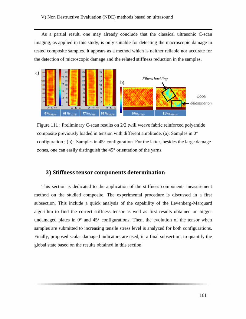
V) Non Destructive Evaluation (NDE) methods based on ultrasound
161
As a partial result, one may already conclude that the classical ultrasonic C-scan
imaging, as applied in this study, is only suitable for detecting the macroscopic damage in
tested composite samples. It appears as a method which is neither reliable nor accurate for
the detection of microscopic damage and the related stiffness reduction in the samples.
3) Stiffness tensor components determination
This section is dedicated to the application of the stiffness components measurement
method on the studied composite. The experimental procedure is discussed in a first
subsection. This include a quick analysis of the capability of the Levenberg-Marquard
algorithm to find the correct stiffness tensor as well as first results obtained on bigger
undamaged plates in 0° and 45° configurations. Then, the evolution of the tensor when
samples are submitted to increasing tensile stress level is analyzed for both configurations.
Finally, proposed scalar damaged indicators are used, in a final subsection, to quantify the
global state based on the results obtained in this section.
Fibers buckling
Local
delamination
Figure 111 : Preliminary C-scan results on 2/2 twill weave fabric reinforced polyamide
composite previously loaded in tension with different amplitude. (a): Samples in 0°
configuration ; (b): Samples in 45° configuration. For the latter, besides the large damage
zones, one can easily distinguish the 45° orientation of the yarns.
b)
a)
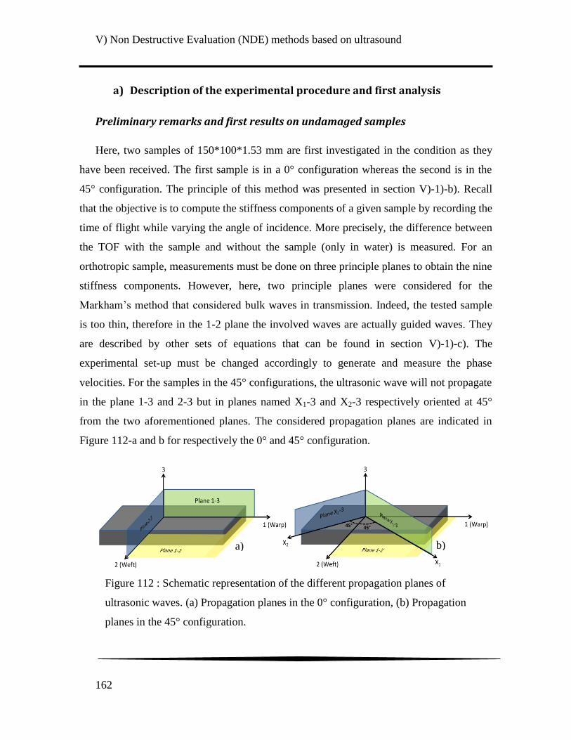
V) Non Destructive Evaluation (NDE) methods based on ultrasound
162
a) Description of the experimental procedure and first analysis
Preliminary remarks and first results on undamaged samples
Here, two samples of 150*100*1.53 mm are first investigated in the condition as they
have been received. The first sample is in a 0° configuration whereas the second is in the
45° configuration. The principle of this method was presented in section V)-1)-b). Recall
that the objective is to compute the stiffness components of a given sample by recording the
time of flight while varying the angle of incidence. More precisely, the difference between
the TOF with the sample and without the sample (only in water) is measured. For an
orthotropic sample, measurements must be done on three principle planes to obtain the nine
stiffness components. However, here, two principle planes were considered for the
Markham‟s method that considered bulk waves in transmission. Indeed, the tested sample
is too thin, therefore in the 1-2 plane the involved waves are actually guided waves. They
are described by other sets of equations that can be found in section V)-1)-c). The
experimental set-up must be changed accordingly to generate and measure the phase
velocities. For the samples in the 45° configurations, the ultrasonic wave will not propagate
in the plane 1-3 and 2-3 but in planes named X1-3 and X2-3 respectively oriented at 45°
from the two aforementioned planes. The considered propagation planes are indicated in
Figure 112-a and b for respectively the 0° and 45° configuration.
Figure 112 : Schematic representation of the different propagation planes of
ultrasonic waves. (a) Propagation planes in the 0° configuration, (b) Propagation
planes in the 45° configuration.
a) b)

V) Non Destructive Evaluation (NDE) methods based on ultrasound
163
All the acquisitions were done at Georgia Tech Lorraine using a customer-designed
immersion scanner, visible in Figure 113, fabricated by Inspection Technology Europe BV.
The pulse is emitted by a dual pulser-receiver DPR500 made by JSR ultrasonics. The
experimental data are acquired with Winspect software and are post-processed in Matlab.
Two immersion Panasonic transducers with a central frequency of 2.25MHz are used in
order to satisfy the homogenous media hypothesis. The shape and the spectrum of the
emitted pulse are represented on the Figure 114. It can be noted that the actual emitted
pulse, as is, frequency is 2.1 MHz.
X
Y
Z A axis
B axis
Figure 113 : LUNE lab's 5 axis ultrasonic robot from Inspection Technology
2.1 MHz
Figure 114 : Emitted pulse shape (Left) and spectrum (Right) for a
2.25MHz centered frequency transducer; The experimentally
mesured central frequency is about 2.1 MHz
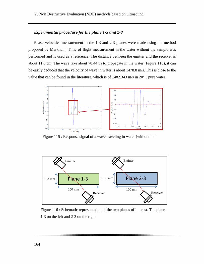
V) Non Destructive Evaluation (NDE) methods based on ultrasound
164
Experimental procedure for the plane 1-3 and 2-3
Phase velocities measurement in the 1-3 and 2-3 planes were made using the method
proposed by Markham. Time of flight measurement in the water without the sample was
performed and is used as a reference. The distance between the emitter and the receiver is
about 11.6 cm. The wave take about 78.44 us to propagate in the water (Figure 115), it can
be easily deduced that the velocity of wave in water is about 1478.8 m/s. This is close to the
value that can be found in the literature, which is of 1482.343 m/s in 20°C pure water.
Figure 115 : Response signal of a wave traveling in water (without the
1.53 mm
Emitter
Receiver
150 mm
Plane 1-3 1.53 mm
Emitter
Receiver
100 mm
Plane 2-3
Figure 116 : Schematic representation of the two planes of interest. The plane
1-3 on the left and 2-3 on the right
V) Non Destructive Evaluation (NDE) methods based on ultrasound
165
The sample is then added to the experimental set-up and measurements are made in the
planes 1-3 and 2-3 of the sample as depicted in Figure 116. The present subsection (a) will
only considered undamaged samples. Note that on both signals, i.e. with and without the
sample, the time of flight is actually measured on the first intersection of the signal with the
axis of zero amplitude in order to accurately obtain the velocity of the different wave
modes. This is easily performed here because of the measured ultrasonic centered on 0
Volts. But when this is not the case, one can measure the time of flight on each first
positive peak. This leads to a measured time of flight of 78.65us when the wave travels in
water only for a velocity of 1478.8 m/s. This value will be considered for the further stages
of the study.
In order to have an accurate computation of the stiffness tensor, a large number of
experimental results are necessary. However, wave mode mixing in the recorded signal can
make the quasi transversal time of flight measurement difficult. It may possibly lead to
inaccurate computation of the mode propagation velocities. In order to be sure of the
presence of additional modes, it is necessary to visualize the transmitted signal by varying
the incidence angle. This will induce the progressive appearance and disappearance of
additional modes. The modes can also be made visible on the spectral response of the
transmitted signal. As an example, the transmitted signal and associated spectral response
signal after propagating through a pristine composite sample are represented for 0° and 13°
angles of incidence in Figure 117. The same information is also plotted on the same figure
for a wave propagating only in water for reference purposes. The identified additional quasi
transversal mode is circled in red in the 13° incidence angle time signal. This mode also has
a visible influence on the spectral response. A full set a quasi-longitudinal and quasi-
transversal modes are then acquired for the two chosen principle planes.

V) Non Destructive Evaluation (NDE) methods based on ultrasound
166
Then, the velocity of every wave is computed with the following equations explained
earlier:
(V.46)
(V.47)
Experimental procedure for the plane 1-2
Now for measurements in the 1-2 plane of the tested samples an experimental set-up
(Visible in Figure 118) in immersion using two transducers in pitch-catch mode, both at a
chosen incidence angle, can be used to obtained the phase velocities [76], [102]. For each
azimuthal direction of propagation (ψ) in the 1-2 plane, the incidence angle is adjusted to
find the same guided wave mode at every acquisition. The phase velocities are then
calculated with the use of the Snell‟s law with 0° i.e.:
Figure 117 : Transmitted signal (left) and associated spectral response (Right)
propagated in an undamaged sample for incidence angle of 0° and 13°. Information
for a signal propagated only in water was added for comparison purpose

V) Non Destructive Evaluation (NDE) methods based on ultrasound
167
(V.48)
This experimental set-up is visible in Figure 118.
Measurements in those three planes give phase velocities for different propagation
directions in the tested sample. All the experimental data are then processed in Matlab,
through procedures developed for this study, to compute the rigidity constants. The
Christoffel equation are used to post-process phase velocities measured in planes 1-3 and 2-
3, whereas the guided waves characteristics equations are used to post-process the phase
velocities measured in the plane 1-2. The program uses the Levenberg-Marquardt algorithm
function available in Matlab.
Preliminary analysis on undamaged samples
The algorithm is initialized with an estimation (initial guess) of the stiffness tensor. This
must be relatively close to the real solution to avoid local, i.e. false, minima. This is why
the complete stiffness tensor of a woven glass fabric/polyamide was computed. The
homogenization theory [103] was used on a composite with a woven fabric. The yarns‟ size
used was obtained from the previously discussed microstructural analysis in chapter IV).
The computation was performed for a composite oriented along the warp direction. Then
the tensor was rotate, along the third axis, at 45° to consider sample oriented at 45° from
Figure 118 : Experimental set-up for measurement in the plane 1-2

V) Non Destructive Evaluation (NDE) methods based on ultrasound
168
warp direction. The numerically computed rigidity components for both 0° and 45°
configurations are indicated in the Table 16.
C11 C12 C13 C22 C23 C33 C44 C55 C66
0° - Stiffness
Components (GPa) 20 2.1 1.5 20 1.5 4.5 2.3 1.3 1.3
45° - Stiffness
Components (GPa) 13.3 8.7 1.5 13.3 1.5 4.5 8.9 1.3 1.3
Table 16 : Numerical stiffness components for the 0° and 45° configurations obtained by
periodic homogenization courtesy of Francis Praud
In order to improve the efficiency and get rid of numerical issues when using the
Christoffel equation as is, in the optimization algorithm, it is better to re-write the equation
as a cubic equation. The three roots of this cubic equation are then determined with the
Cardan‟s solution of a cubic equation as:
√
(
)
(V.49)
√
(
)
(V.50)
√
(
)
(V.51)
Where
( )
(V.52)
(V.53)
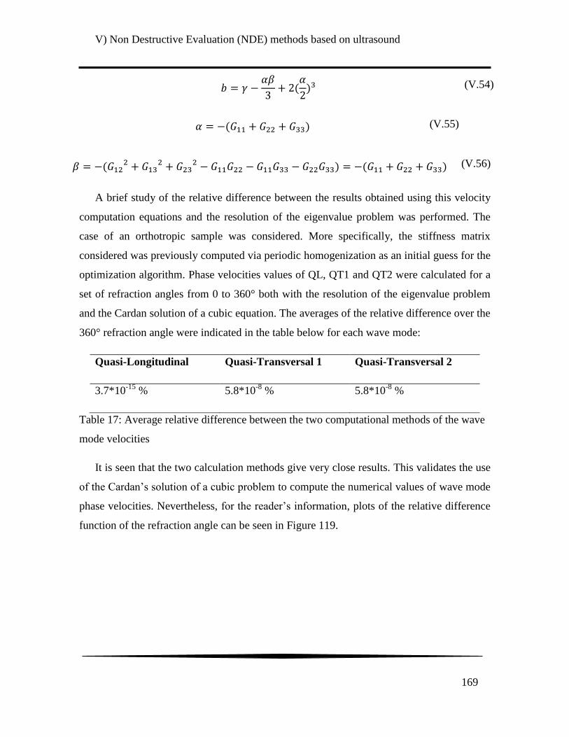
V) Non Destructive Evaluation (NDE) methods based on ultrasound
169
(V.54)
(V.55)
(V.56)
A brief study of the relative difference between the results obtained using this velocity
computation equations and the resolution of the eigenvalue problem was performed. The
case of an orthotropic sample was considered. More specifically, the stiffness matrix
considered was previously computed via periodic homogenization as an initial guess for the
optimization algorithm. Phase velocities values of QL, QT1 and QT2 were calculated for a
set of refraction angles from 0 to 360° both with the resolution of the eigenvalue problem
and the Cardan solution of a cubic equation. The averages of the relative difference over the
360° refraction angle were indicated in the table below for each wave mode:
Quasi-Longitudinal Quasi-Transversal 1 Quasi-Transversal 2
3.7*10-15
% 5.8*10-8
% 5.8*10-8
%
Table 17: Average relative difference between the two computational methods of the wave
mode velocities
It is seen that the two calculation methods give very close results. This validates the use
of the Cardan‟s solution of a cubic problem to compute the numerical values of wave mode
phase velocities. Nevertheless, for the reader‟s information, plots of the relative difference
function of the refraction angle can be seen in Figure 119.
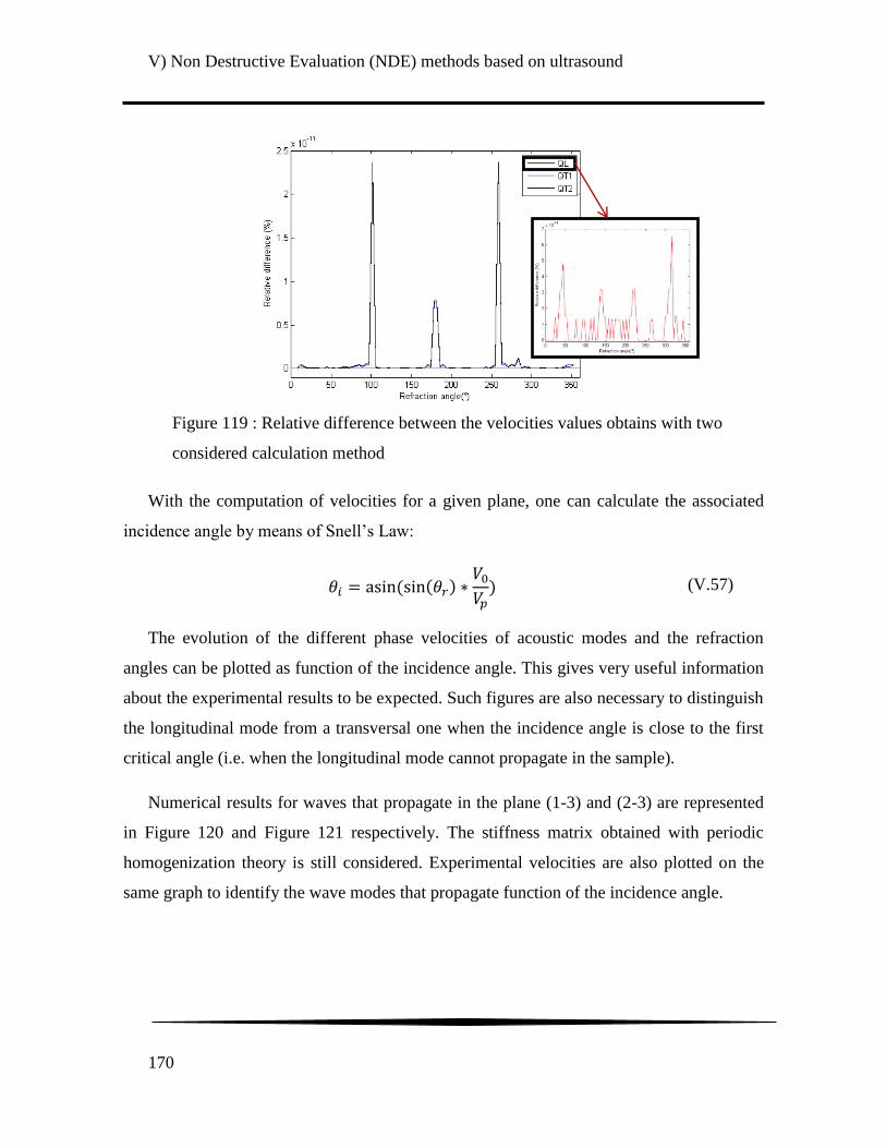
V) Non Destructive Evaluation (NDE) methods based on ultrasound
170
With the computation of velocities for a given plane, one can calculate the associated
incidence angle by means of Snell‟s Law:
(V.57)
The evolution of the different phase velocities of acoustic modes and the refraction
angles can be plotted as function of the incidence angle. This gives very useful information
about the experimental results to be expected. Such figures are also necessary to distinguish
the longitudinal mode from a transversal one when the incidence angle is close to the first
critical angle (i.e. when the longitudinal mode cannot propagate in the sample).
Numerical results for waves that propagate in the plane (1-3) and (2-3) are represented
in Figure 120 and Figure 121 respectively. The stiffness matrix obtained with periodic
homogenization theory is still considered. Experimental velocities are also plotted on the
same graph to identify the wave modes that propagate function of the incidence angle.
Figure 119 : Relative difference between the velocities values obtains with two
considered calculation method
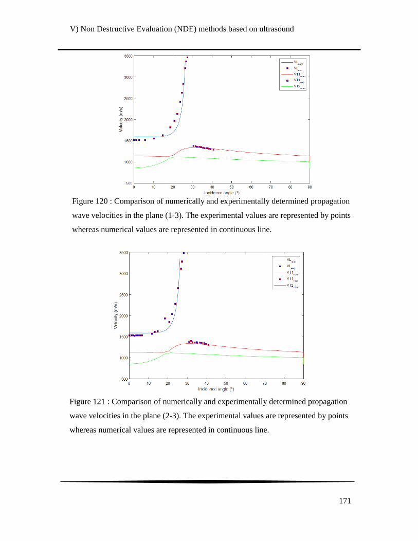
V) Non Destructive Evaluation (NDE) methods based on ultrasound
171
Figure 120 : Comparison of numerically and experimentally determined propagation
wave velocities in the plane (1-3). The experimental values are represented by points
whereas numerical values are represented in continuous line.
Figure 121 : Comparison of numerically and experimentally determined propagation
wave velocities in the plane (2-3). The experimental values are represented by points
whereas numerical values are represented in continuous line.

V) Non Destructive Evaluation (NDE) methods based on ultrasound
172
It was found that quasi-longitudinal and quasi-transversal 1 mode velocities were
measured in the two planes 1-3 and 2-3. In fact, the experimental velocities exhibit a good
correlation with the numerical ones for both modes. This result indicates that the calculated
stiffness tensor is a good choice for the initialization of the algorithm.
The dispersion curves of the woven glass fibers reinforced PA66/6 for waves
propagating in the 1-2 plane along the fibers axis was computed using the Disperse
software. They are visible in Figure 122. Those curves are necessary in order to know what
mode is propagated in the material for the chosen configuration. The frequency of every
recorded signal is carefully measured to compare the experimental results with numerical
dispersion curves. The mode S2 was found to propagate in the 1-2 planes. It is worth
mentioning that for the considered frequency range, the mode seems to be relatively little
dispersive. This made the measurement of the phase velocity and the calculation of the
stiffness components easier. Indeed, in order to simplify the optimization procedure, the
frequency is fixed to 2.1 MHz, as measured from the frequency spectrum of the propagated
signal.
Figure 122 : Dispersion curves computed with the Disperse software for guided
wave propagation in a 1.53mm thick studied composite along the fibers direction.
(a) Phase Velocities, (b): Group Velocities.
a) b)

V) Non Destructive Evaluation (NDE) methods based on ultrasound
173
Then, the phase velocity of this S2 mode is numerically computed, for the
experimentally measured frequencies, as a function of the direction of propagation in the 1-
2 plane from 0° to 45° from the warp direction. To do so, the stiffness tensor is rotated
along the 3 direction by the angle of the considered propagation direction. This result is
plotted in Figure 123 with the experimental velocities measured for the sample in the 0°
configuration. As for the acquisitions in plane 1-3 and 2-3, the experimental and numerical
phase velocities showed good correlation. The difference in velocity appears as a shift for
all the considered angle of propagation. This indicates that the numerical stiffness tensor
determined by periodic homogenization is underestimated in comparison with the real
sample elastic behavior.
Investigation of the optimization algorithm robustness to input parameters
Before using the optimization algorithm on experimental data, its robustness must be
evaluated. The most critical parameters are its sensitivity to the number of experimental
input data, the boundary limits of each stiffness constants and the initial guess of the
solution. In order to investigate its robustness, a set of simulated ultrasonic wave velocities
were calculated. Both the optimized stiffness components and their associated confidence
Figure 123 : Comparison between experimental and
numerical phase velocities for different propagation
direction in the 1-2 plane.

V) Non Destructive Evaluation (NDE) methods based on ultrasound
174
intervals are given for each set of simulated velocities. As mentioned above, the Christoffel
equation (V.9) is used for the plane 1-3 and 2-3 and the guided waves characteristic
equations (V.28) and (V.29) are used for the plane 1-2. In a first attempt, the velocities for
the 3 wave modes were calculated for refraction angles from 0° to 70°, with a step of 2°, for
the 2 main principle planes 1-3 and 2-3. This means 36 values for each wave mode, for
those two planes or 216 values in total. In addition, the S2 phase velocities were calculated
between 0° and 45°, with a step of 2°, based on the curve visible in Figure 123. As a matter
of fact, in this way 23 values were added for the optimization process. The lower and upper
bounds of the stiffness components were set to respectively 0.1 GPa and 200 GPa for each
component.
As initial guess, the expected stiffness matrix with a perturbation of 20%, 50%, 100%,
200%, 500% and 1000% is considered. The initial guess is then always an orthotropic
matrix. The results are summarized in the Table 18. It can be noted that even for large
deviation of the initial guess from the expected solution (x10), the accurate solution is
always found.
A next attempt was made with an initial guess that is not an orthotropic matrix. First,
the initial guess is chosen as 20GPa for each component, and then an isotropic stiffness
matrix is considered. The other parameters are unchanged. The initial guess and the
resultant optimized components are given in the Table 19. For the first initial guess tested,
the algorithm is not even able to start and find a new solution. However, when the isotropic
matrix is considered as initial guess, the algorithm is able to find the correct solution. The
optimization is then performed with an initial guess that is the isotropic matrix multiply by
10: the algorithm can still find the accurate solution.

V) Non Destructive Evaluation (NDE) methods based on ultrasound
175
C11 C12 C13 C22 C23 C33 C44 C55 C66
Expected
+ 20%
20
(0.1e-3)
2.1
(0.2e-3) 1.5
(0.2e-3)
20
(0.1e-3)
1.5
(0.2e-3) 4.5
(0.03e-3) 2.3
(0.04e-3) 1.3
(0.02e-3) 1.3
(0.02e-3)
Expected
+ 50%
20
(0.3e-3)
2.1
(0.7e-3) 1.5
(0.5e-3)
20
(0.4e-3)
1.5
(0.5e-3) 4.5
(0.1e-3) 2.3
(0.1e-3) 1.3
(0.07e-3) 1.3
(0.08e-3)
Expected
+ 100%
20
(0.07e-1)
2.1
(0.1e-1) 1.5
(0.1e-1)
20
(0.08e-1)
1.5
(0.1e-1) 4.5
(0.03e-1) 2.3
(0.02e-1) 1.3
(0.01e-1) 1.3
(0.01e-1)
Expected
+ 200% 20
(0.08e-2) 2.1
(0.1e-2) 1.5
(0.03e-2) 20
(0.02e-2) 1.5
(0.01e-2) 4.5
(0.01e-2) 2.3
(0.08e-2) 1.3
(0.1e-2) 1.3
(0.03e-2)
Expected
+ 500% 20
(0.09e-3) 2.1
(0.2e-3) 1.5
(0.1e-3)
20
(0.1e-3)
1.5
(0.2e-3) 4.5
(0.03e-3) 2.3
(0.03e-3) 1.3
(0.02e-3) 1.3
(0.02e-3)
Expected
+ 1000%
20
(0.2e-3)
2.1
(0.4e-3) 1.5
(0.3e-3)
20
(0.2e-3)
1.5
(0.4e-3) 4.5
(0.1e-3) 2.3
(0.7e-4) 1.3
(0.4e-4) 1.3
(0.4e-4)
Table 18 : Identified stiffness components for different orthotropic stiffness tensor as initial
guess of the solution. 239 velocity values are used as an input
The algorithm appears to be very reliable in finding accurate solution for various initial
guesses; even when the initial values insinuate a different symmetry. Nevertheless, the
mentioned first tests are insufficient to evaluate the efficiency of the considered
optimization algorithm for values obtained from experiments. Indeed, during experimental
acquisitions the time of flight of the quasi-transversal wave mode 2 usually cannot be
measured for plane 1-3 and 2-3. In addition, the number of incidence angles that can be
considered before wave modes vanish are less important as it can be seen in Figure 120,
Figure 121 and Figure 123. A new set of simulated ultrasonic wave velocities is now
computed based on the mentioned experimental observations. In order to account for
experimental errors during the time of flight measurements, a random perturbation up to
5% is applied on all the new wave velocities. Optimization tests similar to those performed
earlier on were then carried out. The obtained optimized stiffness constants and their
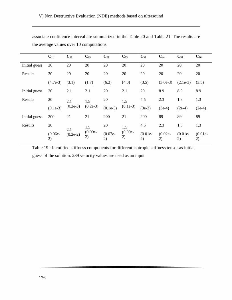
V) Non Destructive Evaluation (NDE) methods based on ultrasound
176
associate confidence interval are summarized in the Table 20 and Table 21. The results are
the average values over 10 computations.
C11 C12 C13 C22 C23 C33 C44 C55 C66
Initial guess 20 20 20 20 20 20 20 20 20
Results 20
(4.7e-3)
20
(3.1)
20
(1.7)
20
(6.2)
20
(4.0)
20
(3.5)
20
(3.0e-3)
20
(2.1e-3)
20
(3.5)
Initial guess 20 2.1 2.1 20 2.1 20 8.9 8.9 8.9
Results 20
(0.1e-3)
2.1
(0.2e-3) 1.5
(0.2e-3)
20
(0.1e-3)
1.5
(0.1e-3)
4.5
(3e-3)
2.3
(3e-4)
1.3
(2e-4)
1.3
(2e-4)
Initial guess 200 21 21 200 21 200 89 89 89
Results 20
(0.06e-
2)
2.1
(0.2e-2)
1.5
(0.09e-
2)
20
(0.07e-
2)
1.5
(0.09e-
2)
4.5
(0.01e-
2)
2.3
(0.02e-
2)
1.3
(0.01e-
2)
1.3
(0.01e-
2)
Table 19 : Identified stiffness components for different isotropic stiffness tensor as initial
guess of the solution. 239 velocity values are used as an input
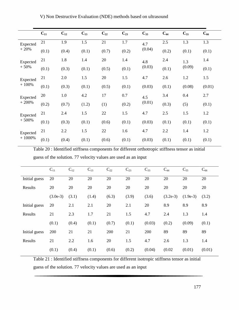
V) Non Destructive Evaluation (NDE) methods based on ultrasound
177
C11 C12 C13 C22 C23 C33 C44 C55 C66
Expected
+ 20%
21
(0.1)
1.9
(0.4)
1.5
(0.1)
21
(0.7)
1.7
(0.2)
4.7
(0.04)
2.5
(0.2)
1.3
(0.1)
1.3
(0.1)
Expected
+ 50%
21
(0.1)
1.8
(0.3)
1.4
(0.1)
20
(0.5)
1.4
(0.1)
4.8
(0.03)
2.4
(0.1)
1.3
(0.09)
1.4
(0.1)
Expected
+ 100%
21
(0.1)
2.0
(0.3)
1.5
(0.1)
20
(0.5)
1.5
(0.1)
4.7
(0.03)
2.6
(0.1)
1.2
(0.08)
1.5
(0.01)
Expected
+ 200%
20
(0.2)
1.0
(0.7)
4.2
(1.2)
17
(1)
0.7
(0.2)
4.5
(0.01)
3.4
(0.3)
0.4
(5)
2.7
(0.1)
Expected
+ 500%
21
(0.1)
2.4
(0.3)
1.5
(0.1)
22
(0.6)
1.5
(0.1)
4.7
(0.03)
2.5
(0.1)
1.5
(0.1)
1.2
(0.1)
Expected
+ 1000%
21
(0.1)
2.2
(0.4)
1.5
(0.1)
22
(0.6)
1.6
(0.1)
4.7
(0.03)
2.2
(0.1)
1.4
(0.1)
1.2
(0.1)
Table 20 : Identified stiffness components for different orthotropic stiffness tensor as initial
guess of the solution. 77 velocity values are used as an input
C11 C12 C13 C22 C23 C33 C44 C55 C66
Initial guess 20 20 20 20 20 20 20 20 20
Results 20
(3.0e-3)
20
(3.1)
20
(1.4)
20
(6.3)
20
(3.9)
20
(3.6)
20
(3.2e-3)
20
(1.9e-3)
20
(3.2)
Initial guess 20 2.1 2.1 20 2.1 20 8.9 8.9 8.9
Results 21
(0.1)
2.3
(0.4)
1.7
(0.1)
21
(0.7)
1.5
(0.1)
4.7
(0.03)
2.4
(0.2)
1.3
(0.09)
1.4
(0.1)
Initial guess 200 21 21 200 21 200 89 89 89
Results 21
(0.1)
2.2
(0.4)
1.6
(0.1)
20
(0.6)
1.5
(0.2)
4.7
(0.04)
2.6
(0.02
1.3
(0.01)
1.4
(0.01)
Table 21 : Identified stiffness components for different isotropic stiffness tensor as initial
guess of the solution. 77 velocity values are used as an input

V) Non Destructive Evaluation (NDE) methods based on ultrasound
178
Even with less simulated input velocities values, the algorithm can still find a stiffness
matrix close to the expected solution. The technique is therefore very robust. It is especially
relevant that TOF measurements of the modes “quasi-transversal 2” are not necessary to
find an appropriate solution. Indeed, this mode cannot be observed during experimental
investigations. The major deviation from the exact solution is observed for the components
C12 and C44.
Finally, in order to know the influence of experimental noise on the optimization
results, different levels of random perturbation is applied on the simulated input velocities
values. It is observed that deflection from the expected tensor only appears after 5 % of
induced perturbation. A maximum of 11 % deflection is measured for a 15 % perturbation
applied on the velocities. On measured time of flight an oscillation effect is noted (Figure
124). It was decided to fit the resulting curves by a fourth order polynomial. Both the
experimental data and the interpolate time of flight values are plotted in the Figure 124.
Those two sets of data are then used in the optimization algorithm, in order to have an idea
of the robustness of this algorithm to experimental uncertainty. After computation, it
appears that there is only a maximum of 1.5 % of difference between the rigidity constants
obtain with or without fitting the results. So the algorithm is robust enough to compute a
proper result despite of this kind of noise in the experimental results. As the oscillation in
the time of flight measurements does not induce significant difference to the results it is
decided not to smooth the resulting TOF for the further stages of the study.

V) Non Destructive Evaluation (NDE) methods based on ultrasound
179
C11 C12 C13 C22 C23 C33 C44 C55 C66
Perturbation
5%
21
(0.1)
1.9
(0.4)
1.5
(0.1)
21
(0.7)
1.7
(0.2)
4.7
(0.04)
2.5
(0.2)
1.3
(0.1)
1.3
(0.1)
Perturbation
15%
23.24
(0.4)
2.1
(1.1)
1.7
(0.4)
22.6
(2.1)
1.8
(0.5)
5.2
(0.1)
2.5
(0.3)
1.3
(0.3)
1.5
(0.4)
Perturbation
25%
25.3
(0.6)
1.5
(2.2)
2.5
(0.8)
24.0
(3.4)
1.5
(0.9)
5.5
(0.2)
3.3
(0.9)
1.1
(0.6)
1.9
(0.6)
Table 22 : Identified stiffness components with different level of perturbation on the
simulated input velocity values
The stiffness tensors were then computed with this optimization procedure using the
experimental velocities measured on the three planes 1-3, 2-3 and 1-2 for both 0° and 45°
configuration. As visible in Table 23, the optimized tensors are close to the numerically
determined values for both samples orientation. Some discrepancy can be noticed but the
symmetry of the material was correctly identified for both material and orders of magnitude
were correct. The experimental results for both samples in 0° and at 45° configuration and
damaged by tensile tests are described in the next subsection.
Figure 124 : Time of flight of longitudinal wave (Left) and transversal wave (Right)
for all the chosen incidence angles
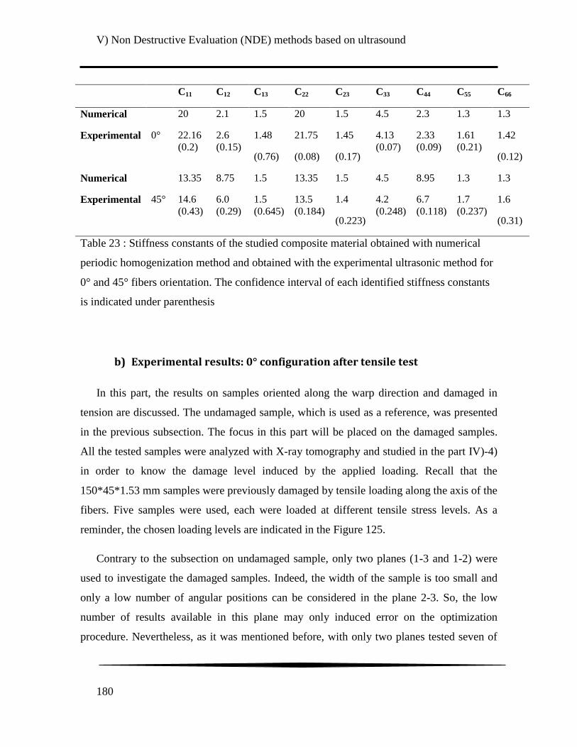
V) Non Destructive Evaluation (NDE) methods based on ultrasound
180
C11 C12 C13 C22 C23 C33 C44 C55 C66
Numerical
0°
20 2.1 1.5 20 1.5 4.5 2.3 1.3 1.3
Experimental 22.16
(0.2) 2.6
(0.15) 1.48
(0.76)
21.75
(0.08)
1.45
(0.17)
4.13
(0.07) 2.33
(0.09) 1.61
(0.21) 1.42
(0.12)
Numerical
45°
13.35 8.75 1.5 13.35 1.5 4.5 8.95 1.3 1.3
Experimental 14.6
(0.43) 6.0
(0.29) 1.5
(0.645) 13.5
(0.184) 1.4
(0.223)
4.2
(0.248) 6.7
(0.118) 1.7
(0.237) 1.6
(0.31)
Table 23 : Stiffness constants of the studied composite material obtained with numerical
periodic homogenization method and obtained with the experimental ultrasonic method for
0° and 45° fibers orientation. The confidence interval of each identified stiffness constants
is indicated under parenthesis
b) Experimental results: 0° configuration after tensile test
In this part, the results on samples oriented along the warp direction and damaged in
tension are discussed. The undamaged sample, which is used as a reference, was presented
in the previous subsection. The focus in this part will be placed on the damaged samples.
All the tested samples were analyzed with X-ray tomography and studied in the part IV)-4)
in order to know the damage level induced by the applied loading. Recall that the
150*45*1.53 mm samples were previously damaged by tensile loading along the axis of the
fibers. Five samples were used, each were loaded at different tensile stress levels. As a
reminder, the chosen loading levels are indicated in the Figure 125.
Contrary to the subsection on undamaged sample, only two planes (1-3 and 1-2) were
used to investigate the damaged samples. Indeed, the width of the sample is too small and
only a low number of angular positions can be considered in the plane 2-3. So, the low
number of results available in this plane may only induced error on the optimization
procedure. Nevertheless, as it was mentioned before, with only two planes tested seven of

V) Non Destructive Evaluation (NDE) methods based on ultrasound
181
the nine stiffness components of an orthotropic sample can be obtained. As a consequence,
during the optimization process, the value of C23 and C66 are fixed, to the values obtained
from periodic homogenization, because they cannot be determined without a third testing
principle plane. The evolution of the resulting stiffness components are presented in the
Table 24 and in Figure 126 for each of the seven computed components.
As first significant results, an important linear decrease of the C11 component with
increasing the loading is noticed. The same observation was made when the reduction of
the elastic modulus with the applied stress obtained in chapter III) is considered. A great
fall of the C13 parameter is also visible. A smaller decrease of C12 and C55 is noted. The
value of C22, C33 and C44 does not seem to really vary when compared to the other rigidity
components. It can be concluded that the rigidity components that are mostly altered during
this mechanical loading are the ones that depend of the loading direction (1), i.e. C11, C13
and C12.
Figure 125 : Stress/strain curve for a tensile test on a 0° oriented sample.
The red circles indicate the chosen loading for the five tested samples

V) Non Destructive Evaluation (NDE) methods based on ultrasound
182
Applied stress
(MPa) C11 C12 C13 C22 C33 C44 C55
0 22.21 2.57 1.41 21.81 4.10 2.33 1.58
100 21.45 1.65 0.5 21.78 3.68 2.71 1.08
150 21.1 2.24 0.01 22.41 3.61 2.41 1.24
200 20.98 1.85 0.2 21.82 3.78 2.28 1.14
250 20.04 1.91 0.008 21.91 3.67 2.77 1.21
300 20.23 1.18 0.03 21.28 4.09 2.685 1.33
Table 24 : Stiffness components of the studied composite material with an ultrasonic
method for various values of loading in tension for samples in the 0° configuration
Figure 126 : Evolution of seven of the stiffness components with the increase of the
loading for different 0° oriented sample

V) Non Destructive Evaluation (NDE) methods based on ultrasound
183
Another way to represent the stiffness evolution is to plot the stiffness curves of a tested
sample. A full set of velocities (QL, QT1 and QT2) are computed from the identified
stiffness matrixes obtained with the optimization procedure. The anisotropy of the
considered samples as well as the stiffness components affected by the mechanical
solicitation can be more accurately visualized. The results are plot in the
[rho*cos(r)*V2]*[rho*sin(r)*V
2] space. Indeed, if Chrisoffel equation (V.9) is considered it
is quickly apparent that the stiffness components are directly formulate in this space. For
example, in the principal plane 1-2, for a refraction angle of 0 one have rho*VL2=C11,
whereas for a refraction angle of 90 rho*VL2=C22. Stiffness curves of both the reference and
the highest damaged sample (300 MPa), for the principal plane 1-2, can be observed on the
Figure 127. Indications of some of the stiffness components that can be extracting from this
figure are indicated for each wave mode. The stiffness decreases previously discussed can
also be observed of this stiffness curves plot. That is to say, an important decrease of the
C11 component and a very low decrease of C22, observed from the red stiffness curves.
C44
C55
2
2
C22
2
1
C11
Figure 127 : Stiffness curves for two samples oriented at 0° from the fiber's
axis. An undamaged sample and a sample loaded in tension at 300 MPa

V) Non Destructive Evaluation (NDE) methods based on ultrasound
184
c) Experimental results: 45° configuration after tensile test
In the 45° configurations, another propagation plane, named X1-3 is considered. The
latter is of course oriented at 45° from the plane 1-3 used in the 0° configuration. Indeed,
when the sample is oriented at 45° from the warp direction, the axis of the sample will of
course correspond to the axis of the plane X1-3. The different planes of propagation are
illustrated in Figure 128 as a reminder. The X1-3 plane is not a principal plane of the
composite but the axis X1 remains an axis of symmetry in its undamaged state. The same
procedure can then be applied when undamaged. However, when submitted to tension at
45° from the warp direction, the damage induced in the sample can introduce loss in elastic
symmetry. This can be provoked by the fiber‟s reorientations or unexpected micro cracks
perpendicular to the loading direction; even though the Figure 84-b indicates that the
majority of the damage is appearing along the two fiber axis (i.e. -/+ 45°). Therefore, to
describe the elastic behavior of the samples oriented at 45° with respect to the warp
direction, thirteen stiffness components are necessary. The Christoffel equation is
consequently modified by considering C56, C14, C24 and C34 components for the stiffness
tensor. However, ultrasonic measurements in four planes are needed to have a good
estimation of these thirteen stiffness components. Some non-negligible errors may result
from this limitation in the number of measurements.

V) Non Destructive Evaluation (NDE) methods based on ultrasound
185
As in the previous part, different samples were loaded to different stress levels to induce
different damage states originate from the tensile test. After considering the stress to failure
(134 MPa) the chosen levels are set to 40, 80 and 120 MPa. They are indicated as a
reminder in Figure 129. The important results are presented below, in a similar way to the
previous subsection, in Figure 130 and Table 25.
Figure 128 : Schematic representation of the different propagation planes of
ultrasonic waves. For samples in the 0° configurations, the planes 1-3 and 1-2 were
used. For the samples in the 45° configuration, the plane X1-3 and 1-2 were used.
Figure 129 : Stress/strain curve for a tensile test on a 45° oriented
sample. The red circles indicate the chosen loading for the three tested
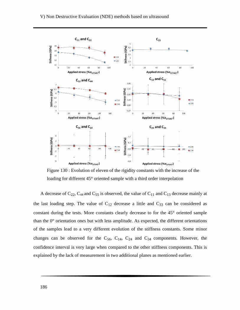
V) Non Destructive Evaluation (NDE) methods based on ultrasound
186
A decrease of C22, C44 and C55 is observed, the value of C11 and C13 decrease mainly at
the last loading step. The value of C12 decrease a little and C33 can be considered as
constant during the tests. More constants clearly decrease to for the 45° oriented sample
than the 0° orientation ones but with less amplitude. As expected, the different orientations
of the samples lead to a very different evolution of the stiffness constants. Some minor
changes can be observed for the C56, C14, C24 and C34 components. However, the
confidence interval is very large when compared to the other stiffness components. This is
explained by the lack of measurement in two additional planes as mentioned earlier.
Figure 130 : Evolution of eleven of the rigidity constants with the increase of the
loading for different 45° oriented sample with a third order interpolation
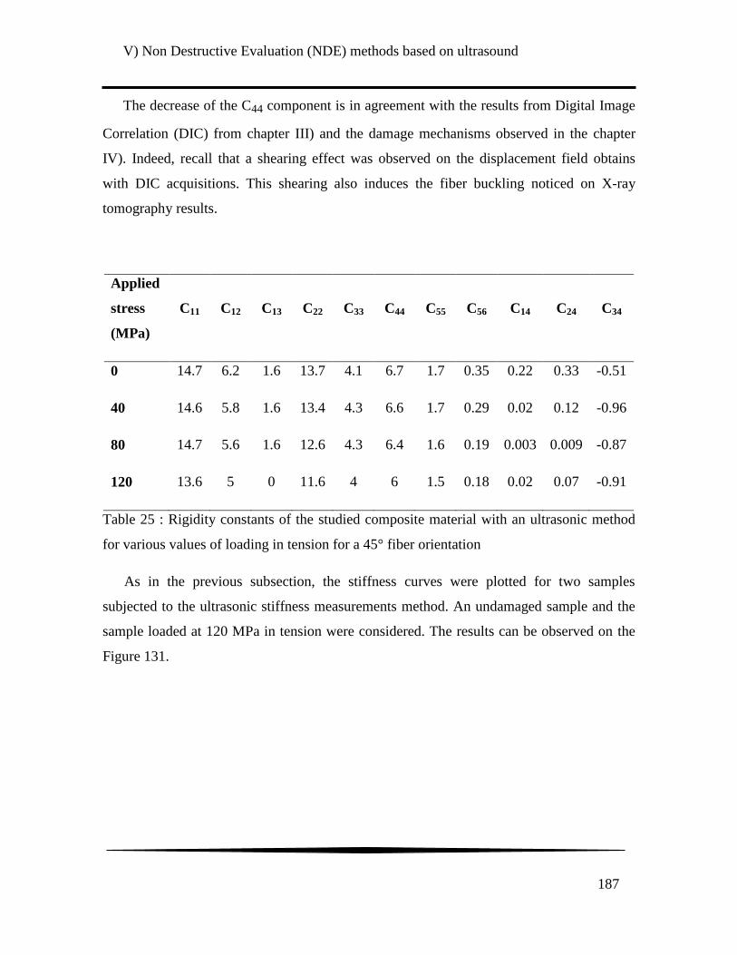
V) Non Destructive Evaluation (NDE) methods based on ultrasound
187
The decrease of the C44 component is in agreement with the results from Digital Image
Correlation (DIC) from chapter III) and the damage mechanisms observed in the chapter
IV). Indeed, recall that a shearing effect was observed on the displacement field obtains
with DIC acquisitions. This shearing also induces the fiber buckling noticed on X-ray
tomography results.
Applied
stress
(MPa)
C11 C12 C13 C22 C33 C44 C55 C56 C14 C24 C34
0 14.7 6.2 1.6 13.7 4.1 6.7 1.7 0.35 0.22 0.33 -0.51
40 14.6 5.8 1.6 13.4 4.3 6.6 1.7 0.29 0.02 0.12 -0.96
80 14.7 5.6 1.6 12.6 4.3 6.4 1.6 0.19 0.003 0.009 -0.87
120 13.6 5 0 11.6 4 6 1.5 0.18 0.02 0.07 -0.91
Table 25 : Rigidity constants of the studied composite material with an ultrasonic method
for various values of loading in tension for a 45° fiber orientation
As in the previous subsection, the stiffness curves were plotted for two samples
subjected to the ultrasonic stiffness measurements method. An undamaged sample and the
sample loaded at 120 MPa in tension were considered. The results can be observed on the
Figure 131.
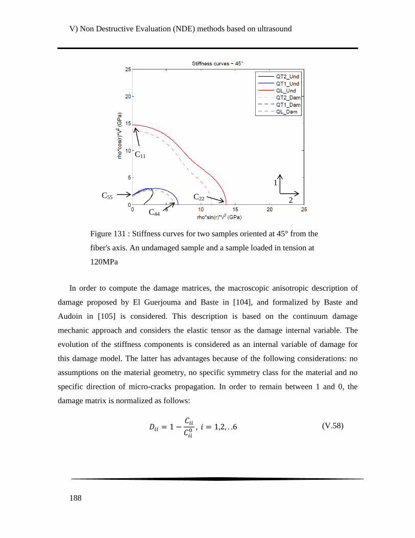
V) Non Destructive Evaluation (NDE) methods based on ultrasound
188
In order to compute the damage matrices, the macroscopic anisotropic description of
damage proposed by El Guerjouma and Baste in [104], and formalized by Baste and
Audoin in [105] is considered. This description is based on the continuum damage
mechanic approach and considers the elastic tensor as the damage internal variable. The
evolution of the stiffness components is considered as an internal variable of damage for
this damage model. The latter has advantages because of the following considerations: no
assumptions on the material geometry, no specific symmetry class for the material and no
specific direction of micro-cracks propagation. In order to remain between 1 and 0, the
damage matrix is normalized as follows:
(V.58)
C44
C22
C22
C11
C55
2
2
1
Figure 131 : Stiffness curves for two samples oriented at 45° from the
fiber's axis. An undamaged sample and a sample loaded in tension at
120MPa
2

V) Non Destructive Evaluation (NDE) methods based on ultrasound
189
√
(V.59)
The damage matrix has been calculated for the two samples orientations, this will result
in the anisotropic evolution of damage presented in Figure 132. As aforementioned, one
can note that the two samples configuration exhibit an evolution of their stiffness
components with the damage state induced by increasing the applied stress level different
from one another. For the samples in the 0° configuration, the highest evolution is achieved
by the components C11, C13, C55 and C12 to a lesser extent. The other components remain
mostly unaltered. However, for the sample in the 45° configuration, almost all components
seem to exhibit a noticeable evolution when increasing the applied stress level. It is first
worth recalling that the components C56, C14, C24, C34, have an important uncertainty on
their values as visible in Figure 130, therefore the associated evolution of damage must be
considered with caution. In addition, the evolution of C33 and C12 remain limited when
compared to the other components. At last, the evolution of C11, C13, C22, C44 and C55 is
really remarkable, in particular the last three. In this subsection, it was shown that the
ultrasonic method of rigidity constants measurement is very sensitive to the evolution of the
damage in the polyamide 66/6 reinforced with woven glass fibers. Another significant
result is that damage schemes, different from one another, were observed for the two
investigated sample configurations.
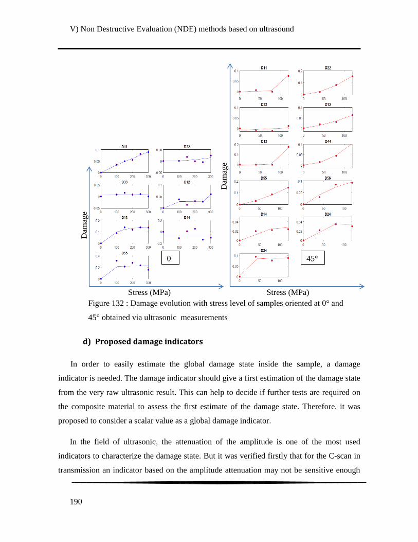
V) Non Destructive Evaluation (NDE) methods based on ultrasound
190
d) Proposed damage indicators
In order to easily estimate the global damage state inside the sample, a damage
indicator is needed. The damage indicator should give a first estimation of the damage state
from the very raw ultrasonic result. This can help to decide if further tests are required on
the composite material to assess the first estimate of the damage state. Therefore, it was
proposed to consider a scalar value as a global damage indicator.
In the field of ultrasonic, the attenuation of the amplitude is one of the most used
indicators to characterize the damage state. But it was verified firstly that for the C-scan in
transmission an indicator based on the amplitude attenuation may not be sensitive enough
Figure 132 : Damage evolution with stress level of samples oriented at 0° and
45° obtained via ultrasonic measurements
Stress (MPa)
Dam
age
Stress (MPa)
Dam
age
0 45°
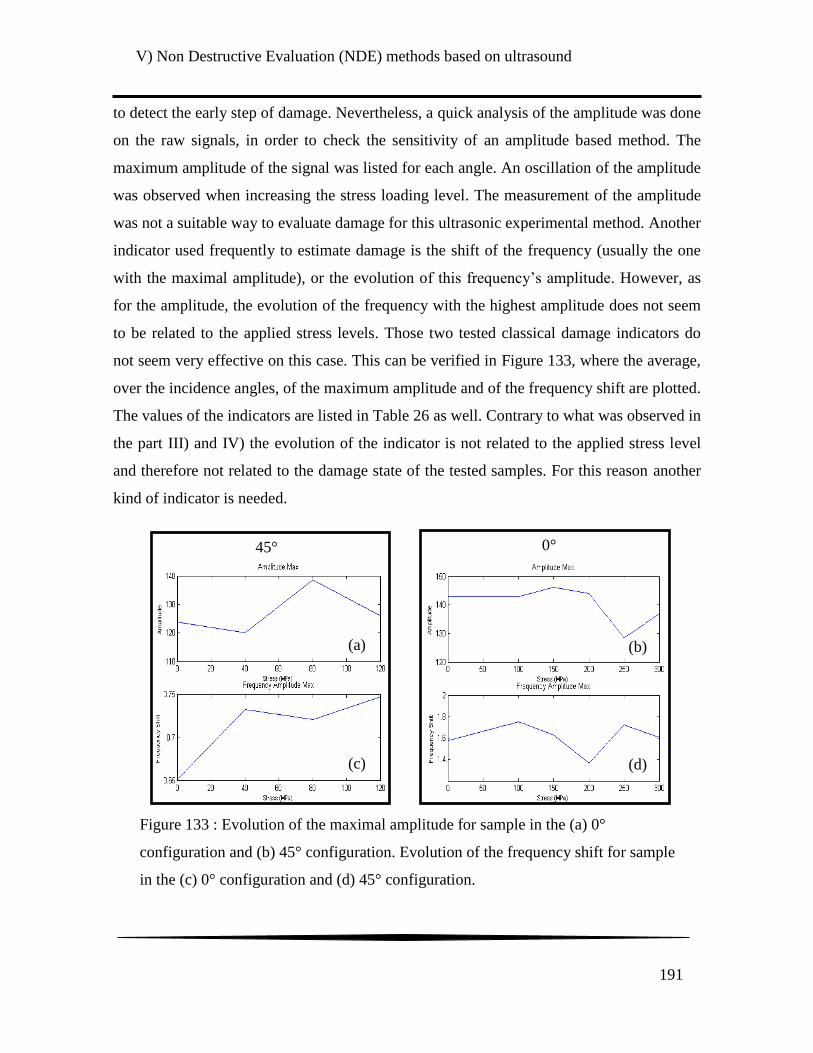
V) Non Destructive Evaluation (NDE) methods based on ultrasound
191
to detect the early step of damage. Nevertheless, a quick analysis of the amplitude was done
on the raw signals, in order to check the sensitivity of an amplitude based method. The
maximum amplitude of the signal was listed for each angle. An oscillation of the amplitude
was observed when increasing the stress loading level. The measurement of the amplitude
was not a suitable way to evaluate damage for this ultrasonic experimental method. Another
indicator used frequently to estimate damage is the shift of the frequency (usually the one
with the maximal amplitude), or the evolution of this frequency‟s amplitude. However, as
for the amplitude, the evolution of the frequency with the highest amplitude does not seem
to be related to the applied stress levels. Those two tested classical damage indicators do
not seem very effective on this case. This can be verified in Figure 133, where the average,
over the incidence angles, of the maximum amplitude and of the frequency shift are plotted.
The values of the indicators are listed in Table 26 as well. Contrary to what was observed in
the part III) and IV) the evolution of the indicator is not related to the applied stress level
and therefore not related to the damage state of the tested samples. For this reason another
kind of indicator is needed.
0° 45°
Figure 133 : Evolution of the maximal amplitude for sample in the (a) 0°
configuration and (b) 45° configuration. Evolution of the frequency shift for sample
in the (c) 0° configuration and (d) 45° configuration.
(a) (b)
(c) (d)
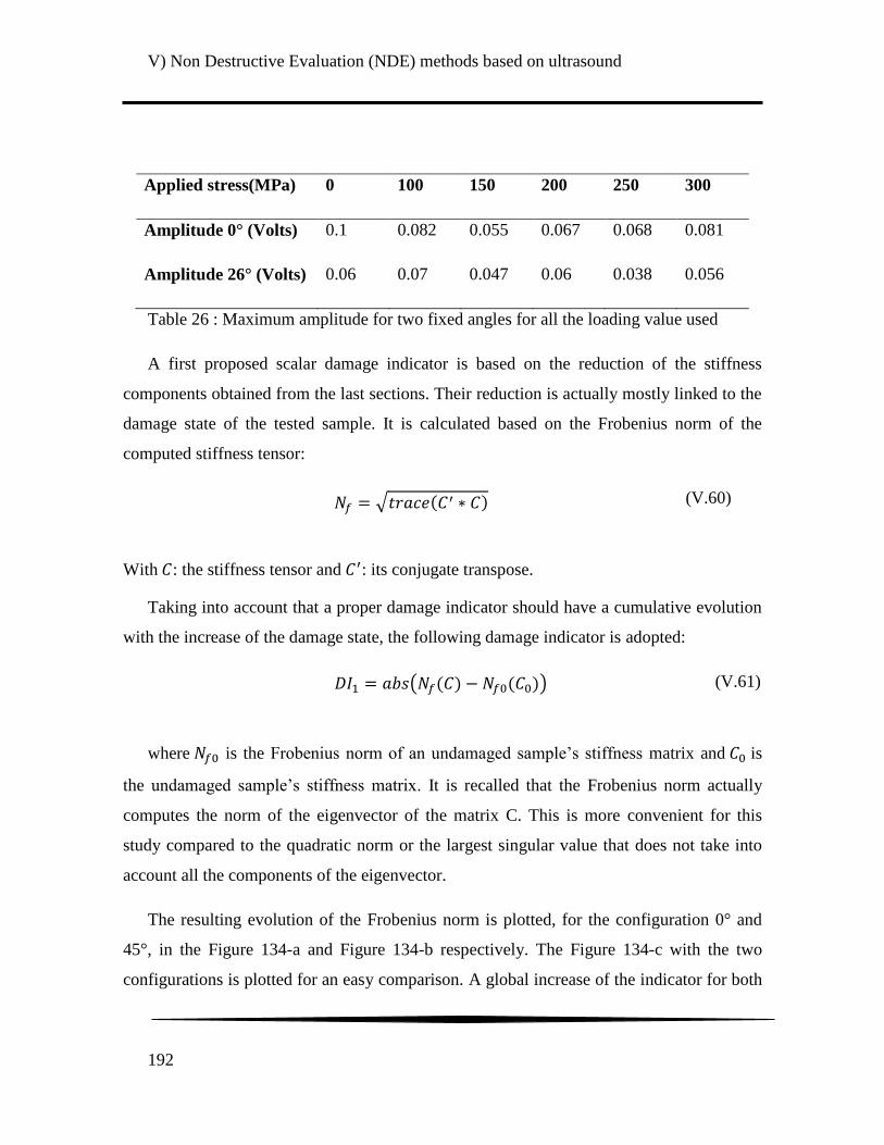
V) Non Destructive Evaluation (NDE) methods based on ultrasound
192
Applied stress(MPa) 0 100 150 200 250 300
Amplitude 0° (Volts) 0.1 0.082 0.055 0.067 0.068 0.081
Amplitude 26° (Volts) 0.06 0.07 0.047 0.06 0.038 0.056
Table 26 : Maximum amplitude for two fixed angles for all the loading value used
A first proposed scalar damage indicator is based on the reduction of the stiffness
components obtained from the last sections. Their reduction is actually mostly linked to the
damage state of the tested sample. It is calculated based on the Frobenius norm of the
computed stiffness tensor:
√ (V.60)
With : the stiffness tensor and : its conjugate transpose.
Taking into account that a proper damage indicator should have a cumulative evolution
with the increase of the damage state, the following damage indicator is adopted:
( ) (V.61)
where is the Frobenius norm of an undamaged sample‟s stiffness matrix and is
the undamaged sample‟s stiffness matrix. It is recalled that the Frobenius norm actually
computes the norm of the eigenvector of the matrix C. This is more convenient for this
study compared to the quadratic norm or the largest singular value that does not take into
account all the components of the eigenvector.
The resulting evolution of the Frobenius norm is plotted, for the configuration 0° and
45°, in the Figure 134-a and Figure 134-b respectively. The Figure 134-c with the two
configurations is plotted for an easy comparison. A global increase of the indicator for both
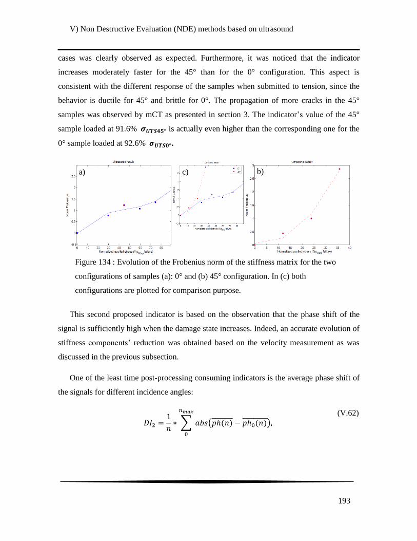
V) Non Destructive Evaluation (NDE) methods based on ultrasound
193
cases was clearly observed as expected. Furthermore, it was noticed that the indicator
increases moderately faster for the 45° than for the 0° configuration. This aspect is
consistent with the different response of the samples when submitted to tension, since the
behavior is ductile for 45° and brittle for 0°. The propagation of more cracks in the 45°
samples was observed by mCT as presented in section 3. The indicator‟s value of the 45°
sample loaded at 91.6% ° is actually even higher than the corresponding one for the
0° sample loaded at 92.6% °.
This second proposed indicator is based on the observation that the phase shift of the
signal is sufficiently high when the damage state increases. Indeed, an accurate evolution of
stiffness components‟ reduction was obtained based on the velocity measurement as was
discussed in the previous subsection.
One of the least time post-processing consuming indicators is the average phase shift of
the signals for different incidence angles:
∑ ( )
(V.62)
Figure 134 : Evolution of the Frobenius norm of the stiffness matrix for the two
configurations of samples (a): 0° and (b) 45° configuration. In (c) both
configurations are plotted for comparison purpose.
a) b) c)
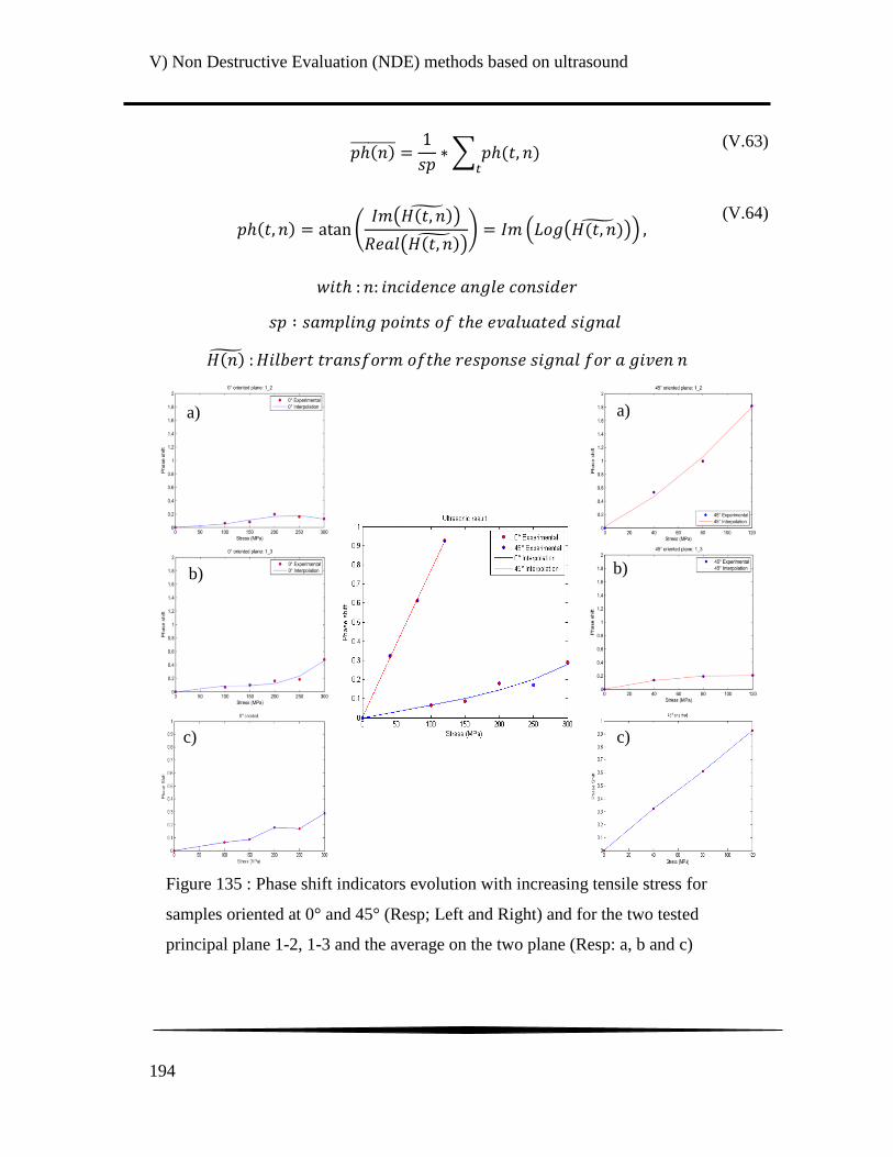
V) Non Destructive Evaluation (NDE) methods based on ultrasound
194
∑
(V.63)
(
( )
( )) ( ( ))
(V.64)
Figure 135 : Phase shift indicators evolution with increasing tensile stress for
samples oriented at 0° and 45° (Resp; Left and Right) and for the two tested
principal plane 1-2, 1-3 and the average on the two plane (Resp: a, b and c)
a)
b)
c)
a)
b)
c)

V) Non Destructive Evaluation (NDE) methods based on ultrasound
195
The evolution of this parameter was plotted for both samples‟ orientation as well as for
the two principal planes considered for the rigidity measurements, i.e. 1-2 and 1-3. The
average on the two principal planes is also represented. All the results can be found on the
Figure 135.
Contrary to the previously discussed indicators of damage, the phase shift does detect
an increase of the damage state as function of the applied tensile stress load. Then, if one
look at the central figure that compares the evolution of the indicator for the two samples‟
orientation, one can see a clear difference of the evaluated damage state. The increase of
damage is more important for the samples oriented at 45° from the fiber‟s axis. This result
is in correlation with the elastic modulus losses and void volume fraction evolution. This
can be verified on the Figure 136 on which those three indicators of the damage state are
presented.
4) Guided Lamb waves
As was discussed in the literature review section, Lamb waves are very effective to
study and evaluate the damage state of complex media. Indeed, recall that because of its
guided properties, a Lamb wave can investigate efficiently complex structures over long
Ultrasonic DI Void volume % Tensile tests
Figure 136 : Evolution of the void volume fraction evolution measured with X-ray
tomography; Signal phase shase shift measured with an ultrasonic method and the elastic
modulus loss measured during incremental cycling tensile tests
V) Non Destructive Evaluation (NDE) methods based on ultrasound
196
distances. Because of the necessity to have an ultrasonic damage evaluation method that
can be used to inspect various automotive parts, it was quickly chosen to investigate the
sensibility of guided waves. A clear difference was indeed observed with the proposed
phase shift indicator. Consequently, the current part is dedicated to the study of the
sensitivity of guided Lamb waves to different states of damage induced in the polyamide
66/6 reinforced by woven glass fibers composite material. The samples used in the previous
section were considered for the investigation of guided waves. However, prior to
considering the polyamide 66/6 reinforced by woven glass fibers, preliminary tests are
performed on an aluminum plate with defects of various sizes. Both the evolution of the
time shift and the signal amplitude will be investigated in order to be linked with the
evolution of damage magnitude.
a) Preliminary investigation on an aluminum plate
This is an aluminum plate of 470 x 470 x 5 mm with several defects within. Most of
them consist of holes of different diameter but a large notch was also induced. A photo of
this tested plate is visible in Figure 137, information on the different investigated defect is
also proposed in the Table 27. The guided waves investigations were performed in
transmission using two Panametrics V103 contact sensors of 1 MHz polarized
longitudinally. A waveform generator (Agilent Technilogy model) was used to create the
emitting signals. The signal is amplified after reception by an amplifier (from Krohn-Hite
model 7500) and eventually captured using an oscilloscope. The two transducers were
spaced by 4 cm and a coupling gel, Sofranel coupling Gel-D is used for both transducers to
increase the transmission between the two media. For these tests a burst of 5 cycles were
generated, frequencies of 500 Hz and 1 MHz were considered in order to investigate the
difference in sensibility in terms of damage detection. For each frequency, a transmitted
signal was acquired and used as a reference.
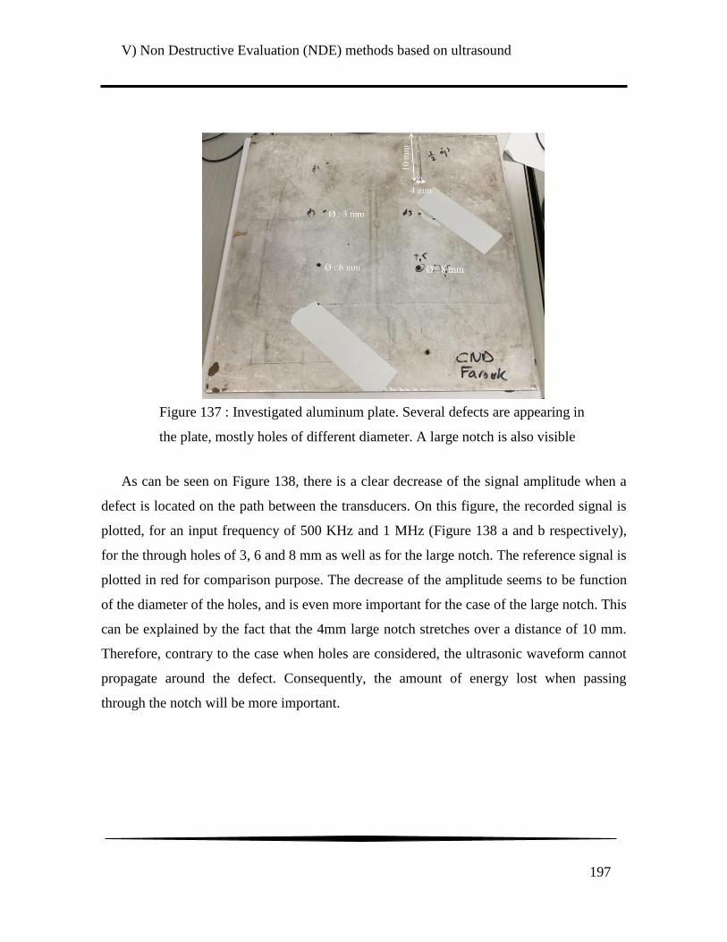
V) Non Destructive Evaluation (NDE) methods based on ultrasound
197
As can be seen on Figure 138, there is a clear decrease of the signal amplitude when a
defect is located on the path between the transducers. On this figure, the recorded signal is
plotted, for an input frequency of 500 KHz and 1 MHz (Figure 138 a and b respectively),
for the through holes of 3, 6 and 8 mm as well as for the large notch. The reference signal is
plotted in red for comparison purpose. The decrease of the amplitude seems to be function
of the diameter of the holes, and is even more important for the case of the large notch. This
can be explained by the fact that the 4mm large notch stretches over a distance of 10 mm.
Therefore, contrary to the case when holes are considered, the ultrasonic waveform cannot
propagate around the defect. Consequently, the amount of energy lost when passing
through the notch will be more important.
Figure 137 : Investigated aluminum plate. Several defects are appearing in
the plate, mostly holes of different diameter. A large notch is also visible

V) Non Destructive Evaluation (NDE) methods based on ultrasound
198
In order to quantify this reduction more precisely, it was chosen to calculate the energy
Es of the transmitted signal x(t). The latter was considered as a damage indicator because it
takes into account the full response of the guided waves signal. The integral is indeed
calculated on the entire response signal between the first positive peak and the time when
the signal became only noise. The energy was calculated for all the acquired signals using
this definition:
∫
The signal energy function of the size of the defects is indicated in Table 27 for both
considered frequencies. The signal energy with and without normalization by the energy of
the reference signal are determined. Indeed, a significant difference in the magnitude of the
energy is noted between 500 KHz and 1 MHz because the two transducers are centered at 1
MHz. However, after a normalization of the calculated energy by their respective reference
signal, both evolutions of the absolute energy are close and indicate a correlation with the
size of the considered defect. This damage indicator is effective to distinguish large defect
on samples. It will be now applied on the woven fiber reinforced polyamide 66/6.
Figure 138 : Transmitted signal for different defects and a reference case when a burst
of a) 500KHz and b) 1MHz is emitted
a) b)
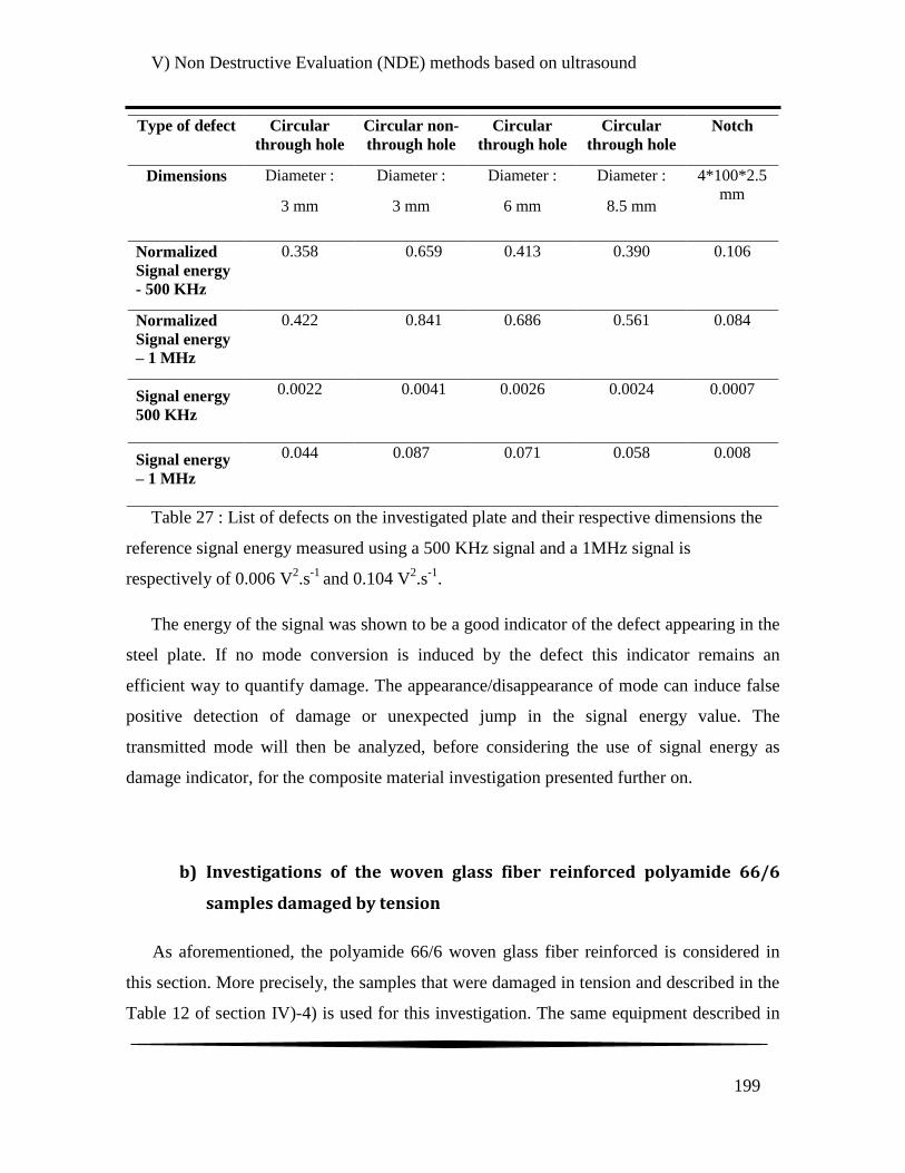
V) Non Destructive Evaluation (NDE) methods based on ultrasound
199
Type of defect Circular
through hole Circular non-
through hole Circular
through hole Circular
through hole Notch
Dimensions Diameter :
3 mm
Diameter :
3 mm
Diameter :
6 mm
Diameter :
8.5 mm
4*100*2.5
mm
Normalized
Signal energy
- 500 KHz
0.358 0.659 0.413 0.390 0.106
Normalized
Signal energy
– 1 MHz
0.422 0.841 0.686 0.561 0.084
Signal energy
500 KHz
0.0022 0.0041
0.0026 0.0024 0.0007
Signal energy
– 1 MHz
0.044 0.087
0.071 0.058 0.008
Table 27 : List of defects on the investigated plate and their respective dimensions the
reference signal energy measured using a 500 KHz signal and a 1MHz signal is
respectively of 0.006 V2.s
-1 and 0.104 V
2.s
-1.
The energy of the signal was shown to be a good indicator of the defect appearing in the
steel plate. If no mode conversion is induced by the defect this indicator remains an
efficient way to quantify damage. The appearance/disappearance of mode can induce false
positive detection of damage or unexpected jump in the signal energy value. The
transmitted mode will then be analyzed, before considering the use of signal energy as
damage indicator, for the composite material investigation presented further on.
b) Investigations of the woven glass fiber reinforced polyamide 66/6
samples damaged by tension
As aforementioned, the polyamide 66/6 woven glass fiber reinforced is considered in
this section. More precisely, the samples that were damaged in tension and described in the
Table 12 of section IV)-4) is used for this investigation. The same equipment described in

V) Non Destructive Evaluation (NDE) methods based on ultrasound
200
previous section will be considered here. In addition, the robot arm from the polar-scan will
be used to move precisely the receiver from one position to another on the tested samples.
As in the previous subsection, frequencies of 500 KHz and 1 MHz are planned for use.
However, a main frequency of 500 KHz was observed during preliminary analysis of the
transmitted guided waves in the frequency domain for both emitted frequencies. Therefore,
it was chosen to consider only the 500 KHz here in order to have a transmitted signal with
the main frequency at really center. Consequently, the waveform generator is used to emit a
500 KHz burst of 5 cycles. The emitting transducer is fixed on the sample and the receiving
transducer is moving so that the distance between the two transducers, noted di, goes from
4.25 cm to 7.25 cm a signal is recorded every 0.5 cm. The receiving transducer is attached
to a robot arm in order to control precisely the displacement between each increment
measurement. The experimental set-up is summarized in Figure 139. The two transducers
are on the same surface of the sample, which allows controlling the sample more easily
than with the method presented in section V)-3) that require an access to both surface of the
sample.
Analysis of dispersion curves/Lamb waves modes
In order to check that guided waves are indeed generate with this experimental set-up,
the dispersion curves will be calculated based on the signals recorded at different positions.
Indeed, as mentioned in the review section (V)-1)-c)), a representation of the dispersion
curves can be obtained by applying a 2D Fast Fourier Transform (2D FFT) on the obtained
wave signals. The mode(s) that propagate in the tested composite specimen can be
determined consequently. In addition, mode conversion can be induced by defect in a
X
Z
Receiver Emitter
Figure 139 : Experimental set-up of the guided waves experiment
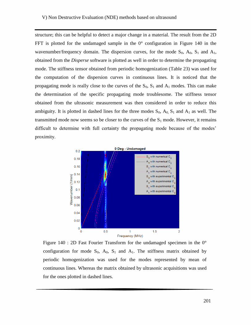
V) Non Destructive Evaluation (NDE) methods based on ultrasound
201
structure; this can be helpful to detect a major change in a material. The result from the 2D
FFT is plotted for the undamaged sample in the 0° configuration in Figure 140 in the
wavenumber/frequency domain. The dispersion curves, for the mode S0, A0, S1 and A1,
obtained from the Disperse software is plotted as well in order to determine the propagating
mode. The stiffness tensor obtained from periodic homogenization (Table 23) was used for
the computation of the dispersion curves in continuous lines. It is noticed that the
propagating mode is really close to the curves of the S0, S1 and A1 modes. This can make
the determination of the specific propagating mode troublesome. The stiffness tensor
obtained from the ultrasonic measurement was then considered in order to reduce this
ambiguity. It is plotted in dashed lines for the three modes S0, A0, S1 and A1 as well. The
transmitted mode now seems so be closer to the curves of the S1 mode. However, it remains
difficult to determine with full certainty the propagating mode because of the modes‟
proximity.
Figure 140 : 2D Fast Fourier Transform for the undamaged specimen in the 0°
configuration for mode S0, A0, S1 and A1. The stiffness matrix obtained by
periodic homogenization was used for the modes represented by mean of
continuous lines. Whereas the matrix obtained by ultrasonic acquisitions was used
for the ones plotted in dashed lines.
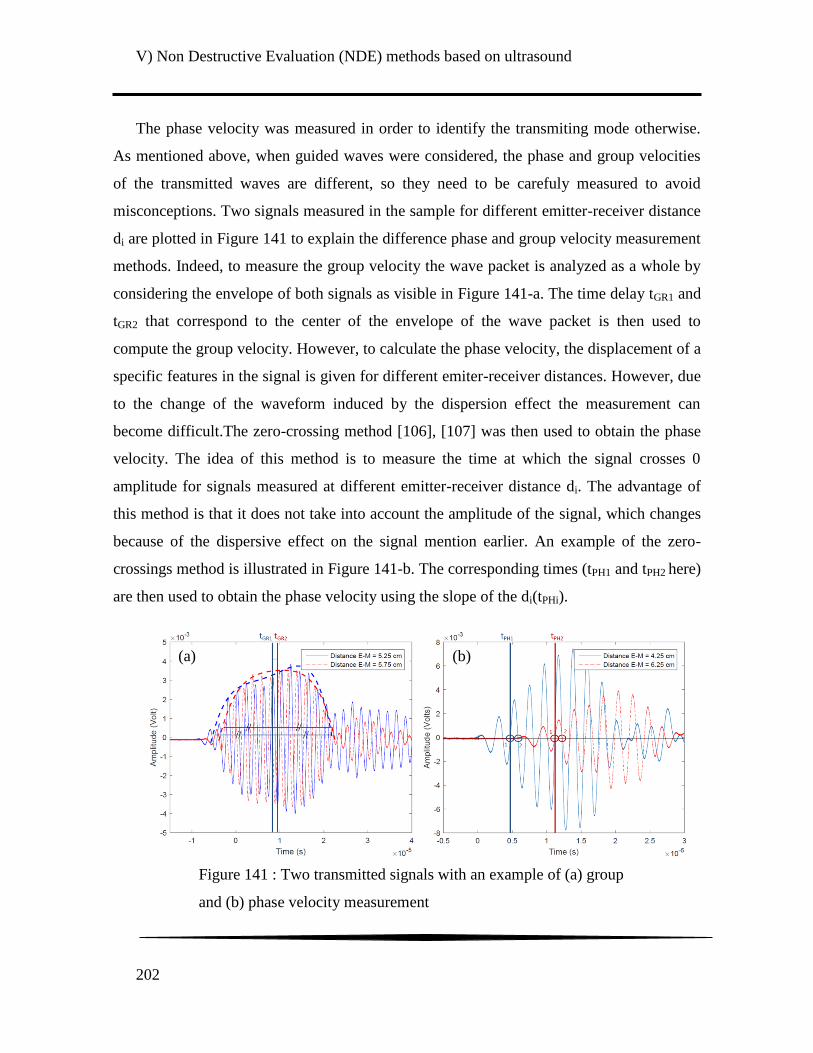
V) Non Destructive Evaluation (NDE) methods based on ultrasound
202
The phase velocity was measured in order to identify the transmiting mode otherwise.
As mentioned above, when guided waves were considered, the phase and group velocities
of the transmitted waves are different, so they need to be carefuly measured to avoid
misconceptions. Two signals measured in the sample for different emitter-receiver distance
di are plotted in Figure 141 to explain the difference phase and group velocity measurement
methods. Indeed, to measure the group velocity the wave packet is analyzed as a whole by
considering the envelope of both signals as visible in Figure 141-a. The time delay tGR1 and
tGR2 that correspond to the center of the envelope of the wave packet is then used to
compute the group velocity. However, to calculate the phase velocity, the displacement of a
specific features in the signal is given for different emiter-receiver distances. However, due
to the change of the waveform induced by the dispersion effect the measurement can
become difficult.The zero-crossing method [106], [107] was then used to obtain the phase
velocity. The idea of this method is to measure the time at which the signal crosses 0
amplitude for signals measured at different emitter-receiver distance di. The advantage of
this method is that it does not take into account the amplitude of the signal, which changes
because of the dispersive effect on the signal mention earlier. An example of the zero-
crossings method is illustrated in Figure 141-b. The corresponding times (tPH1 and tPH2 here)
are then used to obtain the phase velocity using the slope of the di(tPHi).
Figure 141 : Two transmitted signals with an example of (a) group
and (b) phase velocity measurement
(a) (b)
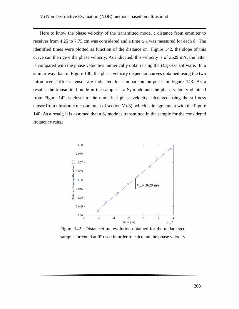
V) Non Destructive Evaluation (NDE) methods based on ultrasound
203
Here to know the phase velocity of the transmitted mode, a distance from emmiter to
receiver from 4.25 to 7.75 cm was considered and a time tPHi was measured for each di. The
identified times were plotted as function of the distance on Figure 142, the slope of this
curve can then give the phase velocity. As indicated, this velocity is of 3629 m/s, the latter
is compared with the phase velocities numerically obtain using the Disperse software. In a
similar way than in Figure 140, the phase velocity dispersion curves obtained using the two
introduced stiffness tensor are indicated for comparison purposes in Figure 143. As a
results, the transmitted mode in the sample is a S1 mode and the phase velocity obtained
from Figure 142 is closer to the numerical phase velocity calculated using the stiffness
tensor from ultrasonic measurement of section V)-3), which is in agreement with the Figure
140. As a result, it is assumed that a S1 mode is transmitted in the sample for the considered
frequency range.
Figure 142 : Distance/time evolution obtained for the undamaged
samples oriented at 0° used in order to calculate the phase velocity
Vph= 3629 m/s
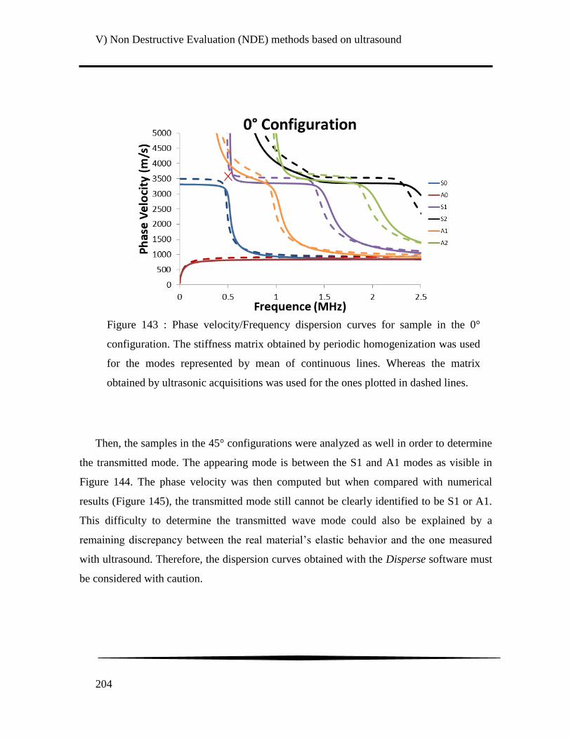
V) Non Destructive Evaluation (NDE) methods based on ultrasound
204
Then, the samples in the 45° configurations were analyzed as well in order to determine
the transmitted mode. The appearing mode is between the S1 and A1 modes as visible in
Figure 144. The phase velocity was then computed but when compared with numerical
results (Figure 145), the transmitted mode still cannot be clearly identified to be S1 or A1.
This difficulty to determine the transmitted wave mode could also be explained by a
remaining discrepancy between the real material‟s elastic behavior and the one measured
with ultrasound. Therefore, the dispersion curves obtained with the Disperse software must
be considered with caution.
Figure 143 : Phase velocity/Frequency dispersion curves for sample in the 0°
configuration. The stiffness matrix obtained by periodic homogenization was used
for the modes represented by mean of continuous lines. Whereas the matrix
obtained by ultrasonic acquisitions was used for the ones plotted in dashed lines.

V) Non Destructive Evaluation (NDE) methods based on ultrasound
205
Figure 144 : 2D Fast Fourier Transform for the undamaged specimen in the 45°
configuration for mode S0, A0, S1 and A1. The stiffness matrix obtained by periodic
homogenization was used for the modes represented by mean of continuous lines.
Whereas the matrix obtained by ultrasonic acquisitions was used for the ones plotted in
dashed lines.
Figure 145 : Phase velocity/Frequency dispersion curves for sample in the 45°
configuration. The stiffness matrix obtained by periodic homogenization was used
for the modes represented by mean of continuous lines. Whereas the matrix obtained
by ultrasonic acquisitions was used for the ones plotted in dashed lines.
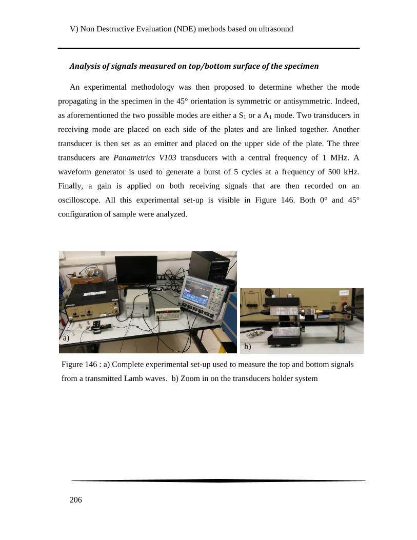
V) Non Destructive Evaluation (NDE) methods based on ultrasound
206
Analysis of signals measured on top/bottom surface of the specimen
An experimental methodology was then proposed to determine whether the mode
propagating in the specimen in the 45° orientation is symmetric or antisymmetric. Indeed,
as aforementioned the two possible modes are either a S1 or a A1 mode. Two transducers in
receiving mode are placed on each side of the plates and are linked together. Another
transducer is then set as an emitter and placed on the upper side of the plate. The three
transducers are Panametrics V103 transducers with a central frequency of 1 MHz. A
waveform generator is used to generate a burst of 5 cycles at a frequency of 500 kHz.
Finally, a gain is applied on both receiving signals that are then recorded on an
oscilloscope. All this experimental set-up is visible in Figure 146. Both 0° and 45°
configuration of sample were analyzed.
Figure 146 : a) Complete experimental set-up used to measure the top and bottom signals
from a transmitted Lamb waves. b) Zoom in on the transducers holder system
a) b)
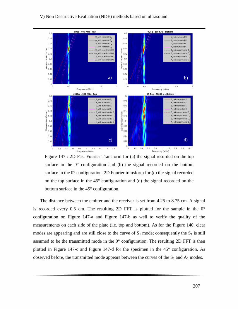
V) Non Destructive Evaluation (NDE) methods based on ultrasound
207
The distance between the emitter and the receiver is set from 4.25 to 8.75 cm. A signal
is recorded every 0.5 cm. The resulting 2D FFT is plotted for the sample in the 0°
configuration on Figure 147-a and Figure 147-b as well to verify the quality of the
measurements on each side of the plate (i.e. top and bottom). As for the Figure 140, clear
modes are appearing and are still close to the curve of S1 mode; consequently the S1 is still
assumed to be the transmitted mode in the 0° configuration. The resulting 2D FFT is then
plotted in Figure 147-c and Figure 147-d for the specimen in the 45° configuration. As
observed before, the transmitted mode appears between the curves of the S1 and A1 modes.
Figure 147 : 2D Fast Fourier Transform for (a) the signal recorded on the top
surface in the 0° configuration and (b) the signal recorded on the bottom
surface in the 0° configuration. 2D Fourier transform for (c) the signal recorded
on the top surface in the 45° configuration and (d) the signal recorded on the
bottom surface in the 45° configuration.
a) b)
c) d)
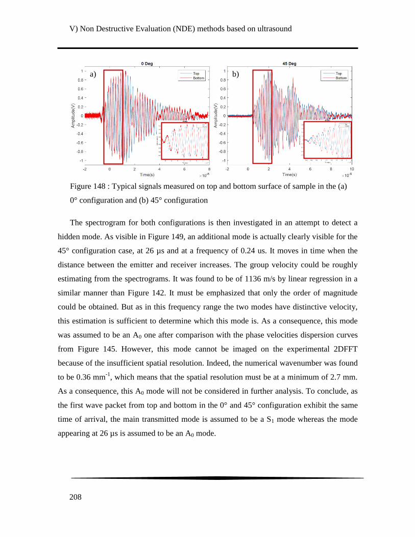
V) Non Destructive Evaluation (NDE) methods based on ultrasound
208
The spectrogram for both configurations is then investigated in an attempt to detect a
hidden mode. As visible in Figure 149, an additional mode is actually clearly visible for the
45° configuration case, at 26 µs and at a frequency of 0.24 us. It moves in time when the
distance between the emitter and receiver increases. The group velocity could be roughly
estimating from the spectrograms. It was found to be of 1136 m/s by linear regression in a
similar manner than Figure 142. It must be emphasized that only the order of magnitude
could be obtained. But as in this frequency range the two modes have distinctive velocity,
this estimation is sufficient to determine which this mode is. As a consequence, this mode
was assumed to be an A0 one after comparison with the phase velocities dispersion curves
from Figure 145. However, this mode cannot be imaged on the experimental 2DFFT
because of the insufficient spatial resolution. Indeed, the numerical wavenumber was found
to be 0.36 mm-1
, which means that the spatial resolution must be at a minimum of 2.7 mm.
As a consequence, this A0 mode will not be considered in further analysis. To conclude, as
the first wave packet from top and bottom in the 0° and 45° configuration exhibit the same
time of arrival, the main transmitted mode is assumed to be a S1 mode whereas the mode
appearing at 26 µs is assumed to be an A0 mode.
Figure 148 : Typical signals measured on top and bottom surface of sample in the (a)
0° configuration and (b) 45° configuration
b) a)
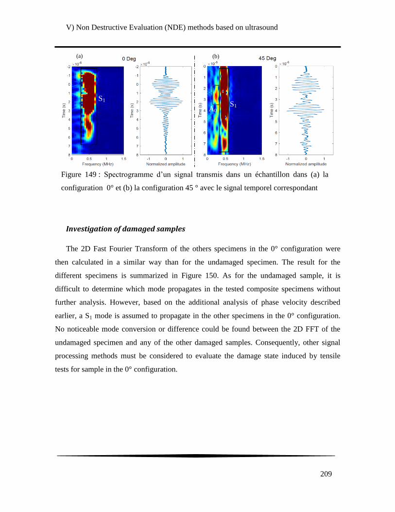
V) Non Destructive Evaluation (NDE) methods based on ultrasound
209
Investigation of damaged samples
The 2D Fast Fourier Transform of the others specimens in the 0° configuration were
then calculated in a similar way than for the undamaged specimen. The result for the
different specimens is summarized in Figure 150. As for the undamaged sample, it is
difficult to determine which mode propagates in the tested composite specimens without
further analysis. However, based on the additional analysis of phase velocity described
earlier, a S1 mode is assumed to propagate in the other specimens in the 0° configuration.
No noticeable mode conversion or difference could be found between the 2D FFT of the
undamaged specimen and any of the other damaged samples. Consequently, other signal
processing methods must be considered to evaluate the damage state induced by tensile
tests for sample in the 0° configuration.
Figure 149 : Spectrogramme d‟un signal transmis dans un échantillon dans (a) la
configuration 0° et (b) la configuration 45 ° avec le signal temporel correspondant
A0 S1
S1
(a) (b)

V) Non Destructive Evaluation (NDE) methods based on ultrasound
210
In a similar manner, the samples in the 45° configuration submitted to tensile tests were
analyzed in order to identify a potential mode conversion effect. However, when the
loading level reaches 80 MPa and 120 MPa the 2DFFT (Figure 151), gives inconclusive
results. For those samples, no transmitted mode can be really distinguished. This is mostly
due to signal attenuation when the tensile loading exceeds 80 MPa as will be discussed in
the next subsection.
Figure 150 : 2D Fast Fourier Transform for the samples, in the 0° configuration,
loaded in tension at a) 150, b) 200, c) 250 and d) 300MPa.
The stiffness matrix obtained by periodic homogenization was used for the modes
represented by mean of continuous lines. Whereas the matrix obtained by ultrasonic
acquisitions was used for the ones plotted in dashed lines.
a) b)
c) d)

V) Non Destructive Evaluation (NDE) methods based on ultrasound
211
Investigation of proposed damage indicators
In a next attempt, the evolution of the signal‟s amplitude was then investigated as in the
previous section. It was observed in section V)-4)-a) that the evolution of the signal energy
could be a good indicator to quantify the criticality of the damage state in a sample. The
undamaged sample and the sample loaded at the highest level, for both sample
Figure 151 : 2D Fast Fourier Transform for the samples, in the 45° configuration,
a) undamaged and loaded in tension at b) 40, c) 80 and d) 120MPa.
The stiffness matrix obtained by periodic homogenization was used for the modes
represented by mean of continuous lines. Whereas the matrix obtained by
ultrasonic acquisitions was used for the ones plotted in dashed lines.
a) b)
c) d)

V) Non Destructive Evaluation (NDE) methods based on ultrasound
212
configurations, were considered for a first approach. That is to say a sample loaded in
tension until 300 MPa along the warp‟s axis and a sample in the 45° configuration loaded
in tension until 120 MPa. The time signal is plotted in Figure 152 for all those considered
samples for a distance of 7.5 cm between the two transducers.
First of all, an attenuation of the signal, between the undamaged and damaged sample,
is noted for both fiber orientations. So a variation of the damage state can be detected with
this ultrasonic technique. During a first analysis, the attenuation is noticed to be higher for
the samples oriented at 45° from the yarns direction; as expected based on the results
presented in the previous sections of this manuscript. Those observations are also noted for
other distance between emitter and receiver.
In order to quantify this evolution in the damage state, the two damage indicators used
to investigate the defects on the aluminum plate were then used. Each indicator is
calculated for each experimentally considered transducer‟s positions. As a reminder, the
first indicator is just the highest amplitude of the signal response. The second proposed
damage indicator is the energy of the signal which is calculated as the area of the absolute
response signal.
Figure 152 : Time signal of guided waves propagation inside an undamaged and a
highly damage sample for a): Sample oriented at 0° from the yarns direction; b):
Sample oriented at 45° from the yarns direction
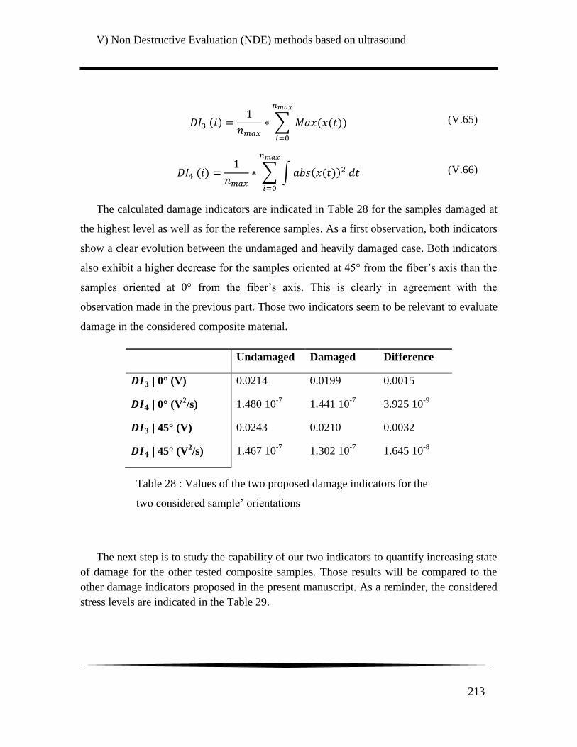
V) Non Destructive Evaluation (NDE) methods based on ultrasound
213
∑
(V.65)
∑ ∫
(V.66)
The calculated damage indicators are indicated in Table 28 for the samples damaged at
the highest level as well as for the reference samples. As a first observation, both indicators
show a clear evolution between the undamaged and heavily damaged case. Both indicators
also exhibit a higher decrease for the samples oriented at 45° from the fiber‟s axis than the
samples oriented at 0° from the fiber‟s axis. This is clearly in agreement with the
observation made in the previous part. Those two indicators seem to be relevant to evaluate
damage in the considered composite material.
Undamaged Damaged Difference
| 0° (V) 0.0214 0.0199 0.0015
| 0° (V2/s) 1.480 10
-7 1.441 10
-7 3.925 10
-9
| 45° (V) 0.0243 0.0210 0.0032
| 45° (V2/s) 1.467 10
-7 1.302 10
-7 1.645 10
-8
The next step is to study the capability of our two indicators to quantify increasing state
of damage for the other tested composite samples. Those results will be compared to the
other damage indicators proposed in the present manuscript. As a reminder, the considered
stress levels are indicated in the Table 29.
Table 28 : Values of the two proposed damage indicators for the
two considered sample‟ orientations

V) Non Destructive Evaluation (NDE) methods based on ultrasound
214
Applied stress
0° (MPa)
0 100 150 200 250 300
Applied stress
45° (MPa)
0 40 80 120 -- --
The same experimental procedure is considered for those samples. The calculated
values of the two damage indicators are plotted in Figure 153 for both considered samples‟
orientation.
Contrary to the preliminary results, the DI3 indicator does not seems to be reliable to
distinguish the different damage states. Indeed, its evolution is not a clear function of the
0° 45°
DI3
DI4
Figure 153 : Evolution the damage indicators DI3 for the samples oriented at 0°
and 45° in respectively a) and b).
Evolution the damage indicators DI4 for the samples oriented at 0° and 45° in
respectively c) and d)
a) b)
c) d)
Table 29 : Stress level of each sample considered for the experimental set-up
using guided waves

V) Non Destructive Evaluation (NDE) methods based on ultrasound
215
tensile loading. This is especially relevant for the samples oriented along the fiber‟s axis,
for which the indicator value starts to decrease after 150 MPa until 250 MPa. For the
samples oriented at 45° from the fiber‟s axis, the DI3 indicator announces a lower damage
state for the samples preliminary loaded at 40 MPa than for the undamaged sample. These
two results are in contradiction with the observations made in the previous sections of this
manuscript. This first indicator seems not to be reliable to quantify low amount of damage.
It could be used as an alert to prevent failure in a structural part but not accurately evaluate
the actual damage state.
However, the DI4 indicator (which is the signal energy) appears to be better in
agreement with the trend observed with the damage estimations from tensile tests, X-ray
tomography etc…. i.e. an evolution of the damage state as function of the loading level for
the two considered sample orientations. In addition, a more important increase of the global
damage state before breakage is also noted for the samples oriented at 45° from the fiber‟s
axis. This is particularly relevant in Figure 154 which proposes a comparison of the two
samples orientation for the two proposed damage indicators.
5) Conclusion
This chapter described an investigation of the different ultrasonic based Non
Destructive Evaluation (NDE) methods that were considered for this study. A
Figure 154 : Comparison of the evolution of the two considered damage
indicator, DI3 in (a) and DI4 in (b), for the two considered samples' orientation
a) b)
DI 3
DI 4
V) Non Destructive Evaluation (NDE) methods based on ultrasound
216
bibliographical review of many techniques based on ultrasound was firstly held. It was
meant to be focused on techniques that are currently under investigations by research teams
for an application on composites materials.
The samples damaged during tension tests were first investigated by mean of ultrasonic
C-scan in transmission. However, only macroscopic damage appearing on most damaged
samples in the 45° configuration could be imaged.
Then, because it was investigated in previous works, the stiffness components
measurement technique was chosen. In addition, it could provide a lot of information on
the residual stiffness properties of the tested material. A different evolution of the stiffness
properties between the sample tested in tension along the warp axis and the sample tested
in tension at 45° from the warp axis was indeed observed. This means a decrease mostly of
the stiffness components as function of the loading direction (namely C11, C12, C13 … ) for
samples in the 0° configuration. On the other hand, for samples in the 45° configuration,
almost all the stiffness components in the main plane of the sample (namely the plane of
the woven reinforcement) were impacted. A damage indicator based on the ultrasonic
measurement made for the stiffness components was then proposed. It consists of a
measurement of the phase shift between a pristine sample, used as a reference, and the
tested one for different incidence angles. It was shown to indicate a higher value for the
samples in the 45° configuration than for the ones in 0° configurations. This result is in
agreement with the observations made during the tensile tests or during the X-ray
tomography investigation, in respectively chapters III) and IV). Using this method of
stiffness constants measurements, an evolution of the residual mechanical properties of the
tested samples can be consequently obtained. This evolution can be used to later confirm
numerical results from finite elements for example. In addition, this method could give a
realistic estimation of the damage state of the tested specimens by considering
investigations in multiple directions. However, this method remains complicated for use
on-site in its current form. Another method that could more easily be used must then be
considered.
V) Non Destructive Evaluation (NDE) methods based on ultrasound
217
It was then chosen to use guided waves to investigate the damage growth in samples.
First, preliminary investigations on a steel plate with different induced defects showed that
the energy of the transmitted signal could be used to classify those defects by size. The
same method was consequently performed on the polyamide 66/6 reinforced with woven
glass fibers samples. It was shown to be able to quantify the damage state when used on
samples damaged by tension at a stepwise loading increment. Its evolution was shown to
be in accordance with the observation made in the previous sections; that is to say a higher
increase of the damage state for the sample in the 45° configuration than for the ones in the
0° configuration.
An investigation of the propagated guided waves mode was proposed beforehand but
does not give conclusive results to quantify the induced damage. When compared with the
results from the Disperse software, the mode S1 was found to propagate in the samples
oriented along the yarn‟s axis. For the undamaged sample in the 45° configuration, both S1
and A1 modes were found to propagate. However, neither mode conversion nor apparitions
of additional modes were observed in the damaged state of the samples in both
configurations. In this frequency range, the analysis of the propagated wave mode does not
seem to be able to characterize the damage state. It was just observed that when an applied
loading of 80 MPa is reached, the attenuation in the transmitted signal is too high to
properly use a 2D Fast Fourier Transform to distinguish any transmitted mode.

V) Non Destructive Evaluation (NDE) methods based on ultrasound
218

VI) Validation on samples impacted by drop weight
219
VI) Validation on samples impacted by drop weight
Contents
1) Drop weight impact tests ............................................................. 221
2) X-Ray tomography investigations of the impacted plates ........ 225
3) Ultrasonic C-scan results ............................................................. 226
4) Validation of the ultrasonic based damage indicators .............. 232
a) Ultrasonic measurement of stiffness components on the impacted plates ... 232
b) Guided waves based approach ...................................................................... 235
5) Conclusion ..................................................................................... 239
In the chapter V), the damage state, induced by tensile tests, of samples were
investigated by mean of ultrasonic based methods. However, in the automotive industry the
investigation of damage after impact, as well as, the study of fatigue post-impact is of
highest importance. Hence, the present chapter is dedicated to the validation of the
experimental approaches developed in chapter V). It focuses on the results for woven glass
fibers reinforced polyamide 66/6 plates damaged at different impact energies. More
specifically, drop weight test on geometrically adapted plates is considered. The damage
introduced through the impact is visually inspected and then is investigated via ultrasonic
C-scan imaging, in transmission and reflection. The related experimental results are deeply
discussed. The last subsection deals with the validation of the different proposed damage
indicators based on ultrasound. The evolution of stiffness components, with the impact
energy, is firstly obtained via ultrasonic measurements based on the method used in section
V)-3)-a). The two first damage indicators are consequently evaluated. Guided waves are
then used to investigate the samples. An attempt is made to validate the remaining two

VI) Validation on samples impacted by drop weight
220
damage indicators. However, it must be pointed out that another signal processing was
required to detect the damage induced in those samples.

VI) Validation on samples impacted by drop weight
221
1) Drop weight impact tests
Four woven glass fibers reinforced polyamide 66/6 plates of 100 mm x150 mm x1.53
mm (fibers oriented) were impacted at different drop weight energies, which are
respectively: 10, 15, 17.5 and 20 Joule. The specimens were all cut along the fibers axis (in
0° configuration). Information about the tested plates are sum-up in the Table 30. The
impact tests were performed in the LAMPA at ENSAM Angers campus with the help of Pr.
Laurent Guillaumat. A 16 mm diameter impactor of 1.02 kg was used. The plates were
clamped during the tests, a force sensor is mounted on the impactor and a displacement
sensor is installed below the plates (Figure 155). Both force vs time and displacement vs
time curves could therefore be extracted from the experiments, and they are plotted on the
Figure 156-a and Figure 156-b. The evolution of the energy E(t) is then computed as
∫
, with F the contact force and z the deflection, and plotted in Figure
156-c. Using the evolution of the energy, the real impact energy and the absorbed energy
are finally estimated as indicated in Figure 156-c. The real impact energy corresponds to
the maximal energy whereas the absorbed energy corresponds to the energy that remains
when the applied load returns to zero. This information is summed-up in Table 30. The
absorbed energy can also be estimated as the difference between the impact energy
and the rebound energy or: . They are calculated from the kinematic
energy relation:
and
. The two velocities are measured from the
displacement vs time curve respectively before and after the time when the impactor
rebound on the plate. It was found the evaluation of the absorbed energies using the integral
calculus and using the kinematic energies gives similar results. The absorbed energies
given in Table 30 were estimated using the first method.
On the force vs time curve, the plate impacted at 10 J exhibit measured force amplitude
clearly lower than the measured value for the other impacted samples. The same
observation can be done on the displacement time curve. In addition, the curves for the 20 J
shows important oscillation of the displacement; it must be mentioned that this effect is
only due to the saturation of the displacement transducer (sensor). This saturation may

VI) Validation on samples impacted by drop weight
222
induce errors in the calculation of the energy; consequently the measured impact energy
and the absorbed energy for the samples impacted at 20 J could be incorrect.
Plate number 8 9 7 10
Drop height (m) 1.00 1.50 1.75 2.00
Expected impact
energy (J) 10.00 15.00 17.50 20.00
Measured impact
energy (J) 8.92 14.45 16.36 17.59(*)
Absorbed energy (J) 3.24 6.65 7.73 4.48(*)
Table 30 : Drop height and impact energies of the four impacted composite plates. The
displacement sensor saturates during the test. The values with (*) must be considered with
caution because of the displacement sensor saturation noticed during some impact tests
Figure 155 : Drop weigh test machine installation of LAMPA at ENSAM Angers
campus
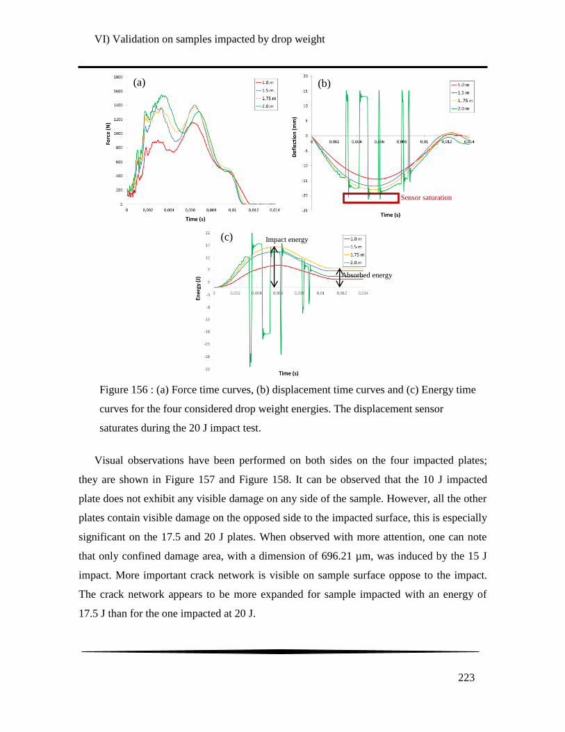
VI) Validation on samples impacted by drop weight
223
Visual observations have been performed on both sides on the four impacted plates;
they are shown in Figure 157 and Figure 158. It can be observed that the 10 J impacted
plate does not exhibit any visible damage on any side of the sample. However, all the other
plates contain visible damage on the opposed side to the impacted surface, this is especially
significant on the 17.5 and 20 J plates. When observed with more attention, one can note
that only confined damage area, with a dimension of 696.21 µm, was induced by the 15 J
impact. More important crack network is visible on sample surface oppose to the impact.
The crack network appears to be more expanded for sample impacted with an energy of
17.5 J than for the one impacted at 20 J.
Figure 156 : (a) Force time curves, (b) displacement time curves and (c) Energy time
curves for the four considered drop weight energies. The displacement sensor
saturates during the 20 J impact test.
(a) (b)
(c) Impact energy
Absorbed energy
Sensor saturation
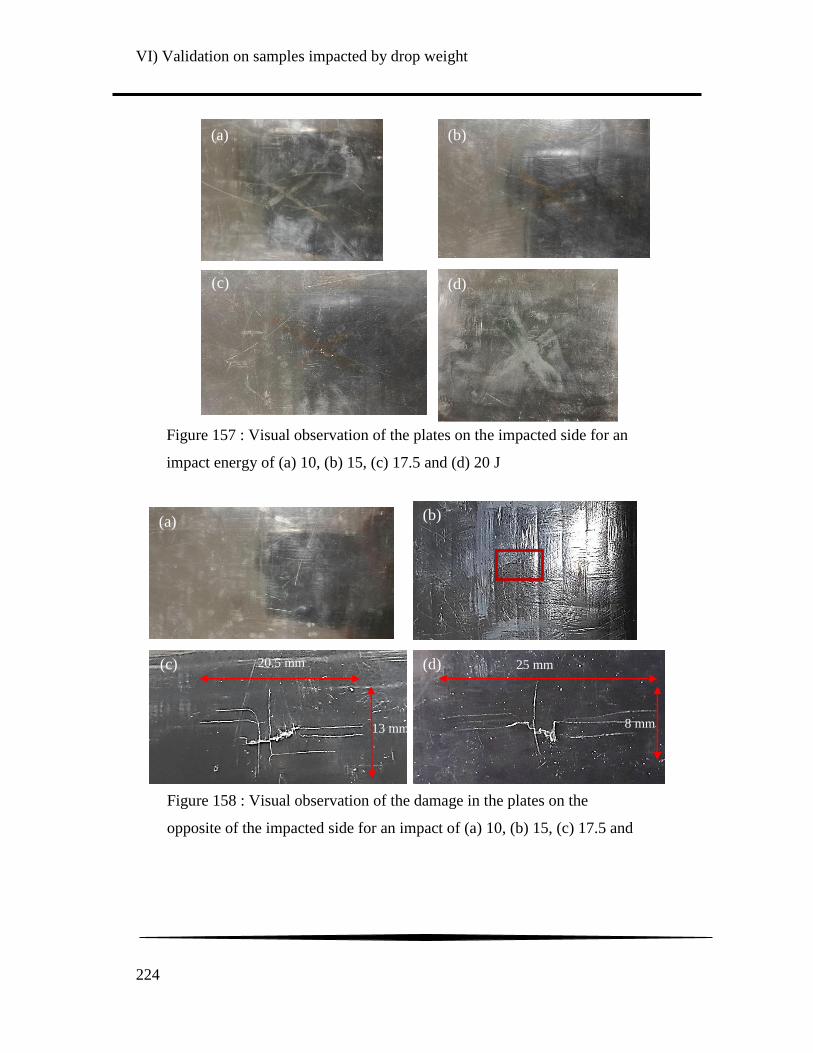
VI) Validation on samples impacted by drop weight
224
Figure 157 : Visual observation of the plates on the impacted side for an
impact energy of (a) 10, (b) 15, (c) 17.5 and (d) 20 J
(a)
(b)
(c)
(d)
Figure 158 : Visual observation of the damage in the plates on the
opposite of the impacted side for an impact of (a) 10, (b) 15, (c) 17.5 and
(d) 20 J
(a) (b)
(c) (d) 20.5 mm
13 mm
25 mm
8 mm

VI) Validation on samples impacted by drop weight
225
2) X-Ray tomography investigations of the impacted plates
The four plates were investigated using the X-ray tomography method presented and
used earlier in this manuscript. The same acquisition parameters as the ones in section IV)-
4) were considered for this investigation. It is worth reminding that volumes of 16.5 x 16.5
x 1.5 mm were obtained from those acquisitions. All the acquisitions were centered where
the plates were impacted. First of all, no particular damage was noticed on the plate
impacted at 10 J. The observed defects, such as micro-porosity and void near the yarn‟s
extremities does not look larger in size or present a larger extent than what has been
observed on undamaged samples investigated on chapter IV) For the sample impacted at 15
J, the crack visible on the surface was imaged. It was found to be a superficial crack with a
dimension of 0.7 mm compatible with the results found in the upper section. The other two
samples impacted at 17.5 J and 20 J, exhibit larger crack network with associated fibers
breakage. Images from those samples are respectively represented in Figure 159 and Figure
160. For both samples, the damaged area remains located in the first layer of the composite.
Crack network + Associated fiber
breakage on back surface
Fiber breakage
Crack network
17.5 J: Large crack network
Figure 159 : X-ray tomography observations performed on the impacted at an
energy level of 17.5 J
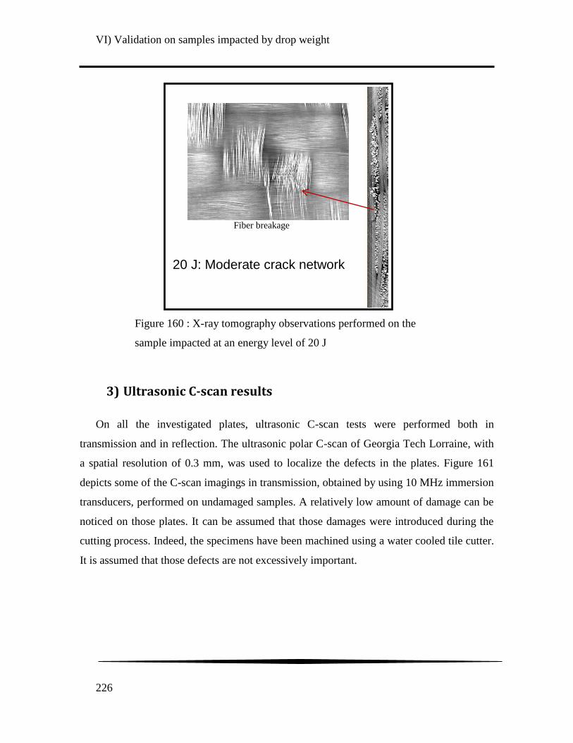
VI) Validation on samples impacted by drop weight
226
3) Ultrasonic C-scan results
On all the investigated plates, ultrasonic C-scan tests were performed both in
transmission and in reflection. The ultrasonic polar C-scan of Georgia Tech Lorraine, with
a spatial resolution of 0.3 mm, was used to localize the defects in the plates. Figure 161
depicts some of the C-scan imagings in transmission, obtained by using 10 MHz immersion
transducers, performed on undamaged samples. A relatively low amount of damage can be
noticed on those plates. It can be assumed that those damages were introduced during the
cutting process. Indeed, the specimens have been machined using a water cooled tile cutter.
It is assumed that those defects are not excessively important.
20 J: Moderate crack network
Fiber breakage
Figure 160 : X-ray tomography observations performed on the
sample impacted at an energy level of 20 J
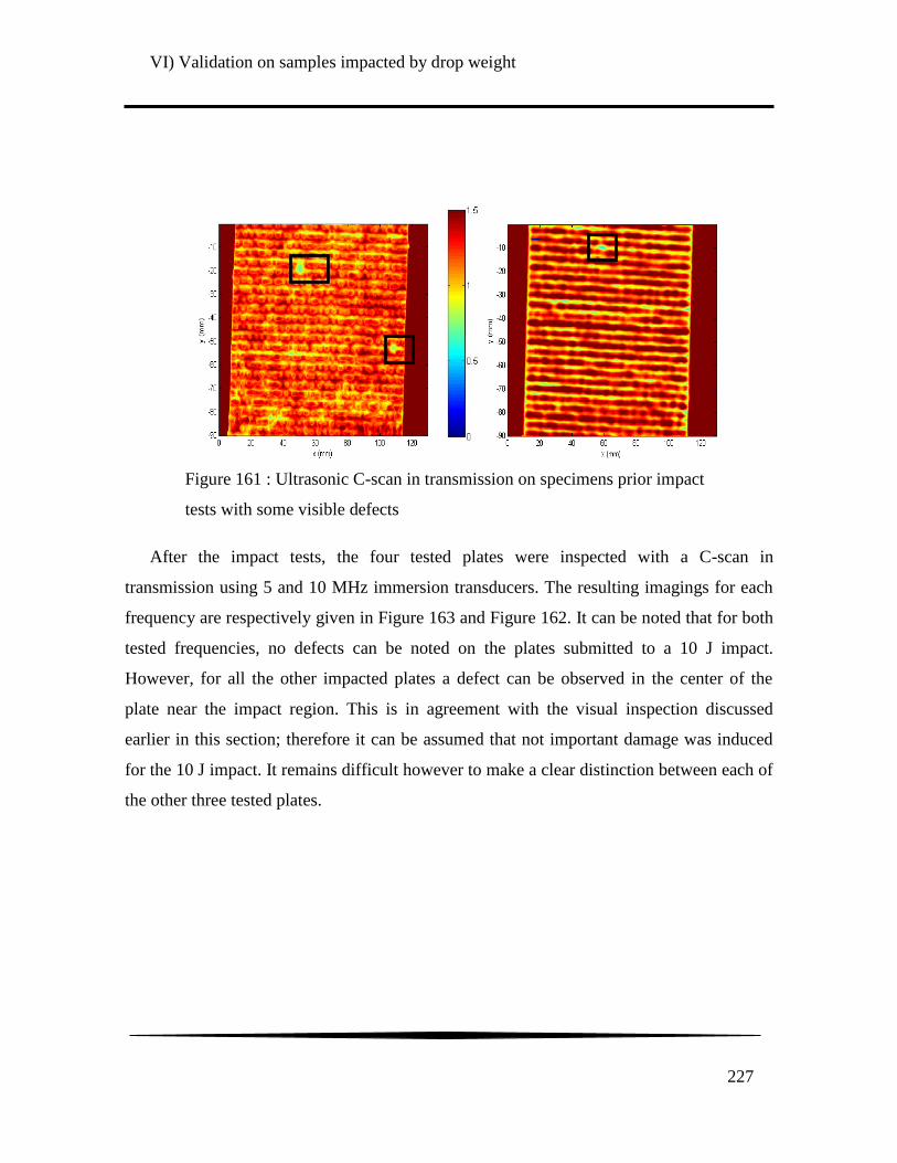
VI) Validation on samples impacted by drop weight
227
After the impact tests, the four tested plates were inspected with a C-scan in
transmission using 5 and 10 MHz immersion transducers. The resulting imagings for each
frequency are respectively given in Figure 163 and Figure 162. It can be noted that for both
tested frequencies, no defects can be noted on the plates submitted to a 10 J impact.
However, for all the other impacted plates a defect can be observed in the center of the
plate near the impact region. This is in agreement with the visual inspection discussed
earlier in this section; therefore it can be assumed that not important damage was induced
for the 10 J impact. It remains difficult however to make a clear distinction between each of
the other three tested plates.
Figure 161 : Ultrasonic C-scan in transmission on specimens prior impact
tests with some visible defects
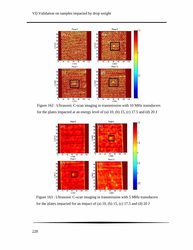
VI) Validation on samples impacted by drop weight
228
Figure 162 : Ultrasonic C-scan imaging in transmission with 10 MHz transducers
for the plates impacted at an energy level of (a) 10, (b) 15, (c) 17.5 and (d) 20 J
(a) (b)
(c) (d)
Figure 163 : Ultrasonic C-scan imaging in transmission with 5 MHz transducers
for the plates impacted for an impact of (a) 10, (b) 15, (c) 17.5 and (d) 20 J
(a) (b)
(c) (d)

VI) Validation on samples impacted by drop weight
229
Finally, ultrasonic C-scans in reflection were carried out on the four samples. A 10
MHz immersion focused transducer was used for the investigations. This study is
considered in order to localize the defects along the thickness of the samples. To do so, two
scans were performed on each sample, one on the impacted side and other on the opposite
side. The obtained imagings for the plate impacted at 20 J are all shown in Figure 164. On
both investigated surfaces the location of damage induced by the impact could be
identified. It can be found at the area where the black lines intersect. B-scan observations
along the thickness are proposed along those black lines. For the B-scan imaging performed
on the surface with the damage visible, discontinuity appear near the impact location.
However, it is not possible to locate the position along the thickness of the defect because
of reverberation effect that seems to be induced. On the imaging from the impacted surface,
one can see that no damage is noted on the first reflection line; an unaltered line is actually
clearly visible. However, a permanent indentation, that could not be detected prior this
investigation, is also identified at the location of the impact. This defect is caused by the
impact and is usually referred to as a Barely Visible Indentation Damage (BVID). This
visible indentation is used during visual inspection to indicate the presence of internal
impact induced damage as explained in the Figure 165. For the plate impacted at 20 J, this
permanent indentation was actually not noticeable by naked eye earlier on. The permanent
indentation was consequently in the Barely Visible Indentation Damage (BVID) domain.
Figure 164 : Ultrasonic imaging in reflection of the plate impacted at 20 J. Impacted side
(Left) and the opposite one (Right). B-scan in the X and Y directions for both side.
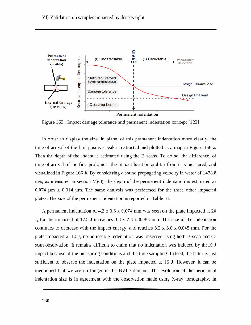
VI) Validation on samples impacted by drop weight
230
In order to display the size, in plane, of this permanent indentation more clearly, the
time of arrival of the first positive peak is extracted and plotted as a map in Figure 166-a.
Then the depth of the indent is estimated using the B-scans. To do so, the difference, of
time of arrival of the first peak, near the impact location and far from it is measured, and
visualized in Figure 166-b. By considering a sound propagating velocity in water of 1478.8
m/s, as measured in section V)-3), the depth of the permanent indentation is estimated as
0.074 µm ± 0.014 µm. The same analysis was performed for the three other impacted
plates. The size of the permanent indentation is reported in Table 31.
A permanent indentation of 4.2 x 3.6 x 0.074 mm was seen on the plate impacted at 20
J; for the impacted at 17.5 J it reaches 3.8 x 2.8 x 0.088 mm. The size of the indentation
continues to decrease with the impact energy, and reaches 3.2 x 3.0 x 0.045 mm. For the
plate impacted at 10 J, no noticeable indentation was observed using both B-scan and C-
scan observation. It remains difficult to claim that no indentation was induced by the10 J
impact because of the measuring conditions and the time sampling. Indeed, the latter is just
sufficient to observe the indentation on the plate impacted at 15 J. However, it can be
mentioned that we are no longer in the BVID domain. The evolution of the permanent
indentation size is in agreement with the observation made using X-ray tomography. In
Figure 165 : Impact damage tolerance and permanent indentation concept [123]
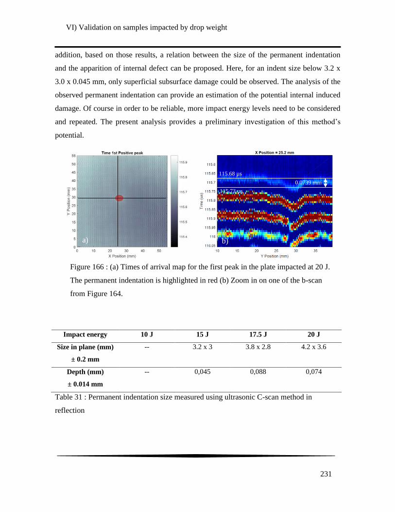
VI) Validation on samples impacted by drop weight
231
addition, based on those results, a relation between the size of the permanent indentation
and the apparition of internal defect can be proposed. Here, for an indent size below 3.2 x
3.0 x 0.045 mm, only superficial subsurface damage could be observed. The analysis of the
observed permanent indentation can provide an estimation of the potential internal induced
damage. Of course in order to be reliable, more impact energy levels need to be considered
and repeated. The present analysis provides a preliminary investigation of this method‟s
potential.
Impact energy 10 J 15 J 17.5 J 20 J
Size in plane (mm)
± 0.2 mm
-- 3.2 x 3 3.8 x 2.8 4.2 x 3.6
Depth (mm)
± 0.014 mm
-- 0,045 0,088 0,074
Table 31 : Permanent indentation size measured using ultrasonic C-scan method in
reflection
Figure 166 : (a) Times of arrival map for the first peak in the plate impacted at 20 J.
The permanent indentation is highlighted in red (b) Zoom in on one of the b-scan
from Figure 164.
115.68 µs
115.73 µs
0.0739 mm
a) b)
VI) Validation on samples impacted by drop weight
232
4) Validation of the ultrasonic based damage indicators
a) Ultrasonic measurement of stiffness components on the impacted
plates
The four impacted plates are investigated with the ultrasonic method of stiffness
components measurement described in the previous chapter. Since those plates are bigger
than the tensile samples presented in the two previous sections, the three main planes of the
samples are investigated whereas only two could be used for the tensile samples. Therefore,
the nine stiffness components may be identified as for the first undamaged sample
presented in the section V)-3)-a). The nine obtained stiffness components for the four plates
are represented on the Figure 167. The components obtained on the undamaged sample in
section VI)-2)-a) are also added on those graphs. It must be pointed out that those results
come from another experiment campaign; therefore the measurement uncertainties could
not be comparable to those determined for the present section. However, the stiffness
components identified on the sample impacted at 10 J are close to the ones acquired on
tensile tests samples.
When compared to the stiffness components evolution performed in chapter V), the
observed scheme is different from the ones observed for samples damaged by tension. This
indicates that this method can still evaluate damage state that results for different kind of
mechanical solicitations. A global decrease of the components is noticed starting from 17.5
J at the exception of C12, C44 and at a lower level the C55. However, it must be noted that
the uncertainty on the C12 and C44 is very important; it remains difficult to be sure of the
evolution depicted. This is in accordance with the estimation of damage from other
techniques. That said the damage state of the sample impacted at 17.5 J clearly differs from
the two samples impacted at lower energy. It is difficult however to conclude on the
sensitivity of the method to detecting the damage on the sample impacted at 15 J. A
decrease of the components C11 and C13 from 10 J compared to 15 J is noted but remains
low in amplitude compared to the decrease from 15 J to 17.5 J. The following important

VI) Validation on samples impacted by drop weight
233
point is to know if the difference, in terms of damage level, between the sample impacted at
17.5 J and the sample impacted at 20 J could be determined. However, as for the
investigation by mean of X-ray tomography, it is difficult to draw a definitive conclusion.
Indeed, only minor evolution of the components is noted between 17.5 J and 20 J.
Therefore, others impact energies should be considered to determine the correct evolution
of stiffness components when increasing the impact energy.
In a similar manner, as for the samples damaged by quasi-static tension loading, the
proposed ultrasound based damage indicators are calculated in this subsection. It is worth
recalling, that the first damage indicator is calculated as the Frobenius norm of the
Figure 167 : Evolution of the nine stiffness components of the tested composite
material when increasing drop weight energy

VI) Validation on samples impacted by drop weight
234
computed stiffness tensor. The second indicator is calculated as the average, over the three
investigated main planes of the composite, of the phase shift between signals propagating in
the damaged sample and signals propagating in a reference undamaged sample. They are
referred to as DI1 and DI2 later in this section as in section V)-3)-d). The evolution of the
two indicators is plotted in Figure 168 as function of the chosen impact energy.
The two indicators exhibit a similar evolution when increasing the impact energy. For
both curves, the indicator starts to increase noticeably after an impact of 15 J. A step
between 15 J and 17.5 J is visible for both cases. It is more pronounced however for the
Frobenius norm. Finally, the value of the indicator continues to increase until 20 J. This
observed evolution of the two proposed indicators is in agreement with the samples
analysis performed using X-Ray tomography. Indeed, no noticeable damage was detected
on the samples impacted at 10 J, whereas a minor damage was seen on the 15 J impacted
samples and, finally, the two other samples exhibit large cracks network.
Figure 168 : (a) Evolution of the Frobenius norm of the stiffness tensor
obtained by ultrasound method and (b) evolution of the phase shift indicator
with the impact energy
(a)
(b)

VI) Validation on samples impacted by drop weight
235
b) Guided waves based approach
The same experimental procedure using guided waves, introduced in V)-4), in used on
the four impacted composite plates. Two 1 MHz Panametrics V103 contact transducers are
used in transmission. They are put on the surface of the plate on each side of the location
were the plate was impacted. Each of the transducers is spaced of 3 cm from the impact
location. A burst of 5 cycles of a 500 KHz cycles is emitted using a waveform generator
(Agilent Technilogy model). The transmitted signal is amplified after reception by an
amplifier (from Krohn-Hite model 7500) and recorded with an oscilloscope. The
transmitted signals recorded for each of the four plates are plotted in Figure 169-a.
However, the transmitted amplitude of the signal clearly not decreases with the level of
impact energy. This is not in agreement with the evolution of the damage indicator DI4
proposed in V)-4). Therefore, the quantification of damage using the signal energy is not
reliable. Another approach is considered to evaluate the damage; it is based on the time of
arrival change. The time shift is calculated by cross correlation whereas; the correlation
coefficient is expressed as:
∑
√∑ √∑
(VI.1)
With: x the investigated signal and y the signal from the reference plate and * is the
complex conjugate.
Recall that when using this method, the investigated signal (x) is shifted in time by
different given , the correlation coefficient is calculated for each . When a maximal
value of is found, the associated is the time shift between the signals x and y. This is
of course true if the value of the correlation coefficient is sufficiently high (typically higher
that 0.9). Otherwise, the two compared signals are too different from each other and the
value of time shift found may not be induced by difference in time of arrival.

VI) Validation on samples impacted by drop weight
236
The correlation coefficient is plotted function of the time lag in Figure 169-b. The
signal recorded on the plate impacted at an energy level of 10 J was used as a reference.
Here, the time lag that correspond to the highest correlation coefficient increase with the
drop height impact. Indeed, as observed in the previous subsection no damage could be
detected on this sample. The values of time lag are indicated in Table 32. The estimation of
the time lag does seem to be relevant to detect damage.
10 J 15 J 17.5 J 20 J
0 1.12e-7 1.92e-7 3.20e-7
Table 32: Time lag obtained with cross correlation with the 10 J impacted plate considered
as a reference
Now, the experimental procedure is extended in order to consider measurement over all
the size of the plate. The two transducers are now attached to the robot arm already used in
the previous section. The robot then scans a 70 mm long line on the plate impacted at 20 J.
A schematic representation of this experimental set-up can be found in Figure 170.
Figure 169 : (a) Transmitted guided wave signals measured on the
plates impacted at different energy levels. (b) Cross-correlation results
obtained on the plates impacted at different energy levels with
considering the plate impacted at 10 J as a reference
(a) (b)
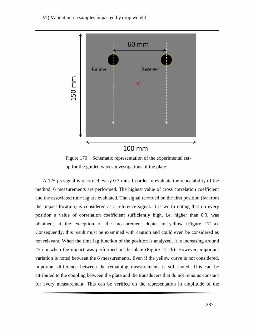
VI) Validation on samples impacted by drop weight
237
A 125 µs signal is recorded every 0.3 mm. In order to evaluate the repeatability of the
method, 6 measurements are performed. The highest value of cross correlation coefficient
and the associated time lag are evaluated. The signal recorded on the first position (far from
the impact location) is considered as a reference signal. It is worth noting that on every
position a value of correlation coefficient sufficiently high, i.e. higher than 0.9, was
obtained; at the exception of the measurement depict in yellow (Figure 171-a).
Consequently, this result must be examined with caution and could even be considered as
not relevant. When the time lag function of the position is analyzed, it is increasing around
25 cm when the impact was performed on the plate (Figure 171-b). However, important
variation is noted between the 6 measurements. Even if the yellow curve is not considered,
important difference between the remaining measurements is still noted. This can be
attributed to the coupling between the plate and the transducers that do not remains constant
for every measurement. This can be verified on the representation in amplitude of the
100 mm
15
0 m
m
60 mm
Figure 170 : Schematic representation of the experimental set-
up for the guided waves investigations of the plate
Emitter
Receiver

VI) Validation on samples impacted by drop weight
238
measured signal (Figure 172). Indeed, with this experimental set-up, the amplitude is
varying a lot from a measurement to another. So the attenuation in amplitude cannot be
induced only by the impact from damage. Nevertheless, the difference in time near the
impact location is high enough to be used to detect damage (Figure 171-b). It is yet difficult
to discuss the sensibility of this set-up; the latter requires to be upgraded to avoid a loss of
coupling between sample and transducers. One proposed solution is to change the system
that holds the transducers in order to add springs inside.
Impact localization
(a)
(b)
Figure 171 : (a) Evolution of the maximum correlation coefficient with the transducers
position. (b) Evolution of the time lag with the transducers position

VI) Validation on samples impacted by drop weight
239
5) Conclusion
This chapter was dedicated to the validation of the obtained ultrasonic results on
impacted samples. Drop weight impact solicitation was chosen because it is more close to
events that composite parts may undergo both during their manufacturing or life in service.
The chosen energy levels of impact were selected in order to remain in the Barely Visible
Impact Damage (BVID) range. By doing so, the capability of ultrasound to detect those
small damages can be experienced. The drop weight impact tests were performed. At
impact energies of 10 J, 15 J, 17.5 J and 20 J were chosen.
Figure 172 : Example of three typical L-scans obtained from the plate
impacted at 20 J
(a) (b)
(c)
VI) Validation on samples impacted by drop weight
240
The samples were investigated using X-ray tomography after the impact tests. Cracks
were observed most in the 17.5 J and 20 J impacted plates. The main damaged area is
located for both cases in the first ply on the non-impacted surface. Some meta-delamination
was even imaged for the samples impacted at 20 J. However, for the sample impacted at 15
J, only a small subsurface crack was noticed on the non-impacted surface whereas no
particular damage could be distinguished on the sample impacted at 10 J.
Then, ultrasonic C-scan in transmission and reflection were used to display the damaged
area. Using C-scan in transmission, a damaged area can be noticed for samples impacted at
15 J, 17.5 J and 20 J. Nothing was observed for the sample impacted at 10 J. Ultrasound in
reflection was used afterward to measure the size of the Barely Visible Indentation Damage
(BVID). This permanent indentation is used in the industry during visual inspection to
estimate the induced internal damage. Here, the permanent indentation were barely visible
by naked eye but could be precisely measured using ultrasound. This permanent indentation
was found to increase in size and depth with the energy level of impact. The size of the
permanent indentation of the sample impacted at 15 J could be used at a damage threshold.
Indeed, below this energy level, no damage was detected using X-ray tomography.
The decrease of stiffness components with the energy level of impact, calculated using
the method from section V)-3), was found to exhibit a specific scheme. This latter is
different from the ones observed for samples in 0° and 45° configuration damaged by
tension. Here, a global decrease of the components could be observed starting from 15 J.
The in-plane components C12 and C44 remain unaltered by the impact tests. It is logical to
observe an important decrease of the out plane components when submitted to impact.
Those results are of primary importance for the estimation of the residual mechanical
behavior of the impacted plate. The two proposed indicators, the Frobenius norm of the
stiffness tensor and the multi angle phase shift, were then calculated in a same manner as in
chapter V). Their evolution was shown to be in adequacy with the X-ray tomography
analysis. With this result, the first two indicators were found to be suitable to quantify the
damage induced by impact which validates as well the results from chapter V). However,
VI) Validation on samples impacted by drop weight
241
the proposed damage indicator based on guided waves could not be validated in this chapter
using the experimental results presented in this chapter. Indeed, it was observed that the
energy of the signal could not be used to quantify nor detect the damage induced by impact.
But, the time shift, compared with a reference state, estimated by cross-correlation was
found to be a better damage indicator, when the area near the impact location is
investigated. An experimental set-up was made up in order to investigate the whole sample.
Even though the location of the impact was accurately detected, this set-up still requires to
be updated. In fact, the variation in the quality of the coupling between the transducers and
the plates can lead to major deviation.

VI) Validation on samples impacted by drop weight
242
VII) Concluding remarks and further works
243
VII) Concluding remarks and further works
1) Concluding remarks
The current work has two main objectives, first it was aimed at investigating the growth
of damage in a polyamide 66/6 reinforced with woven glass fiber. This composite material
developed by DuPont is used by the cars manufactures PSA to replace some of the metallic
parts. This material can help reduce the weight of cars without decreasing their mechanical
resistance and lifetime. Then, this work was also focused on the study of Non Destructive
Evaluation (NDE) methods, based on ultrasound, and more specifically on their capability
to quantify different induced damage states on composite materials. Several NDE methods
were considered to evaluate damage induced using several mechanical loading.
In order to propose a suitable experimental approach founded on NDE methods, the
investigation of the mechanical and damage behavior of the composite material was
performed by mean of static tensile tests. Two samples orientation were chosen: oriented
along the warp axis (later referred as 0° configuration) and oriented at 45° from the warp
axis (later referred as 45° configuration). From a macroscopic point of view, the two
configurations exhibit different mechanical responses. For the 0° configuration, a linear
brittle stress/strain behavior with limited induced damage was witnessed. Whereas for the
45° configuration, a non-linear ductile stress/strain behavior with higher appearance of
damage was observed. Evolution of damage was calculated as the elastic modulus on
stress/strain curve decreases. Using Digital Image Correlation (DIC), the two dimensional
strain fields showed in addition that, in 0° configuration, the tensile test induced only strain
along the loading direction. For the other configuration, the mechanical response also first
exhibits an increase of the strain along the loading direction. However, after some time, the
response exhibits a coupling between in-plane shear and tension. This response was found
to be induced by reorientation of fibers along the loading direction. This difference in terms
of mechanical response also induces different rupture mechanisms after tensile tests
between each sample configuration. Smooth cracks in the 0° configuration and cracks in

VII) Concluding remarks and further works
244
stair shape with delamination visible on sample edges for the 45° configuration, were
observed.
The damage mechanisms at the microscopic scale were then investigated. The initiation
of damage by fibers/matrix debonding was first observed by means of Scanning Electronic
Microscopy (SEM). Because of some issues during the SEM tests, the following of the
study was done using X-ray tomography. Samples in 0° and 45° configuration damaged by
tensile tests was found to exhibit different damage schemes in links with the stress/strain
response. In the first case, low scale damage was found to grow, whereas for 45°
configuration large scale damage can appear for high levels of loading, mostly fibers
buckling and delamination. This difference in terms of growing state was also observed
when analyzing the void volume fraction evolution with increasing the loading level on the
3D volumes reconstructed from X-ray tomography. The evolution of the void volume
fraction as a function of the applied stress level, exhibited a similar increase as the
evolution of the macroscopic damage estimated from the Young‟s modulus reduction.
Different Non Destructive Evaluation (NDE) methods based on ultrasound were then
investigated. First, the ultrasonic C-scan does not give interesting results on the samples in
0° configuration. Only macroscopic damage on the samples in 45° configuration could be
imaged. Other methods were consequently considered, first the computation of stiffness
components based on phase velocities measurements. The evolution of the anisotropic
damage was obtained on samples in 0° and 45° configuration damaged by tensile tests. This
evolution was in agreement with the evolution of the 2D strain field computed from DIC.
That is the components function of the loading direction that decrease for 0° configuration
and every in-plane components, including in-plane shearing, decreasing for the other
configuration. Then two damage indicators were proposed and were found to give a correct
quantification of the induced damage. The first damage indicator is the Frobenius norm of
the stiffness tensor, the second damage indicator is the phase shift for all the incident angles
and all the investigation planes considered for the measurement of phase velocities.

VII) Concluding remarks and further works
245
Then guided waves are used to inspect the same samples. Indeed, because of the more
complex apparatus required for the previous method, the latter can be apply less easily on
site than guided waves based methods. First the wave modes were investigated but no mode
conversion could be observed with increasing the applied loading levels. Therefore, other
damage indicators were proposed in order to quantify the damage state. The evolution of
the signal energy with the induced damage was found to be the more effective. Its
efficiency was first validated using a steel plate with different kind of defect induced on it.
This indicator was then applied on the composite samples preliminary damaged by means
of tensile tests. The evolution of the signal energy was found to be in agreement with the
phase shift damage indicator as well as with the other damage estimation methods.
Finally, a validation of the proposed methods using samples preliminary damaged by
drop weight impacts was proposed. Several impact energies were considered, they were
chosen in order to remain in the BVID domain. The damage induced on the plate was found
to increase with the impact energy when observed by means of X-ray tomography. The
permanent indentation was evaluated as well using pulse-echo measurements. Its size was
found to increase with the impact energy which makes the estimation of the indentation a
good indicator of the internal damage. The stiffness measurement method introduced in
chapter V), was able to detect a clear increase of the damage state starting from 17.5 J as
impact energy. Indeed, starting from this level of energy, all the stiffness components, at
the exception of the C12 and C44 components, decrease with increasing the impact energy.
The phase shift damage indicator was found to be able to detect a real change in the
damage state starting from an impact energy value of 15 J. Finally, as the damage
indicators from guided waves, based on the signal amplitude, could not detect the damage
from impact, damage evaluation using time shift was considered. The latter was estimated
by cross correlation and found to be able to quantify increasing damage state. The damage
location can be detected when investigation on the whole sample is considered. However,
the proposed experimental set-up requires some adjustment in order to avoid fluctuation in
coupling between the transducers and the sample.

VII) Concluding remarks and further works
246
2) Further works
As aforementioned, enhancement in the signal processing when considering guided
waves based methods should be investigated in future work. As an example, two methods
dealing with the propagation of guided waves are investigated in the appendix section.
Those two methods are respectively based on the analysis of the non-linear response of
propagated elastic waves and on the analysis of the late arrival signals (or coda part of the
signal). They could be interesting alternatives even though some limitations are highlight in
the investigation.
Then, in order to consider more diffuse damage that could appear before a catastrophic
failure, the fatigue behavior of the material need to be investigated. Indeed, fatigue damage
is known to be one of the most difficult to detect in composite material. Often when they
are detected by NDE method the material has seen its stiffness and strength decrease to a
large extent. The case of fatigue post-impact should also be considered.
Numerical modeling of the wave propagation in the investigated composites is also a
challenging topic that deserves to be studied. Indeed, the layering aspect of the composite
material and the waviness of the fabric made the real propagation of wave more difficult to
predict. As an example, the dispersion curves of the material could be influenced by these
effects, even not if the high frequency regime is not considered. Consequently, the
homogenous anisotropic hypothesis considered in this work for computing the dispersion
curves may be too inadequate.
VIII) References
247
VIII) References
[1] C. Atas and O. Sayman, “An overall view on impact response of woven fabric
composite plates,” Compos. Struct., vol. 82, pp. 336–345, 2008.
[2] M. Karayaka and P. Kurath, “Deformation and Failure Behavior of Woven
Composite Laminates,” J. Eng. Mater. Techology, vol. 116, no. April 1994, pp. 222–
232, 1994.
[3] L. Marcin, “Modelisation du comportement, de l‟endommagement et de la rupture de
materiaux compositea renforts tisses pour le dimensionnement robuste de
structures,” Université Bordeaux 1, 2010.
[4] P. Boisse, N. Hamila, A. Madeo, G. Hivet, D. Isola, P. Boisse, N. Hamila, A. Madeo,
and G. Hivet, “The bias-extension test for the analysis of in-plane shear properties of
textile composite reinforcements and prepregs : a review,” Int. J. Mater. Form., vol.
10, no. 4, 2017.
[5] P. Ladeveze and E. Le Dantec, “Damage modelling of the elementary ply for
laminated composites,” Compos. Sci. Technol., vol. 43, pp. 257–267, 1992.
[6] P. Cazuc, “Advancing lightweighting solutions to the industry,” DuPont - Autofocus
#23, 2013. [Online]. Available: http://www.arpae-
summit.com/paperclip/exhibitor_docs/14AE/DuPont_138.pdf.
[7] S. Latieule, “Dossier automobile - Les matériaux biosourcés s‟imposent en douceur,”
Formule Verte #18, 2014. [Online]. Available:
http://averousl.free.fr/fichiers/Formule Verte Juin 2014.pdf.
[8] N. Piccirelli and A. Giocosa, “Les composites dans l‟industrie automobile,”
Techniques de l’ingénieur, 2011. [Online]. Available: http://www.techniques-
ingenieur.fr/base-documentaire/ingenierie-des-transports-th14/carburants-batteries-
et-materiaux-alleges-pour-vehicule-propre-42629210/les-composites-dans-l-
industrie-automobile-am5600/.
[9] P. Passebon, “Les composites ont rendez-vous avec les hautes cadences,” Industrie
& technologies, 2015. [Online]. Available: http://www.industrie-techno.com/2-
automobile-les-composites-ont-rendez-vous-avec-les-hautes-cadences.36589.
[10] L. Fery, “Quels composites pour l‟automobile de demain?,” Industrie &
technologies, 2013. [Online]. Available: http://www.industrie-techno.com/quels-
composites-pour-l-automobile-de-demain.23015.
[11] R. N. Yancey, Challenges, Opportunities, and Perspectives on Lightweight
Composite Structures: Aerospace Versus Automotive. Elsevier Ltd, 2016.

VIII) References
248
[12] A. M. Abdelhay and M. I. Mubark, “ULTRASONIC EVALUATION OF SURFACE
ROUGHNESS USING NORMAL INCIDENCE PULSE - ECHO TECHNIQUE,” e-
Journal Nondestruct. Test., vol. 9, no. 4, 2004.
[13] S. Gholizadeh, “A review of non-destructive testing methods of composite
materials,” in Procedia Structural Integrity, 2016, vol. 1, pp. 50–57.
[14] E. G. Henneke, W. W. Stinchcomb, and K. L. Reifsnider, “Some ultrasonic methods
for characterizing response of composite materials,” in International Sympozium on
Ultrasonic materials Characterization, 1980.
[15] F. Dal Maso and J. Mézière, “Calcul des propriétés élastiques des tissus utilisés dans
les matériaux composites,” Rev. l’institut Français du Pétrole, vol. 53, no. 1, pp.
857–870, 1998.
[16] J. Cunningham, “Woven or unwoven fibres?,” Materials for Engineering, 2013.
[Online]. Available: http://www.materialsforengineering.co.uk/engineering-
materials-features/woven-or-unwoven-fibres/48611/.
[17] W. Albouy, “De la contribution de la visco-élasto-plasticité au comportement en
fatigue de composite a matrice thermoplastique et thermodurcissable,” INSA Rouen,
2013.
[18] G. Couégnat, “Approche multiéchelle du comportement mécanique de matériaux
composites à renfort tissé,” École des Mines d‟Alby-Carmaux, 2008.
[19] B. Vieille and L. Taleb, “About the influence of temperature and matrix ductility on
the behavior of carbon woven-ply PPS or epoxy laminates: Notched and unnotched
laminates,” Compos. Sci. Technol., vol. 71, no. 7, pp. 998–1007, 2011.
[20] W. Albouy, B. Vieille, and L. Taleb, “Influence of matrix ductility on the high-
temperature fatigue behavior of off-axis woven-ply thermoplastic and thermoset
laminates,” Int. J. Fatigue, vol. 63, pp. 85–96, 2014.
[21] S. D. Pandita, G. Huysmans, M. Wevers, and I. Verpoest, “Tensile fatigue behaviour
of glass plain-weave fabric composites in on- and off-axis directions,” Compos. Part
A Appl. Sci. Manuf., vol. 32, no. 10, pp. 1533–1539, 2001.
[22] BASF_Corporation, “Conditioning of Ultramid modlings,” 2016.
[23] M. Chanda and S. K. Roy, Plastics Technology Handbook. CRC Press, 2007.
[24] A. Launay, Y. Marco, M. H. Maitournam, and I. Raoult, “Modelling the influence of
temperature and relative humidity on the time-dependent mechanical behaviour of a
short glass fibre reinforced polyamide,” Mech. Mater., vol. 56, pp. 1–10, 2013.
[25] BASF_Corporation, “MECHANICAL PERFORMANCE OF POLYAMIDES

VIII) References
249
WITH INFLUENCE OF MOISTURE AND TEMPERATURE – ACCURATE
EVALUATION AND BETTER UNDERSTANDING,” 2003.
[26] M. F. Arif, F. Meraghni, Y. Chemisky, N. Despringre, and G. Robert, “In situ
damage mechanisms investigation of PA66/GF30 composite: Effect of relative
humidity,” Compos. Part B Eng., vol. 58, pp. 487–495, 2013.
[27] G. W. Ehrenstein and R. P. Theriault, Polymeric materials: structure, properties,
applications. 2001.
[28] M. F. Ashby and D. R. H. Jones, Matériaux 2. microstructure et mise en œuvre.
Paris, 1991.
[29] M. F. Herman, Encyclopedia of Polymer Science and Technology, Concise. 2013.
[30] V. Miri, O. Persyn, J. Lefebvre, and R. Seguela, “Effect of water absorption on the
plastic deformation behavior of nylon 6,” Eur. Polym. J., vol. 45, no. 3, pp. 757–762,
2009.
[31] A. Malpot, F. Touchard, and S. Bergamo, “Etude du comportement en fatigue d ‟ un
composite à matrice thermoplastique tissé de fibres de verre pour application
automobile Study of the behaviour of a woven glass-fibre-reinforced composite with
a thermoplastic matrix for automotive application,” in Journées Nationales des
Compositees 19, 2015, pp. 1–9.
[32] T. Osada, A. Nakai, and H. Hamada, “Initial fracture behavior of satin woven fabric
composites,” Compos. Struct., vol. 61, pp. 333–339, 2003.
[33] P. Boisse, N. Hamila, E. Vidal-sallé, and F. Dumont, “Simulation of wrinkling
during textile composite reinforcement forming . Influence of tensile , in-plane shear
and bending stiffnesses,” Compos. Sci. Technol., vol. 71, no. 5, pp. 683–692, 2011.
[34] A. Gay, J. Roche, P. Lapeyronnie, and P. Bertrand, “Non-destructive inspection of
initial defects of PA6 . 6-GF50 / aluminum self-piercing riveted joints and damage
monitoring under mechanical static loading,” Int. J. Damage Mech., vol. 26, no. 8,
pp. 1127–1146, 2017.
[35] J. L. Rose, K. M. Rajana, and M. K. T. Hansch, “Ultrasonic Guided Waves for NDE
of Adhesively Bonded Structures,” J. Adhes., vol. 50, no. 1, pp. 71–82, 1995.
[36] P. Cawley and D. Alleyne, “The use of Lamb waves for the long range inspection of
large structures,” Ultrasonics, vol. 34, no. 2, pp. 287–290, 1996.
[37] Z. Su, L. Ye, and Y. Lu, “Guided Lamb waves for identification of damage in
composite structures : A review,” J. Sound Vib., vol. 295, pp. 753–780, 2006.
[38] M.-L. Pastor, C. Garnier, and C. Pescay, “Comparison of two Non-destructive Tests
in Carbon/Epoxy Composites,” J. Mater. Sci. Eng., vol. 4, no. 10, 2010.
VIII) References
250
[39] L. Satyanarayan, J. M. Vander Weide, and N. F. Declercq, “Ultrasonic polar scan
imaging of damaged fiber reinforced composites,” Mater. Eval., pp. 733–739, 2010.
[40] J. Liu and N. F. Declercq, “Ultrasonic geometrical characterization of periodically
corrugated surfaces,” Ultrasonics, vol. 53, pp. 853–861, 2013.
[41] Q. Shen, M. Omar, and S. Dongri, “Ultrasonic NDE Techniques for Impact Damage
Inspection on CFRP Laminates,” J. Mater. Sci. Res., vol. 1, no. 1, pp. 2–16, 2011.
[42] A. Osman, U. Hassler, V. Kaftandjian, and J. Hornegger, “An automated data
processing method dedicated to 3D ultrasonic non destructive testing of composite
pieces,” in IOP Conference Series Materials Science and Engineering International
- Symposium on Ultrasound in the Control of Industrial Processes (UCIP 2012),
2012, no. 42(1):2005.
[43] C. Garnier, M.-L. Pastor, F. Eyma, and B. Lorrain, “The detection of aeronautical
defects in situ on composite structures using Non Destructive Testing,” Compos.
Struct., vol. 93, no. 5, pp. 1328–1336, Apr. 2011.
[44] J. Dong, B. Kim, A. Locquet, P. McKeon, N. F. Declercq, and D. S. Citrin,
“Nondestructive evaluation of forced delamination in glass fiber-reinforced
composites by terahertz and ultrasonic waves,” Compos. Part B Eng., vol. 79, pp.
667–675, 2015.
[45] Cenaero, Sirris, and Multitel, “Comparison and complementary of non-destructive
evaluation technologies on composite materials,” Yutz, France, 2013.
[46] F. Destic and C. Bouvet, “Impact damages detection on composites materials by
THz imaging,” Case Stud. Nondestruct. Test. Eval., vol. 6, no. Part A, pp. 53–62,
2016.
[47] D. K. Hsu and D. J. Barnard, “An exploration of the utilities of terahertz waves for
the NDE of composites,” 2010.
[48] M. F. Markham, “Measurement of the elastic constants of fibre composites by
ultrasonics,” Composites, vol. 1, no. 2, pp. 145–149, 1969.
[49] P. Marguères, F. Meraghni, and M. L. Benzeggagh, “Comparison of stiffness
measurements and damage investigation techniques for a fatigued and post-impact
fatigued GFRP composite obtained by RTM process,” Compos. Part A Appl. Sci.
Manuf., vol. 31, pp. 151–163, 2000.
[50] P. Marguères and F. Meraghni, “Damage induced anisotropy and stiffness reduction
evaluation in composite materials using ultrasonic wave transmission,” Compos.
Part A Appl. Sci. Manuf., vol. 45, pp. 134–144, 2013.
[51] W. Hufenbach, T. Ritschel, R. Böhm, and A. Langkamp, “Ultrasonic determination
VIII) References
251
of anisotropic damage in fibre and textile reinforced composite materials,” in
Conference on Damage in Composite Materials, 2006.
[52] S. Baste and C. Aristégui, “Induced anisotropy and crack systems orientations of a
ceramic matrix composite under off-principal axis loading,” Mech. Mater., vol. 29,
no. 1, pp. 19–41, 1998.
[53] A. Dalmaz, D. Ducret, R. El Guerjouma, P. Reynaud, P. Franciosi, D. Rouby, G.
Fantozzi, and J. C. Baboux, “Elastic moduli of a 2.5D C f / SiC composite :
experimental and theoretical estimates,” Compos. Sci. Technol., vol. 60, 2000.
[54] J. L. Rose, J. J. Ditri, Y. Huang, D. P. Dandekar, and S.-C. Chou, “One-sided
ultrasonic inspection technique for the elastic constant determination of advanced
anisotropic materials,” J. Nondestruct. Eval., vol. 10, no. 4, pp. 159–166, 1991.
[55] S. I. Rokhlin and W. Wang, “Ultrasonic evaluation of in plane and out of plane
elastic properties of composite materials,” Rev. Prog. Quant. Nondestruct. Eval., vol.
8, no. B, pp. 1489–1496, 1989.
[56] S. I. Rokhlin and W. Wang, “Double through transmission bulk wave method for
ultrasonic phase velocity measurement and determination of elastic constants of
composite materials,” J. Acoust. Soc. Am., vol. 91, no. 6, pp. 3303–3312, 1992.
[57] M. Mah and D. R. Schmitt, “Determination of the complete elastic stiffnesses from
ultrasonic phase velocity measurements,” J. Geophys. reasearch, vol. 108, no.
October 2003, pp. 1–11, 2016.
[58] E. Grippon, S. Baste, E. Martin, C. Aristegui, and G. Couégnat, “Caractérisation
ultrasonore et modélisation multi-échelle de l‟endommagement sous charge d‟un
composite 3D SiC/SiC,” in Congrés Français de Mécanique, 2013, pp. 3–8.
[59] B. Audoin, S. Baste, and B. Castagnede, “Estimation de l‟intervalle de confiance des
constantes d‟élasicité identidiées à partir des vitesses de propagation ultrasonore,”
Compte rendus Acad. des Sci., vol. 312, no. 2, pp. 676–686, 1991.
[60] M. Kersemans, I. De Baere, J. Degrieck, K. Van Den Abeele, L. Pyl, F. Zastavnik,
H. Sol, and W. Van Paepegem, “Nondestructive damage assessment in fiber
reinforced composites with the pulsed ultrasonic polar scan,” Polym. Test., vol. 34,
pp. 85–96, Apr. 2014.
[61] N. F. Declercq, J. Degrieck, and O. Leroy, “On the influence of fatigue on ultrasonic
polar scans of fiber reinforced composites,” Ultrasonics, vol. 42, no. 1–9, pp. 173–
177, 2004.
[62] N. F. Declercq, J. Decrieck, and O. Leroy, “Ultrasonic polar scans Numerical
simulation on generally,” Ultrasonics, vol. 45, pp. 32–39, 2006.
[63] N. F. Declercq, J. Degrieck, and O. Leroy, “Simulations of harmonic and pulsed
VIII) References
252
ultrasonic polar scans,” NDT E Int., vol. 39, no. 3, pp. 205–216, 2006.
[64] S. W. Herbison and N. F. Declercq, “Theoretical and experimental ultrasonic
investigation of a thin plate with regions of different periodic double-corrugations,”
J. Acoust. Soc. Am., vol. 123, no. 5, 2008.
[65] S. W. Herbison and N. F. Declercq, “Diffraction phenomena associated with a
composite plate containing an interior periodically corrugated interface,” J. Acoust.
Soc. Am., vol. 123, no. 5, 2008.
[66] S. W. Herbison, “Ultrasonic Diffraction Effects On Periodic Surfaces,” Georgia
Institute of Technology, 2011.
[67] M. Kersemans, W. Van Paepegem, D. Van Nuffel, G. Luyckx, I. De Baere, J. Gu, H.
Sol, K. Van Den Abeele, and J. Degrieck, “Polar Scan Technique for Material
Characterization and Identification of New Operating Regimes,” in International
Conference on Experimental Mechanics, 2010, vol. 1, pp. 1–12.
[68] J. L. Rose, Ultrasonic waves in solid media. 1999.
[69] N. Adnan H., Wave propagation in layered anisotropic media, North Holl. North
Holland: Elsevier, 1995.
[70] W. H. Ong, N. Rajic, W. K. Chiu, and C. Rosalie, “Determination of the elastic
properties of woven composite panels for Lamb wave studies,” Compos. Struct., vol.
141, pp. 24–31, 2016.
[71] E. Moreno, N. Galarza, B. Rubio, and J. A. Otero, “Phase Velocity Method for
Guided Wave Measurements in Composite Plates,” Phys. Procedia, vol. 63, pp. 54–
60, 2015.
[72] W. Gao, C. Glorieux, and J. Thoen, “Laser ultrasonic study of Lamb waves :
determination of the thickness and velocities of a thin plate,” Int. J. Eng. Sci., vol.
41, pp. 219–228, 2003.
[73] H. J. Shin and S.-J. Song, “Observation of Lamb Wave Mode Conversion on an
Aluminum Plate,” in 15th World Conference on Non-Destructive Testing, 2000.
[74] P. Mckeon, S. Yaacoubi, N. F. Declercq, S. Ramadan, and W. K. Yaacoubi,
“Baseline subtraction technique in the frequency – wavenumber domain for high
sensitivity damage detection,” Ultrasonics, vol. 54, no. 2, pp. 592–603, 2014.
[75] D. N. Alleyne and P. Cawley, “A 2-dimensional Fourier transform method for the
quantitative measurement of Lamb modes,” Proc. IEEE Ultrason. Symp., vol. 2, pp.
1143–1146, 1990.
[76] M. R. Karim and A. K. Mal, “Determination of the elastic constants of composites
VIII) References
253
through the inversion of Leaky Lamb Waves data,” Rev. Prog. Quant. Nondestruct.
Eval., vol. 9, 1990.
[77] K. Imano and T. Endo, “Experimental Study on the Mode Conversion of Lamb
Waves in a Metal Plate of Stepped Thickness Using Optical Detection,” Int. J. Soc.
Mater. Eng. Resour., vol. 17, no. 2, pp. 201–204, 2010.
[78] W. Li, Y. Cho, J. Lee, and J. D. Achenbach, “Assessment of Heat Treated Inconel X-
750 Alloy by Nonlinear Ultrasonics,” Exp. Mech., vol. 53, no. 5, pp. 775–781, 2013.
[79] J. Jingpin, M. Xiangji, H. Cunfu, and W. Bin, “Nonlinear Lamb wave-mixing
technique for micro-crack detection in plates,” NDT E Int., vol. 85, pp. 63–71, 2017.
[80] U. Rabe, T. Helfen, M. Weikert, S. Hirsekorn, H.-G. Herrmann, C. Boller, D. Backe,
F. Balle, and D. Eifler, “Nonlinear ultrasonic testing of carbon fibre reinforced
plastics in the very high cycle fatigue regime,” Proc. Meet. Acoust., vol. 16, no.
2012, pp. 1–6, 2012.
[81] G. Ren, J. Kim, and K.-Y. Jhang, “Relationship between second- and third-order
acoustic nonlinear parameters in relative measurement,” Ultrasonics, vol. 56, pp.
539–544, 2015.
[82] U. Dahlen, N. Ryden, and A. Jakobsson, “Damage identification in concrete using
impact non-linear reverberation spectroscopy,” NDT E Int., vol. 75, pp. 15–25, 2015.
[83] M. Meo, U. Polimeno, and G. Zumpano, “Detecting damage in composite material
using nonlinear elastic wave spectroscopy methods,” Appl. Compos. Mater., vol. 15,
pp. 115–126, 2008.
[84] K. E. Van Den Abeele, A. Sutin, J. Carmeliet, and P. a. Johnson, “Micro-damage
diagnostics using nonlinear elastic wave spectroscopy (NEWS),” NDT E Int., vol.
34, pp. 239–248, 2001.
[85] L. . Ostrovsky and P. A. Johnson, “Dynamic nonlinear elasticity in geo materials,”
Riv. del Nuovo Cim. della Soc. Ital. di Fis., vol. 24, no. 7, pp. 1–46, 2001.
[86] L. . Ostrovsky, S. N. Gurbatov, and J. N. Didenkulov, “Nonlinear Acoustics in
Nizhni Novgorod ( A Review ),” Acoust. Phys., vol. 51, no. 2, pp. 114–127, 2005.
[87] K. Van Den Abeele and J. De Visscher, “Damage assessment in reinforced concrete
using spectral and temporal nonlinear vibration techniques,” Cem. Concr. Res., vol.
30, no. 9, pp. 1453–1464, 2000.
[88] V. Genovés, L. Soriano, M. V Borrachero, J. Eiras, and J. Payá, “Preliminary study
on short-term sulphate attack evaluation by non-linear impact resonance acoustic
spectroscopy technique,” Constr. Build. Mater., vol. 78, pp. 295–302, 2015.
[89] K. E. -a. Van Den Abeele, P. a. Johnson, and A. Sutin, “Nonlinear Elastic Wave
VIII) References
254
Spectroscopy (NEWS) Techniques to Discern Material Damage, Part II: Single-
Mode Nonlinear Resonance Spectroscopy (NWMS),” Res. Nondestruct. Eval., vol.
12, no. 1, pp. 17–30, 2000.
[90] A. Quiviger, J.-P. Zardan, J.-F. Chaix, C. Payan, V. Garnier, J. Moysan, and J. Salin,
“Caracterisation Ultrasonore de Fissures dans les Bétons Méthodes Linéaires et Non
Linéaires,” 10éme Congrés Français d’Acoustique, p. , 2010.
[91] K. E. -a. Van Den Abeele, P. a. Johnson, and a. Sutin, “Nonlinear Elastic Wave
Spectroscopy (NEWS) Techniques to Discern Material Damage, Part I: Nonlinear
Wave Modulation Spectroscopy (NWMS),” Res. Nondestruct. Eval., vol. 12, no. 1,
pp. 17–30, 2000.
[92] F. Aymerich and W. J. Staszewski, “Experimental Study of Impact-Damage
Detection in Composite Laminates using a Cross-Modulation Vibro-Acoustic
Technique,” Struct. Heal. Monit., vol. 9, no. 0, pp. 541–553, 2010.
[93] T. B. Helfen, “Nichtlinearer Ultraschall zur Charakterisierung von
Ermüdungsschäden während der Hochfrequenz - Beanspruchung von C - Faser -
Kunststoffverbunden,” Universitat des Saarlandes, 2014.
[94] M. Herraiz and A. F. Espinosa, “Coda Waves-A Review,” Pageoph, vol. 125, no. 4,
pp. 499–577, 1987.
[95] P. Fröjd and P. Ulriksen, “Amplitude and phase measurements of continuous diffuse
fields for structural health monitoring of concrete structures,” NDT E Int., vol. 77,
pp. 35–41, 2016.
[96] R. Livings, V. Dayal, and D. Barnard, “Coda wave interferometry for the
measurement of thermally induced ultrasonic velocity variations in CFRP
laminates,” AIP Conf. Proc., vol. 1706, 2016.
[97] R. Livings, V. Dayal, and D. Barnard, “Feasibility of detecting fatigue damage in
composites with coda waves,” AIP Conf. Proc., vol. 1650, pp. 1130–1139, 2015.
[98] G. Briotti and C. Scarponi, “Ultrasonic NDI Detection of Delaminations on,” J.
Reinf. Plast. Compos., vol. 20, no. 1, pp. 76–87, 2001.
[99] Z. Liu, J. Huang, and J. Li, “Comparison of four techniques for estimating temporal
change of seismic velocity with passive image interferometry,” Earthq. Sci., vol. 23,
no. 5, pp. 511–518, 2010.
[100] J. E. Michaels and T. E. Michaels, “Detection of structural damage from the local
temporal coherence of diffuse ultrasonic signals,” IEEE Trans. Ultrason.
Ferroelectr. Freq. Control, vol. 52, no. 10, pp. 1769–1782, 2005.
[101] Y. Zhang, O. Abraham, V. Tournat, A. Le Duff, B. Lascoup, A. Loukili, F. Grondin,
VIII) References
255
and O. Durand, “Validation of a thermal bias control technique for Coda Wave
Interferometry (CWI),” Ultrasonics, vol. 53, no. 3, pp. 658–664, 2013.
[102] Y. H. Kim, S. Song, and S. Kwon, “Measurement of phase velocity dispersion
curves and group velocities in a plate using leaky Lamb waves,” in Conference and
exhibition on Non Destructive Evaluation 2002 - ISNT, 2002.
[103] S. V Lomov, D. S. Ivanov, I. Verpoest, A. E. Bogdanovich, D. Mungalov, M. Zako,
T. Kurashiki, and H. Nakai, “Predictive analyses and experimental validations of
effective elastic properties of 2D and 3D woven composites,” in 13th European
Conference on Composite Materials (ECCM-13), 2008.
[104] R. El Guerjouma and S. Baste, “Evaluation of anisotropic damage in ceramic-
ceramic (SiC-SiC) composite by ultrasonic method,” in Ultrasonic international,
1989, pp. 895–900.
[105] S. Baste and B. Audoin, “On internal variable in anisotropic damage,” Eur. J. Mech.,
vol. 10, no. 6, pp. 587–606, 1991.
[106] E. Ž. L. Mažeika, L. Draudvilienė, “Influence of the dispersion on measurement of
phase and group velocities of Lamb waves,” Ultrasound, vol. 64, no. 4, pp. 18–21,
2009.
[107] L. Draudviliene, H. Ait Aider, O. Tumsys, and L. Mazeika, “The Lamb waves phase
velocity dispersion evaluation using an hybrid measurement technique,” Compos.
Struct., vol. 184, no. October 2017, pp. 1156–1164, 2018.
[108] S. Eckel, F. Meraghni, P. Pomarède, and N. F. Declercq, “Investigation of Damage
in Composites Using Nondestructive Nonlinear Acoustic Spectroscopy,” Exp.
Mech., 2016.
[109] “DIN IEC 268-2:1994-08,” Elektroakustische Geräte – Tl. 2 Allg. Begr. und
Berechnungsverfahren (lEC 268-2 1987 + A1 1991) Dtsch. Fassung HD 483.2 S2
1993.
[110] “DIN EN 60268-3:2014-03,” Elektroakustische Geräte – Tl. 3 Verstärker (IEC
60268-32013), Dtsch. Fassung EN 60268-32013.
[111] N. Yoder, “PeakFinder (Version 13 Aug 2014). File Exchange. MATLAB Central,”
2014. [Online]. Available:
http://www.mathworks.com/matlabcentral/fileexchange/25500-peakfinder.m.
[Accessed: 01-Jun-2015].
[112] S. C. Stähler, C. Sens-Schönfelder, and E. Niederleithinger, “Monitoring stress
changes in a concrete bridge with coda wave interferometry.,” J. Acoust. Soc. Am.,
vol. 129, no. 4, pp. 1945–1952, 2011.
[113] Y. ZHANG, “Contrôle de santé des matériaux et structures par analyse de la coda
VIII) References
256
ultrasonore,” Université Nantes Angers Le Mans, 2013.
[114] B. N. Cox and G. Flanagan, “Handbook Composites of Analytical Methods for
Textile,” 1997.
[115] F. Praud, G. Chatzigeorgiou, Y. Chemisky, and F. Meraghni, “Modélisation multi-
échelle des composites tissés à matrice thermoplastique sous chargements cycliques
non proportionnels,” in JNC 20 : Journées Nationales sur les Composites 2017,
2017.
[116] B. Vieille and W. Albouy, “About the applicability of a simple model to predict the
fatigue life and behavior of woven-ply thermoplastic laminates at T > T g,” Compos.
Part B Eng., vol. 61, pp. 181–190, 2014.
[117] F. A. Myers, “Stress-state effects on the viscoelastic response of PPS based
thermoplastic composites,” in Advances in Thermoplastic Matrix Composite
Materials, ASTM STP 1., G. M. Newaz, Ed. ASTM International, 1989, pp. 154–
162.
[118] C. Potel, “Propagation et Contrôle Non Destructif dans les solides - AC03,” in
Master’s degree course From Master Sciences et Technologie Mention “Acoustique
et Mécanique.”
[119] M. Kersemans, N. Lammens, J. Degrieck, K. Van Den Abeele, L. Pyl, F. Zastavnik,
H. Sol, and W. Van Paepegem, “Extraction of bulk wave characteristics from a
pulsed ultrasonic polar scan,” Wave Motion, vol. 51, no. 7, pp. 1071–1081, 2014.
[120] G. Huang, F. Song, and X. Wang, “Quantitative modeling of coupled piezo-
elastodynamic behavior of piezoelectric actuators bonded to an elastic medium for
structural health monitoring: A review,” Sensors, vol. 10, no. 4, pp. 3681–3702,
2010.
[121] C. M. Yeum, “Lamb Wave Mode Decomposition,” 2016. [Online]. Available:
https://datacenterhub.org/resources/150.
[122] T. Planès and E. Larose, “A review of ultrasonic Coda Wave Interferometry in
concrete,” Cem. Concr. Res., vol. 53, pp. 248–255, 2013.
[123] N. Hongkarnjanakul, “Modélisation numérique pour la tolérance aux dommages
d‟impact sur stratifié composite : de l‟impact à la résistance résiduelle en
compression,” 2013.
IX) Appendix
257
IX) Appendix
1) Appendix 1: Damage investigation using nonlinear acoustic
methods on different woven fiber reinforced composite
materials
The next presented study was done in close collaboration with Sebastian Eckel during
his internship at both LEM3 lab and LUNE lab from Georgia Tech Lorraine. Some of the
work described here was summarized and published in a paper [108]. The goal was to
verify the ability of the nonlinear acoustic method to accurately quantify the damage level
on composite material. Three experimental damage evaluation acoustic methods will be
presented and discussed in this first appendix. First, the NEWS (Nonlinear Waves
Modulation Spectroscopy) method is considered and then the NRUS method (Nonlinear
Resonant Ultrasound Spectroscopy). These two very well know nonlinear acoustic methods
are among the methods that were introduced in subsection V)-1)-d) from the literature
review on ultrasonic based NDE methods. Between these two investigated methods, a
complementary study of the resonance frequency shift function of the induced damage is
presented.
Several fiber reinforced composite materials available at the LEM3 lab were tested. All
these samples are woven glass fabric reinforced composites and were submitted to tension
along the axis of the fiber. The three composites selected are: a vinylester, an epoxy and a
polyamide 66/6 matrix based composites. Different stress level values were used in order to
induce different damage state in the investigated samples. These data are sum-up in the
following table:

IX) Appendix
258
Material Sample 1 Sample 2 Sample 3 Sample 4 Sample 5 Sample 6 Sample 7 Sample 8
Vinylester/glass fiber 100 200 300 400 ---------- ---------- ---------- ----------
Epoxy/glass fiber 50 100 150 200 250 300 350 400
Polyamide 66/6 glass
fiber 45 90 135 180 225 270 315 ----------
Table 33 : Materials tested and loading value used on the different sample
The procedure to induced damage is the same as in the chapter III) at the exception that
only the extensometer was used to measure the displacement. The dimensions of the three
considered material are indicated in Figure 173.
Figure 173 : Photo of the sample of each selected woven composite materials.
a) : Woven glass vinylester composite, b) Woven glass polyamide 6.6/6
composite, c) : Woven glass epoxy composite
a)
c)
b)
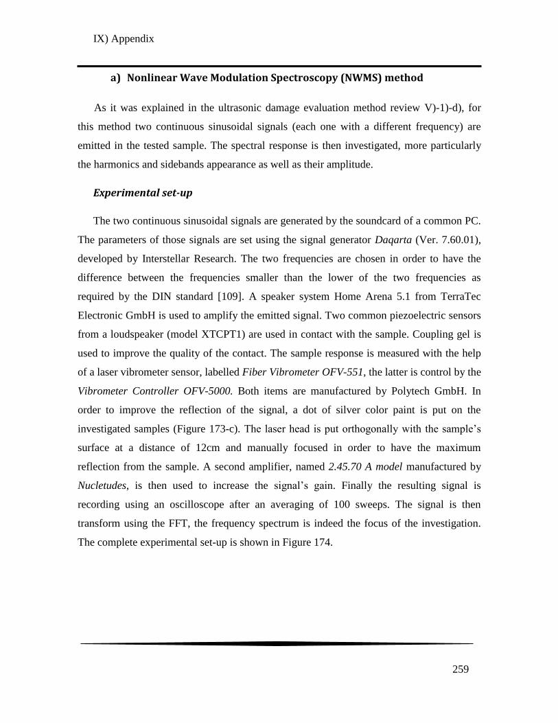
IX) Appendix
259
a) Nonlinear Wave Modulation Spectroscopy (NWMS) method
As it was explained in the ultrasonic damage evaluation method review V)-1)-d), for
this method two continuous sinusoidal signals (each one with a different frequency) are
emitted in the tested sample. The spectral response is then investigated, more particularly
the harmonics and sidebands appearance as well as their amplitude.
Experimental set-up
The two continuous sinusoidal signals are generated by the soundcard of a common PC.
The parameters of those signals are set using the signal generator Daqarta (Ver. 7.60.01),
developed by Interstellar Research. The two frequencies are chosen in order to have the
difference between the frequencies smaller than the lower of the two frequencies as
required by the DIN standard [109]. A speaker system Home Arena 5.1 from TerraTec
Electronic GmbH is used to amplify the emitted signal. Two common piezoelectric sensors
from a loudspeaker (model XTCPT1) are used in contact with the sample. Coupling gel is
used to improve the quality of the contact. The sample response is measured with the help
of a laser vibrometer sensor, labelled Fiber Vibrometer OFV-551, the latter is control by the
Vibrometer Controller OFV-5000. Both items are manufactured by Polytech GmbH. In
order to improve the reflection of the signal, a dot of silver color paint is put on the
investigated samples (Figure 173-c). The laser head is put orthogonally with the sample‟s
surface at a distance of 12cm and manually focused in order to have the maximum
reflection from the sample. A second amplifier, named 2.45.70 A model manufactured by
Nucletudes, is then used to increase the signal‟s gain. Finally the resulting signal is
recording using an oscilloscope after an averaging of 100 sweeps. The signal is then
transform using the FFT, the frequency spectrum is indeed the focus of the investigation.
The complete experimental set-up is shown in Figure 174.

IX) Appendix
260
Signal Post-processing
A Matlab routine has been written to evaluate the frequency spectrum response from the
investigated samples. The aim of this routine is to compute the TDFD (Total Difference
Frequency Distorsion) according to the standard described in [110]. This TDFD provides a
quantification of the signal intermodulation level, it is calculated as follow:
√∑
(IX.1)
with: are the amplitudes of the intermodulation products and
and respectively are the amplitudes of the two excitation frequencies in the
response‟s spectrum.
Figure 174 : Experimental set-up. The differents components are labeled
and the path's signal is shown by yellow arrows
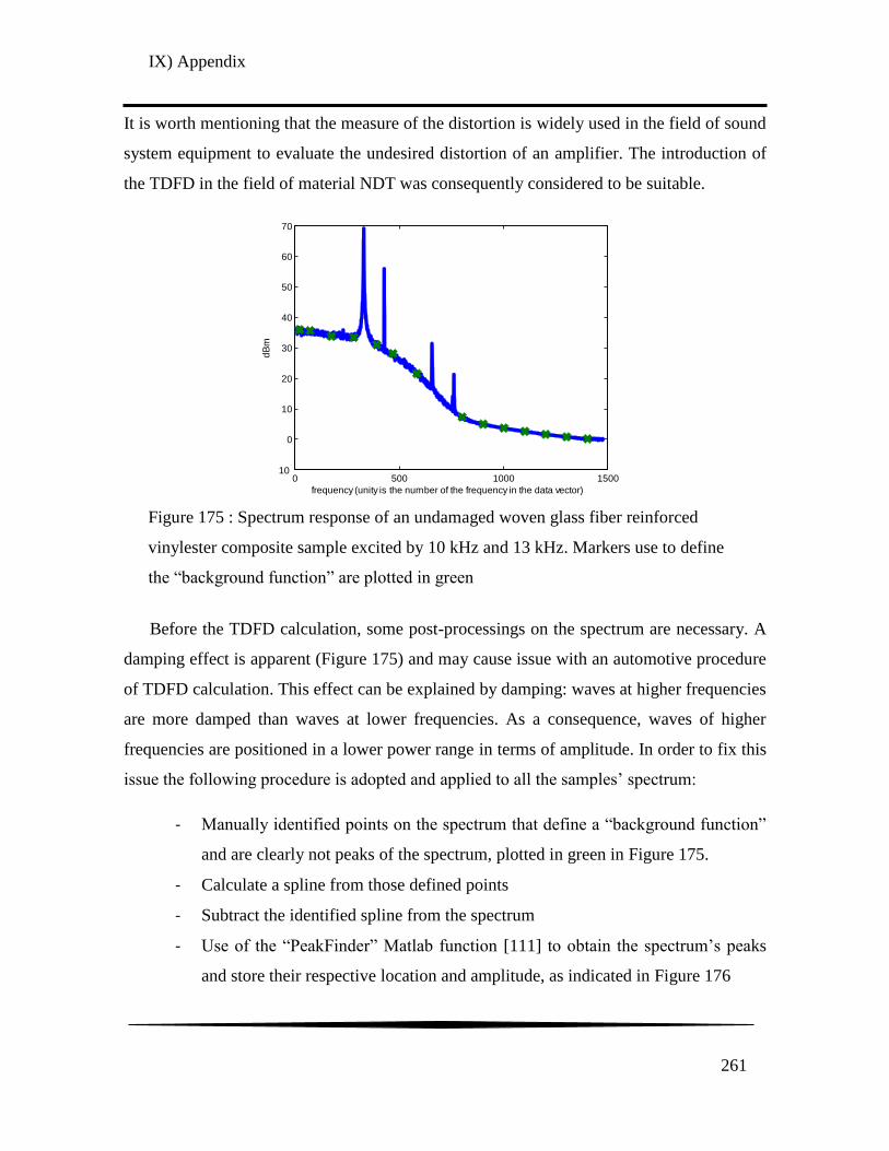
IX) Appendix
261
It is worth mentioning that the measure of the distortion is widely used in the field of sound
system equipment to evaluate the undesired distortion of an amplifier. The introduction of
the TDFD in the field of material NDT was consequently considered to be suitable.
Before the TDFD calculation, some post-processings on the spectrum are necessary. A
damping effect is apparent (Figure 175) and may cause issue with an automotive procedure
of TDFD calculation. This effect can be explained by damping: waves at higher frequencies
are more damped than waves at lower frequencies. As a consequence, waves of higher
frequencies are positioned in a lower power range in terms of amplitude. In order to fix this
issue the following procedure is adopted and applied to all the samples‟ spectrum:
- Manually identified points on the spectrum that define a “background function”
and are clearly not peaks of the spectrum, plotted in green in Figure 175.
- Calculate a spline from those defined points
- Subtract the identified spline from the spectrum
- Use of the “PeakFinder” Matlab function [111] to obtain the spectrum‟s peaks
and store their respective location and amplitude, as indicated in Figure 176
Figure 175 : Spectrum response of an undamaged woven glass fiber reinforced
vinylester composite sample excited by 10 kHz and 13 kHz. Markers use to define
the “background function” are plotted in green
0 500 1000 1500 10
0
10
20
30
40
50
60
70
frequency (unity is the number of the frequency in the data vector)
dB
m

IX) Appendix
262
- The TDFD is then calculated from each spectrum
It is worth mentioning that measurements were done 3 times on each sample, and the
same TDFD‟s values were obtained for the three measurements.
Results and discussion
The different frequency response from the vinylester/glass composite, obtained for
samples loaded at different stress levels, are all plotted in Figure 177. As a first observation,
it can be noted that the number and amplitude of peak increased with increasing the tensile
loading value. The same observation was made for epoxy/glass composite; it was however
not the case for the polyamide/glass sample.
Figure 176 : Spectrum response of an undamaged woven glass fiber reinforced
vinylester composite sample excited by 10 kHz and 13 kHz. The background
function has been subtract and the identified peak are marked in red
0 500 1000 1500 5
0
5
10
15
20
25
30
35
40
frequency (unity is the number in the data vector)
dB
m
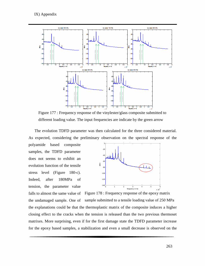
IX) Appendix
263
The evolution TDFD parameter was then calculated for the three considered material.
As expected, considering the preliminary observation on the spectral response of the
polyamide based composite
samples, the TDFD parameter
does not seems to exhibit an
evolution function of the tensile
stress level (Figure 180-c).
Indeed, after 180MPa of
tension, the parameter value
falls to almost the same value of
the undamaged sample. One of
the explanations could be that the thermoplastic matrix of the composite induces a higher
closing effect to the cracks when the tension is released than the two previous thermoset
matrixes. More surprising, even if for the first damage state the TDFD parameter increase
for the epoxy based samples, a stabilization and even a small decrease is observed on the
Figure 177 : Frequency response of the vinylester/glass composite submitted to
different loading value. The input frequencies are indicate by the green arrow
Figure 178 : Frequency response of the epoxy matrix
sample submitted to a tensile loading value of 250 MPa
0 1 2 3 4 5 6
x 104
-140
-120
-100
-80
-60
-40
-20
0
frequency in Hz
dB
m
Spectrum of the epoxy-sample damaged by a traction stress of 250 MPa
and excited by the frequencies of 11 kHz and 14 kHz

IX) Appendix
264
Figure 179 after 200MPa. An increasing evolution of the TDFD parameter function of the
stress level is noted for the vinylester base composite level (Figure 180-a).
However, it was noticed that for the epoxy matrix based composites the appearance of
high frequencies (Higher that 40 KHz as visible in Figure 178) for every tested samples
when the tensile loading value exceed 250MPa. Those higher frequencies seem to be
sensitive to the damage state. It was consequently propose to modify the TDFD parameter
to add a higher weight on those high frequencies. In order to do so, the amplitude of those
high frequencies was cubed:
√∑
∑
This parameter was used for the three different studied materials and for all the different
loading value considered. Input frequencies of 10 kHz and 13 kHz were used for all the
tested samples. Evolution of the TDFDalt function of the tensile loading value is plotted on
the Figure 180 for all those woven composite materials. Of course, since those higher
0 50 100 150 200 250 300 350 400 450
0.35
0.4
0.45
0.5
0.55
0.6
0.65
0.7
0.75
0.8
Measure of the nonlinear transmission behavior of the epoxy-samples
under excitation of 11 kHz and 14 kHz and plotted cubic regression
tota
l diffe
rence f
requency d
isto
rtio
n (
TD
FD
)
tensile stress in MPa
data1
cubic
Figure 179 : Standard measure of the nonlinear transmission
behavior of the epoxy matrix samples under excitation of 11
kHz and 14 kHz including the plot of a cubic regression
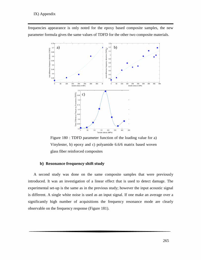
IX) Appendix
265
frequencies appearance is only noted for the epoxy based composite samples, the new
parameter formula gives the same values of TDFD for the other two composite materials.
b) Resonance frequency shift study
A second study was done on the same composite samples that were previously
introduced. It was an investigation of a linear effect that is used to detect damage. The
experimental set-up is the same as in the previous study; however the input acoustic signal
is different. A single white noise is used as an input signal. If one make an average over a
significantly high number of acquisitions the frequency resonance mode are clearly
observable on the frequency response (Figure 181).
Figure 180 : TDFD parameter function of the loading value for a)
Vinylester, b) epoxy and c) polyamide 6.6/6 matrix based woven
glass fiber reinforced composites
0 50 100 150 200 250 300 350 400
0.35
0.4
0.45
0.5
0.55
0.6
0.65
0.7
0.75
measure of the nonlinear transmission behavior
of the vinyl ester-samples under excitation of 10kHz and 13 kHz
tensile stress in MPa
tota
l diffe
rence f
requency d
isto
rtio
n (
TD
FD
)
data1
quadratic
0 50 100 150 200 250 300 350 400 450
0.4
0.5
0.6
0.7
0.8
0.9
1
1.1
1.2
1.3
Measure of the nonlinear transmission behavior of the epoxy-samples
under excitation of 11 kHz and 14 kHz and with traced quadratic regression
tensile stress in MPa
tota
l diffe
rence f
requency d
isto
rtio
n (
TD
FD a
lt)
data1
quadratic
a)
b)
c)

IX) Appendix
266
The shift, with an undamaged sample, of the frequency with the maximum amplitude is
measured for each damaged samples and for the three considered material. The evolution of
this frequency shift is plotted for each material in Figure 182. As for the previous study on
NWMS method, a clear damage growth was detected by the method for the epoxy (Figure
182-a) and vinylester matrix based samples (Figure 182-b). However, the frequency shift
evolution for the polyamide 66/6 samples, plotted in Figure 182-c, exhibits a great
oscillation when the tensile loading value increases. The indicator does not seem to be
effective to accurately evaluate the damage state inside the polyamide based samples.
Figure 181 : Frequency response of the undamaged vinylester matrix based sample
(In blue) and the 400MPa previously loaded in tension vinylester matrix based
sample (in green) for a white noise as input signal
0 0.5 1 1.5 2
x 104
-70
-60
-50
-40
-30
-20
frequency in Hz
dB
m
spectrums of the undamaged vinyl ester-sample (blue trace) and the vinyl ester-sample
damaged by 400 MPa traction stress (green trace) in the case of excitation by white noise
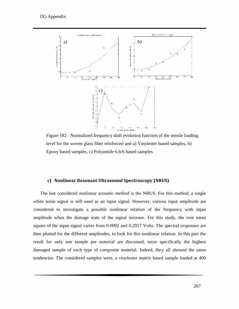
IX) Appendix
267
c) Nonlinear Resonant Ultrasound Spectroscopy (NRUS)
The last considered nonlinear acoustic method is the NRUS. For this method, a single
white noise signal is still used as an input signal. However, various input amplitude are
considered to investigate a possible nonlinear relation of the frequency with input
amplitude when the damage state of the signal increase. For this study, the root mean
square of the input signal varies from 0.0092 and 0.2917 Volts. The spectral responses are
then plotted for the different amplitudes, to look for this nonlinear relation. In this part the
result for only one sample per material are discussed, more specifically the highest
damaged sample of each type of composite material. Indeed, they all showed the same
tendencies. The considered samples were, a vinylester matrix based sample loaded at 400
N
or
m
ali
ze
d
fre
qu
en
cy
shi
ft
(%
)
N
or
m
ali
ze
d
fre
qu
en
cy
shi
ft
(%
)
Figure 182 : Normalized frequency shift evolution function of the tensile loading
level for the woven glass fiber reinforced and a) Vinylester based samples, b)
Epoxy based samples, c) Polyamide 6.6/6 based samples
a)
b)
c)

IX) Appendix
268
MPa, an epoxy matrix based sample loaded at 400 MPa, and a Polyamide 66/6 based
sample loaded at 315 MPa.
As it can be observed on the Figure 183, at least three different Eigen frequencies are
detected on each composite material, a fourth one is observable on the vinylester based
composite samples tested. However, there is no nonlinear relation between the input
amplitude and the highest amplitude frequencies; i.e. Eigen frequencies of the sample, for
the three tested composite materials. Contrary to what is predicted in the literature, there is
no frequency shift when the input amplitude is increasing. Unlike the two other acoustic
methods, this last investigated damage evaluation method is not sensitive to the increasing
damage state of the samples.
0 0.5 1 1.5 2 2.5
x 104
-80
-70
-60
-50
-40
-30
frequency in Hz
dB
m
Spectrum of the vinyl ester-matrix-sample damaged by 400 MPa
and exciting by white noise under a stepwise increase of excitation's power
Increasing
excitation’s power
Resonance 1 Resonance 2 Resonance 3 R. 4
0.5 1 1.5 2 2.5
x 104
-70
-60
-50
-40
-30
-20
frequency in Hz
dB
m
Spectrum of the epoxy-matric-sample damaged by 400 MP
exciting by white noise under a stepwise increase of excitation's power
Increasing
excitation’s power
Resonance 1 Resonance 2 Resonance 3
0 0.5 1 1.5 2 2.5 3
x 104
-80
-70
-60
-50
-40
-30
-20
frequency in Hz
dB
m
Spectrums of the polyamide-matrix-sample damaged by 350 MPa
and exciting by white noise under a stepwise increase of excitaion's power
Increasing
excitation’s power
Resonance 1 Resonance 2 Resonance 3
Figure 183 : Spectrum of the epoxy matrix sample damaged by a tensile stress of 400
MPa and excited by white noise under a stepwise increase of the excitation‟s power
for the a) Vinylester samples, b) Epoxy samples, c) Polyamide 66 samples

IX) Appendix
269
d) Conclusion
The NWMS as well as the resonance frequency shift study was found successful to
evaluate increasing state of damage in the epoxy and vinylester based samples. Yet, as it is
known that for loading tests along the fiber‟s axis only small micros-cracks appear inside
the sample, it can be state that both methods are sensitive enough to detect very low level of
damage inside composite material. In addition it was observed that the sensitivity to
damage of the TDFD parameter, used for the NWMS method, is higher than the normalized
resonance frequency shift considered for the other method. Indeed, for the vinylester based
composite materials the indicators show an evolution, between the undamaged and the 400
MPa loaded sample, of 100% and 6.2% for respectively the NWMS and the resonance
frequency shift method. Similarly, for the epoxy based composite the indicators exhibit an
evolution of respectively 200% and 10% between the undamaged and the 400MPa loaded
sample. It can be remind that those two methods are respectively nonlinear and linear
ultrasound spectroscopy based methods. Hence, the noted difference in sensitivity between
those methods are in accordance to the literature review from V)-1)-d) ([83], [84] as an
example).
However, those two methods were not able to quantify accurately the damage state for
the tested polyamide based composite samples. It may be relative to the different nature of
the material matrix. Indeed, both epoxy and vinylester are thermoset matrixes whereas
polyamide 66/6 is a thermoplastic matrix. However, further experiments are necessary to
assess this hypothesis. Both samples shapes and thickness are in fact different from one
sample to another. This make difficult to draw yet a definite conclusion about the origin of
the damage indicator evolution's contrast between the polyamide 66/6 based composite and
the other investigated materials.
The last considered evaluation method, the NRUS method, was not effective to evaluate
damage in any of the tested composite materials. Indeed, unlike what is predicted by the
literature, no shift in frequency was noted, for the same sample, when increasing the
amplitude of the input signal.

IX) Appendix
270
2) Appendix 2: Damage investigation using Coda Waves
Interferometry (CWI) technique on a woven carbon fibers
reinforced composite material
This study was done in close collaboration with Lynda Chehami during her post-doc
position at the LUNE lab from Georgia Tech Lorraine. In this part, the capability of the
coda wave interferometry (CWI) technique to evaluate small amount of damage in carbon
fibers reinforced polymer based composite samples was investigated. As a recall, a
literature review of the CWI technique was proposed in the section V)-1)-e) of this
manuscript, and give complementary information about the recent application of this
technique. Here the sample was subjected to four points bending at different levels of
applied displacement until failure of the sample is reached. Time shift of the later part of
the signal (i.e. Coda wave) is investigated by mean of windowed cross-correlation. A
description of this chosen post-processing method is also included in the literature review
from section V)-1)-e).
a) Presentation of the investigated composite material
It must be emphasized that, contrary to the rest of the thesis manuscript, the
investigation of coda waves was performed only on polypropylene sulfide based composite
reinforced with eight layers of woven carbon fibers with the following stacking sequence:
[0°/90°, -45°/45°, 0°/90°, -45°/45°]s Indeed, it is known that glass fiber reinforced
composite induces a higher attenuation coefficient than for carbon fiber reinforced
composite. As explained in the literatures review (Section V)-1)-e)), the Coda Wave
Interferometry (CWI) method consists in the study of the later part of the receiving signal.
Therefore, to be able to process with more efficiency this coda part with a correct signal to
noise ratio it was chosen to consider this carbon fiber reinforced material for the first
investigations on this method. Two samples of 160 x 25 x 2.4 mm were produced by water
jet cutting. One of those samples is submitted to increasing levels of 4 points bending
loading. The method is known to be sensitive to the influence of temperature during the

IX) Appendix
271
investigation. Consequently, the other sample is kept undamaged during the experimental
procedure and is used as a reference. Acquisitions on this reference sample were performed
at the same time than for the damaged sample, i.e. after each four points bending test.
b) Experimental set-up
Monotonic four points bending tests set-up
As mentioned, various displacement levels were consider and applied to one of the
carbon fiber composite sample by using four point bending set-up (Figure 184). This is
performed in order to investigate the sensitivity to the coda wave interferometry method to
quantify this amount of damage accurately. Eleven bending displacement levels were
considered, starting from 2 mm to 12 mm with an increment of 1 mm. This 12 mm actually
corresponds to the apparition of a visible crack on the surface of the sample and the latter
was considered to have consequently reach failure. The resulting force is indicated, for
every applied displacement value, in the Table 34. Force/displacement response under
bending is plotted in Figure 185 for an applied displacement of 9 and 12mm. The bending
test is performed on a tensile test machine (Zwick Roell Z050) in compliance with the ISO
5893 standard. The sample is loaded at a constant displacement of 24mm.min-1
. An
ultrasonic acquisition is done prior to any bending loading and will be used as a reference.
After each bending tests an ultrasonic acquisition is also performed on the reference
sample.
Displacement
(mm)
2 3 4 5 6 7 8 9 10 11 12
Force (N) 187 292 399 519 638 761 876 978 1100 1200 1240
Table 34 : Displacement and loading values for monotonic four points bending loading

IX) Appendix
272
A first estimation of the damage was made based on the bending modulus reduction
measured after each loading is a similar way than in part III)-4). This estimation of damage
was calculated as:
; with En the unloaded bending modulus for each considered
Figure 184 : a) Schematic representation and b) photography of the four points
bending setup
a) b)
Figure 185 : Force displacement curve for the 12mm and 9mm four
points bending tests

IX) Appendix
273
applied displacement and E0 the bending loading modulus measured for the first bending
test. The evolution of the calculated damage (Figure 186) can be divided into three main
steps. From 0 to 3 mm of applied displacement, no evolution is noted yet, micro-cracks are
assumed to initiate in the specimen during this step. But after a displacement of 4 mm, a
close to linear evolution of the damage could be observed up to 0.13 for a displacement of 8
mm. An abrupt change in the damage sate evolution is noted after this point. The calculated
damage then remains around 0.13 from 9 to 11 mm of applied displacement and may
indicate a saturation of damage. The displacement of 12 mm actually corresponds to the
failure of the sample as mention earlier and consequently this last value of measured
damage must be considered with caution.
Figure 186 : Evolution of damage, calculated as the reduction of the
bending modulus, with increasing the magnitude of the 4 points bending
applied displacement

IX) Appendix
274
Ultrasonic measurements set-up and processing
All the ultrasonic acquisitions were performed using the following procedure. After
each bending tests, two Panametrics V103 sensors 1MHz PZT disks, polarized
longitudinally, are used in transmission. The emitting signal is produce by a waveform
generator, Agilent Technology model, connected to the first transducer. The emitting signal
consists in a sinus burst of 1cycles at a 1MHz frequency with an amplitude of 10 Volt peak-
to-peak. The second transducer, in reception, is put at a distance of 83 mm from the first
one. The receiving signal is then amplify by 100dB by an amplifier from Krohn-Hite
(model 7500), and recorded using an oscilloscope. A coupling gel, Sofranel coupling Gel-D
is used for both transducers. All the experimental set-up is depict in Figure 187.
The length of the recorded signal is set at 1000 µs, after this given time the signal is
almost null, as it can be seen in Figure 188, with a low signal to noise ratio which could
induce wrong results from the cross-correlation processing later on. Before recording each
signal the latter is averaged over 250 measurements, which confers an increasing of the
Figure 187 : a) Complete experimental set-up for the ultrasonic signal
recording. b) Zoom in on one of the tested sample with indication of
transducers position
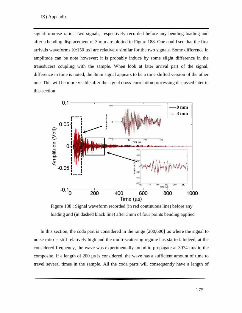
IX) Appendix
275
signal-to-noise ratio. Two signals, respectively recorded before any bending loading and
after a bending displacement of 3 mm are plotted in Figure 188. One could see that the first
arrivals waveforms [0:150 µs] are relatively similar for the two signals. Some difference in
amplitude can be note however; it is probably induce by some slight difference in the
transducers coupling with the sample. When look at later arrival part of the signal,
difference in time is noted, the 3mm signal appears to be a time shifted version of the other
one. This will be more visible after the signal cross-correlation processing discussed later in
this section.
In this section, the coda part is considered in the range [200,600] µs where the signal to
noise ratio is still relatively high and the multi-scattering regime has started. Indeed, at the
considered frequency, the wave was experimentally found to propagate at 3074 m/s in the
composite. If a length of 200 µs is considered, the wave has a sufficient amount of time to
travel several times in the sample. All the coda parts will consequently have a length of
Figure 188 : Signal waveform recorded (in red continuous line) before any
loading and (in dashed black line) after 3mm of four points bending applied
0 mm
3 mm

IX) Appendix
276
Tt=400 µs and a sampling time of Δt=0.002 µs. As it was mentioned in [96], [112] for
example, when the sample‟s perturbation is small, the induced relative velocity change of
the signal‟s coda part can be considered as constant. In such a case, the time lag increase
with the arrival time. The damage state induced by four point bending will be considered to
match this hypothesis. This will be verified with the experimental results that will be
presented further on. In order to have a good estimation of δt, the cross correlation must be
performed on small part of the signal (i.e. window) where the variation of δt over the time
arrival is sufficiently low to be considered as constant. The length T of the windows must
satisfy the interferometry hypothesis which is : T*ΔF<<1, with ΔF is the frequency band of
the coda signal [113]. In this study, the frequency band of the coda part is of 400 KHz, the
time window T must be at minimum 2.5 µs. Here T was set to 50 µs for each window. The
cross-correlation coefficient R(ts) is then calculated for each windows by shifting this
window over each ts increment with ts between [-T:T]. The time lag that corresponds to the
maximum of correlation is measured as well for each window. Each window is spaced by
T/2 in order to consider overlapped windows. This allowed smoothing the evolution of the
δt with the time arrival. Before choosing the coda part the whole recorded signals, of 1000
µs long, were all adjusted in time in order to have the first wave packet arrival at the same
time than for the reference signal. Indeed, the two transducers were positioned by hand
after each 4 points bending tests on the sample on marks draw in the samples. This
adjustment in the first wave packet arrival was done to reduce influence of bad transducers
positioning that could interfere with a correct estimation of relative velocity change. In
addition, the applied loading may induce small change in size of the sample which may
introduce additional time shift in the calculation of the velocity change. It can be mentioned
that on the raw data however, there is no major shift of the first pulse from all the signals
recorded after bending tests when compare with signal recorded before any applied loading
at the exception of the signals recorded after 6mm of applied displacement.
For the sample 1, submitted to 4 points bending test, all signals are compared with the
first signal recorded for this sample prior to any loading. For the sample 2, that is kept
undamaged, all signals are compared with the 1st signal recorded from this sample 2. It was

IX) Appendix
277
recorded at the same time than the first signal from the sample 1. The evolution of the
cross-correlation coefficient and the time lag with the arrival is plotted in Figure 189 for
both the damaged and reference sample. The signals for the all the applied loading
considered are plotted on each graph accordingly.
As observed in Figure 189-a, no major evolution of the cross-correlation is observed for
the sample damaged from 2mm to 11mm. Its value remains close to 0.8 which indicate
Figure 189 : a) Normalized cross-correlation coefficient between the sample loaded
(200-1200N) and the sample before loading. b) Normalized cross-correlation
coefficient for the reference sample between different moment and the first signal
record for this sample. c) Time shift between the sample loaded (200-1200N) and the
sample before loading. d) Time shift coefficient for the reference sample between
different moment and the first signal record for this sample
a)
a)
b)
b) c)
c)
d)
d)

IX) Appendix
278
important similarity with the signal before any loading. However, an important decrease of
the coefficient is noted after 12mm of loading apply; its value oscillates around 0.5. Here
the similarity with the signal before any loading is too low and it was consequently choose
to not calculate time shift for this sample. Indeed, since the signals are not similar, the
results from the cross-correlation could not be function of simple time-shift only. For the
reference sample, the cross-correlation coefficient (in Figure 189-b) remains sufficiently
high and does not evolve significantly as the experiment going on.
As mentioned, the time lag that corresponds to the maximum of correlation is extracted
for each window on each signal. The results is plotted in Figure 189-c for the sample
submitted to four points bending. As explained earlier, the results for the 12mm loading
were not considered because of the lower correlation coefficient obtained from Figure 189-
a for this loading. A clear evolution of the time lag is observed when increased the
displacement loading; it is even more pronounced after 8mm. The time lag increases with
the time arrival which confirmed the hypothesis made before. For the reference sample
however, the evolution of time lag with the time arrival is limited for every measurement
performed; at the exception of the signal recorded after a 6mm loading was applied to the
other sample. The time lag is distant from the other measurements but remains mostly
constant with the time arrival.
Finally, the relative velocity change δV/V is calculated from each signals by estimated
the slope of δt/t from the Figure 189-c and Figure 189-d. This relative velocity change is
then calculated as δV/V =-δt/t if the effective velocity change is considered as homogenous
over the whole sample. The evolution of the relative velocity change δV/V for sample 1
with applied displacement is plotted in Figure 190. The same graph is plotted for sample 2
for all the recorded signals on the same figure. For the reference sample (n° 2), the relative
velocity change does not appear to be significant at the exception of the measurements
number 6 and 10 (Whose correspond to the applied displacement of 7 and 11mm
respectively). However, for the sample 1 an evolution of the relative velocity change is
noted which seems to involve 3 main steps. This evolution is actually really similar to the
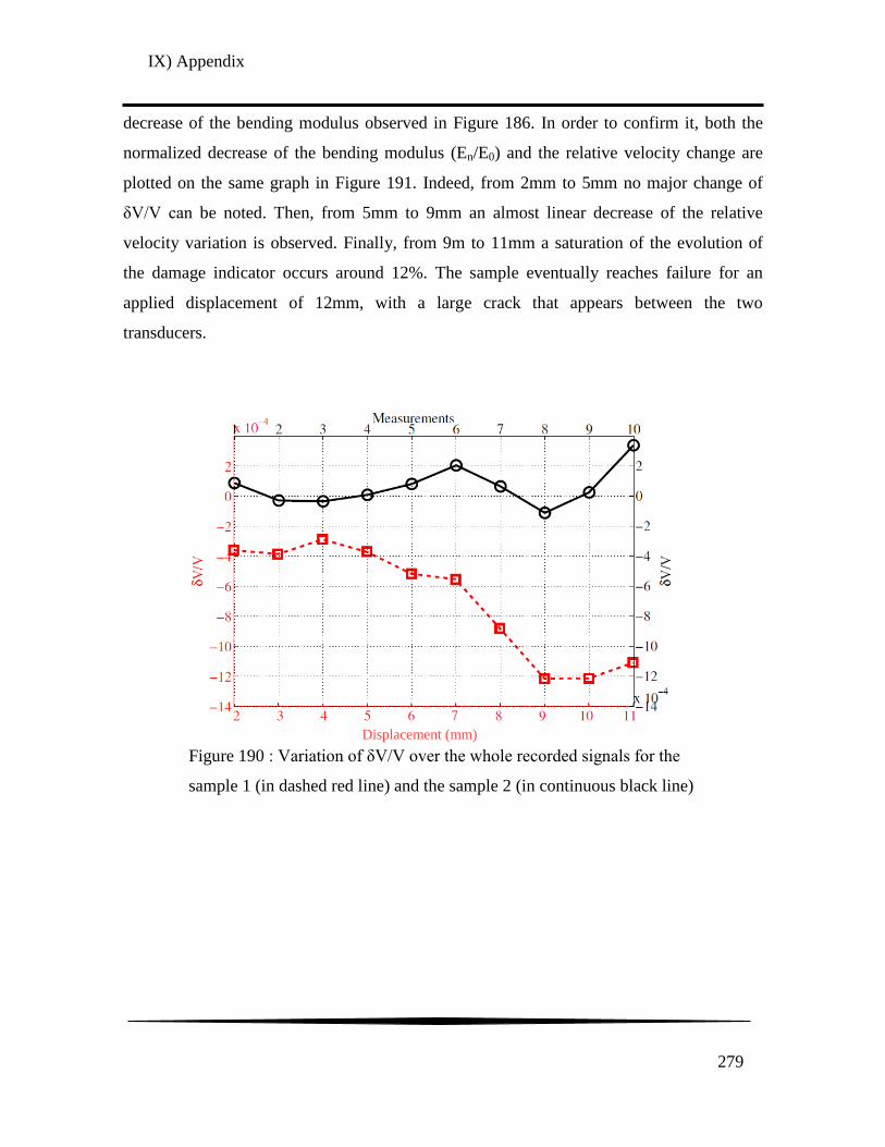
IX) Appendix
279
decrease of the bending modulus observed in Figure 186. In order to confirm it, both the
normalized decrease of the bending modulus (En/E0) and the relative velocity change are
plotted on the same graph in Figure 191. Indeed, from 2mm to 5mm no major change of
δV/V can be noted. Then, from 5mm to 9mm an almost linear decrease of the relative
velocity variation is observed. Finally, from 9m to 11mm a saturation of the evolution of
the damage indicator occurs around 12%. The sample eventually reaches failure for an
applied displacement of 12mm, with a large crack that appears between the two
transducers.
Displacement (mm)
Figure 190 : Variation of δV/V over the whole recorded signals for the
sample 1 (in dashed red line) and the sample 2 (in continuous black line)
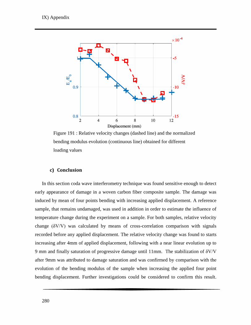
IX) Appendix
280
c) Conclusion
In this section coda wave interferometry technique was found sensitive enough to detect
early appearance of damage in a woven carbon fiber composite sample. The damage was
induced by mean of four points bending with increasing applied displacement. A reference
sample, that remains undamaged, was used in addition in order to estimate the influence of
temperature change during the experiment on a sample. For both samples, relative velocity
change (δV/V) was calculated by means of cross-correlation comparison with signals
recorded before any applied displacement. The relative velocity change was found to starts
increasing after 4mm of applied displacement, following with a near linear evolution up to
9 mm and finally saturation of progressive damage until 11mm. The stabilization of δV/V
after 9mm was attributed to damage saturation and was confirmed by comparison with the
evolution of the bending modulus of the sample when increasing the applied four point
bending displacement. Further investigations could be considered to confirm this result.
Figure 191 : Relative velocity changes (dashed line) and the normalized
bending modulus evolution (continuous line) obtained for different
loading values

IX) Appendix
281
Some noticeable evolution of δV/V was observed on the reference sample and could induce
wrong interpretation on measured signal. Its evolution remains nevertheless lower when
compared to the other sample. The observed decreasing of δV/V on the sample subjected to
four points bending couldn‟t then be ascribed to temperature evolution.
This method could therefore worth further investigation in order to confirm the relation
between the evolution of damage state and cracks propagation and the relative velocity
variation obtain from the coda part investigation. Those additional investigation could help
to determine what are the case when the method could be consider under simple hypothesis
and when some caution must be taken when interpreting the results. Consequently, at the
moment this method should still be used with caution because of the known sensitivity of
the method to the transducer‟s positions on the tested sample and to the ambient
temperature change. Nevertheless, the overall methodology is very promising for structural
health monitoring because of its sensitivity to small defects, nondestructive aspects and the
continuous time monitoring of the health condition of composites. It could be used as a
complementary signal processing technique in order to increase the amount of information
to analyze to make a proper decision about the damage state of a part. Future investigations
should also consider samples submitted to fatigue damage; such tests are indeed closer to
the solicitation that a structure may undergo in the industrial field.

IX) Appendix
282


DETECTION DE L’ENDOMMAGEMENT DANS UN COMPOSITE TISSE
PA66/6|FIBRES DE VERRE A L’AIDE DE TECHNIQUES ULTRASONORES EN VUE
D’UNE PREDICTION DE LA DURABILITE DE PIECES AUTOMOBILES
RESUME : Ces travaux de thèse portent sur l'étude expérimentale approfondie d'un composite à base
polyamide 66/6 renforcé par des fibres de verres tissées suivant un motif sergé 2/2. L’objectif est de
proposer des solutions de Contrôle Non Destructif (CND) basées sur les ultrasons afin de détecter
différents niveaux d’endommagement induit. Pour cela, une étude approfondie des mécanismes
d’endommagement apparaissant lors de sollicitations en traction suivant l’axe des fibres et hors axes
est réalisé. Le cas d’impact induit par poids tombant est également étudié. En effet, ces différents cas
de sollicitions entraînent l’apparition de différents mécanismes d’endommagement. Ces derniers,
ainsi que leur ordre d’apparition, sont caractérisés par Microscopie Electronique à Balayage (MEB)
et tomographie à rayons X principalement. L’évaluation de la réduction du module élastique pré et
post chargement ainsi que la fraction volumique de vides montrent une évolution de
l’endommagement plus importante lors de chargement en traction hors axes des fibres que lors de
chargement suivant l’axe. Lors des essais d’impact par poids tombant, différents niveaux d’énergie
sont considérés en restant proche du domaine des BVID en vue d’éprouver la sensibilité des
méthodes de CND. Deux méthodes de CND par ultrasons étudiées durant ce projet peuvent être
mises en avant. Premièrement, par mesure de la vitesse de propagation des ondes dans plusieurs
directions du composite, le tenseur de rigidité est estimé dans tous ces cas de sollicitation mécanique
pour différents niveaux d’endommagement. Des indicateurs d’endommagement basés sur ces
mesures montrent une évolution de l’état d’endommagement similaire à celle discutée
précédemment. Deuxièmement, une étude de la détection de l’endommagement par ondes guidées
est menée. Aucun changement des modes transmis n’est visible lors de l’augmentation de l’état
d’endommagement. L’évolution de l’énergie du signal transmis est alors proposée et validée comme
indicateur d’endommagement efficace pour des chargements en traction mais pas pour l’impact. La
mesure du décalage temporel a en revanche permis une localisation et une quantification de
l’endommagement induit par impact.
Mots clés : Matériau composite, Contrôle Non Destructif (CND), Ultrasons, Endommagement
DAMAGE DETECTION IN PA 66/6|GLASS WOVEN FABRIC USING ULTRASONIC
TECHNIQUES TOWARDS DURABILITY PREDICTION OF AUTOMOTIVE PARTS
ABSTRACT: The present study is focused on the experimental study of a polyamide 66/6 based
composite reinforced by a 2/2 twill weave glass fabric. The aim is to propose Non Destructive
Evaluation (NDE) methods based on ultrasound that can efficiently distinguish different damage
states. In order to do so, an investigation of the damage mechanisms induced by different types of
mechanical solicitations. Tension along and off the axis of the fibers was considered as well as the
case of drop weight impact. Those solicitations were shown to induce different damage mechanisms.
The latter were characterized by means of Scanning Electronic Microscopy (SEM) and X-Ray
tomography mostly. The decreasing of the elastic modulus and the void volume fraction evolution
were shown to be more significant for the samples loaded in tension off-axis. During the drop weight
impact tests, the energies were considered in order to remain close to the Barely Visible Impact
Damage (BVID) regime and to experience the capability of the ultrasound based NDE methods.
Two NDE methods investigated during this study deserve to be highlighted. Firstly, the stiffness
tensor was estimated by means of phase velocities measurements in different propagation direction.
Damage indicators based on results from this method were proposed. They were found to give
results similar with those from the evaluation of damage discussed earlier on. Secondly, a study of
the damage detection using guided waves was performed. No mode conversion effect was observed
from this investigation. Consequently, the signal energy was proposed as damage indicator and was
found to be suitable to detect damage induced by tension but not by impact. The measure of time
shift allowed obtaining a localization and evaluation of the damage induced by impact.
Keywords: Composite material, Non Destructive Testing (NDT), Ultrasonic wave, Damage