Desired Future Condition Explanatory Report (Final) Carrizo ...
481
Desired Future Condition Explanatory Report (Final) Carrizo-Wilcox/Queen City/Sparta Aquifers for Groundwater Management Area 13 William R. Hutchison, Ph.D., P.E., P.G. Independent Groundwater Consultant 9305 Jamaica Beach Jamaica Beach, TX 77554 512-745-0599 [email protected] February 22, 2017
-
Upload
khangminh22 -
Category
Documents
-
view
3 -
download
0
Transcript of Desired Future Condition Explanatory Report (Final) Carrizo ...
Desired Future Condition Explanatory Report (Final) Carrizo-Wilcox/Queen City/Sparta Aquifers for Groundwater
Management Area 13
William R. Hutchison, Ph.D., P.E., P.G. Independent Groundwater Consultant
9305 Jamaica Beach Jamaica Beach, TX 77554
512-745-0599 [email protected]
February 22, 2017
Desired Future Condition Explanatory Report (Final) Carrizo-Wilcox/Queen City/Sparta Aquifers for Groundwater Management Area 13
Page 1
Table of Contents
1.0 Groundwater Management Area 13 .......................................................................................... 3
2.0 Proposed Desired Future Condition ........................................................................................ 6
3.0 Policy Justification .................................................................................................................... 7
4.0 Technical Justification ............................................................................................................... 9
5.0 Factor Consideration ................................................................................................................ 13
5.1 Aquifer Uses and Conditions ............................................................................................ 13
5.2 Water Supply Needs and Water Management Strategies ................................................. 13
5.3 Hydrologic Conditions within Groundwater Management Area 13 ................................. 15
5.3.1 Total Estimated Recoverable Storage ........................................................................... 16
5.3.2 Average Annual Recharge, Inflows and Discharge ...................................................... 17
5.4 Other Environmental Impacts, Including Spring Flow and Other Interactions between Groundwater and Surface Water ................................................................................................... 19
5.5 Subsidence ......................................................................................................................... 19
5.6 Socioeconomic Impacts .................................................................................................... 19
5.7 Impact on Private Property Rights ..................................................................................... 20
5.8 Feasibility of Achieving the Desired Future Condition .................................................... 20
5.9 Other Information ............................................................................................................. 20
6.0 Discussion of Other Desired Future Conditions Considered ................................................... 21
7.0 Discussion of Other Recommendations ................................................................................ 22
8.0 References ............................................................................................................................. 23
Desired Future Condition Explanatory Report (Final) Carrizo-Wilcox/Queen City/Sparta Aquifers for Groundwater Management Area 13
Page 2
List of Figures
Figure 1. Groundwater Management Area 13 ................................................................................... 3
Figure 2. Counties Entirely or Partially in GMA 13 ......................................................................... 4
Figure 3. Groundwater Conservation Districts in GMA 13 .............................................................. 5
Figure 4. Conceptual Model of Flow (from Kelley and others, 2004, Figure 5.1) ......................... 10
List of Tables
Table 1. Alternative Estimates of Groundwater Availability .......................................................... 11
Table 2. Groundwater Budget for Groundwater Management Area 13 .......................................... 18
List of Appendices
Appendix A – Proposed Desired Future Condition Resolution
Appendix B – Groundwater Use Estimates
Appendix C – Comparison of Groundwater Monitoring Data with Groundwater Model Results, Groundwater Management Area 13
Appendix D – Water Supply Needs and Water Management Strategies Data
Appendix E – TWDB GAM Task 13-036 (Revised): Total Estimated Recoverable Storage for Aquifers in Groundwater Management Area 13
Appendix F – Paper authored by James Bene of R.W. Harden & Associates regarding the Joint Planning Process
Appendix G – Socioeconomic Impacts Analyses for Regions K, L, and M
Appendix H – James Bene PowerPoint: November 20, 2013 GMA 13 Meeting
Appendix I – GBRA letter of February 26, 2016 Regarding Surface Water Impacts
Appendix J – James Beach PowerPoint: March 30, 2016 Regarding Modeling Groundwater-Surface Water Interactions
Desired Future Condition Explanatory Report (Final) Carrizo-Wilcox/Queen City/Sparta Aquifers for Groundwater Management Area 13
Page 3
1.0 Groundwater Management Area 13
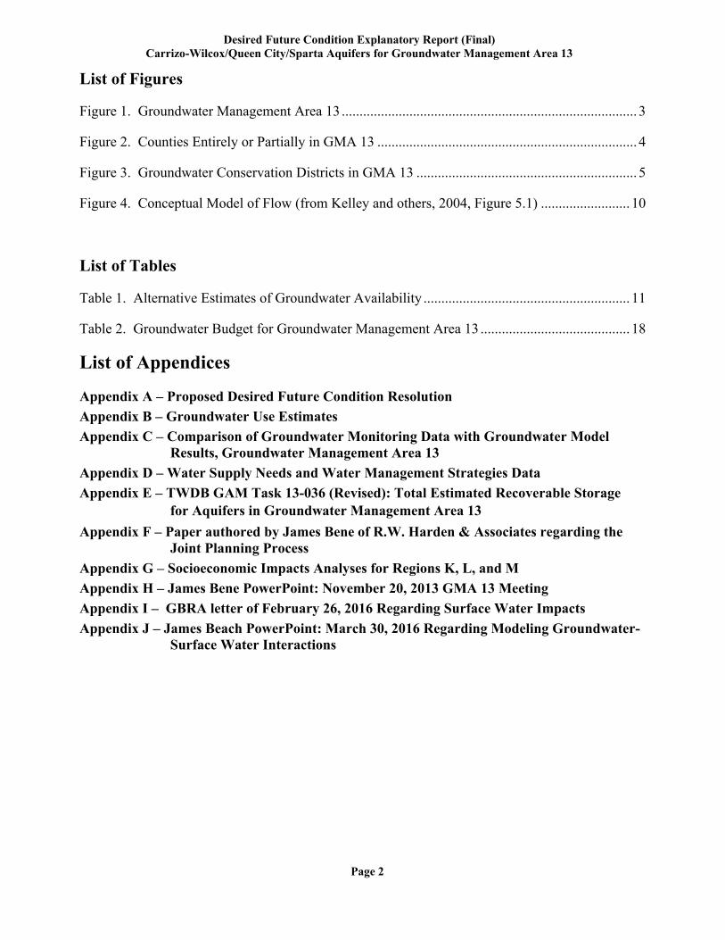
Groundwater Management Area 13 is one of sixteen groundwater management areas in Texas, and covers a large portion of the southwest part of the state (Figure 1).
Figure 1. Groundwater Management Area 13
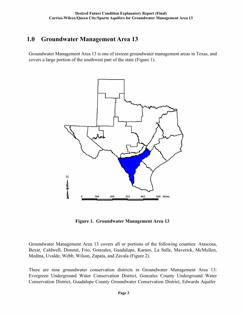
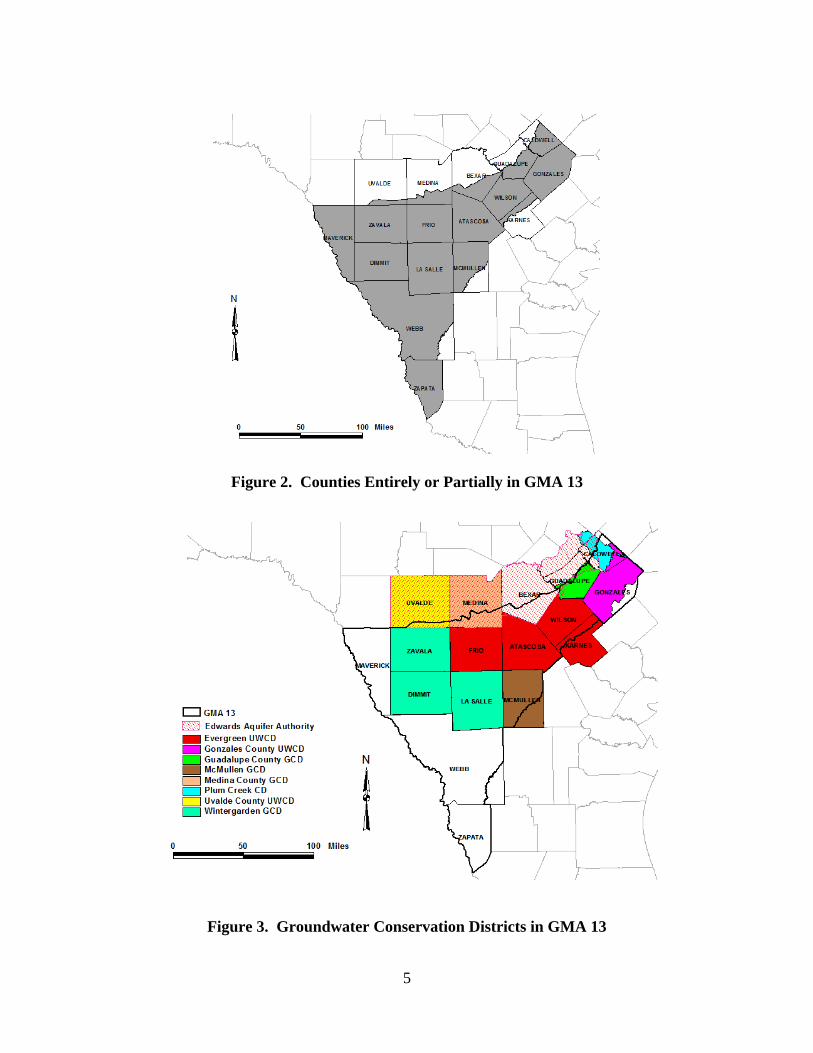
Groundwater Management Area 13 covers all or portions of the following counties: Atascosa, Bexar, Caldwell, Dimmit, Frio, Gonzales, Guadalupe, Karnes, La Salle, Maverick, McMullen, Medina, Uvalde, Webb, Wilson, Zapata, and Zavala (Figure 2).
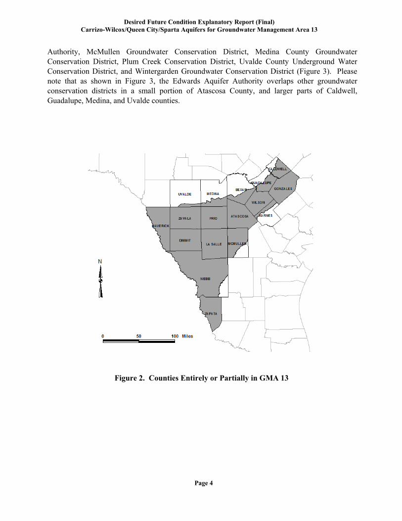
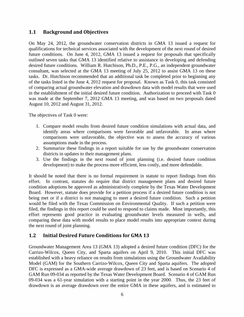
There are nine groundwater conservation districts in Groundwater Management Area 13: Evergreen Underground Water Conservation District, Gonzales County Underground Water Conservation District, Guadalupe County Groundwater Conservation District, Edwards Aquifer
Desired Future Condition Explanatory Report (Final) Carrizo-Wilcox/Queen City/Sparta Aquifers for Groundwater Management Area 13
Page 4
Authority, McMullen Groundwater Conservation District, Medina County Groundwater Conservation District, Plum Creek Conservation District, Uvalde County Underground Water Conservation District, and Wintergarden Groundwater Conservation District (Figure 3). Please note that as shown in Figure 3, the Edwards Aquifer Authority overlaps other groundwater conservation districts in a small portion of Atascosa County, and larger parts of Caldwell, Guadalupe, Medina, and Uvalde counties.
Figure 2. Counties Entirely or Partially in GMA 13
Desired Future Condition Explanatory Report (Final) Carrizo-Wilcox/Queen City/Sparta Aquifers for Groundwater Management Area 13
Page 5
Figure 3. Groundwater Conservation Districts in GMA 13

Desired Future Condition Explanatory Report (Final) Carrizo-Wilcox/Queen City/Sparta Aquifers for Groundwater Management Area 13
Page 6
2.0 Proposed Desired Future Condition
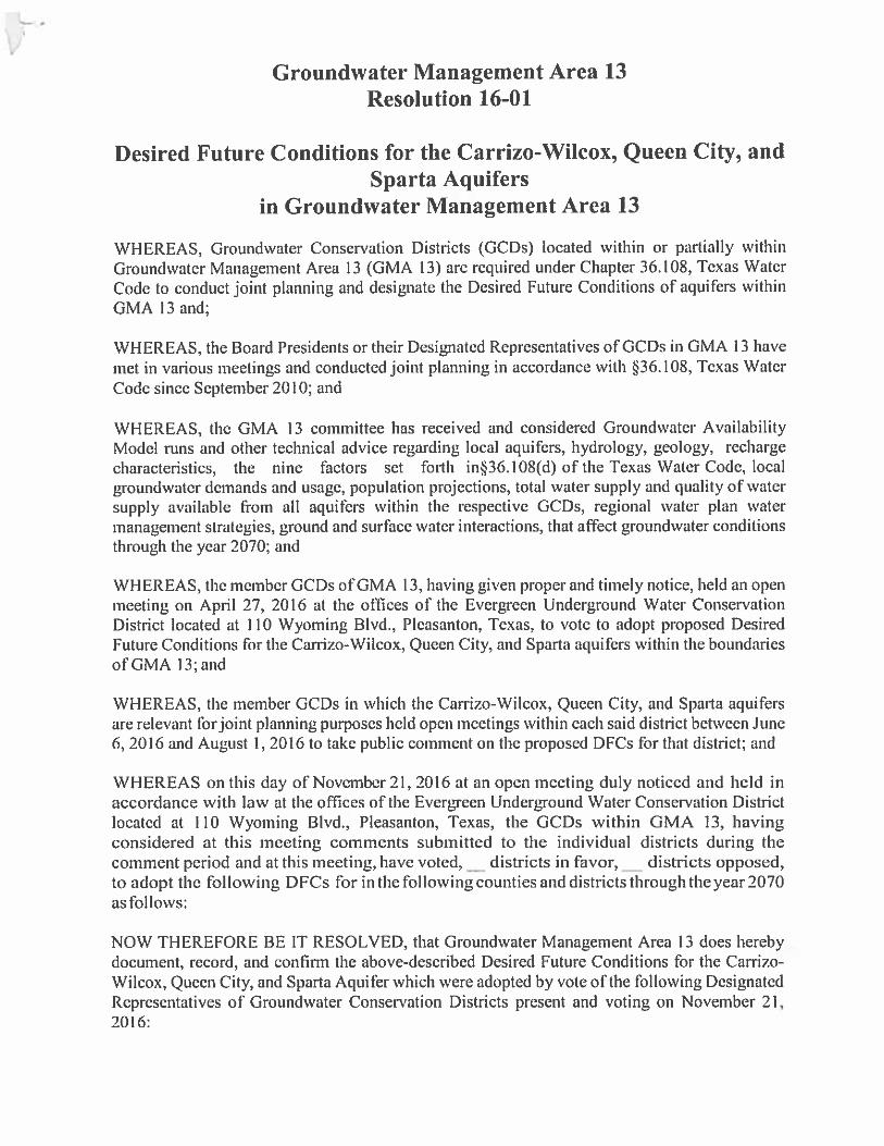
Due to limitations with the model as described in Technical Memorandum 16-08, two proposed desired future conditions were selected for the Carrizo-Wilcox/Queen City/Sparta aquifers as described below. The first proposed desired future condition for the Carrizo-Wilcox/Queen City/Sparta Aquifers in Groundwater Management Area 13 is that 75 percent of the saturated thickness at the end of 2012 remains in 2070. This desired future condition is considered feasible despite model predictions to the contrary as detailed in Technical Memorandum 16-08. In addition, a secondary proposed desired future condition for the Carrizo-Wilcox/Queen City/Sparta Aquifers in Groundwater Management Area 13 is an average drawdown of 48 feet for all of GMA 13. The drawdown is calculated from the end of 2012 conditions to the year 2070. This desired future condition is consistent with Scenario 9 as detailed in GMA 13 Technical Memorandum 16-01 and GMA 13 Technical Memorandum 16-08. The vote to send the proposed desired future conditions to the groundwater conservation districts was taken at the April 27, 2016 meeting of GMA 13. Appendix A is the final resolution for the desired future conditions. The geographic area covered by the proposed desired future condition is defined by the grid file for the Groundwater Availability Model of the Carrizo-Wilcox, Queen City, and Sparta aquifers (Kelly and others, 2004). This file (qcsp_s_grid_poly052212.csv) was downloaded from the Texas Water Development Board website:
http://www.twdb.state.tx.us/groundwater/models/gam/qcsp/qcsp.as
Desired Future Condition Explanatory Report (Final) Carrizo-Wilcox/Queen City/Sparta Aquifers for Groundwater Management Area 13
Page 7
3.0 Policy Justification
As developed more fully in this report, the proposed desired future condition was adopted after considering:
Aquifer uses and conditions within Groundwater Management Area 13 Water supply needs and water management strategies included in the 2012 State Water
Plan Hydrologic conditions within Groundwater Management Area 13 including total
estimated recoverable storage, average annual recharge, inflows, and discharge Other environmental impacts, including spring flow and other interactions between
groundwater and surface water The impact on subsidence Socioeconomic impacts reasonably expected to occur The impact on the interests and rights in private property, including ownership and the
rights of landowners and their lessees and assigns in Groundwater Management Area 13 in groundwater as recognized under Texas Water Code Section 36.002
The feasibility of achieving the desired future condition Other information
In addition, the proposed desired future condition provides a balance between the highest practicable level of groundwater production and the conservation, preservation, protection, recharging, and prevention of waste of groundwater in Groundwater Management Area 13. There is no set formula or equation for calculating groundwater availability. This is because an estimate of groundwater availability requires the blending of policy and science. Given that the tools for scientific analysis (groundwater models) contain limitations and uncertainty, policy provides the guidance and defines the bounds that science can use to calculate groundwater availability. The maximum amount of groundwater available is the amount of water stored in the aquifer plus groundwater “captured” by wells. The captured groundwater includes induced inflow into an area by pumping and reductions in natural discharge (e.g. spring flow surface water base flow). This is the extreme case where the goal is to entirely deplete, or mine, the aquifer. GMA 13 rejected this policy because it conflicts with the mission to conserve, preserve and protect the aquifers. One common definition of groundwater availability is the amount of water that can be recovered annually over a specified planning period without causing irreversible harm. The irreversible harm can include drying up existing wells and spring flow depletion, and are dependent on local conditions and policies. GMA 13 is in general agreement with this policy of determining groundwater availability because it coincides with the mission to conserve, preserve, and protect the aquifers. After agreeing on a policy to estimate groundwater availability, the next step was to define the factors that would cause irreversible harm due to the impacts of such production on the system.
Desired Future Condition Explanatory Report (Final) Carrizo-Wilcox/Queen City/Sparta Aquifers for Groundwater Management Area 13
Page 8
These factors include:
Economics of producing water from depth Intrusion of poor water quality due to changes in vertical flow gradients Interaction between stream flow and groundwater Changes in groundwater evapotranspiration rates Groundwater storage recovery rates Timeframe of pumping capture and sustainable pumpage
As developed more fully below, many of these factors could only be considered on a qualitative level since the available tools to evaluate these impacts have limitations and uncertainty.
Desired Future Condition Explanatory Report (Final) Carrizo-Wilcox/Queen City/Sparta Aquifers for Groundwater Management Area 13
Page 9
4.0 Technical Justification
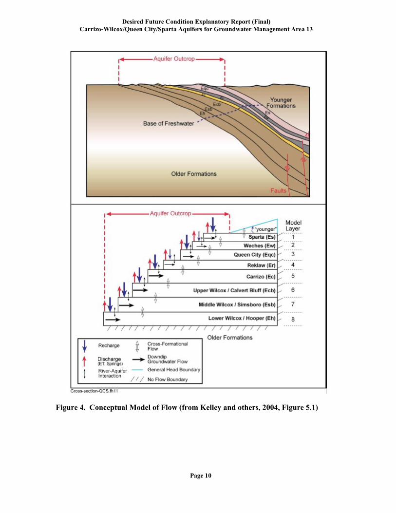
The proposed desired future condition for the Carrizo-Wilcox/Queen City/Sparta Aquifers was developed based on simulations of alternative scenarios of future pumping using the Groundwater Availability Model (GAM) of the Carrizo-Wilcox, Queen City, and Sparta aquifers (Kelley and others, 2004). This GAM superseded the GAM of the southern Carrizo-Wilcox Aquifer (Deeds and others, 2003). The GAM used in this process was developed to make predictions of groundwater availability through 2050 based on current projections of groundwater demands during drought-of-record conditions (Kelley and others, 2004, pg. xxvii). The calibration period for the GAM was 1980 to 1989, and the verification period was 1990 to 1999. The documentation for the GAM stated that the GAM provides an “integrated tool for the assessment of water management strategies to directly benefit state planners, Regional Water Planning Groups (RWPGs), and Groundwater Conservation Districts (GCDs)”. Furthermore, the documentation stated that based on the model grid (one square mile), the GAM is “not capable of predicting aquifer responses at specific points such as a particular well”, and that the GAM is “accurate at the scale of tens of miles, which is adequate to understand groundwater availability at the regional scale” (Kelley and others, 2004, pg. xxviii). As detailed in Technical Memorandum 17-01, the model calibration period was extended, and this extended model was used to establish the initial conditions for all predictive scenarios. The calibration period of the model as published ended at the end of 1999. Technical Memorandum describes the effort to extend this period to the end of 2011 (12 additional stress periods). Thus, all predictive drawdown calculations use the end of 2011 as the initial groundwater elevation. Conceptually, the model simulates groundwater flow in eight layers as shown in Figure 4. Due to the vertical interaction between aquifer units that is simulated in the GAM, the proposed desired future condition for all three aquifers were developed together.
Desired Future Condition Explanatory Report (Final) Carrizo-Wilcox/Queen City/Sparta Aquifers for Groundwater Management Area 13
Page 10
Figure 4. Conceptual Model of Flow (from Kelley and others, 2004, Figure 5.1)
Desired Future Condition Explanatory Report (Final) Carrizo-Wilcox/Queen City/Sparta Aquifers for Groundwater Management Area 13
Page 11
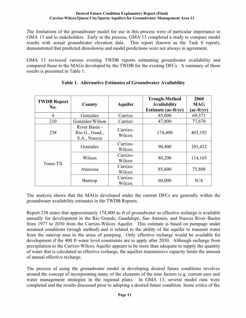
The limitations of the groundwater model for use in this process were of particular importance to GMA 13 and to stakeholders. Early in the process, GMA 13 completed a study to compare model results with actual groundwater elevation data. This report (known as the Task 0 report), demonstrated that predicted drawdowns and model predictions were not always in agreement. GMA 13 reviewed various existing TWDB reports estimating groundwater availability and compared those to the MAGs developed by the TWDB for the existing DFCs. A summary of those results is presented in Table 1.
Table 1. Alternative Estimates of Groundwater Availability
TWDB Report No.
County Aquifer Trough-Method
Availability Estimate (ac-ft/yr)
2060 MAG
(ac-ft/yr) 4 Gonzales Carrizo 85,000 69,371
210 Gonzales/Wilson Carrizo 47,800 77,670
238 River Basin - Rio G., Guad., S.A., Nueces
Carrizo-Wilcox
174,400 403,192
Trans-TX
Gonzales Carrizo-Wilcox
90,400 101,432
Wilson Carrizo-Wilcox
80,200 114,165
Atascosa Carrizo-Wilcox
85,600 75,808
Bastrop Carrizo-Wilcox
60,000 N/A
The analysis shows that the MAGs developed under the current DFCs are generally within the groundwater availability estimates in the TWDB Reports. Report 238 states that approximately 174,400 ac-ft of groundwater as effective recharge is available annually for development in the Rio Grande, Guadalupe, San Antonio, and Nueces River Basins from 1977 to 2030 from the Carrizo-Wilcox Aquifer. This estimate is based on pumpage under assumed conditions (trough method) and is related to the ability of the aquifer to transmit water from the outcrop area to the areas of pumping. Only effective recharge would be available for development if the 400 ft water level constraints are to apply after 2030. Although recharge from precipitation to the Carrizo-Wilcox Aquifer appears to be more than adequate to supply the quantity of water that is calculated as effective recharge, the aquifers transmissive capacity limits the amount of annual effective recharge. The process of using the groundwater model in developing desired future conditions revolves around the concept of incorporating many of the elements of the nine factors (e.g. current uses and water management strategies in the regional plan). In GMA 13, several model runs were completed and the results discussed prior to adopting a desired future condition. Some critics of the
Desired Future Condition Explanatory Report (Final) Carrizo-Wilcox/Queen City/Sparta Aquifers for Groundwater Management Area 13
Page 12
process asserted that the districts were “reverse-engineering” the desired future conditions by specifying pumping (e.g., the modeled available groundwater) and then adopting the resulting drawdown as the desired future condition. However, it must be remembered that among the input parameters for a predictive groundwater model run is pumping, and among the outputs of a predictive groundwater model run is drawdown. Thus, an iterative approach of running several predictive scenarios with models and then evaluating the results is a necessary (and time-consuming) step in the process of developing desired future conditions. One part of the reverse-engineering critique of the process has been that “science” should be used in the development of desired future conditions. The critique plays on the unfortunate name of the groundwater models in Texas (Groundwater Availability Models) which could suggest that the models yield an availability number. This is simply a mischaracterization of how the models work (i.e. what is a model input and what is a model output). The critique also relies on a narrow definition of the term science and fails to recognize that the adoption of a desired future condition is primarily a policy decision. The call to use science in the development of desired future conditions seems to equate the term science with the terms facts and truth. Although the Latin origin of the word means knowledge, the term science also refers to the application of the scientific method. The scientific method is discussed in many textbooks and can be viewed to quantify cause-and-effect relationships and to make useful predictions. In the case of groundwater management, the scientific method can be used to understand the relationship between groundwater pumping and drawdown, or groundwater pumping and spring flow. A groundwater model is a tool that can be used to run “experiments” to better understand the cause-and-effect relationships within a groundwater system as they relate to groundwater management. Much of the consideration of the nine statutory factors involves understanding the effects or the impacts of a desired future condition (e.g. groundwater-surface water interaction and property rights). The use of the models in this manner in evaluating the impacts of alternative futures is an effective means of developing information for the groundwater conservation districts as they develop desired future conditions.
Desired Future Condition Explanatory Report (Final) Carrizo-Wilcox/Queen City/Sparta Aquifers for Groundwater Management Area 13
Page 13
5.0 Factor Consideration
Section 36.108(d) of the Texas Water Code requires that groundwater conservation districts include documentation of how nine listed factors were considered prior to proposing a desired future condition, and how the proposed desired future condition impact each factor. This section of the explanatory report summarizes the information that the groundwater conservation districts used in its deliberations and discussions.
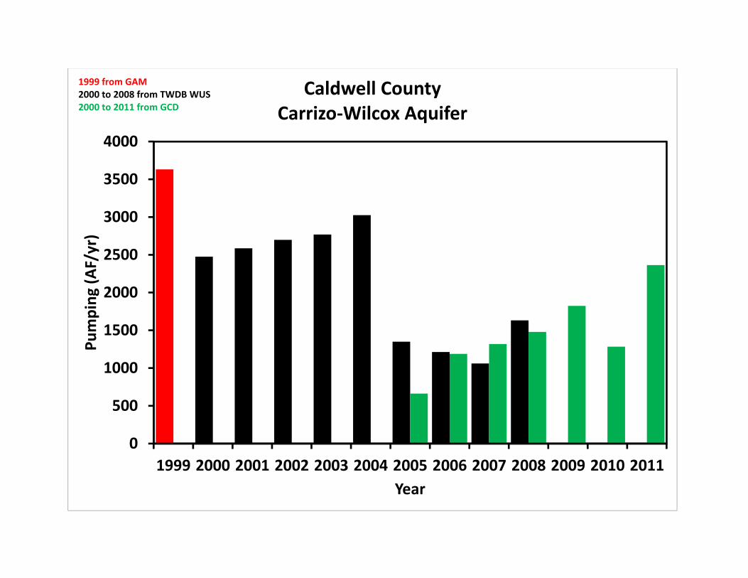
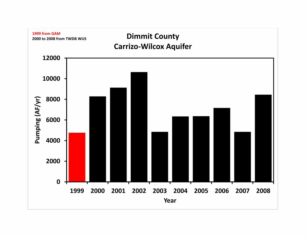
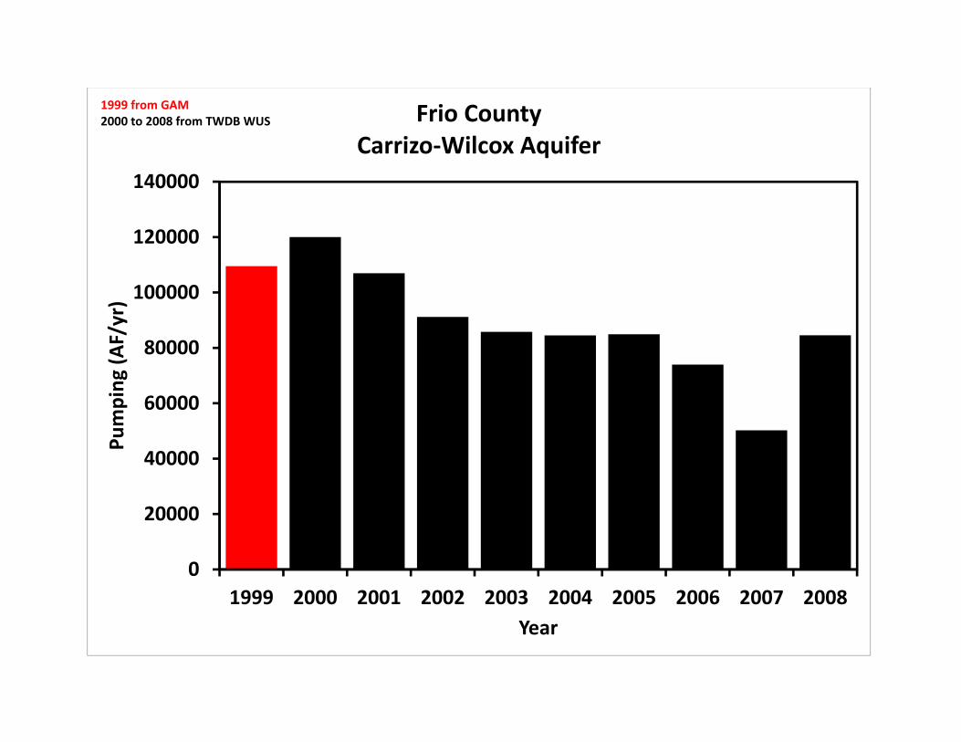
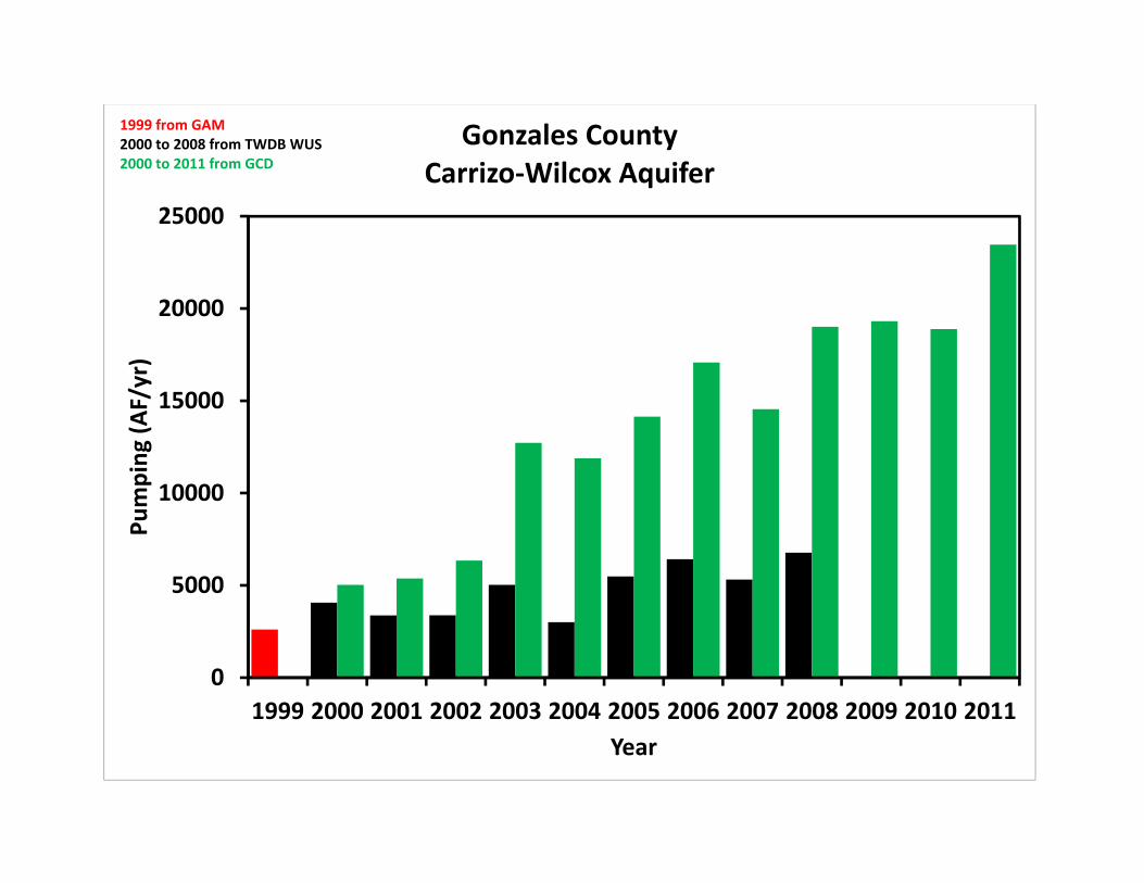
5.1 Aquifer Uses and Conditions
For the purposes of the development of a proposed desired future condition, the groundwater conservation districts in Groundwater Management Area 13 considered the following in the category of aquifer uses (i.e. pumping): Estimates of 1999 pumping from the GAM (Kelley and others, 2004) Estimates of pumping from 2000 to 2008 from the TWDB Water Use Survey database Estimates of pumping from Gonzales County UWCD for the years 2000 to 2011 Estimates of pumping from Plum Creek CD for the years 2000 to 2011 The information considered by the groundwater conservation districts in Groundwater Management Area 13 is presented in Appendix B. For the purposes of the development of a proposed desired future condition, the groundwater conservation districts in Groundwater Management Area 13 considered groundwater monitoring data (i.e. groundwater elevations) from wells in the TWDB groundwater database. The monitoring data were compared to groundwater elevation from the calibrated GAM (Kelley and others, 2004), and with future projections of groundwater elevations from Scenario 4 of TWDB GAM Run 09- 034 (Wade and Jigmond, 2010) that was the basis of the desired future condition adopted in 2010. This comparison also included evaluating the pumping that was estimated in the calibrated GAM for the period 1980 to 1999, and estimated future pumping associated with Scenario 4 of TWDB GAM Run 09-034 (the basis for the desired future condition adopted in 2010). This evaluation was detailed in a report completed for Groundwater Management Area 13 (Hutchison, 2013), and is included as Appendix C. This report was circulated as a draft report on December 21, 2012 and public comments were solicited and received. The final report was issued on March 20, 2013, and includes a response to those comments.
5.2 Water Supply Needs and Water Management Strategies
Initially, data from the 2012 State Water Plan were used by the groundwater conservation districts of Groundwater Management Area 13 in considering this factor. Specifically, county-by-county data on groundwater sources, groundwater demands, and water management strategies. In
Desired Future Condition Explanatory Report (Final) Carrizo-Wilcox/Queen City/Sparta Aquifers for Groundwater Management Area 13
Page 14
addition, data from the Bureau of Economic Geology report that presents estimates of oil and gas water use (Nicot and others, 2012) were considered. SAWS provided an update to pumping projections in southern Bexar County and Gonzales County on June 27, 2013 via email. Groundwater Conservation District input included:
Guadalupe County Groundwater Conservation District Gonzales County Underground Water Conservation District McMullen Groundwater Conservation District Plum Creek Conservation District Wintergarden Groundwater Conservation District
Tabular summaries of all these data are presented in Appendix D. Appendix D also includes the Modeled Available Groundwater Report (Wade, 2012) that was developed by TWDB associated with the previously developed desired future condition adopted in 2010. The data and estimates in Appendix D provide a range of estimates of future pumping that were considered in completing the initial eight scenarios that were developed and run with the GAM through the year 2070. A base case (Scenario 4) was developed based on input from the groundwater conservation districts in GMA 13 as follows:
Pumping in the Carrizo Aquifer in Bexar County was increased as compared to the MAG that was developed from the DFC that was adopted in 2010 in response to a request from SAWS
Pumping in the Carrizo Aquifer in Gonzales County was increased as compared to the MAG that was developed from the DFC that was adopted in 2010 in response to a request from Gonzales County UWCD
Pumping the Wilcox Aquifer in Gonzales County was decreased as compared to the MAG that was developed from the DFC that was adopted in 2010 in response to a request from Gonzales County UWCD
Pumping in the Carrizo Aquifer in McMullen County was increased as compared to the MAG that was developed from the DFC that was adopted in 2010 in response to a request from McMullen GCD
Scenarios 1 to 3 represented incremental reductions of Scenario 4, and Scenarios 4 to 7 represented incremental increases of Scenario 4. After reviewing the results, Scenario 8 was completed which represented the following changes to Scenario 4:
Gonzales County UWCD requested that pumping be revised to match the current MAG Guadalupe County GCD requested increases in both the Carrizo and Wilcox aquifers
Results of Scenario 8 were completed and reviewed at the GMA 13 meeting of March 13, 2014. Because of the comments received at the March 13, 2014 meeting, additional pumping was to be
Desired Future Condition Explanatory Report (Final) Carrizo-Wilcox/Queen City/Sparta Aquifers for Groundwater Management Area 13
Page 15
included in the next simulation that reflected additional pumping by SAWS. However, due to changes in the administration in GMA 13, the work was left pending as of mid-2014. In considering the request of SAWS to simulate additional pumping, and the potential incremental effect of each entity in GMA 13 requesting similar simulations in the future, a more comprehensive approach was employed to consider all recommended and alternative water management strategies from the Region L plan. Sam Vaugh of HDR provided the initial data on August 22, 2014. However, due to the imminent release of the Region L IPP, it was decided to wait until the IPP was released to ensure that all strategies were current. A meeting with HDR was held on May 27, 2015 to clarify the strategies and the data contained in the IPP. The IPP contained 12 strategies that were relevant to GMA 13. One of these was a collective strategy called “Local Carrizo Wells” that covered several areas in GMA 13. The pumping for all other strategies totaled 116,000 AF/yr in 2020, and 222,000 AF/yr in 2070. The IPP distinguished between recommended and alternative strategies in areas where future pumping exceeded the MAG that was set in 2010 consistent with the DFC that was established by GMA 13. Water management strategies are developed to meet deficits between current supply and future demand as part of the regional planning process. TWDB considers the MAG to be a hard limit, and recommended water management strategies cannot result in pumping that exceeds the MAG. Thus, Region L has included strategies that exceed the MAG as alternative strategies. Technical Memorandum 16-01 summarized four simulations that focused on simulating the recommended and alternative water management strategies in the 2015 Region L plan. Scenario 9 includes all pumping from Scenario 8 described above, and all recommended and alternative water management strategies. Scenarios 10 to 12 simulated reductions in all Wilcox Aquifer strategies as a means to understand the interaction between the Wilcox and the overlying Carrizo Aquifer. Discussion of the results of these simulations was held at a GMA 13 meeting on January 22, 2016. Additional discussion of the effects of Scenarios 9 to 12 on the outcrop area are summarized in Technical Memorandum 16-02, which was reviewed at the GMA 13 meeting on February 25, 2016. In response to comments, further investigation of the outcrop area was covered in Technical Memorandum 16-03, and was discussed at the GMA 13 meeting on March 30, 2016. Much of the discussion focused on the limitations of the GAM in simulating the reduction in groundwater storage in the outcrop area. Finally, Technical Memorandum 16-08 summarizes the drawdown and outcrop results for Scenario 9, which was the basis for the proposed desired future condition. In summary, Scenario 9 included all the future pumping of Scenario 8 plus all recommended and alternative water management strategies in the 2015 Region L plan.
5.3 Hydrologic Conditions within Groundwater Management Area 13
As required by statute, the groundwater conservation districts in Groundwater Management Area 13 considered total estimated recoverable storage, average annual recharge, inflows, and discharge prior to adopting a proposed desired future condition.
Desired Future Condition Explanatory Report (Final) Carrizo-Wilcox/Queen City/Sparta Aquifers for Groundwater Management Area 13
Page 16
5.3.1 Total Estimated Recoverable Storage
As required by statute, the Texas Water Development Board provided the groundwater conservation districts in Groundwater Management Area 13 with estimates of total recoverable storage (Wade and Bradley, 2013). This report is included as Appendix E. The estimate of total recoverable storage may be a measure of “physical” availability, but is less meaningful in an analysis of groundwater availability as defined by Chapter 36 of the Water Code, and should be viewed with caution. The groundwater availability developed after following the process in Chapter 36 involves consideration of many factors, some technical and some policy-based. In addition, the Texas water Code Sec. 36.108(d-2) states: “The desired future condition proposed under Subsection (d) must provide a balance between the highest practicable level of groundwater production and the conservation, preservation, protection, recharging, and prevention of waste of groundwater and control of subsidence in the management area”. This balancing test illustrates how the total estimated recoverable storage value is by itself meaningless in an analysis of groundwater availability. As calculated, the TWDB estimated recoverable storage represents the approximate fraction of total storage in the aquifer that is in the producing zones (e.g. sands), not what is “recoverable”. Therefore, in most cases, the total estimated recoverable storage is far greater than the highest practicable level of groundwater production. In addition to the TWDB total recoverable storage report, GMA 13 received a report from a stakeholder regarding selection of DFCs based on use of an acceptable amount of water from aquifer storage through time. A copy of this report is included in Appendix F. The stakeholder followed up on the report with a presentation at the GMA 13 meeting on November 21, 2013. The report in general made a case against GMA 13’s current use of drawdown as a DFC and provided an alternative approach founded on changes in aquifer storage or the protection of unique hydrologic features or conditions. This concept was rejected by GMA 13 for several reasons:
The presentation inaccurately implied that the DFC adopted in 2010 by GMA 13 are arbitrary and were used to limit impacts on exiting users. It also implied that model runs reflect relatively arbitrary model pumpage inputs and that individual groundwater projects were not included in the DFC model.
The author failed to explain how choosing an aquifer drawdown limit through time is considered arbitrary but choosing an acceptable amount of water in aquifer storage through time is not arbitrary.
The author stated that artesian pressure declines do not have a meaningful impact on aquifer storage or groundwater flows to surface features and are, therefore, not suitable as DFCs in those respects. GMA 13 generally agrees with this statement; however, artesian pressure declines are important management tools in dipping confined aquifers where pumpage of non-renewable “fossil” groundwater resources occur. It is important to distinguish renewable from non-renewable or “fossil” groundwater. Groundwater pumpage of renewable resources is limited by fluxes or recharge rates, whereas pumpage of non-renewable resources is limited by groundwater storage.
The author states that managing aquifer storage makes sense because it can be verified
Desired Future Condition Explanatory Report (Final) Carrizo-Wilcox/Queen City/Sparta Aquifers for Groundwater Management Area 13
Page 17
easily and inexpensively through monitoring of the water table levels. However, the accuracy of assessing aquifer storage amounts through monitoring of water table levels is actually rather complex whereas assessing water table drawdown levels is simple and straight forward.
5.3.2 Average Annual Recharge, Inflows and Discharge
Although not specifically required in 2010 as it is now, during the development of the existing desired future condition for the Carrizo-Wilcox, Queen City, and Sparta aquifers in 2010, the groundwater conservation districts in Groundwater Management Area 13 considered the historic groundwater budget for GMA 13 as a management unit, and considered the simulated water budget in 2060 for each groundwater conservation district (or county where a groundwater conservation district did not exist) for four alternative scenarios. The information on these water budget comparisons were provided in a PowerPoint presentation at the Groundwater Management Area 13 meeting on February 19, 2010, and in GAM Report 09-034 (Wade and Jigmond, 2010). This information was presented again during the development of this desired future condition. The groundwater budgets for Groundwater Management Area 13 based on the updated calibration period (2000 to 2011) and Scenario 9 (the basis for the desired future condition) calibrated are summarized in Table 2.
Desired Future Condition Explanatory Report (Final) Carrizo-Wilcox/Queen City/Sparta Aquifers for Groundwater Management Area 13
Page 18
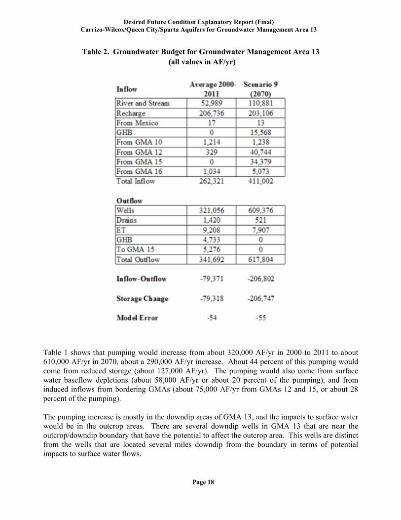
Table 2. Groundwater Budget for Groundwater Management Area 13
(all values in AF/yr)
Table 1 shows that pumping would increase from about 320,000 AF/yr in 2000 to 2011 to about 610,000 AF/yr in 2070, about a 290,000 AF/yr increase. About 44 percent of this pumping would come from reduced storage (about 127,000 AF/yr). The pumping would also come from surface water baseflow depletions (about 58,000 AF/yr or about 20 percent of the pumping), and from induced inflows from bordering GMAs (about 75,000 AF/yr from GMAs 12 and 15, or about 28 percent of the pumping). The pumping increase is mostly in the downdip areas of GMA 13, and the impacts to surface water would be in the outcrop areas. There are several downdip wells in GMA 13 that are near the outcrop/downdip boundary that have the potential to affect the outcrop area. This wells are distinct from the wells that are located several miles downdip from the boundary in terms of potential impacts to surface water flows.
Desired Future Condition Explanatory Report (Final) Carrizo-Wilcox/Queen City/Sparta Aquifers for Groundwater Management Area 13
Page 19
The GAM is not necessarily calibrated to a degree where surface water impacts are particularly reliable or can be viewed as quantitative. However, the GAM is the best tool to address this factor. Since the GAM is an imperfect tool, the conclusion of this analysis is that the increased pumping will cause impacts in addition to reduction in storage.
5.4 Other Environmental Impacts, Including Spring Flow and Other Interactions between Groundwater and Surface Water The evaluation of all water budget components was discussed in Section 5.3.2 above. Guadalupe Blanco River Authority submitted a letter on February 24, 2016 to Groundwater Management Area 13 that expressed a concern about the cumulative effects of the Carrizo-Wilcox pumpage from the 2016 South Central Regional Water Plan (GAM Simulation Scenario 9) on the potential reduction in streamflow and adverse effects on surface water rights and environmental flows in the Guadalupe and San Antonio River Basins, as well as fresh water inflows to the Guadalupe Estuary.
5.5 Subsidence
Subsidence has not been an issue historically in these aquifers.
5.6 Socioeconomic Impacts
The Texas Water Development Board prepared reports on the socioeconomic impacts of not meeting water needs for each of the Regional Planning Groups during development of the 2011 Regional Water Plans. Because the development of this desired future condition used the State Water Plan demands and water management strategies as an important foundation, it is reasonable to conclude that the socioeconomic impacts associated with this proposed desired future condition can be evaluated in the context of not meeting the listed water management strategies. Groundwater Management Area 13 is covered by Regional Planning Groups L and M. In addition, there is an important water management strategy that is sourced in Gonzales County to meet demands in Regional Planning Group K. The socioeconomic impact reports for Regions K, L, and M are included in Appendix G. Socioeconomic Impacts to local landowners due to development of water management strategies within GMA 13 must also be taken into account. The Texas Water Development Board is not tasked with preparing reports on the socioeconomic impacts to local landowners, therefore this information must come from the local groundwater districts. There are two groundwater mitigation projects currently on-going in the GMA 13 area. One is operated by the Gonzales County Underground Water Conservation District (GCUWCD) and the other is operated by the San Antonio Water System in an area just outside of GMA 13. Economic impacts to the local landowners to date can be estimated from one of these mitigation projects. The GCUWCD mitigation project began in 2011 and has spent more than $1,124,000 to date to mitigate the effects of pumpage from large-scale water management strategies. Per well mitigation costs to lower pumps or re-drill water wells deeper has ranged from about $4,200 to
Desired Future Condition Explanatory Report (Final) Carrizo-Wilcox/Queen City/Sparta Aquifers for Groundwater Management Area 13
Page 20
$28,000.
5.7 Impact on Private Property Rights
The impact on the interests and rights in private property, including ownership and the rights of landowners and their lessees and assigns in Groundwater Management Area 13 in groundwater is recognized under Texas Water Code Section 36.002. The desired future conditions adopted by GMA 13 are consistent with protecting property rights of landowners who are currently pumping groundwater and landowners who have chosen to conserve groundwater by not pumping. All current and projected uses (as defined in the 2015 Region L plan) were included in Scenario 9 (the basis for the desired future condition). The increase in pumping associated with meeting the Region L water management strategies will cause impacts to exiting well owners and to surface water. However, as required by Chapter 36 of the Water Code, GMA 13 considered these impacts and balanced them with the increasing demand of water in the GMA 13 area, and concluded that, on balance and with appropriate monitoring and project specific review during the permitting process, all the Region L strategies can be included in the desired future condition.
5.8 Feasibility of Achieving the Desired Future Condition
Groundwater levels are routinely monitored by the districts and by the TWDB in GMA 13. Evaluating the monitoring data is a routine task for the districts, and the comparison of these data with the desired future condition and model results that were used to develop the DFCs is covered in each district’s management plan. These comparisons will be useful to guide the update of the DFCs that are required every five years.
5.9 Other Information
The process to develop the proposed desired future conditions at numerous GMA 13 meetings from 2013 to 2016 included submitted materials and presentations at the meetings, as wells as detailed discussion during the meetings. James Bene of R.W. Harden & Associates submitted a paper on September 20, 2013 to Groundwater Management Area 13 that discussed the joint planning process. This paper provided one perspective on how to develop desired future conditions. The paper made several points that were used in the development of this proposed desired future condition as discussed in Section 5.3.1 of this report, and, as stated above, is included in this report as Appendix F. James Bene of R.W. Harden & Associates gave a presentation at the November 21, 2013 Groundwater Management Area 13 meeting on potential alternative DFCs. A copy of this presentation is included as Appendix H.
Desired Future Condition Explanatory Report (Final) Carrizo-Wilcox/Queen City/Sparta Aquifers for Groundwater Management Area 13
Page 21
Guadalupe Blanco River Authority submitted a letter on February 24, 2016 to Groundwater Management Area 13 that expressed a concern about the cumulative effects of the Carrizo-Wilcox pumpage from the 2016 South Central Regional Water Plan (GAM Simulation Scenario 9) on the potential reduction in streamflow and adverse effects on surface water rights and environmental flows in the Guadalupe and San Antonio River Basins, as well as fresh water inflows to the Guadalupe Estuary. This letter is included as Appendix I. James Beach of LBG-Guyton Associates gave a presentation at the March 30, 2016 Groundwater Management Area 13 meeting on modeling groundwater-surface water interaction. A copy of this presentation is included as Appendix J.
6.0 Discussion of Other Desired Future Conditions Considered
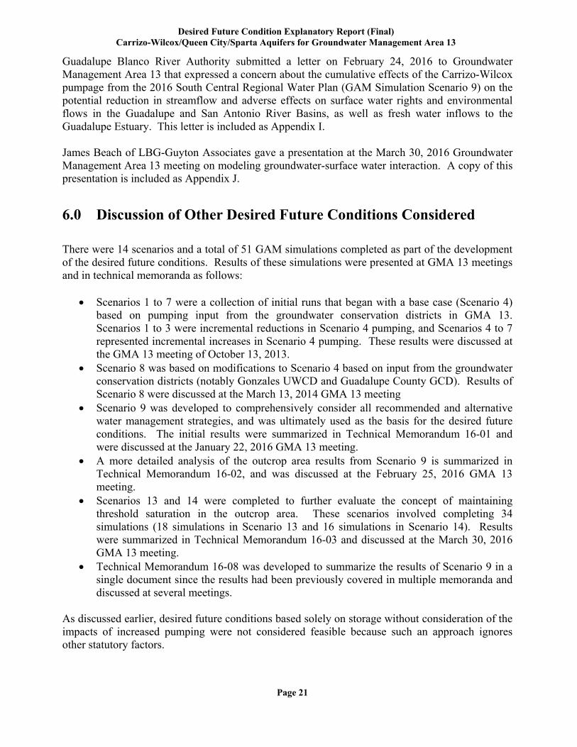
There were 14 scenarios and a total of 51 GAM simulations completed as part of the development of the desired future conditions. Results of these simulations were presented at GMA 13 meetings and in technical memoranda as follows:
Scenarios 1 to 7 were a collection of initial runs that began with a base case (Scenario 4) based on pumping input from the groundwater conservation districts in GMA 13. Scenarios 1 to 3 were incremental reductions in Scenario 4 pumping, and Scenarios 4 to 7 represented incremental increases in Scenario 4 pumping. These results were discussed at the GMA 13 meeting of October 13, 2013.
Scenario 8 was based on modifications to Scenario 4 based on input from the groundwater conservation districts (notably Gonzales UWCD and Guadalupe County GCD). Results of Scenario 8 were discussed at the March 13, 2014 GMA 13 meeting
Scenario 9 was developed to comprehensively consider all recommended and alternative water management strategies, and was ultimately used as the basis for the desired future conditions. The initial results were summarized in Technical Memorandum 16-01 and were discussed at the January 22, 2016 GMA 13 meeting.
A more detailed analysis of the outcrop area results from Scenario 9 is summarized in Technical Memorandum 16-02, and was discussed at the February 25, 2016 GMA 13 meeting.
Scenarios 13 and 14 were completed to further evaluate the concept of maintaining threshold saturation in the outcrop area. These scenarios involved completing 34 simulations (18 simulations in Scenario 13 and 16 simulations in Scenario 14). Results were summarized in Technical Memorandum 16-03 and discussed at the March 30, 2016 GMA 13 meeting.
Technical Memorandum 16-08 was developed to summarize the results of Scenario 9 in a single document since the results had been previously covered in multiple memoranda and discussed at several meetings.
As discussed earlier, desired future conditions based solely on storage without consideration of the impacts of increased pumping were not considered feasible because such an approach ignores other statutory factors.
Desired Future Condition Explanatory Report (Final) Carrizo-Wilcox/Queen City/Sparta Aquifers for Groundwater Management Area 13
Page 22
7.0 Discussion of Other Recommendations
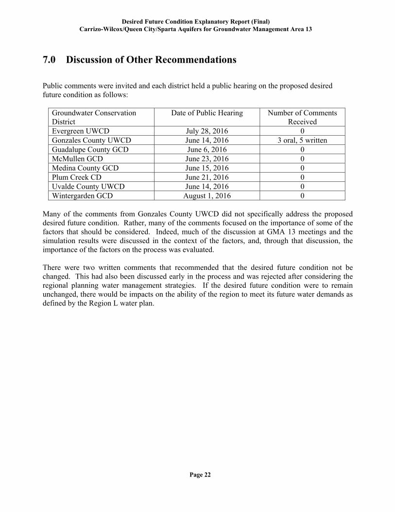
Public comments were invited and each district held a public hearing on the proposed desired future condition as follows:
Groundwater Conservation District
Date of Public Hearing Number of Comments Received
Evergreen UWCD July 28, 2016 0 Gonzales County UWCD June 14, 2016 3 oral, 5 written Guadalupe County GCD June 6, 2016 0 McMullen GCD June 23, 2016 0 Medina County GCD June 15, 2016 0 Plum Creek CD June 21, 2016 0 Uvalde County UWCD June 14, 2016 0 Wintergarden GCD August 1, 2016 0
Many of the comments from Gonzales County UWCD did not specifically address the proposed desired future condition. Rather, many of the comments focused on the importance of some of the factors that should be considered. Indeed, much of the discussion at GMA 13 meetings and the simulation results were discussed in the context of the factors, and, through that discussion, the importance of the factors on the process was evaluated. There were two written comments that recommended that the desired future condition not be changed. This had also been discussed early in the process and was rejected after considering the regional planning water management strategies. If the desired future condition were to remain unchanged, there would be impacts on the ability of the region to meet its future water demands as defined by the Region L water plan.
Desired Future Condition Explanatory Report (Final) Carrizo-Wilcox/Queen City/Sparta Aquifers for Groundwater Management Area 13
Page 23
8.0 References
Deeds, N., Kelley, V., Fryar, D., Jones, T., Whallon, A. J., and Dean, K. E., 2003, Groundwater Availability Model for the Southern Carrizo-Wilcox Aquifer: contract report to the Texas Water Development Board, 452 p.
Hutchison, W.R., Comparison of Groundwater Monitoring Data with Groundwater Model Results,
Groundwater Management Area 13. Contracted report for Groundwater Management Area 13, 178 p.
Kelley, V. A., Deeds, N. E., Fryar, D. G., and Nicot, J. P., 2004, Groundwater availability models
for the Queen City and Sparta aquifers: contract report to the Texas Water Development Board, 867 p.
Nicot, J-P, Reedy, R.C., Costley, R.A., and Huang, Y., 2012. Oil & Gas Water Use in Texas:
Update to the 2011 Mining Water Use Report. Bureau of Economic Geology, Jackson School of Geosciences, The University of Texas at Austin. Report prepared for Texas Oil & Gas Association, Austin, Texas.
Wade, S. and Bradley, R., 2013, GAM Task 13-036 (Revised): Total Estimated Recoverable Storage for Aquifers in Groundwater Management Area 13. Texas Water Development Board GAM Task Report, 30 p.
Wade, S. and Jigmond, M., 2010. GAM Run 09-034, Texas Water Development Board GAM Run
Report, 146 p.
Appendix A
Proposed Desired Future Condition Resolution

Appendix B
Groundwater Use Estimates
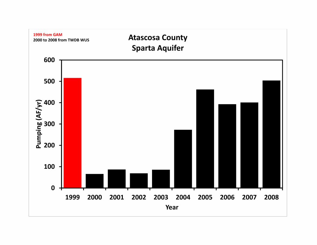
0
100
200
300
400
500
600
1999 2000 2001 2002 2003 2004 2005 2006 2007 2008
Pumping
(AF/yr)
Year
Atascosa CountySparta Aquifer
1999 from GAM2000 to 2008 from TWDB WUS
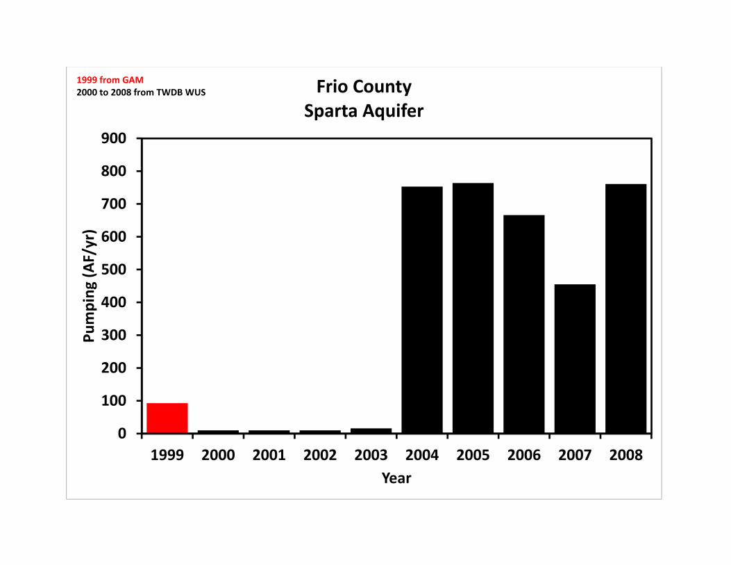
0
100
200
300
400
500
600
700
800
900
1999 2000 2001 2002 2003 2004 2005 2006 2007 2008
Pumping
(AF/yr)
Year
Frio CountySparta Aquifer
1999 from GAM2000 to 2008 from TWDB WUS
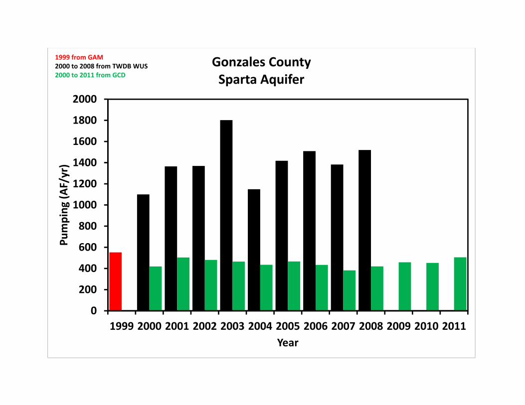
0
200
400
600
800
1000
1200
1400
1600
1800
2000
1999 2000 2001 2002 2003 2004 2005 2006 2007 2008 2009 2010 2011
Pumping
(AF/yr)
Year
Gonzales CountySparta Aquifer
1999 from GAM2000 to 2008 from TWDB WUS2000 to 2011 from GCD
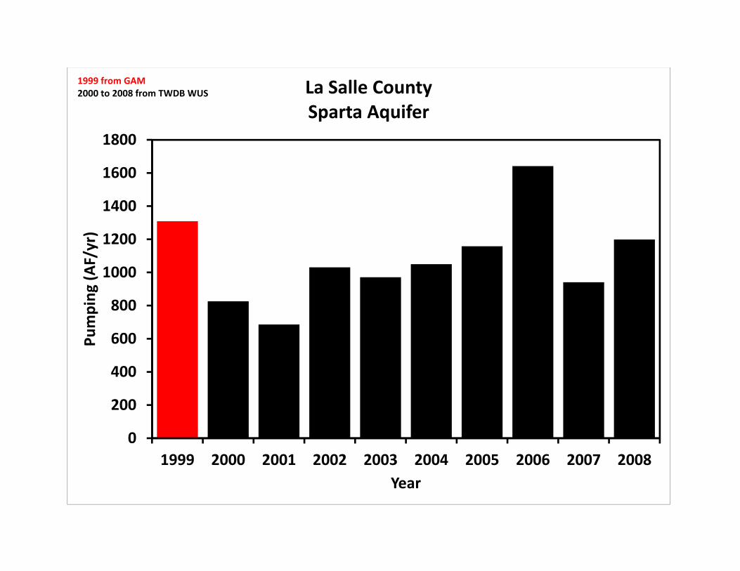
0
200
400
600
800
1000
1200
1400
1600
1800
1999 2000 2001 2002 2003 2004 2005 2006 2007 2008
Pumping
(AF/yr)
Year
La Salle CountySparta Aquifer
1999 from GAM2000 to 2008 from TWDB WUS
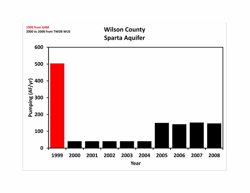
0
100
200
300
400
500
600
1999 2000 2001 2002 2003 2004 2005 2006 2007 2008
Pumping
(AF/yr)
Year
Wilson CountySparta Aquifer
1999 from GAM2000 to 2008 from TWDB WUS
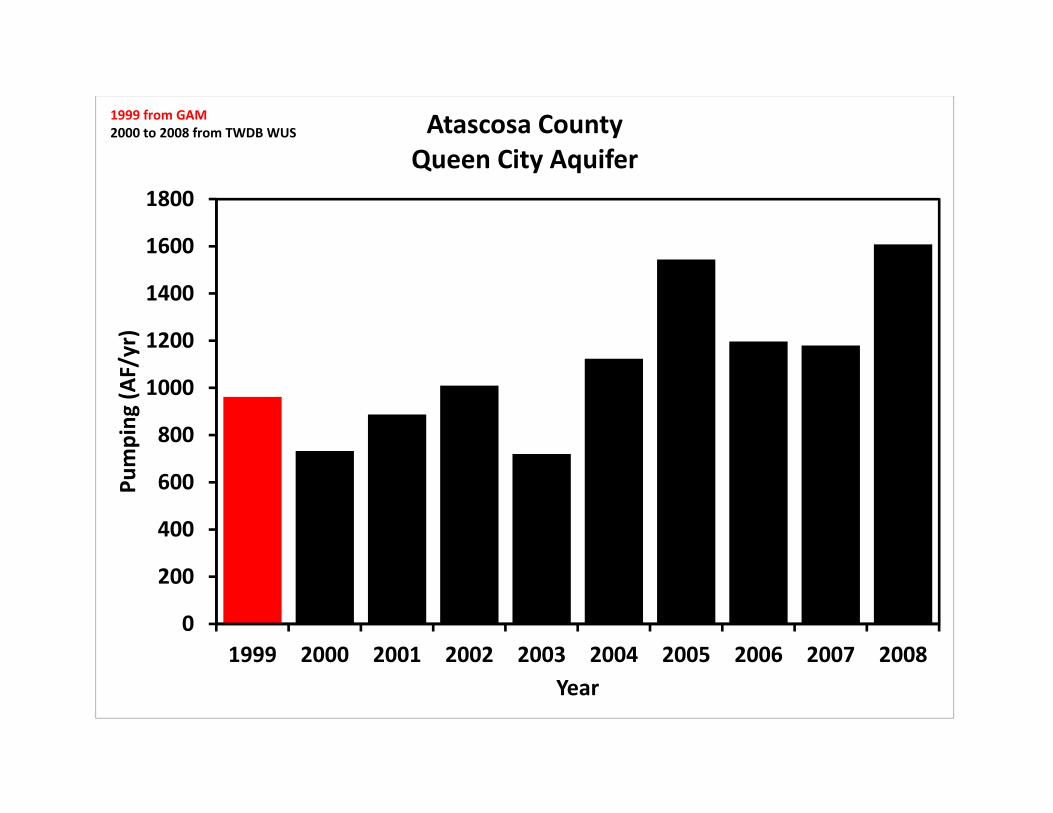
0
200
400
600
800
1000
1200
1400
1600
1800
1999 2000 2001 2002 2003 2004 2005 2006 2007 2008
Pumping
(AF/yr)
Year
Atascosa CountyQueen City Aquifer
1999 from GAM2000 to 2008 from TWDB WUS
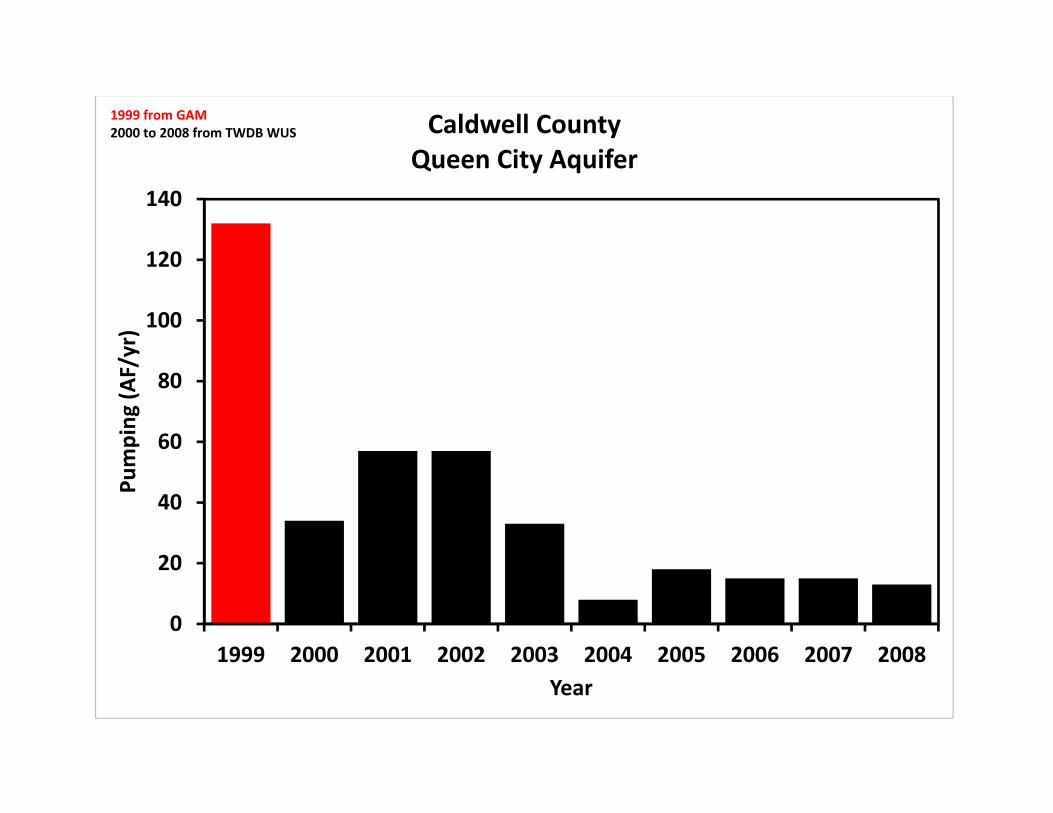
0
20
40
60
80
100
120
140
1999 2000 2001 2002 2003 2004 2005 2006 2007 2008
Pumping
(AF/yr)
Year
Caldwell CountyQueen City Aquifer
1999 from GAM2000 to 2008 from TWDB WUS
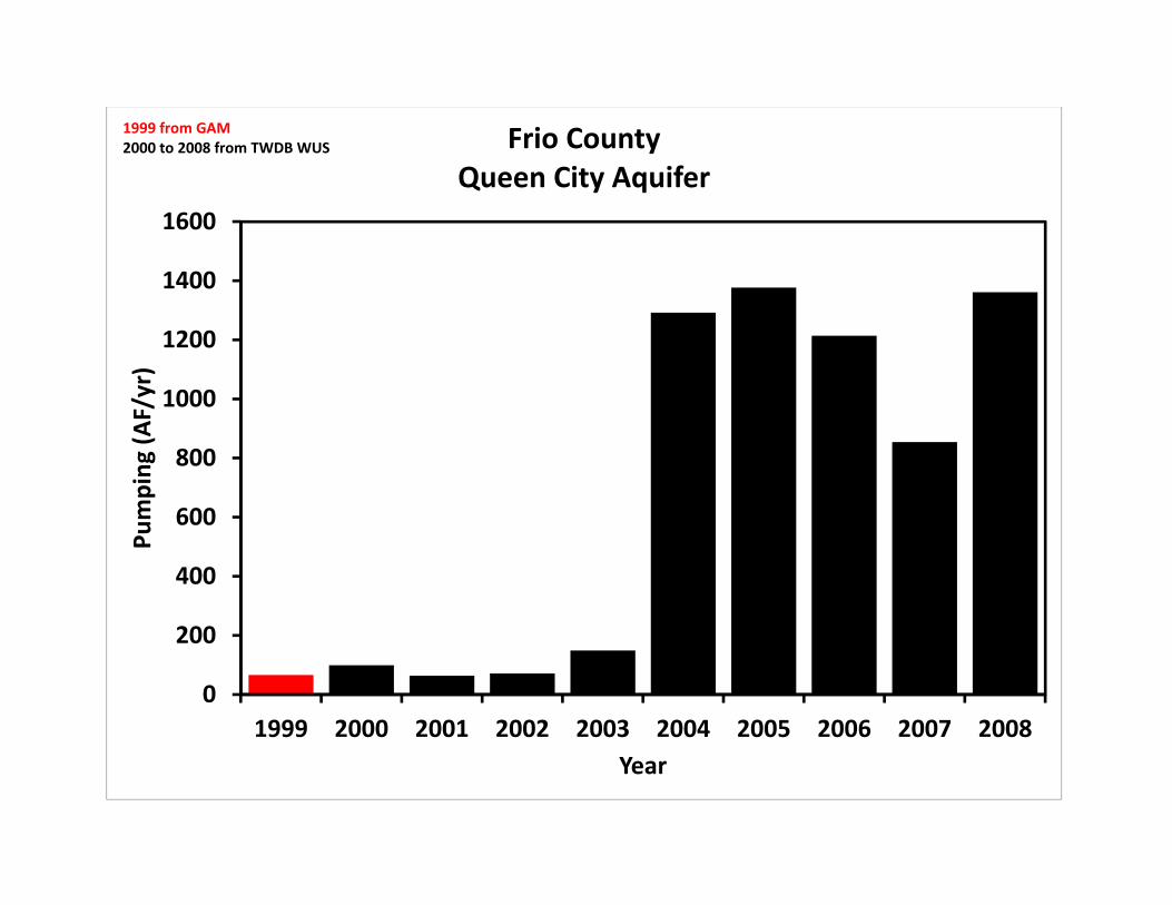
0
200
400
600
800
1000
1200
1400
1600
1999 2000 2001 2002 2003 2004 2005 2006 2007 2008
Pumping
(AF/yr)
Year
Frio CountyQueen City Aquifer
1999 from GAM2000 to 2008 from TWDB WUS
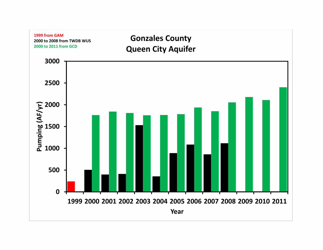
0
500
1000
1500
2000
2500
3000
1999 2000 2001 2002 2003 2004 2005 2006 2007 2008 2009 2010 2011
Pumping
(AF/yr)
Year
Gonzales CountyQueen City Aquifer
1999 from GAM2000 to 2008 from TWDB WUS2000 to 2011 from GCD
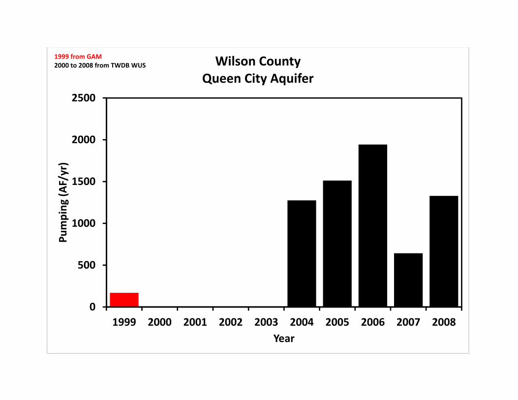
0
500
1000
1500
2000
2500
1999 2000 2001 2002 2003 2004 2005 2006 2007 2008
Pumping
(AF/yr)
Year
Wilson CountyQueen City Aquifer
1999 from GAM2000 to 2008 from TWDB WUS
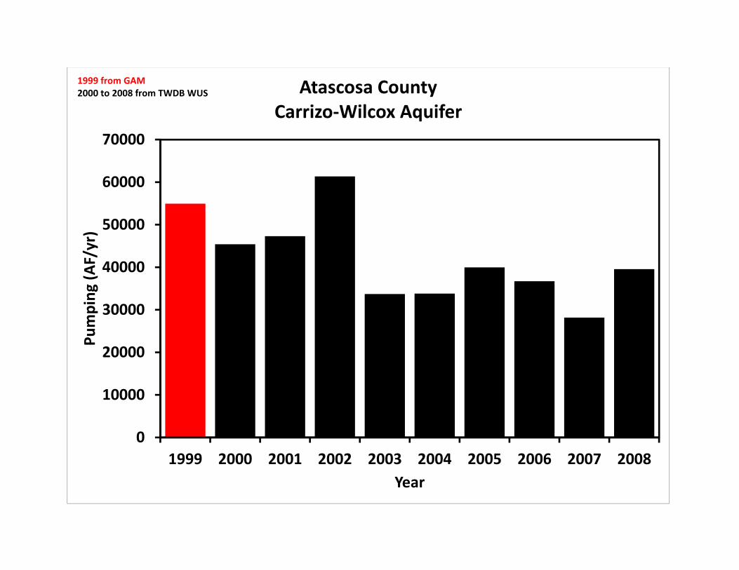
0
10000
20000
30000
40000
50000
60000
70000
1999 2000 2001 2002 2003 2004 2005 2006 2007 2008
Pumping
(AF/yr)
Year
Atascosa CountyCarrizo‐Wilcox Aquifer
1999 from GAM2000 to 2008 from TWDB WUS
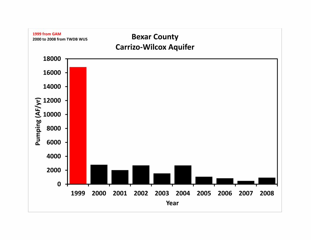
0
2000
4000
6000
8000
10000
12000
14000
16000
18000
1999 2000 2001 2002 2003 2004 2005 2006 2007 2008
Pumping
(AF/yr)
Year
Bexar CountyCarrizo‐Wilcox Aquifer
1999 from GAM2000 to 2008 from TWDB WUS
0
500
1000
1500
2000
2500
3000
3500
4000
1999 2000 2001 2002 2003 2004 2005 2006 2007 2008 2009 2010 2011
Pumping
(AF/yr)
Year
Caldwell CountyCarrizo‐Wilcox Aquifer
1999 from GAM2000 to 2008 from TWDB WUS2000 to 2011 from GCD
0
2000
4000
6000
8000
10000
12000
1999 2000 2001 2002 2003 2004 2005 2006 2007 2008
Pumping
(AF/yr)
Year
Dimmit CountyCarrizo‐Wilcox Aquifer
1999 from GAM2000 to 2008 from TWDB WUS
0
20000
40000
60000
80000
100000
120000
140000
1999 2000 2001 2002 2003 2004 2005 2006 2007 2008
Pumping
(AF/yr)
Year
Frio CountyCarrizo‐Wilcox Aquifer
1999 from GAM2000 to 2008 from TWDB WUS
0
5000
10000
15000
20000
25000
1999 2000 2001 2002 2003 2004 2005 2006 2007 2008 2009 2010 2011
Pumping
(AF/yr)
Year
Gonzales CountyCarrizo‐Wilcox Aquifer
1999 from GAM2000 to 2008 from TWDB WUS2000 to 2011 from GCD
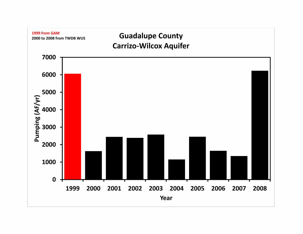
0
1000
2000
3000
4000
5000
6000
7000
1999 2000 2001 2002 2003 2004 2005 2006 2007 2008
Pumping
(AF/yr)
Year
Guadalupe CountyCarrizo‐Wilcox Aquifer
1999 from GAM2000 to 2008 from TWDB WUS
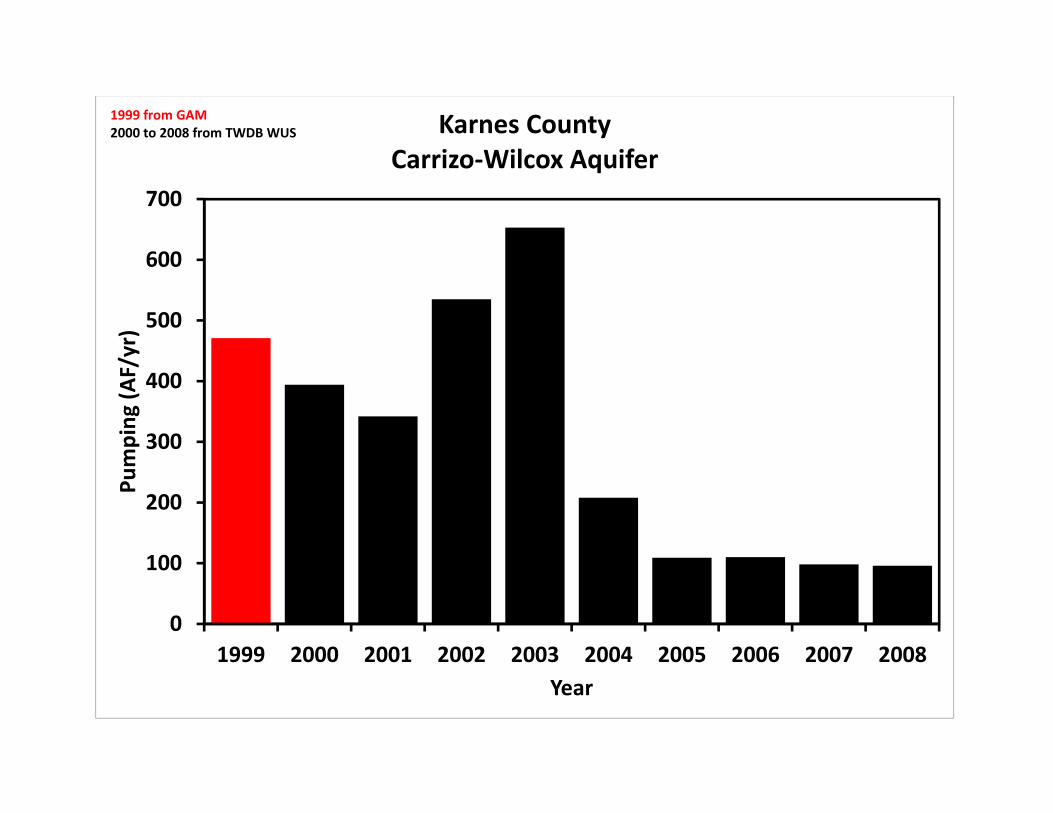
0
100
200
300
400
500
600
700
1999 2000 2001 2002 2003 2004 2005 2006 2007 2008
Pumping
(AF/yr)
Year
Karnes CountyCarrizo‐Wilcox Aquifer
1999 from GAM2000 to 2008 from TWDB WUS
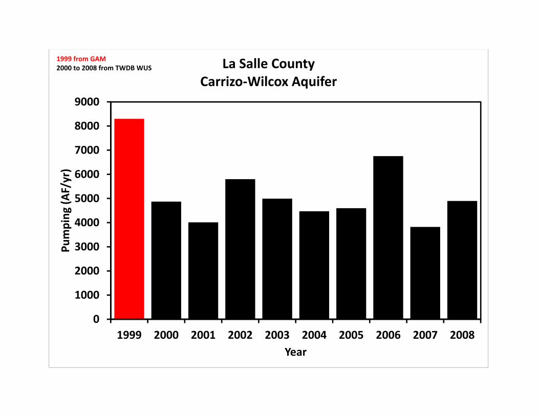
0
1000
2000
3000
4000
5000
6000
7000
8000
9000
1999 2000 2001 2002 2003 2004 2005 2006 2007 2008
Pumping
(AF/yr)
Year
La Salle CountyCarrizo‐Wilcox Aquifer
1999 from GAM2000 to 2008 from TWDB WUS
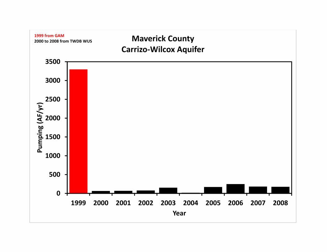
0
500
1000
1500
2000
2500
3000
3500
1999 2000 2001 2002 2003 2004 2005 2006 2007 2008
Pumping
(AF/yr)
Year
Maverick CountyCarrizo‐Wilcox Aquifer
1999 from GAM2000 to 2008 from TWDB WUS
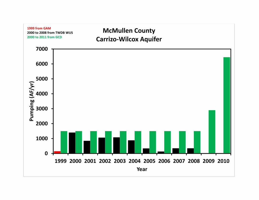
0
1000
2000
3000
4000
5000
6000
7000
1999 2000 2001 2002 2003 2004 2005 2006 2007 2008 2009 2010
Pumping
(AF/yr)
Year
McMullen CountyCarrizo‐Wilcox Aquifer
1999 from GAM2000 to 2008 from TWDB WUS2000 to 2011 from GCD
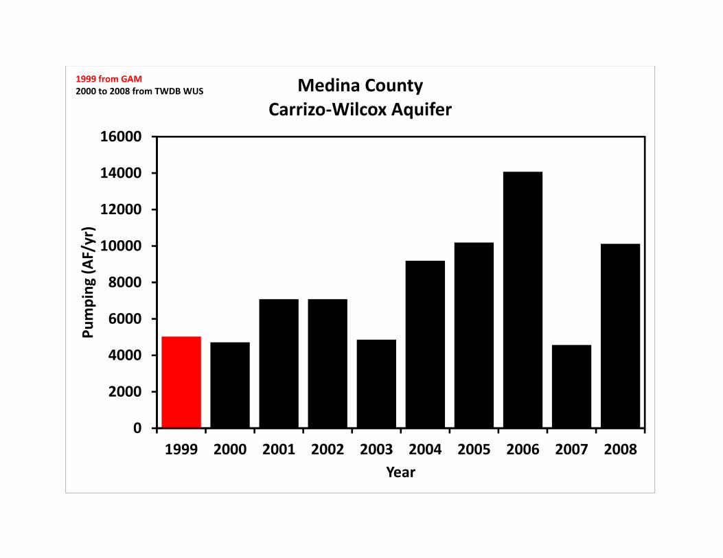
0
2000
4000
6000
8000
10000
12000
14000
16000
1999 2000 2001 2002 2003 2004 2005 2006 2007 2008
Pumping
(AF/yr)
Year
Medina CountyCarrizo‐Wilcox Aquifer
1999 from GAM2000 to 2008 from TWDB WUS
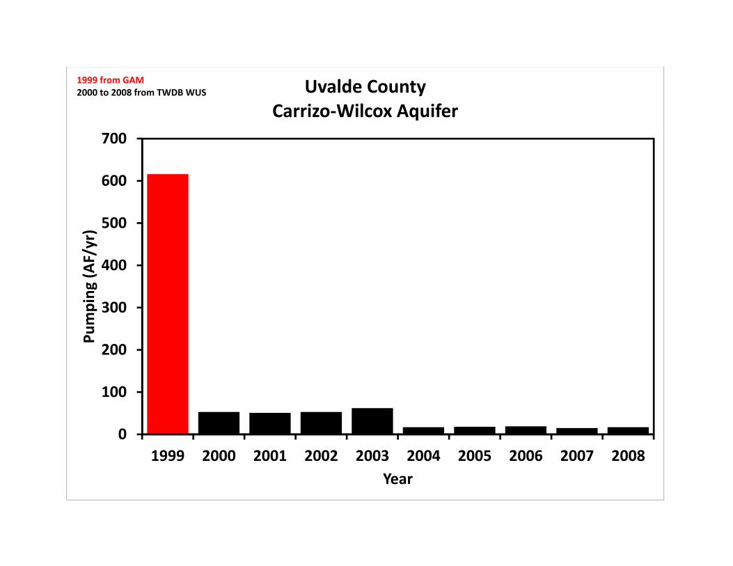
0
100
200
300
400
500
600
700
1999 2000 2001 2002 2003 2004 2005 2006 2007 2008
Pumping
(AF/yr)
Year
Uvalde CountyCarrizo‐Wilcox Aquifer
1999 from GAM2000 to 2008 from TWDB WUS
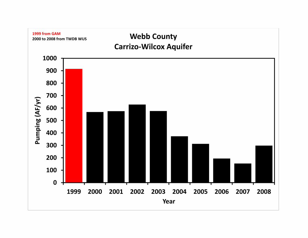
0
100
200
300
400
500
600
700
800
900
1000
1999 2000 2001 2002 2003 2004 2005 2006 2007 2008
Pumping
(AF/yr)
Year
Webb CountyCarrizo‐Wilcox Aquifer
1999 from GAM2000 to 2008 from TWDB WUS
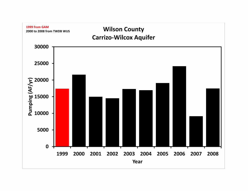
0
5000
10000
15000
20000
25000
30000
1999 2000 2001 2002 2003 2004 2005 2006 2007 2008
Pumping
(AF/yr)
Year
Wilson CountyCarrizo‐Wilcox Aquifer
1999 from GAM2000 to 2008 from TWDB WUS
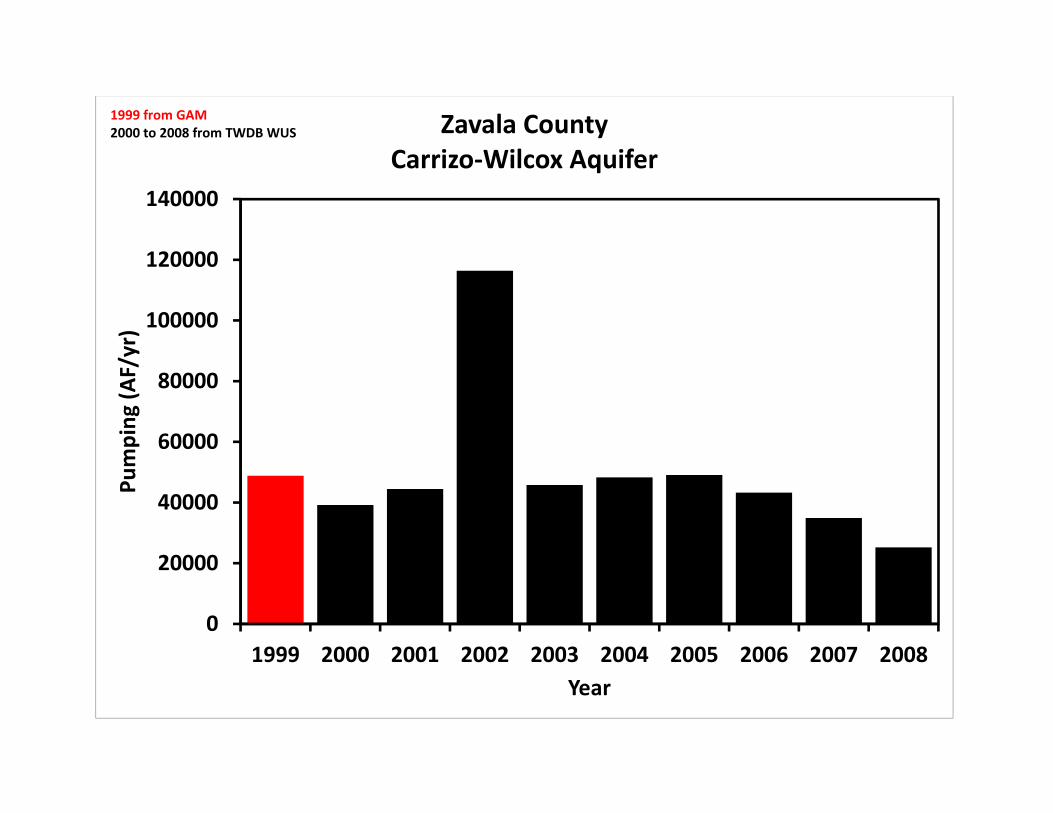
0
20000
40000
60000
80000
100000
120000
140000
1999 2000 2001 2002 2003 2004 2005 2006 2007 2008
Pumping
(AF/yr)
Year
Zavala CountyCarrizo‐Wilcox Aquifer
1999 from GAM2000 to 2008 from TWDB WUS
Appendix C
Comparison of Groundwater Monitoring Data with Groundwater Model Results,
Groundwater Management Area 13
Final Report
Comparison of Groundwater Monitoring Data with Groundwater Model Results
Groundwater Management Area 13
March 20, 2013
William R. Hutchison, Ph.D., P.E., P.G. Independent Groundwater Consultant
9802 Murmuring Creek Drive Austin, TX 78736
512-745-0599 [email protected]
1
ExecutiveSummary This effort was authorized by the groundwater conservation districts of GMA 13 as the initial step of the current round of joint planning. The objectives were:
1. Compare model results from desired future condition simulations with actual data, and identify areas where comparisons were favorable and unfavorable. In areas where comparisons were unfavorable, the objective was to assess how the accuracy of various assumptions made in the process.
2. Summarize these findings in a report suitable for use by the groundwater conservation districts in updates to their management plans.
3. Use the findings in the next round of joint planning (i.e. desired future condition development) to make the process more efficient, less costly, and more defendable.
This report represents a resource document for use in the current round of joint planning, and contains the results of analyses completed to meet the objectives:
Plotting hydrographs of actual groundwater elevations for 92 wells and comparing the data to estimates of historic and future pumping and estimates of groundwater elevations at those points from the model simulation of the initial desired future condition statement.
Comparing actual drawdowns (from 1999 conditions) and drawdowns estimated from the model simulation at those points of the initial desired future condition statement for 70 wells.
In general, the comparisons of actual drawdowns and estimated drawdowns from the desired future condition simulation were favorable. Differences appear to be attributable to pumping increases or decreases assumed to occur from 2000 to 2011 that did not occur, increased groundwater use associated with hydraulic fracturing operations, and drought conditions. The establishment of the initial desired future conditions for the Carrizo-Wilcox, Queen City and Sparta aquifers relied heavily on simulations using the groundwater availability model of the area. Comparisons of these model results with actual data provide a foundation for future discussions related to the current round of joint planning. The major areas for discussion include:
Improvement in 2000 to 2011 pumping estimates Timing of future pumping increases and decreases Evaluate the “average” recharge assumption for the entire DFC simulation Evaluate the assumption that future pumping does not vary between wet years and
droughts Review model assumptions and implementation for recharge and stream flow Assess county-to-county impacts more explicitly The use of actual well data as part of the statement of desired future conditions
2
Table of Contents
Executive Summary ........................................................................................................................ 1
List of Figures and Tables............................................................................................................... 3
1.0 Introduction .......................................................................................................................... 4
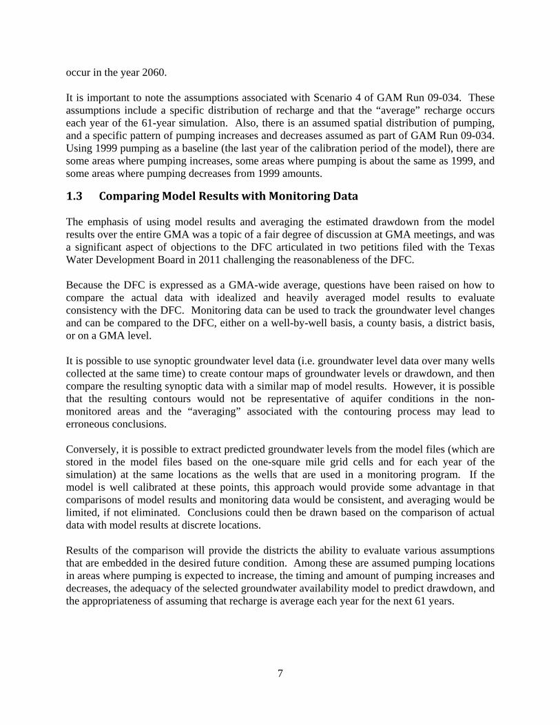
1.1 Background and Objectives ............................................................................................. 6
1.2 Initial Desired Future Conditions for GMA 13 ................................................................ 6
1.3 Comparing Model Results with Monitoring Data ............................................................ 7
2.0 Review of GAM Run 09-034 ............................................................................................... 8
3.0 Point-by-Point Comparison of Groundwater Elevations ................................................... 19
3.1 Hydrographs of Groundwater Elevations and Pumping ................................................ 19
3.2 Well-by-Well Drawdown Comparison .......................................................................... 23
3.3 Average Drawdown Comparison ....................................................................................... 28
4.0 County-Level Data Suitable for use in Management Plan Updates .................................. 31
5.0 Recommendations for Current Round of Joint Planning ................................................... 32
Appendix 1 – GMA 13 Drawdown Maps for All Years ............................................................... 34
Appendix 2 – Atascosa County..................................................................................................... 46
Appendix 3 – Bexar County ......................................................................................................... 57
Appendix 4 – Caldwell County..................................................................................................... 60
Appendix 5 – Dimmit County ...................................................................................................... 69
Appendix 6 – Frio County ............................................................................................................ 79
Appendix 7 – Gonzales County .................................................................................................... 88
Appendix 8 – Guadalupe County .................................................................................................. 98
Appendix 9 – La Salle County .................................................................................................... 106
Appendix 10 – Maverick County ................................................................................................ 115
Appendix 11 – McMullen County .............................................................................................. 123
Appendix 12 – Medina County ................................................................................................... 131
Appendix 13 – Webb County ..................................................................................................... 138
Appendix 14 – Wilson County ................................................................................................... 146
Appendix 15 – Zavala County .................................................................................................... 160
Appendix 16 – Responses to Comments from Draft Report dated December 21, 2012 ............ 170
3
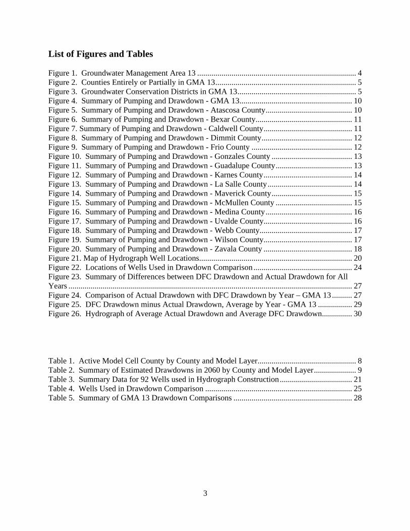
List of Figures and Tables Figure 1. Groundwater Management Area 13 ............................................................................... 4 Figure 2. Counties Entirely or Partially in GMA 13 ...................................................................... 5 Figure 3. Groundwater Conservation Districts in GMA 13 ........................................................... 5 Figure 4. Summary of Pumping and Drawdown - GMA 13 ........................................................ 10 Figure 5. Summary of Pumping and Drawdown - Atascosa County ........................................... 10 Figure 6. Summary of Pumping and Drawdown - Bexar County................................................ 11 Figure 7. Summary of Pumping and Drawdown - Caldwell County ............................................ 11 Figure 8. Summary of Pumping and Drawdown - Dimmit County ............................................. 12 Figure 9. Summary of Pumping and Drawdown - Frio County .................................................. 12 Figure 10. Summary of Pumping and Drawdown - Gonzales County ........................................ 13 Figure 11. Summary of Pumping and Drawdown - Guadalupe County ...................................... 13 Figure 12. Summary of Pumping and Drawdown - Karnes County ............................................ 14 Figure 13. Summary of Pumping and Drawdown - La Salle County .......................................... 14 Figure 14. Summary of Pumping and Drawdown - Maverick County ........................................ 15 Figure 15. Summary of Pumping and Drawdown - McMullen County ...................................... 15 Figure 16. Summary of Pumping and Drawdown - Medina County ........................................... 16 Figure 17. Summary of Pumping and Drawdown - Uvalde County ............................................ 16 Figure 18. Summary of Pumping and Drawdown - Webb County.............................................. 17 Figure 19. Summary of Pumping and Drawdown - Wilson County ............................................ 17 Figure 20. Summary of Pumping and Drawdown - Zavala County ............................................ 18 Figure 21. Map of Hydrograph Well Locations ............................................................................ 20 Figure 22. Locations of Wells Used in Drawdown Comparison ................................................. 24 Figure 23. Summary of Differences between DFC Drawdown and Actual Drawdown for All Years ............................................................................................................................................. 27 Figure 24. Comparison of Actual Drawdown with DFC Drawdown by Year – GMA 13 .......... 27 Figure 25. DFC Drawdown minus Actual Drawdown, Average by Year - GMA 13 ................. 29 Figure 26. Hydrograph of Average Actual Drawdown and Average DFC Drawdown ............... 30
Table 1. Active Model Cell County by County and Model Layer ................................................. 8 Table 2. Summary of Estimated Drawdowns in 2060 by County and Model Layer ..................... 9 Table 3. Summary Data for 92 Wells used in Hydrograph Construction .................................... 21 Table 4. Wells Used in Drawdown Comparison ......................................................................... 25 Table 5. Summary of GMA 13 Drawdown Comparisons ........................................................... 28
4
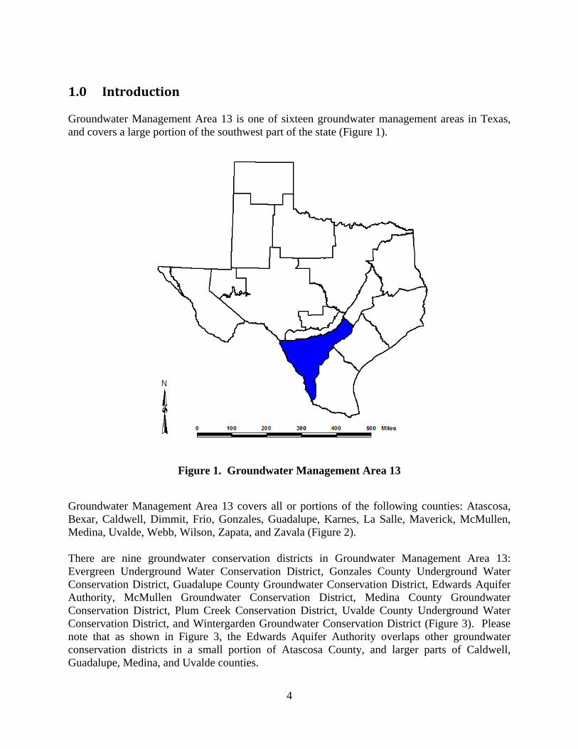
1.0 Introduction Groundwater Management Area 13 is one of sixteen groundwater management areas in Texas, and covers a large portion of the southwest part of the state (Figure 1).
Figure 1. Groundwater Management Area 13
Groundwater Management Area 13 covers all or portions of the following counties: Atascosa, Bexar, Caldwell, Dimmit, Frio, Gonzales, Guadalupe, Karnes, La Salle, Maverick, McMullen, Medina, Uvalde, Webb, Wilson, Zapata, and Zavala (Figure 2). There are nine groundwater conservation districts in Groundwater Management Area 13: Evergreen Underground Water Conservation District, Gonzales County Underground Water Conservation District, Guadalupe County Groundwater Conservation District, Edwards Aquifer Authority, McMullen Groundwater Conservation District, Medina County Groundwater Conservation District, Plum Creek Conservation District, Uvalde County Underground Water Conservation District, and Wintergarden Groundwater Conservation District (Figure 3). Please note that as shown in Figure 3, the Edwards Aquifer Authority overlaps other groundwater conservation districts in a small portion of Atascosa County, and larger parts of Caldwell, Guadalupe, Medina, and Uvalde counties.
5
Figure 2. Counties Entirely or Partially in GMA 13
Figure 3. Groundwater Conservation Districts in GMA 13
6
1.1 BackgroundandObjectives On May 24, 2012, the groundwater conservation districts in GMA 13 issued a request for qualifications for technical services associated with the development of the next round of desired future conditions. On June 4, 2012, GMA 13 issued a request for proposals that specifically outlined seven tasks that GMA 13 identified relative to assistance in developing and defending desired future conditions. William R. Hutchison, Ph.D., P.E., P.G., an independent groundwater consultant, was selected at the GMA 13 meeting of July 25, 2012 to assist GMA 13 on these tasks. Dr. Hutchison recommended that an additional task be completed prior to beginning any of the tasks listed in the June 4, 2012 request for proposal. Known as Task 0, this task consisted of comparing actual groundwater elevation and drawdown data with model results that were used in the establishment of the initial desired future condition. Authorization to proceed with Task 0 was made at the September 7, 2012 GMA 13 meeting, and was based on two proposals dated August 10, 2012 and August 31, 2012. The objectives of Task 0 were:
1. Compare model results from desired future condition simulations with actual data, and identify areas where comparisons were favorable and unfavorable. In areas where comparisons were unfavorable, the objective was to assess the accuracy of various assumptions made in the process.
2. Summarize these findings in a report suitable for use by the groundwater conservation districts in updates to their management plans.
3. Use the findings in the next round of joint planning (i.e. desired future condition development) to make the process more efficient, less costly, and more defendable.
It should be noted that there is no formal requirement in statute to report findings from this effort. In contrast, statutes do require that district management plans and desired future condition adoptions be approved as administratively complete by the Texas Water Development Board. However, statute does provide for a petition process if a desired future condition is not being met or if a district is not managing to meet a desired future condition. Such a petition would be filed with the Texas Commission on Environmental Quality. If such a petition were filed, the findings in this report could be used to respond to claims made. Most importantly, this effort represents good practice in evaluating groundwater levels measured in wells, and comparing these data with model results to place model results into appropriate context during the next round of joint planning.
1.2 InitialDesiredFutureConditionsforGMA13 Groundwater Management Area 13 (GMA 13) adopted a desired future condition (DFC) for the Carrizo-Wilcox, Queen City, and Sparta aquifers on April 9, 2010. This initial DFC was established with a heavy reliance on results from simulations using the Groundwater Availability Model (GAM) for the Southern Carrizo-Wilcox, Queen City and Sparta aquifers. The adopted DFC is expressed as a GMA-wide average drawdown of 23 feet, and is based on Scenario 4 of GAM Run 09-034 as reported by the Texas Water Development Board. Scenario 4 of GAM Run 09-034 was a 61-year simulation with a starting point in the year 2000. Thus, the 23 feet of drawdown is an average drawdown over the entire GMA in these aquifers, and is estimated to
7
occur in the year 2060. It is important to note the assumptions associated with Scenario 4 of GAM Run 09-034. These assumptions include a specific distribution of recharge and that the “average” recharge occurs each year of the 61-year simulation. Also, there is an assumed spatial distribution of pumping, and a specific pattern of pumping increases and decreases assumed as part of GAM Run 09-034. Using 1999 pumping as a baseline (the last year of the calibration period of the model), there are some areas where pumping increases, some areas where pumping is about the same as 1999, and some areas where pumping decreases from 1999 amounts.
1.3 ComparingModelResultswithMonitoringData The emphasis of using model results and averaging the estimated drawdown from the model results over the entire GMA was a topic of a fair degree of discussion at GMA meetings, and was a significant aspect of objections to the DFC articulated in two petitions filed with the Texas Water Development Board in 2011 challenging the reasonableness of the DFC. Because the DFC is expressed as a GMA-wide average, questions have been raised on how to compare the actual data with idealized and heavily averaged model results to evaluate consistency with the DFC. Monitoring data can be used to track the groundwater level changes and can be compared to the DFC, either on a well-by-well basis, a county basis, a district basis, or on a GMA level. It is possible to use synoptic groundwater level data (i.e. groundwater level data over many wells collected at the same time) to create contour maps of groundwater levels or drawdown, and then compare the resulting synoptic data with a similar map of model results. However, it is possible that the resulting contours would not be representative of aquifer conditions in the non-monitored areas and the “averaging” associated with the contouring process may lead to erroneous conclusions. Conversely, it is possible to extract predicted groundwater levels from the model files (which are stored in the model files based on the one-square mile grid cells and for each year of the simulation) at the same locations as the wells that are used in a monitoring program. If the model is well calibrated at these points, this approach would provide some advantage in that comparisons of model results and monitoring data would be consistent, and averaging would be limited, if not eliminated. Conclusions could then be drawn based on the comparison of actual data with model results at discrete locations. Results of the comparison will provide the districts the ability to evaluate various assumptions that are embedded in the desired future condition. Among these are assumed pumping locations in areas where pumping is expected to increase, the timing and amount of pumping increases and decreases, the adequacy of the selected groundwater availability model to predict drawdown, and the appropriateness of assuming that recharge is average each year for the next 61 years.
8
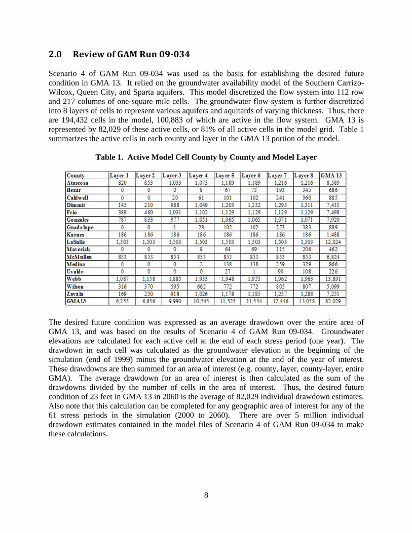
2.0 ReviewofGAMRun09‐034 Scenario 4 of GAM Run 09-034 was used as the basis for establishing the desired future condition in GMA 13. It relied on the groundwater availability model of the Southern Carrizo-Wilcox, Queen City, and Sparta aquifers. This model discretized the flow system into 112 row and 217 columns of one-square mile cells. The groundwater flow system is further discretized into 8 layers of cells to represent various aquifers and aquitards of varying thickness. Thus, there are 194,432 cells in the model, 100,883 of which are active in the flow system. GMA 13 is represented by 82,029 of these active cells, or 81% of all active cells in the model grid. Table 1 summarizes the active cells in each county and layer in the GMA 13 portion of the model.
Table 1. Active Model Cell County by County and Model Layer
The desired future condition was expressed as an average drawdown over the entire area of GMA 13, and was based on the results of Scenario 4 of GAM Run 09-034. Groundwater elevations are calculated for each active cell at the end of each stress period (one year). The drawdown in each cell was calculated as the groundwater elevation at the beginning of the simulation (end of 1999) minus the groundwater elevation at the end of the year of interest. These drawdowns are then summed for an area of interest (e.g. county, layer, county-layer, entire GMA). The average drawdown for an area of interest is then calculated as the sum of the drawdowns divided by the number of cells in the area of interest. Thus, the desired future condition of 23 feet in GMA 13 in 2060 is the average of 82,029 individual drawdown estimates. Also note that this calculation can be completed for any geographic area of interest for any of the 61 stress periods in the simulation (2000 to 2060). There are over 5 million individual drawdown estimates contained in the model files of Scenario 4 of GAM Run 09-034 to make these calculations.
9
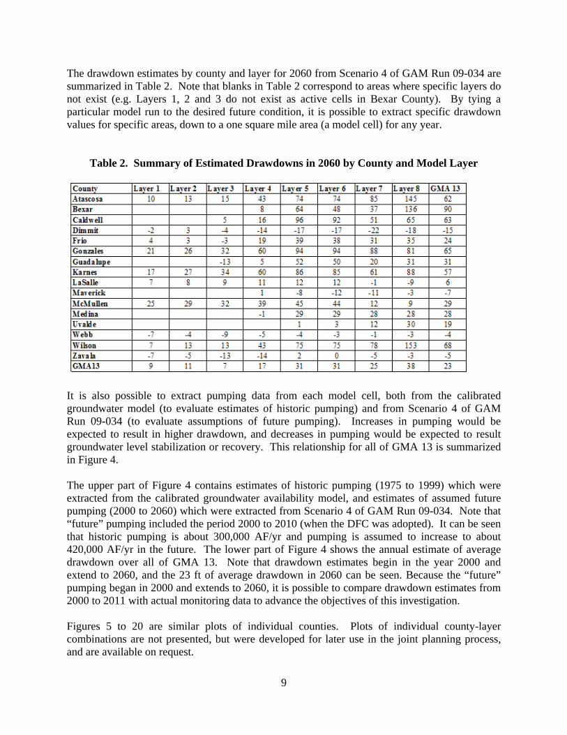
The drawdown estimates by county and layer for 2060 from Scenario 4 of GAM Run 09-034 are summarized in Table 2. Note that blanks in Table 2 correspond to areas where specific layers do not exist (e.g. Layers 1, 2 and 3 do not exist as active cells in Bexar County). By tying a particular model run to the desired future condition, it is possible to extract specific drawdown values for specific areas, down to a one square mile area (a model cell) for any year.
Table 2. Summary of Estimated Drawdowns in 2060 by County and Model Layer
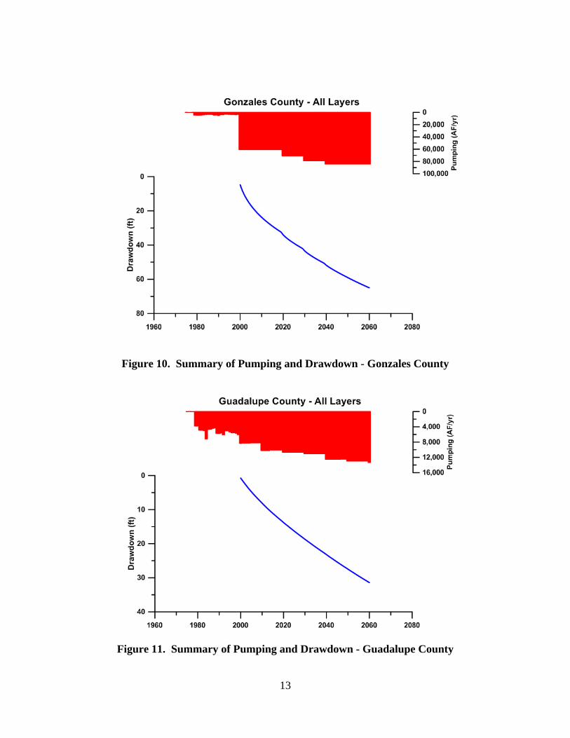
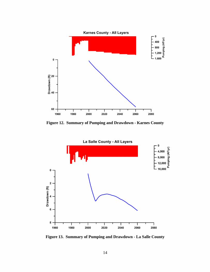
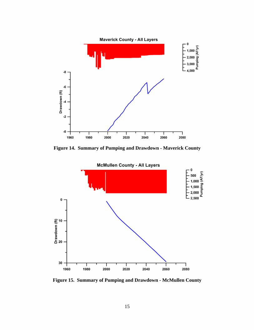
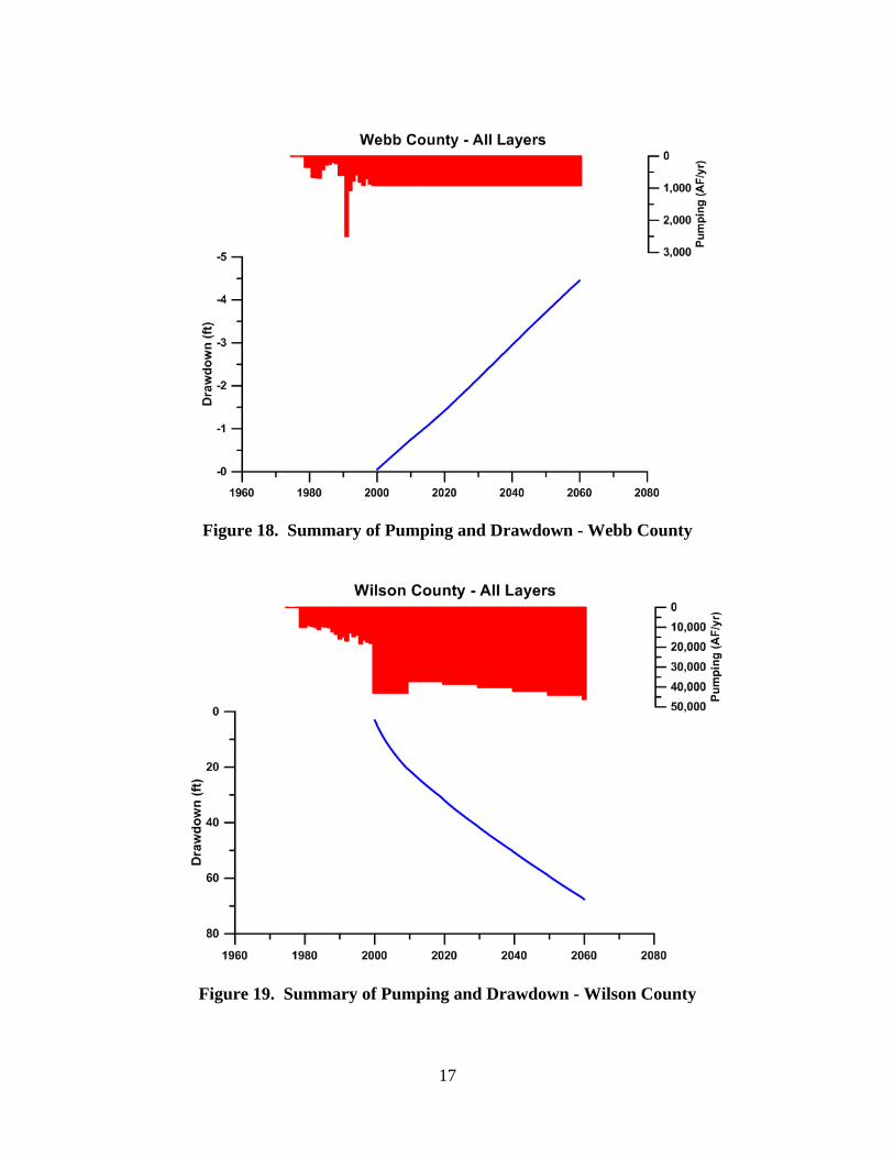
It is also possible to extract pumping data from each model cell, both from the calibrated groundwater model (to evaluate estimates of historic pumping) and from Scenario 4 of GAM Run 09-034 (to evaluate assumptions of future pumping). Increases in pumping would be expected to result in higher drawdown, and decreases in pumping would be expected to result groundwater level stabilization or recovery. This relationship for all of GMA 13 is summarized in Figure 4. The upper part of Figure 4 contains estimates of historic pumping (1975 to 1999) which were extracted from the calibrated groundwater availability model, and estimates of assumed future pumping (2000 to 2060) which were extracted from Scenario 4 of GAM Run 09-034. Note that “future” pumping included the period 2000 to 2010 (when the DFC was adopted). It can be seen that historic pumping is about 300,000 AF/yr and pumping is assumed to increase to about 420,000 AF/yr in the future. The lower part of Figure 4 shows the annual estimate of average drawdown over all of GMA 13. Note that drawdown estimates begin in the year 2000 and extend to 2060, and the 23 ft of average drawdown in 2060 can be seen. Because the “future” pumping began in 2000 and extends to 2060, it is possible to compare drawdown estimates from 2000 to 2011 with actual monitoring data to advance the objectives of this investigation. Figures 5 to 20 are similar plots of individual counties. Plots of individual county-layer combinations are not presented, but were developed for later use in the joint planning process, and are available on request.
10
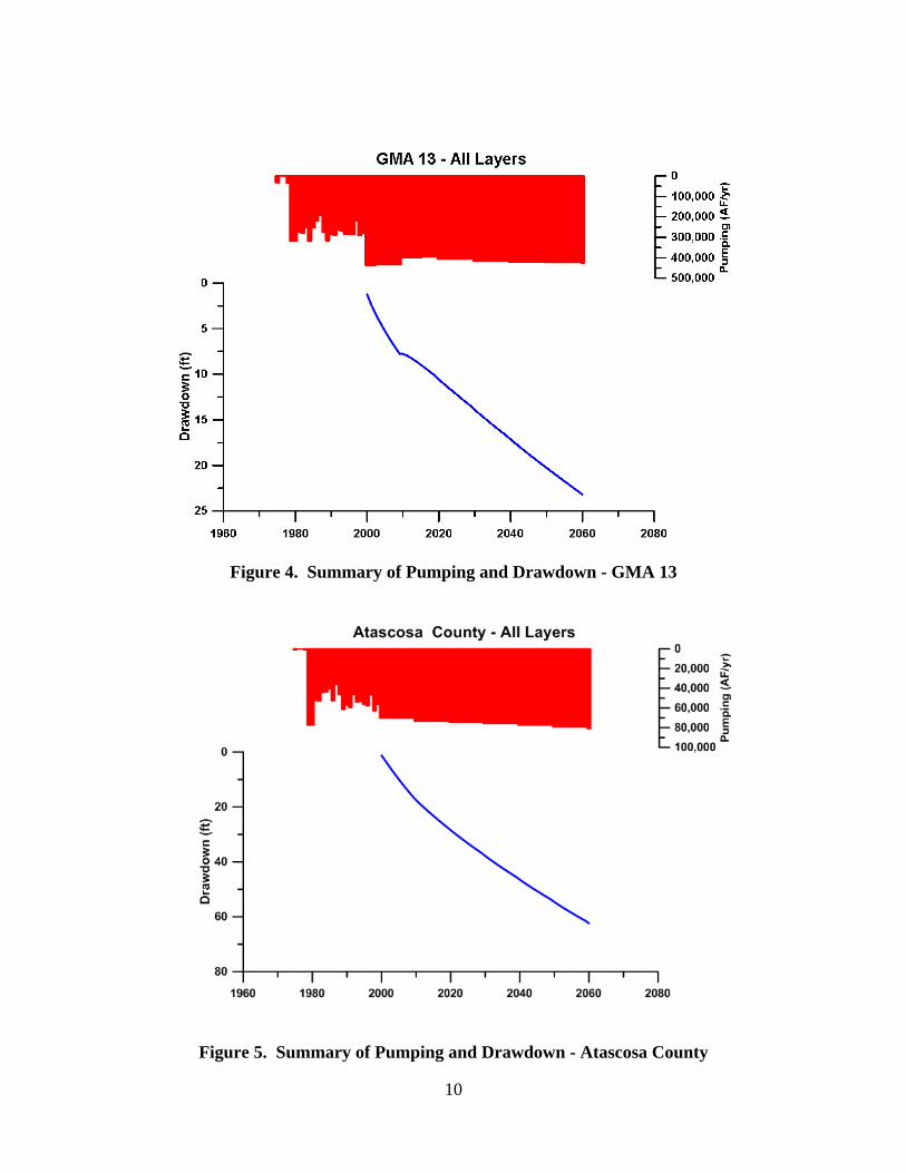
Figure 4. Summary of Pumping and Drawdown - GMA 13
Figure 5. Summary of Pumping and Drawdown - Atascosa County
11
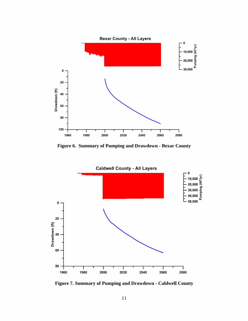
Figure 6. Summary of Pumping and Drawdown - Bexar County
Figure 7. Summary of Pumping and Drawdown - Caldwell County
12
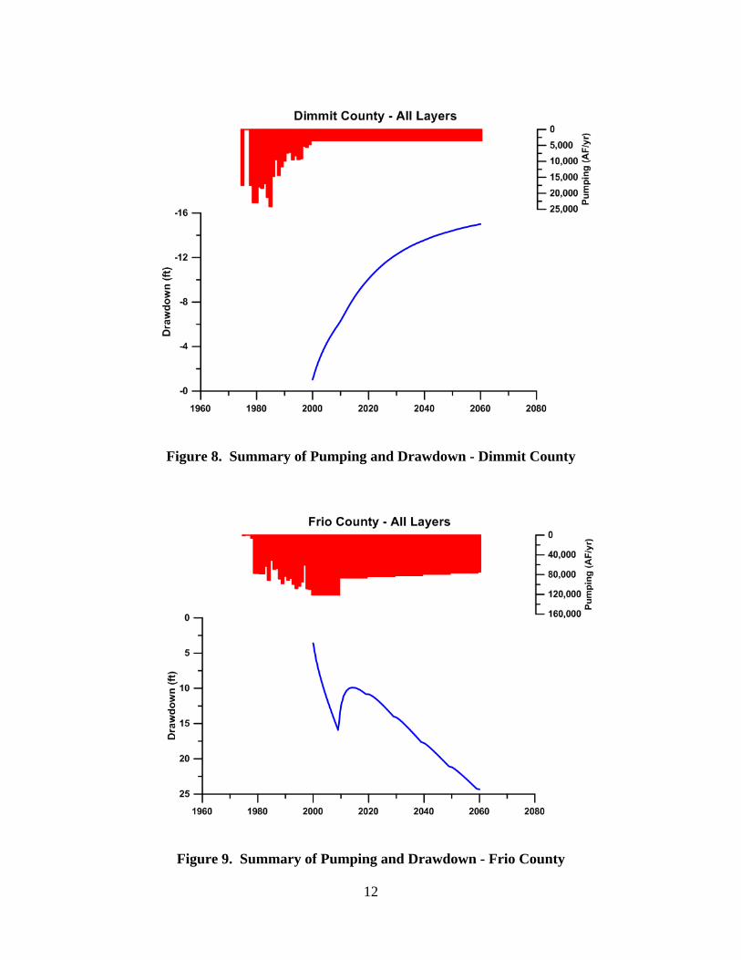
Figure 8. Summary of Pumping and Drawdown - Dimmit County
Figure 9. Summary of Pumping and Drawdown - Frio County
13
Figure 10. Summary of Pumping and Drawdown - Gonzales County
Figure 11. Summary of Pumping and Drawdown - Guadalupe County
14
Figure 12. Summary of Pumping and Drawdown - Karnes County
Figure 13. Summary of Pumping and Drawdown - La Salle County
15
Figure 14. Summary of Pumping and Drawdown - Maverick County
Figure 15. Summary of Pumping and Drawdown - McMullen County

16
Figure 16. Summary of Pumping and Drawdown - Medina County
Figure 17. Summary of Pumping and Drawdown - Uvalde County
17
Figure 18. Summary of Pumping and Drawdown - Webb County
Figure 19. Summary of Pumping and Drawdown - Wilson County
18
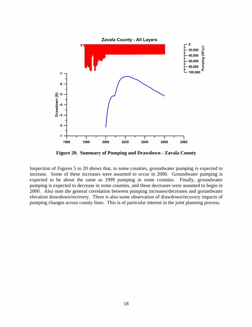
Figure 20. Summary of Pumping and Drawdown - Zavala County
Inspection of Figures 5 to 20 shows that, in some counties, groundwater pumping is expected to increase. Some of these increases were assumed to occur in 2000. Groundwater pumping is expected to be about the same as 1999 pumping in some counties. Finally, groundwater pumping is expected to decrease in some counties, and these decreases were assumed to begin in 2000. Also note the general correlation between pumping increases/decreases and groundwater elevation drawdown/recovery. There is also some observation of drawdown/recovery impacts of pumping changes across county lines. This is of particular interest in the joint planning process.
19
3.0 Point‐by‐PointComparisonofGroundwaterElevations Historic groundwater elevation data were obtained from the Texas Water Development Board for use in this analysis. Data maintained in this database include well location (latitude and longitude), well depth, completion data (screen top and bottom depth), and groundwater elevation data. In GMA 13, the database contains 31,247 groundwater elevation measurements from 1906 to 2012 in 6,956 wells. However, in 5,112 wells there are no details of screened intervals, but many of these have an aquifer code. Of the 1,844 wells that have screened interval data, 574 wells have no groundwater elevation data, 695 have exactly one groundwater elevation data point, and 575 have two or more groundwater elevation measurements. The wells with screened interval data were used in conjunction with the Groundwater Availability Model (GAM) for the Southern Carrizo-Wilcox, Queen City and Sparta aquifers. Each well was located in the model grid (i.e. row and column), and the completion interval was compared to the model layering data. Model data were then extracted for each cell with a well (e.g. aquifer parameters, historic and future pumping, and simulated groundwater elevations). Based on this analysis, 748 wells in GMA 13 were selected as being completed in a single model layer. 412 wells had exactly one groundwater level measurement. 207 wells had five or more groundwater elevation measurements. 92 wells had 10 or more groundwater elevation measurements with at least one data point collected after the year 2000.
3.1 HydrographsofGroundwaterElevationsandPumping These 92 wells were used to construct hydrographs of groundwater elevation and pumping. The locations of these 92 wells are shown in Figure 21, and details of these 92 wells are presented in Table 3. Please note that Table 3 is sorted by county and well number, and includes details of screen elevation, period of available groundwater elevation measurements, and data on aquifer parameters from the GAM. Hydrographs of these 92 wells are presented in individual appendices organized by county. These hydrographs include historic groundwater elevations data, future groundwater elevation data from the results of GAM Run 09-034, land surface elevation, screened intervals and historic and future pumping in three zones: 1) pumping within the cell where the well is located, 2) pumping in the cells immediately surrounding zone 1, and 3) pumping in cells immediately surrounding zone 2. Thus, pumping (both historic and projected) in a 25 square mile area surrounding the well of interest is presented in aid interpretation of the groundwater elevation changes. The appendices also present the locations of these wells, and contain data, maps and graphs from other analyses described later in this report.

20
Figure 21. Map of Hydrograph Well Locations
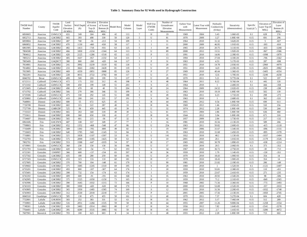
Table 3. Summary Data for 92 Wells used in Hydrograph Construction
TWDB Well Number
CountyTWDB Aquifer
Code
Land Surface
Elevation (ft MSL)
Well Depth (ft)
Elevation of Screen
Top (ft MSL)
Elevation of Screen Bottom (ft
MSL)
Model RowModel
ColumnModel Layer
Well Use (TWDB Code)
Number of Groundwater
Elevation Measurements
Ealiest Year with
Measurement
Latest Year with Measrement
Hydraulic Conductivity
(ft/day)
Storativity (dimensionless)
Specific
Yield (ft-1)
Elevation of Layer Top (ft
MSL)
Elevation of Layer
Bottom (ft MSL)
6850603 Atascosa 124WLCX 655 249 504 406 42 113 7 H 19 1969 2004 5.43 1.06E-03 0.1 628 276
6852713 Atascosa 124CRRZ 665 393 498 330 50 120 5 U 81 1970 2009 3.27 1.00E+00 0.15 691 296
6859804 Atascosa 124CRRZ 487 740 -56 -213 54 109 5 I 31 1964 2010 31.32 3.62E-03 0.15 5 -827
6860852 Atascosa 124CRRZ 470 1130 -460 -650 58 117 5 I 11 2000 2009 46.95 1.91E-03 0.15 -303 -810
6861905 Atascosa 124CRRZ 482 1413 -718 -931 63 125 5 I 40 1965 2010 20.75 3.11E-03 0.15 -433 -1268
7804508 Atascosa 124CRRZ 466 1850 -1234 -1344 64 113 5 U 89 2008 2012 13.51 1.92E-03 0.15 -967 -1586
7804612 Atascosa 124CRRZ 420 2125 -1286 -1518 65 115 5 P 15 1991 2010 14.06 2.39E-03 0.15 -1098 -1870
7805212 Atascosa 124CRRZ 405 1637 -957 -1232 64 121 5 I 13 1994 2010 27.04 3.10E-03 0.15 -706 -1562
7805409 Atascosa 124QNCT 380 800 -260 -420 64 117 3 P 31 1963 2010 4.53 5.17E-03 0.15 287 -698
7814801 Atascosa 124CRRZ 241 3992 -3239 -3319 82 118 5 U 20 1951 2010 14.78 2.03E-03 0.15 -2960 -4079
7814802 Atascosa 124CRRZ 233 3663 -3382 -3428 81 119 5 U 19 1951 2010 14.9 2.19E-03 0.15 -2825 -3982
7815805 Atascosa 124CRRZ 469 4359 -3851 -3888 85 126 5 P 27 1969 2010 40.44 1.36E-03 0.15 -3405 -4354
7822201 Atascosa 124CRRZ 228 4015 -3722 -3782 84 117 5 U 21 1951 2010 12.6 1.70E-03 0.15 -3240 -4258
6846702 Bexar 124WLCX 499 500 269 199 53 137 7 U 28 1970 2011 5.21 9.77E-04 0.1 522 197
6712111 Caldwell 124WLCX 472 175 332 312 45 198 8 S 48 1964 2011 8.12 9.76E-04 0.1 445 120
6713102 Caldwell 124WLCX 599 450 199 149 51 203 7 S 25 1964 2010 1 2.40E-03 0.1 444 -358
6713605 Caldwell 124CRRZ 490 470 60 40 55 204 5 H 24 1964 2009 24.52 2.02E-03 0.15 238 -198
6713702 Caldwell 124CRRZ 566 270 366 346 55 199 5 H 12 1963 2010 19.19 1.00E+00 0.15 502 139
6719306 Caldwell 124WLCX 475 330 292 145 51 188 8 U 49 1964 2011 6.23 1.71E-03 0.1 298 -273
6720802 Caldwell 124WLCX 410 200 241 221 57 191 7 S 50 1963 2010 1 2.68E-03 0.1 362 -531
7648801 Dimmit 124CRRZ 680 55 672 625 45 12 5 H 44 1965 2012 0.54 1.00E+00 0.15 690 613
7726708 Dimmit 124CRRZ 602 315 522 287 40 33 5 H 36 1969 2012 1.46 2.05E-03 0.15 550 256
7727709 Dimmit 124BGDF 525 99 459 445 43 39 3 U 32 1974 2012 2.28 1.00E+00 0.15 530 244
7733322 Dimmit 124CRRZ 665 263 560 518 40 30 5 G 61 1971 2004 2.86 1.00E+00 0.15 636 460
7733611 Dimmit 124CRRZ 690 360 650 330 41 27 5 H 39 1944 2012 5.94 1.00E+00 0.15 671 316
7734607 Dimmit 124CRRZ 565 601 215 -36 47 32 5 S 42 1957 2009 2.84 1.73E-03 0.15 217 -132
6961606 Frio 124CZWX 687 338 557 349 27 77 5 I 16 1981 2010 35.56 2.13E-03 0.15 589 266
7708803 Frio 124CRRZ 652 1352 -468 -548 47 86 5 U 254 1963 2011 50.82 2.60E-03 0.15 -415 -1118
7716409 Frio 124CRRZ 589 1392 -705 -800 49 82 5 I 19 1997 2006 31.67 1.54E-03 0.15 -696 -1155
7716603 Frio 124CRRZ 640 1785 -945 -1145 53 84 5 I 35 1963 2010 31.68 1.45E-03 0.15 -895 -1378
7716801 Frio 124CRRZ 521 1828 -1107 -1307 53 81 5 U 141 1952 2010 48.2 1.13E-03 0.15 -1037 -1404
7722703 Frio 124CRRZ 575 2000 -1185 -1425 50 63 5 I 10 2001 2010 20.1 1.01E-03 0.15 -1179 -1526
7802701 Frio 124CRRZ 553 1588 -647 -1035 54 97 5 H 17 1965 2002 30.78 1.89E-03 0.15 -638 -1214
6719901 Gonzales 124WLCX 360 230 150 130 56 186 7 U 37 1959 2010 20.5 2.06E-03 0.1 373 -312
6721703 Gonzales 124CRRZ 420 520 -54 -75 62 193 5 S 34 1967 2010 36.72 2.75E-03 0.15 -30 -713
6722301 Gonzales 124SPRT 366 600 -137 -234 65 207 1 H 36 1959 2010 1.79 1.14E-03 0.15 -130 -351
6727502 Gonzales 124CRRZ 435 180 280 259 60 181 5 U 29 1970 2010 18.43 1.90E-03 0.15 354 14
6727503 Gonzales 124WLCX 433 323 133 110 60 181 5 H 17 1979 2010 18.43 1.90E-03 0.15 354 14
6727805 Gonzales 124CRRZ 370 700 104 -148 61 179 5 U 99 1981 2010 21.82 2.19E-03 0.15 286 -149
6729602 Gonzales 124CRRZ 375 1685 -1245 -1310 69 195 4 S 29 1969 2010 1 1.52E-03 0.1 -1121 -1407
6735201 Gonzales 124CRRZ 493 800 -107 -307 64 176 5 I 20 1959 2010 55.81 2.38E-03 0.15 110 -451
6735401 Gonzales 124CRRZ 398 732 154 -174 63 174 5 I 25 1959 2010 23.67 2.41E-03 0.15 271 -235
6742202 Gonzales 124CRRZ 409 600 -91 -191 65 168 5 S 35 1963 2010 20.92 2.54E-03 0.15 98 -506
6742905 Gonzales 124CRRZ 375 1525 -1050 -1150 73 165 5 H 23 1959 2010 71.2 2.31E-03 0.15 -849 -1565
6742906 Gonzales 124CRRZ 390 1645 -1032 -1215 72 166 5 P 10 1968 2002 71.56 2.36E-03 0.15 -773 -1493
6743103 Gonzales 124CRRZ 380 1000 -420 -620 68 170 5 I 28 2000 2010 53.08 2.52E-03 0.15 -357 -1033
6743805 Gonzales 124CRRZ 365 1950 -1485 -1585 74 169 5 S 12 1959 2010 31.56 2.20E-03 0.15 -1032 -1748
6743903 Gonzales 124CRRZ 312 2530 -2018 -2218 77 172 5 P 13 2001 2005 17.56 2.13E-03 0.15 -1850 -2745
6840310 Guadalupe 124WLCX 585 130 475 455 50 161 8 U 40 1970 2011 7.37 5.27E-04 0.1 604 428
7722801 LaSalle 124LRDO 583 252 383 331 52 63 1 H 35 1962 2012 5.17 7.46E-04 0.15 512 289
7730801 LaSalle 124CRRZ 516 2051 -1284 -1535 59 58 5 H 44 1955 2007 11.26 9.80E-04 0.15 -1258 -1554
7748301 LaSalle 124CRRZ 420 3483 -2914 -3063 80 67 5 H 54 1956 2012 7.82 1.64E-03 0.15 -2541 -3278
7764401 LaSalle 124CRRZ 395 4280 -3535 -3885 92 50 5 H 45 1959 2012 2.7 1.41E-03 0.15 -3286 -4072
7607901 Maverick 124CRRZ 703 100 623 603 8 34 5 U 48 1955 2012 2.28 1.00E+00 0.15 715 602
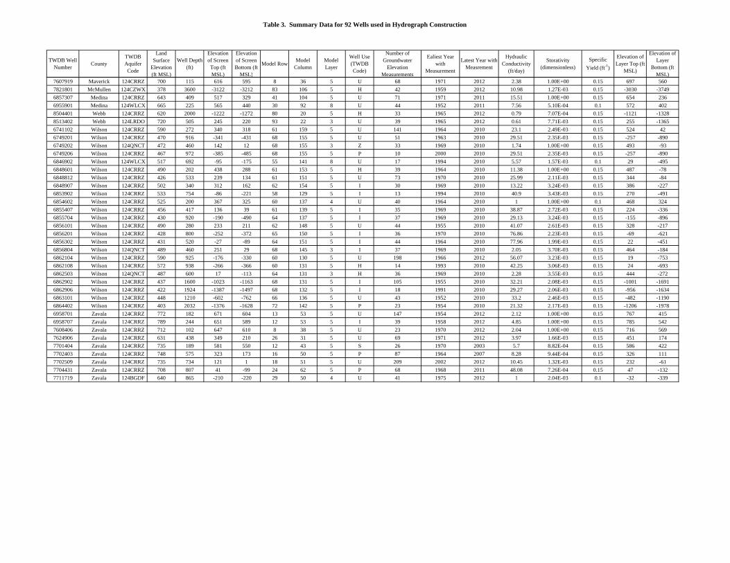
Table 3. Summary Data for 92 Wells used in Hydrograph Construction
TWDB Well Number
CountyTWDB Aquifer
Code
Land Surface
Elevation (ft MSL)
Well Depth (ft)
Elevation of Screen
Top (ft MSL)
Elevation of Screen Bottom (ft
MSL)
Model RowModel
ColumnModel Layer
Well Use (TWDB Code)
Number of Groundwater
Elevation Measurements
Ealiest Year with
Measurement
Latest Year with Measrement
Hydraulic Conductivity
(ft/day)
Storativity (dimensionless)
Specific
Yield (ft-1)
Elevation of Layer Top (ft
MSL)
Elevation of Layer
Bottom (ft MSL)
7607919 Maverick 124CRRZ 700 115 616 595 8 36 5 U 68 1971 2012 2.38 1.00E+00 0.15 697 560
7821801 McMullen 124CZWX 378 3600 -3122 -3212 83 106 5 H 42 1959 2012 10.98 1.27E-03 0.15 -3030 -3749
6857307 Medina 124CRRZ 643 409 517 329 41 104 5 U 71 1971 2011 15.51 1.00E+00 0.15 654 236
6955901 Medina 124WLCX 665 225 565 440 30 92 8 U 44 1952 2011 7.56 5.10E-04 0.1 572 402
8504401 Webb 124CRRZ 620 2000 -1222 -1272 80 20 5 H 33 1965 2012 0.79 7.07E-04 0.15 -1121 -1328
8513402 Webb 124LRDO 720 505 245 220 93 22 3 U 39 1965 2012 0.61 7.71E-03 0.15 255 -1365
6741102 Wilson 124CRRZ 590 272 340 318 61 159 5 U 141 1964 2010 23.1 2.49E-03 0.15 524 42
6749201 Wilson 124CRRZ 470 916 -341 -431 68 155 5 U 51 1963 2010 29.51 2.35E-03 0.15 -257 -890
6749202 Wilson 124QNCT 472 460 142 12 68 155 3 Z 33 1969 2010 1.74 1.00E+00 0.15 493 -93
6749206 Wilson 124CRRZ 467 972 -385 -485 68 155 5 P 10 2000 2010 29.51 2.35E-03 0.15 -257 -890
6846902 Wilson 124WLCX 517 692 -95 -175 55 141 8 U 17 1994 2010 5.57 1.57E-03 0.1 29 -495
6848601 Wilson 124CRRZ 490 202 438 288 61 153 5 H 39 1964 2010 11.38 1.00E+00 0.15 487 -78
6848812 Wilson 124CRRZ 426 533 239 134 61 151 5 U 73 1970 2010 25.99 2.11E-03 0.15 344 -84
6848907 Wilson 124CRRZ 502 340 312 162 62 154 5 I 30 1969 2010 13.22 3.24E-03 0.15 386 -227
6853902 Wilson 124CRRZ 533 754 -86 -221 58 129 5 I 13 1994 2010 40.9 3.43E-03 0.15 270 -491
6854602 Wilson 124CRRZ 525 200 367 325 60 137 4 U 40 1964 2010 1 1.00E+00 0.1 468 324
6855407 Wilson 124CRRZ 456 417 136 39 61 139 5 I 35 1969 2010 38.87 2.72E-03 0.15 224 -336
6855704 Wilson 124CRRZ 430 920 -190 -490 64 137 5 I 37 1969 2010 29.13 3.24E-03 0.15 -155 -896
6856101 Wilson 124CRRZ 490 280 233 211 62 148 5 U 44 1955 2010 41.07 2.61E-03 0.15 328 -217
6856201 Wilson 124CRRZ 428 800 -252 -372 65 150 5 I 36 1970 2010 76.86 2.23E-03 0.15 -69 -621
6856302 Wilson 124CRRZ 431 520 -27 -89 64 151 5 I 44 1964 2010 77.96 1.99E-03 0.15 22 -451
6856804 Wilson 124QNCT 489 460 251 29 68 145 3 I 37 1969 2010 2.05 3.70E-03 0.15 464 -184
6862104 Wilson 124CRRZ 590 925 -176 -330 60 130 5 U 198 1966 2012 56.07 3.23E-03 0.15 19 -753
6862108 Wilson 124CRRZ 572 938 -266 -366 60 131 5 H 14 1993 2010 42.25 3.06E-03 0.15 24 -693
6862503 Wilson 124QNCT 487 600 17 -113 64 131 3 H 36 1969 2010 2.28 3.55E-03 0.15 444 -272
6862902 Wilson 124CRRZ 437 1600 -1023 -1163 68 131 5 I 105 1955 2010 32.21 2.08E-03 0.15 -1001 -1691
6862906 Wilson 124CRRZ 422 1924 -1387 -1497 68 132 5 I 18 1991 2010 29.27 2.06E-03 0.15 -956 -1634
6863101 Wilson 124CRRZ 448 1210 -602 -762 66 136 5 U 43 1952 2010 33.2 2.46E-03 0.15 -482 -1190
6864402 Wilson 124CRRZ 403 2032 -1376 -1628 72 142 5 P 23 1954 2010 21.32 2.17E-03 0.15 -1206 -1978
6958701 Zavala 124CRRZ 772 182 671 604 13 53 5 U 147 1954 2012 2.12 1.00E+00 0.15 767 415
6958707 Zavala 124CRRZ 789 244 651 589 12 53 5 I 39 1958 2012 4.85 1.00E+00 0.15 785 542
7608406 Zavala 124CRRZ 712 102 647 610 8 38 5 U 23 1970 2012 2.04 1.00E+00 0.15 716 569
7624906 Zavala 124CRRZ 631 438 349 210 26 31 5 U 69 1971 2012 3.97 1.66E-03 0.15 451 174
7701404 Zavala 124CRRZ 735 189 581 550 12 43 5 S 26 1970 2003 5.7 8.82E-04 0.15 586 422
7702403 Zavala 124CRRZ 748 575 323 173 16 50 5 P 87 1964 2007 8.28 9.44E-04 0.15 326 111
7702509 Zavala 124CRRZ 735 734 121 1 18 51 5 U 209 2002 2012 10.45 1.32E-03 0.15 232 -61
7704431 Zavala 124CRRZ 708 807 41 -99 24 62 5 P 68 1968 2011 48.08 7.26E-04 0.15 47 -132
7711719 Zavala 124BGDF 640 865 -210 -220 29 50 4 U 41 1975 2012 1 2.04E-03 0.1 -32 -339

23
The hydrographs are useful to compare model calibration by comparing pre-1999 historic groundwater elevations to the estimates of groundwater elevation at that point (the black line). In many cases the comparison is favorable, in other areas it is not. The estimates of historic pumping in the vicinity of the well are sometimes a useful guide to interpret the comparisons. In general, the recovering future groundwater elevations are well correlated with assumed decreases in pumping, and declining future groundwater elevations are well correlated with assumed increases in pumping.
3.2 Well‐by‐WellDrawdownComparison In order to compare drawdown estimates from GAM Run 09-034 with drawdown data from specific wells, the group of wells used in hydrograph construction were filtered further to include wells that had a late 1999/early 2000 groundwater elevation measurement and at least one measurement at the end of the year/beginning of the year from late 2000/early 2001 to late 2011/early 2012. As a result of this additional filtering 70 wells with 628 groundwater drawdown measurements were identified that met these criteria. Locations of these wells are presented in Figure 22 and the selected details of the wells and the 628 actual drawdown measurements from 2000 to 2011 are presented in Table 4. Please note that blank entries in Table 4 represent years where no data were collected. The comparison of actual drawdown and model-estimated drawdown was completed by calculating the difference between the model-estimated drawdown and actual drawdown. A positive number means that the actual groundwater elevation is higher than the groundwater elevation projected by GAM Run 09-034 in that cell of the model. For example, if the drawdown from GAM Run 09-034 is 10 feet, and the actual drawdown is 8 feet, the difference is 2 feet, which means that the groundwater elevation is two feet higher than projected in GAM Run 09-034. Conversely, a negative number from this calculation means that actual groundwater elevations are lower than the estimated groundwater elevation from GAM Run 09-034. Results were summarized by GMA, year, and county. The overall summary of the analysis for GMA 13 is shown in Figure 23, which is a histogram of the difference between DFC drawdown and actual drawdown for all years evaluated (2000 to 2011). Maps showing this analysis for each year for GMA 13 are presented in Appendix 1. More detailed maps for 2001, 2006 and 2011 which include well numbers for each county are presented in the county-specific appendices. Please note that a difference of greater than 3 feet (actual groundwater elevation is 3 feet or more higher than the DFC simulation elevation) is shown in green, differences of between -3 and 3 feet are shown in yellow (actual groundwater elevation and DFC simulation elevation is within 3 feet), and differences less than -3 feet are shown in red (actual groundwater elevation is 3 feet or lower than the DFC simulation elevation). From this plot, it can be seen that about 18 percent of all groundwater elevation measurements are below the projected groundwater elevation from the DFC condition, about 25 percent are within 3 feet of the DFC condition, and about 57 percent are 3 feet or higher than the DFC condition.
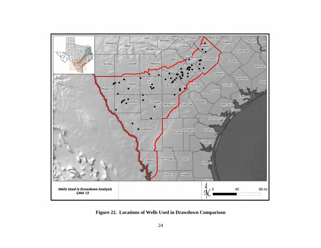
24
Figure 22. Locations of Wells Used in Drawdown Comparison
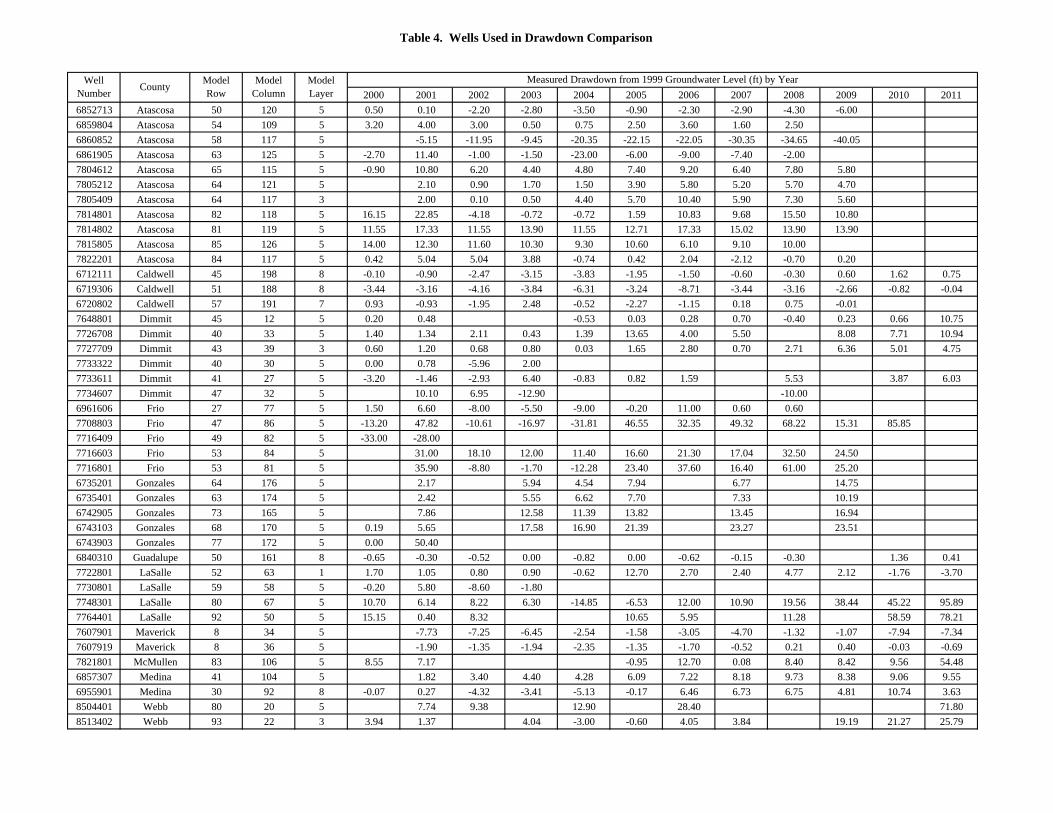
Table 4. Wells Used in Drawdown Comparison
2000 2001 2002 2003 2004 2005 2006 2007 2008 2009 2010 2011
6852713 Atascosa 50 120 5 0.50 0.10 -2.20 -2.80 -3.50 -0.90 -2.30 -2.90 -4.30 -6.00
6859804 Atascosa 54 109 5 3.20 4.00 3.00 0.50 0.75 2.50 3.60 1.60 2.50
6860852 Atascosa 58 117 5 -5.15 -11.95 -9.45 -20.35 -22.15 -22.05 -30.35 -34.65 -40.05
6861905 Atascosa 63 125 5 -2.70 11.40 -1.00 -1.50 -23.00 -6.00 -9.00 -7.40 -2.00
7804612 Atascosa 65 115 5 -0.90 10.80 6.20 4.40 4.80 7.40 9.20 6.40 7.80 5.80
7805212 Atascosa 64 121 5 2.10 0.90 1.70 1.50 3.90 5.80 5.20 5.70 4.70
7805409 Atascosa 64 117 3 2.00 0.10 0.50 4.40 5.70 10.40 5.90 7.30 5.60
7814801 Atascosa 82 118 5 16.15 22.85 -4.18 -0.72 -0.72 1.59 10.83 9.68 15.50 10.80
7814802 Atascosa 81 119 5 11.55 17.33 11.55 13.90 11.55 12.71 17.33 15.02 13.90 13.90
7815805 Atascosa 85 126 5 14.00 12.30 11.60 10.30 9.30 10.60 6.10 9.10 10.00
7822201 Atascosa 84 117 5 0.42 5.04 5.04 3.88 -0.74 0.42 2.04 -2.12 -0.70 0.20
6712111 Caldwell 45 198 8 -0.10 -0.90 -2.47 -3.15 -3.83 -1.95 -1.50 -0.60 -0.30 0.60 1.62 0.75
6719306 Caldwell 51 188 8 -3.44 -3.16 -4.16 -3.84 -6.31 -3.24 -8.71 -3.44 -3.16 -2.66 -0.82 -0.04
6720802 Caldwell 57 191 7 0.93 -0.93 -1.95 2.48 -0.52 -2.27 -1.15 0.18 0.75 -0.01
7648801 Dimmit 45 12 5 0.20 0.48 -0.53 0.03 0.28 0.70 -0.40 0.23 0.66 10.75
7726708 Dimmit 40 33 5 1.40 1.34 2.11 0.43 1.39 13.65 4.00 5.50 8.08 7.71 10.94
7727709 Dimmit 43 39 3 0.60 1.20 0.68 0.80 0.03 1.65 2.80 0.70 2.71 6.36 5.01 4.75
7733322 Dimmit 40 30 5 0.00 0.78 -5.96 2.00
7733611 Dimmit 41 27 5 -3.20 -1.46 -2.93 6.40 -0.83 0.82 1.59 5.53 3.87 6.03
7734607 Dimmit 47 32 5 10.10 6.95 -12.90 -10.00
6961606 Frio 27 77 5 1.50 6.60 -8.00 -5.50 -9.00 -0.20 11.00 0.60 0.60
7708803 Frio 47 86 5 -13.20 47.82 -10.61 -16.97 -31.81 46.55 32.35 49.32 68.22 15.31 85.85
7716409 Frio 49 82 5 -33.00 -28.00
7716603 Frio 53 84 5 31.00 18.10 12.00 11.40 16.60 21.30 17.04 32.50 24.50
7716801 Frio 53 81 5 35.90 -8.80 -1.70 -12.28 23.40 37.60 16.40 61.00 25.20
6735201 Gonzales 64 176 5 2.17 5.94 4.54 7.94 6.77 14.75
6735401 Gonzales 63 174 5 2.42 5.55 6.62 7.70 7.33 10.19
6742905 Gonzales 73 165 5 7.86 12.58 11.39 13.82 13.45 16.94
6743103 Gonzales 68 170 5 0.19 5.65 17.58 16.90 21.39 23.27 23.51
6743903 Gonzales 77 172 5 0.00 50.40
6840310 Guadalupe 50 161 8 -0.65 -0.30 -0.52 0.00 -0.82 0.00 -0.62 -0.15 -0.30 1.36 0.41
7722801 LaSalle 52 63 1 1.70 1.05 0.80 0.90 -0.62 12.70 2.70 2.40 4.77 2.12 -1.76 -3.70
7730801 LaSalle 59 58 5 -0.20 5.80 -8.60 -1.80
7748301 LaSalle 80 67 5 10.70 6.14 8.22 6.30 -14.85 -6.53 12.00 10.90 19.56 38.44 45.22 95.89
7764401 LaSalle 92 50 5 15.15 0.40 8.32 10.65 5.95 11.28 58.59 78.21
7607901 Maverick 8 34 5 -7.73 -7.25 -6.45 -2.54 -1.58 -3.05 -4.70 -1.32 -1.07 -7.94 -7.34
7607919 Maverick 8 36 5 -1.90 -1.35 -1.94 -2.35 -1.35 -1.70 -0.52 0.21 0.40 -0.03 -0.69
7821801 McMullen 83 106 5 8.55 7.17 -0.95 12.70 0.08 8.40 8.42 9.56 54.48
6857307 Medina 41 104 5 1.82 3.40 4.40 4.28 6.09 7.22 8.18 9.73 8.38 9.06 9.55
6955901 Medina 30 92 8 -0.07 0.27 -4.32 -3.41 -5.13 -0.17 6.46 6.73 6.75 4.81 10.74 3.63
8504401 Webb 80 20 5 7.74 9.38 12.90 28.40 71.80
8513402 Webb 93 22 3 3.94 1.37 4.04 -3.00 -0.60 4.05 3.84 19.19 21.27 25.79
Well Number
CountyModel Row
Model Column
Model Layer
Measured Drawdown from 1999 Groundwater Level (ft) by Year
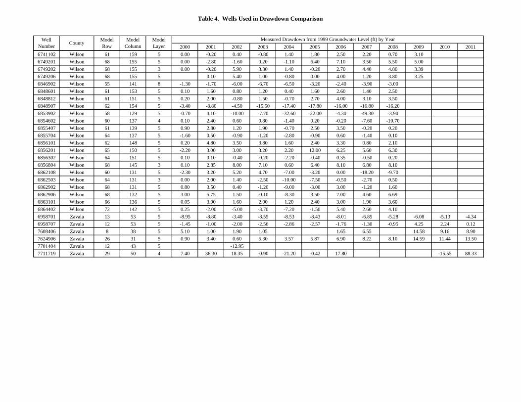
Table 4. Wells Used in Drawdown Comparison
2000 2001 2002 2003 2004 2005 2006 2007 2008 2009 2010 2011
Well Number
CountyModel Row
Model Column
Model Layer
Measured Drawdown from 1999 Groundwater Level (ft) by Year
6741102 Wilson 61 159 5 0.00 -0.20 0.40 -0.80 1.40 1.80 2.50 2.20 0.70 3.10
6749201 Wilson 68 155 5 0.00 -2.80 -1.60 0.20 -1.10 6.40 7.10 3.50 5.50 5.00
6749202 Wilson 68 155 3 0.00 -0.20 5.90 3.30 1.40 -0.20 2.70 4.40 4.80 3.39
6749206 Wilson 68 155 5 0.10 5.40 1.00 -0.80 0.00 4.00 1.20 3.80 3.25
6846902 Wilson 55 141 8 -1.30 -1.70 -6.00 -6.70 -6.50 -3.20 -2.40 -3.90 -3.00
6848601 Wilson 61 153 5 0.10 1.60 0.80 1.20 0.40 1.60 2.60 1.40 2.50
6848812 Wilson 61 151 5 0.20 2.00 -0.80 1.50 -0.70 2.70 4.00 3.10 3.50
6848907 Wilson 62 154 5 -3.40 -8.80 -4.50 -15.50 -17.40 -17.80 -16.00 -16.80 -16.20
6853902 Wilson 58 129 5 -0.70 4.10 -10.00 -7.70 -32.60 -22.00 -4.30 -49.30 -3.90
6854602 Wilson 60 137 4 0.10 2.40 0.60 0.80 -1.40 0.20 -0.20 -7.60 -10.70
6855407 Wilson 61 139 5 0.90 2.80 1.20 1.90 -0.70 2.50 3.50 -0.20 0.20
6855704 Wilson 64 137 5 -1.60 0.50 -0.90 -1.20 -2.80 -0.90 0.60 -1.40 0.10
6856101 Wilson 62 148 5 0.20 4.80 3.50 3.80 1.60 2.40 3.30 0.80 2.10
6856201 Wilson 65 150 5 -2.20 3.00 3.00 3.20 2.20 12.00 6.25 5.60 6.30
6856302 Wilson 64 151 5 0.10 0.10 -0.40 -0.20 -2.20 -0.40 0.35 -0.50 0.20
6856804 Wilson 68 145 3 0.10 2.85 8.00 7.10 0.60 6.40 8.10 6.80 8.10
6862108 Wilson 60 131 5 -2.30 3.20 5.20 4.70 -7.00 -3.20 0.00 -18.20 -9.70
6862503 Wilson 64 131 3 0.00 2.00 1.40 -2.50 -10.00 -7.50 -0.50 -2.70 0.50
6862902 Wilson 68 131 5 0.80 3.50 0.40 -1.20 -9.00 -3.00 3.00 -1.20 1.60
6862906 Wilson 68 132 5 3.00 5.75 1.50 -0.10 -8.30 3.50 7.00 4.60 6.69
6863101 Wilson 66 136 5 0.05 3.00 1.60 2.00 1.20 2.40 3.00 1.90 3.60
6864402 Wilson 72 142 5 0.25 -2.00 -5.00 -3.70 -7.20 -1.50 5.40 2.60 4.10
6958701 Zavala 13 53 5 -8.95 -8.80 -3.40 -8.55 -8.53 -8.43 -8.01 -6.85 -5.28 -6.08 -5.13 -4.34
6958707 Zavala 12 53 5 -1.45 -1.00 -2.00 -2.56 -2.86 -2.57 -1.76 -1.30 -0.95 4.25 2.24 0.12
7608406 Zavala 8 38 5 5.10 1.00 1.90 1.05 1.65 6.55 14.58 9.16 8.90
7624906 Zavala 26 31 5 0.90 3.40 0.60 5.30 3.57 5.87 6.90 8.22 8.10 14.59 11.44 13.50
7701404 Zavala 12 43 5 -12.95
7711719 Zavala 29 50 4 7.40 36.30 18.35 -0.90 -21.20 -0.42 17.80 -15.55 88.33
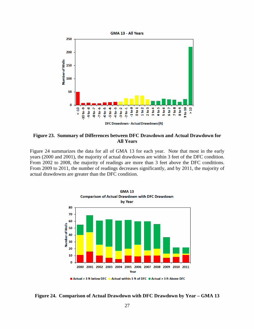
27
Figure 23. Summary of Differences between DFC Drawdown and Actual Drawdown for All Years
Figure 24 summarizes the data for all of GMA 13 for each year. Note that most in the early years (2000 and 2001), the majority of actual drawdowns are within 3 feet of the DFC condition. From 2002 to 2008, the majority of readings are more than 3 feet above the DFC conditions. From 2009 to 2011, the number of readings decreases significantly, and by 2011, the majority of actual drawdowns are greater than the DFC condition.
Figure 24. Comparison of Actual Drawdown with DFC Drawdown by Year – GMA 13
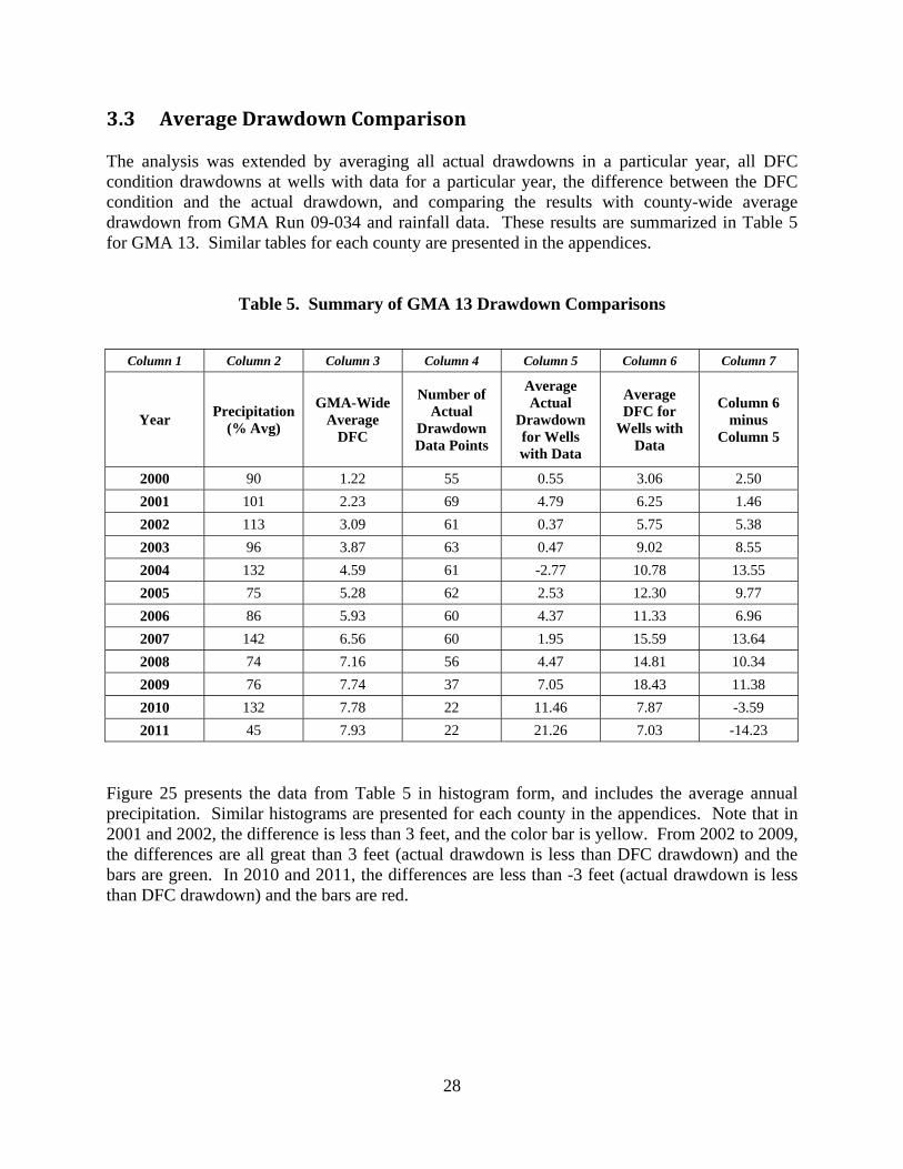
28
3.3 AverageDrawdownComparison The analysis was extended by averaging all actual drawdowns in a particular year, all DFC condition drawdowns at wells with data for a particular year, the difference between the DFC condition and the actual drawdown, and comparing the results with county-wide average drawdown from GMA Run 09-034 and rainfall data. These results are summarized in Table 5 for GMA 13. Similar tables for each county are presented in the appendices.
Table 5. Summary of GMA 13 Drawdown Comparisons
Column 1 Column 2 Column 3 Column 4 Column 5 Column 6 Column 7
Year Precipitation
(% Avg)
GMA-Wide Average
DFC
Number of Actual
Drawdown Data Points
Average Actual
Drawdown for Wells with Data
Average DFC for
Wells with Data
Column 6 minus
Column 5
2000 90 1.22 55 0.55 3.06 2.50
2001 101 2.23 69 4.79 6.25 1.46
2002 113 3.09 61 0.37 5.75 5.38
2003 96 3.87 63 0.47 9.02 8.55
2004 132 4.59 61 -2.77 10.78 13.55
2005 75 5.28 62 2.53 12.30 9.77
2006 86 5.93 60 4.37 11.33 6.96
2007 142 6.56 60 1.95 15.59 13.64
2008 74 7.16 56 4.47 14.81 10.34
2009 76 7.74 37 7.05 18.43 11.38
2010 132 7.78 22 11.46 7.87 -3.59
2011 45 7.93 22 21.26 7.03 -14.23
Figure 25 presents the data from Table 5 in histogram form, and includes the average annual precipitation. Similar histograms are presented for each county in the appendices. Note that in 2001 and 2002, the difference is less than 3 feet, and the color bar is yellow. From 2002 to 2009, the differences are all great than 3 feet (actual drawdown is less than DFC drawdown) and the bars are green. In 2010 and 2011, the differences are less than -3 feet (actual drawdown is less than DFC drawdown) and the bars are red.
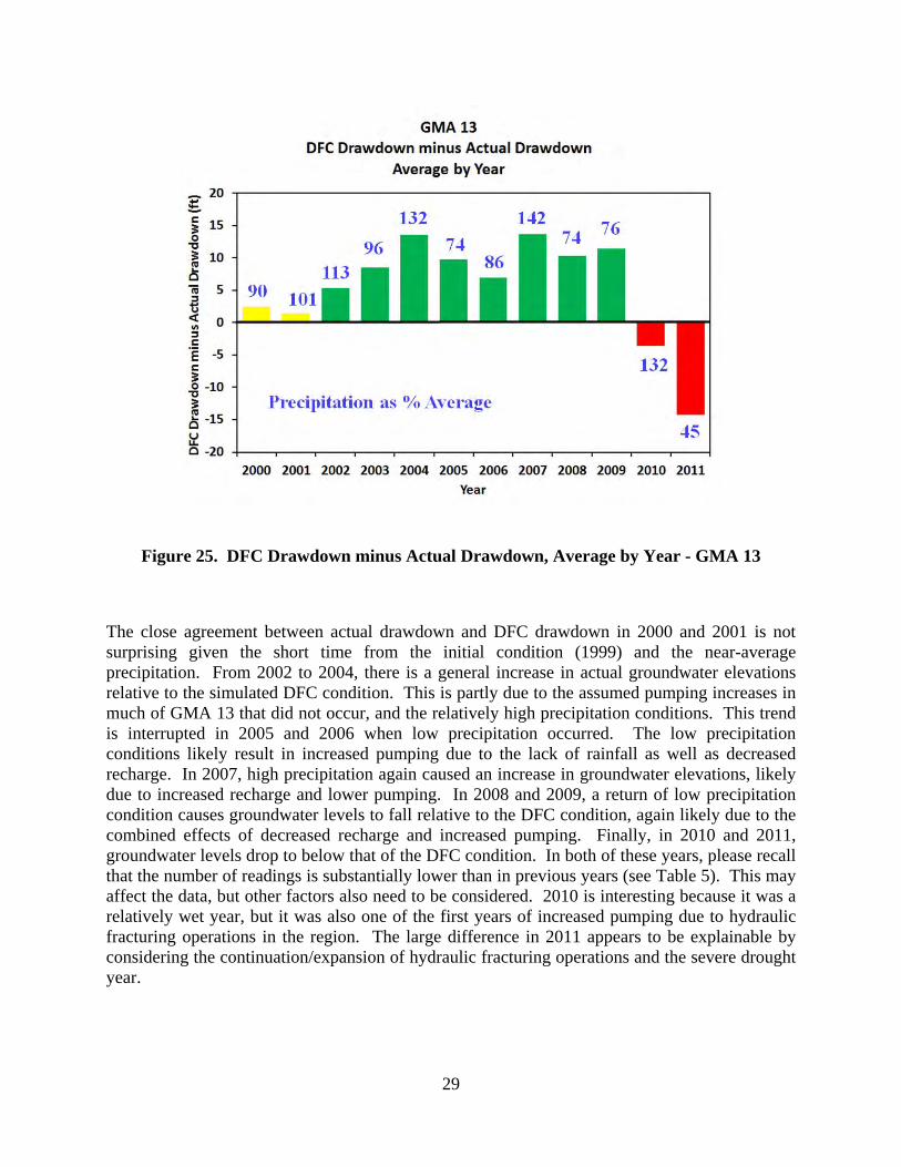
29
Figure 25. DFC Drawdown minus Actual Drawdown, Average by Year - GMA 13
The close agreement between actual drawdown and DFC drawdown in 2000 and 2001 is not surprising given the short time from the initial condition (1999) and the near-average precipitation. From 2002 to 2004, there is a general increase in actual groundwater elevations relative to the simulated DFC condition. This is partly due to the assumed pumping increases in much of GMA 13 that did not occur, and the relatively high precipitation conditions. This trend is interrupted in 2005 and 2006 when low precipitation occurred. The low precipitation conditions likely result in increased pumping due to the lack of rainfall as well as decreased recharge. In 2007, high precipitation again caused an increase in groundwater elevations, likely due to increased recharge and lower pumping. In 2008 and 2009, a return of low precipitation condition causes groundwater levels to fall relative to the DFC condition, again likely due to the combined effects of decreased recharge and increased pumping. Finally, in 2010 and 2011, groundwater levels drop to below that of the DFC condition. In both of these years, please recall that the number of readings is substantially lower than in previous years (see Table 5). This may affect the data, but other factors also need to be considered. 2010 is interesting because it was a relatively wet year, but it was also one of the first years of increased pumping due to hydraulic fracturing operations in the region. The large difference in 2011 appears to be explainable by considering the continuation/expansion of hydraulic fracturing operations and the severe drought year.
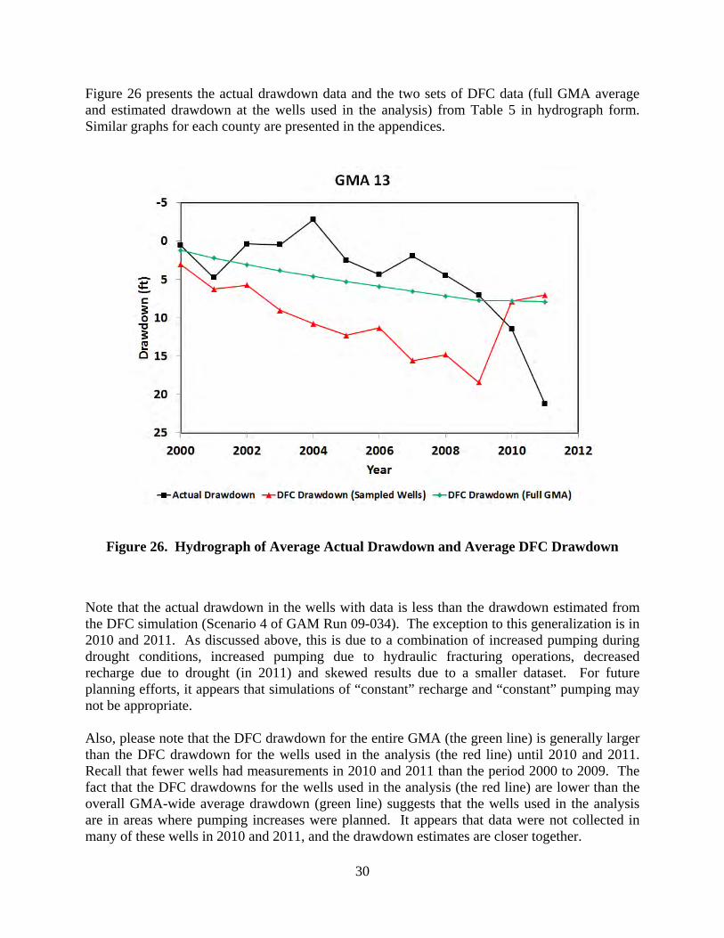
30
Figure 26 presents the actual drawdown data and the two sets of DFC data (full GMA average and estimated drawdown at the wells used in the analysis) from Table 5 in hydrograph form. Similar graphs for each county are presented in the appendices.
Figure 26. Hydrograph of Average Actual Drawdown and Average DFC Drawdown
Note that the actual drawdown in the wells with data is less than the drawdown estimated from the DFC simulation (Scenario 4 of GAM Run 09-034). The exception to this generalization is in 2010 and 2011. As discussed above, this is due to a combination of increased pumping during drought conditions, increased pumping due to hydraulic fracturing operations, decreased recharge due to drought (in 2011) and skewed results due to a smaller dataset. For future planning efforts, it appears that simulations of “constant” recharge and “constant” pumping may not be appropriate. Also, please note that the DFC drawdown for the entire GMA (the green line) is generally larger than the DFC drawdown for the wells used in the analysis (the red line) until 2010 and 2011. Recall that fewer wells had measurements in 2010 and 2011 than the period 2000 to 2009. The fact that the DFC drawdowns for the wells used in the analysis (the red line) are lower than the overall GMA-wide average drawdown (green line) suggests that the wells used in the analysis are in areas where pumping increases were planned. It appears that data were not collected in many of these wells in 2010 and 2011, and the drawdown estimates are closer together.

31
4.0 County‐LevelDataSuitableforuseinManagementPlanUpdates One of the objectives of this effort was to develop data and information useful for the districts in their updates to groundwater management plans. One of the required elements of those plans is to address desired future conditions. The main body of the report focused on GMA-level analyses with various tables, maps and graphs. Pertinent tables, maps and graphs were also developed for each county in GMA 13 for which suitable well data were available. These data are presented in the appendices (one for each county). In general, the appendices contain:
A map of the location of wells used in the hydrograph analysis The hydrographs of all wells that met the criteria previously described, A table analogous to Table 5 in the text summarizing annual average drawdown (actual
and DFC)
A figure analogous to Figure 23 in text showing differences between actual drawdown and DFC conditions
A figure analogous to Figure 26 in text showing time history of drawdown (actual and DFC) from 2000 to 2011
32
5.0 RecommendationsforCurrentRoundofJointPlanning This effort was authorized by the groundwater conservation districts of GMA 13 as the initial step of the current round of joint planning. The establishment of the initial desired future conditions for the Carrizo-Wilcox, Queen City and Sparta aquifers relied heavily on simulations using the groundwater availability model of the area. Comparisons of these model results with actual data provide a foundation for future discussions related to the current round of joint planning. The major areas for discussion include:
Improvement in 2000 to 2011 pumping estimates Timing of future pumping increases and decreases Evaluate the “average” recharge assumption for the entire DFC simulation Evaluate the assumption that future pumping does not vary between wet years and
droughts Review model assumptions and implementation for recharge and stream flow Assess county-to-county impacts more explicitly The use of actual well data as part of the statement of desired future conditions
In reviewing the results of the comparisons between groundwater elevations and pumping in general, and between actual groundwater elevations and groundwater elevations estimated through the joint planning process, it is evident that the future pumping assumptions used in Scenario 4 of GAM Run 09-034 from 2000 to 2011 need updating for the current round of joint planning. Projected increases and decreases are envisioned and the timing of those changes needs to be better incorporated into the planning process. The comparison analysis also yielded interesting observations regarding the variation in groundwater elevations from wet years to dry years. Sharp declines in dry years appear to be the result of the combined effect of decreased recharge and increased pumping during drought periods. Scenario 4 of GAM Run 09-034 included an assumption that recharge was constant and “average” each year of the 61 year simulation. Also, there was no assumption of pumping variation as a result of dry years. For a long-term planning process, this may be the most cost-effective means of simulating future conditions. However, it is a point that should be discussed in the context of how much detail the desired future condition statement will contain. In reviewing the results of the analysis, there were a few examples where the model results identified some county-to-county impacts of pumping changes that seemed to be consistent with the conceptual model and others that may have been a result of model implementation. These should to be investigated further as part of the joint planning process to assure that the model simulations of the desired future condition are rational and defendable. A discussion that needs to occur is how actual well data could be incorporated into the desired future condition statement and the role of the model in the process. It needs to be recognized that a model run, while not an absolute requirement, is certainly going to be made by the TWDB in the development of the Modeled Available Groundwater. Therefore, the groundwater conservation districts should realize that the GAM will continue to be an important aspect of the process. By linking the model run results to the desired future condition statement, however, the

33
issues of whether to describe the DFC as a single GMA-wide average or as county-averaged DFCs, or as county-layer averaged DFCs is somewhat irrelevant since all describe the same set of assumptions that are explicitly and implicitly tied to the DFC. The decision on how to express the DFC statement in terms of averaging and the decision to include or not include actual data will be policy decisions by the groundwater conservation districts of GMA 13. The data and results in this analysis will assist the districts in those decisions.

34
Appendix1–GMA13DrawdownMapsforAllYears This appendix presents GMA-wide maps of the point-by-point year-by-year drawdown analysis. These maps provide a GMA-wide perspective of the drawdown comparison. Each well on these maps is color coded to show the difference between actual drawdown and the estimated drawdown at that point in that year.
A difference of greater than 3 feet (actual groundwater elevation is 3 feet or more higher than the DFC simulation elevation) is shown in green
Differences of between -3 and 3 feet are shown in yellow (actual groundwater elevation and DFC simulation elevation is within 3 feet)
Differences less than -3 feet are shown in red (actual groundwater elevation is 3 feet or lower than the DFC simulation elevation).
Detailed maps for each county using the same color coding for 2001, 2006 and 2011 (with well numbers) are presented in the appropriate county appendix.

35

36

37

38

39

40
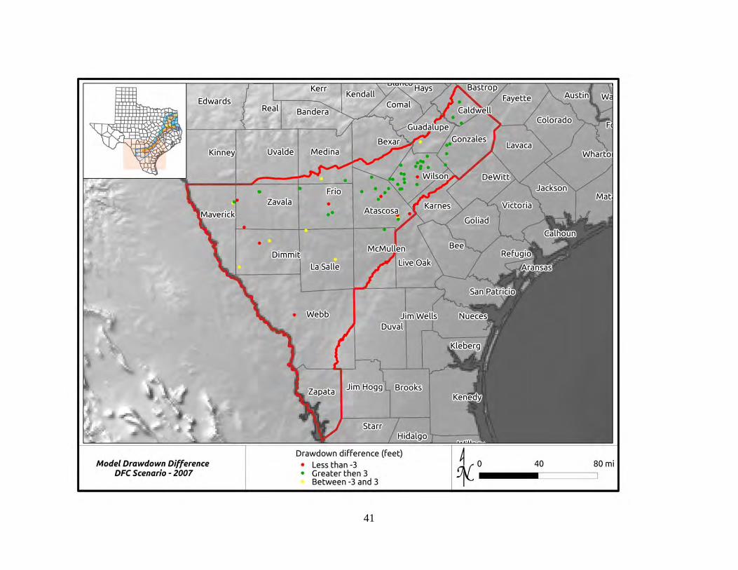
41

42
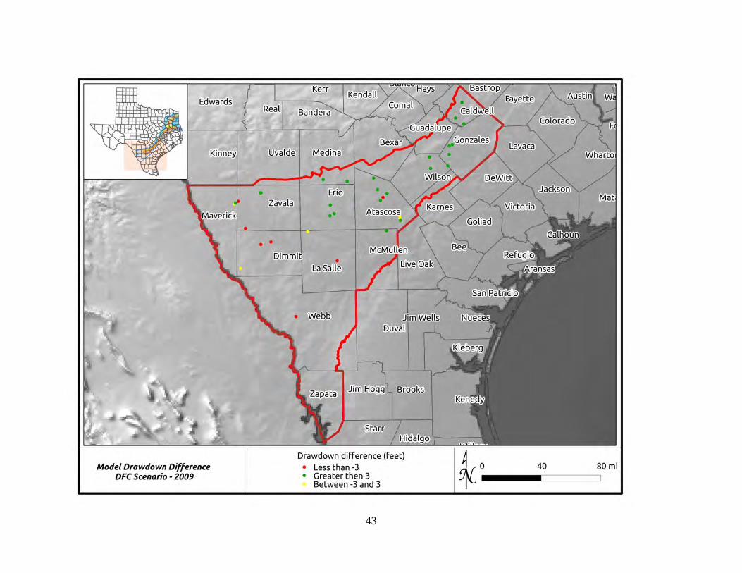
43

44

45

46
Appendix2–AtascosaCounty
Location Map of Hydrograph Wells
Hydrographs
Note that pumping data are expressed in three zones:
Pump 1 = pumping from cell where well is located
Pump 2 = pumping in cells adjacent to Zone 1
Pump 3 = pumping in cells adjacent to Zone 2
Screen Bottom and Screen Top = Elevation of Well Completion Interval
Land Surface = Elevation of Land Surface at Well
Groundwater Elevations
Measured = Actual data from TWDB database
Calibrated Model = Results for cell defined by well from calibrated model
DFC = Results for cell defined by well from Scenario 4 of GAM Run 09-034
Drawdown Comparison Maps for 2001 and 2006
Summary of Drawdown Comparisons
Table analogous to Table 5 in text summarizing annual average drawdown (actual and DFC)
Histogram of Differences between DFC Drawdown and Actual Drawdown for All Years
Figure analogous to Figure 23 in text showing differences between actual drawdown and DFC conditions
Hydrograph of Actual Drawdown and DFC Drawdown
Figure analogous to Figure 26 in text showing time history of drawdown (actual and DFC) from 2000 to 2011
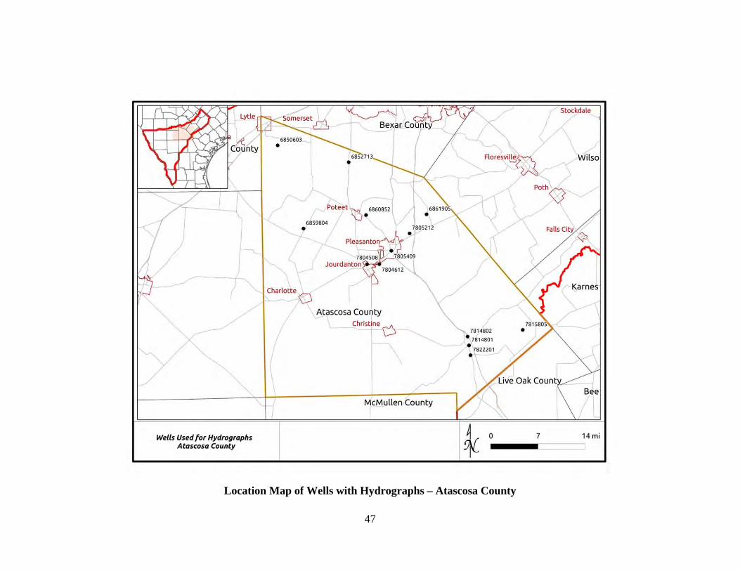
47
Location Map of Wells with Hydrographs – Atascosa County
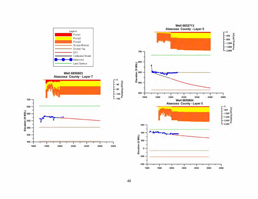
48
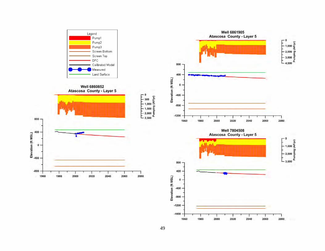
49
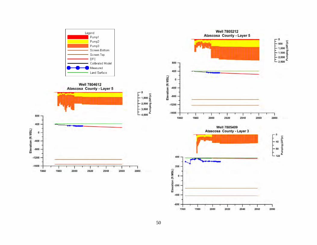
50
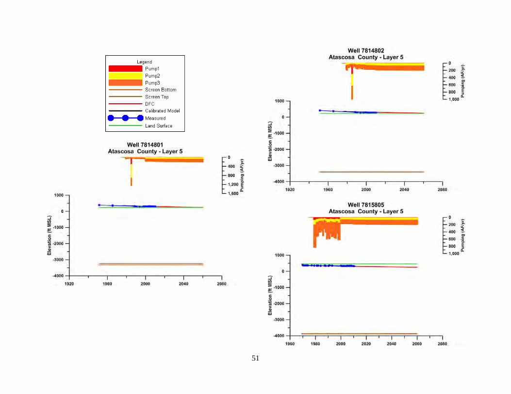
51
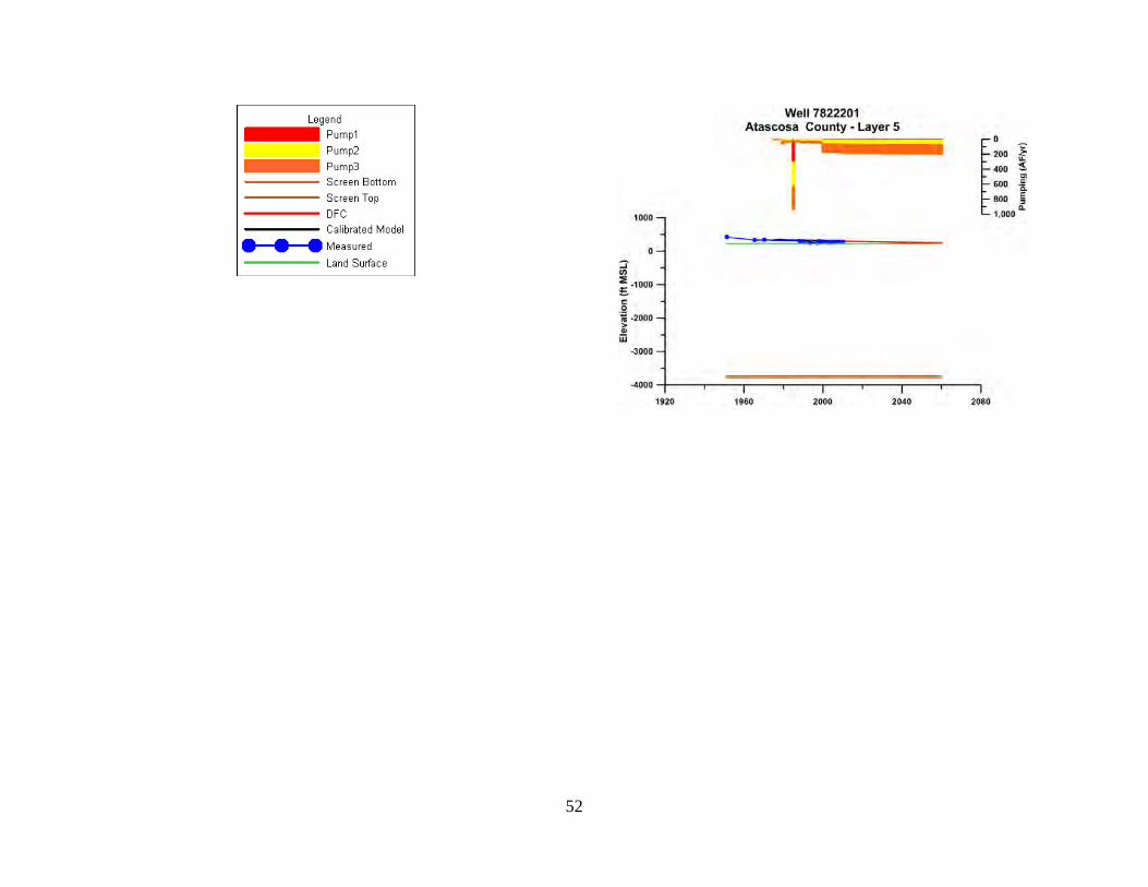
52
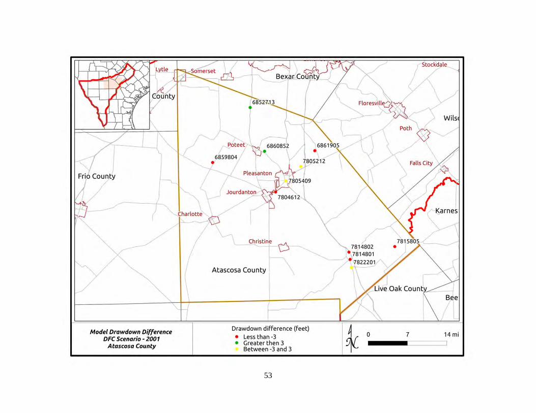
53
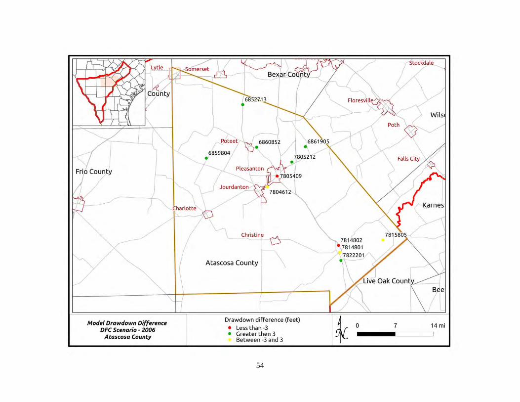
54
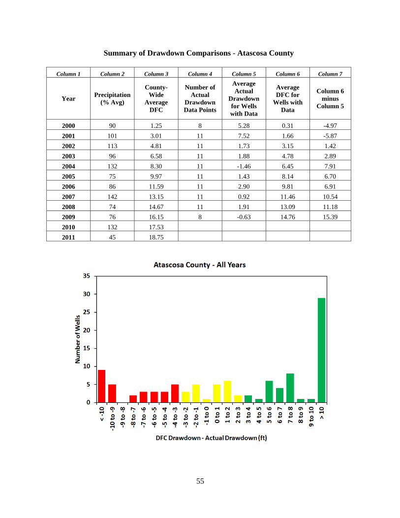
55
Summary of Drawdown Comparisons - Atascosa County
Column 1 Column 2 Column 3 Column 4 Column 5 Column 6 Column 7
Year Precipitation
(% Avg)
County-Wide
Average DFC
Number of Actual
Drawdown Data Points
Average Actual
Drawdown for Wells with Data
Average DFC for
Wells with Data
Column 6 minus
Column 5
2000 90 1.25 8 5.28 0.31 -4.97
2001 101 3.01 11 7.52 1.66 -5.87
2002 113 4.81 11 1.73 3.15 1.42
2003 96 6.58 11 1.88 4.78 2.89
2004 132 8.30 11 -1.46 6.45 7.91
2005 75 9.97 11 1.43 8.14 6.70
2006 86 11.59 11 2.90 9.81 6.91
2007 142 13.15 11 0.92 11.46 10.54
2008 74 14.67 11 1.91 13.09 11.18
2009 76 16.15 8 -0.63 14.76 15.39
2010 132 17.53
2011 45 18.75
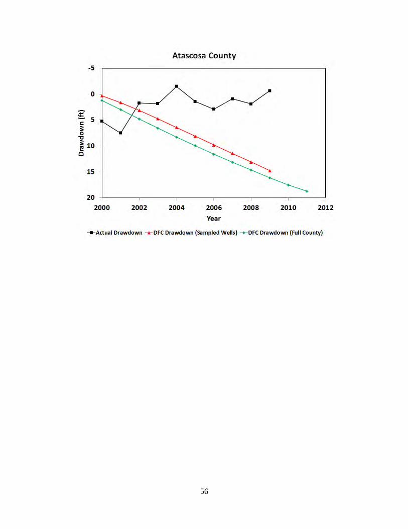
56
57
Appendix3–BexarCounty
Location Map of Hydrograph Wells
Hydrographs
Note that pumping data are expressed in three zones:
Pump 1 = pumping from cell where well is located
Pump 2 = pumping in cells adjacent to Zone 1
Pump 3 = pumping in cells adjacent to Zone 2
Screen Bottom and Screen Top = Elevation of Well Completion Interval
Land Surface = Elevation of Land Surface at Well
Groundwater Elevations
Measured = Actual data from TWDB database
Calibrated Model = Results for cell defined by well from calibrated model
DFC = Results for cell defined by well from Scenario 4 of GAM Run 09-034
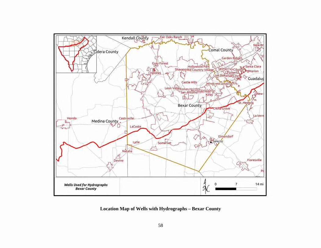
58
Location Map of Wells with Hydrographs – Bexar County
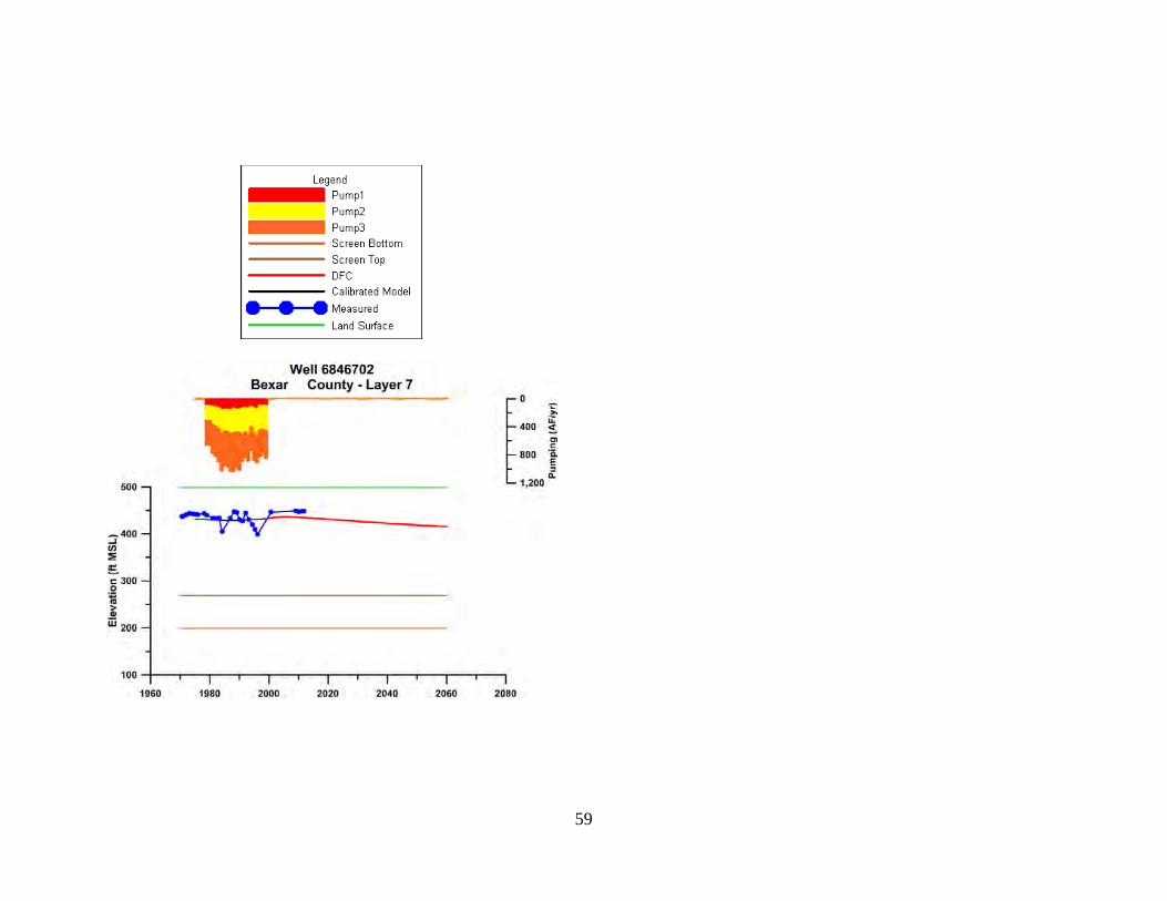
59
60
Appendix4–CaldwellCounty Location Map of Hydrograph Wells
Hydrographs
Note that pumping data are expressed in three zones:
Pump 1 = pumping from cell where well is located
Pump 2 = pumping in cells adjacent to Zone 1
Pump 3 = pumping in cells adjacent to Zone 2
Screen Bottom and Screen Top = Elevation of Well Completion Interval
Land Surface = Elevation of Land Surface at Well
Groundwater Elevations
Measured = Actual data from TWDB database
Calibrated Model = Results for cell defined by well from calibrated model
DFC = Results for cell defined by well from Scenario 4 of GAM Run 09-034
Drawdown Comparison Maps for 2001, 2006 and 2011
Summary of Drawdown Comparisons
Table analogous to Table 5 in text summarizing annual average drawdown (actual and DFC)
Histogram of Differences between DFC Drawdown and Actual Drawdown for All Years
Figure analogous to Figure 23 in text showing differences between actual drawdown and DFC conditions
Hydrograph of Actual Drawdown and DFC Drawdown
Figure analogous to Figure 26 in text showing time history of drawdown (actual and DFC) from 2000 to 2011
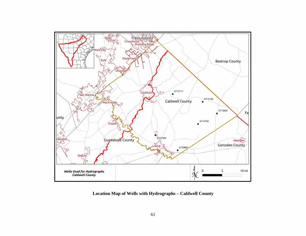
61
Location Map of Wells with Hydrographs – Caldwell County
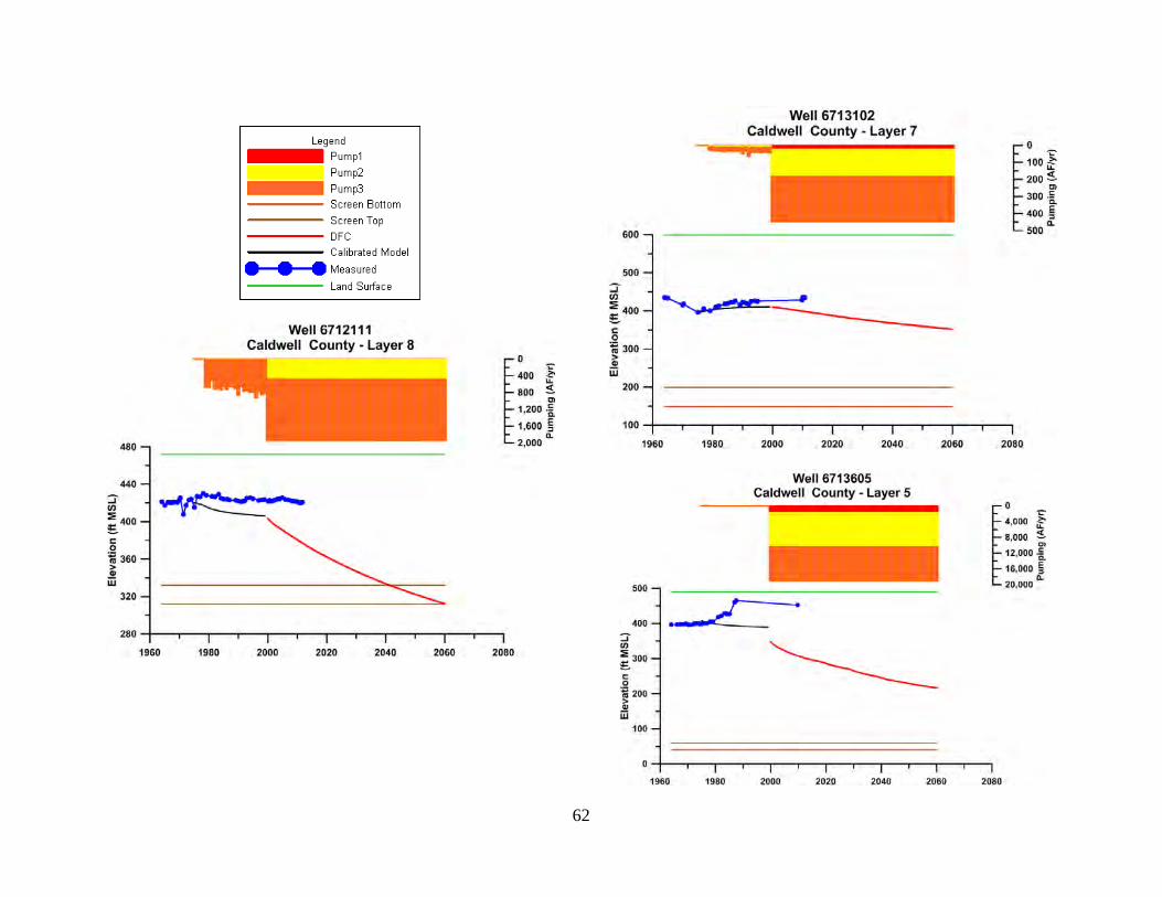
62
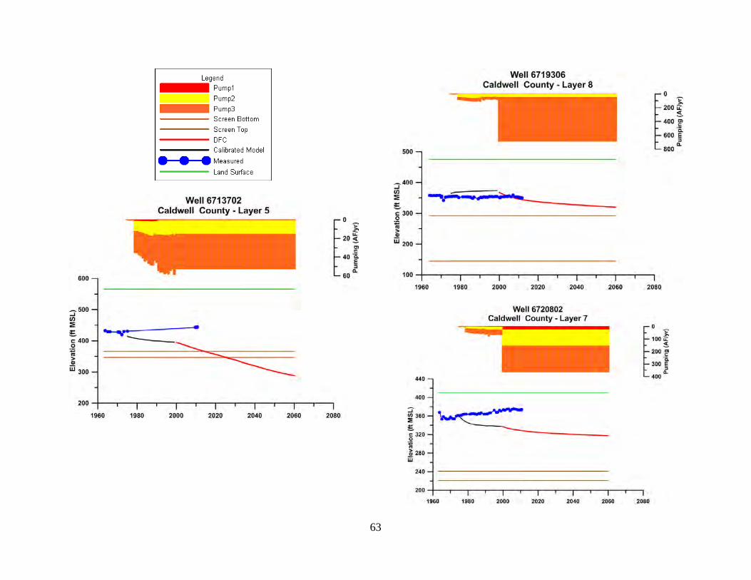
63
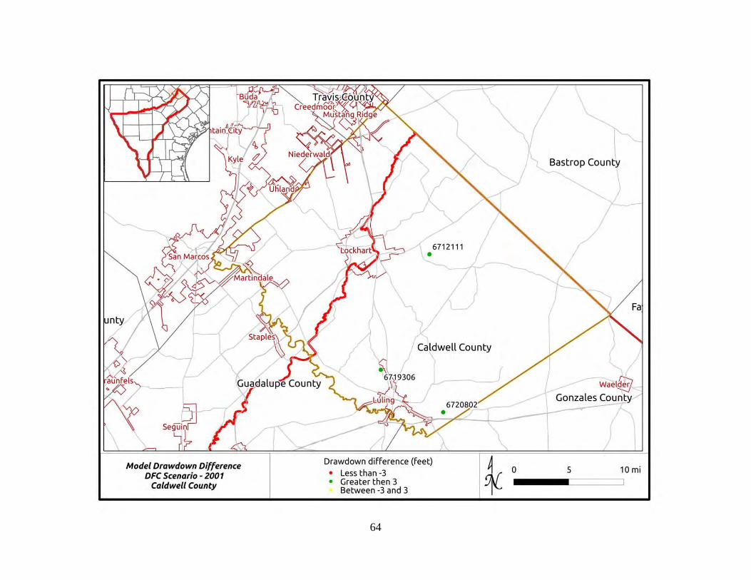
64

65
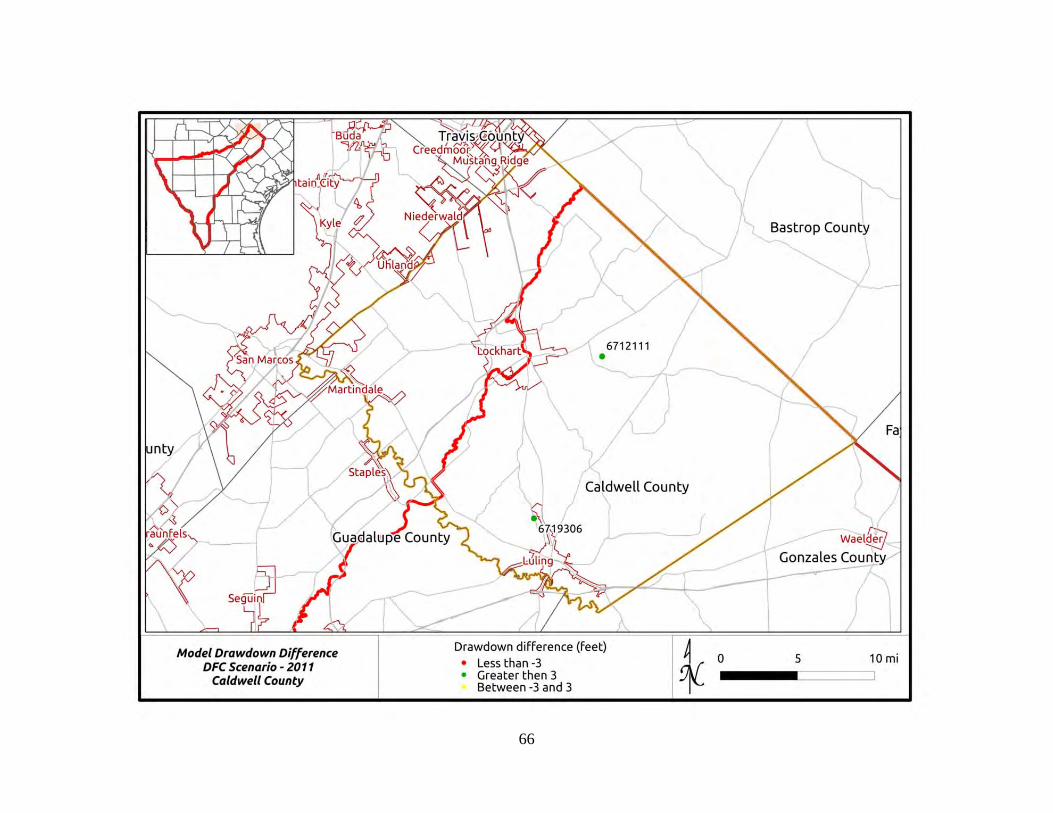
66
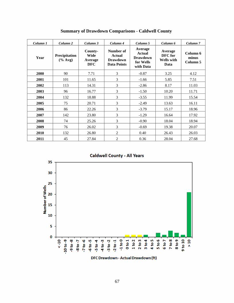
67
Summary of Drawdown Comparisons - Caldwell County
Column 1 Column 2 Column 3 Column 4 Column 5 Column 6 Column 7
Year Precipitation
(% Avg)
County-Wide
Average DFC
Number of Actual
Drawdown Data Points
Average Actual
Drawdown for Wells with Data
Average DFC for
Wells with Data
Column 6 minus
Column 5
2000 90 7.71 3 -0.87 3.25 4.12
2001 101 11.65 3 -1.66 5.85 7.51
2002 113 14.31 3 -2.86 8.17 11.03
2003 96 16.77 3 -1.50 10.20 11.71
2004 132 18.88 3 -3.55 11.99 15.54
2005 75 20.71 3 -2.49 13.63 16.11
2006 86 22.26 3 -3.79 15.17 18.96
2007 142 23.80 3 -1.29 16.64 17.92
2008 74 25.26 3 -0.90 18.04 18.94
2009 76 26.02 3 -0.69 19.38 20.07
2010 132 26.80 2 0.40 26.43 26.03
2011 45 27.84 2 0.36 28.04 27.68
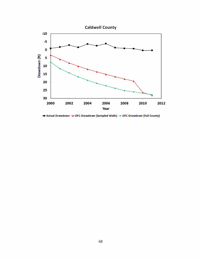
68

69
Appendix5–DimmitCounty Location Map of Hydrograph Wells
Hydrographs
Note that pumping data are expressed in three zones:
Pump 1 = pumping from cell where well is located
Pump 2 = pumping in cells adjacent to Zone 1
Pump 3 = pumping in cells adjacent to Zone 2
Screen Bottom and Screen Top = Elevation of Well Completion Interval
Land Surface = Elevation of Land Surface at Well
Groundwater Elevations
Measured = Actual data from TWDB database
Calibrated Model = Results for cell defined by well from calibrated model
DFC = Results for cell defined by well from Scenario 4 of GAM Run 09-034
Drawdown Comparison Maps for 2001, 2006 and 2011
Summary of Drawdown Comparisons
Table analogous to Table 5 in text summarizing annual average drawdown (actual and DFC)
Histogram of Differences between DFC Drawdown and Actual Drawdown for All Years
Figure analogous to Figure 23 in text showing differences between actual drawdown and DFC conditions
Hydrograph of Actual Drawdown and DFC Drawdown
Figure analogous to Figure 26 in text showing time history of drawdown (actual and DFC) from 2000 to 2011
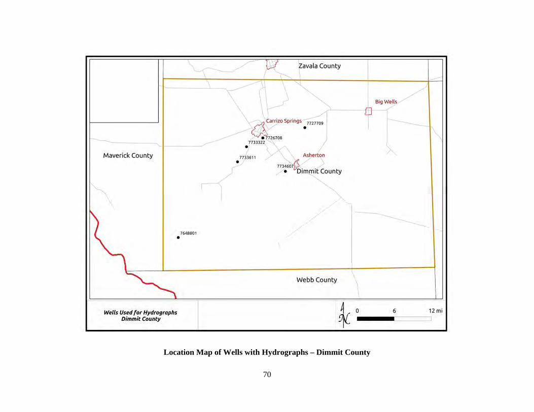
70
Location Map of Wells with Hydrographs – Dimmit County
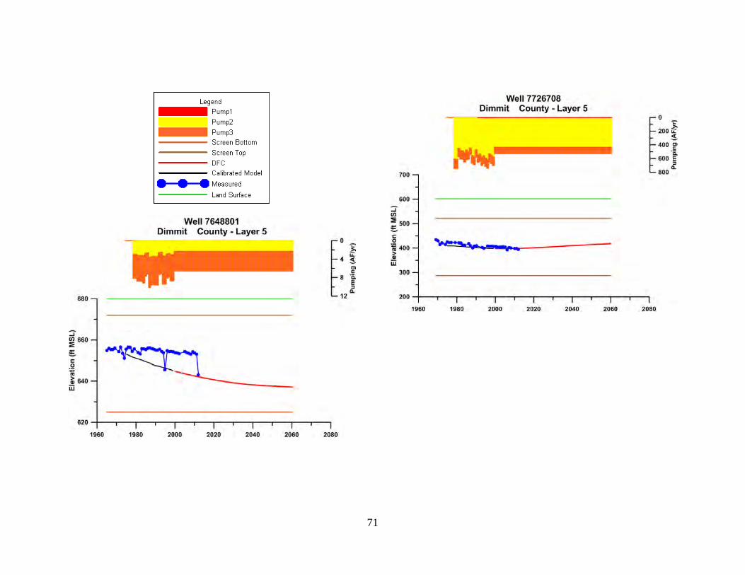
71
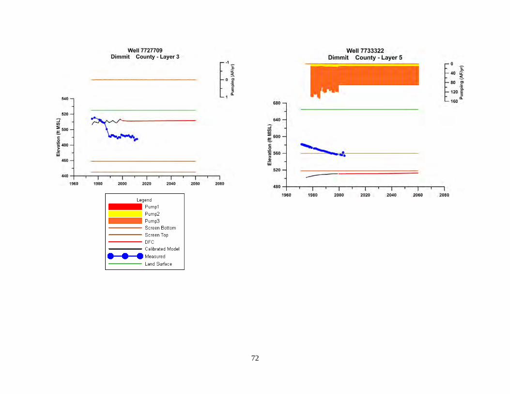
72
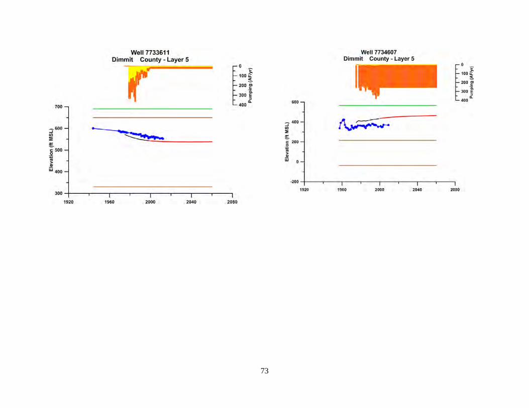
73
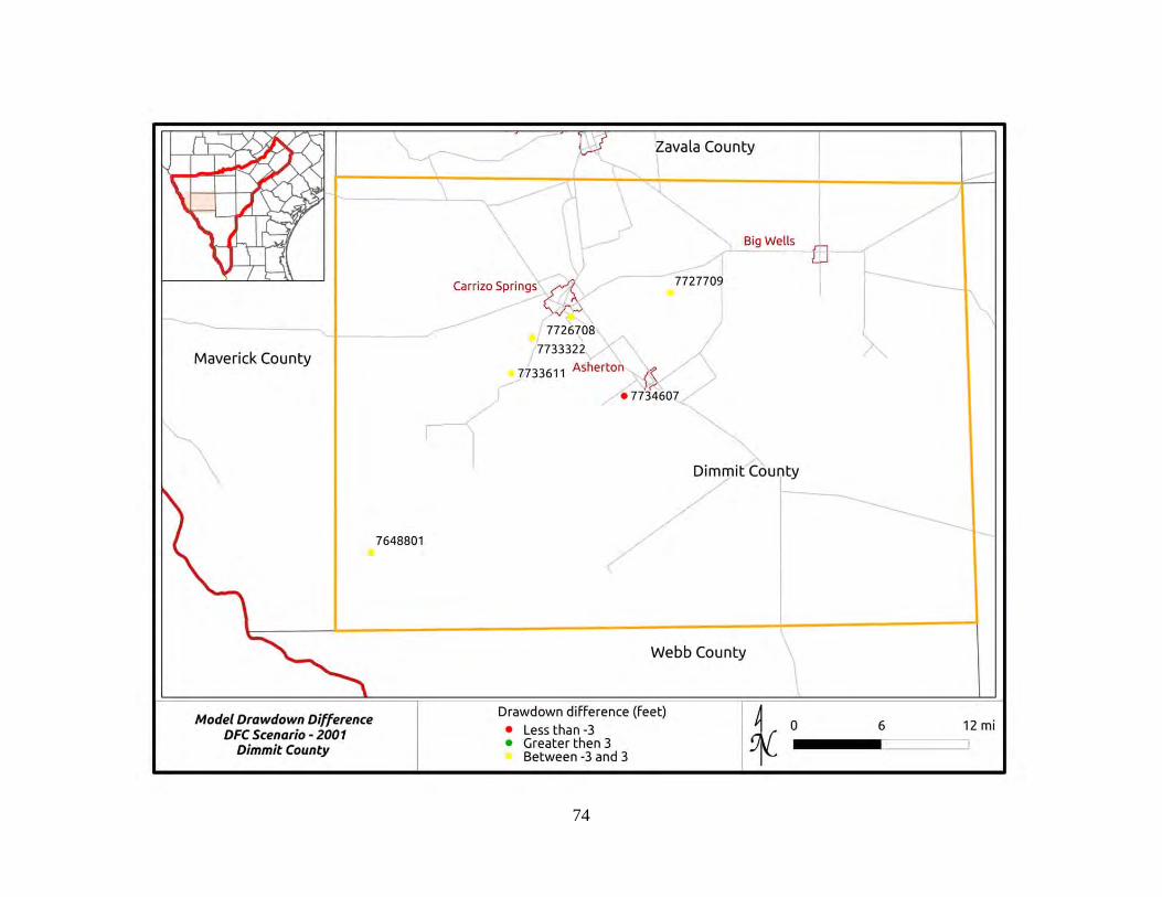
74
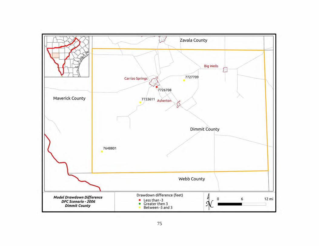
75
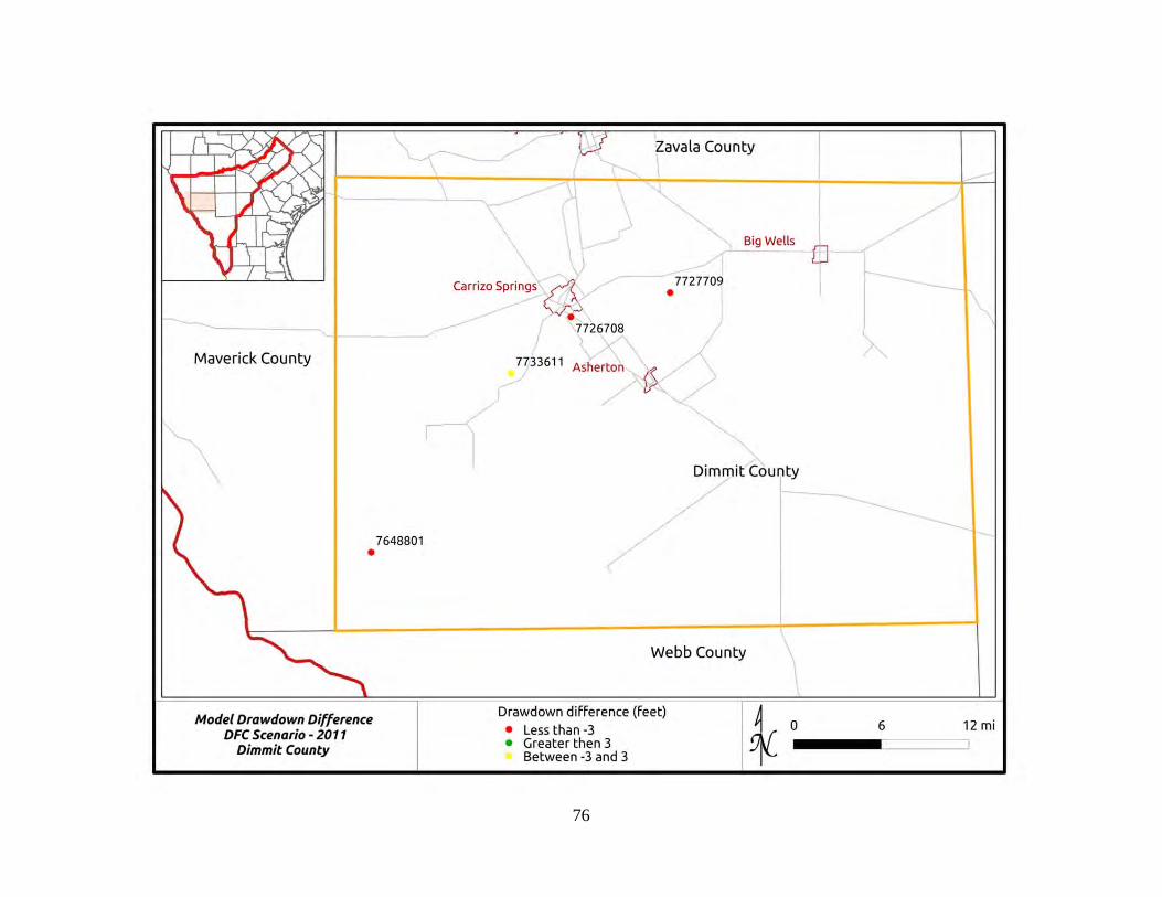
76
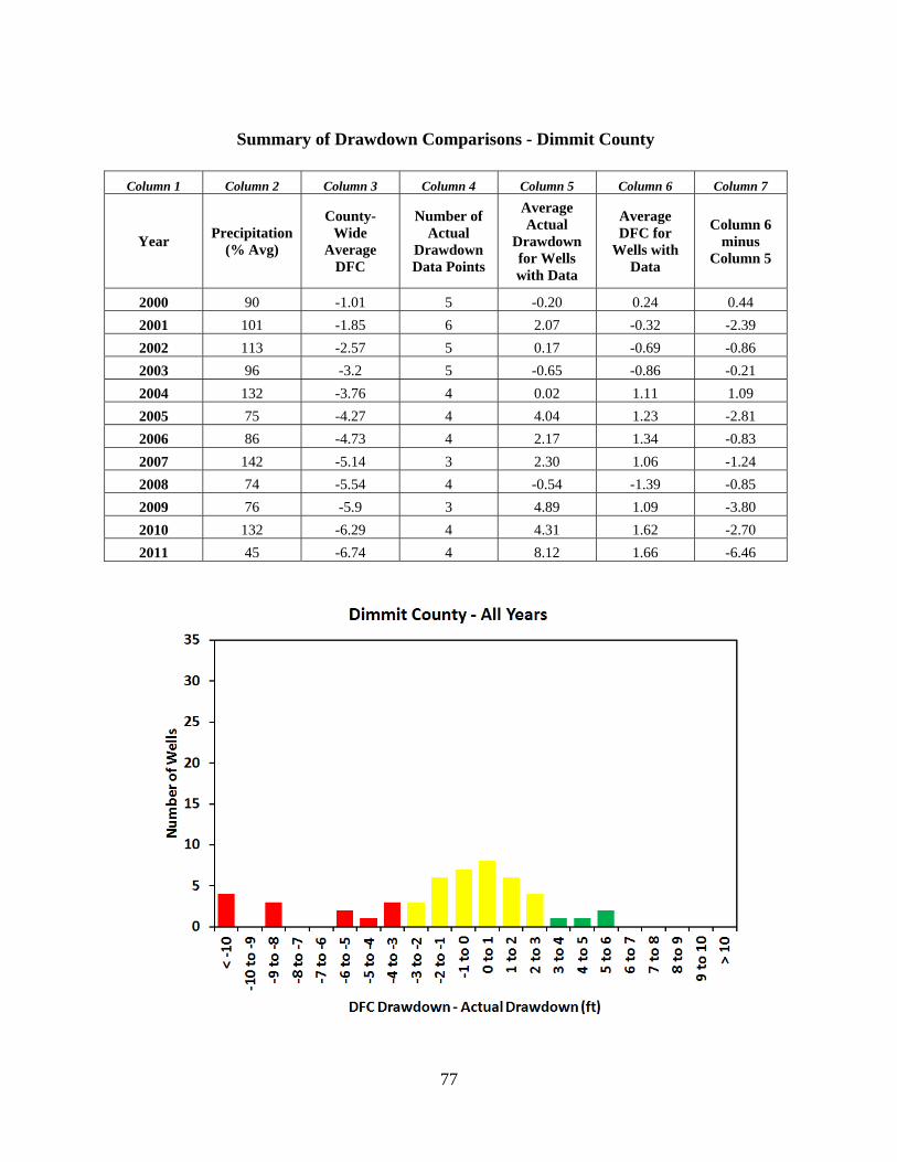
77
Summary of Drawdown Comparisons - Dimmit County
Column 1 Column 2 Column 3 Column 4 Column 5 Column 6 Column 7
Year Precipitation
(% Avg)
County-Wide
Average DFC
Number of Actual
Drawdown Data Points
Average Actual
Drawdown for Wells with Data
Average DFC for
Wells with Data
Column 6 minus
Column 5
2000 90 -1.01 5 -0.20 0.24 0.44
2001 101 -1.85 6 2.07 -0.32 -2.39
2002 113 -2.57 5 0.17 -0.69 -0.86
2003 96 -3.2 5 -0.65 -0.86 -0.21
2004 132 -3.76 4 0.02 1.11 1.09
2005 75 -4.27 4 4.04 1.23 -2.81
2006 86 -4.73 4 2.17 1.34 -0.83
2007 142 -5.14 3 2.30 1.06 -1.24
2008 74 -5.54 4 -0.54 -1.39 -0.85
2009 76 -5.9 3 4.89 1.09 -3.80
2010 132 -6.29 4 4.31 1.62 -2.70
2011 45 -6.74 4 8.12 1.66 -6.46
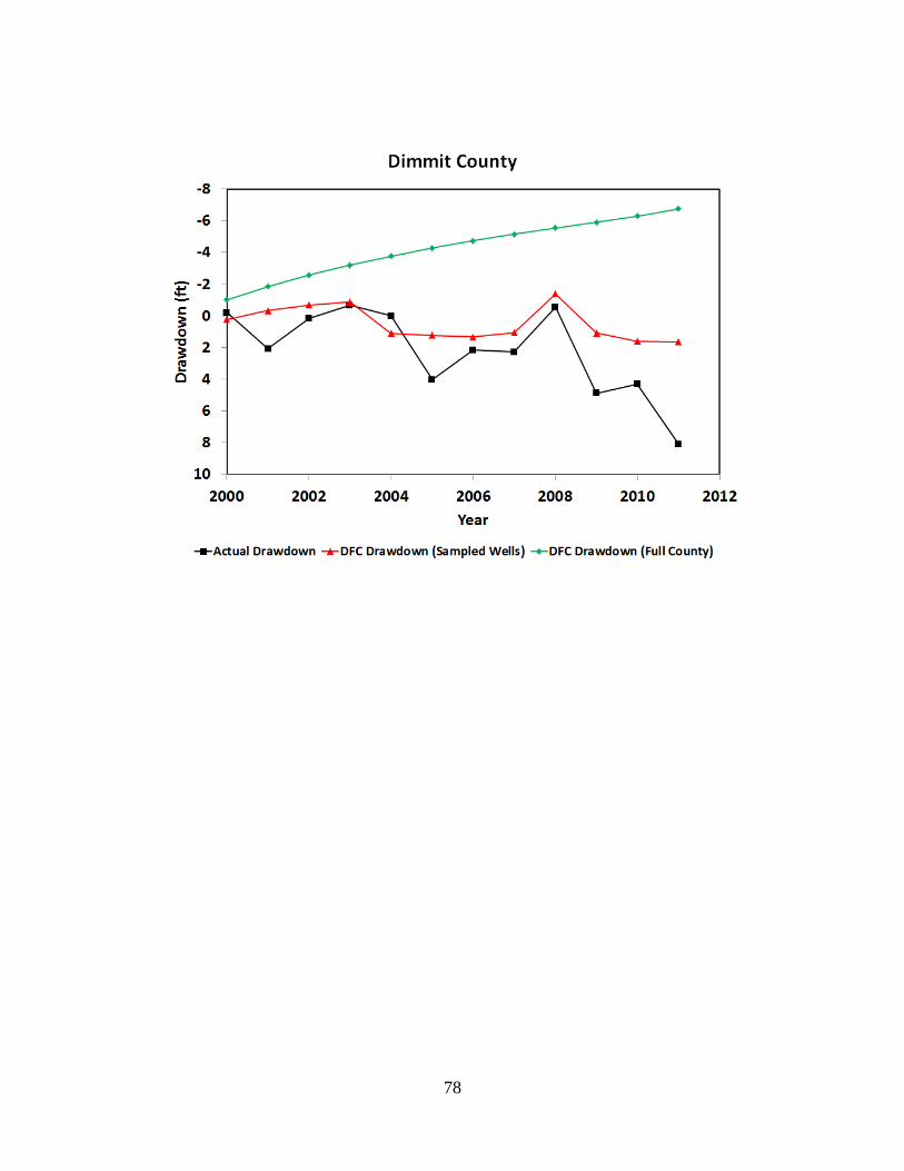
78
79
Appendix6–FrioCounty Location Map of Hydrograph Wells
Hydrographs
Note that pumping data are expressed in three zones:
Pump 1 = pumping from cell where well is located
Pump 2 = pumping in cells adjacent to Zone 1
Pump 3 = pumping in cells adjacent to Zone 2
Screen Bottom and Screen Top = Elevation of Well Completion Interval
Land Surface = Elevation of Land Surface at Well
Groundwater Elevations
Measured = Actual data from TWDB database
Calibrated Model = Results for cell defined by well from calibrated model
DFC = Results for cell defined by well from Scenario 4 of GAM Run 09-034
Drawdown Comparison Maps for 2001 and 2006
Summary of Drawdown Comparisons
Table analogous to Table 5 in text summarizing annual average drawdown (actual and DFC)
Histogram of Differences between DFC Drawdown and Actual Drawdown for All Years
Figure analogous to Figure 23 in text showing differences between actual drawdown and DFC conditions
Hydrograph of Actual Drawdown and DFC Drawdown
Figure analogous to Figure 26 in text showing time history of drawdown (actual and DFC) from 2000 to 2011
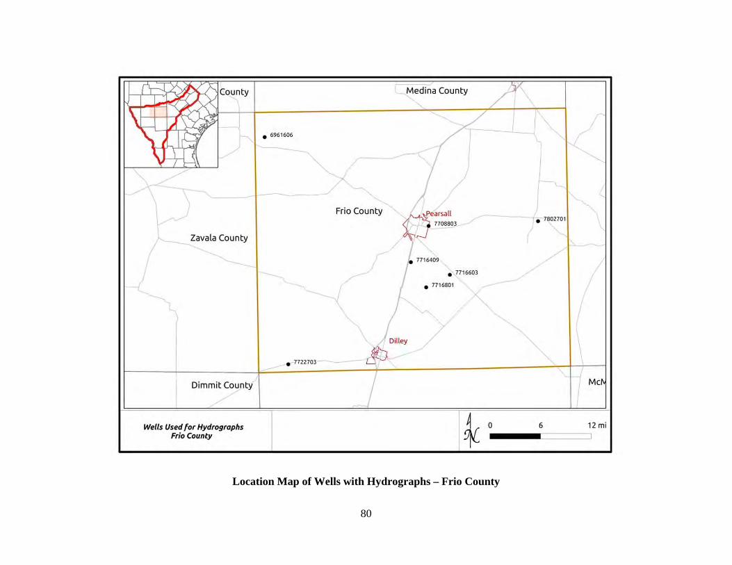
80
Location Map of Wells with Hydrographs – Frio County
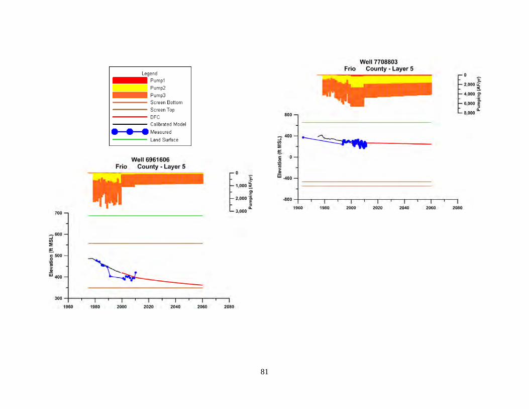
81
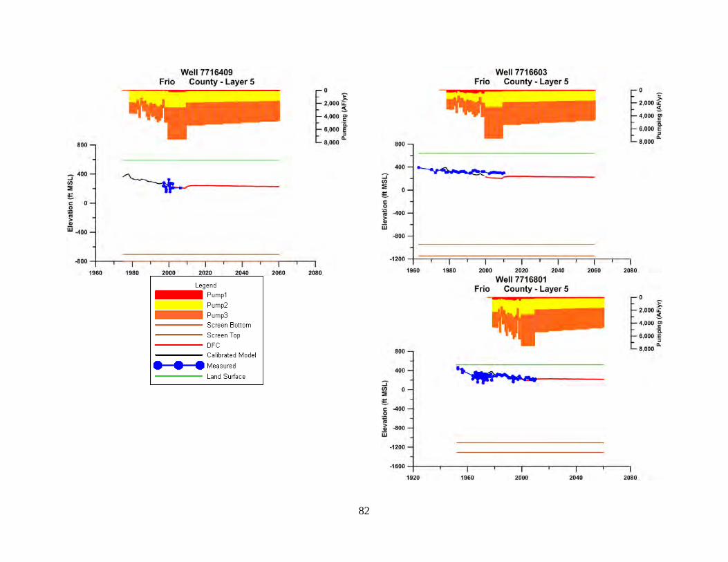
82
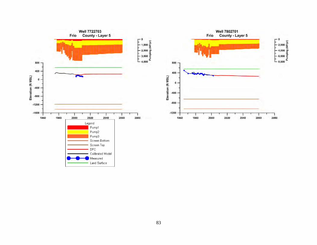
83
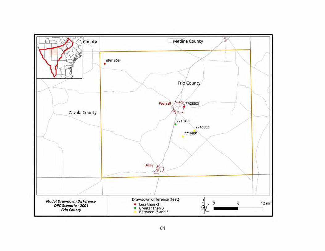
84
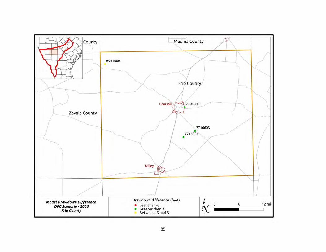
85
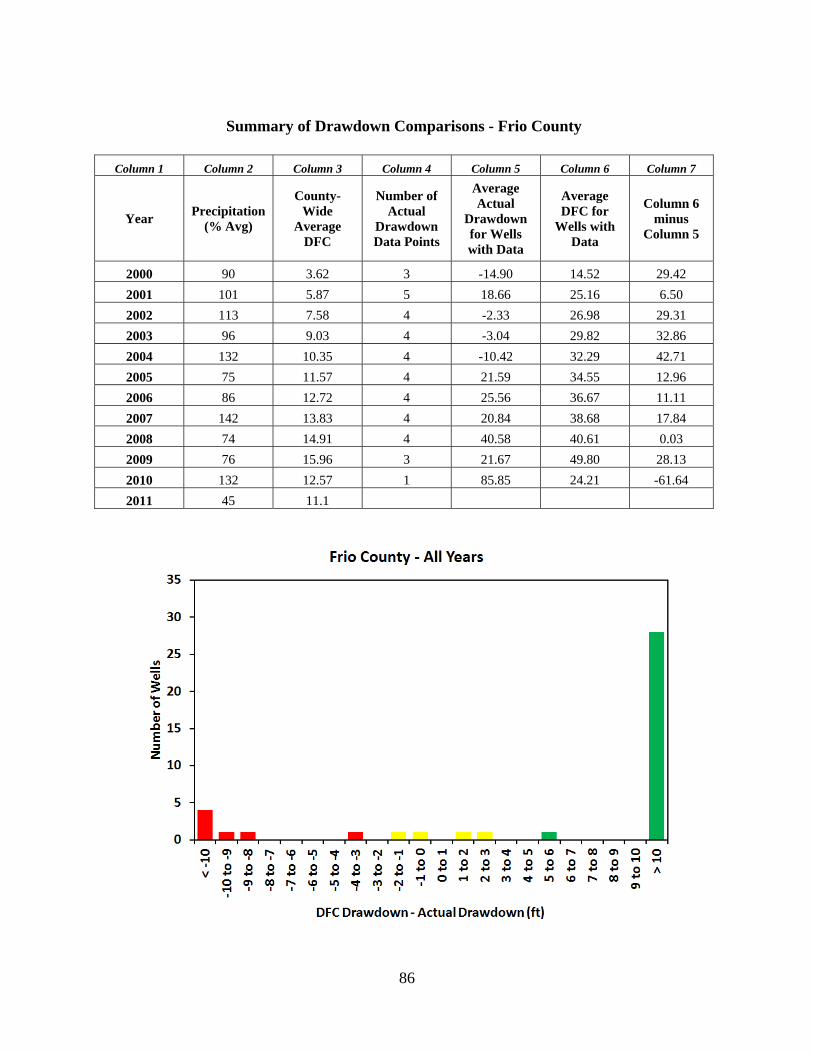
86
Summary of Drawdown Comparisons - Frio County
Column 1 Column 2 Column 3 Column 4 Column 5 Column 6 Column 7
Year Precipitation
(% Avg)
County-Wide
Average DFC
Number of Actual
Drawdown Data Points
Average Actual
Drawdown for Wells with Data
Average DFC for
Wells with Data
Column 6 minus
Column 5
2000 90 3.62 3 -14.90 14.52 29.42
2001 101 5.87 5 18.66 25.16 6.50
2002 113 7.58 4 -2.33 26.98 29.31
2003 96 9.03 4 -3.04 29.82 32.86
2004 132 10.35 4 -10.42 32.29 42.71
2005 75 11.57 4 21.59 34.55 12.96
2006 86 12.72 4 25.56 36.67 11.11
2007 142 13.83 4 20.84 38.68 17.84
2008 74 14.91 4 40.58 40.61 0.03
2009 76 15.96 3 21.67 49.80 28.13
2010 132 12.57 1 85.85 24.21 -61.64
2011 45 11.1
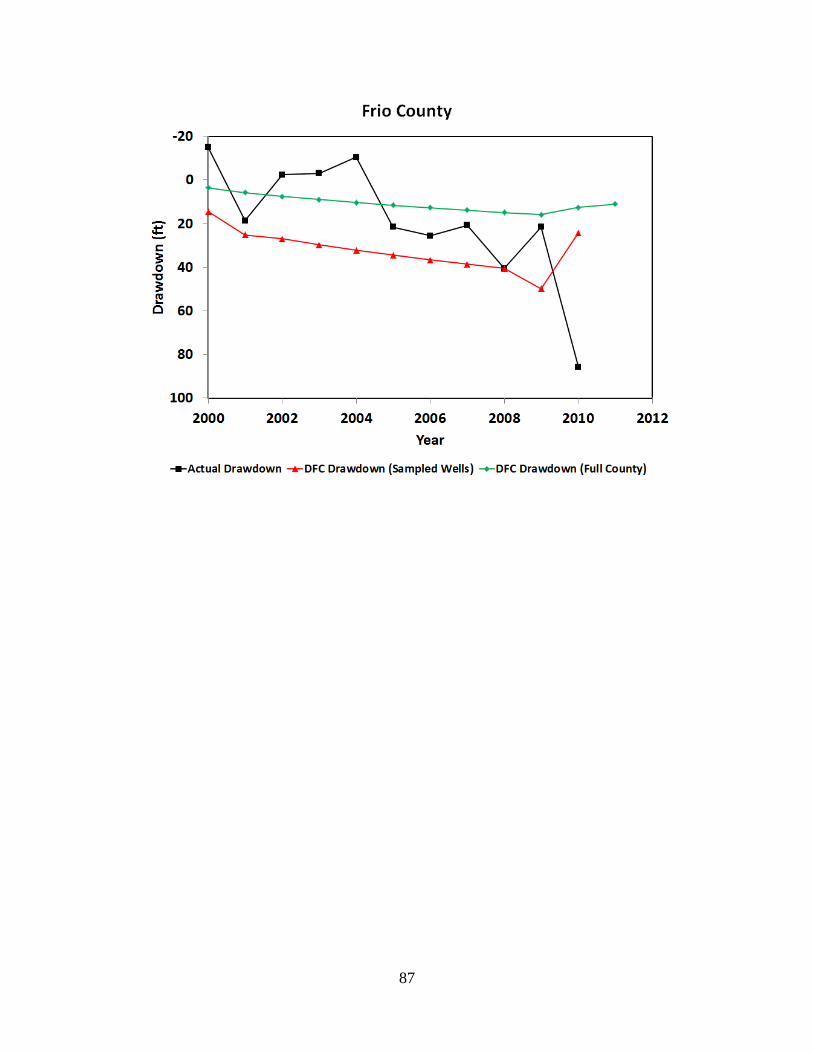
87
88
Appendix7–GonzalesCounty Location Map of Hydrograph Wells
Hydrographs
Note that pumping data are expressed in three zones:
Pump 1 = pumping from cell where well is located
Pump 2 = pumping in cells adjacent to Zone 1
Pump 3 = pumping in cells adjacent to Zone 2
Screen Bottom and Screen Top = Elevation of Well Completion Interval
Land Surface = Elevation of Land Surface at Well
Groundwater Elevations
Measured = Actual data from TWDB database
Calibrated Model = Results for cell defined by well from calibrated model
DFC = Results for cell defined by well from Scenario 4 of GAM Run 09-034
Drawdown Comparison Map for 2001
Summary of Drawdown Comparisons
Table analogous to Table 5 in text summarizing annual average drawdown (actual and DFC)
Histogram of Differences between DFC Drawdown and Actual Drawdown for All Years
Figure analogous to Figure 23 in text showing differences between actual drawdown and DFC conditions
Hydrograph of Actual Drawdown and DFC Drawdown
Figure analogous to Figure 26 in text showing time history of drawdown (actual and DFC) from 2000 to 2011
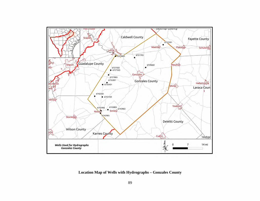
89
Location Map of Wells with Hydrographs – Gonzales County

90
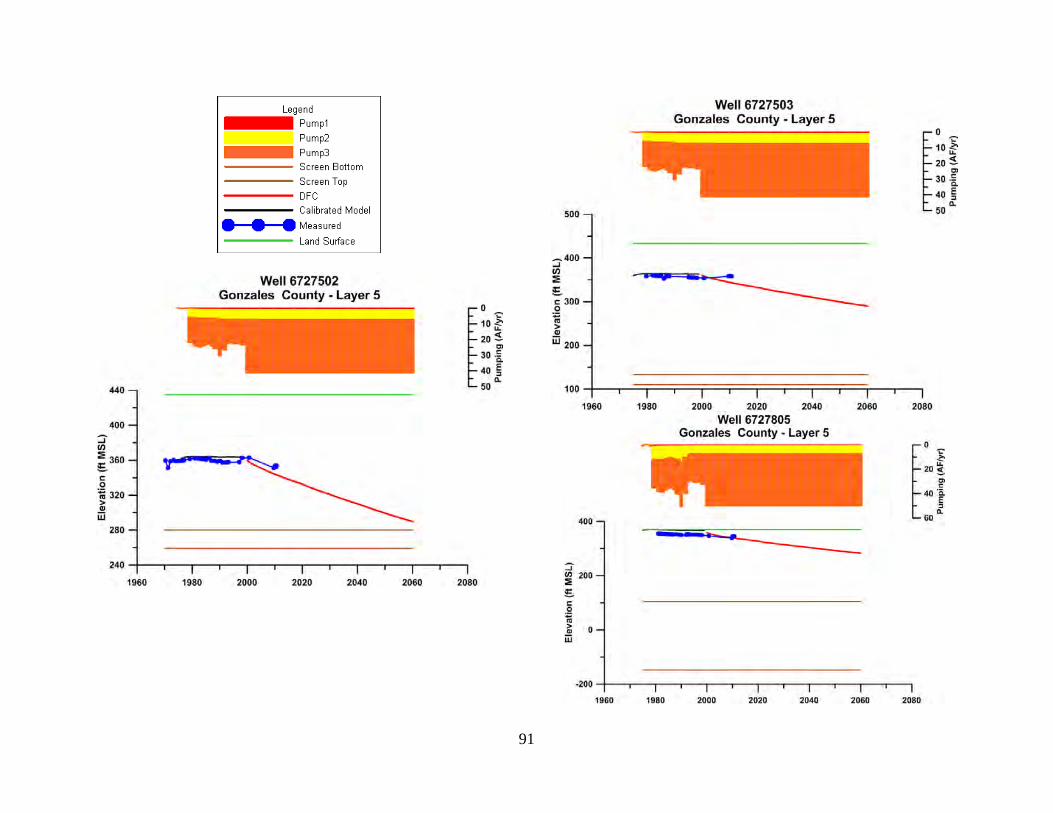
91
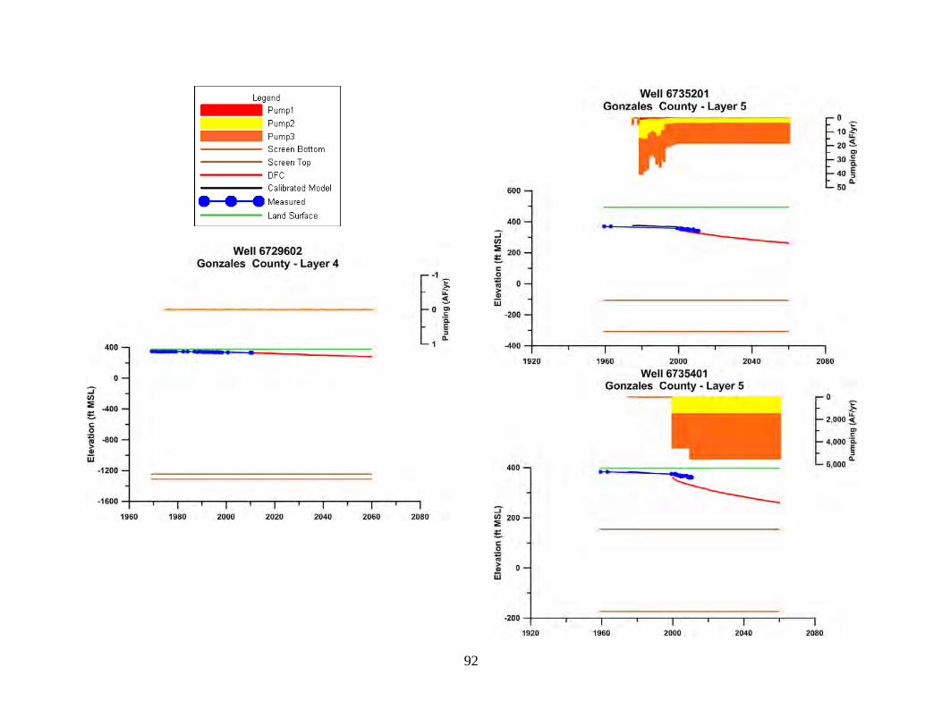
92
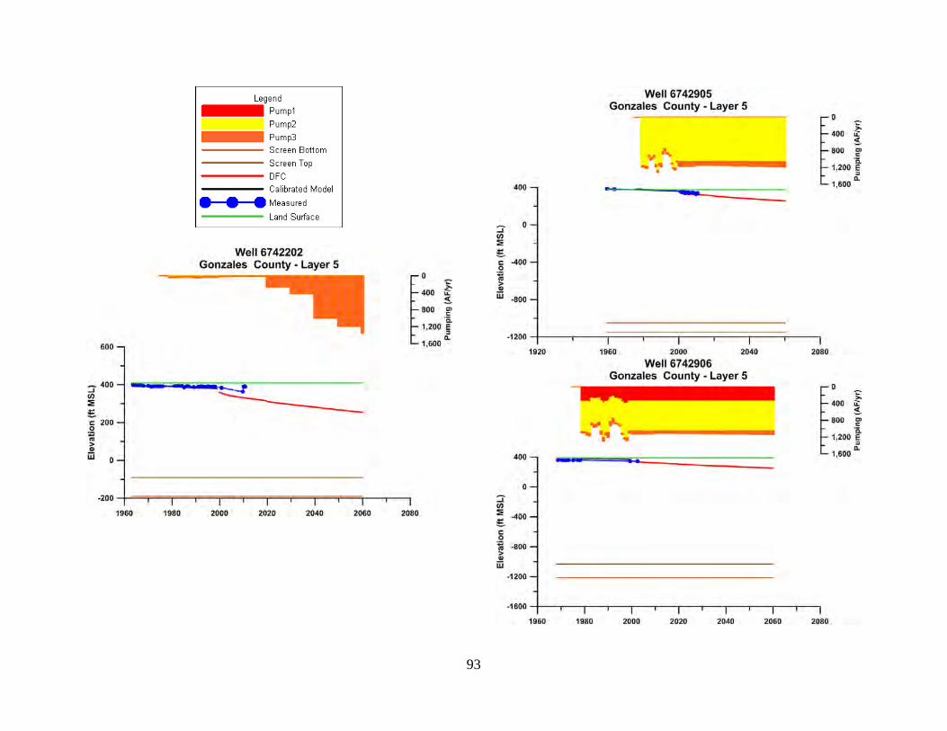
93
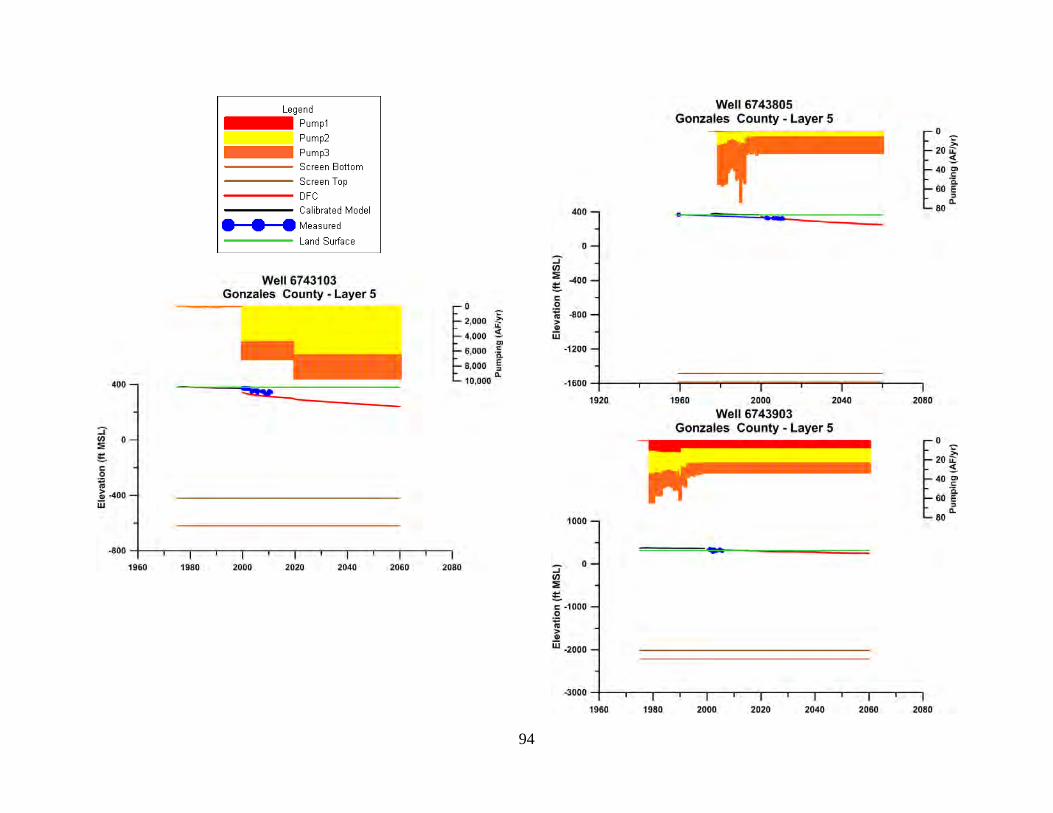
94
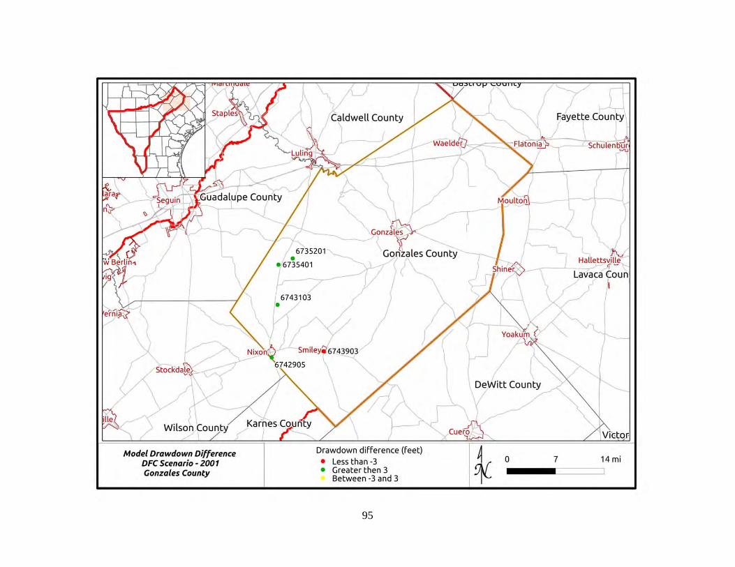
95
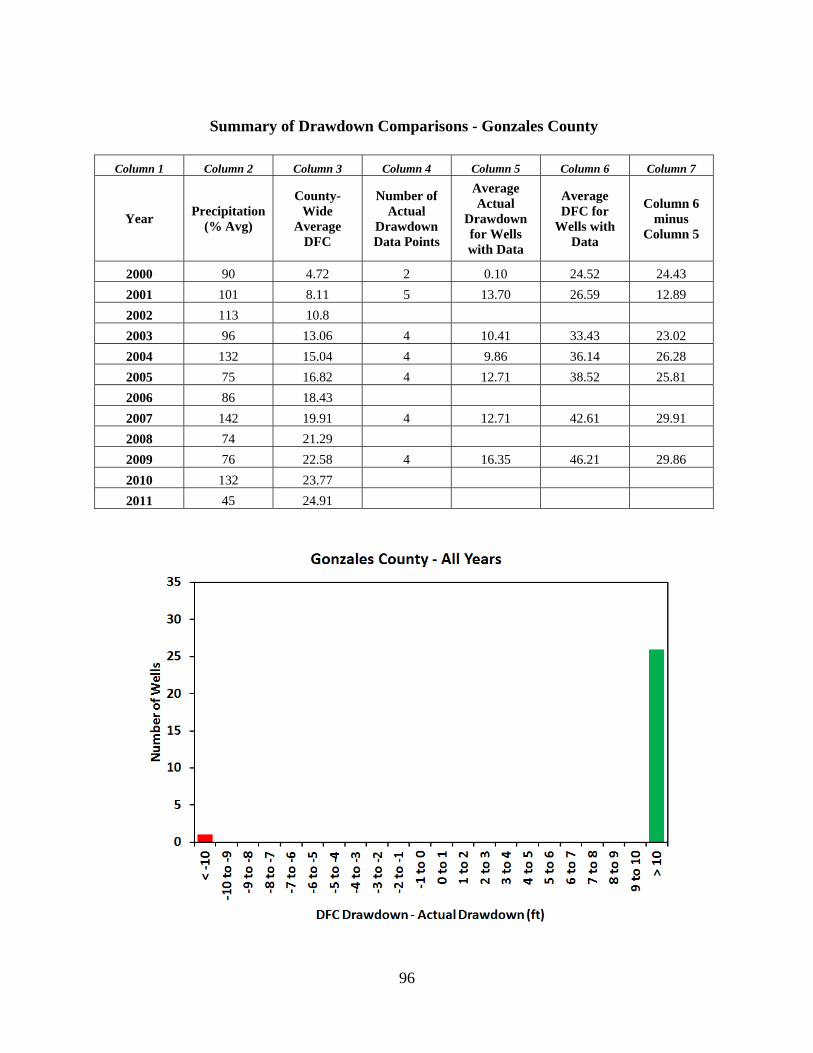
96
Summary of Drawdown Comparisons - Gonzales County
Column 1 Column 2 Column 3 Column 4 Column 5 Column 6 Column 7
Year Precipitation
(% Avg)
County-Wide
Average DFC
Number of Actual
Drawdown Data Points
Average Actual
Drawdown for Wells with Data
Average DFC for
Wells with Data
Column 6 minus
Column 5
2000 90 4.72 2 0.10 24.52 24.43
2001 101 8.11 5 13.70 26.59 12.89
2002 113 10.8
2003 96 13.06 4 10.41 33.43 23.02
2004 132 15.04 4 9.86 36.14 26.28
2005 75 16.82 4 12.71 38.52 25.81
2006 86 18.43
2007 142 19.91 4 12.71 42.61 29.91
2008 74 21.29
2009 76 22.58 4 16.35 46.21 29.86
2010 132 23.77
2011 45 24.91
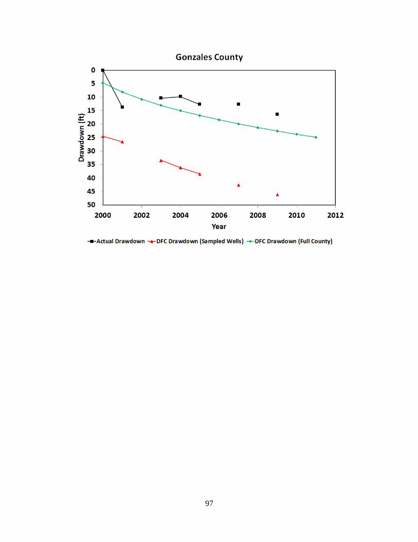
97
98
Appendix8–GuadalupeCounty Location Map of Hydrograph Wells
Hydrographs
Note that pumping data are expressed in three zones:
Pump 1 = pumping from cell where well is located
Pump 2 = pumping in cells adjacent to Zone 1
Pump 3 = pumping in cells adjacent to Zone 2
Screen Bottom and Screen Top = Elevation of Well Completion Interval
Land Surface = Elevation of Land Surface at Well
Groundwater Elevations
Measured = Actual data from TWDB database
Calibrated Model = Results for cell defined by well from calibrated model
DFC = Results for cell defined by well from Scenario 4 of GAM Run 09-034
Drawdown Comparison Maps for 2001, 2006 and 2011
Summary of Drawdown Comparisons
Table analogous to Table 5 in text summarizing annual average drawdown (actual and DFC)
Histogram of Differences between DFC Drawdown and Actual Drawdown for All Years
Figure analogous to Figure 23 in text showing differences between actual drawdown and DFC conditions
Hydrograph of Actual Drawdown and DFC Drawdown
Figure analogous to Figure 26 in text showing time history of drawdown (actual and DFC) from 2000 to 2011
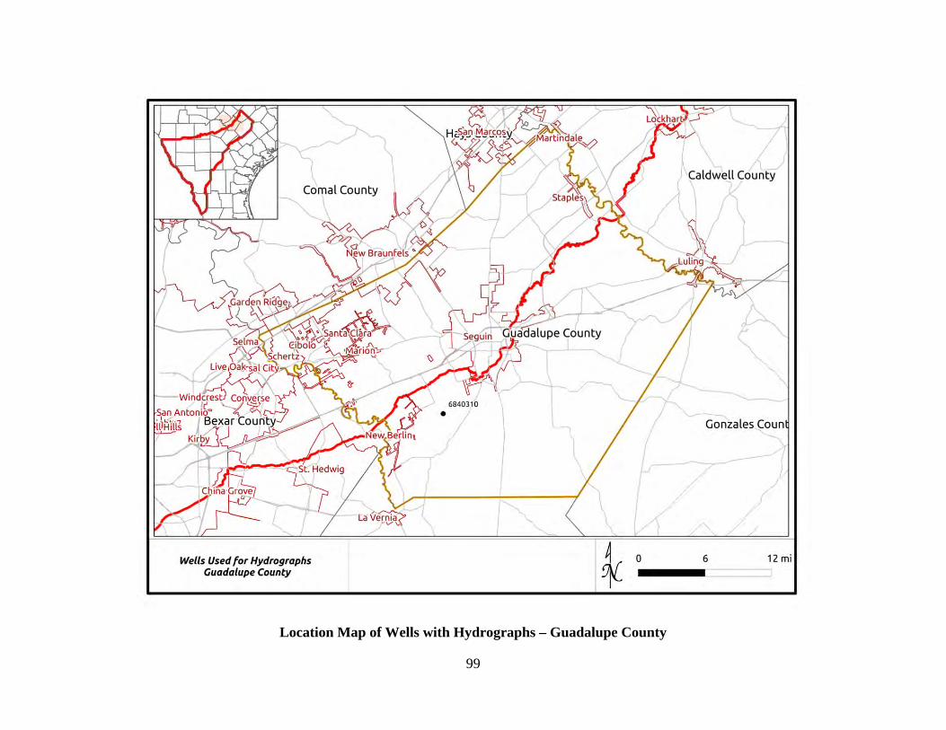
99
Location Map of Wells with Hydrographs – Guadalupe County
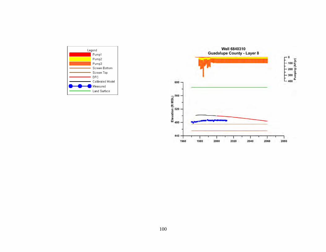
100
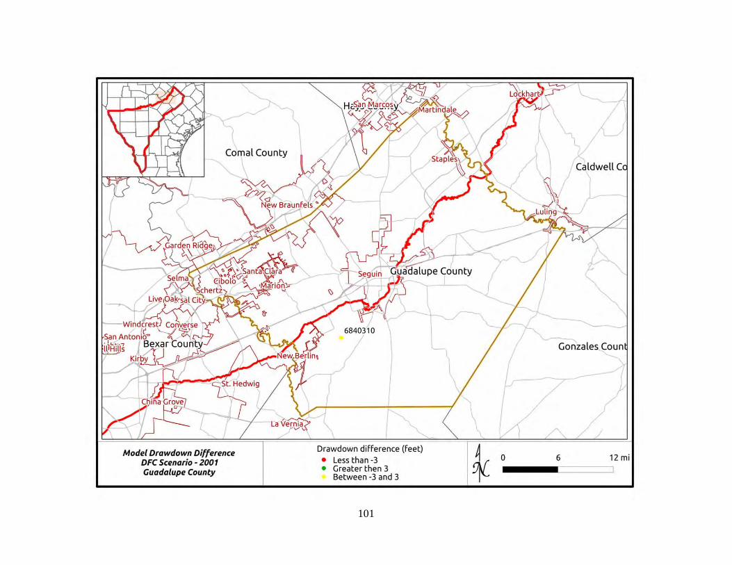
101
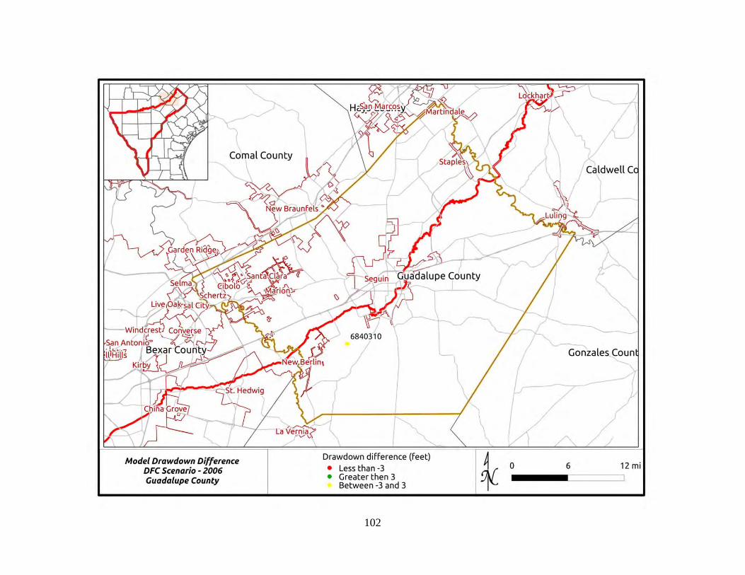
102

103
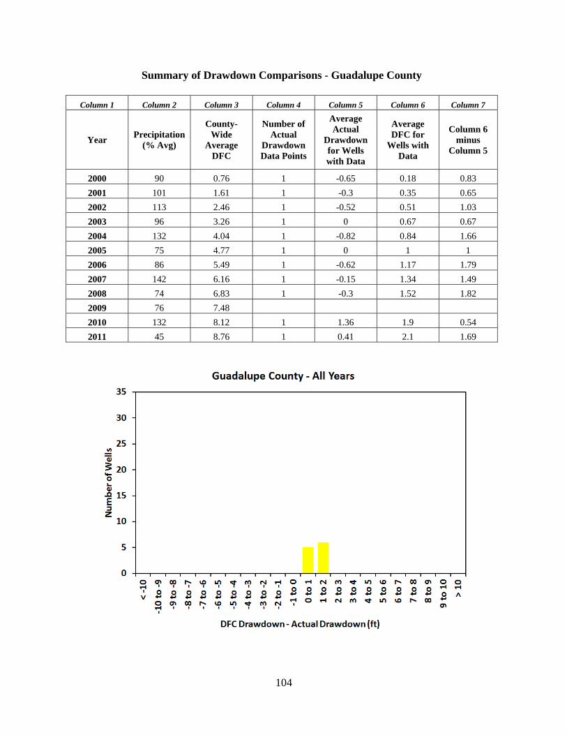
104
Summary of Drawdown Comparisons - Guadalupe County
Column 1 Column 2 Column 3 Column 4 Column 5 Column 6 Column 7
Year Precipitation
(% Avg)
County-Wide
Average DFC
Number of Actual
Drawdown Data Points
Average Actual
Drawdown for Wells with Data
Average DFC for
Wells with Data
Column 6 minus
Column 5
2000 90 0.76 1 -0.65 0.18 0.83
2001 101 1.61 1 -0.3 0.35 0.65
2002 113 2.46 1 -0.52 0.51 1.03
2003 96 3.26 1 0 0.67 0.67
2004 132 4.04 1 -0.82 0.84 1.66
2005 75 4.77 1 0 1 1
2006 86 5.49 1 -0.62 1.17 1.79
2007 142 6.16 1 -0.15 1.34 1.49
2008 74 6.83 1 -0.3 1.52 1.82
2009 76 7.48
2010 132 8.12 1 1.36 1.9 0.54
2011 45 8.76 1 0.41 2.1 1.69
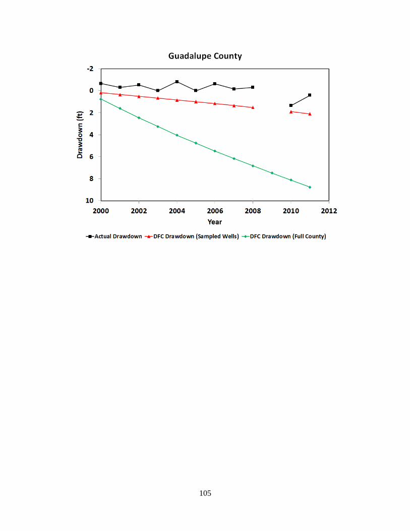
105
106
Appendix9–LaSalleCounty
Location Map of Hydrograph Wells
Hydrographs
Note that pumping data are expressed in three zones:
Pump 1 = pumping from cell where well is located
Pump 2 = pumping in cells adjacent to Zone 1
Pump 3 = pumping in cells adjacent to Zone 2
Screen Bottom and Screen Top = Elevation of Well Completion Interval
Land Surface = Elevation of Land Surface at Well
Groundwater Elevations
Measured = Actual data from TWDB database
Calibrated Model = Results for cell defined by well from calibrated model
DFC = Results for cell defined by well from Scenario 4 of GAM Run 09-034
Drawdown Comparison Maps for 2001, 2006 and 2011
Summary of Drawdown Comparisons
Table analogous to Table 5 in text summarizing annual average drawdown (actual and DFC)
Histogram of Differences between DFC Drawdown and Actual Drawdown for All Years
Figure analogous to Figure 23 in text showing differences between actual drawdown and DFC conditions
Hydrograph of Actual Drawdown and DFC Drawdown
Figure analogous to Figure 26 in text showing time history of drawdown (actual and DFC) from 2000 to 2011
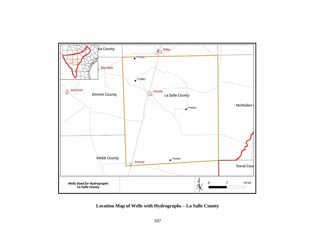
107
Location Map of Wells with Hydrographs – La Salle County
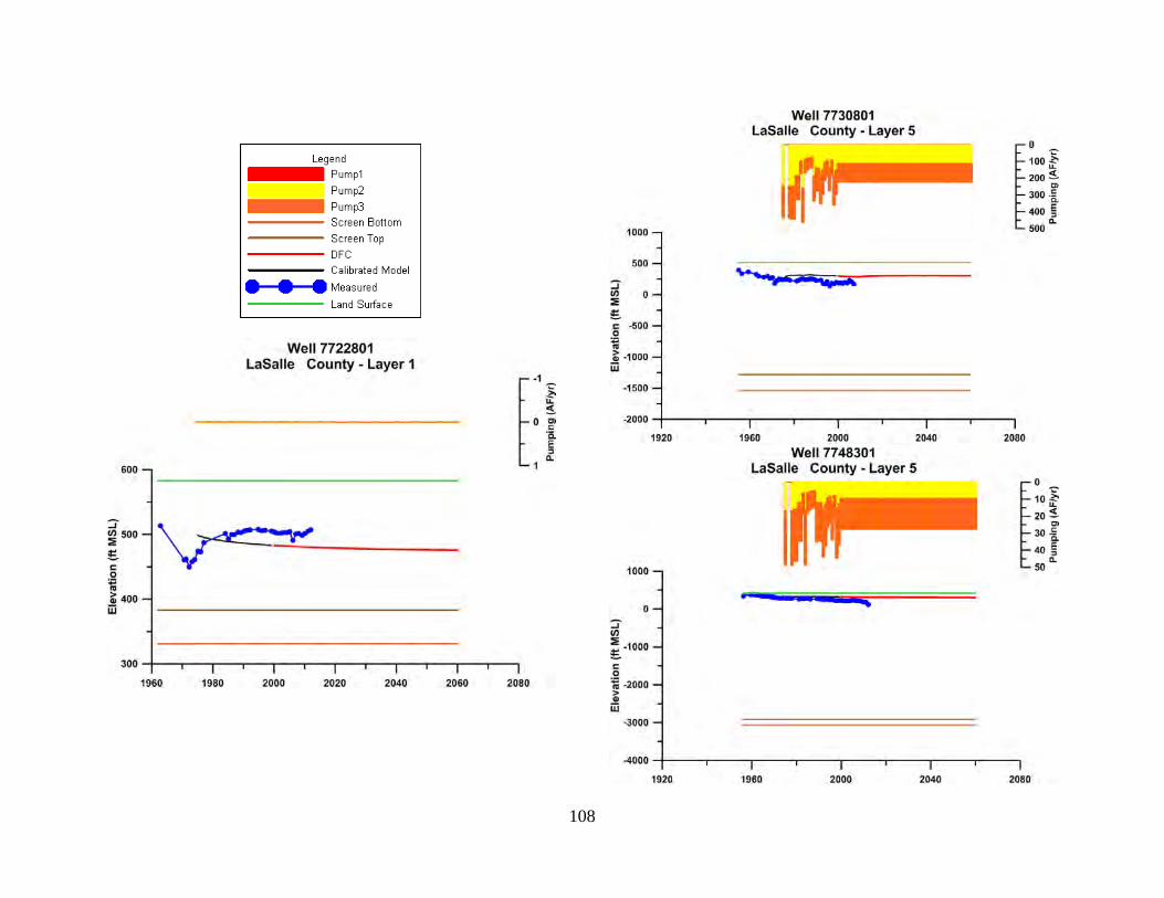
108
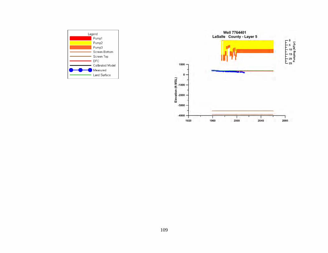
109
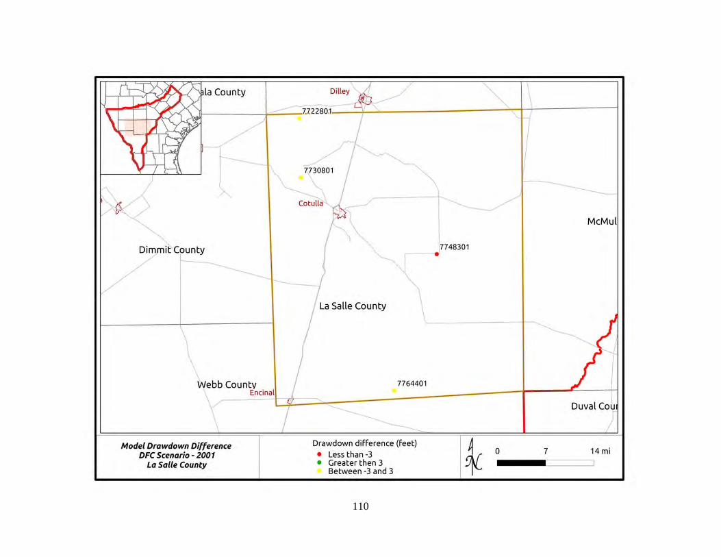
110
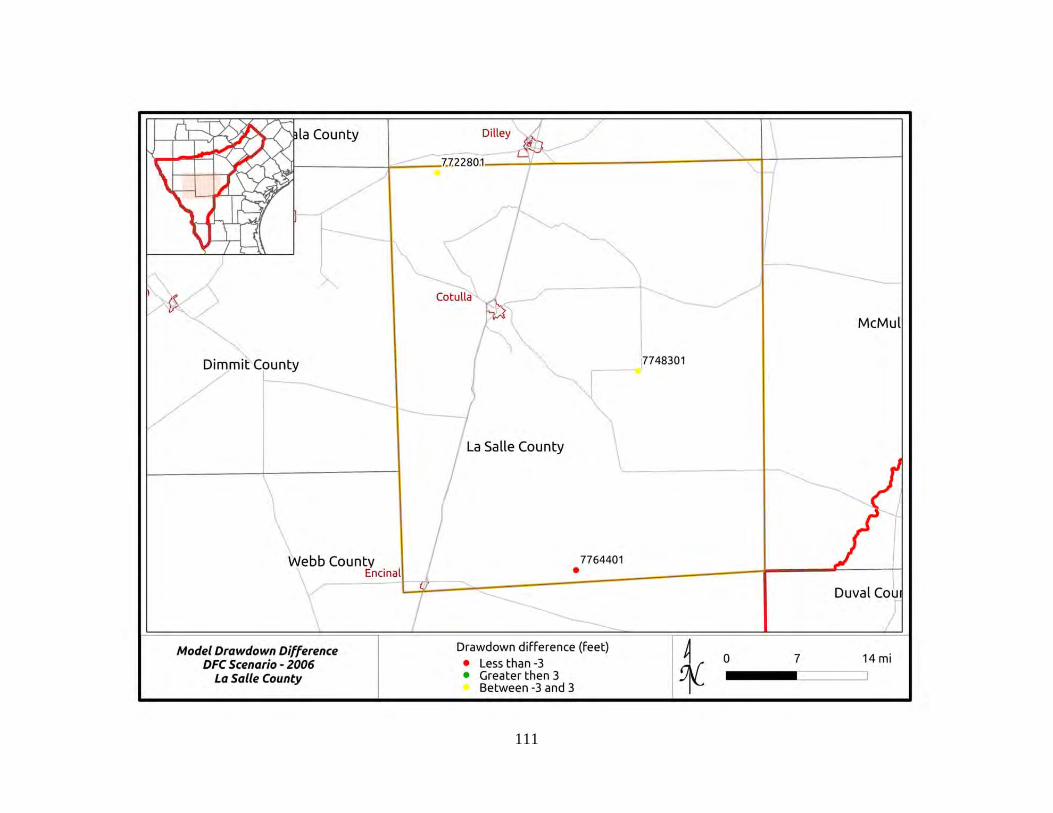
111
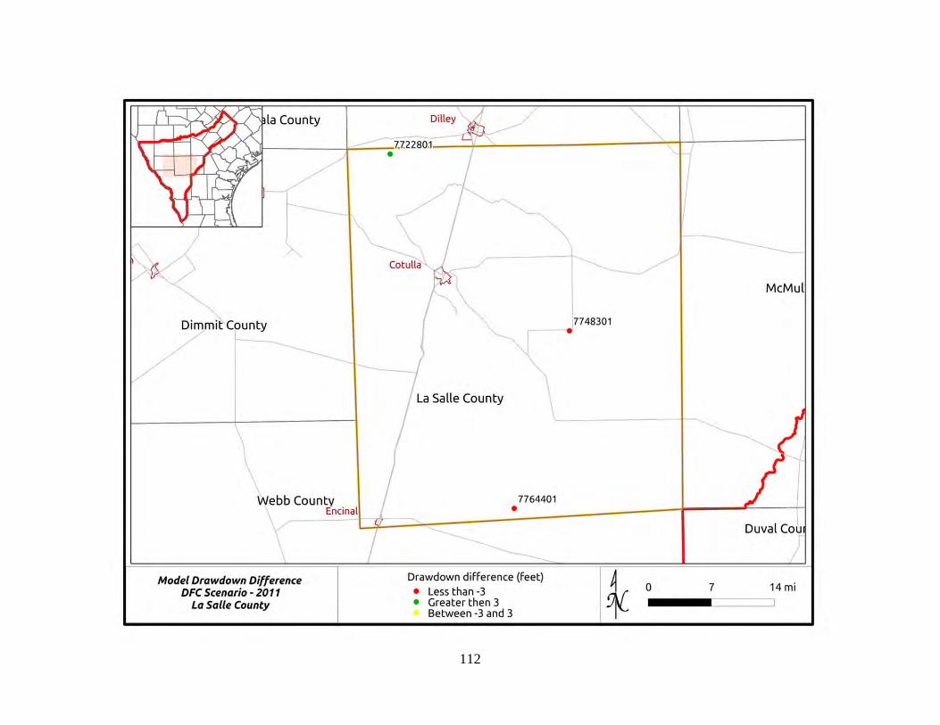
112
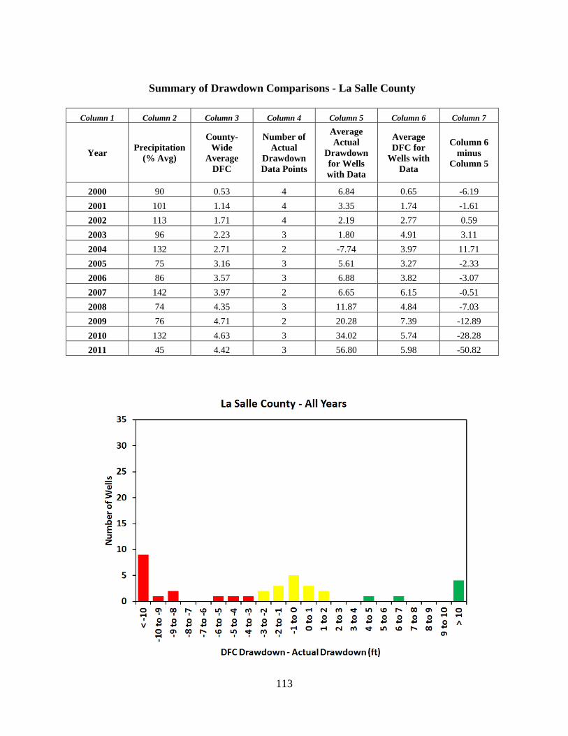
113
Summary of Drawdown Comparisons - La Salle County
Column 1 Column 2 Column 3 Column 4 Column 5 Column 6 Column 7
Year Precipitation
(% Avg)
County-Wide
Average DFC
Number of Actual
Drawdown Data Points
Average Actual
Drawdown for Wells with Data
Average DFC for
Wells with Data
Column 6 minus
Column 5
2000 90 0.53 4 6.84 0.65 -6.19
2001 101 1.14 4 3.35 1.74 -1.61
2002 113 1.71 4 2.19 2.77 0.59
2003 96 2.23 3 1.80 4.91 3.11
2004 132 2.71 2 -7.74 3.97 11.71
2005 75 3.16 3 5.61 3.27 -2.33
2006 86 3.57 3 6.88 3.82 -3.07
2007 142 3.97 2 6.65 6.15 -0.51
2008 74 4.35 3 11.87 4.84 -7.03
2009 76 4.71 2 20.28 7.39 -12.89
2010 132 4.63 3 34.02 5.74 -28.28
2011 45 4.42 3 56.80 5.98 -50.82
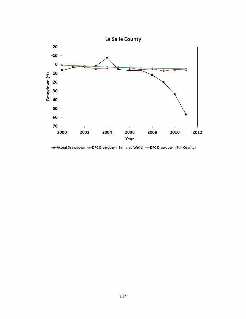
114

115
Appendix10–MaverickCounty
Location Map of Hydrograph Wells
Hydrographs
Note that pumping data are expressed in three zones:
Pump 1 = pumping from cell where well is located
Pump 2 = pumping in cells adjacent to Zone 1
Pump 3 = pumping in cells adjacent to Zone 2
Screen Bottom and Screen Top = Elevation of Well Completion Interval
Land Surface = Elevation of Land Surface at Well
Groundwater Elevations
Measured = Actual data from TWDB database
Calibrated Model = Results for cell defined by well from calibrated model
DFC = Results for cell defined by well from Scenario 4 of GAM Run 09-034
Drawdown Comparison Maps for 2001, 2006 and 2011
Summary of Drawdown Comparisons
Table analogous to Table 5 in text summarizing annual average drawdown (actual and DFC)
Histogram of Differences between DFC Drawdown and Actual Drawdown for All Years
Figure analogous to Figure 23 in text showing differences between actual drawdown and DFC conditions
Hydrograph of Actual Drawdown and DFC Drawdown
Figure analogous to Figure 26 in text showing time history of drawdown (actual and DFC) from 2000 to 2011
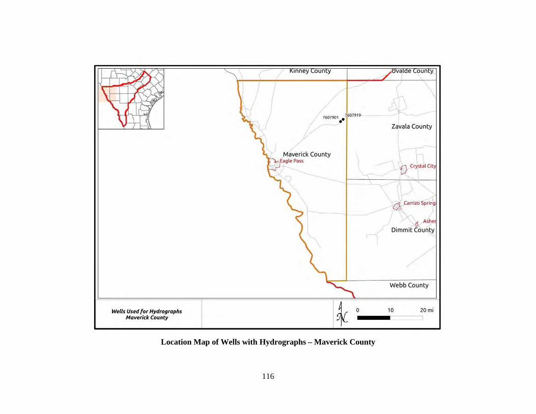
116
Location Map of Wells with Hydrographs – Maverick County
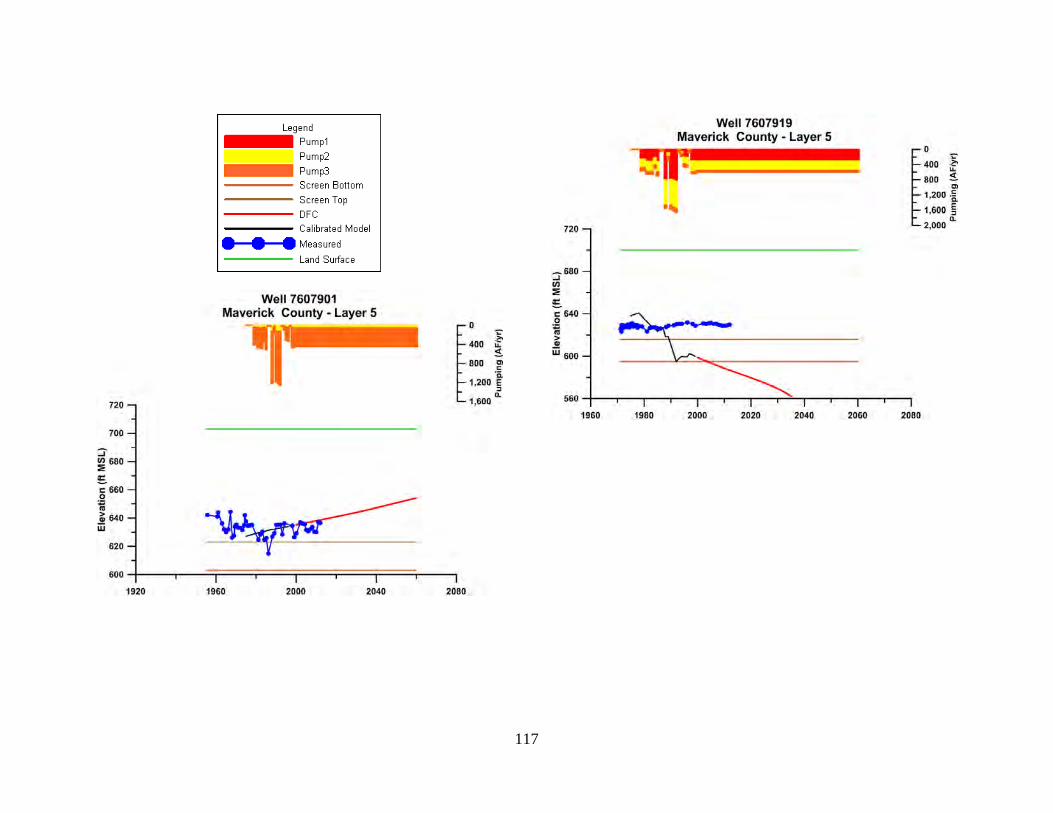
117
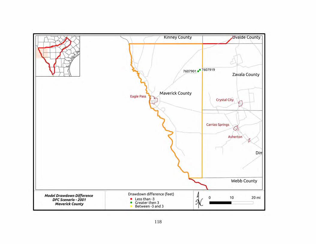
118

119

120
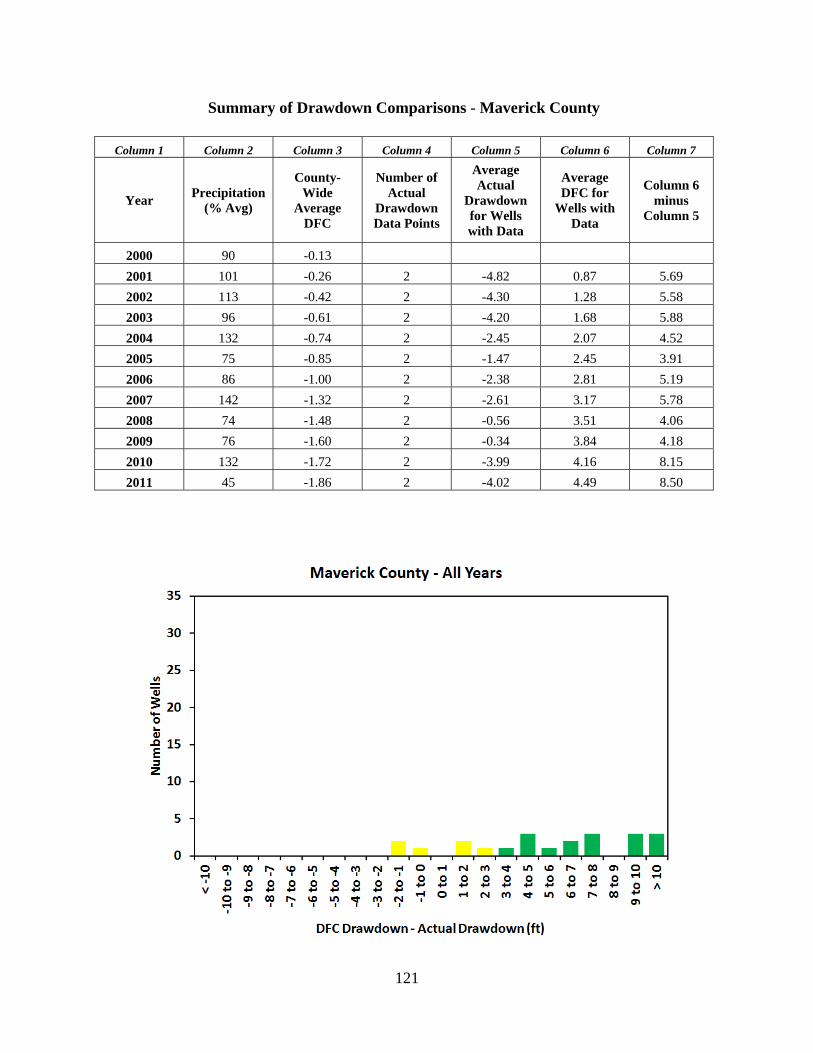
121
Summary of Drawdown Comparisons - Maverick County
Column 1 Column 2 Column 3 Column 4 Column 5 Column 6 Column 7
Year Precipitation
(% Avg)
County-Wide
Average DFC
Number of Actual
Drawdown Data Points
Average Actual
Drawdown for Wells with Data
Average DFC for
Wells with Data
Column 6 minus
Column 5
2000 90 -0.13
2001 101 -0.26 2 -4.82 0.87 5.69
2002 113 -0.42 2 -4.30 1.28 5.58
2003 96 -0.61 2 -4.20 1.68 5.88
2004 132 -0.74 2 -2.45 2.07 4.52
2005 75 -0.85 2 -1.47 2.45 3.91
2006 86 -1.00 2 -2.38 2.81 5.19
2007 142 -1.32 2 -2.61 3.17 5.78
2008 74 -1.48 2 -0.56 3.51 4.06
2009 76 -1.60 2 -0.34 3.84 4.18
2010 132 -1.72 2 -3.99 4.16 8.15
2011 45 -1.86 2 -4.02 4.49 8.50
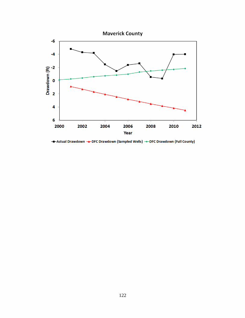
122

123
Appendix11–McMullenCounty
Location Map of Hydrograph Wells
Hydrographs
Note that pumping data are expressed in three zones:
Pump 1 = pumping from cell where well is located
Pump 2 = pumping in cells adjacent to Zone 1
Pump 3 = pumping in cells adjacent to Zone 2
Screen Bottom and Screen Top = Elevation of Well Completion Interval
Land Surface = Elevation of Land Surface at Well
Groundwater Elevations
Measured = Actual data from TWDB database
Calibrated Model = Results for cell defined by well from calibrated model
DFC = Results for cell defined by well from Scenario 4 of GAM Run 09-034
Drawdown Comparison Maps for 2001, 2006 and 2011
Summary of Drawdown Comparisons
Table analogous to Table 5 in text summarizing annual average drawdown (actual and DFC)
Histogram of Differences between DFC Drawdown and Actual Drawdown for All Years
Figure analogous to Figure 23 in text showing differences between actual drawdown and DFC conditions
Hydrograph of Actual Drawdown and DFC Drawdown
Figure analogous to Figure 26 in text showing time history of drawdown (actual and DFC) from 2000 to 2011
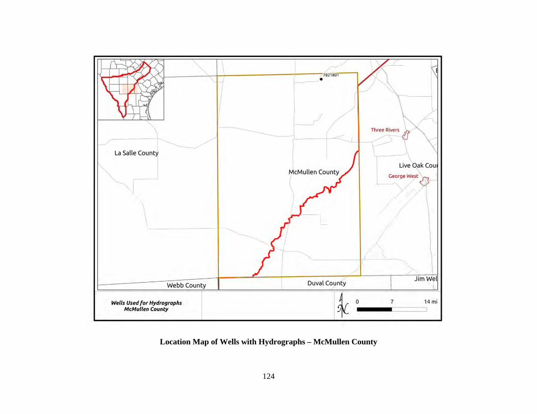
124
Location Map of Wells with Hydrographs – McMullen County
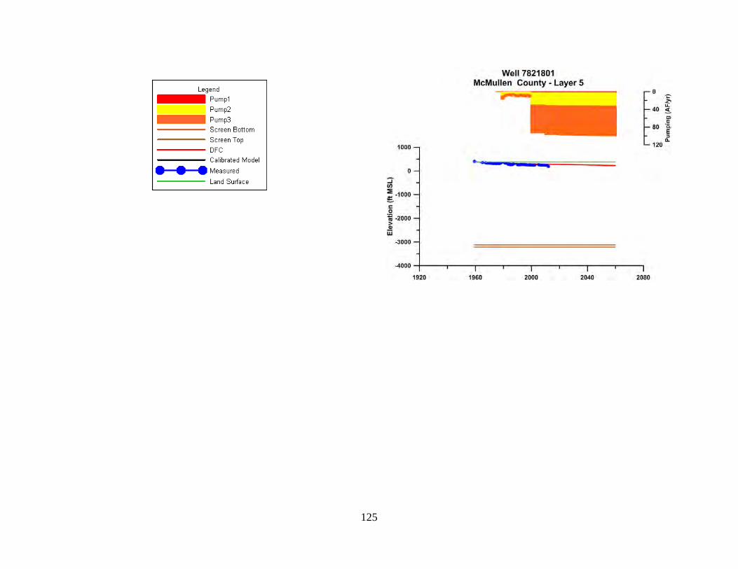
125

126
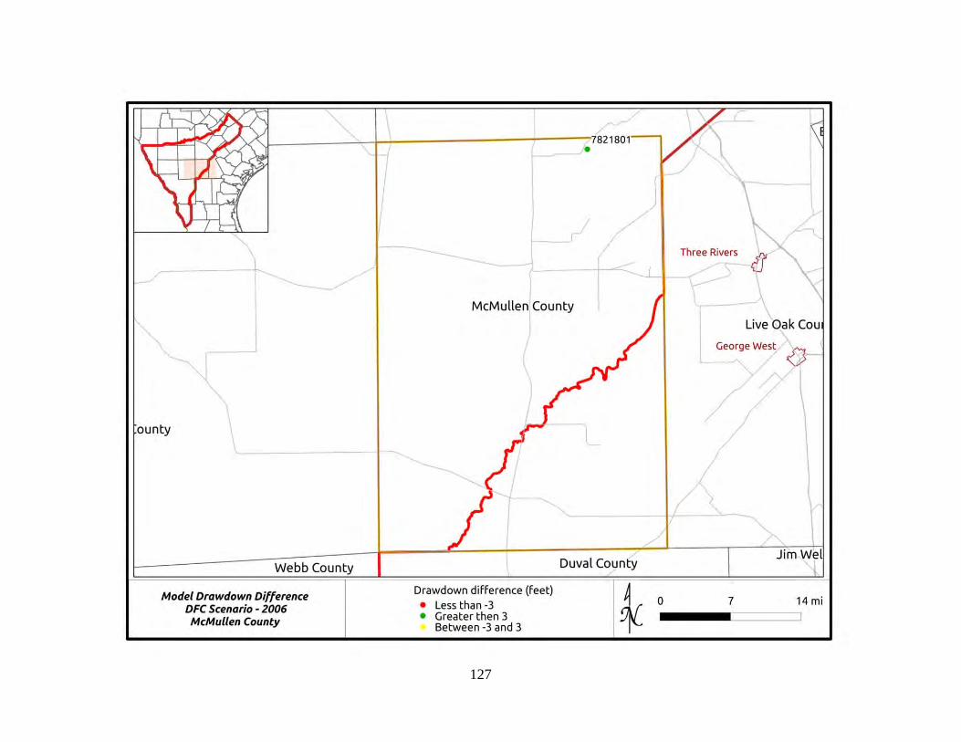
127

128
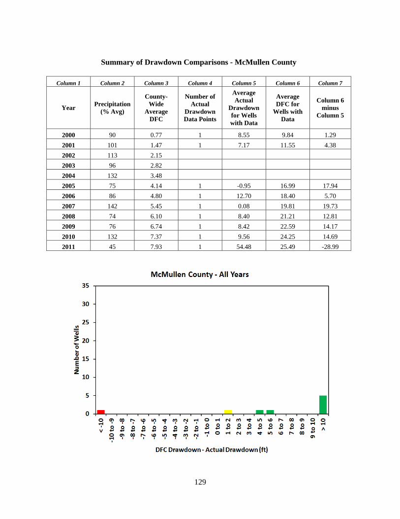
129
Summary of Drawdown Comparisons - McMullen County
Column 1 Column 2 Column 3 Column 4 Column 5 Column 6 Column 7
Year Precipitation
(% Avg)
County-Wide
Average DFC
Number of Actual
Drawdown Data Points
Average Actual
Drawdown for Wells with Data
Average DFC for
Wells with Data
Column 6 minus
Column 5
2000 90 0.77 1 8.55 9.84 1.29
2001 101 1.47 1 7.17 11.55 4.38
2002 113 2.15
2003 96 2.82
2004 132 3.48
2005 75 4.14 1 -0.95 16.99 17.94
2006 86 4.80 1 12.70 18.40 5.70
2007 142 5.45 1 0.08 19.81 19.73
2008 74 6.10 1 8.40 21.21 12.81
2009 76 6.74 1 8.42 22.59 14.17
2010 132 7.37 1 9.56 24.25 14.69
2011 45 7.93 1 54.48 25.49 -28.99

130

131
Appendix12–MedinaCounty
Location Map of Hydrograph Wells
Hydrographs
Note that pumping data are expressed in three zones:
Pump 1 = pumping from cell where well is located
Pump 2 = pumping in cells adjacent to Zone 1
Pump 3 = pumping in cells adjacent to Zone 2
Screen Bottom and Screen Top = Elevation of Well Completion Interval
Land Surface = Elevation of Land Surface at Well
Groundwater Elevations
Measured = Actual data from TWDB database
Calibrated Model = Results for cell defined by well from calibrated model
DFC = Results for cell defined by well from Scenario 4 of GAM Run 09-034
Drawdown Comparison Maps for 2001, 2006 and 2011
Summary of Drawdown Comparisons
Table analogous to Table 5 in text summarizing annual average drawdown (actual and DFC)
Histogram of Differences between DFC Drawdown and Actual Drawdown for All Years
Figure analogous to Figure 23 in text showing differences between actual drawdown and DFC conditions
Hydrograph of Actual Drawdown and DFC Drawdown
Figure analogous to Figure 26 in text showing time history of drawdown (actual and DFC) from 2000 to 2011
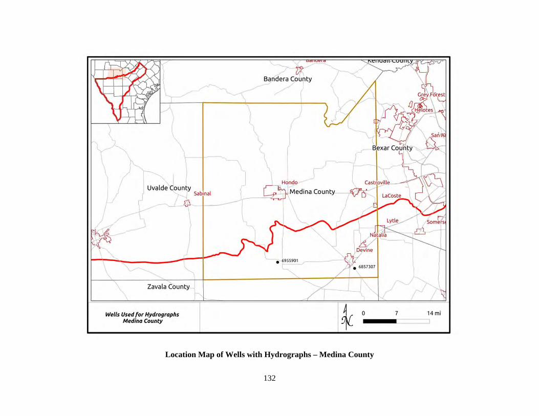
132
Location Map of Wells with Hydrographs – Medina County
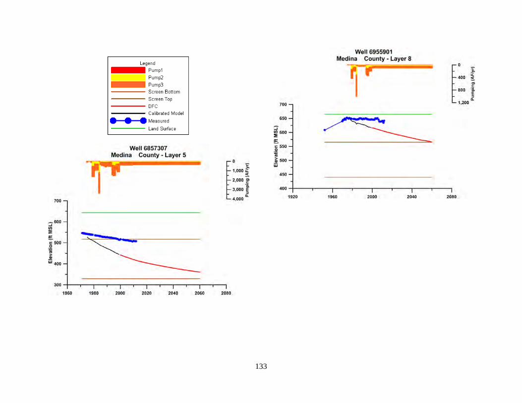
133
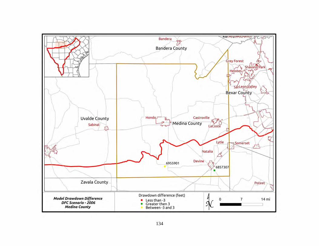
134

135
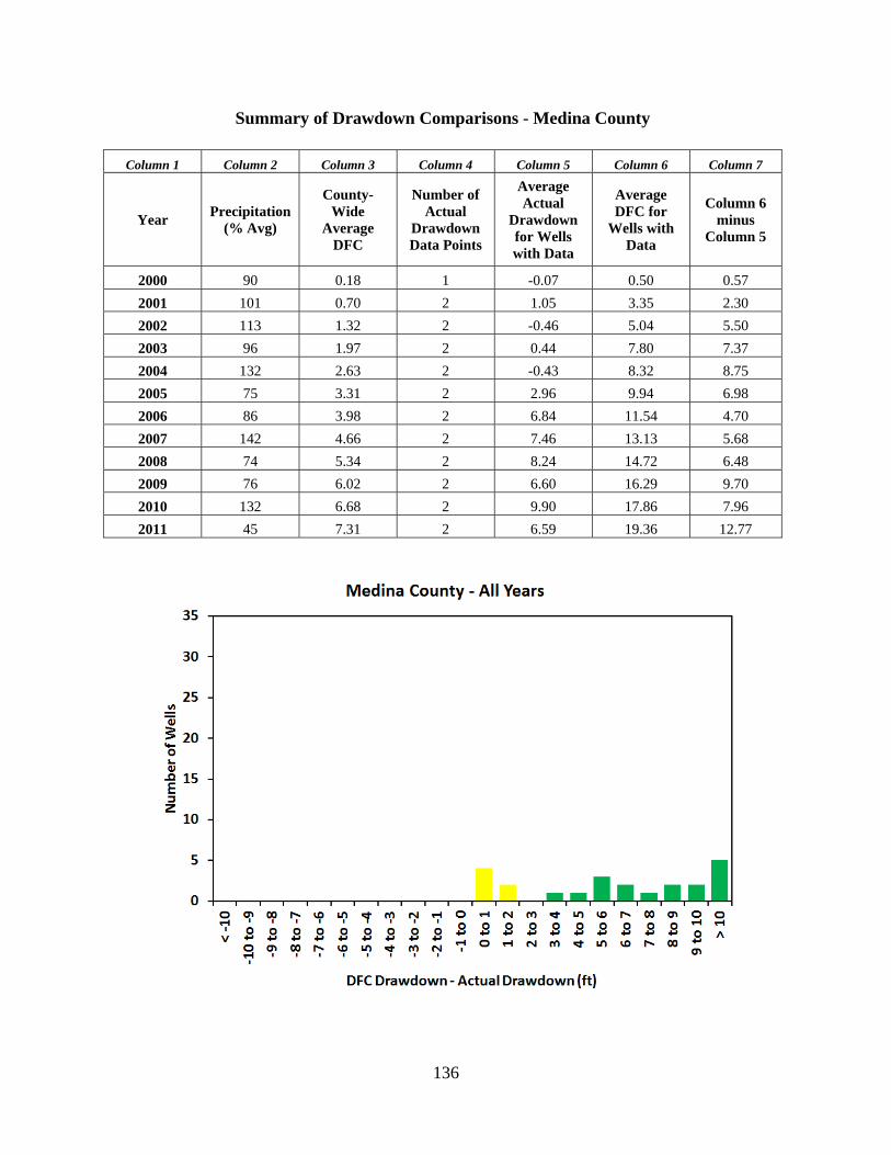
136
Summary of Drawdown Comparisons - Medina County
Column 1 Column 2 Column 3 Column 4 Column 5 Column 6 Column 7
Year Precipitation
(% Avg)
County-Wide
Average DFC
Number of Actual
Drawdown Data Points
Average Actual
Drawdown for Wells with Data
Average DFC for
Wells with Data
Column 6 minus
Column 5
2000 90 0.18 1 -0.07 0.50 0.57
2001 101 0.70 2 1.05 3.35 2.30
2002 113 1.32 2 -0.46 5.04 5.50
2003 96 1.97 2 0.44 7.80 7.37
2004 132 2.63 2 -0.43 8.32 8.75
2005 75 3.31 2 2.96 9.94 6.98
2006 86 3.98 2 6.84 11.54 4.70
2007 142 4.66 2 7.46 13.13 5.68
2008 74 5.34 2 8.24 14.72 6.48
2009 76 6.02 2 6.60 16.29 9.70
2010 132 6.68 2 9.90 17.86 7.96
2011 45 7.31 2 6.59 19.36 12.77
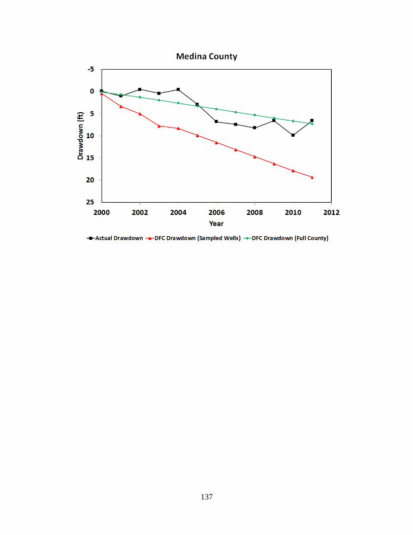
137

138
Appendix13–WebbCounty
Location Map of Hydrograph Wells
Hydrographs
Note that pumping data are expressed in three zones:
Pump 1 = pumping from cell where well is located
Pump 2 = pumping in cells adjacent to Zone 1
Pump 3 = pumping in cells adjacent to Zone 2
Screen Bottom and Screen Top = Elevation of Well Completion Interval
Land Surface = Elevation of Land Surface at Well
Groundwater Elevations
Measured = Actual data from TWDB database
Calibrated Model = Results for cell defined by well from calibrated model
DFC = Results for cell defined by well from Scenario 4 of GAM Run 09-034
Drawdown Comparison Maps for 2001, 2006 and 2011
Summary of Drawdown Comparisons
Table analogous to Table 5 in text summarizing annual average drawdown (actual and DFC)
Histogram of Differences between DFC Drawdown and Actual Drawdown for All Years
Figure analogous to Figure 23 in text showing differences between actual drawdown and DFC conditions
Hydrograph of Actual Drawdown and DFC Drawdown
Figure analogous to Figure 26 in text showing time history of drawdown (actual and DFC) from 2000 to 2011
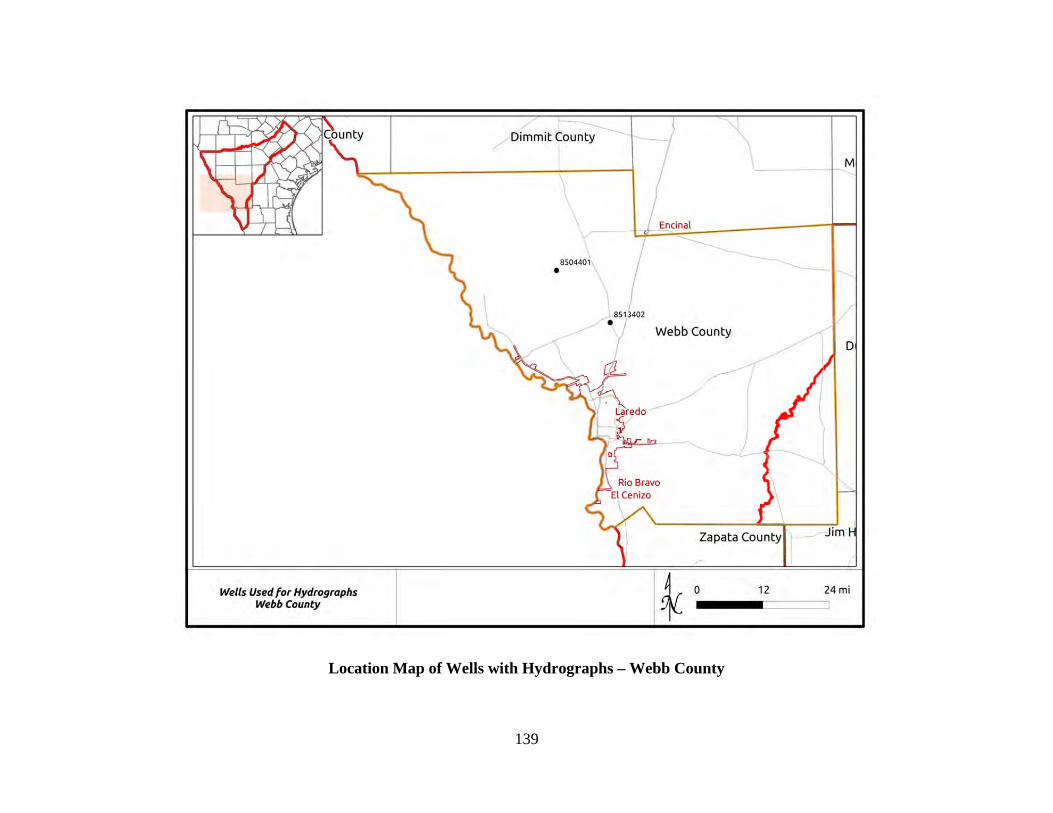
139
Location Map of Wells with Hydrographs – Webb County
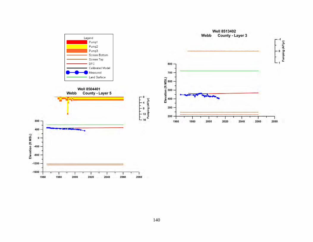
140

141
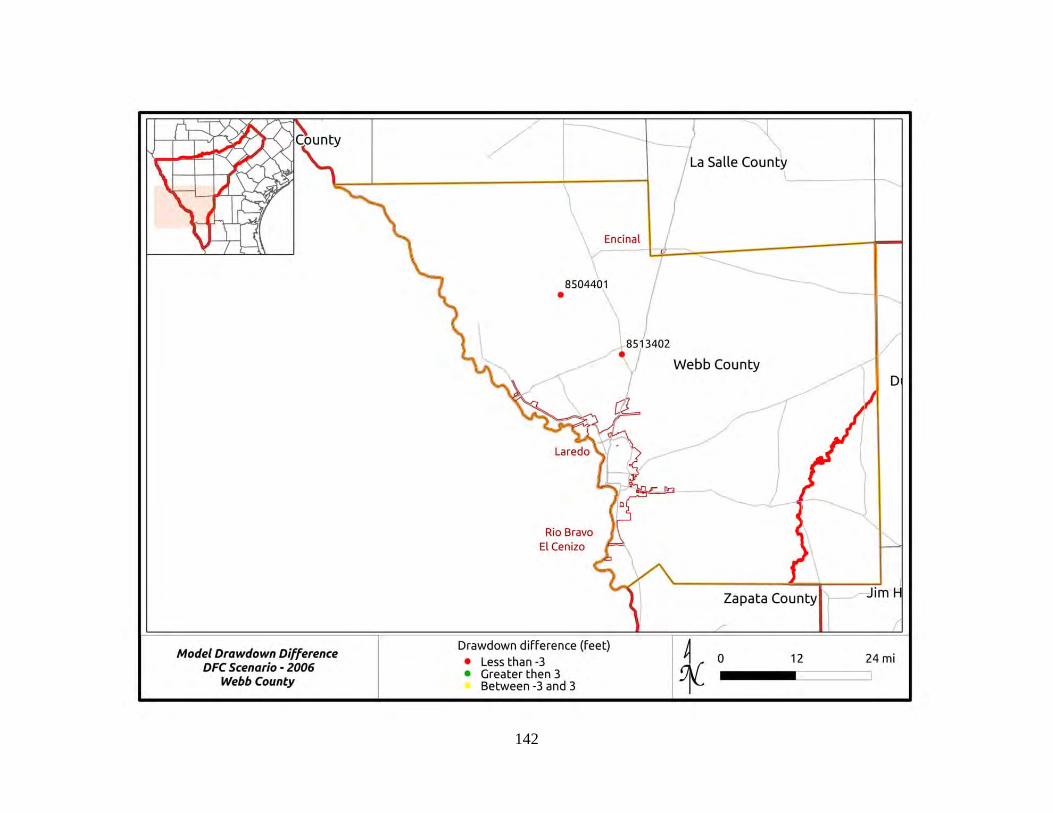
142
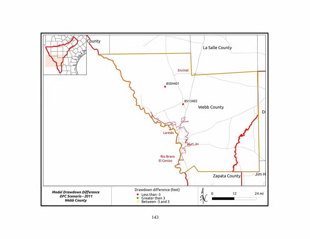
143
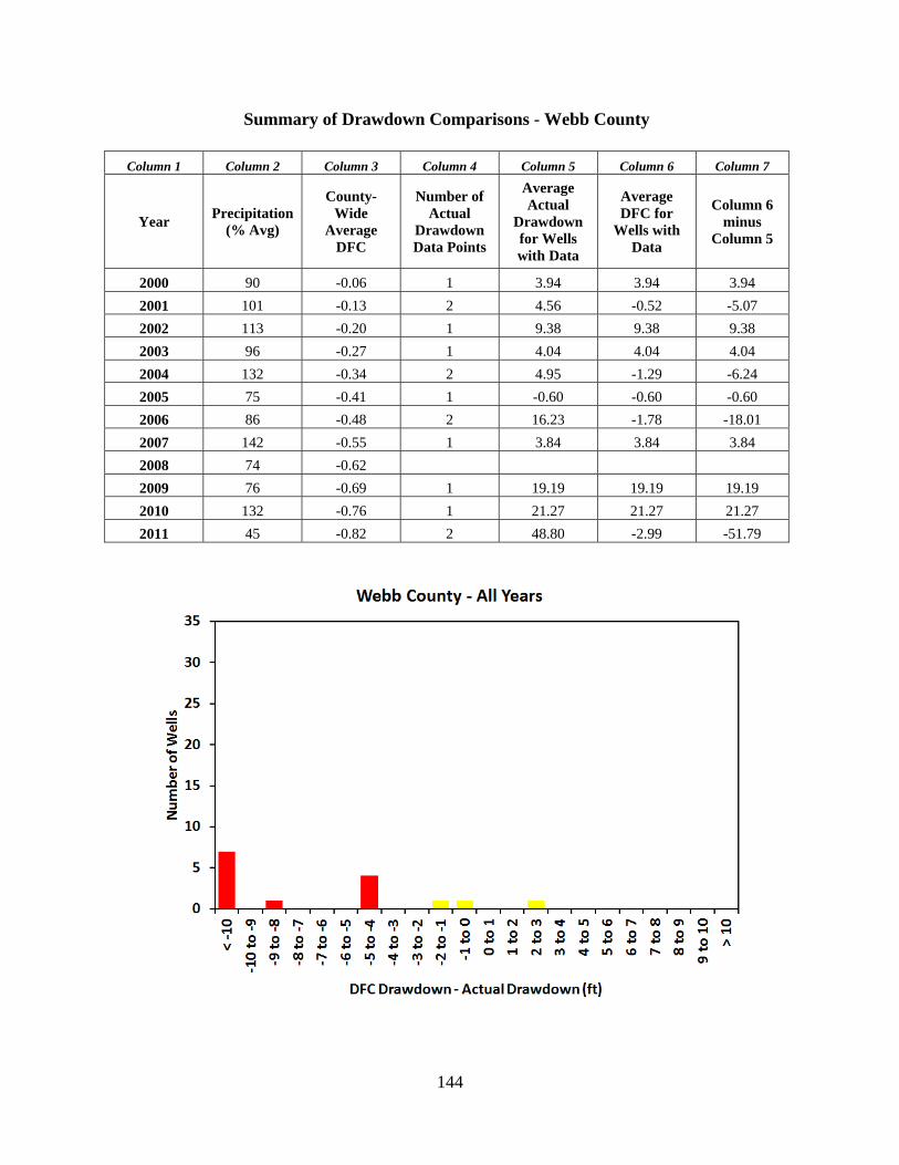
144
Summary of Drawdown Comparisons - Webb County
Column 1 Column 2 Column 3 Column 4 Column 5 Column 6 Column 7
Year Precipitation
(% Avg)
County-Wide
Average DFC
Number of Actual
Drawdown Data Points
Average Actual
Drawdown for Wells with Data
Average DFC for
Wells with Data
Column 6 minus
Column 5
2000 90 -0.06 1 3.94 3.94 3.94
2001 101 -0.13 2 4.56 -0.52 -5.07
2002 113 -0.20 1 9.38 9.38 9.38
2003 96 -0.27 1 4.04 4.04 4.04
2004 132 -0.34 2 4.95 -1.29 -6.24
2005 75 -0.41 1 -0.60 -0.60 -0.60
2006 86 -0.48 2 16.23 -1.78 -18.01
2007 142 -0.55 1 3.84 3.84 3.84
2008 74 -0.62
2009 76 -0.69 1 19.19 19.19 19.19
2010 132 -0.76 1 21.27 21.27 21.27
2011 45 -0.82 2 48.80 -2.99 -51.79
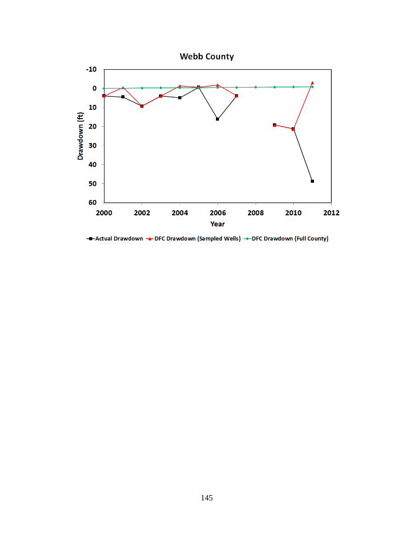
145

146
Appendix14–WilsonCounty
Location Map of Hydrograph Wells
Hydrographs
Note that pumping data are expressed in three zones:
Pump 1 = pumping from cell where well is located
Pump 2 = pumping in cells adjacent to Zone 1
Pump 3 = pumping in cells adjacent to Zone 2
Screen Bottom and Screen Top = Elevation of Well Completion Interval
Land Surface = Elevation of Land Surface at Well
Groundwater Elevations
Measured = Actual data from TWDB database
Calibrated Model = Results for cell defined by well from calibrated model
DFC = Results for cell defined by well from Scenario 4 of GAM Run 09-034
Drawdown Comparison Maps for 2001 and 2006
Summary of Drawdown Comparisons
Table analogous to Table 5 in text summarizing annual average drawdown (actual and DFC)
Histogram of Differences between DFC Drawdown and Actual Drawdown for All Years
Figure analogous to Figure 23 in text showing differences between actual drawdown and DFC conditions
Hydrograph of Actual Drawdown and DFC Drawdown
Figure analogous to Figure 26 in text showing time history of drawdown (actual and DFC) from 2000 to 2011
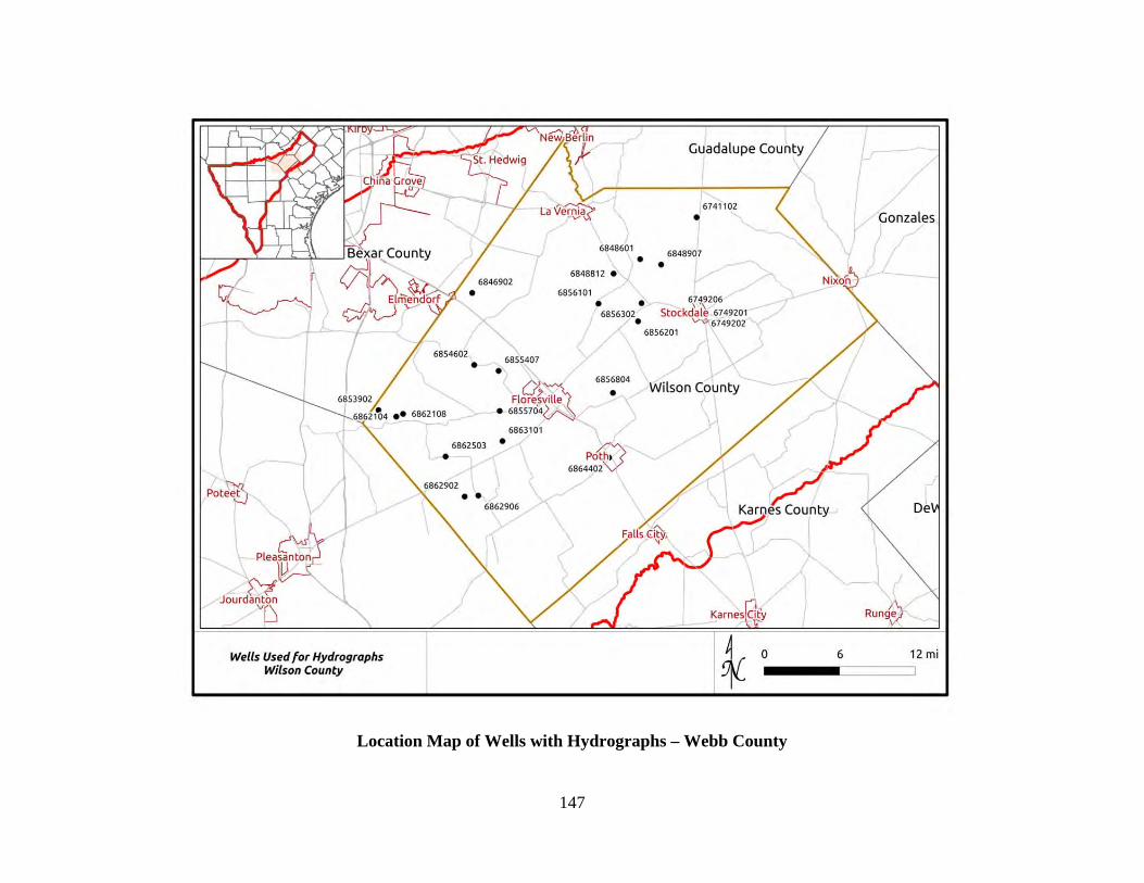
147
Location Map of Wells with Hydrographs – Webb County
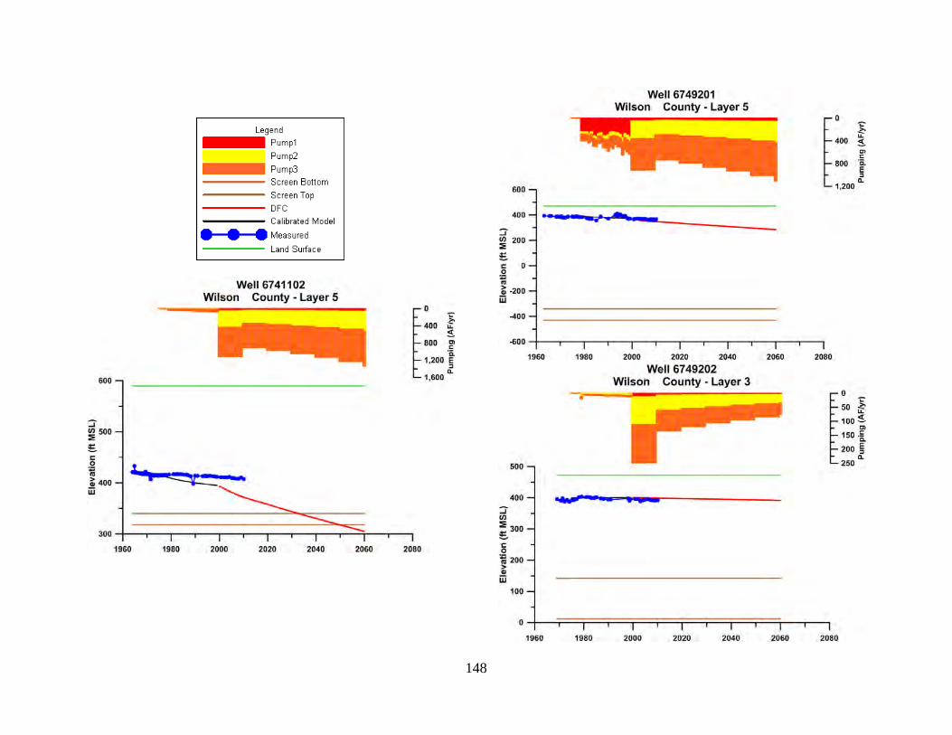
148
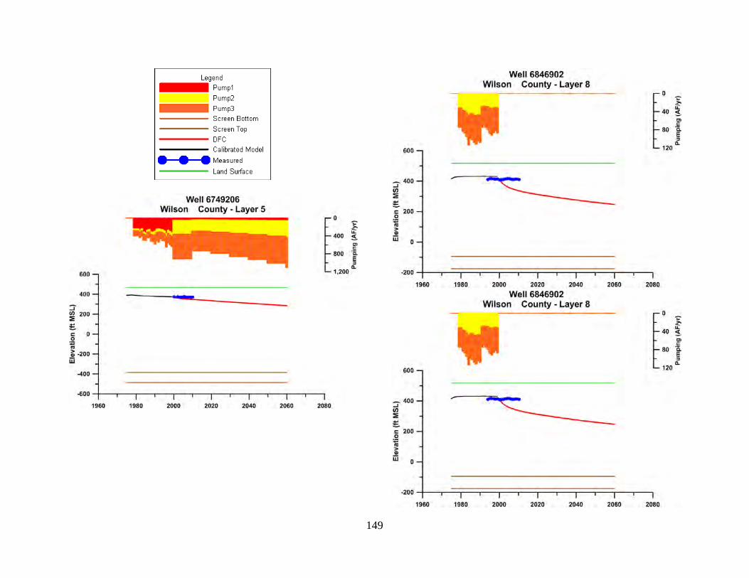
149

150
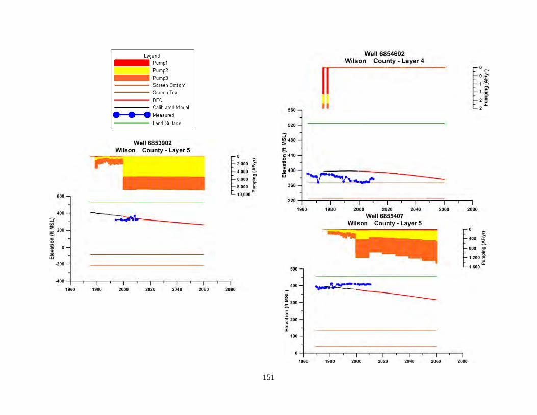
151
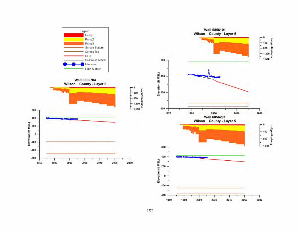
152
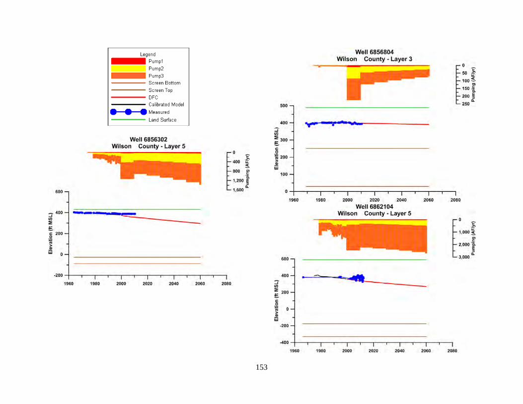
153

154
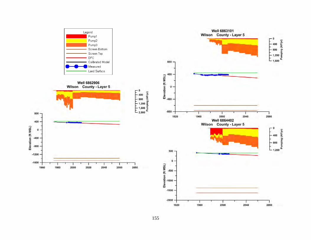
155
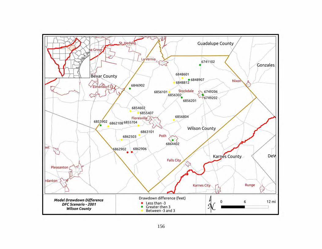
156
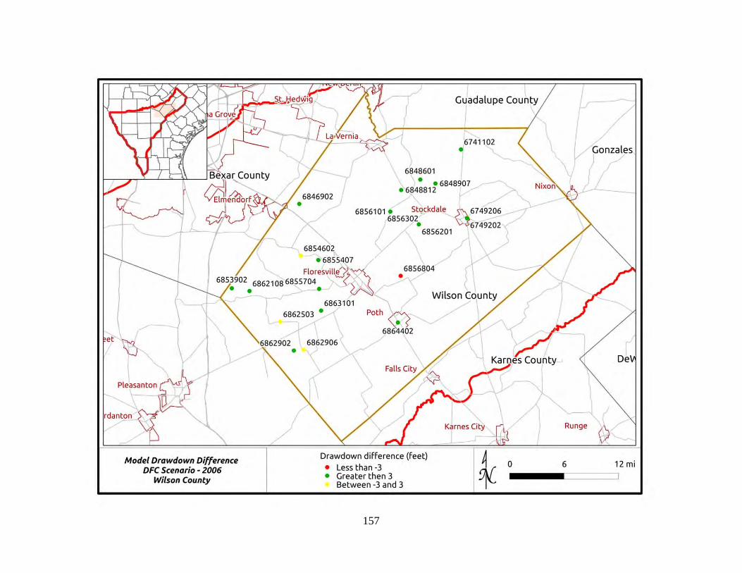
157
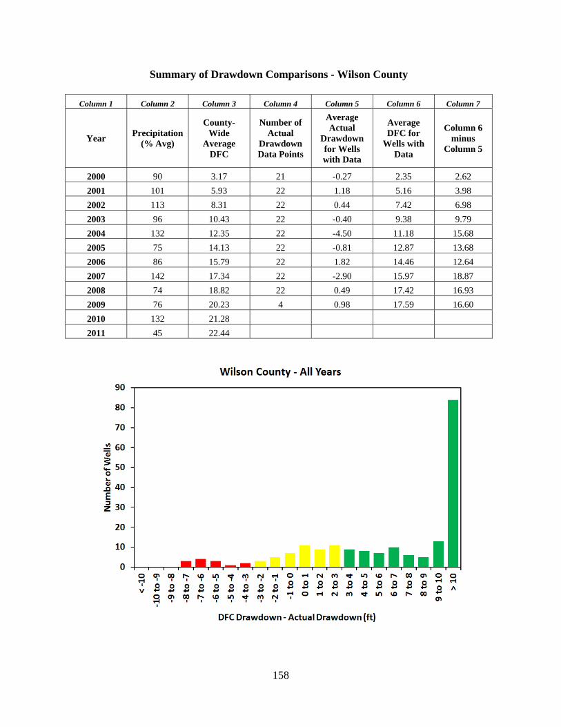
158
Summary of Drawdown Comparisons - Wilson County
Column 1 Column 2 Column 3 Column 4 Column 5 Column 6 Column 7
Year Precipitation
(% Avg)
County-Wide
Average DFC
Number of Actual
Drawdown Data Points
Average Actual
Drawdown for Wells with Data
Average DFC for
Wells with Data
Column 6 minus
Column 5
2000 90 3.17 21 -0.27 2.35 2.62
2001 101 5.93 22 1.18 5.16 3.98
2002 113 8.31 22 0.44 7.42 6.98
2003 96 10.43 22 -0.40 9.38 9.79
2004 132 12.35 22 -4.50 11.18 15.68
2005 75 14.13 22 -0.81 12.87 13.68
2006 86 15.79 22 1.82 14.46 12.64
2007 142 17.34 22 -2.90 15.97 18.87
2008 74 18.82 22 0.49 17.42 16.93
2009 76 20.23 4 0.98 17.59 16.60
2010 132 21.28
2011 45 22.44
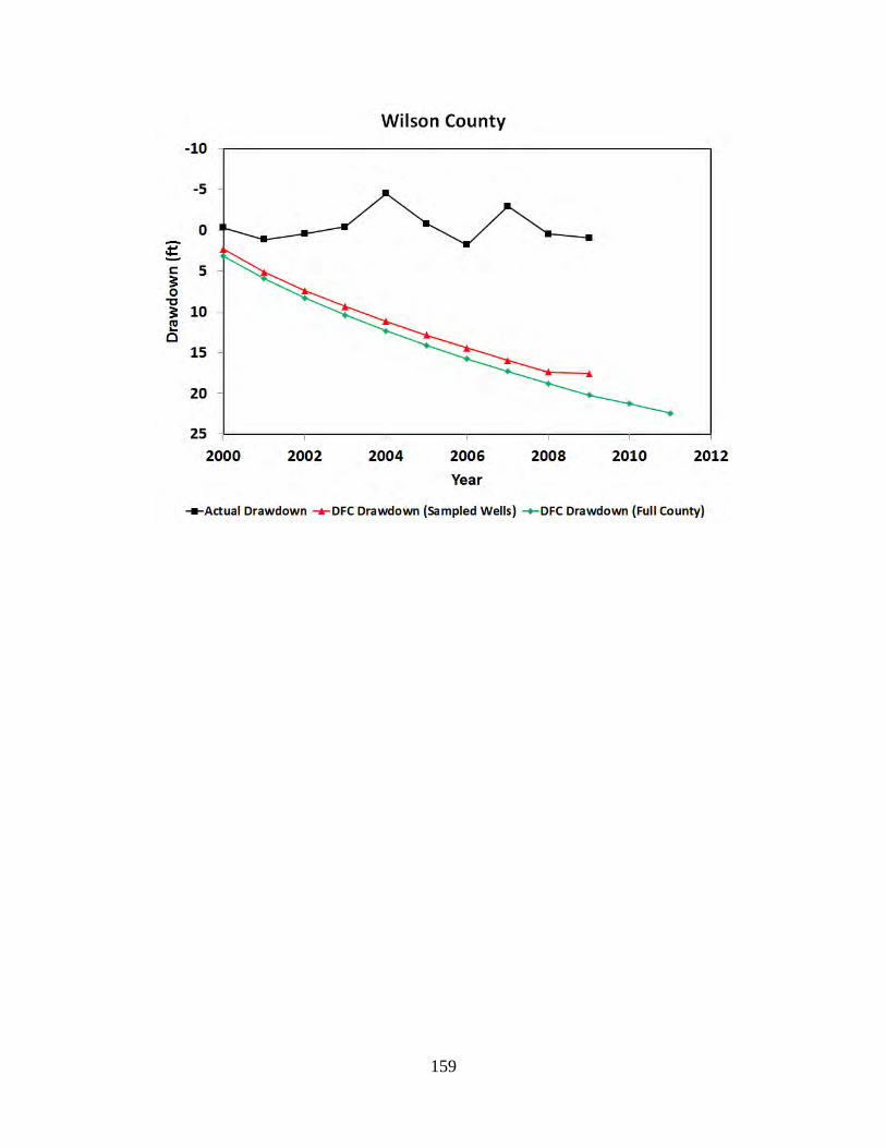
159

160
Appendix15–ZavalaCounty
Location Map of Hydrograph Wells
Hydrographs
Note that pumping data are expressed in three zones:
Pump 1 = pumping from cell where well is located
Pump 2 = pumping in cells adjacent to Zone 1
Pump 3 = pumping in cells adjacent to Zone 2
Screen Bottom and Screen Top = Elevation of Well Completion Interval
Land Surface = Elevation of Land Surface at Well
Groundwater Elevations
Measured = Actual data from TWDB database
Calibrated Model = Results for cell defined by well from calibrated model
DFC = Results for cell defined by well from Scenario 4 of GAM Run 09-034
Drawdown Comparison Maps for 2001, 2006 and 2011
Summary of Drawdown Comparisons
Table analogous to Table 5 in text summarizing annual average drawdown (actual and DFC)
Histogram of Differences between DFC Drawdown and Actual Drawdown for All Years
Figure analogous to Figure 23 in text showing differences between actual drawdown and DFC conditions
Hydrograph of Actual Drawdown and DFC Drawdown
Figure analogous to Figure 26 in text showing time history of drawdown (actual and DFC) from 2000 to 2011
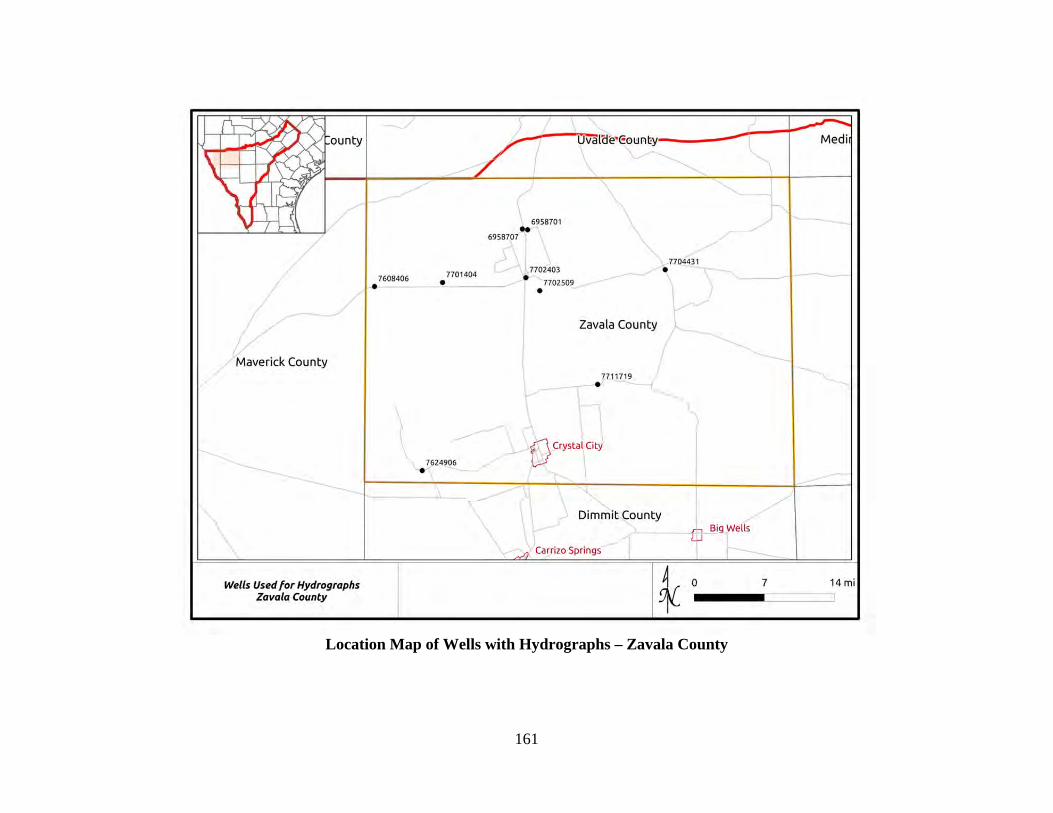
161
Location Map of Wells with Hydrographs – Zavala County
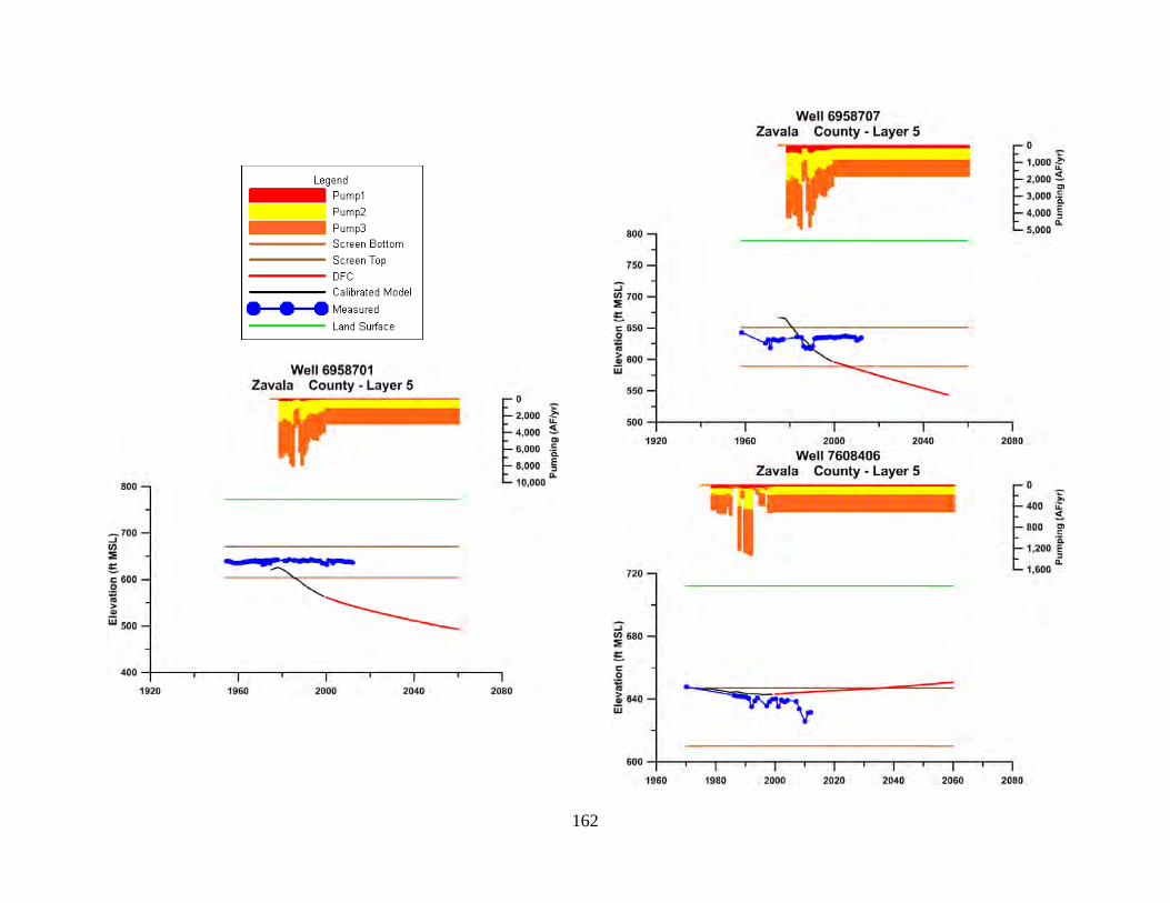
162
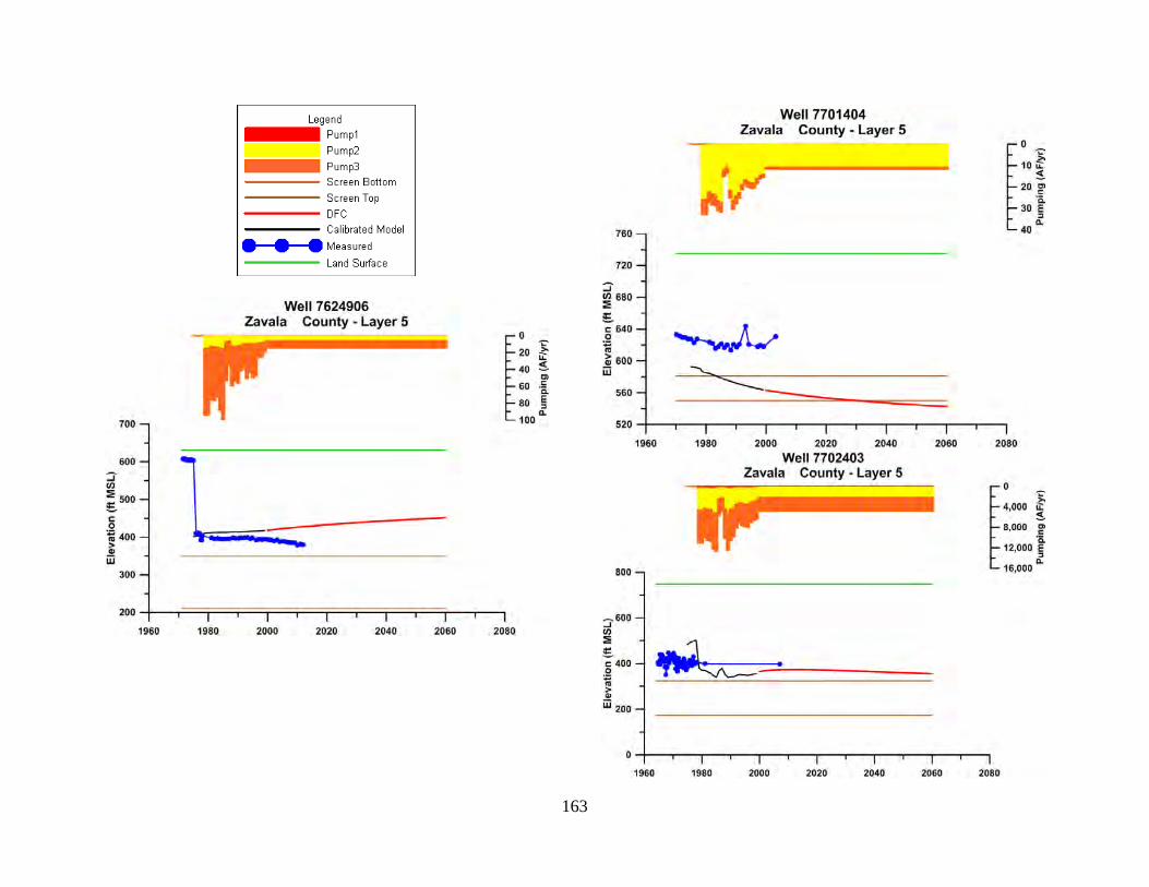
163
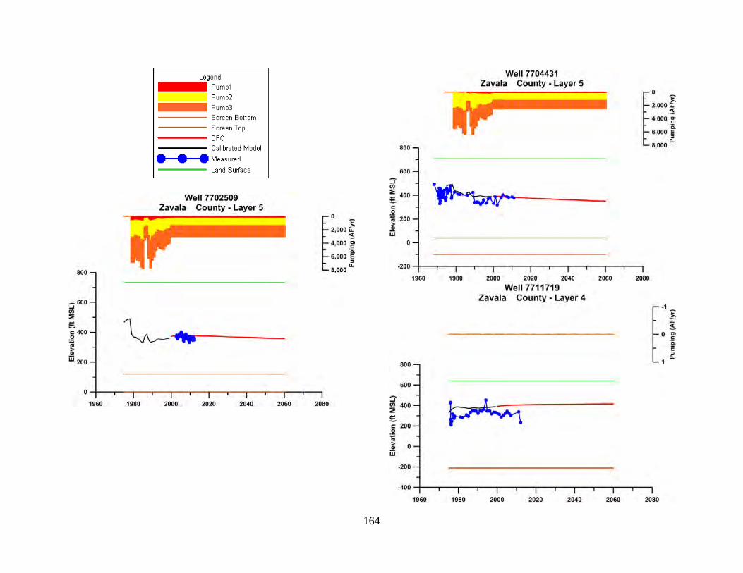
164
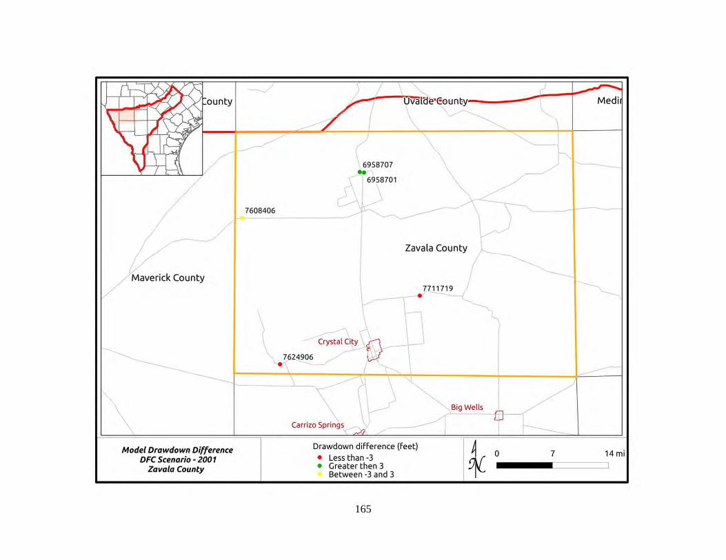
165

166
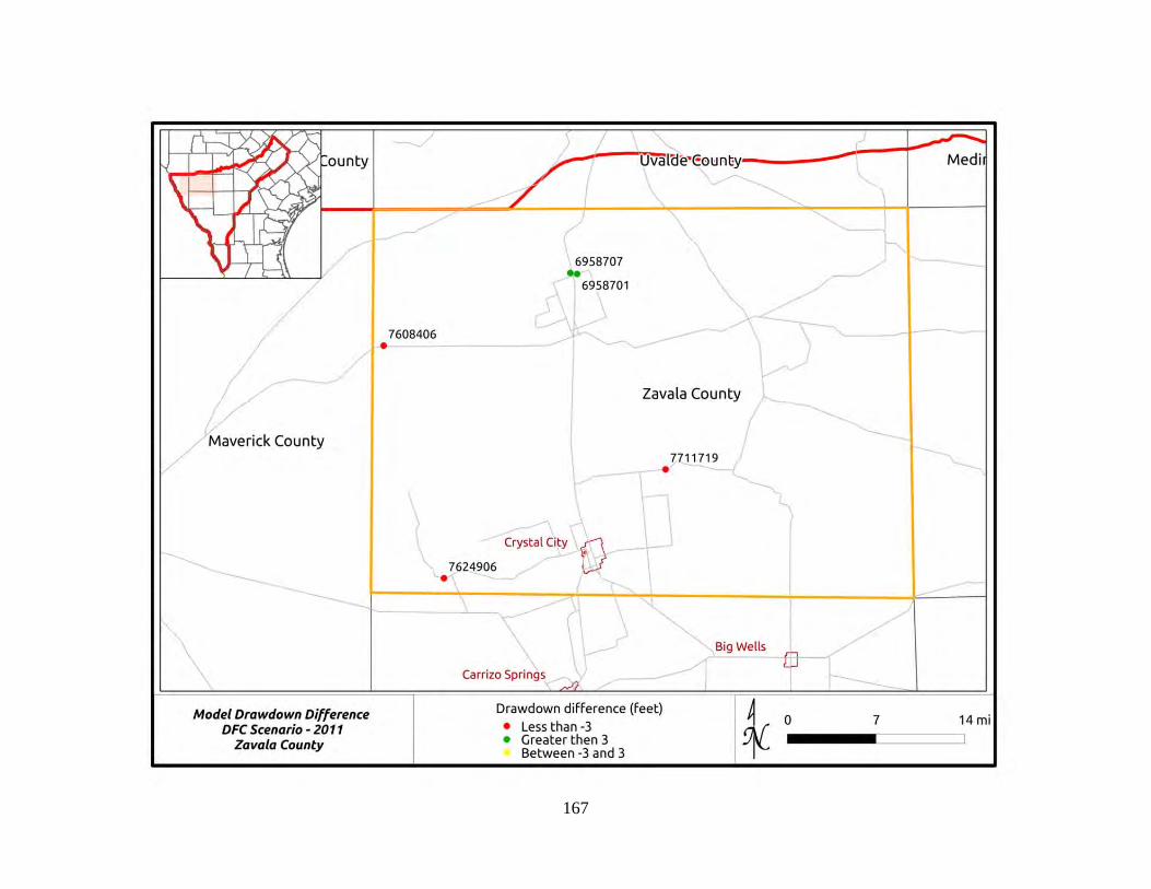
167
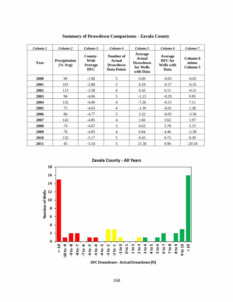
168
Summary of Drawdown Comparisons - Zavala County
Column 1 Column 2 Column 3 Column 4 Column 5 Column 6 Column 7
Year Precipitation
(% Avg)
County-Wide
Average DFC
Number of Actual
Drawdown Data Points
Average Actual
Drawdown for Wells with Data
Average DFC for
Wells with Data
Column 6 minus
Column 5
2000 90 -1.86 5 0.60 -0.05 -0.65
2001 101 -2.88 5 6.18 -0.17 -6.35
2002 113 -3.58 6 0.42 0.11 -0.31
2003 96 -4.06 5 -1.13 -0.29 0.85
2004 132 -4.40 4 -7.26 -0.15 7.11
2005 75 -4.63 4 -1.39 -0.01 1.38
2006 86 -4.77 5 3.32 -0.05 -3.36
2007 142 -4.85 4 1.66 3.62 1.97
2008 74 -4.87 3 0.62 5.78 5.15
2009 76 -4.85 4 6.84 4.46 -2.38
2010 132 -5.17 5 0.43 0.73 0.30
2011 45 -5.54 5 21.30 0.96 -20.34
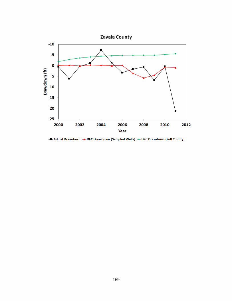
169
170
Appendix16–ResponsestoCommentsfromDraftReportdatedDecember21,2012
Email from Jay Troell on February 13, 2013 containing 11 numbered comments.
Forwarded email from Louis Rosenberg on February 14, 2013 with comments from James Bene and a summary of the comment from Mr. Rosenberg.
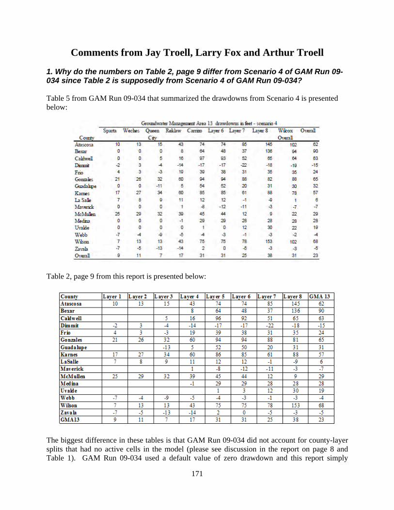
171
Comments from Jay Troell, Larry Fox and Arthur Troell 1. Why do the numbers on Table 2, page 9 differ from Scenario 4 of GAM Run 09-034 since Table 2 is supposedly from Scenario 4 of GAM Run 09-034? Table 5 from GAM Run 09-034 that summarized the drawdowns from Scenario 4 is presented below:
Table 2, page 9 from this report is presented below:
The biggest difference in these tables is that GAM Run 09-034 did not account for county-layer splits that had no active cells in the model (please see discussion in the report on page 8 and Table 1). GAM Run 09-034 used a default value of zero drawdown and this report simply
172
reported blank values when there were no active cells. Individual differences in the tables are summarized below, with the drawdown value from GAM Run 09-034 reported first, and the drawdown value from this report presented second:
Caldwell County, Layer 5 (97 vs. 96) Guadalupe County, Layer 5 (54 vs. 52) Karnes County, Layer 5 (85 vs. 86) Caldwell County, Layer 6 (93 vs. 92) Guadalupe County, Layer 6 (52 vs. 50) Uvalde County, Layer 6 (0 vs. 3) Caldwell County, Layer 7 (52 vs. 51) Gonzales County, Layer 8 (82 vs. 81) Guadalupe County, GMA 13 (32 vs. 31)
In most cases, the difference is a foot. Two of the differences are two feet, and one is three feet. The method used to develop the estimates in GAM Run 09-034 was different than that used to develop the table in this report. Rounding error and the fact that different methods were used are the reasons for these slight differences. It would be helpful for the reader to define/label the “Layers” in Table 1 and Table 2, i.e. Layer 1 (Sparta Aquifer), Layer 2 (Weches Formation), Layer 3 ( Queen City Aquifer), Layer 4 (Reklaw Formation), Layer 5 (Carrizo Aquifer), Layer 6 (upper Wilcox Aquifer), Layer 7 (middle Wilcox Aquifer), Layer 8 (lower Wilcox Aquifer). The reason that I simply reported the layer number and did not attach a name to the layer was addressed at the November 15, 2012 GMA 13 meeting. I presented a series of slides at that meeting that compared the well completions (screen top and bottom elevation) that defined what layer the wells were located in with the TWDB assignment of aquifer units. Assuming that the TWDB aquifer designations are accurate, this analysis suggests that the model layering did not always honor the stratigraphy. Alternatively, if the model layers are assumed accurate, then the TWDB aquifer designations have errors. Although the possibility of some errors in the TWDB aquifer designations are likely, it is more likely that the model layers do not always accurately honor the stratigraphy. 2. Figure 5, page 10 shows pumping of about 70,000 AF/yr for Atascosa County in 2000 and 80,000 AF/yr in 2060. Please explain why the increase will be only 10,000 AF/yr. All pumping changes were specified by the groundwater conservation districts in GMA 13 during the development of the DFC. 3. The largest draw-down will occur in northern Atascosa of 110 ft. From 2000 to 2060 northern Atascosa County and Bexar County will be highly pumped areas so why are Carrizo well data on either side of SAWS ASR unit not being used? The
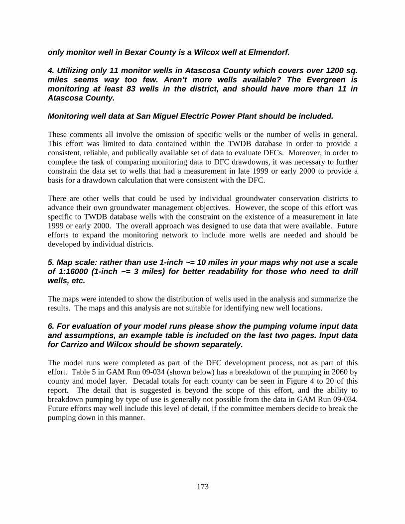
173
only monitor well in Bexar County is a Wilcox well at Elmendorf. 4. Utilizing only 11 monitor wells in Atascosa County which covers over 1200 sq. miles seems way too few. Aren’t more wells available? The Evergreen is monitoring at least 83 wells in the district, and should have more than 11 in Atascosa County. Monitoring well data at San Miguel Electric Power Plant should be included. These comments all involve the omission of specific wells or the number of wells in general. This effort was limited to data contained within the TWDB database in order to provide a consistent, reliable, and publically available set of data to evaluate DFCs. Moreover, in order to complete the task of comparing monitoring data to DFC drawdowns, it was necessary to further constrain the data set to wells that had a measurement in late 1999 or early 2000 to provide a basis for a drawdown calculation that were consistent with the DFC. There are other wells that could be used by individual groundwater conservation districts to advance their own groundwater management objectives. However, the scope of this effort was specific to TWDB database wells with the constraint on the existence of a measurement in late 1999 or early 2000. The overall approach was designed to use data that were available. Future efforts to expand the monitoring network to include more wells are needed and should be developed by individual districts. 5. Map scale: rather than use 1-inch ~= 10 miles in your maps why not use a scale of 1:16000 (1-inch ~= 3 miles) for better readability for those who need to drill wells, etc. The maps were intended to show the distribution of wells used in the analysis and summarize the results. The maps and this analysis are not suitable for identifying new well locations. 6. For evaluation of your model runs please show the pumping volume input data and assumptions, an example table is included on the last two pages. Input data for Carrizo and Wilcox should be shown separately. The model runs were completed as part of the DFC development process, not as part of this effort. Table 5 in GAM Run 09-034 (shown below) has a breakdown of the pumping in 2060 by county and model layer. Decadal totals for each county can be seen in Figure 4 to 20 of this report. The detail that is suggested is beyond the scope of this effort, and the ability to breakdown pumping by type of use is generally not possible from the data in GAM Run 09-034. Future efforts may well include this level of detail, if the committee members decide to break the pumping down in this manner.
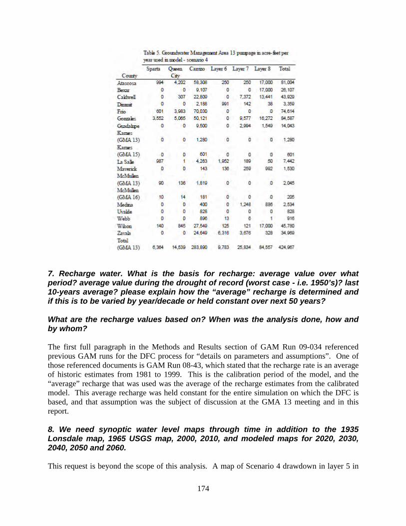
174
7. Recharge water. What is the basis for recharge: average value over what period? average value during the drought of record (worst case - i.e. 1950’s)? last 10-years average? please explain how the “average” recharge is determined and if this is to be varied by year/decade or held constant over next 50 years? What are the recharge values based on? When was the analysis done, how and by whom? The first full paragraph in the Methods and Results section of GAM Run 09-034 referenced previous GAM runs for the DFC process for “details on parameters and assumptions”. One of those referenced documents is GAM Run 08-43, which stated that the recharge rate is an average of historic estimates from 1981 to 1999. This is the calibration period of the model, and the “average” recharge that was used was the average of the recharge estimates from the calibrated model. This average recharge was held constant for the entire simulation on which the DFC is based, and that assumption was the subject of discussion at the GMA 13 meeting and in this report. 8. We need synoptic water level maps through time in addition to the 1935 Lonsdale map, 1965 USGS map, 2000, 2010, and modeled maps for 2020, 2030, 2040, 2050 and 2060. This request is beyond the scope of this analysis. A map of Scenario 4 drawdown in layer 5 in
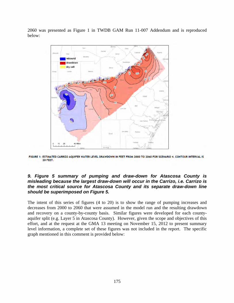
175
2060 was presented as Figure 1 in TWDB GAM Run 11-007 Addendum and is reproduced below:
9. Figure 5 summary of pumping and draw-down for Atascosa County is misleading because the largest draw-down will occur in the Carrizo, i.e. Carrizo is the most critical source for Atascosa County and its separate draw-down line should be superimposed on Figure 5. The intent of this series of figures (4 to 20) is to show the range of pumping increases and decreases from 2000 to 2060 that were assumed in the model run and the resulting drawdown and recovery on a county-by-county basis. Similar figures were developed for each county-aquifer split (e.g. Layer 5 in Atascosa County). However, given the scope and objectives of this effort, and at the request at the GMA 13 meeting on November 15, 2012 to present summary level information, a complete set of these figures was not included in the report. The specific graph mentioned in this comment is provided below:
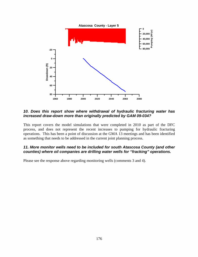
176
80,000
60,000
40,000
20,000
0
Pu
mp
ing
(A
F/y
r)
80
60
40
20
0
-20D
raw
do
wn
(ft
)
1960 1980 2000 2020 2040 2060 2080
Atascosa County - Layer 5
10. Does this report show where withdrawal of hydraulic fracturing water has increased draw-down more than originally predicted by GAM 09-034? This report covers the model simulations that were completed in 2010 as part of the DFC process, and does not represent the recent increases to pumping for hydraulic fracturing operations. This has been a point of discussion at the GMA 13 meetings and has been identified as something that needs to be addressed in the current joint planning process. 11. More monitor wells need to be included for south Atascosa County (and other counties) where oil companies are drilling water wells for “fracking” operations. Please see the response above regarding monitoring wells (comments 3 and 4).
177
Comments from Lou Rosenberg and James Bene Mr. Rosenberg’s comments summarizing Mr. Bene’s comment: DEVELOPING details, but not necessarily completed and sufficient upon which to make major, life defining decisions. In polite terms, we have a distance to travel for greater courtroom reliability. But progress is in motion, however it is incomplete. Mr. Bene’s comments: The general consensus is that generating written comments on the report wouldn’t be meaningful or helpful at this time because the Board is going to ignore it anyway. My primary beef with the report is that it attempts to draw meaningful conclusions by comparing real‐world water level measurements to DFC Scenario 4 model outputs, which is absurd because the pumpage in the model doesn’t correspond to real‐world pumpage. However, it sounded to me during the last meeting that Bill and everyone else now understands that in order to gage the model’s performance over the last decade then real pumpage numbers need to be input. That’s what they’re working on now: the districts are compiling pumpage records and Bill will decipher their data, insert it into the model, and then make another report. One of the objectives stated in the report was to “use the findings in the next round of joint planning (i.e. desired future condition development) to make the process more efficient, less costly, and more defendable.” This effort identified specific areas where the model simulations that will be used in the current round of joint planning can be improved (e.g. pumping from 2000 to present), and, thus, advance the stated objective.
Appendix D
Water Supply Needs and Water Management Strategies Data
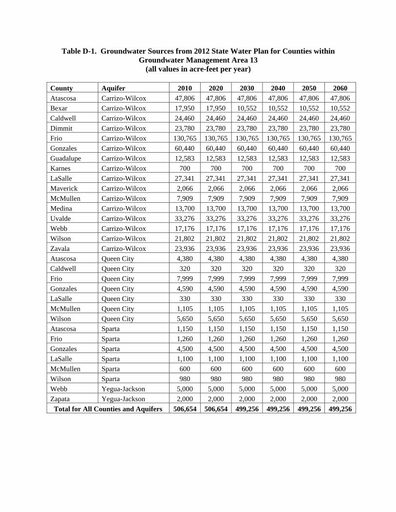
Table D-1. Groundwater Sources from 2012 State Water Plan for Counties within Groundwater Management Area 13
(all values in acre-feet per year)
County Aquifer 2010 2020 2030 2040 2050 2060
Atascosa Carrizo-Wilcox 47,806 47,806 47,806 47,806 47,806 47,806
Bexar Carrizo-Wilcox 17,950 17,950 10,552 10,552 10,552 10,552
Caldwell Carrizo-Wilcox 24,460 24,460 24,460 24,460 24,460 24,460
Dimmit Carrizo-Wilcox 23,780 23,780 23,780 23,780 23,780 23,780
Frio Carrizo-Wilcox 130,765 130,765 130,765 130,765 130,765 130,765
Gonzales Carrizo-Wilcox 60,440 60,440 60,440 60,440 60,440 60,440
Guadalupe Carrizo-Wilcox 12,583 12,583 12,583 12,583 12,583 12,583
Karnes Carrizo-Wilcox 700 700 700 700 700 700
LaSalle Carrizo-Wilcox 27,341 27,341 27,341 27,341 27,341 27,341
Maverick Carrizo-Wilcox 2,066 2,066 2,066 2,066 2,066 2,066
McMullen Carrizo-Wilcox 7,909 7,909 7,909 7,909 7,909 7,909
Medina Carrizo-Wilcox 13,700 13,700 13,700 13,700 13,700 13,700
Uvalde Carrizo-Wilcox 33,276 33,276 33,276 33,276 33,276 33,276
Webb Carrizo-Wilcox 17,176 17,176 17,176 17,176 17,176 17,176
Wilson Carrizo-Wilcox 21,802 21,802 21,802 21,802 21,802 21,802
Zavala Carrizo-Wilcox 23,936 23,936 23,936 23,936 23,936 23,936
Atascosa Queen City 4,380 4,380 4,380 4,380 4,380 4,380
Caldwell Queen City 320 320 320 320 320 320
Frio Queen City 7,999 7,999 7,999 7,999 7,999 7,999
Gonzales Queen City 4,590 4,590 4,590 4,590 4,590 4,590
LaSalle Queen City 330 330 330 330 330 330
McMullen Queen City 1,105 1,105 1,105 1,105 1,105 1,105
Wilson Queen City 5,650 5,650 5,650 5,650 5,650 5,650
Atascosa Sparta 1,150 1,150 1,150 1,150 1,150 1,150
Frio Sparta 1,260 1,260 1,260 1,260 1,260 1,260
Gonzales Sparta 4,500 4,500 4,500 4,500 4,500 4,500
LaSalle Sparta 1,100 1,100 1,100 1,100 1,100 1,100
McMullen Sparta 600 600 600 600 600 600
Wilson Sparta 980 980 980 980 980 980
Webb Yegua-Jackson 5,000 5,000 5,000 5,000 5,000 5,000
Zapata Yegua-Jackson 2,000 2,000 2,000 2,000 2,000 2,000
Total for All Counties and Aquifers 506,654 506,654 499,256 499,256 499,256 499,256
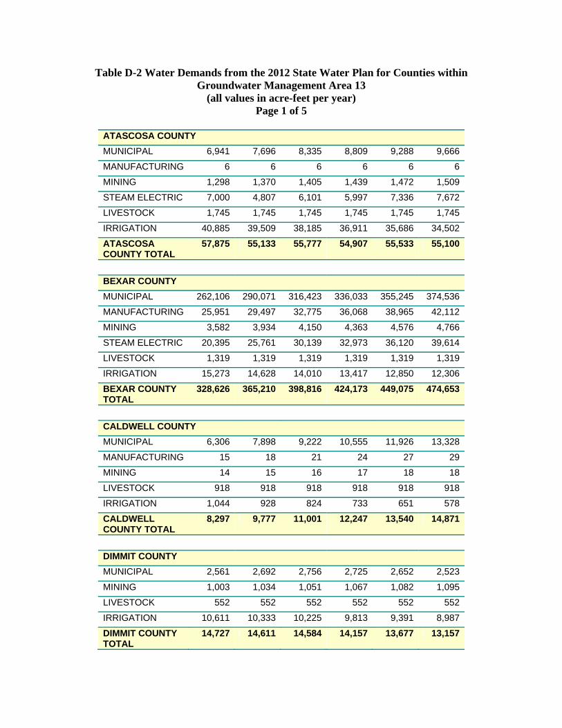
Table D-2 Water Demands from the 2012 State Water Plan for Counties within Groundwater Management Area 13
(all values in acre-feet per year) Page 1 of 5
ATASCOSA COUNTY
MUNICIPAL 6,941 7,696 8,335 8,809 9,288 9,666
MANUFACTURING 6 6 6 6 6 6
MINING 1,298 1,370 1,405 1,439 1,472 1,509
STEAM ELECTRIC 7,000 4,807 6,101 5,997 7,336 7,672
LIVESTOCK 1,745 1,745 1,745 1,745 1,745 1,745
IRRIGATION 40,885 39,509 38,185 36,911 35,686 34,502
ATASCOSA COUNTY TOTAL
57,875 55,133 55,777 54,907 55,533 55,100
BEXAR COUNTY
MUNICIPAL 262,106 290,071 316,423 336,033 355,245 374,536
MANUFACTURING 25,951 29,497 32,775 36,068 38,965 42,112
MINING 3,582 3,934 4,150 4,363 4,576 4,766
STEAM ELECTRIC 20,395 25,761 30,139 32,973 36,120 39,614
LIVESTOCK 1,319 1,319 1,319 1,319 1,319 1,319
IRRIGATION 15,273 14,628 14,010 13,417 12,850 12,306
BEXAR COUNTY TOTAL
328,626 365,210 398,816 424,173 449,075 474,653
CALDWELL COUNTY
MUNICIPAL 6,306 7,898 9,222 10,555 11,926 13,328
MANUFACTURING 15 18 21 24 27 29
MINING 14 15 16 17 18 18
LIVESTOCK 918 918 918 918 918 918
IRRIGATION 1,044 928 824 733 651 578
CALDWELL COUNTY TOTAL
8,297 9,777 11,001 12,247 13,540 14,871
DIMMIT COUNTY
MUNICIPAL 2,561 2,692 2,756 2,725 2,652 2,523
MINING 1,003 1,034 1,051 1,067 1,082 1,095
LIVESTOCK 552 552 552 552 552 552
IRRIGATION 10,611 10,333 10,225 9,813 9,391 8,987
DIMMIT COUNTY TOTAL
14,727 14,611 14,584 14,157 13,677 13,157
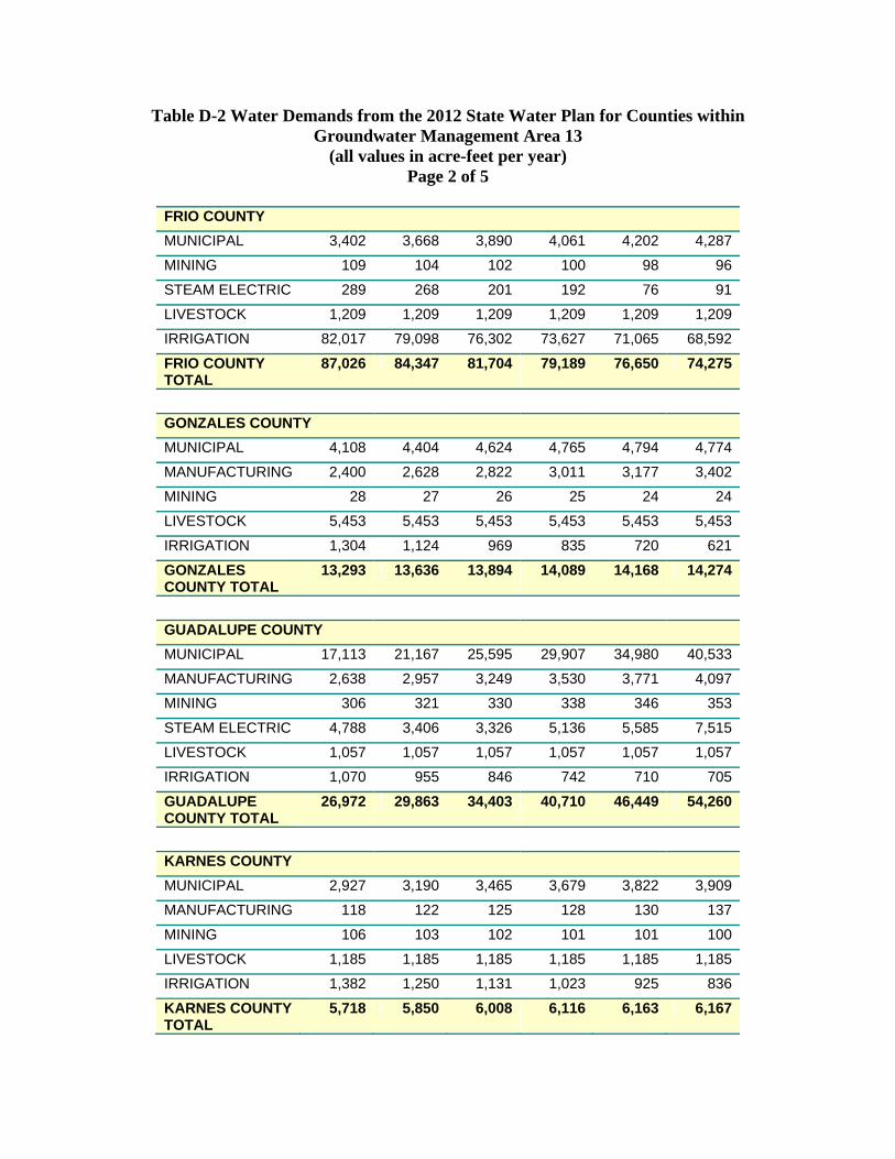
Table D-2 Water Demands from the 2012 State Water Plan for Counties within Groundwater Management Area 13
(all values in acre-feet per year) Page 2 of 5
FRIO COUNTY
MUNICIPAL 3,402 3,668 3,890 4,061 4,202 4,287
MINING 109 104 102 100 98 96
STEAM ELECTRIC 289 268 201 192 76 91
LIVESTOCK 1,209 1,209 1,209 1,209 1,209 1,209
IRRIGATION 82,017 79,098 76,302 73,627 71,065 68,592
FRIO COUNTY TOTAL
87,026 84,347 81,704 79,189 76,650 74,275
GONZALES COUNTY
MUNICIPAL 4,108 4,404 4,624 4,765 4,794 4,774
MANUFACTURING 2,400 2,628 2,822 3,011 3,177 3,402
MINING 28 27 26 25 24 24
LIVESTOCK 5,453 5,453 5,453 5,453 5,453 5,453
IRRIGATION 1,304 1,124 969 835 720 621
GONZALES COUNTY TOTAL
13,293 13,636 13,894 14,089 14,168 14,274
GUADALUPE COUNTY
MUNICIPAL 17,113 21,167 25,595 29,907 34,980 40,533
MANUFACTURING 2,638 2,957 3,249 3,530 3,771 4,097
MINING 306 321 330 338 346 353
STEAM ELECTRIC 4,788 3,406 3,326 5,136 5,585 7,515
LIVESTOCK 1,057 1,057 1,057 1,057 1,057 1,057
IRRIGATION 1,070 955 846 742 710 705
GUADALUPE COUNTY TOTAL
26,972 29,863 34,403 40,710 46,449 54,260
KARNES COUNTY
MUNICIPAL 2,927 3,190 3,465 3,679 3,822 3,909
MANUFACTURING 118 122 125 128 130 137
MINING 106 103 102 101 101 100
LIVESTOCK 1,185 1,185 1,185 1,185 1,185 1,185
IRRIGATION 1,382 1,250 1,131 1,023 925 836
KARNES COUNTY TOTAL
5,718 5,850 6,008 6,116 6,163 6,167
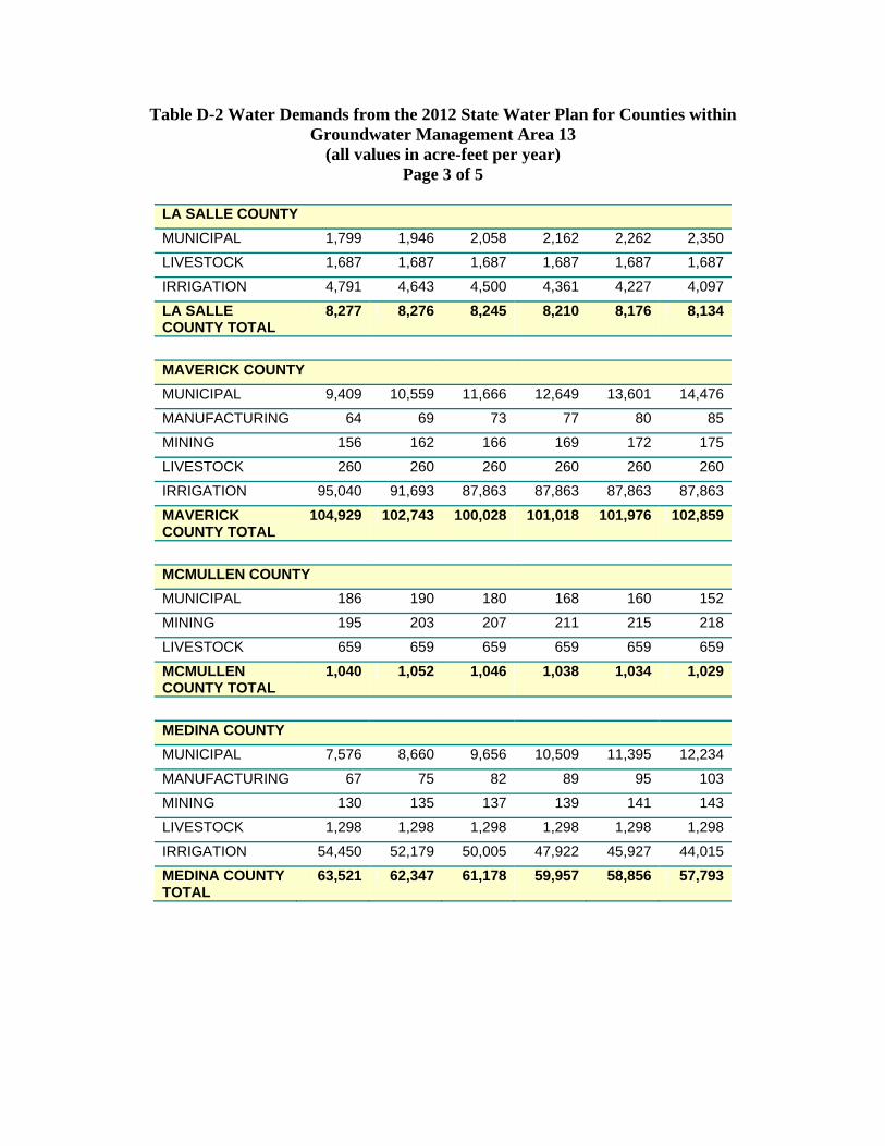
Table D-2 Water Demands from the 2012 State Water Plan for Counties within Groundwater Management Area 13
(all values in acre-feet per year) Page 3 of 5
LA SALLE COUNTY
MUNICIPAL 1,799 1,946 2,058 2,162 2,262 2,350
LIVESTOCK 1,687 1,687 1,687 1,687 1,687 1,687
IRRIGATION 4,791 4,643 4,500 4,361 4,227 4,097
LA SALLE COUNTY TOTAL
8,277 8,276 8,245 8,210 8,176 8,134
MAVERICK COUNTY
MUNICIPAL 9,409 10,559 11,666 12,649 13,601 14,476
MANUFACTURING 64 69 73 77 80 85
MINING 156 162 166 169 172 175
LIVESTOCK 260 260 260 260 260 260
IRRIGATION 95,040 91,693 87,863 87,863 87,863 87,863
MAVERICK COUNTY TOTAL
104,929 102,743 100,028 101,018 101,976 102,859
MCMULLEN COUNTY
MUNICIPAL 186 190 180 168 160 152
MINING 195 203 207 211 215 218
LIVESTOCK 659 659 659 659 659 659
MCMULLEN COUNTY TOTAL
1,040 1,052 1,046 1,038 1,034 1,029
MEDINA COUNTY
MUNICIPAL 7,576 8,660 9,656 10,509 11,395 12,234
MANUFACTURING 67 75 82 89 95 103
MINING 130 135 137 139 141 143
LIVESTOCK 1,298 1,298 1,298 1,298 1,298 1,298
IRRIGATION 54,450 52,179 50,005 47,922 45,927 44,015
MEDINA COUNTY TOTAL
63,521 62,347 61,178 59,957 58,856 57,793
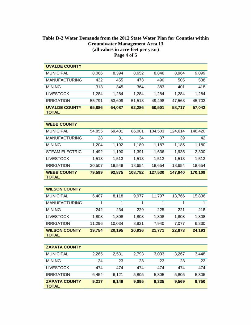
Table D-2 Water Demands from the 2012 State Water Plan for Counties within
Groundwater Management Area 13 (all values in acre-feet per year)
Page 4 of 5
UVALDE COUNTY
MUNICIPAL 8,066 8,394 8,652 8,846 8,964 9,099
MANUFACTURING 432 455 473 490 505 538
MINING 313 345 364 383 401 418
LIVESTOCK 1,284 1,284 1,284 1,284 1,284 1,284
IRRIGATION 55,791 53,609 51,513 49,498 47,563 45,703
UVALDE COUNTY TOTAL
65,886 64,087 62,286 60,501 58,717 57,042
WEBB COUNTY
MUNICIPAL 54,855 69,401 86,001 104,503 124,614 146,420
MANUFACTURING 28 31 34 37 39 42
MINING 1,204 1,192 1,189 1,187 1,185 1,180
STEAM ELECTRIC 1,492 1,190 1,391 1,636 1,935 2,300
LIVESTOCK 1,513 1,513 1,513 1,513 1,513 1,513
IRRIGATION 20,507 19,548 18,654 18,654 18,654 18,654
WEBB COUNTY TOTAL
79,599 92,875 108,782 127,530 147,940 170,109
WILSON COUNTY
MUNICIPAL 6,407 8,118 9,977 11,797 13,766 15,836
MANUFACTURING 1 1 1 1 1 1
MINING 242 234 229 225 221 218
LIVESTOCK 1,808 1,808 1,808 1,808 1,808 1,808
IRRIGATION 11,296 10,034 8,921 7,940 7,077 6,330
WILSON COUNTY TOTAL
19,754 20,195 20,936 21,771 22,873 24,193
ZAPATA COUNTY
MUNICIPAL 2,265 2,531 2,793 3,033 3,267 3,448
MINING 24 23 23 23 23 23
LIVESTOCK 474 474 474 474 474 474
IRRIGATION 6,454 6,121 5,805 5,805 5,805 5,805
ZAPATA COUNTY TOTAL
9,217 9,149 9,095 9,335 9,569 9,750

Table D-2 Water Demands from the 2012 State Water Plan for Counties within Groundwater Management Area 13
(all values in acre-feet per year) Page 5 of 5
ZAVALA COUNTY
MUNICIPAL 3,111 3,300 3,477 3,578 3,676 3,741
MANUFACTURING 1,043 1,106 1,154 1,200 1,238 1,315
MINING 122 125 127 128 129 130
LIVESTOCK 756 756 756 756 756 756
IRRIGATION 71,800 68,963 66,238 63,621 61,107 58,692
ZAVALA COUNTY TOTAL
76,832 74,250 71,752 69,283 66,906 64,634
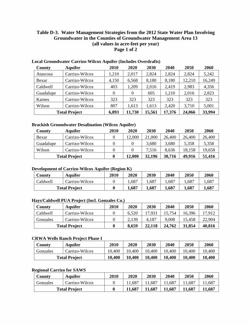
Table D-3. Water Management Strategies from the 2012 State Water Plan Involving Groundwater in the Counties of Groundwater Management Area 13
(all values in acre-feet per year) Page 1 of 2
Local Groundwater Carrizo-Wilcox Aquifer (Includes Overdrafts)
County Aquifer 2010 2020 2030 2040 2050 2060
Atascosa Carrizo-Wilcox 1,210 2,017 2,824 2,824 2,824 5,242
Bexar Carrizo-Wilcox 4,150 6,568 8,180 8,180 12,210 16,249
Caldwell Carrizo-Wilcox 403 1,209 2,016 2,419 2,983 4,356
Guadalupe Carrizo-Wilcox 0 0 605 1,210 2,016 2,823
Karnes Carrizo-Wilcox 323 323 323 323 323 323
Wilson Carrizo-Wilcox 807 1,613 1,613 2,420 3,710 5,001
Total Project 6,893 11,730 15,561 17,376 24,066 33,994
Brackish Groundwater Desalination (Wilcox Aquifer)
County Aquifer 2010 2020 2030 2040 2050 2060
Bexar Carrizo-Wilcox 0 12,000 21,000 26,400 26,400 26,400
Guadalupe Carrizo-Wilcox 0 0 3,680 3,680 5,358 5,358
Wilson Carrizo-Wilcox 0 0 7,516 8,636 18,158 19,658
Total Project 0 12,000 32,196 38,716 49,916 51,416
Development of Carrizo-Wilcox Aquifer (Region K)
County Aquifer 2010 2020 2030 2040 2050 2060
Caldwell Carrizo-Wilcox 0 1,687 1,687 1,687 1,687 1,687
Total Project 0 1,687 1,687 1,687 1,687 1,687
Hays/Caldwell PUA Project (Incl. Gonzales Co.)
County Aquifer 2010 2020 2030 2040 2050 2060
Caldwell Carrizo-Wilcox 0 6,520 17,931 15,754 16,396 17,912
Gonzales Carrizo-Wilcox 0 2,139 4,187 9,008 15,458 22,904
Total Project 0 8,659 22,118 24,762 31,854 40,816
CRWA Wells Ranch Project Phase I
County Aquifer 2010 2020 2030 2040 2050 2060
Gonzales Carrizo-Wilcox 10,400 10,400 10,400 10,400 10,400 10,400
Total Project 10,400 10,400 10,400 10,400 10,400 10,400
Regional Carrizo for SAWS
County Aquifer 2010 2020 2030 2040 2050 2060
Gonzales Carrizo-Wilcox 0 11,687 11,687 11,687 11,687 11,687
Total Project 0 11,687 11,687 11,687 11,687 11,687
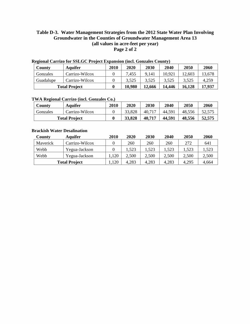
Table D-3. Water Management Strategies from the 2012 State Water Plan Involving Groundwater in the Counties of Groundwater Management Area 13
(all values in acre-feet per year) Page 2 of 2
Regional Carrizo for SSLGC Project Expansion (incl. Gonzales County)
County Aquifer 2010 2020 2030 2040 2050 2060
Gonzales Carrizo-Wilcox 0 7,455 9,141 10,921 12,603 13,678
Guadalupe Carrizo-Wilcox 0 3,525 3,525 3,525 3,525 4,259
Total Project 0 10,980 12,666 14,446 16,128 17,937
TWA Regional Carrizo (incl. Gonzales Co.)
County Aquifer 2010 2020 2030 2040 2050 2060
Gonzales Carrizo-Wilcox 0 33,828 40,717 44,591 48,556 52,575
Total Project 0 33,828 40,717 44,591 48,556 52,575
Brackish Water Desalination
County Aquifer 2010 2020 2030 2040 2050 2060
Maverick Carrizo-Wilcox 0 260 260 260 272 641
Webb Yegua-Jackson 0 1,523 1,523 1,523 1,523 1,523
Webb Yegua-Jackson 1,120 2,500 2,500 2,500 2,500 2,500
Total Project 1,120 4,283 4,283 4,283 4,295 4,664
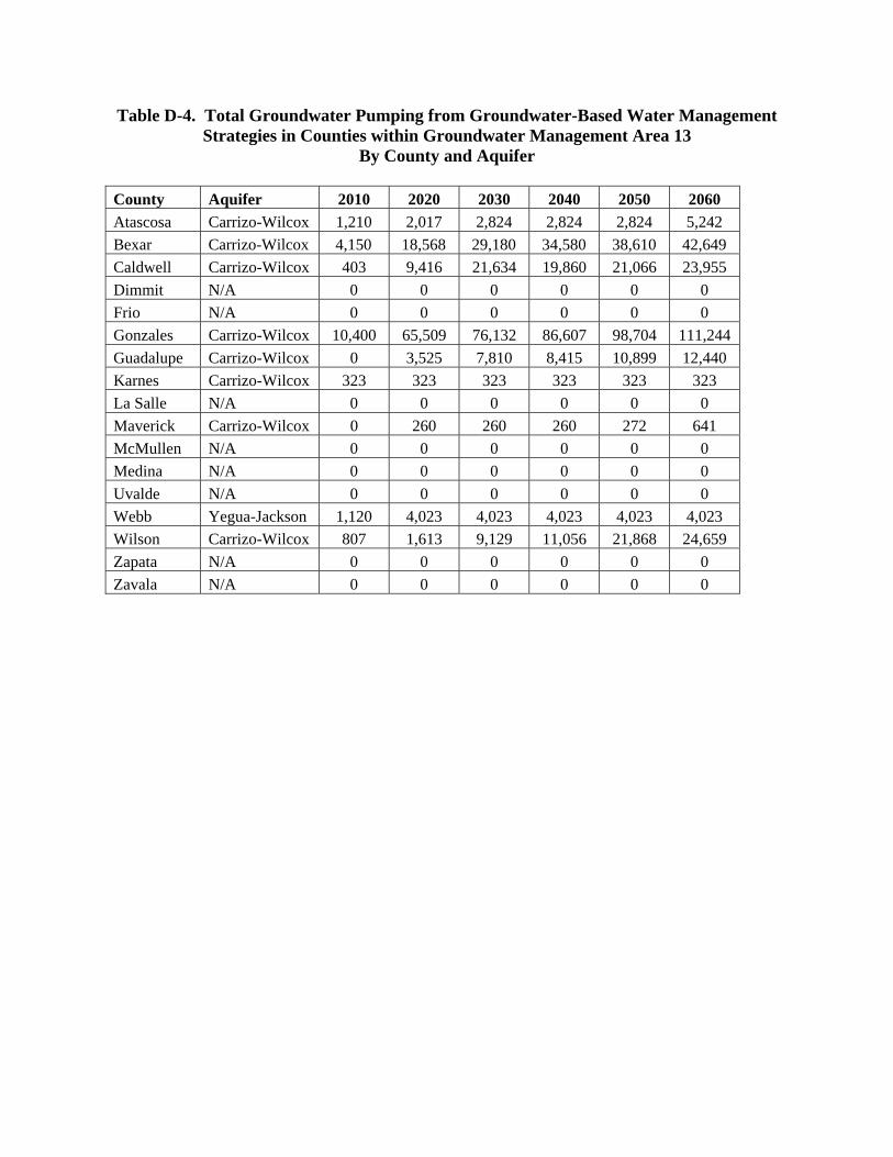
Table D-4. Total Groundwater Pumping from Groundwater-Based Water Management Strategies in Counties within Groundwater Management Area 13
By County and Aquifer
County Aquifer 2010 2020 2030 2040 2050 2060
Atascosa Carrizo-Wilcox 1,210 2,017 2,824 2,824 2,824 5,242
Bexar Carrizo-Wilcox 4,150 18,568 29,180 34,580 38,610 42,649
Caldwell Carrizo-Wilcox 403 9,416 21,634 19,860 21,066 23,955
Dimmit N/A 0 0 0 0 0 0
Frio N/A 0 0 0 0 0 0
Gonzales Carrizo-Wilcox 10,400 65,509 76,132 86,607 98,704 111,244
Guadalupe Carrizo-Wilcox 0 3,525 7,810 8,415 10,899 12,440
Karnes Carrizo-Wilcox 323 323 323 323 323 323
La Salle N/A 0 0 0 0 0 0
Maverick Carrizo-Wilcox 0 260 260 260 272 641
McMullen N/A 0 0 0 0 0 0
Medina N/A 0 0 0 0 0 0
Uvalde N/A 0 0 0 0 0 0
Webb Yegua-Jackson 1,120 4,023 4,023 4,023 4,023 4,023
Wilson Carrizo-Wilcox 807 1,613 9,129 11,056 21,868 24,659
Zapata N/A 0 0 0 0 0 0
Zavala N/A 0 0 0 0 0 0
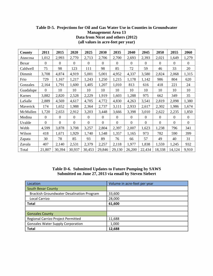
Table D-5. Projections for Oil and Gas Water Use in Counties in Groundwater Management Area 13
Data from Nicot and others (2012) (all values in acre-feet per year)
County 2011 2015 2020 2025 2030 2035 2040 2045 2050 2055 2060
Atascosa 1,012 2,993 2,770 2,713 2,706 2,700 2,693 2,393 2,021 1,649 1,279
Bexar 0 0 0 0 0 0 0 0 0 0 0
Caldwell 75 98 123 111 98 85 72 59 46 33 20
Dimmit 3,708 4,874 4,919 5,001 5,001 4,952 4,337 3,580 2,824 2,068 1,315
Frio 729 1,167 1,217 1,243 1,250 1,215 1,178 1,142 986 804 620
Gonzales 2,164 1,791 1,600 1,405 1,207 1,010 813 616 418 221 24
Guadalupe 0 10 10 10 10 10 10 10 10 10 10
Karnes 3,882 2,820 2,528 2,229 1,919 1,603 1,288 975 662 349 35
LaSalle 2,889 4,569 4,617 4,705 4,772 4,830 4,263 3,541 2,819 2,098 1,380
Maverick 174 1,652 1,988 2,364 2,737 3,111 2,933 2,617 2,302 1,986 1,674
McMullen 1,720 2,653 2,912 3,203 3,448 3,666 3,398 3,010 2,622 2,235 1,850
Medina 0 0 0 0 0 0 0 0 0 0 0
Uvalde 0 0 0 0 0 0 0 0 0 0 0
Webb 4,599 3,878 3,708 3,257 2,804 2,397 2,007 1,623 1,238 796 341
Wilson 418 1,671 1,929 1,740 1,548 1,357 1,165 973 782 590 399
Zapata 30 78 85 93 89 76 66 57 49 40 31
Zavala 407 2,140 2,531 2,379 2,257 2,118 1,977 1,838 1,559 1,245 932
Total 21,807 30,394 30,937 30,453 29,846 29,130 26,200 22,434 18,338 14,124 9,910
Table D-6. Submitted Updates to Future Pumping by SAWS Submitted on June 27, 2013 via email by Steven Siebert
Location Volume in acre‐feet per year South Bexar County Brackish Groundwater Desalination Program 33,600 Local Carrizo 28,000 Total 61,600 Gonzales County Regional Carrizo Project Permitted 11,688 Gonzales Water Supply Corporation 1,000 Total 12,688
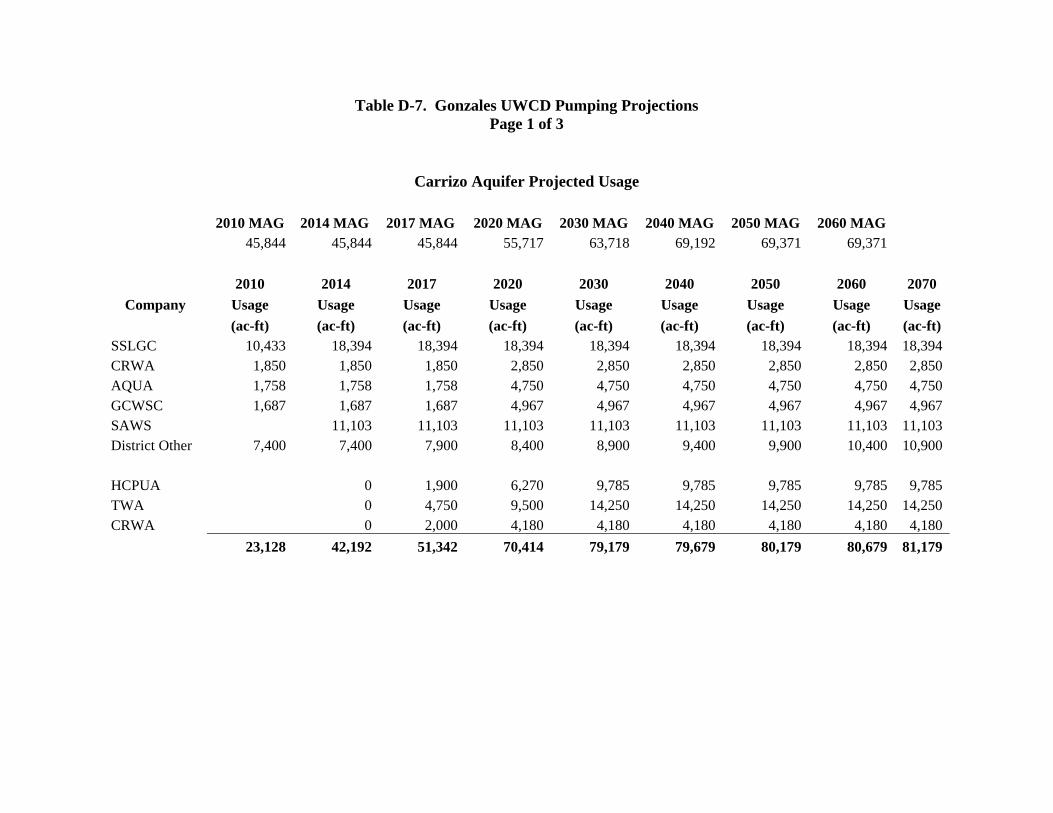
Table D-7. Gonzales UWCD Pumping Projections Page 1 of 3
Carrizo Aquifer Projected Usage
2010 MAG 2014 MAG 2017 MAG 2020 MAG 2030 MAG 2040 MAG 2050 MAG 2060 MAG 45,844 45,844 45,844 55,717 63,718 69,192 69,371 69,371
2010 2014 2017 2020 2030 2040 2050 2060 2070
Company Usage Usage Usage Usage Usage Usage Usage Usage Usage
(ac-ft) (ac-ft) (ac-ft) (ac-ft) (ac-ft) (ac-ft) (ac-ft) (ac-ft) (ac-ft) SSLGC 10,433 18,394 18,394 18,394 18,394 18,394 18,394 18,394 18,394CRWA 1,850 1,850 1,850 2,850 2,850 2,850 2,850 2,850 2,850AQUA 1,758 1,758 1,758 4,750 4,750 4,750 4,750 4,750 4,750GCWSC 1,687 1,687 1,687 4,967 4,967 4,967 4,967 4,967 4,967SAWS 11,103 11,103 11,103 11,103 11,103 11,103 11,103 11,103District Other 7,400 7,400 7,900 8,400 8,900 9,400 9,900 10,400 10,900
HCPUA 0 1,900 6,270 9,785 9,785 9,785 9,785 9,785TWA 0 4,750 9,500 14,250 14,250 14,250 14,250 14,250CRWA 0 2,000 4,180 4,180 4,180 4,180 4,180 4,180
23,128 42,192 51,342 70,414 79,179 79,679 80,179 80,679 81,179
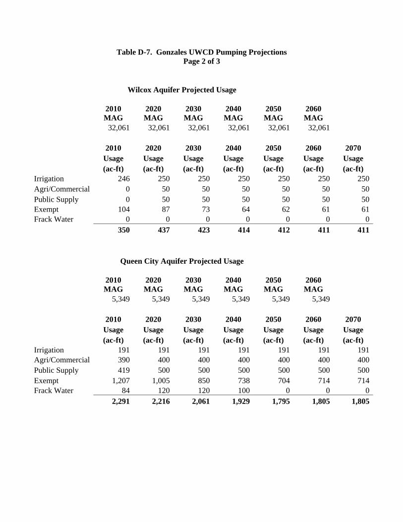
Table D-7. Gonzales UWCD Pumping Projections Page 2 of 3
Wilcox Aquifer Projected Usage
2010 MAG
2020 MAG
2030 MAG
2040 MAG
2050 MAG
2060 MAG
32,061 32,061 32,061 32,061 32,061 32,061
2010 2020 2030 2040 2050 2060 2070 Usage Usage Usage Usage Usage Usage Usage (ac-ft) (ac-ft) (ac-ft) (ac-ft) (ac-ft) (ac-ft) (ac-ft)
Irrigation 246 250 250 250 250 250 250Agri/Commercial 0 50 50 50 50 50 50Public Supply 0 50 50 50 50 50 50Exempt 104 87 73 64 62 61 61Frack Water 0 0 0 0 0 0 0
350 437 423 414 412 411 411
Queen City Aquifer Projected Usage
2010 MAG
2020 MAG
2030 MAG
2040 MAG
2050 MAG
2060 MAG
5,349 5,349 5,349 5,349 5,349 5,349
2010 2020 2030 2040 2050 2060 2070 Usage Usage Usage Usage Usage Usage Usage (ac-ft) (ac-ft) (ac-ft) (ac-ft) (ac-ft) (ac-ft) (ac-ft)
Irrigation 191 191 191 191 191 191 191Agri/Commercial 390 400 400 400 400 400 400Public Supply 419 500 500 500 500 500 500Exempt 1,207 1,005 850 738 704 714 714Frack Water 84 120 120 100 0 0 0
2,291 2,216 2,061 1,929 1,795 1,805 1,805
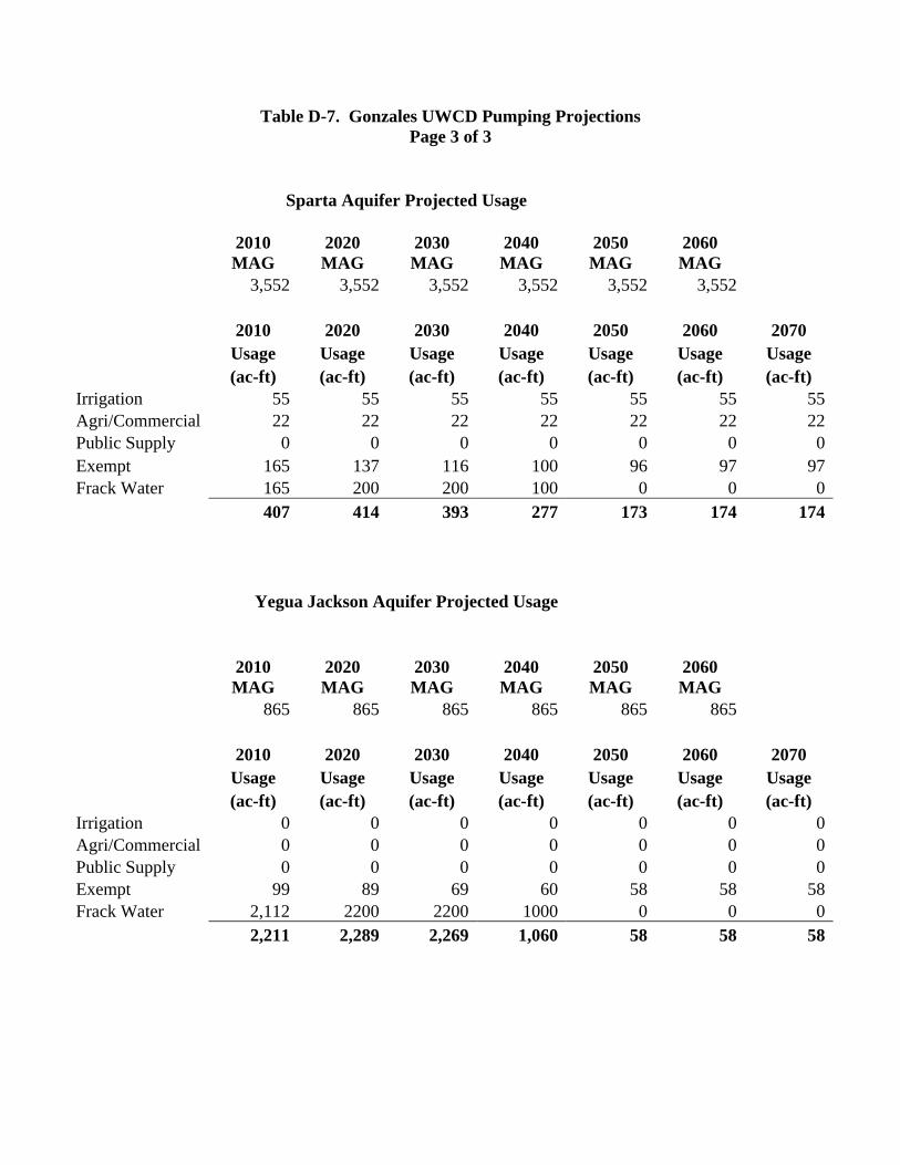
Table D-7. Gonzales UWCD Pumping Projections Page 3 of 3
Sparta Aquifer Projected Usage
2010 MAG
2020 MAG
2030 MAG
2040 MAG
2050 MAG
2060 MAG
3,552 3,552 3,552 3,552 3,552 3,552
2010 2020 2030 2040 2050 2060 2070 Usage Usage Usage Usage Usage Usage Usage (ac-ft) (ac-ft) (ac-ft) (ac-ft) (ac-ft) (ac-ft) (ac-ft)
Irrigation 55 55 55 55 55 55 55Agri/Commercial 22 22 22 22 22 22 22Public Supply 0 0 0 0 0 0 0Exempt 165 137 116 100 96 97 97Frack Water 165 200 200 100 0 0 0
407 414 393 277 173 174 174
Yegua Jackson Aquifer Projected Usage
2010 MAG
2020 MAG
2030 MAG
2040 MAG
2050 MAG
2060 MAG
865 865 865 865 865 865
2010 2020 2030 2040 2050 2060 2070 Usage Usage Usage Usage Usage Usage Usage (ac-ft) (ac-ft) (ac-ft) (ac-ft) (ac-ft) (ac-ft) (ac-ft)
Irrigation 0 0 0 0 0 0 0Agri/Commercial 0 0 0 0 0 0 0Public Supply 0 0 0 0 0 0 0Exempt 99 89 69 60 58 58 58Frack Water 2,112 2200 2200 1000 0 0 0
2,211 2,289 2,269 1,060 58 58 58
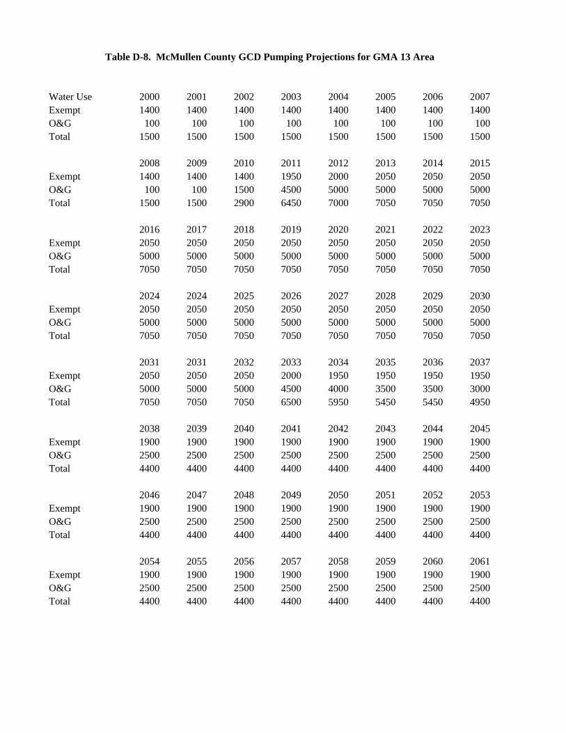
Water Use 2000 2001 2002 2003 2004 2005 2006 2007Exempt 1400 1400 1400 1400 1400 1400 1400 1400O&G 100 100 100 100 100 100 100 100Total 1500 1500 1500 1500 1500 1500 1500 1500
2008 2009 2010 2011 2012 2013 2014 2015Exempt 1400 1400 1400 1950 2000 2050 2050 2050O&G 100 100 1500 4500 5000 5000 5000 5000Total 1500 1500 2900 6450 7000 7050 7050 7050
2016 2017 2018 2019 2020 2021 2022 2023Exempt 2050 2050 2050 2050 2050 2050 2050 2050O&G 5000 5000 5000 5000 5000 5000 5000 5000Total 7050 7050 7050 7050 7050 7050 7050 7050
2024 2024 2025 2026 2027 2028 2029 2030Exempt 2050 2050 2050 2050 2050 2050 2050 2050O&G 5000 5000 5000 5000 5000 5000 5000 5000Total 7050 7050 7050 7050 7050 7050 7050 7050
2031 2031 2032 2033 2034 2035 2036 2037Exempt 2050 2050 2050 2000 1950 1950 1950 1950O&G 5000 5000 5000 4500 4000 3500 3500 3000Total 7050 7050 7050 6500 5950 5450 5450 4950
2038 2039 2040 2041 2042 2043 2044 2045Exempt 1900 1900 1900 1900 1900 1900 1900 1900O&G 2500 2500 2500 2500 2500 2500 2500 2500Total 4400 4400 4400 4400 4400 4400 4400 4400
2046 2047 2048 2049 2050 2051 2052 2053Exempt 1900 1900 1900 1900 1900 1900 1900 1900O&G 2500 2500 2500 2500 2500 2500 2500 2500Total 4400 4400 4400 4400 4400 4400 4400 4400
2054 2055 2056 2057 2058 2059 2060 2061Exempt 1900 1900 1900 1900 1900 1900 1900 1900O&G 2500 2500 2500 2500 2500 2500 2500 2500Total 4400 4400 4400 4400 4400 4400 4400 4400
Table D-8. McMullen County GCD Pumping Projections for GMA 13 Area
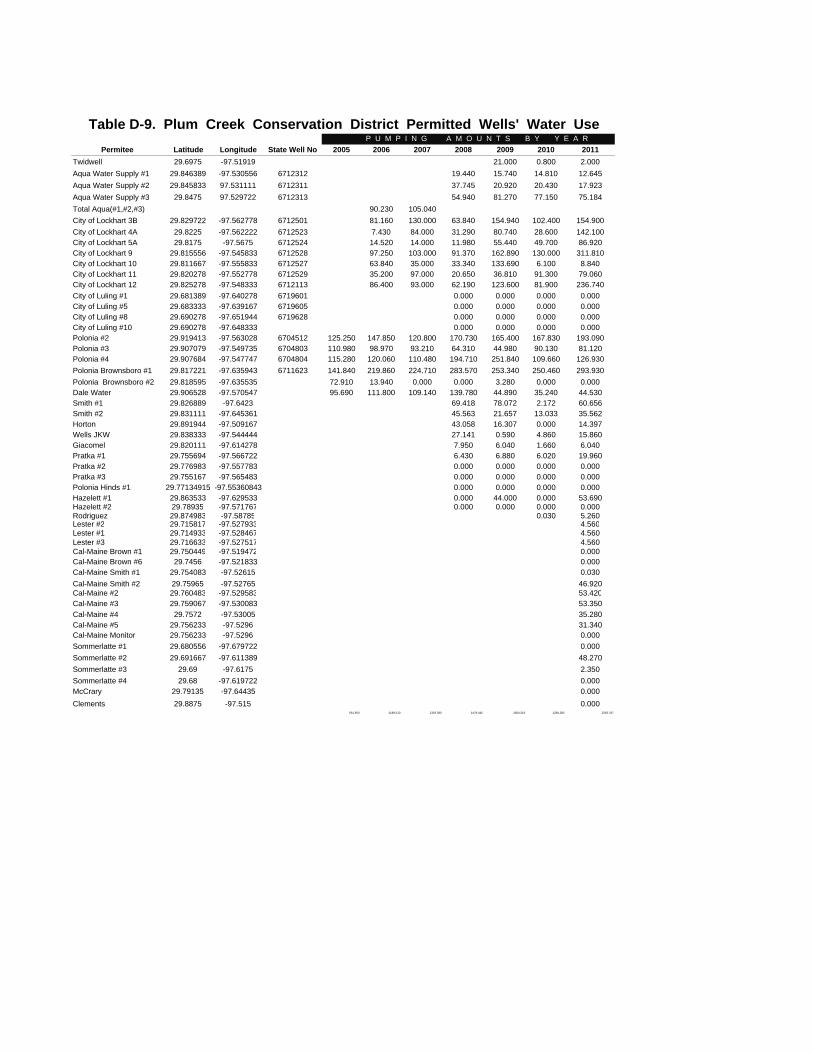
P U M P I N G A M O U N T S B Y Y E A R
Permitee Latitude Longitude State Well No 2005 2006 2007 2008 2009 2010 2011
Twidwell 29.6975 -97.51919 21.000 0.800 2.000
Aqua Water Supply #1 29.846389 -97.530556 6712312 19.440 15.740 14.810 12.645
Aqua Water Supply #2 29.845833 97.531111 6712311 37.745 20.920 20.430 17.923
Aqua Water Supply #3 29.8475 97.529722 6712313 54.940 81.270 77.150 75.184
Total Aqua(#1,#2,#3) 90.230 105.040
City of Lockhart 3B 29.829722 -97.562778 6712501 81.160 130.000 63.840 154.940 102.400 154.900
City of Lockhart 4A 29.8225 -97.562222 6712523 7.430 84.000 31.290 80.740 28.600 142.100City of Lockhart 5A 29.8175 -97.5675 6712524 14.520 14.000 11.980 55.440 49.700 86.920City of Lockhart 9 29.815556 -97.545833 6712528 97.250 103.000 91.370 162.890 130.000 311.810City of Lockhart 10 29.811667 -97.555833 6712527 63.840 35.000 33.340 133.690 6.100 8.840City of Lockhart 11 29.820278 -97.552778 6712529 35.200 97.000 20.650 36.810 91.300 79.060City of Lockhart 12 29.825278 -97.548333 6712113 86.400 93.000 62.190 123.600 81.900 236.740
City of Luling #1 29.681389 -97.640278 6719601 0.000 0.000 0.000 0.000City of Luling #5 29.683333 -97.639167 6719605 0.000 0.000 0.000 0.000City of Luling #8 29.690278 -97.651944 6719628 0.000 0.000 0.000 0.000City of Luling #10 29.690278 -97.648333 0.000 0.000 0.000 0.000Polonia #2 29.919413 -97.563028 6704512 125.250 147.850 120.800 170.730 165.400 167.830 193.090Polonia #3 29.907079 -97.549735 6704803 110.980 98.970 93.210 64.310 44.980 90.130 81.120Polonia #4 29.907684 -97.547747 6704804 115.280 120.060 110.480 194.710 251.840 109.660 126.930
Polonia Brownsboro #1 29.817221 -97.635943 6711623 141.840 219.860 224.710 283.570 253.340 250.460 293.930
Polonia Brownsboro #2 29.818595 -97.635535 72.910 13.940 0.000 0.000 3.280 0.000 0.000Dale Water 29.906528 -97.570547 95.690 111.800 109.140 139.780 44.890 35.240 44.530Smith #1 29.826889 -97.6423 69.418 78.072 2.172 60.656Smith #2 29.831111 -97.645361 45.563 21.657 13.033 35.562Horton 29.891944 -97.509167 43.058 16.307 0.000 14.397Wells JKW 29.838333 -97.544444 27.141 0.590 4.860 15.860Giacomel 29.820111 -97.614278 7.950 6.040 1.660 6.040Pratka #1 29.755694 -97.566722 6.430 6.880 6.020 19.960Pratka #2 29.776983 -97.557783 0.000 0.000 0.000 0.000Pratka #3 29.755167 -97.565483 0.000 0.000 0.000 0.000Polonia Hinds #1 29.77134915 -97.55360843 0.000 0.000 0.000 0.000Hazelett #1 29.863533 -97.629533 0.000 44.000 0.000 53.690Hazelett #2 29.78935 -97.571767 0.000 0.000 0.000 0.000Rodriguez 29.874983 -97.58785 0.030 5.260Lester #2 29.715817 -97.527933 4.560Lester #1 29.714933 -97.528467 4.560Lester #3 29.716633 -97.527517 4.560Cal-Maine Brown #1 29.750449 -97.519472 0.000Cal-Maine Brown #6 29.7456 -97.521833 0.000Cal-Maine Smith #1 29.754083 -97.52615 0.030
Cal-Maine Smith #2 29.75965 -97.52765 46.920Cal-Maine #2 29.760483 -97.529583 53.420Cal-Maine #3 29.759067 -97.530083 53.350
Cal-Maine #4 29.7572 -97.53005 35.280Cal-Maine #5 29.756233 -97.5296 31.340Cal-Maine Monitor 29.756233 -97.5296 0.000
Sommerlatte #1 29.680556 -97.679722 0.000
Sommerlatte #2 29.691667 -97.611389 48.270
Sommerlatte #3 29.69 -97.6175 2.350
Sommerlatte #4 29.68 -97.619722 0.000McCrary 29.79135 -97.64435 0.000
Clements 29.8875 -97.515 0.000661.950 1188.510 1319.380 1479.445 1824.316 1284.285 2363.787
Table D-9. Plum Creek Conservation District Permitted Wells' Water Use
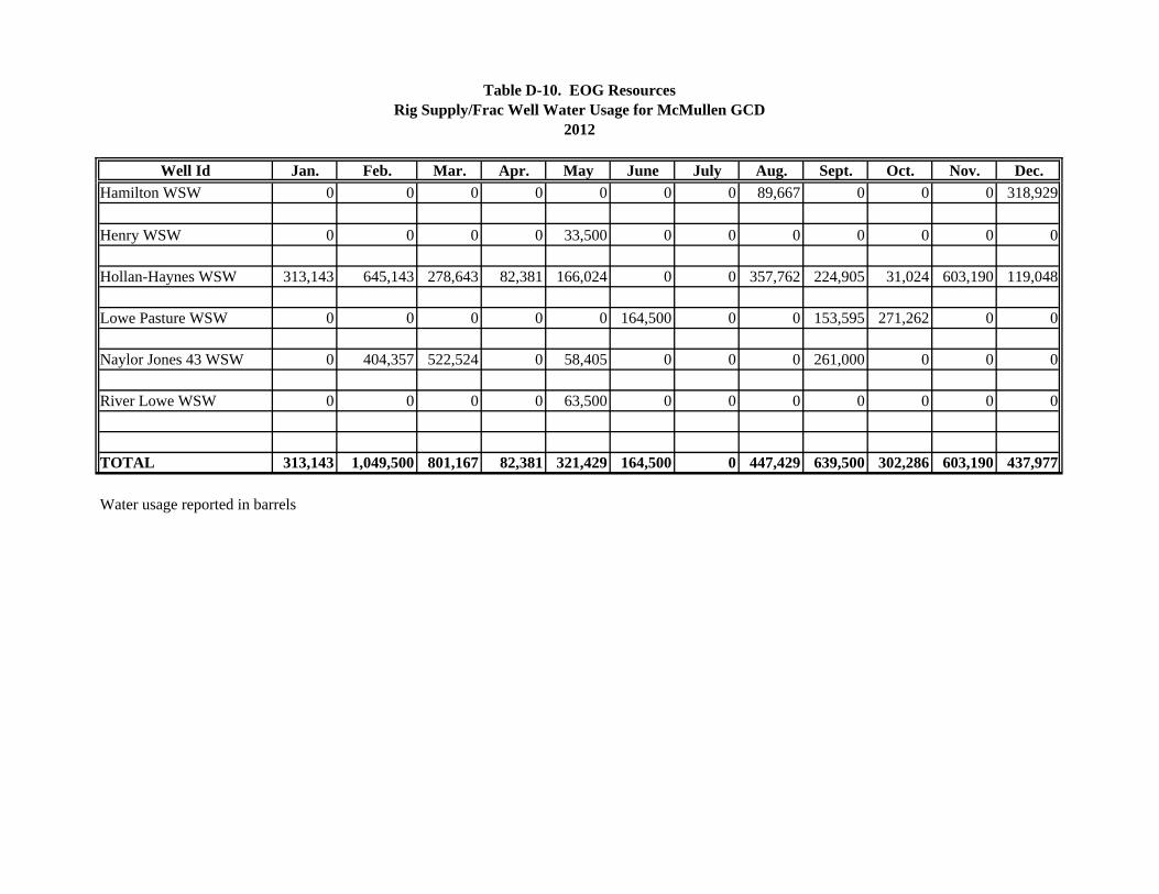
Well Id Jan. Feb. Mar. Apr. May June July Aug. Sept. Oct. Nov. Dec.
Hamilton WSW 0 0 0 0 0 0 0 89,667 0 0 0 318,929
Henry WSW 0 0 0 0 33,500 0 0 0 0 0 0 0
Hollan-Haynes WSW 313,143 645,143 278,643 82,381 166,024 0 0 357,762 224,905 31,024 603,190 119,048
Lowe Pasture WSW 0 0 0 0 0 164,500 0 0 153,595 271,262 0 0
Naylor Jones 43 WSW 0 404,357 522,524 0 58,405 0 0 0 261,000 0 0 0
River Lowe WSW 0 0 0 0 63,500 0 0 0 0 0 0 0
TOTAL 313,143 1,049,500 801,167 82,381 321,429 164,500 0 447,429 639,500 302,286 603,190 437,977
Water usage reported in barrels
Rig Supply/Frac Well Water Usage for McMullen GCDTable D-10. EOG Resources
2012
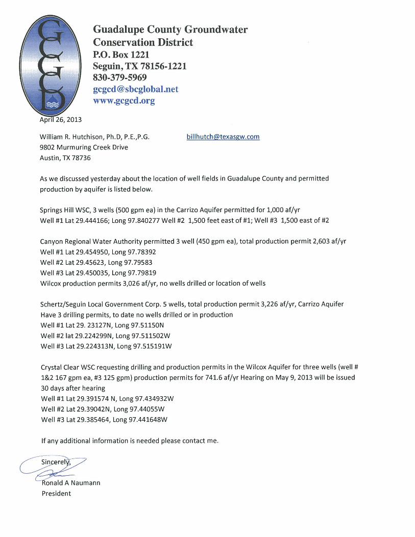
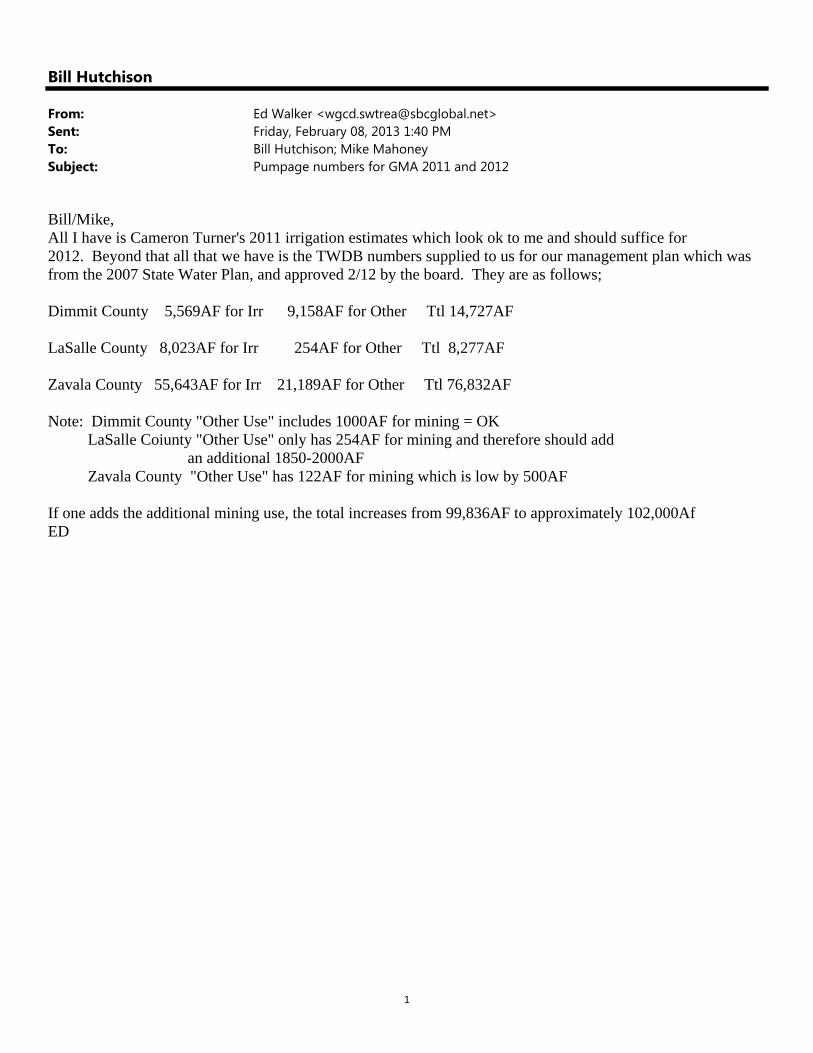
1
Bill Hutchison
From: Ed Walker <[email protected]>Sent: Friday, February 08, 2013 1:40 PMTo: Bill Hutchison; Mike MahoneySubject: Pumpage numbers for GMA 2011 and 2012
Bill/Mike, All I have is Cameron Turner's 2011 irrigation estimates which look ok to me and should suffice for 2012. Beyond that all that we have is the TWDB numbers supplied to us for our management plan which was from the 2007 State Water Plan, and approved 2/12 by the board. They are as follows; Dimmit County 5,569AF for Irr 9,158AF for Other Ttl 14,727AF LaSalle County 8,023AF for Irr 254AF for Other Ttl 8,277AF Zavala County 55,643AF for Irr 21,189AF for Other Ttl 76,832AF Note: Dimmit County "Other Use" includes 1000AF for mining = OK LaSalle Coiunty "Other Use" only has 254AF for mining and therefore should add an additional 1850-2000AF Zavala County "Other Use" has 122AF for mining which is low by 500AF If one adds the additional mining use, the total increases from 99,836AF to approximately 102,000Af ED
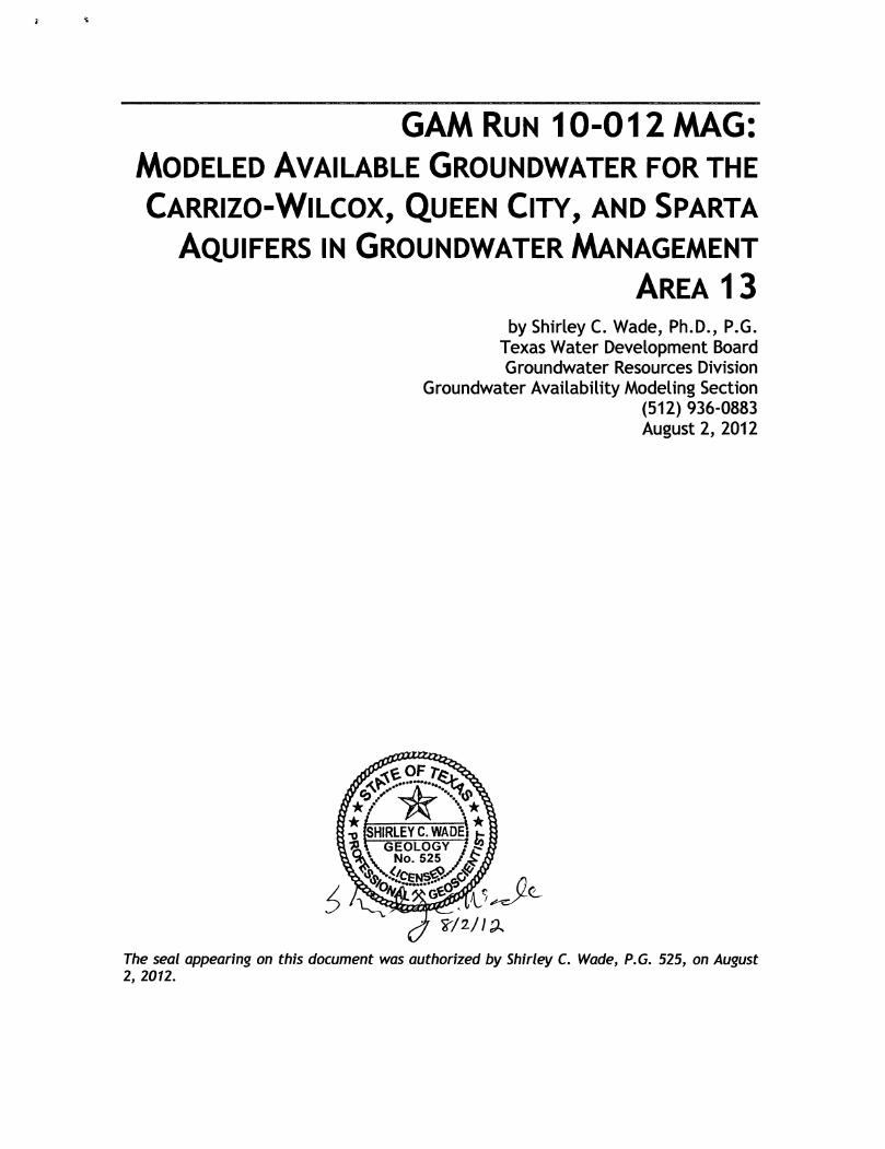

This page is intentionally left blank
GAM RUN 10-012 MAG: MODELED AVAILABLE GROUNDWATER FOR THE CARRIZO-WILCOX, QUEEN CITY, AND SPARTA
AQUIFERS IN GROUNDWATER MANAGEMENT AREA 13
by Shirley C. Wade, Ph.D., P.G. Texas Water Development Board Groundwater Resources Division
Groundwater Availability Modeling Section (512) 936-0883 August 2, 2012
EXECUTIVE SUMMARY: The modeled available groundwater for Groundwater Management Area 13 for the Carrizo-Wilcox, Queen City, and Sparta aquifers is summarized in Table 1, 2, and 3 for use in the regional water planning process. These values are also listed by decade for each aquifer by county (Table 4), river basin (Table 5), regional water planning group (Table 6), and groundwater conservation district (Table 7). The modeled available groundwater estimates for the Queen City, Sparta, and Carrizo-Wilcox aquifers range from approximately 399,000 acre-feet per year in 2010 to 425,000 acre-feet per year in 2060 (Table 4). The estimates were extracted from results of Groundwater Availability Model Run 09-034, scenario 4, which meets the desired future conditions adopted by members of Groundwater Management Area 13.
This report reflects the official release of the revised groundwater district boundaries by the Texas Commission on Environmental Quality (TCEQ). Specifically, this report reflects the division of modeled available groundwater between the Gonzales County Underground Water Conservation District and Plum Creek Conservation District based on the new groundwater conservation district boundaries.
REQUESTOR: Mr. Mike Mahoney from the Evergreen Underground Water Conservation District acting on behalf of Groundwater Management Area 13.
GAM Run 10-012 MAG: Modeled Available Groundwater for the Carrizo-Wilcox, Queen City, and Sparta Aquifers in Groundwater Management Area 13 August 2, 2012 Page 4 of 19
DESCRIPTION OF REQUEST: In a letter dated April 13, 2010 and received by the Texas Water Development Board (TWDB) on April 15, 2010, Mr. Mike Mahoney provided the TWDB with the desired future conditions of the Carrizo-Wilcox, Queen City, and Sparta aquifers adopted by the groundwater conservation districts in Groundwater Management Area 13. The desired future conditions for the Carrizo-Wilcox, Queen City, and Sparta aquifers, as described in Resolution R 2010-01 and adopted April 9, 2010 by the groundwater conservation districts within Groundwater Management Area 13, are described below:
• “In reference to GAM Run 09-034, the committee has considered, the base scenario of an average drawdown of 22 feet, scenario 2 an average drawdown of 22 feet, scenario 3 an average drawdown of 23 feet and scenario 4 an average drawdown of 23 feet;”
• “The district members of Groundwater Management Area 13, adopt scenario 4, and an average drawdown of 23 feet for the Sparta, Weches, Queen City, Reklaw, Carrizo, and the Wilcox Aquifers”
In response to receiving the adopted desired future conditions, TWDB has estimated the modeled available groundwater for the Carrizo-Wilcox, Queen City, and Sparta Aquifers in Groundwater Management Area 13.
METHODS: Groundwater Management Area 13, located in south central Texas, includes the southern part of the Queen City, Sparta, and Carrizo-Wilcox aquifers (Figure 1). For the previously completed Groundwater Availability Model Run 09-034 (Wade and Jigmond, 2010) average recharge and evapotranspiration rates and initial streamflows based on the historical calibration-verification runs, representing 1981 to 1999 were summarized. These averages were then used for each year of the 61-year predictive simulations along with pumping specified by Groundwater Management Area 13 members in four scenarios. The results of the pumping scenarios were reviewed by members of Groundwater Management Area 13 to develop their desired future conditions. Model scenario 4 resulted in an overall average drawdown of 23 feet for the Queen City, Sparta, and Carrizo-Wilcox aquifers and for the Weches and Reklaw confining units. The pumping for scenario 4 was extracted from the model results and divided by county, river basin, regional water planning area and groundwater conservation district within Groundwater Management Area 13 (Figure 2).
GAM Run 10-012 MAG: Modeled Available Groundwater for the Carrizo-Wilcox, Queen City, and Sparta Aquifers in Groundwater Management Area 13 August 2, 2012 Page 5 of 19
Modeled Available Groundwater and Permitting As defined in Chapter 36 of the Texas Water Code, “modeled available groundwater” is the estimated average amount of water that may be produced annually to achieve a desired future condition. Groundwater conservation districts are required to consider modeled available groundwater, along with several other factors, when issuing permits in order to manage groundwater production to achieve the desired future condition(s). The other factors districts must consider include annual precipitation and production patterns, the estimated amount of pumping exempt from permitting, existing permits, and a reasonable estimate of actual groundwater production under existing permits. The estimated amount of pumping exempt from permitting, which the Texas Water Development Board is required to develop after soliciting input from applicable groundwater conservation districts, will be provided in a separate report.
PARAMETERS AND ASSUMPTIONS: The parameters and assumptions for the groundwater availability model for the southern part of the Queen City, Sparta, and Carrizo-Wilcox aquifers are described below:
• Version 2.01 of the groundwater availability model for the southern part of the Queen City, Sparta, and Carrizo-Wilcox aquifers was used for this analysis
• See Deeds and others (2003) and Kelley and others (2004) for assumptions and limitations of the groundwater availability model for the southern part of the Queen City, Sparta, and Carrizo-Wilcox aquifers.
• The model includes eight layers representing:
• the Sparta Aquifer (layer 1),
• the Weches Formation (layer 2),
• the Queen City Aquifer (layer 3),
• the Reklaw Formation (layer 4),
• the Carrizo Aquifer (layer 5),
• the upper and where the upper is missing, the middle Wilcox Aquifer (layer 6),
• the middle Wilcox Aquifer (layer 7), and
• the lower Wilcox Aquifer (layer 8).
GAM Run 10-012 MAG: Modeled Available Groundwater for the Carrizo-Wilcox, Queen City, and Sparta Aquifers in Groundwater Management Area 13 August 2, 2012 Page 6 of 19
• Groundwater in the groundwater availability model for the southern portion of the Queen City, Sparta, and Carrizo-Wilcox aquifers ranges from fresh to saline (Kelley and others, 2004).
• The root mean square error (a measure of the difference between simulated and measured water levels during model calibration) in the entire model for 1999 is 23 feet for the Sparta Aquifer, 18 feet for the Queen City aquifer, and 33 feet for the Carrizo aquifer (Kelley and others, 2004).
• Recharge rates, evapotranspiration rates, and initial streamflows are averages of historic estimates from 1981 to 1999.
RESULTS: The modeled available groundwater for the Carrizo-Wilcox Aquifer that achieves the desired future conditions adopted by Groundwater Management Area 13 increases from 375,654 to 404,000 acre-feet per year between 2010 and 2060 (Table 1). The modeled available groundwater for the Queen City Aquifer in Groundwater Management Area 13 declines from 16,311 to 14,538 acre-feet per year over the same time period (Table 2). The modeled available groundwater for the Sparta Aquifer in Groundwater Management Area 13 declines from 6,800 to 6,365 acre-feet per year (Table 3). The modeled available groundwater in tables 1, 2, and 3 has been summarized by county, river basin, and regional water planning area for use in the regional water planning process.
The modeled available groundwater is also summarized by county (Table 4), river basin (Table 5), regional water planning area (Table 6), and groundwater conservation district (Table 7). In Table 7, the modeled available groundwater among all districts has been calculated both excluding and including areas outside the jurisdiction of a groundwater conservation district.
GAM Run 10-012 MAG: Modeled Available Groundwater for the Carrizo-Wilcox, Queen City, and Sparta Aquifers in Groundwater Management Area 13 August 2, 2012 Page 7 of 19
LIMITATIONS: The groundwater model used in completing this analysis is the best available scientific tool that can be used to meet the stated objective(s). To the extent that this analysis will be used for planning purposes and/or regulatory purposes related to pumping in the past and into the future, it is important to recognize the assumptions and limitations associated with the use of the results. In reviewing the use of models in environmental regulatory decision making, the National Research Council (2007) noted:
“Models will always be constrained by computational limitations, assumptions, and knowledge gaps. They can best be viewed as tools to help inform decisions rather than as machines to generate truth or make decisions. Scientific advances will never make it possible to build a perfect model that accounts for every aspect of reality or to prove that a given model is correct in all respects for a particular regulatory application. These characteristics make evaluation of a regulatory model more complex than solely a comparison of measurement data with model results.”
A key aspect of using the groundwater model to evaluate historic groundwater flow conditions includes the assumptions about the location in the aquifer where historic pumping was placed. Understanding the amount and location of historic pumping is as important as evaluating the volume of groundwater flow into and out of the district, between aquifers within the district (as applicable), interactions with surface water (as applicable), recharge to the aquifer system (as applicable), and other metrics that describe the impacts of that pumping. In addition, assumptions regarding precipitation, recharge, and streamflow are specific to a particular historic time period.
Because the application of the groundwater model was designed to address regional scale questions, the results are most effective on a regional scale. The TWDB makes no warranties or representations relating to the actual conditions of any aquifer at a particular location or at a particular time.
It is important for groundwater conservation districts to monitor groundwater pumping and overall conditions of the aquifer. Because of the limitations of the groundwater model and the assumptions in this analysis, it is important that the groundwater conservation districts work with the TWDB to refine this analysis in the future given the reality of how the aquifer responds to the actual amount and location of pumping now and in the future. Historic precipitation patterns also need to be placed in context as future climatic conditions, such as dry and wet year precipitation patterns, may differ and affect groundwater flow conditions.
GAM Run 10-012 MAG: Modeled Available Groundwater for the Carrizo-Wilcox, Queen City, and Sparta Aquifers in Groundwater Management Area 13 August 2, 2012 Page 8 of 19
REFERENCES:
Deeds, N., Kelley, V., Fryar, D., Jones, T., Whallon, A. J., and Dean, K. E., 2003, Groundwater Availability Model for the Southern Carrizo-Wilcox Aquifer: contract report to the Texas Water Development Board, 452 p.
Donnelly, A.C.A., 2007a, GAM Run 06-29, Texas Water Development Board GAM Run Report, 59 p.
Donnelly, A.C.A., 2007b, GAM Run 07-16, Texas Water Development Board GAM Run Report, 63 p.
Donnelly, A.C.A., 2007c, GAM Run 07-17, Texas Water Development Board GAM Run Report, 38 p.
Kelley, V. A., Deeds, N. E., Fryar, D. G., and Nicot, J. P., 2004, Groundwater availability models for the Queen City and Sparta aquifers: contract report to the Texas Water Development Board, 867 p.
National Research Council, 2007, Models in Environmental Regulatory Decision Making. Committee on Models in the Regulatory Decision Process, National Academies Press, Washington D.C., 287 p.
Wade S.C., 2008a, GAM Run 08-41, Texas Water Development Board GAM Run Report, 56 p.
Wade S.C., 2008b, GAM Run 08-42, Texas Water Development Board GAM Run Report, 56 p.
Wade S.C., 2008c, GAM Run 08-43, Texas Water Development Board GAM Run Report, 58 p.
Wade S.C. and Jigmond, M., 2010, GAM Run 09-034, Texas Water Development Board GAM Run Report, 146 p.
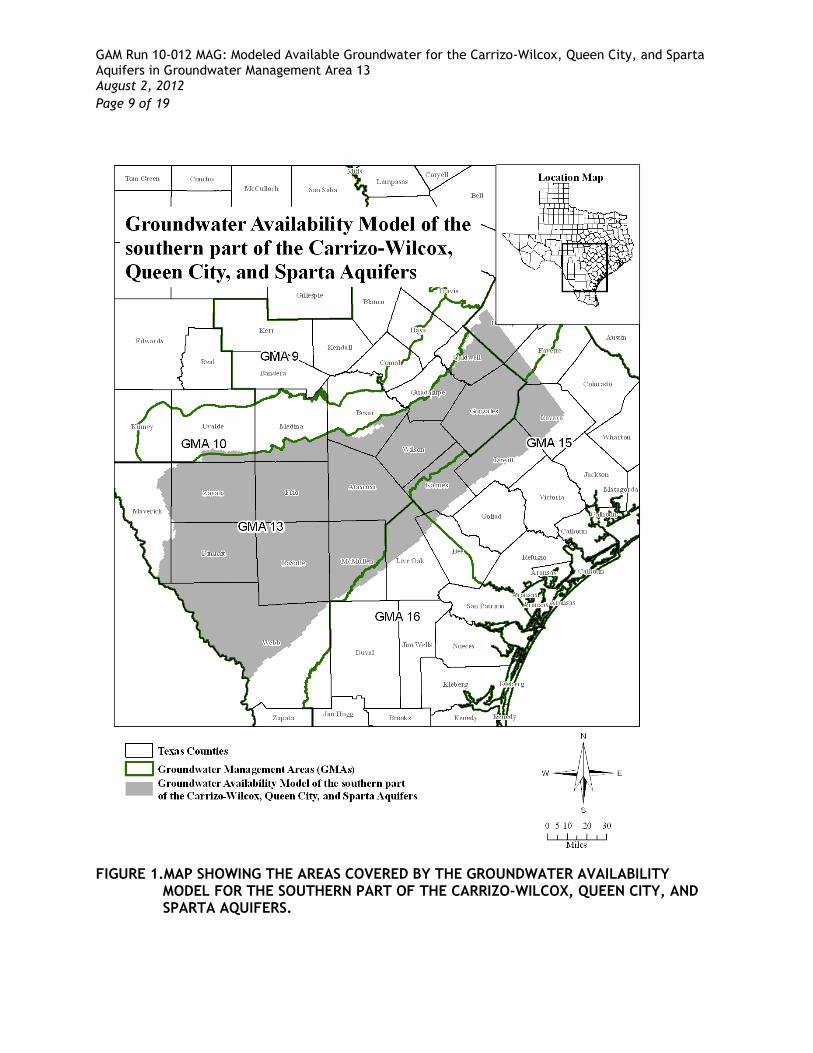
GAM Run 10-012 MAG: Modeled Available Groundwater for the Carrizo-Wilcox, Queen City, and Sparta Aquifers in Groundwater Management Area 13 August 2, 2012 Page 9 of 19
FIGURE 1.MAP SHOWING THE AREAS COVERED BY THE GROUNDWATER AVAILABILITY
MODEL FOR THE SOUTHERN PART OF THE CARRIZO-WILCOX, QUEEN CITY, AND SPARTA AQUIFERS.
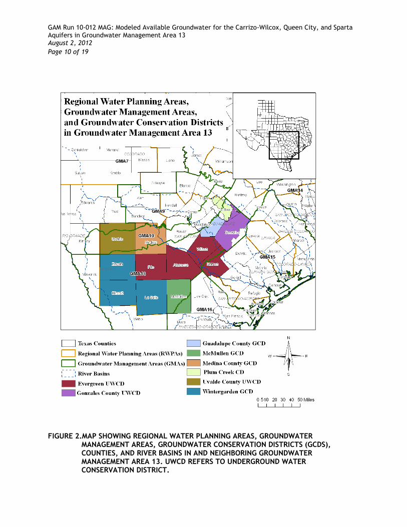
GAM Run 10-012 MAG: Modeled Available Groundwater for the Carrizo-Wilcox, Queen City, and Sparta Aquifers in Groundwater Management Area 13 August 2, 2012 Page 10 of 19
FIGURE 2.MAP SHOWING REGIONAL WATER PLANNING AREAS, GROUNDWATER MANAGEMENT AREAS, GROUNDWATER CONSERVATION DISTRICTS (GCDS), COUNTIES, AND RIVER BASINS IN AND NEIGHBORING GROUNDWATER MANAGEMENT AREA 13. UWCD REFERS TO UNDERGROUND WATER CONSERVATION DISTRICT.
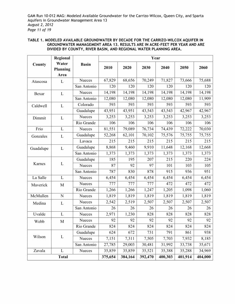
GAM Run 10-012 MAG: Modeled Available Groundwater for the Carrizo-Wilcox, Queen City, and Sparta Aquifers in Groundwater Management Area 13 August 2, 2012 Page 11 of 19 TABLE 1. MODELED AVAILABLE GROUNDWATER BY DECADE FOR THE CARRIZO-WILCOX AQUIFER IN
GROUNDWATER MANAGEMENT AREA 13. RESULTS ARE IN ACRE-FEET PER YEAR AND ARE DIVIDED BY COUNTY, RIVER BASIN, AND REGIONAL WATER PLANNING AREA.
County Regional
Water Planning
Area
Basin Year
2010 2020 2030 2040 2050 2060
Atascosa L Nueces 67,829 68,656 70,249 71,827 73,666 75,688 San Antonio 120 120 120 120 120 120
Bexar L Nueces 14,198 14,198 14,198 14,198 14,198 14,198 San Antonio 12,080 12,080 12,080 12,080 12,080 11,909
Caldwell L Colorado 593 593 593 593 593 593 Guadalupe 43,951 43,951 43,543 43,543 42,967 42,967
Dimmit L Nueces 3,253 3,253 3,253 3,253 3,253 3,253 Rio Grande 106 106 106 106 106 106
Frio L Nueces 81,551 79,089 76,734 74,439 72,222 70,030
Gonzales L Guadalupe 52,268 62,101 70,102 75,576 75,755 75,755 Lavaca 215 215 215 215 215 215
Guadalupe L Guadalupe 8,868 9,460 9,910 11,648 12,168 12,668 San Antonio 1,373 1,373 1,373 1,373 1,373 1,373
Karnes L Guadalupe 185 195 207 215 220 224
Nueces 87 92 97 101 103 105 San Antonio 787 830 878 915 936 951
La Salle L Nueces 6,454 6,454 6,454 6,454 6,454 6,454
Maverick M Nueces 777 777 777 472 472 472 Rio Grande 1,266 1,266 1,247 1,205 1,098 1,060
McMullen N Nueces 1,819 1,819 1,819 1,819 1,819 1,819
Medina L Nueces 2,542 2,519 2,507 2,507 2,507 2,507 San Antonio 26 26 26 26 26 26
Uvalde L Nueces 2,971 1,230 828 828 828 828
Webb M Nueces 92 92 92 92 92 92 Rio Grande 824 824 824 824 824 824
Wilson L Guadalupe 624 672 731 791 861 938
Nueces 7,151 7,311 7,505 7,703 7,932 8,185 San Antonio 27,785 29,003 30,481 31,992 33,738 35,671
Zavala L Nueces 35,859 35,859 35,521 35,388 35,288 34,969 Total 375,654 384,164 392,470 400,303 401,914 404,000
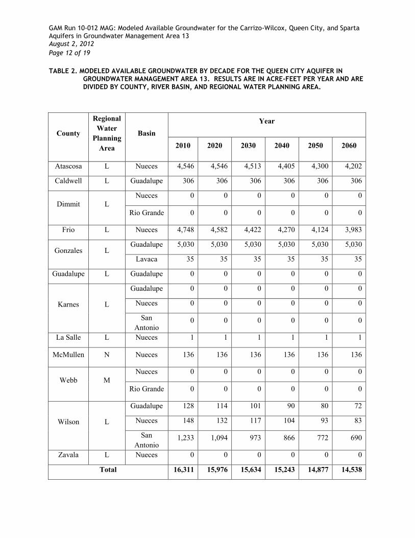
GAM Run 10-012 MAG: Modeled Available Groundwater for the Carrizo-Wilcox, Queen City, and Sparta Aquifers in Groundwater Management Area 13 August 2, 2012 Page 12 of 19 TABLE 2. MODELED AVAILABLE GROUNDWATER BY DECADE FOR THE QUEEN CITY AQUIFER IN
GROUNDWATER MANAGEMENT AREA 13. RESULTS ARE IN ACRE-FEET PER YEAR AND ARE DIVIDED BY COUNTY, RIVER BASIN, AND REGIONAL WATER PLANNING AREA.
County
Regional Water
Planning Area
Basin Year
2010 2020 2030 2040 2050 2060
Atascosa L Nueces 4,546 4,546 4,513 4,405 4,300 4,202
Caldwell L Guadalupe 306 306 306 306 306 306
Dimmit L Nueces 0 0 0 0 0 0
Rio Grande 0 0 0 0 0 0
Frio L Nueces 4,748 4,582 4,422 4,270 4,124 3,983
Gonzales L Guadalupe 5,030 5,030 5,030 5,030 5,030 5,030
Lavaca 35 35 35 35 35 35
Guadalupe L Guadalupe 0 0 0 0 0 0
Karnes L
Guadalupe 0 0 0 0 0 0
Nueces 0 0 0 0 0 0
San Antonio
0 0 0 0 0 0
La Salle L Nueces 1 1 1 1 1 1
McMullen N Nueces 136 136 136 136 136 136
Webb M Nueces 0 0 0 0 0 0
Rio Grande 0 0 0 0 0 0
Wilson L
Guadalupe 128 114 101 90 80 72
Nueces 148 132 117 104 93 83
San Antonio
1,233 1,094 973 866 772 690
Zavala L Nueces 0 0 0 0 0 0
Total 16,311 15,976 15,634 15,243 14,877 14,538
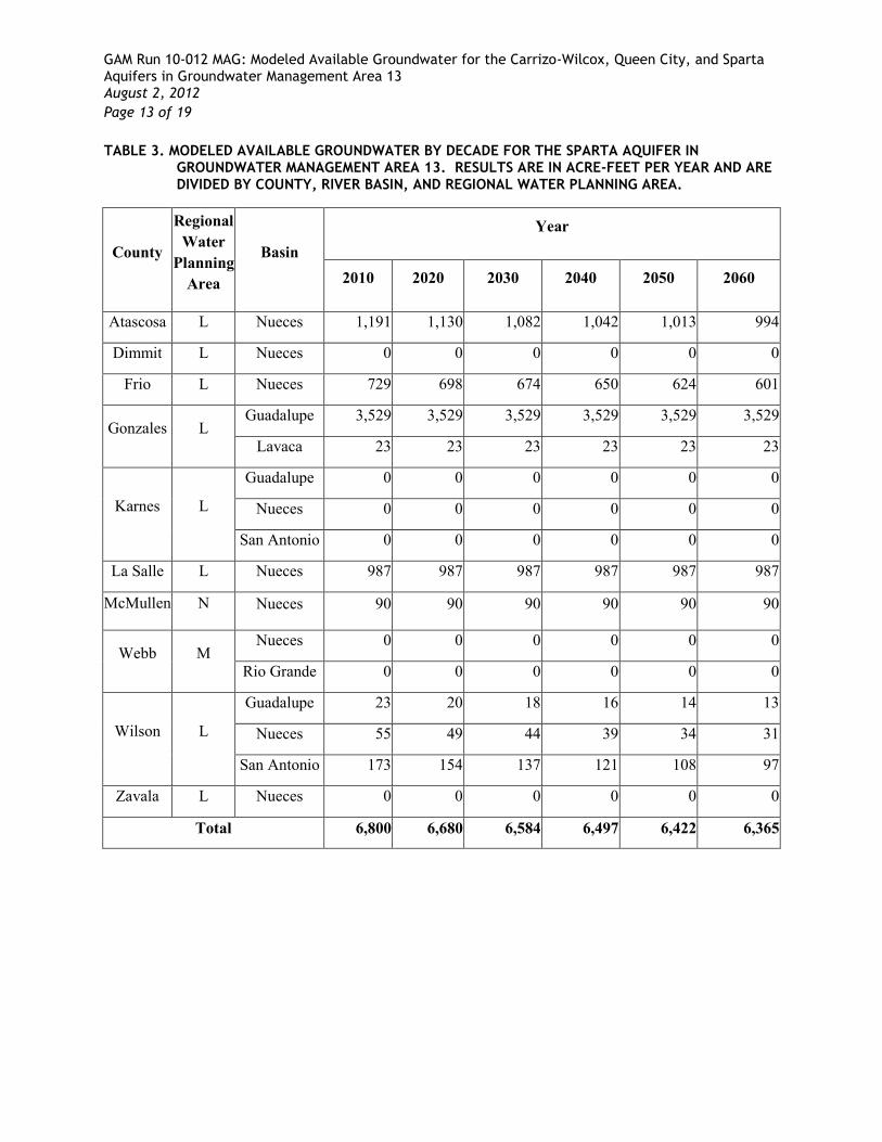
GAM Run 10-012 MAG: Modeled Available Groundwater for the Carrizo-Wilcox, Queen City, and Sparta Aquifers in Groundwater Management Area 13 August 2, 2012 Page 13 of 19 TABLE 3. MODELED AVAILABLE GROUNDWATER BY DECADE FOR THE SPARTA AQUIFER IN
GROUNDWATER MANAGEMENT AREA 13. RESULTS ARE IN ACRE-FEET PER YEAR AND ARE DIVIDED BY COUNTY, RIVER BASIN, AND REGIONAL WATER PLANNING AREA.
County
Regional Water
Planning Area
Basin Year
2010 2020 2030 2040 2050 2060
Atascosa L Nueces 1,191 1,130 1,082 1,042 1,013 994
Dimmit L Nueces 0 0 0 0 0 0
Frio L Nueces 729 698 674 650 624 601
Gonzales L Guadalupe 3,529 3,529 3,529 3,529 3,529 3,529
Lavaca 23 23 23 23 23 23
Karnes L
Guadalupe 0 0 0 0 0 0
Nueces 0 0 0 0 0 0
San Antonio 0 0 0 0 0 0
La Salle L Nueces 987 987 987 987 987 987
McMullen N Nueces 90 90 90 90 90 90
Webb M Nueces 0 0 0 0 0 0
Rio Grande 0 0 0 0 0 0
Wilson L
Guadalupe 23 20 18 16 14 13
Nueces 55 49 44 39 34 31
San Antonio 173 154 137 121 108 97
Zavala L Nueces 0 0 0 0 0 0
Total 6,800 6,680 6,584 6,497 6,422 6,365
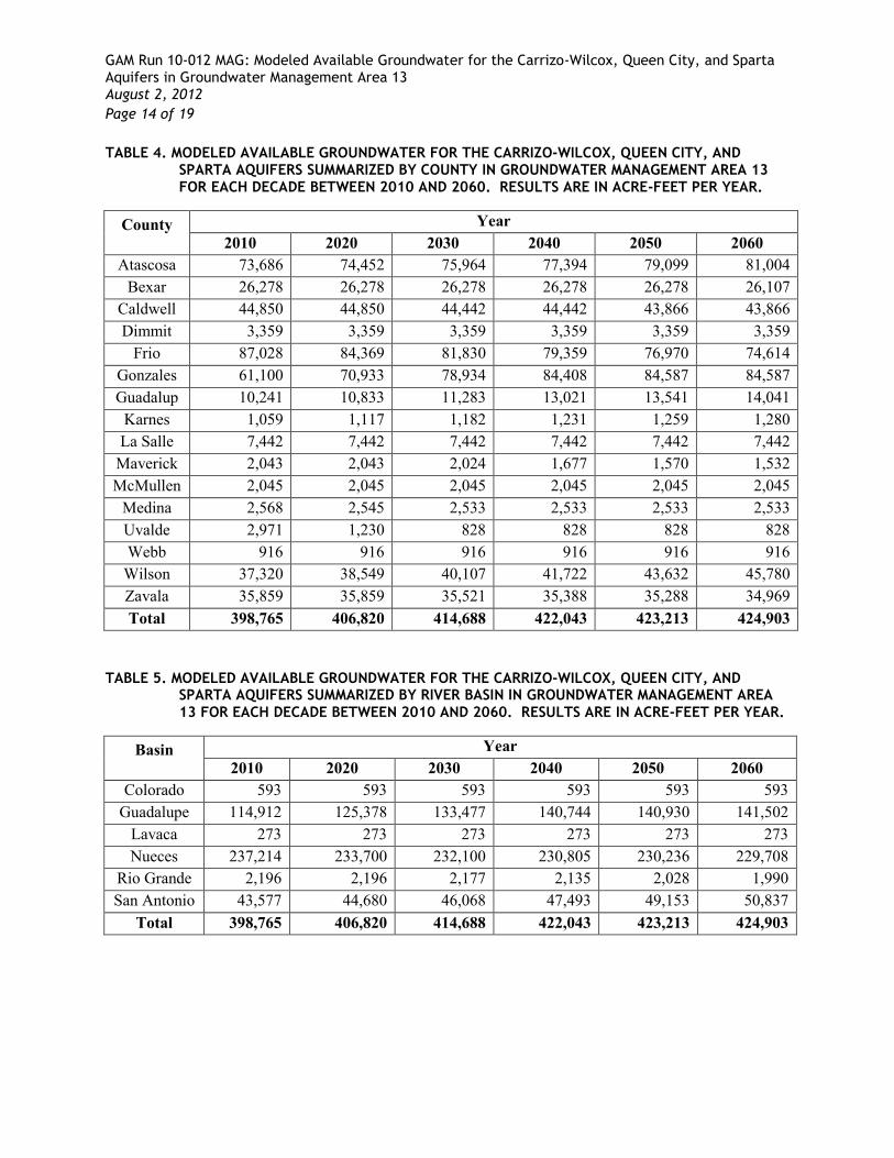
GAM Run 10-012 MAG: Modeled Available Groundwater for the Carrizo-Wilcox, Queen City, and Sparta Aquifers in Groundwater Management Area 13 August 2, 2012 Page 14 of 19 TABLE 4. MODELED AVAILABLE GROUNDWATER FOR THE CARRIZO-WILCOX, QUEEN CITY, AND
SPARTA AQUIFERS SUMMARIZED BY COUNTY IN GROUNDWATER MANAGEMENT AREA 13 FOR EACH DECADE BETWEEN 2010 AND 2060. RESULTS ARE IN ACRE-FEET PER YEAR.
County Year 2010 2020 2030 2040 2050 2060
Atascosa 73,686 74,452 75,964 77,394 79,099 81,004 Bexar 26,278 26,278 26,278 26,278 26,278 26,107
Caldwell 44,850 44,850 44,442 44,442 43,866 43,866 Dimmit 3,359 3,359 3,359 3,359 3,359 3,359
Frio 87,028 84,369 81,830 79,359 76,970 74,614 Gonzales 61,100 70,933 78,934 84,408 84,587 84,587 Guadalup
10,241 10,833 11,283 13,021 13,541 14,041
Karnes 1,059 1,117 1,182 1,231 1,259 1,280 La Salle 7,442 7,442 7,442 7,442 7,442 7,442
Maverick 2,043 2,043 2,024 1,677 1,570 1,532 McMullen 2,045 2,045 2,045 2,045 2,045 2,045
Medina 2,568 2,545 2,533 2,533 2,533 2,533 Uvalde 2,971 1,230 828 828 828 828 Webb 916 916 916 916 916 916 Wilson 37,320 38,549 40,107 41,722 43,632 45,780 Zavala 35,859 35,859 35,521 35,388 35,288 34,969 Total 398,765 406,820 414,688 422,043 423,213 424,903
TABLE 5. MODELED AVAILABLE GROUNDWATER FOR THE CARRIZO-WILCOX, QUEEN CITY, AND SPARTA AQUIFERS SUMMARIZED BY RIVER BASIN IN GROUNDWATER MANAGEMENT AREA 13 FOR EACH DECADE BETWEEN 2010 AND 2060. RESULTS ARE IN ACRE-FEET PER YEAR.
Basin Year 2010 2020 2030 2040 2050 2060
Colorado 593 593 593 593 593 593 Guadalupe 114,912 125,378 133,477 140,744 140,930 141,502
Lavaca 273 273 273 273 273 273 Nueces 237,214 233,700 232,100 230,805 230,236 229,708
Rio Grande 2,196 2,196 2,177 2,135 2,028 1,990 San Antonio 43,577 44,680 46,068 47,493 49,153 50,837
Total 398,765 406,820 414,688 422,043 423,213 424,903
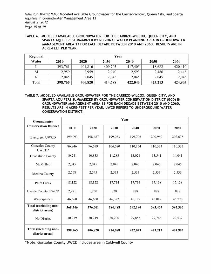
GAM Run 10-012 MAG: Modeled Available Groundwater for the Carrizo-Wilcox, Queen City, and Sparta Aquifers in Groundwater Management Area 13 August 2, 2012 Page 15 of 19 TABLE 6. MODELED AVAILABLE GROUNDWATER FOR THE CARRIZO-WILCOX, QUEEN CITY, AND
SPARTA AQUIFERS SUMMARIZED BY REGIONAL WATER PLANNING AREA IN GROUNDWATER MANAGEMENT AREA 13 FOR EACH DECADE BETWEEN 2010 AND 2060. RESULTS ARE IN ACRE-FEET PER YEAR.
Regional Water
Year 2010 2020 2030 2040 2050 2060
L 393,761 401,816 409,703 417,405 418,682 420,410 M 2,959 2,959 2,940 2,593 2,486 2,448 N 2,045 2,045 2,045 2,045 2,045 2,045
Total 398,765 406,820 414,688 422,043 423,213 424,903
TABLE 7. MODELED AVAILABLE GROUNDWATER FOR THE CARRIZO-WILCOX, QUEEN CITY, AND SPARTA AQUIFERS SUMMARIZED BY GROUNDWATER CONSERVATION DISTRICT (GCD) IN GROUNDWATER MANAGEMENT AREA 13 FOR EACH DECADE BETWEEN 2010 AND 2060. RESULTS ARE IN ACRE-FEET PER YEAR. UWCD REFERS TO UNDERGROUND WATER CONSERVATION DISTRICT.
Groundwater Conservation District
Year
2010 2020 2030 2040 2050 2060
Evergreen UWCD 199,093 198,487 199,083 199,706 200,960 202,678
Gonzales County UWCD*
86,846 96,679 104,680 110,154 110,333 110,333
Guadalupe County 10,241 10,833 11,283 13,021 13,541 14,041
McMullen 2,045 2,045 2,045 2,045 2,045 2,045
Medina County 2,568 2,545 2,533 2,533 2,533 2,533
Plum Creek 18,122 18,122 17,714 17,714 17,138 17,138
Uvalde County UWCD 2,971 1,230 828 828 828 828
Wintergarden 46,660 46,660 46,322 46,189 46,089 45,770
Total (excluding non-district areas)
368,546 376,601 384,488 392,190 393,467 395,366
No District 30,219 30,219 30,200 29,853 29,746 29,537
Total (including non-district areas)
398,765 406,820 414,688 422,043 423,213 424,903
*Note: Gonzales County UWCD includes area in Caldwell County
GAM Run 10-012 MAG: Modeled Available Groundwater for the Carrizo-Wilcox, Queen City, and Sparta Aquifers in Groundwater Management Area 13 August 2, 2012 Page 16 of 19
Appendix A
Estimates of total pumping split by aquifer layers for Groundwater Conservation Districts
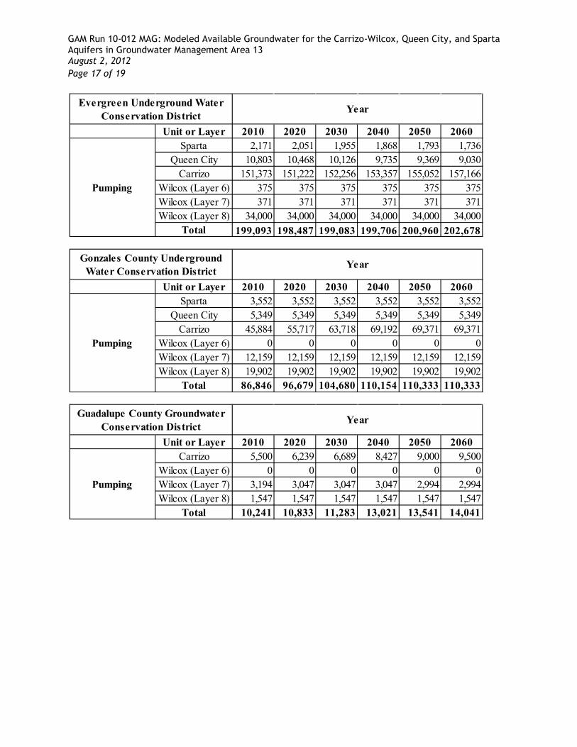
GAM Run 10-012 MAG: Modeled Available Groundwater for the Carrizo-Wilcox, Queen City, and Sparta Aquifers in Groundwater Management Area 13 August 2, 2012 Page 17 of 19
Unit or Layer 2010 2020 2030 2040 2050 2060Sparta 2,171 2,051 1,955 1,868 1,793 1,736
Queen City 10,803 10,468 10,126 9,735 9,369 9,030Carrizo 151,373 151,222 152,256 153,357 155,052 157,166
Wilcox (Layer 6) 375 375 375 375 375 375Wilcox (Layer 7) 371 371 371 371 371 371Wilcox (Layer 8) 34,000 34,000 34,000 34,000 34,000 34,000
Total 199,093 198,487 199,083 199,706 200,960 202,678
YearEvergreen Underground Water Conservation District
Pumping
Unit or Layer 2010 2020 2030 2040 2050 2060Sparta 3,552 3,552 3,552 3,552 3,552 3,552
Queen City 5,349 5,349 5,349 5,349 5,349 5,349Carrizo 45,884 55,717 63,718 69,192 69,371 69,371
Wilcox (Layer 6) 0 0 0 0 0 0Wilcox (Layer 7) 12,159 12,159 12,159 12,159 12,159 12,159Wilcox (Layer 8) 19,902 19,902 19,902 19,902 19,902 19,902
Total 86,846 96,679 104,680 110,154 110,333 110,333
YearGonzales County Underground Water Conservation District
Pumping
Unit or Layer 2010 2020 2030 2040 2050 2060Carrizo 5,500 6,239 6,689 8,427 9,000 9,500
Wilcox (Layer 6) 0 0 0 0 0 0Wilcox (Layer 7) 3,194 3,047 3,047 3,047 2,994 2,994Wilcox (Layer 8) 1,547 1,547 1,547 1,547 1,547 1,547
Total 10,241 10,833 11,283 13,021 13,541 14,041
YearGuadalupe County Groundwater Conservation District
Pumping
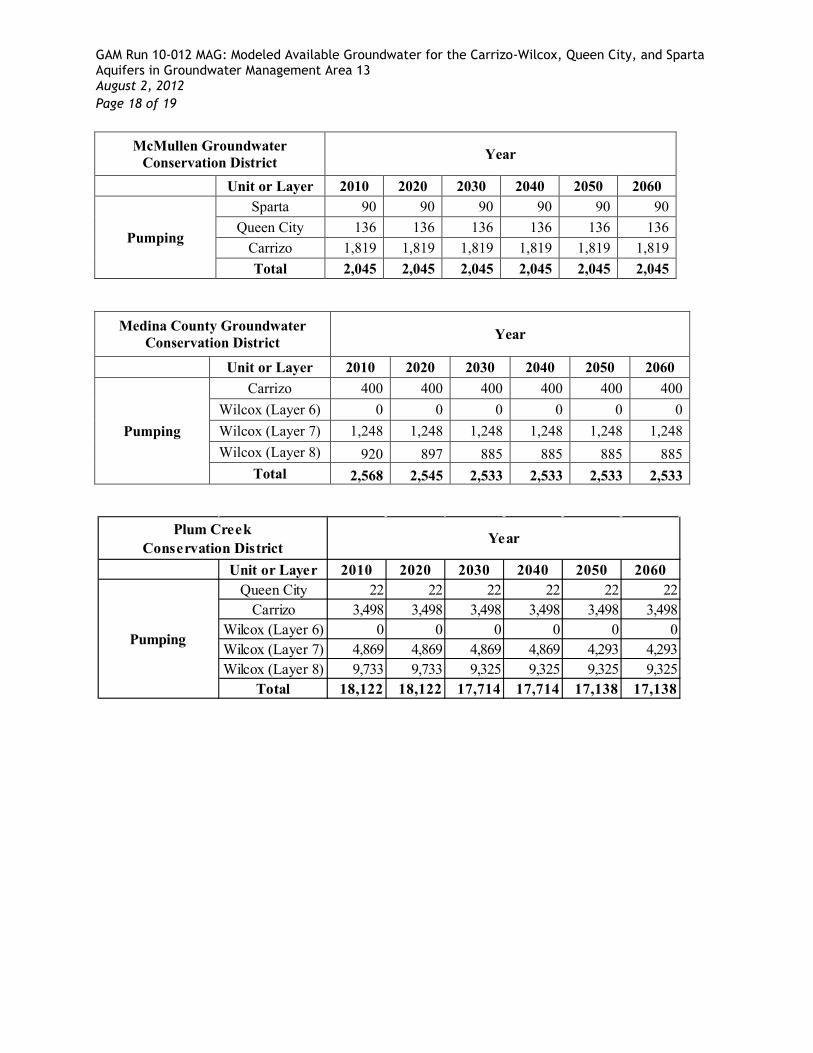
GAM Run 10-012 MAG: Modeled Available Groundwater for the Carrizo-Wilcox, Queen City, and Sparta Aquifers in Groundwater Management Area 13 August 2, 2012 Page 18 of 19
McMullen Groundwater Conservation District Year
Unit or Layer 2010 2020 2030 2040 2050 2060
Pumping
Sparta 90 90 90 90 90 90 Queen City 136 136 136 136 136 136
Carrizo 1,819 1,819 1,819 1,819 1,819 1,819 Total 2,045 2,045 2,045 2,045 2,045 2,045
Medina County Groundwater Conservation District Year
Unit or Layer 2010 2020 2030 2040 2050 2060
Pumping
Carrizo 400 400 400 400 400 400 Wilcox (Layer 6) 0 0 0 0 0 0 Wilcox (Layer 7) 1,248 1,248 1,248 1,248 1,248 1,248 Wilcox (Layer 8) 920 897 885 885 885 885
Total 2,568 2,545 2,533 2,533 2,533 2,533
Unit or Layer 2010 2020 2030 2040 2050 2060Queen City 22 22 22 22 22 22
Carrizo 3,498 3,498 3,498 3,498 3,498 3,498Wilcox (Layer 6) 0 0 0 0 0 0Wilcox (Layer 7) 4,869 4,869 4,869 4,869 4,293 4,293Wilcox (Layer 8) 9,733 9,733 9,325 9,325 9,325 9,325
Total 18,122 18,122 17,714 17,714 17,138 17,138
Pumping
YearPlum Creek Conservation District

GAM Run 10-012 MAG: Modeled Available Groundwater for the Carrizo-Wilcox, Queen City, and Sparta Aquifers in Groundwater Management Area 13 August 2, 2012 Page 19 of 19
Unit or Layer 2010 2020 2030 2040 2050 2060Carrizo 828 828 828 828 828 828
Wilcox (Layer 6) 2,143 402 0 0 0 0Total 2,971 1,230 828 828 828 828
YearUvalde County Underground Water Conservation District
Pumping
Unit or Layer 2010 2020 2030 2040 2050 2060Sparta 987 987 987 987 987 987
Queen City 1 1 1 1 1 1Carrizo 31,990 31,990 31,652 31,519 31,419 31,100
Wilcox (Layer 6) 9,259 9,259 9,259 9,259 9,259 9,259Wilcox (Layer 7) 4,007 4,007 4,007 4,007 4,007 4,007Wilcox (Layer 8) 416 416 416 416 416 416
Total 46,660 46,660 46,322 46,189 46,089 45,770
YearWintergarden Groundwater Conservation District
Pumping

Appendix E
TWDB GAM Task 13-036 (Revised): Total Estimated Recoverable Storage for Aquifers in
Groundwater Management Area 13

This page is intentionally blank
GAM TASK 13-036 (REVISED): TOTAL ESTIMATED
RECOVERABLE STORAGE FOR AQUIFERS IN
GROUNDWATER MANAGEMENT AREA 13 by Shirley Wade, Ph. D., P.G. and Robert Bradley, P.G.
Texas Water Development Board Groundwater Resources Division
(512) 936-0883 July 15, 2013
EXECUTIVE SUMMARY:
Texas Water Code, §36.108 (d) (Texas Water Code, 2011) states that, before voting on the
proposed desired future conditions for a relevant aquifer within a groundwater management
area, the groundwater conservation districts shall consider the total estimated recoverable
storage as provided by the executive administrator of the Texas Water Development Board
(TWDB) along with other factors listed in §36.108 (d). Texas Administrative Code Rule §356.10
(Texas Administrative Code, 2011) defines the total estimated recoverable storage as the
estimated amount of groundwater within an aquifer that accounts for recovery scenarios that
range between 25 percent and 75 percent of the porosity-adjusted aquifer volume.
This report discusses the methods, assumptions, and results of an analysis to estimate the
total recoverable storage for the Trinity, Edwards (Balcones Fault Zone), Carrizo-Wilcox,
Queen City, Sparta, Yegua-Jackson, and Gulf Coast (including parts of the Catahoula
Formation) aquifers within Groundwater Management Area 13. Tables 1 through 14 summarize
the total estimated recoverable storage required by the statute. Figures 2 through 8 indicate
the official extent of the aquifers in Groundwater Management Area 13 used to estimate the
total recoverable storage.
DEFINITION OF TOTAL ESTIMATED RECOVERABLE STORAGE:
The total estimated recoverable storage is defined as the estimated amount of groundwater
within an aquifer that accounts for recovery scenarios that range between 25 percent and 75
percent of the porosity-adjusted aquifer volume. In other words, we assume that only 25 to
75 percent of groundwater held within an aquifer can be removed by pumping.
GAM Task 13-036 (Revised): Total Estimated Recoverable Storage for Aquifers in Groundwater Management Area 13 July 15, 2013 Page 4 of 30
The total recoverable storage was estimated for the portion of the aquifer within the official
lateral aquifer boundaries as delineated by George and others (2011). Total estimated
recoverable storage values may include a mixture of water quality types, including fresh,
brackish, and saline groundwater, because the available data and the existing groundwater
availability models do not permit the differentiation of different water quality types. These
values do not take into account the effects of land surface subsidence, degradation of water
quality, or any changes to surface water-groundwater interaction.
METHODS:
To estimate the total recoverable storage of an aquifer, we first calculated the total storage
in an aquifer within the official aquifer boundary. The total storage is the volume of
groundwater removed by pumping that completely drains the aquifer.
Aquifers can be either unconfined or confined (figure 1). A well screened in an unconfined
aquifer will have a water level equal to the water level outside the well or in the aquifer.
Thus, unconfined aquifers have water levels within the aquifers. A confined aquifer is
bounded by low permeable geologic units at the top and bottom, and the aquifer is under
hydraulic pressure above the ambient atmospheric pressure. The water level at a well
screened in a confined aquifer will be above the top of the aquifer. As a result, calculation of
total storage is also different between unconfined and confined aquifers. For an unconfined
aquifer, the total storage is equal to the volume of groundwater removed by pumping that
makes the water level fall to the aquifer bottom. For a confined aquifer, the total storage
contains two parts. The first part is the groundwater released from the aquifer when the
water level falls from above the top of the aquifer to the top of the aquifer. The reduction of
hydraulic pressure in the aquifer by pumping causes expansion of groundwater and
deformation of aquifer solids. The aquifer is still fully saturated to this point. The second
part, just like unconfined aquifer, is the groundwater released from the aquifer when the
water level falls from the top to the bottom of the aquifer. Given the same aquifer area and
water level drop, the amount of water released in the second part is much greater than the
first part. The difference is quantified by two parameters: storativity related to confined
aquifer and specific yield related to unconfined aquifer. For example, storativity values range
from 10-5 to 10-3 for most confined aquifers, while the specific yield values can be 0.01 to 0.3
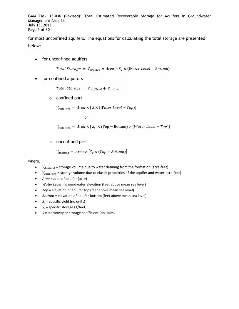
GAM Task 13-036 (Revised): Total Estimated Recoverable Storage for Aquifers in Groundwater Management Area 13 July 15, 2013 Page 5 of 30
for most unconfined aquifers. The equations for calculating the total storage are presented
below:
for unconfined aquifers
( )
for confined aquifers
o confined part
[ ( )]
or
[ ( ) ( )]
o unconfined part
[ ( )]
where:
= storage volume due to water draining from the formation (acre-feet)
= storage volume due to elastic properties of the aquifer and water(acre-feet)
Area = area of aquifer (acre)
Water Level = groundwater elevation (feet above mean sea level)
Top = elevation of aquifer top (feet above mean sea level)
Bottom = elevation of aquifer bottom (feet above mean sea level)
Sy = specific yield (no units)
Ss = specific storage (1/feet)
S = storativity or storage coefficient (no units)
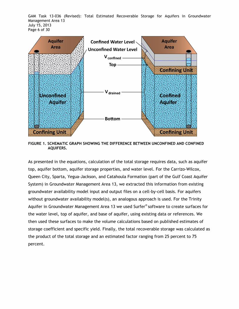
GAM Task 13-036 (Revised): Total Estimated Recoverable Storage for Aquifers in Groundwater Management Area 13 July 15, 2013 Page 6 of 30
FIGURE 1. SCHEMATIC GRAPH SHOWING THE DIFFERENCE BETWEEN UNCONFINED AND CONFINED AQUIFERS.
As presented in the equations, calculation of the total storage requires data, such as aquifer
top, aquifer bottom, aquifer storage properties, and water level. For the Carrizo-Wilcox,
Queen City, Sparta, Yegua-Jackson, and Catahoula Formation (part of the Gulf Coast Aquifer
System) in Groundwater Management Area 13, we extracted this information from existing
groundwater availability model input and output files on a cell-by-cell basis. For aquifers
without groundwater availability model(s), an analogous approach is used. For the Trinity
Aquifer in Groundwater Management Area 13 we used Surfer® software to create surfaces for
the water level, top of aquifer, and base of aquifer, using existing data or references. We
then used these surfaces to make the volume calculations based on published estimates of
storage coefficient and specific yield. Finally, the total recoverable storage was calculated as
the product of the total storage and an estimated factor ranging from 25 percent to 75
percent.
GAM Task 13-036 (Revised): Total Estimated Recoverable Storage for Aquifers in Groundwater Management Area 13 July 15, 2013 Page 7 of 30
PARAMETERS AND ASSUMPTIONS:
Trinity Aquifer
The Trinity Aquifer within Groundwater Management Area 13 is under confined
conditions throughout the area.
The potentiometric surface is based on the water-level measurements from several
sources (Holt, C.L.R, 1956, p.129; Welder and Reeves, 1962, p. 129; TWDB, 2013, and
Texas Department of Licensing and Regulation, 2013). Because all of the
measurements are located north of the study area and not within the Groundwater
Management Area 13 area, an estimate of the head at the southern boundary was
made using the head gradient from the available water levels. These estimates were
included with the water-level measurements to create a potentiometric surface grid in
Surfer® software to calculate the total head above the top of the aquifer.
We used the base of the San Antonio segment of the Edwards (Balcones Fault Zone)
Aquifer from the associated groundwater availability model (Lindgren and others,
2004) as the top of the Trinity Aquifer within the area. The base of the Trinity Aquifer
is from Plate 4 in Flawn and others (1961). These surfaces were created as grids in
Surfer® software and used to calculate aquifer thickness.
No storage data was discovered for the area, but because the calculations include all
of the Trinity Aquifer as a whole, we used conservative estimates for a storage
coefficient of 1 X 10⁻⁵ and a specific yield of 0.01 based on Trinity Aquifer references
(Johnson, 1967; Jones and others, 2009; Hunt and others, 2010).
The confined volume is calculated by taking the difference in the potentiometric
surface and top of the Trinity Aquifer to estimate total estimated head. This value is
multiplied by a storage coefficient of 1 X 10⁻⁵ resulting in the total storage volume for
the portion above the top of the aquifer.
The unconfined drained volume is calculated by taking the aquifer thickness and
multiplied by a specific yield of 0.01.
Zonal statistics in ArcMap 10.1 software summed the data from grid calculations by
county.
GAM Task 13-036 (Revised): Total Estimated Recoverable Storage for Aquifers in Groundwater Management Area 13 July 15, 2013 Page 8 of 30
Edwards (Balcones Fault Zone) Aquifer
We used version 1.01 of the groundwater availability model for the San Antonio
segment of the Edwards (Balcones Fault Zone) Aquifer to estimate the total
recoverable storage for the aquifer. See Lindgren and others (2004) for assumptions
and limitations of the groundwater availability model.
This groundwater availability model includes one layer which represents the Edwards
(Balcones Fault Zone) Aquifer.
The confined portion of the Edwards (Balcones Fault Zone) Aquifer includes water
ranging in total dissolved solids concentration from 250 milligrams per liter (mg/L) to
more than 250,000 mg/L (Lindgren and others, 2004). The down-dip boundary of the
model is based on the 10,000 mg/L total dissolved solids concentration line and is
assumed to represent the limit of groundwater flow in the confined zone of the
aquifer (Lindgren and others, 2004).
Carrizo-Wilcox, Queen City, and Sparta aquifers
We used version 2.01 of the groundwater availability model for the southern part of
the Carrizo-Wilcox, Queen City, and Sparta aquifers to estimate the total recoverable
storage for the Carrizo-Wilcox, Queen City, and Sparta aquifers. See Deeds and others
(2003) and Kelley and others (2004) for assumptions and limitations of the
groundwater availability model.
This groundwater availability model includes eight layers which generally represent
the Sparta Aquifer (Layer 1), the Weches Confining Unit (Layer 2), the Queen City
Aquifer (Layer 3), the Reklaw Confining Unit (Layer 4), the Carrizo Aquifer (Layer 5),
the Upper Wilcox Formation (Layer 6), the Middle Wilcox Formation (Layer 7), and the
Lower Wilcox Formation (Layer 8). To develop the estimates for the total estimated
recoverable storage, we used Layer 1 (Sparta Aquifer), Layer 3 (Queen City Aquifer),
and Layers 5 through 8 (Carrizo-Wilcox Aquifer system).
The down-dip boundary of the model is based on the location of the Wilcox Growth
Fault Zone, which is considered to be a barrier to flow (Kelley and others, 2004). This
boundary is relatively deep and in the portion of the aquifer that is characterized as
brackish to saline; consequently, the model includes parts of the formation beyond
GAM Task 13-036 (Revised): Total Estimated Recoverable Storage for Aquifers in Groundwater Management Area 13 July 15, 2013 Page 9 of 30
potable portions of the aquifer. The groundwater in the official extent of the Carrizo-
Wilcox, Queen City, and Sparta aquifers ranges from fresh to brackish in composition
(Kelley and others, 2004).
Yegua-Jackson Aquifer and the Catahoula Formation portion of the Gulf Coast
Aquifer System
We used version 1.01 of the groundwater availability model for the Yegua-Jackson
Aquifer to estimate the total recoverable storages of the Yegua-Jackson Aquifer and
parts of the Catahoula Formation. See Deeds and others (2010) for assumptions and
limitations of the groundwater availability model.
This groundwater availability model includes five layers which represent the outcrop
section for the Yegua-Jackson Aquifer and the Catahoula Formation and other younger
overlying units (Layer 1), the upper portion of the Jackson Group (Layer 2), the lower
portion of the Jackson Group (Layer 3), the upper portion of the Yegua Group (Layer
4), and the lower portion of the Yegua Group (Layer 5). To develop the estimates for
the total estimated recoverable storage in the Yegua-Jackson Aquifer, we used layers
1 through 5; however, we only used model cells in Layer 1 that represent the outcrop
area of the Yegua-Jackson Aquifer. We also used selected model cells in Layer 1 to
develop the estimates for the total estimated recoverable storage in the Catahoula
Formation, which is considered part of the Gulf Coast Aquifer system, for Zapata
County as the groundwater availability models for the Gulf Coast Aquifer System did
not fully model this area.
The down-dip boundary for the Yegua-Jackson Aquifer in this model was set to
approximately coincide with the extent of the available geologic data, well beyond
any active portion (groundwater use) of the aquifer (Deeds and others, 2010).
Consequently, the model extends into zones of brackish and saline groundwater. The
groundwater in the official extent of the Yegua-Jackson Aquifer ranges from fresh to
brackish in composition (Deeds and others, 2010).
GAM Task 13-036 (Revised): Total Estimated Recoverable Storage for Aquifers in Groundwater Management Area 13 July 15, 2013 Page 10 of 30
Gulf Coast Aquifer
We use version 1.01 of the groundwater availability model for the central portion of
the Gulf Coast Aquifer System for this analysis for Gonzales County. See Chowdhury
and others (2004) and Waterstone and others (2003) for assumptions and limitations of
the groundwater availability model.
The model for the central portion of the Gulf Coast Aquifer System assumes partially
penetrating wells in the Evangeline Aquifer due to a lack of data for aquifer properties
in the deeper section of the aquifer located closer to the Gulf of Mexico.
This groundwater availability model includes four layers, which generally represent
the Chicot Aquifer (Layer 1), the Evangeline Aquifer (Layer 2), the Burkeville Confining
Unit (Layer 3), and the Jasper Aquifer including parts of the Catahoula Formation
(Layer 4).
As depicted by Kalaswad and Arroyo (2006), groundwater in the Gulf Coast Aquifer
System ranges from fresh to saline. The reported values in this report for flow terms
include fresh (less than 1,000 milligrams per liter total dissolved solids) and brackish
(1,000 to 10,000 milligrams per liter total dissolved solids) groundwater.
RESULTS:
Tables 1 through 14 summarize the total estimated recoverable storage required by statute.
The county and groundwater conservation district total estimates are rounded to two
significant digits. Figure 2 indicates the extent of the Trinity Aquifer in Groundwater
Management Area 13 used to estimate the total recoverable storage information. Figures 3
through 8 indicate the extent of the groundwater availability models in Groundwater
Management Area 13 for the Edwards (Balcones Fault Zone), Carrizo-Wilcox, Queen City,
Sparta, Yegua-Jackson aquifers, and Gulf Coast Aquifer System, from which the storage
information was extracted.
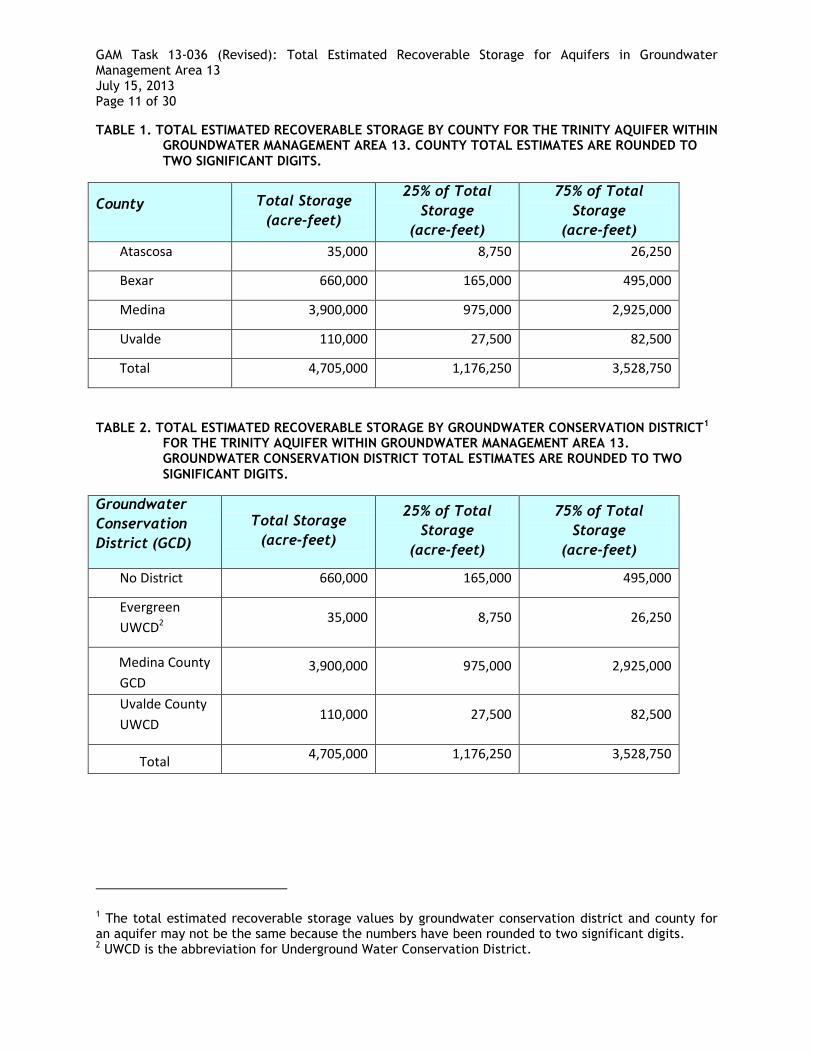
GAM Task 13-036 (Revised): Total Estimated Recoverable Storage for Aquifers in Groundwater Management Area 13 July 15, 2013 Page 11 of 30
TABLE 1. TOTAL ESTIMATED RECOVERABLE STORAGE BY COUNTY FOR THE TRINITY AQUIFER WITHIN GROUNDWATER MANAGEMENT AREA 13. COUNTY TOTAL ESTIMATES ARE ROUNDED TO
TWO SIGNIFICANT DIGITS.
County Total Storage
(acre-feet)
25% of Total
Storage
(acre-feet)
75% of Total
Storage
(acre-feet)
Atascosa 35,000 8,750 26,250
Bexar 660,000 165,000 495,000
Medina 3,900,000 975,000 2,925,000
Uvalde 110,000 27,500 82,500
Total 4,705,000 1,176,250 3,528,750
TABLE 2. TOTAL ESTIMATED RECOVERABLE STORAGE BY GROUNDWATER CONSERVATION DISTRICT1 FOR THE TRINITY AQUIFER WITHIN GROUNDWATER MANAGEMENT AREA 13. GROUNDWATER CONSERVATION DISTRICT TOTAL ESTIMATES ARE ROUNDED TO TWO
SIGNIFICANT DIGITS.
Groundwater
Conservation
District (GCD)
Total Storage
(acre-feet)
25% of Total
Storage
(acre-feet)
75% of Total
Storage
(acre-feet)
No District 660,000 165,000 495,000
Evergreen
UWCD2 35,000 8,750 26,250
Medina County
GCD 3,900,000 975,000 2,925,000
Uvalde County
UWCD 110,000 27,500 82,500
Total 4,705,000 1,176,250 3,528,750
1 The total estimated recoverable storage values by groundwater conservation district and county for an aquifer may not be the same because the numbers have been rounded to two significant digits. 2 UWCD is the abbreviation for Underground Water Conservation District.
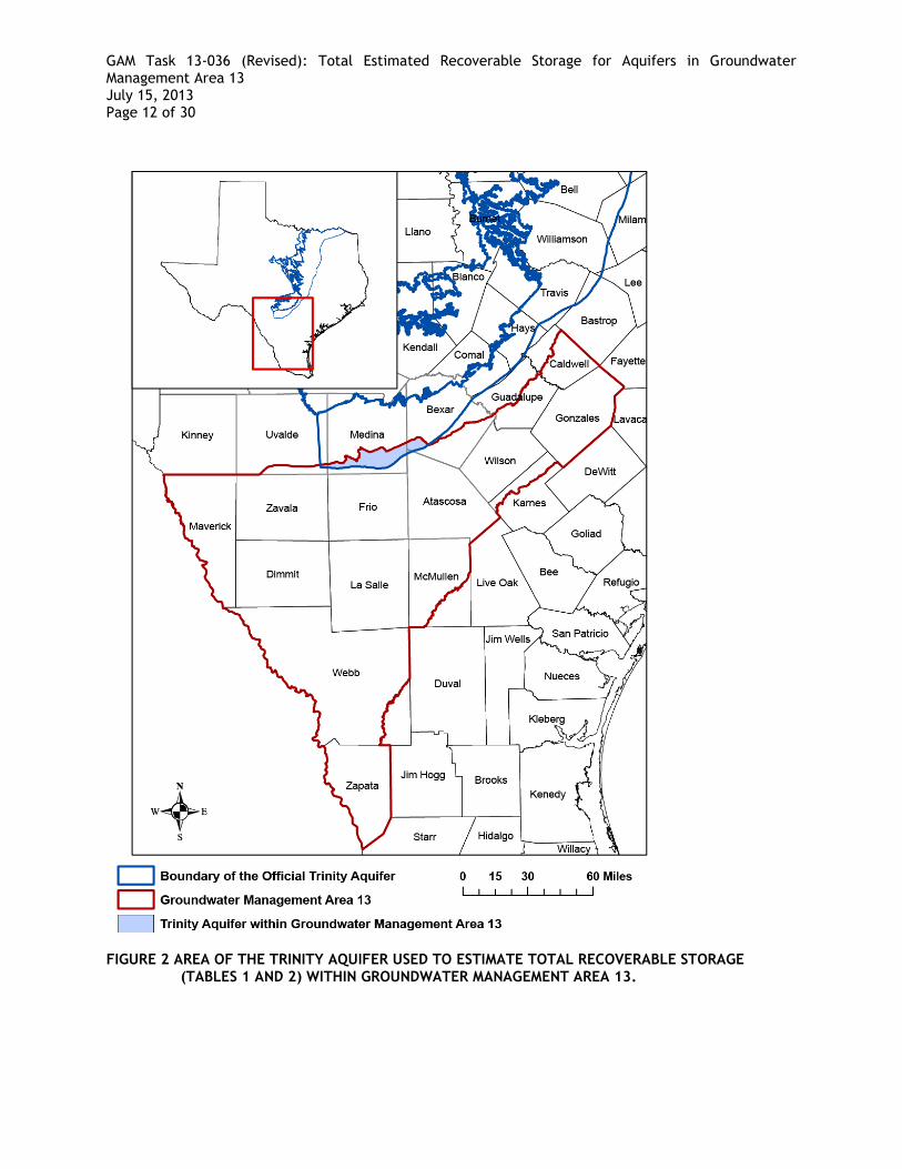
GAM Task 13-036 (Revised): Total Estimated Recoverable Storage for Aquifers in Groundwater Management Area 13 July 15, 2013 Page 12 of 30
FIGURE 2 AREA OF THE TRINITY AQUIFER USED TO ESTIMATE TOTAL RECOVERABLE STORAGE
(TABLES 1 AND 2) WITHIN GROUNDWATER MANAGEMENT AREA 13.
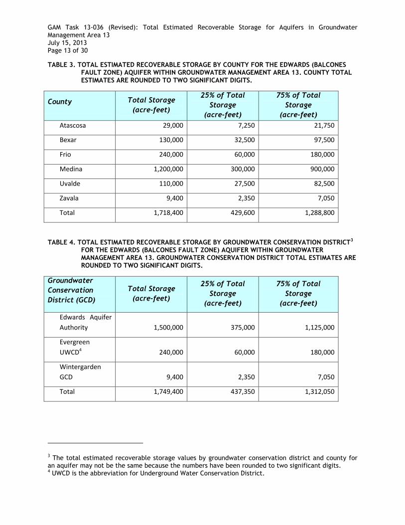
GAM Task 13-036 (Revised): Total Estimated Recoverable Storage for Aquifers in Groundwater Management Area 13 July 15, 2013 Page 13 of 30
TABLE 3. TOTAL ESTIMATED RECOVERABLE STORAGE BY COUNTY FOR THE EDWARDS (BALCONES FAULT ZONE) AQUIFER WITHIN GROUNDWATER MANAGEMENT AREA 13. COUNTY TOTAL
ESTIMATES ARE ROUNDED TO TWO SIGNIFICANT DIGITS.
County Total Storage
(acre-feet)
25% of Total
Storage
(acre-feet)
75% of Total
Storage
(acre-feet)
Atascosa 29,000 7,250 21,750
Bexar 130,000 32,500 97,500
Frio 240,000 60,000 180,000
Medina 1,200,000 300,000 900,000
Uvalde 110,000 27,500 82,500
Zavala 9,400 2,350 7,050
Total 1,718,400 429,600 1,288,800
TABLE 4. TOTAL ESTIMATED RECOVERABLE STORAGE BY GROUNDWATER CONSERVATION DISTRICT3 FOR THE EDWARDS (BALCONES FAULT ZONE) AQUIFER WITHIN GROUNDWATER MANAGEMENT AREA 13. GROUNDWATER CONSERVATION DISTRICT TOTAL ESTIMATES ARE ROUNDED TO TWO SIGNIFICANT DIGITS.
Groundwater
Conservation
District (GCD)
Total Storage
(acre-feet)
25% of Total
Storage
(acre-feet)
75% of Total
Storage
(acre-feet)
Edwards Aquifer
Authority 1,500,000 375,000 1,125,000
Evergreen
UWCD4 240,000 60,000 180,000
Wintergarden
GCD 9,400 2,350 7,050
Total 1,749,400 437,350 1,312,050
3 The total estimated recoverable storage values by groundwater conservation district and county for an aquifer may not be the same because the numbers have been rounded to two significant digits. 4 UWCD is the abbreviation for Underground Water Conservation District.
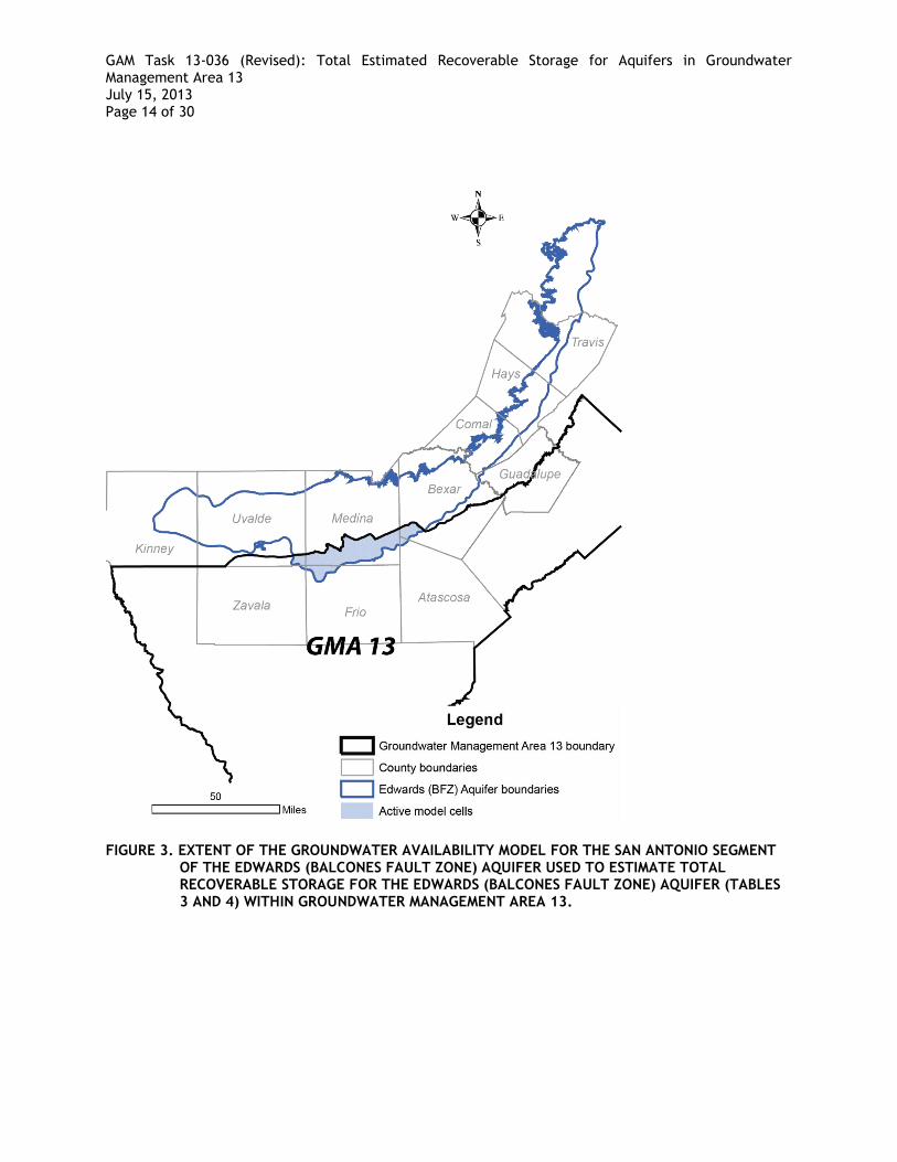
GAM Task 13-036 (Revised): Total Estimated Recoverable Storage for Aquifers in Groundwater Management Area 13 July 15, 2013 Page 14 of 30
FIGURE 3. EXTENT OF THE GROUNDWATER AVAILABILITY MODEL FOR THE SAN ANTONIO SEGMENT OF THE EDWARDS (BALCONES FAULT ZONE) AQUIFER USED TO ESTIMATE TOTAL RECOVERABLE STORAGE FOR THE EDWARDS (BALCONES FAULT ZONE) AQUIFER (TABLES 3 AND 4) WITHIN GROUNDWATER MANAGEMENT AREA 13.
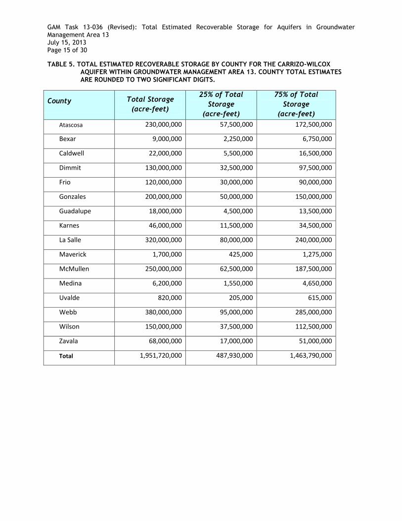
GAM Task 13-036 (Revised): Total Estimated Recoverable Storage for Aquifers in Groundwater Management Area 13 July 15, 2013 Page 15 of 30
TABLE 5. TOTAL ESTIMATED RECOVERABLE STORAGE BY COUNTY FOR THE CARRIZO-WILCOX AQUIFER WITHIN GROUNDWATER MANAGEMENT AREA 13. COUNTY TOTAL ESTIMATES
ARE ROUNDED TO TWO SIGNIFICANT DIGITS.
County Total Storage
(acre-feet)
25% of Total
Storage
(acre-feet)
75% of Total
Storage
(acre-feet)
Atascosa 230,000,000 57,500,000 172,500,000
Bexar 9,000,000 2,250,000 6,750,000
Caldwell 22,000,000 5,500,000 16,500,000
Dimmit 130,000,000 32,500,000 97,500,000
Frio 120,000,000 30,000,000 90,000,000
Gonzales 200,000,000 50,000,000 150,000,000
Guadalupe 18,000,000 4,500,000 13,500,000
Karnes 46,000,000 11,500,000 34,500,000
La Salle 320,000,000 80,000,000 240,000,000
Maverick 1,700,000 425,000 1,275,000
McMullen 250,000,000 62,500,000 187,500,000
Medina 6,200,000 1,550,000 4,650,000
Uvalde 820,000 205,000 615,000
Webb 380,000,000 95,000,000 285,000,000
Wilson 150,000,000 37,500,000 112,500,000
Zavala 68,000,000 17,000,000 51,000,000
Total 1,951,720,000 487,930,000 1,463,790,000
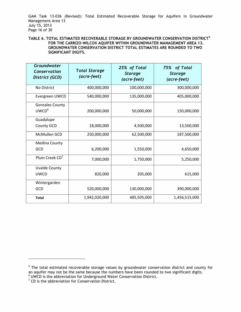
GAM Task 13-036 (Revised): Total Estimated Recoverable Storage for Aquifers in Groundwater Management Area 13 July 15, 2013 Page 16 of 30
TABLE 6. TOTAL ESTIMATED RECOVERABLE STORAGE BY GROUNDWATER CONSERVATION DISTRICT5 FOR THE CARRIZO-WILCOX AQUIFER WITHIN GROUNDWATER MANAGEMENT AREA 13. GROUNDWATER CONSERVATION DISTRICT TOTAL ESTIMATES ARE ROUNDED TO TWO
SIGNIFICANT DIGITS.
5 The total estimated recoverable storage values by groundwater conservation district and county for an aquifer may not be the same because the numbers have been rounded to two significant digits. 6 UWCD is the abbreviation for Underground Water Conservation District. 7 CD is the abbreviation for Conservation District.
Groundwater
Conservation
District (GCD)
Total Storage
(acre-feet)
25% of Total
Storage
(acre-feet)
75% of Total
Storage
(acre-feet)
No District 400,000,000 100,000,000 300,000,000
Evergreen UWCD 540,000,000 135,000,000 405,000,000
Gonzales County
UWCD6 200,000,000 50,000,000 150,000,000
Guadalupe
County GCD 18,000,000 4,500,000 13,500,000
McMullen GCD 250,000,000 62,500,000 187,500,000
Medina County
GCD 6,200,000 1,550,000 4,650,000
Plum Creek CD7 7,000,000 1,750,000 5,250,000
Uvalde County
UWCD 820,000 205,000 615,000
Wintergarden
GCD 520,000,000 130,000,000 390,000,000
Total 1,942,020,000 485,505,000 1,456,515,000
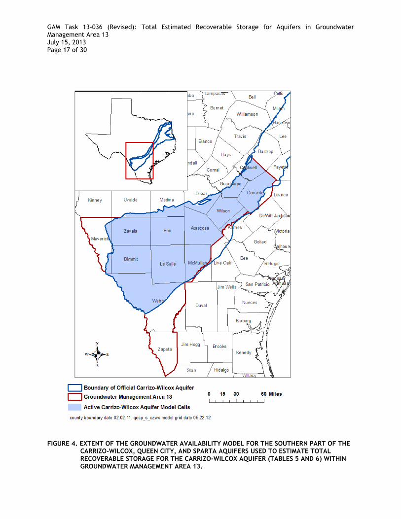
GAM Task 13-036 (Revised): Total Estimated Recoverable Storage for Aquifers in Groundwater Management Area 13 July 15, 2013 Page 17 of 30
FIGURE 4. EXTENT OF THE GROUNDWATER AVAILABILITY MODEL FOR THE SOUTHERN PART OF THE CARRIZO-WILCOX, QUEEN CITY, AND SPARTA AQUIFERS USED TO ESTIMATE TOTAL RECOVERABLE STORAGE FOR THE CARRIZO-WILCOX AQUIFER (TABLES 5 AND 6) WITHIN GROUNDWATER MANAGEMENT AREA 13.
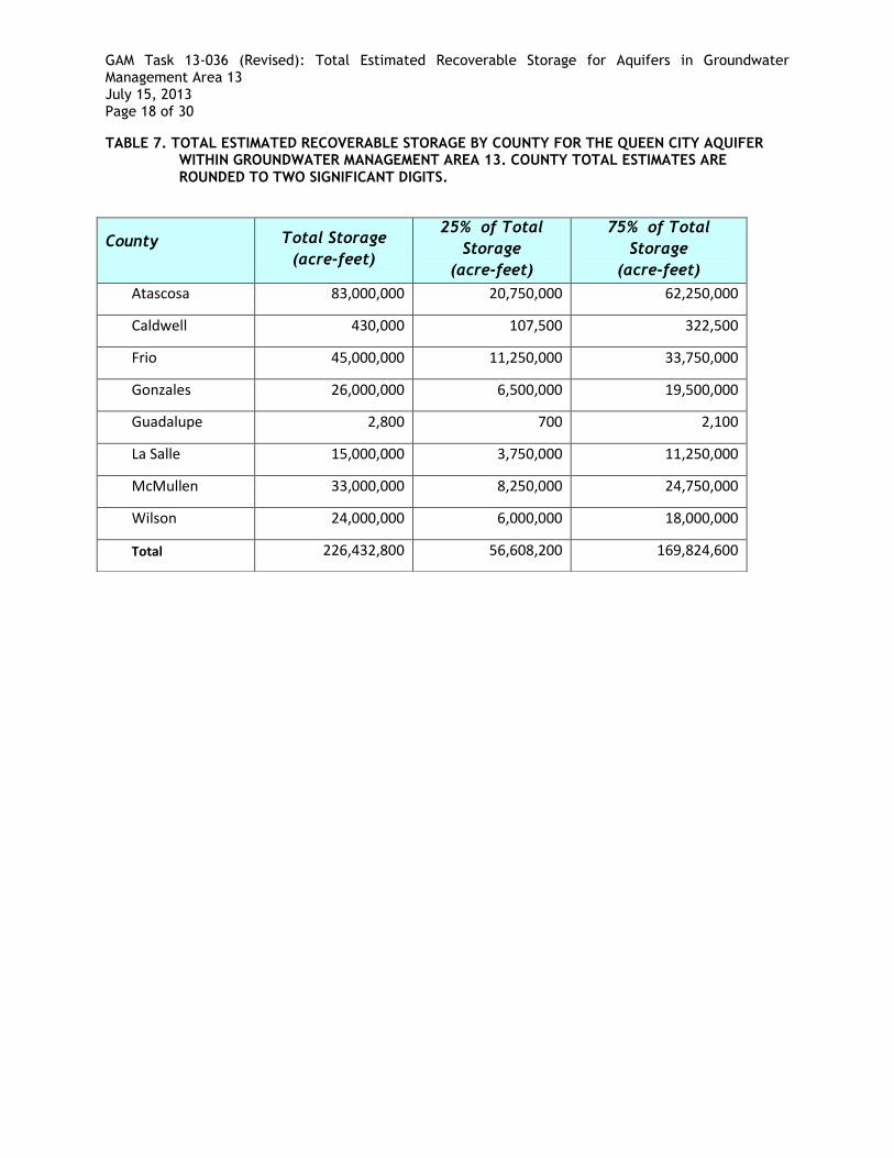
GAM Task 13-036 (Revised): Total Estimated Recoverable Storage for Aquifers in Groundwater Management Area 13 July 15, 2013 Page 18 of 30
TABLE 7. TOTAL ESTIMATED RECOVERABLE STORAGE BY COUNTY FOR THE QUEEN CITY AQUIFER WITHIN GROUNDWATER MANAGEMENT AREA 13. COUNTY TOTAL ESTIMATES ARE
ROUNDED TO TWO SIGNIFICANT DIGITS.
County Total Storage
(acre-feet)
25% of Total
Storage
(acre-feet)
75% of Total
Storage
(acre-feet)
Atascosa 83,000,000 20,750,000 62,250,000
Caldwell 430,000 107,500 322,500
Frio 45,000,000 11,250,000 33,750,000
Gonzales 26,000,000 6,500,000 19,500,000
Guadalupe 2,800 700 2,100
La Salle 15,000,000 3,750,000 11,250,000
McMullen 33,000,000 8,250,000 24,750,000
Wilson 24,000,000 6,000,000 18,000,000
Total 226,432,800 56,608,200 169,824,600
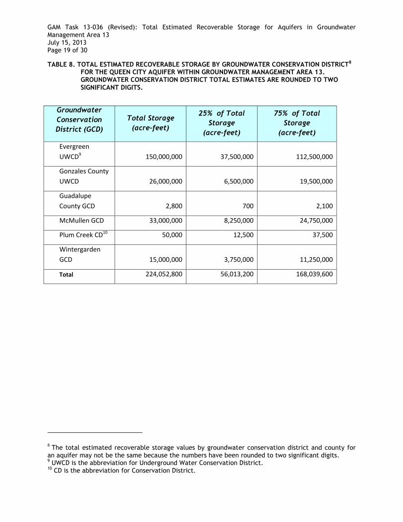
GAM Task 13-036 (Revised): Total Estimated Recoverable Storage for Aquifers in Groundwater Management Area 13 July 15, 2013 Page 19 of 30
TABLE 8. TOTAL ESTIMATED RECOVERABLE STORAGE BY GROUNDWATER CONSERVATION DISTRICT8 FOR THE QUEEN CITY AQUIFER WITHIN GROUNDWATER MANAGEMENT AREA 13. GROUNDWATER CONSERVATION DISTRICT TOTAL ESTIMATES ARE ROUNDED TO TWO
SIGNIFICANT DIGITS.
8 The total estimated recoverable storage values by groundwater conservation district and county for
an aquifer may not be the same because the numbers have been rounded to two significant digits. 9 UWCD is the abbreviation for Underground Water Conservation District. 10 CD is the abbreviation for Conservation District.
Groundwater
Conservation
District (GCD)
Total Storage
(acre-feet)
25% of Total
Storage
(acre-feet)
75% of Total
Storage
(acre-feet)
Evergreen
UWCD9 150,000,000 37,500,000 112,500,000
Gonzales County
UWCD 26,000,000 6,500,000 19,500,000
Guadalupe
County GCD 2,800 700 2,100
McMullen GCD 33,000,000 8,250,000 24,750,000
Plum Creek CD10 50,000 12,500 37,500
Wintergarden
GCD 15,000,000 3,750,000 11,250,000
Total 224,052,800 56,013,200 168,039,600
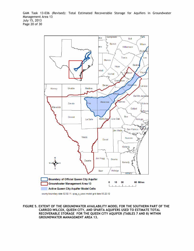
GAM Task 13-036 (Revised): Total Estimated Recoverable Storage for Aquifers in Groundwater Management Area 13 July 15, 2013 Page 20 of 30
FIGURE 5. EXTENT OF THE GROUNDWATER AVAILABILITY MODEL FOR THE SOUTHERN PART OF THE CARRIZO-WILCOX, QUEEN CITY, AND SPARTA AQUIFERS USED TO ESTIMATE TOTAL RECOVERABLE STORAGE FOR THE QUEEN CITY AQUIFER (TABLES 7 AND 8) WITHIN GROUNDWATER MANAGEMENT AREA 13.
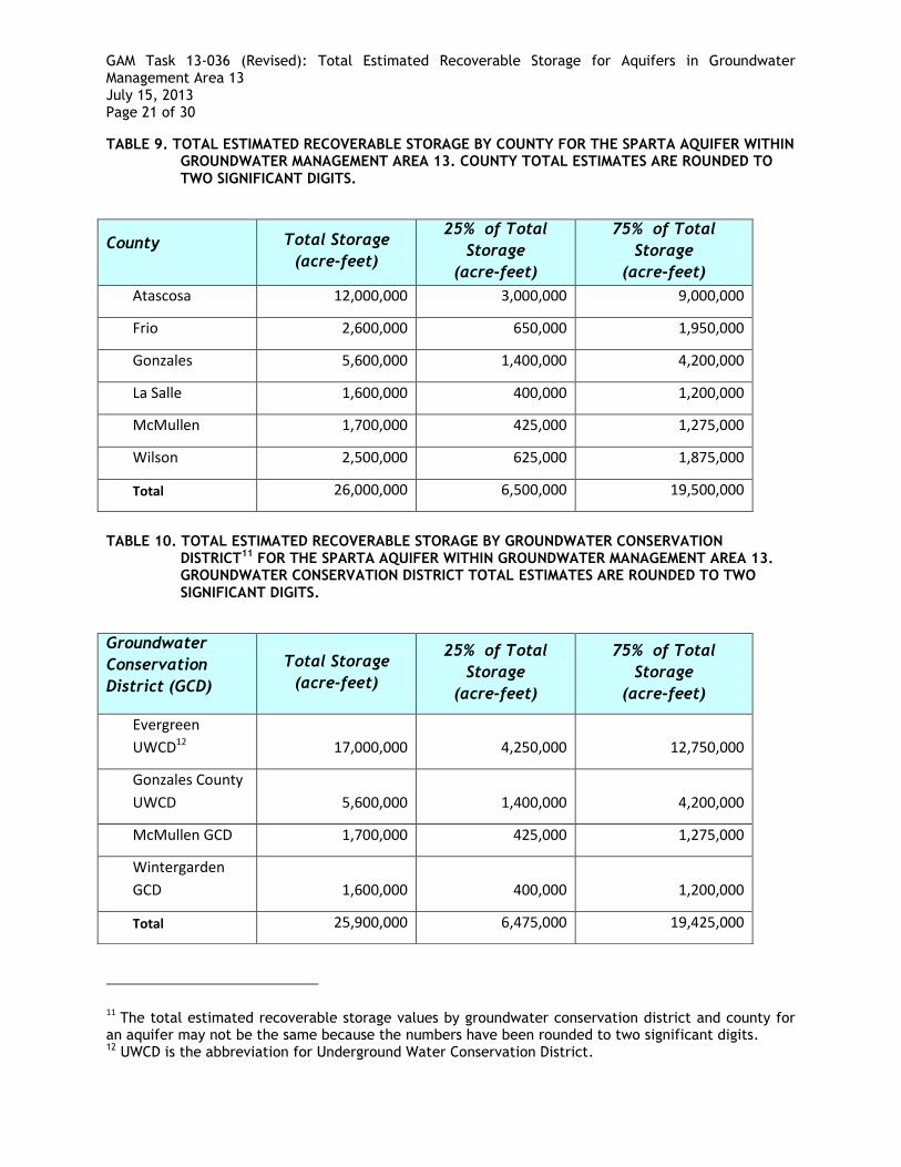
GAM Task 13-036 (Revised): Total Estimated Recoverable Storage for Aquifers in Groundwater Management Area 13 July 15, 2013 Page 21 of 30
TABLE 9. TOTAL ESTIMATED RECOVERABLE STORAGE BY COUNTY FOR THE SPARTA AQUIFER WITHIN GROUNDWATER MANAGEMENT AREA 13. COUNTY TOTAL ESTIMATES ARE ROUNDED TO
TWO SIGNIFICANT DIGITS.
TABLE 10. TOTAL ESTIMATED RECOVERABLE STORAGE BY GROUNDWATER CONSERVATION DISTRICT11 FOR THE SPARTA AQUIFER WITHIN GROUNDWATER MANAGEMENT AREA 13. GROUNDWATER CONSERVATION DISTRICT TOTAL ESTIMATES ARE ROUNDED TO TWO
SIGNIFICANT DIGITS.
11 The total estimated recoverable storage values by groundwater conservation district and county for
an aquifer may not be the same because the numbers have been rounded to two significant digits. 12 UWCD is the abbreviation for Underground Water Conservation District.
County Total Storage
(acre-feet)
25% of Total
Storage
(acre-feet)
75% of Total
Storage
(acre-feet)
Atascosa 12,000,000 3,000,000 9,000,000
Frio 2,600,000 650,000 1,950,000
Gonzales 5,600,000 1,400,000 4,200,000
La Salle 1,600,000 400,000 1,200,000
McMullen 1,700,000 425,000 1,275,000
Wilson 2,500,000 625,000 1,875,000
Total 26,000,000 6,500,000 19,500,000
Groundwater
Conservation
District (GCD)
Total Storage
(acre-feet)
25% of Total
Storage
(acre-feet)
75% of Total
Storage
(acre-feet)
Evergreen
UWCD12 17,000,000 4,250,000 12,750,000
Gonzales County
UWCD 5,600,000 1,400,000 4,200,000
McMullen GCD 1,700,000 425,000 1,275,000
Wintergarden
GCD 1,600,000 400,000 1,200,000
Total 25,900,000 6,475,000 19,425,000
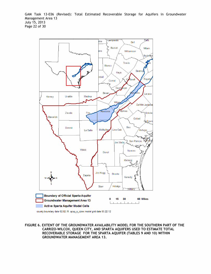
GAM Task 13-036 (Revised): Total Estimated Recoverable Storage for Aquifers in Groundwater Management Area 13 July 15, 2013 Page 22 of 30
FIGURE 6. EXTENT OF THE GROUNDWATER AVAILABILITY MODEL FOR THE SOUTHERN PART OF THE CARRIZO-WILCOX, QUEEN CITY, AND SPARTA AQUIFERS USED TO ESTIMATE TOTAL RECOVERABLE STORAGE FOR THE SPARTA AQUIFER (TABLES 9 AND 10) WITHIN GROUNDWATER MANAGEMENT AREA 13.
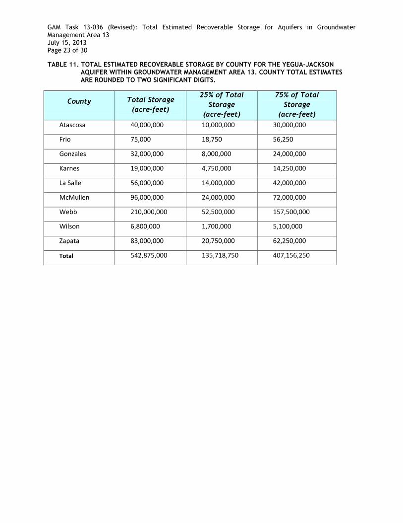
GAM Task 13-036 (Revised): Total Estimated Recoverable Storage for Aquifers in Groundwater Management Area 13 July 15, 2013 Page 23 of 30
TABLE 11. TOTAL ESTIMATED RECOVERABLE STORAGE BY COUNTY FOR THE YEGUA-JACKSON AQUIFER WITHIN GROUNDWATER MANAGEMENT AREA 13. COUNTY TOTAL ESTIMATES
ARE ROUNDED TO TWO SIGNIFICANT DIGITS.
County Total Storage
(acre-feet)
25% of Total
Storage
(acre-feet)
75% of Total
Storage
(acre-feet)
Atascosa 40,000,000 10,000,000 30,000,000
Frio 75,000 18,750 56,250
Gonzales 32,000,000 8,000,000 24,000,000
Karnes 19,000,000 4,750,000 14,250,000
La Salle 56,000,000 14,000,000 42,000,000
McMullen 96,000,000 24,000,000 72,000,000
Webb 210,000,000 52,500,000 157,500,000
Wilson 6,800,000 1,700,000 5,100,000
Zapata 83,000,000 20,750,000 62,250,000
Total 542,875,000 135,718,750 407,156,250
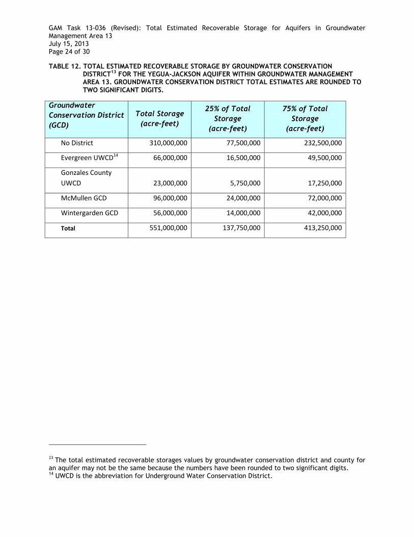
GAM Task 13-036 (Revised): Total Estimated Recoverable Storage for Aquifers in Groundwater Management Area 13 July 15, 2013 Page 24 of 30
TABLE 12. TOTAL ESTIMATED RECOVERABLE STORAGE BY GROUNDWATER CONSERVATION DISTRICT13 FOR THE YEGUA-JACKSON AQUIFER WITHIN GROUNDWATER MANAGEMENT AREA 13. GROUNDWATER CONSERVATION DISTRICT TOTAL ESTIMATES ARE ROUNDED TO
TWO SIGNIFICANT DIGITS.
Groundwater
Conservation District
(GCD)
Total Storage
(acre-feet)
25% of Total
Storage
(acre-feet)
75% of Total
Storage
(acre-feet)
No District 310,000,000 77,500,000 232,500,000
Evergreen UWCD14 66,000,000 16,500,000 49,500,000
Gonzales County
UWCD 23,000,000 5,750,000 17,250,000
McMullen GCD 96,000,000 24,000,000 72,000,000
Wintergarden GCD 56,000,000 14,000,000 42,000,000
Total 551,000,000 137,750,000 413,250,000
13 The total estimated recoverable storages values by groundwater conservation district and county for
an aquifer may not be the same because the numbers have been rounded to two significant digits. 14 UWCD is the abbreviation for Underground Water Conservation District.

GAM Task 13-036 (Revised): Total Estimated Recoverable Storage for Aquifers in Groundwater Management Area 13 July 15, 2013 Page 25 of 30
FIGURE 7. EXTENT OF THE GROUNDWATER AVAILABILITY MODEL FOR THE YEGUA-JACKSON AQUIFER USED TO ESTIMATE TOTAL RECOVERABLE STORAGE (TABLES 11 AND 12) FOR THE YEGUA-JACKSON AQUIFER AND CATAHOULA FORMATION PORTION OF THE GULF COAST AQUIFER SYSTEM (TABLES 13 AND 14) WITHIN GROUNDWATER MANAGEMENT
AREA 13.
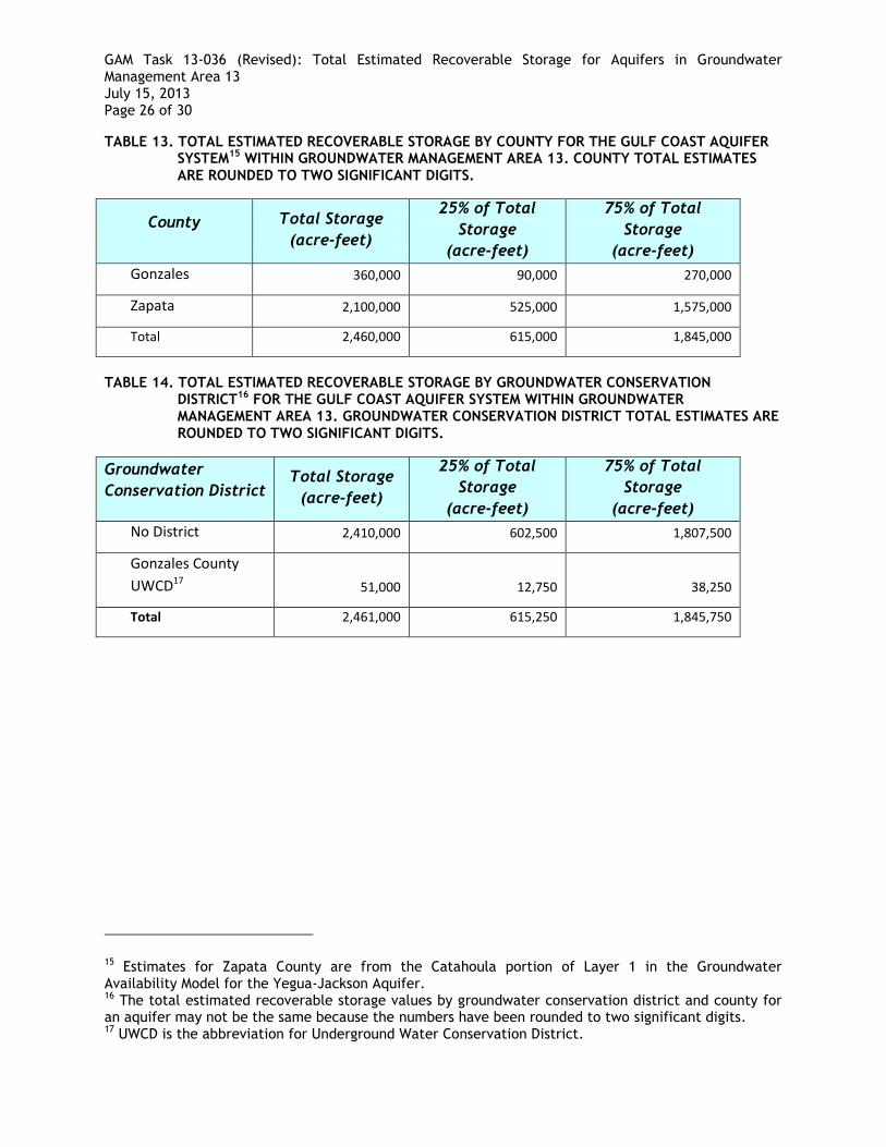
GAM Task 13-036 (Revised): Total Estimated Recoverable Storage for Aquifers in Groundwater Management Area 13 July 15, 2013 Page 26 of 30
TABLE 13. TOTAL ESTIMATED RECOVERABLE STORAGE BY COUNTY FOR THE GULF COAST AQUIFER SYSTEM15 WITHIN GROUNDWATER MANAGEMENT AREA 13. COUNTY TOTAL ESTIMATES
ARE ROUNDED TO TWO SIGNIFICANT DIGITS.
County Total Storage
(acre-feet)
25% of Total
Storage
(acre-feet)
75% of Total
Storage
(acre-feet)
Gonzales 360,000 90,000 270,000
Zapata 2,100,000 525,000 1,575,000
Total 2,460,000 615,000 1,845,000
TABLE 14. TOTAL ESTIMATED RECOVERABLE STORAGE BY GROUNDWATER CONSERVATION DISTRICT16 FOR THE GULF COAST AQUIFER SYSTEM WITHIN GROUNDWATER MANAGEMENT AREA 13. GROUNDWATER CONSERVATION DISTRICT TOTAL ESTIMATES ARE
ROUNDED TO TWO SIGNIFICANT DIGITS.
Groundwater
Conservation District Total Storage
(acre-feet)
25% of Total
Storage
(acre-feet)
75% of Total
Storage
(acre-feet)
No District 2,410,000 602,500 1,807,500
Gonzales County
UWCD17 51,000 12,750 38,250
Total 2,461,000 615,250 1,845,750
15 Estimates for Zapata County are from the Catahoula portion of Layer 1 in the Groundwater Availability Model for the Yegua-Jackson Aquifer. 16 The total estimated recoverable storage values by groundwater conservation district and county for an aquifer may not be the same because the numbers have been rounded to two significant digits. 17 UWCD is the abbreviation for Underground Water Conservation District.
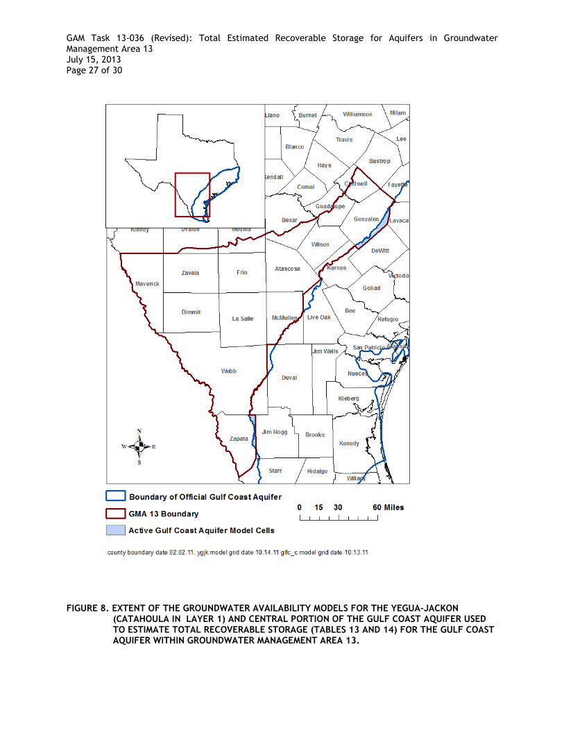
GAM Task 13-036 (Revised): Total Estimated Recoverable Storage for Aquifers in Groundwater Management Area 13 July 15, 2013 Page 27 of 30
FIGURE 8. EXTENT OF THE GROUNDWATER AVAILABILITY MODELS FOR THE YEGUA-JACKON (CATAHOULA IN LAYER 1) AND CENTRAL PORTION OF THE GULF COAST AQUIFER USED TO ESTIMATE TOTAL RECOVERABLE STORAGE (TABLES 13 AND 14) FOR THE GULF COAST AQUIFER WITHIN GROUNDWATER MANAGEMENT AREA 13.
GAM Task 13-036 (Revised): Total Estimated Recoverable Storage for Aquifers in Groundwater Management Area 13 July 15, 2013 Page 28 of 30
LIMITATIONS
The groundwater models used in completing this analysis are the best available scientific
tools that can be used to meet the stated objective(s). To the extent that this analysis will be
used for planning purposes and/or regulatory purposes related to pumping in the past and
into the future, it is important to recognize the assumptions and limitations associated with
the use of the results. In reviewing the use of models in environmental regulatory decision
making, the National Research Council (2007) noted:
“Models will always be constrained by computational limitations, assumptions, and
knowledge gaps. They can best be viewed as tools to help inform decisions rather
than as machines to generate truth or make decisions. Scientific advances will never
make it possible to build a perfect model that accounts for every aspect of reality or
to prove that a given model is correct in all respects for a particular regulatory
application. These characteristics make evaluation of a regulatory model more
complex than solely a comparison of measurement data with model results.”
Because the application of the groundwater model was designed to address regional scale
questions, the results are most effective on a regional scale. The TWDB makes no warranties
or representations relating to the actual conditions of any aquifer at a particular location or
at a particular time.
REFERENCES: Deeds, N., Kelley, V., Fryar, D., Jones, T., Whallon, A.J., and Dean, K.E., 2003, Groundwater
Availability Model for the Southern Carrizo-Wilcox Aquifer: Contract report to the Texas Water Development Board, 452 p., http://www.twdb.texas.gov/groundwater/models/gam/czwx_s/CZWX_S_Full_Report.pdf.
Deeds, N.E., Yan, T., Singh, A., Jones, T.L., Kelley, V.A., Knox, P.R., Young, S.C., 2010, Groundwater availability model for the Yegua-Jackson Aquifer: Final report prepared for the Texas Water Development Board by INTERA, Inc., 582 p., http://www.twdb.texas.gov/groundwater/models/gam/ygjk/YGJK_Model_Report.pdf.
Flawn, P.T., Goldstein, A, King, P.B., and Weaver, C.E.,1961, The Ouachita System, University of Texas at Austin, Bureau of Economic Geology, Publication No. 6120 Plate 4, 401 p.
GAM Task 13-036 (Revised): Total Estimated Recoverable Storage for Aquifers in Groundwater Management Area 13 July 15, 2013 Page 29 of 30
George, P.G., Mace, R.E., and Petrossian, R, 2011, Aquifers of Texas, Texas Water Development Board Report 380, http://www.twdb.texas.gov/groundwater/aquifer/index.asp
Holt, C.L.R., 1956, Geology and ground-water resources of Medina County, Texas Board of Water Engineers, Bulletin 5601, 278 p.
Hunt, B. B, Smith, B.A., Kromann, J, Wiereman, D.A, and Mikels, J.K., 2010, Compilation of pumping tests in Travis and Hays Counties, Central Texas, Barton Springs/Edwards Aquifer Conservation District Data Series Report 2010-0701, p.
Johnson, A.I., 1967, Specfic yield – compilation of specific yields for various materials, U.S. Geological Survey, Water Supply Paper 1662-D, 74p.
Jones, I.C., Anaya, R. and Wade, S., 2009, Groundwater Availability Model for the Hill Country portion of the Trinity Aquifer System, Texas, Texas Water Development Board unpublished report, 193 p.
Kalaswad, S., and Arroyo, J., 2006, Status report on brackish groundwater and desalination in the Gulf Coast Aquifer of Texas in Mace, R.E., Davison, S.C., Angle, E.S., and Mullican, III, W.F., eds., Aquifers of the Gulf Coast of Texas: Texas Water Development Board Report 365, p. 231–240., http://www.twdb.texas.gov/publications/reports/numbered_reports/doc/R365/R365_Composite.pdf
Kelley, V.A., Deeds, N.E., Fryar, D.G., and Nicot, J.P., 2004, Groundwater availability models for the Queen City and Sparta aquifers: Contract report to the Texas Water Development Board, 867 p., http://www.twdb.texas.gov/groundwater/models/gam/qcsp/QCSP_Model_Report.pdf.
Lindgren, R.J., Dutton, A.R, Hovorka, S.D., Worthington, S.R.H., and Painter, S., Conceptualization and simulation of the Edwards Aquifer, San Antonio Region, Texas, U. S. Geological Survey, Scientific Investigations Report 2004-5277
National Research Council, 2007, Models in Environmental Regulatory Decision Making Committee on Models in the Regulatory Decision Process, National Academies Press, Washington D.C., 287 p., http://www.nap.edu/catalog.php?record_id=11972.
Texas Department of Licensing and Regulation, 2013, Texas Well Record Submission and Retrieval System: Texas Department of Licensing and Regulation, Water Well and Pump Installers program.
Texas Administrative Code, 2011, http://info.sos.state.tx.us/pls/pub/readtac$ext.viewtac
Texas Water Code, 2011, http://www.statutes.legis.state.tx.us/docs/WA/pdf/WA.36.pdf
Texas Water Development Board, 2013, Groundwater database: Texas Water Development Board, Water Science and Conservation Division.

GAM Task 13-036 (Revised): Total Estimated Recoverable Storage for Aquifers in Groundwater Management Area 13 July 15, 2013 Page 30 of 30
Welder, F.A. and Reeves, R.D., 1962, Geology and Ground-water resources of Uvalde County, Texas, Texas Water Commission, Bulletin 6212, 252 p.

Appendix F
Paper authored by James Bene of R.W. Harden & Associates regarding the Joint Planning Process
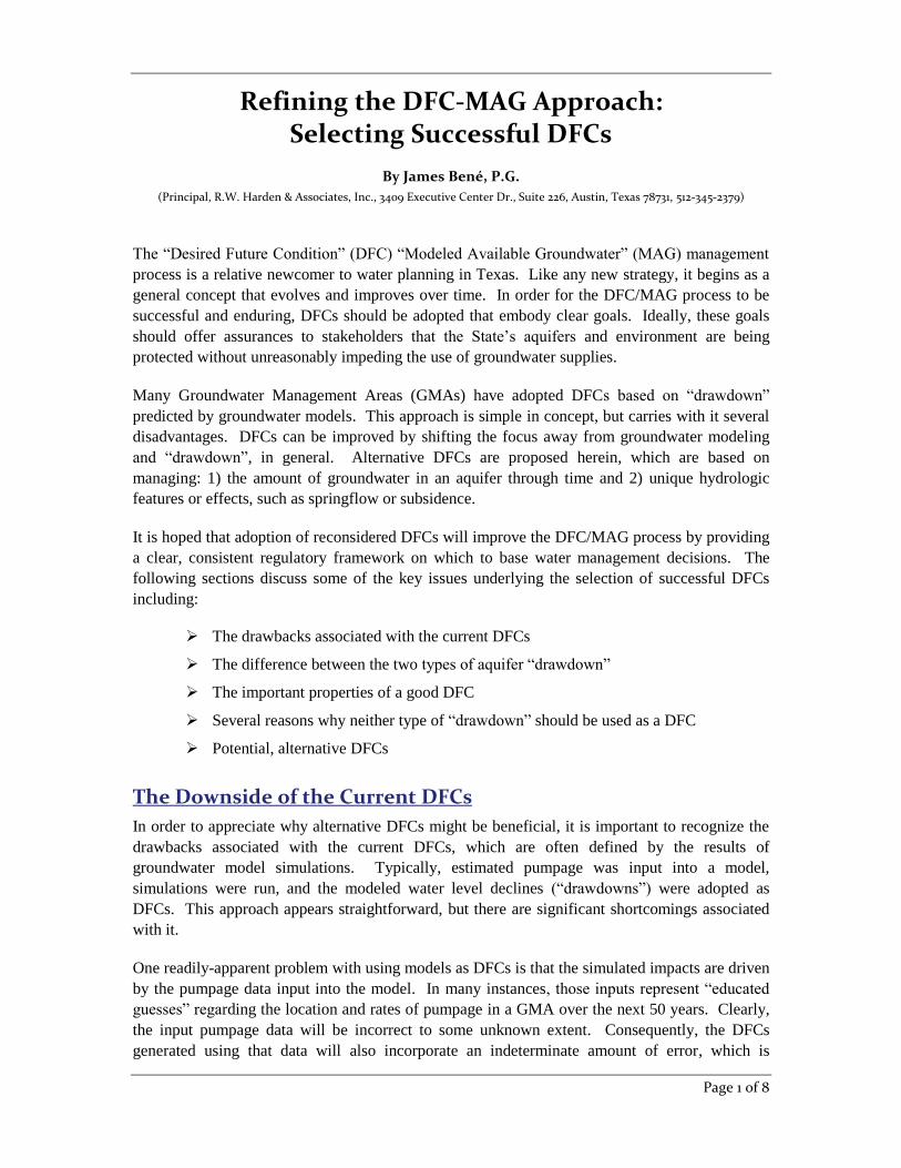
Page 1 of 8
Refining the DFC-MAG Approach: Selecting Successful DFCs
By James Bené, P.G.
(Principal, R.W. Harden & Associates, Inc., 3409 Executive Center Dr., Suite 226, Austin, Texas 78731, 512-345-2379)
The “Desired Future Condition” (DFC) “Modeled Available Groundwater” (MAG) management
process is a relative newcomer to water planning in Texas. Like any new strategy, it begins as a
general concept that evolves and improves over time. In order for the DFC/MAG process to be
successful and enduring, DFCs should be adopted that embody clear goals. Ideally, these goals
should offer assurances to stakeholders that the State’s aquifers and environment are being
protected without unreasonably impeding the use of groundwater supplies.
Many Groundwater Management Areas (GMAs) have adopted DFCs based on “drawdown”
predicted by groundwater models. This approach is simple in concept, but carries with it several
disadvantages. DFCs can be improved by shifting the focus away from groundwater modeling
and “drawdown”, in general. Alternative DFCs are proposed herein, which are based on
managing: 1) the amount of groundwater in an aquifer through time and 2) unique hydrologic
features or effects, such as springflow or subsidence.
It is hoped that adoption of reconsidered DFCs will improve the DFC/MAG process by providing
a clear, consistent regulatory framework on which to base water management decisions. The
following sections discuss some of the key issues underlying the selection of successful DFCs
including:
The drawbacks associated with the current DFCs
The difference between the two types of aquifer “drawdown”
The important properties of a good DFC
Several reasons why neither type of “drawdown” should be used as a DFC
Potential, alternative DFCs
The Downside of the Current DFCs
In order to appreciate why alternative DFCs might be beneficial, it is important to recognize the
drawbacks associated with the current DFCs, which are often defined by the results of
groundwater model simulations. Typically, estimated pumpage was input into a model,
simulations were run, and the modeled water level declines (“drawdowns”) were adopted as
DFCs. This approach appears straightforward, but there are significant shortcomings associated
with it.
One readily-apparent problem with using models as DFCs is that the simulated impacts are driven
by the pumpage data input into the model. In many instances, those inputs represent “educated
guesses” regarding the location and rates of pumpage in a GMA over the next 50 years. Clearly,
the input pumpage data will be incorrect to some unknown extent. Consequently, the DFCs
generated using that data will also incorporate an indeterminate amount of error, which is
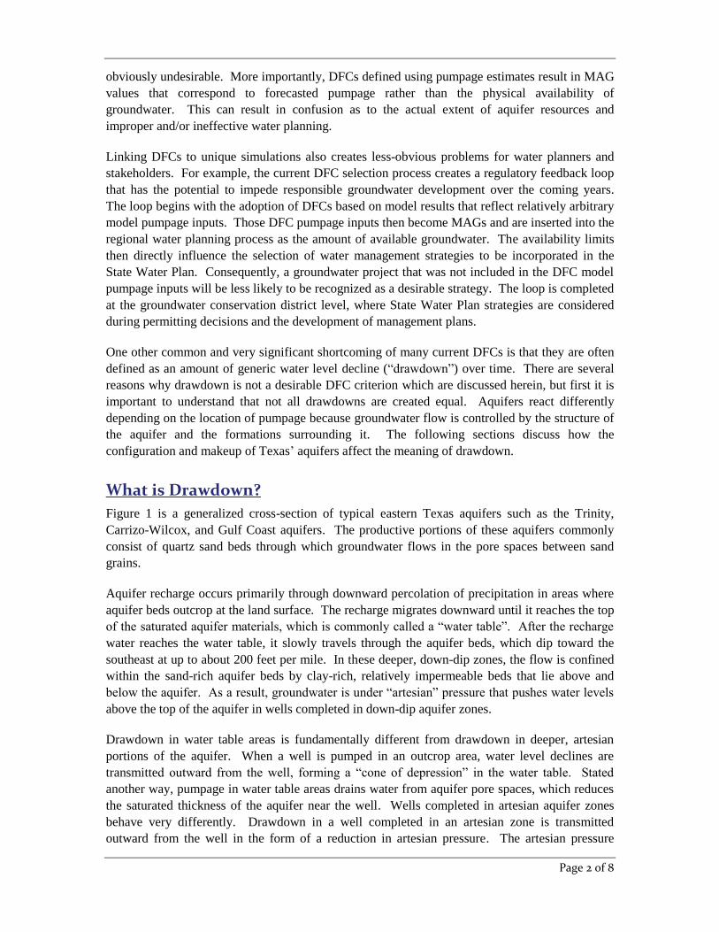
Page 2 of 8
obviously undesirable. More importantly, DFCs defined using pumpage estimates result in MAG
values that correspond to forecasted pumpage rather than the physical availability of
groundwater. This can result in confusion as to the actual extent of aquifer resources and
improper and/or ineffective water planning.
Linking DFCs to unique simulations also creates less-obvious problems for water planners and
stakeholders. For example, the current DFC selection process creates a regulatory feedback loop
that has the potential to impede responsible groundwater development over the coming years.
The loop begins with the adoption of DFCs based on model results that reflect relatively arbitrary
model pumpage inputs. Those DFC pumpage inputs then become MAGs and are inserted into the
regional water planning process as the amount of available groundwater. The availability limits
then directly influence the selection of water management strategies to be incorporated in the
State Water Plan. Consequently, a groundwater project that was not included in the DFC model
pumpage inputs will be less likely to be recognized as a desirable strategy. The loop is completed
at the groundwater conservation district level, where State Water Plan strategies are considered
during permitting decisions and the development of management plans.
One other common and very significant shortcoming of many current DFCs is that they are often
defined as an amount of generic water level decline (“drawdown”) over time. There are several
reasons why drawdown is not a desirable DFC criterion which are discussed herein, but first it is
important to understand that not all drawdowns are created equal. Aquifers react differently
depending on the location of pumpage because groundwater flow is controlled by the structure of
the aquifer and the formations surrounding it. The following sections discuss how the
configuration and makeup of Texas’ aquifers affect the meaning of drawdown.
What is Drawdown?
Figure 1 is a generalized cross-section of typical eastern Texas aquifers such as the Trinity,
Carrizo-Wilcox, and Gulf Coast aquifers. The productive portions of these aquifers commonly
consist of quartz sand beds through which groundwater flows in the pore spaces between sand
grains.
Aquifer recharge occurs primarily through downward percolation of precipitation in areas where
aquifer beds outcrop at the land surface. The recharge migrates downward until it reaches the top
of the saturated aquifer materials, which is commonly called a “water table”. After the recharge
water reaches the water table, it slowly travels through the aquifer beds, which dip toward the
southeast at up to about 200 feet per mile. In these deeper, down-dip zones, the flow is confined
within the sand-rich aquifer beds by clay-rich, relatively impermeable beds that lie above and
below the aquifer. As a result, groundwater is under “artesian” pressure that pushes water levels
above the top of the aquifer in wells completed in down-dip aquifer zones.
Drawdown in water table areas is fundamentally different from drawdown in deeper, artesian
portions of the aquifer. When a well is pumped in an outcrop area, water level declines are
transmitted outward from the well, forming a “cone of depression” in the water table. Stated
another way, pumpage in water table areas drains water from aquifer pore spaces, which reduces
the saturated thickness of the aquifer near the well. Wells completed in artesian aquifer zones
behave very differently. Drawdown in a well completed in an artesian zone is transmitted
outward from the well in the form of a reduction in artesian pressure. The artesian pressure
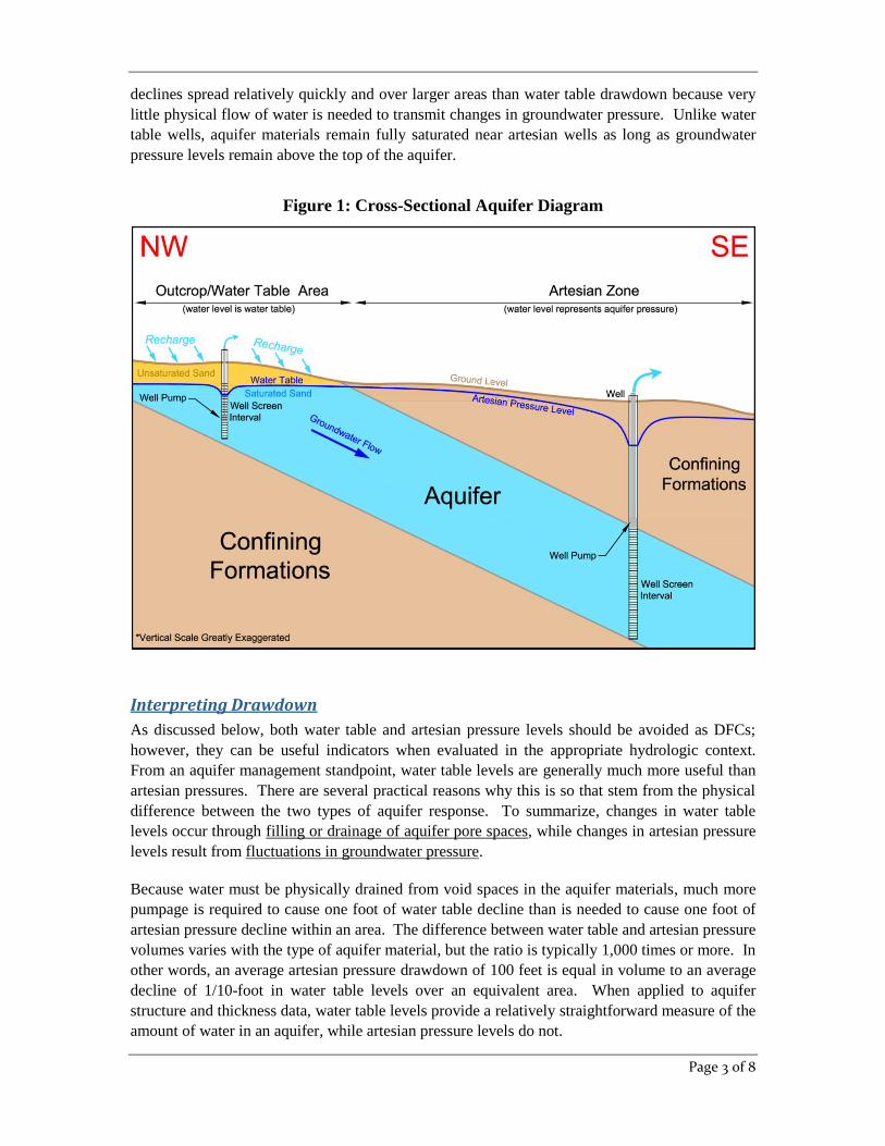
Page 3 of 8
declines spread relatively quickly and over larger areas than water table drawdown because very
little physical flow of water is needed to transmit changes in groundwater pressure. Unlike water
table wells, aquifer materials remain fully saturated near artesian wells as long as groundwater
pressure levels remain above the top of the aquifer.
Figure 1: Cross-Sectional Aquifer Diagram
Interpreting Drawdown
As discussed below, both water table and artesian pressure levels should be avoided as DFCs;
however, they can be useful indicators when evaluated in the appropriate hydrologic context.
From an aquifer management standpoint, water table levels are generally much more useful than
artesian pressures. There are several practical reasons why this is so that stem from the physical
difference between the two types of aquifer response. To summarize, changes in water table
levels occur through filling or drainage of aquifer pore spaces, while changes in artesian pressure
levels result from fluctuations in groundwater pressure.
Because water must be physically drained from void spaces in the aquifer materials, much more
pumpage is required to cause one foot of water table decline than is needed to cause one foot of
artesian pressure decline within an area. The difference between water table and artesian pressure
volumes varies with the type of aquifer material, but the ratio is typically 1,000 times or more. In
other words, an average artesian pressure drawdown of 100 feet is equal in volume to an average
decline of 1/10-foot in water table levels over an equivalent area. When applied to aquifer
structure and thickness data, water table levels provide a relatively straightforward measure of the
amount of water in an aquifer, while artesian pressure levels do not.
Page 4 of 8
Water table levels are also more useful for evaluating many environmental effects. Biological
environments and habitats that rely on groundwater depend on sufficiently high water table levels
to maintain adequate outflows to springs, seeps, and/or streams. In conjunction with other factors
such as aquifer structure, composition, and hydraulic boundaries, water table levels play an
important role in managing surface/groundwater flow. Artesian pressures also affect groundwater
flow to surface features, but only through their subdued influence on water table levels.
Historical well records indicate that, in general, changes in water table levels progress at a slow,
steady pace. In contrast, large, short-term fluctuations in artesian pressure levels are common in
Texas’ aquifers as pumpage rates change in response to seasonal demands or individual well
pumping cycles. Monitoring of slow, steady water table declines is preferred because it allows
regulators and stakeholders enough time to carefully respond to changes in aquifer conditions.
What makes a good DFC?
Texas has been and continues to be relatively progressive with respect to collecting, analyzing,
modeling, and distributing groundwater data. We have a long-term record of the changes in
groundwater systems throughout the State, which allows us to be comparatively confident in our
predictions. Nevertheless, groundwater regulations ought to be structured to provide safeguards
against unexpected, adverse effects in case we are wrong about how our aquifers will behave in
the future.
Experience suggests that the core motivation for regulating groundwater use is the common
desire to prevent three basic types of unwanted impacts:
Resource Depletion – Will there be enough groundwater for future needs?
Environmental Impacts – Will pumping harm the hydrogeologic system or
ecosystems that depend on groundwater? Will pumping cause significant subsidence
in low-lying areas?
Economic Impacts – Will the use of groundwater cause an undue financial burden on
stakeholders? What are the costs of promoting or limiting economic development in
a region?
Good DFCs will account for all of these factors and will focus on addressing clearly-defined,
well-documented goals. In keeping with the principle of “Occam’s Razor”, which tells us that the
simplest solution is usually the correct one, it is also desirable that DFCs be defined as plainly
and concisely as possible. From a practical standpoint, there should be simple methods for
verifying that DFC goals are being met in the real world. It is also important that a DFC be
structured in a way that promotes fair and impartial regulation for all groundwater owners.
Drawdown is NOT a good DFC
Neither water table nor artesian pressure drawdowns make good DFCs. While monitoring both
types of declines is informative, there are more-straightforward criteria that can be used when
defining DFCs. The following sections discuss why using drawdown (in either form) to control
aquifer depletion, environmental impacts, and/or economic costs is not the best way to manage
Texas’ aquifers.
Page 5 of 8
Managing Groundwater Availability and the Environment with Drawdown
Artesian pressure declines do not have a meaningful impact on aquifer storage or groundwater
flows to surface features and are, therefore, not suitable as DFCs in those respects. Subsidence
can result from artesian pressure declines in clay-rich layers; therefore, in areas where subsidence
is a concern, selecting DFCs based on artesian pressure drawdown appears fitting. Water table
levels can be used to monitor the amount of water in an aquifer and directly influence natural
discharge to springs, seeps, streams, and other surface features. For these reasons, water table
drawdowns also appear to be suitable as DFCs.
However, water table and artesian pressure declines do not represent good DFCs because they are
not important in and of themselves; they must always be “translated” into information that speaks
to the actual, desired management objectives. For example, when considering aquifer depletion,
how much water table decline is acceptable? Obviously, the significance of the amount of water
table drawdown can only be determined when compared and contrasted to other hydrologic
information such as the structure, thickness, and permeability of an aquifer. If we want to
manage groundwater availability, then a DFC explicitly stating the allowable changes in storage
over time is more practical than attempting to manage depletion through drawdown limits.
Similarly, if it is decided that it is important to maintain flow from a certain spring, then the DFC
should be based on a rate of springflow. While water table levels can influence groundwater
discharge to springs, selection of a DFC based on water table drawdown only accomplishes the
actual goal indirectly. Likewise, using artesian pressure drawdown to control subsidence is much
less direct than simply choosing a DFC that expressly limits the allowable amount of subsidence.
In addition to being more straightforward, direct limits are preferable because there are several
factors other than water table and artesian pressure drawdown that affect springflow and
subsidence.
Management of Impacts on Existing Users
Both water table levels and artesian pressures affect maximum well yields and the cost of
producing groundwater. In general, maximum well production rates decline as regional artesian
pressure or water table declines occur. Depending on the site-specific conditions, water table
drawdown may reduce saturated thickness of updip portions of an aquifer to the point where it is
no longer practical to produce groundwater. In addition to reduced well yields, pumping lift costs
increase as wellbore pumping levels deepen.
Given these facts, water table and artesian pressure levels undoubtedly have the potential to affect
the availability and economics of groundwater use, which suggests that regulating them is a
necessary part of groundwater management. However, adopting drawdown as a DFC to limit
potential impacts on existing users should be avoided because it sets the stage for unequal
regulation. In order to understand why, it is helpful to consider the responsibilities of the
landowners and the State with regard to the use and management of groundwater.
Groundwater is a common resource that is owned by every Texan who owns land over an aquifer.
However, while a landowner may own the subsurface water, there is no assurance that the site-
specific hydrologic conditions will allow him or her to produce as much as neighboring
landowners. Consequently, it is not possible for the State to guarantee equal groundwater
supplies for every landowner. Rather, it is the State’s responsibility to ensure that: 1)

Page 6 of 8
groundwater resources are being beneficially used and managed and 2) that all stakeholders are
allowed to try to produce their fair share. There should be no conflict between these two
responsibilities; if it is decided that limiting groundwater use benefits the community, then those
limits should be applied consistently to all stakeholders. If unequal restrictions are imposed, the
landowner who is required to shoulder a heavier regulatory burden should be compensated for it.
Using DFCs as a way to limit impacts on existing users sets the stage for inequitable regulation
because every user of groundwater from an aquifer contributes to artesian pressure and water
table declines in that aquifer. Existing well owners have benefitted from a common resource and
have drained water from neighboring landowners who have not used groundwater. In essence,
DFCs designed to protect existing users elevate the rights of those who have profited from
groundwater by limiting the rights of landowners who have conserved it.
Management of Regional Economic Impacts with Drawdown
But what about the effects that water table and artesian pressure levels have on the overall
economy of a region? Won’t too much drawdown reduce groundwater availability and
negatively impact economic development? Yes, excessive declines have the potential to affect
groundwater availability and the economic health of a region. However, it’s important to realize
that water table and artesian pressure levels are not the real issues in this instance; assuring that
there is enough water for future needs is the true goal. DFCs defined specifically as acceptable
amounts of available groundwater are much more appropriate than attempting to control
availability by way of generic drawdown limits. It should also be noted that there are negative
economic impacts associated with not using groundwater. In general, the increased electrical and
well maintenance costs resulting from new pumpage are typically heavily outweighed by the
economic benefits gained through development of additional groundwater supplies.
Alternative DFCs
As an alternative to current DFCs, an approach founded on changes in aquifer storage and the
protection of unique hydrologic features or conditions is proposed. Two types of DFCs are
recommended:
1) Aquifer Storage DFC – Adopt DFCs describing the acceptable amount of water in
aquifer storage through time. An example could be: “We want at least 95% of the
available water currently stored in the aquifer to still be available in 50 years.”
2) “Spotlight” DFC – Select conditions for specific areas or features that are uniquely
affected by groundwater flows or effects. Examples of this kind of DFC could be: “The
flow from Clearwater Spring shall be maintained at or above a minimum rate of ten cubic
feet per second over the next 50 years,” or “The average land surface subsidence in Area
1 shall be limited to five feet over the next 50 years.”
DFCs defining acceptable declines in aquifer storage are not new; they have been in place in the
Texas Panhandle for several years and have been shown to enjoy several advantages. DFCs
based on regional aquifer storage allow for flexible water planning, while maintaining clear
assurances that resource depletion is controlled. On a local level, managing aquifer storage
makes sense because it can be verified easily and inexpensively through monitoring of water table
Page 7 of 8
levels. In addition, changes in aquifer storage generally occur at a slow, steady pace that allows
groundwater conservation districts to distinguish between important aquifer trends and localized,
short-term fluctuations in artesian pressure. When definite, long-term trends can be recognized
and discussed over time in a public forum, relations between regulators and stakeholders
generally improve. Perhaps most importantly, managing groundwater in storage targets a primary
concern of most Texans, succinctly and without uncertainty.
“Spotlight” DFCs that focus on managing special groundwater flows or effects can also be a
helpful management tool for exceptional circumstances. In general, this type of DFC may be
implemented where it is in the public interest to manage a specific hydrologic feature or
condition, such as springflow or subsidence. A careful cost/benefit analysis should be completed
before enacting a DFC targeted to achieve a specific public interest because of the greater
potential for inflicting inconsistent regulatory burdens and subsequent property takings on
landowners. However, while these types of DFCs may be more difficult to implement fairly, they
can provide assurance that unique features or effects are properly managed.
Section 36.108(d) of the Texas Water Code lists several factors that must be considered (and
reported) by GMAs during the selection of DFCs. Some of the most pertinent are:
hydrological conditions, including for each aquifer in the management area the total
estimated recoverable storage as provided by the executive administrator, and the
average annual recharge, inflows, and discharge;
other environmental impacts, including impacts on spring flow and other interactions
between groundwater and surface water;
the impact on subsidence;
socioeconomic impacts reasonably expected to occur;
the impact on the interests and rights in private property…
The proposed DFCs are advantageous because they allow for more straightforward assessments
of these factors. Evaluation of the relationship between the DFCs and the “recoverable storage”
and aquifer recharge/discharge flows is much simpler when the DFC specifically manages the
volumes of groundwater in aquifer storage through time. Similarly, feature-specific “spotlight”
DFCs (and the processes used to develop them) support relatively clear-cut discussions of
environmental and economic impacts.
Concluding Thoughts
Section 36.108(d-2) of the Texas Water Code states that DFCs must provide a balance between:
…the highest practicable level of groundwater production and the
conservation, preservation, protection, recharging, and prevention of waste of
groundwater…
The existing DFCs make it more difficult for stakeholders to assess this balance because they are
based on simulated drawdown, which does not directly speak to aquifer depletion, environmental
concerns, or economic issues. The DFC/MAG process can be improved by shifting the focus
Page 8 of 8
away from modeling results toward real-world aquifer measurements; groundwater models can be
very useful tools for some tasks, but it is a mistake to integrate them so completely into the
management process.
The alternative DFCs proposed herein are intended to improve the regulatory process by
specifically managing the amount of groundwater in storage, as well as environmental flows or
effects. By directly controlling these concerns, the proposed DFCs provide clear-cut assurances
that groundwater resources are being properly managed. By concentrating on physical data and
sensible goals, Texans can reshape the current regulatory system into something that promotes
both responsible stewardship and use of our aquifers.
Appendix G
Socioeconomic Impacts Analyses for Regions K, L, and M
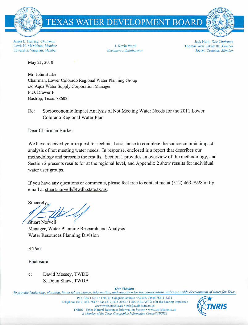

Stuart D. Norvell, Managing Economist Water Resources Planning Division Texas Water Development Board Austin, Texas S. Doug Shaw, Agricultural Economist Water Resources Planning Division Texas Water Development Board Austin, Texas May 2010
Socioeconomic Impacts of Projected Water Shortages for the
Lower Colorado Regional Water Planning Area (Region K)
Prepared in Support of the 2011 Lower Colorado Regional Water Plan
Table of Contents
Section Title Page
Introduction……………..………………………………………………………………………………………………………………………..…………………… 3
1.0 Methodology……………………………………………………………………………………………….……………………………………..…................... 3
1.1 Economic Impacts of Water Shortages………………………………………………………………………………………………………………… 3
1.1.1 General Approach……………………………………………………….................................................................................. 8
General Assumptions and Clarifications of the Methodology.…….…….……………………….……….…........... 9
1.1.2 Impacts to Agriculture……………………………………………………………………………………………………..……………............... 9
Irrigation………………………………..………………….……………………………………………………………………..….………… 9
Livestock…………………………………..……………………………………………………………………………………………..……… 11
1.1.3 Impacts to Municipal Water User Groups……………………..…………………………………………………………….…….………… 12
Disaggregation of Municipal Water Demands.………………………………………………………….……….……………... 13
Domestic Water Uses……………………………………………………………………….………..………….………………………... 14
Commercial Businesses……………………………………………………………………………….………..……………….………... 17
Water Utility Revenues………….……………………………………………………………………………....………………………. 18
Horticulture and Landscaping.….………………………………………………………………………………….………………... 18
Recreational Impacts…………………………………………………………………………….……………………………….………… 19
1.1.4 Impacts to Industrial Water User Groups……………………………………………………….……………………………………………. 19
Manufacturing………………………………………………………………………………………………………………..………………… 20
Mining..………..….……………………………………………………………………………………………………..……………………….. 20
Steam-electric..…………………………………………………………………………………………….………..………………………… 21
1.2 Social Impacts of Water Shortages……………………………………………………………………………………………..………………………… 21
2.0 Results………………………………………………………………………………………………………………………………………………………….………….. 22
2.1 Overview of Regional Economy…………………………………………………………………………………………………………….……………… 22
2.2 Impacts to Agricultural Water User Groups……………………………………………………………………………………………..…………… 23
2.3 Impacts to Municipal Water User Groups……………………………………………………………………………………………………………… 24
2.4 Impacts to Manufacturing Water User Groups……………………………………………………………………………………….……………… 24
2.5 Impacts to Mining Water User Groups……………………………………………………………………………………………………………..…… 25
2.6 Impacts to Steam-electric Water User Groups………………………………………………………………………….………...………………… 26
2.7 Social Impacts……………………………………………………………………………………………………………………………….…………..………….. 26
2.8 Distribution of Impacts by Major River Basin……………………………………………………………………………….……………….………. 27
Appendix 1: Economic Data for Individual IMPLAN Sectors…………………………………………………………………………….......…………………….. 29
Appendix 2: Impacts by County………………………………………………………………………….....………………..………………………….………………………. 33
Tables
1 Crop Classifications and Corresponding IMPLAN Crop Sectors…………………………………………………………………………………... 10
2 Summary of Irrigated Crop Acreage and Water Demand….…………………………..………………………………………………………...… 10
3 Average Gross Sales Revenues per Acre for Irrigated Crops………………………………………………………………………………….……. 11
4 Description of Livestock Sectors…………………………………………………………………………………………………………………………….…… 12
5 Water Use and Costs Parameters Used to Estimated Domestic Water Demand Functions………………………………………… 14
6 Economic Losses Associated with Domestic Water Shortages……………………………………………………………………………………. 16
7 Impacts of Municipal Water Shortages at Different Magnitudes of Shortages…………………………………………..………………. 19
8 Regional Baseline Economy by Water User Group………………………….….……………………………………………………………..…….… 23
9 Economic Impacts of Water Shortages for Irrigation Water User Groups……………………………………………….……………….… 23
10 Economic Impacts of Water Shortages for Municipal Water User Groups……………………………………………….………………… 24
11 Economic Impacts of Water Shortages for Manufacturing Water User Groups…………………………………….…………………… 25
12 Economic Impacts of Water Shortages for Mining Water User Groups….…………..……………………………………………………… 25
13 Economic Impacts of Water Shortages for Steam-electric Water User Groups…..……………………………………………………… 26
14 Social Impacts of Water Shortages………………..…………………………………………………………………………………………………………… 26
15 Distribution of Impacts by Major River Basin…………………………………………………………………………………………………………….. 27
3
Introduction
Water shortages during drought would likely curtail or eliminate economic activity in business
and industries reliant on water. For example, without water farmers cannot irrigate; refineries cannot produce gasoline, and paper mills cannot make paper. Unreliable water supplies would not only have an immediate and real impact on existing businesses and industry, but they could also adversely affect economic development in Texas. From a social perspective, water supply reliability is critical as well. Shortages would disrupt activity in homes, schools and government and could adversely affect public health and safety. For all of the above reasons, it is important to analyze and understand how restricted water supplies during drought could affect communities throughout the state.
Administrative rules require that regional water planning groups evaluate the impacts of not
meeting water needs as part of the regional water planning process, and rules direct TWDB staff to provide technical assistance: “The executive administrator shall provide available technical assistance to the regional water planning groups, upon request, on water supply and demand analysis, including methods to evaluate the social and economic impacts of not meeting needs” [(§357.7 (4)(A)]. Staff of the TWDB’s Water Resources Planning Division designed and conducted this report in support of the Lower Colorado Regional Water Planning Group (Region K).
This document summarizes the results of our analysis and discusses the methodology used to generate the results. Section 1 outlines the overall methodology and discusses approaches and assumptions specific to each water use category (i.e., irrigation, livestock, mining, steam-electric, municipal and manufacturing). Section 2 presents the results for each category where shortages are reported at the regional planning area level and river basin level. Results for individual water user groups are not presented, but are available upon request.
1. Methodology
Section 1 provides a general overview of how economic and social impacts were measured. In addition, it summarizes important clarifications, assumptions and limitations of the study.
1.1 Economic Impacts of Water Shortages
1.1.1 General Approach
Economic analysis as it relates to water resources planning generally falls into two broad areas. Supply side analysis focuses on costs and alternatives of developing new water supplies or implementing programs that provide additional water from current supplies. Demand side analysis concentrates on impacts or benefits of providing water to people, businesses and the environment. Analysis in this report focuses strictly on demand side impacts. When analyzing the economic impacts of water shortages as defined in Texas water planning, three potential scenarios are possible:
1) Scenario 1 involves situations where there are physical shortages of raw surface or groundwater due to drought of record conditions. For example, City A relies on a reservoir with average conservation storage of 500 acre-feet per year and a firm yield of 100 acre feet. In 2010, the city uses about 50 acre-feet per year, but by 2030 their demands are expected to increase to 200 acre-feet. Thus, in 2030 the reservoir would not have enough water to meet the city’s demands, and people would experience a shortage of 100 acre-feet assuming drought of record conditions.
4
Under normal or average climatic conditions, the reservoir would likely be able to provide reliable water supplies well beyond 2030.
2) Scenario 2 is a situation where despite drought of record conditions, water supply sources can meet existing use requirements; however, limitations in water infrastructure would preclude future water user groups from accessing these water supplies. For example, City B relies on a river that can provide 500 acre-feet per year during drought of record conditions and other constraints as dictated by planning assumptions. In 2010, the city is expected to use an estimated 100 acre-feet per year and by 2060 it would require no more than 400 acre-feet. But the intake and pipeline that currently transfers water from the river to the city’s treatment plant has a capacity of only 200 acre-feet of water per year. Thus, the city’s water supplies are adequate even under the most restrictive planning assumptions, but their conveyance system is too small. This implies that at some point – perhaps around 2030 - infrastructure limitations would constrain future population growth and any associated economic activity or impacts.
3) Scenario 3 involves water user groups that rely primarily on aquifers that are being depleted. In this scenario, projected and in some cases existing demands may be unsustainable as groundwater levels decline. Areas that rely on the Ogallala aquifer are a good example. In some communities in the region, irrigated agriculture forms a major base of the regional economy. With less irrigation water from the Ogallala, population and economic activity in the region could decline significantly assuming there are no offsetting developments.
Assessing the social and economic effects of each of the above scenarios requires various levels
and methods of analysis and would generate substantially different results for a number of reasons; the most important of which has to do with the time frame of each scenario. Scenario 1 falls into the general category of static analysis. This means that models would measure impacts for a small interval of time such as a drought. Scenarios 2 and 3, on the other hand imply a dynamic analysis meaning that models are concerned with changes over a much longer time period.
Since administrative rules specify that planning analysis be evaluated under drought of record conditions (a static and random event), socioeconomic impact analysis developed by the TWDB for the state water plan is based on assumptions of Scenario 1. Estimated impacts under scenario 1 are point estimates for years in which needs are reported (2010, 2020, 2030, 2040, 2050 and 2060). They are independent and distinct “what if” scenarios for a particular year and shortages are assumed to be temporary events resulting from drought of record conditions. Estimated impacts measure what would happen if water user groups experience water shortages for a period of one year.
The TWDB recognize that dynamic models may be more appropriate for some water user groups; however, combining approaches on a statewide basis poses several problems. For one, it would require a complex array of analyses and models, and might require developing supply and demand forecasts under “normal” climatic conditions as opposed to drought of record conditions. Equally important is the notion that combining the approaches would produce inconsistent results across regions resulting in a so-called “apples to oranges” comparison.
A variety tools are available to estimate economic impacts, but by far, the most widely used today are input-output models (IO models) combined with social accounting matrices (SAMs). Referred to as IO/SAM models, these tools formed the basis for estimating economic impacts for agriculture (irrigation and livestock water uses) and industry (manufacturing, mining, steam-electric and commercial business activity for municipal water uses).

5
Since the planning horizon extends through 2060, economic variables in the baseline are adjusted in accordance with projected changes in demographic and economic activity. Growth rates for municipal water use sectors (i.e., commercial, residential and institutional) are based on TWDB population forecasts. Future values for manufacturing, agriculture, and mining and steam-electric activity are based on the same underlying economic forecasts used to estimate future water use for each category. The following steps outline the overall process. Step 1: Generate IO/SAM Models and Develop Economic Baseline
IO/SAM models were estimated using propriety software known as IMPLAN PRO
TM (Impact for
Planning Analysis). IMPLAN is a modeling system originally developed by the U.S. Forestry Service in the late 1970s. Today, the Minnesota IMPLAN Group (MIG Inc.) owns the copyright and distributes data and software. It is probably the most widely used economic impact model in existence. IMPLAN comes with databases containing the most recently available economic data from a variety of sources.
1 Using IMPLAN
software and data, transaction tables conceptually similar to the one discussed previously were estimated for each county in the region and for the region as a whole. Each transaction table contains 528 economic sectors and allows one to estimate a variety of economic statistics including:
total sales - total production measured by sales revenues;
intermediate sales - sales to other businesses and industries within a given region;
final sales – sales to end users in a region and exports out of a region;
employment - number of full and part-time jobs (annual average) required by a given industry including self-employment;
regional income - total payroll costs (wages and salaries plus benefits) paid by industries, corporate income, rental income and interest payments; and
business taxes - sales, excise, fees, licenses and other taxes paid during normal operation of an industry (does not include income taxes).
TWDB analysts developed an economic baseline containing each of the above variables using
year 2000 data. Since the planning horizon extends through 2060, economic variables in the baseline were allowed to change in accordance with projected changes in demographic and economic activity. Growth rates for municipal water use sectors (i.e., commercial, residential and institutional) are based on TWDB population forecasts. Projections for manufacturing, agriculture, and mining and steam-electric activity are based on the same underlying economic forecasts used to estimate future water use for each category. Monetary impacts in future years are reported in constant year 2006 dollars.
It is important to stress that employment, income and business taxes are the most useful
variables when comparing the relative contribution of an economic sector to a regional economy. Total sales as reported in IO/SAM models are less desirable and can be misleading because they include sales to other industries in the region for use in the production of other goods. For example, if a mill buys grain from local farmers and uses it to produce feed, sales of both the processed feed and raw corn are counted as “output” in an IO model. Thus, total sales double-count or overstate the true economic value of goods
1The IMPLAN database consists of national level technology matrices based on benchmark input-output accounts generated by the U.S. Bureau of Economic Analysis and estimates of final demand, final payments, industry output and employment for various economic sectors. IMPLAN regional data (i.e. states, a counties or groups of counties within a state) are divided into two basic categories: 1) data on an industry basis including value-added, output and employment, and 2) data on a commodity basis including final demands and institutional sales. State-level data are balanced to national totals using a matrix ratio allocation system and county data are balanced to state totals.

6
and services produced in an economy. They are not consistent with commonly used measures of output such as Gross National Product (GNP), which counts only final sales.
Another important distinction relates to terminology. Throughout this report, the term sector refers to economic subdivisions used in the IMPLAN database and resultant input-output models (528 individual sectors based on Standard Industrial Classification Codes). In contrast, the phrase water use category refers to water user groups employed in state and regional water planning including irrigation, livestock, mining, municipal, manufacturing and steam electric. Each IMPLAN sector was assigned to a specific water use category.
Step 2: Estimate Direct and Indirect Economic Impacts of Water Needs Direct impacts are reductions in output by sectors experiencing water shortages. For example,
without adequate cooling and process water a refinery would have to curtail or cease operation, car washes may close, or farmers may not be able to irrigate and sales revenues fall. Indirect impacts involve changes in inter-industry transactions as supplying industries respond to decreased demands for their services, and how seemingly non-related businesses are affected by decreased incomes and spending due to direct impacts. For example, if a farmer ceases operations due to a lack of irrigation water, they would likely reduce expenditures on supplies such as fertilizer, labor and equipment, and businesses that provide these goods would suffer as well.
Direct impacts accrue to immediate businesses and industries that rely on water and without
water industrial processes could suffer. However, output responses may vary depending upon the severity of shortages. A small shortage relative to total water use would likely have a minimal impact, but large shortages could be critical. For example, farmers facing small shortages might fallow marginally productive acreage to save water for more valuable crops. Livestock producers might employ emergency culling strategies, or they may consider hauling water by truck to fill stock tanks. In the case of manufacturing, a good example occurred in the summer of 1999 when Toyota Motor Manufacturing experienced water shortages at a facility near Georgetown, Kentucky.
2 As water levels in the Kentucky
River fell to historic lows due to drought, plant managers sought ways to curtail water use such as reducing rinse operations to a bare minimum and recycling water by funneling it from paint shops to boilers. They even considered trucking in water at a cost of 10 times what they were paying. Fortunately, rains at the end of the summer restored river levels, and Toyota managed to implement cutbacks without affecting production, but it was a close call. If rains had not replenished the river, shortages could have severely reduced output.
3
To account for uncertainty regarding the relative magnitude of impacts to farm and business
operations, the following analysis employs the concept of elasticity. Elasticity is a number that shows how a change in one variable will affect another. In this case, it measures the relationship between a percentage reduction in water availability and a percentage reduction in output. For example, an elasticity of 1.0 indicates that a 1.0 percent reduction in water availability would result in a 1.0 percent reduction in economic output. An elasticity of 0.50 would indicate that for every 1.0 percent of unavailable water, output is reduced by 0.50 percent and so on. Output elasticities used in this study are:
4
2 Royal, W. “High And Dry - Industrial Centers Face Water Shortages.” in Industry Week, Sept, 2000. 3 The efforts described above are not planned programmatic or long-term operational changes. They are emergency measures that individuals might pursue to alleviate what they consider a temporary condition. Thus, they are not characteristic of long-term management strategies designed to ensure more dependable water supplies such as capital investments in conservation technology or development of new water supplies. 4 Elasticities are based on one of the few empirical studies that analyze potential relationships between economic output and water shortages in the United States. The study, conducted in California, showed that a significant number of industries would suffer reduced output during water shortages. Using a survey based approach researchers posed two scenarios to different industries. In
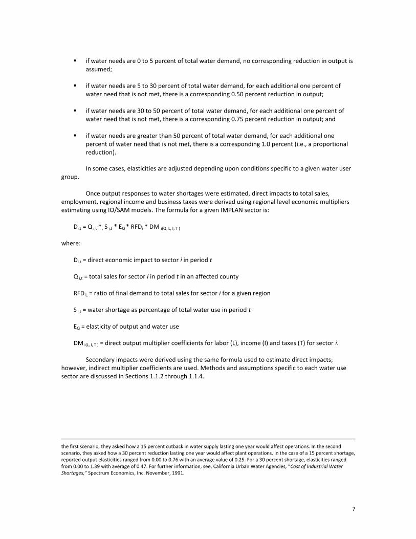
7
if water needs are 0 to 5 percent of total water demand, no corresponding reduction in output is
assumed; if water needs are 5 to 30 percent of total water demand, for each additional one percent of
water need that is not met, there is a corresponding 0.50 percent reduction in output; if water needs are 30 to 50 percent of total water demand, for each additional one percent of
water need that is not met, there is a corresponding 0.75 percent reduction in output; and
if water needs are greater than 50 percent of total water demand, for each additional one percent of water need that is not met, there is a corresponding 1.0 percent (i.e., a proportional reduction).
In some cases, elasticities are adjusted depending upon conditions specific to a given water user group.
Once output responses to water shortages were estimated, direct impacts to total sales,
employment, regional income and business taxes were derived using regional level economic multipliers estimating using IO/SAM models. The formula for a given IMPLAN sector is:
Di,t = Q i,t *, S i,t * EQ * RFDi * DM i(Q, L, I, T )
where:
Di,t = direct economic impact to sector i in period t Q i,t = total sales for sector i in period t in an affected county RFD i, = ratio of final demand to total sales for sector i for a given region S i,t = water shortage as percentage of total water use in period t EQ = elasticity of output and water use DM i(L, I, T ) = direct output multiplier coefficients for labor (L), income (I) and taxes (T) for sector i.
Secondary impacts were derived using the same formula used to estimate direct impacts;
however, indirect multiplier coefficients are used. Methods and assumptions specific to each water use sector are discussed in Sections 1.1.2 through 1.1.4.
the first scenario, they asked how a 15 percent cutback in water supply lasting one year would affect operations. In the second scenario, they asked how a 30 percent reduction lasting one year would affect plant operations. In the case of a 15 percent shortage, reported output elasticities ranged from 0.00 to 0.76 with an average value of 0.25. For a 30 percent shortage, elasticities ranged from 0.00 to 1.39 with average of 0.47. For further information, see, California Urban Water Agencies, “Cost of Industrial Water Shortages,” Spectrum Economics, Inc. November, 1991.
8
General Assumptions and Clarification of the Methodology
As with any attempt to measure and quantify human activities at a societal level, assumptions are necessary and every model has limitations. Assumptions are needed to maintain a level of generality and simplicity such that models can be applied on several geographic levels and across different economic sectors. In terms of the general approach used here several clarifications and cautions are warranted:
1. Shortages as reported by regional planning groups are the starting point for socioeconomic analyses.
2. Estimated impacts are point estimates for years in which needs are reported (i.e., 2010, 2020,
2030, 2040, 2050 and 2060).They are independent and distinct “what if” scenarios for each particular year and water shortages are assumed to be temporary events resulting from severe drought conditions combined with infrastructure limitations. In other words, growth occurs and future shocks are imposed on an economy at 10-year intervals and resultant impacts are measured. Given, that reported figures are not cumulative in nature, it is inappropriate to sum impacts over the entire planning horizon. Doing so, would imply that the analysis predicts that drought of record conditions will occur every ten years in the future, which is not the case. Similarly, authors of this report recognize that in many communities needs are driven by population growth, and in the future total population will exceed the amount of water available due to infrastructure limitations, regardless of whether or not there is a drought. This implies that infrastructure limitations would constrain economic growth. However, since needs as defined by planning rules are based upon water supply and demand under the assumption of drought of record conditions, it improper to conduct economic analysis that focuses on growth related impacts over the planning horizon. Figures generated from such an analysis would presume a 50-year drought of record, which is unrealistic. Estimating lost economic activity related to constraints on population and commercial growth due to lack of water would require developing water supply and demand forecasts under “normal” or “most likely” future climatic conditions.
3. While useful for planning purposes, this study is not a benefit-cost analysis. Benefit cost analysis
is a tool widely used to evaluate the economic feasibility of specific policies or projects as opposed to estimating economic impacts of unmet water needs. Nevertheless, one could include some impacts measured in this study as part of a benefit cost study if done so properly. Since this is not a benefit cost analysis, future impacts are not weighted differently. In other words, estimates are not discounted. If used as a measure of economic benefits, one should incorporate a measure of uncertainty into the analysis. In this type of analysis, a typical method of discounting future values is to assign probabilities of the drought of record recurring again in a given year, and weight monetary impacts accordingly. This analysis assumes a probability of one.
4. IO multipliers measure the strength of backward linkages to supporting industries (i.e., those
who sell inputs to an affected sector). However, multipliers say nothing about forward linkages consisting of businesses that purchase goods from an affected sector for further processing. For example, ranchers in many areas sell most of their animals to local meat packers who process animals into a form that consumers ultimately see in grocery stores and restaurants. Multipliers do not capture forward linkages to meat packers, and since meat packers sell livestock purchased from ranchers as “final sales,” multipliers for the ranching sector do fully account for all losses to a region’s economy. Thus, as mentioned previously, in some cases closely linked sectors were moved from one water use category to another.
5. Cautions regarding interpretations of direct and secondary impacts are warranted. IO/SAM
multipliers are based on ”fixed-proportion production functions,” which basically means that input use - including labor - moves in lockstep fashion with changes in levels of output. In a
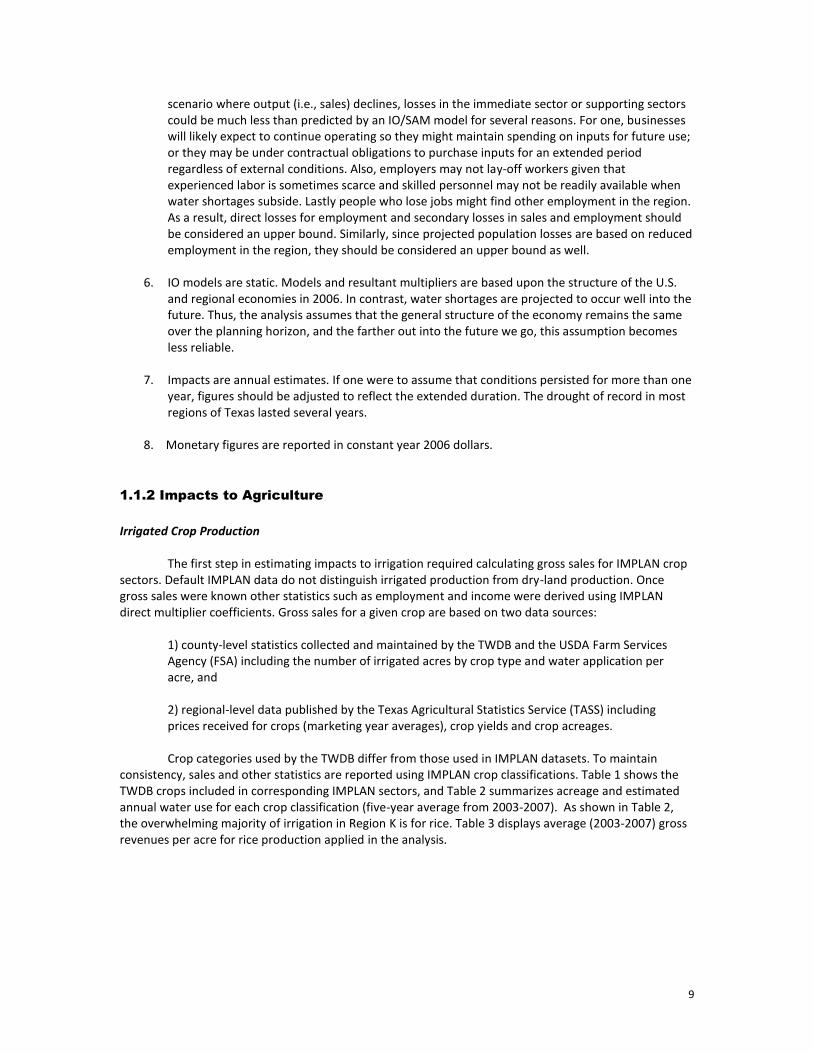
9
scenario where output (i.e., sales) declines, losses in the immediate sector or supporting sectors could be much less than predicted by an IO/SAM model for several reasons. For one, businesses will likely expect to continue operating so they might maintain spending on inputs for future use; or they may be under contractual obligations to purchase inputs for an extended period regardless of external conditions. Also, employers may not lay-off workers given that experienced labor is sometimes scarce and skilled personnel may not be readily available when water shortages subside. Lastly people who lose jobs might find other employment in the region. As a result, direct losses for employment and secondary losses in sales and employment should be considered an upper bound. Similarly, since projected population losses are based on reduced employment in the region, they should be considered an upper bound as well.
6. IO models are static. Models and resultant multipliers are based upon the structure of the U.S.
and regional economies in 2006. In contrast, water shortages are projected to occur well into the future. Thus, the analysis assumes that the general structure of the economy remains the same over the planning horizon, and the farther out into the future we go, this assumption becomes less reliable.
7. Impacts are annual estimates. If one were to assume that conditions persisted for more than one
year, figures should be adjusted to reflect the extended duration. The drought of record in most regions of Texas lasted several years.
8. Monetary figures are reported in constant year 2006 dollars.
1.1.2 Impacts to Agriculture
Irrigated Crop Production
The first step in estimating impacts to irrigation required calculating gross sales for IMPLAN crop sectors. Default IMPLAN data do not distinguish irrigated production from dry-land production. Once gross sales were known other statistics such as employment and income were derived using IMPLAN direct multiplier coefficients. Gross sales for a given crop are based on two data sources:
1) county-level statistics collected and maintained by the TWDB and the USDA Farm Services Agency (FSA) including the number of irrigated acres by crop type and water application per acre, and 2) regional-level data published by the Texas Agricultural Statistics Service (TASS) including prices received for crops (marketing year averages), crop yields and crop acreages. Crop categories used by the TWDB differ from those used in IMPLAN datasets. To maintain
consistency, sales and other statistics are reported using IMPLAN crop classifications. Table 1 shows the TWDB crops included in corresponding IMPLAN sectors, and Table 2 summarizes acreage and estimated annual water use for each crop classification (five-year average from 2003-2007). As shown in Table 2, the overwhelming majority of irrigation in Region K is for rice. Table 3 displays average (2003-2007) gross revenues per acre for rice production applied in the analysis.
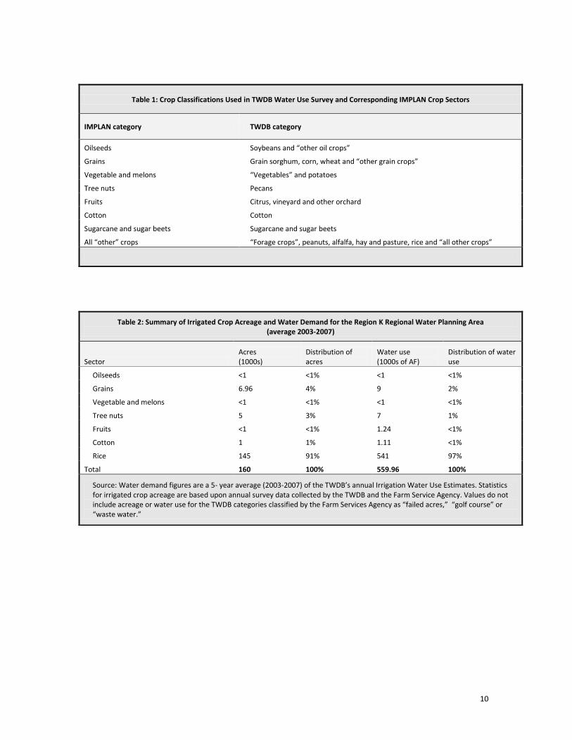
10
Table 1: Crop Classifications Used in TWDB Water Use Survey and Corresponding IMPLAN Crop Sectors
IMPLAN category TWDB category
Oilseeds Soybeans and “other oil crops”
Grains Grain sorghum, corn, wheat and “other grain crops”
Vegetable and melons “Vegetables” and potatoes
Tree nuts Pecans
Fruits Citrus, vineyard and other orchard
Cotton Cotton
Sugarcane and sugar beets Sugarcane and sugar beets
All “other” crops “Forage crops”, peanuts, alfalfa, hay and pasture, rice and “all other crops”
Table 2: Summary of Irrigated Crop Acreage and Water Demand for the Region K Regional Water Planning Area (average 2003-2007)
Sector Acres (1000s)
Distribution of acres
Water use (1000s of AF)
Distribution of water use
Oilseeds <1 <1% <1 <1%
Grains 6.96 4% 9 2%
Vegetable and melons <1 <1% <1 <1%
Tree nuts 5 3% 7 1%
Fruits <1 <1% 1.24 <1%
Cotton 1 1% 1.11 <1%
Rice 145 91% 541 97%
Total 160 100% 559.96 100%
Source: Water demand figures are a 5- year average (2003-2007) of the TWDB’s annual Irrigation Water Use Estimates. Statistics for irrigated crop acreage are based upon annual survey data collected by the TWDB and the Farm Service Agency. Values do not include acreage or water use for the TWDB categories classified by the Farm Services Agency as “failed acres,” “golf course” or “waste water.”

11
The following steps outline the overall process used to estimate direct impacts to irrigated
agriculture:
1. Distribute shortages across predominant crop types in the region. Again, unmet water needs were distributed equally across crop sectors that constitute one percent or more of irrigated acreage.
2. Estimate associated reductions in output for affected crop sectors. Output reductions are based
on elasticities discussed previously and on estimated values per acre for different crops. Values per acre stem from the same data used to estimate output for the year 2006 baseline. Using multipliers, we then generate estimates of forgone income, jobs, and tax revenues based on reductions in gross sales and final demand.
3. Reduce sales revenues for forward processers in proportion to lost rice production. As discussed in
Section 1.1, input output models capture indirect losses to suppliers and other businesses that depend upon rice farming, but only those providing inputs to rice production. Multipliers do not capture potential impacts to forward processors, in this case rice mills, which add considerable value to the product and hence income and jobs to the state. For example, Texas rice farming directly generates about $60 to $80 in gross state product. Once the rice harvested it is sold to rice mills that process and resell the crop. This added value generates an additional $60 to $80 million in direct gross state product. Impacts measured in the study capture this additional value added.
Livestock
The approach used for the livestock sector is basically the same as that used for crop production. As is the case with crops, livestock categorizations used by the TWDB differ from those used in IMPLAN datasets, and TWDB groupings were assigned to a given IMPLAN sector (Table 4). Then we:
1) Distribute projected water needs equally among predominant livestock sectors and estimate lost output: As is the case with irrigation, shortages are assumed to affect all livestock sectors equally; however, the category of “other” is not included given its small size. If water needs were small relative to total demands, we assume that producers would haul in water by truck to fill
Table 3: Average Gross Sales Revenues per Acre for Irrigated Crops for the Region K Regional Water Planning Area (2003-2007)
IMPLAN Sector Gross revenues per acre Crops included in estimates
All Other Crops $460 Based on five-year (2003-2007) average weighted by acreage for “rice.”
*Figures are rounded. Source: Based on data from the Texas Agricultural Statistics Service, Texas Water Development Board, and Texas A&M University.
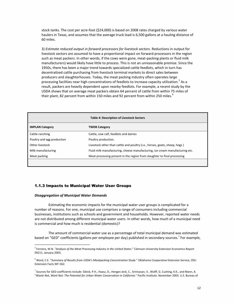
12
stock tanks. The cost per acre-foot ($24,000) is based on 2008 rates charged by various water haulers in Texas, and assumes that the average truck load is 6,500 gallons at a hauling distance of 60 miles. 3) Estimate reduced output in forward processors for livestock sectors. Reductions in output for livestock sectors are assumed to have a proportional impact on forward processors in the region such as meat packers. In other words, if the cows were gone, meat-packing plants or fluid milk manufacturers) would likely have little to process. This is not an unreasonable premise. Since the 1950s, there has been a major trend towards specialized cattle feedlots, which in turn has decentralized cattle purchasing from livestock terminal markets to direct sales between producers and slaughterhouses. Today, the meat packing industry often operates large processing facilities near high concentrations of feedlots to increase capacity utilization.
5 As a
result, packers are heavily dependent upon nearby feedlots. For example, a recent study by the USDA shows that on average meat packers obtain 64 percent of cattle from within 75 miles of their plant, 82 percent from within 150 miles and 92 percent from within 250 miles.
6
Table 4: Description of Livestock Sectors
IMPLAN Category TWDB Category
Cattle ranching Cattle, cow calf, feedlots and dairies
Poultry and egg production Poultry production.
Other livestock Livestock other than cattle and poultry (i.e., horses, goats, sheep, hogs )
Milk manufacturing Fluid milk manufacturing, cheese manufacturing, ice cream manufacturing etc.
Meat packing Meat processing present in the region from slaughter to final processing
1.1.3 Impacts to Municipal Water User Groups
Disaggregation of Municipal Water Demands
Estimating the economic impacts for the municipal water user groups is complicated for a number of reasons. For one, municipal use comprises a range of consumers including commercial businesses, institutions such as schools and government and households. However, reported water needs are not distributed among different municipal water users. In other words, how much of a municipal need is commercial and how much is residential (domestic)?
The amount of commercial water use as a percentage of total municipal demand was estimated
based on “GED” coefficients (gallons per employee per day) published in secondary sources.7 For example,
5 Ferreira, W.N. “Analysis of the Meat Processing Industry in the United States.” Clemson University Extension Economics Report ER211, January 2003. 6 Ward, C.E. “Summary of Results from USDA’s Meatpacking Concentration Study.” Oklahoma Cooperative Extension Service, OSU Extension Facts WF-562.
7 Sources for GED coefficients include: Gleick, P.H., Haasz, D., Henges-Jeck, C., Srinivasan, V., Wolff, G. Cushing, K.K., and Mann, A. "Waste Not, Want Not: The Potential for Urban Water Conservation in California." Pacific Institute. November 2003. U.S. Bureau of
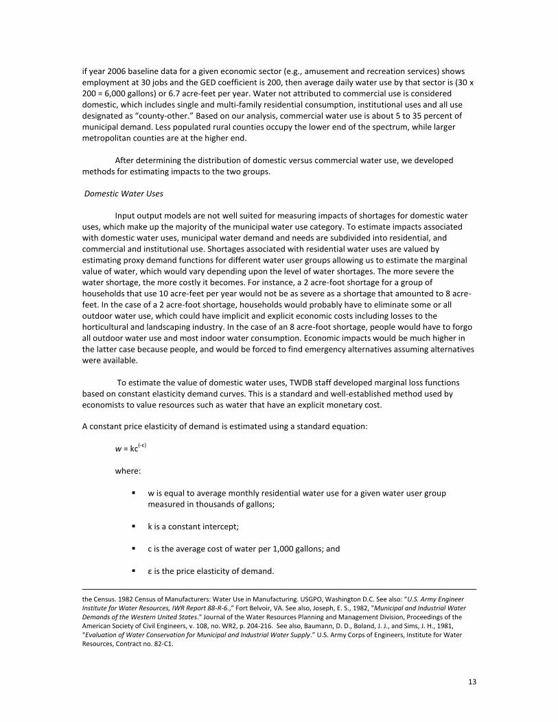
13
if year 2006 baseline data for a given economic sector (e.g., amusement and recreation services) shows employment at 30 jobs and the GED coefficient is 200, then average daily water use by that sector is (30 x 200 = 6,000 gallons) or 6.7 acre-feet per year. Water not attributed to commercial use is considered domestic, which includes single and multi-family residential consumption, institutional uses and all use designated as “county-other.” Based on our analysis, commercial water use is about 5 to 35 percent of municipal demand. Less populated rural counties occupy the lower end of the spectrum, while larger metropolitan counties are at the higher end.
After determining the distribution of domestic versus commercial water use, we developed
methods for estimating impacts to the two groups. Domestic Water Uses
Input output models are not well suited for measuring impacts of shortages for domestic water
uses, which make up the majority of the municipal water use category. To estimate impacts associated with domestic water uses, municipal water demand and needs are subdivided into residential, and commercial and institutional use. Shortages associated with residential water uses are valued by estimating proxy demand functions for different water user groups allowing us to estimate the marginal value of water, which would vary depending upon the level of water shortages. The more severe the water shortage, the more costly it becomes. For instance, a 2 acre-foot shortage for a group of households that use 10 acre-feet per year would not be as severe as a shortage that amounted to 8 acre-feet. In the case of a 2 acre-foot shortage, households would probably have to eliminate some or all outdoor water use, which could have implicit and explicit economic costs including losses to the horticultural and landscaping industry. In the case of an 8 acre-foot shortage, people would have to forgo all outdoor water use and most indoor water consumption. Economic impacts would be much higher in the latter case because people, and would be forced to find emergency alternatives assuming alternatives were available.
To estimate the value of domestic water uses, TWDB staff developed marginal loss functions
based on constant elasticity demand curves. This is a standard and well-established method used by economists to value resources such as water that have an explicit monetary cost.
A constant price elasticity of demand is estimated using a standard equation:
w = kc(-ε)
where:
w is equal to average monthly residential water use for a given water user group measured in thousands of gallons;
k is a constant intercept;
c is the average cost of water per 1,000 gallons; and
ε is the price elasticity of demand.
the Census. 1982 Census of Manufacturers: Water Use in Manufacturing. USGPO, Washington D.C. See also: “U.S. Army Engineer Institute for Water Resources, IWR Report 88-R-6.,” Fort Belvoir, VA. See also, Joseph, E. S., 1982, "Municipal and Industrial Water Demands of the Western United States." Journal of the Water Resources Planning and Management Division, Proceedings of the American Society of Civil Engineers, v. 108, no. WR2, p. 204-216. See also, Baumann, D. D., Boland, J. J., and Sims, J. H., 1981, “Evaluation of Water Conservation for Municipal and Industrial Water Supply.” U.S. Army Corps of Engineers, Institute for Water Resources, Contract no. 82-C1.
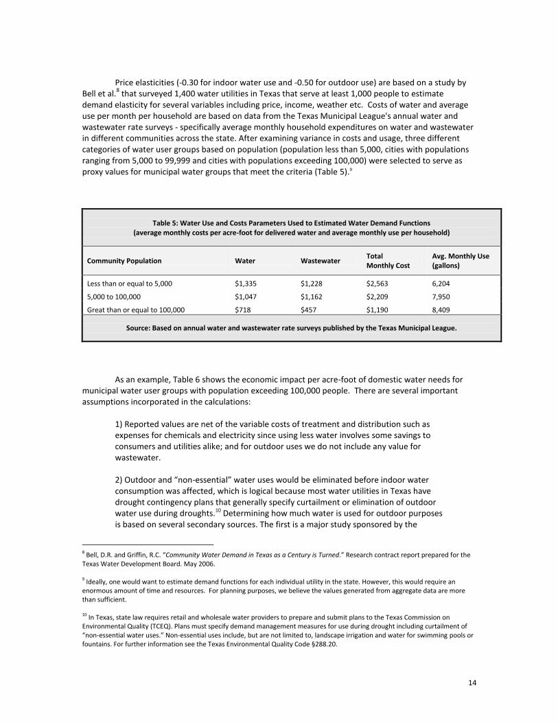
14
Price elasticities (-0.30 for indoor water use and -0.50 for outdoor use) are based on a study by
Bell et al.8 that surveyed 1,400 water utilities in Texas that serve at least 1,000 people to estimate
demand elasticity for several variables including price, income, weather etc. Costs of water and average use per month per household are based on data from the Texas Municipal League's annual water and wastewater rate surveys - specifically average monthly household expenditures on water and wastewater in different communities across the state. After examining variance in costs and usage, three different categories of water user groups based on population (population less than 5,000, cities with populations ranging from 5,000 to 99,999 and cities with populations exceeding 100,000) were selected to serve as proxy values for municipal water groups that meet the criteria (Table 5).9
Table 5: Water Use and Costs Parameters Used to Estimated Water Demand Functions (average monthly costs per acre-foot for delivered water and average monthly use per household)
Community Population Water Wastewater Total Monthly Cost
Avg. Monthly Use (gallons)
Less than or equal to 5,000 $1,335 $1,228 $2,563 6,204
5,000 to 100,000 $1,047 $1,162 $2,209 7,950
Great than or equal to 100,000 $718 $457 $1,190 8,409
Source: Based on annual water and wastewater rate surveys published by the Texas Municipal League.
As an example, Table 6 shows the economic impact per acre-foot of domestic water needs for municipal water user groups with population exceeding 100,000 people. There are several important assumptions incorporated in the calculations:
1) Reported values are net of the variable costs of treatment and distribution such as expenses for chemicals and electricity since using less water involves some savings to consumers and utilities alike; and for outdoor uses we do not include any value for wastewater. 2) Outdoor and “non-essential” water uses would be eliminated before indoor water consumption was affected, which is logical because most water utilities in Texas have drought contingency plans that generally specify curtailment or elimination of outdoor water use during droughts.10 Determining how much water is used for outdoor purposes is based on several secondary sources. The first is a major study sponsored by the
8 Bell, D.R. and Griffin, R.C. “Community Water Demand in Texas as a Century is Turned.” Research contract report prepared for the Texas Water Development Board. May 2006. 9 Ideally, one would want to estimate demand functions for each individual utility in the state. However, this would require an enormous amount of time and resources. For planning purposes, we believe the values generated from aggregate data are more than sufficient. 10 In Texas, state law requires retail and wholesale water providers to prepare and submit plans to the Texas Commission on Environmental Quality (TCEQ). Plans must specify demand management measures for use during drought including curtailment of “non-essential water uses.” Non-essential uses include, but are not limited to, landscape irrigation and water for swimming pools or fountains. For further information see the Texas Environmental Quality Code §288.20.
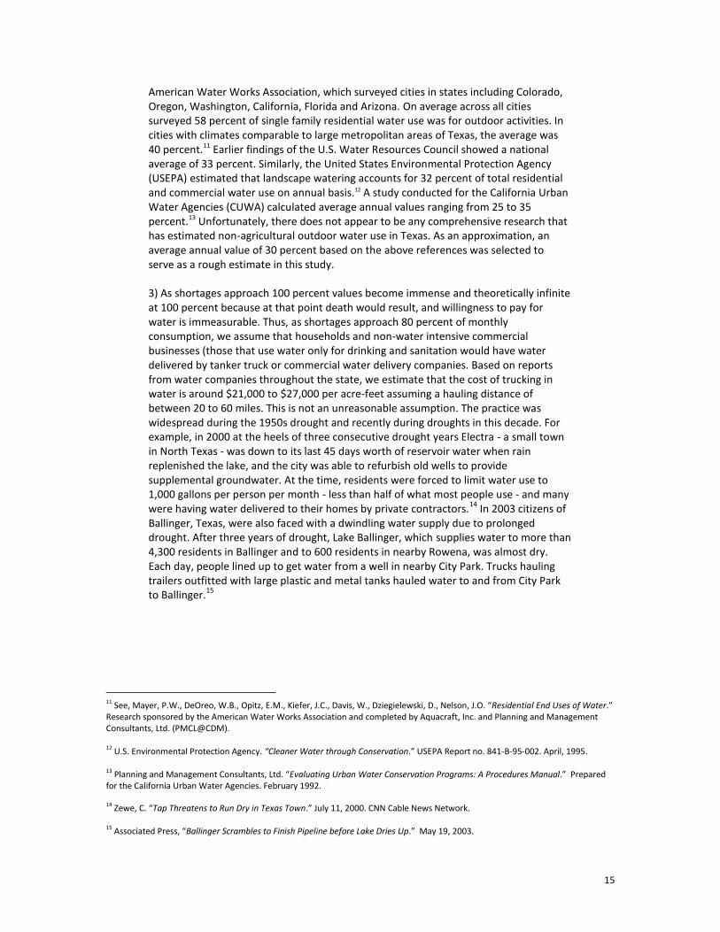
15
American Water Works Association, which surveyed cities in states including Colorado, Oregon, Washington, California, Florida and Arizona. On average across all cities surveyed 58 percent of single family residential water use was for outdoor activities. In cities with climates comparable to large metropolitan areas of Texas, the average was 40 percent.11 Earlier findings of the U.S. Water Resources Council showed a national average of 33 percent. Similarly, the United States Environmental Protection Agency (USEPA) estimated that landscape watering accounts for 32 percent of total residential and commercial water use on annual basis.12 A study conducted for the California Urban Water Agencies (CUWA) calculated average annual values ranging from 25 to 35 percent.13 Unfortunately, there does not appear to be any comprehensive research that has estimated non-agricultural outdoor water use in Texas. As an approximation, an average annual value of 30 percent based on the above references was selected to serve as a rough estimate in this study. 3) As shortages approach 100 percent values become immense and theoretically infinite at 100 percent because at that point death would result, and willingness to pay for water is immeasurable. Thus, as shortages approach 80 percent of monthly consumption, we assume that households and non-water intensive commercial businesses (those that use water only for drinking and sanitation would have water delivered by tanker truck or commercial water delivery companies. Based on reports from water companies throughout the state, we estimate that the cost of trucking in water is around $21,000 to $27,000 per acre-feet assuming a hauling distance of between 20 to 60 miles. This is not an unreasonable assumption. The practice was widespread during the 1950s drought and recently during droughts in this decade. For example, in 2000 at the heels of three consecutive drought years Electra - a small town in North Texas - was down to its last 45 days worth of reservoir water when rain replenished the lake, and the city was able to refurbish old wells to provide supplemental groundwater. At the time, residents were forced to limit water use to 1,000 gallons per person per month - less than half of what most people use - and many were having water delivered to their homes by private contractors.
14 In 2003 citizens of
Ballinger, Texas, were also faced with a dwindling water supply due to prolonged drought. After three years of drought, Lake Ballinger, which supplies water to more than 4,300 residents in Ballinger and to 600 residents in nearby Rowena, was almost dry. Each day, people lined up to get water from a well in nearby City Park. Trucks hauling trailers outfitted with large plastic and metal tanks hauled water to and from City Park to Ballinger.
15
11 See, Mayer, P.W., DeOreo, W.B., Opitz, E.M., Kiefer, J.C., Davis, W., Dziegielewski, D., Nelson, J.O. “Residential End Uses of Water.” Research sponsored by the American Water Works Association and completed by Aquacraft, Inc. and Planning and Management Consultants, Ltd. (PMCL@CDM). 12 U.S. Environmental Protection Agency. “Cleaner Water through Conservation.” USEPA Report no. 841-B-95-002. April, 1995. 13 Planning and Management Consultants, Ltd. “Evaluating Urban Water Conservation Programs: A Procedures Manual.” Prepared for the California Urban Water Agencies. February 1992. 14 Zewe, C. “Tap Threatens to Run Dry in Texas Town.” July 11, 2000. CNN Cable News Network. 15 Associated Press, “Ballinger Scrambles to Finish Pipeline before Lake Dries Up.” May 19, 2003.
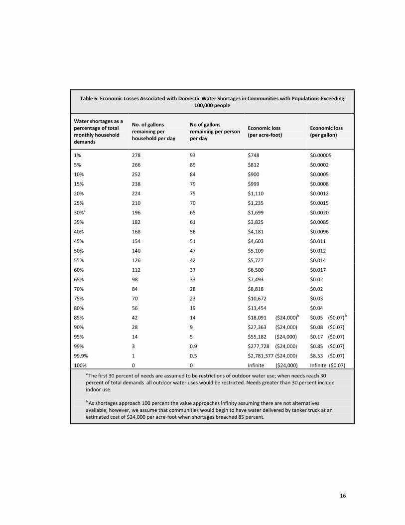
16
Table 6: Economic Losses Associated with Domestic Water Shortages in Communities with Populations Exceeding 100,000 people
Water shortages as a percentage of total monthly household demands
No. of gallons remaining per household per day
No of gallons remaining per person per day
Economic loss (per acre-foot)
Economic loss (per gallon)
1% 278 93 $748 $0.00005
5% 266 89 $812 $0.0002
10% 252 84 $900 $0.0005
15% 238 79 $999 $0.0008
20% 224 75 $1,110 $0.0012
25% 210 70 $1,235 $0.0015
30%a 196 65 $1,699 $0.0020
35% 182 61 $3,825 $0.0085
40% 168 56 $4,181 $0.0096
45% 154 51 $4,603 $0.011
50% 140 47 $5,109 $0.012
55% 126 42 $5,727 $0.014
60% 112 37 $6,500 $0.017
65% 98 33 $7,493 $0.02
70% 84 28 $8,818 $0.02
75% 70 23 $10,672 $0.03
80% 56 19 $13,454 $0.04
85% 42 14 $18,091 ($24,000)b $0.05 ($0.07) b
90% 28 9 $27,363 ($24,000) $0.08 ($0.07)
95% 14 5 $55,182 ($24,000) $0.17 ($0.07)
99% 3 0.9 $277,728 ($24,000) $0.85 ($0.07)
99.9% 1 0.5 $2,781,377 ($24,000) $8.53 ($0.07)
100% 0 0 Infinite ($24,000) Infinite ($0.07)
a The first 30 percent of needs are assumed to be restrictions of outdoor water use; when needs reach 30 percent of total demands all outdoor water uses would be restricted. Needs greater than 30 percent include indoor use. b As shortages approach 100 percent the value approaches infinity assuming there are not alternatives available; however, we assume that communities would begin to have water delivered by tanker truck at an estimated cost of $24,000 per acre-foot when shortages breached 85 percent.
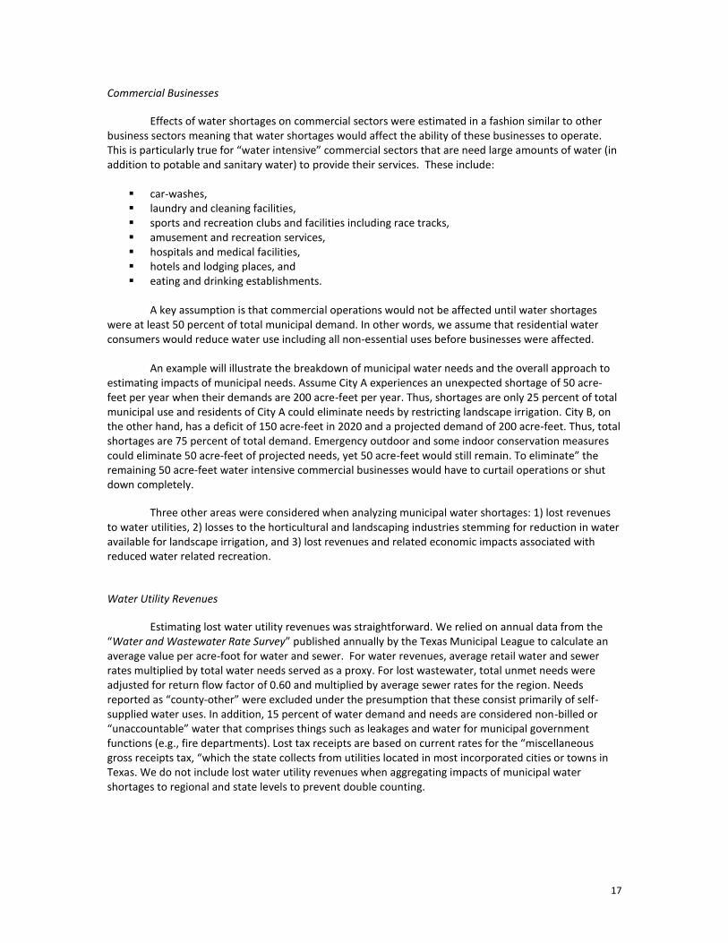
17
Commercial Businesses
Effects of water shortages on commercial sectors were estimated in a fashion similar to other business sectors meaning that water shortages would affect the ability of these businesses to operate. This is particularly true for “water intensive” commercial sectors that are need large amounts of water (in addition to potable and sanitary water) to provide their services. These include:
car-washes, laundry and cleaning facilities, sports and recreation clubs and facilities including race tracks, amusement and recreation services, hospitals and medical facilities, hotels and lodging places, and eating and drinking establishments.
A key assumption is that commercial operations would not be affected until water shortages
were at least 50 percent of total municipal demand. In other words, we assume that residential water consumers would reduce water use including all non-essential uses before businesses were affected.
An example will illustrate the breakdown of municipal water needs and the overall approach to estimating impacts of municipal needs. Assume City A experiences an unexpected shortage of 50 acre-feet per year when their demands are 200 acre-feet per year. Thus, shortages are only 25 percent of total municipal use and residents of City A could eliminate needs by restricting landscape irrigation. City B, on the other hand, has a deficit of 150 acre-feet in 2020 and a projected demand of 200 acre-feet. Thus, total shortages are 75 percent of total demand. Emergency outdoor and some indoor conservation measures could eliminate 50 acre-feet of projected needs, yet 50 acre-feet would still remain. To eliminate” the remaining 50 acre-feet water intensive commercial businesses would have to curtail operations or shut down completely.
Three other areas were considered when analyzing municipal water shortages: 1) lost revenues to water utilities, 2) losses to the horticultural and landscaping industries stemming for reduction in water available for landscape irrigation, and 3) lost revenues and related economic impacts associated with reduced water related recreation. Water Utility Revenues
Estimating lost water utility revenues was straightforward. We relied on annual data from the “Water and Wastewater Rate Survey” published annually by the Texas Municipal League to calculate an average value per acre-foot for water and sewer. For water revenues, average retail water and sewer rates multiplied by total water needs served as a proxy. For lost wastewater, total unmet needs were adjusted for return flow factor of 0.60 and multiplied by average sewer rates for the region. Needs reported as “county-other” were excluded under the presumption that these consist primarily of self-supplied water uses. In addition, 15 percent of water demand and needs are considered non-billed or “unaccountable” water that comprises things such as leakages and water for municipal government functions (e.g., fire departments). Lost tax receipts are based on current rates for the “miscellaneous gross receipts tax, “which the state collects from utilities located in most incorporated cities or towns in Texas. We do not include lost water utility revenues when aggregating impacts of municipal water shortages to regional and state levels to prevent double counting.
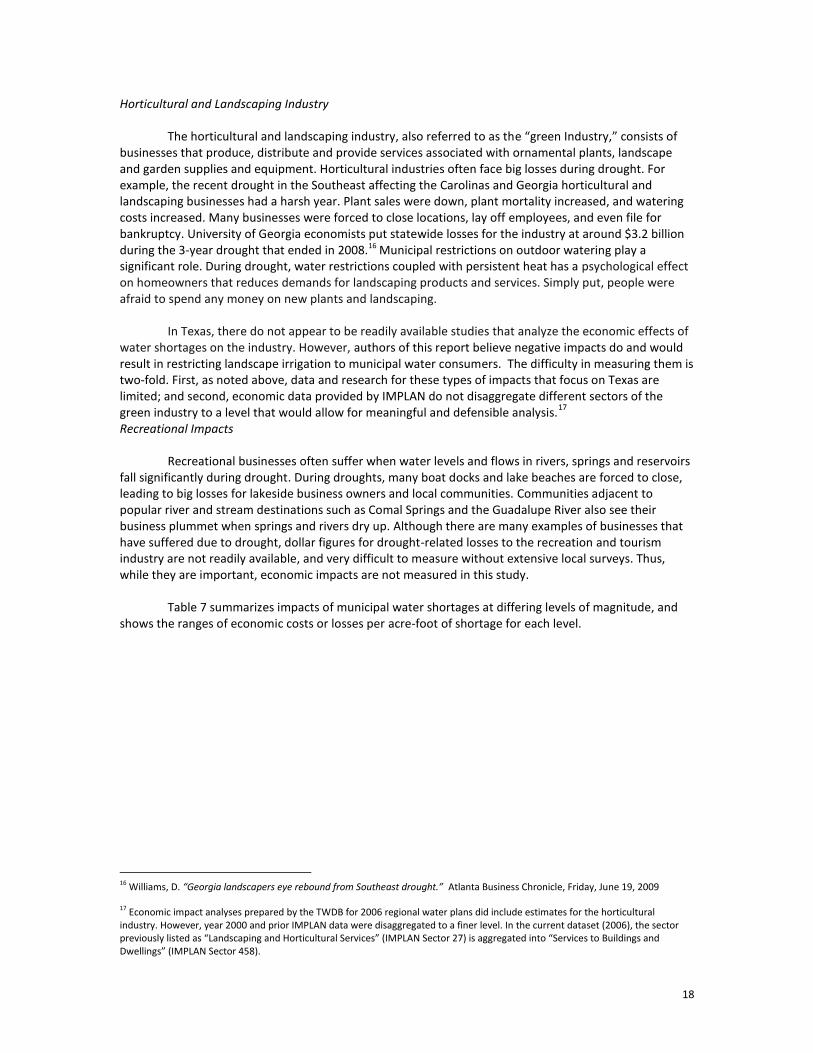
18
Horticultural and Landscaping Industry
The horticultural and landscaping industry, also referred to as the “green Industry,” consists of businesses that produce, distribute and provide services associated with ornamental plants, landscape and garden supplies and equipment. Horticultural industries often face big losses during drought. For example, the recent drought in the Southeast affecting the Carolinas and Georgia horticultural and landscaping businesses had a harsh year. Plant sales were down, plant mortality increased, and watering costs increased. Many businesses were forced to close locations, lay off employees, and even file for bankruptcy. University of Georgia economists put statewide losses for the industry at around $3.2 billion during the 3-year drought that ended in 2008.16
Municipal restrictions on outdoor watering play a significant role. During drought, water restrictions coupled with persistent heat has a psychological effect on homeowners that reduces demands for landscaping products and services. Simply put, people were afraid to spend any money on new plants and landscaping.
In Texas, there do not appear to be readily available studies that analyze the economic effects of
water shortages on the industry. However, authors of this report believe negative impacts do and would result in restricting landscape irrigation to municipal water consumers. The difficulty in measuring them is two-fold. First, as noted above, data and research for these types of impacts that focus on Texas are limited; and second, economic data provided by IMPLAN do not disaggregate different sectors of the green industry to a level that would allow for meaningful and defensible analysis.
17
Recreational Impacts
Recreational businesses often suffer when water levels and flows in rivers, springs and reservoirs fall significantly during drought. During droughts, many boat docks and lake beaches are forced to close, leading to big losses for lakeside business owners and local communities. Communities adjacent to popular river and stream destinations such as Comal Springs and the Guadalupe River also see their business plummet when springs and rivers dry up. Although there are many examples of businesses that have suffered due to drought, dollar figures for drought-related losses to the recreation and tourism industry are not readily available, and very difficult to measure without extensive local surveys. Thus, while they are important, economic impacts are not measured in this study.
Table 7 summarizes impacts of municipal water shortages at differing levels of magnitude, and shows the ranges of economic costs or losses per acre-foot of shortage for each level.
16 Williams, D. “Georgia landscapers eye rebound from Southeast drought.” Atlanta Business Chronicle, Friday, June 19, 2009 17 Economic impact analyses prepared by the TWDB for 2006 regional water plans did include estimates for the horticultural industry. However, year 2000 and prior IMPLAN data were disaggregated to a finer level. In the current dataset (2006), the sector previously listed as “Landscaping and Horticultural Services” (IMPLAN Sector 27) is aggregated into “Services to Buildings and Dwellings” (IMPLAN Sector 458).
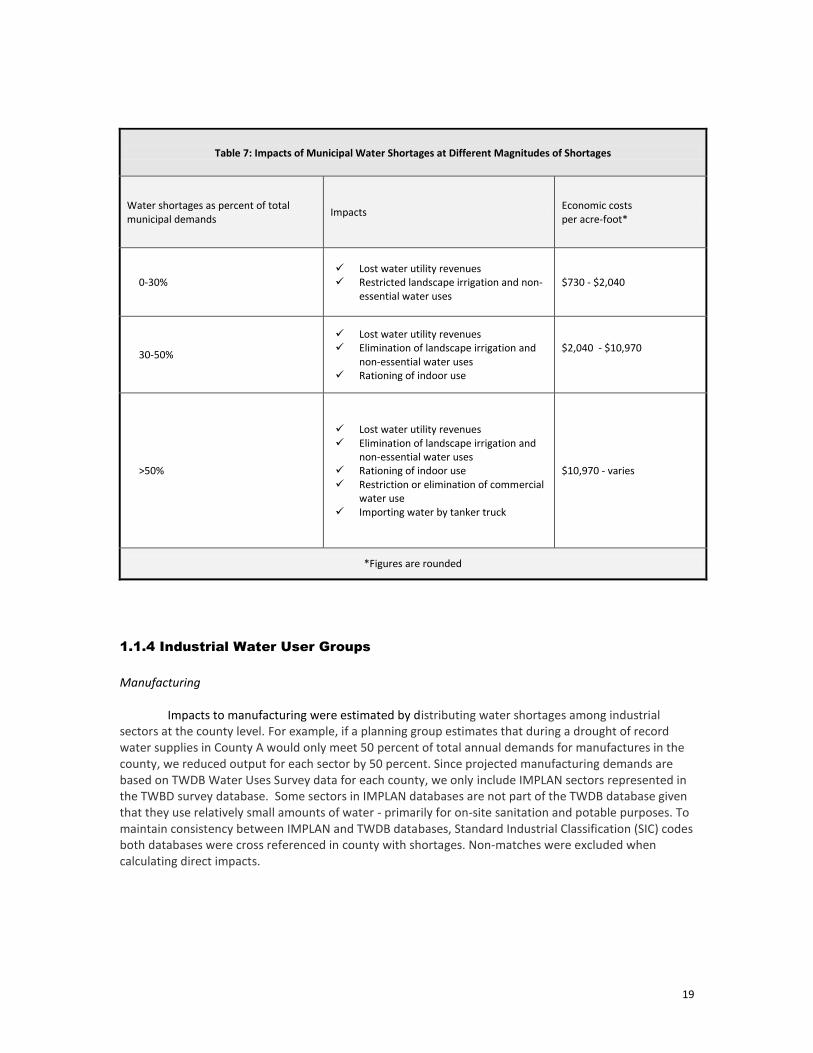
19
Table 7: Impacts of Municipal Water Shortages at Different Magnitudes of Shortages
Water shortages as percent of total municipal demands
Impacts Economic costs per acre-foot*
0-30% Lost water utility revenues Restricted landscape irrigation and non-
essential water uses $730 - $2,040
30-50%
Lost water utility revenues Elimination of landscape irrigation and
non-essential water uses Rationing of indoor use
$2,040 - $10,970
>50%
Lost water utility revenues Elimination of landscape irrigation and
non-essential water uses Rationing of indoor use Restriction or elimination of commercial
water use Importing water by tanker truck
$10,970 - varies
*Figures are rounded
1.1.4 Industrial Water User Groups
Manufacturing
Impacts to manufacturing were estimated by distributing water shortages among industrial sectors at the county level. For example, if a planning group estimates that during a drought of record water supplies in County A would only meet 50 percent of total annual demands for manufactures in the county, we reduced output for each sector by 50 percent. Since projected manufacturing demands are based on TWDB Water Uses Survey data for each county, we only include IMPLAN sectors represented in the TWBD survey database. Some sectors in IMPLAN databases are not part of the TWDB database given that they use relatively small amounts of water - primarily for on-site sanitation and potable purposes. To maintain consistency between IMPLAN and TWDB databases, Standard Industrial Classification (SIC) codes both databases were cross referenced in county with shortages. Non-matches were excluded when calculating direct impacts.
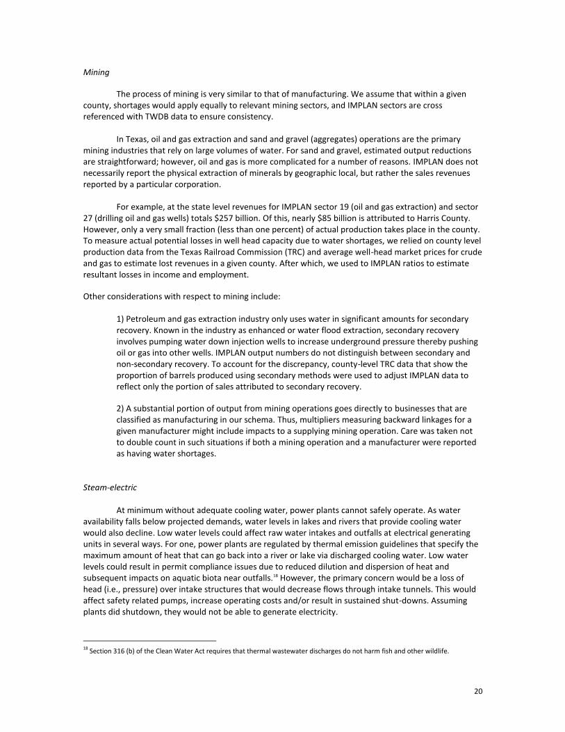
20
Mining
The process of mining is very similar to that of manufacturing. We assume that within a given county, shortages would apply equally to relevant mining sectors, and IMPLAN sectors are cross referenced with TWDB data to ensure consistency.
In Texas, oil and gas extraction and sand and gravel (aggregates) operations are the primary
mining industries that rely on large volumes of water. For sand and gravel, estimated output reductions are straightforward; however, oil and gas is more complicated for a number of reasons. IMPLAN does not necessarily report the physical extraction of minerals by geographic local, but rather the sales revenues reported by a particular corporation.
For example, at the state level revenues for IMPLAN sector 19 (oil and gas extraction) and sector
27 (drilling oil and gas wells) totals $257 billion. Of this, nearly $85 billion is attributed to Harris County. However, only a very small fraction (less than one percent) of actual production takes place in the county. To measure actual potential losses in well head capacity due to water shortages, we relied on county level production data from the Texas Railroad Commission (TRC) and average well-head market prices for crude and gas to estimate lost revenues in a given county. After which, we used to IMPLAN ratios to estimate resultant losses in income and employment.
Other considerations with respect to mining include:
1) Petroleum and gas extraction industry only uses water in significant amounts for secondary recovery. Known in the industry as enhanced or water flood extraction, secondary recovery involves pumping water down injection wells to increase underground pressure thereby pushing oil or gas into other wells. IMPLAN output numbers do not distinguish between secondary and non-secondary recovery. To account for the discrepancy, county-level TRC data that show the proportion of barrels produced using secondary methods were used to adjust IMPLAN data to reflect only the portion of sales attributed to secondary recovery.
2) A substantial portion of output from mining operations goes directly to businesses that are classified as manufacturing in our schema. Thus, multipliers measuring backward linkages for a given manufacturer might include impacts to a supplying mining operation. Care was taken not to double count in such situations if both a mining operation and a manufacturer were reported as having water shortages.
Steam-electric
At minimum without adequate cooling water, power plants cannot safely operate. As water
availability falls below projected demands, water levels in lakes and rivers that provide cooling water would also decline. Low water levels could affect raw water intakes and outfalls at electrical generating units in several ways. For one, power plants are regulated by thermal emission guidelines that specify the maximum amount of heat that can go back into a river or lake via discharged cooling water. Low water levels could result in permit compliance issues due to reduced dilution and dispersion of heat and subsequent impacts on aquatic biota near outfalls.18 However, the primary concern would be a loss of head (i.e., pressure) over intake structures that would decrease flows through intake tunnels. This would affect safety related pumps, increase operating costs and/or result in sustained shut-downs. Assuming plants did shutdown, they would not be able to generate electricity.
18 Section 316 (b) of the Clean Water Act requires that thermal wastewater discharges do not harm fish and other wildlife.
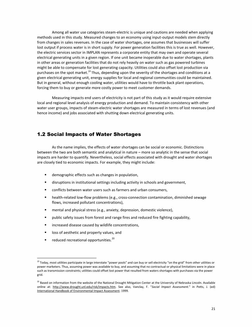
21
Among all water use categories steam-electric is unique and cautions are needed when applying methods used in this study. Measured changes to an economy using input-output models stem directly from changes in sales revenues. In the case of water shortages, one assumes that businesses will suffer lost output if process water is in short supply. For power generation facilities this is true as well. However, the electric services sector in IMPLAN represents a corporate entity that may own and operate several electrical generating units in a given region. If one unit became inoperable due to water shortages, plants in other areas or generation facilities that do not rely heavily on water such as gas powered turbines might be able to compensate for lost generating capacity. Utilities could also offset lost production via purchases on the spot market.19
Thus, depending upon the severity of the shortages and conditions at a given electrical generating unit, energy supplies for local and regional communities could be maintained. But in general, without enough cooling water, utilities would have to throttle back plant operations, forcing them to buy or generate more costly power to meet customer demands.
Measuring impacts end users of electricity is not part of this study as it would require extensive local and regional level analysis of energy production and demand. To maintain consistency with other water user groups, impacts of steam-electric water shortages are measured in terms of lost revenues (and hence income) and jobs associated with shutting down electrical generating units.
1.2 Social Impacts of Water Shortages
As the name implies, the effects of water shortages can be social or economic. Distinctions
between the two are both semantic and analytical in nature – more so analytic in the sense that social impacts are harder to quantify. Nevertheless, social effects associated with drought and water shortages are closely tied to economic impacts. For example, they might include:
demographic effects such as changes in population,
disruptions in institutional settings including activity in schools and government,
conflicts between water users such as farmers and urban consumers,
health-related low-flow problems (e.g., cross-connection contamination, diminished sewage flows, increased pollutant concentrations),
mental and physical stress (e.g., anxiety, depression, domestic violence),
public safety issues from forest and range fires and reduced fire fighting capability,
increased disease caused by wildlife concentrations,
loss of aesthetic and property values, and
reduced recreational opportunities.20
19 Today, most utilities participate in large interstate “power pools” and can buy or sell electricity “on the grid” from other utilities or power marketers. Thus, assuming power was available to buy, and assuming that no contractual or physical limitations were in place such as transmission constraints; utilities could offset lost power that resulted from waters shortages with purchases via the power grid. 20 Based on information from the website of the National Drought Mitigation Center at the University of Nebraska Lincoln. Available online at: http://www.drought.unl.edu/risk/impacts.htm. See also, Vanclay, F. “Social Impact Assessment.” in Petts, J. (ed) International Handbook of Environmental Impact Assessment. 1999.

22
Social impacts measured in this study focus strictly on demographic effects including changes in population and school enrollment. Methods are based on demographic projection models developed by the Texas State Data Center and used by the TWDB for state and regional water planning. Basically, the social impact model uses results from the economic component of the study and assesses how changes in labor demand would affect migration patterns in a region. Declines in labor demand as measured using adjusted IMPLAN data are assumed to affect net economic migration in a given regional water planning area. Employment losses are adjusted to reflect the notion that some people would not relocate but would seek employment in the region and/or public assistance and wait for conditions to improve. Changes in school enrollment are simply the proportion of lost population between the ages of 5 and 17.
2. Results
Section 2 presents the results of the analysis at the regional level. Included are baseline
economic data for each water use category, and estimated economics impacts of water shortages for water user groups with reported deficits. According to the 2011 Lower Colorado Regional Water Plan, during severe drought irrigation, municipal, manufacturing, mining and steam-electric water user groups would experience water shortages in the absence of new water management strategies.
2.1 Overview of Regional Economy
On an annual basis, the Region K economy generates slightly more than $79 billion in gross state
product for Texas ($73 billion in income and $6 billion in state and local business taxes) and supports nearly 1,033,690 jobs (Table 8). Generating nearly $12 billion worth of income per year manufacturing (particularly computer electronics and pharmaceuticals) is the primary base economic sector in the region.21 Municipal sectors also generate substantial amounts of activity, nearly $61 billion per year in gross state product, and are major employers in the region. While municipal sectors are the largest employer and source of wealth, many businesses that make up the municipal category such as restaurants and retail stores are non-basic industries meaning they exist to provide services to people who work would in base industries such as manufacturing. In other words, without base industries many municipal jobs would not exist.
21 Base industries are those that supply markets outside of a region. These industries are crucial to the local economy and are called the economic base of a region. Appendix A shows how IMPLAN’s 529 sectors were allocated to water use category, and shows economic data for each sector.
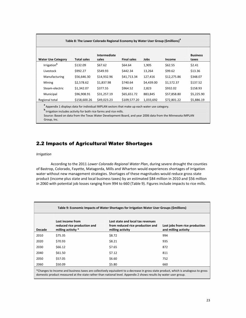
23
Table 8: The Lower Colorado Regional Economy by Water User Group ($millions)a
Water Use Category Total sales Intermediate sales Final sales Jobs Income
Business taxes
Irrigationb $132.09 $67.62 $64.64 1,905 $62.55 $2.41
Livestock $992.27 $549.93 $442.34 13,264 $99.62 $13.36
Manufacturing $56,646.30 $14,932.96 $41,713.34 127,416 $12,275.86 $348.07
Mining $2,578.62 $1,837.98 $740.64 $4,439.00 $1,572.37 $137.52
Steam-electric $1,342.07 $377.55 $964.52 2,823 $932.02 $158.93
Municipal $96,908.91 $31,257.19 $65,651.72 883,845 $57,858.80 $5,225.90
Regional total $158,600.26 $49,023.23 $109,577.20 1,033,692 $72,801.22 $5,886.19
a Appendix 1 displays data for individual IMPLAN sectors that make up each water use category.
b Irrigation includes activity for both rice farms and rice mills.
Source: Based on data from the Texas Water Development Board, and year 2006 data from the Minnesota IMPLAN Group, Inc.
2.2 Impacts of Agricultural Water Shortages
Irrigation
According to the 2011 Lower Colorado Regional Water Plan, during severe drought the counties of Bastrop, Colorado, Fayette, Matagorda, Mills and Wharton would experiences shortages of irrigation water without new management strategies. Shortages of these magnitudes would reduce gross state product (income plus state and local business taxes) by an estimated $84 million in 2010 and $56 million in 2060 with potential job losses ranging from 994 to 660 (Table 9). Figures include impacts to rice mills.
Table 9: Economic Impacts of Water Shortages for Irrigation Water User Groups ($millions)
Decade
Lost income from reduced rice production and milling activity *
Lost state and local tax revenues from reduced rice production and milling activity
Lost jobs from rice production and milling activity
2010 $75.35 $8.72 994
2020 $70.93 $8.21 935
2030 $66.12 $7.65 872
2040 $61.50 $7.12 811
2050 $57.05 $6.60 752
2060 $50.09 $5.80 660
*Changes to Income and business taxes are collectively equivalent to a decrease in gross state product, which is analogous to gross domestic product measured at the state rather than national level. Appendix 2 shows results by water user group.
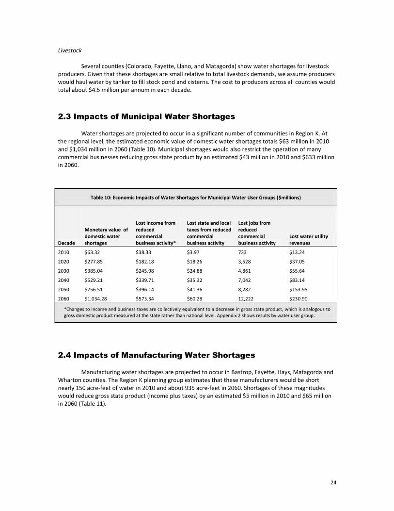
24
Livestock
Several counties (Colorado, Fayette, Llano, and Matagorda) show water shortages for livestock producers. Given that these shortages are small relative to total livestock demands, we assume producers would haul water by tanker to fill stock pond and cisterns. The cost to producers across all counties would total about $4.5 million per annum in each decade.
2.3 Impacts of Municipal Water Shortages
Water shortages are projected to occur in a significant number of communities in Region K. At
the regional level, the estimated economic value of domestic water shortages totals $63 million in 2010 and $1,034 million in 2060 (Table 10). Municipal shortages would also restrict the operation of many commercial businesses reducing gross state product by an estimated $43 million in 2010 and $633 million in 2060.
2.4 Impacts of Manufacturing Water Shortages
Manufacturing water shortages are projected to occur in Bastrop, Fayette, Hays, Matagorda and
Wharton counties. The Region K planning group estimates that these manufacturers would be short nearly 150 acre-feet of water in 2010 and about 935 acre-feet in 2060. Shortages of these magnitudes would reduce gross state product (income plus taxes) by an estimated $5 million in 2010 and $65 million in 2060 (Table 11).
Table 10: Economic Impacts of Water Shortages for Municipal Water User Groups ($millions)
Decade
Monetary value of domestic water shortages
Lost income from reduced commercial business activity*
Lost state and local taxes from reduced commercial business activity
Lost jobs from reduced commercial business activity
Lost water utility revenues
2010 $63.32 $38.33 $3.97 733 $13.24
2020 $277.85 $182.18 $18.26 3,528 $37.05
2030 $385.04 $245.98 $24.88 4,861 $55.64
2040 $529.21 $339.71 $35.32 7,042 $83.14
2050 $756.51 $396.14 $41.36 8,282 $153.95
2060 $1,034.28 $573.34 $60.28 12,222 $230.90
*Changes to Income and business taxes are collectively equivalent to a decrease in gross state product, which is analogous to gross domestic product measured at the state rather than national level. Appendix 2 shows results by water user group.
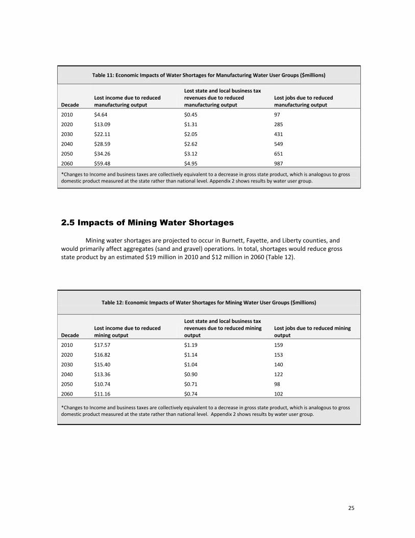
25
2.5 Impacts of Mining Water Shortages
Mining water shortages are projected to occur in Burnett, Fayette, and Liberty counties, and
would primarily affect aggregates (sand and gravel) operations. In total, shortages would reduce gross state product by an estimated $19 million in 2010 and $12 million in 2060 (Table 12).
Table 11: Economic Impacts of Water Shortages for Manufacturing Water User Groups ($millions)
Decade Lost income due to reduced manufacturing output
Lost state and local business tax revenues due to reduced manufacturing output
Lost jobs due to reduced manufacturing output
2010 $4.64 $0.45 97
2020 $13.09 $1.31 285
2030 $22.11 $2.05 431
2040 $28.59 $2.62 549
2050 $34.26 $3.12 651
2060 $59.48 $4.95 987
*Changes to Income and business taxes are collectively equivalent to a decrease in gross state product, which is analogous to gross domestic product measured at the state rather than national level. Appendix 2 shows results by water user group.
Table 12: Economic Impacts of Water Shortages for Mining Water User Groups ($millions)
Decade Lost income due to reduced mining output
Lost state and local business tax revenues due to reduced mining output
Lost jobs due to reduced mining output
2010 $17.57 $1.19 159
2020 $16.82 $1.14 153
2030 $15.40 $1.04 140
2040 $13.36 $0.90 122
2050 $10.74 $0.71 98
2060 $11.16 $0.74 102
*Changes to Income and business taxes are collectively equivalent to a decrease in gross state product, which is analogous to gross domestic product measured at the state rather than national level. Appendix 2 shows results by water user group.
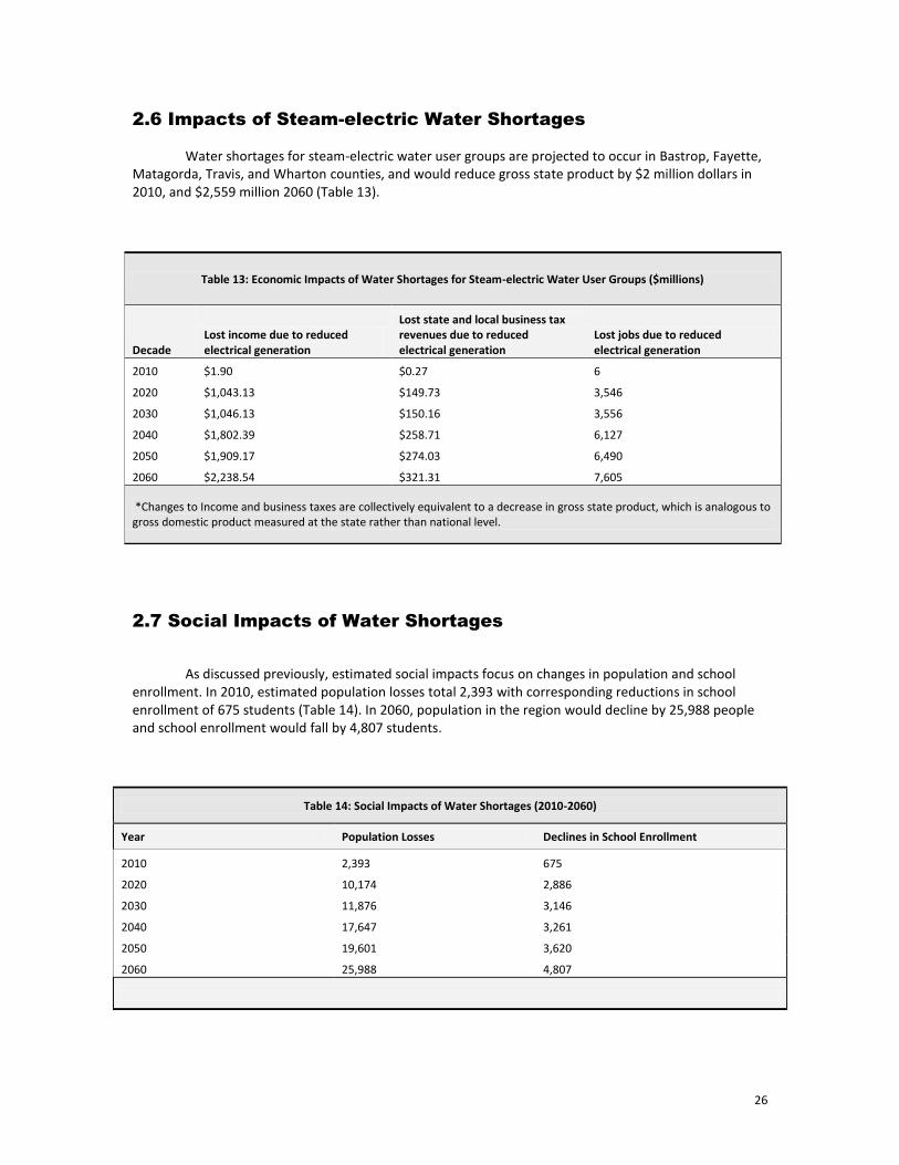
26
2.6 Impacts of Steam-electric Water Shortages
Water shortages for steam-electric water user groups are projected to occur in Bastrop, Fayette, Matagorda, Travis, and Wharton counties, and would reduce gross state product by $2 million dollars in 2010, and $2,559 million 2060 (Table 13).
2.7 Social Impacts of Water Shortages
As discussed previously, estimated social impacts focus on changes in population and school
enrollment. In 2010, estimated population losses total 2,393 with corresponding reductions in school enrollment of 675 students (Table 14). In 2060, population in the region would decline by 25,988 people and school enrollment would fall by 4,807 students.
Table 14: Social Impacts of Water Shortages (2010-2060)
Year Population Losses Declines in School Enrollment
2010 2,393 675
2020 10,174 2,886
2030 11,876 3,146
2040 17,647 3,261
2050 19,601 3,620
2060 25,988 4,807
Table 13: Economic Impacts of Water Shortages for Steam-electric Water User Groups ($millions)
Decade Lost income due to reduced electrical generation
Lost state and local business tax revenues due to reduced electrical generation
Lost jobs due to reduced electrical generation
2010 $1.90 $0.27 6
2020 $1,043.13 $149.73 3,546
2030 $1,046.13 $150.16 3,556
2040 $1,802.39 $258.71 6,127
2050 $1,909.17 $274.03 6,490
2060 $2,238.54 $321.31 7,605
*Changes to Income and business taxes are collectively equivalent to a decrease in gross state product, which is analogous to gross domestic product measured at the state rather than national level.
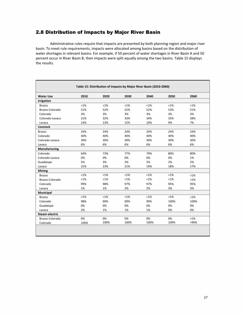
27
2.8 Distribution of Impacts by Major River Basin
Administrative rules require that impacts are presented by both planning region and major river
basin. To meet rule requirements, impacts were allocated among basins based on the distribution of water shortages in relevant basins. For example, if 50 percent of water shortages in River Basin A and 50 percent occur in River Basin B, then impacts were split equally among the two basins. Table 15 displays the results.
Table 15: Distribution of Impacts by Major River Basin (2010-2060)
Water Use 2010 2020 2030 2040 2050 2060
Irrigation
Brazos <1% <1% <1% <1% <1% <1%
Brazos-Colorado 51% 52% 52% 52% 53% 51%
Colorado 3% 3% 3% 3% 3% 3%
Colorado-Lavaca 31% 32% 33% 34% 35% 38%
Lavaca 14% 13% 12% 10% 9% 7%
Livestock
Brazos 24% 24% 24% 24% 24% 24%
Colorado 40% 40% 40% 40% 40% 40%
Colorado-Lavaca 30% 30% 30% 30% 30% 30%
Lavaca 6% 6% 6% 6% 6% 6%
Manufacturing
Colorado 64% 73% 77% 79% 80% 80%
Colorado-Lavaca 0% 0% 0% 0% 0% 1%
Guadalupe 5% 3% 2% 2% 2% 2%
Lavaca 31% 23% 21% 19% 18% 17%
Mining
Brazos <1% <1% <1% <1% <1% <1%
Brazos-Colorado <1% <1% <1% <1% <1% <1%
Colorado 99% 98% 97% 97% 95% 95%
Lavaca 1% 1% 2% 2% 3% 3%
Municipal
Brazos <1% <1% <1% <1% <1% <1%
Colorado 98% 99% 99% 99% 100% 100%
Guadalupe 0% 0% 0% 0% 0% 0%
Lavaca 2% 1% 1% 1% 0% 0%
Steam-electric Brazos-Colorado 0% 0% 0% 0% 0% <1%
Colorado 100% 100% 100% 100% 100% >99%
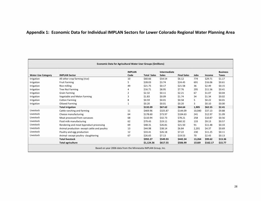
28
Appendix 1: Economic Data for Individual IMPLAN Sectors for Lower Colorado Regional Water Planning Area
Economic Data for Agricultural Water User Groups ($millions)
Water Use Category IMPLAN Sector IMPLAN Code Total Sales
Intermediate Sales Final Sales Jobs Income
Business Taxes
Irrigation All other crop farming (rice) 10 $60.66 $54.54 $6.12 774 $29.71 $1.17
Irrigation Fruit Farming 5 $28.03 $3.74 $24.45 691 $16.06 $0.61
Irrigation Rice milling 49 $21.75 $0.17 $21.58 36 $2.49 $0.15
Irrigation Tree Nut Farming 4 $16.71 $8.95 $7.76 295 $11.56 $0.41
Irrigation Grain Farming 2 $2.32 $0.11 $2.21 67 $1.07 $0.04
Irrigation Vegetable and Melon Farming 3 $1.83 $0.09 $1.74 34 $1.34 $0.02
Irrigation Cotton Farming 8 $0.59 $0.01 $0.58 5 $0.22 $0.01
Irrigation Oilseed Farming 1 $0.20 $0.01 $0.20 3 $0.10 $0.00
Total irrigation $132.09 $67.62 $64.64 1,905 $62.55 $2.41 Livestock Cattle ranching and farming 11 $469.96 $325.87 $144.09 10,040 $37.13 $9.88 Livestock Cheese manufacturing 64 $178.60 $73.97 $104.63 241 $12.97 $1.09 Livestock Meat processed from carcasses 68 $110.94 $32.73 $78.21 258 $10.87 $0.56 Livestock Fluid milk manufacturing 62 $79.43 $19.11 $60.32 133 $9.13 $0.57 Livestock Rendering and meat byproduct processing 69 $48.31 $26.81 $21.50 91 $11.48 $0.33 Livestock Animal production- except cattle and poultry 13 $44.98 $38.14 $6.84 2,201 $4.37 $0.69 Livestock Poultry and egg production 12 $33.41 $26.18 $7.22 230 $11.25 $0.11 Livestock Animal- except poultry- slaughtering 67 $26.65 $7.13 $19.53 70 $2.43 $0.13
Total livestock $992.27 $549.93 $442.34 13,264 $99.62 $13.36
Total agriculture $1,124.36 $617.55 $506.99 15169 $162.17 $15.77
Based on year 2006 data from the Minnesota IMPLAN Group, Inc.
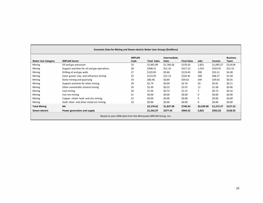
29
Economic Data for Mining and Steam-electric Water User Groups ($millions)
Water Use Category IMPLAN Sector IMPLAN Code Total Sales
Intermediate Sales Final Sales Jobs Income
Business Taxes
Mining Oil and gas extraction 19 $1,901.89 $1,766.26 $135.63 1,831 $1,095.27 $114.04
Mining Support activities for oil and gas operations 28 $368.31 $51.16 $317.15 1,553 $333.91 $15.15
Mining Drilling oil and gas wells 27 $120.05 $0.60 $119.45 200 $33.21 $4.38
Mining Sand- gravel- clay- and refractory mining 25 $114.95 $12.13 $102.81 568 $68.27 $3.28
Mining Stone mining and quarrying 24 $66.46 $6.84 $59.62 249 $39.02 $0.35
Mining Support activities for other mining 29 $2.74 $0.04 $2.70 20 $0.91 $0.11
Mining Other nonmetallic mineral mining 26 $2.30 $0.23 $2.07 11 $1.06 $0.06
Mining Coal mining 20 $1.94 $0.73 $1.21 7 $0.73 $0.16
Mining Iron ore mining 21 $0.00 $0.00 $0.00 0 $0.00 $0.00
Mining Copper- nickel- lead- and zinc mining 22 $0.00 $0.00 $0.00 0 $0.00 $0.00
Mining Gold- silver- and other metal ore mining 23 $0.00 $0.00 $0.00 0 $0.00 $0.00
Total Mining NA $2,578.62 $1,837.98 $740.64 $4,439.00 $1,572.37 $137.52
Steam-electric Power generation and supply $1,342.07 $377.55 $964.52 2,823 $932.02 $158.93
Based on year 2006 data from the Minnesota IMPLAN Group, Inc.
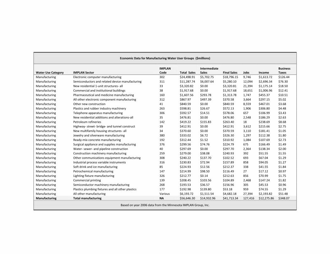
Economic Data for Manufacturing Water User Groups ($millions)
Water Use Category IMPLAN Sector IMPLAN Code Total Sales
Intermediate Sales Final Sales Jobs Income
Business Taxes
Manufacturing Electronic computer manufacturing 302 $24,498.91 $5,702.75 $18,796.15 9,746 $1,613.72 $126.44
Manufacturing Semiconductors and related device manufacturing 311 $11,287.74 $6,007.64 $5,280.10 12,094 $2,696.34 $76.30
Manufacturing New residential 1-unit structures- all 33 $3,320.82 $0.00 $3,320.81 21,394 $1,175.14 $18.50
Manufacturing Commercial and institutional buildings 38 $1,917.68 $0.00 $1,917.68 18,651 $1,006.96 $12.41
Manufacturing Pharmaceutical and medicine manufacturing 160 $1,607.56 $293.78 $1,313.78 1,747 $455.37 $10.51
Manufacturing All other electronic component manufacturing 312 $867.97 $497.39 $370.58 3,664 $297.15 $5.02
Manufacturing Other new construction 41 $840.59 $0.00 $840.59 8,559 $467.01 $3.68
Manufacturing Plastics and rubber industry machinery 263 $598.81 $26.67 $572.13 1,906 $306.80 $4.48
Manufacturing Telephone apparatus manufacturing 306 $592.57 $14.51 $578.06 657 $106.99 $3.43
Manufacturing New residential additions and alterations-all 35 $476.81 $0.00 $476.80 2,548 $186.29 $2.63
Manufacturing Petroleum refineries 142 $419.22 $155.83 $263.40 18 $238.69 $8.68
Manufacturing Highway- street- bridge- and tunnel construct 39 $412.91 $0.00 $412.91 3,612 $215.66 $2.75
Manufacturing New multifamily housing structures- all 34 $370.60 $0.00 $370.59 3,110 $181.41 $1.05
Manufacturing Jewelry and silverware manufacturing 380 $333.02 $6.72 $326.30 1,297 $112.38 $1.80
Manufacturing Ready-mix concrete manufacturing 192 $312.44 $1.52 $310.92 1,084 $107.69 $2.73
Manufacturing Surgical appliance and supplies manufacturing 376 $299.56 $74.76 $224.79 675 $166.49 $1.49
Manufacturing Water- sewer- and pipeline construction 40 $297.69 $0.00 $297.70 2,364 $138.34 $2.00
Manufacturing Construction machinery manufacturing 259 $279.00 $38.08 $240.93 392 $51.55 $1.55
Manufacturing Other communications equipment manufacturing 308 $240.22 $137.70 $102.52 693 $67.04 $1.29
Manufacturing Industrial process variable instruments 316 $230.83 $72.94 $157.89 858 $94.05 $1.27
Manufacturing Soft drink and ice manufacturing 85 $224.93 $12.56 $212.37 338 $41.55 $1.84
Manufacturing Petrochemical manufacturing 147 $214.99 $98.50 $116.49 27 $17.12 $0.97
Manufacturing Lighting fixture manufacturing 326 $212.77 $0.14 $212.63 856 $70.99 $1.75
Manufacturing Commercial printing 139 $208.45 $103.56 $104.89 2,468 $147.24 $1.82
Manufacturing Semiconductor machinery manufacturing 268 $193.53 $36.57 $156.96 305 $45.53 $0.96
Manufacturing Plastics plumbing fixtures and all other plastics 177 $192.98 $139.80 $53.18 959 $74.55 $1.29
Manufacturing All other manufacturing Various $6,193.72 $1,511.54 $4,682.18 27,394 $2,193.82 $51.48
Manufacturing Total manufacturing NA $56,646.30 $14,932.96 $41,713.34 127,416 $12,275.86 $348.07
Based on year 2006 data from the Minnesota IMPLAN Group, Inc.
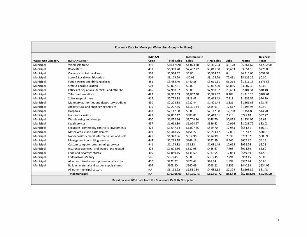
31
Economic Data for Municipal Water User Groups ($millions)
Water Use Category IMPLAN Sector IMPLAN Code Total Sales
Intermediate Sales Final Sales Jobs Income
Business Taxes
Municipal Wholesale trade 390 $10,178.94 $4,873.30 $5,305.64 45,128 $5,361.62 $1,502.90
Municipal Real estate 431 $6,309.70 $2,497.72 $3,811.98 30,663 $3,651.19 $776.89
Municipal Owner-occupied dwellings 509 $5,564.52 $0.00 $5,564.52 0 $4,310.65 $657.97
Municipal State & Local Non-Education 504 $5,125.29 -$0.01 $5,125.29 77,431 $5,125.29 $0.00
Municipal Food services and drinking places 481 $3,452.49 $440.88 $3,011.61 66,214 $1,511.16 $176.53
Municipal State & Local Education 503 $3,007.31 $0.00 $3,007.30 68,855 $3,007.30 $0.00
Municipal Offices of physicians- dentists- and other he 465 $2,950.97 $0.00 $2,950.97 23,663 $2,104.31 $18.48
Municipal Telecommunications 422 $2,932.63 $1,007.30 $1,925.32 8,188 $1,210.29 $202.61
Municipal Software publishers 417 $2,728.88 $313.45 $2,415.43 7,518 $1,535.59 $24.39
Municipal Monetary authorities and depository credit in 430 $2,223.88 $732.44 $1,491.44 8,321 $1,561.65 $28.45
Municipal Architectural and engineering services 439 $2,207.35 $1,391.44 $815.91 17,617 $1,198.94 $9.90
Municipal Hospitals 467 $2,112.08 $0.00 $2,112.08 17,768 $1,151.85 $14.70
Municipal Insurance carriers 427 $2,002.12 $583.81 $1,418.31 7,713 $745.18 $92.77
Municipal Warehousing and storage 400 $1,852.94 $1,704.24 $148.70 30,873 $1,354.05 $9.63
Municipal Legal services 437 $1,613.89 $1,024.27 $589.62 10,916 $1,035.79 $32.03
Municipal Securities- commodity contracts- investments 426 $1,547.14 $1,027.45 $519.70 12,953 $554.51 $16.41
Municipal Motor vehicle and parts dealers 401 $1,418.75 $154.27 $1,264.47 12,081 $737.12 $208.18
Municipal Nondepository credit intermediation and rela 425 $1,327.96 $812.96 $514.99 7,539 $793.32 $60.69
Municipal Management consulting services 444 $1,229.18 $946.19 $282.99 8,545 $657.82 $5.13
Municipal Custom computer programming services 441 $1,179.82 $98.33 $1,081.49 10,095 $998.26 $6.21
Municipal Insurance agencies- brokerages- and related 428 $1,078.66 $632.98 $445.67 7,705 $914.89 $5.69
Municipal Food and beverage stores 405 $1,059.15 $141.60 $917.55 17,064 $549.69 $120.19
Municipal Federal Non-Military 506 $963.45 $0.00 $963.45 7,791 $963.45 $0.00
Municipal All other miscellaneous professional and tech 450 $922.27 $823.43 $98.84 1,894 $332.44 $6.66
Municipal Building material and garden supply stores 404 $903.30 $140.09 $763.21 8,855 $440.94 $134.02
All other municipal sectors NA $6,193.72 $1,511.54 $4,682.18 27,394 $2,193.82 $51.48
Total municipal NA $96,908.91 $31,257.19 $65,651.72 883,845 $57,858.80 $5,225.90
Based on year 2006 data from the Minnesota IMPLAN Group, Inc.

32
Appendix 2: Impacts by Water User Group
Irrigation ($millions)
2010 2020 2030 2040 2050 2060
Bastrop County
Reduced income from reduced crop production $0.0133 $0.0056 $0.0045 $0.0035 $0.0027 $0.0019
Reduced business taxes from reduced crop production $0.0015 $0.0006 $0.0005 $0.0004 $0.0003 $0.0002
Reduced jobs from reduced crop production 0 0 0 0 0 0
Colorado County
Reduced income from curtailed rice production and milling activity $6.90 $5.89 $4.91 $3.96 $3.04 $2.16
Reduced business taxes from curtailed rice production and milling activity $0.80 $0.68 $0.57 $0.46 $0.35 $0.25
Reduced jobs from curtailed rice production and milling activity 91 78 65 52 40 28
Fayette County
Reduced income from reduced crop production $0.00 $0.01 $0.01 $0.01 $0.01 $0.01
Reduced business taxes from reduced crop production $0.00 $0.00 $0.00 $0.00 $0.00 $0.00
Reduced jobs from reduced crop production 0 0 0 0 0 0
Matagorda County
Reduced income from curtailed rice production and milling activity $70.93 $67.75 $63.99 $60.38 $56.92 $53.58
Reduced business taxes from curtailed rice production and milling activity $8.21 $7.84 $7.41 $6.99 $6.59 $6.20
Reduced jobs from curtailed rice production and milling activity 935 893 844 796 751 706
Mills County
Reduced income from reduced crop production $0.04 $0.03 $0.03 $0.02 $0.02 $0.02
Reduced business taxes from reduced crop production $0.00 $0.00 $0.00 $0.00 $0.00 $0.00
Reduced jobs from reduced crop production 0 0 0 0 0 0
Wharton County
Reduced income from curtailed rice production and milling activity $13.03 $11.98 $10.97 $9.99 $9.05 $5.48
Reduced business taxes from curtailed rice production and milling activity $1.51 $1.39 $1.27 $1.16 $1.05 $0.63
Reduced jobs from curtailed rice production and milling activity 172 158 145 132 119 72
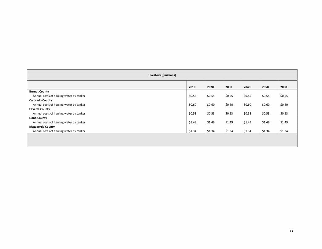
33
Livestock ($millions)
2010 2020 2030 2040 2050 2060
Burnet County
Annual costs of hauling water by tanker $0.55 $0.55 $0.55 $0.55 $0.55 $0.55
Colorado County
Annual costs of hauling water by tanker $0.60 $0.60 $0.60 $0.60 $0.60 $0.60
Fayette County
Annual costs of hauling water by tanker $0.53 $0.53 $0.53 $0.53 $0.53 $0.53
Llano County
Annual costs of hauling water by tanker $1.49 $1.49 $1.49 $1.49 $1.49 $1.49
Matagorda County
Annual costs of hauling water by tanker $1.34 $1.34 $1.34 $1.34 $1.34 $1.34
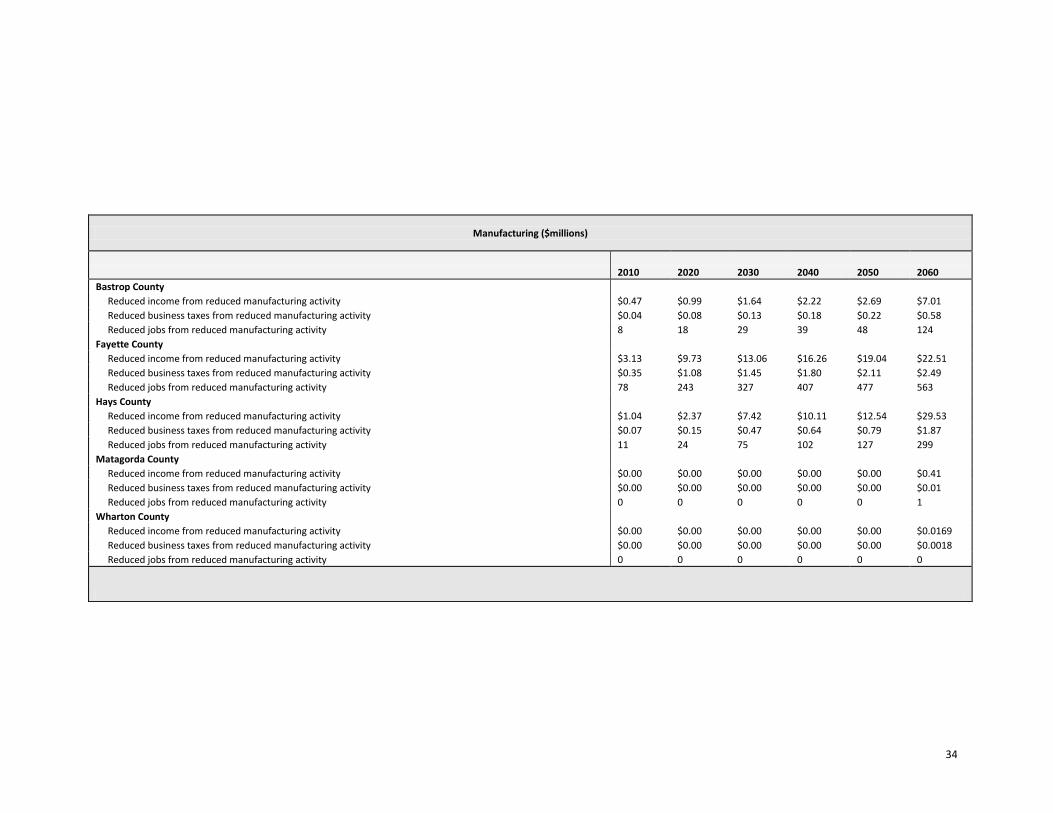
34
Manufacturing ($millions)
2010 2020 2030 2040 2050 2060
Bastrop County
Reduced income from reduced manufacturing activity $0.47 $0.99 $1.64 $2.22 $2.69 $7.01
Reduced business taxes from reduced manufacturing activity $0.04 $0.08 $0.13 $0.18 $0.22 $0.58
Reduced jobs from reduced manufacturing activity 8 18 29 39 48 124
Fayette County
Reduced income from reduced manufacturing activity $3.13 $9.73 $13.06 $16.26 $19.04 $22.51
Reduced business taxes from reduced manufacturing activity $0.35 $1.08 $1.45 $1.80 $2.11 $2.49
Reduced jobs from reduced manufacturing activity 78 243 327 407 477 563
Hays County
Reduced income from reduced manufacturing activity $1.04 $2.37 $7.42 $10.11 $12.54 $29.53
Reduced business taxes from reduced manufacturing activity $0.07 $0.15 $0.47 $0.64 $0.79 $1.87
Reduced jobs from reduced manufacturing activity 11 24 75 102 127 299
Matagorda County
Reduced income from reduced manufacturing activity $0.00 $0.00 $0.00 $0.00 $0.00 $0.41
Reduced business taxes from reduced manufacturing activity $0.00 $0.00 $0.00 $0.00 $0.00 $0.01
Reduced jobs from reduced manufacturing activity 0 0 0 0 0 1
Wharton County
Reduced income from reduced manufacturing activity $0.00 $0.00 $0.00 $0.00 $0.00 $0.0169
Reduced business taxes from reduced manufacturing activity $0.00 $0.00 $0.00 $0.00 $0.00 $0.0018
Reduced jobs from reduced manufacturing activity 0 0 0 0 0 0

35
Mining ($millions)
2010 2020 2030 2040 2050 2060
Burnet County
Reduced income from reduced mining activity $1.45 $1.62 $1.69 $1.76 $1.80 $1.89
Reduced business taxes from reduced mining activity $0.08 $0.09 $0.09 $0.09 $0.10 $0.10
Reduced jobs from reduced mining activity 14 16 17 18 18 19
Colorado County
Reduced income from reduced mining activity $16.12 $15.20 $13.63 $11.50 $8.83 $9.16
Reduced business taxes from reduced mining activity $1.12 $1.05 $0.94 $0.80 $0.61 $0.63
Reduced jobs from reduced mining activity 145 137 123 103 79 82
Fayette County
Reduced income from reduced mining activity $0.00 $0.00 $0.08 $0.11 $0.11 $0.11
Reduced business taxes from reduced mining activity $0.00 $0.00 $0.01 $0.01 $0.01 $0.01
Reduced jobs from reduced mining activity 0 0 1 1 1 1
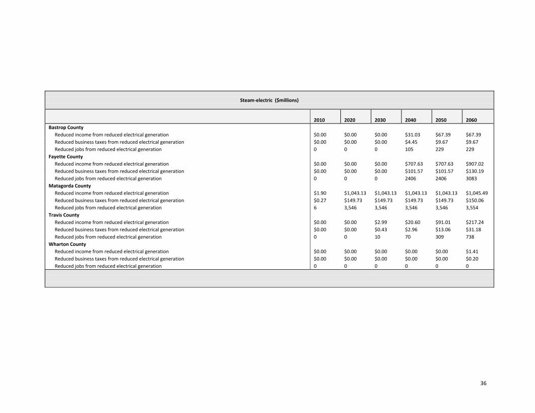
36
Steam-electric ($millions)
2010 2020 2030 2040 2050 2060
Bastrop County
Reduced income from reduced electrical generation $0.00 $0.00 $0.00 $31.03 $67.39 $67.39
Reduced business taxes from reduced electrical generation $0.00 $0.00 $0.00 $4.45 $9.67 $9.67
Reduced jobs from reduced electrical generation 0 0 0 105 229 229
Fayette County
Reduced income from reduced electrical generation $0.00 $0.00 $0.00 $707.63 $707.63 $907.02
Reduced business taxes from reduced electrical generation $0.00 $0.00 $0.00 $101.57 $101.57 $130.19
Reduced jobs from reduced electrical generation 0 0 0 2406 2406 3083
Matagorda County
Reduced income from reduced electrical generation $1.90 $1,043.13 $1,043.13 $1,043.13 $1,043.13 $1,045.49
Reduced business taxes from reduced electrical generation $0.27 $149.73 $149.73 $149.73 $149.73 $150.06
Reduced jobs from reduced electrical generation 6 3,546 3,546 3,546 3,546 3,554
Travis County
Reduced income from reduced electrical generation $0.00 $0.00 $2.99 $20.60 $91.01 $217.24
Reduced business taxes from reduced electrical generation $0.00 $0.00 $0.43 $2.96 $13.06 $31.18
Reduced jobs from reduced electrical generation 0 0 10 70 309 738
Wharton County
Reduced income from reduced electrical generation $0.00 $0.00 $0.00 $0.00 $0.00 $1.41
Reduced business taxes from reduced electrical generation $0.00 $0.00 $0.00 $0.00 $0.00 $0.20
Reduced jobs from reduced electrical generation 0 0 0 0 0 0
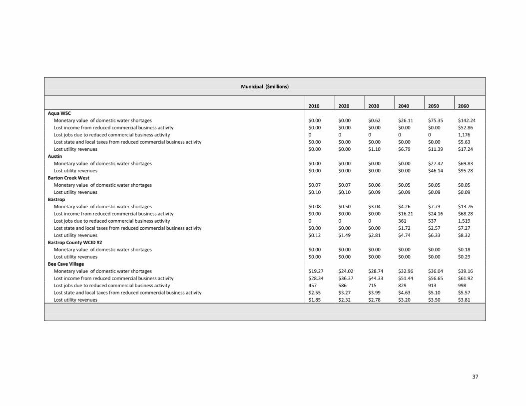
37
Municipal ($millions)
2010 2020 2030 2040 2050 2060
Aqua WSC
Monetary value of domestic water shortages $0.00 $0.00 $0.62 $26.11 $75.35 $142.24
Lost income from reduced commercial business activity $0.00 $0.00 $0.00 $0.00 $0.00 $52.86
Lost jobs due to reduced commercial business activity 0 0 0 0 0 1,176
Lost state and local taxes from reduced commercial business activity $0.00 $0.00 $0.00 $0.00 $0.00 $5.63
Lost utility revenues $0.00 $0.00 $1.10 $6.79 $11.39 $17.24
Austin
Monetary value of domestic water shortages $0.00 $0.00 $0.00 $0.00 $27.42 $69.83
Lost utility revenues $0.00 $0.00 $0.00 $0.00 $46.14 $95.28
Barton Creek West
Monetary value of domestic water shortages $0.07 $0.07 $0.06 $0.05 $0.05 $0.05
Lost utility revenues $0.10 $0.10 $0.09 $0.09 $0.09 $0.09
Bastrop
Monetary value of domestic water shortages $0.08 $0.50 $3.04 $4.26 $7.73 $13.76
Lost income from reduced commercial business activity $0.00 $0.00 $0.00 $16.21 $24.16 $68.28
Lost jobs due to reduced commercial business activity 0 0 0 361 537 1,519
Lost state and local taxes from reduced commercial business activity $0.00 $0.00 $0.00 $1.72 $2.57 $7.27
Lost utility revenues $0.12 $1.49 $2.81 $4.74 $6.33 $8.32
Bastrop County WCID #2
Monetary value of domestic water shortages $0.00 $0.00 $0.00 $0.00 $0.00 $0.18
Lost utility revenues $0.00 $0.00 $0.00 $0.00 $0.00 $0.29
Bee Cave Village
Monetary value of domestic water shortages $19.27 $24.02 $28.74 $32.96 $36.04 $39.16
Lost income from reduced commercial business activity $28.34 $36.37 $44.33 $51.44 $56.65 $61.92
Lost jobs due to reduced commercial business activity 457 586 715 829 913 998
Lost state and local taxes from reduced commercial business activity $2.55 $3.27 $3.99 $4.63 $5.10 $5.57
Lost utility revenues $1.85 $2.32 $2.78 $3.20 $3.50 $3.81
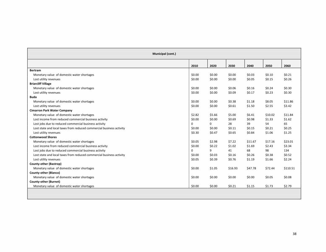
38
Municipal (cont.)
2010 2020 2030 2040 2050 2060
Bertram
Monetary value of domestic water shortages $0.00 $0.00 $0.00 $0.03 $0.10 $0.21
Lost utility revenues $0.00 $0.00 $0.00 $0.05 $0.15 $0.26
Briarcliff Village
Monetary value of domestic water shortages $0.00 $0.00 $0.06 $0.16 $0.24 $0.30
Lost utility revenues $0.00 $0.00 $0.09 $0.17 $0.23 $0.30
Buda
Monetary value of domestic water shortages $0.00 $0.00 $0.38 $1.18 $8.05 $11.86
Lost utility revenues $0.00 $0.00 $0.61 $1.50 $2.55 $3.42
Cimarron Park Water Company
Monetary value of domestic water shortages $2.82 $5.66 $5.00 $6.41 $10.02 $11.84
Lost income from reduced commercial business activity $0.00 $0.00 $0.69 $0.98 $1.33 $1.62
Lost jobs due to reduced commercial business activity 0 0 28 39 54 65
Lost state and local taxes from reduced commercial business activity $0.00 $0.00 $0.11 $0.15 $0.21 $0.25
Lost utility revenues $0.30 $0.47 $0.65 $0.84 $1.06 $1.25
Cottonwood Shores
Monetary value of domestic water shortages $0.05 $2.98 $7.22 $11.67 $17.16 $23.01
Lost income from reduced commercial business activity $0.00 $0.22 $1.02 $1.69 $2.43 $3.34
Lost jobs due to reduced commercial business activity 0 9 41 68 98 134
Lost state and local taxes from reduced commercial business activity $0.00 $0.03 $0.16 $0.26 $0.38 $0.52
Lost utility revenues $0.05 $0.39 $0.76 $1.19 $1.66 $2.24
County-other (Bastrop)
Monetary value of domestic water shortages $0.00 $1.05 $16.93 $47.78 $72.44 $110.51
County-other (Blanco)
Monetary value of domestic water shortages $0.00 $0.00 $0.00 $0.00 $0.05 $0.08
County-other (Burnet)
Monetary value of domestic water shortages $0.00 $0.00 $0.21 $1.15 $1.73 $2.79
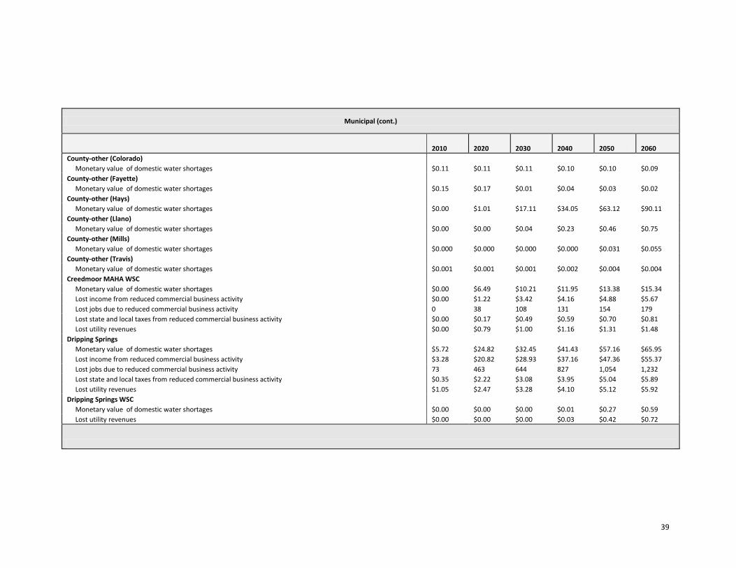
39
Municipal (cont.)
2010 2020 2030 2040 2050 2060
County-other (Colorado)
Monetary value of domestic water shortages $0.11 $0.11 $0.11 $0.10 $0.10 $0.09
County-other (Fayette)
Monetary value of domestic water shortages $0.15 $0.17 $0.01 $0.04 $0.03 $0.02
County-other (Hays)
Monetary value of domestic water shortages $0.00 $1.01 $17.11 $34.05 $63.12 $90.11
County-other (Llano)
Monetary value of domestic water shortages $0.00 $0.00 $0.04 $0.23 $0.46 $0.75
County-other (Mills)
Monetary value of domestic water shortages $0.000 $0.000 $0.000 $0.000 $0.031 $0.055
County-other (Travis)
Monetary value of domestic water shortages $0.001 $0.001 $0.001 $0.002 $0.004 $0.004
Creedmoor MAHA WSC
Monetary value of domestic water shortages $0.00 $6.49 $10.21 $11.95 $13.38 $15.34
Lost income from reduced commercial business activity $0.00 $1.22 $3.42 $4.16 $4.88 $5.67
Lost jobs due to reduced commercial business activity 0 38 108 131 154 179
Lost state and local taxes from reduced commercial business activity $0.00 $0.17 $0.49 $0.59 $0.70 $0.81
Lost utility revenues $0.00 $0.79 $1.00 $1.16 $1.31 $1.48
Dripping Springs
Monetary value of domestic water shortages $5.72 $24.82 $32.45 $41.43 $57.16 $65.95
Lost income from reduced commercial business activity $3.28 $20.82 $28.93 $37.16 $47.36 $55.37
Lost jobs due to reduced commercial business activity 73 463 644 827 1,054 1,232
Lost state and local taxes from reduced commercial business activity $0.35 $2.22 $3.08 $3.95 $5.04 $5.89
Lost utility revenues $1.05 $2.47 $3.28 $4.10 $5.12 $5.92
Dripping Springs WSC
Monetary value of domestic water shortages $0.00 $0.00 $0.00 $0.01 $0.27 $0.59
Lost utility revenues $0.00 $0.00 $0.00 $0.03 $0.42 $0.72
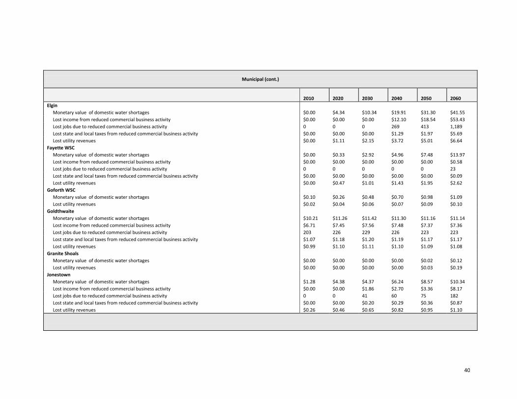
40
Municipal (cont.)
2010 2020 2030 2040 2050 2060
Elgin
Monetary value of domestic water shortages $0.00 $4.34 $10.34 $19.91 $31.30 $41.55
Lost income from reduced commercial business activity $0.00 $0.00 $0.00 $12.10 $18.54 $53.43
Lost jobs due to reduced commercial business activity 0 0 0 269 413 1,189
Lost state and local taxes from reduced commercial business activity $0.00 $0.00 $0.00 $1.29 $1.97 $5.69
Lost utility revenues $0.00 $1.11 $2.15 $3.72 $5.01 $6.64
Fayette WSC
Monetary value of domestic water shortages $0.00 $0.33 $2.92 $4.96 $7.48 $13.97
Lost income from reduced commercial business activity $0.00 $0.00 $0.00 $0.00 $0.00 $0.58
Lost jobs due to reduced commercial business activity 0 0 0 0 0 23
Lost state and local taxes from reduced commercial business activity $0.00 $0.00 $0.00 $0.00 $0.00 $0.09
Lost utility revenues $0.00 $0.47 $1.01 $1.43 $1.95 $2.62
Goforth WSC
Monetary value of domestic water shortages $0.10 $0.26 $0.48 $0.70 $0.98 $1.09
Lost utility revenues $0.02 $0.04 $0.06 $0.07 $0.09 $0.10
Goldthwaite
Monetary value of domestic water shortages $10.21 $11.26 $11.42 $11.30 $11.16 $11.14
Lost income from reduced commercial business activity $6.71 $7.45 $7.56 $7.48 $7.37 $7.36
Lost jobs due to reduced commercial business activity 203 226 229 226 223 223
Lost state and local taxes from reduced commercial business activity $1.07 $1.18 $1.20 $1.19 $1.17 $1.17
Lost utility revenues $0.99 $1.10 $1.11 $1.10 $1.09 $1.08
Granite Shoals
Monetary value of domestic water shortages $0.00 $0.00 $0.00 $0.00 $0.02 $0.12
Lost utility revenues $0.00 $0.00 $0.00 $0.00 $0.03 $0.19
Jonestown
Monetary value of domestic water shortages $1.28 $4.38 $4.37 $6.24 $8.57 $10.34
Lost income from reduced commercial business activity $0.00 $0.00 $1.86 $2.70 $3.36 $8.17
Lost jobs due to reduced commercial business activity 0 0 41 60 75 182
Lost state and local taxes from reduced commercial business activity $0.00 $0.00 $0.20 $0.29 $0.36 $0.87
Lost utility revenues $0.26 $0.46 $0.65 $0.82 $0.95 $1.10
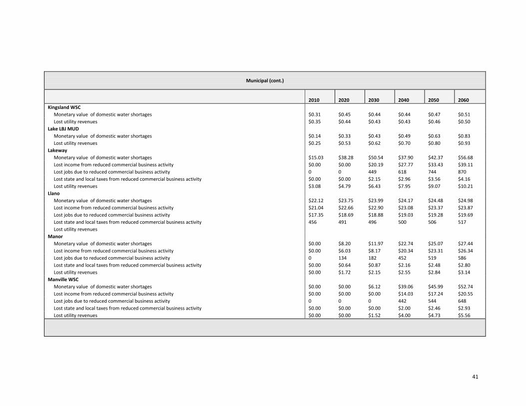
41
Municipal (cont.)
2010 2020 2030 2040 2050 2060
Kingsland WSC
Monetary value of domestic water shortages $0.31 $0.45 $0.44 $0.44 $0.47 $0.51
Lost utility revenues $0.35 $0.44 $0.43 $0.43 $0.46 $0.50
Lake LBJ MUD
Monetary value of domestic water shortages $0.14 $0.33 $0.43 $0.49 $0.63 $0.83
Lost utility revenues $0.25 $0.53 $0.62 $0.70 $0.80 $0.93
Lakeway
Monetary value of domestic water shortages $15.03 $38.28 $50.54 $37.90 $42.37 $56.68
Lost income from reduced commercial business activity $0.00 $0.00 $20.19 $27.77 $33.43 $39.11
Lost jobs due to reduced commercial business activity 0 0 449 618 744 870
Lost state and local taxes from reduced commercial business activity $0.00 $0.00 $2.15 $2.96 $3.56 $4.16
Lost utility revenues $3.08 $4.79 $6.43 $7.95 $9.07 $10.21
Llano
Monetary value of domestic water shortages $22.12 $23.75 $23.99 $24.17 $24.48 $24.98
Lost income from reduced commercial business activity $21.04 $22.66 $22.90 $23.08 $23.37 $23.87
Lost jobs due to reduced commercial business activity $17.35 $18.69 $18.88 $19.03 $19.28 $19.69
Lost state and local taxes from reduced commercial business activity 456 491 496 500 506 517
Lost utility revenues
Manor
Monetary value of domestic water shortages $0.00 $8.20 $11.97 $22.74 $25.07 $27.44
Lost income from reduced commercial business activity $0.00 $6.03 $8.17 $20.34 $23.31 $26.34
Lost jobs due to reduced commercial business activity 0 134 182 452 519 586
Lost state and local taxes from reduced commercial business activity $0.00 $0.64 $0.87 $2.16 $2.48 $2.80
Lost utility revenues $0.00 $1.72 $2.15 $2.55 $2.84 $3.14
Manville WSC
Monetary value of domestic water shortages $0.00 $0.00 $6.12 $39.06 $45.99 $52.74
Lost income from reduced commercial business activity $0.00 $0.00 $0.00 $14.03 $17.24 $20.55
Lost jobs due to reduced commercial business activity 0 0 0 442 544 648
Lost state and local taxes from reduced commercial business activity $0.00 $0.00 $0.00 $2.00 $2.46 $2.93
Lost utility revenues $0.00 $0.00 $1.52 $4.00 $4.73 $5.56
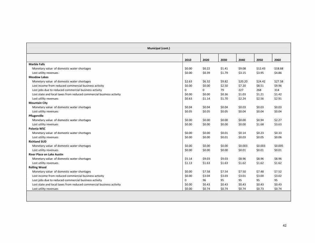
42
Municipal (cont.)
2010 2020 2030 2040 2050 2060
Marble Falls
Monetary value of domestic water shortages $0.00 $0.22 $1.41 $9.08 $12.43 $18.68
Lost utility revenues $0.00 $0.39 $1.79 $3.15 $3.95 $4.86
Meadow Lakes
Monetary value of domestic water shortages $2.63 $6.32 $9.82 $20.20 $24.42 $27.58
Lost income from reduced commercial business activity $0.00 $0.00 $2.50 $7.20 $8.51 $9.96
Lost jobs due to reduced commercial business activity 0 0 79 227 268 314
Lost state and local taxes from reduced commercial business activity $0.00 $0.00 $0.36 $1.03 $1.21 $1.42
Lost utility revenues $0.63 $1.14 $1.70 $2.24 $2.56 $2.91
Mountain City
Monetary value of domestic water shortages $0.04 $0.04 $0.04 $0.03 $0.03 $0.03
Lost utility revenues $0.05 $0.05 $0.05 $0.04 $0.04 $0.04
Pflugerville
Monetary value of domestic water shortages $0.00 $0.00 $0.00 $0.00 $0.94 $2.27
Lost utility revenues $0.00 $0.00 $0.00 $0.00 $1.68 $3.63
Polonia WSC
Monetary value of domestic water shortages $0.00 $0.00 $0.01 $0.14 $0.23 $0.33
Lost utility revenues $0.00 $0.00 $0.01 $0.03 $0.05 $0.06
Richland SUD
Monetary value of domestic water shortages $0.00 $0.00 $0.00 $0.003 $0.003 $0.005
Lost utility revenues $0.00 $0.00 $0.00 $0.01 $0.01 $0.01
River Place on Lake Austin
Monetary value of domestic water shortages $5.14 $9.03 $9.03 $8.96 $8.96 $8.96
Lost utility revenues $1.13 $1.63 $1.63 $1.62 $1.62 $1.62
Rolling Wood
Monetary value of domestic water shortages $0.00 $7.58 $7.54 $7.50 $7.48 $7.52
Lost income from reduced commercial business activity $0.00 $3.04 $3.03 $3.01 $3.00 $3.02
Lost jobs due to reduced commercial business activity 0 96 95 95 95 95
Lost state and local taxes from reduced commercial business activity $0.00 $0.43 $0.43 $0.43 $0.43 $0.43
Lost utility revenues $0.00 $0.74 $0.74 $0.74 $0.73 $0.74
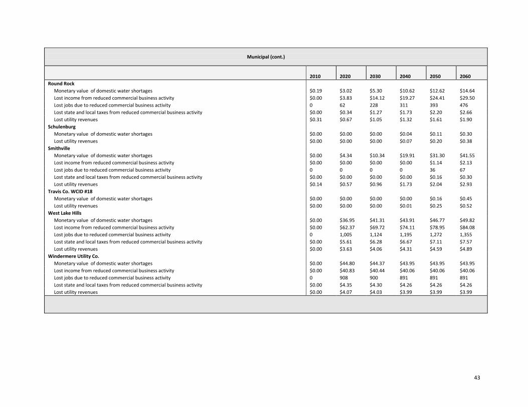
43
Municipal (cont.)
2010 2020 2030 2040 2050 2060
Round Rock
Monetary value of domestic water shortages $0.19 $3.02 $5.30 $10.62 $12.62 $14.64
Lost income from reduced commercial business activity $0.00 $3.83 $14.12 $19.27 $24.41 $29.50
Lost jobs due to reduced commercial business activity 0 62 228 311 393 476
Lost state and local taxes from reduced commercial business activity $0.00 $0.34 $1.27 $1.73 $2.20 $2.66
Lost utility revenues $0.31 $0.67 $1.05 $1.32 $1.61 $1.90
Schulenburg
Monetary value of domestic water shortages $0.00 $0.00 $0.00 $0.04 $0.11 $0.30
Lost utility revenues $0.00 $0.00 $0.00 $0.07 $0.20 $0.38
Smithville
Monetary value of domestic water shortages $0.00 $4.34 $10.34 $19.91 $31.30 $41.55
Lost income from reduced commercial business activity $0.00 $0.00 $0.00 $0.00 $1.14 $2.13
Lost jobs due to reduced commercial business activity 0 0 0 0 36 67
Lost state and local taxes from reduced commercial business activity $0.00 $0.00 $0.00 $0.00 $0.16 $0.30
Lost utility revenues $0.14 $0.57 $0.96 $1.73 $2.04 $2.93
Travis Co. WCID #18
Monetary value of domestic water shortages $0.00 $0.00 $0.00 $0.00 $0.16 $0.45
Lost utility revenues $0.00 $0.00 $0.00 $0.01 $0.25 $0.52
West Lake Hills
Monetary value of domestic water shortages $0.00 $36.95 $41.31 $43.91 $46.77 $49.82
Lost income from reduced commercial business activity $0.00 $62.37 $69.72 $74.11 $78.95 $84.08
Lost jobs due to reduced commercial business activity 0 1,005 1,124 1,195 1,272 1,355
Lost state and local taxes from reduced commercial business activity $0.00 $5.61 $6.28 $6.67 $7.11 $7.57
Lost utility revenues $0.00 $3.63 $4.06 $4.31 $4.59 $4.89
Windermere Utility Co.
Monetary value of domestic water shortages $0.00 $44.80 $44.37 $43.95 $43.95 $43.95
Lost income from reduced commercial business activity $0.00 $40.83 $40.44 $40.06 $40.06 $40.06
Lost jobs due to reduced commercial business activity 0 908 900 891 891 891
Lost state and local taxes from reduced commercial business activity $0.00 $4.35 $4.30 $4.26 $4.26 $4.26
Lost utility revenues $0.00 $4.07 $4.03 $3.99 $3.99 $3.99

Socioeconomic Impacts of Projected Water Shortages for the South Central Texas Regional Water Planning Area (Region L) Prepared in Support of the 2011 South Central Texas Regional Water Plan
Stuart D. Norvell, Managing Economist Water Resources Planning Division Texas Water Development Board Austin, Texas S. Doug Shaw, Agricultural Economist Water Resources Planning Division Texas Water Development Board Austin, Texas June 2010
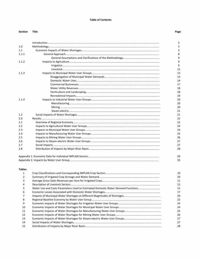
Table of Contents
Section Title Page
Introduction……………..………………………………………………………………………………………………………………………………… 3 1.0 Methodology……………………………………………………………………………………………….…………………………..................... 3 1.1 Economic Impacts of Water Shortages…………………………………………………………………………………………………… 3 1.1.1 General Approach……………………………………………………….................................................................... 8 General Assumptions and Clarifications of the Methodology.…….…….………………….…............ 9 1.1.2 Impacts to Agriculture……………………………………………………………………………………………………................. 9 Irrigation………………………………..………………….………………………………………………………..….…………. 9 Livestock…………………………………..………………………………………………………………………………..……… 12 1.1.3 Impacts to Municipal Water User Groups……………………..…………………………………………….…….………….. 13 Disaggregation of Municipal Water Demands.………………………………………………….……………...... 13 Domestic Water Uses……………………………………………………….……………….………………………………... 14 Commercial Businesses………………………………………….……………………………………………….…………... 17 Water Utility Revenues……..…….………………………………………………………………..……………………..…. 18 Horticulture and Landscaping.….…..…………………………………………………………………………………..... 18 Recreational Impacts……………………….…………………………………………………………………….………….… 19 1.1.4 Impacts to Industrial Water User Groups……………………………………………………….………………………………. 20 Manufacturing………………………………………………………………………………………………………………..…… 20 Mining..………..….……………………………………………………………………………………………………………..….. 20 Steam‐electric..…………………………………………………………………………………………….…………………..… 21 1.2 Social Impacts of Water Shortages………………………………………………………………………………………………………..… 21 2.0 Results………………………………………………………………………………………………………………………………………….…………….. 22 2.1 Overview of Regional Economy……………………………………………………………………………………………….……………… 22 2.2 Impacts to Agricultural Water User Groups……………………………………………………………………………..……………… 24 2.3 Impacts to Municipal Water User Groups………………………………………………………………………………..……………… 24 2.4 Impacts to Manufacturing Water User Groups…………………………………………………………………………..…………… 25 2.5 Impacts to Mining Water User Groups………………………………………………………………………………………..……..…… 26 2.6 Impacts to Steam‐electric Water User Groups………………………………………………………………….………..…………… 27 2.7 Social Impacts………………………………………………………………………………………………………………………………..……….. 27 2.8 Distribution of Impacts by Major River Basin………………………………………………………………………………….………. 28 Appendix 1: Economic Data for Individual IMPLAN Sectors……………………………………………………………………………............…. 29 Appendix 2: Impacts by Water User Group.……………………………………………………….....………………..……………………………….…. 33
Tables
1 Crop Classifications and Corresponding IMPLAN Crop Sectors……………………………………………………………..…….. 10 2 Summary of Irrigated Crop Acreage and Water Demand….…………………………..……………………………………….…… 10 3 Average Gross Sales Revenues per Acre for Irrigated Crops…………………………………………………………………..……. 11 4 Description of Livestock Sectors…………………………………………………………………………………………………………..……… 13 5 Water Use and Costs Parameters Used to Estimated Domestic Water Demand Functions…………………..……… 15 6 Economic Losses Associated with Domestic Water Shortages………………………………………………………………..……. 17 7 Impacts of Municipal Water Shortages at Different Magnitudes of Shortages…………………………………..…………. 20 8 Regional Baseline Economy by Water User Group………………………….….……………………………………………………….… 23 9 Economic Impacts of Water Shortages for Irrigation Water User Groups……………………………………………..…….… 24 10 Economic Impacts of Water Shortages for Municipal Water User Groups……………………………………………..……… 24 11 Economic Impacts of Water Shortages for Manufacturing Water User Groups……………………………………..……… 25 12 Economic Impacts of Water Shortages for Mining Water User Groups………….....…………………………………..……… 26 13 Economic Impacts of Water Shortages for Steam‐electric Water User Groups....…………………………………..……… 27 14 Social Impacts of Water Shortages……………………………………………………………………..……………………………….………… 27 15 Distribution of Impacts by Major River Basin…………………………………………………………………………………………………. 28
2
Introduction
Water shortages during drought would likely curtail or eliminate economic activity in business and industries reliant on water. For example, without water farmers cannot irrigate; refineries cannot produce gasoline, and paper mills cannot make paper. Unreliable water supplies would not only have an immediate and real impact on existing businesses and industry, but they could also adversely affect economic development in Texas. From a social perspective, water supply reliability is critical as well. Shortages would disrupt activity in homes, schools and government and could adversely affect public health and safety. For all of the above reasons, it is important to analyze and understand how restricted water supplies during drought could affect communities throughout the state.
Administrative rules require that regional water planning groups evaluate the impacts of not
meeting water needs as part of the regional water planning process, and rules direct TWDB staff to provide technical assistance: “The executive administrator shall provide available technical assistance to the regional water planning groups, upon request, on water supply and demand analysis, including methods to evaluate the social and economic impacts of not meeting needs” [(§357.7 (4)(A)]. Staff of the TWDB’s Water Resources Planning Division designed and conducted this report in support of the South Central Texas Regional Water Planning Group (Region L).
This document summarizes the results of our analysis and discusses the methodology used to generate the results. Section 1 outlines the overall methodology and discusses approaches and assumptions specific to each water use category (i.e., irrigation, livestock, mining, steam‐electric, municipal and manufacturing). Section 2 presents the results for each category where shortages are reported at the regional planning area level and river basin level. Results for individual water user groups are not presented, but are available upon request.
1. Methodology
Section 1 provides a general overview of how economic and social impacts were measured. In addition, it summarizes important clarifications, assumptions and limitations of the study.
1.1 Economic Impacts of Water Shortages 1.1.1 General Approach
Economic analysis as it relates to water resources planning generally falls into two broad areas. Supply side analysis focuses on costs and alternatives of developing new water supplies or implementing programs that provide additional water from current supplies. Demand side analysis concentrates on impacts or benefits of providing water to people, businesses and the environment. Analysis in this report focuses strictly on demand side impacts. When analyzing the economic impacts of water shortages as defined in Texas water planning, three potential scenarios are possible:
1) Scenario 1 involves situations where there are physical shortages of raw surface or groundwater due to drought of record conditions. For example, City A relies on a reservoir with average conservation storage of 500 acre‐feet per year and a firm yield of 100 acre feet. In 2010, the city uses about 50 acre‐feet per year, but by 2030 their demands are expected to increase to 200
3
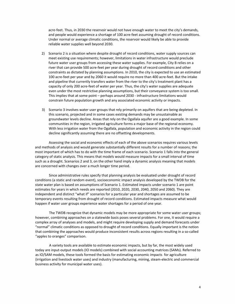
acre‐feet. Thus, in 2030 the reservoir would not have enough water to meet the city’s demands, and people would experience a shortage of 100 acre‐feet assuming drought of record conditions. Under normal or average climatic conditions, the reservoir would likely be able to provide reliable water supplies well beyond 2030.
2) Scenario 2 is a situation where despite drought of record conditions, water supply sources can meet existing use requirements; however, limitations in water infrastructure would preclude future water user groups from accessing these water supplies. For example, City B relies on a river that can provide 500 acre‐feet per year during drought of record conditions and other constraints as dictated by planning assumptions. In 2010, the city is expected to use an estimated 100 acre‐feet per year and by 2060 it would require no more than 400 acre‐feet. But the intake and pipeline that currently transfers water from the river to the city’s treatment plant has a capacity of only 200 acre‐feet of water per year. Thus, the city’s water supplies are adequate even under the most restrictive planning assumptions, but their conveyance system is too small. This implies that at some point – perhaps around 2030 ‐ infrastructure limitations would constrain future population growth and any associated economic activity or impacts.
3) Scenario 3 involves water user groups that rely primarily on aquifers that are being depleted. In this scenario, projected and in some cases existing demands may be unsustainable as groundwater levels decline. Areas that rely on the Ogallala aquifer are a good example. In some communities in the region, irrigated agriculture forms a major base of the regional economy. With less irrigation water from the Ogallala, population and economic activity in the region could decline significantly assuming there are no offsetting developments.
Assessing the social and economic effects of each of the above scenarios requires various levels
and methods of analysis and would generate substantially different results for a number of reasons; the most important of which has to do with the time frame of each scenario. Scenario 1 falls into the general category of static analysis. This means that models would measure impacts for a small interval of time such as a drought. Scenarios 2 and 3, on the other hand imply a dynamic analysis meaning that models are concerned with changes over a much longer time period.
Since administrative rules specify that planning analysis be evaluated under drought of record conditions (a static and random event), socioeconomic impact analysis developed by the TWDB for the state water plan is based on assumptions of Scenario 1. Estimated impacts under scenario 1 are point estimates for years in which needs are reported (2010, 2020, 2030, 2040, 2050 and 2060). They are independent and distinct “what if” scenarios for a particular year and shortages are assumed to be temporary events resulting from drought of record conditions. Estimated impacts measure what would happen if water user groups experience water shortages for a period of one year.
The TWDB recognize that dynamic models may be more appropriate for some water user groups; however, combining approaches on a statewide basis poses several problems. For one, it would require a complex array of analyses and models, and might require developing supply and demand forecasts under “normal” climatic conditions as opposed to drought of record conditions. Equally important is the notion that combining the approaches would produce inconsistent results across regions resulting in a so‐called “apples to oranges” comparison.
A variety tools are available to estimate economic impacts, but by far, the most widely used today are input‐output models (IO models) combined with social accounting matrices (SAMs). Referred to as IO/SAM models, these tools formed the basis for estimating economic impacts for agriculture (irrigation and livestock water uses) and industry (manufacturing, mining, steam‐electric and commercial business activity for municipal water uses).
4
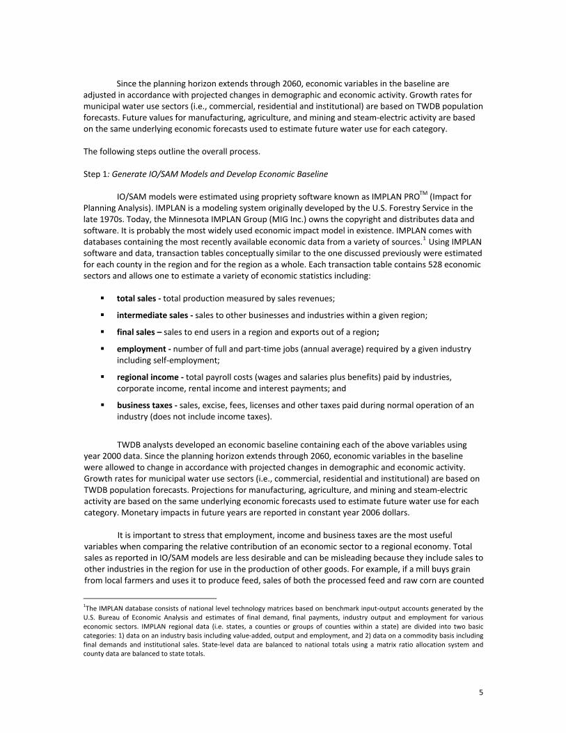
Since the planning horizon extends through 2060, economic variables in the baseline are
adjusted in accordance with projected changes in demographic and economic activity. Growth rates for municipal water use sectors (i.e., commercial, residential and institutional) are based on TWDB population forecasts. Future values for manufacturing, agriculture, and mining and steam‐electric activity are based on the same underlying economic forecasts used to estimate future water use for each category. The following steps outline the overall process. Step 1: Generate IO/SAM Models and Develop Economic Baseline
IO/SAM models were estimated using propriety software known as IMPLAN PROTM (Impact for
Planning Analysis). IMPLAN is a modeling system originally developed by the U.S. Forestry Service in the late 1970s. Today, the Minnesota IMPLAN Group (MIG Inc.) owns the copyright and distributes data and software. It is probably the most widely used economic impact model in existence. IMPLAN comes with databases containing the most recently available economic data from a variety of sources.1 Using IMPLAN software and data, transaction tables conceptually similar to the one discussed previously were estimated for each county in the region and for the region as a whole. Each transaction table contains 528 economic sectors and allows one to estimate a variety of economic statistics including:
total sales ‐ total production measured by sales revenues;
intermediate sales ‐ sales to other businesses and industries within a given region;
final sales – sales to end users in a region and exports out of a region;
employment ‐ number of full and part‐time jobs (annual average) required by a given industry including self‐employment;
regional income ‐ total payroll costs (wages and salaries plus benefits) paid by industries, corporate income, rental income and interest payments; and
business taxes ‐ sales, excise, fees, licenses and other taxes paid during normal operation of an industry (does not include income taxes).
TWDB analysts developed an economic baseline containing each of the above variables using
year 2000 data. Since the planning horizon extends through 2060, economic variables in the baseline were allowed to change in accordance with projected changes in demographic and economic activity. Growth rates for municipal water use sectors (i.e., commercial, residential and institutional) are based on TWDB population forecasts. Projections for manufacturing, agriculture, and mining and steam‐electric activity are based on the same underlying economic forecasts used to estimate future water use for each category. Monetary impacts in future years are reported in constant year 2006 dollars.
It is important to stress that employment, income and business taxes are the most useful
variables when comparing the relative contribution of an economic sector to a regional economy. Total sales as reported in IO/SAM models are less desirable and can be misleading because they include sales to other industries in the region for use in the production of other goods. For example, if a mill buys grain from local farmers and uses it to produce feed, sales of both the processed feed and raw corn are counted
1The IMPLAN database consists of national level technology matrices based on benchmark input‐output accounts generated by the U.S. Bureau of Economic Analysis and estimates of final demand, final payments, industry output and employment for various economic sectors. IMPLAN regional data (i.e. states, a counties or groups of counties within a state) are divided into two basic categories: 1) data on an industry basis including value‐added, output and employment, and 2) data on a commodity basis including final demands and institutional sales. State‐level data are balanced to national totals using a matrix ratio allocation system and county data are balanced to state totals.
5
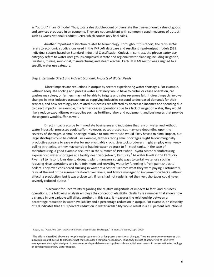
as “output” in an IO model. Thus, total sales double‐count or overstate the true economic value of goods and services produced in an economy. They are not consistent with commonly used measures of output such as Gross National Product (GNP), which counts only final sales.
Another important distinction relates to terminology. Throughout this report, the term sector
refers to economic subdivisions used in the IMPLAN database and resultant input‐output models (528 individual sectors based on Standard Industrial Classification Codes). In contrast, the phrase water use category refers to water user groups employed in state and regional water planning including irrigation, livestock, mining, municipal, manufacturing and steam electric. Each IMPLAN sector was assigned to a specific water use category.
Step 2: Estimate Direct and Indirect Economic Impacts of Water Needs Direct impacts are reductions in output by sectors experiencing water shortages. For example,
without adequate cooling and process water a refinery would have to curtail or cease operation, car washes may close, or farmers may not be able to irrigate and sales revenues fall. Indirect impacts involve changes in inter‐industry transactions as supplying industries respond to decreased demands for their services, and how seemingly non‐related businesses are affected by decreased incomes and spending due to direct impacts. For example, if a farmer ceases operations due to a lack of irrigation water, they would likely reduce expenditures on supplies such as fertilizer, labor and equipment, and businesses that provide these goods would suffer as well.
Direct impacts accrue to immediate businesses and industries that rely on water and without
water industrial processes could suffer. However, output responses may vary depending upon the severity of shortages. A small shortage relative to total water use would likely have a minimal impact, but large shortages could be critical. For example, farmers facing small shortages might fallow marginally productive acreage to save water for more valuable crops. Livestock producers might employ emergency culling strategies, or they may consider hauling water by truck to fill stock tanks. In the case of manufacturing, a good example occurred in the summer of 1999 when Toyota Motor Manufacturing experienced water shortages at a facility near Georgetown, Kentucky.2 As water levels in the Kentucky River fell to historic lows due to drought, plant managers sought ways to curtail water use such as reducing rinse operations to a bare minimum and recycling water by funneling it from paint shops to boilers. They even considered trucking in water at a cost of 10 times what they were paying. Fortunately, rains at the end of the summer restored river levels, and Toyota managed to implement cutbacks without affecting production, but it was a close call. If rains had not replenished the river, shortages could have severely reduced output.3
To account for uncertainty regarding the relative magnitude of impacts to farm and business
operations, the following analysis employs the concept of elasticity. Elasticity is a number that shows how a change in one variable will affect another. In this case, it measures the relationship between a percentage reduction in water availability and a percentage reduction in output. For example, an elasticity of 1.0 indicates that a 1.0 percent reduction in water availability would result in a 1.0 percent reduction in
2 Royal, W. “High And Dry ‐ Industrial Centers Face Water Shortages.” in Industry Week, Sept, 2000. 3 The efforts described above are not planned programmatic or long‐term operational changes. They are emergency measures that individuals might pursue to alleviate what they consider a temporary condition. Thus, they are not characteristic of long‐term management strategies designed to ensure more dependable water supplies such as capital investments in conservation technology or development of new water supplies.
6
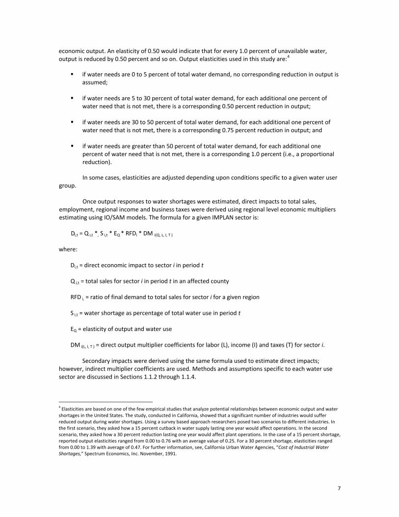
economic output. An elasticity of 0.50 would indicate that for every 1.0 percent of unavailable water, output is reduced by 0.50 percent and so on. Output elasticities used in this study are:4
if water needs are 0 to 5 percent of total water demand, no corresponding reduction in output is
assumed; if water needs are 5 to 30 percent of total water demand, for each additional one percent of
water need that is not met, there is a corresponding 0.50 percent reduction in output; if water needs are 30 to 50 percent of total water demand, for each additional one percent of
water need that is not met, there is a corresponding 0.75 percent reduction in output; and
if water needs are greater than 50 percent of total water demand, for each additional one percent of water need that is not met, there is a corresponding 1.0 percent (i.e., a proportional reduction).
In some cases, elasticities are adjusted depending upon conditions specific to a given water user
group. Once output responses to water shortages were estimated, direct impacts to total sales,
employment, regional income and business taxes were derived using regional level economic multipliers estimating using IO/SAM models. The formula for a given IMPLAN sector is:
Di,t = Q i,t *, S i,t * EQ * RFDi * DM i(Q, L, I, T )
where:
Di,t = direct economic impact to sector i in period t Q i,t = total sales for sector i in period t in an affected county RFD i, = ratio of final demand to total sales for sector i for a given region S i,t = water shortage as percentage of total water use in period t EQ = elasticity of output and water use DM i(L, I, T ) = direct output multiplier coefficients for labor (L), income (I) and taxes (T) for sector i.
Secondary impacts were derived using the same formula used to estimate direct impacts;
however, indirect multiplier coefficients are used. Methods and assumptions specific to each water use sector are discussed in Sections 1.1.2 through 1.1.4. 4 Elasticities are based on one of the few empirical studies that analyze potential relationships between economic output and water shortages in the United States. The study, conducted in California, showed that a significant number of industries would suffer reduced output during water shortages. Using a survey based approach researchers posed two scenarios to different industries. In the first scenario, they asked how a 15 percent cutback in water supply lasting one year would affect operations. In the second scenario, they asked how a 30 percent reduction lasting one year would affect plant operations. In the case of a 15 percent shortage, reported output elasticities ranged from 0.00 to 0.76 with an average value of 0.25. For a 30 percent shortage, elasticities ranged from 0.00 to 1.39 with average of 0.47. For further information, see, California Urban Water Agencies, “Cost of Industrial Water Shortages,” Spectrum Economics, Inc. November, 1991.
7
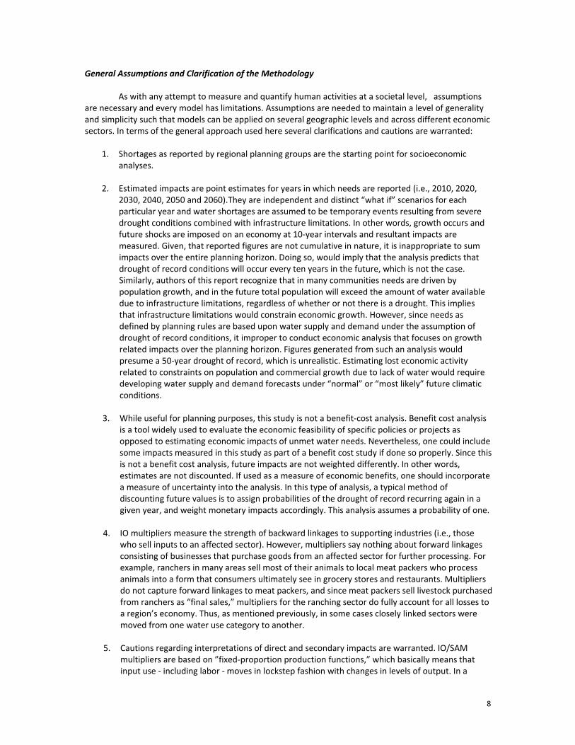
General Assumptions and Clarification of the Methodology
As with any attempt to measure and quantify human activities at a societal level, assumptions are necessary and every model has limitations. Assumptions are needed to maintain a level of generality and simplicity such that models can be applied on several geographic levels and across different economic sectors. In terms of the general approach used here several clarifications and cautions are warranted:
1. Shortages as reported by regional planning groups are the starting point for socioeconomic analyses.
2. Estimated impacts are point estimates for years in which needs are reported (i.e., 2010, 2020,
2030, 2040, 2050 and 2060).They are independent and distinct “what if” scenarios for each particular year and water shortages are assumed to be temporary events resulting from severe drought conditions combined with infrastructure limitations. In other words, growth occurs and future shocks are imposed on an economy at 10‐year intervals and resultant impacts are measured. Given, that reported figures are not cumulative in nature, it is inappropriate to sum impacts over the entire planning horizon. Doing so, would imply that the analysis predicts that drought of record conditions will occur every ten years in the future, which is not the case. Similarly, authors of this report recognize that in many communities needs are driven by population growth, and in the future total population will exceed the amount of water available due to infrastructure limitations, regardless of whether or not there is a drought. This implies that infrastructure limitations would constrain economic growth. However, since needs as defined by planning rules are based upon water supply and demand under the assumption of drought of record conditions, it improper to conduct economic analysis that focuses on growth related impacts over the planning horizon. Figures generated from such an analysis would presume a 50‐year drought of record, which is unrealistic. Estimating lost economic activity related to constraints on population and commercial growth due to lack of water would require developing water supply and demand forecasts under “normal” or “most likely” future climatic conditions.
3. While useful for planning purposes, this study is not a benefit‐cost analysis. Benefit cost analysis
is a tool widely used to evaluate the economic feasibility of specific policies or projects as opposed to estimating economic impacts of unmet water needs. Nevertheless, one could include some impacts measured in this study as part of a benefit cost study if done so properly. Since this is not a benefit cost analysis, future impacts are not weighted differently. In other words, estimates are not discounted. If used as a measure of economic benefits, one should incorporate a measure of uncertainty into the analysis. In this type of analysis, a typical method of discounting future values is to assign probabilities of the drought of record recurring again in a given year, and weight monetary impacts accordingly. This analysis assumes a probability of one.
4. IO multipliers measure the strength of backward linkages to supporting industries (i.e., those
who sell inputs to an affected sector). However, multipliers say nothing about forward linkages consisting of businesses that purchase goods from an affected sector for further processing. For example, ranchers in many areas sell most of their animals to local meat packers who process animals into a form that consumers ultimately see in grocery stores and restaurants. Multipliers do not capture forward linkages to meat packers, and since meat packers sell livestock purchased from ranchers as “final sales,” multipliers for the ranching sector do fully account for all losses to a region’s economy. Thus, as mentioned previously, in some cases closely linked sectors were moved from one water use category to another.
5. Cautions regarding interpretations of direct and secondary impacts are warranted. IO/SAM
multipliers are based on ”fixed‐proportion production functions,” which basically means that input use ‐ including labor ‐ moves in lockstep fashion with changes in levels of output. In a
8
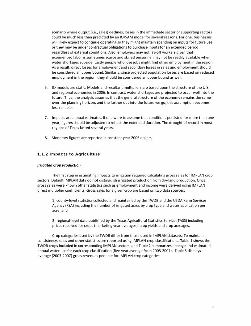
scenario where output (i.e., sales) declines, losses in the immediate sector or supporting sectors could be much less than predicted by an IO/SAM model for several reasons. For one, businesses will likely expect to continue operating so they might maintain spending on inputs for future use; or they may be under contractual obligations to purchase inputs for an extended period regardless of external conditions. Also, employers may not lay‐off workers given that experienced labor is sometimes scarce and skilled personnel may not be readily available when water shortages subside. Lastly people who lose jobs might find other employment in the region. As a result, direct losses for employment and secondary losses in sales and employment should be considered an upper bound. Similarly, since projected population losses are based on reduced employment in the region, they should be considered an upper bound as well.
6. IO models are static. Models and resultant multipliers are based upon the structure of the U.S.
and regional economies in 2006. In contrast, water shortages are projected to occur well into the future. Thus, the analysis assumes that the general structure of the economy remains the same over the planning horizon, and the farther out into the future we go, this assumption becomes less reliable.
7. Impacts are annual estimates. If one were to assume that conditions persisted for more than one
year, figures should be adjusted to reflect the extended duration. The drought of record in most regions of Texas lasted several years.
8. Monetary figures are reported in constant year 2006 dollars.
1.1.2 Impacts to Agriculture Irrigated Crop Production
The first step in estimating impacts to irrigation required calculating gross sales for IMPLAN crop sectors. Default IMPLAN data do not distinguish irrigated production from dry‐land production. Once gross sales were known other statistics such as employment and income were derived using IMPLAN direct multiplier coefficients. Gross sales for a given crop are based on two data sources:
1) county‐level statistics collected and maintained by the TWDB and the USDA Farm Services Agency (FSA) including the number of irrigated acres by crop type and water application per acre, and 2) regional‐level data published by the Texas Agricultural Statistics Service (TASS) including prices received for crops (marketing year averages), crop yields and crop acreages. Crop categories used by the TWDB differ from those used in IMPLAN datasets. To maintain
consistency, sales and other statistics are reported using IMPLAN crop classifications. Table 1 shows the TWDB crops included in corresponding IMPLAN sectors, and Table 2 summarizes acreage and estimated annual water use for each crop classification (five‐year average from 2003‐2007). Table 3 displays average (2003‐2007) gross revenues per acre for IMPLAN crop categories.
9
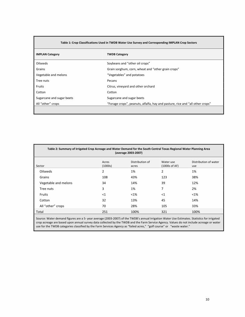
Table 1: Crop Classifications Used in TWDB Water Use Survey and Corresponding IMPLAN Crop Sectors
IMPLAN Category TWDB Category
Oilseeds Soybeans and “other oil crops”
Grains Grain sorghum, corn, wheat and “other grain crops”
Vegetable and melons “Vegetables” and potatoes
Tree nuts Pecans
Fruits Citrus, vineyard and other orchard
Cotton Cotton
Sugarcane and sugar beets Sugarcane and sugar beets
All “other” crops “Forage crops”, peanuts, alfalfa, hay and pasture, rice and “all other crops”
Table 2: Summary of Irrigated Crop Acreage and Water Demand for the South Central Texas Regional Water Planning Area (average 2003‐2007)
Sector Acres (1000s)
Distribution of acres
Water use (1000s of AF)
Distribution of water use
Oilseeds 2 1% 2 1%
Grains 108 43% 123 38%
Vegetable and melons 34 14% 39 12%
Tree nuts 3 1% 7 2%
Fruits <1 <1% <1 <1%
Cotton 32 13% 45 14%
All “other” crops 70 28% 105 33%
Total 251 100% 321 100%
Source: Water demand figures are a 5‐ year average (2003‐2007) of the TWDB’s annual Irrigation Water Use Estimates. Statistics for irrigated crop acreage are based upon annual survey data collected by the TWDB and the Farm Service Agency. Values do not include acreage or water use for the TWDB categories classified by the Farm Services Agency as “failed acres,” “golf course” or “waste water.”
10
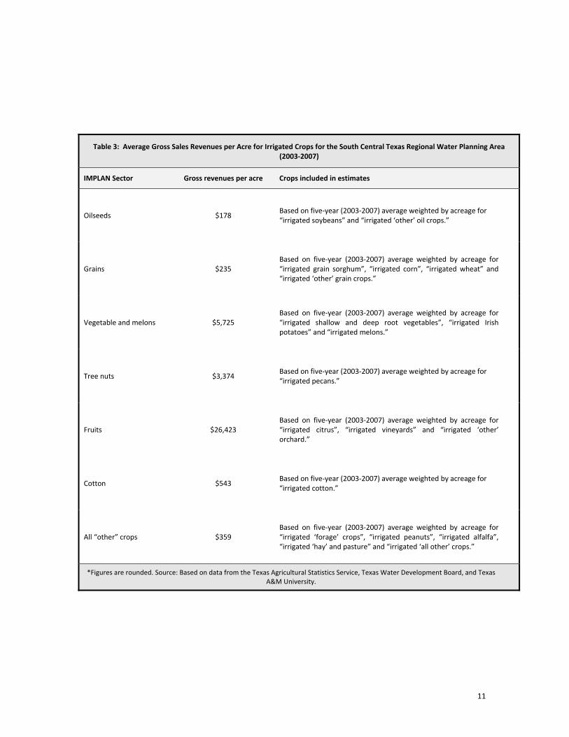
Table 3: Average Gross Sales Revenues per Acre for Irrigated Crops for the South Central Texas Regional Water Planning Area (2003‐2007)
IMPLAN Sector Gross revenues per acre Crops included in estimates
Oilseeds $178 Based on five‐year (2003‐2007) average weighted by acreage for “irrigated soybeans” and “irrigated ‘other’ oil crops.”
Grains $235 Based on five‐year (2003‐2007) average weighted by acreage for “irrigated grain sorghum”, “irrigated corn”, “irrigated wheat” and “irrigated ‘other’ grain crops.”
Vegetable and melons $5,725 Based on five‐year (2003‐2007) average weighted by acreage for “irrigated shallow and deep root vegetables”, “irrigated Irish potatoes” and “irrigated melons.”
Tree nuts $3,374 Based on five‐year (2003‐2007) average weighted by acreage for “irrigated pecans.”
Fruits $26,423 Based on five‐year (2003‐2007) average weighted by acreage for “irrigated citrus”, “irrigated vineyards” and “irrigated ‘other’ orchard.”
Cotton $543 Based on five‐year (2003‐2007) average weighted by acreage for “irrigated cotton.”
All “other” crops $359 Based on five‐year (2003‐2007) average weighted by acreage for “irrigated ‘forage’ crops”, “irrigated peanuts”, “irrigated alfalfa”, “irrigated ‘hay’ and pasture” and “irrigated ‘all other’ crops.”
*Figures are rounded. Source: Based on data from the Texas Agricultural Statistics Service, Texas Water Development Board, and Texas A&M University.
11

An important consideration when estimating impacts to irrigation was determining which crops are affected by water shortages. One approach is the so‐called rationing model, which assumes that farmers respond to water supply cutbacks by fallowing the lowest value crops in the region first and the highest valued crops last until the amount of water saved equals the shortage.5 For example, if farmer A grows vegetables (higher value) and farmer B grows wheat (lower value) and they both face a proportionate cutback in irrigation water, then farmer B will sell water to farmer A. Farmer B will fallow her irrigated acreage before farmer A fallows anything. Of course, this assumes that farmers can and do transfer enough water to allow this to happen. A different approach involves constructing farm‐level profit maximization models that conform to widely‐accepted economic theory that farmers make decisions based on marginal net returns. Such models have good predictive capability, but data requirements and complexity are high. Given that a detailed analysis for each region would require a substantial amount of farm‐level data and analysis, the following investigation assumes that projected shortages are distributed equally across predominant crops in the region. Predominant in this case are crops that comprise at least one percent of total acreage in the region.
The following steps outline the overall process used to estimate direct impacts to irrigated
agriculture:
1. Distribute shortages across predominant crop types in the region. Again, unmet water needs were distributed equally across crop sectors that constitute one percent or more of irrigated acreage.
2. Estimate associated reductions in output for affected crop sectors. Output reductions are based
on elasticities discussed previously and on estimated values per acre for different crops. Values per acre stem from the same data used to estimate output for the year 2006 baseline. Using multipliers, we then generate estimates of forgone income, jobs, and tax revenues based on reductions in gross sales and final demand.
Livestock
The approach used for the livestock sector is basically the same as that used for crop production. As is the case with crops, livestock categorizations used by the TWDB differ from those used in IMPLAN datasets, and TWDB groupings were assigned to a given IMPLAN sector (Table 4). Then we:
1) Distribute projected water needs equally among predominant livestock sectors and estimate lost output: As is the case with irrigation, shortages are assumed to affect all livestock sectors equally; however, the category of “other” is not included given its small size. If water needs were small relative to total demands, we assume that producers would haul in water by truck to fill stock tanks. The cost per acre‐foot ($24,000) is based on 2008 rates charged by various water haulers in Texas, and assumes that the average truck load is 6,500 gallons at a hauling distance of 60 miles. 3) Estimate reduced output in forward processors for livestock sectors. Reductions in output for livestock sectors are assumed to have a proportional impact on forward processors in the region such as meat packers. In other words, if the cows were gone, meat‐packing plants or fluid milk manufacturers) would likely have little to process. This is not an unreasonable premise. Since the
5 The rationing model was initially proposed by researchers at the University of California at Berkeley, and was then modified for use in a study conducted by the U.S. Environmental Protection Agency that evaluated how proposed water supply cutbacks recommended to protect water quality in the Bay/Delta complex in California would affect farmers in the Central Valley. See, Zilberman, D., Howitt, R. and Sunding, D. “Economic Impacts of Water Quality Regulations in the San Francisco Bay and Delta.” Western Consortium for Public Health. May 1993.
12
1950s, there has been a major trend towards specialized cattle feedlots, which in turn has decentralized cattle purchasing from livestock terminal markets to direct sales between producers and slaughterhouses. Today, the meat packing industry often operates large processing facilities near high concentrations of feedlots to increase capacity utilization.6 As a result, packers are heavily dependent upon nearby feedlots. For example, a recent study by the USDA shows that on average meat packers obtain 64 percent of cattle from within 75 miles of their plant, 82 percent from within 150 miles and 92 percent from within 250 miles.7
Table 4: Description of Livestock Sectors
IMPLAN Category TWDB Category
Cattle ranching and farming Cattle, cow calf, feedlots and dairies
Poultry and egg production Poultry production.
Other livestock Livestock other than cattle and poultry (i.e., horses, goats, sheep, hogs )
Milk manufacturing Fluid milk manufacturing, cheese manufacturing, ice cream manufacturing etc.
Meat packing Meat processing present in the region from slaughter to final processing
1.1.3 Impacts to Municipal Water User Groups Disaggregation of Municipal Water Demands
Estimating the economic impacts for the municipal water user groups is complicated for a number of reasons. For one, municipal use comprises a range of consumers including commercial businesses, institutions such as schools and government and households. However, reported water needs are not distributed among different municipal water users. In other words, how much of a municipal need is commercial and how much is residential (domestic)?
The amount of commercial water use as a percentage of total municipal demand was estimated
based on “GED” coefficients (gallons per employee per day) published in secondary sources.8 For example, if year 2006 baseline data for a given economic sector (e.g., amusement and recreation serviceshows employment at 30 jobs and the GED coefficient is 200, then average daily water use by that sector
s)
6 Ferreira, W.N. “Analysis of the Meat Processing Industry in the United States.” Clemson University Extension Economics Report ER211, January 2003. 7 Ward, C.E. “Summary of Results from USDA’s Meatpacking Concentration Study.” Oklahoma Cooperative Extension Service, OSU Extension Facts WF‐562. 8 Sources for GED coefficients include: Gleick, P.H., Haasz, D., Henges‐Jeck, C., Srinivasan, V., Wolff, G. Cushing, K.K., and Mann, A. "Waste Not, Want Not: The Potential for Urban Water Conservation in California." Pacific Institute. November 2003. U.S. Bureau of the Census. 1982 Census of Manufacturers: Water Use in Manufacturing. USGPO, Washington D.C. See also: “U.S. Army Engineer Institute for Water Resources, IWR Report 88‐R‐6.,” Fort Belvoir, VA. See also, Joseph, E. S., 1982, "Municipal and Industrial Water Demands of the Western United States." Journal of the Water Resources Planning and Management Division, Proceedings of the American Society of Civil Engineers, v. 108, no. WR2, p. 204‐216. See also, Baumann, D. D., Boland, J. J., and Sims, J. H., 1981, “Evaluation of Water Conservation for Municipal and Industrial Water Supply.” U.S. Army Corps of Engineers, Institute for Water Resources, Contract no. 82‐C1.
13
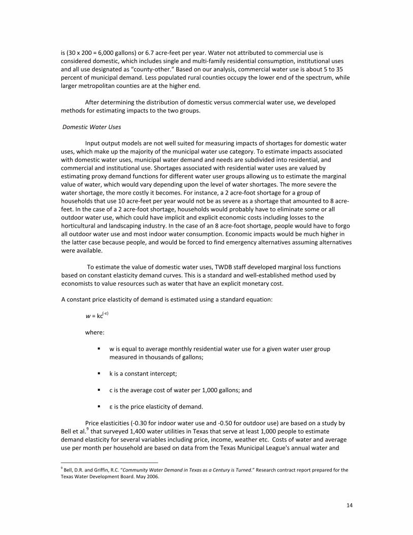
is (30 x 200 = 6,000 gallons) or 6.7 acre‐feet per year. Water not attributed to commercial use is considered domestic, which includes single and multi‐family residential consumption, institutional uses and all use designated as “county‐other.” Based on our analysis, commercial water use is about 5 to 35 percent of municipal demand. Less populated rural counties occupy the lower end of the spectrum, whlarger metropolitan counties are at the higher
ile end.
After determining the distribution of domestic versus commercial water use, we developed
methods for estimating impacts to the two groups. Domestic Water Uses
Input output models are not well suited for measuring impacts of shortages for domestic water
uses, which make up the majority of the municipal water use category. To estimate impacts associated with domestic water uses, municipal water demand and needs are subdivided into residential, and commercial and institutional use. Shortages associated with residential water uses are valued by estimating proxy demand functions for different water user groups allowing us to estimate the marginal value of water, which would vary depending upon the level of water shortages. The more severe the water shortage, the more costly it becomes. For instance, a 2 acre‐foot shortage for a group of households that use 10 acre‐feet per year would not be as severe as a shortage that amounted to 8 acre‐feet. In the case of a 2 acre‐foot shortage, households would probably have to eliminate some or all outdoor water use, which could have implicit and explicit economic costs including losses to the horticultural and landscaping industry. In the case of an 8 acre‐foot shortage, people would have to forgo all outdoor water use and most indoor water consumption. Economic impacts would be much higher in the latter case because people, and would be forced to find emergency alternatives assuming alternatives were available.
To estimate the value of domestic water uses, TWDB staff developed marginal loss functions
based on constant elasticity demand curves. This is a standard and well‐established method used by economists to value resources such as water that have an explicit monetary cost.
A constant price elasticity of demand is estimated using a standard equation:
w = kc(‐ε)
where:
w is equal to average monthly residential water use for a given water user group measured in thousands of gallons;
k is a constant intercept;
c is the average cost of water per 1,000 gallons; and
ε is the price elasticity of demand.
Price elasticities (‐0.30 for indoor water use and ‐0.50 for outdoor use) are based on a study by
Bell et al.9 that surveyed 1,400 water utilities in Texas that serve at least 1,000 people to estimate demand elasticity for several variables including price, income, weather etc. Costs of water and average use per month per household are based on data from the Texas Municipal League's annual water and
9 Bell, D.R. and Griffin, R.C. “Community Water Demand in Texas as a Century is Turned.” Research contract report prepared for the Texas Water Development Board. May 2006.
14
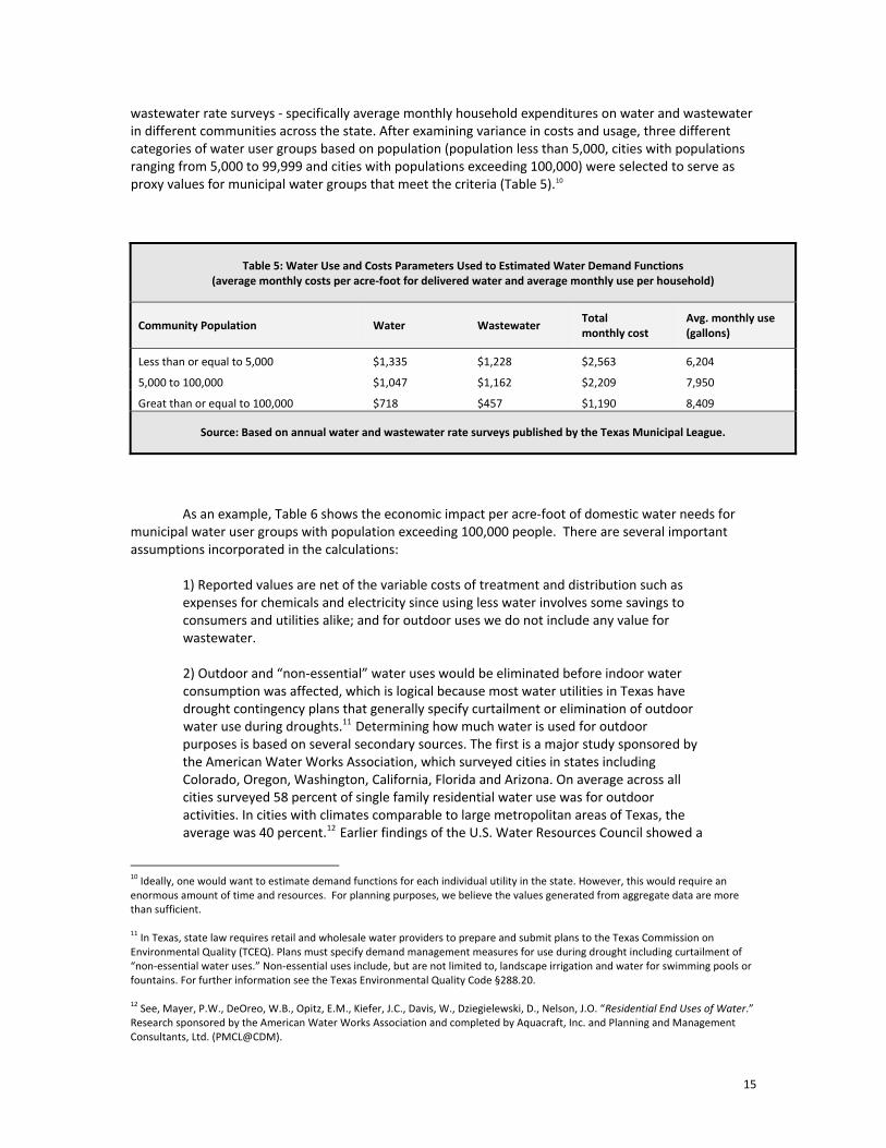
wastewater rate surveys ‐ specifically average monthly household expenditures on water and wastewater in different communities across the state. After examining variance in costs and usage, three different categories of water user groups based on population (population less than 5,000, cities with populations ranging from 5,000 to 99,999 and cities with populations exceeding 100,000) were selected to serve as proxy values for municipal water groups that meet the criteria (Table 5).10
Table 5: Water Use and Costs Parameters Used to Estimated Water Demand Functions (average monthly costs per acre‐foot for delivered water and average monthly use per household)
Community Population Water Wastewater Total monthly cost
Avg. monthly use (gallons)
Less than or equal to 5,000 $1,335 $1,228 $2,563 6,204
5,000 to 100,000 $1,047 $1,162 $2,209 7,950
Great than or equal to 100,000 $718 $457 $1,190 8,409
Source: Based on annual water and wastewater rate surveys published by the Texas Municipal League.
As an example, Table 6 shows the economic impact per acre‐foot of domestic water needs for municipal water user groups with population exceeding 100,000 people. There are several important assumptions incorporated in the calculations:
1) Reported values are net of the variable costs of treatment and distribution such as expenses for chemicals and electricity since using less water involves some savings to consumers and utilities alike; and for outdoor uses we do not include any value for wastewater. 2) Outdoor and “non‐essential” water uses would be eliminated before indoor water consumption was affected, which is logical because most water utilities in Texas have drought contingency plans that generally specify curtailment or elimination of outdoor water use during droughts.11 Determining how much water is used for outdoor purposes is based on several secondary sources. The first is a major study sponsorethe American Water Works Association, which surveyed cities in states including Colorado, Oregon, Washington, California, Florida and Arizona. On average acrosscities surveyed 58 percent of single family residential water use was for outdoor activities. In cities with climates comparable to large metropolitan areas of Texas, the average was 40 percent.
d by
all
d a
12 Earlier findings of the U.S. Water Resources Council showe
10 Ideally, one would want to estimate demand functions for each individual utility in the state. However, this would require an enormous amount of time and resources. For planning purposes, we believe the values generated from aggregate data are more than sufficient. 11 In Texas, state law requires retail and wholesale water providers to prepare and submit plans to the Texas Commission on Environmental Quality (TCEQ). Plans must specify demand management measures for use during drought including curtailment of “non‐essential water uses.” Non‐essential uses include, but are not limited to, landscape irrigation and water for swimming pools or fountains. For further information see the Texas Environmental Quality Code §288.20. 12 See, Mayer, P.W., DeOreo, W.B., Opitz, E.M., Kiefer, J.C., Davis, W., Dziegielewski, D., Nelson, J.O. “Residential End Uses of Water.” Research sponsored by the American Water Works Association and completed by Aquacraft, Inc. and Planning and Management Consultants, Ltd. (PMCL@CDM).
15
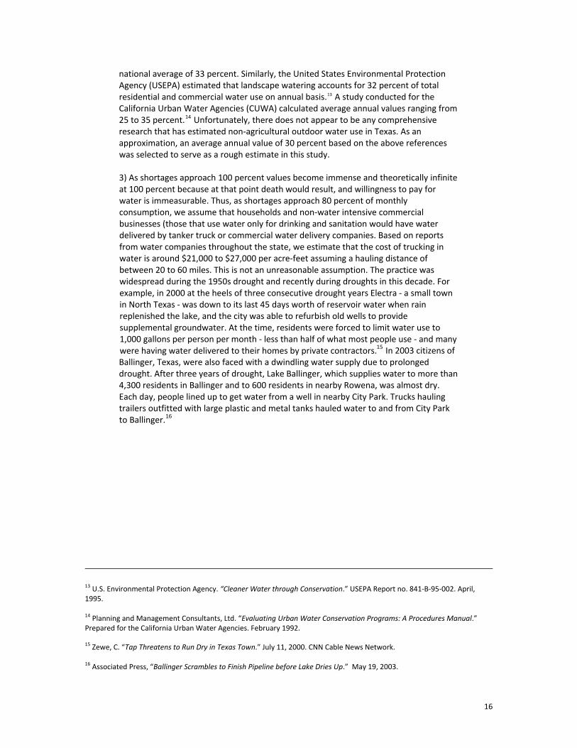
national average of 33 percent. Similarly, the United States Environmental ProtectionAgency (USEPA) estimated that landscape watering accounts for 32 percent of total residential and commercial water use on annual basis.
g from
s e in this study.
13 A study conducted for the California Urban Water Agencies (CUWA) calculated average annual values rangin25 to 35 percent.14 Unfortunately, there does not appear to be any comprehensive research that has estimated non‐agricultural outdoor water use in Texas. As an approximation, an average annual value of 30 percent based on the above referencewas selected to serve as a rough estimat 3) As shortages approach 100 percent values become immense and theoretically infinite at 100 percent because at that point death would result, and willingness to pay for water is immeasurable. Thus, as shortages approach 80 percent of monthly consumption, we assume that households and non‐water intensive commercial businesses (those that use water only for drinking and sanitation would have water delivered by tanker truck or commercial water delivery companies. Based on reports from water companies throughout the state, we estimate that the cost of trucking in water is around $21,000 to $27,000 per acre‐feet assuming a hauling distance of between 20 to 60 miles. This is not an unreasonable assumption. The practice was widespread during the 1950s drought and recently during droughts in this decade. For example, in 2000 at the heels of three consecutive drought years Electra ‐ a small town in North Texas ‐ was down to its last 45 days worth of reservoir water when rain replenished the lake, and the city was able to refurbish old wells to provide supplemental groundwater. At the time, residents were forced to limit water use to 1,000 gallons per person per month ‐ less than half of what most people use ‐ and many were having water delivered to their homes by private contractors.15 In 2003 citizens of Ballinger, Texas, were also faced with a dwindling water supply due to prolonged drought. After three years of drought, Lake Ballinger, which supplies water to more than 4,300 residents in Ballinger and to 600 residents in nearby Rowena, was almost dry. Each day, people lined up to get water from a well in nearby City Park. Trucks hauling trailers outfitted with large plastic and metal tanks hauled water to and from City Park to Ballinger.16
13 U.S. Environmental Protection Agency. “Cleaner Water through Conservation.” USEPA Report no. 841‐B‐95‐002. April, 1995. 14 Planning and Management Consultants, Ltd. “Evaluating Urban Water Conservation Programs: A Procedures Manual.” Prepared for the California Urban Water Agencies. February 1992. 15 Zewe, C. “Tap Threatens to Run Dry in Texas Town.” July 11, 2000. CNN Cable News Network. 16 Associated Press, “Ballinger Scrambles to Finish Pipeline before Lake Dries Up.” May 19, 2003.
16

Table 6: Economic Losses Associated with Domestic Water Shortages in Communities with Populations Exceeding 100,000 people
Water shortages as a percentage of total monthly household demands
No. of gallons remaining per household per day
No of gallons remaining per person per day
Economic loss (per acre‐foot)
Economic loss (per gallon)
1% 278 93 $748 $0.00005
5% 266 89 $812 $0.0002
10% 252 84 $900 $0.0005
15% 238 79 $999 $0.0008
20% 224 75 $1,110 $0.0012
25% 210 70 $1,235 $0.0015
30%a 196 65 $1,699 $0.0020
35% 182 61 $3,825 $0.0085
40% 168 56 $4,181 $0.0096
45% 154 51 $4,603 $0.011
50% 140 47 $5,109 $0.012
55% 126 42 $5,727 $0.014
60% 112 37 $6,500 $0.017
65% 98 33 $7,493 $0.02
70% 84 28 $8,818 $0.02
75% 70 23 $10,672 $0.03
80% 56 19 $13,454 $0.04
85% 42 14 $18,091 ($24,000)b $0.05 ($0.07) b
90% 28 9 $27,363 ($24,000) $0.08 ($0.07)
95% 14 5 $55,182 ($24,000) $0.17 ($0.07)
99% 3 0.9 $277,728 ($24,000) $0.85 ($0.07)
99.9% 1 0.5 $2,781,377 ($24,000) $8.53 ($0.07)
100% 0 0 Infinite ($24,000) Infinite ($0.07) a The first 30 percent of needs are assumed to be restrictions of outdoor water use; when needs reach 30 percent of total demands all outdoor water uses would be restricted. Needs greater than 30 percent include indoor use b As shortages approach 100 percent the value approaches infinity assuming there are not alternatives available; however, we assume that communities would begin to have water delivered by tanker truck at an estimated cost of $24,000 per acre‐foot when shortages breached 85 percent.
17
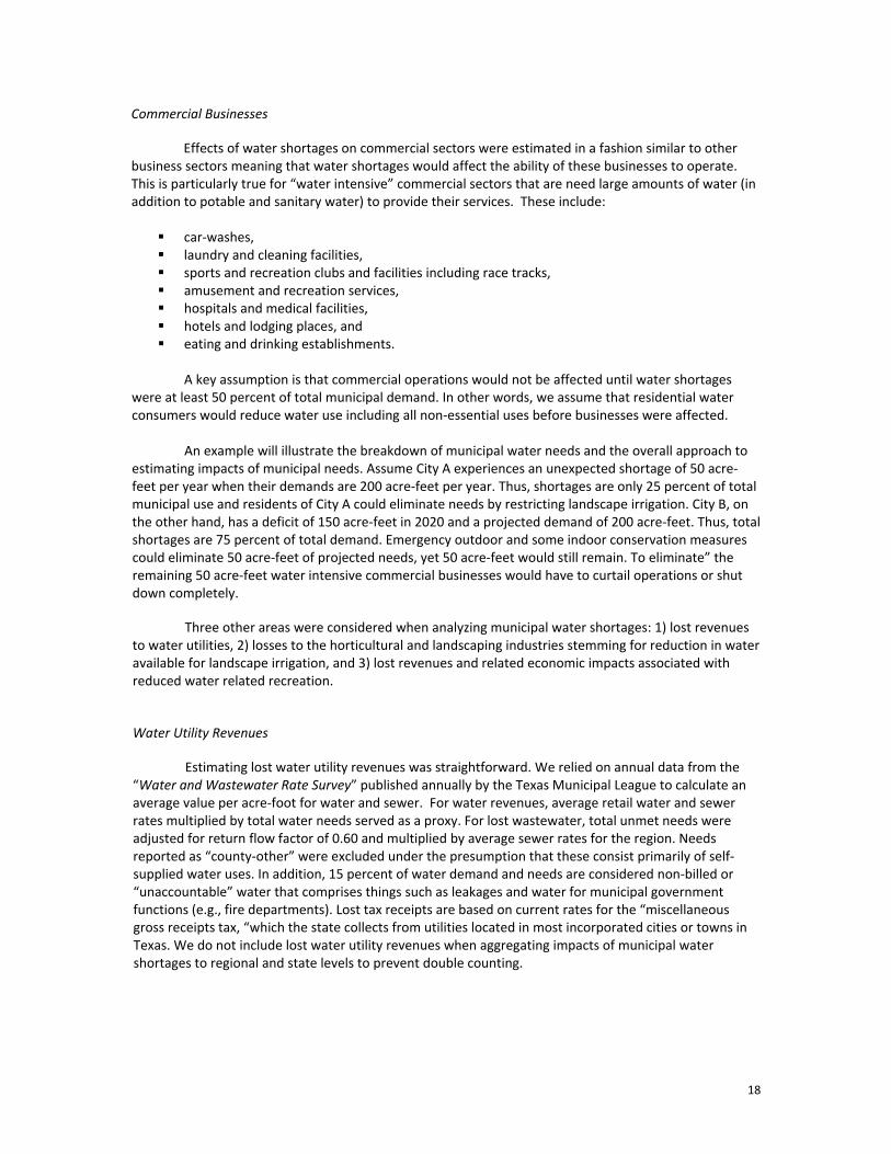
Commercial Businesses
Effects of water shortages on commercial sectors were estimated in a fashion similar to other business sectors meaning that water shortages would affect the ability of these businesses to operate. This is particularly true for “water intensive” commercial sectors that are need large amounts of water (in addition to potable and sanitary water) to provide their services. These include:
car‐washes, laundry and cleaning facilities, sports and recreation clubs and facilities including race tracks, amusement and recreation services, hospitals and medical facilities, hotels and lodging places, and eating and drinking establishments.
A key assumption is that commercial operations would not be affected until water shortages
were at least 50 percent of total municipal demand. In other words, we assume that residential water consumers would reduce water use including all non‐essential uses before businesses were affected.
An example will illustrate the breakdown of municipal water needs and the overall approach to estimating impacts of municipal needs. Assume City A experiences an unexpected shortage of 50 acre‐feet per year when their demands are 200 acre‐feet per year. Thus, shortages are only 25 percent of total municipal use and residents of City A could eliminate needs by restricting landscape irrigation. City B, on the other hand, has a deficit of 150 acre‐feet in 2020 and a projected demand of 200 acre‐feet. Thus, total shortages are 75 percent of total demand. Emergency outdoor and some indoor conservation measures could eliminate 50 acre‐feet of projected needs, yet 50 acre‐feet would still remain. To eliminate” the remaining 50 acre‐feet water intensive commercial businesses would have to curtail operations or shut down completely.
Three other areas were considered when analyzing municipal water shortages: 1) lost revenues to water utilities, 2) losses to the horticultural and landscaping industries stemming for reduction in water available for landscape irrigation, and 3) lost revenues and related economic impacts associated with reduced water related recreation. Water Utility Revenues
Estimating lost water utility revenues was straightforward. We relied on annual data from the “Water and Wastewater Rate Survey” published annually by the Texas Municipal League to calculate an average value per acre‐foot for water and sewer. For water revenues, average retail water and sewer rates multiplied by total water needs served as a proxy. For lost wastewater, total unmet needs were adjusted for return flow factor of 0.60 and multiplied by average sewer rates for the region. Needs reported as “county‐other” were excluded under the presumption that these consist primarily of self‐supplied water uses. In addition, 15 percent of water demand and needs are considered non‐billed or “unaccountable” water that comprises things such as leakages and water for municipal government functions (e.g., fire departments). Lost tax receipts are based on current rates for the “miscellaneous gross receipts tax, “which the state collects from utilities located in most incorporated cities or towns in Texas. We do not include lost water utility revenues when aggregating impacts of municipal water shortages to regional and state levels to prevent double counting.
18
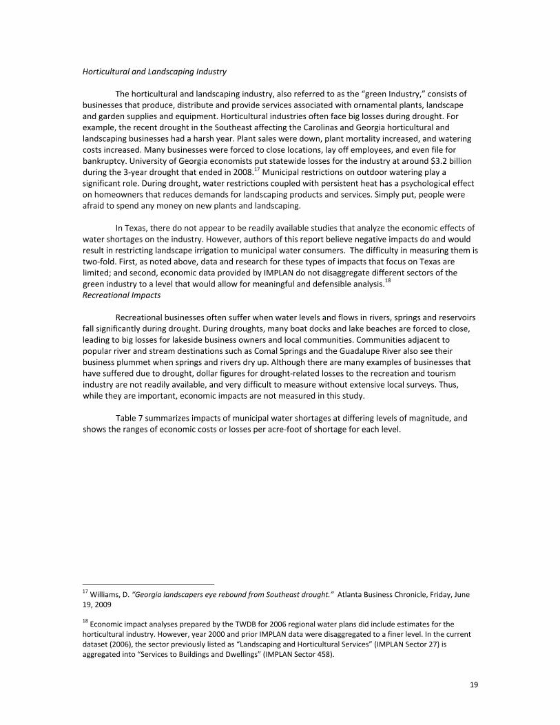
Horticultural and Landscaping Industry
The horticultural and landscaping industry, also referred to as the “green Industry,” consists of businesses that produce, distribute and provide services associated with ornamental plants, landscape and garden supplies and equipment. Horticultural industries often face big losses during drought. For example, the recent drought in the Southeast affecting the Carolinas and Georgia horticultural and landscaping businesses had a harsh year. Plant sales were down, plant mortality increased, and watering costs increased. Many businesses were forced to close locations, lay off employees, and even file for bankruptcy. University of Georgia economists put statewide losses for the industry at around $3.2 billion during the 3‐year drought that ended in 2008.17 Municipal restrictions on outdoor watering play a significant role. During drought, water restrictions coupled with persistent heat has a psychological effect on homeowners that reduces demands for landscaping products and services. Simply put, people were afraid to spend any money on new plants and landscaping.
In Texas, there do not appear to be readily available studies that analyze the economic effects of
water shortages on the industry. However, authors of this report believe negative impacts do and would result in restricting landscape irrigation to municipal water consumers. The difficulty in measuring them is two‐fold. First, as noted above, data and research for these types of impacts that focus on Texas are limited; and second, economic data provided by IMPLAN do not disaggregate different sectors of the green industry to a level that would allow for meaningful and defensible analysis.18 Recreational Impacts
Recreational businesses often suffer when water levels and flows in rivers, springs and reservoirs fall significantly during drought. During droughts, many boat docks and lake beaches are forced to close, leading to big losses for lakeside business owners and local communities. Communities adjacent to popular river and stream destinations such as Comal Springs and the Guadalupe River also see their business plummet when springs and rivers dry up. Although there are many examples of businesses that have suffered due to drought, dollar figures for drought‐related losses to the recreation and tourism industry are not readily available, and very difficult to measure without extensive local surveys. Thus, while they are important, economic impacts are not measured in this study.
Table 7 summarizes impacts of municipal water shortages at differing levels of magnitude, and shows the ranges of economic costs or losses per acre‐foot of shortage for each level.
17 Williams, D. “Georgia landscapers eye rebound from Southeast drought.” Atlanta Business Chronicle, Friday, June 19, 2009 18 Economic impact analyses prepared by the TWDB for 2006 regional water plans did include estimates for the horticultural industry. However, year 2000 and prior IMPLAN data were disaggregated to a finer level. In the current dataset (2006), the sector previously listed as “Landscaping and Horticultural Services” (IMPLAN Sector 27) is aggregated into “Services to Buildings and Dwellings” (IMPLAN Sector 458).
19
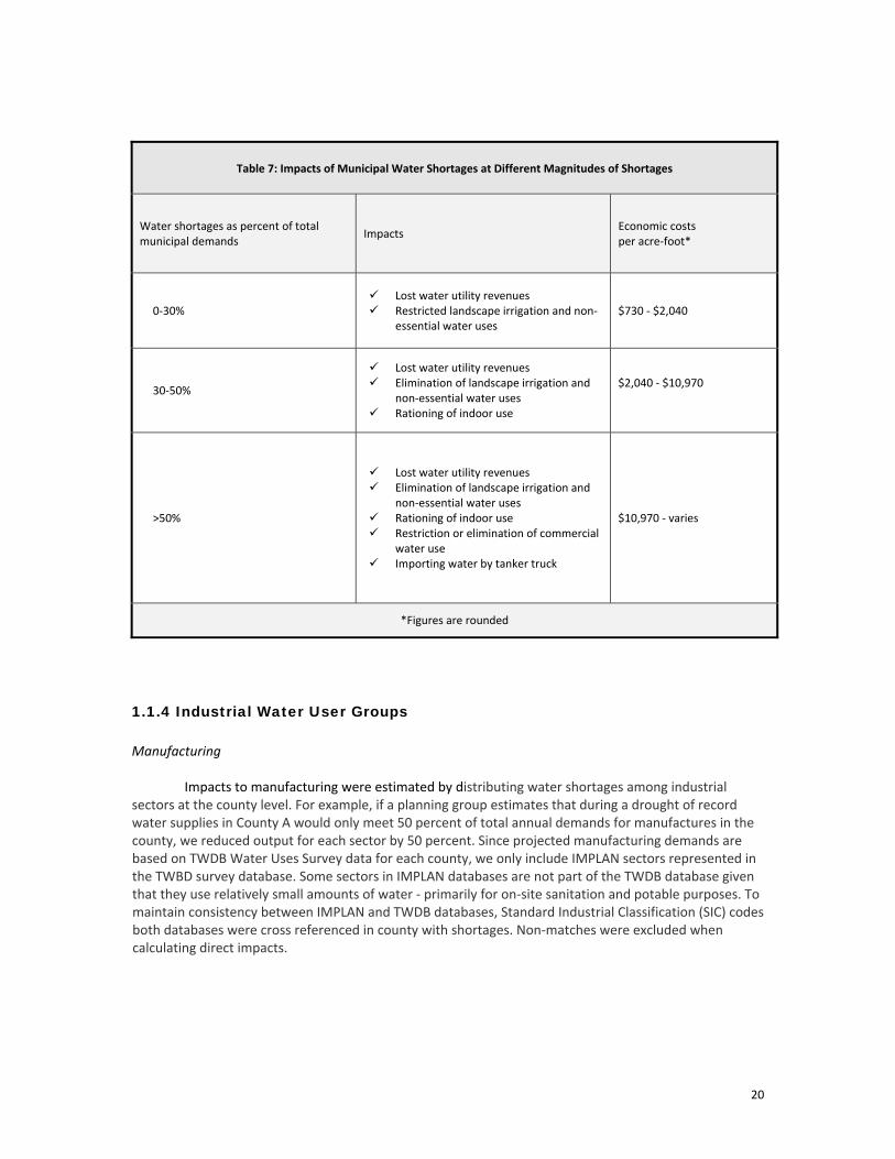
Table 7: Impacts of Municipal Water Shortages at Different Magnitudes of Shortages
Water shortages as percent of total municipal demands
Impacts Economic costs per acre‐foot*
0‐30% Lost water utility revenues Restricted landscape irrigation and non‐
essential water uses $730 ‐ $2,040
30‐50%
Lost water utility revenues Elimination of landscape irrigation and
non‐essential water uses Rationing of indoor use
$2,040 ‐ $10,970
>50%
Lost water utility revenues Elimination of landscape irrigation and
non‐essential water uses Rationing of indoor use Restriction or elimination of commercial
water use Importing water by tanker truck
$10,970 ‐ varies
*Figures are rounded
1.1.4 Industrial Water User Groups Manufacturing
Impacts to manufacturing were estimated by distributing water shortages among industrial sectors at the county level. For example, if a planning group estimates that during a drought of record water supplies in County A would only meet 50 percent of total annual demands for manufactures in the county, we reduced output for each sector by 50 percent. Since projected manufacturing demands are based on TWDB Water Uses Survey data for each county, we only include IMPLAN sectors represented in the TWBD survey database. Some sectors in IMPLAN databases are not part of the TWDB database given that they use relatively small amounts of water ‐ primarily for on‐site sanitation and potable purposes. To maintain consistency between IMPLAN and TWDB databases, Standard Industrial Classification (SIC) codes both databases were cross referenced in county with shortages. Non‐matches were excluded when calculating direct impacts.
20
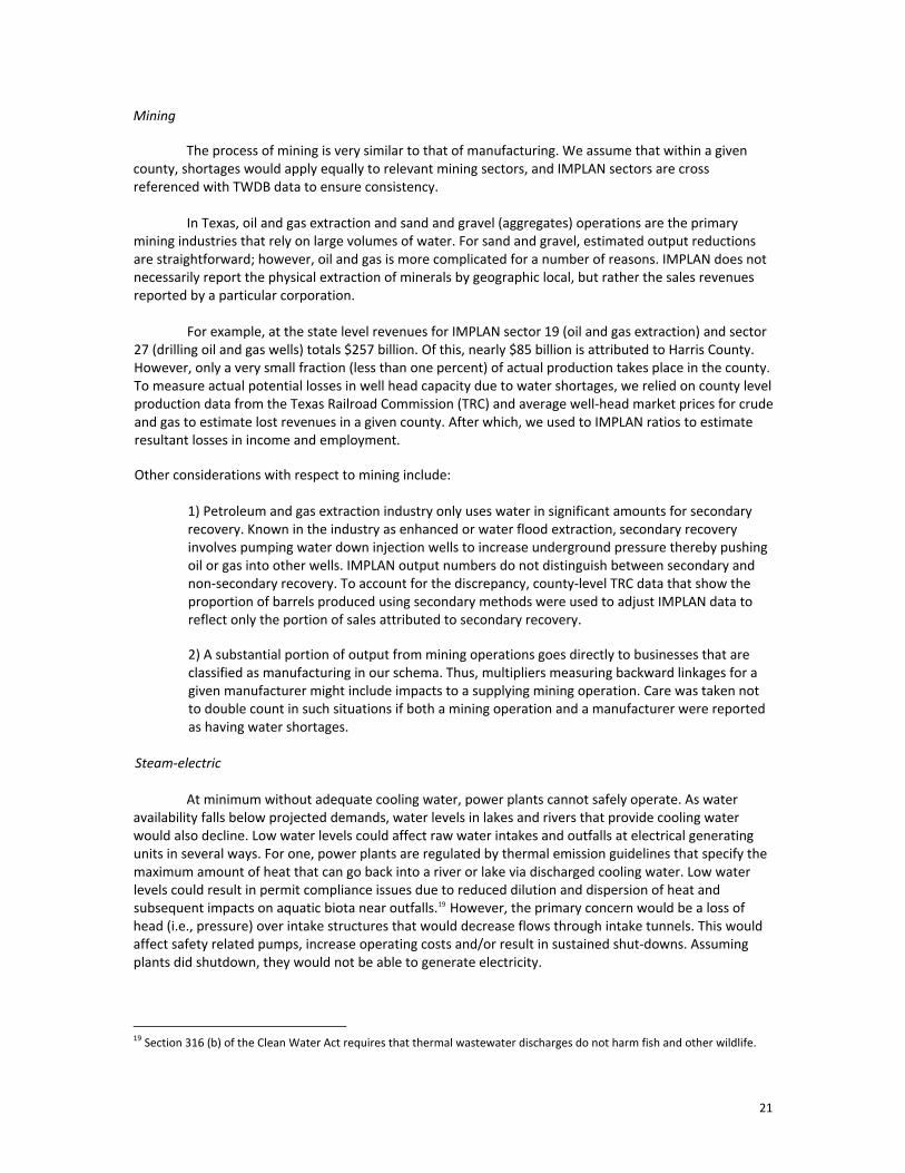
Mining
The process of mining is very similar to that of manufacturing. We assume that within a given county, shortages would apply equally to relevant mining sectors, and IMPLAN sectors are cross referenced with TWDB data to ensure consistency.
In Texas, oil and gas extraction and sand and gravel (aggregates) operations are the primary
mining industries that rely on large volumes of water. For sand and gravel, estimated output reductions are straightforward; however, oil and gas is more complicated for a number of reasons. IMPLAN does not necessarily report the physical extraction of minerals by geographic local, but rather the sales revenues reported by a particular corporation.
For example, at the state level revenues for IMPLAN sector 19 (oil and gas extraction) and sector
27 (drilling oil and gas wells) totals $257 billion. Of this, nearly $85 billion is attributed to Harris County. However, only a very small fraction (less than one percent) of actual production takes place in the county. To measure actual potential losses in well head capacity due to water shortages, we relied on county level production data from the Texas Railroad Commission (TRC) and average well‐head market prices for crude and gas to estimate lost revenues in a given county. After which, we used to IMPLAN ratios to estimate resultant losses in income and employment. Other considerations with respect to mining include:
1) Petroleum and gas extraction industry only uses water in significant amounts for secondary recovery. Known in the industry as enhanced or water flood extraction, secondary recovery involves pumping water down injection wells to increase underground pressure thereby pushing oil or gas into other wells. IMPLAN output numbers do not distinguish between secondary and non‐secondary recovery. To account for the discrepancy, county‐level TRC data that show the proportion of barrels produced using secondary methods were used to adjust IMPLAN data to reflect only the portion of sales attributed to secondary recovery.
2) A substantial portion of output from mining operations goes directly to businesses that are classified as manufacturing in our schema. Thus, multipliers measuring backward linkages for a given manufacturer might include impacts to a supplying mining operation. Care was taken not to double count in such situations if both a mining operation and a manufacturer were reported as having water shortages.
Steam‐electric
At minimum without adequate cooling water, power plants cannot safely operate. As water availability falls below projected demands, water levels in lakes and rivers that provide cooling water would also decline. Low water levels could affect raw water intakes and outfalls at electrical generating units in several ways. For one, power plants are regulated by thermal emission guidelines that specify the maximum amount of heat that can go back into a river or lake via discharged cooling water. Low water levels could result in permit compliance issues due to reduced dilution and dispersion of heat and subsequent impacts on aquatic biota near outfalls.19 However, the primary concern would be a loss of head (i.e., pressure) over intake structures that would decrease flows through intake tunnels. This would affect safety related pumps, increase operating costs and/or result in sustained shut‐downs. Assuming plants did shutdown, they would not be able to generate electricity.
19 Section 316 (b) of the Clean Water Act requires that thermal wastewater discharges do not harm fish and other wildlife.
21

Among all water use categories steam‐electric is unique and cautions are needed when applying methods used in this study. Measured changes to an economy using input‐output models stem directly from changes in sales revenues. In the case of water shortages, one assumes that businesses will suffer lost output if process water is in short supply. For power generation facilities this is true as well. However, the electric services sector in IMPLAN represents a corporate entity that may own and operate several electrical generating units in a given region. If one unit became inoperable due to water shortages, plants in other areas or generation facilities that do not rely heavily on water such as gas powered turbines might be able to compensate for lost generating capacity. Utilities could also offset lost production via purchases on the spot market.20 Thus, depending upon the severity of the shortages and conditions at a given electrical generating unit, energy supplies for local and regional communities could be maintained. But in general, without enough cooling water, utilities would have to throttle back plant operations, forcing them to buy or generate more costly power to meet customer demands.
Measuring impacts end users of electricity is not part of this study as it would require extensive local and regional level analysis of energy production and demand. To maintain consistency with other water user groups, impacts of steam‐electric water shortages are measured in terms of lost revenues (and hence income) and jobs associated with shutting down electrical generating units.
1.2 Social Impacts of Water Shortages
As the name implies, the effects of water shortages can be social or economic. Distinctions between the two are both semantic and analytical in nature – more so analytic in the sense that social impacts are harder to quantify. Nevertheless, social effects associated with drought and water shortages are closely tied to economic impacts. For example, they might include:
demographic effects such as changes in population,
disruptions in institutional settings including activity in schools and government,
conflicts between water users such as farmers and urban consumers,
health‐related low‐flow problems (e.g., cross‐connection contamination, diminished sewage flows, increased pollutant concentrations),
mental and physical stress (e.g., anxiety, depression, domestic violence),
public safety issues from forest and range fires and reduced fire fighting capability,
increased disease caused by wildlife concentrations,
loss of aesthetic and property values, and
reduced recreational opportunities.21
20 Today, most utilities participate in large interstate “power pools” and can buy or sell electricity “on the grid” from other utilities or power marketers. Thus, assuming power was available to buy, and assuming that no contractual or physical limitations were in place such as transmission constraints; utilities could offset lost power that resulted from waters shortages with purchases via the power grid. 21 Based on information from the website of the National Drought Mitigation Center at the University of Nebraska Lincoln. Available online at: http://www.drought.unl.edu/risk/impacts.htm. See also, Vanclay, F. “Social Impact Assessment.” in Petts, J. (ed) International Handbook of Environmental Impact Assessment. 1999.
22
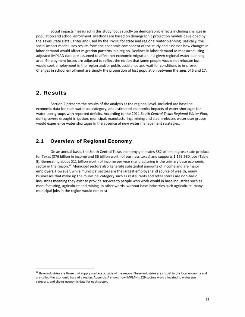
Social impacts measured in this study focus strictly on demographic effects including changes in population and school enrollment. Methods are based on demographic projection models developed by the Texas State Data Center and used by the TWDB for state and regional water planning. Basically, the social impact model uses results from the economic component of the study and assesses how changes in labor demand would affect migration patterns in a region. Declines in labor demand as measured using adjusted IMPLAN data are assumed to affect net economic migration in a given regional water planning area. Employment losses are adjusted to reflect the notion that some people would not relocate but would seek employment in the region and/or public assistance and wait for conditions to improve. Changes in school enrollment are simply the proportion of lost population between the ages of 5 and 17.
2. Results
Section 2 presents the results of the analysis at the regional level. Included are baseline economic data for each water use category, and estimated economics impacts of water shortages for water user groups with reported deficits. According to the 2011 South Central Texas Regional Water Plan, during severe drought irrigation, municipal, manufacturing, mining and steam‐electric water user groups would experience water shortages in the absence of new water management strategies.
2.1 Overview of Regional Economy
On an annual basis, the South Central Texas economy generates $82 billion in gross state product for Texas ($76 billion in income and $6 billion worth of business taxes) and supports 1,163,680 jobs (Table 8). Generating about $11 billion worth of income per year manufacturing is the primary base economic sector in the region.22 Municipal sectors also generate substantial amounts of income and are major employers. However, while municipal sectors are the largest employer and source of wealth, many businesses that make up the municipal category such as restaurants and retail stores are non‐basic industries meaning they exist to provide services to people who work would in base industries such as manufacturing, agriculture and mining. In other words, without base industries such agriculture, many municipal jobs in the region would not exist.
22 Base industries are those that supply markets outside of the region. These industries are crucial to the local economy and are called the economic base of a region. Appendix A shows how IMPLAN’s 529 sectors were allocated to water use category, and shows economic data for each sector.
23
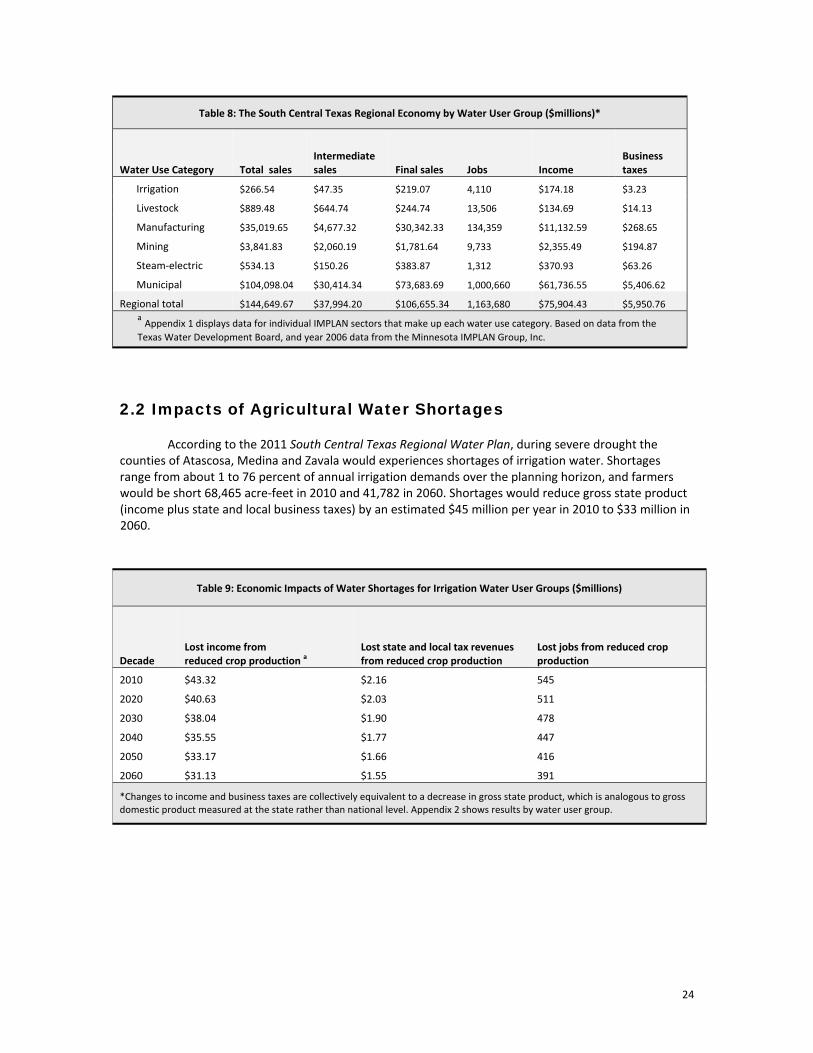
Table 8: The South Central Texas Regional Economy by Water User Group ($millions)*
Water Use Category Total sales Intermediate sales Final sales Jobs Income
Business taxes
Irrigation $266.54 $47.35 $219.07 4,110 $174.18 $3.23
Livestock $889.48 $644.74 $244.74 13,506 $134.69 $14.13
Manufacturing $35,019.65 $4,677.32 $30,342.33 134,359 $11,132.59 $268.65
Mining $3,841.83 $2,060.19 $1,781.64 9,733 $2,355.49 $194.87
Steam‐electric $534.13 $150.26 $383.87 1,312 $370.93 $63.26
Municipal $104,098.04 $30,414.34 $73,683.69 1,000,660 $61,736.55 $5,406.62
Regional total $144,649.67 $37,994.20 $106,655.34 1,163,680 $75,904.43 $5,950.76 a Appendix 1 displays data for individual IMPLAN sectors that make up each water use category. Based on data from the Texas Water Development Board, and year 2006 data from the Minnesota IMPLAN Group, Inc.
2.2 Impacts of Agricultural Water Shortages According to the 2011 South Central Texas Regional Water Plan, during severe drought the
counties of Atascosa, Medina and Zavala would experiences shortages of irrigation water. Shortages range from about 1 to 76 percent of annual irrigation demands over the planning horizon, and farmers would be short 68,465 acre‐feet in 2010 and 41,782 in 2060. Shortages would reduce gross state product (income plus state and local business taxes) by an estimated $45 million per year in 2010 to $33 million in 2060.
Table 9: Economic Impacts of Water Shortages for Irrigation Water User Groups ($millions)
Decade Lost income from reduced crop production a
Lost state and local tax revenues from reduced crop production
Lost jobs from reduced crop production
2010 $43.32 $2.16 545
2020 $40.63 $2.03 511
2030 $38.04 $1.90 478
2040 $35.55 $1.77 447
2050 $33.17 $1.66 416
2060 $31.13 $1.55 391
*Changes to income and business taxes are collectively equivalent to a decrease in gross state product, which is analogous to gross domestic product measured at the state rather than national level. Appendix 2 shows results by water user group.
24
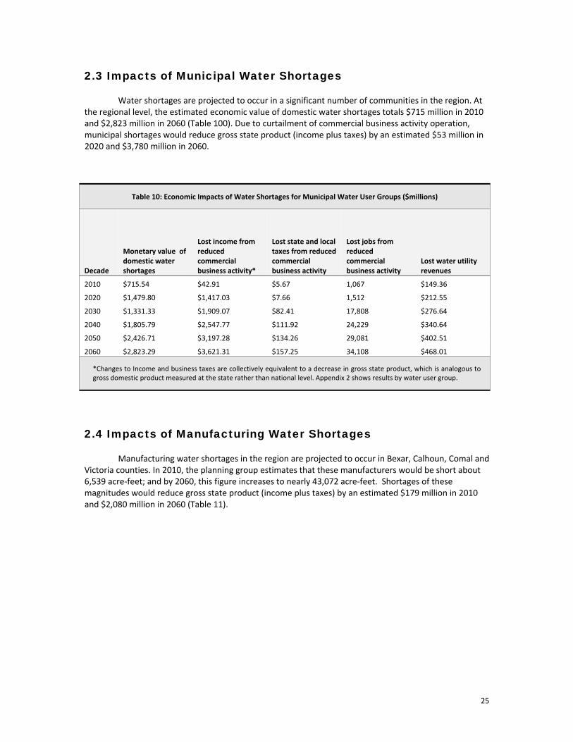
2.3 Impacts of Municipal Water Shortages
Water shortages are projected to occur in a significant number of communities in the region. At the regional level, the estimated economic value of domestic water shortages totals $715 million in 2010 and $2,823 million in 2060 (Table 100). Due to curtailment of commercial business activity operation, municipal shortages would reduce gross state product (income plus taxes) by an estimated $53 million in 2020 and $3,780 million in 2060.
Table 10: Economic Impacts of Water Shortages for Municipal Water User Groups ($millions)
Decade
Monetary value of domestic water shortages
Lost income from reduced commercial business activity*
Lost state and local taxes from reduced commercial business activity
Lost jobs from reduced commercial business activity
Lost water utility revenues
2010 $715.54 $42.91 $5.67 1,067 $149.36
2020 $1,479.80 $1,417.03 $7.66 1,512 $212.55
2030 $1,331.33 $1,909.07 $82.41 17,808 $276.64
2040 $1,805.79 $2,547.77 $111.92 24,229 $340.64
2050 $2,426.71 $3,197.28 $134.26 29,081 $402.51
2060 $2,823.29 $3,621.31 $157.25 34,108 $468.01
*Changes to Income and business taxes are collectively equivalent to a decrease in gross state product, which is analogous to gross domestic product measured at the state rather than national level. Appendix 2 shows results by water user group.
2.4 Impacts of Manufacturing Water Shortages
Manufacturing water shortages in the region are projected to occur in Bexar, Calhoun, Comal and Victoria counties. In 2010, the planning group estimates that these manufacturers would be short about 6,539 acre‐feet; and by 2060, this figure increases to nearly 43,072 acre‐feet. Shortages of these magnitudes would reduce gross state product (income plus taxes) by an estimated $179 million in 2010 and $2,080 million in 2060 (Table 11).
25
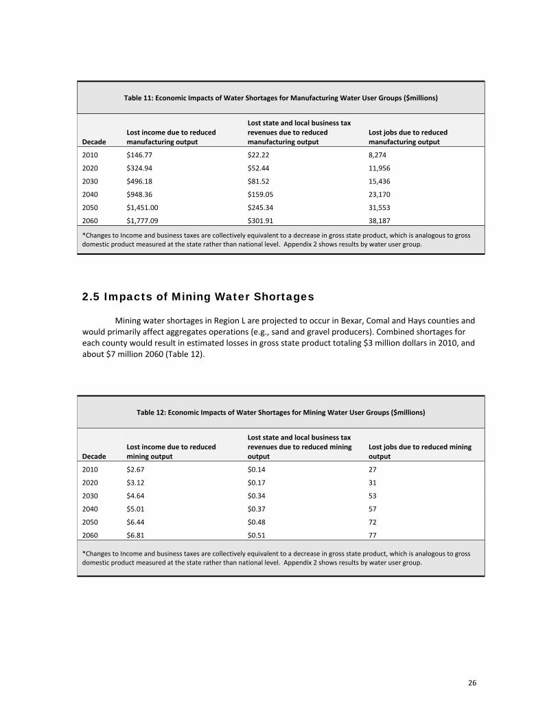
Table 11: Economic Impacts of Water Shortages for Manufacturing Water User Groups ($millions)
Decade Lost income due to reduced manufacturing output
Lost state and local business tax revenues due to reduced manufacturing output
Lost jobs due to reduced manufacturing output
2010 $146.77 $22.22 8,274
2020 $324.94 $52.44 11,956
2030 $496.18 $81.52 15,436
2040 $948.36 $159.05 23,170
2050 $1,451.00 $245.34 31,553
2060 $1,777.09 $301.91 38,187
*Changes to Income and business taxes are collectively equivalent to a decrease in gross state product, which is analogous to gross domestic product measured at the state rather than national level. Appendix 2 shows results by water user group.
2.5 Impacts of Mining Water Shortages
Mining water shortages in Region L are projected to occur in Bexar, Comal and Hays counties and would primarily affect aggregates operations (e.g., sand and gravel producers). Combined shortages for each county would result in estimated losses in gross state product totaling $3 million dollars in 2010, and about $7 million 2060 (Table 12).
Table 12: Economic Impacts of Water Shortages for Mining Water User Groups ($millions)
Decade Lost income due to reduced mining output
Lost state and local business tax revenues due to reduced mining output
Lost jobs due to reduced mining output
2010 $2.67 $0.14 27
2020 $3.12 $0.17 31
2030 $4.64 $0.34 53
2040 $5.01 $0.37 57
2050 $6.44 $0.48 72
2060 $6.81 $0.51 77
*Changes to Income and business taxes are collectively equivalent to a decrease in gross state product, which is analogous to gross domestic product measured at the state rather than national level. Appendix 2 shows results by water user group.
26
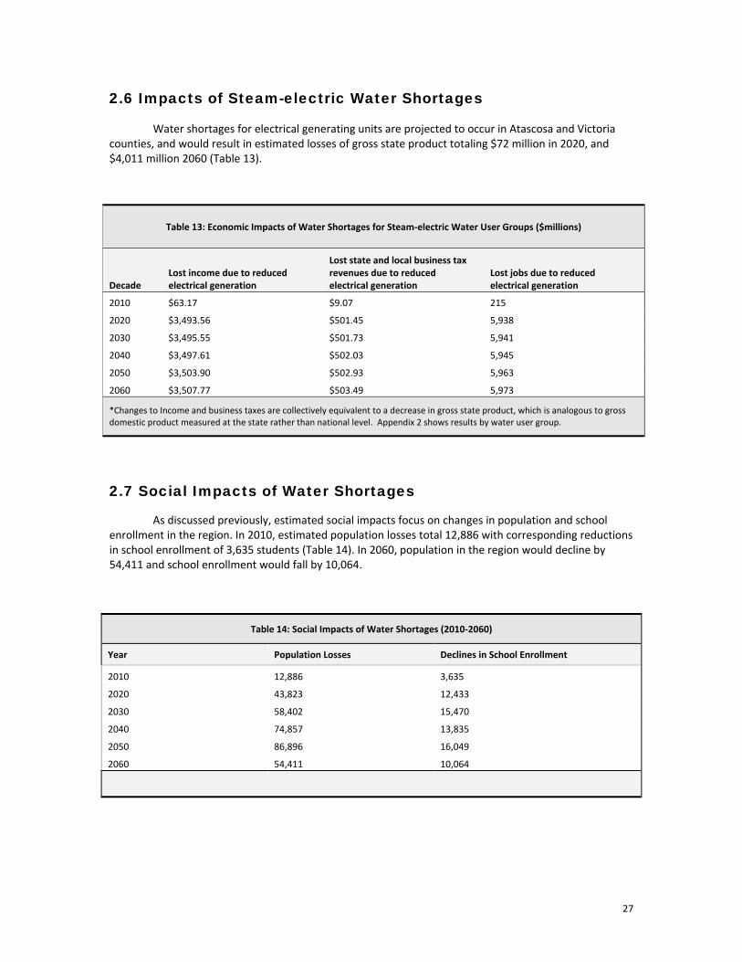
2.6 Impacts of Steam-electric Water Shortages
Water shortages for electrical generating units are projected to occur in Atascosa and Victoria counties, and would result in estimated losses of gross state product totaling $72 million in 2020, and $4,011 million 2060 (Table 13).
Table 13: Economic Impacts of Water Shortages for Steam‐electric Water User Groups ($millions)
Decade Lost income due to reduced electrical generation
Lost state and local business tax revenues due to reduced electrical generation
Lost jobs due to reduced electrical generation
2010 $63.17 $9.07 215
2020 $3,493.56 $501.45 5,938
2030 $3,495.55 $501.73 5,941
2040 $3,497.61 $502.03 5,945
2050 $3,503.90 $502.93 5,963
2060 $3,507.77 $503.49 5,973
*Changes to Income and business taxes are collectively equivalent to a decrease in gross state product, which is analogous to gross domestic product measured at the state rather than national level. Appendix 2 shows results by water user group.
2.7 Social Impacts of Water Shortages
As discussed previously, estimated social impacts focus on changes in population and school enrollment in the region. In 2010, estimated population losses total 12,886 with corresponding reductions in school enrollment of 3,635 students (Table 14). In 2060, population in the region would decline by 54,411 and school enrollment would fall by 10,064.
Table 14: Social Impacts of Water Shortages (2010‐2060)
Year Population Losses Declines in School Enrollment
2010 12,886 3,635
2020 43,823 12,433
2030 58,402 15,470
2040 74,857 13,835
2050 86,896 16,049
2060 54,411 10,064
27
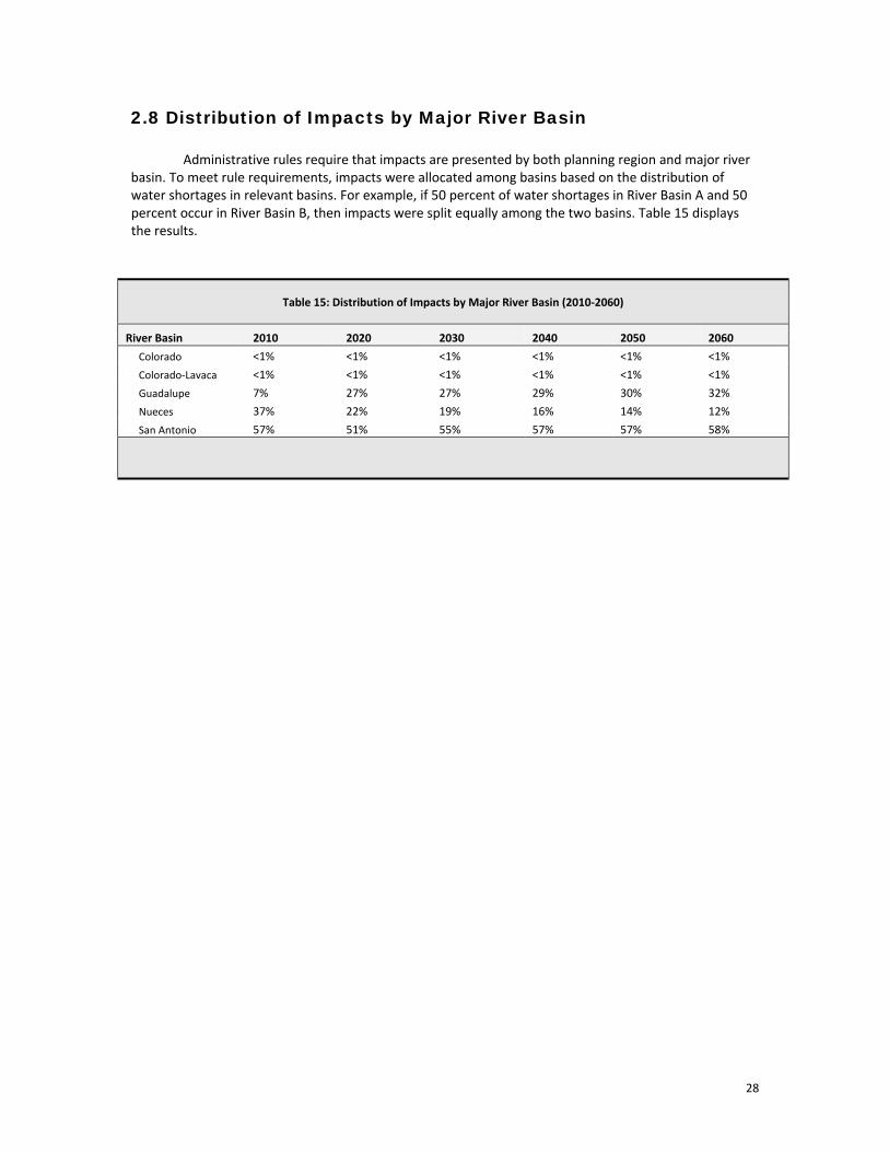
28
2.8 Distribution of Impacts by Major River Basin
Administrative rules require that impacts are presented by both planning region and major river basin. To meet rule requirements, impacts were allocated among basins based on the distribution of water shortages in relevant basins. For example, if 50 percent of water shortages in River Basin A and 50 percent occur in River Basin B, then impacts were split equally among the two basins. Table 15 displays the results.
Table 15: Distribution of Impacts by Major River Basin (2010‐2060)
River Basin 2010 2020 2030 2040 2050 2060
Colorado <1% <1% <1% <1% <1% <1%
Colorado‐Lavaca <1% <1% <1% <1% <1% <1%
Guadalupe 7% 27% 27% 29% 30% 32%
Nueces 37% 22% 19% 16% 14% 12%
San Antonio 57% 51% 55% 57% 57% 58%
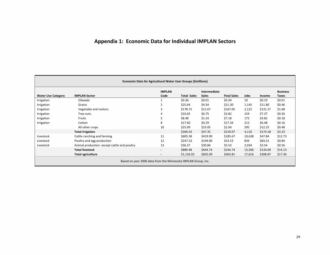
Appendix 1: Economic Data for Individual IMPLAN Sectors
Economic Data for Agricultural Water User Groups ($millions)
Water Use Category IMPLAN Sector IMPLAN Code Total Sales
Intermediate Sales Final Sales Jobs Income
Business Taxes
Irrigation Oilseeds 1 $0.36 $0.01 $0.34 10 $0.19 $0.01 Irrigation Grains 2 $25.64 $4.34 $21.30 1,145 $11.80 $0.46 Irrigation Vegetable and melons 3 $178.72 $11.67 $167.05 2,122 $131.27 $1.68 Irrigation Tree nuts 4 $10.65 $6.75 $3.82 154 $7.37 $0.26 Irrigation Fruits 5 $8.48 $1.24 $7.18 172 $4.82 $0.18 Irrigation Cotton 8 $17.60 $0.29 $17.34 212 $6.48 $0.16 All other crops 10 $25.09 $23.05 $2.04 295 $12.25 $0.48 Total irrigation $266.54 $47.35 $219.07 4,110 $174.18 $3.23 Livestock Cattle ranching and farming 11 $605.58 $419.90 $185.67 10,638 $47.84 $12.73 Livestock Poultry and egg production 12 $247.53 $194.00 $53.53 834 $83.31 $0.84 Livestock Animal production‐ except cattle and poultry 13 $36.37 $30.84 $5.53 2,034 $3.54 $0.56 Total livestock ‐ $889.48 $644.74 $244.74 13,506 $134.69 $14.13 Total agriculture ‐ $1,156.02 $692.09 $463.81 17,616 $308.87 $17.36
Based on year 2006 data from the Minnesota IMPLAN Group, Inc.
29

Economic Data for Mining and Steam‐electric Water User Groups ($millions)
Water Use Category IMPLAN Sector IMPLAN Code Total Sales
Intermediate Sales Final Sales Jobs Income
Business Taxes
Mining Oil and gas extraction 19 $1,996.63 $1,854.24 $142.38 3,290 $1,148.96 $120.59 Mining Support activities for oil and gas operations 28 $1,026.56 $142.59 $883.98 4,522 $930.58 $42.34 Mining Drilling oil and gas wells 27 $577.01 $2.88 $574.13 997 $150.15 $19.80 Mining Sand‐ gravel‐ clay‐ and refractory mining 25 $92.43 $9.76 $82.67 537 $54.54 $2.53 Mining Coal mining 20 $64.63 $24.22 $40.41 207 $23.55 $7.12 Mining Stone mining and quarrying 24 $44.53 $4.58 $39.95 149 $26.40 $0.27 Mining Gold‐ silver‐ and other metal ore mining 23 $39.13 $21.85 $17.27 27 $20.87 $2.20
Mining Other nonmetallic mineral mining 26 $0.58 $0.06 $0.52 3 $0.26 $0.02
Mining Support activities for other mining 29 $0.33 $0.00 $0.33 1 $0.19 $0.00
Total mining $534.13 $150.26 $383.87 1,312 $370.93 $63.26
Steam‐electric Power generation and supply 30 $3,841.83 $2,060.19 $1,781.64 9,733 $2,355.49 $194.87
Based on year 2006 data from the Minnesota IMPLAN Group, Inc.
30
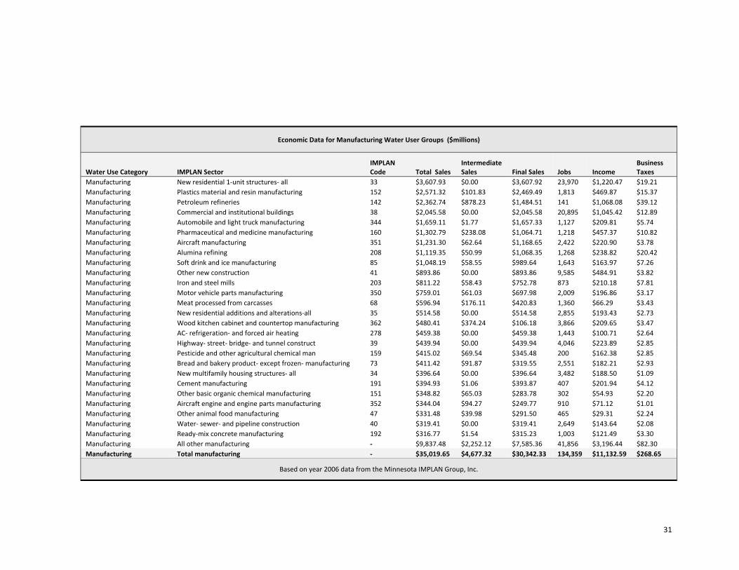
Economic Data for Manufacturing Water User Groups ($millions)
Water Use Category IMPLAN Sector IMPLAN Code Total Sales
Intermediate Sales Final Sales Jobs Income
Business Taxes
Manufacturing New residential 1‐unit structures‐ all 33 $3,607.93 $0.00 $3,607.92 23,970 $1,220.47 $19.21 Manufacturing Plastics material and resin manufacturing 152 $2,571.32 $101.83 $2,469.49 1,813 $469.87 $15.37 Manufacturing Petroleum refineries 142 $2,362.74 $878.23 $1,484.51 141 $1,068.08 $39.12 Manufacturing Commercial and institutional buildings 38 $2,045.58 $0.00 $2,045.58 20,895 $1,045.42 $12.89 Manufacturing Automobile and light truck manufacturing 344 $1,659.11 $1.77 $1,657.33 1,127 $209.81 $5.74 Manufacturing Pharmaceutical and medicine manufacturing 160 $1,302.79 $238.08 $1,064.71 1,218 $457.37 $10.82 Manufacturing Aircraft manufacturing 351 $1,231.30 $62.64 $1,168.65 2,422 $220.90 $3.78 Manufacturing Alumina refining 208 $1,119.35 $50.99 $1,068.35 1,268 $238.82 $20.42 Manufacturing Soft drink and ice manufacturing 85 $1,048.19 $58.55 $989.64 1,643 $163.97 $7.26 Manufacturing Other new construction 41 $893.86 $0.00 $893.86 9,585 $484.91 $3.82 Manufacturing Iron and steel mills 203 $811.22 $58.43 $752.78 873 $210.18 $7.81 Manufacturing Motor vehicle parts manufacturing 350 $759.01 $61.03 $697.98 2,009 $196.86 $3.17 Manufacturing Meat processed from carcasses 68 $596.94 $176.11 $420.83 1,360 $66.29 $3.43 Manufacturing New residential additions and alterations‐all 35 $514.58 $0.00 $514.58 2,855 $193.43 $2.73 Manufacturing Wood kitchen cabinet and countertop manufacturing 362 $480.41 $374.24 $106.18 3,866 $209.65 $3.47 Manufacturing AC‐ refrigeration‐ and forced air heating 278 $459.38 $0.00 $459.38 1,443 $100.71 $2.64 Manufacturing Highway‐ street‐ bridge‐ and tunnel construct 39 $439.94 $0.00 $439.94 4,046 $223.89 $2.85 Manufacturing Pesticide and other agricultural chemical man 159 $415.02 $69.54 $345.48 200 $162.38 $2.85 Manufacturing Bread and bakery product‐ except frozen‐ manufacturing 73 $411.42 $91.87 $319.55 2,551 $182.21 $2.93 Manufacturing New multifamily housing structures‐ all 34 $396.64 $0.00 $396.64 3,482 $188.50 $1.09 Manufacturing Cement manufacturing 191 $394.93 $1.06 $393.87 407 $201.94 $4.12 Manufacturing Other basic organic chemical manufacturing 151 $348.82 $65.03 $283.78 302 $54.93 $2.20 Manufacturing Aircraft engine and engine parts manufacturing 352 $344.04 $94.27 $249.77 910 $71.12 $1.01 Manufacturing Other animal food manufacturing 47 $331.48 $39.98 $291.50 465 $29.31 $2.24 Manufacturing Water‐ sewer‐ and pipeline construction 40 $319.41 $0.00 $319.41 2,649 $143.64 $2.08 Manufacturing Ready‐mix concrete manufacturing 192 $316.77 $1.54 $315.23 1,003 $121.49 $3.30 Manufacturing All other manufacturing ‐ $9,837.48 $2,252.12 $7,585.36 41,856 $3,196.44 $82.30 Manufacturing Total manufacturing ‐ $35,019.65 $4,677.32 $30,342.33 134,359 $11,132.59 $268.65
Based on year 2006 data from the Minnesota IMPLAN Group, Inc.
31
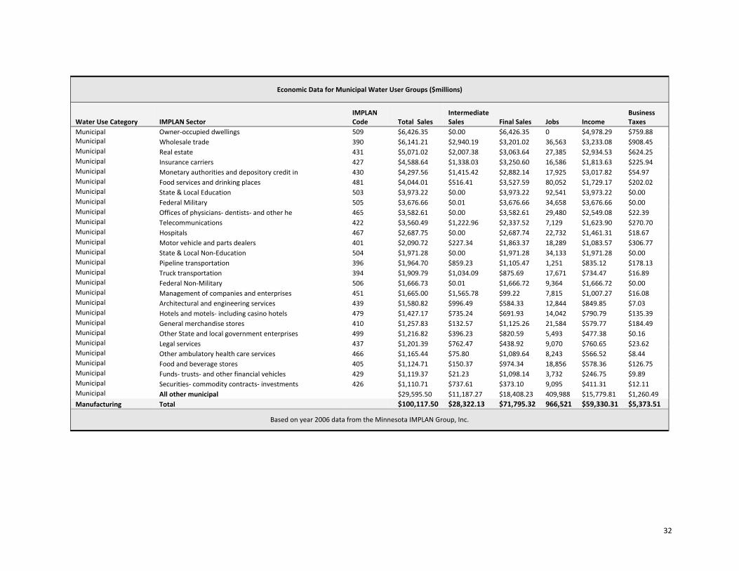
Economic Data for Municipal Water User Groups ($millions)
Water Use Category IMPLAN Sector IMPLAN Code Total Sales
Intermediate Sales Final Sales Jobs Income
Business Taxes
Municipal Owner‐occupied dwellings 509 $6,426.35 $0.00 $6,426.35 0 $4,978.29 $759.88 Municipal Wholesale trade 390 $6,141.21 $2,940.19 $3,201.02 36,563 $3,233.08 $908.45 Municipal Real estate 431 $5,071.02 $2,007.38 $3,063.64 27,385 $2,934.53 $624.25 Municipal Insurance carriers 427 $4,588.64 $1,338.03 $3,250.60 16,586 $1,813.63 $225.94 Municipal Monetary authorities and depository credit in 430 $4,297.56 $1,415.42 $2,882.14 17,925 $3,017.82 $54.97 Municipal Food services and drinking places 481 $4,044.01 $516.41 $3,527.59 80,052 $1,729.17 $202.02 Municipal State & Local Education 503 $3,973.22 $0.00 $3,973.22 92,541 $3,973.22 $0.00 Municipal Federal Military 505 $3,676.66 $0.01 $3,676.66 34,658 $3,676.66 $0.00 Municipal Offices of physicians‐ dentists‐ and other he 465 $3,582.61 $0.00 $3,582.61 29,480 $2,549.08 $22.39 Municipal Telecommunications 422 $3,560.49 $1,222.96 $2,337.52 7,129 $1,623.90 $270.70 Municipal Hospitals 467 $2,687.75 $0.00 $2,687.74 22,732 $1,461.31 $18.67 Municipal Motor vehicle and parts dealers 401 $2,090.72 $227.34 $1,863.37 18,289 $1,083.57 $306.77 Municipal State & Local Non‐Education 504 $1,971.28 $0.00 $1,971.28 34,133 $1,971.28 $0.00 Municipal Pipeline transportation 396 $1,964.70 $859.23 $1,105.47 1,251 $835.12 $178.13 Municipal Truck transportation 394 $1,909.79 $1,034.09 $875.69 17,671 $734.47 $16.89 Municipal Federal Non‐Military 506 $1,666.73 $0.01 $1,666.72 9,364 $1,666.72 $0.00 Municipal Management of companies and enterprises 451 $1,665.00 $1,565.78 $99.22 7,815 $1,007.27 $16.08 Municipal Architectural and engineering services 439 $1,580.82 $996.49 $584.33 12,844 $849.85 $7.03 Municipal Hotels and motels‐ including casino hotels 479 $1,427.17 $735.24 $691.93 14,042 $790.79 $135.39 Municipal General merchandise stores 410 $1,257.83 $132.57 $1,125.26 21,584 $579.77 $184.49 Municipal Other State and local government enterprises 499 $1,216.82 $396.23 $820.59 5,493 $477.38 $0.16 Municipal Legal services 437 $1,201.39 $762.47 $438.92 9,070 $760.65 $23.62 Municipal Other ambulatory health care services 466 $1,165.44 $75.80 $1,089.64 8,243 $566.52 $8.44 Municipal Food and beverage stores 405 $1,124.71 $150.37 $974.34 18,856 $578.36 $126.75 Municipal Funds‐ trusts‐ and other financial vehicles 429 $1,119.37 $21.23 $1,098.14 3,732 $246.75 $9.89 Municipal Securities‐ commodity contracts‐ investments 426 $1,110.71 $737.61 $373.10 9,095 $411.31 $12.11 Municipal All other municipal $29,595.50 $11,187.27 $18,408.23 409,988 $15,779.81 $1,260.49 Manufacturing Total $100,117.50 $28,322.13 $71,795.32 966,521 $59,330.31 $5,373.51
Based on year 2006 data from the Minnesota IMPLAN Group, Inc.
32
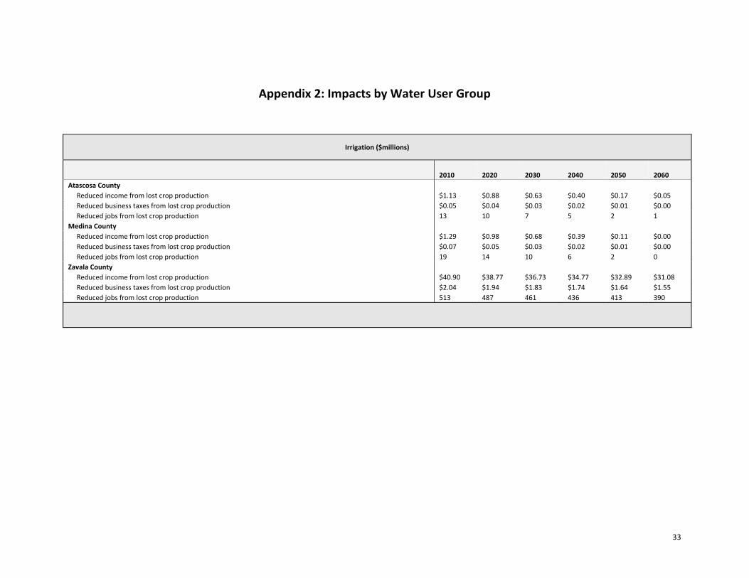
Appendix 2: Impacts by Water User Group
Irrigation ($millions)
2010 2020 2030 2040 2050 2060 Atascosa County
Reduced income from lost crop production $1.13 $0.88 $0.63 $0.40 $0.17 $0.05 Reduced business taxes from lost crop production $0.05 $0.04 $0.03 $0.02 $0.01 $0.00 Reduced jobs from lost crop production 13 10 7 5 2 1
Medina County Reduced income from lost crop production $1.29 $0.98 $0.68 $0.39 $0.11 $0.00 Reduced business taxes from lost crop production $0.07 $0.05 $0.03 $0.02 $0.01 $0.00 Reduced jobs from lost crop production 19 14 10 6 2 0
Zavala County Reduced income from lost crop production $40.90 $38.77 $36.73 $34.77 $32.89 $31.08 Reduced business taxes from lost crop production $2.04 $1.94 $1.83 $1.74 $1.64 $1.55 Reduced jobs from lost crop production 513 487 461 436 413 390
33
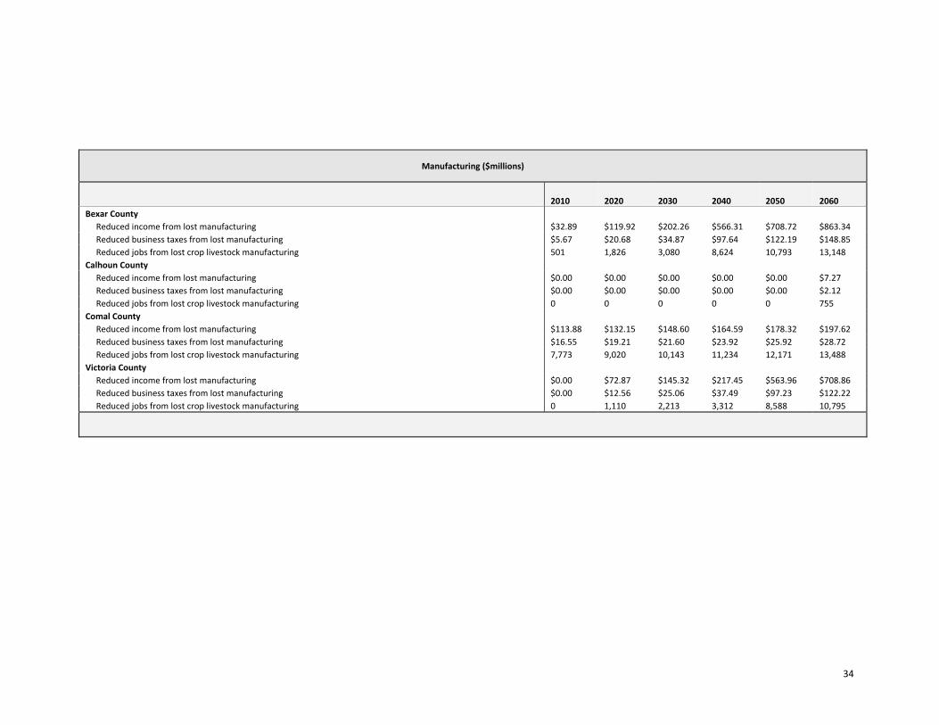
Manufacturing ($millions)
2010 2020 2030 2040 2050 2060 Bexar County
Reduced income from lost manufacturing $32.89 $119.92 $202.26 $566.31 $708.72 $863.34 Reduced business taxes from lost manufacturing $5.67 $20.68 $34.87 $97.64 $122.19 $148.85 Reduced jobs from lost crop livestock manufacturing 501 1,826 3,080 8,624 10,793 13,148
Calhoun County Reduced income from lost manufacturing $0.00 $0.00 $0.00 $0.00 $0.00 $7.27 Reduced business taxes from lost manufacturing $0.00 $0.00 $0.00 $0.00 $0.00 $2.12 Reduced jobs from lost crop livestock manufacturing 0 0 0 0 0 755
Comal County Reduced income from lost manufacturing $113.88 $132.15 $148.60 $164.59 $178.32 $197.62 Reduced business taxes from lost manufacturing $16.55 $19.21 $21.60 $23.92 $25.92 $28.72 Reduced jobs from lost crop livestock manufacturing 7,773 9,020 10,143 11,234 12,171 13,488
Victoria County Reduced income from lost manufacturing $0.00 $72.87 $145.32 $217.45 $563.96 $708.86 Reduced business taxes from lost manufacturing $0.00 $12.56 $25.06 $37.49 $97.23 $122.22 Reduced jobs from lost crop livestock manufacturing 0 1,110 2,213 3,312 8,588 10,795
34
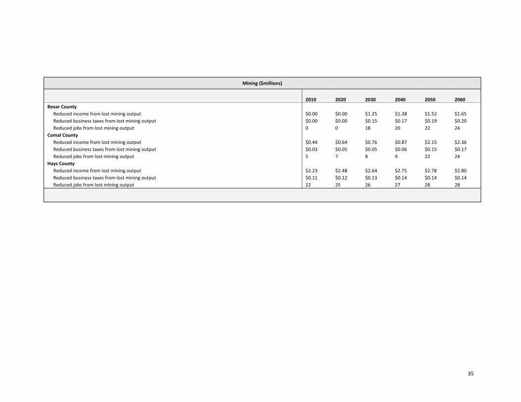
Mining ($millions)
2010 2020 2030 2040 2050 2060 Bexar County
Reduced income from lost mining output $0.00 $0.00 $1.25 $1.38 $1.52 $1.65 Reduced business taxes from lost mining output $0.00 $0.00 $0.15 $0.17 $0.19 $0.20 Reduced jobs from lost mining output 0 0 18 20 22 24
Comal County Reduced income from lost mining output $0.44 $0.64 $0.76 $0.87 $2.15 $2.36 Reduced business taxes from lost mining output $0.03 $0.05 $0.05 $0.06 $0.15 $0.17 Reduced jobs from lost mining output 5 7 8 9 22 24
Hays County Reduced income from lost mining output $2.23 $2.48 $2.64 $2.75 $2.78 $2.80 Reduced business taxes from lost mining output $0.11 $0.12 $0.13 $0.14 $0.14 $0.14 Reduced jobs from lost mining output 22 25 26 27 28 28
35
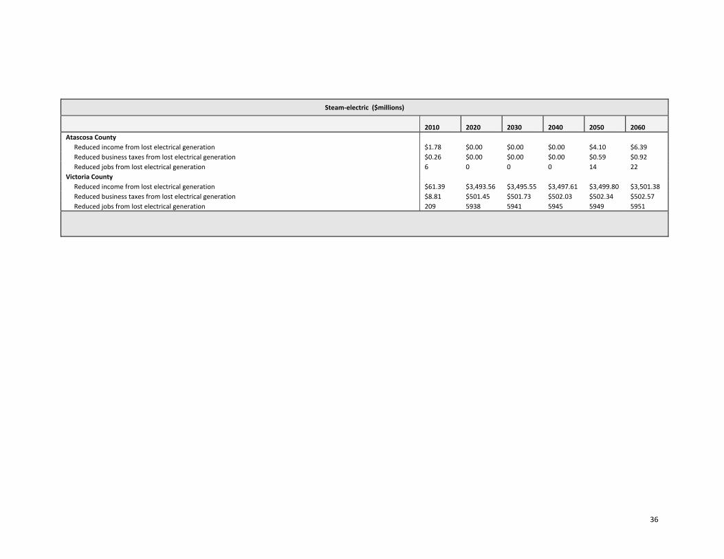
Steam‐electric ($millions)
2010 2020 2030 2040 2050 2060 Atascosa County
Reduced income from lost electrical generation $1.78 $0.00 $0.00 $0.00 $4.10 $6.39 Reduced business taxes from lost electrical generation $0.26 $0.00 $0.00 $0.00 $0.59 $0.92 Reduced jobs from lost electrical generation 6 0 0 0 14 22
Victoria County
Reduced income from lost electrical generation $61.39 $3,493.56 $3,495.55 $3,497.61 $3,499.80 $3,501.38 Reduced business taxes from lost electrical generation $8.81 $501.45 $501.73 $502.03 $502.34 $502.57 Reduced jobs from lost electrical generation 209 5938 5941 5945 5949 5951
36
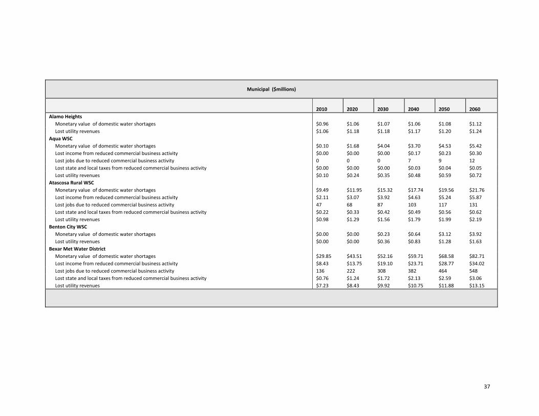
Municipal ($millions)
2010 2020 2030 2040 2050 2060 Alamo Heights
Monetary value of domestic water shortages $0.96 $1.06 $1.07 $1.06 $1.08 $1.12 Lost utility revenues $1.06 $1.18 $1.18 $1.17 $1.20 $1.24
Aqua WSC Monetary value of domestic water shortages $0.10 $1.68 $4.04 $3.70 $4.53 $5.42 Lost income from reduced commercial business activity $0.00 $0.00 $0.00 $0.17 $0.23 $0.30 Lost jobs due to reduced commercial business activity 0 0 0 7 9 12 Lost state and local taxes from reduced commercial business activity $0.00 $0.00 $0.00 $0.03 $0.04 $0.05 Lost utility revenues $0.10 $0.24 $0.35 $0.48 $0.59 $0.72
Atascosa Rural WSC Monetary value of domestic water shortages $9.49 $11.95 $15.32 $17.74 $19.56 $21.76 Lost income from reduced commercial business activity $2.11 $3.07 $3.92 $4.63 $5.24 $5.87 Lost jobs due to reduced commercial business activity 47 68 87 103 117 131 Lost state and local taxes from reduced commercial business activity $0.22 $0.33 $0.42 $0.49 $0.56 $0.62 Lost utility revenues $0.98 $1.29 $1.56 $1.79 $1.99 $2.19
Benton City WSC Monetary value of domestic water shortages $0.00 $0.00 $0.23 $0.64 $3.12 $3.92 Lost utility revenues $0.00 $0.00 $0.36 $0.83 $1.28 $1.63
Bexar Met Water District
Monetary value of domestic water shortages $29.85 $43.51 $52.16 $59.71 $68.58 $82.71 Lost income from reduced commercial business activity $8.43 $13.75 $19.10 $23.71 $28.77 $34.02 Lost jobs due to reduced commercial business activity 136 222 308 382 464 548 Lost state and local taxes from reduced commercial business activity $0.76 $1.24 $1.72 $2.13 $2.59 $3.06 Lost utility revenues $7.23 $8.43 $9.92 $10.75 $11.88 $13.15
37
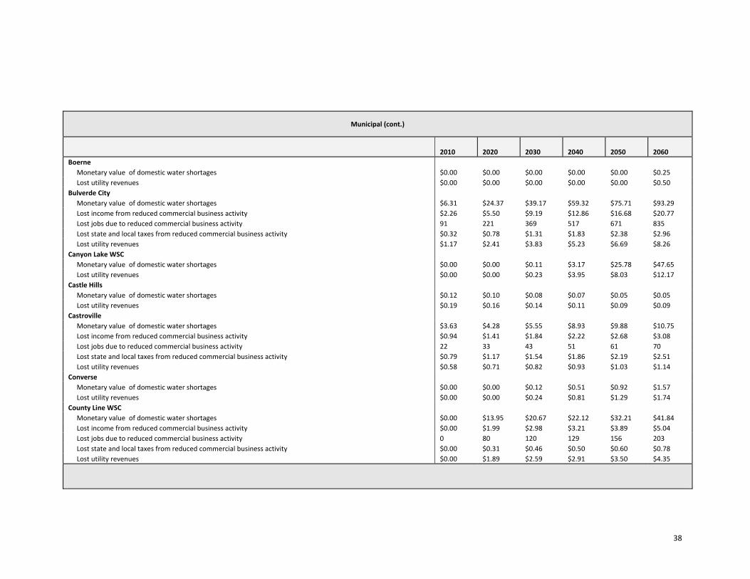
Municipal (cont.)
2010 2020 2030 2040 2050 2060 Boerne
Monetary value of domestic water shortages $0.00 $0.00 $0.00 $0.00 $0.00 $0.25 Lost utility revenues $0.00 $0.00 $0.00 $0.00 $0.00 $0.50
Bulverde City Monetary value of domestic water shortages $6.31 $24.37 $39.17 $59.32 $75.71 $93.29 Lost income from reduced commercial business activity $2.26 $5.50 $9.19 $12.86 $16.68 $20.77 Lost jobs due to reduced commercial business activity 91 221 369 517 671 835 Lost state and local taxes from reduced commercial business activity $0.32 $0.78 $1.31 $1.83 $2.38 $2.96 Lost utility revenues $1.17 $2.41 $3.83 $5.23 $6.69 $8.26
Canyon Lake WSC Monetary value of domestic water shortages $0.00 $0.00 $0.11 $3.17 $25.78 $47.65 Lost utility revenues $0.00 $0.00 $0.23 $3.95 $8.03 $12.17
Castle Hills Monetary value of domestic water shortages $0.12 $0.10 $0.08 $0.07 $0.05 $0.05 Lost utility revenues $0.19 $0.16 $0.14 $0.11 $0.09 $0.09
Castroville Monetary value of domestic water shortages $3.63 $4.28 $5.55 $8.93 $9.88 $10.75 Lost income from reduced commercial business activity $0.94 $1.41 $1.84 $2.22 $2.68 $3.08 Lost jobs due to reduced commercial business activity 22 33 43 51 61 70 Lost state and local taxes from reduced commercial business activity $0.79 $1.17 $1.54 $1.86 $2.19 $2.51 Lost utility revenues $0.58 $0.71 $0.82 $0.93 $1.03 $1.14
Converse Monetary value of domestic water shortages $0.00 $0.00 $0.12 $0.51 $0.92 $1.57 Lost utility revenues $0.00 $0.00 $0.24 $0.81 $1.29 $1.74
County Line WSC Monetary value of domestic water shortages $0.00 $13.95 $20.67 $22.12 $32.21 $41.84 Lost income from reduced commercial business activity $0.00 $1.99 $2.98 $3.21 $3.89 $5.04 Lost jobs due to reduced commercial business activity 0 80 120 129 156 203 Lost state and local taxes from reduced commercial business activity $0.00 $0.31 $0.46 $0.50 $0.60 $0.78 Lost utility revenues $0.00 $1.89 $2.59 $2.91 $3.50 $4.35
38
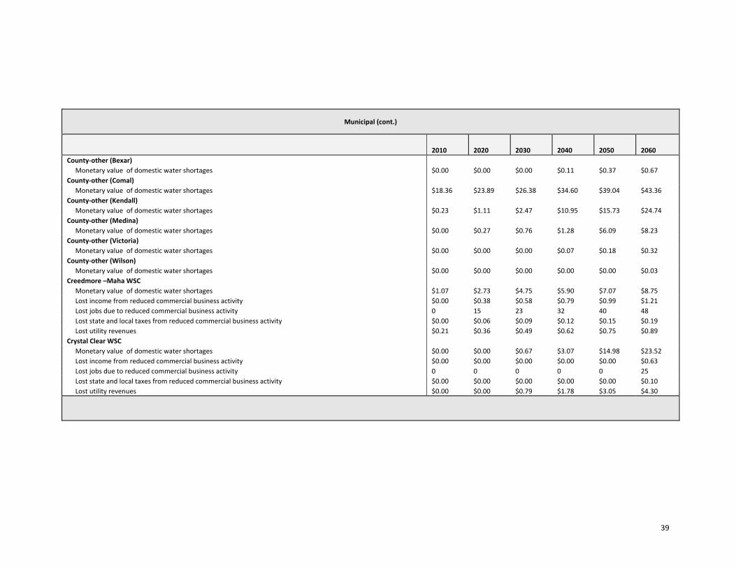
Municipal (cont.)
2010 2020 2030 2040 2050 2060 County‐other (Bexar)
Monetary value of domestic water shortages $0.00 $0.00 $0.00 $0.11 $0.37 $0.67 County‐other (Comal)
Monetary value of domestic water shortages $18.36 $23.89 $26.38 $34.60 $39.04 $43.36 County‐other (Kendall)
Monetary value of domestic water shortages $0.23 $1.11 $2.47 $10.95 $15.73 $24.74 County‐other (Medina)
Monetary value of domestic water shortages $0.00 $0.27 $0.76 $1.28 $6.09 $8.23 County‐other (Victoria)
Monetary value of domestic water shortages $0.00 $0.00 $0.00 $0.07 $0.18 $0.32 County‐other (Wilson)
Monetary value of domestic water shortages $0.00 $0.00 $0.00 $0.00 $0.00 $0.03 Creedmore –Maha WSC
Monetary value of domestic water shortages $1.07 $2.73 $4.75 $5.90 $7.07 $8.75 Lost income from reduced commercial business activity $0.00 $0.38 $0.58 $0.79 $0.99 $1.21 Lost jobs due to reduced commercial business activity 0 15 23 32 40 48 Lost state and local taxes from reduced commercial business activity $0.00 $0.06 $0.09 $0.12 $0.15 $0.19 Lost utility revenues $0.21 $0.36 $0.49 $0.62 $0.75 $0.89
Crystal Clear WSC Monetary value of domestic water shortages $0.00 $0.00 $0.67 $3.07 $14.98 $23.52 Lost income from reduced commercial business activity $0.00 $0.00 $0.00 $0.00 $0.00 $0.63 Lost jobs due to reduced commercial business activity 0 0 0 0 0 25 Lost state and local taxes from reduced commercial business activity $0.00 $0.00 $0.00 $0.00 $0.00 $0.10 Lost utility revenues $0.00 $0.00 $0.79 $1.78 $3.05 $4.30
39
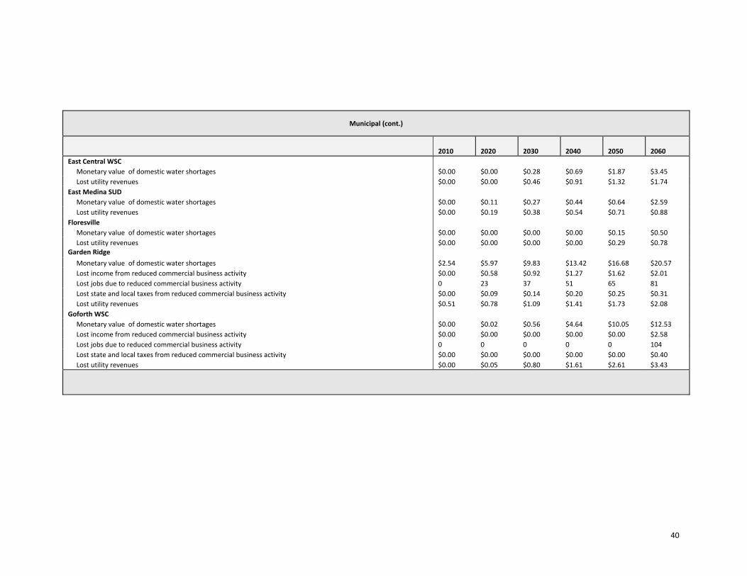
Municipal (cont.)
2010 2020 2030 2040 2050 2060 East Central WSC
Monetary value of domestic water shortages $0.00 $0.00 $0.28 $0.69 $1.87 $3.45 Lost utility revenues $0.00 $0.00 $0.46 $0.91 $1.32 $1.74
East Medina SUD Monetary value of domestic water shortages $0.00 $0.11 $0.27 $0.44 $0.64 $2.59 Lost utility revenues $0.00 $0.19 $0.38 $0.54 $0.71 $0.88
Floresville Monetary value of domestic water shortages $0.00 $0.00 $0.00 $0.00 $0.15 $0.50 Lost utility revenues $0.00 $0.00 $0.00 $0.00 $0.29 $0.78
Garden Ridge Monetary value of domestic water shortages $2.54 $5.97 $9.83 $13.42 $16.68 $20.57 Lost income from reduced commercial business activity $0.00 $0.58 $0.92 $1.27 $1.62 $2.01 Lost jobs due to reduced commercial business activity 0 23 37 51 65 81 Lost state and local taxes from reduced commercial business activity $0.00 $0.09 $0.14 $0.20 $0.25 $0.31 Lost utility revenues $0.51 $0.78 $1.09 $1.41 $1.73 $2.08
Goforth WSC
Monetary value of domestic water shortages $0.00 $0.02 $0.56 $4.64 $10.05 $12.53 Lost income from reduced commercial business activity $0.00 $0.00 $0.00 $0.00 $0.00 $2.58 Lost jobs due to reduced commercial business activity 0 0 0 0 0 104 Lost state and local taxes from reduced commercial business activity $0.00 $0.00 $0.00 $0.00 $0.00 $0.40 Lost utility revenues $0.00 $0.05 $0.80 $1.61 $2.61 $3.43
40
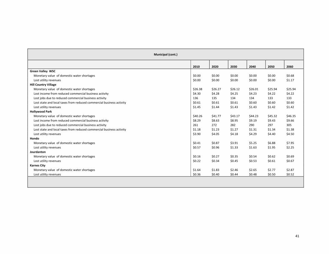
Municipal (cont.)
2010 2020 2030 2040 2050 2060 Green Valley WSC
Monetary value of domestic water shortages $0.00 $0.00 $0.00 $0.00 $0.00 $0.68 Lost utility revenues $0.00 $0.00 $0.00 $0.00 $0.00 $1.17
Hill Country Village Monetary value of domestic water shortages $26.38 $26.27 $26.12 $26.01 $25.94 $25.94 Lost income from reduced commercial business activity $4.30 $4.28 $4.25 $4.23 $4.22 $4.22 Lost jobs due to reduced commercial business activity 136 135 134 134 133 133 Lost state and local taxes from reduced commercial business activity $0.61 $0.61 $0.61 $0.60 $0.60 $0.60 Lost utility revenues $1.45 $1.44 $1.43 $1.43 $1.42 $1.42
Hollywood Park Monetary value of domestic water shortages $40.26 $41.77 $43.17 $44.23 $45.32 $46.35 Lost income from reduced commercial business activity $8.29 $8.63 $8.95 $9.19 $9.43 $9.66 Lost jobs due to reduced commercial business activity 261 272 282 290 297 305 Lost state and local taxes from reduced commercial business activity $1.18 $1.23 $1.27 $1.31 $1.34 $1.38 Lost utility revenues $3.90 $4.05 $4.18 $4.29 $4.40 $4.50
Hondo Monetary value of domestic water shortages $0.41 $0.87 $3.91 $5.25 $6.88 $7.95 Lost utility revenues $0.57 $0.96 $1.33 $1.63 $1.95 $2.25
Jourdanton Monetary value of domestic water shortages $0.16 $0.27 $0.35 $0.54 $0.62 $0.69 Lost utility revenues $0.22 $0.34 $0.45 $0.53 $0.61 $0.67
Karnes City Monetary value of domestic water shortages $1.64 $1.83 $2.46 $2.65 $2.77 $2.87 Lost utility revenues $0.36 $0.40 $0.44 $0.48 $0.50 $0.52
41
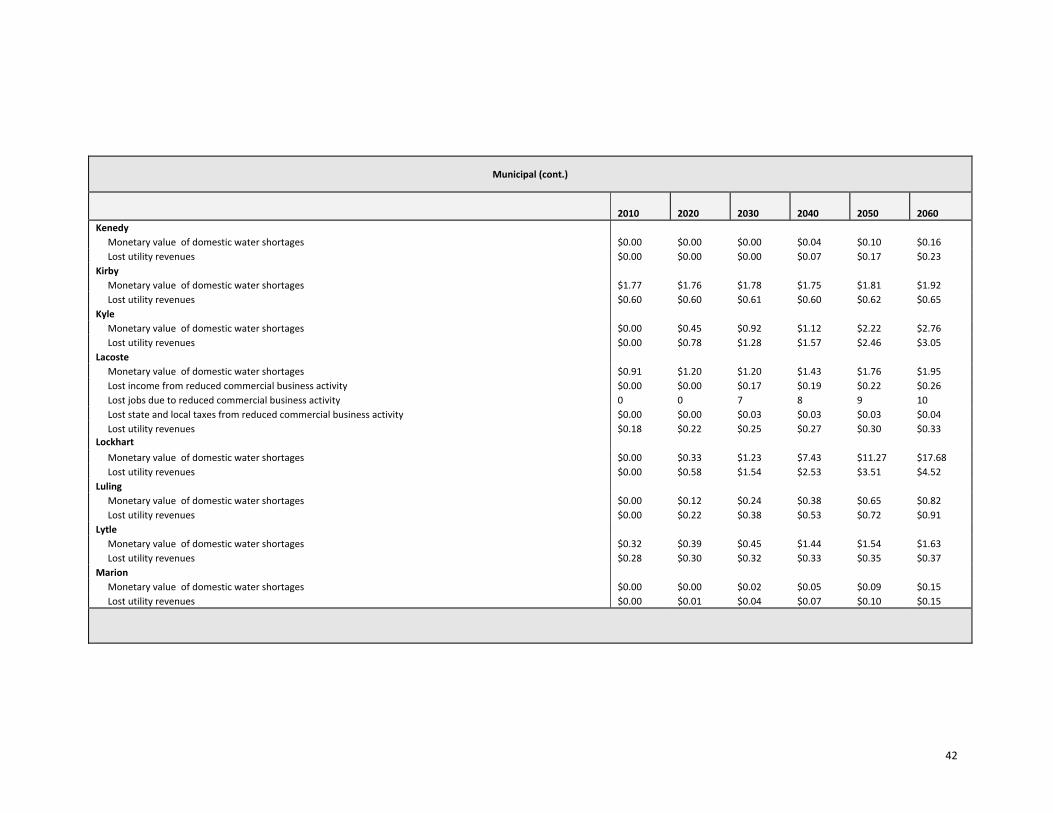
Municipal (cont.)
2010 2020 2030 2040 2050 2060 Kenedy
Monetary value of domestic water shortages $0.00 $0.00 $0.00 $0.04 $0.10 $0.16 Lost utility revenues $0.00 $0.00 $0.00 $0.07 $0.17 $0.23
Kirby Monetary value of domestic water shortages $1.77 $1.76 $1.78 $1.75 $1.81 $1.92 Lost utility revenues $0.60 $0.60 $0.61 $0.60 $0.62 $0.65
Kyle Monetary value of domestic water shortages $0.00 $0.45 $0.92 $1.12 $2.22 $2.76 Lost utility revenues $0.00 $0.78 $1.28 $1.57 $2.46 $3.05
Lacoste Monetary value of domestic water shortages $0.91 $1.20 $1.20 $1.43 $1.76 $1.95 Lost income from reduced commercial business activity $0.00 $0.00 $0.17 $0.19 $0.22 $0.26 Lost jobs due to reduced commercial business activity 0 0 7 8 9 10 Lost state and local taxes from reduced commercial business activity $0.00 $0.00 $0.03 $0.03 $0.03 $0.04 Lost utility revenues $0.18 $0.22 $0.25 $0.27 $0.30 $0.33
Lockhart Monetary value of domestic water shortages $0.00 $0.33 $1.23 $7.43 $11.27 $17.68 Lost utility revenues $0.00 $0.58 $1.54 $2.53 $3.51 $4.52
Luling Monetary value of domestic water shortages $0.00 $0.12 $0.24 $0.38 $0.65 $0.82 Lost utility revenues $0.00 $0.22 $0.38 $0.53 $0.72 $0.91
Lytle Monetary value of domestic water shortages $0.32 $0.39 $0.45 $1.44 $1.54 $1.63 Lost utility revenues $0.28 $0.30 $0.32 $0.33 $0.35 $0.37
Marion Monetary value of domestic water shortages $0.00 $0.00 $0.02 $0.05 $0.09 $0.15 Lost utility revenues $0.00 $0.01 $0.04 $0.07 $0.10 $0.15
42
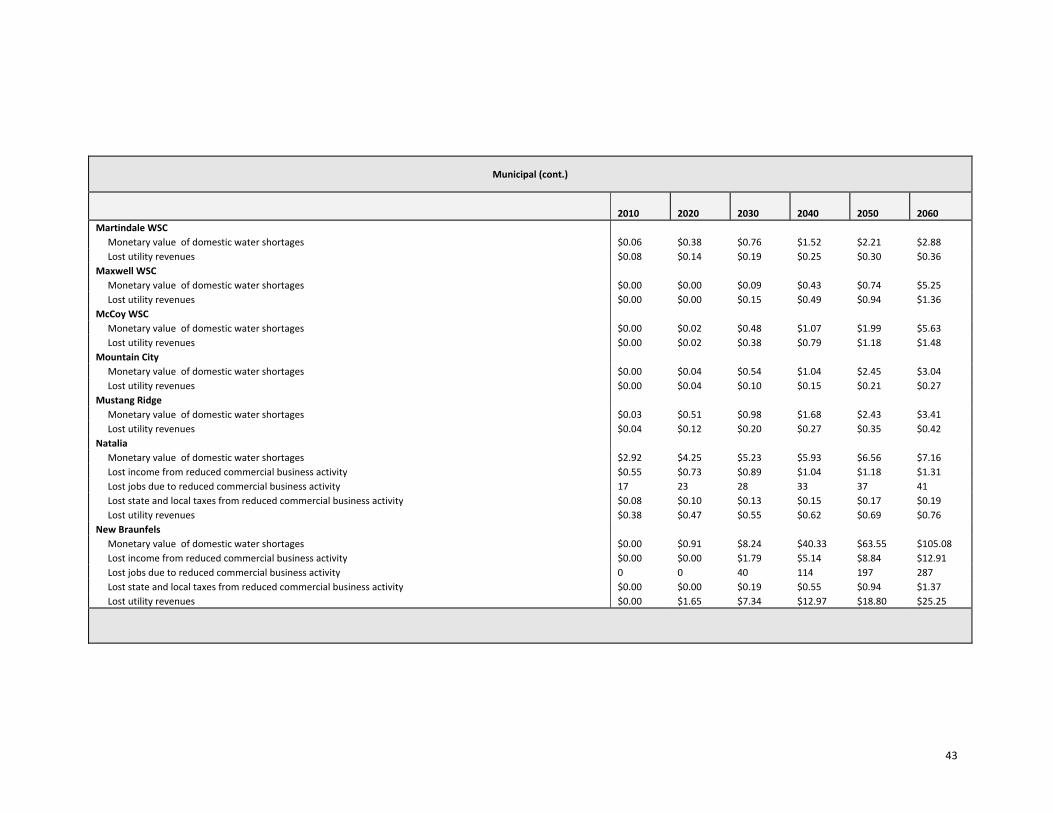
Municipal (cont.)
2010 2020 2030 2040 2050 2060 Martindale WSC
Monetary value of domestic water shortages $0.06 $0.38 $0.76 $1.52 $2.21 $2.88 Lost utility revenues $0.08 $0.14 $0.19 $0.25 $0.30 $0.36
Maxwell WSC Monetary value of domestic water shortages $0.00 $0.00 $0.09 $0.43 $0.74 $5.25 Lost utility revenues $0.00 $0.00 $0.15 $0.49 $0.94 $1.36
McCoy WSC Monetary value of domestic water shortages $0.00 $0.02 $0.48 $1.07 $1.99 $5.63 Lost utility revenues $0.00 $0.02 $0.38 $0.79 $1.18 $1.48
Mountain City Monetary value of domestic water shortages $0.00 $0.04 $0.54 $1.04 $2.45 $3.04 Lost utility revenues $0.00 $0.04 $0.10 $0.15 $0.21 $0.27
Mustang Ridge Monetary value of domestic water shortages $0.03 $0.51 $0.98 $1.68 $2.43 $3.41 Lost utility revenues $0.04 $0.12 $0.20 $0.27 $0.35 $0.42
Natalia Monetary value of domestic water shortages $2.92 $4.25 $5.23 $5.93 $6.56 $7.16 Lost income from reduced commercial business activity $0.55 $0.73 $0.89 $1.04 $1.18 $1.31 Lost jobs due to reduced commercial business activity 17 23 28 33 37 41 Lost state and local taxes from reduced commercial business activity $0.08 $0.10 $0.13 $0.15 $0.17 $0.19 Lost utility revenues $0.38 $0.47 $0.55 $0.62 $0.69 $0.76
New Braunfels Monetary value of domestic water shortages $0.00 $0.91 $8.24 $40.33 $63.55 $105.08 Lost income from reduced commercial business activity $0.00 $0.00 $1.79 $5.14 $8.84 $12.91 Lost jobs due to reduced commercial business activity 0 0 40 114 197 287 Lost state and local taxes from reduced commercial business activity $0.00 $0.00 $0.19 $0.55 $0.94 $1.37 Lost utility revenues $0.00 $1.65 $7.34 $12.97 $18.80 $25.25
43
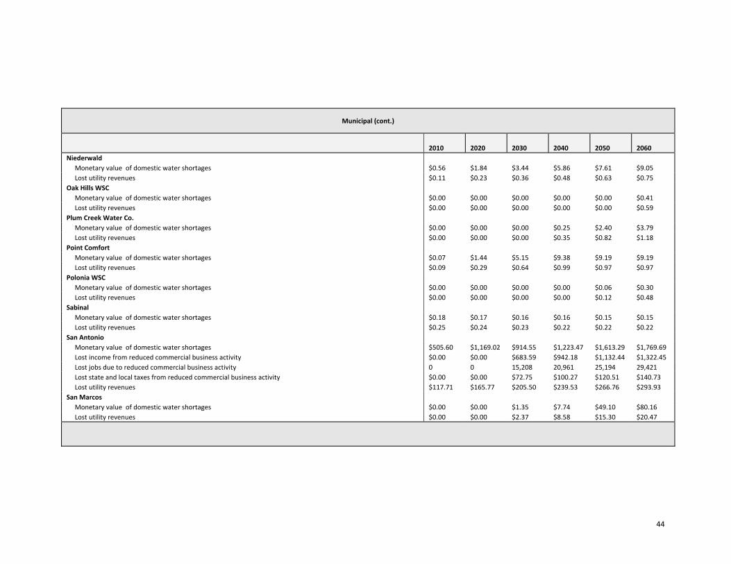
Municipal (cont.)
2010 2020 2030 2040 2050 2060 Niederwald
Monetary value of domestic water shortages $0.56 $1.84 $3.44 $5.86 $7.61 $9.05 Lost utility revenues $0.11 $0.23 $0.36 $0.48 $0.63 $0.75
Oak Hills WSC Monetary value of domestic water shortages $0.00 $0.00 $0.00 $0.00 $0.00 $0.41 Lost utility revenues $0.00 $0.00 $0.00 $0.00 $0.00 $0.59
Plum Creek Water Co. Monetary value of domestic water shortages $0.00 $0.00 $0.00 $0.25 $2.40 $3.79 Lost utility revenues $0.00 $0.00 $0.00 $0.35 $0.82 $1.18
Point Comfort Monetary value of domestic water shortages $0.07 $1.44 $5.15 $9.38 $9.19 $9.19 Lost utility revenues $0.09 $0.29 $0.64 $0.99 $0.97 $0.97
Polonia WSC Monetary value of domestic water shortages $0.00 $0.00 $0.00 $0.00 $0.06 $0.30 Lost utility revenues $0.00 $0.00 $0.00 $0.00 $0.12 $0.48
Sabinal Monetary value of domestic water shortages $0.18 $0.17 $0.16 $0.16 $0.15 $0.15 Lost utility revenues $0.25 $0.24 $0.23 $0.22 $0.22 $0.22
San Antonio Monetary value of domestic water shortages $505.60 $1,169.02 $914.55 $1,223.47 $1,613.29 $1,769.69 Lost income from reduced commercial business activity $0.00 $0.00 $683.59 $942.18 $1,132.44 $1,322.45 Lost jobs due to reduced commercial business activity 0 0 15,208 20,961 25,194 29,421 Lost state and local taxes from reduced commercial business activity $0.00 $0.00 $72.75 $100.27 $120.51 $140.73 Lost utility revenues $117.71 $165.77 $205.50 $239.53 $266.76 $293.93
San Marcos Monetary value of domestic water shortages $0.00 $0.00 $1.35 $7.74 $49.10 $80.16 Lost utility revenues $0.00 $0.00 $2.37 $8.58 $15.30 $20.47
44

Municipal (cont.)
2010 2020 2030 2040 2050 2060 Santa Clara
Monetary value of domestic water shortages $0.63 $2.85 $6.54 $11.64 $15.41 $19.44 Lost utility revenues $0.15 $0.41 $0.69 $0.96 $1.27 $1.60
Schertz Monetary value of domestic water shortages $0.00 $0.00 $0.00 $0.00 $0.67 $3.15 Lost utility revenues $0.00 $0.00 $0.00 $0.00 $1.17 $4.40
Selma Monetary value of domestic water shortages $0.00 $0.56 $1.54 $1.52 $2.01 $2.63 Lost utility revenues $0.00 $0.71 $1.51 $1.50 $1.48 $1.49
Shavano Park Monetary value of domestic water shortages $2.88 $3.03 $3.14 $3.22 $3.32 $3.43 Lost utility revenues $0.63 $0.67 $0.69 $0.71 $0.73 $0.75
SS WSC Monetary value of domestic water shortages $0.26 $4.99 $12.19 $19.80 $35.60 $44.69 Lost utility revenues $0.40 $1.55 $2.78 $3.98 $5.28 $6.63
Sunko WSC Monetary value of domestic water shortages $0.00 $0.00 $0.00 $0.00 $0.00 $0.07 Lost utility revenues $0.00 $0.00 $0.00 $0.00 $0.00 $0.14
Universal City Monetary value of domestic water shortages $0.10 $0.48 $0.87 $0.81 $0.78 $0.78 Lost utility revenues $0.20 $0.76 $1.22 $1.13 $1.09 $1.09
Uvalde
Monetary value of domestic water shortages $28.56 $28.86 $29.03 $29.06 $29.08 $29.31 Lost income from reduced commercial business activity $16.03 $16.34 $16.51 $16.54 $16.56 $16.79 Lost jobs due to reduced commercial business activity 357 364 367 368 368 374 Lost state and local taxes from reduced commercial business activity $1.71 $1.74 $1.76 $1.76 $1.76 $1.79 Lost utility revenues $5.70 $5.77 $5.81 $5.81 $5.82 $5.87
45
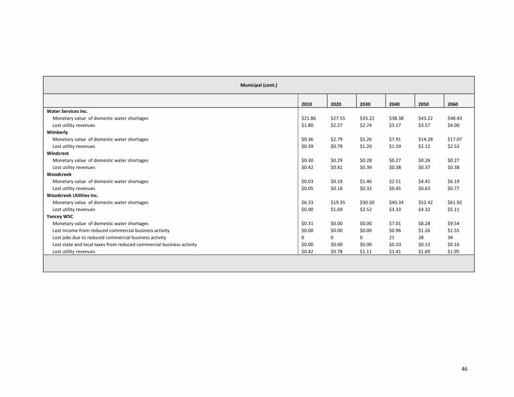
46
Municipal (cont.)
2010 2020 2030 2040 2050 2060 Water Services Inc.
Monetary value of domestic water shortages $21.86 $27.55 $33.22 $38.38 $43.22 $48.43 Lost utility revenues $1.80 $2.27 $2.74 $3.17 $3.57 $4.00
Wimberly Monetary value of domestic water shortages $0.36 $2.79 $5.26 $7.91 $14.28 $17.07 Lost utility revenues $0.39 $0.79 $1.20 $1.59 $2.12 $2.53
Windcrest Monetary value of domestic water shortages $0.30 $0.29 $0.28 $0.27 $0.26 $0.27 Lost utility revenues $0.42 $0.41 $0.39 $0.38 $0.37 $0.38
Woodcreek Monetary value of domestic water shortages $0.03 $0.19 $1.46 $2.51 $4.41 $6.19 Lost utility revenues $0.05 $0.18 $0.32 $0.45 $0.63 $0.77
Woodcreek Utilities Inc. Monetary value of domestic water shortages $6.33 $19.35 $30.50 $40.34 $52.42 $61.92 Lost utility revenues $0.90 $1.69 $2.52 $3.33 $4.32 $5.11
Yancey WSC Monetary value of domestic water shortages $0.31 $0.00 $0.00 $7.01 $8.28 $9.54 Lost income from reduced commercial business activity $0.00 $0.00 $0.00 $0.96 $1.26 $1.55 Lost jobs due to reduced commercial business activity 0 0 0 21 28 34 Lost state and local taxes from reduced commercial business activity $0.00 $0.00 $0.00 $0.10 $0.13 $0.16 Lost utility revenues $0.42 $0.78 $1.11 $1.41 $1.69 $1.95

Stuart D. Norvell, Managing Economist Water Resources Planning Division Texas Water Development Board Austin, Texas S. Doug Shaw, Agricultural Economist Water Resources Planning Division Texas Water Development Board Austin, Texas June 2010
Socioeconomic Impacts of Projected Water Shortages for the
Rio Grande Regional Water Planning Area (Region M)
Prepared in Support of the 2011 Rio Grande Regional Water Plan
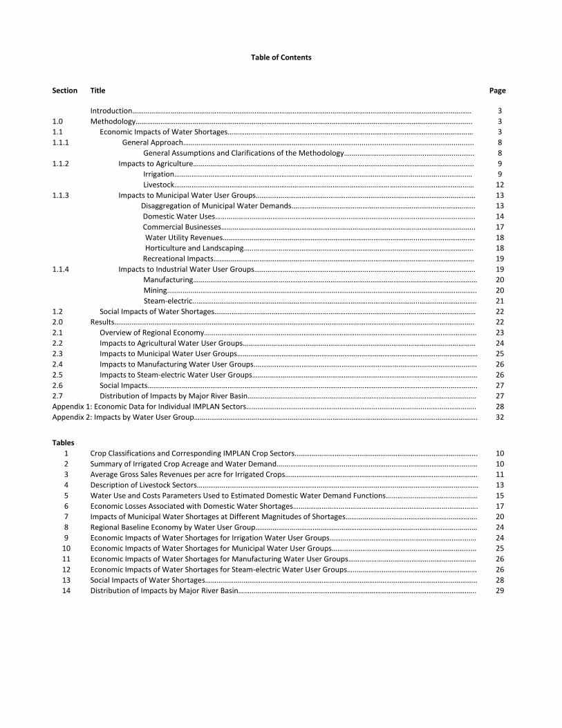
Table of Contents
Section Title Page
Introduction……………..………………………………………………………………………………………………………………………..…………………… 3
1.0 Methodology……………………………………………………………………………………………….……………………………………..…................... 3
1.1 Economic Impacts of Water Shortages………………………………………………………………………………………………………………… 3
1.1.1 General Approach……………………………………………………….................................................................................. 8
General Assumptions and Clarifications of the Methodology.…….…….……………………….……….…........... 8
1.1.2 Impacts to Agriculture……………………………………………………………………………………………………..……………............... 9
Irrigation………………………………..………………….……………………………………………………………………..….………… 9
Livestock…………………………………..……………………………………………………………………………………………..……… 12
1.1.3 Impacts to Municipal Water User Groups……………………..…………………………………………………………….…….………… 13
Disaggregation of Municipal Water Demands.………………………………………………………….……….……………... 13
Domestic Water Uses……………………………………………………………………….………..………….………………………... 14
Commercial Businesses……………………………………………………………………………….………..……………….………... 17
Water Utility Revenues………….……………………………………………………………………………....………………………. 18
Horticulture and Landscaping.….………………………………………………………………………………….………………... 18
Recreational Impacts…………………………………………………………………………….……………………………….………… 19
1.1.4 Impacts to Industrial Water User Groups……………………………………………………….……………………………………………. 19
Manufacturing………………………………………………………………………………………………………………..………………… 20
Mining..………..….……………………………………………………………………………………………………..……………………….. 20
Steam-electric..…………………………………………………………………………………………….………..………………………… 21
1.2 Social Impacts of Water Shortages……………………………………………………………………………………………..………………………… 22
2.0 Results………………………………………………………………………………………………………………………………………………………….………….. 22
2.1 Overview of Regional Economy……………………….…………………………………………………………………………………….……………… 23
2.2 Impacts to Agricultural Water User Groups……………………………………………………………………………………………..…………… 24
2.3 Impacts to Municipal Water User Groups……..……………………………………………………………………………………….……………… 25
2.4 Impacts to Manufacturing Water User Groups.………………………………………………………………………………………………..…… 26
2.5 Impacts to Steam-electric Water User Groups………………………………………………………………………….………...………………… 26
2.6 Social Impacts……………………………………………………………………………………………………………………………….…………..………….. 27
2.7 Distribution of Impacts by Major River Basin……………………………………………………………………………….……………….………. 27
Appendix 1: Economic Data for Individual IMPLAN Sectors…………………………………………………………………………….......…………………….. 28
Appendix 2: Impacts by Water User Group…………………………….………………………….....………………..………………………….………………………. 32
Tables
1 Crop Classifications and Corresponding IMPLAN Crop Sectors…………………………………………………………………………………... 10
2 Summary of Irrigated Crop Acreage and Water Demand….…………………………..………………………………………………………...… 10
3 Average Gross Sales Revenues per acre for Irrigated Crops………………………………………………………………………………….……. 11
4 Description of Livestock Sectors…………………………………………………………………………………………………………………………….…… 13
5 Water Use and Costs Parameters Used to Estimated Domestic Water Demand Functions………………………………………… 15
6 Economic Losses Associated with Domestic Water Shortages……………………………………………………………………………………. 17
7 Impacts of Municipal Water Shortages at Different Magnitudes of Shortages…………………………………………..………………. 20
8 Regional Baseline Economy by Water User Group………………………….….……………………………………………………………..…….… 24
9 Economic Impacts of Water Shortages for Irrigation Water User Groups……………………………………………….……………….… 24
10 Economic Impacts of Water Shortages for Municipal Water User Groups……………………………………………….………………… 25
11 Economic Impacts of Water Shortages for Manufacturing Water User Groups…………………………………….…………………… 26
12 Economic Impacts of Water Shortages for Steam-electric Water User Groups…..……………………………………………………… 26
13 Social Impacts of Water Shortages………………..…………………………………………………………………………………………………………… 28
14 Distribution of Impacts by Major River Basin…………………………………………………………………………………………………………….. 29
3
Introduction
Water shortages during drought would likely curtail or eliminate economic activity in business
and industries reliant on water. For example, without water farmers cannot irrigate; refineries cannot produce gasoline, and paper mills cannot make paper. Unreliable water supplies would not only have an immediate and real impact on existing businesses and industry, but they could also adversely affect economic development in Texas. From a social perspective, water supply reliability is critical as well. Shortages would disrupt activity in homes, schools and government and could adversely affect public health and safety. For all of the above reasons, it is important to analyze and understand how restricted water supplies during drought could affect communities throughout the state.
Administrative rules require that regional water planning groups evaluate the impacts of not
meeting water needs as part of the regional water planning process, and rules direct TWDB staff to provide technical assistance: “The executive administrator shall provide available technical assistance to the regional water planning groups, upon request, on water supply and demand analysis, including methods to evaluate the social and economic impacts of not meeting needs” [(§357.7 (4)(A)]. Staff of the TWDB’s Water Resources Planning Division designed and conducted this report in support of the Rio Grande Regional Water Planning Group (Region M).
This document summarizes the results of our analysis and discusses the methodology used to generate the results. Section 1 outlines the overall methodology and discusses approaches and assumptions specific to each water use category (i.e., irrigation, livestock, mining, steam-electric, municipal and manufacturing). Section 2 presents the results for each category where shortages are reported at the regional planning area level and river basin level. Results for individual water user groups are not presented, but are available upon request.
1. Methodology
Section 1 provides a general overview of how economic and social impacts were measured. In addition, it summarizes important clarifications, assumptions and limitations of the study.
1.1 Economic Impacts of Water Shortages
1.1.1 General Approach
Economic analysis as it relates to water resources planning generally falls into two broad areas. Supply side analysis focuses on costs and alternatives of developing new water supplies or implementing programs that provide additional water from current supplies. Demand side analysis concentrates on impacts or benefits of providing water to people, businesses and the environment. Analysis in this report focuses strictly on demand side impacts. When analyzing the economic impacts of water shortages as defined in Texas water planning, three potential scenarios are possible:
1) Scenario 1 involves situations where there are physical shortages of raw surface or groundwater due to drought of record conditions. For example, City A relies on a reservoir with average conservation storage of 500 acre-feet per year and a firm yield of 100 acre feet. In 2010, the city uses about 50 acre-feet per year, but by 2030 their demands are expected to increase to 200 acre-feet. Thus, in 2030 the reservoir would not have enough water to meet the city’s demands,
4
and people would experience a shortage of 100 acre-feet assuming drought of record conditions. Under normal or average climatic conditions, the reservoir would likely be able to provide reliable water supplies well beyond 2030.
2) Scenario 2 is a situation where despite drought of record conditions, water supply sources can meet existing use requirements; however, limitations in water infrastructure would preclude future water user groups from accessing these water supplies. For example, City B relies on a river that can provide 500 acre-feet per year during drought of record conditions and other constraints as dictated by planning assumptions. In 2010, the city is expected to use an estimated 100 acre-feet per year and by 2060 it would require no more than 400 acre-feet. But the intake and pipeline that currently transfers water from the river to the city’s treatment plant has a capacity of only 200 acre-feet of water per year. Thus, the city’s water supplies are adequate even under the most restrictive planning assumptions, but their conveyance system is too small. This implies that at some point – perhaps around 2030 - infrastructure limitations would constrain future population growth and any associated economic activity or impacts.
3) Scenario 3 involves water user groups that rely primarily on aquifers that are being depleted. In this scenario, projected and in some cases existing demands may be unsustainable as groundwater levels decline. Areas that rely on the Ogallala aquifer are a good example. In some communities in the region, irrigated agriculture forms a major base of the regional economy. With less irrigation water from the Ogallala, population and economic activity in the region could decline significantly assuming there are no offsetting developments.
Assessing the social and economic effects of each of the above scenarios requires various levels
and methods of analysis and would generate substantially different results for a number of reasons; the most important of which has to do with the time frame of each scenario. Scenario 1 falls into the general category of static analysis. This means that models would measure impacts for a small interval of time such as a drought. Scenarios 2 and 3, on the other hand imply a dynamic analysis meaning that models are concerned with changes over a much longer time period.
Since administrative rules specify that planning analysis be evaluated under drought of record conditions (a static and random event), socioeconomic impact analysis developed by the TWDB for the state water plan is based on assumptions of Scenario 1. Estimated impacts under scenario 1 are point estimates for years in which needs are reported (2010, 2020, 2030, 2040, 2050 and 2060). They are independent and distinct “what if” scenarios for a particular year and shortages are assumed to be temporary events resulting from drought of record conditions. Estimated impacts measure what would happen if water user groups experience water shortages for a period of one year.
The TWDB recognize that dynamic models may be more appropriate for some water user groups; however, combining approaches on a statewide basis poses several problems. For one, it would require a complex array of analyses and models, and might require developing supply and demand forecasts under “normal” climatic conditions as opposed to drought of record conditions. Equally important is the notion that combining the approaches would produce inconsistent results across regions resulting in a so-called “apples to oranges” comparison.
A variety tools are available to estimate economic impacts, but by far, the most widely used today are input-output models (IO models) combined with social accounting matrices (SAMs). Referred to as IO/SAM models, these tools formed the basis for estimating economic impacts for agriculture (irrigation and livestock water uses) and industry (manufacturing, mining, steam-electric and commercial business activity for municipal water uses).
5
Since the planning horizon extends through 2060, economic variables in the baseline are adjusted in accordance with projected changes in demographic and economic activity. Growth rates for municipal water use sectors (i.e., commercial, residential and institutional) are based on TWDB population forecasts. Future values for manufacturing, agriculture, and mining and steam-electric activity are based on the same underlying economic forecasts used to estimate future water use for each category. The following steps outline the overall process. Step 1: Generate IO/SAM Models and Develop Economic Baseline
IO/SAM models were estimated using propriety software known as IMPLAN PRO
TM (Impact for
Planning Analysis). IMPLAN is a modeling system originally developed by the U.S. Forestry Service in the late 1970s. Today, the Minnesota IMPLAN Group (MIG Inc.) owns the copyright and distributes data and software. It is probably the most widely used economic impact model in existence. IMPLAN comes with databases containing the most recently available economic data from a variety of sources.
1 Using IMPLAN
software and data, transaction tables conceptually similar to the one discussed previously were estimated for each county in the region and for the region as a whole. Each transaction table contains 528 economic sectors and allows one to estimate a variety of economic statistics including:
total sales - total production measured by sales revenues;
intermediate sales - sales to other businesses and industries within a given region;
final sales – sales to end users in a region and exports out of a region;
employment - number of full and part-time jobs (annual average) required by a given industry including self-employment;
regional income - total payroll costs (wages and salaries plus benefits) paid by industries, corporate income, rental income and interest payments; and
business taxes - sales, excise, fees, licenses and other taxes paid during normal operation of an industry (does not include income taxes).
TWDB analysts developed an economic baseline containing each of the above variables using
year 2000 data. Since the planning horizon extends through 2060, economic variables in the baseline were allowed to change in accordance with projected changes in demographic and economic activity. Growth rates for municipal water use sectors (i.e., commercial, residential and institutional) are based on TWDB population forecasts. Projections for manufacturing, agriculture, and mining and steam-electric activity are based on the same underlying economic forecasts used to estimate future water use for each category. Monetary impacts in future years are reported in constant year 2006 dollars.
It is important to stress that employment, income and business taxes are the most useful
variables when comparing the relative contribution of an economic sector to a regional economy. Total sales as reported in IO/SAM models are less desirable and can be misleading because they include sales to other industries in the region for use in the production of other goods. For example, if a mill buys grain from local farmers and uses it to produce feed, sales of both the processed feed and raw corn are counted as “output” in an IO model. Thus, total sales double-count or overstate the true economic value of goods
1The IMPLAN database consists of national level technology matrices based on benchmark input-output accounts generated by the U.S. Bureau of Economic Analysis and estimates of final demand, final payments, industry output and employment for various economic sectors. IMPLAN regional data (i.e. states, a counties or groups of counties within a state) are divided into two basic categories: 1) data on an industry basis including value-added, output and employment, and 2) data on a commodity basis including final demands and institutional sales. State-level data are balanced to national totals using a matrix ratio allocation system and county data are balanced to state totals.
6
and services produced in an economy. They are not consistent with commonly used measures of output such as Gross National Product (GNP), which counts only final sales.
Another important distinction relates to terminology. Throughout this report, the term sector refers to economic subdivisions used in the IMPLAN database and resultant input-output models (528 individual sectors based on Standard Industrial Classification Codes). In contrast, the phrase water use category refers to water user groups employed in state and regional water planning including irrigation, livestock, mining, municipal, manufacturing and steam electric. Each IMPLAN sector was assigned to a specific water use category.
Step 2: Estimate Direct and Indirect Economic Impacts of Water Needs Direct impacts are reductions in output by sectors experiencing water shortages. For example,
without adequate cooling and process water a refinery would have to curtail or cease operation, car washes may close, or farmers may not be able to irrigate and sales revenues fall. Indirect impacts involve changes in inter-industry transactions as supplying industries respond to decreased demands for their services, and how seemingly non-related businesses are affected by decreased incomes and spending due to direct impacts. For example, if a farmer ceases operations due to a lack of irrigation water, they would likely reduce expenditures on supplies such as fertilizer, labor and equipment, and businesses that provide these goods would suffer as well.
Direct impacts accrue to immediate businesses and industries that rely on water and without
water industrial processes could suffer. However, output responses may vary depending upon the severity of shortages. A small shortage relative to total water use would likely have a minimal impact, but large shortages could be critical. For example, farmers facing small shortages might fallow marginally productive acreage to save water for more valuable crops. Livestock producers might employ emergency culling strategies, or they may consider hauling water by truck to fill stock tanks. In the case of manufacturing, a good example occurred in the summer of 1999 when Toyota Motor Manufacturing experienced water shortages at a facility near Georgetown, Kentucky.
2 As water levels in the Kentucky
River fell to historic lows due to drought, plant managers sought ways to curtail water use such as reducing rinse operations to a bare minimum and recycling water by funneling it from paint shops to boilers. They even considered trucking in water at a cost of 10 times what they were paying. Fortunately, rains at the end of the summer restored river levels, and Toyota managed to implement cutbacks without affecting production, but it was a close call. If rains had not replenished the river, shortages could have severely reduced output.
3
To account for uncertainty regarding the relative magnitude of impacts to farm and business
operations, the following analysis employs the concept of elasticity. Elasticity is a number that shows how a change in one variable will affect another. In this case, it measures the relationship between a percentage reduction in water availability and a percentage reduction in output. For example, an elasticity of 1.0 indicates that a 1.0 percent reduction in water availability would result in a 1.0 percent reduction in economic output. An elasticity of 0.50 would indicate that for every 1.0 percent of unavailable water, output is reduced by 0.50 percent and so on. Output elasticities used in this study are:
4
2 Royal, W. “High And Dry - Industrial Centers Face Water Shortages.” in Industry Week, Sept, 2000. 3 The efforts described above are not planned programmatic or long-term operational changes. They are emergency measures that individuals might pursue to alleviate what they consider a temporary condition. Thus, they are not characteristic of long-term management strategies designed to ensure more dependable water supplies such as capital investments in conservation technology or development of new water supplies. 4 Elasticities are based on one of the few empirical studies that analyze potential relationships between economic output and water shortages in the United States. The study, conducted in California, showed that a significant number of industries would suffer reduced output during water shortages. Using a survey based approach researchers posed two scenarios to different industries. In
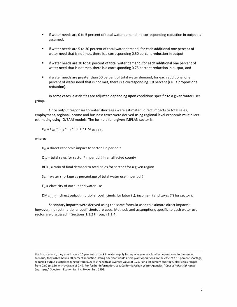
7
if water needs are 0 to 5 percent of total water demand, no corresponding reduction in output is
assumed; if water needs are 5 to 30 percent of total water demand, for each additional one percent of
water need that is not met, there is a corresponding 0.50 percent reduction in output; if water needs are 30 to 50 percent of total water demand, for each additional one percent of
water need that is not met, there is a corresponding 0.75 percent reduction in output; and
if water needs are greater than 50 percent of total water demand, for each additional one percent of water need that is not met, there is a corresponding 1.0 percent (i.e., a proportional reduction).
In some cases, elasticities are adjusted depending upon conditions specific to a given water user group.
Once output responses to water shortages were estimated, direct impacts to total sales,
employment, regional income and business taxes were derived using regional level economic multipliers estimating using IO/SAM models. The formula for a given IMPLAN sector is:
Di,t = Q i,t *, S i,t * EQ * RFDi * DM i(Q, L, I, T )
where:
Di,t = direct economic impact to sector i in period t Q i,t = total sales for sector i in period t in an affected county RFD i, = ratio of final demand to total sales for sector i for a given region S i,t = water shortage as percentage of total water use in period t EQ = elasticity of output and water use DM i(L, I, T ) = direct output multiplier coefficients for labor (L), income (I) and taxes (T) for sector i.
Secondary impacts were derived using the same formula used to estimate direct impacts;
however, indirect multiplier coefficients are used. Methods and assumptions specific to each water use sector are discussed in Sections 1.1.2 through 1.1.4.
the first scenario, they asked how a 15 percent cutback in water supply lasting one year would affect operations. In the second scenario, they asked how a 30 percent reduction lasting one year would affect plant operations. In the case of a 15 percent shortage, reported output elasticities ranged from 0.00 to 0.76 with an average value of 0.25. For a 30 percent shortage, elasticities ranged from 0.00 to 1.39 with average of 0.47. For further information, see, California Urban Water Agencies, “Cost of Industrial Water Shortages,” Spectrum Economics, Inc. November, 1991.
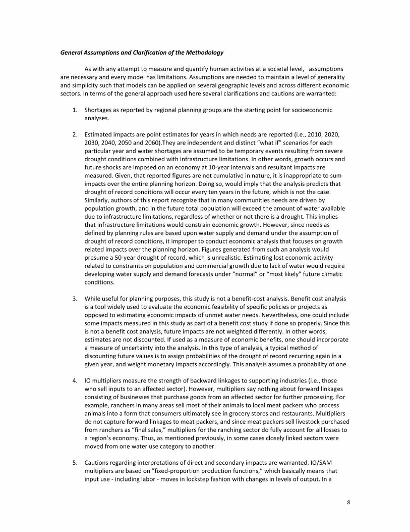
8
General Assumptions and Clarification of the Methodology
As with any attempt to measure and quantify human activities at a societal level, assumptions are necessary and every model has limitations. Assumptions are needed to maintain a level of generality and simplicity such that models can be applied on several geographic levels and across different economic sectors. In terms of the general approach used here several clarifications and cautions are warranted:
1. Shortages as reported by regional planning groups are the starting point for socioeconomic analyses.
2. Estimated impacts are point estimates for years in which needs are reported (i.e., 2010, 2020,
2030, 2040, 2050 and 2060).They are independent and distinct “what if” scenarios for each particular year and water shortages are assumed to be temporary events resulting from severe drought conditions combined with infrastructure limitations. In other words, growth occurs and future shocks are imposed on an economy at 10-year intervals and resultant impacts are measured. Given, that reported figures are not cumulative in nature, it is inappropriate to sum impacts over the entire planning horizon. Doing so, would imply that the analysis predicts that drought of record conditions will occur every ten years in the future, which is not the case. Similarly, authors of this report recognize that in many communities needs are driven by population growth, and in the future total population will exceed the amount of water available due to infrastructure limitations, regardless of whether or not there is a drought. This implies that infrastructure limitations would constrain economic growth. However, since needs as defined by planning rules are based upon water supply and demand under the assumption of drought of record conditions, it improper to conduct economic analysis that focuses on growth related impacts over the planning horizon. Figures generated from such an analysis would presume a 50-year drought of record, which is unrealistic. Estimating lost economic activity related to constraints on population and commercial growth due to lack of water would require developing water supply and demand forecasts under “normal” or “most likely” future climatic conditions.
3. While useful for planning purposes, this study is not a benefit-cost analysis. Benefit cost analysis
is a tool widely used to evaluate the economic feasibility of specific policies or projects as opposed to estimating economic impacts of unmet water needs. Nevertheless, one could include some impacts measured in this study as part of a benefit cost study if done so properly. Since this is not a benefit cost analysis, future impacts are not weighted differently. In other words, estimates are not discounted. If used as a measure of economic benefits, one should incorporate a measure of uncertainty into the analysis. In this type of analysis, a typical method of discounting future values is to assign probabilities of the drought of record recurring again in a given year, and weight monetary impacts accordingly. This analysis assumes a probability of one.
4. IO multipliers measure the strength of backward linkages to supporting industries (i.e., those
who sell inputs to an affected sector). However, multipliers say nothing about forward linkages consisting of businesses that purchase goods from an affected sector for further processing. For example, ranchers in many areas sell most of their animals to local meat packers who process animals into a form that consumers ultimately see in grocery stores and restaurants. Multipliers do not capture forward linkages to meat packers, and since meat packers sell livestock purchased from ranchers as “final sales,” multipliers for the ranching sector do fully account for all losses to a region’s economy. Thus, as mentioned previously, in some cases closely linked sectors were moved from one water use category to another.
5. Cautions regarding interpretations of direct and secondary impacts are warranted. IO/SAM
multipliers are based on ”fixed-proportion production functions,” which basically means that input use - including labor - moves in lockstep fashion with changes in levels of output. In a
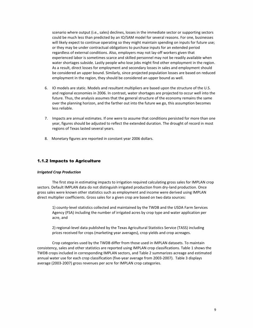
9
scenario where output (i.e., sales) declines, losses in the immediate sector or supporting sectors could be much less than predicted by an IO/SAM model for several reasons. For one, businesses will likely expect to continue operating so they might maintain spending on inputs for future use; or they may be under contractual obligations to purchase inputs for an extended period regardless of external conditions. Also, employers may not lay-off workers given that experienced labor is sometimes scarce and skilled personnel may not be readily available when water shortages subside. Lastly people who lose jobs might find other employment in the region. As a result, direct losses for employment and secondary losses in sales and employment should be considered an upper bound. Similarly, since projected population losses are based on reduced employment in the region, they should be considered an upper bound as well.
6. IO models are static. Models and resultant multipliers are based upon the structure of the U.S.
and regional economies in 2006. In contrast, water shortages are projected to occur well into the future. Thus, the analysis assumes that the general structure of the economy remains the same over the planning horizon, and the farther out into the future we go, this assumption becomes less reliable.
7. Impacts are annual estimates. If one were to assume that conditions persisted for more than one
year, figures should be adjusted to reflect the extended duration. The drought of record in most regions of Texas lasted several years.
8. Monetary figures are reported in constant year 2006 dollars.
1.1.2 Impacts to Agriculture
Irrigated Crop Production
The first step in estimating impacts to irrigation required calculating gross sales for IMPLAN crop sectors. Default IMPLAN data do not distinguish irrigated production from dry-land production. Once gross sales were known other statistics such as employment and income were derived using IMPLAN direct multiplier coefficients. Gross sales for a given crop are based on two data sources:
1) county-level statistics collected and maintained by the TWDB and the USDA Farm Services Agency (FSA) including the number of irrigated acres by crop type and water application per acre, and 2) regional-level data published by the Texas Agricultural Statistics Service (TASS) including prices received for crops (marketing year averages), crop yields and crop acreages. Crop categories used by the TWDB differ from those used in IMPLAN datasets. To maintain
consistency, sales and other statistics are reported using IMPLAN crop classifications. Table 1 shows the TWDB crops included in corresponding IMPLAN sectors, and Table 2 summarizes acreage and estimated annual water use for each crop classification (five-year average from 2003-2007). Table 3 displays average (2003-2007) gross revenues per acre for IMPLAN crop categories.
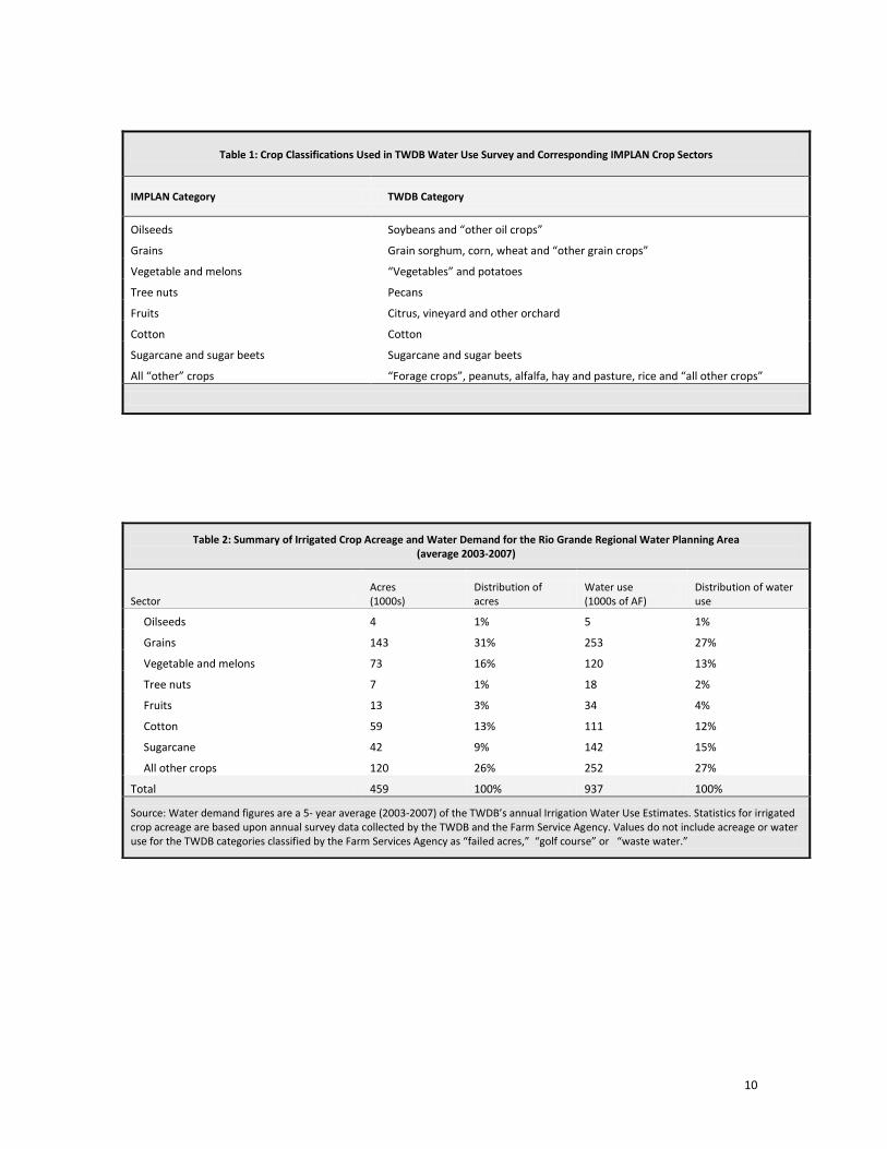
10
Table 1: Crop Classifications Used in TWDB Water Use Survey and Corresponding IMPLAN Crop Sectors
IMPLAN Category TWDB Category
Oilseeds Soybeans and “other oil crops”
Grains Grain sorghum, corn, wheat and “other grain crops”
Vegetable and melons “Vegetables” and potatoes
Tree nuts Pecans
Fruits Citrus, vineyard and other orchard
Cotton Cotton
Sugarcane and sugar beets Sugarcane and sugar beets
All “other” crops “Forage crops”, peanuts, alfalfa, hay and pasture, rice and “all other crops”
Table 2: Summary of Irrigated Crop Acreage and Water Demand for the Rio Grande Regional Water Planning Area (average 2003-2007)
Sector Acres (1000s)
Distribution of acres
Water use (1000s of AF)
Distribution of water use
Oilseeds 4 1% 5 1%
Grains 143 31% 253 27%
Vegetable and melons 73 16% 120 13%
Tree nuts 7 1% 18 2%
Fruits 13 3% 34 4%
Cotton 59 13% 111 12%
Sugarcane 42 9% 142 15%
All other crops 120 26% 252 27%
Total 459 100% 937 100%
Source: Water demand figures are a 5- year average (2003-2007) of the TWDB’s annual Irrigation Water Use Estimates. Statistics for irrigated crop acreage are based upon annual survey data collected by the TWDB and the Farm Service Agency. Values do not include acreage or water use for the TWDB categories classified by the Farm Services Agency as “failed acres,” “golf course” or “waste water.”
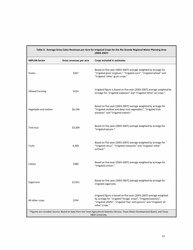
11
Table 3: Average Gross Sales Revenues per Acre for Irrigated Crops for the Rio Grande Regional Water Planning Area (2003-2007)
IMPLAN Sector Gross revenues per acre Crops included in estimates
Grains $267 Based on five-year (2003-2007) average weighted by acreage for “irrigated grain sorghum,” “irrigated corn”, “irrigated wheat” and “irrigated ‘other’ grain crops.”
Oilseed Farming $214 Irrigated figure is based on five-year (2003-2007) average weighted by acreage for “irrigated soybeans” and “irrigated ‘other’ oil crops.”
Vegetable and melons $6,246 Based on five-year (2003-2007) average weighted by acreage for “irrigated shallow and deep root vegetables”, “irrigated Irish potatoes” and “irrigated melons.”
Tree nuts $3,304 Based on five-year (2003-2007) average weighted by acreage for “irrigated pecans.”
Fruits 6,305 Based on five-year (2003-2007) average weighted by acreage for “irrigated citrus”, “irrigated vineyards” and “irrigated ‘other’ orchard.”
Cotton $389 Based on five-year (2003-2007) average weighted by acreage for “irrigated cotton.”
Sugarcane $1,051 Based on five-year (2003-2007) average weighted by acreage for irrigated sugarcane.
All other crops $254
Irrigated figure is based on five-year (2003-2007) average weighted by acreage for “irrigated ‘forage’ crops”, “irrigated peanuts”, “irrigated alfalfa”, “irrigated ‘hay’ and pasture” and “irrigated ‘all other’ crops.”
*Figures are rounded. Source: Based on data from the Texas Agricultural Statistics Service, Texas Water Development Board, and Texas A&M University.
12
An important consideration when estimating impacts to irrigation was determining which crops are affected by water shortages. One approach is the so-called rationing model, which assumes that farmers respond to water supply cutbacks by fallowing the lowest value crops in the region first and the highest valued crops last until the amount of water saved equals the shortage.5 For example, if farmer A grows vegetables (higher value) and farmer B grows wheat (lower value) and they both face a proportionate cutback in irrigation water, then farmer B will sell water to farmer A. Farmer B will fallow her irrigated acreage before farmer A fallows anything. Of course, this assumes that farmers can and do transfer enough water to allow this to happen. A different approach involves constructing farm-level profit maximization models that conform to widely-accepted economic theory that farmers make decisions based on marginal net returns. Such models have good predictive capability, but data requirements and complexity are high. Given that a detailed analysis for each region would require a substantial amount of farm-level data and analysis, the following investigation assumes that projected shortages are distributed equally across predominant crops in the region. Predominant in this case are crops that comprise at least one percent of total acreage in the region.
The following steps outline the overall process used to estimate direct impacts to irrigated
agriculture:
1. Distribute shortages across predominant crop types in the region. Again, unmet water needs were distributed equally across crop sectors that constitute one percent or more of irrigated acreage.
2. Estimate associated reductions in output for affected crop sectors. Output reductions are based
on elasticities discussed previously and on estimated values per acre for different crops. Values per acre stem from the same data used to estimate output for the year 2006 baseline. Using multipliers, we then generate estimates of forgone income, jobs, and tax revenues based on reductions in gross sales and final demand.
Livestock
The approach used for the livestock sector is basically the same as that used for crop production. As is the case with crops, livestock categorizations used by the TWDB differ from those used in IMPLAN datasets, and TWDB groupings were assigned to a given IMPLAN sector (Table 4). Then we:
1) Distribute projected water needs equally among predominant livestock sectors and estimate lost output: As is the case with irrigation, shortages are assumed to affect all livestock sectors equally; however, the category of “other” is not included given its small size. If water needs were small relative to total demands, we assume that producers would haul in water by truck to fill stock tanks. The cost per acre-foot ($24,000) is based on 2008 rates charged by various water haulers in Texas, and assumes that the average truck load is 6,500 gallons at a hauling distance of 60 miles. 3) Estimate reduced output in forward processors for livestock sectors. Reductions in output for livestock sectors are assumed to have a proportional impact on forward processors in the region such as meat packers. In other words, if the cows were gone, meat-packing plants or fluid milk manufacturers) would likely have little to process. This is not an unreasonable premise. Since the
5 The rationing model was initially proposed by researchers at the University of California at Berkeley, and was then modified for use in a study conducted by the U.S. Environmental Protection Agency that evaluated how proposed water supply cutbacks recommended to protect water quality in the Bay/Delta complex in California would affect farmers in the Central Valley. See, Zilberman, D., Howitt, R. and Sunding, D. “Economic Impacts of Water Quality Regulations in the San Francisco Bay and Delta.” Western Consortium for Public Health. May 1993.
13
1950s, there has been a major trend towards specialized cattle feedlots, which in turn has decentralized cattle purchasing from livestock terminal markets to direct sales between producers and slaughterhouses. Today, the meat packing industry often operates large processing facilities near high concentrations of feedlots to increase capacity utilization.
6 As a
result, packers are heavily dependent upon nearby feedlots. For example, a recent study by the USDA shows that on average meat packers obtain 64 percent of cattle from within 75 miles of their plant, 82 percent from within 150 miles and 92 percent from within 250 miles.
7
Table 4: Description of Livestock Sectors
IMPLAN Category TWDB Category
Cattle ranching and farming Cattle, cow calf, feedlots and dairies
Poultry and egg production Poultry production.
Other livestock Livestock other than cattle and poultry (i.e., horses, goats, sheep, hogs )
Milk manufacturing Fluid milk manufacturing, cheese manufacturing, ice cream manufacturing etc.
Meat packing Meat processing present in the region from slaughter to final processing
1.1.3 Impacts to Municipal Water User Groups
Disaggregation of Municipal Water Demands
Estimating the economic impacts for the municipal water user groups is complicated for a number of reasons. For one, municipal use comprises a range of consumers including commercial businesses, institutions such as schools and government and households. However, reported water needs are not distributed among different municipal water users. In other words, how much of a municipal need is commercial and how much is residential (domestic)?
The amount of commercial water use as a percentage of total municipal demand was estimated
based on “GED” coefficients (gallons per employee per day) published in secondary sources.8 For example,
if year 2006 baseline data for a given economic sector (e.g., amusement and recreation services) shows employment at 30 jobs and the GED coefficient is 200, then average daily water use by that sector is (30 x
6 Ferreira, W.N. “Analysis of the Meat Processing Industry in the United States.” Clemson University Extension Economics Report ER211, January 2003. 7 Ward, C.E. “Summary of Results from USDA’s Meatpacking Concentration Study.” Oklahoma Cooperative Extension Service, OSU Extension Facts WF-562.
8 Sources for GED coefficients include: Gleick, P.H., Haasz, D., Henges-Jeck, C., Srinivasan, V., Wolff, G. Cushing, K.K., and Mann, A. "Waste Not, Want Not: The Potential for Urban Water Conservation in California." Pacific Institute. November 2003. U.S. Bureau of the Census. 1982 Census of Manufacturers: Water Use in Manufacturing. USGPO, Washington D.C. See also: “U.S. Army Engineer Institute for Water Resources, IWR Report 88-R-6.,” Fort Belvoir, VA. See also, Joseph, E. S., 1982, "Municipal and Industrial Water Demands of the Western United States." Journal of the Water Resources Planning and Management Division, Proceedings of the American Society of Civil Engineers, v. 108, no. WR2, p. 204-216. See also, Baumann, D. D., Boland, J. J., and Sims, J. H., 1981, “Evaluation of Water Conservation for Municipal and Industrial Water Supply.” U.S. Army Corps of Engineers, Institute for Water Resources, Contract no. 82-C1.
14
200 = 6,000 gallons) or 6.7 acre-feet per year. Water not attributed to commercial use is considered domestic, which includes single and multi-family residential consumption, institutional uses and all use designated as “county-other.” Based on our analysis, commercial water use is about 5 to 35 percent of municipal demand. Less populated rural counties occupy the lower end of the spectrum, while larger metropolitan counties are at the higher end.
After determining the distribution of domestic versus commercial water use, we developed
methods for estimating impacts to the two groups. Domestic Water Uses
Input output models are not well suited for measuring impacts of shortages for domestic water
uses, which make up the majority of the municipal water use category. To estimate impacts associated with domestic water uses, municipal water demand and needs are subdivided into residential, and commercial and institutional use. Shortages associated with residential water uses are valued by estimating proxy demand functions for different water user groups allowing us to estimate the marginal value of water, which would vary depending upon the level of water shortages. The more severe the water shortage, the more costly it becomes. For instance, a 2 acre-foot shortage for a group of households that use 10 acre-feet per year would not be as severe as a shortage that amounted to 8 acre-feet. In the case of a 2 acre-foot shortage, households would probably have to eliminate some or all outdoor water use, which could have implicit and explicit economic costs including losses to the horticultural and landscaping industry. In the case of an 8 acre-foot shortage, people would have to forgo all outdoor water use and most indoor water consumption. Economic impacts would be much higher in the latter case because people, and would be forced to find emergency alternatives assuming alternatives were available.
To estimate the value of domestic water uses, TWDB staff developed marginal loss functions
based on constant elasticity demand curves. This is a standard and well-established method used by economists to value resources such as water that have an explicit monetary cost.
A constant price elasticity of demand is estimated using a standard equation:
w = kc(-ε)
where:
w is equal to average monthly residential water use for a given water user group measured in thousands of gallons;
k is a constant intercept;
c is the average cost of water per 1,000 gallons; and
ε is the price elasticity of demand.
Price elasticities (-0.30 for indoor water use and -0.50 for outdoor use) are based on a study by
Bell et al.9 that surveyed 1,400 water utilities in Texas that serve at least 1,000 people to estimate
demand elasticity for several variables including price, income, weather etc. Costs of water and average use per month per household are based on data from the Texas Municipal League's annual water and
9 Bell, D.R. and Griffin, R.C. “Community Water Demand in Texas as a Century is Turned.” Research contract report prepared for the Texas Water Development Board. May 2006.

15
wastewater rate surveys - specifically average monthly household expenditures on water and wastewater in different communities across the state. After examining variance in costs and usage, three different categories of water user groups based on population (population less than 5,000, cities with populations ranging from 5,000 to 99,999 and cities with populations exceeding 100,000) were selected to serve as proxy values for municipal water groups that meet the criteria (Table 5).10
Table 5: Water Use and Costs Parameters Used to Estimated Water Demand Functions (average monthly costs per acre-foot for delivered water and average monthly use per household)
Community Population Water Wastewater Total monthly cost
Avg. monthly use (gallons)
Less than or equal to 5,000 $1,335 $1,228 $2,563 6,204
5,000 to 100,000 $1,047 $1,162 $2,209 7,950
Great than or equal to 100,000 $718 $457 $1,190 8,409
Source: Based on annual water and wastewater rate surveys published by the Texas Municipal League.
As an example, Table 6 shows the economic impact per acre-foot of domestic water needs for municipal water user groups with population exceeding 100,000 people. There are several important assumptions incorporated in the calculations:
1) Reported values are net of the variable costs of treatment and distribution such as expenses for chemicals and electricity since using less water involves some savings to consumers and utilities alike; and for outdoor uses we do not include any value for wastewater. 2) Outdoor and “non-essential” water uses would be eliminated before indoor water consumption was affected, which is logical because most water utilities in Texas have drought contingency plans that generally specify curtailment or elimination of outdoor water use during droughts.11 Determining how much water is used for outdoor purposes is based on several secondary sources. The first is a major study sponsored by the American Water Works Association, which surveyed cities in states including Colorado, Oregon, Washington, California, Florida and Arizona. On average across all cities surveyed 58 percent of single family residential water use was for outdoor activities. In cities with climates comparable to large metropolitan areas of Texas, the average was 40 percent.12 Earlier findings of the U.S. Water Resources Council showed a national
10 Ideally, one would want to estimate demand functions for each individual utility in the state. However, this would require an enormous amount of time and resources. For planning purposes, we believe the values generated from aggregate data are more than sufficient. 11 In Texas, state law requires retail and wholesale water providers to prepare and submit plans to the Texas Commission on Environmental Quality (TCEQ). Plans must specify demand management measures for use during drought including curtailment of “non-essential water uses.” Non-essential uses include, but are not limited to, landscape irrigation and water for swimming pools or fountains. For further information see the Texas Environmental Quality Code §288.20. 12 See, Mayer, P.W., DeOreo, W.B., Opitz, E.M., Kiefer, J.C., Davis, W., Dziegielewski, D., Nelson, J.O. “Residential End Uses of Water.” Research sponsored by the American Water Works Association and completed by Aquacraft, Inc. and Planning and Management Consultants, Ltd. (PMCL@CDM).
16
average of 33 percent. Similarly, the United States Environmental Protection Agency (USEPA) estimated that landscape watering accounts for 32 percent of total residential and commercial water use on annual basis.13 A study conducted for the California Urban Water Agencies (CUWA) calculated average annual values ranging from 25 to 35 percent.14 Unfortunately, there does not appear to be any comprehensive research that has estimated non-agricultural outdoor water use in Texas. As an approximation, an average annual value of 30 percent based on the above references was selected to serve as a rough estimate in this study. 3) As shortages approach 100 percent values become immense and theoretically infinite at 100 percent because at that point death would result, and willingness to pay for water is immeasurable. Thus, as shortages approach 80 percent of monthly consumption, we assume that households and non-water intensive commercial businesses (those that use water only for drinking and sanitation would have water delivered by tanker truck or commercial water delivery companies. Based on reports from water companies throughout the state, we estimate that the cost of trucking in water is around $21,000 to $27,000 per acre-feet assuming a hauling distance of between 20 to 60 miles. This is not an unreasonable assumption. The practice was widespread during the 1950s drought and recently during droughts in this decade. For example, in 2000 at the heels of three consecutive drought years Electra - a small town in North Texas - was down to its last 45 days worth of reservoir water when rain replenished the lake, and the city was able to refurbish old wells to provide supplemental groundwater. At the time, residents were forced to limit water use to 1,000 gallons per person per month - less than half of what most people use - and many were having water delivered to their homes by private contractors.
15 In 2003 citizens of
Ballinger, Texas, were also faced with a dwindling water supply due to prolonged drought. After three years of drought, Lake Ballinger, which supplies water to more than 4,300 residents in Ballinger and to 600 residents in nearby Rowena, was almost dry. Each day, people lined up to get water from a well in nearby City Park. Trucks hauling trailers outfitted with large plastic and metal tanks hauled water to and from City Park to Ballinger.
16
13 U.S. Environmental Protection Agency. “Cleaner Water through Conservation.” USEPA Report no. 841-B-95-002. April, 1995. 14 Planning and Management Consultants, Ltd. “Evaluating Urban Water Conservation Programs: A Procedures Manual.” Prepared for the California Urban Water Agencies. February 1992. 15 Zewe, C. “Tap Threatens to Run Dry in Texas Town.” July 11, 2000. CNN Cable News Network. 16 Associated Press, “Ballinger Scrambles to Finish Pipeline before Lake Dries Up.” May 19, 2003.

17
Table 6: Economic Losses Associated with Domestic Water Shortages in Communities with Populations Exceeding 100,000 people
Water shortages as a percentage of total monthly household demands
No. of gallons remaining per household per day
No of gallons remaining per person per day
Economic loss (per acre-foot)
Economic loss (per gallon)
1% 278 93 $748 $0.00005
5% 266 89 $812 $0.0002
10% 252 84 $900 $0.0005
15% 238 79 $999 $0.0008
20% 224 75 $1,110 $0.0012
25% 210 70 $1,235 $0.0015
30%a 196 65 $1,699 $0.0020
35% 182 61 $3,825 $0.0085
40% 168 56 $4,181 $0.0096
45% 154 51 $4,603 $0.011
50% 140 47 $5,109 $0.012
55% 126 42 $5,727 $0.014
60% 112 37 $6,500 $0.017
65% 98 33 $7,493 $0.02
70% 84 28 $8,818 $0.02
75% 70 23 $10,672 $0.03
80% 56 19 $13,454 $0.04
85% 42 14 $18,091 ($24,000)b $0.05 ($0.07) b
90% 28 9 $27,363 ($24,000) $0.08 ($0.07)
95% 14 5 $55,182 ($24,000) $0.17 ($0.07)
99% 3 0.9 $277,728 ($24,000) $0.85 ($0.07)
99.9% 1 0.5 $2,781,377 ($24,000) $8.53 ($0.07)
100% 0 0 Infinite ($24,000) Infinite ($0.07)
a The first 30 percent of needs are assumed to be restrictions of outdoor water use; when needs reach 30 percent of total demands all outdoor water uses would be restricted. Needs greater than 30 percent include indoor use b As shortages approach 100 percent the value approaches infinity assuming there are not alternatives available; however, we assume that communities would begin to have water delivered by tanker truck at an estimated cost of $24,000 per acre-foot when shortages breached 85 percent.

18
Commercial Businesses
Effects of water shortages on commercial sectors were estimated in a fashion similar to other business sectors meaning that water shortages would affect the ability of these businesses to operate. This is particularly true for “water intensive” commercial sectors that are need large amounts of water (in addition to potable and sanitary water) to provide their services. These include:
car-washes, laundry and cleaning facilities, sports and recreation clubs and facilities including race tracks, amusement and recreation services, hospitals and medical facilities, hotels and lodging places, and eating and drinking establishments.
A key assumption is that commercial operations would not be affected until water shortages
were at least 50 percent of total municipal demand. In other words, we assume that residential water consumers would reduce water use including all non-essential uses before businesses were affected.
An example will illustrate the breakdown of municipal water needs and the overall approach to estimating impacts of municipal needs. Assume City A experiences an unexpected shortage of 50 acre-feet per year when their demands are 200 acre-feet per year. Thus, shortages are only 25 percent of total municipal use and residents of City A could eliminate needs by restricting landscape irrigation. City B, on the other hand, has a deficit of 150 acre-feet in 2020 and a projected demand of 200 acre-feet. Thus, total shortages are 75 percent of total demand. Emergency outdoor and some indoor conservation measures could eliminate 50 acre-feet of projected needs, yet 50 acre-feet would still remain. To eliminate” the remaining 50 acre-feet water intensive commercial businesses would have to curtail operations or shut down completely.
Three other areas were considered when analyzing municipal water shortages: 1) lost revenues to water utilities, 2) losses to the horticultural and landscaping industries stemming for reduction in water available for landscape irrigation, and 3) lost revenues and related economic impacts associated with reduced water related recreation. Water Utility Revenues
Estimating lost water utility revenues was straightforward. We relied on annual data from the “Water and Wastewater Rate Survey” published annually by the Texas Municipal League to calculate an average value per acre-foot for water and sewer. For water revenues, average retail water and sewer rates multiplied by total water needs served as a proxy. For lost wastewater, total unmet needs were adjusted for return flow factor of 0.60 and multiplied by average sewer rates for the region. Needs reported as “county-other” were excluded under the presumption that these consist primarily of self-supplied water uses. In addition, 15 percent of water demand and needs are considered non-billed or “unaccountable” water that comprises things such as leakages and water for municipal government functions (e.g., fire departments). Lost tax receipts are based on current rates for the “miscellaneous gross receipts tax, “which the state collects from utilities located in most incorporated cities or towns in Texas. We do not include lost water utility revenues when aggregating impacts of municipal water shortages to regional and state levels to prevent double counting.
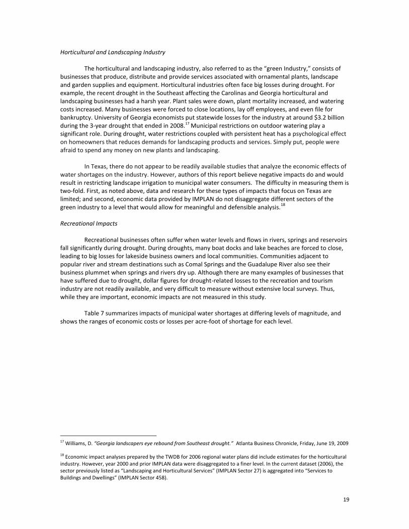
19
Horticultural and Landscaping Industry
The horticultural and landscaping industry, also referred to as the “green Industry,” consists of businesses that produce, distribute and provide services associated with ornamental plants, landscape and garden supplies and equipment. Horticultural industries often face big losses during drought. For example, the recent drought in the Southeast affecting the Carolinas and Georgia horticultural and landscaping businesses had a harsh year. Plant sales were down, plant mortality increased, and watering costs increased. Many businesses were forced to close locations, lay off employees, and even file for bankruptcy. University of Georgia economists put statewide losses for the industry at around $3.2 billion during the 3-year drought that ended in 2008.17
Municipal restrictions on outdoor watering play a significant role. During drought, water restrictions coupled with persistent heat has a psychological effect on homeowners that reduces demands for landscaping products and services. Simply put, people were afraid to spend any money on new plants and landscaping.
In Texas, there do not appear to be readily available studies that analyze the economic effects of
water shortages on the industry. However, authors of this report believe negative impacts do and would result in restricting landscape irrigation to municipal water consumers. The difficulty in measuring them is two-fold. First, as noted above, data and research for these types of impacts that focus on Texas are limited; and second, economic data provided by IMPLAN do not disaggregate different sectors of the green industry to a level that would allow for meaningful and defensible analysis.
18
Recreational Impacts
Recreational businesses often suffer when water levels and flows in rivers, springs and reservoirs fall significantly during drought. During droughts, many boat docks and lake beaches are forced to close, leading to big losses for lakeside business owners and local communities. Communities adjacent to popular river and stream destinations such as Comal Springs and the Guadalupe River also see their business plummet when springs and rivers dry up. Although there are many examples of businesses that have suffered due to drought, dollar figures for drought-related losses to the recreation and tourism industry are not readily available, and very difficult to measure without extensive local surveys. Thus, while they are important, economic impacts are not measured in this study.
Table 7 summarizes impacts of municipal water shortages at differing levels of magnitude, and shows the ranges of economic costs or losses per acre-foot of shortage for each level.
17 Williams, D. “Georgia landscapers eye rebound from Southeast drought.” Atlanta Business Chronicle, Friday, June 19, 2009 18 Economic impact analyses prepared by the TWDB for 2006 regional water plans did include estimates for the horticultural industry. However, year 2000 and prior IMPLAN data were disaggregated to a finer level. In the current dataset (2006), the sector previously listed as “Landscaping and Horticultural Services” (IMPLAN Sector 27) is aggregated into “Services to Buildings and Dwellings” (IMPLAN Sector 458).

20
Table 7: Impacts of Municipal Water Shortages at Different Magnitudes of Shortages
Water shortages as percent of total municipal demands
Impacts Economic costs per acre-foot*
0-30% Lost water utility revenues Restricted landscape irrigation and non-
essential water uses $730 - $2,040
30-50%
Lost water utility revenues Elimination of landscape irrigation and
non-essential water uses Rationing of indoor use
$2,040 - $10,970
>50%
Lost water utility revenues Elimination of landscape irrigation and
non-essential water uses Rationing of indoor use Restriction or elimination of commercial
water use Importing water by tanker truck
$10,970 - varies
*Figures are rounded
1.1.4 Industrial Water User Groups
Manufacturing
Impacts to manufacturing were estimated by distributing water shortages among industrial sectors at the county level. For example, if a planning group estimates that during a drought of record water supplies in County A would only meet 50 percent of total annual demands for manufactures in the county, we reduced output for each sector by 50 percent. Since projected manufacturing demands are based on TWDB Water Uses Survey data for each county, we only include IMPLAN sectors represented in the TWBD survey database. Some sectors in IMPLAN databases are not part of the TWDB database given that they use relatively small amounts of water - primarily for on-site sanitation and potable purposes. To maintain consistency between IMPLAN and TWDB databases, Standard Industrial Classification (SIC) codes both databases were cross referenced in county with shortages. Non-matches were excluded when calculating direct impacts.

21
Mining
The process of mining is very similar to that of manufacturing. We assume that within a given county, shortages would apply equally to relevant mining sectors, and IMPLAN sectors are cross referenced with TWDB data to ensure consistency.
In Texas, oil and gas extraction and sand and gravel (aggregates) operations are the primary
mining industries that rely on large volumes of water. For sand and gravel, estimated output reductions are straightforward; however, oil and gas is more complicated for a number of reasons. IMPLAN does not necessarily report the physical extraction of minerals by geographic local, but rather the sales revenues reported by a particular corporation.
For example, at the state level revenues for IMPLAN sector 19 (oil and gas extraction) and sector
27 (drilling oil and gas wells) totals $257 billion. Of this, nearly $85 billion is attributed to Harris County. However, only a very small fraction (less than one percent) of actual production takes place in the county. To measure actual potential losses in well head capacity due to water shortages, we relied on county level production data from the Texas Railroad Commission (TRC) and average well-head market prices for crude and gas to estimate lost revenues in a given county. After which, we used to IMPLAN ratios to estimate resultant losses in income and employment.
Other considerations with respect to mining include:
1) Petroleum and gas extraction industry only uses water in significant amounts for secondary recovery. Known in the industry as enhanced or water flood extraction, secondary recovery involves pumping water down injection wells to increase underground pressure thereby pushing oil or gas into other wells. IMPLAN output numbers do not distinguish between secondary and non-secondary recovery. To account for the discrepancy, county-level TRC data that show the proportion of barrels produced using secondary methods were used to adjust IMPLAN data to reflect only the portion of sales attributed to secondary recovery.
2) A substantial portion of output from mining operations goes directly to businesses that are classified as manufacturing in our schema. Thus, multipliers measuring backward linkages for a given manufacturer might include impacts to a supplying mining operation. Care was taken not to double count in such situations if both a mining operation and a manufacturer were reported as having water shortages.
Steam-electric
At minimum without adequate cooling water, power plants cannot safely operate. As water
availability falls below projected demands, water levels in lakes and rivers that provide cooling water would also decline. Low water levels could affect raw water intakes and outfalls at electrical generating units in several ways. For one, power plants are regulated by thermal emission guidelines that specify the maximum amount of heat that can go back into a river or lake via discharged cooling water. Low water levels could result in permit compliance issues due to reduced dilution and dispersion of heat and subsequent impacts on aquatic biota near outfalls.19 However, the primary concern would be a loss of head (i.e., pressure) over intake structures that would decrease flows through intake tunnels. This would affect safety related pumps, increase operating costs and/or result in sustained shut-downs. Assuming plants did shutdown, they would not be able to generate electricity.
19
Section 316 (b) of the Clean Water Act requires that thermal wastewater discharges do not harm fish and other wildlife.
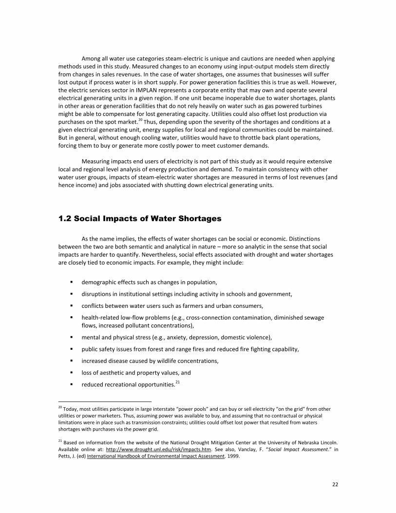
22
Among all water use categories steam-electric is unique and cautions are needed when applying
methods used in this study. Measured changes to an economy using input-output models stem directly from changes in sales revenues. In the case of water shortages, one assumes that businesses will suffer lost output if process water is in short supply. For power generation facilities this is true as well. However, the electric services sector in IMPLAN represents a corporate entity that may own and operate several electrical generating units in a given region. If one unit became inoperable due to water shortages, plants in other areas or generation facilities that do not rely heavily on water such as gas powered turbines might be able to compensate for lost generating capacity. Utilities could also offset lost production via purchases on the spot market.20
Thus, depending upon the severity of the shortages and conditions at a given electrical generating unit, energy supplies for local and regional communities could be maintained. But in general, without enough cooling water, utilities would have to throttle back plant operations, forcing them to buy or generate more costly power to meet customer demands.
Measuring impacts end users of electricity is not part of this study as it would require extensive local and regional level analysis of energy production and demand. To maintain consistency with other water user groups, impacts of steam-electric water shortages are measured in terms of lost revenues (and hence income) and jobs associated with shutting down electrical generating units.
1.2 Social Impacts of Water Shortages
As the name implies, the effects of water shortages can be social or economic. Distinctions
between the two are both semantic and analytical in nature – more so analytic in the sense that social impacts are harder to quantify. Nevertheless, social effects associated with drought and water shortages are closely tied to economic impacts. For example, they might include:
demographic effects such as changes in population,
disruptions in institutional settings including activity in schools and government,
conflicts between water users such as farmers and urban consumers,
health-related low-flow problems (e.g., cross-connection contamination, diminished sewage flows, increased pollutant concentrations),
mental and physical stress (e.g., anxiety, depression, domestic violence),
public safety issues from forest and range fires and reduced fire fighting capability,
increased disease caused by wildlife concentrations,
loss of aesthetic and property values, and
reduced recreational opportunities.21
20 Today, most utilities participate in large interstate “power pools” and can buy or sell electricity “on the grid” from other utilities or power marketers. Thus, assuming power was available to buy, and assuming that no contractual or physical limitations were in place such as transmission constraints; utilities could offset lost power that resulted from waters shortages with purchases via the power grid. 21 Based on information from the website of the National Drought Mitigation Center at the University of Nebraska Lincoln. Available online at: http://www.drought.unl.edu/risk/impacts.htm. See also, Vanclay, F. “Social Impact Assessment.” in Petts, J. (ed) International Handbook of Environmental Impact Assessment. 1999.
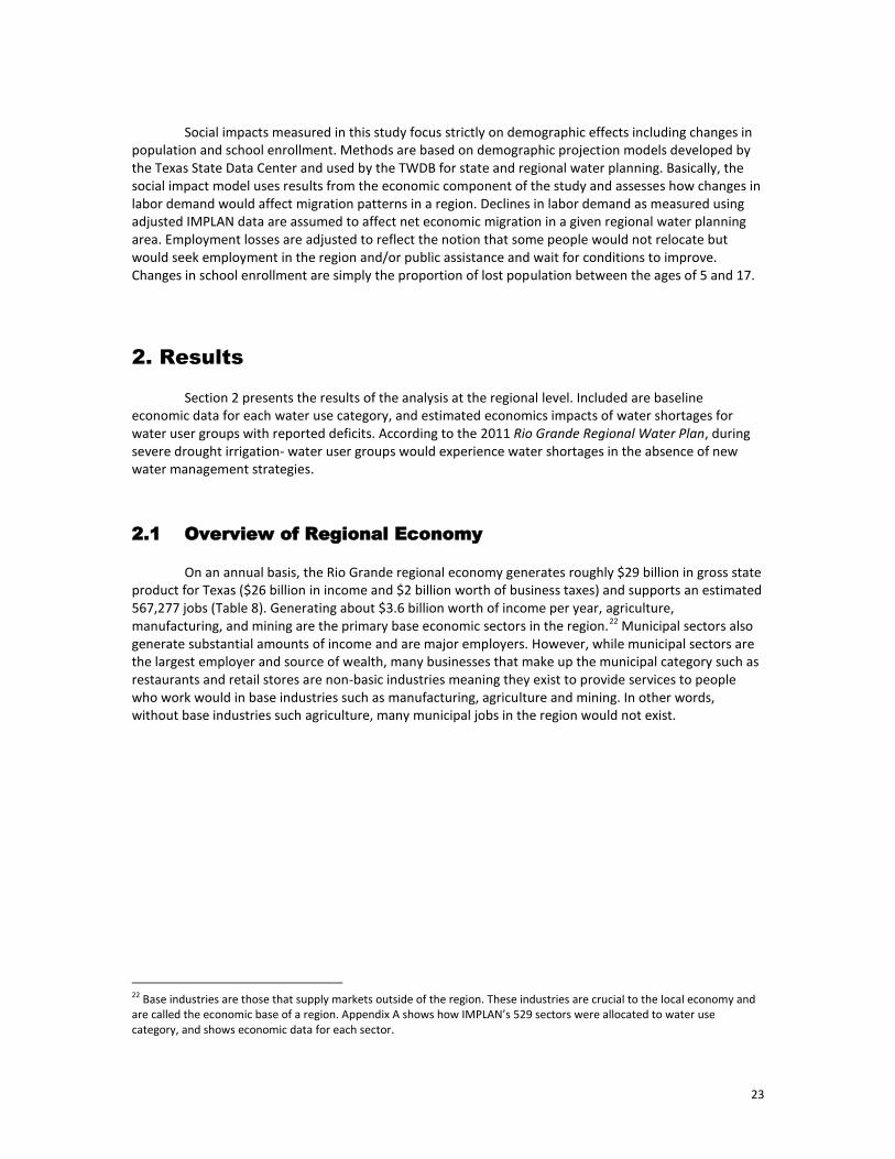
23
Social impacts measured in this study focus strictly on demographic effects including changes in
population and school enrollment. Methods are based on demographic projection models developed by the Texas State Data Center and used by the TWDB for state and regional water planning. Basically, the social impact model uses results from the economic component of the study and assesses how changes in labor demand would affect migration patterns in a region. Declines in labor demand as measured using adjusted IMPLAN data are assumed to affect net economic migration in a given regional water planning area. Employment losses are adjusted to reflect the notion that some people would not relocate but would seek employment in the region and/or public assistance and wait for conditions to improve. Changes in school enrollment are simply the proportion of lost population between the ages of 5 and 17.
2. Results
Section 2 presents the results of the analysis at the regional level. Included are baseline
economic data for each water use category, and estimated economics impacts of water shortages for water user groups with reported deficits. According to the 2011 Rio Grande Regional Water Plan, during severe drought irrigation- water user groups would experience water shortages in the absence of new water management strategies.
2.1 Overview of Regional Economy
On an annual basis, the Rio Grande regional economy generates roughly $29 billion in gross state
product for Texas ($26 billion in income and $2 billion worth of business taxes) and supports an estimated 567,277 jobs (Table 8). Generating about $3.6 billion worth of income per year, agriculture, manufacturing, and mining are the primary base economic sectors in the region.22 Municipal sectors also generate substantial amounts of income and are major employers. However, while municipal sectors are the largest employer and source of wealth, many businesses that make up the municipal category such as restaurants and retail stores are non-basic industries meaning they exist to provide services to people who work would in base industries such as manufacturing, agriculture and mining. In other words, without base industries such agriculture, many municipal jobs in the region would not exist.
22 Base industries are those that supply markets outside of the region. These industries are crucial to the local economy and are called the economic base of a region. Appendix A shows how IMPLAN’s 529 sectors were allocated to water use category, and shows economic data for each sector.

24
2.2 Impacts of Agricultural Water Shortages
According to the 2011 Rio Grande Regional Water Plan, during severe drought the counties of
Cameron, Hidalgo, Maverick, Starr, Webb, Willacy, and Zapata would experiences shortages of irrigation water. Shortages range from 28 to 45 percent of annual irrigation demands, and farmers would be short nearly 407,500 acre-feet in 2010 and 258,375 acre-feet in 2060. Shortages of these magnitudes would reduce gross state product (income plus state and local business taxes) by an estimated $126 million per year in 2010 and $50 million in 2060.
Table 8: The Rio Grande Regional Economy by Water User Group ($millions)*
Water Use Category Total sales Intermediate sales Final sales Jobs Income
Business taxes
Irrigation $587.19 $66.29 $472.13 9,576 $368.38 $8.80
Livestock $337.00 $162.43 $174.57 3,253 $28.32 $4.20
Manufacturing $7,516.54 $804.21 $6,712.33 51,443 $2,051.56 $43.87
Mining $1,489.38 $641.26 $848.12 4,822 $1,034.67 $71.02
Steam-electric $295.72 $83.19 $212.53 790 $205.34 $35.05
Municipal $36,755.66 $8,169.71 $28,585.95 497,393 $22,215.26 $1,788.13
Regional total $46,981.49 $9,927.09 $37,005.63 567,277 $25,903.53 $1,951.07 a Appendix 1 displays data for individual IMPLAN sectors that make up each water use category. Based on data from the
Texas Water Development Board, and year 2006 data from the Minnesota IMPLAN Group, Inc.
Table 9: Economic Impacts of Water Shortages for Irrigation Water User Groups ($millions)
Decade Lost income from reduced crop production a
Lost state and local tax revenues from reduced crop production
Lost jobs from reduced crop production
2010 $123.82 $2.91 1,235
2020 $62.69 $1.59 785
2030 $44.56 $1.16 613
2040 $45.79 $1.19 627
2050 $47.02 $1.22 641
2060 $48.16 $1.25 655
*Changes to income and business taxes are collectively equivalent to a decrease in gross state product, which is analogous to gross domestic product measured at the state rather than national level. Appendix 2 shows results by water user group.
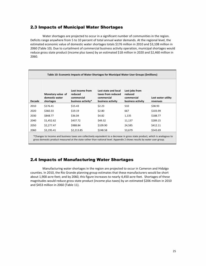
25
2.3 Impacts of Municipal Water Shortages
Water shortages are projected to occur in a significant number of communities in the region.
Deficits range anywhere from 5 to 10 percent of total annual water demands. At the regional level, the estimated economic value of domestic water shortages totals $176 million in 2010 and $3,108 million in 2060 (Table 10). Due to curtailment of commercial business activity operation, municipal shortages would reduce gross state product (income plus taxes) by an estimated $18 million in 2020 and $2,460 million in 2060.
2.4 Impacts of Manufacturing Water Shortages
Manufacturing water shortages in the region are projected to occur in Cameron and Hidalgo
counties. In 2010, the Rio Grande planning group estimates that these manufacturers would be short about 1,900 acre-feet; and by 2060, this figure increases to nearly 4,450 acre-feet. Shortages of these magnitudes would reduce gross state product (income plus taxes) by an estimated $206 million in 2010 and $453 million in 2060 (Table 11).
Table 10: Economic Impacts of Water Shortages for Municipal Water User Groups ($millions)
Decade
Monetary value of domestic water shortages
Lost income from reduced commercial business activity*
Lost state and local taxes from reduced commercial business activity
Lost jobs from reduced commercial business activity
Lost water utility revenues
2010 $176.41 $15.43 $2.23 510 $38.93
2020 $360.33 $19.19 $2.80 667 $103.99
2030 $848.77 $36.04 $4.82 1,135 $188.77
2040 $1,452.62 $437.72 $49.32 11,137 $289.15
2050 $2,277.47 $988.84 $109.90 24,585 $412.11
2060 $3,195.41 $2,213.85 $248.58 53,679 $543.69
*Changes to Income and business taxes are collectively equivalent to a decrease in gross state product, which is analogous to gross domestic product measured at the state rather than national level. Appendix 2 shows results by water user group.
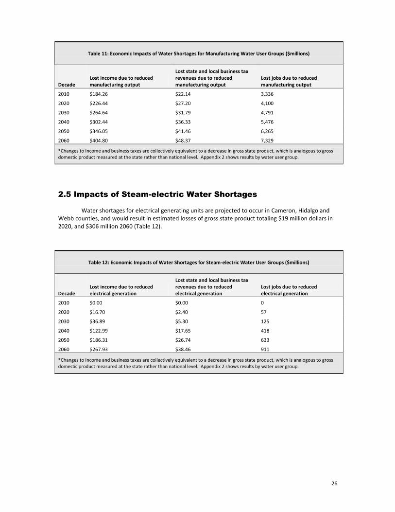
26
2.5 Impacts of Steam-electric Water Shortages
Water shortages for electrical generating units are projected to occur in Cameron, Hidalgo and Webb counties, and would result in estimated losses of gross state product totaling $19 million dollars in 2020, and $306 million 2060 (Table 12).
Table 11: Economic Impacts of Water Shortages for Manufacturing Water User Groups ($millions)
Decade Lost income due to reduced manufacturing output
Lost state and local business tax revenues due to reduced manufacturing output
Lost jobs due to reduced manufacturing output
2010 $184.26 $22.14 3,336
2020 $226.44 $27.20 4,100
2030 $264.64 $31.79 4,791
2040 $302.44 $36.33 5,476
2050 $346.05 $41.46 6,265
2060 $404.80 $48.37 7,329
*Changes to Income and business taxes are collectively equivalent to a decrease in gross state product, which is analogous to gross domestic product measured at the state rather than national level. Appendix 2 shows results by water user group.
Table 12: Economic Impacts of Water Shortages for Steam-electric Water User Groups ($millions)
Decade Lost income due to reduced electrical generation
Lost state and local business tax revenues due to reduced electrical generation
Lost jobs due to reduced electrical generation
2010 $0.00 $0.00 0
2020 $16.70 $2.40 57
2030 $36.89 $5.30 125
2040 $122.99 $17.65 418
2050 $186.31 $26.74 633
2060 $267.93 $38.46 911
*Changes to Income and business taxes are collectively equivalent to a decrease in gross state product, which is analogous to gross domestic product measured at the state rather than national level. Appendix 2 shows results by water user group.
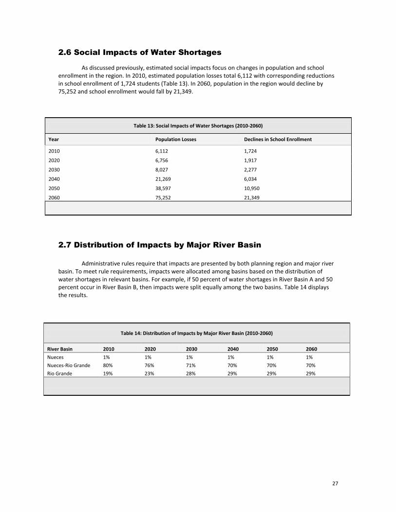
27
2.6 Social Impacts of Water Shortages
As discussed previously, estimated social impacts focus on changes in population and school enrollment in the region. In 2010, estimated population losses total 6,112 with corresponding reductions in school enrollment of 1,724 students (Table 13). In 2060, population in the region would decline by 75,252 and school enrollment would fall by 21,349.
Table 13: Social Impacts of Water Shortages (2010-2060)
Year Population Losses Declines in School Enrollment
2010 6,112 1,724
2020 6,756 1,917
2030 8,027 2,277
2040 21,269 6,034
2050 38,597 10,950
2060 75,252 21,349
2.7 Distribution of Impacts by Major River Basin
Administrative rules require that impacts are presented by both planning region and major river
basin. To meet rule requirements, impacts were allocated among basins based on the distribution of water shortages in relevant basins. For example, if 50 percent of water shortages in River Basin A and 50 percent occur in River Basin B, then impacts were split equally among the two basins. Table 14 displays the results.
Table 14: Distribution of Impacts by Major River Basin (2010-2060)
River Basin 2010 2020 2030 2040 2050 2060
Nueces 1% 1% 1% 1% 1% 1% Nueces-Rio Grande 80% 76% 71% 70% 70% 70%
Rio Grande 19% 23% 28% 29% 29% 29%
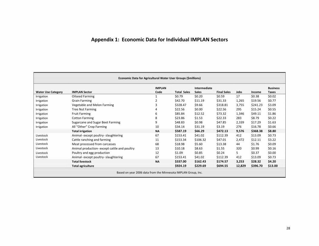
28
Appendix 1: Economic Data for Individual IMPLAN Sectors
Economic Data for Agricultural Water User Groups ($millions)
Water Use Category IMPLAN Sector IMPLAN Code Total Sales
Intermediate Sales Final Sales Jobs Income
Business Taxes
Irrigation Oilseed Farming 1 $0.79 $0.20 $0.59 17 $0.38 $0.02
Irrigation Grain Farming 2 $42.70 $11.19 $31.33 1,265 $19.56 $0.77
Irrigation Vegetable and Melon Farming 3 $328.47 $9.66 $318.81 3,755 $241.23 $3.09
Irrigation Tree Nut Farming 4 $22.56 $0.00 $22.56 295 $15.24 $0.55
Irrigation Fruit Farming 6 $85.84 $12.52 $73.32 1,346 $49.11 $1.86
Irrigation Cotton Farming 8 $23.86 $1.53 $22.33 283 $8.79 $0.22
Irrigation Sugarcane and Sugar Beet Farming 9 $48.83 $0.98 $47.85 2,339 $17.29 $1.63
Irrigation All “Other” Crop Farming 10 $34.14 $31.19 $3.19 276 $16.78 $0.66
Total irrigation NA $587.19 $66.29 $472.13 9,576 $368.38 $8.80
Livestock Animal- except poultry- slaughtering 67 $153.41 $41.02 $112.39 412 $13.09 $0.73 Livestock Cattle ranching and farming 11 $153.34 $106.32 $47.01 2,472 $12.11 $3.22 Livestock Meat processed from carcasses 68 $18.98 $5.60 $13.38 44 $1.76 $0.09 Livestock Animal production- except cattle and poultry 13 $10.18 $8.63 $1.55 320 $0.99 $0.16
Livestock Poultry and egg production 12 $1.09 $0.85 $0.24 5 $0.37 $0.00 Livestock Animal- except poultry- slaughtering 67 $153.41 $41.02 $112.39 412 $13.09 $0.73
Total livestock NA $337.00 $162.43 $174.57 3,253 $28.32 $4.20
Total agriculture $924.19 $229.69 $694.55 12,829 $396.70 $13.00
Based on year 2006 data from the Minnesota IMPLAN Group, Inc.
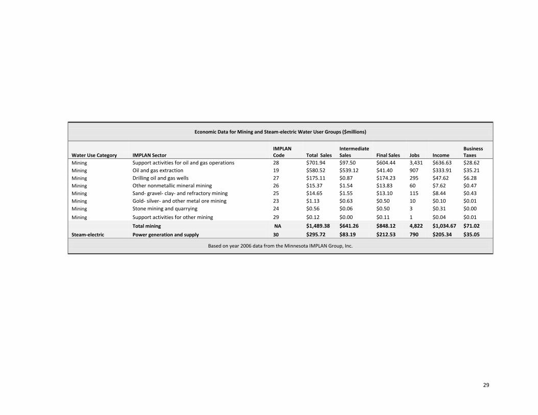
29
Economic Data for Mining and Steam-electric Water User Groups ($millions)
Water Use Category IMPLAN Sector IMPLAN Code Total Sales
Intermediate Sales Final Sales Jobs Income
Business Taxes
Mining Support activities for oil and gas operations 28 $701.94 $97.50 $604.44 3,431 $636.63 $28.62
Mining Oil and gas extraction 19 $580.52 $539.12 $41.40 907 $333.91 $35.21
Mining Drilling oil and gas wells 27 $175.11 $0.87 $174.23 295 $47.62 $6.28
Mining Other nonmetallic mineral mining 26 $15.37 $1.54 $13.83 60 $7.62 $0.47
Mining Sand- gravel- clay- and refractory mining 25 $14.65 $1.55 $13.10 115 $8.44 $0.43
Mining Gold- silver- and other metal ore mining 23 $1.13 $0.63 $0.50 10 $0.10 $0.01
Mining Stone mining and quarrying 24 $0.56 $0.06 $0.50 3 $0.31 $0.00
Mining Support activities for other mining 29 $0.12 $0.00 $0.11 1 $0.04 $0.01
Total mining NA $1,489.38 $641.26 $848.12 4,822 $1,034.67 $71.02
Steam-electric Power generation and supply 30 $295.72 $83.19 $212.53 790 $205.34 $35.05
Based on year 2006 data from the Minnesota IMPLAN Group, Inc.
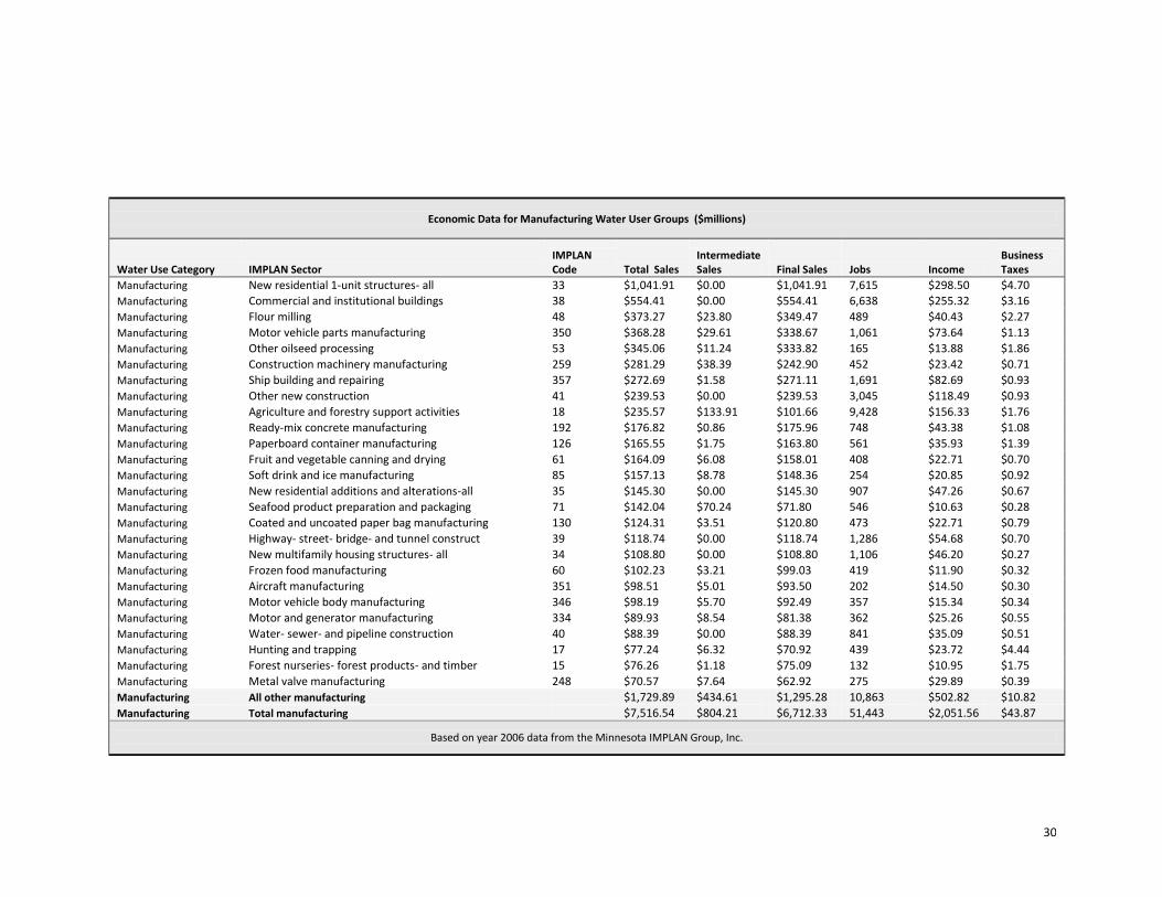
30
Economic Data for Manufacturing Water User Groups ($millions)
Water Use Category IMPLAN Sector IMPLAN Code Total Sales
Intermediate Sales Final Sales Jobs Income
Business Taxes
Manufacturing New residential 1-unit structures- all 33 $1,041.91 $0.00 $1,041.91 7,615 $298.50 $4.70
Manufacturing Commercial and institutional buildings 38 $554.41 $0.00 $554.41 6,638 $255.32 $3.16
Manufacturing Flour milling 48 $373.27 $23.80 $349.47 489 $40.43 $2.27
Manufacturing Motor vehicle parts manufacturing 350 $368.28 $29.61 $338.67 1,061 $73.64 $1.13
Manufacturing Other oilseed processing 53 $345.06 $11.24 $333.82 165 $13.88 $1.86
Manufacturing Construction machinery manufacturing 259 $281.29 $38.39 $242.90 452 $23.42 $0.71
Manufacturing Ship building and repairing 357 $272.69 $1.58 $271.11 1,691 $82.69 $0.93
Manufacturing Other new construction 41 $239.53 $0.00 $239.53 3,045 $118.49 $0.93
Manufacturing Agriculture and forestry support activities 18 $235.57 $133.91 $101.66 9,428 $156.33 $1.76
Manufacturing Ready-mix concrete manufacturing 192 $176.82 $0.86 $175.96 748 $43.38 $1.08
Manufacturing Paperboard container manufacturing 126 $165.55 $1.75 $163.80 561 $35.93 $1.39
Manufacturing Fruit and vegetable canning and drying 61 $164.09 $6.08 $158.01 408 $22.71 $0.70
Manufacturing Soft drink and ice manufacturing 85 $157.13 $8.78 $148.36 254 $20.85 $0.92
Manufacturing New residential additions and alterations-all 35 $145.30 $0.00 $145.30 907 $47.26 $0.67
Manufacturing Seafood product preparation and packaging 71 $142.04 $70.24 $71.80 546 $10.63 $0.28
Manufacturing Coated and uncoated paper bag manufacturing 130 $124.31 $3.51 $120.80 473 $22.71 $0.79
Manufacturing Highway- street- bridge- and tunnel construct 39 $118.74 $0.00 $118.74 1,286 $54.68 $0.70
Manufacturing New multifamily housing structures- all 34 $108.80 $0.00 $108.80 1,106 $46.20 $0.27
Manufacturing Frozen food manufacturing 60 $102.23 $3.21 $99.03 419 $11.90 $0.32
Manufacturing Aircraft manufacturing 351 $98.51 $5.01 $93.50 202 $14.50 $0.30
Manufacturing Motor vehicle body manufacturing 346 $98.19 $5.70 $92.49 357 $15.34 $0.34
Manufacturing Motor and generator manufacturing 334 $89.93 $8.54 $81.38 362 $25.26 $0.55
Manufacturing Water- sewer- and pipeline construction 40 $88.39 $0.00 $88.39 841 $35.09 $0.51
Manufacturing Hunting and trapping 17 $77.24 $6.32 $70.92 439 $23.72 $4.44
Manufacturing Forest nurseries- forest products- and timber 15 $76.26 $1.18 $75.09 132 $10.95 $1.75
Manufacturing Metal valve manufacturing 248 $70.57 $7.64 $62.92 275 $29.89 $0.39
Manufacturing All other manufacturing $1,729.89 $434.61 $1,295.28 10,863 $502.82 $10.82
Manufacturing Total manufacturing $7,516.54 $804.21 $6,712.33 51,443 $2,051.56 $43.87
Based on year 2006 data from the Minnesota IMPLAN Group, Inc.
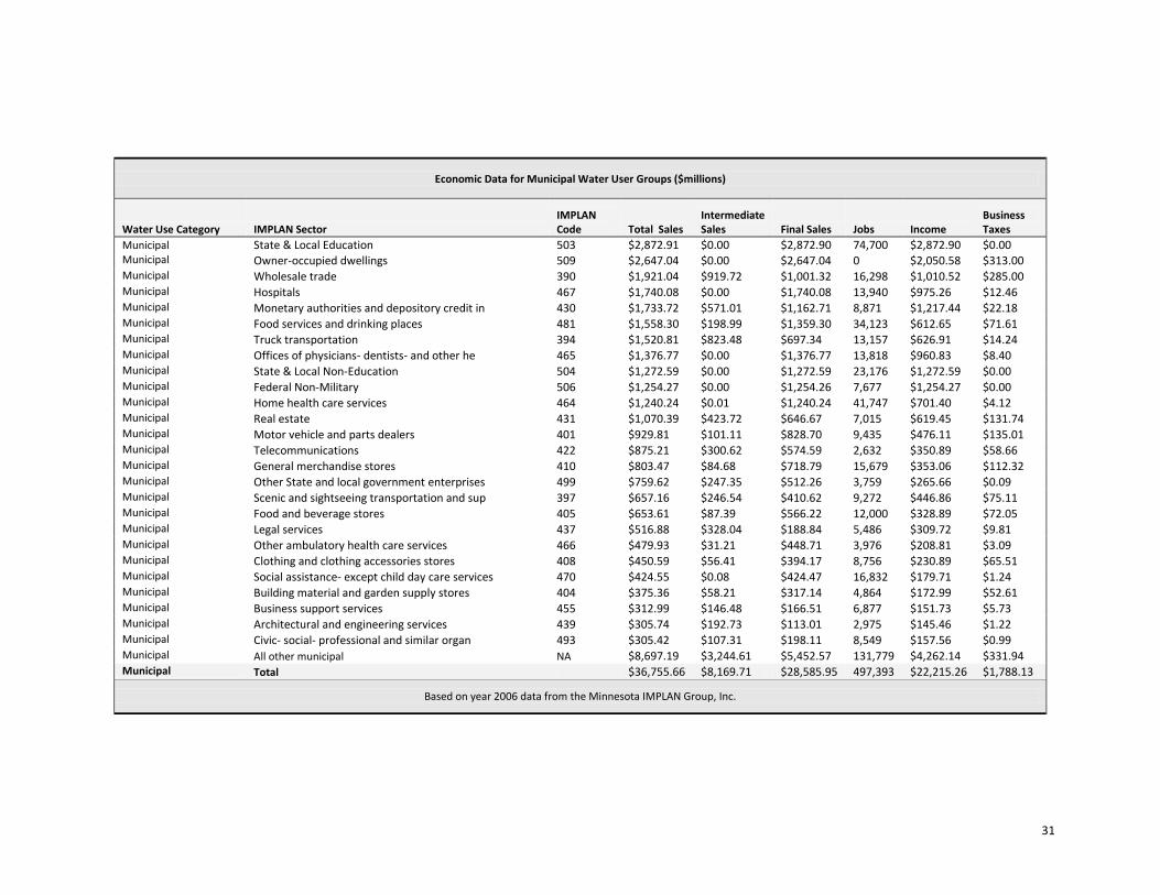
31
Economic Data for Municipal Water User Groups ($millions)
Water Use Category IMPLAN Sector IMPLAN Code Total Sales
Intermediate Sales Final Sales Jobs Income
Business Taxes
Municipal State & Local Education 503 $2,872.91 $0.00 $2,872.90 74,700 $2,872.90 $0.00 Municipal Owner-occupied dwellings 509 $2,647.04 $0.00 $2,647.04 0 $2,050.58 $313.00 Municipal Wholesale trade 390 $1,921.04 $919.72 $1,001.32 16,298 $1,010.52 $285.00 Municipal Hospitals 467 $1,740.08 $0.00 $1,740.08 13,940 $975.26 $12.46 Municipal Monetary authorities and depository credit in 430 $1,733.72 $571.01 $1,162.71 8,871 $1,217.44 $22.18 Municipal Food services and drinking places 481 $1,558.30 $198.99 $1,359.30 34,123 $612.65 $71.61 Municipal Truck transportation 394 $1,520.81 $823.48 $697.34 13,157 $626.91 $14.24 Municipal Offices of physicians- dentists- and other he 465 $1,376.77 $0.00 $1,376.77 13,818 $960.83 $8.40 Municipal State & Local Non-Education 504 $1,272.59 $0.00 $1,272.59 23,176 $1,272.59 $0.00 Municipal Federal Non-Military 506 $1,254.27 $0.00 $1,254.26 7,677 $1,254.27 $0.00 Municipal Home health care services 464 $1,240.24 $0.01 $1,240.24 41,747 $701.40 $4.12 Municipal Real estate 431 $1,070.39 $423.72 $646.67 7,015 $619.45 $131.74 Municipal Motor vehicle and parts dealers 401 $929.81 $101.11 $828.70 9,435 $476.11 $135.01 Municipal Telecommunications 422 $875.21 $300.62 $574.59 2,632 $350.89 $58.66 Municipal General merchandise stores 410 $803.47 $84.68 $718.79 15,679 $353.06 $112.32 Municipal Other State and local government enterprises 499 $759.62 $247.35 $512.26 3,759 $265.66 $0.09 Municipal Scenic and sightseeing transportation and sup 397 $657.16 $246.54 $410.62 9,272 $446.86 $75.11 Municipal Food and beverage stores 405 $653.61 $87.39 $566.22 12,000 $328.89 $72.05 Municipal Legal services 437 $516.88 $328.04 $188.84 5,486 $309.72 $9.81 Municipal Other ambulatory health care services 466 $479.93 $31.21 $448.71 3,976 $208.81 $3.09 Municipal Clothing and clothing accessories stores 408 $450.59 $56.41 $394.17 8,756 $230.89 $65.51 Municipal Social assistance- except child day care services 470 $424.55 $0.08 $424.47 16,832 $179.71 $1.24 Municipal Building material and garden supply stores 404 $375.36 $58.21 $317.14 4,864 $172.99 $52.61 Municipal Business support services 455 $312.99 $146.48 $166.51 6,877 $151.73 $5.73 Municipal Architectural and engineering services 439 $305.74 $192.73 $113.01 2,975 $145.46 $1.22 Municipal Civic- social- professional and similar organ 493 $305.42 $107.31 $198.11 8,549 $157.56 $0.99 Municipal All other municipal NA $8,697.19 $3,244.61 $5,452.57 131,779 $4,262.14 $331.94 Municipal Total $36,755.66 $8,169.71 $28,585.95 497,393 $22,215.26 $1,788.13
Based on year 2006 data from the Minnesota IMPLAN Group, Inc.
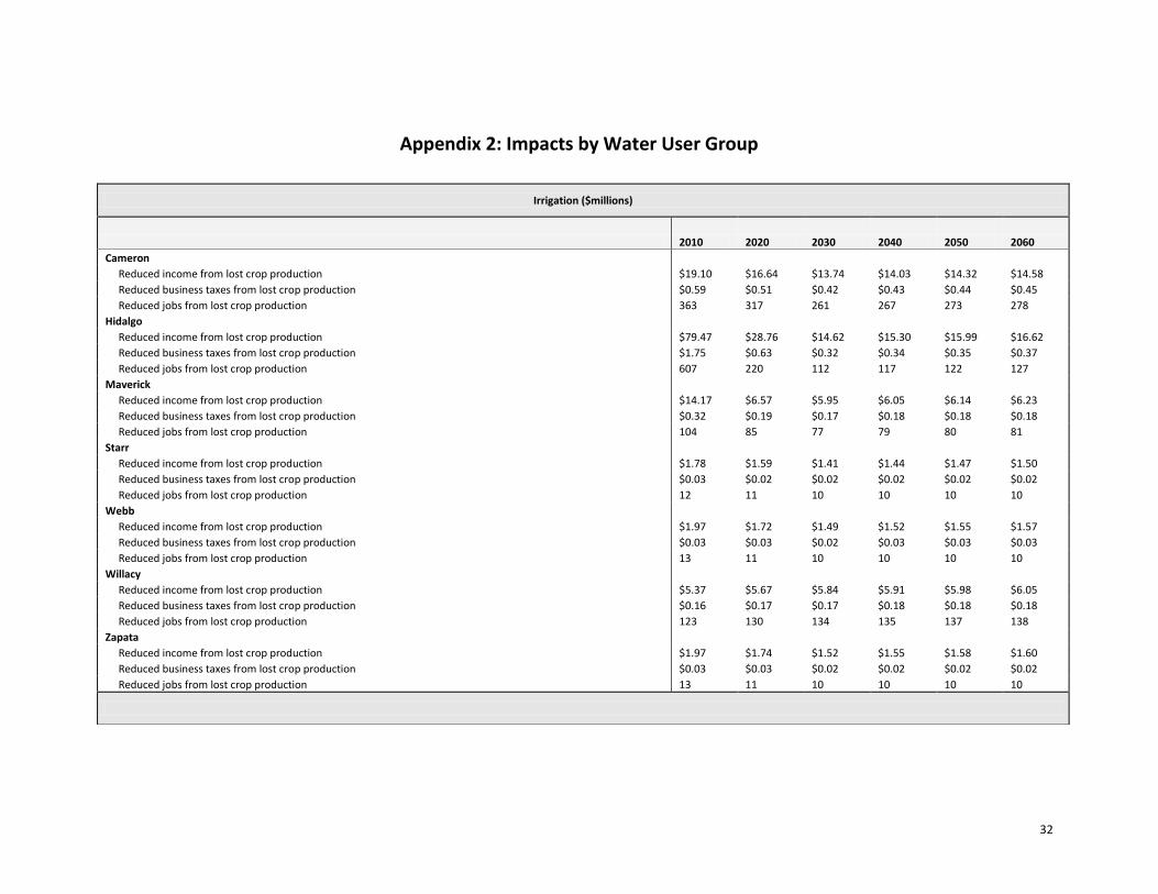
32
Appendix 2: Impacts by Water User Group
Irrigation ($millions)
2010 2020 2030 2040 2050 2060
Cameron
Reduced income from lost crop production $19.10 $16.64 $13.74 $14.03 $14.32 $14.58
Reduced business taxes from lost crop production $0.59 $0.51 $0.42 $0.43 $0.44 $0.45
Reduced jobs from lost crop production 363 317 261 267 273 278
Hidalgo
Reduced income from lost crop production $79.47 $28.76 $14.62 $15.30 $15.99 $16.62
Reduced business taxes from lost crop production $1.75 $0.63 $0.32 $0.34 $0.35 $0.37
Reduced jobs from lost crop production 607 220 112 117 122 127
Maverick
Reduced income from lost crop production $14.17 $6.57 $5.95 $6.05 $6.14 $6.23
Reduced business taxes from lost crop production $0.32 $0.19 $0.17 $0.18 $0.18 $0.18
Reduced jobs from lost crop production 104 85 77 79 80 81
Starr
Reduced income from lost crop production $1.78 $1.59 $1.41 $1.44 $1.47 $1.50
Reduced business taxes from lost crop production $0.03 $0.02 $0.02 $0.02 $0.02 $0.02
Reduced jobs from lost crop production 12 11 10 10 10 10
Webb
Reduced income from lost crop production $1.97 $1.72 $1.49 $1.52 $1.55 $1.57
Reduced business taxes from lost crop production $0.03 $0.03 $0.02 $0.03 $0.03 $0.03
Reduced jobs from lost crop production 13 11 10 10 10 10
Willacy
Reduced income from lost crop production $5.37 $5.67 $5.84 $5.91 $5.98 $6.05
Reduced business taxes from lost crop production $0.16 $0.17 $0.17 $0.18 $0.18 $0.18
Reduced jobs from lost crop production 123 130 134 135 137 138
Zapata
Reduced income from lost crop production $1.97 $1.74 $1.52 $1.55 $1.58 $1.60
Reduced business taxes from lost crop production $0.03 $0.03 $0.02 $0.02 $0.02 $0.02
Reduced jobs from lost crop production 13 11 10 10 10 10
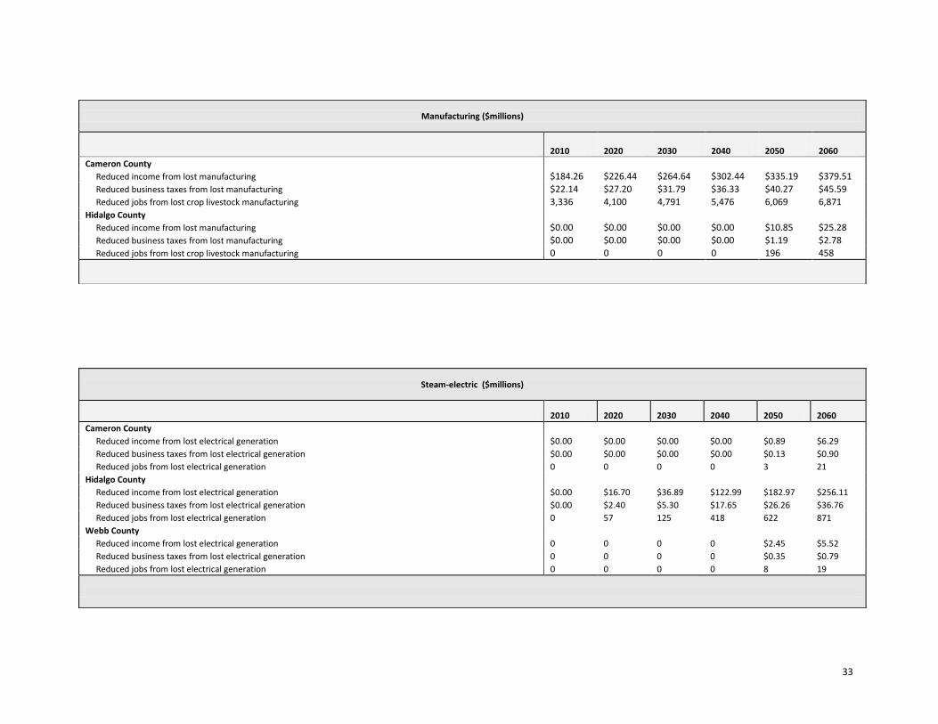
33
Manufacturing ($millions)
2010 2020 2030 2040 2050 2060
Cameron County
Reduced income from lost manufacturing $184.26 $226.44 $264.64 $302.44 $335.19 $379.51
Reduced business taxes from lost manufacturing $22.14 $27.20 $31.79 $36.33 $40.27 $45.59
Reduced jobs from lost crop livestock manufacturing 3,336 4,100 4,791 5,476 6,069 6,871
Hidalgo County
Reduced income from lost manufacturing $0.00 $0.00 $0.00 $0.00 $10.85 $25.28
Reduced business taxes from lost manufacturing $0.00 $0.00 $0.00 $0.00 $1.19 $2.78
Reduced jobs from lost crop livestock manufacturing 0 0 0 0 196 458
Steam-electric ($millions)
2010 2020 2030 2040 2050 2060
Cameron County
Reduced income from lost electrical generation $0.00 $0.00 $0.00 $0.00 $0.89 $6.29
Reduced business taxes from lost electrical generation $0.00 $0.00 $0.00 $0.00 $0.13 $0.90
Reduced jobs from lost electrical generation 0 0 0 0 3 21
Hidalgo County
Reduced income from lost electrical generation $0.00 $16.70 $36.89 $122.99 $182.97 $256.11
Reduced business taxes from lost electrical generation $0.00 $2.40 $5.30 $17.65 $26.26 $36.76
Reduced jobs from lost electrical generation 0 57 125 418 622 871
Webb County
Reduced income from lost electrical generation 0 0 0 0 $2.45 $5.52
Reduced business taxes from lost electrical generation 0 0 0 0 $0.35 $0.79
Reduced jobs from lost electrical generation 0 0 0 0 8 19
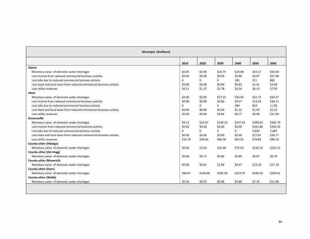
34
Municipal ($millions)
2010 2020 2030 2040 2050 2060
Alamo
Monetary value of domestic water shortages $0.05 $4.40 $18.75 $24.08 $33.17 $50.40
Lost income from reduced commercial business activity $0.00 $0.00 $0.00 $5.86 $9.87 $27.98
Lost jobs due to reduced commercial business activity 0 0 0 185 311 882
Lost state and local taxes from reduced commercial business activity $0.00 $0.00 $0.00 $0.83 $1.41 $3.99
Lost utility revenues $0.11 $1.37 $2.78 $4.34 $6.13 $7.95
Alton
Monetary value of domestic water shortages $0.00 $0.00 $17.22 $33.49 $51.71 $64.37
Lost income from reduced commercial business activity $0.00 $0.00 $0.00 $9.27 $13.54 $36.11
Lost jobs due to reduced commercial business activity 0 0 0 584 854 1,139
Lost state and local taxes from reduced commercial business activity $0.00 $0.00 $0.00 $1.32 $1.93 $5.15
Lost utility revenues $0.00 $0.00 $4.84 $6.77 $8.88 $11.09
Brownsville
Monetary value of domestic water shortages $9.13 $23.47 $149.52 $247.63 $399.63 $465.79
Lost income from reduced commercial business activity $0.00 $0.00 $0.00 $0.00 $261.86 $345.50
Lost jobs due to reduced commercial business activity 0 0 0 0 5,826 7,687
Lost state and local taxes from reduced commercial business activity $0.00 $0.00 $0.00 $0.00 $27.87 $36.77
Lost utility revenues $14.79 $30.60 $46.58 $63.25 $79.82 $96.19
County-other (Hidalgo)
Monetary value of domestic water shortages $0.00 $3.04 $32.68 $73.03 $135.24 $242.12
County-other (Jim Hogg)
Monetary value of domestic water shortages $0.66 $0.72 $0.86 $0.89 $0.87 $0.79
County-other (Maverick)
Monetary value of domestic water shortages $0.06 $0.81 $1.89 $9.47 $13.10 $17.19
County-other (Starr)
Monetary value of domestic water shortages $68.67 $148.68 $185.90 $223.97 $260.26 $294.62
County-other (Webb)
Monetary value of domestic water shortages $0.16 $0.55 $0.96 $4.80 $7.76 $11.06
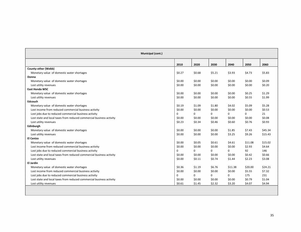
35
Municipal (cont.)
2010 2020 2030 2040 2050 2060
County-other (Webb)
Monetary value of domestic water shortages $0.27 $0.68 $5.21 $3.93 $4.73 $5.83
Donna
Monetary value of domestic water shortages $0.00 $0.00 $0.00 $0.00 $0.00 $0.09
Lost utility revenues $0.00 $0.00 $0.00 $0.00 $0.00 $0.20
East Honda WSC
Monetary value of domestic water shortages $0.00 $0.00 $0.00 $0.00 $0.25 $1.29
Lost utility revenues $0.00 $0.00 $0.00 $0.00 $0.55 $1.99
Edcouch
Monetary value of domestic water shortages $0.19 $1.09 $1.80 $4.02 $5.09 $5.28
Lost income from reduced commercial business activity $0.00 $0.00 $0.00 $0.00 $0.00 $0.53
Lost jobs due to reduced commercial business activity 0 0 0 0 0 21
Lost state and local taxes from reduced commercial business activity $0.00 $0.00 $0.00 $0.00 $0.00 $0.08
Lost utility revenues $0.23 $0.34 $0.46 $0.60 $0.76 $0.93
Edinburgh
Monetary value of domestic water shortages $0.00 $0.00 $0.00 $1.85 $7.43 $45.34
Lost utility revenues $0.00 $0.00 $0.00 $3.25 $9.26 $15.43
El Cenizo
Monetary value of domestic water shortages $0.00 $0.05 $0.61 $4.61 $11.08 $15.02
Lost income from reduced commercial business activity $0.00 $0.00 $0.00 $0.00 $2.93 $4.64
Lost jobs due to reduced commercial business activity 0 0 0 0 92 146
Lost state and local taxes from reduced commercial business activity $0.00 $0.00 $0.00 $0.00 $0.42 $0.66
Lost utility revenues $0.00 $0.11 $0.74 $1.44 $2.23 $3.08
El Jardin
Monetary value of domestic water shortages $0.36 $1.19 $6.76 $11.38 $20.00 $24.21
Lost income from reduced commercial business activity $0.00 $0.00 $0.00 $0.00 $5.55 $7.32
Lost jobs due to reduced commercial business activity 0 0 0 0 175 231
Lost state and local taxes from reduced commercial business activity $0.00 $0.00 $0.00 $0.00 $0.79 $1.04
Lost utility revenues $0.61 $1.45 $2.32 $3.20 $4.07 $4.94
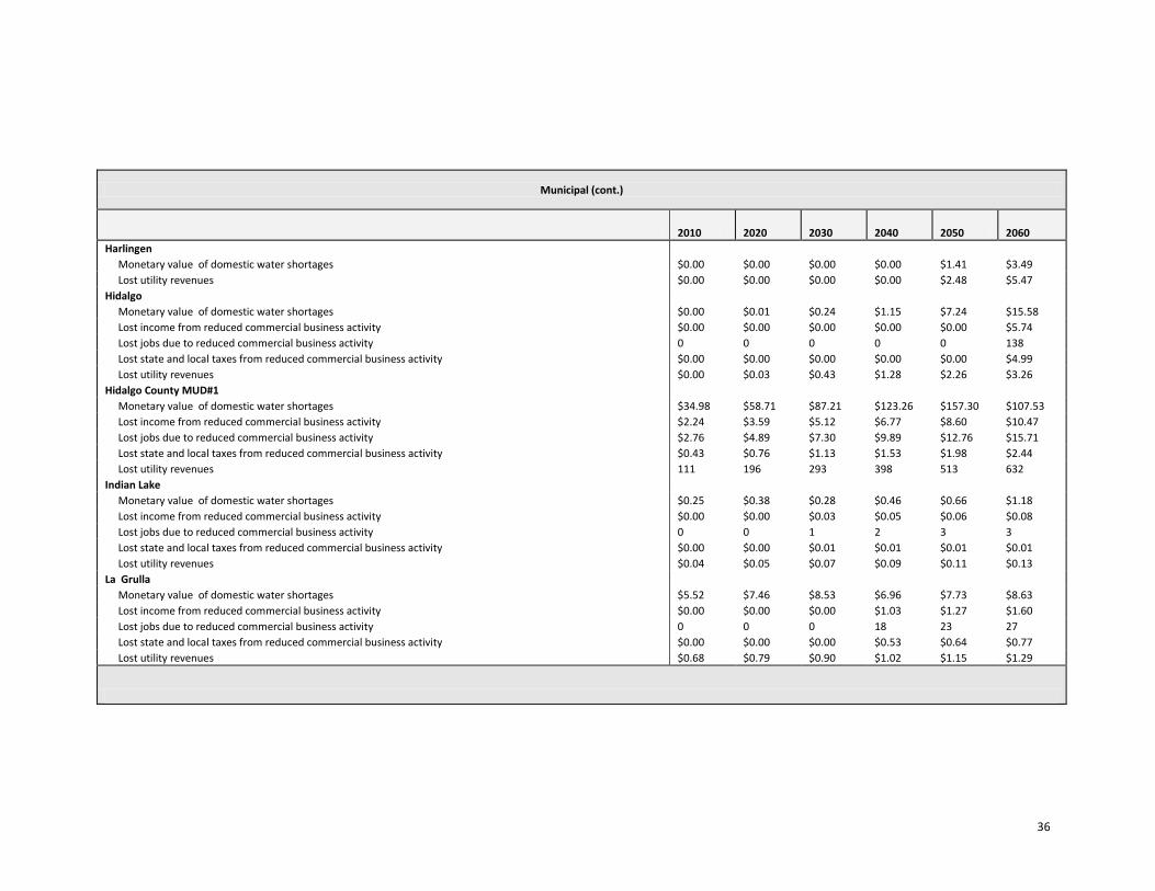
36
Municipal (cont.)
2010 2020 2030 2040 2050 2060
Harlingen
Monetary value of domestic water shortages $0.00 $0.00 $0.00 $0.00 $1.41 $3.49
Lost utility revenues $0.00 $0.00 $0.00 $0.00 $2.48 $5.47
Hidalgo
Monetary value of domestic water shortages $0.00 $0.01 $0.24 $1.15 $7.24 $15.58
Lost income from reduced commercial business activity $0.00 $0.00 $0.00 $0.00 $0.00 $5.74
Lost jobs due to reduced commercial business activity 0 0 0 0 0 138
Lost state and local taxes from reduced commercial business activity $0.00 $0.00 $0.00 $0.00 $0.00 $4.99
Lost utility revenues $0.00 $0.03 $0.43 $1.28 $2.26 $3.26
Hidalgo County MUD#1
Monetary value of domestic water shortages $34.98 $58.71 $87.21 $123.26 $157.30 $107.53
Lost income from reduced commercial business activity $2.24 $3.59 $5.12 $6.77 $8.60 $10.47
Lost jobs due to reduced commercial business activity $2.76 $4.89 $7.30 $9.89 $12.76 $15.71
Lost state and local taxes from reduced commercial business activity $0.43 $0.76 $1.13 $1.53 $1.98 $2.44
Lost utility revenues 111 196 293 398 513 632
Indian Lake
Monetary value of domestic water shortages $0.25 $0.38 $0.28 $0.46 $0.66 $1.18
Lost income from reduced commercial business activity $0.00 $0.00 $0.03 $0.05 $0.06 $0.08
Lost jobs due to reduced commercial business activity 0 0 1 2 3 3
Lost state and local taxes from reduced commercial business activity $0.00 $0.00 $0.01 $0.01 $0.01 $0.01
Lost utility revenues $0.04 $0.05 $0.07 $0.09 $0.11 $0.13
La Grulla
Monetary value of domestic water shortages $5.52 $7.46 $8.53 $6.96 $7.73 $8.63
Lost income from reduced commercial business activity $0.00 $0.00 $0.00 $1.03 $1.27 $1.60
Lost jobs due to reduced commercial business activity 0 0 0 18 23 27
Lost state and local taxes from reduced commercial business activity $0.00 $0.00 $0.00 $0.53 $0.64 $0.77
Lost utility revenues $0.68 $0.79 $0.90 $1.02 $1.15 $1.29
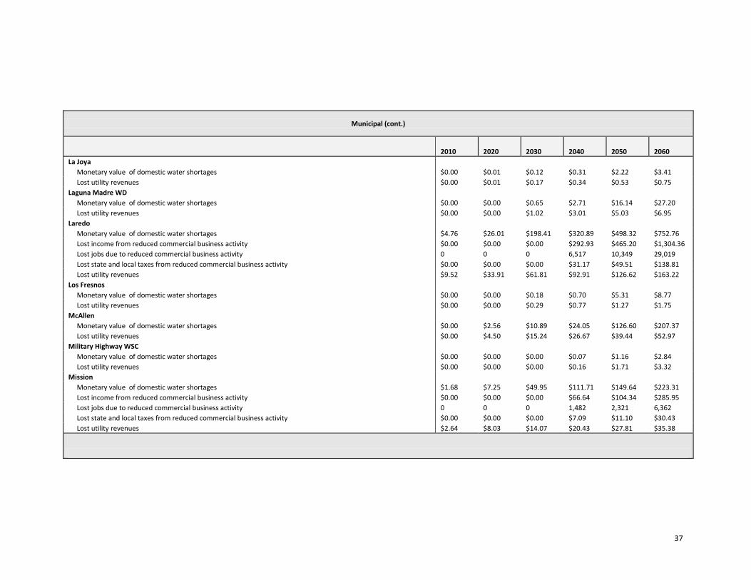
37
Municipal (cont.)
2010 2020 2030 2040 2050 2060
La Joya
Monetary value of domestic water shortages $0.00 $0.01 $0.12 $0.31 $2.22 $3.41
Lost utility revenues $0.00 $0.01 $0.17 $0.34 $0.53 $0.75
Laguna Madre WD
Monetary value of domestic water shortages $0.00 $0.00 $0.65 $2.71 $16.14 $27.20
Lost utility revenues $0.00 $0.00 $1.02 $3.01 $5.03 $6.95
Laredo
Monetary value of domestic water shortages $4.76 $26.01 $198.41 $320.89 $498.32 $752.76
Lost income from reduced commercial business activity $0.00 $0.00 $0.00 $292.93 $465.20 $1,304.36
Lost jobs due to reduced commercial business activity 0 0 0 6,517 10,349 29,019
Lost state and local taxes from reduced commercial business activity $0.00 $0.00 $0.00 $31.17 $49.51 $138.81
Lost utility revenues $9.52 $33.91 $61.81 $92.91 $126.62 $163.22
Los Fresnos
Monetary value of domestic water shortages $0.00 $0.00 $0.18 $0.70 $5.31 $8.77
Lost utility revenues $0.00 $0.00 $0.29 $0.77 $1.27 $1.75
McAllen
Monetary value of domestic water shortages $0.00 $2.56 $10.89 $24.05 $126.60 $207.37
Lost utility revenues $0.00 $4.50 $15.24 $26.67 $39.44 $52.97
Military Highway WSC
Monetary value of domestic water shortages $0.00 $0.00 $0.00 $0.07 $1.16 $2.84
Lost utility revenues $0.00 $0.00 $0.00 $0.16 $1.71 $3.32
Mission
Monetary value of domestic water shortages $1.68 $7.25 $49.95 $111.71 $149.64 $223.31
Lost income from reduced commercial business activity $0.00 $0.00 $0.00 $66.64 $104.34 $285.95
Lost jobs due to reduced commercial business activity 0 0 0 1,482 2,321 6,362
Lost state and local taxes from reduced commercial business activity $0.00 $0.00 $0.00 $7.09 $11.10 $30.43
Lost utility revenues $2.64 $8.03 $14.07 $20.43 $27.81 $35.38
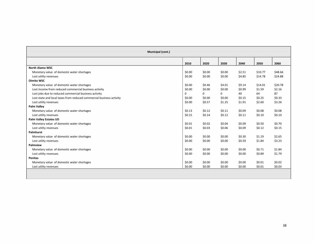
38
Municipal (cont.)
2010 2020 2030 2040 2050 2060
North Alamo WSC
Monetary value of domestic water shortages $0.00 $0.00 $0.00 $2.51 $10.77 $48.66
Lost utility revenues $0.00 $0.00 $0.00 $4.85 $14.78 $24.88
OImito WSC
Monetary value of domestic water shortages $0.00 $0.46 $4.01 $9.14 $14.01 $20.78
Lost income from reduced commercial business activity $0.00 $0.00 $0.00 $0.99 $1.59 $2.16
Lost jobs due to reduced commercial business activity 0 0 0 40 64 87
Lost state and local taxes from reduced commercial business activity $0.00 $0.00 $0.00 $0.15 $0.25 $0.33
Lost utility revenues $0.00 $0.57 $1.25 $1.91 $2.60 $3.26
Palm Valley
Monetary value of domestic water shortages $0.13 $0.12 $0.11 $0.09 $0.08 $0.08
Lost utility revenues $0.15 $0.14 $0.12 $0.11 $0.10 $0.10
Palm Valley Estates UD
Monetary value of domestic water shortages $0.01 $0.02 $0.04 $0.09 $0.50 $0.70
Lost utility revenues $0.01 $0.03 $0.06 $0.09 $0.12 $0.15
Palmhurst
Monetary value of domestic water shortages $0.00 $0.00 $0.00 $0.30 $1.19 $2.65
Lost utility revenues $0.00 $0.00 $0.00 $0.59 $1.84 $3.23
Palmview
Monetary value of domestic water shortages $0.00 $0.00 $0.00 $0.00 $0.71 $1.84
Lost utility revenues $0.00 $0.00 $0.00 $0.00 $0.89 $1.79
Penitas
Monetary value of domestic water shortages $0.00 $0.00 $0.00 $0.00 $0.01 $0.02
Lost utility revenues $0.00 $0.00 $0.00 $0.00 $0.01 $0.03
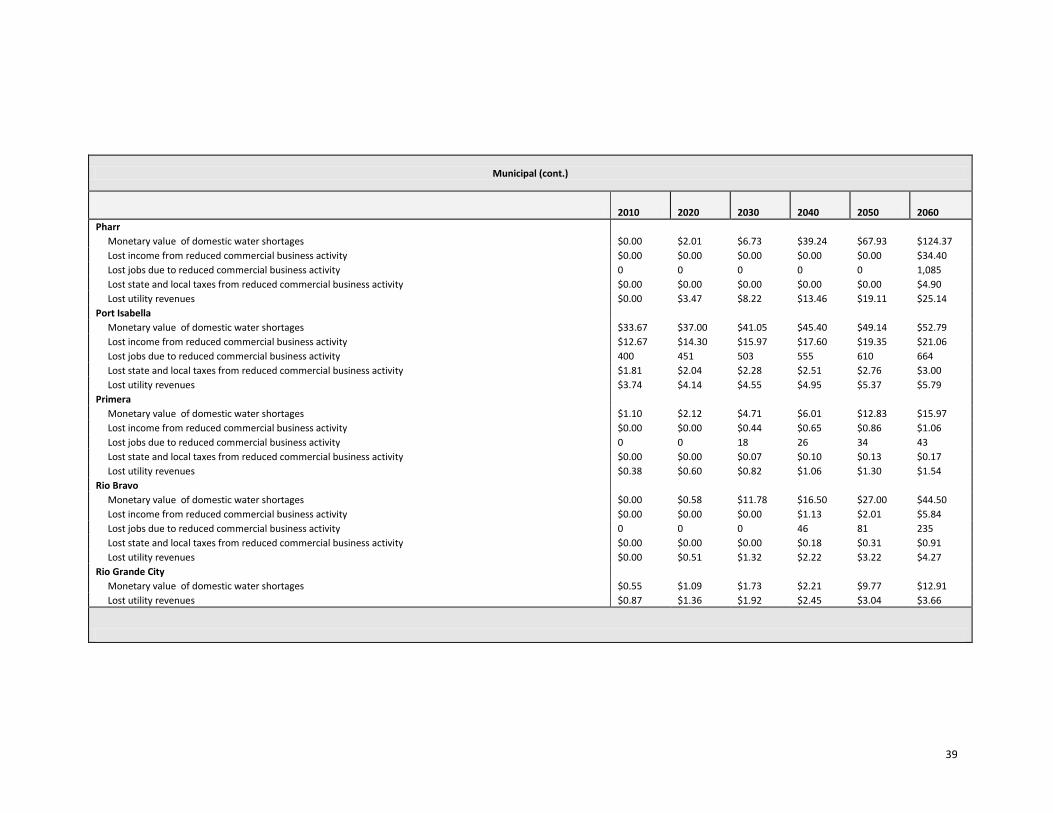
39
Municipal (cont.)
2010 2020 2030 2040 2050 2060
Pharr
Monetary value of domestic water shortages $0.00 $2.01 $6.73 $39.24 $67.93 $124.37
Lost income from reduced commercial business activity $0.00 $0.00 $0.00 $0.00 $0.00 $34.40
Lost jobs due to reduced commercial business activity 0 0 0 0 0 1,085
Lost state and local taxes from reduced commercial business activity $0.00 $0.00 $0.00 $0.00 $0.00 $4.90
Lost utility revenues $0.00 $3.47 $8.22 $13.46 $19.11 $25.14
Port Isabella
Monetary value of domestic water shortages $33.67 $37.00 $41.05 $45.40 $49.14 $52.79
Lost income from reduced commercial business activity $12.67 $14.30 $15.97 $17.60 $19.35 $21.06
Lost jobs due to reduced commercial business activity 400 451 503 555 610 664
Lost state and local taxes from reduced commercial business activity $1.81 $2.04 $2.28 $2.51 $2.76 $3.00
Lost utility revenues $3.74 $4.14 $4.55 $4.95 $5.37 $5.79
Primera
Monetary value of domestic water shortages $1.10 $2.12 $4.71 $6.01 $12.83 $15.97
Lost income from reduced commercial business activity $0.00 $0.00 $0.44 $0.65 $0.86 $1.06
Lost jobs due to reduced commercial business activity 0 0 18 26 34 43
Lost state and local taxes from reduced commercial business activity $0.00 $0.00 $0.07 $0.10 $0.13 $0.17
Lost utility revenues $0.38 $0.60 $0.82 $1.06 $1.30 $1.54
Rio Bravo
Monetary value of domestic water shortages $0.00 $0.58 $11.78 $16.50 $27.00 $44.50
Lost income from reduced commercial business activity $0.00 $0.00 $0.00 $1.13 $2.01 $5.84
Lost jobs due to reduced commercial business activity 0 0 0 46 81 235
Lost state and local taxes from reduced commercial business activity $0.00 $0.00 $0.00 $0.18 $0.31 $0.91
Lost utility revenues $0.00 $0.51 $1.32 $2.22 $3.22 $4.27
Rio Grande City
Monetary value of domestic water shortages $0.55 $1.09 $1.73 $2.21 $9.77 $12.91
Lost utility revenues $0.87 $1.36 $1.92 $2.45 $3.04 $3.66

40
Municipal (cont.)
2010 2020 2030 2040 2050 2060
Rio WSC
Monetary value of domestic water shortages $1.91 $3.44 $6.92 $10.66 $13.94 $17.11
Lost income from reduced commercial business activity $0.00 $0.00 $0.51 $1.46 $1.93 $2.38
Lost jobs due to reduced commercial business activity 0 0 21 59 78 96
Lost state and local taxes from reduced commercial business activity $0.00 $0.00 $0.08 $0.23 $0.30 $0.37
Lost utility revenues $0.34 $0.62 $0.91 $1.19 $1.49 $1.77
Roma City
Monetary value of domestic water shortages $0.09 $0.56 $1.29 $2.13 $10.06 $13.81
Lost utility revenues $0.21 $0.97 $1.77 $2.60 $3.45 $4.31
San Benito
Monetary value of domestic water shortages $0.00 $0.00 $0.00 $0.00 $0.19 $0.85
Lost utility revenues $0.00 $0.00 $0.00 $0.00 $0.38 $1.49
San Juan
Monetary value of domestic water shortages $0.55 $8.68 $20.65 $42.22 $69.32 $137.01
Lost income from reduced commercial business activity $0.00 $0.00 $0.00 $12.41 $38.15 $51.83
Lost jobs due to reduced commercial business activity 0 0 0 391 1,203 1,634
Lost state and local taxes from reduced commercial business activity $0.00 $0.00 $0.00 $1.77 $5.44 $7.39
Lost utility revenues $0.95 $3.25 $5.81 $8.64 $11.90 $15.24
San Perlita
Monetary value of domestic water shortages $0.00 $0.00 $0.00 $0.00 $0.01 $0.01
Lost utility revenues $0.00 $0.00 $0.00 $0.00 $0.01 $0.01
Sebastian
Monetary value of domestic water shortages $0.00 $0.00 $0.04 $0.10 $0.13 $0.17
Lost utility revenues $0.00 $0.00 $0.07 $0.12 $0.16 $0.18
Sharyland WSC
Monetary value of domestic water shortages $0.00 $0.40 $0.41 $1.71 $3.72 $19.25
Lost utility revenues $0.00 $0.77 $0.79 $2.64 $4.55 $6.60
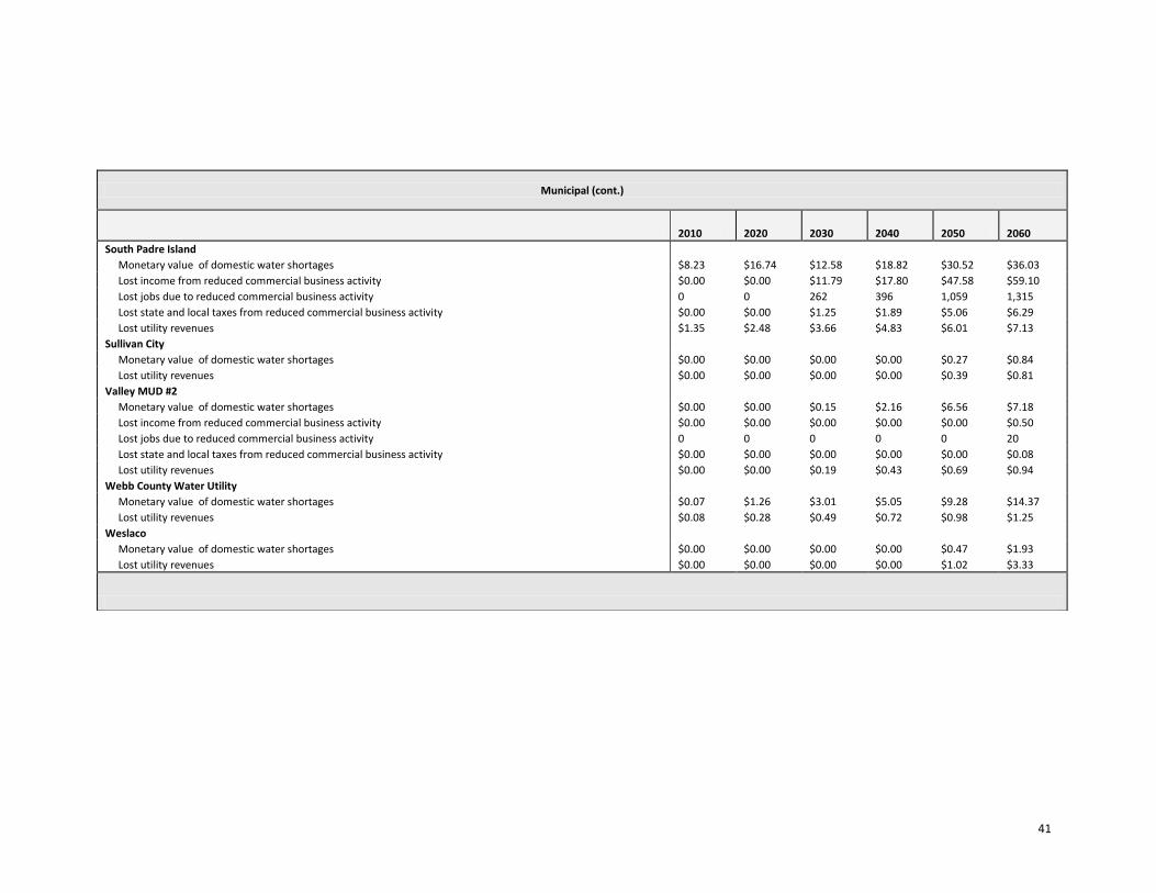
41
Municipal (cont.)
2010 2020 2030 2040 2050 2060
South Padre Island
Monetary value of domestic water shortages $8.23 $16.74 $12.58 $18.82 $30.52 $36.03
Lost income from reduced commercial business activity $0.00 $0.00 $11.79 $17.80 $47.58 $59.10
Lost jobs due to reduced commercial business activity 0 0 262 396 1,059 1,315
Lost state and local taxes from reduced commercial business activity $0.00 $0.00 $1.25 $1.89 $5.06 $6.29
Lost utility revenues $1.35 $2.48 $3.66 $4.83 $6.01 $7.13
Sullivan City
Monetary value of domestic water shortages $0.00 $0.00 $0.00 $0.00 $0.27 $0.84
Lost utility revenues $0.00 $0.00 $0.00 $0.00 $0.39 $0.81
Valley MUD #2
Monetary value of domestic water shortages $0.00 $0.00 $0.15 $2.16 $6.56 $7.18
Lost income from reduced commercial business activity $0.00 $0.00 $0.00 $0.00 $0.00 $0.50
Lost jobs due to reduced commercial business activity 0 0 0 0 0 20
Lost state and local taxes from reduced commercial business activity $0.00 $0.00 $0.00 $0.00 $0.00 $0.08
Lost utility revenues $0.00 $0.00 $0.19 $0.43 $0.69 $0.94
Webb County Water Utility
Monetary value of domestic water shortages $0.07 $1.26 $3.01 $5.05 $9.28 $14.37
Lost utility revenues $0.08 $0.28 $0.49 $0.72 $0.98 $1.25
Weslaco
Monetary value of domestic water shortages $0.00 $0.00 $0.00 $0.00 $0.47 $1.93
Lost utility revenues $0.00 $0.00 $0.00 $0.00 $1.02 $3.33

Appendix H
James Bene PowerPoint: November 20, 2013 GMA 13 Meeting

2/22/2017
1
1
Presented by:
James Bené, P.G.
Groundwater Management Area No. 13
November 21, 2013
Presentation Outline
1. Current DFCs/MAGs and some of their shortcomings
2. What is “drawdown” – why it is important to distinguish between the different types
3. What makes a good DFC?
4. Alternative DFCs and their advantages
2
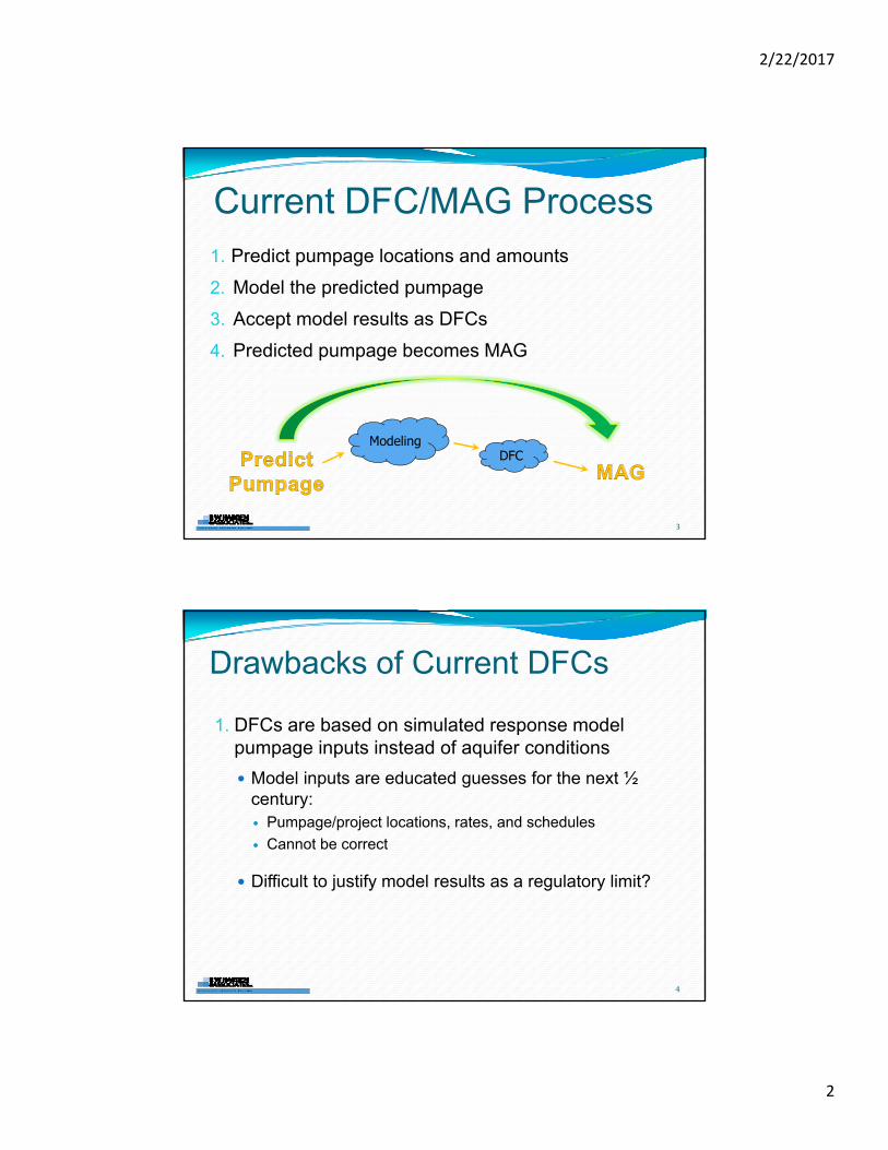
2/22/2017
2
Current DFC/MAG Process1. Predict pumpage locations and amounts
2. Model the predicted pumpage
3. Accept model results as DFCs
4. Predicted pumpage becomes MAG
ModelingDFC
3
Drawbacks of Current DFCs
1. DFCs are based on simulated response model pumpage inputs instead of aquifer conditions
Model inputs are educated guesses for the next ½ century: Pumpage/project locations, rates, and schedules
Cannot be correct
Difficult to justify model results as a regulatory limit?
4
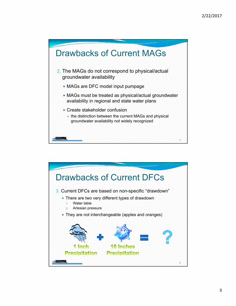
2/22/2017
3
Drawbacks of Current MAGs
2. The MAGs do not correspond to physical/actual groundwater availability
MAGs are DFC model input pumpage
MAGs must be treated as physical/actual groundwater availability in regional and state water plans
Create stakeholder confusion the distinction between the current MAGs and physical
groundwater availability not widely recognized
5
Drawbacks of Current DFCs
3. Current DFCs are based on non-specific “drawdown”
There are two very different types of drawdown1. Water table2. Artesian pressure
They are not interchangeable (apples and oranges)
6
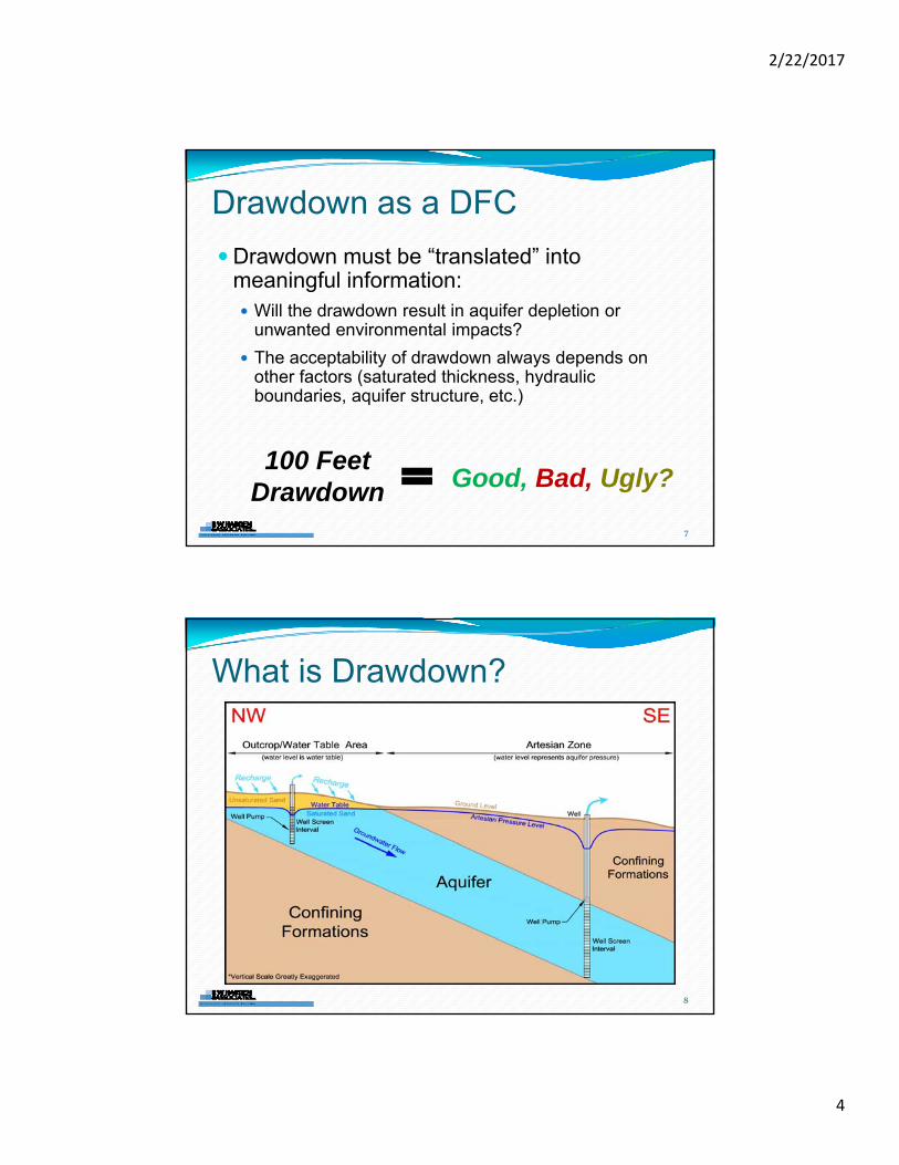
2/22/2017
4
Drawdown as a DFC
Drawdown must be “translated” into meaningful information: Will the drawdown result in aquifer depletion or
unwanted environmental impacts?
The acceptability of drawdown always depends on other factors (saturated thickness, hydraulic boundaries, aquifer structure, etc.)
7
100 Feet Drawdown Good, Bad, Ugly?
What is Drawdown?
8
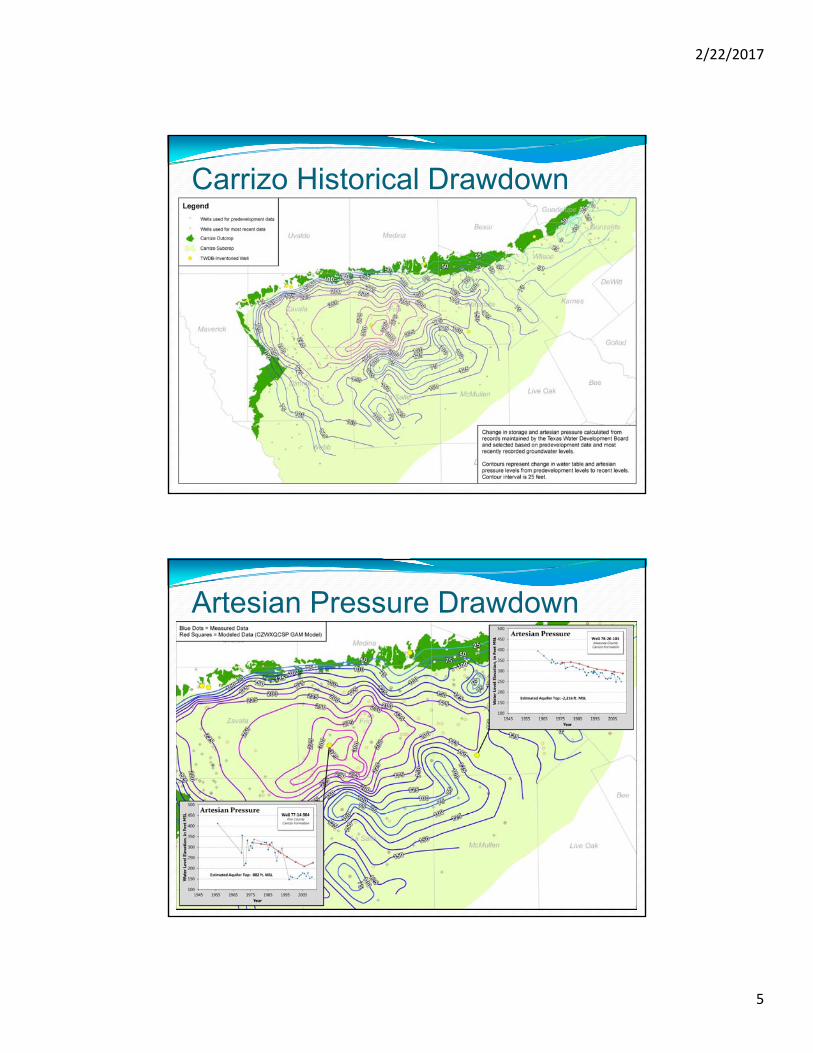
2/22/2017
5
9
Carrizo Historical Drawdown
10
Artesian Pressure Drawdown
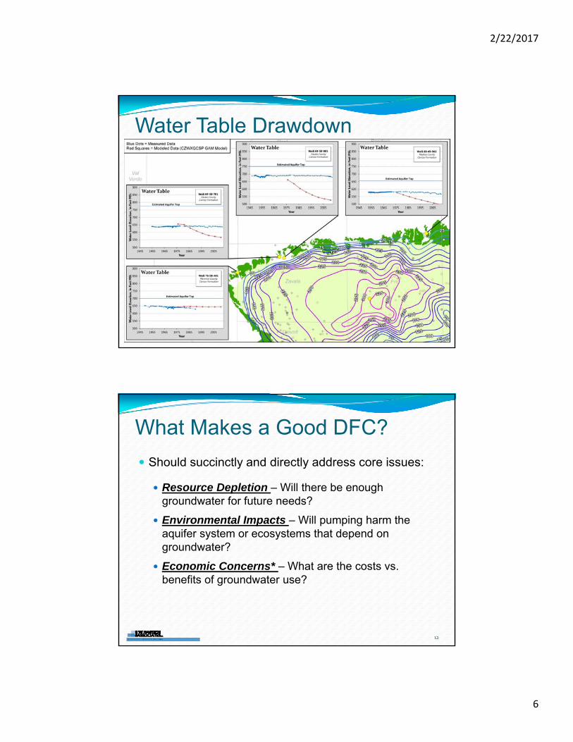
2/22/2017
6
11
Water Table Drawdown
What Makes a Good DFC?
Should succinctly and directly address core issues:
Resource Depletion – Will there be enough groundwater for future needs?
Environmental Impacts – Will pumping harm the aquifer system or ecosystems that depend on groundwater?
Economic Concerns* – What are the costs vs. benefits of groundwater use?
12
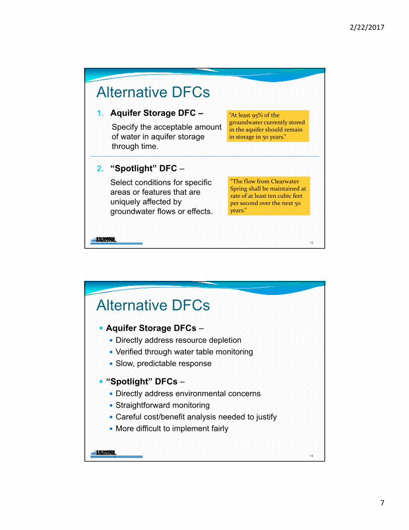
2/22/2017
7
Alternative DFCs1. Aquifer Storage DFC –
Specify the acceptable amount of water in aquifer storage through time.
2. “Spotlight” DFC –
Select conditions for specific areas or features that are uniquely affected by groundwater flows or effects.
13
“At least 95% of the groundwater currently stored in the aquifer should remain in storage in 50 years.”
“The flow from Clearwater Spring shall be maintained at rate of at least ten cubic feet per second over the next 50 years.”
Alternative DFCs Aquifer Storage DFCs –
Directly address resource depletion
Verified through water table monitoring
Slow, predictable response
“Spotlight” DFCs – Directly address environmental concerns
Straightforward monitoring
Careful cost/benefit analysis needed to justify
More difficult to implement fairly
14
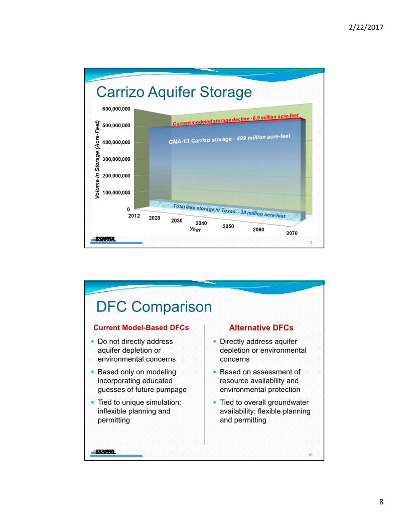
2/22/2017
8
Carrizo Aquifer Storage
15
DFC ComparisonAlternative DFCsCurrent Model-Based DFCs
Directly address aquifer depletion or environmental concerns
Based on assessment of resource availability and environmental protection
Tied to overall groundwater availability: flexible planning and permitting
Do not directly address aquifer depletion or environmental concerns
Based only on modeling incorporating educated guesses of future pumpage
Tied to unique simulation: inflexible planning and permitting
16
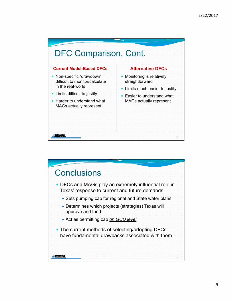
2/22/2017
9
DFC Comparison, Cont.
Alternative DFCsCurrent Model-Based DFCs
Monitoring is relatively straightforward
Limits much easier to justify
Easier to understand what MAGs actually represent
Non-specific “drawdown” difficult to monitor/calculate in the real-world
Limits difficult to justify
Harder to understand what MAGs actually represent
17
Conclusions DFCs and MAGs play an extremely influential role in
Texas’ response to current and future demands
Sets pumping cap for regional and State water plans
Determines which projects (strategies) Texas will approve and fund
Act as permitting cap on GCD level
The current methods of selecting/adopting DFCs have fundamental drawbacks associated with them
18
2/22/2017
10
Conclusions, Cont.
There are other options to be considered –
the DFCs can and should be improved
We have time, there is no pressing deadline requiring action
19
More detailed article available:[email protected]
512-345-2379
20

Appendix I
GBRA letter of February 26, 2016 Regarding Surface Water Impacts
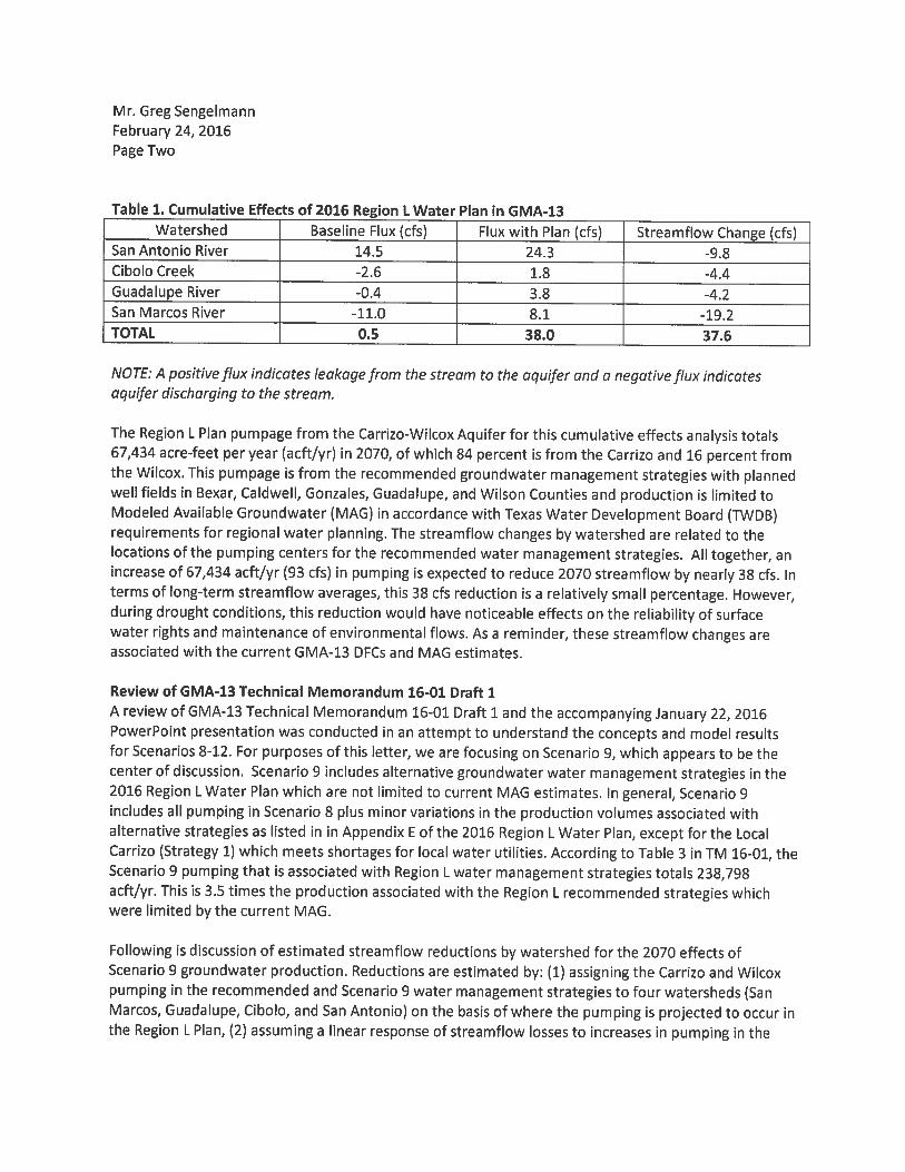
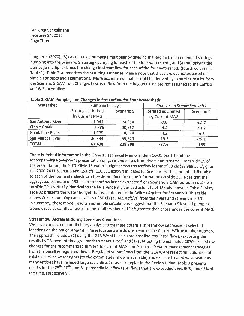
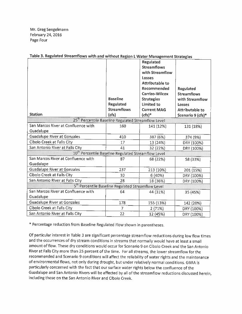
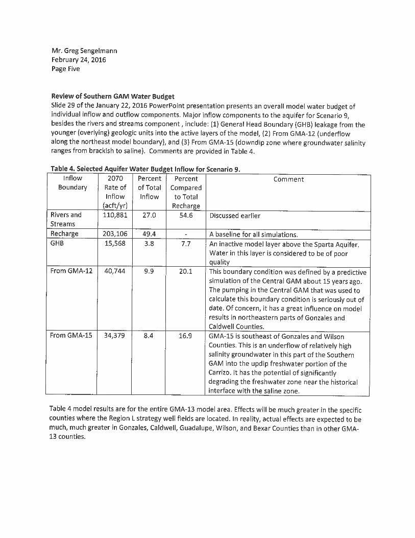
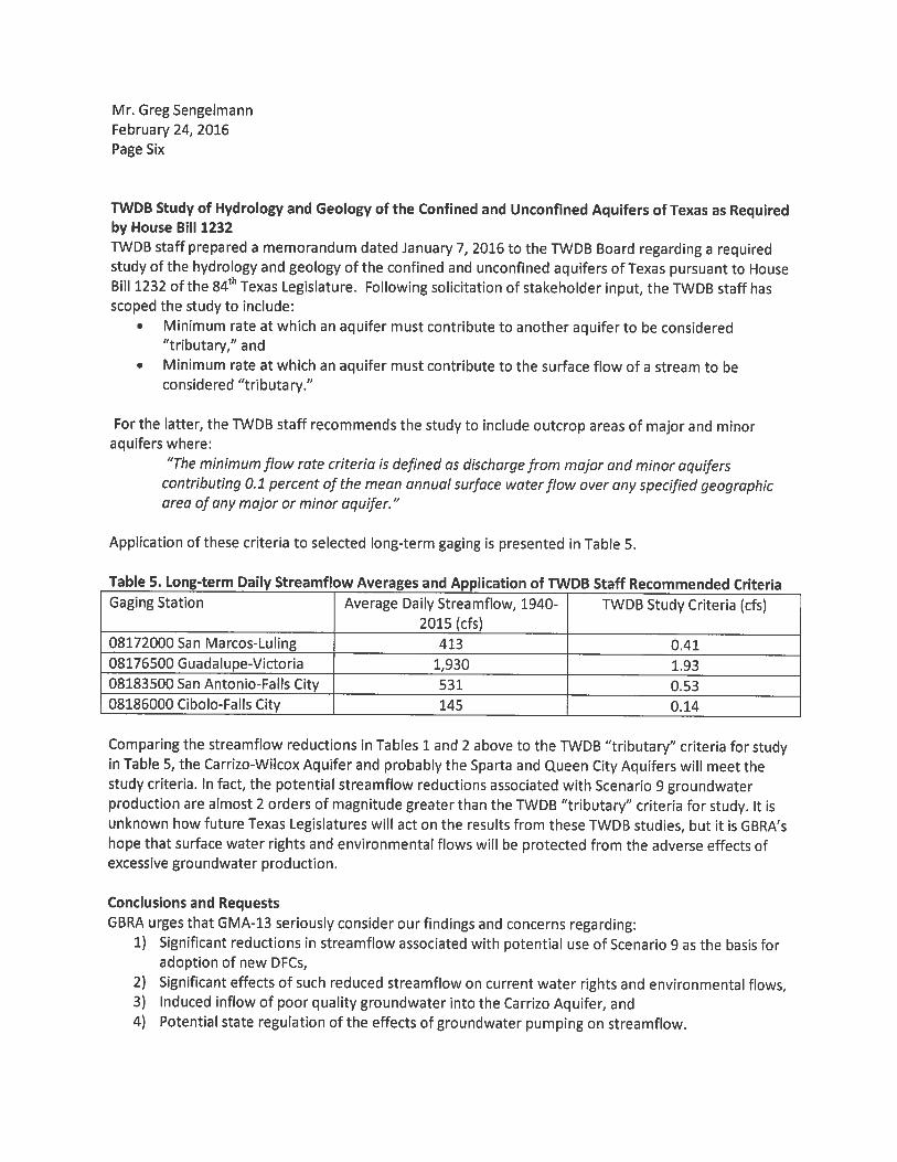

Appendix J
James Beach PowerPoint: March 30, 2016 Regarding Modeling Groundwater-Surface Water Interactions

Historical Data and Modeling of Groundwater Surface water
Interaction
by James Beach, P.G.
LBG-Guyton Associates
March 30, 2016
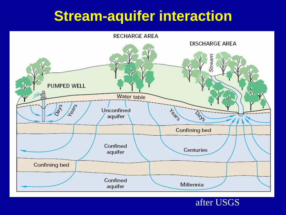
Stream-aquifer interaction
after USGS
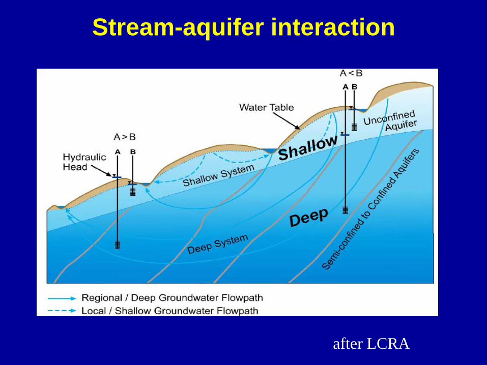
Stream-aquifer interaction
after LCRA
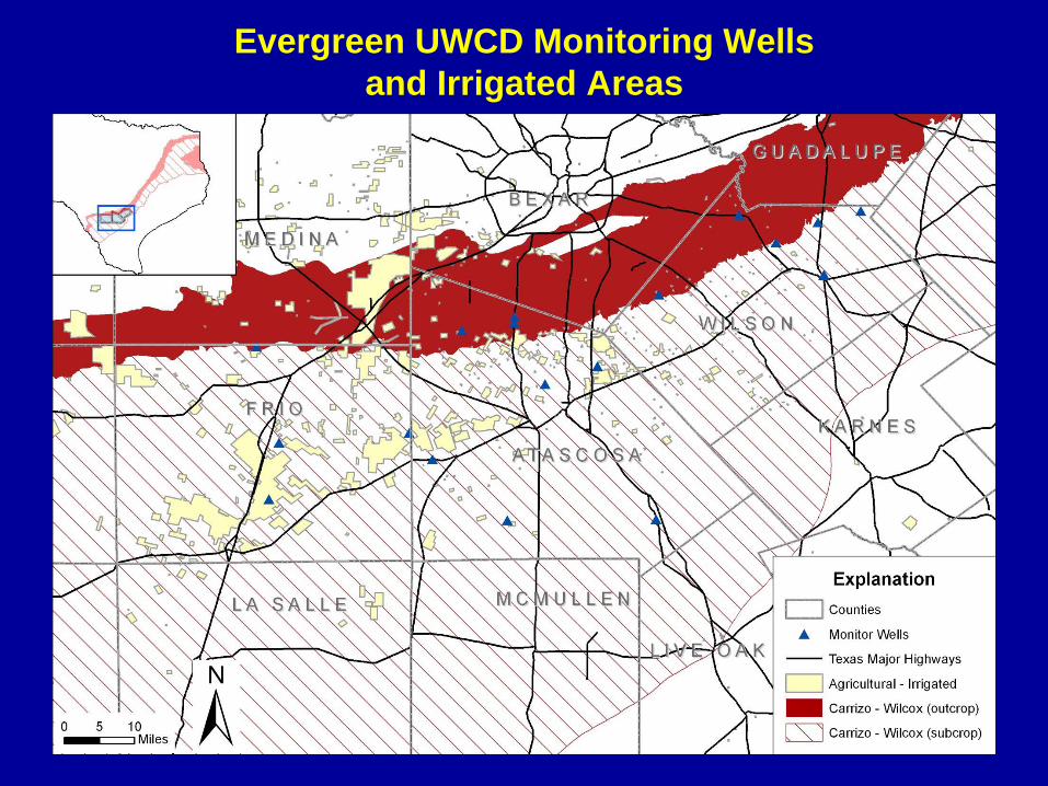
Evergreen UWCD Monitoring Wells and Irrigated Areas
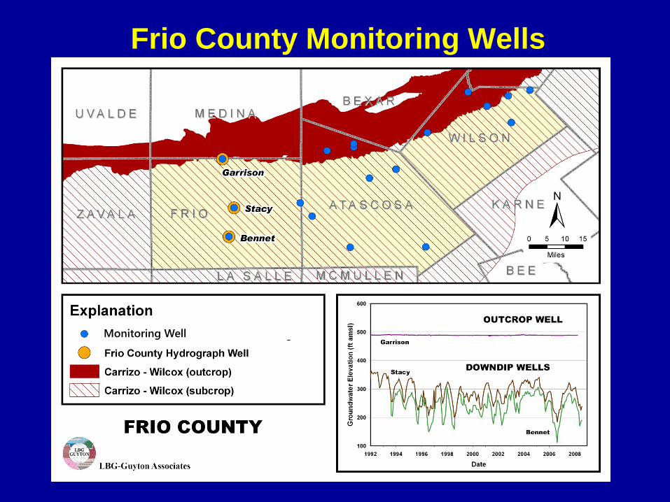
Page 5
Frio County Monitoring Wells
Monitoring Well
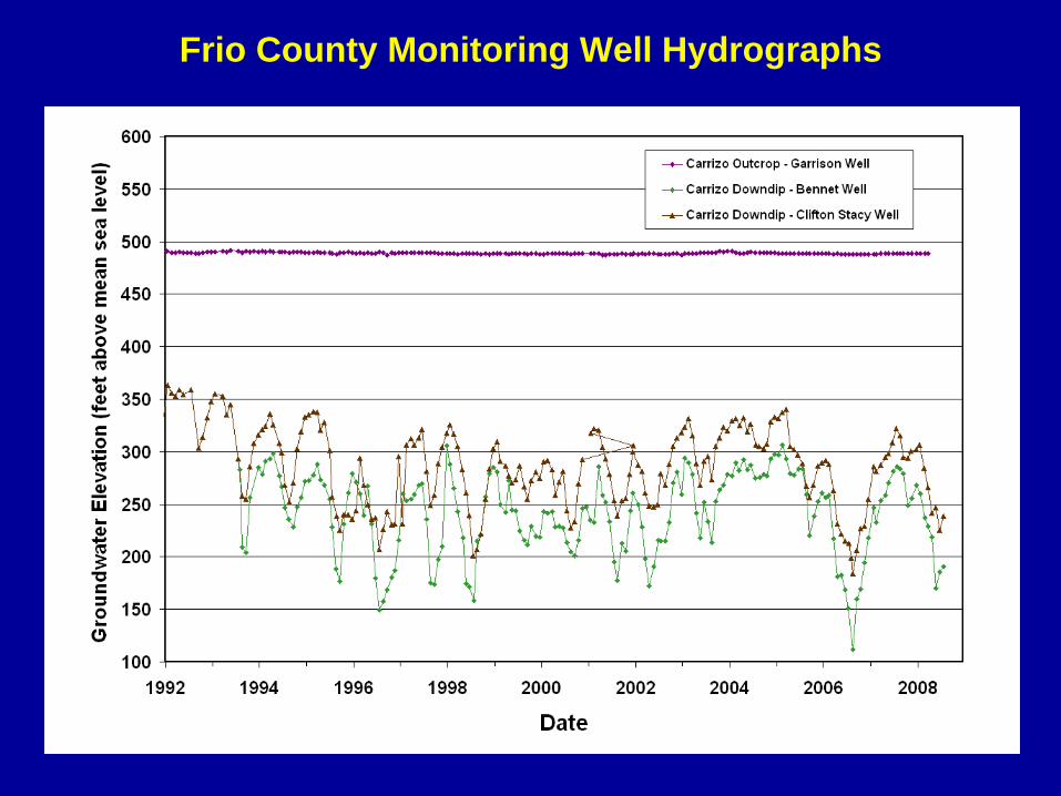
Frio County Monitoring Well Hydrographs
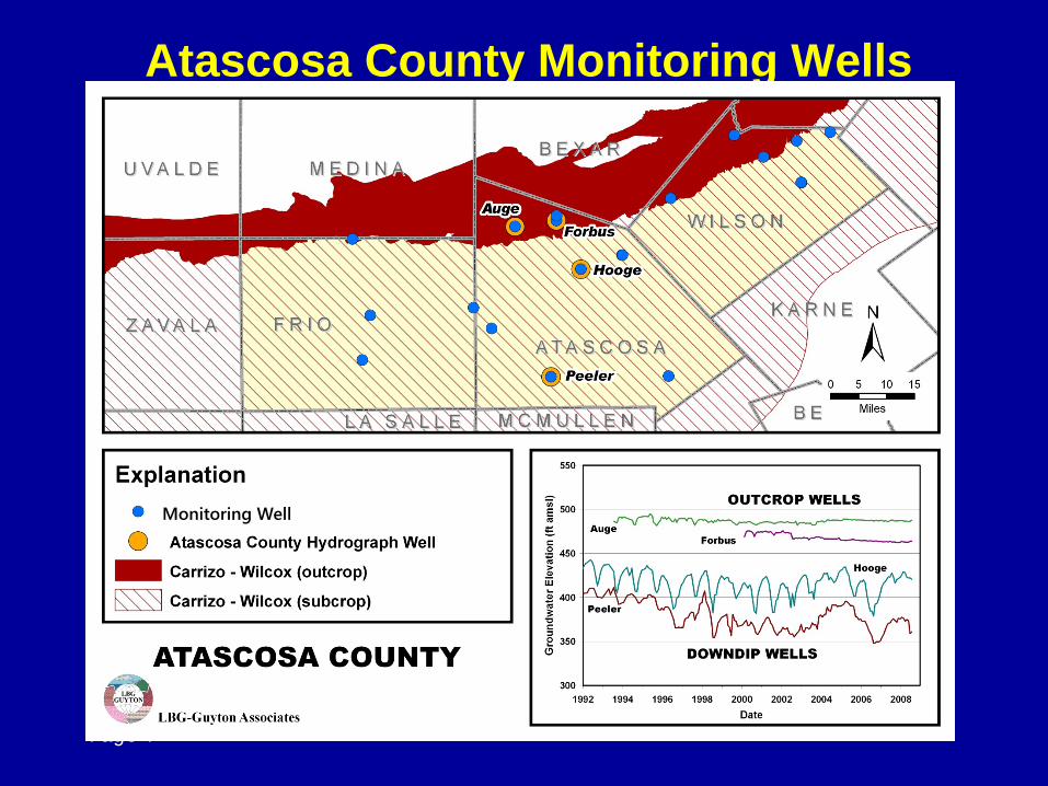
Page 7
Atascosa County Monitoring Wells
Monitoring Well
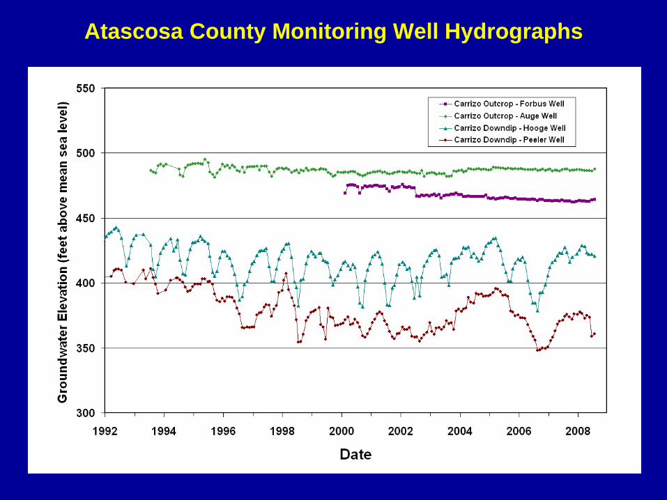
Atascosa County Monitoring Well Hydrographs
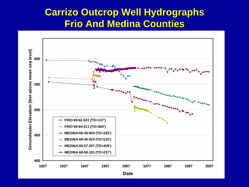
Page 9
Carrizo Outcrop Well Hydrographs Frio And Medina Counties
400
450
500
550
600
1927 1937 1947 1957 1967 1977 1987 1997 2007
Date
Gro
un
dw
ate
r E
lev
ati
on
(fe
et
ab
ov
e m
ea
n s
ea
lev
el)
FRIO 69-62-501 (TD=137')
FRIO 69-64-411 (TD=360')
MEDINA 68-49-902 (TD=182')
MEDINA 68-49-923 (TD=120')
MEDINA 68-57-307 (TD=409')
MEDINA 68-58-101 (TD=237')
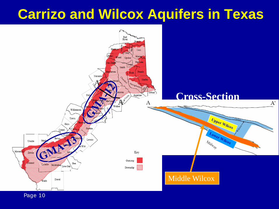
Page 10
Carrizo and Wilcox Aquifers in Texas
Cross-Section
Middle Wilcox
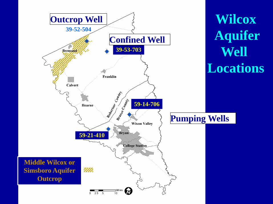
Page 11
Wilcox Aquifer
Well Locations
39-52-504
39-53-703
59-14-706
59-21-410
Outcrop Well
Confined Well
Pumping Wells
Middle Wilcox or Simsboro Aquifer
Outcrop
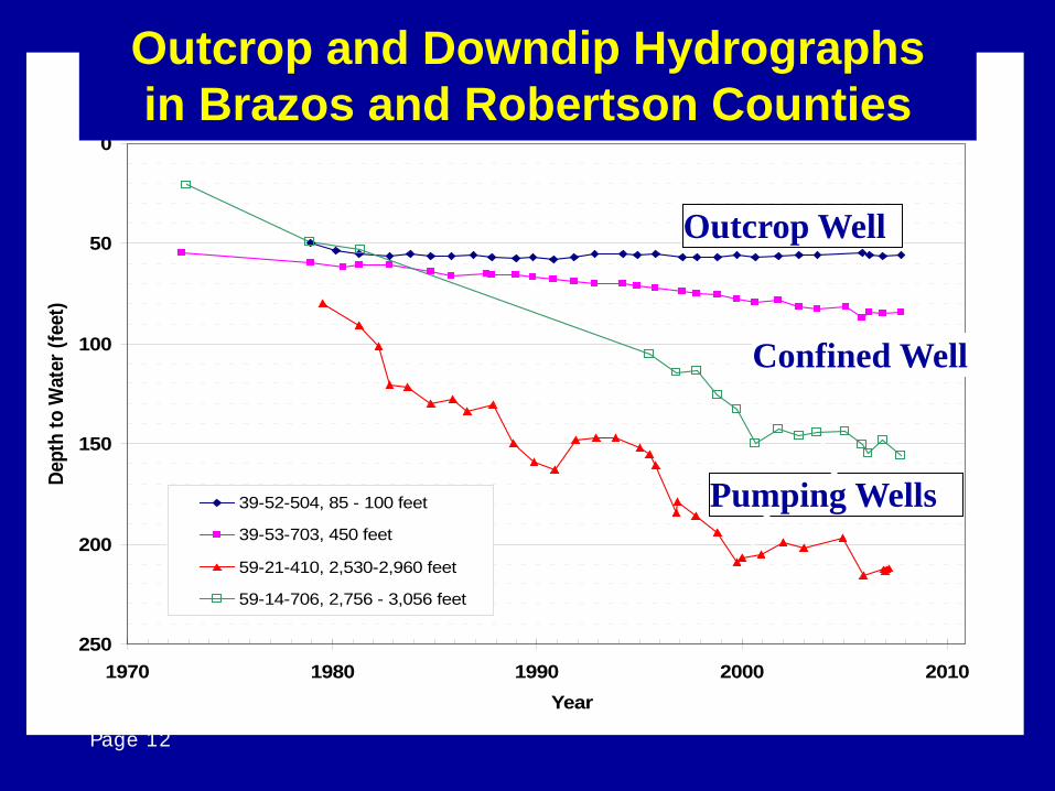
Page 12
Brazos County and Robertson County Simsboro Aquifer Static Water Levels
0
50
100
150
200
250
1970 1980 1990 2000 2010
Year
Dep
th t
o W
ater
(fe
et)
39-52-504, 85 - 100 feet
39-53-703, 450 feet
59-21-410, 2,530-2,960 feet
59-14-706, 2,756 - 3,056 feet
State Well Number, Screened Interval or Total Depth
Outcrop Well
Pumping Wells
Outcrop and Downdip Hydrographs in Brazos and Robertson Counties
Confined Well
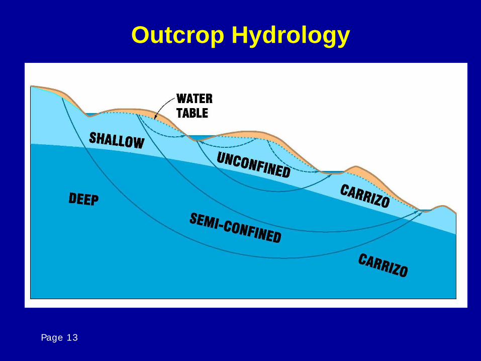
Page 13
Outcrop Hydrology
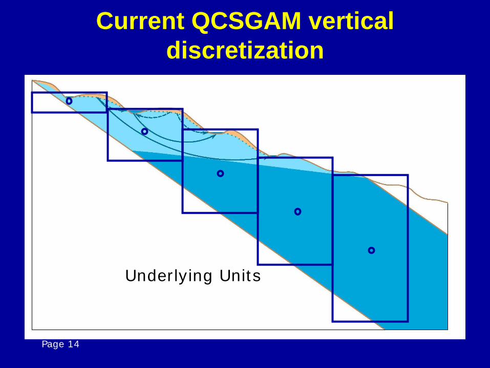
Page 14
Current QCSGAM vertical discretization
Underlying Units
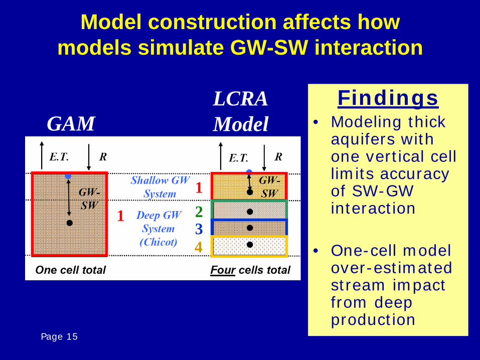
Page 15
Model construction affects how models simulate GW-SW interaction
Findings • Modeling thick
aquifers with one vertical cell limits accuracy of SW-GW interaction
• One-cell model over-estimated stream impact from deep production
LCRA Model GAM
1
2 3 4
1