Design, taking into account the partial discharges
204
HAL Id: tel-03124398 https://tel.archives-ouvertes.fr/tel-03124398 Submitted on 28 Jan 2021 HAL is a multi-disciplinary open access archive for the deposit and dissemination of sci- entific research documents, whether they are pub- lished or not. The documents may come from teaching and research institutions in France or abroad, or from public or private research centers. L’archive ouverte pluridisciplinaire HAL, est destinée au dépôt et à la diffusion de documents scientifiques de niveau recherche, publiés ou non, émanant des établissements d’enseignement et de recherche français ou étrangers, des laboratoires publics ou privés. Design, taking into account the partial discharges phenomena, of the electrical insulation system (EIS) of high power electrical motors for hybrid electric propulsion of future regional aircrafts Philippe Collin To cite this version: Philippe Collin. Design, taking into account the partial discharges phenomena, of the electrical insula- tion system (EIS) of high power electrical motors for hybrid electric propulsion of future regional air- crafts. Electric power. Université Paul Sabatier - Toulouse III, 2020. English. NNT : 2020TOU30116. tel-03124398
-
Upload
khangminh22 -
Category
Documents
-
view
1 -
download
0
Transcript of Design, taking into account the partial discharges

HAL Id: tel-03124398https://tel.archives-ouvertes.fr/tel-03124398
Submitted on 28 Jan 2021
HAL is a multi-disciplinary open accessarchive for the deposit and dissemination of sci-entific research documents, whether they are pub-lished or not. The documents may come fromteaching and research institutions in France orabroad, or from public or private research centers.
L’archive ouverte pluridisciplinaire HAL, estdestinée au dépôt et à la diffusion de documentsscientifiques de niveau recherche, publiés ou non,émanant des établissements d’enseignement et derecherche français ou étrangers, des laboratoirespublics ou privés.
Design, taking into account the partial dischargesphenomena, of the electrical insulation system (EIS) of
high power electrical motors for hybrid electricpropulsion of future regional aircrafts
Philippe Collin
To cite this version:Philippe Collin. Design, taking into account the partial discharges phenomena, of the electrical insula-tion system (EIS) of high power electrical motors for hybrid electric propulsion of future regional air-crafts. Electric power. Université Paul Sabatier - Toulouse III, 2020. English. �NNT : 2020TOU30116�.�tel-03124398�

Résumé
1
Le 03 novembre 2020

Résumé
2

Résumé
3
Résumé La réduction des émissions de CO2 est un enjeu majeur pour l’Europe dans les années à venir.
Les transports sont en effet aujourd’hui à l’origine de 24% des émissions mondiales de CO2. L’aviation
ne représente cependant que 2-3% des émissions globales de CO2 mais le trafic aérien est en pleine
expansion et, déjà, des inquiétudes apparaissent légitimement. A titre d’exemple, en Suède, depuis les
années 1990, les émissions de CO2 dues au trafic aérien ont augmenté de 61%. Ce constat explique
l’apparition du mouvement « Flygskam » qui se repend dans de plus en plus de pays Européens.
C’est dans ce contexte que l’Union Européenne a lancé en septembre 2016 le projet Hybrid
Aircraft academic reSearch on Thermal and Electrical Components and Systems (HASTECS). Le
consortium regroupe différents laboratoires ainsi que l’avionneur Airbus. Ce projet s’inscrit dans le
programme « H2020 Clean Sky 2 » qui vise à développer une aviation plus verte. L’objectif ambitieux
est de réduire de 20% les émissions de CO2 ainsi que le bruit produit par les avions, d’ici 2025. Pour
cela, le consortium a décidé d’étudier une architecture hybride de type série. La propulsion est assurée
par une motorisation électrique pour laquelle deux cibles ont été définies. En 2025, les moteurs
devront en effet atteindre une densité de puissance de 5kW/kg, système de refroidissement inclus. En
2035, cette densité de puissance devra être doublée (10kW/kg). Pour atteindre ces cibles, le niveau de
tension sera considérablement augmenté, probablement au-delà du kilovolt. Le risque d’apparition de
décharges électriques dans les stators des moteurs électriques sera considérablement accru et doit
être pris en compte dès la phase de conception du moteur.
L’objectif de cette thèse est de mettre au point un outil d’aide au design du Système d’Isolation
Electrique (SIE) primaire du stator des moteurs électriques qui seront pilotés par convertisseurs. Le
manuscrit qui synthétise les travaux effectués est découpé en cinq parties.
La première partie commencera par préciser les enjeux et défis d’une aviation plus verte. La
constitution du SIE d’un stator de moteur électrique sera ensuite développée. Enfin, les contraintes
qui s’appliquent sur le SIE dans l’environnement aéronautique seront identifiées.
La deuxième partie présentera les différents types de décharges électriques que l’on peut
retrouver dans les dispositifs électriques. Le principal risque vient des Décharges Partielles (DP) qui
détériorent peu à peu le SIE. Le principal mécanisme permettant d’expliquer l’apparition des DP est
l’avalanche électronique. Le critère de Paschen permet d’évaluer le Seuil d’Apparition des Décharges
Partielles (SADP). Différentes techniques permettent de détecter et mesurer l’activité des DP. Des
modèles numériques permettent d’évaluer le SADP.
La troisième partie présentera une méthode originale pour déterminer les lignes de champ
électrique dans un problème électrostatique. Elle n’utilisera qu’une formulation en potentiel scalaire.
La quatrième partie présentera une étude expérimentale pour établir une correction du critère
de Paschen. En effet, un bobinage de moteur électrique est très loin des hypothèses dans lesquelles
ce critère a été originellement défini.
Enfin, la cinquième partie sera consacrée à l’élaboration de l’outil d’aide au design du SIE. Des
abaques seront construits afin de fournir des recommandations sur le dimensionnement des différents
isolants dans une encoche de stator. Une réduction du SADP due à une variation combinée de la
température et de la pression sera également prise en compte.
Mots clefs : Décharges partielles, théorie de Paschen, Modélisation, Eléments finis, Champ électrique,
Dimensionnement, Diélectriques, Isolation électrique, SADP.

Abstract
4
Abstract Reducing CO2 emissions is a major challenge for Europe in the forthcoming years. Nowadays,
transport represents 24% of the world CO2 emissions. Aviation accounts for only 2-3% of these world
CO2 emissions. However, air traffic is booming and concerns are legitimately emerging. As an example,
CO2 emissions from air traffic have increased by 61% in Sweden since the 90s. This explains the
emergence of the "Flygskam" movement which is spreading in more and more European countries.
It is in this context that the European Union launched in September 2016 the project Hybrid Aircraft
academic reSearch on Thermal and Electrical Components and Systems (HASTECS). The consortium
brings together different research laboratories and Airbus. This project is part of the program “H2020
- Clean Sky 2” which aims to develop a greener aviation. Its ambitious goal consists in reducing CO2
emissions and noise produced by aircraft by 20%, by 2025. To do that, the consortium has decided to
study a serial hybrid architecture. Propulsion is provided by electric motors. Two targets have been
defined. In 2025, the engines must reach a power density of 5kW/kg, including the cooling system. In
2035, this power density of the engines will have to be doubled (10kW/kg). To reach these targets, the
voltage level will be considerably increased, probably beyond one kilovolt. The electric discharges
appearance risk will be considerably increased and need to be considered right from the motor design
stage. The objective of this thesis is then to develop a tool in order to help the designer of electric
motors fed by a converter when he will deal with its primary Electrical Insulation System (EIS). This
manuscript is organized into five parts.
The first part will begin by clarifying both issues and challenges of a greener aviation. The EIS
composition in electric motors will then be developed. Finally, the constraints withstood by the EIS in
an aeronautical environment will be identified.
The second part will present the different types of electric discharges that can be found in
electric devices. The main risk comes from Partial Discharges (PD) which gradually deteriorate the EIS.
The main mechanism for explaining the appearance of PD is the electronic avalanche. The Paschen
criterion makes it possible to evaluate the Partial Discharge Inception Voltage (PDIV). Different
techniques may be used to detect and measure the activity of these PD. Numerical models may also
be used to evaluate the PDIV.
The third part will present an original method for determining the electric field lines in an
electrostatic problem. It only uses a scalar potential formulation.
The fourth part will present an experimental study to establish a correction of the Paschen
criterion. Indeed, an electric motor winding is very far from the assumptions in which this criterion was
originally defined.
Finally, the fifth part will be devoted to the development of the SIE design aid tool. Graphs will
be generated to provide recommendations on the sizing of the various insulators in a stator slot. A
reduction in the PDIV due to a combined variation in temperature and pressure will also be taken into
account.
Keywords: Partial discharges, Paschen, Modelling, Finite elements, Electric field, Sizing, Dielectrics,
Electrical insulation, PDIV.

Remerciements
5
Remerciements
Ces travaux de thèse ont été réalisés au laboratoire LAPLACE (Laboratoire PLAsma et Conversion
d’Energie). Ils ont été financés par l’Union Européenne dans le cadre du programme H2020.
Je tiens tout d’abord à grandement remercier mes deux directeurs de thèse David Malec et Yvan
Lefevre. Ils m’ont accompagné tout au long de cette aventure tant humaine que scientifique. Je garde
de très bon souvenirs de nos escapades aux cours des différentes conférences auxquelles j’ai eu la
chance de participer. Je suis très heureux de l’amitié qui nous lie désormais. Egalement merci aux
membres des deux équipes du laboratoire qui m’ont accueilli chaleureusement : le MDCE sur le site
université Paul Sabatier et le GREM 3 sur le site INPT-ENSEEIHT.
Je tiens à remercier Stéphane Duchesne (LSEE, Université d’Artois) et Olivier Gallot-Lavallee (G2ELab,
Université Grenoble-Alpes) d’avoir accepté d’être rapporteurs de ma thèse. Merci également aux
autres membres du jury, Anca Petre (SIAME, Université de Pau et des Pays de l’Adour), Pierre Bidan
(LAPLACE, Université de Toulouse) pour l’évaluation de ce travail en tant qu’examinateurs. Merci à
Thierry Lebey (SAFRAN), Laurent Albert (IRT Saint-Exupéry) et Jean François Allias (AIRBUS) d’avoir pris
part au jury en tant que membres invités. Je vous suis très reconnaissant d’avoir pris le temps pour
évaluer mon travail et pour la richesse des échanges que nous avons eu lors de la soutenance de cette
thèse.
Je voudrais remercier Sorin Dinculescu, Zarel Valdez-Nava, Vincent Bley, Céline Combettes, Benoit
Lantin, Benoit Schlegel, Pierre Hernandez et Nofel Merbahi pour leur aide à la réalisation de mes
travaux expérimentaux.
Merci également à tous les doctorants, post-doctorants et stagiaires qui ont fait un passage dans le
bureau porte 102 du bâtiment 3R3 : Mallys Banda, Fernando Pedro, Riccardo Albani, Kemas M Tofani,
Imadeddine Benfridja, Youcef Kemari, Pawel Piotr Pietrzak, Trong Trung Le et bien d’autres ! Il y a
toujours eu une bonne ambiance dans ce bureau !
Un grand merci aussi aux doctorants et docteurs du troisième étage sur le site ENSEEIHT : Maxime
Bonnet, Théo Carpi, Mateus Carvalho Costa, Jessica Neumann, Jordan Stekke, Youness Rtimi. C’était
toujours un plaisir de passer vous dire bonjour et de squatter un siège et votre café !
Merci à tous mes collègues du projet HASTECS. Aux doctorants : Sarah Touhami, Najoua Erroui, Amal
Zeaiter, Flavio Accorinti, Malik Tognan et Matthieu Pettes-Duler. J’ai passé d’excellents moments en
votre compagnie ce qui a rendu mon travail encore plus agréable. Bon courage à toi Matthieu qui est
le dernier à soutenir !
Je tiens à remercier tous mes compères de l’Association des Laplaciens (ADeL) que j’ai eu le plaisir de
présider : Marjorie Morvan, Aurélien Pujol, Plinio Bau, Bojan Djuric et Matthieu Pettes-Duler (encore
toi !). On a vraiment fait du bon boulot et on s’est bien éclaté !
Merci aussi aux nombreux doctorants et docteurs du PRHE avec lesquels j’ai passé beaucoup de bon
temps : Cyril Van de Steen, Julien Cosimi, Maxime Bafoil, Tristan Gouriou, Aurélie Marches, Eléna
Griseti, Valentin Ferrer. Je pense aussi à d’autres gens bien sympas : Maxime Castelain, Aurélie
Tokarski, Benoit Prochet, Nicolas Millet, Davin Guedon, Andréa Al Haddad.

Remerciements
6
Merci à mes anciens camarades de l’ENSEEIHT : Thomas Longchamps, Etienne Farman, Yoann Scotto,
Baptiste Genet et tous les autres pour les très bons moments passés même après l’obtention de notre
diplôme d’ingénieur.
Je remercie ma famille étendue (les Collin et les Chauvin) pour leur soutien pendant ces années de
thèse.
Enfin je dédie mes derniers remerciements à ma compagne Julie Chauvin. Tu es toujours à mes côtés
pour me supporter et pour me donner la force d’aller de l’avant. Je t’aime!

Remerciements
7
Table of contents Résumé .................................................................................................................................................... 3
Abstract ................................................................................................................................................... 4
Remerciements ....................................................................................................................................... 5
General Introduction ............................................................................................................................. 13
Chapter 1: Toward full-electric transportation ..................................................................................... 17
1 Implications and challenges .......................................................................................................... 19
1.1 Sustainable transportation .................................................................................................... 19
1.1.1 International context ..................................................................................................... 19
1.1.2 European and France contexts ...................................................................................... 21
1.2 The “Flygskam” movement ................................................................................................... 21
2 Toward more electric aircrafts ...................................................................................................... 22
2.1 Classic aircraft architecture ................................................................................................... 22
2.1.1 Pneumatic network ....................................................................................................... 22
2.1.2 Hydraulic network ......................................................................................................... 22
2.1.3 Mechanical power ......................................................................................................... 23
2.1.4 Electrical network .......................................................................................................... 23
2.2 Projects of more electric aircrafts ......................................................................................... 24
2.2.1 E-FanX ............................................................................................................................ 25
2.2.2 CityAirbus ...................................................................................................................... 26
3 HASTECS project ............................................................................................................................ 26
3.1 Targets ................................................................................................................................... 26
3.2 Serial hybrid configuration .................................................................................................... 27
3.3 Work packages ...................................................................................................................... 27
3.3.1 Work Package 1 (WP1) .................................................................................................. 28
3.3.2 Work Package 2 (WP2) .................................................................................................. 29
3.3.3 Work Package 3 (WP3) .................................................................................................. 30
3.3.4 Work Package 4 (WP4) .................................................................................................. 32
3.3.5 Work Package 5 ............................................................................................................. 33
3.3.5.1 DC busbar .................................................................................................................. 33
3.3.5.2 Motor Electrical Insulation System (EIS) ................................................................... 35
3.3.6 Work Package 6 ............................................................................................................. 35
4 Electric motors electrical insulation .............................................................................................. 36
4.1 Low voltage machine ............................................................................................................. 36
4.1.1 Turn-to-turn insulation .................................................................................................. 38

Remerciements
8
4.1.2 Phase-to-phase insulation ............................................................................................. 41
4.1.3 Turn-to-slot insulation ................................................................................................... 41
4.1.4 Slot impregnation .......................................................................................................... 42
4.2 High voltage machine ............................................................................................................ 44
5 Thermal aspect .............................................................................................................................. 46
5.1 Cooling strategies .................................................................................................................. 46
5.2 Thermally enhanced polymers .............................................................................................. 47
6 Impact of power electronics .......................................................................................................... 49
6.1 Pulse Width Modulation (PWM) basis .................................................................................. 49
6.2 Power feeding cable .............................................................................................................. 51
6.3 Frequency increase................................................................................................................ 55
6.4 Voltage distribution ............................................................................................................... 57
Chapter 2: Physics of Partial Discharges (PD) ........................................................................................ 61
1 Different kinds of discharges ......................................................................................................... 63
1.1 Discharges in non-vented cavities ......................................................................................... 64
1.2 Discharges in vented cavities ................................................................................................ 65
1.3 Discharges on the surface ..................................................................................................... 66
1.4 Corona discharge ................................................................................................................... 67
1.5 PD consequences on stator insulation .................................................................................. 68
2 Physics of plasma ........................................................................................................................... 69
2.1 Townsend mechanism ........................................................................................................... 69
2.1.1 First Townsend’s coefficient .......................................................................................... 70
2.1.2 Second coefficient ......................................................................................................... 73
2.2 Paschen’s law ........................................................................................................................ 74
2.3 Impact of aeronautics conditions .......................................................................................... 75
2.3.1 Environmental variations .............................................................................................. 75
2.3.2 Impact of temperature .................................................................................................. 77
2.3.3 Impact of humidity ........................................................................................................ 80
3 PD analysis ..................................................................................................................................... 82
3.1 Experimental detection of PD activity ................................................................................... 82
3.1.1 Radio-frequency detection ............................................................................................ 83
3.1.2 Optical detection ........................................................................................................... 83
3.1.3 Power factor/capacitance tip-up test............................................................................ 84
3.1.4 Used electric detection.................................................................................................. 84
3.2 Parameters linked to PD ........................................................................................................ 85
3.2.1 Partial Discharge Inception Voltage (PDIV) ................................................................... 85

Remerciements
9
3.2.2 Partial Discharge Extinction Voltage (PDEV) ................................................................. 86
3.2.3 Apparent charge ............................................................................................................ 86
3.3 Statistical processing of the results ....................................................................................... 87
4 Degradation of the polymer insulation in aeronautic environment ............................................. 90
4.1 Pressure ................................................................................................................................. 91
4.2 Humidity ................................................................................................................................ 92
4.3 Temperature .......................................................................................................................... 93
4.4 Frequency and voltage .......................................................................................................... 94
4.5 Lifetime evaluation ................................................................................................................ 96
5 Modelling partial discharges activity ............................................................................................. 98
5.1 Streamer criterion ................................................................................................................. 98
5.2 Paschen’s criterion .............................................................................................................. 100
Chapter 3: Electric field lines computation ......................................................................................... 103
1 Introduction ................................................................................................................................. 105
2 The electrostatic problem ........................................................................................................... 105
2.1 Presentation of the field of study ........................................................................................ 105
2.2 Electrostatic equations and formulations ........................................................................... 106
2.3 Advantages and disadvantages of each formulation .......................................................... 108
2.3.1 Vector potential ........................................................................................................... 108
2.3.2 Scalar potential ............................................................................................................ 109
3 Electric field lines computation derived from a scalar potential formulation ............................ 109
3.1 Ballistic method ................................................................................................................... 109
3.2 Flux tubes based method .................................................................................................... 113
4 Proposed method ........................................................................................................................ 116
4.1 Electric field and electric flux .............................................................................................. 116
4.2 Equipotential lines ............................................................................................................... 118
4.3 Flux function ........................................................................................................................ 120
4.4 Illustrative examples............................................................................................................ 122
5 Another method using Matlab functions .................................................................................... 124
5.1 Building the additional mesh ............................................................................................... 124
5.2 Electric field ......................................................................................................................... 125
5.3 Comparison with the proposed method ............................................................................. 126
6 Conclusion ................................................................................................................................... 128
Chapter 4: Correction of the Paschen’s criterion ................................................................................ 129
1 Motivations ................................................................................................................................. 131
1.1 Configuration different from the initial one........................................................................ 131
Remerciements
10
1.2 Experimental observation ................................................................................................... 131
2 Experimental approach ............................................................................................................... 133
2.1 Samples ............................................................................................................................... 133
2.2 Experimental protocol ......................................................................................................... 135
3 Results ......................................................................................................................................... 136
3.1 PDIV results ......................................................................................................................... 136
3.2 Dielectric constant measurements ..................................................................................... 139
4 Mixed experimental and numerical approaches ......................................................................... 141
5 Single layer insulation .................................................................................................................. 144
6 Secondary electron emission coefficients ................................................................................... 146
6.1 Impact of the incoming angle of bombarding ions ............................................................. 147
6.2 Influence of the enamel chemistry ..................................................................................... 149
7 Additional experimentation ........................................................................................................ 150
7.1 Set up ................................................................................................................................... 150
7.2 Results ................................................................................................................................. 152
8 Conclusions and perspectives ..................................................................................................... 154
Chapter 5: Tool to predict PD activity in machine slot ........................................................................ 157
1 Dielectric constant evolution with temperature and frequency ................................................ 159
2 Partial Discharge Evaluation Criterion ......................................................................................... 160
3 Partial Discharge Inception Voltage (PDIV) decrease for a combined variation of temperature
and pressure ........................................................................................................................................ 161
4 Wire design graphs ...................................................................................................................... 162
4.1 Simple analytical model for electric field in air gap computation ....................................... 162
4.2 Validation of Simple Analytical Model with finite elements ............................................... 164
4.3 Enamel thickness as a function of applied voltage ............................................................. 165
4.4 Copper diameter as function of computed enamel thickness ............................................ 167
4.5 Validation ............................................................................................................................ 168
5 Slot insulation design graphs ....................................................................................................... 170
5.1 Simple analytical model for electric field in air gap computation ....................................... 170
5.2 Validation of Simple Analytical Model with finite elements ............................................... 171
5.3 Slot liner thickness as a function of applied voltage and insulation materials ................... 172
5.3.1 First imbrication .......................................................................................................... 173
5.3.2 Second imbrication ...................................................................................................... 174
5.3.3 Third imbrication ......................................................................................................... 175
5.4 Validation ............................................................................................................................ 175
6 Evaluation of the electric stresses under normal temperature and pressure conditions .......... 176

Remerciements
11
6.1 Turn/turn electric stress ...................................................................................................... 176
6.2 Turn/slot electric stress ....................................................................................................... 178
7 Partial Discharge Evaluation Tool (PDET) .................................................................................... 178
7.1 PDET algorithm .................................................................................................................... 179
7.2 Inputs ................................................................................................................................... 180
8 Illustrative example ..................................................................................................................... 181
9 Conclusion ................................................................................................................................... 186
General conclusion and perspectives .................................................................................................. 189
Publications ......................................................................................................................................... 193
Annex ................................................................................................................................................... 195
References: .......................................................................................................................................... 197

12

General Introduction
13
General Introduction
Aircrafts manufacturers such as Airbus, Boeing and Bombardier are engaged in the
competition to develop more- and full- electric aircrafts. That incoming revolution takes place in a
context where more and more people and countries are expecting a much greener air transportation.
The first step of this change is to progressively replace turboshafts by electric motors to ensure the
propulsion of the aircraft. More and more on-board electric power is consequently required.
The risk of electric discharges in propelling electric motors will then increased, as the feeding
voltage will probably be higher than one kilovolt. The Electric Insulation System (EIS) ensures the
protection of a machine against electric hazards. It can be divided into two categories. Type I is used
in low-voltage rotating machine. The International Electric Commission (IEC) considers a machine with
a phase-to-phase voltage lower than 700 Vrms as a low-voltage machine. Type I insulation is almost
exclusively made of polymer materials. These are also called organic materials. On the other hand,
Type II insulation is used in machine with phase-to-phase voltage upper than 700 Vrms. It uses inorganic
materials such as fibber glass, mica, ceramics, composite materials,... These are more expensive
materials which lifespan is increased in presence of electric discharges. Type I insulation is also used in
machines fed by voltages higher tan 700 Vrms, as the EIS has been designed to be free from electric
discharges.
Since the introduction of power electronic power supplies, that provides easy control of the
machine rotational speed, the electrical insulation of such motors faces new hazards. Fast changing
supply voltage, with high dV/dt, may cause the apparition of partial discharges (PD), that results in
accelerated insulation aging and often leads to premature failure of the motors. In low voltage rotating
machines, the stator insulation system is multi-level. Its first component (primary insulation) is the
polymer enamel on the magnet wire, among the others: inter-phase insulation, slot insulation and
impregnation varnish. Depending on the desired thermal properties, there are several types of
polymers being used nowadays in enameled wires: polyamide (PA), polyamide-imide (PAI), polyester-
imide (PEI) and polyimide (PI). Inorganic nano-particles (SiO2, Al2O3, ZnO,…) may also be used as fillers
to obtained corona-resistant enamels. In random-wound stators powered by power inverters, in
comparison with sinusoidal power supply, the magnet wire insulation is far more endangered. Hence,
the objective is to concentrate on this primary insulation. Once the voltage exceeds the Partial
Discharge Inception Voltage (PDIV), electronic avalanches will take place in the EIS, leading to:
- an ions bombardment of the insulator surfaces;
- an increase in temperature the the area submitted to PD;

General Introduction
14
- a chemical degradation of the insulators.
All these actions will strongly increase the insulator degradation rate. Usually, there are three ways
used to avoid and/or to resist to such damage. Firstly, the use of corona-resistant enameled wires,
especially formulated to increase the lifetime under PD attacks. Secondly, a suitable design of the
primary electrical insulation: choice of right enamel wires (size and shape), insulation thickness (grade),
choice of wires arrangement in the slots... Third, the use of both of these two solutions.
A non-closed motor embedded in an aircraft is submitted to severe environmental variations.
These are mainly the temperature, the pressure, the humidity and vibration. These environmental
parameters have a significant impact on the physics describing PD. It is for example known that a
combined temperature increase and pressure decrease in dry air reduces the PDIV.
The objective of this thesis is to develop an automatic tool, based on PD physics, in order to
help the machine designer to better design and size the EIS of rotating machines fed by inverters. The
scope of investigation of the tool is limited to the stator slot. It considers only one phase per slot (an
upgrade could be considered thereafter to treat more than one phase per slot). Therefore, the
turn/turn and turn/slot electric stresses are studied. First, a criterion to evaluate PDIV in both
configuration is established. It is a correction of the Paschen’s criterion, taking into account the
dielectric over-coating and a combined variation of temperature and pressure in micro gaps. Simple
Analytical Models (SAM) are developed and validated with 2D-Finite Elements Models (2D-FEM).
Graphs are derived from parametric studies to size the EIS in order to withstand electric stress without
PD in turn/turn and turn/slot configurations.
This thesis is founded by the Hybrid Aircraft reSearch on Thermal and Electrical Components
and Systems (HASTECS) project. It is part of the “H2020 - Clean Sky 2” European program. It is a
consortium composed of public laboratories and Airbus. The PhD research work takes place in the
LAboratory on PLAsma and Conversion of Energy (LAPLACE) in Toulouse. The works in LAPLACE were
conducted in collaboration between 2 research teams: the Dielectrics Materials in the Energy
Conversion (MDCE) group and the Research Group in Electrodynamics (GREM3). MDCE has provided
the facilities for the experimental studies, whereas GREM3 has provided the license and expertise on
Ansys finite elements software.
This PhD dissertation is divided into five chapters. A short description of each chapter is given
in the following.

General Introduction
15
Chapter I: Toward full electric transportations
Chapter I will start by presenting the challenges on the road toward a green aviation, based on
Worldwide and European scales. Then, a classic aircraft architecture will be detailed. Projects of more
electric aircrafts will be introduced alongside the HASTECS project with its serial-hybrid electric
architecture. Chapter I will continue with the explanation of a motor EIS composition for Type I and
Type II machines. It will finish by identifying power electronics impacts on electric stresses occurring
at the motor terminals.
Chapter II: Physics of Partial Discharges
Chapter II will begin with a presentation of the different kinds of electric discharges. The
electronic avalanche will be identified as the main mechanism involved in PD. It will be described by
the Paschen’s law. The impact of aeronautical conditions on Paschen’s law will be detailed. Chapter II
will then describe the experimental methods to detect and measure a PD activity in an electric device.
The parameters impacting the insulation lifespan will be identified. Finally, two main numerical models
to evaluate PD activity will be introduced; each of them uses a different criterion.
Chapter III: Electric field lines computation
This chapter will be dedicated to the electrostatic problem composed by two enamelled round
wires in close contact. The formulations in both vector and scalar potential will be presented. It will
come that the scalar formulation is the easiest to handle. It will be consequently used to propose an
original method to compute field lines. The proposed method will be compared to a ballistic method
implanted in Matlab software. The field lines geometry and the scalar potential distribution are
required for the application of the PDIV evaluation criterion based on Paschen’s law.
Chapter IV: Correction of Paschen’s criterion
Paschen’s criterion has been experimentally established for a configuration which is
completely different from the ones found in a machine stator slot. Therefore, the validity of this
criterion will be investigated. Experimental observations of PD degradation between enamelled round
wires in close contact has revealed that the Paschen’s law shape is conserved. The dielectric over-
coating has been found to simply increase the PDIV level. An experimental study coupled with a 2D-
FEM will be performed to evaluate the secondary electron coefficient value in the presence of a
dielectric over-coating.

16
Chapter V
This chapter will present in detail the tool to implement the EIS design in order to avoid any
PD in stator slots. It will start by giving the assumptions used in the different models. A focus will be
on turn/turn and turn/slot configurations. Parametric studies on the impacting parameters will be
realized using SAM. Sizing graphs will be derived from these studies. These graphs will then be
implanted in a Partial Discharge Evaluation Tool (PDET). The interest and efficiency of the developed
PDET will finally be proved with an illustrative example.
Finally, conclusions as well as perspectives for future works will be proposed.

Chapter 1: Toward full-electric transportation
17
Chapter 1: Toward full-electric transportation

Chapter 1: Toward full-electric transportation
18

Chapter 1: Toward full-electric transportation
19
1 IMPLICATIONS AND CHALLENGES
1.1 SUSTAINABLE TRANSPORTATION
1.1.1 International context
The role of transportation in the world sustainable development was firstly pointed out during the
1992 United Nation’s Earth Summit at Rio de Janeiro [1]. Since then, the strong role of transportation
in climate change, raw material depletion, human health and ecosystems equilibrium is as important
as ever. Indeed, the transportation sector:
- is responsible of 24% of world CO2 emissions [2]. Every person on our planet produces, on
average, 1.5t of CO2 emissions per year, just for being on the move [3]. Both passengers and
freight road vehicles are responsible of 74% of the total transportation CO2 emissions, while
both aviation and shipping reach 22% and rail 1.3%;
- remains the largest consumer of oil : 57% of the global demand [4], i.e. : 55.8 Mb/day where
road represents 78.1%, air 11.4%, sea 7.3% and rail 3.2% ;
- is responsible of 12-70% of the total tropospheric air pollution mix [5]; Asia, Africa and the
Middle East suffer more due to the use of old and inefficient vehicles. Outdoor air pollution
(O3, NOX, SO2, CO, PM10, PM2.5,…) kills more than 8 million people across the world every year.
Transportations, mainly road ones, would be responsible of almost 50% of these premature
deaths [6] ;
- is responsible of direct and indirect damages, or major changes, on ecosystems (air, marine
and earth), which are often unpredictable [7].
In order to identify guidelines, different scenarii such as the Sustainable Development Scenario (SDS),
the Clean Air Scenario and the Future is Electric Scenario have been established by using the World
Energy Model developed by the International Energy Agency [8]. As an example, Figure 1 shows the
CO2 emissions SDS targets versus transportation sectors ; direct transport emissions must peak around
2020 and then fall by more than 9% by 2030.

Chapter 1: Toward full-electric transportation
20
Figure 1: CO2 emissions versus transportation sectors (past evolution and SDS targets) [2]
In order to put global warming, human health and environmental impacts of transportation on track
to meet all 2030 goals, different efforts must be undertaken or pursued in all kind of transport by
increasing even more:
1) the efficiency of existing ICE (Internal Combustion Engine) powertrains: lower fuel
consumption, use of bio- or low carbon- fuels, better decontamination of exhaust gas,… ;
2) the electrification of ICE powertrains: hybridization or full electrification;
3) the capacity, the efficiency, the lifetime and the hybridization of embedded power
sources;
4) the efficiency of existing powertrains, traditionally electric ;
5) the good consumer’s behaviours (better transportation planning, carpooling,…) and the
voluntary city transport policies.
The transportation sector has now entered a critical transition period where existing measures listed
below must be deepened and extended in order to reach the environmental goals, whereas in the
meantime the need in this sector is continuously growing. This process will need to be set in motion
over the next decade. Any delay would require stricter measures beyond 2030, which could noticeably
increase the cost of reaching environmental and health targets. This must be accompanied, of course,
by the power sector decarbonisation since 41% of world CO2 emissions is due to electricity generation
[2]. Among all the measures listed below, items 2), 3), 4) and 1) for electric-assisted solutions, are
essentially dependent on R&D efforts in the field of both Electrical and Electrochemical (-applied to
energy) Engineering.
Chapter 1: Toward full-electric transportation
21
1.1.2 European and France contexts
In the European Union (EU), more and more societies aim to be greener; fossils energies are more and
more substituted by sustainable ones. As an example, in France, the proportion of sustainable energy
into the total energy consumption has increased by about 69% from 1990 to 2016 [9]. It represents
16% of the total consumption of energy in France in 2018. With the Accord de Paris and the Climate
Plan, EU aims to increase this proportion up to 27% in 2030 [9].
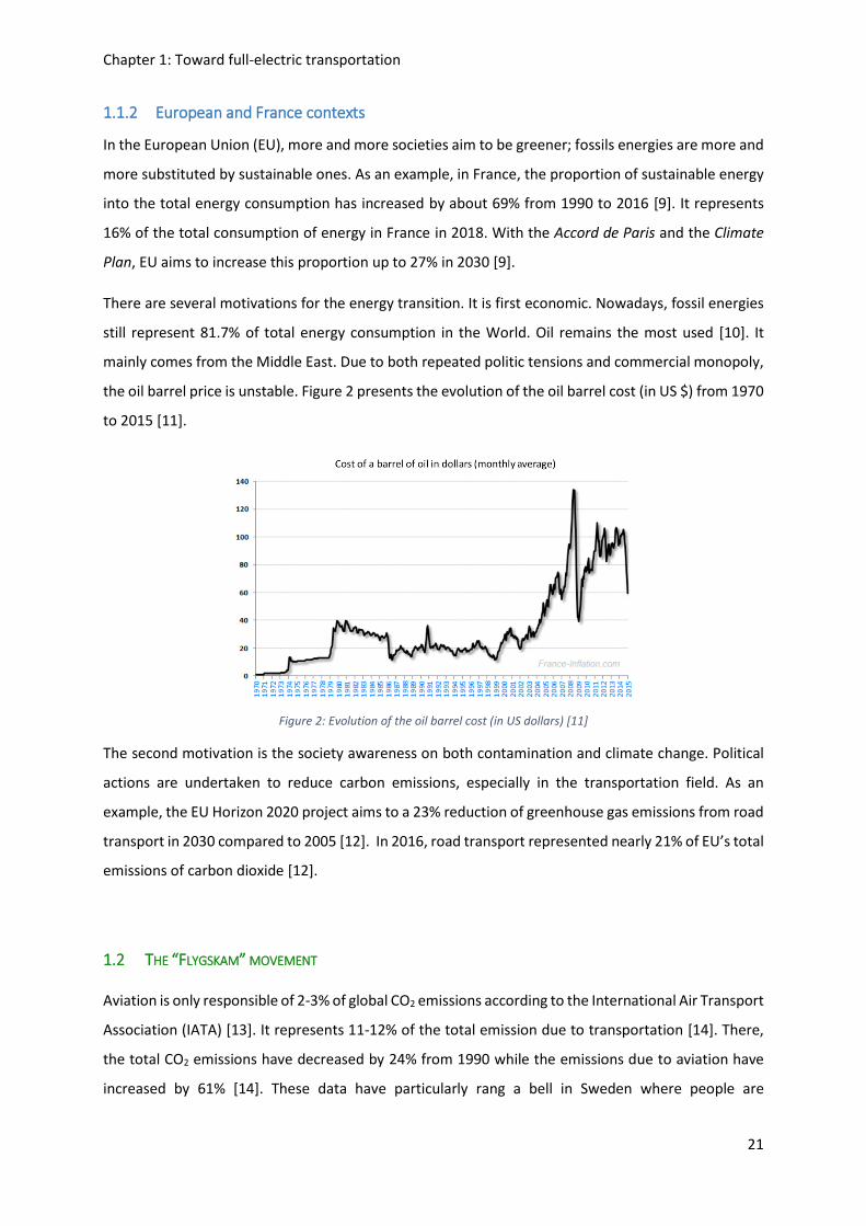
There are several motivations for the energy transition. It is first economic. Nowadays, fossil energies
still represent 81.7% of total energy consumption in the World. Oil remains the most used [10]. It
mainly comes from the Middle East. Due to both repeated politic tensions and commercial monopoly,
the oil barrel price is unstable. Figure 2 presents the evolution of the oil barrel cost (in US $) from 1970
to 2015 [11].
Figure 2: Evolution of the oil barrel cost (in US dollars) [11]
The second motivation is the society awareness on both contamination and climate change. Political
actions are undertaken to reduce carbon emissions, especially in the transportation field. As an
example, the EU Horizon 2020 project aims to a 23% reduction of greenhouse gas emissions from road
transport in 2030 compared to 2005 [12]. In 2016, road transport represented nearly 21% of EU’s total
emissions of carbon dioxide [12].
1.2 THE “FLYGSKAM” MOVEMENT
Aviation is only responsible of 2-3% of global CO2 emissions according to the International Air Transport
Association (IATA) [13]. It represents 11-12% of the total emission due to transportation [14]. There,
the total CO2 emissions have decreased by 24% from 1990 while the emissions due to aviation have
increased by 61% [14]. These data have particularly rang a bell in Sweden where people are

Chapter 1: Toward full-electric transportation
22
increasingly abandoning air planes for internal trips; internal flights have decreased by 3% from
January to September 2018 [14]. This movement that has received the name “Flygskam”, literally the
shame to take the plane, is growing in other countries.
2 TOWARD MORE ELECTRIC AIRCRAFTS
2.1 CLASSIC AIRCRAFT ARCHITECTURE
Multiple sources of energy are present in an aircraft. It includes mechanical, electrical, hydraulic and
pneumatic energies. Figure 3 illustrates the implantation of a conventional power distribution [15].
Figure 3: Schematic of a conventional power distribution in aricrafts [15]
2.1.1 Pneumatic network
The pneumatic power is bled from the engine high-pressure compressor. It is commonly used to power
the Environmental Control System (ECS). It also supplies hot air for Wing Ice Protection System (WIPS).
The major drawback of air bleeding from the engine is that it reduces thrust efficiency.
2.1.2 Hydraulic network
The hydraulic power is provided by a central hydraulic pump. The power is transfered to actuation
systems (primary and secondary flight control), landing gears, engine actuation, thrust reversal system
and several other auxiliary systems.

Chapter 1: Toward full-electric transportation
23
As an example, the A320 hydraulic system is composed of three fully independent circuits: Green,
Yellow and Blue (see Figure 3) . The normal hydraulic source on the blue circuit is the electrical pump.
The auxiliary source is the Ram Air Turbine (RAT), used in case of a huge electrical power failure. On
the green and yellow circuits, the normal hydraulic source is the Engine Driven Pump (EDP). The
auxiliary source is the Power Transfer Unit (PTU). It is a hydraulic motor pump which transfers hydraulic
power between the green and yellow systems without transfer of fluid [16].
The main drawback of a hydraulic power is the economic cost in maintenance due to the system
complexity.
Figure 4: Green, Blue and Yellow A320 hydraulic circuits [16]
2.1.3 Mechanical power
The gearbox is the heart of the mechanical power transmission. It transfers the power from the engines
to central hydraulic pumps, to local pumps for engine equipment, to other mechanically driven
subsystems and to the main electrical generator [15].
2.1.4 Electrical network
The proportion of on board electric power has continuously increased in aircrafts. The electric power
tends to replace more and more systems which were powered by either pneumatic or hydraulic power.
Figure 5 illustrates the increasing of inboard electrical equipment demand in commercial aviation [17].

Chapter 1: Toward full-electric transportation
24
Figure 5: Increasing on board electrical equipment demand in commercial aviation [17]
The former on board electric bus first provided both constant voltage and frequency to the aircrafts
devices. An Integrated Drive Generator (IDG) was used to change the variable speed of the jet engine
to constant speed [18]. Between 1936 and 1946, the voltage supply has increased from 14.25 VDC to
28 VDC [19].
In recent aircrafts such as Airbus A380, Airbus A350 and Boeing 787, there is no more IDG. A gearbox
is used to directly couple the engine generator to the jet engine. An alternative voltage of 115/200
VAC is produced with a frequency range from 350 to 800 Hz [18].
The interest to replace pneumatic and hydraulic system with electric ones is mainly economic.
Moreover, electric aircrafts have a lower maintenance cost.
2.2 PROJECTS OF MORE ELECTRIC AIRCRAFTS
Almost ten years ago, focusing in EU, Airbus revealed its first full electric aircraft. Up to now, new
demonstrators try to develop and optimize the electric propulsion technology.

Chapter 1: Toward full-electric transportation
25
Figure 6: A timeline of Airbus's achievement in electric propulsion [20]
2.2.1 E-FanX
The E-FanX is the last Airbus-Rolls Royce project dealing with airplanes electrification. The objective is
to develop a flight demonstrator testing a 2MW hybrid-electric propulsion system on a 100 seat
regional jet. One of the four jet engines will be replaced with a 2 MW electric motor fed by a 3 kVDC
electrical distribution. The flight testing should have started by the end of 2020 but, due to the corona
virus pandemic, it has been stopped until further notice [21].
Figure 7: Airbus-Rolls Royce E-FanX (in green : the electric propeller) [21]

Chapter 1: Toward full-electric transportation
26
2.2.2 CityAirbus
The CityAirbus is an all-electric four-seat multicopter vehicle demonstrator. It is an electric Vertical
Take-Off and Landing vehicle (eVTOL). It is remotely piloted. The CityAirbus demonstrator first take-
off happened in May 2019. This vehicle produces less noise and zero emission compared to a classic
helicopter.
Figure 8: CityAirbus technical data [22]
3 HASTECS PROJECT
3.1 TARGETS
The Hybrid Aircraft academic reSearch on Thermal and Electrical Components and Systems (HASTECS)
is part of the “H2020 - Clean Sky 2” program. It is a heavy EU aeronautics research program which aims
to reduce by 20% the CO2 emissions and the noise produced by airplanes by 2025. It regroups several
laboratories, including LAPLACE, in partnership with Airbus Toulouse.
HASTECS objectives are to identify the most promising technological breakthrough solutions and to
develop tools to considerably increase the efficiency of the electric hybrid powertrain systems. The
final objective is to obtain both fuel consumption and noise contamination significant saves as it is
currently the case for road vehicles (cars, buses, trucks). To successfully achieve such objectives, the
specific powers will have to be increased.
HASTECS consortium aims to double the specific power of electric motors including cooling system.
The targets are 5 kW/kg by 2025 and 10kW/kg by 2035. Concerning the power electronics, the specific
power, including cooling, aims to be 15kW/kg by 2025 and 25kW/kg by 2035. These targets are to be
achieved despite challenging environmental conditions such as harsh environmental conditions.

Chapter 1: Toward full-electric transportation
27
This technological breakthrough should reduce by 1.8 ton the weight of a 1.5MW inverter-motor
powertrain. Consequently, 3.5% fuel save should be achieved on a 300 nautical miles’ regional flight.
The kick-off meeting on September 13th 2016 has marked the start of HASTECS project for five years.
It involves six PhD students and two post-doctoral students for a total founding of 1.5 M€ [23].
3.2 SERIAL HYBRID CONFIGURATION
There are several possible architectures for an electric hybrid powertrain [24]. HASTECS consortium
has retained the serial hybrid one. It has mainly been selected because it is the architecture of the
future Airbus demonstrator eFanX [21]. It is illustrated in Figure 9.
Figure 9: Serial hybrid powertrain [25]
Gas turboshafts driving electric generators are the main sources of power. Rectifiers supply an ultra-
high DC voltage. Bus voltages are in the range of kVs [26]. The power is directed toward the Electrical
Power Distribution Center (EPDC). Auxiliary power is delivered by batteries and/or fuel cells. The power
supplies inverter fed motors. The propellers are driven through gearboxes.
HASTECS perimeter is composed of the batteries/fuel cells, the high voltage DC bus, the power
electronics and the inverter fed motors. The tasks are dispatched between six Work Packages (WP).
3.3 WORK PACKAGES
Figure 10 below illustrates the tasks carried by each WP and the possible interactions.

Chapter 1: Toward full-electric transportation
28
Figure 10: HASTECS work packages [23]
3.3.1 Work Package 1 (WP1)
This WP focuses on the electromechanical sizing of the electric motors. The first target for 2025 is a 5
kW/kg specific power, including cooling. The second target for 2035 is to reach 10 kW/kg. WP1 strongly
interacts with WP3 (thermal study) and WP5 (partial discharges study). To choose the motor
architecture, an analytic calculation tool has been developed [27]. It makes quick trade-offs of high
specific torque electric motors using the loadability concepts developed by designers. The loadability
concepts are mainly the electric, magnetic and thermal loads (see Table 1). Such loads are introduced
in the tool as inputs to get the main sizes, weight and performances of the electric motor. The main
interest is that there is no need to specify neither the stator winding configuration, nor the rotor
structure. Additional inputs data such as the mechanical power or the rotational speed are required
[28].
Load Parameter Description Constraint
Magnetic loading Bm Magnetic flux in air gap Magnetic materials
Electric loading Km Surface current density Insulation materials
Cooling technology
Electromagnetic loading 𝜎𝑡 =
𝐵𝑚 ∗ 𝐾𝑚2
𝑇𝑒𝑚 = 2 ∗ 𝜎𝑡 ∗ 𝜋 ∗ 𝑅2 ∗ 𝐿
𝜎𝑡 : tangential stress in
airgap
Tem: maximum
electromagnetic torque
R: inner stator radius
L: motor active length
Magnetic materials
Insulation materials
Cooling technology
Table 1: Electric machine loads [28]

Chapter 1: Toward full-electric transportation
29
3.3.2 Work Package 2 (WP2)
The task of this WP is to develop a tool to facilitate high-power converters design in a limited time to
analyse and compare several conversion topologies to power the motorization system. The first
objective for 2025 is to size a 15 kW/kg power converter, including cooling. The second objective for
2035 is to increased this value to 25 kW/kg. To reach such high values, the power converter losses have
to be minimized.
First, this WP determines an optimal DC bus voltage. This key parameter is determinant in both
machine sizing and partial discharges study. The efficiency and power density of different multileveled
topologies are investigated using a developed tool and real semiconductors datasheets (Figure 11).
Figure 11: Power electronics efficiency for several topologies using available database components [29]. 2L PWM: 2 Layers Pulse Wide Modulation, FC-3L PWM: Flying Cap-3 Layers Pulse Wide Modulation, FC-5L PWM: Flying Cap-5 Layers Pulse
Wide Modulation
This WP carried out a work to develop a simulation tool for pre-sizing converters. It makes it possible
to size a converter from a chosen topology. Parametric studies by varying the DC bus voltage, the
requested power or the modulation index make it possible to determine the optimum operating point.
An algorithm was developed to select the best suited component for both desired voltage and current
values [29]. The performances are being computed based on analytical calculations of the losses in the
semiconductors components for multiple multilevel architectures. Pulse Width Modulation (PWM)
control is mainly considered [29].
Discontinuities in the results (see Figure 10) are due to discontinuities in component calibres and have
been overcome by generating virtual components with continuous calibres. Components parameters
Chapter 1: Toward full-electric transportation
30
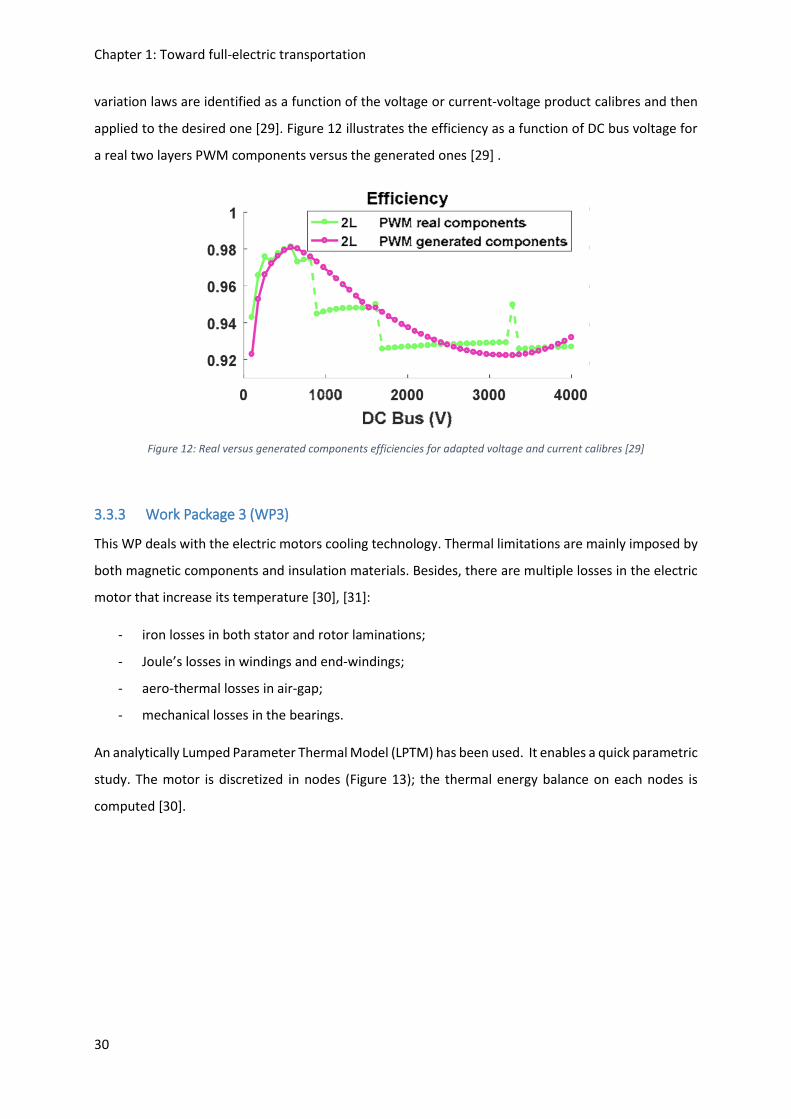
variation laws are identified as a function of the voltage or current-voltage product calibres and then
applied to the desired one [29]. Figure 12 illustrates the efficiency as a function of DC bus voltage for
a real two layers PWM components versus the generated ones [29] .
Figure 12: Real versus generated components efficiencies for adapted voltage and current calibres [29]
3.3.3 Work Package 3 (WP3)
This WP deals with the electric motors cooling technology. Thermal limitations are mainly imposed by
both magnetic components and insulation materials. Besides, there are multiple losses in the electric
motor that increase its temperature [30], [31]:
- iron losses in both stator and rotor laminations;
- Joule’s losses in windings and end-windings;
- aero-thermal losses in air-gap;
- mechanical losses in the bearings.
An analytically Lumped Parameter Thermal Model (LPTM) has been used. It enables a quick parametric
study. The motor is discretized in nodes (Figure 13); the thermal energy balance on each nodes is
computed [30].

Chapter 1: Toward full-electric transportation
31
Figure 13: Motor nodes locations in axial and radial sections [30]
The connections between nodes (Figure 14) depends on material properties such as thermal
conductance.
Figure 14: Motor nodal network [30]
As an example, for a motor configuration similar to the Lexus 2008 [32] and considering a water jacket
cooling solution [30], the hot spots have been identified (see Figure 15):
Figure 15: Resulting temperatures in different locations inside a motor. Adapted from [30].

Chapter 1: Toward full-electric transportation
32
The hot spots are located in the winding and end-winding where the thermal conductivities are the
lowest [30], [32].
3.3.4 Work Package 4 (WP4)
This WP aims to design and to optimize solutions to cool the electric power converters. The cooling
solution also has to provide a constant operating temperature for the whole mission of the aircraft.
Climb and descent stages are the most stressful. The temperature difference between ground and
flight can reach 40 °K [33]. The Capillary Pumped Loop for Integrated Power (CPLIP) cooling solution
has been chosen. It suits the Power electronics In the Nacelle (PIN) configuration. Figure 16 illustrates
the CPLIP concept [33]:
Figure 16: CPLIP concept schema [33]
The power electronic is set up around the evaporator wall. A tank delivers the liquid at ambient
temperature to the evaporator. In this porous component, there is a heat exchange occurring between
the power electronics and the fluid. The fluid then turns to vapour and is directed toward the
condenser through the vapour line. In the condenser, the vapour is cooled and turns back to liquid.
The liquid is sent back to the reservoir through the liquid line.
The choice of the design point is particularly sensitive as it influences the weight of the cooling system.
It has been chosen at the beginning of the take-off and climb stage [33] . Whatever the selected power
converter topology, the energy to be evacuated during the take-off and climb stage represent 44% to
45% of the energy to be evacuated in the cruise stage but in a much smaller amount of time [33].

Chapter 1: Toward full-electric transportation
33
Figure 17 gives the results obtained from an experimental test in a mission profile of a single-phase
fed power converter [33]. The maximal losses to be evacuated are Qmax greater than 15 kW. It can be
seen that the power converter temperature (evaporator wall) is maintained lower than 150 °C which
is the highest temperature the components can withstand.
Figure 17: Diagram resulting from an experimental test in a mission profile of a single-phase fed power converter. Stages: taxi out (I), take-off and climb (II), cruise (III), descent and landing (IV), taxi in (V) [33]
3.3.5 Work Package 5
This WP deals with partial discharges (PD) that may occur. Two systems are studied by this WP: the
Electrical Insulation System (EIS) of the DC busbar powering the power electronic and the motor EIS
design.
3.3.5.1 DC busbar
Concerning the EIS busbar design, the main results/achievements are:
the evidence that the risk of PD appearance in busbars is high at triple points areas;
simulations to evaluate and to prevent the PD appearance.
The power converter topology is based on a design provided by WP2. It is made of seven busbars slats.
The DC bus voltage is 2.5 kV and the insulation is made of Polytétrafluoroethylen (PTFE) film located
between the slats [34]. Such configuration results in multiple triple points busbars/PTFE/air interfaces.
PD are more likely to appear at these points due to a local electric field reinforcement. Figure 18 is a
schematic view of power busbars embedded inside a power converter [34].

Chapter 1: Toward full-electric transportation
34
Figure 18: Schematic view of power busbars embedded inside a power electronics converter; example of triple point [34]
2D-finite elements study of a characteristic triple point has been done. It has pointed out the sensitivity
of the charge accumulation in the dielectric interfaces on the air gap electric field. There are two
possible scenarios:
- firstly, the charges accumulated in the insulator near the interfaces have the same sign than
the conductor polarities: these are so called homo-charges. The electric field in the triple point
is then reduced. The gaps are larger than 1 mm, thus the air will breakdown if the electric field
exceeds 3kV/mm. Figure 19 displays the numerical results for a configuration without any
dielectric charge density and with an homo-charges absolute charge density of 1 C/m3 [34].
Figure 19: Simulated electric field associated to homo-charges; left) Absolute charge density of 0 C/m3; right) Absolute charge density of 1 C/m3 [34]
With the dielectric uncharged (left) the electric field in the triple point reaches the air breakdown
threshold (3kV/mm). PD are more likely to occur. However, with the dielectric charged with homo-
charges with an absolute density of 1 C/m3, the electric field in the triple point areas is decreased under

Chapter 1: Toward full-electric transportation
35
the breakdown threshold. The electric field is reinforced inside the dielectric. However, such material
has a higher dielectric strength than air: classical values are 60-100 kV/mm.
- The other scenario is that the charges accumulated in the insulator near the interfaces are of
opposite signs than the conductors. These are so called hetero-charges. In such case, the numerical
results are less optimistic concerning PD in the triple points (Figure 20).
Figure 20: Simulated electric field associated to hetero-charges; left) Absolute charge density of 0 C/m3; right) Absolute charge density of 1 C/m3 [34]
In such case, the electric field is reinforced in the triple points area and the electric field exceeds the
breakdown threshold.
This work has shown that the charging of the dielectric has hazardous consequences on the electric
field at triple points areas. One conclusion is the special care to design a non-charged insulation system,
for example by using insulators well known to accumulate a low amount of charges.
3.3.5.2 Motor Electrical Insulation System (EIS)
This task is the research subject of this PhD dissertation. The aim is to provide a tool to help the
machine designers to avoid or to reduce PD that may occur in the EIS of inverter fed motors. The work
has mainly been focused on the Paschen’s criterion application in the context of electric motor working
under aeronautics conditions.
3.3.6 Work Package 6
This WP centralises the multiple models developed by the others WP. It realizes the global optimization
of the whole powertrain. From an input data set and given environmental conditions (temperature,
pressure, aircraft speed,…) “surrogate” models are used to quickly assess the efficiencies and masses

Chapter 1: Toward full-electric transportation
36
from each devices to the whole powertrain. The regional aircraft structure is fixed, only the propulsive
system can be modified thanks to an implicit loop as pictured in Figure 21.
Figure 21: Implicit looped integrated process [26]
This WP has also realized a state of the art and prospects on auxiliary sources (batteries and fuel cells).
4 ELECTRIC MOTORS ELECTRICAL INSULATION
4.1 LOW VOLTAGE MACHINE
The electric insulation of electric motors is generally made of organic materials. These are the
polymers; they are mainly found in the motor as foils, papers, varnishes and resins.
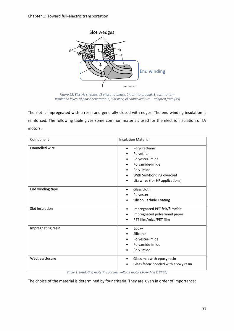
The primary electrical insulation of Low Voltage (LV) rotating machine stators is composed of three
main insulation layers. These are the turn-to-turn, turn-to-ground and phase-to-phase insulations.
Figure 22 is a sketch of the three insulation layers of a stator.
Chapter 1: Toward full-electric transportation
37
Figure 22: Electric stresses: 1) phase-to-phase, 2) turn-to-ground, 3) turn-to-turn Insulation layer: a) phase separator, b) slot liner, c) enamelled turn – adapted from [35]
The slot is impregnated with a resin and generally closed with edges. The end winding insulation is
reinforced. The following table gives some common materials used for the electric insulation of LV
motors:
Component Insulation Material
Enamelled wire Polyurethane
Polyether
Polyester-imide
Polyamide-imide
Poly-imide
With Self-bonding overcoat
Litz wires (for HF applications)
End winding tape Glass cloth
Polyester
Silicon Carbide Coating
Slot insulation Impregnated PET felt/film/felt
Impregnated polyaramid paper
PET film/mica/PET film
Impregnating resin Epoxy
Silicone
Polyester-imide
Polyamide-imide
Poly-imide
Wedges/closure Glass mat with epoxy resin
Glass fabric bonded with epoxy resin
Table 2: Insulating materials for low-voltage motors based on [19][36]
The choice of the material is determined by four criteria. They are given in order of importance:

Chapter 1: Toward full-electric transportation
38
1) Dielectric strength. Usually expressed in [kV/mm]. It represents the maximum electric field
amplitude the material is able to endure. Most of the organic materials of dozens of
micrometers in thickness have dielectric strength of the order of 100 kV/mm.
2) Maximum working temperature. It defines the maximum temperature at which the material
ensures its insulating function. The best organic materials have maximum working
temperature up to 240 °C.
3) Mechanical properties for the implementation of the material inside the stator slot.
4) Thermal conductivity. It characterises the ability of the material to evacuate the heat flux
toward the cooling system. Organic materials have thermal conductivity of the order of 0.1-
0.3 W.m-1.K-1.
4.1.1 Turn-to-turn insulation
It is made with a polymer enamel coating the conductor core, generally made of copper. The thickness
of the enamel varies from some micro-meters to dozens of micro-meters for turn copper diameter up
to 5mm [37].
Anton [38] detailed the enamel technology and realized a comparative study of the common polymers
used as enamel.
The enamel is the result of a varnish being cured. The varnish is a complex mix in which are present:
the solvent, a polymer precursor, the cross-linking agents and some additives.
The solvent prevents the polymer precursor from polymerizing. It represents between 60-80% of the
total solution. It is mainly composed of a mix of phenol and cresylic acid. The solvent is evaporated
during the curing process. Some additives such as naphtha or xylene are added to the solvent to adjust
the viscosity of the varnish. The polymer precursors represent 18-40% of the solution.
The enamel overcoat is made of multiple layers which are successively polymerized at high
temperature in an oven. The first layers (i.e.: the closest to the copper) goes much more in the oven
than the external layers. The cross-linking is therefore not uniform in the whole enamel thickness. The
process to get an enamelled wire is illustrated in Figure 23.

Chapter 1: Toward full-electric transportation
39
Figure 23: Enamelled wires glazing line process [38]
Multiple polymers are generally found in the enamel coating. The enamel has to resist the biggest
thermal stress present in a motor slot due to its location just over the copper wire, which is the main
heat source. Besides, it is surrounded by the resin which impregnates the whole slot. The choice of the
polymers thus strongly depends on the temperature and the chemical compatibility with the
impregnation resin. The insulation power of polymers is highly affected by the temperature. They are
distributed into thermal classes. They define the higher temperature at which the polymer is able to
ensure its insulation function up to 20 000 hours. Some are presented in Table 3.
Thermal class Y A E B F H N - - -
Temperature (°C) 90 105 120 130 155 180 200 220 240 280*
Table 3: Some thermal classes [39]
(*) 280°C thermal class is obtained by adding non-organic nano-fillers in a PI matrix [40]
Here are the different materials commonly used:
- Polyvinyl formal: thermal class 120 °C, they have very good mechanical properties. They are
particularly used on big round wires or flat wires in transformer application due to their good
resistance to hydrolysis.
- Polyurethane (PUR): thermal class 180 °C, they are used on thin wires (from 0.02 to 2 mm).
One can find them in household appliances, television or phone.
- Polyester imide (PEI): thermal class 180 °C, they are very flexible and they have a good grip
on copper. They are applied on wires from 0.03 to 0.8 mm.
- Polyester THEIC (TriHydroxyEthyl IsoCyanurate): thermal class 200 °C. They are usually used
as undercoat of polyamides imides in order to improve their mechanical properties (flexibility, grip)
while keeping a good heat resistance. They are used on diameter from 0.5 to 5 mm.

Chapter 1: Toward full-electric transportation
40
- Polyester imide THEIC: thermal class 200 °C, they have a good heat resistance and a good
chemical resistance. They are also used as undercoat of polyamides imides.
- Polyamide imide (PAI): they have a very good thermal stability, a very good resistance to
thermal shock and very good mechanical properties. Used as full coat, they have a thermal class of 220
°C and are used with diameters from 0.1 to 1.3 mm. Because of their high cost, they are generally used
as upper layer of polyester imides THEIC to get wires of thermal class of 200 °C with diameters from
0.1 to 5 mm.
- Polyimide (PI): they have a very good heat resistance (up to 240 °C) and a very good resistance
to thermal shock. They are used on wires from 0.05 to 6 mm diameter.
These properties are summarized in Table 4.
Properties Formal PUR PEI PET-THEIC
+ PAI
PEI-THEIC
+ PAI
PAI PI
Thermal class
[°C]
120 155 180 200 200 220 240
Copper
diameters
[mm]
0.6 - 5 0.02 - 2 0.05 - 2 0.05 - 5 0.1 - 5 0.1 – 1.3 0.05 – 6
Electric
strength (EIC
V/µm)
170 180 175 180 180 180 180
Abrasion (2) (3) (2) (2) (2) (5)
Grip (2) (2) (1) (2)
Flexibility (2) (2) (2)
Solvent
resistance
(3) (2) (2) (2)
Thermal
conductivity
[W.m-1.K-1]
Mainly between 0.1-0.3 [41]
Properties: (1): excellent, (2): very good, (3) good, (5): very bad
Table 4: Main properties of standard enamel wires adapted from [38]
The thermal conductivity characterizes the behaviour of a material to a heat flux. The lowest this value,
the more difficult the heat flux cross over and evacuation from the winding. For comparison, the
thermal conductivity of iron is 80 W.m-1.K-1. Conductivity values of standards enamel materials are very
low compared to iron.

Chapter 1: Toward full-electric transportation
41
4.1.2 Phase-to-phase insulation
The phase-to-phase insulation ensures the electrical insulation between different phases in the end
winding and/or into the slots (if there is more than one phase by slot). Depending on the number of
different phases which overlaps and the winding configuration, such insulation has to resist up to twice
a phase peak voltage.
It is mainly composed of porous fabric from aramid fibers. This porous material is impregnated with
resin, during the winding impregnation step. Aramid fibers have also good both heat and humidity
resistances [42].
4.1.3 Turn-to-slot insulation
The slot insulation ensures the electrical insulation between the winding and the stator slot. Mainly,
the stator frame is grounded. This insulation has to be able to resist the whole phase peak voltage.
It is inserted inside the slot before the winding operation. It also protects the wires during their
insertion in the slot against stator abrasion. Slot insulation is mainly formed with paper, film or flexible
materials. It is also used to ensure a physical separation between the end winding and the stator slot.
The common materials used are mica and/or aramid. Slot wedges are an additional protection which
increases the mechanical handling of the winding.
Figure 24: Slot wedges and phase insulation seen with the winding in place; one wedge is partially inserted [43]

Chapter 1: Toward full-electric transportation
42
Tensile
strength
[N/mm²]
Operation
temp. [°C]
Moisture
absorb.
(% by
weight)
Chemical strength;
Graded 0-4
Voltage
strength
[kV/mm]
Trade
names
Acid
s
Alkali
s
Orga
nic
solv
ent
Insulating
foils
Polyester
PETP
140-160 130 0.5 2 1 4 150 Mylar
Melinex
Hostaph-
an
Polyimide 180 220 3 3 0 4 280 Kapton
Polysulp-
hone PS
90 180 1.1 3 3 1 175 Folacron
PES
Fiber
insulator
Cotton
fibers
250-500 105 (impregnate
d)
10 1 2 4 - -
Polyester
fibers
500-600 155 0.4 2 1 4 - -
Glass
fibers
1000-
2000
130-200 (depending
the
impregnant)
- 4 3 4 - -
Aramid
paper
1250 210 7-9 3 3 4 20 (1min,
50Hz test) Nomex
Table 5: Characteristics of foils and fiber insulators [39]
4.1.4 Slot impregnation
The slot is filled with a resin. It aims to electrically insulate the whole slot. It also holds the winding in
place and improve the heat dissipation toward the stator cylinder head. Impregnation resins are mainly
composed of both solvent and polymer precursor. The solvent prevents the precursor from
polymerizing. That is the reason why it is necessary to heat the resin during impregnation. The solvent
evaporates and the precursors assembles to form the polymer.
The main function of the resin is to mechanically hold the winding in place (to avoid damage due to
friction between the winding and the core) and to protect it against moisture, pollution and dust in the
case of an open motor. It is not in direct contact with the copper so it does not have to resist such a
high temperature as the enamel. It has to be chemically stable.

Chapter 1: Toward full-electric transportation
43
Several process exist to fix the resin. They have been documented by [44] in his PhD dissertation:
- drop by drop method. The resin is slowly deposited on the winding so that it impregnates
the winding by capillarity. It is the most employed method in the industry. However, it is quite possible
that some parts of the winding may not well be impregnated.
- brush method. The impregnation is done during the manufacturing of hand-made windings.
The resin is repeatedly applied with a brush. The repartition of the resin is more uniform than the one
obtained with the drop by drop method. The resin is directly put in the middle of the winding. This
method is only applied to specific machine for small series production.
- soaking method. The machine is slowly lowered in a tank full of resin. It stays here a while so
that the air trapped between the wires is extracted. The machine is then slowly pulled up and drained.
- Vacuum Pressure Impregnation (VPI) method. It is composed of different steps:
- Preheating: the motor is placed in an oven that heats it and allows moisture to
evaporate. This will also help the resin better penetrate the material;
- Dry Vacuuming: the motor is removed from the oven and placed into a vacuum
chamber to remove air and any remaining moisture;
- Filling: the chamber is filled with resin, coating the part and filling in all the gaps of
the EIS;
- Wet Vacuuming: the vacuum levels is reduced and hold it for a set period of time;
- Pressure: the pressure is increased within the chamber using dry air (nitrogen for
example) to allow deeper penetration of the resin;
- Draining: the pressure is vented and the motor is removed;
- Curing: the motor is finally placed into an oven to cure the impregnating resin.
Figure 25: Vacuum impregnation steps given by Von Roll [45]
This method is found to be better than the others.

Chapter 1: Toward full-electric transportation
44
- double VPI: the vacuum impregnation steps are done twice to reinforce the holding of the
winding. It is used when a high quality of impregnation is required.
Table 6 gives the common varnishes characteristics.
Mechanical
strength;
Grades 0-4
Operation
temperature
[°C]
Moisture
resistance;
Grades 0-4
Chemical
strength;
Grades 0-4
Typical
materials
Impregnating
varnishes
3 155 3 3 Alkyd polyester
1 180 3 3 Silicone epoxy
Impregnating
resins
3 155 3 3 Polyester alkyd
Epoxy
4 180 4 4 Polyester
Epoxy
Coating
(surface)
varnishes
2 130 3 3 Alkyd
Polyruethane
2 155 4 4 Alkyd
Polyruethane
1 180 4 3 Alkyd
Silicone
Epoxy
Table 6: Characteristics of varnishes and resins [39]
4.2 HIGH VOLTAGE MACHINE
Machines powered with a phase to phase voltage higher than 700Vrms are considered as high voltage
machines [35]. When the applied voltage is more than a few kV, these machines have to work
doubtless with partial discharges. Their EIS is consequently reinforced by using non-organic materials.
Figure 26 illustrates a classical EIS used in such high voltage machines.

Chapter 1: Toward full-electric transportation
45
Figure 26: High voltage machine electrical insulation system [46]
In most high voltage motors the winding is composed of enamelled copper bars. It is well organized in
the slot. Bars reduce the end winding congestion outside the slot. For high frequency application, the
bars are subdivided. This is to prevent frequency losses such as skin and proximity effects.
Some specifications for high voltage motor insulation are given in [39]. Mica tape wound is widely used
in layers around the conductors due to its very good partial discharge resistance. On the end windings,
stress grading tapes are applied on the bars extremity close to the slot end. The most common stress
grading materials are a semi-conductive silicon carbide tape or paint. It aims to progressively reduce
the electric field at the area where the stator cylinder head, the insulation tape and the surrounding
air meet together (triple point). That is a weak spot in the system which is susceptible to easily lead to
electric discharges [34].
The groundwall insulation is usually made out from natural resins and mineral used as fillers. The resins
include refined petroleum oils, waxes, asphalts, etc. Minerals include mica, asbestos or quartz [47].
In this PhD dissertation, we consider that the level of the applied voltage (i.e.: 2.5 kV) allows to find
solution leading to PD-free working conditions. This is the reason why the following chapters will deal
with an organic EIS. However, if partial discharges appear, the methodology that will be developed
may be applied just by changing both size and permittivity of the EIS components.
Ø Winding wire (A)Ø Conductor insulation (B)Ø Stack insulation (C)Ø Main wall insulation: Mica tape (D) + VPI resin (H)Ø Conductive paint or tape (F)Ø Stress grading paint or tape (F)Ø Finishing or sealing tapes (E)Ø Bracing materials (G)Ø Slot wedging materials (I)
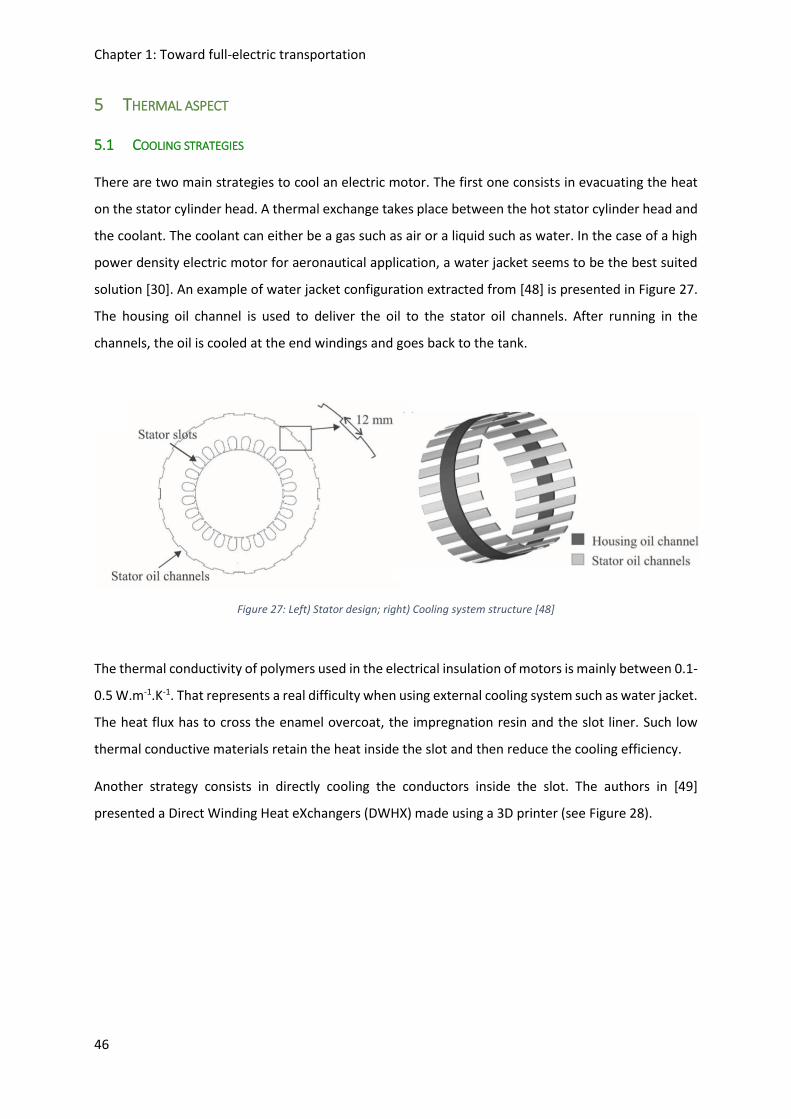
Chapter 1: Toward full-electric transportation
46
5 THERMAL ASPECT
5.1 COOLING STRATEGIES
There are two main strategies to cool an electric motor. The first one consists in evacuating the heat
on the stator cylinder head. A thermal exchange takes place between the hot stator cylinder head and
the coolant. The coolant can either be a gas such as air or a liquid such as water. In the case of a high
power density electric motor for aeronautical application, a water jacket seems to be the best suited
solution [30]. An example of water jacket configuration extracted from [48] is presented in Figure 27.
The housing oil channel is used to deliver the oil to the stator oil channels. After running in the
channels, the oil is cooled at the end windings and goes back to the tank.
Figure 27: Left) Stator design; right) Cooling system structure [48]
The thermal conductivity of polymers used in the electrical insulation of motors is mainly between 0.1-
0.5 W.m-1.K-1. That represents a real difficulty when using external cooling system such as water jacket.
The heat flux has to cross the enamel overcoat, the impregnation resin and the slot liner. Such low
thermal conductive materials retain the heat inside the slot and then reduce the cooling efficiency.
Another strategy consists in directly cooling the conductors inside the slot. The authors in [49]
presented a Direct Winding Heat eXchangers (DWHX) made using a 3D printer (see Figure 28).

Chapter 1: Toward full-electric transportation
47
Figure 28: left) 3D-DWHX CF-Nylon prototype for heat transfer testing; right) 3D-DWHX shown in the stator slot of a motor equipped with permanent magnets [49]
The numerical results of the maximum temperature in several spots obtained by using only water
jacket, only the 3D-DWHX and the combination of both are presented on Table 7:
Maximum Temperature [°C]
Winding Stator iron Magnet
Water Jacket 30.1 22.5 21.1
3D-DWHX 58.1 67.6 37.3
Combined 16.9 15 18.6
Table 7: Comparison of stator cooling strategies involving 3D-DWHX [49]
The worst performance is obtained by using 3D-DWHX alone. This can be explained by the low thermal
conductivity of the Nylon constituting the DWHX and of the winding. However, significant temperature
reduction is obtained combining both cooling solutions, especially in the winding.
5.2 THERMALLY ENHANCED POLYMERS
Hitachi and Hitachi Chemical has developed an enhanced thermal epoxy resin [50]. They change the
amorphous molecular structure into a crystal-like structure (see Figure 28). These liquid crystal
molecules are called mesogens. They form a highly ordered structure which increase both thermal
conductivity and flexibility of the resin. The enhanced thermal conductivities can reach 0.96 W.m-1.K-1,
which is up to 5 times greater than classic epoxy resin.

Chapter 1: Toward full-electric transportation
48
Figure 29: Structure of a new high thermal properties epoxy resin [50]
The authors in [48] compared the maximal temperature in a water cooled machine using three
different impregnation materials. The main thermal and electric properties are summarized in Table
8.
Materials Varnish Epoxylite SbTCM
Thermal conductivity
[W.m-1.K-1]
0.25 0.85 3.20
Dielectric strength
[kV/mm]
80 20 10
Table 8: Materials used by [48]
SbTCM stands for silicone-based thermally conductive material. The simulation results obtained for a
coolant flow rate of 2.5 L/min are presented on Figure 30. The temperature decrease compared to
classic varnish at 3.2 A is of around 20% for Epoxylite and 30% for SbTCM. The current amplitude is at
the stator winding.
Figure 30: Simulation results: comparison between the hot spot temperature in electric machines using different impregnation materials at different current magnitude (at the stator winding). The inlet coolant flow rate is assumed to be
2.5L/min [48]

Chapter 1: Toward full-electric transportation
49
The drawback of such efficient thermal properties for SbTCM is a reduction of a factor 8 of the
dielectric strength compared to classic varnish. SbTCM looks attractive but for some application, such
as high power density motors, its dielectric strength may be too low.
Other high thermal conductivity composites have been reported by [51] (Table 9).
Properties PA 66 PPS PPA LCP PEEK
Std Enh Std Enh Std Enh Std Enh Std Enh
Thermal
conductivity
[W.m-1.K-1]
0.24 20-32 0.08-
0.29
10-20 0.15 20 0.0837 20 0.25 10
Tensile
strength
[MPa]
95 65-117 48-86 45-70 76 44-83 110-
186
80 70-
103
70
Elongation
%
15-90 0.75-
1.5
1-6 0.31-
0.75
30 0.6-1 1.3-4.5 0.25 30-
150
0.5
Table 9: Comparison of standard (Std) versus thermally enhanced (Enh) polymer composites material properties [51]
As shown in Table 9, very high thermal conductivity are reached. However, the enhanced composites
are much more mechanically fragile than the standard ones: the elongation is much lower. The
enhanced materials are closer to ceramics than polymers.
On the other hand in [52] the Direct Current electric properties of polyimide/boron nitride (PI/BN)
nano-composites for a large range of nanoparticle size and filler content have been investigated. It was
shown that an efficient control of the charge carrier mobility allows a huge enhancement of the
insulating properties of PI films.
6 IMPACT OF POWER ELECTRONICS
6.1 PULSE WIDTH MODULATION (PWM) BASIS
Power electronic offers a wide range of possibilities in machine control. AC motors now replace DC
motors in application that require to control the machine rotation speed. AC motors are less expensive
in particular due to less wearing parts. However, the power has to be converted from DC to AC. This is
done via an inverter. Figure 31 illustrates such a classic electromechanical chain.

Chapter 1: Toward full-electric transportation
50
Figure 31: Diagram of an electromechanical chain [53]
If one considers the application of an electric aircraft, the load would be a fan. In case the motor is not
pressurized, the group composed of the motor and the fan will be submitted to pressure (P) and
temperature (T) variations.
An example of classic three phase inverter architecture is presented in Figure 32.
Figure 32: Classic three-phase inverter based from [54]
It is composed of three commutation cells. One cell is made of two switches. A switch is composed of
a switching semi-conductive component, such as MOSFET or IGBT, and its anti-parallel diode. The two
switches composing a cell are complementary. When the one at the top is ON (i.e.: the electric current
can flow through it) the one below is OFF (i.e.: the electric current cannot pass). A commutation
function fm is defined. It equal either 0 or 1 depending on which switch is ON or not. So, for the
commutation cell on phase 1, the output voltage is:
𝑉𝑠1 = 𝑓𝑚1 ∗ 𝐸
One of the most common command of PWM is the intersective one. It consists in comparing the
modulant to a carrier signal. The modulant defines the shape of the wanted output signal. The carrier
generally has a triangular shape. Its frequency is much higher than the modulant frequency. Figure 33
illustrates the principle of three-phase sinusoidal PWM.

Chapter 1: Toward full-electric transportation
51
Two sinusoidal waveform modulants signals are represented. These are the ideal voltage on phases 1
and 2. The phase shift between the two signals is 120°. The output of fm1 is equal to 1 if the phase 1
modulant has a larger amplitude than the one of the carrier and 0 otherwise. It is the same for fm2 but
comparing the phase 2 modulant to the carrier. The frequency of fm1 and fm2 pulses is constant. Only
the width of the pulse changes. The phase to phase voltage is simply the difference of the cells output
voltages. So, the resulting modulated phase to phase voltage between phase 1 and 2 is obtained by
subtracting the fm1 and fm2 signals.
Figure 33: Example of three-phase sinusoidal PWM based from [54]
6.2 POWER FEEDING CABLE
The power cable connects the inverter to the motor. It has an impact on the overshoot that happen at
the motor terminals. This cable is generally modelled using a transmission line harness [53],[55].
Figure 34 illustrates the single conductor transmission line model. It corresponds to a phase-to-ground
connection. It is a repetition of infinitesimal elements. The number of elements to used depend on
the line length and the frequency of the output inverter signal.

Chapter 1: Toward full-electric transportation
52
Figure 34: Transmission line phase to neutral model
Figure 35 details the constitutive elements of an infinitesimal line element. The line behaves as a global
inductive behaviour modelled with a per-unit-length inductance (L*dx). Joule’s losses are modelled by
a per-unit-length resistance (R*dx) in serial with the per-unit-length inductance. The capacitive
coupling between the line and the ground is modelled connecting a per-unit-length capacitor (C*dx).
The dielectric losses in the insulation of the line are modelled with a per-unit-length resistance (G*dx)
in parallel with the line capacitor.
Figure 35: Transmission line elementary cell
Let us designate by Zc, Zm and Zi the impedances of respectively the power cable, the motor and the
inverter. As these three impedances are different, there are reflexions of the input voltage waveform
in the cable. At each time step, the voltage at a point along the cable is the sum of the reflected voltage
waveforms toward the inverter and toward the motor. The reflexion of the voltage waveform toward
the inverter output is characterized by the reflexion coefficient Γ𝑟𝑖:
Γ𝑟𝑖 =𝑍𝑖 − 𝑍𝐶𝑍𝑖 + 𝑍𝑐
Eq 1
The reflexion of the voltage waveform toward the motor is similarly characterized by the reflexion
coefficient Γ𝑟𝑚:
Γ𝑟𝑚 =𝑍𝑚 − 𝑍𝐶𝑍𝑚 + 𝑍𝑐
Eq 2

Chapter 1: Toward full-electric transportation
53
The impedance of the cable Zc is function of its dimensions. It can be computed from both its per-unit-
length inductance L (H/m) and per-unit-length capacity C (F/m):
𝑍𝑐 = √𝐿
𝐶
Eq 3
The voltage at the motor terminals is submitted to damped oscillations. The first oscillation has the
biggest amplitude. Figure 36 adapted from [56] presents the phase-to-ground and first stator coil
maximum voltage amplitudes. It can be seen in this example that the overshoot can reach 1.5 the DC
voltage bus for a cable of 25m.
Figure 36: Maximum motor terminal voltage during PWM inverter operation depending on the cable length. Pulse frequency 9kHz, Ubus=560V, 4kW induction motor, rise time tr=100ns. Adapted from [56]
The authors in [57] has proposed an improved model for computing the phase-to-phase voltage
overshoots at a motor terminals. An equivalent two phase model of the electromechanical chain
(inverter+cable+motor) is considered (Figure 37), where j is the complex operator and w is the angular
frequency. The model is composed of classic RLCG(j) elements and a propagation function 𝛾𝑐(𝑗𝑤).

Chapter 1: Toward full-electric transportation
54
Figure 37: Proposed equivalent two-phase model of an electromechanical chain [57]
Figure 38 presents the computed phase-to-phase motor terminals overshoots as a function of the
cable length. Different transistor gate resistance (Rg) values were used. This resistance modulates the
output rising time. The biggest the Rg value, the slowest the rising time. It can be seen that the phase-
to-phase voltage overshoot increases considerably for cable length higher than 2 m. For the biggest Rg
values, it happens for length superior to 3 m. Besides, compared to Figure 36, the phase-to-phase high
overshoots occur for cable length much shorter than in the case of phase-to-ground or coil-to-ground
overshoot. For phase-to-phase, one can consider a critical cable length of 2 m whereas for phase-to-
ground and coil-to-ground the critical cable length is about 20 m.
Figure 38: Maximal overvoltage at motor terminals for different harness lengths, obtained by simulation using trapezoidal inverter waveforms [57]

Chapter 1: Toward full-electric transportation
55
6.3 FREQUENCY INCREASE
New semi-conductive components based on SiC and GaN technologies permit power electronics to
switch higher levels of voltage in shorter time than classic silicon components [58]. Besides, SiC
components have a bigger energy gap. That means that at a fixed temperature, an electron in a SiC
components will need more energy to cross the gap than in a silicon component. Therefore, SiC
technology enables to work at higher temperature [59].
The rise of inverters switching frequencies lead to faster rising time on the machine terminals. It is the
time interval in which the voltage amplitude goes from 10% to 90% of the peak voltage. Figure 39
illustrates an incoming voltage front wave at motor terminals fed by a PWM inverter.
Figure 39: Voltage front wave at a machine terminasl fed with PWM inverter [35]
The author in [60] has investigated the impact of the voltage front coming from an inverter over the
overshoot at the stator winding. A 41 turns coil has been powered by a pulse generator with rising
times of 10 ns and 85 ns. The results are displayed in Figure 40. It can be seen that for the front of 10
ns the overshoot is 1.73 times the DC bus voltage. However, there is barely no overshoot for a slower
rising time of 85 ns.

Chapter 1: Toward full-electric transportation
56
Figure 40: Voltage at a 41 turns coil terminals; top) rising time 10ns; below) rising time 85ns [60]
An evaluation of the overvoltage at the motor terminals as a function of both rising time and cable
length is proposed in EIC Standard (60034-18-41). On Figure 41, the overvoltage factor defined by the
ratio of the phase-to-phase peak voltage over the pulse voltage is given versus cable length and rising
time. The results obtained by [57] on Figure 38 are coherent with the EIC Standard evaluation.
Figure 41: Overvoltage ratio in function of cable length and rising time proposed in EIC Standard (60034-18-41)

Chapter 1: Toward full-electric transportation
57
However, it is no more the case when considering fast switching frequency of a SiC inverter. A complex
ringing phenomena may happen for cable length lower than 3 m [61]. This ringing phenomena is
attenuated with the increase in the power cable length. Figure 42 illustrates the overvoltage at the
motor terminals powered with a silicium based inverter (dashed blue lines) versus a SiC inverter (red
line).
Figure 42: Overvoltage ratio as a function of both cable length and rising time (dashed blue curve: tr=50ns, red curve: tr=8ns) [61]
6.4 VOLTAGE DISTRIBUTION
Figure 43 presents the voltage waveforms measured between 5 coils constituting one phase. A step
voltage amplitude E has been used. The coil number one is the first to receive the incoming voltage
front. The first coil receives a much bigger overshoot (top). After the transient regime the voltage is
uniformly distributed between the coils (below). However, during transient, the voltage between the
coils can be of the same magnitude than the step voltage.

Chapter 1: Toward full-electric transportation
58
Figure 43: Overvoltage measured in a stator coils. Top) voltage distribution; Below) voltage between coils turns [62]
The voltage crossing the first coil as a function of the incoming front rising time has been investigated
by [56]. It is expressed as a percentage of the phase-to-neutral motor terminal voltage. Figure 44 shows
that for rising time lower than 50 ns, the first coil is susceptible to get more than 70% of the maximum
phase-to-neutral motor voltage.

Chapter 1: Toward full-electric transportation
59
Figure 44: Percentage of the voltage across the first coil as a function of the rise time [56]
Works have been done to evaluate the non linear voltage repartition within the winding. The author
in [60] modelled a coil by using a RLC circuit model. The parameters have been determined either by
experimental measurements or 2D-finite elements computation. Figure 45 compares the results
obtained with the RLC circuit and the experimental measurements. A 41 turns coil is considered. It is
powered by a 300V DC bus voltage. The top figure shows the response of the coil terminals to a voltage
front. The bottom picture represents the maximal turn to turn voltage drop obtained between turns 4
and 9. The RLC model provides a good evaluation of the first peak.
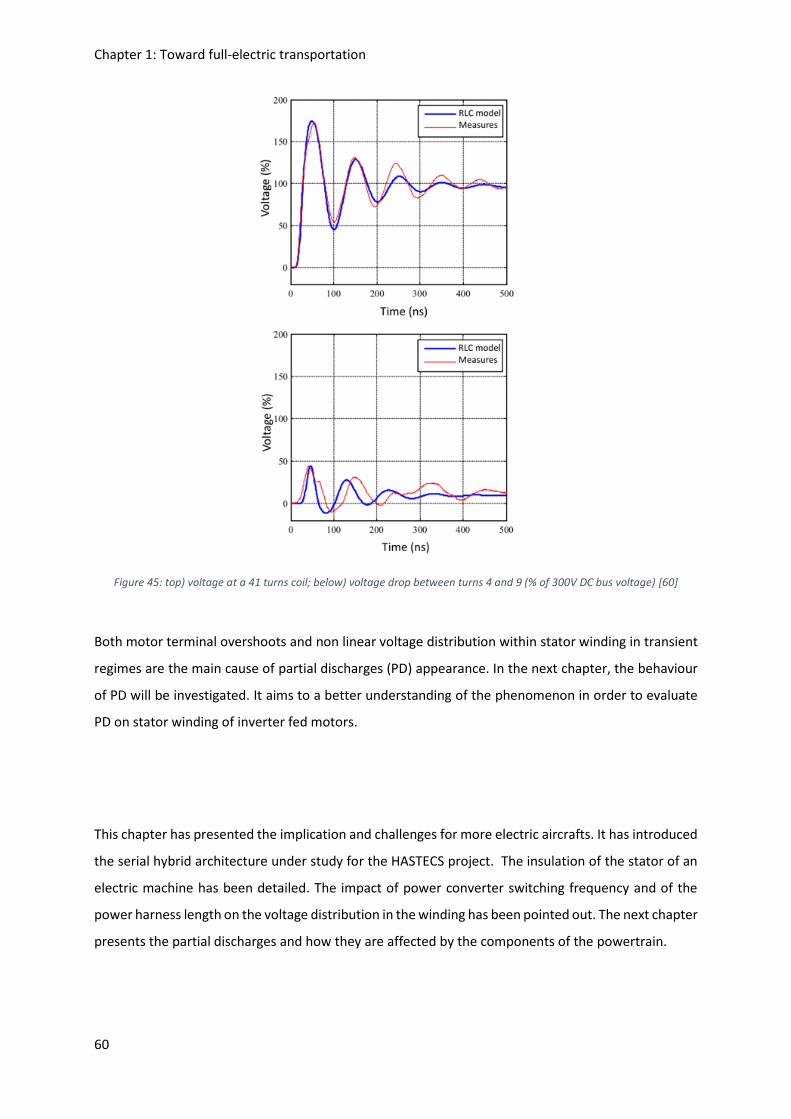
Chapter 1: Toward full-electric transportation
60
Figure 45: top) voltage at a 41 turns coil; below) voltage drop between turns 4 and 9 (% of 300V DC bus voltage) [60]
Both motor terminal overshoots and non linear voltage distribution within stator winding in transient
regimes are the main cause of partial discharges (PD) appearance. In the next chapter, the behaviour
of PD will be investigated. It aims to a better understanding of the phenomenon in order to evaluate
PD on stator winding of inverter fed motors.
This chapter has presented the implication and challenges for more electric aircrafts. It has introduced
the serial hybrid architecture under study for the HASTECS project. The insulation of the stator of an
electric machine has been detailed. The impact of power converter switching frequency and of the
power harness length on the voltage distribution in the winding has been pointed out. The next chapter
presents the partial discharges and how they are affected by the components of the powertrain.

Chapter 2: Physics of Partial Discharges (PD)
61
Chapter 2: Physics of Partial Discharges (PD)

Chapter 2: Physics of Partial Discharges (PD)
62

Chapter 2: Physics of Partial Discharges (PD)
63
This chapter is dedicated to Partial Discharges (PD). It will start with the definition of a PD and the
explanation of the mechanism which ignites it. Then, the experimental techniques to detect and
measure PD activity will be presented. The effect of aeronautical environment on PD will be then
considered. Finally, the principle of common numerical models to evaluate PD will be introduced.
1 DIFFERENT KINDS OF DISCHARGES
There are different ways to classify electric discharges. For instance in [63] the discharges were
classified depending on their nature. The nature of the discharge varies depending on the voltage and
current characteristics.
Another way to sort discharges is to classify them by the location where they take place. In [64] the
discharges are sorted in four main categories: inner discharges, surface discharges, corona discharges
and treeings. Treeings take place during ageing, so that this kind of discharge will not be considered in
our study. Figure 46 illustrates the three kinds of discharges that may take place in machines during a
PDIV measurement.
Figure 46: Different kinds of discharges depending on their location: 1) Townsend discharges in both embedded and vented voids, 2) surface tracking discharges, 3) corona discharges
In this paragraph the discharges sorted in the way of [64] are developed.

Chapter 2: Physics of Partial Discharges (PD)
64
1.1 DISCHARGES IN NON-VENTED CAVITIES
These discharges happen inside the insulation material. It is due to the presence of defects in the
insulator (Figure 47). These defects can be introduced during the manufacturing process (air bubbles)
or during the polymer aging (delamination).. Additional defects may be introduced during the winding
operation mainly because of mechanical stress. Besides, at working conditions, there can be
displacement of insulating materials due to both vibration and thermal cyclings. Air gaps are then
introduced between insulators and metallic parts of the EIS. As these gaps are not vented (they are
embedded inside the EIS), PD are not sensitive to the environmental working conditions (temperature,
humidity, dust, fluids, …).
Figure 47: Mica insulation showing various defects (red rectangles) – adapted from [65]
The PD activity causes the insulator structure damage by ions bombardments, heat, physico-chemical
attacks, UV and other radiations effects. With the repetition of PD, electrical trees can grow inside the
polymer (Figure 48). At term, some branches go through the whole insulator thickness, leading to its
electric breakdown.

Chapter 2: Physics of Partial Discharges (PD)
65
Figure 48: 3D electrical treeing in a block of clear acrylic [66]
In the presence of humidity inside a hydrophilic insulator, so called water treeing are ignited at much
lower electric field amplitude. The author in [67] reported an amplitude around 10 kV/mm for water
treeing and around 100 kV/mm for normal treeing.
1.2 DISCHARGES IN VENTED CAVITIES
Most of electric motors are not hermetic. That means that the air is free to circulate all over the stator
winding and that it is submitted to the external air. The authors in [68] investigates the impact of air
flow on a two-dimensional array of integrated coaxial micro-hollow coplanar DBD in air at atmospheric
pressure. It is shown that the discharge is considerably impacted by the air flow as presented on Figure
49, as this air flow modifies the physics on the insulator surface.
Figure 49: Typical current and voltage waveforms of the 2D-micro-discharges in air. The peak-to-peak applied voltage is identical for all the flow rates [68]

Chapter 2: Physics of Partial Discharges (PD)
66
In [69] the impact of pressure on the stator winding PDIV was investigated. Figure 50 indicates a
decrease of PDIV when the pressure decreases.
Figure 50: PDIV as a function of pressure (temperature 25°C, relative humidity 50%) - 2 stators are tested [69]
In our research project, an open motor will be considered. So the impact of environmental conditions
on PDIV have to be taken into account. These are detailed further.
1.3 DISCHARGES ON THE SURFACE
These kind of discharges occur when a high tangential electric field appear at the insulator surface
(surface tracking PD type). If contaminants, moisture,… are present on the insulator surface,
discharges can be triggered with lower electric field. This phenomenon may be increased when it takes
place at a triple point (in an area where air, polymer and metal are present). The partial surface
discharges propagate on the insulator surface and cause damage on it (Figure 51). When the
propagation link two conductors, the discharge switches from a partial to a total one.

Chapter 2: Physics of Partial Discharges (PD)
67
Figure 51: Example of surface tracking discharges effects on an insulator due to contamination/humidity [70]
The end windings of high voltage electric motors are more susceptible to trigger such surface
discharges. It is possible to limit such discharges by a suitable design, the choice of insulators having
high surface resistivity and by adding a semi-conductive paint on the winding close to the stator slot
edge [71]. This additional overcoat will gradually decrease the electric field.
1.4 CORONA DISCHARGE
This kind of discharges takes place in strongly non uniform electric field zone. These are needle-plane
or cylinder wire–plane configuration. The electric field is very high in a small region directly surrounded
the needle, the wire, the busbar, the junction… and remains weak in the rest of the domain. The size
of the electrodes has to be very small compare to the gap between electrodes. They represent a great
deal on high voltage power line design (Figure 52).
Figure 52: Corona discharge on an insulator string of a 500 kV overhead power line [72]

Chapter 2: Physics of Partial Discharges (PD)
68
1.5 PD CONSEQUENCES ON STATOR INSULATION
Three types of solid insulator dielectric breakdown due to high electric field can be distinguished. These
can combine each other:
- Electromechanical breakdown: an electrostatic pressure is applied by the conductors on the
insulators. This leads to a decrease of the slot insulation thickness or a creation of cracks in it. This
phenomenon can lead to an irreversible electromechanical rupture of the material. Moreover, initial
cracks existing in the insulator (defects) may lead to a filamentary electromechanical breakdown.
- Thermal breakdown: it occurs when the material conductivity increases due to a high current
density. That causes additional losses and therefore heating by Joule’s effect. Thermal runaway can
then cause a dielectric breakdown, call thermal breakdown. As for electromechanical breakdown,
filamentary thermal breakdown may take place in insulators.
- Electronic breakdown: a sufficiently high electric field may cause different breakdown
mechanisms, each initiated by electrons: electronic avalanche, field effect emission, free volume
effect. These phenomena all lead to the breakdown by generating a large amount of electrons that
transform the insulator in a conductor.
PD activity is responsible of premature failure. A PD generates erosion (by ions bombardment), heat
but also ozone. Ozone rapidly attack polymers and reduce its lifetime [73]. This PD activity slowly
degrade the insulators and at term can lead to a complete failure of the motor.
Figure 53: Consequences of PD on a stator winding insulation; left) Corroded enamel layer [40]; right) Slot liner flashover [74]

Chapter 2: Physics of Partial Discharges (PD)
69
2 PHYSICS OF PLASMA
Townsend type PD happen in cavities (embedded bubble, delamination) inside the polymer or in the
surrounding air submitted to a high electric field (vented voids). If the field intensity exceeds a critical
value, the air is ionized. Negatively and positively charged particles are then present in such proportion
that the air remains electrically neutral. The air is in an another physical state: it is a so called plasma.
The evaluation of the PD activity is extremely dependent on the formation of this plasma. In this
paragraph, the predominant mechanism, supposed to take place in our motors EIS, will be presented.
2.1 TOWNSEND MECHANISM
It describes the ionization of a gas between two metallic plane electrodes. It was established by John
Townsend in 1901, following the empirical discovery by Friedrich Paschen in 1889 [75]. The electric
breakdown of the gas results from an electronic avalanche (Figure 54). It requires that an initial free
electron is present in the gas gap (the germ electron). This electron is submitted to an uniform electric
field produced by the voltage applied to the electrodes. The electron is accelerated by this electric
field. During its motion in the gas gap, impacts occur with gas neutral particles. Additional electrons
are then pulled from the impacted particles. The neutral particles then turn to positive ions. If the
electric field is strong enough, there is an electronic flow toward the positive electrode and a positive
ionic flow toward the negative electrode. An electric current is established in the gas gap. This leads
consequently to the gas electric breakdown.
Figure 54: Electronic avalanche mechanism; green circles are electrons, red circles are positive ions [76]
Two coefficients mainly impact on the described mechanism, as described below.

Chapter 2: Physics of Partial Discharges (PD)
70
2.1.1 First Townsend’s coefficient
The first Townsend’s coefficient is commonly designated as 𝛼. It represents the quantity 𝑑𝑛 of
electrons generated by 𝑛 electrons moving along a distance 𝑑𝑥 during the avalanche process (4). The
solution of Eq 4 is of the form given by Eq 5.
𝑑𝑛 = 𝛼. 𝑛. 𝑑𝑥 Eq 4
𝑛 = 𝑛0. exp(𝛼. 𝑥) Eq 5
With 𝑛0 being the initial number of electrons at 𝑥 = 0.
The 𝛼 coefficient describes the formation of additional electrons by the collision of a single initial
electron with the other particles in the gas. It is mainly dependent from the chemical composition of
the gas and the energy of the incoming electron. Different outputs may result from a collision. In some
cases, an additional electron is generated but in others it is simply absorbed by the impacted particle.
Table 10 summarizes some reactions which happen in the plasma between gas particles (𝐴 and 𝐵) and
colliding electrons (𝑒−).
Process Reactions
Ionization by electronic collision 𝑒− + 𝐴 → 2𝑒− + 𝐴+
Excitation by electronic collision 𝑒− + 𝐴 → 𝑒− + 𝐴∗
Radiative recombination 𝑒− + 𝐴+ → 𝐴∗ + ℎ𝜐
Three corpses recombination 𝑒− + 𝐴+ + 𝐵 → 𝐵 + 𝐴∗
Detachment by electronic collision 𝑒− + 𝐴− → 2𝑒− + 𝐴
Three corpses attachment 𝑒− + 𝐴 + 𝐵 → 𝐵− + 𝐴
Dissociative ionization 𝑒− + 𝐴𝐵 → 2𝑒− + 𝐴 + 𝐵+
Dissociation by electronic collision 𝑒− + 𝐴𝐵 → 𝑒− + 𝐴 + 𝐵
Table 10: Main collision reactions in a plasma. Adapted from [76] [75]; * symbol designates an exited state of the particle, h𝜐 indicates light emission
Collisions are characterised by the notion of effective cross-section. Let us consider an electron moving
at the speed 𝑣 toward 𝑁 particles contained in an elementary volume of gas designated by the product
𝜎. 𝑑𝑥. The particles are moving at a speed much slower than the electron one (𝑣). Let’s define 𝑣𝑟 as
the relative speed of the electron compared to the particles speed. Thus, the surface 𝜎 is dependent
of the relative speed 𝑣𝑟 and the species in interaction [77]. The surface 𝜎 is the so called effective
cross-section.

Chapter 2: Physics of Partial Discharges (PD)
71
Figure 55 illustrates the concept of effective cross-section.
Figure 55: Effective cross-section.
The number of collision 𝑛𝑐 is defined as:
𝑛𝑐 = 𝑁. 𝜎. 𝑑𝑥 Eq 6
The density N of the gas can be derived from the perfect gas law:
𝑝 = 𝑁. 𝑘. 𝑇 Eq 7
With p the gas pressure, k the Boltzmann’s constant and T the gas temperature.
The electron mean free path 𝜆 is a notion derived from the number of collision 𝑛𝑐 and the travelled
length in the plasma 𝑑𝑥:
𝜆 =𝑑𝑥
𝑛𝑐=
1
𝑁. 𝜎
Eq 8
Let us consider one electron (𝑛 = 1) travelling over the distance 𝑑𝑥 and doing one single collision
(𝑛𝑐 = 1) which generates one electron (𝑑𝑛 = 1) . Combining Eq 4, Eq 6 and Eq 8 one gets:
𝛼 =1
𝜆
Eq 9
The diminution of the number of free paths 𝑑𝑛𝜆 travelled through a unit of length 𝑑𝑥 due to 𝑛𝑐
collisions is expressed by Eq 10. The solution is given by Eq 11.
𝑑𝑛𝜆 = −𝑛𝜆. 𝑛𝑐 = −𝑛𝜆. 𝑁. 𝜎. 𝑑𝑥
𝑑𝑛𝜆 = −1
𝜆. 𝑛𝜆. 𝑑𝑥
Eq 10

Chapter 2: Physics of Partial Discharges (PD)
72
𝑛𝜆 = 𝑛𝜆,0. exp(−𝑥
𝜆) Eq 11
With 𝑛𝜆,0 the total number of free path.
Let us consider that an electron which ionizes an atom starts with a zero speed in the direction of the
electric field between two collisions. The electron then transfers all its kinetic energy to the impacted
atom. The probability of ionizing the atom is taken as 1 as long as the electron kinetic energy is equal
or above the atom ionizing energy. This is written as:
𝑒. 𝐸. 𝜆𝑖 ≥ 𝑒. 𝑉𝑖
𝐸. 𝜆𝑖 ≥ 𝑉𝑖
Eq 12
With e the electron’s charge, E the electric field amplitude, 𝜆𝑖 the electron minimal free path, 𝑒𝑉𝑖 is
the atom ionizing energy.
The probability for an electron free path being superior to the minimal free path 𝜆𝑖 is expressed as the
variation of the number of free paths, which length is at least of 𝜆𝑖, over dx compared to the total
number of free paths 𝑛𝜆,0. Combining Eq 10 and Eq 11 one gets:
𝑛𝜆(𝜆𝑖) − 𝑛𝜆(𝜆𝑖 + 𝑑𝑥)
𝑛𝜆,0= −
𝑑𝑛𝜆(𝜆𝑖)
𝑛𝜆,0=1
𝜆. exp (
−𝜆𝑖𝜆) . 𝑑𝑥
Eq 13
By definition, this probability also represents the number of electrons generated by electronic
avalanche per unit of length which is in fact the 𝛼 coefficient itself. So Eq 13 can be written as:
𝛼 =1
𝜆. exp(
−𝜆𝑖𝜆)
Eq 14
Combining Eq 8 and Eq 7, it has been demonstrated that the mean free path 𝜆 is proportional to the
ratio T/p with T the plasma temperature and p the pressure. One can now get to the well-known
formula:
𝛼
𝑝= 𝐴. exp(
−𝐵. 𝑝
𝐸)
With:
1
𝜆= 𝐴(𝑇). 𝑝
Eq 15

Chapter 2: Physics of Partial Discharges (PD)
73
𝐵 = 𝐴(𝑇). 𝑉𝑖
The authors in [78] gives the value of A and B, at normal temperature and pressure conditions, for
different gases. The results are presented on Table 11:
Gas A [Torr-1.cm-1] B [V.Torr-1.cm-1] Validity domain of E/p
[V.Torr-1.cm-1]
H2 5 130 150-600
N2 12 342 100-600
CO2 20 466 500-1000
Air 15 365 100-800
H2O 13 290 150-1000
HCL 25 380 200-1000
He 3 34 20-150
Ne 4 100 100-400
Ar 14 180 100-600
Kr 7 240 100-1000
Xe 26 350 200-800
Hg 20 370 200-600
Table 11: A and B constants values for different gases [78]
2.1.2 Second coefficient
The second coefficient is commonly designated with 𝛾. It characterises the emission of secondary
electrons in the gap due to ions impacting the cathode (Figure 54.c). However, not all the electrons
being ejected from the cathode will participate to the electronic avalanche. Some will be absorbed by
atoms, others may be recaptured by the cathode and others may leave the gap [79].
In the Townsend’s mechanism, the 𝛾 coefficient represents the part of electrons which are ejected
from the cathode and which participate to the electronic avalanche over the number of ions bombing
the cathode. For a metallic plane electrode in air, a common value found in the literature for this
coefficient is 𝛾 = 0.01 [78] [55] [44]. The value of this coefficient strongly depend on the gas
composition and the electrode geometry and chemical composition [80].
Let us consider an air gap of length d. Initially, only one electron is present in the gap (𝑛0 = 1). The
total number of electrons present in the gap due to electronic avalanche is given by Eq 5. So, the
number of electrons generated by electronic avalanche initialized by the one present electron is:

Chapter 2: Physics of Partial Discharges (PD)
74
𝑒𝛼.𝑑 − 1 Eq 16
It is also the number of generated positive ions.
The Townsend’s mechanism considers the electronic avalanche to be self-maintained. The ions
bombing the cathode have to eject at least one electron which will ignite another avalanche. This
condition is expressed as:
𝛾. (𝑒𝛼.𝑑 − 1) = 1
𝛼. 𝑑 = ln(1
𝛾+ 1)
Eq 17
2.2 PASCHEN’S LAW
In 1889, Friedrich Paschen investigated the breakdown of air located between two metallic plane
electrodes [81]. The authors in [82] represented the Paschen’s curve in different gazes based on
multiple data sources. The Paschen’s curve in air at normal temperature and humidity conditions is
shown in Figure 56.
Figure 56: Paschen’s curve for various gases [83]
The abscissa axis corresponds to the product of the air pressure p times the gap length d. It is expressed
in torr.mm in Figure 56. The ordinate axis indicates the voltage level (peak value, not rms value) at
which the electric breakdown of the air gap due to a self-maintained electronic avalanche occurs. At
such voltage level, the equation Eq 17 is verified.
The Paschen’s curves can be plot using the following equation:

Chapter 2: Physics of Partial Discharges (PD)
75
𝑉 =𝐵 ∗ 𝑝 ∗ 𝑑
𝐶 + ln(𝑝 ∗ 𝑑)
With:
𝐶 = ln(𝐴
ln (1 +1𝛾))
Eq 18
The Paschen’s curve is displayed in logarithmic scale. It presents a minimum voltage of about 306 Vpeak
for a product pd=0.01bar.mm. The presence of this minimum can be explained by simply considering
a fixed d gap length and keeping in mind that the electronic avalanche breakdown is the only
mechanism represented by this curve. On the left of the minimum, the pressure p decreases. That
means that the density of atoms decreases too. The less atoms in the gap, the more important the
probability for an electron to cross the gap without impacting any atom. Thus, it is more difficult to get
an electronic avalanche and consequently the breakdown voltage increases. On the right of the
minimum, the pressure p increases and so does the density of atoms. The number of collisions
increases but the energy of the electron between two collisions decreases. A higher energy is required
for an electron to travel through the gap without being absorbed. So the breakdown voltage increases.
At air pressure of 1 bar the minimum is obtained for an air gap of 8μm width. This correspond to the
order of magnitude of big air bubbles trapped in the secondary insulation (impregnation resin) [31],
[55].
2.3 IMPACT OF AERONAUTICS CONDITIONS
The aeronautics conditions impact on PD appearance have been studied in [1] and [11]. Thus, the
results and figures displayed in the following paragraph are mainly extracted from these works.
2.3.1 Environmental variations
The Pashen’s curve has originally been computed under normal condition of temperature and humidity
[81] [82]. This means a temperature of 20 °C and an absolute humidity of 11 g/m3.
In the aeronautical context, the environmental conditions may change, especially for equipment
located in non-pressurized areas of the fuselage, the wings, the landing gears and the nacelles. The
ground temperature amplitude can go from – 40 °C (polar climate) up to + 50 °C (arid desert climate).
During the aircraft climb, the temperature is considered to decrease of 2 °C per 300 m. At 15 000 m
(about 49 000 ft) the external temperature is about - 60°C. However, the calculated temperature within
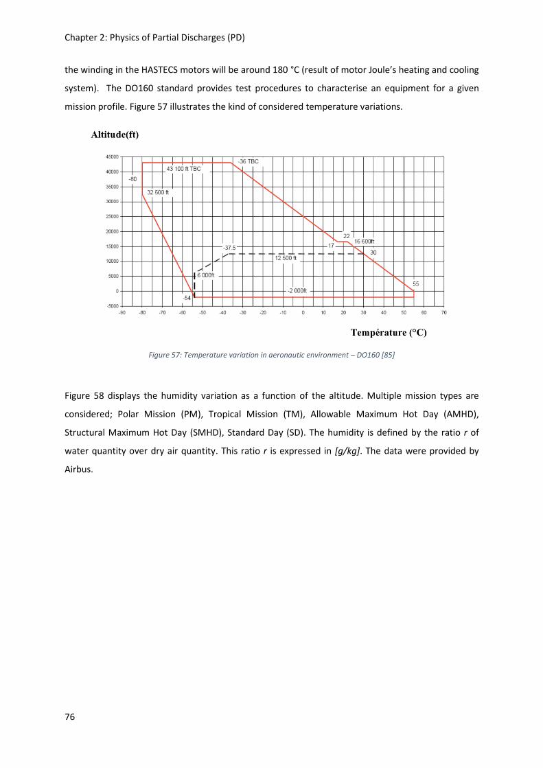
Chapter 2: Physics of Partial Discharges (PD)
76
the winding in the HASTECS motors will be around 180 °C (result of motor Joule’s heating and cooling
system). The DO160 standard provides test procedures to characterise an equipment for a given
mission profile. Figure 57 illustrates the kind of considered temperature variations.
Figure 57: Temperature variation in aeronautic environment – DO160 [85]
Figure 58 displays the humidity variation as a function of the altitude. Multiple mission types are
considered; Polar Mission (PM), Tropical Mission (TM), Allowable Maximum Hot Day (AMHD),
Structural Maximum Hot Day (SMHD), Standard Day (SD). The humidity is defined by the ratio r of
water quantity over dry air quantity. This ratio r is expressed in [g/kg]. The data were provided by
Airbus.

Chapter 2: Physics of Partial Discharges (PD)
77
Figure 58: Humidity profile in altitude [76] [84]
For a tropical mission (TM), the humidity level changes significantly as a function of the altitude. For
the other missions, the humidity can be considered as constant whatever the altitude.
2.3.2 Impact of temperature
Two main corrections are used to consider the impact of the temperature in dry air on the original
Paschen’s curves. These are the Peek’s [86] and Dunbar’s [87] corrections.
The Peek’s correction introduces a factor 𝛿. It is an image of the air density. The breakdown voltage
level V for a considered temperature T and pressure p is deduced from the breakdown voltage V0 at
standard temperature T0= 293 K and pressure p0= 760 Torr
𝑉(𝑝, 𝑇, 𝐻𝑟0) = 𝛿 ∗ 𝑉(𝑝0, 𝑇0, 𝐻𝑟0)
𝛿 =293
𝑇[𝐾]∗𝑝[𝑇𝑜𝑟𝑟]
760
Eq 19
With 𝐻𝑟0: the standard humidity rate 11 g/m3. Temperatures are expressed in K and pressures in Torr.
The Peek’s correction moves the original Paschen’s curve along the ordinate axis (Figure 59).
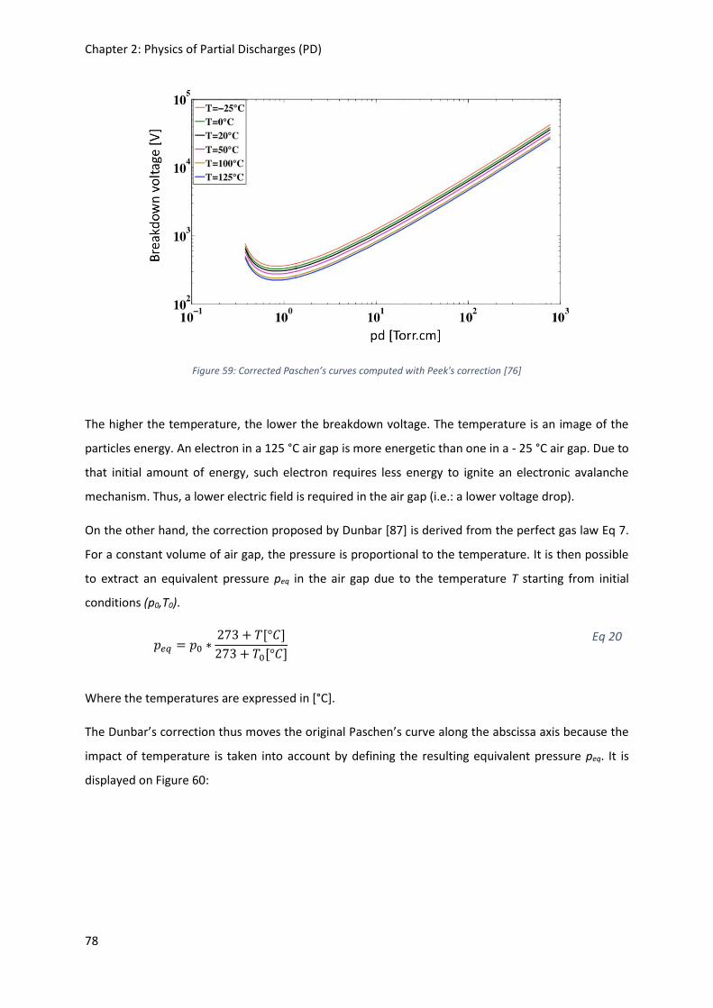
Chapter 2: Physics of Partial Discharges (PD)
78
Figure 59: Corrected Paschen’s curves computed with Peek's correction [76]
The higher the temperature, the lower the breakdown voltage. The temperature is an image of the
particles energy. An electron in a 125 °C air gap is more energetic than one in a - 25 °C air gap. Due to
that initial amount of energy, such electron requires less energy to ignite an electronic avalanche
mechanism. Thus, a lower electric field is required in the air gap (i.e.: a lower voltage drop).
On the other hand, the correction proposed by Dunbar [87] is derived from the perfect gas law Eq 7.
For a constant volume of air gap, the pressure is proportional to the temperature. It is then possible
to extract an equivalent pressure peq in the air gap due to the temperature T starting from initial
conditions (p0,T0).
𝑝𝑒𝑞 = 𝑝0 ∗273 + 𝑇[°𝐶]
273 + 𝑇0[°𝐶]
Eq 20
Where the temperatures are expressed in [°C].
The Dunbar’s correction thus moves the original Paschen’s curve along the abscissa axis because the
impact of temperature is taken into account by defining the resulting equivalent pressure peq. It is
displayed on Figure 60:

Chapter 2: Physics of Partial Discharges (PD)
79
Figure 60: Corrected Paschen’s curves computed with Dunbar's correction [76]
At higher temperature the curves are shifted to the right because it results in higher equivalent
pressure in the air gap.
In her PhD work, Sili [76] identified the domain of validity of both Peek’s and Dunbar’s corrections.
Peek’s correction is validated for pressure or distance variations at temperatures lower than 25 °C.
Dunbar’s correction is validated for variations of distance at atmospheric pressure at temperatures
upper than 25 °C. However, if both the temperature and pressure varies, Dunbar correction is no more
validated. A new empirical formulation for breakdown voltage computation has then been proposed.
This formulation is validated for temperatures upper than 35 °C.
Table 12 recaps the different corrections in temperatures and give their domains of validity.
Experimental
conditions
Domain of validity Correction
p=760Torr
d varies
or
p varies
d= 1 mm
T<25°C Peek:
𝑉(𝑝, 𝑇, 𝐻𝑟0) = 𝛿 ∗ 𝑉(𝑝0, 𝑇0, 𝐻𝑟0)
𝛿 =293
𝑇[𝐾]∗𝑝[𝑇𝑜𝑟𝑟]
760
p=760Torr
d varies
T>25°C Dunbar:
𝑝𝑒𝑞 = 𝑝0 ∗273 + 𝑇[°𝐶]
273 + 𝑇0[°𝐶]

Chapter 2: Physics of Partial Discharges (PD)
80
p varies
d=1mm
T>35°C Sili:
𝑉𝑇 =𝑉𝑃𝑎𝑠𝑐ℎ𝑒𝑛,𝑚𝑜𝑑
𝐾𝑇
With
𝑉𝑃𝑎𝑠𝑐ℎ𝑒𝑛,𝑚𝑜𝑑 = {
𝐵∗𝑝∗𝑑
𝐶+ln(𝑝∗𝑑)𝑓𝑜𝑟𝑝 ∗ 𝑑 > 𝑝 ∗ 𝑑𝑚𝑖𝑛
306𝑉𝑓𝑜𝑟𝑝 ∗ 𝑑 < 𝑝 ∗ 𝑑𝑚𝑖𝑛
𝐾𝑇 = 𝑎. 𝛿𝑏
{𝑎 = 0.0226 ∗ 𝑇(𝐾) − 6.13
𝑏 = 0.0027 ∗ 𝑇(𝐾) − 0.74
Table 12: Temperature corrections of the Paschen's curve
2.3.3 Impact of humidity
Figure 61 displays the evolution of the breakdown voltage of air as a function of the relative humidity
[84]. Three temperatures have been considered: 10 °C, 20 °C and 30 °C.
Figure 61: Impact of relative humidity versus air breakdown voltage for different temperatures [84]
Globally, an increase in humidity leads to an increase in breakdown voltage. Water molecules in the
gap produce a screen effect. Thus, more energy is required for the electrons to ionize the particles.

Chapter 2: Physics of Partial Discharges (PD)
81
One can also notice that, in presence of humidity, the breakdown voltage increases with the
temperature. This observation is in opposition with the conclusions in dry air presented in the previous
paragraph. This can be explained by other mechanisms which are now introduced by the presence of
humidity and which dynamic may be dependant on the temperature [88].
A correction can be found in the literature to take into account the humidity alone in the Paschen’s
theory [89]:
𝑉ℎ = 𝑉𝑁𝐶𝑇𝑃 ∗ (1 +𝐾ℎ100
∗ (ℎ − ℎ𝑁𝐶𝑇𝑃)) Eq 21
With:
𝑉ℎ is the corrected breakdown voltage for an absolute humidity ℎ compared to the standard
absolute humidity ℎ𝑁𝐶𝑇𝑃 = 11𝑔/𝑚3.
𝑉𝑁𝐶𝑇𝑃 is the breakdown voltage under normal condition of temperature and pressure given
by the IEC Publication 60 (1970).
The 𝐾ℎ coefficient is linked to the humidity. For a gap smaller than 1m, IEC suggests that it does not
depend on the gap length:
𝐾ℎ = (1 +ℎ − ℎ𝑁𝐶𝑇𝑃100
) Eq 22
Table 13 gives the correspondence between some absolute humidity and the corresponding relative
humidity at a fixed temperature (from Mollier’s diagram):
Relative humidity % Absolute humidity [𝑔/𝑚3]
20% 4
40% 8.29
52.5% 11
60% 12.56
80% 16.7
90% 18
Table 13: Correspondence between absolute humidity and relative humidity at 25°C
Figure 62 displays the corrected breakdown voltages for absolute humidity of 4g/m3, 11g/m3 and
18g/m3 [44].
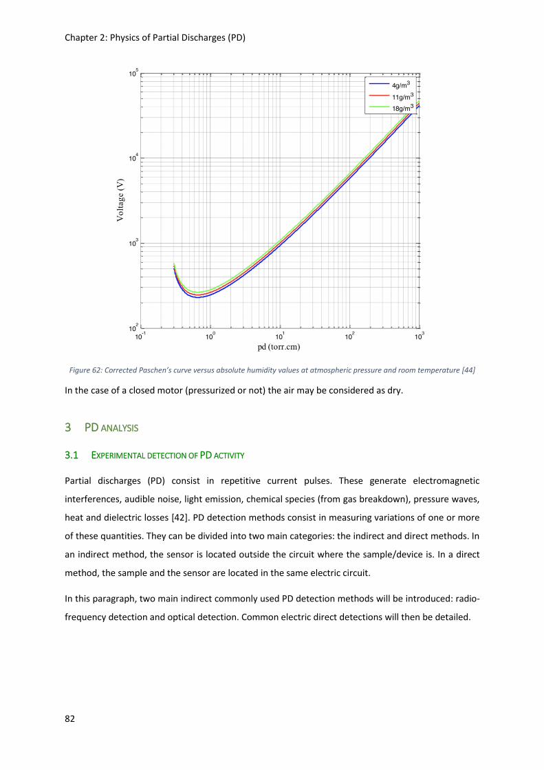
Chapter 2: Physics of Partial Discharges (PD)
82
Figure 62: Corrected Paschen’s curve versus absolute humidity values at atmospheric pressure and room temperature [44]
In the case of a closed motor (pressurized or not) the air may be considered as dry.
3 PD ANALYSIS
3.1 EXPERIMENTAL DETECTION OF PD ACTIVITY
Partial discharges (PD) consist in repetitive current pulses. These generate electromagnetic
interferences, audible noise, light emission, chemical species (from gas breakdown), pressure waves,
heat and dielectric losses [42]. PD detection methods consist in measuring variations of one or more
of these quantities. They can be divided into two main categories: the indirect and direct methods. In
an indirect method, the sensor is located outside the circuit where the sample/device is. In a direct
method, the sample and the sensor are located in the same electric circuit.
In this paragraph, two main indirect commonly used PD detection methods will be introduced: radio-
frequency detection and optical detection. Common electric direct detections will then be detailed.
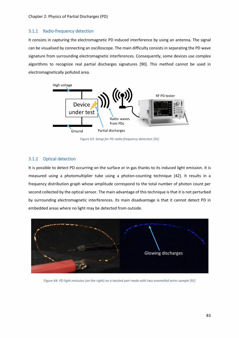
Chapter 2: Physics of Partial Discharges (PD)
83
3.1.1 Radio-frequency detection
It consists in capturing the electromagnetic PD induced interference by using an antenna. The signal
can be visualised by connecting an oscilloscope. The main difficulty consists in separating the PD wave
signature from surrounding electromagnetic interferences. Consequently, some devices use complex
algorithms to recognize real partial discharges signatures [90]. This method cannot be used in
electromagnetically polluted area.
Figure 63: Setup for PD radio-frequency detection [91]
3.1.2 Optical detection
It is possible to detect PD occurring on the surface or in gas thanks to its induced light emission. It is
measured using a photomultiplier tube using a photon-counting technique [42]. It results in a
frequency distribution graph whose amplitude correspond to the total number of photon count per
second collected by the optical sensor. The main advantage of this technique is that it is not perturbed
by surrounding electromagnetic interferences. Its main disadvantage is that it cannot detect PD in
embedded areas where no light may be detected from outside.
Figure 64: PD light emission (on the right) on a twisted pair made with two enamelled wires sample [91]

Chapter 2: Physics of Partial Discharges (PD)
84
3.1.3 Power factor/capacitance tip-up test
This test is commonly used to determine the quality of a coil or a bar ground insulation. It uses the fact
that the power factor (also called dissipation factor) or the capacity of such insulation will change with
applied AC voltage if defects (voids, delaminations) exist. Indeed, when applying high voltage, PD will
take place in these defects leading to an increase in the dissipation factor (PD induce losses) and a
decrease in the capacity (PD short-circuit the defects). The difference between low and high voltage
values gives an indication of how void-free that insulation is.
In high voltage machines, two measurements are performed at 25% and 100% of the rated line-to-
ground voltage. For new coils, it is suggested that the power factor tip-up should be < 0.5% and the
capacitance tip-up should be < 1% for new machines and < 4% for old generation machines [47].
3.1.4 Used electric detection
The detection is operated with a non-destructive electric measurements under a 50 Hz sine voltage. A
high-pass RLC filter is employed, allowing the measurement of high frequency current pulses by
considerably reducing the low frequency current signature from the power source.
Figure 65 illustrates the whole setup for a direct electric PD detection. A high voltage transformer (220
V / 20 kV - PD free) is used to applied high voltage to the sample. A low frequency generator (FX 1641A)
coupled with a low frequency amplifier deliver the power to the high voltage transformer in order to
be fully independent from the power network and its perturbations. The whole detection circuit is
located inside a Faraday cage to avoid surrounding electromagnetic perturbations. The coupling
capacity Ck associated with the measurement impedance Zm are used to detect PD. For each PD
occurring in the sample or in the air gap surrounding it, image charges at both sample electrodes are
modified. As the external circuit (Ck,Zm) has a very low high frequency impedance, these image charges
change leads to a pulse current in the detection circuit. A voltage measurement is performed at the
measurement impedance terminals. The acquisition is done on an oscilloscope.

Chapter 2: Physics of Partial Discharges (PD)
85
Figure 65: Setup for PD electric detection; a) Schematic of the PD measurement circuit, b) LFG: Low Frequency Generator, amplifier and oscilloscope, c) Sample inside the Faraday cage
3.2 PARAMETERS LINKED TO PD
3.2.1 Partial Discharge Inception Voltage (PDIV)
The PDIV is defined as the lowest voltage value at which PD are ignited and remain maintained. Indeed,
during a first PDIV test, surface discharges may occur, corresponding to the ionization of dust, moisture
or contaminant on the sample surface. These kind of PD quickly disappear and the corresponding
voltage do not have to be considered as the PDIV. IEC standard recommends that the PDIV corresponds
to the lowest voltage at which a measured quantity exceeds a predefined threshold. We will not used
these definition but the one described before. Figure 66 illustrates a PD pattern obtained at the PDIV.
Figure 66: Illustration of PD detection; below) Applied voltage, top) PD signals [92]

Chapter 2: Physics of Partial Discharges (PD)
86
3.2.2 Partial Discharge Extinction Voltage (PDEV)
The PDEV is the voltage at which PD disappear when progressively reducing the applied voltage from
PDIV. Practically, PD continue to be maintained when the voltage is decreasing from the PDIV up a to
a value from which they disappear.
3.2.3 Apparent charge
A PD between electrodes at different voltage results in a release of charges. The charges move in the
gap between the electrodes. Such displacement of charges over the thickness of the electrodes induces
either a transient voltage pulse at the electrodes terminals or a transient current pulse (this is our
case). This phenomenon is attributed to the so called apparent charge. The evaluation of the apparent
charge quantity is required for the PD quantification. However, the apparent charge does not
correspond to the total charge locally released by the PD. It is affected by the electrodes geometries,
the material properties, the measurement circuit impedance…. Thus, the real PD charge cannot be
directly measured.
Considering the work in [93], it is possible to get the real charge from the measurable charge. Let us
consider two plane parallel electrodes at a voltage V separated by air. A discharge occurs and results
in a charge q being present in the gap. Figure 67 illustrates the considered configuration.
Figure 67: Charge circulation in an air gap between two plane parallel electrodes [84]
When travelling a dx length in the gap, the charge q submitted to the electric field E realise a work W.
This work is provided by the power source.
𝑊 = 𝑞 ∗ 𝐸 ∗ 𝑑𝑥 = 𝑖 ∗ 𝑉 ∗ 𝑑𝑡 Eq 23

Chapter 2: Physics of Partial Discharges (PD)
87
With {𝐸 = 𝐸 ∗ 𝑢𝑑𝑥 = 𝑑𝑥 ∗ 𝑢‖𝑢‖ = 1
Let us consider that a displacement of charge q over a length dx results in a voltage drop Δ𝑉. The
apparent charge 𝑞𝑎𝑝𝑝 in the circuit is given by (24).
𝑞𝑎𝑝𝑝 = ∫ 𝑖 ∗ 𝑑𝑡Δ𝑡
𝑜
=𝑞
𝑉∗ ∫ 𝐸 ∗ 𝑑𝑥
Δ𝑥
0
𝑞𝑎𝑝𝑝 = 𝑞 ∗Δ𝑉
𝑉
Eq 24
The apparent charge is only a part of the charge released by the PD.
3.3 STATISTICAL PROCESSING OF THE RESULTS
PDIV experimental evaluations always present dispersions in the results from one sample to another
one. It comes from difference in the manufacturing process, dimensions tolerance and incertitude
from the measurement equipment. Dispersion may also be expected when reproducing the same
measurement successively on the same sample. This is due to the fact that PD do not exactly take place
in the same area from one test to another. Despite the same breakdown mechanism (electronic
avalanche), the PDIV values (and thus the breakdown electric field values) will consequently be
different and need to be treated by a statistical analysis.
The Weibull’s distribution, commonly used to treat dielectric strength data, has been used for the
statistical processing of PDIV values. It is also applicable with lifetime data processing. First, the results
are distributed into 𝑛𝑖intervals. A probability density 𝑃(𝐸) is defined. This function is obtained when
the width of the 𝑛𝑖intervals tend to zero and when the number of intervals tend to the infinite. In other
words, 𝑃(𝐸) is the continuous distribution of the discontinuous data. Figure 68 illustrates an example
of data distribution and the associated 𝑃(𝐸) function.

Chapter 2: Physics of Partial Discharges (PD)
88
Figure 68: Illustration of PDIV data distribution
The cumulative probability density 𝑃𝐶(𝐸) is computed as follow:
𝑃𝐶(𝐸) = ∫ 𝑃(𝐸) ∗ 𝑑𝐸𝐸
0
Eq 25
Figure 69 illustrates the 𝑃𝐶 cumulative probability. It comes from different results than the one
presented on Figure 68.
Figure 69: Example of PC cumulative probability
A good and simple approximation of 𝑃𝐶(𝐸) is recommended by EIC 62539 standard and given by [94]:

Chapter 2: Physics of Partial Discharges (PD)
89
𝑃𝐶(𝑖, 𝑛) =𝑖 − 0.44
𝑛 + 0.25
With
i: breakdown value in ascendant order;
n: total number of breakdown values.
Eq 26
Experimental PDIV data show that 𝑃𝐶(𝐸) is generally of the form:
𝑃𝐶(𝐸) = 1 − (exp(𝐸
𝛼)𝛽)
Eq 27
With 𝛽 the shape parameter and 𝛼 the characteristic breakdown field value such that:
𝑃𝐶(𝛼) = 63.2% Eq 28
By manipulating Eq 27 with log operator on can gets:
log (log (1
1 − 𝑃𝐶(𝐸))) = 𝛽 ∗ log(𝐸) − 𝛽 ∗ log(𝛼)
Eq 29
By taking an axis system log (log (1
1−𝑃𝐶(𝐸))) = 𝑓(log(𝐸)) the points can be interpolated with a slope
𝛽.
Figure 70 illustrates an example of 𝑃𝐶(𝐸) evolution in the particular axis system defined by Eq 29.
Figure 70: PC(E) evolution in the axis system defined by (26)

Chapter 2: Physics of Partial Discharges (PD)
90
Another way to determine the 𝛼 and 𝛽 coefficients is through computation. This approach is based on
least square regression and used weighting coefficients given by White in [95]. Let us apply the
following change of variable:
𝑋𝑖 = log(− log(1 − 𝑃𝐶(𝑖)))
𝑌𝑖 = log(𝐸𝑖)
Eq 30
Where the index i refers to sample i.
First, the weighted averages of 𝑋𝑖 and 𝑌𝑖 are computed Eq 31 and Eq 32. It is considered that all the
samples are used: there is no sample excluded due any sample defect or artefact occurring during the
experimental measurements.
𝑋𝑚 =∑ 𝑤𝑖 ∗ 𝑋𝑖𝑛𝑖=1
∑ 𝑤𝑖𝑛𝑖=1
Eq 31
𝑌𝑚 =∑ 𝑤𝑖 ∗ 𝑌𝑖𝑛𝑖=1
∑ 𝑤𝑖𝑛𝑖=1
Eq 32
With 𝑤𝑖 the weighted coefficient associated to the broken sample i given by [95]. Samples are sorted
in ascendant breakdown values.
The 𝛼 and 𝛽 coefficients are finally computed in Eq 33 and Eq 34:
𝛽 =∑ 𝑤𝑖 ∗ (𝑋𝑖 − 𝑋𝑚)
2𝑛𝑖=1
∑ 𝑤𝑖 ∗ (𝑋𝑖 − 𝑋𝑚) ∗ (𝑌𝑖 − 𝑌𝑚)𝑛𝑖=1
Eq 33
𝛼 = exp(𝑌𝑚 −𝑋𝑚
𝛽) Eq 34
4 DEGRADATION OF THE POLYMER INSULATION IN AERONAUTIC ENVIRONMENT
There are different mechanisms which may impact the time to failure of dielectrics under an electric
field [96]. The intrinsic failure of a polymer mainly results from electrical, thermal and mechanical
mechanisms, sometimes acting simultaneously. A PD activity does not lead to an instantaneous
breakdown of the polymer: the time to failure can goes from seconds to days. It is an extrinsic stress
which degrades the polymer insulation progressively up to the final breakdown. The extrinsic time to
failure, occurring above the PDIV, is always lower than the intrinsic one. It has been introduced in the
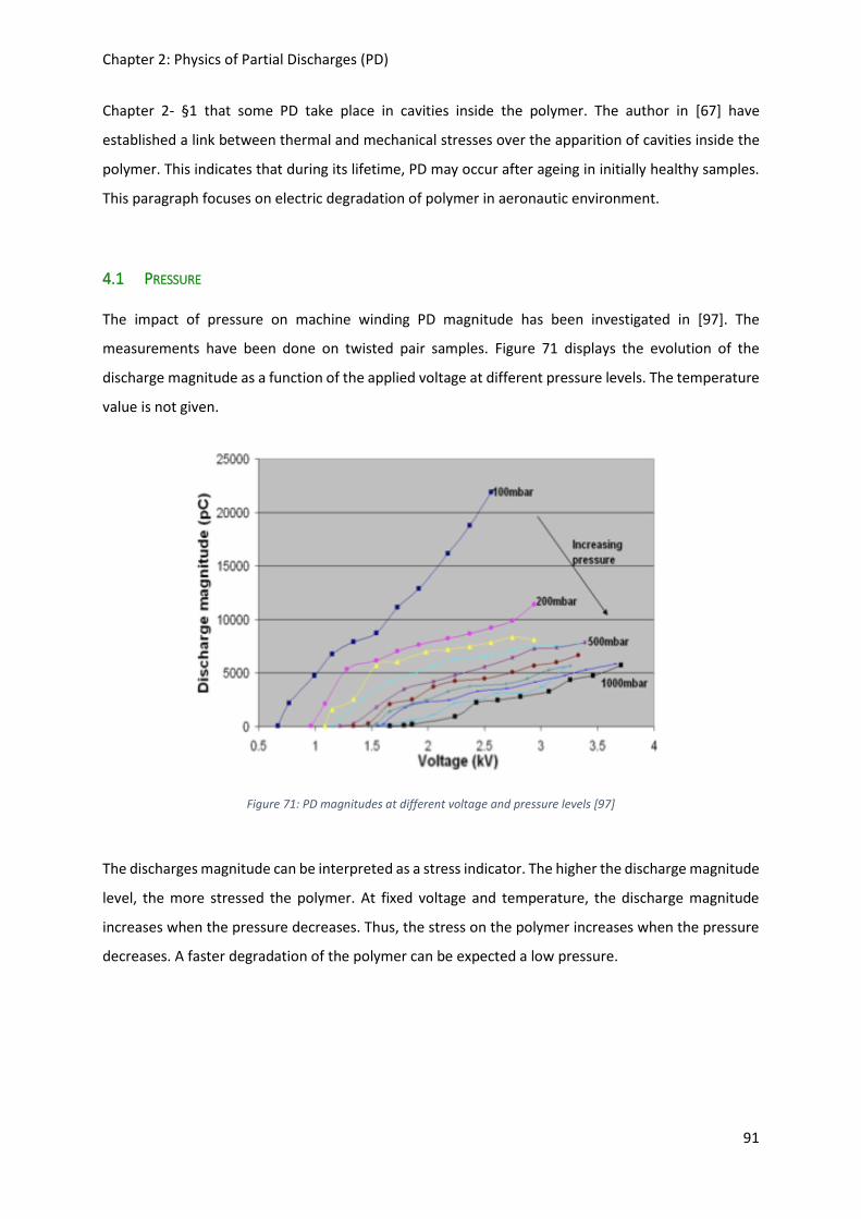
Chapter 2: Physics of Partial Discharges (PD)
91
Chapter 2- §1 that some PD take place in cavities inside the polymer. The author in [67] have
established a link between thermal and mechanical stresses over the apparition of cavities inside the
polymer. This indicates that during its lifetime, PD may occur after ageing in initially healthy samples.
This paragraph focuses on electric degradation of polymer in aeronautic environment.
4.1 PRESSURE
The impact of pressure on machine winding PD magnitude has been investigated in [97]. The
measurements have been done on twisted pair samples. Figure 71 displays the evolution of the
discharge magnitude as a function of the applied voltage at different pressure levels. The temperature
value is not given.
Figure 71: PD magnitudes at different voltage and pressure levels [97]
The discharges magnitude can be interpreted as a stress indicator. The higher the discharge magnitude
level, the more stressed the polymer. At fixed voltage and temperature, the discharge magnitude
increases when the pressure decreases. Thus, the stress on the polymer increases when the pressure
decreases. A faster degradation of the polymer can be expected a low pressure.

Chapter 2: Physics of Partial Discharges (PD)
92
4.2 HUMIDITY
Humidity changes the degradation of the polymer into two opposite directions whether considering
surface discharges or inner discharges. The authors in [98] have investigated the effect of exposure to
ambient relative humidity on the dielectric degradation. Figure 72 displays the evolution of the time
to failure as a function of the electric field applied to the dielectric for different relative humidity
exposure. The magnitudes are in arbitrary unit (AU).
Figure 72: Time to failure as a function of the electric field for different humidity - 60Hz AC voltage [98]
In this experiment, samples have been exposed to different humidity levels for two weeks. The higher
the humidity level, the higher the humidity inside the dielectric sample. At a fixed electric field
amplitude, the time to failure decreases when the humidity inside the dielectric increases. This can be
explained by a failure due to water treeing as presented by [67] and/or by the increase in dielectric
losses due to humidity.
In [99] the degradation of polyethylene under corona discharges is studied at different external
humidity level. Here, there is no humidity inside the dielectric. Figure 73 displays the obtained results.

Chapter 2: Physics of Partial Discharges (PD)
93
Figure 73:Polyethylene failure time as a function of the external relative humidity under corona discharges (E=8kV/mm, f=60Hz) [99]
In the case of corona discharge, the time to failure extends with the augmentation of the humidity. In
fact, water particles act as a screen effect which shielded the polymer.
4.3 TEMPERATURE
The impact of temperature over electrical tree development inside a dielectric has been studied in
[100]. Figure 74 presents the trees average growth rate in Low Density Polyethylene (LDPE) and
branched LDPR (BPEQ) as a function of the applied voltage for temperatures ranging from 20 °C to 50
°C.
Figure 74: Average tree growth rate as a function of voltage and temperature in LDPE and branched LDPE (BPEQ) [100]
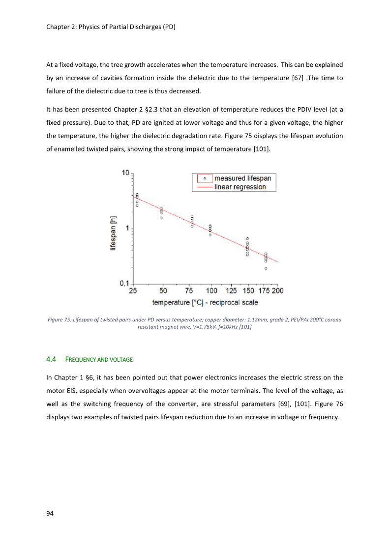
Chapter 2: Physics of Partial Discharges (PD)
94
At a fixed voltage, the tree growth accelerates when the temperature increases. This can be explained
by an increase of cavities formation inside the dielectric due to the temperature [67] .The time to
failure of the dielectric due to tree is thus decreased.
It has been presented Chapter 2 §2.3 that an elevation of temperature reduces the PDIV level (at a
fixed pressure). Due to that, PD are ignited at lower voltage and thus for a given voltage, the higher
the temperature, the higher the dielectric degradation rate. Figure 75 displays the lifespan evolution
of enamelled twisted pairs, showing the strong impact of temperature [101].
Figure 75: Lifespan of twisted pairs under PD versus temperature; copper diameter: 1.12mm, grade 2, PEI/PAI 200°C corona resistant magnet wire, V=1.75kV, f=10kHz [101]
4.4 FREQUENCY AND VOLTAGE
In Chapter 1 §6, it has been pointed out that power electronics increases the electric stress on the
motor EIS, especially when overvoltages appear at the motor terminals. The level of the voltage, as
well as the switching frequency of the converter, are stressful parameters [69], [101]. Figure 76
displays two examples of twisted pairs lifespan reduction due to an increase in voltage or frequency.

Chapter 2: Physics of Partial Discharges (PD)
95
Figure 76: Lifespan of twisted pairs under P. Left) Lifespan versus voltage (f=10kHz, T=30°C), Right) Lifespan versus frequency (V=1.75kV, T=30°C); copper diameter: 1.12mm, grade 2, PEI/PAI 200°C corona resistant magnet wire [101]
Besides, the introduction of wide-band gap materials such as SiC or GaN rises some interrogation on
the impact of the dV/dt slope on the dielectric ageing. The impact of all these parameters on the ageing
of the electric insulation is investigated in [57], [61], [102].
In [102], two voltage signals were used: a sinusoidal one and a square-wave voltage. The applied
voltage amplitudes, frequencies and duty cycles are the same for both signals. Figure 77 displays the
main results. As expected, at a fixed frequency, the lifetime decreases when the voltage increases
whereas at fixed voltage, the lifetime decreases when the frequency increases. Finally, the slope of the
applied voltage seems to have no significant impact on the lifetime as under the same conditions, the
measured lifetimes by applying a sine or a square wave voltage are very close together.

Chapter 2: Physics of Partial Discharges (PD)
96
Figure 77: Comparison between square and sine voltage effect on lifetime under PD. Boxplots representing lifetimes (median, quartiles, extrema): (a) V=1445 Vpeak, (50%) (b) V=1540 Vpeak (60%) [102]
4.5 LIFETIME EVALUATION
There are different models to predict the lifespan of a sample. The simplest ones take only one
constraint into account. The commonly used are the Inverse Power Model and the Exponential Model
[103]. Table 14 presents the equations used.
Model Parameters Equation
Inverse Power Model L: time to failure at voltage V
V: voltage
k: constant
N: constant
𝐿 = 𝑘 ∗ 𝑉−𝑁

Chapter 2: Physics of Partial Discharges (PD)
97
Exponential Model L : time to failure at voltage V
V: voltage
c: constant
k: constant
𝐿 = 𝑐 ∗ exp(−𝑘 ∗ 𝑉)
Table 14: Inverse power model and exponential model for lifetime under PD evaluation; adapted from [103]
The authors in [104] studied the combined impact of temperature, voltage and frequency on the
lifetime. Concerning the electrical stresses (i.e.: voltage and frequency) an inverse power model was
applied. For the temperature, an exponential model was applied.
Stress Parameters Model
Electrical 𝐸𝑉: constant derived from both
the material and power law
applied to voltage V
V: voltage
𝐸𝐹 : constant derived from both
the material and power law
applied to frequency F
F: frequency
L: time to failure
{log(𝐿) = 𝐸𝑉 ∗ log(𝑉)
log(𝐿) = 𝐸𝐹 ∗ log(𝐹)
Thermal 𝐸𝑇 and b: constants derived from
the material and obtained from
lifetime data under electro-
thermal stress
T: temperature
log(𝐿) = 𝐸𝑇 ∗ exp(−𝑏 ∗ 𝑇)
Table 15:Lifetime models applied for electrical and thermal stresses; adapted from [104]
The model which couples the electrical and thermal stresses is expressed in Eq 35.
log(𝐿)~𝑀 + 𝐸𝑉 ∗ log(𝑉) + 𝐸𝐹∗ log(𝐹) + 𝐸𝑇 ∗ exp(−𝑏 ∗ 𝑇) + 𝐸𝐹𝑉∗ log(𝑉) ∗ log(𝐹) + 𝐸𝑉𝑇∗ log(𝑉) ∗ exp(−𝑏 ∗ 𝑇) + 𝐸𝐹𝑇∗ log(𝐹) ∗ exp(−𝑏 ∗ 𝑇) + 𝐸𝑉𝐹𝑇∗ log(𝑉) ∗ log(𝐹) ∗ exp(−𝑏 ∗ 𝑇)
Eq 35
The first four terms in Eq 35 correspond respectively to the averaged lifetime M, the impact of voltage
alone, the impact of frequency alone and the impact of temperature alone. The terms five to seven
coupled two by two temperature, voltage and frequency. For example, the constant 𝐸𝐹𝑉 is attached
to the coupling frequency-voltage term. Finally, the last term couples all three parameters (i.e.:
temperature, frequency and voltage).

Chapter 2: Physics of Partial Discharges (PD)
98
The design of experiment regression has been applied to characterise the influence of each terms on
the lifetime [104].
On board electrical motors are usually designed to have a lifetime of several ten thousand hours. It will
be obviously too much money and time consuming to check its lifetime under nominal working
conditions. An alternative is to use accelerated lifetime tests. It consists in testing the machine at
higher stress levels. Stresses can be the voltage, frequency, current, temperature or pressure. Stresses
level have to remain under maximum values defined by standards [105] [106] in order not to produce
irrelevant degradation mechanisms (for example testing at a temperature above the thermal class).
The results are then treated using regression methods. A survey of several regression methods is
presented in [107]. These are the design of experiments, response surface, multilinear and robust
regression. Each method has its advantages. As an example, design of experiments is accurate with a
limited experimental cost.
5 MODELLING PARTIAL DISCHARGES ACTIVITY
5.1 STREAMER CRITERION
This approach considers that the mechanism at the origin of the discharge is the ionization of the gas.
It introduces the effective ionization 𝛼𝑒𝑓𝑓. It corresponds to the rate of net production of free electrons
in the gas. This coefficient strongly depends on the electric field amplitude E. The function varies
depending the gas. This function is given in air by [108]:
𝛼𝑒𝑓𝑓(𝐸) = 𝑝 ∗ [𝑘 ∗ (𝐸
𝑝− Λ)
2
− 𝐴] Eq 36
With 𝑘 = 1.6𝑚𝑚. 𝑏𝑎𝑟/𝑘𝑉2, Λ = 2.2𝑘𝑉/(𝑚𝑚. 𝑏𝑎𝑟) and 𝐴 = 0.31/(𝑚𝑚. 𝑏𝑎𝑟). p is the pressure in
[bar]. 𝛼𝑒𝑓𝑓(𝐸) > 0 for 𝐸 > 2.6𝑘𝑉/𝑚𝑚. That is the critical field strength at which there is a net
production of free electrons.
Figure 78 displays the evolution of this reduced coefficient as a function of the reduced electric field.
Three different sets of experimental data points are used [108].
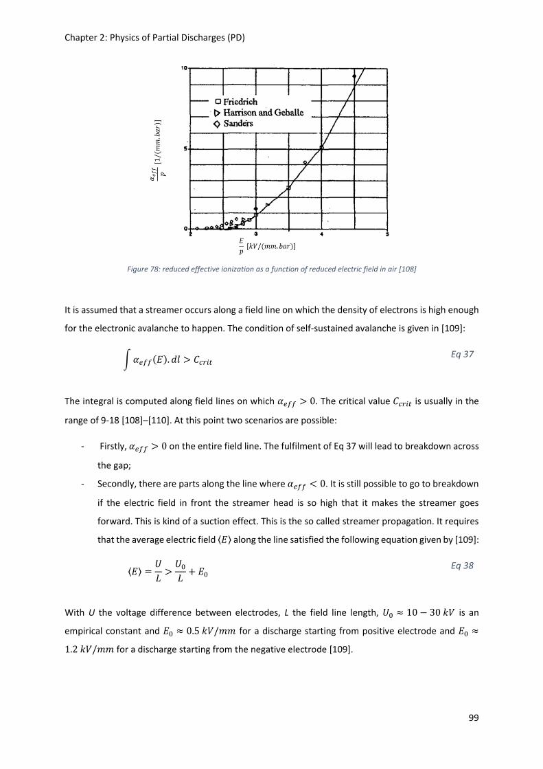
Chapter 2: Physics of Partial Discharges (PD)
99
Figure 78: reduced effective ionization as a function of reduced electric field in air [108]
It is assumed that a streamer occurs along a field line on which the density of electrons is high enough
for the electronic avalanche to happen. The condition of self-sustained avalanche is given in [109]:
∫𝛼𝑒𝑓𝑓(𝐸). 𝑑𝑙 > 𝐶𝑐𝑟𝑖𝑡 Eq 37
The integral is computed along field lines on which 𝛼𝑒𝑓𝑓 > 0. The critical value 𝐶𝑐𝑟𝑖𝑡 is usually in the
range of 9-18 [108]–[110]. At this point two scenarios are possible:
- Firstly, 𝛼𝑒𝑓𝑓 > 0 on the entire field line. The fulfilment of Eq 37 will lead to breakdown across
the gap;
- Secondly, there are parts along the line where 𝛼𝑒𝑓𝑓 < 0. It is still possible to go to breakdown
if the electric field in front the streamer head is so high that it makes the streamer goes
forward. This is kind of a suction effect. This is the so called streamer propagation. It requires
that the average electric field ⟨𝐸⟩ along the line satisfied the following equation given by [109]:
⟨𝐸⟩ =𝑈
𝐿>𝑈0𝐿+ 𝐸0
Eq 38
With U the voltage difference between electrodes, L the field line length, 𝑈0 ≈ 10 − 30𝑘𝑉 is an
empirical constant and 𝐸0 ≈ 0.5𝑘𝑉/𝑚𝑚 for a discharge starting from positive electrode and 𝐸0 ≈
1.2𝑘𝑉/𝑚𝑚 for a discharge starting from the negative electrode [109].

Chapter 2: Physics of Partial Discharges (PD)
100
This methodology has been implanted in COMSOL [110]. Figure 79 presents an application of COMSOL
Particle Tracing Module for the evaluation of field lines starting from a positive electrode where Eq 37
is verified and on which a streamer is likely to appear.
Figure 79: Field lines satisfying the streamer propagation condition (Eq 37) for discharges starting from the positive electrode [110]
The main advantage of this method is that it does not require an uniform electric field along the field
line.
5.2 PASCHEN’S CRITERION
Another approach consists in using the Paschen’s criterion. It requires the computation of the field
lines. The electric field has to be uniform along a field line. This approach was used in [55] to determine
the PDIV between two enamelled round copper wires. The field lines are considered as straight lines.
They are computed using geometrical relations. Figure 80 displays the used 2D-model.

Chapter 2: Physics of Partial Discharges (PD)
101
Figure 80: Parallel enamelled round wires; 2D-model [55]
This model is solved using finite elements. The voltage is then available on the whole model. The
voltage difference at the extremities of a field line 𝑑𝑖 is computed. The results are displayed in a
Paschen’s plot as presented in Figure 81. The abscissa axis is the product 𝑝𝑑(𝑝 = 1𝑏𝑎𝑟) (i.e.: the field
line length) and the ordinate axis is the voltage difference.
Figure 81: Example of simulated results versus the experimental Paschen's criterion [55]

Chapter 2: Physics of Partial Discharges (PD)
102
The intersection of the simulated curve (red line) with the Paschen’s curve (green line) indicates that
the field line at this intersection is probably subject to PD. In this case the field line of length 20𝜇𝑚 is
the one on which PD may occur.
This approach is selected to evaluate PD activity in this work. That choice is made for mainly three
reasons. First, it is simple to code. Second, it gives precise results. Third, only uniform fields are
considered in this work. Chapter III will present the original developed method for precise field lines
computation. Chapter IV will then detail an experimental study on the Paschen’s criterion and will
propose a correction adapted to enamelled round wires configurations. Finally, Chapter V will present
the integration of the field lines computation module and the corrected Paschen’s curve in an
automatic tool to evaluate PD activity inside an electric motor slot under aeronautical environment.
This chapter has detailed the Partial Discharges (PD). The Paschen’s law and some deviations which
take into account the aeronautic environmental conditions have been given. The different
experimental set-ups to detect and analysis the PD have been given. Results concerning the impact of
frequency, voltage and temperature on insulation lifespan have been presented. At the end of this
chapter two methods have been presented to evaluate the Partial Discharge Inception Voltage (PDIV).
The Paschen’s criterion has been retained. The next chapter deals with the computation of electric
field lines. Field lines geometry and voltage drop are required to apply the Paschen’s criterion.

Chapter 3: Electric field lines computation
103
Chapter 3: Electric field lines computation

Chapter 3: Electric field lines computation
104

Chapter 3: Electric field lines computation
105
1 INTRODUCTION
Our research for the evaluation of Partial Discharges (PD) leads us to the computation of electric field
lines using Matlab software. However, in some configuration, strange results have been observed.
These are field lines which are not perpendicular to iso-potential lines. In order to investigate the cause
of such weirdness and to fully understand the methods used in Matlab software, we have to reinforce
our knowledge on numerical methods used for the electric field lines computation in an electrostatic
problem composed of both conductors and dielectric materials.
After the presentation of electrostatic formulations, the Whitakker’s method is illustrated on a simple
example. From the presentation of the Horowitz’s method, we propose an improvement in the
computation of field lines. This improvement makes it possible to present a more synthetic field map:
the field lines are drawn so that their density is proportional to the intensity of the electric field. Finally,
an example is treated with the Whitakker’s method implemented in Matlab and the proposed method
which allows them to be compared.
2 THE ELECTROSTATIC PROBLEM
2.1 PRESENTATION OF THE FIELD OF STUDY
The problem consists of two enameled round wires in close contact in air. It is a configuration
representative of a contact between two adjacent wires in a stator slot in the presence of a default (air
bubble or bad impregnation) in the surrounding impregnating resin.
The copper areas are obviously not modelled since there is no electric field in conductor materials.
Boundary conditions (i.e.: voltages) are applied on the copper areas contours.
The air and the enamel are considered charge carrier free.
The wires are considered infinitely long in the machine active length dimension and the voltage drops
are neglected. Due to invariance along this dimension and symmetries the problem is reduced to a
2D-electrostatic problem with only a quarter of the wires being modelled.
Figure 82 displays the 2D-problem.

Chapter 3: Electric field lines computation
106
Figure 82: Enamelled wires 2D-electrostatic problem
In such electrostatic problem, the materials are characterized with their dielectric constant. The
dielectric constant of air is 1. The dielectric constant of the enamel is greater than 1 and depends on
the polymer used. In this chapter, the dielectric constant of the enamel will be taken as 3.5.
2.2 ELECTROSTATIC EQUATIONS AND FORMULATIONS
The basis of electromagnetism are the Maxwell’s equations. These are recap in Table 16.
𝐶𝑢𝑟𝑙�⃗⃗� = 𝐽 +𝜕�⃗⃗�
𝜕𝑡
Eq 39
𝐶𝑢𝑟𝑙�⃗� = −𝜕�⃗�
𝜕𝑡
Eq 40
𝑑𝑖𝑣�⃗� = 0 Eq 41
𝑑𝑖𝑣�⃗⃗� = 𝜌 Eq 42
Table 16: Complete Maxwell's equations [42]
Five field vectors are introduced: the electric field intensity �⃗� , the magnetic field intensity �⃗⃗� , the
electric flux density �⃗⃗� , the magnetic flux density �⃗� and the current density 𝐽 . The volume charge
density of the dielectric medium in which the field is considered is noted 𝜌.
The fields produced by a power frequency alternating voltage are not electrostatic. However, they are
considered quasi-stationary: the fields time variation is neglected. Besides, in this work both air and

Chapter 3: Electric field lines computation
107
polymer insulation materials are considered free of charge carrier. Table 17 gives the simplified
Maxwell’s equations which comes into play in the considered electrostatic problem.
𝐶𝑢𝑟𝑙�⃗� = 0 Eq 43
𝑑𝑖𝑣�⃗⃗� = 0 Eq 44
Table 17: Maxwell's equations used for a charge carrier free electrostatic problem
Because �⃗� is curl free, it can be expressed as a gradient of a scalar potential. This scalar is the electric
potential V:
�⃗� = −𝑔𝑟𝑎𝑑𝑉 Eq 45
The electric flux density �⃗⃗� is derived from the electric field intensity �⃗� and the medium properties:
�⃗⃗� = 휀𝑟 ∗ 휀0 ∗ �⃗� = ε ∗ �⃗� Eq 46
With 휀0 the vacuum dielectric constant, 휀𝑟 the medium relative dielectric constant (equals 1 in air).
The medium is considered isotropic thus ε is a constant.
By injecting Eq 45 and Eq 46 into Eq 44 one gets:
𝑑𝑖𝑣(휀 ∗ (−𝑔𝑟𝑎𝑑𝑉)) = 0
𝑑𝑖𝑣(𝑔𝑟𝑎𝑑𝑉) = 0
∇2𝑉 = 0
Eq 47
Equation Eq 47 is called the Poisson’s equation. It is the scalar potential formulation of a charge carrier
free electrostatic problem.
As �⃗⃗� is divergent free it thus can be expressed as the curl of an electric vector potential �⃗� :
�⃗⃗� = 𝑐𝑢𝑟𝑙�⃗� Eq 48
By injecting Eq 48 in Eq 43 one gets:
𝑐𝑢𝑟𝑙(𝑐𝑢𝑟𝑙�⃗� ) = 0
𝑔𝑟𝑎𝑑(𝑑𝑖𝑣�⃗� ) − ∇2�⃗� = 0
Eq 49
The Coulomb’s gauge applied to the vector potential �⃗� is defined as follow:
𝑑𝑖𝑣(�⃗� ) = 0 Eq 50
Applying the Coulomb’s gauge in Eq 49 results in:

Chapter 3: Electric field lines computation
108
∇2�⃗� = 0 Eq 51
Equation Eq 51 is the vector potential formulation of a charge carrier free electrostatic problem.
There are thus two formulations for solving the electrostatic problem. The first uses a scalar potential
V. The second uses a vector potential �⃗� . Each formulation has its advantages and disadvantages.
2.3 ADVANTAGES AND DISADVANTAGES OF EACH FORMULATION
2.3.1 Vector potential
In case of a 2D-problem in a (x,y) plane, the electric vector potential �⃗� is written as:
�⃗� = 𝑢. 𝑧
With:
‖𝑧 ‖ = 1
Eq 52
The main advantage of the vector potential is that it directly gives the electric field lines. Field lines are
in fact level curves (i.e.: contour) of a scalar function u. Such function is usually called the stream
function [111]. By injecting Eq 52 in Eq 48 one gets:
{
𝑑u
𝑑𝑥= −𝐷𝑦
𝑑u
𝑑𝑦= 𝐷𝑥
Eq 53
Using the relationship between the electric field �⃗� and the electric flux density �⃗⃗� (Eq 46), Eq 53 can
be expressed under the form:
{
𝑑𝑢
𝑑𝑥= −ε ∗ 𝐸𝑦
𝑑u
𝑑𝑦= ε ∗ 𝐸𝑥
Eq 54
With 𝐸𝑥 and 𝐸𝑦 respectively the projections of �⃗� along 𝑥 and 𝑦 axis in a 2D-system.
The vector potential formulation is complex to execute in an electrostatic problem with multiple
conductors. It requires to put in place a network of branches and cuts all across the field of study [112],
[113]. However, [113], [114] have successfully put in application that formulation to solve an
electrostatic problem with multiple conductors. Their work has been done almost at the same time we
started our researches on this topic.
Besides, none of the software at our disposal uses the vector potential formulation.

Chapter 3: Electric field lines computation
109
2.3.2 Scalar potential
The formulation with the scalar potential V is the simplest to use. Contrary to the vector potential u,
there is no need to introduce cuts if multiple conductors are present in the domain of study. That is
because the solution using a V formulation is unique. The scalar potential is also easy to handle for the
computation of equipotential lines.
The main inconvenient of the V formulation is that it does not give directly the electric field lines.
Additional steps are consequently required. Two main methods were found in the literature to
compute field lines by using a numerical calculation software (such as Matlab) from the scalar potential
solution.
The formulation with the scalar potential V was finally chosen for several reasons. First, the finite
elements software at our disposal (Ansys Emag, Ansys Maxwell, Femm or Jmag) are using the scalar
potential formulation. Then, it is simple to manipulate. Finally, methods exist in the literature to
compute field lines from the scalar potential solutions. They constitute a strong base to start our work.
3 ELECTRIC FIELD LINES COMPUTATION DERIVED FROM A SCALAR POTENTIAL FORMULATION
3.1 BALLISTIC METHOD
The first method to compute field lines from a scalar potential formulation solution is presented by
[115]. By definition, the electric field �⃗� is parallel to a field line 𝑙 . In a direct orthonormal system, the
cross-product of this two quantities is null:
𝑙 × �⃗� = 0
𝑙𝑥 ∗ 𝐸𝑦 − 𝑙𝑦 ∗ 𝐸𝑥 = 0
Eq 55
With 𝑙𝑥 and 𝑙𝑦 respectively the projections of 𝑙 along 𝑥 and 𝑦 axis in a 2D-system.
From Eq 55 it comes:
𝐸𝑦
𝐸𝑥=𝑙𝑦
𝑙𝑥
Eq 56
𝐸𝑥, 𝐸𝑦 are the field components over the mesh. These are known.
Starting at any point, the field line 𝑙 can be computed by incrementing Eq 56 given an arbitrary
displacement ∆𝑥 along x axis. Thus, the vertical displacement ∆𝑦along y axis is expressed as follow:

Chapter 3: Electric field lines computation
110
∆𝑦= ∆𝑥 ∗𝐸𝑦
𝐸𝑥
Eq 57
Let us express equation Eq 57 between two consecutive points 𝑀𝑖(𝑥𝑖, 𝑦𝑖) and 𝑀𝑖+1(𝑥𝑖+1, 𝑦𝑖+1) :
(𝑦𝑖+1 − 𝑦𝑖) = (𝑥𝑖+1 − 𝑥𝑖) ∗𝐸𝑦,𝑖
𝐸𝑥,𝑖
Eq 58
Let us define a constant step increase ∆𝑠𝑡𝑒𝑝 at each iteration, so that:
∆𝑠𝑡𝑒𝑝=(𝑦𝑖+1 − 𝑦𝑖)
𝐸𝑦,𝑖=(𝑥𝑖+1 − 𝑥𝑖)
𝐸𝑥,𝑖
Eq 59
It is thus possible to express the 𝑀𝑖+1(𝑥𝑖+1, 𝑦𝑖+1) coordinates from 𝑀𝑖(𝑥𝑖, 𝑦𝑖) data (coordinates and
field components) and ∆𝑠𝑡𝑒𝑝:
𝑥𝑖+1 = 𝑥𝑖 + ∆𝑠𝑡𝑒𝑝 ∗ 𝐸𝑥,𝑖
𝑦𝑖+1 = 𝑦𝑖 + ∆𝑠𝑡𝑒𝑝 ∗ 𝐸𝑦,𝑖
Eq 60
When chosen arbitrary, the starting point may not be the start of the field line. It is then necessary to
integrate Eq 60 backward to complete the line.
This method is called a ballistic method. The mesh is swept and field lines are started in elements which
do not already contain a field line. The field lines are computed by integration. The integration process
is stopped if one of the following condition is checked:
the field line enters a forbidden region (for instance the limit of the domain);
the field line reaches a null field;
the field line loops back onto itself;
the field line has too many segments. This is a safety measure in case the previous conditions
do not work properly.
By doing so, there is the same density of field line all over the model. It does not allow to represent
the electric field intensity.
As an illustration, let us consider an electrostatic problem made of two infinitely long cylinder
oppositely. Due to the symmetries, only a quarter of the field of study is considered as displayed on
Figure 83. The mesh is represented with black crosses. It is made of rectangular elements (dotted red
line). The blue line delimits the conductor contour.

Chapter 3: Electric field lines computation
111
Figure 83: System of 2 infinite cylinders oppositely charges - field of study represents one quarter of the system - mesh (dots) and half conductor contour (blue)
Let us apply the Whittaker ballistic method on that system. The algorithm noted above is implanted in
a Matlab script.
The orientation vector of the electric field is computed on all mesh nodes, except for the ones located
inside the conductor. The starting points are chosen on the contour of the domain. Figure 84 displays
the computed orientation vectors and the starting points (circles). The starting points are arbitrary
chosen on the limit of the field of study.
Figure 84: Electric field orientation vectors and starting points (red circles)
Let us designate the starting point 𝑄(𝑥0, 𝑦𝑜) of a field line. Then, the next point on the line 𝑀1(𝑥1, 𝑦1)
is computed by iteration from point Q. The iteration is backward because the starting points are on
the end of the field lines:
𝑥1 = 𝑥0 − ∆𝑠𝑡𝑒𝑝 ∗ 𝐸𝑥,0 Eq 61

Chapter 3: Electric field lines computation
112
𝑦1 = 𝑦0 − ∆𝑠𝑡𝑒𝑝 ∗ 𝐸𝑦,0
With 𝐸𝑥,0 and 𝐸𝑦,0 the electric field orientation vector components along x and y axis respectively on
starting point Q. The step increase ∆𝑠𝑡𝑒𝑝 at each iteration is taken equal to the grid spacing along x
axis 𝑑𝑥. Figure 85 displays the field lines after one iteration backward from starting points.
Figure 85: Field lines after a first iteration backward
It can be seen that the 𝑀1 points do not coincide with a mesh node. The electric field orientation
vectors are interpolated on the extra 𝑀1 points using the interp2 function.
At each iteration, the field lines extend. The ith iteration between two consecutive points 𝑀𝑖(𝑥𝑖, 𝑦𝑖)
and 𝑀𝑖+1(𝑥𝑖+1, 𝑦𝑖+1) correspond to:
𝑥𝑖+1 = 𝑥𝑖 − ∆𝑠𝑡𝑒𝑝 ∗ 𝐸𝑥,𝑖
𝑦𝑖+1 = 𝑦𝑖 − ∆𝑠𝑡𝑒𝑝 ∗ 𝐸𝑦,𝑖
Eq 62
The computed field lines after 11 iterations are displays on Figure 86.

Chapter 3: Electric field lines computation
113
Figure 86: Computed field lines after 11 backward iterations
In this method, the starting points are chosen arbitrarily. In the next presented method, the choice of
the starting points is a key step in order to represent a field intensity with the density of field lines.
3.2 FLUX TUBES BASED METHOD
The objective is to represent the strength of the electric field by the density of the electric flux lines
[111]. The core of the method is the choice of the field lines starting points.
A predetermined amount of flux 𝛿 has to be present between two adjacent lines a and b:
𝛿 = ∫ 𝐸. 𝑛. 𝑑𝑠𝑏
𝑎
Eq 63
Where n is the normal vector and s is the path between the lines a and b. This path is chosen as the
contour of scalar potential V. Figure 87 illustrates the equation Eq 63.
Figure 87: Illustration of flux quantity 𝛿 located between two consecutive field lines a and b
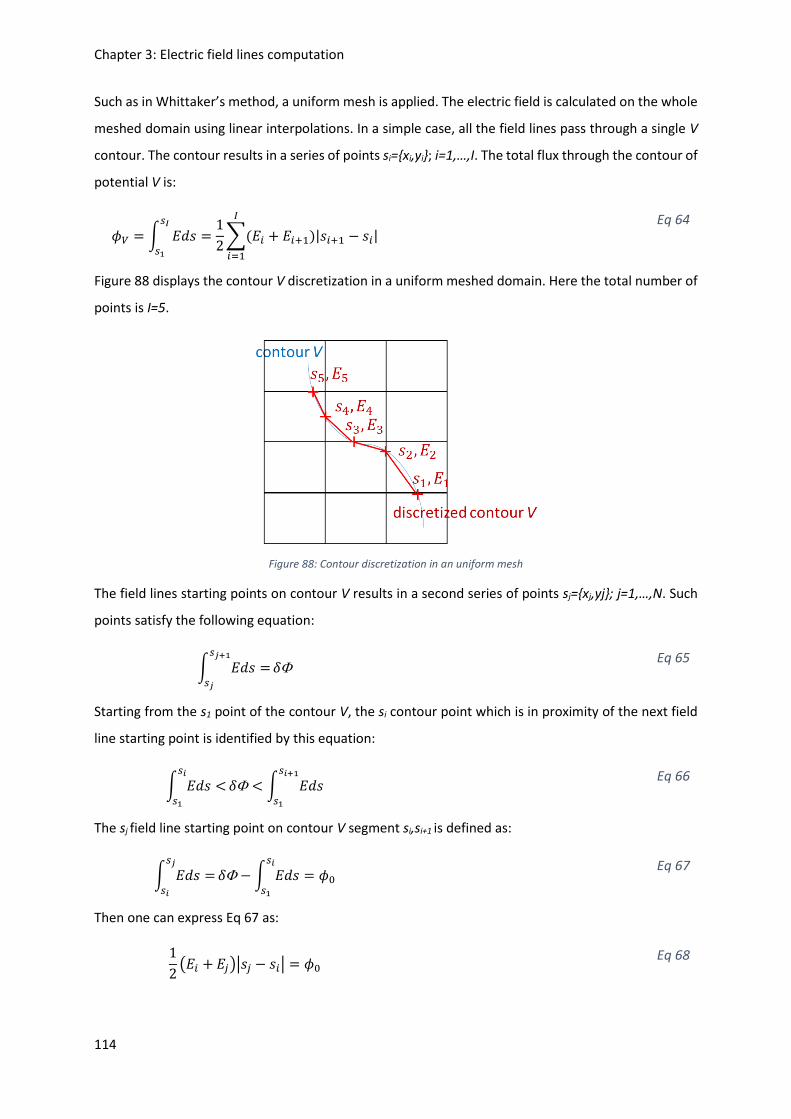
Chapter 3: Electric field lines computation
114
Such as in Whittaker’s method, a uniform mesh is applied. The electric field is calculated on the whole
meshed domain using linear interpolations. In a simple case, all the field lines pass through a single V
contour. The contour results in a series of points si={xi,yi}; i=1,…,I. The total flux through the contour of
potential V is:
𝜙𝑉 = ∫ 𝐸𝑑𝑠 =1
2∑(𝐸𝑖
𝐼
𝑖=1
𝑠𝐼
𝑠1
+ 𝐸𝑖+1)|𝑠𝑖+1 − 𝑠𝑖| Eq 64
Figure 88 displays the contour V discretization in a uniform meshed domain. Here the total number of
points is I=5.
Figure 88: Contour discretization in an uniform mesh
The field lines starting points on contour V results in a second series of points sj={xj,yj}; j=1,…,N. Such
points satisfy the following equation:
∫ 𝐸𝑑𝑠 =𝑠𝑗+1
𝑠𝑗
𝛿 Eq 65
Starting from the s1 point of the contour V, the si contour point which is in proximity of the next field
line starting point is identified by this equation:
∫ 𝐸𝑑𝑠 <𝑠𝑖
𝑠1
𝛿 < ∫ 𝐸𝑑𝑠𝑠𝑖+1
𝑠1
Eq 66
The sj field line starting point on contour V segment si,si+1 is defined as:
∫ 𝐸𝑑𝑠 =𝑠𝑗
𝑠𝑖
𝛿 −∫ 𝐸𝑑𝑠𝑠𝑖
𝑠1
= 𝜙0 Eq 67
Then one can express Eq 67 as:
1
2(𝐸𝑖 + 𝐸𝑗)|𝑠𝑗 − 𝑠𝑖| = 𝜙0
Eq 68

Chapter 3: Electric field lines computation
115
Let 𝑎 =|𝑠𝑗−𝑠𝑖|
|𝑠𝑖+1−𝑠𝑖| be the fractional distance from contour point si to field line starting point sj. As the
electric field �⃗� is linear along the grid, one finally gets Eq 69 [111]:
𝑎 = 𝜙0/𝐸𝑖|𝑠𝑖+1 − 𝑠𝑖| Eq 69
Starting points 𝑠𝑗 of field lines on contour V are finally determined [111]:
𝑠𝑗 = {𝑥𝑗, 𝑦𝑗}
𝑠𝑗 = {(1 − 𝑎) ∗ 𝑥𝑖 + 𝑎 ∗ 𝑥𝑖+1, (1 − 𝑎) ∗ 𝑦𝑖 + 𝑎
∗ 𝑦𝑖+1}
Eq 70
The field lines are then built from their starting point by integrating as in Whittaker’s method [111]. As
the same flux quantity 𝛿 is present between two adjacent lines, the electric field strength is
represented by the concentration of field lines. The same termination criteria as in Whittaker’s method
are used.
However, an electric machine slot filled with conductors is a more complex case. It mainly happens
that all the field lines do not pass through a single V contour. Let us consider two conductors at
potential of V1 and V2 respectively. A field line starting from V1 contour is identified by 𝑙𝑛11 ; n1=1,…,N1.
The same procedure described in the simple case is applied to V1 contour. However, the intersections
of 𝑙𝑛11 field lines with V2 contour have to be tracked. To do that, each segment of 𝑙𝑛1
1 is checked to
verify whether or not it intersects with V2 contour. The intersection points are added to V2 contour
points series. Now, one can apply the same procedure with V2 contour adding some steps:
Step 1: choose as a starting point of field lines from V2 contour ( 𝑙𝑛22 ; n2=1,…,N2) one of the
intersection point of a 𝑙𝑛11 field line with V2 contour;
Step 2: integrate from that point until (a) another intersection point of a 𝑙𝑛11 field line with V2
contour is reached or (b) the integral exceed the fixed flux quantity 𝛿. In case (b), the next
point as to be determined the same way sj point is in the simple case;
Step 3: repeat step 2 until the whole V2 contour is swept;
Step 4: integrate backward from the first intersection point to find the remaining starting
points.
Figure 89 illustrates the field lines computed between two conductors at potential V1 and V2 using the
presented algorithm.

Chapter 3: Electric field lines computation
116
Figure 89: Electric field lines from two infinitely long wires of opposite charge in free space. V1 and V2 are potential contours. The solid field lines were drawn from V1. The dashed field lines were drawn from V2 [111]
4 PROPOSED METHOD
The proposed method we developed is an upgrade of the method presented by Horowitz [111]. A flux
function is built from the electric field components on all the nodes. The field lines correspond to iso-
values of this scalar function. The proposed method does not require a uniform mesh. The calculation
is done on the same mesh on which the scalar potential V is computed.
4.1 ELECTRIC FIELD AND ELECTRIC FLUX
The 2D-finite element model on Ansys Mechanical APDL uses 8 nodes elements. On each element, the
coordinates and the scalar potential solution are expressed as a combination of each nodes data with
a defined shape function. Shape functions are expressed in the local coordinate system (u,v) of the
element. It is a coordinate system attached to the element which define the location of each node.
{
𝑥𝑒(𝑢, 𝑣) =∑𝑁𝑖(𝑢, 𝑣). 𝑥𝑒(𝑖)
8
𝑖=1
𝑦𝑒(𝑢, 𝑣) =∑𝑁𝑖(𝑢, 𝑣). 𝑦𝑒(𝑖)
8
𝑖=1
𝑉𝑒(𝑢, 𝑣) =∑𝑁𝑖(𝑢, 𝑣). 𝑉𝑒(𝑖)
8
𝑖=1
With:
Eq 71

Chapter 3: Electric field lines computation
117
{𝑁𝑖(𝑢, 𝑣) = 1𝑎𝑡𝑛𝑜𝑑𝑒𝑖
𝑁𝑖(𝑢, 𝑣) = 0𝑒𝑙𝑠𝑒𝑤ℎ𝑒𝑟𝑒
With 𝑥𝑒 and 𝑦𝑒 the coordinates in the global coordinate system (x,y) of the nodes of an element e. For
an 8 nodes elements, the shape functions N are given in [116].
The electric field on the nodes of an element is derived from the voltage values on the node using Eq
45. It requires the expression of partial derivatives in the global system.
First, the partial derivatives of a function in the local system (u,v) can be expressed from its partial
derivatives in the global system (x,y):
(
𝜕𝜕𝑢𝜕𝜕𝑣
) = [
𝜕𝑥
𝜕𝑢
𝜕𝑦
𝜕𝑢𝜕𝑥
𝜕𝑣
𝜕𝑦
𝜕𝑣
](
𝜕𝜕𝑥𝜕𝜕𝑦
) = 𝐽(
𝜕𝜕𝑥𝜕𝜕𝑦
)
With:
𝐽 = [𝐽11 𝐽12𝐽21 𝐽22
]
Eq 72
With J the Jacobian matrix. It is computed from the known shape functions partial derivatives in the
local system when putting Eq 71 in Eq 72.
Then, the partial derivatives of a function in the global system (x,y) can be expressed from its partial
derivatives in the local system (u,v):
(
𝜕𝜕𝑥𝜕𝜕𝑦
) =
[ 𝜕𝑢
𝜕𝑥
𝜕𝑣
𝜕𝑥𝜕𝑢
𝜕𝑦
𝜕𝑣
𝜕𝑦]
(
𝜕𝜕𝑢𝜕𝜕𝑣
) = 𝐼 (
𝜕𝜕𝑢𝜕𝜕𝑣
)
With:
𝐼 = [𝐼11 𝐼12𝐼21 𝐼22
]
𝐼 = 𝐽−1
Eq 73
It is matrix I which is use in practise because the data have to be expressed in the global system. It is
computed as follow:
𝐼 = 𝐽−1 =1
det(𝐽)[𝐽22 −𝐽12−𝐽21 𝐽11
]
With:
det(𝐽) = 𝐽11𝐽22 − 𝐽12𝐽21
Eq 74
Chapter 3: Electric field lines computation
118
The electric field components on the nodes of an element e can finally be expressed in the global
system by combining Eq 71 and Eq 73:
{
𝐸𝑥,𝑒= −
𝜕𝑉𝑒𝜕𝑥
= −∑(𝐼11𝜕𝑁𝑖𝜕𝑢
+ 𝐼12𝜕𝑁𝑖𝜕𝑣) . 𝑉𝑒(𝑖)
8
𝑖=1
𝐸𝑦,𝑒= −𝜕𝑉𝑒𝜕𝑦
= −∑(𝐼21𝜕𝑁𝑖𝜕𝑢
+ 𝐼22𝜕𝑁𝑖𝜕𝑣) . 𝑉𝑒(𝑖)
8
𝑖=1
Eq 75
The electric flux components are computed from electric field components using Eq 46.
4.2 EQUIPOTENTIAL LINES
The next step consists in forming equipotential lines. These are contours on which the voltage value is
constant. Equipotential lines are obtained by regrouping nodes with the same voltage value. Let us see
the steps to compute an equipotential line at voltage V.
A test is done on each edge of each element to check whether or not it is crossed by the equipotential
line V. As can be seen on Figure 90, each edge is composed of three nodes. There are three possible
outcomes:
The voltage V is lower or bigger than any of the three nodes voltage. The edge is not
intersected by the equipotential line V;
The voltage V is equal to one of the three nodes voltage. The equipotential line intersects the
edge at the corresponding node of voltage V;
The voltage V is between any of the three nodes voltage. The edge is intersected by the
equipotential line at a point which is interpolated.
Figure 90 illustrates an equipotential intersecting two edges of an element. On one edge the
intersection point is an already existing node (node 6). The second edge intersection point has to be
interpolated (red cross). The local numbering of the nodes is rearranged compared to Ansys 8 nodes
reference element to facilitate the programming.

Chapter 3: Electric field lines computation
119
Figure 90: Equipotential line V intersecting an element edges
A second order polynomial is used for the interpolation. The following equation gives the parametric
expression of the polynomial:
𝑧(𝑡) = 𝑎1,𝑧 + 𝑎2,𝑧 ∗ 𝑡 + 𝑎3,𝑧 ∗ 𝑡2
With:
𝑡 ∈ [0,1]
Eq 76
The parameter t represents the edge on which the interpolation is performed.
Figure 91 displays Eq 76 along a parameterized edge:
Figure 91: Illustration of a second order polynomial interpolation over a parameterized edge
For instance, on Figure 90 the interpolation is done on the edge containing the nodes (1,2,3). The nodes
are parameterized according to the local numbering order: t=0 for node 1, t=0.5 for node 2 and t=1 for
node 3. By solving Eq 76 in term of voltage it is possible to derived the polynomial coefficients:
𝑉(𝑡) = 𝑎1,𝑉 + 𝑎2,𝑉 ∗ 𝑡 + 𝑎3,𝑉 ∗ 𝑡2
With:
{
𝑉(0) = 𝑎1,𝑉 = 𝑉0𝑉(0.5) = 𝑎1,𝑉 + 𝑎2,𝑉 ∗ 0.5 + 𝑎3,𝑉 ∗ 0.25 = 𝑉0.5
𝑉(1) = 𝑎1,𝑉 + 𝑎2,𝑉 + 𝑎3,𝑉 = 𝑉1
Eq 77

Chapter 3: Electric field lines computation
120
In the considered example, (𝑉0, 𝑉0.5, 𝑉1) are respectively the finite elements voltage solution on nodes
(1,2,3) in Figure 90. The three polynomial coefficients (𝑎1,𝑉, 𝑎2,𝑉 , 𝑎3,𝑉) are thus determined.
𝑉(𝑡0) = 𝑉 = 𝑎1,𝑉 + 𝑎2,𝑉 ∗ 𝑡0 + 𝑎3,𝑉 ∗ 𝑡02 Eq 78
With V the voltage of the considered equipotential line V.
The obtained parameter𝑡0 is injected back into Eq 77 to determine the interpolated node coordinates,
electric field components and electric flux components. As in Eq 78, the associated polynomial
coefficients are deduced from the known nodes data.
4.3 FLUX FUNCTION
At this point, equipotential lines made of nodes at the same scalar potential V are determined. The
coordinates and fields components are determined on all these nodes. The number of equipotential
lines depends on the accuracy from which the electric scalar potential problem is solved. The finer the
mesh used to solve the problem, the higher the number of equipotential lines that can be accurately
determined.
For each equipotential line a geometrical reference is defined on its barycentre. The points on the line
are located by using polar coordinates in this reference. A starting point 𝑄 is chosen for instance by
means of the angular coordinates. Figure 92 illustrates the barycentre reference attached to an
equipotential line V. Point G is the barycentre. A point M located on the equipotential line is identified
by its curvilinear abscissa s(M).
Figure 92: Barycentre system associated to an equipotential line V
A flux function (𝑀) of points on each equipotential is defined as the flux per meter crossing the line
between the starting point Q and point 𝑀:
(𝑀) = ∫ 𝐷𝑛𝑑𝑠𝑀
𝑄
Eq 79
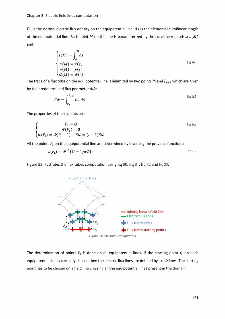
Chapter 3: Electric field lines computation
121
𝐷𝑛 is the normal electric flux density on the equipotential line, 𝑑𝑠 is the elemental curvilinear length
of the equipotential line. Each point 𝑀 on the line is parameterized by the curvilinear abscissa 𝑠(𝑀)
and:
{
𝑠(𝑀) = ∫ 𝑑𝑠
𝑀
𝑄
𝑥(𝑀) = 𝑥(𝑠)
𝑦(𝑀) = 𝑦(𝑠)
(𝑀) = (𝑠)
Eq 80
The trace of a flux tube on the equipotential line is delimited by two points 𝑃𝑖 and 𝑃𝑖+1 which are given
by the predetermined flux per meter 𝛿 :
𝛿 = ∫ 𝐷𝑛𝑑𝑠𝑃𝑖+1
𝑃𝑖
Eq 81
The properties of these points are:
{
𝑃1 = 𝑄
(𝑃1) = 0
(𝑃𝑖) = (𝑃𝑖 − 1) + 𝛿 = (𝑖 − 1)𝛿
Eq 82
All the points 𝑃𝑖 on the equipotential line are determined by inversing the previous functions:
𝑠(𝑃𝑖) = −1((𝑖 − 1)𝛿) Eq 83
Figure 93 illustrates the flux tubes computation using Eq 80, Eq 81, Eq 82 and Eq 83:
Figure 93: Flux tubes computation
The determination of points 𝑃𝑖 is done on all equipotential lines. If the starting point 𝑄 on each
equipotential line is correctly chosen then the electric flux lines are defined by iso- lines. The starting
point has to be chosen on a field line crossing all the equipotential lines present in the domain.

Chapter 3: Electric field lines computation
122
4.4 ILLUSTRATIVE EXAMPLES
In this paragraph the proposed method is used to compute electric field lines in the studied
electrostatic problem. Table 18 gives the parameters used.
Wires’ parameters
𝑅𝑖𝑛𝑡 Round wire copper radius 0.75 mm
e Enamel overcoat thickness 70𝜇𝑚
휀𝑟 Enamel dielectric constant 3.5
Applied voltages
𝑉1 Left wire voltage amplitude 1000 V
𝑉2 Right wire voltage amplitude 0 V
Equipotential lines parameters
𝑉𝑖𝑚𝑝 Imposed potentials intervals [0;
𝑉14; 2 ∗ 𝑉14
; 3 ∗ 𝑉14
; 𝑉1]
𝑁𝑖𝑚𝑝 Imposed number of computed equipotential lines
on each potential interval
[25; 25; 25; 25]
Table 18: Parameters used in the illustrative example
It can be seen that there are one hundred equipotential lines which will be formed. The voltage
amplitude is divided into four intervals. A same number of twenty-five equipotential lines per voltage
interval is chosen.
The finite element software used is Ansys Mechanical APDL. The used mesh is displayed on Figure 94.
The computation time is given as an order of magnitude. It is obtained using tic-toc on Matlab. It
changes depending on the system computing speed. Thus, the computation time presented on Figure
94 is the sum of the loading times of data transfer between Ansys and Matlab, the meshing time and
the resolution time.

Chapter 3: Electric field lines computation
123
Mesh
Number of
elements: 4144
Computation
time: 12.6 s
Figure 94: Used mesh (white: copper, purple: enamel, green: air)
The significant results are given on Figure 95 and Figure 96
Figure 95: Total electric fluxes crossing each equipotential line
The electric flux across each equipotential line is constant. The starting point of the twenty field lines
displayed on Figure 96 are chosen by dividing the total electric flux crossing each equipotential line by
nineteen. That is because there is already one known field line that is the reference line chosen on the
symmetry axis.

Chapter 3: Electric field lines computation
124
Figure 96: Electric field lines obtained with the mesh of Figure 94
The post processing time is the time required to build the field lines starting from the finite elements
solution. It is of 9.11 s.
In this approach, the density of the field lines is linked to the electric field amplitude.
5 ANOTHER METHOD USING MATLAB FUNCTIONS
Another method to plot electric field lines from scalar potential solution is developed using Matlab
functions. It is likely a Whittaker based approach [115]. The different steps in order to obtain such
results are presented.
5.1 BUILDING THE ADDITIONAL MESH
The mesh created by the finite element software cannot be used directly by Matlab functions. Indeed,
it has to be uniform. So the first step consists in building a second uniform mesh. The finite element
(FEM) computed nodes coordinates (X,Y) and scalar potential V lists are imported. Axis vectors 𝑋𝑎 , 𝑌𝑎
are built from X, Y lists such that:
𝑋𝑎 ∈ [𝑋𝑚𝑖𝑛, 𝑋𝑚𝑎𝑥] 𝑎𝑛𝑑 𝑌𝑎 ∈ [𝑌𝑚𝑖𝑛, 𝑌𝑚𝑎𝑥]
𝑋𝑎 and 𝑌𝑎 results in a N uniformly spaced values
The linspace function is used so that:
𝑋𝑎 = 𝑙𝑖𝑛𝑠𝑝𝑎𝑐𝑒(𝑋𝑚𝑖𝑛, 𝑋𝑚𝑎𝑥, 𝑁)

Chapter 3: Electric field lines computation
125
𝑌𝑎 = 𝑙𝑖𝑛𝑠𝑝𝑎𝑐𝑒(𝑌𝑚𝑖𝑛, 𝑌𝑚𝑎𝑥, 𝑁)
A new mesh is generated from these axis vectors. It is made of identical rectangles.
The meshgrid function is used:
[𝑋𝑔, 𝑌𝑔] = 𝑚𝑒𝑠ℎ𝑔𝑟𝑖𝑑(𝑋𝑎 , 𝑌𝑎)
The 𝑋𝑔, 𝑌𝑔 matrix contain the coordinate of all the points of the new mesh. This mesh is referred as
Matlab mesh.
5.2 ELECTRIC FIELD
The Matlab mesh is different from the one generated with the FEM software. Multiple points of the
FEM mesh are deleted. Besides, the Matlab mesh adds some points. The voltage solution on these
points are linearly interpolated from the existing ones.
The griddata function is used:
𝑉𝑔 = 𝑔𝑟𝑖𝑑𝑑𝑎𝑡𝑎(𝑋, 𝑌, 𝑉, 𝑋𝑔 , 𝑌𝑔,′ 𝑙𝑖𝑛𝑒𝑎𝑟′)
The 𝑉𝑔 matrix contain the scalar potential values on all points in Matlab mesh.
The electric field components over the Matlab mesh is computed based on Eq 45.
The gradient function is used. It computes only the voltage drops over the mesh between two
consecutive points.
[𝛿𝑉𝑔,𝑥, 𝛿𝑉𝑔,𝑦] = 𝑔𝑟𝑎𝑑𝑖𝑒𝑛𝑡(−𝑉𝑔)
Field lines starting points are chosen on one of the wire external contour (i.e.: on the enamel overcoat).
The starting points coordinates are designated by (𝑋0, 𝑌0).
The field lines are built using the stream2 function. This function generates field lines over the Matlab
mesh following Whittaker methodology [115].
𝐹𝑖𝑒𝑙𝑑𝐿𝑖𝑛𝑒𝑠 = 𝑠𝑡𝑟𝑒𝑎𝑚2(𝑋𝑔, 𝑌𝑔 , 𝛿𝑉𝑔,𝑥 , 𝛿𝑉𝑔,𝑦, 𝑋0, 𝑌0)

Chapter 3: Electric field lines computation
126
5.3 COMPARISON WITH THE PROPOSED METHOD
The proposed method and the method based on Matlab functions are compared. The parameters are
given in Table 18. The Figure 94 mesh configuration is used. For Matlab functions, the additional mesh
generated with meshgrid has a resolution of 600*600.
Proposed method Matlab functions
20 field lines 20 field lines
Post processing time: 9.11 s Post processing time: 1.4 s
Figure 97: Proposed method versus Matlab functions to obtain electric field lines
The post process refers to all the steps from the finite element solution to the field lines. Matlab
algorithm is much more efficient than the developed approach. It is almost ten time faster.
In PD evaluation, only the part of the electric field line in the air gap is considered. Besides, the electric
field along the field lines has to be uniform. Figure 98 displays the electric field amplitude. It can be
seen that the electric field in the air gap is quite constant along the obtained field lines.

Chapter 3: Electric field lines computation
127
Figure 98: Electric field amplitude [V/m] obtained with finite elements
So the Paschen’s criterion could be applied on the part of the field lines in the air gap to evaluate the
PDIV. The PDIV is evaluated at 1040 V at 20°C, 1 bar pressure. The voltage on the enamel overcoat
contours at the interface with the air is picked up at PDIV. Figure 99 displays the computed voltage
drops along each part of field lines in air for the two approaches. The points intersecting with the
Paschen’s curve indicates field lines on which PD activity is likely to occur.
Figure 99: Computed voltage drops along field lines in air (p=1 bar) obtained with the two compared methods; ɣ=0.01

Chapter 3: Electric field lines computation
128
The results coincide for field lines longer than 10𝜇𝑚. Both methods evaluate a PD activity on the field
line of 37 µm length in the gap. The additional inflection point on the orange curve for field lines of a
few micrometers length could be due to a resolution issue and do not have to be taken into
consideration.
In the tool to evaluate PD risk, the Matlab approach will be used. It is much faster than the developed
method and gives similar results for the field lines of interest (i.e.: a few dozens of micrometers).
However, Matlab functions are black boxes. Strange results have already been obtained with some
configuration due to numerical errors. Numerical errors are much easier to deal with in the developed
method because there is no black box. The whole code is accessible and modifiable.
6 CONCLUSION
The method using Matlab functions to plot electric field lines is most likely based on Whittaker’s
approach [115]. The work presented in this chapter clarifies the functions used by Matlab.
The method presented by Horowitz [111] make it possible to plot field lines with the electric field
strength being represented by the density of lines. In this chapter, this method has been upgraded. A
flux function is defined which iso-values directly give the field lines. For now, starting with the scalar
potential solution obtained with Ansys Emag and using our proposed method, the computation times
are long. However, it must be possible to significantly reduce the computation time by implanting the
proposed method in a field calculation code. The main advantage of the proposed method is that it
reuses the initial Ansys Emag mesh on which the scalar solution is first obtained.
Due to high computation times, the method using Matlab functions is used for now to derive field lines
on a simplified problem with two conductors. The results given by the two methods are in good
agreement for field lines in air longer than 10𝜇𝑚. In the evaluation of PD using the Paschen’s criterion,
smaller field lines are not of interest.
In the next chapter, the validity of the Paschen’s criterion for a configuration of two enamelled round
wires in contact is investigated.

Chapter 4: Correction of the Paschen’s criterion
129
Chapter 4: Correction of the Paschen’s criterion

Chapter 4: Correction of the Paschen’s criterion
130

Chapter 4: Correction of the Paschen’s criterion
131
1 MOTIVATIONS
1.1 CONFIGURATION DIFFERENT FROM THE INITIAL ONE
The Paschen’s criterion has been presented in Chapter 2. It defines the required electric field strength
in a gas gap in order to produce a self-maintained electronic avalanche. This criterion has been
established for two metallic plane electrodes facing each other in an uniform electric field [81], [82].
In the literature, the Paschen’s criterion has been widely used to determine the Partial Discharges
Inception Voltage (PDIV) in the Electrical Insulation Systems (EIS) of electric devices (rotating machines,
power electronics, connectors,…) [44], [55], [117], [118]. A representative configuration encountered
in rotating machines EIS is two round enamelled wires in close contact. A 2D-finite elements model
has been developed with Ansys Mechanical APDL (Figure 82). It has provided results showing non-
uniform electric field in some air gap areas, as presented on Figure 98. Consequently, the conditions
in which the Paschen’s criterion has been established are not present in all the air gap surrounding the
two neighbouring wires. The use of this criterion in the configuration of two enamelled wires in close
contact, as it is the case in stator slots, is then questionable and need to be clarified.
1.2 EXPERIMENTAL OBSERVATION
Figure 100 confronts the observation of PD induced damage between two enamelled round wires in
close contact in air (under normal pressure and temperature conditions) and the well-known Paschen’s
curve.
Figure 100: Left) Round enamelled wires damaged by PD [40]. Right) Paschen's curve in air [81]

Chapter 4: Correction of the Paschen’s criterion
132
As clearly shown in Figure 100, PD damage is neither located in small air gap zones (coloured in green)
nor in large ones (coloured in blue), but in the intermediate air gap zone (coloured in white). This is
coherent with the existence of a minimum which is well known in the Paschen’s curve.
However differences have been observed by [44] between experimental and theoretical results
obtained by using a 2D-finite element model. A correction was proposed by fitting the original
Paschen’s curve by coupling the numerical model with experimental results. This approach uses the
secondary electron emission coefficient 𝛾 as a parameter, as it could be different from a material to
another (Figure 101).
Figure 101: Paschen’s curves in air plotted for three different 𝛾values [44]
The introduction of two polymer layers may modify the mechanisms brought out by Paschen. This
could even change the well-known Paschen’s curve shape. However, in this work, the hypothesis
consists in considering that the Paschen’s curve shape is conserved (the theory is considered to be
always applicable). In that case, the enamel layers only modify the breakdown voltage values. Such
vertical translation of the Paschen’s curve (at a given temperature and humidity rate) depends on the
secondary electronic emission coefficient. In that way, the study will be focused on the evolution of
the electronic secondary emission coefficient 𝛾 (also referred as Townsend’s second coefficient) as a
function of the copper diameters and the enamel nature used by the wire manufacturers.

Chapter 4: Correction of the Paschen’s criterion
133
2 EXPERIMENTAL APPROACH
2.1 SAMPLES
Investigation over four different enamelled copper wires were performed with (see Table 19):
- a (THEIC) Polyester-imide enamelled copper wire, overcoated with Polyamide-imide;
- a (THEIC) Polyester-imide enamelled copper wire, overcoated with a Polyamide-imide layer
and overcoated with a self-bonding Polyamide layer;
- a Polyamide-imide copper, overcoated with a corona resistant Polyamide-imide layer;
- a Polyamide-imide copper, overcoated with a corona resistant Polyester-imide layer;
Three different copper diameters were investigated: 0.5 mm, 0.71 mm and 1 mm. Table 19 recaps
the wires designations and layers order. The first named layer is in contact with the copper, the
last named is the external layer, in contact with the air. These four magnet wires are overcoated
with an external layer made with different polymers: Polyamide-imide, self-bonding Polyamide,
corona-resistant Polyamide-imide and corona-resistant Polyester-imide.
Item Polymer coating Designation (number of layer) Thermal class [°C]
Magnetemp
CA 200
THEIC-modified Polyesterimide /
Polyamide imide
PEI-THEIC / PAI (2) 200
Magnebond
CAR-200
THEIC-modified
Polyesterimide/Polyamide
imide/self-bonding aromatic
Polyamide
PEI-
THEIC
/ PAI /
self-
bond
PAI
(3)
210
KMKED 22A Polyamide-imide/ corona
resistant Polyamide imide
PAI / PAI-PD (2) 220
KMKED 20E Polyamide-imide / corona
resistant Polyesterimide
PAI / PEI-PD (2) 220
Table 19: Recap of tested magnet wires
The samples consist in two parallel enamelled round wires in close contact. Their length is
approximatively 3.5 cm. These kind of samples has been chosen instead of twisted pairs that are too
complex samples. Indeed the contacts (gaps) between the wires are not well controlled and may vary
along the wire and also from one sample to another. Moreover, this needs a 3D-modelling that is too
complex and time-consuming to perform.

Chapter 4: Correction of the Paschen’s criterion
134
On one extremity of each wire, the enamel is removed in order to connect the samples to the high
voltage power supply (and to the earth for the second wire). Three samples per diameter were tested.
At both extremities of the samples, the gaps between the wires are filled with a glue, in order to avoid
any discharge in this area and to be sure that PD will occur only just along the part of the wires in
contact. The samples have been carefully examined by using a digital microscope (Keyence VHX1000)
in order to verify whether there is no air gap between the two wires (Figure 102.b). If any small gap is
detected, the sample is removed and a brand new one is built up and examined again. To detect small
gaps, the sample is illuminated from below and carefully examined on all its length. If any bubble
(where PD may appear) is observed in the the glue at both sample extremities, the sample is removed
as well.
Figure 102 shows a typical sample. We may notice that small ‘particles’ are observed on the surface of
the samples. This is not dust, as the samples have been carefully dusted off by blowing and cleaned
with ethanol before testing. These are protrusions in the external layer of the wires. These protrusions
appear during the wire manufacturing process presented in Chapter 1 paragraph 4.1.1 Turn-to-turn
insulation. Such protrusions, that may reach 40 m length and 20 m tall for the larger ones, may
probably modify the field distribution in air and consequently reduce the PDIV. We may however take
them into account, as they are representative of defects in commercial wires, but when bigger ones
are located close to the contact area, the sample is rejected. All these precautions are needed to obtain
samples close to ideal ones modelled in our 2D-finite element simulations.

Chapter 4: Correction of the Paschen’s criterion
135
Figure 102: a) 0.71 mm 200°C studied sample; b) zoom on contact between the 2 wires; c) zoom on one glued extremity
2.2 EXPERIMENTAL PROTOCOL
Samples were tested under normal pressure and temperature conditions in a Faraday’s cage to
measure their respective PDIV. The experimental set-up followed, as well as we can, the IEEE standard
[119]. Figure 65 displays the used setup for PD electric detection.
In order to compare both measurement and simulation, it is absolutely necessary to get the real sizes
of each wire (copper diameter, enamel thickness, eccentricity) to introduce them into the simulation.
These data may indeed vary from one sample to another (the standard allows a tolerance in the
enamel thickness – see Annex 1). After each PDIV measurements, all samples were consequently
encapsulated in Varykleer (Buehler) acrylic resin under pressure (2 bar) during twenty minutes.
Encapsulated samples were then cut by using a circular saw (STRUERS SECOTOM 10) equipped with
Buehler’s grinder (ref 11-4217-010). Finally, the sections were polished by using at first 68 m grains
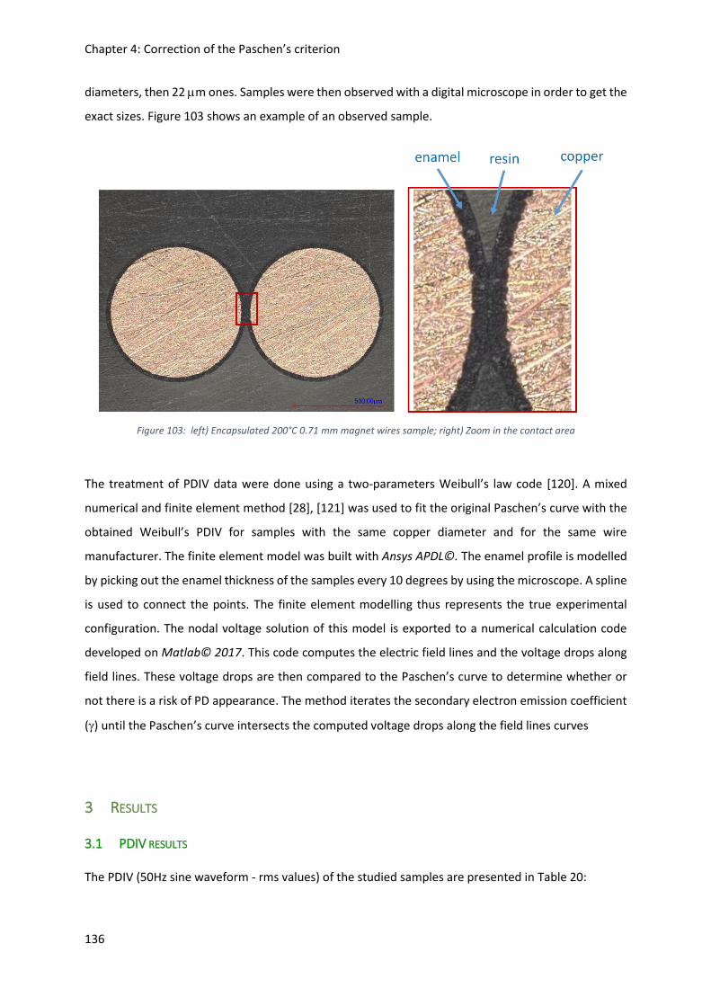
Chapter 4: Correction of the Paschen’s criterion
136
diameters, then 22 m ones. Samples were then observed with a digital microscope in order to get the
exact sizes. Figure 103 shows an example of an observed sample.
Figure 103: left) Encapsulated 200°C 0.71 mm magnet wires sample; right) Zoom in the contact area
The treatment of PDIV data were done using a two-parameters Weibull’s law code [120]. A mixed
numerical and finite element method [28], [121] was used to fit the original Paschen’s curve with the
obtained Weibull’s PDIV for samples with the same copper diameter and for the same wire
manufacturer. The finite element model was built with Ansys APDL©. The enamel profile is modelled
by picking out the enamel thickness of the samples every 10 degrees by using the microscope. A spline
is used to connect the points. The finite element modelling thus represents the true experimental
configuration. The nodal voltage solution of this model is exported to a numerical calculation code
developed on Matlab© 2017. This code computes the electric field lines and the voltage drops along
field lines. These voltage drops are then compared to the Paschen’s curve to determine whether or
not there is a risk of PD appearance. The method iterates the secondary electron emission coefficient
() until the Paschen’s curve intersects the computed voltage drops along the field lines curves
3 RESULTS
3.1 PDIV RESULTS
The PDIV (50Hz sine waveform - rms values) of the studied samples are presented in Table 20:

Chapter 4: Correction of the Paschen’s criterion
137
Manufacturer Copper diameter [mm]
Sample number PDIV [Vrms]
Magnetemp CA 200
0.5
1 541; 552; 559; 536; 546; 539; 530; 559
2 549; 534; 558; 554; 553; 563; 556; 556
3 561; 566; 533; 557; 541; 543; 523; 544
0.71
1 524; 539; 546; 529; 535; 541; 538; 533
2 572; 568; 579; 580; 566; 570; 581; 574
3 582; 588; 641; 600; 602; 631; 634; 687
1
1 676; 696; 667; 686; 682; 702; 710; 679
2 717; 685; 751; 737; 748; 787; 778; 749
3 691; 713; 747; 735; 720; 759; 704; 730
KMKED 20E
0.5
1 572; 567; 546; 547; 558; 536; 530; 555
2 546; 548; 518; 537; 539; 532; 539; 519
3 548; 544; 539; 533; 537; 538; 541; 546
KMKED 22A
0.5
1 595; 629; 622; 604; 617; 625; 640; 631
2 560; 575; 611; 565; 613; 607; 580; 641
3 568; 545; 526; 559; 579; 543; 595; 549
Magnebond CAR-200 NAT
0.5 1 674; 698; 717; 719; 733; 748; 763; 788
2 666; 672; 684; 690; 690; 691; 712; 716
3 767; 775; 781; 805; 817; 822; 825; 877 Table 20: Experimental PDIV versus wire diameter and kind of enamel (T=23°C, RH=36%)
Eight measurements for each sample have been done successively. When the PDIV is reached, the
voltage is no longer maintained in order to avoid any damage cause by PD that may modified the
enamel surface and then the other remaining measurements.
For each sample, the experimental PDIV were analysed by using a two-parameters Weibull’s code
[122]. It gives the PDIV characteristic values (i.e.: at 63.2% of probability) and the corresponding
regressive voltage with 90% confidence bounds. For each manufacturer and for a fixed copper
diameter, the confidence intervals are displayed and the estimated Weibull’s PDIV is determined. Such
plot is shown on Figure 104 that gives an example for three 200 °C samples made with the same
magnet wires (copper diameter: 0.5 mm).

Chapter 4: Correction of the Paschen’s criterion
138
Figure 104: Measured PDIV - 0.5mm copper diameter (PEI overcoated with PAI, 200°C wire, T=23°C; RH=36%)
The PDIV values reported in Figure 104 show three characteristic PDIV close together. The average
value is determined (dotted line). The average PDIV for each copper diameter and each wire
manufacturer are recapitulated on Table 21.
Enamel Copper diameter [mm] Average PDIV [Vrms]
PEI-THEIC/PAI 0.5 553
0.71 580
1 721
PEI-THEIC/PAI/PA-self-bonding 0.5 768
PAI/PAI-PD 0.5 588
PAI/PEI-PD 0.5 546
Table 21: Average PDIV versus manufacturer and copper diameter
It should be noticed that the highest PDIV value is obtained with the 0.5 mm copper diameter PEI-
THEIC/PAI/PA self-bonding wire. That wire has three layers of insulation leading to a higher enamel
thickness, then the higher PDIV. The external additional layer is used as a varnish and may be
polymerized by different technics (self heating by Joule’s effect, oven, UV).
These average PDIV values will be applied as boundary conditions on the 2D-finite element model in
the proposed method (Figure 106).

Chapter 4: Correction of the Paschen’s criterion
139
3.2 DIELECTRIC CONSTANT MEASUREMENTS
The equivalent dielectric constant of each enamel were measured by using a Novocontrol Alpha-A
dielectric spectrometer [123]. This device is able to determine the dielectric constant in a wide range
of temperature and frequency.
We used our magnet wires samples. For that, they were metallized (gold sputtering - pressure 10-5
mbar) in order to form a cylindrical coaxial capacitor as illustrated on Figure 105. It is a vacuum
metallization; the resulting gold deposit has a thickness of about 125 nm.
Figure 105: Gold metallization of an enamelled copper wire. Left) Equivalent 2D-coaxial capacitor - R1: external radius; R2: copper radius; e: enamel whole thickness.; Right) Real sample for test in the Novocontrol.
At first, the parasitic capacitance is evaluated using both 2D- and 3D-finite elements model. Due to the
limitation in the number of elements, a wire of 100 m length is considered.
The capacitance values are derived from the total electric energy of the models:
𝐶2𝐷[𝐹.𝑚] =2 ∗ 𝐸2𝐷[𝐽.𝑚]
𝑉2
Eq 84
𝐶3𝐷[𝐹] = (𝐶2𝐷 + 𝐶𝑝𝑎𝑟) =2 ∗ 𝐸3𝐷[𝐽]
𝑉2
Eq 85
In these relationships, 𝐶2𝐷 and 𝐸2𝐷 are the respectively the linear capacitance and the electric energy
on the 2D-model, V is the applied voltage peak value. 𝐶3𝐷 and 𝐸3𝐷 are the capacitance and electric
energy in the 3D-model. 𝐶𝑝𝑎𝑟 represents the parasitic capacitance.
Let us consider one configuration presented in Table 22.

Chapter 4: Correction of the Paschen’s criterion
140
Copper radius 522𝜇𝑚
Enamel thickness 36𝜇𝑚
Enamel dielectric constant 4.07
Applied voltage 1𝑉𝑟𝑚𝑠
Wire length 𝐿𝑡𝑜𝑡 = 100𝜇m Table 22: Test configuration for parasitic capacitance evaluation
The 𝐶2𝐷 and 𝐶3𝐷 are computed using Eq 84 and Eq 85. The main results are given in the Table 23 below:
2D-model 3D-model
Electric energy E2D=0.339497 10-8J.m E2D*Ltot=0.339497 10-12J
E3D=0.36652 10-12J
Capacitance 𝐶2𝐷 ∗ 𝐿𝑡𝑜𝑡 = 0.34𝑝F 𝐶3𝐷 = 0.37𝑝𝐹 Table 23: 2D- and 3D-capacitance evaluations
The parasitic capacitance is low (8% of the total capacitance) for a 100 m-long wire, so that we can
reasonably neglect it in the case of wire length of several centimetres. So the results given by the
Novocontrol are directly the wanted coaxial equivalent capacitance.
The voltage (1 Vrms) is applied to the copper core via the pin. The sample is deposit on a grounded
electrode. The sample is adapted to the Novocontrol electrode dimensions, that is the reason why in
Figure 105 it is bent. The equivalent capacitor corresponds to a coaxial capacitor of total length 𝐿𝑡𝑜𝑡 =
2 ∗ 𝐿.
To get a good measurement with the Novocontrol, the sample capacitance has to be bigger than 100
pF. The 2D-finite element model of the enamelled wire is used to determine the required total length
𝐿𝑡𝑜𝑡. With Ltot=5 cm, the evaluated capacitance is 170 pF, considering an enamel with a dielectric
constant of 3.5.
A coaxial capacitor analytical formulation is given by Eq 86. The parameters are defined on Figure 105.
𝐶 = 휀0 ∗ 휀𝑟 ∗2 ∗ 𝜋 ∗ 𝐿𝑡𝑜𝑡
ln(𝑅1𝑅2)
Eq 86
With C the capacity of the sample, 휀𝑟 the wanted enamel dielectric constant.
However, to the Novocontrol requires a diameter D because it considers a disc capacitor Eq 87:
𝐶 = 휀0 ∗ 휀𝑟 ∗𝜋 ∗ (
𝐷2)
2
𝑒
Eq 87
With e being the enamel thickness.
By identification, it comes that the equivalent diameter of the sample seen by the Novocontrol is:

Chapter 4: Correction of the Paschen’s criterion
141
𝐷 = 2 ∗ √2 ∗ 𝑒 ∗ 𝐿
ln(𝑅1𝑅2)
Eq 88
This value is given to the Novocontrol prior to the measurements.
Finally, the dielectric constant is derived from the capacitance computation Eq 87. The enamel
thickness e is obtained using a digital microscope. Table 24 gives the computed dielectric constants at
20°C and 50 Hz:
Wire (0.5 mm) Polymer coating 휀𝑟
(20°C, 50 Hz)
Capacitance
(20°C, 50 Hz) [pF]
Magnetemp CA 200 PEI-THEIC/PAI 3.3 162.81
Magnebond CAR-200 NAT PEI-THEIC/PAI/PA self-
bonding
4.4 122.27
KMKED 22A PAI/PAI-PD 3.8 108.08
KMKED 20E PAI/PEI-PD 4.2 126.84
Table 24: Samples computed dielectric constants at 20°C, 50 Hz
These values are in range to the ones found in the literature [124]. The measured dielectric constants
will be introduced into the 2D-finite element model in the proposed method (Figure 106).
4 MIXED EXPERIMENTAL AND NUMERICAL APPROACHES
The experimental data are introduced into a numerical code which iterates the secondary electron
emission coefficient value in order to make the Paschen’s curve intersect the simulated voltage drop
across field lines length curves. The experiments were conducted under normal temperature and
pressure conditions. Thus, the computed are only valid at atmospheric pressure and 20°C.
The algorithm of the mixed experimental and numerical proposed approach is presented in Figure 106.

Chapter 4: Correction of the Paschen’s criterion
142
Figure 106: Algorithm, combining experimental and numerical approaches, used to determine
Field lines are computed by using Matlab approach presented in Chapter 3, paragraph 5: Another
method using Matlab functions. Figure 107 displays an example of field lines between two 0.71 mm
copper diameter wires in close contact.
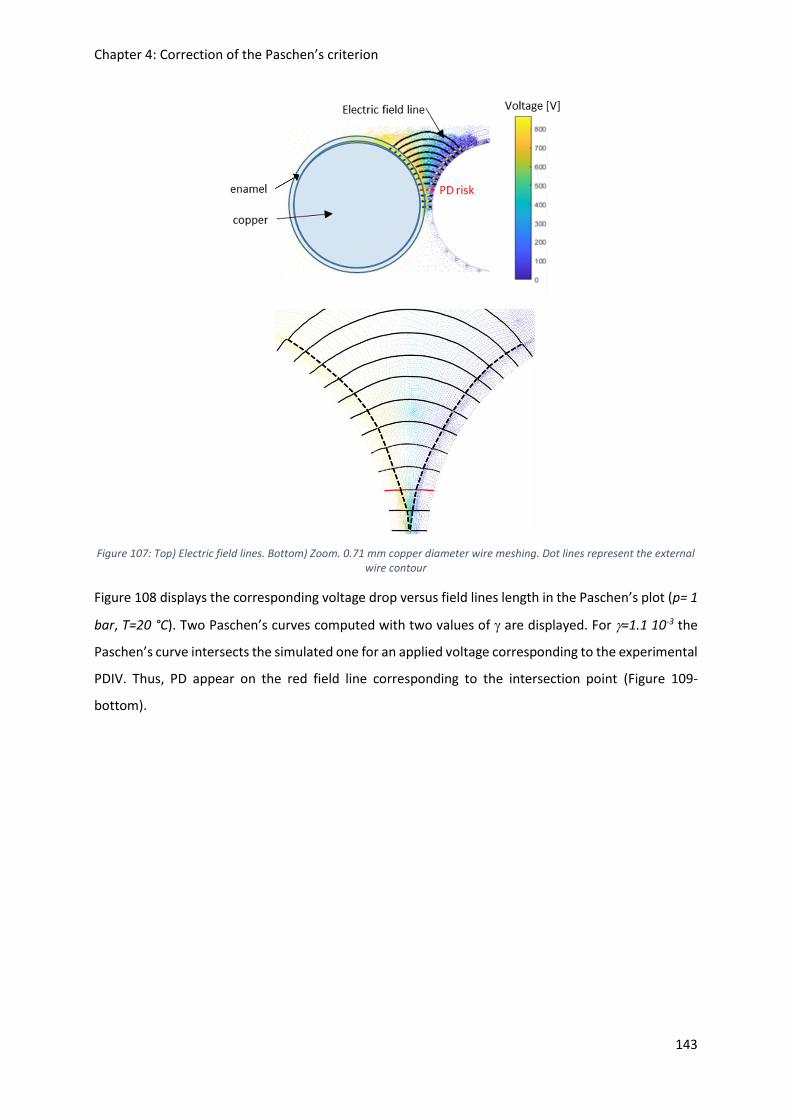
Chapter 4: Correction of the Paschen’s criterion
143
Figure 107: Top) Electric field lines. Bottom) Zoom. 0.71 mm copper diameter wire meshing. Dot lines represent the external wire contour
Figure 108 displays the corresponding voltage drop versus field lines length in the Paschen’s plot (p= 1
bar, T=20 °C). Two Paschen’s curves computed with two values of are displayed. For =1.1 10-3 the
Paschen’s curve intersects the simulated one for an applied voltage corresponding to the experimental
PDIV. Thus, PD appear on the red field line corresponding to the intersection point (Figure 109-
bottom).

Chapter 4: Correction of the Paschen’s criterion
144
Figure 108: Corresponding voltage drop versus field lines length (in air, p=1 bar, T=20°C)
5 SINGLE LAYER INSULATION
Most of the commercial enamel overcoating the copper wires are composed of multiple layers of
polymers. The dielectric constant of each layer may be different. The slot insulation may also be multi-
layered. Previously, we have considered a unique insulating layer, taking into account the equivalent
global permittivity of all the layers. In order to verify whether this assumption is valid, we have
estimated the PDIV for a multi layers insulation and a single one (with an equivalent dielectric
constant). The simulated system is composed of two enamelled round wires in close contact, as
presented in Figure 82. Table 25 gives the parameters values.
Parameter Value
Copper diameter 0.5 mm
Enamel thickness 31.5m
Multi layered configuration:
Dielectric constant layer 1
Dielectric constant layer 2
3.5
4.5
Single layered configuration:
Equivalent dielectric constant
3.94 Table 25: Multi layers versus single layer enamel parameters
In the case of multi-layered enamel, each layer has the same thickness. The given enamel thickness in
Table 25 is the total thickness (layer 1 + layer 2).
γ=1 10-6
γ=1.1 10-3

Chapter 4: Correction of the Paschen’s criterion
145
The equivalent dielectric constant is derived from the capacitance calculation. The capacitance
associated to layer 1 (𝐶𝑙𝑎𝑦𝑒𝑟1) and layer 2 (𝐶𝑙𝑎𝑦𝑒𝑟2) of the enamel are connected in series. The
equivalent capacitance (𝐶𝑒𝑞) is expressed as follow:
1
𝐶𝑒𝑞=
1
𝐶𝑙𝑎𝑦𝑒𝑟1+
1
𝐶𝑙𝑎𝑦𝑒𝑟2
Eq 89
In both configurations, 2-layers and 1-layer, the same geometry has been considered. The capacitances
𝐶𝑙𝑎𝑦𝑒𝑟1 and 𝐶𝑙𝑎𝑦𝑒𝑟2 are computed on half the enamel thickness. In the capacitance computation, the
only variable is the material dielectric constant. Eq 89 can be written as follow:
1
휀𝑒𝑞=
1
2 ∗ 휀𝑙𝑎𝑦𝑒𝑟1+
1
2 ∗ 휀𝑙𝑎𝑦𝑒𝑟2
Eq 90
The PDIV for both configurations was evaluated under normal temperature and pressure conditions
by using the 2D-finite element model introduced in Chapter 3 and a secondary electron emission
coefficient γ=9 10-4. Figure 109 displays the voltage drop across the field lines at 1 bar.
Figure 109: Voltage drop across field lines in air gap with a multi-layers enamel versus an equivalent single layered enamel. Applied voltage is 840 Vpeak
Clearly, the results given by the model in the air gap by considering an equivalent single layer insulation
are the same that the one considering a multi-layered one (the dots are superimposed).
In the PD evaluation tool, the multi-layered enamel and the multi-layered slot insulation will thus be
considered as an equivalent single layer, as this do not affect the voltage repartition in the air, so that

Chapter 4: Correction of the Paschen’s criterion
146
the PDIV is unchanged. However, slot insulation may be composed of different layers having great
differences between their permittivity, i.e.: organic (polymer) and non-organic layers (polymer filled
with ceramic, mica,…). In that case, the same modelling has to be performed to be sure of the veracity
the of one layer assumption.
6 SECONDARY ELECTRON EMISSION COEFFICIENTS
The impact of the wire radius in the secondary electron emission coefficient 𝛾 is presented in Figure
11 for a Magnetemp CA 200 wire. The coefficient is computed for three different copper diameters:
0.5 mm, 0.71 mm and 1 mm. The 𝛾 values displayed in Figure 110 result from a Weibull’s law applied
to treat the values computed of all samples for each copper diameter.
Figure 110: Secondary electron emission coefficient for 0.5 mm, 0.71 mm and 1 mm copper diameter (PAI overcoat, T=23°C, RH=36%)
The three coefficients found for a PAI overcoat enamel are close together. The observed differences
may be due to the random distribution of defects (protusions) and the difference in the external layer
structure (even if they are made with the same monomer, the final structure depend on the deposit
and polymerization process that may be different versus wire diameter). In Figure 111 we have drawn
the effect of changing the value on the Paschen’s curve. As clearly shown, from 6.7 10-4 to 11 10-4,
the resulting Paschen’s curve is quite the same (Figure 111). The difference between the lowest an

Chapter 4: Correction of the Paschen’s criterion
147
highest Paschen’s minimum values is less than 7% (i.e.: 32V). The mean value is γPAI=9 10-4. It is almost
one decade lower than the traditional value found in the literature for metallic electrodes (= 0.01).
A similar value is obtained by [125].
Figure 111: Paschen’s curves in air for 3 γ coefficients
6.1 IMPACT OF THE INCOMING ANGLE OF BOMBARDING IONS
The impact of the ions incident angle of attack has been investigated in [126]. A monochromatic Hg+
ion beam was use to bomb different kinds of electrodes. The energy of the incoming ion beam was
adjusted from 5 to 25keV. Three angles of attack were tested: 0°, 30° and 45°. The higher the angle,
the higher . The difference is amplified with the energy of the incoming ion beam.
In our experiments, it is assumed that the positive ions move along the field lines. Therefore, they are
impacting the wire with a null incidence angle (i.e.: perpendicular to the bombarded area). We have
investigated the incidence angle (Δ) of straight lines. It is calculated between the straight field line and
the normal to the tangent at the point of impact. Copper diameters from 0.5 to 5mm were
investigated. Figure 112 displays the field lines in the air gaps computed using the 2D-numerical model.
The red field lines are subject to PD. The incoming angle Δ is introduced. Table 26 recaps the evolution
of the incoming angle as a function of the wire copper diameter. It appears that the bigger the wire
diameter, the closest to a straight line the field line in the air gap where PD occur.
γ=6.7 10-4
γ=7.2 10-4
γ=11 10-4
γ=1 10-2

Chapter 4: Correction of the Paschen’s criterion
148
However, it is not certain that the positive ions move along the electric field lines. Their trajectory may
be perturbed by complex interactions and by particles distribution in the air gap. Their mass may also
reinforce these perturbations.
Figure 112: Field lines in air gap between two enamelled copper wires; Red lines are subject to PD; Δ is the incidence angle of positive ions following a straight field line ; Copper diameters of 0.5 mm (a), 0.71 mm (b), 1 mm (c) and 5 mm (d); Axes
are in meter
Copper diameter [mm]
Length of the field line where PD occur Incidence angle Δ (with straight field line) [degree]
0.5 32µm 23°
0.71 32µm 11°
1 37µm 8°
5 43µm 4° Table 26: Incidence angles for copper diameters between 0.5 and 5mm - Evaluated at PDIV considering an average grade 2
insulation thickness (see Annex 1)
Let us evaluate the energy of a positive ion impacting the enamel layer for the configuration
corresponding to Figure 112 c). The enamel thickness is e=39.25 µm and the evaluated PDIV is 970
Vpeak. The resulting voltage drop in the air gap is evaluated using Eq 92 and equals 604 Vpeak. A

Chapter 4: Correction of the Paschen’s criterion
149
positive nitrogen ion N2+ is considered in the air gap. We suppose that this ion is accelerated from one
side of the air gap to the other without any collision. Thus, only the electric force is applied to this ion.
That force is a conservative one, so the mechanical energy of the ion is constant. The mechanical
energy is the sum of the kinetic energy and of the potential energy. Initially, we consider that the ion
starts with zero kinetic energy. Thus, the mechanical energy equals the potential energy alone. The
potential electric energy of the ion is of 604 eV. That energy is fully converted to kinetic energy when
the ion crashes on the enamel layer on the other side of the air gap. In [126], a 30° incidence angle
has an impact on the γ coefficient for an energy bigger than 5 keV. We may reasonably consider that
for enamelled wires of diameters ranging from 0.5 to 5 mm, will only depend on the external layer
chemistry (and do not depend on the copper wire diameter). Consequently, if is estimated from an
experiment performed with one wire, this value may be used for enamelled wires having the same
external polymer layer but having another copper diameter.
6.2 INFLUENCE OF THE ENAMEL CHEMISTRY
The influence of the enamel chemistry is presented in Figure 113 for 0.5 mm enamelled wires. Different
wires were tested with different external layers (p=1 bar; T = 23 °C). The results show that naturally
depends on the enamel overcoat. From left to right, values are: 7.2 10-4, 5.5 10-4, 6.2 10-4 and 5.5 10-
5.

Chapter 4: Correction of the Paschen’s criterion
150
Figure 113: γ versus external enamel layer nature - copper diameter 0.5 mm – T=23°C, RH=34%
For PAI, PAI-PD and PEI-PD external overcoats, the obtained values are very close together while for
self-bonding PA it is almost one decade lower. In the particular case of self-bonding PA, the
polymerization is not achieved. We can reasonably consider that this value may change after the curing
process.
As a conclusion, preliminary measurements of such important coefficient has to be performed prior to
any modelling.
7 ADDITIONAL EXPERIMENTATION
In the experiments previously described, no proof has been found to dismiss the Paschen’s theory in
our samples. However, another experimentation has been performed in order to check that both
Paschen’s theory and our proposed methodology are applicable. The idea consisted in determining the
PDIV between two enamelled round wires in parallel to rebuilt the Paschen’s curve.
7.1 SET UP
Samples were prepared with 3 mm copper diameter wires overcoated with PAI (wire length about 3
cm). The choice of the diameter was mainly due to the great rigidity of the samples, allowing an easy
manipulation. The two pieces of enamelled wires were manually positioned and glued. One on the
micrometre screw and the other on the support (see Figure 114). The screw and the support are

Chapter 4: Correction of the Paschen’s criterion
151
electrically isolated. The gap is approximatively obtained by interleaving wedges of the wanted
thickness in between the wires. Then the two wire samples are glued on the micrometre screw
measuring contacts. Once the glue is dry, the wedge was removed and the potential was brought by
two needles to the copper cores on the edge. The needles were equipped with small springs to ensure
a good electrical contact with the copper. Some glue was finally applied at each wire extremities to
avoid any discharge in these areas. If bubbles were found inside the glue, the sample was removed. It
is assumed that the wires are infinitely long so that the 2D-finite element model is relevant to
determine the field lines and the voltage drops in air for the corresponding gap value. A particular
attention was also paid to be sure that the two wires were perfectly parallel. This has been checked by
using an electronic microscope. In this condition, the electric field may still be calculated with a 2D-
finite element model, while if the wires are not parallel, the electric field is strongly modified and need
to be modelled by a 3D-finite element model (see an example in Figure 115).
Figure 114: Experimental sample holder for rebuilding the Paschen’s curve with two parallel enamelled wire samples

Chapter 4: Correction of the Paschen’s criterion
152
Figure 115: Electric field calculation between to enamelled wires in close contact [127]. Left) parallel wires: Emax=19.2
kV/mm; Right) non-parallel wires: Emax= 2kV/mm. 0.7 mm enamelled wires; enamel thickness: 100 m; dielectric constant: 4.2; Applied voltage: 2 kVpeak.
The micrometre screw was used to obtain the parallelism. If the wires were not satisfactorily fixed (as
shown in Figure 116 where the gap is not constant), they were removed to built-up another ones. A
very large number of attempts were necessary to obtain suitable samples!
Figure 116: Gap observed with an electronic microscope in between two non-rigorously parallel enamelled wires
7.2 RESULTS
The measured PDIV and the corresponding gap values are presented in Table 27.
Measured gap [µm +/- 2m] PDIV [Vrms]
30µm 634; 589; 631; 616; 593; 611; 619; 600
100µm 887; 859; 893; 921; 885; 880; 922; 942
140µm 985; 1033; 1080; 972; 1007; 993; 1014; 1004
210µm 1318; 1319; 1221; 1301; 1299; 1253; 1191; 1248 Table 27: Experimental PDIV for different values of the gap in between the two parallel enamelled wires

Chapter 4: Correction of the Paschen’s criterion
153
Figure 117 displays a cross section of the tested 3mm diameter PAI overcoated wires. The enamel
thickness entered in the numeric model is close to 50 µm (see Figure 117). The dielectric constant is
taken equal to 3.5.
Figure 117: Cross section of a 3mm copper diameter wire (PAI overcoat)
The experimental PDIV were treated using the 2 parameters Weibull’s law. The characteristic PDIV at
63% along with the 90% boundary intervals were determined. These data were entered in the
previously introduced numeric model. The electric field lines was thus computed. The voltage drops
along the field line crossing the air gap were collected. It is designated as the breakdown voltage Vbd.
Table 28 recaps the voltage drops (peak values) of the field lines crossing the air gaps.
Measured gap [µm] Vbd in air [Vpeak]
30 437
100 1000
140 1210
210 1612 Table 28: Breakdown voltages of air gap between parallel enamelled wires versus gap thickness
Figure 118 displays two Paschen’s curves plotted with two γ values coefficients: 𝛾𝑚𝑒𝑡𝑎𝑙 = 0.01 and
ɣPAI=9 10-4 (mean value calculated for different diameter of PAI overcoated wires – see Figure 110). The
computed air breakdown voltages, calculated from the measured PDIV, are positioned on the graph.

Chapter 4: Correction of the Paschen’s criterion
154
Figure 118: Vbd of air gap between parallel enamelled wires versus gap thickness
As clearly shown in Figure 118, experimental air breakdown voltage data obtained with PAI overcoated
wires fit well with the theoretical Paschen’s curve plotted by using the value obtained with this kind
of wire. Concerning the measurement performed for the lower gap (i.e.: 30 m), the effect of surface
irregularities and/or defects may strongly affect (by lowering) the PDIV. This value should not be
considered in the same way as the others.
8 CONCLUSIONS AND PERSPECTIVES
In this chapter it has been demonstrated that the Paschen’s criterion is still valid in a configuration of
two enamelled round wires in close contact. A methodology to determine the secondary electron
emission coefficient of enamelled round wires was proposed. It combines both experimental data and
numerical models. This coefficient is obtained by fitting the Paschen’s curve with a computed voltage
drops along straight field lines curve. Close results have been obtained for the same overcoating
enamel (PAI) with different copper diameters, i.e.: 𝛾=7.2, 11 and 6.7 10-4 for 0.5, 0.71 and 1 mm
respectively. It can be concluded that if a secondary electron emission coefficient is found by using this
proposed method on a sample having a given copper diameter, this coefficient could be used to
predetermine the PDIV of wires having others copper diameters but made with the same overcoating
enamel. This study has also shown that this method has to be applied each time the wire enamel

Chapter 4: Correction of the Paschen’s criterion
155
chemistry is changed or if the same thermal class wire is used but provided by different manufacturers.
However, the developed numerical model is a static one. Physical dynamic effects, such as memory
effect [128], are not taken into account in the model. Our model is thus only valid when the first
discharges occur.
In the next chapter, the corrected Paschen’s criterion is used to evaluate PDIV and compute sizing
graphs for the insulation layers.

Chapter 4: Correction of the Paschen’s criterion
156

Chapter 5: Tool to predict PD activity in machine slot
157
Chapter 5: Tool to predict PD activity in machine slot

Chapter 5: Tool to predict PD activity in machine slot
158

Chapter 5: Tool to predict PD activity in machine slot
159
This chapter presents the Partial Discharge Evaluation Tool (PDET) that has been developed. It has
been coded with Matlab. It provides recommendations regarding the sizing of the Electrical Insulation
System inside a stator slot. As it is considered only one phase per slot, the hot spot for Partial
Discharges (PD) activity are turn/turn and turn/slot contacts. It could be naturally upgraded to treat
the case of slots embedding more than a single phase.
This chapter starts by considering the impact of both temperature, frequency and pressure. Then the
Partial Discharge Evaluation Criterion (PDEC) will be given. It will take into account the variable
environmental conditions which should be withstood by the motor in a non-pressurized area.
Simplified Analytical Models (SAMs) of turn/turn and turn/slot contacts will be developed. These SAMs
will be validated with 2D Finite Elements Models (2D FEMs). Parametric studies will be done by using
the SAMs in order to compute design graphs for the enamel and slot liner insulation design. Finally,
the graphs will be arranged into the PDET. The solutions provide the minimal thicknesses necessary to
withstand the determined electric stresses in both turn/turn and turn/slot contacts.
1 DIELECTRIC CONSTANT EVOLUTION WITH TEMPERATURE AND FREQUENCY
In inverter fed motors, the dielectric properties of insulators may change as a function of both working
temperature and converter frequency. To study the impact on the PDIV, some enamelled wires have
been characterised by using a dielectric spectrometer (Novocontrol Alpha-A). The measurement
method was presented in Chapter 4. Figure 119 displays the evolution of the dielectric constant as a
function of both applied temperature and frequency for two different enamelled wires.
Figure 119: Evolution of the dielectric constant as a function of both applied temperature and frequency for two enamelled wires (PEI-THEIC/PAI and PEI-THEIC/PAIS/PA-therm)
It can be seen that the dielectric constant 휀𝑟 is classically inversely dependent on the frequency. This
evolution is strongly dependent on the nature of the material. Thus, it is absolutely necessary to
characterise the dielectric materials following a similar approach presented on Chapter 4, prior to any

Chapter 5: Tool to predict PD activity in machine slot
160
modelling, as no general model can be used. Even if the data sheets of different commercial enamelled
wires indicate that they are made with the same enamels, it is necessary to proceed to such dielectric
characterization as it is well known that polymers properties are strongly dependent on their thermo-
mechanical history which may be different from one manufacturer to another.
2 PARTIAL DISCHARGE EVALUATION CRITERION
In stator slot, where enamelled wires having diameters ranging from 0.5 to 5 mm are used under
normal conditions of temperature and pressure, the PD risk was evaluated to take place in gaps of
about 30𝜇𝑚 length (Chapters 2,3 and 4).
The strong environmental variations along the mission profile of an aircraft have been highlighted in
Chapter 2. Some deviations to the Paschen’s curve are then taken into account (Table 12). Such
deviations have been verified experimentally for gaps of about 1 mm with a variable pressure.
However, it has been pointed out that for a same pd product (with p the pressure in the gap and d the
gap length) the breakdown voltage is not the same either the gap length is fixed and the pressure
varies or the pressure is fixed and the gap length varies [129]. Moreover, deviations to the Paschen’s
curve have been observed for micro gaps smaller than 10μm at room temperature [130], [131].
The authors in [132] have presented an approach to evaluate the PDIV in a planar geometry with many
length scales. It was experimentally observed that for small pressure values the breakdown voltage
versus pd product curve shows an extended flat region rather than a narrow dip. Multiple curves are
plotted, each one associated to a gap length.
The corrected Paschen’s criterion implanted in the PDET was derived from [132]. The standard
Paschen’s equation was used. However, the narrow dip on the left of the minimum is replaced by a
flat region. The temperature was taken into account by defining an equivalent pressure as
recommended by Dunbar [87]. Figure 120 displays the breakdown voltage as a function of pressure
curves for different gap length at a temperature of 180 °C. The secondary electron emission coefficient
is taken equals to 0.01 for further comparison with experimental data obtained with metallic
electrodes (Figure 121).

Chapter 5: Tool to predict PD activity in machine slot
161
Figure 120: Breakdown voltage as a function of pressure for several gap length ( T= 180°C - = 0.01)
Figure 121: Comparison between the corrected Paschen’s criterion and experimental data from [84] - = 0.01
The model is in good agreement with the experimental data.
The criterion is defined with γPAI=9 10-4. The criterion is designated as the Partial Discharge Evaluation
Criterion (PDEC).
3 PARTIAL DISCHARGE INCEPTION VOLTAGE (PDIV) DECREASE FOR A COMBINED VARIATION OF
TEMPERATURE AND PRESSURE
The Partial Discharge Evaluation Criterion (PDEC) was used to produce a graph which indicates the
decrease in PDIV level due to a combined variation of temperature and pressure (Figure 122). The

Chapter 5: Tool to predict PD activity in machine slot
162
system into consideration was composed of two enamelled round wires in close contact. That was
designated as turn/turn close contact. The copper diameter of the wire was 0.5 mm, the enamel
thickness overcoating the copper was 30𝜇𝑚 . The enamel dielectric constant was 3.5.
Figure 122: PDIV decrease for a combined variation of temperature and pressure
The PDIV is maximum at normal temperature and pressure conditions (i.e.: 20 °C, 760 Torr). This PDIV
is designated as PDIVref. Using the graph in Figure 122, it is possible to evaluate the PDIV level between
two enamelled round wires in close contact for any point on the mission profile. It is directly derived
from PDIVref obtained with a numerical model.
It was assumed that the decrease of the PDIV level with temperature and pressure is the same
considering the turn/slot close contact.
4 WIRE DESIGN GRAPHS
4.1 SIMPLE ANALYTICAL MODEL FOR ELECTRIC FIELD IN AIR GAP COMPUTATION
A Simple Analytical Model (SAM) was developed. It is a simplified vision of the 2D-Finite Elements
Model (2D FEM) of turn/turn close contact. It requires no finite element computation that makes it
much faster. The electric field line where PD takes place was approximated to a straight line. The lines
length in the gap between two round conductors was determined by using geometric relations. The
field line was delimited with a tube. The tube was considered thin enough so that the materials are
considered as planar capacitances. Figure 123 illustrates the idea of flux tube and the resulting
analytical circuit model representing the turn to turn configuration. We must notice that this

Chapter 5: Tool to predict PD activity in machine slot
163
assumption is consider as valid only at PDIV, as for applied voltages much higher than the PDIV, electric
field lines involved in the PD area may not necessary be all straight lines.
The wire grade refers to the standard enamel thickness applied on a wire given the copper radius. In
the model, grades 1, 2 and 3 were considered. The data were taken from catalogue [36].
Figure 123: Top) example of straight field line and associated tube; below) resulting SAM circuit model
In the analytical model, the electric field �⃗� and electric field density �⃗⃗� are purely normal. They are
noted E and D respectively. The D field is conservative on the interfaces air/polymer:
𝐷𝑎𝑖𝑟 = 𝐷𝑑𝑖𝑒𝑙
𝐸𝑎𝑖𝑟 . 휀0 = 𝐸𝑑𝑖𝑒𝑙 . 휀0. 휀𝑟,𝑒𝑛𝑎𝑚𝑒𝑙
Eq 91
With 𝐸𝑎𝑖𝑟 and 𝐸𝑑𝑖𝑒𝑙 the electric field respectively in the air gap and in the dielectric overcoating the
conductors, 𝐷𝑎𝑖𝑟 and 𝐷𝑑𝑖𝑒𝑙 the electric field density in the air gap and the dielectric respectively, 휀0
and 휀𝑟 the dielectric constants of vacuum and the dielectric respectively.
It is thus possible to derive the electric field in the air gap as a function of the applied voltage V, the
geometric and dielectric parameters:
𝐸𝑎𝑖𝑟 =𝑉
𝑑𝑖 + 2. 𝑒.1
휀𝑟,𝑒𝑛𝑎𝑚𝑒𝑙
Eq 92
The copper radius comes in the computation of 𝑑𝑖. Field lines length in air 𝑑𝑖 are computed using
geometrical relations as in [55].

Chapter 5: Tool to predict PD activity in machine slot
164
4.2 VALIDATION OF SIMPLE ANALYTICAL MODEL WITH FINITE ELEMENTS
Figure 124 displays the evaluation of the PDIV as a function of the enamel thickness for both 2D FEM
and SAM. The wire copper radius and associated enamel thicknesses are extracted from [36]. The
enamel dielectric constant was 휀𝑟,𝑒𝑛𝑎𝑚𝑒𝑙 = 3.5. The PDIV was evaluated under normal temperature
and pressure conditions (i.e.: 20 °C, 760 Torr) by using the PDEC.
Figure 124: Evaluation of the PDIV as a function of the enamel thickness - 2D-FEM model versus SAM - 휀𝑟,𝑒𝑛𝑎𝑚𝑒𝑙 = 3.5
Field lines from 2D-FEM are computed by using Matlab approach presented in Chapter 3, paragraph
5: Another method using Matlab functions. It can be seen important variations on some consecutive
2D FEM points. These are due to numerical errors mainly introduced by:
- the same mesh used for each configuration.
- the variation of the field lines length for each configuration. This is due to, firstly, to the same
number of field lines to be computed, and secondly, the same angular coordinate of each field
line starting point. In some configurations, field lines that lengths are close to the Paschen’s
minimum, may not be computed. That leads to an overestimated PDIV value.
The SAM gives an evaluation of the PDIV very close to the one obtained with the 2D-FEM. Besides, the
SAM returns undervalued results compared to the 2D-FEM. It means that the design choices resulting
from the SAM will be slightly oversized. As an example, for an enamel thickness of 30 m, the oversize
is about 3%, at 90 m, it is about 10%.

Chapter 5: Tool to predict PD activity in machine slot
165
The main advantage of the SAM is its speed of execution. The results presented on Figure 124 requires
only few minutes of computation compared to dozens of hours in the case of 2D-FEM ! To study the
impact of parameters presented on Table 2 on the wire design, multiple variations have to be tested.
Therefore, the simple analytical model was used in this chapter for the computation of the wire design
model.
4.3 ENAMEL THICKNESS AS A FUNCTION OF APPLIED VOLTAGE
The SAM was used to realize a parametric study on the impacting parameters for the turn/turn
insulation design. These parameters are indicated on Table 29:
Parameters Designation
Partial Discharge Inception Voltage PDIV
Enamel dielectric constant 휀𝑟,𝑒𝑛𝑎𝑚𝑒𝑙
The grade of the wire grade Table 29: Impacting parameters in wire insulation design
The parameter grade in the model takes into account this standardized overcoat thickness associated
to a copper diameter. It is defined as follow:
Grade Tolerance
0 min grade 1
1/5 max grade 1
2/5 min grade 2
3/5 max grade 2
4/5 min grade 3
1 max grade 3
The catalogue [36] was swept. For each configuration of copper radius and enamel thickness, the
maximal voltage that the wire can stand was evaluated with the simple analytical model illustrated on
Figure 123. The impact of the material was investigated by changing the dielectric constant values.
Figure 125 displays the evolution of the enamel thickness as a function of the PDIV occur in the air gap.
The PDIV in the air gap were evaluated using the introduced Partial Discharge Evaluation Criterion
(PDEC) under normal conditions of temperature and pressure with the secondary electron emission
coefficient = 9 10-4.

Chapter 5: Tool to predict PD activity in machine slot
166
Figure 125: Enamel thickness as a function PDIV - PDIV evaluated using the PDEC under normal temperature and pressure
conditions – (= 9.10-4)
The required enamel thickness e was interpolated over the PDIV domain using a 3rd order polynom.
The polynom coefficients are dependant on the material dielectric constant.
𝑒 = 𝑎1(휀𝑟,𝑒𝑛𝑎𝑚𝑒𝑙) ∗ 𝑃𝐷𝐼𝑉3 + 𝑎2(휀𝑟,𝑒𝑛𝑎𝑚𝑒𝑙)
∗ 𝑃𝐷𝐼𝑉2+𝑎3(휀𝑟,𝑒𝑛𝑎𝑚𝑒𝑙)
∗ 𝑃𝐷𝐼𝑉 + 𝑎4(휀𝑟,𝑒𝑛𝑎𝑚𝑒𝑙)
Eq 93
The evolution of the 𝑎𝑖 (𝑖 ∈ [1: 4]) polynomial coefficients was investigated for dielectric constant
values ranging from 1 to 10. Most of the polymer used for the enamel overcoat have dielectric
constant in this interval. Figure 126 displays the evolution of the 𝑎𝑖 polynomial coefficients as a
function of the dielectric constant. It was obtained under normal temperature and pressure conditions
(i.e.: 20 °C, 760 Torr).
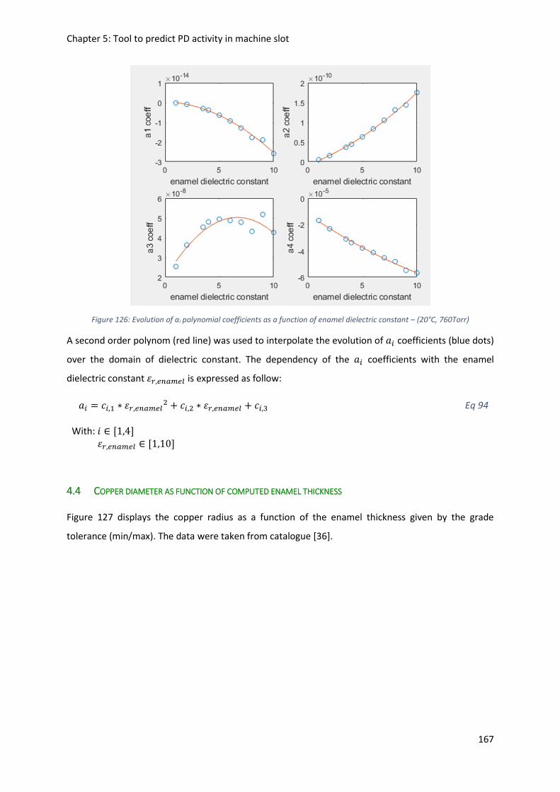
Chapter 5: Tool to predict PD activity in machine slot
167
Figure 126: Evolution of ai polynomial coefficients as a function of enamel dielectric constant – (20°C, 760Torr)
A second order polynom (red line) was used to interpolate the evolution of 𝑎𝑖 coefficients (blue dots)
over the domain of dielectric constant. The dependency of the 𝑎𝑖 coefficients with the enamel
dielectric constant 휀𝑟,𝑒𝑛𝑎𝑚𝑒𝑙 is expressed as follow:
𝑎𝑖 = 𝑐𝑖,1 ∗ 휀𝑟,𝑒𝑛𝑎𝑚𝑒𝑙2 + 𝑐𝑖,2 ∗ 휀𝑟,𝑒𝑛𝑎𝑚𝑒𝑙 + 𝑐𝑖,3
With: 𝑖 ∈ [1,4] 휀𝑟,𝑒𝑛𝑎𝑚𝑒𝑙 ∈ [1,10]
Eq 94
4.4 COPPER DIAMETER AS FUNCTION OF COMPUTED ENAMEL THICKNESS
Figure 127 displays the copper radius as a function of the enamel thickness given by the grade
tolerance (min/max). The data were taken from catalogue [36].

Chapter 5: Tool to predict PD activity in machine slot
168
Figure 127: Copper radius versus enamel thickness for all grade tolerances in [36]
It can be seen that the tolerances max grade 1 and min grade 2 are overlapping. It is the same for the
tolerances max grade 2 and min grade 3.
The discrete data from the catalogue (dots) can be interpolated with a 3rd order polynom. The
coefficients of such polynom are dependent on the wire grade.
𝑅𝑐𝑜𝑝𝑝𝑒𝑟 = 𝑏1(𝑔𝑟𝑎𝑑𝑒) ∗ 𝑒3 + 𝑏2(𝑔𝑟𝑎𝑑𝑒) ∗ 𝑒
2 + 𝑏3(𝑔𝑟𝑎𝑑𝑒) ∗ 𝑒
+ 𝑏4(𝑔𝑟𝑎𝑑𝑒)
Eq 95
4.5 VALIDATION
The results given by the wire design model were confronted to the ones using the simple analytical
model. The catalogue [36] was swept considering a min grade 2 insulation, (i.e.: grade=2/5). The
enamel dielectric constant was taken as 휀𝑟,𝑒𝑛𝑎𝑚𝑒𝑙 = 4.2.
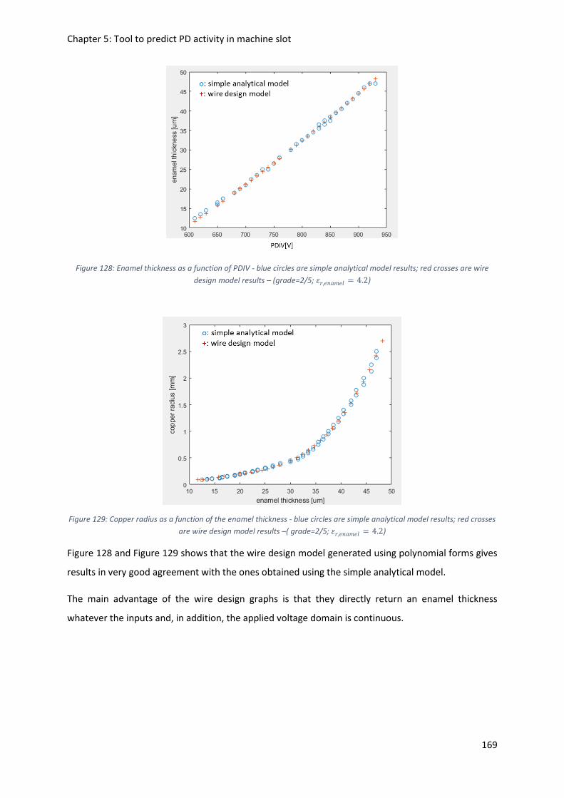
Chapter 5: Tool to predict PD activity in machine slot
169
Figure 128: Enamel thickness as a function of PDIV - blue circles are simple analytical model results; red crosses are wire
design model results – (grade=2/5; 휀𝑟,𝑒𝑛𝑎𝑚𝑒𝑙 = 4.2)
Figure 129: Copper radius as a function of the enamel thickness - blue circles are simple analytical model results; red crosses
are wire design model results –( grade=2/5; 휀𝑟,𝑒𝑛𝑎𝑚𝑒𝑙 = 4.2)
Figure 128 and Figure 129 shows that the wire design model generated using polynomial forms gives
results in very good agreement with the ones obtained using the simple analytical model.
The main advantage of the wire design graphs is that they directly return an enamel thickness
whatever the inputs and, in addition, the applied voltage domain is continuous.

Chapter 5: Tool to predict PD activity in machine slot
170
5 SLOT INSULATION DESIGN GRAPHS
The same approach was carried on for the slot liner design evaluation. This case is more complex due
to the presence of two different insulation materials: the enamel and the slot liner. Table 30 presents
the impacting parameters on the slot liner thickness choice.
Parameters Designation
Partial Discharge Inception Voltage PDIV
Enamel dielectric constant 휀𝑟,𝑒𝑛𝑎𝑚𝑒𝑙
The grade of the wire Grade
Enamel thickness E
Slot liner dielectric constant 휀𝑟,𝑙𝑖𝑛𝑒𝑟 Table 30: Impacting parameters on slot insulation design
5.1 SIMPLE ANALYTICAL MODEL FOR ELECTRIC FIELD IN AIR GAP COMPUTATION
The electric field lines in this model were approximated to straight line too. The lines length in the gap
between a round conductor and the slot liner was determined using geometric relations, as in [55].
The field lines were delimited with a tube. The tube is considered thin enough so that the materials
are considered as planar capacitances. Figure 130 illustrates the idea of flux tube and the resulting
Simple Analytical Model (SAM) representing the turn/slot configuration.
Figure 130: Top) Example of straight field line and its associated tube; below) SAM. (red: slot insulator, purple: enamel, blue: air)
In the SAM, the electric field �⃗� and electric field density �⃗⃗� are purely normal. They are noted E and D
respectively. The D field is conservative on the interfaces air/polymer:
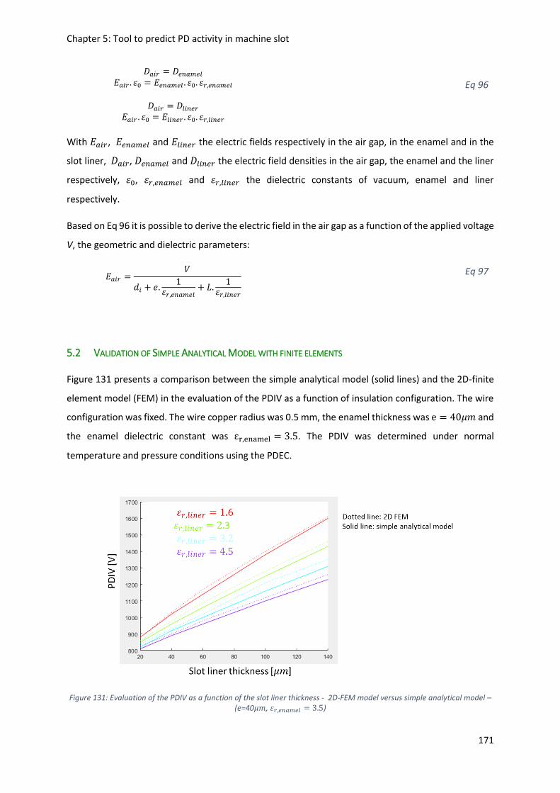
Chapter 5: Tool to predict PD activity in machine slot
171
𝐷𝑎𝑖𝑟 = 𝐷𝑒𝑛𝑎𝑚𝑒𝑙 𝐸𝑎𝑖𝑟 . 휀0 = 𝐸𝑒𝑛𝑎𝑚𝑒𝑙 . 휀0. 휀𝑟,𝑒𝑛𝑎𝑚𝑒𝑙
𝐷𝑎𝑖𝑟 = 𝐷𝑙𝑖𝑛𝑒𝑟
𝐸𝑎𝑖𝑟 . 휀0 = 𝐸𝑙𝑖𝑛𝑒𝑟 . 휀0. 휀𝑟,𝑙𝑖𝑛𝑒𝑟
Eq 96
With 𝐸𝑎𝑖𝑟, 𝐸𝑒𝑛𝑎𝑚𝑒𝑙 and 𝐸𝑙𝑖𝑛𝑒𝑟 the electric fields respectively in the air gap, in the enamel and in the
slot liner, 𝐷𝑎𝑖𝑟, 𝐷𝑒𝑛𝑎𝑚𝑒𝑙 and 𝐷𝑙𝑖𝑛𝑒𝑟 the electric field densities in the air gap, the enamel and the liner
respectively, 휀0, 휀𝑟,𝑒𝑛𝑎𝑚𝑒𝑙 and 휀𝑟,𝑙𝑖𝑛𝑒𝑟 the dielectric constants of vacuum, enamel and liner
respectively.
Based on Eq 96 it is possible to derive the electric field in the air gap as a function of the applied voltage
V, the geometric and dielectric parameters:
𝐸𝑎𝑖𝑟 =𝑉
𝑑𝑖 + 𝑒.1
휀𝑟,𝑒𝑛𝑎𝑚𝑒𝑙+ 𝐿.
1휀𝑟,𝑙𝑖𝑛𝑒𝑟
Eq 97
5.2 VALIDATION OF SIMPLE ANALYTICAL MODEL WITH FINITE ELEMENTS
Figure 131 presents a comparison between the simple analytical model (solid lines) and the 2D-finite
element model (FEM) in the evaluation of the PDIV as a function of insulation configuration. The wire
configuration was fixed. The wire copper radius was 0.5 mm, the enamel thickness was e = 40𝜇𝑚 and
the enamel dielectric constant was εr,enamel = 3.5. The PDIV was determined under normal
temperature and pressure conditions using the PDEC.
Figure 131: Evaluation of the PDIV as a function of the slot liner thickness - 2D-FEM model versus simple analytical model – (e=40𝜇𝑚, 휀𝑟,𝑒𝑛𝑎𝑚𝑒𝑙 = 3.5)

Chapter 5: Tool to predict PD activity in machine slot
172
The simple analytical model gives results close to the one obtained with the 2D-FEM. The evaluation
of the PDIV is slightly undervalued compared to 2D FEM. As an example, for εr,liner = 3.2,the oversize
is only 4% for a 140 m-thick slot liner. The simple analytical model was used in this chapter for the
study of the impacting parameters on the slot liner design mainly because of its fast computation time.
5.3 SLOT LINER THICKNESS AS A FUNCTION OF APPLIED VOLTAGE AND INSULATION MATERIALS
Figure 132 displays the evaluation of the required slot liner thickness depending on the PDIV and the
wire insulation parameters. The wire insulation parameters are its enamel dielectric constant 휀𝑟,𝑒𝑛𝑎𝑚𝑒𝑙
and its thickness e. The slot liner dielectric constant was fixed at εr,liner = 4.5. The PDIV was
determined under normal temperature and pressure conditions using the PDEC.
Figure 132: Evaluated slot liner insulation as a function of PDIV for different wire insulation configurations (thickness e and
permittivity r,enamel) – ( 휀𝑟,𝑙𝑖𝑛𝑒𝑟 = 4.5)
A 2nd order polynom was used to interpolate the slot liner thickness L as a function of the PDIV. The
polynomial coefficients are dependent on the enamel thickness e and dielectric constant 휀𝑟,𝑒𝑛𝑎𝑚𝑒𝑙 and
of the slot liner dielectric constant 휀𝑟,𝑙𝑖𝑛𝑒𝑟.
𝐿 = 𝑎1(𝑒, 휀𝑟,𝑒𝑛𝑎𝑚𝑒𝑙 , 휀𝑟,𝑙𝑖𝑛𝑒𝑟) ∗ 𝑃𝐷𝐼𝑉2
+𝑎2(𝑒, 휀𝑟,𝑒𝑛𝑎𝑚𝑒𝑙 , 휀𝑟,𝑙𝑖𝑛𝑒𝑟)
∗ 𝑃𝐷𝐼𝑉
+𝑎3(𝑒, 휀𝑟,𝑒𝑛𝑎𝑚𝑒𝑙 , 휀𝑟,𝑙𝑖𝑛𝑒𝑟)
Eq 98
The polynomial coefficients are dependent on three parameters. Therefore, three imbrications were
required to fully spell out Eq 98.

Chapter 5: Tool to predict PD activity in machine slot
173
The first imbrication expresses the 𝑎𝑖 (𝑖 ∈ [1: 3]) polynomial coefficients as a function of 휀𝑟,𝑙𝑖𝑛𝑒𝑟. A
polynomial form was also used here. The polynomial coefficients are named “first imbrication
polynomial coefficients”.
The second imbrication expresses the “first imbrication polynomial coefficient” as a function of e.
Another polynomial has been used, resulting in the apparition of “second imbrication polynomial
coefficients”.
Finally, the third imbrication expresses the “second imbrication polynomial coefficients” as a function
of 휀𝑟,𝑒𝑛𝑎𝑚𝑒𝑙.
By going up from the third imbrication to the first one, equation Eq 98 was fully determined.
Figure 133 illustrates the described imbrications:
Figure 133: Imbrications equations
5.3.1 First imbrication
Figure 134 displays the evolution of 𝑎𝑖 (𝑖 ∈ [1: 3]) polynomial coefficients present in Eq 98 as a
function of 휀𝑟,𝑙𝑖𝑛𝑒𝑟. The enamel thickness is 𝑒 = 5𝜇𝑚.

Chapter 5: Tool to predict PD activity in machine slot
174
Figure 134: ai (𝑖 ∈ [1: 3]) polynomial coefficients as a function of 휀𝑟,𝑙𝑖𝑛𝑒𝑟 - e=5𝜇𝑚
The ai (𝑖 ∈ [1: 3]) coefficients are interpolating over the 휀𝑟,𝑙𝑖𝑛𝑒𝑟 domain using a second order polynom.
𝑎𝑖 = 𝑏𝑖,1(𝑒, 휀𝑟,𝑒𝑛𝑎𝑚𝑒𝑙) ∗ 휀𝑟,𝑙𝑖𝑛𝑒𝑟2
+𝑏𝑖,2(𝑒, 휀𝑟,𝑒𝑛𝑎𝑚𝑒𝑙) ∗ 휀𝑟,𝑙𝑖𝑛𝑒𝑟+𝑏𝑖,3(𝑒, 휀𝑟,𝑒𝑛𝑎𝑚𝑒𝑙)
With 𝑖 ∈ [1: 3]
Eq 99
The 𝑏𝑖,𝑗 (𝑖, 𝑗 ∈ [1: 3]) are the “first imbrication polynomial coefficients”.
5.3.2 Second imbrication
Figure 135 displays as an example the evolution of 𝑏1,1 coefficient presents in Eq 99 as a function of
the enamel thickness e for different 휀𝑟,𝑒𝑛𝑎𝑚𝑒𝑙.
Figure 135: b1,1 coefficients as a function of enamel thickness
The bi,j (𝑖 ∈ [1: 3]) coefficients were interpolating over the 휀𝑟,𝑙𝑖𝑛𝑒𝑟 domain using a third order polynom.

Chapter 5: Tool to predict PD activity in machine slot
175
𝑏𝑖,𝑗 = 𝑐𝑖,𝑗,1(휀𝑟,𝑒𝑛𝑎𝑚𝑒𝑙) ∗ 𝑒3 +𝑐𝑖,𝑗,2(휀𝑟,𝑒𝑛𝑎𝑚𝑒𝑙)
∗ 𝑒2 +𝑐𝑖,𝑗,3(휀𝑟,𝑒𝑛𝑎𝑚𝑒𝑙) ∗ 𝑒
+𝑐𝑖,𝑗,4(휀𝑟,𝑒𝑛𝑎𝑚𝑒𝑙)
With 𝑖, 𝑗 ∈ [1: 3]
Eq 100
The 𝑐𝑖,𝑗,𝑘 (𝑖, 𝑗 ∈ [1: 3]and𝑘 ∈ [1: 4]) are the “second imbrication polynomial coefficients”.
5.3.3 Third imbrication
Figure 136 presents as an example the evolution of 𝑐3,𝑗,𝑘 (𝑗 ∈ [1: 3]and𝑘 ∈ [1: 4]) coefficients in Eq
100 as a function of 휀𝑟,𝑒𝑛𝑎𝑚𝑒𝑙.
Figure 136: c3,j,k coefficients as a function of 휀𝑟,𝑒𝑛𝑎𝑚𝑒𝑙
The 𝑐𝑖,𝑗,𝑘 (𝑖, 𝑗 ∈ [1: 3]and𝑘 ∈ [1: 4]) are finally interpolated over 휀𝑟,𝑒𝑛𝑎𝑚𝑒𝑙 using second order
polynomial forms.
5.4 VALIDATION
The results given by the slot insulation design model were then compared to the ones using the simple
analytical one. The wire copper radius was 𝑅𝑐𝑜𝑝𝑝𝑒𝑟 = 0.5𝑚𝑚, the enamel thickness was 𝑒 = 31.5𝜇𝑚
and the enamel dielectric constant was 휀𝑟,𝑒𝑛𝑎𝑚𝑒𝑙 = 4.2. The slot insulation was taken as 휀𝑟,𝑙𝑖𝑛𝑒𝑟 = 3.5.

Chapter 5: Tool to predict PD activity in machine slot
176
Figure 137: Slot liner thickness versus PDIV - blue circles are simple analytical model results; red crosses are wire design
model results - 𝑅𝑐𝑜𝑝𝑝𝑒𝑟 = 0.5𝑚𝑚; 𝑒 = 31.5𝜇𝑚; 휀𝑟,𝑒𝑛𝑎𝑚𝑒𝑙 = 4.2; 휀𝑟,𝑙𝑖𝑛𝑒𝑟 = 3.5
Figure 137 shows that the results given by the slot insulation design model are in very good agreement
with the ones given by the simple analytical model.
As for turn/turn insulation, the main advantages of the slot insulation design model is that it directly
returns a slot liner thickness whatever the inputs and moreover the applied voltage domain is
continuous. An abacus can therefore be produced.
6 EVALUATION OF THE ELECTRIC STRESSES UNDER NORMAL TEMPERATURE AND PRESSURE
CONDITIONS
6.1 TURN/TURN ELECTRIC STRESS
The transient regime determines the maximum turn/turn electric stress. In transient regime, voltage
phase terminals have to withstand pulses train of amplitude Vstep as illustrated in Figure 138.

Chapter 5: Tool to predict PD activity in machine slot
177
Figure 138: Example of both output voltage (phase to ground) and current waveforms of a 5-level ANPC obtained with Plecs software. Vdc is the bus voltage.
The effect of the impacting parameters on the the motor terminals overshoots have been presented
in Chapter 1, paragraph 6 Impact of power electronics. The power cable length between the inverter
output and the motor terminals is considered shorter than 1 m. Thus, only the rising time remains
impacting. In the example of Figure 138, the multilevel converter enables to reduce the voltage pulse
amplitude.
The impact of the rising time of inverter voltage pulse was derived from [60] results. Figure 139
presents a simple evaluation of voltage overshoot at phase terminals expressed as a percentage of the
inverter voltage pulse amplitude.
Figure 139: Overshoot at phase terminals expressed as a percentage of inverter voltage pulse amplitude as a function of the rising time
Overshoot start to appear for rising time shorter than 80 ns. It was considered that during transient
the first conductor of the phase receives 70% of the transient phase voltage [56]. The voltage front
does not reach the other conductors during a fraction time of transient regime [62].

Chapter 5: Tool to predict PD activity in machine slot
178
6.2 TURN/SLOT ELECTRIC STRESS
The maximal electric stress between turn and slot insulation is the nominal phase peak voltage.
A linear voltage repartition was considered all over a phase. There was one single phase per slot. The
number of conductors inside a slot represent the number of passing of the phase inside the slot. The
machine active length was considered long enough so that the end winding length was neglected.
The voltage on the 𝑖𝑡ℎ conductor of the phase in the slot is expressed as:
𝑉𝑐𝑜𝑛𝑑,𝑖 = 𝑉𝑝𝑒𝑎𝑘 ∗ (1 −𝐿𝑖𝐿𝑡𝑜𝑡
)
With 𝐿𝑖 the length of the phase in the slot lugs for the 𝑖𝑡ℎ conductor, 𝐿𝑡𝑜𝑡 the total phase length and
𝑉𝑝𝑒𝑎𝑘 the phase to neutral peak voltage.
7 PARTIAL DISCHARGE EVALUATION TOOL (PDET)
The perimeter of the PDET is only the stator slot. The PDET provides solution(s) in order to get a PD-
free stator slot. These(this) correspond(s) to minimal required insulation thicknesses to withstand the
electric stresses in both turn/turn and turn/slot close contacts.
The solutions are derived from graphs computed using the presented Simple Analytical Model (SAM)
validated with 2D-Finite Elements Model (2D FEM) in the case of a uniform electric field.
The developed PDET scope is:
inside a rectangular stator slot;
only one phase in the slot;
considered slot is the phase entrance;
round enamelled wires constitute the turns;
turns in close contact with each other and with the slot insulation;
a catalogue of round enamelled copper wires is already integrated.
Obviously, the scope of this study may be changed to take into account other configurations: flat wires,
trapezoidal slots, more than one phase per slot,...

Chapter 5: Tool to predict PD activity in machine slot
179
7.1 PDET ALGORITHM
Figure 140 illustrates the PDET organigram. There are five main steps. Each step is managed by a
function. These steps are automatically executed when PDET is running.
Figure 140: PDET organigram
F3_wire_design and F4_slot_insulation_design uses the graphs above presented. In
F2_PDIV_environmental_sizing_point function, the graph on Figure 122 is applied on turn/turn and
turn/slot evaluated electric stresses. It comes the oversized electric stresses at (20°C, 1bar) to ensure
that the solution takes into account the decrease in PDIV with temperature increase and pressure
decrease.

Chapter 5: Tool to predict PD activity in machine slot
180
7.2 INPUTS
The inputs are listed on Table 31.
Input Description Unit
Motor
𝑛𝑏_𝑝ℎ𝑎𝑠𝑒 Number of electric phases of the motor
𝑛𝑏_𝑠𝑙𝑜𝑡 Total number of slots in the stator
𝑛𝑏_𝑐𝑜𝑛𝑑 Number of conductors per slot. The conductors are the passages of a phase in the slot
𝐿_𝑠𝑙𝑜𝑡 Slot width [m]
ℎ_𝑠𝑙𝑜𝑡 Slot height [m]
𝑘𝑓𝑖𝑙𝑙 Filling factor
Converter
𝑚𝑎 Maximal modulation width
𝑉𝑒𝑚𝑜𝑡_max_𝑐𝑜𝑛𝑑1 Equivalent 1 conductor / slot / phase peak voltage
[V]
𝑛𝑏_𝑙𝑒𝑣𝑒𝑙 Number of levels of the converter
𝑟𝑖𝑠𝑒_𝑡𝑖𝑚𝑒 Switch component rise time [ns]
Sizing point
𝑇𝑒𝑚𝑝0 Stator operating temperature [°C]
ℎ0 Operating altitude [m]
Material
𝑣𝑎𝑙_𝑒𝑝𝑠𝑟_𝑒𝑛𝑎𝑚𝑒𝑙 Enamel dielectric constant
𝑣𝑎𝑙_𝑒𝑝𝑠𝑟_𝑐𝑎𝑙𝑒 Slot insulation dielectric constant
𝑣𝑎𝑙_𝑐𝑎𝑙𝑒_𝑚𝑖𝑛 Minimal slot insulation thickness [µm]
Wire
𝑅_𝑐𝑢 Copper radius – 0 if no selected wire (default)
[m]
𝑒 Enamel thickness – 0 if no selected wire (default)
[m]
Table 31: PDET inputs
The user may use the tool with a pre-selected wire configuration. PDET will then check that the
selected wire can withstand turn/turn electric stress. It will design the slot insulation to withstand the
electric stress between turn/slot. It will finally check that the solution fits in the slot.
The DC bus voltage is evaluated from the parameters 𝑉𝑒𝑚𝑜𝑡_max_𝑐𝑜𝑛𝑑1, 𝑚𝑎 and 𝑛𝑏_𝑐𝑜𝑛𝑑. At iso
power, increasing the number of conductors of the phase reduces the current density on the
conductors. On the other hand, the phase voltage increases.
𝑉𝑒𝑚𝑜𝑡_𝑚𝑎𝑥 = 𝑉𝑒𝑚𝑜𝑡_max_𝑐𝑜𝑛𝑑1 ∗ 𝑛𝑏𝑐𝑜𝑛𝑑 𝑉𝑖𝑛𝑣_𝑚𝑎𝑥 = 𝑉𝑒𝑚𝑜𝑡_𝑚𝑎𝑥/𝑚𝑎
𝑉_𝑑𝑐 = 2 ∗ 𝑉𝑖𝑛𝑣_𝑚𝑎𝑥
Eq 101
The wires are in close contact with each other and with the slot liner. That is because of the
assumptions made for the elaboration of the wire design and slot insulation graphs. These graphs are
established for round enamelled wires.

Chapter 5: Tool to predict PD activity in machine slot
181
A default minimal slot liner thickness is fixed at 20µm. It may be a constraint given by the user.
8 ILLUSTRATIVE EXAMPLE
As an example, let us consider the configuration presented on Table 32. No wire is preselected.
Parameters Designation Value
Inverter Maximal modulation width
𝑚𝑎 1.15
Equivalent 1 conductor / slot / phase peak voltage
𝑉𝑒𝑚𝑜𝑡_max_𝑐𝑜𝑛𝑑1 450 V
Number of levels 𝑛𝑏_𝑙𝑒𝑣𝑒𝑙 5
Voltage pulse amplitude
Voltage pulse rising time 𝑟𝑖𝑠𝑒_𝑡𝑖𝑚𝑒 200𝑛𝑠
Motor Number of phases 𝑛𝑏_𝑝ℎ𝑎𝑠𝑒 3
Number of slots 𝑛𝑏_𝑠𝑙𝑜𝑡 36
Number of conductors 𝑛𝑏_𝑐𝑜𝑛𝑑 4
Slot width 𝐿_𝑠𝑙𝑜𝑡 8𝑚𝑚
Slot pitch ℎ_𝑠𝑙𝑜𝑡 46𝑚𝑚
Filling factor 𝑘𝑓𝑖𝑙𝑙 0.5
Sizing point Temperature 𝑇𝑒𝑚𝑝 180°𝐶
Altitude ℎ0 8000𝑚
Materials Enamel dielectric constant
휀𝑟,𝑒𝑛𝑎𝑚𝑒𝑙 3.5
Slot liner dielectric constant
𝑣𝑎𝑙_𝑒𝑝𝑠𝑟_𝑒𝑛𝑎𝑚𝑒𝑙 4.5
Minimal slot liner thickness
𝑣𝑎𝑙_𝑒𝑝𝑠𝑟_𝑐𝑎𝑙𝑒 20𝜇𝑚
Table 32: Tool inputs - Example values
Referring to PDET organigram in Figure 140, the first step is the determination of the electric stresses
for turn/turn and turn/slot contacts. That is detailed in above §6: Evaluation of the electric stresses
under normal temperature and pressure conditions. The second step is to determine the overvalued
electric stresses at (20 °C, 1 bar) corresponding to the impact of the sizing point. For that, the graph on
Figure 122 is used.
Figure 141 displays PDET window where the electric stresses are computed. The tab pages on the top
(Inputs, Electric stresses, Wire design, Slot liner design and Solutions) are the steps to compute in
successive order. The DC bus voltage computed using Eq 101 is Vdc=3130 V. The inverter voltage pulse
amplitude is Vstep=782.6 V. The turn/turn and turn/slot electric stresses are respectively designated by
PDIV0_turn_turn and PDIV0_turn_slot. The rise time of 200 ns is slow enough so that no additional
overshoot is considered. The turn/turn electric stress thus correspond to 70% of Vstep. The turn/slot
electric stress is the nominal voltage of the first conductor. The graph on Figure 141 displays the PDIV
evolution as a function of the temperature on the ground (triangles) and at 8000 m (crosses). The blue

Chapter 5: Tool to predict PD activity in machine slot
182
curves correspond to turn/slot contact, the red curves to turn/turn contact. To be able to stand the
identified electric stresses at 180°C, 8000 m (green circles) the insulation has to be oversized at 20 °C,
on the ground (purple circles). Table 33 gives the electric stresses and the resulting overvalued stresses
at (20°C, 1bar) due to the sizing point environmental conditions.
Interface Electric stresses Oversized electric stresses at (20°C, 1bar) due to sizing point impact
Turn/turn 547.8 V 807.8 V
Turn/slot 1800 V 2640 V Table 33: Calculated overvalued voltages
The third step is the evaluation of wire solution(s). Figure 142 displays PDET Wire design window.
The left graph on Figure 142 is the enamel thickness design graph corresponding to the used material.
The right graph is the used catalogue. For each copper radius, there are six possible enamel
thicknesses. These correspond to the tolerances min and max of grade 1, grade 2 and grade 3 wires.
PDET returned a required enamel thickness of 27.65 µm using the left graph. That results in five
possible wires configuration (Table 34). Each configuration has an enamel thickness close to the
required one.
Copper radius [mm] Enamel thickness [m] Grade
0.425 29.5 0.2 (i.e.: max grade 1)
0.3750 28 0.4 (i.e.: min grade 2)
0.1675 28 0.6 (i.e.: max grade 2)
0.1675 28.5 0.8 (i.e.: min grade 3)
0.1060 28 1 (i.e.: max grade 3)
Table 34: Wire solutions
The two solutions corresponding to a copper radius of 0.1675 mm are quite the same as explained
with Figure 127. The enamel thickness given by PDET is the minimal required thickness to withstand
both overshoot and sizing point conditions.

Chapter 5: Tool to predict PD activity in machine slot
183
Figure 141: PDET - Electric stresses window

Chapter 5: Tool to predict PD activity in machine slot
184
Figure 142: PDET - Wire design window

Chapter 5: Tool to predict PD activity in machine slot
185
The fourth step is the evaluation of the minimal required liner thickness to withstand the turn/slot
electric stress at sizing point conditions. Figure 143 displays PDET Slot liner design window. The graph
provides a slot liner thickness of 716.4 µm.
Figure 143: PDET - Slot liner design window
The final step consists in checking if the wire solutions are fitting in the slot considering a liner thickness
of 716.4 µm. The fitting solutions are displayed on Figure 144:
Figure 144: PDET - Solutions window

Chapter 5: Tool to predict PD activity in machine slot
186
The color bar on the plots represent the nominal voltage [V] on each conductor. As four conductors
are considered in this example, there are four colors. The outer rectangle is the slot. The inner
rectangle is the free space in the slot once the liner is inserted. Each blank circle is the copper area of
the wires. The colored contour is the enamel overcoat. Each conductor is subdivided depending the
copper radius of the solution so that the filling factor is close to 0.5. From the five original solutions
only four fit in the slot.
Table 35 recap the solutions:
Copper radius
[mm]
Enamel thickness
[m]
Grade Number of wires per
conductor
Wire 0.425 29.5 0.2 (i.e.: max grade
1)
82
0.3750 28 0.4 (i.e.: min grade 2) 105
0.1675 28 0.6 (i.e.: max grade
2)
522
0.1675 28.5 0.8 (i.e.: min grade 3) 522
Liner Liner thickness
716.4 µm
Table 35: PDET solutions
In case no solution fits the slot, different actions are possible:
Changing the material parameters alone (i.e.: the insulation materials) ;
Changing inverter parameters alone;
Changing motor parameters alone;
Changing sizing point alone;
A combination of the previous four possible actions.
Therefore, several actions to supress PD have an impact on the whole powertrain sizing. The strong
connection with the other WP has been clearly shown.
9 CONCLUSION
This chapter has presented the tool coded on Matlab which automatically size the insulation in a stator
slot to avoid PD risk. First, the criterion to evaluate PDIV was presented. That criterion takes into
account a combined variation of temperature and altitude for different field lines length. That criterion
has been used to produce a graph to quantify the PDIV decrease (compared to 20 °C, 1 bar conditions)
due to changing environmental conditions (sizing point).

Chapter 5: Tool to predict PD activity in machine slot
187
Then, Simple Analytical Models (SAMs) of the turn/turn and turn/slot contacts have been presented
and validated by 2D-Finite Element Models (2D-FEMs). The SAMs have been used to compute graphs
which give the minimal required insulation thickness to withstand electric stresses considering the
chosen materials and taking into account a transient voltage overshoot. Besides, the electric stresses
are overestimated in order to take into account the decrease in PDIV at the sizing point.
Finally, it came out that multiple actions are possible to avoid PD. Some of them may actually have a
real impact on the whole powertrain sizing.

Chapter 5: Tool to predict PD activity in machine slot
188

General conclusion and perspectives
189
General conclusion and perspectives
This PhD work has consisted in studying the Electrical Insulation System (EIS) of rotating
machines fed by inverters that will equip future hybrid propulsion aircrafts. It is a part of the European
H2020 project HASTECS (Hybrid Aircraft reSearch on Thermal and Electrical Components and Systems).
Partial Discharges (PD) phenomenon represents a great deal in the design of future rotating
machines fed by inverter. On one hand, new faster components made out of SiC and GaN technologies
will considerably improve the performances of the inverters. On the other hand, they will generate
harder voltage fronts at the motor terminals which lead to higher transient voltage overshoots. PD will
be more likely to appear and the insulation lifespan will be reduced due to both voltage overshoots
and high switching frequency. That is the reason why it is absolutely necessary to take into account
such a phenomenon when designing the motor to avoid any PD appearance, rather than searching for
solutions in a motor already produced to remove them.
It was appeared relevant in this project to integrate both inverters and motors in the nacelles.
That will reduces the voltage overshoots at motor terminals by using a power harness length shorter
than 2 m. Nevertheless, in an aeronautical non-pressurized environment where equipment are
submitted to great temperature and pressure variations, the Partial Discharge Inception Voltage (PDIV)
will be considerably affected, as it is very sensitive to them.
It has appeared that the choices for the EIS will considerably impact the design of the cooling
system. Polymer materials widely used in EIS have very low thermal conductivity. Therefore, an
oversizing of the EIS results in much more thermal resistance in the path of the heat flux to be
evacuated by the cooling system. New insulating materials having higher thermal conductivity are
nowadays under study (not only for aircraft electric devices). These are composites made of a polymer
matrix in which ceramic particles are inserted. Such particles are used in micro- or nano-sizes. The
proportion of ceramic introduced in the polymer material is completely adjustable. It improves thermal
properties but also have a negative impact on mechanical properties.
Experimental works about the relevant use of the well-known Paschen’s criterion in motor EIS
design have been carried on during this PhD work. PDIV measurements have been performed on
samples of PEI/PAI overcoated round copper wires (polymers able to support the estimated motors
working temperature). A correction of the secondary electron emission coefficient has been proposed
for the configuration of two parallel enamelled round copper wires in close contact (representative of
two neighbouring conductors in a machine slot). This corrected coefficient has been found to be almost
General conclusion and perspectives
190
ten times lower compare to the value found in the literature obtained with metallic planar electrodes.
That leads to higher PDIV levels in the case of enamelled round wires.
The Paschen’s criterion requires the complete knowledge of electric field lines geometry. A
numerical code has then been developed on Matlab to drawn electric field lines from a 2D-Finite
Elements (2D-FEM) solution of an electrostatic problem. The originality of the proposed method is that
only the scalar potential solution is required and the density of displayed lines is analogous to the field
intensity. It has been compared to a ballistic approach already implanted on Matlab. It results that the
Matlab function is much faster. Both methods give similar results for the considered 2D-electrostatic
problem. The development of the proposed method provided better understanding on scalar potential
formulation and the notions of electric flux tubes.
Simple Analytical Models (SAM) of the turn/turn and turn/slot configurations have been
established. Results given by the SAM have been verified with the corresponding 2D-FEM. The SAM
enabled parametric studies which has lead to design graphs. They indicate the minimal insulation
thicknesses to ensure a PD-free slot in order to withstand the nominal electric stresses.
Finally, the design graphs have been implanted in tool specifically developed in this work: the
Partial Discharge Evaluation Tool (PDET). It is a fully automatic tool which dimensions the EIS inside a
stator slot to avoid PD appearance. This tool can be implanted in an optimization loop of the whole
powertrain. For now, the tool perimeter is inside a stator slot with only one phase, but it may be
upgraded to treat more than one phase per slot. The conductors are made of enamelled round wires
in close contacts. The hot spots are the turn/turn and turn/slot electric stresses. The stresses were
automatically evaluated from the inverter and motor parameters. The decrease in PDIV due to a
combined variation of pressure and temperature was also considered.
PDET provides PD-free solutions for Type I-EIS motors. It is obviously transposable to Type II-
EIS motors (high voltage motors). In case of Type II-EIS motors (able to support PD), the PDET will
provide an EIS design that will limit the PD amplitude.
The work carried on during this PhD work offers multiple perspectives:
The use of flat wire for windings. In such geometry, SAM are not valid anymore.
Besides, the electric field is slightly non uniform. Design graphs will have to be derived
from 2D-FEM and the degree of uniformity of the electric field will have to be carefully
checked in order to apply the corrected Paschen’s criterion.

General conclusion and perspectives
191
The consideration of multiple phases per slot. An additional insulation layer will be
required to insulate the different phases. The maximum electric stress will be now
found between two different phases.
The addition of cooling pipes embedded in the slot for a more efficient cooling inside
the winding. The coolant may be composed of glycoled water, which is an electric
insulating liquid. However, the pipes are usually conductors. That will add new zones
where the electric stress has to be carefully investigated. Hollow wires may also be
investigated.
The end winding is the zone where electric stress may also be high. Indeed, in this
area, the different phases overlap. Besides, there is triple points at the exit of the slot
between the metallic carcass of the motor, the air, and the insulation. Tackle such
configuration will need to develop a 3D-modelling.

General conclusion and perspectives
192

Publications
193
Publications P. Collin, D. Malec, Y. Lefevre, “Tool to Design the Primary Electrical Insulation System of Low Voltage Rotating Machines Fed by Inverters”, In 2018 IEEE Electrical Insulation Conference (EIC) (pp. 8-13). IEEE
P. Collin, D. Malec, Y. Lefevre, “Outil d’aide au design du système d’isolation primaire de machines tournantes basse tension alimentées par onduleur”, In SFE Grenoble 2018
"Design of Electric Machine Taking Into Account the Partial Discharges Phenomena for Future Hybrid Propelled Aircrafts", P.Collin, S.Touhami, D.Malec, Y.Lefevre, J.F.Llibre, More Electric Aircraft, February 6-7, 2019, Toulouse
"Concernant la pertinence de l’utilisation du critère de Paschen pour l’estimation de la tension d’apparition des décharges partielles (TADP) lors du design du système d’isolation électrique de moteurs alimentés par onduleur", P. Collin, D. Malec, Y. Lefevre, Jeunes Chercheurs en Génie Electrique, 11-14 juin, 2019, Olérons
“About the relevance of using Paschen’s criterion for partial discharges inception voltage (PDIV) estimation when designing the electrical insulation system of inverter fed motors”, P. Collin, D. Malec, Y. Lefevre, Electrical Insulation Conference, June 16-19, 2019, Calgary
“A general method to compute the electric flux lines in the slots of electric machines for the evaluation of partial discharges risk”, P. Collin, D. Malec, Y. Lefevre, Compumag, July 15-19, 2019, Paris
"Tool to predict and avoid Partial Discharges in stator slot of rotating motors fed by inverter", P. Collin, D. Malec, Y. Lefevre, Aerospace Europe Conference, February 25-28, 2020, Bordeaux

Publications
194

Annex
195
Annex
Nominal conductor diameter [mm]
Minimum increase due to the insulation thickness [mm]
Maximal overall diameter [mm]
Grade 1 Grade 2 Grade 3 Grade 1 Grade 2 Grade3
0,180 0,013 0,025 0,036 0,204 0,217 0,229
0,190 0,014 0,027 0,039 0,216 0,228 0,240
0,200 0,014 0,027 0,039 0,226 0,239 0,252
0,212 0,015 0,029 0,043 0,240 0,254 0,268
0,224 0,015 0,029 0,043 0,252 0,266 0,280
0,236 0,017 0,032 0,048 0,267 0,283 0,298
0,250 0,017 0,032 0,048 0,281 0,297 0,312
0,265 0,018 0,033 0,050 0,297 0,314 0,330
0,280 0,018 0,033 0,050 0,312 0,329 0,345
0,300 0,019 0,035 0,053 0,334 0,352 0,360
0,315 0,019 0,035 0,053 0,349 0,367 0,384
0,335 0,020 0,038 0,06 0,372 0,391 0,408
0,355 0,020 0,038 0,057 0,392 0,411 0,428
0,375 0,021 0,040 0,060 0,414 0,434 0,453
0,400 0,021 0,040 0,060 0,439 0,459 0,478
0,425 0,022 0,042 0,064 0,466 0,488 0,508
0,450 0,022 0,042 0,064 0,491 0,513 0,533
0,475 0,024 0,045 0,067 0,519 0,541 0,562
0,500 0,024 0,045 0,068 0,544 0,566 0,587
0,530 0,025 0,047 0,071 0,576 0,600 0,623
0,560 0,025 0,047 0,071 0,606 0,630 0,653
0,600 0,027 0,050 0,075 0,649 0,674 0,698
0,630 0,027 0,050 0,075 0,679 0,704 0,728
0,670 0,028 0,053 0,080 0,722 0,749 0,774
0,710 0,028 0,053 0,080 0,762 0,789 0,814
0,750 0,030 0,056 0,085 0,805 0,834 0,861
0,800 0,030 0,056 0,085 0,855 0,884 0,911
0,850 0,032 0,060 0,090 0,909 0,938 0,968
0,900 0,032 0,060 0,090 0,959 0,989 1,081
0,950 0,034 0,063 0,095 1 1 1,074
1,000 0,034 0,063 0,095 1,062 1,094 1,124
1,060 0,034 0,065 0,098 1,124 1,157 1,188
1,120 0,034 0,065 0,098 1,184 1,217 1,248
1,180 0,035 0,067 0,100 1,246 1,279 1,311
1,250 0,035 0,067 0,100 1,316 1,349 1,381
1,320 0,036 0,069 0,103 1,388 1,422 1,455
1,400 0,036 0,069 0,103 1,468 1,502 1,535
1,500 0,038 0,071 0,107 1,570 1,606 1,640
1,600 0,038 0,071 0,107 1,670 1,706 1,740
1,700 0,039 0,073 0,110 1,772 1,809 1,844
1,800 0,039 0,073 0,110 1,872 1,909 1,944
1,900 0,040 0,075 0,113 1,974 2,012 2,048
2,000 0,040 0,075 0,113 2,074 2,112 2,148
2,120 0,041 0,077 0,116 2,196 2,235 2,272
2,240 0,041 0,077 0,116 2,316 2,355 2,392
2,360 0,042 0,079 0,119 2,438 2,478 2,516
2,500 0,042 0,079 0,119 2,578 2,618 2,656
2,650 0,04 0,081 0,123 2,730 2,772 2,811

Annex
196
2,800 0,043 0,081 0,123 2,880 2,922 2,961
3,000 0,045 0,084 0,127 3,083 3,126 3,166
3,150 0,045 0,084 0,127 3,233 3,276 3,316
3,350 0,046 0,086 0,130 3,435 3,479 3,521
3,550 0,046 0,086 0,130 3,635 3,679 3,721
3,750 0,047 0,089 0,134 3,838 3,883 3,926
4,000 0,047 0,089 0,134 4,088 4,133 4,176
4,250 0,049 0,092 0,138 4,341 4,387 4,431
4,500 0,049 0,092 0,138 4,591 4,637 4,681
4,750 0,050 0,094 0,142 4,843 4,891 4,936
5,000 0,050 0,094 0,142 5,093 5,141 5,186 Annex 1: Enamel thickness tolerances picked from [37]

References:
197
References:
[1] ‘Agenda 21 (Rio Declaration on Environment and Development)’, 1992, p. 79. [2] ‘IEA World energy outlook 2018’. International Energy Agency, Jul. 2018. [3] ‘ITF Transport outlook 2017’. International Transport Forum , OECD iLibrary, 2017. [4] ‘OPEC World Oil Outlook 2040’. Organization of the Petroleum Exporting Countries, Sep. 2018. [5] ‘WHO Health and sustainable development - Transport and health risks’. World Health
Organization, 2019. [6] ‘The cost of air pollution – Health impacts of road transport’. ISBN 978-92-64-210448, OECD
iLibrary, 2014. [7] J. P. RODRIGUE, C. COMTOIS, and B. SLACK, The geography of transports systems, 4th edition.
New York Routledge Edition, 2017. [8] ‘World Energy Model’. International Energy Agency, Version 2018. [9] ‘Les énergies renouvelables en France : les chiffres clés 2018’. Ministère de la Transition
écologique et solidaire, May 24, 2018. [10] ‘Quelle est la source d’énergie la plus utilisée dans le monde ?’ ENGIE, Mar. 29, 2019. [11] ‘Historique évolution du cours du baril (159 litres) de pétrole WTI’. france-inflation.com, 2020. [12] ‘Road transport: Reducing CO2 emissions from vehicles’. European Comission, 2019. [13] ‘Aviation carbon offset programmes’. IATA, 2008. [14] E. Férard, ‘En Suède, la “honte de prendre l’avion” pousse les voyageurs à favoriser le train’.
Géo, Apr. 16, 2019. [15] L. Faleiro, J. Herzog, B. Schievelbusch, and T. Seung, ‘INTEGRATED EQUIPMENT SYSTEMS FOR A
MORE ELECTRIC AIRCRAFT – HYDRAULICS AND PNEUMATICS’, Hydraul. Pneum., p. 10. [16] M. Palomeque, ‘A320 - Dual hydraulic loss’. Safety first #4, Jun. 2017. [17] J. Robinson, ‘Collins Aerospace building $67M electric aircraft lab’, Wings Mag., Apr. 2019. [18] B. Sarlioglu and C. T. Morris, ‘More Electric Aircraft: Review, Challenges, and Opportunities for
Commercial Transport Aircraft’, IEEE Trans. Transp. Electrification, vol. 1, no. 1, pp. 54–64, Jun. 2015, doi: 10.1109/TTE.2015.2426499.
[19] R. Hemmati, F. Wu, and A. El-Refaie, ‘Survey of Insulation Systems in Electrical Machines’, in 2019 IEEE International Electric Machines & Drives Conference (IEMDC), San Diego, CA, USA, May 2019, pp. 2069–2076, doi: 10.1109/IEMDC.2019.8785099.
[20] ‘Electric flight - Bringing zero-emission technology to aviation’. Airbus. [21] ‘The future is electric’. Airbus, Jul. 17, 2018. [22] ‘CityAirbus’. Airbus. [23] ‘HASTECS’. http://www.laplace.univ-tlse.fr/HASTECS (accessed Jan. 09, 2020). [24] J. Thauvin, ‘Exploring the design space for a hybrid-electric regional aircraft with
multidisciplinary design optimisation methods’, Institut National Polytechnique de Toulouse, 2018.
[25] ‘Hybrid Aircraft Academic reSearch on Thermal & Electrical Components and Systems (HASTECS), Project selected from CFP in Cleansky II (H2020) framework’. .
[26] M. Pettes-Duler, X. Roboam, and B. Sareni, ‘Integrated design process and sensitivity analysis of a hybrid electric propulsion system for future aircraft’, Salerno, Italy, May 2019.
[27] Y. Lefevre, S. El-Aabid, J.-F. Llibre, C. Henaux, and S. Touhami, ‘Performance assessment tool based on loadability concepts’, Int. J. Appl. Electromagn. Mech., vol. 59, no. 2, pp. 687–694, Mar. 2019, doi: 10.3233/JAE-171059.
[28] P. Collin, S. Touhami, D. Malec, Y. Lefevre, and J. F. Llibre, ‘Design of Electric Machine Taking Into Account the Partial Discharges Phenomena for Future Hybrid Propelled Aircrafts’, 2019.

References:
198
[29] N. Erroui, G. Gateau, and N. Roux, ‘Continuous-caliber semiconductor components’, in 2018 IEEE International Conference on Industrial Technology (ICIT), Lyon, Feb. 2018, pp. 658–663, doi: 10.1109/ICIT.2018.8352256.
[30] A. Zeaiter and M. Fenot, ‘Thermal Sensitivity Analysis of a High Power Density Electric Motor for Aeronautical Application’, in 2018 IEEE International Conference on Electrical Systems for Aircraft, Railway, Ship Propulsion and Road Vehicles & International Transportation Electrification Conference (ESARS-ITEC), Nottingham, Nov. 2018, pp. 1–6, doi: 10.1109/ESARS-ITEC.2018.8607393.
[31] R. Wrobel, S. J. Williamson, J. D. Booker, and P. H. Mellor, ‘Characterizing the in situ Thermal Behavior of Selected Electrical Machine Insulation and Impregnation Materials’, IEEE Trans. Ind. Appl., vol. 52, no. 6, pp. 4678–4687, Nov. 2016, doi: 10.1109/TIA.2016.2589219.
[32] S. Touhami, Y. Bertin, Y. Lefèvre, J.-F. Llibre, C. Henaux, and M. Fenot, ‘Lumped Parameter Thermal Model of Permanent Magnet Synchronous Machines’, p. 7.
[33] F. Accorinti et al., ‘High-efficiency cooling system for highly integrated power electronics for hybrid propulsion aircraft’, in 2019 IEEE 28th International Symposium on Industrial Electronics (ISIE), Vancouver, BC, Canada, Jun. 2019, pp. 870–877, doi: 10.1109/ISIE.2019.8781086.
[34] M. E. Banda, D. Malec, and J.-P. Cambronne, ‘Simulation of Space Charge Impact on Partial Discharge Inception Voltage in Power Busbars Dedicated to Future Hybrid Aircrafts’, Circuits Syst., vol. 09, no. 11, pp. 196–212, 2018, doi: 10.4236/cs.2018.911018.
[35] ‘EIC 60034-18-41, “Partial discharge free electrical insulation systems (Type I) used in rotating electrical machines fed from voltage converters – Qualification and quality control tests,” 2014.’
[36] ‘Enamelled copper wire, SONA’. . [37] ‘enamlled_copper_wire.pdf’.
http://www.universalmetals.com.pk/pdf/enamlled_copper_wire.pdf (accessed Jan. 15, 2020). [38] A. Anton, ‘Émaux isolants et fils émaillés’, Tech. Ing., vol. D2330, p. 19, 2009. [39] J. Pyrhonen, T. Jokinen, and V. Hrabovcová, Design of rotating electrical machines. Chichester,
West Sussex, United Kingdom ; Hoboken, NJ: Wiley, 2008. [40] ‘Magnet Wire – Selection and Use Directions for Magnet Wire’,
https://www.ecmenzies.com.au/images/productpdf/COROCUdatasheet_1.pdf. . [41] Y. Agari, A. Ueda, and S. Nagai, ‘Thermal conductivity of a polymer composite’, J. Appl. Polym.
Sci., vol. 49, no. 9, pp. 1625–1634, Sep. 1993, doi: 10.1002/app.1993.070490914. [42] R. Arora and W. Mosch, ‘High Voltage and Electrical Insulation Engineering’. A John Wiley &
Sons, Inc., Publication, 2011. [43] M. Chapman, N. Frost, and R. Bruetsch, ‘Insulation Systems for Rotating Low-Voltage
Machines’, in Conference Record of the 2008 IEEE International Symposium on Electrical Insulation, Vancouver, BC, Jun. 2008, pp. 257–260, doi: 10.1109/ELINSL.2008.4570323.
[44] J. Moeneclaey, ‘Méthode de conception des bobinages des actionneurs électriques adaptés aux nouvelles contraintes de l’avionique’, University of Artois, Béthune, 2015.
[45] ‘Resins and Varnishes 2013 - VON ROLL - PDF Catalogs | Technical Documentation | Brochure’. https://pdf.directindustry.com/pdf/von-roll/resins-varnishes-2013/12485-556569.html (accessed Jan. 21, 2020).
[46] ‘Design and Testing of Insulation for Adjustable Speed Drives - PDFHALL.COM’. https://pdfhall.com/design-and-testing-of-insulation-for-adjustable-speed-drives_5b69f350097c4775388b45ee.html (accessed Jan. 22, 2020).
[47] G. C. Stone, Ed., Electrical insulation for rotating machines: design, evaluation, aging, testing, and repair. Piscataway, NJ : Hoboken, NJ: IEEE ; Wiley-Interscience, 2004.
[48] S. Nategh, A. Krings, O. Wallmark, and M. Leksell, ‘Evaluation of Impregnation Materials for Thermal Management of Liquid-Cooled Electric Machines’, IEEE Trans. Ind. Electron., vol. 61, no. 11, pp. 5956–5965, Nov. 2014, doi: 10.1109/TIE.2014.2308151.

References:
199
[49] W. Sixel, M. Liu, G. Nellis, and B. Sarlioglu, ‘Cooling of Windings in Electric Machines via 3D Printed Heat Exchanger’, in 2018 IEEE Energy Conversion Congress and Exposition (ECCE), Portland, OR, Sep. 2018, pp. 229–235, doi: 10.1109/ECCE.2018.8557845.
[50] Y. Ohki, ‘Development of epoxy resin composites with high thermal conductivity’, IEEE Electr. Insul. Mag., vol. 26, no. 1, pp. 48–49, Jan. 2010, doi: 10.1109/MEI.2010.5383936.
[51] P. Rodgers, V. Eveloy, and L. El Sayed, ‘Candidate thermally enhanced polymer composite materials for cooling of electronic systems’, in 20th International Workshop on Thermal Investigations of ICs and Systems, Greenwich, London, United Kingdom, Sep. 2014, pp. 1–6, doi: 10.1109/THERMINIC.2014.6972495.
[52] S. Diaham, ‘Modulation of the dielectric breakdown strength in polyimide nanocomposites by deep traps tailoring in interphase regions’, IEEE Trans. Dielectr. Electr. Insul., vol. 26, no. 1, pp. 247–252, Feb. 2019, doi: 10.1109/TDEI.2018.007540.
[53] C. Abadie, T. Lebey, and T. Billard, ‘On-line non-intrusive partial discharges detection in aeronautical systems’, Université Toulouse 3 Paul Sabatier, 2017.
[54] H. Foch, F. Forest, and T. Meynard, ‘Onduleurs de tension - Structures. Principes. Applications’, p. 21, 1998.
[55] L. Benmamas, ‘Méthodes d’évaluation du risque de décharges partielles dans le bobinage de machines électriques destinées à la traction automobile’, University of Paris-Saclay, Gif-sur-Yvette, 2017.
[56] M. Kaufhold, H. Aninger, M. Berth, J. Speck, and M. Eberhardt, ‘Electrical stress and failure mechanism of the winding insulation in PWM-inverter-fed low-voltage induction motors’, IEEE Trans. Ind. Electron., vol. 47, no. 2, pp. 396–402, Apr. 2000, doi: 10.1109/41.836355.
[57] B. Taghia, B. Cougo, H. Piquet, D. Malec, A. Belinger, and J.-P. Carayon, ‘Advanced analysis of transient overvoltage in electromechanical chain fed by SiC inverter’, Electrimacs 2017, p. 8, 2017.
[58] A. Ong, J. Carr, J. Balda, and A. Mantooth, ‘A Comparison of Silicon and Silicon Carbide MOSFET Switching Characteristics’, in 2007 IEEE Region 5 Technical Conference, Fayetteville, AR, USA, Apr. 2007, pp. 273–277, doi: 10.1109/TPSD.2007.4380318.
[59] L. Dupont, S. Lefebvre, and Z. Khatir, ‘Characterisationof Silicon Carbide Schottky diodes and COOLMOSTMtransistors at high temperature’, 35th Annu. IEEE Power Electron. Spec. Conf., p. 6, 2004.
[60] V. Mihaila, ‘Nouvelle Conception des bobinages statoriques des machines à courant alternatif pour réduire les effets négatifs des dV/dt.’, Artois, 2011.
[61] B. Taghia, B. Cougo, H. Piquet, D. Malec, A. Belinger, and J.-P. Carayon, ‘Overvoltage at motor terminals in SiC-based PWM drives’, Math. Comput. Simul., vol. 158, pp. 264–280, Apr. 2019, doi: 10.1016/j.matcom.2018.09.009.
[62] P. Bidan, T. Lebey, and C. Neacsu, ‘Development of a new off-line test procedure for low voltage rotating machines fed by adjustable speed drives (ASD)’, IEEE Trans. Dielectr. Electr. Insul., vol. 10, no. 1, pp. 168–175, Feb. 2003, doi: 10.1109/TDEI.2003.1176584.
[63] R. Bartnikas and E. McMahon, ‘Engineering dielectrics - Volume 1 - Corona measurements and interpreation’, Am. Soc. Test. Mater., no. STP669, 1979.
[64] F. H. Keuger, ‘Partial discharge detection in high voltage equipment’, Butterworth-Heinemann, pp. 78–85, 1990.
[65] R. Bruetsch, M. Tari, K. Froehlich, T. Weiers, and R. Vogelsang, ‘Insulation Failure Mechanisms of Power Generators’, p. 7.
[66] ‘Lichtenberg figure’, Wikipedia. Jan. 25, 2020, Accessed: Feb. 12, 2020. [Online]. Available: https://en.wikipedia.org/w/index.php?title=Lichtenberg_figure&oldid=937573574.
[67] C. Mayoux, ‘Aging of polymeric insulating materials in power cables’, IEEE Trans. Dielectr. Electr. Insul., vol. 4, no. 6, pp. 665–673, Dec. 1997, doi: 10.1109/94.654573.
[68] G. Nayak, Y. Du, R. Brandenburg, and P. J. Bruggeman, ‘Effect of air flow on the micro-discharge dynamics in an array of integrated coaxial microhollow dielectric barrier discharges’, Plasma Sources Sci. Technol., vol. 26, no. 3, p. 035001, Feb. 2017, doi: 10.1088/1361-6595/aa56a4.

References:
200
[69] M. Q. Nguyen, ‘Etude de l’impact des contraintes aéronautiques sur les systèmes d’isolation des moteurs de conditionnement d’air’, University of Toulouse, Toulouse, 2012.
[70] G. Stone, ‘Partial Discharges in Electrical Insulation’. . [71] J. Kurimský, I. Kolcunová, and R. Cimbala, ‘Understanding surface partial discharges in HV coils
and the role of semi-conductive protection’, Electr. Eng., vol. 92, no. 7–8, pp. 283–289, Dec. 2010, doi: 10.1007/s00202-010-0184-0.
[72] ‘Corona discharge’, Wikipedia. Feb. 03, 2020, Accessed: Feb. 13, 2020. [Online]. Available: https://en.wikipedia.org/w/index.php?title=Corona_discharge&oldid=938928794.
[73] ‘Ozonation of Polymers’. https://polymerdatabase.com/polymer%20chemistry/Ozone.html (accessed Feb. 13, 2020).
[74] ‘Failures in Three-Phase Stator Windings’. https://easa.com/resources/failures-in-three-phase-stator-windings (accessed Feb. 13, 2020).
[75] C. Julie, ‘Etude des mécanismes anti-cancéreux induits par milieux activés par jet de plasma froid : vers une nouvelle approche thérapeutique.’, Toulouse 3 Paul Sabatier, 2018.
[76] E. SILI, ‘Etude et caractérisation des décharges partielles et du vieillissement du polyimide en environnement aéronautique’, Toulouse 3 Paul Sabatier, 2012.
[77] C. Van De Steen, ‘Modélisation des propriétés de transport des ions moléculaires de krypton et xénon pour l’optimisation des générateurs de plasma froids utilisant les gaz rares’, Université Toulouse 3 Paul Sabatier, Toulouse, 2018.
[78] I. Popescu and E. Badareu, Gaz Ionisés, Décharges Electriques dans les Gaz, Dunod. Paris, 1968. [79] E. R. B. Adamson and A. Dissertation, ‘SECONDARY ELECTRON EMISSION COEFFICIENT FROM
LEXAN: THE LOW ENERGY CROSSOVER’, p. 78. [80] O. Eichwald, M. Yousfi, and O. Ducasse, ‘Breakdown criteria in air: an overview supported by
predictive simulations’, p. 6. [81] F. Paschen, ‘Ueber die zum Funkenübergang in Luft, Wasserstoff und Kohlensäure bei
verschiedenen Drucken erforderliche Potentialdifferenz’, Ann. Phys., vol. 273, no. 5, pp. 69–96, 1889, doi: 10.1002/andp.18892730505.
[82] T. W. Dakin, G. Luxa, G. Oppermann, J. Vigreux, G. Wind, and H. Winkelnkemper, ‘Breakdown of Gases in Uniform Fields Paschen Curves for Nitrogen, Air and Sulfur Hexafluoride’, Electra, 1974.
[83] H. H. Wittenberg, ‘Gas Tube Design’, Electron Tube Des. RCA Electron Tube Div., pp. 792–817, 1962.
[84] F. Koliatene, ‘CONTRIBUTION A L’ETUDE DE L’EXISTENCE DES DECHARGES DANS LES SYSTEMES DE L’AVIONIQUE’, Toulouse 3 Paul Sabatier, 2009.
[85] ‘RTCA DO-160, Environmental Conditions and test Procedures for Airborne Equipment’. . [86] F. W. Peek, Dielectric Phenomena in High Voltage Engineering, McGraw Hill. 1929. [87] W. G. Dunbar and J. W. Seabrook, ‘High Voltage Design Guide for Airborne Equipment’, Boeing
Aerosp. Co., p. 217, 1976. [88] V. L. Bychkov, S. A. Volkov, and I. V. Kochetov, ‘Ionization process in the humid air of the lower
troposphere’, Russ. J. Phys. Chem. B, vol. 5, no. 6, pp. 940–945, Dec. 2011, doi: 10.1134/S1990793111060054.
[89] P. Mikropoulos, C. Stassinopoulos, and B. Sarigiannidou, ‘Positive Streamer Propagation and Breakdown in Air: the Influence of Humidity’, IEEE Trans. Dielectr. Electr. Insul., vol. 15, no. 2, pp. 416–425, Apr. 2008, doi: 10.1109/TDEI.2008.4483460.
[90] G. Robles, J. Fresno, J. Martínez-Tarifa, J. Ardila-Rey, and E. Parrado-Hernández, ‘Partial Discharge Spectral Characterization in HF, VHF and UHF Bands Using Particle Swarm Optimization’, Sensors, vol. 18, no. 3, p. 746, Mar. 2018, doi: 10.3390/s18030746.
[91] B. Cella, ‘On-line partial discharges detection in conversion systems used in aeronautics’, University of Toulouse, 2015.
[92] T. Balachandran, S. Sirimmana, A. Jin, and K. S. Haran, ‘Partial Discharge Testing of Form-Wound Air-Core Armature Windings for a High-Frequency PMSM for Electric Aircraft Applications’, in 2018 IEEE International Conference on Information and Automation for
References:
201
Sustainability (ICIAfS), Colombo, Sri Lanka, Dec. 2018, pp. 1–6, doi: 10.1109/ICIAFS.2018.8913342.
[93] J. M. Wetzer and P. C. T. van der Laan, ‘Prebreakdown currents: Basic interpretation and time-resolved measurements’, IEEE Trans. Electr. Insul., vol. 24, no. 2, pp. 297–308, Apr. 1989, doi: 10.1109/14.90288.
[94] R. Ross, ‘Graphical methods for plotting and evaluating Weibull distributed data’, in Proceedings of 1994 4th International Conference on Properties and Applications of Dielectric Materials (ICPADM), Brisbane, Qld., Australia, 1994, vol. 1, pp. 250–253, doi: 10.1109/ICPADM.1994.413986.
[95] J. S. White, ‘The Moments of Log-Weibull Order Statistics’, Technometrics, pp. 373–386, 1969. [96] J. C. Fothergill, ‘Ageing, Space Charge and Nanodielectrics: Ten Things We Don’t Know About
Dielectrics’, in 2007 IEEE International Conference on Solid Dielectrics, Winchester, UK, Jul. 2007, pp. 1–10, doi: 10.1109/ICSD.2007.4290739.
[97] R. Rui and I. Cotton, ‘Impact of low pressure aerospace environment on machine winding insulation’, in 2010 IEEE International Symposium on Electrical Insulation, San Diego, CA, USA, Jun. 2010, pp. 1–5, doi: 10.1109/ELINSL.2010.5549718.
[98] S. Palit, D. Varghese, H. Guo, S. Krishnan, and M. A. Alam, ‘The Role of Dielectric Heating and Effects of Ambient Humidity in the Electrical Breakdown of Polymer Dielectrics’, IEEE Trans. Device Mater. Reliab., vol. 15, no. 3, pp. 308–318, Sep. 2015, doi: 10.1109/TDMR.2015.2431998.
[99] E. McMahon and J. Perkins, ‘Surface and Volume Phenomena in Dielectric Breakdown of Polyethylene’, IEEE Trans. Power Appar. Syst., vol. 82, no. 69, pp. 1128–1136, Dec. 1963, doi: 10.1109/TPAS.1963.291505.
[100] J. V. Champion, S. J. Dodd, A. S. Vaughan, and S. J. Sutton, ‘THE EFFECT OF VOLTAGE, TEMPER4TURE AND MORPHOLOGY ON ELECTRICAL TREEING IN POLYETHYLENE BLENDS’, IEEE Dielectr. Mater. Meas. Appl. Conf. Publ., no. 473, p. 6, 2000.
[101] M. Szczepanski, ‘Development of methods allowing the test and the comparison of low-voltage motors insulation systems running under partial discharges (fed by inverter)’, p. 214.
[102] R. Acheen, C. Abadie, T. Lebey, T. Billard, and S. Duschesne, ‘Comparison of the Electrical Ageing Under Sinusoidal and Square-Wave Stresses’, San Antonio, TX, 2018, pp. 353–356.
[103] ‘IEEE Guide for the Statistical Analysis of Electrical Insulation Voltage Endurance Data’. ANSI/IEEE Std 930, 1987.
[104] N. Lahoud, J. Faucher, D. Malec, and P. Maussion, ‘Electrical Aging of the Insulation of Low-Voltage Machines: Model Definition and Test With the Design of Experiments’, IEEE Trans. Ind. Electron., vol. 60, no. 9, pp. 4147–4155, Sep. 2013, doi: 10.1109/TIE.2013.2245615.
[105] ‘Qualification and type tests for Type I electrical insulation systems used in rotating electrical machines when fed from voltage converters’. IEC 60034-18-CD International Standard, 2012.
[106] ‘Qualification and acceptance tests for partial discharge resistant electrical insulation systems (Type II) used in rotating electrical machines when fed from voltage converters’. IEC 60034-18-42 TS, International Standards, 2008.
[107] P. Maussion, A. Picot, M. Chabert, and D. Malec, ‘Lifespan and aging modeling methods for insulation systems in electrical machines: A survey’, in 2015 IEEE Workshop on Electrical Machines Design, Control and Diagnosis (WEMDCD), Torino, Italy, Mar. 2015, pp. 279–288, doi: 10.1109/WEMDCD.2015.7194541.
[108] K. Petcharaks, ‘A contribution to the streamer breakdown criterion’, in 11th International Symposium on High-Voltage Engineering (ISH 99), London, UK, 1999, vol. 1999, pp. v3-19-v3-19, doi: 10.1049/cp:19990689.
[109] A. Pedersen, T. Christen, A. Blaszczyk, and H. Boehme, ‘Streamer inception and propagation models for designing air insulated power devices’, in 2009 IEEE Conference on Electrical Insulation and Dielectric Phenomena, Virginia Beach, VA, USA, Aug. 2009, pp. 604–607, doi: 10.1109/CEIDP.2009.5377740.

References:
202
[110] G. Eriksson, ‘Easy Evaluation of Streamer Discharge Criteria’, Proc. 2012 COMSOL Conf. Milan, p. 7, 2012.
[111] E. J. Horowitz, ‘A general field-line plotting algorithm’, Comput. Phys., vol. 4, no. 4, p. 418, 1990, doi: 10.1063/1.168384.
[112] Z. Ren, ‘2-D dual finite-element formulations for the fast extraction of circuit parameters in VLSI’, IEEE Trans. Magn., vol. 39, no. 3, pp. 1590–1593, May 2003, doi: 10.1109/TMAG.2003.810548.
[113] G. Parent, S. Duchesne, and P. Dular, ‘Determination of Flux Tube Portions by Adjunction of Electric or Magnetic Multivalued Equipotential Lines’, IEEE Trans. Magn., vol. 53, no. 6, pp. 1–4, Jun. 2017, doi: 10.1109/TMAG.2017.2661401.
[114] G. Parent, M. Rossi, S. Duchesne, and P. Dular, ‘Determination of Partial Discharge Inception Voltage and Location of Partial Discharges by Means of Paschen’s Theory and FEM’, IEEE Trans. Magn., vol. 55, no. 6, pp. 1–4, Jun. 2019, doi: 10.1109/TMAG.2019.2902374.
[115] T. M. Whittaker, Mon Weather., 1977. [116] G. Dhatt and G. Touzot, Une présentation de la méthode des éléments finis,
Les Presses de l’Université Laval. Québec, et Maloine, Paris, 1981. [117] F. Pauli, N. Driendl, L. Yang, and K. Hameyer, ‘Corona resistant enameled wires as a solution for
electrical motor winding systems supplied by high du/dt inverter voltage: An insulation life-time estimation’, IEEE Submitt., p. 7, 2019.
[118] N. Hayakawa and H. Okubo, ‘Partial discharge characteristics of inverter-fed motor coil samples under ac and surge voltage conditions’, IEEE Electr. Insul. Mag., vol. 21, no. 1, pp. 5–10, Jan. 2005, doi: 10.1109/MEI.2005.1389265.
[119] ‘IEC 60270 (2000-12), High-voltage test techniques — Partial discharge measurements’. . [120] W. Weibull, ‘A Statistical Distribution Function of Wide Applicability’, J. Appl. Mech., no. 18, pp.
293–297, 1951. [121] P. Collin, D. Malec, and Y. Lefevre, ‘Tool to Design the Primary Electrical Insulation System of
Low Voltage Rotating Machines Fed by Inverters’, 2018 IEEE Electr. Insul. Conf. EIC, pp. 8–13, 2018, doi: 10.1109/EIC.2018.8481037.
[122] M. Szczepanski, D. Malee, P. Maussion, B. Petitgas, and P. Manfe, ‘Prediction of the lifespan of enameled wires used in low voltage inverter-fed motors by using the Design of Experiments (DoE)’, in 2017 IEEE Industry Applications Society Annual Meeting, Cincinnati, OH, Oct. 2017, pp. 1–6, doi: 10.1109/IAS.2017.8101798.
[123] H. Xu, Y. Zhang, and F. Zheng, ‘Study on measuring method of dielectric spectroscopy for polymer dielectrics’, in 2009 IEEE 9th International Conference on the Properties and Applications of Dielectric Materials, Harbin, China, Jul. 2009, pp. 922–925, doi: 10.1109/ICPADM.2009.5252247.
[124] F. Aymonino, ‘Contribution à l’étude du comportement des systèmes d’isolation des machines tournantes à courant alternatif fonctionnant sous très hautes températures (200-400°C)’, University of Toulouse Paul Sabatier, Toulouse, 2008.
[125] M. G. D. L. Calle, J. M. Martínez-Tarifa, Á. M. G. Solanilla, and G. Robles, ‘Uncertainty Sources in the Estimation of the Partial Discharge Inception Voltage in Turn-to-Turn Insulation Systems’, IEEE Access, vol. 8, pp. 157510–157519, 2020, doi: 10.1109/ACCESS.2020.3018870.
[126] H. Ismail, ‘Étude du taux de pulvérisation et du coefficient d’émission électronique secondaire de cibles métalliques polycristallines bombardées par des ions Hg+, dans un domaine d’énergie allant de 5 à 30 keV’, Rev. Phys. Appliquée, vol. 5, no. 5, pp. 759–764, 1970, doi: 10.1051/rphysap:0197000505075900.
[127] M. Florkowski, B. Florkowska, and P. Zydron, ‘Partial Discharges in Insulating Systems of Low Voltage Electric Motors Fed by Power Electronics—Twisted-Pair Samples Evaluation’, Energies, vol. 12, no. 5, p. 768, Feb. 2019, doi: 10.3390/en12050768.
[128] N. Naudé, A. Belinger, S. Dap, and N. Gherardi, ‘Memory effects in Atmospheric Pressure Townsend Discharges in N2 and air’, p. 4, 2015.

References:
203
[129] D. Marić, N. Škoro, P. D. Maguire, C. M. O. Mahony, G. Malović, and Z. L. Petrović, ‘On the possibility of long path breakdown affecting the Paschen curves for microdischarges’, Plasma Sources Sci. Technol., vol. 21, no. 3, p. 035016, Jun. 2012, doi: 10.1088/0963-0252/21/3/035016.
[130] P. G. Slade and E. D. Taylor, ‘Electrical breakdown in atmospheric air between closely spaced (0.2 μm-40 μm) electrical contacts’, IEEE Trans. Compon. Packag. Technol., vol. 25, no. 3, pp. 390–396, Sep. 2002, doi: 10.1109/TCAPT.2002.804615.
[131] A. Peschot, N. Bonifaci, O. Lesaint, C. Valadares, and C. Poulain, ‘Deviations from the Paschen’s law at short gap distances from 100 nm to 10 μ m in air and nitrogen’, Appl. Phys. Lett., vol. 105, no. 12, p. 123109, Sep. 2014, doi: 10.1063/1.4895630.
[132] P. Carazzetti and H. R. Shea, ‘Electrical breakdown at low pressure for planar microelectromechanical systems with 10- to 500-m gaps’, vol. 8, p. 9.