
design of solar pond for water preheating used in the copper ...
138
PONTIFICIA UNIVERSIDAD CATOLICA DE CHILE ESCUELA DE INGENIERIA DESIGN OF SOLAR POND FOR WATER PREHEATING USED IN THE COPPER CATHODES WASHING PROCESS AT SPENCE MINE FELIPE JAVIER GARRIDO GONZALEZ Thesis submitted to the Office of Research and Graduate Studies in partial fulfillment of the requirements for the Degree of Master of Science in Engineering Advisor: JULIO VERGARA AIMONE Santiago de Chile, (December, 2012) © MMXII, Felipe Javier Garrido Gonzalez
-
Upload
khangminh22 -
Category
Documents
-
view
4 -
download
0
Transcript of design of solar pond for water preheating used in the copper ...

PONTIFICIA UNIVERSIDAD CATOLICA DE CHILE
ESCUELA DE INGENIERIA
DESIGN OF SOLAR POND FOR WATER
PREHEATING USED IN THE COPPER
CATHODES WASHING PROCESS AT SPENCE
MINE
FELIPE JAVIER GARRIDO GONZALEZ
Thesis submitted to the Office of Research and Graduate Studies in partial
fulfillment of the requirements for the Degree of Master of Science in
Engineering
Advisor:
JULIO VERGARA AIMONE
Santiago de Chile, (December, 2012)
© MMXII, Felipe Javier Garrido Gonzalez

PONTIFICIA UNIVERSIDAD CATOLICA DE CHILE
ESCUELA DE INGENIERIA
DESIGN OF SOLAR POND FOR WATER PREHEATING USED IN THE COPPER
CATHODES WASHING PROCESS AT SPENCE MINE
FELIPE JAVIER GARRIDO GONZALEZ
Members of the Committee:
JULIO VERGARA AIMONE
RODRIGO PASCUAL JIMENEZ
JOSE HERNAN GARCIA
HECTOR JORQUERA GONZALEZ
Thesis submitted to the Office of Research and Graduate Studies in partial
fulfillment of the requirements for the Degree of Master of Science in
Engineering
Santiago de Chile, (December, 2012)

"The greatest challenge to any thinker
is stating the problem in a way that
will allow a solution."
Bertrand Russell

ACKONWLEDGMENTS
I would like to express my gratitude towards my family and especially my parents, Mario and
Silvia, for their love and the unconditional support they have given me throughout this process.
I would like to thank my supervisor, Dr. Julio Vergara, for his wise advise, excellent disposi-
tion and for believing in my work. I would like to acknowledge JHG Ingenierıa Ltda. for sharing
valuable information for the development of this thesis.
And at last but not least, I would also like to thank Fabian Cadiz, Matias Salas, Dennis Dunlop,
Mario Abarca, Philipp Kanehl, Juan Guillermo Vidal and Rodrigo Soto for always being there to
share a talk, their thoughts on a matter, to aid in moments of difficulty or simply for being my
friends.
Felipe Garrido
I

TABLE OF CONTENTS
ACKNOWLEDGEMENTS I
LIST OF TABLES V
LIST OF FIGURES VI
ABSTRACT IX
RESUMEN X
1 INTRODUCTION 1
1.1 Copper extractive processes . . . . . . . . . . . . . . . . . . . . . . . . . . . . . . 2
1.2 Characterization of the energy demand of copper mining in Chile . . . . . . . . . . 6
1.3 Electrowon copper cathodes . . . . . . . . . . . . . . . . . . . . . . . . . . . . . 12
1.4 Spence Mine . . . . . . . . . . . . . . . . . . . . . . . . . . . . . . . . . . . . . 12
1.5 Solar pond technology: State of the art . . . . . . . . . . . . . . . . . . . . . . . . 14
1.6 Objectives . . . . . . . . . . . . . . . . . . . . . . . . . . . . . . . . . . . . . . . 18
1.7 Organization of the thesis . . . . . . . . . . . . . . . . . . . . . . . . . . . . . . . 19
2 SOLAR POND MODEL 21
2.1 Insolation . . . . . . . . . . . . . . . . . . . . . . . . . . . . . . . . . . . . . . . 22
2.2 Radiation Absorption . . . . . . . . . . . . . . . . . . . . . . . . . . . . . . . . . 25
2.3 Solar Pond fluid dynamics . . . . . . . . . . . . . . . . . . . . . . . . . . . . . . 26
2.3.1 Balance Equations . . . . . . . . . . . . . . . . . . . . . . . . . . . . . . 28
3 NUMERICAL SOLUTION FOR A ONE-ZONE MODEL 32
3.1 Boundary conditions . . . . . . . . . . . . . . . . . . . . . . . . . . . . . . . . . 34
3.1.1 NCZ boundary conditions . . . . . . . . . . . . . . . . . . . . . . . . . . 34
3.1.2 Solar pond boundary conditions . . . . . . . . . . . . . . . . . . . . . . . 35
3.2 Numerical Modulation . . . . . . . . . . . . . . . . . . . . . . . . . . . . . . . . 37
3.3 Time and space mesh . . . . . . . . . . . . . . . . . . . . . . . . . . . . . . . . . 39
II

3.4 Model validation . . . . . . . . . . . . . . . . . . . . . . . . . . . . . . . . . . . 43
3.5 Model restrictions . . . . . . . . . . . . . . . . . . . . . . . . . . . . . . . . . . . 44
4 DESIGN PARAMETERS 47
4.1 Site Selection . . . . . . . . . . . . . . . . . . . . . . . . . . . . . . . . . . . . . 47
4.2 Solar pond walls . . . . . . . . . . . . . . . . . . . . . . . . . . . . . . . . . . . 47
4.3 Bottom and wall lining . . . . . . . . . . . . . . . . . . . . . . . . . . . . . . . . 50
4.4 Layers thickness . . . . . . . . . . . . . . . . . . . . . . . . . . . . . . . . . . . . 54
4.5 Salt gradient establishment . . . . . . . . . . . . . . . . . . . . . . . . . . . . . . 57
4.6 Salt and water . . . . . . . . . . . . . . . . . . . . . . . . . . . . . . . . . . . . . 59
4.7 Heat extraction . . . . . . . . . . . . . . . . . . . . . . . . . . . . . . . . . . . . 60
4.8 Water circulation power . . . . . . . . . . . . . . . . . . . . . . . . . . . . . . . . 65
4.9 Solar pond monitoring and control . . . . . . . . . . . . . . . . . . . . . . . . . . 67
4.10 Solar pond maintenance . . . . . . . . . . . . . . . . . . . . . . . . . . . . . . . . 69
4.10.1 Salt gradient maintenance . . . . . . . . . . . . . . . . . . . . . . . . . . 69
4.10.2 Wind effects . . . . . . . . . . . . . . . . . . . . . . . . . . . . . . . . . 75
4.10.3 Turbidity effects . . . . . . . . . . . . . . . . . . . . . . . . . . . . . . . 76
4.11 Thermal efficiency . . . . . . . . . . . . . . . . . . . . . . . . . . . . . . . . . . 79
5 CASE STUDY AND PROPOSED DESIGN 80
5.1 Case study . . . . . . . . . . . . . . . . . . . . . . . . . . . . . . . . . . . . . . . 80
5.1.1 Internal heat exchanger design . . . . . . . . . . . . . . . . . . . . . . . . 80
5.1.2 Determination of the layers thicknesses . . . . . . . . . . . . . . . . . . . 83
5.1.3 Required effective solar collecting surface area . . . . . . . . . . . . . . . 85
5.1.4 Wall angle . . . . . . . . . . . . . . . . . . . . . . . . . . . . . . . . . . 86
5.1.5 Thermal insulation . . . . . . . . . . . . . . . . . . . . . . . . . . . . . . 88
5.2 Proposed solar pond design . . . . . . . . . . . . . . . . . . . . . . . . . . . . . . 88
5.2.1 Single versus modular configuration . . . . . . . . . . . . . . . . . . . . . 89
6 RESULTS 92
6.1 Predicted performance . . . . . . . . . . . . . . . . . . . . . . . . . . . . . . . . 92
III

6.2 Economical analysis . . . . . . . . . . . . . . . . . . . . . . . . . . . . . . . . . 93
6.2.1 Investment Cost . . . . . . . . . . . . . . . . . . . . . . . . . . . . . . . . 93
6.2.2 Maintenance costs . . . . . . . . . . . . . . . . . . . . . . . . . . . . . . 96
6.2.3 Operational costs . . . . . . . . . . . . . . . . . . . . . . . . . . . . . . . 97
6.2.4 Discounted cash flows . . . . . . . . . . . . . . . . . . . . . . . . . . . . 98
6.2.5 Sensitivity analysis . . . . . . . . . . . . . . . . . . . . . . . . . . . . . . 99
7 CONCLUSIONS 103
BIBLIOGRAPHY 106
APPENDICES 116
IV

LIST OF TABLES
1 Energy consumption of the Chilean copper mining industry in 2010 . . . . . . . . 7
2 Constants for the transmissivity function . . . . . . . . . . . . . . . . . . . . . . . 26
3 Properties of common materials used for solar pond lining . . . . . . . . . . . . . 53
4 Effect of adding an insulating layer to solar ponds close to the water table in the
average temperature of the LCZ . . . . . . . . . . . . . . . . . . . . . . . . . . . 53
5 Parameters used for Scanning injection technique at El Paso solar pond . . . . . . 58
6 Cost per meter of PP and PE tubes . . . . . . . . . . . . . . . . . . . . . . . . . . 65
7 IHE composed by 20 tubes for different diameters . . . . . . . . . . . . . . . . . . 82
8 IHE composed by 20 tubes for different diameters . . . . . . . . . . . . . . . . . . 83
9 Temperature range of the LCZ after the third year of operation for different thick-
nesses . . . . . . . . . . . . . . . . . . . . . . . . . . . . . . . . . . . . . . . . . 84
10 Required surface area for different water table depth and outlet temperature for the
third year of operation . . . . . . . . . . . . . . . . . . . . . . . . . . . . . . . . 86
11 Increment of volume and wall area of a solar pond due to slopping walls . . . . . . 87
12 Proposed solar pond design, single configuration, water table at 55 m deep . . . . . 89
13 Performance of the solar pond design after seven years of operation . . . . . . . . 92
14 Investment cost of a solar pond with and without thermal insulation for different
water table depths . . . . . . . . . . . . . . . . . . . . . . . . . . . . . . . . . . . 95
15 Life cycle and energy cost of of the current process and with solar pond preheating 98
16 Base case DCF calculation . . . . . . . . . . . . . . . . . . . . . . . . . . . . . . 121
17 Single solar pond, open salt cycle DCF calculation . . . . . . . . . . . . . . . . . 122
18 Single solar pond, closed salt cycle DCF calculation . . . . . . . . . . . . . . . . . 123
19 Modular solar pond, open salt cycle DCF calculation . . . . . . . . . . . . . . . . 124
20 Modular solar pond, closed salt cycle DCF calculation . . . . . . . . . . . . . . . 125
V

LIST OF FIGURES
1.1 Chilean refined copper exports by destination . . . . . . . . . . . . . . . . . . . . 2
1.2 Stages of Pyrometallurgy . . . . . . . . . . . . . . . . . . . . . . . . . . . . . . . 3
1.3 Stages of Hydrometallurgy . . . . . . . . . . . . . . . . . . . . . . . . . . . . . . 5
1.4 Energy demand of copper mining in Chile . . . . . . . . . . . . . . . . . . . . . . 7
1.5 Chilean copper cathode production between 1995 and 2010 . . . . . . . . . . . . . 8
1.6 Greenhouse gas emissions and copper production of the Chilean copper mining
industry . . . . . . . . . . . . . . . . . . . . . . . . . . . . . . . . . . . . . . . . 9
1.7 Daily average of solar radiation in northern Chile . . . . . . . . . . . . . . . . . . 11
1.8 Aerial view of Spence mine . . . . . . . . . . . . . . . . . . . . . . . . . . . . . . 13
1.9 Water heating system for EW cathode washing at Spence mine . . . . . . . . . . . 14
1.10 Brine stratification in a Solar Pond . . . . . . . . . . . . . . . . . . . . . . . . . . 15
1.11 The Beith Ha’Arava solar pond, Israel . . . . . . . . . . . . . . . . . . . . . . . . 17
1.12 Solar Pond at El Paso, New Mexico . . . . . . . . . . . . . . . . . . . . . . . . . 19
2.1 Phenomena that present in the behavior of a solar pond . . . . . . . . . . . . . . . 21
2.2 Declination angle for an observer in the North hemisphere . . . . . . . . . . . . . 23
2.3 The Hour angle . . . . . . . . . . . . . . . . . . . . . . . . . . . . . . . . . . . . 23
2.4 The Zenith or Incidence angle . . . . . . . . . . . . . . . . . . . . . . . . . . . . 24
2.5 Simulation of motion in a fluid at rest due to salt-finger phenomena. . . . . . . . . 27
3.1 Meassured data for Ambient Temperature at Spence for year 2010 and Fourier
fitted curve . . . . . . . . . . . . . . . . . . . . . . . . . . . . . . . . . . . . . . 38
3.2 Solar radiation modeled for a summer and winter day . . . . . . . . . . . . . . . . 39
3.3 Discretization of the NCZ used for numerical resolution . . . . . . . . . . . . . . . 40
3.4 Comparison of the simulated and measured LCZ temperature evolution of a solar
pond . . . . . . . . . . . . . . . . . . . . . . . . . . . . . . . . . . . . . . . . . . 44
3.5 Predicted and recorded temperature profile of Los Alamos solar pond . . . . . . . 45
4.1 Effect of depth of water table on maximum temperature of salt gradient solar pond. 48
4.2 Convective layer generated due to wall heating by Sun exposition . . . . . . . . . . 49
4.3 Scheme of angles used to calculate the NRI . . . . . . . . . . . . . . . . . . . . . 49
VI

4.4 Variation of yearly maximum NIP for different latitudes . . . . . . . . . . . . . . . 51
4.5 Lining scheme for solar ponds developed in India . . . . . . . . . . . . . . . . . . 52
4.6 Growth of the upper-convective zone in a solar pond caused by wind and rain . . . 55
4.7 Circular diffuser design . . . . . . . . . . . . . . . . . . . . . . . . . . . . . . . . 59
4.8 Diffuser design used in the El Paso solar pond . . . . . . . . . . . . . . . . . . . . 59
4.9 In-pond heat exchanger (IHE) used at Pyramid Hill . . . . . . . . . . . . . . . . . 61
4.10 Instrumentation tower at El Paso solar pond . . . . . . . . . . . . . . . . . . . . . 68
4.11 Scanner used for monitoring procedures at El Paso solar pond . . . . . . . . . . . 69
4.12 Evolution of salt concentration profile in the NCZ pond without maintenance . . . 70
4.13 Schematic of flows in a salt recycling system for gradient maintenance . . . . . . . 71
4.14 Schematic of flows for gradient maintenance without salt recycling . . . . . . . . . 74
4.15 Schematic view of the pond with three water zones, salt charger and surface wash-
ing system . . . . . . . . . . . . . . . . . . . . . . . . . . . . . . . . . . . . . . . 75
4.16 Wind suppressors installed at Pyramid Hill solar pond, Australia . . . . . . . . . . 77
4.17 Collection efficiency versus turbidity levels in a solar pond . . . . . . . . . . . . . 78
5.1 Interface created to facilitate the supervision of the simulation runs. . . . . . . . . 81
5.2 Outlet temperature of the water flow for different LCZ thicknesses. . . . . . . . . . 84
5.3 Outlet temperature of the water flow for a 1.1 m thick LCZ. . . . . . . . . . . . . . 85
5.4 Outlet temperature of the water flow for different solar pond surface area. . . . . . 85
5.5 Normalized instability potential of solar pond wall angle at Spence . . . . . . . . . 87
5.6 Proposed site for construction of a solar pond at Spence mine . . . . . . . . . . . . 90
5.7 Proposed modular setup for the solar pond . . . . . . . . . . . . . . . . . . . . . . 91
6.1 Prospected energy supply composition with a solar pond preheating stage during
lifetime operation . . . . . . . . . . . . . . . . . . . . . . . . . . . . . . . . . . . 93
6.2 Investment cost composition of single and modular solar pond configuration . . . . 95
6.3 LCC of the heating stage with solar pond for different scenarios of water price
annual growth . . . . . . . . . . . . . . . . . . . . . . . . . . . . . . . . . . . . . 100
6.4 LCC of the heating stage with solar pond for different scenarios of liner replace-
ment frequency . . . . . . . . . . . . . . . . . . . . . . . . . . . . . . . . . . . . 101
6.5 LCC of the heating stage with solar pond for different learning stage lengths . . . . 102
VII

A.1 Evolution of the Chilean electrical generation matrix between years 2000 and 2009 117
B.1 Closed and open cycle configurations for in-pond heat extraction method . . . . . . 118
C.1 Solar pond design, single configuration, drained . . . . . . . . . . . . . . . . . . . 119
C.2 Solar pond design, modular configuration, filled . . . . . . . . . . . . . . . . . . . 120
VIII

ABSTRACT
The Chilean copper industry is increasingly dependent on coal-generated electricity and diesel
fuel for mining operations and therefore its associated green house emissions have experimented a
significant growth in the late years, in addition to scarcity of less polluting energy sources. How-
ever, solar energy is breaking through in mining processes that require heating of fluids. At Spence
mine, 6% of the national total of fine copper is produced for which 1,400 tonnes of diesel are burnt
per year to heat up the water used only to wash the copper cathodes at the end of the electrowinning
stage.
Solar ponds are a body of water that collect insolation and store it at the bottom as hot water
due to the presence of a density gradient, which can be extracted to provide heat 24 hours per
day, making them suitable for application with a constant demand. Considering the insolation
conditions at Spence, the use of solar ponds is proposed to preheat the water flow used to wash
the copper cathodes. In this thesis a solar pond has been designed taking into account the site
conditions and energy demand. The pond resulted with an effective collecting area of 23,240 m2
and a 1.8 m thick density gradient to prevent convection.
The design is simulated using site weather conditions. The predicted performance shows that
it delivers up to 12,300 MWh-year on site, reducing the annual diesel consumption of this process
in 77% with a collecting efficiency of 24%. As a result the emission of 3,300 tonnes of CO2 is
avoided and the cost of heat is reduced in 37.7%.
It can be concluded that solar ponds can reduce the fuel dependency and greenhouse emis-
sions of the copper mining industry without compromising competitiveness. Future work should
address the study of phenomena not considered in the theoretical model such as biological growth
and ground vibrations caused by detonations at the mine.
Keywords: Solar pond, solar thermal energy, renewable energy, process heat.
IX

RESUMEN
La minerıa chilena del cobre depende cada vez mas en combustibles fosiles para la generacion
electrica y termica y por lo tanto, sus emisiones de gases de efecto invernadero han aumentado
significativamente en los ultimos anos, lo que se suma a la escasez de fuentes energeticas menos
contaminantes. Sin embargo, la energıa solar se esta abriendo paso en procesos mineros que re-
quieren calor de proceso. En la mina Spence, se produce el 6% de del cobre fino del paıs para lo
cual se queman 1,400 toneladas de diesel solo para calentar el agua con que se lavan los catodos
al final de la etapa de electroobtencion.
Las pozas solares son cuerpos de agua que acumulan irradiacion solar y la almacenan en el
fondo en forma de calor debido a la presencia de un gradiente de densidad, el cual puede ser
extraıdo para proveer de calor 24 horas, haciendolo util para procesos con demandas constantes.
Considerando las condiciones de radiacion solar en Spence, se propone el uso de pozas solares
para precalentar el flujo de agua usado para lavar los catodos. En esta tesis, se ha disenado una
poza, teniendo en cuenta las condiciones de sitio y demanda energetica. El area de coleccion nece-
saria es de 23,240 m2.
El desempeno previsto muestra que el diseno es capaz de entregar 12,300 MWh-ano, re-
duciendo el consumo de diesel en 77% con una eficiencia de 24%. Como resultado, se evita la
emision de 3,300 toneladas CO2 y reduccion del costo de energıa en 37.7%.
Se cuncluye que las pozas pueden reducir la dependencia de los combustibles y las emisiones
de gases de efecto invernadero de la minera chilena del cobre sin comprometer competitividad.
Trabajos futuros deberıan considerar el estudio de fenomenos no incluıdos en este trabajo como
formacion biologica y vibraciones de suelo producto de detonaciones en la mina.
Palabras clave: Poza solar, energıa solar termica, energıa renovable, calor de proceso.
X

1
1. INTRODUCTION
Copper and copper-based alloys can be found in a wide range of applications for its multiple
properties, some of them known by men for at least 10,000 years. Sumerians, Egyptians, Greeks,
Romans and Chinese used copper and its alloys for decorative and utilitarian purposes. Its mal-
leability and formability made it perfect for the production of coins, ornaments and utensils and its
antimicrobial effect was no mystery for the Egyptians who used it to treat infections and sterilize
water. During the Middle-Ages and Renaissance copper was used in the military for the fabrica-
tion of gun cannons and tools, in art for church bells and statuary (Davis, 2001). At the end of the
XVIII century, with the discoveries related to electricity and magnetism, copper found new uses
and played an important role during the Industrial Revolution. Its excellent current-conductivity
makes copper not only the key of nowadays power transmission and generation, but also virtu-
ally an exclusive element used in data transmission and widely used in electronics, heat sinks and
heat exchangers, automotive industry, plumbing and roofing and in biostatic surfaces (Interna-
tional Copper Study Group, 2010). The important role of copper in modern technology has led
to doubling its consumption in the last fifty years totaling 22,000 billion of metric tonnes in 2009
(International Copper Study Group, 2010), positioning it as the third most demanded metal in the
world, only behind of aluminum and steel (U.S. Geological Survey, 2010).
Driven by the Asian development and particularly that of China in the last decade (Figure 1.1),
the increasing demand of copper has greatly benefited Chile, whose exports raised from 2,411
thousand of tonnes of fine copper (ktF) in 1995 to 5,442 ktF in 2010, positioning the country as the
main producer in the world and responsible for one third of the total production (Ocaranza, 2011).
Over the years this industry has grown in importance for the Chilean economy, tripling its gross
domestic product (GDP) contribution in the last thirty years (Guajardo, 2011), now representing
17% of the total (Ocaranza, 2011).
Copper has been also the engine of development for mining–related manufacture and services
sectors. Proof of it is that the regions in the country with copper mining as a main activity have

2
0
1000
2000
3000
4000
5000
6000
1995
19
96 19
97 19
98 19
99 20
00 20
01 20
02 20
03 20
04 20
05 20
06 20
07 20
08 20
09 20
10
ktF
Year
Others China Rest of Asia America Europe
Figure 1.1: Chilean refined copper exports by destination (Ocaranza, 2011).
always been those with the greatest product growth since 1990, over those with manufacturing
industry and agriculture as their main activity (Guajardo, 2011).
1.1. Copper extractive processes
Copper is present in nature in very small concentrations (0.5 – 2%) and therefore it has to be
benefited to make it suitable for its final uses. The method used to extract the copper depends on
the ore composition. The most common are the copper-iron-sulfide and copper-sulfide ores, from
which nearly 80% of the world production of copper is obtained through an extraction process
known as pyrometallurgy (PM) (Figure 1.2). In it, the concentration of copper is increased pro-
gressively by means of three consecutive stages: concentration, smelting and refining.
In the first stage, the Cu is separated from the waste minerals by froth flotation in which a
solution of water and crushed ore are mixed in tanks with reagents driving the copper minerals
(of about 20-30% purity) to the top and leaving the wastes in the bottom. In the second stage,
the concentrate is smelted in a large furnace at 1250◦C to obtain a molten high-Cu sulfide phase
(50-70% Cu) known as matte. Later, the molten matte is converted (oxidized) in a furnace where
iron and sulfur are removed, obtaining molten copper with a 99% concentration, known as impure

3
Sulfide Ores (0.5-2.0% Cu)
Comminution
Flotation
Concentrates (20 - 30% Cu)
Other smelting processes
Submerged tuyeresmelting
Drying Drying Drying
Flash smelting Direct-to-copper smelting
Matte (50-70% Cu) Multi-furnacecontinuous
coppermakingConverting
Blister Cu (99% Cu)
Anode refiningand casting
Anodes (99.5% Cu)
Electrowinning
Stripped cathodes plates
Melting
Continuous casting
Molten copper, <20 ppm impurities250 ppm oxygen approx.
Fabrication and use
Figure 1.2: Stages of Pyrometallurgy required to extract copper from sulfide ores (Davenport et al.,2002).

4
copper. In the third stage, the molten blister is converted into flat anodes to be electrochemically
refined (ER), obtaining copper cathodes of 99.99%, suitable for commercial use.
Copper can also be found in oxidized ores, from which is obtained the remaining 20% of the
world primary production by means of a process known as hydrometallurgy (Figure 1.3). In it,
copper is leached in piles and then concentrated and recovered, being the most common meth-
ods for the last two mentioned processes the solvent extraction (SX) and electro-wining (EW),
respectively. More recently, certain sulfides ores such as chalcocite ores are being extracted using
a modified hydrometallurgy process (Davenport et al., 2002).
In the first stage, the crushed ore is pilled in large heaps, where an aqueous-acid solution (com-
monly sulfuric acid) known as lixiviant, is trickled from the top to dissolve the copper present in
the mineral. To dissolve copper from sulfide ores an oxidant is also required, threfore air is injected
inside the heap and, to speed up the process to economic rates, the leach is assisted by bacterial
action. These bacteria are indigenous to sulfide ore bodies and their aqueous environment and can
speed up the leaching up to a million times under certain pH, temperature and nutrients conditions
(Davenport et al., 2002).
The copper-pregnant solution is accumulated in tanks outside the leaching heap and then driven
by means of gravity to the SX stage, where organic liquid chemicals known as extractants are
mixed with the pregnant solution in a tank known as settler, forming two phases that are sepa-
rated by gravity: an organic Cu-loaded solution which is used to produce the electrolyte for the
EW stage and an aqueous Cu-depleted solution (known as raffinatte) that is pumped back to the
leaching process to be recycled (Davenport et al., 2002). In the EW stage, an electrical potential
is applied between inert anodes (commonly made of lead) and stainless steel cathodes (sometimes
also made of copper), electroplating the copper present in the electrolyte on the surface of the
cathodes. After this step, the cathodes are washed to remove impurities, then stripped and sent to
the market, while the depleted electrolyte is returned to the solvent extraction process for copper
replenishment. The purity of the copper obtained from the EW is similar to that of ER obtained

5
H2SO4 leach solution, recycle from solvent extraction
Ore “heap”
Make-up H2SO4
10 kg H2SO4/m3, 0.3 kg Cu/m3
Collection dam
1 to 6 kg Cu/ m3
Solvent extraction
Electrolyte, 40 kg Cu/m3
Electrowinning
Stripped cathodes plates
Melting
Continuous casting
Molten copper, <20 ppm impurities250 ppm oxygen approx.
Fabrication and use
Figure 1.3: Stages of Hydrometallurgy required to extract copper from oxidized ores (Davenportet al., 2002).
6
copper (Davenport et al., 2002).
The first generation of copper hydrometallurgical processes were developed in 1970 but only in
the nineties these became economically viable thanks to several improvements in the SX and EW
stages, resulting in low capital and operation cost processes and easier operations and production of
cathodes near the mine site made the economics of this process very attractive and interested cop-
per companies, especially in Chile, which in 2010 produced 66% of the copper obtained globally
from SX-EW (Ocaranza, 2011). This interest has motivated research efforts in order to improve
and develop alternative hydrometallurgic processes suitable for ores that have been traditionally
recovered by flotation, smelting and electro-refining (Peacey et al., 2004). EW appears to solve
the main disadvantages of PM, such as higher energy requirements, CO2 and CO emission from
carbon oxidation, SO2 and dioxin emissions (whose treatment involve large capital investments in
advanced technologies and equipment) as well as sulfuric acid market saturation, higher capital
cost and impurity limitations (Liew, 2008).
1.2. Characterization of the energy demand of copper mining in Chile
The ascending trend of the production of refined copper has been accompanied with an increase
in the energy consumption in the industry, however, the composition of such demand has varied
through the years due to the employment of new and improved techniques (Figure 1.4). In 2010,
the copper production ascended to 5,4 millions of tonnes of copper and demanded around 120,000
TJ, the latter equivalent to 33.7% of the national total, of which 45% corresponded to the fuel used
in the exploitation, beneficiation plants and to a lesser extent to stages of hydrometallurgy, whereas
the remaining 55% to the electricity used to supply the extractive processes (Table 1).
Whereas the production of ER cathodes has been relatively stable since 1995, the introduction
of HM in the nineties has absorbed the increase in the demand of refined copper, almost triplicating
its share in 15 years (Figure 1.5) and it is now responsible for 66% of the total production in Chile.
One of the reasons for this, is that HM requires 30% less energy to produce a cathode than the
one obtained with PM and it is supplied with 23% of fuel and 77% of electricity, compared to the
29% of fuel and 71% electricity composition of the PM energy requirements. This phenomenon

7
-500,0!
500,0!
1500,0!
2500,0!
3500,0!
4500,0!
5500,0!
6500,0!
0,0!
20000,0!
40000,0!
60000,0!
80000,0!
100000,0!
120000,0!
1995! 1996! 1997! 1998! 1999! 2000! 2001! 2002! 2003! 2004! 2005! 2006! 2007! 2008!
Thou
sand
s of M
etri
c To
nes o
f cop
per!
Tera
Jou
les!
Year!
Electricity! Fuel! Total Energy! Copper prod!
1995 1996 1997 1998 1999 2000 2001 2002 2003 2004 2005 2006 2007 2008
20,000
40,000
60,000
80,000
100,000
120,000
0 0
500
1,500
2,500
3,500
4,500
5,500
6,500
Electrcity Fuel Total Energy Copper prod.
Thousands of tonnes of copper
Tera
Jou
les
Year
Figure 1.4: Evolution of the energy demand and the copper production in Chile (Perez, 2010).
Table 1: Energy consumption of the Chilean copper mining industry in 2010 (Ocaranza, 2011)Stage Process Production Fuel Electricity Total Consumption
(ktF) (MJ/tF) (TJ)
ExploitationIn mine
5,418.95,705.9 772.4 37,098.3
Related Services 367.8 679.7 5,676.3
Beneficiation 2,614.7 206.4 8,945.6 –PM Smelter 1,559.8 4,679.5 3,741 27,409.6
ER 1,054.9 869.1 1,311.8 20,837.9
HM LX-SX-EW 2,088.5 3,185.1 10,633.8 28,860.8
Overall 119,882.8

8
has led the electricity demand to gain importance over fuel (Ocaranza, 2011), as seen in Figure 1.4.
0
500
1000
1500
2000
2500
1995
19
96
1997
19
98
1999
20
00
2001
20
02
2003
20
04
2005
20
06
2007
20
08
2009
20
10
kt o
f cat
hode
s
Year
EW ER Fire refined
Figure 1.5: Chilean copper cathode production between 1995 and 2010 (Ocaranza, 2011).
The increase in the energy demand by the copper mining industry, as consequence, has incre-
mented its greenhouse gas (GHG) emissions. During the first half of the last decade, this effect
was mitigated with the progressive introduction of natural gas to the matrix of electrical energy
generation in replacement of diesel and coal at the end of the nineties (Figure A.1), and therefore
the CO2e went from 10.31 millions of tonnes in 2000 to only 11.15 millions of tonnes in 2005
(Ocaranza, 2011). However, in 2006 shortages in the supply of natural gas from Argentina (that
in the end would become permanent) reduced its consumption to less than a third and forced the
use of oil, coal and coal-petroleum coke mixture instead for power production (Pimentel, 2010).
This migration produced an important leap in the greenhouse emissions of an industry increasingly
based on electrical energy. It can be noticed in Figure 1.6 that the production of refined copper in
2008 was virtually the same to that in 2005 (≈5.2 millions of tonnes of fine copper) and neverthe-

9
less, the GHG emissions were 53% higher.
0
2
4
6
8
10
12
14
16
18
20
0
1.000
2.000
3.000
4.000
5.000
6.000
2000
20
01
2002
20
03
2004
20
05
2006
20
07
2008
20
09
Mill
ions
of t
onne
s of C
O2
eq.
ktF
Year
Copper production GHG Emissions
Figure 1.6: Greenhouse gas emissions and copper production of the Chilean copper mining indus-try (Ocaranza, 2011).
In the context of global warming, this represents one of the major challenges that require the
focus of private and governmental organizations, in order to reduce these figures to sustainable
levels. The introduction of new and more environmentally friendly energy sources, such as solar,
geothermal and wind power appears as an attractive option in the reduction of GHG emissions,
however limited by the intermittence of daylight and wind and the required size for a geothermal
project.
The majority of the mining operations are located in northern Chile, which according to Perez
(2010), together produced in 2010 over 67% of the refined copper (around 3.1 millions of tonnes
of fine copper) of which 63% corresponds to EW copper cathodes, equivalent to 92% of the refined
copper produced with this technique in Chile. The required fuel for such EW cathodes production
ascended to 454,000 tonnes of diesel. However, the high insolation (Figure 1.7) and vast inhab-

10
ited terrains in the region represent a major opportunity to develop thermal solar projects that can
replace part of the supply produced with fossil fuels. Evidence of exploitation of such potential
in seeking to reduce GHG emissions of this stage already exists. In May of 2012 Antofagasta
Minerals announced the investment of 16 millions of dollars for the construction of a solar field at
the El Tesoro mine (with a production of 95 ktF per year), located in the Antofagasta Region, near
Sierra Gorda, consisting on 1,280 solar thermal collectors (parabolic troughs) which would deliver
55% of the thermal energy demanded by the SX-EW process, equivalent to 24,850 MWh per year
(Cavalli, 2012). Later this year, the state mining company CODELCO announced adjudication of
a solar thermal project for the Gaby mine (with a production of 120,000 ktF) to a Chilean-Danish
consortium, which seeks to provide heat for the pre-heating of the electrolyte used in the EW as
well as heating of service water used in the cathodes wash, avoiding the combustion of 80% of the
diesel used in this stage. The solar field will consist on 39,000 m2 of flat panels collectors and an
investment of USD$60 millions for a 10 year operation (El Mercurio, 2012).

11
4 kwh/m2 day
4.5 kwh/m2 day
5 kwh/m2 day
5.5 kwh/m2 day
6 kwh/m2 day
6.5 kwh/m2 day
7 kwh/m2 day
7.5 kwh/m2 day
8 kwh/m2 day
El Tesoro Mine
AntofagastaGaby Mine
Spence Mine
Sierra Gorda
Figure 1.7: Daily average of solar radiation in northern Chile (CNE, 2009).

12
1.3. Electrowon copper cathodes
At the end of the electrowinning stage, when enough copper has been electrodeposited in both
surfaces of the steel cathode to reach a thickness of 3 – 4 cm and the standard weight (usually 40
kg), cathodes are ready to be sent to the stripping process, where copper is removed and sent to
the market. But before this, cathodes are washed with pressurized hot water to remove electrolyte
remnants, waxes, and other impurities. Water is heated by conventional means, namely diesel wa-
ter heaters, that consume 9% of the fuel used in the HM process.
1.4. Spence Mine
The Spence mine (Figure 1.8) is an operation of property of BHP Billiton, located 1,700 m
above sea level and 150 km north-east of Antofagasta, Chile, that uses hydrometallurgy as extrac-
tive process exclusively (Mining Technology, 2011). In 2010 it produced 178 ktF as cathodes (6%
of the national production), (Ocaranza, 2011), which placed it as the 19th most producing mine in
the world, and the only one that one that uses SX-EW as exclusive extractive process in this list
(International Copper Study Group, 2010). The energy demand of this mine ascended in 2010 to
around 3,610 TJ of which 68% were intended for the LX-SX-EW stages.
The cathodes washing step in this mine uses 21.45 m3/h of hot water, 24 hours a day. As seen
in Figure 1.9 a flow of water at ambient temperature (that is 15 ◦C) is stored in a 100 m3 tank that
acts as a buffer. Then, the flow is circulated through a heat exchanger whose hot working fluid is
provided by a diesel water heater with (ηt = 84%), in order to raise its temperature to 62.3 ◦C and
then returned to the tank. The water, before being used in the cathode washing, is heated up in a
second heat exchanger (whose hot working fluid is provided by the same diesel water heater) to
raise its temperature to 78.6 ◦C. The contaminated water resulting from this process is discarded
to sinks. The volume of discarded water is constantly replenished to the tank (Arancibia, 2012a).
The annual energy consumption of this process is of 13,880 MWh to increase the temperature of
the water flow and 2,120 MWh to maintain the temperature in the tank, supplied by 1,600 t of

13
Figure 1.8: Aerial view of Spence mine (Lobos, 2007).

14
diesel, emitting 4,270 t of CO2 eq1.
Figure 1.9: Water heating system for EW cathode washing at Spence mine.
1.5. Solar pond technology: State of the art
Solar pond is a type of non-conventional renewable energy source that find application in in-
dustrial and commercial applications that require low temperature heat in the range of 45 to 85 ◦C,
as in the water heating for EW cathodes washing. They basically consist of a body of saltwater
that acts like a low cost solar collector, absorbing the incident solar radiation and storing it in the
bottom as hot water that, with the aid of a heat exchanger, can be extracted for practical use (Srithar
and Velmurugan, 2008). Due to the nature of this technology it becomes specially attractive in the
context of the mining operations located in the northern regions of Chile, where high insolation
and low opportunity cost land are available.
1Calculated based on the IPCC emissions factors (Gomez and Watterson, 2006)

15
The operational principle of solar pond is simple: like any body of water under insolation, they
absorb the solar radiation increasing its temperature but unlike oceans or lakes, solar ponds avoid
the buoyancy generated by the presence of a hot fluid in the bottom with an artificial salinity gra-
dient that goes from a negligible concentration on top, to around 30% at the bottom (Ouni et al.,
2003) assuring a greater density in the lower depths even when heated (Kurt et al., 2000). This
prevents the convection currents that otherwise would homogenize its temperature profile due to
thermal diffusion, allowing the solar radiation to be absorbed and stored as heat below this gradi-
ent. Because of this, the brine stratifies into three layers clearly identifiable (Figure 1.10) of which
two are convective, with a constant salinity and temperature. The upper convective zone (UCZ)
is usually at ambient temperature and low salt concentration whereas the lower convective zone
(LCZ) has a high salt concentration and is where the solar radiation is absorbed and from where
the heat is extracted. The third layer is the non convective zone (NCZ) which is where the salt
gradient is (therefore its name), the temperature increases with depth through this layer, and due
to the low thermal conductivity of water, acts as a transparent insulation for the hot layer below
(Leblanc et al., 2011). In order to maintain this stratification and the solar pond functionality in
time, the gradient has to be preserved by means of maintenance routines that take care of the salt
that migrates from the LCZ to the UCZ due to diffusion.
Upper Convective Zone (UPZ)!
Lower Convective Zone (LCZ)!
Non Convective Zone (NCZ)!
Salinity! Temperature!
Figure 1.10: Brine stratification and characteristics of each layer in a Solar Pond.
This phenomena has existed in nature for a long time, though it has only been noticed and stud-
ied recently. The first recorded reference date back to early XX century, in which temperatures of
up to 70◦C were measured in the bottom of the Medve Lake in Transylvania, Romania (Mills,
16
2001) though the effect of factors that could cause these temperatures such as biological activity,
chemical heating, hot springs or geothermal gradients under the lake were not detected (Abdel-
Salam and Probert, 1986). However, the presence of salt leaching at the bottom of the lake and the
supply of fresh water at the top were noticed (Kaushika, 1984). Similar observations have been
reported from lakes in Oroville WA, Eilat in Israel and Lake Vanda in Antarctica (Kurt et al., 2000).
Such findings led Dr. Rudolph Bloch to the idea of creating artificial solar ponds that could
collect solar energy more effectively than solar lakes in nature, and deliver it as useful energy. An
extensive research on the key aspects of the behavior of solar ponds, including the development of
analytic models, experimental testing and economic analysis was carried out (Srithar and Velmu-
rugan, 2008) with particular emphasis in Israel. After 8 years of hiatus the R & D was restarted
in 1974 when development of this technology was declared ”national project”. With the idea that
solar ponds could produce low calories already accepted, the Israeli effort in the development of
this technology focused primarily on proving that these moderate–temperature calories could be
converted into electrical and mechanical power. Needed for the conversion to mechanical power
a suitable organic vapor Rankine cycle turbine was developed. Several small solar ponds (of up
to 1,000 m2) for the collection of data and three demonstration solar ponds of 1,500, 7,000 and
40,000 m2 to prove their practical use to produce electric power where built (Tabor, 1981). The
encouraging results obtained motivated the construction of the largest solar pond built so far (of
210,000 m2) at Beith Ha’Arava (Figure 1.11) in 1982, which was able to deliver 5 MWe to the
electric grid with a 65% load factor, operating with a bottom temperature of up to 96◦C. The It
remained operative until 1988 as the power generation cost was higher than the existing electricity
price of that time(Tabor and Doron, 1990).
Following the Israeli experience, the Commonwealth Scientific and Industrial Research Orga-
nization (CSIRO), Australia started the research on solar pond technology in 1964 focused in the
use of the technology for the production of salt. However, deficiencies in the operation (turbid-
ity and algae control) led to poor results and the program was terminated in 1966. In 1998, solar
ponds re-gained interest when the Royal Melbourne Institute of Technology (RMIT) started a solar
pond program led by Dr. Aliakbar Akbarzadeh to develop this technology. A 53 m2 experimental

17
Figure 1.11: Aerial picture of the installations at Beith Ha’Arava solar pond, Israel (Tabor andDoron, 1990).
salinity-gradient solar pond was built at the Renewable Energy Park of the School of Aerospace,
Mechanical and Manufacturing Engineering at RMIT, primarily to aid in the validation of math-
ematical models. In 2000, fruit of the collaboration between RMIT, Pyramid Salt Pty Ltd. and
Geo-Eng Australia Pty Ltd. a 3,000 m2 solar pond was built at Pyramid Hill, Victoria to demon-
strate and commercialize a solar pond system as an innovative, cost-effective method of capturing
and storing solar energy for a range of applications. The solar pond is currently used to provide hot
air (at 45◦C) necessary for the crystallization phases of the salt production at Pyramid Salt, equiva-
lent to 60 kW. It has also been used to demonstrate its performance as an autonomous desalination
for in-land brines, where the by products (low concentration brines) are used as make up water
for the solar pond. The current cost of the heat produced with Pyramid Hill solar pond is of US$
12.7 per GJ, and it is projected that with further improvements the cost could decrease to US$ 9
per GJ (Leblanc et al., 2011). The Australian program has also participated in the development of
other solar ponds outside the country, such as the Solvay-Martorell solar pond in Granada, Spain,
which was designed and built in 2007, in conjunction with Universitat Politecnica de Catalunya
and Solvay Minerals. The solar pond is currently tested for the desalination of water (Valderrama
et al., 2011).

18
Significant development has also been made in the USA since 1974, when researchers from
Ohio State University proposed that solar ponds could be used for energy storage. The first two
experimental solar ponds were built a year later to test their suitability for space heating, obtaining
encouraging results (Tabor, 1981). Three years later, a 2,020 m2 was built in Miamisburg to heat
up an outdoor swimming pool in summer and a building in winter. In 1985, a 3,000 m2 multi
purpose experimental solar pond was put into operation at El Paso, New Mexico (Figure 1.12),
that in 1986 became the first solar pond electric power generating facility in USA, and a year later,
became the first solar pond powered water desalination facility in the country. After 18 years of
operation, in which numerous developments were achieved such as new durable insulating liners,
an automated system for control and monitoring, operation strategies and improved heat extraction
systems, the project was shut down in 2003 (Leblanc et al., 2011). Based on the performance of
this solar pond economical projections were made. It was noticed that bigger the solar pond, the
cheaper was the industrial heat produced. The leveled cost of energy cost (LEC) at temperatures
between 50 – 90◦C ranges from US$6.6 per GJ for a 1 hectare solar pond to US$1.3 per GJ for a
100 hectares solar pond, making it very competitive against heat produced from natural gas or coal
(Lu et al., 2004).
Since the discovery of the thermal inversion in solar lakes due to the presence of a salinity
gradient, more than 60 pilot projects have been realized in countries (besides of the already men-
tioned) such as Argentina, India, Canada, Portugal, the Russian Federation, Kuwait, Turkey among
others to test the technical and economical performance of this technology in commercial uses with
positive results (Kurt et al., 2000).
1.6. Objectives
Main objective
Design a solar pond to be coupled to the current water heating system used in the copper
cathodes washing step and evaluate its performance in reducing the fuel consumption at the Spence
mine.

19
Figure 1.12: El Paso solar pond, New Mexico (Leblanc et al., 2011).
Secondary objective
Study the solar pond working principle and identify the design parameters that determine its
performance.
1.7. Organization of the thesis
The thesis begins describing the energy context in which the copper industry operates and how
solar energy is breaking through as a way to reduce the dependency on fossil fuels in processes
that require hot water. The working principle of solar ponds was presented and was proposed, as
an alternative to flat panels and parabolic through collectors, to provide process heat for the copper
cathodes washing at the Spence mine.
In section two the phenomena to which a solar pond is subject are described and their mathe-
matical formulation is given to model the behavior if this technology. In chapter three the numer-
ical methods chosen, as well as the assumptions used to facilitate model solution are presented.

20
Validation of the model against operational records of a solar pond is presented.
In chapter four, the main parameters that determine the performance of a solar pond are de-
tailed. In section five, results of the iterative process carried out considering the parameters pre-
viously presented and the site conditions to design the solar pond are presented. Performance of
the solar pond is predicted using numerical solution of the model and potential reduction in diesel
consumption by preheating the water flow used to wash cathodes with the designed solar pond is
exposed. An economic analysis that estimates cost of investment, operation and maintenance of
the solar pond is given to estimate the cost of energy of water heating system with a solar pond
preheating step. The economic analysis also includes the sensitization of key parameters. Finally,
in chapter six, main conclusions are presented.

21
2. SOLAR POND MODEL
In order to design a solar pond it is needed first to identify and understand the phenomena un-
der study (Figure 2.1). When solar radiation reaches the surface of the pond, part of it is reflected
back or scattered and the rest penetrates through the water layers. In its way through the pond, a
fraction of this radiation is refracted and the rest is attenuated due to turbidity and therefore it does
not reach the LCZ. The solar radiation that does reach the LCZ heats up the water at such depth,
induces a temperature gradient between the water body and the ground and causing the loss of
part of this heat through the bottom. The remaining energy is available to be withdrawn by a heat
extraction system. The presence of a density gradient created by the addition of salt, counters the
buoyancy of the hot fluid, preventing it from reaching the surface and dissipating the heat to the
atmosphere. At the same time, that gradient causes migration of salt from the higher concentration
layer (LCZ) to the lower concentration zone (UCZ) due to simple diffusion mechanism, which is
very slow, but that over time tends to homogenize that salinity profile in the pond. Therefore, in
order to maintain the inherent feature of solar ponds to store thermal energy, the density gradient
has to be preserved in time. Also, surface water is evaporated mostly by the action of wind, relative
humidity and temperature differences between the UCZ and the ambient.
BOTTOM HEAT LOSS!
EVAPORATION!INSOLATION!
SURFACE REFLECTION!
ATTENUATION!
ABSORPTION!
REFRACTION!
SALINITY! TEMPERATURE!
UCZ!
NCZ!
LCZ!Heat Extraction!
TRANSMISSION!
Figure 2.1: Phenomena present in the behavior of a solar pond.

22
The development of mathematical models for these phenomena, allow the prediction of the
behavior of a solar pond under different conditions and design configurations. Weinberger (1964)
was the first to give a mathematical formulation of a solar pond. Later, Rabl and Nielsen (1975),
expanded the one-zone model proposed by Weinberger into a two-zone model of a solar pond.
Akbarzadeh and Ahmadi (1981) studied the attenuation of the solar radiation in a solar pond,
caused by salt concentration, biological formation, radiation propagation, bottom and wall reflec-
tion. Kishore and Joshi (1984) studied the heat losses to the ambient and the efficiency of solar
ponds. A lot of effort has been put into modeling the heat and salt diffusion, and its numerical
solution, field in which Hull (1980), Rubin and Benedict (1984), Liao (1987), Dah et al. (2005),
Karim et al. (2010) and other authors have made important contributions (Busquets et al., 2012).
2.1. Insolation
The thermal performance of solar pond is determined by the amount of solar radiation that
reaches the LCZ, which is a small portion of the total incident radiation on the surface of the pond.
The fraction of solar radiation that is reflected back to the atmosphere can be estimated with the
Fresnel Law and the position of the sun referred to the location of the pond, or more specifically,
the zenith (or incident) and refraction angle (Wang and Akbarzadeh, 1983). The refraction angle
is calculated with the zenith and, at the same time, the latter is determined by the hour angle, decli-
nation angle and latitude. Therefore, prior to the study of the radiation absorption in a solar pond,
it was essential to understand how these angles describe the position of the sun. To do so, notions
given by Duffie and Beckman (2006) were used and herein presented.
The declination of the Sun is the angle between the an incident ray and the plane of the equator
in the Earth (Figure 2.2) and It is calculated (in degrees) with expression equation (2.1.1):
ϑDE = 23.45 sin
(360 (284 + n)
365.25
)(2.1.1)
where 23.45 is the inclination angle of the axis of the Earth respect of the vertical and n is the
day of the year, being n=1 equivalent to January 1st.

23
Sun
Equator
WinterSummer
Observer
N N
Figure 2.2: Declination angle for an observer in the North hemisphere.
The hour angle is the angular displacement of the Sun, east or west of the local meridian and
is due to the rotation of the Earth on its axis at 15◦ per hour (Figure 2.3) and is given by:
ϑHA = 2 π(h− 12)
24(2.1.2)
Sun
Solar Noon
Figure 2.3: The Hour angle.
where h is the local hour of the day.
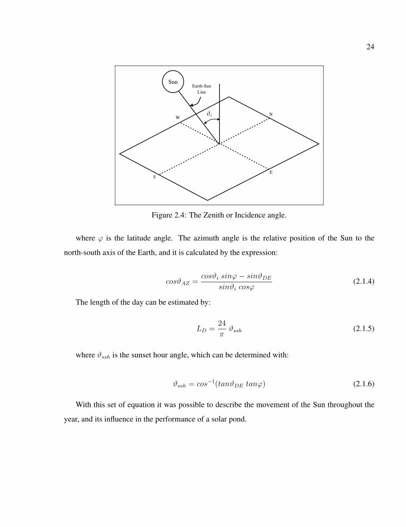
The zenith angle or incidence angle is the angle of the Sun relative to a line perpendicular to the
surface of the Earth at the observer location (Figure 2.4) and it is calculated with the expression:
cosϑi = cosϑDE cosϕ cosϑHA + sinϑDE sinϕ (2.1.3)
24
SunEarth-Sun
Line
N
SE
W
Figure 2.4: The Zenith or Incidence angle.
where ϕ is the latitude angle. The azimuth angle is the relative position of the Sun to the
north-south axis of the Earth, and it is calculated by the expression:
cosϑAZ =cosϑi sinϕ− sinϑDE
sinϑi cosϕ(2.1.4)
The length of the day can be estimated by:
LD =24
πϑssh (2.1.5)
where ϑssh is the sunset hour angle, which can be determined with:
ϑssh = cos−1(tanϑDE tanϕ) (2.1.6)
With this set of equation it was possible to describe the movement of the Sun throughout the
year, and its influence in the performance of a solar pond.

25
2.2. Radiation Absorption
Viskanta and Tabor (1978) proposed the following expression to quantify the solar radiation
absorbed by the solar pond:
QI(Z, t) =−dI(Z, t)
dZ(2.2.1)
where I(Z,t) is the direct radiation flux at depth Z of the pond and time t. This flux is a fraction
of the total incident on the surface. Wang and Akbarzadeh (1983) proposed the use of the Fresnel
Law of reflection for a smooth surface water body to calculate the portion of solar radiation that is
reflected back to the atmosphere as follows:
R =1
2
[sin2(ϑi − ϑr)sin2(ϑi + ϑr)
+tan2(ϑi − ϑr)tan2(ϑi + ϑr)
](2.2.2)
where ϑr is the angle of refraction, which can be obtained as follows (Rezachek, 1993):
sinϑr = 0.752 sinϑi (2.2.3)
The flux of solar radiation in the pond is attenuated by the effect of turbidity caused by algae
formation, by bottom and side wall reflectivity and propagation through the water layers. Ak-
barzadeh and Ahmadi (1980) summarized all the effects of radiation reduction factors in a coeffi-
cient of θ′ = 0.83 and Jaefarzadeh (2004) proposed the use of θ′ = 0.85 if the reflection is calculated
with equation (2.2.2), as shown in (2.2.5).
A penetrating flux of solar radiation into a body of water decays exponentially with depth, as
fluid layers absorb energy. The rate of decay (or transmissivity) in a solar pond was studied by
Rabl and Nielsen (1975) and proposed the following expression, function of the wavelength of the
radiation for the whole spectrum, to calculate it:
4∑j=0
ηcj exp
(−µcj Zcosϑr
)(2.2.4)
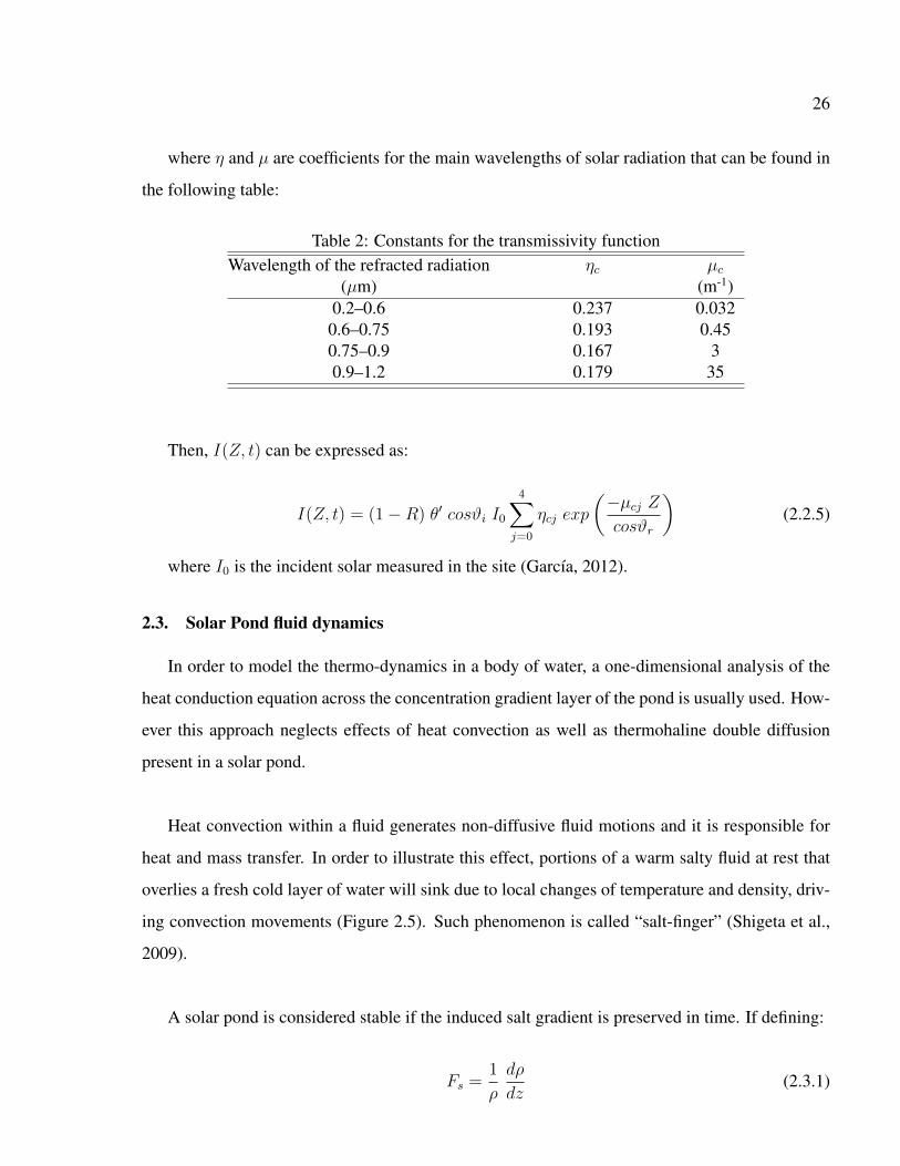
26
where η and µ are coefficients for the main wavelengths of solar radiation that can be found in
the following table:
Table 2: Constants for the transmissivity functionWavelength of the refracted radiation ηc µc
(µm) (m-1)0.2–0.6 0.237 0.032
0.6–0.75 0.193 0.450.75–0.9 0.167 30.9–1.2 0.179 35
Then, I(Z, t) can be expressed as:
I(Z, t) = (1−R) θ′ cosϑi I0
4∑j=0
ηcj exp
(−µcj Zcosϑr
)(2.2.5)
where I0 is the incident solar measured in the site (Garcıa, 2012).
2.3. Solar Pond fluid dynamics
In order to model the thermo-dynamics in a body of water, a one-dimensional analysis of the
heat conduction equation across the concentration gradient layer of the pond is usually used. How-
ever this approach neglects effects of heat convection as well as thermohaline double diffusion
present in a solar pond.
Heat convection within a fluid generates non-diffusive fluid motions and it is responsible for
heat and mass transfer. In order to illustrate this effect, portions of a warm salty fluid at rest that
overlies a fresh cold layer of water will sink due to local changes of temperature and density, driv-
ing convection movements (Figure 2.5). Such phenomenon is called “salt-finger” (Shigeta et al.,
2009).
A solar pond is considered stable if the induced salt gradient is preserved in time. If defining:
Fs =1
ρ
dρ
dz(2.3.1)

27
Figure 2.5: Incompressible Smoothed Particle Hydrodynamics (SPH) Simulation of the motion ina fluid at rest due to salt-finger phenomena (Shigeta et al., 2009).

28
as a factor of stability, with the depth z equal to zero at the bottom and positive upwards, it is
clear that the pond will remain stable if Fs < 0 at all time. Considering that in a solar pond, the
density at a certain depth z is a function of the salinity S and temperature T (Pande and Chaudhary,
1984). Then, applying the chain rule to the right hand side of equation (2.3.1) results:
Fs =1
ρ
dρ
dz=
1
ρ
[(∂ρ
∂S
)(∂S
∂z
)+
(∂ρ
∂T
)(∂T
∂z
)](2.3.2)
Therefore, it can be seen the stability condition (Fs < 0) is satisfied when:
∂T
∂z<β
α
(∂S
∂z
)(2.3.3)
where α is the thermal expansion coefficient and β is the salinity expansion coefficient (Ma-
maev, 1975), given by:
α =1
ρ
∂ρ
∂T
β = −1
ρ
∂ρ
∂S
2.3.1. Balance Equations
In order to predict the dynamic temperature distribution in the solar pond, balance equations
for the gradient layer as well as at singular faces at the bottom and sides of the pond were used. The
Navier-Stokes equations for incompressible fluids in 3 dimensions consist of 6 balance equations,
which can be solved numerically with the aid of suitable boundary and initial conditions.
The differential form of the general balance equation for an arbitrary physical quantity φ can
be derived by applying the Gauss theorem to the Reynolds transport theorem for an infinitely small
volume moving with a fluid (Henningson and Berggren, 2005), which results in:
∂
∂t(ρ φ) +
∂
∂xi(Ji) = Sφ (2.3.4)

29
where Ji represents the flux vector of the quantity φ and Sφ its external source. The flux vector
is composed of convection and conduction fluid motion components:
Ji = (ρ ui φ)convection + ξconduction (2.3.5)
where ξconduction is the non-convective flow. By substituting (2.3.5) in (2.3.4) results in:
∂
∂t(ρ φ) +
∂
∂xi(ρ ui φ) +
∂
∂xiξconduction = Sφ (2.3.6)
which is the expression used to obtain the balance equations by replacing φ with the relevant
physical quantities.
• Continuity equation
The continuity equation of mass for an incompressible fluid (∇·u = 0) is obtained by replacing
φ = 1 in (2.3.4), resulting in:
∂ρ
∂t+ ui
∂ρ
∂xi= 0 (2.3.7)
It can be noticed that the source term (Sφ) disappears since no mass can be generated.
•Momentum conservation
In order to obtain the momentum conservation equation of an incompressible Newtonian fluid
(with constant viscosity µ), φ in (2.3.4) is replaced by the components of convection velocity u as
follows:
∂
∂t(ρ uj) +
∂
∂xi(ρ ui uj) +
∂
∂xi(−σij) = ρ gj (2.3.8)
where g is the external accelerations vector due to gravity and σij is the simplified stress tensor
for a Newtonian fluid, and equal to:
σij = −p δij + µ (∂ui∂xj
+∂uj∂xi
) (2.3.9)

30
being p the pressure and δij the Kronecker delta. Replacing (2.3.9) in (2.3.8), considering that
the fluid is incompressible and simplifying the results gives this:
∂uj∂t
+ uj∂uj∂xi
=1
ρ
[∂
∂xi
(µ∂uj∂xi
)− ∂p
∂xi
]+ gj (2.3.10)
• Energy conservation
In order to obtain the energy conservation equation the quantity φ in (2.3.4) is replaced by the
internal energy Uint, the source term Sφ is replaced by the solar radiation flux I(z, t) derived in
(2.2.5), ξconduction by the conducting heat flux in the fluid (qi) and the continuity equation (2.3.7)
is also taken into account, resulting:
ρ∂Uint∂t
+ ρ ui∂Uint∂xi
+∂
∂xiqi = σij
∂ui∂xj
+∂I(x3, t)
∂x3(2.3.11)
being the direction coordinate x3 the z direction coordinate. The conducting heat flux can be
substituted by Fourier law of heat conduction:
qi = −k ∂T
∂xi(2.3.12)
where k is the heat conductivity of the fluid. Considering that in ideal fluids the variation of
internal energy is proportional to the change of temperature:
C∂T
∂xi=∂Uint∂xi
(2.3.13)
with C as the heat capacity of the fluid. Replacing (2.3.12) and (2.3.13) in (2.3.11) results:
ρ C∂T
∂t+ ρ ui C
∂T
∂xi=
∂
∂xi
(k∂T
∂xi
)+ σij
∂ui∂xj
+∂I(x3, t)
∂x3
(2.3.14)
• Salinity conservation
The vertical motion due to convection leads to salt migration to upper zones of the pond,
jeopardizing the insulating function of the salt gradient in the NCZ and therefore, the study of

31
salinity conservation in a solar pond is of most importance. Hence, another equation is added to
the set of balance equations, by replacing φ in (2.3.4) by the salinity S, which results in:
ρ∂S
∂t+ ρ ui
∂S
∂xi= − ∂
∂xi
(D ρ
∂S
∂xi
)+ si − s0 (2.3.15)
where D represents the coefficient of salt diffusion, si represents the incoming salt per time
unit of makeup brine required to maintain the salt profile and s0 represents the salt lost due to
surface evaporation or brine withdrawal.
32
3. NUMERICAL SOLUTION FOR A ONE-ZONE MODEL
The general mathematical model presented in the previous section was solved with the aid of
numerical methods executed with MatlabTM. Also, special assumptions specific for solar ponds
were used to simplify the Navier-Stokes equations solution.
The balance equations for the physical quantities have been derived for a 3 dimensional space,
necessary to describe phenomena like convective vortices that occur naturally when, for example,
a fluid is heated from below (like in a stove) which, at first, decreases its density locally. The con-
vective motions generated inside the fluid lead to very fast transport of mass and therefore ensure
that the salinity and temperature are distributed homogeneously throughout the fluid. However, in
solar ponds and in particular inside the non-convective zone these convective motions are coun-
tered by the presence of a salinity gradient that increases with depth. The transport of thermal
energy and salinity are then limited to diffusive motions, which occur over a much longer period
of time. This time scale makes possible the preservation of the salinity gradient by replenishing
the LCZ with salt at the same rate as it diffuses upward and maintain the functionality of a solar
pond.
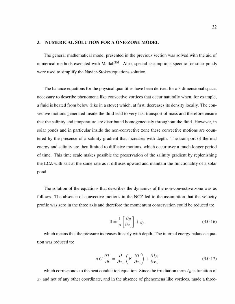
The solution of the equations that describes the dynamics of the non-convective zone was as
follows. The absence of convective motions in the NCZ led to the assumption that the velocity
profile was zero in the three axis and therefore the momentum conservation could be reduced to:
0 =1
ρ
[∂p
∂xj
]+ gj (3.0.16)
which means that the pressure increases linearly with depth. The internal energy balance equa-
tion was reduced to:
ρ C∂T
∂t=
∂
∂xi
(K
∂T
∂xi
)+∂IR∂x3
(3.0.17)
which corresponds to the heat conduction equation. Since the irradiation term IR is function of
x3 and not of any other coordinate, and in the absence of phenomena like vortices, made a three-

33
dimensional analysis unnecessary and therefore the problem was simplified to an uni-dimensional
analysis. Also, the salinity conservation can be written as follows:
∂c
∂t=
∂
∂xi
(D∂c
∂xi
)(3.0.18)
where c is the concentration of salt obtained with
c = S × ρ
The set of equation that describe the dynamics in the NCZ for an uni–dimensional analysis
with respect of the depth of the pond then becomes
ρ C∂T
∂t=
∂
∂z
(K
∂T
∂z
)+∂IR∂z
(3.0.19)
∂c
∂t=
∂
∂z
(D∂c
∂z
)(3.0.20)
The physical properties of sodium chloride brines were calculated with empirical correlations,
which are function of temperature and salt concentration (Jaefarzadeh, 2004):
C(c) = 4180 + 4.396 c+ 0.0048 c2 (3.0.21)
ρ(c, T ) = 998 + 0.65 c− 0.4 (T − 10) (3.0.22)
K(c, T ) = 0.5553− 0.0000813 c+ 0.0008 (T − 10) (3.0.23)
D(c, T ) = (8.16 + 0.255 T + 0.00254 T 2 − 0.00025 c)× 10−10 (3.0.24)

34
3.1. Boundary conditions
3.1.1. NCZ boundary conditions
As for the upper and lower convection zones, the salinity and temperature were considered
constant with respect to depth, based on the fact that thermal convective motions presence in
these layers tend to homogenize the salinity and temperature throughout the layers. To make
the numerical model representative of a three-zones solar pond, it was assumed that the UCZ
and LCZ acted as storage for salt and thermal energy and interacted with the NCZ by means of
specified boundary conditions. The absence of convective motions in the NCZ implies that the heat
transfer between this layer and the interfaces (UCZ-NCZ, LCZ-NCZ, sidewalls-NCZ) are only due
to conduction and can be described with the aid of Fourier Law of heat conduction. Therefore the
boundary conditions for the NCZ are as follows:
• NCZ-LCZ interface
KNCZ∂T (z, t)
∂z
∣∣∣∣z=δLCZ
= hLCZ [TLCZ(t)− TNCZ(z = δLCZ , t)] (3.1.1)
• NCZ-UCZ interface
−KNCZ∂T (z, t)
∂z
∣∣∣∣z=δLCZ+δNCZ
= hUCZ [TUCZ(t)− TNCZ(z = δLCZ + δNCZ , t)] (3.1.2)
where z = 0 at the bottom of the pond and positive upwards, KNCZ is the conductivity of the
NCZ, hLCZ , hUCZ correspond to the heat transfer coefficients of the LCZ and NCZ, respectively,
δLCZ , δNCZ and δUCZ corresponds to the thickness of the LCZ, NCZ and UCZ, respectively. The
values for hUCZ and hLCZ have been obtained from Sodha et al. (1981).
The boundary conditions used for mass transfer at the interfaces where proposed by Alagao
(1996), and are as follow:

35
•NCZ-LCZ interface
DNCZ∂c(z, t)
∂z
∣∣∣∣z=δLCZ
= ν ci (3.1.3)
where left hand side of the equation corresponds to the Fick’s Law of diffusion for the NCZ
characteristics and the right hand side is the rate of make-up salt injection expressed in terms of
brine velocity (ν) and brine concentration (ci). This implies that the LCZ is being replenished with
salt as it diffuses to upper layers.
•NCZ-UCZ interface
cNCZ,UCZ = cUCZ (3.1.4)
where cNCZ,UCZ is the concentration of the NCZ at the boundary with the UCZ, and cUCZ is
the concentration of the UCZ.
3.1.2. Solar pond boundary conditions
It was assumed that the interaction between the solar pond and its environment was by means
of heat transfer only, and therefore no salt was loss through any interface. The results of the energy
balances between the pond and the environment are as follow:
•Sidewalls heat losses
The heat loss through the sidewalls are given by:
Qs = KNCZ [TNCZ(z, t)− Tw] = Kw [Tw − Tg] (3.1.5)
where Tw is the mean temperature of the wall, Kw is the conductivity of the wall and Tg is the
temperature of the ground, far from the interface.

36
• Bottom heat losses
The heat losses through this interface are given by:
Qb = (1−Rb) ILCZ,b + hLCZ,b(TLCZ − Tb) = Kb∂T
∂z(3.1.6)
where Rb is the reflectivity of the bottom, ILCZ,b is the solar radiation that reaches that reaches
the bottom of the LCZ, hLCZ,b is the heat transfer coefficient due to natural convection for the LCZ
water-boundary interface and Kb is the thermal conductivity of the bottom.
•Surface heat losses
The heat loss through the of the solar pond consists of heat loss due to evaporation, black body
radiation and convection. The latter has been already considered in the balance equations, but to
account for the losses due to radiation and evaporation the following empirical models proposed
by Kishore and Joshi (1984) were used to represent the real behavior of the solar pond.
• Heat loss due to radiation
This empirical model assumes that the bottom of the solar pond acts as a black body and
therefore the surface of the pond will emit both short and long wave radiation, respectively. The
heat flow due to radiation can thus be described with the aid of the Boltzmann Law:
Qrad = ε σ (T 4s − T 4
sky) (3.1.7)
where ε is the emissivity of the surface, σ the Stefan-Boltzmann constant and TS is the surface
temperature of the pond. The atmospheric temperature Tsky was approximated with the following
correlation:
Tsky ≈ Ta (0.55 + 0.61√Pa)
14 (3.1.8)
where Ta is the ambient temperature and Pa is the partial pressure (in mm Hg) of water vapor
in the air.

37
• Heat loss due to evaporation
The heat loss due to evaporation was estimated with this expression (Mansour et al., 2004):
Qev =λ hc
1.6 Cs Pt(Ps − Pa) (3.1.9)
where, λ is the latent heat of evaporation of water, Cs the humid heat capacity of air, Pt the at-
mospheric pressure (in mm Hg). The wind convective heat transfer coefficient hc can be estimated
with:
hc = 5.7 + 3.8 Vw (3.1.10)
where Vw is the wind velocity at the surface of the pond. The vapor pressure (in mm Hg)
evaluated at the surface of the pond Ps is given by:
Ps = exp
(18.403− 3885
Ts + 230
)(3.1.11)
where Ts is the temperature of the surface of the pond. The partial pressure (in mm Hg) of
water vapor in ambient air Pa can be estimated with:
Pa = RH exp
(18.403− 3885
Ta + 230
)(3.1.12)
where Ta is the ambient temperature.
3.2. Numerical Modulation
In order to obtain a representative behavior of a solar pond at the site from the numerical model,
the simulation are run with weather data measured at the Spence mine. The data for temperature,
humidity, wind speed, evaporation and insolation corresponding to the year 2010 has been provided
(Garcıa, 2012) and used to realistically model the respective conditions. Since the weather data
available is for only one year, a periodic behavior has been assumed. A Fourier analysis was used

38
to generate continuous data from the discrete measurements and for each quantity the coefficients
of a fifth order Fourier expansion of the shape
Y (t) =5∑i=0
(aisin iωt+ bicos iωt) (3.2.1)
was computed and then fitted to the data, as presented in Figure 3.1 were the measured data
and the Fourier fit for ambient temperature.
Jan Feb Mar Apr May Jun Jul Aug Sep Oct Nov Dec0
5
10
15
20
Month of the year
Tem
per
ature
(ºC
)
Measured Data
Fitted Curve
Figure 3.1: Meassured data of ambient temperature for year 2010 and Fourier fitted curve.
The insolation has been modeled with the solar angles and length of day functions presented
in section 3.1 and modulated with discrete radiation measures taken in site2. The result is a model
able to generate continuous insolation data and to illustrate a Figure 3.2 shows the solar radiation
that reaches the surface of the pond for two different days of the year, one in summer and the other
in winter.
2Data provided by JHG Ingenierıa Ltda.

39
0
150
300
450
600
750
900
0 6 12 18 24
W/m
^2
Hour of the day
June 4thJanuary 1st
Sola
r Rad
iatio
n (W
/m2 )
Hour of the day
Figure 3.2: Solar radiation modeled for a summer and winter day.
3.3. Time and space mesh
To solve the partial derivatives of the mathematical model the finite differences method has
been chosen, due to its simplicity in implementation, particularly when the space grid and its
boundaries have no complex geometry like in a solar pond. The interior spatial derivatives were
solved using a second order, centered finite difference approximation as follows:
duidx
=ui+1 − ui−1
2 ∆ x+O(∆x2) (3.3.1)
At the interfaces, three point forward and backward approximations were used for the upper
and lower boundary, respectively as follows:
duidx
=−ui+1 + 4 ui − 3 ui−1
2 ∆ x+O(∆x2) (3.3.2)
duidx
=ui+1 − 4 ui + 3 ui−1
2 ∆ x+O(∆x2) (3.3.3)

40
This method approximates a partial differential equation by linear combinations of function
values for grid points. The more grid points used to calculate a derivative the higher the accuracy,
however, at a higher numerical costs. Therefore, the NCZ is discretized into N points (Figure 3.3)
whereby the results of the model of salinity and temperature are available only for these points.
The finite length corresponding to the non-convective zone is:
∆z =hNCZN − 1
(3.3.4)
UPZ
NCZ
LCZ
NCZ 1 2 3
ΔZ
i i-1
i+1
Figure 3.3: Discretization of the NCZ used for numerical resolution of the spatial derivatives.

41
Then, the derivative of a temperature array of N points, can be calculated with the following
matrix multiplication
∂T
∂z≈ 1
2∆z
−3 4 −1
−1 0 1 · · · 0
0 −1 0 · · ·...
...... . . . ...
0 1 0
0 −1 0 1
1 −4 3
T 0
T 1
T 2
...
T N-2
T N-1
T N
=∑i
Dij Ti (3.3.5)
being Dij the central difference derivative matrix. The heat conductive equation can then be
rewritten as:
∂Tk∂t
=1
ρk Ck
[∑j
Djk
(Kj
∑i
Dij Ti
)+ Ik
](3.3.6)
whereas the equation for salt concentration can be rewritten as:
∂ck∂t
=∑j
Djk
(Dj
∑i
Dij Ti
)(3.3.7)
For equations (3.3.6) and (3.3.7), the respective Neumann boundary conditions exist at the
upper and lower interface, which control the flow from the LCZ to the NCZ and from the NCZ
to the UCZ. It was assumed that both the LCZ and UCZ layers were constantly in motion due
to convection and therefore, mass and heat fluxes get equally distributed in the layer in a short
period of time, and therefore presented a uniform temperature and salinity profile. Numerically
both layers act as a storage whose capacity instantly changes as the influx changes. In order to
determine the flow,Fourier Law is used for the temperature, whereas Fick Law is used for the salt
concentration. With TLCZ and cLCZ as the temperature and salinity of the lower convection zone
respectively, the applicable boundary conditions are:
Q = KN+ 12
TN − TLCZ∆z
(3.3.8)

42
JR = DN+ 12
cN − cLCZ∆z
(3.3.9)
In order to study the evolution in time of concentration c and temperature T in the NCZ, the
time derivatives in the balance equations (3.0.19) and (3.0.20) have to be solved and integrated for
each discretized point of the NCZ. To do so, the explicit Runge–Kutta of fourth order method (also
known as RK4) has been chosen:
∂T
∂t=
1
ρ C
[∂
∂z
(K
∂T
∂z
)+∂IR∂z
]= f(c, T, t) (3.3.10)
∂c
∂t=
∂
∂z
(D∂c
∂z
)= g(c, T, t) (3.3.11)
The method executes the following steps at each grid point, for a time step ∆t
αi = f(cni , Tni , t)
εi = g(cni , Tni , t)
βi = f(cni +εi2, T ni +
αi2, t+
∆t
2)
εi = g(cni +εi2, T ni +
αi2, t+
∆t
2)
γi = f(cni +εi2, T ni +
βi2, t+
∆t
2)
ζi = g(cni +εi2, T ni +
βi2, t+
∆t
2)
δi = f(cni + ζi, Tni + γi, t+ ∆t)

43
ηi = f(cni + ζi, Tni + γi, t+ ∆t)
And the evolution in time of T and c are given by:
T n+1i = T ni + ∆t
1
6(αi + 2βi + 2γi + δδi) (3.3.12)
cn+1i = cni + ∆t
1
6(εi + 2εi + 2ζi + ηi) (3.3.13)
The evolution in time of these quantities is complemented with the study of the stability in the
NCZ using the criteria presented in (2.3.3).
3.4. Model validation
In the absence of empirical data obtained from a pilot, the validation was carried out with op-
erational data measured in 1982 of a 232 m2 solar pond at the Los Alamos National Laboratory,
whose objective was to study pond hydrodynamics with the aid of an underwater pyranometer.
The pond was built in a ground whose geology is composed of a soft volcanic rock known as tuff,
which has an approximate thermal conductivity of λ = 0.05 W/m2C. The layers thicknesses were
of 1.2 m for the LCZ and a salinity of 22%, whereas the NCZ and UCZ a thickness of 1.2 m and 0.1
m respectively. On the other hand, initial water temperature and makeup water temperature were
measured at about 25◦C (Jones et al., 1983). Because the performance of a solar pond depends
directly on weather conditions, such data was also required to recreate the behavior of the solar
pond with the model. However, only incomplete records for the year 1982 were found and so,
weather data from the year 1985 (Weather Underground, 2012) and historical insolation records
(Morris et al., 1985) were used in the simulation instead.
The temperature evolution record in the lower convective zone of the solar pond started on Au-
gust 4th, which was the day after the gradient zones was formed and ended on October 17th, hence
sets the time frame for the simulation. The radiation attenuation factor (θ′) was set to 0.8, a value
that has been used to model ponds of similar characteristics (Jaefarzadeh, 2004). The numerical

44
results were then compared to the experimental ones (Figure 3.4) from which it could be observed
that the model did indeed provide reasonably accurate results.
60
70
)R2 = 94.3%
RMSD = 1.476
MPE = -2.5%
40
50
Tem
pera
ture
(°C)
experimental
20
30
10 20 30 40 50 60 70
Time (days)
numerical
R2 = 94.3%
RMSD = 1.476
MPE = -2.5%
70
60
50
40
30
2010 20 30 40 50 60 70
Time (days)
Tem
pera
ture
(ºC
)
Experimental
Numerical
Figure 3.4: Comparison of the simulated and measured LCZ temperature evolution of the solarpond built at El Paso National Laboratory
In addition, the evolution of the entire temperature profile for the three layers were also esti-
mated and compared (Figure 3.5). Even though the numerical results resemble the actual salinity
profile, discrepancies in the LCZ and UCZ were observed. The fact that numerical results were
considered for the noon, whereas the factual time of measurement is unknown and that the sim-
ulation was run with weather data different of 1982 can explain the the divergences for the UCZ
temperature, which is strongly influenced by the ambient temperature. The deviation of in the LCZ
can be attributed to a higher solar radiation penetration than presumed or to deviation from perfect
black body behavior at the bottom.
3.5. Model restrictions
The one zone model presented is able to simulate conductive and radiation absorption processes
over a long period of time and can approximate heat losses and heat extraction. However, next
to linearization, discretization and averaging several other assumptions and simplifications were
made to formulate the theory and they are as follows:

45
0.0
10 20 30 40 50 60
Temperature (°C)
R2 = 95.0%
RMSD = 2.155
1.0
0.5
Dep
th(m
)
RMSD = 2.155
MPE = -3.1%
2.0
1.5Dep
th
experimental
numericalnumerical
2.5
10 20 30 40 50 600.0
0.5
1.0
1.5
2.0
2.5
Temperature (ºC)
Dep
th (m
)
R2 = 95.0%RMSD = 2.155
MPE = -3.1%
Experimental
Numerical
Figure 3.5: Predicted and recorded temperature profile of Los Alamos solar pond on September3rd
• No vertical fluid motion exist inside the non-convective zone.
• Infinitely fast homogenization inside the convective layers (time steps ∆ t>>1 s), therefore
temperature and salinity profiles are constant in such regions.
• The boundaries between the convective and not convective layers do not move, therefore the
NCZ does not grow with salt diffusion. This is equivalent to assume that perfect maintenance
to the gradient is performed.
• The bottom of the solar pond behaves like a perfect black body, and therefore no radiation is
reflected back to the water body.
• Modulation of density, diffusivity, conductivity and heat capacity are valid for temperatures
ranging from 5 to 100◦C and salinity ranging from 0 to 25%.
• The heat exchanger tubes extract heat equally throughout the lower convective zone, and
therefore no horizontal gradients occur.
• Because the model is uni-dimensional, the effect of walls could not be included. However,
if the surface of the bottom of the solar is large compared to surfaces of the sides of the pond

46
and therefore the heat losses through this interface are small compared to those through the
bottom.
The time step has been set to 1 hour to ensure numerical stability and homogeneous distribution
of temperature and salt concentration in the convective layers. As a result events in shorter periods
of time cannot be described. Also, during times when there is no heat withdrawal, temperatures in
the storage zone can raise above 100◦C at which, the model becomes unreliable.
Improvements for the model would be the implementation of side walls, which would lead to
additional heat losses and the separate investigation of convective motions, in order to determine
the degree of homogenization and its effect (degradation) on adjacent interfaces.

47
4. DESIGN PARAMETERS
In this section, different parameters regarding to site conditions that condition performance as
well as considerations for a proper maintenance and operation of a solar pond are reviewed in order
to provide a design that addresses their effect.
4.1. Site Selection
There are parameters that make a site suitable to place a solar pond that should be considered.
Solar ponds are a low energy density technology and therefore require of large areas. Knowing
this, it should be situated on a land with no other potential uses, namely low mineral importance
and relatively sterile. It should also be as flat as possible in order to maintain land-works to a min-
imum. The underlying geophysical structure should be homogeneous and free of stresses, strains
and fissures. Special attention should be put into the latter, for temperature increase caused by the
solar pond will lead to differential thermal expansions that can result in earth movements (Tabor,
1980).
At a certain depth below the solar pond exists an underground region where the soil or rocks
are permanently saturated with water due to the presence of underground waters, which is known
as water table. The presence of underground waters not only represents a threat of accidental
pollution due to leakage but also it has been noticed that this layer acts as a heat sink that lowers
the thermal performance of the solar pond. Saxena et al. (2009) studied the effect of the depth of
the water table on the thermal performance of a solar pond, and noted that the deeper the water
table is, the higher the temperature achieved in the LCZ but does not affect the time that takes to
the solar pond to achieve its maximum operational temperature.
4.2. Solar pond walls
Usually solar ponds are not built by digging out the whole volume of earth, unless they are
very small solar ponds, but instead they are constructed by flattening the ground with conventional
land-machinery and the removed earth is used to build the walls, generally with an angle to avoid
the use of wall supports and to facilitate the digging for the machinery because they can easily go

48
0 5 10 15 20 25 30 35 40115
120
125
130
135
140
Max
imum
tem
pera
ture
(ºC
)
Depth of water table (m)
45 50 55
Figure 4.1: Effect of depth of water table on maximum temperature of salt gradient solar pond(Saxena et al., 2009).
in out of the excavation site, reducing the associated costs (Tabor, 1981).
Experience gained in experimental solar ponds show that walls can be a source of instability
in solar ponds. Akbarzadeh (1989) observed that solar pond walls heated by insolation, after a
period of time, generate convective layers on its surface (Figure 4.2) product of horizontal density
and temperature gradients. These gradients would then cause variations of pressure spreading the
convective layers horizontally through the pond and hence enhancing the upward salt transfer and
therefore resulting in faster erosion of the salt gradient (Akbarzadeh, 1988).
In further studies, Akbarzadeh and Golding (1992) studied the influence of wall angle in the
stability of the salt gradient and described its effects. To do so, they defined the normalized radia-
tion on the inclined wall (NRI) as a measure of the enhancement of the flux of solar radiation that
reaches the inclined wall by deviation from the vertical, which is written as:
NRI =qiqv
= sinψ + cosψ
√n2
sin2ϑi− 1 (4.2.1)
where ψ is the inclined wall angle with respect of the horizontal (Figure 4.3).

49
Wall
Convective layer
Figure 4.2: Convective layer generated due to wall heating by Sun exposition (Akbarzadeh, 1989)
Akbarzadeh and Golding (1992) noticed that most of the values of equation (4.2.1) are greater
than one, and therefore concluded that any deviation from the vertical enhance the absorption of
solar radiation by the wall.
Figure 4.3: Scheme of angles used to calculate the NRI
Previously, Chen and Skok (1974) studied the effect in the stability of the temperature differ-
ence of a wall and a stratified fluid, concluding that for the same temperature difference the system
becomes more stable as it deviates from the vertical, mainly to an attenuated effect of gravity.

50
Considering the fact that this effect opposes the effect of the absorbed radiation at the surface of a
slopping wall, Akbarzadeh and Golding (1992) defined the normalized instability potential (NIP)
that combines both effects as follows:
NIP = NRI × sinψ (4.2.2)
where sinψ is the the effect of the slope on improving the stability by reducing the gravity
along the inclined wall. Combining (4.2.1) and (4.2.2) results in:
NIP =
(sinψ + cosψ
√n2
sin2ϑi− 1
)sinψ (4.2.3)
The NIP then can be used as a parameter to compare an inclined wall with a vertical wall and
its potential effect of destabilization. They also noted that (4.2.2) maximizes when:
ψ =1
2arctan
(−
√n2
sin2ϑi− 1
)(4.2.4)
and can be therefore considered as the wall angle of least stability and must be considered in
the design of a solar pond. It is important to mention that this angle varies with respect of the local
latitude (ϕ), starting with about 54◦ in the equator and decreasing to 45◦ for a latitude of 23.45◦
(Figure 4.4).
4.3. Bottom and wall lining
The main function of the lining system in a solar pond is to prevent the leakage of hot brine
between the LCZ and the ground soil, which would result in the loss of heat and salt as well as
groundwater contamination. The materials used for such purpose then have to be robust, imper-
meable, resistant to UV radiation, tolerant to temperatures up to 90◦C and to aggressive aqueous
media such as brine near saturation. Most of the experimental solar ponds built so far have relied in
the use synthetic liners such as high density polyethylene (HDPE), Hypalon, interpolymer alloys
(such as XR-5) (Raman and Kishore, 1990) and propylene which can also be found in landfills and
water containments. The estimated lifetime of these geomembranes is of approximately 20 years
under temperatures of up to 160◦C and high insolation; however, a lining used at El Paso solar pond

51
10 20 30 40 50 60 70 80 90
5
0
10
Wall angle ( )
NIP
25º
20º
15º
10º0º
50º
40º
30º
Figure 4.4: Variation of yearly maximum NIP as a function of wall angle for different latitudes(Akbarzadeh and Golding, 1992)
consisting of a cover layer of XR-5 and Hypalon layer, failed after 7 years of operation when hun-
dreds of holes where found due to an increased brittleness in the material. The liner was replaced
by a polypropylene (PP) layer which was used until the end of the project, in 2003 (Lu et al., 2004).
An important disadvantage of the synthetic liners is their high cost, that in the case of El Paso
solar pond, accounted for 26% of the initial investment (Raman and Kishore, 1990). Hence, new
inexpensive and effective lining techniques needed to be developed for the construction of larger
solar ponds such as the Beith Ha’Arava, where a scheme consisting on polyethylene layers in a
“sandwich” filled with locally available compacted clay (Tabor and Doron, 1990) was used. This
new lining method reduced the cost per square meter from the US$ 42 spent in previous projects to
only US$ 12 3. This scheme has been improved by Kumar and Kishore (1999), which developed
a cost–effective system for a 6,000 m2 solar pond in Kutch, India (Figure 4.5). Such results moti-
vated the study by Silva and Almanza (2009), who analyzed in depth the performance of several
31990 dollars in present value

52
types of compacted clays (CCL) under solar pond conditions, and concluded that some can be
impermeable enough to work even without a synthetic layer, whereas others where not suitable for
lining. The attractiveness of clay liners, however, underlies mostly in the cost of the material which
is very site-specific, being cheap if available nearby and expensive if not (ANCID, 2004), for they
are difficult to build, have to be thicker and require more land work than using geosynthetic mem-
branes (Silva and Almanza, 2009). Clays have also been used in geosynthetic clay liners (GCL),
which are a mixture of clay and synthetic membranes that are easy to install and are cost attractive.
They were tested also at El Paso solar pond, however with discouraging results due to low UV
resistance and manufacturing defects, failing only two years after its installation.
Figure 4.5: Lining scheme for solar ponds developed in India (Kumar and Kishore, 1999)
Some properties of lining materials and costs (material and installation) have been provided by
Garrido (2012b), senior engineer at Environmental Information and Logistic (EIL), LLC 4 (except
for the bentonite CCL) and are presented in Table 3.
4http://www.eilllc.com

53
Table 3: Properties of common materials used for solar pond liningMaterial Thickness k Permeability Cost
(mm) (W/m◦C) US$/m2
HDPE 1.5 0.46-0.52 – 5.2LDPE 1 0.3-0.34 – 3.2
Bontomat CL (GCL) 6.7 0.17 2.32 (cm s-1)×10−11 5.8Bentonite (CCL) 600 0.6 1.4 (cm s-1)×10−7 5-22 *
*Depending on availability (Silva and Almanza, 2009)
In certain cases, the lining not only works as a hydraulic barrier, but can also work as a thermal
insulation layer to reduce the heat losses through conduction between the LCZ and the ground.
This results useful in cases where the soil has a relatively high thermal conduction or the water table
is located near to the surface. Zhang and Wang (1990) studied the effect of adding an insulating
layer to a solar pond where the water table is located at 5.5 m below the bottom of the solar pond
and compared it to the same solar pond without thermal insulation and with a solar pond where
the water table is located 20.5 m below (Table 4). They noticed that the insulation layer not only
helped to increase the average temperature of the LCZ in almost 20 ◦C compared to the pond
without it, but also to reach a higher temperature to that of the solar pond with a lower water table.
Zhang and Wang (1990) proposed the inclusion of polystyrene foam (XPS) layers as insulation to
the lining, for its low thermal conductivity (≈ 0.035) and durability.
Table 4: Effect of adding an insulating layer to solar ponds close to the water table in the averagetemperature of the LCZWater table depth 20.5 m 5.5 m
Thermal Insulation No No 0.4 m XPSYears Average LCZ temperature (◦C)
1 68.3 66.2 82.22 93.6 84.0 102.83 98.4 84.4 103.04 100.7 84.5 103.25 102.0 84.5 103.3

54
The thermal performance of the lining insulation to be used solar pond can be assessed by
calculating the heat losses through the ground. To do so, firstly the overall heat transfer coefficient
has to be estimated as follows:
1
Ug=
1
hLCZ+
tiKi
+lsinkKg
(4.3.1)
where hLCZ is the heat transfer coefficient due to natural convection in the LCZ that research
by Sodha et al. (1981) determined to be 78,92 W/m2◦C. Also, ti corresponds to the thickness of
the insulation, Ki is the thermal conductivity of the insulation, lsink is the depth of the water table
and Kg is the thermal conductivity of the ground. Then, the heat losses through the ground per
square meter are given by:
Qg = Ug (TLCZ,t − Tsink) (4.3.2)
where TLCZ,t is the temperature of the of the LCZ at time t and Tsink is the temperature of the
water table.
4.4. Layers thickness
As mentioned before part of the solar radiation that reaches the surface of the solar pond is
absorbed, reflected back to the atmosphere and scattered by the UCZ and the NCZ before it can be
absorbed by the LCZ and be available for its extraction. Therefore, to collect the maximum amount
of energy it is necessary to let as much solar radiation as possible to reach the bottom. The thicker
the UCZ and NCZ are, the less solar radiation is absorbed by the LCZ (Peinan and Hongfei, 1994).
The presence of the UCZ at the top of a solar pond is product of wind mixing, penetrative con-
vection and the action of salt diffusion. This layer grows at expense of the NCZ thickness (FIgure
4.6), which reduces the conductive insulation hence increasing the heat losses to the atmosphere
(Punyasena et al., 2003). Also, about one third of the total solar radiation incident on the surface
of the pond is absorbed by this layer and then lost to the atmosphere, thus reducing the thermal
efficiency (Akbarzadeh et al., 1983). Then, it is desirable that the UCZ is kept as thin as possible,
preferably in the range of 5 cm (Tabor, 1980) and at a maximum of 20 cm (Shladow, 1984), by

55
counteracting the aforementioned phenomena.
Figure 4.6: Initial salinity profile (a) and growth of the UCZ (b) by the action of wind and rainregistered in a solar pond in Sri Lanka (Punyasena et al., 2003)

56
When the remnant energy is stored in the LCZ, part of it is scattered or lost through walls and
bottom, but if they are adequately insulated, then the heat is lost mostly by conduction through
the NCZ. If such is the case, the NCZ plays an important role as a thermal insulation layer, and
therefore cannot be too thin. Peinan and Hongfei (1994) proposed a method to optimize the size of
this layer to obtain a better thermal performance. By assuming that the initial temperature of both
the UCZ and NCZ equal to the ambient temperature, that the stratification of the layers is clear and
that the temperature within the NCZ increases gradually from top to bottom, they proposed that
the useful energy in the LCZ is:
Qu = p I0
[a− b ln
(δUCZ + δNCZ
cosϑI
)]−(k ∆T
δNCZ
)−Qw (4.4.1)
where, p is the average weighted coefficient of direct and diffuse irradiation, I0 is the average
surface solar irradiance,a and b are constants (a = 0.36, b = 0.08), δUCZ and δNCZ are the
thicknesses of the UCZ and NCZ respectively, ϑI is the refraction angle, ∆T is the temperature
difference between the ambient temperature and the objective temperature and Qw is the heat lost
by conduction through walls and bottom. By optimizing (4.4.1) with respect of δNCZ results:
dQu
dδNCZ=
−b p I0
δUCZ + δNCZ+k ∆T
δNCZ= 0 (4.4.2)
and solving:
δ∗NCZ = k ∆TΓ
2 b p I0
(4.4.3)
where Γ = 1 +√
1 + (4 x1 p I0/k∆t) and δ∗NCZ is the thickness of the NCZ that maximizes
the energy that penetrates through the layer below. As for the LCZ, this layer is responsible for one
of the distinguishing features of the solar pond, that is having a built-in seasonal energy storage
whose capacity is proportional to the thickness of this layer (Prasad and Rao, 1996). However, as
the LCZ consists of nearly saturated brine, an increase in the thickness of the LCZ increases the
salt requirements and hence the cost of the pond. Therefore the thickness of the pond should be
the minimum necessary to meet the energy requirements, considering energy losses. Also, the heat
withdrawal from this layer induces temperature variations that can lead to the erosion of the NCZ
if the LCZ does not have the adequate thickness. The end-use of the energy determines the heat

57
withdrawal pattern and the minimum acceptable temperature at the LCZ, whereas the maximum
temperature is limited by the boiling point of the brine (Prasad and Rao, 1996).
4.5. Salt gradient establishment
The salt gradient in the NCZ is the key element of a solar pond whose establishment is not
trivial. In earlier ponds, the gradient was established with a highly time demanding and expen-
sive technique, in which progressively less dense brine were superposed. This method required an
additional pond in which the batches of decreasing salinity were prepared and then pumped and
injected into the pond with a diffuser to avoid stirring of the layers that was usually suspended over
the pond or floating on the rising surface (Zangrando, 1980).
Zangrando (1980) proposed a simpler method that did not require additional mixing tanks or
ponds and that was suitable for solar ponds of any size. The procedure consisted basically in filling
partially the pond with high salinity brine and then inject fresh water at low speed with a diffuser
immersed in the upper portion of the brine, which progressively dilutes the brine above it creating
the gradient. Because the level of water increases in the pond, the diffuser has to be raised either
in a continuous motion or in discrete steps of 5 cm each (determined from experience) with such
timing that when the water reaches the desired level the diffuser reaches the surface.
An improved variation of this method was developed in 1995 at the El Paso solar pond named
”Scanning injection technique” (Lu et al., 2004), in which the diffuser, instead of staying fixed
in each step, it continuously goes up and down (scans) within a preset region during each step of
injection (scanning region). In this method, the steps are of 5 cm and the scanning region is set to
20 cm. The volume of fresh water injected in each step is determined by:
Vinj = (Vz)i
[cz,i − cz,fcz,f
](4.5.1)

58
where Vinj is the volume of fresh water added, cz,i is the initial concentration of the brine at
step z and cz,f is the desired concentration of the brine after the injection of water at step z.
At the El Paso solar pond, 990 t of salt were used to develop a LCZ of 120 cm with brine at
near saturation concentration and a NCZ of 150 cm thick in about one week. The water injection
was carried out in 30 steps (Table 5), in which the flow rate ranged from 7.6 to 9.5 l/s at a velocity
of 2.5 to 2.9 m/sec. The scanning speed of the diffuser was set to 10 cm/min for the downward
movement and 7 cm/min for the upward movement.
Table 5: Parameters used for Scanning injection technique at El Paso solar pondStep Scan Range Volume Injected Flow rate
(cm) (m3) (l/s)1 120–140 36.8 9.51 125–145 36.8 9.5. . . .24 235–255 41.8 9.125 240–257 45.4 9.126 245–259 41.6 9.127 250–261 47.1 8.228 260 47.4 7.629 265 49.1 7.630 270 Level of pond is completed adding water onto the top
Both the fixed level and scanning injection techniques have been used at El Paso solar pond,
which Lu et al. (2004) compared and concluded that the scanning injection technique is able to
create a smoother gradient, with less labor and in 50% of the time. Therefore, the latter is the
method that should be used to construct the gradient.
The diffuser has also been subject of improvement at El Paso solar pond. Prior to 1995, the
design of diffusers consisted of two circular plates with a small gap between them (Figure 4.7),
however this type of design had difficulties when placed near the banks or the instrumentation
tower. The new technique for the construction of the salt gradient also considered an improved
design of PVC diffuser (Figure 4.8) of tubular shape with 12 slots from where the water exits at
a design velocity of 2.8 m/s and flow rate of 0.57 m3/min. The injection diffuser is driven by a

59
computer software controlled DC motor and a drum-cable system (Lu et al., 2004).
Figure 4.7: Circular diffuser design (Leblanc et al., 2011)
Figure 4.8: Diffuser design used in the El Paso solar pond (Lu et al., 2004)
4.6. Salt and water
In principle, any inorganic salt can be used to establish the density gradient in a solar. However,
aspects such as cost, availability, pollution risk and solubility without significant solar radiation at-
tenuation limit the range. Therefore, most solar ponds are built in places where water and salt are
already available. Such is the case of the El Paso solar pond that used salt from an underground
salt mine used to store nuclear wastes and the Beith Ha’Arava solar pond was filled with Dead Sea
compounds (Mehta et al., 1988). The most commonly used salts are sodium chloride (known also
as common salt) and magnesium chloride obtained from the evaporation of seawater (Kaushika,
1984). Hassairi et al. (2001) studied the use of natural brines and compared its performance against
a sodium chloride solar pond, noticing that the latter had a better thermal performance.

60
4.7. Heat extraction
In a solar pond, the heat is usually withdrawn from the LCZ and this has been achieved with
two different approaches. In the first one, hot brine is pumped out of the LCZ, circulated through a
heat exchanger and then pumped back at a lesser temperature into the lower layer. In the second, a
heat exchanger is placed inside the LCZ, hence known as internal heat exchanger (IHE), in which
a cold flow (usually of water) is passed through and heated up. Alternatively, the flow can be
circulated through the IHE and a secondary external heat exchanger in a closed loop configuration
to heat up a different cold flow (Appendix B.1). The brine withdrawal approach was used at the
El Paso solar pond and the second is currently used at the Pyramid Hill solar pond (Leblanc et al.,
2011).
Based on the experience of a solar pond built in Miamisburg, OH that employed both ap-
proaches in two stages of operation, Sabetta et al. (1985) identified the main problems of each.
The hot brine withdrawal requires heat transfer equipment withstand corrosion, which can signifi-
cantly increase the cost of the system (twice the cost of an in-pond heat exchanger). Secondly, the
extraction of hot brine has to be carried out at low velocities to avoid the erosion of the NCZ for
which large diffusers are used. However, at the Miamisburg solar pond, it was found that most of
the flow was suctioned within the inital 10% of the dffuser pipe length, resulting in much larger
than predicted velocities and constant gradient erosion.
With regard to the internal heat exchanger Sabetta et al. (1985) indicate that the IHE is subject
to corrosion and therefore commonly used materials for heat transfer cannot be used. For main-
tenance and repairing, the internal heat extraction may have to be removed, rendering the solar
pond useless. This method can also generate a non uniform temperature distribution in the UCZ
if the solar pond is large compared to the IHE. The main advantage of the IHE over the hot brine
withdrawal is that it has a negligible effect on the gradient stability and therefore (Sabetta et al.,
1985) suggest that the employment of the internal heat exchanger is preferable if corrosion and
maintenance issues can be avoided, no matter the size of the solar pond.

61
To avoid all of the aforementioned issues of an internal heat exchanger, the IHE used at the
Pyramid Hill solar pond was entirely made of polyethylene, whose low thermal conductivity was
compensated with a larger heat transfer area. As it can be seen in Figure4.9, it consists of a dis-
charge manifold that distributes a water flow to a mesh of evenly separated tubes that transversely
crosses the pond, right below the NCZ-LCZ interface to facilitate convection, and connects to a
return manifold that collects the hot water (Leblanc et al. (2011)).
Figure 4.9: In-pond heat exchanger (IHE) used at Pyramid Hill (Leblanc et al., 2011)
To design an IHE that withdraws the heat from the LCZ at temperature TLCZ , and raise the
inlet temperature Tin of a constant mass flow to an outlet temperature Tout, first the heat exchange
rate between the LCZ and a differential volume of the tube has to be characterized as follows:
dQ = UHX (TLCZ − T ) dAs,HX (4.7.1)
where Uhx is the overall heat transfer coefficient, dAHX is the infinitesimal surface area of a
tube that composes the IHE. As a result, the temperature of the fluid inside the tube will increase
its temperature as follows:
UHX dx pc,HX (TLCZ − T ) dt = dx Ac,HX ρ C dT (4.7.2)
where dx is an infinitesimal length of one of the tubes that composes the IHE, pc,HX and
Ac,HX are the cross section perimeter and area of one of the tubes respectively whereas ρ and C

62
are the density and specific heat of the fluid inside the tube. The left hand side of equation (4.7.2)
corresponds to the heat that goes into the infinitesimal section of the tube during dt whereas the
right hand side corresponds to the increase in the energy of the flow in the section during dt.
Rearranging equation (4.7.2) it gives:
d(T − TLCZ)
T − TLCZ=UHX pc,HXρ C Ac,HX
dt (4.7.3)
Integrating equation (4.7.3), it yields:
lnT (t)− TLCZTin − TLCZ
=UHX pc,HXρ C Ac,HX
t (4.7.4)
Isolating T(t) in equation (4.7.4), results:
T (t) = TLCZ − (TLCZ − Tin) exp
(− UHX pHXρ C Ac,HX
t
)(4.7.5)
Equation (4.7.5) provides the temperature of the pumped water in the tube over time. Using it
to replace T in equation (4.7.1), the resultant equation yields the energy transfer as follows:
dQ = (TLCZ − Tin) exp
(− UHX pHXρ C Ac,HX
t
)UHX pHX dx (4.7.6)
Assuming that the mass flow moves at a constant velocity W = x/t through a heat exchanger
composed by N tubes equation (4.7.6) gives:
dQ = (TLCZ − Tin) exp
(− UHX pHXW ρ C Ac,HX
x
)UHX pHX dx (4.7.7)
Integrating equation (4.7.7) through the length of the tube results:
Q = W Ac,HX ρ C (TLCZ − Tin)
(1− exp
(− UHX pHX L
W AcHXρ C
))(4.7.8)
where L is the length of a single tube. The surface area of each tube corresponds to As,HX =
pHX L and m = W Ac,HXρ . Equation (4.7.8) can be re written as:
Q = m C (TLCZ − Tin)
(1− exp
(−UHX As,HX
m C
))(4.7.9)

63
Equation (4.7.9) provides the energy extracted from the LCZ by one tube. If the IHE is com-
possed by N tubes, then m corresponds to the Nth part of the total mass flow that has to be heated
up, namely the water used to wash cathodes.
The outlet temperature of the flow is then calculated with
Tout = T (L/W ) = TLCZ − (TLCZ − Tin) exp
(−UHX As,HX
m C
)(4.7.10)
And the required heat exchange surface area to achieve Tout is given by:
As,HX =m C
Uln
(TLCZ−TinTLCZ − Tout
)(4.7.11)
The overall heat transfer coefficient (UHX) is given by
1
UHX=dedi
(1
hi
)+
de2 KHX
ln
(dedi
)+
1
he(4.7.12)
where hi is the heat transfer coefficient due to forced convection inside the tube, de and di are
the external and internal diameters of the tube and KHX is the conductivity of the tube and he is
the heat transfer coefficient due to natural convection outside the tube. The determination of hi
depends of the geometry of the tubes and type of flow, namely laminar or turbulent and are given
by:
h =Kw
diNu (4.7.13)
whereKw is the conductivity of the internal flow andNu is the Nusselt number, whose calcula-
tion varies with the type of fluid. For laminar flow it can be assumed that Nu = 3.66 (Jaefarzadeh,
2006) whereas for turbulent flow the Nusselt number can be calculated with the Dittus-Boelter
correlation:
Nu = 0.023 Re0.8 Pr0.4 (4.7.14)

64
where Re is the Reynolds number, which is given by:
Re =ρw v diµw
(4.7.15)
and Pr is the Prandtl number, calculated with:
Pr =Cw µwKw
(4.7.16)
where ρw is the density, v is the mean velocity, µw is the dynamic viscosity and Cw is the
specific heat of the fluid running inside the tube that in this case is water. To calculate he, the
following correlation for a long pipe under external natural convection is used (Kern, 1950):
he =0.53 KLCZ
de
[(d3e ρ
2LCZ,f g β (Tw − TLCZ)
µ2LCZ,f
) (C µLCZ,fKLCZ
)](4.7.17)
where KLCZ is the thermal conductivity ρ is the density, g is the gravity acceleration, β is the
volumetric expansion coefficient,ν is the kinematic viscosity, α is the linear thermal expansion
coefficient, Tw is the temperature of the external wall of the tubes and the subscript “LCZ, f”
means that the properties are evaluated for LCZ brine at film temperature. The film temperature is
the defined as:
Tf =Tw + TTLCZ
2(4.7.18)
As mentioned above, corrosion represents a major threat for the IHE. Hence, they are usu-
ally designed with materials resistant to saturated brine at moderately high temperatures such as
polypropylene (PP) or polyethylene (PE) compounds (Leblanc et al. (2011); Sabetta et al. (1985)).
These materials are usually used for piping and not for heat exchange and hence the low thermal
conductivity of PP (0.22 W/m ◦C) and PE (0.38 W/m ◦C) (Simona AG, 2011a), which results in
large heat exchange areas and proportionally large lengths of tubes. Table 6 shows the cost per
meter of pressure tubes made of PP-H AlphaPlus R© (Simona AG, 2011b) and PE-100 (Simona AG,
2011a) for various commercial diameters and thicknesses:

65
Table 6: Cost per meter of PP and PE tubesPP-H AlphaPlus R© PE-100
Diameter Thickness US$/ m Thickness US$/ mmm mm mm
32 1.8 3 1.9 2.650 2.9 4.8 3 3.975 4.3 10.2 4.5 7,090 5.1 14.3 5.4 9.1
From Table 6, both the PE and PP have been used in in-pond heat extraction systems with good
results, but PE-100 not only has a 72% higher thermal conductivity than the PP-H but from Table
6 it can be noticed that it is also cheaper, making it more suitable for the purpose of the solar pond
and is therefore chosen for the design.
4.8. Water circulation power
To circulate the water through the heat extraction system it is necessary to use a pump to over-
come the pressure loss due to friction inside the tubes and intake and discharge height differences.
The power required by the pump can be calculated as follows:
Pp =mcw wpηp
(4.8.1)
where ˙mcw corresponds to the water flow used to wash the cathodes, wp is the specific work of
the pump and ηp is the efficiency. The specific work of the pump can be calculated with (ASHRAE,
2009):
wp =∆pt + ∆p∆p
ρw(T )(4.8.2)
where ∆pt is the pressure loss due to the friction inside the tubes of the heat exchanger, ∆p∆p
is the pressure loss due to height difference between the intake and point of discharge and ρw(T )

66
is the density of the water flow inside the tubes at temperature T. The pressure loss due to friction
in a circular pipe can be calculated with the Darcy-Weisbach equation:
∆pt = ft
(LtDi
)ρw(T ) V 2
w
2(4.8.3)
where ft is the friction factor of the tubes, Lt is the length of the tubes composing each heat
exchanger, Di is the internal diameter of the tubes and Vw is the average velocity of the water
flow. The friction factor can be either determined with the Moody chart or calculated with the
Churchill equation, which is valid for any value of the Reynolds number and not iterative (Menon
and Menon, 2010):
ft = 8
[(8
Ret
)12
+ (A+B)−32
] 112
(4.8.4)
where the parameters A and B are calculated as follows:
A =
[2.457 ln
((7
Ret
0.9)
+ 0.27εtDi
)]16
B =
(37530
Ret
)16
where εt is the absolute roughness in the interior of the tubes and Ret is the Reynolds number
for the water flow inside the tubes, which is given by:
Ret =Di Vw ρw(T )
µw(T )(4.8.5)
where µw(T ) is the dynamic viscosity of water at temperature T. The pressure loss in the
discharge manifold can be calculated with (Green and Perry, 2008):
∆p =
(4fL
3D− 2K
)ρV 2
i
2(4.8.6)
where ∆p is the net pressure loss over the length of he manifold distributor, L is the length
of the manifold, D is the diameter of the manifold, f is the Fanning friction factor and Vi is the
manifold inlet velocity. The factor K represents the losses due to momentum recovery, which for

67
discharge manifolds is usually 0.5. The pressure loss in the return manifold can be calculated with
(Green and Perry, 2008):
∆p =
(4fL
3D+ 2K
)ρV 2
i
2(4.8.7)
For return manifolds, the factor K is usually very close to 1.
The pressure loss due to height difference between the intake and discharge point can be cal-
culated with the following relationship:
∆p∆p
ρw(T ) g= ∆z − 1
ρw(T )
(∆z
2[ρw(Ti) + ρw(To)]
)(4.8.8)
where g is he gravity acceleration, ∆z is the height difference between the intake and outlet
point, ρw(Ti) is the density of the water flow at intake temperature and ρw(To) is the density of the
water flow after being heated up.
4.9. Solar pond monitoring and control
The efficient operation of a solar pond requires the establishment of a density gradient of a
determined thickness, the maintenance of its stability, and the clarity of the brine and the early
detection and solution of any undesired phenomena so the performance of the pond can be kept as
predicted. It is therefore necessary to count with monitoring procedures for the measurement of
key parameters in the thermal performance of a solar pond such as brine clarity, temperature and
salinity distribution to estimate the shape of both the density and temperature gradients in order to
asses the stability of the pond with the criteria presented in (2.3.3)) in a regular basis by means of
reliable instrumentation.
One of the many developments achieved during the operation of El Paso solar pond was an
automated instrumentation system (Lu et al., 2004) that consisted of a DC motorized drum-cable
scanner with a sensor head and two thermocouples, a sample pump mounted on the deck of an in-
strumentation tower (Figure 4.10), an ”U” tube density meter, pH probe, turbidimeter and cooling

68
heat exchanger mounted on the same enclosure on the pond bank near the instrumentation tower.
This integrated configuration allowed the simultaneous measurement of temperature, salinity and
brine clarity for the entire depth of the pond in 3 hours.
The polypropylene sensor head (Figure 4.11) withdrew small samples of brine at each step and
flowed them through the cooling heat exchanger to decrease their temperature, before sending them
to the turbidimeter, density meter and pH probe. The thermocouples were aligned and mounted in
opposite sides of the scanner and provided of redundant information of the temperature. To ensure
a smooth downward movement and to avoid the buoyancy of the scanner in the high density brine
a counter weight was attached to the bottom of the sensor head.
Figure 4.10: Instrumentation tower at El Paso solar pond (Leblanc et al., 2011)
The measurement of salinity, pH and turbidity could be performed on a weekly basis, since
changes of these parameters occured very slowly. However, temperature measurement has to be
taken on a daily basis. The spatial steps for temperature and salinity measurement should be of 5

69
Figure 4.11: Scanner used for monitoring procedures at El Paso solar pond (Leblanc et al., 2011)
cm or less, in order to ensure a resolution capable of detect gradient breakdowns, whereas turbidity
should be performed in steps of 10 cm (Lu et al., 2004).
4.10. Solar pond maintenance
4.10.1. Salt gradient maintenance
The optimal operation of a solar pond requires measures to counteract the action of salt diffu-
sion in order to maintain the design thicknesses, concentrations of the layers and expected thermal
performance. If no maintenance is carried out to the gradient in the NCZ, the three layers stratifica-
tion and the salt gradient will eventually disappear, resulting in a pond filled with a homogeneous
brine without any of the characteristics of a solar pond (Figure 4.12). This is because of the mass
diffusion of the salt from the bottom to top, caused by both molecular and thermo diffusion tend
to homogenize or flatten the concentration profile of the pond (Angeli and Leonardi, 2005). The
phenomenon decreases the concentration in the LCZ and simultaneously increases the concentra-
tion in the UCZ, therefore in order to preserve the gradient in the NCZ the concentration in both
layers has to be re-established by adding salt or concentrated brine in the bottom and fresh water at
the top. The rate of this diffusion process depends on the molecular diffusivity of the salt, the salt
concentration gradient, and the induced mass eddy diffusivity, caused by surface waves or other
perturbations. Different rates of upward salt diffusion have been estimated and they can range
from approximately 27 to 200 g/m2 per day if the pond is located in an area subject to high wind

70
velocities (Akbarzadeh and Ahmadi, 1981).
Initial state
After 30 years
After 1 year
40
60
80
100
120
140
160
180
200C
once
ntra
tion
(kg
/ m3 )
Solar pond height (m)1.4 1.6 1.8 2.0 2.42.2
Figure 4.12: Evolution of salt concentration profile in a solar pond without maintenance after 1year and 30 years (Angeli and Leonardi, 2005).
To re-establish the concentration in both convective zones, there are two general approaches.
The first one considers the recycling of the extracted brine from the top of the UCZ by pumping
it back into the lower convective zone after a concentration process. The second implies that part
of the water from the UCZ is discarded after it has reached a certain concentration of salt and
replaced with fresh water, while new concentrated brine is added at the bottom convective zone
(Alagao et al., 1994).
Alagao et al. (1994) proposed a theoretical model to determine the size of the evaporation pond
required to concentrate the brine extracted from the top to be then re-injected at the bottom. To do
so, two main assumptions were made:

71
1. Volume flow rates and other parameters are taken as average values over a particular period.
Annual averages are preferred because of the extreme variation of some parameters like
rainfall and evaporation.
2. The system is assumed to undergo a steady state, steady flow process.
Figure 4.13 shows the flows associated with the operation of solar pond with a salt recycling
system for salt gradient maintenance, where Q1 is the make-up water in, Q2 is the water lost by
evaporation from the pond,Q3 is the rainfall over the solar pond in m3/year,Q4 is the overflow sent
to the evaporation pond, Q5 is the rainfall over the evaporation pond in, Q6 is the evaporation from
the evaporation pond and Q7 is the saturated brine injected at the bottom of the solar pond, being
all these quantities in m3/year, whereas C1, C4, C7 correspond to salt concentrations (kg/m3), Asp
and Aep are the areas of the solar pond and evaporation pond respectively in m2 and ST is the total
salt diffused from the bottom to top in kg/m2 per year.
Q2 Q3Q1
C1
ST
Q4, C4
Q7, C7
Q6 Q5
Asp Aep
Solar Pond
Evaporation Pond
Salt
Figure 4.13: Schematic of flows in a salt recycling system for gradient maintenance (Alagao et al.,1994).
To calculate the rate of make-up water Q1, first the volume balance over the solar pond has to
be considered, which yields:
Q4 = Q1 + (Q3 −Q2) +Q7 (4.10.1)

72
To maintain the salt balance in the SP, the amount of brine re-injected must equal the total salt
transport to the surface, which can be expressed as:
C7 Q7 = Asp ST (4.10.2)
Knowing that:
Q3 −Q2 = Asp (R− Esp) (4.10.3)
where R and Esp are rainfall and evaporation rates at the solar pond in m/year. Combining
(4.10.1), (4.10.2) and (4.10.3) gives:
Q4 = Q1 + Asp (R− Esp) +Asp ST
C7
(4.10.4)
The salt balance at the solar pond can be expressed as:
Q1 C1 +Q7 C7 = Q4 C4 (4.10.5)
Combining (4.10.1), (4.10.4) and (4.10.5) and rearranging gives:
Q1 = Asp
[ST
(1
C4
− 1
C7
)+ (Esp −R)
] [C4
(C4 − C1)
](4.10.6)
which corresponds to the volume of make-up water needed for a known SP size. Considering
that Esp = Vsp evap A−1sp , where Vsp evap is the total volume of water evaporated from the solar pond
in a year, and that if fresh water is used as make-up water (C1 = 0), (4.10.6) can be reduced to:
Q1 = Asp ST
(1
C4
− 1
C7
)+ Vsp evap (4.10.7)
It can be noticed that the expression (4.10.7) corresponds to the amount of water necessary to
compensate the evaporation in the solar pond and the fraction of water removed from the UCZ, sent
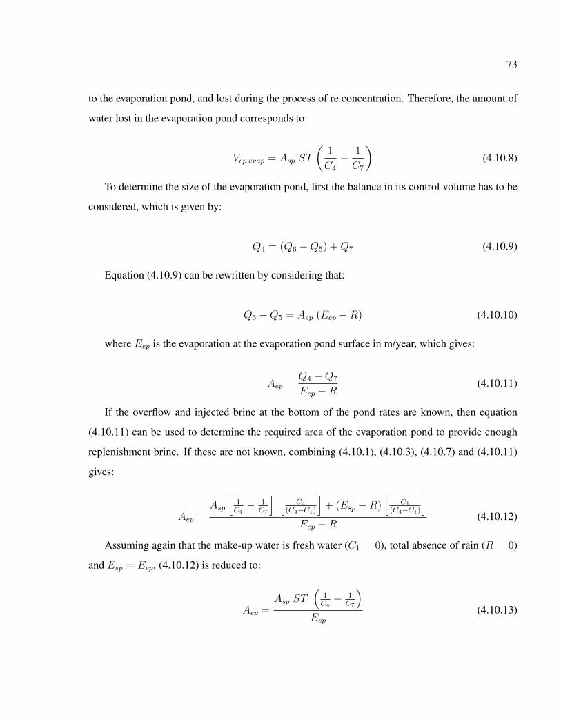
73
to the evaporation pond, and lost during the process of re concentration. Therefore, the amount of
water lost in the evaporation pond corresponds to:
Vep evap = Asp ST
(1
C4
− 1
C7
)(4.10.8)
To determine the size of the evaporation pond, first the balance in its control volume has to be
considered, which is given by:
Q4 = (Q6 −Q5) +Q7 (4.10.9)
Equation (4.10.9) can be rewritten by considering that:
Q6 −Q5 = Aep (Eep −R) (4.10.10)
where Eep is the evaporation at the evaporation pond surface in m/year, which gives:
Aep =Q4 −Q7
Eep −R(4.10.11)
If the overflow and injected brine at the bottom of the pond rates are known, then equation
(4.10.11) can be used to determine the required area of the evaporation pond to provide enough
replenishment brine. If these are not known, combining (4.10.1), (4.10.3), (4.10.7) and (4.10.11)
gives:
Aep =Asp
[1C4− 1
C7
] [C4
(C4−C1)
]+ (Esp −R)
[C1
(C4−C1)
]Eep −R
(4.10.12)
Assuming again that the make-up water is fresh water (C1 = 0), total absence of rain (R = 0)
and Esp = Eep, (4.10.12) is reduced to:
Aep =Asp ST
(1C4− 1
C7
)Esp
(4.10.13)

74
A similar model can be derived for the case in which the UCZ overflow is simply discarded
and new salt is added to compensate the diffused salt with the aid of Figure 4.14:
Q2 Q3Q1
C1
ST
Q4, C4
Q7, C7
Asp
Solar Pond
Salt
Figure 4.14: Schematic of flows for gradient maintenance without salt recycling (Alagao et al.,1994).
The rate of make-up water can be calculated by considering again the control volume balance
over the solar pond, which is:
Q1 −Q7 = Q2 +Q4 −Q3 (4.10.14)
By neglecting the rain (Q3 = 0) and expressingQ4 in terms of concentration, equation (4.10.14)
can be reduced to:
Q1 +Q7 = Vsp evap +Asp ST
C4
(4.10.15)
where the terms on the left hand side represent the total amount of make-up water required to
compensate for the water that has evaporated and the water that has been extracted. Therefore, the
extracted volume can be calculated as:
Vextracted =Asp ST
C4
(4.10.16)

75
The required salt to re establish the concentration in the LCZ is simply given by:
required salt = Asp ST (4.10.17)
The process of salt replenishment requires different equipment and procedures if the salt is
added as concentrated brine or if it is granular, no matter if the salt is recycled or not. If the salt
is to be added as brine, the same scanning injection system used to establish the salt gradient, has
been proved to be very effective to inject the brine with the diffuser and re establish the design-
concentration profile in the solar pond (Lu et al., 2004). Moreover, if the salt is to be added in
granular form, the use of salt chargers (Figure 4.15) distributed in the perimeter of the pond has
been proved to be efficient in maintaining the concentration and thickness of the LCZ by Jae-
farzadeh and Akbarzadeh (2002).
LCZ
UCZ
Gradient zone
Overflow
To waste
Salt charger
Salt
Figure 4.15: Schematic view of the pond with three zones, salt charger and surface washing systemused in RMIT solar pond, Melbourne (Jaefarzadeh and Akbarzadeh, 2002).
4.10.2. Wind effects
The thickness of the UCZ is another important factor that limits the efficiency of a solar pond.
This is because around one third of the solar heat that reaches the surface, is absorbed by this layer
and then dissipated back to the atmosphere, and the thicker this layer is, the more radiation it will
absorb rather than facilitating the LCZ heat collection. Therefore, it is desirable to maintain this
layer as thin as possible. The formation of this layer is mainly caused by two factors (Akbarzadeh
et al., 1983):

76
1. The absorption of solar radiation in the first few centimeters depth of the water causes a large
temperature gradient, which results in the development of a convective current. The depth
of this layer varies with the intensity of the solar radiation and therefore, decrements of up
to 50% in the thickness of the UCZ can be experienced between day and night.
2. Wind causes mixing in the top region of solar ponds whose action can be separated into two
effects: surface waves and wind-driven currents. Waves cause turbulence and induce eddy
diffusivity that erode the salt gradient in the NCZ, which in time may result in convection in
this region. Wind shear effect also generates currents at the surface that creates circulation
in the vertical plane resulting in layer mixing and erosion of the top surface of the density
gradient layer.
To counter the harmful effects of wind in the thickness of the UCZ and stability of the salt
gradient, the use of floating rings (Figure 4.16) as wave suppressors that reduce the fetching area
of wind, has been successfully tested in experimental solar ponds, in which the average thickness
of this layer decreased in 50% compared to the operation without the wind suppression system
(Akbarzadeh et al., 1983). Tang and Hassab (1990) also noted that the use of wind suppressors not
only helps to avoid the formation of wind-induced localized convective zones in he NCZ, but also
to overcome these perturbations. They carried out several experiments where artificially induced
convective layers were created in the gradient of a small solar pond with and without wind sup-
pressors. In the presence of the latter, the perturbations in the gradient were self-repaired after a
few days without any direct action by the operators.
4.10.3. Turbidity effects
Turbidity is another important factor in the thermal performance of a solar pond because it
reduces the penetration of solar radiation into the storage zone and high turbidity levels could im-
pede the storage of energy. Temperatures registered in a solar pond with significant presence of
turbidity (1 nephelometric turbidity units or NTU) are much lower than in a pond with clear wa-
ter (0.3 NTU) under same conditions of heat extraction (Figure 4.17) (Wang and Seyed-Yagoobi,
1995). This undesirable phenomena in a solar pond can be caused mainly by the growth of algae,

77
Figure 4.16: Wind suppressors installed at Pyramid Hill solar pond, Australia (Leblanc et al.,2011).
bacteria and the presence detritus. Therefore, in order to maintain the design efficiency of solar
radiation collection , monitoring and maintenance of the clarity of the pond is necessary.
In presence of phosphorus (P) and with increasing salinity, certain halotolerant species, such
as the Dunaliella can grow and subsist in a solar pond (however, cannot withstand temperatures
greater than 45◦C) (Sherman and Imberger, 1991). Common sources of P are water, soil, rocks
and also airborne sources, such as leafs, bird excreta and windblown dust and soil. So far, several
techniques to counter turbidity have been tested in working solar ponds. The main approach has
been the use of chemicals in order to make the brine incapable of sustaining any biological activity.
These chemicals methods include chlorination, coagulation/flocculation, precipitation, peroxida-
tion, algacide addition and acidification (Hull, 1990). Also, natural control methods have been
tested, such as the use of brine shrimps Artemia salina, which feed of algal population and detritus
and excrete dense fecal pellets that sink to the bottom of the pond. The growth and survival of the

78
Figure 4.17: Collection efficiency versus turbidity levels in a solar pond (Li et al., 2010).
shrimp population is influenced by temperature and salinity, commonly in the range of 19-25◦C
and 35-110 ppt respectively, and are therefore useful for turbidity control of the upper region of
the pond (Jaefarzadeh and Akbarzadeh, 2002).
While shrimps can control the growth of algae and maintain a reasonable transparency in the
solar pond, Hull (1990) proposes the use of alum (Al2(SO4)3) as phosphate control, in order to
completely avoid the occurrence of algae growth. Alum not only precipitates phosphate (in the
form of Al-P that is relatively sterile) without impairing the pond transparency but also its coagu-
lant effect increases the settling rate of suspended particles. After years of operation of the 1,000
m2 Argonne National Lab solar pond, IL, and the test of several combinations of chemicals for
clarity control with relative success, Hull (1990) found out that the use of modest doses of granu-
lated alum (< 5 g m-2 per year) in addition to chlorine (2.8 g m-2 per year) can effectively maintain
a transparency such that the bottom was easily visible below 4 m of brine throughout the year,
result that should be achievable in any sodium chloride solar pond.

79
4.11. Thermal efficiency
Beniwal and Singh (1987) define the thermal efficiency of a solar pond as the effective available
heat stored in the LCZ qeff over the average insolation I , which can be expressed as:
η =qeff
I(4.11.1)
The effective available heat is defined as the total absorbed heat by the LCZ minus the losses.
It can be expressed as follows:
qeff = (1−R) θ′ I − UL ∆T − Ug ∆T (4.11.2)
where R is the fraction of solar radiation reflected to the atmosphere, θ′ is the attenuation
factor given by turbidity and other effects, UL is the heat loss coefficient given by the losses by
the convective and radiation losses to the atmosphere, Ug is the heat loss coefficient to the ground.
Therefore, the equation 4.11.1 can be rewritten as:
η = (1−R) θ′ − ULg ∆T
I(4.11.3)
which resembles the Hottel-Whillier-Bliss equation for flat panel solar collectors. It can be
seen that the efficiency decreases when ∆T increases, and therefore it can be concluded that the
hotter the solar pond is, the less efficient it becomes.

80
5. CASE STUDY AND PROPOSED DESIGN
The design of a solar pond is as determined by the site conditions (i.e. solar radiation, ground,
wind, etc.) as by its purpose. This section is divided in two subsections; the first corresponds to the
case study, where the design parameters where evaluated under site conditions and according to
the energy demand of the cathode washing process at Spence. In the second subsection, a design
is provided.
With exception of the IHE design, all the values herein presented were obtained by means of
simulation routines carried out using MATLABTM that solved the numerical model presented in
Section 3, for various input parameters. The software provides “real time” information with a
graphic interface of the status of the simulated solar pond, such as temperature profile, salinity
profile, stability and also information related to the thermal performance or any other desired in-
formation (Figure 5.1).
The simulations assumed that the salt gradient is already formed at t = 0 (January 1st, at 12
pm) and therefore, did not consider the necessary time to establish it. Also, a two month period
was assigned to heat up the solar pond and therefore, no heat is extracted during that time. Due to
model restrictions, the thicknesses of the layers do not vary in time. This is equivalent to assume
that adequate maintenance is carried out and enough water was being supplied to make up for
evaporation and surface flushing as well as diffused salt was either being re-injected (if closed salt
loop is used) in the LCZ or replaced by new salt (open salt loop). Finally, all the simulations were
carried out taking care that the stability criterion (Fs<0) was fulfilled at all times.
5.1. Case study
5.1.1. Internal heat exchanger design
The working principle of the IHE to be used is similar to the one used at the Pyramid Hill
solar pond, namely the distribution of the flow with manifolds and passed through a mesh of tubes
located in the LCZ. In this case, the circulated fluid corresponds to the water used for the cathodes

81
0 50 100
1.5
2
2.5
Temperature NCZ
Temperature in °C
Z in
m
0 0.1 0.2
1.5
2
2.5
Salinity NCZ
Salinity in %
Z in
m
−0.1 −0.09 −0.08 −0.07
1.5
2
2.5
Stability
Fs (stable for Fs<0)Z
in m
0 500 10000
20
40
60
80Delivered heat: 19847.7583 MWh
time in days
Tem
pera
ture
of p
umpe
d w
ater
0 500 10000
0.1
0.2
0.3
0.4Efficiency
time in days
effic
ienc
y
0 500 10000
20
40
60
80
100Evaporated water: 324741.6296 tonnes
time in days
LCZ
Tem
pera
ture
in °C
Figure 5.1: Interface created to facilitate the supervision of the simulation runs.

82
washing, avoiding the need of secondary heat exchangers. The diameter and number of the tubes
that compose the mesh were analyzed in order to obtain a technically and economically efficient
IHE. Table 7 presents an IHE composed with a 20 PE-100 tubes mesh with different commercial
diameters and PE-100 manifolds of 125 mm of diameter:
Table 7: IHE composed by 20 tubes for different diametersDiameter Reynolds UHX Surface area Length per tube Cost Pressure drop
mm Number W/m2 ◦C m2 m US$ kPa32 22580 57.76 807 401 24,986 5350 14472 52.35 890 283 25,902 1575 9648 17.43 2673 567 83,031 12
The values presented in Table 7 were calculated for a constant flow of 21.45 m3/h and for a ∆
T of at least 48.2◦C. The pressure drop has been calculated considering the absolute roughness of
PE-100, equal to 7× 10⁻⁶ m and assuming that the discharge and return manifolds are at the same
height. It can be noticed that for a smaller diameter tubes (i.e. 32 mm), the required surface area is
smaller compared to the other options and hence cheaper. This is due to thinner tube walls and a
higher Reynolds number (faster flow) which results in a higher convective heat transfer coefficient.
However, a faster flow results and higher pressure drops. On the other hand, a larger diameter (i.e.
50 mm) reduces the length of each of the tubes, avoiding the need of complicated geometries (i.e.
coils) to fit the pond and the slower flow results in lesser pressure drops. However, if the diameter
is large enough (i.e. 75 mm) the Reynolds number falls into the transitional flow range (between
2,300 and 10,000), where the flow behaves randomly as turbulent or laminar (Cengel, 2003), the
heat transfer coefficient is considerably reduced and therefore the required heat exchange surface
area increases notably.
A different approach to reduce the flow velocity and thus the pressure drop, is by adding tubes
to the mesh instead of increasing the diameter. This would allow the conduction of heat through
thinner walls and therefore with a better overall heat transfer coefficient and a more uniform heat
withdrawal. Table shows the effect of a larger mesh of tubes of 32 mm of diameter:

83
Table 8: IHE composed by 20 tubes for different diametersNumber Reynolds UHX Surface area Length per tube Cost Pressure dropof tubes Number W/m2 ◦C m2 m US$ kPa
20 22580 57.76 807 401 24,986 5330 15054 57.16 815 270 25,205 2540 11290 56.61 823 205 25,410 1844 10264 56.40 826 187 25,509 1650 9032 17.43 1510 301 43,291 18
From Table 8 it can be seen that the even though the Reynolds number was decreased, it did not
affected significantly the overall heat transfer coefficient, and the pressure drop was diminished 3
times by using 44 tubes instead of 20. In comparison, the 44 tubes mesh and 32 mm of diameter
is US$400 cheaper than the 20 tube mesh and 50 mm diameter, each tube is 96 m shorter and the
overall heat coefficient is 8% higher. To compensate the pressure 18 kPa of pressure drop a power
of only 97 W is required. Based on these arguments, it has been decided that the 44 tubes mesh of
32 mm of diameter is the most suitable configuration among the aforementioned.
5.1.2. Determination of the layers thicknesses
In order to maximize the solar radiation absorption in the LCZ, the thickness of the UCZ should
be kept as thin as possible. Therefore, the simulations were run assuming a thickness, practical
to maintain in a solar pond (Jaefarzadeh and Akbarzadeh, 2002), of 20 cm. The thickness of the
NCZ was kept constant due to model restrictions and calculated using equation 4.4.3, the average
insolation throughout a year at Spence (215.3 W/m2) and the average weighted coefficient of direct
and diffuse irradiation (p) was calculated using data obtained from CNE et al. (2008) for the city of
Calama, which is the nearest city (62 km, north-east of Spence) with an available registry. Under
these conditions, the thickness of optimum NCZ thickness was found to be 1.8 m. On the other
hand, the determination of the LCZ thickness required an iterative process in order to find the one
that was able to store enough heat to deliver water in the desired range of temperatures. Table 9
presents the effect of the LCZ thickness on its average temperature as well as on its variability.

84
Table 9: Temperature range of the LCZ after the third year of operation for different thicknessesThickness 0.5 m 0.75 m 1 m 1.25 1.5
Min. T 63.5 ◦C 64.8 ◦C 66.0 ◦C 67.0 ◦C 67.8 ◦CAvg. T 75.8 ◦C 75.8 ◦C 75.8 ◦C 75.8 ◦C 75.8 ◦CMax. T 86.8 ◦C 85.7 ◦C 84.8 ◦C 83.9 ◦C 83.1 ◦C
It can be noticed that the thickness of the LCZ controls the amplitude of its range of tempera-
ture. A thicker LCZ takes longer to heat up and to cool down and therefore, the difference between
the extreme bounds of the range is smaller compared to that of a thinner LCZ. The effect of the
LCZ thickness on the outlet temperature of the HX is presented in Figure 5.2.
0
10
20
30
40
50
60
70
80
90
180
270
360
450
540
630
720
810
900
990
ºC
Days
0.5 m 0.75 m 1 m 1.25 m 1.5 m
Figure 5.2: Outlet temperature of the water flow for different LCZ thicknesses.
It shows the different temperature amplitude of the heated up flow for the LCZ thicknesses.
In order to obtain a flow within the 63.2-78.6 ◦C range, the amplitude of the flow should not be
greater than of 15.4◦C. Considering that the amplitude of the temperature curve obtained with a
LCZ thickness of 1 m is 15.9 ◦C and that obtained with a 1.25 thick LCZ is 14.3 ◦C, then the
desired LCZ thickness is within such range. From Figure 5.3 it can be noticed that a thickness of
1.1 m provides such temperature amplitude.

85
0
10
20
30
40
50
60
70
80
90
180
270
360
450
540
630
720
810
900
990
ºC
Days
LCZ thickness: 1.1 m
Figure 5.3: Outlet temperature of the water flow for a 1.1 m thick LCZ.
5.1.3. Required effective solar collecting surface area
The collected solar radiation is proportional to the surface area of the LCZ, and therefore, the
larger it is, the more energy can be withdrawn from it. Figure 5.4 shows how the outlet temperature
of a flow varies with the LCZ surface area:
0
10
20
30
40
50
60
70
80
90
90
180
270
360
450
540
630
720
810
900
990
ºC
Days
5,000 m2 15,000 m2 25,000 m2
Figure 5.4: Outlet temperature of the water flow for different solar pond surface area.

86
On the other hand, the site conditions, such as solar radiation, water table depth and ground
thermal conductivity, determine the surface area of the solar pond to meet its purpose. At Spence,
the average insolation is 215.3 W/m2, according to ground studies performed by SGA (2009) the
water table depth at Spence Mine site varies between 16 and 93 m and the thermal conductivity of
the ground is 1 W/(m K) approximately (Arancibia, 2012d). With these conditions, the necessary
surface area to deliver the flow of water within the desired temperature range has been determined
to be of 24,100 m2 if the water table is at 16 m and of 22,500 m2 if the water table is at 93 m of
depth (Table 10).
Table 10: Required surface area for different water table depth and outlet temperature for the thirdyear of operation
Water table depth16 m 55 m 93 m
Surface area 24,100m2 22,600 m2 22,500 m2
Min. T 63.2 ◦C 63.2 ◦C 63.3 ◦CAvg. T 71.3 ◦C 71.3 ◦C 71.5 ◦CMax. T 78.8 ◦C 78.8 ◦C 78.9 ◦C
In absence of further information regarding to the depth of the water at the Spence mine facil-
ities, it was assumed that a water table at 55 m below the surface corresponds to the most likely
case.
5.1.4. Wall angle
Large solar ponds are usually built with sloping walls (also called banks) of between 1:1 to 1:3
(1 horizontal per 1 vertical) Srinivasan (1993) instead of vertical, for they facilitate the circulation
of heavy machinery during construction and maintenance, and to prevent operation accidents, such
as the fall of an operator into the hot layer. The slope, however induces instabilities in the NCZ.
The wall angle with highest NIP was calculated using equation 4.2.2 for the latitude of Spence
Mine (22◦48’) and its curve is presented in Figure 5.5:
It can be noticed that a vertical wall offers the best stability and that a wall with a 45.3◦ angle
has the highest NIP, therefore the 1:1 slope (45 ◦) should be avoided whereas the 1:3 slope is 33%

87
0
10
20
30
40
50
60
10 15 20 25 30 35 40 45 50 55 60 65 70 75 80 85 90
NIP
Wall Angle (º)
Spence Mine
Figure 5.5: Normalized instability potential of solar pond wall angle at Spence
more stable than the 1:2 slope. The wall angle also increase the excavated volume and the wall
area respect to that of a solar pond with vertical walls with the same depth and LCZ volume (Table
11) due to the addition of ineffective surface area.
Table 11: Increment of volume and wall area of a solar pond due to slopping wallsSlope Pond Volume Wall area Surface area
m3 m2 m2
Vertical 67,800 1,851 22,6001:2 70,364 4,205 25,3541:3 71,657 5,994 26,785

88
It can be noticed that the total area of the walls increases significantly with the addition of
a slope (in 127 and 224%), which undermines the assumption of the model that the heat losses
through this interfaces are small compared those through the bottom. In order to include the extra
heat losses, the area of the bottom of the pond was increased by the horizontal projection of the
total wall area (cos(ψ) Awall). Then, it was found that by increasing the effective collecting area
in 800, 400 or 200 m2 for a water table at 16, 55 or 93 m of depth respectively, the heat losses due
to a 1:3 sloped wall could be compensated.
5.1.5. Thermal insulation
The use of a thermal insulating layer is critical when the water table is close to the surface (< 5
m), whereas in other cases is less significant and an impermeable layer would suffice. In this case,
if a 60 cm thermal insulating layer of XPS is added, the required collecting areas for a water table
at a depth of 16 m, 55 m and 93 m are reduced to 22,600, 22,200 and 22,100 m2 respectively.
The described thermal insulation layer would represent an extra investment estimated to be of
US$5.25 per square meter (Zhangjiagang Leader Co. Ltd., 2012) and therefore, in order to decide
if it would be a significant improvement for the solar pond, it should be contrasted to the benefit
of reducing the size of the pond, construction costs and water and salt requirements.
5.2. Proposed solar pond design
The main parameters for a suitable solar pond have already been established. These are the re-
quired surface area for a certain water table depth, the effect of the addition of a thermal insulation,
the layer thicknesses as well as the IHE characteristics and therefore a design can be presented for
the most likely case (Table 12, Appendix C.1).
For the design HDPE liners have been chosen among the other material options, since they are
resistant to brine at temperatures found in the LCZ (PDL Staff, 2001). After a literature review,
no evidence of premature failure in solar ponds has been reported and are the cheapest alterna-
tive. The first liner would be buried under 30 cm of soil to reduce the exposure to solar radiation,

89
Table 12: Proposed solar pond design, single configuration, water table at 55 m deepSurface Area 27,213 m2
Wall Slope 1:3Layer Thickness UCZ: 0.2 m
NCZ: 1.8 mLCZ: 1.1 m
Required Salt 15,122 tRequired Water 72,883 m3
Lining on the bottom: 1.5 mm HDPE smooth, double layeron the walls: 1.5 mm HDPE textured, double layer
IHE 44 PE-100 tube mesh connecting 2 manifoldsWave Suppression 70 HDPE rings, 15 m of perimeter
whereas the second liner would be placed 30 cm below. A 1:3 slope has been chosen over 1:2,
for it has been decided to favor the stability and functionality of the solar pond while ensuring
operation safety and ease of maintenance. Filling the pond with the saturated brine would take five
days with a 360 m3/h pump and the establishment of the gradient would take 18 days using two
diffusers similar to the one used at the El Paso solar pond. From Figure 5.6 it can be noticed that
nearby the electrowinning stage in the Spence mine there are terrains available to locate a solar
pond of the mentioned characteristics.
5.2.1. Single versus modular configuration
The occurrence of accidental breakdown of solar pond essential components (i.e. liners) is a
permanent threat that conditions the system performance, due to the aggressive thermohaline en-
vironment which they are subject to. The repair of liners is difficult and at in case of failure of
this, it requires shutdown of the pond and its drainage to replace the liner. The conception of the
design as a modular system can increase its reliability, since the simultaneous failure of modules is
less likely compared to one pond. It also allows partial maintenance of the system, and therefore,
it is better to stop a fraction of the heat production during the procedure rather than the whole
plant. The proposed modular array consists of two solar ponds that together are able to provide the
same heat supply as that of the single solar pond, since their main parameters, i.e. IHE, lining, wall

90
Figure 5.6: Proposed site for construction of a solar pond at Spence mine
slope and the layers thicknesses have been kept as in the former design (Figure 5.7, Appendix C.2).
However the dual array has a larger wall area, hence the effective collecting area had to be
adjusted in order to deliver the same heat load of the single array, increasing the sum of the volumes
of the two modules in 4% compared to the volume of the single pond.

91
Figure 5.7: Proposed modular setup for the solar pond

92
6. RESULTS
6.1. Predicted performance
Since the parameters that determine the performance of the solar pond are the same for both
configurations, the simulations of uninterrumped operation yielded identical results for both. Per-
formance numbers for a period of seven years are presented in Table 13.
Table 13: Performance of the solar pond design after seven years of operationYear Average Water temperature (◦C)
efficiency Min Max Average1 21.3% 52.3 75.0 60.12 23.3% 63.0 77.5 70.83 23.8% 63.2 78.9 71.44 24.0% 63.2 79.0 71.45 24.1% 63.2 79.1 71.46 24.2% 63.2 79.1 71.57 24.3% 63.2 79.2 71.5
It can be noticed that the solar pond would be able to deliver process heat with the minimum
required temperature (63.2◦) from the third year of operation. It can also be seen that the efficiency
of the solar pond increases notably during the first three years of operation and less significantly
after the fourth, reaching a maximum of 24.3% at the end of the seventh year. At the end of the first
year of operation, 7,700 MWh would have been generated, while in the seventh year of operation
12,300 MWh would be delivered, covering 77% of the annual energy demand of the EW cathodes
washing process. Therefore, it can be asserted that the solar pond can significantly reduce the
diesel consumption in the make up water heating for the copper cathodes washing process, how-
ever it cannot completely replace the water heater.
The performance of the modular setup is slightly better if the system operation considers
planned shutdowns. In a year that maintenance procedures requiring drainage of the pond take
place, the ability of the modular setup to remain partially operative allows it to deliver half of the
flow within the temperature range, whereas the single solar pond setup would require the diesel
water heater to provide the whole heat supply during such period, which results in 29% of more

93
energy generated by the modular configuration that year. Assuming an operation lifetime of 20
years, in which 2 maintenance procedures would be carried out at beginning of the eighth and
sixteenth year, the solar pond would have reduced the diesel consumption in 72% if modular and
71% otherwise of the copper cathode washing process (Figure 6.1).
0
2000
4000
6000
8000
10000
12000
14000
16000
18000
1 2 3 4 5 6 7 8 9 10 11 12 13 14 15 16 17 18 19 20
MW
h/ye
ar
Year
Diesel water heater Solar pond
Figure 6.1: Prospected energy supply composition with a dual array solar pond preheating stageduring lifetime operation
6.2. Economical analysis
6.2.1. Investment Cost
In order to reduce the cost associated to the construction of the solar pond, it should be carried
out by excavating the fraction of depth of the pond that would allow the construction of banks of
walls with the volume of removed earth. Considering an excavation cost of US$ 3.1 per cubic
meter and banking of walls at US$ 3.9 per cubic meter (Garrido, 2012a) the cost of earthworks
of the single pond would be of US$ 300,000 and for the dual array would be of US$ 347,000. If
the depth of the pond was achieved by excavating only, the earthworks cost would be around 20%
higher for both cases.

94
The wall and bottom areas of the single solar pond are 5,994 and 21,099 m2 respectively,
whereas those of the dual array these are 9,695 and 20,197 m2. To estimate the cost of lining of
the pond, it was assumed that a 10% larger area was necessary due to overlapping of the sheets
for welding, and a price, including installation, of US$ 3.9 per square meter for the bottom liner
and US$ 3.0 per square meter for the wall liner. The cost of lining for the single pond would be of
US$273,000 and US$ 283,000 for the dual array.
The first load of water and salt were considered part of the initial investment. The water and
salt required to fill the pond, generate the salt gradient and layers with the thicknesses of the de-
sign would be of 73,000 m3 and 15,120 t for the single pond or 76,000 m3 and 15,400 t for the
dual array. The cost of filling the pond was estimated considering a cost of water of industrial
quality of US$ 2 per cubic meter (Arancibia, 2012c) and a cost of salt of US$ 100 per t (Antou,
2012), which for the single pond would be of US$ 1,658,000 and US$ 1,668,000 for the dual array.
The heat exchanger would be the same for both single and dual array solar ponds, which con-
siders 44 PE-100 tubes (22 per module for the dual array), 2 manifolds and a 100 W circulating
pump (Wenzhou Kaixin Pump Co., Ltd., 2012). Then, the cost of the IHE would be of US$ 25,660.
The wave suppression system of the single pond and of the dual array consist of 70 and 73
floating rings respectively made of HDPE (980 kg/m3), 15 m of perimeter, 74 mm wide and 5 m
thick. Assuming a price of US$ 1 per, kg (Qingdao TSD Plastic Co., Ltd., 2012), the cost of the
rings for the single pond was estimated to be US$ 27,000 and US$28,000 for the dual array.
The investment in instrumentation equipment was estimated considering a Mettler Toledo DA
-100M densitymeter at US$ 8,600 (Mettler Toledo, 2012), a LaMotte 2020wew turbidimeter at
US$ 880 (Miller Analytical, 2012), a thermocouple datalogger at US$ 100 (Computing, 2012) and
a Global Water variable speed peristaltic pump for water sampling at US$ 630 (Meadows, 2012),
which gives a total of US$ 10,210.

95
The investment cost of a solar pond, in single and dual array ca be seen in Figure 6.2:
$0
$500.000
$1.000.000
$1.500.000
$2.000.000
$2.500.000
Single Modular
US$
Configuration
Instrumentation Wave suppression Heat Extraction Wall Lining Bottom Lining Banking Expenses Excavation expenses Water cost Salt cost
Figure 6.2: Investment cost composition of single and modular solar pond configuration.
It can be seen that the investment of the dual array is 3.6% higher than that of the single pond
and that the salt represent around 65% of the cost of the solar pond in both configurations.
The convenience of the use of a thermal insulating layer was verified by comparing the invest-
ment cost of a solar smaller solar pond with insulation against one without insulation. The results
are presented in the following table:
Table 14: Investment cost of a solar pond with and without thermal insulation for different watertable depthsWater table depth 16 m 55 m 93 m
Investment cost (US$)Without XPS layer 2,420,741 2,241,409 2,213,093
With XPS layer 2,373,224 2,332,906 2,322,827

96
From Table 14 it can be noticed that the inclusion of a thermal insulation layer to the lining
scheme represents a benefit only if the solar pond is built over a water table at a depth of 16 m,
which represents the worse case scenario.
The choice of a closed salt cycle would require an extra investment destined to the construction
of an evaporation pond. The required Aep to recycle the diffused of the single pond would be of
2,160 m2 and 3,600 m2 for the dual array, representing an extra investment of US$ 37,500 and US$
41,500 respectively.
Considering the the participation of salt and water in the initial investment and that the solar
pond may have to be drained due to failure of components or maintenance, to avoid discarding the
content of the solar pond, the construction of a ”service” pond is proposed, which would serve as
storage for the brine while the pond is repaired or maintained. This service pond would have to
have the volume of the single pond or that of one of the modules of the dual array. The drainage of
the pond would require a 400 m3/h anti-corrosion centrifugal pump (75 kW of power consumption
with 77% of efficiency) at US$ 5,000 (Zehjiang YonJou Technology Co. Ltd., 2012). In order to
estimate the extra investment that this would represent, the costs of earthworks were assumed to
be the same to those of the single pond or of one of the modules, and that a single layer of lining
would suffice. Then, the extra investment due to the inclusion of a service pond would be of US$
463,000 for the single pond and US$ 274,000 for the dual array, plus the cost of the pump.
6.2.2. Maintenance costs
The maintenance of the density gradient requires of make up water to compensate the water
loss due to surface evaporation and overflow, i.e. a salt concentration of 2.5% on top for the the
single solar pond setup would be of 44,400 m3 per year whereas from the dual array it would be of
49,000 m3 per year. Assuming a water cost of US$ 2 per cubic meter, then the cost of water make
up would be of US$ 88,800 for the single pond and US$ 98,000 for the dual array. Whereas in
the bottom, the restitution of salt in the LCZ lost due to diffusion to the upper layers is necessary
to maintain near saturation concentrations, which for the single solar pond would be of 93,200 kg

97
per year and for the dual array 103,250 kg per year. If a closed salt cycle is chosen, then make up
salt is required only for the first year of operation and from the second year, the evaporation pond
would provide the salt.
Following the water clarity maintenance proposed by Hull (1990), the required chlorine and
alum would be of 76 and 136 kg, respectively, for the single solar pond whereas for the modular
setup 84 kg of chlorine and 150 kg of alum would be necessary. With a cost of US$ 6 per kg of
chlorine (55%) (Gasulla et al., 2011) US$ and 5.4 per kg of non-ferrous alum sulfate, the turbidity
control would represent an annual cost of US$ 1,192 and US$ 1,317 for the single and dual setup,
respectively.
Less frequent maintenance were also considered. These would consist in the drainage of the
pond, the removal of deposited contaminants by replacing 15 cm of the solar pond bottom, the re-
placement of the top liner and re-establishment of the salt gradient. It was assumed that the whole
procedure would be carried out after seven years of operation, that would cost US$ 142,000 and
take two months for the single pond (one week to drain the pond, one month to do the maintenance
and three weeks to fill the pond and re-establish the density gradient) whereas for the dual array
it would cost US$ 69,000 and take one month per module for the dual array (three days to drain
the pond, two weeks to do the maintenance and two weeks the fill and re-establish the density
gradient). The cost of the electricity used to drain and fill the single pond would be of US$ 4,000
whereas for the dual array it would be US$ 4,500.
6.2.3. Operational costs
The operation of the solar pond would require of technicians responsible for the proper func-
tioning of the pond. Considering that solar ponds as large as the Beith’Ha Arava solar pond were
operated by only two persons, it was assumed that such workforce is enough for the one proposed.
The control of the temperature gradient would be performed with T-type thermocouples, which
were assumed to have a lifetime of 1 week, and therefore 52 thermocuoples, at US$ 30 (Micro-

98
DAQ, 2012) each, would be required per year. The control of the clarity of the water would require
of 30 test vials, whose lifetime was assumed to be of 1 year, being cost of a pack of six of US$ 28
(Miller Analytical, 2012).
The circulation of the water flow through the IHE would require an energy supply of 850
kWh per year. The cost of the electricity at the Spence mine was assumed to be US$ 0.12 per
kWh (CNE, 2012). Since the diesel water heater would still be necessary to supply part of the
energy demand, the cost of the consumed fuel was also considered, at US$ 0.88 per cubic meter
(Arancibia, 2012b).
6.2.4. Discounted cash flows
The purpose of the analysis herein presented was to verify if the inclusion of the solar pond
technology to the current setup at the Spence mine (base case) represented an opportunity of re-
ducing its costs. It was carried out using the Discounted Cash flows (DCF) method, common in
the decision making, which presents the worth of the project today. Since the water heating pro-
cess for the copper cathodes washing is an intermediate process without added value to the final
product, no direct incomes are perceived and therefore it was not possible to use the Net Present
Value method, but instead the investment, operational and maintenance costs were considered for
the calculation of the Life Cycle Cost of each (LCC), assuming a constant energy demand, planned
shut downs for maintenance every 8 years in a horizon of time of 20 years and a discount rate of
10% (Appendix D). The DCF for each alternative are presented in Table 15:
Table 15: Life cycle and energy cost of of the current process and with solar pond preheatingAlternative LCC Cost of Energy
US$ US$/MWhBase case 16,011,000 47.7Single solar pond, open salt cycle 10.067.500 30.0Single solar pond, closed salt cycle 10,029,709 29.9Modular solar pond, open salt cycle 10,027,727 29.8Modular solar pond, closed salt cycle 9,992,345 29.7

99
It can be noticed that the solar pond reduces the cost of operation of the water heating process
in around 38%, because the cost of the MWh delivered by the solar pond is of US$ 18. The use of
a closed salt cycle reduces the cost of operation in US$ 35,000. Even though the conception of the
solar pond as a dual setup would have higher investment cost it would still reduce the LCC in US$
37,300, mainly due to a lower contribution of the diesel water heater and a smaller service pond.
Therefore, the dual array with a closed salt cycle should be preferred.
The estimated cost of the energy delivered by the prospected solar pond corresponds to half
the cost of the energy produced by the Pyramid Hill solar pond (Leblanc et al., 2011). However,
at Pyramid Hill solar pond is located over a water table at 3 m of depth. In order to verify the
reliability of the estimated cost of energy, a similar calculation was done for a dual array solar
pond with closed salt cycle, over a water table of 3 m deep, and determined to be of US$ 38.8 per
MWh, which is similar to the value of the Pyramid Hill solar pond.
6.2.5. Sensitivity analysis
In the previous calculations of the LCC, the prices of inputs were assumed to be invariant in
time. Since the main input of a solar pond with closed salt cycle is water, a scenario in which water
becomes increasingly scarce and hence more expensive would represent a threat to the economic
performance. Therefore a sensitivity analysis was carried out by increasing the price of water in a
constant percentage after the third year of operation (Figure 6.3).
Figure 6.3 shows that even for a 10% of annual growth, scenario in which the cost of water
at the 20th year would be more than five times the current cost, the implementation of the solar
pond would still be profitable for the company. Another factor that could diminish the solar pond
performance is the frequency of shut downs. For the LCC calculations it was assumed that the
solar pond is stopped only every 8 years, and therefore the components can withstand such period
of time. However, if by any chance the lifetime of e.g. the liners was less than expected, it would
reduce the participation of the pond in the heat supply and would increase the maintenance costs.
Figure 6.4 shows the LCC of a solar pond that remains operative 7, 3 and 1 year before the next

100
$0
$2
$4
$6
$8
$10
$12
$14
$16
$18
0 1 2 3 4 5 6 7 8 9 10
Mill
ions
of U
S$
Annual growth (%)
LCC with solar pond LCC Base case
Figure 6.3: LCC of the heating stage with solar pond for different scenarios of water price annualgrowth
liner replacement. It can be seen that if the liner lifetime is of 1 year, scenario in which 55% of the
heat would be supplied by the solar pond, it would still be profitable for the company.
So far, it has been assumed that the operation of the solar pond starts right after the construc-
tion is finished, it is carried out by trained technician and therefore, do not require a learning stage.
Such scenario is likely for commercially available and mature technologies, where the operation
is usually taught by the supplier. Whereas in the case of solar ponds, no technology supplier exist
yet and therefore, the operational experience could be gained by having the operators trained by
experts at one of the few operative a projects, by learning from advice of experts but without access
to their facilities, or through a longer, independent learning process.
To estimate the impact of each scenario in the LCC, it was assumed that the construction of the
dual array solar pond begins during the last year of training. The first scenario would not require
the construction of a pilot pond, and the learning stage would be completed in year zero whereas
the second and third scenario requires the construction of a pilot pond and take 2 and 4 years re-
spectively. During the learning stage, the pilot solar pond would not generate useful energy and
therefore the diesel water heater would supply the demand. It was assumed that the training solar
pond has the same layer thicknesses that the designed pond and a surface area such that it could be

101
$0
$2
$4
$6
$8
$10
$12
$14
$16
$18
1 3 7
Mill
ions
of U
S$
Years
LCC with solar pond LCC Base case
Figure 6.4: LCC of the heating stage with solar pond for different scenarios of liner replacementfrequency.
used later as the evaporation pond for the salt recycling process.
The cost of the pilot, including instrumentation, has been estimated to be US$ 147,200, the
operational cost would be US$ 73,800 and the maintenance. The LCC for different learning stage
lengths is presented in Figure 6.5:

102
$0
$2
$4
$6
$8
$10
$12
$14
$16
$18
1 2 4
Mill
ions
of U
S$
Learning stage length (years)
LCC with solar pond LCC Base case
Figure 6.5: LCC of the heating stage with solar pond for different learning stage lengths.
It can be noticed that a learning stage of four years would increase the cost of the generated
energy in US$ 5 being per MWh, nonetheless it would be still below the US$ 47.7 per MWh
currently paid. Therefore a development program of a solar pond project would be still profitable
for the company.

103
7. CONCLUSIONS
The copper mining industry in Chile is one of the main energy consumers, which relies on a
matrix dominated by fossil fuels due to limited energy sources. In the last years it has experi-
enced a significant increase in their green house gasses emissions caused by a forced migration
from natural gas to diesel and coal, which in a climate change context seems to be little sustain-
able. However during the year, announcements made by important industry players gave signals
of diversification towards less conventional energy sources. More specifically, taking advantage
of the favorable insolation conditions, these companies have opted for the use of solar collectors
(parabolic through and flat panels) to reduce their diesel consumption in the heat supply for the
electrowinning stage of the hydrometallurgic process. In this thesis, a different type of solar col-
lector was studied and proposed. A design, as well as its predicted performance, were provided for
the preheating of water used in the copper cathodes washing step at the end of the electrowinning
stage.
Solar ponds are a body of stratified brine that collect and store the solar radiation as thermal
energy in the bottom, from where the heat can be withdrawn providing temperatures that range
between 50 and 80◦C making it suitable for the requirements of the target process. The buoyancy
of the heated water at the bottom is prevented by the artificial formation of a density gradient by
adding salt in the bottom, and maintaining negligible salt concentrations at the top. Its simple
working principle was discovered by chance at the beginning of the XX century and it has been
studied in depth, both analytically and experimentally, since the 1970s in Israel, USA and Australia
among others. However this technology is still in an experimental condition and therefore several
practical aspects remain unclear and open for improvements.
The performance of a solar pond varies, both with its design and location where it is placed.
Therefore, a mathematical model was put together based on scattered sources, was solved numer-
ically for the non convective zone and weather measures obtained at Spence mine were used to
predict the behavior of the prospected pond for different design parameters, in order to obtain
a suitable combination. The validation of the estimated parameters against operational records

104
obtained from a solar pond shows that despite the limitations of an uni-dimensional model, it gen-
erated values that resembled the empirical data with acceptable accuracy.
It was determined that the conception of the solar pond design in a modular setup would in-
crease the reliability of the system and reduce the participation of the diesel water heater in the
supply of the energy demand. Therefore, the proposed design consists on a dual array of solar
ponds of 15,574 m2 each, with 1:3 slopping banks made out of the removed earth to level the
ground would collect solar radiation with an efficiency of 24.% to provide a flow of 21.45 m3/h
in a temperature range of 63.2 and 78.9 ◦C after the third year of operation, 24 hours per day, no
matter the depth of the water table. However, a layer of thermal insulation would be necessary if
the water table is at 16 m deep to keep a similar surface area. The required salt to establish the
density gradient would be 15,386 t of sodium chloride, which represents 67% of the investment
cost. Salt diffuses to upper regions of the pond, and therefore the maintenance of the gradient
requires the re-injection of saturated brine at the bottom and flushing of the upper convective zone.
It was found that the recycling of the salt by means of an evaporation pond that re-concentrates the
brine is cheaper than discarding and make-up for the diffused salt.
The proposed design addresses stability of the gradient as the main issues in the operation of
the solar pond. Therefore, a simple in-pond heat exchanger composed by a corrosion resistant
polyethylene tubes mesh located in the lower convective zone was chosen over the extraction and
re-injection of the hot brine. The chosen liner material was HDPE over clay based liners for no
evidence of premature failure associated to their use was found and they are also cheaper.
The cost of the heat supplied by the proposed solar pond, estimated based on its predicted
performance at site conditions, would be of US$ 18 per MWh. Then, the inclusion of the solar
pond preheating stage could reduce the cost of the thermal kilowatt-hour in 37.7% and in 77%
the diesel consumption by the water heater after 20 years of operation, resulting in the avoidance
of 62,000 t of CO2 at the end of the pond lifetime. These results were sensitized in scenarios of
increasingly expensive water, frequent shutdowns and the requirement of operation learning stage
prior the adoption of the technology, and none of these affected the life cycle cost of the system

105
with a solar pond preheating stage in a way that would make the current setup preferable.
In order to get a better understanding of the behavior of a solar pond under the environmental
conditions found at Spence mine, and therefore refine the results herein presented, the measure-
ment of weather data for a longer period of time (more than 1 year) would be required. A model
of a solar pond that considers the convective layers, with its temperature gradients and motions
should be implemented. This however, requires of a 3 dimensional analysis of the solar pond and
the use of complex physics and mathematics that are beyond the scope of the present thesis. The
implementation of a small pilot in the site would be of most utility. It could help to gain experi-
ence in the operation of a solar pond, it would provide empirical data to contrast those generated
by the model, would help in the study of variables such as biological growth and solar radiation
attenuation and also, how ground vibrations generated by explosives detonations could affect the
stability of the density gradient. The latter has not been addressed by any research up to date.

106
BIBLIOGRAPHY
Abdel-Salam, H. E. A. and Probert, S. D. (1986). Solar ponds: Design and prospects. Applied
Energy, 24:91–126.
Akbarzadeh, A. (1988). Convective layers generated by side walls in solar ponds. Solar Energy,
41(6):521–529.
Akbarzadeh, A. (1989). Convective layers generated by side walls in solar ponds: observations.
Solar Energy, 43(1):17–23.
Akbarzadeh, A. and Ahmadi, G. (1980). Computer simulation of the performance of a solar pond
in the southern part of Iran. Solar Energy, 24:143–151.
Akbarzadeh, A. and Ahmadi, G. (1981). On the development of the salt concentration profile in a
solar pond. Energy, 6:369–382.
Akbarzadeh, A. and Golding, P. (1992). The importance of wall angle for stability in solar ponds.
Solar Energy, 49(2):123–126.
Akbarzadeh, A., MacDonald, W. G., and Wang, Y. F. (1983). Reduction of surface mixing in
solar ponds by floating rings. Solar Energy, 31(4):377–380.
Alagao, F. B. (1996). Simulation of the transient behavior of a closed-cycle salt-gradient solar
pond. Solar Energy, 56(3):245–260.
Alagao, F. B., Akbarzadeh, A., and Johnson, P. W. (1994). The design, construction and initial
operation of a closed-cycle salt-gradient solar pond. Solar Energy, 53(4):343–351.
ANCID (2004). Bentonite treatments. http://www.irrigation.org.au/seepage/4 2 5 bentonite.html.
Angeli, C. and Leonardi, E. (2005). The effect of thermodiffusion on the stability of a salt
gradient solar pond. International Journal of Heat and Mass Transfer, 48:4633–4639.
Antou, Z. (2012). Sodium chloride/industrial salt price.
http://www.alibaba.com/product-gs/608280459/Sodium Chloride industrial salt price.html.

107
Arancibia, F. (2012a). Copper cathods washing process at Spence mine. Personal
Communication.
Arancibia, F. (2012b). Cost of diesel at spence mine. Personal Communication.
Arancibia, F. (2012c). Cost of water at spence mine. Personal Communication.
Arancibia, F. (2012d). Thermal conductivity of the ground at spence mine. Personal
Communication.
ASHRAE (2009). Handbook - Fundamentals (SI Edition). American Society of Heating,
Refrigerating and Air-Conditioning Engineers, Inc.
Beniwal, R. S. and Singh, R. (1987). Calculation of efficiency of salt gradient solar ponds. Heat
Recovery Systems & CHP, 7(6):497–516.
Busquets, E., Kumar, V., Mota, J., Chacon, R., and Lu, H. (2012). Thermal analysis of a solar
pond prototype to study the non-convective zone salt gradient stability. Solar Energy,
86(5):1366–1377.
Cavalli, P. (2012). ”Minera construye planta termosolar mas grande de su tipo”. El Mercurio.
Cengel, Y. A. (2003). Heat Transfer: A Practical Approach. McGraw-Hill.
Chen, C. F. and Skok, M. W. K. (1974). Cellular convection in a salinity gradient along a heated
inclined wall. International Journal of Heat and Mass Transfer, 17:51–60.
CNE (2009). Modelacion del recurso solar y eolico en el norte de chile.
CNE (2012). Serie precio medio de mercado sistema interconectado del Norte Grande (PMM
SING).
http://www.cne.cl/tarificacion/electricidad/precios-de-nudo-de-corto-plazo/467-pmm-sing.
CNE, PNUD, and UTFSM (2008). Irradiancia solar en territorios de la Republica de Chile:
Registro solarimetrico.

108
Computing, M. (2012). Battery-powered remote thermocouple data logger with lcd.
http://www.mccdaq.com/usb-data-acquisition/usb-501-tc-lcd.aspx.
Dah, M. M. O., Ouni, M., Guizani, A., and Belghith, A. (2005). Study of thermal salinity profiles
development of solar pond in laboratory. Desalination, 183(1-3):179–185.
Davenport, W. G., King, M., Schlesinger, M., and Biswas, A. (2002). Extractive Metallurgy of
Copper. Elsevier, fourth edition.
Davis, J. R. (2001). ASM Specialty Handbook: Copper and Copper Alloys. Asm International.
Duffie, J. A. and Beckman, W. A. (2006). Solar Engineering of Thermal Processes. Wiley, third
edition.
El Mercurio (2012). Codelco adjudica a consorcio chileno–danes construccion y operacion de
mayor planta solar termica del mundo para la minerıa.
Garcıa, J. H. (2012). Weather measurements record at spence for year 2010. Personal
Communication.
Garrido, C. (2012a). Costs of excavation, earth movements, and banking. Personal
Communication.
Garrido, C. (2012b). Properties and costs of liners. Personal Communication.
Gasulla, N., Yaakob, Y., Leblanc, J., Akbarzadeh, A., and Cortina, J. L. (2011). Brine clarity
maintenance in salinity-gradient solar ponds. Solar Energy, 85:2894–2902.
Gomez, D. R. and Watterson, J. D. (2006). Guidelines for National Greenhouse Gas Inventories,
volume 2. Intergovernmental Panel on Climate Change.
Green, D. W. and Perry, R. H. (2008). Perry’s Chemical Engineers’ Handbook. McGraw-Hill,
8th edition.
Guajardo, J. (2011). Situacion actual y perspectivas para la mineria en chile.

109
Hassairi, M., Safi, M. J., and Chibani, S. (2001). Natural brine solar pond: An experimental
study. Solar Energy, 70(1):45–50.
Henningson, D. S. and Berggren, M. (2005). Fluid Dynamics: Theory and Computation.
Department of Mechanics and the department of Numerical Analysis and Computer Science,
Royal Institute of Technology (KTH), Sweden.
Hull, J. R. (1980). Computer simulation of solar pond thermal behavior. Solar Energy, 25:33–40.
Hull, J. R. (1990). Maintenance of brine transparency in salinity gradient solar ponds. Journal of
Solar Energy Enegineering, 112:65–69.
IEA (2011). Energy statistics for Chile: Electricity generation by fuel.
http://www.iea.org/stats/pdf graphs/CLELEC.pdf.
International Copper Study Group (2010). World copper fact book 2010.
Jaefarzadeh, M. R. (2004). Thermal behavior of a small salinity-gradient solar pond thermal
behavior of a small salinity-gradient solar pond with wall shading effect. Solar Energy,
77:281–290.
Jaefarzadeh, M. R. (2006). Heat extraction from a salinity-gradient solar pond using in pond heat
exchanger. Applied Thermal Engineering, 26:1858–1865.
Jaefarzadeh, M. R. and Akbarzadeh, A. (2002). Towards the design of low maintenance salinity
gradient solar ponds. Solar Energy, 73(5):375–384.
Jones, G. F., Meyer, K. A., Hedstrom, J. C., Jones, G. F., Meyer, K. A., Hedstrom, J. C., Dreicer,
J. S., and Grimmer, D. P. (1983). Design, construction and initial operation of The Los Alamos
Laboratory salt-gradient solar pond. ASME Solar Energy Division.
Karim, C., Slim, Z., Kais, C., Jomaa, S. M., and Akbarzadeh, A. (2010). Experimental study of
the salt gradient solar pond stability. Solar Energy, 84(1):24–31.
Kaushika, N. D. (1984). Solar ponds: A review. Energy Conversion & Management,
24(4):353–376.

110
Kern, D. Q. (1950). Process Heat Transfer. McGraw-Hill Book.
Kishore, V. V. N. and Joshi, V. (1984). A practical collector efficiency equation for nonconvecting
solar ponds. Solar Energy, 33(5):391–395.
Kumar, A. and Kishore, V. V. N. (1999). Construction and operational experience of a 6,000 m2
solar pond at Kutch, India. Solar Energy, 65(4):237–249.
Kurt, H., Halici, F., and Binark, A. K. (2000). Solar pond conception-experimental and
theoretical studies. Energy Conversion & Management, 41:939–951.
Leblanc, J., Akbarzadeh, A., Andrews, J., Lu, H., and Golding, P. (2011). Heat extraction
methods from salinity-gradient solar ponds and introduction of a novel system of heat extraction
for improved efficiency. Solar Energy, 85(12):3103–3142.
Li, N., Yin, F., Sun, W., Zhang, C., and Shi, Y. (2010). Turbidity study of solar ponds utilizing
seawater as salt source. Solar Energy, 84:289–295.
Liao, Y. (1987). Gradient stability and injection analysis for the el paso solar pond. Master’s
thesis, The University of Texas at El Paso.
Liew, F. (2008). Tes-amm analysis: Pyrometallurgy versus hydrometallurgy. Technical report,
TES-AMM Singapore Engineering Department.
Lobos, A. (2007). Aereal view of spence mine.
http://www.flickr.com/photos/armandolobos/1664601542/.
Lu, H., Swift, A. H. P., Hein Jr., H. D., and Walton, J. C. (2004). Advancement in salinity
gradient solar pond technology based on sixteen years of operational experience. Solar Energy
Engineering, 126:759–767.
Mamaev, O. I. (1975). Temperature-Salinity Analysis of World Ocean Waters. Elsevier
Oceanography Series. Elsevier Scientific Publishing.
Mansour, R. B., Nguyen, C. T., and Galanis, N. (2004). Numerical study of transient heat and
mass transfer and stability in a salt-gradient solar pond. International Journal of Thermal
Sciences, 43:779–790.

111
Meadows, B. (2012). Global water instrumentation variable speed peristaltic pump.
http://www.benmeadows.com/global-water-instrumentation-variable-speed-peristaltic-
pump s 129093/#mainProductBottom.
Mehta, A. S., Pathak, N., Shah, B. M., and Gomkale, S. D. (1988). Performance analysis of a
bittern-based solar pond. Solar Energy, 40(5):469–475.
Menon, E. and Menon, P. (2010). Working Guide to Pumps and Pumping Stations - Calculations
Working Guide to Pumps and Pumping stations - Calculations and Simulations. Elsevier.
Mettler Toledo (2012). Mettler toledo da - 100m benchtop density meter built in peltier
thermostat, 0.001 g/cm3 accuracy.
http://www.amazon.com/Mettler-Toledo-DA-Benchtop-Thermostat/dp/B003P9WRAO.
MicroDAQ (2012). Mineral insulated thermocouples.
http://www.microdaq.com/thermocouples/mineral-insulated.php.
Miller Analytical (2012). Lamotte turbidimeter price.
http://www.milleranalytical.com/Turbidimeters.htm.
Mills, D. (2001). Solar energy: the state of the art : ISES position papers, chapter 11. Solar
thermal electricity, pages 628–637. Jamas & James (Science Publishers) Ltd.
Mining Technology (2011). Spence copper cathode mine, Chile.
http://www.mining-technology.com/projects/spence copper.
Morris, W. S., Haggard, K. W., Bahm, R. J., and Fosdick, E. K. (1985). New Mexico climate
manual: solar and weather data. Technical Report 2-72-4523, New Mexico Energy, Minerals and
Natural Resources Department.
Ocaranza, J. (2011). Estadısticas del cobre y otros minerales: 1991 - 2010. Comision Chilena del
Cobre.
Ouni, M., Guizani, A., Lu, H., and Belghith, A. (2003). Simulation of the control of a salt
gradient solar pond in the south of Tunisia. Solar Energy, 75:95–101.

112
Pande, R. N. and Chaudhary, D. R. (1984). Stability, effective insulation and heat loss of a salt-
stability, effective insulation and heat loss of a salt-gradient solar pond. Applied Energy,
17(117-131).
PDL Staff (2001). Chemical Resistance of Plastics and Elastomers (3rd Electronic Edition).
William Andrew Publishing/Plastics Design Library.
Peacey, J., Xian-jian, G. U. O., and Robles, E. (2004). Copper hyidrometallurgy -current status,
preliminary economics, future directions and positioning versus smelting. The Chinese Journal of
Nonferrus Metals, 14(3):560–568.
Peinan, M. and Hongfei, Z. (1994). Optimum thickness of the gradient layer and maximum
energy gains of a solar pond. Energy, 19(8):901–904.
Perez, V. (2010). Demanda de energıa electrica en la minerıa del cobre y perspectivas de
seguridad en su abastecimiento.
Pimentel, S. (2010). Consumo de energıa y emisiones de gases de efecto invernadero asociadas a
la minerıa del cobre de Chile. Ano 2009. Comision Chilena del Cobre.
Prasad, R. and Rao, D. P. (1996). Estimation of the thickness of the lower convective layer of
solar ponds. Renewable Energy, 7(4):401–407.
Punyasena, M. A., Amarasekara, C. D., Jayakody, J. R. P., and Perera, P. A. A. (2003). An
investigation of rain and wind effects on thermal stability of large-area saltpan solar ponds. Solar
Energy, 74:447–451.
Qingdao TSD Plastic Co., Ltd. (2012). High density polyethylene sheet.
http://www.alibaba.com/product-gs/367207590/High Density Polyethylene Sheet.html.
Rabl, A. and Nielsen, C. (1975). Solar ponds for space heating. Solar Energy, 17(1):1–12.
Raman, P. and Kishore, V. V. N. (1990). An alternate lining scheme for solar ponds– Results of a
liner test rig. Solar Energy, 45(4):193–199.

113
Rezachek, D. (1993). Development of a solar pond system design computational model. In
Proceedings of the 3rd International Conference PROGRESS IN SOLAR PONDS. University of
Texas - El Paso.
Rubin, H. and Benedict, B. A. (1984). Modeling the performance of a solar pond as a source of
thermal energy. Solar Energy, 33(5):391–395.
Sabetta, F., Pacetti, M., and Principi, P. (1985). An internal heat extraction system for solar
ponds. Solar Energy, 34(4/5):295–302.
Saxena, A. K., Sugandhi, S., and Husain, M. (2009). Significant depth of ground water table for
thermal performance of salt gradient solar pond. Renewable Energy, 34:790–793.
SGA (2009). Declaracion de impacto ambiental: “modificaciones menores en Minera Spence”.
Sherman, B. S. and Imberger, J. (1991). Control of a solar pond. Solar Energy, 46(2):71–81.
Shigeta, M., Watanabe, T., Izawa, S., and Fukunishi, Y. (2009). Incompressible SPH simulation
of double-diffusive convection phenomena. International Journal of Emerging Multidisciplinary
Fluid Sciences, 1(1):1–18.
Shladow, S. G. (1984). The upper mixed zone of a salt gradient solar pond: Its dynamics,
prediction and control. Solar Energy, 33(5):417–426.
Silva, G. and Almanza, R. (2009). Use of clays as liners in solar ponds. Solar Energy,
83:905–919.
Simona AG (2011a). Bruttopreisliste rohre, formteile, armaturen Pe 100, Pe 80, Pe-el.
Simona AG (2011b). Bruttopreisliste rohre, formteile, armaturen PP, PPs, PVDF, E-CTFE.
Sodha, M. S., Kaushik, N. D., and Rao, S. K. (1981). Thermal analysis of three zone solar pond.
Energy Research, 5:321–340.
Srinivasan, J. (1993). Solar pond technology. Sadhana, 18:39–55.

114
Srithar, K. and Velmurugan, V. (2008). Prospects and scopes of solar pond: A detailed review.
Renewable & Sustainable Energy Reviews, 12:2253–2263.
Tabor, H. (1980). Non-convecting solar ponds. Philosophical Transactions of the Royal Society
of London. Series A, Mathematical and Physical Sciences, 295(1414):423–433.
Tabor, H. (1981). Solar ponds. Solar Energy, 27(3):181–194.
Tabor, H. and Doron, B. (1990). The Beith Ha’Arava solar pond power plant (SPPP) – Progress
report. Solar Energy, 45(4):247–253.
Tang, I. A. and Hassab, M. A. (1990). Performance of solar ponds with wind suppressors. Solar
& wind technology, 7(4):367–377.
U.S. Geological Survey (2010). Copper statistical compendium.
http://minerals.usgs.gov/minerals/pubs/commodity/copper/stat/.
Valderrama, C., Gibert, O., Arcal, J., Solano, P., Akbarzadeh, A., Larrotcha, E., and Cortina, J. L.
(2011). Solar energy storage by salinity gradient solar pond: Pilot plant construction and gradient
control. Desalination, 279:445–450.
Viskanta, R. and Tabor, J. S. (1978). Absorption of solar radiation in ponds. Solar Energy,
21:17–25.
Wang, J. and Seyed-Yagoobi, J. (1995). Effect of water turbidity on thermal performance of a
salt-gradient solar pond. Solar Energy, 54(5):301–308.
Wang, Y. F. and Akbarzadeh, A. (1983). A parametric study on solar ponds. Solar Energy,
30(6):555–562.
Weather Underground (2012). Weather history for Los Alamos, NM.
http://www.wunderground.com/history/.
Weinberger, H. (1964). The physics of the solar pond. Solar Energy, 8(2):45–56.

115
Wenzhou Kaixin Pump Co., Ltd. (2012). 25pg14-5 shield booster circulation pump.
http://www.alibaba.com/product-
gs/605485856/25PG14 5 Shield Booster Circulation Pump.html.
Zangrando, F. (1980). A simple method to establish salt gradient solar ponds. Solar Energy,
25:467–470.
Zehjiang YonJou Technology Co. Ltd. (2012). Is,ih anti-corrosion multistage pump.
http://goodpump.en.alibaba.com/product/534727230-
200149155/IS IH Anti corrosion Multistage Pump.html.
Zhang, Z. M. and Wang, Y. F. (1990). A study on thermal storage of the ground beneath solar
ponds by computer simulation. Solar Energy, 44(5):243–248.
Zhangjiagang Leader Co. Ltd. (2012). XPS / extruded polystyrene foam board.
http://www.alibaba.com/product-gs/641608569/Thermal Insulation Boards XPS.html.

116
APPENDICES

117
A Chilean electrical generation matrix between years 2000 and 2009
40 000
50 000
60 000
70 000
Electricity generation by fuel
IEA Energy Statistics
Chile
Statistics on the Web: http://www.iea.org/stats/index.asp
0
10 000
20 000
30 000
40 000
1971 1973 1975 1977 1979 1981 1983 1985 1987 1989 1991 1993 1995 1997 1999 2001 2003 2005 2007 2009
GW
h
Coal/peat Oil Natural gas Nuclear Hydro Biofuels & waste Geothermal/solar/wind
For more detailed data, please consult our on-line data service at http://data.iea.org.© OECD/IEA 2011 For more detailed data, please consult our on-line data service at http://data.iea.org.© OECD/IEA 2011
20,000
30,000
40,000
50,000
60,000
10,000
1990 1992 1994 1996 1998 2000 2002 2004 2006 2008
GWh
Coal/Peat
Oil
Natural Gas
Hydro
Biofuels & waste
Geothermal/solar/wind
Year
Figure A.1: Evolution of the Chilean electrical generation matrix between years 2000 and 2009(IEA, 2011)

118
B In-pond heat exchanger configuration variations
Cold WaterHot Water
Figure B.1: Closed and open cycle configurations for in-pond heat extraction method (Leblancet al., 2011)

119
C Solar pond designs
Figure C.1: Solar pond design, single configuration, drained.

120
Figure C.2: Solar pond design, modular configuration, filled.

121
D Discounted cash flows calculation
Table 16: Base case DCF calculation.
YEAR 0 1 2 3 4 5 6 7 8PROJECTIONS
Energy demand (MWh) 13880 13880 13880 13880 13880 13880 13880 13880Diesel Consumption (t) 1159,4 1159,4 1159,4 1159,4 1159,4 1159,4 1159,4 1159,4
COSTS
OperationalDiesel (US$ 0.88 /L) $1.226.258 $1.226.258 $1.226.258 $1.226.258 $1.226.258 $1.226.258 $1.226.258 $1.226.258
CASH FLOW $0 $-1.226.258 $-1.226.258 $-1.226.258 $-1.226.258 $-1.226.258 $-1.226.258 $-1.226.258 $-1.226.258
9 10 11 12 13 14 15 16 17 18 19 20
13880 13880 13880 13880 13880 13880 13880 13880 13880 13880 13880 138801159,4 1159,4 1159,4 1159,4 1159,4 1159,4 1159,4 1159,4 1159,4 1159,4 1159,4 1159,4
$1.226.258 $1.226.258 $1.226.258 $1.226.258 $1.226.258 $1.226.258 $1.226.258 $1.226.258 $1.226.258 $1.226.258 $1.226.258 $1.226.258
$-1.226.258 $-1.226.258 $-1.226.258 $-1.226.258 $-1.226.258 $-1.226.258 $-1.226.258 $-1.226.258 $-1.226.258 $-1.226.258 $-1.226.258 $-1.226.258PV $-10.439.827

122
Table 17: Single solar pond, open salt cycle DCF calculation.
YEAR 0 1 2 3 4 5 6 7 8PROJECTIONS
Energy demand (MWh) 13880 13880 13880 13880 13880 13880 13880 13880SP thermal generation (MWh) 7697 12125 12281 12287 12288 12288 12288 5589Diesel Consumption (t) 516 147 134 133 133 133 133 693
COSTS
InvestmentSolar Pond $2.293.487 $0 $0 $0 $0 $0 $0 $0 $0Service Pond $0 $0 $0 $0 $0 $0 $0 $468.325 $0
OperationalSolar pond operators salary (2 employees) $0 $72.000 $72.000 $72.000 $72.000 $72.000 $72.000 $72.000 $72.000Electricity (cUS$ 12 /kWh) $0 $102 $102 $102 $102 $102 $102 $102 $102Thermocouples (1 per week) $0 $1.560 $1.560 $1.560 $1.560 $1.560 $1.560 $1.560 $1.560Test Vials (30 per year) $140 $140 $140 $140 $140 $140 $140 $140 $140Diesel (US$ 0.88 /l) $0 $546.240 $155.055 $141.309 $140.699 $140.646 $140.646 $140.611 $732.482
MaintenanceDiffusion make-up salt (US$ 100 /MT) $0 $9.321 $9.321 $9.321 $9.321 $9.321 $9.321 $9.321 $9.321Evaporation make-up water (US$ 2 /m3) $0 $375.539 $375.539 $375.539 $375.539 $375.539 $375.539 $375.539 $375.539Flushing water (US$ 2 /m3) $0 $14.224 $14.224 $14.224 $14.224 $14.224 $14.224 $14.224 $14.224Clarity treatment $0 $1.192 $1.192 $1.192 $1.192 $1.192 $1.192 $1.192 $1.192Bottom maintenance $0 $0 $0 $0 $0 $0 $0 $0 $146.108
CASH FLOW $-2.293.487 $-1.020.319 $-629.134 $-615.387 $-614.777 $-614.724 $-614.724 $-1.083.014 $-1.352.668
9 10 11 12 13 14 15 16 17 18 19 20
13880 13880 13880 13880 13880 13880 13880 13880 13880 13880 13880 1388012159 12128 12287 12288 12288 12288 12289 5589 12038 12299 12311 12311144 146 133 133 133 133 133 693 154 132 131 131
$0 $0 $0 $0 $0 $0 $0 $0 $0 $0 $0 $0$0 $0 $0 $0 $0 $0 $0 $0 $0 $0 $0 $0
$72.000 $72.000 $72.000 $72.000 $72.000 $72.000 $72.000 $72.000 $72.000 $72.000 $72.000 $72.000$102 $102 $102 $102 $102 $102 $102 $102 $102 $102 $102 $102
$1.560 $1.560 $1.560 $1.560 $1.560 $1.560 $1.560 $1.560 $1.560 $1.560 $1.560 $1.560$140 $140 $140 $140 $140 $140 $140 $140 $140 $140 $140 $140
$152.016 $154.773 $140.708 $140.664 $140.637 $140.620 $140.593 $732.473 $162.697 $139.657 $138.649 $138.596
$9.321 $9.321 $9.321 $9.321 $9.321 $9.321 $9.321 $9.321 $9.321 $9.321 $9.321 $9.321$375.539 $375.539 $375.539 $375.539 $375.539 $375.539 $375.539 $375.539 $375.539 $375.539 $375.539 $375.539$14.224 $14.224 $14.224 $14.224 $14.224 $14.224 $14.224 $14.224 $14.224 $14.224 $14.224 $14.224$1.192 $1.192 $1.192 $1.192 $1.192 $1.192 $1.192 $1.192 $1.192 $1.192 $1.192 $1.192
$0 $0 $0 $0 $0 $0 $0 $146.108 $0 $0 $0 $0
$-626.094 $-628.851 $-614.786 $-614.742 $-614.716 $-614.698 $-614.671 $-1.352.659 $-636.775 $-613.735 $-612.728 $-612.675PV $-8.667.132

123
Table 18: Single solar pond, closed salt cycle DCF calculation.
YEAR 0 1 2 3 4 5 6 7 8PROJECTIONS
Energy demand (MWh) 13880 13880 13880 13880 13880 13880 13880 13880SP thermal generation (MWh) 7702,4 12150,6 12304,2 12310,8 12311,2 12311,4 12311,4 5589Diesel Consumption (t) 516 147 134 133 133 133 133 693
COSTS
InvestmentSolar Pond $2.293.487 $0 $0 $0 $0 $0 $0 $0 $0Evaporation Pond $8.507 $0 $0 $0 $0 $0 $0 $0 $0Service Pond $0 $0 $0 $0 $0 $0 $0 $468.325 $0
OperationalSolar pond operators salary (2 employees) $0 $72.000 $72.000 $72.000 $72.000 $72.000 $72.000 $72.000 $72.000Electricity (cUS$ 1 /kWh) $0 $102 $102 $102 $102 $102 $102 $102 $102Thermocouples (1 per week) $0 $1.560 $1.560 $1.560 $1.560 $1.560 $1.560 $1.560 $1.560Test Vials (30 per year) $0 $140 $140 $140 $140 $140 $140 $140 $140Diesel (US$ 0.88 /l) $0 $546.240 $155.055 $141.309 $140.699 $140.646 $140.646 $140.611 $732.482
MaintenanceDiffusion make-up salt (US$ 100 /MT) $0 $9.321 $0 $0 $0 $0 $0 $0 $0Evaporation make-up water (US$ 2 /m3) $0 $375.539 $375.539 $375.539 $375.539 $375.539 $375.539 $375.539 $375.539Flushing water (US$ 2 /m3) $0 $14.224 $6.528 $6.528 $6.528 $6.528 $6.528 $6.528 $6.528Clarity treatment $0 $1.173 $1.173 $1.173 $1.173 $1.173 $1.173 $1.173 $1.173Bottom maintenance $0 $0 $0 $0 $0 $0 $0 $0 $146.108
CASH FLOW $-2.301.995 $-1.020.300 $-612.098 $-598.351 $-597.742 $-597.689 $-597.689 $-1.065.978 $-1.335.632
9 10 11 12 13 14 15 16 17 18 19 20
13880 13880 13880 13880 13880 13880 13880 13880 13880 13880 13880 1388012038,4 12299,2 12310,6 12311,2 12311,4 12311,6 12311,9 5589 12038,4 12299,2 12310,6 12311,2
144 146 133 133 133 133 133 693 154 132 131 131
$0 $0 $0 $0 $0 $0 $0 $0 $0 $0 $0 $0$0 $0 $0 $0 $0 $0 $0 $0 $0 $0 $0 $0$0 $0 $0 $0 $0 $0 $0 $0 $0 $0 $0 $0
$72.000 $72.000 $72.000 $72.000 $72.000 $72.000 $72.000 $72.000 $72.000 $72.000 $72.000 $72.000$102 $102 $102 $102 $102 $102 $102 $102 $102 $102 $102 $102
$1.560 $1.560 $1.560 $1.560 $1.560 $1.560 $1.560 $1.560 $1.560 $1.560 $1.560 $1.560$140 $140 $140 $140 $140 $140 $140 $140 $140 $140 $140 $140
$152.016 $154.773 $140.708 $140.664 $140.637 $140.620 $140.593 $732.473 $162.697 $139.657 $138.649 $138.596
$0 $0 $0 $0 $0 $0 $0 $0 $0 $0 $0 $0$375.539 $375.539 $375.539 $375.539 $375.539 $375.539 $375.539 $375.539 $375.539 $375.539 $375.539 $375.539$6.528 $6.528 $6.528 $6.528 $6.528 $6.528 $6.528 $6.528 $6.528 $6.528 $6.528 $6.528$1.173 $1.173 $1.173 $1.173 $1.173 $1.173 $1.173 $1.173 $1.173 $1.173 $1.173 $1.173
$0 $0 $0 $0 $0 $0 $0 $146.108 $0 $0 $0 $0
$-609.059 $-611.815 $-597.750 $-597.706 $-597.680 $-597.662 $-597.636 $-1.335.623 $-619.740 $-596.699 $-595.692 $-595.639PV $-8.546.075

124
Table 19: Modular solar pond, open salt cycle DCF calculation.
YEAR 0 1 2 3 4 5 6 7 8PROJECTIONS
Energy demand (MWh) 13880 13880 13880 13880 13880 13880 13880 13880SP thermal generation (MWh) 7697 12125 12281 12287 12288 12288 12288 7201Diesel Consumption (t) 516 147 134 133 133 133 133 558
COSTS
InvestmentSolar Pond $2.337.928 $0 $0 $0 $0 $0 $0 $0 $0Service Pond $0 $0 $0 $0 $0 $0 $0 $278.492 $0
OperationalSolar pond operators salary (2 employees) $0 $72.000 $72.000 $72.000 $72.000 $72.000 $72.000 $72.000 $72.000Electricity (cUS$ 12 /kWh) $0 $102 $102 $102 $102 $102 $102 $102 $102Thermocouples (1 per week) $0 $1.560 $1.560 $1.560 $1.560 $1.560 $1.560 $1.560 $1.560Diesel (US$ 0.88 /l) $0 $546.240 $155.055 $141.309 $140.699 $140.646 $140.646 $140.611 $590.060
MaintenanceDiffusion make-up salt (US$ 100 /MT) $0 $9.321 $9.321 $9.321 $9.321 $9.321 $9.321 $9.321 $9.321Evaporation make-up water (US$ 2 /m3) $0 $415.090 $415.090 $415.090 $415.090 $415.090 $415.090 $415.090 $415.090Flushing water (US$ 2 /m3) $0 $14.224 $14.224 $14.224 $14.224 $14.224 $14.224 $14.224 $14.224Clarity treatment $0 $1.317 $1.317 $1.317 $1.317 $1.317 $1.317 $1.317 $1.317Bottom maintenance $0 $0 $0 $0 $0 $0 $0 $0 $142.188
CASH FLOW $-2.337.928 $-1.059.854 $-668.669 $-654.923 $-654.313 $-654.260 $-654.260 $-932.717 $-1.245.861
9 10 11 12 13 14 15 16 17 18 19 20
13880 13880 13880 13880 13880 13880 13880 13880 13880 13880 13880 1388011948 12272 12287 12288 12288 12288 12289 7201 11948 12272 12287 12288161 134 133 133 133 133 133 558 161 134 133 133
$0 $0 $0 $0 $0 $0 $0 $0 $0 $0 $0 $0$0 $0 $0 $0 $0 $0 $0 $0 $0 $0 $0 $0
$72.000 $72.000 $72.000 $72.000 $72.000 $72.000 $72.000 $72.000 $72.000 $72.000 $72.000 $72.000$102 $102 $102 $102 $102 $102 $102 $102 $102 $102 $102 $102
$1.560 $1.560 $1.560 $1.560 $1.560 $1.560 $1.560 $1.560 $1.560 $1.560 $1.560 $1.560$170.657 $142.024 $140.726 $140.646 $140.646 $140.620 $140.505 $590.060 $170.657 $142.024 $140.726 $140.646
$9.321 $9.321 $9.321 $9.321 $9.321 $9.321 $9.321 $9.321 $9.321 $9.321 $9.321 $9.321$415.090 $415.090 $415.090 $415.090 $415.090 $415.090 $415.090 $415.090 $415.090 $415.090 $415.090 $415.090$14.224 $14.224 $14.224 $14.224 $14.224 $14.224 $14.224 $14.224 $14.224 $14.224 $14.224 $14.224$1.317 $1.317 $1.317 $1.317 $1.317 $1.317 $1.317 $1.317 $1.317 $1.317 $1.317 $1.317
$0 $0 $0 $0 $0 $0 $0 $142.188 $0 $0 $0 $0
$-684.271 $-655.638 $-654.340 $-654.260 $-654.260 $-654.234 $-654.119 $-1.245.861 $-684.271 $-655.638 $-654.340 $-654.260PV $-8.856.251

125
Table 20: Modular solar pond, closed salt cycle DCF calculation.
YEAR 0 1 2 3 4 5 6 7 8PROJECTIONS
Energy demand (MWh) 13880 13880 13880 13880 13880 13880 13880 13880SP thermal generation (MWh) 7702 12151 12304 12311 12311 12311 12311 5969Diesel Consumption (t) 516 147 134 133 133 133 133 558
COSTS
InvestmentSolar Pond $2.337.928 $0 $0 $0 $0 $0 $0 $0 $0Evaporation Pond $9.396 $0 $0 $0 $0 $0 $0 $0 $0Service Pond $0 $0 $0 $0 $0 $0 $0 $278.492 $0
OperationalSolar pond operators salary (2 employees) $0 $72.000 $72.000 $72.000 $72.000 $72.000 $72.000 $72.000 $72.000Electricity (cUS$ 1 /kWh) $0 $102 $102 $102 $102 $102 $102 $102 $102Thermocouples (1 per week) $0 $1.560 $1.560 $1.560 $1.560 $1.560 $1.560 $1.560 $1.560Test vials (30 per year) $0 $140 $140 $140 $140 $140 $140 $140 $140Diesel (US$ 0.88 /l) $0 $546.240 $155.055 $141.309 $140.699 $140.646 $140.646 $140.611 $590.060
MaintenanceDiffusion make-up salt (US$ 102 /MT) $0 $10.325 $0 $0 $0 $0 $0 $0 $0Evaporation make-up water (US$ 2 /m3) $0 $415.090 $415.090 $415.090 $415.090 $415.090 $415.090 $415.090 $415.090Flushing water (US$ 2 /m3) $0 $14.224 $7.232 $7.232 $7.232 $7.232 $7.232 $7.232 $7.232Clarity treatment $0 $1.287 $1.287 $1.287 $1.287 $1.287 $1.287 $1.287 $1.287Bottom maintenance $0 $0 $0 $0 $0 $0 $0 $0 $142.188
CASH FLOW $-2.347.324 $-1.060.969 $-652.467 $-638.720 $-638.111 $-638.058 $-638.058 $-916.514 $-1.229.659
9 10 11 12 13 14 15 16 17 18 19 20
13880 13880 13880 13880 13880 13880 13880 13880 13880 13880 13880 1388012072 12296 12311 12311 12311 12312 12312 5969 12072 12296 12311 12311161 134 133 133 133 133 133 558 161 134 133 133
$0 $0 $0 $0 $0 $0 $0 $0 $0 $0 $0 $0$0 $0 $0 $0 $0 $0 $0 $0 $0 $0 $0 $0$0 $0 $0 $0 $0 $0 $0 $0 $0 $0 $0 $0
$72.000 $72.000 $72.000 $72.000 $72.000 $72.000 $72.000 $72.000 $72.000 $72.000 $72.000 $72.000$102 $102 $102 $102 $102 $102 $102 $102 $102 $102 $102 $102
$1.560 $1.560 $1.560 $1.560 $1.560 $1.560 $1.560 $1.560 $1.560 $1.560 $1.560 $1.560$140 $140 $140 $140 $140 $140 $140 $140 $140 $140 $140 $140
$170.657 $142.024 $140.726 $140.646 $140.646 $140.620 $140.505 $590.060 $170.657 $142.024 $140.726 $140.646
$0 $0 $0 $0 $0 $0 $0 $0 $0 $0 $0 $0$415.090 $415.090 $415.090 $415.090 $415.090 $415.090 $415.090 $415.090 $415.090 $415.090 $415.090 $415.090$7.232 $7.232 $7.232 $7.232 $7.232 $7.232 $7.232 $7.232 $7.232 $7.232 $7.232 $7.232$1.287 $1.287 $1.287 $1.287 $1.287 $1.287 $1.287 $1.287 $1.287 $1.287 $1.287 $1.287
$0 $0 $0 $0 $0 $0 $0 $142.188 $0 $0 $0 $0
$-668.069 $-639.436 $-638.137 $-638.058 $-638.058 $-638.031 $-637.916 $-1.229.659 $-668.069 $-639.436 $-638.137 $-638.058PV $-8.743.449