Design of robust output predictors under scarce

measurementswith time-varyingdelays ?

Roberto Sanchis a, Ignacio Penarrocha a,1, Pedro Albertos b,

aDepartament d’Enginyeria de Sistemes Industrials i Disseny, Universitat Jaume I de Castello, Spain

bDepartament d’Enginyeria de Sistemes i Automatica, Universitat Politecnica de Valencia, Spain

Abstract

In this paper, the design of an output predictor for systems with scarce irregular measurements with time varying delays isaddressed. A model based predictor that takes into account the past measured outputs is used. Robustness of the predictor tothe time varying delays and data availability as well as disturbance attenuation is dealt with via H∞ performance. A designstrategy is proposed based on the available disturbances information.

Key words: Unconventional Sampling; Missing-Data; Linear Matrix Inequalities; Time Delay; Estimation Algorithms;Prediction Methods

1 Introduction

In many industrial applications the control signal is up-dated with a fixed rate T , but the output cannot be mea-sured at the same rate due to the use of slow measuringprocedures such as image processing or chemical or bio-chemical analysis. The presence of communication er-rors and delays could produce lost of synchronism on themeasurements availability. This implies that the outputis available with a (possibly time variant) delay and at alower (and possibly time variant) rate than the controlinput updating, T .

The issue of missing data is usually tackled by design-ing a predictor based on the process model to either in-fer the lacking measurements (inference systems) or es-timate the state and all the required process variables,by using a Kalman filter. Both approaches are suitableto deal with specific cases. The basic inference approachshould be modified to deal with unstable processes and

? This project has been partially granted by the CICYTproject number DPI2002-04432.

Email addresses: rsanchis@esid.uji.es (RobertoSanchis), ipenarro@esid.uji.es (Ignacio Penarrocha),pedro@aii.upv.es (Pedro Albertos).1 Supported through FPI grant numberCTBPRB/2002/245 from Generalitat Valenciana

to consider nonconventional and regular sampling pat-terns.

In works like [10,15] an internal model of the system wasused to estimate the states and the missing outputs ofirregular sampled systems with the use of a Kalman fil-ter. In [6] several possibilities were analyzed to incorpo-rate delayed measurements to the Kalman filter. Theseapproaches can be applied when the data availability isnot regular, but the resulting algorithms require a highcomputational effort. Moreover, the Kalman filter doesnot guarantee an optimal performance when either thereis uncertainty on the model or the disturbances are notgaussian noises with known statistics.

Several authors, like [12,13,14], have studied the robustperformance on the filtering problem on discrete-timesystems using LMI techniques, but none of them con-sidered the case of scarce irregular measurements or theinclusion of delayed measurements. Some of the resultsof those works have been adapted in this paper to solvethe scarce measurements prediction problem.

This paper deals with the prediction of the not mea-sured outputs at the fixed control rate when the mea-surements are taken irregularly and scarcely in time, andwith a time varying delay. Other than the analysis re-sults, some of them reported in previous works, the maincontribution of this paper is an LMI based design proce-

Preprint submitted to Automatica 27 September 2007

dure for a low computational cost input/output modelbased predictor, that guarantees stability and perfor-mance against disturbances, under irregular data avail-ability and time varying delay. The predictor just esti-mates the outputs at a fixed period T using an input-output model of the system. The plant is assumed to bea disturbed time invariant linear plant. The corruptedby noise measurements are assumed to be taken scarcelywith a time variant availability pattern and with time-varying delays. The prediction error dynamics is demon-strated to be modeled by a linear time-variant systemon a polytopic domain. Quadratic stability conditionsare set up, and disturbance and noise attenuation is ad-dressed in anH∞ framework, leading to a predictor gaindesign procedure. A variation of the technique presentedin [5] is here applied for design purposes. A class of sys-tem uncertainty can be modeled by an equivalent dis-turbance, and, therefore, the prediction error due to un-certainties can be dealt with, as it is treated as a distur-bance. Furthermore, no assumption of stability is neededin the plant, and the procedure can be applied to digitalcontrol as well as signal processing.

In [1,2] a disturbance free input-output model was used,leading to a low computational cost algorithm, but sta-bility was only guaranteed for regular dual rate sam-pling. In [7], the design of this predictor was extendedto systems with random data availability using an LMIapproach, leading to a design procedure that guaran-tees the stability of the resulting predictor. Furthermore,there were no tuning parameters to change the dynamicsof the resulting predictor. In [8] the closed loop stabilityanalysis of control systems making use of that predictorwas addressed, leading as a result a separation princi-ple allowing to separately design the predictor and thecontroller. However, the measurements were assumed tobe delay free and the performance against disturbanceswas not addressed.

The layout of this paper is as follows: In section 2 theplant and the sampling scenario are defined, includingthe predictor algorithm and the output estimation errordynamics. In section 3 the predictor design is addressedthrough H∞ performance on the disturbances attenua-tion. Some numerical examples are analyzed on section4, illustrating the validity of the proposed design strat-egy. Finally, on section 5 the main conclusions are sum-marized.

2 Problem statement

Consider the digital control system shown in figure 1,where G(s) is a continuous time SISO linear processwhose input is updated with period T by a conventionaldigital controller C(z) with a zero-order hold. A new in-put u[t] arrives every control period, where t ∈ N is thenumber of control periods (the number of updates of theinput). The relationship between the discrete signal and

ZOH(T ) G(s)-u(τ)

- - h? -

h?++6

y(τ)

v(τ)

Predictor ¾mk

z−dk- ¾NkT

++h+

−r[t]

u[t]

?y[t]

w(τ)

6-- C(z)

Fig. 1. Predictor under random delayed measurements.

the continuous one is

u(τ) = u[t] τ ∈ [t T, t T + T ).

The process output y(τ) (affected by a disturbance v(τ))is synchronously measured with the input update butscarcely, with a time variant period. The k-th sampledoutput is denoted with yk. The measurement of the k-thsampled output (mk) is affected by a noise wk and it is as-sumed to be available dkT seconds later (due to the time-delay present on the communication system or measure-ment procedure). This measurement time-varying delay(dk) is assumed to vary in a given finite set

dk ∈ D = {δ1, . . . , δp}. (1)

The k-th measurement is available at t = tk and thenext relationship can be established:

mk = m[tk] = y[tk−dk] + w[tk−dk] = yk + wk (2)

The number of control periods updates from mk−1 tomk is denoted with Nk (Nk = tk − tk−1, see figure 2)and is assumed to vary in a given finite set

Nk ∈ N = {ν1, . . . , νm}. (3)

A relationship between the sequence of sampled outputs

6

-

k − 3

u(τ)

yk+1

mk+1yk−3

τ

◦◦

◦ ?

-¾dk−1T

?

y(τ)◦yk−2

?¾ -

¾ -¾ -¾ -¾ - Nk+1TNkTNk−1T

dk−3T

?

mk−3

k k + 1k − 1k − 2

Nk−2T

yk−1mk−2

◦yk ?

¾ -dkT

mk−1

mk

¾ -dk−2T

Fig. 2. Synchronous random delayed sampling.

(yk), the output discrete signal with period T (y[t]), andthe continuous one (y(τ)) is established as

yk = y[tk−dk] = y((tk−dk)T ),

2

where tk =∑k

i=1 Ni represents the instant in which thet-th input update occurs and the k-th output samplingis given.

All measurement instants are defined by the values Nk

and dk. These values can vary within sets (3) and (1), butin many practical cases, only some of the combinations(Nk, dk) are possible. A new parameter

sk ∈ S = {1, . . . , q} (4)

is introduced to define the sampling scenario (combina-tion (Nk, dk)) at the time of the k-th sampling. The pa-rameters Nk and dk can be written as a function of sk:Nk = N(sk) and dk = d(sk).

The process G(s) is assumed to be free of delays. If it isnot the case, the delay of the process can be assigned tothe measurement system (adding it in dk) without loos-ing generality on the prediction problem. The objectiveof the predictor is to provide the predictions of the out-put at control period T to the controller.

2.1 Plant

The plant (stable or unstable) is modeled by the discretezero order hold (ZOH) equivalent of G(s) with period T ,defined by the difference equation

y[t] = −θᵀa (Y [t− 1]− V [t− 1])+θ

ᵀb U [t−1]+v[t], (5)

where θa = [a1 · · · an]ᵀ

and θb = [b1 · · · bn]ᵀ

arethe parameter vectors of the process model, Y [t] =[y[t] · · · y[t− n + 1]]

ᵀis the output vector, U [t] =

[u[t] · · · u[t− n + 1]]ᵀ

is the input vector and V [t] =[v[t] · · · v[t− n + 1]]

ᵀis the disturbance vector (with

y[t] = y(tT ), u[t] = u(tT ), v[t] = v(tT )).

In a compact form, the plant model (5) is defined by 2

Y [t] =A (Y [t−1]− V [t−1]) + BU [t−1] + V [t], (6a)

A =

[−θ

ᵀa

I(n−1)×(n)

], B =

[θ

ᵀb

0(n−1)×(n)

]

at every input update instant, and the measurementequation (2) is

m[t] = y[t−dk] + w[t−dk] (6b)

anytime a measurement is available, (t = tk).

2 I(n−1)×(n) indicates the n−1 first rows and n first columnsof the identity matrix, and 0(n−1)×(n) is a null matrix oforder (n− 1)× (n)

2.2 Predictor

The digital controller C(z) needs the sequence of out-puts with period T , but the process output is measuredirregularly at a slower rate and with time-delay 3 . Theuse of a model based output predictor is proposed toobtain the estimates of the not measured outputs withperiod T .

The predictor (introduced in [2] and analysed in depthin [9] without delayed measurements) uses the model ofthe plant, all the previous inputs and the delayed mea-surements of the output. The output is initially esti-mated running the model in open loop, leading to

Y [t|t− 1] = A Y [t− 1] + B U [t− 1], (7a)

where Y [t|t − 1] = [y[t|t− 1] · · · y[t− n + 1|t− 1]]ᵀ.

When a measurement is available at t = tk (i.e. mk),the estimated output regression vector is updated by

Y [tk] =Y [tk|tk−1] + `k (mk − y[tk−dk|tk−1]) (7b)

where Y [tk] = Y [tk|tk]. The output prediction is the firstelement of vector Y [t] given by

y[t] = cY [t], (8)

with c = [1 0 · · · 0]. The estimation of the delayed out-put at the time of output measurement (y[tk−dk|t− 1])used in (7b), is defined as the first element of a delayedoutput estimation vector that fulfills

Y [tk|tk−1] = Adk Y [tk−dk|tk−1] +dk∑

i=1

Ai−1 B U [tk−i]

and, therefore, it can be calculated as

y[tk−dk|tk−1] =

c

(A−dk Y [tk|tk−1] +

dk∑

i=1

Ai−1−dk B U [tk−i]

). (9)

The dynamics of the predictor depends on the vectorgain

`k = [l1 · · · ln]ᵀk (10)

defined at measuring instants (t = tk), that must be de-signed to assure: the predictor stability, robustness tothe irregular data availability and a proper attenuation

3 The time delay due to the control action computation isassumed to be negligible. If it is not the case, it could beconsidered as included in the global loop delay

3

of the disturbances and measurement noise. The pro-posed strategy, defines a different `k for each combina-tion (Nk, dk), i.e., for any sk. The gains `k are calculatedoff line giving as a result a finite set of gains

`k = `(sk) ∈ L = {`(1), `(2), . . . , `(q)} (11)

where q is the number of possible sampling situations.Every time a new measurement arrive, one of the gainsin L is used, depending on the value of sk, to computethe equation (7b). The predictor gain is assumed to betime varying in general, but the particular case of a con-stant gain is also analyzed. Note the difference with theKalman filter [10], where the gain varies, generally, ar-bitrarily with time because the time varying gain `k iscomputed online with every new measurement.

2.3 Implementation

With the prediction algorithm described in the previoussection, every time a new measurement arrives, the es-timation of the delayed output y[tk−dk|tk − 1] must becomputed by means of (9). This is a relatively complexequation, and therefore, a high computational power isnecessary in order to avoid an undesired delay in the es-timation of the actual output of interest. In order to re-duce the required computational power, an alternativeimplementation of the previous predictor is proposed.The idea is to store the necessary previous output es-timations and to update them every time a measure-ment arrives. In this way, the delayed output estimationy[tk−dk|tk−1] is known before the measurement y[tk−dk]is available.

For this purpose, an extended order regression vectoris used. The output is initially estimated running the(extended) model in open loop, leading to

Y[t|t−1] = AY[t−1] +BU [t−1], (12a)

with Y[t−1] = Y[t−1|t−1], and

Y[t|t−1] =

Y [t|t−1]

Y [t−n|t−1]

Y [t−2n|t−1]...

η×1

=

y[t|t−1]

y[t−1|t−1]...

y[t−η+1|t−1]

η×1

;

Aη×η =

−θᵀa 0 · · · 0

I

...

0

; Bη×n =

θᵀb

0...

0

where η = max(n, δp + 1), being δp the maximum possi-ble delay. When a new measurement is available (t = tk),

the estimated output extended regression vector is up-dated by

Y[tk] =Y[tk|tk−1]+Lk (mk−y[tk−dk|tk−1]) , (12b)

with Y[tk] = Y[tk|tk], and where the delayed outputestimation is obtained as

y[tk−dk|t− 1] = [

dk+1︷ ︸︸ ︷0 · · · 0 1 0 · · · 0 ] · Y[tk|tk − 1],

and the extended vector gain is defined as

Lk (η×1) =

I

A−n

A−2n

...

ζ×n

· `k

0

η×1

, (13)

where ζ = max {n, maxsk∈S(d(sk)−N(sk))} ≤ η. ThevectorLk has η−ζ null elements because the only delayedestimations that must be updated are those needed inlater updates and this reduces the computational cost.Matrix Lk is constructed taking into account that theupdate of the past regression vectors is done as

Y [t−d|t]= Y [t−d|t−1]+A−d `k (mk− y[t−d|t−1]). (14)

The output prediction is the first element of vector Y[t]given by y[t] = [1 0 · · · 0] Y[t].

In order to design a predictor, that is, the predictorgain (10) with these properties, the prediction error dy-namic equation must be obtained.

2.4 Prediction error

For the general case of a noisy and disturbed plant (6),with an exact model, the prediction error can be modeledby the following lemma.

Lemma 1 (Prediction error dynamics) The pre-diction error dynamics of the algorithm (7) applied tosystem (6) when there is no modeling error and the mea-surements are available every Nk input periods (withNk time variant), is described by the linear time-variantsystem

Ek =(I − `k cA−dk)ANk (Ek−1 − V [tk−1])+ V [tk]− `k c V [tk−dk]− `k wk, (15a)

ek =cEk (15b)

4

that is updated every measuring instant. The estimationerror vector and the output prediction error are definedanytime the measurement is available (t = tk) as

Ek ≡ E[tk] = Y [tk]− Y [tk],ek ≡ e[tk] = y[tk]− y[tk].

PROOF. At the measuring instant, t = tk, expres-sion (2) holds and the measured value can be written as

mk = cY [tk−dk] + wk, (16)

and, therefore, the output prediction can be expressedby

Y [tk|tk] = Y [tk|tk − 1]+

+ `k

(c

(Y [tk−dk]− Y [tk−dk|t− 1]

)+ wk

). (17)

Vectors Y [tk−dk] and Y [tk−dk|tk−1] can be expressed asa function of Y [tk−Nk] and Y [tk−Nk] (the instant whenthe previous measurement and prediction update wasmade) if expressions (6) and (7a) are applied recursively,leading to

Y [tk−dk]− Y [tk−dk|tk−1] = V [tk−dk]+ (18)

+ ANk−dk

(Y [tk−Nk]− Y [tk−Nk]− V [tk−Nk]

).

Vector Y [tk|tk − 1] can also be expressed by means ofY [tk−Nk] applying (7a) recursively, leading to

Y [tk|tk−1] = ANk Y [tk−Nk]+Nk∑

i=1

Ai−1BU [tk−i]. (19)

The output Y [tk] can also be expressed (by means of (6))as a function of Y [tk−Nk]:

Y [tk] =ANk (Y [tk−Nk]−V [tk−Nk])+

+Nk∑

i=1

Ai−1BU [tk−i] + V [tk]. (20)

Introducing expressions (18) and (19) in (17) and sub-tracting the resulting expression from (20), it yields

Y [tk]− Y [tk] = −`k (cV [tk−dk] + wk)+

+ ANk

(Y [tk−Nk]− Y [tk−Nk]− V [tk−Nk]

)+ V [tk]

− `kcANk−dk

(Y [tk−Nk]− Y [tk−Nk]− V [tk−Nk]

)

that is exactly the equation (15a) because at the mea-suring instant tk−Nk = tk−1.

Remark 2 If sampling conditions are written as a func-tion of sk and a new vector gathering the disturbancesbetween measurements is defined as

Vk =

V [tk]

V [tk − d(sk)]

V [tk −N(sk)]

, (21)

the prediction error dynamics can be written as

Ek = A(sk)Ek−1 + B(sk)

[Vk

wk

], (22a)

ek = c Ek, (22b)

where

A(sk) = (I − `(sk) cA−d(sk)) AN(sk),

B(sk) = [I − `(sk) c −A(sk) − `(sk)].

3 H∞ disturbance attenuation based predictordesign

The following result deals with the disturbances atten-uation using H∞ performance (see [3,11,12]).

Theorem 3 (Robust H∞ performance) Considerthe predictor (7) applied to system (6), and considerthat the number of control periods between availablemeasurements varies within the set (3), and the de-lay (measured as the number of control periods) varieswithin the set (1). For a given γv, γw > 0, assume thatthere exist matrices P = P

ᵀ ∈ Rn×n, Q(sk) ∈ Rn×n,X(sk) ∈ Rn×1 such that

Q(sk) + Q(sk)ᵀ−P MA(sk) MB(sk)

MA(sk)ᵀ

P−cᵀc 0

MB(sk)ᵀ

0 Γ2

Â0, (23)

for any sampling sequence {sk}, being

MA(sk)=(Q(sk)−X(sk)cA−d(sk)

)AN(sk), (24)

MB(sk)=[Q(sk) −X(sk)c −MA(sk) −X(sk)

](25)

Γ=diag{

γv√3n

, · · · ,γv√3n

, γw

}

(3n+1)

. (26)

Then, defining the predictor gain as a function of thesampling scenario by means of

`(sk) = Q(sk)−1X(sk), (27)

the prediction error of algorithm (7) fulfils:

5

(i) asymptotical convergence to zero under null distur-bance and measurement noise,

(ii) under zero-initial condition,

‖ek‖22 ≤ γ2v‖vk‖22 + γ2

w‖wk‖22. (28)

PROOF. Condition Q(sk) + Q(sk)ᵀ − P Â 0 from

element (1,1) in (23) implies that Q(sk) is non singular,and then, (P −Q(sk))P−1(P −Q(sk))

ᵀ º 0 is fulfilled,and therefore

Q(sk) + Q(sk)ᵀ − P ¹ Q(sk)P−1Q(sk)

ᵀ. (29)

Applying this condition to (23) and introducinggain (27), it is obtained that

Q(sk)P−1Q(sk)ᵀ

Q(sk)A(sk) Q(sk)B(sk)

A(sk)ᵀQ(sk)

ᵀP − c

ᵀc 0

B(sk)ᵀQ(sk)

ᵀ0 Γ2

Â0, (30)

taking into account that

MA(sk) = Q(sk)A(sk),MB(sk) = Q(sk)B(sk).

Applying Schur complements on (30) it leads to

(A(sk)

ᵀPA(sk)

−P + cᵀc

)A(sk)

ᵀPB(sk)

B(sk)ᵀPA(sk) B(sk)

ᵀPB(sk)− Γ2

≺ 0.

(31)As c

ᵀc º 0, inequality (31) implies

Eᵀk−1A(sk)

ᵀPA(sk)Ek − E

ᵀk−1PEk−1 < 0.

Assuming that there is no disturbances or measurementnoise, it leads, by means of (22a), that

EᵀkPEk − E

ᵀk−1PEk−1 < 0,

that assures quadratic stability if the Lyapunov functionL(Ek) = E

ᵀkPEk is defined.

Now, multiplying inequality (31) by [Eᵀk−1 V

ᵀk w

ᵀk] on

the left, and by its transpose on the right, it leads

EᵀkPEk − E

ᵀk−1PEk−1 + e

ᵀk−1ek−1

− γ2v

3nV

ᵀkVk − γ2

wwᵀkwk < 0. (32)

Assuming a null initial prediction error (E0 = 0) andadding from k = 1 to k = K it leads

EᵀKPEK +

K∑

k=1

(e

ᵀk−1ek−1− γ2

v

3nV

ᵀkVk−γ2

wwᵀkwk

)<0.

(33)As P > 0, then E

ᵀKPEK Â 0, leading to

K∑

k=1

(e

ᵀk−1ek−1 − γ2

v

3nV

ᵀkVk − γ2

wwᵀkwk

)< 0. (34)

When K tends to ∞, the `2 norm of the signals is ob-tained

‖ek‖22 < γ22‖vk‖22 + γ2

w‖wk‖22.Note that ‖Vk‖2 norm is 3n times higher than ‖vk‖2because vector Vk has 3n values of the history of signalv[t] in (21) (see [4, chapter 8]).

Remark 4 The solution of LMI (23) also returns thepredictor that bounds the RMS value of the predictionerror over disturbances and noises with bounded RMSvalue, i.e.,

‖ek‖2RMS ≤ γ2v‖vk‖2RMS + γ2

w‖wk‖2RMS . (35)

This is easily demonstrated dividing expression (34) byK and taking the limit when K →∞.

In the previous theorem, different matrices X(sk) andQ(sk) have been assumed for every sk. This would leadto a set of q different predictor gains that should bestored in order to apply the correct one depending on thevalues of sk (combination of Nk and dk). The theorem,however, is also valid if some restrictions are imposedon the matrices X(sk) in order to reduce the numberof gains to be stored. The purpose is to make the gainrobust against the variation of Nk and dk.

The most general case can be defined as follows. Let usdivide the total set of possible delays and inter measuringperiods, S, into r disjoint subsets, Si, i = 1, . . . , r anddefine r different matrices Q(i) and X(i), i = 1, . . . , rsuch that Q(sk) = Q(i) and X(sk) = X(i) if sk ∈Si. As a result, a reduced set of r gain vectors `(i) =Q(i)−1X(i), i = 1, . . . , r must be stored. Which gainwill be used in a given measuring instant will dependon the subset Si, that the pair (Nk, dk) belongs to. Thedrawback of imposing this restriction is that the set ofLMI’s that must be solved is less likely to be feasible.

An interesting particular case (that leads to the simplestpredictor algorithm) is defined when there is only onesubset, i.e. two constant matrices Q(i) = Q and X(i) =X, i = 1, . . . , q are used in the LMI set, leading to aconstant gain ` = Q−1X.

6

Design procedure If the `2 (or RMS) norms of thedisturbance and noise are known, the design procedureconsists of minimizing the norm of the prediction error,i.e., minimizing the linear expression γ2

v‖vk‖22+γ2w‖wk‖22

(or γ2v‖vk‖2RMS + γ2

w‖wk‖2RMS) along the variables γv,γw, P , Q(sk), X(xk) that satisfy LMI (23). This convexoptimization can be solved with standard LMI solvers.

In system (6) the signal w can model both an impulsemeasurement disturbance (as for example a wrong mea-sured sample) or a persistent random measurementnoise. On the other hand, signal v can model an inputdisturbance filtered by the process G(s), an output dis-turbance or even the model uncertainty. In that case, ifthe difference between the discrete-time model and the“real” process is ∆G(z), the output of the system is

Y (z) = (G(z) + ∆G(z)) U(z) = G(z)U(z) + V (z)

where the output of the system ∆G(z) under the inputsignal u is equivalent to an output disturbance for theprocess, v. If a bound on the H∞ norm of the modeluncertainty is assumed to be known ‖∆G(z)‖∞ ≤ β,then, the bound on the disturbance ‖vk‖2 ≤ β ‖uk‖2(or ‖vk‖RMS ≤ β ‖uk‖RMS) can be used in order todesign a stable predictor guaranteeing a predictionerror bounded by ‖ek‖22 ≤ γv β ‖uk‖22 + γw ‖wk‖22 or‖ek‖2RMS ≤ γv β ‖uk‖2RMS + γw ‖wk‖2RMS .

The result in theorem 3 can be used to analyze anotherproblem, that can be useful for some applications. Theidea is to fix γv, γw, and a given subsets definition pol-icy, and then to find the widest sets N and D such thatthe set of LMIs (23) remains feasible, i.e., such that theperformance of the predictor does not degrade. The sim-plest example of subsets definition policy could be to de-fine only 1 subset (constant gain). The opposite examplecould be to define mp sets (a different gain for every pair(Nk, dk).

4 Examples

Example 1 Consider the continuous-time LTI systemG(s) = 10/(s2 + 20 s + 80) where the input is assumedto be updated with a constant period T = 0.05 seconds.Assume that the output is measured every ν input peri-ods, with possible values randomly distributed between5 and 15 (ν ∈ N = {5, . . . , 15}), and assume a ran-dom delay in the measurements between 1 and 3 periods(d ∈ D = {1, 2, 3}). The system is assumed to be affectedby a white noise input disturbance with variance σ2

up =0.0131, that is equivalent to an output disturbance ofvalue σ2

v = σ2up

∑∞t=0 g[t]2 = 20.1 · 10−6, and a white

measurement noise with variance σ2w = 0.56 · 10−3. For

this example, three different subsets have been tested. Inthe first one, a unique subset is used (N×D), leading to aconstant gain. On the second one, 16 subsets are defined

20 30 40 50 60 70 80 900

0.1

0.2

0.3

0.4

0.5

0.6

Time t

y

process outputsampling instantKalman filterpredictor (constant gain)predictor (scheduled gain)

Fig. 3. Prediction with N = {5, . . . , 15}, D = {1, 2, 3}

as νi × D, leading to a time-varying gain that only de-pends on Nk. On the third one, 48 subsets are defined as(νi, dj), leading to a time varying gain that depends bothon Nk and dk. The three alternatives lead to the sameminimum attenuation γw = 0.3, γv = 8.1. Nevertheless,the behaviour of the three predictors is not identical, be-cause the values γv and γw represent the worst case guar-anteed minimum attenuations. In order to check the be-haviour of the estimators, several simulations have beencarried out with a bandwidth limited random signal asprocess input. The real output and the estimation of oneof those simulations are shown in figure 3, where the es-timation of a time varying Kalman filter (implementedas explained in [10] and assuming known covariances)has been also included for comparison purposes. The er-ror variance (averaged over 100 simulations) has beenof σ = 0.0045 for the Kalman filter, σ = 0.0055 for theconstant gain predictor, and σ = 0.0046 for the predic-tor with variable gain. In this case a reasonable compro-mise between performance and computational cost couldbe to use a constant gain (` = [0.1481 0.1890]

ᵀ). The

different computational cost between the Kalman filterand the proposed predictor has been measured countingthe floating point operations (flops) that requires eachimplementation to update the output estimation everytime a new measurement is available. The Kalman fil-ter required 90 flops in each output estimation update,while the proposed predictor only required 9 flops.

Example 2 Consider the continuous-time modelG(s) = 10(1− 0.1 s)/(s2 + s) where the input is as-sumed to be updated with a constant period T = 0.1seconds. Assume that the output is measured everyν input periods, with possible values randomly dis-tributed between 2 and 5 (ν ∈ N = {2, . . . , 5}). Assumea random delay in the measurements of 1 or 2 periods(d ∈ D = {1, 2}). A bound on the uncertainty of the pro-cess model is assumed to known as ‖∆G(z)‖∞ < 0.15.The input is assumed to be a random signal of varianceσ2

u = 0.8, and therefore, an output disturbance of valueσ2

v = 0.15σ2u = 0.12 is considered for design purposes.

7

80 85 90 95 100 105 110 115−0.3

−0.2

−0.1

0

0.1

0.2

0.3

0.4

0.5

0.6

0.7

Time t

e

Absolut prediction errors

predictor (constant gain)predictor (scheduled gain)Kalman filter

Fig. 4. Prediction errors with N = {2, . . . , 5}, D = {1, 2}on an unstable system

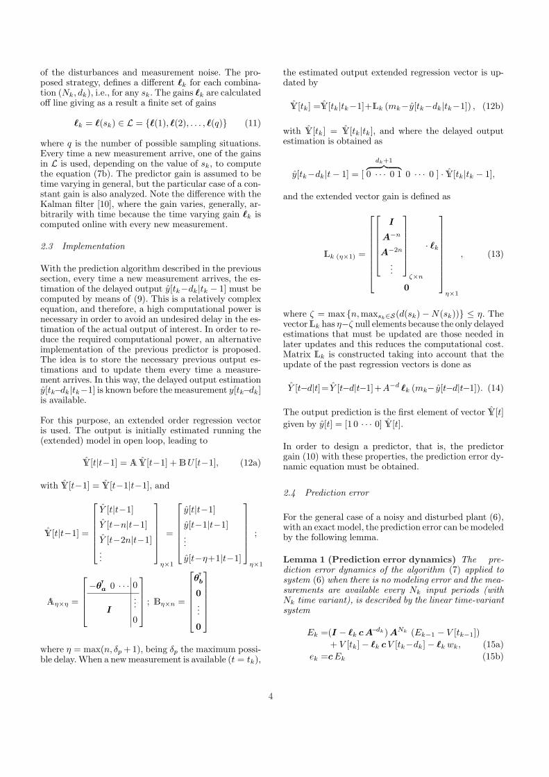
A measurement noise of typical deviation σw = 0.023 isalso present. The design with a time varying gain thatdepends both on Nk and dk leads to the same minimumγv = 5.1, γw = 234 that the design with a constantgain. The behaviour, however, is not identical. In orderto test the predictors on a simulation, the “real” sys-tem is assumed to be defined by the transfer functionG(s) = (9.9(1− 0.12 s))/(s2 + 1.1 s). The results of onesimulation are shown in figure 4 and the error varianceobtained with each method (averaged over 100 simula-tions) are σ = 0.0611 for the Kalman filter, σ = 0.0699for the constant gain predictor and σ = 0.0628 for thepredictor with variable gain. Therefore, a constant gain(` = [1.3433 1.1082]

ᵀ) is again a reasonable choice due

to its easier implementation. In this case, the Kalmanfilter required 106 flops in each output estimation up-date, while the proposed predictor only required 9.

Example 3 Consider the system G(s) = 1/(s2 + 6 s)with an input update period of T = 0.05 s and a mea-surement delay that can be 0 or 1 (D = {0, 1}). Let usassume attenuations γv = γw = 40. When a constantgain design is addressed (only 1 subset), the largest setof inter-sampling periods that leads to a feasible solu-tion of the associated LMI problem is N = {1, . . . , 4}.When a time varying gain that depends on ν and δ isconsidered, the upper limit of the set (leading to a feasi-ble solution of the LMI) can be extended to 100 samples,at least, as found by the LMI settings, and possibly toan infinite number of samples.

5 Conclusions

In this work, the design of an output predictor for sys-tems under delayed and irregular time-spaced measure-ments has been addressed. The main contribution isa procedure for designing the gains of a low comput-ing cost algorithm, that guarantees stability and per-

formance against disturbances, despite the non periodicdata availability pattern and the time varying delay.

The predictor uses the input-output model of the system,the previous inputs and the scarcely measured outputsto predict the output every control period. The numberof control periods between measurements (Nk) and thesamples delay (dk) are assumed to be time-varying valuesthat belong to known finite sets and that are known aposteriori.

The convergence of the predictor algorithm and the at-tenuation of output disturbances and measurement noisehas been taken into account by H∞ performance, trans-forming the H∞ condition into a convex optimizationproblem over a set of LMI. A predictor design procedurehas been proposed based on the available informationabout the disturbances. The result is a finite set of pre-dictor gains that are applied depending on the charac-teristics of the last measurement (dk and Nk). The pro-cedure allows to define the size of that set (and hencethe resources needed by the final algorithm implemen-tation), from the simplest case (constant gain) up to themost complex one (one gain for every pair (dk, Nk)). Theprocedure is applicable on stable and unstable plants.

References

[1] P. Albertos, I. Penarrocha, and P. Garcıa. Virtual sensorsunder delayed scarce measurements. 7th IFAC Symposiumon Cost Oriented Automation (SCOA-2004), 2004.

[2] P. Albertos, R. Sanchis, and A. Sala. Output prediction underscarce data operation: Control applications. Automatica,35:1671–1681, 1999.

[3] S. Boyd, L. Gaoui, E. Feron, and V. Balakrishnan. LinearMatrix Inequalities in Systems and Control Theory. SIAM.Philadelphia, 1994.

[4] T. Chen and B. Francis. Optimal Sampled-Data ControlSystems. Springer, 1995.

[5] M.C. de Oliveira, J. Bernossou, and J.C. Geromel. A newdiscrete-time robust stability condition. Systems & Controlletters, 37:261–265, 1999.

[6] T. D. Larsen, N. A. Andersen, O. Ravn, and N. K. Poulsen.Incorporation of time delayed measurements in a discrete-time kalman filter. In Proceeding ofIEEE 37th Conference ofDecision and Control, pages 3972–3977, December 1998.

[7] I. Penarrocha, A. Sala, R. Sanchis, and P. Albertos. Outputprediction under random measurements. an LMI approach.16th IFAC World Congress, 2005.

[8] I. Penarrocha, R. Sanchis, and P. Albertos. Closed loopanalysis of control systems under scarce measurements. 44thIEEE Conference on Decision and Control, and the EuropeanControl Conference, 2005.

[9] R. Sanchis. Control de Procesos Industriales con MedidasEscasas. Tesis Doctoral, Universitat Politecnica de Valencia,1999.

[10] R. Sanchis and P. Albertos. Virtual sensors: model basedoutput prediction. First EurAsia Conference on Advancesin Information and Communication Technology, 2002.

8

[11] C. Scherer, P. Gahinet, and M. Chilali. Multiobjectiveoutput-feedback control via LMI optimization. IEEETransactions on automatic control, 42(7):896–911, 1997.

[12] J. Wang, C. Wang, and H. Gao. RobustH∞ filtering for LPVdiscrete-time state-delayed systems. Nature and Science,2(2):36–45, 2004.

[13] L. Xie, L. Lu, D. Zhang, and H. Zhang. Improved robustH2 and H∞ filtering for uncertain discrete-time systems.Automatica, 40:873–880, 2004.

[14] S. Xu and T. Chen. Robust H∞ filtering for uncertainimpulsive stochastic systems under sampled measurements.Automatica, 39:509–516, 2003.

[15] H. Zhang, M.V. Basin, and M. Skliar. Optimal stateestimation with continuous, multirate and randomly sampledmeasurements. Proceedings of the American ControlConference, 2004.

9