Design of Power Split Hybrid Powertrains with Multiple ...

Design of Power Split Hybrid Powertrains with Multiple

Planetary Gears and Clutches

by

Xiaowu Zhang

A dissertation submitted in partial fulfillment of the requirements for the degree of

Doctor of Philosophy (Mechanical Engineering)

in The University of Michigan 2015

Doctoral Committee:

Professor Huei Peng, Co-Chair Professor Jing Sun, Co-Chair Professor Henry Liu Professor Jeffery L Stein

© Xiaowu Zhang

2015

ii

ACKNOWLEDGEMENTS

I would like to express my sincerest appreciation to both of my advisors, Professor

Huei Peng and Professor Jing Sun, for their continuous support and encouragement over

the past five years. Their guidance, patience, motivation and immense knowledge have not

only helped me complete the PhD study, but also made it the most amazing journey thus

far in my life. I would also like to thank my other committee members, Professor Henry

Liu and Professor Jeff Stein, for their helpful advice and comments.

I am indebted to the Department of Mechanical Engineering, the Rackham

Graduate School and the US-China Clean Energy Research Center for its funding support.

I am highly grateful for the internship opportunity that Robert Bosch LLC provided

me. That experience offered me exposure to the industry and helped improve my study

with more realistic considerations. I also want to thank Ford Motor Company and Denso

International for their constructive suggestions and comments on my PhD research.

As a proud member of the Vehicle Dynamics Lab, I would like to first express my

earnest gratitude to three of the lab alumni: Chiao-Ting Li, Shengbo Li and Dongsuk Kum,

whose instructions and patient guidance helped me through my rookie years. Great

appreciation should go to my colleague and four year roommate – Tianyou Guo, without

his introduction, I might not have been able to join the team. Many thanks should be given

to my colleagues in VDL for their help, discussion and all the good times we have had in

the office: Byung-joo Kim, William Smith, Ahn Changsun, Jong-Hwa Yoon, Zhenzhong

Jia, Xiaosong Hu, Huajie Ding, Yalian Yang, Daofei Li, Yugong Luo, Diange Yang, Ding

Zhao, Ziheng Pan, Xuerui Ma, Baojin Wang, Steven Karamihas, Yuxiao Chen, Oguz Dagzi,

Su-Yang Shieh, Xianan Huang and Geunseob Oh.

iii

I am sincerely grateful to Elizabeth Hildinger, my English tutor, for her patient

guidance and professional help on my writing.

Last, but not least, my deepest thank to my parents for their love and support, and

to my dear wife, Yue Xu, for her encouragement and companionship.

iv

TABLE OF CONTENTS

ACKNOWLEDGEMENTS ................................................................................................ ii

LIST OF FIGURES .......................................................................................................... vii

LIST OF TABLES ............................................................................................................ xii

NOMENCLATURE ........................................................................................................ xiv

ABSTRACT .................................................................................................................... xv

INTRODUCTION ........................................................................................ 1

1.1 Motivation ................................................................................................................ 1

1.2 Background .............................................................................................................. 2

1.2.1 Series Hybrid Vehicles .................................................................................... 3

1.2.2 Parallel Hybrid Vehicles ................................................................................. 4

1.2.3 Power-split Hybrid Vehicles ........................................................................... 5

1.2.4 Multi-mode Hybrid Vehicles .......................................................................... 6

1.3 Literature Review of Hybrid Vehicle Modeling and Control .................................. 9

1.3.1 Modeling of Hybrid Electric Vehicles ............................................................ 9

1.3.2 Control of Hybrid Electric Vehicles ............................................................. 10

1.4 Contributions .......................................................................................................... 12

1.5 Outline of the Dissertation ..................................................................................... 13

POWER SPLIT HYBRID VEHICLES USING A SINGLE PLANETARY

GEAR ......................................................................................................... 15

2.1 Models of Powertrain Components ........................................................................ 15

2.1.1 Planetary Gear Set ......................................................................................... 15

2.1.2 Powertrain Components ................................................................................ 19

2.2 Analysis of Single PG Powertrain System with Multiple Operating Modes ......... 21

2.3 Optimization Using Dynamic Programming ......................................................... 31

v

2.3.1 The Toyota Prius Configuration.................................................................... 34

2.3.2 The Chevy Volt Configuration...................................................................... 37

2.4 Discussion .............................................................................................................. 40

AUTOMATED MODELING, MODE SCREENING AND MODE

CLASSIFICATION OF MULTIPLE PLANETARY GEAR

POWERTRAIN SYSTEMS ....................................................................... 44

3.1 General Planetary Gear System with Clutches ...................................................... 45

3.2 Automatic Modeling .............................................................................................. 46

3.3 Mode Screening ..................................................................................................... 49

3.4 Mode Classification ............................................................................................... 51

3.5 Discussion on Mode Types .................................................................................... 54

3.6 Case Study: the 2nd Generation of Chevrolet Volt ................................................. 63

MODE SHIFT ANALYSIS FOR MULTI-MODE HEVS USING

PLANETARY GEAR SYSTEMS .............................................................. 67

4.1 General Mode Shift Description ............................................................................ 67

4.2 Direct Mode Shift Classification ............................................................................ 69

4.3 Optimal Mode Shift Pathway for Indirect Mode Shifts ......................................... 71

A NEAR-OPTIMAL ENERGY MANAGEMENT STRATEGY ............. 76

5.1 Power-weighted Efficiency Analysis for Rapid Sizing (PEARS) ......................... 76

5.2 Comparison between PEARS and DP.................................................................... 85

5.2.1 Computational Load Analysis ....................................................................... 85

5.2.2 Optimization Results and Discussion ........................................................... 86

SYSTEMATIC DESIGN METHODOLOGY FOR MULTI-MODE

POWER-SPLIT HYBRID VEHICLEs ...................................................... 91

6.1 Drivability Performance Evaluation ...................................................................... 92

6.1.1 Launching ...................................................................................................... 92

6.1.2 Climbing and Towing ................................................................................... 96

6.2 The Multi-Mode Passenger HEV Design Based on the THS-II Configuration ..... 96

vi

6.3 The Optimal Design Procedure Based on Volt Gen 2 ......................................... 104

6.4 The Design of Multi-mode Hybrid F150 Using Double PGs .............................. 108

CONCLUSION AND FUTURE WORK ................................................. 116

7.1 Conclusions .......................................................................................................... 116

7.2 Future Work ......................................................................................................... 118

BIBLIOGRAPHY ........................................................................................................... 120

vii

LIST OF FIGURES

Figure 1.1 The US CAFE standard for passenger vehicles from 1977 to 2014.......... 1

Figure 1.2 Schematic diagram of a series hybrid electric vehicle .............................. 3

Figure 1.3 Schematic diagram of a parallel hybrid electric vehicle ........................... 4

Figure 1.4 Schematic diagram of a power-split hybrid electric vehicle ..................... 5

Figure 1.5 The diagrams of the Allison Hybrid System (AHS) dual-mode HEV ...... 7

Figure 1.6 The component speed profiles of the AHS dual-mode HEV .................... 7

Figure 1.7 The diagrams of the Chevy Volt MY2011 ................................................ 8

Figure 2.1 Planetary gear and its lever diagram [65] ................................................ 16

Figure 2.2 Lever diagram of Toyota Prius 2004 Hybrid System .............................. 17

Figure 2.3 The lever diagram of the Prius MY 2010 (a) and its simplified version (b)

........................................................................................................................... 18

Figure 2.4 Engine BSFC map of the Toyota 2RZ engine used in Prius 2010 .......... 19

Figure 2.5 The efficiency map of the MG ................................................................ 20

Figure 2.6 The open circuit voltage and internal resistance of the battery ............... 21

Figure 2.7 All possible clutch locations of an input-split configuration................... 22

Figure 2.8 All possible clutch operations for an input-split configuration ............... 24

Figure 2.9 The four useful operating modes of the Prius Configuration .................. 25

Figure 2.10 All possible clutch locations of an output-split configuration............... 26

Figure 2.11 All possible clutch operations for an input-split configuration ............. 27

Figure 2.12 The four useful operating modes of output-split configurations ........... 28

Figure 2.13 Schematic diagrams of the original Prius and Prius++ ........................... 34

Figure 2.14 The speeds of powertrain elements and optimal mode selection of the

Prius++ in the FUDS and HWFET cycles.......................................................... 35

Figure 2.15 Schematic diagram of Prius+ ................................................................. 36

viii

Figure 2.16 The schematic diagram of the original Volt and Volt- .......................... 37


Chevy Volt in FUDS and HWFET cycles ........................................................ 38


Volt- in FUDS and HWFET cycle .................................................................... 38

Figure 2.19 Speeds of the powertrain devices and optimal mode selection of the Volt

in the HWFET cycle in the charge depleting scenario ..................................... 39

Figure 2.20 Energy analysis for different amount of available battery energy ........ 40

Figure 2.21 Energy analysis of the Prius in case (d) ................................................. 42

Figure 2.22 Energy analysis of the Prius+ in case (d) ............................................... 43

Figure 3.1 All 16 possible clutch locations for a double PG system ........................ 45

Figure 3.2 The lever diagram of THS-II ................................................................... 47

Figure 3.3 An example of a parallel mode in THS-II configuration ........................ 50

Figure 3.4 The topology of all possible mode types ................................................. 52

Figure 3.5 All feasible and non-redundant modes for the configuration used in Prius

2010, grouped into 14 mode types .................................................................... 54

Figure 3.6 Tow examples of Series mode with double PGs ..................................... 55

Figure 3.7 Two examples of 3 DoF mode with double PGs ..................................... 55

Figure 3.8 Two examples of Compound-split mode with double PGs ..................... 56

Figure 3.9 Two examples of Input-split mode with double PGs .............................. 57

Figure 3.10 Two examples of Output-split mode with double PGs ......................... 57

Figure 3.11 Two examples of Parallel with EVT mode (1MG) with double PGs.... 58

Figure 3.12 Two examples of Parallel with EVT mode (2MG, 1DoF) with double

PGs .................................................................................................................... 59

Figure 3.13 Two examples of Engine of only mode with double PGs ..................... 59

Figure 3.14 Two examples of Parallel with fixed-gear mode (2MGs, 2DoF) with

double PGs ........................................................................................................ 60

ix

Figure 3.15 Two examples of Parallel with fixed-gear mode (2MG, 1DoF) with

double PGs ........................................................................................................ 61

Figure 3.16 An example of Parallel with fixed-gear mode (1MG) with double PGs 61

Figure 3.17 Two examples of EV mode (2MG, 2DoF) with double PGs ................ 62

Figure 3.18 Two examples of EV mode (2MG, 1DoF) with double PGs ................ 62

Figure 3.19 Two examples of EV mode (1MG) with double PGs ........................... 63

Figure 3.20 Lever diagrams of the Volt Gen 1 and Gen 2 ........................................ 63

Figure 3.21 All 8 possible clutch operating states of Volt Gen 2 ............................. 65

Figure 4.1 General mode shift category .................................................................... 68

Figure 4.2 Two examples of direct mode shifts for the Volt Gen 2 powertrain: (a)

unconditional direct and (b) conditional direct ................................................. 69

Figure 4.3 An example indirect mode shift in the Volt Gen 2 powertrain ............... 69

Figure 4.4 Optimal mode shift pathway from Mode 1 to Mode 4 in Volt Gen 2 at

30mph vehicle speed ......................................................................................... 72

Figure 4.5 Optimal mode shift pathway from Mode 1 to Mode 4 in 7-mode Volt Gen

2 at 30mph vehicle speed .................................................................................. 73

Figure 4.6 Minimum mode shift cost for the 7-mode Volt Gen 2 at 30mph vehicle

speed ................................................................................................................. 74

Figure 4.7 Optimal mode shift pathway from Mode 1 to Mode 4 in the 7-mode Volt

Gen 2 at 60mph vehicle speed .......................................................................... 75

Figure 5.1 Flow chart of the PEARS method ........................................................... 77

Figure 5.2 Power flow in the hybrid modes .............................................................. 79

Figure 5.3 The flow chart of the mode shift cost table generation ........................... 83

Figure 5.4 Trajectories comparison between DP and PEARS in FUDS cycle for the

Volt Gen 2 design ............................................................................................. 87

Figure 5.5 Engine operating points comparison between DP and PEARS in the

FUDS cycle for the Volt Gen 2 design ............................................................. 88

Figure 5.6 Energy analysis for DP in FUDS cycle for the Volt Gen 2 design ......... 88

x

Figure 5.7 Energy analysis for PEARS in FUDS cycle for the Volt Gen 2 design .. 89

Figure 5.8 Trajectories comparison between DP and PEARS in the FUDS cycle for

the Prius++ design .............................................................................................. 90

Figure 6.1 The flow chart of the acceleration evaluation process ............................ 93

Figure 6.2 An example acceleration contour plot for a two DoF HEV mode at 31

mph ................................................................................................................... 94

Figure 6.3 0-75 mph acceleration trajectories of the direct DP and FAE ................. 96

Figure 6.4 Two types of configurations using 2PG .................................................. 97

Figure 6.5 Optimization results comparing 3-clutch designs and the benchmarks .. 99

Figure 6.6 Lever diagrams of the two sub-optimal designs selected in Figure 6.5 .. 99

Figure 6.7 The state and control trajectories of the sub-optimal design for fuel

economy .......................................................................................................... 100

Figure 6.8 The mode usage frequencies of the sub-optimal design for fuel economy

......................................................................................................................... 101

Figure 6.9 0-60 mph acceleration trajectories of the acceleration performance-

focused sub-optimal design............................................................................. 102

Figure 6.10 Maximum output torque comparison between the acceleration

performance-focused sub-optimal design and the original Prius .................... 103

Figure 6.11 The state and control trajectories of the sub-optimal design for

acceleration performance ................................................................................ 103

Figure 6.12 The mode usage frequencies of the sub-optimal design for acceleration

performance .................................................................................................... 104

Figure 6.13 Optimization results comparing 3-clutch designs and the benchmark

with Volt Gen 2’s parameters ......................................................................... 105

Figure 6.14 Optimization results for the 18 superior designs in CD ...................... 105

Figure 6.16 Optimization results for the downsized 18 superior designs in CD .... 106

Figure 6.15 Optimization results comparing the winning 18 designs with downsized

MGs and the benchmarks................................................................................ 106

xi

Figure 6.17 Lever diagrams of the 18 winning designs in the Volt Gen 2 case study

......................................................................................................................... 107

Figure 6.18 The mode usage frequencies of the sub-optimal design (o) ................ 108

Figure 6.19 The sketch diagram of the conventional F150 .................................... 109

Figure 6.20 The sketch diagram of the conceptual parallel F150 ........................... 110

Figure 6.21 The state and control trajectories of the conceptual parallel F150 ...... 111

Figure 6.22 Optimization results comparing 3-clutch designs and the benchmark of

the F150 case study ......................................................................................... 112

Figure 6.23 Lever diagrams of the three designs on the Pareto front of the F150 case

study ................................................................................................................ 112

Figure 6.24 The mode usage frequencies of the sub-optimal design (b) in the F150

case study ........................................................................................................ 113

Figure 6.25 Optimization results of the F150 case study of designs with Mode Type

4, 10 and 12 highlighted.................................................................................. 114

xii

LIST OF TABLES

Table 1.1 Four operating modes of the Chevy Volt .................................................... 8

Table 1.2 Multi-mode HEV patents ............................................................................ 8

Table 2.1 Clutch states & operating modes of an input-split configuration ............. 23

Table 2.2 Clutch states & operating modes of the output-split configurations ........ 28

Table 2.3 States and control variables in the Dynamic Programming problem ....... 32

Table 2.4 Parameters of the powertrain elements (IS: Input-Split; OS: Output-Split)

........................................................................................................................... 33

Table 2.5 Optimal fuel consumption of Prius/Prius+/Prius++ in the FUDS cycle ..... 35

Table 2.6 Optimal fuel consumption of Prius/Prius+/Prius++ in the HWFET cycle . 36

Table 2.7 Optimal fuel consumption of Prius/Prius+/Prius++ in the FUDS cycle

obtained by the “5-D DP problem” ................................................................... 37

Table 2.8 Optimal fuel economy of the Volt/Volt- in the FUDS cycle .................... 39

Table 2.9 Optimal fuel economy of Volt/Volt- in HWFET Cycle ............................ 39

Table 2.10 Fuel economy comparison between the Prius and Prius+ with different

battery energy consumption in the FUDS cycle ............................................... 41

Table 2.11 Energy loss and efficiency comparison between the Prius and Prius++ in

charge sustaining operation in the FUDS cycle ................................................ 42

Table 3.1 Mode types and criteria ............................................................................. 53

Table 3.2 Parameters of Volt Gen 1 and Volt Gen 2 ................................................ 64

Table 3.3 Operating modes of the Volt Gen 2 powertrain ........................................ 64

Table 4.1 The mode shift classification table of the Volt Gen 2............................... 70

Table 4.2 The mode shift classification table of the 7-mode Volt Gen 2 ................. 73

Table 5.1 Power-flow of the hybrid system .............................................................. 79

Table 5.2 The table of auxiliary modes for HEV modes .......................................... 81

xiii

Table 5.3 The states and controls for the DP procedure in the PEARS problem ..... 82

Table 5.4 Mode shift penalty within the same Power-split/Series mode .................. 84

Table 5.5 Mode shift penalty within the same Parallel with Fixed-gear mode ........ 84

Table 5.6 Mode shift penalty within the same 3 DoF/ Parallel with EVT mode ...... 84

Table 5.7 Mode shift penalty within the same EV mode .......................................... 84

Table 5.8 The states and controls of the benchmark DP of the Volt Gen 2 vehicle . 86

Table 5.9 The states and controls for the simpler DP problem solved in the PEARS

process of Volt Gen 2 vehicle ........................................................................... 86

Table 5.10 The speed and torque demand grids for Volt Gen 2 ............................... 86

Table 5.11 Comparison between PEARS and traditional DP for the Volt Gen 2

design ................................................................................................................ 88

Table 5.12 Comparison between PEARS and traditional DP for the Prius++ design 89

Table 6.1 The States and control variables of the acceleration problem with DP .... 93

Table 6.2 Acceleration performance evaluations of the Prius++ ............................... 95

Table 6.3 Weighted fuel economy for the Prius and Prius++ by PEARS optimization

........................................................................................................................... 98

Table 6.4 The clutch states and operating modes of the fuel economy focused sub-

optimal design in the Prius configuration ....................................................... 100

Table 6.5 The clutch states and operating modes of the performance-focused sub-

optimal design in the Prius configuration ....................................................... 101

Table 6.6 The clutch states and operating modes of the design (o) ........................ 108

Table 6.7 Powertrain parameters of the F150 MY2012 ......................................... 109

Table 6.8 Performance comparison between the conventional F150 and the

conceptual Parallel F150 ................................................................................. 110

Table 6.9 Additional powertrain parameters of the Hybrid F150 ........................... 111

Table 6.10 The clutch states and operating modes of the sub-optimal design (b) in

the F150 case study ......................................................................................... 113

xiv

NOMENCLATURE

DP Dynamic Programing

DOF Degrees Of Freedom

EPA Environmental Protection Agency

EVT Electric Variable Transmission

ECMS Equivalent Consumption Minimization Strategy

FAE Fast Acceleration Evaluation

FR Final drive Ratio

FUDS Federal Urban Drive Schedule

HEV Hybrid Electric Vehicle

HWFET HighWay Fuel Economy Test

MG Motor/Generator

MY Model Year

PE Power-weighted Efficiency

PEARS Power-weighted Efficiency for Rapid Sizing

PG Planetary Gear

PMP Pontriyagin’s Minimum Principle

SOC State Of Charge

STC Speed and Torque Cell

xv

ABSTRACT

Fuel economy standards for automobiles have become much tighter in many

countries in the past decades. Hybrid electric vehicles (HEVs), as one of the most

promising solutions to take on these challenging standards, have been successful in the US

market. Today, about 40 hybrid vehicle models are available on the US market. Yet only

those based on the power-split architecture, including Toyota Prius, Ford Fusion Hybrid

and Chevrolet Volt, have been successful. In the last few years, an observed trend is to use

multiple planetary gears with multiple operating modes to further improve vehicle fuel

economy and driving performance.

Most work in existing literature on HEV design and optimization has been based

on specific configurations, rather than exhaustively searching through all possible

configurations. This limitation arises from the large size of the design space–millions to

trillions of possible topological candidates. In this dissertation, we present a systematic

design methodology that enables the exhaustive search of multi-mode powertrain systems.

This dissertation starts by performing a systematic analysis on multi-mode single

PG power-split hybrid powertrain systems. All 12 possible single PG configurations are

identified and classified into two categories: 6 input-split and 6 output-split configurations.

All the possible clutch locations are enumerated, and the maximum number of useful

clutches is found to be three. The Dynamic Programming (DP) technique is used to solve

the optimal energy management problems for each design candidate.

After a thorough examination of single PG systems, we went on to study multiple

PG-systems. An automated modeling and mode classification methodology is developed,

which makes it possible to exhaustively search all possible designs. In a case study, the

second generation of Chevrolet Volt is used as the benchmark in our later case study for

two-PG, three-clutch powertrain system.

xvi

Understanding the mode shift dynamics is crucial for multi-mode hybrid designs.

We first analyze shifts between all mode pairs and define different mode shift types. Mode

shift cost is evaluated using Dijkstra’s algorithm, which identifies the optimal mode shift

path.

For each design candidate, the optimal control problem needs to be solved, so that

all designs candidates can be compared based on their best possible execution. Because

solving the true optimal solution using DP is very timing consuming, a fast and near-

optimal energy management strategy is proposed. The comparison results show that it is

up to 10,000 times faster than DP while achieving similar performance.

Although fuel economy is a very important metric in HEV designs, acceleration

performance is also important. In this dissertation, a fast and optimal acceleration

performance test procedure is developed, which can be used to determine optimal control

inputs and mode shift schedule during the acceleration evaluation.

Combining all proposed methodologies produces a systematic and optimal design

procedure. Three case studies are performed to illustrate the concepts of the design process.

These three case studies use three production vehicles as benchmarks: Prius, Volt and F150.

Optimization results show that the exhaustive search design method is able to identify

dozens of better designs than the production hybrid vehicle models available in today’s

market.

1

INTRODUCTION

1.1 Motivation

Fuel economy began to receive more attention from US consumers after the oil

crisis of 1973. In 1975, the U.S Congress enacted the Corporate Average Fuel Economy

(CAFE) standard to reduce consumption and import of the crude oil. This legislation is

regulated by the National Highway Traffic Safety Administration (NHTSA), while the fuel

economy is enforced by the U.S. Environmental Protection Agency (EPA). In the past few

decades, NHTSA had gradually raised the CAFE standard from 18 mpg in 1978 to 34.1

mpg in 2014 (Figure 1.1) [1]. This number is expected to rise to 54.5mpg in 2025 [2].

Figure 1.1 The US CAFE standard for passenger vehicles from 1977 to 2014

2

To meet this very challenging fuel economy standard, different technologies have

been studied and developed. Among them, one of the most promising technologies is

vehicle electrification. The resulting vehicle, when more than one energy source is used, is

called a hybrid vehicle. Among various possible hybrid vehicle designs, the hybrid electric

vehicle (HEV) is the most popular choice.

HEVs usually use an internal combustion (IC) engine as the primary power source,

and a battery pack as the secondary power source. Electric Motors/Generators (MG) are

used to complement the engine load so that it operates more efficiently and effectively.

After more than 15 years of improvement, HEV technologies have become mature for

passenger cars; one of the next steps is to introduce them for sport utility vehicles (SUVs)

and light trucks (LTs).

1.2 Background

The HEV concept has a history almost as long as that of the automobile itself. Its

original primary purpose was to improve drivability, and it involved using electric

machine(s) to assist the IC engine to achieve better launching performance. Fuel economy,

on the other hand, is the main performance metric for today’s HEVs.

The first hybrid vehicle was shown at the Paris Salon in 1899 [3]: it was a parallel

hybrid with gasoline engine, assisted by an electric motor and lead-acid batteries. Today,

if we categorize the hybrid vehicles by the battery size and their ability to charge from the

grid, there are two types: the conventional HEV and plug-in HEV. If we categorize the

hybrid vehicle by the mechanical powertrain connection and power flow, they fall into four

categories: series hybrid vehicles, parallel hybrid vehicles, series-parallel (power-split)

hybrid vehicles and multi-mode hybrid vehicles. Since there is no fundamental difference

between the conventional HEV and plug-in HEV in terms of mechanical connections, in

this dissertation, we will put more emphasis on the HEV powertrain structure and the

variations that are enabled by clutches.

3

1.2.1 Series Hybrid Vehicles

A series hybrid vehicle typically uses a traction motor to drive the vehicle output

shaft while the engine drives the generator, as shown in Figure 1.2. The motor can be

powered by the battery and/or the generator.

Since there is no mechanical coupling between the engine and vehicle drive axle,

the engine speed and power are not rigidly constrained by the vehicle speed and road load,

which enables the engine to operate efficiently. In addition, because the traction motor

usually can provide enough traction torque, transmission may not be needed.

Since the motor power is determined only by the driver demand, the power

management strategy of series hybrid vehicles is relatively simple. Many research studies

have been carried out on this topic [4] [5] [6] [7]. The fuel economy can be improved in

comparison to that of conventional vehicles, while both powertrain design and control

algorithms are straightforward (compared with those of other hybrid vehicle types). Series

hybrid powertrains are frequently used for heavy urban vehicles such as buses and delivery

trucks [5] [8]. There is no series hybrid vehicle on the US market today, even though both

the first generation of Chevrolet Volt (MY2011 - 2015) and the BMW i3 use a series mode

for range-extended driving.

Figure 1.2 Schematic diagram of a series hybrid electric vehicle

As noted above, the series hybrid vehicle powertrain is simple and easy to control.

However, it suffers from high energy conversion losses: 100% of the engine output must

be converted to electrical power and some of it is then converted to electrochemical form

and stored in the battery. The low efficiency is more pronounced when the vehicle is

running on the highway. Additionally, because the motor is the only power source to propel

the vehicle, the motor size must be large enough to provide the required drivability

performance.

4

1.2.2 Parallel Hybrid Vehicles

The parallel hybrid powertrain, as shown in Figure 1.4, usually adds one

motor/generator (MG), a battery pack and an inverter on top of, and can provide power in

parallel with, the conventional powertrain. When the MG is relatively small, it can only

start/stop the engine, provide some regenerative power features, and drive the vehicle in

limited circumstances; when the MG is large, it can drive the vehicle by itself or

simultaneously with the engine. The MG can be used to shift the engine operating points

to a higher-efficiency area by acting as a generator when the power demand is low or as a

motor at high power demand.

Figure 1.3 Schematic diagram of a parallel hybrid electric vehicle

The first parallel hybrid vehicle in mass production was the Honda Insight in 1999

[9]. Since the parallel hybrid can be designed as an incremental add-on to a traditional

powertrain and thus incur relatively small investment and engineering effort, major

automotive manufactures have developed a considerable number of parallel hybrid

vehicles, including Honda Civic hybrid [10], Volkswagen Passat hybrid and Chevy Malibu

hybrid. The modeling and control of parallel hybrids have been investigated quite

intensively in the past fifteen years [10] [11] [12] [13] [14].

Because the MG cannot be used to charge the battery and assist the engine

simultaneously, the power assist and EV operations must be controlled carefully to avoid

depleting the battery, especially during city driving, when frequent start-stops consume a

significant amount of battery energy and force the engine to generate power in its low

efficiency area. The efficiency of parallel hybrid vehicles can be very high on highways

since the engine can directly drive the vehicle near its sweet spot and energy circulation

between the mechanical energy and electric energy can be significantly reduced. Parallel

hybrid vehicles had a market share of less than 10% in the year of 2013 [15].

5

1.2.3 Power-split Hybrid Vehicles

A typical power-split vehicle uses two MGs and one engine, connected by one or

multiple planetary gears [16] [17] [18]. A single PG power-split vehicle is shown in Figure

1.4. There are three power-split vehicle configurations: Input-split, output-split and

compound-split. For input-split vehicles, one of the MGs is collocated with the output shaft

of the vehicle (sometimes with an additional set of gears in between), while the other MG

is collocated neither with the output shaft nor the engine [19]. For an output-split vehicle,

one of the MGs is collocated with the engine (sometimes with an additional set of gears in

between) while the other MG is collocated neither with the output shaft nor the engine [17].

For a compound-split vehicle, there is no collocation of MGs with either the output shaft

or the engine [20].

Figure 1.4 Schematic diagram of a power-split hybrid electric vehicle

For a power-split vehicle, the engine power can go to the final drive through two

paths: either through the mechanical path or via the electrical path, which is also known as

the engine-generator-motor path. With the PG(s), the engine speed can be regulated

independent of the vehicle speed, achieving the Electric-continuous Variable Transmission

(EVT) function, which results in efficient engine operation regardless of the vehicle speed.

The early power-split transmission appeared in the late 1960s [21] and early 1970s

[22], when such power-split mechanisms were used in lawn tractors. Although other early

studies on power-split hybrid vehicles followed, including the flywheel-transmission

hybrid vehicle [23] and planetary gear train with Continuous Variable Transmission (CVT)

[24], there was no passenger power-split hybrid vehicle until the Toyota Motor Corporation

introduced the Prius, the first mass-production hybrid vehicle in the world, in Japan in 1997

[25]. This hybrid powertrain system, called the Toyota Hybrid System (THS), is the

6

framework and the foundation of all Toyota hybrid vehicles, as well as hybrid vehicles

from several other companies, including the Ford Fusion Hybrid. Another major design

featuring a power-split powertrain is the General Motor Allison Hybrid System [20], which

will be discussed in detail in the next sub-section.

Power-split hybrid vehicles are efficient in city driving conditions as a result of the

EVT function, and successfully dominate the hybrid vehicle market with over 90% of the

strong hybrid sales in 2013 [15]. However, due to the energy circulation from the generator

to the motor, the power-split vehicles may have higher energy losses than parallel HEVs

in highway driving. This problem for single-mode power split hybrids can be avoided by

multi-mode hybrid designs, a concept that will be explained in the next section.

1.2.4 Multi-mode Hybrid Vehicles

Adding clutches to the power-split hybrid powertrain can achieve multiple

operating modes. The freedom to choose from different modes can improve both drivability

and fuel economy.

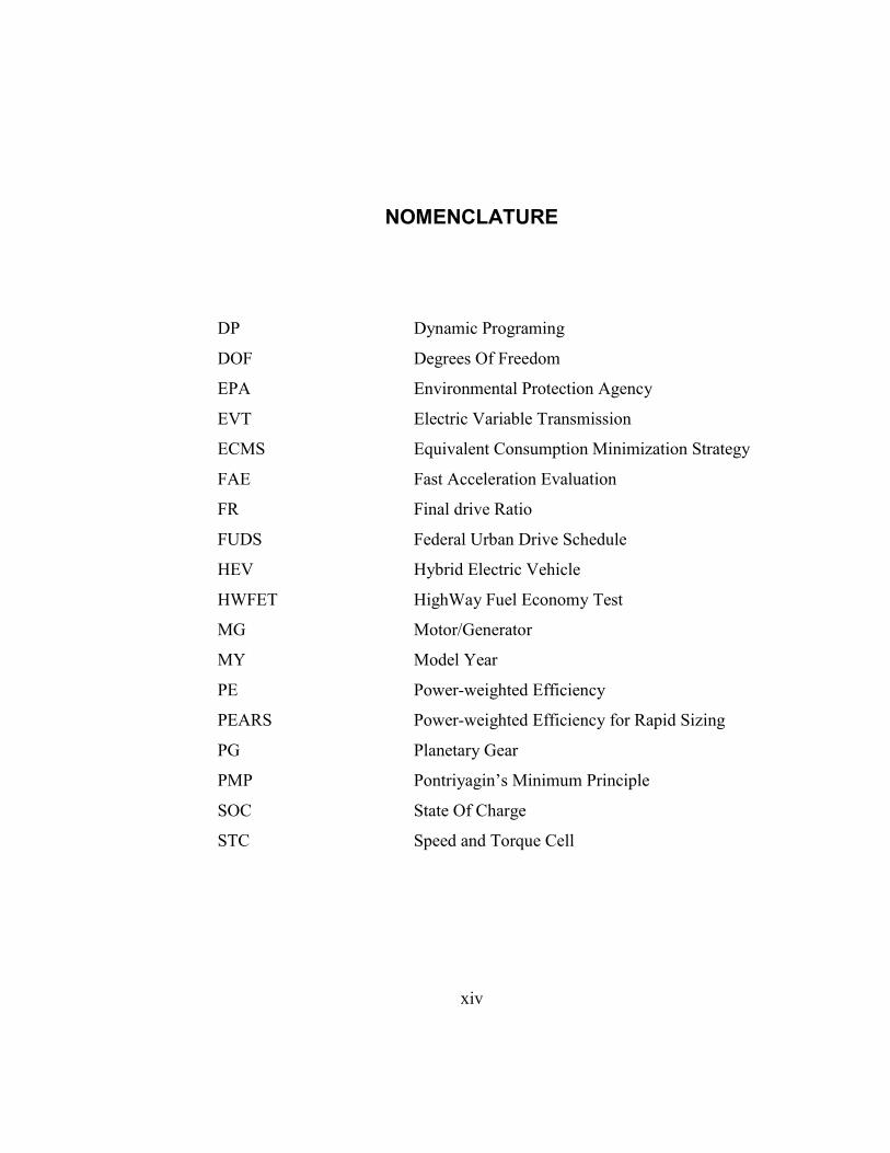
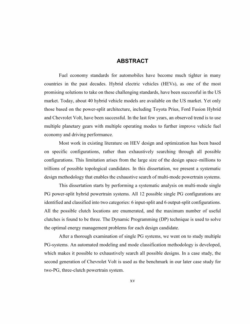
An example multi-mode hybrid vehicle design is shown in Figure 1.5. It is a dual-

mode HEV design (Allison Hybrid System) patented by General Motors in 2001 [20]. In

this design, the vehicle has two modes, achieving better drivability and fuel economy. In

addition, the maximum rotational speed of the MGs can be reduced, resulting in cheaper

and more reliable designs. Assuming that the engine speed stays the same, when the vehicle

speed is low, CL1 is open and CL2 is engaged. This makes the vehicle operate in the input-

split mode, which can provide larger output torque than its second mode. As the vehicle

speed increases, at point 92A (see Figure 1.6), when the speed of MG1 reaches zero, then

CL1 is engaged and CL2 is open, and the vehicle switches to its second mode, which is a

compound-split mode. Unlike the input-split mode, the compound split mode prevents the

speed of MG2 from increasing continuously with the vehicle speed, extending the

operating range of the vehicle.

7

Figure 1.5 The diagrams of the Allison Hybrid System (AHS) dual-mode HEV

Figure 1.6 The component speed profiles of the AHS dual-mode HEV

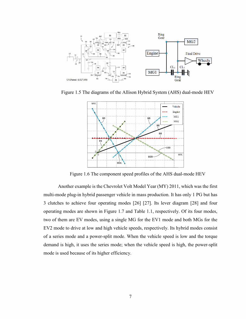
Another example is the Chevrolet Volt Model Year (MY) 2011, which was the first

multi-mode plug-in hybrid passenger vehicle in mass production. It has only 1 PG but has

3 clutches to achieve four operating modes [26] [27]. Its lever diagram [28] and four

operating modes are shown in Figure 1.7 and Table 1.1, respectively. Of its four modes,

two of them are EV modes, using a single MG for the EV1 mode and both MGs for the

EV2 mode to drive at low and high vehicle speeds, respectively. Its hybrid modes consist

of a series mode and a power-split mode. When the vehicle speed is low and the torque

demand is high, it uses the series mode; when the vehicle speed is high, the power-split

mode is used because of its higher efficiency.

8

Figure 1.7 The diagrams of the Chevy Volt MY2011

Table 1.1 Four operating modes of the Chevy Volt

Mode # Clutch Operation

Mode Type C1 C2 C3

1 1 0 0 EV1, MG2 Only

2 0 1 0 EV2, 2MGs, 2DoF

3 1 0 1 Series Mode

4 0 1 1 Output-split Mode

Description: “1” means that the clutch is closed; “0” means that the clutch is open.

Multi-mode hybrid powertrain concepts have also been proposed by other

automobile manufacturers, including Chrysler, Toyota, Hyundai, and others, with a large

number of patents filed. A few of them are shown in Table 1.2. All of the examples

provided in this table use 2 planetary gears and up to 5 clutches to achieve multiple modes.

Table 1.2 Multi-mode HEV patents

Manufacture Patent # # of PGs # of Clutches Description

GM US2007/7192373 2 4 EVT (2 modes), 4-

speed fixed gear

Chrysler US2009/0275439 2 5 EVT (5 modes), 6-

speed fixed gear

Toyota EP2004/1657094A1 2 2 EVT (2 modes)

Hyundai US2007/8147367 2 5 EVT (3 modes), 5-

speed fixed gear

Besides achieving a large vehicle speed range, in comparison with single operating

modes hybrid vehicles, multiple-mode hybrid vehicles have several other benefits:

9

launching performance can be improved by fixed gear modes; multiple EV modes can

increase efficiency in different driving conditions; using both power-split modes and

parallel modes can achieve high efficiency in both city and highway driving. Since

multiple-mode hybrid vehicles can combine the advantages of all three types of hybrid

vehicle, achieve better launching performance in EV drive, and potentially reduce the total

cost because a simpler automatic transmission is used, they deserve further study. In this

dissertation, we will perform a systematic study on multiple-mode hybrid vehicles from

the modeling, control and design perspectives.

1.3 Literature Review of Hybrid Vehicle Modeling and Control

1.3.1 Modeling of Hybrid Electric Vehicles

Modeling is important for all model-based vehicle design and energy management

strategy development. When one aims to explore an enormous design space to identify an

optimal design, the model needs to be computationally efficient. Commercial modeling

and simulation software like Powertrain System Analysis Toolkit (PSAT) [28], Autonomie

[30] and GT-Power [30] can simulate fuel economy and emission accurately, but they are

usually computationally expensive and not suitable for exhaustive search in a large design

space.

Besides the above mentioned commercial modeling packages, HEV models have

also been studied intensively in the academia for design purposes rather than for

simulations. In 1999, Rizzoni et al. [31] proposed a system-oriented approach to the

modeling and simulation of hybrid vehicles, based on an energy conversion model of

drivetrain subsystems which are scalable and composable (i.e. the system can be composed

by defining appropriate topological rules). In 2001, Lin et al. [32] developed a Simulink-

based model for HEV power management studies. For power-split hybrid vehicles,

Rizoulis et al. [33] presented a mathematical model based on steady-state analysis in 2001.

Colon et al. presented a general EVT analysis method to study the fuel economy and

performance sensitivity of different power-split configurations [34]. Liu et al. [35] used

Simulink to build a comprehensive model for the Toyota Prius system, and then further

10

developed a methodology that can automatically generate mathematical models for general

power-split vehicles with multiple PGs in 2007 [36] [37].

Adding clutches to a planetary gear system can add flexibility to the powertrain

functionality, which could improve driving performance and/or fuel economy. To explore

the entire design space including multiple operating modes and identify the optimal design,

a systematic modeling procedure is required to accommodate the massive number of design

candidates. For instance, for a double PG planetary gear hybrid powertrain system, there

can be up to a million designs when 3 clutches and 1 fixed connection are used (this fact

will be demonstrated in Chapter 6). Therefore, it is very crucial to develop an automated

modeling procedure to represent each candidate design in performing an exhaustive search

through the large design space. To the best of our knowledge, such a modeling approach

has not been reported in the literature.

1.3.2 Control of Hybrid Electric Vehicles

Like many other control problems, the control of hybrid vehicles can have a two-

level hierarchical architecture: the lower level control, and the supervisory control. For the

lower level control, each subsystem (e.g. engine, MGs, battery) is equipped with actuators,

sensors and a control system to regulate its behavior, in response to the supervisory control

commands. The design of lower level controllers can be separated from the supervisory

controller, and this dissertation does not focus on it. The supervisory control of the hybrid

vehicles determines the operating mode and power levels of all power devices to balance

design objectives such as drivability, fuel economy and battery health. The supervisory

level control and its use in assessing the optimality of design candidates are the focus of

this dissertation.

The supervisory commands must satisfy the demand from the driver, which is

frequently represented in the form of desired power or torque. In the meantime, if possible,

other performance metrics such as fuel economy can be optimized. In general, the

supervisory control algorithms can be categorized into three types: heuristic/rule-based

control, instantaneous optimization, and horizon optimization.

Heuristic controls are frequently implemented in the form of lookup tables. This

approach is usually based on the concept of load-leveling, attempting to operate the engine

11

at its efficient region and use the battery as the leverage [4] [39]. Sometimes a set of

thresholds is used to adopt a rule-based structure, such as fuzzy logic controls [40] [41].

These strategies are computationally efficient, requiring less computational load than

optimization methods. However, optimality cannot be guaranteed in the heuristic control

approaches.

The instantaneous optimization approaches minimize cost functions on the basis of

current information. The equivalent consumption minimization strategy (ECMS) is one of

the best-known examples. In this approach, the electric power is transformed into an

equivalent fuel consumption rate. By minimizing the instantaneous equivalent fuel

consumption, the resulting algorithm achieves an optimized selection between engine

power and battery power. After the pioneering work by Kim et al. in 1999 [42] and

Paganelli et al. in 2000 [43], there has been a great deal of follow-up work [44] [45] [46].

This methodology can be improved by introducing a periodically refreshed conversion

factor on the basis of the road load condition and the SOC level [47] [48] [49].

The horizon optimization approaches optimize a cost function over a time horizon.

A popular method is Dynamic Programming (DP). The concept of DP was proposed by

Richard Bellman in the 1940’s and refined by Bellman himself in 1954 [50]. This global

optimization method was first introduced to the HEV problem by H. Mosbech in the 1980’s

[51]. However, because it was constrained by the computation power, this approach did

not draw much attention until the later work by Brahma et al. in 2000 [52] and Lin et al. at

2001 [53]. Since then, this topic has been studied extensively [13] [54] [55] [56] and was

extended to power-split HEVs by Liu in 2006 [37] [57]. The stochastic dynamic program

(SDP) approach aims to optimize a stochastic version of the cost function, which

mathematically can be formulated as an infinite-horizon optimization problem with a

forgetting factor, or an indefinite time-horizon problem with a terminal absorbing state.

Therefore, the SDP approach is equivalent to a (time-) horizon optimization approach [58]

[59] [60]. Besides DP and SDP, there are other approaches of global optimization based on

Pontryagin’s Minimum Principle (PMP) [61] [62] and convex optimization [63] [64].

These HEV control approaches all have pros and cons. The load leveling methods

are heuristic and cannot guarantee optimality, ECMS is an instantaneous optimization

method and the equivalent fuel consumption factor needs tuning based on the drive cycle;

12

DP is optimal, but its computation load grows exponentially with the number of state and

input variables as well as the length of horizon, a well-known phenomenon commonly

referred as “curse of dimensionality”; PMP frequently has numerical convergence

challenge if the underlying two-point-boundary-value problem is nonlinear; the convex

optimization methods, though numerically fast, since they aim to optimize a convex

function over a convex set, they cannot address integer decisions, such as mode selection

and engagement of clutches. Therefore, to appropriately address the multi-mode hybrid

vehicles optimal control problem, a fast, robust and reliable optimization method is needed.

1.4 Contributions

This dissertation focuses on the systematic modeling, design, and control

optimization process of power-split hybrid vehicles with multiple operating modes. The

main contributions are listed below:

A thorough analysis of power-split hybrid powertrains using a single PG

with multiple operating modes was conducted, including the analysis of all 12 possible

input-split and output-split configurations using a single PG, identification of all possible

clutch locations and their corresponding operating modes. A procedure to construct the

dynamic models for all operating modes was developed, and the dynamic programming

technique was used to explore the full potential of multi-mode operations.

A systematic modeling procedure was developed for hybrid vehicles with

multiple operating modes. Such procedure features automatic generation of all the models

with possible clutch locations, systematic screening to eliminate infeasible and redundant

ones, and streamlined classification to combine similar modes into 14 types according to

their dynamic matrices and degrees of freedom.

Mode shift and transient dynamics were studied to guarantee practical and

feasible mode shifts for multiple-mode hybrid vehicles. All possible types of mode shifts

were identified and the mode shift criteria were established. The optimal mode shift

pathway finding method for indirect mode shift was proposed using Dijkstra’s algorithm,

which can be used in the real-time control development in the future.

13

On the basis of the power analysis for the components, the optimal torque

and speed were determined to achieve best acceleration performance, for all mode types.

A low-dimension DP was solved to calculate the optimal mode shift schedule during the

acceleration subject to mode shift penalties. Besides the acceleration performance analysis,

towing and climbing capabilities were considered in the performance evaluation procedure

for hybrid light truck applications.

Since DP is computationally expensive, an alternative, near-optimal energy

management algorithm was developed for optimal design and sizing. Built on the concepts

of “probability-based discretized cycle” and “power-weighted efficiency”, the algorithm

led to a factor of 10,000 in computational time reduction compared with the DP

methodology without significantly reducing the optimality. The method is not only suitable

for power-split hybrid vehicles, but can be applied to parallel, series hybrid vehicles, or

even Electric Vehicles (EVs).

A systematic design procedure was developed by combining the proposed

methodologies including modeling, mode shift analysis, performance evaluation and

PEARS, making it possible to do exhaustive search for large-scale design studies involving

a large number of design candidates.

1.5 Outline of the Dissertation

This dissertation is organized as follows: in Chapter II, a thorough analysis on

hybrid vehicle powertrain systems using a single planetary gear (PG) is conducted: all

possible clutch locations are considered and automated models for all modes are

established. The DP method is used as the global optimal energy management algorithm

to execute the mode shift and identify optimal torque input. Energy analysis is done to

emphasize the benefits of multiple-mode operations. In Chapter III, a universal automatic

modeling, screening and mode classification algorithm is developed for hybrid vehicles

using multiple planetary gears and clutches. In Chapter IV, mode shift analysis is presented

to categorize and distinguish different types of mode shifts. In Chapter V, a near-optimal

energy management strategy on the basis of efficiency analysis and cycle speed-torque

probability is proposed which is several orders of magnitude faster than the Dynamic

14

Programming approach. In Chapter VI, a systematic design procedure for hybrid vehicles

with planetary gears and multiple operating modes is presented. A novel drivability

performance evaluation is processed to screen out infeasible designs in terms of poor

drivability. The PEARS method is applied to finalize the candidate pool. Finally, in

Chapter VII, the conclusion and future work are presented.

15

POWER SPLIT HYBRID VEHICLES USING A SINGLE

PLANETARY GEAR

The strong HEV market has been dominated by power-split hybrid designs. In 2013,

more than 90% of the strong HEVs sold in the US market were power-split hybrid vehicles

[15]. Among them, the top-sellers including the Toyota Prius, Chevy Volt (MY2011), Ford

Fusion and C-Max hybrid all use a single planetary gear or are functionally equivalent.

Besides regular power-split HEVs with a fixed component connection (such as the

Toyota Prius and Ford Fusion), clutches began to be added to enable multiple operating

modes, such as Chevy Volt [26]. To the best of our knowledge, the number of possible

configurations, the impact of having multiple operating modes, and the best locations of

clutches for single PG systems have not been systematically studied in the literature. We

will address all these issues and use the DP method to optimize the mode selection and

show the results for two design targets: the Toyota Prius and Chevy Volt.

This chapter is presented in the following way: First, the components of a planetary

gear (PG) are introduced and its operation principle described. The modeling and dynamics

of the hybrid powertrain components are then introduced. Subsequently, the procedure to

automatically generate the dynamic model for each possible operating mode of a hybrid

powertrain is introduced. Dynamic programming is used to evaluate the performance of

each design. Finally, the energy analysis method is introduced to end this chapter.

2.1 Models of Powertrain Components

2.1.1 Planetary Gear Set

As shown in Figure 2.1, a planetary gear set, or epicyclical gear set, consists of a

sun gear in the center, several pinion gears supported by the carrier, and a ring gear. It is

the key device that connects all power sources and the vehicle drive axle together in today’s

16

power split hybrid vehicles. The speeds of the ring gear (ωr), sun gear (ωs), and carrier (ωc)

must satisfy Eq. (2-1):

s r cS R R S (2-1)

where S and R are the radii of the sun gear and the ring gear. This kinematic constraint can

be visualized by the lever diagram shown on the right in Figure 2.1, where the lever lengths

S and R are proportional to the radii or teeth numbers of the sun gear and the ring gear, and

the three vectors represent the direction and magnitude of the speeds of the three nodes.

The tips of three speed vectors define the straight dash line, indicating that the kinematic

constraint, Eq. (2-1) must be satisfied.

Figure 2.1 Planetary gear and its lever diagram [65]

In the following contents, the mass and inertia of the pinion gears are assumed to

be small and negligible. Then, the dynamics of the gear nodes can be represented as

r r rI F R T (2-2)

c c cI F R F S T (2-3)

s s sI F S T (2-4)

where Ir, Ic and Is are the component inertia connected to the ring gear node, carrier node

and sun gear node, respectively, and Tr, Tc and Ts are the resultant moment. F is the internal

force between the pinion gears and other gears.

Combining Eqs. (2-2) (2-3) and (2-4), the dynamics of the planetary gear set system

can be represented in a matrix form. For a power-split hybrid powertrain using a single

planetary gear, the component inertia and corresponding torque can be added to Eq. (2-5).

17

Figure 2.2 shows the lever diagram of the powertrain system of the Toyota Prius model

year (MY) 2004, and its dynamic matrix is shown in Eq. (2-6) [37]:

0 0

0 0

0 0

0 0

r r r

c c c

s s s

I R T

I R S T

I S T

R R S S F

(2-5)

2

2 2

11

2 32

1

0 0

0 0

0 0

0

1[ 0.5 ( ) ]

0

tireoutr MG

ec e

MGs MG

rMG fb r tire d tire

e

MG

RI I m R

K

I I R S

I I SF

R R S S

T T mgf R AC RK K

T

T

(2-6)

where m is the vehicle mass, Rtire is the wheel radius, K is the final drive ratio; Ie, IMG1, IMG2

and Te, TMG1, TMG2 are inertia and torques of the engine, first electric machine and second

electric machine; Tload is the load imposed by the rolling resistance and aerodynamic drag

during driving and defined at the transmission output shaft; F is the internal force acting

between gears on the PG; ωe, ωMG1 and ωout are speeds of the engine, first electric machine

and the output shaft. It should be noted that, in this particular configuration, the second

electric machine is connected to the output shaft, so its torque acts on the same node at

which the output shaft is located, and no additional equation is required to describe its

dynamics.

Figure 2.2 Lever diagram of Toyota Prius 2004 hybrid system

18

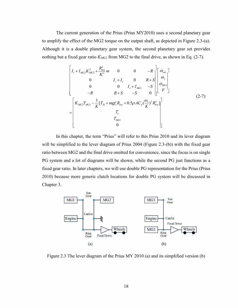
The current generation of the Prius (Prius MY2010) uses a second planetary gear

to amplify the effect of the MG2 torque on the output shaft, as depicted in Figure 2.3-(a).

Although it is a double planetary gear system, the second planetary gear set provides

nothing but a fixed gear ratio KMG2 from MG2 to the final drive, as shown in Eq. (2-7).

22

2 2 2

11

2 32 2

1

0 0

0 0

0 0

0

1[ 0.5 ( ) ]

0

tireoutr MG MG

ec e

MGs MG

rMG MG fb r tire d tire

e

MG

RI I K m R

K

I I R S

I I SF

R R S S

K T T mgf R AC RK K

T

T

(2-7)

In this chapter, the term “Prius” will refer to this Prius 2010 and its lever diagram

will be simplified to the lever diagram of Prius 2004 (Figure 2.3-(b)) with the fixed gear

ratio between MG2 and the final drive omitted for convenience, since the focus is on single

PG system and a lot of diagrams will be shown, while the second PG just functions as a

fixed gear ratio. In later chapters, we will use double PG representation for the Prius (Prius

2010) because more generic clutch locations for double PG system will be discussed in

Chapter 3.

Figure 2.3 The lever diagram of the Prius MY 2010 (a) and its simplified version (b)

19

2.1.2 Powertrain Components

Engine and motor are two of the key components in a HEV powertrain system. In

theory, thermodynamics-based models like GT-Power [66] can fit experimental data and

used as an accurate simulation tool. However, its high computation requirement makes it

unsuitable for large-scale system control or design studies. Instead, in this dissertation, we

use quasi-static models for both the engine and motor systems.

The engine is modeled as a lookup table which provides instantaneous fuel rate as

a function of the engine speed and output torque. For supervisory control studies and fast

prototype design, the engine transient dynamics due to spark-timing and fuel injection are

ignored. Figure 2.4 shows the engine brake specific fuel consumption (BSFC) contour plots

based on the Toyota 2RZ engine used in Prius 2010 [67].

Figure 2.4 Engine BSFC map of the Toyota 2RZ engine used in Prius 2010

In our research, MGs are assumed to be controlled by a servo-loop motor control

unit which can deliver the demand torque specified by the supervisory-level control

instantaneously. The lumped thermal, mechanical and power electronic losses are modeled

by a map reported in [68], as shown in Figure 2.5. In design studies when the motor size is

a design variable, the shape of the efficiency map is assumed to stay the same while the

speed and torque ranges of the motor are scaled linearly with the maximum rated power

[69].

20

Figure 2.5 The efficiency map of the MG

The power consumed by the MG is calculated based on Eq. (2-8), where TMG and

ωMG are the torque and rotational speed. If the signs of the electric machine torque and

speed are the same, the MG is acting as a motor, and k = -1; if the signs of the electric

machine torque and speed are different, it means that the MG is acting as a generator, and

k = 1.

kMG MG MG MGP T (2-8)

The power flows into the battery is represented as Eq. (2-9), where N = 1 or 2,

depending on whether the HEV uses one or two MGs.

1

Nk

batt MGi MGi MGii

P T

(2-9)

The battery is modeled by an equivalent circuit. The open circuit voltage Voc and

internal resistant R are both state of charge (SOC) dependent parameters. The battery

temperature is assumed to be well-regulated around a constant set-point (25oC) and the

temperature effect is ignored. The relationship between the Voc, R and SOC are modeled as

shown in in Figure 2.6, which comes from the test data of Chevy Volt 2013 [70].

21

Figure 2.6 The open circuit voltage and internal resistance of the battery

The power of the battery can be presented as a function of battery current Ibatt, as

shown in Eq. (2-10).

2batt oc batt batt battP V I I R (2-10)

By solving Eq. (2-11), we obtain

2 4

2oc oc batt batt

batt

batt

V V P RI

R

(2-11)

The SOC, which represents the remaining charge available from the battery, is

calculated from the battery capacity Qmax and the current Ibatt, as described in Eq. (2-12).

max

battISOC

Q (2-12)

2.2 Analysis of Single PG Powertrain System with Multiple Operating

Modes

In order to design a mechanically feasible configuration for a single PG system, all

three PG nodes must be connected to at least one powertrain element instead of left

“hanging freely”—because free nodes cannot provide any reaction torque. The permutation

starts with assigning the engine, output shaft and one electric machine to the three PG

22

nodes, which gives us six combinations (�� = 6). The second electric machine is then

randomly assigned to one of the three nodes. However, having the two electric machines

on the same node makes no sense, so we really have only two choices: the second electric

machine can collocate with either the engine or the output shaft. When it is collocated with

the output shaft, the resulting design has an input-split configuration; when it is collocated

with the engine, the resulting design has an output-split configuration [34]. Therefore, there

are a total of 12 possible configurations (�� × 2 = 12) for HEVs with one PG; six are input-

split type (one of which is used for Prius) and six are output-split type (one of which is

used for the first generation Chevy Volt).

Using clutches can introduce new operating modes and various functionalities. For

instance, a clutch can disengage the engine from the transmission so that an HEV can

operate in a pure electric drive mode. It can also ground a node to use the PG as a simple

step gear, which could be useful during a vehicle-launch. Finally, a clutch can disconnect

the output shaft so that the engine can charge the battery while the vehicle is stationary.

This last functionality is not considered in this dissertation as it goes against the desire to

displace fossil fuel with electricity, and we believe such desperate charging can be avoided

by intelligent power management.

The clutch placements around the PG determine the number of operating modes

and its characteristics. In order to find all feasible multi-mode single PG configurations,

we start the permutation of clutch locations without any constraints, and then eliminate

those that are not feasible/useful.

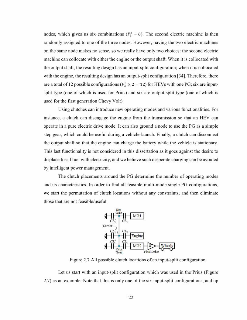
Figure 2.7 All possible clutch locations of an input-split configuration.

Let us start with an input-split configuration which was used in the Prius (Figure

2.7) as an example. Note that this is only one of the six input-split configurations, and up

23

to six clutches can be added to this particular configuration. One should also notice that the

clutches between any two nodes of a single PG are not considered since the focus for hybrid

mode in this chapter is mode with EVT function. However, more generalized cases will be

discussed in Chapter 3, when multiple PGs are used. The six clutches in Figure 2.7 can be

grouped into 3 pairs, and the two clutches on the same node need to be operated in an XOR

fashion, meaning when one clutch is open, the other must be closed, and vice versa.

Therefore, there are eight possible modes (23=8), as shown in Figure 2.8. The states of

clutches in these eight modes are summarized in Table 2.1 and characteristics of each mode

are detailed below.

Table 2.1 Clutch states & operating modes of an input-split configuration

Mode CL1 CL2 CL3

1 (EV1) 0 0 1

2 (EV2) 1 0 1

3 (Series) 0 1 1

4 (Input-split) 1 1 1

5 (= EV1) 0 0 0

6 (Infeasible) 1 0 0

7 (= EV1) 0 1 0

8 (Not EVT) 1 1 0

Description: “1” means that the clutch is closed; “0” means that the clutch is open.

1) Mode 1 is a pure electric mode (EV1). In this mode, the engine and the first

electric machine are disconnected from the PG. The vehicle is driven only by the second

electric machine (MG2).

2) Mode 2 is also a pure electric mode (EV2). The engine is disconnected and

the carrier gear is grounded. The vehicle is driven by both MG1 and MG2.

3) Mode 3 is a series mode (Series). Both the engine and MG1 are connected

to the PG to charge the battery, but the vehicle is only driven by MG2 mechanically since

MG2 is disconnected from the PG.

4) Mode 4 is an input power-split mode (Input-split). The engine, MG1, and

MG2 are all connected to the PG. The vehicle is running as an input-split hybrid vehicle.

5) Mode 5 is equivalent to Mode 1. Both the engine and MG1 are

24

disconnected, and the vehicle is driven only by MG2.

Figure 2.8 All possible clutch operations for an input-split configuration

6) Mode 6 is infeasible and the word “infeasible” in this dissertation refers to

the scenarios that the vehicle output shaft cannot rotate or cannot be powered by any of the

engine/MGs. In this mode, MG2 is locked by the grounded sun gear and carrier, and the

output shaft cannot rotate.

25

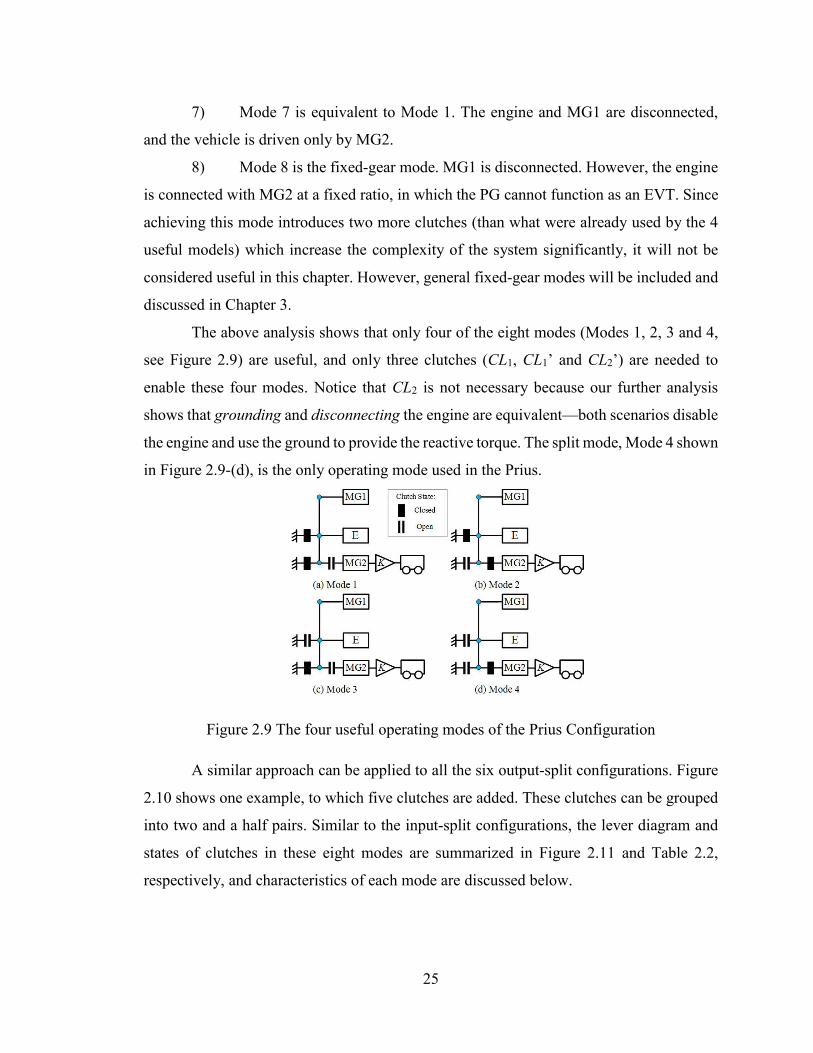
7) Mode 7 is equivalent to Mode 1. The engine and MG1 are disconnected,

and the vehicle is driven only by MG2.

8) Mode 8 is the fixed-gear mode. MG1 is disconnected. However, the engine

is connected with MG2 at a fixed ratio, in which the PG cannot function as an EVT. Since

achieving this mode introduces two more clutches (than what were already used by the 4

useful models) which increase the complexity of the system significantly, it will not be

considered useful in this chapter. However, general fixed-gear modes will be included and

discussed in Chapter 3.

The above analysis shows that only four of the eight modes (Modes 1, 2, 3 and 4,

see Figure 2.9) are useful, and only three clutches (CL1, CL1’ and CL2’) are needed to

enable these four modes. Notice that CL2 is not necessary because our further analysis

shows that grounding and disconnecting the engine are equivalent—both scenarios disable

the engine and use the ground to provide the reactive torque. The split mode, Mode 4 shown

in Figure 2.9-(d), is the only operating mode used in the Prius.

Figure 2.9 The four useful operating modes of the Prius Configuration

A similar approach can be applied to all the six output-split configurations. Figure

2.10 shows one example, to which five clutches are added. These clutches can be grouped

into two and a half pairs. Similar to the input-split configurations, the lever diagram and

states of clutches in these eight modes are summarized in Figure 2.11 and Table 2.2,

respectively, and characteristics of each mode are discussed below.

26

Figure 2.10 All possible clutch locations of an output-split configuration

1) Mode 1 is a pure electric mode (EV1). In this mode, the engine and the first

electric machine are disconnected from the PG. The vehicle is driven only by the second

electric machine (MG2).

2) Mode 2 is also a pure electric mode (EV2). The engine is disconnected from

the MG1. The vehicle is driven by both MG1 and MG2 and the speed of MG1 and MG2

are not coupled with the vehicle drive shaft.

3) Mode 3 is a series mode (Series). The engine and MG1 are connected

together to charge the battery. The vehicle is only driven by MG2.

4) Mode 4 is an output power-split mode (Output-split). The engine, MG1, and

MG2 are all connected to the PG. The vehicle runs as an output-split hybrid vehicle.

5) Mode 5 is infeasible. Both MGs and the engine are disconnected from the

PG system and the vehicle cannot be powered.

6) Mode 6 is an EV mode with only MG1 driving the vehicle. It is almost the

same as the EV1 but uses two more clutches, which adds cost and complexity. Therefore,

this mode will not be considered in this chapter.

7) Mode 7 is infeasible. The vehicle cannot be driven by the powertrain

components.

8) Mode 8 is a fixed-gear mode. The MG2 is disconnected from the

powertrain. The engine is connected with MG1 at a fixed ratio to the final drive, in which

the PG cannot function as an EVT. Similar to the input-split case, since achieving this mode

introduces two more clutches (than what were already used by the other four useful modes)

which increase the complexity of the system, it will not be considered in this chapter.

27

Figure 2.11 All possible clutch operations for an input-split configuration

28

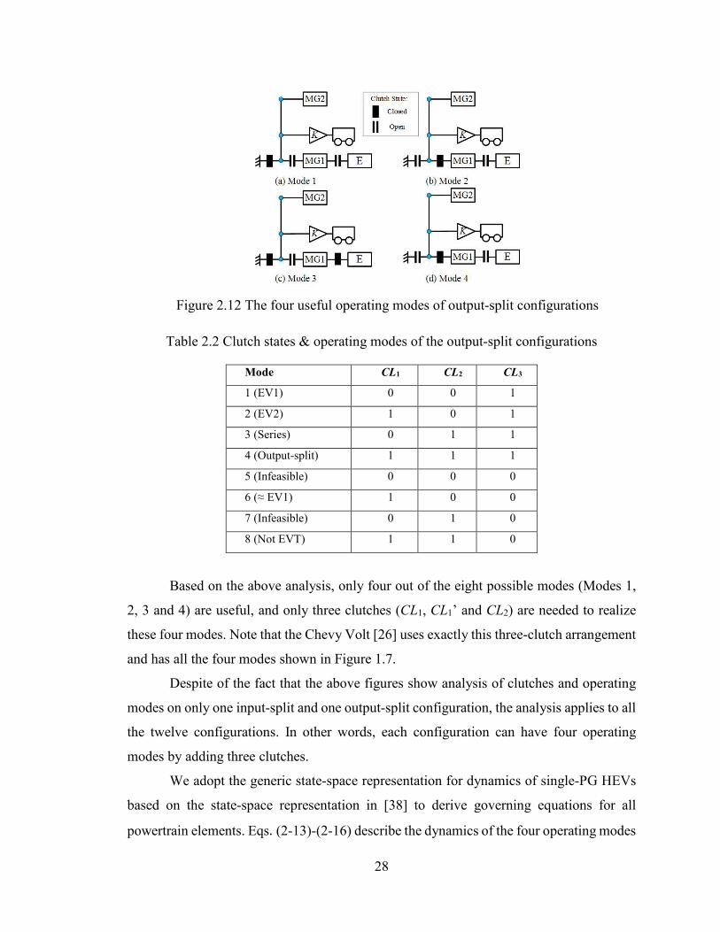
Figure 2.12 The four useful operating modes of output-split configurations

Table 2.2 Clutch states & operating modes of the output-split configurations

Mode CL1 CL2 CL3

1 (EV1) 0 0 1

2 (EV2) 1 0 1

3 (Series) 0 1 1

4 (Output-split) 1 1 1


6 (≈ EV1) 1 0 0


8 (Not EVT) 1 1 0

Based on the above analysis, only four out of the eight possible modes (Modes 1,

2, 3 and 4) are useful, and only three clutches (CL1, CL1’ and CL2) are needed to realize

these four modes. Note that the Chevy Volt [26] uses exactly this three-clutch arrangement

and has all the four modes shown in Figure 1.7.

Despite of the fact that the above figures show analysis of clutches and operating

modes on only one input-split and one output-split configuration, the analysis applies to all

the twelve configurations. In other words, each configuration can have four operating

modes by adding three clutches.

We adopt the generic state-space representation for dynamics of single-PG HEVs

based on the state-space representation in [38] to derive governing equations for all

powertrain elements. Eqs.(2-13)-(2-16) describe the dynamics of the four operating modes

29

of the input-split configuration. Note that Modes 2, 3 and 4 use four equations to describe

the powertrain dynamics, while Modes requires only one equation, because the loss of

degree of freedom through clutch engagements. Note that in Mode 2, the engine

acceleration is always zero since it is grounded and no input can be applied.

Mode 1 (EV1):

22

2 2 2 22( )MG MG out MG MG Loadmr K I K T TK

(2-13)

Mode 2 (EV2):

22

2 22 2 22

1 11 3

2 3

0 0 0 0

0 0

0 000 0

ee

out MG MG LoadMG MG

MG MGMG

I

mr K T TK I DK

TI DFD D

(2-14)

Mode 3 (Series):

1

22

2 22 22

1 11 3

1 3

0 0

0 0 0

0 000 0

ee e

out MG MG LoadMG MG

MG MGMG

I D Tmr K T TK IK

TI DFD D

(2-15)

Mode 4 (Power Split):

1

22

2 22 2 22

1 11 3

1 2 3

0 0

0 0

0 000

ee e

out MG MG LoadMG MG

MG MGMG

I D Tmr K T TK I DK

TI DFD D D

(2-16)

where m is the vehicle mass, r is the wheel radius, K is the final drive ratio. Ie, IMG1, IMG2

and Te, TMG1, TMG2 are the inertia and torques of the engine, first electric machine and

second electric machine. TLoad is the load imposed by the rolling resistance and

aerodynamic drag during driving and defined at the transmission output shaft, as shown in

Eq. (2-17):

31 [ 0 .5 ]L o a d fb r t ir e F d w h e e l tir eT T m g f R A C RK

(2-17)

30

where Tfb is the friction brake, fr is the rolling resistance coefficient, Cd is the aerodynamic

coefficient, AF is the frontal area, ρ is the air density, ωwheel is the speed of the wheel and

Rtire is the radius of each wheel. F is the internal force acting between gears on the PG. ωe,

ωMG1 and ωout are speeds of the engine, first electric machine and output shaft. It should be

noted that, in this particular configuration, the second electric machine is connected to the

output shaft, so its torque acts on the same node at which the output shaft is located, and

no additional equation is necessary to describe its dynamics. Elements D1, D2 and D3 are

permutations of -R, -S and R+S, which denote the configuration of the hybrid system. More

specifically, -R is used if the powertrain component is connected to the ring gear; -S is used

if the powertrain component is connected to the sun gear; and R+S is used if the powertrain

component is connected to the carrier.

As an example, for the Prius configuration, since the vehicle output shaft (and

MG2), the engine and MG1 are connected to the ring gear, the carrier and the sun gear

respectively, D1 = -R, D2 = R+S, D3 = -S.

Similarly, the dynamic model for the output-split configurations can be derived,

except that now the first electric machine is connected to the engine, TMG1 will act on the

node connected to the engine. Equations (2-18) – (2-21) describe the governing equations

for the four operating modes of the Volt shown in Figure 2.12.

Mode1 (EV1):

1

2

222

1 11 3

1 3

0 0

0 0 0

0 00

0 0

ee e

out MG LoadMG

MG MGMG

I DT

mrT TI

KT

I DF

D D

(2-18)

Mode2 (EV2):

1 11 1

2

22

2 22 3

1 2 3

0 0

0 0

0 000

MGMG MG

out Load

MG MGMG

I D Tmr TDK

TI DFD D D

(2-19)

31

Mode3 (Series):

11 1

2

22

2 22 3

2 3

0 0 0

0 0

0 000 0

MG eMG MG e

out Load

MG MGMG

I I T Tmr TDK

TI DFD D

(2-20)

Mode4 (Power Split):

1 11 1

2

22

2 22 3

1 2 3

0 0

0 0

0 000

MG eMG MG e

out Load

MG MGMG

I I D T Tmr TDK

TI DFD D D

(2-21)

For the Volt configuration, since the vehicle output shaft, the engine (and MG1)

and MG2 are connected to the carrier, the ring gear and the sun gear respectively, D1 =

R+S, D2 = -R, D3 = -S.

2.3 Optimization Using Dynamic Programming

The optimal energy management problem needs to be solved in order to have a fair

comparison of the fuel consumption of various designs, to understand the effects of adding

clutches to enable more operating modes on single-PG configurations. Assuming that

minimum fuel consumption is the goal, an optimal control problem can be defined as in

Eq. (2-22), in which the engine speed � �, MG1 speed � �� , MG2 speed � �� , engine

torque Te, MG1 torque TMG1, MG2 torque TMG2 and the operating mode determine the fuel

consumption.

32

0

min max

min max

min max

min ma

1 2 1 2

0

1 2 1 2

min max

1 1 1

2 2 2

min [ ( , , , , , , , ) ]

subject to

( ) ( )

( , , , , , , , )

ft

e MG MG e MG MG

t

f

e MG MG e MG MG

e e

MG MG MG

MG MG MG

e e e

J L T T T Mode t dt

SOC t SOC t

SOC f SOC T T T Mode

SOC SOC SOC

T Te T

T T T

T T T

：

x

min max

min max

1 1 1

2 2 2

MG MG MG

MG MG MG

availableMode Mode

(2-22)

In Eq. (2-22), �(� �,� �� ,� �� ,��,�� ,�� ,��,�) is the rate of fuel

consumption, SOC the battery state-of-charge. The available modes for the both Prius and

Volt are {1, 2, 3, 4}.

Table 2.3 States and control variables in the Dynamic Programming problem

Vehicle

Configuration States Control Variables

Input-split ωe, SOC, Mode(k-1) Te, TMG1, Mode(k)

Output-split ωMG1(ωe), SOC, Mode(k-1) TMG1, Mode(k)

To solve this deterministic optimal control problem, in this section, Dynamic

Programming is adopted. As shown in Table 2.3, the states of the input-split and of the

output-split configurations are not the same. Nevertheless, for both input- and output-split

configurations, the speed of the output shaft (ωout) is specified by the drive cycle, and then

the speeds of all other powertrain elements are calculated when the engine speed is known

as a state. For input-split configurations, the control variables are engine torque, MG1

torque and the Mode selected. For output-split configurations, to reduce computation load,

we assume that the engine operates on its best BSFC line. This assumption will be verified

later in the next section. For both configurations, the torque of MG2 is then calculated

based on the power balance. For each closed clutch, the PG will lose one degree of freedom,

33

which will result in reduced number of state variables and/or control variables.

In addition to the fuel consumption, in the cost function, we add penalties, as shown

in Eq. (2-23), to mode shifts based on the components’ speed difference, to avoid frequent

or harsh mode shifts. The SOC penalty ensures that the vehicle uses the battery efficiently

in the electric modes (Mode 1 and 2), and the penalty weights, β and γ, are small positive

numbers, so that the fuel consumption is still the dominating term in the optimization.

Therefore

2 2 21 2 1 3 2

1

2

min[ ( )

( ) ]

N

t e MG MG kt

desired N

J L SOC

SOC SOC

(2-23)

Table 2.4 Parameters of the powertrain elements (IS: Input-Split; OS: Output-Split)

Parameters MG1 MG2 Engine

Max. Speed (RPM) 10000 (IS)

6000 (OS)

12000 (IS)

9500 (OS) 5200

Max. Torque (Nm) 140 (IS)

200 (OS)

200 (IS)

370 (OS) 140@4000 rpm

Max. Power (kW) 42 (IS)

55 (OS)

60 (IS)

110 (OS) 73

Battery size (kWh) 16.3

Planetary Gear Ratio (R:S) 2.6:1 (IS); 2.24:1 (OS)

Final Drive Ratio 3.3 (IS); 2.16 (OS)

Vehicle Mass (kg) 1450 (IS); 1750 (OS)

In this section, we demonstrate the proposed design method on two target vehicles:

one is the input-split configuration used by the Toyota Prius (Figure 2.9-(d)), and the other

is the output-split configuration used by the Chevy Volt [26]. The Federal Urban Driving

Schedule (FUDS) and Highway Fuel Economy Test (HWFET) cycles are used to test their

fuel economy and the dynamic programming selects the most efficient operation freely

among the four operating modes. The parameters of the powertrain elements for both

vehicles are obtained from [17] [71]. Efficiency maps for the engine and electric machines

are obtained from [67] [68]. The efficiency maps for the powertrain elements may not be

identical to those on the production Prius and Volt, and thus our analysis should not be

34

interpreted as a comparison of the two vehicles, but rather a demonstration of how the

proposed design framework can be used to improve the design of each HEV powertrain

configuration.

2.3.1 The Toyota Prius Configuration

The powertrain configurations of the original Prius and the conceptual design, the

Prius++, are shown in Figure 2.13. The Prius++ is obtained by adding three clutches to the

Prius powertrain, while keeping everything else intact. The original Prius has no clutch and

thus only operates in Mode 4, while the Prius++ can operate in any of the four modes (and

the DP solver will choose the best control inputs, including modes). Three energy

management cases are examined: Charge Sustaining (CS), Charge Depleting (CD), and

Electric Vehicle (EV). In the CS case, the initial and final SOC are both set at 0.53. In the

CD case, the SOC drops to 0.48 (5% of the battery capacity), which is enough for the

powertrain with a 16.3 kWh battery to drive in pure EV modes for about 3 miles in the

FUDS cycle, so that we can evaluate the performance of both EV and HEV modes. In the

EV case, available battery energy is enough to finish a single FUDS cycle to examine the

performance of the pure EV drive.

The optimal fuel consumptions of these two configurations are listed in Table 2.5.

It should be pointed out that the control signals are updated every 1s while the sampling

time in simulation is 0.1s. It can be seen that the Prius++ achieves significant improvement

for all cases in the urban (FUDS) cycle, which shows the benefit of the three additional

operating modes. Detailed analysis will be shown in the discussion section of this chapter.

Figure 2.13 Schematic diagrams of the original Prius and Prius++

35

Table 2.5 Optimal fuel consumption of Prius/Prius+/Prius++ in the FUDS cycle

Vehicle Fuel Economy (mpg) Improvement (%)

CS CD CS CD

Prius (only Mode 4) 69.7 173.9 N/A N/A

Prius+ (Modes 2 & 4) 72.1 195.0 3.4 12.3

Prius++ (all four modes) 72.1 195.0 3.4 12.3

Further analysis of the DP solutions shows that the Prius++ mostly operates in

Modes 2 and 4 (see Figure 2.14-(a)). The other two modes are rarely used. Therefore, we

looked into an alternative design, the Prius+, which has only one clutch to switch between

Mode 2 and Mode 4. The Prius+ configuration is shown in Figure 2.15. The fuel economy

of Prius+ is also listed in Table 2.5, which is the same as the Prius++. This confirms that the

simplified one-clutch design can achieve near-optimal fuel economy.

Figure 2.14 The speeds of powertrain elements and optimal mode selection of the Prius++

in the FUDS and HWFET cycles.

We also examine the fuel economy of the three vehicles (Prius, Prius+ and Prius++)

in highway driving using the HWFET cycle. The optimal fuel consumptions for the Prius++

and Prius+ configurations are identical, because only Mode2 and Mode4 are used in Prius++,

as shown in Figure 2.14-(b) (also see Table 2.6). Since the HWFET cycle is more

36

demanding than the FUDS cycle in terms of required traction power, the vehicle operates

more frequently in Mode 4 with engine on. Therefore, the benefit of having the extra EV

mode (EV2) is not as significant as it is in the city driving condition, leading to less

improvement in fuel economy (comparing Prius+ and Prius++) in the FUDS cycle.

Figure 2.15 Schematic diagram of Prius+

Table 2.6 Optimal fuel consumption of Prius/Prius+/Prius++ in the HWFET cycle

Vehicle Fuel Economy (mpg) Improvement (%)

CS CD CS CD

Prius (only Mode 4) 57.8 90.3 N/A N/A

Prius+ (Mode 2 & 4) 58.7 93.5 1.9 3.5

Prius++ (all four modes) 58.7 93.5 1.9 3.5

In summary, adding a clutch (see Figure 2.15) to enable Mode 2 on the Prius

configuration is beneficial, especially for urban driving in charge depletion mode, i.e.,

when a sizeable battery is available. However, the additional clutch/mode has little benefit

on fuel economy in highway driving.

The calculation of DP with three states and three controls takes more than 40 hours

to finish the FUDS cycle and consumes 11G-Byte of memory. For output-split

configurations, because of the wider speed range of MG1, if we keep the same control input

grid size, the computational load will be more than tripled compared to input-split

configurations and cause memory issues in computation. To reduce the computation load,

we assume that the engine operates on its best BSFC line and thus eliminate the engine

torque as a control variable. The results for the this DP with five state and control

dimensions (5-D) in the FUDS and HWFET cycles for Prius cases in charge sustaining

operation are shown in Table 2.7.

37

Table 2.7 Optimal fuel consumption of Prius/Prius+/Prius++ in the FUDS cycle obtained by the “5-D DP problem”

Vehicle

Fuel Consumption (g)

(CS)

Difference between the

Optimal DP and 5-D DP (%)

FUDS HWFET FUDS HWFET

Prius (only Mode 4) 69.5 57.6 0.29% 0.35%

Prius+ (Mode 2 & 4) 71.9 58.6 0.28% 0.17%

Prius++ (all four modes) 71.9 58.6 0.28% 0.17%

The total computation time is reduced from 40 hours to 6 hours when we reduced

the dimension of the problem by one. In addition, it can be seen from Table 2.7 that the 5-

D performs very close to the original DP. Therefore, it is justified that we use the engine

BSFC line as an approximation for the optimal engine operation. This approximation will

be used for the output-split configurations in the following.

2.3.2 The Chevy Volt Configuration

The original design of the Chevy Volt has three clutches and can operate in any of

the four modes shown in Figure 2.11. The DP solution of the Volt vehicle in the FUDS

drive cycle is shown in Figure 2.17-(a). We observe that Modes 1 and 4 are frequently used.

Inspired by the design of the Prius+, we propose an alternative configuration which only

switches between these two modes, named the Volt- (shown in Figure 2.16-(b)). Our

analysis confirms that Mode 1 is overall more efficient than Mode 2 in urban driving, and

Mode 4 is more efficient than Mode 3 in almost all conditions. The fuel consumptions of

these two powertrains in the FUDS cycle are shown in Table 2.8 and they are very close.

Figure 2.16 The schematic diagram of the original Volt and Volt-

38

Figure 2.17 The speeds of powertrain elements and optimal mode selection of the Chevy

Volt in FUDS and HWFET cycles

Figure 2.18 The speeds of powertrain elements and optimal mode selection of the Volt-

in FUDS and HWFET cycle

39

Table 2.8 Optimal fuel economy of the Volt/Volt- in the FUDS cycle

Vehicle Fuel Economy (mpg) Difference (%)

CS CD CS CD

Volt (all four modes) 55.5 117.0 N/A N/A

Volt- (Mode 1 & 4) 55.1 113.7 -0.7 -2.8

The HWFET cycle is again used to examine the fuel economy in highway driving.

The optimal fuel consumptions of the original Volt and Volt- are shown in Table 2.9. It can

be found that the difference between Volt and Volt- is larger than in the city cycle,

especially in the charge depleting scenario. From the trajectory of the charge depleting

scenario for Volt shown in Figure 2.19, we can see that Mode 2 was used as the primary

EV mode for high speed driving, which is consistent to Volt’s generic control strategy

described in [27].

Table 2.9 Optimal fuel economy of Volt/Volt- in HWFET Cycle

Vehicle Fuel Economy (mpg) Difference (%)

CS CD CS CD

Volt (all four modes) 50.0 75.1 N/A N/A

Volt- (Mode 1 & 4) 48.9 71.3 -2.2 -5.1

Figure 2.19 Speeds of the powertrain devices and optimal mode selection of the Volt in

the HWFET cycle in the charge depleting scenario

40

In summary, the simplified Volt- design in Figure 2.16-(b) with one clutch and two

operating modes (Modes 1 and 4) achieves fuel economy similar to that of the original Volt

for urban driving. However, the EV2 mode with 2 DoF does provide noticeable benefits

than the regular EV1 mode with 1 DoF in high speed cruising.

2.4 Discussion

To obtain more insights behind the numbers of the simulation results, we will

further analyze the Prius+ results: a series of cases with different available battery energy

are examined. Since it is rare that two designs consume exactly the same amount of battery

energy, SOC correction is necessary to compare the fuel economy between any two designs.

We can select different SOC drops to reflect different battery energy consumption from

charge depletion to charge sustaining scenarios, as shown in Figure 2.20 and Table 2.10.

Figure 2.20 Energy analysis for different amount of available battery energy

In Figure 2.20-(a), both Prius and Prius+ vehicles are forced to run in their EV

modes (i.e., the engine cannot be turned on), and the improvement from pure EV driving

is 5.3%. For Prius, MG2 is the only electric machine that can be used in the EV mode. For

Prius+, on the other hand, MG1 has smaller size and lower torque range, which makes it

possible to run more efficiently. Therefore, under the same operating conditions, especially

in less demanding cycles like FUDS, it is more likely for MG1 to operate in a more efficient

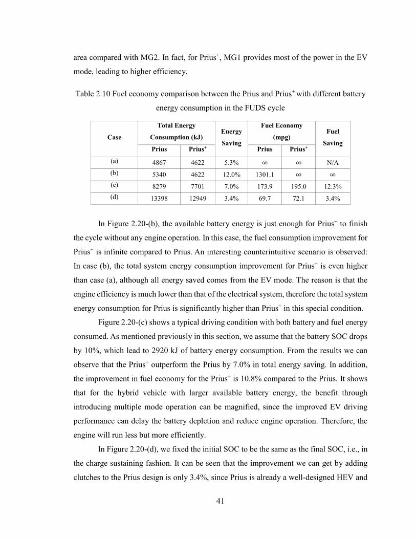
41

area compared with MG2. In fact, for Prius+, MG1 provides most of the power in the EV

mode, leading to higher efficiency.

Table 2.10 Fuel economy comparison between the Prius and Prius+ with different battery

energy consumption in the FUDS cycle

Case

Total Energy

Consumption (kJ) Energy

Saving

Fuel Economy

(mpg) Fuel

Saving Prius Prius+ Prius Prius+

(a) 4867 4622 5.3% ∞ ∞ N/A

(b) 5340 4622 12.0% 1301.1 ∞ ∞

(c) 8279 7701 7.0% 173.9 195.0 12.3%

(d) 13398 12949 3.4% 69.7 72.1 3.4%

In Figure 2.20-(b), the available battery energy is just enough for Prius+ to finish

the cycle without any engine operation. In this case, the fuel consumption improvement for

Prius+ is infinite compared to Prius. An interesting counterintuitive scenario is observed:

In case (b), the total system energy consumption improvement for Prius+ is even higher

than case (a), although all energy saved comes from the EV mode. The reason is that the

engine efficiency is much lower than that of the electrical system, therefore the total system

energy consumption for Prius is significantly higher than Prius+ in this special condition.

Figure 2.20-(c) shows a typical driving condition with both battery and fuel energy

consumed. As mentioned previously in this section, we assume that the battery SOC drops

by 10%, which lead to 2920 kJ of battery energy consumption. From the results we can

observe that the Prius+ outperform the Prius by 7.0% in total energy saving. In addition,

the improvement in fuel economy for the Prius+ is 10.8% compared to the Prius. It shows

that for the hybrid vehicle with larger available battery energy, the benefit through

introducing multiple mode operation can be magnified, since the improved EV driving

performance can delay the battery depletion and reduce engine operation. Therefore, the

engine will run less but more efficiently.

In Figure 2.20-(d), we fixed the initial SOC to be the same as the final SOC, i.e., in

the charge sustaining fashion. It can be seen that the improvement we can get by adding

clutches to the Prius design is only 3.4%, since Prius is already a well-designed HEV and

42

the advantage of the added EV mode cannot be fully realized in this charge sustaining case.

The detailed loss analysis of case (d) is shown in Figure 2.21. It can be observed in Table

2.11 that the additional two-MG EV mode of the Prius+ reduces the total loss of the electric

system and engine operation, which means the engine can run less and more efficiently,

leading to superior fuel economy.

Table 2.11 Energy loss and efficiency comparison between the Prius and Prius+ in charge

sustaining operation in the FUDS cycle

Source Energy Loss (kJ)/Efficiency

Prius Prius+

Vehicle drag 3670 (N/A) 3670 (N/A)

Engine 8628(35.6%) 8311(35.8%)

MG1 190 (91.2%) 704(89.8%)

MG2 912 (86.0%) 248 (89.0%)

Battery 45 (99.3%) 55 (99.2%)

Figure 2.21 Energy analysis of the Prius in case (d)

43

Figure 2.22 Energy analysis of the Prius+ in case (d)

In summary, with the introduction of multiple-mode operations, not only the overall

efficiency of the system can be improved due to the introduction of a more efficient EV

mode (EV2 mode), but the difference in fuel consumption is amplified due to the small

amount of fuels consumed. Based on the discussions above, adding clutches will be

especially beneficial when the vehicle uses EV modes more frequently. One such example

is for plug-in hybrid vehicles with a sizable battery operating in the charge depletion mode.

In other words, if someone mostly drives in an urban environment, and has a plug-in Prius,

then adding a clutch to form the imagined “Prius+” powertrain will be more beneficial.

44

AUTOMATED MODELING, MODE SCREENING AND MODE

CLASSIFICATION OF MULTIPLE PLANETARY GEAR

POWERTRAIN SYSTEMS

In Chapter 2, all possible configurations with clutches have been explored for single

PG hybrid powertrain systems. It has been shown that when clutches are used in a power-

split powertrain, different operating modes can be achieved, which adds flexibility to the

vehicle operations. For power-split vehicles using more than one PG, a general modeling

method was developed [37]. However, general clutch allocation and identification of

unique modes have not been discussed in the literature. In this chapter, more general cases

with multiple PG and clutches will be discussed. In a double PG system, for example, the

input-split modes can be used for better launching performance while the compound-split

mode can be used for better high-speed driving while curtailing the operating speed of the

electric machines [20]. It is also possible to have power-split modes, pure EV modes and

fixed-gear modes on the same powertrain [72] [73]. Having a diverse set of operating

modes makes it possible to fully realize the potential of the powertrain and achieve better

fuel economy and improved drivability, when comparing to conventional vehicles and

traditional hybrid vehicles.

Although many configurations and designs have been patented and some

implemented commercially [26] [72] [73] [74], much more remain unexplored.

“Configuration” in this dissertation refers to the way how power devices (engine and

generator/motors) and output shaft are connected to the nodes of the PGs, while “design”

stands for a specific clutch selection set for a certain configuration. In this chapter, an

automated modeling methodology will be proposed, which will be used to develop

dynamic modes for all possible modes for any given design.

45

3.1 General Planetary Gear System with Clutches

Many of today’s popular power-split hybrid vehicles use two motor/generators

(MGs) to complement the engine. In this dissertation, we adopt this general powertrain

setup. Assuming no component collocation on any of the planetary gear node, the number

of different configurations (nconfiguration_total) and the maximum number of clutches

(nclutch_total) can be calculated by Eq. (3-1) and Eq. (3-2),

4_ 3configuration total nn C (3-1)

2_ 3 3 2 1clutch total nn C n n (3-2)

where n is the number of PG sets. The first term in Eq. (3-2) stands for the number of

clutches that can be added between any two nodes of the PGs, while the second term

represents the grounding clutch that can be added. The third term is the number of

redundant clutches that can be eliminated from the system: for each PG, locking any two

nodes makes all three nodes rotating at the same speed. Therefore, for each PG, (�� − 1 =

2) clutches can be eliminated. In addition, the grounding clutch for the vehicle output shaft

is meaningless during driving, leading to the last term in Eq. (3-2).

The diagram of a double PG system is shown in Figure 3.1, where 16 clutches can

be implemented and the redundant clutches (which are not implemented) are shown in red

color (assuming the vehicle output is on the 2nd ring gear).

Figure 3.1 All 16 possible clutch locations for a double PG system

To avoid redundant designs and to facilitate the systematic, automatic modeling

procedure, an assumption is made: each node cannot be connected to all three nodes on

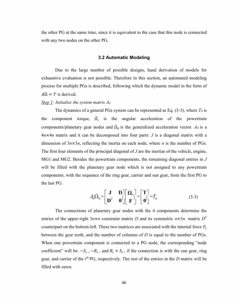
46

the other PG at the same time, since it is equivalent to the case that this node is connected

with any two nodes on the other PG.

3.2 Automatic Modeling

Due to the large number of possible designs, hand derivation of models for

exhaustive evaluation is not possible. Therefore in this section, an automated modeling

process for multiple PGs is described, following which the dynamic model in the form of

�Ω̇ = � is derived.

Step 1: Initialize the system matrix A0

The dynamics of a general PGs system can be represented as Eq. (3-3), where T0 is

the component torque, �̇∗ is the angular acceleration of the powertrain

components/planetary gear nodes and �̇� is the generalized acceleration vector. A0 is a

4n× 4n matrix and it can be decomposed into four parts: J is a diagonal matrix with a

dimension of 3n× 3n, reflecting the inertia on each node, where n is the number of PGs.

The first four elements of the principal diagonal of J are the inertias of the vehicle, engine,

MG1 and MG2. Besides the powertrain components, the remaining diagonal entries in J

will be filled with the planetary gear node which is not assigned to any powertrain

components, with the sequence of the ring gear, carrier and sun gear, from the first PG to

the last PG.

*0 0 0= = =

TA T

J D TΩ

D 0 0F

(3-3)

The connections of planetary gear nodes with the 4 components determine the

entries of the upper-right 3n× n constraint matrix D and its symmetric n× 3n matrix DT

counterpart on the bottom-left. These two matrices are associated with the internal force ��

between the gear teeth, and the number of columns of D is equal to the number of PGs.

When one powertrain component is connected to a PG node, the corresponding “node

coefficient” will be: −�� , −�� , and �� + �� , if the connection is with the sun gear, ring

gear, and carrier of the ith PG, respectively. The rest of the entries in the D matrix will be

filled with zeros.

47

An example for the configuration used in the Toyota Hybrid System (THS-II) used

in Prius MY2010 is shown in Figure 3.2, its corresponding matrices are given in Eq. (3-4).

It should be noted that different from the single PG representation in Chapter 2, in and after

this chapter, all Prius MY2010 lever diagrams use double PG representations because all

possible clutch locations on multiple PG system will be discussed.

Figure 3.2 The lever diagram of THS-II

2 2

1 1 1

1 1 1

2 2 2

0

1 1

2 2 2

1 1 1 1

2 2 2 2

0 1 2

0 1

0 0 0 0 0 0

0 0 0 0 0 0

0 0 0 0 0 0

0 0 0 0 0 0,

0 0 0 0 0 0

0 0 0 0 0 0

0 0 0 0 0

0 0 0 0 0

0 0 0 0 ,

out r

e c

MG s

MG s

r

c

T

Load e MG MG

out eng MG

I I R

I I R S

I I S

I I SA

I R

I R S

R S S R

R S R S

T T T T T

2 1 2 1 2

T

MG r c F F

(3-4)

Step 2: Define the transition matrices

Transition matrices M and P are defined according to the clutch engagement. M is

initialized as a 4n× 4n identity matrix with the same dimension as A0. When the ith PG node

is connected with the jth PG node, without losing generality, assuming i < j, the processes

shown in Eqs. (3-5) and (3-6) are executed for the M matrix. If the clutch is engaged to

ground the ith node, ith row = [], where [] means that the row is eliminated. After this step,

M becomes a (4n-q) × 4n matrix, where q is the number of clutches engaged. th th thi row i row j row (3-5)

[]thj row (3-6)

48

The generation of P is similar to that of M but only row elimination is followed: P

is initiated as a 4n× 4n identity matrix. When the ith node is connected with the jth node,

without losing generality, assuming i < j, Eq. (3-6) is applied. If the clutch is engaged to

ground the ith node, ith row = []. After this step, P becomes a (4n-q) × 4n matrix. M and P

matrices are needed to calculate the dynamic of the system after clutch engagement, as

shown in Eq. (3-7) and Eq. (3-8).

Note that since there are three power components (engine, MG1 and MG2), the

system degree of freedom must be within the range of one to three so that the vehicle is

controllable and drivable. For each non-redundant clutch engagement, one degree of

freedom will be reduced. Therefore the total number of clutches q to be engaged is within

the range of [2n-3, 2n-1].

Step 3: Obtain the dynamic equations of the system

The dynamic matrix A of the powertrain system with clutch engagement is

generated through Eq. (3-7). The dynamic model of an given mode can be represented in

Eq. (3-8). As an example, Eq. (3-9) and Eq. (3-10) show the equations of the THS-II

powertrain system depicted in Figure 3.2.

0 0 0, ,TA M A M T M T P (3-7)

A T (3-8)

1 0 0 0 1 0 0 0 1 0 0 0 0 0 0 0

0 1 0 0 0 0 0 0 0 1 0 0 0 0 0 0

0 0 1 0 0 0 0 0 0 0 1 0 0 0 0 0,

0 0 0 1 0 0 0 0 0 0 0 1 0 0 0 0

0 0 0 0 0 0 1 0 0 0 0 0 0 0 1 0

0 0 0 0 0 0 0 1 0 0 0 0 0 0 0 1

M P

(3-9)

49

3.3 Mode Screening

Not all modes achievable by clutch engagement are useful. If the vehicle cannot be

powered by any powertrain component in a mode, it is defined as an infeasible mode. For

modes with identical dynamic equations, one is kept and the rest are deemed as redundant.

Distinguishing redundant modes is important for simulation speed in the optimization

process later on. In this section, the process and steps to identify and eliminate infeasible

and redundant modes are described.

Step 1: Constructing the A* matrix

The A matrix is inverted to obtain the dynamic equations that relate inputs to state

derivatives. For a controllable powertrain system (i.e., the speed of each PG node can be

controlled), the A matrix is always invertible. Meanwhile, not every element of the A-1

matrix is useful. The useful part of A-1 is extracted as follows, to obtain a final 4× 4 matrix

A*, as shown in Eq. (3-11).

*

1 1

2 2

out load

e e

m g m g

m g m g

T

TA

T

T

(3-11)

In order to construct the A* matrix, the last n columns and rows as well as the

columns and rows associated with any free node (node with no powertrain component

2 1 1 2

1 1 2

1 1 1

2 2 2

1 1 2 1

2 2

11

22

1

2

0 0 0

0 0 0 0

0 0 0 0

0 0 0 0

0 0 0

0 0 0 0

,

0

0

out r r

e c

MG s

MG s

outLoad

ee

MGMG

MGMG

I I I R R

I I R R

I I SA

I I S

R R R S

R S

T

T

TT

T

F

F

(3-10)

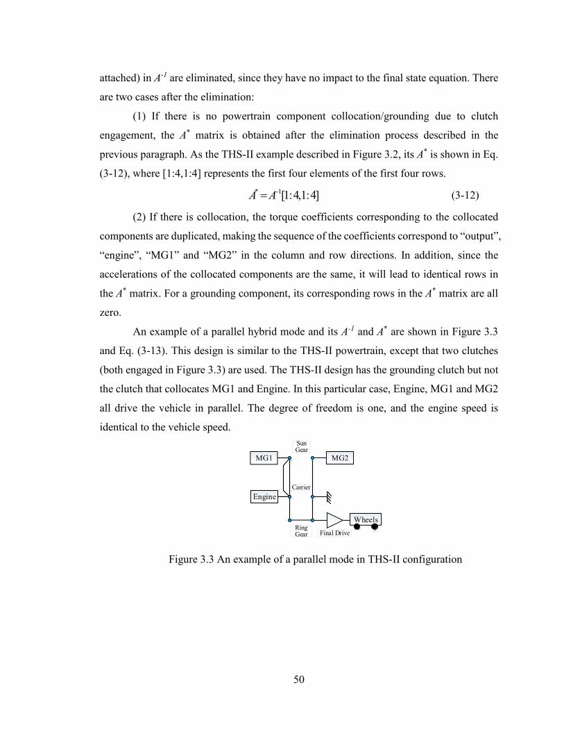
50

attached) in A-1 are eliminated, since they have no impact to the final state equation. There

are two cases after the elimination:

(1) If there is no powertrain component collocation/grounding due to clutch

engagement, the A* matrix is obtained after the elimination process described in the

previous paragraph. As the THS-II example described in Figure 3.2, its A* is shown in Eq.

(3-12), where [1:4,1:4] represents the first four elements of the first four rows.

* 1[1:4,1:4]A A (3-12)

(2) If there is collocation, the torque coefficients corresponding to the collocated

components are duplicated, making the sequence of the coefficients correspond to “output”,

“engine”, “MG1” and “MG2” in the column and row directions. In addition, since the

accelerations of the collocated components are the same, it will lead to identical rows in

the A* matrix. For a grounding component, its corresponding rows in the A* matrix are all

zero.

An example of a parallel hybrid mode and its A-1 and A* are shown in Figure 3.3

and Eq. (3-13). This design is similar to the THS-II powertrain, except that two clutches

(both engaged in Figure 3.3) are used. The THS-II design has the grounding clutch but not

the clutch that collocates MG1 and Engine. In this particular case, Engine, MG1 and MG2

all drive the vehicle in parallel. The degree of freedom is one, and the engine speed is

identical to the vehicle speed.

MG1 MG2

Engine

Ring Gear Final Drive

Carrier

Sun Gear

Wheels

Figure 3.3 An example of a parallel mode in THS-II configuration

51

11 12 13 14 15

121 22 23 24 25

1231 32 33 34 35

141 42 43 44 45

251 52 53 54 55

( )

inv inv inv inv invout

inv inv inv inv inve MG

inv inv inv inv invMG

inv inv inv inv inv

inv inv inv inv inv

A A A A A

A A A A A

A A A A A A

FA A A A A

FA A A A A

，1

12

11 12 12 13

* 21 22 22 23

21 22 22 23

31 32 32 33

0

0

load

e MG

MG

inv inv inv inv

inv inv inv inv

inv inv inv inv

inv inv inv inv

T

T T

A T

A A A A

A A A AA

A A A A

A A A A

(3-13)

Step 2: Refining the A* matrix

If three of the four elements are zero for any row of A*, the correspondence

component has no connection with the other three components, i.e., the rest of the

powertrain, then all the elements in the row are set to zero for future rank check purpose.

If both the 1st and the 2nd element of the 3rd and 4th row of A* are zero, it means the

MGs are neither connected with the engine nor the vehicle, they will not affect the function

of the mode, and the entire 3rd and 4th row of A* are set to 0.

Step 3: Define entries in A* matrix

The four rows of the A* matrix are named Vveh, Veng, VMG1 and VMG2 , respectively,

and the elements of the Vveh row vector are named Cveh, Ceng, CMG1, CMG2 for later use.

If the first row of A* is zero, the vehicle output is not affected by any powertrain

component, making it infeasible (not drivable). In addition, vehicle modes with identical

A* matrices are deemed identical and only one mode will be kept to the mode classification

procedure.

3.4 Mode Classification

All feasible modes are classified into the mode types shown in Table 3.1. Since the

degree of freedom (DoF) of the powertrain varies between one and three, and the mode

type can be EV, hybrid, or engine only, the 14 mode types in Table 3.1 are all possible

modes when one engine, one output shaft and two MGs are assigned, regardless of the

number of PGs. All possible topologies of mode types are shown in Figure 3.4. In this

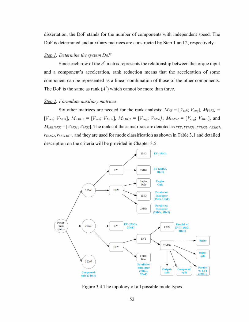
52

dissertation, the DoF stands for the number of components with independent speed. The

DoF is determined and auxiliary matrices are constructed by Step 1 and 2, respectively.

Step 1: Determine the system DoF

Since each row of the A* matrix represents the relationship between the torque input

and a component’s acceleration, rank reduction means that the acceleration of some

component can be represented as a linear combination of those of the other components.

The DoF is the same as rank (A*) which cannot be more than three.

Step 2: Formulate auxiliary matrices

Six other matrices are needed for the rank analysis: MVE = [Vveh; Veng], MVMG1 =

[Vveh; VMG1], MVMG2 = [Vveh; VMG2], MEMG1 = [Veng; VMG1], MEMG2 = [Veng; VMG2], and

MMG1MG2 = [VMG1; VMG2]. The ranks of these matrixes are denoted as rVE, rVMG1, rVMG2, rEMG1,

rEMG2, rMG1MG2, and they are used for mode classification as shown in Table 3.1 and detailed

description on the criteria will be provided in Chapter 3.5.

Figure 3.4 The topology of all possible mode types

53

Table 3.1 Mode types and criteria

Mode Type Criteria

1 Series Mode DoF=2, Ceng = 0, Veng ≠ 0,

CMG1CMG2 = 0,

2 Compound Split (3 DoF) DoF = 3

3 Compound Split (2 DoF)

DoF = 2, CengCMG1CMG2 ≠ 0,

rVMG1 = 2, rVE = 2, rVMG2 = 2,

rEMG1 = 2, rEMG2 = 2, rMG1MG2 = 2

4 Input Split DoF = 2, Ceng CMG1CMG2 ≠ 0

rVMG1 rVMG2 = 2

5 Output Split DoF = 2, Ceng CMG1CMG2 ≠ 0,

rEMG1 rEMG2 = 2

6 Parallel with EVT

(Engine + 1MG)

DoF = 2, Ceng ≠ 0,

CMG1 CMG2 = 0, CMG12 +CMG2

2 ≠ 0

7 Parallel with EVT

(Engine + 2 MGs in serial)

DoF = 2, Ceng ≠ 0,

CMG1CMG2 ≠ 0, rMG1MG2 = 1

8 Engine Only

(Fixed Gear)

DoF = 1, Ceng ≠ 0

CMG12 +CMG2

2 = 0

9 Parallel with Fixed Gear

(Engine + 2MGs, 2 DoF)

DoF = 2, Ceng ≠ 0

rVE = 1, CMG1CMG2 ≠ 0


(Engine + 2MGs, 1DoF)

DoF = 1, Ceng ≠ 0

CMG1CMG2 ≠ 0


(Engine + 1MG, 1DoF)

DoF = 1, Ceng ≠ 0


2 ≠ 0

12 EV (2MGs,2 DoF) DoF = 2, Veng = 0

13 EV (2MGs,1 DoF) DoF = 1, Veng = 0, CMG1CMG2 ≠ 0

14 EV (1MG) DoF = 1, Veng = 0


2 ≠ 0

For double PG powertrain system, 16 clutches may have 216=65,536 clutch states

in theory as discussed previously. If we take the THS-II configuration as an example, it

can be found that after automated modeling and screening process, only 101 feasible and

non-redundant modes remain, whose distribution is shown in Figure 3.5.

54

Figure 3.5 All feasible and non-redundant modes for the configuration used in Prius

2010, grouped into 14 mode types

3.5 Discussion on Mode Types

In this section, all 14 possible types of mode will be discussed separately and

examples from a double PG system are used to demonstrate each type of modes. Note that

the classification criteria of each mode type is mutually exclusive.

Mode type 1: Series mode

As it is introduced in the first chapter, in a Series mode, the DoF equals to two,

while one MG is coupled with the engine mechanically and the other MG drives the vehicle,

as shown in Figure 3.6. Since the engine is not mechanically connected with the vehicle

but a MG, its corresponding coefficient Ceng on the Vveh row is zero and Veng row is nonzero.

In addition, two MGs are not mechanically connected, leading to CMG1CMG2 = 0. Therefore,

the criteria to classify Mode type 1 is: DoF = 2, Veng ≠ 0, Ceng=0, CMG1CMG2 = 0, as shown

in Table 3.1.

Because the engine speed and power is not rigidly constrained by the vehicle status,

the engine operation points can be manipulated efficiently. In addition, the traction motor

provides the flexibility which makes the vehicle drive reversely without the need of

mechanical reverse gear while the engine can constantly provide power. However, due to

the fact that the vehicle is driven by one single MG, the overall efficiency might be suffered.

55

Figure 3.6 Tow examples of Series mode with double PGs

Mode type 2: 3 DoF mode

With two MGs, one engine and, the powertrain system can achieve three DoF (i.e.,

three linearly independent equations are required to describe the speed relationship of the

powertrain components), if the appropriate clutch connections are made, as an example

shown in Figure 3.7. Since this mode is the only mode type that has three DoF, the criteria

to classify Mode type 2 is simply DoF = 3.

Figure 3.7 Two examples of 3 DoF mode with double PGs

In this mode, not only the speed of the vehicle and engine, but also the speed of one

of the two MGs can be controlled independently. However, since the number of

controllable powertrain component and the DoF are both three, no flexibility on

components’ torque is allowed if their accelerations are determined. This can also be

explained by Eq. (3-11): assuming the first three rows of the A* matrix are used to calculate

the torque input when desired components’ acceleration are determined, since the vehicle

56

load torque Tload is uncontrollable, it can be easily seen that the torque from all three

powertrain components are fixed, which may lead to inefficient operations. In addition,

when the engine is off, the components’ speeds will become uncontrollable, which can be

observed from Eq. (3-11).

Mode type 3: Compound-split mode (2DoF)

In a compound-split mode, the DoF is two. The vehicle speed, engine speed as well

as two MGs speed is not coupled with each other (i.e., DoF = 2, rVMG1 = 2, rVE = 2, rVMG2 =

2, rEMG1 = 2, rEMG2 = 2, rMG1MG2 = 2). All powertrain components are connected

mechanically through the PG system (i.e., CengCMG1CMG2 ≠ 0). Therefore, the criteria to

classify Mode type 3 is: DoF = 2, CengCMG1CMG2 ≠ 0, rVMG1 = 2, rVE = 2, rVMG2 = 2, rEMG1 =

2, rEMG2 = 2.

This mode type has been used as a high speed mode in production multimode

hybrid vehicles such as the Silverado Hybrid and the second generation of Chevrolet Volt.

An example of the Compound-split mode, used in the second generation of the Chevrolet

Volt, is shown in Figure 3.8.

Figure 3.8 Two examples of Compound-split mode with double PGs

Mode type 4: Input-split mode

In an Input-split mode, the DoF is two and all components are mechanically

connected to the output shaft via the PG system (i.e., DoF = 2, Ceng ≠ 0, CMG1CMG2 ≠ 0).

The speed of one MG is coupled with the vehicle speed, while the engine and the other

MG’s speed are uncoupled with the vehicle speed (i.e., rVMG1 rVMG2 = 2). Therefore, the

criteria to classify Mode type 4 is: DoF = 2, Ceng ≠ 0, rVMG1 rVMG2 = 2, CMG1CMG2 ≠ 0.

57

In this mode type, the MG that has a fixed gear ratio with the vehicle output shaft

can provide significant torque assist when launching the vehicle. In addition, since the

engine speed is decoupled from the vehicle speed, the engine can be operated efficiently

regardless of the vehicle speed. These attributes make this mode type the most popular

hybrid mode type nowadays: it is widely applied in all current Toyota hybrid vehicle fleets,

Ford Fusion and some multimode hybrid vehicles such as the Silverado Hybrid and the

second generation of Chevrolet Volt. Figure 3.9-(a) and (b) present the Prius and the Input-

split mode of the second generation of Chevrolet, respectively.

Figure 3.9 Two examples of Input-split mode with double PGs

Mode type 5: Output-split mode

In an Output-split mode (Figure 3.10), the DoF is two and all powertrain

components are mechanically connected with each other via the PG system (i.e., DoF = 2,

CengCMG1CMG2 ≠ 0). The engine speed is always coupled with one MG while uncoupled

with the other MG and the vehicle speed (i.e., rEMG1rEMG2 = 2). Therefore, the criteria to

classify Mode type 5 is: DoF = 2, Ceng ≠ 0, rEMG1 rEMG2 = 2, CMG1CMG2 ≠ 0.

Figure 3.10 Two examples of Output-split mode with double PGs

58

Similar to other power-split types (Mode type 3 and 4), the engine operation in an

Output-split mode can be optimized regardless of the vehicle speed. An example of the

Output-split mode in production vehicle is the first generation of the Chevrolet Volt, whose

configuration shown in Figure 2.12-(d).

Mode type 6: Parallel with EVT mode (1MG)

The Mode type 6 can be viewed as a “one motor case” of Input-split modes without

the MG coupled with the vehicle output shaft (i.e., DoF = 2, Ceng ≠ 0, CMG1CMG2 = 0, CMG12

+CMG22 ≠ 0), as an example shown in Figure 3.11.

Figure 3.11 Two examples of Parallel with EVT mode (1MG) with double PGs

In this mode, the vehicle is driven by the engine and one of the two MGs. While

such powertrain arrangement provides an EVT function so that the engine speed can be

controlled regardless of the vehicles speed, it does not offer the same flexibility in

controlling the engine torque. Similar to the 3 DoF Mode, because the number of

controllable powertrain components is equal to the DoF of the powertrain system, the

engine torque cannot be arbitrary assigned when the engine is operating at the desired

speed. In addition, when the engine fuel is cut, its speed is no longer controllable.

Therefore, such mode type has very limited capability to drive the vehicle along, although

it may be used as an intermediate mode when mode shift happens while components speeds

need to be changed for clutch engagement conditions.

59

Mode type 7: Parallel with EVT mode (2MGs)

In mode type 7, an EVT function is realized by the engine, output shaft and two

MGs which are connected in serial (DoF = 2, Ceng ≠ 0, CMG1CMG2 ≠ 0, rMG1MG2 = 1), as two

examples shown in Figure 3.12.

This mode type is just a topologically feasible mode type based on the two MG,

one engine and one output shaft assumption and there is no such mode in a commercialized

vehicle. Similarly to the mode type 6, although two MGs are used, when the engine fuel is

cut, the components’ speeds will be uncontrollable.

Figure 3.12 Two examples of Parallel with EVT mode (2MG, 1DoF) with double PGs

Mode type 8: Engine only mode

The mode type 8 is an engine only mode since both MGs are disabled in the

powertrain system (CMG12 + CMG2

2 = 0). In this circumstance, the output shaft is driven

only by the engine with a fixed-gear ratio (DoF = 1, Ceng ≠ 0), as shown in Figure 3.13. In

an Engine only mode, the vehicle is just running as a conventional vehicle without MGs.

Figure 3.13 Two examples of Engine of only mode with double PGs

60

Mode type 9: Parallel with fixed-gear mode (2MGs, 2 DoF)

In mode type 9 (Figure 3.14), the engine is connected to the drive shaft directly

(Ceng ≠ 0, rVE = 1,). The DoF is two since the speeds of the two MGs are decoupled from

the vehicle speed (DoF = 2, CMG1CMG2 ≠ 0). Therefore, the criteria to classify the Mode

type 9 is: DoF = 2, CMG1CMG2 ≠ 0, Ceng ≠ 0, rVE = 1.

In this mode type, since the speed of MGs can be manipulated, possibly higher

efficiency may be achieved, compared with the mode type whose MGs’ speed are

proportional to the vehicle speed. However, it should be noted that this mode type is only

a topologically feasible mode by our assumption of powertrain components, not in any

commercialized vehicles to the best of our knowledge.

Figure 3.14 Two examples of Parallel with fixed-gear mode (2MGs, 2DoF) with double

PGs

Mode type 10: Parallel with fixed-gear mode (2MGs, 1 DoF)

In Mode type 10, the engine and MGs speeds are all proportional to the vehicle

speed (DoF = 1, Ceng ≠ 0), as two examples shown in Figure 3.15. Both MGs can either

assist or recuperate from the vehicle (CMG1CMG2 ≠ 0). The criteria to classify the Mode type

10 is: DoF = 1, Ceng ≠ 0, CMG1CMG2 ≠ 0.

As a parallel mode, the engine torque can be chosen around the area with best

efficiency and the MGs can either provide or consume torque to compensate the driver’s

demand. Since two MGs are used in this mode type, the torque distribution of the two MGs

can be adjusted in order to achieve best overall efficiency. An example type 10 mode is

shown in Figure 3.15. This mode type can be found in multi-mode HEVs, such as Silverado

Hybrid and Honda Accord Hybrid [75] [76].

61

Figure 3.15 Two examples of Parallel with fixed-gear mode (2MG, 1DoF) with double

PGs

Mode type 11: Parallel with fixed-gear mode (1MG)

Similar to mode type 10, in mode type 11, all operating components’ speeds are

proportional to each other (DoF = 1, Ceng ≠ 0) and the engine torque can be chosen around

the area with best efficiency. The only difference is that in this mode type, only one instead

of two MG is used (CMG12+ CMG2

2 ≠ 0), as two examples shown in Figure 3.16. This mode

type is a typical mode type in parallel HEVs, such as the Honda Insight [77].

Figure 3.16 An example of Parallel with fixed-gear mode (1MG) with double PGs

Mode type 12: EV mode (2MGs, 2DoF)

In mode type 12, the engine is disabled/grounded (Veng = 0) and the both of MGs

are operating. In this mode, DoF = 2 and the speeds of two MGs speeds are not coupled

with the vehicle speed, as two examples shown in Figure 3.17. Such mode type can be

found in the first generation of Chevrolet Volt, as discussed in Chapter 2. In this mode

type, the speeds of two MGs can be manipulated to improve their efficiency.

62

Figure 3.17 Two examples of EV mode (2MG, 2DoF) with double PGs

Mode type 13: EV mode (2MGs, 1DoF)

In mode type 13, the engine is disabled/grounded (Veng = 0) and two MGs can both

provide torque to the output shaft (CMG1CMG2 ≠ 0). Unlike Mode type 12, their speeds are

coupled with the vehicle speed (DoF = 1). The torque of the two MGs can be superimposed

to achieve great launching performance. In addition, the torque distribution of the two MGs

can be manipulated in order to achieve better efficiency while satisfying driver’s demand.

Such mode type is available in the 2nd generation of Chevrolet Volt (Figure 3.18-(a)), which

will be discussed in the next section of this Chapter. Another example is presented in Figure

3.18-(b), which shows the lever diagram of the EV (2MGs, 1DoF) mode in the Prius++.

Figure 3.18 Two examples of EV mode (2MG, 1DoF) with double PGs

Mode type 14: EV mode (1MG)

In mode type 14 (Figure 3.19), the vehicle is driven by only one MG and the rest

powertrain component are mechanically disabled (DoF = 1, Veng = 0, CMG1CMG2 = 0, CMG12

63

+ CMG22 ≠ 0). In theory, this mode type can be viewed as a special case of the Mode type

1, 4 and 13 when the engine or the rest MG are not in use.

Figure 3.19 Two examples of EV mode (1MG) with double PGs

3.6 Case Study: the 2nd Generation of Chevrolet Volt

The first generation (MY 2011) of Chevrolet Volt used a single PG system and

three clutches to achieve four operating modes, as it was well discussed in Chapter 2. In

2015, Chevrolet announced its next generation of Volt [78] (MY 2016, referred as Volt

Gen 2 in this dissertation). As its lever diagram shown in Figure 3.20, it is equipped with

a double PG system, three clutches and a fixed connection. The main powertrain

parameters of Volt Gen 1 and Gen 2 are shown in Table 3.2. In this section, the proposed

modeling and analysis methodologies are adopted to the Volt Gen 2 to perform a case study.

Figure 3.20 Lever diagrams of the Volt Gen 1 and Gen 2

64

Table 3.2 Parameters of Volt Gen 1 and Volt Gen 2

Component Parameters

Volt Gen 1 Volt Gen 2

Engine 1.4L I4

63kW@5200rpm

1.5L I4

75kW@5600rpm

PMG1max(kW) 55 48

PMG2max(kW) 111 87

Battery 16.3kWh

Max power: 110kW

18.4kWh

Max Power:120kW

Final Drive Ratio 2.16 2.64

R1:S1 Ratio 2.24 1.87

R2:S2 Ratio N/A 2.077

Vehicle curb mass(kg) 1717 1607

Volt Gen 2 has three clutches and a fixed connection, therefore in theory 23=8

clutch operating states (modes) can be realized. According to the proposed automated

modeling method and the parameters in Table 3.2, the diagram of its possible clutch state

combinations and associated A* matrices are shown in Figure 3.21. By the feasible mode

classification criteria proposed in Chapter 3.4, the 8th mode is an infeasible mode since the

vehicle cannot be driven by any components; the rest 7 modes are feasible and their

corresponding mode types and criteria are shown in Table 3.3.

Table 3.3 Operating modes of the Volt Gen 2 powertrain

Mode #

Classification Criteria

Mode Type

Description Clutch Operation

CL1 CL2 CL3

1 DoF = 1, Veng = 0

CMG1CMG2 ≠ 0 13

EV (2MGs, 1

DoF) 0 1 1

2

DoF = 1, Ceng ≠ 0

CMG1 CMG2 = 0,

CMG12 +CMG2

2 ≠ 0

11

Parallel with

Fixed-Gear

(MG2 + Engine)

1 1 0

3 DoF = 2, Ceng ≠ 0,

rVMG1 rVMG2 = 2, CMG1CMG2 ≠ 0 4 Input-split 0 1 0

4

DoF = 2, Ceng ≠ 0,

CMG1CMG2 ≠ 0, rVMG1 = 2, rVE = 2,

rVMG2 = 2, rEMG1 = 2, rEMG2 = 2

3 Compound split

(2 DoF) 1 0 0

65

Mode #

Classification Criteria

Mode Type


CL1 CL2 CL3

5 DoF = 1, Ceng = 0

CMG1CMG2 ≠ 0 13

EV (2MGs, 1

DoF) 1 0 1

6 DoF = 1, Veng = 0


2 ≠ 0 14 EV (MG1) 0 0 1

7 DoF = 2, Ceng ≠ 0,


2 ≠ 0 6

Parallel with

EVT (Engine +

MG1)

0 0 0

Figure 3.21 All 8 possible clutch operating states of Volt Gen 2

66

Mode 1 uses both MGs to power the vehicle, similar to the EV mode of the Prius+

in Chapter 2. This mode can be used at any vehicle speed, enabling Volt Gen 2 to achieve

better launching performance than Volt Gen 1, despite the fact that the MGs are smaller.

Mode 2 is a parallel mode, and the gear ratios between the engine, MG2 and the

output shaft are fixed, with the MG1 grounded. The engine can run at a high efficiency at

medium vehicle speed (around 40 to 60 km/h according to [78]). It has high efficiency

because there is no energy circulation in the electrical power path.

Mode 3 is an input-split mode. The efficiency is high due to the EVT function while

the launching performance is good due to the direct drive of MG2. However, the speed

range of MG2 limits its operation and efficiency when vehicle speed is high.

Mode 4 is a compound split mode, which can be used at a high vehicle speed while

retaining the EVT function. Using a compound split mode at high vehicle speed is a concept

that was used in previous designs from General Motors [35] [79].

It should be noted that only the first four modes are used in the Volt Gen 2 [80]

(though the EV status of the Mode 3 is treated as an additional 5th mode). The rest three

modes, while mechanically feasible, suffer from a few problems: Mode 5 is an EV mode

with 2 MGs and 1 DoF, which is similar to the Mode 1. However, its clutch connection

makes it hard to be shifted from the first four modes for reasons that will be explained by

the mode shift feasibility analysis presented in Chapter 4; Mode 6 can be viewed as an

inferior case of Mode 5 with MG 2 disabled, therefore it has less output power compared

with Mode 5; Mode 7 is a parallel with EVT mode, as discussed in Chapter 3.4, it has

controllability problem and it is just an inferior case of Mode 3 when MG2 is disabled.

Therefore, the Mode 5, 6 and 7 are not preferred as the “highlighted” operating modes in

Volt Gen 2, although Mode 6 and 7 might be used as intermediate mode to coordinate

components’ speeds during mode shift.

67

MODE SHIFT ANALYSIS FOR MULTI-MODE HEVS USING

PLANETARY GEAR SYSTEMS

Mode shift is critical for multi-mode HEV fuel economy and driving experience.

Therefore, the mode shift feasibility should be considered in the design procedure when

evaluating and comparing different design candidates. Designs with multiple modes have

been proposed in recent years, such as the GM two mode hybrid [34] [79] and the Chevrolet

Volt series [27] [78]. Although their specific operating mode shifts have been discussed in

these literatures, to the best of our knowledge, very little research has been done on general

mode shift analysis for multi-mode hybrid vehicles. To conduct exhaustive search for all

possible designs, analysis and theories on general mode shift are proposed in this chapter.

4.1 General Mode Shift Description

A mode shift occurs when clutch states are varied to change the dynamics of a

hybrid powertrain. A clutch that was open can be engaged only when the speeds of its two

discs are close. Otherwise significant NVH issues will arise and/or significant energy lose

will incur. In this research, we impose a strict constraint such that the speed of the two

discs of a clutch must be the same to execute a clutch engagement. In addition, no slip is

assumed when a clutch is engaged and both clutch engagement and disengagement

procedures are assumed to be instantaneous. In this chapter, we define the starting mode as

Mode A and the target mode as Mode B. Mode shifts are then categorized to several types

in Figure 4.1, and the details are described as follows:

Feasible/Infeasible Mode Shift: A feasible mode shift is defined as a mode shift

sequence from A to B that can occur when the vehicle speed is not zero. Else it is said to

be infeasible.

68

Indirect/Direct Mode shift: For feasible mode shifts, in some circumstances, the

speed constraint of the clutch engagement for mode shift between A and B can never be

satisfied. In this case, intermediate modes are required and components speeds will be

synchronized in the intermediate modes. If no intermediate mode is required, the mode

shift is defined as a direct mode shift. Otherwise, it is an indirect mode shift.

Figure 4.1 General mode shift category

Unconditional/Conditional Direct Mode Shift: it is assumed that the speeds of

components do not change from the start of the first clutch operation to the end of the last

clutch operation for any direct mode shift. Direct mode shift can be categorized into two

types: unconditional direct mode shift and conditional direct mode shift, according to

whether or not the clutch speed constraint is met automatically. When no clutch state

switches from disengagement to engagement, this mode shift is said to be unconditional.

In contrast, if one or more clutch engagement is needed, it is said to be conditional. For the

latter type of shifts, the speeds of the clutch discs must be synchronized before a conditional

direct mode shift can occur.

Take the Volt Gen 2 presented in Chapter 3 as an example, the shift from Mode 2

to Mode 3 is an unconditional direct mode shift since only CL1 needs to be disengaged, as

shown in Figure 4.2-(a). The shift from Mode 3 to Mode 2 is a conditional direct mode

shift, since the speed of MG1 must be zero to be connected to the 2nd ring gear (CL1 needs

to be engaged), as shown in Figure 4.2-(b).

An example of indirect mode shift is the shift from Mode 4 to Mode 1 in the Volt

Gen 2. As shown in Figure 4.3, the shift from Mode 4 to Mode 1 cannot be executed in a

single step, because the speeds of the engine and MG1 cannot be zero simultaneously for

69

CL2 and CL3 to be engaged when the vehicle is driving. However, it is possible for Mode

4 to first shift to Mode 3 and then to Mode 1 in two steps.

Figure 4.2 Two examples of direct mode shifts for the Volt Gen 2 powertrain: (a) unconditional direct and (b) conditional direct

Figure 4.3 An example indirect mode shift in the Volt Gen 2 powertrain

4.2 Direct Mode Shift Classification

To evaluate mode shift feasibility, it is crucial to detect whether a mode shift from

A to B is a direct mode shift and if it is, whether it is conditional or unconditional. In this

section, it is assumed that the speed of both discs of every non-grounding clutch is

controllable. Under this assumption, direct mode shifts can be identified by the three

theorems as follows:

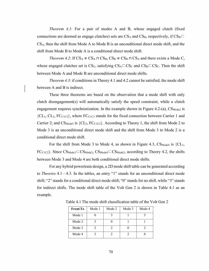
70

Theorem 4.1: For a pair of modes A and B, whose engaged clutch (fixed

connections are deemed as engage clutches) sets are CSA and CSB, respectively, if CSB⊂

CSA, then the shift from Mode A to Mode B is an unconditional direct mode shift, and the

shift from Mode B to Mode A is a conditional direct mode shift.

Theorem 4.2: If CSA ≠ CSA ∩ CSB, CSB ≠ CSB ∩ CSA and there exists a Mode C,

whose engaged clutches set is CSC, satisfying CSA⊂CSC and CSB⊂CSC. Then the shift

between Mode A and Mode B are unconditional direct mode shifts.

Theorem 4.3: if conditions in Theory 4.1 and 4.2 cannot be satisfied, the mode shift

between A and B is indirect.

These three theorems are based on the observation that a mode shift with only

clutch disengagement(s) will automatically satisfy the speed constraint, while a clutch

engagement requires synchronization. In the example shown in Figure 4.2-(a), CSMode2 is

{CL1, CL2, FCC1C2}, where FCC1C2 stands for the fixed connection between Carrier 1 and

Carrier 2; and CSMode3 is {CL2, FCC1C2}. According to Theory 1, the shift from Mode 2 to

Mode 3 is an unconditional direct mode shift and the shift from Mode 3 to Mode 2 is a

conditional direct mode shift.

For the shift from Mode 3 to Mode 4, as shown in Figure 4.3, CSMode4 is {CL1,

FCC1C2}. Since CSMode3⊂CSMode2, CSMode4⊂CSMode2, according to Theory 4.2, the shifts

between Mode 3 and Mode 4 are both conditional direct mode shifts.

For any hybrid powertrain design, a 2D mode shift table can be generated according

to Theories 4.1 - 4.3. In the tables, an entry “1” stands for an unconditional direct mode

shift; “2” stands for a conditional direct mode shift; “0” stands for no shift, while “3” stands

for indirect shifts. The mode shift table of the Volt Gen 2 is shown in Table 4.1 as an

example.

Table 4.1 The mode shift classification table of the Volt Gen 2

From\To Mode 1 Mode 2 Mode 3 Mode 4

Mode 1 0 3 1 3

Mode 2 3 0 1 1

Mode 3 2 2 0 2

Mode 4 3 2 2 0

71

4.3 Optimal Mode Shift Pathway for Indirect Mode Shifts

The optimal mode shift schedule can be automatically calculated by DP when the

speed constraints are well defined, as in Chapter 2.3. However, for instantaneous decision

making problems such as a mode shift in real-time control, the cost of mode shift needs to

be estimated.

If a mode shift from A to B is direct, its cost can be estimated by the kinematic

energy difference of the components involved before and after the shift, as shown in Eq.

(4-1), where λMG1 = sign(ωMG1_BωMG1_A) and λMG2 = sign(ωMG2_BωMG2_A). If the direct mode

shift is unconditional, no energy loss is involved. Each mode shift is assumed to be

penalized by an additional 10J to discourage busy shifts.

2 2_ _

2 21 1_ 1 1_

2 22 2 _ 2 2 _

0.5(

)

A B Eng E B E A

MG MG B MG MG A

MG MG B MG MG A

Cost I

I

I

(4-1)

If a mode shift from A to B is indirect, it is not trivial to identify its cost, because

multiple indirect mode shift pathways may exist. We must first find the mode shift pathway

with the minimum cost, which can be formulated as a shortest path problem, solved from

the graph theory [80].

The shortest path problem is defined below: given a directed graph D = (V, E) and

a length function l: � → ℝ, where V is the set of vertices and E is the set of edges, find the

shortest-length path from a given vertex s to a target vertex y. Past studies on graph theory

dated back to the 19th century, by Wiener (1873), Lucas (1882) and Tarry (1895) [81]. In

the 1950’s, significant progress was made in [82] [83] [84] [85] [86]. Among them,

Dijkstra’s algorithm [86] is known to be the most efficient shortest path algorithm for

problems where no path has negative cost [87], which is the case for our mode shift

problem.

Define s as the initial vertex and u, v as two other arbitrary vertices; d is the

accumulated distance function, l(u, v) is the length function which reflect cost of the edge

from u to v. A vertex is said to be a neighbor of another vertex when there is an edge

connecting these two vertices; set Ψ is defined as the unvisited set and set Θ is defined as

visited set. Dijkstra’s algorithm is then described in six steps:

72

1. Initially, set d(s) = 0 and all other d(v) = ∞. All vertices are in the unvisited set Ψ.

2. Update the distance function of s’s neighbor vertices with d(v) = l(s, v). s is then

removed from the unvisited set Ψ and put into the visited set Θ

3. Choose the vertex from the unvisited set Ψ with lowest distance function and start

to update the distance function of its neighbor u in set Ψ. If d(u) > d(v) + l(u, v), set

d(u) = d(v) + l(u, v).

4. After the accumulated distance function of all neighbor vertices of v are updated,

eliminate v from the unvisited set Ψ and put v into the visited set Θ.

5. If the target vertex is in set Θ, or the smallest distance function of nodes in set Ψ is

infinity, the search has finished.

6. Otherwise, go back to Step 3.

This algorithm is programed in Matlab to find the optimal shift solution. When the

shift between two modes is direct, the cost can be calculated by Eq. (4-1). When the mode

shift is not direct, there is no single edge connecting the two modes. Taking the Volt Gen

2 as an example, assuming the nominal engine speed in the power-split modes (Mode 3

and Mode 4) are 2000 rpm (which may change with vehicle speed and power requirement),

with Table 4.1 and Eq. (4-1), the optimal mode shift pathway from Mode 1 to Mode 4 is

marked red in Figure 4.4, where the gray arrows are possible direct mode shifts. During

the mode shift, CL3 is first disengaged so that the engine can be launched in Mode 3. When

the speed of MG1 becomes 0, CL1 is engaged and CL2 is released simultaneously.

Figure 4.4 Optimal mode shift pathway from Mode 1 to Mode 4 in Volt Gen 2 at 30mph vehicle speed

73

To further elaborate the potential in applying Dijkstra’s algorithm in optimal mode

shift, the optimal mode shift pathway from Mode 1 to Mode 4 of the 7-mode Volt Gen 2 is

shown in Figure 4.5. It is found that the Mode 1 - 3 - 4 path is the optimal pathway. The

optimal mode shift pathway between other modes can be calculated by the same method,

and the minimum mode shift cost between each pair of two modes can be calculated, as

shown in Figure 4.6, where each row indicates the starting mode and each column indicates

the target mode.

Table 4.2 The mode shift classification table of the 7-mode Volt Gen 2

From\To Mode 1 Mode 2 Mode 3 Mode 4 Mode 5 Mode 6 Mode 7

Mode 1 0 3 1 3 3 1 3

Mode 2 3 0 1 1 3 3 1

Mode 3 2 2 0 2 3 2 1

Mode 4 3 2 2 0 2 2 1

Mode 5 3 3 3 1 0 1 3

Mode 6 2 3 2 2 2 0 2

Mode 7 3 2 2 2 3 3 0

Figure 4.5 Optimal mode shift pathway from Mode 1 to Mode 4 in 7-mode Volt Gen 2 at 30mph vehicle speed

74

Figure 4.6 Minimum mode shift cost for the 7-mode Volt Gen 2 at 30mph vehicle speed

It should be noted that the optimal mode shift pathway may change with the vehicle

speed and the engine speed in modes with EVT function. For example, for the same vehicle,

at 60 mph, the optimal mode shift pathway from Mode 1 to Mode 4 goes through Mode 3

and 6, as shown in Figure 4.7. In this pathway, CL2 will be disengaged first, shifting from

Mode 1 to Mode 3. When the speed of the engine reaches the target speed, CL2 will be

disengaged to shift from Mode 3 to Mode 7. In Mode 7, the speed of R2 is manipulated by

MG2 so that CL1 can be engaged to shift to Mode 4. The cost of this pathway 1-3-7-4 is

8.5 kJ, whereas the cost of 1-3-4 pathway is higher at 32.4 kJ due to the fact that engine

speed has to reach 3315 rpm to engage CL1 first and then drop to the nominal speed of

2000 rpm.

75

Figure 4.7 Optimal mode shift pathway from Mode 1 to Mode 4 in the 7-mode Volt Gen 2 at 60mph vehicle speed

76

A NEAR-OPTIMAL ENERGY MANAGEMENT STRATEGY

To mitigate the drawbacks of the existing optimal control methodologies, a rapid

power management algorithm using statistics information of the drive cycle is proposed

and presented in this Chapter. DP, as the only approach that guarantees global optimality,

is used as the benchmark for optimality in evaluating the proposed method.

5.1 Power-weighted Efficiency Analysis for Rapid Sizing (PEARS)

In principle, energy loss minimization could be an effective way to obtain near-

optimal control strategy for hybrid vehicles. However if we blindly apply it to multi-mode

hybrid vehicles, chances are the engine will not be used, because all engine-on modes

(including hybrid modes) have much higher energy loss. ECMS, a well-known

instantaneous optimization method, could be applied to compare EV modes and hybrid

modes. However, since the ECMS strategy is not inherently designed for multiple mode

hybrid vehicles, and since it does not utilize the overall cycle information, the mode shift

timing could not be decided sensibly. Moreover, recursive calculations are required to

determine the equivalent fuel consumption factor for each design or sizing candidate,

leading to a tedious and time-consuming trail-and-error procedure. We propose a new

method, called Power-weighted Efficiency Analysis for Rapid Sizing (PEARS), which can

systematically address both charge sustaining and charge depleting scenarios. Meanwhile,

the control sequence and operation status for PEARS are based on optimal efficiency

analysis without requiring heuristic trial-and-errors.

The PEARS concept proposed in this dissertation is based on the efficiency analysis

of powertrain components. For a given drive cycle, we consider all possible vehicle speeds

and load combinations and rearrange them into a 2D table. By looping through all cells of

the table, referred as the speed-torque cells (STC), we can find the best efficiency and best

77

Power-weighted Efficiency (PE) for given vehicle operation. The battery open circuit

voltage and internal resistance are assumed to be constant. After the optimal operating

states and the associated cost for each mode is determined in each STC, a low-dimension

Dynamic Programming is used to calculate the optimal mode shift schedule and fuel

consumption. The process of PEARS is summarized in Figure 5.1 and details are described

below.

Figure 5.1 Flow chart of the PEARS method

Step 1: Discretize the target drive cycle

The target drive cycle is discretized into a 2D table with the X and Y axes being

the vehicle speed and torque demand, respectively. The table entries represent the

probability density of the cells. The reason why we choose the vehicle torque demand

instead of vehicle acceleration is that the road grade can be taken into consideration in the

future study without adding another dimension when discretizing the target drive cycle.

With this table, similar vehicle operations will not be examined repeatedly just because

road grade exists. In addition, with a fully explored STC table, we do not have to repeat

Step 2 for different drive cycles, making it possible for real-time Model Predictive Control

(MPC) applications in the future.

Step 2: Determine the efficiency for each mode

The Power-weighted Efficiency (PE) for every mode in each STC with non-zero

probability density is examined. The 14 types of modes are divided into two categories

depending on whether the engine is operational or not: EV modes and Hybrid modes. Note

that the engine-only modes are treated as special cases of Hybrid modes.

78

Step 2.1: Determine EV modes efficiency and energy consumption

The efficiency of the EV modes is described by Eq. (5-1), where �� includes

both battery loss and electric-mechanical loss; ��

refers to the power flowing into the

system. In the driving scenario, ��

is the battery power. In the braking case, it is the

regenerative braking power. Note that the friction braking will assist when the regenerative

braking power is inadequate. For modes with one DoF, all possible torque combinations

(TMG1, TMG2) will be compared and the mode with the best efficiency is recorded. For modes

with two DoF, the accelerations of all powertrain components are assumed to be the same.

The best possible efficiency of each mode is calculated from Eq. (5-2). The efficiency of

infeasible MG operation (due to infeasible MG speed or torque) will be excluded from

consideration and the control with the highest efficiency is selected as the optimal control

for each mode in each STC, and the corresponding battery energy consumption will be

recorded.

1loss

EVEV in

EV

P

P (5-1)

*1 2 ,,

max[ ( , )]out outout out

EV EV MG MGT T

(5-2)

Step 2.2: Determine hybrid modes efficiency and energy consumption

When the vehicle is driving, there are two possible power sources for hybrid modes:

the engine and the battery. In general, the power can be divided into four parts as shown in

Figure 5.2 and Table 5.1, where Pe_1 + Pe_2 + Pe_3 is the total engine output power. Pbatt is

the battery power consumed. Figure 5.2 describes the power flow paths where � is a flag

to indicate whether the battery assist is on or not.

The power-weighted efficiency is calculated in Eq. (5-3), where Pfuel is the rate of

fuel energy injected; footnotes G and M denotes whether the electric machine acts as a

generator (when the power is negative) or a motor (when the power is positive or zero). η

e_max, ηG_max and ηM_max are the highest efficiency of the engine, generator and the motor.

Due to the fact that the engine efficiency is much lower than that of the electrical system,

normalization has to be used, otherwise the engine operation will not be selected.

79

_1 _ max _ max

_ 2 _ max _ max _ max

_ 3 _ max _ max

/ ( )( , )

/ ( )

/ + /

e G batt e G

Hybrid e e

fuel batt

e G M e G M

fuel batt

e e batt batt M M

fuel batt

PT

P P

P

P P

P P

P P

(5-3)

*

,,max[ ( , )]

out outout outHybrid Hybrid e eT

(5-4)

Figure 5.2 Power flow in the hybrid modes

Table 5.1 Power-flow of the hybrid system

Power flow Description

Pe_1 Engine power that goes through the generator to the battery

Pe_2 Engine power that goes through generator to motor

Pe_3 Engine power that directly flows to the final drive

Pbatt Battery power

Similar to the EV cases, all speed and torque combinations will be examined. The

control combination associated with the highest efficiency is then selected for each hybrid

mode in each STC. Meanwhile, the corresponding battery energy and fuel consumption are

80

recorded. It should be pointed out that the hybrid mode power-weighted efficiency analysis

are only executed for the driving scenario.

When the vehicle is braking (i.e., torque demand is less than zero), the power-

weighted efficiency analysis for HEV modes is skipped. To avoid frequent mode shift,

special operation states called auxiliary modes for hybrid modes in the braking scenario

are introduced in Step 2.3.

Step 2.3: Determine energy consumption of the bridging and auxiliary modes

Because the component speeds are optimized in Step 2.1 and Step 2.2, they are no

longer states in the optimization problem in the following steps. However, the engine

transient behavior for the EVT modes and the mode shift transient cannot be well captured

if we only calculate the optimal operating points based on power-weighted efficiency. In

addition, due to the cost of mode shift, it is not always efficient to shift to a pure EV mode

if only a short period of engine off is needed in a HEV mode (ex., a short brake). Therefore,

two types of modes for special operating states are introduced to capture the transient

behavior and calculate accurate fuel consumption in the DP procedure in the next step.

The first type of modes for special states is referred as bridging modes. A bridging

mode is defined as a synchronizing state for mode shift when a conditional direct mode

shift happens or is the transient state for a power-split mode shift between its engine-off

and engine-on status. The battery energy and fuel consumption during the bridging mode

are calculated, which covers the period from the time when the mode shift starts till the

time when the components’ speed of the starting mode matches the components’ speed of

the target mode.

Another type of modes for that require special treatment are the auxiliary modes,

which are defined specifically for HEV modes, since the normal HEV operation discussed

in Step 2.2 cannot cover all possible engine working condition for HEV modes. It should

be noted that EV and engine only modes do not need any auxiliary modes, because no

engine operation is involved for the EV modes and the engine operation is predetermined

for Engine only modes. The auxiliary modes for HEV modes are shown in Table 5.2.

For each Parallel with fixed-gear mode, an auxiliary mode which represents the

dynamic of engine off operation is required, because it is not efficient to shift to an EV

81

mode when engine assist is not needed. Such auxiliary modes during engine fuel cut-off is

important to avoid excessive mode shift.

Table 5.2 The table of auxiliary modes for HEV modes

Mode Type Auxiliary Sub Modes

Power-split modes and Series mode (mode type 1,3,4,5) Engine off

Engine idling

Parallel with fixed-gear modes (mode type 9, 10, 11) Engine off

Parallel with EVT modes (mode type 6, 7) None

3 DoF mode (mode type 2) None

EV modes (mode type 12, 13, 14) None

Engine only mode (mode type 8) None

There are two auxiliary modes associated with power-split modes and series modes.

Similar to the Parallel with fixed-gear modes, an EV states which reflect engine off status

is indispensable for each power-split modes and series mode. The engine speed in this

engine off status is zero. In addition, since the HEV mode power-weighted efficiency

analysis are skipped for braking scenarios, the engine idling status is required to avoid

frequent engine on/off when the driver demand decreases

It should be noted that the 3 DoF modes (mode type 2) and Parallel with EVT modes

(mode type 6 and 7) do not need an auxiliary mode. The reason is that the components’

speeds are not controllable when then engine torque is fixed or the engine is off, as

discussed in Chapter 3.5.

The total number of mode for each design Ntotal in the next DP procedure can be

calculated as Eq. (5-5), where NType(.) is the number of mode in certain types and NBridging is

the number of bridging mode.

(2,6,7,8,12,13,14) (9,10,11) (1,3,4,5)2 3total Type Type Type BridgingN N N N N (5-5)

Step 3: Calculate the optimal mode shift using DP

With Eq. (5-2) and Eq. (5-4), once the optimal control is determined for each mode

for each vehicle STC, the next step is to determine the mode to be used during the drive

cycle.

82

The states and controls of the DP problem are shown in Table 5.3. The first state is

the battery energy consumption, which is calculated from Step 2; the second state and

control are both the operating mode, including the bridging and auxiliary modes. Note that

the mode is a state because the cost function includes the mode shift penalty.

Table 5.3 The states and controls for the DP procedure in the PEARS problem

States and Controls Description

State 1 Battery energy consumption (Equivalent to SOC)

State 2 Mode

Control 1 Mode

In theory, the auxiliary/bridging modes can be constructed as extra states. However,

due to the fact that the number of auxiliary modes and bridging modes varies dramatically

from one mode to another, it is much more efficient to keep them and the normal EV and

HEV operation calculated in Step 2.1 and Step 2.2 in the same state and control grid.

Here we take the Volt Gen 2 as an example: as discussed in Chapter 2.3, the Volt

Gen 2 has four modes (2 EV modes and 2 HEV modes). From its mode shift classification

table it can be found that the mode shift between Modes 3 & 1, Modes 3 & 2, Modes 3 &

4, Modes 4 & 2, and Modes 4 & 3 are conditional direct mode shift. Therefore, five

bridging modes are required. In addition, Mode 2 is a Parallel with fixed-gear mode,

therefore it needs one auxiliary mode; Modes 3 and 4 are both power-split modes, four

auxiliary modes are added for each of them. In total, 4+5+1+8 = 18 modes are required for

the State 1 and Control 1 for the Volt Gen 2 DP procedure in the PEARS Solution process.

Step 3.1: Infeasible mode shift detection

In this step, hard constraints on mode shifts are added according to the mode shift

classification and the specifications of the auxiliary/bridging modes. It is known that a shift

may happen between any two modes. Therefore, a 2D cost table is generated and applied

to the DP cost function.

The mode shift cost table is generated by the flow chart shown in Figure 5.3. In

principle, the mode shift transient cost is already calculated in Step 2.3. However, to avoid

83

excessive mode shifts, additional mode shift penalties are added: the mode shift penalty 1

is set as 0.1g of fuel.

Figure 5.3 The flow chart of the mode shift cost table generation

If the next mode is not mechanically the same, penalties can be added easily: if the

mode shift between the current and next mode is not a direct mode shift, infinite (very large)

penalty is added to prevent such mode being chosen; if the shift is an unconditional directed

mode shift, a very small amount of fuel (e.g. 0.1g) is added as the clutch disengagement

cost; if the shift is a conditional mode shift, a small penalty (e.g. 0.1g) is added to avoid

excessive mode shift; note that a bridging mode has to be used in a conditional mode shift

(to evaluate the cost precisely), otherwise infinite mode shift penalty is added.

If the next mode is mechanically the same as the current mode, appropriate

penalties also should be added to avoid a phenomenon known as “free energy” which will

encourage excessive mode shift in the DP optimization of the PEARS. The for the

auxiliary/bridging mode shift with the same mechanical topology is more complicated, and

84

it is described from Table 5.4 to Table 5.7, where AUX stands for auxiliary modes, “X”

stands for infeasible mode shift (with large penalty) and “O” stands for feasible mode shift

(with zero penalty).

Table 5.4 Mode shift penalty within the same Power-split/Series mode

From\To

Engine

on

AUX

(engine

off)

AUX

(engine

idling)

Bridging

(engine

launch)

Bridging

(engine

shutdown)

Bridging(synchr

onizing for mode

shift)

Engine on O X O X O O

AUX(engine off) X O X O X O

AUX(engine idling) O X O X O O

Bridging(engine

launch)

O X O X X X

Bridging(engine

shutdown)

X O X X X X

Bridging(synchronizing

for mode shift)

X X X X X X

Table 5.5 Mode shift penalty within the same Parallel with Fixed-gear mode

From\To Engine on AUX(engine off) Bridging

Engine on O O O

AUX(engine off) O O O

Bridging X X X

Table 5.6 Mode shift penalty within the same 3 DoF/ Parallel with EVT mode

From\To Engine on Bridging

Engine on O O

Bridging X X

Table 5.7 Mode shift penalty within the same EV mode

From\To EV Bridging

EV O O

Bridging X X

85

Step 3.2: Calculate the optimal mode shift schedule

The cost function of the DP problem is described in Eq. (5-6): the optimization

objective is to minimize the fuel consumption while ensuring that the mode shifts are

feasible, and the final SOC close to its desired level. The term βModeshift is the mode shift

penalty from Step 3.1

2

1

min[ ( ) ( ) ]N

shift desired ft

J fuel Mode SOC SOC

(5-6)

Since the dimension of this DP problem is significantly reduced by Step 2, it takes

only 15 to 30 seconds to solve for the optimal modes for a 1,372 seconds long FUDS cycle

on a desktop computer (with Intel i5-2500K 3.5GHz CPU and 16GB RAM). The

computation time varies with the number of modes of the hybrid powertrain.

5.2 Comparison between PEARS and DP

In this sub-section, DP is used as the benchmark to validate the PEARS algorithm.

The Volt Gen 2 design and Prius++ design are used in our case study. In the DP problem,

states and controls for both Volt Gen 2 and Prius++ are identical to those shown in Table

2.3 in Chapter 2, while their cost function is shown in Eq. (2-23).

5.2.1 Computational Load Analysis

Since the states and controls of the DP problem for both Volt Gen 2 and Prius++ are

the same, here we only show the full DP grid formulation of the Volt Gen 2 problem in

Table 5.8. It can be seen that the number of elements in the DP table is

61×53×4×41×119×4=252,380,912 for each step (one second) in a driving cycle. On the

other hand, for the same design (Volt Gen 2), the DP procedure in the PEARS consists of

two states and one control, as shown in

Table 5.9, where the four mechanical modes shown in Table 3.3 are extended to 18

modes according to the procedure outlined in Section 5.1. The total number of element of

the DP table in this PEARS problem is 107×18×18=34,668, which is 1/7,300 of the size of

the full dimension DP.

86

Table 5.8 The states and controls of the benchmark DP of the Volt Gen 2 vehicle

States and Controls Description Grid

State 1 Battery SOC [0.4:0.005:0.7]

State 2 Engine speed [0:100:5200] rpm

State 3 Mode [1:4]

Control 1 Engine torque [-20,0,45:2.5:140]

Control 2 MG1 torque [-118:2:118]

Control 3 Mode [1:4]

Table 5.9 The states and controls for the simpler DP problem solved in the

PEARS process of Volt Gen 2 vehicle

States and Controls Description Grid

State 1 Accumulated battery energy [-1600:30:1600] kJ

State2 Mode [1:18]

Control 3 Mode [1:18]

Both FUDS and HWFET cycles are used for the fuel economy study. Taking the

1,372s FUDS cycle as an example, in the PEARS procedure, the original 1,372 grid point

in time domain is discretized into 531 grid points in the vehicle speed and torque domain,

as the grids shown in Table 5.10.

Table 5.10 The speed and torque demand grids for Volt Gen 2

Grid description Grid

Vehicle speed grid [0:0.5:65] mph

Vehicle torque demand grid [-400:5:400] Nm

5.2.2 Optimization Results and Discussion

The state/control trajectory and engine operating points for the Volt Gen 2 in FUDS

cycle are shown in Figure 5.4 and Figure 5.5, whereas the fuel economy and computation

time comparison are shown in Table 5.9. It can be seen that the PEARS achieves very

similar fuel economy with similar control and state trajectories in comparison with the

results from the full-sized DP. In the meantime, the number of mode shifts is smaller. From

87

the plots (Figure 5.4-(a) and Figure 5.5-(a)) showing the engine operating points of the full-

sized DP, the engine torque from 17 seconds (170 sampling points) fall between 40 and 80

Nm. This is a small percentage of the total number of points when the engine is turned on

(226s, 2260 sampling points). These points represent inefficient engine operations during

launching or mode shifting. The inefficient engine operation at the end of the cycle is likely

due to the final state constraint. In the PEARS results, transient dynamics are approximated

when calculating the optimal operating points, which is why the fuel economy is slightly

worse than the full-sized DP even though the engine appears to operate more efficiently.

The components loss and efficiency by both methods are shown in Figure 5.6 and Figure

5.7. Although the engine efficiencies of the two methods are similar, the vehicle optimized

by the PEARS method does incur more losses (albeit inconsequential) in the electric path

because of the approximation in the efficiency analysis and mode shifting process.

However, it can be seen from Table 5.11 that the computation time for PEARS is about

10,000 times faster than the full-sized DP, making it more suitable for the large-scale

exhaustive search based design process.

Figure 5.4 Trajectories comparison between DP and PEARS in FUDS cycle for the Volt Gen 2 design

88

Figure 5.5 Engine operating points comparison between DP and PEARS in the FUDS cycle for the Volt Gen 2 design

Table 5.11 Comparison between PEARS and traditional DP for the Volt Gen 2 design

Method

Fuel Consumption (mpg) /Difference

Computation Time (s)


PEARS 63.8 1.5%

51.9 1.7%

29 16

DP 64.8 52.8 356,720 199,160

Figure 5.6 Energy analysis for DP in FUDS cycle for the Volt Gen 2 design

89

Figure 5.7 Energy analysis for PEARS in FUDS cycle for the Volt Gen 2 design

The results for the Prius++ design are shown in Figure 5.8 and Table 5.12. Similarly

to the Volt Gen 2’s results, PEARS consistently leads to near-optimal fuel consumption,

similar engine operating points, and even less frequent mode shifts. In addition, it should

be noted that the fast computation speed and near-optimal solution make PEARS feasible

for fast prototyping design and sizing, and may even be practical for embedded model

predictive control applications when the prediction horizon is not too long. The later (real-

time) application is not explored in this dissertation because we think that is a very different

application direction. In the following chapters, we will use PEARS as the optimization

approach to generate energy management strategies for exhaustive hybrid powertrain

designs.

Table 5.12 Comparison between PEARS and traditional DP for the Prius++ design

Method

Fuel Consumption (mpg) /Difference

Computation Time (s)


PEARS 70.5 2.3%

57.3 2.4%

27 16

DP 72.1 58.7 301,840 168,520

90

Figure 5.8 Trajectories comparison between DP and PEARS in the FUDS cycle for the Prius++ design

91

SYSTEMATIC DESIGN METHODOLOGY FOR MULTI-MODE

POWER-SPLIT HYBRID VEHICLES

Although major automotive manufacturers made intensive researches on multi-

mode hybrid vehicles and filed a significant number of patents [26] [72] [73] [74], the

majority of the design space has not been explored. With the proposed automated modeling

and near-optimal control algorithm, it becomes feasible to exhaustively search for optimal

design from a large pool of design candidates. With the models of all possible modes

constructed, we are ready for performance screening to reduce the candidate pool size.

However, the size of the remaining design space may still be too large to be managed. In

addition, it is necessary to impose “beyond fuel economy” requirements so that the

resulting designs are well-balanced. And such requirement can ensure that the number of

designs that we examine is reasonably small. Therefore, in this chapter, we first present a

screening technology based on drivability performance, including launching, climbing and

towing. Then, in the second part, a case study is presented, combined with the modeling

procedure introduced in Chapter 3, mode shift feasibility analysis in Chapter 4, PEARS

described in Chapter 5 and the screening procedure introduced in this chapter to find

optimal and sub-optimal designs for passenger-sized HEVs based on the THS-II

configuration. In the third part of this chapter, a systematic design based on the Volt Gen

2 with an extended design space using double PG will be proposed. In the last part of this

chapter, the proposed design methodology is applied to light truck application using the

entire double PG design space, and the results are compared with a P2 parallel benchmark

using the same powertrain parameters from Ford F150 MY2012.

92

6.1 Drivability Performance Evaluation

Drivability is crucial for any production vehicle; it involves various metrics such as

launching performance, climbing, towing, handling, etc. In this dissertation, we only focus

on the longitudinal driving performance, i.e., launching, climbing, and towing for heavy

duty vehicles such as pickup trucks.

6.1.1 Launching

Adequate launching performance is important to ensure that the vehicle is “drivable”

and has acceptable grade climbing capability. In this dissertation, we use 0-60 mph

acceleration time to evaluate the launching performance of each design.

For conventional vehicles, finding the best 0-60mph strategy is easy: set the throttle

wide open and apply the best gear for maximum output torque. The same strategy applies

for parallel HEVs: maximize the motor torque plus the engine torque, and use the best gear.

For power-split HEVs and multi-mode HEVs, however, finding the optimal strategy is not

trivial because the engine speed is not proportional to the vehicle speed and multiple modes

can be used. In theory, Dynamic Programing can be used directly to determine the

powertrain component output torque and mode selection, as its state and control variables

shown in

. The stage of this direct DP problem is the vehicle speed, and the acceleration time

duration Ti at each vehicle speed sub-interval is calculated as the instantaneous cost at each

stage. Since the engine speed is a state, only indirect mode shifts calculated by Theory 4.1

and Theory 4.2 need to be penalized by the βModeshift portion with large penalty number,

the objective is to minimize the total time cost during the acceleration subject to the

constraints on the powertrain components, as shown in Eq. (6-1).

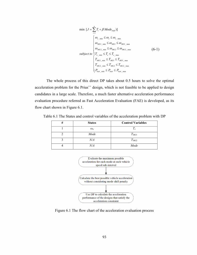
93

1

_ min _ max

1_ min 1 1_ max

2_ min 2 2_ max

_ min _ max

1_ min 1 1_ max

2 _ min 2 2 _ max

_ min _ max

min [ )]n

i shifti

e e e

MG MG MG

MG MG MG

e e e

MG MG MG

MG MG MG

batt batt batt

J T Mode

subject to T T T

T T T

T T T

P P P

(6-1)

The whole process of this direct DP takes about 0.5 hours to solve the optimal

acceleration problem for the Prius++ design, which is not feasible to be applied to design

candidates in a large scale. Therefore, a much faster alternative acceleration performance

evaluation procedure referred as Fast Acceleration Evaluation (FAE) is developed, as its

flow chart shown in Figure 6.1.

Table 6.1 The States and control variables of the acceleration problem with DP

# States Control Variables

1 ωe Te

2 Mode TMG1

3 N/A TMG2

4 N/A Mode

Figure 6.1 The flow chart of the acceleration evaluation process

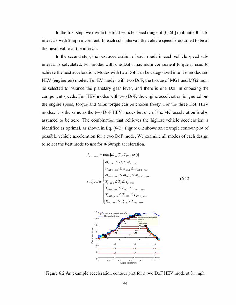
94

In the first step, we divide the total vehicle speed range of [0, 60] mph into 30 sub-

intervals with 2 mph increment. In each sub-interval, the vehicle speed is assumed to be at

the mean value of the interval.

In the second step, the best acceleration of each mode in each vehicle speed sub-

interval is calculated. For modes with one DoF, maximum component torque is used to

achieve the best acceleration. Modes with two DoF can be categorized into EV modes and

HEV (engine-on) modes. For EV modes with two DoF, the torque of MG1 and MG2 must

be selected to balance the planetary gear lever, and there is one DoF in choosing the

component speeds. For HEV modes with two DoF, the engine acceleration is ignored but

the engine speed, torque and MGs torque can be chosen freely. For the three DoF HEV

modes, it is the same as the two DoF HEV modes but one of the MG acceleration is also

assumed to be zero. The combination that achieves the highest vehicle acceleration is

identified as optimal, as shown in Eq. (6-2). Figure 6.2 shows an example contour plot of

possible vehicle acceleration for a two DoF mode. We examine all modes of each design

to select the best mode to use for 0-60mph acceleration.

_ max 1

_ min _ max

1_ min 1 1_ max

2 _ min 2 2 _ max

_ min _ max

1_ min 1 1_ max

2 _ min 2 2 _ max

_ min _ max

max[ ( , , )]out out e MG e

e e e

MG MG MG

MG MG MG

e e e

MG MG MG

MG MG MG

batt batt batt

T T

subject to T T T

T T T

T T T

P P P

(6-2)

Figure 6.2 An example acceleration contour plot for a two DoF HEV mode at 31 mph

0 1000 2000 3000 4000 50000

20

40

60

80

100

120

140

0

0

0

0

0

1

1

1

1

1

2

2

2

2

2

3

3

3

3

3

4

4

4

4

45

5

5

5

5555

5.05

5.05

5.05

5.05

5.055.055.05

5.1

5.1

5.1

5.15.15.1

5.15

5.15

5.1

5

5.155.15

5.2

5.2

5.2

5.25.2

5.25

5.2

5

5.255.25

5.3

5.3

5.35.3

5.35

5.3

5

5.35

5.4 5.4

5.4

5.45

5.455.5

5.5

0

0

0

0

0

0.1

0.1

0.1

0.1

0.1

0.2

0.2

0.2

0.2

0.2

0.3

0.3

0.3

0.3

0.3

0.4

0.4

0.4

0.4

0.4

0.5

0.5

0.5

0.5

0.5

0.6

0.6

0.6

0.6

0.6

0.7

0.7

0.7

0.7

0.7

0.8

0.8

0.8

0.8

0.8

0.9

0.9

0.9

0.9

0.9

1

1

1

1

1

1.1

1.1

1.1

1.1

1.1

1.2

1.2

1.2

1.2

1.2

1.3

1.3

1.3

1.3

1.3

1.4

1.4

1.4

1.4

1.4

1.5

1.5

1.5

1.5

1.5

1.6

1.6

1.6

1.6

1.6

1.7

1.7

1.7

1.7

1.7

1.8

1.8

1.8

1.8

1.8

1.9

1.9

1.9

1.9

1.9

2

2

2

2

2

2.1

2.1

2.1

2.1

2.1

2.2

2.2

2.2

2.2

2.2

2.3

2.3

2.3

2.3

2.3

2.4

2.4

2.4

2.4

2.4

2.5

2.5

2.5

2.5

2.5

2.6

2.6

2.6

2.6

2.6

2.7

2.7

2.7

2.7

2.7

2.8

2.8

2.8

2.8

2.8

2.9

2.9

2.9

2.9

2.9

3

3

3

3

3

3.1

3.1

3.1

3.1

3.1

3.2

3.2

3.2

3.2

3.2

3.3

3.3

3.3

3.3

3.33.4

3.4

3.4

3.4

3.4

3.5

3.5

3.5

3.5

3.5

3.6

3.6

3.6

3.6

3.6

3.7

3.7

3.7

3.7

3.7

3.8

3.8

3.8

3.8

3.8

3.9

3.9

3.9

3.9

3.9

4

4

4

4

4

4.1

4.1

4.1

4.1

4.1

4.2

4.2

4.2

4.2

4.2

4.3

4.3

4.3

4.3

4.3

4.4

4.4

4.4

4.4

4.4

4.5

4.5

4.5

4.5

4.5

4.6

4.6

4.6

4.6

4.6

4.6 4.6 4.6

4.7

4.7

4.7

4.7

4.7

4.7 4.7 4.7

4.8

4.8

4.8

4.8

4.8

4.8 4.8 4.8

4.9

4.9

4.9

4.9

4.9

4.9 4.9 4.9

5

5

5

5

5555

5.05

5.05

5.05

5.05

5.055.055.05

5.1

5.1

5.1

5.15.15.1

5.15

5.15

5.1

5

5.155.15

5.2

5.2

5.2

5.25.2

5.25

5.2

5

5.255.25

5.3

5.3

5.35.3

5.35

5.3

5

5.35

5.4 5.4

5.4

5.45

5.455.5

5.5

Engine speed (rpm)

Engin

e t

orq

ue (

Nm

)

Vehicle acceleration (m/s^2)

X= 3500

Y= 130

Level= 5.5465

Vehicle acceleration (m/s2)

Max engine torque

95

After the best operation for each mode at each vehicle speed interval is calculated,

Dynamic Programming is used to decide the optimal mode shift schedule. Since the

maximum acceleration for each mode at each vehicle interval has been calculated, this DP

problem only have one state and one control, which are current mode and mode to be

selected respectively. The cost function aims to minimize the total time for 0 to 60 mph

acceleration along with the mode shift penalty, as Eq. (6-3) shows, similar to Eq. (4-1),

where Ti is the minimum time sent in acceleration during each vehicle speed interval;

footnotes A and B represent the modes before and after each mode shift, respectively; θ1,

θ2 and θ3 are factors that weight the kinematic energy difference to the associated time cost

in a conditional direct mode shift, λMG1 = sign(ωMG1_BωMG1_A) and λMG2 = sign(ωMG2_Bω-

MG2_A). It is assumed that the kinematic energy corresponding to 0 to 3000rpm engine speed

launching is normalized to 1s time cost; the βModeshift portion penalizes the indirect mode

shift calculated by the Theory 4.1 and Theory 4.2 with a large penalty number.

2 2 2 21 _ _ 2 1_ 1 1_

1

2 23 2_ 2 2_

(min

+ )

, 0; , 1

n

i E B E A MG B MG MG Ai

MG B MG MG A shift

i j

J T

Mode

if Mode Mode else

(6-3)

The acceleration performance results of the Prius++ calculated by both methods are

shown in Table 6.2. It should be noted that 0-75 mph acceleration performance is shown

since in 0-60 mph acceleration no mode shift happens due to the mode shift cost. The

trajectories generated by direct DP and FAE are shown in Figure 6.3. It can be seen from

the results that the FAE method can achieve the same acceleration performance compared

to that of the benchmark direct DP method, but is about 95,000 times faster. Due to the

simplification of the FAE method, mode shift transient behavior such as torque change of

the MG1 cannot be addressed. However, the FAE method leads to similar trajectories for

mode shift schedule, engine speed and torque, etc. Therefore, the proposed FAE will be

used to analyze the acceleration performance of all design candidates in the pool.

Table 6.2 Acceleration performance evaluations of the Prius++

Method 0-75 mph Calculation time

The direct DP 13.56s 1800s

FAE 13.65s 0.02s

96

Figure 6.3 0-75 mph acceleration trajectories of the direct DP and FAE

6.1.2 Climbing and Towing

The acceleration performance is evaluated for all vehicle designs. For heavy duty

vehicles such as pickup trucks and SUVs, when towing should also be evaluated. In this

dissertation, the towing capacity is defined as the launching capability with towing a 10,000

lbs trailer on a 12% grade with engine on in both forward and backward directions. Note

that all available HEV modes will be tested for each design candidates.

6.2 The Multi-Mode Passenger HEV Design Based on the THS-II

Configuration

For a double PG powertrain system with one engine, one output-shaft and two MGs,

as it can be calculated from Eq. (3-1), there are 360 different configurations. Since having

three powertrain components on the same PG will lead to very limited operation flexibility,

we only considered the cases when two powertrain components are connected to each of

the PG. Therefore, the number of configurations is C��P�

�P�� = 216. In addition,

topologically, these 216 configurations can be classified into two types, depending on

whether the engine and output shaft are on the same PG or not, as depicted in Figure 6.4.

For type (a), there are C��C�

�P��P�

� = 144 configurations; while for type (b), there are

97

C��P�

�P�� = 72 configurations. The THS-II (Toyota Hybrid Synergy Drive) design, which is

used in the current generation of Prius, Camry hybrid and Highlander hybrid is an example

of category (a) configurations shown in Figure 6.4.

Figure 6.4 Two types of configurations using 2PG

In this section, we will pick THS-II configuration and use the powertrain

components of the Prius in Table 2.4. In other words, we are only exploring the clutch

placement but not the design search in the configuration nor the sizing dimension in this

case study. Searching in those dimensions may result in even better designs.

While we start by studying the design cases with all 16 clutches, it is clear that the

resulting design only serves as a benchmark and is difficult to implement in practice. In

addition, it is believed that we do not need all the modes enabled by 16 clutches. In this

study, we will further investigate the subset of all possible designs, when three clutches

and one fixed connection are used for the following reasons: First, three clutches may lead

to as many as 7 different modes, resulting in many feasible and suboptimal designs. In

addition, the Chevy Volt uses 3 clutches, so we assume it is feasible in practice today.

As it was demonstrated at the end of Chapter 3, for double PGs, 16 clutches may

have 216=65,536 clutch states in theory. After the screening process, for configurations

described in Figure 6.4-(a), only 101 feasible and non-redundant modes remain, when the

two MGs are treated as different components as shown in Figure 3.5. The reason why all

144 configurations of category (a) have the same number and type of modes is that varying

the connection of a node on one planetary gear will only change the relative speed ratio,

but not the fundamental attribute of the mode.

In theory, a “Utopian” design equipped with all 16 clutches and can achieve all

possible modes [88]. However, considering hard constraint on mode shift to rule out

infeasible and backward driving modes, we have 448 mechanically different modes

98

(including functionally identical modes with different clutch status) left. According to Eq.

(5-5), 3126 modes, including auxiliary and bridging modes, will be examined. Together

with the battery state, the DP procedure of PEARS will have over 1000,000,000 elements

to evaluate in each stage, which will create memory issues for today’s PC. In addition, it is

not economically and technologically feasible to produce such “Utopian” design.

Therefore, for practical purposes, we consider the sub-optimal cases when only 3

clutches and 1 fixed connection are allowed, which leads to C�� C��

� = 7,280 different

designs. Each design may have up to 7 different modes. In the following context, “a design”

refers to one such particular combination of clutch allocation for the THS-II configuration.

The 0 to 60 launching performance requirement is set at 8.5 seconds. 308 of the 7,280

designs passed this drivability requirement and advanced to the fuel economy evaluation

step.

The optimization results from PEARS for FUDS and HWFET cycle are shown in

Table 6.3. We use a weighted fuel economy following the US Environmental Protection

Agency’s practice of using 55% weight on the city cycle (FUDS) and 45% on the highway

cycle (HWFET) [89] .

Table 6.3 Weighted fuel economy for the Prius and Prius++ by PEARS optimization

Cycle\Design Fuel Consumption (mpg)

Prius Prius++

FUDS 67.6 69.9

HWFET 56.2 56.8

Out of the 7,280 designs, 139 achieve better performance in both fuel economy and

drivability than the benchmark Prius, as shown in Figure 6.5. We highlight two sub-optimal

designs, one for better fuel economy (highlighted in green), and one for better launching

performance (highlighted in pink). Compared with the original Prius, the fuel economy-

focused sub-optimal design improves fuel economy and launching performance by 4.0%

and 23.2%, respectively. Compared with the imagined Prius++ (not available on production

vehicles), the best 3-clutch fuel economy-focused design is better by about 1.6% and 7.4%,

respectively. If we are to put more emphasis on launching performance, the sub-optimal

design highlighted in pink can be an alternative for a more balanced design, which is at the

99

corner of the Pareto front. This design can achieve an improvement 33.9% on launching

compared to the Prius, while retain a similar performance in fuel economy compared with

the Prius++. The lever diagrams of the two sub-optimal designs are shown in Figure 6.6.

Figure 6.5 Optimization results comparing 3-clutch designs and the benchmarks

Figure 6.6 Lever diagrams of the two sub-optimal designs selected in Figure 6.5

The operating modes of the fuel economy-focused sub-optimal design are shown

in Table 6.4. It can be seen that with three clutches and a fixed connection, seven different

mode can be realized, including three power-split modes, two fixed-gear modes, one EV

mode and one parallel with EVT mode. Note that the 7th mode is a backward driving mode

which will not be used in regular driving cycles. The states and control trajectories and the

corresponding mode usage frequencies are shown in Figure 6.7 and Figure 6.8.

100

Table 6.4 The clutch states and operating modes of the fuel economy focused sub-optimal

design in the Prius configuration

Mode Number


CL1 CL2 CL3 1 EV (1 DoF, 2 MGs) 0 1 1

2 Input-split 0 0 1

3 Parallel with Fixed-Gear ( 1 DoF, Engine +

MG2) 1 1 0

4 Compound-split 0 1 0

5 Output-split 1 0 0

6 Parallel with EVT (Engine+MG1) 0 0 0


MG2, Backward) 1 0 1

Figure 6.7 The state and control trajectories of the sub-optimal design for fuel

economy

101

Figure 6.8 The mode usage frequencies of the sub-optimal design for fuel economy

It can be seen that similarly to Prius++, the fuel economy focused sub-optimal design

only uses the input-split mode and one EV with 2MGs mode on the FUDS cycle. For the

HWFET cycle, the output-split mode dominates the cycle, while more other modes are

used. With the output-split mode, the speed of MG2 can be significantly reduced in high

speed compared with its input-split mode, making it possible for MG2 to provide higher

torque to the powertrain system. Besides the output-split mode, a fixed-gear mode (Mode

3) is also used at the beginning of the cycle as a HEV mode. It should be noted that since

the mode shift between Mode 2 and Mode 3 is indirect, Mode 6 was used as an intermediate

mode in which component speed can be rearranged to meet the mode shift condition.

The operating modes of the acceleration performance-focused sub-optimal design

is shown Table 6.5. Similarly to the fuel economy-focused sub-optimal design, it can use

three clutches and one fixed connection to achieve seven different modes, including four

fixed-gear modes, two EV modes and one input-split mode. Note that the 7th mode is an

engine-on backward mode which will not be used in regular driving cycles.

Table 6.5 The clutch states and operating modes of the performance-focused sub-optimal

design in the Prius configuration

Mode Number


CL1 CL2 CL3


2MGs) 1 1 0


2MGs) 0 0 1

102

Mode Number


CL1 CL2 CL3


MG2) 0 1 0

4 EV (2MGs, 1 DoF) 1 0 0

5 Input-split 0 0 1

6 EV (MG2) 0 0 0


2MGs) 1 0 1

The optimal states and control trajectories during the 0 to 60 mph of the acceleration

performance-focused sub-optimal design is shown in Figure 6.11. It can be found that due

to the mode shift penalty, the 1st mode is chosen as the only operating mode. In this mode,

two MGs provide their maximum torque to the output shaft throughout the acceleration

procedure. When the engine speed reaches its idling condition, it starts to provide output

torque in addition to the MGs. As it can be seen from Figure 6.10, the maximum output

torque of this acceleration performance-focused sub-optimal design is significantly higher

than the benchmark original Prius. That explains why this design can achieve 33.9% better

improvement in the 0 to 60 mph acceleration performance compared to the benchmark.

Figure 6.9 0-60 mph acceleration trajectories of the acceleration performance-focused

sub-optimal design

103

Figure 6.10 Maximum output torque comparison between the acceleration performance-

focused sub-optimal design and the original Prius

Besides the excellent acceleration performance, this sub-optimal design can also

achieve 2.5% improvement on fuel economy compared with the benchmark Prius. From

the states and control trajectories and mode usage frequency pie charts shown in Figure

6.11 and Figure 6.12, one can find that the input-split mode (Mode 5) and a Parallel with

fixed-gear mode (Mode 2) dominate the HEV operations in both FUDS and HWFET cycles.

In general, the input-split mode is good for both city and highway operation for this design

while the Parallel with fixed-gear mode is chosen when the vehicle speed is around 20 to

40 mph.

Figure 6.11 The state and control trajectories of the sub-optimal design for acceleration

performance

104

Figure 6.12 The mode usage frequencies of the sub-optimal design for acceleration

performance

It should be noted that the final candidate designs and two sub-optimal designs on

the Pareto front are different from what we have reported in [90] because hard constraint

on mode shift is involved in this dissertation. In this section, we use this case study on the

Prius configuration to demonstrate the potential of this proposed design methodology.

More case studies on larger scopes will be discussed in the next two sections of this chapter.

6.3 The Optimal Design Procedure Based on Volt Gen 2

In this section, the hybrid vehicle design is extended to all 144 configurations with

engine and vehicle on different PGs, while each PG has only one MG. As discussed in 6.2,

the total number of design candidates in double PG with 3 clutches and 1 fixed connection

can be as much as 144 × 7,280 = 1,048,320. With the same powertrain parameters as the

Volt Gen 2 (Table 3.2), we narrow down the design candidate pool to 1,567 after the

performance screening by requiring the same or better 0-60mph time than that of Volt Gen

2 be achieved.

The PEARS method is then applied to all 1,567 designs to compute the optimal fuel

consumption for both FUDS and HWFET cycles. Following the process for the design case

study based on the Prius’ configuration, the weighted average (55/45) is used to represent

the combined fuel consumption of the designs shown in Figure 6.13.

105

Figure 6.13 Optimization results comparing 3-clutch designs and the benchmark with

Volt Gen 2’s parameters

As can be seen from Figure 6.13, only 18 designs achieve better fuel economy and

launching performance than the benchmark. The improvement on fuel economy is very

limited (less than 1%), while the launching performance can be improved significantly (by

about 1.5 seconds) with the same powertrain components.

Figure 6.14 Optimization results for the 18 superior designs in CD

106

We further evaluated the charge depleting (CD) performance of both HWFET and

FUDS driving cycle for the 18 superior designs, and found that all of them have better

weighted MPGe, as shown in Figure 6.14.

Figure 6.15 Optimization results for the downsized 18 superior designs in CD

Figure 6.16 Optimization results comparing the winning 18 designs with downsized MGs

and the benchmarks

Cost is a key factor for the success of hybrid vehicles. If smaller MGs are used,

there are trickle-down effects on other components such as the power electronics and

cooling system. Therefore, we further tested those 18 winning designs with the MG1 and

107

MG2 downsized by 10% and 20%, respectively. The results are shown in Figure 6.16 and

Figure 6.15, indicating that 2 out of 9 designs can achieve better performance in launching

performance and fuel economy in both charge depleting and charge sustaining scenarios.

We summarize all 18 designs in Figure 6.17 with the 2 “better even downsized” designs

highlighted.

Figure 6.17 Lever diagrams of the 18 winning designs in the Volt Gen 2 case

study

108

Since the design (o) of Figure 6.17 is in every way on the Pareto front, we now

zoom into it and show its operating modes in Table 6.6. As can be seen the mode usage

frequency charts in Figure 6.20, input-split and 2-MG-1DoF-EV modes are preferred in

most driving scenarios, which is very similar to the Prius++ concept proposed in Chapter 2.

Table 6.6 The clutch states and operating modes of the design (o)

Mode Number


CL1 CL2 CL3

1 Parallel with Fixed-Gear ( 1 DoF,

Engine + 2MGs) 1 1 0

2 EV (1 DoF, 2MGs) 1 0 0

3 EV (1 DoF, 2MGs) 0 1 1

4 Input-split 0 1 0

5 EV (MG1) 0 0 0

Figure 6.18 The mode usage frequencies of the sub-optimal design (o)

6.4 The Design of Multi-mode Hybrid F150 Using Double PGs

In this section, we will present a design case study of a pickup-size truck multi-

mode hybrid vehicle to further demonstrate the proposed design methodology. For

comparison purpose, a benchmark conventional F150 model is constructed with the

parameters from Ford F150 MY2012 and the main vehicle powertrain parameters are

selected from the Ford F150 MY2012, as shown in Table 6.7 and Figure 6.19. It is assumed

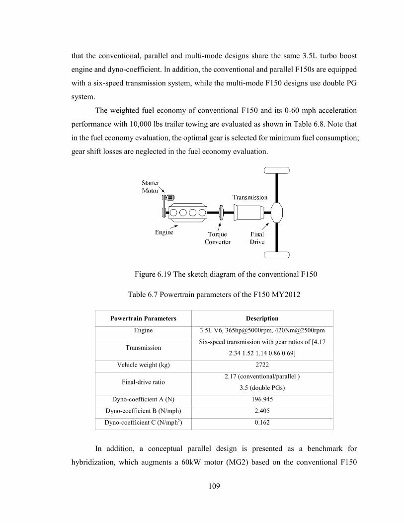
109

that the conventional, parallel and multi-mode designs share the same 3.5L turbo boost

engine and dyno-coefficient. In addition, the conventional and parallel F150s are equipped

with a six-speed transmission system, while the multi-mode F150 designs use double PG

system.

The weighted fuel economy of conventional F150 and its 0-60 mph acceleration

performance with 10,000 lbs trailer towing are evaluated as shown in Table 6.8. Note that

in the fuel economy evaluation, the optimal gear is selected for minimum fuel consumption;

gear shift losses are neglected in the fuel economy evaluation.

Figure 6.19 The sketch diagram of the conventional F150

Table 6.7 Powertrain parameters of the F150 MY2012

Powertrain Parameters Description

Engine 3.5L V6, 365hp@5000rpm, 420Nm@2500rpm

Transmission Six-speed transmission with gear ratios of [4.17

2.34 1.52 1.14 0.86 0.69]

Vehicle weight (kg) 2722

Final-drive ratio 2.17 (conventional/parallel )

3.5 (double PGs)

Dyno-coefficient A (N) 196.945

Dyno-coefficient B (N/mph) 2.405

Dyno-coefficient C (N/mph2) 0.162

In addition, a conceptual parallel design is presented as a benchmark for

hybridization, which augments a 60kW motor (MG2) based on the conventional F150

110

powertrain system, as shown in Figure 6.20. The engine of this parallel benchmark can be

disengaged from the transmission and the vehicle is then driven only by the traction motor,

while the engine can be launched by the belt starter motor and reconnected to the

transmission whenever it is necessary. The fuel economy of the parallel benchmark is

evaluated by PEARS and the results are shown in Table 6.8. As it can be seen from the

states and control trajectories shown in Figure 6.21, the engine drag can be avoided in the

single motor EV drive by having the engine disengagement ability.

Figure 6.20 The sketch diagram of the conceptual parallel F150

Table 6.8 Performance comparison between the conventional F150 and the conceptual

Parallel F150

Vehicle Designs Weighted MPG 0 - 60 mph (s) w/

Towing 10,000 lbs. Conventional F150 20.2 21.6

Parallel F150 37.6 16.0

The acceleration performance of the conventional and parallel F150s are both

evaluated and the results are provided in Table 6.8. During the evaluation, maximum

engine and motor torques are applied and the gear selections are optimized by maximizing

output torque on the output shaft.

111

Table 6.9 Additional powertrain parameters of the Hybrid F150

Powertrain Parameters Description

MG1 (parallel/double PG) 60kW, Max torque: 267Nm, Max speed: 9000rpm

MG2 (double PG) 60kW, Max torque: 200Nm, Max speed: 12000rpm

R1:S1 (double PG) 2.5

R2:S2 (double PG) 3.0

Gear ratio from the motor to the

transmission (parallel) 3.0

Figure 6.21 The state and control trajectories of the conceptual parallel F150

The powertrain parameters for multi-mode double PG F150 is shown in Table 6.9,

where the twin 60kW motor concept is adopted from the Silverado Hybrid [75] -- a Hybrid

pickup truck with similar size. The methodology proposed in this chapter is applied to all

144× 7,280 double PG designs. The 10,000 lbs. forward and backward engine on towing

requirement is included and the slop grade constraint is set as 12% according to the SAE

J2807 standard. Note that the 0 to 60 mph acceleration performance is evaluated with

10,000 lbs. towing; and such constraint is defined the same as the performance of the

parallel benchmark, which is 16.0 seconds.

112

After the drivability screening step, 743 designs are advanced to the fuel economy

evaluation step. The PEARS are applied to all of them to optimize the energy management

strategy. After the fuel economy evaluation, 68 designs achieve both better fuel economy

and 0-60 mph launching performance, as shown in Figure 6.22. Note that the performance

of conventional F150 benchmark is not displayed because it is far away (fuel economy =

20.2 mpg, acceleration performance = 21.6s) to the right bottom corner direction. It should

be pointed out that towing weight is not included in the fuel economy evaluation.

Figure 6.22 Optimization results comparing 3-clutch designs and the benchmark of the

F150 case study

Figure 6.23 Lever diagrams of the three designs on the Pareto front of the F150 case

study

113

Three designs on the Pareto Front are highlighted and their lever diagrams are

depicted in Figure 6.23. Interesting results can be observed when comparing the

optimization results of the three case studies: the optimal design (c) is just a mirror of the

optimal design (b) with PG1 and PG2 switched. Moreover, similar types of modes can be

observed by comparing the optimal design (b) of the Prius case study, the highlighted

optimal design (o) of the Volt case study with the optimal design (b) of the F150 case study

whose operating modes are shown in Table 6.10.

Table 6.10 The clutch states and operating modes of the sub-optimal design (b) in the

F150 case study

Mode Number

Description Clutch Operation CL1 CL2 CL3






Engine + MG2) 0 1 0



5 EV (1 DoF, 2MGs) 1 0 0

6 Input-split 0 0 1

7 EV (MG2) 0 0 0

Figure 6.24 The mode usage frequencies of the sub-optimal design (b) in the F150 case

study

114

Those similarities indicate that appropriately selected input-split and 2MGs-1DoF

EV modes can be very beneficial for fuel economy. As can be seen from Figure 6.12,

Figure 6.18 and Figure 6.24, those two mode occupy significant portions of mode usage in

both city and highway driving scenarios. In addition, certain 2MGs-1DoF parallel with

fixed-gear modes can provide great launching performance since both two MGs and the

engine can provide torque simultaneously, as they are chosen as the only mode in the 0 to

60 mph acceleration evaluation. When we take a closer look at the F150 optimization result,

it can be found that 43 of 68 designs have at least one input-split mode, one 2MGs-1DoF

EV mode and one 2MGs-1DoF parallel with fixed-gear mode, as shown in Figure 6.25.

Figure 6.25 Optimization results of the F150 case study of designs with Mode Type 4, 10

and 12 highlighted

From the optimization result, it should be noted that the fuel economy of the optimal

multi-mode F150 designs does not improved dramatically in comparison with the parallel

benchmark. However, the cost of the transmission system can be reduced significantly if a

double PG instead of an automatic transmission is applied. Meanwhile, the launching

performance can be improved by 27% and 46% compared with the parallel and

conventional benchmarks, respectively.

It should be pointed out that component sizing has not been considered in this

research. One could certainly repeat the design exercise and study improved designs using

varied ring gear/sun gear ratios, final drive ratios, etc., in addition to the crude and

preliminary effort in finding “better” motor sizes that we present here. The preferred modes

115

and winning designs are likely to change when the design sizing space is included.

Therefore, we do not intend to convey that identification of the optimal designs is primary

goal of the study presented in this chapter. Rather, the systematic and exhaustive search

process with the effective tools adopted in these three case studies is the key intellectual

contribution of this dissertation.

116

CONCLUSION AND FUTURE WORK

7.1 Conclusions

This dissertation focuses on modeling, control and design of multi-mode power-

split hybrid vehicles. The primary objective is to develop a systematic design procedure

that can enable the exhaustive search of a large candidate space and find the optimal design

in terms of fuel economy and drivability.

As discussed in the introductory chapter, adopting hybrid electric vehicle

technology is one of the most promising approaches for addressing the energy crisis and

reducing the CO2 emission. Among all hybrid vehicle powertrain architectures, the multi-

mode power-split architecture is the best candidate, since it has the potential to take

advantages of other hybrid powertrains while mitigating their drawbacks. However, to the

best of our knowledge, no complete methodology had been developed to address both the

modeling and the control problem of the multi-mode hybrid vehicles. This work addresses

this need.

In Chapter 2, a systematic analysis has been done for the single PG hybrid vehicles

with multiple operating modes. The analysis shows that there are 12 possible

configurations for the single PG hybrid vehicles, with 6 input- and 6 output-split

configurations, respectively. For each configuration, to achieve the greatest benefit with

appropriate cost, 3 clutches can be added to achieve 4 operating modes. In the case study,

the Toyota Prius and Chevy Volt were chosen as the representative designs of the input-

split and output-split for further analysis. Dynamic Programming was applied as the global

117

optimal energy management strategy to identify the best control for each design. Findings

from the detailed analysis demonstrate that the conceptual design Prius+ with one clutch

can achieve significant improvement on fuel economy in charge depleting drive in

comparison with the original Prius. For the Volt, results show that we can use a simplified

design to achieve similar performance on fuel economy, especially for city driving

conditions.

In Chapter 3, we have extended the analysis from the single PG to multiple PG

powertrain systems with all possible clutch locations. The proposed automated modeling,

mode screening and classification can generate all possible designs with any number of PG

and clutches. It can also screen out infeasible designs and detect identical modes. Mode

classification results show that for a multi-mode PG hybrid vehicle with one engine, one

output-shaft and two MGs, all possible modes can be classified into 14 types.

In Chapter 4, since mode shift is critical for multi-mode HEVs, we have conducted

a study on the mode shift feasibility problem. All possible mode shift types are identified

and the criteria for mode shift are defined. In addition, the optimal mode shift pathway

finding problem for indirect mode shift is solved by Dijkstra’s algorithm, which can

potentially be used in real-time application in the future.

In Chapter 5, since all current optimal control methodologies have limitation to be

implemented in multi-mode hybrid vehicle optimization, we proposed a near-optimal

energy management algorithm named PEARS. This algorithm can produce qualitatively

similar performance to that of DP, but can be up to 10,000 times faster. This great speed

and accuracy make PEARS feasible for fast conceptual design, and even for on-board MPC

when a short driving profile can be predicted. To further compare DP and PEARS, this

chapter provides additional detailed discussion of their performance.

In Chapter 6, on the basis of the automated modeling, mode shift analysis and near-

optimal control strategy, we developed a systematic design procedure for multi-mode

hybrid vehicles which can explore an enormous design space. In the first case study, we

118

focus on the passenger hybrid vehicle design based on the THS-II configuration. The 3-

clutch optimal designs in terms of the fuel economy and drivability, respectively, are

identified. In the second case study, we extended the design space to all 144 configurations

with engine and vehicle on different PGs. The Volt Gen 2 is selected as the benchmark. In

addition to the HEV drive fuel economy, EV drive equivalent have also been evaluated.

Results shows that three optimal designs with downsized MGs are found in terms of both

fuel economy and drivability. Similarities in their operating modes are investigated. In the

third case study, F150 is selected as a heavy duty vehicle application. A conceptual

benchmark of parallel F150 is constructed. Not only launching but also towing

performances are evaluated for all design candidates. Similarities in optimal designs are

observed, which indicates that certain types of mode can be universally beneficial for both

passenger vehicle and heavy duty designs like hybrid pickup trucks.

7.2 Future Work

In this dissertation, we have proposed a systematic design methodology which

enables efficient and exhaustive search for multi-mode HEV designs with planetary gear

system. Yet some potential future directions that merit further studies are listed as follows:

Optimal component sizing

In this dissertation, optimal component sizing is not involved. All optimal designs

calculated in Chapter 6 are on the basis of fixed parameters from the benchmarks. In theory,

exhaustive and brute-force method can be applied to each design candidate. However, the

design space will become tremendously large even for fast energy management methods

like PEARS. For example, if optimal component sizing is considered for all 144 double

PG configurations with 3 clutches and 1 fixed connection, assuming R1:S1, R2:S2, FR and

clutch locations are design variables, the design candidates can be up to 109 even when

motor sizes are fixed. Therefore, an optimal design method not relying on brute-force

119

search should be developed when component sizing is pursued. Due to the non-convex

characteristic of the clutch location optimization, research challenges are expected.

Real-time control based on PEARS algorithm

In Chapter 5, the optimality of PEARS is demonstrated through the comparison

with DP. Its discretized efficiency analysis based on different vehicle status offers the

potential for offline efficiency computation. In addition, together with the analysis on

optimal pathway finding by Dijkstra’s algorithm in Chapter 4, the mode shift cost can be

estimated accurately with online computation. These attributes and accomplishments build

a solid foundation to create a real-time control algorithm on the basis of PEARS. The

challenges on the real-time implementation come from the relationship between the

optimal mode selection and battery SOC. Reliable prediction methodologies on traffic

should be developed to estimate battery energy consumption therefore enable optimal

mode selection.

Optimal design methodology considering other metrics

Although fuel economy and drivability are crucial for almost any vehicle design,

other metrics such as emission and lifetime cost may be considered in the early stage design

process. Due to the large design candidate space if exhaustive search is adopted, fast energy

management strategy considering emissions should be developed, possibly on the basis of

the PEARS algorithm.

120

BIBLIOGRAPHY

[1] "Summary of fuel economy performance," U.S. Department of Transportation,

2014.

[2] The White House Office of the Press Secretary, 28 Aug 2012. [Online]. Available:

http://www.whitehouse.gov/the-press-office/2012/08/28/obama-administration-

finalizes-historic-545-mpg-fuel-efficiency-standard. [Accessed 15 Jul 2014].

[3] E. H. Wakefield, History of the Electric Automobile: Hybrid Electric Vehicles,

Society of Aumotive Engineers(SAE), ISBN: 0-7680-0125-0, 1998.

[4] N. Jalil, N. Kheir and M. Salman, "A Rule-Based Energy Management Strategy for

a Series Hybrid Vehicle," in American Control Conference (ACC), Albuqueerque,

NM, 1997.

[5] Y. Guezennec and G. Rizzoni, "Optimal Energy Management in Series Hybrid

Electric Vehicles," in American Control Conference (ACC), Chicago, IL, 2000.

[6] H. Yoo, S. Member, S.-k. Sul, Y. Park and J. Jeong, "System Integration and

Power-Flow Management for a Series Hybrid Electric Vehicle Using

Supercapacitors and Batteries," IEEE transactions on Industry Applications, vol.

44, no. 1, pp. 108-114, 2008.

[7] S. Barsali, C. Miulli and A. Possenti, "A Control Strategy to Minimize Fuel

Consumption of Series Hybrid Electric Vehicles," IEEE Transactions on Energy

Conversion, vol. 19, no. 1, pp. 187-195, 2004.

[8] Y. Kim and Z. Filipi, "Series Hydraulic Hybrid Propulsion for a Light Truck

Optimizing the Thermostatic Power Management," SAE International, 2007.

121

[9] K. Kelly, M. Zolot, G. Glinsky and A. Hieronymus, "Test Results and Modeling of

the Honda Insight using ADVISOR," in Future Transportation Technology

Conference & Exposition, 2001.

[10] H. Ogawa, M. Matsuki and T. Eguchi, "Development of a Power Train for the

Hybrid Automobile - the Civic Hybrid," in SAE World Congress, Detroit, MI, 2003.

[11] A. Nedungadi, M. Walls and D. Dardalis, "A Parallel Hybrid Drivetrain," SAE

Paper, 8 1999.

[12] Z. Rahman, K. Butler and M. Ehsani, "A Comparison Study Between Two Parallel

hybrid Control Concepts," in SAE World Congress, Detroit, MI, 2000.

[13] C.-C. Lin, H. Peng, J. W. Grizzle and J.-M. Kang, "Power Management Strategy for

a Parallel Hybrid Electric Truck," IEEE Transaction on Control System

Technology, vol. 11, pp. 839-849, 2003.

[14] A. Sciarretta, M. Back and L. Guzzella, "Optimal control of parallel hybrid electric

vehicles," IEEE transactions on Control System Technology, pp. 352-363, 2004.

[15] Z. Shahan, "Electric Car Sales Increased 228.88% In 2013 (US EV & Hybrid Sales

Update)," 7 1 2014. [Online]. Available: http://evobsession.com/electric-car-sales-

increased-228-88-2013/. [Accessed 4 11 2014].

[16] M. Olszewski, "Evaluation of 2004 Toyota Prius Hybrid Electric Drive System,"

U.S. Department of Energy, Washington, D.C., 2006.

[17] K. Rahman, M. Anwar, S. Schulz, E. Kaiser, P. Turnbull, S. Gleason, B. Given and

M. Grimmer, "The Voltec 4ET50 Electric Drive System," SAE International, 2011.

[18] M. Schmidt, D. Klemen and A. G. Holmes, "Powertrain with electrically variable

transmission". United States of America Patent 7169073 , 2005.

[19] D. Hermance, "Toyota Hybrid System," in SAE TOPTEC Conference, Albany, NY,

1999.

[20] A. G. Holmes, D. Klemen and M. R. Schmidt, "Electrically variable transmission

with selective input split, compound split neutral and reverse modes". United States

Patent 6527658 B2, 4 March 2003.

122

[21] W. G. Livezey, "Input-split-power, output-split-power, compound-split-power,

power train". US. Patent 3470769A, 17 Oct 1969.

[22] G. Gelb, N. Richardson, T. Wang and B. Berman, "An Electromechanical

Transmission for Hybrid Vehicle Power Trains - Design and Dynamometer

Testing," SAE Technical Paper, 1971.

[23] N. H. Beachley and A. A. Frank, "Control Considerations for a Flywheel Hybrid

Automobile with a Mechanical Continuously Variable Transmission," in Flywheel

technology symposium, Scottsdale, AZ, 1980.

[24] R. Wohl, T. Long, V. Mucino and J. E. Smith, "A Model for a Planetary-CVT

Mechanism: Analysis and Synthesis," in SAE Congress and Exposition, Detoirt,

MI, 1993.

[25] S. Abe, S. Sasaki, H. Matsui and K. Kubo, "Development of Hybrid System for

Mass Productive Passenger Car," JSAE Proceeding, pp. 21-24, 1997.

[26] B. M. Conlon, P. J. Savagian, A. G. Holmes and M. O. Harpster, "Output Split

Electrically-Variable Transmission with Electric Proposion using One or Two

Motors". US. Patent 2009/0082171 A1, 26 March 2009.

[27] M. Miller, A. G. Holmes, B. M. Conlon and P. J. Savagian, "The GM 'Voltec'

4ET50 Multi-Mode Electric Transaxle," SAE International, Apr 2011.

[28] H. Benford and M. Leising, "The lever analogy: a new tool in transmission

analysis," SAE Paper, vol. 01, no. 02, 1981.

[29] A. Rousseau, S. Pagerit, G. Monnet and A. Feng, "The New PNGV System

Analysis Toolkit PSAT V4.1 - Evolution and Improvement," SAE Technical Paper,

2001.

[30] Argonne National Laboratory, Autonomie Documentation, 2009.

[31] G. Manual, GT-Suite Version 6.1, Gamma Technologies, 2004.

[32] G. Rizzoni, L. Guzzella and B. M. Baumann, "Unified Modeling of Hybrid Electric

Vehicle Drivetrains," IEEE/ASME Transactions on Mechatronics, pp. 246-257,

Nov 1999.

123

[33] C.-C. Lin, Z. Filipi, Y. Wang, L. Louca, H. Peng, D. Assanis and J. Stein,

"Integrated, Feed-Forward Hybrid Electirc Vehicle Simulation in Simulink and its

Use for Power Management Studies," SAE Technical Paper, 2001.

[34] D. Rizoulis, J. Burl and J. Beard, "Control Strategies for a Series-Parallel Hybrid

Electric Vehicle," in SAE World Congress, 2011.

[35] B. Conlon, "Comparative Analysis of Single and Combined Hybrid Electrically

Variable Transmission Operating Modes," in SAE World Congress, Detroit,

Michigan, 2005.

[36] J. Liu, H. Peng and Z. Filipi, "Modeling and Analysis of the Toyota Hybrid

System," in International Conference on Advanced Intelligent Mechatronics,

Monterey, California, 2005.

[37] J. Liu and H. Peng, "Configuration , Sizing and Control of Power-Split Hybrid

Vehicles," in AVEC 2007, 2007.

[38] J. Liu and H. Peng, "Modeling and Control of a Power-Split Hybrid Vehicle," IEEE

Transactions on Control Systems Technology, vol. 16, no. 6, pp. 1242-1251, 2008.

[39] Z. Rahman, K.L.Butler and M. Ehsani, "A Comparison Study Between Two

Parallel Hybrid Control Concepts," in SAE Wold Congress, Detroit, Michigan,

2000.

[40] M. Salman, N. Schouten and N. Kheir, "Control Strategies for Parallel Hybrid

Vehicles," in American Control Conference, Chicago, IL, 2000.

[41] X. He, M. Parten and T. Maxwell, "Energy Management Strategies for a Hybrid

Electric Vehicle," in 2005 IEEE Vehicle Power and Propulsion Conference, 2005.

[42] C. Kim, E. NamGoong, S. Lee and T. Kim, "Fuel Economy Optimization for

Parallel Hybrid Vehicles with CVT," SAE Paper, vol. 1, no. 1148, 1999.

[43] G. Paganelli, T. Guerra, S. Delprat, J. Santin, M. Delhom and E. C ombes,

"Simulation and Assessment of Power Control Strategies for a Parallel Hybrid Car,"

SAE International, vol. 214, pp. 705-718, 2000.

124

[44] G. Paganelli, M. Tateno, A. Brahma, G. Rizzoni and Y. Guezennec, "Control

Development for a Hybrid-Electric Sport-Utility Vehicle: Strategy, Implementation

and Field Test Results," in American Control Conference, Arlington, VA, 2001.

[45] G. Paganelli, G. Ercole, A. Brahma, Y. Guezennec and G. Rizzoni, "General

Supervisory Control Policy for the Energy Optimization of Charge-Sustaining

Hybrid Electric Vehicles," JSAE Review, pp. 511-518.

[46] J. S. Won, R. Langari and M. Ehsani, "An Energy Management and Charge," IEEE

Transactions on Control System Technology Sustraining Strategy for a Parallel

Hybrid Vehicle With CVT, pp. 313-320, 2005.

[47] P. Pisu, G. Rizzoni, C. Musardo and B. and Staccia, "A Comparative Study of

Supervisory Control Strategies for Hybrid Electric Vehicles," in International

Mechanical Engineering Congress and Exposition, Anaheim, CA, 2004.

[48] C. Musard, G. Rizzoni and B. Staccia, "A-ECMS: An Adaptive Algorithm for

Hybrid Electric Vehicle Energy Management," in IEEE Conference on Decision

and Control, Seville, Spain, 2005.

[49] S. Onori, L. Serrao and G. Rizzoni, "Adaptive Equivalent Consumption

Minimization Strategy for Hybrid Electric Vehicles," in Dynamic Systems and

Control Conference, Cambridge, MA, 2010.

[50] R. Bellman, The Theory of Dynamic Programming, Bulletin of American

Mathematical Society, 1954.

[51] H. Mosbech, "Optimal control of hybrid vehicle," in ISATA, pp 303-20 vol 2, 1980.

[52] A. Brahma, Y. Guezennec and G. Rizzoni, "Optimal Energy Management in Series

Hybrid Electric Vehicles," in American Control Conference, Chicago, IL, 2000.

[53] C. Lin, Z. Filipi, Y. Wang, L. Louca, H. Peng, D. Assanis and J. Stein, "Integrated,

Feed-Forward Hybrid Electric Vehicle Simulation in SIMULINK and its Use for

Power Management Studies," in SAE World Congress, Detroit, MI, 2001.

[54] C. Lin, H. Peng, J. Grizzle, J. Liu and M. Busdiecker, "Control System

Development for an Advanced-Technology Medium-Duty Hybrid Electric Truck,"

in International Truck & Bus Meeting & Exhibition, 2003.

125

[55] A. Sciarretta, M. Back and L. Guzzella, "Optimal Control of Parallel Hybrid

Electric Vehicles," IEEE Transactions on Control Systems Technology, vol. 12, no.

3, pp. 352-363, May 2004.

[56] J. Scordia, M. Desbois-Renaudin, R. Trigui, B. Jeanneret, F. Badin and C. Plasse,

"Global optimisation of energy management laws in hybrid vehicles using dynamic

programming," International Journal of Vehicle Design, pp. 349-367, 2005.

[57] J. Liu and H. Peng, "Control optimization for a power-split hybrid vehicle," in

American Control Conference, Minneapolis, MN, 2006.

[58] C.-c. Lin, H. Peng and J. W. Grizzle, "A Stochastic Control Strategy for Hybrid

Electric Vehicles," in American Control Conference, Boston, MA, 2004.

[59] L. Johannesson, M. Åsbogård and B. Egardt, "Assessing the Potential of Predictive

Control for Hybrid Vehicle Powertrains Using Stochastic Dynamic Programming,"

IEEE Transaction on Intelligent Transportation Systems, vol. 8, no. 1, pp. 71-83,

2007.

[60] J. Liu, J. Hagena, H. Peng and Z. S. Filipi, "Engine-in-the-loop study of the

stochastic dynamic programming optimal control design for a hybrid electric

HMMWV," International Journal of Heavy Vehicle Systems, vol. 15, no. 1, pp.

309-326, 2008.

[61] G. Rousseau, D. Sinoquet and P. Rouchon, "Constrained Optimization of Energy

Management for a Mild-Hybrid Vehicle," Oil & Gas Science and Technology , pp.

623-634, 2007.

[62] N. Kim, S. Cha and H. Peng, "Optimal Control of Hybrid Electric Vehicles Based

on Pontryagin's Minimum Principle," IEEE Transactions on Control Systems

Technology, vol. 19, no. 5, pp. 1279-1287, Sep 2011.

[63] N. Murgovski, L. Johannesson, J. Hellgren, B. Egardt and J. Sjöberg, "Convex

optimization of charging infrastructure design and component sizing of a plug-in

series HEV powertrain," in 18th IFAC World Congress, Milano, 2011.

126

[64] N. Murgovski, L. Johannesson, J. Sjöberg and B. Egardt, "Component sizing of a

plug-in hybrid electric powertrain via convex optimization," Mechatronics, pp. 106-

120, 2012.

[65] G.-P. U. Manual, GT-Suite Version 7.6, Gamma Technologies, 2013.

[66] N. Kawamoto, K. Naiki, T. Kawa, T. Shikida and M. Tomatsuri, "Development of

New 1.8-Liter Engine for Hybrid Vehicles," SAE Technical Paper, vol. 01, 2009.

[67] M. Olszewski, "Evaluation of the 2010 Toyota Prius Hybrid Synergy Drive

System," U.S. Department of Energy Vehicle Technologies, Washington DC, 2011.

[68] O. Sundström, L. Guzzella and P. Soltic, "Torque-Assist Hybrid Electric Powertrain

Sizing : From Optimal Control Towards a Sizing Law," IEEE Transactions on

Control Systems Technology, pp. 837-849, 2010.

[69] Idaho National Laboratory, "PHEV Battery Testing Results: 2013 Chevrolet Volt -

Vin 3929," Idaho National Laboratory, Idaho Falls, 2014.

[70] N. R. A. a. R. E. Kim, "Autonomie Model Validation with Test Data for 2010

Toyota Prius," SAE International, 2012.

[71] N. K. Bucknor, J. D. Hendrickson, M. Raghavan, A. G. Holmes and P. B. Usoro,

"Electrically Variable Transmission Having Two Planetary Gear Sets with One

Fixed Interconnection". US. Patent 7192373, 20 March 2007.

[72] K. Seo and H. Yang, "Powertrain for Hybrid Vehicle". US. Patent 8147367, 3 April

2012.

[73] B. Si, "Dual Mode Input Split Compound Split Configuration Eppv Transmission".

US. Patent 8075435B2, 13 December 2011.

[74] P. Desai, M. Anwar, S. Gleason and S. Hawkins, "Power Electronics for GM 2-

Mode Hybrid Electric Vehicles," SAE interational, vol. 01, p. 1253, 2010.

[75] H. Ide, Y. Sunaga and N. Higuchi, "Development of SPORT HYBRID i-MMD

Control System for 2014 Model Year Accord," Introduction of new technologies,

2014.

127

[76] M. Douba, H. Ng and R. Lasen, "Characterization and Comparison of Two Hybrid

Electric Vehicles (HEVs) - Honda Insight and Toyota Prius," SAE International,

vol. 01, p. 1335, 2001.

[77] B. Conlon, T. Blohm, M. Harpster and A. Holmes, "The Next Generation “Voltec”

Extended Range EV Propulsion System," SAE Int. J. Alt. Power, vol. 4, no. 2, 2015.

[78] T. M. Grewe, B. M. Conlon and A. G. Holmoes, "Defining the General Motors 2-

Mode Hybrid Transmission," in SAE World Congress, Detroit, Michigan, USA,

Apr, 2007.

[79] B. Conlon, T. Blohm, M. Harpster and A. Holmes, "The Next Generation “Voltec”

Extended Range EV Propulsion System," SAE Int. J. Alt. Power, vol. 4, no. 2, 2015.

[80] A. Schrijver, "On the Histroy of the Shortest Path Problem," Documenta

Mathematica, vol. 17, p. 155, 2012.

[81] N. Biggs, K. Lloyd and R. Wilson, Graph Theory 1736-1936, Oxford: Clarendon

Press, 1976.

[82] H. D. Landahl and R. Runge, "Outline of a matrix algebra for neural nets," Bulletin

of Mathematical Biophsics, vol. 8, pp. 75-81, 1946.

[83] A. Shimbel, "Structure in Communication Nets," in The Symposium of Information

Networks, Brooklyn, New York, 1954.

[84] L. Ford, "Network Flow Theory," Santa Monica, CA, The RAND Corporation,

1956.

[85] R. BellMan, "On a Routing Problem," Quarterly of Applied Mathematics, vol. 16,

pp. 87-90, 1958.

[86] E. W. Dijkstra, "A Not on Two Problems in Connexion with Graphs," Numerische

Mathematik, vol. 1, pp. 269-271, 1959.

[87] M. L. Fredman and R. E. Tarjan, "Fibonacci heps and their uses in improved

network optimization algorithms," in 25th Annual Symposium on Foundations of

Computer Science, 1984.

128

[88] X. Zhang, S. E. Li, H. Peng and J. Sun, "Efficient Exhaustive Search of Power-Split

Hybrid Powertrains With Multiple Planetary Gears and Clutches," Journal of

Dynamic Systems, Measurement, and Control, vol. 137, no. 12, 2015.

[89] Office of Transportation and Air Quality, "Gasoline Vehicles: Learn Mode About

the New Label," 6 11 2014. [Online]. Available:

http://www.fueleconomy.gov/feg/label/learn-more-gasoline-label.shtml. [Accessed

6 11 2014].

[90] X. Zhang, E. Li, H. Peng and J. Sun, "Efficient Exhaustive Search of Power-Split

Hybrid Powertrains With Multiple Planetary Gears and Clutches," ASME Journal of

Dynamic System, Measurement and Control, 2015.

[91] S.-i. Jeon, S.-t. Jo, Y.-i. Park and J.-m. Lee, "Multi-Mode Driving Control of a

Parallel Hybrid Electric Vehicle Using Driving Pattern Recognition," ASME

Journal of Dynamic Systems, Measurement, and Control, vol. 124, no. 1, pp. 141-

149, 2002.

[92] S. Goldschmidt, A. Krolo, R. Patzold and J.-P. Ziegele, "Power-split Transmission

for A Hybrid Vehicle". US. Patent 20080171625, 17 July 2008.

[93] H. Ogawa, M. Matsuki and T. Eguchi, "Development of a Power Train for the

Hybrid Automobile - The Civic Hybrid," in SAE Wolrd Congress & Exhibition,

Detroit, MI, 2003.

[94] Argonne National Laboratory, Autonomie Documentation, 2009.

Design of Power Split Hybrid Powertrains with Multiple ...

Documents

Transcript of Design of Power Split Hybrid Powertrains with Multiple ...