applied sciences

Article

Design of Autonomous Mobile Robot for Cleaning in theEnvironment with Obstacles

Arpit Joon * and Wojciech Kowalczyk *

�����������������

Citation: Joon, A.; Kowalczyk, W.

Design of Autonomous Mobile Robot

for Cleaning in the Environment with

Obstacles. Appl. Sci. 2021, 11, 8076.

https://doi.org/10.3390/app11178076

Academic Editor: Alessandro

Gasparetto

Received: 30 July 2021

Accepted: 27 August 2021

Published: 31 August 2021

Publisher’s Note: MDPI stays neutral

with regard to jurisdictional claims in

published maps and institutional affil-

iations.

Copyright: © 2021 by the authors.

Licensee MDPI, Basel, Switzerland.

This article is an open access article

distributed under the terms and

conditions of the Creative Commons

Attribution (CC BY) license (https://

creativecommons.org/licenses/by/

4.0/).

Institute of Automatic Control and Robotics, Poznan University of Technology, Piotrowo 3A,60-965 Poznan, Poland* Correspondence: joonarpit@gmail.com (A.J.); wojciech.kowalczyk@put.poznan.pl (W.K.)

Abstract: This paper describes the design and development of a cleaning robot, using adaptivemanufacturing technology and its use with a control algorithm for which there is a stability proof.The authors’ goal was to fill the gap between theory and practical implementation based on availablelow-cost components. Adaptive manufacturing was chosen to cut down the cost of manufacturingthe robot. Practical verification of the effectiveness of the control algorithm was achieved with theexperiments. The robot comprises mainly three assemblies, a four-wheel-drive platform, a four-degrees-of-freedom robotic arm, and a vacuum system. The inlet pipe of the vacuum system wasattached to the end effector of the robotic arm, which makes the robot more flexible to clean unevenareas, such as skirting on floors. The robot was equipped with a LIDAR sensor and web camera,giving the opportunity to develop more complex methods. A low-level proportional–integral–derivative (PID) speed controller was implemented, and a high-level controller that uses artificialpotential functions to generate repulsive components, which avoids collision with obstacles. Robotoperating system (ROS) was installed in the robot’s on-board system. With the help of the ROS node,the high-level controller generates control signals for the low-level controller.

Keywords: cleaning robot; ROS; 3D printing; four-wheel drive; robotic arm; vacuum system; LIDARsensor; low-level PID controller; high-level obstacle avoidance controller; artificial potential function

1. Introduction

Researchers and many companies have introduced different types of cleaning robotdesigns over the last two decades [1–5]. A study was conducted on some of the vacuumrobots available in the market about cleaning efficiency, which showed that the manualvacuum cleaner is still more efficient for cleaning than vacuum robots [6]. The coveragearea issue of the vacuum robots was also mentioned in the same article. The area abovethe floor, such as skirting, is unreachable for the vacuum robots (iRobot, Xiaomi Mi RobotVacuum, etc.) having a fixed inlet on the bottom side. A vacuum robot with a flexiblevacuum inlet may increase the cleaning efficiency and coverage area problems. In 1997, anautonomous vacuum cleaner, “Koala”, was introduced [7], which has a two-degrees-of-freedom robotic arm, cleaning head on the second link of the arm.

The paper presents experimental verification of the method, which was developed bythe second author and presented in paper [8], including a stability analysis. The resultsdescribed here are a continuation of these studies. The authors’ goal was to fill the gapbetween theory and practical implementation based on available low-cost components.Adaptive manufacturing was used to cut down the cost of manufacturing the robot. Prac-tical verification of the effectiveness of the algorithm is an undeniably important phaseof the research process. Proper operation, even though the test was used on a relativelysimple, inexpensive mobile platform equipped with units of low computing power, is anadditional advantage of the method presented here. Although the algorithm was not testedon expensive laboratory hardware equipped with high-precision sensors and actuators, itproved to be effective. Figure 1 demonstrates the cleaning robot, where the inlet pipe of the

Appl. Sci. 2021, 11, 8076. https://doi.org/10.3390/app11178076 https://www.mdpi.com/journal/applsci

Appl. Sci. 2021, 11, 8076 2 of 13

vacuum system was attached to the end effector of the robotic arm. The robot is equippedwith a LIDAR sensor and web camera, giving the opportunity to develop more complexmethods. The touch screen on the robot helps to displays the information from the robot.A low-level proportional–integral–derivative (PID) speed controller is used to achieve thedesired speeds. A high-level controller [8] helps the robot to follow a virtual robot pathwith avoiding obstacles.

Figure 1. Cleaning robot.

Creating a virtual model of the robot opens another field where we can verify thealgorithm and potential problems in the design of the robot [9]. The FPGA-based controlleralso shows high potentials for the robotic arm [10] and power-saving architecture for themotions [11].

Artificial potential fields were introduced by Khatib [12] in 1986. In this controlalgorithm, attraction (to the goal) and repulsion (from the obstacle) are negated gradientsof the artificial potential functions (APF). Many articles have been published using thenavigation function (NF) [12–17]. The control of multiple mobile robots based on thekinematic model [18,19] and dynamic model [20,21] have also been published.

A sliding mode control strategy with an artificial potential field was shown in [22].An obstacle potential field function considers the robot’s size and obstacle size and accord-ingly changes the weight of the obstacle potential field function, which adaptively makesthe robot escape from local minima [23].

Authors of [24] addressed the problem of tracking the control of multiple differentiallydriven mobile platforms (leader–follower approach is used). The algorithm is distinguishedby its simplicity and ease of implementation. The components of the control have anobvious physical interpretation, which facilitates the tuning based on observations of therobot’s behavior. The linear velocity control depends on the linear velocity of the referencerobot (virtual leader) and the position error along the axis perpendicular to the axle of therobot wheels. The angular velocity is a function of the angular velocity of the virtual leader,orientation error, and the position error along the axle of the robot wheels, transformed bya non-linear function and activated periodically by a square persistently exciting function.The stability proof is based on the decomposition of the error dynamics into position andorientation subsystems that are ISS (input to state stable). Simulations confirm the effectiveerror reduction for stadium-circuit shape trajectories composed of two straight lines andtwo half circumferences. The collision avoidance was not taken into account.

Collision avoidance with other robots and static obstacles was added in [8]. Theposition errors were replaced by correction variables, which combine the position errorsand the gradients of APFs surrounding obstacles. When robots are outside of collision

Appl. Sci. 2021, 11, 8076 3 of 13

avoidance regions of other robots/obstacles (APF takes the value zero) the analysis givenin [24] is actual. For the other cases, stability analysis based on the Lyapunov-like functionwas presented. Numerical verification was performed on a formation of fifteen robots inthe environment with five obstacles. The desired trajectory was composed of straight linesand arcs.

The trajectory tracking algorithm proposed in [8] was based on [24]. In its originalform, the collision avoidance was not included. It was assumed that the initial positions ofrobots guarantee that no collisions would occur. The extension proposed in [24] removesthis limitation. The method guarantees the stability of the closed-loop system and collisionsavoidance. A tracking method with similar computational complexity was proposed inwork [25]. It does not involve a persistent excitation block. The stability of the system wasalso proven. Another method that was considered is the VFO (vector field orientation)algorithm [26]. This approach uses a special vector field and an auxiliary orientationvariable. Stability was also proven for it, but its implementation on a real robot is morecomplex. In [27], this approach was extended by collision avoidance capability. Thereis tracking and collision avoidance for the multiple robots, but it takes into account therobot’s dynamics (mass, inertia) and is very complex to implement [20].

Section 2 shows the mechanical design and electronics parts of the robot. The con-trol algorithm is presented in Section 3. Section 4 describes the methodology, and theexperiment results are presented in Section 5.

2. Mechanical Design and Electronics Parts

Solid Edge 2020 software was used as a modeling tool to design our robot. Thesoftware’s synchronous technology was one of the main features by which authors modifiedthe parts and assembly at any time. The 3D-printing support of this software makes itmore user-friendly. The cloud feature of the software was helpful for the authors to workin a team and shared the design. The following points were considered while designingthe parts:

• Lightweight parts.• Suitable for 3D printing.• Strength of PLA material.• Ease of assembly.

The designs were saved as STL files, which were later used in the 3D printer. The“Creality Ender 3” 3D printer was used to print the parts. PLA material was used, whichhad the property of showing minor printing failures without close enclosure of the printer.The printer was set up for 200 degrees Celsius for the nozzle temperature and 60 degreesCelsius for the heat bed. The robot consist of mainly three assemblies as follows:

• Robotic arm.• Vacuum system.• Mobile platform.

2.1. Robotic Arm

The robot was equipped with a four-degrees-of-freedom robotic arm. All the jointsconsisted of revolute joints. The total length of the fully enlarged robotic arm was 44.8 cm,and the width was 14.8 cm.

Table 1 shows the details of the servo motors used in the robotic arm. Ball bearingswere used to support and transfer the weight of one part to another. ABEC 3 skate-board bearings were used, with an outer diameter of 22 mm, core diameter of 8 mm, and7 mm width.

Appl. Sci. 2021, 11, 8076 4 of 13

Table 1. Details of servo motors.

Joint Number Servo Name Quantity Torque

Joint 1 Tower Pro SG-5010 1 6.5 kg × cmJoint 2 Feetech FS5115M 2 15.5 kg × cmJoint 3 Tower Pro SG-5010 1 6.5 kg × cmJoint 4 Tower Pro SG-90-micro 1 1.8 kg × cm

2.2. Vacuum System

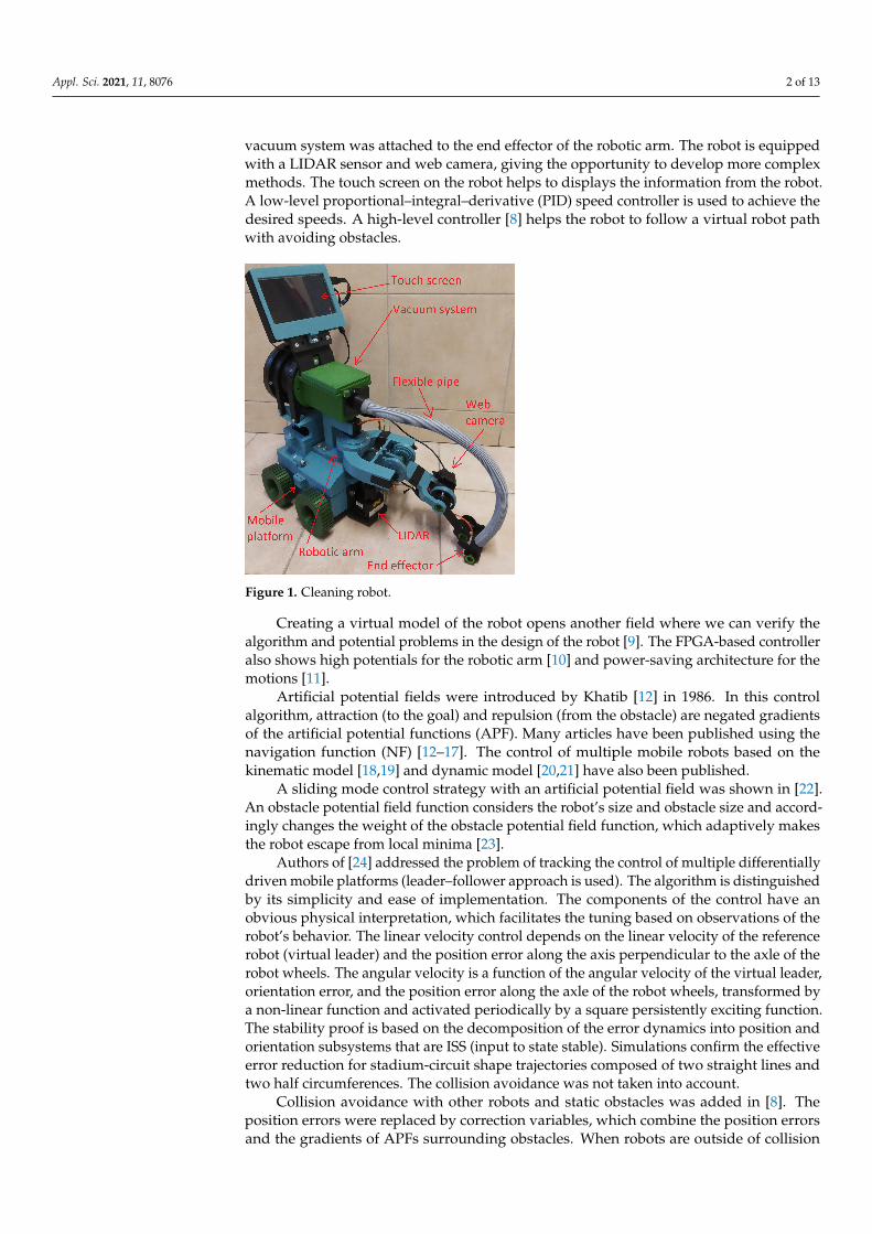
The vacuum system of the robot consists of 3D-printed parts, such as a fan, collectorbox, cover of the collector box, and fan chamber. Other parts include the filter, flexiblepipe, and brushless motor. One end of the flexible tube is connected to the vacuum systemand another end to the end-effector of the robotic arm. The collector box has a volume of378 cubic cm (10 cm × 6 cm × 6.3 cm). Figure 2 shows the cut sectional view of the vacuumsystem. When the vacuum system starts vacuuming the floor, the air with the dust comesinto the collector box, where the layer of vertical filter stops the dust, while allowing the airto pass through it.

Figure 2. Cut sectional view of the vacuum system.

Table 2 shows the electronics items used for the vacuum system.

Table 2. Details of electronics component for vacuum system.

S.No Component Name Specification

1 ESC, skywalker Input- 2–4 s Lipo, continous current 50 A2 Brushless motor, iFlight XING 2750 KV , max current 50.03 A3 Lipo battery 11.1v, 50C, 5000 mAh

2.3. Mobile Platform

The robot has a four-wheel-drive platform, which gives the robot more power to carrythe weight of its robotic arm and vacuum system. DC geared motors with encoders areused in the mobile platform. A low-level PID speed controller is implemented in ArduinoMega. Each wheel has a diameter of 10 cm. The total length of the mobile platform is23.9 cm, and the width is 24.9 cm with wheels. The lead battery is used to power theelectronics of the mobile platform.

The upper body of the mobile platform is made up of three parts. These parts playa vital role in connecting the lower body part of the mobile platform with the vacuumsystem and robotic arm. The LIDAR holder provides the platform for the LIDAR sensor.The touch screen holder is also designed to hold a 7 inch touch screen connected to thetop of the vacuum system. The height of the complete robot is 54.1 cm from the ground, alength of 54.1 cm when the robotic arm is fully enlarged, and 24.9 cm is the width of theplatform with tires.

Appl. Sci. 2021, 11, 8076 5 of 13

Table 3 shows the components of the electronics part of the mobile platform. Therobot in total has two batteries. A 6 V DC battery is used to power the motor driversand low-level controllers, such as Arduino UNO and Arduino Mega, while a Lipo batteryis used to power the servo motors of the robotic arm, vacuum system, and RaspberryPi computer. The robot has three controllers. Raspberry Pi acts as the master controllerconnected through the serial link to Arduino Mega, which serves as the first slave controller.The Arduino Mega is also connected with Arduino Uno, using serial communication. As aresult, Arduino Uno serves as the second slave controller, which controls the direction andspeed of one motor. The other three motors are controlled with Arduino Mega, due tothe limitations of the external interrupt pins. The L298n motor drivers control the motors’direction and speed. Each motor driver is capable of controlling two motors. Two wiresfrom the microcontroller to the motor driver control the direction, and one wire controlsthe speed of the motor.

“Camera Tracer HD WEB008” is the digital camera used for the vision system. Thedevice captures HD-quality images with a resolution of 1280 × 720 pixels. The lens hasa wide-angle view of horizontal 100 degrees and can capture images with 30 frames persecond. “Hokuyo urg-04lx-ug01” is used as the LIDAR sensor.

Table 3. Details of electronics part of mobile platform.

S.No Component Name Quantity Specification

1 Motor Driver, L298N 2 Maximum current 2A2 Arduino Mega 1 54 digital input/output pins3 Arduino Uno 1 14 digital input/output pins4 Raspberry Pi 4 1 2 GB RAM5 Battery 1 6 V, 12 Ah6 DC motor- Pololu 99:1 Metal 4 Integrated 48 CPR quadrature encoder

gearmotor 25D×66L 4741.44 CPR , Torque-15 kg/cm14 digital input/output pins

3. Control Algorithm

The control algorithm for the mobile platform was taken from the research paper [8].The control algorithm was tested in the numerical simulation in the same research paper.To move one step further, the authors decided to test the algorithm with the proposedcleaning robot. With this control algorithm, the cleaning robot tried to follow a virtual robotpath while avoiding the obstacles with artificial potential functions (APF). A repulsive fieldwas generated to repel the robot from the obstacles.

The kinematics of the robot is given by the following formula:

q =

cos θ 0sin θ 0

0 1

u (1)

where vector u =[v ω

]> is the control vector with v denoting linear velocity control, andω denotes the angular velocity control of the follower robot. Vector q = [x y θ]> denotesthe pose, and x, y, θ are the position coordinates and orientation of the robot with respectto a global, fixed coordinate frame.

The robot has to follow the virtual robot, which moves with the desired linear velocityand angular velocity [vd ωd]

T along the planned trajectory. The robot should achieve thesame velocities as that of the virtual robot; [xd yd]

T are the position coordinates of thevirtual leader, which acts as a reference position of the real robot, and its orientation θconverges to the orientation of the virtual leader θd.

The APF repels the robot from the obstacles as it rises to infinity near the obstacle’sborders, rj (j—number of the obstacles) and decreases to zero at some distance Rj, Rj > rj.

Appl. Sci. 2021, 11, 8076 6 of 13

Equations for APF are written as follows:

Baj(lj) =

0 for lj < rj

elj−rjlj−Rj for rj ≤ lj < Rj0 for lj ≥ Rj

, (2)

which gives output Baj(lj) ∈ 〈0, 1), the distance between the robot and the j-th obstacle,which is defined as the Euclidean length lj =

∥∥[xj yj]> − [x y]>

∥∥.Scaling the function given by Equation (2) within the range 〈0, ∞) can be given

as follows:

Vaj(lj) =Baj(lj)

1− Baj(lj), (3)

which is used later to avoid collisions.In further description terms, the ’collision area’ is used for location fulfilling conditions

lj < rj. The range rj < lj < Rj is called the ’collision avoidance area’.The goal of the controller is to drive the robot along the desired trajectory along with

avoiding obstacles, which result brings the following quantities to zero:

px = xd − x

py = yd − y

pθ = θd − θ. (4)

Assumption 1. ∀{i, j}, i 6= j, ||[xd yd]T − [xj yj]

T || > Rj where [xj yj]T is location of the

center of the j-th obstacle.

Assumption 2. If the robot gets into the avoidance region, its desired trajectory is temporarilyfrozen (xd = 0, yd = 0). If the robot leaves the collision avoidance area, then its desired coordinatesare immediately updated. As long as the robot remains in the avoidance region, its desired coordinatesare periodically updated at certain discrete instants of time. The time period tu of this update processis large in comparison to the main control loop sample time.

Assumption 1 tells that the desired path of the virtual robot should be planned insuch a way that in the steady state, the virtual robot should remain outside of the collisionavoidance regions.

Assumption 2 means that the tracking process is temporarily suspended when thefollower robot gets into collision regions because collision avoidance has a higher priority.Once the robot is outside of the collision detection region, it updates the reference tothe new values. In addition, when the robot is in the collision avoidance region, itsreference trajectory is periodically updated. It supports leaving the unstable equilibriumpoints (which occurs, for example, when one robot is located precisely between the otherrobots and its goal) if the reference trajectory is exciting enough. In rare cases, the robotmay get stuck at a saddle point, but the set of such points is of measure zero and is notconsidered further.

The error with respect to the coordinate frame fixed to the robot can be calculatedas follows: ex

eyeθ

=

cos(θ) sin(θ) 0− sin(θ) cos(θ) 0

0 0 1

pxpypθ

. (5)

The error dynamics can be written with the above equations and non-holonomicconstraint y cos(θ)− x sin(θ) = 0 as follows:

Appl. Sci. 2021, 11, 8076 7 of 13

ex = eyω− v + vd cos eθ

ey = −exω + vd sin eθ

eθ = ωd −ω, (6)

where vd and ωd are controls of the reference virtual robot.The position error and collision avoidance terms can be used to calculate position

correction variables as follows:

Px = px −M

∑j=1

∂Vaj

∂x

Py = py −M

∑j=1

∂Vaj

∂y. (7)

Vaj depends on x and y according to Equation (3); M is a number of static obstacles inthe task space. The robot avoids collisions with them. The correction variables can betransformed to the local coordinate frame fixed to the geometric center of the mobileplatform: Ex

Eyeθ

=

cos(θ) sin(θ) 0− sin(θ) cos(θ) 0

0 0 1

PxPypθ

. (8)

Equation (8) can be transformed to the following form [8]:

Ex = px cos(θ) + py sin(θ) +M

∑j=1

∂Vaj

∂ex

Ey = −px sin(θ) + py cos(θ) +M

∑j=1

∂Vaj

∂ey

eθ = pθ (9)

where each derivative of the APF is transformed from the global coordinate frame to thelocal coordinate frame fixed to the robot. Finally, the correction variables expressed withrespect to the local coordinate frame are as follows:

Ex = ex +M

∑j=1

∂Vaj

∂ex

Ey = ey +M

∑j=1

∂Vaj

∂ey. (10)

The trajectory tracking algorithm combined with collision avoidance is as follows:

v = vd + c2Exω = ωd + h(t, Ey) + c1eθ

(11)

where c1 and c2 are the positive constant design parameters, while h(t, Ey) depends onEy and continuously differentiable function. h(t, Ey) plays a vital role in the persistentexcitation of the virtual robots angular velocity.

Assumption 3. If the value of the linear control signal is less than the considered threshold valuevt, i.e., |v| < vt (vt—positive constant), it is replaced by a new scalar function v = S(v)vt, wherethe following holds:

S(v) ={−1 for v < 01 for v ≥ 0

. (12)

Appl. Sci. 2021, 11, 8076 8 of 13

Substituting (11) into (6), the error dynamics is given by the following equations:

ex = eyω− c2Ex + vd(cos eθ − 1)ey = −exω + vd sin eθ

eθ = −h(t, Ey)− c1eθ

. (13)

Transforming (13) using (11) and taking into account Assumption 2 (when the robotgets into the collision avoidance area, velocities vd and ωd are substituted as 0) errordynamics can be expressed in the following form:

ex = h(t, Ey)ey + c1eyeθ − c2Exey = −h(t, Ey)ex − c1eθex

eθ = −h(t, Ey)− c1eθ

. (14)

A stability analysis based on Lyapunov-like function was given in [8].The control algorithm generates the linear and angular velocity for the real robot. The

equations which convert these control velocities into wheel velocities are as follows:

vr = v + (ωL)/2vl = v− (ωL)/2

. (15)

where vr is the robot right side velocities for both wheels, and vl is the robot left sidevelocities for both wheels. v and ω are the linear and angular velocities respectively. L isthe distance between the left- and right-side wheels.

Now, the velocities for each wheels can be written using (15) as follows:

vr f = vrb = vrvl f = vlb = vl

. (16)

where vr f represents the linear speed for the right-hand side front wheel, vrb representsthe linear speed for the right-hand side back wheel, vl f represents the linear speed for theleft-hand side front wheel, and vlb represents the linear speed for the left-hand side backwheel.

Wheel velocities are desired signals of the motor’s PID controllers.

4. Methodology

Two experiments were performed to verify the high-level controller explained inSection 3. A standard PC was used with the Linux system (Ubuntu 20.04) and the robotoperating system (ROS) Noetic to collect data and implement the high-level controller.For the cleaning robot, Ubuntu LTS 20.04 with ROS Noetic was installed in the RaspberryPi. The kinematic equations of the unicycle-like robot, low-level PID controller, odometryequations were installed in Arduino Mega (slave controller of Raspberry Pi). The PCand the cleaning robot were connected under the same Wi-Fi router to establish the ROSmaster and slave connectivity. The control algorithm in the graphical form is representedin Figure 3. The Figure 4 shows the real-time data exchange between the PC and the robotduring the experiments. The high-level control algorithm was implemented in a ROS nodewritten in Python language on the PC. In real-time, the odometry data coming from therobot were directly injected into the control algorithm to calculate the control signals forthe robot. The calculated control signals were sent to the robot by the PC. The generateddata were also saved by the PC as text files during the experiments. After completing theexperiments, the authors used MATLAB software to plot the graphs from the text (txt)files. The control method was not very computationally complex, as it had 52 additionand subtraction operators, 54 multiplication operators, 19 sines, cosine, and hyperbolictangent functions, and one exponential function. The computational complexity analysiswas conducted for one obstacle.

Appl. Sci. 2021, 11, 8076 9 of 13

Figure 3. The graphical form of control algorithm.

Figure 4. Working diagram of real-time data exchange between PC and robot.

5. Experiment Results

Experiments 1 and 2 were both performed in the indoor areas with even flooring.A long corridor was selected for Experiment 1, while the authors chose a rectangular areafor Experiment 2. The scenarios presented in the experiments (motion along the line andcircle that can be divided into arcs) were not accidental. These two types of motion can beused as components of a complex movement that a cleaning platform can carry out.

5.1. Experiment 1

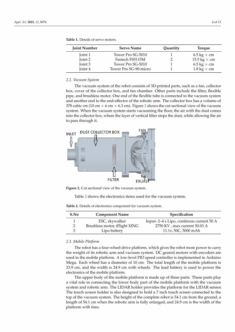
In this experiment, one obstacle was placed at (2, 1) coordinates, the virtual robot startsfrom (0, 0) coordinates, and the real robot (cleaning robot) was placed at (1, 0) coordinates.Other settings included the following: c1 was 2, and c2 was 0.5, obstacle radius r was0.23 m, tu was 0.5 s, and R was 0.7 m. The total experiment was performed for 140 s.The linear velocity for the virtual robot was 0.15 m/s, whereas the angular velocity was0 rad/s. Persistent excitation was h(t, Ey) = φ(t)tanh(Ey) where φ(t) was a non-smoothpulse function of amplitude 0.5, 4 s period with the pulse width of 80 percent. Figure 5shows the experimental results of this experiment. The scale of Figure 5a is 2 m for 1 unitof the x-axis and 0.5 m for 1 unit of the y-axis. Due to the scale, the circular obstaclelooks elliptical. Figure 5a shows the paths of both the robots in the XY plot. The greencolor indicates the path of the virtual robot, which started from (0, 0) coordinates andtraveled into a straight path. The robot starts from (0, 1), avoids the obstacle in its way, andconverges to the desired trajectory in 45 s. Figure 5b shows the error in the x-coordinatesas a function of time. As time passes, the controller helps the robot to achieve near-zeroerror in the x-axis. Figure 5c shows the error in the y-coordinates as a function of time,which also shows that error in the y-axis converges near zero, due to the controller. Theerror graph starts with 1 m in the negative direction, due to the initial setup of the robotconcerning the virtual robot. The robot orientation error also tries to converge to zero, asshown in Figure 5d. The real-time control signal generated by the controller (linear velocityand angular velocity) for the robot can be shown in Figure 5e,f. However, in these plots,some high linear velocities and angular velocities are generated. In that case, the robot only

Appl. Sci. 2021, 11, 8076 10 of 13

moves to its top speeds. Freeze signals for the robot can be seen in Figure 5g, where zeromeans no freeze signal is generated and one unit shows that the robot is frozen. These aregenerated by the controller when the robot is in the potential field near the obstacle.

(a) (b) (c)

(d) (e) (f)

(g)Figure 5. Experiment 1 results—(a) real and virtual robots path in (x, y)-plane; (b) position errors in x direction as a functionof time; (c) position errors in y direction as a function of time; (d) orientation errors as a function of time; (e) linear velocitycontrol; (f) angular velocity control; (g) ’freeze’ signal.

5.2. Experiment 2

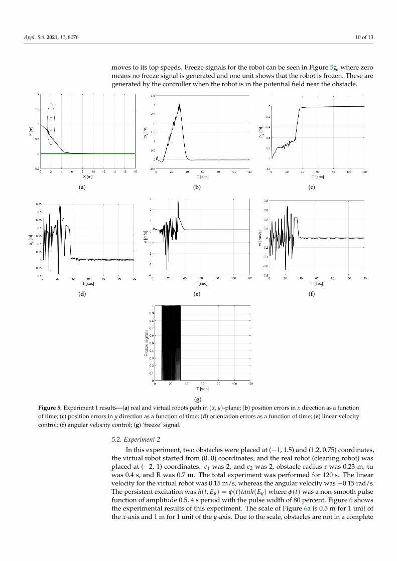
In this experiment, two obstacles were placed at (−1, 1.5) and (1.2, 0.75) coordinates,the virtual robot started from (0, 0) coordinates, and the real robot (cleaning robot) wasplaced at (−2, 1) coordinates. c1 was 2, and c2 was 2, obstacle radius r was 0.23 m, tuwas 0.4 s, and R was 0.7 m. The total experiment was performed for 120 s. The linearvelocity for the virtual robot was 0.15 m/s, whereas the angular velocity was −0.15 rad/s.The persistent excitation was h(t, Ey) = φ(t)tanh(Ey) where φ(t) was a non-smooth pulsefunction of amplitude 0.5, 4 s period with the pulse width of 80 percent. Figure 6 showsthe experimental results of this experiment. The scale of Figure 6a is 0.5 m for 1 unit ofthe x-axis and 1 m for 1 unit of the y-axis. Due to the scale, obstacles are not in a complete

Appl. Sci. 2021, 11, 8076 11 of 13

circular shape. Figure 6a shows the paths of both the robots in the XY plot. The green colorindicates the path of the virtual robot, which starts from (0, 0) coordinates and moves in acircle in the anti-clockwise direction. The robot starts from (0, 1), avoids the two obstaclesin its way, and converges to the desired trajectory at the end. Figure 6b shows the errorin the x-coordinates as a function of time. As time passes, the controller helps the robotto achieve near-zero error in the x-axis. Figure 6c shows the error in the y-coordinatesas a function of time, which also shows that error in the y-axis converges near zero, dueto the controller. The robot orientation error also tries to converge to zero, as shown inFigure 6d. The real-time control signal generated by the controller (linear velocity andangular velocity) for the robot can be shown in Figure 6e,f. However, in these plots, somehigh linear velocities and angular velocities are generated. In that case, the real robot onlymoves to its top speeds. Freeze signals for the robot can be seen in Figure 6g, where zeromeans no freeze signal is generated and one unit shows that the robot is frozen. These aregenerated by the controller when the robot is in the potential field near the obstacle.

(a) (b) (c)

(d) (e) (f)

(g)Figure 6. Experiment 2 results—(a) real and virtual robots path in (x, y)-plane; (b) position errors in x direction as a functionof time; (c) position errors in y direction as a function of time; (d) orientation errors as a function of time; (e) linear velocitycontrol; (f) angular velocity control; (g) ’freeze’ signal.

Appl. Sci. 2021, 11, 8076 12 of 13

6. Conclusions

In this paper, experimental verification of the control algorithm was done on a cleaningrobot. The robot was built with readily available electronics on the market and manufac-tured with additive manufacturing to cut down the cost. The design and the electronics ofthe robot were well explained in the paper. Experiments 1 and 2 were performed for 120 s.In Experiment 1, the robot errors were smaller than 1 percent after 52 s. In Experiment 2,the robot’s errors were smaller than 1 percent after 110 s. The initial conditions were chosenso that in the transient state, the robot had to avoid collisions with two obstacles. It workedwell, as a collision did not occur, but this lengthened the transient state and thus the con-vergence time. The two experiment results show the effectiveness of the control algorithm.The robot avoided the obstacles and achieved the desired trajectory after some time. ROSgave a platform to implement the control algorithm on the standard PC and control therobot wirelessly. The proposed cleaning robot is already equipped with LIDAR and a webcamera, which can create a map of an unknown environment and terrain, using the visionsystem to detect dust on the floor. Mecanum wheels can also be used to have more degreesof freedom for the mobile platform. The control of the robotic arm, vacuum system, visionsystem, and mobile platform can be synchronized to make a fully autonomous system forcleaning in an unknown environment.

Author Contributions: Writing—original draft preparation, A.J. and W.K. All authors have read andagreed to the published version of the manuscript.

Funding: This work is supported by statutory grant 09/93/DSPB/0811.

Acknowledgments: The authors of this paper want to express their deepest gratitude to KrzysztofKozlowski who guided the authors to improve this research.

Conflicts of Interest: The authors declare no conflict of interest.

References1. Prassler, E.; Ritter, A.; Schaeffer, C. A Short History of Cleaning Robots. Auton. Robots 2000, 9, 211–226. [CrossRef]2. Asafa, T.B.; Afonja, T.M.; Olaniyan, E.A.; Alade, H.O. Development of a vacuum cleaner robot. Alex. Eng. J. 2018, 57, 2911–2920.

[CrossRef]3. Murdan, A.P.; Ramkissoon, P.K. A smart autonomous floor cleaner with an Android-based controller. In Proceedings of the 3rd

International Conference on Emerging Trends in Electrical, Electronic and Communications Engineering (ELECOM), Balaclava,Mauritius, 25–27 November 2020; Volume 57, pp. 235–239. [CrossRef]

4. Hasan, K.M.; Nahid, A.A.; Reza, K.J. Path planning algorithm development for autonomous vacuum cleaner robots. In Pro-ceedings of the International Conference on Informatics, Electronics and Vision (ICIEV), Dhaka, Bangladesh, 23–24 May 2014;Volume 57, pp. 1–6. [CrossRef]

5. Prayash, H.A.S.H.; Shaharear, M.R.; Islam, M.F.; Islam, S.; Hossain, N.; Datta, S. Designing and Optimization of An AutonomousVacuum Floor Cleaning Robot. In Proceedings of the IEEE International Conference on Robotics, Automation, Artificial-Intelligence and Internet-of-Things (RAAICON), Dhaka, Bangladesh, 29 November–1 December 2019; pp. 25–30. [CrossRef]

6. Vaussard, F.; Fink, J.; Bauwens, V.; Rétornaz, P.; Hamel, D.; Dillenbourg, P.; Mondada, F. Lessons learned from robotic vacuumcleaners entering the home ecosystem. Robot. Auton. Syst. 2014, 62, 376–391. [CrossRef]

7. Ulrich, I.; Mondada, F.; Nicoud, J.-D. Autonomous vacuum cleaner. Robot. Auton. Syst. 1997, 19, 233–245. [CrossRef]8. Kowalczyk, W.; Kozłowski, K. Trajectory tracking and collision avoidance for the formation of two-wheeled mobile robots. Bull.

Pol. Acad. Sci. 2019, 67, 915–924. [CrossRef]9. Garcia-Sillas, D.; Gorrostieta-Hurtado, E.; Vargas, J.E.; Rodrí-guez-Reséndiz, J.; Tovar, S. Kinematics modeling and simulation of

an autonomous omni-directional mobile robot. Ing. Investig. 2015, 35, 74–79. [CrossRef]10. Martínez-Prado, M.; Rodríguez-Reséndiz, J.; Gómez-Loenzo, R.; Herrera-Ruiz, G.; Franco-Gasca, L. An FPGA-Based Open

Architecture Industrial Robot Controller. IEEE Access 2018, 6, 13407–13417. [CrossRef]11. Montalvo, V.; Estévez-Bén, A.A.; Rodríguez-Reséndiz, J.; Macias-Bobadilla, G.; Mendiola-Santíbañez, J.D.; Camarillo-Gómez,

K.A. FPGA-Based Architecture for Sensing Power Consumption on Parabolic and Trapezoidal Motion Profiles. Electronics 2020,57, 1301. [CrossRef]

12. Khatib, O. Real-Time Obstacle Avoidance for Manipulators and Mobile Robots. Int. J. Robot. Res. 1986, 5, 90–98. [CrossRef]13. Dimarogonasa, D.V.; Loizoua, S.G.; Kyriakopoulos, K.J.; Zavlanosb, M.M. A Feedback Stabilization and Collision Avoidance

Scheme for Multiple Independent Non-point Agents. Bull. Pol. Acad. Sci. 2006, 67, 229–243. [CrossRef]

Appl. Sci. 2021, 11, 8076 13 of 13

14. Filippidis, I.; Kyriakopoulos, K.J. Adjustable Navigation Functions for Unknown Sphere Worlds. In Proceedings of the IEEEConference on Decision and Control and European Control Conference (CDCECC), Orlando, FL, USA, 12–15 December 2011;pp. 4276–4281. [CrossRef]

15. Roussos, G.; Kyriakopoulos, K.J. Decentralized and Prioritized Navigation and Collision Avoidance for Multiple Mobile Robots.Distrib. Auton. Robot. Syst. Springer Tracts Adv. Robot. 2013, 83, 189–202. [CrossRef]

16. Roussos, G.; Kyriakopoulos, K.J. Completely Decentralised Navigation of Multiple Unicycle Agents with Prioritisation and FaultTolerance. In Proceedings of the IEEE Conference on Decision and Control (CDC), Atlanta, GA, USA, 15–17 December 2010;pp. 1372–1377.

17. Roussos, G.; Kyriakopoulos, K.J. Decentralized Navigation and Conflict Avoidance for Aircraft in 3-D Space. IEEE Trans. Control.Syst. Technol. 2012, 20, 1622–1629. [CrossRef]

18. Mastellone, S.; Stipanovic, D.; Spong, M. Formation control and collision avoidance for multi-agent non-holonomic systems:Theory and experiments. Int. J. Robot. Res. 2008, 27, 107–126. [CrossRef]

19. Kowalczyk, W.; Kozłowski, K. Leader-Follower Control and Collision Avoidance for the Formation of Differentially-DrivenMobile Robots. In Proceedings of the 23rd International Conference on Methods and Models in Automation and Robotics MMAR,Miedzyzdroje, Poland, 27–30 August 2018.

20. Do, K. Formation Tracking Control of Unicycle-Type Mobile Robots with Limited Sensing Ranges. IEEE Trans. Control. Syst.Technol. 2008, 16, 527–538. [CrossRef]

21. Kowalczyk, W.; Kozłowski, K.; Tar, J.K. Trajectory tracking for multiple unicycles in the environment with obstacles. In Proceed-ings of the 19th International Workshop on Robotics in Alpe-Adria-Danube Region RAAD, Budapest, Hungary, 24–26 June 2010;pp. 451–456. [CrossRef]

22. Guldner, J.; Utkin, V.I.; Hashimoto, H.; Harashima, F. Tracking gradients of artificial potential fields with non-holonomicmobile robots. In Proceedings of the 1995 American Control Conference-ACC’95, Seattle, WA, USA, 21–23 June 1995; Volume 4,pp. 2803–2804. [CrossRef]

23. Zhou, L.; Li, W. Adaptive Artificial Potential Field Approach for Obstacle Avoidance Path Planning. In Proceedings of the SeventhInternational Symposium on Computational Intelligence and Design, Hangzhou, China, 13–14 December 2014; pp. 429–432.[CrossRef]

24. Loria, A.; Dasdemir, J.; Alvarez Jarquin, N. Leader—Follower Formation and Tracking Control of Mobile Robots Along StraightPaths. IEEE Trans. Control Syst. Technol. 2016, 57, 727–732. [CrossRef]

25. De Wit, C.C.; Khennouf, H.; Samson, C.; Sordalen, O.J. Nonlinear Control Design for Mobile Robots. In Recent Trends in MobileRobots; World Scientific Publishing Company: Singapore, 1994; pp. 121–156.

26. Michałek, M.; Kozłowski, K. Vector-Field-Orientation Feedback Control Method for a Differentially Driven Vehicle. IEEE Trans.Control Syst. Technol. 2010, 18, 45–65. [CrossRef]

27. Kowalczyk, W.; Michałek, M.; Kozłowski, K. Trajectory tracking control with obstacle avoidance capability for unicycle-likemobile robot. Bull. Pol. Acad. Sci. Tech. Sci. 2012, 60, 537–546. [CrossRef]