Design and Evaluation of a Novel Conveyor Utilizing a Screw ...

DEGREE PROJECT IN MECHANICAL ENGINEERING,SECOND CYCLE, 30 CREDITSSTOCKHOLM, SWEDEN 2021

Design and Evaluationof a Novel ConveyorUtilizing a ScrewMechanism to MoveObjects WithIntegrated Racks

Måns Nilsson and Mathias Nordqvist

KTH ROYAL INSTITUTE OF TECHNOLOGYSCHOOL OF INDUSTRIAL ENGINEERING AND MANAGEMENT

Master Thesis MMK TRITAITMEX 2021:387

Design and Evaluation of a Novel ConveyorUtilizing a Screw Mechanism to Move

Objects With Integrated Racks

KTH Industrial Engineering Måns Nilssonand Management Mathias Nordqvist

Approved Examiner Supervisor

20210611 Hans Johansson José Manuel Gaspar Sánchez

Abstract

Intralogistics, or material handling, traditionally use roller or chain conveyors to move

objects and goods in factories and warehouses. One negative aspect of the traditional

types of conveyors is that they are expensive, as they are comprised of manymoving parts.

This thesis proposes a novel type of conveyor solution in which a transportation fixture

with an integrated open thread slides on Lshaped profiles and is propelled forward by a

screw. A potential obstacle to the usefulness of such a conveyor is that a screw has innately

low efficiency due to the mechanics of screws compared to the principle of rolling that is

employed in a roller or chain conveyor.

This thesis investigates the functionality and efficiency of the proposed conveyor, or more

particularly the core functionality, which is the screw and thread mechanism. A test rig

was designed and built, in which experiments were carried out. In the experiments, the

material, manufacturing technology, and helix angle of the screw and thread, and the

speed were varied. The influence on torque, power demand, and efficiency among other

parameters were measured and evaluated. Additionally, a method for automatic thread

meshing is presented and testing of it was carried out, which showed reliability with and

without positional feedback, which gives the conveyor more use cases.

iii

It was found that the efficiency of the screw and thread mechanism was higher for screws

with a higher lead, steel screws with a diameter of 50 mm exhibited an efficiency of

31%± 4.5 % with a lead of 32 mm but only 8.7%± 1.6 % with a lead of 8 mm. 3D printed

plastic screws had slightly lower but similar early life efficiency as steel screws, but seized

or wore down when tested in an accelerated lifetime experiment.

Because a high screw lead is favorable, and because of the size and geometry constraints

of such a conveyor (discussed in the conclusion of the report), a direct drive motor

is not suitable, and instead a motor and gearbox combination is recommended. The

conveyor shows promise as an alternative solution to traditional conveyors in low load

applications.

Keywords

Screw Conveyor, Intralogistics, Material Handling, Thread Meshing, Worm rack drive,

Brushless motor

iv

Examensarbete MMK TRITAITMEX 2021:387

Design och utvärdering av en ny transportör somanvänder en skruvmekanism för att flyttaföremål med integrerade kuggstänger

KTH Industriell teknik Måns Nilssonoch management Mathias Nordqvist

Godkänt Examinator Handledare

20210611 Hans Johansson José Manuel Gaspar Sánchez

Sammanfattning

Intralogistik, eller materialhantering, använder traditionellt rull eller kedjetransportörer

för att flytta gods i fabriker och lager. En negativ aspekt med dessa traditionella

transportörer är att de är dyra, då de består av ett stort antal rörliga delar. Detta

examensarbete föreslår enny typ av transportör i vilken en transportfixturmed en inbyggd

kuggstång glider på Lformade profiler and drivs framåt av en skruv. Ett potentiellt hinder

för denna typ av transportörs användbarhet är att en skruv naturligt har låg verkningsgrad

på grund av skruvensmekanik i jämförelsemed principen av rullning somanvänds av rull

och kedjetransportörer.

Detta examensarbete undersöker funktionaliteten och verkningsgraden av den föreslagna

transportören, mer specifikt kärnfunktionaliten som är en skruv och gängmekanism. En

testrigg designades och byggdes, i vilken experiment utfördes. I experimenten varierades

materialet och spiralvinkeln av skruven och gängan, samt hastigheten. Vridmomentet,

effekten, verkningsgraden och andra parametrar mättes och utvärderades.

v

Dessutom presenteras en metod för automatiskt gängingrepp som även testades,

som visade sig vara tillförlitligt både med och utan positionsåterkoppling, vilket ger

skruvtransportören fler användningsområden.

Resultaten visade att verkningsgraden av skruv och gängmekanismen var högre för

skruvar med högre spiralvinkel. Stålskruvar med en diameter på 50 mm visade på en

verkningsgrad om 31% ± 4.5 % med en stigning på 32 mm men endast 8.7% ± 1.6 %

med en stigning på 8 mm. 3DPrintade plastskruvar hade något lägre men liknande

verkningsgrad som stålskruvar i början av sin livslängd, men skar fast eller nöttes ned

när de testades i ett långtidsexperiment.

Eftersom hög stigning på skruven är fördelaktigt och på grund av de geometriska

begränsningar av en sådan transportör (diskuteras i slutsatsen av rapporten), är det inte

lämpligt att driva skruven direkt från en elmotor, utan istället rekommenderas en motor

växellådekombination. Transportören verkar lovande som ett alternativ till traditionella

transportörer i applikationer med låg last.

Nyckelord

Skruvtransportör, Intralogistik, Materialhantering, gängingrepp, Snäckskruv och

kuggstång, borstlös motor

vi

Acknowledgements

We would like to extend our gratitude towards our academic supervisor José Manuel

Gaspar Sánchez, our examiner Hans Johansson and the course responsible for the

mechatronics master thesis course Fredrik Asplund for their support. In addition, we

would like to thank the company at which the master thesis was carried out for their

hospitality and for enabling us to carry out our work in their facilities in a safe way in

spite of the ongoing pandemic. A special thanks to our industrial supervisor for giving us

the opportunity to conduct this thesis as well as for the support during the thesis. Lastly,

we would like to extend a big thank you to all the colleagues at the company that have

helped us with practicalities and by sharing their knowledge.

With warmest regards,

Måns Nilsson & Mathias Norqvist

vii

Acronyms

PV Pressure Velocity

MCU Microcontroller Unit

BLDC Brushless Direct Current

PMSM PermanentMagnet Synchronous Motor

PWM Pulse Width Modulation

IC Integrated Circuit

FOC FieldOriented Control

EMF Electromotive Force

USB Universal Serial Bus

GUI Graphical User Interface

FDM Fused Deposition Modeling

SLS Selective Laser Sintering

SLA Stereolithography

opamp Operational amplifier

ANOVA Analysis of Variance

ANCOVA Analysis of Covariance

RMS Root Mean Square

viii

Contents

1 Introduction 11.1 Background . . . . . . . . . . . . . . . . . . . . . . . . . . . . . . . . . . . . 1

1.2 Problem . . . . . . . . . . . . . . . . . . . . . . . . . . . . . . . . . . . . . . 3

1.3 Definition of parts . . . . . . . . . . . . . . . . . . . . . . . . . . . . . . . . 5

1.4 Purpose . . . . . . . . . . . . . . . . . . . . . . . . . . . . . . . . . . . . . . 6

1.5 Benefits, Ethics and Sustainability . . . . . . . . . . . . . . . . . . . . . . . 6

1.6 Methodology . . . . . . . . . . . . . . . . . . . . . . . . . . . . . . . . . . . 7

1.7 Limitations and Delimitations . . . . . . . . . . . . . . . . . . . . . . . . . . 7

2 Frame of reference 92.1 Related work . . . . . . . . . . . . . . . . . . . . . . . . . . . . . . . . . . . 9

2.2 Lead Screws . . . . . . . . . . . . . . . . . . . . . . . . . . . . . . . . . . . 10

2.2.1 The parameters of a lead screw . . . . . . . . . . . . . . . . . . . . 11

2.2.2 Different types of threads . . . . . . . . . . . . . . . . . . . . . . . . 12

2.2.3 Lead screw equations . . . . . . . . . . . . . . . . . . . . . . . . . . 12

2.3 Forces . . . . . . . . . . . . . . . . . . . . . . . . . . . . . . . . . . . . . . . 14

2.4 Polymer materials in lead screw application . . . . . . . . . . . . . . . . . . 16

2.5 Additive Manufacturing . . . . . . . . . . . . . . . . . . . . . . . . . . . . . 18

2.6 ODrive . . . . . . . . . . . . . . . . . . . . . . . . . . . . . . . . . . . . . . . 18

2.7 Brushless Motors . . . . . . . . . . . . . . . . . . . . . . . . . . . . . . . . . 20

2.8 Gearbox . . . . . . . . . . . . . . . . . . . . . . . . . . . . . . . . . . . . . . 24

2.9 Sensors . . . . . . . . . . . . . . . . . . . . . . . . . . . . . . . . . . . . . . 25

2.9.1 Torque sensor . . . . . . . . . . . . . . . . . . . . . . . . . . . . . . 25

2.9.2 Force gauge . . . . . . . . . . . . . . . . . . . . . . . . . . . . . . . 27

2.9.3 Current sensor . . . . . . . . . . . . . . . . . . . . . . . . . . . . . . 27

2.9.4 Encoders . . . . . . . . . . . . . . . . . . . . . . . . . . . . . . . . . 29

2.10 Aliasing . . . . . . . . . . . . . . . . . . . . . . . . . . . . . . . . . . . . . . 29

ix

CONTENTS

2.11 Filters . . . . . . . . . . . . . . . . . . . . . . . . . . . . . . . . . . . . . . . 30

3 Implementation 333.1 Mechanical Design . . . . . . . . . . . . . . . . . . . . . . . . . . . . . . . . 333.2 Torque Sensor . . . . . . . . . . . . . . . . . . . . . . . . . . . . . . . . . . 383.3 Force gauge . . . . . . . . . . . . . . . . . . . . . . . . . . . . . . . . . . . 393.4 Electric motor and gearbox . . . . . . . . . . . . . . . . . . . . . . . . . . . 393.5 Motor driver . . . . . . . . . . . . . . . . . . . . . . . . . . . . . . . . . . . . 403.6 Data gathering . . . . . . . . . . . . . . . . . . . . . . . . . . . . . . . . . . 413.7 Filter . . . . . . . . . . . . . . . . . . . . . . . . . . . . . . . . . . . . . . . . 423.8 Determining sliding friction . . . . . . . . . . . . . . . . . . . . . . . . . . . 433.9 Experiments . . . . . . . . . . . . . . . . . . . . . . . . . . . . . . . . . . . 44

3.9.1 Experiment 0: Varying material of screw . . . . . . . . . . . . . . . 443.9.2 Experiment 1: Varying materials of screw and rack . . . . . . . . . 473.9.3 Experiment 2: Varying screw lead with same material . . . . . . . . 483.9.4 Experiment 3: Fastest possible move time with a given load . . . . 503.9.5 Experiment 4: Automatic thread meshing . . . . . . . . . . . . . . . 513.9.6 Experiment 5: Accelerated lifetime test . . . . . . . . . . . . . . . . 54

4 Results 554.1 Sliding friction . . . . . . . . . . . . . . . . . . . . . . . . . . . . . . . . . . 554.2 Varying materials of screw and rack . . . . . . . . . . . . . . . . . . . . . . 554.3 Varying screw lead with same material . . . . . . . . . . . . . . . . . . . . 584.4 Fastest possible move time with a given load . . . . . . . . . . . . . . . . . 614.5 Automatic thread meshing . . . . . . . . . . . . . . . . . . . . . . . . . . . 634.6 Accelerated lifetime test . . . . . . . . . . . . . . . . . . . . . . . . . . . . . 65

4.6.1 Steel screws with different leads . . . . . . . . . . . . . . . . . . . . 664.6.2 Different materials . . . . . . . . . . . . . . . . . . . . . . . . . . . . 71

4.7 Motor selection . . . . . . . . . . . . . . . . . . . . . . . . . . . . . . . . . . 74

5 Conclusions 775.1 Conclusion . . . . . . . . . . . . . . . . . . . . . . . . . . . . . . . . . . . . 775.2 Discussion and Recommendation . . . . . . . . . . . . . . . . . . . . . . . 80

x

Chapter 1

Introduction

Material handling deals with moving objects around in factories or warehouses. Typical

material handling equipment includes roller, belt and chain conveyors. This thesis

focuses on a way of material handling that uses a special linear actuation mechanism,

consisting of a screw and a rack, similar to a lead screw and a nut to convey an object.

In this design, the screw is mounted on a stationary machine and the rack integrated

into the object being handled. Further, to engage and disengage the screw in the rack of

the object, another more typical lead screw and nut assembly is used to move the main

screw axially. Both of these are driven by brushless electric motors. More particularly,

this thesis evaluates the functionality and efficiency of this electrical linear transmission

system.

1.1 Background

Material handling deals with moving objects within buildings or between buildings and

vehicles. Especially in factories and manufacturing facilities. An object that is being

manufactured or assembled often needs to be moved internally in the factory between

different work stations where different processes take place. For example, a cog wheel

might go through one work station where the cogs are cut and then one where it is

hardened in an oven. Typical material handling equipment for horizontal movement

of solid materials include belt, chain and roller conveyors. For material handling of

liquid or powder materials, such as water or cement, conveyors utilizing the principle of

Archimedes screw are often used.

1

CHAPTER 1. INTRODUCTION

Often, when dealing with solid materials, the material that is being handled does not

possess a shape that is advantageous for transportation on a conveyor. Therefore, an

intermediate object, that holds the material and that is suitable for transportation on a

conveyor, is often used. This object can be a simple pallet, but is most often a customized

transportation fixture. An example of this can be seen in Figure 1.1.1.

Figure 1.1.1: A car seat, mounted on a transportation fixture, being transported on a rollerconveyor [49]

Conveyors that use belts, rollers, or chains have both positive and negative attributes.

One negative aspect is that they are expensive. For example, a single roller in a roller

conveyor usually consists of a chain sprocket and at least two ball bearings. Furthermore,

the rollers need to be placed close together, and thus it takes a lot of rollers to make up a

roller conveyor.

The screw and rack actuation system that is investigated in this thesis could be placed in

the manner shown in Figure 1.1.2. With one motor driving one long shaft with several

screws attached to it. As long as the screws are placed no further apart than the length

of the transportation fixture and their rotational orientation is correct in relation to each

other, there does not need to be threads on the entire length of the shaft. A device for

engaging the rack of the transportation fixture in the screw is needed at the start of the

conveyor.

2


Figure 1.1.2: Screw conveyor

1.2 Problem

One negative aspect of the aforementioned conveyance solution compared to roller or

chain conveyors is the efficiency. Both roller and chain conveyors rely on the principle

of rolling. In a roller conveyor, this is obvious, but even chain conveyors utilize rolling,

they use roller chains, in which the rollers of the chain roll on plastic chain guides. Rolling

friction is significantly lower than sliding friction, in the order of 10100 times lower[17,

p, 309312].

There is little literature about the efficiencies of worm rack drives. However, there is

literature regarding the efficiencies of worm gears and lead screws with varying materials

and geometries. The geometry of the screw and rack could be seen as a lead screw with

an open nut. The efficiency of a lead screw can vary between 20 and 80%[22]. Figure 1.2.1

shows the main mechanical principle of study, a screw and rack. The screws in the figure

could be seen as either the worm in a worm gear or a lead screw in a lead screw and nut

assembly.

Figure 1.2.1: Screw and rack.

3


From literature, it is found that themain parameters affecting the efficiency of a lead screw

are the helix angle and the coefficient of friction between the materials of the screw and

nut[22].

The greater the helix angle, the higher the efficiency. Electric motors on the other hand,

reach their peak efficiency at high speeds. Furthermore, a greater helix angle demands

a greater torque to be driven and hence the choice of motor and gearbox are highly

dependent on this parameter.

Varying the material of the screw and rack will affect the efficiency by means of varying

friction coefficients and varying rotational inertia. I will also influence the system price.

Comparisons of differentmaterial combinations inwormgears have beenmadepreviously

[42], and studies about the efficiency of plastic worm gears[27][20], but the studies are

usually limited to regular worm gears and not worm rack drives.

Beneath the transportation fixture, there are Lprofiles holding it up. The friction

between the transportation fixture and the Lprofile will affect the force required tomove

the object. Reduced friction enables the use of smaller motors, due to the lower force

requirement. One can see that this is a highly integrated mechatronic problem with many

degrees of freedom.

4


1.3 Definition of parts

For the reader to efficiently comprehend the topics discussed in the report, a description

of themost central parts of the study is provided below, along with a visual representation

of the parts described. This visualization can be seen in Figure 1.3.1.

• Rack

– An ”open nut” is similar to a rack in a ”rack and pinion” setup, except the rack

meshes with a screw instead of a pinion and thus has a helix angle. The rack is

integrated into the transportation fixture.

• Screw

– A short lead screw that has a large diameter. It is stationary and is driven

by an electric motor, it mates with the rack, and when it turns it moves the

transportation fixture.

• Transportation fixture

– The transportation fixture is the mass that is being moved, it has an integrated

rack. The transportation fixture is moved within in the test rig.

• Test Rig

– The Test rig provides a support underneath the transportation fixture as well

as hold the screw mechanism and motor that drives it.

Figure 1.3.1: Description of parts

5


1.4 Purpose

The purpose of this thesis is to develop an electromechanical transmission system based

on a screw and rack and evaluate how different variations of geometry and material

choices influence the performance and efficiency as well as the cost and size of the system.

Research questions are formulated to fulfil this purpose and are stated as:

• Are 3D printed plastic screws or CNC Lathed Steel screws in combination with

3D printed plastic racks a valid alternative in this application, and how do they

compare to each other?

• What lead of the screw and rack mechanism, in combination with size of motor,

provides the best tradeoff regarding system cost, size, speed and efficiency?

• Is it possible to achieve initial thread meshing with a high rate of repeatability by

using dual motors run in synchronization?

1.5 Benefits, Ethics and Sustainability

The system investigated in this study can be seen as a type ofmaterial handling equipment,

which is a type of automation. The topic of automation as an ethical problem has been

a topic of discussion for a long time. The main worry is that automation is stealing jobs.

This is a complex subject, but studies have shown that employment actually increases with

increased automation as it creates more job opportunities[34]. Other studies have shown

that the number of jobs that can be automated are overestimated because the substantial

heterogeneity of tasks within jobs are neglected[1]. Further, the equipment investigated

is merely an alternative to existing conveyor solutions, an area of industry that is already

very automated.

Since this transmissionmight have the possibility to move heavy weights, the safety of the

device must be considered. If it breaks, it might injure people working in close proximity

and damage the goods. In this thesis, tests will be performed on a smallscale controlled

test rig in an controlled environment. To test the reliability and safety aspects of the final

product, more thorough testing in a real world scenario with a more developed product

would be needed before release.

6


1.6 Methodology

To fully understand the problem, the authors theoretical knowledge of the problem area

needed to be deepened. Particularly regarding the trapezoidal screws, their geometry and

what parameters influence their efficiency, the materials that were used, and electrical

motors. This was obtained by reading scientific articles, reports, conference papers, and

books.

To test the conveyor, four different subsystems were designed. The screw, the drivetrain,

the transportation fixture, and the test rig.

To efficiently iterate the design, 3D printing was used extensively. This made it possible

to test different designs simultaneously in a rapid pace. When the design of the screws

were finalized, an order was placed to have them manufactured in metal. The test rig

was designed and built using aluminium extrusions. This enabled convenient and fast

prototyping as well as ease of expansion for future ideas.

To answer the research questions, several hypotheses were formed. Experiments were

performed to test these hypotheses, most of which were analyzed quantitatively using

different variations of analysis of variance while some aspects were analyzed qualitatively.

The conditions of each experiment are described in detail in Section 3.9.

1.7 Limitations and Delimitations

For the project to be feasible as a thesis project some limitations and delimitations were

set.

• The experiments were performed on a test rig and not in a real conveyor. The test rig

built was very short compared to the real world case of a conveyor, as building a long

conveyor would be laborintensive and costly. Besides, for testing and experiments,

no real value is gained from building a longer one.

• Most parts designed during the thesis are manufactured using 3D printing. Some

parts, most notably the racks, would not be 3D printed in high volume production.

They wouldmost likely be injectionmoulded, pressed, ormachined. However, these

manufacturing methods require the manufacturing of special tools, which are costly

and timeconsuming and thus not feasible during a master thesis.

• The testing was limited to a load of 32 kg.

7


• Due to limitations in time and budget, some of the screws that were to be tested were

ordered from a Chinese manufacturer. Mainly due to no Swedish company agreeing

to manufacture the small volumes and large variations of screws that were required

for this study. Originally, screws in brass and bronze were meant to be included in

the study as well. However, due to poor packaging, the hard steel screws that were

packaged together with the softer bronze and brass screws damaged the brass and

bronze screws. The result was that their performance was unreliable, and they could

not be used in the study. Due to time limitations, reordering the screws was not an

option. The surface finish of the steel screws made by the Chinese manufacturer

were not as good as the ones made by a Swedish manufacturer.

• To fully investigate the internal difference between screws of the same geometry,

same manufacturing technology, and material, more samples of each screw would

be needed. Due to budget and resource constraints, this was not possible during this

thesis.

8

Chapter 2

Frame of reference

2.1 Related work

The use of a screw in combination with a rack is not very common, but a few applications

have been found. A cylindrical robotic crawler unit that has a worm screw in the center

and utilizes a worm rack drive to actuate its track belts, was developed by researchers in

Japan[28]. When the worm screw spins inside the cylinder, the track belts spin and the

entire crawler unit is moved forward. Figure 2.1.1 shows a picture of the crawler unit.

Worm rack drives have also been used in heavy industrial manufacturing equipment, in

Figure 2.1.1: A robotic crawler unit that utilizes a worm rack drive, developed byresearchers in Japan [28].

mills[6] and in lathes[51]. In these applications, the worm screw is mounted on a piece

of equipment, like a mill bed, that is moving relative to the world frame, while the rack is

stationary in relation to the world frame. A picture of such a worm rack combination can

be seen in Figure 2.1.2.

No previous works where the screw is stationary relative to the world frame and the rack

is moving relative to the world frame have been found.

9

CHAPTER 2. FRAME OF REFERENCE

Figure 2.1.2: A worm rack drive for heavy industrial equipment[51].

2.2 Lead Screws

A lead screw is a special type of screw which is used to translate rotational motion into

linear motion. Typically, a lead screw assembly consists of a lead screw and a nut, where

the nut is attached to an object and the lead screw is coupled to a motor. The rotational

motion of the lead screw is transformed to linear motion of the nut and the object. See

Figure 2.2.1.

Figure 2.2.1: A typical lead screw example

Lead screws are common parts in for example 3D printers, milling machines, linear

actuators, CDROM drives and many more.

10


2.2.1 The parameters of a lead screw

Lead screws have a couple of parameters that influence their performance, these are

mentioned below.

Figure 2.2.2: Parameters of a lead screw

The following definitions are inspired by the ones described in Design of machine

elements, page 187188, [4].

Pitch The pitch is defined as the distance between the same edge of two adjacent

threads. It is denoted by the letter p.

Lead The lead is defined as the distance between the same edge of two adjacent threads

that belong to the same thread start. It is denoted by the letter l. The lead is the length of

the pitch times the number of thread starts.

Core diameter The core diameter is the smallest diameter of the screw thread and is

denoted by dc.

Nominal diameter The nominal diameter is the outer diameter of the screw and is

denoted by d.

Mean diameter The mean diameter can be obtained by

dm =1

2(d+ dc)

11


Helix angle Also called lead angle and denoted by α. It is defined as the angle between

the helix of the thread and a plane perpendicular to the axis of the screw. This angle is

related to the screw lead and mean diameter in the following manner

tan α =l

πdm

2.2.2 Different types of threads

For power screws there are two common types of threads, square and trapezoidal, which

can be seen in Figure 2.2.3. Each of these thread types have their advantages and

disadvantages. For the square thread, the benefit is higher efficiency than trapezoidal

threads. Its disadvantages are being difficult to manufacture, lower strength due to less

thread thickness at the core diameter compared to the trapezoidal thread.[4] For the

trapezoidal thread, there are two common standards ACME[2] and DIN 103[44] metric,

where the thread angle, γ for ACME is 29 and 30 for the metric thread.

(a) Square thread profile (b) Trapezoidal thread profile

Figure 2.2.3: Thread profiles

2.2.3 Lead screw equations

The lead screw and nut act as a transmission system, transforming the rotational velocity

and torque of the lead screw to translational velocity and force of the nut and object. The

lead is a measurement of the linear distance the object is moved during one revolution

of rotation. Thus, when the lead is increased, the linear distance per revolution, i.e, the

translational velocity, is increased. The relationship between rotational and translational

velocity can be described by

V =ω · L2π

, (2.1)

where ω is the rotational speed[rad/s] and L is the screw lead[m]. For righthand helix, ω

and V are the same sign and for lefthand they have opposite signs.

12


The torque, τ required for a given axial force has the relationship that when the lead is

increased, the required torque is increased as well and can be described by

τ =Fa · L2π · η

, (2.2)

where Fa is the axial force and η the efficiency and is calculated as

η = tan(α) · 1–µ · sec (γ) tan (α)

µ · sec (γ) + tan (α), (2.3)

where γ is the thread half angle and µ the friction coefficient between screw and nut [4].

This shows that the efficiency of a lead screw is primarily dependent on the helix angle

and the friction coefficient between the screw and the nut and in this case, rack instead of

nut. This is visualized with different coefficients of friction in Figure 2.2.4. The vertical

dotted lines correspond to the helix angles of the different screw leads used in this project.

Maximum efficiencies are marked as red dots for each coefficient of friction.

0° 10° 20° 30° 40° 50° 60°

Helix angle [deg]

0%

10%

20%

30%

40%

50%

60%

70%

Eff

icie

ncy

[%

]

Trapezoidal lead screw efficiency for different coefficient of friction

= 0.2

= 0.25

= 0.3

= 0.35

= 0.4

= 0.45

8 mm

16 mm

24 mm

32 mm

Figure 2.2.4: Trapezoidal lead screw efficiency with different coefficients of friction

13


2.3 Forces

mg

N

Fu

Fa

Figure 2.3.1: Free body diagram

To slide an object on a surface two types of forces needs to be overcome. The friction

force and inertial force. Both are a function of the mass of the object. The inertial part

depends on the acceleration of the object and can be described by Newtons second law of

motion,

Fi = ma,

where m is the mass and a is the acceleration. The friction force is generally described

as

Ff = µN,

where µ is the coefficient of friction and N is the normal force. This is a simplified model

of reality. Many different models of friction between moving bodies have been formed

over the years[31]. Figure 2.3.2 presents one model of friction.

Figure 2.3.2: A model of friction [9].

14


Even though many different models exist, they are similar in the way that they all contain

a peak in the force when the object is moved from a standstill, that is higher than the force

required to slide the object at a constant velocity. As the velocity is increased, the viscous

friction becomes a factor.

Fa =

ma+ Fbrk, v = 0

ma+ Fc + Fv, v > 0,(2.4)

where Fbrk is the breakaway friction, Fc is the Coulomb friction and Fv is the viscous

friction. They can be further broken down into

Fbrk = µsN,

Fc = µkN,

Fv = µvv,

where µs is the static friction coefficient, µk is the kinetic friction coefficient and µv is the

viscous friction coefficients. Friction coefficients are material combination parameters,

for example steel/steel. It is hard to find reliable values of these coefficients online,

the value can vary greatly between various sources even though the same material

combination is used. This is probably because the friction coefficients are not only

dependent on the material but also the surface roughness of the objects and the

temperature of the contact area and lubrication[17]. Even if a source was found that

specified these parameters, to be able to apply that value to ones own design, one would

have to know these parameters of the intended objects to be used in one’s design, which

requires special instruments which are not common.

To calculate the efficiency of the screw rack transmission, the work done by the

transmission and the required work to move the transportation fixture must be

calculated.

Work done by the transmission is calculated as

Wtransmission =

∫ t

0

T · ω dt (2.5)

15


The work required to move the transportation fixture can be calculated as

Wtransport =

∫ t

0

F · v dt =

∫ x(t2)

x(t1)

F ds ≈ µ ·N · L, (2.6)

where µ is the friction coefficient, N the normal force and L the length travelled. This

assumes that the static and kinetic friction coefficients are the same and that the viscous

friction is close to zero. This also assumes that the acceleration and deceleration have the

same profile.

The efficiency, ηt is now defined as

ηt =Wtransport

Wtransmission

. (2.7)

2.4 Polymer materials in lead screw application

When considering an application where a component made of polymer material is either

rotating or sliding, one must take note of its pressurevelocity, Pressure Velocity (PV)

rating. The PV rating determines the relation between load capacity and speed. If one

is increased, the other one must be lowered to keep the product below the maximum

specified rating. This is due to the frictional heat that is generated, which if becomes

too large will deform the polymer material and if it goes too far, even seize the lead

screw[13].

Often it is the nut that is made of a polymer material and the screw made of metal, since

the nut is often the smaller, cheaper, and more exchangeable part.

To calculate the PV value, the projected area between the threads of the nut and screw, A

is needed. These calculations are shown in both [21] and [13]. The area is defined as

A = Lh · dt, (2.8)

where Lh is the helix length and dt depth of engagement.

The helix length, Lh is calculated as

Lh = Lhr ·Ln

L· St, (2.9)

where Lhr is the helix length per revolution, Ln the nut length, L the screw lead and St the

16


number of thread starts. For this application, however, the nut length is set to the screw

length since this is the moving part and not the nut. Furthermore, this is what determines

the projected area of the thread engagement. By looking at Figure 2.2.2 the Lhr can be

seen as the hypotenuse of the triangle giving the relation

Lhr =√L2 + d2m. (2.10)

The depth of engagement is found from Figure 2.2.2 to be

dt = d− dc = p/2 (2.11)

Since a polymer material is more flexible than the metal screw, there will be deflection

between the thread of the screw and nut [21]. This will reduce the contact area and hence

increase the contact pressure since the force remains the same. To account for this issue,

a correction factor, Cf is normally used with values ranging from 0.75 to 0.25, depending

on the load [21]. This results in a final area of

A = CF · Lh · dt. (2.12)

With the area defined, the contact pressure, P can be calculated as

P =Fa

A. (2.13)

To get the PV value the linear speed between the nut and screw, Vh is needed and calculated

as

Vh = Lhr ·ω

2π. (2.14)

Now everything is known, and the PV value can be computed according to

PV = P · Vh. (2.15)

It is possible to exceed the PV rating for a short duration of time, however, the generated

friction heat will not disappear immediately due to thermal inertia. This limits how often

this can be done and the duty cycle of the process must be limited accordingly [21].

In this application, it is the nut which is stationary and the screw that is moving along the

nut. This means that new material will be in engagement when the screws move.

17


However, the material will experience a second pass when the second screw engages in

the threads of the first one.

As stated, the use of polymer materials in lead screw applications has its downsides when

it comes to longevity, but there are also benefits. One of them is that plastic nuts in a lead

screw application can be used without lubrication, whereas this is not recommended in

most situations with a steel or bronze nut [22]. They also provide the benefits of lower

cost, less noise and corrosion resistance [19].

Regarding the friction coefficient of plastics, it is often in the range of 0.1 to 0.5, but

exceptions do exists. This coefficient is also load depended.[17, p. 66]

2.5 Additive Manufacturing

Additive manufacturing, or more commonly called 3D printing, is the process of

fabricating parts by adding material instead of starting with a stock and removing

material, which is what is done in traditional manufacturing such as milling or lathing.

Additive manufacturing has risen highly in popularity in recent years[3]. The most

common additive manufacturing technologies are Fused Deposition Modeling (FDM),

Selective Laser Sintering (SLS), and Stereolithography (SLA). They all work by building

the parts layer by layer. FDMmelts plastic filament and extrudes it through a nozzle, this

is the technology used in most hobby 3D printers. SLA works by shining ultraviolet light

on a sensitive resin which makes it harden, and SLS works by shining a laser on powder

material.

2.6 ODrive

ODrive is an Open Source driver for brushless servomotors. Two brushless motors and

one encoder for each motor as well as two limit switches for each motor can be connected

to it. The limit switches can be used for homing the axis to a welldefined starting point.

The board used in this project was V3.6 56V version.

The ODrive acts as an abstraction layer to the control of the brushless motors, taking care

of the electrical commutation as well as the control algorithms.

When breaking an electric motor, the backElectromotive Force (EMF) energy has to go

somewhere. This driver allows for an external break resistor to be connected to its AUX

port to dissipate this energy. This is good if a power supply is used, since the backEMFwill

18


Figure 2.6.1: ODrive V3.6 56V Servo Driver board

charge the output capacitors of the power supply and depending on the size of these, they

might not be able to store all energy. This makes the voltage off the capacitors increase to

the point where the power supply’s overvoltage protection will trip. If batteries are used,

the need for brake resistor is limited, since the batteries are able to takemost, if not all the

backEMF energy. This will depend on the charge level of the batteries, since if they are

fully charged, they can absorb less energy.

Internally, the ODrive operates a cascaded style position, velocity, and current control

loop. It uses a variation of a PID (Proportional Integral Derivative) controller for all

stages. For the position control, it uses a simple P controller and for the velocity and

current control it uses PI controllers[12]. The sampling rate of the all the control loops is

8kHz.

Figure 2.6.2: Odrive control loop [12]

The ODrive can be configured to use trajectory control. This means that the maximum

values for acceleration and velocity can be set while controlling the motors with position

control. This allows for the motors to be controlled smoothly, without jerky movements.

This limits the stress put on the system since peak current and torque will be sufficiently

lowered compared to those when not using trajectory control. This is because internally,

when trajectory control is used, the position controller is given a ramp input instead of a

step input. An example of a trajectory planner can be seen in Figure 2.6.3.

19


0 0.5 1 1.5 2 2.5 3 3.5 4 4.5 5

Time [s]

0

500

1000

1500

Po

sitio

n [

rad

]

Position profile

Pos

0 0.5 1 1.5 2 2.5 3 3.5 4 4.5 5

Time [s]

0

200

400

600

Ve

locity [

rad

/s]

Velocity profile

Velocity

0 0.5 1 1.5 2 2.5 3 3.5 4 4.5 5

Time [s]

-500

0

500

Acce

lera

tio

n [

rad

/s2]

Acceleration profile

Acceleration

Figure 2.6.3: Example of an trapezoidal velocity trajectory control

In this project, a trajectory with 1/3 time acceleration, 1/3 constant velocity and

1/3 deceleration. The maximum acceleration, velocity, and deceleration values were

calculated as follows:

vmax =3

2· rt· nL, (2.16)

where r is the setpoint, n the gear ratio and t is the desired travel time.

amax =vmax

ta= ta = 1/3 · t =

9

2

r

t2, (2.17)

where ta is the acceleration time. For deceleration, the same value as for the acceleration

was used.

The control parameters and other settings can be configured over Universal Serial Bus

(USB)(port on the backside of the board), with a Command Line Interface (CLI) program

called ODriveTool. This can be installed through Python’s package installer pip.

2.7 Brushless Motors

Brushless motors, unlike the traditional DC motor, which uses brushes for commutation,

have electronic commutation instead. The electronic commutation improves the

efficiency over regular DC motors and makes them more durable, since it lacks brushes

that can wear out. The enhanced efficiencymakes it possible to have a smaller sizedmotor

20


with the same power output compared to a regular DC motor [16].

The downsides of a brushless motor are increased complexity and with that higher cost.

The electrical commutation comes with a need for a controller that can provide current at

the correct timing and amount to control the speed.

Two common types of brushless synchronousmotors are BrushlessDirect Current (BLDC)

and PermanentMagnet SynchronousMotor (PMSM). The difference between them lie in

the shape of their backEMF. BLDCmotors have a trapezoidal wave form, while PMSMs

have a sinusoidal one [50]. This is illustrated in Figure 2.7.1 These motor types are

socalled ”synchronous” devices, which means that the stator magnetic flux must be in

synchronization with the rotor position. As a consequence, the rotor positionmust always

be known.

Figure 2.7.1: Showing sinusoidal and trapezoidal back EMF wave forms [45].

PMSMmotor control Since the control currentmust have the same shape as the back

EMF, the current for a PMSMmotormust be sinusoidal shaped. This can be achievedwith

the use of FieldOriented Control (FOC) control. The maximum efficiency is obtained

when the magnetic flux is 90 from the magnetic flux of the stator. The three phases have

120 displacement between each other, but that coordinate system is not very convenient.

Instead, there is a transformation called ClarkePark transformation that transforms the

three currents into a coordinate system with two resulting currents, Iq and Id, which

are 90 separated. One benefit from this is that the control are now DC instead of AC,

which makes it possible to use conventional control methods like PID controllers. The

transformed coordinate system is shown in Figure 2.7.2.

Now the orientation of Iq is placed in the direction of which maximum efficiency is

obtained, that is so the magnetic flux of the stator and rotor is 90 from each other.

21


Figure 2.7.2: Picture of PMSMmotor with qdaxis shown [35].

The Id is given zero input when controlled to minimize the unwanted torque component.

The Iq current is then the one used for controlling the torque and speed of the motor.

Through the inverse transformation, the corresponding currents that have to be applied to

the three phases are calculated, and appropriate Pulse Width Modulation (PWM) signals

are applied from the controller to the power stage of the driver. This technique is what the

ODrive uses and the currents reported to the user are iq and id.

For the FOC control to work there is need for current sensing of the phases and rotor

position. The position must be known to be able to control the direction of Iq correctly.

For PMSM motor this feedback is often achieved with an encoder [50]. Good position

feedback is also required to be able to control the currents in a sinusoidal manner. More

indepth about current sensing can be read in Section 2.9.3.

BLDC motor control To better suit the trapezoidal back EMF of an BLDC motor, a

sixstep commutation strategy is used. This method changes the state of the transistors in

the power supply for the three phases at each 60s of rotation. This is done so that the two

phases are supplied with current at a time and the third is left floating. The order in which

this is done can be seen in Figure 2.7.3. To do this correctly, the rotor position must be

known as previously mentioned. In a BLDC this is often achieved with halleffect sensors

placed with 60 separation to match the commutation order. The use of these halleffect

sensors helps bring the price down from the use ofmore expensive encoders, which is used

with PMSMmotors.

22


Figure 2.7.3: Commutation steps of an BLDC motor [26]

Selection of motor and gearbox Selecting a motor and gearbox for a mechatronic

application is a complex task, as there are many variables to account for. Often, it is

desirable for the motor to have a small footprint. Small motors can output high power,

but only at high speeds. Therefore, a gearbox is often needed. However, as gearboxes are

often limited in input speed, it is hard to fully utilize the full power of small motors. It is

mainly the torque requirement that determines the size of the motor.

Dimensioning of motor and gearhead combinations are not always intuitive. Roos et al.

presents a method for optimal selection of motor and gearhead[41]. According to Roos,

when checking if a motor can drive a given load, some limits have to be checked, Root

Mean Square (RMS) of the required motor torque has to be lower than the continuous

torque rating of the motor. The required peak torque has to be lower than the peak torque

rating of themotor, and the required peakmotor speed has to be lower than themaximum

allowed speed of the motor. These criteria were followed during the motor and gearhead

selection process in this thesis.

23


2.8 Gearbox

When higher torque is desired, a gearbox could be used in combination with a motor. It

reduces the output speed and increases the torque by a factor known as the gear ratio, i,

which is defined as

i =ωout

ωin

, (2.18)

where ωout is the output and ωin the input speed in [rad/s].

However, gearboxes introduces losses and hence the efficiency, η is not 100%. The

efficiency is defined as

η =Pout

Pin

=⇒ Pin =Pout

η, (2.19)

where P is the power[W] and is calculated by

P = ω · T. (2.20)

By combining equations (2.18),(2.19) and (2.20) gives the input torque including losses

as

η =ωin · i · Tout

ωin · Tin

=⇒ Tin =i · Tout

η. (2.21)

The efficiency of gearboxes depends on several factors such as load, speed, heat, friction

coefficients, and so on[23]. A single stage in a planetary gearbox is usually limited to a

gear reduction of about 10. When greater gear reductions are needed, several gear stages

are used in series. This reduces the efficiency, since it is reduced by

ηtotal = ηN , (2.22)

where N is the number of stages assuming equal efficiency for each added stage. Typical

efficiency values of single stage planetary gearboxes are 95 to 80 % and the efficiency

typically decreases by 510% with every added gear stage[36][33].

In this scenario, when using a screw and rack transmission in combinationwith a gearbox,

the efficiency will depend on both. In Figure 2.8.1 the combined efficiencies of both the

screw and rack at different leads and gearboxes with different ratios are plotted. It can be

seen that varying the lead has a larger influence on the combined efficiency than varying

the gear ratio. It can be seen that there are two steps in efficiency when increasing the gear

ratio, that is because the values are obtained from the data sheet of available gearboxes for

24


the motor used in this project. This is not representable for all gearboxes on the market,

but the same reasoning can be applied for the general case.

Figure 2.8.1: Combined efficiency as a function of gear ratio and screw lead.

2.9 Sensors

In this section, the different sensors used in the thesis are described.

2.9.1 Torque sensor

Torque sensors come in two types, reaction torque sensors and rotary torque sensors.

A reaction torque sensor measures static torque while a rotary torque sensor measures

dynamic torque.

The heart of a torque sensor is a strain gauge. A strain gauge is made up of a small metal

wire spread out on a plastic film. The fundamental principle is to measure the resistance

through the metal wire, since when it is elongated, the resistance changes and thus the

strain can be measured. A strain gauge can be seen in Figure 2.9.1.

25


Figure 2.9.1: A strain gauge.[25]

In rotary torque sensors, strain gauges are placed on a shaft. When torque is applied to

the shaft, it will twist by a small amount. In Figure 2.9.2 two shafts can be seen, one that

is at rest and one that is being twisted. The lines that go down the length of the shaft all

become slightly longer when the shaft is twisted. It is this elongation of the strain gauges

and the resulting increase of resistance that is measured.

Figure 2.9.2: Strain gauge placed on shaft. [47]

26


Several strain gauges are usually placed around the circumference of the shaft. Since the

torque ismeasured during rotation by a rotary torque sensor, a slip ring is used tomeasure

the resistance of the strain gauges during rotation. The sensor comes in a package that

includes the shaft with mounted strain gauges on a slip ring, and bearings. See Figure

2.9.3.

Figure 2.9.3: The components of a rotary torque sensor.[47]

2.9.2 Force gauge

A force gauge is a device used to measure force. It can be either mechanical or digital.

Common mechanical gauges use a spring and measure the elongation to determine the

force.

Digital gauges tend to use strain gauges to calculate the force. The working principle of a

strain gauge is described earlier in section 2.9.1.

2.9.3 Current sensor

There exist several methods to sense the phase current of an electric motor. One of the

simplest methods is to use global lowside current measurement, see Figure 2.9.4a. This

uses a single opamp and is a good option if low cost is a high priority. However, one

problem is that it can not detect shorts to ground and therefore can not detect motor

failures. Additionally, the current does not fully represent the current flowing through

the motor, since it is the driver current that is measured and not the motor current, which

does not have to be the same. Another thing is that the current can only be sensed when

the lowside switch is turned on(PWM= 0V ) and not through the complete PWM cycle.

27


A lowside technique that allows for a better approximation of the phase current flowing

into the motor is the use of a 3shunt version. This can be seen in Figure 2.9.4b. The

downside is still that it can not detect shorts to ground, due to being a lowside technique.

It is also sensitive to disturbances in the ground.[26]

(a) Global low side (b) Low side 3shunt

Figure 2.9.4

Themeasurement of the third phase is optional since it can be calculated from information

from two phases using Kirchhoff’s current law [46]. This configuration is what the ODrive

controller uses and can be seen from its schematic in Appendix A.3, where it measures

phase B and C [30].

Another method is to use highside sensing, which can detect shorts to ground and

is robust to ground disturbances. As with the lowside methods, this can not exactly

determine the current going into the motor.

The best method to determine the current flowing into the motor phases are to use in

line measurement. Then the shunt resistors are placed directly in line with the PWM

driver. With this method, it is possible to sense the current through the complete PWM

and provides shortcircuit detection of the motor phases. However, this method requires

more expensive opamps and is most often used when precise highend motor control is

needed [26]. This configuration can be seen in Figure 2.9.5.

28


Figure 2.9.5: Inline current measurement example schematic made in Eagle Cad 9.6.2.

Current clamps All the aforementioned methods involve shunt resistors, but current

clamps can also be used to measure the current through a conductor. These are placed

around the cables and measure the magnetic flux and are nonintrusive in comparison to

the shunt resistor.

2.9.4 Encoders

An encoder is a type of sensor that is used to measure position. Encoders come in many

forms, rotary or linear, incremental or absolute, magnetic, optical, or capacitive. The

encoders used in this thesis are rotary incremental magnetic encoders.

Magnetic encoders function by attaching a permanent magnet to the rotating shaft and

placing a Halleffect sensor Integrated Circuit (IC) next to the magnet. The IC senses the

variation of the magnetic field orientation during a rotation. They are more robust to

rough environments than optical encoders, however they usually offer lower resolution

and accuracy.

2.10 Aliasing

In discrete time systems, such as a Microcontroller Unit (MCU) one must consider the

implication of aliasing. Aliasing in signal processing means that signals at different

frequencies become indistinguishable from each other when sampled. This is called

folding. From the Nyquist–Shannon sampling theorem, we have that the sampling

29


frequency, fs must be at least

fs > 2 · f, (2.23)

where f is the highest frequency of the signal to be measured. With this satisfied, a

bandlimited signal can be perfectly reconstructed. If this is not met, a signal with higher

frequency content will be aliased(folded) in the discrete sampling process into a signal

with a lower frequency, since in discrete time these are indistinguishable.

2.11 Filters

To mitigate the effect of aliasing in the sampling process one can utilize a lowpass filter

to only let the desired frequencies pass and reduce the amplitude of the higher frequency

content.

Lowpass filters can be either passive or active. The simplest filter is a first order passive

filter. It can be constructed with one resistor and either one capacitor or one inductor. A

first order filter will have an attenuation of −3dB at the crossover frequency of the filter,

which can be calculated as

fc =1

2πRC(2.24)

for a filter with a capacitor and resistor, and with an inductor and resistor as

fc =R

2πL, (2.25)

where R is the resistance, C the capacitance and L the inductance. To get higher

attenuation one can increase the order of the filter by adding them in series. For every

addition, a reduction of −3 dB will be gained. However, the disadvantage of higher order

filters is the increased phase delay which turns into a time delay when sampling. This can

be a problem in a feedback system where the time delay will reduce the stability margin

of the system. The higher order also leads to more series resistance and the impedance of

the filter will be higher and reduce the signal level seen by the microcontroller. This can

of course also be a problem with oneorder filters if the resistor of the filter is chosen too

high and begins to approach the same level of magnitude as the input impedance of the

ADC of the MCU.

This problem is illustrated in Figure 2.11.1, were the same cutoff frequency of 1.6 kHz is

used but with different values for the resistor and capacitor. It can be seen that with a

larger resistor in the filter the larger the voltage drop is.

30


This is to be expected since the currents flowing through them are the same and from

ohms law we know that the voltage drop is U = RI.

(a) Low value of series resistance (b) High value of series resistance

Figure 2.11.1: Difference with high and low series resistance of a first order analog lowpass filter simulated in Falstad [7].

To get rid of the problem with impedance of analog filters, one can use an active filter.

These filters utilize an Operational amplifier (opamp) and an analog filter in its feedback

loop. One can here opt for either a noninverting or an inverting configuration.

An example of double inverting opamps with the same filter configuration as the previous

analog filters can be seen in Figure 2.11.2. It can be seen that the output voltage is not

depending on the series resistor anymore.

(a)

(b)

Figure 2.11.2: Difference with high and low series resistance of a first order active low passfilter simulated in Falstad [7].

31


32

Chapter 3

Implementation

3.1 Mechanical Design

In order to answer the research questions, experiments were performed, but to be able

to perform these experiments a physical test rig, as well as the components to be tested

had to be designed. This section describes the mechanical design of the system. The text

frequently references the numbers in Figures 3.1.1, 3.1.2, 3.1.4, 3.1.5, 3.1.6, 3.1.7, 3.1.8

and 3.1.9. Most often, the text references the Figure precisely below it, but sometimes

references items that are in other figures.

The racks 1 were fabricated by 3D Printing with the thread oriented upwards and with a

layer height of 0.1 mm on a Markforged Mark Two[24] using the material Onyx[32] and

on an Ultimaker S5[48] using the material iglide® I180PF[18]. It was split into three

identical parts that were connected via pegs and holes that were designed into the part.

This was done because the length of the rack 1 exceeds the build size of the 3D Printer.

The pegs and holes assured proper alignment between parts.

Figure 3.1.1: Thread

33

CHAPTER 3. IMPLEMENTATION

The screw 2 consists of nine different types of parts. The parts are listed in a numbered list

below, where the number in the list refers to the number in Figures 3.1.2 and 3.1.3.

3. End caps

4. Custom screws

5. Set screws

6. Distance rings

7. Ball bearings

8. Circlip

9. Timing belt pulley

10. Steel shaft

11. KeystoneFigure 3.1.2: Screw assembly

The custom screws 4 are kept in place by the end caps 3 and the set screws 5. Since

both custom screws 4 are in simultaneous mesh with the same rack 1, it is important

that the custom screws 4 are orientated in such a way, relative to each other, that they

behave as one continuous screw. The custom screws were CNC machined in CR45 steel

and 3Dprintedwith a layer height of 0.05mmoriented tilted at 45°using a Formslabs Fuse

1[10] and the material Nylon12[11] and using a Formslabs Form 3[8] with the material

Tough2000 [40].

Figure 3.1.3: An exploded view of the screw.

The transportation fixture 12 ismade primarily out of 500mm long 20x20mmaluminium

profiles 13. The rack 1 is attached to the transportation fixture 12. Low friction pads

14 allow the transportation fixture 12 to slide on aluminium with low friction. The low

friction pads 14were 3D printed on an Ultimaker S5[48] using the material iglide® I180

34


PF[18] with the sliding surface facing the build plate and a layer height of 0.2 mm. The

transportation fixture 12 is oriented upside down in Figure 3.1.4 in relation to how it is

oriented when in use.

Figure 3.1.4: Transportation fixture

The test rig 15 consists of 80x80mm Lshaped aluminium profiles 16, 40x40mm square

shaped aluminium profiles 17 and 3D printed angle brackets 18. The test rig 15 acts as the

conveyor mentioned in Section 1. The low friction pads 14 of the transportation fixture 12

slides on the Lshaped aluminium profiles 16 of the test rig 15.

Figure 3.1.5: Test rig

A belt connecting the timing belt pulley 9 of the screw 2 to the driving pulley 20 of the

motor 19. A belt tensioning arm 21 holds an idler pulley 22 that pushes on the outside of

the belt. The belt tensioning arm 21 is hinged in its center.

35


Tightening a screw located on the opposite side from the idler pulley 22 in relation to

the hinge, allows the belt to be tightened. The belt tensioning arm 21 acts as a Class 1

lever.

Figure 3.1.6: Drive train 1

The Screw 2 and the Motor 19 are kept in place in a Transmission Housing 23.


The transmission housing 23 has linear ball bearings 24 built into it which slide on

hardened steel shafts 25. The hardened steel shafts 25 are firmly attached to the shaft

brackets 26 which are bolted to the test rig 15.

36


This allows the entire transmission housing 23 along with the screw 2 and motor 19 to

travel a limited distance axially along the hardened steel shafts 25.


A nut 27, captivated inside the transmission housing 23, limits the axial movement. The

nut 27 is threaded on a lead screw 28. The lead screw is attached to bearing houses 29

which hold ball bearings inside them that keep the lead screw 28 in place. The lead screw

28 is coupled to a second motor 30. When the lead screw rotates, the nut 27, and along

with it the transmission housing 23, screw 2 and motor 19moves axially. This makes the

initial thread meshing possible.


Figures 3.1.10a, 3.1.10b, and 3.1.11 shows real pictures of the Drive train, transportation

fixture, and the entire test rig.

37


(a) Drive train (b) Transportation Fixture

Figure 3.1.10

Figure 3.1.11: The entire test rig

3.2 Torque Sensor

The sensor used in this thesis is a NCTE 2200, which is a bidirectional rotary torque

sensor. It can measure a torque of ± 7.5 Nm while rotating at a speed of up to 5000 rpm,

with an accuracy < ±1% and a repeatability < ±0.05% of its max value. It produces an

analog signal between0 and 5V,were, 2.5V represents zero torque, 0Vmaximumnegative,

and 5V maximum positive torque respectively.

It provides an interface in the form of shafts with key stones that allows the sensor to be

mounted in line with the shafts that to be measured. The torque sensor was placed in

series between the motor and the load.

38


This sensor was selected for the measurement range, but the availability and price also

played a large part in the selection. The datasheet can be seen in Appendix A.4.

Figure 3.2.1: The NCTE 2200 Torque sensor used in this thesis.[29]

3.3 Force gauge

For this project, a SAUTER Fk500 force gauge was used. It can measure up to 500 N in

both compression and tension. It has a precision of 2.5 N. The datasheet can be found in

Appendix A.1.

3.4 Electric motor and gearbox

One Engel HBR2260 PMSMmotor was used for each drive. These were selected because

they were available at the start of the project and because they could drive the load. A

picture of this motor can be seen in Figure 3.4.1a.

An Engel GPK45 planetary gearbox with a gear ratio of 7:1 was used for the large screw

drive, as shown in Figure 3.4.1. It was chosen for its compatibility with the motor and

availability at the start of the project. According to its datasheet, see Appendix A.5 it

has an efficiency of 95% at the nominal load. The gearbox cost 38,8% of the HBR2260

motor.

The encoder used for this project was a magnetic incremental encoder that is built in to

the Engel HBR2260 motor. It has a 12 bit encoder, providing a maximum of 4096 pulses

per revolution.

39


(a) Engel HBR2260 PMSMMotor usedin thesis[14].

(b) Engel GPK45 planetary gearbox.

Figure 3.4.1: The motor and gearbox used in thesis.

During the different experiments that were performed, the torque was measured with the

torque sensor and the angular velocity was measured with the encoder. The resulting

values from these experiments were then used to select a motor based on the criteria

described by [41] and some additional considerations regarding cost and size.

3.5 Motor driver

The motor driver used in this project was an ODrive, earlier mentioned in 2.6. This was

selected due to its ability to control a PMSMmotor. Other factors were prior knowledge of

the device, its known good functionality, and lowprice. Apart from controlling themotors,

this device was used for gathering data. It offers the functionality to request measuring

data for position and velocity estimates as well as current and other parameters. This data

can be read over USB, UART and some values over CAN.

For this application, the USB interface was used, since it offers flexibility and ease of use

with the native library developed for Python. One thing to consider using this approach

is that the sampling time will be nondeterministic. This is due to several things, one of

which is the fact that the host PC is running a general purpose OS (Ubuntu 20.10) and

not a real time OS as the MCU used in the ODrive does. The host PC is therefore busy

doing things in the background. One other aspect is the large overhead in the USB driver

[5].

40


3.6 Data gathering

To make the data gathering process as well as monitoring of the parameters of interest

robust and userfriendly, a Graphical User Interface (GUI) was developed. This GUI is

based on a template from [37], created for ODrive firmware version 4.X. It was modified

to work with the current firmware 5.1 and suit the needs specific of this project. The

GUI’s design was made with a tool named QtCreator [38], which is free to use for non

commercial applications. Code that connects the buttons, displays, etc. to functions

in the program were made with Python3 and the PyQt5 library. This library makes the

design elements into objects that have their own methods that can be used to suit one’s

needs.

The interface can set all the settings of the motor driver, including control parameters.

In Figure 3.6.1 the main window is shown. Here one can turn closedloop control on/off,

calibrate the encoder, set the travel distance, etc. It provides live plotting of the position,

velocity, current, and torque from the external sensor. These could be individually turned

on and off depending on scenario. This was done by integrating a plotting tool known as

pyqtgraph. This live plotting made it easier to tune the control loop.

Figure 3.6.1: Main window.

41


Beside the main window, it has a dialog on startup, that will ask for the current

configuration of the material, the screw lead, mass, and if the gearbox is used or not, as

shown in Figure 3.6.2. This information is used to create a filename with the following

sequence:Material_LeadXXmm_MassYYkg_Gearbox_RunNum_Z. This

was very convenient and made it less prone to user errors regarding the configuration

currently under testing. The automatic filename generation also made it easy to import

data reliably to Matlab for analysis.

Figure 3.6.2: Startup dialog of the GUI.

3.7 Filter

To avoid aliasing when sampling the analog signal from the torque sensor, an analog low

pass filter was used. The cutoff frequency was determined by running a few data gathering

sequences and analysing the highest observed sampling time, Ts, from three test runs. This

can be seen in Table 3.7.1. From this, it can be observed that the mean value is around 1.1

ms, which was deemed good enough for this application.

Table 3.7.1: Sample Time.

Test number Max [ms] Mean [ms] Median [ms] Min [ms]1 3.19 ms 1.10 ms 1.03 ms 0.78 ms2 2.97 ms 1.12 ms 1.11 ms 0.76 ms3 3.33 ms 1.13 ms 1.13 ms 0.78 ms

By using the equation (2.23) with a larger safety margin of 3.3 instead of two, due to first

order filter slope and uncertainty in the worst case sampling time. With Ts = 3.33ms, the

resulting cutoff frequency was

fc =1

3.3· 1

Ts

= 91.8Hz. (3.1)

The sensor signal had 05V output but the oDrive used 3.3V logic and therefore this signal

had to be scaled down using a voltage divider.

42


Using the available resistors, this gave a combination of 2.2 kOhmand 4.3 kOhm resistors.

This resistor combination gave a capacitor value of 1.2 µF , by using equation (2.24). The

schematic can be seen in Figure 3.7.1.

Figure 3.7.1: Anti aliasing low pass filter for the torque sensor.

3.8 Determining sliding friction

To determine the sliding friction between the Lprofiles of the test rig and the low friction

cushions of the transportation fixture, the force required to move the transportation

fixture was measured with the force gauge. The weight of the transportation fixture

was measured with the force gauge to be 2.38 kg. Two 15 kg weights were put on the

transportation fixture.

The transportation fixture was then put in the test rig and the force gauge was hooked on

to it. The force gauge was then pulled manually by human power. To not include inertial

forces in themeasurement, it was pulled as slow as possible at a constant speed. The digital

display of the force gauge was then observed and noted. This was repeated 10 times.

It was anticipated that there would be a significant difference between the Fbrk and Fc, as

can be seen in Figure 2.3.2 in Section 2.3. However, this was not observed, the breakaway

friction seemed to be no larger than the Coulomb friction. This might be due to a low

update frequency of the digital display of the force gauge, but no sign of a larger breakaway

friction could be observed during the torque measurements either.

43


3.9 Experiments

This section describes the experiments that were conducted, what the dependent and

independent variables are for the different experiments, and the circumstances under

which the experiments were carried out. Experiment 0 was the first experiment

conducted, which did not yield valid results, and the results of it are thus not included

in Section 4. It is included anyway since it has some value as a precursor to the later

experiments. The main experiments of this thesis are Experiments 1, 2, and 5. Which

together help answer the first and second research questions. Experiments 3 and 4 can

be seen as extra experiments that were added because it was possible to test them in the

physical test bed that was built during the thesis and the results were of interest to the

company atwhich the thesiswas carried out. However, they are not as rigorously validated

for scientific accuracy as the other experiments.

Throughout all experiments the motor position, velocity, and the Iq current earlier

explained in Section 2.7, were measured. Additionally, the torque after the motor or if a

gearbox was attached after it, were measured. The load was 32kg for all the experiments,

this load was chosen as there were two 15 kg weights available during the thesis, and

because it was a suitable load for the mechanical structure. During the experiments, the

weights were distributed as evenly as possible and their location was marked. They were

always placed at the same location.

3.9.1 Experiment 0: Varying material of screw

The aim of this experiment was to test the difference in efficiency between different

screws, made out of different material and produced using different 3D printing

technologies and to compare these to a CNC Lathed steel screw. Due to unforeseen

confounding variables effecting the results, the experiment was cut short and discarded.

However, it is still included in this report as the insights gained during it brought

knowledge that influenced the execution of the following experiments, as well as helped

form new hypotheses.

In this experiment, the geometry of the screw and rack is kept constant, meaning the

lead is the same. The screws have varying materials and are manufactured by different

processes. One screw is made of steel and were manufactured by a machinist using a CNC

lathe. Three of the screws were made using 3D printing. The aim of this experiment was

to determine how varying thematerial and themanufacturing technology used to produce

44


the screws would affect the torque requirements and energy demand of the system, with

the main goal of benchmarking the capabilities of the different 3D printing technologies

in comparison to traditional manufacturing. The materials and 3D printing technologies

were chosen based on what was available during the thesis work. The screws used in this

experiment are listed in Table 3.9.1 and shown in Figure 3.9.1.

Table 3.9.1: The different screws that were tested in the experiment

Material Technology 3D Printer Layer Height WeightC45 Steel CNC Lathe 498gNylon12 SLS 3D Printing Formlabs Fuse 0.11 mm 68gIglidur I180 FDM 3D Printing Ultimaker S5 0.06 mm 58gTough2000(SLA) SLA 3D Printing Formlabs Form 3 0.05 mm 81g

(a) SLA printedTough2000 Screw.

(b) SLS printed Nylon12screw.

(c) FDM Printed IglidurI180 Screw.

(d) CNC Lathed Steelscrew.

Figure 3.9.1: Pictures of the different screws.

At first, rapid subsequent tests were run and the torque and current required to perform

the test run was observed. It could be observed that the current and torque required to

perform one run increased each run.

45


A hypothesis was formed that it was due to the temperature rise in the thread mesh

between the screw and the rack that locally changed the material properties and led to

an increase in friction.

In an attempt to mitigate this effect, the temperature of the screw was measured with a

thermal camera, the FLIR ONE PRO LT. It could be observed that the temperature was

elevated in the screw threads after a run. This can be seen in Figure 3.9.2a. The thermal

camerawas held pointed at the screw, and it could be observedhow the temperature slowly

sunk. The time between a run had just been made and until a decline in temperature was

no longer observable was measured to about two minutes. Figure 3.9.2b shows the screw

once the threads have cooled down. To account for different material properties and to

have a safety margin, a cool downtime in between runs of 3 minutes was chosen.

(a) Directly after one run (b) After having cooled down for 2min

Figure 3.9.2: Pictures of temperature difference of 16 mm Onyx after 2min cool down.

The experiment was then conducted by running a programmed test sequence that took 6

repeated measurements with a time delay of 3 minutes between them with one screw at a

time. The screw was then changed, and the next screw was run 6 times and so on. After

all screws had been run 6 times each, the procedure was repeated 4 times, adding up to

24 runs per screw. The result of this experiment can be seen in Figure 3.9.3.

46


2 4 6 8 10 12 14 16 18 20 22 24

Test run

0.08

0.1

0.12

0.14

0.16

0.18

0.2R

MS

Torq

ue [N

m]

Torque demand with different material of screw on onyx rack

Figure 3.9.3: RMS torque over one run with different materials

Although attempts were made to mitigate the effects of temperature rise in the screw

threads, there still seemed to be a substantial difference between runs. Therefore, this

experiment was cut short due to the unforeseen temperature dependence that damaged

the internal validity of the experiment.

3.9.2 Experiment 1: Varying materials of screw and rack

The second round of experiments were conducted in a different manner. In this

experiment, themachine was run once with one type of screw, then the screwwas changed

randomly. For each type of screw there were two samples. This was done to see that the

differences between screws were not larger than the difference between materials. The

limited number of samples is previously discussed in Section 1.7. In addition to keeping

track of what measurement belonged to which screw, the run number for that screw as

well as the run number for the rack was noted. This was done to further keep track of the

eventual heat build up in the screw that would affect the measurement results as well as

to be able to account for confounding variables such as screw and rack wear.

In this experiment three different types of screws were tested in two different racks.

The same types of screws as mentioned in 3.9.1, except for the Iglidur I180 screw that

unfortunately had to be excluded from the study, as it was too brittle to be securely

47


attached to the screw shaft using set screws, and cracked before the experiment. The tests

were conducted using screws with the same lead and with the same load.

In addition to varying the screws, the racks were also varied. Table 3.9.2 lists the racks

used in the experiments. Figure 3.9.4 shows the 3D printed racks.

Table 3.9.2: The different racks that were tested in the experiment

Material Technology 3D Printer Layer HeightIglidur FDM 3D Printing Ultimaker S5 0.1 mmOnyx FDM 3D Printing Markforged Mark Two 0.1 mm

(a) 3D Printed Onyx rack. (b) 3D Printed Iglidur rack.

Figure 3.9.4: 3D Printed Racks

The rack materials were chosen as it is interesting to see the differences between Iglidur,

which is a low friction material, and Onyx which is a strong durable material. In this

experiment the independent variables are the screw and the rack materials. The Screw

material is a nominal variable and the rack material is a dichotomous variable. The

dependent variable is the torque that is produced by the motor, which is a continuous

variable.

3.9.3 Experiment 2: Varying screw lead with same material

In this experiment, the materials of both the screws and the racks were kept constant

as well as the load, the distance travelled during the measurement, and the total move

time. For this test, the gearbox was mounted. The velocity, acceleration, and deceleration

limits of the trajectory controller were all set as functions of the lead and gearbox gear

ratio according to equation (2.16) and (2.17). These trajectories are shown for both the

motor and the transportation fixture in Figure 3.9.5 and 3.9.6 respectively. This made for

very comparable results as the transportation fixture’s movement trajectory is the same.

The screws that were used in the test were steel screws manufactured in China and the

racks that were used were made out of Onyx and were printed on the Markforged Mark

Two.

48


The independent variable in this experiment is the screw lead, which is an ordinal

variable. The dependent variables are the torque, current, energy and power, which are

all continuous variables.

0 0.5 1 1.5 2 2.5 3 3.5 4 4.5

Time [s]

0

2000

4000

6000

8000

10000

RP

M

Velocity

8mm

16mm

24mm

32mm

0 0.5 1 1.5 2 2.5 3 3.5 4 4.5

Time [s]

0

100

200

300

400

Moto

r positio

n [T

urn

s]

Position

8mm

16mm

24mm

32mm

Figure 3.9.5: Motor velocity and position for the different screws with the same movetime.

0 0.5 1 1.5 2 2.5 3 3.5 4 4.5

Time [s]

0

0.05

0.1

0.15

0.2

Ob

ject

ve

locity [

m/s

]

Velocity object

8mm

16mm

24mm

32mm

0 0.5 1 1.5 2 2.5 3 3.5 4 4.5

Time [s]

0

200

400

600

Ob

ject

po

sitio

n [

mm

]

Position object

8mm

16mm

24mm

32mm

Figure 3.9.6: Object velocity and position for the different screws with the same movetime.

49


(a) Steel screw with8 mm lead and onethread start.

(b) Steel screw with16 mm lead and twothread starts.

(c) Steel screwwith 24mm lead andthree thread starts.

(d) Steel screw with32 mm lead and fourthread starts.

Figure 3.9.7: Steel screws with different leads.

3.9.4 Experiment 3: Fastest possible move time with a givenload

In this experiment, it was investigated how fast it was possible to move a load of 32 kg a

distance of 500 mm with a given screw lead with and without a gearbox. The distance of

500mmwas chosen as this was the length of the transportation fixture. A current limit of

50 A was set on the motor. The maximum allowed input speed to the torque sensor was

5000 rpm. When runningwithout a gearbox, themaximummotor speed had to be limited

to 5000 rpm. This was the maximum allowed rotational speed of the torque sensor, see

Appendix A.4.

50


3.9.5 Experiment 4: Automatic thread meshing

What ismeant by threadmeshing is that the thread of the screw threads itself into the rack

of the transportation fixture, ideally without moving the transportation fixture during the

process. This is achieved by moving the screw axially and rotating it at the same time.

Automatic thread meshing is necessary at the beginning of the conveyor described in

Section 1 in order for the transportation fixture to enter the screw conveyor.

With successful automatic thread meshing, the conveyor could also be used as an

accumulating conveyor, allowing for several transportation fixtures to be moved

independently of each other. Figure 3.9.8 shows pictures of the screw in disengaged and

engaged state.

(a) A picture showing the screw ready toengage in the rack

(b) A picture showing the screw engagedin the rack

Figure 3.9.8: Two pictures showing the thread meshing procedure

To test thread meshing, the two motors were run synchronously. The motors were run in

trajectory control mode. The lead, l1, of the small lead screw that moves the drive train

axially is 2 mm. The leads, l2, of the screws are 8, 16, 24 and 32 mm. Additionally, the

motor driving the small lead screw had no gearbox attached to it during the test, while the

motor driving the large lead screw had a planetary gearbox with a gear ratio, i of 1:7. Thus,

the ratio between the movement speed and the travel length that needs to be commanded

to the motors can be described as

ω2 =l1

l2 · iω1, (3.2)

51


where ω1 denote the angular velocity of the smaller lead screw and ω2 denote the angular

velocity of the larger lead screw.

To show this relation a run with a screw lead, l2 of 8 mm is shown in Figure 3.9.9. The

resulting linear movement position error was 0.13 mm or 0.52%.

0 2 4 6 8

Time [s]

-5

0

5

10

15

20

25

Po

sitio

n [

Tu

rns]

Motor Position

Motor 1

Motor 2

0 2 4 6 8

Time [s]

-5

0

5

10

15

20

25

Po

sitio

n [

mm

]

Linear movement

Motor 1

Motor 2

Figure 3.9.9: Graph showing the relation between motor position and the resulting linearmovement, when using a screw lead, l2 of 8 mm.

To test the reliability and repeatability of thread meshing, 90 test meshes were run for

each screw lead. Before each test run the transportation fixture’s position was set to a

predefined location. This locationwas kept constant during testing andbefore starting test

runs, the rotational zero position of the screw was set so that it achieved perfect meshing

when the transportation fixture was located at the predefined position. In each test run,

the rotational starting position of the big screw was incremented by 12 degrees away from

its zero position in order to test its robustness to angular deviations.

During a mesh the transportation fixture can be moved from its predefined starting

position. During testing, the distance it was moved was measured with a steel ruler.

During each test run, it was observed and noted if the transportation fixture was moved,

if it was lifted or if the thread meshing was perfect.

52


Theremight be an error in placing the transportation fixture of up to±0.5mmand another

error of ±0.5 mm when measuring the offset. Thus, the combined standard uncertainty

can be described by

uc =

√(0.5√3

)2

+

(0.5√3

)2

= ±0.41mm.

Figure 3.9.10: A measurement of the movement of the transportation fixture from itspredefined position.

During the thesis, an alternative thread meshing control algorithm was theorized, but not

tested. The idea is to have the large screw controlled to spin with a constant velocity of

the same magnitude as described by Equation 3.2. The motor driving the small screw has

a current limit and is given a positional set point. The current limit should be set in such

a manner that it is high enough to not be tripped during a perfect thread mesh but low

enough so that the smaller lead screw can not push the transportation fixture nor damage

the thread. The idea is that the large screw should spin in place without pushing the

transportation fixture until a thread mesh is achieved. After the thread mesh is achieved

the current in the motor driving the smaller screw should dip below the current limit and

the smaller screw should start to spin again. Both motors should stop spinning once the

smaller lead screw has reached its position goal.

53


3.9.6 Experiment 5: Accelerated lifetime test

To simulate extensive use, the screw was run 400 times with 80% duty cycle. The torque

and current was measured as well as the temperature of the screw, rack and gearbox was

checkedwith a Flir Pro LT camera, see Appendix A.2. Themotor external temperaturewas

checked with an KType thermocouple probe and EEVBlog BM235 multimeter, shown in

Figure 3.9.11.

(a) EEVBlog BM235multimeter.

(b) KType thermocoupleprobe.

Figure 3.9.11: Multimeter and thermocouple probe.

54

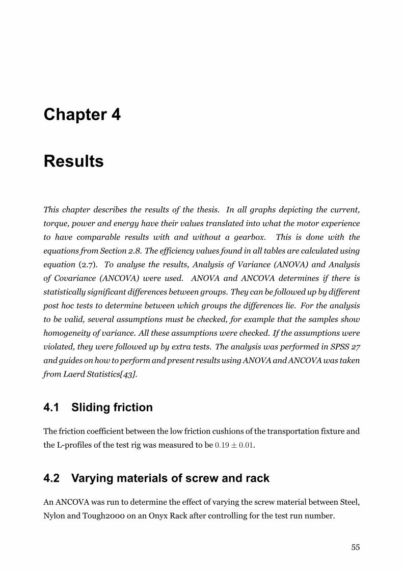
Chapter 4

Results

This chapter describes the results of the thesis. In all graphs depicting the current,

torque, power and energy have their values translated into what the motor experience

to have comparable results with and without a gearbox. This is done with the

equations from Section 2.8. The efficiency values found in all tables are calculated using

equation (2.7). To analyse the results, Analysis of Variance (ANOVA) and Analysis

of Covariance (ANCOVA) were used. ANOVA and ANCOVA determines if there is

statistically significant differences between groups. They can be followed up by different

post hoc tests to determine between which groups the differences lie. For the analysis

to be valid, several assumptions must be checked, for example that the samples show

homogeneity of variance. All these assumptions were checked. If the assumptions were

violated, they were followed up by extra tests. The analysis was performed in SPSS 27

and guides on how to performand present results usingANOVAandANCOVAwas taken

from Laerd Statistics[43].

4.1 Sliding friction

The friction coefficient between the low friction cushions of the transportation fixture and

the Lprofiles of the test rig was measured to be 0.19± 0.01.

4.2 Varying materials of screw and rack

An ANCOVA was run to determine the effect of varying the screw material between Steel,

Nylon and Tough2000 on an Onyx Rack after controlling for the test run number.

55

CHAPTER 4. RESULTS

There was a linear relationship between the test run and RMS torque for each screw

material, as assessed by visual inspection of a scatterplot. There was homogeneity of

regression slopes as the interaction term was not statistically significant, F(2,144) =

1.637, p = .198. Standardized residuals for the screw materials and for the overall

model were normally distributed, as assessed by ShapiroWilk’s test (p > .05). There

was homoscedasticity and homogeneity of variances, as assessed by visual inspection

of a scatterplot and Levene’s test of homogeneity of variance (p = .329), respectively.

There were no outliers in the data, as assessed by no cases with standardized residuals

greater than ±3 standard deviations. After adjustment for test run number, there was a

statistically significant difference in RMS torque between the screwmaterials, F(2, 146) =

320.934, p < .0005, partial η2 = .815.

Post hoc analysis was performed with a Bonferroni adjustment. RMS torque was

statistically significantly lower when using a steel screw compared to when using a Nylon

or a Though2000 screw (mean difference of 0.022 [95% CI, 0.024 to 0.020] Nm, p

< .0005) but there were no statistically significant difference between the Nylon and the

Though2000Screw. TheRMS torque for the different screwmaterials when using an onyx

rack is shown in Figure 4.2.1.

5 10 15 20 25

Test run

0.11

0.12

0.13

0.14

0.15

0.16

0.17

RM

S T

orq

ue [N

m]

Torque demand with different material of screw on Onyx rack

Steel Nylon(SLS) Tough2000 Steel(2) Nylon(SLS)(2) Tough2000(2)

Figure 4.2.1: Torque demandwhen varying screwmaterial on Onyx plastic rack. The solidlines depict the first screw sample and the dotted the second sample.

56

CHAPTER 4. RESULTS

Another ANCOVA was run to determine the effect of varying the screw material between

Steel, Nylon and Tough2000 on an Iglidur Rack after controlling for the test run number.

There was a linear relationship between the test run and RMS torque for each screw

material, as assessed by visual inspection of a scatterplot. There was homogeneity of

regression slopes as the interaction term was not statistically significant, F(2,144) =

2.272, p = .107. Standardized residuals for the screw materials and for the overall

model were normally distributed, as assessed by ShapiroWilk’s test (p > .05). There

was homoscedasticity and homogeneity of variances, as assessed by visual inspection

of a scatterplot and Levene’s test of homogeneity of variance (p = .232), respectively.

There were no outliers in the data, as assessed by no cases with standardized residuals

greater than ±3 standard deviations. After adjustment for test run number, there was a

statistically significant difference in RMS torque between the screwmaterials, F(2, 146) =

774.678, p < .0005, partial η2 = .914.

Post hoc analysis was performed with a Bonferroni adjustment. RMS torque was

statistically significantly lower when using a Nylon screw compared to when using a

Though2000 screw (meandifference of 0.008 [95%CI, 0.010 to 0.007]Nm, p< .0005).

The steel screw demanded the lowest RMS torque, which was statistically significantly

lower than for the Nylon screw (mean difference of 0.016 [95% CI, 0.018 to 0.015] Nm,

p < .0005). The RMS torque for the different screw materials when using an Iglidur rack

is shown in Figure 4.2.2.

5 10 15 20 25

Test run

0.09

0.095

0.1

0.105

0.11

0.115

0.12

0.125

0.13

0.135

0.14

RM

S T

orq

ue

[N

m]

Torque demand with different material of screw on Iglidur rack

Steel Nylon(SLS) Tough2000 Steel(2) Nylon(SLS)(2) Tough2000(2)

Figure 4.2.2: Torque demand when varying screw material on Iglidur plastic rack. Thesolid lines depict the first screw sample and the dotted the second smaple.

57

CHAPTER 4. RESULTS

Estimated marginal means of the RMS Torque are presented in Table 4.2.1, descriptive

statistics of RMS current, RMS torque, RMS power, energy and efficiency are presented

in Table 4.2.2.

Table 4.2.1: Estimated marginal means for all screw and rack combinations.

Screw/RackMaterial

combination

EstimatedMarginal Mean

RMSTorque[Nm]

Steel/Iglidur 0.101± 0.01Nylon/Iglidur 0.117± 0.01

Tough2000/Iglidur 0.126± 0.01Steel/Onyx 0.120± 0.01Nylon/Onyx 0.142± 0.01

Tough2000/Onyx 0.141± 0.01

Table 4.2.2: Mean values and standard deviation for all test runs with different screw andrack material

MaterialRMS

Current[A]RMS

Torque[Nm]RMS

Power[W]Energy[J]

Efficiency[%]

Onyx rackSteel

4.8± 0.25 0.12± 0.01 50± 3.5 175± 13 17± 2.5

Nylon12(SLS)

5.3± 0.19 0.14± 0.01 55± 2.5 193± 7 16± 1.1

Tough2000(SLA)

5.3± 0.24 0.14± 0.01 54± 2.2 191± 9.7 16± 1.5

Iglidur rackSteel

4.1± 0.15 0.10± 0.01 42± 1.6 146± 5.8 20± 1.7

Nylon12(SLS)

4.5± 0.13 0.12± 0.01 51± 1.8 176± 6.3 17± 1.3

Tough2000(SLA)

4.7± 0.16 0.13± 0.01 54± 2.4 186± 8.9 16± 1.6

4.3 Varying screw lead with same material

This section presents the results of the experiment when the screw lead was varied. The

first paragraphdescribes underwhat circumstances the statistical analysiswas performed.

Then graphs of the results are shown together with text describing what was found in

the statistical analysis. Finally, the mean values along with the standard deviation are

presented in a table.

58

CHAPTER 4. RESULTS

Several oneway ANOVAs were conducted to determine if the torque, Energy, power and

current was different for screws with different leads both when using and not using a

gearbox. The leads were 8 mm (n = 10), 16 mm (n = 10), 24 mm (n = 10) and 32 mm

(n = 10). There were no outliers, as assessed by boxplot; data was normally distributed

for each lead, as assessed by ShapiroWilk test (p > .05). Levene’s test of homogeneity of

variance was violated in all cases except for when looking at the energy and power when

using a gearbox and when looking at the current when a gearbox was not used (lowest

p=0.094). When Levene’s test was not violated, Tukeys post hoc analysis was used to

analyse statistically significant differences between dependent values. When Levenes test

was violated, a Welch robust test of equality of means was performed, which passed for

all dependent variables(lowest F(3,17.923)=6,494, p=0.004). When Levene’s test was

violated, GamesHowell post hoc analysis was used to analyse statistically significant

differences between dependent values. Figure 4.3.1 shows the measured results when

not using a gearbox. The statistical analysis revealed that when a gearbox was not used,

there was a statistically significant difference in Power and Energy between all leads,

but statistically significant differences in Current and Torque could only be determined

between the 32 mm screw and the other screws, but not between the other screws.

Different screw lead on onyx rack without gearbox

2 4 6 8 10

Test run

20

25

30

RM

S C

urr

en

t [A

]

Current

2 4 6 8 10

Test run

0.7

0.8

0.9

1

1.1

RM

S T

orq

ue

[N

m]

Torque

2 4 6 8 10

Test run

20

40

60

80

100

RM

S P

ow

er

[W]

Power

2 4 6 8 10

Test run

100

200

300

400

En

erg

y [

J]

Energy

8mm 16 mm 24 mm 32 mm

Figure 4.3.1: Different screw leads on onyx rack without gearbox.

59

CHAPTER 4. RESULTS

Figure 4.3.2 shows the measured results when a gearbox was used. When a gearbox

was used, statistically significant differences could not be observed in Power and Energy

between the 24 mm and 32 mm leads, but in all other combinations. When looking at the

torque, statistically significant differences could not be observed between the 8 mm and

24mm lead, but for all other combinations. Looking at the current, statistically significant

differences could not be observed between the 8 mm and 32 mm leads, but for all other

combinations. A summary of all data is presented as mean ± standard deviation in Table

4.3.1.

Different screw lead on onyx rack with gearbox

2 4 6 8 10

Test run

5

5.5

6

6.5

RM

S C

urr

en

t [A

]

Current

2 4 6 8 10

Test run

0.1

0.15

0.2

RM

S T

orq

ue

[N

m]

Torque

2 4 6 8 10

Test run

40

60

80

100

RM

S P

ow

er

[W]

Power

2 4 6 8 10

Test run

100

200

300

400

En

erg

y [

J]

Energy

8mm 16 mm 24 mm 32 mm

Figure 4.3.2: Different screw lead on onyx rack with gearbox.

Table 4.3.1: Mean values and standard deviation for all test runs

Lead[mm]

RMSCurrent[A]

RMSTorque[Nm]

RMSPower[W]

Energy[J] Efficiency[%]

With gearbox8 5.86± 0.15 0.13± 0.075 106.67± 1.82 381.53± 6.8816 5.35± 0.023 0.12± 0.075 48.01± 2.27 170.19± 8.3924 4.91± 0.065 0.13± 0.075 35.57± 1.74 125.40± 5.9632 6.16± 0.28 0.18± 0.075 37.19± 2.39 132.65± 8.59

Without gearbox8 21.23± 1.86 0.83± 0.075 99.45± 8.41 348.45± 29.77 8.69± 1.6316 22.10± 1.097 0.85± 0.075 51.65± 2.69 176.46± 9.61 17.14± 2.0224 21.49± 1.55 0.84± 0.075 34.55± 1.91 115.06± 7.17 26.30± 3.3432 24.58± 2.11 0.95± 0.075 28.96± 1.66 97.76± 7.16 30.97± 4.45

60

CHAPTER 4. RESULTS

4.4 Fastest possible move time with a given load

The following text presents the results of trying to achieve the fastest possible move time

with a given screw lead and without a gearbox.It can be observed in Figure 4.4.1a, that the

24 and 32mm screws produced worse results than the 8 and 16mm screws. It can be seen

that the 16 mm provided the fastest move time. This goes against the expected outcome

that higher leads should provide shorter move time. However, this becomes clear when

looking at the current consumption in Figure 4.4.1b. It shows that the current hit the

limiter of 50 A for the 16, 24 and 32 mm screws while the 8 mm did not. Even though the

16 mm hit the limit, it was only for a short time and the controller could keep up with the

trajectory. This is not the case for the 24 and 32mm screws where the controller struggled

to maintain the trajectory since the current demand was larger than what the driver could

supply due to the current limit. Summary of the results are seen in Table 4.4.1.

0 0.5 1 1.5 20

20

40

60

Positio

n [T

urn

s]

Position

8mm

16mm

24mm

32mm

0 0.5 1 1.5 2Time [s]

0

2000

4000

Velo

city [rp

m]

Velocity

8mm

16mm

24mm

32mm

(a) Position and velocity without gearbox

0 0.5 1 1.5 20

20

40

60

Curr

ent [A

]

Current

8mm 16mm 24mm 32mm

0 0.5 1 1.5 2Time [s]

0

1

2

Torq

ue [N

m]

Torque

(b) Current and torque without gearbox

Figure 4.4.1: Results without a gearbox

0 0.2 0.4 0.6 0.8 1 1.2 1.4 1.6 1.8 20

200

400

500

Po

we

r [W

]

Power

8mm

16mm

24mm

32mm

0 0.2 0.4 0.6 0.8 1 1.2 1.4 1.6 1.8 2Time [s]

0

100

200

300

En

erg

y [

J]

Energy cumulative

8mm

16mm

24mm

32mm

Figure 4.4.2: Power and accumulated energy without a gearbox

61

CHAPTER 4. RESULTS

When the same test was performed with a gearbox added, it can be seen in Figure 4.4.3a,

that the move time becomes lower with increased lead, which was the expected outcome.

This is now possible due to the lower current and torque demand, which can be seen in

Figure 4.4.3b. Summary of the results are seen in Table 4.4.1.

0 1 2 3 40

200

400

Positio

n [T

urn

s]

Position

8mm

16mm

24mm

32mm

0 1 2 3 4Time [s]

0

5000

10000

Velo

city [rp

m]

Velocity

8mm

16mm

24mm

32mm

(a) Position and velocity with gearbox

0 1 2 3 40

10

20

Curr

ent [A

]

Current

8mm 16mm 24mm 32mm

0 1 2 3 4Time [s]

0

0.2

0.4

0.6

Torq

ue [N

m]

Torque

8mm 16mm 24mm 32mm

(b) Current and torque with gearbox

Figure 4.4.3: Results with a gearbox

0 0.5 1 1.5 2 2.5 3 3.5 40

200

400

Pow

er

[W]

Power

8mm 16mm 24mm 32mm

0 0.5 1 1.5 2 2.5 3 3.5 4Time [s]

0

200

400

Energ

y [J]

Energy cumulative

8mm

16mm

24mm

32mm

Figure 4.4.4: Power and accumulated energy with a gearbox

62

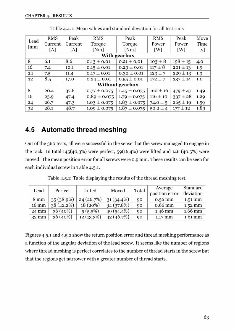
CHAPTER 4. RESULTS

Table 4.4.1: Mean values and standard deviation for all test runs

Lead[mm]

RMSCurrent[A]

PeakCurrent[A]

RMSTorque[Nm]

PeakTorque[Nm]

RMSPower[W]

PeakPower[W]

MoveTime[s]

With gearbox8 6.1 8.6 0.13± 0.01 0.21± 0.01 103± 8 198± 15 4.016 7.4 10.1 0.15± 0.01 0.29± 0.01 117± 8 201± 13 1.924 7.5 11.4 0.17± 0.01 0.30± 0.01 123± 7 229± 13 1.332 8.5 17.0 0.24± 0.01 0.55± 0.01 172± 7 337± 14 1.0

Without gearbox8 20.4 37.6 0.77± 0.075 1.45± 0.075 160± 16 479± 47 1.4916 23.9 47.4 0.89± 0.075 1.79± 0.075 116± 10 337± 28 1.2924 26.7 47.3 1.03± 0.075 1.83± 0.075 74.0± 5 265± 19 1.5932 28.1 48.7 1.09± 0.075 1.87± 0.075 50.2± 4 177± 12 1.89

4.5 Automatic thread meshing

Out of the 360 tests, all were successful in the sense that the screw managed to engage in

the rack. In total 145(40,3%) were perfect, 59(16,4%) were lifted and 146 (40.5%) were

moved. Themean position error for all screws were 0.9 mm. These results can be seen for

each individual screw in Table 4.5.1.

Table 4.5.1: Table displaying the results of the thread meshing test.

Lead Perfect Lifted Moved TotalAverage

position errorStandarddeviation

8 mm 35 (38.9%) 24 (26,7%) 31 (34,4%) 90 0.56 mm 1.51 mm16 mm 38 (42.2%) 18 (20%) 34 (37,8%) 90 0.66 mm 1.52 mm24 mm 36 (40%) 5 (5.5%) 49 (54,4%) 90 1.46 mm 1.66 mm32 mm 36 (40%) 12 (13.3%) 42 (46,7%) 90 1.17 mm 1.61 mm

Figures 4.5.1 and 4.5.2 show the return position error and threadmeshing performance as

a function of the angular deviation of the lead screw. It seems like the number of regions

where thread meshing is perfect correlates to the number of thread starts in the screw but

that the regions get narrower with a greater number of thread starts.

63

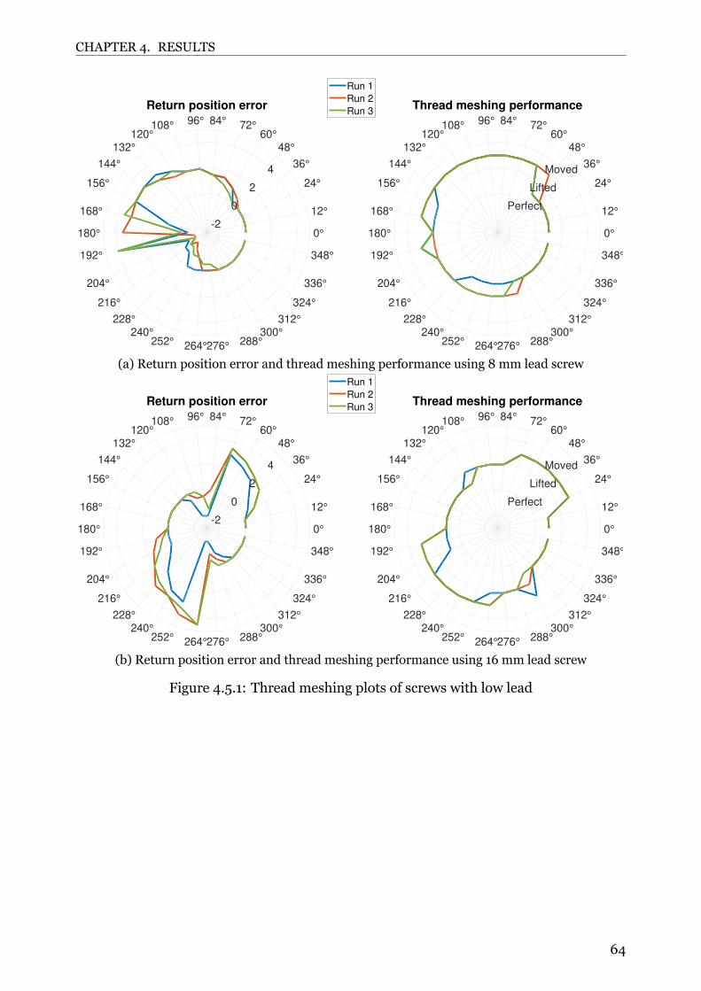
CHAPTER 4. RESULTS

Return position error

0°

12°

24°

36°

48°

60°72°

84°96°108°

120°

132°

144°

156°

168°

180°

192°

204°

216°

228°

240°252°

264°276°288°

300°

312°

324°

336°

348°

-2

0

2

4

Thread meshing performance

0°

12°

24°

36°

48°

60°72°

84°96°108°

120°

132°

144°

156°

168°

180°

192°

204°

216°

228°

240°252°

264°276°288°

300°

312°

324°

336°

348°

Perfect

Lifted

Moved

Run 1

Run 2

Run 3

(a) Return position error and thread meshing performance using 8 mm lead screw


0°

12°

24°

36°

48°

60°72°

84°96°108°

120°

132°

144°

156°

168°

180°

192°

204°

216°

228°

240°252°

264°276°288°

300°

312°

324°

336°

348°

-2

0

2

4


0°

12°

24°

36°

48°

60°72°

84°96°108°

120°

132°

144°

156°

168°

180°

192°

204°

216°

228°

240°252°

264°276°288°

300°

312°

324°

336°

348°

Perfect

Lifted

Moved

Run 1

Run 2

Run 3

(b) Return position error and thread meshing performance using 16 mm lead screw

Figure 4.5.1: Thread meshing plots of screws with low lead

64

CHAPTER 4. RESULTS


0°

12°

24°

36°

48°

60°72°

84°96°108°

120°

132°

144°

156°

168°

180°

192°

204°

216°

228°

240°252°

264°276°288°

300°

312°

324°

336°

348°

-2

0

2

4


0°

12°

24°

36°

48°

60°72°

84°96°108°

120°

132°

144°

156°

168°

180°

192°

204°

216°

228°

240°252°

264°276°288°

300°

312°

324°

336°

348°

Perfect

Lifted

Moved

Run 1

Run 2

Run 3

(a) Return position error and thread meshing performance using 24 mm lead screw


0°

12°

24°

36°

48°

60°72°

84°96°108°

120°

132°

144°

156°

168°

180°

192°

204°

216°

228°

240°252°

264°276°288°

300°

312°

324°

336°

348°

-2

0

2

4


0°

12°

24°

36°

48°

60°72°

84°96°108°

120°

132°

144°

156°

168°

180°

192°

204°

216°

228°

240°252°

264°276°288°

300°

312°

324°

336°

348°

Perfect

Lifted

Moved

Run 1

Run 2

Run 3

(b) Return position error and thread meshing performance using 32 mm lead screw

Figure 4.5.2: Thread meshing plots of screws with high lead

4.6 Accelerated lifetime test

In this section, the results of the accelerated lifetime tests are presented. First the results of

varying the lead are presented and then of varying the material. In addition to presenting

the measured data in graphs and tables, observations during the test have been noted and

are presented in text. After each test the temperature of the equipment wasmeasured and

pictures were taken off parts that showedwear. It should be noted that the thermal images

can not be relied on to be accurate, and their inclusion is only to serve as a visualization

of where heat builds up.

65

CHAPTER 4. RESULTS

4.6.1 Steel screws with different leads

Results from the accelerated lifetime test with steel screws of different leads can be seen in

Figure 4.6.1 and in Table 4.6.1. From this, one can see that the lower leads start out with

low torque and power requirements but increases with the number of runs when the heat

in the screw and rack builds up. For the 8 mm screw, smoke started to appear after 160

runs and after 163 runs it was so much that the test had to be aborted. The 16 mm screw

did last for the full 400 runs without smoke, but with highly increased torque and power

requirements.

Better results are obtained from the 24 and 32 mm screws with both having less increase

in torque and power than the others. Thermal images and picture of the rack after this

test can be seen below with all final temperatures seen in Table 4.6.4

0 100 200 300 400

Test run

4

6

8

10

12

14

RM

S C

urr

ent [A

]

Current

0 100 200 300 400

Test run

0

0.1

0.2

0.3

0.4

0.5

RM

S T

orq

ue [N

m]

Torque

0 100 200 300 400

Test run

0

50

100

150

200

250

RM

S P

ow

er

[W]

Power

0 100 200 300 400

Test run

0

200

400

600

800

1000

Energ

y [J]

Energy

8mm 16 mm 24 mm 32 mm

Accelerated life time test with different screw leads on onyx rack

Figure 4.6.1

Table 4.6.1: Final values for the accelerated lifetime test with steel screws of different lead.

Lead[mm]

RMSCurrent[A]

RMSTorque[Nm]

RMSPower[W]

Energy[J]

8 9.4 0.31± 0.01 240± 8 875± 2816 12.2 0.44± 0.01 188± 4 657± 1524 5.8 0.20± 0.01 54± 3 198± 1032 7.0 0.25± 0.01 52± 2 181± 7

66

CHAPTER 4. RESULTS

Steel 8 mm screw

Looking at Figure 4.6.2 it can be seen that the plastic melted and was pushed out. In

Figure 4.6.3 it can be seen that the screwwasmore than 150C andwith the thermal probe

this was measured to be 158C. The rack reached 130C. These high temperatures were

the reason for the melted plastic in the rack. The motor and gearbox also reached high

temperatures of 87C and 98C after only 163 runs.

Figure 4.6.2: Worn rack after 163 runs with 8 mm steel screw.

(a) Screw temperature (b) Gearbox temperature

(c) Motor temperature (d) Rack temperature

Figure 4.6.3: Thermal images when running 8 mm steel screw 163 times with 80% dutycycle.

67

CHAPTER 4. RESULTS

Steel 16 mm screw

In Figure 4.6.2 it can be seen that the plastic melted and was pushed out in the same

manner as with the 8 mm screw. The screw temperature was more than 150C, as shown

inFigure 4.6.5 andwith the thermal probe thiswasmeasured to be 157C.The rack reached

a temperature 130C. The motor and gearbox reached higher temperatures than with the

8 mm screw of 96C and 100C, but was run for 400 runs instead of 163, giving time for

temperature increase.





68

CHAPTER 4. RESULTS

Steel 24 mm screw

For the 24 mm screw, there were no melted plastic, but a slight wear on the thread flank

could be observed, as seen in Figure 4.6.6. The screw temperature ended up at 78C as

seen in Figure 4.6.7 and the rack at 69C. The motor and gearbox reached temperatures

61C and 62C respectively. All these temperatures were lower than when the 8 and 16

mm screws were used.





69

CHAPTER 4. RESULTS

Steel 32 mm screw

As with the 24 mm screw, there were no melted plastic when the 32 mm screw was used,

but a slight wear on the thread flank could be observed, as seen in Figure 4.6.8. When

this screw was used the temperature was the lowest of all tested and ended up at 66C as

seen in Figure 4.6.7 and the rack at 67C. The motor and gearbox reached temperatures

of 66C and 66C.





70

CHAPTER 4. RESULTS

Table 4.6.2: Final temperature values for test with steel screws of different lead.

Lead[mm]

ScrewTemp.[C]

RackTemp.[C]

MotorTemp.[C]

GearboxTemp.[C]

8 158 130 87 9816 157 136 96 10024 78 69 60 6232 65 61 65 66

4.6.2 Different materials

The results from the accelerated lifetime test using screws of different materials can be

seen in Figure 4.6.10 and the final values of the variables that were measured can be seen

in Table 4.6.3.

0 100 200 300 400

Test run

4

6

8

10

12

14

RM

S C

urr

ent [A

]

Current

0 100 200 300 400

Test run

0.1

0.2

0.3

0.4

0.5

RM

S T

orq

ue [N

m]

Torque

0 100 200 300 400

Test run

50

100

150

200

RM

S P

ow

er

[W]

Power

0 100 200 300 400

Test run

200

300

400

500

600

Energ

y [J]

Energy

Steel Nylon Tough 2000

Accelerated life time test with different screw materials on onyx rack

Figure 4.6.10: Final values for the accelerated lifetime test with 16 mm screws of differentmaterials.

Table 4.6.3: Final values for material lifetime test

MaterialRMS

Current[A]RMS

Torque[Nm]RMS

Power[W]Energy[J]

Nylon 4.6 0.15± 0.01 57± 4 205± 14Tough2000 9.3 0.32± 0.01 130± 4 443± 14Steel 12.2 0.44± 0.01 187± 4 657± 15

71

CHAPTER 4. RESULTS

Nylon 16 mm

The Nylon screw produced different results from the steel screws as the required torque

decreased as the test progressed. After the test was finished, significant wearwas observed

on both the screw and the rack and pulverized plastic could be observed under the screw.

This can be seen in Figure 4.6.11

(a) Worn onyx rack. (b) Worn off plastics.

Figure 4.6.11: Worn off material after the test with nylon 16 mm screw.

The thread width of the nylon screw was measured to 3.33 mm before the test and 2.13

mm after the test, as shown in Figure 4.6.12.

(a) Nylon 16 mm screw before the test. (b) Nylon 16 mm screw after the test.

Figure 4.6.12: Thread thickness before and after stress test of the 16 mm nylon screw.

72

CHAPTER 4. RESULTS

(a) Screw temperature (b) Rack temperature

Figure 4.6.13: Temperature of nylon 16 mm screw and rack after the test

Tough2000 16 mm

During the lifetime test of the Tough2000 screw, smoke was observed after just a few runs

and after 25 runs the screw seized in the thread. After the test, it could be observed that

the screw was intact but that the Onyx rack was severely damaged. This can be seen in

Figure 4.6.14.

Figure 4.6.14: Worn rack after test with tough2000 16 mm screw

During the test, the screw and rack reached temperatures of 90C and 83C

respectively.

Table 4.6.4: Final temperature values for test with different materials

MaterialScrew

Temp.[C]Rack

Temp.[C]Motor

Temp.[C]Nylon 111 130 88

Tough2000 90 69 83Steel 157 136 96

73

CHAPTER 4. RESULTS

(a) Screw temperature (b) Rack temperature

Figure 4.6.15: Temperature of tough2000 16 mm screw and rack after the test

4.7 Motor selection

To choose an appropriate motor, data about 31 brushless motors, from several different

motor series, were compiled from electrical motor manufacturer Maxon[15].

The compiled data can be seen in Appendix A.6. From this list, motors that could drive the

load of 32.38 kgwith a 32mm lead screw, a distance of 500mmin4 seconds, continuously,

were chosen. This configuration requires a motor and gearbox combination capable of

handling a peak torque of 1.79Nm, an RMS torque of 0.925 Nm, and a maximum angular

velocity of 410 rpm.

Out of thesemotors, the smallest ones in each series, in regard to the power and torque that

could drive the load, as per the criteria stated in Section 2.7, with and without a gearbox,

were selected. The motors, along with their characteristics, are presented in Table 4.7.1.

In Table 4.7.1 the diameter row lists the largest diameter out of themotor and the gearbox,

if used, and the length lists the combined length of the motor and gearbox. The prices are

listed as percentages of the cost of the motor used in the experiments.

74

CHAPTER 4. RESULTS

Table 4.7.1: Motors that can drive the load and their parameters.

Motor name ECmax 40 ECi 30 EC 45 flat ECi 52 EC 90 flatGearbox Yes Yes Yes No NoPower [W] 70 75 50 420 400

Motor Cont. Torque [mNm] 92.4 104 102 1010 1210Motor Peak Torque [mNm] 636 1910 1190 10300 14900

Motor Velocity [rpm] 9030 8210 5740 5090 1960Gear Ratio 15:1 14:1 14:1 1:1 1:1

Cont. Output Torque [mNm] 1060 1092 1071 1010 1210Max Output Torque [mNm] 7500 3400 3400 10300 14900

Output speed [rpm] 533 571 410 5090 1960Diameter [mm] 42 32 45 52 90Length [mm] 114.8 90.8 58.4 80 39.9Volume [cm^3] 159 73 93 170 254

Price [%] 140 104 72 130 61Volume+Price+3*Diameter [] 425 272 300 456 555

Looking at Table 4.7.1 one can see that to drive the load without a gearbox, a motor that

is rated for high power is needed, in comparison to when using a gearbox. However, the

price of themotor is not necessarily higher because of this. The prices are lower for the flat

motors, which are short but have a high diameter. The bottom row of Table 4.7.1 shows

a comparable figure, which is a weighted sum of the price, volume, and diameter of the

motorgearbox combination. The diameter is given a weight of three to one compared

to the price and volume to bring it up to roughly the same order of magnitude. But also

because the diameter is an important factor in the conveyor design. The diameter of the

motor directly determines the minimum height of the conveyor. This is shown in Figure

4.7.1, where two conveyors are placed side by side and seen from the front.

Figure 4.7.1: Demonstration of conveyor height dependence on screw diameter.

75

CHAPTER 4. RESULTS

The left conveyor in Figure 4.7.1 has a low diameter motor, while the one on the right

has a high diameter motor. If the motor is to not collide with either the transportation

fixture or the floor, the conveyor needs to be raised when using a larger motor. Due to

this the conveyor on the right will need longer and sturdier legs and thus will be a more

expensive and less space efficient alternative. The motor could be put on the side of the

conveyor instead and a longer belt could be used to couple the motor to the screw, which

would eliminate the need for a height increase. However, this increases the width of the

conveyor and is thus not optimal.

76

Chapter 5

Conclusions

5.1 Conclusion

The aim of this section is to evaluate and analyze the results in Section 4 in order to

answer the research questions in Section 1.4.

The first research question, was stated as

”Are 3D printed plastic screws or CNC Lathed Steel screws in combination

with 3Dprinted plastic racks a valid alternative in this application and how

do they compare to each other?”.

During the thesis it was concluded that the screw can not be made out of 3D printed

plastic, but that the racks can be plastic, because they experience a significantly lower

duty cycle.

The results of experiment 1 showed that the use of 3D printed screws required an increase

of 1050% in torque compared to using steel screws, depending on the type of screw and

rack material used. However, experiment 5 revealed that none of the 3D printed screws

that were tested were suitable for long time use. The combination of an Onyx rack with

a Tough2000 Screw generated so much heat that smoke was observed after just 20 runs.

The threads of the Nylon12 screw were worn down to less than 65% of their initial width

after having run for little over an hour at 80% duty cycle. Experiment 5 showed that the

Onyx racks of higher lead, 24 and 32 mm, held up well when used together with steel

screws.

77

CHAPTER 5. CONCLUSIONS

A lot of friction heat is generated in the thread mesh of the screw and rack. As stated in

2.3, the temperature affects the friction coefficient. This could be seen in the experiments

as the torque required to move the transportation fixture under identical circumstances

increased each run.

Because of the generated heat in the threadmesh, it was concluded in this thesis that a 3D

printed screw is not a suitable alternative in an application with similar or higher loads

than the ones used in this thesis. However, they could perhaps be used in an application

with lower loads or duty cycles, but further testing is needed to verify this. The racks,

on the other hand, experienced a substantially lower duty cycle than the screw. In our

experiments, the screw was 40 mm long and the rack was 500 mm. This resulted in

that each portion of the rack experienced at most 40/500 = 8% duty cycle. It could

also be imagined that for a material handling application in which the screw would be

in continuous use while several transportation fixtures would be in intermittent use. This

would bring down the duty cycle of the rack threads even further in comparison to the

screw. It is therefore concluded that plastic racks are a viable alternative because of the

lower duty cycle.

What lead of the screw and rack mechanism, in combination with size of

motor, provides the best tradeoff regarding system cost, size, speed and

efficiency?

It was concluded that screwswith high leadswere preferable as they have higher efficiency.

Low efficiency leads to heat buildup that damages the equipment. For geometrical and

economic reasons, a motor with a gearbox should be used in favour of a direct drive

motor.

From experiment 2, it can be seen that the efficiency varies greatly between screws with

different leads, with an efficiency of 31%±4.5 %with a lead of 32mmbut only 8.7%±1.6 %with a lead of 8 mm. These results correspond to what was expected from the theory in

Section 2.2. In experiment 5, it could be seen that the 8 mm and 16 mm lead screws

generated so much heat that the friction coefficient increased rapidly. In the test with

the 8 mm lead, it increased so quickly that the test had to be aborted as smoke started to

appear. Since the efficiency of the lead screw makes such a big difference in the system,

as can be seen in Figure 2.8.1, not only for the torque and power requirement but also the

longevity of the rack, it is advised to use a lead screw with a high lead.

From a comparison of different candidate motors with and without gearbox and of

78


different shapes in Section 4.7 it was found that a 75Wmotor with a nominal torque of 104

mNm coupled with a gearbox with a gear ratio of 14:1 was the best choice for the particular

load case used in the experiments. The size, particularly the diameter of motors that can

directly drive the load makes them a disadvantageous choice as the diameter limits the

minimum height of the conveyor.

FromEquation 2.4 it can be seen that the force required tomove the transportation fixture

increases with mass, acceleration, and velocity. The torque required from the motor

depends on the screw lead and the aforementioned force, as per 2.2. The power increases

with both angular velocity and torque, as per 2.20. Therefore, in a general case, the power

and torque requirements increase proportionally to the increase in mass and retain the

same relationship of having a high torque and a low speed requirement. When the move

time is lowered however, the torque will increase because of the acceleration and because

of the vicious part of the frictional load. However, the static friction is believed to be the

largest part of the frictional load, and this will stay constant. Therefore, the power will

increase at a faster rate than the torque when the move time is lowered. This might give

a more advantageous ratio between torque and power. However, in this case, one might

opt to go for a screw with an even higher lead as this is better for the plastic thread.

If one looks at the results from Section 4.4, it can be seen that the fastest move time

that could be achieved without a gearbox was 1.29 s with a 16 mm lead and the fastest

with a gearbox attached is 1.05 s with a 32 mm lead. Between these configurations, the

difference is about 22%, which might not be substantial. However, looking at the current,

the difference between them is larger. As could be seen, the current hit the limiter for the

16, 24 and 32mm lead without a gearbox and never when the gearbox was attached.

To conclude, the highest efficiency is obtained with high screw lead, which creates a high

demand for torque. Since the geometrical constraints of the proposed conveyor favors a

motor of a small diameter, it is recommended to use a motorgearbox combination.

Is it possible to achieve initial thread meshing with a high rate of

repeatability by using dual motors run in synchronization?

It was concluded that initial thread meshing can be achieved with a high rate of

repeatability. Experiment 4 showed that thread meshing by running two motors in

synchronization was reliable, as all 360 tests were successful.

The process proved to be robust to deviations in position. However, when there were

79


positional deviations, a perfect thread mesh was not guaranteed. Therefore, when

designing an application using this principle, it is advisable to have the ability to sense

the orientation of the screw and the position of the transportation fixture. A screw with

more thread starts provides a greater number of regions where thread meshing is perfect,

however, in each region, the tolerance for error gets smaller as the number of thread starts

increases. This implies that more accurate position control is needed to achieve perfect

thread meshing when several thread starts are used.

5.2 Discussion and Recommendation

In experiment 0, it was observed that the test run number affected the results as a

confounding variable. This can be seen in the results of the other experiments as well.

From the theory presented in Section 2.3, it can be read that temperature has an impact on

friction coefficients, especially in polymers. The increase in torque demand with test run

number can be explained by this. However, in experiment 5, the torque required to drive

the nylon screw decreased with the test run number. During this test, some material was

worn off. This suggests that wear might lower the friction coefficient. However, until this

is tested more thoroughly, the evidence for this claim is limited. Since wear is unwanted,

this might not be of interest to test more thoroughly.

In Figure 4.6.7, uneven wear can be seen. The wear seems to be concentrated at the edge

of the thread. Because this mechanism consists of an open thread as opposed to a closed

nut, which is the usual case in a lead screw and nut assembly, the side forces in the nut and

screw mesh will not cancel out. The uneven wear might be a result of the transportation

fixture skewing a small amount. As there is some lateral play between the transportation

fixture and the Lprofiles of the test rig, this is possible. This might also be the reason

wear lowers the required torque, as the screw and thread mesh might take on a more

advantageous geometry for a skewed conveyance after wear has occurred. To cancel out

lateral forces, it would be interesting to look at a solution with dual screws with opposite

hand threads spinning in opposite directions. As the screws with higher lead proved to be

so much more efficient, it would be interesting to gain empirical data of screws with even

higher leads than the ones tested in this thesis. As the temperature developed in the thread

mesh greatly affected the torque, it would be interesting to see howdifferent changes to the

thermal circumstances would affect the results. Some proposed changes are, to employ

forced air cooling of the screw; to run the screw continuously while alternating between

several transportation fixtures to see how the lower duty cycle of the rack effects results;

80


to change the materials of the screw and rack with the thermal properties in mind.

In Section 3.9.5 a alternative threadmeshing algorithmwas described. Testing this would

be of interest as it has the advantage that it does theoretically not push the transportation

fixture. The disadvantage is that it requires more complex control.

81

Appendix Contents

A 83A.1 Force gauge . . . . . . . . . . . . . . . . . . . . . . . . . . . . . . . . . . . 84A.2 Thermal camera . . . . . . . . . . . . . . . . . . . . . . . . . . . . . . . . . 85A.3 Odrive motor driver schematics . . . . . . . . . . . . . . . . . . . . . . . . . 86A.4 NCTE series 2000 torque sensor . . . . . . . . . . . . . . . . . . . . . . . . 87A.5 Gearbox . . . . . . . . . . . . . . . . . . . . . . . . . . . . . . . . . . . . . . 88A.6 Motor list . . . . . . . . . . . . . . . . . . . . . . . . . . . . . . . . . . . . . 89

References 90

82

APPENDIX A.

Appendix A

A.1 Force gauge

9

01

SAUTER

[Max]N

[d]N KERN KERN KERN

FK 10. 10 0,005 961-161O 961-261O 961-361OFK 25. 25 0,01 961-161O 961-261O 961-361OFK 50. 50 0,02 961-161O 961-261O 961-361OFK 100. 100 0,05 961-161O 961-261O 961-361OFK 250. 250 0,1 961-161O 961-261O 961-361OFK 500. 500 0,2 961-161O 961-261O 961-361OFK 1K. 1000 0,5 961-162O 961-262O 961-362O

www.sauter.eu · Order hotline +49 [0] 7433 9933 - 0 Force measurement

Digital force gauge SAUTER FK

STANDARD OPTION

Robust Push/Pull force gauge for simple measurements

Features

· Turnable display: automatic direction identification

· Secure operability due to the ergonomic design

· Peak-Hold function to capture peaks (value is “frozen” for approx. 10 seconds) or Track function mode for a continuous measure ment indication

· Selectable measuring units: N, lb, kg, oz · Auto-Power-Off · Standard attachments: as shown below, extension rod: 90 mm

· Can be mounted on all SAUTER test stands

Technical data

· Precision: 0,5 % of [Max] · Internal measuring frequency: 1000 Hz · Overload protection: 200 % of [Max] · Dimensions W×D×H 195×82×35 mm · Thread: M8 · Ready for use: Batteries included, 6×1,5 V AA · Net weight approx. 0,72 kg

Accessories

· With one of the two optional attachments for tensile strength testing, the SAUTER FK can become a tensiometer for testing the material tension characteristics of cables, threads, wires, twine etc. (up to ∅ 5 mm):

· Tensiometer attachment with Safe-insert function: Pull and release to insert the running cable in between the rolls, for tensile strength testing up to 250 N, aluminium attachment, rolls can be adjusted inwards, SAUTER FK-A01

· Tensiometer kit for high-capacity tensile strength testing up to 1000 N, steel attachment and steel rollers, rollers cannot be adjusted, SAUTER FK-A02

· Standard attachments, SAUTER AC 430

· Further accessory see www.sauter.eu and page 25 et seqq.

Model Measuring range Readout Option Factory calibration certificateTensile force Compressive force Tensile/Compressive force

SAUTER GmbH · c/o KERN & SOHN GmbH · Ziegelei 1 · 72336 Balingen · Germany · Tel. + 49-[0]7433-9933-0 · Fax + 49-[0]7433-9933-149 · www.sauter.eu

SAUT

ER C

atal

ogue

201

8 |

GB

84

APPENDIX A.

A.2 Thermal camera

Equipment described herein is subject to US export regulations and may require a license prior to export. Diversion contrary to US law is prohibited. Imagery for illustration purposes only. Specifications are subject to change without notice. ©2018 FLIR Systems, Inc. All rights reserved. 06/18

18-1165-INS_EMEA

www.flir.comNASDAQ: FLIR

Specifications are subject to change without notice. For the most up-to-date specs, go to www.flir.com

Specifications by product FLIR ONE Pro LT FLIR ONE Pro

Thermal pixel size 17 µm 12 µm

Thermal resolution 4,800 pixels (80 × 60) 19,200 pixels (160 × 120)

Thermal sensitivity 100 mK 70 mK

Object temperature range -20°C to 120°C (-4°F to 248°F)

-20°C to 400°C (-4°F to 752°F)

Common features

Certifications MFi (iOS version), RoHS, CE/FCC, CEC-BC, EN62133

Operating temperature 0°C to 35°C (32°F to 95°F), battery charging 0°C to 30°C (32°F to 86°F)

Non-operating temperature -20°C to 60°C (-4°F to 140°F)

Size (w × h × d) 68 × 34 × 14 mm (2.7 × 1.3 × 0.6 in)

Weight (incl. battery) 36.5 g

Mechanical shock Drop from 1.8 m (5.9 ft)

Optical data

Spectral range 8 – 14 µm

Visual resolution 1440 × 1080

HFOV / VFOV 50° ±1° / 43° ±1°

Frame rate 8.7 Hz

Focus Fixed 15 cm – infinity

Measurement

Accuracy ±3°C (5.4°F) or ±5%, typical percent of the difference between ambient and scene temperature. Applicable 60 sec after start-up when the unit is within 15°C to 35°C (59°F to 95°F) and the scene is within 5°C to 120°C (41°F to 248°F)

Emissivity correction Matte, Semi-Matte, Semi-Glossy, Glossy

Measurement correction Emissivity; Reflected apparent temperature (22°C / 72°F)

S P E C I F I C A T I O N S

Shutter Automatic/Manual

Power

Battery life Approximately 1 hr

Battery charge time 40 min

Interfaces

Video Male Lightning (iOS), Male USB-C (Android), Micro-USB (Android)

Charging Female USB-C (5V/1A)

App

Image presentation modes Infrared, visual, MSX, gallery

VividIR Yes

Palettes Gray (white hot), Hottest, Coldest, Iron, Rainbow, Rainbow HC, Arctic, Lava, and Wheel

Capture modes Video, photo, time-lapse

Video and still image display/capture

Saved as 1440 × 1080

File formats Radiometric JPG, MPEG-4 (file format MOV (iOS), MP4 (Android))

Spot meter On/off; Resolution 0.1°C (0.1°F)

Adjustable MSX distance 0.3 m – infinity

Visual battery indicator 0-100%

CORPORATE HEADQUARTERSFLIR Systems, Inc.27700 SW Parkway Ave.Wilsonville, OR 97070PH: +1 877.773.3547

LATIN AMERICAFLIR Systems BrasilAv. Antonio Bardella, 320Sorocaba, SP 18085-852BrasilPH: +55 15 3238 7080

CHINAFLIR Systems Co., LtdRm 1613-16, Tower IIGrand Central Plaza138 Shatin Rural Committee Rd.Shatin, New TerritoriesHong KongPH: +852 2792 8955

EUROPEFLIR Systems, Inc.Luxemburgstraat 22321 MeerBelgiumPH: +32 (0) 3665 5100

FLIR ONE Pro LT FLIR ONE Pro

85

APPENDIX A.

A.3 Odrive motor driver schematics

Figure A.3.1: Schematic over the motor driver of the Odrive board [30].

86

APPENDIX A.

A.4 NCTE series 2000 torque sensor

Series 2000 Torque Sensor www.ncte.de

Revision K Page 1 Nov 2014

2. Model Series 2000

1. Short description

Model Series 2000 Nominal-Torque Max. load Speed

[rpm]

Round shaft (Rd)

Square shaft (Sq) Unit bidirectional (+/-) bidirectional (+/-) Rd/Sq

Ø 9 mm ¼ Inch

[Nm] 2.5 5.0 5000/1000

[ft-lb] 1.8 3.7

[Nm] 5.0 10.0 5000/1000

[ft-lb] 3.7 7.4

[Nm] 7.5 15.0 5000/1000

[ft-lb] 5.5 11.1

[Nm] 17.5 35.0 5000/1000

[ft-lb] 12.9 25.8

Ø 14 mm ⅜ Inch [Nm] 75.0 150.0

5000/1000 [ft-lb] 55.3 110.6

Ø 19 mm ½ Inch

[Nm] 175.0 350.0 5000/1000

[ft-lb] 129.0 258.0

[Nm] 250.0 350.0 5000/1000

[ft-lb] 184.3 258.0

Ø 25 mm ¾ Inch [Nm] 500.0 750.0

5000/1000 [ft-lb] 368.6 552.9

The series 2000 allows an easy and cheap torque measurement for test benches and production lines. With this torque sensor the effective torque on the gauge bar can be measured bi-directionally in real time both at rest and in rotation. The sensor is delivered as a complete unit with corresponding connecting cable and key stones. The torque sensor is particularly characterized by its low price and high robustness.

Properties Maintenance-free operation

High tolerable dynamic loads

High tolerable transverse forces and bending moments

Integrated signal conditioning

Performance Bi-directional measurement range from 0 to 500 Nm

Accuracy class1) 1

Torque measurements up to 5000 rpm

Analog output signal

Modifications reserved. All details describe our products in general form only. They are not to be understood as a guarantee of quality or durability and do not constitute any liability whatsoever.

2crop

Figure A.4.1: Schematic over the motor driver of the Odrive board [30].

87

APPENDIX A.

A.5 Gearbox

HBR 22 - GPK 45

Motor series HBR 22with linear hall sensor systemwith or without parking brake

with permanent magnetic field

Motor design:

The Synchronous Servo Motors of series HBR 22 are fitted with a 3-phase concentrated stator-winding system. The 6-pole rotor-magnet system is made of plastic-bonded Neodymium Iron Boron ring magnets.

The motors have a sinusoidal Back EMF.

The position information of the rotor will be generated using the integrated linear hall sensor system with 12Bit resolution and pure digital interface (BiSS).

To avoid thermal overload a PTC resistor is embedded in the stator winding.

All geared motors are also available with integrated parking brake.

Special designs on request.

Planetary gear series GPK 45up to 20 Nm peak torque

type HBR 22 - GPK 45series -operation acc. to standards VDE 0530 S1isolation acc. to standards VDE 0530 Fprotection acc. to standards VDE 0530 IP 54kind of connection flange connectorrotating direction reversiblebearing (motor and gear box) ball bearinggear box not self-lockingparking brake B 7.01:nominal voltage V 24nominal current A 0,45static break torque Nm 1

for detailed motor data please refer to data sheet HBR 22

Gearbox design:

The planetary gear GPK 45 splits the torque to be transmitted into three symmetrical parts. In conjunction with the one-piece gear housing and with the combination of output bearing and centring flange it leads to a very compact design.

The connection to the motor shaft is done via a clamping hub and offers easy possi-bilities of interchanging.

All toothing parts are made of heat-treated high-strength steel.

The gearbox has a synthetic grease lifetime lubrication.

The planet wheels are equipped with needle bearings.

The output shaft is double-supported by roller bearing which leads to high axial and radial load capabilities.

Through the very robust construction the gearboxes series GPK 45 are well suited for industrial applications.

Type Gear RatioDimension

L1 *) **) L2 **)

HBR2230-GPK45 4 :1 - 7:1(1-stage) 170 73HBR2230-GPK45 9 :1 - 49:1(2-stage) 185 88HBR2230-GPK45 64 :1 - 196:1(3-stage) 200 103

HBR2260-GPK45 4 :1 - 7:1(1-stage) 200 73HBR2260-GPK45 9 :1 - 49:1(2-stage) 215 88HBR2260-GPK45 64 :1 - 196:1(3-stage) 230 103

*) Designs with parking brake respectively 32 mm longer.**) Shorter designs with teethed motorshaft on request.

GearedSynchronousServo Motors

preliminary edition 06.17

ENGEL Elektroantriebe GmbH · Am Klingenweg 10 · D-65396 WallufTelefon +49 6123 9942 - 0 · Telefax +49 6123 9942 - 50 · [email protected] · www.engelantriebe.de

2crop

Figure A.5.1: Gearbox datasheet [39].

88

APPENDIX A.

A.6 Motor list

MotorSeries

Power[W]

Torque[mNm]

Speed[rpm]

Diameter[mm]

Length[mm]

Volume[cm^3]

Price[%]

ECmax 40 120 211 3610 40 88 111 115ECmax 40 70 94.2 9030 40 58 73 75ECmax 30 60 63.1 9350 30 64 45 67ECmax 30 40 33.4 9250 30 42 30 52ECmax 22 25 23.2 1290 22 48.5 18 53ECi 52 420 1010 5090 52 80 170 130ECi 52 250 618 5090 52 80 170 116ECi 52 200 622 3790 52 110 234 104ECi 52 180 419 4870 52 80 170 80ECi 40 130 340 4640 40 90.8 114 75ECi 40 100 222 5000 40 56 70 68ECi 40 70 151 4930 40 36 45 64ECi 30 75 104 8210 30 64 45 60ECi 30 50 58.4 10200 30 64 45 51ECi 30 45 63.8 8520 30 42 30 51ECi 30 30 37.7 9010 30 42 30 44EC 90 flat 600 1490 1960 90 39.9 254 63EC 90 flat 400 1210 1960 90 39.9 254 61EC 90 flat 260 964 1960 90 39.9 254 58EC 90 flat 360 933 3120 90 27.4 174 52EC 90 flat 220 715 3070 90 27.4 174 50EC 90 flat 160 453 3070 90 27.4 174 48EC 45 flat 120 146 5580 45 27 43 41EC 45 flat 80 140 5580 45 27 43 38EC 45 flat 70 112 5580 45 27 43 37EC 45 flat 90 149 5740 45 22 35 37EC 45 flat 60 122 5740 45 22 35 34EC 45 flat 50 102 5740 45 22 35 33EC 60 flat 150 437 4020 60 38 107 31EC 45 flat 30 66 4750 45 16.5 26 30EC 60 flat 100 298 4020 60 38 107 28

89

Bibliography

[1] Arntz, Melanie, Gregory, Terry, and Zierahn, Ulrich. “Revisiting the risk of

automation”. In: Economics Letters 159 (2017), pp. 157–160. ISSN: 01651765.

DOI: 10.1016/j.econlet.2017.07.001. URL: http://dx.doi.org/10.1016/j.

econlet.2017.07.001.

[2] ASME. “Acme Screw Threads Asme B1.5”. In: Science 1997 (1997). ISSN: 0036

8075.

[3] Attaran, Mohsen. “The rise of 3D printing:The advantages of additive

manufacturing over traditional manufacturing Sustainability Rating Systems View

project Manufacturing Automation View project”. In: (2017). DOI: 10.1016/j.

bushor.2017.05.011. URL: http://dx.doi.org/10.1016/j.bushor.2017.05.

011.

[4] Bhandari, V. B. Design of machine elements. Vol. 256. 2. 2010, p. 199. DOI: 10.

1016/0016-0032(53)90967-3. URL: www.Civildatas.com.

[5] Broenink, J F and Orlic, B. Adequacy of the Universal Serial Bus for realtime

systems Niels Korver Individual Design Assignment. Tech. rep. 2003.

[6] Cassinari, Alberto, Bianchi, Giacomo, and Poli, Mario. “Analysis of an hydrostatic

worm rack drive for large machine tools”. In: 5th World Tribology Congress, WTC

2013. 2013. ISBN: 9781634393522.

[7] Falstad circuit simulator. URL: https://www.falstad.com/circuit/circuitjs.

html.

[8] Form 3: IndustrialQuality Desktop SLA 3D Printer | Formlabs. URL: https://

formlabs.com/3d-printers/form-3/.

[9] Friction in contact between moving bodies MATLAB MathWorks Nordic.

URL: https : / / se . mathworks . com / help / physmod / simscape / ref /

translationalfriction.html.

90

https://doi.org/10.1016/j.econlet.2017.07.001

http://dx.doi.org/10.1016/j.econlet.2017.07.001

http://dx.doi.org/10.1016/j.econlet.2017.07.001

https://doi.org/10.1016/j.bushor.2017.05.011

https://doi.org/10.1016/j.bushor.2017.05.011

http://dx.doi.org/10.1016/j.bushor.2017.05.011

http://dx.doi.org/10.1016/j.bushor.2017.05.011

https://doi.org/10.1016/0016-0032(53)90967-3

https://doi.org/10.1016/0016-0032(53)90967-3

www.Civildatas.com

https://www.falstad.com/circuit/circuitjs.html

https://www.falstad.com/circuit/circuitjs.html

https://formlabs.com/3d-printers/form-3/

https://formlabs.com/3d-printers/form-3/

https://se.mathworks.com/help/physmod/simscape/ref/translationalfriction.html

https://se.mathworks.com/help/physmod/simscape/ref/translationalfriction.html

BIBLIOGRAPHY

[10] Fuse 1: Benchtop Selective Laser Sintering (SLS) 3D Printer | Formlabs. URL:

https://formlabs.com/3d-printers/fuse-1/.

[11] Fuse 1: Benchtop Selective Laser Sintering (SLS) 3D Printer | Formlabs. URL:

https://formlabs.com/3d-printers/fuse-1/#nylon-12.

[12] Getting Started | ODrive. URL: https://docs.odriverobotics.com/.

[13] Haydon Kerk Motion Solutions. PRESSURE VELOCITY AND LEADSCREW

ASSEMBLIES. Tech. rep. URL: www.HaydonKerk.de.

[14] “HBR 22 Synchronous Servo Motors with permanent magnetic field ENGEL

Elektroantriebe GmbH · Am Klingenweg 10 · D65396 Walluf”. In: (), pp. 5–7.

[15] High Quality Precision Brushless DC Motors by maxon | maxon group. URL:

https://www.maxongroup.com/maxon/view/content/Overview- brushless-

DC-motors.

[16] How to Power and Control Brushless DC Motors | DigiKey. URL: https://www.

digikey.se/en/articles/how-to-power-and-control-brushless-dc-motors?

utm_adgroup=General&utm_source=google&utm_medium=cpc&utm_campaign=

Dynamic%20Search_EN_Product&utm_term=&productid=&gclid=Cj0KCQiAzsz-

BRCCARIsANotFgMHYZ3M3gaRqNcAYDFyEWm9Sv0ilI_b.

[17] Hutchings, I.M. Tribology: friction and wear of engineering materials. Vol. 13. 3.

1992, p. 187. ISBN: 9780081009109. DOI: 10.1016/0261-3069(92)90241-9.

[18] iglide® I180PF, filament for 3D printing. URL: https : / / www . igus . com /

product/700.

[19] Igus. drylin® Trapezoidal leadscrew nut Technical data. URL: https://www.

igus.eu/info/lead-screw-units-technical-data.

[20] Kim, Seong Han, Shin, Min Chul, Byun, Jung Won, Kwang Hwan, O., and Chu,

Chong Nam. “Efficiency prediction of worm gear with plastic worm wheel”. In:

International Journal of Precision Engineering and Manufacturing 13.2 (Feb.

2012), pp. 167–174. ISSN: 12298557. DOI: 10.1007/s12541-012-0021-7. URL:

https://link-springer-com.focus.lib.kth.se/article/10.1007/s12541-

012-0021-7.

[21] Lipsett, Robert. “The Pressure Velocity (PV) Relationship for Lead Screws”. In:

(2014), p. 6. URL: www.thomsonlinear.com.

91

https://formlabs.com/3d-printers/fuse-1/

https://formlabs.com/3d-printers/fuse-1/#nylon-12

https://docs.odriverobotics.com/

www.HaydonKerk.de

https://www.maxongroup.com/maxon/view/content/Overview-brushless-DC-motors

https://www.maxongroup.com/maxon/view/content/Overview-brushless-DC-motors

https://www.digikey.se/en/articles/how-to-power-and-control-brushless-dc-motors?utm_adgroup=General&utm_source=google&utm_medium=cpc&utm_campaign=Dynamic%20Search_EN_Product&utm_term=&productid=&gclid=Cj0KCQiAzsz-BRCCARIsANotFgMHYZ3M3gaRqNcAYDFyEWm9Sv0ilI_b





https://doi.org/10.1016/0261-3069(92)90241-9

https://www.igus.com/product/700

https://www.igus.com/product/700

https://www.igus.eu/info/lead-screw-units-technical-data

https://www.igus.eu/info/lead-screw-units-technical-data

https://doi.org/10.1007/s12541-012-0021-7

https://link-springer-com.focus.lib.kth.se/article/10.1007/s12541-012-0021-7

https://link-springer-com.focus.lib.kth.se/article/10.1007/s12541-012-0021-7

www.thomsonlinear.com

BIBLIOGRAPHY

[22] Lipsett, Robert. Why Lead Screws are the Best Fit for Many Linear Motion

Applications andHow to Rightly Apply Them. Tech. rep. 2016, p. 8. URL: https:

//www.thomsonlinear.com/downloads/articles/Why_Lead_Screws_Best_Fit_

Linear_Motion_Applications_taen.pdf.

[23] Mårdestam, P Gustavsson and Lundin, Adam. “Efficiency Analysis of a Planetary

Gearbox”. In: (2010), pp. 10–21. URL: http://www.diva- portal.org/smash/

record.jsf?pid=diva2:397023.

[24] Mark Two Carbon Fiber 3D Printer | Markforged. URL: https://markforged.

com/3d-printers/mark-two.

[25] Metal Strain Gauge an overview | ScienceDirect Topics. URL: https://www.

sciencedirect.com/topics/engineering/metal-strain-gauge.

[26] N. Aupetit. “Current sensing in BLDCmotor applicationAN5423Application note”.

In: January (2020), p. 2. URL: www.st.com.

[27] NAGAMURA, Kazuteru, IKEJO, Kiyotaka, HATA, Masato, and KIJIMA, Ryuichi.

“Efficiency and Noise of Plastic Worm Gear with Small Module Tooth”. In: The

Proceedings of Conference of ChugokuShikoku Branch (2003). DOI: 10.1299/

jsmecs.2003.41.267.

[28] Nagase, Jun Ya, Suzumori, Koichi, and Saga, Norihiko. “Development of worm

rack driven cylindrical crawler unit”. In: Journal of Advanced Mechanical Design,

Systems and Manufacturing 7.3 (2013), pp. 422–431. ISSN: 18813054. DOI: 10.

1299/jamdsm.7.422.

[29] NCTE AG. “Series 2000 Torque Sensor revision K”. In: November (2014), pp. 1–6.

URL: http://ncte.com/wp-content/uploads/2014/11/Data_Series2000_EN.

pdf.

[30] ODriveHardware/schematic_v3.5.pdf at

master · madcowswe/ODriveHardware · GitHub. URL: https://github.com/

madcowswe/ODriveHardware/blob/master/v3/v3.5docs/schematic_v3.5.pdf.

[31] Olsson, H., Åström, K. J., Canudas De Wit, C., Gäfvert, M., and Lischinsky, P.

“FrictionModels and Friction Compensation”. In:European Journal of Control 4.3

(1998), pp. 176–195. ISSN: 09473580. DOI: 10.1016/S0947-3580(98)70113-X.

[32] Onyx Composite 3D Printing Material. URL: https : / / markforged . com /

materials/plastics/onyx.

[33] “Option: Lownoise version”. In: October (2020), pp. 2020–2021.

92

https://www.thomsonlinear.com/downloads/articles/Why_Lead_Screws_Best_Fit_Linear_Motion_Applications_taen.pdf



http://www.diva-portal.org/smash/record.jsf?pid=diva2:397023

http://www.diva-portal.org/smash/record.jsf?pid=diva2:397023

https://markforged.com/3d-printers/mark-two

https://markforged.com/3d-printers/mark-two

https://www.sciencedirect.com/topics/engineering/metal-strain-gauge

https://www.sciencedirect.com/topics/engineering/metal-strain-gauge

www.st.com

https://doi.org/10.1299/jsmecs.2003.41.267

https://doi.org/10.1299/jsmecs.2003.41.267

https://doi.org/10.1299/jamdsm.7.422

https://doi.org/10.1299/jamdsm.7.422

http://ncte.com/wp-content/uploads/2014/11/Data_Series2000_EN.pdf

http://ncte.com/wp-content/uploads/2014/11/Data_Series2000_EN.pdf

https://github.com/madcowswe/ODriveHardware/blob/master/v3/v3.5docs/schematic_v3.5.pdf

https://github.com/madcowswe/ODriveHardware/blob/master/v3/v3.5docs/schematic_v3.5.pdf

https://doi.org/10.1016/S0947-3580(98)70113-X

https://markforged.com/materials/plastics/onyx

https://markforged.com/materials/plastics/onyx

BIBLIOGRAPHY

[34] Parschau, Christian and Hauge, Jostein. “Is automation stealing manufacturing

jobs? Evidence from South Africa’s apparel industry”. In: Geoforum 115 (Oct.

2020), pp. 120–131. ISSN: 00167185. DOI: 10.1016/j.geoforum.2020.07.002.

URL: https://doi.org/10.1016/j.geoforum.2020.07.002.

[35] Permanentmagnet synchronousmotor defined in terms ofmagnetic flux linkage

Simulink MathWorks Nordic. URL: https://se.mathworks.com/help/physmod/

sps/ref/femparameterizedpmsm.html.

[36] Planetary gear GPK 45 | EGBGetriebe GmbH. URL: https://www.egb-getriebe.

de/en/produkte/planetengetriebe/gpk-45/.

[37] Povilas / UI_odrivetool · GitLab. URL: https://gitlab.com/p87942130/ui_

odrivetool.

[38] Qt Group. Qt Creator A Crossplatform IDE for Application Development. URL:

https://www.qt.io/product/development-tools.

[39] Ratio, Gear. “Geared Synchronous Servo Motors with permanent magnetic field”.

In: ().

[40] Resin Family: Tough and Durable | Formlabs. URL: https://formlabs.com/

materials/tough-durable/.

[41] Roos, Fredrik, Johansson, Hans, and Wikander, Jan. “Optimal selection of motor

and gearhead in mechatronic applications”. In:Mechatronics 16.1 (2006), pp. 63–

72. ISSN: 09574158. DOI: 10.1016/j.mechatronics.2005.08.001.

[42] Sabiniak, Henryk G. “Testing worm gears with cooperating elements made of

different materials”. In: Proceedings of the Institution of Mechanical Engineers,

Part J: Journal of Engineering Tribology 231.3 (Mar. 2017), pp. 341–346. ISSN:

13506501. DOI: 10.1177/1350650116656982. URL: http://journals.sagepub.

com/doi/10.1177/1350650116656982.

[43] SPSS Statistics Tutorials and Statistical Guides | Laerd Statistics. URL: https:

//statistics.laerd.com/.

[44] Standard ISO Metric Trapezoidal Screw Thread; Profiles DIN 1031. URL:

https://www.sis.se/produkter/mekaniska-system-och-komponenter/gangor/

metriska-gangor/din10313/.

93

https://doi.org/10.1016/j.geoforum.2020.07.002

https://doi.org/10.1016/j.geoforum.2020.07.002

https://se.mathworks.com/help/physmod/sps/ref/femparameterizedpmsm.html

https://se.mathworks.com/help/physmod/sps/ref/femparameterizedpmsm.html

https://www.egb-getriebe.de/en/produkte/planetengetriebe/gpk-45/

https://www.egb-getriebe.de/en/produkte/planetengetriebe/gpk-45/

https://gitlab.com/p87942130/ui_odrivetool

https://gitlab.com/p87942130/ui_odrivetool

https://www.qt.io/product/development-tools

https://formlabs.com/materials/tough-durable/

https://formlabs.com/materials/tough-durable/

https://doi.org/10.1016/j.mechatronics.2005.08.001

https://doi.org/10.1177/1350650116656982

http://journals.sagepub.com/doi/10.1177/1350650116656982

http://journals.sagepub.com/doi/10.1177/1350650116656982

https://statistics.laerd.com/

https://statistics.laerd.com/

https://www.sis.se/produkter/mekaniska-system-och-komponenter/gangor/metriska-gangor/din10313/

https://www.sis.se/produkter/mekaniska-system-och-komponenter/gangor/metriska-gangor/din10313/

BIBLIOGRAPHY

[45] Things in Motion: Why most hobby grade BLDC out runners are actually

permanent magnet synchronous motors (PMSM). URL: https: / / things- in -

motion.blogspot.com/2018/12/why-most-hobby-grade-bldc-out-runners.

html.

[46] TI. “Current Sensing With <1µs Settling for 1, 2, and 3Shunt FOC Inverter

Reference Design”. In: March (2017), pp. 1–47.

[47] Torque Measurement | How Torque Sensor works? | How to measure torque?

URL: https://www.futek.com/torque-measurement.

[48] Ultimaker S5: Reliability at scale. URL: https://ultimaker.com/3d-printers/

ultimaker-s5.

[49] VECTO AB. URL: https://vecto.com/.

[50] Wang, Ming Shyan, Chen, Seng Chi, and Shih, Cih Huei. “Speed control of

brushless DC motor by adaptive networkbased fuzzy inference”. In:Microsystem

Technologies 24.1 (2018), pp. 33–39. ISSN: 09467076. DOI: 10.1007/s00542-

016-3148-0.

[51] Worm Rack Drive | 3D CAD Model Library | GrabCAD. URL: https://grabcad.

com/library/worm-rack-drive-1.

94

https://things-in-motion.blogspot.com/2018/12/why-most-hobby-grade-bldc-out-runners.html



https://www.futek.com/torque-measurement

https://ultimaker.com/3d-printers/ultimaker-s5

https://ultimaker.com/3d-printers/ultimaker-s5

https://vecto.com/

https://doi.org/10.1007/s00542-016-3148-0

https://doi.org/10.1007/s00542-016-3148-0

https://grabcad.com/library/worm-rack-drive-1

https://grabcad.com/library/worm-rack-drive-1

TRITA ITM-EX 2021:387

www.kth.se

Design and Evaluation of a Novel Conveyor Utilizing a Screw ...

Documents

Transcript of Design and Evaluation of a Novel Conveyor Utilizing a Screw ...