design and development of a 3d printed uav - ShareOK

DESIGN AND DEVELOPMENT OF A 3D PRINTED

UAV

By

CHRISTOPHER P. BANFIELD

Bachelor of Science in Aerospace Engineering

Oklahoma State University

Stillwater, Oklahoma

2013

Submitted to the Faculty of the

Graduate College of the

Oklahoma State University

in partial fulfillment of

the requirements for

the Degree of

MASTER OF SCIENCE

July, 2015

ii

DESIGN AND DEVELOPMENT OF A 3D PRINTED

UAV

Thesis Approved:

Dr. Jamey Jacob

Thesis Adviser

Dr. James Kidd

Dr. Joseph Conner

iii

Name: Christopher P. Banfield

Date of Degree: July, 2015

Title of Study: DESIGN AND DEVELOPMENT OF A 3D PRINTED UAV

Major Field: Mechanical & Aerospace Engineering

ABSTRACT:

The purpose of this project was to investigate the viability and practicality of using a

desktop 3D printer to fabricate small UAV airframes. To that end, ASTM based bending

and tensile tests were conducted to assess the effects of print orientation, infill density,

infill pattern, and infill orientation on the structural properties of 3D printed components.

A Vernier Structures & Materials Tester was used to record force and displacement data

from which stress-strain diagrams, yielding strength, maximum strength, and the moduli

of elasticity were found. Results indicated that print orientation and infill density had the

greatest impact on strength. In bending, vertically printed test pieces showed the greatest

strength, with yield strengths 1.6 – 10.4% higher than conventionally extruded ABS’s

64.0MPa average flexural strength. In contrast, the horizontally printed specimens

showed yield strengths reduced anywhere from 17.0 – 34.9%. The tensile test specimens

also exhibited reduced strength relative to ABS’s average tensile yield strength of

40.7MPa. Test pieces with 20% infill density saw strength reductions anywhere from

47.8 – 55.6%, and those with 50% saw strength reductions from 33.6 – 47.8%. Only a

single test piece with 100%, 45° crisscross infill achieved tensile performance on par

with that of conventionally fabricated ABS. Its yield strength was 43MPa, a positive

strength difference of 5.5%.

As a supplement to the tensile and bending tests, a prototype printable airplane, the

Phoebe, was designed. Its development process in turn provided the opportunity to

develop techniques for printing various aircraft components such as fuselage sections,

airfoils, and live-in hinges. Initial results seem promising, with the prototype’s first

production run requiring 19 hours of print time and an additional 4 – 5 hours of assembly

time. The maiden flight test demonstrated that the design was stable and controllable in

sustained flight.

iv

TABLE OF CONTENTS

Chapter Page

1. INTRODUCTION ...................................................................................................12

1.1 Motivation ........................................................................................................12

1.2 3D Printing .......................................................................................................13

1.2.1 Fused Deposition Modeling .....................................................................13

1.2.2 Selective Laser Sintering .........................................................................14

1.2.3 Stereolithography .....................................................................................15

1.3 Goals & Objectives ..........................................................................................15

2. REVIEW OF LITERATURE ..................................................................................17

2.1 Structural Print Effects .....................................................................................17

2.1.1 Bending Effects ........................................................................................17

2.1.2 Tensile Effects .........................................................................................19

2.2 3D Printed UAVs .............................................................................................22

2.2.1 Univ. of Southampton ..............................................................................22

2.2.2 Univ. of Virginia ......................................................................................23

2.2.3 Univ. of Sheffield.....................................................................................24

2.3 3D Printing in Industry ....................................................................................26

3. METHODOLOGY ..................................................................................................29

3.1 Experimental Approach ...................................................................................29

3.2 3D Printing .......................................................................................................29

3.2.1 Hardware ..................................................................................................29

3.2.2 Software ...................................................................................................31

3.2.3 Printing Process .......................................................................................33

3.2.4 Design Drivers .........................................................................................34

3.3 Structural Tests ................................................................................................37

3.3.1 Bending Tests............................................................................................37

3.3.2 Tensile Tests .............................................................................................43

v

Chapter Page

3.4 Airframe Design...............................................................................................47

3.4.1 Fuselage Design ........................................................................................47

3.4.2 Wing Design .............................................................................................52

3.4.3 Tail Design ................................................................................................57

3.4.4 Airframe Design Summary .......................................................................60

4. FINDINGS ...............................................................................................................68

4.1 Structural Tests ................................................................................................68

4.1.1 Bending Tests............................................................................................68

4.1.2 Tensile Tests .............................................................................................83

4.2 3D Printing Assessment ...................................................................................99

4.2.1 Alternate Materials Introduction ...............................................................99

4.2.2 Strength Comparison ..............................................................................100

4.2.3 Strength-to-Weight Comparison .............................................................101

4.2.4 Deployment Considerations ....................................................................102

4.2.5 Fabrication Considerations .....................................................................104

4.3 Flight Testing .................................................................................................105

5. CONCLUSION .....................................................................................................109

5.1 In Summary ....................................................................................................109

5.2 Future Work ...................................................................................................112

5.2.1 Future Phoebe ........................................................................................112

5.2.2 Future 3D Printing .................................................................................113

5.2.3 Fabrication Considerations ....................................................................121

5.2.4 Viability vs Practicality..........................................................................122

5.3 Future Work ...................................................................................................123

5.3.1 Future Phoebe ........................................................................................123

5.3.2 Future 3D Printing .................................................................................124

REFERENCES ..........................................................................................................115

A. PROTOTYPE AERODYNAMICS ......................................................................118

A.1 Lift ..................................................................................................................118

A.2 Drag ................................................................................................................122

A.3 Stability ..........................................................................................................124

vi

Chapter Page

B. PROTOTYPE PROPULSION ..............................................................................133

B.1 Power Requirements ......................................................................................133

B.2 Component Selection .....................................................................................134

B.3 Propulsion Testing Methodology ...................................................................136

B.4 Propulsion Testing Results .............................................................................142

C. PROTOTYPE PERFORMANCE .........................................................................148

C.1 Performance Estimates Methodology ............................................................148

C.2 Performance Estimates Results ......................................................................152

vii

LIST OF TABLES

Table Page

1: Bending test specimens .........................................................................................38

2: Tensile test specimens ..........................................................................................45

3: Phoebe airframe geometry ....................................................................................60

4: Phoebe prototype abridged print log .....................................................................63

5: Printed vs off-the-shelf components .....................................................................64

6: Bending test data summary ...................................................................................79

7: Printed vs extruded ABS bending results .............................................................82

8: Tensile test data summary .....................................................................................97

9: Printed vs extruded ABS tensile results ................................................................99

10: Tail volume coefficients .....................................................................................132

11: Calibration weights and scale readings ...............................................................140

12: 10x7 propulsion test data ....................................................................................143




viii

LIST OF FIGURES

Figure Page

1: Aerovironment RQ – 11 Raven ..........................................................................12

2: Fused deposition modeling (FDM) .....................................................................14

3: Selective laser sintering (SLS) ............................................................................14

4: Stereolithography (SL) .......................................................................................15

5: Wong and Pfahnl’s sample print orientations .....................................................18

6: Yield strength and stiffness ratios for ABS ........................................................19

7: Ahn et al tensile results (0.0in air gap) ...............................................................20

8: Ahn et al tensile results (-0.003in air gap) ..........................................................21

9: Univ. of Southampton laser sintered aircraft (SULSA) ......................................23

10: Univ. of Virginia conventional 3D printed UAV ...............................................23

11: Univ. of Virginia flying wing UAV ....................................................................24

12: AMRC blended-wing-body 3D printed glider ....................................................25

13: AMRC blended-wing-body 3D printed glider ....................................................21

14: Airbus A350 XWB .............................................................................................26

15: Boeing F/A – 18 Super Hornet ...........................................................................27

16: Panavia Tornado GR4 .........................................................................................27

17: GE 3D printed jet engine ....................................................................................28

18: ISS 3D printed ratchet wrench ...........................................................................28

19: Airwolf AW3D HD printer .................................................................................30

20: SLDPRT (left) and STL (right) part representation ............................................31

21: MatterControl printer interface ...........................................................................33

22: 50°, 55°, and 60° (right to left) overhang test (good surface quality) ................35

23: 65°, 70°, and 75° (right to left) overhang test (diminishing surface quality) .....35

24: 80°, 85°, and 90° (right to left) overhang test (poor surface quality) .................36

25: Wing test piece with leading edge split ..............................................................36

26: Rectilinear (left) and honeycomb (right) infill patterns ......................................38

27: Horizontally printed bending test specimen .......................................................38

28: Vertically printed bending test specimen............................................................38

29: Vernier Structures & Materials Tester ................................................................39

30: VSMT supports and loading nose .......................................................................40

31: Characteristic stress-strain curve ........................................................................42

32: Tensile test dog bone (dimensions in mm) .........................................................44

33: Tensile test sample with grip add-ons.................................................................45

34: Tensile test sample installation ...........................................................................46

35: Early fuselage conceptual design ........................................................................48

36: Phoebe fuselage assembly ..................................................................................49

ix

Figure Page

37: Phoebe fuselage assembly (exploded view) ........................................................50

38: Phoebe fuselage assembly (internal layout).........................................................51

39: Horizontally printed wing section (leading edge and airfoil profile) ..................52

40: Horizontally printed wing section (planform) .....................................................53

41: Vertically printed wing section ............................................................................54

42: Wing standard rib.................................................................................................54

43: Wing base rib .......................................................................................................55

44: Wing cap rib.........................................................................................................55

45: Wing pylon rib .....................................................................................................55

46: Wing assembly (partially exploded) ....................................................................56

47: Vertical stabilizer with print-in hinge ..................................................................57

48: Rudder deflection .................................................................................................58

49: Horizontal stabilizer .............................................................................................59

50: Tail assembly .......................................................................................................59

51: Phoebe (left view) ................................................................................................61

52: Phoebe (top view) ................................................................................................61

53: Phoebe (3D view) ................................................................................................62

54: Phoebe prototype .................................................................................................66

55: Phoebe prototype with externally mounted cameras ...........................................67

56: Sample 1 stress-strain diagram ............................................................................69

57: Sample 1 ..............................................................................................................69


59: Sample 2 ..............................................................................................................70


61: Sample 3 ..............................................................................................................71


63: Sample 4 ..............................................................................................................72

64: Sample S1 stress-strain diagram ..........................................................................73

65: Sample S1 ............................................................................................................73


67: Sample 5 ..............................................................................................................74


69: Sample 6 ..............................................................................................................75


71: Sample 7 ..............................................................................................................76


73: Sample 8 ..............................................................................................................77


75: Sample S2 ............................................................................................................78

76: Horizontal (top) and vertical (bottom) test sample material distribution ............80


78: Sample 9 ..............................................................................................................84

x

Figure Page

80: Sample 10 stress-strain diagram ..........................................................................85

81: Sample 10 ............................................................................................................85

82: Sample 10 fracture ...............................................................................................85


84: Sample 11 ............................................................................................................86

85: Sample 11 fracture ...............................................................................................87


87: Sample 12 ............................................................................................................88

88: Sample 12 fracture ...............................................................................................88


90: Sample S3 ............................................................................................................89

91: Sample S3 fracture ...............................................................................................89


93: Sample 13 ............................................................................................................90

94: Sample 13 fracture ...............................................................................................91


96: Sample 14 ............................................................................................................92

97: Sample 14 fracture ...............................................................................................92


99: Sample 15 ............................................................................................................93

100: Sample 15 fracture ...............................................................................................93


102: Sample 16 ............................................................................................................94

103: Sample 16 fracture ...............................................................................................95


105: Sample S4 ............................................................................................................96

106: Sample S4 fracture ...............................................................................................96

107: Material tensile strength comparison .................................................................101

108: Material specific strength comparison ...............................................................102

109: Material specific volume comparison ................................................................104

110: Phoebe maiden flight (ground view) .................................................................106

111: Phoebe port wing (onboard camera) ..................................................................107

112: Phoebe tail reference state with angle measurements ........................................108

113: Phoebe tail deflected state with angle measurements ........................................108

114: Bending stress-strain data summary ..................................................................110

115: Tensile stress-strain data summary ....................................................................111

116: Stratasys 3D printed wing with circuitry ...........................................................113

117: Voxel8 printed part with circuitry .....................................................................114

118: Lift and weight forces ........................................................................................118

119: SD7037 airfoil....................................................................................................119

120: SD7037 theoretical lift and drag curves at Re = 1000,000 ................................119

121: Drag and thrust forces ........................................................................................122

122: Stability scenarios ..............................................................................................125

123: Aircraft axes and moments ................................................................................125

xi

Figure Page

124: Fuselage pitching moment factor .......................................................................128

125: Downwash estimates..........................................................................................129

126: Propeller normal force coefficient .....................................................................130

127: Propeller normal force factor .............................................................................130

128: Propulsion system flowchart ..............................................................................135

129: E-flite Park 480 brushless outrunner motor .......................................................135

130: Two-bladed propeller .........................................................................................136

131: E-flite Lite Pro Brushless ESC ..........................................................................136

132: E-flite 3S, 1800mAh battery ..............................................................................137

133: Static thrust stand with test instrumentation and propulsion system .................138

134: Thrust stand calibration setup ............................................................................139

135: Calibration weight vs scale reading ...................................................................140

136: Propeller balancer ..............................................................................................141

137: Propeller thrust vs throttle..................................................................................145

138: Propeller current vs thrust ..................................................................................146

139: Propeller power vs thrust ...................................................................................147

140: Theoretical maximum speed graphical solution ................................................150

141: Theoretical maximum climb angle graphical solution ......................................141

142: Theoretical drag polar ........................................................................................153

143: Theoretical drag vs velocity ...............................................................................154

144: Theoretical power available vs power required (steady, level flight) ................156

145: Theoretical power available vs power required .................................................157

146: Theoretical endurance vs velocity .....................................................................158

147: Theoretical range vs velocity .............................................................................159

1

CHAPTER 1

INTRODUCTION

1.1 MOTIVATION

Unmanned aerial vehicles (UAVs) are gradually changing the US military’s projection of

air power by providing new and innovative ways to conduct surveillance and tactical missions

with reduced risk to their human operators.1 For instance, the 4.2lb Aerovironment RQ – 11

Raven, pictured in Figure 1, demonstrates the value of small UAVs (SUAV) as tactical assets by

providing ground units with rucksack-portable, short-range reconnaissance capabilities. In fact,

the Raven is currently the US military’s most widely deployed UAV system with the Army’s

inventory alone projected to exceed 7,000 units by 2017.2,3 In consideration of the logistical

burdens inherent in manufacturing, shipping, deploying, and maintaining such a large number of

small UAVs, this project sought to evaluate 3D printing as an on-site alternative to the

conventional manufacturing techniques and materials.

Figure 1: Aerovironment RQ - 11 Raven (army-technology.com)

2

With the ability to replicate complex geometry in a variety of materials, 3D printers have

already been proven as a valuable tool for rapid prototyping. If techniques for rapidly printing

SUAVs and their components could be developed and adapted to portable printers, on-demand

fabrication could become an on-site solution for creating both entire vehicle structures and as-

needed replacement parts. Such a possibility merits the question “Is desktop 3D printing a viable

and practical alternative to conventional SUAV manufacturing techniques?”

1.2 3D PRINTING

The term 3D printing is an informal description of additive manufacturing processes, by

which parts are fabricated through the deposition of material. Originally developed in the 1980s,

three additive manufacturing techniques are most commonly categorized as 3D printing: fused

deposition modeling (FDM), selective laser sintering (SLS), and stereolithography (SL).

1.2.1 FUSED DEPOSITION MODELING

Fused deposition modeling, illustrated in Figure 2, is the most widely used and

recognizable 3D printing process thanks in part to its domination of the consumer market. FDM

printers construct parts by extruding thermoplastic filament through a heated, computer-

controlled nozzle. As the nozzle traces the part’s cross-section on the print bed, the melted plastic

fuses to form layers that in turn form the part. Once the part is completed, any redundant support

material is removed and the surface finished by sanding, milling, or acetone vapor bathing.4

3

Figure 2: Fused deposition modeling (FDM) (printspace3d.com)

1.2.2 SELECTIVE LASER SINTERING

Selective laser sintering is illustrated in Figure 3. SLS printers construct parts from

plastic, ceramic, metal, or glass that is powdered and spread evenly over the entire print bed. A

computer-controlled laser fuses a portion of the material to form the layers of the part. Given the

precision of the laser and the structural support of the unfused material, parts created on an SLS

printer need minimal post-print processing.5

Figure 3: Selective laser sintering (SLS) (printspace3d.com)

4

1.2.3 STEREOLITHOGRAPHY

Stereolithography is illustrated in Figure 4. Rather than use solid print materials

like their FDM and SLS counterparts, SL printers construct parts from a vat of liquid

photopolymer. A computer-controlled ultra-violet (UV) laser hardens the photopolymer

on a perforated plate within the vat to form the layers of the part. Once completed, the

part is cleaned of any support material and baked in a UV oven to complete curing.6

Figure 4: Stereolithography (SL) (printspace3d.com)

1.3 GOALS AND OBJECTIVES

The goal of this project was to assess the viability and practicality of using a desktop 3D

printer as an on-site, on-demand method of fabrication by examining the structural implications

of using a small 3D printer to develop a UAV airframe. Would 3D printing impact the yield

strength and ultimate strength of the airframe’s components? How do 3D printed materials

compare to their conventionally fabricated counterparts in terms of strength, weight, and volume?

Also, what airframe components can and cannot be easily made on a portable printer? To begin

answering these questions, the following primary objectives were defined.

Review the literature. The literature was surveyed to establish what work had been done

in determining the structural characteristics of 3D printed parts. 3D printing applications

in UAV research and aerospace industrial manufacturing were also reviewed.

5

Characterize the printer. Understanding the capabilities and limitations of the printer and

software needed to design and fabricate parts was the foundation on which the design and

printing work were done.

Conduct three-point bending tests. ASTM based three-point bending tests were

conducted to assess the effects of print orientation, infill density, and infill pattern on the

yield strength, ultimate strength, and flexural moduli of 3D printed test samples.

Conduct tensile tests. ASTM based tensile tests were conducted to assess the effects of

infill orientation, infill density, and infill pattern on the yield strength, ultimate strength,

and moduli of elasticity of 3D printed test samples.

Develop a SUAV airframe. A small UAV airframe (named for the tyrant flycatcher

Phoebe) was developed to determine which components could and could not be easily

made on a desktop 3D printer.

In support of the primary objectives, a number of secondary objectives were defined to make

the Phoebe airframe a flyable prototype. Note that since the Phoebe airframe was developed to be

foremost 3D printable, the following objectives were pursued only so far as to ensure that the

prototype was capable of stable, controllable flight.

Analyze the prototype’s lift, drag, and stability characteristics.

Analyze the prototype’s propulsion requirements.

Estimate the prototype’s theoretical flight performance.

Test the prototype’s propulsion system.

Flight test the prototype.

6

CHAPTER 2

REVIEW OF THE LITERATURE

2.1 STRUCTURAL PRINT EFFECTS

2.1.1 BENDING EFFECTS

As part of their investigation into the 3D printability of surgical instruments, Julielynn

Wong and Andreas Pfahnl tested the effects of thickness and print orientation on 3D printed

coupons’ bending stiffness and yield strength. Using a Stratasys Dimension Elite 3D FDM

printer, they printed 25 solid ABS samples based on five different rectangular profiles, which had

the following thicknesses: 0.254mm, 0.508mm, 1.588mm, 3.175mm, and 6.35mm. All 25 test

samples had the same 76.2mm length and 25.4mm width. For each type of sample, three print

orientations were used: horizontal, vertical, and upright. Figure 5 illustrates the print orientations

and shows their relative positions with respect to the testing apparatus. In addition to the 25 test

samples, geometrically identical control samples were made from solid ABS sheets and tested to

provide a benchmark against which to evaluate the printed coupons.7

7

Figure 5: Wong and Pfahnl's sample print orientations (7)

The test and control samples were evaluated with three-point bending tests. To support

the coupons, the authors made a custom test fixture with two 6.35mm rollers spaced 38.1mm

apart. In turn, each sample was placed on the fixture and bent until a decrease in carried load was

observed. The loads were applied with either a MTS 858 hydraulic load frame (1.588mm,

3.175mm, and 6.35mm samples) or an EnduraTEC ELF 3200 series electromechanical load

frame (0.254mm and 0.508mm samples) at a displacement rate of 10mm/min. Data was collected

at a rate of 30Hz and analyzed with a custom MATLAB script to find the yield strength and linear

region stiffness.7

Though the authors failed to report any exact values for the coupons’ yield strength or

stiffness, they did provide a chart, reproduced as Figure 6, illustrating the effects of thickness and

print orientation on yield strength and stiffness values. Unfortunately, the lack of corroborating

data and inconsistencies between the original figure caption and the axes’ labels make it difficult

to understand the authors’ results. However, it appears that the horizontally printed samples

exhibited both increasing strength and stiffness with increasing sample thickness. In fact, the

8

authors noted that for thicknesses beyond 5.75mm, the horizontally printed samples were within

10% of the control samples’ strength and stiffness. With respect to the vertically and upright

printed samples, all seem to exhibit some level of decreased strength and stiffness with increased

thickness, but the exact trends are impossible to determine from the data as presented.

Nonetheless, the authors’ work clearly demonstrates that print orientation and part geometry

effect structural characteristics, and that 3D printed parts can be expected to be out performed by

conventionally fabricated parts made of the same material.7

Figure 6: Yield strength (solid lines) and stiffness (dashed lines) ratios for conventionally manufactured ABS plastic

(control) coupons versus horizontally, vertically, and upright 3D printed ABS plastic (test) coupons [sic] (7)

2.1.2 TENSILE EFFECTS

In an examination of the directionally dependent structural properties of 3D printed ABS,

Ahn et al tested the effects of air gap (infill density) and raster orientation (infill direction) on

ABS’s tensile yield strength. For their tests, they created eight different 3D printed samples

(229mm x 25.4mm x 3.3mm) by using four different raster orientations and two different air gap

settings. Raster orientations were measured relative to the coupons’ longitudinal axes and had the

9

following values: 0° (axial), 45°/-45° (crisscross), 0°/90° (cross), and 90° (transverse). For each

raster orientation, samples were made with 0.0in air gaps and -0.003in air gaps. Air gap values

specified the distance between each line of plastic laid down by the printer’s nozzle. Zero inch air

gaps implied a solid part, and negative air gaps indicated a part with increased density achieved

by overlapping each line of printed plastic. All eight samples were tested against a geometrically

identical control sample made from injection molded ABS. Tensile tests were conducted in

accordance with ASTM D3039 during which load and strain data were recorded. A loading rate

of 2mm/min was used.8

The measured tensile yield strengths for the control sample and each of the four 3D

printed samples with the 0.0in air gaps are presented in Figure 7. The injection molded coupon,

which yielded at 26MPa, showed the highest strength. The strongest 3D printed sample, the 0°

(axial) raster orientation, yielded at 19MPa, or 73% of the control’s yield strength. The sample

with the 90° (transverse) raster orientation was by far the weakest, yielding at only 2.6MPa. Both

the 45°/-45° (crisscross) and 0°/90° (cross) raster orientations had comparable strengths of

approximately 12MPa.8

Figure 7: Ahn et al tensile results (0.0in air gap) (8)

10

The measured tensile yield strengths for the control sample and each of the four 3D

printed samples with the -0.003in air gaps are provided in Figure 8. From the figure, it is clear

that the control coupon, which failed at 26MPa, was still the strongest. However, each of the 3D

printed samples saw an increase in yield strength thanks to increased density. The 0° (axial) raster

orientation sample remained the strongest printed specimen, with a small increase in strength

from 19MPa to 21MPa, or 81% of the control sample’s strength. The 90° transverse sample, still

the weakest of the printed coupons, gained a significant strength increase from 2.6MPa to nearly

12MPa. Both the 45°/-45° (crisscross) and 0°/90° (cross) samples also gained strength, improving

from roughly 12MPa to 16MPa and 18MPa respectively.8

Figure 8: Ahn et al tensile results (-0.003in air gap) (8)

Like Wong and Pfahnl’s bending results, the results presented by Ahn et al indicate that

print properties can have significant effects on the strength of 3D printed parts, and that

regardless of print properties, 3D printed components can be expected to be out performed

structurally by their conventionally fabricated counterparts.

11

2.2 3D PRINTED UAVS

Within the past six years, small UAVs that are mostly or entirely 3D printed have been

developed as part of on-going research. The most notable examples come from the Universities of

Southampton and Sheffield in the UK and the University of Virginia in the US.

2.2.1 UNIV. OF SOUTHAMPTON

In 2009, the University of Southampton unveiled the world’s first 3D printed airplane.

Developed for less than £5000 ($7800), the SULSA (Southampton University laser sintered

aircraft), shown in Figure 9, had a 2m wingspan and a top speed of 100mph.9,10 Though primarily

controlled with a remote control (RC) transmitter, it also was equipped with an ARM-microchip

based autopilot for autonomous flight. Printed in 5 days by the UK 3D printing firm 3T RPD, the

SULSA demonstrated that additive manufacturing was not only viable but also advantageous for

small UAV fabrication.10

Thanks to the capabilities of the EOSINT P 730 SLS printer used, the SULSA’s

designers were able to effortlessly incorporate elliptical wings and a geodesic airframe into their

UAV.11 Originally seen in aircraft such as the Spitfire fighter and Vickers Wellington bomber,

these features are known to be aerodynamically and structurally advantageous but difficult to

produce with conventional manufacturing.10 Additionally, SULSA’s structure also included print-

in control surface hinges and snap fit connectors. Consequently, the entire airplane could be

assembled in minutes without tools.11

12

Figure 9: Univ. of Southampton laser sintered aircraft (SULSA) (southampton.ac.uk)

2.2.2 UNIV. OF VIRGINIA

Within three years of SULSA’s launch, students from the University of Virginia, in

cooperation with The MITRE Corporation, produced their own 3D printed airplane, shown in

Figure 10, for an Army feasibility study. Unlike the entirely 3D printed SULSA, this airplane

structure was based on conventional modeling techniques, with underlying 3D printed

components supporting an external skin. It had a 6.5ft wingspan, 45mph cruise speed, and was

controlled exclusively by an RC transmitter.12

Figure 10: Univ. of Virginia conventional 3D printed UAV (12)

By 2014, the University of Virginia released another, more advanced 3D printed airplane.

Like the SULSA, this plane was entirely 3D printed as a collection of snap fitted parts. Pictured

in Figure 11, the Razor had a wingspan of 4ft and a GTOW of 6lb, including 1.5lb of payload. It

13

could fly for 45min at 40mph under remote control or on autopilot. The autopilot and avionics

were run through a custom Android app on a Google Nexus 5 smartphone allowing flight

commands to be sent long distance over an available 4G LTE network. The entire airframe was

printed in 31hr with $800 of material, and the system was completed with $1700 of on-board and

ground based electronics.13

Figure 11: Univ. of Virginia flying wing UAV (wired.com)

2.2.3 UNIV. OF SHEFFIELD

Engineers from the University of Sheffield’s Advanced Manufacturing Research Centre

also unveiled their 3D printed airplane in early 2014. Optimized for FDM printing, this airplane

could be fabricated out of ABS on a Stratasys Fortus 900mc printer in less than 24hr. Like many

of the planes already developed, it utilized snap fit construction, including control surfaces. The

plane’s 1.5m, 2kg blended-wing-body configuration was chosen because its geometry could be

printed without any supplemental support material, minimizing print time. Once completed, this

prototype, shown in Figure 12, was flown exclusively as a hand-launched, RC slope glider.14

14

Figure 12: AMRC blended-wing-body 3D printed glider (amrc.co.uk)

By late 2014, the AMRC’s glider prototype had been converted into a powered aircraft

with the incorporation of twin electric ducted fans. To accommodate the additional geometric

complexity required to mount the fans, the engineers’ self-imposed prohibition against support

material was relaxed. The design also came to include carbon fiber wing skins, duck tail,

intermediate ribs, and access hatch. The center body, wind end ribs, elevons, and wing tips were

still 3D printed, as were the molds, jigs, and fixtures for fabricating the carbon fiber components.

Flight ready, this airplane (Figure 13) weighed 3.5kg and required a catapult for takeoff. Cruise

speed was approximately 20m/s.15

Figure 13: AMRC powered blended-wing-body 3D printed UAV (gizmag.com)

15

2.3 3D PRINTING IN INDUSTRY

Within the past decade, 3D printing has begun to supplant the aerospace industry’s

established and more traditional manufacturing techniques. Companies such as Airbus, Boeing,

BAE Systems, GE, and even NASA have all started utilizing 3D printers and 3D printed parts.

Airbus in particular has taken advantage of 3D printed parts in its A310 and A350

models. The A350 XWB, pictured in Figure 14, has over 1000 printed parts onboard.16 Although

the parts are currently limited to simple plastic components, Airbus has been able to reduce costs

and lead times for these printable components by as much as 70% and 100 days respectively

using FDM 3D printing in partnership with additive manufacturing company Stratasys.17

Figure 14: Airbus A350 XWB (bbc.com)

Boeing is also utilizing 3D printing to produce plastic components. Using SLS printers,

they currently produce 300 unique parts such as air ducts and hinges for 10 different aircraft

programs, including the F/A-18 Super Hornet, which is shown below in Figure 15. As of March

2015, Boeing estimates that they have delivered more than 20,000 3D printed parts for use on

their aircraft.18

16

Figure 15: Boeing F/A - 18 Super Hornet (boeing.com)

In 2013, BAE Systems in cooperation with the Royal Air Force (RAF) set the precedent

for 3D printed components on a fighter aircraft, a Panavia Tornado GR4, pictured in Figure 16.

With a 3D printer on the air force base, designers were able to locally produce needed radio

covers, power shaft covers, and small support struts. The RAF estimates that such on-site 3D

printing will save £1.2 million ($1.86 million) through 2017 in repair and maintenance costs.19

Figure 16: Panavia Tornado GR4 (dezeen.com)

General Electric has also made particularly large investments into 3D printing

technology. In the fall of 2012, they purchased two additive manufacturing companies, Morris

Technology and Rapid Quality Manufacturing, in pursuit of developing 3D printed engine

nozzles.20 These complex nozzles, traditionally manufactured as an assembly of 20 different

parts, can be fabricated on an SLS printer as a single piece, resulting in a stronger, lighter finished

product.21 To further demonstrate the capabilities of 3D printers, GE has also produced an 8in

diameter working jet engine (Figure 17) assembled entirely from 3D printed components.22 By

17

2020, GE hopes to expand their 3D printing capacity to over 100,000 components for both their

commercial and military engines.23

Figure 17: GE 3D printed jet engine (forbes.com)

Finally, in the ultimate demonstration of 3D printing’s on-site fabrication capabilities,

NASA has begun evaluating an FDM 3D printer onboard the International Space Station (ISS). In

December 2014, astronauts used the 3D printer to create the first tool manufactured in space. The

4.48in long ratcheting wrench, designed on earth and transmitted electronically to the space

station, was printed over the course of a 4hr build session and is shown in Figure 18. Though the

wrench was not intended to be used in space, it will help NASA assess the feasibility of using 3D

printers for on-demand manufacturing in microgravity, an asset which could prove invaluable for

long duration space missions or Mars expeditions.24

Figure 18: ISS 3D printed ratchet wrench (nasa.gov)

18

CHAPTER 3

METHODOLOGY

3.1 EXPERIMENTAL APPROACH

As stated earlier, the goal of this project was to assess the viability and practicality of

desktop 3D printers as an alternative to conventional manufacturing techniques for small UAVs.

The emphasis of that assessment was an examination of the structural implications of using a 3D

printer to create airframe components. That process is outlined in the following Methodology

section, which begins with an introduction to the 3D printer used. Following that introduction,

ASTM based bending and tensile tests are discussed. Their primary purpose was to identify

differences between conventionally fabricated and 3D printed material characteristics that could

be attributed to print properties such as print orientation and infill density. The Methodology

section concludes with a design summary of the developed Phoebe airframe and its subsequent

flight test, which was intended to validate the development of a proof-of-concept 3D printable

UAV.

3.2 3D PRINTING

3.2.1 HARDWARE

The Airwolf AW3D HD is a consumer-grade, FDM 3D printer currently retailing for

$2995. It weighs 17kg and has overall dimensions of 610mm x 445mm x 460mm. The printer’s

heated print bed is 300mm x 200mm, and total build volume is 300mm x 200mm x 300mm.

19

The build volume’s coordinate system is defined with the origin at the lower left corner of the

print bed and the positive X, Y, and Z axes running left to right, front to back, and bottom to top

respectively. As currently configured, the printer has a single extruder, Airwolf’s standard JR

(jam resistant) 3D printer hot end with a 0.50mm nozzle.Typical print layer thickness is 0.20mm,

and maximum print speed is 150mm/s. Printer controls are handled through a USB connected

computer or the integrated VIKI LCD interface on the printer’s lower front side.25

Print materials for the AW3D HD, which is pictured in Figure 19, come as 3mm diameter

filament on 2.2lb or 5lb spools. The most commonly used thermoplastics are ABS and PLA.

ABS, the plastic used for this project, is a synthetic polymer with good impact resistance and

toughness. It also demonstrates good chemical and heat resistance. PLA, a biodegradable

thermoplastic polyester, is not as strong or heat resistant as ABS, but provides a better surface

finish for 3D printed parts. Other printable materials include stone-textured Laybrick, food-safe

HIPS, water-soluble PVA, transparent T-Glase, and flexible TPE. Nylon and polycarbonate can

also be printed, but require an upgraded high temperature hot end.25

Figure 19: Airwolf AW3D HD printer

20

3.2.2 SOFTWARE

Three different programs were required to take a part from design to print:

SOLIDWORKS, Netfabb Basic, and MatterControl.

SOLIDWORKS was the computer-aided design (CAD) program with which parts and

assemblies were designed. For each part created, two file formats were saved: .SLDPRT and

.STL (standard tessellation language). The .SLDPRT files were the standard SOLIDWORKS files

used for design. The .STL files were binary part files used for printing. Because the .STL format

reduces a part’s attributes to coordinates for triangulated surfaces, all information about the part

other than surface geometry is lost. To accommodate this simplified part representation and

ensure accurate printing, part files had to be saved in units of millimeters before being converted

to .STL to prevent scaling issues with the printer, which by default assumes all .STL coordinate

points, regardless of intended units, are expressed in millimeters. Once the part was saved as an

.STL file, it was sent to Netfabb for pre-print processing. Figure 20 provides a comparison

between the .STL and .SLDPRT part representations.

Figure 20: SLDPRT (left) and STL (right) part representation

21

Netfabb Basic is a free .STL processing program that was used to check for and repair

any gaps or discontinuities in a part’s triangulated surface mesh. The repair functions are

automated and only require the user to initialize the process. Netfabb was also used to scale,

translate, and rotate .STL files into the desired print orientation. If a part was too large or too

complex to print as a single piece, Netfabb’s cutting function could be used to subdivide the part

into two or more smaller subcomponents. Once the part was repaired and correctly oriented, it

was exported as a new .STL file and imported into MatterControl for slicing and printing.

MatterControl combines printer settings and slice engines to provide a unified printer

control interface. Once the repaired .STL file was imported, the print parameters were set. The

most commonly manipulated settings included layers/perimeters, infill, speed, support material,

and filament options. The slice engine uses these settings and the imported .STL to plan the

individual cross-sectional layers produced by the printer. MatterControl includes three different

slice engines: Slic3r, CuraEngine, and MatterSlice. Though all three ultimately do the same thing,

they each provide the user with different available print settings, which can affect print quality.

For this project, Slic3r was used exclusively because it provided far more user control than

CuraEngine or MatterSlice. Once the part was sliced, layer profiles were automatically converted

into g-code printer commands and relayed to the printer over a USB cable to begin the print.

Figure 21 provides a typical representation of the MatterControl printer interface.

22

Figure 21: MatterControl printer interface

3.2.3 PRINTING PROCESS

Regardless of the part’s specific geometry, the AW3D HD followed the same two-step

procedure for printing each layer of the part. First, the external surfaces were printed as a hollow

outline of the part’s two-dimensional profile. Known as perimeters, these outlines would be

analogous to the walls of a house. Then, the printer would proceed to fill in material between the

perimeters as though it were coloring in the lines. This internal material, known as infill, provided

structural support for the walls and top surfaces of the part build. Though the infill may be solid,

it may also be partially hollow, having an infill density less than 100%. In these cases, the infill

would be laid down in a prescribed pattern, typically either rectilinear (straight lines crisscrossed

in subsequent layers) or honeycomb. In either case, the topmost and bottommost layers were

always printed solid to provide sealed outer surfaces.

In addition to the inner and outer material of the part, the printer has the capability of

adding supplemental external material to aid in the build process. For instance, a skirt, which is a

23

ring of extra material attached to the outside of the part’s base layer, increases the part’s footprint

and adhesion to the print bed. A raft accomplishes a similar goal by providing an expendable bed

of material on which the part can be constructed. The printer can also add optional support

material in the event that the part being constructed has any significant overhangs. During the

build, the support material acts like an external scaffold on which the part’s overhangs can be

fabricated. After the build, the extra material is removed leaving behind the otherwise unprintable

geometry and finished part.

3.2.4 DESIGN DRIVERS

Using the AW3D HD imposed three primary limitations that had to be considered during

part design: limited build volume, poor support material quality, and ABS’s tendency to warp and

split.

Limited build volume was perhaps the most obvious and most easily accommodated

limitation. The AW3D’s maximum build volume is 300mm x 200mm x 300mm. It cannot

physically print a part with any dimension exceeding this volume. The simplest approach was to

design parts smaller than the printer’s build volume. However, when this was not an option,

Netfabb’s cutting function was used to divide large, unprintable parts into smaller, printable

pieces that could be assembled after fabrication.

The AW3D HD’s poor support material quality was the most difficult and restricting

limitation to accommodate because it directly impacted the allowable geometric complexity.

Problems occurred because the single extruder necessitated that the support be printed in the same

material as the part. If the scaffolding were placed close enough to the part to support the

overhangs, it tended to fuse to the part and was difficult if not impossible to remove. If the

scaffolding was placed clear of the part’s surface to prevent fusing, it failed to provide sufficient

support for the overhangs allowing the filaments on the underside to collapse, resulting in

significantly deformed and unfused surfaces. Consequently, the safe approach for achieving good

24

quality parts with the AW3D HD was to avoid using support material entirely. A printed test

piece indicated that this would restrict overhanging geometry to 65° or less as measured from a

vertical reference (straight up and down was the 0° reference). Figures 22, 23, and 24 depict the

overhang test piece in which the printer’s performance can be seen to vary with overhang angle.

Figure 22: 50°, 55°, and 60° (right to left) overhang test (good surface quality)

Figure 23: 65°, 70°, and 75° (right to left) overhang test (diminishing surface quality)

25

Figure 24: 80°, 85°, and 90° (left to right) overhang test (poor surface quality)

Finally, for parts printed with ABS, warping and splitting became an issue for extended

build sessions, typically those longer than two hours. The result of uneven cooling, warping

primarily presented at sharp corners around the perimeter of the part, starting with the base layer

pulling away from the print bed. Given enough time, the warping would become severe enough to

cause the part’s layers to delaminate. Such a structural split is shown in Figure 25 on a small wing

test piece. The heated print bed helped mitigate warping by keeping the ABS warm, and Elmer’s

School Glue stick helped increase adhesion to the bed. If warping still proved inevitable, the

splits were patched with epoxy.

Figure 25: Wing test piece with leading edge split

26

3.3 STRUCTURAL TESTS

Bending and tensile testing were undertaken to determine if print orientation and infill

properties had any impact on the 3D printed ABS’s structural characteristics. To that end, force

and displacement measurements were made and used to calculate stress-strain relationships. Both

test methodologies were based on applicable ASTM standards, though neither test setup was

strictly ASTM compliant due to the limited capabilities of the available testing equipment.

3.3.1 BENDING TESTS

The three-point bending tests were based on ASTM D 790 – 02 Standard Test Methods

for Flexural Properties of Unreinforced and Reinforced Plastics and Electrical Insulating

Materials. A Vernier Structures & Materials Tester (VSMT) was used to test eight different 3D

printed samples in order to examine the effects of print orientation, infill pattern, and infill

density. The collected force and displacement data was then used to calculate yield forces, yield

stresses, maximum forces, maximum stresses, stress-strain curves, and the flexural modulus.

Ten distinct specimens were tested to explore the structural effects of print orientation,

infill pattern, and infill density. Per ASTM D 790 – 02, each specimen was 127mm x 12.7mm x

3.2mm.26 Five were printed horizontally, so that a 127mm x 12.7mm face started flat on the print

bed and rose 3.2mm upward. The others were printed vertically, so that a 127mm x 3.2mm face

was built 12.7mm upward. For each orientation, two samples were printed with 20% infill density

and two samples were printed with 50% infill density; one horizontal and one vertical sample

were also printed with 100% infill density (solid). For each infill density, one sample was printed

with a rectilinear infill pattern. For the 20% and 50% infill densities, one sample was also printed

with a honeycomb infill pattern. Both patterns are illustrated in Figure 26. Table 1 numbers each

sample according to its print properties and Figures 27 and 28 provide characteristic illustrations

of the horizontally and vertically printed test samples respectively. Note that the curved ends

27

were simply added for a cleaner print and did not affect the test results as they fell outside the

outermost supports.

Figure 26: Rectilinear (left) and honeycomb (right) infill patterns (manual.sli3er.org)

Horizontally Printed Vertically Printed

20%

Infill

50%

Infill

100%

Infill

20%

Infill

50%

Infill

100%

Infill

Rectilinear

Infill

1 3 S1

Rectilinear

Infill

5 7 S2

Honeycomb

Infill

2 4 NA

Honeycomb

Infill

6 8 NA

Table 1: Bending test specimens

Figure 27: Horizontally printed bending test specimen

Figure 28: Vertically printed bending test specimen

28

Each of the eight samples in turn was placed on the VSMT, which stands 50cm tall and

weighs just over 22lbs. Optimized for bending testing, it can apply a downward force of up to

1000N on a beam placed across its top support bars.27 The force is generated by the hand wheel at

the bottom of the unit and transferred to the test specimen by means of a chain link tackle.

Depending on the tackle used, the tester can impose downward displacements of up to 7cm. Since

the supporting cross bars and the U-bolt load plate did not meet the cylindrical support and

loading nose requirements outlined in the ASTM standard, small adapters were printed giving the

cross bars the required 5mm radius of curvature and the load plate a permissible 12mm radius of

curvature.26 Figure 29 shows the Vernier structures and materials tester and Figure 30 provides a

close up of the sample supports and loading nose with a test sample in place.

Figure 29: Vernier Structures & Materials Tester

29

Figure 30: VSMT supports and loading nose

The VSMT is equipped with two measurement sensors: a load cell for measuring force

and an optical encoder for measuring vertical displacement. The load cell, which comes pre-

calibrated, has an operational range is 0 – 1000N with a resolution of 1N. The encoder can

measure displacements up to 7cm (a limit imposed by the vertical screw used for translation) at a

resolution of 0.01cm.27 Both sensors feed into a Vernier LabPro data acquisition board that

connects to a computer running Logger Pro 3. Logger Pro was used to capture and save both the

force and displacement data for each of the eight tests.

30

Regardless of which specimen was being tested, the testing procedure was the same. The

cross bars at the top of the VSMT were placed 51.2mm apart for a 16:1 support span to depth

ratio as prescribed in the ASTM standard.26 Note this distance was measured from the top of the

printed support add-ons and not the inside edges or centers of the bars. With the correct spacing,

both bars were positioned with the load cell’s tackle connection centered under the span so that

the downward force would be applied symmetrically through the center of the test sample. With

the sample centered over the support span, the U-bolt with its load plate and printed loading nose

were secured over the sample as was illustrated in Figure 30. Once the tackle was in place, the

hand wheel was tightened enough to remove the excess slack but not so much as to apply any

significant force to the test sample. Next, the DAQ board and Logger Pro were initialized, and the

weight of the tackle was entered into Logger Pro so that it could correct for the fact that the test

specimen had to support the 92g tackle weight. Setup was completed by zeroing both the load cell

and the optical encoder.

With both sensors zeroed, data collection was initialized and the hand wheel slowly

turned to apply force to the test specimen. For the duration of the test, Logger Pro sampled force

in Newtons and displacement in centimeters at a rate of 16Hz. Force was applied until

displacement reached 0.685cm, which per Equation 1 would produce the 5% strain in the

sample’s lower fibers required by the ASTM standard.26 Note that by the standard’s

nomenclature, D represents linear deflection in mm; r represents strain in mm/mm; L represents

the support span in mm; and d represents the specimen’s depth or thickness in mm.

𝐷 =𝑟𝐿2

6𝑑 (1)

Once the needed deflection was achieved, collection was stopped and the data were exported as a

.CSV document for processing with Microsoft Excel.

31

The primary purpose of the data analysis was to use the force and deflection curves to

generate a stress-strain diagram for each of the eight samples. Then, from the diagram, other

metrics of interest such as the modulus of elasticity, the yield force, the yield stress, the maximum

force, and maximum stress could be calculated. To that end, Equation 2 provided the flexural

stress (σf, MPa) as a function of measured load (P, N) and sample geometry. Similarly, Equation

3 provided flexural strain (εf, mm/mm) as a function of measured vertical displacement (D, mm)

and sample geometry. Again, following the standard’s notation, b indicates the sample width in

mm; L and d continue to represent the support span and specimen depth in mm respectively.26

𝜎𝑓 =3𝑃𝐿

2𝑏𝑑2 (2)

𝜀𝑓 =6𝐷𝑑

𝐿2 (3)

Once stress and strain were calculated from the force and displacement data, stress was

plotted as a function of strain to produce stress-strain curves similar to that pictured in Figure 31.

Figure 31: Characteristic stress-strain curve (efatigue.com)

32

From each of the eight stress-strain curves, the flexural modulus was calculated as the slope of

the elastic region which was found using a linear curve fit applied only to the straight line portion

of the plot. Yield stress was found at the intersection between the stress curve and a straight line

parallel to and offset 0.2% from the straight-line segment. The ultimate strength was found at the

peak of the stress curve. Both the yield stress and maximum stress were then used to pull the

corresponding yield force and maximum force from the collected data.

3.3.2 TENSILE TESTS

A similar methodology was used to assess tensile structural characteristics. Tensile tests

were based on ASTM D 638 – 02a Standard Test Method for Tensile Properties of Plastics.28 The

VSMT was used to ten different 3D printed samples in order to examine the structural effects of

infill pattern, infill density, and infill orientation. As before, the collected force and displacement

data was used to calculate yield forces, yield stresses, maximum forces, maximum stresses,

stress-strain curves, and the moduli of elasticity.

The ten specimens tested were variations of the Type IV dog bone specified in the ASTM

standard for non-rigid plastics. Deviations from the standard were made to accommodate

mounting in the VSMT and included widened grips, a lengthened grip, and a single grip hole.

Figure 32 depicts the final dog bone design whose overall length, width, and height were

137.3mm, 25mm, and 4mm respectively. The narrow section was maintained at the specified

6mm width to ensure that plastic deformation and failure were contained to the central portion of

the sample.28

33

Figure 32: Tensile test dog bone (dimensions in mm)

Since the modified dog bone had to be printed flat on the bed, print orientation was

replaced by infill orientation, joining infill density and infill pattern as the experimental variables.

Of the ten samples, five were printed with infill oriented 45° offset from the longitudinal axis.

The other five samples were printed with their infill at 90° to the longitudinal axis. For each infill

orientation, two samples were printed with 20% density and 50% density. An additional sample

with 100% density was also printed for each infill orientation. For each density, one sample had a

rectilinear infill pattern. For the 20% and 50% densities, a honeycomb patterned sample was also

made. Table 2 categorizes and numbers each of the tensile samples according to its respective

print properties.

34

45° Infill Orientation 90° Infill Orientation

20%

Infill

50%

Infill

100%

Infill

20%

Infill

50%

Infill

100%

Infill

Rectilinear

Infill

9 11 S4

Rectilinear

Infill

13 15 S4

Honeycomb

Infill

10 12 NA

Honeycomb

Infill

14 16 NA

Table 2: Tensile test specimens

Since the Vernier Structures & Materials Tester does not have clamps for vertical

mounting, each of the samples was also augmented with grip add-ons. Epoxied directly onto the

sample, the 3D printed add-ons helped reinforce the grip material and provided the mounting

interface needed for the VSMT. The top grip add-ons, applied to the extended grip, were sized to

fit around the top, interior, and bottom surfaces of the tester’s 1in square cross bars, which when

pressed together around the part secured it in place. The bottom grip was reinforced with 1mm

thick solid pieces of ABS whose profiles matched that of the grip. These add-ons’ primary

purpose was to prevent yielding or failure at the stress concentration created by the hole added for

the chain quick link. Figure 33 depicts one of the test samples with the additional grip add-ons.

Figure 33: Tensile test sample with grip add-ons

35

The testing procedure for each of the eight completed tensile samples was the same. In

turn, each dog bone was mounted vertically in the VSMT with its top sandwiched between the

two cross bars directly above the load cell, which was connected to the bottom grip by an eye

hook and single quick link. Figure 34 illustrates the installation. Once the sample was installed,

the hand wheel was used to remove any slack from the tackle, and both the load cell and optical

encoder readings were zeroed. As with the bending tests, Logger Pro was configured to record

both force and displacement. It was also used to automatically account for the 10g weight of the

single quick link supported by the test specimen. With both sensors zeroed, data collection was

initialized, and the hand wheel was slowly turned until the dog bone fractured, at which point the

data were saved and exported for analysis.

Figure 34: Tensile test sample installation

36

As with bending, the goal of the tensile test analyses was to use the force and deflection

curves to generate stress-strain diagrams that in turn would provide the modulus of elasticity,

yield stress, yield force, maximum stress, and maximum force. Stresses were calculated by

dividing the measured force by the cross sectional area of the sample’s narrow region.34 Strains

were given by the measured deflection divided by the original distance between the grips

(57.8mm). Once the stress-strain diagrams were plotted, the modulus of elasticity was calculated

as the slope of the linear elastic region using a linear curve fit. Yield stress and its corresponding

yield force were found using the same 0.2% offset method applied to the bending test results,

while the peak stress and its force provided the maximum strength.

3.4 AIRFRAME DESIGN

The structural design of Phoebe’s airframe was primarily driven by limitations imposed

by the AW3D HD printer, namely small build volume, poor support material quality, and ABS’s

tendency to warp and split. Aerodynamic considerations, such as lift generation, drag, and

stability also factored in, as did aesthetics.

3.4.1 FUSELAGE DESIGN

The primary design driver for the fuselage was sizing. Though never intended to be large,

Phoebe needed enough capacity to house an electric motor, electronic speed controller (ESC),

battery, receiver, servos, and ideally a compact camera. Relying on off-the-shelf RC components

drove Phoebe’s initial sizing toward comparable hobbyist airplanes with wingspans and fuselage

lengths on the order of 1m. This posed a challenge: design and fabricate a fuselage whose length

is significantly longer than the printer build volume’s maximum dimension of 300mm. Though

insufficient for the entire fuselage, the build volume did provide enough space in which to create

a streamlined component housing large enough for the required propulsion and control

37

electronics. This housing, when augmented with a carbon rod boom, provided the length needed

for conventional-tail stability and was the starting point for the fuselage conceptual designs.

The earliest conceptual design was a pusher configuration with the motor mounted at the

rear of the component housing and a boom-mounted conventional tail. As envisioned, it would

have been horizontally printed in two pieces: a 280mm x 140mm primary base piece acting like a

box and a smaller secondary piece serving as the lid. The division between pieces would lie along

the vertical plane aligned with the plane’s longitudinal axis.

Inside, the housing would have been compartmentalized. The bottom of the fuselage

would have hosted the boom interface structure, servos for the rudder and elevator, the RC

receiver, and camera bay. The battery and ESC would have occupied the middle of the fuselage,

where space was most plentiful. The top of the fuselage would have housed servos for the

ailerons and provided a firewall and wing box for the externally mounted motor and high

mounted wing. Figure 35 shows an early conceptual sketch of this fuselage design.

Figure 35: Early fuselage conceptual design

38

This configuration was promising for a number of positive characteristics but ultimately

deemed unsuitable. At 280mm long, it would have been large enough to comfortably house all

the needed internal components yet small enough to be printed, and since it could have been

printed horizontally instead of vertically, fabrication time would have been minimized.

Additionally, placing the motor at the top of the housing above the boom would have protected

the user’s hands during a hand launch or the propeller from ground strikes during a belly landing.

However, printed test pieces, open topped boxes with varying bottom and wall thicknesses,

revealed the box-lid fuselage components would have acted like open sections under torsion and

twisted significantly under load. Also, creating enough internal capacity and accommodating the

rear-mounted propeller would have resulting in a blunt, separation prone rear surface. Finally,

using the boom as a shield would have severely restricted the propeller diameter to an

unreasonably narrow range. Consequently, this concept was reworked to yield the current

production fuselage.

Phoebe’s current fuselage is a tractor-configured component housing with a boom-

mounted conventional tail. Elliptical in shape, the housing has a maximum diameter of 72mm and

a length of 247mm. It is assembled from four separately printed components: a forward ellipsoid

section, an aft ellipsoid section, a bulkhead, and a servo wall. Figure 36 illustrates the assembled

fuselage, and an exploded view showcasing the individual components is provided in Figure 37.

Figure 36: Phoebe fuselage assembly

39

The 127.5mm long forward ellipsoid section, printed vertically like a vase, forms the first

half of the component housing. Externally, it has been flattened on the front to provide a firewall

for the motor and a suitable starting surface for printing. Internally, it incorporates a flat floor and

ceiling for mounting electronics. At the rear of the forward section is space to install the

bulkhead, which provides structure for the component housing’s magnetic closure. The tail boom,

which runs internally above the ceiling like a spine, provides primary structural support for the

forward section.

The aft fuselage section continues the fuselage’s elliptical profile for another 79.5mm.

Also printed vertically, the rear section is open at both ends to accommodate internal components

and permit printing without supplemental support. Externally, it integrates the wing mounting

pylon, which sets the wing’s 5° dihedral. Internally, it continues the forward section’s floor and

ceiling for electronics mounting. At the rear of the aft section is space to vertically install the

servo wall, which provides the mounting structure for the rudder and elevator servos.

The servo wall also serves an aesthetic purpose by rounding out the final 40mm of the housing’s

elliptical profile beyond the rear opening of the aft section.

Figure 37: Phoebe fuselage assembly (exploded view)

The assembled housing is used to contain the needed propulsion and control electronics.

Phoebe’s single electric motor is supported externally on the front firewall, directly behind which

40

the ESC is mounted on the front section’s ceiling. The propulsion battery is fixed to the floor

somewhere between the forward and aft sections as needed to balance the center of gravity (CG).

The RC receiver is placed behind the ESC and battery in the rear section, and the servos for the

rudder and elevator are mounted on the servo wall. Unlike the early conceptual design, the

production fuselage has no camera bay and will require any cameras, if installed, to be externally

mounted. Figure 38 provides a see-through side view of the fuselage illustrating the approximate

component layout.

In conclusion, transitioning to a vertically printed, elliptical fuselage solved the torsional

deformation problems anticipated for the early fuselage concept at the cost of increased print

time. Moving the propeller from a pusher to a tractor configuration removed the restrictions on

usable diameter at the cost of increased risk for ground strikes on landing. Streamlining the

fuselage mitigated drag at the cost of any internal payload bay. The production fuselage is then, in

essence, the result of compromises that remove functional convenience but solve critical

structural, aerodynamic, and propulsive problems.

Figure 38: Phoebe fuselage assembly (internal layout)

Motor

Speed Controller

LiPo Battery

1

2

1: RC Receiver

2: Elevator & Rudder Servos

41

3.4.2 WING DESIGN

The primary design drivers for the wing were the printer’s limited build volume and

ABS’s tendency to warp and split. Anticipating a span of up to 1m, the wing had to be printed in

pieces and assembled prior to or during installation. Test parts also indicated that these pieces

would be prone to warping and splitting if build session time were more than 2hrs. Three

different concepts for printed wing components were explored: horizontally printed sections,

vertically printed sections, and vertically printed ribs.

The horizontal sections were printed so that the wing’s lower surface aligned with the

print bed. Span was oriented across the length of the bed, and airfoil curvature was built vertically

in the Y-Z plane. The horizontal sections initially seemed promising given their minimal print

time and negligible warping. However, they were significantly heavier than their vertically

printed counterparts because they required more infill to support the upper surface. Also, printing

the airfoil profile in the Y-Z plane resulted in a poor quality leading edge and an extremely rough

upper surface. Forcing the lower surface to align with the print bed also restricted feasible airfoils

to those with flat bottoms, such as the Clark Y used for the test pieces. Figure 39 shows one such

test piece and the poor leading edge quality. Figure 40 provides the top view of the same test

piece where the rough, wood-grained surface texture is clearly visible.

Figure 39: Horizontally printed wing section (leading edge and airfoil profile)

42

Figure 40: Horizontally printed wing section (planform)

The alternative was to print the wing sections in a vertical orientation, which placed the

airfoil profile in the X-Y plane parallel to the print bed and developed the span upward in the Z

direction. Most importantly, this removed the restriction to flat-bottomed airfoils and provided

significantly improved airfoil profiles and surface quality. The vertically printed sections were

also lighter because their outer mold line could be printed as a thin skin structure with strategic

supports rather than the conventional semi-solid infill. Figure 41 provides a top down view of a

vertically printed wing test piece in which the skin and support structures are clearly visible. The

distinct disadvantage to the vertical sections is that they required roughly three times as long to

print as their horizontal counterparts, and consequently exhibited detrimental warping and

splitting. Mitigating the wing section’s splitting tendencies required reducing the span to reduce

the print height, leading to the third and final concept, vertically printed ribs.

43

Figure 41: Vertically printed wing section

The vertically printed ribs are in essence extremely short vertically printed wing sections.

They utilize the same thin skin structure as the originally planned wing sections but with

significantly reduced span to reduce the print time and prevent splitting. The drawback to

shortening the sections into ribs is that the ribs have to be installed on carbon rod spars and

wrapped in a film skin (Ultracote) to function as a completed wing. Four different rib styles

compose Phoebe’s wing: a standard rib, a wing base rib, a wing cap rib, and a pylon rib.

The standard rib, which is illustrated in Figure 42, has a chord of 152mm, thickness of

15.6mm, and span of 10mm. At its thinnest, skin thickness is approximately 1mm. The rib has

three primary support substructures. Near the leading and trailing edges are the frames for the

6mm square primary spars that support the wing. Between the spar frames is a 14.5mm circular

support that prevents the upper and lower surfaces from warping inward during printing. At the

leading edge there is circular cutout for a 4mm carbon rod that helps support the Ultracote at the

front of the wing. Similarly, the trailing edge has been shortened to accommodate a 2mm carbon

rod that helps support the skin at the back of the wing.

Figure 42: Wing standard rib

X

Y

Z

44

The wing base rib, shown in Figure 43, and wing cap rib, shown in Figure 44, are

identical to the standard rib with three exceptions. Neither the wing base nor wing cap has cutouts

for the leading and trailing edge skin support spars. Instead, the entire SD7037 profile is intact.

The wing base rib also adds a small lip around its surface closest to the fuselage to help capture

the Ultracote. To the same effect, the wing cap incorporates a small end cap, which is also

intended to protect the lower film surface during landing.

Figure 43: Wing base rib

Figure 44: Wing cap rib

The pylon rib, as seen in Figure 45, also incorporates the 152mm SD7037 profile but

diverges from the thin-skinned structure of the other ribs. Instead, the pylon rib is 25mm thick

with 20% solid rectilinear infill to provide a structurally sound anchor point for the wing support

spars. It has three internal cutouts: two 6mm square holes for the carbon spars and one partial

cutout for the rear fuselage’s raised pylon.

Figure 45: Wing pylon rib

45

The wing as a whole has a 1m projected span and a 152mm chord giving it an aspect ratio

of 6.6. Assembled, the wing is composed of 8 carbon spars and 16 printed ribs. It is anchored to

the pylon by port and starboard versions of the pylon rib, which are glued in place. Into each

pylon rib, two 6mm square carbon spars are glued to form the primary support structure of the

wing. The first ribs placed on the spars are the base ribs, which attach to the pylon ribs and

provide the lip to capture the Ultracote skin. Between the base ribs and the ends of each side of

the wing are 5 standard ribs spaced 68mm apart. Each end of the wing is capped with a port or

starboard end cap rib as appropriate. The 4mm and 2mm circular carbon spars are added to

reinforce the leading and trailing edges of both sides of the wing. Finally, the wing is wrapped in

Ultracote film to complete the assembly. In an effort to keep the wing’s structure as simple as

possible, no ailerons were incorporated into the design, necessitating the 5° positive dihedral for

lateral stability. Consequently, full aircraft control is delegated to the tail. Figure 46 provides a

partially exploded view of the wing assembly.

Figure 46: Wing assembly (partially exploded)

Cap Rib

Standard Rib

Base Rib

Pylon Rib

Primary Spar

Trailing Edge Support Spar

Leading Edge Support Spar

46

3.4.3 TAIL DESIGN

For simplicity and stability’s sake, a conventional tail with a horizontal and vertical

stabilizer was used. Unlike the fuselage and wing assemblies whose designs were driven by

printer limitations, the primary design drivers for the tail were the print-in elevator and rudder

hinges, which required the lower stabilizer surfaces to be aligned with the print bed. Since this

horizontal orientation would have rendered poor quality airfoils in the Y-Z plane, a flat plate

cross section was used. Both stabilizers were also printed with an elliptical planform to match the

aesthetic of the ellipsoid fuselage.

The most critical feature of both stabilizers is the print-in hinge, which allows each

stabilizer to be printed as a single piece with its control surface in place. The hinge itself is simply

a 0.3mm thick, 2mm wide segment of plastic connecting the body of the stabilizer to the control

surface. Printed as a single layer of solid plastic whose infill is oriented parallel to the stabilizer’s

chord, the hinge is flexible enough to allow the control surface to deflect nearly 180°. Figures 47

and 48 depict the vertical stabilizer with its rudder deflected as a demonstration of the print in

hinge.

Figure 47: Vertical stabilizer with print-in hinge

47

Figure 48: Rudder deflection

The vertical stabilizer, shown above in Figure 47, is a 2mm thick elliptical flat plate with

a span of 180mm and a maximum width of 90mm. Its mean aerodynamic chord (MAC) is

81.5mm. The rudder, which occupies the back half of the vertical stabilizer, has a span of 157mm

and a maximum width of 42.2mm. It is connected to the main body of its stabilizer by a print-in

hinge along its entire length. The vertical stabilizer has a single cutout centered 9mm above its

central axis for connecting to the boom. The cutout is offset in order to center the vertical

stabilizer with respect to the horizontal stabilizer, which rests below the boom on a pylon.

The horizontal stabilizer, which is illustrated in Figure 49, is a 2mm thick elliptical flat

plate with a span of 280mm. Width at the centerline is 103mm and the MAC is 93.3mm. The

elevator, which was printed into the back half of the stabilizer, spans 249mm and has a maximum

width of 44.6mm. Like the rudder, it is connected to the body of the stabilizer by a print-in hinge

along its entire length. Centered at the leading edge of the horizontal stabilizer’s upper surface is

a 5mm high, 40mm long pylon with which to attach to the boom. It is used to set the elevator’s

-1.5° incidence and provide clearance between the boom and elevator during positive elevator

deflections. The elevator also has a center line cutout to prevent accidental contact with the boom.

45°

48

Figure 49: Horizontal stabilizer

The tail is assembled by epoxying each of the two stabilizers to the boom. The horizontal

and vertical stabilizers are mounted with their leading edges 278mm and 383mm behind the rear

fuselage section. As assembled, they do not overlap. Tail assembly is completed with the

installation of two small push rod braces along the boom between the tail stabilizers and the rear

fuselage section to prevent the rudder and elevator push rods from buckling. Note that the

elevator and rudder servos were mounted in the fuselage instead of the tail to keep the tail’s

aerodynamic profile as streamlined as possible. Figure 50 depicts the tail assembly.

Figure 50: Tail assembly

49

3.4.4 AIRFRAME DESIGN SUMMARY

All of the previously discussed structures come together to form Phoebe, a proof-of-

concept vehicle designed to explore the advantages and limitations of desktop 3D printing.

Simply described, its airframe is a tractor-configured ellipsoid with a high wing and boom-

mounted conventional tail. Table 3 summarizes its general geometric characteristics based on the

CAD drawings including gross takeoff weight, wingspan, wing aspect ratio, length, fuselage

diameter, and height. Figures 51, 52, and 53 illustrate the completed SolidWorks assembly on

which the prototype’s construction was based.

Gross Takeoff Weight (GTOW) 830g

Wingspan 1m

Wing Area 0.152m2

Wing Aspect Ratio 6.6

W/S 5.46kg/m2

Length 0.730m

Fuselage Diameter 72mm

Height 180mm

Number of Printed Components 24

Printed Mass Fraction 35%

Print Time 19hr 6min

Table 3: Phoebe airframe geometry

50

Figure 51: Phoebe (left view)

Figure 52: Phoebe (top view)

51

Figure 53: Phoebe (3D view)

3.5 PROTOTYPE PRODUCTION AND FLIGHT TESTING

In order to validate Phoebe’s conceptual design, a prototype was created with which

flight tests could be conducted.

Producing the prototype began with printing the components whose design was discussed

in Section 3.2 Structures. A total of 19 hours and 6 minutes was required to print the 24

components used to assemble Phoebe. Table 4 lists each of the components and their respective

quantities and print times. Note that the indicated print time does not include the necessary warm

up and cool down periods between each build session. Table 5 summarizes the prototype’s

printable components and off-the-shelf components needed for completion.

52

Part Name Quantity

Print Time Per Part

(hh:mm:ss)

Fuselage Front 1 03:44:15

Fuselage Back 1 02:48:03

Fuselage Bulkhead 1 00:25:28

Fuselage Servo Wall 1 00:24:45

Wing Standard Rib 10 00:21:14

Wing Base Rib (Port) 1 00:30:54

Wing Base Rib (Starboard) 1 00:30:54

Wing Cap Rib (Port) 1 00:36:05

Wing Cap Rib (Starboard) 1 00:36:05

Wing Pylon Rib (Port) 1 01:03:03

Wing Pylon Rib (Starboard) 1 01:03:03

Tail Vertical Stabilizer 1 01:08:01

Tail Horizontal Stabilizer 1 01:58:26

Tail Push Rod Brace 2 00:22:20

00:19:06

Table 4: Phoebe prototype abridged print log

53

Airframe Section Printed Off-The-Shelf

Fuselage

Forward Section Propeller

Rear Section Motor

Internal Bulkhead Electronic Speed Controller

Internal Partition (Servo Wall) Battery

---- RC Receiver

---- Servos

Wing

Ribs Carbon Spars

---- Ultracote Film

Tail

Horizontal Stabilizer w/

Elevator

Push Rods

Vertical Stabilizer w/ Rudder Control Horns

Push Rod Braces ----

Table 5: Printed vs off-the-shelf components

Once the necessary parts were printed, the fuselage, tail, and wing were assembled and

augmented with the required RC components.

Structurally, the ellipsoid shaped fuselage consisted of a front section, back section,

bulkhead, and servo wall. In addition to the printed parts, the fuselage also contained the

outrunner electric motor, brushless speed controller, 1800mAh 3S LiPo battery, Futaba RC

receiver, two Hitec servos, and two 3/8” diameter neodymium magnets. Assembly began by

bolting the motor to the exterior side of the forward fuselage section’s firewall. Next, one of the

magnets was imbedded in the bulkhead which was then epoxied into the rear of the fuselage front

section. The second magnet was imbedded in the lower side of the rear fuselage section.

Together, the magnets served as a clasp to hold the two sections together in flight. The servos

54

were mounted in the rectangular cutouts in the servo wall in such a way that the two push rods

would connect to their respective servos on opposite sides of the fuselage. Once the servos were

mounted, the servo wall was epoxied into the rear fuselage section. The remaining RC

components (ESC, battery, and receiver) were mounted inside the fuselage with Velcro. Fuselage

structural assembly was completed with the insertion of a 550mm long, 6mm square carbon rod

through the top of the rear section into the forward section. Epoxy was applied to the rod to

secure it to the rear fuselage section. The portion of the rod ahead of the rear fuselage was left

unglued to provide a rail on which the forward section could be mounted, and the portion to the

rear of the fuselage provided the boom on which the tail assembly would mount.

The tail assembly consisted of the vertical stabilizer, horizontal stabilizer, two pushrod

braces, and two t-style control horns. Tail assembly began with sliding both pushrod braces onto

the 550mm long tail boom. One brace would ultimately be glued in place directly ahead of the

horizontal stabilizer and the other would be positioned between the aft most brace and the servos.

With the pushrod braces in place, the vertical stabilizer was epoxied onto the end of the boom.

Directly ahead of the vertical stabilizer, the horizontal stabilizer was also epoxied directly to the

boom. Once both stabilizers were in place, control horns were glued to the elevator and rudder.

The tail assembly was completed by running the elevator and rudder pushrods from the servos,

through the braces, and to their respective control surfaces.

Finally, the port and starboard halves of the wing were assembled. Each wing half

consisted of one pylon rib; one base rib; five standard ribs; one cap rib; two 500mm long, 6mm

square carbon rods; one 460mm long, 4mm diameter carbon rod; and one 460mm long, 2mm

diameter carbon rod. Assembly began by stacking the ribs on the parallel 6mm carbon rods,

which acted as spars. Both spars were anchored in the pylon ribs. Directly adjacent to each pylon

rib was the base rib. Next, the five standard ribs were added at a spacing of approximately 70mm.

The ends of the spars where then covered with the wing cap ribs. Once the ribs were in place, the

4mm and 2mm carbon rods were epoxied onto the leading and trailing edges respectively to

55

reinforce rib spacing and provide additional structure for the skin. Each wing half was finished by

wrapping the lower and upper surfaces with the Ultracote film. With both wings wrapped, each

was glued together and in place on the rear fuselage section’s pylon, thereby completing the

assembly process. In total, assembly required about 4 hours bringing the total prototype

production time up to 23hrs. Figure 54 shows the completed Phoebe prototype, whose airframe

cost $11.60 in plastic ($47.03 with carbon rods, magnets, Ultracote, pushrods, and control horns).

Total cost for the flight-ready prototype (airframe and RC components) was $396.51.

Figure 54: Phoebe prototype

The purpose of the completed prototype was to provide the opportunity to conduct a

flight test, the primary objective of which was to determine if the designed structure was capable

of stable, controllable flight. Since the current design was optimized for printing instead of a

particular mission, there were no specific performance metrics to determine if the flight test was a

success or failure. Instead, the prototype was assessed qualitatively through flight observations

and pilot feedback. As configured for the test flight, ready-to-fly weight was 780g. The addition

56

of two externally mounted cameras, aimed at the tail and port wing, brought the gross takeoff

weight to a total of 830g. Figure 55 depicts the prototype’s flight configuration with on-board

cameras.

Figure 55: Phoebe prototype with externally mounted cameras

57

CHAPTER 4

FINDINGS

4.1 STRUCTURAL TESTS

4.1.1 BENDING TESTS

Three-point bending tests were conducted on ten different 3D printed specimens to

examine the impact of print orientation, infill pattern, and infill density on strength characteristics

up to strain levels of 5%. From the collected force and displacement data, stress-strain diagrams

were created and flexural moduli, yield strengths, yield forces, maximum strengths, and

maximum forces were found.

Figure 56 provides the stress-strain diagram for sample 1, the horizontally printed

specimen with 20% rectilinear infill pictured in Figure 57. With a curve fit on the linear elastic

region of the plot, the flexural modulus was calculated as 1.810GPa. Yielding appears to occur at

a stress of approximately 45MPa, which corresponded to a force of 76N. The maximum stress

and load the sample carried were 51MPa and 86N respectively. Note that the standard error,

depicted as error bars in Figure 56, was 0.698MPa.

58

Figure 56: Sample 1 stress-strain diagram

Figure 57: Sample 1

Figure 58 provides the stress-strain diagram for sample 2, the horizontally printed

specimen with 20% honeycomb infill pictured in Figure 59. From the slope of the linear elastic

region, the flexural modulus was 1.805GPa. Yielding occurred at a stress and force of 46MPa and

78N. The maximum stress encountered was 49MPa, and the corresponding maximum force was

83N. The standard error for sample 2 was 0.862MPa.

59


Figure 59: Sample 2

Figure 60 provides the stress-strain diagram for the horizontally printed sample 3, which

increased sample 1’s 20% rectilinear infill to 50% and is pictured in Figure 61. Its flexural

modulus worked out to 1.943GPa, and its yield stress and force solved to 50MPa and 85N

respectively. Maximum stress was 58MPa and the corresponding maximum force was 98N.

Standard error was 1.032MPa.

60


Figure 61: Sample 3

Figure 62 provides the stress-strain diagram for sample 4, which is pictured in Figure 63.

Its infill was a 50% honeycomb. The flexural modulus worked out to 1.946GPa. The yielding

stress was approximately 53MPa, corresponding to a force of 90N. Maximum stress topped out at

60MPa, and maximum force reached 102N. Error bars in Figure 83 depict the 1.040MPa standard

error.

61


Figure 63: Sample 4

Figure 64 provides the stress-strain diagram for sample S1, the horizontally printed

specimen with 100% rectilinear infill pictured in Figure 65. From the slope of the linear elastic

region, the flexural modulus was 1.677GPa. Yielding occurred at a stress and force of 54MPa and

91N. The maximum stress encountered was 62MPa, and the corresponding maximum force was

105N. The standard error for sample S1 was 0.954MPa.

62

Figure 64: Sample S1 stress-strain diagram

Figure 65: Sample S1

Figure 66 provides the stress-strain diagram for the first of the vertically printed samples

which is pictured in Figure 67. Its infill was 20% rectilinear. From the slope of the linear elastic

region, its flexural modulus was 2.438GPa. Yield stress and its corresponding force were 71MPa

and 120N respectively. Maximum stress and force were 80MPa and 136N. The calculated error

was 1.279MPa.

63


Figure 67: Sample 5

Figure 68 provides the stress-strain diagram for sample 6 (Figure 69), which was

vertically printed with a 20% honeycomb infill. Its flexural modulus was 2.388GPa, and yield

stress was approximately 65MPa. Force at yield was 110N. The maximum stress and its

corresponding force were 76MPa and 128N respectively. Lastly, sample 6’s error was found to be

1.167MPa.

64


Figure 69: Sample 6

Figure 70 provides the stress-strain diagram for the vertically printed sample 7 (Figure

71), whose infill was 50% rectilinear. The flexural modulus solved to 2.489GPa. Yield stress and

force at yield were 68MPa and 114N respectively. Maximum stress and the maximum force were

77MPa and 130N. Sample 7’s standard error was 1.264MPa.

65


Figure 71: Sample 7

Figure 72 provides the stress-strain diagram for sample 8, pictured in Figure 73. Printed

vertically, its infill was a 50% honeycomb. From the slope of its linear elastic region, the flexural

modulus was 2.526GPa. Its yield stress and corresponding force were 67MPa and 113N

respectively. The maximum stress sample 8 encountered was 76MPa resulting from a force of

128N. Error was found to be 1.147MPa.

66


Figure 73: Sample 8

Figure 74 provides the stress-strain diagram for sample S2 (Figure 75), which was

vertically printed with a 100% rectilinear infill. Its flexural modulus was 1.965GPa, and yield

stress was approximately 66MPa. Force at yield was 112N. The maximum stress and its

corresponding force were 74MPa and 125N respectively. Lastly, sample 6’s error was found to be

1.224MPa.

67



Table 6 provides a brief summary of the analyzed data for each of the ten samples.

Sample 8, the vertically printed 50% honeycomb, had the highest flexural modulus value at

2.526GPa. The highest values of yield strength and maximum strength, 71MPa and 80MPa

respectively, were both exhibited by sample 5 (vertically printed, 20% rectilinear infill. Sample

S1, horizontally printed with 100% rectilinear infill, had the lowest flexural modulus (1.805GPa),

and sample 1 had the lowest yield strength (45MPa). The lowest maximum strength, 49MPa, was

found with sample 2.

68

Sample #

Print

Orientation

Infill Density

and Pattern

Flexural

Modulus

[GPa]

Yield

Strength

[MPa]

Maximum

Strength

[MPa]

1 Horizontal

20%

Rectilinear

1.810 45 51

2 Horizontal

20%

Honeycomb

1.805 46 49

3 Horizontal

50%

Rectilinear

1.943 50 58

4 Horizontal

50%

Honeycomb

1.946 53 60

S1 Horizontal

100%

Rectilinear

1.677 54 62

5 Vertical

20%

Rectilinear

2.438 71 80

6 Vertical

20%

Honeycomb

2.388 65 76

7 Vertical

50%

Rectilinear

2.489 68 77

8 Vertical

50%

Honeycomb

2.526 67 76

S2 Vertical

100%

Rectilinear

1.965 66 74

Table 6: Bending test data summary

69

From Table 6, it is evident that the samples’ print orientation had the greatest impact on

structural characteristics given that the vertically printed samples consistently exhibited higher

flexural moduli, yield strengths, and maximum strengths than their horizontally printed

counterparts. This was likely due to the fact that the vertically printed coupons had approximately

25% more material than the vertically printed samples (5g vs 4g) and that their material was

distributed further from the neutral bending axis, increasing the area moment of inertia. The

sketches provided in Figure 76 illustrate the material distribution in both the horizontal and

vertical test pieces.

Figure 76: Horizontal (top) and vertical (bottom) test sample material distribution

70

Increasing infill from 20% to 50% also seemed to increase yield and maximum strength,

but only within the horizontally printed specimens. Odds are that the 1.2mm of free space in the

interior of the vertically printed samples provided too little space for the extra infill to make any

difference, especially when considered against the vertically printed samples’ already thick

perimeters. With respect to infill pattern, the eight tested samples were insufficient to establish

any distinct trends favoring either the rectilinear or honeycomb pattern.

Regardless of infill pattern, the vertically printed samples achieved structural

performance on par with and in some cases exceeding that of traditionally extruded ABS. The

horizontally printed samples were understandably weaker. Table 7 provides the percent difference

between the measured values for flexural moduli and flexural yield strengths and their

characteristic counterparts for traditionally extruded ABS, which have average values of 2.20GPa

and 64.0MPa respectively.29

71

Sample # Description

Flexural Modulus %

Difference (2.20GPa)

Yield Strength %

Difference (64.0MPa)

1

Horizontal, 20%

Rectilinear Infill

-19.44% -34.86%

2

Horizontal, 20%

Honeycomb Infill

-19.73% -32.73%

3

Horizontal, 50%

Rectilinear Infill

-12.43% -24.56%

4

Horizontal, 50%

Honeycomb Infill

-12.24% -18.80%

S1

Horizontal, 100%

Rectilinear Infill

-26.98% -16.95%

5

Vertical, 20%

Rectilinear Infill

+10.27% +10.37%

6

Vertical, 20%

Honeycomb Infill

+8.18% +1.55%

7

Vertical, 50%

Rectilinear Infill

+12.31% +6.06%

8

Vertical, 50%

Honeycomb Infill

+13.81% +4.58%

S2

Vertical, 100%

Rectilinear Infill

+11.30% +3.08%

Table 7: Printed vs extruded ABS bending results

72

4.1.2 TENSILE TESTS

Tensile tests were conducted on ten different 3D printed specimens to examine the

impact of infill orientation, infill pattern, and infill density on strength characteristics up to

fracture. From the collected force and displacement data, stress-strain diagrams were created and

the moduli of elasticity, yield strengths, yield forces, maximum strengths, and maximum forces

were found.

Figure 77 provides the stress-strain diagram for sample 9 (20% rectilinear infill, 45°).

With a curve fit on the linear elastic region of the plot, the modulus of elasticity was calculated as

0.503GPa. Yielding appears to occur at a stress of approximately 23MPa, which corresponded to

a force of 552N. The maximum stress and load the sample carried were 25MPa and 588N

respectively. Standard error for sample 9’s data was 0.412MPa. Figures 78 and 79 provide

pictures of sample 9 taken after its tensile test. Note the distinct plastic deformation patterns along

the narrow region of the specimen.


73

Figure 78: Sample 9

Figure 79: Sample 9 fracture

Figure 80 provides the stress-strain diagram for sample 10 (20% honeycomb infill, 45°).

From the slope of the linear elastic region, the modulus of elasticity was 0.559GPa. Yielding

occurred at a stress and force of 24MPa and 576N. The maximum stress encountered was 25MPa,

and the corresponding maximum force was 591N. Error was found to be 0.463MPa. Figures 81

and 82 provide the post-test pictures of sample 10 in which the plastic yielding patterns and

fracture are visible.

74


Figure 81: Sample 10


75

Figure 83 provides the stress-strain diagram for the sample 11 (50% rectilinear infill,

45°). Its modulus of elasticity worked out to 0.599GPa, and its yield stress and force solved to

29MPa and 696N respectively. Maximum stress was 30MPa, and the corresponding maximum

force was 720N. Standard error was 0.815MPa. Figures 84 and 85 depict sample 11, which shows

no obvious signs of plastic deformation prior to fracture.



76



The modulus of elasticity worked out to 0.581GPa. The yielding stress was approximately

28MPa, corresponding to a force of 672N. Maximum stress topped out at 29MPa, and maximum

force reached 686N. Error bars indicate the sample 12’s 0.631MPa standard error. Figures 87 and

88 show sample 12, its faint signs of plastic deformation, and its fracture point.


77



Figure 89 provides the stress-strain diagram for sample S3 (100% rectilinear infill, 45°).

From the slope of the linear elastic region, the modulus of elasticity was 0.678GPa. Yielding

occurred at a stress and force of 43MPa and 1032N. The maximum stress encountered was

45MPa, and the corresponding maximum force was 1072N. Error was found to be 0.570MPa.

Figures 90 and 91 provide the post-test pictures of sample S3 in which the plastic yielding

patterns and fracture are visible.

78



Figure 91: Sample S3 fracture

79

Figure 92 provides the stress-strain diagram for sample 13 (20% rectilinear infill, 90°).

From the slope of the linear elastic region, its modulus of elasticity was 0.522GPa. Yield stress

and its corresponding force were 24MPa and 576N respectively. Maximum stress and force were

25MPa and 591N. Standard error was 0.669MPa. Figures 93 and 94 depict sample 13, which

showed minimal plastic yielding prior to fracture.



80



Its modulus of elasticity was 0.505GPa, and yield stress was approximately 25MPa. Force at

yielding was 600N. The maximum stress and its corresponding force were 25MPa and 612N

respectively. Error was 0.569MPa. Figures 96 and 97 show sample 14 and its yielding and failure

points.


81



Figure 98 provides the stress-strain diagram for the sample 15 (50% rectilinear infill,

90°). The modulus of elasticity solved to 0.530GPa. Yield stress and the force at yield were

27MPa and 648N respectively. Maximum stress and the maximum force were 28MPa and 661N

respectively. The standard error was found to be 0.593MPa. Figures 99 and 100 show sample

15’s significant plastic yielding prior to failure.

82




83


From the slope of its linear elastic region, the modulus of elasticity was 0.566GPa. Its yield stress

and corresponding force were 30MPa and 720N respectively. The maximum stress encountered

was also 30MPa at a force of 724N, and standard error was 0.725MPa. Figures 102 and 103

depict the yielding and failure of sample 16.



84


Figure 104 provides the stress-strain diagram for sample S4 (100% rectilinear infill, 90°).

Its modulus of elasticity was 0.516GPa, and yield stress was approximately 29MPa. Force at

yielding was 696N. The maximum stress and its corresponding force were 30MPa and 722N

respectively. Error was 0.625MPa. Figures 105 and 106 show sample S4 and its yielding and

failure points.


85


Figure 106: Sample S4 fracture

Table 8 provides a brief summary of the analyzed data for each of the ten samples.

Sample S3, the solid dog bone with infill offset at 45°, had the highest modulus of elasticity value

(0.678GPa), the highest yield strength (43MPa), and the highest maximum strength (45MPa).

Sample 9 with the 45°, 20% rectilinear infill, had the lowest modulus of elasticity (0.503GPa) and

the lowest yield stress (23MPa). The lowest maximum stress value, 25MPa, was seen in samples

9, 10, 13, and 14, all of which had 20% infill density.

86

Sample #

Infill

Orientation

Infill Density

and Pattern

Modulus of

Elasticity

[GPa]

Yield Stress

[MPa]

Maximum

Stress [MPa]

9 45°

20%

Rectilinear

0.503 23 25

10 45°

20%

Honeycomb

0.559 24 25

11 45°

50%

Rectilinear

0.600 29 30

12 45°

50%

Honeycomb

0.581 28 29

S3 45°

100%

Rectilinear

0.678 43 45

13 90°

20%

Rectilinear

0.522 24 25

14 90°

20%

Honeycomb

0.505 25 25

15 90°

50%

Rectilinear

0.530 27 28

S4 90°

100%

Rectilinear

0.516 29 30

Table 8: Tensile test data summary

From Table 8, it is evident that the samples’ infill density does influence structural

characteristics. Sample S3, thanks to its solid cross-section and 45° offset infill, had the highest

yield and maximum strength values at 43MPa and 45MPa respectively. The fact that the other

87

solid sample (S4, 90° infill) failed with the 50% infilled samples at a stress of 30MPa, suggests

that 3D printed ABS may be weakest when oriented axially and transversely to an applied tensile

load. However, a fabrication defect rendering sample S4’s cross-section not entirely solid (Figure

106) necessitates further investigation. With regard to the 20% infilled samples, strength

continued to decrease with failures occurring at 25MPa. Yield strengths followed a similar

pattern, with every sample yielding within 2MPa of its maximum stress.

These results intuitively make sense for the simple reason that higher infill densities

provide more material to carry the load, reducing the effective stress without increasing the

coupons’ cross-sectional area. Images of the fractures confirm that the parts consistently failed at

areas where there was reduced material due to the empty pockets in the infill. It is likely that such

a failure mechanism, in addition to infill orientation, contributed to the surprisingly low strength

of sample S4 given its failure to print with an entirely solid infill, despite the specified print

settings. Sample S3, whose fracture point confirmed a truly solid cross-section, was the only

sample to have strength comparable to that of conventionally extruded ABS. Table 9 provides the

percent differences between the moduli of elasticity and yield strengths of the printed samples

and conventionally extruded ABS, for which the average modulus of elasticity is 2.05GPa and the

average yield strength is 40.7MPa.

88

Sample # Description

Modulus of Elasticity

% Difference

(2.05GPa)

Yield Strength %

Difference (40.7MPa)

9 45°, 20% Rectilinear -121.21% -55.57%

10 45°, 20% Honeycomb -114.29% -51.62%

11 45°, 50% Rectilinear -109.48% -33.57%

12 45°, 50% Honeycomb -111.63% -36.97%

S3 45°, 100% Rectilinear -100.57% +5.50%

13 90°, 20% Rectilinear -118.77% -51.62%

14 90°, 20% Honeycomb -121.0% -47.79%

15 90°, 50% Rectilinear -117.88% -40.47%

16 90°, 50% Honeycomb -113.44% -30.27%

S4 90°, 100% Rectilinear -119.54% -33.57%

Table 9: Printed vs extruded ABS tensile results

4.2 3D PRINTING ASSESSMENT

4.2.1 ALTERNATE MATERIALS INTRODUCTION

In addition to ABS, there are a number of materials commonly seen in small UAV

construction that offer viable alternatives to plastic, such as balsa, foam, and composites (carbon

fiber, fiberglass, and Kevlar).

Balsa is a soft, light wood sourced from Central and South America. Its density on

average is 160kg/m3, and it has an ultimate tensile strength of 1MPa.30 Creating a balsa UAV

typically involves using a laser cutter to produce ribs, spars, and other airframe components from

a flat sheet of wood. Once cut, the components are assembled and skinned to produce the finished

airplane.

89

Foam is another commonly seen SUAV material thanks to its prevalence in the RC

airplane market. Frequently used foams include expanded polystyrene (EPS), extruded

polystyrene (Depron), and expanded polypropylene (EPP). While foam by itself can be made

significantly lighter than balsa, it also ends up being significantly weaker, with only the densest

foams having comparable strength to balsa. For instance, EPP, whose density can vary from

20kg/m3 to 90kg/m3, has tensile strength between 0.26MPa and 0.97MPa.31 Unlike balsa, foam

can be used to create whole sections of the airplane, like the fuselage or wings, by expanding

foam beads within a mold.

Composites can also be used to make large, one-piece aircraft structures. Created by

combining carbon fiber, fiberglass, or Kevlar with an epoxy resin, composites offer significantly

more strength than either balsa or foam but incur a weight penalty in terms of higher densities.

For instance, a unidirectional carbon fiber-epoxy composite might have a tensile strength as high

as 1730MPa at the expense of a high 1600kg/m3 density. Glass filled epoxy and Kevlar filled

epoxy have similarly high strengths and densities, with strength values ranging between 870MPa

(fiberglass) and 1100MPa (Kevlar) and density values ranging between 1800kg/m3 (fiberglass)

and 1350kg/m3 (Kevlar).32 Like foam, creating an airframe with composites requires a molding

process.

4.2.2 STRENGTH COMPARISON

Figure 107 illustrates the ultimate yield strengths for ABS and the previously discussed

alternate materials. From the figure, it is clear that the composites offer the highest ultimate

strengths. Carbon fiber, Kevlar, and fiberglass round out the top three strongest materials with

tensile strength values of 1730MPa, 1100MPa, and 870MPa respectively.32 The next five

strongest materials are all ABS. This project’s solid sample with 45° crisscross infill had the

highest strength value at 45MPa. The average value for injection molded ABS was next at

38.5MPa.33 The third strongest ABS sample was this project’s solid 90° cross infill whose

90

strength was 30MPa. The 90° cross and 45° crisscross samples from Ahn et al provided the fourth

and fifth ABS entries with strength values of approximately 18MPa and 16MPa respectively.B

Lastly, the weakest materials surveyed were balsa and EPP foam, whose highest strength values

were 0.1 and 0.97MPa respectively.30, 31

Figure 107: Material tensile strength comparison

4.2.3 STRENGH-TO-WEIGHT COMPARISON

Using the data presented in Figure 107, specific strength was calculated for each of the

materials by dividing its ultimate tensile strength by its respective density. The results are

presented in Figure 108. Carbon fiber, Kevlar, and fiberglass, the strongest three materials, also

had the highest specific strengths (1081kN*m/kg, 815kN*m/kg, and 483kN*m/kg). The specific

strengths for the ABS samples were 42.5kN*m/kg (45° crisscross printed ABS), 36.3kN*m/kg

(molded ABS), 28.3kN*m/kg (90° cross printed ABS), 17.0kN*m/kg (Ahn 45° crisscross printed

ABS), and 15.1kN*m/kg (Ahn 90° crisscross printed ABS). Note that the order of the ABS

91

samples with respect to specific strength was the same as the order with respect to ultimate tensile

strength. In contrast, EPP foam, whose ultimate strength was the lowest, had higher specific

strength (10.8kN*m/kg) than balsa, whose specific strength (6.3kN*m/kg) was the lowest of all

the referenced materials.

Figure 108: Material specific strength comparison

4.2.4 DEPLOYMENT CONSIDERATIONS

Beyond simple material properties, selecting an on-site fabrication solution necessitates

consideration of shipping implications imposed by the weight and volume of the raw material and

required processing equipment, for the simple reason that an on-site fabrication setup that cannot

be easily deployed is of little use.

For instance, if fabrication is to be carried out in ABS, at the very minimum the raw

material and a 3D printer must be shipped to the site. ABS requires at least 0.00094m3 of volume

per kilogram of raw material, not including any additional volume for packaging. A small printer,

92

such as the AW3D HD, is going to add at least another 17kg of shipping weight with a required

volume of 0.125m3.

Similarly, composite fabrication requires shipping the carbon fiber, Kevlar, or fiberglass

and also the molds necessary for shaping the composite. The specific volumes of carbon fiber,

Kevlar, and fiberglass are 0.0063m3/kg, 0.0074m3/kg, and 0.00055m3/kg respectively. The total

volume of the molds, while heavily dependent upon the specific aircraft being made, will always

exceed that of the aircraft since the molds shape the outer profile.

EPP foam, whose specific volume is 0.0111m3/kg, also requires a molding fabrication

process. However, its molds must be part of an industrial molding machine, a small example of

which could easily weigh 1000kg and have a volume of 2m3.34

Finally, balsa, whose specific volume is 0.0063m3/kg, must be shipped with a laser cutter.

Laser cutters on the order of 43kg and 0.122m3 would be sufficient for material sheets as thick as

4.5in.35

In summary, when considered against other materials and fabrication techniques, 3D

printed ABS provides a competitive option for on-site manufacturing. Though ABS’s specific

volume is not as low as a composite’s, it is significantly less than that of balsa or foam, as

illustrated in Figure 109. 3D printed ABS also does not require any large molds or industrial

equipment to process. A printer, ABS filament, and a laptop are all that are essentially required,

and all are easily transportable.

93

Figure 109: Material specific volume comparison

4.2.5 FABRICATION CONSIDERATIONS

In addition to material properties and shipping considerations, ease of fabrication must

also be considered when selected an on-site manufacturing solution. If the solution can create the

UAV or UAV components with the minimum number of touches while providing easy design

modifications, time and money can be saved.

Of all the previously discussed fabrication techniques and materials, 3D printing provides

what is probably the most streamlined manufacturing process thanks to its high level of

automation. Once a given design is complete, the file simply has to be transferred to the printer

for fabrication, and that is essentially it. Once running, the printer is capable of making complex

components with no human intervention. In the case of small printers, it is likely that the printed

parts will require some assembly process after their build sessions, but that is no different than

with any of the other discussed methods or materials. And since the printer can build three-

94

dimensional components with features inside and out, original designs optimized for printing

have the potential for reducing post-processing and assembly to an absolute minimum. Printers

also offer the advantage of easily altering and remaking any needed parts. The part files simply

have to be modified and reprinted.

Balsa also offers similar automation and design modification capabilities since the laser

cutter, like the printer, is likely computer controlled and utilizes no permanent molds or fixtures.

The primary disadvantage to using balsa is that any part made on a laser cutter is limited to a two-

dimensional profile that can be cut from a flat sheet of wood. Having only two-dimensional parts

then inherently complicates the airframe design, requiring more pieces and more assembly.

Composites, whether based on carbon fiber, Kevlar, or fiberglass, all suffer from the

same fabrication disadvantages, namely a labor intensive layup procedure and extremely

impractical design modifications. Unlike a 3D printer for which the user designs a part and

pushes a start button, creating a composite requires layering the selected material cloth (carbon

fiber, Kevlar, or fiberglass) with epoxy to create the composite inside the molds, which give the

composite its shape. Since creating any type of composite airframe component requires a

permanent mold, instituting even minor design changes is extremely impractical, since an entirely

new mold has to be made before any modified airframe components can be produced.

EPP foam demonstrates the same inflexibility in terms of design modifications since its

fabrication also depends a permanent mold. And even though using an industrial machine to

expand and shape the raw foam beads into large airframe components is likely simpler than

laying up a composite by hand, foam fabrication is still more cumbersome than the automation

offered by 3D printing.

4.3 FLIGHT TESTING

The Phoebe prototype was used to conduct a single flight test to validate the design’s

capability, with an emphasis placed on the qualitative assessment of the plane’s stability and

95

controllability. By all accounts, the maiden flight, which lasted for 5 minutes, was a success. The

pilot indicated that though the prototype behaved as though it were slightly nose heavy, it was

stable, easily controllable, and highly maneuverable despite its lack of ailerons. Figure 110 shows

the prototype in flight.

Figure 110: Phoebe maiden flight (ground view)

Video of the flight taken by the two onboard video cameras also indicated that the

airframe structure performed well but could be improved with simple modifications. Footage

taken of the port wing showed little to no deflection during the entire flight, suggesting that the

wing’s underlying structure is overbuilt for the loads it experienced. Figure 111 provides a

representative still image taken from the wing facing camera.

96

Figure 111: Phoebe port wing (onboard camera)

In contrast to the wing’s high stiffness, the tail showed significant twisting deflections as

evidenced by the following still images taken from the tail facing camera. Figure 112 depicts the

tail in a relatively level reference state. Note that as mounted, the horizontal stabilizer was 2° off

level. Figure 113 depicts the tail in a highly deflected state. Angle measurements made between

the two images, shown as orange lines, indicate that the tail boom was twisting up to 5° and that

the relative angle between the horizontal and vertical stabilizers was increasing by 1°. The high

degree of twisting suggests that the design needs to move toward either a stiffer tail boom or twin

boom configuration.

97

Figure 112: Phoebe tail reference state with angle measurements

Figure 113: Phoebe tail deflected state with angle measurements

92°

7°

2°

93°

98

CHAPTER 5

CONCLUSION

5.1 IN SUMMARY

In the thirty years since its inception, 3D printing has proven itself as a valuable

manufacturing tool thanks to its ability to rapidly and efficiently produce parts that would

otherwise be impractical, inefficient, or impossible to make with conventional manufacturing

techniques. And thanks to companies like GE, Airbus, and Boeing, all of whom have made

significant investments in 3D printing technology, the aerospace industry stands to benefit for the

foreseeable future. Aerospace academia has also reaped benefits by utilizing 3D printers to

produce entirely 3D printed UAVs, whose fabrication effectively showcases the notable

advantages of additive manufacturing: complex geometry replication and rapid fabrication.

The ability to rapidly produce complex structural geometry makes 3D printers an

appealing option for UAV fabrication since it grants designers additional freedom to design for

form and function over manufacturing accommodation. Features such as geodesic airframes,

elliptical wings, and live-in hinges suddenly become not only attractive options but also easily

viable features. Additionally, the ability to rapidly prototype means that working vehicles can be

quickly made and often customized for mission specific tasks.

99

Even with their advantages, 3D printers are not without their limitations and imposed

design considerations, namely build volume, supplementary support material, and print

properties. Perhaps the greatest restriction on a 3D printer’s utility is the strict size limits imposed

by its available build volume. Even the largest printers only offer half a cubic meter of build

volume, and smaller printers such as the Airwolf AW3D HD used for this project may offer as

little as 0.02m3 or less, which can drastically effect the range of parts that can be fabricated. Build

volume aside, the geometric complexity of the part must also be taken into consideration. FDM

printers are especially sensitive to features such as overhangs and horizontal holes and may

require the addition of expendable support material to facilitate the build. Beyond part geometry,

print quality is highly dependent on the specified print properties.

The bending and tensile testing confirmed that settings such as print orientation and infill

density can have sizeable effects on the fabricated parts’ structural characteristics, and that

printed parts will typically be outperformed by their conventionally fabricated counterparts.

Figures 114 and 115 provide a summary of the bending and tensile stress-strain data collected for

this project.

Figure 114: Bending stress-strain data summary

100

Figure 115: Tensile stress-strain data summary

From Figure 114, it is evident that print orientation had the single greatest effect on the

samples’ load carrying capacity. It was concluded that this resulted from the extra 20% of

material required for a vertical print and the resulting higher area moment of inertia. In contrast,

Figure 115 illustrates that infill density had the greatest effect on tensile strength, since increasing

the infill provided more material within each sample’s cross-section, effectively reducing stress

without increasing overall cross-sectional area.

Beyond the evaluation of structural characteristics, Phoebe was developed to explore the

advantages and limitations of desktop 3D printing as they apply to UAV airframe fabrication.

Though not optimized for any specific mission, the prototype provided a suitable platform on

which to develop techniques for printing fuselage sections, airfoils, and live-in hinges. The

assembled prototype, made for the sake of conducting a flight test, demonstrated that the design

and its constituent 3D printed parts were more than capable of stable, controllable flight.

101

5.2 FUTURE WORK

5.2.1 FUTURE PHOEBE

In spite of Phoebe’s demonstrated success, there certainly remain aspects of its design

suitable for improvement, notably structural design and mission optimization.

Conducting another structural design iteration would allow reconsideration of problems

that due to project time constraints had to be solved effectively at the expense of elegance. For

instance, the wing’s current design with some thought could be reworked to require fewer

underlying spars and 3D printed pieces, reducing weight and complexity. Experience gained

applying the Ultracote film could also be incorporated into a redesign to simplify the wing

assembly and finishing process. Additionally, the collapse of the rear fuselage section (chronicled

in Section 3.1.3 Design Drivers) could be readdressed to produce a new fuselage that rivals the

current design’s capacity and aesthetics without the separation drag penalty imposed by removing

the offending overhang of the rear fuselage’s original ellipsoid profile. Finally, given time, it

seems likely that Phoebe’s overall assembly could be reimagined to rely less on permanent epoxy

joints and instead substitute live-in snap connectors similar to those seen on larger 3D printed

UAVs such as the SULSA, thereby reducing assembly time and improving reparability through

the integration of a more modular design philosophy.

In addition to improving Phoebe’s current configuration, another design cycle would also

provide an opportunity to optimize Phoebe for any given mission or set of missions. As built, the

current prototype was only ever intended as a proof-of-concept vehicle with which to validate

ideas related to 3D printed UAVs. To that end, printability was the primary focus throughout the

design process. Performance and payload were considered only so far as they were required for

insuring that the prototype would provide a viable platform on which to test 3D printed parts.

With the design and feasibility of desktop printed parts now established, modification of the

current Phoebe design for the sake of mission optimization would be a reasonably straight-

forward process.

102

5.2.2 FUTURE 3D PRINTING

Even with the progress that has been made in the last 30 years, 3D printing continues to

show growth and promise as improvements aim to make additive manufacturing a more versatile

fabrication technique. Of notable interest is the recent development of 3D printable circuitry and

electronics, which could have a great impact on UAV and aerospace manufacturing by allowing

components such as wiring, antennas, and sensors to be directly printed into supporting

structures. In 2012, additive manufacturing companies Stratasys and Optomec demonstrated just

such an application by printing a conformal sensor, antenna, and circuitry directly into an FDM

printed UAV wing.36 Figure 116 illustrates the proof-of-concept wing with a small electric motor

wired to its printed circuitry.

Figure 116: Stratasys 3D printed wing with circuitry (35)

Printable electronics are also beginning to permeate the consumer market. At the 2015

Consumer Electronics Show, Harvard professor Jennifer Lewis unveiled her Voxel8 FDM

printer, which in addition to PLA can print in conductive silver ink, allowing it to make integrated

wiring for circuits or other small electronic components. This special ink, reported to be 5,000

times more conductive than its carbon based counterparts, was specifically formulated to be fast

drying at room temperature, making it well suited to being laid down on top of a freshly printed

103

part, of which the Voxel8 can produce sizes up to 10cm x 15cm x 10cm.37 Figure 117 depicts the

Voxel8 producing a part with 3D printed circuitry.

Figure 117: Voxel8 printed part with circuitry (36)

As 3D printing technology continues to mature and develop, capabilities such as the

ability to integrate circuits and sensors into complex geometric structures should make additive

manufacturing a very attractive option for UAV fabrication and the aerospace industry in general.

Even with 3D printers’ current limitations, such as small build volume and somewhat limited

material selection, the commitments made by companies such as GE, Boeing, and Airbus

demonstrate that 3D printing is here to stay, and it seems reasonable to assume that additive

manufacturing is poised to make significant contributions to the aerospace industry in the coming

years and beyond into the foreseeable future.

104

REFERENCES

1 Glade, David. "Unmanned Aerial Vehicles: Implications for Military Operations." Occasional

Paper No. 16, Center for Strategy and Technology, Air War College, Air University, Maxwell

AFB. 2000.

2 Department of Defense. Program Acquisition Cost By Weapon System. 2014

3 Department of Defense. Report to Congress on Future Unmanned Aircraft Systems Training,

Operations, and Sustainability. 2012.

4 Palermo, Elizabeth. "Fused Deposition Modeling: Most Common 3D Printing Method." Live

Science. September 19, 2013. Accessed September 1, 2014.

5 Palermo, Elizabeth. "What Is Selective Laser Sintering?" Live Science. August 13, 2013.

Accessed September 1, 2014.

6 Palermo, Elizabeth. "What Is Stereolithography?" Live Science. July 16, 2013. Accessed

September 1, 2014.

7 Wong, J., & Pfahnl, A. (2014). 3D Printing of Surgical Instruments for Long-Duration Space

Missions. Aviation, Space, and Environmental Medicine, 85(7), 758-763. Retrieved July 1, 2015,

from ncib.nlm.nih.gov.

8 Ahn, Sung-Hoon, Michael Montero, Dan Odell, Shad Roundy, and Paul Wright. "Anistropic

Material Properties of Fused Deposition Modeling ABS." Rapid Prototyping 8, no. 4 (2002): 248-

57. Accessed July 10, 2015. emeraldinsight.com.

9 Marks, Paul. "3D Printing: The World's First Printed Plane." New Scientist. August 1, 2011.

Accessed August 29, 2014.

10 "Industrial Revolution. 3D Printing Ushers in a New Age." University of Southampton.


11 "World's First "3D-printed" UAV." Machine Design, September 8, 2011, 22-23.

12 Samarrai, Fariss. "Student Engineers Design, Build, Fly 'Printed' Airplane." UVA Today.

October 5, 2012. Accessed August 29, 2014.

105

13 Golson, Jordan. "A Military-Grade Drone That Can Be Printed Anywhere." Wired. September

16, 2014. Accessed September 17, 2014.

14 "FDM-Printed Fixed Wing UAV." Advanced Manufacturing Research Centre - Univ. of

Sheffield. March 13, 2014. Accessed September 2, 2014.

15 "Rapid Manufactured Fixed Wing Powered UAV." Advanced Manufacturing Research Centre -

Univ. of Sheffield. 2014. Accessed October 26, 2014.

16 Simmons, Dan. “Airbus had 1,000 parts 3D printed to meet deadline.” BBC. May 6, 2015.

Accessed May 7, 2015.

17 The AirbusVoice Team. "How 3D Printing Is Delivering Airplane Parts On Demand." Forbes.

July 15, 2014. Accessed August 29, 2014.

18 Catalano, Frank. "Boeing Files Patent for 3D-printed Aircraft Parts - and Yes, It's Already

Using Them." Geekwire. March 6, 2015. Accessed April 13, 2015.

19 "First Combat Aircraft with 3D-Printed Parts Completes Test Flight." Dezeen. January 6, 2013.


20 Coburn, David. "The Future of Flight: 3-D Printed Planes." Popular Science. July 8, 2013.


21 Catts, Tim. "GE Turns to 3D Printers for Plane Parts." Bloomberg Businessweek. November

27, 2013. Accessed August 29, 2014

22 Knapp, Alex. "GE Engineers 3D-Printed A Working, Mini Jet Engine." Forbes. May 11, 2015.

Accessed May 12, 2015.

23 O'Dwyer, Michael. "Why Your Next Airplane Might Be 3D Printed." Forbes. July 7, 2014.


24 "Space Station 3-D Printer Builds Ratchet Wrench To Complete First Phase Of Operations."

NASA. December 22, 2014. Accessed April 13, 2015.

25 Airwolf 3D. AW3D HD and HDx User Manual. Airwolf 3D, Costa Mesa, California, 2014.

26 ASTM Standard D 790 – 02. “Standard Test Methods for Flexural Properties of Unreinforced

and Reinforced Plastics and Electrical Insulating Materials.” ASTM International, West

Conshohocken, PA, 2002. astm.org

27 “Vernier Structures & Materials Tester.” Vernier. 2015. Accessed June 15, 2015.

106

28 ASTM Standard D 638 – 02. “Standard Test Methods for Tensile Properties of Plastics.”

ASTM International, West Conshohocken, PA, 2002. astm.org.

29 “Overview of Materials for Acrylonitrile Butadiene Styrene (ABS), Extruded.” MatWeb. 2015.

Accessed June 16, 2015.

30 “Tropical Balsa Wood.” MatWeb. 2015. Accessed June 29, 2015.

31 “Material Physical Properties for Foam.” Foam Fabricators. 2015. Accessed July 18, 2015.

32 “Engineering Materials.” The Engineering Toolbox. 2015. Accessed July 18, 2015.

33 “Overview of Materials for Acrylonitrile Butadiene Styrene (ABS), Molded.” MatWeb. 2015.

Accessed July 18, 2015.

34 “Horizontal Injection Molding Machines.” Sodick. 2015. Accessed July 19, 2015.

35 “Epilog Zing Laser Series.” Epilog Laser. 2015. Accessed July 19, 2015

36 "3D Printing Is Merged with Printed Electronics." Stratasys. March 23, 2012. Accessed

September 22, 2014.

37 Borghino, Dario. "Voxel8 Paves the Way for 3D-Printed Electronics." Gizmag. January 14,

2015. Accessed January 16, 2015.

38 Selig, Michael, James Guglielmo, Andy Broeren, and Philippe Giguere. Summary of Low-speed

Airfoil Data. Vol. 1. Virginia Beach, Virginia: SoarTech Publications, 1995.

39 “SD7037-092-88 (sd7037-il).” Airfoil Tools. 2015. Accessed May 21, 2015.

40 “GM15 (smoothed) (gm15sm-il).” Airfoil Tools. 2015. Accessed May 21, 2015.

41 “A18 (original) (a18-il).” Airfoil Tools. 2015. Accessed May 21, 2015.

42 Raymer, D. Aircraft Design: A Conceptual Approach. Fifth ed. Reston, Virginia: American

Institute of Aeronautics and Astronautics, 2012.

43 Gaeta, R. “Propulsion Lecture – Electric 1. MAE 4243 Propulsion and Power. Oklahoma State

University. 2012.

44 ”Park 480 Brushless Outrunner Motor, 1020Kv.” Horizon Hobby. Accessed April 5, 2015.

horizonhobby.com.

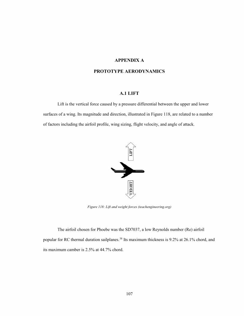
107

APPENDIX A

PROTOTYPE AERODYNAMICS

A.1 LIFT

Lift is the vertical force caused by a pressure differential between the upper and lower

surfaces of a wing. Its magnitude and direction, illustrated in Figure 118, are related to a number

of factors including the airfoil profile, wing sizing, flight velocity, and angle of attack.

Figure 118: Lift and weight forces (teachengineering.org)

The airfoil chosen for Phoebe was the SD7037, a low Reynolds number (Re) airfoil

popular for RC thermal duration sailplanes.38 Its maximum thickness is 9.2% at 26.1% chord, and

its maximum camber is 2.5% at 44.7% chord.

108

The airfoil’s two-dimensional lift curve slope is approximately 6.11 per radian and its

maximum lift coefficient is 1.3 at an angle of attack of 12.5°. For a Reynolds number of 100,000,

its maximum lift-to-drag ratio is 55.2 at an angle of attack of 5.25°.39 Figures 119 and 120 provide

the SD7037’s profile and its lift and drag curves for a Re of 100,000.

Figure 119: SD7037 airfoil (airfoiltools.com)

Figure 120: SD7037 theoretical lift and drag curves at Re = 100,000 (airfoiltools.com)

The SD7037 was selected from the airfoils detailed in Selig’s Summary of Low-Speed

Airfoil Data. The 34 airfoils for which testing data were reported were ranked according to their

maximum lift-to-drag ratios at a Reynolds number of 100,000, which was close to the estimated

cruise Re of 120,000 expected for the wing. The top three airfoils selected for printing were the

GM15, the A18, and the SD7037 whose maximum lift-to-drag ratios were 66.2, 65, and 55.2

respectively.40,41,39 Since the GM15 had the highest lift-to-drag ratio, it was the first to be

prototyped. However, with a maximum thickness of only 6.7%, it did not provide enough interior

space for the needed support structures to prevent warping and splitting during the build session.

109

Similarly, the 7.3% thick A18 also proved too thin for practical printing. Consequently,

manufacturing concerns dictated that the 9.2% thick SD7037 be selected since it could be made to

hold together during fabrication. With an airfoil formally chosen, lift characteristics and wing

geometry were analyzed.

The lift force is described by Equation 4 as the product of dynamic pressure (q), projected

wing area (S), and three-dimensional lift coefficient (CL).42

𝐿 = 𝑞𝑆𝐶𝐿 (4)

Per Equation 5, the dynamic pressure, q, is calculated as one half the product of air density (ρ)

and flight velocity (V) squared.42

𝑞 =1

2𝜌𝑉2 (5)

Per Equation 6, the projected wing area for a rectangular wing such as Phoebe’s is calculated as

the product of straight line tip-to-tip span (b) and chord (c).42

𝑆 = 𝑏𝑐 (6)

Per Equation 7, the three-dimensional lift coefficient is given as the product of the three-

dimensional lift curve slope (𝐶𝐿𝛼) and the difference between the angle-of-attack (α) and the

zero-lift angle of attack (α0), where the angle of attack is defined as the angle between the

incoming freestream velocity and the airfoil’s chord line.42

𝐶𝐿 = 𝐶𝐿𝛼(𝛼 − 𝛼0) (7)

110

The three-dimensional lift curve slope, 𝐶𝐿𝛼, was calculated with Equation 8, a semi-

empirical formula relating the two-dimensional lift curve slope (𝐶𝑙𝛼), aspect ratio (AR), Mach

number (M), exposed wing area (Sexposed), reference wing area (S), wing sweep (Λ), and fuselage

lift factor (F).42

𝐶𝐿𝛼=

2𝜋𝐴𝑅

2+√

4+𝐴𝑅2(1−𝑀2)

(𝐶𝑙𝛼

(1−𝑀2)0.5

2𝜋)

2(1+(tan Λ)2

1−𝑀2 )

(𝑆𝑒𝑥𝑝𝑜𝑠𝑒𝑑

𝑆) (𝐹) (8)

Since Phoebe has a high wing that does not intersect the fuselage, (𝑆𝑒𝑥𝑝𝑜𝑠𝑒𝑑

𝑆) and F were both

assumed to be 1. Also, noting Phoebe’s lack of wing sweep and negligible Mach number due to

the anticipated low flight velocity, Equation 8 was simplified and expressed as Equation 9.

𝐶𝐿𝛼=

2𝜋𝐴𝑅

2+√

4+𝐴𝑅2

(𝐶𝑙𝛼2𝜋

)

2

(9)

Finally, the wing’s maximum coefficient of lift (𝐶𝐿𝑚𝑎𝑥) was estimated from the airfoil’s

two-dimensional maximum lift coefficient (𝐶𝑙𝑚𝑎𝑥) and the wing sweep (Λ) according to Equation

10.42

𝐶𝐿𝑚𝑎𝑥= 0.9𝐶𝑙𝑚𝑎𝑥

cos Λ (10)

111

A.2 DRAG

Drag, illustrated in Figure 121, can be conveniently subdivided into two categories based

on cause: parasite (zero-lift) drag due to skin friction and flow separation effects and drag due to

lift. For steady, level flight, the total drag force dictates the aircraft’s thrust requirement.

Figure 121: Drag and thrust forces (teachengineering.org)

Parasite (zero-lift) drag is the result of skin friction and flow separation across the

aircraft’s wetted area. It can be estimated by calculating and summing the zero-lift drag

coefficients, CD_0, of the aircraft’s individual components (e.g. fuselage, wing, horizontal

stabilizer, vertical stabilizer, etc.). This component build up method is formally stated below for

subsonic flow as Equation 11.42

𝐶𝐷_0 =∑(𝐶𝑓_𝑐𝐹𝐹𝑐𝑄𝑐𝑆𝑤𝑒𝑡_𝑐)

𝑆𝑟𝑒𝑓+ 𝐶𝐷_𝑚𝑖𝑠𝑐 + 𝐶𝐷_𝐿&𝑃 (11)

Cf is the component skin friction coefficient. It is defined in terms of Reynolds number

and Mach number for turbulent flow by Equation 12.42 For Phoebe, all flow was assumed

turbulent given the inherent roughness of unfinished ABS. Once calculated, the skin friction

coefficient could have been empirically scaled to accommodate the particularly rough skin

surface. However, since no reliable empirical correction was available for 3D printed ABS, the

skin friction coefficient was left uncorrected with the expectation that the actual drag would be

greater than the estimated drag.

𝐶𝑓 =0.455

(log10 𝑅𝑒)2.58(1+0.144𝑀2)0.65 (12)

112

FFc is the component form factor adjustment that accounts for pressure drag due to

separation. It is defined by Equations 13 and 14 for specific aircraft components. Equation 15 is a

supplemental equation that provides a geometric term required for Equation 14.42

𝐹𝐹𝑐 = [1 +0.6

(𝑥/𝑐)𝑚(

𝑡

𝑐) + 100 (

𝑡

𝑐)

4] [1.34𝑀0.18(𝑐𝑜𝑠Λ𝑚)0.28] (13) (wing, tail, pylon)

𝐹𝐹𝑐 = (1 +60

𝑓3 +𝑓

400) (14) (fuselage, smooth canopy)

𝑓 =𝑙

𝑑=

𝑙

√(4/𝜋)𝐴𝑚𝑎𝑥 (15)

Qc is the component interference drag factor. It scales the component’s zero-lift drag to

account for increases caused by intersection with other aircraft components. For a high-mounted

wing, the interference is negligible and Q was assumed to be 1. Likewise, the fuselage sees

negligible interference and Q was set equal to 1. For a conventional tail, interference is typically

assumed to be 5% for a Q value of 1.05.28 However, since Phoebe’s horizontal and vertical

stabilizers do not intersect, a Q value of 1 was used instead.

The ratio Swet_c/Sref provides a weighting function for each individual component’s zero-

lift drag coefficient.

CD_misc is a catchall term for component drags that do not lend themselves to calculation

with skin friction. For parts such as Phoebe’s wing pylons and push rod braces, drag was

calculated with frontal area and an empirical value for (D/q)/(frontal area) where D is drag force

and q is dynamic pressure.42 These terms in conjunction with Equation 16 provide CD_misc.

𝐶𝐷_𝑚𝑖𝑠𝑐 =(𝐷/𝑞)

𝑓𝑟𝑜𝑛𝑡𝑎𝑙 𝑎𝑟𝑒𝑎∗

𝑓𝑟𝑜𝑛𝑡𝑎𝑙 𝑎𝑟𝑒𝑎

𝑆𝑟𝑒𝑓 (16)

113

CD_L&P represents the leakage and protuberance drag. This drag term accounts for air

leakage through the fuselage and small protuberances such as external hinges, control horns, and

surface imperfections.42 Because leakage and protuberance drag is extremely difficult to

accurately approximate, it was assumed to be 10% of the total zero-lift drag.

The drag due to lift was calculated as function of the wing’s lift coefficient and geometry

as shown in Equation 17, where AR is the wing’s aspect ratio and e is the Oswald’s efficiency

factor.42 The efficiency factor corrects for non-elliptical lift distributions and is calculated with

Equation 18.

𝐶𝐷_𝑙𝑖𝑓𝑡 =𝐶𝐿

2

𝜋𝐴𝑅𝑒 (17)

𝑒 = 1.78(1 − 0.45𝐴𝑅0.68) − 0.64 (18)

A.3 STABILITY

Stability analysis addresses an aircraft’s tendency to return to or diverge from a given

state when perturbed. A statically stable aircraft will experience restoring forces directing it to its

original state as the result of a perturbation. Dynamic stability extends this concept beyond simple

forces by requiring the aircraft’s dynamic motions to also return it to its original state over a

period of time. It is possible for an aircraft to be statically stable and dynamically neutral or

unstable as shown in Figure 122.42

114

Figure 122: Stability scenarios (differencebetween.com)

Since analyzing dynamic stability requires a full six degree-of-freedom analysis, which

was beyond the scope of this project, only static stability was evaluated. Evaluating static stability

consisted of summing moments around the aircraft’s CG and calculating moment derivatives

describing the plane’s response to perturbations in pitch, roll, and yaw. Pitch response was

analyzed independently as longitudinal stability. Roll and yaw response were coupled and

analyzed as lateral-directional stability.42 Figure 123 illustrates the various aircraft axes as they

pertain to the calculation of stability moments and derivatives.

Figure 123: Aircraft axes and moments (code7700.com)

115

Longitudinal stability was evaluated by summing pitching moments about the airplane’s

CG and calculating the moment derivative with respect to the angle of attack (𝐶𝑚𝛼). For an

aircraft in trimmed, steady flight, 𝐶𝑚𝑐𝑔 must equal 0. For a statically stable aircraft, 𝐶𝑚𝛼

must

also be negative. This implies that a positive pitch up or negative pitch down maneuver will result

in an opposing negative or positive moment that will restore the aircraft to its original state. For

simplicity, the moments were nondimensionalized (𝐶𝑚) by dividing through by dynamic pressure

(q), wing area (S), and wing chord (c). Equation 19 demonstrates the nondimensionalization as a

function of pitching moment (M).28

𝑐𝑚 =𝑀

𝑞𝑆𝑐 (19)

Equations 20 and 21 provide the nondimensionalized moment summation (𝐶𝑚𝑐𝑔) and its

derivative with respect to the angle to attack (𝐶𝑚𝛼). Both equations contain terms from the wing,

fuselage, horizontal stabilizer, and propulsion system. Within these terms, forces are represented

by their respective coefficients. For instance, the lift force is expressed as CL. Distance values are

similarly nondimensionalized with the wing chord and represented with bar notation. For

instance, the dimensionless location of the center of gravity along the X axis is represented by

�̅�𝑐𝑔.28

𝐶𝑚𝑐𝑔= 𝐶𝐿(�̅�𝑐𝑔 − �̅�𝑎𝑐𝑤) + 𝐶𝑚𝑤

+ 𝐶𝑚𝑓𝑢𝑠− 𝜂ℎ

𝑆ℎ

𝑆𝐶𝐿ℎ

(�̅�𝑎𝑐ℎ − �̅�𝑐𝑔) −𝑇

𝑞𝑆𝑍𝑇̅̅̅̅ +

𝐹𝑝

𝑞𝑆(�̅�𝑐𝑔 − �̅�𝑝)

(20)

𝐶𝑚𝛼= 𝐶𝐿𝛼

(�̅�𝑐𝑔 − �̅�𝑎𝑐𝑤) + 𝐶𝑚𝛼 𝑓𝑢𝑠− 𝜂ℎ

𝑆ℎ

𝑆𝐶𝐿𝛼ℎ

𝜕𝛼ℎ

𝜕𝛼(�̅�𝑎𝑐ℎ − �̅�𝑐𝑔) +

𝐹𝑝𝛼

𝑞𝑆

𝜕𝛼𝑝

𝜕𝛼(�̅�𝑐𝑔 − �̅�𝑝) (21)

116

The wing contributes the first two terms of Equation 20 and the first term of Equation 21

to the longitudinal stability analysis. In Equation 20, the first term, 𝐶𝐿(�̅�𝑐𝑔 − �̅�𝑎𝑐𝑤), represents

the moment caused by the wing’s lift force acting over the distance between the aircraft’s center

of gravity the wing’s aerodynamic center. The second term, 𝐶𝑚𝑤, is the wing’s pitching moment

coefficient, a function of airfoil characteristics and wing geometry. It can be calculated with the

airfoil’s pitching moment (𝐶𝑚0𝑎𝑖𝑟𝑓𝑜𝑖𝑙), the wing’s aspect ratio (AR), and the wing’s sweep (Λ) as

shown in Equation 22.42

𝐶𝑚𝑤= 𝐶𝑚0𝑎𝑖𝑟𝑓𝑜𝑖𝑙

(𝐴𝑅(cos Λ)2

𝐴𝑅+2 cos 𝛬) (22)

The first term in Equation 21, 𝐶𝐿𝛼(�̅�𝑐𝑔 − �̅�𝑎𝑐𝑤), is the change in moment caused by the change

in lift force with respect to angle of attack (α). There is no additional term in Equation 21 to

correlate with the wing’s pitching moment since 𝐶𝑚𝑤 is considered constant with respect to α.42

The fuselage contributes a single term to both Equations 20 and 21. Per Equation 23, the

derivative with respect to the angle of attack (𝐶𝑚𝛼𝑓𝑢𝑠) is calculated first as a function of width

(Wf), length (Lf), chord length (c), wing area (S), and an empirical pitching moment factor (Kfus)

that is referenced from Figure 124.

𝐶𝑚𝛼𝑓𝑢𝑠=

𝐾𝑓𝑢𝑠𝑊𝑓2𝐿𝑓

𝑐𝑆 [per degree] (23)

117

Figure 124: Fuselage pitching moment factor (42)

The resulting value for 𝐶𝑚𝛼𝑓𝑢𝑠 can be used directly in Equation 21. When multiplied with an

angle of attack, it provides the moment coefficient (𝐶𝑚𝛼) for Equation 20.42

The horizontal stabilizer, whose primary job is to longitudinally stabilize and control the

aircraft, adds one term to both Equations 20 and 21. The fourth term in Equation 20,

𝜂ℎ𝑆ℎ

𝑆𝐶𝐿ℎ

(�̅�𝑎𝑐ℎ − �̅�𝑐𝑔), represents the moment caused by the horizontal stabilizer’s lift force

acting over the distance between its aerodynamic center and the aircraft’s center of gravity. The

variable ηh is the dynamic pressure ratio accounting for the fact that the tail does not see

freestream dynamic pressure thanks to wing’s downwash and propulsion effects. The thrust-off

value for 𝜂ℎ𝑇=0 was initially assumed to be 0.90 and subsequently corrected for thrust effects

according to Equation 24 as a function of thrust (T), freestream dynamic pressure (q), and

propeller disk area (Ap).28

𝜂ℎ = 𝜂ℎ𝑇=0(1 +

𝑇

𝑞𝐴𝑝) (24)

The derivative with respect to angle of attack of 𝜂ℎ𝑆ℎ

𝑆𝐶𝐿ℎ

(�̅�𝑎𝑐ℎ − �̅�𝑐𝑔) in represented in

Equation 21 with two notable changes as 𝜂ℎ𝑆ℎ

𝑆𝐶𝐿𝛼ℎ

𝜕𝛼ℎ

𝜕𝛼(�̅�𝑎𝑐ℎ − �̅�𝑐𝑔). First, the coefficient of lift

has been exchanged for the horizontal stabilizer’s lift curve slope (𝐶𝐿𝛼ℎ). Second, an additional

118

term, 𝜕𝛼ℎ

𝜕𝛼, has been added to account for changes in the horizontal stabilizer’s angle of attack

relative to the aircraft’s angle of attack. A function of downwash, 𝜕𝛼ℎ

𝜕𝛼 is calculated with Equation

25 and the downwash estimates provided in Figure 125.42

𝜕𝛼ℎ

𝜕𝛼= 1 −

𝜕𝜀

𝜕𝛼 (25)

Lastly, the two-fold effects of the propulsion system on longitudinal stability are

accounted for in last two terms of Equation 20 and the last term of Equation 21. These effects are

derived from both the direct thrust force and the perpendicular force due to the air’s momentum

change at the propeller face. From Equation 20, 𝑇

𝑞𝑆�̅�𝑇 represents the moment caused by the thrust

force acting over the distance between the thrust line and the aircraft’s longitudinal axis through

its center of gravity. The final term of Equation 20, 𝐹𝑝

𝑞𝑆(�̅�𝑐𝑔 − �̅�𝑝), represents the moment caused

the propulsion’s perpendicular force acting over the distance between the propeller face and the

Figure 125: Downwash estimates (42)

119

aircraft’s center of gravity. For propeller driven aircraft, the perpendicular force can be solved for

by multiplying the angle of attack with the perpendicular force’s derivative with respect to angle

of attack as given by Equation 26.28

𝐹𝑝𝛼= 𝑞𝑁𝐵𝐴𝑝

𝜕𝐶𝑁𝑏𝑙𝑎𝑑𝑒

𝜕𝛼𝑓(𝑇) (26)

Note that q is the freestream dynamic pressure; NB is the number of blades on the

propeller; Ap is the area of the propeller disk; and 𝜕𝐶𝑁𝑏𝑙𝑎𝑑𝑒

𝜕𝛼 and 𝑓(𝑇) are empirical terms derived

from Figures 126 and 127 as functions of thrust (T), air density (ρ), velocity (V), propeller

diameter (D) and propeller rotational speed (n) in rotations per second.42

Figure 127: Propeller normal force factor (42)

Figure 126: Propeller normal force coefficient (28)

120

For equation 21, there is no derivative term that correlates to 𝑇

𝑞𝑆�̅�𝑇 since thrust is constant with

angle of attack. Also, to remove stability’s dependence upon velocity, the 𝐹𝑝𝛼

𝑞𝑆

𝜕𝛼𝑝

𝜕𝛼(�̅�𝑐𝑔 − �̅�𝑝)

term of Equation 21 is commonly neglected to render what could be considered power-off

stability with the understanding that for every chord length between the propeller and the center

of gravity, stability will be reduced by approximately 2%.42

To make the longitudinal stability analysis more readily applicable, Equation 21 can be

set equal to 0 and solved for the location of the aircraft’s neutral point (�̅�𝑛𝑝), the point at which

the pitching moment does not change with angle of attack. The equation for the neutral point,

nondimensionalized with wing chord, is given by Equation 27.28

�̅�𝑛𝑝 =𝐶𝐿𝛼�̅�𝑎𝑐𝑤−𝐶𝑚𝛼 𝑓𝑢𝑠

+𝜂ℎ𝑆ℎ𝑆

𝐶𝐿𝛼ℎ

𝜕𝛼ℎ𝜕𝛼

�̅�𝑎𝑐ℎ

𝐶𝐿𝛼+𝜂ℎ𝑆ℎ𝑆

𝐶𝐿𝛼ℎ

𝜕𝛼ℎ𝜕𝛼

(27)

If the locations of the neutral point (�̅�𝑛𝑝) and center of gravity (�̅�𝑐𝑔) are known, their

difference, the static margin (SM), can found with Equation 28 and used to describe the aircraft’s

longitudinal stability.42

𝑆𝑀 = �̅�𝑛𝑝 − �̅�𝑐𝑔 (28)

For a center of gravity ahead of the neutral point, the static margin will be positive implying that

the moment coefficient derivative with respect to angle of attack (𝐶𝑚𝛼) is negative and that the

aircraft is longitudinally stable.42

A similar process of summing moments can be followed for analyzing lateral and

direction stability, with the exception that derivatives are taken with respect to the angle of

sideslip (β) rather than the angle of attack (α). Since both lateral and directional stability hinge on

121

β, they are typically coupled. At face value, this would seem to simply the analysis. However,

since the roll and yaw effects cannot be effectively separated, obtaining accurate stability

characteristics becomes impractical without a full six degree-of-freedom analysis, which was

beyond the scope of this project.42 Consequently, rules of thumb such as tail volume coefficients

and known dihedral effects were relied upon for lateral-directional stability with the expectation

that if problems presented during the fabrication or testing of the aircraft they could be corrected.

Equations 29 and 30 provide the tail volume coefficient equations solved for stabilizer area as

functions of empirical tail volume coefficients (cVT, cHT), wingspan (b), wing chord (c), wing area

(S), and the distances between the center of gravity and the aerodynamic centers of the vertical

and horizontal stabilizers (LVT, LHT). Table 10 lists the empirical tail volume coefficients

referenced from Raymer.42

𝑆𝑉𝑇 =𝑐𝑉𝑇𝑏𝑆

𝐿𝑉𝑇 (29)

𝑆𝐻𝑇 =𝑐𝐻𝑇𝑐𝑆

𝐿𝐻𝑇 (30)

Typical Values

Horizontal cHT Vertical cVT

Sailplane 0.50 0.02

Homebuilt 0.50 0.04

General aviation – one engine 0.70 0.04

General aviation – two engine 0.80 0.07

Agricultural 0.50 0.04

Table 10: Tail volume coefficients (28)

122

APPENDIX B

PROTOTYPE PROPULSION

The purpose of the propulsion system is to provide the thrust needed for flight. Since

Phoebe is propeller driven, thrust requirements were used in conjunction with anticipated flight

velocities to develop power requirements, which were in turn used to estimate aircraft

performance. For the sake of simplicity and compact size, a basic electric propulsion system,

similar to those seen on comparable RC airplanes, was selected. Its constituent components

included a brushless outrunner motor, two-bladed propeller, electronic speed controller, and

lithium polymer (LiPo) battery.

B.1 POWER REQUIREMENTS

Required power (Preq) was estimated as the product of thrust (T) and velocity (V) for a

given flight regime and is formalized in Equation 31.43

𝑃𝑟𝑒𝑞 = 𝑇𝑉 (31)

For steady level flight, thrust was calculated with the thrust-to-weight ratio (T/W), which

by definition must be equal to the inverse of the lift-to-drag ratio (L/D). Equation 32 illustrates

the calculation as a function of lift (L), drag (D), and weight (W).42

𝑇 =𝑇

𝑊𝑊 =

𝑊

(𝐿/𝐷) (32)

123

Velocity for steady level flight could have been any anticipated cruise speed above the aircraft’s

stall speed. For Phoebe, the minimum drag velocity was assumed.

The thrust required for steady, climbing flight was also calculated with a known thrust-to-

weight ratio that included a climb angle term, as shown in Equation 33. The angle, γ, indicates the

degrees above horizontal at which the aircraft is ascending.42

𝑇 =𝑇

𝑊𝑊 = (

cos 𝛾

(𝐿/𝐷)+ sin 𝛾) 𝑊 (33)

Again, velocity could have been any anticipated speed at which the airplane would be expected to

climb. Assuming takeoff conditions, 1.2Vstall was used to ensure that Phoebe could safely climb

out to cruising altitude without stalling.

Typically, maneuverability is also considered when estimating power requirements since

turn rates are directly related to an airplane’s thrust-to-weight ratio.42 However, since Phoebe

does not have ailerons, it was highly unlikely that the pilot would have the control authority to

induce high performance turning maneuvers such as a knife edge turn. Consequently, the steady

climb scenario was used to set the maximum power requirement.

B.2 COMPONENT SELECTION

A basic electric propulsion system such as Phoebe’s requires at least four individual

components: a motor, a propeller, an electronic speed controller, and a battery. The selected

components were chosen based on manufacturer recommendations and RC plane benchmarking.

Power requirements and power availability were subsequently used to estimate aircraft

performance. Figure 128 provides a flowchart for the assembled propulsion system including the

link to the RC receiver, and individual components are detailed below.

124

Figure 128: Propulsion system flowchart

The selected motor, pictured in Figure 129, was an E-flite Park 480 brushless outrunner

with a Kv value of 1020 and a maximum power rating of 275W. Per the manufacturer, this motor

is suitable for scale park flyers weighing up to 990g (9.71N), which includes Phoebe.44 The motor

has a maximum diameter of 35.5mm and a length of 32.2mm not including the length of its 4mm

diameter propeller shaft. With its connectors and mounting hardware, the Park 480 has a total

weight of 97g. An efficiency of 80% was assumed for the motor.

To accompany the Park 480 motor, the manufacturer recommended propellers between

10 x 7 – 12 x 6. Within this range, four specific, two-bladed propellers were selected: 10 x 7, 11 x

7, 11 x 6, and 12 x 6. They weighed 16g, 21g, 22g, and 29g respectively. All four propellers were

manufactured by Master Airscrew and are composed of glass-filled nylon. Figure 130 provides a

representative illustration. An efficiency of 75% was assumed for each of the propellers.

Propeller MotorElectronic Speed

Controller

RC Receiver

Battery

Figure 129: E-flite Park 480 brushless outrunner motor

(horizonhobby.com)

125

Figure 130: Two-bladed propeller

The selected E-flite Lite Pro Brushless Electronic Speed Controller was also a

recommendation for the selected motor. It is rated for up to 40A of continuous current and 55A of

burst current. The ESC also includes a 5V battery elimination circuit (BEC) to power the RC

receiver and servos. It is 66mm long, 31mm wide, and 12mm thick with a weight of 48g. Figure

131 shows the ESC, whose efficiency was assumed to be 75%.

Figure 131: E-flite Lite Pro Brushless ESC

Finally, as its source of power, Phoebe can use any 11.1V (three cell, 3S) lithium

polymer battery with a capacity as high as 1800mAh, a limit imposed simply by the available

space within the fuselage. The specific model selected for testing, shown in Figure 132, was an E-

flite 3S LiPo with an 1800mAh capacity and a maximum discharge rate of 36A. Its length, width,

and height are 101mm, 34mm, and 18mm respectively, and it weighs a total of 141g. An

efficiency of 75% was assumed for the battery.

126

Figure 132: E-flite 3S, 1800mAh battery

The available power supplied by this propulsion system was the basis for evaluating

performance metrics such as maximum speed, sustainable climb angle, endurance, and range. It is

important to note that available power was not set equal to the 275W maximum power rating of

the system, but was instead set equal to the maximum power multiplied by each of the

components’ efficiencies to account for losses throughout the system. Doing so resulted in a

conservative 92.8W of available power that was compared to flight power requirements for

conducting performance estimates.

B.3 PROPULSION TESTING METHODOLOGY

Propulsion testing was intended to experimentally validate the selected propulsion

components prior to flight testing and provide an indication of the optimal propeller to install on

the Phoebe prototype.

The apparatus used for testing was a custom designed static thrust stand. Structurally, the

thrust stand consisted of three 3D printed components: a base, a pivoting arm, and a motor

adaptor. To increase rigidity and reduce vibrations, the arm was augmented with two 4mm carbon

rods. The thrust stand’s maximum height was 230mm allowing it to accommodate propellers up

to 12in in diameter.

The thrust stand was instrumented to measure thrust, voltage, current, and power. Thrust

was measured by a digital scale placed under the pivoting arm’s foot. The scale was capable of

127

measuring up to 5000g with 1g resolution. Voltage, current, and power were measured by the E-

flite inline multimeter installed between the battery and the ESC. The meter was capable of

measuring currents up to 120A, voltages up to 50V, and power up to 6000W. Resolutions for

current, voltage, and power were 0.1A, 0.1V, and 0.1W respectively. Since neither the scale nor

the multimeter was capable of data logging, a digital camera was positioned to record both digital

displays for the duration of each test. Figure 133 illustrates the thrust stand with the test

instrumentation and propulsion system installed.

Figure 133: Static thrust stand with test instrumentation and propulsion system

In principle, the thrust stand works by creating a static moment balance. By necessity, the

moment created by the thrust force acting over the distance between the horizontal thrust line and

pivot point must be equal to the opposing moment created by the scale’s normal force and the

distance between the pivoting arm’s foot and the pivot point. The specific mathematical

relationship between the thrust force and the scale’s normal force, indicated as weight, was

determined with a calibration procedure.

128

The thrust stand was calibrated with a set of metric weights used to impose a known

horizontal force along the thrust line to which the scale’s indicated normal force could be

correlated. Calibration began by taring the scale with the pivot arm resting freely on the scale to

remove any influence of the thrust stand or propulsion system weight on the scale’s reading.

Next, a short piece of 15lb fishing line was attached to the propeller nut and run horizontally

through a small pulley positioned in front of the thrust stand. Weights were then suspended from

a loop tied in the free end of the fishing line on the far side of the pulley as pictured in Figure

134.

Figure 134: Thrust stand calibration setup

To generate the calibration curve, scale readings were recorded for 11 different weight values.

The weights and corresponding scale readings are presented in Table 11 and plotted in Figure

135. Equation 42, the linear fit of the calibration data, provides thrust (T) as a function of scale

reading (SR).

129

Weight [g] Scale Reading [g]

0 0

10 14

20 24

50 57

100 121

200 241

500 616

Weight [g] Scale Reading [g]

700 828

1000 1180

1200 1462

1500 1880

Table 11: Calibration weights and scale readings

Figure 135: Calibration weight vs scale reading

130

𝑇 = 0.8131𝑆𝑅 + 5.2368 (42)

Prior to testing, each of the four propellers was balanced using a Dubro Tru-Spin prop

balancer. With a sheet of 220-grit sandpaper, material was carefully removed from the blades and

hubs of the propellers until they would remain stationary in both horizontal and vertical

orientations. Figure 136 depicts the propeller balancer setup.

Once balanced, each of the propellers (10x7, 11x7, 11x6, 12x6) was installed onto the

thrust stand’s test motor, the E-flite outrunner. Connected in series to the motor was the E-flite

40A ESC, the E-flite in-line multimeter, and the E-flite 3S 1800mAh battery. Batteries were

recharged between each test to ensure consistent voltages. The assembled propulsion system was

controlled with a Spektrum AR8000 8-channel DSMX receiver bound to a Spektrum DX9

transmitter. This particular model of transmitter was selected because it provided a digital throttle

readout allowing consistent test points for each of the separate propellers. The digital scale was

placed under the pivoting arm and tared between each test to remove the weight effects of the

propulsion system and thrust stand mass, and the 12MP Canon digital camera was positioned on

its flexible tripod so that it could record the multimeter and scale displays.

In turn, each propeller was tested at 11 points across the throttle range: 1%, 10%, 20%,

30%, 40%, 50%, 60%, 70%, 80%, 90%, and 99%. At each point, the thrust stand was given

Figure 136: Propeller balancer

131

approximately 10s to settle before thrust values were recorded. Once the camera was given time

to record the scale’s reading, the multimeter was cycled through its voltage, current, and power

display settings so that each value could also be captured by the camera. To protect the motor,

throttle profiles for the 11x7, 11x6, and 12x6 propellers were cutoff once the power draw

exceeded the motor’s maximum 275W rating. The motor was also given time to cool to the touch

between each of the four tests.

Once the tests were complete, the videos captured by the camera were reviewed so that

values for the scale reading, battery voltage, current, and power could be transferred to an Excel

document for processing. Scale readings were converted to thrust values with Equation 42, and

plots for thrust vs throttle, power vs thrust, and current vs thrust were prepared to compare the

propellers.

B.4 PROPULSION TESTING RESULTS

Propulsion testing was conducted to generate thrust profiles for each of the four selected

propellers and examine their respective current draws and power requirements. Tables 12, 13, 14,

and 15 provide the measured data and calculated static thrust values for the 10x7, 11x7, 11x6, and

12x6 propellers respectively. Table entries with a value of OP (over power) indicate throttle

settings for which no data was taken because the motor was drawing more than its 275W

maximum power rating. Also, note that power values indicate power delivered by the battery to

the propulsion components, not the power delivered by the propeller to the airflow. Since the

multimeter was placed in line between the battery and speed controller, it was unable to account

for losses incurred in the ESC, motor, and propeller.

132

Table 12: 10x7 propulsion test data


133



From the tables, throttle settings below 10% were consistently insufficient to spin up any

of the four propellers. By 20%, all propellers were generating measureable thrust. The 10x7 was

the only propeller to be run through the entire throttle range, since its maximum power draw of

260W at 99% was below the motor’s 275W rating. At maximum throttle, it generated 1311.1g of

134

thrust. Both the 11x7 and 11x6 were run as high was 80% throttle, and the 12x6 was run as high

as 70% throttle. The maximum measured thrust was 1407.0g generated by the 11x6. However,

both the 11x7 and 12x6 nearly matched maximum thrust with maximum values of 1103.9g and

1391.6g respectively. Figure 137 provides a plot of the four propellers’ measured thrust values

against throttle setting and suggests that the thrust response follows an s-curve profile. Error bars

depict the 155.5g, 184.1g, 180.6g, and 193.0g standard errors for the 10x7, 11x7, 11x6, and 12x6

thrust values respectively.

Figure 137: Propeller thrust vs throttle

As expected, each of the propeller’s required current was proportional to the thrust it

generated. The maximum measured currents, 25.3A and 25.2A, were drawn by the 11x6 and

11x7 respectively as they generated just over 1400g of thrust. At full throttle, the 10x7 drew

24.3A to produce 1311.1g of thrust, and the 12x6 drew a maximum of 21.3A at 1391g of thrust.

Figure 138 provides required current as a function of thrust. From the figure, it is clear that the

135

larger propellers were typically able to produce a given thrust with less required current. Errors

for the current data were calculated as 2.9A, 3.0A, 3.0A, and 2.8A for the 10x7, 11x7, 11x6, and

12x6 propellers respectively.

Figure 138: Propeller current vs thrust

Power consumption followed a similar trend to current, in that each propeller required

more power to generate more thrust. The 11x6 required the most power at 80% throttle: 273.2W

for 1407.0g of thrust. Recall that no power value exceeded 275W because the motor was

intentionally kept below its maximum power rating. The 11x7 drew nearly as much power as the

11x6, requiring 269.9W to generate 1403.8g of thrust. The 10x7 and 12x6 power requirements

peaked at 260.0W and 235.8W for 1311.1g and 1391.6g of thrust respectively. Figure 139 plots

power draw as a function of thrust. As expected, it is nearly identical visually to Figure 136.

136

Figure 137 also presents the calculated standard error for the power data, which for the 10x7,

11x7, 11x6, and 12x6 propellers was 31.2W, 33.3W, 33.3W, and 30.9W respectively.

Figure 139: Propeller power vs thrust

Even without exceeding the motor’s maximum power rating, the static tests demonstrated

that each of the four propellers is more than capable of delivering sufficient thrust for the Phoebe

prototype, which according to preliminary drag estimates will only require 61g of thrust for

steady, level flight. If the actual drag values end up being significantly higher than estimated, the

propulsion system should still be more than capable, as the maximum thrust values seen in the

tests approached a 1.7:1 thrust-to-weight ratio. In short, Phoebe should fly just fine regardless of

which propeller is installed. That being said, the 10x7 seems the best choice for the initial flight

tests since it minimizes the risk of over exerting the motor and other propulsion components.

137

APPENDIX C

PROTOTYPE PERFORMANCE

C.1 PERFORMANCE ESTIMATES METHODOLOGY

Conducting performance estimates for the as-designed Phoebe configuration began with

examining likely steady, level flight conditions, which require lift equal to weight and thrust

equal to drag.

Since lift must equal the aircraft’s weight, weight (W) can be substituted into the lift

equations previously discussed. Also, the aircraft’s maximum lift coefficient, found with

Equation 10, can be substituted into the lift force equation (Equation 3) and subsequently solved

for stall velocity as seen in Equation 34.

𝑉𝑠𝑡𝑎𝑙𝑙 = √2𝑊

𝜌𝑆𝐶𝐿𝑚𝑎𝑥

(34)

The drag analysis provided not only the required thrust and power as functions of

velocity, but also potential cruise speeds for optimal performance. Equations 35 and 36 provide

the minimum drag and minimum power velocities respectively as functions of weight (W), air

density (ρ), wing area (S), Oswald’s efficiency factor (e), aspect ratio (AR), and the zero-lift drag

coefficient (𝐶𝐷0), which was solved for using the component build up method. 42

138

𝑉𝑚𝑖𝑛 𝑑𝑟𝑎𝑔 = √2𝑊

𝜌𝑆√

1

𝜋𝐴𝑅𝑒𝐶𝐷0

(35)

𝑉𝑚𝑖𝑛 𝑝𝑜𝑤𝑒𝑟 = √2𝑊

𝜌𝑆√

1

3𝜋𝐴𝑅𝑒𝐶𝐷0

(36)

Flying at the minimum drag or minimum power velocity maximizes range or endurance, and

either of these velocities can be used to remove another unknown from the lift equations needed

for steady, level flight conditions.42

Finally, with the aircraft’s weight, wing area, and anticipated cruise speeds known, the

lift force equation can be solved for the needed coefficient of lift which can subsequently be used

to find the required angle of attack. Equation 37 illustrates the rearrangement of the lift equation

to solve for the coefficient of lift, and Equation 38 provides the angle of attack (α) as a function

of the coefficient of lift (CL), the lift curve slope (𝐶𝐿𝛼), and the zero-lift angle of attack (α0).

𝐶𝐿 =𝑊

𝑞𝑆 (37)

𝛼 =𝐶𝐿

𝐶𝐿𝛼

+ 𝛼0 (38)

Knowing the aircraft’s weight and geometry and solving for lift, stall velocity, drag,

thrust, cruise velocities, and angle of attack provide a reasonably thorough description of the

aircraft’s steady, level flight condition. These performance estimates can be expanded to include

maximum speed, sustainable climb angle, endurance, and range by considering the maximum

power and energy available.

139

The aircraft’s maximum speed is directly related to the available power and can be found

by solving for the velocity at which the required power overtakes the available power. Done

graphically, this involves plotting both the available and required powers as functions of velocity

and finding the intersection between the two data series. Figure 140 provides a representative

illustration.

Figure 140: Theoretical maximum speed graphical solution

A similar graphical method can be used to solve for the aircraft’s maximum sustainable

climb angle by plotting available and required powers as functions of climb angle and finding the

intersection of the data series. As before, available power is assumed constant. The required

power for the climb can be found by multiplying Equation 33, which defines the needed thrust-to-

weight ratio, by the aircraft’s weight and climb velocity. Equation 39 provides the required

power, and Figure 141 illustrates the graphical solution for maximum climb angle.

𝑃𝑟𝑒𝑞𝑐𝑙𝑖𝑚𝑏= 1.2𝑉𝑠𝑡𝑎𝑙𝑙𝑊 (

cos 𝛾

𝐿 𝐷⁄+ sin 𝛾) (39)

140

Figure 141: Theoretical maximum climb angle graphical solution

Unlike top speed and maximum climb angle, the aircraft’s endurance is not related to the

maximum available power. Instead, it is dependent upon the total available energy from the

battery and the power settings used during cruise. Equation 40 defines endurance (E) in terms of

battery voltage (Vbatt), battery capacity (Cbatt), and power required (Preq).43

𝐸 =(𝑐𝑜𝑛𝑠𝑡)𝑉𝑏𝑎𝑡𝑡𝐶𝑏𝑎𝑡𝑡

𝑃𝑟𝑒𝑞 (40)

The constant value (const) in Equation 40 varies depending on the units of the other variables and

the desired units for endurance. For battery voltage in Volts, battery capacity in mAh, and

required power in Watts, a constant value of 0.06 places endurance in units of minutes. Though

perhaps not immediately obvious from Equation 40, endurance does vary with velocity since drag

and required power vary with velocity. The minimum power velocity, as found with Equation 36,

provides optimal endurance by minimizing power draw, a relationship that is obvious from

Equation 40.

141

Range is also a function of the available energy and cruise power settings. If endurance

values (E) and corresponding velocity values (V) are already known, range (R) can be simply

calculated as the product, demonstrated by Equation 41.

𝑅 = (𝑐𝑜𝑛𝑠𝑡)𝐸𝑉 (41)

The constant value (const) in Equation 41 varies depending on the units of endurance and

velocity and the desired units for range. For endurance in minutes and velocity in meters per

second, a constant value of 0.06 provides range in units of kilometers. Like endurance, range is a

function of velocity and is optimized at the minimum drag velocity as found with Equation 35.

C.2 PERFROMANCE ESTIMATES RESULTS

With the classical flight equations presented in Raymer’s Aircraft Design: A Conceptual

Approach, theoretical performance estimations were made prior to flight testing to predict what

the Phoebe prototype’s steady, level flight conditions might look like. Note that though the

solution methodology is presented as linearly as possible, solving for each of the following

performance metrics required iterative methods since lift, drag, velocity, and angles of attack are

all related to one another.

The solution for steady, level flight was based on the requirements that lift equal weight

and thrust equal drag. From the preliminary CAD model, weight estimations placed Phoebe at

approximately 830g, which matched the prototype’s camera-augmented gross takeoff weight. The

wing needed to produce at least this much lift to keep the prototype airborne. This weight in

conjunction with the wing’s 0.152m2 area and 1.3 𝐶𝐿𝑚𝑎𝑥 were sufficient to use Equation 33 to

solve for Phoebe’s 19.6m/s stall speed. Estimating additional lift characteristics such as

coefficients of lift and angles of attack required first completing the drag analysis.

142

Using Raymer’s component build up method and iterative values for the coefficient of

lift, Phoebe’s parasite and induced drag profiles were calculated. The parasite drag coefficient,

𝐶𝐷0, solved to 0.023. However, since the equations used did not incorporate empirical corrections

for 3D printed ABS’s inherent roughness or Phoebe’s blunt back end, the actual value is likely

higher.

Figure 142 provides Phoebe’s theoretical drag polar, in which the total drag coefficient,

CD, is clearly minimized when the coefficient of lift, CL, is zero. The drag due to lift, a function of

𝐶𝐿2, creates the parabolic curve typical of such drag polars.

Figure 142: Theoretical drag polar

Figure 143 illustrates the anticipated drag force as a function of velocity. The minimum

drag value is approximately 61g, and the graph follows the expected pseudo-parabolic curve

143

which results from the parasite drag’s dependence on velocity squared and the induced drag’s

dependence on the inverse of velocity squared.

Figure 143: Theoretical drag vs velocity

Figure 143, or alternatively Equation 35 (a function of 𝐶𝐷0, aspect ratio, Oswald’s

efficiency factor, weight, and wing area) was used to find the minimum drag velocity at which

range is optimized. For Phoebe, it was approximately 11.9m/s. Similarly, Equation 36 was used

to solve for Phoebe’s 9.1m/s minimum power velocity at which endurance is optimized.

For the sake of completing the steady, level flight estimations, the Phoebe prototype was

assumed to cruise near its minimum drag velocity of 11.9m/s to maximize range. This velocity, in

conjunction with the weight estimation and wing area, allowed Equation 37 to be used to

calculate the needed lift coefficient for Phoebe to fly. In this specific case, CL works out to 0.65.

144

With the lift coefficient, the 4.6/rad lift curve slope from Equation 8, and the SD7037’s -3.5°

zero-lift angle of attack, Equation 38 indicated that the prototype needed to cruise at an angle of

attack of approximately 4.5°.

In summary, for steady, level flight, the 830g Phoebe prototype will need to generate

830g of lift. For optimal range, it will fly at a velocity of 11.9m/s with a 4.5° angle of attack

giving it a total lift coefficient of 0.65. At these cruise conditions, drag and its opposing thrust are

both estimated to be 61g, a value well within the demonstrated capability of the selected

propulsion system.

Looking beyond steady, level flight, the characteristics of the selected propulsion system

can be used to estimate additional performance metrics, namely maximum speed, maximum

steady climb angle, endurance, and range.

Maximum speed was determined by comparing the propulsion system’s available power

to the prototype’s estimated power requirements. The available power was assumed to be 92.8W,

which was the product of the motor’s 275W maximum power rating and the individual propulsion

components’ efficiencies. The required power was derived from the drag analysis by setting

thrust equal to drag for a specific velocity and multiplying thrust by that velocity according to

Equation 31. Figure 144 plots both the constant available power and the varying required power

as functions of velocity. Note that the power requirement reached a minimum value of 5.2W at a

velocity of 9.1m/s, which agrees with the minimum power velocity predicted by Equation 36. To

either side of this velocity, power requirements increased, eventually intersecting the available

power curve at Phoebe’s estimated maximum velocity of 35.5m/s.

145

Figure 144: Theoretical power available vs power required (steady, level flight)

The maximum sustainable climb angle was also estimated graphically by comparing the

available power to the power required. Figure 145 plots the propulsion system’s constant 92.8W

of available power against the power required for climb as a function of climb angle, which was

calculated by multiplying the required thrust (Equation 33) by the assumed constant velocity of

1.2Vstall (10.6m/s). Since the power available and power required curves did not intersect, it

appears that the Phoebe prototype will not face power restrictions with respect to climb angle.

This conclusion was validated by the static propulsion testing results which indicated that the

propulsion system is capable of producing thrust-to-weight ratios greater than 1.

146

Figure 145: Theoretical power available vs power required (climbing flight)

Considering battery specifications such as voltage and capacity with the calculated power

requirements allowed endurance to be estimated with Equation 40. Figure 146 provides the

endurance as a function of velocity calculated for the selected 11.1V, 1800mAh battery used for

testing. Endurance peaked at 55.5min at 9.1m/s, the minimum power velocity as expected. At

Phoebe’s anticipated top speed of 35.5m/s, endurance dropped to 4.3min.

147

Figure 146: Theoretical endurance vs velocity

Endurance as a function of velocity provided the basis for calculating range, which

according to Equation 41 is the product of endurance at a specific speed and that specific speed.

Figure 147 provides the plot of the range curve with respect to velocity. Note that the peak value

of 36.8km shifted to the minimum drag velocity of 11.9m/s. At top speed, the Phoebe prototype’s

range is limited to 9.1km.

148

Figure 147: Theoretical range vs velocity

VITA

Christopher Phillip Banfield

Candidate for the Degree of

Master of Science

Thesis: DESIGN AND DEVELOPMENT OF A 3D PRINTED UAV

Major Field: Mechanical and Aerospace Engineering

Biographical:

Education:

Completed the requirements for the Bachelor of Science in Aerospace

Engineering at Oklahoma State University, Stillwater, Oklahoma in 2013.

Professional Memberships:

AIAA

design and development of a 3d printed uav - ShareOK

Documents

Transcript of design and development of a 3d printed uav - ShareOK