International Journal of Research in Engineering, Science and Management

Volume-2, Issue-9, September-2019

www.ijresm.com | ISSN (Online): 2581-5792

177

Abstract: Lugs are joint type elements most widely used as

structural supports for pin connections type assemblies. Lug and

pin joints have been designed based on theoretical strength of

materials models and experimental data developed in the 1950’s.

With the increasing technology in mathematics usage of numerical

methods like finite element analysis (FEA) code components can

be tested virtually. It is important to determine whether the results

obtained from Finite element analysis with the standard

theoretical acceptable values. This project deals with the design

and analysis of a typical lug joint representative of an airframe

structure applications. The design will provide safety against a)

Lug failure, b) Pin failure. The types of loadings to be considered

are axial, transverse or drag load. Aircraft design practices will be

used for calculations. For this study, geometry was determined

and analyzed using the theoretical calculations to determine the

ultimate joint loads for design. Margin of safety for each lug joint

component was calculated based on ultimate load. This geometry

was then modeled in ANSYS Software. Margin of safety for each

lug joint component was calculated using two methods, max peak

stress and stress averaged over the contact area. Using peak stress

was very conservative and predicted margins were much less than

those calculated from the theoretical calculations. In most cases,

the FEA average stress plot margin of safety was less conservative

than the margin calculated by the classical methods. However, this

difference was generally less than 5-10%. Thus, analyzing lug

joints using ANSYS leads to similar kind of results as compared

with classical strength of materials approach. Aircraft design

practices will be used for calculations.

Keywords: FEA, Lugs, Stress concentration, Margin of safety,

Principle stress, Failure theories

1. Introduction

A. Introduction to aircraft structures

Aircraft structural design is a subset of structural design in

general, including ships, land vehicles, bridges, towers, and

buildings. All structures must be designed with care because

human life often depends on their performance. Structures are

subject to one-way and oscillating stresses, the latter giving rise

to fatigue. Metal structures are subject to corrosion, and some

kinds of corrosion are accelerated in the presence of stress.

Aircraft structures are designed with particular attention to

weight, for obvious reasons. If we could see beneath the interior

fittings of passenger aircraft, we would see numerous lightening

holes in the frames as well as regions where the skins have been

thinned by chemical milling. On Boeing aircraft, it is not

unusual to find regions as small as the palm of your hand with

their own thickness, and four or more individual thicknesses are

often found on a single skin. These regions differ in thickness

by as little as a millimeter or two, indicating that considerable

effort is expended to find regions that are too lightly stressed.

Such regions are deliberately made thinner to remove metal that

is not doing its share of load-bearing.

The first aircraft had two wings made of light weight wood

frames with cloth skins, held apart by wires and struts. The

upper wing and the struts provided compression support while

the lower wing and the wires supported tension loads.

In the 1920s, metal began to be used for aircraft structure. A

metal wing is a box structure with the skins comprising the top

and bottom, with front and back formed by I-beams called

spars, interior fore-aft stiffeners called ribs and in-out stiffeners

called stringers. In level flight, the lower skin is intension while

the upper skin is in compression. For this reason, this design is

referred to as stressed skin construction. During turbulence,

upper and lower skins can experience both tension and

compression. This box structure is able to support the above-

mentioned moments, making single wing aircraft possible. The

elimination of the struts and wires so dramatically reduced air

drag that aircraft were able to fly twice as fast as before with

the same engine.

B. Lug joint

Rivet, lug and bolt joints in aircraft are the critical element in

airframe integrity. Great care is expended on creating these

joints because they are subject to high stresses. The holes are

drilled with keen attention to making their axes normal to the

skin surface and their diameters correct. In highly stressed

regions of the wing, each hole is manually reamed out to pre-

stress the region around the hole. Each rivet or bolt is

compressed or torque precisely in order to achieve the stress-

carrying capability intended by the structural engineers. Rivet

diameter and compression are calculated tonsure that the

installed rivet not only completely fills the hole but also creates

compressive stress in the surrounding material. If there is any

possibility that drilling a hole will leave a burr on the back side,

this burr must be manually removed because it could puncture

the corrosion-resisting paint when the skins are pulled together

by the fastener.

Design and Analysis of Lug Joint in an Airframe

Structure using Finite Element Method

K. Siva Sankar1, B. Anjaneyulu2

1Post Graduate Student, Department of Civil Engineering, Gates Institute of Technology, Anantapur, India 2Assistant Professor, Department of Civil Engineering, Gates Institute of Technology, Anantapur, India

International Journal of Research in Engineering, Science and Management

Volume-2, Issue-9, September-2019

www.ijresm.com | ISSN (Online): 2581-5792

178

Structural engineers take care to choose the size of the

fastener to support the stresses it is expected to bear. The same

is true of skin thicknesses, as mentioned above. On an aircraft

wing, the skin may be as much as ten times thicker at the root

than it is at the tip. The diameter of fasteners varies similarly,

with diameters as large as your thumb at the root and as small

as 3or 4 mm at the tip. Such specialization raises the cost

because it reduces economies of scale in purchasing and

inventory control, but it saves considerable weight

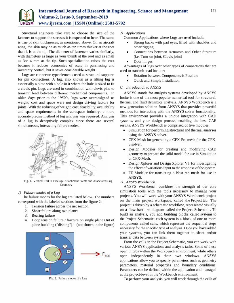
Lugs are connector type elements used as structural supports

for pin connections. A lug, also known as a lifting lug is

essentially a plate with a hole in it where the hole is sized to fit

a clevis pin. Lugs are used in combination with clevis pins to

transmit load between different mechanical components. In

olden days prior to the 1950’s, lugs were overdesigned as

weight, cost and space were not design driving factors for

joints. With the reducing of weight, cost, feasibility, availability

and space requirements in the aerospace industry, a more

accurate precise method of lug analysis was required. Analysis

of a lug is deceptively complex since there are several

simultaneous, interacting failure modes.

Fig. 1. Vertical Tail to Fuselage Attachment Points and Associated Lug

Geometry

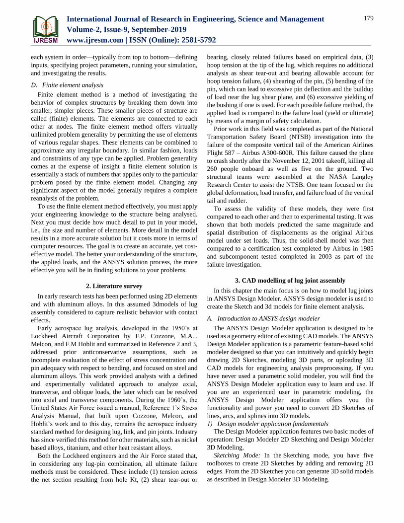
1) Failure modes of a Lug

The failure modes for the lug are listed below. The numbers

correspond with the labeled sections from the figure 2:

1. Tension failure across the net section

2. Shear failure along two planes

3. Bearing failure

4. Hoop tension failure / fracture on single plane Out of

plane buckling ("dishing") -- (not shown in the figure)

Fig. 2. Failure modes of a Lug

2) Applications

Common Applications where Lugs are used include:

Strong backs with pad eyes, lifted with shackles and

other rigging

Connections between Actuators and Other Structure

(i.e. Turn-on joint, Clevis joint)

Door hinges

Advantages of lugs over other types of connections that are

used to transmit load include:

Rotation between Components is Possible

Quick and Simple Installation

C. Introduction to ANSYS

ANSYS stands for analysis systems developed by ANSYS

Incite is one of the most popular numerical tool for structural,

thermal and fluid dynamics analysis. ANSYS Workbench is a

new-generation solution from ANSYS that provides powerful

methods for interacting with the ANSYS solver functionality.

This environment provides a unique integration with CAD

systems, and your design process, enabling the best CAE

results. ANSYS Workbench is comprised of five modules:

Simulation for performing structural and thermal analyses

using the ANSYS solver.

CFX-Mesh for generating a CFX-Pre mesh for the CFX-

5 solver.

Design Modeler for creating and modifying CAD

geometry to prepare the solid model for use in Simulation

or CFX-Mesh.

Design Xplorer and Design Xplorer VT for investigating

the effect of variations input to the response of the system.

FE Modeler for translating a Nast ran mesh for use in

ANSYS.

1) ANSYS Workbench

ANSYS Workbench combines the strength of our core

simulation tools with the tools necessary to manage your

projects. You will work with your ANSYS Workbench project

on the main project workspace, called the Project tab. The

project is driven by a schematic workflow, represented visually

on a flowchart-like diagram called the Project Schematic. To

build an analysis, you add building blocks called systems to

the Project Schematic; each system is a block of one or more

components called cells, which represent the sequential steps

necessary for the specific type of analysis. Once you have added

your systems, you can link them together to share and/or

transfer data between systems.

From the cells in the Project Schematic, you can work with

various ANSYS applications and analysis tasks. Some of these

open in tabs within the Workbench environment, while others

open independently in their own windows. ANSYS

applications allow you to specify parameters such as geometry

parameters, material properties and boundary conditions.

Parameters can be defined within the application and managed

at the project-level in the Workbench environment.

To perform your analysis, you will work through the cells of

International Journal of Research in Engineering, Science and Management

Volume-2, Issue-9, September-2019

www.ijresm.com | ISSN (Online): 2581-5792

179

each system in order—typically from top to bottom—defining

inputs, specifying project parameters, running your simulation,

and investigating the results.

D. Finite element analysis

Finite element method is a method of investigating the

behavior of complex structures by breaking them down into

smaller, simpler pieces. These smaller pieces of structure are

called (finite) elements. The elements are connected to each

other at nodes. The finite element method offers virtually

unlimited problem generality by permitting the use of elements

of various regular shapes. These elements can be combined to

approximate any irregular boundary. In similar fashion, loads

and constraints of any type can be applied. Problem generality

comes at the expense of insight a finite element solution is

essentially a stack of numbers that applies only to the particular

problem posed by the finite element model. Changing any

significant aspect of the model generally requires a complete

reanalysis of the problem.

To use the finite element method effectively, you must apply

your engineering knowledge to the structure being analysed.

Next you must decide how much detail to put in your model,

i.e., the size and number of elements. More detail in the model

results in a more accurate solution but it costs more in terms of

computer resources. The goal is to create an accurate, yet cost-

effective model. The better your understanding of the structure,

the applied loads, and the ANSYS solution process, the more

effective you will be in finding solutions to your problems.

2. Literature survey

In early research tests has been performed using 2D elements

and with aluminum alloys. In this assumed 3dmodels of lug

assembly considered to capture realistic behavior with contact

effects.

Early aerospace lug analysis, developed in the 1950’s at

Lockheed Aircraft Corporation by F.P. Cozzone, M.A...

Melcon, and F.M Hoblit and summarized in Reference 2 and 3,

addressed prior anticonservative assumptions, such as

incomplete evaluation of the effect of stress concentration and

pin adequacy with respect to bending, and focused on steel and

aluminum alloys. This work provided analysts with a defined

and experimentally validated approach to analyze axial,

transverse, and oblique loads, the later which can be resolved

into axial and transverse components. During the 1960’s, the

United States Air Force issued a manual, Reference 1’s Stress

Analysis Manual, that built upon Cozzone, Melcon, and

Hoblit’s work and to this day, remains the aerospace industry

standard method for designing lug, link, and pin joints. Industry

has since verified this method for other materials, such as nickel

based alloys, titanium, and other heat resistant alloys.

Both the Lockheed engineers and the Air Force stated that,

in considering any lug-pin combination, all ultimate failure

methods must be considered. These include (1) tension across

the net section resulting from hole Kt, (2) shear tear-out or

bearing, closely related failures based on empirical data, (3)

hoop tension at the tip of the lug, which requires no additional

analysis as shear tear-out and bearing allowable account for

hoop tension failure, (4) shearing of the pin, (5) bending of the

pin, which can lead to excessive pin deflection and the buildup

of load near the lug shear plane, and (6) excessive yielding of

the bushing if one is used. For each possible failure method, the

applied load is compared to the failure load (yield or ultimate)

by means of a margin of safety calculation.

Prior work in this field was completed as part of the National

Transportation Safety Board (NTSB) investigation into the

failure of the composite vertical tail of the American Airlines

Flight 587 – Airbus A300-600R. This failure caused the plane

to crash shortly after the November 12, 2001 takeoff, killing all

260 people onboard as well as five on the ground. Two

structural teams were assembled at the NASA Langley

Research Center to assist the NTSB. One team focused on the

global deformation, load transfer, and failure load of the vertical

tail and rudder.

To assess the validity of these models, they were first

compared to each other and then to experimental testing. It was

shown that both models predicted the same magnitude and

spatial distribution of displacements as the original Airbus

model under set loads. Thus, the solid-shell model was then

compared to a certification test completed by Airbus in 1985

and subcomponent tested completed in 2003 as part of the

failure investigation.

3. CAD modelling of lug joint assembly

In this chapter the main focus is on how to model lug joints

in ANSYS Design Modeler. ANSYS design modeler is used to

create the Sketch and 3d models for finite element analysis.

A. Introduction to ANSYS design modeler

The ANSYS Design Modeler application is designed to be

used as a geometry editor of existing CAD models. The ANSYS

Design Modeler application is a parametric feature-based solid

modeler designed so that you can intuitively and quickly begin

drawing 2D Sketches, modeling 3D parts, or uploading 3D

CAD models for engineering analysis preprocessing. If you

have never used a parametric solid modeler, you will find the

ANSYS Design Modeler application easy to learn and use. If

you are an experienced user in parametric modeling, the

ANSYS Design Modeler application offers you the

functionality and power you need to convert 2D Sketches of

lines, arcs, and splines into 3D models.

1) Design modeler application fundamentals

The Design Modeler application features two basic modes of

operation: Design Modeler 2D Sketching and Design Modeler

3D Modeling.

Sketching Mode: In the Sketching mode, you have five

toolboxes to create 2D Sketches by adding and removing 2D

edges. From the 2D Sketches you can generate 3D solid models

as described in Design Modeler 3D Modeling.

International Journal of Research in Engineering, Science and Management

Volume-2, Issue-9, September-2019

www.ijresm.com | ISSN (Online): 2581-5792

180

1. Draw Toolbox: drawing lines, rectangles, and splines

2. Modify Toolbox: modifying by trimming, cutting, and

pasting

3. Dimensions Toolbox: defining dimensions in

length/distance, diameter, and angle

4. Constraints Toolbox: applying tangent, symmetry,

and concentricity constraints.

5. Settings Toolbox: plane settings such as grid and grid

spacing

Modeling mode: Modeling mode allows you to create

models, for example, by extruding or revolving profiles from

your Sketches.

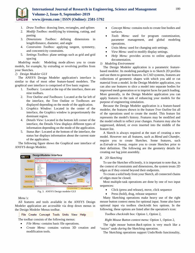
2) Design Modeler GUI

The ANSYS Design Modeler application's interface is

similar to that of most other feature-based modelers. The

graphical user interface is comprised of five basic regions:

1. Toolbars: Located at the top of the interface, there are

nine toolbars.

2. Tree Outline and Toolboxes: Located at the far left of

the interface, the Tree Outline or Toolboxes are

displayed depending on the mode of the application.

3. Graphics Window: Located in the center of the

interface, the Graphics window is proportionately the

dominant region.

4. Details View: Located in the bottom left corner of the

interface, the Details View displays different types of

information depending on the mode of the application.

5. Status Bar: Located at the bottom of the interface, the

status bar displays information about the current state

of the application.

The following figure shows the Graphical user interface of

ANSYS design Modeler.

Fig. 3. ANSYS Design modeler GUI

Menu’s:

All features and tools available in the ANSYS Design

Modeler application are accessible via drop down menus in

the Design Modeler Menus toolbar.

The toolbar consists of the following menus:

File Menu: contains basic file operations.

Create Menu: contains various 3D creation and

modification tools.

Concept Menu: contains tools to create line bodies and

surfaces.

Tools Menu: used for program customization,

parameter management, and global modeling

operations.

Units Menu: used for changing unit settings.

View Menu: used to modify display settings.

Help Menu: provides access to online application

documentation.

3) Modeling Environment

The Design Modeler application is a parametric feature-

based modeler. Its modeling paradigm is to Sketch 2D profiles

and use them to generate features. In CAD systems, features are

collections of geometric shapes with which you add or cut

material from a model. In the Design Modeler application, you

can also use features to slice a model into separate bodies for

improved mesh generation or to imprint faces for patch loading.

More generally, in the Design Modeler application you can

apply features to the task of enhancing your models for the

purpose of engineering simulation.

Because the Design Modeler application is a feature-based

modeler, the features shown in the feature Tree Outline list all

of the operations used to create the model. This feature list

represents the model's history. Features may be modified and

the model rebuilt to reflect your changes. Features may also be

suppressed, deleted, or even inserted into the middle of the

feature list.

A Sketch is always required at the start of creating a new

model. However not all features, such as Blend and Chamfer,

require you to create Sketches. Some features, such

as Extrude or Sweep, require you to create Sketches prior to

their definition. The following are the geometry details for

creating our lug joint assembly.

B. 2D Sketching

To use the Sketcher efficiently, it is important to note that, in

the context of constraints and dimensions, the system treats 2D

edges as if they extend beyond their endpoints.

To create a solid body from your Sketch, all connected chains

of edges must be closed.

Most multiple-task operations are done by one of two input

sequences:

Click (press and release), move, click sequence

Press (hold), drag, release sequence

Many Sketching operations make heavy use of the right

mouse button context menu for optional input. Some also have

optional input via toolbox check/edit box options. In the

following, these options are listed after the operation's icon:

Toolbox check/edit box: Option 1, Option 2,

Right Mouse Button context menu: Option 1, Option 2,

The right mouse button Back option is very much like a

“micro” undo during the Sketching operation.

The Sketching operations support Undo/Redo functionality,

International Journal of Research in Engineering, Science and Management

Volume-2, Issue-9, September-2019

www.ijresm.com | ISSN (Online): 2581-5792

181

but note that each plane stores its own Undo/Redo stacks.

Also note that while in Sketching mode, you can always exit

whatever function you are in and go to the general Select mode,

by pressing the Escape key (Esc). Note that if you have

accessed a window external to the ANSYS Design Modeler

application, you will need to click somewhere back in the

ANSYS Design Modeler application window before

the Escape key (Esc) will be usable.

Undo

Use the Undo command to rescind the last Sketching action

performed.

Redo

Use the Redo command to “redo” a Sketching action

previously undone.

2D Sketching topics include:

Sketches and Planes

Auto Constraints

Details View in Sketching Mode

Draw Toolbox

Modify Toolbox

Dimensions Toolbox

Constraints Toolbox

Settings Toolbox

Sketch Projection

Sketch Instances

1) Sketches and Planes

A Sketch is a collection of 2D edges. A plane can hold any

number of Sketches. Whenever you create a 2D edge using one

of the tools in the Draw Toolbox, it is added to the currently

"active" Sketch. You can click the New Sketch button to create

a new Sketch in the currently "active" plane, or you can select

an already existing Sketch to make it the new active Sketch. In

addition, there are two special types of Sketches:

Sketch Instances (accessible via the Context menus)

allows you to place copies of existing Sketches in

other planes.

Sketch Projection (accessible via the Context menus)

allows you to project 3D bodies, faces, edges, points,

and vertices into a special Sketch in a plane.

Planes without Sketches

If you begin drawing on a plane that has no Sketches, a new

Sketch will be automatically created for you. Once created,

Sketches can be used for feature creation, and they can be

modified at any time using the various Sketching tools.

Points are created automatically at the ends of 2D edges. The

points can then be used for dimensions and constraints.

Additionally, there are options in the Draw Toolbox to create a

point at a screen location or at the intersection of 2D edges.

2) Auto Constraints

During drawing input, if the Auto Constraints Cursor mode

is on, symbols are displayed confirming snapping to either of:

Coincident, depicted by the letter C

Coincident Point, depicted by the letter P

Horizontal, depicted by the letter H

Vertical, depicted by the letter V

Parallel, depicted by the parallel symbol: //

Tangent, depicted by the letter T

Perpendicular, depicted by the perpendicular symbol:

⊥

Equal Radius, depicted by the letter R

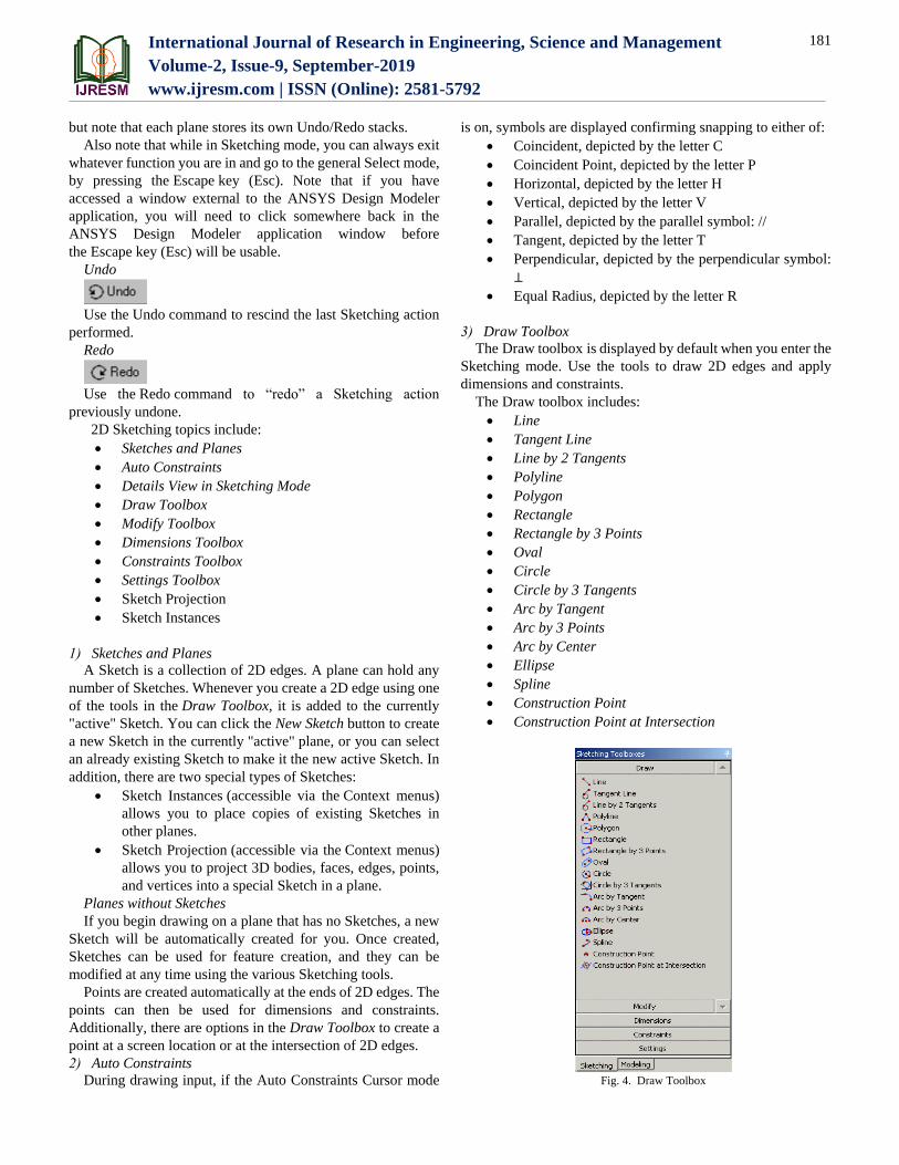
3) Draw Toolbox

The Draw toolbox is displayed by default when you enter the

Sketching mode. Use the tools to draw 2D edges and apply

dimensions and constraints.

The Draw toolbox includes:

Line

Tangent Line

Line by 2 Tangents

Polyline

Polygon

Rectangle

Rectangle by 3 Points

Oval

Circle

Circle by 3 Tangents

Arc by Tangent

Arc by 3 Points

Arc by Center

Ellipse

Spline

Construction Point

Construction Point at Intersection

Fig. 4. Draw Toolbox

International Journal of Research in Engineering, Science and Management

Volume-2, Issue-9, September-2019

www.ijresm.com | ISSN (Online): 2581-5792

182

Modify Toolbox

Use the Modify toolbox to edit your Sketches.

Fig. 5. Modify Toolbox

The Modify toolbox includes:

Fillet, Chamfer, Corner, Trim , Extend, Split, Drag, Cut,

Copy, Paste, Move, Replicate, Duplicate, Offset, Spline Edit.

C. Modeling lug joint Sketch

From the previous discussion about ANSYS Sketch

commands we have to create Sketch for lug assembly:

The following steps followed to create Sketch. Geometry

details are as follows:

Thickness of female lug is: 10mm

Thickness of male lug is : 23mm

Width of lug is : 50mm

Pin diameter is : 20mm

Step-1: Start ANSYS Design modeler and set the units to mm

system

Fig. 6. Units Setting

Step-2: Draw Sketch1 for Base Female Lug as shown

Fig. 7. Female Lug Sketch 1

Step-3: Draw Sketch 2 which represents the pin diameter

Fig. 8. Pin Sketch 2

Step-4: Draw Sketch 3 for male lug Sketch

Fig. 9. Male Lug Sketches

Step-5: Draw Sketch 4 from YZ plane for lug mounting part

Fig. 10. Lug Mounting Sketches

Step-6: Use 3d operations for creating the 3D models of each

part. Here we use extrude option. Use existing suitable Sketch

for each part.

Fig. 11. Female Lug Model

International Journal of Research in Engineering, Science and Management

Volume-2, Issue-9, September-2019

www.ijresm.com | ISSN (Online): 2581-5792

183

Fig. 12. Pin and Male Lug Model

Step-7: Create assembly part for female lugs

Fig. 13. Female Lug Assembly

Step-8: Complete all 3D models for analysis. The following

figure shows the complete assembly of lug joint.

Fig. 14. Full Lug Assembly

Step-9: Observe geometry properties. Here we can see the

volume, area etc.

Fig. 15. Geometry Properties

With the above steps creating the CAD MODEL for lug

analysis completed. Now we can go for further steps to

complete the analysis. Before preceding the analysis we have

to arrange the geometry according to the type of test that

performed on assembly. In this thesis we are performing

analysis in 3 loading conditions on male lug.

1) Axial testing

2) Bending testing

3) Inclined condition testing

The following figures show the Position of Assemblies.

Fig. 16. Lug Joint Assembly in Axial Position

Fig. 17. Lug Joint Assembly in Bending Position

Fig. 18. Lug Joint Assembly Inclined Position

International Journal of Research in Engineering, Science and Management

Volume-2, Issue-9, September-2019

www.ijresm.com | ISSN (Online): 2581-5792

184

4. Static analysis of a lug joint assembly

In this section the main focus is on different design

configuration modes of failures that will affect in the

operational conditions in aero structures.

A. Introduction to analysis procedure in ANSYS

There are mainly 3 stages to complete the analysis in

ANSYS.

1) Preprocessing

2) Solution

3) Post processing

The following diagram shows the methodology

Fig. 19. ANSYS Preprocessing Steps

In previous chapter we discussed creating geometry. Now we

have to convert geometry in to Finite element model by using

meshing operation.

B. Meshing in ANSYS

The ANSYS Meshing application is a separate ANSYS

Workbench application. The Meshing application is data-

integrated with ANSYS Workbench, meaning that although the

interface remains separate, the data from the application

communicates with the native ANSYS Workbench data.

1) Overview of the Meshing Process in ANSYS Workbench

The following steps provide the basic workflow for using the

Meshing application as part of an ANSYS Workbench analysis

(non-Fluid Flow). Refer to the ANSYS Workbench help for

detailed information about working in ANSYS Workbench.

1. Select the appropriate template in the Toolbox, such

as Static Structural. Double-click the template in the

Toolbox, or drag it onto the Project Schematic.

2. If necessary, define appropriate engineering data for

your analysis. Right-click the Engineering Data cell,

and select Edit, or double-click the Engineering Data

cell. The Engineering Data workspace appears where

you can add or edit material data as necessary.

3. Attach geometry to your system or build new

geometry in the ANSYS Design Modeler application.

Right-click the Geometry cell and select Import

Geometry... to attach an existing model or select New

Geometry... to launch the Design Modeler application.

4. Access the Meshing application functionality. Right-

click the Model cell and choose Edit. This step will

launch the ANSYS Mechanical application.

5. Once you are in the Mechanical application, you can

move between its components by highlighting the

corresponding object in the Tree as needed. Click on

the Mesh object in the Tree to access Meshing

application functionality and apply mesh controls.

6. Define loads and boundary conditions. Right-click the

Setup cell and select Edit. The appropriate application

for your selected analysis type will open (such as the

Mechanical application). Set up your analysis using

that application's tools and features.

7. You can solve your analysis by issuing an Update,

either from the data-integrated application you're

using to set up your analysis, or from the ANSYS

Workbench GUI.

8. Review your analysis results.

Here for lug joint analysis we prefer solid mesh.

2) About Solid Mesh

The nodes and elements representing the geometry model

make up the mesh:

A “default” mesh is automatically generated during

a solution.

It is generally recommended that additional controls

be added to the default mesh before solving.

A finer mesh produces more precise answers but

also increases CPU time and memory requirements.

Meshing Methods:

• Meshing Methods available for 3D bodies

– Automatic

– Tetrahedrons

• Patch Conforming

• Patch Independent

– MultiZone

• Mainly hexahedral elements

– Hex dominant

– Sweep

– Cut Cell

• Meshing Methods available for 2D bodies

Fig. 20. 3D Element Types

3) Local Mesh Controls

Local mesh controls are available when you highlight

a Mesh object in the tree and choose a tool from either the Mesh

International Journal of Research in Engineering, Science and Management

Volume-2, Issue-9, September-2019

www.ijresm.com | ISSN (Online): 2581-5792

185

Control drop-down menu, or from first choosing Insert in the

context menu (displayed from a right mouse click on

a Mesh object).

C. Boundary Conditions

Boundary conditions are often called "loads" or "supports".

They constrain or act upon your model by exerting forces or

rotations or by fixing the model it such a way that it cannot

deform.

Boundary conditions are typically applied to 2D or 3D

simulations but exceptions do exist. Any exceptions are

discussed in detail on the Help page for the particular boundary

condition. The boundary conditions you apply depend on the

type of analysis you are performing. In addition, the geometry

(body, face, edge, or vertex) or finite element selection to which

a boundary condition is applied also varies per analysis type.

Once applied, and as applicable to the boundary condition

type, the loading characteristics must be considered. This

includes, whether the boundary condition is defined as a

constant, by using tabular entries (time history or spatially

varying), or as a function (time history or spatially varying).

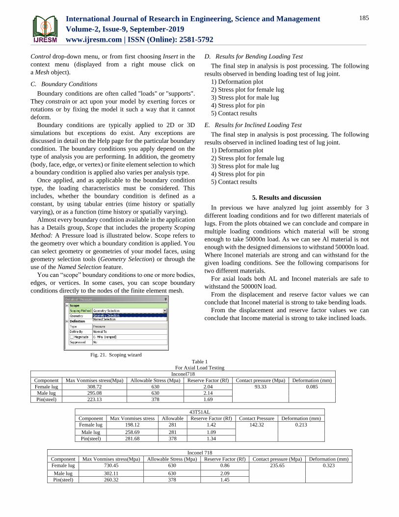
Almost every boundary condition available in the application

has a Details group, Scope that includes the property Scoping

Method: A Pressure load is illustrated below. Scope refers to

the geometry over which a boundary condition is applied. You

can select geometry or geometries of your model faces, using

geometry selection tools (Geometry Selection) or through the

use of the Named Selection feature.

You can “scope” boundary conditions to one or more bodies,

edges, or vertices. In some cases, you can scope boundary

conditions directly to the nodes of the finite element mesh.

Fig. 21. Scoping wizard

D. Results for Bending Loading Test

The final step in analysis is post processing. The following

results observed in bending loading test of lug joint.

1) Deformation plot

2) Stress plot for female lug

3) Stress plot for male lug

4) Stress plot for pin

5) Contact results

E. Results for Inclined Loading Test

The final step in analysis is post processing. The following

results observed in inclined loading test of lug joint.

1) Deformation plot

2) Stress plot for female lug

3) Stress plot for male lug

4) Stress plot for pin

5) Contact results

5. Results and discussion

In previous we have analyzed lug joint assembly for 3

different loading conditions and for two different materials of

lugs. From the plots obtained we can conclude and compare in

multiple loading conditions which material will be strong

enough to take 50000n load. As we can see Al material is not

enough with the designed dimensions to withstand 50000n load.

Where Inconel materials are strong and can withstand for the

given loading conditions. See the following comparisons for

two different materials.

For axial loads both AL and Inconel materials are safe to

withstand the 50000N load.

From the displacement and reserve factor values we can

conclude that Inconel material is strong to take bending loads.

From the displacement and reserve factor values we can

conclude that Income material is strong to take inclined loads.

Table 1

For Axial Load Testing

Inconel718

Component Max Vonmises stress(Mpa) Allowable Stress (Mpa) Reserve Factor (Rf) Contact pressure (Mpa) Deformation (mm)

Female lug 308.72 630 2.04 93.33 0.085

Male lug 295.08 630 2.14

Pin(steel) 223.13 378 1.69

43T51AL

Component Max Vonmises stress Allowable Reserve Factor (Rf) Contact Pressure Deformation (mm)

Female lug 198.12 281 1.42 142.32 0.213

Male lug 258.69 281 1.09

Pin(steel) 281.68 378 1.34

Inconel 718

Component Max Vonmises stress(Mpa) Allowable Stress (Mpa) Reserve Factor (Rf) Contact pressure (Mpa) Deformation (mm)

Female lug 730.45 630 0.86 235.65 0.323

Male lug 302.11 630 2.09

Pin(steel) 260.32 378 1.45

International Journal of Research in Engineering, Science and Management

Volume-2, Issue-9, September-2019

www.ijresm.com | ISSN (Online): 2581-5792

186

6. Conclusion

Contact linear static analysis has been carried out to check

the contact pressure, proof stress and deformation of lug and pin

interface. the analysis techniques and knowledge presented here

is most relevant for the design of lug joints in aero structures.

the mechanical design of lug joint has remained relatively

unchanged for even longer. perhaps there is an opportunity for

a total mechanical redesign of lug joint, derived from

intentional design and optimization of all design parameters. the

results show a stress development of around 730 Mpa near the

left side of the pin hole interface; this is due to contracting

contact surface due to bending loading. maximum contact

pressure of 235Mpa & 190.68Mpa has been observed on pin

and lug interface for bending load conditions.

For lug design analysis bending load conditions are crucial.

three analysis tests have been performed on lug joint assembly

under 50000N crucial load in worst conditions of aero

structures. contact status and contact pressures between pin and

lugs have observed in all loading conditions. reserve factors for

all limit loading conditions observed in all three load cases.

References

[1] K. Mahadevan and K. Balaveera Reddy, “Design data hand book,” 3rd

edition, 1987.

[2] B. K. Sriranga, C. N. Chandrappa, R. Kumar and P. K. Dash, “Stress

Analysis of Wing-Fuselage Lug Attachment Bracket of a Transport

Aircraft”, International Conference on Challenges and Opportunities in

Mechanical Engineering, Industrial Engineering and Management

Studies, (ICCOMIM - 2012), 11-13 July 2012.

[3] Military Handbook 5H – Metallic Materials and Elements for Aerospace

Vehicle Structures, Columbus: Battelle Memorial Institute, 1998.

Table 2

For Bending Load Testing-1

20243T51AL

Component Max Vonmises stress Allowable Reserve Factor (Rf) Contact Pressure Deformation (mm)

Female lug 699.54 281 0.40 190.68 0.859

Male lug 272.04 281 1.03

Pin(steel) 314.83 378 1.20

Table 3

For Inclined Load Testing Inconel718

Component Max Vonmises stress(Mpa) Allowable Stress (Mpa) Reserve Factor (Rf) Contact pressure (Mpa) Deformation (mm)

Female lug 625.72 630 1.01 104.81 0.242

Male lug 174.92 630 3.60

Pin(steel) 148.64 378 2.54