Design and Analysis of Algorithms

Design and Analysis of Algorithms

Prof. Sunder Vishwanathan

Department of Computer Science Engineering

Indian Institute of Technology, Bombay

Lecture - 8

Divide and Conquer - III

Surfing Lower Bounds

We will again look at sorting. Many of these algorithms merge sort, quick sort and

some of the other sorting algorithms that we have studied. All of them seem to take n log

n time. I think it is a good question to ask, if we can do faster. And we this n log n, which

most of the sorting algorithms seem to take. And this is the question, we would like to

address in this part of the course.

In fact, we will show that for a large family you have sorting algorithms. N log n is the

best that they can do. If we sort of restrict, the kinds of things that algorithms can do on

inputs. And n log n is the best that we can do. Now, we look at merge sort. Let us take

merge sort, but whatever I say is actually true even for, let us say quick sort. For merge

sort the what really happens.

You split the array into two parts. And then, recursively sort these things. And then, you

merge these two sorted arrays. That is the crucial step. What happens when you merge

two sorted sub arrays, or when you merge two sorted lists. Well, you compare two

elements and then, move them out. Compare the first element in the list. That is the

smallest and we put it as a first element. Then, move your pointers and so on, and so

forth.

So, the most important step there is comparing two elements and then, some reordering.

So, the only operation that, you actually do on these elements in the sorted, in the array is

comparing two elements and moving them out. So, this property actually holds even for

quick sort. So, always quick sort term, you pick a pivot, by your favorite procedure. And

now you compare every element with the pivot.

Once you compare every element with the pivot and then, you move these elements

around. So, the basic operation on two elements of the array is compare these two.

Figure out which one is larger, which one is smaller. So, again the usual sort of operation

is compared, is looking at two elements in the array, comparing them. And then, based

on the result, I mean if one is smaller than the other.

Or first one is bigger than the other, then you sort of either switch them around or change

the order. So, this is the crucial operation, that you do on the array element. You do not

add them, subtract them, divide them. So, the operations that, we use in at least these

popular sorting algorithms, is compare two elements. May be swap them or move them

around. So, if these are the only things, that you can do with array elements.

Then, you need n log n comparisons to sort an array. So, this is our goal. That is what we

are going to show. Then, how do we go about doing this. Well, even if you recall, we

showed that, find the minimum you needed n minus 1 comparison. And even there, it

was not an obvious, sort of the solution was not absolutely obvious. You had to do little

bit of work. And for this actually we need to do a little bit more of work, but it is not

difficult. So, the first thing is to notice that these algorithms can be written as flowcharts,

or comparison trees. What is a comparison tree? Well, basic block is comparison

between two elements.

(Refer Slide Time: 04:52)

.

So, I compare two elements, a i and a j upon array, for a branch this way, if a i less than a

j. I branch this way, if a j is greater than a i. We will assume that, array elements are

distinct, which means I will never have two of them equal. So, compare two elements,

branch this way if a i is less than a j, branch the other way if a i is greater than a j. Now,

using these as building blocks, I can build the large flow chart. So, somewhere here,

maybe I can compare two elements, two other elements a k and a l.

Then again branch and so on. And at the end, I will have these leaves where I will

output. So, the output for us is the order, is the sorted order. So, we will look at flow

charts, which look like this. The input to a flow chart is just an array a, the input is an

array a. And you go through these flow charts and at these leaves, will output the sorted

order. This is the model that we are looking at. Let us do a small example.

(Refer Slide Time: 06.35)

So, for instance if I have two elements, then let us say a 1 and a 2, I compare a 1 and a 2.

If it is less than the order output is a 1, a 2. This is in sorted order. If a 1 is larger, the

order I output is a 2, a 1. So, here is a small flow chart, that sorts 2 numbers. So, it sorts

two elements an array, basically works on arrays of size 2 and sorts these arrays. So, let

us say 3, what if the array size is 3? So, let us see what to do.


So, you compare, let us say a 1 and a 2. Now, if a 1 is less let us say I compare a 1 with a

3, say a 1 is less. Now, I know at this point, that a 1 is the smallest. So, I would like to

compare a 2 and a 3. So, here a 2 is greater than a 3, here a 2 is less than a 3. The sorted

order here is a 1, a 2, a 3. Here it is a 1, a 3, a 2 and so on. So, you can sort of fill this up.

So, you can write down a flow chart like this, with these are the leaves where you get the

answer, which is the array in sorted order. Now, merge sort can also be depicted like this.

So, let us see, why that is do.


So, let us look at merge sort or when four elements. So, I have four elements a 1, a 2, a 3,

a 4. And I want to sort of run merge sort on this. Well, we divide this into two, recurs on

this part, then recurs on this part and then, there is a merge. When we recurs on this part,

the first comparison we do is between a 1 and a 2. So, this is the first comparison we do;

and this could be a 1 is less than a 2.

This is a 1 could be greater than a 2, we do not know what this is. Here the sorted order

which is returned here is a 1, a 2. On this side it is a 2, a 1. Whichever branch we choose,

now we have to recurs on the right hand side. So, this is the next comparison we do, a 3

and a 4; and well these give again two sort of outputs. Now, at this step, we are up to the

merge. The lower things return, these two sorted orders.

And now we are down to the merge, the top level of recursion. So, let us take this

portion. What are the two elements, that are compared? Here I know that a 1 is greater

than a 2. So, the first one returns, this side returns a 2 a 1. And here, I know a 3 is less

than a 4. So, the second list returned is a 3 a 4. These are the two lists. So, the two

elements compared here, are a 2 and a 3.

The smallest elements from the two lists are compared now. So, this is what is compared

here. So, let us go down one more step and see how this looks like. So, here a 2 is less or

a 3 is less. Supposing, we followed this branch, what is the next clue, which are

compared for merge sort. Well, a 3 is less than a 2. So, a 3 is moved to the new list and

our pointers are at a 2 and a 4. So, the next two things, which are compared are a 2 and a

4 and so on.

I can draw this tree out and at the leaves of this tree, are the solution. I mean at each leaf,

I will tell you what is the output, what is the sorted order which it output. In fact, if you

look at this tree, this tree is a binary tree. At each internal load, we have a comparison.

So, we compare two elements, that you branch out into two. And for each branch again

there will an internal node, you compare two elements branch into two, that is it.

So, if I just look at it as, if I forget that, there these comparisons etcetera, etcetera. The

whole structure looks like a tree. In fact, the binary tree and there are leaves, and at these

leaves we have the output. Output mean in the sorted order. So, when I sort of follow this

tree down to a leaf, I get the answer. This leaf whatever is the answer is the output. The

one thing to notice is that, this tree is different for different sizes of the input.

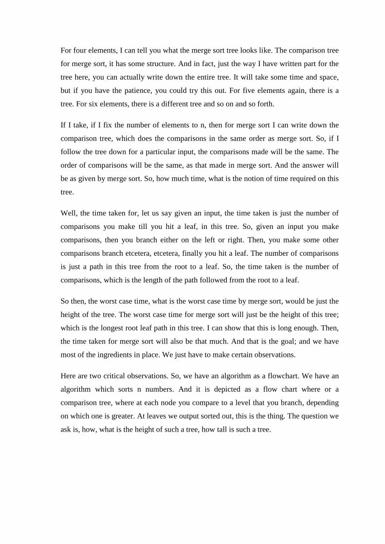
For four elements, I can tell you what the merge sort tree looks like. The comparison tree

for merge sort, it has some structure. And in fact, just the way I have written part for the

tree here, you can actually write down the entire tree. It will take some time and space,

but if you have the patience, you could try this out. For five elements again, there is a

tree. For six elements, there is a different tree and so on and so forth.

If I take, if I fix the number of elements to n, then for merge sort I can write down the

comparison tree, which does the comparisons in the same order as merge sort. So, if I

follow the tree down for a particular input, the comparisons made will be the same. The

order of comparisons will be the same, as that made in merge sort. And the answer will

be as given by merge sort. So, how much time, what is the notion of time required on this

tree.

Well, the time taken for, let us say given an input, the time taken is just the number of

comparisons you make till you hit a leaf, in this tree. So, given an input you make

comparisons, then you branch either on the left or right. Then, you make some other

comparisons branch etcetera, etcetera, finally you hit a leaf. The number of comparisons

is just a path in this tree from the root to a leaf. So, the time taken is the number of

comparisons, which is the length of the path followed from the root to a leaf.

So then, the worst case time, what is the worst case time by merge sort, would be just the

height of the tree. The worst case time for merge sort will just be the height of this tree;

which is the longest root leaf path in this tree. I can show that this is long enough. Then,

the time taken for merge sort will also be that much. And that is the goal; and we have

most of the ingredients in place. We just have to make certain observations.

Here are two critical observations. So, we have an algorithm as a flowchart. We have an

algorithm which sorts n numbers. And it is depicted as a flow chart where or a

comparison tree, where at each node you compare to a level that you branch, depending

on which one is greater. At leaves we output sorted out, this is the thing. The question we

ask is, how, what is the height of such a tree, how tall is such a tree.


Here are two sort of crucial observations, if this flow chart does sort. Then, every input

order must leads to a leaf. Different input orders lead to different leaves. So, why is this

true? Well, firstly we will assume that inputs, in our input every element is distinct. We

do not have two copies of the same element. There are n factorial orders, that are

possible as input. And for each order you make certain comparisons and you trace the

path to a leaf. And at the leaf, we have to give the right order, which is a permutation of

the input.

And for every input order, you must end up with a different leaf, because the

permutations are different. So, for instance, if I look at 1 2 3 this is already sorted. If I

look at 1 3 2, the sorted order is 1 2 3. So, I have to interchange the last two elements.

This order must appear at a different leaf, which means all of these n factorial

permutations; must appear in one of these leaves. And different permutations must

appear at different leaves.

So, because of the order of the input is different and must land up in different leaf. I land

up in the same leaf, I will give the same answer for both orders, which is incorrect. So,

this means, there must be n factorial leaves in this binary tree. And each of these

different orders, must land up in the leaf. And different orders must land up in different

leaves, which means there must be n factorial leaves in this binary tree. So, intuitively

you can see, why the height must be large.

So, if I have a binary tree with large number of leaves, the height better be large. So, we

will invoke theorems, which you must have seen in discrete structures; and we will finish

the proof. So, if I look at this flow chart or this decision tree.


Then, I have a binary tree and I know that number of leaves is at least n factorial. Using

these, I want to conclude that the height is at least something. So, if I can put something

here, the height at least something. Then, I know that the time taken by the algorithm

must also be at least this much. So, why can I say this is the height is most ((Refer Time:

19:42)). Well, supposing I have a binary tree of height h, what is the maximum number

of leaves, that this can have.

This is something which you have done in discrete structures, so let us state this. So,

binary tree of height h has at most, well 2 to the h leaves. The number of leaves can be at

most 2 to the h. Well, let us I hope you can sort of prove this. Let us give a proof

anyway. So, proof is by induction on h, so the base case I will let you do this. H equals 1,

I will let you do this, so the inductive step. So, how do we ((Refer Time: 20:46)) the two

steps.


Well, let us look at a tree, that T be a binary tree of height, let us say K plus 1. So, we

will assume that, the statement is true for all binary trees of height k or smaller. And we

would like to prove, the statement for a height K plus 1. So, the inductive hypothesis is

that, for every tree of height k or smaller, the statement holds. And we would like to

prove this for tree of height K plus 1. So, if I look at T, T has a root and then, there are

two sub trees.

This is what it looks like T 1 and T 2. Now, well I remove the root and now I am going

to apply induction to T 1 and T 2. Apply the inductive hypothesis to T 1 and T 2. Well,

this had height K plus 1, which means both T 1 and T 2 have height k or less. One of

them has height K, the other could be k or it could be less. So, the height of T 1 is less

than equal to k. Similarly, height of T 2 is less than equal to k. That is the reason, we can

apply the inductive hypothesis. Both of them have height less.

Now, we can apply the inductive hypothesis. So, the number of leaves in T 1, is less than

equal to 2 to the k. Similarly, number of leaves in T 2 is less than equal to 2 to the k. And

now you can see, basically the number of leaves in T, is number of leaves in T 1 plus the

number of leaves in T 2; which is this plus this which is at most 2 to the k plus 1. And

that is the end of the proof.


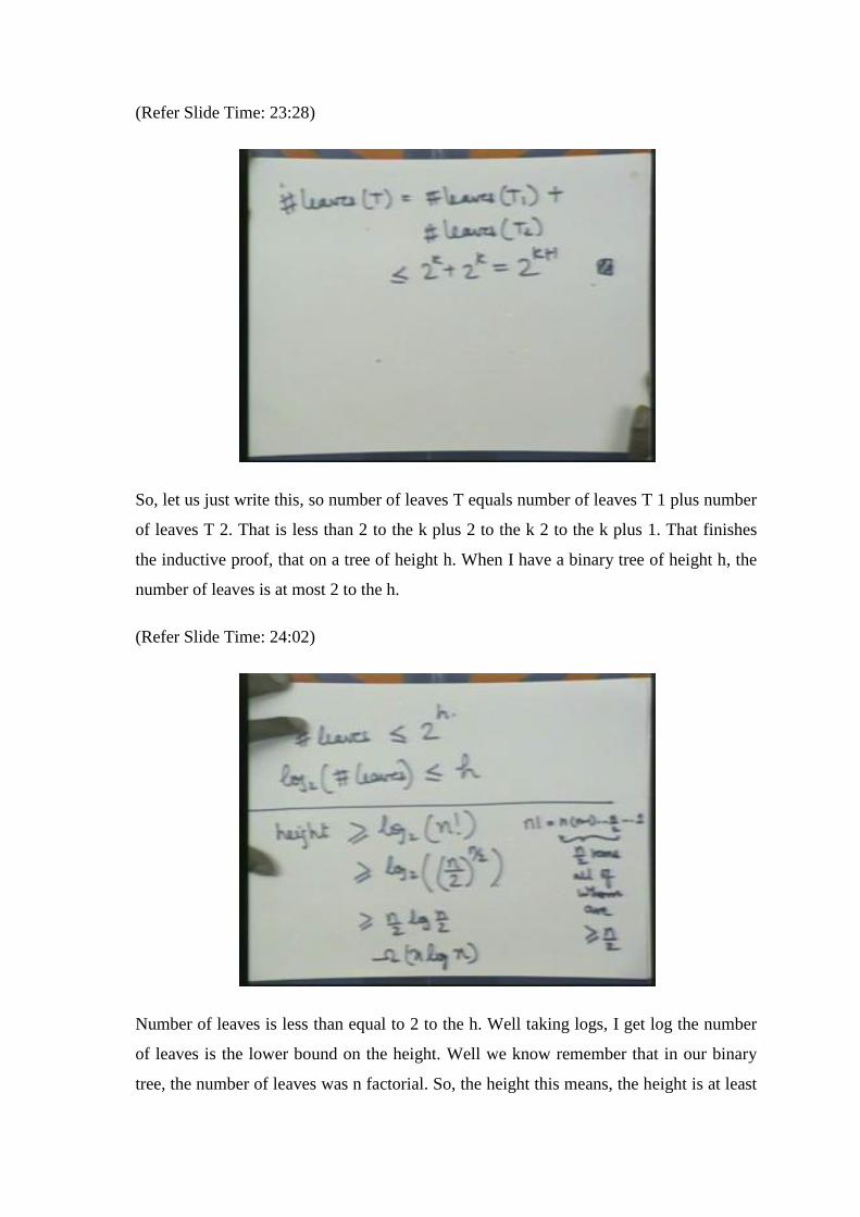
So, let us just write this, so number of leaves T equals number of leaves T 1 plus number

of leaves T 2. That is less than 2 to the k plus 2 to the k 2 to the k plus 1. That finishes

the inductive proof, that on a tree of height h. When I have a binary tree of height h, the

number of leaves is at most 2 to the h.


Number of leaves is less than equal to 2 to the h. Well taking logs, I get log the number

of leaves is the lower bound on the height. Well we know remember that in our binary

tree, the number of leaves was n factorial. So, the height this means, the height is at least

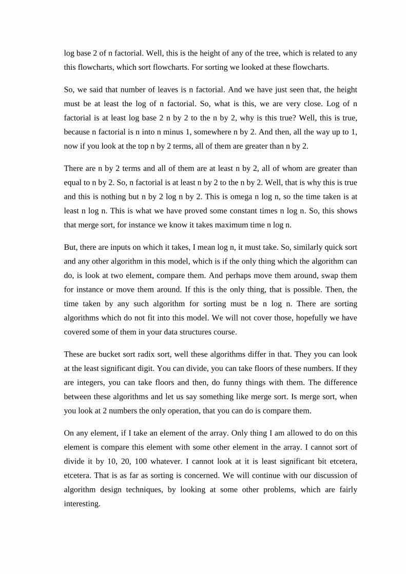
log base 2 of n factorial. Well, this is the height of any of the tree, which is related to any

this flowcharts, which sort flowcharts. For sorting we looked at these flowcharts.

So, we said that number of leaves is n factorial. And we have just seen that, the height

must be at least the log of n factorial. So, what is this, we are very close. Log of n

factorial is at least log base 2 n by 2 to the n by 2, why is this true? Well, this is true,

because n factorial is n into n minus 1, somewhere n by 2. And then, all the way up to 1,

now if you look at the top n by 2 terms, all of them are greater than n by 2.

There are n by 2 terms and all of them are at least n by 2, all of whom are greater than

equal to n by 2. So, n factorial is at least n by 2 to the n by 2. Well, that is why this is true

and this is nothing but n by 2 log n by 2. This is omega n log n, so the time taken is at

least n log n. This is what we have proved some constant times n log n. So, this shows

that merge sort, for instance we know it takes maximum time n log n.

But, there are inputs on which it takes, I mean log n, it must take. So, similarly quick sort

and any other algorithm in this model, which is if the only thing which the algorithm can

do, is look at two element, compare them. And perhaps move them around, swap them

for instance or move them around. If this is the only thing, that is possible. Then, the

time taken by any such algorithm for sorting must be n log n. There are sorting

algorithms which do not fit into this model. We will not cover those, hopefully we have

covered some of them in your data structures course.

These are bucket sort radix sort, well these algorithms differ in that. They you can look

at the least significant digit. You can divide, you can take floors of these numbers. If they

are integers, you can take floors and then, do funny things with them. The difference

between these algorithms and let us say something like merge sort. Is merge sort, when

you look at 2 numbers the only operation, that you can do is compare them.

On any element, if I take an element of the array. Only thing I am allowed to do on this

element is compare this element with some other element in the array. I cannot sort of

divide it by 10, 20, 100 whatever. I cannot look at it is least significant bit etcetera,

etcetera. That is as far as sorting is concerned. We will continue with our discussion of

algorithm design techniques, by looking at some other problems, which are fairly

interesting.

And where this divide and conquer paradigm sort of works, and gives you better results.

In some cases perhaps you the algorithm, that we desire.


The first one is this, so you are you are given a 2 k. So, this is the input by 2 k square.

And what you want as output is a tiling with, I will tell you what all this means, with

this. What do I mean by tiling, a tiling essentially means, I must fill up all these squares.

And try and fill up as many squares as possible with pieces, which look like this. So,

each piece is, let us say a kind of a domino, which sort of looks is of this shape.

And I want to try and fill up, as many squares as possible in this. So, well you can see

immediately, I may not be able to fill up all square. Even for k equals 1, if I have a 2 by 2

square, I have a 2 by 2 square. Well I can put one of them. So, I can put something which

fills up these three squares and this will be an empty square. So, here is a tiling of a 2 by

2 square with a domino of this form, which does everything except one square. So, what

about 2 to the k cross 2 to the k.

Well, the number of squares, we look at the number of squares is 2 to the 2 k. These are

the number of squares, the number of squares and this is 1 mod 3. I will let you figure

this one out. The number of squares is always 1 mod 3. Well it is 2 here and you can see,

that it is always two. If you want you can prove it by induction on k, but even otherwise

you can sort of check that, the number of squares will be always 1 mod 3. Maybe we will

just look at a equals 2.

So, then it is a 4 by 4, how does this look like. So, this is a 4 by 4 thing and you have

well 16 squares; and that is 1 mod 3. When I divide this by 3 I get 1, so 3 times 5 is 15

and 1, one gets left out. So, that is true whatever k I choose, it is always 3 times

something plus 1. So, that is what I mean by 1 modulo 3. When I divide by 3 I get 1, the

remainder is 1.

So, can I sort of now put these dominos. So that, all except 1 square is covered. So, I

have this 2 by 2 k 2 to the k by 2 to the k square. So, I will square with side length to the

k. I have these dominos, which each of them has 3 squares put together. Can I arrange

these on these squares, so that all except 1 square is covered, this is the question; the

answer is yes. And we would like an algorithm to do this and well, we would like to do it

using divide and conquer.

That is the goal, let us do this 4 by 4. And then, we will see what is the scene. Can I do a

4 by 4 with, so here is a 4 by 4 square, can I do this. Well, since I am going to do

something like divide and conquer. I would like to divide this into two parts, or more. In

this case four parts, tile each of them and put them together.


Well, let us take a bigger one and see how this is done. I know how to tile this, so that

one is left, I know how to tile this, so that one is left and so on. Now, how do I tile the

whole thing, so that one is left. Well supposing the one left here is this. One left here is

this and one left here is this. Now, I am able to tile all four of them. So, I tile this, so that

this is my first domino, I use my first domino there, I put it around like this.

This is my second domino, I put it around like this. Here is 3, it does not matter how I

put my fourth as of now. We will we will change this later, supposing the fourth is like

this. Well now I can put the fifth domino here, here 5 5 5. So, I managed to sort of tile at

least 4 by 4 using 5 dominos. I have just one left which is what I want. You would like to

repeat this for 2 k by 2 k. So, how does that look.

So, here we again would like to do a divide and conquer, we would like to divide this. I

would like to first tile this, tile these 4 and then put them together. Well, by looking at

this, this example I can do it if provided this square left off here is this. The square left

off in this, is this. The square left off here is this. Here I really do not care. If I can tile

the entire region here, except this corner and so on. For these 3, then I am able to tile the

entire region on top leaving one squares.

That square left will be in this big sort of region. This is 2 to the k minus 1, 2 to the k

minus 1, 2 to the k minus 1 and so on. So, this whole thing is 2 to the k. So, if I can do

this, then I can fit in this entire, this extra sort of domino here. There will be one square

left over in this region, good. So, again notice a crucial thing, to be able to carry this

inductive process, to completion. I should be able to have the extra square. I mean the

square left over as a corner square.

When I tile a region which is like this, the left over square must be a corner square. So,

this is a square left over or left un tiled. I have tiled the entire region, except this small

square. If I can do this, then clearly I can do the big thing. So, I started out my initial

objective was to tile to 2 to the k by 2 to the k. That is what I started out with, I want to

apply this divide and conquer kind of thing. Well, actually the process is really induction

always.

If I can do it for a small square, can I push it up to a bigger square, that is the goal. Well,

we want to do divide and conquer. So, we saw that, we break it up into these 4 smaller

squares. Now, I want to tile these smaller squares and put them up, to a tiling for the

bigger square. Well, each of these smaller squares, that is one square, one small square

which is not tiled. One piece which is not tiled. Now, this happens to be the corner, then

I can push the induction upwards.

But, for the induction to work even the final, so let us look at this again. For the

induction to work in this big square, I want the one square which is not tiled to be a

corner. Well, it cannot be corner here, because everything else is tiled, this cannot be a

corner, it cannot be a corner. Well, can it be this corner, the answer is yes. It is like I

leave this square un tiled, so leave this...

Now, when I look at these 4 small problems, they all look absolutely alike. I want to tile

everything, except a small square in the corner. I want to tile all of it, except this square

in the corner. Except this in the corner and except this in the corner. And I put them

together like this. This tile is the entire big square, except for this one thing in the corner.

And well this is the algorithm, break it up into 2.

Tile these 4 recursively and put them together like this, and in the middle I just put one

domino. One domino fill up these three squares, so I have tile everything except this. So,

this is a well divide and conquer sort of strategy to tile squares. So, this problem looks a

bit different from the other problems. And that is why I picked this, because the strategy

can be used not just for computer algorithms or puzzles, or whatever you have. And the

other sort of lesson, that we learn through this example. Is that you start with some

problem you want to solve.

We have seen this before, along the way you would like to apply, you want to find

solutions to smaller sub problems. You want to put these together to get a solution to a

larger problem. And while doing this, you may want to solve something slightly more

general. And then, you see this general problem can be solved. So, you try and solve the

general problem now, again using the same technique.

The smaller sub problems, you solve the general problem. And now you see, if you can

put them together, to get a solution to the general problem for the big input. And often

this sort of gives you the solution that want. We saw this in two occasions, one was this

tiling problem, the other was a I hope you can remember. It was when we looked at this

median. We wanted to find the median, but we ended up looking at the problem of

finding an element of given an array and a positive integer r.

So, we found the element of rank r, that is what we did. So, let us look at one more

problem, yet another problem rather, which uses divide and conquer. So, this is a

familiar problem of multiplying to two integers. So, let us look at this.


So, I have 2 n bit integers, x and y, this is x, this is y, these are n bits. Each is n bit long, I

want to find the product of x and y. The normal way is well, we formed the product of

each of these bits with LSB, then with the next one and so on, and so forth. So, there are

n square multiplications. Well, in this case actually it is not, you can just do are and since

they are bits. But, you can think of these as instead of bits, you can think of them as

digits, it really does not matter.

So, each of them could be n digits long and we multiply these digits. So, there are n

square multiplications, this is the high school multiplication algorithm, that we know.

Can we do faster, that is the question. Let us try applying divide and conquer. I have

divide this into two parts. This is x left x right, y left y right. And now I want to compute

the product of these two, well what is the product first of all. X is nothing but 2 to n by 2

times x l plus x r y is 2 to the n by 2 y l plus.

So, this means x y is 2 to n x l y l plus 2 to the n by 2 x l y r. X l y r plus y l x r plus x r

times y r, this is the product x and y. So, we could recursively sort of find these products,

these four products and then, compute this. This is just shifting by n bits, we are just

shifting by n by 2 bits. So, that is an order n operation, so if T n is the time taken, this

what is the recurrence.

There are 1, 2, 3, 4, 4 problems, so 4 times T n by 2 plus order n. This is some constant

times n, which is for shifting and adding. Adding two n bit numbers, it takes alternately.

So, what is the solution to this recurrence? Well, I will let you do this and the solution to

this recurrence. You do a solution to this recurrence, it is order n square. So, we are back

to where we started. Compare these two, well we have done divide and conquer, but we

do not seem to have conquered anything.

We are back to spending order n square times, even with this divide and conquer

approach, but well all is not lost. I will first indicate this algorithm. And then, we will

analyze, and see how we can decrease the number of multiplications. So, well the trick is

this, let us see.


So, the terms that we want to compute are x L y L and then, x L y R plus y L x R and x R

y R. These are the three terms, that we would like to compute. The way we did it, was

each of them separately that gave over problems of size n by 2. So, here is a smart way

of doing this. Well, these two I compute as they are, the third thing I compute is not quite

these two, it is the following. I computer x L plus x R times y L plus y R, I add x L and x

R, I add y L and y R and then, multiply them together.

What is this, this is x L y L plus x L y R plus x R y L plus x R y R, that is what this is.

So, I do three multiplications and not four, this is the first multiplication x L y L. X R y

R is my second multiplication and this is the third. This I do not do, as of now I have not

touched this, this is the third multiplication I do. Well, if you look at this x L y L is

present, x r y r is present; and if I remove these two what is left is this. X L y R plus x R

y L is exactly this.

Well, I have just written x R y L, but it is same as y L x R good. So, how do I compute

this, well from this product I just subtract these two to get this, so call this Z. Now, I just

do Z minus x L y L minus x R y R I get this, good what have I done. Well I have a few

more additions, I have 1, 2, 3, 4 more additions. The number of multiplications has gone

down by 1. Multiplying 2, n by 2 bit numbers I do 1, 2 and 3. There are now only 3

multiplications that I do.

So, what is the recurrence now, well T n is 3 T n by 2 plus order n. Earlier remember it

was 4 T n by 2 plus order n. Now, it is 3 T n by 2 plus order n and it is not surprising,

that the solution to this recurrence is smaller. In fact, we will show the solution to this

recurrence, is order n to the log 3 base 2. Roughly it grows as n to the 1.59, which is

certainly less than n square, which is what we started out with. So, this the number of

multiplications one makes is significantly smaller.


Is 3 T n by 2 plus some let us this take n, it does not matter, so T n is this. We will do the

usual thing which is 3, so 3 T n by 2 square plus n by 2 plus n. This is 3 square T n by 2

square plus 3 times n by 2 plus n. Let us do it once more, to see what happens, so this is

3 square T well n by 2 cube. I am expanding this out, so there should be a 3 here, 3 times

plus n by 2 square plus 3 times n by 2 plus n.

So, this is now 3 cube T n by 2 cube plus, well 3 by 2 whole square times n plus 3 by 2 n

plus n. Now, one can guess the general term, in this when I go down i steps.


So, T n will be 3 to the i T of n by 2 to the i plus 3 by 2 to the i minus 1 n plus 3 by 2 i

minus 2 n so on, to n, good. So, now we would like n by 2 to the i should be 2 or say 1,

for ease of computation. If this is one, if I have one bit and the time is 1, so the time is

just this becomes T of 1 is 1. So, if this is true and T of n is 3 to the i plus, well n times 1

plus 3 half and so on, up to 3 half to the i minus 1. Well, let us do this, so this is 3 to the i

plus n times, well what is this? This is just a geometric series.

So, it is a roughly some constant times 3 half to the i. You can do it more a bit better by

doing the, writing the exact formula, which is 3 half to the i minus 1 by 3 half minus 1.

So, it is at most, let me put it at most this is perhaps 3 half minus 1 which is half, so C

could be 2, so C is most probably 2. In any case, this is bounded by something like this, 3

to the i plus. So, what is i? Well, 2 to the i is n, so i is nothing but log base 2 n.

So, this is 3 to the log base 2 n plus n times constant times, well 3 half to the i, which is 3

half to the log based 2 n. Now, 2 to the log base 2 of n is nothing but n, these two things

cancel. So, I have 3 to the log base 2 of n times constant and 3 to the log base 2 of n here.

So, this is nothing but some C prime times 3 to the log base 2 of n, this is the I time

taken.


So, what is this, well so the time, the total number of multiplications is 3 to the log base

2 of n. This is 3 to the log base 3 of n divided by log base 3 of 2, I could take this up. So,

this is nothing but 3 to the log base 2 of 3 times, use just some general manipulations. So,

that is 3 to the log base 3 of n, I take this inside, n to the log base 2 of 3. This is nothing

but n to the log 2 of 3 as promised. So, this is roughly n to the 1.59. So, the time number

of multiplications, we got it down from n square.

So, the initial thing to roughly n to the 1.59. Of course, we increase the number of

additions, but if multiplications are more expensive than additions. Then, we have saved

on time. This trick of using three multiplications instead of 2 is actually a trick. It is

something you have to really need to come up with somehow. There is no real sort of

way in which you can do it. There is no method and that is the beauty of algorithm

design.

That somehow not every problem can be sort of tackled using everything that, you could

come up. Often you come up with, all the time you come up problems which require you

to design new methods, derive new methods, find new methods. Rack your brain and sort

of come up with good algorithms. And when you do come up with these new algorithms,

you feel again, the kick that you derive, the pleasure that you derive is something else.

This trick by the way or this multiplication is due to Euler. And he used this for the

multiplying complex numbers. We have just used this trick was then used by other

people, who saw that. It can be applicable in multiplying 2 n bit numbers.

Thanks.

Design and Analysis of Algorithms

Documents

Transcript of Design and Analysis of Algorithms