
Simulation analysis of algorithms for interference ... - CORE
81
Universit ` a degli studi di Padova Department of Information Engineering Master Thesis in TELECOMMUNICATION ENGINEERING Simulation analysis of algorithms for interference management in 5G cellular networks using spatial spectrum sharing Supervisor Candidate Dr. Michele Zorzi Mattia Rebato Academic Year 2014/2015
-
Upload
khangminh22 -
Category
Documents
-
view
0 -
download
0
Transcript of Simulation analysis of algorithms for interference ... - CORE
Universita degli studi di Padova
Department of Information Engineering
Master Thesis in
TELECOMMUNICATION ENGINEERING
Simulation analysis of algorithms for
interference management in
5G cellular networks using
spatial spectrum sharing
Supervisor Candidate
Dr. Michele Zorzi Mattia Rebato
Academic Year 2014/2015


A tutti coloro che mi hanno sostenuto in questo lungo percorso...
iii

iv
Abstract
With the increasing demand of data and the growth of the connectionsbetween devices, a new generation of mobile networks, denominated 5G, isnecessary in order to reach data rates required.
In this thesis project we completely overhaul past techniques to the newmillimeter wave frequencies used in 5G and the aim is to study algorithm, pro-tocols and architectures enablers to allow spatial spectrum sharing betweendifferent networks at these frequencies.
With the use of specific modules of the network simulator ns-3, studies ofsimulations has been made in order to analyse performance of several sharingprocedure with the goal of increase performance in a mobile network of fifthgeneration. The simulated scenarios will be deeply examined though figuresand graphs which will be used to compare all the procedures’ performances.
v

vi
Sommario
Con l’aumentare del traffico dati e la crescita delle connessioni tra dispositivi,un nuovo standard per reti cellulari, chiamato 5G, e necessario in modo dasoddisfare i flussi dati richiesti.
In questo progetto di tesi abbiamo completamente revisionato i precedentiprotocolli LTE, in modo da poterli usare su frequenze con onde millimetricheusate nel 5G, lo scopo e quello di studiare algoritmi, protocolli e architet-ture in grado di realizzare una condivisine spaziale dello spettro tra diversinetworks.
Utilizzando specifici moduli del simulatore di reti ns-3, abbiamo realizza-to e studiato simulazioni in modo da analizzare il comportamento di alcunetecniche per la condivisione di risorse, con l’obiettivo di aumentare le presta-zioni in una rete cellulare di quinta generazione. Gli scenari simulati sarannoesaminati a fondo con l’uso di figure e grafici in modo da confrontare leprestazioni delle varie procedure.
vii

viii
Contents
List of Figures xi
List of Tables xiii
Acronyms xv
1 Introduction 1
2 Millimeter waves in 5G cellular systems 52.1 5G overview . . . . . . . . . . . . . . . . . . . . . . . . . . . . 52.2 Millimeter waves (mmW) . . . . . . . . . . . . . . . . . . . . . 6
2.2.1 Challenges of mmW . . . . . . . . . . . . . . . . . . . 72.2.2 Benefits of mmW . . . . . . . . . . . . . . . . . . . . . 10
3 Spatial Spectrum Sharing 113.1 Spectrum Sharing in 4G-LTE . . . . . . . . . . . . . . . . . . 113.2 Spatial SPSH in 5G . . . . . . . . . . . . . . . . . . . . . . . . 13
3.2.1 State of the art . . . . . . . . . . . . . . . . . . . . . . 133.2.2 Analysis and limitations . . . . . . . . . . . . . . . . . 15
4 ns-3 and mmW modules 174.1 Description . . . . . . . . . . . . . . . . . . . . . . . . . . . . 174.2 mmW modules . . . . . . . . . . . . . . . . . . . . . . . . . . 18
4.2.1 Physical layer (PHY): Frame and Transmission schemes 18Frame structure . . . . . . . . . . . . . . . . . . . . . . 18Transmission schemes . . . . . . . . . . . . . . . . . . . 20
Channel Quality Indicator (CQI) . . . . . . . . 204.2.2 Physical layer (PHY): Channel model . . . . . . . . . . 21
MIMO . . . . . . . . . . . . . . . . . . . . . . . . . . . 24Beamforming . . . . . . . . . . . . . . . . . . . . . . . 26
Beam specifics . . . . . . . . . . . . . . . . . . . 27Interference . . . . . . . . . . . . . . . . . . . . . . . . 28
ix
4.2.3 MAC layer . . . . . . . . . . . . . . . . . . . . . . . . . 29Adaptive Modulation and Coding (AMC) . . . . . . . 30Scheduler . . . . . . . . . . . . . . . . . . . . . . . . . 30Resource Allocation . . . . . . . . . . . . . . . . . . . . 30Service Access Point (SAP) . . . . . . . . . . . . . . . 31
PHY-MAC . . . . . . . . . . . . . . . . . . . . . 31MAC-SCHED . . . . . . . . . . . . . . . . . . . 32
4.2.4 Simulation . . . . . . . . . . . . . . . . . . . . . . . . . 324.2.5 Results analysis . . . . . . . . . . . . . . . . . . . . . . 33
5 Sharing procedure 355.1 Blind method . . . . . . . . . . . . . . . . . . . . . . . . . . . 355.2 SPSH scenario between different mmW networks . . . . . . . . 355.3 Training method . . . . . . . . . . . . . . . . . . . . . . . . . 37
5.3.1 Centralised implementation . . . . . . . . . . . . . . . 375.3.2 Training algorithm and ns-3 implementation . . . . . . 38
Step 1 - Inter-network interference detection: . . 38Step 2 - Interference information transfer: . . . . 39Step 3 - Coordination context decision: . . . . . 39Step 4 - Scheduling: . . . . . . . . . . . . . . . . 40
5.4 Heuristic method . . . . . . . . . . . . . . . . . . . . . . . . . 425.4.1 Heuristic algorithm and ns-3 implementation . . . . . . 42
Step 1 - Initialization: . . . . . . . . . . . . . . . 42Step 2 - Sampling and processing: . . . . . . . . 42Step 3 - Share of sequences: . . . . . . . . . . . 43
6 Simulated scenarios and results 456.1 Simulation assumption . . . . . . . . . . . . . . . . . . . . . . 45
6.1.1 Jain’s fairness index . . . . . . . . . . . . . . . . . . . 466.2 Simulated parameters . . . . . . . . . . . . . . . . . . . . . . . 466.3 Description of the results . . . . . . . . . . . . . . . . . . . . . 48
6.3.1 Different antenna configuration . . . . . . . . . . . . . 48Variance of the result . . . . . . . . . . . . . . . . . . . 51
6.3.2 Other results . . . . . . . . . . . . . . . . . . . . . . . 52
7 Conclusions and future works 57
Bibliography 59
x
List of Figures
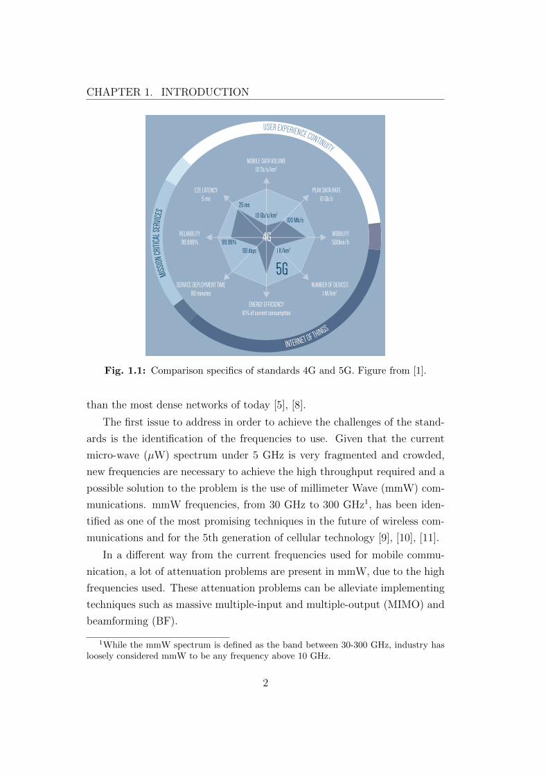
1.1 Comparison specifics of standards 4G and 5G. Figure from [1]. 2
2.1 Overall 5G wireless-access solution consisting of LTE evolutionand new technologies. Figure from [2]. . . . . . . . . . . . . . 6
2.2 Atmospheric absorption across mmW bands. Figure from [3]. . 8
2.3 Rain attenuation in dB/Km at various rainfall rates. Figurefrom [4]. . . . . . . . . . . . . . . . . . . . . . . . . . . . . . . 9
3.1 Example scenario of Spectrum Sharing. . . . . . . . . . . . . . 12
4.1 Example of mmW frame structure. . . . . . . . . . . . . . . . 19
4.2 Procedure to capture characteristic of the mmW channel model. 22
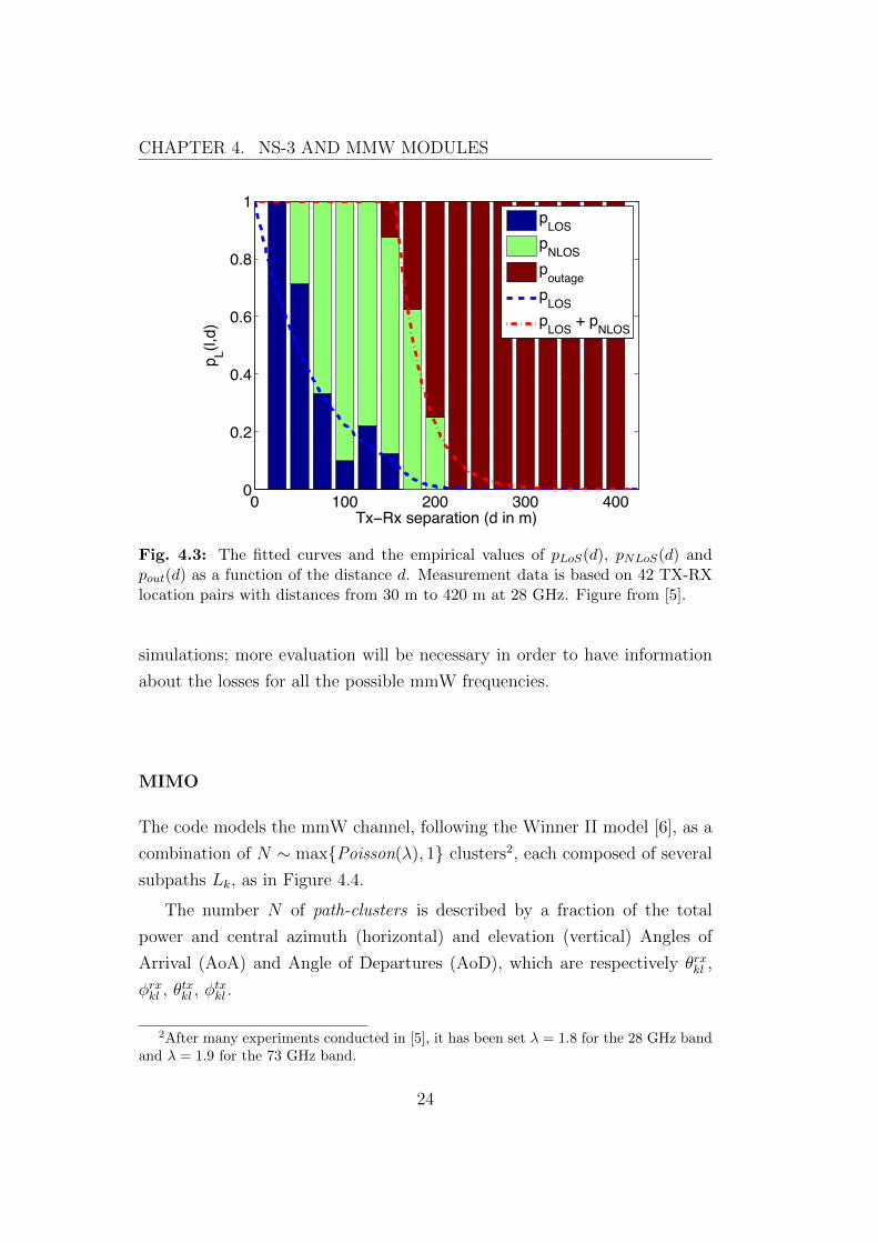
4.3 The fitted curves and the empirical values of pLoS(d), pNLoS(d)and pout(d) as a function of the distance d. Measurement datais based on 42 TX-RX location pairs with distances from 30m to 420 m at 28 GHz. Figure from [5]. . . . . . . . . . . . . 24
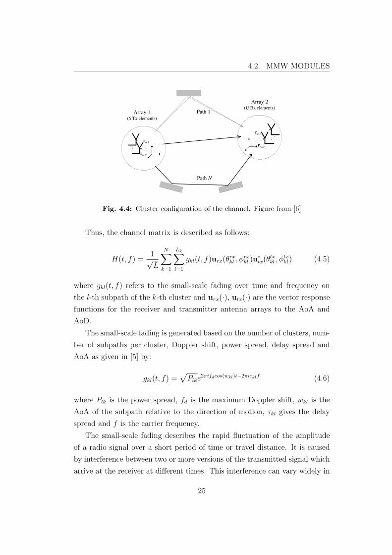
4.4 Cluster configuration of the channel. Figure from [6] . . . . . 25
4.5 Example of interference model. . . . . . . . . . . . . . . . . . 28
4.6 PHY, MAC and scheduler modules with the associated SAPs. 29
5.1 Example of two mmW networks working in the same area. . . 36
5.2 Illustration of a centralised coordination among three differentmmW networks. . . . . . . . . . . . . . . . . . . . . . . . . . . 38
5.3 Block diagram for the training procedure in the case of two BSs. 41
5.4 Block diagram for the heuristic procedure in the case of twoBSs. . . . . . . . . . . . . . . . . . . . . . . . . . . . . . . . . 44
6.1 Evolution of the three methods, for different configurations ofantennas for BS and UE. Configuration with 16−8, 16−4 and4−4 sectors for BS and UE respectively. . . . . . . . . . . . . 48
xi
6.2 A zoomed view of the evolution after time tstart, of the threemethods, for different configuration of antennas for BS andUE. Configuration with 16−8, 16−4 and 4−4 sectors for BSand UE respectively. . . . . . . . . . . . . . . . . . . . . . . . 49
6.3 Example of 20 different runs for the training method in thecase 16−4 of Figure 6.1. . . . . . . . . . . . . . . . . . . . . . 51
6.4 Mean and standard deviation of the 20 different runs for thetraining method in the case 16−4 of Figure 6.1. . . . . . . . . 52
6.5 Evolution, of the three methods, with cell radius R = 10 mand configuration of 16−8 sectors for BS and UE respectively. 53
6.6 A zoomed view of the evolution after time tstart, of the threemethods, with cell radius R = 10 m and configuration of 16−8sectors for BS and UE respectively. . . . . . . . . . . . . . . . 54
6.7 Evolution, of the three methods, with cell radius R = 50 mand configuration of 16−8 sectors for BS and UE respectively. 55
6.8 A zoomed view of the evolution after time tstart, of the threemethods, with cell radius R = 50 m and configuration of 16−8sectors for BS and UE respectively. . . . . . . . . . . . . . . . 56
xii
List of Tables
4.1 Parameters for configuring the mmW frame structure. . . . . . 204.2 Parameters α, β and σ in the case of NLoS or LoS for the two
frequencies: 28 and 73 GHz. . . . . . . . . . . . . . . . . . . . 234.3 Relation between number of antennas and sectors. . . . . . . . 27
6.1 Simulation parameters for the simulations of all the procedures. 476.2 Average fairness index and throughput measured at time t =
200 ms, of the three methods, for different configuration ofantennas for BS and UE. Configuration with 16−8, 16−4 and4−4 sectors for BS and UE respectively. . . . . . . . . . . . . 50
6.3 Average fairness index and throughput measured at time t =200 ms, of the three methods, for different configuration in theposition of UEs. Configuration with R = 10 m and R = 50 m. 56
xiii

xiv
Acronyms
µW micro Wave
AMC Adaptive Modulation and Coding
AoA Angle of Arrival
AoD Angle of Departures
AP Access Point
BER Bit Error Rate
BF Beamforming
BS Base Station
CCU Central Coordination Unit
CC Coordination Context
CQI Channel Quality Indicator
CU Coordination Unit
DL Downlink
IoT Internet of Things
IT Interference Threshold
LoS Line of Sight
LSA Licensed Shared Access
LTE Long Term Evolution
MCS Modulation and Coding Scheme
xv
MIMO Multiple Input and Multiple Output
mmW millimeter Wave
NGMN Next Generation Mobile Networks
NLoS Non Line of Sight
ns-3 networks simulator 3
NYU New York University
OFDMA Orthogonal Frequency-Division Multiple Access
OFDM Orthogonal Frequency Division Multiplexing
PHY Physical
RB Resource Block
RF Radio Frequency
RNTI Radio Network Temporary Identifier
RR Round Robin
SAP Service Access Point
SINR Signal to Interference plus Noise Ratio
SPSH Spectrum Sharing
TB Transport Block
TDD Time Division Duplex
TDMA Time Division Multiple Access
TU Training Unit
UE User Equipment
ULA Uniform Linear Array
UL Uplink
WLAN Wireless Local Area Networks
xvi
Chapter 1
Introduction
With the increasing demand of data and the growth of the connection among
devices, a new generation of mobile networks is necessary in order to reach the
challenges required. For this reason, the Next Generation Mobile Networks
(NGMN) alliance and other leadering companies affirm that, for 5G, data
rates of several tens of Mb/s should be supported for tens of thousands of
users, several hundreds of thousands of simultaneous connections should be
supported for massive sensor deployments, latency significantly reduced to
1 ms end-to-end and 1 Gbit/s should be offered, simultaneously, to tens of
workers on the same office floor [1], [2], [7].
In Figure 1.1 are shown the challenges required in the 5G standard com-
pared with the actual 4G Long Term Evolution (LTE). Several studies are
necessary in order to reach the challenges required for the future generation
of mobile communications.
In addition to simply providing faster speed, NGMN predicts that 5G
networks will also need to meet the needs of new use-cases such as the Internet
of Things (IoT) as well as broadcast-like services and lifeline communications
in times of natural disaster.
These demands for very high system capacity and very high end-user data
rates can be met by networks with distances between access nodes ranging
from a few meters in indoor deployments up to roughly 200 m in outdoor de-
ployments, consequently with an infra-structure density considerably higher
1
CHAPTER 1. INTRODUCTION
In addition, 5G services will complement and largely outperform the current operational capabilities for wide-area systems, reaching the following high-performance indicators:
FIGUR
E 2. R
adar
diagra
m of
5G di
srupti
ve ca
pabil
ities
Guaranteed user data rate
≥ 50Mb/s
Capable of human-oriented terminals
≥ 20 billion
Capable of IoT terminals
≥ 1 trillion
Aggregate service reliability
≥ 99.999%
Mobility support at speed ≥ 500km/h
for ground transportation
Accuracy of outdoor terminal location
≤ 1 meter
Non-quanti tati ve capabiliti es of the technology include a soft ware-based system architecture, simplifi ed authenti cati on, support for shared infrastructure, multi -tenancy and multi -RAT (with seamless handover), support for terrestrial and/or satellite communicati on, robust security, privacy, and lawful intercepti on capacity.
It is important to highlight that not all of the above performance indicators will be required by every terminal everywhere and all the ti me. Each connected device will typically have its mix of latency, bandwidth and traffi c intensity characteristi cs. Also, each connected area will have its specifi c characteristi cs: the network will not provide the same coverage for a business district, a stadium, a residenti al area, or on board of a vehicle (bus, train, boat, airplane…). This is why the infrastructure has to be adapted to the characteristi cs of the service demand expected at each area. In parti cular, ultra-low cost infrastructure opti ons will sati sfy the demands of low ARPU terminals/users, as they will be commonplace in developing regions and as part of IoT services.
99.99%90 days 1 K/km2
4G
5G
USER EXPERIENCE CONTINUITY
MISS
ION CR
ITICA
L SER
VICES
INTERNET OF THINGS
MOBILE DATA VOLUME10 Tb/s/km2
ENERGY EFFICIENCY10% of current consumption
PEAK DATA RATE10 Gb/s
MOBILITY500km/h
RELIABILITY99.999%
NUMBER OF DEVICES1 M/km2
E2E LATENCY5 ms
SERVICE DEPLOYMENT TIME90 minutes
25 ms
10 Gb/s/km2
100 Mb/s
Fig. 1.1: Comparison specifics of standards 4G and 5G. Figure from [1].
than the most dense networks of today [5], [8].
The first issue to address in order to achieve the challenges of the stand-
ards is the identification of the frequencies to use. Given that the current
micro-wave (µW) spectrum under 5 GHz is very fragmented and crowded,
new frequencies are necessary to achieve the high throughput required and a
possible solution to the problem is the use of millimeter Wave (mmW) com-
munications. mmW frequencies, from 30 GHz to 300 GHz1, has been iden-
tified as one of the most promising techniques in the future of wireless com-
munications and for the 5th generation of cellular technology [9], [10], [11].
In a different way from the current frequencies used for mobile commu-
nication, a lot of attenuation problems are present in mmW, due to the high
frequencies used. These attenuation problems can be alleviate implementing
techniques such as massive multiple-input and multiple-output (MIMO) and
beamforming (BF).
1While the mmW spectrum is defined as the band between 30-300 GHz, industry hasloosely considered mmW to be any frequency above 10 GHz.
2
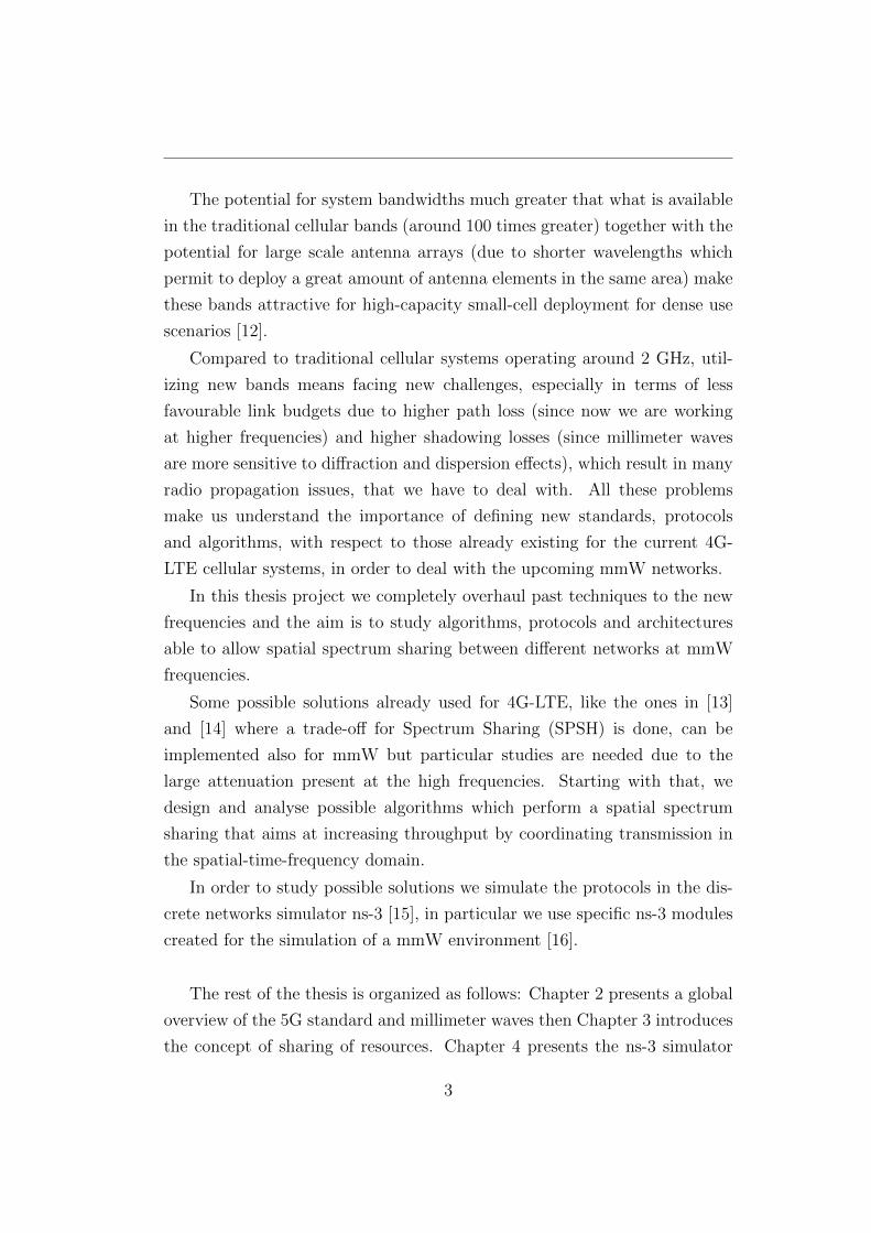
The potential for system bandwidths much greater that what is available
in the traditional cellular bands (around 100 times greater) together with the
potential for large scale antenna arrays (due to shorter wavelengths which
permit to deploy a great amount of antenna elements in the same area) make
these bands attractive for high-capacity small-cell deployment for dense use
scenarios [12].
Compared to traditional cellular systems operating around 2 GHz, util-
izing new bands means facing new challenges, especially in terms of less
favourable link budgets due to higher path loss (since now we are working
at higher frequencies) and higher shadowing losses (since millimeter waves
are more sensitive to diffraction and dispersion effects), which result in many
radio propagation issues, that we have to deal with. All these problems
make us understand the importance of defining new standards, protocols
and algorithms, with respect to those already existing for the current 4G-
LTE cellular systems, in order to deal with the upcoming mmW networks.
In this thesis project we completely overhaul past techniques to the new
frequencies and the aim is to study algorithms, protocols and architectures
able to allow spatial spectrum sharing between different networks at mmW
frequencies.
Some possible solutions already used for 4G-LTE, like the ones in [13]
and [14] where a trade-off for Spectrum Sharing (SPSH) is done, can be
implemented also for mmW but particular studies are needed due to the
large attenuation present at the high frequencies. Starting with that, we
design and analyse possible algorithms which perform a spatial spectrum
sharing that aims at increasing throughput by coordinating transmission in
the spatial-time-frequency domain.
In order to study possible solutions we simulate the protocols in the dis-
crete networks simulator ns-3 [15], in particular we use specific ns-3 modules
created for the simulation of a mmW environment [16].
The rest of the thesis is organized as follows: Chapter 2 presents a global
overview of the 5G standard and millimeter waves then Chapter 3 introduces
the concept of sharing of resources. Chapter 4 presents the ns-3 simulator
3
CHAPTER 1. INTRODUCTION
describing the structure in modules and how it works, after that Chapter 5
describes the protocols studied and introduced in this thesis. Then Chapter
6 report a description of the scenarios implemented and result of simulation.
Conclusion and future works are provided in Chapter 7.
4
Chapter 2
Millimeter waves in 5G cellular
systems
2.1 5G overview
5G is the next step in the evolution of mobile communication, research is just
at the beginning therefore there isn’t a unique definition for 5G yet. It will
be a key component of the Networked Society1 and will help realize the vision
of essentially unlimited access to information and sharing of data anywhere
and anytime for anyone and anything [2].
5G will therefore not only be about mobile connectivity for people. Rather,
the aim of 5G is to provide ubiquitous connectivity for any kind of device
and any kind of application that may benefit from being connected.
Mobile broadband will continue to be important and will drive the need
for higher system capacity and higher data rates. This new generation will
also provide wireless connectivity for a wide range of new applications and use
cases, including wearables, smart homes, traffic safety control, and critical
infrastructure and industry applications, as well as for very-high-speed media
delivery.
In contrast to earlier generations, 5G wireless access should not be seen
1The Networked Society is a term used to describe a future ecosystem, envisionedby the Information and Communications Technology (ICT) company Ericsson, in whichwidespread internet connectivity drives change for individuals and communities.
5
CHAPTER 2. MILLIMETER WAVES IN 5G CELLULAR SYSTEMS
as a specific radio-access technology. Rather, it is an overall wireless-access
solution addressing the demands and requirements of mobile communication
beyond 2020. LTE will continue to develop in a backwards-compatible way
and will be an important part of the 5G wireless-access solution for frequency
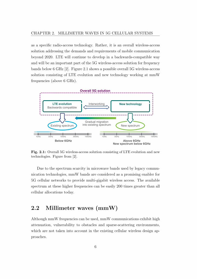
bands below 6 GHz [2]. Figure 2.1 shows a possible overall 5G wireless-access
solution consisting of LTE evolution and new technology working at mmW
frequencies (above 6 GHz).
5G RADIO ACCESS WHAT IS 5G? 2
What is 5G?5G is the next step in the evolution of mobile communication. It will be a key component of the Networked Society and will help realize the vision of essentially unlimited access to information and sharing of data anywhere and anytime for anyone and anything. 5G will therefore not only be about mobile connectivity for people. Rather, the aim of 5G is to provide ubiquitous connectivity for any kind of device and any kind of application that may benefit from being connected.
Mobile broadband will continue to be important and will drive the need for higher system capacity and higher data rates. But 5G will also provide wireless connectivity for a wide range of new applications and use cases, including wearables, smart homes, traffic safety/control, and critical infrastructure and industry applications, as well as for very-high-speed media delivery.
In contrast to earlier generations, 5G wireless access should not be seen as a specific radio-access technology. Rather, it is an overall wireless-access solution addressing the demands and requirements of mobile communication beyond 2020.
LTE will continue to develop in a backwards-compatible way and will be an important part of the 5G wireless-access solution for frequency bands below 6GHz. Around 2020, there will be massive deployments of LTE providing services to an enormous number of devices in these bands. For operators with limited spectrum resources, the possibility to introduce 5G capabilities in a backwards-compatible way, thereby allowing legacy devices to continue to be served on the same carrier, is highly beneficial and, in some cases, even vital.
In parallel, new radio-access technology (RAT) without backwards-compatibility requirements will emerge, at least initially targeting new spectrum for which backwards compatibility is not relevant. In the longer-term perspective, the new non-backwards-compatible technology may also migrate into existing spectrum.
Although the overall 5G wireless-access solution will consist of different components, including the evolution of LTE as well as new technology, the different components should be highly integrated with the possibility for tight interworking between them. This includes dual-connectivity between LTE operating on lower frequencies and new technology on higher frequencies. It should also include the possibility for user-plane aggregation, that is, joint delivery of data via both LTE and a new RAT.
Figure 1: The overall 5G wireless-access solution consisting of LTE evolution and new technology.
3GHz1GHz 10GHz 30GHz 100GHz 3GHz1GHz 10GHz 30GHz 100GHz
Overall 5G solution
LTE evolution New technologyBackwards compatible
Existing spectrum
Below 6GHz Above 6GHzNew spectrum below 6GHz
New spectrum
Gradual migration
into existing spectrum
Interworking
Fig. 2.1: Overall 5G wireless-access solution consisting of LTE evolution and newtechnologies. Figure from [2].
Due to the spectrum scarcity in microwave bands used by legacy commu-
nication technologies, mmW bands are considered as a promising enabler for
5G cellular networks to provide multi-gigabit wireless access. The available
spectrum at these higher frequencies can be easily 200 times greater than all
cellular allocations today.
2.2 Millimeter waves (mmW)
Although mmW frequencies can be used, mmW communications exhibit high
attenuation, vulnerability to obstacles and sparse-scattering environments,
which are not taken into account in the existing cellular wireless design ap-
proaches.
6
2.2. MILLIMETER WAVES (MMW)
In a different way, the small wavelengths of mmW signals make it possible
to incorporate a large number of antenna elements both at the Base Station
(BS) and at the User Equipment (UE), which in turn lead to high directivity
gains and fully-directional communications. This level of directionality can
result in a network that is noise-limited as opposed to interference-limited.
The significant differences between mmW networks and traditional ones
challenge the classical design constraints, objectives, and available degrees of
freedom. An example of this can be a scenario of Non Line of Sight (NLoS),
where communication between transmitter and receiver can not be achieved
due to the high attenuations [8]. This demands a reconsideration of almost
all design aspects in mmW systems.
2.2.1 Challenges of mmW
Despite the potential of mmW cellular systems, there are a number of key
challenges to realize the vision of cellular networks in these bands [17]:
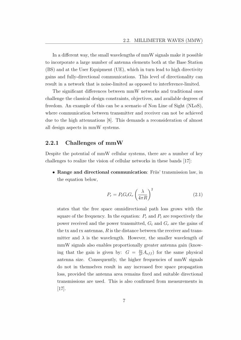
• Range and directional communication: Friis’ transmission law, in
the equation below,
Pr = PtGtGr
(λ
4πR
)2
(2.1)
states that the free space omnidirectional path loss grows with the
square of the frequency. In the equation: Pr and Pt are respectively the
power received and the power transmitted, Gt and Gr are the gains of
the tx and rx antennas, R is the distance between the receiver and trans-
mitter and λ is the wavelength. However, the smaller wavelength of
mmW signals also enables proportionally greater antenna gain (know-
ing that the gain is given by: G = 4πλ2Aeff ) for the same physical
antenna size. Consequently, the higher frequencies of mmW signals
do not in themselves result in any increased free space propagation
loss, provided the antenna area remains fixed and suitable directional
transmissions are used. This is also confirmed from measurements in
[17].
7
CHAPTER 2. MILLIMETER WAVES IN 5G CELLULAR SYSTEMS
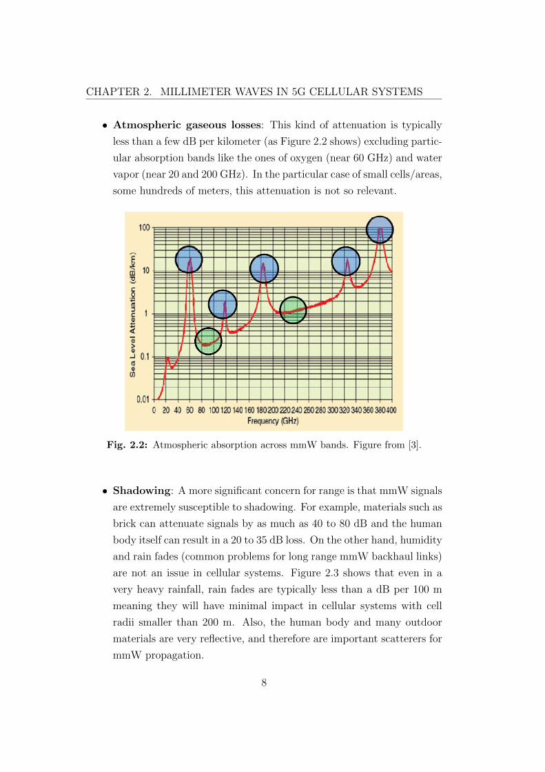
• Atmospheric gaseous losses: This kind of attenuation is typically
less than a few dB per kilometer (as Figure 2.2 shows) excluding partic-
ular absorption bands like the ones of oxygen (near 60 GHz) and water
vapor (near 20 and 200 GHz). In the particular case of small cells/areas,
some hundreds of meters, this attenuation is not so relevant.
communications at 183, 325, and 380 GHz, making theseideal spectrum bands for densely packed electronic mediathat will characterize the future wireless office shown inFig. 1. The dramatic attenuation at these frequency bandsallows Bwhisper radio[ communications, where weaksignals do not propagate more than a few meters before
dropping below the thermal noise level. For communica-tion across tens or hundreds of meters, atmospheric ab-sorption, including rain and fog, can be the dominantphysical factor for determining the correct cell size forwireless communications, with peaks in atmospheric ab-sorption indicating those bands best used for dense, orBwhisper[ deployments of highest spectral frequency re-use, and low-attenuation bands being best suited for longerdistance backhaul or cellular radio applications. In the fu-ture, Federal regulatory agencies around the world, havingagreed upon 60 GHz as an international WPAN band, willlikely approve bandwidths in excess of 10 GHz for severalsubterahertz bands and enable massively broadbandWPAN communications and other scientific and medicalapplications, such as imaging. At lower attenuation bandsof 77 and 240 GHz, cellular, backhaul, fiber-replacement,sensing, and vehicular radar will be viable. In addition toatmospheric and free-space attenuation, it is important tounderstand how wireless signals penetrate materials atthese frequencies, and how the physical environment willaffect propagation indoors and outdoors. We discuss RFpropagation considerations in Section X.
This tutorial provides a comprehensive overview ofsystem and circuits aspects vital to the development ofmm-wave communication systems. We highlight key chal-lenges that research and industrial communities are over-coming to create 60-GHz and future subterahertz wirelessdevices enabled by wireless spectrum policies and semi-conductor technologies. Summaries of recent develop-ments in 60-GHz mm-wave circuit design are provided toallow new researchers or communications and circuitspractitioners to quickly assess the state of the art, and tofind key works from which they can further their under-standing. Section II provides an overview of the level ofintegration achieved for 60-GHz transmitters and
Fig. 2. (Modification of figure in [4] and [8].) The properties of
atmospheric absorption of electromagnetic waves have resulted in
widespread multigovernment agreement on spectrum allocation for
short-range applications in the 60-GHz band. Agreement on allocation
for short-range communications in the 120-, 183-, 325-, and 380-GHz
bands (blue circles) is very likely. In coming years, the 77- and 240-GHz
bands are likely candidates for widespread ISM allocations for longer
range applications. When combined with highly directional antennas,
attenuation for off-boresight links will be extreme at 380 GHz.
See www.mmWconcepts.com for useful attenuation factors caused
by rain, dust, and fog at mm-wave frequencies.
Fig. 1. Government allocation of high carrier frequencies and large bandwidths, along with advances in semiconductor technology,
will create a future of portable and inexpensive mm-wave wireless devices that access the cloud and other large data repositories.
Rappaport et al. : State of the Art in 60-GHz Integrated Circuits and Systems for Wireless Communications
1392 Proceedings of the IEEE | Vol. 99, No. 8, August 2011
Fig. 2.2: Atmospheric absorption across mmW bands. Figure from [3].
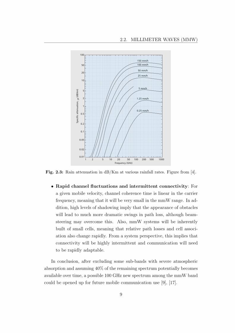
• Shadowing: A more significant concern for range is that mmW signals
are extremely susceptible to shadowing. For example, materials such as
brick can attenuate signals by as much as 40 to 80 dB and the human
body itself can result in a 20 to 35 dB loss. On the other hand, humidity
and rain fades (common problems for long range mmW backhaul links)
are not an issue in cellular systems. Figure 2.3 shows that even in a
very heavy rainfall, rain fades are typically less than a dB per 100 m
meaning they will have minimal impact in cellular systems with cell
radii smaller than 200 m. Also, the human body and many outdoor
materials are very reflective, and therefore are important scatterers for
mmW propagation.
8
2.2. MILLIMETER WAVES (MMW)
IEEE Wireless Communications • December 2014138
hour; and very heavy rain describes rainfall of16mm–50mm per hour. Figure 1 from [8] (pp.59, Figure 10) shows the rain attenuation indB/km at various rainfall rates. We can see thatat a very heavy rainfall of 25mm/hr, the rainattenuation is about 7 dB/km at 28 GHz andabout 10 dB/km at 73 GHz. Considering today’scell sizes in urban environments are on the orderof 200m [3], the rain attenuations reduce to only1.4 dB at 28 GHz and 2 dB at 73 GHz if cellcoverage regions are 200m in radius even in avery heavy rainfall. Hence, rain attenuation willpresent a minimal impact on mmWave propaga-tion for a small cell structure.
BEAMFORMING TECHNOLOGIES INMMWAVE COMMUNICATIONS
As discussed in the previous section, the pathloss of mmWave transmission can be comparableto those of typical cellular frequency bands whenthe transmit and receive antennas are used toproduce beamforming gain. Highly directionalantenna arrays are expected in mmWave com-munication systems, and thanks to the very smallwavelength of mmWave signals, large beamform-ing gain is possible through large antenna arrayspacked into small dimensions. For a given effec-tive area, the directivity of antenna scales withthe inverse of the frequency square.
In traditional cellular communication sys-
tems, both beamforming and precoding (beam-forming with multiple data streams to improvespectral efficiency) are implemented at the base-band. In mmWave systems, however, while addi-tional antenna elements are usually inexpensiveand the additional digital signal processingbecomes even cheaper, the radio frequency (RF)elements are expensive and are more challengingto follow Moore’s law [9]. In digital beamform-ing, for each antenna element at the transmitteror the receiver, a complete dedicated RF chainis required, including low-noise amplifiers,down-converters, and analog-to-digital convert-ers, and so on. Furthermore, due to highly direc-tive antennas, multipath is rather sparse at themmWave band, leading to a possibly low diversi-ty gain from digital beamforming and precoding.Thus, the high cost of mixed analog/digital sig-nals and RF chains, and low multipath diversitygain, make operation in the passband and analogdomains attractive for mmWave transmissions [10].
Correspondingly, in mmWave communica-tion systems, a hybrid beamforming architec-ture with a hybrid combination of analogbeamforming and digital precoding may be onefavorable possibility. Hybrid beamformingoffers a good compromise between all digitaland all analog beamforming structures. Analogbeamforming applies complex coefficients tomanipulate the RF signals by means of control-ling phase shifters and/or variable gain ampli-fiers and aims to compensate for the large passloss at mmWave bands, while digital beamform-ing is done in the form of digital precoding thatmultiplies a particular coefficient to the modu-lated baseband signal per RF chain to optimizecapacity using various MIMO techniques [7].Although multipath is sparse in mmWave dueto the high directivity of antennas, multiple setsof antennas can be spaced several wavelengthsapart in a small effective area to enable MIMOtechniques, even in a LOS environment. In gen-eral, digital beamforming is more flexible andhas a better performance. But as each outputneeds to have a dedicated RF chain, it will havean increased complexity and cost. On the otherhand, analog beamforming is a simple yet effec-tive method to generate high beamforming gainwith a large number of antennas allowed inmmWave bands. Therefore, it is a trade-offbetween flexibility/ cost, simplicity, and perfor-mance that drives the need for hybrid beam-forming architectures.
In Fig. 2 we illustrate the different beam-forming diagrams in a traditional sub 3 GHz cel-lular system and a mmWave system. In atraditional cellular system, beamforming is per-formed in the baseband with the number of RFchains equal to the number of transmit anten-nas. In mmWave transmission, with the verysmall wavelength size, we have a large numberof transmit antennas NT but with limited dedi-cated RF chains NRF (NT ≥ NRF), hence thehybrid beamforming architecture can be onepossible solution. There can be other possibili-ties, such as modular antenna array. In thisstructure, many smaller antenna arrays are puttogether, where each of them steers beams ontheir own. On top of that there is a general con-trol to steer the overall beams together.
Figure 1. Rain attenuation in dB/km at various rainfall rates (figure from[8]).
Frequency (GHz)21
10
0.01
Spec
ific
atte
nuat
ion,
γR
(dB/
km)
20
50
100
5
2
1
0.5
0.2
0.1
0.05
0.02
5 10 20 50 100 200 500 1000
0.25 mm/h
1.25 mm/h
25 mm/h
50 mm/h
100 mm/h
150 mm/h
5 mm/h
HU_LAYOUT_Layout 12/18/14 4:16 PM Page 138
Fig. 2.3: Rain attenuation in dB/Km at various rainfall rates. Figure from [4].
• Rapid channel fluctuations and intermittent connectivity: For
a given mobile velocity, channel coherence time is linear in the carrier
frequency, meaning that it will be very small in the mmW range. In ad-
dition, high levels of shadowing imply that the appearance of obstacles
will lead to much more dramatic swings in path loss, although beam-
steering may overcome this. Also, mmW systems will be inherently
built of small cells, meaning that relative path losses and cell associ-
ation also change rapidly. From a system perspective, this implies that
connectivity will be highly intermittent and communication will need
to be rapidly adaptable.
In conclusion, after excluding some sub-bands with severe atmospheric
absorption and assuming 40% of the remaining spectrum potentially becomes
available over time, a possible 100 GHz new spectrum among the mmW band
could be opened up for future mobile communication use [9], [17].
9
CHAPTER 2. MILLIMETER WAVES IN 5G CELLULAR SYSTEMS
2.2.2 Benefits of mmW
Despite all the challenges listed above, the use of mmW also provides some
advantages.
Due to the small wavelength, the use of MIMO is easily implementable
and this is already a key technology in supporting high data rates in 4G
systems. MIMO enables multi-stream transmission for high spectrum effi-
ciency, improved link quality and adaptation of radiation patterns for signal
gain and interference mitigation via adaptive beamforming using antenna
arrays [18], [19].
Since the tiny wavelengths allow for dozens to hundreds of antenna ele-
ments to be placed in an array on a relatively small physical platform at
the BS, or access point, massive MIMO can be used. Extra antennas help
by focusing energy into ever smaller regions of space to bring huge improve-
ments in throughput and radiated energy efficiency. Other benefits of massive
MIMO include extensive use of inexpensive low-power components, reduced
latency, simplification of the MAC layer, and robustness against intentional
jamming [19], [20].
All these aspects are perfect for scenarios of mmW communications. In
addition, MIMO systems allow to use BeamForming (BF) and so obtain a
directional signal transmission or reception. This is achieved by combining
elements in a phased array in such a way that signals at particular angles
experience constructive interference while others experience destructive in-
terference. BF can be used at both the transmitting and receiving ends in
order to achieve spatial selectivity [21].
After the list of pros and cons, all the studies and in-the-field simulations
have identified mmW frequencies as the means to carry communication in
the systems of fifth generation.
10
Chapter 3
Spatial Spectrum Sharing
The term Spectrum Sharing (SPSH) is used to indicate the sharing of spec-
trum among multiple operators or devices in a wireless environment. The
main concept behind this technique is to share unused spectrum of a net-
work with others that need more resources at particular time. An example
of SPSH can be seen in Figure 3.1.
Spectrum sharing may be orthogonal, meaning that access to the shared
resources by either operator automatically excludes the other one, or non-
orthogonal, where the operators are allowed to use the same transmission
frequency resource simultaneously.
Adding the word spatial, we indicate a sharing of resources that is not
only in the frequency domain but also in the spatial domain: computing
transmission in directions that do not interfere.
In such a way, spatial SPSH coordinates transmission schemes and in-
creases the performance and use of resources.
3.1 Spectrum Sharing in 4G-LTE
In 4G-LTE, several techniques have been studied in order to improve the
efficiency of the allocation. An important solution, taken as an example for
this project, is the one proposed in [13].
Spectrum allocation policies, which impose exclusive usage to a licensed
11
CHAPTER 3. SPATIAL SPECTRUM SHARING
operator, may lead to inefficient management and waste of resources. The use
of the same frequency band by multiple operators, that SPSH is supposed
to realise, helps to improve the efficiency of the spectrum allocation and
therefore the performance of the networks involved.
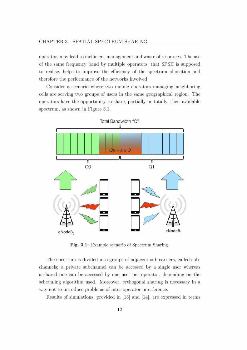
Consider a scenario where two mobile operators managing neighboring
cells are serving two groups of users in the same geographical region. The
operators have the opportunity to share, partially or totally, their available
spectrum, as shown in Figure 3.1.
Qs = s x Q
Total Bandwidth “Q”
Q0 Q1
eNodeB0' eNodeB1'
Fig. 3.1: Example scenario of Spectrum Sharing.
The spectrum is divided into groups of adjacent sub-carriers, called sub-
channels; a private subchannel can be accessed by a single user whereas
a shared one can be accessed by one user per operator, depending on the
scheduling algorithm used. Moreover, orthogonal sharing is necessary in a
way not to introduce problems of inter-operator interference.
Results of simulations, provided in [13] and [14], are expressed in terms
12
3.2. SPATIAL SPSH IN 5G
of throughput, which represents the average sum data rates delivered to all
the UEs. The results show that the throughput increases a lot in the case of
perfect orthogonality. Improvements can be obtain also in a non-orthogonal
scenario. Moreover, [13] shows that it is always better to have a full sharing
of the available frequencies. This may not be possible due to internal policy
requirements of the operators; nevertheless, the larger the fraction of shared
spectrum, the better. For the simulations, a particular extension of ns-3
design has been used in [22].
3.2 Spatial SPSH in 5G
3.2.1 State of the art
In order to face the increase of data demand, a new technology able to support
high amounts of traffic is required. To do so, some researcher have started to
investigate this field and innovative solutions have been proposed. However,
the new generation of mobile networks needs more and more resources to
guarantee the high quality required by the end users. To address this issue,
focusing on SPSH, some papers provide sharing techniques between different
networks. Since mmW is a new technology, there is a lot of study to do
and not a lot of work has been done so far. In fact, most of the prior art
refers to SPSH in Wireless Local Area Networks (WLAN) instead of cellular
networks.
In [23] a mechanism for allowing two different 802.11ad1 Access Points
(AP) to transmit over the same time/frequency resources is proposed, effect-
ively in a way to enable spectrum sharing. This is realised by introducing
a new signalling report broadcast by each AP, to allow it to establish an
interference database and based on these distributed databases a new inter-
network MAC approach is proposed.
1IEEE 802.11ad is an amendment that defines a new physical layer for 802.11 networksto operate in the 60 GHz millimeter wave spectrum. Products implementing the 802.11adstandard are being brought to market under the WiGig brand name. The certificationprogram is now being developed by the Wi-Fi Alliance instead of the now defunct WiGigAlliance. The peak transmission rate of 802.11ad is 7 Gbit/s.
13
CHAPTER 3. SPATIAL SPECTRUM SHARING
Here an open issue is how the interference can be estimated by the differ-
ent nodes with the current versions of the standard. Further analysis is also
needed to understand if this MAC approach can be implemented in a fully
distributed way.
A similar approach is proposed in [24], with both a centralised and a
distributed architecture. In particular, [24] instead of being implemented
for WLAN, is already designed for 5G mmW cellular networks. From a de-
ployment assumption perspective, this document considers the case of two
partially overlapping cellular networks, in which only a subset of the nodes
is interfered. In the centralised case, a new architectural entity (referred as
central coordination functionality) is connected to multiple mmW networks,
receives the interference information measured by each network and makes
the decision on which links cannot be scheduled at the same time. A central-
ised solution is expected to be useful for scenarios where a centralised entity is
already present for other reasons. Centralised control is capable of providing
optimal resource allocation for the entire network and exhibits a fast con-
vergence, but the required amount of signaling may be excessive for medium
to large-sized networks. In the decentralised case, the victim network sends
a message to the interfering network with a proposed coordination pattern.
By definition, distributed control does not require a central entity and allows
BSs and UEs to make autonomous user association decision by themselves
through the interaction between BSs and UEs. The two networks can further
refine the coordination pattern via multiple stages.
Results in [24] provide that with the use of an interference database larger
improvements can be obtained.
In [25] and [26], spectrum reuse mechanisms are proposed to coordinate
multiple ad-hoc links belonging to the same AP. In particular [25] proposes
an extension of the BF training mechanism in 802.11ad to incorporate inter-
ference measurements. Moreover, a centralised interference-aware scheduling
is proposed. A similar centralised approach is proposed in [26], but is instead
based on beam index information rather than interference measurements.
14
3.2. SPATIAL SPSH IN 5G
In [27] a multi-carrier waveform based inter-operator spectrum sharing
concept is presented. The proposed concept is a strong extension of OF-
DMA-based schemes and can support coordinated inter-operator SPSH in
various scenarios, including mutual renting (where operators mutually al-
low other operators to “rent” parts of their licensed resources), co-primary
sharing, Licensed Shared Access (LSA), etc. The key element proposed is
a two-stage spectrum allocation procedure where the first stage is an inter-
operator spectrum allocation, then after that, the second stage is a short
term pre-operator resource allocation to users.
According to this state of the art, in the next section we will analyse
the limitations in order to solve issues and provide spatial SPSH between
mobile operators of fifth generation. Moreover we will focus on the training
procedure presented in [24], studying the result in a scenario where a dense
urban channel model is applied and with a fully directional transmission.
3.2.2 Analysis and limitations
Due to high frequency bands and small coverage, mmW networks are pre-
dominantly expected to be deployed in the form of coverage islands serving
high traffic density areas (e.g., an office building, a shopping mall, etc.). Dif-
ferent mmW networks, representing different operators, may be running in
the same or overlapping area.
Protocols and procedures already implemented in 4G can still be used for
5G but some differences are present and new strategies should be added to
the current implementation. The main new difference is that communica-
tions between BS and UEs will be perform in a directional way. Directional
transmission is really different in comparison with omnidirectional, in fact
frequency reuse and spectrum sharing can be inefficient in a scenario where
directional transmission is implemented.
The use of directional transmission can be perfect to achieve high data
rates. In a scenario in which nearest cells can use the same frequencies
15
CHAPTER 3. SPATIAL SPECTRUM SHARING
(transmitting with large bandwidth) and perform mechanisms to avoid in-
terference with directional transmission, high data rates for a large number
of users can be provided. This is exactly what is required in a millimeter
wave communication.
Therefore, for these reasons, this thesis studies a new approach of Spatial
Spectrum Sharing that can be used in 5G system.
16
Chapter 4
ns-3 and mmW modules
4.1 Description
ns-3 is a discrete-event network simulator for Internet systems, targeted
primarily for research and educational use. ns-3 is an open-source software,
licensed under the GNU GPLv2 license, and is publicly available for research,
development and use [15].
Due to the complexity of the networks this simulator helps to perform
computations that are difficult to perform theoretically.
Another important characteristic of ns-3 is its modularity. In particular,
the ns-3 software infrastructure encourages the development of simulation
models which are sufficiently realistic to allow ns-3 to be used as a real-time
network emulator, interconnected with the real world and which allows many
existing real-world protocol implementations to be reused within ns-3.
For this project, we used a particular mmW module (described in Section
4.2) developed by a research group at New York University (NYU) Wire-
less [28] that helps to simulate mmW mobile networks scenarios [16].
All the simulations designed in this thesis are made with the version 23
of ns-3 (released in May 2015).
17
CHAPTER 4. NS-3 AND MMW MODULES
4.2 mmW modules
The research group at NYU has developed a fully customized model where
the users can plug in various parameters in order to describe the behavior of
the mmW channel and devices [16].
The aim of the framework is to enable researchers to flexibly use this
module for various scenarios and compute simulations of mmW environments.
Part of the design is made following specific recent real-world measurements
at 28 and 73 GHz introduced by [5]. These measurements were made in New
York City to derive detailed spatial statistical models of the channels and
uses these models to provide a realistic assessment of mmW micro and pico
cellular networks in a dense urban deployment.
The framework includes a basic implementation of mmW devices, which
comprises the propagation and channel model, the physical (PHY) layer, and
the MAC layer. The design of this module, developed in C++, is completely
inspired by the ns-3 LENA module [29].
4.2.1 Physical layer (PHY): Frame and Transmission
schemes
The PHY layer implemented in the modules is equipped with some features
that can be set with particular values, which creates scenarios to simulate.
Among all the features that the PHY layer provides, we focus on the ones
used for our simulations that are: a fully customizable Time Division Du-
plex (TDD) frame structure, a radio characterization along with supporting
MIMO techniques such as BF, a decoding error model at the receiver side
and an interference model.
Frame structure
The TDD frame structure is organized as follows. Each frame is subdivided
into a number of subframes of fixed length specified by the UE. Each subframe
in turn is split into a number of slots of fixed duration. Each slot comprises
a specific number of Orthogonal Frequency Division Multiplexing (OFDM)
18
4.2. MMW MODULES
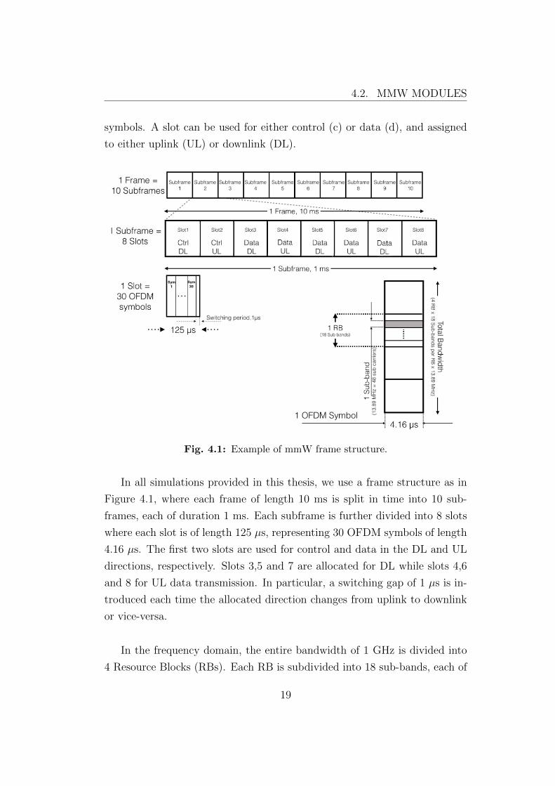
symbols. A slot can be used for either control (c) or data (d), and assigned
to either uplink (UL) or downlink (DL).
Fig. 4.1: Example of mmW frame structure.
In all simulations provided in this thesis, we use a frame structure as in
Figure 4.1, where each frame of length 10 ms is split in time into 10 sub-
frames, each of duration 1 ms. Each subframe is further divided into 8 slots
where each slot is of length 125 µs, representing 30 OFDM symbols of length
4.16 µs. The first two slots are used for control and data in the DL and UL
directions, respectively. Slots 3,5 and 7 are allocated for DL while slots 4,6
and 8 for UL data transmission. In particular, a switching gap of 1 µs is in-
troduced each time the allocated direction changes from uplink to downlink
or vice-versa.
In the frequency domain, the entire bandwidth of 1 GHz is divided into
4 Resource Blocks (RBs). Each RB is subdivided into 18 sub-bands, each of
19
CHAPTER 4. NS-3 AND MMW MODULES
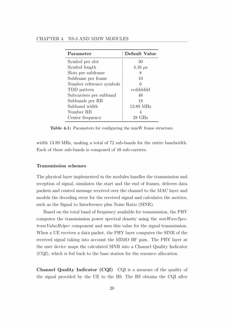
Parameter Default Value
Symbol per slot 30Symbol length 4.16 µsSlots per subframe 8Subframe per frame 10Number reference symbols 6TDD pattern ccddddddSubcarriers per subband 48Subbands per RB 18Subband width 13.89 MHzNumber RB 4Center frequency 28 GHz
Table 4.1: Parameters for configuring the mmW frame structure.
width 13.89 MHz, making a total of 72 sub-bands for the entire bandwidth.
Each of these sub-bands is composed of 48 sub-carriers.
Transmission schemes
The physical layer implemented in the modules handles the transmission and
reception of signal, simulates the start and the end of frames, delivers data
packets and control message received over the channel to the MAC layer and
models the decoding error for the received signal and calculates the metrics,
such as the Signal to Interference plus Noise Ratio (SINR).
Based on the total band of frequency available for transmission, the PHY
computes the transmission power spectral density using the mmWaveSpec-
trumValueHelper component and uses this value for the signal transmission.
When a UE receives a data packet, the PHY layer computes the SINR of the
received signal taking into account the MIMO BF gain. The PHY layer at
the user device maps the calculated SINR into a Channel Quality Indicator
(CQI), which is fed back to the base station for the resource allocation.
Channel Quality Indicator (CQI) CQI is a measure of the quality of
the signal provided by the UE to the BS. The BS obtains the CQI after
20
4.2. MMW MODULES
computing the spectral efficiency with the following equation:
η = log2
(1 +
SINR
Γ
)(4.1)
then chooses the most suitable modulation and coding scheme for each UE
using the Adaptive Modulation and Coding (AMC) module [30]. In (4.1),
Γ is a coefficient introduced to model the difference between the theoretical
bound and the performance of real modulation and coding scheme; such a
coefficient depends on the Bit Error Rate (BER): Γ = − ln(5 · BER)/1.5.
For the computation of the SINR we refer to the section about interference
in the following pages.
The procedure of mapping each CQI value in a Transport Block (TB)
size permits to compute the most suitable modulation and coding scheme for
the communication link. The higher the CQI, the higher the size of the TB
allocated.
4.2.2 Physical layer (PHY): Channel model
With regard to the channel model, it is important to highlight that, in a
mmW channel, the use of a multi-antenna approach is implemented to per-
form BF, in order to increase the gain, which is particularly critical in mil-
limeter wave communication. This gain can be much more exploited, with
respect to the classical cellular networks. A large number of antenna ele-
ments can be packed into a small form factor in mmW bands due to the
much smaller wavelength than legacy cellular bands. Then MIMO becomes
more feasible and can be also useful for transmitting signals over a long dis-
tance in the environments [31].
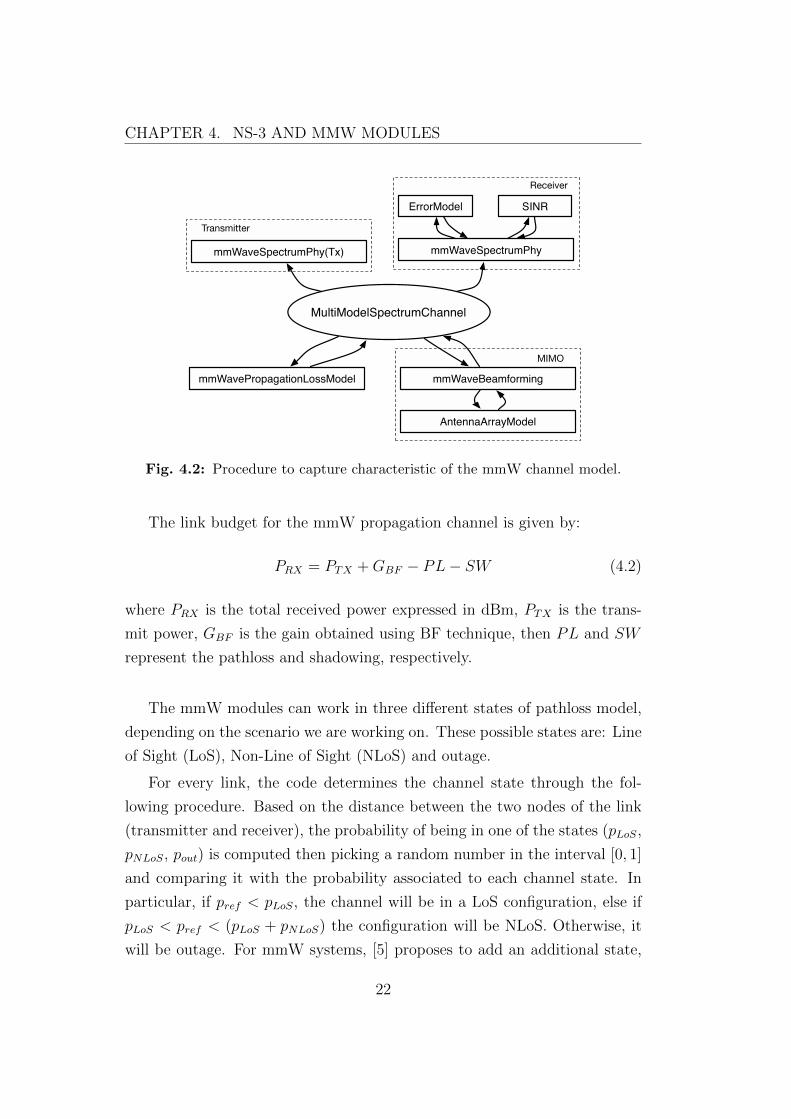
As illustrated in Figure 4.2, the models take into account a large number
of procedures to capture the main characteristics of the mmW propagation.
The key contribution here, as already mentioned, relates to the computation
of the multi-antenna gains, which is particularly critical for mmW commu-
nications.
21
CHAPTER 4. NS-3 AND MMW MODULES
MultiModelSpectrumChannel
mmWavePropagationLossModel mmWaveBeamforming
AntennaArrayModel
MIMO
ErrorModel
mmWaveSpectrumPhy
Receiver
SINR
mmWaveSpectrumPhy(Tx)
Transmitter
Fig. 4.2: Procedure to capture characteristic of the mmW channel model.
The link budget for the mmW propagation channel is given by:
PRX = PTX +GBF − PL− SW (4.2)
where PRX is the total received power expressed in dBm, PTX is the trans-
mit power, GBF is the gain obtained using BF technique, then PL and SW
represent the pathloss and shadowing, respectively.
The mmW modules can work in three different states of pathloss model,
depending on the scenario we are working on. These possible states are: Line
of Sight (LoS), Non-Line of Sight (NLoS) and outage.
For every link, the code determines the channel state through the fol-
lowing procedure. Based on the distance between the two nodes of the link
(transmitter and receiver), the probability of being in one of the states (pLoS,
pNLoS, pout) is computed then picking a random number in the interval [0, 1]
and comparing it with the probability associated to each channel state. In
particular, if pref < pLoS, the channel will be in a LoS configuration, else if
pLoS < pref < (pLoS + pNLoS) the configuration will be NLoS. Otherwise, it
will be outage. For mmW systems, [5] proposes to add an additional state,
22
4.2. MMW MODULES
so that each link can be in one of three conditions: LoS, NLoS or outage. In
the outage condition, is assumed that there is no link between the TX and
RX.
By adding this third state with a random probability for a complete
loss, the model provides a better reflection of outage possibilities inherent
in mmW. As a statistical model, the probability functions above for the
three states are of the form:
pout(d) = max(0, 1− e−aoutd+bout)pLoS(d) = (1− pout(d))e−alosd
pNLoS(d) = 1− pLoS(d)− pout(d)
(4.3)
where the parameters alos, aout and bout are parameters that are fit from the
data [5]. Figure 4.3 shows the fractions of point that were observed to be in
each of the three states - outage, NLoS1 and LoS.
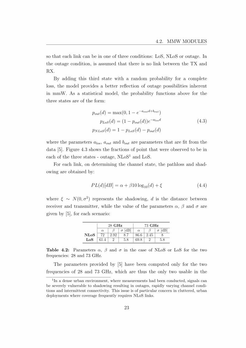
For each link, on determining the channel state, the pathloss and shad-
owing are obtained by:
PL(d)[dB] = α + β10 log10(d) + ξ (4.4)
where ξ ∼ N(0, σ2) represents the shadowing, d is the distance between
receiver and transmitter, while the value of the parameters α, β and σ are
given by [5], for each scenario:
28 GHz 73 GHzα β σ [dB] α β σ [dB]
NLoS 72 2.92 8.7 86.6 2.45 8LoS 61.4 2 5.8 69.8 2 5.8
Table 4.2: Parameters α, β and σ in the case of NLoS or LoS for the twofrequencies: 28 and 73 GHz.
The parameters provided by [5] have been computed only for the two
frequencies of 28 and 73 GHz, which are thus the only two usable in the
1In a dense urban environment, where measurements had been conducted, signals canbe severely vulnerable to shadowing resulting in outages, rapidly varying channel condi-tions and intermittent connectivity. This issue is of particular concern in cluttered, urbandeployments where coverage frequently requires NLoS links.
23
CHAPTER 4. NS-3 AND MMW MODULES6
0 20 400
0.2
0.4
0.6
0.8
1AoD Horiz
Angular std dev (deg)
Cum
m p
rob
MeasuredExponential Fit
0 20 40 600
0.2
0.4
0.6
0.8
1AoA Horiz
Angular std dev (deg)
MeasuredExponential Fit
Fig. 6: Distribution of the rms angular spreads in the horizontal(azimuth) AoA and AoDs. Also plotted is an exponentialdistribution with the same empirical mean.
D. LOS, NLOS, and Outage Probabilities
Up to now, all the model parameters were based on locationsnot in outage. That is, there was some power detected inat least one delay in one angular location – See Section II.However, in many locations, particularly locations > 200mfrom the transmitter, it was simply impossible to detect anysignal with transmit powers between 15 and 30 dBm. Thisoutage is likely due to environmental obstructions that occludeall paths (either via reflections or scattering) to the receiver.The presence of outage in this manner is perhaps the mostsignificant difference moving from conventional microwave /UHF to millimeter wave frequencies, and requires accuratemodeling to properly assess system performance.
Current 3GPP evaluation methodologies such as [25] gener-ally use a statistical model where each link is in either a LOSor NLOS state, with the probability of being in either statebeing some function of the distance. The path loss and otherlink characteristics are then a function of the link state, withpotentially different models in the LOS and NLOS conditions.Outage occurs implicitly when the path loss in either the LOSor NLOS state is sufficiently large.
For mmW systems, we propose to add an additional state,so that each link can be in one of three conditions: LOS,NLOS or outage. In the outage condition, we assume there isno link between the TX and RX — that is, the path loss isinfinite. By adding this third state with a random probabilityfor a complete loss, the model provides a better reflection ofoutage possibilities inherent in mmW. As a statistical model,we assume probability functions for the three states are of theform:
pout(d) = max(0, 1 � e�aoutd+bout) (8a)pLOS(d) = (1 � pout(d))e�alosd (8b)
pNLOS(d) = 1 � pout(d) � pLOS(d) (8c)
where the parameters alos, aout and bout are parameters thatare fit from the data. The outage probability model (8a) issimilar in form to the 3GPP suburban relay-UE NLOS model
0 100 200 300 4000
0.2
0.4
0.6
0.8
1
Tx−Rx separation (d in m)
p L(l,d)
pLOSpNLOSpoutagepLOSpLOS + pNLOS
Fig. 7: The fitted curves and the empirical values of pLOS(d),pNLOS(d), and pout(d) as a function of the distance d. Measure-ment data is based on 42 TX-RX location pairs with distancesfrom 30 m to 420 m at 28 GHz.
[25]. The form for the LOS probability (8b) can be derivedon the basis of random shape theory [48]. See also [47] for adiscussion on the outage modeling and its effect on capacity.
The parameters in the models were fit based on maximumlikelihood estimation from the 42 TX-RX location pairs inthe 28 GHz measurements in [24], [49]. In the simulationsbelow, we assumed that the same probabilities held for the73 GHz. The values are shown in Table I. Fig. 7 shows thefractions of points that were observed to be in each of the threestates – outage, NLOS and LOS. Also plotted is the probabilityfunctions in (8) with the ML estimated parameter values. Itcan be seen that the probabilities provide an excellent fit.
That being said, caution should be exercised in generalizingthese particular parameter values to other scenarios. Outageconditions are highly environmentally dependent, and furtherstudy is likely needed to find parameters that are valid acrossa range of circumstances. Nonetheless, we believe that theexperiments illustrate that a three state model with an explicitoutage state can provide an better description for variability inmmW link conditions. Below we will see assess the sensitivityof the model parameters to the link state assumptions.
E. Small-Scale Fading Simulation
The statistical models and parameters are summarized inTable I. These parameters all represent large-scale fadingcharacteristics, meaning they are parameters associated withthe macro-scattering environment and change relatively slowly[18].
One can generate a random narrowband time-varying chan-nel gain matrix for these parameters following a similar proce-dure as the 3GPP / ITU model [25], [26] as follows: First, wegenerate random realizations of all the large-scale parametersin Table I including the distance-based omni path loss, thenumber of clusters K, their power fractions, central anglesand angular beamspreads. For the small-scale fading model,each of the K path clusters can then be synthesized with alarge number, say L = 20, of subpaths. Each subpath will
Fig. 4.3: The fitted curves and the empirical values of pLoS(d), pNLoS(d) andpout(d) as a function of the distance d. Measurement data is based on 42 TX-RXlocation pairs with distances from 30 m to 420 m at 28 GHz. Figure from [5].
simulations; more evaluation will be necessary in order to have information
about the losses for all the possible mmW frequencies.
MIMO
The code models the mmW channel, following the Winner II model [6], as a
combination of N ∼ max{Poisson(λ), 1} clusters2, each composed of several
subpaths Lk, as in Figure 4.4.
The number N of path-clusters is described by a fraction of the total
power and central azimuth (horizontal) and elevation (vertical) Angles of
Arrival (AoA) and Angle of Departures (AoD), which are respectively θrxkl ,
φrxkl , θtxkl , φ
txkl .
2After many experiments conducted in [5], it has been set λ = 1.8 for the 28 GHz bandand λ = 1.9 for the 73 GHz band.
24
4.2. MMW MODULES
WINNER II D1.1.2 V1.1
Page 26 (82)
3. Channel Modelling Approach WINNER channel model is a geometry based stochastic model. Geometry based modelling of the radio channel enables separation of propagation parameters and antennas. The channel parameters for individual snapshots are determined stochastically, based on statistical distributions extracted from channel measurement. Antenna geometries and field patterns can be defined properly by the user of the model. Channel realisations are generated with geometrical principle by summing contributions of rays (plane waves) with specific small scale parameters like delay, power, AoA and AoD. Superposition results to correlation between antenna elements and temporal fading with geometry dependent Doppler spectrum [Cal+07]. A number of rays constitute a cluster. In the terminology of this document we equate the cluster with a propagation path diffused in space, either or both in delay and angle domains. Elements of the MIMO channel, i.e. antenna arrays at both link ends and propagation paths, are illustrated in Figure 3-1.
Path N
Array 1(S Tx elements)
Array 2(U Rx elements)
N1,rxr
Urx,rO
Stx,r
1,txr
Path 1
Figure 3-1 The MIMO channel
Transfer matrix of the MIMO channel is
( ) ( )∑=
=N
nn tt
1;; ττ HH (3.1)
It is composed of antenna array response matrices Ftx for the transmitter, Frx for the receiver and the propagation channel response matrix hn for cluster n as follows
( ) ( ) ( ) ( )∫∫= ϕφφϕφτϕτ ddtt Ttxnrxn ,,;; FhFH (3.2)
The channel from Tx antenna element s to Rx element u for cluster n is
( )( )( )
( )( )
( )( ) ( )( )( ) ( )mnmn
stxmnurxmn
mnHstx
mnVstx
HHmnHVmn
VHmnVVmnT
mnHurx
mnVurxM
mnsu
tjrjrj
FF
aFF
t
,,
,,1
0,,1
0
,,,
,,,
,,,,
,,,,
,,,
,,,
1,,
2exp 2exp2exp
;H
ττδπυ
φπλϕπλ
φ
φ
α
αα
ϕ
ϕτ
−×
⋅⋅×
=
−−
=∑
(3.3)
where Frx,u,V and Frx,u,H are the antenna element u field patterns for vertical and horizontal polarisations respectively, αn,m,VV and αn,m,VH are the complex gains of vertical-to-vertical and horizontal-to-vertical polarisations of ray n,m respectively. Further λ0 is the wave length of carrier frequency, mn.φ is AoD unit
vector, mn.ϕ is AoA unit vector, stxr , and urxr , are the location vectors of element s and u respectively,
and νn,m is the Doppler frequency component of ray n,m. If the radio channel is modelled as dynamic, all the above mentioned small scale parameters are time variant, i.e. function of t. [SMB01] For interested reader, the more detailed description of the modelling framework can be found in WINNER Phase I deliverable [WIN1D54].
Fig. 4.4: Cluster configuration of the channel. Figure from [6]
Thus, the channel matrix is described as follows:
H(t, f) =1√L
N∑k=1
Lk∑l=1
gkl(t, f)urx(θrxkl , φ
rxkl )u
∗tx(θ
txkl , φ
txkl) (4.5)
where gkl(t, f) refers to the small-scale fading over time and frequency on
the l-th subpath of the k-th cluster and urx(·), utx(·) are the vector response
functions for the receiver and transmitter antenna arrays to the AoA and
AoD.
The small-scale fading is generated based on the number of clusters, num-
ber of subpaths per cluster, Doppler shift, power spread, delay spread and
AoA as given in [5] by:
gkl(t, f) =√Plke
2πifdcos(wkl)t−2πiτklf (4.6)
where Plk is the power spread, fd is the maximum Doppler shift, wkl is the
AoA of the subpath relative to the direction of motion, τkl gives the delay
spread and f is the carrier frequency.
The small-scale fading describes the rapid fluctuation of the amplitude
of a radio signal over a short period of time or travel distance. It is caused
by interference between two or more versions of the transmitted signal which
arrive at the receiver at different times. This interference can vary widely in
25
CHAPTER 4. NS-3 AND MMW MODULES
amplitude and phase over time.
During the simulation execution, the small-scale fading is calculated at
every slot (this means each 125 µs). In a different manner, for the large-scale
fading, the spatial signature matrices are periodically updated every 100 ms,
to simulate a sudden change of the channel.
Beamforming
As already mentioned before, multiple antenna elements with BF are essential
to provide an acceptable range of communication in mmW system.
In order to support phased-array antennas, a new AntennaArrayModel
class is developed, which contains a complex beamforming vector. For both
transmitter and receiver, based on the positions and number of antennas, the
beamforming vectors are extracted from a pre-generated log-file [16].
After the computation of the vectors, the BF gain from transmitter i to
receiver j is given by:
G(t, f)ij = |w∗rxij
H(t, f)ijwtxij |2 (4.7)
where H(t, f)ij is the channel matrix of the ijth link, wtxij is the BF vector
of transmitter i, when transmitting to receiver j and wrxij is the BF vector
of receiver j, when receiving from transmitter i [5].
Starting from the number of antenna elements, that are 64 for the BS and
16 for the UE, the simulator can operate a directional transmission choosing
one of the 16 or 8 beams for BS and UE respectively. Then, beamform-
ing vectors are pre-generated for each beam according with the directional
angle of it. In this manner, exploiting the multiple antenna configuration,
a directional beam can be established and the BF gain can be computed.
The method SetSector of the class AntennaArrayModel permit to load the
right BF vector, based on the right directional sector in which UE and BS
communicate. Giving the number of antennas in the system and the desired
sector, the method returns the BF vector, of a certain width, to be employed
in Equation (4.7).
There are three different types of beamforming: analog, digital and hy-
26
4.2. MMW MODULES
brid [8], [32].
• Analog BF shapes the output beam with only one radio frequency (RF)
chain, using phase shifters. This model saves power by using only a
single A/D or D/A, but has a small flexibility since the BS can only
beamform in one direction at a time.
• Digital BF provides the highest flexibility in shaping the transmitted
beam(s), however it requires one RF chain per antenna element. This
increases the cost and complexity, but permits to transmit on multiple
directions simultaneously.
• Hybrid (two-stage digital and analog BF procedure) BF allows the use
of a very large number of antennas with a limited number of RF chains.
In the current version of the mmW ns-3 framework, only analog beam-
forming can be implemented.
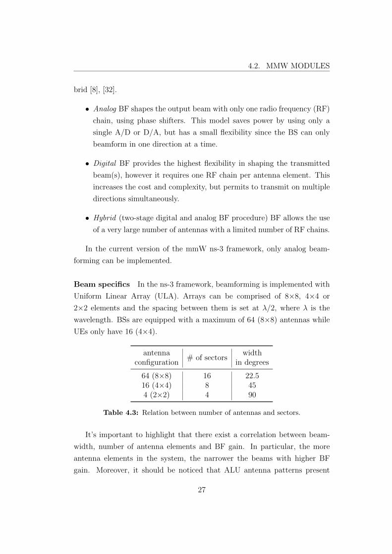
Beam specifics In the ns-3 framework, beamforming is implemented with
Uniform Linear Array (ULA). Arrays can be comprised of 8×8, 4×4 or
2×2 elements and the spacing between them is set at λ/2, where λ is the
wavelength. BSs are equipped with a maximum of 64 (8×8) antennas while
UEs only have 16 (4×4).
antennaconfiguration
# of sectorswidth
in degrees
64 (8×8) 16 22.516 (4×4) 8 454 (2×2) 4 90
Table 4.3: Relation between number of antennas and sectors.
It’s important to highlight that there exist a correlation between beam-
width, number of antenna elements and BF gain. In particular, the more
antenna elements in the system, the narrower the beams with higher BF
gain. Moreover, it should be noticed that ALU antenna patterns present
27
CHAPTER 4. NS-3 AND MMW MODULES
some undesired lobes that must taken into account for interference purposes,
when steering a beam towards a specific direction.
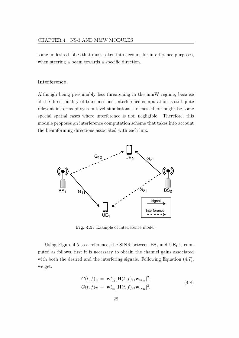
Interference
Although being presumably less threatening in the mmW regime, because
of the directionality of transmissions, interference computation is still quite
relevant in terms of system level simulations. In fact, there might be some
special spatial cases where interference is non negligible. Therefore, this
module proposes an interference computation scheme that takes into account
the beamforming directions associated with each link.
Fig. 4.5: Example of interference model.
Using Figure 4.5 as a reference, the SINR between BS1 and UE1 is com-
puted as follows, first it is necessary to obtain the channel gains associated
with both the desired and the interfering signals. Following Equation (4.7),
we get:
G(t, f)11 = |w∗rx11
H(t, f)11wtx11|2,G(t, f)21 = |w∗
rx11H(t, f)21wtx22|2.
(4.8)
28
4.2. MMW MODULES
Then we can compute the SINR, considering also the interference as follows:
SINR11 =
PTx,11
PL11G11
PTx,22
PL21G21 +BW ×N0
(4.9)
where PTx,11 is the transmit power of BS1, PL11 is the pathloss between BS1
and UE1, and BW ×N0 is the thermal noise.
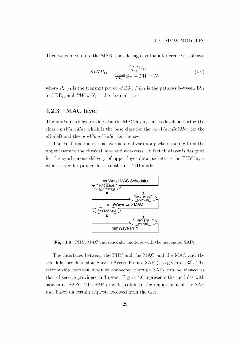
4.2.3 MAC layer
The mmW modules provide also the MAC layer, that is developed using the
class mmWaveMac which is the base class for the mmWaveEnbMac for the
eNodeB and the mmWaveUeMac for the user.
The chief function of this layer is to deliver data packets coming from the
upper layers to the physical layer and vice-versa. In fact this layer is designed
for the synchronous delivery of upper layer data packets to the PHY layer
which is key for proper data transfer in TDD mode.
mmWave PHY
mmWave Enb MAC
mmWave MAC Scheduler
PHY SAP User
PHY SAP
Provider
MAC Sched.
SAP Provider
MAC Sched.
SAP User
Fig. 4.6: PHY, MAC and scheduler modules with the associated SAPs.
The interfaces between the PHY and the MAC and the MAC and the
scheduler are defined as Service Access Points (SAPs), as given in [33]. The
relationship between modules connected through SAPs can be viewed as
that of service providers and users. Figure 4.6 represents the modules with
associated SAPs. The SAP provider caters to the requirement of the SAP
user based on certain requests received from the user.
29
CHAPTER 4. NS-3 AND MMW MODULES
The eNodeB MAC layer is connected to the scheduler module using the
MAC-SCHED SAP. Thus the MAC layer communicates the scheduling and
the resource allocation decision to the PHY layer.
Adaptive Modulation and Coding (AMC)
The working of the AMC is similar to that for LTE. The user measures
the CQI for each downlink data slot it is allocated. The CQI information is
then forwarded to the eNodeB using the mmWaveCqiReport control message.
The eNodeB scheduler uses this information to compute the most suitable
modulation and coding scheme for the communication link.
The AMC is implemented by the eNodeB MAC schedulers. During re-
source allocation, for the current framework, the wide band CQI is used to
generate the Modulation and Coding Scheme (MCS) to be used and TB size
that can be transmitted over the physical layer.
Scheduler
Following the design strategy for the ns-3 LTE module [29], the virtual class
mmWaveMacScheduler defines the interface for the implementation of MAC
scheduling techniques.
The scheduler hosts the AMC module and performs the scheduling and
resource allocation for a subframe with both DL and UL slots.
The TDD scheme enforced by the scheduler module is based on the user
specified parameter TDDControlDataPattern given in Table 4.1. The slots
specified for control are assigned alternately for DL and UL control channels.
The data slots are equally divided between DL and UL slots with the first
n/2 data slots allocated to DL data and rest to uplink, where n is the total
number of data slots. This scheme minimizes the switching time between UL
and DL data transmissions.
Resource Allocation
Using the mmWavePhyMacCommon object, the division of resources in the
frequency domain can be customized as given in Table 4.1. The MAC sched-
30
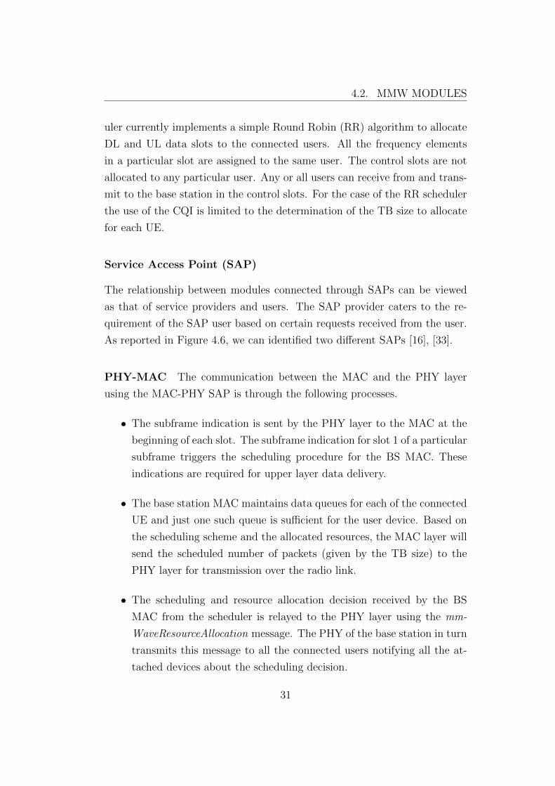
4.2. MMW MODULES
uler currently implements a simple Round Robin (RR) algorithm to allocate
DL and UL data slots to the connected users. All the frequency elements
in a particular slot are assigned to the same user. The control slots are not
allocated to any particular user. Any or all users can receive from and trans-
mit to the base station in the control slots. For the case of the RR scheduler
the use of the CQI is limited to the determination of the TB size to allocate
for each UE.
Service Access Point (SAP)
The relationship between modules connected through SAPs can be viewed
as that of service providers and users. The SAP provider caters to the re-
quirement of the SAP user based on certain requests received from the user.
As reported in Figure 4.6, we can identified two different SAPs [16], [33].
PHY-MAC The communication between the MAC and the PHY layer
using the MAC-PHY SAP is through the following processes.
• The subframe indication is sent by the PHY layer to the MAC at the
beginning of each slot. The subframe indication for slot 1 of a particular
subframe triggers the scheduling procedure for the BS MAC. These
indications are required for upper layer data delivery.
• The base station MAC maintains data queues for each of the connected
UE and just one such queue is sufficient for the user device. Based on
the scheduling scheme and the allocated resources, the MAC layer will
send the scheduled number of packets (given by the TB size) to the
PHY layer for transmission over the radio link.
• The scheduling and resource allocation decision received by the BS
MAC from the scheduler is relayed to the PHY layer using the mm-
WaveResourceAllocation message. The PHY of the base station in turn
transmits this message to all the connected users notifying all the at-
tached devices about the scheduling decision.
31
CHAPTER 4. NS-3 AND MMW MODULES
• Based on the SINR of the received data slots, the UE PHY calculates
the CQI and transmits it to the base station in the next UL control slot.
The BS PHY on receiving the mmWaveCqiReport control message,
relays it to the MAC.
MAC-SCHED The eNodeB MAC uses the service provided by the sched-
uler through the following processes.
• On receiving the subframe indication for slot 1 of a particular sub-
frame, the MAC sends a Scheduling Trigger Request to the scheduler,
which returns the scheduling and allocation decisions in the Scheduling
Configuration Indication in response to the trigger.
• The BS MAC, on receiving the CQI information from the PHY, sends
it to the scheduler. The scheduler needs this information for future
scheduling decisions.
4.2.4 Simulation
The simulation of a network using mmW modules in the ns-3 environment
is made through the following steps:
• The first step is the definition of the scenario, number of UEs and BSs
and the corresponding position. Moreover, it is necessary to specify,
for each UE, which is the cell to being attached and registered.
• Definition of other parameters like carrier frequency, transmission power,
mobility model and path-loss model.
• Development of the main simulation program, written in C++, which
implements the scenario with specific parameters.
• Run of the simulation
32
4.2. MMW MODULES
4.2.5 Results analysis
In order to study the results of the simulations, ns-3 is able to save some
traces that capture the evolution of the system during the simulation.
In the production of results, we focus on TB size allocated3 in each slot
for each user. With the use of this trace, we can see the evolution of the
system and how resources are assigned to each user.
Hence, at the end of the simulation, a .txt log-file is generated for each
user with information about time and size of the allocation. Then with a
simple MATLABr script we parse the results and therefore average them in
order to obtain the graphs in Section 6.3.
3Here we are referring to the size in byte of the transport block that are allocated bythe MAC layer (mmWaveRrMacScheduler class) in a given slot.
33

CHAPTER 4. NS-3 AND MMW MODULES
34
Chapter 5
Sharing procedure
5.1 Blind method
We define the blind method as the default procedure implemented in the ns-3
framework.
Every time a simulation is run, all the frame structure of the code is
configured as reported in Table 4.1. More precisely, DL slots are alternated
with UL slots, under the control of the scheduler that performs a Round
Robin allocated one entire slot (30 OFDM symbols) for user. These settings
correspond to performing a Time Division Multiple Access (TDMA) with the
addition of the RR scheduler in a way to serve equally all the UEs.
5.2 SPSH scenario between different mmW
networks
Before entering in detail with the sharing procedure described in this thesis,
we introduce here an example to understand the scenario we are interesting
in.
Consider a scenario in which there are two mmW networks (as shown
in Figure 5.1), one green and one yellow, that can represent two different
operator BSs in the same area.
Assuming they are operating on the same channel and located in the same
35
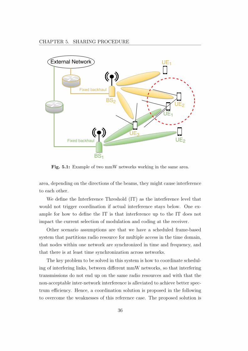
CHAPTER 5. SHARING PROCEDURE
Fig. 5.1: Example of two mmW networks working in the same area.
area, depending on the directions of the beams, they might cause interference
to each other.
We define the Interference Threshold (IT) as the interference level that
would not trigger coordination if actual interference stays below. One ex-
ample for how to define the IT is that interference up to the IT does not
impact the current selection of modulation and coding at the receiver.
Other scenario assumptions are that we have a scheduled frame-based
system that partitions radio resource for multiple access in the time domain,
that nodes within one network are synchronized in time and frequency, and
that there is at least time synchronization across networks.
The key problem to be solved in this system is how to coordinate schedul-
ing of interfering links, between different mmW networks, so that interfering
transmissions do not end up on the same radio resources and with that the
non-acceptable inter-network interference is alleviated to achieve better spec-
trum efficiency. Hence, a coordination solution is proposed in the following
to overcome the weaknesses of this reference case. The proposed solution is
36
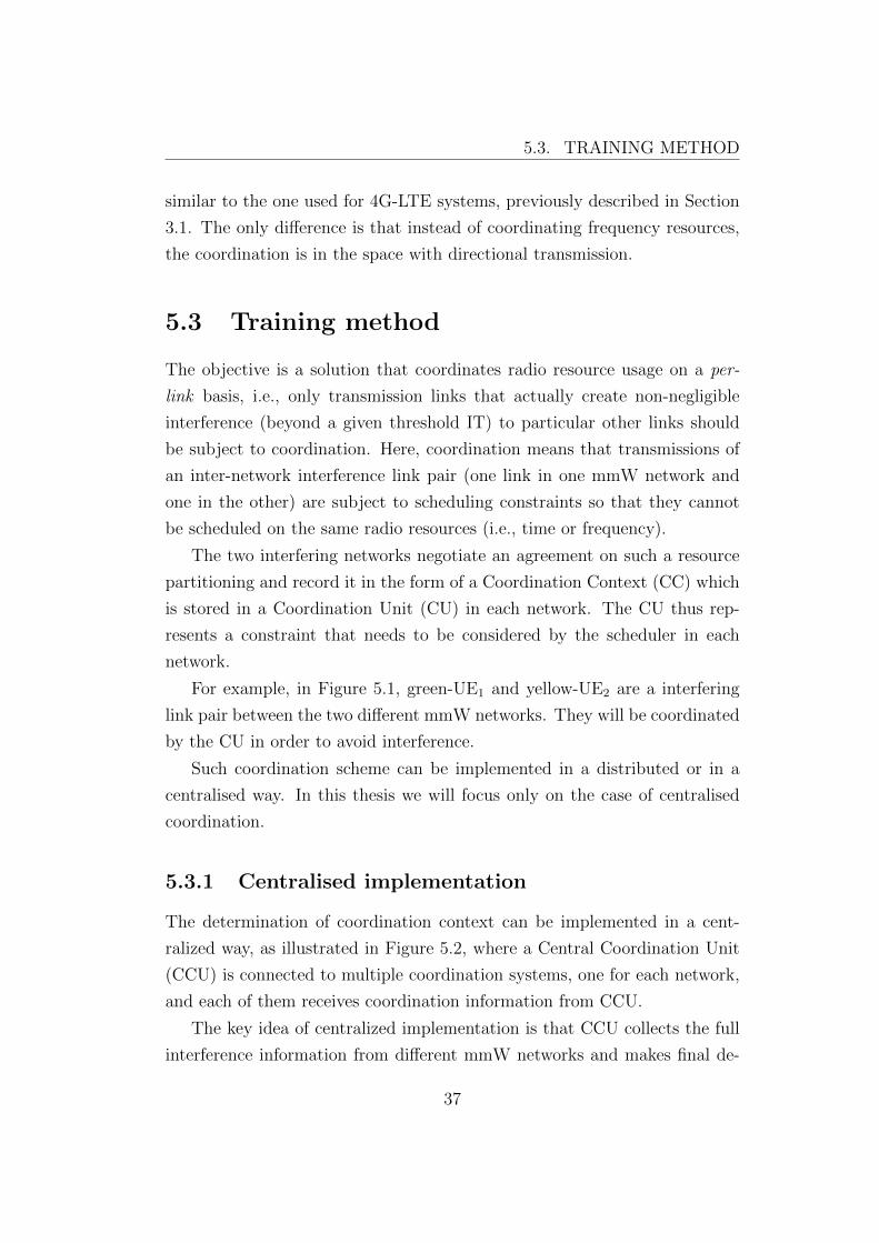
5.3. TRAINING METHOD
similar to the one used for 4G-LTE systems, previously described in Section
3.1. The only difference is that instead of coordinating frequency resources,
the coordination is in the space with directional transmission.
5.3 Training method
The objective is a solution that coordinates radio resource usage on a per-
link basis, i.e., only transmission links that actually create non-negligible
interference (beyond a given threshold IT) to particular other links should
be subject to coordination. Here, coordination means that transmissions of
an inter-network interference link pair (one link in one mmW network and
one in the other) are subject to scheduling constraints so that they cannot
be scheduled on the same radio resources (i.e., time or frequency).
The two interfering networks negotiate an agreement on such a resource
partitioning and record it in the form of a Coordination Context (CC) which
is stored in a Coordination Unit (CU) in each network. The CU thus rep-
resents a constraint that needs to be considered by the scheduler in each
network.
For example, in Figure 5.1, green-UE1 and yellow-UE2 are a interfering
link pair between the two different mmW networks. They will be coordinated
by the CU in order to avoid interference.
Such coordination scheme can be implemented in a distributed or in a
centralised way. In this thesis we will focus only on the case of centralised
coordination.
5.3.1 Centralised implementation
The determination of coordination context can be implemented in a cent-
ralized way, as illustrated in Figure 5.2, where a Central Coordination Unit
(CCU) is connected to multiple coordination systems, one for each network,
and each of them receives coordination information from CCU.
The key idea of centralized implementation is that CCU collects the full
interference information from different mmW networks and makes final de-
37
CHAPTER 5. SHARING PROCEDURE
Central
Coordination
Unit
mmW
system A
Coordination
mmW
system B
Coordination
mmW
system C
Coordination
Fig. 5.2: Illustration of a centralised coordination among three different mmWnetworks.
cisions on the links which need CC to avoid interference above the acceptable
IT.
5.3.2 Training algorithm and ns-3 implementation
In the case of centralised implementation the following procedure would be
needed:
Step 1 - Inter-network interference detection: is operated in each
BS through a measurement process already present in the LTE standard. In
order to facilitate the CC concept, the interference is identified in terms of
CQI level. As already mentioned in LTE, transmission of CQI messages is
automatically performed by all the UEs immediately after having received a
DL slot. In this manner, each BS can identify the victim UEs by reading the
CQI messages received.
Knowing that, starting from the original ns-3 framework, designed by the
NYU Wireless Group [16], we add a class that has the role of central control
unit. The CCU has been implemented as a class called TrainingUnit (TU).
At the beginning of each simulation, this class is initialised, and so connected
38
5.3. TRAINING METHOD
with each BSs and ready to store interference information.
Step 2 - Interference information transfer: The measured interference
information will be transferred to the CCU in order to form the basis for the
CC decision. The interference information will mainly include the Radio
Network Temporary Identifier (RNTI) of the transmitter ID (unique inside
the BS), the cell ID and the CQI value.
TU class, after initialization, is able to receive and save CQI values arrived
from the mmWaveEnbPhy class. This last proceeds with the transmission
of CQI information calling method saveCqi, only in the case the training
procedure is enabled, otherwise it keeps the CQI message and uses it only to
determine the allocation size of the future transmissions.
In addition to keeping all the interference information, TU coordinates
also the schedule of the BS transmissions in order to receive a complete
interference table for each user in the system.
Step 3 - Coordination context decision: Through collecting inform-
ation from multiple BSs, the TU class can obtain interference information
from the involved multiple connected networks. Based on this information,
TU then establishes an interference graph by considering a node and an in-
terference relationship as vertex and edge respectively. In order to avoid
severe interference among different mmW networks, the interference pair of
nodes (i.e., green-UE1 and yellow-UE2 in Figure 5.1) should be scheduled to
different (i.e., orthogonal) radio resources. If we connect with an edge all the
nodes that can’t be allocated in the same resources the CC determination
problem becomes the following graph coloring problem:
Graph coloring problem: Given a graph G(V,E), where V is the set of vertices
and E is the set of edges, find minimum k, and mapping r : V {1, ..., k} such that
r(i) 6= r(j) for each edge (i, j) ∈ E.
In this way, the algorithm ends with the k pairs of nodes that can transmit
in the same resource allocation.
39
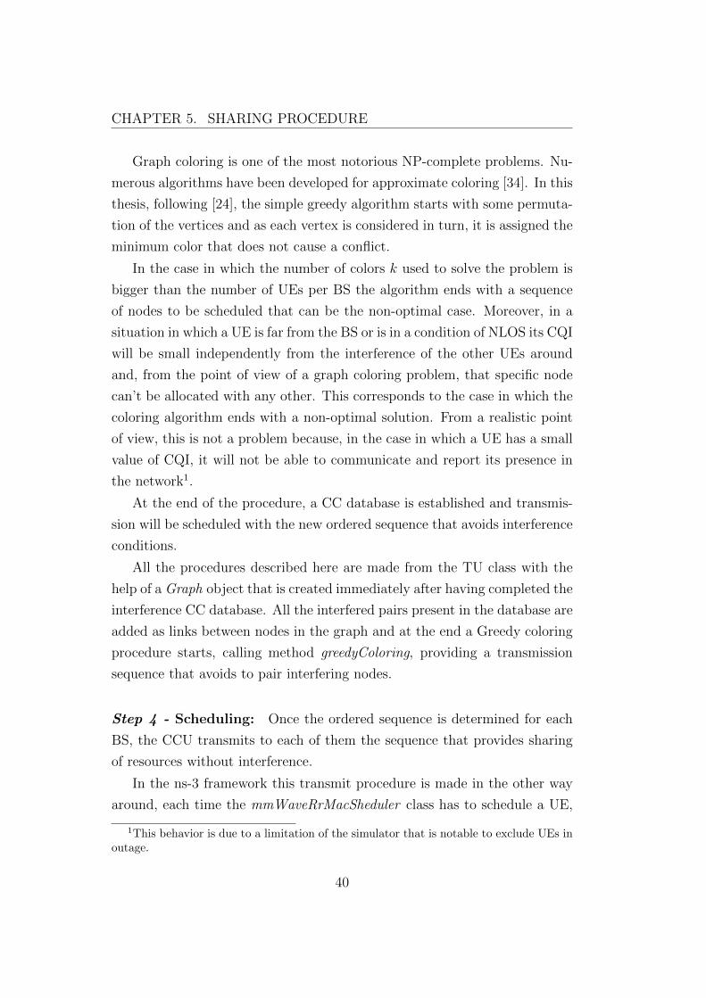
CHAPTER 5. SHARING PROCEDURE
Graph coloring is one of the most notorious NP-complete problems. Nu-
merous algorithms have been developed for approximate coloring [34]. In this
thesis, following [24], the simple greedy algorithm starts with some permuta-
tion of the vertices and as each vertex is considered in turn, it is assigned the
minimum color that does not cause a conflict.
In the case in which the number of colors k used to solve the problem is
bigger than the number of UEs per BS the algorithm ends with a sequence
of nodes to be scheduled that can be the non-optimal case. Moreover, in a
situation in which a UE is far from the BS or is in a condition of NLOS its CQI
will be small independently from the interference of the other UEs around
and, from the point of view of a graph coloring problem, that specific node
can’t be allocated with any other. This corresponds to the case in which the
coloring algorithm ends with a non-optimal solution. From a realistic point
of view, this is not a problem because, in the case in which a UE has a small
value of CQI, it will not be able to communicate and report its presence in
the network1.
At the end of the procedure, a CC database is established and transmis-
sion will be scheduled with the new ordered sequence that avoids interference
conditions.
All the procedures described here are made from the TU class with the
help of a Graph object that is created immediately after having completed the
interference CC database. All the interfered pairs present in the database are
added as links between nodes in the graph and at the end a Greedy coloring
procedure starts, calling method greedyColoring, providing a transmission
sequence that avoids to pair interfering nodes.
Step 4 - Scheduling: Once the ordered sequence is determined for each
BS, the CCU transmits to each of them the sequence that provides sharing
of resources without interference.
In the ns-3 framework this transmit procedure is made in the other way
around, each time the mmWaveRrMacSheduler class has to schedule a UE,
1This behavior is due to a limitation of the simulator that is notable to exclude UEs inoutage.
40
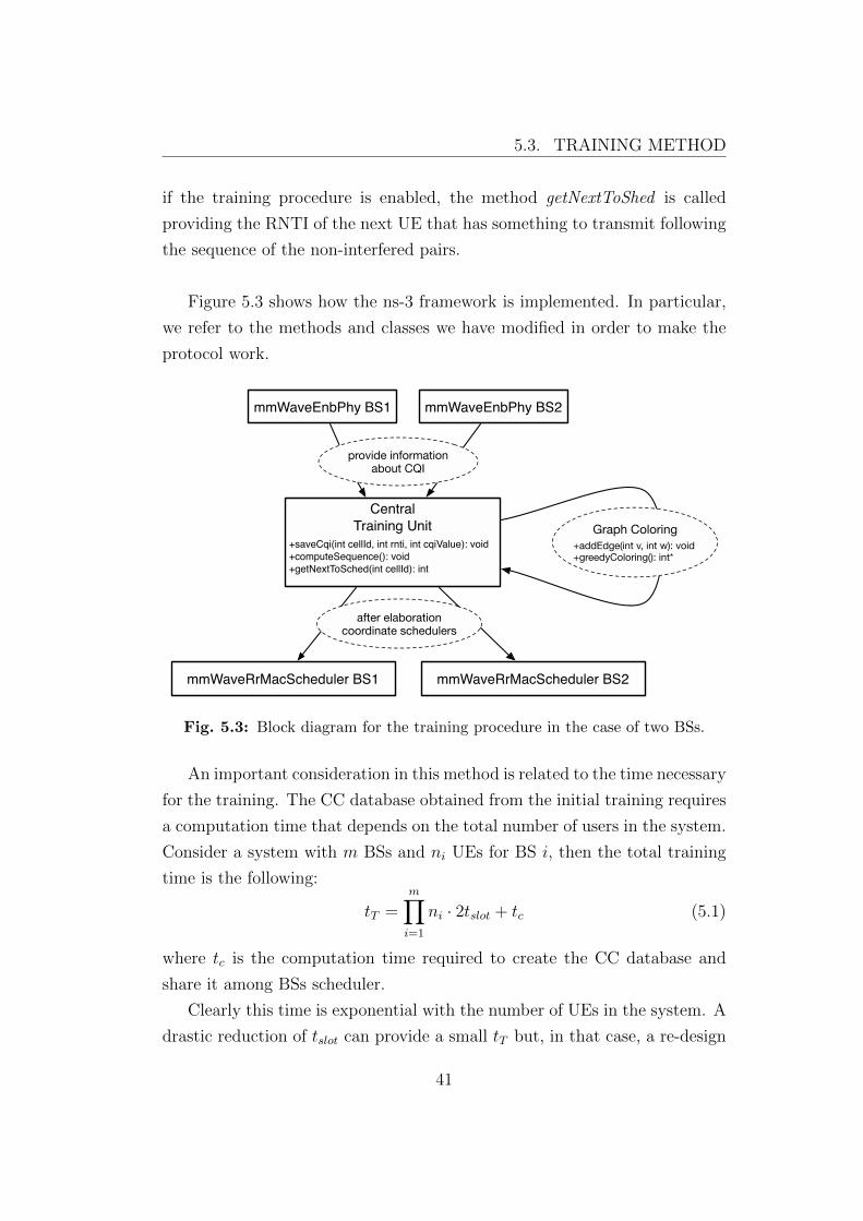
5.3. TRAINING METHOD
if the training procedure is enabled, the method getNextToShed is called
providing the RNTI of the next UE that has something to transmit following
the sequence of the non-interfered pairs.
Figure 5.3 shows how the ns-3 framework is implemented. In particular,
we refer to the methods and classes we have modified in order to make the
protocol work.
mmWaveRrMacScheduler BS1
Central
Training Unit
+saveCqi(int cellId, int rnti, int cqiValue): void
+computeSequence(): void
+getNextToSched(int cellId): int
mmWaveEnbPhy BS1 mmWaveEnbPhy BS2
provide informationabout CQI
Graph Coloring
+addEdge(int v, int w): void+greedyColoring(): int*
mmWaveRrMacScheduler BS2
after elaboration coordinate schedulers
Fig. 5.3: Block diagram for the training procedure in the case of two BSs.
An important consideration in this method is related to the time necessary
for the training. The CC database obtained from the initial training requires
a computation time that depends on the total number of users in the system.
Consider a system with m BSs and ni UEs for BS i, then the total training
time is the following:
tT =m∏i=1
ni · 2tslot + tc (5.1)
where tc is the computation time required to create the CC database and
share it among BSs scheduler.
Clearly this time is exponential with the number of UEs in the system. A
drastic reduction of tslot can provide a small tT but, in that case, a re-design
41
CHAPTER 5. SHARING PROCEDURE
of the frame structure of the ns-3 code is necessary.
5.4 Heuristic method
We implemented and studied also a different approach in which there isn’t
a training procedure that provides a complete table of interference condition
and CC database, but we periodically proceed with a swap in the transmission
scheduler order using the small amount of interference information exchange
in each sub-frame.
5.4.1 Heuristic algorithm and ns-3 implementation
Implemented as before in a centralised way, the procedure is the following:
Step 1 - Initialization: Starting from a normal transmission where a
Round Robin scheduler is implemented, each BS begins to receive CQI values
for each DL slot allocated.
In the ns-3 framework, at the beginning of the simulation, a ControlUnit
class is initialised and again, as the TU, is connect with each BSs.
Step 2 - Sampling and processing: As in the training approach, all the
CQI values with attached RNTI and Cell ID are transmitted to the CCU.
This procedure has been obtained with the call of the method saveCqi of the
ControlUnit class.
In a different manner from before, here the CCU reads all the CQI and
performs a swap in the order, only in the case the minimum CQI value is
below a fixed interference threshold.
In this approach, the code provides a change in the scheduled order by
processing only a part of the total interference information. Therefore, the
change performed can result in a better or worse situation. In order to reduce
the number of changes that result in a worse situation, the ControlUnit class
42
5.4. HEURISTIC METHOD
saves all the changes made in the past2. This helps the code to choose the
future swaps in a way to avoid cycling repetition or previous conditions.
Step 3 - Share of sequences: After the procession, the CCU stores the
new sequence just processed and transmits it to all the BSs. When the
BSs receive the new sequence, they perform the transmission continuing to
send CQI information to the CCU. After a fixed time, that depends on the
computation of the data and the coordination of the schedulers, the whole
procedure can be repeated starting again form step 1.
The ControlUnit class keeps trace of the order in which the transmission
is computed and so can easily identify future interference conditions.
As in the training procedure, when each BS scheduler (mmWaveRrMac-
Scheduler) have to allocate the transmission of a UE, it calls the method
getNextToSched in order to receive the RNTI of the next transmitting ele-
ment.
Figure 5.4 shows the class connection for the ns-3 implementation. Here,
in a different way from the training procedure, the algorithm continues to
run periodically until all the CQI values are above a defines threshold.
Working in a different manner than the training procedure, this heuristic
method doesn’t require particular computational time. The BSs can process
the CQIs received without stopping the transmission by working in a parallel
way.
2Obviously in this procedure the memory to store the changes is limited. In the exe-cution of the results we had enough space to store all the changes in 200ms. For futureimplementation a study is necessary in order to provide a good trade-off between the spaceused for saving changes and the improvements of the algorithm.
43
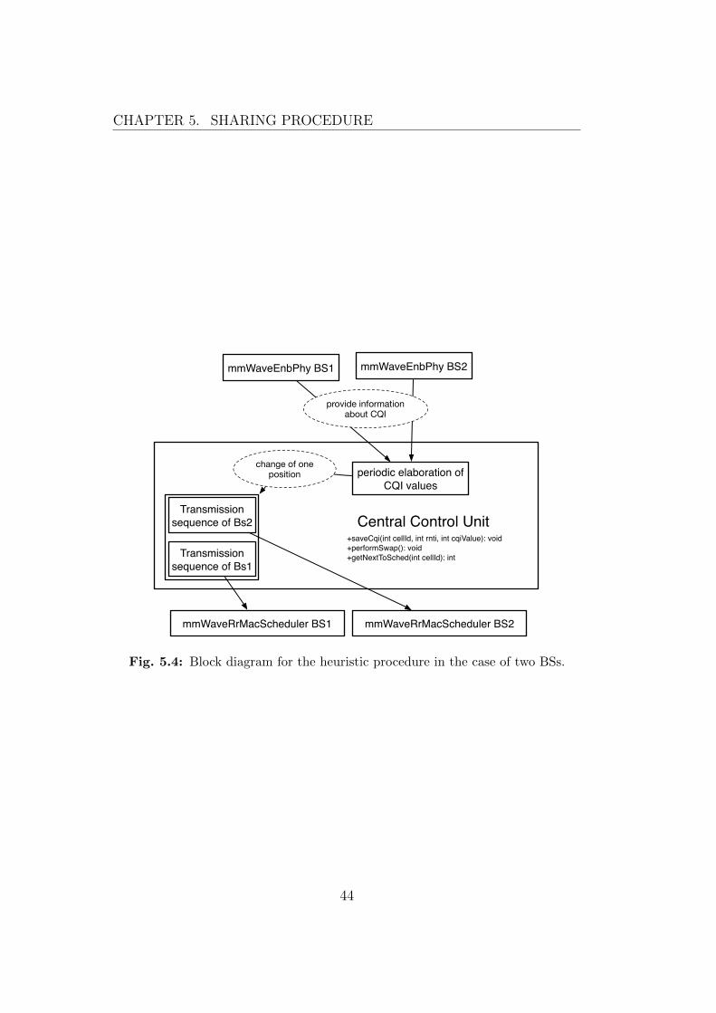
CHAPTER 5. SHARING PROCEDURE
Central Control Unit+saveCqi(int cellId, int rnti, int cqiValue): void+performSwap(): void+getNextToSched(int cellId): int
mmWaveRrMacScheduler BS1
periodic elaboration of CQI values
mmWaveEnbPhy BS1 mmWaveEnbPhy BS2
provide informationabout CQI
change of one position
mmWaveRrMacScheduler BS2
Transmission sequence of Bs1
Transmission sequence of Bs2
Fig. 5.4: Block diagram for the heuristic procedure in the case of two BSs.
44
Chapter 6
Simulated scenarios and results
6.1 Simulation assumption
In all the simulations we will present in this section, we have used the ns-3
framework just described above (Section 4.2) under the following assump-
tions.
We will work at the frequency of 28 GHz as carrier frequency for the
mmW channel. More precisely, the total 72 sub-bands that form the 4 RB
are spread between 27.5 and 28.5 GHz. In addition, we could have used
the other frequency of 73 GHz that is also available in the ns-3 model, but
knowing the characteristic of the propagation explained in Section 2.2.1 we
analysed only the 28 GHz.
We will assume a static deployment, where users and BSs can’t move
during the simulation. In this way, no handover management is required,
path loss and directional beam for the transmission to a specific UE doesn’t
change during the run of the simulation. In the future works, additional
feature (like handover management, mobility, etc) must be implemented in
such a way we can simulate more complicated scenarios.
We will assume to work in a dense urban environment, since the spatial
statistical model provided in [5] has been realised in it. In the literature this
new model is the first that includes channel parameters for mmW like path
loss, number of spatial clusters, angular dispersion and outage.
45
CHAPTER 6. SIMULATED SCENARIOS AND RESULTS
We will also assume to always use analog beamforming, steering direc-
tional beams between BSs and UEs.
All these preliminary assumptions do not affect the performance of the
spatial SPSH procedure here presented and studied. In the near future, when
the ns-3 framework will have more sophisticated features all these assump-
tions will be removed or relaxed.
6.1.1 Jain’s fairness index
Fairness metrics are used in network engineering to determine whether users
or applications are receiving a fair share of system resources. There are
several mathematical and conceptual definitions of fairness, but in this thesis
we decided to use Jain’s fairness index [35] to study the fairness behavior of
the approaches implemented.
Raj Jain’s equation:
J (η1, η2, · · · , ηn) =(∑n
i=1 ηi)2
n∑n
i=1 η2i
(6.1)
rates the fairness of a set of values where there are n users and ηi is the
throughput for the i-th connection. The result J , ranges from 1n
(that rep-
resents the worst case) to 1 (best case), and it is maximum when all users
receive the same allocation.
In the scenarios we are going to study, this index can help to evaluate the
performance. If in a system Jain’s index increases, this means that resources
are better assigned among all the UE. Otherwise if the index decreases, this
means we are allocating more resources for some UE instead of equally dis-
tributing them among all the UEs.
6.2 Simulated parameters
In all the simulations executed in this thesis project, we have used the para-
meters reported in Table 6.1. Moreover, all the specifics of the original ns-3
framework (described in Chapter 4) are kept as default in addition to the
46
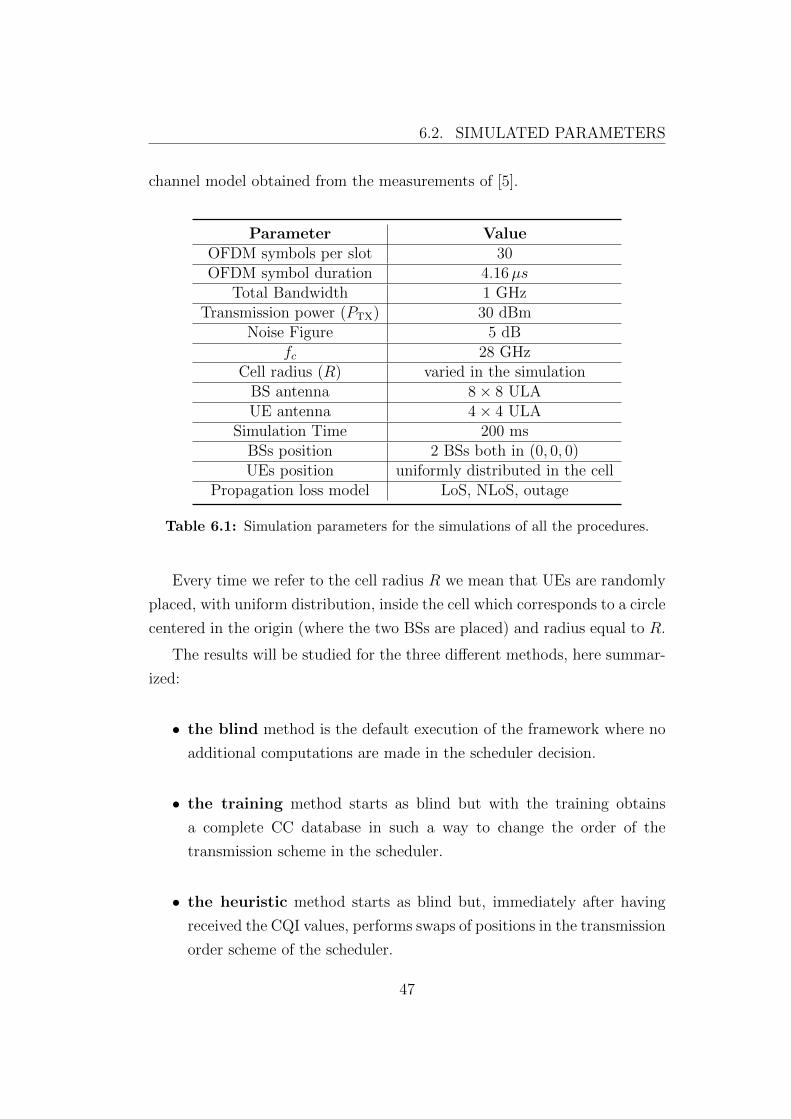
6.2. SIMULATED PARAMETERS
channel model obtained from the measurements of [5].
Parameter ValueOFDM symbols per slot 30OFDM symbol duration 4.16µs
Total Bandwidth 1 GHzTransmission power (PTX) 30 dBm
Noise Figure 5 dBfc 28 GHz
Cell radius (R) varied in the simulationBS antenna 8× 8 ULAUE antenna 4× 4 ULA
Simulation Time 200 msBSs position 2 BSs both in (0, 0, 0)UEs position uniformly distributed in the cell
Propagation loss model LoS, NLoS, outage
Table 6.1: Simulation parameters for the simulations of all the procedures.
Every time we refer to the cell radius R we mean that UEs are randomly
placed, with uniform distribution, inside the cell which corresponds to a circle
centered in the origin (where the two BSs are placed) and radius equal to R.
The results will be studied for the three different methods, here summar-
ized:
• the blind method is the default execution of the framework where no
additional computations are made in the scheduler decision.
• the training method starts as blind but with the training obtains
a complete CC database in such a way to change the order of the
transmission scheme in the scheduler.
• the heuristic method starts as blind but, immediately after having
received the CQI values, performs swaps of positions in the transmission
order scheme of the scheduler.
47
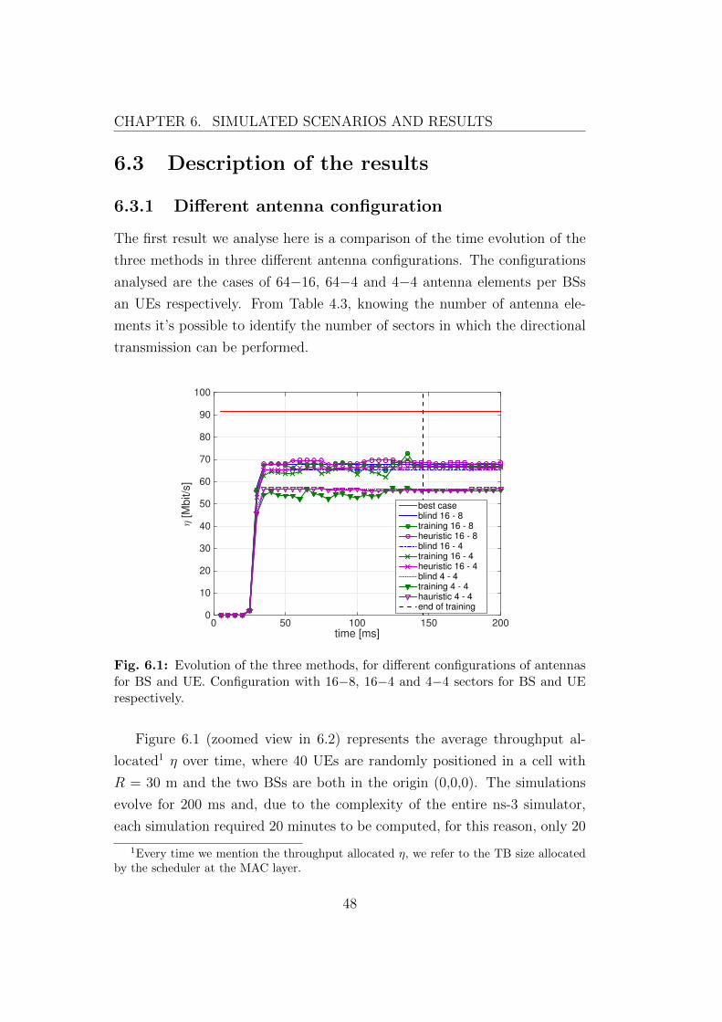
CHAPTER 6. SIMULATED SCENARIOS AND RESULTS
6.3 Description of the results
6.3.1 Different antenna configuration
The first result we analyse here is a comparison of the time evolution of the
three methods in three different antenna configurations. The configurations
analysed are the cases of 64−16, 64−4 and 4−4 antenna elements per BSs
an UEs respectively. From Table 4.3, knowing the number of antenna ele-
ments it’s possible to identify the number of sectors in which the directional
transmission can be performed.
time [ms]0 50 100 150 200
η [
Mb
it/s
]
0
10
20
30
40
50
60
70
80
90
100
best caseblind 16 - 8training 16 - 8heuristic 16 - 8blind 16 - 4training 16 - 4heuristic 16 - 4blind 4 - 4training 4 - 4hauristic 4 - 4end of training
Fig. 6.1: Evolution of the three methods, for different configurations of antennasfor BS and UE. Configuration with 16−8, 16−4 and 4−4 sectors for BS and UErespectively.
Figure 6.1 (zoomed view in 6.2) represents the average throughput al-
located1 η over time, where 40 UEs are randomly positioned in a cell with
R = 30 m and the two BSs are both in the origin (0,0,0). The simulations
evolve for 200 ms and, due to the complexity of the entire ns-3 simulator,
each simulation required 20 minutes to be computed, for this reason, only 20
1Every time we mention the throughput allocated η, we refer to the TB size allocatedby the scheduler at the MAC layer.
48
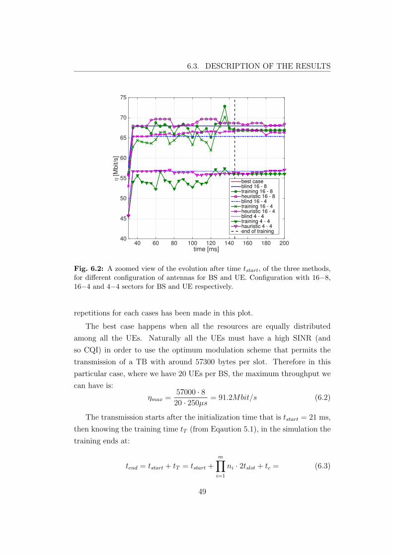
6.3. DESCRIPTION OF THE RESULTS
time [ms]40 60 80 100 120 140 160 180 200
η [M
bit/s
]
40
45
50
55
60
65
70
75
best caseblind 16 - 8training 16 - 8heuristic 16 - 8blind 16 - 4training 16 - 4heuristic 16 - 4blind 4 - 4training 4 - 4hauristic 4 - 4end of training
Fig. 6.2: A zoomed view of the evolution after time tstart, of the three methods,for different configuration of antennas for BS and UE. Configuration with 16−8,16−4 and 4−4 sectors for BS and UE respectively.
repetitions for each cases has been made in this plot.
The best case happens when all the resources are equally distributed
among all the UEs. Naturally all the UEs must have a high SINR (and
so CQI) in order to use the optimum modulation scheme that permits the
transmission of a TB with around 57300 bytes per slot. Therefore in this
particular case, where we have 20 UEs per BS, the maximum throughput we
can have is:
ηmax =57000 · 8
20 · 250µs= 91.2Mbit/s (6.2)
The transmission starts after the initialization time that is tstart = 21 ms,
then knowing the training time tT (from Eqaution 5.1), in the simulation the
training ends at:
tend = tstart + tT = tstart +m∏i=1
ni · 2tslot + tc = (6.3)
49
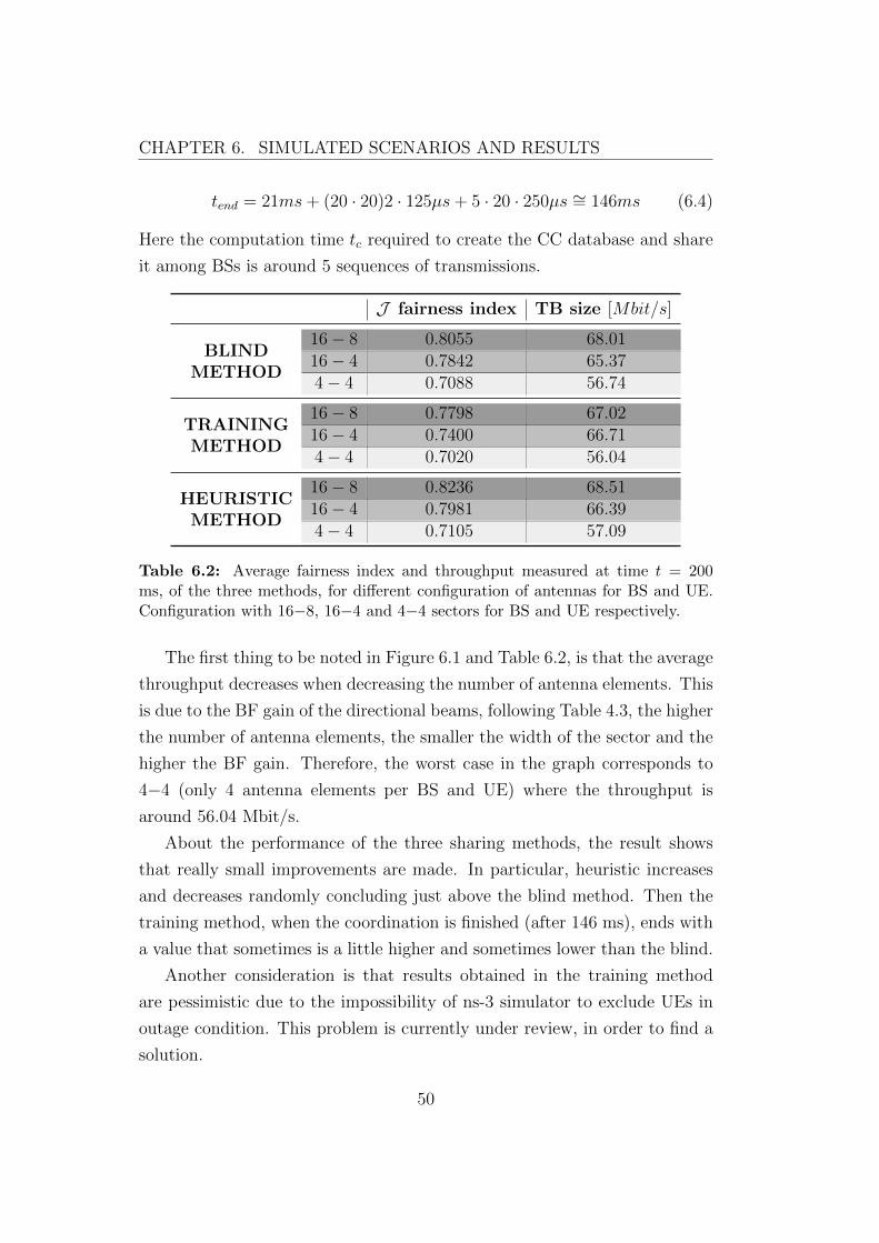
CHAPTER 6. SIMULATED SCENARIOS AND RESULTS
tend = 21ms+ (20 · 20)2 · 125µs+ 5 · 20 · 250µs ∼= 146ms (6.4)
Here the computation time tc required to create the CC database and share
it among BSs is around 5 sequences of transmissions.
J fairness index TB size [Mbit/s]
16− 8 0.8055 68.0116− 4 0.7842 65.37
BLINDMETHOD
4− 4 0.7088 56.74
16− 8 0.7798 67.0216− 4 0.7400 66.71
TRAININGMETHOD
4− 4 0.7020 56.04
16− 8 0.8236 68.5116− 4 0.7981 66.39
HEURISTICMETHOD
4− 4 0.7105 57.09
Table 6.2: Average fairness index and throughput measured at time t = 200ms, of the three methods, for different configuration of antennas for BS and UE.Configuration with 16−8, 16−4 and 4−4 sectors for BS and UE respectively.
The first thing to be noted in Figure 6.1 and Table 6.2, is that the average
throughput decreases when decreasing the number of antenna elements. This
is due to the BF gain of the directional beams, following Table 4.3, the higher
the number of antenna elements, the smaller the width of the sector and the
higher the BF gain. Therefore, the worst case in the graph corresponds to
4−4 (only 4 antenna elements per BS and UE) where the throughput is
around 56.04 Mbit/s.
About the performance of the three sharing methods, the result shows
that really small improvements are made. In particular, heuristic increases
and decreases randomly concluding just above the blind method. Then the
training method, when the coordination is finished (after 146 ms), ends with
a value that sometimes is a little higher and sometimes lower than the blind.
Another consideration is that results obtained in the training method
are pessimistic due to the impossibility of ns-3 simulator to exclude UEs in
outage condition. This problem is currently under review, in order to find a
solution.
50
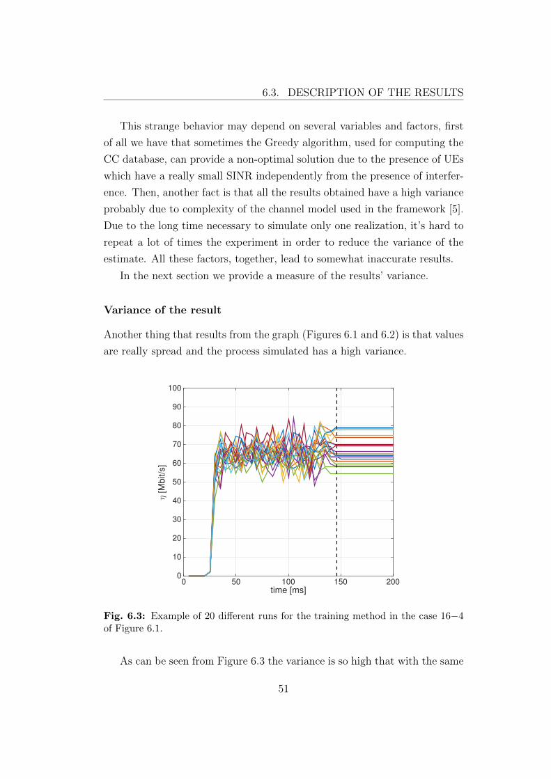
6.3. DESCRIPTION OF THE RESULTS
This strange behavior may depend on several variables and factors, first
of all we have that sometimes the Greedy algorithm, used for computing the
CC database, can provide a non-optimal solution due to the presence of UEs
which have a really small SINR independently from the presence of interfer-
ence. Then, another fact is that all the results obtained have a high variance
probably due to complexity of the channel model used in the framework [5].
Due to the long time necessary to simulate only one realization, it’s hard to
repeat a lot of times the experiment in order to reduce the variance of the
estimate. All these factors, together, lead to somewhat inaccurate results.
In the next section we provide a measure of the results’ variance.
Variance of the result
Another thing that results from the graph (Figures 6.1 and 6.2) is that values
are really spread and the process simulated has a high variance.
time [ms]0 50 100 150 200
η [M
bit/s
]
0
10
20
30
40
50
60
70
80
90
100
Fig. 6.3: Example of 20 different runs for the training method in the case 16−4of Figure 6.1.
As can be seen from Figure 6.3 the variance is so high that with the same
51
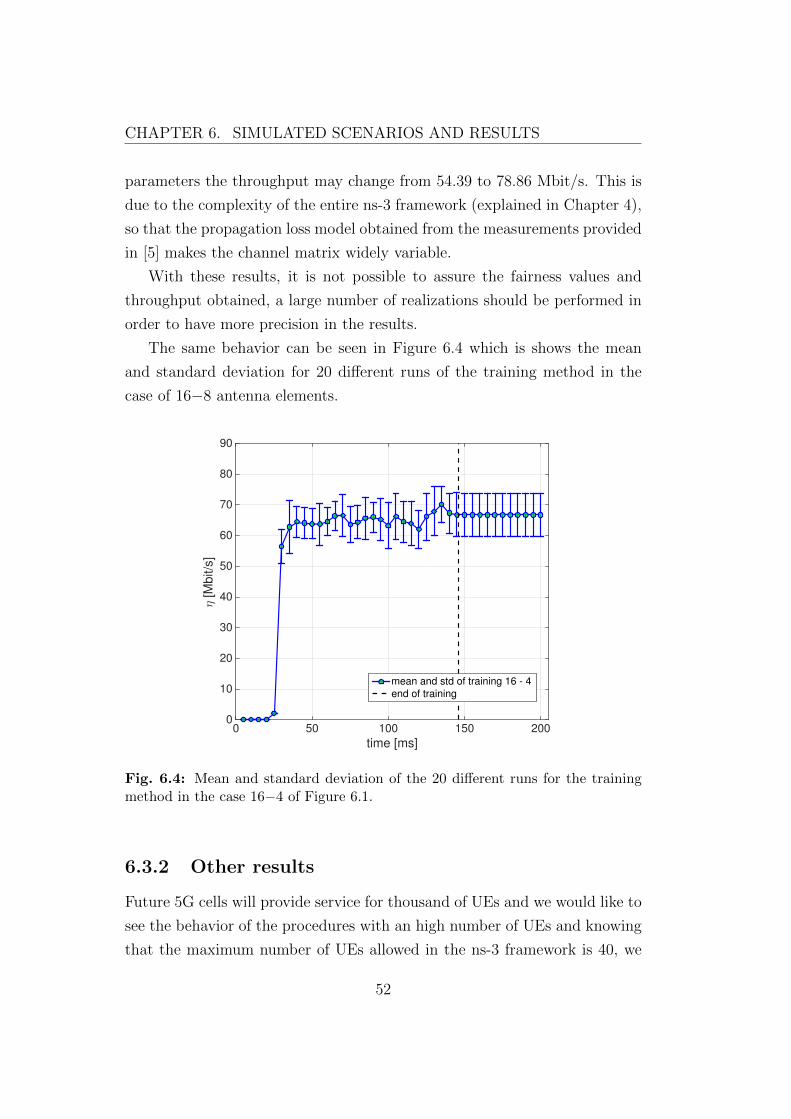
CHAPTER 6. SIMULATED SCENARIOS AND RESULTS
parameters the throughput may change from 54.39 to 78.86 Mbit/s. This is
due to the complexity of the entire ns-3 framework (explained in Chapter 4),
so that the propagation loss model obtained from the measurements provided
in [5] makes the channel matrix widely variable.
With these results, it is not possible to assure the fairness values and
throughput obtained, a large number of realizations should be performed in
order to have more precision in the results.
The same behavior can be seen in Figure 6.4 which is shows the mean
and standard deviation for 20 different runs of the training method in the
case of 16−8 antenna elements.
time [ms]
0 50 100 150 200
η [M
bit/s
]
0
10
20
30
40
50
60
70
80
90
mean and std of training 16 - 4
end of training
Fig. 6.4: Mean and standard deviation of the 20 different runs for the trainingmethod in the case 16−4 of Figure 6.1.
6.3.2 Other results
Future 5G cells will provide service for thousand of UEs and we would like to
see the behavior of the procedures with an high number of UEs and knowing
that the maximum number of UEs allowed in the ns-3 framework is 40, we
52
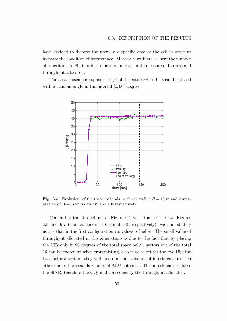
6.3. DESCRIPTION OF THE RESULTS
have decided to dispose the users in a specific area of the cell in order to
increase the condition of interference. Moreover, we increase here the number
of repetitions to 80, in order to have a more accurate measure of fairness and
throughput allocated.
The area chosen corresponds to 1/4 of the entire cell so UEs can be placed
with a random angle in the interval [0, 90] degrees.
time [ms]0 50 100 150 200
η [M
bit/s
]
0
5
10
15
20
25
30
35
40
45
50
blindtrainingheuristicend of training
Fig. 6.5: Evolution, of the three methods, with cell radius R = 10 m and config-uration of 16−8 sectors for BS and UE respectively.
Comparing the throughput of Figure 6.1 with that of the two Figures
6.5 and 6.7 (zoomed views in 6.6 and 6.8, respectively), we immediately
notice that in the first configuration its values is higher. The small value of
throughput allocated in this simulations is due to the fact that by placing
the UEs only in 90 degrees of the total space only 4 sectors out of the total
16 can be chosen so when transmitting, also if we select for the two BSs the
two furthest sectors, they will create a small amount of interference to each
other due to the secondary lobes of ALU antennas. This interference reduces
the SINR, therefore the CQI and consequently the throughput allocated.
53
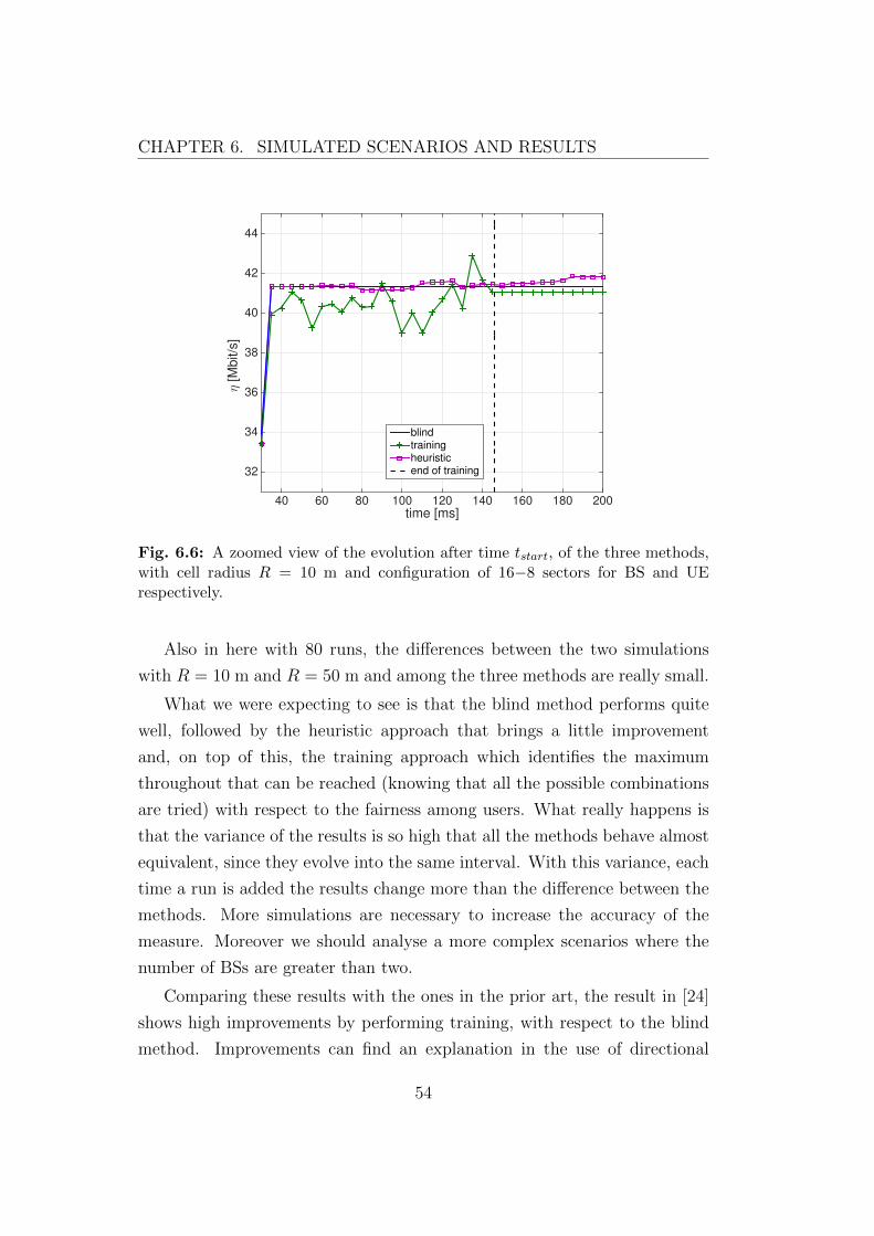
CHAPTER 6. SIMULATED SCENARIOS AND RESULTS
time [ms]40 60 80 100 120 140 160 180 200
η [
Mb
it/s
]
32
34
36
38
40
42
44
blindtrainingheuristicend of training
Fig. 6.6: A zoomed view of the evolution after time tstart, of the three methods,with cell radius R = 10 m and configuration of 16−8 sectors for BS and UErespectively.
Also in here with 80 runs, the differences between the two simulations
with R = 10 m and R = 50 m and among the three methods are really small.
What we were expecting to see is that the blind method performs quite
well, followed by the heuristic approach that brings a little improvement
and, on top of this, the training approach which identifies the maximum
throughout that can be reached (knowing that all the possible combinations
are tried) with respect to the fairness among users. What really happens is
that the variance of the results is so high that all the methods behave almost
equivalent, since they evolve into the same interval. With this variance, each
time a run is added the results change more than the difference between the
methods. More simulations are necessary to increase the accuracy of the
measure. Moreover we should analyse a more complex scenarios where the
number of BSs are greater than two.
Comparing these results with the ones in the prior art, the result in [24]
shows high improvements by performing training, with respect to the blind
method. Improvements can find an explanation in the use of directional
54
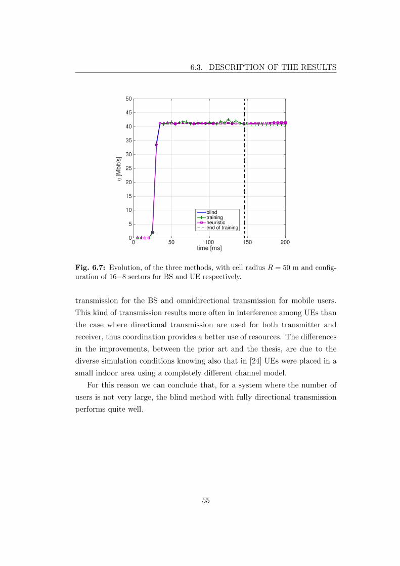
6.3. DESCRIPTION OF THE RESULTS
time [ms]0 50 100 150 200
η [
Mb
it/s
]
0
5
10
15
20
25
30
35
40
45
50
blindtrainingheuristicend of training
Fig. 6.7: Evolution, of the three methods, with cell radius R = 50 m and config-uration of 16−8 sectors for BS and UE respectively.
transmission for the BS and omnidirectional transmission for mobile users.
This kind of transmission results more often in interference among UEs than
the case where directional transmission are used for both transmitter and
receiver, thus coordination provides a better use of resources. The differences
in the improvements, between the prior art and the thesis, are due to the
diverse simulation conditions knowing also that in [24] UEs were placed in a
small indoor area using a completely different channel model.
For this reason we can conclude that, for a system where the number of
users is not very large, the blind method with fully directional transmission
performs quite well.
55
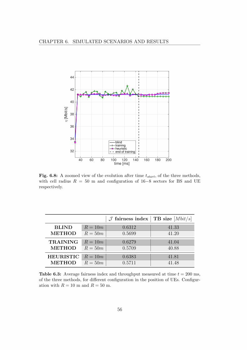
CHAPTER 6. SIMULATED SCENARIOS AND RESULTS
time [ms]40 60 80 100 120 140 160 180 200
η [
Mb
it/s
]
32
34
36
38
40
42
44
blindtrainingheuristicend of training
Fig. 6.8: A zoomed view of the evolution after time tstart, of the three methods,with cell radius R = 50 m and configuration of 16−8 sectors for BS and UErespectively.
J fairness index TB size [Mbit/s]
R = 10m 0.6312 41.33BLINDMETHOD R = 50m 0.5699 41.20
R = 10m 0.6279 41.04TRAININGMETHOD R = 50m 0.5709 40.88
R = 10m 0.6383 41.81HEURISTICMETHOD R = 50m 0.5711 41.48
Table 6.3: Average fairness index and throughput measured at time t = 200 ms,of the three methods, for different configuration in the position of UEs. Configur-ation with R = 10 m and R = 50 m.
56
Chapter 7
Conclusions and future works
In this thesis, we studied and implemented a training procedure that should
provide coordination context in a way to increase performance. We also
introduced a heuristic approach that aims as well to increase the performance,
working simultaneously with the transmission and so the evolution of the
systems.
Staring from sharing procedures already implemented in WLAN and LTE
standards, we have studied similar procedures able to work at mmW frequen-
cies.
Then with the use of the discrete simulator ns-3 we implemented and
aggregated specific class modules that permit the simulation of the algorithms
studied in the thesis.
The starting idea was to develop and so measure the improvements the
training should have provided, as in the prior art [24], in order to have an
upper bound, with respect to fairness among users, that is the maximum
achievable. The results obtained show that the process has a high variance
that is due to the impossibility to compute a very large number of realizations
and to the complexity of the mmW channel model used in the ns-3 simulator.
For this reason we can’t see and measure any kind of significant improvement.
Despite the somewhat negative results obtained in this thesis, this is the
first step that has been made to study the performance of a coordination
57
context-based spectrum sharing where directional transmission is perform in
a mmW channel.
More and more studies are necessary, starting from this first result, in
order to design a protocol that uses, in the best way, the resources for a future
mmW 5G system. A lot of challenges are to be faced, and for this reason,
a system where directional transmissions are coordinated with frequency or
time resources are necessary.
A collaboration has started with the Wireless Group at NYU in order
to improve the ns-3 framework designed by them and study new protocols
able to operate in situations where the number of users is really high and the
blind method can’t perform well.
58
Bibliography
[1] The 5G Infrastructure Public Private Partnership. (2015) 5G vision.
https://5g-ppp.eu/our-vision/. Accessed: 2015-08-03.
[2] Ericsson,“5G radio access,”February 2015, white Paper Uen 284 23-3204
Rev B.
[3] T. Rappaport, J. Murdock, and F. Gutierrez, “State of the art in 60-GHz
integrated circuits and systems for wireless communications,” Proceed-
ings of the IEEE, vol. 99, no. 8, pp. 1390–1436, Aug 2011.
[4] M. Marcus and B. Pattan,“Millimeter wave propagation; spectrum man-
agement implications,” Microwave Magazine, IEEE, vol. 6, no. 2, pp.
54–62, June 2005.
[5] M. R. Akdeniz, Y. Liu, S.Sun, S.Rangan, T. S. Rappaport, and
E. Erkip, “Millimeter wave channel modeling and cellular capacity
evaluation,” CoRR, vol. abs/1312.4921, 2013. [Online]. Available:
http://arxiv.org/abs/1312.4921
[6] P. Kyosti and et al., “WINNER II channel model,” Technical Report
IST-WINNER D1.1.2 ver 1.1, September 2007.
[7] “NGMN 5G white paper,”Feb 2015, https://www.ngmn.org/home.html.
Accessed: 2015-08-03.
[8] H. Shokri-Ghadikolaei, C. Fischione, G. Fodor, P. Popovski,
and M. Zorzi, “Millimeter wave cellular networks: A MAC
59
layer perspective,” Communications, IEEE Transactions on, 2015,
10.1109/TCOMM.2015.2456093.
[9] T. Rappaport, S. Sun, R. Mayzus, H. Zhao, Y. Azar, K. Wang, G. Wong,
J. Schulz, M. Samimi, and F. Gutierrez, “Millimeter wave mobile com-
munications for 5G cellular: It will work!” Access, IEEE, vol. 1, pp.
335–349, 2013.
[10] B. Bangerter, S. Talwar, R. Arefi, and K. Stewart,“Networks and devices
for the 5G era,” Communications Magazine, IEEE, vol. 52, no. 2, pp.
90–96, February 2014.
[11] T. Rappaport, R. Heath, R. Daniels, and J. Murdock, Millimeter
Wave Wireless Communications, ser. Communication engineering
and emerging technologies. Prentice Hall, 2014. [Online]. Available:
https://books.google.it/books?id= Tt BAAAQBAJ
[12] F. Vook, A. Ghosh, and T. Thomas, “MIMO and beamforming solutions
for 5G technology,” in Microwave Symposium (IMS), 2014 IEEE MTT-S
International, June 2014, pp. 1–4.
[13] L. Badia, R. Del Re, F. Guidolin, A. Orsino, and M. Zorzi, “A tunable
framework for performance evaluation of spectrum sharing in LTE net-
works,” in World of Wireless, Mobile and Multimedia Networks (WoW-
MoM), 2013 IEEE 14th International Symposium and Workshops on a,
June 2013, pp. 1–3.
[14] L. Anchora, M. Mezzavilla, L. Badia, and M. Zorzi, “Simulation
models for the performance evaluation of spectrum sharing techniques
in OFDMA networks,” in Proceedings of the 14th ACM International
Conference on Modeling, Analysis and Simulation of Wireless and Mobile
Systems, ser. MSWiM ’11. New York, NY, USA: ACM, 2011, pp. 249–
256. [Online]. Available: http://doi.acm.org/10.1145/2068897.2068941
[15] What is ns-3. https://www.nsnam.org/overview/what-is-ns-3/. Ac-
cessed: 2015-08-03.
60
[16] M. Mezzavilla, S. Dutta, M. Zhang, M. R. Akdeniz, and S. Rangan,
“5G mmwave module for ns-3 network simulator,” CoRR, vol.
abs/1506.08801, 2015. [Online]. Available: http://arxiv.org/abs/1506.
08801
[17] S. Rangan, T. S. Rappaport, and E. Erkip, “Millimeter wave
cellular wireless networks: Potentials and challenges,” CoRR, vol.
abs/1401.2560, 2014. [Online]. Available: http://arxiv.org/abs/1401.
2560
[18] S. Rajagopal, S. Abu-Surra, Z. Pi, and F. Khan, “Antenna array design
for multi-Gbps mmwave mobile broadband communication,” in Global
Telecommunications Conference (GLOBECOM 2011), 2011 IEEE, Dec
2011, pp. 1–6.
[19] E. Larsson, O. Edfors, F. Tufvesson, and T. Marzetta, “Massive MIMO
for next generation wireless systems,”Communications Magazine, IEEE,
vol. 52, no. 2, pp. 186–195, February 2014.
[20] L. Lu, G. Li, A. Swindlehurst, A. Ashikhmin, and R. Zhang, “An over-
view of massive MIMO: Benefits and challenges,” Selected Topics in Sig-
nal Processing, IEEE Journal of, vol. 8, no. 5, pp. 742–758, Oct 2014.
[21] B. Van Veen and K. Buckley, “Beamforming: a versatile approach to
spatial filtering,” ASSP Magazine, IEEE, vol. 5, no. 2, pp. 4–24, April
1988.
[22] L. Anchora, M. Mezzavilla, L. Badia, and M. f, “A performance
evaluation tool for spectrum sharing in multi-operator LTE networks,”
Computer Communications, vol. 35, no. 18, pp. 2218 – 2226, 2012.
[Online]. Available: http://www.sciencedirect.com/science/article/pii/
S0140366412002678
[23] W. Feng, Y. Li, D. Jin, and L. Zeng, “Inter-network spatial sharing
with interference mitigation based on IEEE 802.11ad WLAN system,”
in Globecom Workshops (GC Wkshps), 2014, Dec 2014, pp. 752–758.
61
[24] G. Li, T. Irnich, and C. Shi, “Coordination context-based spectrum shar-
ing for 5G millimeter-wave networks,” in Cognitive Radio Oriented Wire-
less Networks and Communications (CROWNCOM), 2014 9th Interna-
tional Conference on, June 2014, pp. 32–38.
[25] R. Cai, Q. Chen, X. Peng, and D. Liu, “Spatial sharing algorithm in
mmwave WPANs with interference sense beamforming mechanism,” in
Military Communications Conference, MILCOM 2013 - 2013 IEEE, Nov
2013, pp. 163–168.
[26] Q. Chen, X. Peng, J. Yang, and F. Chin, “Spatial reuse strategy in
mmwave WPANs with directional antennas,” in Global Communications
Conference (GLOBECOM), 2012 IEEE, Dec 2012, pp. 5392–5397.
[27] J. Luo, J. Eichinger, Z. Zhao, and E. Schulz, “Multi-carrier waveform
based flexible inter-operator spectrum sharing for 5G systems,” in Dy-
namic Spectrum Access Networks (DYSPAN), 2014 IEEE International
Symposium on, April 2014, pp. 449–457.
[28] NYU wireless. Available at: http://nyuwireless.com.
[29] G. Piro, N. Baldo, and M. Miozzo, “An LTE module for the ns-3
network simulator,” in Proceedings of the 4th International ICST
Conference on Simulation Tools and Techniques, ser. SIMUTools ’11.
ICST, Brussels, Belgium, Belgium: ICST (Institute for Computer
Sciences, Social-Informatics and Telecommunications Engineering),
2011, pp. 415–422. [Online]. Available: http://dl.acm.org/citation.cfm?
id=2151054.2151129
[30] E. Dahlman, S. Parkvall, J. Skold, and P. Beming., 3G Evolution HSPA
and LTE for Mobile Broadband. Academic Press., 2008.
[31] C. Jeong, J. Park, and H. Yu, “Random access in millimeter-wave beam-
forming cellular networks: issues and approaches,” Communications
Magazine, IEEE, vol. 53, no. 1, pp. 180–185, January 2015.
62
[32] S. Sun, T. Rappaport, R. Heath, A. Nix, and S. Rangan, “MIMO for
millimeter-wave wireless communications: beamforming, spatial multi-
plexing, or both?” Communications Magazine, IEEE, vol. 52, no. 12,
pp. 110–121, December 2014.
[33] FemtoForum, “LTE MAC scheduler interface specification v1.11,” Oct.
2010.
[34] A. Lim, Y. Zhu, Q. Lou, and B. Rodrigues, “Heuristic methods
for graph coloring problems,” in Proceedings of the 2005 ACM
Symposium on Applied Computing, ser. SAC ’05. New York,
NY, USA: ACM, 2005, pp. 933–939. [Online]. Available: http:
//doi.acm.org/10.1145/1066677.1066892
[35] R. Jain, D. Chiu, and W. Hawe, “A quantitative measure of
fairness and discrimination for resource allocation in shared computer
systems,” CoRR, vol. cs.NI/9809099, 1998. [Online]. Available:
http://arxiv.org/abs/cs.NI/9809099
63

64

Acknowledgements
Firstly, I would like to express my sincere gratitude to my advisor prof.
Michele Zorzi for his help and his support.
A huge thank you goes to the guys of the NYU Wireless: Russell Ford,
Menglei Zhang, Sourjya Dutta and Marco Mezzavilla, who wrote me hun-
dreds of emails to help make everything work.
Another thank you to the guys of the Signet group, who I thanks for all
the advices and teachings on programming.
Finally, a big hug to all the university friends who believed in me and
supported me during this years. Probably, without their help I couldn’t have
reached this milestone.