ECONOMIC ANALYSIS OF STAPLE FOOD-GRAIN CROPS:

VARIETIES’ INPUT-OUTPUT COMPARISON, ECONOMIC

PRACTICES AND SIGNIFICANCE IN THE ECONOMY OF

DISTRICT SWAT

By

ANWAR HUSSAIN PhD Scholar

DEPARTMENT OF ECONOMICS UNIVERSITY OF PESHAWAR

NWFP PAKISTAN 2010

ECONOMIC ANALYSIS OF STAPLE FOOD-GRAIN CROPS:

VARIETIES’ INPUT-OUTPUT COMPARISON, ECONOMIC

PRACTICES AND SIGNIFICANCE IN THE ECONOMY OF

DISTRICT SWAT

By

ANWAR HUSSAIN

A dissertation submitted to the University of Peshawar in partial fulfillment of the requirements for the degree of

DOCTOR OF PHILOSOPHY IN ECONOMICS

DEPARTMENT OF ECONOMICS UNIVERSITY OF PESHAWAR

NWFP PAKISTAN 2010

i

DEPARTMENT OF ECONOMICS

UNIVERSITY OF PESHAWAR It is recommended that the thesis prepared by Mr. ANWAR HUSSAIN entitled

“Economic Analysis of Staple Food-Grain Crops: Varieties’ Input-Output

Comparison, Economic Practices and Significance in the Economy of

District Swat”

be accepted as fulfilling this part of the requirements for the degree of

DOCTOR OF PHILOSOPHY

IN ECONOMICS

SUPERVISOR CHAIRMAN We hereby approve the thesis for the award of Ph.D Degree INTERNAL EXAMINER EXTERNAL EXAMINER

ii

ACKNOWLEDGEMENTS

I express my deepest sense of gratitude to Almighty Allah who enabled me

to complete this work. I feel proud in expressing my profound indebtness to my

venerable and learned research advisor Prof. Dr. Naeem-ur-Rehman Khattak for

his critical insight, valuable advice and personal interest during the course of this

study.

Countless thanks to all the teachers in general and particularly the

members of the Graduate Studies Committee, for sparing their precious time in

evaluating this research work.

It would do no justice, if I do not mention Mr. Alim said and Mr. Ahmad

Zada, Research officers, Mingora Agriculture Research Station, NWFP, Mr.

Muhammad Sadiq, Research Officer, Cropping Reporting Services, Amankot,

Swat, as their untiring efforts and practical support provided me the chance to

accomplish my research work.

I am thankful to all my friends particularly Dr. Abdul Qayyum Khan for his

in time cooperation during my research.

I am also thankful to the Librarian for his friendly attitude and help in

providing library facilities. Last, but not the least my special thanks must go to my

beloved parents and brothers who wholeheartedly extended their moral and

financial support during the course of this work.

iii

ABSTRACT

The present study aims to make economic analysis of staple food grain crops i.e.

rice, wheat and maize in district Swat. Out of the total seven tehsils, three tehsils namely

Kabal, Matta and Barikot were selected on the basis of purposive sampling technique.

The selected tehsils were situated on the bank of river Swat where food grain crops were

mainly grown. From each tehsil three villages each were randomly selected. The study is

based on primary data which were collected through structured questionnaire using a

sample of 200 farmers allocated proportionally. The respondents (farmers) were selected

randomly from each village. Sample size for the selected villages was adequate because

the villages were quite homogeneous in terms of land condition, cropping pattern,

population and farming activities. For the analysis benefit-cost ratios, log-linear Cobb-

Douglas production functions, stepwise regression and Wald test were used. Fakhr-e-

Malakand (rice variety with benefit-cost ratio 3.41) was the most profitable variety as

compared to all other rice varieties. Fakhr-e-Sarhad (wheat variety with benefit-cost ratio

2.36) was the most profitable variety as compared to all other wheat varieties. Azam

(maize variety with benefit-cost ratio 2.24) was the most profitable variety as compared

to all other maize varieties. For rice crop, the output elasticities of area, tractor hours,

fertilizer, seed, labour and pesticides were 0.24578, 0.6712, 0.0789123, 0.871245,

0.12487 and 0.004871 respectively. For wheat crop, the output elasticities of area, tractor

hours, fertilizer, seed, labour and pesticides were 0.61, 0.1220, 0.0789123, 0.871245,

0.12487 and 0.004871 respectively. For maize crop, the output elasticities of area, tractor

hours, fertilizer, seed, labour and pesticides were 0.64123, 0.124587, 0.55461, 0.31244,

0.5874 and 0.08248 respectively. Proportional increase in the output of rice, wheat and

maize was faster than the increase in the inputs of rice, wheat and maize respectively.

The major pre and post harvest economic practices undertaken in food-grains crops

cultivation were conservation of traditional varieties, land preparation, water

management, transplanting, harvesting and drying, threshing and cleaning, transportation

and straw management. The villagers used to derive their standard of living from food

grain cultivation. The food grains were most closely connected with sources of income,

labour force and capital employment, woman participation, labour distribution within the

villages, food grain marketing, credit and financing, consumption pattern, price

iv

fluctuations, poverty alleviation, self-sufficiency, extension of markets, strengthening

fertilizer business, mechanized farming, reduction in food grain shortages, children

education, reduction in the social problems, extension in tractors and threshers market,

prevailing brotherhood, increasing livestock production and reduction in the prices of

those commodities which requires food grain as raw material. The per acre usage of

labour for rice, wheat and maize was 55, 30 and 35 labours respectively. Majority of the

food growers used to sell their produce in the village markets. The farmers mostly used

non-institutional loans for farm activities. It is recommended that the government should

launch policies for increasing cultivated area under food crops. Awareness should be

given to the farmers to grow profitable varieties rather than traditional varieties. The

farmers should only use recommended seed. Proper storage facilities should be provided

to the food grain growers. Efforts should be made to increase farmers’ income through

improvements in food grain quality, plus better utilization of its by-products. As

proportional increase in the output of food grain crops was higher than their inputs,

therefore, the inputs should be properly and efficiently managed so as to ensure higher

productivity.

v

CONTENTS

CHAPTER TITLE PAGE Approval Certificate i

Acknowledgements ii

Abstract iii

Chapter-1 INTRODUCTION 1-5 1.1 Objectives of the study 3

1.2 Hypotheses to be tested 4

1.3 Organization of the Study 4

Chapter- 2 LITERATURE REVIEW 6-43

2.1 Introduction 6

2.2 Literature on the Economics of Rice Crop 6

2.3 Literature on the Economics of Wheat Crop 27

2.4 Literature on the Economics of Maize Crop 39

2.5 Summary 42

2.6 Contribution of the Present Study 43

Chapter-3 DATA AND METHODOLOGY 44-53

3.1 Introduction 44

3.2 Nature of Data and Data Collection Procedure 44

3.3 Sampling Design 45

3.4 Analytical Tools 46

Chapter -4

SWAT ECONOMY AND FOOD-GRAIN CROPS CULTIVATION 54-70

4.1 Introduction 54

4.2 Profiles of Food Grain Economy of District Swat 54

vi

4.2.1 Study Area Description 54

4.2.2 Climate, Soil and Water 54

4.2.3 Population 55

4.2.4 Occupations 56

4.2.5 Variety-Wise Growing Zones in district Swat 56

4.3 Area and Production of Wheat in District Swat 58

4.4 Area and Production of Maize in District Swat 59

4.5 Area and Production of Rice in District Swat 59

4.6 Characteristics of Food Grain Growers 63

4.6.1 Family Size 63

4.6.2 Education Level 63

4.6.3 Size and Nature of Land Holding 64

4.6.4 Area Wise Distribution of Rice Farmers 65

4.6.5 Variety Wise Distribution of Sample Farmers 66

4.7 Profiles of Major Food Grain Varieties in the District 68

4.7.1 Profiles of Major Rice Varieties of the District 68

4.7.2 Profiles of Major Wheat Varieties of the District 69

4.7.3 Profiles of Major Maize Varieties of the District 69

4.8 Summary 69

Chapter-5

COST AND REVENUE COMPARISON OF

FOOD-GRAIN VARIETIES 77-84

5.1 Introduction 71

5.2 Per Acre Cost and Revenue of Different Rice Varieties 71

5.3 Benefit Cost Ratios of Different Rice Varieties 75

5.4 Per Acre Cost and Revenue of Different Wheat Varieties 76

5.5 Benefit Cost Ratios of Different Wheat Varieties 80

5.6 Per Acre Cost and Revenue of Different Maize Varieties 81

5.7 Benefit Cost Ratios of Different Maize Varieties 83

5.8 Summary 83

vii

Chapter-6

ECONOMETRIC ANALYSIS OF FOOD GRAIN CROPS 85-105

6.1 Introduction 85

6.2 Econometric Analysis of Rice Input-Output Relationship 85

6.2.1 Sample Statistics of Rice Input-Output 85

6.2.2 Estimation of Log- Log Production Function for Rice 86

6.2.3 Determination of Returns to Scale for Rice 88

6.2.4 Total Estimated Rice Production at Mean, Maximum and

Minimum Values of Rice Inputs 88

6.2.5 Estimated Average Production at Mean, Maximum and

Minimum Values of Rice Inputs 89

6.2.6 Marginal Product Estimation at Mean, Maximum and Minimum

Values of Rice Inputs 90

6.2.7 Marginal Rate of Substitution of Inputs at Mean Values

of Rice Inputs 90

6.3 Econometric Analysis of Wheat Input-Output Relationship 91

6.3.1 Sample Statistics of Wheat Input-Output 92

6.3.2 Estimation of Log Log Production Function for Wheat 92

6.3.3 Determination of Returns to Scale for Wheat Crop 94

6.3.4 Estimation of Total Wheat Production at Mean, Maximum and

Minimum Values of Wheat Inputs 95

6.3.5 Average Estimated Wheat Production at Mean, Maximum and

Minimum Values of Wheat Inputs 95

6.3.6 Marginal Product Estimation at Mean, Maximum and Minimum

Values of Wheat Inputs 96

6.3.7 Marginal Rate of Substitution of Inputs at Mean Values of

Wheat Inputs 97

6.4 Econometric Analysis of Maize Input-Output Relationship 98

6.4.1 Sample Statistics of Maize Input-Output 98

viii

6.4.2 Estimation of Log Log Production Function for Maize 98

6.4.3 Determination of Returns to Scale for Maize Crop 100

6.4.4 Estimation of Total Maize Production at Mean, Maximum and

Minimum Values of Maize Inputs 101

6.4.5 Estimation of Average Maize Production at Mean, Maximum and

Minimum Values of Maize Inputs 102

6.4.6 Estimation of Marginal Product at Mean, Maximum and Minimum

Values of Maize Inputs 102

6.4.7 Marginal Rate of Substitution between Wheat Inputs at their Mean,

Maximum and Minimum Values 103

6.5 Summary 104

Chapter-7

ECONOMIC PRACTICES, SIGNIFICANCE AND CAUSES OF LOW

YIELD PER ACRE OF FOOD-GRAIN CROPS CULTIVATION 106-132

7.1 Introduction 106

7.2 Economic Practices in Food Grain Crops Cultivation 106

7.2.1 Usage of land for food grains 106

7.2.2 Conservation of Traditional Varieties 107

7.2.3 Raising Nursery and Maintenance 107

7.2.4 Land Preparation and Water Management 108

7.2.5 Transplanting 109

7.2.6 Weed Control 109

7.2.7 Insect and Disease Control 109

7.2.8 Fertility Management 110

7.2.9 Harvesting and Drying 111

7.2.10 Threshing and Cleaning 111

7.2.11 Transportation 112

7.2.12 Milling 112

7.2.13 Storage 112

7.2.14 Record Keeping/Stock Control 113

ix

7.2.15 Straw Management 113

7.2.16 Marketing of Food Grain Crops 113

7.3 Economic Significance of Food Grains Crops Cultivation 114

7.3.1 Food Grains Cultivation as a Source of Income 114

7.3.2 Labour Force Employment in Food Grain Cultivation 115

7.3.3 Capital Employment in Food Grain Cultivation 118

7.3.4 Woman Participation in Food Grain Cultivation 118

7.3.5 Labour Opportunities and Decision Making in the Households 119

7.3.6 Labour Distribution within the Villages 119

7.3.7 Food Grain Marketing 119

7.3.8 Credit and Financing for Food Grain Cultivation 120

7.3.9 Consumption Pattern of Food Grain Growers 120

7.3.10 Food Grain Production and Price Fluctuations 123

7.3.11 Food Grain Cultivation and Poverty Alleviation 123

7.3.12 Food grain and Self-sufficiency 124

7.3.13 Food Grain and Extension of Markets 124

7.3.14 Strengthening Fertilizer Business 125

7.3.15 Impact on Food Grain Maden Commodities 125

7.3.16 Impact on Farm Mechanization 125

7.3.17 Bridge the Gap for Food Grain Shortages 126

7.3.18 Source for other Sources of Income 126

7.3.19 Impact on Children Education 126

7.3.20 Reduction in the Social problems 126

7.3.21 Food Grain Production and Cultural & Religious Activities 126

7.3.22 Extension in the Market for Tractors and Threshers 127

7.3.23 Food Grain and Sense of Brotherhood 127

7.3.24 Increase in Livestock Production 127

7.4 Causes of Low Yield Per Acre in District Swat 128

7.5 Summary 131

x

Chapter-8

SUMMARY, CONCLUSIONS AND RECOMMENDATIONS 133-146

8.1 Introduction 133

8.2 Summary Findings 133

8.2.1 Findings Relevant to Rice Crop 133

8.2.2 Findings Relevant to Wheat Crop 135

8.2.3 Findings Relevant to Maize Crop 137

8.2.4 Combined Findings about Food Grain 139

8.3 Conclusions 142

8.4 Recommendations 142

8.5 Limitations of the Study 144

8.6 Policy Implications and Future Research 145

REFERENCES 147-161

APPENDICES

Appendix-A 162

Appendix-B 163-168

Appendix-C 169-171

Appendix-D 162-178

Appendix-E 179-189

Appendix-F 190-194

Appendix-G 195

Appendix-H 196

Appendix-I 197

Appendix-J 198-200

Appendix-K 201-203

Appendix-L 204-206

Appendix-M 207

Appendix-N 208

Appendix-O 209

xi

LIST OF TABLES

Table No. TITLE PAGE

Table 4.1 Variety Wise Growing Zones for Rice Cultivation 57

Table 4.2 Variety Wise Growing Zones for Wheat Cultivation 57

Table 4.3 Variety Wise Growing Zones for Maize Cultivation 57

Table 4.4Area and Production of Wheat in district Swat 58

Table 4.5 Area and Production of Maize in district Swat 59

Table 4.6 Area and Production of Rice in District Swat 60

Table 4.7 Variety-wise Rice Production and Area under Cultivation in

District Swat 62

Table 4.8 Distribution of Sample Farmers by Level of Education 63

Table 4.9 Distribution of Sample Farmers by Size of Land Holding 64

Table 4.10 Area Wise Distribution of food growers 65

Table 4.11 Variety Wise Distribution of Sample of Rice Farmers 66

Table 4.12 Variety Wise Distribution of Sample of Wheat Farmers 67

Table 4.13 Variety Wise Distribution of Sample of Maize Farmers 68

Table 5.1 (a) Average Per-acre Cost and Revenue of all Rice Varieties 74

Table 5.1 (b) Average Total and Net Revenue of all Rice Varieties 74

Table 5.2 Benefit Cost Ratios for Different Varieties of Rice 75

Table 5.3 (a) Average Per-acre Costs of all Wheat Varieties 79

Table 5.3 (b) Average Total and Net Revenue of all Wheat Varieties 79

Table 5.4 Benefit Cost Ratios for different Wheat varieties 80

Table 5.5 (a) Average Per-acre Costs of all Maize Varieties 82

Table 5.5 (b) Average Total and Net Revenue of all Maize Varieties 82

Table 5.6 Benefit Cost Ratios for Different Maize Varieties 83

Table 6.1 Sample Statistics of Rice Farmers 86

Table 6.2 Regression Results of Log Linear Production Function for Rice 87

Table 6.3 Wald Test Results for Rice Crop 88

Table 6.4 Total Estimated Rice Production at Mean, Maximum and Minimum

Values of Rice Inputs 89

xii

Table 6.5 Estimated Average Production of inputs at Mean, Maximum and

Minimum Values of Rice Inputs 89

Table 6.6 Rice Output Elasticities’ Ratios 91

Table 6.7 Sample Statistics of Wheat Input Output 92

Table 6.8 Regression Results of Log Linear Production Function for Wheat 93

Table 6.9 Wald Test Results for Wheat Crop 95

Table 6.10 Total Estimated Wheat Production at Mean, Maximum and

Minimum Values of Wheat Inputs 95

Table 6.11 Average Estimated Production at Mean, Maximum and

Minimum Values of Wheat Inputs 96

Table 6.12 Wheat Output Elasticities’ Ratios 97

Table 6.13 Sample Statistics of Maize Input-Output 98

Table 6.14 Regression Results of Log Linear Production Function for Maize 99

Table 6.15 Wald Test Results for Maize Crop 101

Table 6.16 Total Estimated Maize Production at Mean, Maximum and

Minimum Values of Maize Inputs 101

Table 6.17 Average Production of Maize Inputs at their Mean, Maximum and

Minimum Values 102

Table 6.18 Maize Output Elasticities Ratios 103

Table 7.1 Average Amount of Labour for Various Operations in

Rice Crop Cultivation 117

xiii

LIST OF FIGURES

Fig No TITLE Page No.

Fig 8.1: Food Grain Growers’ Consumption Pattern 122

1

Chapter-1

INTRODUCTION

District Swat has been endowed by nature with vast potentialities for

growing food grain crops, the relatively leveled terrain, congenial climatic

conditions and abundant supply of farm labour. Food crops occupy a pivotal place

in Swat’s domestic food and livelihood security system and the prosperity of the

majority of her people is closely bound up with food crops’ production. The

economic variables like capital and labour force employment, sources of income,

consumption pattern, marketing activities, credit and financing, labour

distribution, returns and surpluses are most closely connected with food crops

productivity in district Swat.

A commodity on which the economy of a settlement or region concentrates

much of its labour and capital is called staple commodity (Dolan and Vogt, 1984).

There are two principal crop seasons namely the "Kharif", the sowing season of

which begins in April-June and harvesting during October-December; and the

"Rabi", which begins in October-December and ends in April-May. Rice,

sugarcane, cotton, maize, mong, mash, bajra and jowar are “Kharif" crops while

wheat, gram, lentil (masoor), tobacco, rapeseed, barley and mustard are "Rabi"

crops.

The major staple food grains crops of district Swat are rice, wheat and

maize. Different varieties of these crops are grown in different areas of the district

as compared to bajra, jowar and barley which are not grown extensively. The main

rice varieties grown in Swat are JP-5, Fakhr-e-Malakand, Basmati-385, Sara Saila,

Swat-1, Swat-2, and Dil rosh-97. Basmati-385 is mostly grown in tehsil Barikot

while Fakhr-e-Malakand and JP-5 are mainly grown in tehsil Matta. The major

wheat varieties grown in the district are Saleem-2000, Haider-2002, Khyber-87,

Nowshera-96, Tatara, Bakhtawar-92, Suleman-96, Auqab-200 and Fakhre-Sarhad.

There are five main varieties of maize namely Azam, Pahari, Jalal, Babar, Ghori

which are grown in district Swat (Cropping Reporting Services, Swat, 2004).

2

Food-grain crops mainly rice, maize and wheat, barley, jowar, bajra and gram are

diverse in terms of cost and yielding on the same size of land.

There are various pre and post harvest operations involved in food grain

production, which possess economic significance. To get maximum yields from

various varieties of food grain crops, adoption of improved practices are

indispensable.

The total area of the district is 506528 hectares1 comprised on cultivated

area of 98054 hectares, uncultivated area of 408474 hectares and area under forest

is 136705 hectares. The total area under rice cultivation in 2002-03, 2003-04,

2004-05, 2005-06 and 2006-07 was 6872, 6848, 7019, 7083 and 7349 hectares

respectively while the total rice production was 16533, 16710, 17092, 16922 and

17764 tones respectively. The total area under wheat cultivation in 2002-03, 2003-

04, 2004-05, 2005-06 and 2006-07 was 62111, 59006, 61568, 62198 and 62137

hectares respectively while the total wheat production was 97060, 88185, 93467,

102707 and 103004 tones respectively. Remarkable improvement in production

took place in 2005-06 due to favourable climatic conditions. The total area under

maize cultivation in 2002-03, 2003-04, 2004-05, 2005-06 and 2006-07 was 61334,

63076, 59606, 61088 and 62513 hectares respectively, while the total maize

production was 101412, 106431, 96769, 101109 and 103167 tonnes respectively.

The production reduced in 2004-05 due to fall in the area under maize cultivation

(Cropping Reporting Services, 2006-07).

In the context of economic analysis, it is important to study how food grain

crops’ production is related with labour and capital employment, marketing, credit

and financing, sources of income, consumption pattern and net-returns. What are

the socioeconomic profiles of the food crops’ growers such as family size,

occupation, cropping pattern, crop production, food availability, education level,

livestock, size of land holding, variety-wise distribution of farmers, woman

_______________________________ 1. See details of conversion units in appendix-A

3

participation, decision-making in the households and labour distribution within the

villages? How different varieties of rice, wheat and maize differ in terms of costs

and revenues from each other? What are the different pre and post harvest agro-

economic practices carried out in food grains crops production process? How

various inputs contribute towards output of these three crops? What are the

different causes of low yield per acre in the district and what are appropriate

suggestions? So, it is a researchable issue to analyze food grain crops from

economic viewpoint in district Swat. The present study will answer such like

questions.

Varieties’ input-output comparison and economic practices undertaken in

food-grain crop cultivation will provide a guideline for producers, lenders,

agricultural economists, researchers, extension personnel, policy makers, and

those involved in agriculture for future policy implementation. Linking food grain

productivity with labor and capital employment, marketing, sources of income,

credit and financing, consumption pattern and net-returns will benefit farmers,

credit institutions, industrialists, and marketing personnel. Ultimately, the study

will contribute towards overall development and growth of Swat economy and

will be proved as a push towards balanced growth of the country.

1.1 Objectives of the Study

The objectives of this study are as under:

1) To compare the per acre cost and revenue of different varieties of rice,

wheat, and maize in district Swat.

2) To quantify the contribution of various inputs towards output of rice,

wheat and maize.

3) To identify the pre and post harvest agro-economic practices undertaken

in food grain crops cultivation followed by identifying the factors

responsible for low yield per acre in district Swat.

4

4) To explore the significance of food grain crop cultivation in economic

activities mainly labour force employment, capital employment,

marketing, sources of income, credit and financing.

1.2 Hypotheses tested

In this study, the following hypotheses have been tested.

1. Food grains’ input-output relationship holds constant returns to scale.

2. Food grains production has positive impact on labour force

employment, sources of income and consumption pattern of farmers.

3. Higher food grains production improves the standard of living of

farmers.

1.3 Organization of the Study

The dissertation is organized into eight chapters. In first chapter,

introduction about the study including its objectives and hypotheses have been

given.

In second chapter, literature is reviewed. Literature about the economic

analysis of the three crops i.e. rice, wheat and maize has been discussed. This

chapter contains detailed information of past work on the problem.

In chapter three, data and methodology developed for the study is given.

Details about the nature of data, its collection procedure, sampling design and

analytical tools used are presented.

In chapter four, profiles of Swat economy and food grain cultivations are

discussed. In this regard, study area description, climate, soil and water,

population, occupations, variety-wise growing zones of food grain varieties,

characteristics of food grain growers, and profiles of food grain varieties are

discussed.

Comparison of cost and revenue of food-grain varieties is given in chapter

five. In this connection, different cost and revenue components of rice, wheat and

5

maize have been identified. Benefit cost ratios for each variety of food crops have

been calculated.

In chapter six, econometric analysis of food grain crops has been made. For

each crop the log linear model has been estimated so as to find out the output

elasticities and to determine the nature of returns to scale. For each crop, total

product at mean, maximum and minimum values of the sample observations have

been estimated. The average and marginal product has also been estimated for

each crop.

In chapter seven, economic practices of food-grain crops cultivation and its

significance in the economy of district Swat have been discussed. Pre and post

harvest economic practices undertaken in food grain crops cultivation and causes

of low yield per acre in the area under investigation have also been identified.

Conclusions and recommendations are presented in the last chapter.

6

Chapter- 2

LITERATURE REVIEW

2.1 Introduction

The review of the relevant literature provides basis for meaningful research.

It highlights the background of the issue under research. In addition, valuable

information on research techniques is gained from the earlier research reports. In

this section a detailed review of the previous work done about the economic

analysis of food-grins i.e. rice, wheat and maize is presented.

2.2 Literature on the Economics of Rice Crop

Kim (1993) studied the importance of rice as a staple crop. The study

indicated that the number of farm households cultivating paddy rice had

decreased, yet the proportion of total farm households had increased. He

investigated that there were also many rice milling plants, facilities for rice

storage, and rice wholesalers and retailers, which provided one of the most

important source of employment, especially in the rural areas. Proposals were

made for changes in government policy regarding rice production. He concluded

that reducing production costs would be crucial for Korean rice to become

competitive.

Jabber et al (1993) examined the level of hindrance to rice cultivation

caused by shrimp culture, as well as the economic consequences of differential use

of the land resource. Experimentation in growing rice and shrimp together was

recommended, with selection of appropriate rice varieties to sustain productivity

and farmers' profitability in the area.

Santha (1993) studied the economics of rice cultivation in India, in 1992.

He compared the production cost, input use and profitability of rice production in

three seasons: Viruppu (first crop), Mundakan (second crop) and Punja (third

7

crop). Rice was mainly grown as a transplanted crop during the Munkudan season

and as a direct sown crop in the other seasons. Data were collected from a sample

of 33, 60 and 27 farmers, respectively, for the first, second and third crops.

Cultivation during the Mundakan season was the most profitable in terms of total

returns and net income. The Viruppu crop performed best in terms of benefit cost

ratio and cost of production. Hired labour was the most important input in all

seasons.

Jones (1994) investigated that how any risk benefits for rice growers

depended crucially on the extent their real incomes were linked (as taxpayers) to

the financial flows of the storage scheme. That was because their real incomes and

the financial flows were negatively correlated. Under recent arrangements that

linkage was negligible, so price stabilization raised the share of the production risk

they faced. Thus, recent increases in production were shown to result from larger

expected profits for rice growers, and not from risk benefits. In addition to the

profits from price stabilization, they had benefited from government subsidies on

fertilizer, irrigation and plant research, and from increases in the average domestic

price of rice.

Rebuffel (1994) studied that the development of smallholder rice

production was supported by a number of projects in Ghana. The crop was grown

for commercial purposes, with small farmers renting machinery from larger

private farms. Research carried out had enabled crop sequences to be adapted to

increase production without competing with food crops, and hydrological studies

on the lowlands had also resulted in increased productivity. The economic

conditions of access to credit and mechanization were evaluated, and a number of

solutions were proposed.

Vichitkh (1994) studied the importance of rice production in the economies

of South-East Asia, and the area playing a leading role in terms of sown area and

volume of production. Between 1961 and 1992 the sown area increased by 25% to

8

37.8 million hectares, representing 25.6% of that worldwide. Gross yields rose to

112.7 m tones or 21.6% of world output. Despite yield increased per hectare of

80%, yields themselves remained 86.3% of world average, the highest in 1992

being in Indonesia. The rate of increase in output was just ahead of that in

population; however, self-sufficiency indices in several countries (Lao, Malaysia,

the Philippines, Cambodia and Indonesia) were less than 100%. The main factors

influenced growth in output were introduction of high-yielding varieties and

agrochemicals and improved irrigation. The region supplied 43% of worldwide

exports in 1991, the leading exporter being Thailand, followed by Vietnam.

Medium and long grain rice make up the greatest volume traded. Price fluctuations

were much greater than for wheat. The main causes were monsoon-influenced

weather conditions and technological changes.

Huang (1995) used a production function approach to assess per ha input

levels in Chinese rice production at the provincial level using time-series data for

1984-91. The estimated coefficients were then compared with the price ratio of

output and inputs. The results indicated a large misallocation of resources in rice

production. For fertilizers, the poor allocation was mainly due to unequal fertilizer

distribution between regions. For labour, overuse was observed in all production

regions, indicating the importance of shifting the farm labour force into non-

farming sectors.

Dash et al (1995) studied cost and return per hectare and level of input use

in production for summer rice in Baharagora block of Singhbhum district in Bihar.

From the analysis of data collected in 1991 from 32 sample farmers, it was

observed that on average, per hectare cost of cultivation was Rs. 17 113. The

average yield per hectare was about 56 quintals, which varied from 52.71 quintals

to 58 quintals on the sample farms. The average gross and net returns per hectare

were Rs. 18 923 and Rs. 1920, respectively.

9

Radziunas et al (1995) discussed the world importance of rice as a food

crop which is grown and consumed in all ecologically suitable regions of the

world, eclipsed only by wheat, though 96% of rice production was consumed

locally. Concentration on the European Union was given, where rice was grown in

all southern member states (especially Italy and Spain) and consumed throughout

the EU. Production and consumption figures were compared with Colombia's.

Southeast Europe, Russia and Ukraine as producers were also discussed briefly.

Northern Europe and Portugal were the main consumers in Europe. The

conclusion discussed changes in the rules for subsidies in the post-Uruguay Round

era.

Dev and Hossain (1995) developed a model to estimate the farm specific

technical efficiency of rice farmers under heterogeneous human resources and

technological environment. The study concluded that, under heterogeneous human

resources and technological conditions, farm specific technical efficiency could be

assessed either through incorporation of farmers' education and technology

directly into the production function or through a two stage analysis, estimating

farm specific technical efficiencies first and then regressing the technical

efficiencies on different explanatory variables including farmers' education and the

technology index.

Kumar et al (1996) examined the cropping pattern in different agro-climatic

zones of plateau region of Bihar, India. The growth rate in area, production and

productivity (yield) during the same period was measured and the average

productivity under the two periods was studied. There was a shift in cropping

pattern in favour of wheat and potato crops after introduction of the Green

Revolution in all zones of the plateau region. The yield of paddy per ha increased

during the Green Revolution.

Jabati and Engelhardt (1996) assessed the impact on farm income of

cultivating improved varieties using the full seed multiplication project (SMP)

10

package (improved seeds, fertilizer and mechanical ploughing and harrowing

conditions) as well as using improved varieties alone for three rice growing

environments of Sierra Leone. Self-sustainability of the project, macroeconomic

effects of the project and the impact of price policy on the project itself, and on

farmers' well being were examined. For farmers using the full SMP package, rice

cultivation in the inland valley swamps was the most profitable (36.7% increase in

income per hectare as compared to local varieties). For farmers using improved

varieties alone, cultivation in the uplands was the most profitable (36.3% increase

in income). If the prevailing price of rice was adjusted to reflect the actual value of

inland production, farmers in the different rice growing zones could be increased

their cultivated rice fields by average values ranging from 1 ha to 2.2 ha, provided

the additional income was fully invested.

Kono (1996) used a Cobb-Douglas production function to identify the

factors, which influence rice productivity in the national irrigation area, Taiwan.

The economic performance of pump irrigation was also evaluated. Two factors,

besides land, were found to influence rice productivity: tenurial status and water

shortage. Tenants faced worse field conditions in rented fields and were located

further away from the main and secondary canals. Water shortage in the dry

season had a serious effect on rice productivity. Some progressive tenants have

overcome water unavailability by adopting pump irrigation technology. That

enabled them to achieve higher yields and income. Landlords and owner farmers

of large-scale paddy fields also adopted their own pumps. They mainly used them

to stabilize rice yield. It was concluded that pump irrigation had enhanced

economic performance among farmers who had adopted it as a supplementary

irrigation instrument.

Reddy et al (1996) studied a population of 126 farmers (twenty one small

farms, 21 medium sized farms, and 21 large farms from one or the other of 2

selected villages in the Guntur district of India). The major factors influencing

11

yield gaps were identified as less use of all input levels except nitrogen on sample

farms as compared to the demonstration farms. Therefore, the empirical findings

implied that the yield on actual farms could be increased by 50 per cent over

existing yield level (36 q/ha) by supply of key inputs at subsidized rates, providing

the institutional credit at reasonable interest rates specially to small and medium

farms, making available of irrigation at critical stages of crop growth based on

regional crop planning, remunerative output pricing and streamlining existing

extension system for efficient transfer of technology.

Gangwar and Dubey (1996) compared 10 different rice-based cropping

systems in field trials in 1985-87 at Port Blair, Andaman Island. Maximum net

returns/ha were obtained by rice/rice/black gram [Vigna mungo], rice/rice/sesame

and rice/rice/green gram [Vigna radiata] sequences.

Yap (1996) examined the implications of the general agreement on tariffs

and trade (GATT) Agreement on agriculture for the rice economy, and its impact

on world rice production, trade, consumption and international prices.

Considerable uncertainties, however, existed as to whether the full benefits will be

realized, as they hinge mainly on the implementation of market access provisions

in a limited number of countries. In assessing the impact of the agreement, it was

assumed that there would be full compliance with the commitments made. Some

alternative scenarios were also examined.

Zaffaroni et al (1996) undertook a survey in Brazil, to determine the main

socioeconomic features of small and large scale rice producers. There was no

significant difference between the two for the following parameters:

communication systems; technical assistance; reasons for growing rice. Education,

association, land ownership, cattle production, hired labour and machinery

characterized larger producers.

Reddy (1997) assessed inter-regional variations in the performance of

paddy rice production in Andhra Pradesh state, India, during the period 1981/82-

12

1991-92. Performance was assessed in terms of yield per ha, unit cost and total

factor productivity. Data used in the analysis were collected from 400 holdings

(from 40 villages) for the years 1981/82 and 1982/83 and from 600 holdings (from

60 villages) for the years 1983/84-1991/92, spread over five agro-climatic zones.

The analysis revealed that the relatively lower prices for modern inputs compared

to traditional inputs, partly due to subsidies, had enabled farmers to substitute

modern inputs for traditional inputs and thereby obtained higher yields at lower

costs.

Jabber and Palmer (1997) developed a model to estimate the growth of both

production and adoption of modern rice varieties (MVs) in Bangladesh over the

period 1972-94. The research suggested that (i) location-specific and insect and

disease-resistant varieties need to be developed; (ii) credit facilities be provided on

the basis of land devoted to MV of rice rather than farm size; and (iii) rice farmers

are to be motivated to grow BR-28, BR29 in Boro season, replacing the previous

Boro varieties.

Dipeolu and Kazeem (1997) studied the economics of rice production in the

Itoikin irrigation project in Lagos State, Nigeria. Three functional forms, the

linear, semi-logarithmic, and the double logarithmic (Cobb-Douglas production

function) were estimated using data collected from 32 farms in 1991. The study

revealed that the farmers lacked adequate experience in the improved farming

technologies. They applied seed and fertilizer less intensively than expected and

used agrochemicals and labour excessively. The results showed an average

productivity of 0.994 t/ha, which was low, compared to potential rice yields of 2-3

t/ha. The average gross margin of the sampled farms was less than half that on the

government demonstration farm.

Tejinder et al (1997) investigated the relative performance of individual

states in India analyzing the data on area, production and yield of rice over the

period 1969/70-1989/90. The states of Andhra Pradesh, Uttar Pradesh, Punjab and

13

Haryana showed an increasing share of total rice production over the period. On

the other hand, Bihar, Tamil Nadu, Orissa, Assam, Karnataka, Kerala, Jammu and

Kashmir, and Himachal Pradesh all recorded a decrease in their relative share of

total rice production. West Bengal, Madhya Pradesh, Maharashtra, Gujarat and

Rajasthan experienced a fluctuating share over time. Both area and yield increased

over time in states showing an increase in their share of rice production. For states

exhibiting a declining share of total rice production, the relative share of area

declined, and yield increased, but the level of increase was small. Irrigation was

found to be the most important factor influencing production and yield. The use of

other inputs such as fertilizer, power, and credit were highly associated with

irrigation level.

Vaidya (1997) surveyed management practices and the economics of rice

production using a structured questionnaire. A survey of rice yield in the extension

command area of Lumle Agricultural Research Centre estimated grain yields (not

including post-harvest and processing losses) to be 2.59 t/ha in 1992 and 2.27 t in

1993. These yields, determined by cutting sample plots, were greater than average

government estimates for the area but lower than farmers' estimates.

Ravikash (1997) modeled growth of the rice production area, total rice

production and yield in Nagaland over 1966-95. Annual compound growth rate for

each parameter was positive overall and for each of three periods of about ten

years. Resource use efficiency and return on investment for different inputs

(including labour), was also determined.

Sinha and Singh (1997) examined constraints of rice production in Bihar by

surveying 80 randomly selected farmers of Patna and Gaya districts. On average,

the yields were 1.4 t/ha lower than the potential yield of 4.0 t/ha. Credit problems,

marketing problems, labour problems and tenancies of land were the main

constraints in rice production.

14

Young et al (1998) described the Myanmar rice economy in the context of

the current political situation and state of national economic development. Aspects

covered include: policy, production systems (cultivation methods, variety use,

production constraints), marketing, transport and storage, production costs and

marketing margins, consumption, exports, capacity of land and water resources to

increase production, and the comparative advantage of Myanmar rice production.

Sidibe (1998) characterized, identified and evaluated the economic benefits

of fertilization practices for upland rice production in the Hounde region of

Burkina Faso. A simple linear regression model was used to assess determinants

of fertilizer use for a sample of 29 farmers and an on-farm economic analysis of

fertilizer use was used to show the revenue, costs and net benefits of the two most

common practices (combining urea and farmyard manure, and NPK fertilizer).

Manure use was found to be highly dependent on the upland rice area, the rate of

urea use and the number of on-farm workers, carts and cattle.

Jaikumaran (1998) discussed the sustainability of rice production in

Kerala state, India, noting that conversion of paddy land to other cash crops as

well as non-agricultural uses had severely affected the paddy land ecosystem, as

well as rice production. Faced with this situation, it was considered that the

solution lies in suitable mechanization. Experience with rice mechanization was

described. In particular, the discussion reviewed uptake, constraints, performance

and comparative economics of mechanized transplanting.

Pandey and Sanamongkhoun (1998) carried out the study to generate

qualitative and quantitative understanding of the microeconomics of lowland rice

systems in Laos. The analysis was based on data collected through a survey of 698

farmers from 15 villages in Saravane and Champassak provinces in 1996. Results

covered: demographic characteristics and land use patterns; rice production

practices, input use and economics; household income and expenditure; marketing

of outputs; gender roles; sources and types of technology and information;

15

agricultural credit; and economics of technology adoption. Implications were

drawn for research, extension and policy.

Xu-XiaoSong et al (1998) used a dual stochastic frontier efficiency

decomposition model to estimate productive efficiency for Chinese hybrid and

conventional rice production. Results revealed significant differences in technical

and allocative efficiency between conventional and hybrid rice production, and

indicated significant regional efficiency differences in hybrid rice production, but

not in conventional rice production.

Fischer (1998) discussed that rice was an important agricultural commodity

and a staple food crop for a large proportion of the developing country population.

Challenges for the future of rice production included finding ways to grow enough

rice for the expanding global population, sustaining higher rice production, and

maintaining the natural resource base and protecting the environment. An

overview of the way in which the International Rice Research Institute is

approaching these challenges in terms of research was presented with particular

reference to Asia.

Huang (1998) described the rice research system and recent technological

change in rice production with reference to China. The determinants of rice

technology adoption were identified and a review and discussion of the impacts of

research and technological change on growth in rice yields was presented. The

production constraints and the potential yield increase that could be achieved

through research and technological change was then discussed, and policy

implications and their impact on both the inputs and outputs of rice production

were discussed.

Jha (1998) presented disaggregated data on rice production, yield and

changes in total factor productivity across states (provinces) of India. Production

trends, and the influencing factors were also traced. The extent to which increase

16

in rice yields and production could be attributed to the productivity of Indian rice

research was assessed.

Ishida and Asmuni (1998) explored the changes in rice production and

income distribution in a main granary area of Malaysia. Two rice producing sub-

areas; Sawah Sempadan and Sungai Burong, of the Tanjong Karang Irrigation

Area were chosen for the study. Data on incomes from farm as well as off-farm

workers, farm expenses and practices, demographic characteristics etc., were

collected in the survey. An economic analysis of rice production was presented so

as to trace the impact of agricultural modernization on paddy income; the rural

labour market was discussed with a view to gain some understanding of how

different off-farm employment affects poverty alleviation and distributional equity

among rice farmers; and the incidence of poverty and the situation of income

distribution in the studied area was analyzed.

Dowling et al (1998) studied that the success in generating rapid growth

in rice yields had given rise to excessive complacency on the part of national

governments and international aid agencies. While on-farm yields have continued

to increase, maximum yields at leading research centers had seen no change in the

last 20 years.

Rajendra et al (1999) conducted a study on adoption of rice production

technology during the kharif season of 1997 in 8 villages of 4 tehsils of Balaghat

district. Results indicated that the adoption of scientific rice production technology

in Balaghat was low. 95% of farmers in the district were not using improved

varieties; 89% of farmers were not practicing seed treatment; 67% of farmers were

transplanting rice in the late season (in August). No farmers were using

recommended doses of fertilizer and 24% were only using FYM. 88% of farmers

had adopted the transplanting method of rice cultivation. Only 7% were using

balanced fertilizer, 73% of farmers using nitrogenous fertilizer only. About 70%

had adopted chemical control of insect pests. 32% of farmers were getting

17

technical information from other farmers, 6% from Krishi Vigyan Kendra and

26% were not receiving any technical information. 41% of farmers had cited a

lack of resources as the main reason for non-adoption of improved production

technology.

Singh (1999) evaluated the effect of change in rice production technology

on functional income distribution and determined the extent of change in the

effects of factor specific technical bias on functional income distribution. He

determined the nature and magnitude of biases of the change in technology of rice

production from local varieties (LVs) to high-yielding varieties (HYVs) toward

inputs used in different sizes of own and operational holdings. The study was

conducted in Thoubal district of Manipur state during the year 1991-92. Based on

Hicks' analytical model to evaluate the effects of technical change on functional

income distribution, the analysis revealed that the new agricultural technology

introduced in Manipur had been biased towards the use of labour and fertilizer and

towards the saving of pesticide and insecticide in own holdings. Technical bias

with respect to land was neutral and its estimated factor share remained unaltered

under new technology.

Upendra (1999) studied that per ha cost of cultivation (cost C) was more for

irrigated soils (Rs 8735.27) followed by rainfed lowland (Rs 6407.14), rainfed

upland (Rs 6386.68) and deep water (Rs 3652.05). Per hectare net return was also

comparatively higher in an irrigated rice ecosystem (Rs 3270.13) followed by

rainfed upland rice (Rs 1424.42), rainfed lowland rice (Rs 521.56) and deep water

(Rs 471.35). The average per tonne cost of production of rice was Rs 1898.2, Rs

2266.6, Rs 1601.1 and Rs 2202.5 under rainfed upland, rainfed lowland, irrigated

and deep-water situations, respectively.

Katyal et al (1999) studied on-farm rice production trials in 25 villages in

each year from 1990-93, making a total of 100 trials on irrigated kharif [monsoon]

rice in about 100 villages in Samastipur, Bihar. Treatments included local

18

practices and cultivars, improved cultivars, and recommended NPK fertilizer

application. Data on yields, sustainability index, cost benefit analysis and risk

analysis were tabulated. Use of improved practices, cultivar and NPK application

gave the highest yield, returns and profitability and the lowest risk.

Woo (1999) analyzed the economic impacts of alternative rice policy

adjustments upon the rice market and the input structure of rice production in

Taiwan. An econometric model was constructed to analyse the behaviour of rice

supply and demand. The econometric rice model was then used to perform policy

simulation analyses and evaluate the economic impacts of alternative policy

scenarios. According to the empirical analysis results, the negative impacts on

domestic rice production under trade liberalization could be less significant if the

current government purchase programme for rice persists; but if the goal of policy

adjustments is to pursue a higher level of total social welfare, it was recommended

that the quantities of government purchases be reduced gradually; moreover, while

minimized weighted impacts on interested groups is desired, optimal control

techniques could be adopted to estimate the optimal quantities of government

purchase, stocks.

Pandey (1999) argued that fine-tuning of policy and institutional

innovations are important in further increasing rice yields and farmers' incomes. In

the more intensive irrigated areas, where chemical fertilizer use was already high,

a change in the paradigm from that of encouraging higher input use to achieving

increased input-use efficiency was suggested.

Hanumarangaiah (1999) conducted a study in three taluks of Mandya

district in Karnataka State to identify factors influencing the productivity

[yield/unit area] of rice production (n=300, 1992/93). The 24 variables selected

were classified into personal, motivational, behavioral, situational and extension

participation factors. They pointed out significant variables responsible for

19

variations in productivity. Taken together, the 24 variables accounted for 74.38%

of the variation in productivity.

Dante et al (2000) described the impact on the economic conditions of

agriculture (in particular for rice production and trade) and on the fertilizer

markets (fertilizer prices and consumption) of Indonesia, Malaysia, Philippines

and Thailand during the economic crisis in 1997. Government agricultural policy

initiatives focusing on food security and adequate resources to help farmers

consume agricultural inputs were examined. The lessons learned from these

experiences were: renewal of commitment and support was needed for sustainable

agricultural development; the active participation of the private sector was

imperative for food security and increased competitiveness under globalization;

and precautions should be taken by the government in controlling the production

and marketing of agricultural commodities through liberalization of agricultural

markets that may result in low productivity and poor farm profitability.

Peng (2000) analyzed the efficiency of the use of chemical fertilizers in

rice production in Xiantao, Hubei Province, China, using data for fertilizer use and

other aspects of production collected in early 1998. The analysis included

consideration of the fertilizer use and its efficiency but also included other aspects

of production such as disease control, production costs, the introduction of new

cultivars and yields. The distribution efficiency of chemical fertilizers was

discussed.

Yang and Yang (2000) presented a discussion of the state of mechanization

of rice (Oryza sativa) production in China. The prevailing level of mechanization

was compared to that of other staple crops in China and particular problems

highlighted. Efforts to increase the level of mechanization in double cropped rice,

transplant production and the greater use of small-scale harvesters and processing

machinery were described. The paper concluded with a discussion of the shorter-

20

term development of various aspects of mechanization in the rice producing

industries.

Tian (2000) discussed changes in rice production patterns in China during

the period 1978-95 and the factors affecting rice production. Results of the

modelling of the relocation of rice production suggested that the adjustment of rice

production during the reform period had been consistent with economic principles.

Rice area had declined more rapidly in prosperous regions than in backward

provinces. It was suggested that economic factors should be regarded as important

determinants for the fluctuations and trends in rice production during the reform

period. Important implications for policymaking were also discussed.

Kako et al (2000) investigated the process and prevailing situation of grain

production in Heilongjiang Province, which was one of China's most important

food supply bases, and discussed the province's future potential, focusing on rice

production. Reflecting heightening demand, rice production had been rapidly

increasing in Heilongjiang since the mid-1980s. The discussion looked at the

development process of the rice industry in relation to both decentralization and

marketization trends in China, while at the same time examined the prevailing

situation and challenging issues faced by rice growers regarding production and

distribution, and then offered suggestions about how policy could be improved in

the future.

Hwang (2000) attempted to clarify two important aspects of rice trade faced

by Taiwan when considering the necessary adjustments on food policy

mechanisms. First, the reliability of rice export suppliers to meet both food

security and consumer interests was assessed. Second, the potential rice imports to

Taiwan were of serious concern for maintaining the future competitive position of

domestic rice production. Two important rice import possibilities were considered

as essential to Taiwan's rice supply control programme as well as to the level of

food security. A theoretical model of import demand allocation was presented,

21

which allowed the derivation of empirical estimation and hypothesis tests. The

estimation results for the major groups of rice import sources into Hong Kong and

Singapore markets were presented, and their implications for food policy

adjustments in Taiwan were discussed. It was concluded that reducing self-

sufficiency was relatively safe with reliable export suppliers of rice and the

promotion of high-quality rice production.

Kono and Somarathna (2000) carried out a study in a village of the dry

zone during the 1997 and 1998 dry season (Yala season) to explore the possibility

of crop diversification in paddy fields and to investigate the impact of pump

irrigation on crop diversification. The study also investigated the existing

traditional water management customs (Bethma) in the context of crop

diversification. Statistical analysis showed that pump irrigation had had a

significant impact on crop diversification in paddy lands. It had also influenced

traditional water management customs of the village. Bethma customs were

gradually changing and pump owning farmers were beginning to neglect

traditional water management customs. The resulting heavy withdrawal of

groundwater could cause serious problems that may threaten agricultural

productivity in the future. Consequently emphasis was needed that new rules and

regulations on water management should be established by both the government

and farmers, and should be implemented as soon as possible.

Kundu and Kato (2000) presented an investigation into the extent of land

infrastructure development and its effect upon rice production in terms of

productivity and profitability with particular reference to the north west area of

Bangladesh. The nature and extent of changes in land productivity in Bangladesh

were determined and factors causing such changes were considered.

Tado (2000) studied that the current mechanization level of rice production

in the Philippines was unsatisfactory. Lowering production costs was necessary to

compete with neighbouring countries. Supportive government measures were the

22

goal in modernizing agriculture and improving the quality of life for the rural

population. Besides increasing yields and reducing post harvest losses, innovations

in rice production mechanization could act as a catalyst for rural areas. These

developments must consider social and economic backgrounds, and nowadays,

last but not least, environmental protection.

Imolehin and Wada (2000) highlighted problems that may help to explain

the imbalance between rice production and consumption. They suggested areas of

improvement that would boost local rice production to meet domestic demand.

Prospects for increased rice production in Nigeria were discussed with regard to

rice production ecologies and their potentials. Trends in rice production, imports

and consumption during the 1980s and 1990s were described. Varietal

improvement was discussed and informations were provided on the characteristics

of recommended varieties and germplasm collection and conservation. Farmers

had identified a number of constraints as limiting to rice production efforts. Those

were discussed in the areas of: research; pest and disease management; soil

fertility management; unavailability of simple and cheap farm implements; access

to institutional and infrastructural support credit facilities; inadequate input

delivery, marketing channels, irrigation facilities and extension services.

Addressing these problems was a good first step towards attaining the target of

rice self-sufficiency.

Gaytancioglu and Surek (2000) examined the use of inputs and

determination production costs at farmer level in three rice growing regions in

Turkey (n=294, 1996). Results showed seed, fertilizer, herbicide, labour and

machinery use and credit requirement. Rice production costs were calculated by

region. Further information was provided on rice marketing, reasons for growing

rice, and problems faced in rice cultivation. The study found that there were great

differences among the regions in terms of fertilizer use. In general, farmers applied

nitrogen in excessive dosages, far in excess of the recommended rate. They also

23

used high rates of herbicides. Rice production was more costly than for many

other crops, so the majority of rice farmers needed credit. Machinery was not used

as widely in rice cultivation as for other crops. South Marmara region had the

cheapest rice production cost ($0.30/kg) followed by Thrace and the Black Sea

regions at $0.33/kg. Because of low grain yield per ha, the most expensive

production cost was found in southeastern Anatolia.

Singh (2000) analyzed reasons for lower yields in farmers' fields compared

with the potential yield levels realized at different research stations. Three types of

yield gaps had been identified and analyzed: 1. Yield gap due to technology

dilution from one production station (experimental plots, crop farms,

demonstrations and farmers' fields) to another, 2. Technological gap within rice

production stations and 3. Estimation gap. Experimental-cum-Survey data for the

year 1988-89 obtained from diverse sources were used. Primary analysis of mean

yields gave evidence of yield differentials for rice crops under upland and

medium/lowlands between experimental plots, crop farm, demonstrations and

farmers' fields. Maximum yield per hectare was observed on experimental plots on

both types of land. Results of gap analysis indicated that a considerable gap exists

due to technology dilution from one production station to another, particularly

between experimental plots and farmers' fields. A significant gap in rice yield was

due to differential adoption of technology on all rice production stations. Also,

there was considerable reporting bias in rice productivity. It was suggested that

efforts should be made by agricultural scientists and extension workers to

minimize the observed yield gaps between the research farms and farmers' fields

and demonstrations & farmers' fields, since those gaps were important to farmers.

The yield obtained at experimental plots was generally not realizable by farmers.

It was also suggested that agricultural strategies should be aimed at the proper

utilization of resources along with transfer of technology in order to reduce the

observed gaps and ultimately raise the yield levels of rice under rainfed situations.

24

Cheng and Cheng (2000) reviewed the extension to farmers of new rice

technologies in China in the twentieth century. Since 1949, 80% of the increase in

rice production had been attributable to the introduction of new technologies

through an extension framework, which stretches from the national level through

provincial and county levels to the village and includes agriculture and agricultural

engineering departments, relevant research institutions and educational

establishments. The roles of the extension services (including promoting the

commercialization of transplant production, promoting new cultivation techniques,

and the promotion of more diverse methods of extension) were summarized.

Future requirements, developments and opportunities for extension were also

discussed.

Fan and Fan (2000) estimated empirically the effects of technological

change, technical and allocative efficiency improvement in Chinese agriculture

during the reform period (1980-93). The results revealed that the first phase rural

reforms (1979-84), which focused on the decentralization of the production

system, had had significant impact on technical efficiency but not allocative

efficiency. However, during the second phase reforms, which were supposed to

focus on the liberalization of rural markets, technical efficiency improved very

little and allocative efficiency had increased only slightly.

Ahloowalia (2000) addressed the problem of matching rice production to

population growth through the further combinations of old and new plant breeding

technologies. Targets at IRRI, Philippines, were: to increase rice grain yields to

15 t/ha; to improve the nutrient content and quality of rice; and to incorporate pest

and disease resistance in new rice varieties. Achieving these targets will require

novel genetic modification technology without radically altering the rice crop or

the ecology where it is grown. A major development achieved by Swiss scientists

had been the genetically engineered incorporation of provitamin A and iron into

25

rice, which was of potential benefit to the 800 million people in poor communities

who were malnourished.

Alvarez and Datnoff (2001) described and quantified the beneficial effects

of silicon fertilization on rice culture in numerous literature citations. They

included yield increase, improved disease, insect and fertility management, and

other benefits. Despite the scientific evidence, widespread silicon use was

hindered by the high cost of the material and its application. The beneficial effects

of silicon application on world rice production had been translated to monetary

values using a yield and cost-price structure in the Everglades Agricultural Area of

southern Florida, USA, and later changed to reflect conditions in other countries.

Consequently, land would be liberated for the production of non-traditional,

export-oriented crops. The additional benefits from silicon application may

outweigh its cost in most rice-producing countries.

Islam and Molla (2001) conducted the study at the Bangladesh Rice

Research Institute Regional Station, Comilla, during three rice-growing seasons.

The experiment was consisted of six weeding treatments with three replications.

The objective of the experiment was to determine an economic weeding method as

well as to improve water management practices of paddy rice. The study indicated

that the continuous ponding (100-150 mm) was not effective for weed control and

high yield. Similarly, continuous ponding of 30-70 mm with one hand weeding

was not economically sound. Two-hand weeding or one hand weeding plus

herbicides could be recommended where labour was available. Otherwise only

herbicides should be used to make weeding economic for profitable rice

production. The study revealed that continuous ponding required about 1.5-2.0

times more water than intermittent irrigation.

Xue Zheng (2001) evaluated factors affecting rice yield per unit area in

Shanghai during 1990-98. The major factors increasing rice yield were

summarized as follows: modern rice cultivation techniques, new elite rice varieties

26

produced through successful selection and breeding, a wheat-rice double cropping

system with single-cropping late rice as the main crop (reducing adverse weather

effects on rice production), investment in farmland water conservation projects,

and raising the positivity of peasantry in planting grain crops by increasing the rice

purchasing price and financial subsidy for rice purchasing.

Haq et al (2002) conducted a study in Shigar valley of Baltistan area to

investigate the relationship of farm size and input use and its effect on production

and gross and net incomes of potato. Cobb-Douglas type of production function

technique was used to find out the contribution of each input towards output while

dummy variable approach was used to compare the level of input used, cost of

inputs, gross and net margins of the enterprise. Seed farmyard manure, nitrophos

and labors were the factors significantly contributed towards output. Among all

the inputs, significantly contributing towards the output, labor is the more output

elastic resource. Furthermore, among the farm size categories, the input use by

medium farms was significantly higher than large and small ones. Their output

level and form incomes too were higher than small and large farms. The analysis

indicated that medium forms were the most efficient in potato farming in the area.

2.3 Literature on the Economics of Wheat Crop

Azhar and Ghafoor (1988) carried out a study of the effect of education on

technical efficiency for four major crops in Pakistan. The crops considered were

the high yielding varieties of wheat and rice and the two traditional crops in

Pakistan, namely cotton and sugar. An engineering production function were

estimated using the 1976/77 cross-sectional data for the entire irrigated region. A

modified Cobb-Douglas function combined land, labour and intermediate inputs

with farmer's education introduced as a shift variable. The least square estimates

suggested that the effects on output of cross-farm variations in labour use were not

significant; and that education became important only when the possibility of

27

drawing from historical knowledge was remote, as was the case with Green

Revolution crops.

Akhtar (1988) conducted a survey of wheat production in the district of

Multan, Pakistan Punjab, in the 1984/85 seasons. The survey identified major

factors limiting wheat productivity and the profitability of low and high-yielding

wheat technologies in the cotton zone of the Punjab. Policy implications were

identified for agricultural extension and research. Multan is one of the Punjab's

leading cotton growing areas and 150 randomly selected farmers were involved in

the study. Questions were posed regarding planting time, land preparation,

fertilizer usage, irrigation and previous crops in specific fields. The main factors

responsible for differences in wheat productivity were use of phosphorus

fertilizers, certified seed and the planting of wheat after cotton cultivation. The net

returns of low and average yielding fields barely covered variable costs and the net

returns in high yielding fields were positive. Results emphasize the importance of

cost-reducing technologies if wheat is to compete with alternative crops such as

sunflowers, soyabeans and spring maize. Farmers in cotton areas normally obtain

average wheat yields of 2.5 t/ha but the average yield was 2.2 t/ha in 1984/85,

which was a poor year. However, the feasible economic yields for the area were

3.5 t/ha. This implies a yield gap of some 30% to be filled by the application of

known technologies. Developing appropriate recommendations for more

homogeneous groups of farmers can reduce this gap. Recommendations should be

based on crop rotations, access to irrigation water and the distribution of newer

high yielding wheat varieties.

Bayri (1989) studied the effects of high-yielding wheat technology on

functional income distribution in the spring wheat region of Turkey. The empirical

model was used to test factor neutrality and to measure the biases of HYV wheat

technology. The results showed that technical change in the region had favoured

wheat in production and exhibited labour-saving and fertilizer-using biases. The

28

labour-saving bias was contradictory to the general conviction that through greater

needs for water control, threshing and harvesting HYV, technology would increase

the demand for labour. Two explanations for this were offered: (1) HYV

technology had favoured wheat to other crops in production. This implied a shift

from producing labour-intensive crops such as tobacco and cotton to wheat; and

(2) the demand for labour may be increasing without changing the real wage rate

because the supply of labour in rural areas was ample. The real wage bill may be

rising more slowly than returns to fixed factors, particularly land. These results

were a typical example of the positive impacts of HYV technology on labour

demand being offset by the high rate of population growth.

Hussain (1989) made an attempt to study the influence of the introduction

of high yielding varieties of rice and wheat on cropping structure and crop

combinations in India and the implications for large, medium and marginal

farmers. An attempt was also made to assess the trend in Indian farming for a

move towards market orientation. It was suggested that the introduction of high

yielding varieties of wheat and rice had transformed the traditional subsistence

agriculture into a market-oriented sector and promoted monocultural practices.

The production of staple cereals had improved but social tension had increased

due to widening income disparity.

Vlasak (1990) studied in trials in 1984-85, 1985-87 and 1987-88 at the

Research Institute of Plant Production in Ruzyne of 58 local and foreign varieties,

Czech varieties Regina and Zdar consistently outyielded the foreign varieties

(which attained the average yields of the Czech varieties only in some cases). High

productivity combined with good quality was shown by Apollo (German Federal

Republic), Gala (France) and Brokat (Austria). High fodder yields were produced

by General, Granit and Jaguar (German Federal Republic) and Bert, Galahad,

Gawain, Mercia and Rendezvous (UK). Data on plant height, 1000-grain weight,

29

growth period, wet gluten content, gluten swelling and baking quality were

tabulated.

Singh and Byerlee (1990) analyzed wheat yield variability in light of recent

concern that rapid technological change had caused increased instability in world

cereal production. The coefficient of variation of wheat yields was estimated for

57 countries from detrended data for various periods between 1951 and 1986. The

coefficient of variation in wheat yields is shown to be determined by country size,

moisture regime and temperature. Technological variables, such as level of

adoption of high-yielding varieties and fertilizer dose, had no effect on difference

in yield variability across countries. Analysis of yield variability for the same set

of countries for three periods from 1951 to 1986 shows a general decline in yield

variability since 1975 in developing countries. Analysis of wheat yield variability

in India at the state and district levels confirms the analysis of country level data.

The coefficient of variability of wheat yields in India in the period 1976-85 has

fallen to less than half the level in the 1950s and this decline is statistically

significant.

Tripathi (1993) examined the economics of high yielding variety (HYV)

wheat cultivation for three farm size groups for middle hill and valley farms in

Tehri Garhwal district, Uttar Pradesh, India. Data were collected from a sample of

120 farms for 1987/88. The average operational cost was Rs 2431/ha for middle-

hills farms and Rs 2506/ha on valley farms. Bullock labour accounted for the

highest percentage of operational cost followed by manure, fertilizer and seeds.

The use of plant protection measures was not common. Human labour accounted

for 34% and 29% of the total costs on middle-hill and valley farms, respectively.

Net returns and the input-output ratio were highest for the large size group both for

middle-hill and valley areas. All the input factors, except manure, showed a

positive and highly significant impact on crop yield in valley areas, but no factor

showed a significant influence in the middle-hills.

30

Krystof (1994) studied that the standard variety Viginta gave the highest

grain yield (1037 g/m2). Stability was high for plant height and 1000-grain weight,

while there was wide variability for grain weight and grain number/ear. Prjaspa

had high values for 1000-grain weight and grain number/ear. Italian varieties were

characterized by moderate to low 1000-grain weight but high grain number/ear.

They had low winter hardiness, especially in one of the 3 years of the tests (1991).

Lodging resistance in the varieties tested was seen to depend not only on straw

length and stiffness but also on the root system. Midearly to midlate varieties gave

highest yields; these included the Czech varieties Regina and Viginta. The

varieties Florin, Mironovskaya 90, MV16-85, Berlioz and Real showed high yield

potential on the basis of number of grains/ear and large grains.

Sharma and Bala (1994) examined trends in India's food grain production

and consumption; decomposed the total yield increase into a yield effect and

cropping pattern effect; investigated factors affecting food grain production; and

forecasted future scenarios and presented policy implications. The study covered

rice, wheat, coarse cereals and pulses for the period 1951/52-1988/89. Fertilizer

use and irrigation were important factors accounting for variations in yield levels,

while the effect of high yielding varieties was not significant.

Tripathi (1995) presented results of a comparative study of performance of

local and high yielding varieties (HYV) of wheat in the rainfed hills of India. The

production costs for HYV were between 7-18% higher than for local wheat. Use

of fertilizers and hired labour was also considerably higher. HYV showed poor

performance in terms of net returns although gross returns were higher. The

influence of fertilizer use on HYV returns was significant: the cultivation of HYV

wheat can be made viable in hill farms through increased and balanced fertilizer

use.

Roy and Talukder (1995) analyzed the relative economic performance of a

potato- and a wheat-based cropping pattern in the Chandina Thana, Comilla

31

District, Bangladesh. Two villages were studied which practised the cropping

patterns of potato-Boro-T. Aman and wheat-T. Aus-T. Aman (Boro, Aman and

Aus are varieties of rice planted in different seasons). A total of 40 farmers (20

from each cropping pattern) were surveyed during the crop year 1992/93. Total

gross return per hectare from the potato cropping pattern was about twice that of

the wheat cropping pattern.Profitability analysis of individual crops can be helpful

in short run decision making but over the longer run account needs to be made for

the profitability of crop combinations and rotations on specific plots of land in

specific areas.

Barkley and Porter (1996) used regression analysis to quantify the

relationship between planted varieties and wheat characteristics relating to

production and end-use qualities. Results indicated that Kansas wheat producers

consider end-use qualities, production characteristics, relative yields, yield

stability, and past production decisions when selecting wheat varieties. Simulation

results revealed potential tradeoffs facing wheat breeders and seed dealers. Time

paths of adoption are projected for potential improvements in wheat yields and

quality characteristics.

Maredia (1996) employed an econometric approach using international and

national yield trial data to estimate a spillover matrix for wheat varietal

technology. The global spillover matrix was estimated based on international yield

trial data from 1979-80 to 1987-88, that include 195 international trial locations

and 209 wheat varieties. The locations were classified across countries using the

CIMMYT's wheat megaenvironment system and varieties were classified by both

their environmental and institutional origin. The model gave good explanatory

power and confirmed the location specificity hypothesis, at least, for the varieties

developed by national programmes (NARS). The spillover matrix shows that

NARS varieties developed in the `home' environment generally perform better on

average than varieties developed in other megaenvironments. The country-level

32

analysis, however, indicated that CIMMYT germplasm did not did so well in some

sub-environments, such as the irrigated short-duration environment. The results of

the spillover matrix had implications for the design of crop breeding programmes

both at the national and international levels.

Backman (1997) estimated three physical production functions, the

quadratic, the linear response and plateau (LRP) and the exponential function. The

models differed little in respect of the R2adj value (0.82-0.90) but the calculated

optimum varied, depending on the production function. Data on a long-term field

trial (21 years) were analyzed. The field trial was established in 1973 to

demonstrate the effect of mineral fertilizer in crop production. The crops grown in

the trial were barley, wheat and oats. Different varieties were included in the

models.

Rost and Walther (1997) evaluated the results of the regional variety testing

stations in Saxony-Anhalt obtained for winter wheat. As the process variable, the

output not related to direct costs was chosen. The managerial analysis of the

variety test elucidated the importance of variety selection according to market

situation and site conditions. If cropping was practised under conditions allowing

no or only limited use of plant protection agents, only resistant varieties should be

cultivated. The results demonstrated that a correct variety choice results in

considerably higher production output free of direct costs.

Hartell (1997) made a study using the data on wheat production in the

Punjab of Pakistan from 1979 to 1985 to examine patterns of varietal diversity in

farmers' fields both at the regional and district levels and identify how and in what

ways genetic resources had contributed to wheat productivity and yield stability.

Five indicators were used to describe the system of wheat genetic resource use and

diversity in farmers' fields. The contribution of farmers' previous selections is

expressed as the number of different landraces appearing in the pedigree of a

cultivar. Econometric results suggested that greater genealogical dissimilarity and

33

higher rates of varietal replacement were likely to have positive pay-offs relative

to aggregate yield stability, while in areas where production constraints inhibit

farmers' ability to exploit the yield potential of their varieties, better production

management was likely to have greater yield enhancing effects than the varietal

attributes related to diversity.

Rejesus (1999) investigated sources of yield growth in wheat based on a

stylized framework of technical change. Evidence suggested that the relative

contribution of input intensification to yield growth had diminished in recent years

and was likely to continue to decline in the future. One potential source of yield

growth in wheat during the medium to long term was improved efficiency of input

use, rather than input intensification, through sustainable wheat production

practices rather than pure input increases. Other large gains could be made with

continuous adoption of newer and better modern varieties based on advances in

wheat breeding. Wide crossing and biotechnology could improve the stability of

wheat yields in the intermediate term; their long-term impact on yield under

optimal conditions is less certain. World wheat demand was likely to grow more

slowly over the next 30 years than it did in the past 30 years. At the same time, a

wider variety of technological options will need to be tapped over the next three

decades to achieve the necessary gains in wheat yields. Research costs per unit of

increased wheat production were likely to be somewhat higher. Nonetheless,

continued investment in wheat research was necessary to achieve production

levels consistent with constant or slowly declining real world wheat prices.

Patras (1999) presented some production results from different farm types

in order to outline the production potential and economic efficiency of different

wheat varieties, maize and sunflower hybrids, under different conditions. A gap

between households, in comparison with agricultural and trade societies was

noted. Yield increases, which resulted after the use of crop rotation, fertilization,

herbicide application, phytosanitary treatment application at the optimal time and

34

high quality seed, were evident. With support from the Podu-Iloaiei Agricultural

Research Station and from well-organized production units, demonstrative plots

were set up for testing the agri-productive capacity of some wheat varieties and

zoned maize hybrids. To ease the transfer of technical progress to farms, the paper

considered it necessary to increase farm size to 30-50 ha, through land transfers or

associations of landowners. It was argued that the State should support the

formation of viable farms through e.g. cheap credit, and guaranteed prices.

Pandey (1999) conducted an experiment in Bihar, India during the 1993-95

rabi seasons to study the response of wheat cultivars K 8804, UP 262 and HUW

206 to seed rates (100, 150 and 200 kg/ha) and fertilizer levels (50% of the

recommended rate of fertilizers; 100% of the recommended rate of fertilizers (100

kg N, 50 kg P and 25 kg K/ha) and 150% of the recommended rate of fertilizers).

Wheat cultivars were at par in terms of grain and straw yields, protein content,

economics and nutrient uptake. Yield-attributing characters, except effective

tillers, were unaffected by seed rates. Grain yield, straw yield, net return and net

return per rupee invested increased significantly up to the seed rate of 150 kg/ha.

Further increase in seed rate failed to produce any significant effect on these

parameters. Treatment with 100% of the recommended rate of fertilizers

significantly increased all yield-attributing indices, grain yield, straw yield and

protein content in grain. The highest grain (41.93 and 43.57 q/ha) and straw (73.57

and 74.44 q/ha) yields were obtained upon treatment with 150% of the

recommended rate of fertilizers for both years. Application of 150% of the

recommended rate of fertilizers recorded significantly higher effective tillers, net

return and nutrient uptake than the lower levels of fertilizers. However, the net

return per rupee spent that resulted from the recommended rate and that from the

150% more than the recommended rate of fertilizers were at par. Seed rates had no

effect on wheat protein content and nutrient uptake.

35

Gamba (1999) studied the best known wheat varieties by both small-scale

and large-scale farmers were Mbuni, Nyangumi, Fahari, Kwale and Tembo, while

Mbuni and Kwale were the varieties most widely grown. The recent varieties such

as Duma, Mbege, and Ngamia were hardly known/grown by farmers reflecting the

lack of seed of the new wheat varieties. The main sources of wheat seed (old and

new) for both the small-scale and large-scale farmers were other farmers. Farmers'

wheat seed management practices were on the whole similar between the small-

scale and large-scale farmers. But significantly more large-scale farmers had

separate fields for seed, selected seed at harvest and stored seed separately than

did the small-scale farmers. The adoption of new wheat varieties was significantly

higher in the high potential zone, in Uasin Gishu District and by large-scale

farmers than in the low potential zone, in Nakuru/Narok districts and by small-

scale farmers. The logit model showed that household size and seed retention

period had a negative impact on adoption of new wheat varieties whereas farm

size, commercial wheat price, years in wheat farming and seed selection had a

positive impact.

Negatu (1999) analyzed to assess the impact of improved wheat varieties

and their recommended fertilizer rate on small farmers' food status. The analysis

was based on the primary data collected in 1995 from 192 farmers in two woredas

in the central highlands of Ethiopia. The annual production of cereals, pulses and

oilseed crops (all field crops) grown by the sample farmers were used to measure

the food status of the households. This was done by comparing the total grain food

production in calories with the recommended calorie consumption of 243 kg of

cereal-equivalent per adult annually. The association of farmers' food status with

the adoption of ET-13 wheat variety in Moretna-Jiru woreda and Israel wheat

variety in Gimbichu woreda, and the use of their recommended fertilizer rate was

analysed employing bivariate statistics. The analysis showed that food status of

farm households in Moretna-Jiru was significantly associated with the adoption of

36

ET-13, while in Gimbichu the association of the adoption of Israel with food status

was not significant. In both woredas the users of the recommended fertilizer rate

had significantly higher food status than the nonusers.

Kotu (1999) conducted a survey of 144 small-scale wheat farmers in Adaba

and Dodola woredas of Bale highlands in Ethiopia. to determine the technical and

socioeconomic factors affecting adoption of improved wheat technologies. About

42% of the farmers grew improved wheat varieties. The adopters (92%) applied

significantly more chemical fertilizer than the nonadopters (72%). The adopters

applied about 75 kg/ha of DAP and 36 kg/ha of urea, while the nonadopters

applied about 48 kg/ha of DAP and 6 kg/ha of urea. The logistic regression model

showed that credit for buying improved seeds and livestock ownership had

positive and significant effects on probability of adopting improved wheat

varieties. Credit for buying fertilizer, area under linseed, and use of hired labour

significantly influenced farmers' decision to use fertilizer.

Hailye (1999) survey 200 farmers in Enebssie area. Zembolel (87%) and

Enkoy (91%) were the wheat varieties mostly known in the intermediate and

highland zones, respectively. The most common source of wheat seed planted in

the intermediate zone (57%) was seed from other farmers, 25% of the farmers

retained seed from the previous year's grain crop, and 14% of the farmers

purchased their seed from the local market. About 40% of the farmers in the

highland zone got their seed from other farmers, 34% of the farmers retained seed

from the previous year's grain crop, and 22% of the farmers purchased their seed

from the local market. When farmers first obtained seed of new varieties, the most

common source was other farmers in the intermediate zone (47%) and MOA

(33%), while in the highland zone it was the local market (40%) or other farmers

(38%). The farmers who retained their own seed sought to ensure its purity by

cleaning it at planting, and storing the seed separately from the wheat grain used

for consumption in a local container. The weighted average age of varietal

37

turnover was about 11 years. This indicates the need to strengthen wheat breeding,

extension service, formal seed production and distribution. With regard to seed

policy it is important to note that farmer-to-farmer seed transfer remains the major

means of diffusing seed.

Soni (2000) conducted a study of the impact of improved wheat production

technology, including high yielding varieties with cultural practices, in Sagar

district, Madhya Pradesh, India. Yield, input level and net return were compared

for three technology options: (i) full package: national front line demonstration

plots (FLD); (ii) progressive farming (adjacent plots of FLD participating

farmers); and (iii) traditional farming (farmers in FLD villages). Data relate to the

years 1993/94, 1994/95 and 1995/96. Demonstration fields produced significantly

higher yields than the farmers' practices. Farmers harvested 29.81q/ha and 14.17

q/ha under irrigated and unirrigated conditions, respectively, with the traditional

system of cultivation. The progressive farmers harvested 20% higher yield than

the traditional system. However, farmers adopting advanced technology had

61.92%-76.07% higher yield as compared to the traditional system. The study

concludes that the investment in modern technologies proportionately enhanced

output and net income.

Aklilu (2000) compared three promising bread wheat (Triticum aestivum)

genotypes with two released check varieties by farmers' research groups using

both researcher and farmer-selected crop management practices. Mean grain yields

for the farmer- and researcher-managed plots were 1802 and 2148 kg/ha,

respectively. One advanced line, HAR-2258, was high yielding and preferred by

farmers on the basis of its crop stand, spike size, disease resistance, maturity class

and crop uniformity. HAR-2258 and the check variety Abolla were both preferred

by farmers for their quality in making staple food products. The improved crop

management package for bread wheat was highly profitable for peasant farmers in

N.W. Ethiopia: the researcher-managed production package increased wheat grain

38

yields by an average of 19% across the four locations, and exhibited a marginal

rate of return of 210% in comparison with the farmer-managed production

practices.

Spink (2000) assessed the potential for reducing production costs in wheat,

based on understanding how the crop grows and forms grain. The project assessed

the value to the grower of choosing varieties according to their suitability to

growing conditions, and then adjusting husbandry practices according to

assessments of the crop's progress through the season. The total benefit from this

approach was estimated to be pounds sterling 80-100 per hectare. The estimate

was derived from four sub-projects: matching variety to sowing date; matching

varieties and management to potential "finishing"; matching fungicide rate to crop

nutrient status; and assessment of crop progress.

Ensermu and Hasana (2001) conducted a study in Chilalo area,

southeastern Ethiopia, with the objective of explaining factors related to farmers'

awareness and adoption of new wheat varieties. 18 peasant associations and 180

farmers were included in this study. The results indicate that the two stages of

variety adoption process (i.e., awareness and practical use) are influenced by

different sets of factors. Human capital and information variables have more

impact on creating awareness while the practical take up and use is influenced

more by the nature of the location of the farm.

2.4 Literature on the Economics of Maize Crop

Onstad and Guse (1999) studied that the same level of refuge for resistance

management is used every year over 15-20 year and that no European corn borers

immigrate into the region over the same period. When complete mixing across

blocks between generations is assumed, the transgenic block significantly lowers

damage to maize in the refuges. For most scenarios without toxin-titer decline

during maize senescence, a 20% refuge is a robust, economical choice based on

current value. At extremes of initial pest density or crop value (price × expected

39

yield), refuge levels as low as 8% or as high as 26% can be superior.

Nontransgenic maize can be planted as strips (at least 6 rows per strip) within a

field or as separate but adjacent blocks to be effective at delaying resistance and

providing economic returns at a 20% refuge level. With toxin-titer decline during

senescence, the model results are sensitive to several biological parameters and

assumptions with a 10% refuge level offering a robust, economic choice.

African Crop Science Society (1999) tested PREP-PAC, a soil fertility

replenishment product specifically designed to ameliorate nutrient-depleted

"patches" symptomatic of the worst maize-bean intercrops of smallholders' fields

in western Kenya. PREP-PAC contains two kg Minjingu rock phosphate, 0.2 kg

urea, legume seed, rhizobial seed inoculant, seed adhesive and lime pellet, is

assembled and is sold for Ksh. 42 (US $ 0.76) and is intended for 25 m2 areas.

PREP-PAC was tested on 52 farms in four districts of western Kenya during 1998

and compared with adjacent control plots. Farmers selected either a local bush or

climbing variety (cv. Flora) of Phaseolus vulgaris as an intercrop with maize (Zea

mays). Use of the combined PREP-PAC and climbing bean package increased

maize and bean yields by 0.72 and 0.25 t ha-1, respectively (P < 0.001), resulting in

a 161% return on investment. Total revenue from low pH soils (<5.2) was Ksh. 25

for the control and Ksh. 47 for PREP-PAC. In moderate soil pH >(5.3), total

revenue was Ksh. 31 for control and Ksh. 68 for PREP-PAC (P < 0.05).

Opportunity exists to distribute an affordable soil fertility restoration package

among smallhold farmers but the profitability from its use is dependent upon soil

conditions and accompanying legume intercrops.

Gustavo and Buckles (2002) compared the economics of the abonera maize

production system, in which maize is grown in rotation with a green manure crop

(velvetbean, Mucuna deeringiana), with traditional bush-fallow cultivation of

maize in the Atlantic Coast area of Honduras. A probabilistic cost-benefit analysis

of introducing velvetbean into the existing maize cropping pattern is carried out

40

for the field, farm, and regional level. The probabilistic approach allows for a

more comprehensive assessment of economic profitability, one which recognizes

that farmers are interested in reducing production risk as well as obtaining

increases in average net benefits. The analysis reveals that the abonera system

provides significant returns to land and family labor over the six-year life cycle.

The abonera is not only more profitable than the bush-fallow system but reduces

the variability in economic returns, making second-season maize a less risky

production alternative. Although the labor requirement per unit of land is smaller

in the abonera system than that in the bush-fallow system, the larger area allocated

to maize implies a net increase in labor requirements at the farm level. At the

regional level, widespread adoption of the abonera system appears to have

increased the importance of the second season in total maize production. Although

a causal link to adoption of the abonera system cannot be established conclusively

from the data, adoption of the system remains a likely explanation for the changes

observed in aggregate maize production in the Atlantic Coast region. Land rental

prices for sowing second-season maize also reflect the widespread impact of the

abonera system.

African Crop Science Society (2003) conducted experiments in western

Kenya to determine the agronomic and economic benefits of applying Nitrogen

(N) and Phosphorus (P) to maize. These factors were identified through an

informal survey to be the main cause of low maize yield in the area. The

experiments were conducted in 2 locations on farmers' fields in 1994,1995

and1996. Four levels of Nitrogen (0, 30, 60, 90-Kg ha-1) were combined with

three levels of Phosphorus (0, 40, 80-Kg ha-1) to constitute twelve treatments

which were tested on a randomized complete block design. Statistical analyses of

yield data revealed that N application consistently affected grain yield

significantly in all locations. Phosphorus had a significant effect on yield once in

each location. There was significant nitrogen by phosphorus interaction (N*P)

41

effects once in each location. Analysis across sites showed N and N*P interaction

to be statistically significant. The statistically significant treatments of this

experiment were subjected to economic analysis using the partial budget

procedure to determine rates of N: P that would give acceptable returns at low risk

to farmers. Economic analysis on the interaction across location showed that two

N: P combinations i.e. 30:0 and 60: 40 kg ha-1 are economically superior and

stable within a price variability range of 20%.

Andersen et al (2007) conducted experiments to study agro-ecological

effects on the soil fauna and agro-economic implications of the technology. Bt-

maize produced a higher grain yield and grain size than a near-isogenic non-Bt

variety or allowed a significant reduction in pesticide use. Concentrations of

Cry1Ab in the Bt-varieties were sufficient to effectively control cornborer larvae.

Brookes (2007) studied that in maize growing regions affected by ECB and

MSB, the primary impact of the adoption of Bt maize has been higher yields

compared to conventional non genetically modified (GM) maize. Average yield

benefits have often been +10% and sometimes higher; In 2006, users of Bt maize

have, on average, earned additional income levels of between €65 and €141/ha.

This is equal to an improvement in profitability of +12 to +21%; In certain

regions, Bt maize has delivered important improvements in grain quality through

significant reductions in the levels of mycotoxins found in the grain.

Wesseler et al (2007) observed that the EU-15 forgo several million Euros

of net social benefits per year by postponing the introduction of Bt-maize,

although this can be justified, if decision makers assume that the willingness-to-

pay by household for not having those crops being introduced is about one Euro

on average per year.

42

2.5 Summary

The aforementioned studies indicated different important aspects related to

the economic analysis of food grain crops cultivation. The economics of rice

cultivation including production analysis cost of input use and profitability of rice

policies related to credit, mechanization, fertilizer and plant research were

assessed. Inter-regional variations in the performance of paddy rice production and

technological changes were explored. Econometric models were applied to assess

per hectare input level and technical efficiency in rice production using time series

as well as cross-sectional data. Cropping pattern under different climatic zones

was observed. Constraints of rice production including credit problems, marketing

problems, labor problems and tenancies of land were observed. The economic

benefits of fertilization were identified. Besides, fluctuations in rice production,

adoption of technology, varietal usage, rice marketing and factors influencing rice

productivity were studied. Efficiency of chemical fertilizer, state of

mechanization, rice trade, consumption of rice, economic weeding methods and

relationship of farm size and input use and its impact on rice productivity were

analysed.

Focus has been made on the studies about factors limiting wheat

productivity, performance of high yielding varieties, comparison of different

wheat varieties, impact of recent technology on wheat production, determinants of

wheat yield, impact of seasonal changes in wheat yield, economic analysis of

different crops and the performance of national development strategies. In

addition, Cobb-Douglas production function and regression analysis was also used

to show the contribution of various inputs used.

Furthermore, studies were also conducted about the economic analysis of

Transgenic Maize, on-farm evaluation of improved maize varieties, economic

analysis of maize yield responses, economic analysis of Maize-Bean production,

43

agricultural studies of genetically modified (GM) maize and the benefits of

adopting genetically modified, insect resistant bacillus thuringiensis (Bt) maize.

2.6 Contribution of the Present Study

The present study is concerned with economic analysis of major staple food

grain crops i.e. wheat, rice and maize in district Swat. Comparative analysis of the

costs and revenue of different varieties of rice, wheat and maize has been made.

Different pre and post harvest economic practices have been identified.

Relationship between inputs and output of these crops has been analyzed using

econometric techniques. The study establishes link between food grain crops’

production and labour and capital employment, marketing, credit and financing,

sources of income, consumption pattern and net-returns. Furthermore, causes of

low yield per acre have been identified.

44

Chapter-3

DATA AND METHODOLOGY

3.1 Introduction

Data and methodology clearly depict the nature of the research to be carried

out and provide tools to test the theories perceived. In this chapter information

about nature, sources and collection of data, variables of the study, sampling

procedure and analytical techniques are presented.

The study is confined to the economic analysis of major staple food grains

crops i.e. wheat, rice and maize in three tehsils of district Swat namely Kabal,

Matta and Barikot. The selected site was easily accessible and was situated on

bank of river Swat where farmers mainly grow the selected staple food grains

crops. Details about the data and methodology are given in the subsequent

sections.

3.2 Nature of Data and Data Collection Procedure

The analysis is mostly based on primary data. However, to present facts and

figures, secondary data on area and production of different food grain crops in

Pakistan, NWFP and Swat have been documented from the following sources:

i. Agriculture Statistics of Pakistan (various issues)

ii. Economic Survey of Pakistan (various issues)

iii. District Census Report (1998)

iv. Mingora Agriculture Research Station, Takhta Band (Swat).

v. Cropping Reporting Services, Swat (2008)

vi. Internet World Wide Web, books and journals.

Primary data was collected from the respondents (farmers) through structured

questionnaire (see appendix-B). The data was usually conducted in the farmer’s

fields, homes or in community centers (Hujras). Although the questionnaire was in

English, yet a local language (Pashto) was used to collect the true information.

The questionnaire was based on open and closed form questions about the

following variables:

45

i. Per acre cost and revenue of different varieties of rice, wheat, and maize.

ii. Usage of various inputs of rice, wheat and maize mainly tractor hours, seed

in maunds, fertilizer in bags, labour in man-days etc.

iii. Pre and post harvest economic practices in food grains production process.

iv. Labor and capital employment, marketing, sources of income, credit and

financing, consumption pattern, decision-making, women participation and

net-returns associated with food grains crops i.e. wheat, rice and maize.

v. Factors affecting per acre productivity in the study area and measures for its

solution.

It is important to note that while compiling the data, all items have been valued

at market prices of 2008.

3.3 Sampling Design

For area selection, sample size and its allocation, the following procedure

was adopted:

3.3.1 Area Selection

Out of the total seven tehsils, three tehsils namely Kabal, Matta and Barikot

have been selected on the basis of purposive sampling technique because these

areas were easily accessible. Further, these thesils qualify most of the

characteristics favorable for food grain crops cultivation. The selected areas are

situated on the bank of River Swat, where food grains in general and particularly

rice crop is grown extensively. From each tehsil three villages each were randomly

selected. From Tehsil Kabal, the three villages were Akhunkalay, Hazara and

Dagai. From Tehsil Barikot, Parai, Aboha and Kota were selected while from

Tehsil Matta, the three selected villages were Asharai, Durashkhela and Baidara.

3.3.2 Sample Size and its Allocation

A sample of size two hundred farmers was used and is logical and enough

to use because the villages were quite homogeneous in terms of land condition

(field, soil type and irrigation sources), cropping pattern, population and farming

activities. Sample size was allocated to these nine villages on the basis of

proportional allocation method, using the following formula:

46

SS = ni (Ni/N)

Where

SS = Total sample size used (i.e 200).

Ni = population of particular village.

N = total population of the nine villages.

Accordingly, 66, 68 and 66 respondents were selected from tehsil Kabal,

Barikot and Matta respectively. In tehsil Kabal, 66 respondents comprised on 22,

23 and 21 respondents from villages Akhunkalay, Hazara and Dagai were selected

respectively. In tehsil Barikot, 68 respondents were comprised on 23, 23 and 22

respondents from villages Parai, Aboha and Kota respectively. In Tehsil Matta, 66

respondents were selected, comprised on 23, 21 and 22 respondents from Ashari,

Dureshkhela and Baidara were selected respectively. Further, the respondents

(farmers) have been selected randomly from each village, because the farmers

possessed homogenous farming and socioeconomic condition.

3.4 Analytical Tools

For the analysis of the data, various techniques have been used. The details

of the techniques are given as under:

3.4.1 Computation of Benefit-Cost Ratios (BCRs)

This is an easy technique to compare the cost and revenue of different crop

varieties at a glance and is widely used (Ahmad, et al, 2005) and (Santha, 1993).

For each of the three crops Benefit Cost Ratios have been calculated using the

following formulas:

Benefit Cost Ratio for rice varieties = TRR / TCR ------------- eq. 3.1

Where TRR is the per acre total revenue in rupees generated from variety of rice

and TCR is the total per acre cost in rupees of rice variety.

Benefit Cost Ratio for wheat varieties = TRW / TCW ----------- eq. 3.2

Where TRW is the per acre total revenue in rupees generated from variety of

wheat and TCW is the total per acre cost in rupees of wheat variety.

Benefit Cost Ratio for maize varieties = TRM / TCM ----------- eq. 3.3

47

Where TRM is the per acre total revenue in rupees generated from variety of

maize and TCM is the total per acre cost in rupees of maize variety.

According to the economic theory, higher and higher the values of benefit cost

ratios, higher will be the return to the farmers. The most profitable variety is the

one, which possess highest benefit cost ratio as compared to all other varieties.

3.4.2 Estimation of Cobb-Douglas Production Functions

The Cobb-Douglas production function technique was used to find out the

contribution of various inputs towards food grain output. This model is widely

used in agriculture for determining the nature of returns to scale. The log-log

Cobb-Douglas production function was applied for the three crop i.e. wheat, rice

and maize separately. This approach has been used by Raviksh et al (1997), Haq,

et al (2002) and Khattak & Anwar (2006), while in present study modified form of

these models has been used.

Three different log-log models for rice, wheat and maize have been

estimated. In these models, the included explanatory variables are rice area, tractor

hours, fertilizer, seed, labour and pesticides/insecticides. The economic theory

suggests that all the included explanatory variables have substantial effect on the

response variable. Further, the sign of these coefficients are expected to be

positive.

Furthermore, to check the potential of the included regressors, the forward

stepwise regression analysis has been carried out for each crop. The stepwise

regression analysis helps us in the development of a model and to identify the

potential explanatory variables in terms of their exclusion and inclusion in the

model. In forward regression analysis, the potential variable can be identified by

the highest coefficient of determiantion, as proposed by Hocking (1976), Draper &

Smith (1981), Rencher & Pun (1980) and Copas (1983).

Details of the econometric models are as under:

3.4.2.1 . Estimation of Log-log Cobb-Douglas Production Function for Rice

To show the input-output relationship of rice crop, the following log-log

model was estimated using the Method of Least Square.

48

ln RP = ln a0 + a1 ln RA+a2 ln TRHR + a3 ln FERTR + a4 ln SDR+a5 ln LABR +

a6 ln PSTR +e1 ------------------------------------------------------------- eq. 3.4

The above model was then converted to the following general form:

RP = ao RAa1 TRHR

a2 FERTR

a3 SDRa4 LABR

a5 PSTRa6 ----- eq. 3.5

Where

RP = Total paddy production in kgs

RA = Area under rice crop in acres

TRHR = Tractor hours for cultivated area of rice

FERTR= Total fertilizer used for cultivated area of rice (in bags)

SDR = Seed used for cultivated area of rice (in kgs)

LABR = Total Labour used for cultivated area of rice (in man days)

PSTR= Total pesticides/insecticides used for cultivated area of rice (in Rs.)

Where

ao = Shows the impact of innovations or technology.

a1, a2, a3, a4, a5 and a6 are the output elasticities of RA, TRHR, FERTR, SDR,

LABR and PSTR respectively.

e1 = The residual term (absorbs the effect of those variables, which are not

included in the model).

The equations 3.4 and 3.5 indicate that the rice production (RP) is

dependent variable while RA, TRHR, FERTR, SDR, LABR and PSTR are the

explanatory variables. Irrigation cost has been excluded from the set of

explanatory variables because it was available free of cost in the study area.

3.4.2.2 . Estimation of Log-log Wheat Cobb-Douglas Production Function

To show the input output relationship of wheat crop, the Method of Least

Square was used to estimate the following log-log model:

ln WP = ln b0 + b1 ln WA + b2 ln TRHW+ b3 ln FERTW + b4 ln SDW + b5 ln

LABW + b6 ln PSTW +e2 -------------------------------------------------- eq. 3.6

or in the most general form

WP = bo WAb1 TRHWb2 FERTWb3 SDWb4 LABWb5 PSTWb6 -------- eq. 3.7

49

Where

WP = Total wheat production (in kgs)

WA = Area under wheat crop in acres

TRHW = Tractor hours for cultivated area of wheat

SDW = Seed in Kgs used for cultivated area of wheat

FERTW= Total fertilizer used for wheat (in bags)

LABW = Total Labour used for cultivated area of wheat (in man days)

PSTW= Total pesticides/insecticides used for cultivated area of wheat (in Rs.)

b1, b2, b3 , b4 , b5 and b6 are the output elasticities of WA, TRHW, FERTW, SDW,

LABW and PSTW respectively.

b0 = Shows the impact of innovations or technology.

e2 = The residual term (absorbs the effect of those variables, which are not

included in the model).

3.4.2.3 . Estimation of Log-log Maize Cobb-Douglas Production Function

For maize crop, the following model was estimated:

ln MP = ln c0 + c1 ln MA+ c2 ln TRHM + c3 ln FERTM +c4 lnSDM + c5 ln LABM

+ c6 ln PSTM + e3 ----------------------------------------------------------- eq. 3.8

or the most convenient form:

MP = c0 MAc1 TRHM

c2 FERTMc3 SDM

c4 LABMc5 PSTM

c6 ---- eq. 3.9

Where

MP = Total maize production in kgs

MA = Area under maize crop in acres

TRHM = Tractor hours for cultivated area of maize

SDM = Seed in Kg used by sample farmers

FERTM= Total fertilizer used for maize (in bags)

LABM = Total Labour used for cultivated area of maize (in man days)

PSTM= Total pesticides/insecticides used for cultivated area of maize (in Rs.)

c1 c2 c3 c4 c5 c6 are the output elasticities of MA, TRHM, FERTM, SDM, LABM

and PSTM respectively.

50

c0 = Shows the impact of innovations or technology.

e3 = The residual term (absorbs the effect of those variables, which are not

included in the model).

3.4.3 Determination of Returns to Scale

To check whether, the food crops are characterized by constant, increasing

or decreasing returns to scale, Wald test has been used. The Chi-square statistic is

equal to the F-statistic times the number of restrictions under test (Eviews, 1998).

In this case, there is only one restriction i.e. the sum of exponents equal 1 for each

crop. If the two test statistics are identical with the p-values of both statistics, this

indicates that the null hypothesis of constant returns to scale can be decisively

rejected.

If the sum of exponents of the explanatory variables in eq. 3.5 equals one,

then the input-output relationship holds constant returns to scale for rice crop i.e.

any proportional increase in rice inputs results in an equal increase in rice output.

If the sum of exponents of the explanatory variables in eq. 3.5 is greater than one,

then the input-output relationship holds increasing returns to scale i.e. rice output

increases faster than rice inputs. If the sum of exponents on the explanatory

variables in eq. 3.5 is less than one, then the input-output relationship holds

decreasing returns to scale i.e. rice output increases slower than rice inputs.

In similar pattern, for wheat crop, if the sum of exponents in eq. 3.7 equals

one, then the input-output relationship of wheat crop holds constant returns to

scale. If the sum of exponents in eq. 3.7 greater than one, then the input-output

relationship of wheat crop holds increasing returns to scale. If the sum of

exponents in eq. 3.7 less than one, then the input-output relationship of wheat crop

holds decreasing returns to scale.

To find out the nature of returns to scale for maize crop, if the sum of

exponents in eq. 3.9 equals one, then the input-output relationship of maize crop

holds constant returns to scale. If the sum of exponents in eq. 3.9 greater than one,

then the input-output relationship of maize crop holds increasing returns to scale.

51

If the sum of exponents in eq. 3.9 less than one, then the input-output relationship

of maize crop holds decreasing returns to scale.

3.4.4 Estimation of Total output at Mean, Maximum and Minimum Values

of Inputs

Total productions were estimated at mean, maximum and minimum values

of inputs for rice, wheat and maize.

Total rice production was estimated by substituting the mean, maximum

and minimum values of rice inputs eq.3.5. Total wheat production was estimated

by substituting the mean, maximum and minimum values of wheat inputs eq.3.7.

Similarly, Total maize production was estimated by substituting the mean,

maximum and minimum values of maize inputs eq.3.9.

3.4.5 Estimation of Average Product of each input at their Mean, Maximum

and Minimum Values

To find out the rice production on 1 unit of rice input, average production at

mean, maximum and minimum values of each rice input have been estimated,

using the following formulas:

APRA = ERP / RA ----------------------------------------------- eq. 3.10

APTRHR = ERP / TRHR ----------------------------------------------- eq. 3.11

APFERTR = ERP / FERTR ----------------------------------------------- eq. 3.12

APSDR = ERP / SDR ----------------------------------------------- eq. 3.13

APLABR = ERP / LABR ----------------------------------------------- eq. 3.14

APPSTR = ERP / PSTR ----------------------------------------------- eq. 3.15

APRA, APTRHR, APFERTR, APSDR, APLABR and APPSTR are the average product of

rice inputs i.e. RA, TRHR, SDR, LABR and PSTR respectively. ERP indicates the

total estimated rice production. The average production of each input has been

calculated for the mean, maximum and minimum values of rice inputs. The

approach has been used by Wiens (2009).

The average product of wheat inputs have been estimated using the following

formulas:

52

APWA = EWP / WA ----------------------------------------------- eq. 3.16

APTRHW = EWP / TRHW ----------------------------------------------- eq. 3.17

APFERTW = EWP / FERTW ----------------------------------------------- eq. 3.18

APSDW = EWP / SDW ----------------------------------------------- eq. 3.19

APLABW = EWP / LABW ----------------------------------------------- eq. 3.20

APPSTW = EWP / PSTW ----------------------------------------------- eq. 3.21

Where, APWA, APTRHW, APFERTW, APSDW, APLABW and APPSTW are the average

product of wheat inputs i.e. WA, TRHW, SDW, LABW and PSTW respectively.

The average production of each input has been calculated for the mean, maximum

and minimum values of wheat inputs.

Similarly, the average product of maize inputs have been estimated using the

following formulas:

APMA = EMP / MA ----------------------------------------------- eq. 3.22

APTRHM = EMP / TRHM ----------------------------------------------- eq. 3.23

APFERTM = EMP / FERTM ----------------------------------------------- eq. 3.24

APSDM = EMP / SDM ----------------------------------------------- eq. 3.25

APLABM = EMP / LABM ----------------------------------------------- eq. 3.26

APPSTM = EMP / PSTM ----------------------------------------------- eq. 3.27

APMA, APTRHM, APFERTM, APSDM, APLABM and APPSTM are the average product of

maize inputs i.e. MA, TRHM, SDM, LABM and PSTM respectively. The average

production of each input has been calculated for the mean, maximum and

minimum values of maize inputs.

3.4.6 Estimation of Marginal Product of each Input at their Mean,

Maximum and Minimum Values

Marginal Product of each input at mean, maximum and minimum values of

rice inputs have been estimated to show the responsiveness of the scale of rice

production due to change in the quantity of one rice input and other stay

unchanged. The approach has been applied by Wiens (2009). These have been

calculated by taking the first derivative of eq. 3.5 with respect to RA, TRHR,

53

FERTR, SDR, LABR and PSTR respectively and then substituting the mean,

maximum and minimum values of these inputs in the newly obtained equation.

Marginal product of each input at mean, maximum and minimum values of

wheat inputs have been estimated to show the responsiveness of the scale of wheat

production due to change in the quantity of one wheat input and other stay

unchanged. These have been calculated by taking the first derivative of eq. 3.7

with respect to WA, THRW, FERTW, SDW, LABW and PSTW respectively and

then substituting the mean, maximum and minimum values of these inputs in the

newly obtained equation.

Marginal Product of each input at mean, maximum and minimum values of

maize inputs have been estimated to show the responsiveness of the scale of maize

production due to change in the quantity of one maize input and other stay

unchanged. These have been calculated by taking the first derivative of eq. 3.9

with respect to MA, THRM, FERTM, SDM, LABM and PSTM respectively and

then substituting the mean, maximum and minimum values of these inputs in the

newly obtained equation.

3.4.7 Marginal Rate of Substitution among Inputs

The Marginal Rate of Substitution among inputs have been calculated, to

show how the scale of production respond if quantity of one input is changed

while others stay unchanged. These have been calculated using the following

formula:

MRS (X/Y) = L /M YX-1 -------------------------------------------------- eq. 3.28 Where MRS (X/Y) represents marginal rate of substitution of input X for Y.

L is the output elasticity of X and M is the output elasticity of Y. This formula has

been applied for the three crops i.e. rice, wheat and maize. The approach has been

adopted by Fisk (1996). The formulas used for calculating the Marginal Rate of

Substitution among rice inputs are given in Appendix-C (1). The inputs

substitution formulas for wheat and maize are given in Appendix-C (2) and

Appendix-C (3) respectively.

Statistical package, Eviews has been used for deriving the results.

54

Chapter -4

SWAT ECONOMY AND FOOD-GRAIN CROPS CULTIVATION

4.1 Introduction

Swat is one of the important districts of Pakistan, which has been selected

for the study because no such work has been undertaken in this area so far. The

soil of the study area is well suited for food grain cultivation. It is considered one

of the important rice growing areas of N.W.F.P. In this chapter, agrarian features

of the district including study area description, its climates, soil and water,

population, occupation, family size, education level, size of land holding, variety

and area wise distribution of food growers have been discussed.

4.2 Profiles of Food Grain Economy of District Swat

4.2.1 Study Area Description

Swat is a district of geographical diversity. The district lies from 34" 34' to

35" 55' north latitudes and 72" 08' to 72" 50' east longitudes. It is bounded on the

north by Chitral district and Ghizer district of northern areas, on the east by

Kohistan and Shangla district on the south by Buner district and Malakand

protected area and on the west by Lower Dir and Upper Dir districts (District

Census Report, 1998). The total area of the district is 506528 hectares; cultivated

area 98054 hectares; uncultivated area 408474 hectares and area under forest is

136705 hectares (Cropping Reporting Services, 2006-07).

4.2.2 Climate, Soil and Water

Swat food crops are grown under a Mediterranean climate. The climate is

endowed by warm, dry, clear days, and a long growing season favorable to high

crops yields. The weather is usually clear with immense solar radiation during the

reproductive and ripening periods, which is very much conducive for good yield.

55

The summer season is short and moderate. It is warm in lower Swat valley, but

cool and refreshing in the upper northern part. The hottest month is June with

maximum and minimum temperature of 33◦ C and 16◦ C respectively. The coldest

month is January and the maximum and minimum temperature of 11◦ C and -2◦ C

respectively. The amount of rainfall received during winter season is more than

that of summer season. Paddy and maize are mostly grown in the Kharif season

while heat is Rabi crop. It is grown mostly on fine-textured, poorly drained soils

with impervious hardpans or claypans (Cropping Reporting Services, 2006-07).

Most of the irrigation water for Swat rice comes from River Swat. The irrigation

potential of the district is very satisfactory. Its transplanting coincides with the

onset of monsoon rains, which meet the major portion of its water requirements.

If heavy rain falls just when the paddy is ready for reaping it may be beaten down

into the flooded fields and completely ruined. The water canals are

community/jointly owned.

4.2.3 Population

According to 1998 census, district Swat has a total population of about

125760 of which approximately 648008 are males while the remaining 69594 are

females (NIPS, 2002). The total area of the district is 5337 square kilometer

having population density 235.6 persons per square kilometer in March 1998,

which was 140.3 persons per square kilometer in 1981. The average household

size for the district has increased to 8.8 persons in 1998 from 7.00 persons in

1981 irrespective of the fact that the average annual growth rate has declined

from 3.83 percent in 1981 to 3.37 percent in 1998. The average annual growth

rate of the district is quite higher than the national growth rate of 2.61 percent

(District Census Report, 1998).

Economically active population of the Swat district among the population

aged 10 years and above to the total population is 19.38 percent which is about

244 thousands souls with 97.90 percent males and 2.10 percent females. The

56

remaining 80.62 percent economically inactive population consists of 34.34

percent children below 10 years, 33.36 percent domestic workers including 64.68

percent females amongst the total females and 3.91 percent males workers

amongst total males (District Census Report, 1998).

4.2.4 Occupations

Most of the people living in the research area are farmers. Other

occupations in the district included teaching, fishing and daily wage earners but

these activities also supported farming. It was also observed that people engaged

in those activities only after they had completed their seasonal farming duties.

Agricultural sector is the main stay of the local community and most of

population was related with it. Food grains cultivation occupied a pivotal place in

Swat’s domestic food and livelihood security system.

4.2.5 Variety-Wise Growing Zones in district Swat

In district Swat different varieties of rice, wheat and maize are grown. All

the varieties do not suit for all the areas. This depends upon the nature of the

variety and climatic conditions of that particular region. The major rice varieties

like IRRI-6, KS 282, and Basmati-385 are well suited for plain areas of the

district. While for hilly areas the varieties JP-5, Swat-1, Swat-2, Dil Rosh 97,

Basmati-385, Pakhal and Kashmir Basmati are recommended by the agriculture

research stations in district Swat (Table 4.1).

Wheat varieties like Salim-2000, Tatara, Auqab-2000 are suggested for

Barani areas of the district while the varieties Fakhre-Sarhad, Pir Sabak-2004, Pir

Sabak-2005, Nowshera-96, Bakhtawar-92, Haider-2002, Khyber-87 and

Suleman-96 are recommended for irrigated areas (Table 4.2).

All maize varieties like Azam, Pahari, Jalal, Babar, Ghori are

recommended by the agriculture research station for irrigated rather Barani areas

(Table 4.3).

57

Table 4.1

Variety Wise Growing Zones for Rice Cultivation

Growing Zones Varieties

Plain Areas IRRI-6, KS 282, and Basmati-385

Hilly Areas JP-5, Swat-1, Swat-2, Dil Rosh 97, Basmati-385,

Pakhal and Kashmir Basmati

Source: Agriculture Research Station (North), Rice Botany Section, Mingora, Swat.

Table 4.2

Variety Wise Growing Zones for Wheat Cultivation

Growing Zones Varieties

Barani areas Salim-2000, Tatara, Auqab-2000

Irrigated areas Fakhre-Sarhad, Pir Sabak-2004, Pir Sabak-2005,

Nowshera-96, Bakhtawar-92, Haider-2002,

Khyber-87, Suleman-96

Source: Cropping Reporting Services Swat, Amankot, 2008.

Table 4.3

Variety Wise Growing Zones for Maize Cultivation

Growing Zones Varieties

Barani areas ------------------------------------------------------------

Irrigated areas Azam, Pahari, Jalal, Babar, Ghori

Source: Cropping Reporting Services Swat, Amankot, 2008.

58

4.3 Area and Production of Wheat in District Swat

Total area under wheat crop in 1999-00 was 56015 hectares, decreased to

53519 hectares in 2000-01. In next five years from 2001-02 to 2005-06, total area

under wheat crop increased for two years by 6.19% and 9.28% in 2001-02 and

2002-03 respectively, decreased in third year by 5.00% in 2003-04 and increased

again in last two years by 4.34% and 1.02% in 2004-05 and 2005-06 respectively.

In 2006-07, the total area under wheat crop reached to 62137 hectares. Total

wheat production in district Swat was 65038 tons in 1999-00 and decreased to

47649 tons in 2000-01. In next six years from 2001-02 to 2006-07, total wheat

production in district Swat increased consecutively for first two years by 62.62%

and 25.26% in 2001-02 and 2002-03 respectively, decreased in third year by

9.14% in 2003-04 and increased successively 5.99%, 9.89% and 0.29% in 2004-

05, 2005-06 and 2006-07 respectively. The statistics are given in Table 4.4.

Table 4.4

Area and Production of Wheat in district Swat

Year Area (Hectares) Production (tones)

1999-00 56015 65038

2000-01 53519 47649

2001-02 56834 77486

2002-03 62111 97060

2003-04 59006 88185

2004-05 61568 93467

2005-06 62198 102707

2006-07 62137 103004

Source: Cropping Reporting Services Swat, Amankot, 2008.

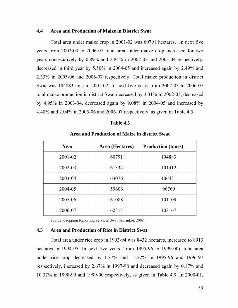
59

4.4 Area and Production of Maize in District Swat

Total area under maize crop in 2001-02 was 60791 hectares. In next five

years from 2002-03 to 2006-07 total area under maize crop increased for two

years consecutively by 0.89% and 2.84% in 2002-03 and 2003-04 respectively,

decreased in third year by 5.50% in 2004-05 and increased again by 2.49% and

2.33% in 2005-06 and 2006-07 respectively. Total maize production in district

Swat was 104883 tons in 2001-02. In next five years from 2002-03 to 2006-07

total maize production in district Swat decreased by 3.31% in 2002-03, decreased

by 4.95% in 2003-04, decreased again by 9.08% in 2004-05 and increased by

4.48% and 2.04% in 2005-06 and 2006-07 respectively, as given in Table 4.5.

Table 4.5

Area and Production of Maize in district Swat

Year Area (Hectares) Production (tones)

2001-02 60791 104883

2002-03 61334 101412

2003-04 63076 106431

2004-05 59606 96769

2005-06 61088 101109

2006-07 62513 103167

Source: Cropping Reporting Services Swat, Amankot, 2008.

4.5 Area and Production of Rice in District Swat

Total area under rice crop in 1993-94 was 8432 hectares, increased to 8913

hectares in 1994-95. In next five years (from 1995-96 to 1999-00), total area

under rice crop decreased by 1.87% and 15.22% in 1995-96 and 1996-97

respectively, increased by 2.67% in 1997-98 and decreased again by 0.17% and

10.37% in 1998-99 and 1999-00 respectively, as given in Table 4.9. In 2000-01,

60

total area under rice crop in Swat reached to 7527 hectares. The total area under

rice crop decreased by 4.05%, 4.85% and 0.35% in 2001-02, 2002-03 and 2003-

04 respectively and increased by 2.5%, 0.91% and 3.76% in 2004-05, 2005-06

and 2006-07 respectively.

Table 4.6

Area and Production of Rice in District Swat

Year Area (Hectares) Production (tones)

1993-94 8432 17180

1994-95 8913 18771

1995-96 8746 18637

1996-97 7415 15991

1997-98 7613 16560

1998-99 7600 16720

1999-00 6812 15422

2000-01 7527 17717

2001-02 7222 16775

2002-03 6872 16533

2003-04 6848 16710

2004-05 7019 17092

2005-06 7083 16922

2006-07 7349 17764

Source: Cropping Reporting Services Swat, Amankot, 2008.

Total rice production in district Swat was 17180 tons in 1993-94 and

reached to 18771 tons in 1994-95. In next four years (from 1995-96 to 1998-99),

total rice production in district Swat decreased consecutively by 0.71% and

14.20% in 1995-96 and 1996-97 respectively and increased successively by

3.56% and 0.97% in 1997-98 and 1998-99 respectively. In 1999-00, total rice

61

production decreased and reached to 15422 tons. In the next five years (from

2000-01 to 2005-06), the total production of rice in Swat, increased by 14.88% in

2000-01, decreased consecutively by 5.32% and 1.44% in 2001-02 and 2002-03

respectively and increased again by 1.07% and 2.29% 2003-04 and 2004-05

respectively. In 2005-06 and in 2006-07, the total rice production in Swat

decreased by 0.99% and 4.98% respectively (Table 4.6).

Variety-wise rice area and production in district Swat has been presented

Table 4.7. Total area under rice crop was 6812 hectares in 1999-00 and increased

to 7019 hectares in 2004-05. Total production of rice was 15422 tons in 1999-00

and increased to 17092 tons in 2004-05. Total area under Irri Pak rice crop was 4

hectares in 1999-00 and decreased to 3 hectares in 2004-05. Total production of

Irri Pak rice was 6 tons in 1999-00 and decreased to 4 tons in 2004-05. Total area

under Basmati rice crop was 2702 hectares in 1999-00 and increased to 2927

hectares in 2004-05. Total production of Basmati rice was 6125 tons in 1999-00

and increased to 6290 tons in 2004-05. Total area under JP-5 rice crop was 2989

hectares in 1999-00 and increased to 3830 hectares in 2004-05. Total production

of JP-5 rice was 6826 tons in 1999-00 and increased to 10246 tons in 2004-05.

Total area under other rice varieties was 1117 hectares in 1999-00 and decreased

to 259 hectares in 2004-05. Total production of other rice varieties was 2465 tons

in 1999-00 and decreased to 552 tons in 2004-05.

54

Table 4.7

Variety-wise Rice Production and Area under Cultivation in District Swat

Year e Irri Pak Basmati JP-5 Other Total

Area

(hectares)

Production

(tones)

Area

(hectares)

Production

(tones)

Area

(hectares)

Production

(tones)

Area

(hectares)

Production

(tones)

Area

(hectares)

Production

(tones)

1999-00 4 6 2702 6125 2989 6826 1117 2465 6812 15422

2000-01 5 7 2971 6302 3326 8865 1225 2543 7525 17717

2001-02 4 6 2852 5970 3295 8665 1071 2134 7222 16775

2002-03 4 6 2830 6076 3145 8571 893 1880 6872 16533

2003-04 4 5 2850 6080 3150 8590 500 2035 6972 16710

2004-05 3 4 2927 6290 3830 10246 259 552 7019 17092

Source: Cropping Reporting Services Swat, Amankot, 2008.

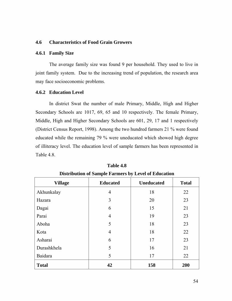
54

4.6 Characteristics of Food Grain Growers

4.6.1 Family Size

The average family size was found 9 per household. They used to live in

joint family system. Due to the increasing trend of population, the research area

may face socioeconomic problems.

4.6.2 Education Level

In district Swat the number of male Primary, Middle, High and Higher

Secondary Schools are 1017, 69, 65 and 10 respectively. The female Primary,

Middle, High and Higher Secondary Schools are 601, 29, 17 and 1 respectively

(District Census Report, 1998). Among the two hundred farmers 21 % were found

educated while the remaining 79 % were uneducated which showed high degree

of illiteracy level. The education level of sample farmers has been represented in

Table 4.8.

Table 4.8

Distribution of Sample Farmers by Level of Education

Village Educated Uneducated Total

Akhunkalay

Hazara

Dagai

Parai

Aboha

Kota

Asharai

Durashkhela

Baidara

4

3

6

4

5

4

6

5

5

18

20

15

19

18

18

17

16

17

22

23

21

23

23

22

23

21

22

Total 42 158 200

55

Source: Field Survey

4.6.3 Size and Nature of Land Holding

The process of passing land from one generation to another was a

complicated one. Households possessed different sizes of land ownership. Some

households have both lowland and upland food grain fields. But the lowland

fields were limited in comparison to upland fields. In the field survey it was

observed that most of the farmers were tenants and they don’t possess their own

land. In the research area 16.5%, 28% and 55.5% were found owner, owner-cum

tenant and tenant respectively as given in Table 4.9.

Table 4.9

Distribution of Sample Farmers by Size of Land Holding

Village Owner Owner-cum-tenant Tenant Total

Akhunkalay 3 6 13 22

Hazara 4 7 12 23

Dagai 3 5 13 21

Parai 4 7 12 23

Aboha 5 5 13 23

Kota 4 6 12 22

Asharai 3 8 12 23

Durashkhela 3 5 13 21

Baidara 4 7 11 22

Total 33 56 111 200

Source: Field survey

56

4.6.4 Area Wise Distribution of Rice Farmers

In the research area the average size of land holding of food grain growers

was 1.5 acres. Larger households generally cultivated more food crops land

primarily because more labour was likely to be available. They are helped by

family members so as to avoid employing outside labour. The information

obtained from the field study about the nature of area possessed by sample

farmers have been presented in Table 4.10 in detail.

Table 4.10

Area Wise Distribution of food growers

Village Average Size of Land Holding

(acre)

No. of Respondents

Akhunkalay 1.0 22

Hazara 2.0 23

Dagai 1.5 21

Parai 1.5 23

Aboha 2.5 23

Kota 3.0 22

Asharai 1.5 23

Durashkhela 1.5 21

Baidara 2.2 22

Total - 200

Source: Field survey

57

4.6.5 Variety Wise Distribution of Sample Farmers

Choice of variety depended on environment, planting date, quality,

marketing, and harvest scheduling. JP-5 was dominated and well-known variety

of the district and its growers were 40% of the total rice growers. The share of

Basmati-385 rice was 7.5%. The share of Sara Saila, Dil Rosh-97, Swat-1, Swat-2

and Fakhr-e-Malakand was 12.5%, 7.5%, 7.5%, 12.5% and 12.5% respectively.

All these figures are shown in Table 4.11.

Table 4.11

Variety Wise Distribution of Sample of Rice Farmers

Variety Number of Growers % age Variety Growers

JP-5 80 40.0

Basmati-385 15 7.5

Sara Saila 25 12.5

Dil Rosh-97 15 7.5

Swat-1 15 7.5

Swat-2 25 12.5

Fakhr-e-Malakand 25 12.5

Total 200 100.0

Source: Field survey

In the study area different varieties of wheat were grown in different areas.

Fakhre-Sarhad was the most well known variety of the district. The variety-wise

distribution of wheat growers is given in Table 4.12. The growers of variety

Salim-2000, Haider-2002, Khyber-87, Nowshera-96, Tatara, Bakhtawar-92,

Auqab-2000, Suleman-96, Fakhre-Sarhad, Pir Sabak-2004 and Pir Sabak-2005

were 11%, 13%, 8%, 13%, 8%, 7%, 5%, 6%, 19%, 6% and 4% of the total wheat

58

growers respectively. This indicates that Fakhre-Sarhad is the dominant variety in

the district.

The variety-wise distribution of maize growers is given in Table 4.13. The

table indicates that the growers of variety Azam, Pahari, Jalal, Babar and Ghori

are 24%, 16%, 12%, 39% and 9% of the total maize growers respectively. The

share of variety Babar grower is the highest as compared to all other varieties

growers.

Table 4.12

Variety Wise Distribution of Sample of Wheat Farmers

Wheat Variety Number of Growers % age Variety Growers

Salim-2000 23 11

Haider-2002 26 13

Khyber-87 15 8

Nowshera-96 26 13

Tatara 16 8

Bakhtawar-92 14 7

Auqab-2000 10 5

Suleman-96 12 6

Fakhre-Sarhad 38 19

Pir Sabak-2004 12 6

Pir Sabak-2005 8 4

Total 200 100

Source: Field survey

59

Table 4.13

Variety Wise Distribution of Sample of Maize Farmers

Wheat Variety Number of Growers % age Variety Growers

Azam 48 24

Pahari 32 16

Jalal 24 12

Babar 78 39

Ghori 18 9

Total 200 100

Source: Field survey

4.7 Profiles of Major Food Grain Varieties in the District

4.7.1 Profiles of Major Rice Varieties of the District

JP-5, Basmati-385 and Sara Saila are the most popular varieties of the

district. JP-5 is a thick grain rice variety. It is sown in a high altitude of about

more than 1000 meters. It is very common in the district. It gives production of 5

to 7 tons per hector, and takes 140 days from sowing to harvesting. Fakhr-e-

Malakand is a new variety grown in the District. It is a high yielding variety as

compared to all other varieties of the district. Swat-1 is a medium grain type. It is

comparatively sown in low altitude areas. From cooking point of view, it is

considered a good variety. It also gives more production like JP-5 in cold areas.

Swat-2 is also a medium grain and productive variety. It gives production 10%

more than that of JP-5. It is sown in low altitude areas but it is a still a cold

resistant variety. It is recommended for those areas where JP-5 is sown in district

Swat. Dil Rosh 97 is also a medium grain variety and from production point of

view, it is considered a good one. It matures from 10-15 days quickly than JP-5.

60

For cooking it is also considered a good quality. Just like JP-5, it is also

recommended in cold areas of district Swat. Basmati-385 is a good and long

grain variety and is grown in various parts of the district.

4.7.2 Profiles of Major Wheat Varieties of the District

In district Swat, various varieties of wheat are grown. Saleem-2000,

Haider-2002, Khyber-87, Noshera-96, Tatara, Bakhtawar-92, Auqab-200,

Suleman-96, Pir Sabak-2004, Pir Sabak-2005 and Fakhri-Sarhad are the most

popular and major varieties grown in the district. The varieties Saleem-2000,

Tatara, Auqab-200 are also grown in barani areas of the district whereas all the

remaining varieties are mainly cultivated in irrigated areas. Further, all these are

the improved varieties and are grown in various areas of the district.

4.7.3 Profiles of Major Maize Varieties of the District

In district Swat different varieties of maize are grown. The major and

popular varieties of the district are Azam, Pahari, Jalal, Babar (White), Ghori

(Yellow). The first three varieties are synthetic varieties while the last two

varieties are hybrid varieties. All these varieties are grown in irrigated areas of the

district.

4.8 Summary

District Swat is well suited area for food grain crops’ cultivation. Major

occupations were teaching, fishing and daily wage earners but most of them were

farmers. They grow different varieties of rice, wheat and maize. The total

production of wheat, maize and rice in 2006-07 was 103004 tones, 103167 tones

and 17764 tones respectively. The average family size of the farmers was 6 per

household. Most of the farmers were uneducated and tenants, cultivating 1.5 acre

area on average. The major rice varieties grown in the district were JP-5,

Basmati-385, Sara Saila, Dil Rosh-97, Swat-1, Swat-2 and Fakhr-e-Malakand. JP-

5 was widely grown variety as compared to other rice varieties. The major wheat

61

varieties grown were Salim-2000, Haider-2002, Khyber-87, Nowshera-96, Tatara,

Bakhtawar-92, Auqab-2000, Suleman-96, Fakhre-Sarhad, Pir Sabak-2004 and Pir

Sabak-2005. Fakhr-e-Sarhad was dominant as compared to all other wheat

varieties. The major maize varieties grown were Azam, Pahari, Jalal, Babar and

Ghori in which Babar variety was extensively grown.

71

Chapter-5

COST AND REVENUE COMPARISON OF FOOD-GRAIN VARIETIES

5.1 Introduction

Information about the revenue and cost of food grain crops i.e. rice, wheat

and maize are presented in this chapter. The perceptions of the farmers about cost

and revenue items were noted and have been converted to the size of one acre

area. In practice, the farmer himself, assisted by members of his family, often co-

operating on a labour exchange basis with other farmers, performs the bulk of the

work. Whenever a "day’s labour" is referred to it means a working day of

approximately eight hours.

Bullocks were necessarily used alongwith tractor by the farmers for rice

cultivation because in standing water in the fields, ploughing was impossible with

tractor. Whereas for maize and wheat there was no need to use the bullock and

tractor collectively. In the study area almost all of the land preparation for food

grins cultivation was done with the help of tractor except for some operations in

rice cultivation. Besides, there was no cost of water (irrigation) except labour

usage in it.

The per acre costs and revenues of rice, wheat and maize are given in subsequent

sections.

5.2 Per Acre Cost and Revenue of Different Rice Varieties

In district Swat, different varieties of rice are grown namely JP-5, Basmti-

385, Sara Saila, Dil Rosh -97, Swat-1, Swat-2 and Fakhre-Malakand. Details about

the cost and revenues of these different varieties are presented in appendix-D:

5.2.1 Cost and Revenue of Variety JP-5

The figures in appendix-D (1) indicate that the land preparation charges

were Rs. 1100 per acre comprised on tractor charges of Rs. 600 and bullock’s

charges of Rs. 500 per acre. The usage of labour for one acre rice area was 55 man

72

days for various operations i.e. nursery bed preparation, maintenance, pulling and

transport; transplanting, cleaning/handling and harvesting. The land rent charges

were Rs. 5500 per acre. The total cost for variety JP-5 was Rs. 16385 per acre. The

total and net revenue was Rs. 44, 000 and Rs. 27, 615 per acre respectively as

given in appendix-D (2).

5.2.2 Cost and Revenue of Variety Basmati-385

For variety Basmati-385, 28 kg seed was used amounting to Rs. 336 per

acre. The total cost for various operations was Rs. 16271 per acre, as given in

appendix-D (3). The total and net revenue from one acre area was Rs. 54900 and

Rs. 38629 respectively. The total revenue is comprised on Rs. 50400 (paddy

production) and Rs. 4500 (rice straw), as presented in appendix-D (4).

5.2.3 Cost and Revenue of Variety Sara saila

In the cultivation of variety Sara Saila, 30 Kg seed was used amounting to

Rs. 300 per acre. The total cost for various activities was Rs. 16235 per acre, given

in appendix-D (5). The total and net revenue of this variety was Rs. 42500 and Rs.

26265 respectively, as presented in appendix-D (6).

5.2.3 Cost and Revenue of Variety Dil Rosh-97

In the cultivation of variety Dil rosh-97, 25 Kg seed was used amounting to

Rs. 250 per acre. The total cost for various activities was Rs. 16185 per acre, given

in appendix-D (7). The total and net revenue of this variety was Rs. 33700 and

Rs.17515 respectively, as presented in appendix-D (8).

5.2.4 Cost and Revenue of Variety Swat-1

In the cultivation of variety Swat-1, 30 Kg seed was used amounting to Rs.

300 per acre. The total cost for various activities was Rs. 16235 per acre, given in

appendix-D (9). The total and net revenue of this variety was Rs. 35300 and

Rs.19065 respectively, as presented in appendix-D (10).

73

5.2.5 Cost and Revenue of Variety Swat-2

In the cultivation of variety Swat-2, 30 Kg seed was used amounting to Rs.

360 per acre. The total cost for various activities was Rs. 16295 per acre, given in

appendix-D (11). The total and net revenue of this variety was Rs. 35300 and

Rs.19005 respectively, as presented in appendix-D (12).

5.2.6 Cost and Revenue of Variety Fakhr-e-Malakand

In the cultivation of variety Fakhr-e-Malakands, 30 Kg seed was used

amounting to Rs. 360 per acre. The total cost for various activities was Rs. 16295

per acre, given in appendix-D (13). The total and net revenue of this variety was

Rs. 55500 and Rs.39205 respectively, as presented in appendix-D (14).

5.2.7 Average Cost and Revenue of all varieties

The average per acre cost for all varieties is Rs. 16, 272, which comprised

on cost of seed Rs. 337, fertilizers Rs. 655, labour usage (man days) Rs. 6600,

transplanting 1800, harvesting Rs. 1200 and threshing Rs. 1260, as given in table

5.1 (a). The average paddy production is 36 maunds acre area amounting to Rs.

38556. The average amount of rice straw is Rs. 4357 per acre, while the total and

net revenue is Rs. 42913 and Rs. 26647 respectively, given in Table 5.1 (b).

74

Table 5.1 (a) Average Per-acre Cost and Revenue of all Rice Varieties

Particulars Unit Quantity Rates (Rs.)

Amount/acre (Rs.)

Land preparation i) Ploughing with tractor ii) Puddling with bullocks

Hr

Day

3 1

200 500

600 500

Raising nursery i) Seed ii) Nursery bed preparation iii) Nursery maintenance iv) Nursery pulling, transport

Kg Day Day Day

29 2 1 4

12 120 120 120

337 240 120 480

Fertilizers i) DAP ii) Urea

Kg Kg

25 50

9

8.6

225 430

Transplanting Day 15 120 1800

Irrigation Day 4 120 480

Cleaning/handling Day 7 120 840

Pesticides i) Furadan (Insecticides) ii) Machety (weedicides) iii) labour charges

Kg ml

Day

16 800 3

50 300 120

800 300 360

Harvesting Day 10 120 1200 Threshing i) Tractor charges ii) Labour charges

Hr

Day

1 8

300 120

300 960

Gunny bags charges Bag 20 40 800

Land rent -- -- -- 5500

Total Cost - - - 16, 272

Source: Field survey

Table 5.1 (b)

Average Total and Net Revenue of all Rice Varieties

Type of yield Quantity (mds)

Rate / md (Rs.) Total amount (Rs.)

i) Paddy ii) Straw

36 1071 4357

38556 4357

Total Revenue (gross) 42913

Net Revenue 26647

Source: Field survey

75

5.3 Benefit Cost Ratios of Different Rice Varieties

To compare the cost and revenues of different rice varieties, Benefit Cost

Ratios (BCRs) for each variety have been calculated. The BCR for varieties JP-5,

Basmati-385, Sara saila, Dil rosh-97, Swat-1, Swat-2 and Fakhr-e-Malakand were

2.69, 3.37, 2.62, 2.08, 2.17, 2.16 and 3.41 respectively (Table 5.2). It is evident

from this table that variety Fakhr-e-Malakand possesses the highest BCR value,

indicting that it is the most profitable variety of rice as compared to all other rice

varieties, coinciding on the economic theory.

Table 5.2

Benefit Cost Ratios for Different Varieties of Rice

Rice Variety Total Rice Revenue

(Rs.) (TRR)

Total Cost

of Rice

(Rs.)

(TCR)

Benefit Cost Ratios

BCR = TRR/TCR

JP-5 44, 000 16385 2.69

Basmati-385 54, 900 16271 3.37

Sara saila 42, 500 16235 2.62

Dil rosh-97 33700 16185 2.08

Swat-1 35, 300 16235 2.17

Swat-2 35, 300 16295 2.16

Fakhr-e-Malakand 55, 500 16295 3.41

Source: Personal calculations

76

5.4 Per Acre Cost and Revenue of Different Wheat Varieties

Saleem-2000, Haider-2002, Khyber-87, Noshera-96, Tatara, Bakhtawar-92,

Auqab-200, Suleman-96, Pir Sabak-2004, Pir Sabak-2005 and Fakhri-Sarhad were

the most popular and major varieties of the district. These varieties differ from

each other in terms of cost and revenues. Their details are presented in appendix-

E.

5.4.1 Cost and Revenue of Variety Saleem-2000

In the cultivation of variety saleem-2000, 50 Kg seed was used amounting

to Rs. 1500 per acre. The total cost for various activities was Rs. 17960 per acre,

given in appendix-E (1). The total and net revenue of this variety was Rs. 39000

and Rs.21040 respectively, as presented in appendix-E (2).

5.4.2 Cost and Revenue of Variety Haider-2002

In the cultivation of variety Haider-2002, 50 Kg seed was used amounting

to Rs. 1250 per acre. The total cost for various activities was Rs. 17710 per acre,

given in appendix-E (3). The total and net revenue of this variety was Rs.29700

and Rs.11990 respectively, as presented in appendix-E (4).

5.4.3 Cost and Revenue of Variety Khyber-87

In the cultivation of variety Khyber-87, 50 Kg seed was used amounting to

Rs. 1000 per acre. The total cost for various activities was Rs. 17460 per acre,

given in appendix-E (5). The total and net revenue of this variety was Rs.36500

and Rs.19040 respectively, as presented in appendix-E (6).

5.4.4 Cost and Revenue of Variety Nowshera-96

In the cultivation of variety Nowshera-96, 50 Kg seed was used amounting

to Rs. 1400 per acre. The total cost for various activities was Rs. 17860 per acre,

given in appendix-E (7). The total and net revenue of this variety was Rs.34000

and Rs.16140 respectively, as presented in appendix-E (8).

77

5.4.5 Cost and Revenue of Variety Tatara

In the cultivation of variety Tatara, 50 Kg seed was used amounting to Rs.

1250 per acre. The total cost for various activities was Rs. 17710 per acre, given in

appendix-E (9). The total and net revenue of this variety was Rs.31400 and

Rs.13690 respectively, as presented in appendix-E (10).

5.4.6 Cost and Revenue of Variety Bakhtawar-92

In the cultivation of variety Bakhtwar-92, 50 Kg seed was used amounting

to Rs. 1400 per acre. The total cost for various activities was Rs. 17860 per acre,

given in appendix-E (11). The total and net revenue of this variety was Rs.39800

and Rs.21940 respectively, as presented in appendix-E (12).

5.4.7 Cost and Revenue of Variety Auqab-2000

In the cultivation of variety Auqab-2000, 50 Kg seed was used amounting

to Rs. 1250 per acre. The total cost for various activities was Rs. 17710 per acre,

given in appendix-E (13). The total and net revenue of this variety was Rs.37600

and Rs.19890 respectively, as presented in appendix-E (14).

5.4.8 Cost and Revenue of Variety Suleman-96

In the cultivation of variety Suleman-96, 50 Kg seed was used amounting

to Rs. 1250 per acre. The total cost for various activities was Rs. 17710 per acre,

given in appendix-E (15). The total and net revenue of this variety was Rs.34000

and Rs.16290 respectively, as presented in appendix-E (16).

5.4.9 Cost and Revenue of Variety Fakhri-Sarhad

In the cultivation of variety Fakhri-Sarhad, 45 Kg seed was used amounting

to Rs. 1125 per acre. The total cost for various activities was Rs. 17585 per acre,

given in appendix-E (17). The total and net revenue of this variety was Rs.41500

and Rs.23915 respectively, as presented in appendix-E (18).

78

5.4.10 Cost and Revenue of Variety Pir Sabak-2004

In the cultivation of variety Pir Sabak-2004, 50 Kg seed was used

amounting to Rs. 1250 per acre. The total cost for various activities was Rs. 17710

per acre, given in appendix-E (19). The total and net revenue of this variety was

Rs.30600 and Rs.12890 respectively, as presented in appendix-E (20).

5.4.11 Cost and Revenue of Variety Pir Sabak-2005

In the cultivation of variety Pir Sabak-2005, 50 Kg seed was used

amounting to Rs. 1250 per acre. The total cost for various activities was Rs. 17710

per acre, given in appendix-E (21). The total and net revenue of this variety was

Rs.31500 and Rs.13790 respectively, as presented in appendix-E (22).

5.4.12 Average Cost and Revenue of All varieties

The average per acre cost for all varieties is Rs. 17, 760, which comprised

on land preparation cost of Rs. 1300, seed Rs. 1300, fertilizer Rs. 4360, labour

usage (man days) Rs. 3600, threshing Rs. 1260, as given in Table 5.3 (a). The

average wheat production is 26 maunds from one acre area amounting to Rs.

26000. The average amount of wheat Boosa is Rs. 9045 per acre, while the total

and net revenue is Rs. 35045 and Rs. 17285 respectively, given in Table 5.3 (b).

79

Table 5.3 (a)

Average Per-acre Costs of all Wheat Varieties

Particulars Unit Quantity Rates Amount/Acre (Rs.)

Land preparation with tractor Hour 3 400 1200

Seed Kg 50 26 1300

Fertilizers

i) DAP

ii) Urea

bag

bag

1

2

3000

680

3000

1360

Threshing (with tractors) Hour 1 1000 1000

Labour charges

From sowing to threshing

Day

30

120

3600

Bags charges Bag 20 40 800

Land rent -- 5500 5500

Total Cost 17, 760

Source: Field survey

Table 5.3 (b)

Average Total and Net Revenue of all Wheat Varieties

Type of Yield Quantity(mds) Rate/md Total amount (Rs.)

Wheat grain

Boosa

26 1000

9045

26000

9045

Total Revenue (gross) 35045

Net Revenue 17285

Source: Field survey

80

5.5 Benefit Cost Ratios of Different Wheat Varieties

To compare the cost and revenues of different wheat varieties, Benefit Cost

Ratios (BCRs) for each variety have been calculated. The BCR for varieties

Saleem-2000, Haider-2002, Khyber-87, Noshera-96, Tatara, Bakhtawar-92, Auqab-200,

Suleman-96 and Fakhri-Sarhad were 2.17, 1.68, 2.09, 1.90, 1.77, 2.23, 2.21, 1.92,

2.36, 1.71 and 1.78 respectively (Table 5.4). It is evident from this table that

variety Fakhr-e-Sarhad possesses the highest BCR value, indicting that it is the

most profitable variety of wheat as compared to all other varieties, coinciding on

the economic theory.

Table 5.4

Benefit Cost Ratios for Different Wheat Varieties

Wheat Variety Total Revenue

(Rs.) (TR)

Total Cost

(Rs.) (TC)

Benefit Cost Ratios

BCR = TRW/TCW

Salim-2000 39, 000 17, 960 2.17

Haider-2002 29, 700 17, 710 1.68

Khyber-87 36, 500 17, 460 2.09

Nowshera-96 34, 000 17, 860 1.90

Tatara 31, 400 17, 710 1.77

Bakhtawar-92 39, 800 17, 860 2.23

Auqab-2000 37, 600 17, 710 2.21

Suleman-96 34, 000 17, 710 1.92

Fakhre-Sarhad 41, 500 17, 585 2.36

Pir Sabak-2004 30, 600 17, 710 1.71

Pir Sabak-2005 31, 500 17, 710 1.78

Source: Personal calculations

81

5.6 Per Acre Cost and Revenue of Different Maize Varieties

In district Swat different varieties of maize are grown. The major and

popular varieties are Azam, Pahari, Jalal, Babar, Ghori. These varieties differ from

each other in terms of costs and revenues. Their details are given in appendix-F:

5.6.1 Cost and Revenue of Variety Azam

In the cultivation of variety Azam, 20 Kg seed was used amounting to Rs.

800 per acre. The total cost for various activities was Rs. 18960 per acre, given in

appendix-F (1). The total and net revenue of this variety was Rs.42500 and

Rs.23540 respectively, as presented in appendix-F (2).

5.6.2 Cost and Revenue of Variety Pahari

In the cultivation of variety Pahari, 20 Kg seed was used amounting to Rs.

720 per acre. The total cost for various activities was Rs. 18880 per acre, given in

appendix-F (3). The total and net revenue of this variety was Rs.24200 and

Rs.5320 respectively, as presented in appendix-F (4).

5.6.3 Cost and Revenue of Variety Jalal

In the cultivation of variety Jalal, 20 Kg seed was used amounting to Rs.

700 per acre. The total cost for various activities was Rs. 18860 per acre, given in

appendix-F (5). The total and net revenue of this variety was Rs.22500 and

Rs.3640 respectively, as presented in appendix-F (6).

5.6.4 Cost and Revenue of Variety Babar

In the cultivation of variety Babar, 20 Kg seed was used amounting to Rs.

780 per acre. The total cost for various activities was Rs. 18940 per acre, given in

appendix-F (7). The total and net revenue of this variety was Rs.35800 and

Rs.16860 respectively, as presented in appendix-F (8).

5.6.5 Cost and Revenue of Variety Ghori

In the cultivation of variety Ghori, 20 Kg seed was used amounting to Rs.

680 per acre. The total cost for various activities was Rs. 18840 per acre, given in

82

appendix-F (9). The total and net revenue of this variety was Rs.26600 and

Rs.7760 respectively, as presented in appendix-F (10).

5.6.6 Average Cost and Revenue of all varieties

The average per acre cost for all varieties is Rs. 18, 900, which comprised

on land preparation cost of Rs. 1200, seed Rs. 740, fertilizers Rs. 4360, labour

usage (man days) Rs. 4200, threshing with tractor Rs. 1500, as given in table 5.5

(a). The average maize production is 26 maunds from one acre area amounting to

Rs. 24700. The average amount of stalk is Rs. 5000 per acre, while the total and

net revenue is Rs. 29700 and Rs. 10800 respectively, given in Table 5.5 (b).

Table 5.5 (a)

Average Per-acre Costs of All Maize Varieties

Particulars Unit Quantity Rates Amount/Acre (Rs.) Land preparation with tractor Hour 3 400 1200

Seed Kg 20 37 740 Fertilizers i) DAP ii) Urea

Bag Bag

1 2

3000 680

3000 1360

Weedicides - - 600 600

Threshing (with tractors) Hour 1 1500 1500 Labour charges from sowing to threshing

Day

35

120

4200

Bags charges Bag 20 40 800 Land rent -- - 5500 5500

Total Cost 18, 900

Source: Field survey

Table 5.5 (b)

Average Total and Net Revenue of all Maize Varieties Type of Yield Quantity(mds) Rate/md Total amount (Rs.) Maize grain Stalk

26 950 5000

24700 5000

Total Revenue (gross) 29700

Net Revenue 10800

Source: Field survey

83

5.7 Benefit Cost Ratios of Different Maize Varieties To compare the cost and revenues of different maize varieties, Benefit Cost

Ratios (BCRs) for each variety have been calculated. The BCRs for varieties

Azam, Pahari, Jalal, Babar, Ghori were 2.24, 1.28, 1.19, 1.89 and 1.41 respectively

(Table 5.6). It is evident from this table that variety Azam possesses the highest

BCR value (2.24), indicting that it is the most profitable variety of maize as

compared to all other varieties, coinciding on the economic theory.

Table 5.6

Benefit Cost Ratios for Different Maize Varieties

Maize Variety Total Revenue of

Maize (Rs.)

(TRM)

Total Cost

of Maize

(Rs.) (TCM)

Benefit Cost Ratios

BCR = TRM/TCM

Azam 42, 500 18, 960 2.24

Pahari 24200 18, 880 1.28

Jalal 22500 18, 860 1.19

Babar 35800 18, 940 1.89

Ghori 26600 18, 840 1.41

Source: Personal calculations

5.8 Summary

In this chapter, the per acre cost and revenue of different rice, wheat and

maize varieties have been assessed. The major cost components for rice crop

cultivation were land preparation, raising nursery, fertilization, transplanting,

cleaning, pesticides, harvesting, threshing and land rent. Variety Fakhr-e-

Malakand was the most profitable variety in terms of net revenue as compared to

other rice varieties. The major heads of revenue of rice were paddy and rice straw.

The major cost components for wheat crop cultivation were land

preparation, seed, fertilizer, threshing, labour and land rent. Variety Fakhr-e-

Sarhad was the most profitable variety of wheat in terms of net revenue as

84

compared to all other wheat varieties. The major heads of revenue of wheat were

wheat grain and boosa.

The major cost components for maize crop cultivation were land

preparation, seed, fertilizer, threshing, labour and land rent. Variety Babar was the

most profitable variety in terms of net revenue as compared to all other maize

varieties. The major heads of revenue of maize were maize grain and stalk.

85

Chapter-6

ECONOMETRIC ANALYSIS OF FOOD GRAIN CROPS

6.1 Introduction

This chapter intends to furnish information about the econometric analysis of

the input output relationship of food grain crops i.e. rice, wheat and maize. For

each crop the log-log model has been estimated so as to find out the output

elasticities and to determine the nature of returns to scale. For each crop, total

product at mean, maximum and minimum values of the sample observations have

been estimated. The average and marginal product has also been calculated for

each crop. Details are given in subsequent sections.

6.2 Econometric Analysis of Rice Input-Output Relationship

This section provides information about the sample statistics and

econometric analysis of rice crop. The analysis is based on primary data collected

and valued at the market prices of 2008. Details are given as under:

6.2.1 Sample Statistics of Rice Input-Output

The sample statistics based on the field survey information indicates that

the average, maximum and minimum produce of rice farmers was 2750 Kgs, 4500

Kgs and 550 Kgs respectively. The average size of area of rice farmers was 1.5

acres. On average 5 tractor hours, 3 bags of fertilizer, 40 Kgs seed and 3 bottles of

sprays for pesticides/insecticides were used by rice farmers. On average, the

farmers used 75 labours (man days) for cultivating the rice crop. The average,

maximum and minimum amount of inputs used by the farmers are given in Table

6.1.

86

Table 6.1 Sample Statistics of Rice Farmers

RP RA TRHR FERTR SDR LABR PSTR Mean 2750 1.5 5 3 40 75 3

Maximum 4500 3.6 6 4 45 80 4

Minimum 550 0.2 2 1 30 50 1

Observations 200 200 200 200 200 200 200 Source: Personal calculations

6.2.2 Estimation of Log-log Production Function for Rice

The estimated log-log Cobb-Douglas production function is:

ln RP = 2.876+ 0.245781*ln RA+ 0.6712*ln TRHR + 0.0789123*ln FERTR +

0.871245*ln SDR+ 0.12487*ln LABR + 0.004871*ln PSTR ----------------- eq. 6.1

or in the most general form:

RP = 17.74316 RA0.245781 TRHR0.6712 FERTR0.07891 SDR0.871245

LABR0.12487 PSTR0.004871 ------------------------ eq. 6.2

Where ao = e2.4708

= 17.74316

The results indicate that RA, TRHR, LABR and SDR are statistically

significant at both 10% and 5% level of significance. FERTR is significant at 5%

level of significance only. PSTR is not statistically significant variable. Usage of

fertilizer was also at minimum level because the land was too fertile and suitable

for rice crop cultivation.

According to eq. 6.1 and 6.2, the value of the rice area elasticity of

production (0.24578) indicates that if rice area increases by 1% and all other

inputs remain unchanged, the rice production will increase by 0.24%. If TRHR

increases by 1%, the rice production increases by 0.67% taking all other variables

unchanged. The output elasticities of FERTR, SDR, LABR and PSTR are

0.0789123, 0.871245, 0.12487 and 0.004871 respectively which can be interpreted

in the same way. Further, the signs and size of the coefficients are according to the

expectation and are in line with the economic theory. Value of Durbin Watson

87

statistic (1.91) shows that there does not exist any problem of autocorrelation. The

results are given in table 6.2.

Table 6.2

Regression Results of Log-log Production Function for Rice

Dependent Variable: ln RP Included observations: 200 Sample: 1 200

Variable Coefficient Std. Error t-Statistic Prob. C 2.876 0.12487 23.032 0.0000 ln RA 0.245781 0.012457 19.73 0.0083 ln TRHR 0.6712 0.09871 6.7997 0.0034 ln FERTR 0.07891 0.0045781 17.237 0.0468 ln SDR 0.871245 0.012481 69.806 0.0008 ln LABR 0.12487 0.003458 36.11 0.0463 ln PSTR 0.004871 0.0009124 5.3387 0.8523 R-squared 0.718713 Durbin-Watson stat 1.912121 Adjusted R-squared 0.724029

The R-square and adjusted R-square values show that the fit is good. The

high value of R2=0.72 shows that 72% of the variations in the (log of) total rice

production is explained by the (log of) included explanatory variables. Most of the

explanatory variables have a strong relationship with the dependent variable. The

stepwise regression supported the statement. The stepwise regression results are

given in appendix-G. In appendix-G (1), rice production has been regressed on

rice area only. RA is not only statistically significant at 10% and 5% level of

significance but also responsible for changes in the rice production, as indicated

by R2 =0.61.

In appendix-G (2), RA and TRHR have been included. The value of R-

square (0.64) favours the good fit. In appendix-G (3), RA, TRHR and FERT have

been included and the value of R-square is 0.72. This also indicates that these

variables are also responsible for changes in dependent variable (RP). Appendix-G

(4) shows that 77% of the variations in the (log of) total rice product is explained

by the (log of) included explanatory variables. Here the included explanatory

88

variables are RA, TRHR, FERTR and SDR. In appendix-G (5), the included

explanatory variables are RA, TRHR, FERTR, SDR and LABR. This indicates

that 89% of the variations in the (log of) total rice product is explained by the (log

of) included explanatory variables. The inclusion of each explanatory variable and

the values of R-square have a strong coordination in these regression results.

6.2.3 Determination of Returns to Scale for Rice Crop

In the context of input-output relationship, it is necessary to show how the

inputs and output go side by side. The log-log Cobb-Douglas production function

(eq. 6.2) clearly depicts the nature of returns to scale. The sum of all the output

elasticities equals 1.9969 (i.e. > 1), indicates that rice production is characterized

by increasing returns to scale. The Wald-Test (Table 6.3) also support the result.

The test has the null hypothesis that the rice production is characterized by

constant returns to scale and has only one restriction i.e. a1+a2+ a3+ a4+ a5 + a6 =1.

As, the Chi-square statistic is equal to the F-statistic times the number of

restrictions under test, so the null hypothesis of constant returns to scale is

decisively rejected.

Table 6.3

Wald Test Results for Rice Crop

Wald Test: Sample: 1 200 Null Hypothesis: a1 + a2 + a3+ a4+ a5 + a6 =1

F-statistic 8.689398 Probability 0.007222

Chi-square 8.689398 Probability 0.007201

Where a1, a2 , a3, a4, a5 and a6 are the coefficients of RA, TRHR, FERTR, SDR,

LABR and PSTR respectively.

6.2.4 Total Estimated Rice Production at Mean, Maximum and Minimum

Values of Rice Inputs

The total rice production at the mean, maximum and minimum values of

rice inputs in the sample have been estimated in Table 6.4, by using eq. 6.2.

89

Putting the mean rice inputs, the total estimated rice production is 2700 Kgs. For

maximum and minimum values of rice inputs, the total estimated rice production

is 4330 Kgs and 600 Kgs respectively.

Table 6.4

Total Estimated Rice Production at Mean, Maximum and Minimum Values

of Rice Inputs

Rice Inputs Total Estimated Rice Production (Kgs) RA TRHR FERTR SDR LABR PSTR

Mean 1.5 5 3 40 75 3 2700

Maximum 3.6 6 4 45 80 4 4330

Minimum 0.2 2 1 30 50 1 600

Observations 200 200 200 200 200 200

Source: Personal calculations

6.2.5 Estimated Average Production at Mean, Maximum and Minimum

Values of Rice Inputs

To find out the rice production on 1 unit of rice input, average production at

mean, maximum and minimum values of each rice inputs have been estimated in

Table 6.5, using eq. 3.10 to 3.15. The average product of RA, TRHR, FERTR,

SDR LABR and PSTR at their mean values are 1800, 540, 900, 67.5, 36 and 900

Kgs respectively. The averages product of each input for their maximum and

minimum values is given in Table 6.5.

Table 6.5

Estimated Average Production of inputs at Mean, Maximum and Minimum

Values of Rice Inputs

Average product of Inputs (Kgs)

APRA APTRHR APFERTR APSDR APLABR APPSTR Mean 1800 540 900 67.5 36 900 Maximum 1202.778 721.667 1082.5 96.2222 54.125 1082.5 Minimum 3000 300 600 20 12 600Source: Personal calculations

90

6.2.6 Marginal Product Estimation at Mean, Maximum and Minimum

Values of Rice Inputs

To show the responsiveness of the scale of rice production due to change in

the quantity of one rice input and other stay unchanged, the marginal product of

each input has been estimated. These have been calculated by taking the first order

partial derivatives with respect to each rice input of eq. 6.2 one by one. The

marginal product at the mean value of RA is 443.56 Kgs indicating that if rice area

increases by one acre (over 1.5 acre) and all other variables constant, the

production will increase by 443.56 Kgs. On similar pattern, if the tractor hours for

rice are increased by one unit (over 5 hours) and all other variables constant, the

rice production will increase by 299.10 Kgs. The marginal product of FERTR,

SDR LABR and PSTR are 71.20, 50.55, 3.86 and 3.56 respectively, as given in

appendix-J (1).

The marginal product at maximum values of each rice inputs has been

estimated in appendix-J (2). The marginal product at the maximum values of RA,

TRHR, FERTR, SDR, LABR and PSTR are 281.84, 461.77, 81.42, 79.92, 6.44

and 5.03 respectively.

The marginal product at the minimum values of RA, TRHR, FERTR, SDR

LABR and PSTR are 726.87, 198.50, 46.67, 17.18, 1.48 and 2.88 respectively, as

given in appendix-J (3).

6.2.7 Marginal Rate of Substitution of Inputs at Mean Values of Rice Inputs

To show how the scale of production respond if quantity of one input is

changed while others stay unchanged, the marginal rate of substitutions have been

calculated using eq. 3.28 and equations given in appendix C(1). To this end, the

ratios of output elasticities are needed which have been presented in Table 6.6.

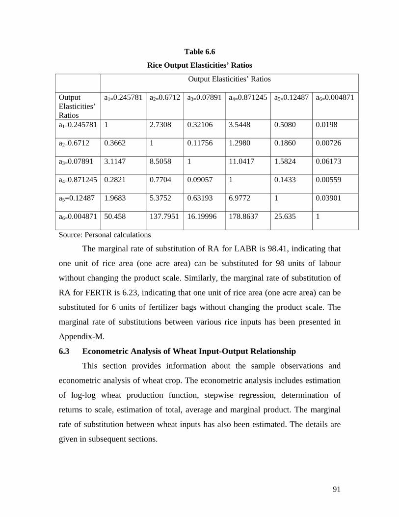
91

Table 6.6

Rice Output Elasticities’ Ratios

Output Elasticities’ Ratios

Output Elasticities’ Ratios

a1=0.245781 a2=0.6712 a3=0.07891 a4=0.871245 a5=0.12487 a6=0.004871

a1=0.245781 1 2.7308 0.32106 3.5448 0.5080 0.0198

a2=0.6712 0.3662 1 0.11756 1.2980 0.1860 0.00726

a3=0.07891 3.1147 8.5058 1 11.0417 1.5824 0.06173

a4=0.871245 0.2821 0.7704 0.09057 1 0.1433 0.00559

a5=0.12487 1.9683 5.3752 0.63193 6.9772 1 0.03901

a6=0.004871 50.458 137.7951 16.19996 178.8637 25.635 1

Source: Personal calculations

The marginal rate of substitution of RA for LABR is 98.41, indicating that

one unit of rice area (one acre area) can be substituted for 98 units of labour

without changing the product scale. Similarly, the marginal rate of substitution of

RA for FERTR is 6.23, indicating that one unit of rice area (one acre area) can be

substituted for 6 units of fertilizer bags without changing the product scale. The

marginal rate of substitutions between various rice inputs has been presented in

Appendix-M.

6.3 Econometric Analysis of Wheat Input-Output Relationship

This section provides information about the sample observations and

econometric analysis of wheat crop. The econometric analysis includes estimation

of log-log wheat production function, stepwise regression, determination of

returns to scale, estimation of total, average and marginal product. The marginal

rate of substitution between wheat inputs has also been estimated. The details are

given in subsequent sections.

92

6.3.1 Sample Statistics of Wheat Input-Output

The sample observations of wheat input-output, indicate that the average

wheat production of 200 farmers was 1950 Kgs while the maximum and minimum

wheat production was 4000 and 350 Kgs respectively. The average size of land

holding was 1.5 acre. The usage of TRHW, FERTW, SDW, LABW and PSTW

are 4 hours, 3 bags, 50 Kgs, 30 labours and 3 bottles respectively. The statistics

are given in Table 6.7.

6.7

Sample Statistics of Wheat Input Output

WP WA TRHW FERTW SDW LABW PSTW

Mean 1950 1.5 4 3 50 30 3

Maximum 4000 3.6 6 4 55 35 4

Minimum 350 0.2 2 1 40 20 1

Observations 200 200 200 200 200 200 200 Source: Personal calculations

6.3.2 Estimation of Log-log Production Function for Wheat

The estimated log-log Cobb-Douglas production function is:

ln WP = 4.9900+ 0.6104*ln WA + 0.1220*ln TRHW+ 0.1479*ln FERTW+

0.2991*ln SDW + 0.2124*ln LABW + 0.1041*ln PSTW -----------eq. 6.3

or in the most general form:

WP = 146.936424 WA0.6104 TRHW0.1220 FERTW0.1479 SDW0.2991

LABW0.2124 PSTW0.1041 -------------------------------------------------- eq. 6.4

Where

bo = e4.9900= 146.936424

The results indicate that WA, TRHW, LABW, FERTR and SDW are

statistically significant at both 10% and 5% level of significance. PSTR is not

statistically significant variable.

According to eq. 6.3 and 6.4, the value of the Wheat Area (WA) elasticity

of production (0.6104) indicates that if wheat area increases by 1% and all other

93

inputs remain unchanged, the wheat production increases by 0.61%. If TRHW

increases by 1%, the wheat production increases by 0.12% taking all other

variables unchanged. The output elasticities of FERT, SDR, LABR and PSTR are

0.0789123, 0.871245, 0.12487 and 0.004871 respectively which can be interpreted

in the same way. Further, the signs and size of the coefficients are according to the

expectation and are in line with the economic theory. Value of Durbin Watson

statistic (2.14) shows that there does not exist any serious problem of

autocorrelation. The results are given in Table 6.8.

Table 6.8

Regression Results of Log-log Production Function for Wheat

Dependent Variable: ln WP

Sample: 1 200

Variable Coefficient Std. Error t-Statistic Prob.

C 4.9900 0.12487 39.96156 0.0018

ln WA 0.6104 0.012457 49.00056 0.0003

ln TRHW 0.1220 0.009871 12.35964 0.0003

ln FERTW 0.1479 0.0045781 32.31035 0.0058

ln SDW 0.2991 0.012481 23.96443 0.0000

ln LABW 0.2124 0.003458 61.42568 0.0063

ln PSTW 0.1041 0.91124 0.11424 0.8862

R-squared 0.65713 Durbin-Watson stat 2.14457

Adjusted R-squared 0.65840

The R-square and adjusted R-square values are showing that the fit is good.

The value of R2=0.66 shows that 66% of the variations in the (log of) total wheat

product is explained by the (log of) included explanatory variables. Most of the

explanatory variables have a strong relationship with the dependent variable. To

94

this end, the stepwise regression has been carried out. The results are shown in

appendix-H.

In appendix-H (1), wheat production has been regressed on wheat area

only. WA is not only statistically significant at 10% and 5% level of significance

but also responsible for changes in the total wheat production, as indicated by R2 =

0.65.

In appendix-H (2), WA and TRHW have been included. The value of R-

square increased to 0.70 favours the good fit. In appendix-H (3), WA, TRHW and

FERTW have been included and the value of R-square is 0.75 and also indicates

that these variables are also responsible for changes in dependent variable (WP).

Appendix-H (4) shows that 79% of the variations in the (log of) total wheat

product are explained by the (log of) included explanatory variables. Here the

included explanatory variables are WA, TRHW, FERTW and SDW. In appendix-

H (5), the included explanatory variables are WA, TRHW, FERTW, SDW and

LABW. This indicates that 81% of the variations in the (log of) total wheat

product is explained by the (log of) included explanatory variables. The inclusion

of each explanatory variable and the values of R-square have a strong coordination

in these regression results.

6.3.3 Determination of Returns to Scale for Wheat Crop

To explore the input-output relationship, the log-log Cobb-Douglas

production function (eq. 6.4) was estimated which also clearly depicts the nature

of returns to scale. The sum of all the output elasticities equals 1.50 (i.e. > 1),

indicates that wheat production is characterized by increasing returns to scale. The

Wald-Test (Table 6.9) also supports the result. The test has the null hypothesis

that the wheat production is characterized by constant returns to scale and has only

one restriction i.e. b1+b2+ b3+ b4+ b5 + b6 =1. As, the Chi-square statistic is equal

to the F-statistic times the number of restrictions under test, so the null hypothesis

of constant returns to scale is decisively rejected.

95

Table 6.9

Wald Test Results for Wheat Crop

Sample: 1 200

Null Hypothesis: b1+b2+ b3+ b4+ b5 + b6 =1

F-statistic 12.354678 Probability 0.00674

Chi-square 12.354678 Probability 0.00675

Where b1, b2 , b3, b4, b5 and b6 are the coefficients of ln WA, ln TRHW, ln

FERTW, ln SDW, ln LABW and ln PSTW respectively.

6.3.4 Estimation of Total Wheat Production at Mean, Maximum and

Minimum Values of Wheat Inputs

The total wheat production at the mean, maximum and minimum values of

wheat inputs in the sample has been estimated in Table 6.10, by using eq. 6.4.

Putting the mean values of wheat inputs, the total estimated wheat production is

1950.44 Kgs. For maximum and minimum values of wheat inputs, the total

estimated wheat production is 3996.06 Kgs and 341.19 Kgs respectively.

Table 6.10

Total Estimated Wheat Production at Mean, Maximum and Minimum Values

of Wheat Inputs

Wheat Inputs Total Wheat Output (Kgs)

WA TRHW FERTW SDW LABW PSTW

Mean 1.5 4 3 50 30 3 1950.44

Maximum 3.6 6 4 55 35 4 3996.04

Minimum 0.2 2 1 40 20 1 341.19

Source: Personal calculations

6.3.5 Average Estimated Wheat Production at Mean, Maximum and

Minimum Values of Wheat Inputs

The wheat production on 1 unit of wheat input (Average Production) at

mean, maximum and minimum values of each wheat inputs have been estimated

in Table 6.11, using eq. 3.16-3.21. The average product of WA, TRHW, FERTW,

96

SDW LABW and PSTW at their mean values are 1300, 488, 650, 39, 65 and 650

Kgs respectively. The average product of each input for their maximum and

minimum values is also given in Table 6.11.

Table 6.11

Average Estimated Production at Mean, Maximum and Minimum Values of Wheat

Inputs

Average product of Inputs

APWA APTRHW APFERTW APSDW APLABW APPSTW

Mean 1300 488 650 39 65 650

Maximum 1110 666 999 73 114 999

Minimum 1706 171 341 9 17 341

Source: Personal calculations

6.3.6 Marginal Product Estimation at Mean, Maximum and Minimum

Values of Wheat Inputs

To show the responsiveness of the scale of wheat production due to change

in the quantity of one wheat input and other stay unchanged, the marginal product

of each input has been estimated. These have been calculated by taking the first

order partial derivatives with respect to each wheat input of eq. 6.4 one by one.

The marginal product at the mean value of WA is 794 Kgs indicating that if wheat

area increases by one acre (over 1.5 acre) and all other variables constant, the

production will increase by 794 Kgs. Similarly, if the tractor hours for wheat is

increased by one unit (over 4 hours) and all other variables constant, the wheat

production will increase by 59 Kgs. The marginal product FERTW, SDW LABW

and PSTW are 96, 12, 14 and 68 respectively, as given in appendix-K (1).

The marginal product at maximum values of each wheat inputs has been

estimated in appendix-K (2). The marginal product at the maximum values of WA,

TRHW, FERTW, SDW, LABW and PSTW are 678, 81, 148, 22, 24 and 104 Kgs

respectively.

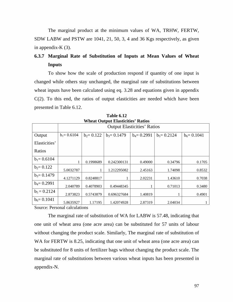
97

The marginal product at the minimum values of WA, TRHW, FERTW,

SDW LABW and PSTW are 1041, 21, 50, 3, 4 and 36 Kgs respectively, as given

in appendix-K (3).

6.3.7 Marginal Rate of Substitution of Inputs at Mean Values of Wheat

Inputs

To show how the scale of production respond if quantity of one input is

changed while others stay unchanged, the marginal rate of substitutions between

wheat inputs have been calculated using eq. 3.28 and equations given in appendix

C(2). To this end, the ratios of output elasticities are needed which have been

presented in Table 6.12.

Table 6.12 Wheat Output Elasticities’ Ratios

Output Elasticities’ Ratios

Output

Elasticities’

Ratios

b1= 0.6104 b2= 0.122 b3= 0.1479 b4= 0.2991 b5= 0.2124 b6= 0.1041

b1= 0.6104 1 0.1998689 0.242300131 0.49000 0.34796 0.1705

b2= 0.122 5.0032787 1 1.212295082 2.45163 1.74098 0.8532

b3= 0.1479 4.1271129 0.8248817 1 2.02231 1.43610 0.7038

b4= 0.2991 2.040789 0.4078903 0.49448345 1 0.71013 0.3480

b5 = 0.2124 2.873823 0.5743879 0.696327684 1.40819 1 0.4901

b6= 0.1041 5.8635927 1.17195 1.42074928 2.87319 2.04034 1

Source: Personal calculations

The marginal rate of substitution of WA for LABW is 57.48, indicating that

one unit of wheat area (one acre area) can be substituted for 57 units of labour

without changing the product scale. Similarly, The marginal rate of substitution of

WA for FERTW is 8.25, indicating that one unit of wheat area (one acre area) can

be substituted for 8 units of fertilizer bags without changing the product scale. The

marginal rate of substitutions between various wheat inputs has been presented in

appendix-N.

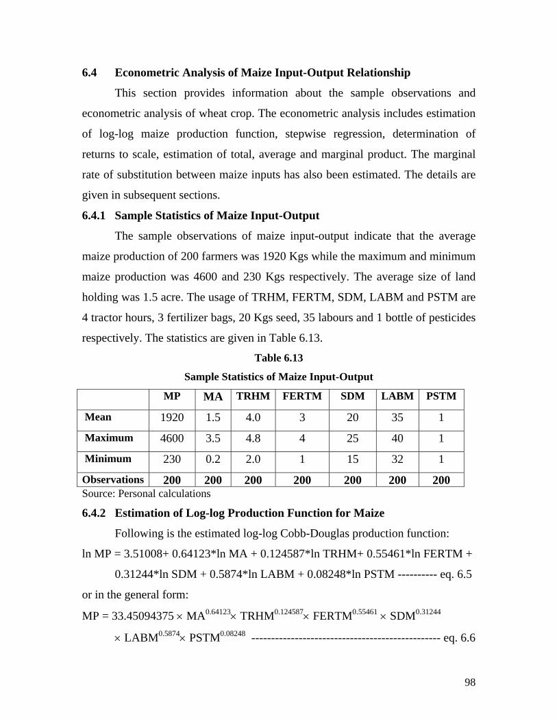
98

6.4 Econometric Analysis of Maize Input-Output Relationship

This section provides information about the sample observations and

econometric analysis of wheat crop. The econometric analysis includes estimation

of log-log maize production function, stepwise regression, determination of

returns to scale, estimation of total, average and marginal product. The marginal

rate of substitution between maize inputs has also been estimated. The details are

given in subsequent sections.

6.4.1 Sample Statistics of Maize Input-Output

The sample observations of maize input-output indicate that the average

maize production of 200 farmers was 1920 Kgs while the maximum and minimum

maize production was 4600 and 230 Kgs respectively. The average size of land

holding was 1.5 acre. The usage of TRHM, FERTM, SDM, LABM and PSTM are

4 tractor hours, 3 fertilizer bags, 20 Kgs seed, 35 labours and 1 bottle of pesticides

respectively. The statistics are given in Table 6.13.

Table 6.13

Sample Statistics of Maize Input-Output

MP MA TRHM FERTM SDM LABM PSTM

Mean 1920 1.5 4.0 3 20 35 1

Maximum 4600 3.5 4.8 4 25 40 1

Minimum 230 0.2 2.0 1 15 32 1

Observations 200 200 200 200 200 200 200 Source: Personal calculations

6.4.2 Estimation of Log-log Production Function for Maize

Following is the estimated log-log Cobb-Douglas production function:

ln MP = 3.51008+ 0.64123*ln MA + 0.124587*ln TRHM+ 0.55461*ln FERTM +

0.31244*ln SDM + 0.5874*ln LABM + 0.08248*ln PSTM ---------- eq. 6.5

or in the general form:

MP = 33.45094375 MA0.64123 TRHM0.124587 FERTM0.55461 SDM0.31244

LABM0.5874 PSTM0.08248 ------------------------------------------------ eq. 6.6

99

Where co = e3.51008 = 33.45094375

The results indicate that MA, TRHM, LABM, FERTM and SDM are

statistically significant at both 10% and 5% level of significance. PSTR is not

statistically significant variables. Due to good climatic conditions the farmers

rarely used pesticides/insecticides.

According to eq. 6.5 and 6.6, the value of the Maize Area (MA) elasticity

of production (0.64) indicates that if maize area increases by 1% and all other

inputs remain unchanged, the maize production will increase by 0.64%. If TRHM

increases by 1%, the maize production will increase by 0.12% taking all other

variables unchanged. The output elasticities of FERTM, SDM, LABM and PSTM

are 0.55461, 0.31244, 0.5874 and 0.08248 respectively which can be interpreted in

the same way. Further, the signs and size of the coefficients are according to the

expectation and are in line with the economic theory. Value of Durbin Watson

statistic (1.78), which is closer to 2, shows that there does not exist any problem of

autocorrelation. The R-square and adjusted R-square values are showing that the

fit is good. The value of R2=0.73 shows that 73% of the variations in the (log of)

total maize product is explained by the (log of) included explanatory variables.

The results are given in Table 6.14.

Table 6.14

Regression Results of Log-log Production Function for Maize

Dependent Variable: ln MP Sample: 1 200

Variable Coefficient Std. Error t-Statistic Prob. C 3.51008 0.12487 28.10987 0.0000 ln MA 0.64123 0.012457 51.47548 0.0000 ln TRHM 0.124587 0.012 10.38225 0.0003 ln FERTM 0.55461 0.045781 12.11441 0.0011 ln SDM 0.31244 0.012481 25.03325 0.0068 ln LABM 0.5874 0.0248 23.68548 0.0063 ln PSTM 0.08248 0.08124 1.015263 0.73623 R-squared 0.732153 Durbin-Watson stat 1.7758 Adjusted R-squared 0.738987

100

The output elasticities values indicate that most of the explanatory variables

have a substantial effect of the response variable. The stepwise regression has

been carried out for maize crop. The results are given in appendix-I.

In appendix-I (1), maize production has been regressed on maize area (MA)

only. MA is not only statistically significant at 10% and 5% level of significance

but also responsible for changes in the maize production, as indicated by R2 =

0.61.

In appendix-I (2), MA and TRHM have been included as explanatory

variables. The value of R-square turned out to be 0.67 showing that 67% of the

variations in the (log of) total maize product is explained by the (log of) included

explanatory variables. In appendix-I (3), MA, TRHM and FERTM have been

included yielding the value of R-square equal to 0.71 and also indicates that these

variables are also responsible for changes in dependent variable (MP). Appendix-I

(4) shows that 77% of the variations in the (log of) total maize product is

explained by the (log of) included explanatory variables. Here the included

explanatory variables are MA, TRHM, FERTM and SDM. In appendix-I (5), the

included explanatory variables are MA, TRHM, FERTM, SDM and LABM which

indicates that 80% of the variations in the (log of) total maize product are

explained by the (log of) included explanatory variables. The inclusion of each

explanatory variable and the values of R-square have a strong correlation with

each other.

6.4.3 Determination of Returns to Scale for Maize Crop

To explore the input-output relationship, the log-log Cobb-Douglas

production function (eq. 6.6) has been estimated which also clearly depicts the

nature of returns to scale. The Sum of all the output elasticities equals 2.50 (i.e. >

1), indicates that maize production is characterized by increasing returns to scale.

The Wald-Test (Table 6.15) also supports the result. The test has the null

hypothesis that the maize production is characterized by constant returns to scale

and has only one restriction i.e. c1+c2+ c3+ c4+ c5 + c6 = 1. As, the Chi-square

101

statistic is equal to the F-statistic times the number of restrictions under test, so the

null hypothesis of constant returns to scale is determinedly rejected.

Table 6.15

Wald Test Results for Maize Crop

Sample: 1 200

Null Hypothesis: c1+c2+ c3+ c4+ c5 + c6 = 1

F-statistic 17.184579 Probability 0.02354

Chi-square 17.184579 Probability 0.02355

Where c1, c2, c3, c4, c5 and c6 are the coefficients of ln MA, ln TRHM, ln FERTM,

ln SDW, ln LABM and ln PSTM respectively.

6.4.4 Estimation of Maize Production at Mean, Maximum and Minimum

Values of Maize Inputs

The total maize production at the mean, maximum and minimum values of

maize inputs in the sample has been estimated in Table 6.16, by using eq. 6.6.

Putting the mean values of maize inputs, the total estimated maize production is

1932 Kgs. For maximum and minimum values of maize inputs, the total estimated

maize production is 4698 Kgs and 232 Kgs respectively.

Table 6.16

Total Estimated Maize Production at Mean, Maximum and Minimum Values

of Maize Inputs

Inputs Total Output (Kgs) MA TRHM FERTM SDM LABM PSTM

Mean 1.5 4.0 3 20 35 1 1932

Maximum 3.6 4.8 4 25 40 1 4698

Minimum 0.2 2.0 1 15 32 1 232

Source: Personal calculations

102

6.4.5 Estimation of Average Maize Production at Mean, Maximum and

Minimum Values of Maize Inputs

The maize production on 1 unit of maize input (Average Production) at

mean, maximum and minimum values of each maize inputs have been estimated

in Table 6.17, using eqs. 3.22-3.27. The average product of MA, TRHM, FERTM,

SDM, LABM and PSTM at their mean values is 1288.24, 483.09, 644.12,

96.6186, 55.21 and 1932.37Kgs respectively. The average product of each input

for their maximum and minimum values is also given in Table 6.17.

Table 6.17

Average Production of of Maize Inputs at their Mean, Maximum and Minimum

Values

Average product of Inputs

APMA APTRHM APFERTM APSDM APLABM APPSTM

Mean 1288.24 483.09 644.12 96.6186 55.21 1932.37

Maximum 1304.96 978.72 1174.46 187.9149 117.44 4697.87

Minimum 1160.88 116.09 232.18 15.478 7.255 232.18

Source: Personal calculations

6.4.6 Estimation of Marginal Product at Mean, maximum and minimum

Values of Maize Inputs

To show the responsiveness of the scale of wheat production due to change

in the quantity of one maize input and other stay unchanged, the marginal product

of each input has been estimated. These have been calculated by taking the first

order partial derivatives with respect to each maize input of eq. 6.6 one by one.

The marginal product at the mean value of MA is 800 Kgs indicating that if maize

area increases by one acre (over 1.5 acre) and all other variables constant, the

production will increase by 800 Kgs. Similarly, if the tractor hours for maize is

increased by one unit (over 4 hours) and all other variables constant, the maize

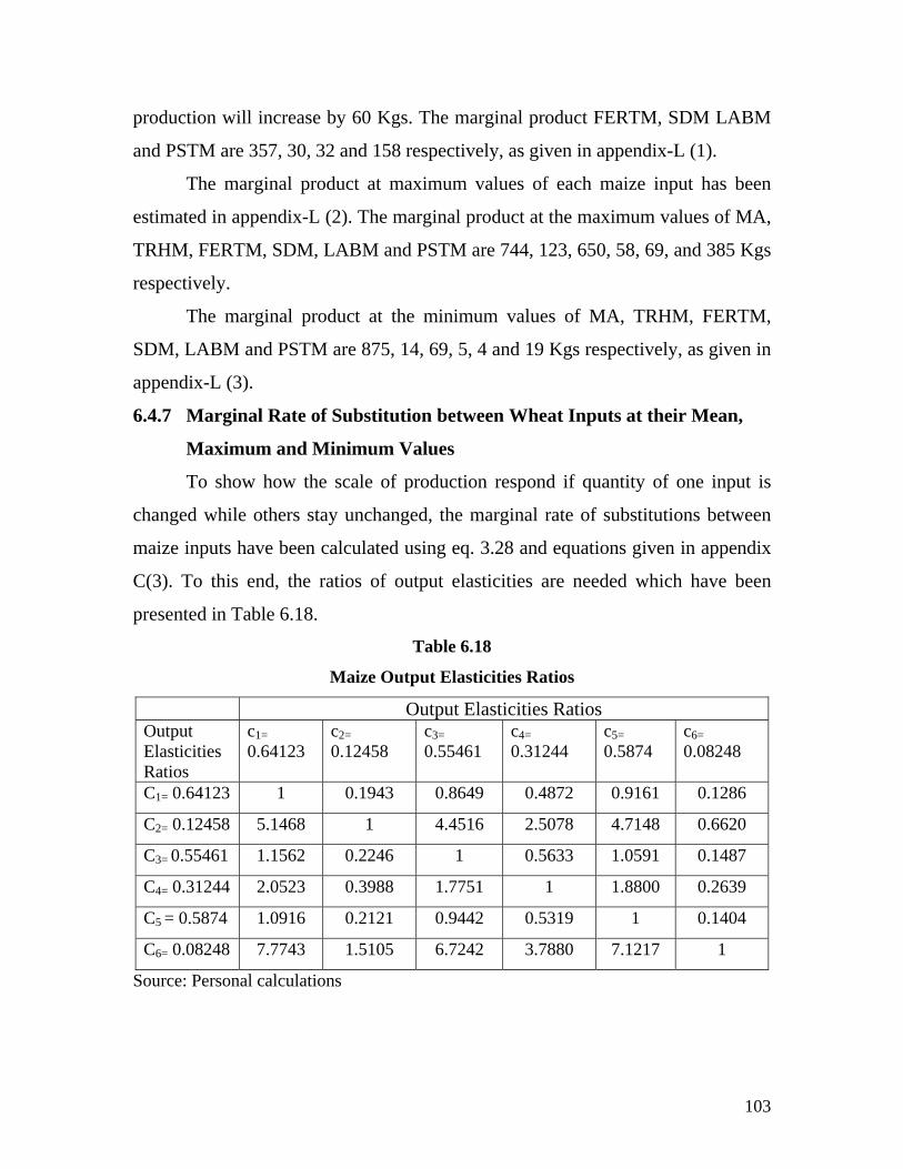
103

production will increase by 60 Kgs. The marginal product FERTM, SDM LABM

and PSTM are 357, 30, 32 and 158 respectively, as given in appendix-L (1).

The marginal product at maximum values of each maize input has been

estimated in appendix-L (2). The marginal product at the maximum values of MA,

TRHM, FERTM, SDM, LABM and PSTM are 744, 123, 650, 58, 69, and 385 Kgs

respectively.

The marginal product at the minimum values of MA, TRHM, FERTM,

SDM, LABM and PSTM are 875, 14, 69, 5, 4 and 19 Kgs respectively, as given in

appendix-L (3).

6.4.7 Marginal Rate of Substitution between Wheat Inputs at their Mean,

Maximum and Minimum Values

To show how the scale of production respond if quantity of one input is

changed while others stay unchanged, the marginal rate of substitutions between

maize inputs have been calculated using eq. 3.28 and equations given in appendix

C(3). To this end, the ratios of output elasticities are needed which have been

presented in Table 6.18.

Table 6.18

Maize Output Elasticities Ratios

Output Elasticities Ratios Output Elasticities Ratios

c1= 0.64123

c2= 0.12458

c3= 0.55461

c4= 0.31244

c5= 0.5874

c6= 0.08248

C1= 0.64123 1 0.1943 0.8649 0.4872 0.9161 0.1286

C2= 0.12458 5.1468 1 4.4516 2.5078 4.7148 0.6620

C3= 0.55461 1.1562 0.2246 1 0.5633 1.0591 0.1487

C4= 0.31244 2.0523 0.3988 1.7751 1 1.8800 0.2639

C5 = 0.5874 1.0916 0.2121 0.9442 0.5319 1 0.1404

C6= 0.08248 7.7743 1.5105 6.7242 3.7880 7.1217 1

Source: Personal calculations

104

The marginal rate of substitution of MA for TRHM is 13.72, indicating that

one unit of maize area (one acre area) can be substituted for 14 units of labour

without changing the product scale. Similarly, the marginal rate of substitution of

MA for LABR is 25.47, indicating that one unit of maize area (one acre area) can

be substituted for 25 units of labour (man days) without changing the product

scale. The marginal rate of substitutions between various maize inputs has been

presented in appendix-O.

6.5 Summary

This chapter states that the output elasticities of area, tractor hours,

fertilizer, seed, labour and pesticides for rice crop were 0.24578, 0.6712,

0.0789123, 0.871245, 0.12487 and 0.004871 respectively. Proportional increase in

the output of rice was faster than the increase in the inputs of rice (increasing

returns to scale). The total estimated rice production for mean, maximum and

minimum values of rice inputs were 2700, 4330 and 600 kgs respectively. The

average product of area, tractor hours, fertilizer, seed, labour and pesticides at their

mean values were 1800, 540, 900, 67.5, 36 and 900 kgs respectively. At the mean

values of the sample, the marginal product of area, tractor hours, fertilizer, seed,

labour and pesticides were 443.56, 299.10, 71.20, 50.55, 3.86 and 3.56 kgs

respectively.

For wheat crop, the output elasticities of area, tractor hours, fertilizer, seed,

labour and pesticides were 0.61, 0.1220, 0.0789123, 0.871245, 0.12487 and

0.004871 respectively. Proportional increase in the output of wheat was faster than

the increase in the inputs of wheat (increasing returns to scale). The total estimated

wheat production for mean, maximum and minimum values of wheat inputs were

1950.44, 3996.06 and 341.19 kgs respectively. The average product of area,

tractor hours, fertilizer, seed, labour and pesticides at their mean values were 1300,

488, 650, 39, 65 and 650 kgs respectively. The marginal product at the mean

values of area, tractor hours, fertilizer, seed, labour and pesticides were 794, 59,

96, 12, 14 and 68 kgs respectively. The marginal product at the maximum values

105

of area, tractor hours, fertilizer, seed, labour and pesticides were 678, 81, 148, 22,

24 and 104 kgs respectively.

For maize crop, the output elasticities of area, tractor hours, fertilizer, seed,

labour and pesticides were 0.64123, 0.124587, 0.55461, 0.31244, 0.5874 and

0.08248 respectively. Proportional increase in the output of maize was faster than

the increase in the inputs of maize (increasing returns to scale). The total estimated

maize production for mean, maximum and minimum values of maize inputs were

1932, 4698 and 232 kgs respectively. The average product of area, tractor hours,

fertilizer, seed, labour and pesticides at their mean values were 1288.24, 483.09,

644.12, 96.6186, 55.21 and 1932.37Kgs respectively. The marginal product at the

mean values of area, tractor hours, fertilizer, seed, labour and pesticides were 800,

60, 357, 30, 32 and 158 kgs respectively.

106

Chapter-7

ECONOMIC PRACTICES, SIGNIFICANCE AND CAUSES OF LOW

YIELD OF FOOD-GRAIN CROPS CULTIVATION

7.1 Introduction

District Swat has been endowed by nature with vast potentialities for

growing food-grains. Farmers are generally satisfied with traditional late-maturing

food-grains varieties. These soils are well suited for crop cultivation. Paddy and

maize is mostly grown in the Kharif season and is harvested in November and

December. While wheat is Rabi crop grown in October-November and harvested

in June-July. This chapter intends to highlight the major economic practices

undertaken in food grins cultivation followed by its significance in the economy of

district Swat. Economic practices implies all those practices relevant to food grain

crops cultivation which can make food grain crops economic and profitable if

practiced properly.

7.2 Economic Practices in Food Grain Crops Cultivation

Food-grains production practices differ from place to place but it is tried to

state all those activities, which are generally practiced in the study area. These

practices possess economic significance and if managed properly, the crops can be

made most profitable. The important pre and post harvest economic practices

undertaken in food-grains crops cultivation are detailed as under:

7.2.1 Usage of land for food grains

Having studied the research area it was observed that most of land was

rented on IJARA basis. The payments were paid either at the beginning of

production process or after harvesting rice production. Payments were also used to

make in the form of grain production. In the research area, usually the rent of land

was charged as half of the total production. Due to the existence of chances of

107

floods, it was negotiated between the owners and tenants in some areas. The actual

rent paid varied from place to place but on average Rs.5500 for six months were

paid for one acre of land, which is a large share out of total costs.

7.2.2 Conservation of Traditional Varieties

There have been some changes in the methods of farming and the high

yielding varieties are now being grown with the traditional food grain varieties.

However, apart from the traditional emotional attachment to these inherited

varieties, the local farmers are aware that the local varieties have some advantages.

They believe it is superior in taste and nutritive value. The old varieties are more

resistant to pests and diseases as well as droughts and floods. They do not need

more chemical fertilizer or pesticides and insecticides and are therefore quite

viable economically as well when the cash input and output are compared. It is

quite clear that the local people are aware of the importance of conserving these

traditional varieties. Besides, the use of high yielding varieties, which are tolerant

to the agro-climatic conditions of Swat, is one avenue by which production and

productivity can be increased. Some farmers were found to use certified seed

material for cultivation. When seeds are retained from the previous crop, the crop

is found to be contaminated with seeds from other varieties and weed seeds.

Sowing of mixed varieties often result to loose fair market prices for these crops.

7.2.3 Raising Nursery and Maintenance

High yielding rice cultivation starts from a suitable nursery. Healthy

seedlings of a good nursery are tough, have short but erect leaves, and vigorous

roots, recover quickly after transplanting, of highly uniform size easy to pull and

transplant, and free of diseases and pests. All these characteristics can be obtained

through pure seed of improved varieties, seeding density, fertility level of nursery

bed, and time of sowing, water management and pest control. As far as the nursery

sowing is concerned, the land is ploughed with tractor 2-3 times and the field is

irrigated. The weeds germinated after a week is eradicated through ploughing and

108

planking. During this process water remains in the fields. The field is puddled well

and harrowed thoroughly so as to retain equal level of water in the seedbed. The

sprouted seed is spread over the puddle bed. During the early few days of growth

the water is drained out daily at night. Afterwards, water is kept 2-4 cm deep to

suppress weeds. Just enough water should be added to the seedbed to saturate the

soil during the first 5-7 days. Afterwards, water should be increased gradually up

to 5 cm depending on the height of the seedling to control weeds. These practices

are done for rice only rather for maize and wheat.

7.2.4 Land Preparation and Water Management

The methods of land preparation affect food grain yield. Inefficient land

preparation was one of the most important causes of poor yields. Through better

land preparation of lands weed control becomes possible. It also facilitates easy

sowing which is helpful to establish good seed and soil contact. Through effective

land preparation easy absorption of moisture, water holding capacity and provision

of sufficient aeration is ensured. For rice cultivation, deep ploughing 2-3 times

followed by planking is enough to get well-pulverized soil. Mixing of organic

matter (rice straw, stubbles, and farmyard manure) improves the soil structure and

fertility. After the land is prepared in dry condition, field should be divided in

suitable plots for better water management and other operations. It is essential also

that an appropriate height of water be maintained in relation to the stage of growth

of the crop. To this end, the field is leveled in order to have an even stand of

water, to control weeds and to facilitate the complete drying out at harvest time.

Land preparation and water management is necessary for maize and wheat

cultivation. There are some stages where water is necessary for maize crop mainly

these are seedling, knee- height, tasseling, silking and grain filling stage. Fertile

land and timely and balanced water management can increase the efficiency of

land to produce more.

109

7.2.5 Transplanting

When the main field is puddled and leveled thoroughly, transplanting is

done. In rice cultivation, the levees (bunds) are properly made and plastered to

avoid water loss. During transplanting the water nursery seedlings are brought and

distributed throughout the field in small bundles. In wheat and maize cultivation,

the final grins are transferred manually in the fields and then proper arrangements

are made for channalizing the water in future.

7.2.6 Weed Control

For healthy food grains production hand weeding is a significant factor.

Through proper and effective weeding, high rice productivity is ensured. Farmers

performed that activity by themselves and in some cases hired labour are used. In

rice cultivation, the plant produces seeds by the millions and is usually introduced

through the irrigation water as the seeds are small and floats. The seeds will

germinate when the water is deep and clear. The duckweed seedlings germinate

and grow very slowly and then rapidly expand leaf size, suckers and branches.

This process smothers all other vegetation including cultivated rice.

In case of wheat and maize cultivation, this practice is also necessary so as

to protect the grain crops from wild plants.

7.2.7 Insect and Disease Control

It is common practice that agricultural productivity is mostly sensitive to

pests and diseases. However in the relevant area, it was observed that such like

possibility was minimum. In case if it occurs the services of research stations are

utilized. Generally, sprays are recommended for this purpose.

The paddy bug attacks the rice grain at two stages. Firstly at the milk stage

and secondly at the dough stage. The damage during the milk stage results in

unfilled or underfilled grains while damage during the dough stage causes

discolored and broken grains after milling. Rice blast was the most important

110

disease of rice in Swat. This disease caused severe yield reductions whenever it

occurred. To follow the situation, the farmers in District Swat used to spray as

directed by the agricultural research station. Generally in rice cultivation, Furadan

(insecticide) and Machety (weedicides) were used by the farmers.

In wheat and maize cultivation, special insecticides and weedicides were

also used by the farmers so as to protect the food grain crops.

7.2.8 Fertility Management

Fertilizer application is considered an important factor for increasing rice

productivity. The use of chemical fertilizer has been proven increased rice yield up

to 50% when given on proper time and in proper dosage. The major elements

required by the crops are nitrogen, phosphorus, and potash, while among the

minor elements zinc is the most important. The practices of using farmyard

manure or rice straw during puddling economizes the use of chemical fertilizers.

Green manuring can reduce the dependence of rice crop on artificial fertilizers.

Immediately after rice harvest, green manuring crops like shaptal berseem can be

sown and then can be ploughed in by the end May before transplantation. The

farmers also use DAP and Urea for rice cultivation. In wheat and maize

cultivation, apart from DAP and Urea, NPK was also used by the farmers.They

were generally available with the village shopkeepers minimizes the transportation

cost. In most villages it was seen that this facility was provided by Karigars

(peoples having horses as occupation).

The farmyard manure used at the farm was valued at the village average

rate, and for the purchased quantities, actual prices paid were charged. In all the

villages, the average price of animal manure was Rs.40 per Horse Bag.

111

7.2.9 Harvesting and Drying

To get higher paddy yields, it should be harvested just in time. The

appropriate time for harvesting ranges from 30-35 days after flowering. This is the

stage at which 85-90% of the upper portion of the panicle is straw colored and the

moisture content is 20-23%. The water should be stopped from 10-15 days before

harvesting. Standing water in the field deteriorates grains if the crop lodges, and

also the grain quality are affected. The crop is harvested at the time when there is

no dew in the field. Peak grain quality occurs at harvest. Care is taken during the

subsequent steps to preserve these quality characteristics in order to meet the high

quality standard demanded by domestic and international processors as well as

consumers. Maintenance of milling quality during harvesting and drying was a

major consideration because value was based on quality. When maize and wheat

grains fully matures, dried in the sun light, are then harvested by the farmers.

7.2.10 Threshing and Cleaning

In old days threshing of rice bullocks, obtained on exchange basis,

performed paddy but nowadays tractors were used for this purpose in all the

research area. Those were easily available and time saving. It finishes all the rice

paddy of one acre within one or two hours.

The recommended time for threshing is 2-4 days after paddy harvesting.

Threshing methods were included manual and mechanical. Tractors instead of

bullocks nowadays practice threshing the paddy. To improve product quality and

marketing, proper cleaning played significant role in the research area. This

activity was generally performed through the experienced members of the family.

In case if it was not available then the required labours were hired. The activity

required smooth air to clean the paddy. Maize and wheat crops are also threshed

with the help of tractors and are then carefully separated good quality from poor

quality. The broken grains are also separated so as get fair prices for their product.

112

7.2.11 Transportation

The food grains were generally carried through horses of corresponding

village Karigars taking their wages in terms of paddy at 20% rate of the total

production. During the cropping process of rice, seedlings were properly

distributed in small plot for transplanting.

7.2.12 Milling

After cleaned the paddy, it was carried to the local mills and was milled to

make it fresh for consumption. At milling time care was taken to voide from

broken rice in return. The milling facilities were available at each village level for

rice farmers in district Swat. However the mill were not in good conditions rather

were badly ventilated, infested with rice and paddy weevil. The mills were also

lacking storage and drying spaces. There were on average 1 mill in the villages

where rice was grown. Peoples used to prefer small mills because they could mill

their production with their own will and interference. The small mills thus were

able to produce marketable grades of rice.

The wheat and maize grains were also carried to the floor mills on a fixed

milling rate. In district Swat there was a certain amount of competition, and a few

mills were willing to mill at lower cost as compared to other mills. The mill

owners thus used to advance loans interest-free to farmers.

7.2.13 Storage

Farmers seldom used to store paddy. However, rice mills used to store it for

a short period. Milled rice was also stored by the rice farmers rarely. Rice

undergoes certain changes during storage in the first 3 to 4 months after harvest.

These changes improve rice quality, making it more acceptability to consumers.

For satisfactory storage of rice the moisture content is kept before 9%. Fumigation

in storage, insect proofing of bags, and dis-infestation with inorganic salts are all

measures, which can successfully be applied under our conditions. However

113

efforts were made by the owners to ensure that the warehouse/store was in good

condition for storage of the grain. Warehouse/storage areas were be properly

cleaned. All refuse were removed and burnt. Areas around the warehouse/storage

area were cleaned with care taken to remove vegetation, refuse, and discarded

machinery which only served as breeding ground for rodents and insects.

7.2.14 Record Keeping/Stock Control

In case of surplus production, the food grains were transferred to

warehouses either private or government. Checks were made to have proper record

of food grains bags so s to avoid any theft or loss. Domestic shopkeepers generally

performed this activity. No food grain was allowed to leave the warehouse before

taking proper permission from the manger.

7.2.15 Straw Management

Rice straw can be used for various purposes. In district Swat rice straw was

mostly used for livestock as well as for commercial purposes. It has a good market

in local economy. The farmers also used the wheat straw (Boosa) and maize straw

(stalk) mainly for livestock.

7.2.16 Marketing of Food Grain Crops

Effective marketing provides food production to users when, where and in

them form they want. The produce of food grain crops was used to sell by the food

growers mainly in small markets. However, some of Beoparis, commission agents

and Arthiyas used to purchase the farmers produce and then re-selled in big

markets. The poor farmers did not get fair prices for their products due their

requirement of cash for day-to-day consumption. The farmers also used to keep

some portion of their produce in their homes and then sell to village shopkeepers

for their daily requirement.

114

7.3 Economic Significance of Food Grains Crops Cultivation

Food grains played a vital role in the economy of District Swat. Food grains

is most closely connected with capital and labour employment, sources of income,

marketing activities, credit and financing, labour distribution, returns and

surpluses and decision-making. The subsequent sections will provide knowledge

about the assessment of rice cultivation in connection with economic variables of

food grain economy of district Swat.

7.3.1 Food Grains Cultivation as a Sources of Income

Agriculture was the largest sector of the district economy. The topography

of the district was such that not all the land was suitable for cultivation. Most of

the cultivation was carried out in the southern areas of the district, mainly in

Mingora, Barikot, Kabal, Matta and Khwazakhela.

For the rural population, agriculture was the main source of livelihood.

Rice maize and wheat grains alongwith straw were the source of farmers’ income.

They used these products at home or sold them to supplement their cash income.

Food sustenance by the villagers is generally derived by their own farm

products. However, some families lived mainly on food obtained from other

occupations. Primary food supplies such as rice, wheat, onion or vegetables were

in short supply there. Natural threats to the food supply included floods, droughts

and insect plagues.

For the rice farmers, animal husbandry was another subsidiary income and

also provided a good source of the family’s dietary needs. Cattle, buffalo, cow and

poultry were the major livestock there. Villagers occasionally sold but rarely

consumed those animals. For villagers, to feed their livestock on free grazing lands

was common practice.

The average food grain grower has cow, goats, sheep or poultry as

secondary source of income. When he is not engaged in agriculture activities, he

115

sells his labor locally or outside of the area. But apart from it, agriculture was the

main source of income of the rice farmers. Some rice farmers had their own shops

in the villages while some were found investing their incomes in animal trade.

They were relying on subsistence level of farming. Some members of the family

were carpenters, masons, and public school teachers and very few of them were

Govt. servants. Foreign remittances were also the main component of non-

agriculture incomes.

As most of the villagers derive their food sustenance from farm products so

they were thus dependent on nature for their livelihood because there was chances

of natural threats like floods, droughts and insect plagues Agriculture products like

rice, wheat, maize, onion or vegetables were in short supply there. “Roti” made of

wheat or maize flour was the staple diet of the local people in district Swat. The

green tea in general and particularly milk tea was very popular in the district.

The major crops cultivated in the villages were onion, wheat, maize, tomato

and vegetables. However, in Kharif season rice was mainly grown on area situated

near river Swat. After the harvesting of the rice onion and/or wheat were

cultivated. Some fruit trees like grape, mango, plum, watermelon, apricot, pear

and walnut were also grown in the study area. Due to the lack of precipitation

during the dry season and the lack of any irrigation system, local people tend to

rely on rain-fed agriculture.

7.3.2 Labour Force Employment in Food Grain Cultivation

Food grains cultivation was of great social significance precisely because it

was organized on the basis of small forms rather than large and it provided the

largest share of total labour employment to the local community. Food grains were

labour intensive crops, which included hired and family labour. On average

Rs.120 per day was given to that particular skilled labour.

116

Food grains cultivation in district Swat mobilized family labour for certain

operation, and was in many cases a part-time activity, there were no reliable

figures on the size or composition of the labour force employed. However, in the

field survey, informations were obtained about the average amount of labors

employed on the cultivation of one acre of the three major crops namely rice,

maize and wheat. Many of those farmers spent a part of their time working in

other areas, but it is not false that food grains cultivation absorbed a large

proportion of the total labour force of the local community. At the period of peak

activities like transplanting and harvesting, it took local as well as non-local labors

into account. At transplanting stage Rs.120 was paid to each labour for his

services of eight hours approximately. All the transplanting activities were done at

morning. The average age of labour force involved in the production activities was

ranging from 12-45 years.

A normal working day was about eight hours. Women used to help in some

of the operations like transplanting and reaping out. In case they worked, they

used to return home earlier than men, as they must cook the meal. Their working

day was therefore a little shorter, but on average this was balanced by men who

sometimes work more than eight hours. Sons who had left school used to assist

their fathers for various operations in food grains cultivation like ploughing,

raking, preparing seed beds and threshing. Because they were still living in their

father’s home and they must act upon the orders of their fathers. For both male and

female tasks it was customary for groups of workers to cooperate by working on

each other’s land in turn. This method was used for ploughing, raking, reaping,

threshing and even work connected with milling. In the study area a straight wage

labour system as well as labour exchange system was existed. The amount of time

or number of persons available for work also depended on some social factors. On

Friday they necessarily had to attend the mosque.

117

In rice crop cultivation on average 55 labours (man days) costing Rs. 6600

per acre were used for various activities in its cultivation. The activities alongwith

man-days are given in Table 7.1.

As the total area under rice crop in district Swat is 18372 acres in 2006-07,

it means that it takes into account approximately 1010487 labour man-days for its

cultivation.

Table 7.1

Average Amount of Labour for Various Operations in Rice Crop

Cultivation

Operation Quantity Total Cost (Rs.)

Land Preparation 1 120

Raising nursery 7 840

Transplanting 15 1800

Irrigation 4 480

Cleaning/handling 7 840

Pesticides 3 360

Harvesting 10 1200

Threshing 8 960

Total cost (Rs.) 55 6600

Source: Field survey

In wheat crop cultivation, on average 30 labours (man days) costing Rs.

3600 per acre for various operations (from sowing to threshing) were used. As the

total area under wheat crop in district Swat is 155342 acres in 2006-07, it means

118

that it takes into account approximately 1864110 labour man-days for its

cultivation.

In maize crop cultivation, on average 35 labours (man days) costing Rs.

4200 per acre for various operations (from sowing to threshing) were used

As the total area under maize crop in district Swat is 156282 acres in 2006-

07, it means that it takes into account approximately 5469887 labour man-days for

its cultivation.

7.3.3 Capital Employment in Food Grain Cultivation

Majority of farmers owned at least one pair and those who do not have used

rented oxen pairs. Oxen were considered the chief source of power. In case when

there were heavy rain the tractors could not work satisfactorily, and the farmers

then necessarily used oxen pairs. The oxen were used for various operations like

ploughing, short haulage, harrowing and threshing. But nowadays the tractors are

used for ploughing and threshing. The price of rented oxen pair was observed Rs.

500 per pair. On the other hand cost of tractor was found Rs. 200/hr for ploughing

and for threshing rice paddy it charges Rs. 300/hr.

In food grains cultivation, the farmers used light hand-ploughs, drawn by

oxen. Harrows are made from a long plank studded with large nails, and the

farmer stands on this as it is drawn across the field by oxen. The farmers were

threshing their paddy by driving over the straw with a tractor rather to use bulls to

tread out the grain. Cutlasses, forks and sickles were normal equipment in most

households. The sickles were used for reaping food grains.

7.3.4 Woman Participation in Food Grain Cultivation

None of the women folk of the household worked for wages in district

Swat. They used to help with the family in some operations of food grains

cultivation. They helped the family to sew the children’s clothes, cook, wash and

keep the home scrupulously clean.

119

7.3.5 Labour Opportunities and Decision Making in the Households

Women in the agrarian economy of district Swat had less opportunity than

men in availing labour opportunities. Some women belonging to the most ethnic

group were engaged in craft production for family use and sometimes for sale.

Beyond that household maintenance and childcare was the primary duty of Swati

women. Though female children and grand parents participate in various activities

but men were considered the undisputed heads. They made all the important

decisions about their families. Decisions about expenditures were made by men

but in various cases like saving money and dealing traditions, women generally

used to take the decisions.

7.3.6 Labour Distribution within the Villages

The distribution of labour in the district depends upon the nature of

occupation and skill. Some people performed their services on permanent jobs.

Some were working on daily wages basis. Some workers were found working

together in groups’ forms. Coordination and mobilization of laborers was the

responsibility of the head who served as a conduit for the transfer of information

and to arrange and select appropriate workers. Those of labours were seen in

agriculture sector and lantering as well. In the process of rice production it was

seen at transplanting and harvesting stage. Cooperation and mutual help was the

strong traditions of the villagers. They used to contribute each other when

somebody requires assistance in food grain cultivation process.

7.3.7 Food Grain Marketing

The majority of the small and medium size farmers sold their produce in

the village markets, while the big growers with heavy surpluses preferred to sell

their produce outside the village markets including commission agent and big shop

keepers. The produce was then routed to the terminal markets, which were

generally situated in large urban centers. In those markets, big wholesalers

120

operated, who provided products to the millers, retailers and exporters. The

marketing of all food grains produce in District Swat was controlled by local

markets. The farmers used to retain small quantity for home consumption. Some

of farmers used to sell their produce to the mill owners, because those owners used

to provide loans on soft conditions to the farmers. The production was then

reselled in big cities where they get some fair prices for their products. The food

grain production ensures effective marketing structure in the district economy. Lot

of intermediaries will not only be employed there but also be the source of income

for these market functionaries. This will not only extend the existing food markets

but will also be proven as a push for motivating the terminal markets.

7.3.8 Credit and Financing for Food Grain Cultivation

Credit facilities available to food grain growers were inadequate in district

Swat. The farmers mostly used non-institutional loans for farm activities mainly

purchasing seed, fertilizer and pesticides. The farmers also used to utilize such

loans for house construction or repairs, for domestic consumption or to finance

weddings and some was used to buy oxen. If more adequate agricultural extension

services were available it would be desirable to offer more closely supervised

credit, and to tie it to the provision of better seed, fertilizer or livestock

improvement. There had been an increase in the prosperity of the local community

in recent years, and that was partly reflected in the number of new houses, which

have been built. Provision of agriculture credit and utilization of loans will not

only strengthen the banking structure but will also have a positive impact on the

economy of district Swat. The disbursement of agriculture credit for small farmers

on soft conditions will increase food grain productivity.

7.3.9 Consumption Pattern of Food Grain Growers

Most of the villagers derive their food sustenance from food grain

cultivation and the revenue generated thus has a strong relation with consumption

pattern of food grains growers’ internal economy. The pattern of expenditures also

121

indicates the true picture of standard of living of a particular community.

Whatever is earned from food grain cultivation, are then used for various heads of

daya-to-day expenses. The heads of expenditures of food growers were mainly

food items, clothing, education, health, electricity and housing. The expenditures

on these items depend upon the health of food grain production. In subsequent

sections, the consumption pattern of food grains growers of the district has been

discussed.

7.3.9.1 Food Item Expenditures of Food Grain Growers

Food items included beef, mutton, tea, chicken, sugar, ata, vegetables, eggs,

and fruits. The average expenditures on this head were Rs.4000 per month, which

is 47% of the total expenditures as given in figure 7.1. The total expenditures on

this head were low indicating that the farmers were mostly belonging to low

income families. Household food consumption is more sensitive to price

fluctuations and severely affect the family budget.

7.3.9.2 Clothing Expenditures of Food Grain Growers

Clothing expenditures are not regularly done. However, for their families,

before Eid they used to buy new clothes. The average consumption was Rs. 300

per month, which is 3% of the total expenditure, as given in figure 7.1. Simple

garments are worn by most of Swati people. However, in some special occasions

they wear special dresses like in the days of Eid and marriages.

7.3.9.3 Educational Expenditures of Food Grain Growers

Most of the farmers were not able to admit them due to financial constraints.

Therefore, they used to admit children in government schools rather private

schools. Education expenditures were included on textbooks, uniforms and

transportation. On average, Rs. 2000 per month, which is 23% of the total

expenditure, was used to spend on this head, as given in figure 7.1.

122

Figure 7.1: Food Grain Growers Consumption Pattern (per month)

Health11%

Food items47%

Education23%

Housing3%

Electricity, Gas, Water

13%

Clothing3%

7.3.9.4 Health Expenditures of Food Grain Growers

Health expenditures was not a regular component however it has been tried

to find average monthly amount spent on this head. Headache, toothache, cold,

fever, stomachache and soar throat were the main component in health

expenditures. Total average expenditures were estimated as Rs. 1000 per month,

which is 11% of the total family expenditures, as given in figure 7.1.

123

7.3.9.5 Electricity, Gas and Water Expenditures of Food Grain Growers

The average per month electricity charges were Rs. 600. Iron, washing

machine, fan, radio and bulbs were the main electricity items. Sui-gas average

consumption was Rs. 500 per month. They used to fill empty cylinders by town

shopkeepers. On water purposes, they used to spend Rs. 60 per month. On

monthly basis, the farmers used to pay water bill. On average, the total

expenditures on electricity, gas and water were 13% of the total expenditures, as

depicted in figure 7.1.

7.3.9.6 Housing Expenditures of Food Grain Growers

Most of the farmers used to live in hired houses; however as compared to

that of urban areas they were less expensive. Either in the form of cash or manure,

the farmers used to pay rent. House rent expenditures were Rs. 300 per month,

which is 3% of the total expenditures, as given in figure 7.1.

7.3.9.7 Other Expenditures of Food Grain Growers

Large sums were spent on the marriages, religious and social activities.

Very few of them possessed accounts in the banks for investment purposes. They

used to plan household expenditures were carefully and the total expenditures

recorded were Rs. 11460 per month.

7.3.10 Food Grain Production and Price Fluctuations

The food grain prices were sensitive to its production in the district. As

food grain production is nature-dependent, may be high or low, extremely affect

and food grain prices. In some cases, there may be shortage of food grain and can

also affect the prices of other commodities in the district.

7.3.11 Food Grain Cultivation and Poverty Alleviation

Food grain cultivation represents the way of life for most of the rural rice

farmers in district Swat. It is agriculture sector in general and particularly food

124

grain cultivation from which the poor farmers derive their food sustenance from

farm products. Any improvement in food grain productivity leads towards

improvement in the standard of living of the poor farmers. Expenditures are

financed through revenue generated from food grain crops. In case, when natural

calamities exist, food grain productivity becomes low which creates

socioeconomic problems for the farmers. The productivity in bulk leads reducing

the poverty in the district. The farmers used to start small businesses especially

animal trade and small shops. Each of the farmer gave the perception to construct

houses for themselves if got sufficient resources. Further, most of the farmers

expressed their views to extend their agriculture activities to other crops,

vegetables and horticulture. Having sufficient food grain productivity, most of the

farmers intended to repay the debts to village shopkeeper and relatives who were

waiting for their products to be harvested as early as possible. The food crops also

affect the style of the farmers

7.3.12 Food Grain and Self-sufficiency

Food items were he major heads of expenditures of the food growers in the

district. When nature favours the food grain productivity becomes high and thus

save the resources of the farmers. The farmers used to retain some food grain for

their own consumption in homes while the rest was sold in the local markets. The

health of food diets of the farmers depended on revenue generated from food grain

cultivation. It was hard for the poor farmers to purchase food grain for their own

consumption if not provide by themselves.

7.3.13 Food Grain and Extension of Markets

It was also observed that the farmers having sufficient productivity were

willing to purchase various products like bicycle, Television, radio, sewing

machines, fans, hand cart, telephone and other commodities used in day-to-day

life. Mostly, the farmers intended to purchases Chinese products available in local

markets in district Swat. The farmers mostly purchase the day-to-day commodities

125

from the village shopkeepers and they were also depended upon the revenue

generated to the farmers. The revenue thus obtained has a strong impact on local

markets of the district to be further extended.

The maize productivity further creates good market for locally so-called

“Poli Market” whose products are sold within streets of the villages in the district.

Further, from yellow and white grain, some of the people “locally called BUT”

used to derive their food sustenance from it.

7.3.14 Strengthening Fertilizer Business

In the district, there were lot of fertilizer shops, which used to provide

fertilizer to the farmers like DAP, Urea and NPK, which are the key inputs for

food grain productivity. The high yield of food grain crops will increase the

purchasing power for fertilizer and so the fertilizer industry and fertilizer

businesses will further be motivated.

7.3.15 Impact on Food Grain Maden Commodities

In the district there were small-scale industries like backers shops, small

biscuits firms, bread maker firms whose prices mostly depended on food grain

production. Any shortages in food grain production, will lead severe fluctuation in

the products of these small-scale industries. This burden will further be transferred

to the village shopkeeper and ultimately the village consumers in the district.

7.3.16 Impact on Farm Mechanization

Higher and higher food grain productivity higher will be the income of the

farmers and ultimately higher will be their purchasing power. Most of the farmers

in the study area were poor and were not in a position to use modern implement in

its cultivation. This is the income with which they can use advanced tools in the

cultivation process of food grains. So, the higher productivity has a positive

impact on farm mechanization.

126

7.3.17 Bridge the Gap for Food Grain Shortages

Agriculture productivity is mostly dependent of nature. If nature favours

higher will be the productivity and vice versa. The climatic conditions in the

province and even in the district are not similar. There may be the chance of

shortage in food grain production, which possess adverse impact on food grain

marketing, milling, their prices and even it may not be available in one or some

the areas. The gap may be bridged up by the production of the other areas.

7.3.18 Source for other Sources of Income

In the District it has also been observed that most of the farmers intended to

investigate for foreign labour visas for one or more of the family members aiming

to work there and to support their family through foreign remittances. The foreign

remittances are further used for generating farm and non-farm incomes.

7.3.19 Impact on Children Education

Most of the farmers wanted to admit their children in private schools rather

government schools for getting better education. It is possible only when they

have sufficient income and the income depended upon the health food grain

productivity. The education then can be a contributive factor for the development

of the district.

7.3.20 Reduction in the Social problems

Most of the farmers stated that the involvement of the family members in

food grain cultivation not only contribute to the family but also a mean to avoid

them from social evils in the district. There for it is better to engage them in such

like activities.

7.3.21 Food Grain Production and Cultural & Religious Activities

Marriages of the daughters and sons were also bind up with revenue

generated from food crops. The farmers used rice in traditional occasions like

127

marriages, deaths and births. The farmers use a mixture of food grain in some

occasions like “Hasanain”. The farmers also used rice food in other cultural like

“Sunat of Children”. They also used to give alms to the beggars in kind of rice,

wheat and maize. Similarly, the farmers cook rice at the end of Holy Quran in

their homes or in mosques. The farmers also used to compensate their “Mullas”

either in cash or in kind of wheat or maize. The farmers also used to compensate

the village “Kasabgar” by food grains in the villages.

7.3.22 Extension in the Market for Tractors and Threshers

Now a days, for the land preparation in rice, wheat and maize cultivation,

tractors are used. Threshers are also used for these three crops. Higher productivity

will further extent the market for tractors and threshers. In thresher at least one

driver and for tractor one person was employed. They used to take their charges

either in cash in land preparation and in kind for threshing.

7.3.23 Food Grain and Sense of Brotherhood

In food grain cultivation, in the study area, both hired and volunteer labours

were used. The volunteers were mainly friends and relatives. The volunteers used

to work free of cost but they expect also the same for whom the work was done.

Locally it called “Ashar” which is a kind of working as a labour in exchange.

7.3.24 Increase in Livestock Production

In the study area, each of the farmers possesses at least one cow,

from which he used to derive milk for their own consumption. But it was possible

when they possess food for their livestock. Food for livestock was available from

rice starw, wheat boosa and maize stalk. The increase in the livestock was

observed when they have more and more of food crops’ straw. In more food crops

cultivation in general and particularly, rice, wheat and maize, will thus increase

the livestock production in the study area.

128

7.4 Causes of Low Yield Per Acre in District Swat

In the field survey, the perceptions of the farmers about the problems

relevant to food grain cultivation were noted. Following were the important causes

of low yield per acre in district Swat.

7.4.1 Fragmentation of Holdings

In the research area land has been divided into small plots. Land owned by

a person is scattered over different parts. On this account, improved agricultural

implements cannot be applied. Crops cannot be safeguarded. Due to this, food

grain yield per acre remained low.

7.4.2 Scarcity of Capital

Swati farmers were mostly poor. Due to low income, capital usage was

inadequate. The farmers could utilize land properly. Hence it caused low food

grain yield per acre.

7.4.3 Usage of Primitive Methods of Farming

The farmers in the study area were using out-dated and primitive

implements. Mostly cultivation was carried on with animals and plough. Because

of improper cultivation, the output per acre was low.

7.4.4 Illiteracy

Majority of Swati farmers were illiterate and ignorant. Primitive practices

were used instead of improved practices. Extravagant and unnecessary expenses

were carried on. Hence food grain production per acre was too low.

7.4.5 Inferior Quality Seed

Most of the farmers used traditional varieties instead of improved varieties,

which caused low yield per acre. JP-5 was very common in the area although

profitable varieties of rice existed. However, it was not sufficient for the market

129

demand. The farmers used to store a little portion of grains for seeds, which was

damaged by insects. The farmers could not procure better quality seeds for lack of

money.

7.4.6 Inadequate Fertilizer

The farmers in the relevant area did not use the recommended fertilizers of

Agriculture Research Stations and did not use sufficient doses of fertilizers. This

caused low paddy yield per acre.

7.4.7 Lack of Credit

As most of the farmers in district Swat were poor and having low income,

the required capital was inadequate. The farmers were not given credit on easy rate

of interest so that they may improve their land production of food grain by

applying modern agricultural implements. So, due to non-availability of credit the

rice yield per acre was too low.

7.4.8 High Prices of Inputs

The per-acre yield of food grain was too low due to highest prices of form

inputs in the district. If the inputs had given to the farmers at appropriate prices,

the farmers would have utilized the inputs adequately.

7.4.9 Marketing Facilities

The farmers in the research area were not getting fair prices for their

production. Weights and measures were not uniformed. There were large number

of middlemen between the consumers and the farmers and they got their share and

as a result, farmers’ income was reduced. Farmers could not take their produce to

cities and they preferred to sell them in village because they could not bear high

expenses in market cities. Therefore they were forced to sell at low prices.

130

7.4.10 Lack of Transport and Communication Facility

Means of transport and communication were inadequate, insufficient,

expensive and backward in the research area. Bad roads not only add to cost, but

also lead to increase in number of dealers and middlemen. So under these

conditions farmers could not take their food grain production to market and sold

them at a low price. So they more often sold them to the village money

shopkeepers or traveling merchant for a very low price.

7.4.11 Lack of Storage Facilities

In the research area, storage facilities were very limited and as such

cultivators were forced to sell their food grain production soon after the cutting of

the harvest. In harvesting time there was greater supply of food grain production

as a result prices fall and merchants took advantages of this weakness of the

cultivators. They used to exploit them buying at low prices.

7.4.12 Land Ownership

As most of the farmers in district Swat did not possess their own land, they

were deprived of a greater portion of their produce. Landowners were mainly

interested in extracting as much money/produce from the farmers as they could

and they paid no attention for the improvement of land.

7.4.13 Selection of Appropriate Varieties

High yield depends upon to grow appropriate food grain varieties in general

and particularly of rice, wheat and maize. The farmers still grow the traditional

varieties of rice maize and wheat rather improved and profitable varieties. The

farmers don not grow those varieties according to the climatic conditions of the

district, which caused low yield per acre in district Swat.

131

7.4.14 Selection of Recommended and Certified Seed

Most of the farmers practiced conservation of traditional varieties. The

farmers do not take care for using those certified seeds of food grain, which are

recommended for cultivation in particular areas of the study area. If the farmers

grow only those seeds, which are recommended by the agriculture research station

of district Swat, food grain productivity can be increased.

7.4.15 Marketing of Food Grains

Most of the farmers do not get fair prices for their products due to the

exploitation of middlemen in the study area. Some of the farmers were compelled

to sell their produce at low prices to these middlemen because they have no access

to terminal markets. Due to advancing some loans from these middlemen, the

farmers were exploited for their products. Further, the farmers did not present food

grains in competitive form. The product were not properly graded and weighted.

7.5 Summary

The pre harvest economic practices in food grain crops cultivation were

land use, conservation of traditional varieties, raising nursery and maintenance,

land preparation and water management, transplanting, weed control, insect and

disease control and fertility management. The post harvest economic practices

were drying, threshing and cleaning, transportation, milling, storage, record

keeping/stock control and straw management.

Food grain crops cultivation was strongly associated with sources of

income, labour force and capital employment, woman participation in food grain

cultivation, labour opportunities and decision making in the households, labour

distribution, food grain marketing, credit and financing, consumption pattern,

price fluctuations, poverty alleviation, self-sufficiency in food grain, extension of

markets, strengthening fertilizer business, prices of food grain maden

commodities, farm mechanization, food grain shortages, children education,

132

reduction in the social problems, cultural & religious activities, extension in

tractors and threshers, sense of brotherhood and livestock production.

Food grain cultivation was the main source of livelihood of the farmers.

Decisions about farm operations were generally made by men. The produce of

food grain was generally sold in local markets. The farmers mostly used non-

institutional credit. The major head of expenditures was food items. Causes of low

yield per acre in District Swat were fragmentation of holdings, scarcity of capital,

usage of primitive methods of farming, illiteracy, inferior quality seed, inadequate

fertilizer, cemented water channels, lack of credit, high prices of inputs, marketing

facilities, lack of transport and communication facilities, lack of storage facilities

and land ownerships.

133

Chapter-8

SUMMARY, CONCLUSIONS AND RECOMMENDATIONS

8.1 Introduction

This chapter intends to present the concise findings derived from the study.

Conclusions based on finding of the study followed by appropriate suggestions

have also given in this chapter.

8.2 Summary Findings of the Study

In this section, findings relevant to each crop i.e. rice, wheat and maize have

been given. Details are given in subsequent sections.

8.2.1 Findings Relevant to Rice Crop

Following are the major findings relevant to rice crop in the study:

1. In the study area the rice varieties grown were JP-5, Basmati-385, Sara

Saila, Swat-1, Swat-2, Dil Rosh 97, Basmati-385 and Fakhr-e-Malakand.

Its growers were 40%, 7.5%, 12.5%, 7.5%, 7.5%, 12.5% and 12.5% of the

total growers respectively.

2. The cost components for each variety of rice were land preparation, raising

nursery, fertilizers, transplanting, irrigation, cleaning/handling, pesticides,

harvesting, threshing, gunny bags charges and land rent.

3. The revenue components for each variety of rice were rice paddy and straw.

4. The per acre cost and revenue of variety JP-5, Basmati-385, Sara Saila,

Swat-1, Swat-2, Dil Rosh 97, Basmati-385 and Fakhr-e-Malakand were Rs.

Rs.16385, Rs. 16271, Rs. 16235, Rs. 16185, Rs. 16235, Rs. 16295 and

16295 respectively while the per acre total revenues were Rs. 44, 000, Rs.

54, 900, Rs. 42, 500, Rs. 33700, Rs. 35, 300, Rs. 35, 300 and Rs. 55, 500

respectively.

134

5. The Benefit Cost Ratios for these varieties were 2.69, 3.37, 2.62, 2.08, 2.17,

2.16 and 3.41 respectively, indicated that Fakhr-e-Malakand was the most

profitable variety of rice as compared to all other rice varieties.

6. The average size of area of rice farmers was 1.5 acres, used 5 tractor hours,

75 labours, 3 bags of fertilizer, 40 Kgs seed and 3 bottles of sprays for

pesticides/insecticides.

7. Area, tractor hours, labour and seed were found statistically significant at

both 10% and 5% level of significance. Fertilizer was significant at 5%

level of significance only. PSTR was not statistically significant variables.

8. The output elasticities of area, tractor hours, fertilizer, seed, labour and

pesticides were 0.24578, 0.6712, 0.0789123, 0.871245, 0.12487 and

0.004871 respectively. If rice area is increased by 1% and all other inputs

remain unchanged, the rice production will increase by 0.24%.

9. Value of Durbin Watson statistic (1.91) shows that there does not exist any

problem of autocorrelation. The high value of R2=0.72, showed that the fit

was good.

10. The stepwise regression indicated that all the included explanatory

variables except pesticides have a substantial effect on the response

variable.

11. In the log-log Cobb-Douglas production function, the sum of all output

elasticities equal 1.9969 (i.e. > 1), indicated that rice production was

characterized by increasing returns to scale (also supported by Wald-Test

results).

12. The total estimated rice production for mean, maximum and minimum

values of rice inputs were 2700 Kgs, 4330 Kgs and 600 Kgs respectively.

13. The average product of area, tractor hours, fertilizer, seed, labour and

pesticides at their mean values were 1800, 540, 900, 67.5, 36 and 900 Kgs

respectively.

135

14. The marginal product at the mean values of area was 443.56 Kgs indicated

that if rice area increases by one acre (over 1.5 acre) and all other variables

constant, the production will increase by 443.56 Kgs. The marginal product

of tractor hours, fertilizer, seed, labour and pesticides were 299.10 Kgs,

71.20 Kgs, 50.55 Kgs, 3.86 Kgs and 3.56 Kgs respectively. The marginal

product at the maximum values of area, tractor hours, fertilizer, seed, labour

and pesticides were 281.84, 461.77, 81.42, 79.92, 6.44 and 5.03

respectively. The marginal product at the minimum values of area, tractor

hours, fertilizer, seed, labour and pesticides were 281.84, 461.77, 81.42,

79.92, 6.44 and 5.03 respectively.

15. The marginal rate of substitution of area for labour was 98.41, indicated

that one unit of rice area (one acre area) can be substituted for 98 units of

labour without changing the product scale. The marginal rate of substitution

of area for fertilizer is 6.23, indicated that one unit of rice area (one acre

area) can be substituted for 6 units of fertilizer bags without changing the

product scale.

8.2.2 Findings Relevant to Wheat Crop

16. The major wheat varieties grown in the study area were Saleem-2000,

Haider-2002, Khyber-87, Noshera-96, Tatara, Bakhtawar-92, Auqab-200,

Suleman-96, Fakhri-Sarhad, Pir Sabak-2004 and Pir Sabak-2005 whose

growers were 11%, 13%, 8%, 13%, 8%, 7%, 5%, 6%, 19%, 6% and 4%

respectively.

17. The cost components for each variety of wheat were land preparation with

tractor, seed, fertilizers, threshing (with tractors), labour charges, bags

charges and land rent.

18. The revenue components for each variety of wheat were wheat grains and

wheat Boosa.

19. The per acre cost of variety Salim-2000, Haider-2002, Khyber-87,

Nowshera-96, Tatara, Bakhtawar-92, Auqab-2000, Suleman-96, Fakhre-

136

Sarhad, Pir Sabak-2004 and Pir Sabak-2005 were Rs. 17, 960, Rs. 17, 710,

Rs. 17, 460, Rs. 17, 860, Rs.17, 710, Rs. 17, 860, Rs. 17, 710, Rs. 17, 710,

Rs. 17, 585, Rs. 17, 710 and Rs. 17, 710 respectively while the total per

acre revenues were Rs. 39, 000, Rs. 29, 700, Rs. 36, 500, Rs. 34, 000, Rs.

31, 400, Rs. 39, 800, Rs. 37, 600, Rs. 34, 000, Rs. 41, 500, Rs. 30, 600 and

Rs. 31, 500 respectively.

20. The benefit cost ratios for these varieties were 2.17, 1.68, 2.09, 1.90, 1.77,

2.23, 2.21, 1.92, 2.36, 1.71 and 1.78 respectively indicated that Fakhr-e-

Sarhad was the most profitable variety as compare to all other varieties.

21. The average size of land holding of wheat farmers was 1.5 acre. The usage

of tractor hours, fertilizer, seed, labour and pesticides were 4 hours, 3 bags,

50 Kgs, 30 labours and 3 bottles respectively.

22. The regression results indicated that area, tractor hours, labour, fertilizer

and seed were statistically significant at both 10% and 5% level of

significance as against pesticides, which was not statistically significant

variable.

23. The wheat area (WA) elasticity of production indicated that if wheat area

increases by 1% and all other inputs remain unchanged, the wheat

production will increase by 0.61%. The output elasticities of tractor hours,

fertilizer, seed, labour and pesticides were 0.1220, 0.0789123, 0.871245,

0.12487 and 0.004871 respectively.

24. Value of Durbin Watson statistic (2.14) shows that there does not exist any

problem of autocorrelation. The high value of R2=0.66, showed that the fit

was good.

25. The stepwise regression indicated that all the included explanatory

variables except pesticides have a substantial effect on the response

variable.

26. In the log-log Cobb-Douglas production function, the sum of all output

elasticities equal 1.50 (i.e. > 1), indicated that wheat production was

137

characterized by increasing returns to scale (also supported by Wald-Test

results).

27. The total estimated wheat production for mean, maximum and minimum

values of wheat inputs were 1950.44 Kgs, 3996.06 Kgs and 341.19 Kgs

respectively.

28. The average product of area, tractor hours, fertilizer, seed, labour and

pesticides at their mean values were 1300, 488, 650, 39, 65 and 650 Kgs

respectively.

29. The marginal product at the mean value of area was 794 Kgs indicated that

if wheat area increases by one acre (over 1.5 acre) and all other variables

constant, the production will increase by 794 Kgs. The marginal product for

tractor hours, fertilizer, seed, labour and pesticides were 59, 96, 12, 14 and

68 Kgs respectively. The marginal product at the maximum values of area,

tractor hours, fertilizer, seed, labour and pesticides were 678, 81, 148, 22,

24 and 104 Kgs respectively. The marginal product at the minimum values

of area, tractor hours, fertilizer, seed, labour and pesticides were 1041, 21,

50, 3, 4 and 36 Kgs respectively.

30. The Marginal Rate of Substitution of wheat area for labour was 57.48,

indicated that one unit of wheat area (one acre area) can be substituted for

57 units of labour without changing the product scale. The marginal rate of

substitution of wheat area for fertilizer was 8.25 bags.

8.2.3 Findings Relevant to Maize Crop

31. The major maize varieties grown in district Swat were Azam, Pahari, Jalal,

Babar and Ghori. The growers of variety Azam, Pahari, Jalal, Babar and

Ghori were 24%, 16%, 12%, 39% and 9% of the total growers respectively.

32. The cost components were land preparation with tractor, seed, fertilizers,

weedicides, threshing (with tractors), labour charges, bags charges and land

rent.

138

33. The revenue components for each variety of maize were maize grains and

stalk.

34. The per acre cost and revenue of variety Azam, Pahari, Jalal, Babar and

Ghori were Rs. 18, 960, Rs. 18, 880, Rs. 18, 860, Rs. 18, 940 and Rs. 18,

840 respectively while the total revenues were Rs. 42, 500, Rs. 24200, Rs.

22500, Rs. 35800 and Rs. 26600 respectively.

35. The Benefit Cost Ratios for these varieties were 2.24, 1.28, 1.19, 1.89 and

1.4 respectively, indicated that variety Azam was the most profitable

variety of maize as compared to all other varieties.

36. The average size of land holding was 1.5 acre. The usage of tractor hours,

fertilizer, seed, labour and pesticides were 4 tractor hours, 3 fertilizer bags,

20 Kgs seed, 35 labours and 1 bottle of pesticides respectively.

37. The results indicate that area, tractor hours, labour, fertilizer and seed were

statistically significant at both 10% and 5% level of significance against

pesticides, which was not statistically significant variable.

38. The output elasticities of area, tractor hours, fertilizer, seed, labour and

pesticides were 0.64123, 0.124587, 0.55461, 0.31244, 0.5874 and 0.08248

respectively. Maize Area (MA) elasticity of production (0.64) indicated that

if maize area increases by 1% and all other inputs remain unchanged, the

maize production will increase by 0.64%.

39. Value of Durbin Watson statistic (1.78) shows that there does not exist any

problem of autocorrelation. The high value of R2=0.73, showed that the fit

was good.

40. The stepwise regression indicated that all the included explanatory

variables except PSTR have a substantial effect on the response variable.

41. In the log-log Cobb-Douglas production function, the sum of all output

elasticities equal 2.50 (i.e. > 1), indicated that maize production was

characterized by increasing returns to scale (also supported by Wald-Test

results).

139

42. The total estimated maize production for mean, maximum and minimum

values of maize inputs were 1932 Kgs, 4698 Kgs and 232 Kgs respectively.

43. The average product of area, tractor hours, fertilizer, seed, labour and

pesticides at their mean values were 1288.24, 483.09, 644.12, 96.6186,

55.21 and 1932.37Kgs respectively.

44. The marginal product at the mean values of area was 800 Kgs indicated that

if maize area increases by one acre (over 1.5 acre) and all other variables

constant, the production will increase by 800 Kgs. The marginal product

tractor hours, fertilizer, seed, labour and pesticides were 60 Kgs, 357 Kgs,

30 Kgs, 32 Kgs and 158 Kgs respectively. The marginal product at the

maximum values of area, tractor hours, fertilizer, seed, labour and

pesticides were 744, 123, 650, 58, 69, and 385 Kgs respectively. The

marginal product at the minimum values of area, tractor hours, fertilizer,

seed, labour and pesticides were 875, 14, 69, 5, 4 and 19 Kgs respectively.

45. The Marginal Rate of Substitution of area for tractor hours is 13.72,

indicated that one unit of maize area (one acre area) can be substituted for

14 units of labour without changing the product scale. The marginal rate of

substitution of area for labour is 25.47, indicating that one unit of maize

area (one acre area) can be substituted for 25 units of labour (man days)

without changing the product scale.

8.2.4 Combined Findings about Food Grains

46. The average family size of food growers was found 6 per household.

47. Out of the two hundred farmers 21 % were found educated while the

remaining 79 % were uneducated.

48. The economic practices undertaken in food-grains crops cultivation were

land use, conservation of traditional varieties, raising nursery and

maintenance, land preparation and water management, transplanting, weed

control, insect and disease control, fertility management, harvesting and

140

drying, threshing and cleaning, transportation, milling, storage, record

keeping/stock control and straw management.

49. Food grain crops played positive significant role and have a strong

relationship with sources of income, labour force and capital employment,

woman participation in food grain cultivation, labour opportunities and

decision making in the households, labour distribution within the villages,

food grain marketing, credit and financing, consumption pattern, price

fluctuations, poverty alleviation, self-sufficiency in food grain, extension of

markets, strengthening fertilizer business, prices of food grain maden

commodities, farm mechanization, food grain shortages, children

education, reduction in the social problems, cultural & religious activities,

extension in tractors and threshers, sense of brotherhood and livestock

production.

50. Food grain cultivation was the main source of livelihood of the farmers.

The villagers used to derive their food sustenance from farm products and

livestock and animal husbandry were also the sources of their income.

51. Food grains cultivation was of great social significance because it provided

the largest share of total labour employment to the local community. In rice

crop cultivation on average 55 labours (man days) costing Rs. 6600 per

acre were used for various activities. In wheat crop cultivation, on average

30 labours (man days) costing Rs. 3600 per acre for various operations

(from sowing to threshing) were used. In maize crop cultivation, on average

35 labours (man days) costing Rs. 4200 per acre for various operations

(from sowing to threshing) were used. Further, On average rice crop took

into account approximately 1010487 labour man-days for its cultivation in

district Swat during 2006-07, While wheat and maize crops took into

account approximately 1864110 and 5469887 for labour man-days for its

cultivation in 2006-07.

141

52. The farmers used the oxen for various operations like ploughing, short

haulage, harrowing and threshing. Light hand-ploughs, cutlasses, forks and

sickles were normal equipment used by food growers.

53. None of the women folk of the household worked for wages in district Swat

rather they helped the family to sew the children’s clothes, cook, wash and

keep the home scrupulously clean. Women had less opportunity than men

in availing labour opportunities. Decisions about expenditures were made

by men but in various cases like saving money and dealing traditions,

women generally used to take the decisions.

54. The distribution of labour depended upon the nature of occupation. Some

people were working on daily wages basis while some were working

together in groups’ forms in food grain cultivation.

55. The majority of the food growers used to sell their produce in the village

markets rather terminal markets.

56. The farmers mostly used non-institutional loans for farm activities mainly

for purchasing seed, fertilizer and pesticides.

57. The average expenditures on food items were Rs.4000 per month, which is

47% of the total expenditures. The average consumption on clothing was

Rs. 300 per month, which is 3% of the total expenditure. The average

consumption on education was Rs. 2000 per month, which is 23% of the

total expenditure. The average expenditures on health were Rs. 1000 per

month, which was 11% of expenditures. The average per month electricity

charges was Rs. 600. House rent expenditures were Rs. 300 per month,

which is 3% of the total expenditures.

58. Causes of low yield per acre in District Swat were included fragmentation

of holdings, scarcity of capital, usage of primitive methods of farming,

illiteracy, inferior quality seed, inadequate fertilizer, cemented water

channels, lack of credit, high prices of inputs, marketing facilities, lack of

142

transport and communication facilities, lack of storage facilities and land

ownerships.

8.3 Conclusions

From the facts and figures it is clear that food grain represents the way of

life and its cultivation is most closely connected with the socioeconomic

conditions of food growers in District Swat. Any improvements in food grain

cultivation will ultimately improve the standard of living of the local community

and further will have a positive impact on sources of income, labour force and

capital employment, woman participation, labour distribution within the villages,

food grain marketing, credit and financing, consumption pattern, price

fluctuations, poverty alleviation, self-sufficiency, extension of markets,

strengthening fertilizer business, reduction in prices of food grain maden

commodities, farm mechanization, reduction in food grain shortages, children

education, reduction in the social problems, extension in tractors and threshers

market, prevailing brotherhood and increasing livestock production.

The yield (Kg/ha) is too low as compared to the provincial and national

level. The area under cultivation played significant role in total productivity. The

cultivated area under different food grain crops in the district is still low and needs

to be extended so as to overcome the shortage of food grains in general and

particularly of wheat in the study area.

The results showed that all the three food crops are characterized by

increasing returns to scale i.e. food grains’ output increases more than their inputs.

This provides a place for managing the food grain inputs efficiently so as to ensure

their productivity as required.

8.4 Recommendations

Based on the findings of this study, the following suggestions are made:

1) The government should make efforts to bring more area under food crops

cultivation for increasing food crop production.

143

2) Information (awareness) should be given to the farmers to grow improved

varieties rather traditional varieties. The farmers should grow the most

profitable varieties of food grain according to the climatic conditions of the

district.

3) The farmers should use only recommended seed, which is healthy, desired

resistant and standard.

4) Timely and balanced fertilizer application schedule should be followed.

5) Pest damage should be reduced to tolerable levels through logical and

justified integration of a variety of techniques, such as use of natural

enemies, development of resistant crop varieties, modifications of the pest

environment and when necessary an appropriate and timely use of

chemicals.

6) Proper storage facilities should be provided to the food grain growers.

Further, storage premises and their surroundings should be kept

scrupulously clear so as to provide healthy production to the markets.

7) Institutional credit facilities should be provided to the farmers at a low rate

of interest. The banks should provide loans to the farmers for both long

term and short term. The credit from the debtors should be taken on proper

time so that the farmers may be able to pay.

8) Education should be popularized in the district to protect them from

extravagance and irresponsibility and in this way the resources will be

effectively diverted to agriculture sector. The farming skill will also be

flourished from it.

9) The Government should overcome the problem of water logging and

salinity in the research area. Proper funds should be allocated for this

purpose. The Government should try to discourage fragmentation of

holdings in the district. Appropriate packages should also be allocated for

natural calamities such as locustorm, cyclones floods and droughts. These

packages should be distributed carefully.

144

10) Efforts should be made to increase farmers’ income through improvements

in food grain quality, plus better utilization of its by-products. The

Government should determine support prices to increase rural incomes and

contribute to food security.

11) The agriculture research stations should play active role in solving

farmers’ problems. It should set up a good relationship with the farmers. It

should point out the causes of low yield and suggest measures for

improvement. Furthermore, it should arrange seminars and programmes to

aware the farmers about the agriculture updates. It should work free of

political interference.

12) Multi-cropping system should be adopted in the research area to utilize the

holdings and increasing food grain productivity so as to sell them in

terminal markets.

13) As the food grain productivity is mostly dependent on nature, therefore, the

government should start such initiatives, which reduce the dependence of

the farmers on agriculture sector.

8.5 Limitations of the Study

The present research work suffers from the following limitations:

1) Almost all the cost components have been included but these are not fixed

for all the areas and farmers because the farmers do some of the activities

by themselves rather to hire labour for them.

2) Costs and revenues are sensitive to climatic ones and natural calamities,

while in present study, only routine/normal figures have been taken into

account.

3) Food crops have diverse nature of the cost and revenue in irrigated and

unirrigated areas, while in this study, only irrigated areas have been

considered.

4) The study has been carried out for the sampled observations while the

sampling errors always exist even though the sample has been drawn fairly.

145

5) Time and financial constraints also involved in covering each and every

angle of the study.

6) Some sample farmers hesitated while giving the information.

8.6 Policy Implications and Future Research

In the present study an in-depth analysis of the cost and revenues of

different varieties of rice, wheat and maize has been made which is a guideline for

agriculture economist and farmers for growing the most profitable varieties. The

relationship of crop inputs with their output has been assessed. This will help the

government to formulate policies for increasing cultivated area under food crops

in the study area. The economic practices, which have been identified, if

undertaken properly and efficiently, can be helpful for increasing food grain

productivity in District Swat, NWFP and Pakistan. If the practices undertaken in

food grain cultivation are efficiently managed following the instructions of

agriculture research stations, the food grain productivity will become competitive

in both domestic and national markets.

The average production of labour is still low and needs to be increased

through farm mechanization in the study area. Because, there was abondance of

labour and most of labours remained disguised in the study area.

The policy makers should make attempts to motivate the farmers to grow

food grain crops for commercial purposes rather for subsistence farming.

Further, there is a need to increase the sources of income of farmers, to

make sound the food grain markets, to make credit and financing fruitful, to make

the consumption pattern standard, to ensure women participation, reducing price

fluctuations in food grains, to reduce the poverty level, to be self-sufficient in food

grain, to strengthen fertilizer business, to reduce the prices of food grain maden

commodities, to develop farm mechanization and to reduce food grain shortages,

to spread farmers’ children education, to reduce the social problems, to extend

tractors and threshers market, to prevail brotherhood and to increase livestock

production through food grain cultivation.

146

This research also provides a guideline for carrying such type of research

for the rest of the districts. The study can also be extended, not only to the other

food grain crops, but also to fruits and vegetables in the NWFP in particular and

Pakistan in general.

147

REFERENCES

Aarstad, L. E. (1999). Econometric Analysis of Price Linkages -- an Application to Wheat and Durum Markets. Econometric-analysis-of-price-linkages:-an-application-to-wheat-and-durum-markets. 268 pp.

African Crop Science Society. (2003). Economic analysis of maize yield response to nitrogen and phosphorus in the sub-humid zones of western Kenya. African Crop Science Journal Vol.11 No 3 pp181-188.

African Crop Science Society. (1999). Economic Analysis of Maize-Bean Production Using A Soil Fertility Replenishment Product (Prep-Pac) In Western Kenya. African Crop Science Journal, Vol. 7. No. 4, pp. 585-590.

Ahloowalia, B. S. (2000). The Next Extra Bowl of Rice. Farm and Food, 10, 16-7.

Ahmad, B., S. Hasan, Khuda-Baksh and W. Ahmad. (2005). Profitability and various constraints in potato cultivation. Pak. J. Agric. Sc. 42(3): 68-73.

Akhtar, M. R. (1988). Farmers' Low and High Yielding Wheat Technologies: Cotton Zone of the Punjab. Pakistan-Journal-of-Agricultural-Research. 9: 3, 321-324.

Aklilu, A. (2000). Farmer Participatory Evaluation of Promising Bread Wheat Production Technologies in North-Western Ethiopia. The-Eleventh-Regional-Wheat-Workshop-for-Eastern,-Central-and-Southern-Africa,-Addis-Ababa,-Ethiopia.18-22, 380-390.

Alvarez, J. and L. E. Datnoff. (2001). The Economic Potential of Silicon for Integrated Management and Sustainable Rice Production. Crop Protection, 20, 1, 43-48.

Andersen, M. N., C. Sausse, , B. Lacroix, S. Caul, A.Messean. (2007). gricultural studies of GM maize and the field experimental infrastructure of ECOGEN. Pedobiologia, in press.

Araia, W. (2000). Farmers’ Use of Landraces in the Hanfetz Mixed Cropping System in Eritrea. Encouraging-diversity:-the-conservation-and-development-of-plant-genetic-resources. 49-54.

Asby, C., and I. Sturgess. (1997). Economics of Wheat and Barley Production in Great Britain, 1995/96. Special-Studies-in-Agricultural-Economics. No. 34, 64 pp.

148

Azhar, R. A., and A. Ghafoor. (1988). Education and Technical Efficiency in Pakistan's Agriculture. Pakistan-Development-Review, 27: 4, 687-695.

Backman, S. T. (1997). Long-term Fertilizer Field Trials: Comparison of Three Mathematical Response Models. Agricultural-and-Food-Science-in-Finland. 6: 2, 151-160.

Barkley, A. P. and L. L. Porter. (1996). The Determinants of Wheat Variety Selection in Kansas. American-Journal-of-Agricultural-Economics. 78: 1, 202-211.

Bayri, T.Y. (1989). An Economic Analysis of Technological Change in the Spring Wheat Region of Turkey. Canada: University Microfilms, Inc.

Brookes, G. (2007). The benefits of adopting genetically modified, insect resistant (Bt) maize in the European Union (EU): first results from 1998-2006 plantings. PG Economics Ltd.

Chen, H. H. (1994). Economic Liberalization and Adjustment of Rice Policies in Taiwan. Extension Bulletin ASPAC, Food and Fertilizer Technology Center, 11 pp.

Cheng, Y. and Y.G. Cheng. (2000). Extension Services for Rice Production in China. China Rice, 1, 1, 21-24.

Cobb, C. W. and P. H. Douglas. (1928). A theory of production. American Econ. Review. 18: 139–165.

Copas, J.B. (1983) "Regression, prediction and shrinkage." J. Roy. Statist. Soc. Series B. 45. 311-354.

Cropping Reporting Services. (2006). Agriculture Research Station (Extension Services), Statistics Department, District Swat, Amankot.

Dante, E., P. Hegenbarth and I. Rodricks. (2000). Economic Crisis, Agriculture and Fertilizer Market: The Southeast Asian Experience. Agro Chemicals News in Brief, 23, 4, 15-24.

Dash, J. K., R. P. Singh and R. K. Pandey. (1995). Economic Analysis of Summer Rice Production in Baharagora Block of Singhbhum District, Bihar - A Case Study.” Journal of Research, Birsa Agricultural University, 7, 2, 131-135.

149

Dev, U.K. and M. Hussain. (1995). Farmers' Education, Modern Technology and Technical Efficiency of Rice Growers. Bangladesh Journal of Agricultural Economics, 18, 2, 1-13.

Dipeolu, A. and M.A. Kazeem. (1997). Economics of Lowland Rice Production: A Case Study of the Itoikin Irrigation Project, Lagos, Nigeria. International Journal of Tropical Agriculture, 15, 1-4, 31-35.

Dolan and Vogt. (1984). Basic Economics, 2nd Canadian Edition, Holt Reinhart.

Dowling, N.G., S.M. Greenfield, and K.S. Fischerm. (1998) Sustainability of Rice in the Global Food System. Philippines: IRRI, Manila.

Draper, N. and Smith, H. (1981). Applied Regression Analysis. 2nd Edition, New York.: John Wiley & Sons, Inc.

Erkossa, T. (2000). Response of Some Durum Wheat Landraces to Nitrogen Application on Ethiopian Vertisols. The-Eleventh-Regional-Wheat-Workshop-for-Eastern,-Central-and-Southern-Africa,-Addis-Ababa,-Ethiopia. 18-22,229-238.

Ensermu, R., and M. Hasana. (2001). Factors Influencing Farmers' Awareness and Adoption of New Wheat Varieties in Chilalo Area of South-Eastern Ethiopia. Quarterly-Journal-of-International-Agriculture. 40: 2, 169-185.

Fan, S. and S.G. Fan. (2000). Technological Change, Technical and Allocative Efficiency in Chinese Agriculture: The Case of Rice Production in Jiangsu. Journal of International Development, 12, 1, 1-12.

Figueroa, S. A., and P. Jarpa. (1990). Use of Traditional Wheat Varieties by Peasant Farmers in the Cauquenes (region VII) and Contulmo (region VIII) Areas. Simiente. 60: 2, 95-105.

Fischer, K. S. (1998). Sustainability of Rice in the Global Food System. Philippines: International Rice Research Institute (IRRI), Manila.

Fisk, P. R. (1996). The Estimation of Marginal Product from a Cobb-Douglas Production Function. Econometrica, Vol. 34, No. 1, pp. 162-172.

Floyd, C. N. (1997). The Adoption, Diffusion and Incremental Benefits of Fifteen Technologies for Crops, Horticulture, Livestock and Forestry in the Western Hills of Nepal. Occasional-Paper -Lumle-Agricultural-Centre. 97-1, vi + 129 pp.

150

Gamba, P. (1999). Wheat Farmers' Seed Management and Varietal Adoption in Kenya. Proceedings of the Tenth Regional Wheat Workshop for Eastern, Central and Southern Africa, University of Stellenbosch, South Africa, 14-18 September, 1998. 1999, 53-62.

Gangwar, B. and R. P. Dubey. (1996). Production Potential and Economics of Rice Based Cropping Sequences in Andaman Islands. Bhartiya Krishi Anusandhan Patrika, 11, 2, 85-90.

Gaytancioglu, O. and H. Surek. (2000). Input Use and Production Cost in Rice Cultivation in Turkey. International Rice Commission Newsletter, 49, 53-59.

Government of Pakistan (GOP), Economic Survey 2002-03, Economic Advisors Wing, Ministry of Finance, Islamabad.

Government of Pakistan (GOP), Economic Survey 1999-00, Economic advisors Wing, Ministry of Finance, Islamabad. (Table 4.1).

Government of Pakistan (GOP), Agricultural statistics of Pakistan (1999-00). Economic Wing Ministry of Food, Agriculture and Livestock, Islamabad.

Government of Pakistan (GOP), 1999. District Census Report 1998. Population Census Organization Statistics Division Islamabad.

Gowda, A. (1994). Economics of Rice (Oryza Sativa)-Based Crop Sequences. Indian Journal of Agronomy, 4, 612-613.

Gubbaiah, H.P. Revanna and G.C. Kuberappa. (1993). Economics of Rice Brown Planthopper Management. Current Research University of Agricultural Sciences Bangalore, 22, 6-8, 99-100.

Gustavo, S. and D. Buckles. (2002). An economic Analysis of the Abonera Maize Production System in the Atlantic Coast of Honduras. CIMMYT.

Hailye, A. (1999). Farmers' Sources of Wheat Seed and Wheat Seed Management in Enebssie Area, Ethiopia. Proceedings of the Tenth Regional Wheat Workshop for Eastern, Central and Southern Africa, University of Stellenbosch, South Africa, 14-18 September, 1998. 1999, 96-105.

Hanumarangaiah, A. (1999). Factors Influencing the Productivity of Paddy. Karnataka Journal of Agricultural Sciences, 12, 1-4, 109-113.

151

Haq, Z.A., Munir K. and Mukhtar A. (2002). Role of Farm size in Input Use and Productivity of Potato in Shigar Valley of Baltistan Area: An Econometric Analysis Sarhad Journal of Agriculture, 18, 245.

Haq, Z. (2002). An Investigation into the Factors Affecting Higher Wheat Production in 1999-2000: Causes and Implications. Sarhad Journal of Agriculture, 18.

Hartell, J. (1997). The Contribution of Genetic Resources and Diversity to Wheat Productivity: a case from the Punjab of Pakistan. Working-Paper -CIMMYT-Economics-Program. 97-01, vi + 35 pp.

Hocking, R. R. (1976). The Analysis and Selection of Variables in Linear Regression. Biometrics, 32.

Hossain, M. (1996). Recent Developments in Asian Rice Economy: Challenges for Rice Research. In: Rice Research in Asia: Progress and Priorities. CAB International, Oxon, U.K. - IRRI, Los Baños, Philippines, 17- 34 pp.

Husain, M.I. (1989). Food systems of the world. Jaipur, India; Rawat Publications.

Huang, J. (1995). Agricultural Production Resources Allocation: Rice Input and Output Analysis. Chinese Journal of Rice Science, 9, 1, 39-44.

Huang, J. and J. K. Huang. (1999). Opportunities, Problems and Strategies in the Industrialization of Good Quality Rice Production. China-Rice, 6, 13-16.

Huang, J. (1998). Impact of Rice Research. Philippines: International Rice Research Institute (IRRI), Manila.

Hwang, T. (2000). Ice Import Competition and Demand Allocation in Hong Kong and Singapore. Food Security in Asia: Economics and Policies, pp163-183.

Imolehin, E.D. and A.C. Wada. (2000). Meeting the Rice Production and Consumption Demands of Nigeria with Improved Technologies. International Rice Commission Newsletter, 49, 33-41.

IRRI. (1997). World Rice Statistics, 1993-95 and FAO Electronic Database.

IRRI. (1997). World Rice Statistics, 1993-95 and FAO Electronic Database.

IRRI. (1998). Bridging the Knowledge Systems of Rice Scientists and Farmers.” CREMNET-IRRI Los Baños, Philippines, 19 pp.

152

Ishida, A. and A. Asmuni. (1998). Poverty Eradication and Income Distribution in Malaysia. Journal of Contemporary Asia, 28, 3, 327-345.

Islam, M.J. and H.R. Molla. (2001). Agricultural Water Management. Bangladesh: Bangladesh Rice Research Institute (BRRI), Gazipur.

Izumiya, M. and Y.Tetsuo. (1999). Inter-relationships among Agricultural-income Ratio, Energy Input-output Ratio, and Fossil-energy Income Ratio.Journal of Rakuno Gakuen University. Natural Science. Vol. 23, No. 2, Page.135-138.

Jabati, S., and T. Engelhardt. (1996). Towards Self-sufficiency in Rice Production in Sierra Leone: The Contribution and Economic Efficiency of a Certified Seed Rice Production Product. Quarterly Journal of International Agriculture, 35, 1, 78-94.

Jabber, A., M.S. Alam and R. Islam. (1993). Economics of Rice Cultivation and Shrimp Culture in the Khulna District, Bangladesh. International Rice Commission Newsletter, 42, 25-27.

Jabber, M.A. and J. R. Palmer. (1997). The Growth of MV Rice Production and Adoption in Bangladesh. Bangladesh Journal of Agricultural Economics, 20, 2, 1-19.

Jaikumaran, U. eds. (1998). Mechanization for Sustainability in Rice Ecosystem. Ecological Agriculture and Sustainable Development: Proceedings of International Conference on Ecological Agriculture: Towards Sustainable Development, Chandigarh, India, 2, 601-608.

Jayne, T.S. (1993). Sources and Effects of Instability in the World Rice Market.” MSU International Development Papers, 104 pp.

Jha, D. (1998). Impact of Rice Research. Manila, Philippines: International Rice Research Institute (IRRI).

Jones, C. (1994). Rice Price Stabilization in Indonesia: An Economic Assessment of the Changes in Risk Bearing. Working Papers in Economics and Econometrics, Australian National University, 26 pp.

Kako, T., J. Zhang and J. P. Zhang. (2000). Problems Concerning Grain Production and Distribution in China: The Case of Heilongjiang Province. Special Issue: Marketization of the Chinese Rural Economy and Changes in the Economic Behaviour of Farmers. Developing-Economies, 38, 1, 51-79.

153

Kalia, B. D., P.C. Katoch and K.S. Thakur. (1999). Productivity and Economics of Rice Based Cropping Sequences under Mid-hill Conditions of Himachal Pradesh, India. Oryza, 36, 2, 175-176.

Kamruzzaman, M., A. M. Ferdous and J. Abedin. (1996). Technical Change and Elasticity of Factor Demand in Rice Production in Bangladesh.” Bangladesh Journal of Agricultural Economics, 19, 1-2, 17-30.

Kashem, M. A. (1999). Farmers' Contact with Information Sources in Using Farm Technologies. Bangladesh Journal of Training and Development, 12, 1-2, 61-68.

Kataki, P. K. (2000). The Rice-Wheat Cropping System of South Asia: trends, Constraints and Productivity -- a Prologue. Journal-of-Crop-Production. 3: 2, 1-26.

Katyal, V., K.S. Gangwar and B. Gangwar. (1999). Influence of Input use and Management Practices on Sustainability and Economics of Rice Cultivation.” Journal of the Andaman Science Association, 15, 1, 56-59.

Khan, N.I., & Bajwa, M.A. (1989). Potential of Hybrid Wheat in Punjab. Sarhad-Journal-of-Agriculture. 5: 4, 381-386.

Khattak, N.U and A. Hussain. (2006). Role of farm inputs and rice productivity in district Swat: an econometric analysis. Sarhad J. Agric. 22(1): 163-167.

Kim, M.H. (1993). Structure of the Rice Market and Proposals for Rice Policy Changes in Korea. Journal of Rural Development Seoul, 16, 1, 101-131.

Kinyua, M. G. (2000). Developing Wheat Varieties for the Drought-Prone Areas of Kenya. The-Eleventh-Regional-Wheat-Workshop-for-Eastern,-Central-and-Southern-Africa,-Addis-Ababa,-Ethiopia.18-22, 105-111.

Kono, H. (1996). Economic Analysis of Thai Farmers' Adoption of Pumping Irrigation Method for Ensuring Profit in Rice Production. Research Bulletin of Obihiro University, Natural Science, 19, 4, 45-51.

Kono, H. and H.M. Somarathna. (2000). Expansion of Crop Diversification in Paddy Fields Through New Irrigation Technology and the Change of Bethma Custom in Sri Lanka. Research Bulletin of Obihiro University, Natural Science, 21, 4, 75-84.

154

Kotu, B. H. (1999). Adoption of Improved Wheat Technologies in Adaba and Dodola Woredas of Bale Highlands. Proceedings of the Tenth Regional Wheat Workshop for Eastern, Central and Southern Africa, University of Stellenbosch, South Africa, 14-18 September, 1998.

Kumar, A., R. P. Singh and R. K. Pandey. (1996). Productivity, Growth and Instability in Rice Production an Analysis of Plateau Region, Bihar. Bihar Journal of Agricultural Marketing, 4, 2, 144-156.

Kuchinda, N. C., I. B. D. Kureh, C. Tarfa, Shinggu and R. Omolehin. (2003). On-farm evaluation of improved maize varieties intercropped with some legumes in the control of Striga in the Northern Guinea savanna of Nigeria, Crop protection, Volume 22, Issue 3, 2003, Pages 533-538.

Kundu, T. K. and I. Kato. (2000). Economic Effects of Land Infrastructure on Agricultural Production: a Study in a Northwest Area of Bangladesh with Special Reference to Farm Performances. Journal-of-Rural-Economics, 72, 280-285.

Krystof, Z. (1994). Economic Traits of Varieties in the World Collection of Winter Wheat. Rostlinna-Vyroba. 40: 9, 793-802.

Lisowicz, F. (2000). Occurrence and Economic Importance of the Gout Fly on Cereals in the Podkarpacie Region. Ochrona-Roslin. 44: 4, 12-12.

Lone, A. H. (1999). Yield and Economic Analysis of Different Wheat Arieties Grown on Different Sowing Dates. Applied-Biological-Research. 1: 2, 155-157.

Mahran, H. A. (2000). Food Security and Food Productivity in Sudan, 1970-95. African-Development-Review. 2, 221-232.

Maredia, M. K. and D. Byerlee, (1999). The Global Wheat Improvement System: Prospects for Enhancing Efficiency in the Presence of Spillovers. CIMMYT-Research-Report. No. 5, xxx + 130 pp.; 4 pp.

Maredia, M. K. (1996). Econometric Estimation of a Global Spillover Matrix For Wheat Varietal Technology. Agricultural-Economics.14: 3, 159-173.

Nakada, Y. (1996). When Does a Farmer Sell Rice? A Case Study in a Village in Yasothon Province, Northeast Thailand. Southeast Asian Studies, 33, 4, 91-106.

Nasir, M. S. (2003). Macro Economics & Economic Development of Pakistan. Pakistan: Ilmi Kitab khana, Urdu Bazaar, Lahore.

155

Negatu, W. (1999). Impact of Improved Wheat Production Technology on Food Status of Farm Households in Two Woredas (districts) of ETHIOPIA: a Preliminary Assessment. Proceedings of the Tenth Regional Wheat Workshop for Eastern, Central and Southern Africa, University of Stellenbosch, South Africa, 14-18 September, 1998. 1999, 81-88.

NIPS. (2002). Pakistan Population Date Sheet, An Estimate of Population by Provinces and Districts of Pakistan 2001, 2004, 2011, and 2021. Islamabad: National Institute of Pakistan Study.

Oniki, S. (2001). Induced Innovation with Endogenous Growth in Agriculture: A Case of Japanese Rice Production. Japanese Journal of Rural Economics, 3 ,15-25.

Onstad, D.W. and Guse, C. A. (1999). Economic Analysis of Transgenic Maize and Nontransgenic Refuges for Managing European Corn Borer (Lepidoptera: Pyralidae). Journal of Economic Entomology, Volume 92, Number 6, pp. 1256-1265.

Padhi, A. K. (1993). Productivity and Economics of Rice (Oryza sativa) - Based Cropping Sequences. Indian Journal of Agronomy, 38, 3, 351-356.

Pakistan Rice Exports To Cross $750 Million Mark. (2005, March 1). Daily Times, Pakistan. Retrieved on April, 3, 2006 from site http://oryza.com/asia/pakistan/index.shtml.

Pandey, I. B. (1999). Response of Timely Sown Wheat (Triticum aestivum) Varieties to Seed rate and Fertility Level. Indian-Journal-of-Agronomy. 44: 4, 745-749.

Pandey, S. (1999). Adoption of Nutrient Management Technologies for Rice Production: Economic and Institutional Constraints and Opportunities. Resource Management in Rice Systems: Nutrients. Nutrient-Cycling-in-Agroecosystems , 53 , 1, 103-111.

Pandey, S. and L. Velasco. (1999). Economics of Direct Seeding in Asia: Patterns of Adoption and Research Priorities. International Rice Research Notes, 24, 2, 6-11.

Pandey, S. and M. Sanamongkhoun. (1998). Rainfed Lowland Rice in Laos: A Socio-economic Benchmark Study. International Rice Research Institute (IRRI), Manila, 124 pp.

Papademetriou, M. K. (1998). Current Issues of Rice Production in Asia and the Pacific. International Rice Commission 19th Session, Cairo, Egypt, 18 pp.

156

Patil, B. N. (2000). Response of Emmer Wheat Varieties to Different Levels of Nitrogen Fertilization. Karnataka-Journal-of-Agricultural-Sciences. 13: 2, 284-287.

Patras, J. (1999). Means of Spreading the Results of Scientific Research to NE Moldavian Farms. Cercetari-Agronomice-in-Moldova. 32: 3-4, 49-56.

Pickett, A. A and Galwey. N. W. (1997). A Further Evaluation of Hybrid Wheat. Plant-Varieties-and-Seeds.10: 1, 15-32.

Peng, D. (2000). The Allocative Efficiency of Chemical Fertilizers in Chinese Rice Production: A Case Study in Xiantao City, Hubei Province. Journal of Rural Economics, 71, 188-201.

Pradhan, L. (1995). Relative Efficiency of Three Wheat Varieties at Graded Levels of Fertility on Farmers' Fields in Sambalpur District (Orissa) Under Irrigated Conditions. Current-Agricultural-Research. 8: 1, 6-10.

Radziunas, P., J.P. Gutierrez and N. Aleman. (1995). Rice in the European Economic Community. Arroz, 44, 399, 22-24.

Rajendra, L., B. S. Kirar and R. Lakpale. (1999). Study on Adoption of Improved Rice Production Technology in Balaghat District. Bhartiya Krishi Anusandhan Patrika, 14, 3-4, 57-62.

Rajput, A. M. (2001). Profitability of Wheat Varieties in Indore, M. P. AU; Saxena-KK; Bisoniya-KS. Crop-Research-Hisar. 21: 1, 27-29.

Ravikash, S. (1997). Growth and Resource use Efficiency of Rice in Nagaland. Indian Journal of Hill Farming, 10, 1-2, 1-4.

Rebuffel, P. (1994). The Importance of Smallholder Rice Production in Ghana. Agriculture-et-Developpement, 3, 66-70.

Reddy, P. P. (1997). An Analysis of Inter-regional and Temporal Variations of Costs, Productivity and Sources of Growth of Paddy in Andhra Pradesh. Indian Journal of Agricultural Economics, 52, 3, 406-417.

Reddy, G.R., V.T. Raju and A. Janaiah. (1996). An Economic Analysis of Yields Gaps and Constraints in Rice Production in Guntur District of Andhra Pradesh. Journal of Research ANGRAU, 24, 1-2, 106-111.

Reganold, J. P. and M. J. Singer. (1984). Comparison of farm production input/output ratios to two land classification systems. Journal of Soil and Water Conservation January 1984 vol. 39 no. 1 47-53.

157

Rejesus, R. M. (1999). Sources of Productivity Growth in Wheat: a Review of Recent Performance and Medium- to Long-term Prospects. Working-Paper CIMMYT-Economics-Program. 1999, No. 99-05, v + 50 pp.

Rencher, A.C. and Pun, F.C. (1980). Inflation of R² in Best Subset Regression. Technometrics. 22.49-54.

Roy, A. and Talukder, R. K. (1995). Economics of Alternative Cropping Patterns in a Selected Area of Bangladesh. Economic-Affairs-Calcutta. 40: 3, 177-180, 187.

Said, A., A. Zada. and M. Tahir. (2000). Improved Cultural Practices for Profitable Rice Production in North West Frontier Province. Pakistan: TASRAN Computer Associate, Mingora Swat.

Salassi, M. E. (1996). Implications of the New Farm Bill on the Economics of Rice Production in Louisiana. Louisiana-Agriculture, 39, 35-37.

Santha, A. M. (1993). A Comparative Analysis of Cost and Returns of Paddy Cultivation for Different Seasons in Trichur, Kerala. Madras Agricultural Journal, 80, 2, 41-44.

Santha, A. M. (1993). A Comparative Analysis of Cost and Returns of Paddy Cultivation for Different Seasons in Trichur, Kerala. Madras-Agricultural-Journal, 2, 41-44.

Scott, J. (2000). Wheat Varieties for Organic Production and Processing in New Brunswick, Canada. Encouraging-diversity:-the-conservation-and-development-of-plant-genetic-resources. 85-89.

Sharma, R. K., & Bala,B. (1994). Dynamics of Production and Consumption of Foodgrains in India. Asian-Economic-Review. 36: 2, 443-464.

Sidibe, A. (1998). The Demand for Fertilizer on Upland Rice in the Southwest of Burkina Faso: Determinants and Cost and Returns Analysis. UK: Ashgate Publishing Ltd.

Sinha, R.P. and U.K.. Singh. (1997). Constraints of Rice Production in Bihar - A Case Study. Journal of Applied Biology, 7, 1-2, 101-104.

Singh, B.K., K. Prakash and P. Kumar. (2000). Systematic Approach of Yield Gap Analysis in Rice Production in Ranchi District. Journal of Research, Birsa Agricultural University, 12, 1, 1-6.

158

Singh, W. K. (1999). Technological Change and Functional Income Distribution in Manipur Agriculture. Indian Journal of Agricultural Economics, 54, 2, 220-227.

Singh, A. J., & Byerlee, D. (1990). Relative Variability in Wheat Yields Across Countries and Over Time. Journal-of-Agricultural-Economics. 41: 1, 21-32.

Singh, A. J. & Harrington, L. (1993). Sustaining Agriculture in India's Punjab: Apparent Threats and Possible Responses. Journal-of-the-Asian-Farming-Systems-Association. 2: 1, 59-66.

Singh, G. S. (1997). Energy and Economic Efficiency of the Mountain Farming System: a Case Study in the North-Western Himalaya. Journal-of-Sustainable-Agriculture. 2-3, 25-49.

Sinha, R. P. and U.K. Singh. (1997). Constraints of Rice Production in Bihar: A Case Study Journal of Applied Biology 7: 1-2, 101-104.

Singh, V. P.N., and S. K. Uttam. (1994). Effect of Sowing Dates and Varieties on Yield and Yield Attributes of Wheat under Late Sown Condition. Agricultural-Science-Digest-Karnal. 14: 3-4, 218-220.

Singh, V. P. N. and S. K. Uttam. (1995). Effect of Wheat (Triticum aestivum L.) Varieties on Yield Components, Yield and Moisture Use Pattern Under Rained Condition of Central U.P. Advances-in-Agricultural-Research-in-India. 4: 161-166.

Singh, V. P. N., & Uttam, S. K. (1995). Performance of Different Wheat (Triticum aestivum L.) Varieties and Nitrogen Levels on Yield Potential, Nitrogen Uptake and Protein Content Under Late Sown Condition. Advances-in-Agricultural-Research-in-India. 3: 101-107.

Singh, V. P.N., & Uttam, S. K. (1995). Comparative Performance of Sowing Methods With Different Fertility Levels on Nutrient Uptake and Yield of Wheat Varieties. Indian-Agriculturist. 39: 1, 37-42.

Singh, V. P. N., & Uttam, S. K. (1996). Yield, Protein Content, NPK Concentration and Uptake of Wheat Varieties as Affected by Sowing Dates Under Late Sown Conditions. Advances-in-Agricultural-Research-in-India. 6, 6: 19-25.

Smale, M. (1999). Using Economics to Explain Spatial Diversity in a Wheat Crop: Examples from Australia and China. Working-Paper -CIMMYT-Economics-Program. No. 99-12, 20 pp.

159

Soni, S. N. (2000). Economics of Technical Change of Wheat Production in Sagar District, M. P. Crop-Research-Hisar. 19: 3, 452-456.

Spink, J. (2000). Reducing Winter Wheat Production Costs Through Crop Intelligence Information on Variety and Sowing Date, Rotational Position, and Canopy Management in Relation to Drought and Disease Control. HGCA-Project-Report. 235, 135.

Sreeja, S. and P. Chandrabhanu. (1995). Cobweb Theory Approach: An Application to Rice Production in Kerala. Journal of Tropical Agriculture, 33, 1, 66-69.

Srivastava, R. K. (2000). Adoption of the Improved Varieties of Menthol Mint (Mentha Arvensis) Himalaya and Kosi in Uttar Pradesh. Journal-of-Medicinal-and-Aromatic-Plant-Sciences. 22, 470-473.

Stojanovic, S. (1992). Review of Studies on the Production of Wheat Varieties Resistant to Diseases. Savremena-Poljoprivreda. 40: 5, 55-60.

Subhan, F. (2004). A New Wheat Variety Haider-2000 for Rainfed Areas of NWFP. Journal of Biological Sciences 4 (1): 47-49.

Tado, C. J. (2000). Mechanization of Rice Production in the Philippines. Landtechnik, 55, 2, 91-92.

Tejinder, K.., P. S. Rangi and T. Kaur. (1997). Rice Production Pattern in India - An Inter-State Analysis. Agricultural-Marketing, 40, 1, 30-35.

Thapa, G., K. Otsuka and R. Barker. (1993). Effect of Modern Rice Varieties and Irrigation on Household Income Distribution in Nepalese Villages. Research Report Series Ministry of Agriculture, Nepal Winrock International, Policy Analysis in Agriculture and Related Resource Management, 29 pp.

Tian, W. (2000). China’s Agriculture at the Crossroads. China: Macmillan Press Ltd.

Tripathi, R.S. (1993). An Economic Analysis of High Yielding Wheat Cultivation in the Rainfed Conditions of Northern Central Himalaya. Annals-of-Agricultural-Research. 14: 2, 199-204.

Tripathi, R. S. (1995). Performance of Rainfed HY Wheat in Hills: a Comparative Study. Agricultural-Science-Digest-Karnal. 15: 1-2, 77-80.

160

Umar, F. (2001). The Supply Response of Basmati Rice Growers in Punjab, Pakistan: Price and Non-price Determinants. Journal of International Development, 3,2, 227-237.

Upendra, K. (1999). Economics of Rice Cultivation under Different Eco-system - A Case Study of Pusa Block of North Bihar. Journal of Applied Biology, 9, 1, 97-99.

Usha., T. and U. Tuteja, (1999). Economics of Pulses Production and Identification of Constraints in Raising Production in Haryana. Research-Study -Agricultural-Economics-Research-Centre,-University-of-Delhi. No. 99-3, 89 pp.

Usha, T., and Tuteja, U. (2000). Economics of Pulses Production and Identification of Constraints in Raising Production in Punjab. Research-Study -Agricultural-Economics-Research-Centre,-University-of-Delhi. 99 pp.

U.S. Department of Agriculture (2001). FAS, Grains: Reference Tables on Rice Distribution for Individual Countries, Foreign Agriculture Circular, FG 8-86, Washington D.C.

Vaidya, A. K. (1997). Crop-cut Monitoring and Farm Management Study on Normal Rice in the Extension Command Area. Working Paper Lumle Regional Agricultural Research Center, 16, 97-38.

Vichitkh, C. (1994). Economics of Rice Production in the Countries of South-East Asia. Mezhdunarodnyi-Sel'skokhozyaistvennyi-Zhurnal 3, 20-23.

Vlasak, M., (1990). Evaluation of Economically Important European Winter Bread Wheat Varieties. Rostlinna-Vyroba. 36: 1, 33-38.

Wesseler, J., S. Scatasta, E. Nillesen, (2007). The Maximum Incremental Social Tolerable Irreversible Costs (MISTICs) and other benefits and costs of introducing transgenic maize in the EU-15. Pedobiologia, in press.

Wiens, E. G. (2009). Production Functions. Retrieved from http://www.egwald.ca/economics/productionfunctions.php on Monday July 13, 2009.

Woo, R. (1999). The Economic Impact Analyses of Rice Policy Adjustments upon the Input Structure of Rice Production in Taiwan. Journal of Agricultural Economics Nongye Jingyi , 65 , 53-90.

161

Xu-XiaoSong, X., S. R. Jeffrey and X. S. Xu. (1998). Efficiency and Technical Progress in Traditional and Modern Agriculture: Evidence from Rice Production in China. Agricultural Economics, 18, 2, 157-165.

Xue, Z. (2001). Analysis of Factors Promoting Increases of Unit Area Rice Yield in Shanghai during 1990-1998. Acta Agriculturae Shanghai, 7, 1, 13-17.

Yang, L. and L. Yang. (2000). The Present Status, Difficulties and Future Development of the Mechanization of Rice Production in China. China-Rice, 1, 25-28.

Yap, C. (1996). Implications of the Uruguay Round on the World Rice Economy. Special Issue: Implications of the Uruguay Round for Developing Countries. Food-Policy, 21, 4-5, 377-391.

Young, K. B., G.L. Cramer and E. J. Wailers. (1998). An Economic Assessment of the Myanmar Rice Sector: Current Developments and Prospects. Research Bulletin Arkansas Agricultural Experiment Station, 958, 87.

Zaffaroni, E., P. R. Taboada and D. J.G. Correa. (1996). Analysis of Small and Large Scale Rice Production Systems in Arroio Grande, Rio Grande do Sul: socioeconomic Aspects. Lavoura-Arrozeira, 49, 428, 19-24.

162

APPENDIX-A

AREA MEASUREMENTS / CONVERSION UNITS

1 foot = 12 inches

1 square foot = 12 square inches

16 17 square feet = 1 Marla

20 Marla = 1 Kanal

4 Kanal = 1 Jarib

2 Jaribs = 1 Acre

2.47 Acres = 1 Hectare

1quintal = 100 kilograms

1 Maund = 50 kilograms

1 metric ton = 1000 kilograms

163

APPENDIX-B QUESTIONNAIRE ON

ECONOMIC ANALYSIS OF STAPLE FOOD GRAINS CROPS:

VARIETIES’ INPUT OUTPUT COMPARISON, ECONOMIC PRACTICES AND SIGNIFICANCE IN THE ECONOMY OF

DISTRICT SWAT Date of interview:

Questionnaire No: 1. Identity

a) Name of respondent: __________________________

b) Village’s name: __________________________

c) Tehsil: __________________________

d) Family size __________________________

e) Educational level

i) Educated ii) Uneducated

2. Tenurial Status

i) Owner cultivator ii) Owner cum tenant iii) Tenant

3. Size of Area (Acre) under Food Grain

Size Irrigated Un-irrigated Total

1 to 2

2 to 4

4 & above

4. Cropping Pattern

Kharif crop Rabi crop

Name Area Yield (mds) Name Area Yield (mds)

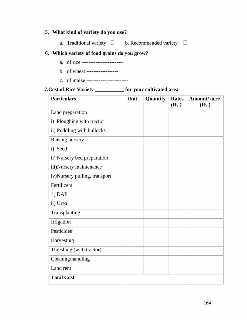
164

5. What kind of variety do you use?

a. Traditional variety b. Recommended variety

6. Which variety of food grains do you grow?

a. of rice ------------------------

b. of wheat ------------------

c. of maize ------------------------

7.Cost of Rice Variety ___________ for your cultivated area

Particulars Unit Quantity Rates (Rs.)

Amount/ acre (Rs.)

Land preparation

i) Ploughing with tractor

ii) Puddling with bullocks

Raising nursery

i) Seed

ii) Nursery bed preparation

iii)Nursery maintenance

iv)Nursery pulling, transport

Fertilizers

i) DAP

ii) Urea

Transplanting

Irrigation

Pesticides

Harvesting

Threshing (with tractor)

Cleaning/handling

Land rent

Total Cost

165

8. Cost of Wheat Variety _________ for your cultivated area

Particulars Unit Quantity Rates Amount (Rs.)

Land preparation with

tractor

Seed

Fertilizers

i) DAP

ii) Urea

Threshing (with tractors)

Labour charges

From sowing to threshing

Bags charges

Land rent

Total Cost

9. Cost of Maize Variety ___________________ for your cultivated area

Particulars Unit Quantity Rates Amount (Rs.) Land preparation with tractor

Seed

Fertilizers

i) DAP

ii) Urea

Weedicides

Threshing (with tractors)

Labour charges from sowing to

threshing

Bags charges

Land rent

Total Cost

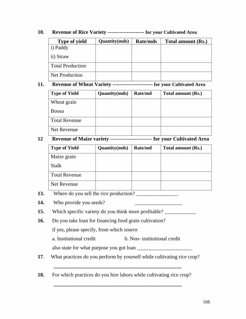
166

10. Revenue of Rice Variety --------------------- for your Cultivated Area

Type of yield Quantity(mds) Rate/mds Total amount (Rs.) i) Paddy

ii) Straw

Total Production

Net Production

11. Revenue of Wheat Variety ----------------------- for your Cultivated Area

Type of Yield Quantity(mds) Rate/md Total amount (Rs.)

Wheat grain

Boosa

Total Revenue

Net Revenue

12 Revenue of Maize variety ------------------------ for your Cultivated Area

Type of Yield Quantity(mds) Rate/md Total amount (Rs.)

Maize grain

Stalk

Total Revenue

Net Revenue

13. Where do you sell the rice production? ________________

14. Who provide you seeds? __________________

15. Which specific variety do you think more profitable? ____________

16. Do you take loan for financing food grain cultivation?

if yes, please specify, from which source

a. Institutional credit b. Non- institutional credit

also state for what purpose you got loan _____________________

17. What practices do you perform by yourself while cultivating rice crop?

_________________________________________________

18. For which practices do you hire labors while cultivating rice crop?

_________________________________________________

167

19. What practices do you perform by yourself while cultivating wheat crop?

_________________________________________________

20. For which practices do you hire labors while cultivating wheat crop?

_________________________________________________

21. What practices do you perform by yourself while cultivating maize crop?

_________________________________________________

22. For which practices do you hire labors while cultivating maize crop?

_________________________________________________

23. Who is the main decision maker in food grain cultivation?

24. What type of labours do you use for agriculture practices?

a. Local b. Non local

also state whether you use hired labour or use volunteers _____________

25. From where you get revenue for financing cultural and social activities?

_________________________________________________

26. What type of capital do you use in food grain cultivation?

a. In rice cultivation

b. In wheat cultivation

c. In maize cultivation

27. From where you get revenue for financing day-to-day expenses

___________________________________

28. Where you plan to utilize your income if you get more productivity from

food grain crops ___________________________________

29. What are your different sources of income?

a. ___________________

b. ___________________

c. ___________________

d. (others) ____________

168

30. Consumption Pattern for various heads

Main Items of Expenditures Amount Spent p.m (Rs.)

a. Food _________________

b. Clothing _________________

c. Education _________________

d. Health _________________

e. Electricity _________________

f. House rent _________________

g. Natural gas _________________

31. Present Assets of your Family

a. ___________________

b. ___________________

c. ___________________

d. ___________________

e. (others)

32. What problems do you face in food grain cultivation?

a. ___________________

b. ___________________

c. ___________________

d. ___________________

e. ___________________

20. What do you suggest for increasing low productivity of food grains?

a. _________________________

b. _________________________

c. _________________________

d. _________________________

169

APPENDIX-C

MARGINAL RATE OF SUBSTITUTION AMONG INPUTS

Appendix-C (1): Marginal Rate of Substitution among Rice Inputs

Substitution Between Variables Marginal Rate of Substitution Equation

Substitution of RA for TRHR MRS RA / TRHR = a1/ a2 (TRHR RA-1) Substitution of RA for FERTR MRS RA / FERTR = a1/ a3 (FERTR RA-1) Substitution of RA for SDR MRS RA / SDR = a1/ a4 (SDR RA-1) Substitution of RA for LABR MRS RA / LABR = a1/ a5 (LABR RA-1) Substitution of RA for PSTR MRS RA / PSTR = a1/ a6 (PSTR RA-1) Substitution of TRHR for RA MRS TRHR / RA = a2/ a1 (RA TRHR-1) Substitution of TRHR for FERTR MRS TRHR / FERTR = a2/ a3 (FERTR TRHR-1) Substitution of TRHR for SDR MRS TRHR / SDR = a2/ a4 (SDR TRHR-1) Substitution of TRHR for LAB MRS TRHR / LAB = a2/ a5 (LAB TRHR-1) Substitution of TRHR for PST MRS TRHR / PSTR = a2/ a6 (PSTR TRHR-1) Substitution of FERTR for RA MRS FERTR / RA = a3/ a1 (RA FERTR-1) Substitution of FERTR for TRHR MRS FERTR / THR = a3/ a2 (THR FERTR-1) Substitution of FERTR for SDR MRS FERTR / SDR = a3/ a4 (SDR FERTR-1) Substitution of FERTR for LABR MRS FERTR / LABR = a3/ a5 (LABR FERTR-1) Substitution of FERTR for PSTR MRS FERTR / PSTR = a3/ a6 (PSTR FERTR-1) Substitution of SDR for RA MRS SDR / RA = a4/ a1 (RA SDR-1) Substitution of SDR for TRHR MRS SDR / THR = a4/ a2 (THR SDR-1) Substitution of SDR for FERTR MRS SDR / FERTR = a4/ a3 (FERTR SDR-1) Substitution of SDR for LABR MRS SDR / LABR = a4/ a5 (LABR SDR-1) Substitution of SDR for PSTR MRS SDR / PSTR = a4/ a6 (PSTR SDR-1) Substitution of LABR for RA MRS LABR / RA = a5/ a1 (RA LABR-1) Substitution of LABR for TRHR MRS LABR / TRHR = a5/ a2 (TRHR LABR-1) Substitution of LABR for FERTR MRS LABR / FERTR = a5/ a3 (FERTR LABR-1) Substitution of LABR for SDR MRS LABR / SDR = a5/ a4 (SDR LABR-1) Substitution of LABR for PSTR MRS LABR / PSTR = a5/ a6 (PSTR LABR-1) Substitution of PSTR for RA MRS PSTR / RA = a6/ a1 (RA PSTR-1) Substitution of PSTR for TRHR MRS PSTR / TRHR = a6/ a2 (TRHR PSTR-1) Substitution of PSTR for FERTR MRS PSTR / FERTR = a6/ a3 (FERT PSTR-1) Substitution of PSTR for SDR MRS PSTR / SDR = a6/ a4 (SDR PSTR-1) Substitution of PSTR for LABR MRS PSTR / LABR = a6/ a5 (LABR PSTR-1)

Source: Personal derivation

170

Appendix-C (2): Marginal Rate of Substitution among Wheat Inputs

Substitution Between Variables Marginal Rate of Substitution Equation

Substitution of WA for TRHW MRS WA / TRHW = b1/ b2 (TRHW WA-1) Substitution of WA for FERTW MRS WA / FERTW = b1/ b3 (FERTW WA-1) Substitution of WA for SDW MRS WA / SDW = b1/ b4 (SDW WA-1) Substitution of WA for LABW MRS WA / LABW = b1/ b5 (LABW WA-1) Substitution of WA for PSTW MRS WA / PSTW = b1/ b6 (PSTW WA-1) Substitution of TRHW for WA MRS THW / WA = b2/ b1 (WA THW-1) Substitution of TRHW for FERTW MRS TRHW / FERTW = b2/ b3 (FERTW TRHW-1) Substitution of TRHW for SDW MRS TRHW / SDW = b2/ b4 (SDW TRHW-1) Substitution of TRHW for LABW MRS TRHW / LABW = b2/ b5 (LABW TRHW-1) Substitution of TRHW for PSTW MRS THW / PSTW = b2/ b6 (PSTW THW-1) Substitution of FERTW for WA MRS FERTW / WA = b3/ b1 (WA FERTW-1) Substitution of FERTW for TRHW MRS FERTW / RTHW = b3/ b2 (TRHW FERTW-1) Substitution of FERTW for SDW MRS FERTW / SDW = b3/ b4 (SDW FERTW-1) Substitution of FERTW for LABW MRS FERTW / LABW = b3/ b5 (LABW FERTW-1) Substitution of FERTW for PSTW MRS FERTW / PSTW = b3/ b6 (PSTW FERTW-1) Substitution of SDW for WA MRS SDW / WA = b4/ b1 (WA SDW-1) Substitution of SDW for TRHW MRS SDW / TRHW = b4/ b2 (TRHW SDW-1) Substitution of SDW for FERTW MRS SDW / FERTW = b4/ b3 (FERTW SDW-1) Substitution of SDW for LABW MRS SDW / LABW = b4/ b5 (LABW SDW-1) Substitution of SDW for PSTW MRS SDW / PSTW = b4/ b6 (PSTW SDW-1) Substitution of LABW for WA MRS LABW / WA = b5/ b1 (WA LABW-1) Substitution of LABW for TRHW MRS LABW / TRHW = b5/ b2 (TRHW LABW-1) Substitution of LABW for FERTW MRS LABW / FERTW = b5/ b3 (FERTW LABW-1) Substitution of LABW for SDW MRS LABW / SDW = b5/ b4 (SDW LABW-1) Substitution of LABW for PSTW MRS LABW / PSTW = b5/ b6 (PSTW LABW-1) Substitution of PSTW for WA MRS PSTW / WA = b6/ b1 (WA PSTW-1) Substitution of PSTW for TRHW MRS PSTW / THW = b6/ b2 (THW PSTW-1) Substitution of PSTW for FERTW MRS PSTW / FERTW = b6/ b3 (FERTW PSTW-1) Substitution of PSTW for SDW MRS PSTW / SDW = b6/ b4 (SDW PSTW-1) Substitution of PSTW for LABW MRS PSTW / LABW = b6/ b5 (LABW PSTW-1)

Source: Personal derivation

171

Appendix-C (3): Marginal Rate of Substitution among Maize Inputs

Substitution Between Variables Marginal Rate of Substitution Equation

Substitution of MA for TRHM MRS MA / TRHM = c1/ c2 (TRHM MA-1) Substitution of MA for FERTM MRS MA / FERTM = c1/ c3 (FERTM MA-1) Substitution of MA for SDM MRS MA / SDM = c1/ c4 (SDM MA-1) Substitution of MA for LABM MRS MA / LABM = c1/ c5 (LABM MA-1) Substitution of MA for PSTM MRS MA / PSTM = c1/ c6 (PSTM MA-1) Substitution of TRHM for MA MRS TRHM / MA = c2/ c1 (MA TRHM-1) Substitution of TRHM for FERTM MRS TRHM / FERTM = c2/ c3 (FERTM TRHM-1) Substitution of TRHM for SDM MRS TRHM / SDM = c2/ c4 (SDM TRHM-1) Substitution of TRHM for LABM MRS TRHM / LABM = c2/ c5 (LABM TRHM-1) Substitution of TRHM for PSTM MRS TRHM / PSTM = c2/ c6 (PSTM TRHM-1) Substitution of FERTM for MA MRS FERTM / MA = c3/ c1 (MA FERTM-1) Substitution of FERTM for TRHM MRS FERTM / TRHM = c3/ c2 (TRHM FERTM-1) Substitution of FERTM for SDM MRS FERTM / SDM = c3/ c4 (SDM FERTM-1) Substitution of FERTM for LABM MRS FERTM / LABW = c3/ c5 (LABM FERTM-1) Substitution of FERTM for PSTM MRS FERTM / PSTM = c3/ c6 (PSTM FERTM-1) Substitution of SDM for MA MRS SDM / MA = c4/ c1 (MA SDM-1) Substitution of SDM for TRHM MRS SDM / THM = c4/ c2 (THM SDM-1) Substitution of SDM for FERTM MRS SDM / FERTM = c4/ c3 (FERTM SDM-1) Substitution of SDM for LABM MRS SDM / LABM = c4/ c5 (LABM SDM-1) Substitution of SDM for PSTM MRS SDM / PSTM = c4/ c6 (PSTM SDM-1) Substitution of LABM for MA MRS LABM / MA = c5/ c1 (MA LABM-1) Substitution of LABM for TRHM MRS LABM / TRHM = c5/ c2 (TRHM LABM-1) Substitution of LABM for FERTM MRS LABM / FERTM = c5/ c3 (FERTM LABM-1) Substitution of LABM for SDM MRS LABM / SDM = c5/ c4 (SDM LABM-1) Substitution of LABM for PSTM MRS LABM / PSTM = c5/ c6 (PSTM LABM-1) Substitution of PSTM for MA MRS PSTM / MA = c6/ c1 (MA PSTM-1) Substitution of PSTM for TRHM MRS PSTM / TRHM = c6/ c2 (TRHM PSTM-1) Substitution of PSTM for FERTM MRS PSTM / FERTM = c6/ c3 (FERTM PSTM-1) Substitution of PSTM for SDM MRS PSTM / SDM = c6/ c4 (SDM PSTM-1) Substitution of PSTM for LABM MRS PSTM / LABM = c6/ c5 (LABM PSTM-1)

Source: Personal derivation

172

APPENDIX-D PER ACRE COST AND REVENUE OF DIFFERENT RICE VARIETIES

Appendix-D (1): Per Acre Cost of Variety JP-5

Particulars Unit Quantity Rates (Rs.)

Amount/acre (Rs.)

Land preparation i) Ploughing with tractor ii) Puddling with bullocks

Hr

Day

3 1

200 500

600 500

Raising nursery i) Seed ii) Nursery bed preparation iii) Nursery maintenance iv) Nursery pulling, transport

Kg Day Day Day

30 2 1 4

15 120 120 120

450 240 120 480

Fertilizers i) DAP ii) Urea

Kg Kg

25 50

9

8.6

225 430

Transplanting Day 15 120 1800

Irrigation Day 4 120 480

Cleaning/handling Day 7 120 840

Pesticides i) Furadan (Insecticides) ii) Machety (weedicides) iii) labour charges

Kg ml

Day

16 800 3

50 300 120

800 300 360

Harvesting Day 10 120 1200 Threshing i) Tractor charges ii) Labour charges

Hr

Day

1 8

300 120

300 960

Gunny bags charges Bag 20 40 800

Land rent -- -- -- 5500

Total Cost - - - 16385

Appendix-D (2): Total and Net Revenue of Variety JP-5

Type of yield Quantity (mds) Rate / md (Rs.) Total amount (Rs.)i) Paddy ii) Straw

40 --

1000 4000

40000 4000

Total Revenue -- -- 44,000

Net Revenue -- -- 27, 615

Source: Field survey

173

Appendix-D (3): Per Acre Cost of Variety Basmati-385

Particulars Unit Quantity Rates (Rs.)

Amount/acre (Rs.)

Land preparation i) Ploughing with tractor ii) Puddling with bullocks

Hr

Day

3 1

200 500

600 500

Raising nursery i) Seed ii) Nursery bed preparation iii) Nursery maintenance iv) Nursery pulling, transport

Kg Day Day Day

28 2 1 4

12 120 120 120

336 240 120 480

Fertilizers i) DAP ii) Urea

Kg Kg

25 50

9

8.6

225 430

Transplanting Day 15 120 1800

Irrigation Day 4 120 480

Cleaning/handling Day 7 120 840

Pesticides i) Furadan (Insecticides) ii) Machety (weedicides) iii) labour charges

Kg ml

Day

16 800 3

50 300 120

800 300 360

Harvesting Day 10 120 1200 Threshing i) Tractor charges ii) Labour charges

Hr

Day

1 8

300 120

300 960

Gunny bags charges Bag 20 40 800

Land rent -- -- -- 5500

Total Cost - - - 16, 271

Appendix-D (4): Total and Net Revenue of Variety Basmati-385

Type of yield Quantity (mds)

Rate / md (Rs.) Total amount (Rs.)

i) Paddy ii) Straw

42 1200 4500

50, 400 4, 500

Total Revenue 54, 900

Net Revenue 38, 629

Source: Field survey

174

Appendix-D (5): Per Acre Cost of Variety Sara Saila

Particulars Unit Quantity Rates (Rs.)

Amount/acre (Rs.)

Land preparation i) Ploughing with tractor ii) Puddling with bullocks

Hr

Day

3 1

200 500

600 500

Raising nursery i) Seed ii) Nursery bed preparation iii) Nursery maintenance iv) Nursery pulling, transport

Kg Day Day Day

30 2 1 4

10 120 120 120

300 240 120 480

Fertilizers i) DAP ii) Urea

Kg Kg

25 50

9

8.6

225 430

Transplanting Day 15 120 1800

Irrigation Day 4 120 480

Cleaning/handling Day 7 120 840

Pesticides i) Furadan (Insecticides) ii) Machety (weedicides) iii) labour charges

Kg ml

Day

16 800 3

50 300 120

800 300 360

Harvesting Day 10 120 1200 Threshing i) Tractor charges ii) Labour charges

Hr

Day

1 8

300 120

300 960

Gunny bags charges Bag 20 40 800

Land rent -- -- -- 5500

Total Cost - - - 16, 235

Appendix-D (6): Total and Net Revenue of Variety Sara Saila

Type of yield Quantity (mds)

Rate / md (Rs.) Total amount (Rs.)

i) Paddy ii) Straw

38 -

1000 4500

38, 000 4500

Total Revenue 42, 500

Net Revenue 26, 265

Source: Field survey

175

Appendix-D (7): Per Acre Cost of Variety Dil Rosh-97

Particulars Unit Quantity Rates (Rs.)

Amount/acre (Rs.)

Land preparation i) Ploughing with tractor ii) Puddling with bullocks

Hr

Day

3 1

200 500

600 500

Raising nursery i) Seed ii) Nursery bed preparation iii) Nursery maintenance iv) Nursery pulling, transport

Kg Day Day Day

25 2 1 4

10 120 120 120

250 240 120 480

Fertilizers i) DAP ii) Urea

Kg Kg

25 50

9

8.6

225 430

Transplanting Day 15 120 1800

Irrigation Day 4 120 480

Cleaning/handling Day 7 120 840

Pesticides i) Furadan (Insecticides) ii) Machety (weedicides) iii) labour charges

Kg ml

Day

16 800 3

50 300 120

800 300 360

Harvesting Day 10 120 1200 Threshing i) Tractor charges ii) Labour charges

Hr

Day

1 8

300 120

300 960

Gunny bags charges Bag 20 40 800

Land rent -- -- -- 5500

Total Cost - - - 16, 185

Appendix-D (8): Total and Net Revenue of Variety Dil Rosh-97

Type of yield Quantity (mds)

Rate / md (Rs.) Total amount (Rs.)

i) Paddy ii) Straw

27 1100 4000

29, 700 4000

Total Revenue 33700

Net Revenue 17, 515

Source: Field survey

176

Appendix-D (9): Per Acre Cost of Variety Swat-1

Particulars Unit Quantity Rates (Rs.)

Amount/acre (Rs.)

Land preparation i) Ploughing with tractor ii) Puddling with bullocks

Hr

Day

3 1

200 500

600 500

Raising nursery i) Seed ii) Nursery bed preparation iii) Nursery maintenance iv) Nursery pulling, transport

Kg Day Day Day

30 2 1 4

10 120 120 120

300 240 120 480

Fertilizers i) DAP ii) Urea

Kg Kg

25 50

9

8.6

225 430

Transplanting Day 15 120 1800

Irrigation Day 4 120 480

Cleaning/handling Day 7 120 840

Pesticides i) Furadan (Insecticides) ii) Machety (weedicides) iii) labour charges

Kg ml

Day

16 800 3

50 300 120

800 300 360

Harvesting Day 10 120 1200 Threshing i) Tractor charges ii) Labour charges

Hr

Day

1 8

300 120

300 960

Gunny bags charges Bag 20 40 800

Land rent -- -- -- 5500

Total Cost - - - 16, 235

Appendix-D (10): Total and Net Revenue of Variety Swat-1

Type of yield Quantity (mds)

Rate / md (Rs.) Total amount (Rs.)

i) Paddy ii) Straw

28 1100 4500

30, 800 4500

Total Revenue 35, 300

Net Revenue 19, 065

Source: Field survey

177

Appendix-D (11): Per Acre Cost of Variety Swat-2

Particulars Unit Quantity Rates (Rs.)

Amount/acre (Rs.)

Land preparation i) Ploughing with tractor ii) Puddling with bullocks

Hr

Day

3 1

200 500

600 500

Raising nursery i) Seed ii) Nursery bed preparation iii) Nursery maintenance iv) Nursery pulling, transport

Kg Day Day Day

30 2 1 4

12 120 120 120

360 240 120 480

Fertilizers i) DAP ii) Urea

Kg Kg

25 50

9

8.6

225 430

Transplanting Day 15 120 1800

Irrigation Day 4 120 480

Cleaning/handling Day 7 120 840

Pesticides i) Furadan (Insecticides) ii) Machety (weedicides) iii) labour charges

Kg ml

Day

16 800 3

50 300 120

800 300 360

Harvesting Day 10 120 1200 Threshing i) Tractor charges ii) Labour charges

Hr

Day

1 8

300 120

300 960

Gunny bags charges Bag 20 40 800

Land rent -- -- -- 5500

Total Cost - - - 16, 295

Appendix-D (12): Total and Net Revenue of Variety Swat-2

Type of yield Quantity (mds)

Rate / md (Rs.) Total amount (Rs.)

i) Paddy ii) Straw

28 1100 4500

30, 800 4500

Total Revenue 35, 300

Net Revenue 19, 005

Source: Field survey

178

Appendix-D (13): Per Acre Cost of Variety Fakhr-e-Malakand

Particulars Unit Quantity Rates (Rs.)

Amount/acre (Rs.)

Land preparation i) Ploughing with tractor ii) Puddling with bullocks

Hr

Day

3 1

200 500

600 500

Raising nursery i) Seed ii) Nursery bed preparation iii) Nursery maintenance iv) Nursery pulling, transport

Kg Day Day Day

30 2 1 4

12 120 120 120

360 240 120 480

Fertilizers i) DAP ii) Urea

Kg Kg

25 50

9

8.6

225 430

Transplanting Day 15 120 1800

Irrigation Day 4 120 480

Cleaning/handling Day 7 120 840

Pesticides i) Furadan (Insecticides) ii) Machety (weedicides) iii) labour charges

Kg ml

Day

16 800 3

50 300 120

800 300 360

Harvesting Day 10 120 1200 Threshing i) Tractor charges ii) Labour charges

Hr

Day

1 8

300 120

300 960

Gunny bags charges Bag 20 40 800

Land rent -- -- -- 5500

Total Cost - - - 16, 295

Appendix-D (14): Total and Net Revenue of Variety Fakhr-e-Malakand

Type of yield Quantity (mds)

Rate / md (Rs.) Total amount (Rs.)

i) Paddy ii) Straw

48 1000 7500

48, 000 7500

Total Revenue 55, 500

Net Revenue 39, 205

Source: Field survey

179

APPENDIX-E

PER ACRE COST AND REVENUE OF DIFFERENT WHEAT VARIETIES

Appendix-E (1): Per Acre Cost of Variety Saleem-2000

Particulars Unit Quantity Rates Amount/Acre (Rs.)

Land preparation with tractor Hour 3 400 1200

Seed Kg 50 30 1500

Fertilizers

i) DAP

ii) Urea

bag

bag

1

2

3000

680

3000

1360

Threshing (with tractors) Hour 1 1000 1000

Labour charges

From sowing to threshing

Day

30

120

3600

Bags charges Bag 20 40 800

Land rent -- 5500 5500

Total Cost 17, 960

Appendix-E (2): Total and Net Revenue of Variety Saleem-2000

Type of Yield Quantity(mds) Rate/md Total amount (Rs.)

Wheat grain

Boosa

25

-

1200

9000

30, 000

9, 000

Total Revenue 39, 000

Net Revenue 21040

Source: Field survey

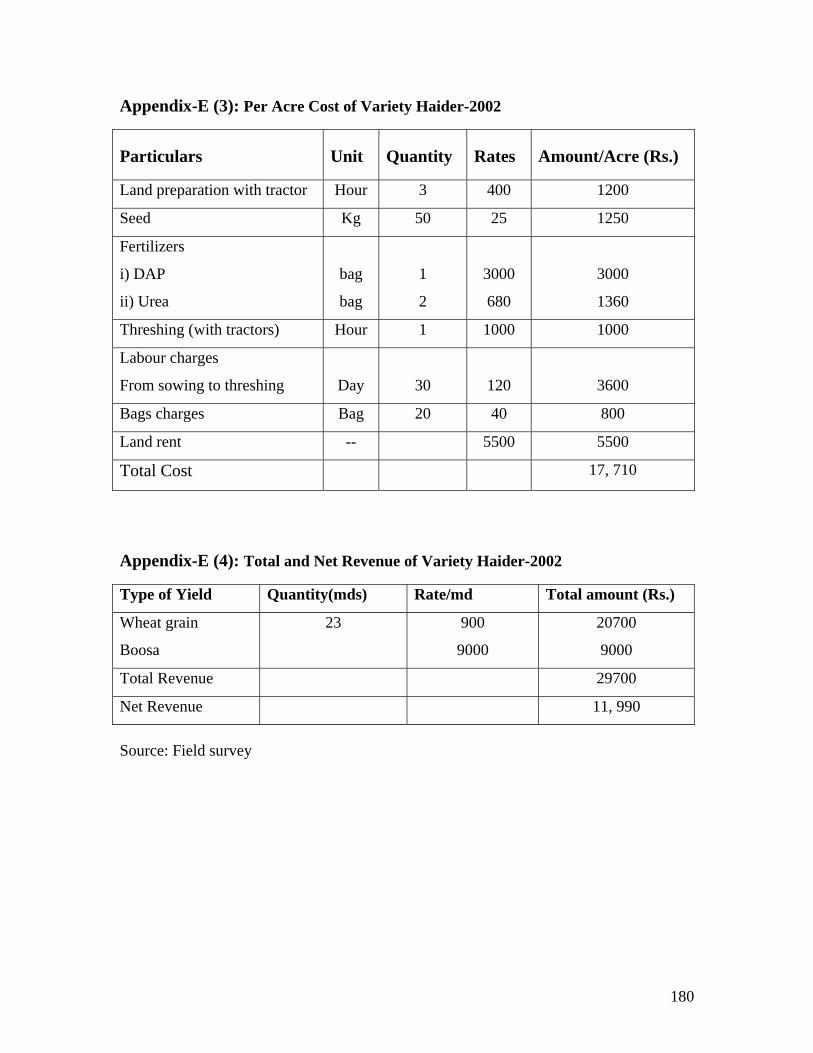
180

Appendix-E (3): Per Acre Cost of Variety Haider-2002

Particulars Unit Quantity Rates Amount/Acre (Rs.)

Land preparation with tractor Hour 3 400 1200

Seed Kg 50 25 1250

Fertilizers

i) DAP

ii) Urea

bag

bag

1

2

3000

680

3000

1360

Threshing (with tractors) Hour 1 1000 1000

Labour charges

From sowing to threshing

Day

30

120

3600

Bags charges Bag 20 40 800

Land rent -- 5500 5500

Total Cost 17, 710

Appendix-E (4): Total and Net Revenue of Variety Haider-2002

Type of Yield Quantity(mds) Rate/md Total amount (Rs.)

Wheat grain

Boosa

23 900

9000

20700

9000

Total Revenue 29700

Net Revenue 11, 990

Source: Field survey

181

Appendix-E (5): Per Acre Cost of Variety Khyber-87

Particulars Unit Quantity Rates Amount/Acre (Rs.)

Land preparation with tractor Hour 3 400 1200

Seed Kg 50 20 1000

Fertilizers

i) DAP

ii) Urea

bag

bag

1

2

3000

680

3000

1360

Threshing (with tractors) Hour 1 1000 1000

Labour charges

From sowing to threshing

Day

30

120

3600

Bags charges Bag 20 40 800

Land rent -- 5500 5500

Total Cost 17, 460

Appendix-E (6): Total and Net Revenue of Variety Khyber-87

Type of Yield Quantity(mds) Rate/md Total amount (Rs.)

Wheat grain

Boosa

25 1100

9000

27500

9000

Total Revenue 36500

Net Revenue 19040

Source: Field survey

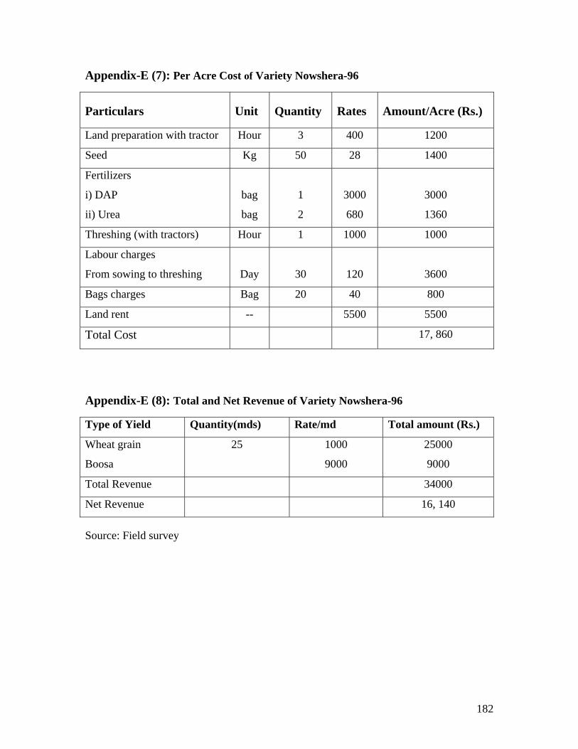
182

Appendix-E (7): Per Acre Cost of Variety Nowshera-96

Particulars Unit Quantity Rates Amount/Acre (Rs.)

Land preparation with tractor Hour 3 400 1200

Seed Kg 50 28 1400

Fertilizers

i) DAP

ii) Urea

bag

bag

1

2

3000

680

3000

1360

Threshing (with tractors) Hour 1 1000 1000

Labour charges

From sowing to threshing

Day

30

120

3600

Bags charges Bag 20 40 800

Land rent -- 5500 5500

Total Cost 17, 860

Appendix-E (8): Total and Net Revenue of Variety Nowshera-96

Type of Yield Quantity(mds) Rate/md Total amount (Rs.)

Wheat grain

Boosa

25 1000

9000

25000

9000

Total Revenue 34000

Net Revenue 16, 140

Source: Field survey

183

Appendix-E (9): Per Acre Cost of Variety Tatara

Particulars Unit Quantity Rates Amount/Acre (Rs.)

Land preparation with tractor Hour 3 400 1200

Seed Kg 50 25 1250

Fertilizers

i) DAP

ii) Urea

bag

bag

1

2

3000

680

3000

1360

Threshing (with tractors) Hour 1 1000 1000

Labour charges

From sowing to threshing

Day

30

120

3600

Bags charges Bag 20 40 800

Land rent -- 5500 5500

Total Cost 17, 710

Appendix-E (10): Total and Net Revenue of Variety Tatara

Type of Yield Quantity(mds) Rate/md Total amount (Rs.)

Wheat grain

Boosa

28 800

9000

22400

9000

Total Revenue 31, 400

Net Revenue 13, 690

Source: Field survey

184

Appendix-E (11): Per Acre Cost of Variety Bakhtawar-92

Particulars Unit Quantity Rates Amount/Acre (Rs.)

Land preparation with tractor Hour 3 400 1200

Seed Kg 50 28 1400

Fertilizers

i) DAP

ii) Urea

bag

bag

1

2

3000

680

3000

1360

Threshing (with tractors) Hour 1 1000 1000

Labour charges

From sowing to threshing

Day

30

120

3600

Bags charges Bag 20 40 800

Land rent -- 5500 5500

Total Cost 17, 860

Appendix-E (12): Total and Net Revenue of Variety Bakhtawar-92

Type of Yield Quantity(mds) Rate/md Total amount (Rs.)

Wheat grain

Boosa

28 1100

9000

30800

9000

Total Revenue 39800

Net Revenue 21, 940

Source: Field survey

185

Appendix-E (13): Per Acre Cost of Variety Auqab-2000

Particulars Unit Quantity Rates Amount/Acre (Rs.)

Land preparation with tractor Hour 3 400 1200

Seed Kg 50 25 1250

Fertilizers

i) DAP

ii) Urea

bag

bag

1

2

3000

680

3000

1360

Threshing (with tractors) Hour 1 1000 1000

Labour charges

From sowing to threshing

Day

30

120

3600

Bags charges Bag 20 40 800

Land rent -- 5500 5500

Total Cost 17, 710

Appendix-E (14): Total and Net Revenue of Variety Auqab-2000

Type of Yield Quantity(mds) Rate/md Total amount (Rs.)

Wheat grain

Boosa

26 1100

9000

28600

9000

Total Revenue 37600

Net Revenue 19, 890

Source: Field survey

186

Appendix-E (15): Per Acre Cost of Variety Suleman-96

Particulars Unit Quantity Rates Amount/Acre (Rs.)

Land preparation with tractor Hour 3 400 1200

Seed Kg 50 25 1250

Fertilizers

i) DAP

ii) Urea

bag

bag

1

2

3000

680

3000

1360

Threshing (with tractors) Hour 1 1000 1000

Labour charges

From sowing to threshing

Day

30

120

3600

Bags charges Bag 20 40 800

Land rent -- 5500 5500

Total Cost 17, 710

Appendix-E (16): Total and Net Revenue of Variety Suleman-96

Type of Yield Quantity(mds) Rate/md Total amount (Rs.)

Wheat grain

Boosa

25 1000

9000

25000

9000

Total Revenue 34000

Net Revenue 16, 290

Source: Field survey

187

Appendix-E (17): Per Acre Cost of Variety Fakhri-Sarhad

Particulars Unit Quantity Rates Amount/Acre (Rs.)

Land preparation with tractor Hour 3 400 1200

Seed Kg 45 25 1125

Fertilizers

i) DAP

ii) Urea

bag

bag

1

2

3000

680

3000

1360

Threshing (with tractors) Hour 1 1000 1000

Labour charges

From sowing to threshing

Day

30

120

3600

Bags charges Bag 20 40 800

Land rent -- 5500 5500

Total Cost 17, 585

Appendix-E (18): Total and Net Revenue of Variety Fakhri-Sarhad

Type of Yield Quantity (mds) Rate/md Total amount (Rs.)

Wheat grain

Boosa

32 1000

9500

32000

9500

Total Revenue 41500

Net Revenue 23, 915

Source: Field survey

188

Appendix-E (19): Per Acre Cost of Variety Pir Sabak-2004

Particulars Unit Quantity Rates Amount/Acre (Rs.)

Land preparation with tractor Hour 3 400 1200

Seed Kg 50 25 1250

Fertilizers

i) DAP

ii) Urea

bag

bag

1

2

3000

680

3000

1360

Threshing (with tractors) Hour 1 1000 1000

Labour charges

From sowing to threshing

Day

30

120

3600

Bags charges Bag 20 40 800

Land rent -- 5500 5500

Total Cost 17, 710

Appendix-E (20): Total and Net Revenue of Variety Pir Sabak-2004

Type of Yield Quantity(mds) Rate/md Total amount (Rs.)

Wheat grain

Boosa

24 900

9000

21600

9000

Total Revenue 30600

Net Revenue 12, 890

Source: Field survey

189

Appendix-E (21): Per Acre Cost of Variety Pir Sabak-2005

Particulars Unit Quantity Rates Amount/Acre (Rs.)

Land preparation with tractor Hour 3 400 1200

Seed Kg 50 25 1250

Fertilizers

i) DAP

ii) Urea

bag

bag

1

2

3000

680

3000

1360

Threshing (with tractors) Hour 1 1000 1000

Labour charges

From sowing to threshing

Day

30

120

3600

Bags charges Bag 20 40 800

Land rent -- 5500 5500

Total Cost 17, 710

Appendix-E (22): Total and Net Revenue of Variety Pir Sabak-2005

Type of Yield Quantity(mds) Rate/md Total amount (Rs.)

Wheat grain

Boosa

25 900

9000

22500

9000

Total Revenue 31500

Net Revenue 13, 790

Source: Field survey

190

APPENDIX-F

PER ACRE COST AND REVENUE OF MAIZE VARIETIES

Appendix-F (1): Per-acre Cost of variety Azam

Particulars Unit Quantity Rates Amount/Acre (Rs.)

Land preparation with tractor Hour 3 400 1200

Seed Kg 20 40 800

Fertilizers

i) DAP

ii) Urea

Bag

Bag

1

2

3000

680

3000

1360

Weedicides - - 600 600

Threshing (with tractors) Hour 1 1500 1500

Labour charges from sowing to

threshing

Day

35

120

4200

Bags charges Bag 20 40 800

Land rent -- - 5500 5500

Total Cost 18, 960

Appendix-F (2): Total and Net Revenue of Variety Azam

Type of Yield Quantity(mds) Rate/md Total amount (Rs.)

Maize grain

Stalk

30 1250

5000

37, 500

5, 000

Total Revenue 42, 500

Net Revenue 23, 540

Source: Field survey

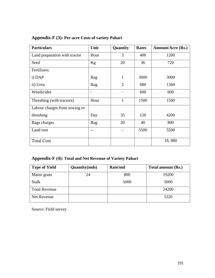
191

Appendix-F (3): Per-acre Costs of variety Pahari

Particulars Unit Quantity Rates Amount/Acre (Rs.)

Land preparation with tractor Hour 3 400 1200

Seed Kg 20 36 720

Fertilizers

i) DAP

ii) Urea

Bag

Bag

1

2

3000

680

3000

1360

Weedicides - - 600 600

Threshing (with tractors) Hour 1 1500 1500

Labour charges from sowing to

threshing

Day

35

120

4200

Bags charges Bag 20 40 800

Land rent -- - 5500 5500

Total Cost 18, 880

Appendix-F (4): Total and Net Revenue of Variety Pahari

Type of Yield Quantity(mds) Rate/md Total amount (Rs.)

Maize grain

Stalk

24 800

5000

19200

5000

Total Revenue 24200

Net Revenue 5320

Source: Field survey

192

Appendix-F (5): Per-acre Costs of variety Jalal

Particulars Unit Quantity Rates Amount/Acre (Rs.)

Land preparation with tractor Hour 3 400 1200

Seed Kg 20 35 700

Fertilizers

i) DAP

ii) Urea

Bag

Bag

1

2

3000

680

3000

1360

Weedicides - - 600 600

Threshing (with tractors) Hour 1 1500 1500

Labour charges from sowing to

threshing

Day

35

120

4200

Bags charges Bag 20 40 800

Land rent -- - 5500 5500

Total Cost 18, 860

Appendix-F (6): Total and Net Revenue of Variety Jalal

Type of Yield Quantity(mds) Rate/md Total amount (Rs.)

Maize grain

Stalk

25 700

5000

17500

5000

Total Revenue 22500

Net Revenue 3640

Source: Field survey

193

Appendix-F (7): Per-acre Costs of variety Babar

Particulars Unit Quantity Rates Amount/Acre (Rs.)

Land preparation with tractor Hour 3 400 1200

Seed Kg 20 39 780

Fertilizers

i) DAP

ii) Urea

Bag

Bag

1

2

3000

680

3000

1360

Weedicides - - 600 600

Threshing (with tractors) Hour 1 1500 1500

Labour charges from sowing to

threshing

Day

35

120

4200

Bags charges Bag 20 40 800

Land rent -- - 5500 5500

Total Cost 18, 940

Appendix-F (8): Total and Net Revenue of Variety Babar

Type of Yield Quantity(mds) Rate/md Total amount (Rs.)

Maize grain

Stalk

28 1100

5000

30800

5000

Total Revenue 35800

Net Revenue 16, 860

Source: Field survey

194

Appendix-F (9): Per-acre Costs of variety Ghori

Particulars Unit Quantity Rates Amount/Acre (Rs.)

Land preparation with tractor Hour 3 400 1200

Seed Kg 20 34 680

Fertilizers

i) DAP

ii) Urea

Bag

Bag

1

2

3000

680

3000

1360

Weedicides - - 600 600

Threshing (with tractors) Hour 1 1500 1500

Labour charges from sowing to

threshing

Day

35

120

4200

Bags charges Bag 20 40 800

Land rent -- - 5500 5500

Total Cost 18, 840

Appendix-F (10): Total and Net Revenue of Variety Ghori

Type of Yield Quantity(mds) Rate/md Total amount (Rs.)

Maize grain

Stalk

24 900

5000

21600

5000

Total Revenue 26600

Net Revenue 7760

Source: Field survey

195

Appendix-G

Stepwise Regression Results for Rice Input Output Relationship

Appendix-G (1): Variable (ln RA) entered Variable Coefficient Std. Error t-Statistic Prob. C 2.00123 0.1324 15.11503 0.0000 ln RA 0.124578 0.013451 9.261616 0.0000 R-Squared 0.610936 Appendix-G (2): Variable (ln RA) and (ln TRHR) entered

Variable Coefficient Std. Error t-Statistic Prob. C 2.31245 0.41257 5.604988 0.0000 ln RA 0.54123 0.09134 5.925443 0.0000 ln TRHR 0.215487 0.04123 5.226461 0.0000 R-Squared 0.638123 Appendix-G (3): Variable (ln RA), (ln TRHR) and (ln FERTR) entered

Variable Coefficient Std. Error t-Statistic Prob. C 1.97845 0.1245 15.89116 0.0000 ln RA 0.554412 0.084512 6.560157 0.0000 ln TRHR 0.336451 0.051874 6.485927 0.0000 ln FERTR 0.01488 0.011334 1.312864 0.0000 R-Squared 0.715261 Appendix-G (4): Variable (ln RA), (ln TRHR), (ln FERTR) and (ln SDR) entered

Variable Coefficient Std. Error t-Statistic Prob. C 2.364581 0.12547 18.84579 0.0000 ln RA 0.61248 0.08451 7.247426 0.0000 ln TRHR 0.31222 0.011123 28.06977 0.0000 ln FERTR 0.55411 0.0487152 11.37448 0.0000 ln SDR 0.54152 0.013412 40.37578 0.0011 R-Squared 0.77006 Appendix-G (5): Variable (ln RA), (ln TRHR), (ln FERTR), (ln SDR) and (ln

LABR) entered

Variable Coefficient Std. Error t-Statistic Prob. C 1.994167 0.113451 17.57734 0.0000 ln RA 0.54126 0.012451 43.47121 0.0000 ln TRHR 0.31254 0.012341 25.32534 0.0002 ln FERTR 0.7145662 0.087161 8.198233 0.0000 ln SDR 0.287771 0.021546 13.35612 0.0011 ln LABR 0.2234661 0.012451 17.94764 0.0052 R-Squared 0.891906

196

Appendix-H

Stepwise Regression Results for Wheat Input Output Relationship

Appendix-H(1): Variable ln WA entered

Variable Coefficient Std. Error t-Statistic Prob. C 5.001245 0.14551

34.37046 0.00032

ln WA 0.1245 0.01123 11.08638 0.00813 R-Squared 0.658936 Appendix-H(2): Variable ln WA and ln TRHW entered Variable Coefficient Std. Error t-Statistic Prob. C 4.781245 0.187413 25.51181 0.0000 ln WA 0.33451 0.01781 18.78214 0.0012 ln TRHW 0.1348 0.0125487 10.74215 0.0001 R-Squared 0.70124

Appendix-H(3): Variable ln WA, ln TRHW and ln FERTW entered

Variable Coefficient Std. Error t-Statistic Prob. C 5.124 0.14612 35.06707 0.0000 ln WA 0.3148 0.01384 22.74566 0.0000 ln TRHW 0.84123 0.064871 12.96774 0.0000 ln FERTW 0.6412 0.03461 18.52644 0.0000 R-Squared 0.752354 Appendix-H(4): Variable ln WA, ln TRHW, ln FERTW and ln SDW entered Variable Coefficient Std. Error t-Statistic Prob. C 5.0171 0.5241 9.572791 0.0000 ln WA 0.28145 0.012354 22.78209 0.0000 ln TRHW 0.84623 0.0413871 20.44671 0.0002 ln FERTW 0.81347 0.064125 12.68569 0.0000 ln SDW 0.1264 0.02813 4.493423 0.0000 R-Squared 0.7912458 Appendix-H(5): Variable ln WA, ln TRHW, ln FERTW, ln SDW and ln LABW entered

Variable Coefficient Std. Error t-Statistic Prob. C 4.12548 0.13254 31.1263 0.0000 ln WA 0.16812 0.012 14.01 0.0000 ln TRHW 0.114782 0.015811 7.259629 0.0036 ln FERTW 0.3518 0.01233 28.53204 0.0048 ln SDW 0.615791 0.104521 5.891553 0.0001 ln LABW 0.125468 0.01547 8.110407 0.000748 R-Squared 0.8101245

197

Appendix-I

Stepwise Regression Results for Maize Input Output Relationship

Appendix-I (1):Variable ln MA entered

Variable Coefficient Std. Error t-Statistic Prob. C 2.0124 0.12487 16.11596 0.00000 ln MA 0.8124 0.082457 9.852408 0.00000 R-Squared 0.6114578 Appendix-I (2):Variable ln MA and ln TRHM entered Variable Coefficient Std. Error t-Statistic Prob. C 3.87123 0.0843 45.92206 0.00457 ln MA 0.63124 0.1022 6.176517 0.00087 ln TRHM 0.84123 0.044456 18.92276 0.02458 R-Squared 0.668798 Appendix-I (3):Variable ln MA, ln TRHM and ln FERTM entered Variable Coefficient Std. Error t-Statistic Prob. C 2.3587 0.04318 54.62483 0.002154 ln MA 0.24561 0.04466 5.499552 0.007845 ln TRHM 0.6412 0.06666 9.618962 0.000897 ln FERTM 0.84512 0.14135 5.978918 0.000548 R-Squared 0.7087974 Appendix-I (4):Variable ln MA, ln TRHM, ln FERTM and ln SDM entered Variable Coefficient Std. Error t-Statistic Prob. C 3.02114 0.244561 12.35332 0.0124574 ln MA 0.31254 0.02487 12.56695 0.000078 ln TRHM 0.513874 0.03311 15.52021 0.004577 ln FERTM 0.4422 0.07713 5.733178 0.000478 ln SDM 0.9874 0.06644 14.86153 0.04545 R-Squared 0.771248 Appendix-I (5):Variable ln MA, ln TRHM, ln FERTM, ln SDW and ln LABM entered Variable Coefficient Std. Error t-Statistic Prob. C 2.038742 0.21547 9.461837 0.000411 ln MA 0.94213 0.08452 11.14683 0.001247 ln TRHM 0.123487 0.001882 65.61477 0.02141 ln FERTM 0.21888 0.013415 16.31606 0.012421 ln SDM 0.99113 0.03546781 27.94449 0.00210 ln LABM 0.228412 0.01987461 11.49265 0.001248 R-Squared 0.8000078

198

APPENDIX-J

Marginal Product Estimation for Rice Inputs

APPENDIX-J (1): Marginal Product Estimation for Mean Values of Rice Inputs

Inputs Marginal Product equation of Inputs Marginal

Product (Kgs)

MPRA 17.74316 0.245781 1.50.245781-1 50.6712 30.07891

400.871245 750.12487 30.004871

443.56

MPTRHR 17.74316 0.6712 1.50.245781 50.6712-1 30.07891

400.871245 750.12487 30.004871

299.10

MPFERTR 17.74316 0.07891 1.50.245781 50.6712 30.07891-1

400.871245 750.12487 30.004871

71.20

MPSDR 17.74316 0.871245 1.50.245781 50.6712 30.07891

400.871245-1 750.12487 30.004871

50.55

MPLABR 17.74316 0.12487 1.50.245781 50.6712 30.07891

400.871245 750.12487-1 30.004871

3.86

MPPSTR 17.74316 0.004871 1.50.245781 50.6712 30.07891

400.871245 750.12487 30.004871-1

3.56

Source: Personal calculations

199

APPENDIX-J (2): Marginal Product Estimation for Maximum Values of Rice Inputs

Inputs Marginal Product equation of Inputs Marginal

product (Kgs)

MPRA 17.74316 0.245781 3.60.245781-1 60.6712 40.07891

450.871245 800.12487 40.004871

281.84

MPTRHR 17.74316 0.6712 3.60.245781 60.6712-1 40.07891

450.871245 800.12487 40.004871

461.77

MPFERTR 17.74316 0.07891 3.60.245781 60.6712 40.07891-1

450.871245 800.12487 40.004871

81.42

MPSDR 17.74316 0.871245 3.60.245781 60.6712 40.07891

450.871245-1 800.12487 40.004871

79.92

MPLABR 17.74316 0.12487 3.60.245781 60.6712 40.07891

450.871245 800.12487-1 40.004871

6.44

MPPSTR 17.74316 0.004871 3.60.245781 60.6712 40.07891

450.871245 800.12487 40.004871-1

5.03

Source: Personal calculations

200

APPENDIX-J (2): Marginal Product Estimation for Minimum Values of Rice Inputs

Inputs Marginal Product equation of Inputs Marginal

product (Kgs)

MPRA 17.74316 0.245781 0.20.245781-1 20.6712 10.07891

300.871245 500.12487 10.004871

726.87

MPTRHR 17.74316 0.6712 0.20.245781 20.6712-1 10.07891

300.871245 500.12487 10.004871

198.50

MPFERTR 17.74316 0.07891 0.20.245781 20.6712 10.07891-1

300.871245 500.12487 10.004871

46.67

MPSDR 17.74316 0.871245 0.20.245781 20.6712 10.07891

300.871245-1 500.12487 10.004871

17.18

MPLABR 17.74316 0.12487 0.20.245781 20.6712 10.07891

300.871245 500.12487-1 10.004871

1.48

MPPSTR 17.74316 0.004871 0.20.245781 20.6712 10.07891

300.871245 500.12487 10.004871-1

2.88

Source: Personal calculations

201

APPENDIX-K

Marginal Product Estimation for Wheat Inputs

APPENDIX-K (1): Estimated Marginal Product at Mean Values of wheat Inputs

Inputs Marginal Product equation of Inputs Marginal

product (Kgs)

MPWA 146.936424 0.6104 WA0.6104-1 TRHW0.1220

FERTW0.1479 SDW0.2991 LABW0.2124 PSTW0.1041

794

MPTRHW 146.936424 0.1220 WA0.6104 TRHW0.1220-1

FERTW0.1479 SDW0.2991 LABW0.2124 PSTW0.1041

59

MPFERTW 146.936424 0.1479 WA0.6104 TRHW0.1220

FERTW0.1479-1 SDW0.2991 LABW0.2124 PSTW0.1041

96

MPSDW 146.936424 0.2991 WA0.6104 TRHW0.1220

FERTW0.1479 SDW0.2991-1 LABW0.2124 PSTW0.1041

12

MPLABW 146.936424 0.2124 WA0.6104 TRHW0.1220

FERTW0.1479 SDW0.2991 LABW0.2124-1 PSTW0.1041

14

MPPSTW 146.936424 0.1041 WA0.6104 TRHW0.1220

FERTW0.1479 SDW0.2991 LABW0.2124 PSTW0.1041-1

68

Source: Personal calculations

202

APPENDIX-K (2): Estimated Marginal Product at Maximum Values of wheat Inputs

Inputs

Marginal Product equation of Inputs

Marginal

product (Kgs)

MPWA 146.936424 0.6104 WA0.6104-1 TRHW0.1220

FERTW0.1479 SDW0.2991 LABW0.2124 PSTW0.1041

678

MPTRHW 146.936424 0.1220 WA0.6104 TRHW0.1220-1

FERTW0.1479 SDW0.2991 LABW0.2124 PSTW0.1041

81

MPFERTW 146.936424 0.1479 WA0.6104 TRHW0.1220

FERTW0.1479-1 SDW0.2991 LABW0.2124 PSTW0.1041

148

MPSDW 146.936424 0.2991 WA0.6104 TRHW0.1220

FERTW0.1479 SDW0.2991-1 LABW0.2124 PSTW0.1041

22

MPLABW 146.936424 0.2124 WA0.6104 TRHW0.1220

FERTW0.1479 SDW0.2991 LABW0.2124-1 PSTW0.1041

24

MPPSTW 146.936424 0.1041 WA0.6104 TRHW0.1220

FERTW0.1479 SDW0.2991 LABW0.2124 PSTW0.1041-1

104

Source: Personal calculations

203

APPENDIX-K (3): Estimated Marginal Product at Minimum Values of wheat Inputs

Inputs Marginal Product equation of Inputs Marginal

product (Kgs)

MPWA 146.936424 0.6104 WA0.6104-1 TRHW0.1220

FERTW0.1479 SDW0.2991 LABW0.2124 PSTW0.1041

1041

MPTRHW 146.936424 0.1220 WA0.6104 TRHW0.1220-1

FERTW0.1479 SDW0.2991 LABW0.2124 PSTW0.1041

21

MPFERTW 146.936424 0.1479 WA0.6104 TRHW0.1220

FERTW0.1479-1 SDW0.2991 LABW0.2124 PSTW0.1041

50

MPSDW 146.936424 0.2991 WA0.6104 TRHW0.1220

FERTW0.1479 SDW0.2991-1 LABW0.2124 PSTW0.1041

3

MPLABW 146.936424 0.2124 WA0.6104 TRHW0.1220

FERTW0.1479 SDW0.2991 LABW0.2124-1 PSTW0.1041

4

MPPSTW 146.936424 0.1041 WA0.6104 TRHW0.1220

FERTW0.1479 SDW0.2991 LABW0.2124 PSTW0.1041-1

36

Source: Personal calculations

204

APPENDIX-L

Estimation of Marginal Product for Maize Inputs

APPENDIX-L (1): Estimation of Marginal Product for Mean Values of Maize Inputs

Inputs Marginal Product equation of Inputs Marginal

Product (Kgs)

MPMA 33.45094375 0.64123 MA0.64123-1 TRHM0.124587

FERTM0.55461 SDM0.31244 LABM0.5874 PSTM0.08248

800

MPTRHM 33.45094375 0.124587 MA0.64123 TRHM0.124587-1

FERTM0.55461 SDM0.31244 LABM0.5874 PSTM0.08248

60

MPFERTM 33.45094375 0.55461 MA0.64123 TRHM0.124587

FERTM0.55461-1 SDM0.31244 LABM0.5874 PSTM0.08248

357

MPSDM 33.45094375 0.31244 MA0.64123 TRHM0.124587

FERTM0.55461 SDM0.31244-1 LABM0.5874 PSTM0.08248

30

MPLABM 33.45094375 0.5874 MA0.64123 TRHM0.124587

FERTM0.55461 SDM0.31244 LABM0.5874-1 PSTM0.08248

32

MPPSTM 33.45094375 0.08248 MA0.64123 TRHM0.124587

FERTM0.55461 SDM0.31244 LABM0.5874-1 PSTM0.08248-1

158

Source: Personal calculations

205

APPENDIX-L (2): Estimation of Marginal Product for Maximum Values of Maize

Inputs

Inputs Marginal Product Equation of Inputs Marginal

Product (Kgs)

MPMA 33.45094375 0.64123 MA0.64123-1 TRHM0.124587

FERTM0.55461 SDM0.31244 LABM0.5874 PSTM0.08248

744

MPTRHM 33.45094375 0.124587 MA0.64123 TRHM0.124587-1

FERTM0.55461 SDM0.31244 LABM0.5874 PSTM0.08248

123

MPFERTM 33.45094375 0.55461 MA0.64123 TRHM0.124587

FERTM0.55461-1 SDM0.31244 LABM0.5874 PSTM0.08248

650

MPSDM 33.45094375 0.31244 MA0.64123 TRHM0.124587

FERTM0.55461 SDM0.31244-1 LABM0.5874 PSTM0.08248

58

MPLABM 33.45094375 0.5874 MA0.64123 TRHM0.124587

FERTM0.55461 SDM0.31244 LABM0.5874-1 PSTM0.08248

69

MPPSTM 33.45094375 0.08248 MA0.64123 TRHM0.124587

FERTM0.55461 SDM0.31244 LABM0.5874-1 PSTM0.08248-1

385

Source: Personal calculations

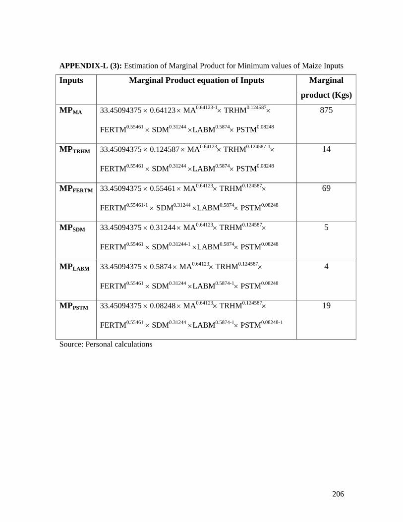
206

APPENDIX-L (3): Estimation of Marginal Product for Minimum values of Maize Inputs

Inputs Marginal Product equation of Inputs Marginal

product (Kgs)

MPMA 33.45094375 0.64123 MA0.64123-1 TRHM0.124587

FERTM0.55461 SDM0.31244 LABM0.5874 PSTM0.08248

875

MPTRHM 33.45094375 0.124587 MA0.64123 TRHM0.124587-1

FERTM0.55461 SDM0.31244 LABM0.5874 PSTM0.08248

14

MPFERTM 33.45094375 0.55461 MA0.64123 TRHM0.124587

FERTM0.55461-1 SDM0.31244 LABM0.5874 PSTM0.08248

69

MPSDM 33.45094375 0.31244 MA0.64123 TRHM0.124587

FERTM0.55461 SDM0.31244-1 LABM0.5874 PSTM0.08248

5

MPLABM 33.45094375 0.5874 MA0.64123 TRHM0.124587

FERTM0.55461 SDM0.31244 LABM0.5874-1 PSTM0.08248

4

MPPSTM 33.45094375 0.08248 MA0.64123 TRHM0.124587

FERTM0.55461 SDM0.31244 LABM0.5874-1 PSTM0.08248-1

19

Source: Personal calculations

207

Appendix-M

Marginal Rate of Substitution between Rice Inputs

Substitution between Marginal Rate of Substitution

Substitution of RA for TRHR 1.22

Substitution of RA for FERTR 6.23

Substitution of RA for SDR 7.52

Substitution of RA for LABR 98.41

Substitution of RA for PSTR 100.92

Substitution of TRHR for RA 0.82

Substitution of TRHR for FERTR 5.10

Substitution of TRHR for SDR 6.16

Substitution of TRHR for LAB 80.61

Substitution of TRHR for PST 82.68

Substitution of FERTR for RA 0.16

Substitution of FERTR for TRHR 0.20

Substitution of FERTR for SDR 1.21

Substitution of FERTR for LABR 15.80

Substitution of FERTR for PSTR 16.20

Substitution of SDR for RA 0.13

Substitution of SDR for TRHR 0.16

Substitution of SDR for FERTR 0.83

Substitution of SDR for LABR 13.08

Substitution of SDR for PSTR 13.41

Substitution of LABR for RA 0.01

Substitution of LABR for TRHR 0.01

Substitution of LABR for FERTR 0.06

Substitution of LABR for SDR 0.08

Substitution of LABR for PSTR 1.03

Substitution of PSTR for RA 0.01

Substitution of PSTR for TRHR 0.01

Substitution of PSTR for FERTR 0.06

Substitution of PSTR for SDR 0.07

Substitution of PSTR for LABR 0.98 Source: Personal calculations

208

Appendix-N

Marginal Rate of Substitution between Wheat Inputs

Substitution between Marginal Rate of Substitution

Substitution of WA for TRHW 13.34

Substitution of WA for FERTW 8.25

Substitution of WA for SDW 68.03

Substitution of WA for LABW 57.48

Substitution of WA for PSTW 11.73

Substitution of TRHW for WA 0.07

Substitution of TRHW for FERTW 0.62

Substitution of TRHW for SDW 5.10

Substitution of TRHW for LABW 4.31

Substitution of TRHW for PSTW 0.88

Substitution of FERTW for WA 0.12

Substitution of FERTW for TRHW 1.62

Substitution of FERTW for SDW 8.24

Substitution of FERTW for LABW 6.96

Substitution of FERTW for PSTW 1.42

Substitution of SDW for WA 0.01

Substitution of SDW for TRHW 0.20

Substitution of SDW for FERTW 0.12

Substitution of SDW for LABW 0.84

Substitution of SDW for PSTW 0.17

Substitution of LABW for WA 0.02

Substitution of LABW for TRHW 0.23

Substitution of LABW for FERTW 0.14

Substitution of LABW for SDW 1.18

Substitution of LABW for PSTW 0.20

Substitution of PSTW for WA 0.09

Substitution of PSTW for TRHW 1.14

Substitution of PSTW for FERTW 0.70

Substitution of PSTW for SDW 5.80

Substitution of PSTW for LABW 4.90 Source: Personal calculations

209

Appendix-O

Marginal Rate of Substitution between Maize Inputs

Substitution Between Marginal Rate of Substitution

Substitution of MA for TRHM 13.72

Substitution of MA for FERTM 2.31

Substitution of MA for SDM 27.36

Substitution of MA for LABM 25.47

Substitution of MA for PSTM 5.18

Substitution of TRHM for MA 0.06

Substitution of TRHM for FERTM 0.17

Substitution of TRHM for SDM 2.00

Substitution of TRHM for LABM 1.86

Substitution of TRHM for PSTM 0.38

Substitution of FERTM for MA 0.43

Substitution of FERTM for TRHM 5.94

Substitution of FERTM for SDM 11.83

Substitution of FERTM for LABM 11.02

Substitution of FERTM for PSTM 2.24

Substitution of SDM for MA 0.04

Substitution of SDM for TRHM 0.50

Substitution of SDM for FERTM 0.08

Substitution of SDM for LABM 0.93

Substitution of SDM for PSTM 0.19

Substitution of LABM for MA 0.04

Substitution of LABM for TRHM 0.54

Substitution of LABM for FERTM 0.09

Substitution of LABM for SDM 1.07

Substitution of LABM for PSTM 0.20

Substitution of PSTM for MA 0.19

Substitution of PSTM for TRHM 2.65

Substitution of PSTM for FERTM 0.45

Substitution of PSTM for SDM 5.28

Substitution of PSTM for LABM 4.91 Source: Personal calculations