1

July 14, 2018

Demand for sexual services in Britain: Does Sex Education Matter?

by

Marilena Locatelli1 and Steinar Strøm2

Abstract On survey data from 1999-2001 and 2010-2012 we estimate the demand for commercial sex among British

men. We estimate a zero-inflated count model, which takes into account the probability of not participating in the sex

market and number of times with a prostitute. We find that sex education in school has a negative and significant role

in the demand for paid sex. We also find that men with a typically middle-class income are more likely to buy sex.

Travelling abroad or living in London increases the likelihood of British men buying sex.

JEL classification: C35, D12 Keywords: Number of times with prostitutes, sex education, Britain.

Acknowledgements This paper uses National Survey of Sexual Attitudes and Lifestyles, 2010-2012 (Natsal-3) and 1999-2001 (Natsal-2). We are indebted to UK Data Archive, University of Essex, Colchester, to make Natsal-2 and 3 freely accessible for research purposes. All results and their interpretation presented in this paper remain the authors’ responsibility. We thank Maria Laura Di Tommaso and two anonymous referees for helpful comments and suggestions.

1 The Ragnar Frisch Centre of Economic Research and Dep. of Economics and Statistics, University of Turin, e-mail: marilena.locatelli@unito.it 2 The Ragnar Frisch Centre of Economic Research, Oslo, and the Department of Economics, University of Oslo, e-mail: steinar.strom@econ.uio.no

2

1. Introduction

The main goal of our paper is to estimate the demand for commercial sex among British men. We

estimate the impact of observed variables on demand for paid sex, based on a zero-inflated count

model estimated on British survey data from 2010-2012. One of the variables is whether the men

have learned about sex in school or not.

In Britain, prostitution is legal, but a number of related activities, including soliciting in a

public place, kerb crawling, keeping brothel, pimping and pandering, are illegal. The Policing and

Crime Act 2009 makes it illegal to pay for sex with a prostitute who has been "subjected to force"

and this is a strict liability offence. The legal age for solicitation is 18 (House of Common Home

Affairs Committee, Prostitution, Third Report of Session 2016-17). In spite of the problematic

aspects related to prostitution, its demand has increased from 1990 to 2010 (White and Johnson,

2014).

In the literature, prostitution is widely studied including topics such as violence, sex tourism,

drug abuse, HIV-risk and necessity of regulation (Gerthler and Shah, 2011, Immordino and Russo,

2015). An important branch of the empirical literature on sexual behaviour focuses on sexually

transmitted infections: Men paying for sex are considered to be a bridging population of the

diffusion of such type of diseases, since their paid partners are often individuals at high risk for

what concerns sexually transmitted infections (White et al 2014).

Of special interest for our paper are studies of the British sex market. Cameron and Collins

(2003) studies male decisions concerning whether or not to buy sex. They used data from a national

survey of sexual attitudes and lifestyles in the UK in 1990/1991. Two logit probabilities are

estimated; the probability of ever have been together with a prostitute and the probability of have

been together with a prostitute during the last 5 years. They find that important determinants for

buying sex are health risk and religious denomination. Ward et al (2005) based their analysis on the

national probability sample surveys of sexual attitudes and lifestyles (“Natsal”) of men aged 16-44

resident in Britain. Their data sets are from 1990 and 2000. They find that paying for sex is more

frequent among men aged between 25 years and 34 years, who were never married, and who lived

in London. They do not find any association with ethnicity, social class, homosexual contact, or

injecting drug use. Men who paid for sex are more likely to report 10 or more sexual partners in the

previous 5 years; only a minority of their lifetime sexual partners (19.3 per cent) were prostitutes.

They were more likely to meet prostitutes abroad. Drawing on 50 in-depth interviews Sanders

(2008) found that the typical male client in the sex market in Britain is an ordinary person searching

for intimacy with a woman. However, the sample is small and skewed towards white middle-class

men. Jones et al (2015) use the British Natsal-3 data set. They report that over the past 20 years,

3

young people refer to school lessons as their main source of information about sex. However, in

2010-2012 as much as 68.1 per cent of young men reported not knowing enough when they first

felt ready for sexual experience.

Recently there have been a few international studies concerning the impact of sex education

programme on the sexual behaviour of young people. Kirby (2011) gives a review of several

international studies assessing the effectiveness of sex education programmes in reducing risky

sexual behaviour and number of partners among adolescents and young people. Reis et al (2011)

studied the significance of sex education in schools and its effects in promoting healthy sexual

behaviour among university students in Portugal. The sample included 3278 students. The most

notable finding is that students who had sex education in school mentioned more often having had

fewer sexual risk behaviors (less occasional partners, less sex associated to alcohol and drugs, less

unwanted pregnancies and abortions). Wylie (2010) review the international experiences

concerning the impact of sex education in school on sexual behavior.

To our knowledge there have been no studies that analyse the effects of sex education in

school on the demand for paid sex. For this reason, we focus on sex education in Britain, but many

other variables are also included in explaining the behaviour of British men in the commercial sex

market. The econometric model we apply to study this phenomenon assumes that zero contacts with

prostitutes occurs in two ways: as a realization of taking part or not in the market for sexual services

and as realization of a count process, i.e. number of times with a prostitute ever in life. The model

we employ is a zero-inflated Poisson model, see Cameron and Trivedi (2005) for further details.

The most notable finding from a policy point of view is that learning about sex in school has

a significant and sizeable negative marginal effect on buying sex from a prostitute. If politicians

want to reduce prostitution in Britain our result gives support to the proposal in Britain, saying that

all schools across the system should have compulsory Sex and Relationship Education (SRE)

program.

Moreover, we find that drugs users, and men declaring that they are religious, are more

inclined to participate in the sex market. We find a strong and significant association between

buying sex and being abroad, and with living in London. Somewhat in line with Sanders (2008) we

find that men with medium and medium-high income, which indicates a middle-class background,

are more likely than other men to participate in the sex market. Masturbation seems to be a substitute

for how often men buy sex, while unprotected sex is associated with how many times sex is bought.

The paper is organised as follows. The next Section gives a brief description of Sex

education in Britain schools. Section 3 describes the econometric model. Section 4 gives details

about the data used to estimate the model. Our main data source is the British survey Natsal-3 (2010-

4

2012, but we also use data from the previous survey, Natsal-2, (1999-2001) and the pooled cross

section data of the two surveys. In Appendix A we report the results from using Natsal-2 and the

pooled data.

2. Sex education in Britain schools

Sex education programs are not yet compulsory in all British schools. Some aspects are

compulsory and some others depend on school teaching programs. The Education Act 1996 requires

that sex education should inform pupils “about sexually transmission infections and HIV and

encourage pupils to have due regard to moral considerations and family life” (Sex and Relationship

Education (SRE, 2010; networks.nhs.uk, 2011). Schools are recommended to offer, even if it is not

compulsory, the broader subject of Sex and Relationship Education (SRE) as part of Personal,

Social and Health Education (PSHE) and Citizenship. SRE should help students to learn about the

emotional, social and physical aspects of growing up, relationships, sex, human sexuality and sexual

health. It seeks to equip children and young people with the information, skills and positive values

to have safe, fulfilling relationships, to enjoy their sexuality and to take responsibility for their

sexual health and well-being.

The topics included in SRE differ from school to school. Both primary and secondary

schools must have an up-to-date policy that describes the content and organization of SRE taught

outside the Science Curriculum. Even if a school decides not to teach non-compulsory SRE

components, it must document this choice. Each school’s governing body is responsible for

developing their school’s policy and inform parents who have the right to withdraw their children

from SRE taught outside the Science Curriculum.

Table 1 shows the number of people who receive sex education lessons at school per age

group. The number of people who declare to have learned sex education at school decreases as the

age increases, but also older men have learned about sex when they went to school. Table 1 is based

on the Natsal-3 survey. Apparently, sex education in British schools varies across schools and a

considerable number of men, at all ages, declare in the survey that they did no learn about sex at

school. This can be because sex education at school has not been compulsory. On March 1, 2017,

the government tabled a proposal of amendments, saying that all schools across the system will be

bound by the same obligation3, making education of sex compulsory in all schools.

3 Proposal of amendments on sex education at school, 1 March 2017: Schools to teach 21st century relationships and

sex education, From: Department for Education and The Rt Hon Justine Greening MP. Part of: School and college qualifications and curriculum (available at: https://www.gov.uk/government/news/schools-to-teach-21st-century-relationships-and-sex-education)

5

Table 1. British men receiving sex education at school, by age group, Natsal-3, 2010-2012

Learned sex education at school Respondent's age group No Yes Total

20-24 188 629 817 25-29 223 613 836 30-34 197 417 614 35-39 146 226 372 40-44 155 244 399 45-49 172 220 392 50-54 158 189 347 55-59 186 135 321 60-64 262 101 363 65-69 255 78 333 70-74 182 57 239

Total 2124 2909 5033

In Table 2 we report sex education at school across Britain regions. Again, we observe that

according to the answers given in the survey there is a variation in Britain with respect to sex

education in schools.

Table 2. British men receiving sex education at school, by Britain regions, Natsal-3, 2010-2012

Sex education at school Region No Yes Total North East 115 142 257 North West 302 365 667 Yorkshire And The Hum 202 233 435 East Midlands 165 269 434 West Midlands 173 238 411 South West 163 261 424 East 225 333 558 London 225 277 502 South East 260 384 644 Wales 121 154 275 Scotland 173 253 426 Total 2124 2909 5033

School and college qualifications and curriculum Sex education to be compulsory in England's schools. By

Katherine Sellgren BBC News education reporter (available at: http://www.bbc.com/news/education-39116783).

The national curriculum: https://www.gov.uk/national-curriculum/other-compulsory-subjects

6

The survey data makes it also possible to estimate the probability of having had sex

education in school as a function of observed covariates. In Table 3 we show the estimate of the

probability of having had sex education in school (Probit) when our observed adult men were school

pupils. When the sons were 14 years old, we observe father’s occupation.

If the man, when he was at school, attended a school with only boys in the class, the

probability of having had sex education is lower compared to if he went to schools with both gender

in class. With respect to father’s occupation, sons of managers and administrators had higher chance

to go to schools where sex education took place than among sons of fathers with other and not so

well paid jobs.

We could have used this estimated probability or an indicator function in the estimation of

demand for sex, that is in the zero-inflated Poisson model outlined in the next section. However, we

prefer instead to use the observed Yes/No dummy.

Table 3. Estimates of the probability of having had sex education in school.

Variable Estimates t-values Constant 0.640 9.75 Attended single sex class -0.808 -10.84 Boarding School 0.066 0.49 Father’s occupation when the boy was 14 years: Farm workers -0.545 -2.70 Skilled manufacturing -0.294 -3.48 Unskilled-manufacturing -0.352 -3.99 Manager, administrator 0.210 1.99 Salesman -0.126 -0.72 Other work -0.211 -2.01

Number of observations 5033 Log likelihood -3348.715

3. The Econometric Model

We will apply a zero-inflated Poisson model, see Cameron and Trivedi (2005) for a discussion of

this and related models. Let y=0,1,2… be the number of times with a prostitute and let f1(.) be a

density that accounts for a binary process. If the binary process takes value 0, with the probability

f1(0) then y=0. If the binary process takes the value 1, with probability f1(1), then y takes the count

values 0,1,2,, from the count density f2(.).Note that f1(1) is the probability of participating in the sex

market, while f2(.) gives the density related to number of times with prostitutes. The main feature

7

of the zero-inflated Poisson model is that the zero counts occur both as a realization of the binary

process and as realization of the count process. The densities that go into the likelihood function

used in estimating the model are:

1 1 2

1 2

(3.1) ( ) (0) (1 (0;)) (0) 0(3.2) ( ) (1 (0)) ( ) 1

g y f f f if yg y f f y if y

= + − == − ≥

In STATA there are two choices with respect to type of probabilities when estimating a zero-inflated

count model: Logit or Probit. We have chosen f1(0;Xiα) to be a Probit probability and f2(y;Ziβ) to be

a Poisson density or more formally the probability mass function Pr( ) , 0,1, 2, , ,!

i iyi

i i ii

eY y yy

µ µ−

= = =

where exp( )i iZµ β= . We assume that a vector Xi of observed covariates affects the Probit

probability and vector Zi the Poisson density. The subscript i indicates male i.

In Della Guista et al. (2009a and 2009b) assume that participation in the prostitution market

is driven by three sets of variables: income and opportunities, loss of reputation, and moral

thresholds. Here, we try to specify an empirical model in accordance with that theoretical model.

Let X1i be a vector of observed variables that represent the reputation issue and moral threshold,

while X2i is a vector of other observed variables that represent income and opportunities. The two

vectors constitute the vector Xi=(X1i,X2i) in the Probit probability f1(0;Xiα).

In the vector X1i we include variables that may represent moral threshold characteristics and

variables that may be related to loss of reputation and trust if it is discovered that the man has been

together with prostitutes. If a man considers himself as religious, we take this as an indicator of high

moral. Moreover, we consider having a permanent partner, children and having grown up with both

parents as characteristics that may make it harder for the man to be together with prostitutes. Finally,

we also include whether the man has a leading position at his workplace. Our conjecture is that the

loss of reputation, if it is discovered that he has had sex with prostitutes, is higher compared to men

with no leading position where they work. We have also included sex education in school. The

justification is that this education may prepare pupils for adulthood and enable them to better take

care of themselves and future partners.

In the vector X2i we include variables like age and age squared, use of drugs, early start in

life with having sex, sex and not necessarily love and relationship, opportunities to having sex

abroad, income and living in London. Our justification for this choice of variables is that the older

a man is, the higher is the chance that he has been tempted to have sex with a prostitute. Use of

drugs, early experience with having sex, and preference for sex, but less interest in establishing a

relationship with a woman, accord with conjectures about the characteristics of men who are more

8

inclined than others to buy sex. The justification for income is that paid sex can be costly. London

is included, because it is a very big city with many opportunities in the sex market. For the same

reason we include sex abroad in this set of variables.

Zi is a vector of variables that we assume have an impact on the number of times a man has

been together with a prostitute up to the time of the survey. Age and age squared is included in the

vector and we expect that the older the man is at the time of the interview, the more prostitutes he

has been together with. Moreover, we have included whether he has used condoms when having

sex with the prostitutes. Also at this stage, we have included the preference for sex, but less interest

in establishing a relationship with a woman. Finally, we have included a variable representing

whether he performs masturbation or not; masturbation could be a complement or a substitute for

having sex with a prostitute.

The X and Z covariates could of course influence the alternative parts (hurdle and count) of

the model. The justification for our choice is based on the discussion in Della Guista et al (2009a

and b) and on our intuition. However, in the appendix we have lumped all variables together and

estimates the hurdle part of the model (a Probit model) on two waves of the British survey. To some

extent, the results give support to our main model.

To estimate the model we have to form the likelihood for the sample we observe, which consists

of N0 number of men that has never participated in the prostitution market; 0iy = , and N1 who has

participated; 1iy ≥ Below, L is this joint probability of the sample we observe.

(1) [ ]0 1

1 1 2 1 21 1

0 1 0 1 0N N

i i i i i i ii i

L f ( , X ) ( f ( , X )) f ( y ,Z ) ( f ( ,X )) f ( y ,Z )α α β α β= =

= + − −∏ ∏ ; yi=0,1,2,,,

4. Data

We use the National Surveys of Sexual Attitudes and Lifestyles (‘Natsal-2 and Natsal 3), which are

surveys undertaken during 1999-2001 and 2010–2012, respectively. The surveys are interviews of

a representative sample of men and women aged respectively 16-44 and 16-74 living in private

households in Britain.4 Data collection was carried out using computer assisted personal interview

4 Johnson, A., London School of Hygiene and Tropical Medicine. Centre for Sexual and Reproductive Health Research and Nat Cen Social Research, National Survey of Sexual Attitudes and Lifestyles, 2010-012. Colchester, Essex: UK Data Archive, September 2015. This work is the result of a collaborative team from five organisations: University College London (UCL); London School of Hygiene & Tropical Medicine (LSHTM); National Centre for Social

9

(CAPI) techniques along with computer assisted self-interview (CASI) for the more sensitive

questions.

The data provide a detailed understanding of patterns and variability of sexual behaviour in

Britain. The data explore sexual behaviour (paying for sex included) and sexual function and

satisfaction over the life-course, health conditions and problems that may affect sexual lifestyles.

We focus on men paying for sex. Selection was constrained to men only since the original

data set includes about 1 per cent cases only of women paying for sex, although there is an increase

of this demand. We also consider only heterosexual orientation since different sexual orientation is

a small percentage of the sample and consequently impossible to consider for consistent estimation.

The data, given our aim to investigate participation among men in the sex market, have

some limits. In fact, they do not give information on prices for paid sex, awareness of reputation

losses, amount of freely exchanged sex and other specific personal characteristics.

We use Natsal-3 (2010–2012) in estimating the zero-inflated model outlined above.

However, we also use Natsal-2 (1999-2001) and pooled cross sections to estimate the participation

in the commercial sex market. The reason for doing this is to check whether the result we obtained

for the non-participation of the zero-inflated model estimated on data from Natsal-3 are in

accordance with estimate from a an earlier data set and with a bigger data set, covering the two

periods 1991-2001 and 2010-2012.

From the original data set Natsal-3, including 15162 men, we selected age 20-74 since for

our purpose age 16-20 includes few cases that do not seem important in the market of paid sex. Due

to the selection of age and to a quite number of missing value, data reduces to 5033 observations:

604 Men Paying for Sex (MPS)5 and 4429 Men Not Paying for Sex (MNPS).

The reported proportion of MPS is 12 per cent of our sample (in line with Jones K.B. et al., 2015).

Considering MPS across regions, we note that London and the regions of North and South

West have higher percentage of men buying sex (see Table 4).

Table 4. Descriptive statistics of men who paid for sex in Britain regions, aged 20-74

Region Mean Std. Dev. Total Freq. North East 0.089 0.286 257 North West (incl.old Mersey region) 0.132 0.339 667 Yorkshire And The Humber 0.108 0.311 435

Research (NatCen); Public Health England (PHE) (formerly the Health Protection Agency); University of Manchester. SN: 7799, http://dx.doi.org/10.5255/UKDA-SN-7799- 5 We define as MPS a man who declares to have paid for sex at least once. MNPS otherwise. From here on we will use the abbreviations MPS and MNPS

10

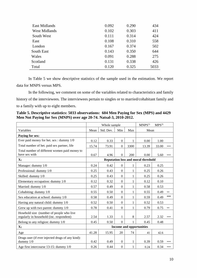
East Midlands 0.092 0.290 434 West Midlands 0.102 0.303 411 South West 0.111 0.314 424 East 0.108 0.310 558 London 0.167 0.374 502 South East 0.143 0.350 644 Wales 0.091 0.288 275 Scotland 0.131 0.338 426 Total 0.120 0.325 5033

In Table 5 we show descriptive statistics of the sample used in the estimation. We report

data for MNPS versus MPS.

In the following, we comment on some of the variables related to characteristics and family

history of the interviewees. The interviewees pertain to singles or to married/cohabitant family and

to a family with up to eight members.

Table 5. Descriptive statistics: 5033 observations: 604 Men Paying for Sex (MPS) and 4429 Men Not Paying for Sex (MNPS) over age 20-74. Natsal-3, 2010-2012. Whole sample MNPS1) MPS2)

Variables Mean Std. Dev. Min Max Mean

Paying for sex:

Ever paid money for het. sex : dummy 1/0 0.12 0.33 0 1 0.00 1.00

Total number of het. paid sex partner, life 15.74 73.91 0 3300 13.39 33.00 *** Total number of different women paid money to have sex with 0.67 4.96 0 200 0.00 5.60 ***

X1 Reputation loss and moral threshold

Manager: dummy 1/0 0.24 0.42 0 1 0.23 0.25

Professional: dummy 1/0 0.25 0.43 0 1 0.25 0.26

Skilled: dummy 1/0 0.25 0.43 0 1 0.25 0.26

Elementary occupation: dummy 1/0 0.12 0.32 0 1 0.12 0.10

Married: dummy 1/0 0.57 0.49 0 1 0.58 0.53

Cohabiting: dummy 1/0 0.55 0.50 0 1 0.55 0.49 **

Sex education at school: dummy 1/0 0.58 0.49 0 1 0.59 0.49 ***

Having any natural child: dummy 1/0 0.52 0.50 0 1 0.52 0.53

Grew up with two parent: dummy 1/0 0.78 0.41 0 1 0.79 0.75 **

Hosehold size (number of people who live regularly in household (inc. respondent) 2.54 1.33 1 8 2.57 2.32 ***

Belong to any religion: dummy 1/0 0.45 0.50 0 1 0.45 0.48

X2 Income and opportunities

Age 41.28 15.95 20 74 41 42.6

Drugs user (if ever injected drugs of any kind): dummy 1/0 0.42 0.49 0 1 0.39 0.59 ***

Age first intercourse 13-15: dummy 1/0 0.26 0.44 0 1 0.24 0.34 ***

11

Sex abroad (if any new paid sex partner while outside UK, last five years): dummy 1/0 0.10 0.30 0 1 0.08 0.26 ***

Household income (£ ) (inc benefits, pensions etc.) pre tax per year:

Income <2,500: dummy 1/0 0.03 0.16 0 1 0.03 0.02

Income 2,500-4.999: dummy 1/0 0.04 0.19 0 1 0.04 0.04

Income 5,000-9,999: dummy 1/0 0.07 0.25 0 1 0.07 0.08

Income 10,000-19,999: dummy 1/0 0.15 0.36 0 1 0.15 0.13

Income 20,000-29,999: dummy 1/0 0.15 0.36 0 1 0.15 0.15

Income 30,000-39,999: dummy 1/0 0.13 0.34 0 1 0.13 0.14

Income40,000-49,999: dummy 1/0 0.10 0.30 0 1 0.10 0.14 ***

Income >=50,000: dummy 1/0 0.20 0.40 0 1 0.20 0.20

Leaving in Great London: dummy 1/0 0.10 0.30 0 1 0.09 0.14 ***

Employee: dummy 1/0 0.77 0.42 0 1 0.77 0.14

Self-employed: dummy 1/0 0.14 0.35 0 1 0.78 0.16

Having sex without love: dummy 1/0 0.64 0.48 0 1 0.62 0.77 ***

Ever masturbed: dummy 1/0 0.95 0.22 0 1 0.94 0.99 ***

Unsafe sex: dummy 1/0 0.07 0.25 0 1 0.06 0.10 ***

Greatly HIV/AIDS risk: dummy 1/0 0.27 0.44 0 1 0.25 0.35 *** 1) MPS (Men Paying for Sex), 2) MNPS (Men Not Paying for Sex)

For dummyi the statistics are computed as: column MNPS: (frequency if dummyi =1)/(total of MNPS); column MPS: (frequency if dummyi =1)/(total of MPS)

Heterosexual behaviour strongly differs between MPS and MNPS: Men who paid for sex

have on average 33 sexual partners compared to 13.4 partners for men not paying. Concerning the

working status, we note that there more managers, professionals, and skilled workers paying for sex

among MPS than among MNPS. This is not the case for elementary occupation.

Learning about sex is an important aspect of sex behaviour: 59 per cent of MNPS learnt

about sex from lessons at school compared to 49 per cent of MPS. Only 5 per cent has an easy

parent-child relationship and mostly from mothers. Around 26 per cent of the interviewees learns

mostly about sex from friends of about same age. Only 2 per cent learns from pornographic sources.

Data does not say if sex education is taught at schools within areas where there are social problems.

It would be interesting to know if sex education made them more conscious of their behaviour, or

implied risk aversion, or has changed some other personal perceptions. However, this we do not

observe.

About 78 per cent of the respondents declare they lived more or less continuously until age

14 with both natural parents, and the mean differs between MNPS and MPS, 79 per cent and 75 per

cent, respectively. It is more frequent to observe MPS in small families than in large families.

Another interesting aspect is about religion: 45 per cent of interviewed declared they belong to a

religion. Analysing age we observe that demand for paid sex is highest in the group 40-44, while it

12

is lower in the group of young 20-34, and after the age of 65 (Table 5). MNPS tend to be younger

than MPS: 41 and 42.6, respectively.

Table 6. Descriptive statistics of MPS at different age group. Fractions.

Man's age at interview, years, grouped Mean Std. Dev. Group Freq. 20-24 0.06 0.242 817 25-29 0.13 0.338 836 30-34 0.13 0.339 614 35-39 0.11 0.310 372 40-44 0.16 0.365 399 45-49 0.15 0.358 392 50-54 0.14 0.346 347 55-59 0.15 0.354 321 60-64 0.15 0.354 363 65-69 0.09 0.287 333 70-74 0.09 0.290 239 Total 0.12 0.325 5033

There is a considerable difference in the drug use: MPS 59 per cent, while MNPS 39 per cent.

Considering the age of first heterosexual intercourse (13-15) we observe that among MNPS it is 24

per cent and 34 per cent for the MPS. Paying for sex remains strongly associated with foreign

partners outside the UK and being in London.

5. Estimates and marginal effects: The zero-inflated count model estimated on British

data from the Natsal-3 survey, 2010-2012.

In Table 7 we report the results of the zero-inflated Poisson count model. The first set of coefficients

is related to variables in the Probit probability of being in the “Always Zero“ group, i.e. those who

never had sex with prostitutes. The second part relates to the variables in the count part of the model.

Table 8 reports the marginal effects of observed variables on the unconditional expectation of

number of times with prostitutes. The unconditional expectation relates to the zero-inflated as well

as the count part of the model.

13

Table 7. Estimate of the zero-inflated Poisson regression (probability of not participating in the sex market and count of the number of time with a prostitute). British men aged 20-74. 2010-2012.

Estimates Robust

Std. Err. t-values Inflate part, Probit probability of not having sex with prostitutes

X1: Reputation loss and moral threshold Constant 3.2690 0.3072 10.64 Manager: dummy 1/0 -0.0108 0.0862 -0.12 Professional: dummy 1/0 -0.0366 0.0819 -0.45 Skilled: dummy 1/0 -0.0200 0.0811 -0.25 Married: dummy 1/0 0.0751 0.0608 1.24 Sex education at school: dummy 1/0 0.2141 0.0537 3.99 Having any natural child: dummy 1/0 0.0006 0.0610 0.01 Grew up with two parent: dummy 1/0 0.1114 0.0609 1.83 Household size 0.0306 0.0238 1.29 Belong to any religion: dummy 1/0 -0.1632 0.0515 -3.17

X2: Income and opportunities Age/10 -0.6870 0.1248 -5.51 Age/10 square 0.0640 0.0134 4.77 Drugs user (if ever injected drugs of any kind): dummy 1/0 -0.4593 0.0563 -8.16 Age first intercourse 13-15: dummy 1/0 -0.1559 0.0558 -2.79 Sex without love -0.2236 0.0615 -3.64 Sex abroad (if any new paid sex partner while outside UK, last five years): dummy 1/0 -0.8813 0.0715 -12.33 Household income (£ ) (inc benefits, pensions etc.) pre tax per year: Income 2,500-4.999: dummy 1/0 -0.0660 0.1449 -0.46 Income 5,000-9,999: dummy 1/0 -0.1884 0.1169 -1.61 Income 10,000-19,999: dummy 1/0 -0.1286 0.0972 -1.32 Income 20,000-29,999: dummy 1/0 -0.1221 0.0947 -1.29 Income 30,000-39,999: dummy 1/0 -0.2552 0.0996 -2.56 Income40,000-49,999: dummy 1/0 -0.3670 0.1015 -3.61 Income >=50,000: dummy 1/0 -0.0945 0.0961 -0.98 Leaving in Great London: dummy 1/0 -0.2204 0.0793 -2.78 Employee -0.0156 0.1091 -0.14 Self-employed -0.0033 0.1281 -0.03 Count part: A Poisson density Constant -0.2656 0.8930 -0.30 Age/10 0.9928 0.3272 3.03 Age/10 squared -0.0784 0.0372 -2.11 Ever masturbed: dummy 1/0 -1.3743 0.5324 -2.58 Unsafe sex: dummy 1/0 0.3538 0.2671 1.32

14

Having sex without love 0.6774 0.2232 3.04

Number of obs. : 5033; Zero obs.: 597; Non zero obs. 4436 Wald chi2(5) 39.48 Prob > chi2 0.00 Log likelihood -5164.193

We start with commenting on the estimates of the probability of not having sex with a

prostitute (the zero-inflate part of the model) and the count part. However, the most interesting

results are the marginal effects on the unconditional expectation of number of times with a

prostitute, including zero. That we will discuss below.

The estimates of coefficients related to the “threshold” variables, the X1i vector, meets our a

priori expectations, with two exceptions. First, the coefficients attached to the professional status,

represented by the four dummies described in Section 3 (the reference case is elementary occupation

and unemployed) are not significant and they all have a negative sign. That is contrary to our

expectation, since men with a professional status may have more to lose; if it becomes known that

they have had sex with a prostitute. Second, belonging to a religion has a significant and negative

effect on the probability of not having sex with a prostitute. Again, this result is contrary to our

expectation. It should be noted that the variable religion includes a variety of beliefs and the dummy

variable is based on the answers the respondent give in the survey. To our knowledge there are no

other similar comprehensive study of sex clients in which participation and number of times with

prostitutes are jointly estimated.

The coefficients related to the working status; employee and self-employed have the

expected negative sign, but they are not significant.

Marriage may prevent individuals for having sex with prostitutes. As expected, the estimate

of the coefficient is positive, but it is not significant.

Sex education at school; the coefficient is positive and significant.

The sign of the coefficient related to have any child is positive but not significant. We got

the same results if we replaced it with the number of children.

Living until age of 16 in traditional families with the presence of both parents has a positive

impact on non-participation in the sex market, but the coefficient is not completely significant. We

get the same result for using the size of the household; the coefficient is positive, but not significant.

15

Turning to the estimates of the coefficients attached to the variables in the X2i vector we

observe from Table 8 that as the age increases up to the age of around 54, there is a decrease in the

probability of not having participated in the sex market.

Drug abusers are represented by the dummy drug use, which equals 1 if ever injected any

kind of drugs and equal 0 otherwise. Drug abuse is widespread and abusers have a stronger

inclination to have sex with a prostitute; the coefficient related to not buying sex is negative and

highly significant.

The variable age at first heterosexual intercourse is represented by a dummy, which is equal

to 1 if the individual had a sexual intercourse between the age of 13 and 15, and equal to 0 if older.

The coefficient is negative and significant, confirming that those who started early with having sex

are also more likely to enter the commercial sex market as an adult.

The coefficients attached to being abroad last 5 years and living in London, are negative and

significant. To be abroad or living in London may give more opportunities to find prostitutes and

less possibilities to be observed being with a prostitute6. The latter means that this variable could

also belong to the X1-vector.

The coefficient attached to men asking for sex without love, i.e. without any obligation or

sentimental value, is negative and significant. Thus, these men are more inclined to buy sex.

Men with a high income, given the professional status, may be more vulnerable socially if

observed with prostitutes. However, to buy sex could be expensive and hence higher income may

have a positive impact on participation in the sex market, in particular if sex takes place indoor in

hotels and apartments. Our estimates partly confirm that latter expectation and show that only for

those with an income around 30,000-50,000 pounds per year the coefficients are negative and

significant. Men with these incomes are typically middle-class men.

In the estimate of the expected number of times with a prostitute, age is significant and

implies that the expected number of times with a prostitute, given participation in the sex market,

increases up to the age 61-62.

The estimates show that masturbation (ever or not) has a negative and significant impact

(given participation), which indicates that masturbation is a substitute for having sex with a

prostitute. Like in the participation probability, the impact of sex without love on the expected

number of times with a prostitute is positive and significant. A worrying result is that the expected

6 Third Report of Session 2016–17 on Prostitution of House of Commons, Home Affairs Committee reports: “Among men ever having paid for sex, 62.6% reported paying for sex outside the UK, most often in Europe and Asia”.

16

number of times with a prostitute is higher among those who are not using condoms than among

those who do.

Table 8 gives the marginal effects of the observed variables on the unconditional expectation

of times with prostitutes in the zero-inflated count model, that is (using one variables as an example)

( | , )(3.3) i i i

ij

E Y X ZX

∂∂

,

Table 8. Marginal effects of variables in the inflated zero-count model on the unconditional expectation of number of times with a prostitutes; E(Yi|Xi,Zi)

Marginal effect Manager: dummy 1/0 0.0080 Professional: dummy 1/0 0.0271 Skilled: dummy 1/0 0.0148 Married: dummy 1/0 -0.0557 Sex education at school: dummy 1/0 -0.1587 *** Having any natural child: dummy 1/0 -0.0004 Grew up with two parent: dummy 1/0 -0.0826 * Household size (number of people who live regularly in the household) -0.0227 Belong to any religion: dummy 1/0 0.1210 *** Drugs user (if ever injected drugs of any kind): dummy 1/0 0.3405 *** Age first intercourse 13-15: dummy 1/0 0.1155 *** Sex abroad (if any new paid sex partner while outside UK, last five years): dummy 1/0 0.6533 *** Household income (£ ) (inc benefits, pensions etc.) pre tax per year: Income 2,500-4.999: dummy 1/0 0.0489 Income 5,000-9,999: dummy 1/0 0.1396 Income 10,000-19,999: dummy 1/0 0.0953 Income 20,000-29,999: dummy 1/0 0.0905 Income 30,000-39,999: dummy 1/0 0.1891 *** Income40,000-49,999: dummy 1/0 0.2720 *** Income >=50,000: dummy 1/0 0.0701 Leaving in Great London: dummy 1/0 0.1634 *** Employee 0.0116 Self-employed 0.0024 Age/10 0.9275 *** Age/10 squared -0.0805 *** Having sex without love: dummy 1/0 -0.5789 ** Ever masturbated: dummy 1/0 0.1747 Unsafe sex: dummy 1/0 0.4076 *** *** p<0..01, ** p<0.05, * p<0.1

We observe that there are several large and clearly significant marginal effects. First, we observe

that the expected number of times with the prostitute increases with the age up to around 55.

17

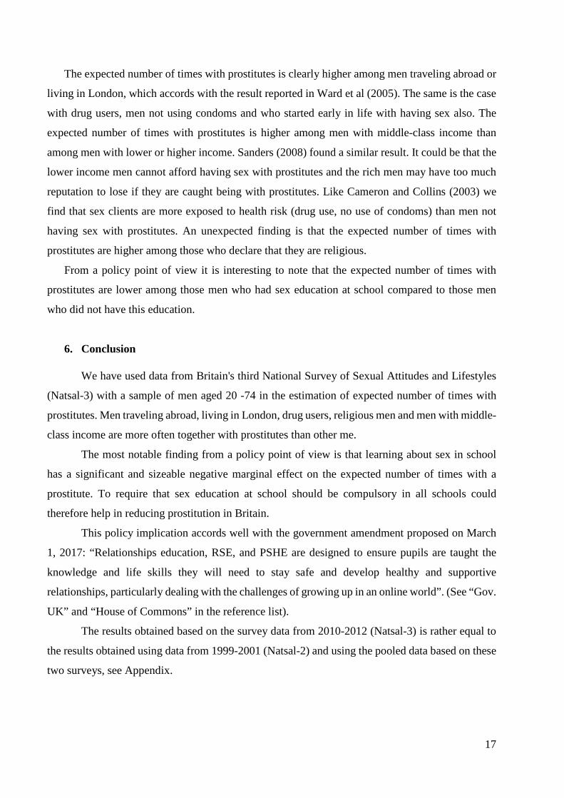
The expected number of times with prostitutes is clearly higher among men traveling abroad or

living in London, which accords with the result reported in Ward et al (2005). The same is the case

with drug users, men not using condoms and who started early in life with having sex also. The

expected number of times with prostitutes is higher among men with middle-class income than

among men with lower or higher income. Sanders (2008) found a similar result. It could be that the

lower income men cannot afford having sex with prostitutes and the rich men may have too much

reputation to lose if they are caught being with prostitutes. Like Cameron and Collins (2003) we

find that sex clients are more exposed to health risk (drug use, no use of condoms) than men not

having sex with prostitutes. An unexpected finding is that the expected number of times with

prostitutes are higher among those who declare that they are religious.

From a policy point of view it is interesting to note that the expected number of times with

prostitutes are lower among those men who had sex education at school compared to those men

who did not have this education.

6. Conclusion

We have used data from Britain's third National Survey of Sexual Attitudes and Lifestyles

(Natsal-3) with a sample of men aged 20 -74 in the estimation of expected number of times with

prostitutes. Men traveling abroad, living in London, drug users, religious men and men with middle-

class income are more often together with prostitutes than other me.

The most notable finding from a policy point of view is that learning about sex in school

has a significant and sizeable negative marginal effect on the expected number of times with a

prostitute. To require that sex education at school should be compulsory in all schools could

therefore help in reducing prostitution in Britain.

This policy implication accords well with the government amendment proposed on March

1, 2017: “Relationships education, RSE, and PSHE are designed to ensure pupils are taught the

knowledge and life skills they will need to stay safe and develop healthy and supportive

relationships, particularly dealing with the challenges of growing up in an online world”. (See “Gov.

UK” and “House of Commons” in the reference list).

The results obtained based on the survey data from 2010-2012 (Natsal-3) is rather equal to

the results obtained using data from 1999-2001 (Natsal-2) and using the pooled data based on these

two surveys, see Appendix.

18

Funding: This study was funded by The Ragnar Frisch Centre of Economic Research, Oslo, Norway and by Small Research Grants from Department of Economics, University of Oslo. Conflict of Interest: Steinar Strøm has received research grants from The Ragnar Frisch Centre of Economic Research, Oslo, Norway. Marilena Locatelli has received research grants from The Ragnar Frisch Centre of Economic Research, Oslo, Norway. The authors declare that they have no conflict of interest.

References Cameron, S. and Collins, A., (2003). ‘Estimates of a model of male participation in the market for

female heterosexual prostitution services, Eur. J. LawEcon, 16, 271–288. Cameron, A.C. and Trivedi, P.K. (2005). Microeconometrics. Methods and Application.

Cambridge University Press, New York. Della Giusta, M., Di Tommaso, M.L., and Strøm, S., (2009a). ‘Who is Watching? The market for

prostitution services’, Journal of Population Economics, 22 (2): 501-516.

Della Giusta, M., Di Tommaso, M.L., Shima, I., and Strøm, S., (2009b). ‘What money buys: clients of street sex workers in the US’, Applied Economics, 41 (18): 2261-2278.

Gerthler. P., and Shah, M., (2011). ‘Sex work and infection: what’s law enforcement got to do with it?, Law Economics, 54: 811-840.

Gov.UK, “Schools to teach 21st century relationships and sex education”, From: Department for Education and The Rt Hon Justine Greening MP. Part of: School and college qualifications and curriculum (available at: https://www.gov.uk/government/news/schools-to-teach-21st-century-relationships-and-sex-education)

Jones, K.G., Johnson, A.M., Wellings, K., Sonnenberg, P., Field, N., Tanton, C., Erens, B., Clifton, S., Datta, J., Mitchell, K.R., Prah, P., and Mercer, C.H., (2015). ‘The prevalence of, and factors associated with, paying for sex among men resident in Britain: findings from the third National Survey of Sexual Attitudes and Lifestyles (Natsal-3)’, Sex Transm Infect, 91:116-123. doi:10.1136/sextrans-2014-051683

House of Common Home Affairs Committee, Prostitution, Third Report of Session 2016-17, available at (https://publications.parliament.uk/pa/cm201617/cmselect/cmhaff/26/26.pdf)

Immordino G., Russo, F.F., (2015). ‘Regulating prostitution: A health risk approach’, Journal of Public Economics, 121:14–31

Kirby, D. (2011). ‘The Impact of Sex Education on the Sexual Behavior of Young People’, United Nation, New York

National Survey of Sexual Attitudes and Lifestyles (‘Natsal-3’), 2010-2012. (available at http://natsal.ac.uk/natsal-3.aspx)

networks.nhs.uk. (2011). ‘Sex Education in the UK’, (available at: https://www.networks.nhs.uk/nhs-networks/sexual-rehabilitation-after-cancer/resources-1/sexuality-in-young-people-facing-chronic-or-life-threatening-illness/Sex%20Education%20in%20the%20UK.docx/file_popview)

19

Reis, M., Ramiro, L., Matos M.G and Diniz, J.A. (2011), ‘The Effects of Sex Education in Promoting Sexual and Reproductive Health in Portuguese University Students’, Social and Behavioral Sciences, 29: 477-485.

Report: Sex and Relationship Education (SRE) - Views from teachers, parents and governors, (2010). (available at http://www.nga.org.uk/uploadfiles/SRE%20Education%20Views%20from%20teachers%20parents%20and%20governors.pdf )

Sanders, T., (2008). ‘Paying for Pleasure: Men who buy sex’, Willan, Cullompton. Ward, H., C.H., Mercer, K.,Wellings, K., Fenton, B., Erens, A., Copas, and A.M., Johnson, (2005).

‘Who pays for sex? An analysis of the increasing prevalence of female commercial sex contacts among men in Britain’, Sex Transm Infect, 81(6): 467–471. doi: 10.1136/sti.2005.014985

White, J., Johonson, A., (2014). ‘The National Surveys of Sexual Attitudes and Lifestyles (Natsal)-Implications for sexual health policy’,Third Joint Conference of the British HIV Association (BHIVA) with the British Association for Sexual Health and HIV (BASHH), (available at http://www.bhiva.org/documents/Conferences/2014Liverpool/Presentations/140403/AnneJohnson.pdf)

Wikipedia, Prostitution in Europe, (available at http://en.wikipedia.org/wiki/Prostitution_in_Europe)

Wylie, K. (2010). ‘Sex Education and the Influence on Sexual Wellbeing’, Social and Behavioral Sciences, 5: 440-444.

Appendix. Estimation of the probabilities of buying sex, Britain 1999-2001, 2010-2012 and pooled data.

In order to use more information about the demand for paid sex we pooled the two last

available National Survey of Sexual Attitudes and Lifestyles (Natsal-2 and Natsal-3).

The two original data sets have some differences: Natsal-2 refers to age 16-44 while Natsal-

3 refers to age 16-74. Furthermore, Natsal-2 does not report any information about income, while

Natsal-3 does. Some of the entries in the questionnaire are not similar in the two surveys. To get

the pooled cross section we had to make some variables homogeneous, and we use education level

as a proxy of income. We also had to limit our analysis to men aged 20-44. The pooled cross section

give us also the opportunity to observe a larger number of men who paid for having sex (i.e. 849).

20

Table A.1 Summary Statistics of Natsal-2 (wave 1999-2001), Natsal-3 (wave 2010-2012) and the pooled data.

Variables Mean Std. Dev.

Min

Max Mean Std. Dev.

Min

Max Mean Std. Dev.

Min

Max

Paying for sex:Ever paid money for het. sex : dummy 1/0 0,116 0,320 0 1 0,117 0,322 0 1 0,115 0,319 0 1Total number. of het. paid sex partner, life 14,133 32,518 0 1000 14,624 37,337 0 1000 13,447 24,236 0 400Total number of different women paid money to have sex with 0,442 2,971 0 150 0,434 3,095 0 150 0,453 2,790 0 100X1Manager: dummy 1/0 0,288 0,453 0 1 0,305 0,460 0 1 0,265 0,441 0 1Professional: dummy 1/0 0,094 0,292 0 1 0,082 0,274 0 1 0,111 0,314 0 1Administrative: dummy 1/0 0,136 0,343 0 1 0,131 0,337 0 1 0,144 0,351 0 1Skilled: dummy 1/0 0,266 0,442 0 1 0,270 0,444 0 1 0,260 0,439 0 1Elementary occupation: dummy 1/0 0,163 0,369 0 1 0,169 0,375 0 1 0,154 0,361 0 1Married: dummy 1/0 0,511 0,500 0 1 0,531 0,499 0 1 0,482 0,500 0 1Sex education at school: dummy 1/0 0,229 0,420 0 1 0,191 0,393 0 1 0,282 0,450 0 1Having any natural child: dummy 1/0 0,428 0,495 0 1 0,464 0,499 0 1 0,378 0,485 0 1Grew up with two parent: dummy 1/0 0,772 0,420 0 1 0,802 0,399 0 1 0,730 0,444 0 1Hosehold size (number of people who live regularly in household (inc. respondent) 2,819 1,428 1 12 2,827 1,459 1 12 2,807 1,385 1 8Belong to any religion: dummy 1/0 0,409 0,492 0 1 0,430 0,495 0 1 0,379 0,485 0 1X2Age 31,380 6,986 20 44 32,515 6,828 20 44 29,797 6,897 20 44Non-smoker: dummy 1/0 0,629 0,483 0 1 0,608 0,488 0 1 0,658 0,474 0 1Light smoker: dummy 1/0 0,215 0,411 0 1 0,201 0,400 0 1 0,235 0,424 0 1Heavy smoker: dummy 1/0 0,155 0,362 0 1 0,190 0,392 0 1 0,107 0,309 0 1

High alcoholic consumption: dummy 1/0 0,051 0,221 0 1 0,028 0,166 0 1 0,083 0,276 0 1Drugs user (if ever injected drugs of any kind): dummy 1/0 0,017 0,128 0 1 0,012 0,111 0 1 0,023 0,149 0 1Age first intercourse 13-15: dummy 1/0 0,271 0,445 0 1 0,258 0,438 0 1 0,290 0,454 0 1Sex abroad (if any new paid sex partner while outside UK, last five years): dummy 1/0 0,154 0,361 0 1 0,161 0,368 0 1 0,144 0,351 0 1Degree level qualification: dummy 1/0 0,283 0,451 0 1 0,270 0,444 0 1 0,301 0,459 0 1A-levels: dummy 1/1 0,166 0,372 0 1 0,145 0,352 0 1 0,197 0,398 0 1O-level: dummy 1/2 0,418 0,493 0 1 0,430 0,495 0 1 0,401 0,490 0 1None 0,132 0,339 0 1 0,155 0,362 0 1 0,100 0,300 0 1Leaving in Great London: dummy 1/0 0,203 0,403 0 1 0,270 0,444 0 1 0,111 0,314 0 1Ever masturbed: dummy 1/0 0,945 0,229 0 1 0,936 0,245 0 1 0,957 0,203 0 1Unsafe sex: dummy 1/0 0,069 0,253 0 1 0,068 0,252 0 1 0,069 0,254 0 1Greatly HIV/AIDS risk: dummy 1/0 0,047 0,212 0 1 0,049 0,216 0 1 0,044 0,206 0 1Wave2010: dummy 1/0 0,418 0,493 0 1

Number of observations 7295 4249 3046

wave 1999-2001 wave 2010-2012Pooled cross section

Reputation loss and moral threshold

Education and opportunities

21

In the following Table A.2 we report the estimate of the probability of participation in the

sex market and the marginal effects of the pooled cross section and, separately, for the two

surveys. Notice that here we estimate the probability of participation, while in the main text above

the zero-inflate part of the model was the probability of not participating.

22

Table A.2. Probability of British men participating in the sex market. Pooled cross section data, wave 1999-2001, and wave 2010-2012, age 20-44

Variables Estimates t Marginal effect

Estimates t Marginal effect

Estimates t Marginal effect

Constant -5.196 -10.120 -4.708 -6.940 -5.85 -7.21

X1

Manager -0.013 -0.210 -0.002 -0.121 -1.450 -0.020 0.14 1.32 0.023Professional -0.125 -1.340 -0.020 -0.168 -1.350 -0.026 -0.04 -0.26 -0.006Administrative 0.067 0.930 0.012 0.044 0.470 0.008 0.10 0.89 0.017Skilled -0.003 -0.040 0.000 -0.100 -1.260 -0.017 0.13 1.33 0.022Married -0.070 -1.440 -0.012 -0.050 -0.790 -0.009 -0.09 -1.16 -0.014Sex education at school -0.200 -3.720 -0.031 -0.203 -2.690 -0.032 -0.20 -2.61 -0.031Having any child -0.142 -2.760 -0.024 -0.239 -3.490 -0.041 -0.03 -0.40 -0.005Grew up with two parents -0.078 -1.600 -0.013 -0.038 -0.570 -0.007 -0.11 -1.57 -0.019Belong to a religion 0.142 3.370 0.024 0.122 2.240 0.021 0.17 2.52 0.028X2

Age/10 1.654 5.280 0.278 1.392 3.360 0.239 2.03 4.11 0.323(Age/10) squared -0.201 -4.220 -0.034 -0.159 -2.530 -0.027 -0.26 -3.45 -0.042Heavy smoker 0.140 2.530 0.025 0.120 1.760 0.022 0.20 2.01 0.034High alcohol use 0.230 2.780 0.044 0.202 1.430 0.039 0.25 2.42 0.046Drug injection 0.557 4.240 0.129 0.515 2.530 0.119 0.55 3.15 0.121Age first intercourse 13_15 0.208 4.500 0.037 0.218 3.580 0.040 0.18 2.56 0.031Sex abroad 0.747 14.800 0.171 0.632 9.680 0.140 0.92 11.35 0.216Degree 0.008 0.100 0.001 0.156 1.520 0.028 -0.26 -2.02 -0.039A-level 0.145 1.800 0.026 0.275 2.650 0.053 -0.08 -0.62 -0.012O-level 0.077 1.160 0.013 0.158 1.870 0.027 -0.10 -0.87 -0.015Unsafe sex 0.233 3.260 0.045 0.343 3.760 0.071 0.06 0.55 0.011Masturbation 0.556 4.630 0.067 0.446 3.210 0.059 0.85 3.38 0.078Living in London 0.281 5.530 0.053 0.288 4.790 0.054 0.23 2.35 0.042Wave_2010-2012 (dummy) 0.130 2.920 0.022

Number of observationsLR chi2(22) Prob > chi2 Pseudo R2 Log Likelihood -2345.258

wave 2010-2012

299.700.00

0.098-1385.386

3046276.00

0.000.1273

-946.30819

Reputation loss and moral threshold

Income and opportunities

Reputation loss and moral threshold

Income and opportunities

wave 1999-2001

542.690.00

0.104

Pooled cross section

4249

Reputation loss and moral threshold

Income and opportunities

7295

Estimates confirm that the probability of demand for paid sex increased from 2000 to 2010.

Estimates also (mostly) confirm results found in the analysis reported in Table 7 above for men

aged 20-74 in Natsal-3. In particular, having had sex education in school has a negative and

significant impact on buying sex both in pooled cross sections and in each wave. In the expanded

set of covariates we observe that men with a risky life-profile (sex without condoms, use of drugs,

23

heavy smoking and high consumption of alcohol) are more inclined to buy sexual services from

prostitutes than other men.