A reinforcement learning ticket-based probing path discovery scheme for MANETs
Upload
khangminh22Category
view
4download
0
Noname manuscript No.(will be inserted by the editor)
Deep Reinforcement Learning for Quadrotor PathFollowing with Adaptive Velocity
Bartomeu Rubı · Bernardo Morcego ·Ramon Perez
Received: date / Accepted: date
Abstract This paper proposes a solution for the path following problem of aquadrotor vehicle based on deep reinforcement learning theory. Three differentapproaches implementing the Deep Deterministic Policy Gradient algorithm arepresented. Each approach emerges as an improved version of the preceding one.The first approach uses only instantaneous information of the path for solvingthe problem. The second approach includes a structure that allows the agent toanticipate to the curves. The third agent is capable to compute the optimal velocityaccording to the path’s shape.
A training framework that combines the tensorflow-python environment withGazebo-ROS using the RotorS simulator is built. The three agents are tested inRotorS and experimentally with the Asctec Hummingbird quadrotor. Experimen-tal results prove the validity of the agents, which are able to achieve a generalizedsolution for the path following problem.
Keywords Unmanned Aerial Vehicles · Trajectory Control · Path Following ·Deep Reinforcement Learning · Deep Deterministic Policy Gradient · Quadrotor
1 Introduction
It is well known that unmanned aerial vehicles (UAV) are prepared to undertake alarge number of applications in the upcoming future (e.g. transportation, surveil-
This work has been partially funded by the Spanish State Research Agency (AEI) and theEuropean Regional Development Fund (ERDF) through the SCAV project (ref. MINECODPI2017-88403-R), and by SMART project (ref. EFA 153/16 Interreg Cooperation ProgramPOCTEFA 2014-2020). Bartomeu Rubı is also supported by the Secretaria d’Universitats iRecerca de la Generalitat de Catalunya, the European Social Fund (ESF) and AGAUR undera FI grant (ref. 2017FI B 00212)
Bartomeu Rubı, Bernardo Morcego and Ramon PerezResearch Center for Supervision, Safety and Automatic Control (CS2AC), UniversitatPolitecnica de Catalunya (UPC). Rbla Sant Nebridi 22, Terrassa (Spain).Tel.: +34-937398973E-mail: [email protected], [email protected], [email protected].

2 Bartomeu Rubı et al.
lance, mapping, exploration, search & rescue, maintenance, filming). It is for thisreason that the research on these vehicles is constantly growing and keeps devel-oping and implementing the most innovative solutions of control theory, computervision and artificial intelligence. To accomplish the final applications, the researchon UAVs tackles several different problems which derive in diverse research fields,such as the stabilization control, trajectory control, obstacle detection and avoid-ance, path planning, mission control, fault tolerant control, formation control andmany more.
In the last few years the authors of this paper focused their effort on the pathfollowing problem, studying and developing the latest techniques to solve thisproblem. Path following (PF) is a control approach to solve the trajectory controlproblem that removes the time dependence from the problem resulting in manyadvantages over the standard trajectory tracking approach [1][2]. In [3] a surveyof quadrotor path following algorithms is presented. Several control-oriented andgeometric algorithms are reviewed and compared. The most prominent are im-plemented in a realistic quadrotor model. Conclusions reveal that, in spite of itsslightly worse performance in comparison with the control-oriented algorithms,geometrical algorithms are easier to implement, require less state information andresult in a lower computational and control effort. Therefore, they become a wisesolution for the PF problem. Nevertheless, the main problem of geometric PF algo-rithms is that tuning their control parameters, which define their performance andstability, depends on factors such as the velocity of the vehicle and the path’s shape[4][5]. Thus, those parameters need to be retuned when experimental conditionschange.
Machine learning is an interesting research field to address the mentioned prob-lem of geometric algorithms. Its application would aim to achieve an adaptive andtuning-less approach while preserving the control structure and the advantagesof the geometrical algorithms. Amongst the diverse machine learning techniquesthe emerging deep reinforcement learning theory appeared as a promising optionto accomplish those objectives. In recent years, a significant progress has beenmade in the fields of reinforcement learning (RL) and deep learning. Thus, nowRL is no longer constrained to discrete and small environments. Deep Q-Network(DQN) [6] and Deep Deterministic Policy Gradient (DDPG) [7] are two of themost popular deep RL algorithms. In DQN the inputs of the agent are images,while DDPG is especially designed for continuous state-action spaces. Both algo-rithms have been used to solve diverse computer science and engineering problems[8][9][10][11][12]. DDPG has been also implemented on a quadrotor vehicle to solvethe landing problem [13] with successful results. Other quadrotor applications ofdeep reinforcement learning can also be found in the literature [14][15][16][17][18].
The authors implemented the standard DDPG algorithm to solve the pathfollowing problem in a quadrotor simulation environment in [19]. That approachimplemented the same structure and concept of the geometrical algorithms. Theagent was trained in the Gazebo-RotorS environment in ROS. Simulation resultsin ideal conditions (without wind and noise) confirmed the potential of the DRLagent. The present paper continues with this research. The contributions of thispaper are: (i) the previous approach is improved to deal with noisy sensor measure-ments and it is trained to perform well when the vehicle is far from the referencepath; (ii) a new improved version of the agent, which is able to compute theoptimal velocity of the vehicle depending on the path’s shape, is presented; (iii)

Deep Reinforcement Learning for Quadrotor Path Following with Adaptive Velocity 3
the resulting agents are implemented and validated in the experimental quadrotorplatform; (iv) the approach presented in this paper is a straightforward applicationof the DDPG algorithm and the contribution relies on the definition and formu-lation of the states, the actions, the reward function and the agent structure andparameters.
2 Problem Statement
The aim of this paper is to develop a deep reinforcement learning agent capable ofsolving the path following problem for a quadrotor vehicle. Moreover, this agentmust compute the proper velocity of the vehicle which, according to the definedreward, best adapts to the shape of the given path. This agent will be implementedwith the Deep Deterministic Policy Gradient algorithm. It will be trained in asimulated environment and tested experimentally.
2.1 Path Following Problem
Path following is an approach to solve the trajectory control problem. The ob-jective of path following is to make the vehicle follow a predefined path in spacewith no preassigned time information. That is, contrarily to the trajectory controlapproach, any time dependence of the problem is removed. A formal definition ofthe path following problem [20][21][2] is given in Definition 1.
Definition 1 Path Following Problem: Let the desired path be described by acurve in the three-dimensional space pd(γ) := [xd(γ), yd(γ), zd(γ)]T , parametrizedby the virtual arc γ ∈ [0; γf ], where γf is the total virtual arc length. The controlobjective is to ensure the convergence of the vehicle’s position p(t) to the pathpd(γ) and p(tf ) = pd(γf ) for a finite time tf .
In this paper, the path following problem is solved by implementing a Sepa-rated Guidance and Control (SGC) structure (Fig. 1). That is, a structure based ona separation between translational dynamics and rigid-body rotational dynamics.An inner controller, known as the autopilot, is used to track the attitude, altitudeand velocity commands. The path following controller is in charge of computingthe altitude command (zcmd), the yaw angle command (ψcmd) and the longitu-dinal and lateral velocity commands (vcmd and ucmd). More information aboutquadrotor inputs, states and dynamic equations in Sec. 3.1.
2.2 Deep Deterministic Policy Gradient
Deep Deterministic Policy Gradient [7] is an actor-critic RL algorithm. It is off-policy since the policy that is being improved is different from the policy thatis used to generate the action to compute the loss function. And it is model-freebecause it makes no effort to learn the dynamics of the environment. Instead, itestimates directly the optimal policy and value function.
Fig. 2 shows a common structure of an actor-critic agent, where the policy(actor) is represented independently from the value function (critic). According

4 Bartomeu Rubı et al.
Path
Following
Algorithm
Quadrotor
Altitude
&
Attitude
ControllerVelocity
Controller
Autopilot
Fig. 1 Separate Guidance and Control structure.
to the learned policy function (µ(s)), the actor computes the optimal action de-pending on a state of the environment. The critic estimates the value function(Q(s, a)) given the state and the action. The value function gives us informationof the expected cumulated future reward for this state-action pair. The critic isalso in charge of calculating the temporal-difference error (TD) (i.e. the loss func-tion) that is used on the learning process for both the critic and the actor. In deepreinforcement learning the policy function and the value function, actor and critic,are approximated by neural networks.
Value
Function
Policy
Environment
Critic
Actor
Action
State
Reward
TD
error
Fig. 2 Actor-Critic agent structure.
DDPG is an improvement of the standard Deterministic Policy Gradient [22]algorithm including new concepts of deep learning theory. One of its major ad-vantages is that it is able to provide good performance in large and continuousstate-action space environments, which motivated its selection for the particularproblem addressed in this paper.
DDPG uses two characteristic elements of Deep-Q-Network [6]; the replaybuffer and the target networks, which are used to stabilize the learning of theQ-function. A replay buffer is a finite sized memory that stores the transition tu-ple at each step. This tuple is formed by the current state (si), the action (ai), theobtained reward (ri), the next state (si+1) and a boolean variable that indicatesif the next state is terminal or not (ti). A terminal state is understood as a statewhere the experiment ends. At each timestep the critic and the actor are trainedfrom a minibatch obtained by sampling random tuples of the replay buffer. This

Deep Reinforcement Learning for Quadrotor Path Following with Adaptive Velocity 5
way of training reduces time correlation between learning samples and facilitatesconvergence in the learning process.
On the other hand, a target network is a network used during the trainingphase. This network is equivalent to the original network being trained and itprovides the target values used to compute the loss function. Once the originalnetwork is trained with the set of tuples of the minibatch, the trained network iscopied to the target network. Nevertheless, in DDPG the target network is mod-ified using a soft update, rather than directly copying the network weights. Thismeans that the target weights are constrained to change slowly. The use of targetnetworks with soft update allows to give consistent targets during the temporal-difference backups and makes the learning process remain stable. Note that DDPGrequires four neural networks; the actor and the critic and their respective targetnetworks.
When the agent states or actions have different physical units it can be dif-ficult for the neural networks to learn properly and to generalize the solution ofthe problem. The batch normalization technique [23] is included in the DDPGalgorithm to avoid this issue. This technique is widely used in deep learning andconsists, essentially, on normalizing each dimension of the samples in a minibatchto have zero mean and unit variance.
Eqs. (1 - 2) show the gradient functions used to update the weights of thecritic and actor, respectively. φ are the set of weights of the critic network and θthe weights of the actor, ηφ and ηθ are the learning rates of the critic and actor,B represents the minibatch of transition tuples and N its size. Target networksare represented with the prime symbol. yk (Eq. 3) are the target Q-values (Notto be confused with target networks) and are used to compute the loss function.The weights of the critic are updated to minimize this loss function. The discountfactor, a value between 0 and 1 that tunes the importance of future rewards tothe current state, is represented by γ. Note that the target Q-Values (Eq. 3) areobtained from the outputs of the actor and critic target networks, following thetarget network concept.
∆φ = ηφ∇φ
(1
N
∑i∈B
(Q(si, ai | φQ
′)− yi
)2)(1)
∆θ = ηθ∇θ
(1
N
∑i∈B
Q(si, µ(si | θµ) | φQ)
)(2)
yi = ri + γQ′(si+1, µ′(si+1 | θµ
′) | φQ
′) (3)
Eqs. (4-5) show the update of the weights of the target networks from thetrained networks. Parameter τ indicates how fast this update is carried on. Thissoft update is made each step after training the main networks.
φQ′← τφQ + (1− τ)φQ
′(4)
θµ′← τθµ + (1− τ)θµ
′(5)
6 Bartomeu Rubı et al.
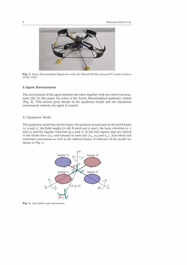
Fig. 3 Asctec Hummingbird Quadrotor with the Odroid XU4Q on-board PC (center bottomof the UAV).
3 Agent Environment
The environment of the agent includes the robot together with the robot’s environ-ment [24]. In this paper the robot is the Asctec Hummingbird quadrotor vehicle(Fig. 3). This section gives details of the quadrotor model and the simulationenvironment wherein the agent is trained.
3.1 Quadrotor Model
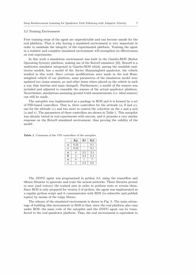
The quadrotor model has twelve states: the position on each axis in the world frame(x, y and z), the Euler angles (φ-roll, θ-pitch and ψ-yaw), the body velocities (u, vand w) and the angular velocities (p, q and r). It has four inputs, that are relatedto the thrust force (uz) and torques on each axis (uφ, uθ and uψ). Axis labels androtational conventions as well as the defined frames of reference of the model areshown in Fig. 4.
Fig. 4 Axis labels and conventions.
Deep Reinforcement Learning for Quadrotor Path Following with Adaptive Velocity 7
3.2 Training Environment
First training steps of the agent are unpredictable and can become unsafe for thereal platform. That is why having a simulated environment is very important inorder to maintain the integrity of the experimental platform. Training the agentin a realistic and complete simulated environment will strengthen its effectivenesson real experiments.
In this work a simulation environment was built in the Gazebo-ROS (RobotOperating System) platform, making use of the RotorS simulator [25]. RotorS is amultirotor simulator integrated in Gazebo-ROS which, among the available mul-tirotor models, has a model of the Asctec Hummingbird quadrotor, the vehiclestudied in this work. Since certain modifications were made in the real Hum-mingbird vehicle of our platform, some parameters of the simulation model wereupdated too (some sensors, pc and other items where placed on the vehicle in sucha way that inertias and mass changed). Furthermore, a model of the sensors wasincluded and adjusted to resemble the sensors of the actual quadrotor platform.Nevertheless, simulations assuming ground truth measurements (i.e. ideal sensors)can still be made.
The autopilot was implemented as a package in ROS and it is formed by a setof PID-based controllers. That is, three controllers for the attitude (φ, θ and ψ),one for the altitude (z) and two more to control the velocities on the x and y axis(u and v). The parameters of these controllers are shown in Table 1. This autopilotwas already tested in real experiments with success, and it presents a very similarresponse on the RotorS simulated environment, thus proving the validity of themodel.
Table 1 Constants of the PID controllers of the autopilot.
Kp Ki Kd
u 0.32 - 0.1
v 0.32 - 0.1
φ 4 2.2 2.4
θ 4 2.2 2.4
ψ 8 1 7
z 4 2.2 6.6
The DDPG agent was programmed in python 3.5, using the tensorflow andtflearn libraries to generate and train the neural networks. These libraries permitto save (and restore) the trained nets in order to perform tests or retrain them.Since ROS is only prepared for version 2 of python, the agent was implemented asa regular python script and it communicates with ROS (to subscribe and publishtopics) by means of the rospy library.
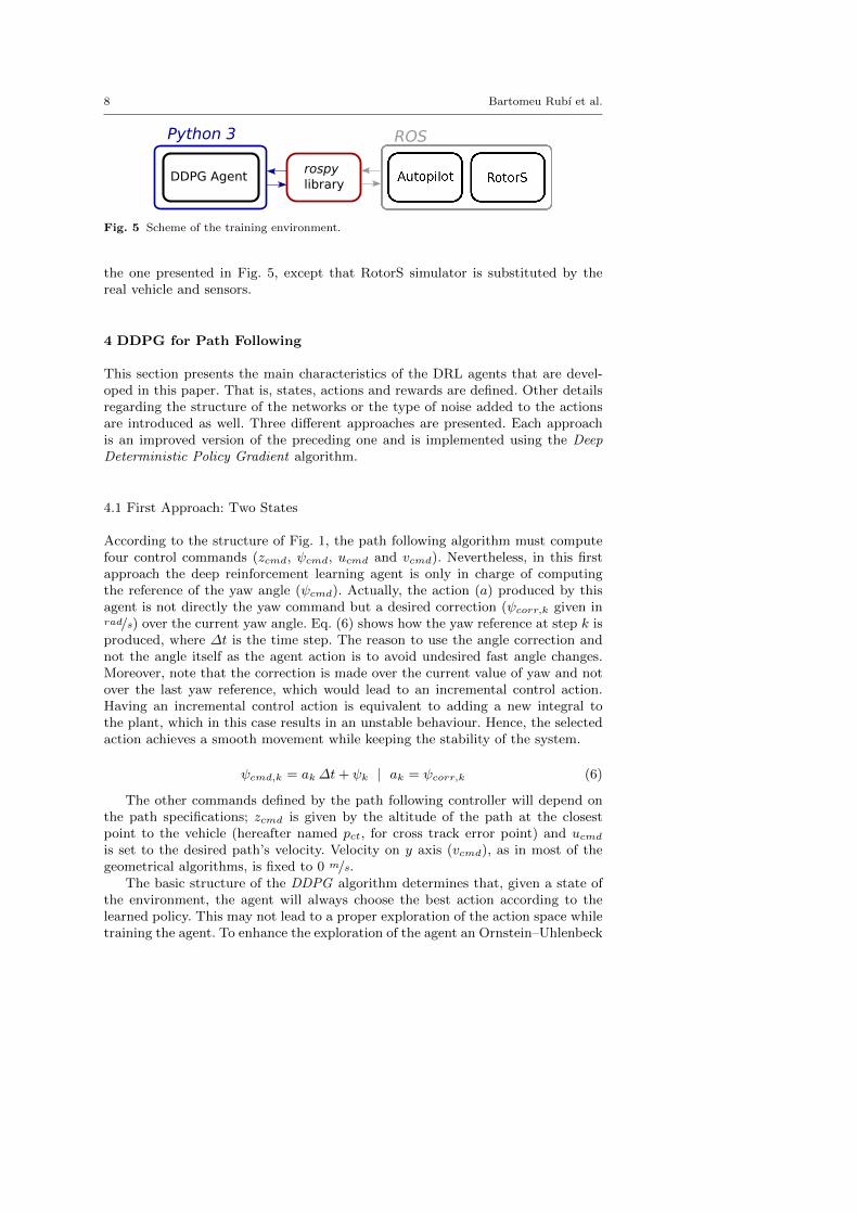
The scheme of the simulated environment is shown in Fig. 5. The main advan-tage of building this environment in ROS is that, since the real platform also runsunder ROS, the same code of the autopilot and the DDPG agent can be trans-ferred to the real quadrotor platform. Thus, the real environment is equivalent to
8 Bartomeu Rubı et al.
ROSPython 3
DDPG Agentrospy
library
Fig. 5 Scheme of the training environment.
the one presented in Fig. 5, except that RotorS simulator is substituted by thereal vehicle and sensors.
4 DDPG for Path Following
This section presents the main characteristics of the DRL agents that are devel-oped in this paper. That is, states, actions and rewards are defined. Other detailsregarding the structure of the networks or the type of noise added to the actionsare introduced as well. Three different approaches are presented. Each approachis an improved version of the preceding one and is implemented using the DeepDeterministic Policy Gradient algorithm.
4.1 First Approach: Two States
According to the structure of Fig. 1, the path following algorithm must computefour control commands (zcmd, ψcmd, ucmd and vcmd). Nevertheless, in this firstapproach the deep reinforcement learning agent is only in charge of computingthe reference of the yaw angle (ψcmd). Actually, the action (a) produced by thisagent is not directly the yaw command but a desired correction (ψcorr,k given inrad/s) over the current yaw angle. Eq. (6) shows how the yaw reference at step k isproduced, where ∆t is the time step. The reason to use the angle correction andnot the angle itself as the agent action is to avoid undesired fast angle changes.Moreover, note that the correction is made over the current value of yaw and notover the last yaw reference, which would lead to an incremental control action.Having an incremental control action is equivalent to adding a new integral tothe plant, which in this case results in an unstable behaviour. Hence, the selectedaction achieves a smooth movement while keeping the stability of the system.
ψcmd,k = ak∆t+ ψk | ak = ψcorr,k (6)
The other commands defined by the path following controller will depend onthe path specifications; zcmd is given by the altitude of the path at the closestpoint to the vehicle (hereafter named pct, for cross track error point) and ucmdis set to the desired path’s velocity. Velocity on y axis (vcmd), as in most of thegeometrical algorithms, is fixed to 0 m/s.
The basic structure of the DDPG algorithm determines that, given a state ofthe environment, the agent will always choose the best action according to thelearned policy. This may not lead to a proper exploration of the action space whiletraining the agent. To enhance the exploration of the agent an Ornstein–Uhlenbeck

Deep Reinforcement Learning for Quadrotor Path Following with Adaptive Velocity 9
Fig. 6 States of the agent are with respect of the tangential frame {T}.
noise (Eq. 7) is added to the action at training time. nk is the value of the noise atthe kth iteration, θn is a parameter that defines the speed rate of mean reversion,µn is the drift term which affects the asymptotic mean, ∆t is the time of a stepand dWt is the standard Wiener process scaled by volatility σn.
Yaw command (ψcmd) including the noise signal is computed as shown inEq. (8). The exploration rate decreases continuously with the number of trainingepisodes (j) in such a way that a smooth transition between exploration andexploitation is achieved while the agent keeps learning. Parameter κ indicates thespeed of this transition.
nk = nk−1 + θn (µn − nk−1)∆t+ σndWt (7)
ψcmd,k =
(ak +
nkj/κ + 1
)∆t+ ψk (8)
In this first approach, the state vector (s) is formed by two states (Eq. 9); thedistance error (ed) and the angle error (eψ), both with respect to pct (Fig. 6).Subscript T is referred to the tangential frame of reference {T} that is placed onpct with x pointing to the path’s tangential direction, z pointing up and y pointingto the resultant direction of x× z.
s = {ed, eψ} | ed = yT , eψ = ψT (9)
The reward defined for this agent is shown in Eq. (10). This is the rewardfunction that achieves the best performance and fastest convergence among thenumerous types of rewards that were evaluated (i.e. continuous or discrete, pe-nalizing bad behaviour or rewarding good path following performance, and mixedstrategies). The term −k1|ed| penalizes the cross-track error (ed). The term k2vTgives positive reward when the vehicle is moving forward on the path and negativeotherwise, where vT is the velocity of the vehicle projected in the x axis of thetangential frame of reference. k1 and k2 are constants that define the importanceof each of the two terms. In this approach these constants take the values of 20 and10, respectively. Being those the best values amongst several that were evaluated.
r = −k1|ed|+ k2vT (10)
The structures of the actor and critic neural networks consist on four layeredfeed forward networks with 400 neurons in the first hidden layer and 300 neurons in
10 Bartomeu Rubı et al.
the second one. However, while in the actor’s network both the state and the actionvectors are connected to the first hidden layer, in the critic networks the actionvector is connected directly to the second hidden layer, following the structure ofthe original algorithm [7]. Making the actions to skip the first layer improves thestability and performance. The neurons of both networks are rectified linear units(ReLU). Batch normalisation technique is used in the two layers of the actor nets,while it is only used in the state input layer in the critic networks.
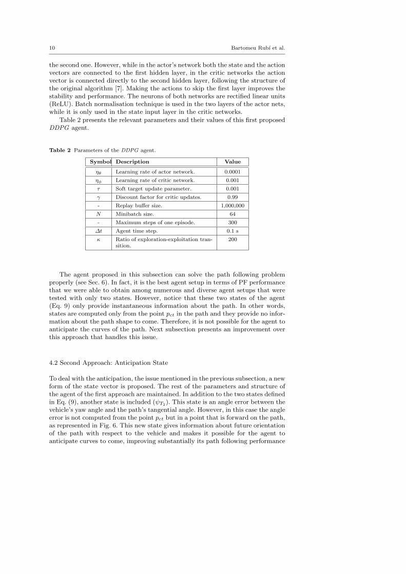
Table 2 presents the relevant parameters and their values of this first proposedDDPG agent.
Table 2 Parameters of the DDPG agent.
Symbol Description Value
ηθ Learning rate of actor network. 0.0001
ηφ Learning rate of critic network. 0.001
τ Soft target update parameter. 0.001
γ Discount factor for critic updates. 0.99
- Replay buffer size. 1,000,000
N Minibatch size. 64
- Maximum steps of one episode. 300
∆t Agent time step. 0.1 s
κ Ratio of exploration-exploitation tran-sition.
200
The agent proposed in this subsection can solve the path following problemproperly (see Sec. 6). In fact, it is the best agent setup in terms of PF performancethat we were able to obtain among numerous and diverse agent setups that weretested with only two states. However, notice that these two states of the agent(Eq. 9) only provide instantaneous information about the path. In other words,states are computed only from the point pct in the path and they provide no infor-mation about the path shape to come. Therefore, it is not possible for the agent toanticipate the curves of the path. Next subsection presents an improvement overthis approach that handles this issue.
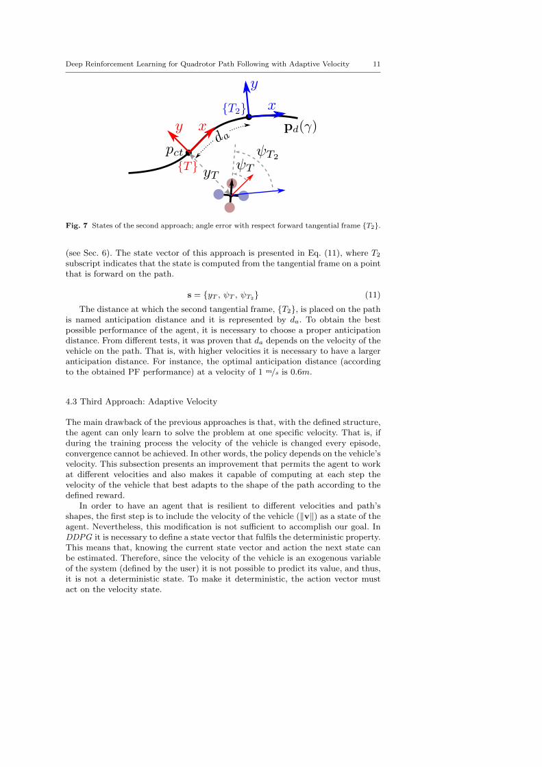
4.2 Second Approach: Anticipation State
To deal with the anticipation, the issue mentioned in the previous subsection, a newform of the state vector is proposed. The rest of the parameters and structure ofthe agent of the first approach are maintained. In addition to the two states definedin Eq. (9), another state is included (ψT2
). This state is an angle error between thevehicle’s yaw angle and the path’s tangential angle. However, in this case the angleerror is not computed from the point pct but in a point that is forward on the path,as represented in Fig. 6. This new state gives information about future orientationof the path with respect to the vehicle and makes it possible for the agent toanticipate curves to come, improving substantially its path following performance
Deep Reinforcement Learning for Quadrotor Path Following with Adaptive Velocity 11
Fig. 7 States of the second approach; angle error with respect forward tangential frame {T2}.
(see Sec. 6). The state vector of this approach is presented in Eq. (11), where T2subscript indicates that the state is computed from the tangential frame on a pointthat is forward on the path.
s = {yT , ψT , ψT2} (11)
The distance at which the second tangential frame, {T2}, is placed on the pathis named anticipation distance and it is represented by da. To obtain the bestpossible performance of the agent, it is necessary to choose a proper anticipationdistance. From different tests, it was proven that da depends on the velocity of thevehicle on the path. That is, with higher velocities it is necessary to have a largeranticipation distance. For instance, the optimal anticipation distance (accordingto the obtained PF performance) at a velocity of 1 m/s is 0.6m.
4.3 Third Approach: Adaptive Velocity
The main drawback of the previous approaches is that, with the defined structure,the agent can only learn to solve the problem at one specific velocity. That is, ifduring the training process the velocity of the vehicle is changed every episode,convergence cannot be achieved. In other words, the policy depends on the vehicle’svelocity. This subsection presents an improvement that permits the agent to workat different velocities and also makes it capable of computing at each step thevelocity of the vehicle that best adapts to the shape of the path according to thedefined reward.
In order to have an agent that is resilient to different velocities and path’sshapes, the first step is to include the velocity of the vehicle (‖v‖) as a state of theagent. Nevertheless, this modification is not sufficient to accomplish our goal. InDDPG it is necessary to define a state vector that fulfils the deterministic property.This means that, knowing the current state vector and action the next state canbe estimated. Therefore, since the velocity of the vehicle is an exogenous variableof the system (defined by the user) it is not possible to predict its value, and thus,it is not a deterministic state. To make it deterministic, the action vector mustact on the velocity state.

12 Bartomeu Rubı et al.
In this third approach, in addition to the yaw correction action defined inEq. (6), a new action that computes a velocity correction (ucorr,k) over the currentvelocity of the vehicle is included. Eq. (12) shows how the velocity command onthe x axis is produced from this action (including exploration noise of Eq. 7, onlyused during the training phase). Again, with the aim of avoiding fast changes onthe velocity and to assure the stability of the system, a correction action has beenused rather than a velocity action or an incremental action of the command.
ucmd,k =
(ucorr,k +
nkj/κ + 1
)∆t+ uk (12)
Introducing this new state (‖v‖) and new action (ucorr,k) to the agent mayseem to be enough to solve the problem. However, as mentioned in Sec. 4.2, no-tice that the path’s position where the future angle error state (ψT2
) is computeddepends on the velocity of the vehicle. Therefore, having only this state computedwith a fixed anticipation distance (da) does not provide enough information tosolve the path following problem at different velocities. Rather than that, twosolutions were considered: Adding more future angle error states at different an-ticipation distances or modifying at each step the anticipation distance at whichthe angle error is computed in function of the vehicle’s velocity.
Including several future angle states at different distances resulted disadvanta-geous for two reasons: first, having more states makes the training process muchslower; second, since at a given velocity only the information of 1 or 2 future anglestates is exploited, the remaining states become irrelevant. Having many statesthat do not provide significant information to solve the problem leads the agent tolose effectiveness. For this reason, in this approach the mentioned issue is solved byhaving only one future angle state (ψT2
), which is computed with an anticipationdistance adapted according to the vehicle’s velocity.
Several tests at different velocities were performed in order to find the relationbetween the velocity of the vehicle and the optimal anticipation distance (da,opt).Optimal in the sense of being the distance that provides more information, andthus, results in a higher performance of the agent. The results obtained from thesetests were approximated by the linear piecewise function shown in Eq. (13). Thisfunction computes the optimal anticipation distance as a function of the currentvelocity of the vehicle.
da,opt =
‖v‖ − 0.3 if ‖v‖ ≥ 1
0.6‖v‖+ 0.1 else(13)
Summarizing, in this approach the velocity of the vehicle is added as part of thestate vector and the future angle state is computed with an adaptive anticipationdistance (da,opt). A velocity correction is included in the action vector. Eqs. 14and 15 present the state and action vectors, respectively. The agent computes thevelocity command on the x axis in such a way that it adapts to the path’s shape.Velocity on the y axis is still fixed to 0. The reward function of the first approach(Eq. 10) is also maintained. Weights of the reward (k1 and k2) acquire a significantrole in this approach, since they define the priority of the trade-off between havingsmall path distance error or travelling at high velocities. All parameters of Table 2are preserved except for the ratio of the exploration-exploitation transition (κ),which is set to 1000. This is because the training process of this approach is slower.

Deep Reinforcement Learning for Quadrotor Path Following with Adaptive Velocity 13
s = {yT , ψT , ψT2(da,opt), ‖v‖} (14)
a = {ψcorr,k, ucorr,k} (15)
The ingredients that make the agent capable of following a trajectory in spacewith adaptive velocity have been defined. Nevertheless, it is of utmost importanceto design a rich training environment that allows the agent to converge to anefficient and robust solution. Details of this training process are given in Sec. 5.
5 Training Process
The training process of the agents has been performed in the training environmentdetailed in Sec. 3.2. This training environment is integrated in a linux Xubuntuvirtual machine with a dedication of 8GB RAM and four 1.80GHz processors(i7-8550U CPU). The training process is performed in real time.
5.1 Training of 1st and 2nd approaches
The first and second approaches followed the same structure in the training phase.That is, the vehicle is required to follow a half lemniscate (8-shaped) path at aconstant velocity of 1 m/s in the x body axis (ucmd). This path is defined inEq. (16), where A is the radius of one of the circumferences of the path, fixedto 4m, and γp is the virtual arc, which ranges from 0 to 2π rad. The path isdiscretized with a precision of 0.01m between each path point.
xd (γp) = 2A cos (γp)
yd (γp) = A sin (2γp)(16)
Both agents were trained following the specified path in ideal conditions, mean-ing that the system uses ground truth measurements and the vehicle starts eachepisode at the initial position of the path with the yaw angle oriented tangen-tially to it. As denoted in Table 2, each episode has 300 steps of 0.1 seconds. Thelearning evolution of the first and the second approaches are shown in Figs. 8 and9, respectively. These figures show. for each episode, the average path distanceerror (|d|) and the accumulated reward (
∑r) in all the steps of the episode. As
the agents keep training the average error decreases and the accumulated rewardgrows until training converges.
It is important to mention that, as the training process is stochastic, even ifthe same parameters and structure are maintained, the performance of the trainedagents can vary. The agents presented in this paper are the ones that achieve thebest performance, in terms of path distance error, among a set of different trainedagents that were obtained. In this particular case, the 1st approach convergedaround the 120th episode while the 2nd approach did it approximately at episode90.
The resulting agents were tested in the RotorS simulation platform (see Sec. 6.1).They proved to perform well with ground truth measurements. However, if a model

14 Bartomeu Rubı et al.
Fig. 8 Average distance error and accumulated reward on each episode during training phaseof 1st approach agent (2 states).
Fig. 9 Average distance error and accumulated reward on each episode during training phaseof 2nd approach agent (3 states).
of the sensors is added, the agents present some difficulties to follow the path prop-erly. Particularly, when the vehicle moves far from the path (due to drift or jumpson sensor measurements) and needs to converge back, the vehicle can start loiteringaround the path without being able to converge to it.
The solution to the mentioned problem could be to train the agent with themodel with sensors. However, to capture the dynamics of the system with noisymeasurements becomes challenging for the agent and, sometimes, training doesnot converge in these conditions. Alternatively, this issue is tackled by retrainingthe agents to learn the policy when the vehicle is far from the path. To do so, the

Deep Reinforcement Learning for Quadrotor Path Following with Adaptive Velocity 15
agents are first trained as explained before, and then, they are retrained followingthe same path but starting at random positions and orientations different fromthe initial point of the path. In this way, the agents learn how to behave out ofthe path. Thus, if the vehicle occasionally moves out of the path because of thenoisy sensor measurements, the agent will be able of driving the vehicle back tothe path.
Both agents (1st and 2nd approaches) were trained 100 more episodes follow-ing the specified lemniscate path (Eq. 16) with random initial conditions. Thatis, in each episode of this training phase the starting position of the vehicle is setat a distance of −2m to 2m from the initial position of the path, and the initialorientation is incremented an angle between −π/2 to π/2 from the initial path tan-gential angle. The initial position and angle are selected randomly with a uniformprobability distribution in the defined intervals.
Fig. 10 Average distance error and accumulated reward on each episode during training phasewith non-ideal initial conditions of 2nd approach agent; gray dashed lines are real values andblack lines are a 20-episodes moving average.
Fig. 10 shows the learning evolution of the 2nd approach with the 100 newtraining episodes. Since the initial position and orientation change randomly ineach episode, the obtained average distance error and accumulated reward alsovary arbitrarily. For this reason, to show better the progression of this learningphase, a 20-values moving average is presented in both plots. That is, episode val-ues are represented with gray dashed lines, while the moving average is representedwith solid black lines in Fig. 10. The learning results show how this training phasepermits the agent to learn to perform better in diverse initial conditions. Thisacquired knowledge will notably improve the performance in real experiments, asrevealed in Sec. 6.

16 Bartomeu Rubı et al.
5.2 Training of 3rd approach
The 3rd DDPG approach developed in this paper requires training in a richerenvironment than the previous versions. That is because the agent needs to trainwith different curves in order to learn the optimal vehicle’s velocity and the yawangle’s policy according to the path radius.
In the training process of this agent the vehicle will be required to follow anasymmetrical half lemniscate path. This is an 8-shaped path where each circlehas a different radius. This path is defined in Eq. (17), where A1 and A2 are theradius of each circumference of the path, respectively. The value of this radiusis changed every episode, taking a random value between 0.5m and 10m witha uniform probability distribution. Again, the virtual arc parameter (γp) rangesfrom 0 to π/2 rads, and the path is discretized with a precision of 0.01m.
xd (γp) =
2A1 cos (γp) if 0 ≤ γp ≤ π/4
2A2 cos (γp) if π/4 < γp ≤ π/2
yd (γp) =
A1 sin (2γp) if 0 ≤ γp ≤ π/4
A2 sin (2γp) if π/4 < γp ≤ π/2
(17)
The first training attempts of the agent with the stated environment resulted tobe quite unfruitful. Concretely, after hundreds of episodes, the agent just learnedthat the best way of maximizing the reward (reward function in Sec. 4) was tokeep the vehicle static. The reason for this strange behaviour can be explained asfollows: since turning around arbitrarily is not penalized when, due to the lack ofexploration the policy is not defined yet, whenever the agent starts moving thevehicle forward, as it is rotating, it ends up moving in the opposite direction ofthe path, receiving a penalty for that policy; therefore the best action is to keepucmd = 0.
A simple but effective solution for such issue is proposed in this paper. Itconsists on forcing the vehicle to move constantly by establishing a minimumvelocity of 0.1 m/s. Even if this condition initially produces negative rewards, itends up promoting the agent to learn the policy of the yaw action. At the sametime, as soon as the velocity vector of the vehicle starts to be parallel to the path,the agent can start learning that higher velocities lead to greater rewards. Hence,a successful learning process is achieved.
The training results of this agent are shown in Fig. 11. This figure shows theaverage distance error (|d|), the average velocity on the x axis (u) and the accu-mulated reward (
∑r) on each episode. A 50-episodes moving average is applied
to episode values to help the interpretation of each of the three plots. Again, graydashed lines represent episode values while black lines show the moving average.
It may seem that training converged around episode 400. However, even theaverage error or reward appear to be constant, evaluating the trained agents withsimulation tests showed that they kept learning and improving their performanceuntil around episode 1000. The reason for that is because training more episodespermits to learn the policy on unusual states.

Deep Reinforcement Learning for Quadrotor Path Following with Adaptive Velocity 17
Fig. 11 Average distance error, average velocity and accumulated reward on each episodeduring training phase of 3rd approach agent; gray dashed lines are real values and black linesare a 50-episodes moving average.
Such long and complex training process allows the agent to learn the policy outof the path. Thus, unlike the 1st and 2nd approaches, this approach does not needany additional training with diverse initial conditions to improve its performanceon experimental results.
6 Results
This section presents the results obtained with the three trained agents whilefollowing a path in different conditions. The agents were tested in simulation andexperimentally with the Asctec Hummingbird platform.
6.1 Simulation
The simulations presented in this paper were performed in the same frameworkwhere the agents were trained. That is, the RotorS simulator integrated in theROS-Gazebo platform.
First, the three approaches were tested following a lemniscate path (Eq. 16),the same path used in the training phase. Again, the radius of the path is A = 4m.However, this time the vehicle was required to follow a full lemniscate, with thevirtual arc parameter, γp, ranging from 0 to 4π rads. The vehicle started at theinitial point on the path with the yaw angle oriented tangentially to it.
18 Bartomeu Rubı et al.
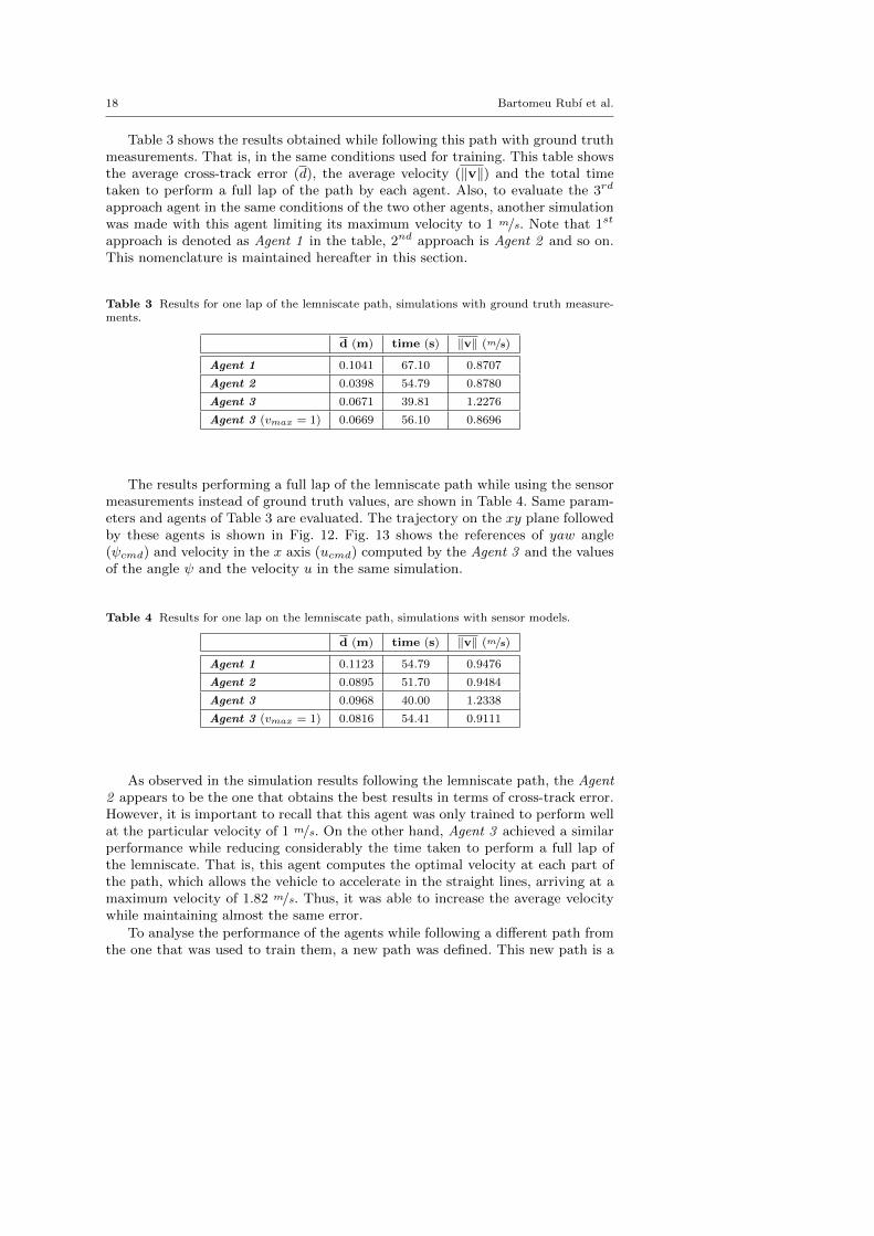
Table 3 shows the results obtained while following this path with ground truthmeasurements. That is, in the same conditions used for training. This table showsthe average cross-track error (d), the average velocity (‖v‖) and the total timetaken to perform a full lap of the path by each agent. Also, to evaluate the 3rd
approach agent in the same conditions of the two other agents, another simulationwas made with this agent limiting its maximum velocity to 1 m/s. Note that 1st
approach is denoted as Agent 1 in the table, 2nd approach is Agent 2 and so on.This nomenclature is maintained hereafter in this section.
Table 3 Results for one lap of the lemniscate path, simulations with ground truth measure-ments.
d (m) time (s) ‖v‖ (m/s)
Agent 1 0.1041 67.10 0.8707
Agent 2 0.0398 54.79 0.8780
Agent 3 0.0671 39.81 1.2276
Agent 3 (vmax = 1) 0.0669 56.10 0.8696
The results performing a full lap of the lemniscate path while using the sensormeasurements instead of ground truth values, are shown in Table 4. Same param-eters and agents of Table 3 are evaluated. The trajectory on the xy plane followedby these agents is shown in Fig. 12. Fig. 13 shows the references of yaw angle(ψcmd) and velocity in the x axis (ucmd) computed by the Agent 3 and the valuesof the angle ψ and the velocity u in the same simulation.
Table 4 Results for one lap on the lemniscate path, simulations with sensor models.
d (m) time (s) ‖v‖ (m/s)
Agent 1 0.1123 54.79 0.9476
Agent 2 0.0895 51.70 0.9484
Agent 3 0.0968 40.00 1.2338
Agent 3 (vmax = 1) 0.0816 54.41 0.9111
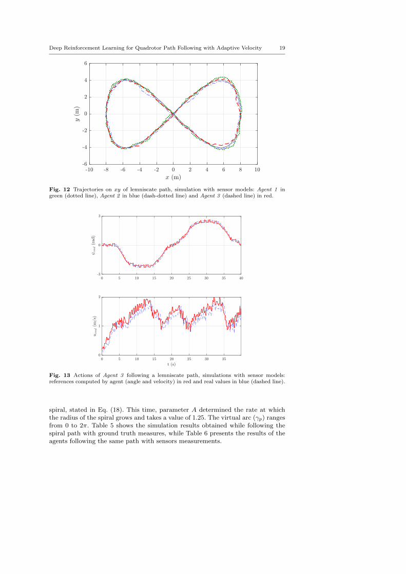
As observed in the simulation results following the lemniscate path, the Agent2 appears to be the one that obtains the best results in terms of cross-track error.However, it is important to recall that this agent was only trained to perform wellat the particular velocity of 1 m/s. On the other hand, Agent 3 achieved a similarperformance while reducing considerably the time taken to perform a full lap ofthe lemniscate. That is, this agent computes the optimal velocity at each part ofthe path, which allows the vehicle to accelerate in the straight lines, arriving at amaximum velocity of 1.82 m/s. Thus, it was able to increase the average velocitywhile maintaining almost the same error.
To analyse the performance of the agents while following a different path fromthe one that was used to train them, a new path was defined. This new path is a
Deep Reinforcement Learning for Quadrotor Path Following with Adaptive Velocity 19
Fig. 12 Trajectories on xy of lemniscate path, simulation with sensor models: Agent 1 ingreen (dotted line), Agent 2 in blue (dash-dotted line) and Agent 3 (dashed line) in red.
Fig. 13 Actions of Agent 3 following a lemniscate path, simulations with sensor models:references computed by agent (angle and velocity) in red and real values in blue (dashed line).
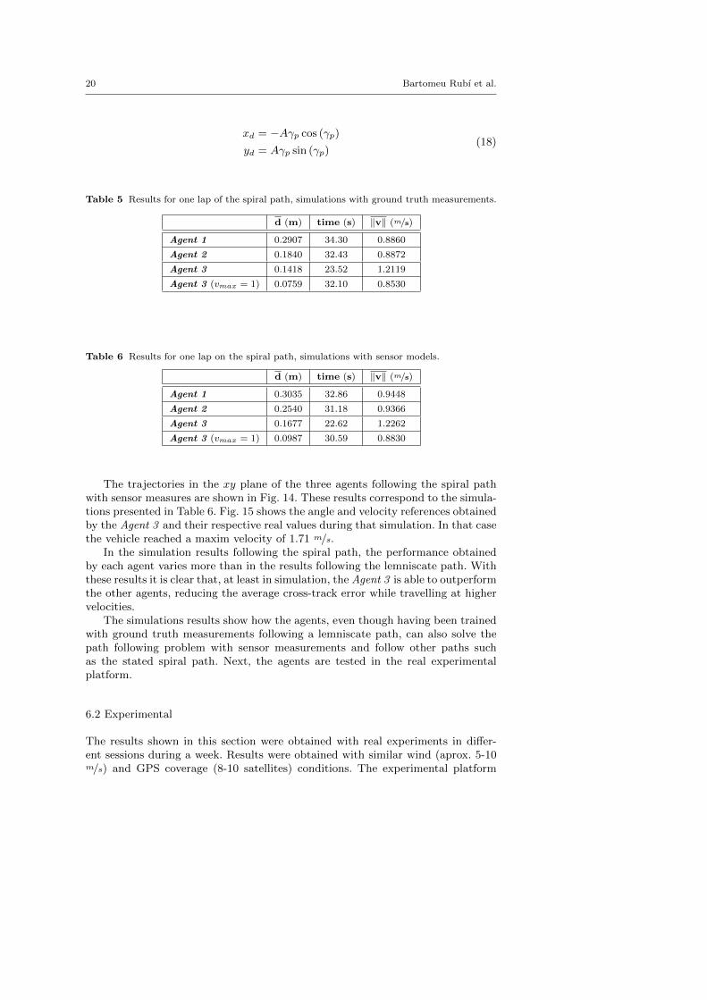
spiral, stated in Eq. (18). This time, parameter A determined the rate at whichthe radius of the spiral grows and takes a value of 1.25. The virtual arc (γp) rangesfrom 0 to 2π. Table 5 shows the simulation results obtained while following thespiral path with ground truth measures, while Table 6 presents the results of theagents following the same path with sensors measurements.
20 Bartomeu Rubı et al.
xd = −Aγp cos (γp)
yd = Aγp sin (γp)(18)
Table 5 Results for one lap of the spiral path, simulations with ground truth measurements.
d (m) time (s) ‖v‖ (m/s)
Agent 1 0.2907 34.30 0.8860
Agent 2 0.1840 32.43 0.8872
Agent 3 0.1418 23.52 1.2119
Agent 3 (vmax = 1) 0.0759 32.10 0.8530
Table 6 Results for one lap on the spiral path, simulations with sensor models.
d (m) time (s) ‖v‖ (m/s)
Agent 1 0.3035 32.86 0.9448
Agent 2 0.2540 31.18 0.9366
Agent 3 0.1677 22.62 1.2262
Agent 3 (vmax = 1) 0.0987 30.59 0.8830
The trajectories in the xy plane of the three agents following the spiral pathwith sensor measures are shown in Fig. 14. These results correspond to the simula-tions presented in Table 6. Fig. 15 shows the angle and velocity references obtainedby the Agent 3 and their respective real values during that simulation. In that casethe vehicle reached a maxim velocity of 1.71 m/s.
In the simulation results following the spiral path, the performance obtainedby each agent varies more than in the results following the lemniscate path. Withthese results it is clear that, at least in simulation, the Agent 3 is able to outperformthe other agents, reducing the average cross-track error while travelling at highervelocities.
The simulations results show how the agents, even though having been trainedwith ground truth measurements following a lemniscate path, can also solve thepath following problem with sensor measurements and follow other paths suchas the stated spiral path. Next, the agents are tested in the real experimentalplatform.
6.2 Experimental
The results shown in this section were obtained with real experiments in differ-ent sessions during a week. Results were obtained with similar wind (aprox. 5-10m/s) and GPS coverage (8-10 satellites) conditions. The experimental platform

Deep Reinforcement Learning for Quadrotor Path Following with Adaptive Velocity 21
Fig. 14 Trajectories on xy of spiral path, simulations with sensor models: Agent 1 in green(dotted line), Agent 2 in blue (dash-dotted line) and Agent 3 (dashed line) in red.
Fig. 15 Actions of Agent 3 following a spiral path, simulations with sensor models: referencescomputed by agent (angle and velocity) in red and real values in blue (dashed line).
is the Asctec Hummingbird vehicle with a supplementary on-board PC (OdroidXU4Q) with ROS framework installed. Fig. 16 shows an image of the experimen-tal platform. As can be observed, it is a an outdoors platform. The vehicle isequipped with an IMU sensor which, among other values, provides an estimationof the orientation of the vehicle, with a pressure sensor that provides the altitude
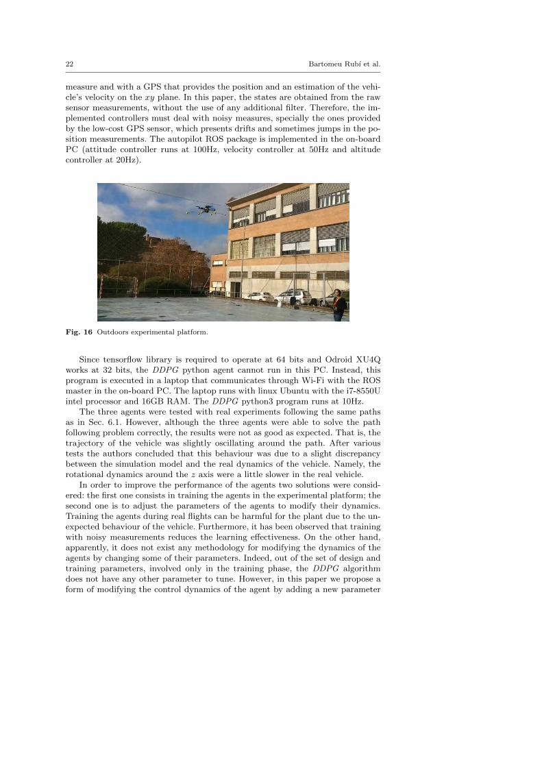
22 Bartomeu Rubı et al.
measure and with a GPS that provides the position and an estimation of the vehi-cle’s velocity on the xy plane. In this paper, the states are obtained from the rawsensor measurements, without the use of any additional filter. Therefore, the im-plemented controllers must deal with noisy measures, specially the ones providedby the low-cost GPS sensor, which presents drifts and sometimes jumps in the po-sition measurements. The autopilot ROS package is implemented in the on-boardPC (attitude controller runs at 100Hz, velocity controller at 50Hz and altitudecontroller at 20Hz).
Fig. 16 Outdoors experimental platform.
Since tensorflow library is required to operate at 64 bits and Odroid XU4Qworks at 32 bits, the DDPG python agent cannot run in this PC. Instead, thisprogram is executed in a laptop that communicates through Wi-Fi with the ROSmaster in the on-board PC. The laptop runs with linux Ubuntu with the i7-8550Uintel processor and 16GB RAM. The DDPG python3 program runs at 10Hz.
The three agents were tested with real experiments following the same pathsas in Sec. 6.1. However, although the three agents were able to solve the pathfollowing problem correctly, the results were not as good as expected. That is, thetrajectory of the vehicle was slightly oscillating around the path. After varioustests the authors concluded that this behaviour was due to a slight discrepancybetween the simulation model and the real dynamics of the vehicle. Namely, therotational dynamics around the z axis were a little slower in the real vehicle.
In order to improve the performance of the agents two solutions were consid-ered: the first one consists in training the agents in the experimental platform; thesecond one is to adjust the parameters of the agents to modify their dynamics.Training the agents during real flights can be harmful for the plant due to the un-expected behaviour of the vehicle. Furthermore, it has been observed that trainingwith noisy measurements reduces the learning effectiveness. On the other hand,apparently, it does not exist any methodology for modifying the dynamics of theagents by changing some of their parameters. Indeed, out of the set of design andtraining parameters, involved only in the training phase, the DDPG algorithmdoes not have any other parameter to tune. However, in this paper we propose aform of modifying the control dynamics of the agent by adding a new parameter

Deep Reinforcement Learning for Quadrotor Path Following with Adaptive Velocity 23
that will scale the output of the agent. That is, since the outputs of the agent arecorrections (angle and velocity corrections), this parameter will regulate the speedat which the correction is made, and thus, it ends up regulating the dynamics ofthe angle and/or velocity reference too.
Since the discrepancy between the two models affects the yaw dynamics, onlythe angle action was scaled with the mentioned parameter. This new parameter,known as the angle correction constant (ka), is apparent in Eq. (19) and it isset experimentally, ka = 2; the value that provided the best performance fromthe different values that were tested experimentally. This correction constant wasincluded in the three agents that were used to obtain all the experimental resultsthat are presented in this paper. It is important to remember that this constantwas just used in the experimental phase to improve the performance of the agents.
ψcmd,k = kaak∆t+ ψk (19)
Next, the agents were tested with the same lemniscate of Sec. 6.1 (Eq. 16) withA = 4 and γp ranging from 0 to 4π. The results of the three agents performinga full lap of this path are shown in Table 7. The results of the Agent 3 with themaximum velocity limited to 1 m/s are also included. Again, the table shows theaverage cross-track error (d), the total time and the average velocity of the vehicle(‖v‖). Fig. 17 presents the trajectory on the xy plane of the agents while followingthis path. Furthermore, Fig. 18 shows the angle and velocity references computedby the Agent 3 while following this lemniscate path, where references are shownin red and real values in blue dashed lines.
Table 7 Experimental results for one lap on the lemniscate path.
d (m) time (s) ‖v‖ (m/s)
Agent 1 0.1739 55.90 0.8859
Agent 2 0.1140 55.01 0.9141
Agent 3 0.1682 39.39 1.6311
Agent 3 (vmax = 1) 0.2275 59.50 0.8829
The experimental results following the lemniscate reveal a behaviour that isvery similar to the simulation results. The Agent 2 displays again the best perfor-mance in terms of cross-track error, but the Agent 3 achieves a similar distanceerror while increasing the average velocity, arriving at a maximum velocity of2.49 m/s.
Another important remark from these experimental results is found in the lastcurve of the trajectory performed by the Agent 3 (bottom-right curve in Fig. 17),a curve that the agent should clearly undertake better. This behaviour in thefast counter-clockwise curves appeared in all the experiments that we performedwith this agent, and was even more evident in the counter-clockwise spiral paths.The cause of that strange pattern was found in the designed training framework.Although the agent was trained with asymmetrical lemniscates with diverse radius,this training framework resulted to be incomplete. The reason is that the agent wastrained with a half lemniscate beginning with a counter-clockwise curve and ending
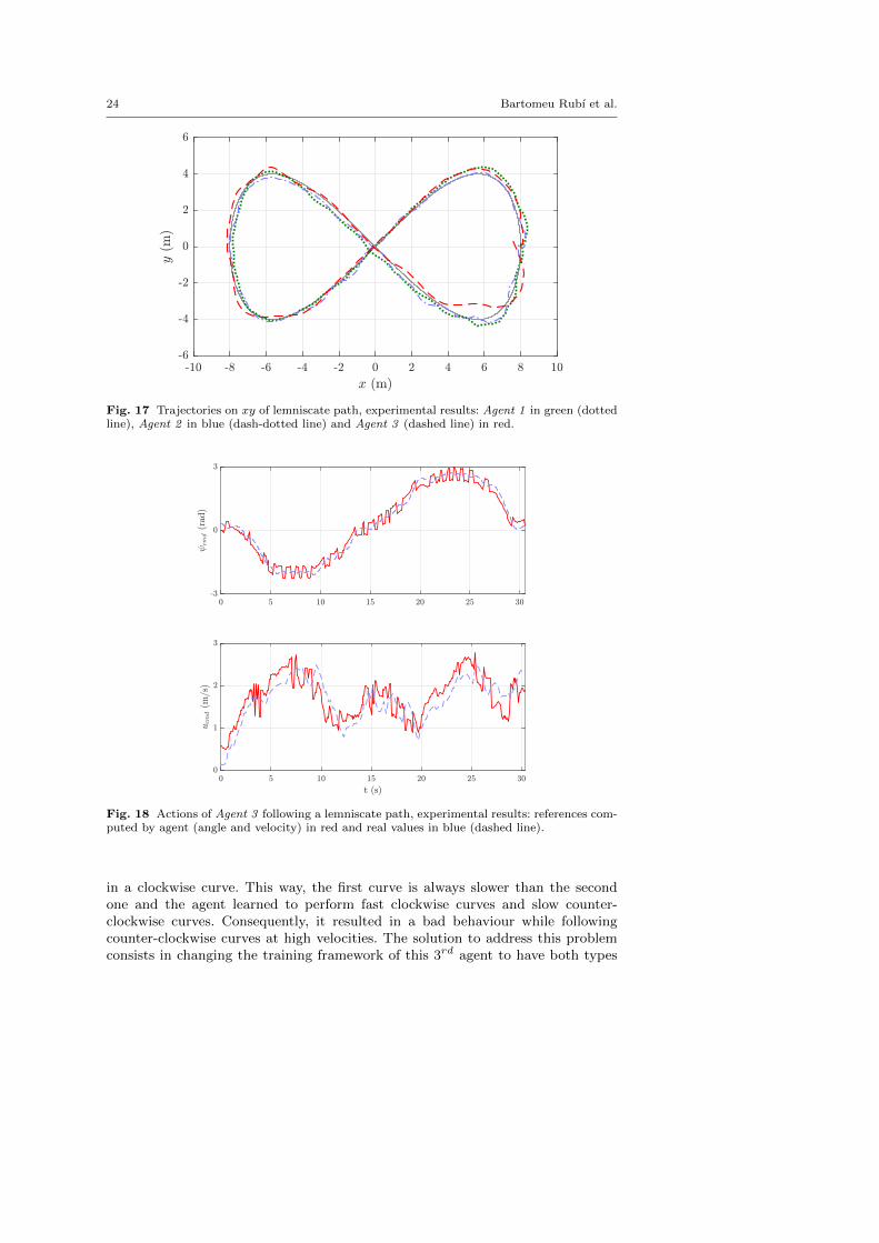
24 Bartomeu Rubı et al.
Fig. 17 Trajectories on xy of lemniscate path, experimental results: Agent 1 in green (dottedline), Agent 2 in blue (dash-dotted line) and Agent 3 (dashed line) in red.
Fig. 18 Actions of Agent 3 following a lemniscate path, experimental results: references com-puted by agent (angle and velocity) in red and real values in blue (dashed line).
in a clockwise curve. This way, the first curve is always slower than the secondone and the agent learned to perform fast clockwise curves and slow counter-clockwise curves. Consequently, it resulted in a bad behaviour while followingcounter-clockwise curves at high velocities. The solution to address this problemconsists in changing the training framework of this 3rd agent to have both types

Deep Reinforcement Learning for Quadrotor Path Following with Adaptive Velocity 25
of curves at slow and fast velocities. It could be done, for instance, with fullasymmetrical lemniscates.
Finally, the agents were tested with the spiral path defined in Eq. (18), withA = 2.5 and γp ranging from 0 to 4π. Table 8 presents the results of the threeagents plus the Agent 3 with limited velocity, just as in Table 7. The trajectoriesof the agents following this spiral path are shown in Fig. 19, and Fig. 20 showsthe angle and velocity references computed from the actions of the Agent 3.
Table 8 Experimental results for one lap on the spiral path.
d (m) time (s) ‖v‖ (m/s)
Agent 1 0.2848 28.81 1.0503
Agent 2 0.2503 27.79 1.0460
Agent 3 0.2257 18.59 1.5844
Agent 3 (vmax = 1) 0.2342 33.10 0.8826
Fig. 19 Trajectories on xy of spiral path, experimental results: DDPG v1 in green (dottedline), DDPG v2 in blue (dash-dotted line) and Agent 3 (dashed line) in red.
In the experimental results following the spiral path, the Agent 3 outperformsthe other agents by exhibiting a lower cross-track error with higher velocity. Specif-ically, this agent arrives at a maximum velocity of 2.52 m/s.
The initial trajectory of the agents when following the spiral path (Fig. 19)evidences a difference of behaviour between each of the three approaches presentedin this paper. That is, the Agent 1 is required to travel at a constant speed of 1 m/sand only has information of the instantaneous distance and orientation error. Thus,due to the lack of anticipation, in the initial part of the path it starts going forward,

26 Bartomeu Rubı et al.
Fig. 20 Actions of Agent 3 following a spiral path, experimental results: references computedby agent (angle and velocity) in red and real values in blue (dashed line).
moving out of the path. The Agent 2 moves also at a constant velocity. However,this agent has information about the upcoming orientation of the path, whichallows it to anticipate the curve. Hence, in the initial part of the path, this agentstarts moving towards the curve. Finally, the Agent 3 knows the evolution of thepath’s curvature in advance and it is able to modify the longitudinal speed. Thatallows it to command slower speeds at the beginning of the path and turn towardsthe curve to follow the path as accurately as possible and then, when it is correctlyoriented, start increasing the velocity.
7 Conclusions
In this paper, a deep reinforcement learning algorithm, the Deep Deterministic Pol-icy Gradient, has been proposed to solve the path following problem in a quadrotorvehicle. The path following control computes the references for the velocity, thealtitude and the angle in the z axis that are then tracked by the autopilot con-troller. Three different DDPG approaches with different behaviours are presented.The first approach solves the PF problem only with information about the instan-taneous position and angle errors. The second approach adds information aboutthe upcoming path. Both approaches work at constant velocity. The third ap-proach permits the agent to compute the optimal vehicle’s velocity that adaptsbetter to the shape of the path, according to the defined agent reward.
Each of the proposed agents arises as an improved version of the previous one,that is one of the main strengths of the methodology used in this work. The mainstructure, common in the three approaches, permits the incorporation of new func-

Deep Reinforcement Learning for Quadrotor Path Following with Adaptive Velocity 27
tionalities (such as having anticipation to curves or adapting the vehicle’s velocity)without changing the core of the agent. This is very promising since it means thatnew functionalities (e.g. wind disturbance rejection) could be straightforwardlyintegrated to the agent without altering the rest of the functionalities.
The agents were programmed in python using the tensorflow library. The de-signed training framework integrates the python script with Gazebo-ROS and usesRotorS, a the realistic multirotor simulator. This simulator includes a model ofthe Asctec Hummingbird, the quadrotor used in the experimental platform. Mod-els of the real sensors of our platform were included in the simulator. The firstand second agents were trained with lemniscate paths of fixed radius. They werealso trained with different initial conditions to improve their performance in theexperimental results. In order to learn the policy of the velocity action with dif-ferent path’s radius, the third agent was trained with asymmetrical lemniscatesand changing the radius on each episode. The three agents were trained assumingground truth measurements. The main advantage of training the agents in ROSis that it facilitates the transition from the simulator to the real plant. Further-more, since ROS is a standard platform in the robotics field, it is supported bya large community, which can be very useful. The only concern to consider whentraining in ROS is that, since simulations are made real-time, it may become atime-consuming process.
The three agents were tested in simulations in the RotorS environment withrealistic models of the sensors. They were evaluated with a lemniscate path andwith a spiral path. Then, the agents were also tested in real experiments withthe Asctec Hummingbird quadrotor following the same paths as in simulation.Even thought the agents were able to follow the pre-established paths correctly inthe first experiments that were carried out, they performed worse than expected.The authors concluded that this behaviour was due to the small errors of thesimulated model, which affected mainly to the yaw dynamics. To improve theperformance of the agents a new parameter (angle correction constant, ka) wasincluded. This parameter scales the yaw action of the agent. And permits to modifythe dynamics of the agent to cope with the model’s discrepancy. Training theagents experimentally was dismissed since it can be harmful for the plant dueto the unexpected behaviour of the vehicle. Furthermore, it was observed thattraining with noisy signals was unfruitful.
The agents were tested experimentally including the angle correction constant,which improved significantly their performance. In the lemniscate path, the Agent2 achieved the best performance in terms of average cross-track error (0.114m),but the Agent 3 exhibited a similar distance error (0.168m) while being able tosignificantly increase the vehicle’s velocity. In the spiral path, the Agent 3 standsout over the other approaches by achieving the lowest average cross-track error(0.223) while travelling at higher velocities. In conclusion, the experimental resultsshow how the agents are able to successfully follow the spiral path, a different pathfrom the one that they were trained with. And thus, it is proved that the proposedapproach is able to find a generalized solution for the path following problem withadaptive velocity.
Nevertheless, a strange pattern was observed in the Agent 3 while performingcounter-clockwise curves at high velocities (Fig. 17). This behaviour was attributedto the design of the training environment. That is, since the agent was trainedwith half asymmetrical lemniscates, the first curve of the path (counter-clockwise)

28 Bartomeu Rubı et al.
is followed in the transient part of the experiment (velocity is still increasing).Therefore, the agent ended up training the clockwise curves at faster velocitiesthan the counter-clockwise ones. This fact highlights the importance of having notonly a proper structure and parametrization of the agent, but also a rich, completeand adequate training framework. The solution to this issue would be to train witha different path that permits the agent to learn both curves at different velocities.
Future work is to study the effect of the trained path in the performance ofthe agent and to find the best training environment to exploit the benefits of theagent. Other future work is to improve the presented agent to make it capable ofsolving other challenging problems such as wind disturbance rejection or reactiveobstacle avoidance.
Conflict of interest
The authors declare that they have no conflict of interest.
References
1. A. P. Aguiar, J. P. Hespanha, and P. V. Kokotovic, “Performance limitations in referencetracking and path following for nonlinear systems,” Automatica, vol. 44, no. 3, pp. 598–610,2008.
2. I. Kaminer, O. Yakimenko, A. Pascoal, and R. Ghabcheloo, “Path generation, path follow-ing and coordinated control for time-critical missions of multiple UAVs,” in 2006 AMER-ICAN CONTROL CONFERENCE, vol. 1-12, pp. 4906+, 2006.
3. B. Rubı, R. Perez, and B. Morcego, “A Survey of Path Following Control Strategies forUAVs Focused on Quadrotors,” Journal of Intelligent & Robotic Systems, vol. 98, pp. 241–265, 2019.
4. P. B. Sujit, S. Saripalli, and J. B. Sousa, “Unmanned aerial vehicle path following: Asurvey and analysis of algorithms for fixed-wing unmanned aerial vehicless,” IEEE ControlSystems, vol. 34, no. 1, pp. 42–59, 2014.
5. G. Heredia and A. Ollero, “Stability of autonomous vehicle path tracking with pure delaysin the control loop,” Advanced Robotics, vol. 21, no. 1-2, pp. 23–50, 2007.
6. V. Mnih, K. Kavukcuoglu, D. Silver, A. A. Rusu, J. Veness, M. G. Bellemare, A. Graves,M. A. Riedmiller, A. Fidjeland, G. Ostrovski, S. Petersen, C. Beattie, A. Sadik,I. Antonoglou, H. King, D. Kumaran, D. Wierstra, S. Legg, and D. Hassabis, “Human-levelcontrol through deep reinforcement learning,” Nature, vol. 518, pp. 529–533, 2015.
7. T. P. Lillicrap, J. J. Hunt, A. Pritzel, N. Heess, T. Erez, Y. Tassa, D. Silver, and D. Wier-stra, “Continuous control with deep reinforcement learning,” in 2016 International Con-ference on Learning Representations (ICLR), 2016.
8. J. C. Caicedo and S. Lazebnik, “Active object localization with deep reinforcement learn-ing,” in 2015 IEEE International Conference on Computer Vision (ICCV), pp. 2488–2496,12 2015.
9. D. Silver, A. Huang, C. J. Maddison, A. Guez, L. Sifre, G. van den Driessche, J. Schrit-twieser, I. Antonoglou, V. Panneershelvam, M. Lanctot, S. Dieleman, D. Grewe, J. Nham,N. Kalchbrenner, I. Sutskever, T. P. Lillicrap, M. Leach, K. Kavukcuoglu, T. Graepel,and D. Hassabis, “Mastering the game of go with deep neural networks and tree search,”Nature, vol. 529, pp. 484–489, 2016.
10. R. Yu, Z. Shi, C. Huang, T. Li, and Q. Ma, “Deep reinforcement learning based opti-mal trajectory tracking control of autonomous underwater vehicle,” in 2017 36th ChineseControl Conference (CCC), pp. 4958–4965, 7 2017.
11. L. P. Tuyen and T. Chung, “Controlling bicycle using deep deterministic policy gradientalgorithm,” in 2017 14th International Conference on Ubiquitous Robots and AmbientIntelligence (URAI), pp. 413–417, 6 2017.
12. L. Li, Y. Lv, and F. Wang, “Traffic signal timing via deep reinforcement learning,”IEEE/CAA Journal of Automatica Sinica, vol. 3, pp. 247–254, 7 2016.

Deep Reinforcement Learning for Quadrotor Path Following with Adaptive Velocity 29
13. A. Rodriguez-Ramos, C. Sampedro, H. Bavle, P. de la Puente, and P. Campoy, “A deep re-inforcement learning strategy for uav autonomous landing on a moving platform,” Journalof Intelligent & Robotic Systems, vol. 93, pp. 351–366, 2 2019.
14. K. Kang, S. Belkhale, G. Kahn, P. Abbeel, and S. Levine, “Generalization through sim-ulation: Integrating simulated and real data into deep reinforcement learning for vision-based autonomous flight,” in 2019 International Conference on Robotics and Automation(ICRA), 2019.
15. W. Koch, R. Mancuso, R. West, and A. Bestavros, “Reinforcement learning for uav atti-tude control,” ACM Trans. Cyber-Phys. Syst., vol. 3, no. 2, 2019.
16. N. O. Lambert, D. S. Drew, J. Yaconelli, R. Calandra, S. Levine, and K. S. J. Pister,“Low level control of a quadrotor with deep model-based reinforcement learning,” IEEERobotics and Automatic Letters, vol. 4, no. 4, 2019.
17. D. Mittall, K. Kumar, S. N. Hashmi, P. Kumar, A. Nanda, and S. Chandra, “Performancecomparison of deep and shallow network for quadcopter automation,” in 2018 IEEE 13thInternational Conference on Industrial and Information Systems (ICIIS), pp. 143–147,2018.
18. R. Polvara, M. Patacchiola, S. Sharma, J. Wan, A. Manning, R. Sutton, and A. Cangelosi,“Toward end-to-end control for uav autonomous landing via deep reinforcement learning,”in 2018 International Conference on Unmanned Aircraft Systems (ICUAS), pp. 115–123,2018.
19. B. Rubı, B. Morcego, and R. Perez, “A Deep Reinforcement Learning Approach for PathFollowing on a Quadrotor,” in 2020 European Control Conference, 2020.
20. A. P. Aguiar and J. P. Hespanha, “Trajectory-tracking and path-following of underactu-ated autonomous vehicles with parametric modeling uncertainty,” IEEE Transactions onAutomatic Control, vol. 52, pp. 1362–1379, 8 2007.
21. D. Cabecinhas, R. Cunha, and C. Silvestre, “Rotorcraft path following control for extendedflight envelope coverage,” in Proceedings of the 48th IEEE Conference on Decision andControl, held jointly with the 28th Chinese Control Conference (CDC/CCC), pp. 3460–3465, 2009.
22. D. Silver, G. Lever, N. Heess, T. Degris, D. Wierstra, and M. Riedmiller, “Deterministicpolicy gradient algorithms,” in Proceedings of the 31st International Conference on In-ternational Conference on Machine Learning - Volume 32, pp. I–387–I–395, JMLR.org,2014.
23. S. Ioffe and C. Szegedy, “Batch normalization: Accelerating deep network training byreducing internal covariate shift,” ArXiv, vol. abs/1502.03167, 2015.
24. R. S. Sutton and A. Barto, Reinforcement Learning: An Introduction. The MIT Press,1992.
25. F. Furrer, M. Burri, M. Achtelik, and R. Siegwart, RotorS—A Modular Gazebo MAVSimulator Framework, pp. 595–625. Cham: Springer International Publishing, 2016.
Copyright © 2022 FDOKUMEN