deep neural networks for vehicle driving - Archivo Digital UPM
227
UNIVERSIDAD POLITÉCNICA DE MADRID ESCUELA TÉCNICA SUPERIOR DE INGENIEROS DE TELECOMUNICACIÓN DEEP NEURAL NETWORKS FOR VEHICLE DRIVING CHARACTERIZATION BY MEANS OF SMARTPHONE SENSORS TESIS DOCTORAL SARA HERNÁNDEZ SÁNCHEZ Ingeniera de Telecomunicación 2020
-
Upload
khangminh22 -
Category
Documents
-
view
3 -
download
0
Transcript of deep neural networks for vehicle driving - Archivo Digital UPM
UNIVERSIDAD POLITÉCNICA DE MADRID
ESCUELA TÉCNICA SUPERIOR DE INGENIEROS DE
TELECOMUNICACIÓN
DEEP NEURAL NETWORKS FOR VEHICLE DRIVING
CHARACTERIZATION BY MEANS OF SMARTPHONE SENSORS
TESIS DOCTORAL
SARA HERNÁNDEZ SÁNCHEZ
Ingeniera de Telecomunicación
2020


DEPARTAMENTO DE SEÑALES, SISTEMAS Y
RADIOCOMUNIACIONES
ESCUELA TÉCNICA SUPERIOR DE INGENIEROS DE TELECOMUNICACIÓN
DEEP NEURAL NETWORKS FOR VEHICLE DRIVING
CHARACTERIZATION BY MEANS OF SMARTPHONE SENSORS
Autora: SARA HERNÁNDEZ SÁNCHEZ
Ingeniera de Telecomunicación
Directores: LUIS ALFONSO HERNÁNDEZ GÓMEZ
Doctor Ingeniero de Telecomunicación
RUBÉN FERNÁNDEZ POZO
Doctor Ingeniero de Telecomunicación
Madrid, 2020


Department: Señales, Sistemas y Radiocomunicaciones Escuela Técnica Superior de Ingenieros de Telecomunicación Universidad Politécnica de Madrid (UPM)
PhD Thesis: Deep Neural Networks for vehicle driving characterization by means of smartphone sensors
Author: Sara Hernández Sánchez Ingeniera de Telecomunicación (UPM)
Advisors: Luis Alfonso Hernández Gómez Doctor Ingeniero de Telecomunicación (UPM) Rubén Fernández Pozo Doctor Ingeniero de Telecomunicación (UPM)
Year: 2020
Board named by the Rector of Universidad Politécnica de Madrid, on the …… of …........................ 202... .
Board:
After the defense of the PhD Thesis on the …… of …........................ 202... , at the E.T.S.I. de
Telecomunicación, the board agrees to grant the following qualification:
………………………………………………………………………………………………….
CHAIR SECRETARY
MEMBERS
The research described in this Thesis was developed at “Grupo de Aplicaciones de Procesado de Señales”
(GAPS) between 2016 and 2020. This work was partially funded by the 2016 FPI scholarship from the Spanish Ministry
of Science and Innovation (MICINN) and the European Union (FEDER) as part of the TEC2015-68172-C2-2-P project.
The author is grateful to Jesús Bernat Vercher for his support and assistance and to the Telefónica I+D and Drivies
(PhoneDrive S.L.) for supporting the driving research and allowing access to the journey databases.


I
Resumen
a presente Tesis analiza la caracterización de la conducción a través de los
acelerómetros presentes en los smartphones de los conductores, aplicando técnicas
de Deep Learning. Mediante esta investigación se estudia tanto las posibilidades de
los acelerómetros para llevar a cabo dicha caracterización, como la habilidad de las
herramientas de Deep Learning para aprender dichas características.
La mayoría de las investigaciones abordan la caracterización de la conducción
empleando un gran número de sensores, siendo necesario frecuentemente tanto instalar
equipamiento extra para capturar dichas señales, como tener acceso a la información
procedente del vehículo. A pesar de que las señales de los acelerómetros son ampliamente
utilizadas, por ejemplo para tareas de reconocimiento de actividad o sistemas de asistencia
inteligente, éstas suelen ir acompañadas de otras de diversa naturaleza. En concreto en el
campo de la conducción, la mayoría de los trabajos emplean señales procedentes del CAN
bus del vehículo, como señales de los pedales de freno y aceleración, información del
volante, el motor o el combustible, entre otras. También es habitual el uso de señales de
localización, como es el caso del Sistema de Posicionamiento Global (GPS), o sensores de
movimiento, como el giróscopo y el magnetómetro.
Las Redes Neuronales se han convertido en el estado del arte de muchos problemas
de Machine Learning. Estas redes están formadas por neuronas o redes de neuronas, donde
cada una de ellas actúa como una unidad computacional. Como se conectan las neuronas
está relacionado con el algoritmo de aprendizaje empleado para el entrenamiento.
Principalmente hay tres tipos: redes de alimentación de una sola capa, redes de
alimentación de múltiples capas y redes recurrentes. Para nuestro estudio dentro de la Tesis
nos hemos centrado en las redes multicapa y en las recurrentes. Más en concreto en los
Perceptores Multicapa Convolucionales, o como se conocen habitualmente Redes
Neuronales Convolucionales (CNN), y en las Redes Long Short-Term Memory (LSTM) y
Gated Recurrent Unit (GRU), dentro de las Redes Neuronales Recurrentes (RNN). Cada uno
de estos tipos de Red Neuronal posee unas cualidades diferentes para reconocer patrones.
Las CNNs están especialmente ideadas para reconocer formas bidimensionales con un alto
grado de invarianza a diferentes formas de distorsión (como la traslación o la escala),
mediante tres pasos habituales: la extracción de características, el mapeo de características
y el submuestreo. Las RNN son sistemas no lineales, caracterizados por presentar al menos
un bucle de retroalimentación. Han demostrado ser muy eficaces extrayendo patrones
cuando los atributos de los datos son muy dependientes unos de otros, ya que estas redes
comparten parámetros en el tiempo. En (Bengio & LeCun, 2007) argumentan que las
arquitecturas profundas presentan un gran potencial para generalizar de manera no local,
lo cual es muy importante en el diseño de algoritmos de aprendizaje automático aplicables
a tareas complejas. Consideramos que la caracterización de la conducción es una tarea
altamente compleja, por lo que confiamos en las redes profundas como una buena
herramienta de extracción de patrones y autentificación del conductor.
L

II
En este trabajo hemos analizado dos problemas duales para abordar la
caracterización de la conducción: la determinación del comportamiento del conductor y la
autentificación del conductor. Partiendo de la hipótesis de que cada conductor posee un
comportamiento único, creemos que la extracción de sus patrones característicos permite
tanto analizar el tipo de maniobras o eventos que realiza, como reconocer a dicho conductor
frente a otros. Normalmente esta autentificación o reconocimiento comprende tanto la
identificación como la verificación del conductor.
Para realizar esta investigación, hemos recopilado dos bases de datos diferentes
según la tarea a llevar a cabo. La primera de ellas para la caracterización de las maniobras,
está formada por más de 60000 trayectos reales de conducción, de más de 300 conductores
diferentes. Para la segunda, empleada para la autentificación de conductores, hay más de
23000 trayectos de un total de 83 conductores.
Los resultados obtenidos durante la Tesis demuestran la viabilidad de la
caracterización de la conducción empleando únicamente los acelerómetros de los
smartphones de los conductores. Pocos trabajos han abordado dicha caracterización
optimizando el número de señales empleadas, así como utilizando sensores que favorecen
tanto el ahorro de energía como de coste. Incluso los pocos trabajos que han tratado la
caracterización utilizando exclusivamente los acelerómetros incluyen condiciones
adicionales, como que el smartphone debe ir colocado en una posición fija para poder
identificar las direcciones de orientación durante la conducción. Nosotros desarrollamos un
sistema alternativo a las tradicionales matrices de rotación, el cual permite mapear de un
sistema de coordenadas del teléfono a un sistema de coordenadas del vehículo. A través de
los procedimientos presentados durante la Tesis se han propuesto diferentes técnicas de
clasificación de maniobras. Mediante métodos que permiten obtener las aceleraciones
longitudinales y transversales de los acelerómetros crudos originales, hemos logrado
precisiones del 90.07% en la asignación de estas señales. Para el reconocimiento del
conductor también se han analizado arquitecturas de red habitualmente empleadas en
otras tareas, como puede ser la clasificación de imágenes o el reconocimiento de voz.
Muchos modelos pre-entrenados de la literatura así como muchas técnicas de aumento de
datos han sido desarrollados para imágenes, pocos trabajos lo han aplicado sobre series
temporales. Mediante nuestras pruebas contribuimos tanto al estudio de técnicas de
transformación de señales temporales 1-D a imágenes 2-D, para poder utilizar potentes
modelos pre-entrenados del estado del arte, así como al estudio de diferentes técnicas de
aumento de datos en series temporales. Nuestros experimentos nos han llevado a
resultados en el campo de la identificación de casi el 72% de accuracy para la base de datos
de partida, y de casi el 76% para otra base de datos pública de la literatura. Mientras que en
verificación se han alcanzado tasas de casi el 80% de precision y 74% de F1 score.
Con el presente trabajo se abren posibles líneas futuras que continúen con la
caracterización de la conducción, para mejorar los sistemas de asistencia al conductor y
contribuir hacia el camino de la conducción autónoma, mejorando la seguridad, la movilidad
y los efectos medioambientales.

III
Abstract
his Thesis analyzes the driving characterization by means of the accelerometers
present in drivers' smartphones, applying Deep Learning techniques. This research
studies both the accelerometer possibilities to address the characterization, and the
ability of Deep Learning tools to learn these attributes.
Most research have addressed the driving characterization employing a large
number of sensors, generating in many cases the need for both the installation of extra
equipment in order to capture these signals, and the access to the vehicle information.
Although accelerometer signals are widely used, for example for activity recognition tasks
or intelligent assistance systems, these are often complemented by others to different
nature. In particular, in the driving task, most works use information from the Controller
Area Network (CAN) bus of the vehicle, such as signals from the gas and brake pedals,
information from the steering wheel, engine or fuel, among others. It is also common the
use of location signals, such as the Global Positioning System (GPS), or motion sensors, as
the gyroscope and the magnetometer.
Neural Networks have become the state-of-the-art for many Machine Learning
problems. These networks consist of neurons or neuron networks, where each of them acts
as a computational unit. How the neurons are connected is related to the learning algorithm
used for the training. There are mainly three types: single layer feedforward networks,
multilayer feedforward networks and recurrent networks. For our research in the Thesis
we have focused on multilayer and recurrent networks. More specifically in Convolutional
Multilayer Perceptron, or Convolutional Neural Networks (CNN) as these are commonly
known, and in Long Short-Term Memory Networks (LSTM) and Gated Recurrent Units
(GRU), within the Recurrent Neural Networks (RNN). Each one of these types of Neural
Network has different properties to recognize patterns. CNNs are especially designed to
recognize two-dimensional shapes with a high degree of invariance to different forms of
distortion (such as translation or scaling), using three common steps: feature extraction,
feature mapping, and subsampling. RNNs are non-linear systems, characterized by
presenting at least one feedback loop. These are very effective at extracting patterns when
the data attributes are highly dependent on each other, since these networks share
parameters over time. In (Bengio & LeCun, 2007), it is argued that deep architectures have
great potential to generalize in a nonlocal way, which is very important in the design of
Machine Learning algorithms applicable to complex tasks. We consider that driving
characterization is a highly complex task, therefore we hope these deep networks will be a
good tool for pattern extraction and driver authentication.
In this work we have faced two dual problems in order to address the driving
characterization: the driver behavior description and the driver authentication. On the basis
of the hypothesis that each driver has a unique behavior, we believe that the extraction of
their characteristic patterns allows both to analyze the type of maneuvers or events
T
IV
performed, and to recognize the driver against others. Generally this authentication or
recognition includes both identification and verification of the driver.
We have collected two different databases according to the task under analysis. The
first one, for the maneuver characterization, is composed of more than 60000 real driving
journeys, of more than 300 different drivers. For the second one, employed for driver
authentication, there are more than 23000 journeys out of a total of 83 drivers.
The results obtained during the Thesis demonstrate that the driving
characterization is possible using only the accelerometer signals from drivers'
smartphones. Few works have addressed this characterization optimizing the number of
signals employed, as well as using sensors that promote both energy efficiency and costs.
Even works that have carried out the characterization using exclusively the accelerometers
include additional conditions, such as the need to place the smartphone in a fixed position
in order to identify the orientation directions during the driving. We offer an alternative
system to traditional rotation matrices, which allows mapping from the smartphone
coordinate system to the vehicle coordinate system. By means of the procedures presented
in the Thesis, different maneuver classification techniques have been proposed. Using
methods that allow obtaining the longitudinal and transversal accelerations from the
original raw accelerometers, we have achieved accuracies of 90.07% in the assignment of
these signals. For driver recognition, network architectures commonly used in other tasks
such as image classification or speech recognition have also been analyzed. Many pre-
trained models of the literature as well as many data augmentation techniques have been
developed for images, however few works have applied these techniques on time series.
Through our tests we contribute both to the study of transformation techniques for 1-D time
signals to 2-D images, in order to use powerful pre-trained state-of-the-art models, as well
as to the study of different techniques to increase data in temporal signals. Our experiments
have achieved results in the field of identification of almost 72% of accuracy for the baseline
database, and almost 76% for another pubic database of the literature. Whereas verification
rates have reached almost 80% of precision and 74% of F1 score.
This work opens possible future lines to continue with the driving characterization
task, in order to improve driver assistance systems and to contribute to the autonomous
driving, improving safety, mobility and environmental effects.

A mis padres, a mi hermano, a Javi y a Silvia.

VII
Table of Contents
Resumen ................................................................................................................................................... I
Abstract .................................................................................................................................................. III
1. Introduction .................................................................................................................................... 1
1.1. Background ....................................................................................................................................... 1
1.2. Motivation of the Thesis ............................................................................................................... 3
1.3. Goals of the Thesis .......................................................................................................................... 4
1.4. Outline of the Dissertation .......................................................................................................... 5
2. Introduction to Deep Neural Networks ................................................................................. 7
2.1. Basic concepts of Machine Learning ....................................................................................... 7
2.2. Introduction to Neural Networks ........................................................................................... 11
2.3. Convolutional Neural Networks ............................................................................................. 15
2.4. Recurrent Neural Networks ..................................................................................................... 18
2.4.1. Bidirectional Networks ................................................................................. 20
2.4.2. Long Short-Term Memory ............................................................................ 21
2.4.3. Gated Recurrent Unit .................................................................................... 23
2.5. Chapter summary ......................................................................................................................... 23
3. Definitions and databases ........................................................................................................ 25
3.1. Introduction to smartphone motion sensors for driving characterization .......... 25
3.2. Definitions and procedures ...................................................................................................... 28
3.3. Database and hardware/software specifications ............................................................ 32
3.4. Chapter summary ......................................................................................................................... 33
4. Driving maneuvers characterization ................................................................................... 35
4.1. Related works in driving maneuver characterization ................................................... 35
4.2. Obtaining acceleration forces in the vehicle reference system ................................. 39
4.3. Broad driving maneuver characterization ......................................................................... 41
4.3.1. Energy-based maneuvers time detection .................................................... 42
4.3.2. Maneuvers segmentation using fixed-length windows for Deep Learning
models ...................................................................................................................... 46

VIII
4.3.3. Maneuvers segmentation using variable-length windows for Deep
Learning models ...................................................................................................... 52
4.3.4. Maneuvers segmentation using sliding windows for Deep Learning
models ...................................................................................................................... 53
4.3.5. Windowing strategies comparison .............................................................. 57
4.4. Improved driving maneuver characterization .................................................................. 59
4.4.1. Method 1: stop detection .............................................................................. 61
4.4.2. Method 2: acceleration forces classification ............................................... 69
4.4.3. Method 3: longitudinal and transversal acceleration assignment ............ 83
4.4.4. Maneuver characterization by VMD ............................................................ 87
4.4.5. Comparison with the state of the art ........................................................... 88
4.5. Conclusions ...................................................................................................................................... 89
5. Driver recognition ...................................................................................................................... 91
5.1. State of the art in driver recognition ..................................................................................... 92
5.1.1. General driving characterization ................................................................. 93
5.1.2. Driver identification ...................................................................................... 96
5.1.2.1. Deep Learning for driver identification .......................................... 99
5.1.2.2. Driven identification applications ................................................. 101
5.1.3. Driver verification ....................................................................................... 103
5.2. Driver identification .................................................................................................................. 105
5.2.1. Experimental framework ............................................................................ 106
5.2.2. Driver identification from accelerometer signals ..................................... 109
5.2.2.1. Driver identification procedure .................................................... 110
5.2.2.2. Transformation methods from 1-D to 2-D ................................... 114
5.2.2.3. Experiments and Results ............................................................... 124
5.2.2.4. Driver identification error analysis .............................................. 128
5.2.3. Driver identification using acceleration signals derived from GPS ......... 135
5.2.3.1. From {x,y} sequences to acceleration signals .............................. 138
5.2.3.2. Experiments and results ................................................................ 141
5.2.3.3. Driver identification error analysis .............................................. 142
5.2.3.4. Improving driver identification in AXA Telematics database ..... 145
5.2.3.5. Comparison with the state of the art ............................................ 157
5.3. Driver verification ..................................................................................................................... 158
5.3.1. Siamese Neural Networks ........................................................................... 159
5.3.2. Embeddings ................................................................................................. 162

IX
5.3.3. Triplet loss ................................................................................................... 164
5.3.4. Comparison with the state of the art ......................................................... 167
5.4. Conclusions ................................................................................................................................... 167
6. Conclusions and Future Work ............................................................................................. 171
6.1. Conclusions ................................................................................................................................... 171
6.2. Research contributions............................................................................................................ 175
6.3. Future work .................................................................................................................................. 178
6.3.1. Developed work........................................................................................... 178
6.3.1.1. Roundabout detector with Neural Networks ............................... 178
6.3.1.2. Differentiation of acceleration and deceleration/braking
maneuvers ...................................................................................................... 180
6.3.1.3. Differentiation of transport modes ............................................... 180
6.3.1.4. Sequence-to-Sequence (Seq2Seq) networks to predict longitudinal
and transversal signals of accelerations ...................................................... 181
6.3.1.5. i-vectors for driver identification .................................................. 182
6.3.2. Future new lines .......................................................................................... 183
References ......................................................................................................................................... 185

XI
List of Figures
Chapter 1: Introduction
FIGURE 1.1: THESIS STRUCTURE. THE SOLID RED ARROWS INDICATE THE RECOMMENDED ORDER OF CHAPTERS
READING. CHAPTERS 3, 4 AND 5 ARE RELATED TO THE DATA USED FOR THE EXPERIMENTS AND THE METHODS
DEVELOPED TO THE TASKS. CHAPTER 2 IS OPTIONAL FOR READERS WITH DEEP LEARNING KNOWLEDGE. THE
REST OF THE CHAPTERS INCLUDE INTRODUCTIONS AND CONCLUSIONS OF THE WORK. ............................................. 6
Chapter 2: Introduction to Deep Neural Networks
FIGURE 2.1: DEEP LEARNING IS CONSIDERED A SUBSET OF MACHINE LEARNING, BUT ACCORDING TO THE DEFINITION
MACHINE LEARNING CAN BE PARTLY OR ENTIRELY A SUBSET OF ARTIFICIAL INTELLIGENCE. ................................ 8 FIGURE 2.2: EXAMPLE OF LINEAR REGRESSION. IMAGE OBTAINED FROM THE BOOK “THE HUNDRED-PAGE MACHINE
LEARNING BOOK” (BURKOV, 2019). ................................................................................................................................ 9 FIGURE 2.3: A) GRADIENT DESCENT WITH A PROPER LEARNING RATE. B) GRADIENT DESCENT WITH A TOO SMALL
LEARNING RATE. C) GRADIENT DESCENT WITH A TOO HIGH LEARNING RATE. ......................................................... 10 FIGURE 2.4: NEURON SCHEME. ................................................................................................................................................... 11 FIGURE 2.5: NEURAL NETWORK WITH ONE NEURON. ............................................................................................................ 12 FIGURE 2.6: MULTILAYER PERCEPTRON. .................................................................................................................................. 12 FIGURE 2.7: ACTIVATION FUNCTIONS. ...................................................................................................................................... 13 FIGURE 2.8: A) EXAMPLE OF FULLY CONNECTED FEEDFORWARD NETWORK. B) EXAMPLE OF RECURRENT NETWORK.
............................................................................................................................................................................................... 15 FIGURE 2.9: ORIGINAL IMAGE ON THE LEFT AND ITS RESPECTIVE DECOMPOSITION IN THE RGB CHANNELS ON THE
RIGHT. ................................................................................................................................................................................... 15 FIGURE 2.10: EXAMPLE OF 2-D CONVOLUTION. ..................................................................................................................... 16 FIGURE 2.11: EXAMPLE OF CONVOLUTION WITH AN INPUT VOLUME OF DEPTH 3. ........................................................... 16 FIGURE 2.12: SPATIAL CHANGE OF THE DIMENSIONS OF AN IMAGE WHEN APPLYING 3 CONVOLUTIONAL LAYERS. .... 17 FIGURE 2.13: RELU ACTIVATION FUNCTION. .......................................................................................................................... 17 FIGURE 2.14: EXAMPLE OF A RECURRENT NEURAL NETWORK. BIAS WEIGHTS ARE OMITTED. ..................................... 19 FIGURE 2.15: DIFFERENT CONFIGURATIONS OF RECURRING NETWORKS. .......................................................................... 19 FIGURE 2.16: EXAMPLE OF BIDIRECTIONAL NETWORK. ........................................................................................................ 20 FIGURE 2.17: TRADITIONAL LSTM MEMORY BLOCK WITH ONE CELL. IMAGE ADAPTED FROM (GREFF, SRIVASTAVA,
JAN KOUTNÍK, STEUNEBRINK, & SCHMIDHUBER, 2015). ........................................................................................... 21 FIGURE 2.18: LSTM MEMORY BLOCK WITH ONE CELL AND WITH PEEPHOLE CONNECTIONS. IMAGE OBTAINED FROM
(GREFF, SRIVASTAVA, JAN KOUTNÍK, STEUNEBRINK, & SCHMIDHUBER, 2015). ................................................... 22 FIGURE 2.19: COMMON MOTION AND LOCATION SENSORS PRESENT IN SMARTPHONES. ................................................. 26
Chapter 3: Definitions and databases
FIGURE 3.1: THE SMARTPHONE CAN BE IN ANY POSITION INSIDE THE VEHICLE. ............................................................... 29

XII
FIGURE 3.2: 3D VECTORS AND FORMULA TO CALCULATE ANGLE BETWEEN TWO VECTORS. ........................................... 30 FIGURE 3.3: STEPS FOR CREATION OF THE MINIMUM SPHERE. A) MINIMUM ANGLES; B) CLUSTERS WITH VECTORS
SEPARATED LESS THAN A MAXIMUM ANGLE; C) GOOD CLUSTER AND FINAL DIRECTION. ....................................... 31
Chapter 4: Driving maneuvers characterization
FIGURE 4.1: THE COORDINATES OF THE SMARTPHONE ACCELEROMETERS (X1, Y1, Z1) ARE REORIENTED TO THE
COORDINATES OF THE VEHICLE (X2, Y2, Z2). ................................................................................................................. 40 FIGURE 4.2: DIAGRAM OF BROAD DRIVING MANEUVER CHARACTERIZATION PROCESS. ................................................... 42 FIGURE 4.3: SIGNALS OBTAINED FROM AN ANDROID SMARTPHONE. A) POSITION OF THE MOBILE WHILE THE JOURNEY
WAS RECORDED. B) RAW ACCELEROMETERS. C) HORIZONTAL PROJECTION MODULE. D) VERTICAL PROJECTION
MODULE. ............................................................................................................................................................................... 44 FIGURE 4.4: SIGNALS OBTAINED FROM AN IOS SMARTPHONE. A) POSITION OF THE MOBILE WHILE THE JOURNEY WAS
RECORDED. B) RAW ACCELEROMETERS. C) HORIZONTAL PROJECTION MODULE. D) VERTICAL PROJECTION
MODULE. ............................................................................................................................................................................... 44 FIGURE 4.5: EXAMPLE OF PROCESS OF DELIMITATION OF MANEUVERING AREAS. A) NOISE/GROUND ZONES
ESTIMATION. B) JOINING AND CENTERING OF EVENTS. ................................................................................................ 46 FIGURE 4.6: TWO-LAYER CLASSIFIER APPLIED FOR FIXED-LENGTH WINDOW SEGMENTATION STRATEGY, BROAD
DRIVING MANEUVERS CHARACTERIZATION. ................................................................................................................... 47 FIGURE 4.7: CONVOLUTIONAL NEURAL NETWORK APPLIED FOR FIXED-LENGTH WINDOW SEGMENTATION STRATEGY,
BROAD DRIVING MANEUVERS CHARACTERIZATION. ...................................................................................................... 48 FIGURE 4.8: BASIC OPERATION LSTM CELL. ........................................................................................................................... 49 FIGURE 4.9: HISTOGRAM OF THE MANEUVERS DURATIONS FOR A SET OF MORE THAN 40000 REAL DRIVING JOURNEYS.
............................................................................................................................................................................................... 49 FIGURE 4.10: PREPARATION OF THE WINDOWS OF THE NETWORK, FOR MANEUVERS OF LESS THAN 100 SAMPLES OF
DURATION. A) MODULE OF THE HORIZONTAL PROJECTION OF ACCELERATIONS. B) MODULE OF THE FILTERED
GYROSCOPES. ....................................................................................................................................................................... 50 FIGURE 4.11: APPLICATION EXAMPLE ABOUT SLIDING WINDOW ON A REAL JOURNEY, WITH A WINDOW OF 10 SECONDS
SHIFTED TO 50%. THE PROBABILITIES OBTAINED FOR EACH CLASS IS SHOWN TO THE RIGHT OF EACH IMAGE.55 FIGURE 4.12: REAL EXAMPLE ON DRIVING JOURNEY, USING FOR THE MANEUVER CLASSIFICATION A BIDIRECTIONAL
LSTM NETWORK OF ONE LAYER (GRU CELLS), SIZE WINDOWS OF 10 SECONDS, SHIFT 20% AND LABELING THE
LAST 2 SECOND OF THE WINDOW. THE FIRST SUBPLOT PRESENTS THE MODULE OF THE HORIZONTAL
ACCELERATION PROJECTIONS, THE SECOND SUBPLOT THE MODULE OF THE FILTERED GYROSCOPE AND FINALLY,
THE THIRD SUBPLOT PRESENTS THE FINAL PROBABILITIES OBTAINED (ADDING THE RESULTS IN EACH MOMENT
OF TIME). .............................................................................................................................................................................. 56 FIGURE 4.13: CONFUSION MATRIX OBTAINED FOR THE MANEUVER CLASSIFICATION EXPERIMENTS USING SLIDING
WINDOW AND SEQUENCE VARIABLE LENGTH. A) LSTM NETWORK WITH TWO STACKED LAYERS, GRU CELLS AND
64 NEURONS. B) LSTM NETWORK WITH TWO STACKED LAYERS, GRU CELLS AND 128 NEURONS. ................... 57 FIGURE 4.14: OVERALL SCHEME OF THE THREE DEVELOPED METHODS FOR OBTAINING THE VEHICLE MOVEMENT
DIRECTION (VMD). ............................................................................................................................................................ 60 FIGURE 4.15: SCHEME METHOD 1 OF STOP DETECTION. ....................................................................................................... 61 FIGURE 4.16: CONFUSION MATRIX FOR THE STOP DETECTOR, STRATEGY 1: A) ACCORDING TO THE NUMBER OF
WINDOWS OF EACH CLASS, B) ACCORDING TO THE TYPE OF FORCE. ........................................................................... 62 FIGURE 4.17: HISTOGRAM OF THE STOP AND NON-STOP ZONES DURATIONS. .................................................................... 63 FIGURE 4.18: CONFUSION MATRIX FOR THE STOP DETECTOR, STRATEGY 2: A) ACCORDING TO THE NUMBER OF
WINDOWS OF EACH CLASS, B) ACCORDING TO THE TYPE OF FORCE. ........................................................................... 63 FIGURE 4.19: SOME OF THE ALGORITHM STEPS TO OBTAIN THE VMD USING EVENT CLASSIFICATION AND STOP
DETECTOR. A) EXAMPLE OF PROCESS TO OBTAIN ORIENTATION VECTORS. B) EXAMPLE OF ACCELERATION AND
BRAKING SAMPLES OF THE STOPS FITTED TO THE ORIENTATION DIRECTIONS. C) EXAMPLE OF THE VECTORS USED
TO OBTAIN THE FINAL VMD. ............................................................................................................................................ 65

XIII
FIGURE 4.20: SIGNALS CORRESPONDING TO TWO MANEUVERS DETECTED DURING A DRIVING JOURNEY. A) RAW
ACCELEROMETERS. B) RAW GYROSCOPE. C) HORIZONTAL PROJECTION MODULE. D) MODULE OF FILTERED
GYROSCOPE. ......................................................................................................................................................................... 66 FIGURE 4.21: DISTRIBUTION VECTORS RELATED TO THE MOBILE. ...................................................................................... 66 FIGURE 4.22: EXAMPLE OF DATA PROJECTION THROUGH PCA. A) OBSERVATIONS ON THE VARIABLES X1 AND X2. B)
THE SAME OBSERVATIONS WITH RESPECT TO THEIR PRINCIPAL COMPONENTS Y1 AND Y2. .................................. 68 FIGURE 4.23: SCHEME METHOD 2 OF ACCELERATION FORCES CLASSIFICATION. .............................................................. 69 FIGURE 4.24: DEEP NEURAL NETWORK ARCHITECTURE FOR MANEUVER CLASSIFICATION. ............................................ 70 FIGURE 4.25: CONFUSION MATRIX ON RAW ACCELEROMETERS TESTS, METHOD 2: A) ACCORDING TO THE NUMBER OF
TESTED ACCELERATION FORCES, B) ACCORDING TO THE TYPE OF FORCE. ................................................................ 73 FIGURE 4.26: CONFUSION MATRIX ON RAW ACCELEROMETERS TESTS REMOVING GRAVITY, METHOD 2: A) ACCORDING
TO THE NUMBER OF TESTED ACCELERATION FORCES, B) ACCORDING TO THE TYPE OF FORCE. ............................. 75 FIGURE 4.27: CONFUSION MATRIX ON HORIZONTAL PROJECTIONS TESTS, METHOD 2: A) ACCORDING TO THE NUMBER
OF TESTED ACCELERATION FORCES, B) ACCORDING TO THE TYPE OF FORCE. ........................................................... 76 FIGURE 4.28: CONFUSION MATRIX ON RAW ACCELEROMETERS TESTS REMOVING GRAVITY AND ADDING SPEED
ESTIMATION, METHOD 2: A) ACCORDING TO THE NUMBER OF TESTED ACCELERATION FORCES, B) ACCORDING TO
THE TYPE OF FORCE. ........................................................................................................................................................... 78 FIGURE 4.29: PERFORMANCE METRICS FOR MANEUVERS CLASSIFICATION. A) ACCURACY. B) MACRO-AVERAGED
METRICS. C) MICRO-AVERAGED METRICS. ...................................................................................................................... 79 FIGURE 4.30: TWO-DIMENSIONAL T-DISTRIBUTED STOCHASTIC NEIGHBOR EMBEDDING (T-SNE 2D) PROJECTIONS OF
FEATURE VECTORS FOR RAW ACCELEROMETERS INPUT SIGNALS TO THE OUTPUT OF THE CONVOLUTIONAL
NETWORK (CNN) (LEFT REPRESENTATIONS) AND GATED RECURRENT UNIT (GRU) NETWORK (RIGHT
REPRESENTATIONS). A), D) PROJECTION DEPENDS ON TYPE OF ACCELERATION FORCE. B), E) ACCORDING TO
GRAVITY DISTRIBUTION. C), F) ACCORDING TO NOISE THRESHOLD OF THE JOURNEY (M/S2). .............................. 81 FIGURE 4.31: T-SNE 2D PROJECTIONS OF FEATURE VECTORS FOR RAW ACCELEROMETERS REMOVING GRAVITY INPUT
SIGNALS TO THE OUTPUT OF GRU NETWORK. A) PROJECTION DEPENDS ON TYPE OF ACCELERATION FORCE. B)
ACCORDING TO GRAVITY DISTRIBUTION. C) ACCORDING TO NOISE THRESHOLD OF THE JOURNEY (M/S2). ........ 82 FIGURE 4.32: T-SNE 2D PROJECTIONS OF FEATURE VECTORS FOR HORIZONTAL PROJECTIONS INPUT SIGNALS TO THE
OUTPUT OF GRU NETWORK. A) PROJECTION DEPENDS ON TYPE OF ACCELERATION FORCE. B) ACCORDING TO
GRAVITY DISTRIBUTION. C) ACCORDING TO NOISE THRESHOLD OF THE JOURNEY (M/S2). .................................... 83 FIGURE 4.33: T-SNE 2D PROJECTIONS OF FEATURE VECTORS FOR RAW ACCELEROMETERS REMOVING GRAVITY INPUT
SIGNALS PLUS SPEED ESTIMATION TO THE OUTPUT OF GRU NETWORK. A) PROJECTION DEPENDS ON TYPE OF
ACCELERATION FORCE. B) ACCORDING TO GRAVITY DISTRIBUTION. C) ACCORDING TO NOISE THRESHOLD OF THE
JOURNEY (M/S2). ................................................................................................................................................................ 83 FIGURE 4.34: SCHEME METHOD 3 OF LONGITUDINAL AND TRANSVERSAL ACCELERATION ASSIGNMENT. .................... 84 FIGURE 4.35: DEEP NEURAL NETWORK ARCHITECTURE FOR LONGITUDINAL AND TRANSVERSAL PREDICTION, METHOD
3. ........................................................................................................................................................................................... 85 FIGURE 4.36: ROUNDABOUT MANEUVER. A) PRINCIPAL COMPONENTS OF THE ACCELEROMETERS. B) PREDICTED
OUTPUT OF THE MANEUVER METHOD 3. C) MANEUVER MAP. .................................................................................... 86 FIGURE 4.37: A) DRIVING MANEUVER VECTORS. B) MAP MANEUVER WITH START AT THE PURPLE POINT AND END AT
THE RED POINT. ................................................................................................................................................................... 87
Chapter 5: Driver recognition
FIGURE 5.1: DRIVER RECOGNITION OBJECTIVE: MODELING SPECIFIC DRIVER BEHAVIOR BY USING ACCELEROMETER
SIGNALS. ............................................................................................................................................................................... 92 FIGURE 5.2: JOURNEY EXAMPLE OF THE “LEVIN VEHICLE TELEMATICS DATA” DATABASE. A) ACCELEROMETERS
SIGNALS. B) VELOCITY DATA. ......................................................................................................................................... 108 FIGURE 5.3: INFORMATION ABOUT THE DATABASE TIDRIVIES_IDENVER USED FOR DRIVER IDENTIFICATION AND
VERIFICATION ACCORDING TO: A) THE TYPE OF SMARTPHONE OPERATING SYSTEM, B) THE TYPE OF ROUTE, AND
C) GRAVITY FORCE MEASURED BY AXIS. ....................................................................................................................... 110

XIV
FIGURE 5.4: DRIVER IDENTIFICATION PROCESS. .................................................................................................................. 110 FIGURE 5.5: 1D TIME SERIES TRANSFORMATIONS TO 2D IMAGES FOR DRIVER IDENTIFICATION. ............................... 111 FIGURE 5.6: DEEP NEURAL NETWORK ARCHITECTURE FOR DRIVER IDENTIFICATION. ................................................ 112 FIGURE 5.7: RESIDUAL BLOCK (TWO-LAYER RESIDUAL BLOCK). ...................................................................................... 113 FIGURE 5.8: ARCHITECTURE 50-LAYER RESIDUAL. ............................................................................................................. 113 FIGURE 5.9: EXAMPLE OF DRIVING MANEUVER. A,B,C) LONGITUDINAL ACCELERATION, TRANSVERSAL ACCELERATION
AND ANGULAR VELOCITY OF THE ORIGINAL SIGNALS, RESPECTIVELY. D,E,F) RECURRENCE PLOT OF THE
LONGITUDINAL ACCELERATION, TRANSVERSAL ACCELERATION AND ANGULAR VELOCITY, RESPECTIVELY. .... 118 FIGURE 5.10: EXAMPLE OF DRIVING MANEUVER. A,B,C) LONGITUDINAL ACCELERATION, TRANSVERSAL ACCELERATION
AND ANGULAR VELOCITY OF THE ORIGINAL SIGNALS, RESPECTIVELY. D,E,F) GRAMIAN ANGULAR SUMMATION
FIELD OF THE LONGITUDINAL ACCELERATION, TRANSVERSAL ACCELERATION AND ANGULAR VELOCITY,
RESPECTIVELY. ................................................................................................................................................................. 119 FIGURE 5.11: EXAMPLE OF DRIVING MANEUVER. A,B,C) LONGITUDINAL ACCELERATION, TRANSVERSAL ACCELERATION
AND ANGULAR VELOCITY OF THE ORIGINAL SIGNALS, RESPECTIVELY. D,E,F) GRAMIAN ANGULAR DIFFERENCE
FIELD OF THE LONGITUDINAL ACCELERATION, TRANSVERSAL ACCELERATION AND ANGULAR VELOCITY,
RESPECTIVELY. ................................................................................................................................................................. 120 FIGURE 5.12: EXAMPLE OF DRIVING MANEUVER. A,B,C) LONGITUDINAL ACCELERATION, TRANSVERSAL ACCELERATION
AND ANGULAR VELOCITY OF THE ORIGINAL SIGNALS, RESPECTIVELY. D,E,F) MARKOV TRANSITION FIELD OF THE
LONGITUDINAL ACCELERATION, TRANSVERSAL ACCELERATION AND ANGULAR VELOCITY, RESPECTIVELY. .... 121 FIGURE 5.13: EXAMPLE OF DRIVING MANEUVER. A,B,C) LONGITUDINAL ACCELERATION, TRANSVERSAL ACCELERATION
AND ANGULAR VELOCITY OF THE ORIGINAL SIGNALS, RESPECTIVELY. D,E,F) SPECTROGRAM OF THE
LONGITUDINAL ACCELERATION, TRANSVERSAL ACCELERATION AND ANGULAR VELOCITY, RESPECTIVELY. .... 122 FIGURE 5.14: EXAMPLE OF DRIVING MANEUVER. A,B,C) LONGITUDINAL ACCELERATION, TRANSVERSAL ACCELERATION
AND ANGULAR VELOCITY OF THE ORIGINAL SIGNALS, RESPECTIVELY. D,E,F) FEATURES LAYERS (FROM CNN) OF
THE LONGITUDINAL ACCELERATION, TRANSVERSAL ACCELERATION AND ANGULAR VELOCITY, RESPECTIVELY.
............................................................................................................................................................................................ 123 FIGURE 5.15: DEEP NEURAL NETWORK ARCHITECTURE FOR GETTING THE FEATURE VECTORS USED AS IMAGES. . 124 FIGURE 5.16: STRATEGIES TO SELECT TIME-SEGMENTS FOR DRIVER IDENTIFICATION................................................. 125 FIGURE 5.17: DEEP NEURAL NETWORK ARCHITECTURE FOR DRIVER IDENTIFICATION, REPLACING THE PRE-TRAINED
RESNET50 MODEL WITH SIMPLE CONVOLUTIONAL LAYERS. ................................................................................... 126 FIGURE 5.19: CONFUSION MATRIX FOR RESNET-50+GRU WITH FEATURE MAPS, FOR TIDRIVIES_IDENVER. ........ 129 FIGURE 5.18: TOP-1 AND TOP-5 ACCURACY RESULTS IN DRIVER IDENTIFICATION FOR RESNET-50+GRU WITH
FEATURE MAPS, FOR TIDRIVIES_IDENVER. ................................................................................................................. 130 FIGURE 5.20: CUMULATIVE MATCH CHARACTERISTIC CURVE FOR THE RESNET+GRU IDENTIFICATION NETWORK,
USING THE FEATURE MAPS FROM THE CNN AS INPUTS, DATABASE TIDRIVIES_IDENVER. ................................. 130 FIGURE 5.21: TWO-DIMENSIONAL T-DISTRIBUTED STOCHASTIC NEIGHBOR EMBEDDING (T-SNE 2D) PROJECTIONS OF
THE FEATURE VECTORS OF THE DENSE LAYERS, USING CNN LIKE INPUTS IN THE RESNET+GRU MODEL.
PROJECTIONS FOR 25 DRIVERS, DATABASE TIDRIVIES_IDENVER. .......................................................................... 131 FIGURE 5.22: EXAMPLES OF TEST JOURNEY SECTIONS, REPRESENTING FOR EACH ONE: THE RAW ACCELEROMETERS
AND THE HORIZONTAL PROJECTION MODULUS OF THE ACCELERATIONS. A), B) AND C): JOURNEYS OF DRIVER
SEVEN, WHICH THE NETWORK HAS INCORRECTLY CLASSIFIED FOR DRIVER EIGHTEEN. D), E) AND F): JOURNEYS
OF DRIVER EIGHTEEN CORRECTLY IDENTIFIED. .......................................................................................................... 132 FIGURE 5.23: EXAMPLES OF TEST JOURNEY SECTIONS, REPRESENTING FOR EACH ONE: THE RAW ACCELEROMETERS
AND THE HORIZONTAL PROJECTION MODULUS. A) AND B): NINE DRIVER JOURNEYS INCORRECTLY CLASSIFIED AS
TWENTY FIVE DRIVER. C) AND D): NINE DRIVER JOURNEYS CORRECTLY CLASSIFIED. E) AND F): JOURNEYS OF
DRIVER TWENTY FIVE CORRECTLY IDENTIFIED. ......................................................................................................... 133 FIGURE 5.24: BACKGROUND NOISE LEVELS FOR THE TEST JOURNEYS, ACCORDING TO WHETHER THESE TRIPS HAVE
BEEN CORRECTLY ASSOCIATED WITH EACH DRIVER OR NOT. ................................................................................... 134 FIGURE 5.25: ACCURACIES OBTAINED FOR THE WINDOWS OF THE TEST JOURNEYS, DEPENDING ON THE TYPE OF
MANEUVER PRESENT IN THE WINDOWS. ...................................................................................................................... 135 FIGURE 5.26: EXAMPLE OF POLYLINE WITH FIVE VERTICES REDUCED TO A POLYLINE OF THREE VERTICES WITH THE
RDP ALGORITHM (TOLERANCE E). A) POLYLINE OF FIVE VERTICES. B) POLYLINE OF THREE VERTICES. ........ 136

XV
FIGURE 5.27: HISTOGRAM OF DRIVING MANEUVER LENGTHS IN A SET OF 47240 JOURNEYS IN TIDRIVIES_IDENVER
DATABASE. A) ACCELERATION MANEUVERS DURATION. B) TURN MANEUVERS DURATION. .............................. 139 FIGURE 5.28: EXAMPLE OF MANEUVER DETECTION OBTAINED EMPIRICALLY FOR THE AXA DRIVER TELEMATICS
DATABASE. THE STEM IN CYAN REPRESENTS THE AREAS WHERE THE ACCELERATION/DECELERATION
MANEUVERS ARE DETECTED AND IN RED WHERE THE TURN EVENTS ARE DETECTED. A) SPEED. B) LONGITUDINAL
ACCELERATION. C) TRANSVERSAL ACCELERATION. D) ANGULAR VELOCITY. ........................................................ 140 FIGURE 5.29: DRIVER IDENTIFICATION PROCESS, FOR THE AXA DRIVER TELEMATICS DATABASE. .......................... 141 FIGURE 5.30: TOP-1 AND TOP-5 ACCURACY RESULTS IN DRIVER IDENTIFICATION USING THE RESNET50+GRU
MODEL, DATABASE OF AXA DRIVER TELEMATICS. .................................................................................................... 143 FIGURE 5.31: CUMULATIVE MATCH CHARACTERISTIC CURVE FOR THE RESNET50+GRU IDENTIFICATION NETWORK,
USING THE FEATURE MAPS FROM THE CNN AS INPUTS, DATABASE OF AXA DRIVER TELEMATICS. ................. 143 FIGURE 5.32: ACCURACIES AT WINDOW LEVEL, FOR THE ARCHITECTURE OF RESNET50+GRUS, BASED ON: A)
JOURNEYS WITH A GIVEN NUMBER OF WINDOWS, B) JOURNEYS WITH A MINIMUM NUMBER OF WINDOWS. .... 144 FIGURE 5.33: RECURRENT NEURAL NETWORK ARCHITECTURE, FOR DRIVER IDENTIFICATION IN AXA DRIVER
TELEMATICS DATABASE. ................................................................................................................................................. 145 FIGURE 5.34: OVERALL ARCHITECTURE PROPOSED BY (CUI, CHEN, & CHEN, 2016) FOR TIME SERIES CLASSIFICATION.
IMAGEN OBTAINED FROM (CUI, CHEN, & CHEN, 2016). ......................................................................................... 147 FIGURE 5.35: EXAMPLES OF WW DATA AUGMENTATION. IMAGE OBTAINED FROM (RASHID & LOUIS, 2019). ..... 147 FIGURE 5.36: IMAGE OBTAINED FROM (PETITJEAN, ET AL., 2016) A) DIFFERENT INPUT SIGNALS BELONGING TO THE
SAME CLASS. B) AVERAGE TIME SERIES PRODUCED BY EUCLIDEAN AVERAGE. C) AVERAGE TIME SERIES PRODUCED
BY DBA. ............................................................................................................................................................................ 148 FIGURE 5.37: HISTOGRAM OF THE DISTRIBUTIONS FOR THE A) LONGITUDINAL ACCELERATIONS, B) TRANSVERSAL
ACCELERATIONS DISTRIBUTION, AND C) ANGULAR VELOCITIES. .............................................................................. 150 FIGURE 5.38: TOP-1 AND TOP-5 ACCURACY RESULTS IN DRIVER IDENTIFICATION FOR 1-LAYER LSTM MODEL AND
DATA AUGMENTATION TECHNIQUES, DATABASE OF AXA DRIVER TELEMATICS. ................................................. 154 FIGURE 5.39: CUMULATIVE MATCH CHARACTERISTIC CURVE FOR 1-LAYER LSTM MODEL AND DATA AUGMENTATION
TECHNIQUES, DATABASE OF AXA DRIVER TELEMATICS. .......................................................................................... 155 FIGURE 5.40: ACCURACIES AT WINDOW LEVEL, FOR 1-LAYER LSTM MODEL AND DATA AUGMENTATION TECHNIQUES,
DATABASE OF AXA DRIVER TELEMATICS, BASED ON: A) JOURNEYS WITH A GIVEN NUMBER OF WINDOWS, B)
JOURNEYS WITH A MINIMUM NUMBER OF WINDOWS. ................................................................................................ 156 FIGURE 5.41: SIAMESE NEURAL NETWORK FOR DRIVER VERIFICATION. ......................................................................... 160 FIGURE 5.42: PRECISION, RECALL AND F1 SCORE PER DRIVER, FOR DRIVER VERIFICATION USING SIAMESE NEURAL
NETWORK ARCHITECTURE. ............................................................................................................................................ 161 FIGURE 5.43: RESULT CURVES FOR DRIVER VERIFICATION WITH SIAMESE NEURAL NETWORK: DET PLOT (PURPLE)
AND ROC PLOT (MAGENTA), TIDRIVIES_IDENVER DATABASE................................................................................ 161 FIGURE 5.44: ACCURACIES OBTAINED FOR CLASSIFICATION OF INDIVIDUAL WINDOWS DEPENDING ON THE TYPE OF
MANEUVER, WITH SIAMESE NEURAL NETWORK ARCHITECTURE. .......................................................................... 162 FIGURE 5.45: TYPICAL ARCHITECTURE FOR A DNN USED FOR OBTAINING EMBEDDINGS. ........................................... 163 FIGURE 5.46: EXAMPLE OF ONE OF THE ARCHITECTURE USED TO EXTRACT THE EMBEDDINGS FOR THE DRIVER
VERIFICATION. .................................................................................................................................................................. 164 FIGURE 5.47: TRIPLET LOSS GOAL: TO MINIMIZE DISTANCES BETWEEN ANCHOR (A) AND POSITIVE (P) EXAMPLES AND
TO MAXIMIZE DISTANCES BETWEEN ANCHOR (A) AND NEGATIVE (N) EXAMPLES. .............................................. 165 FIGURE 5.48: TRIPLET LOSS TRAINING FOR DRIVER VERIFICATION. ................................................................................ 166
Chapter 6: Conclusions and Future Work
FIGURE 6.1: EXAMPLE OF REAL JOURNEY, WHERE THE WHOLE TRIP IS CLASSIFIED ACCORDING TO TWO CLASSES: NO
ROUNDABOUT MANEUVER AND ROUNDABOUT MANEUVER. DRIVING EVENTS ARE MARKED WITH A GREEN
DOTTED BOX, FORMED BY A BLUE BOX WHEN IT CORRESPONDS TO ACCELERATION/DECELERATION ZONE AND A
RED BOX WHEN IT CORRESPONDS TO TURN ZONE. ROUNDABOUTS ARE MARKED IN A SOLID BROWN BOX. A)

XVI
MODULE OF THE HORIZONTAL PROJECTION OF ACCELERATIONS. B) MODULE OF THE FILTERED GYROSCOPES. C)
PROBABILITIES OBTAINED IN THE CLASSIFICATION BY THE NEURAL NETWORK. ................................................. 179 FIGURE 6.2: EXAMPLE OF REAL JOURNEY, WHERE ONLY THE EVENTS ARE CLASSIFIED ACCORDING TO TWO CLASSES: NO
ROUNDABOUT MANEUVER AND ROUNDABOUT MANEUVER. DRIVING EVENTS ARE MARKED WITH A GREEN
DOTTED BOX, FORMED BY A BLUE BOX WHEN IT CORRESPONDS TO ACCELERATION/DECELERATION ZONE AND A
RED BOX WHEN IT CORRESPONDS TO TURN ZONE. ROUNDABOUTS ARE MARKED IN A SOLID BROWN BOX. A)
MODULE OF THE HORIZONTAL PROJECTION OF ACCELERATIONS. B) MODULE OF THE FILTERED GYROSCOPES. C)
PROBABILITIES OBTAINED IN THE CLASSIFICATION BY THE NEURAL NETWORK. ................................................. 180 FIGURE 6.3: DESIRED SIGNALS THAT WE SHOULD PREDICT AGAINST THE RESULTS OBTAINED AS OUTPUT IN THE
SEQ2SEQ NETWORK. A) ORIGINAL AND PREDICTED LONGITUDINAL SIGNALS. B) ORIGINAL AND PREDICTED
TRANSVERSAL SIGNALS. .................................................................................................................................................. 182
XVII
List of Tables
Chapter 2: Introduction to Deep Neural Networks
TABLE 2.1: COMMON SENSORS IN MOBILE PHONE SYSTEMS. ................................................................................................ 27
Chapter 4: Driving maneuvers characterization
TABLE 4.1: OUTSTANDING WORKS RELATED TO MANEUVER CHARACTERIZATION IN THE STATE OF THE ART. THE
TABLE HAS BEEN SORTED ALPHABETICALLY ACCORDING TO THE REFERENCE. ........................................................ 38 TABLE 4.2: RESULTS IN MANEUVER CLASSIFICATION EXPERIMENTS USING FIXED-LENGTH WINDOWS. ....................... 51 TABLE 4.3: RESULTS IN MANEUVER CLASSIFICATION EXPERIMENTS USING VARIABLE LENGTH WINDOWS. ................. 53 TABLE 4.4: RESULTS IN MANEUVER CLASSIFICATION EXPERIMENTS USING SLIDING WINDOW. ...................................... 54 TABLE 4.5: RESULTS IN MANEUVER CLASSIFICATION EXPERIMENTS USING SLIDING WINDOW AND SEQUENCE VARIABLE
LENGTH. ................................................................................................................................................................................ 57 TABLE 4.6: RESULTS IN STOP CLASSIFICATION. ....................................................................................................................... 63 TABLE 4.7: RESULTS OBTAINED IN THE CALCULATION OF THE VMD WITH THE METHOD OF STOP DETECTION. ........ 68 TABLE 4.8: NUMBER OF JOURNEYS, MANEUVERS AND OVERLAPPING WINDOWS USED FOR THE ACCELERATION FORCES
CHARACTERIZATION, BY OPERATING SYSTEM AND DATASET. ..................................................................................... 73 TABLE 4.9: VMD RESULTS USING RAW ACCELEROMETERS, METHOD 2. ............................................................................. 75 TABLE 4.10: VMD RESULTS USING RAW ACCELEROMETERS REMOVING GRAVITY, METHOD 2. ...................................... 76 TABLE 4.11: VMD RESULTS USING HORIZONTAL PROJECTIONS, METHOD 2. ..................................................................... 77 TABLE 4.12: VMD RESULTS USING RAW ACCELEROMETERS REMOVING GRAVITY ADDING SPEED ESTIMATION, METHOD
2. ........................................................................................................................................................................................... 78 TABLE 4.13: COMPARISON OF PERFORMANCES IN VMD ESTIMATION WHEN WE REQUIRE 60 OR MORE SAMPLES. .. 80 TABLE 4.14: POSSIBLE COMBINATIONS OF THE INPUT SIGNALS FOR THE METHOD 3 TRAINING NETWORK. ................ 85 TABLE 4.15: RESULTS OBTAINED FOR THE LONGITUDINAL AND TRANSVERSAL COMPONENT PREDICTION, METHOD 3.
............................................................................................................................................................................................... 87 TABLE 4.16: SMARTPHONE-BASED ESTIMATION OF VEHICLE MOVEMENT DIRECTION. ................................................... 88
Chapter 5: Driver recognition
TABLE 5.1: STATE OF THE ART IN DRIVING CHARACTERIZATION (ALPHABETICALLY ORDERED). .................................. 95 TABLE 5.2: STATE OF THE ART IN DRIVER IDENTIFICATION (ALPHABETICALLY ORDERED). ........................................... 98 TABLE 5.3: STATE OF THE ART IN DEEP LEARNING FOR DRIVER IDENTIFICATION (ALPHABETICALLY ORDERED). . 100 TABLE 5.4: STATE OF THE ART IN DRIVER IDENTIFICATION APPLICATIONS (ALPHABETICALLY ORDERED). ............. 103 TABLE 5.5: STATE OF THE ART IN DRIVER VERIFICATION (ALPHABETICALLY SORTED). ............................................... 105 TABLE 5.6: DRIVER IDENTIFICATION ACCURACY FOR TIDRIVIES_IDENVER. .................................................................. 126 TABLE 5.7: COMPLEXITY FOR EACH DRIVER IDENTIFICATION ARCHITECTURE. .............................................................. 127 TABLE 5.8: CONFIDENCE INTERVALS FOR DRIVER IDENTIFICATION WITH THE TIDRIVIES_IDENVER DATABASE. .... 127

XVIII
TABLE 5.9: RESULTS OF THE WORK OF (DONG, ET AL., 2016) FOR DRIVER IDENTIFICATION, IN THE DATABASE OF AXA
“DRIVER TELEMATICS ANALYSIS”. ................................................................................................................................. 137 TABLE 5.10: RESULTS FOR DRIVER IDENTIFICATION USING THE RESNET50+GRU MODEL, DATABASES OF AXA
DRIVER .............................................................................................................................................................................. 142 TABLE 5.11: CONFIDENCE INTERVALS FOR DRIVER IDENTIFICATION USING THE RESNET50+GRU MODEL. .......... 142 TABLE 5.12: RNN MODEL RESULTS FOR DRIVER IDENTIFICATION ON AXA DRIVER TELEMATICS, FOR 25 DRIVERS.
............................................................................................................................................................................................ 151 TABLE 5.13: RESULTS FOR DRIVER IDENTIFICATION, DATABASE OF AXA DRIVER TELEMATICS, FOR 25 DRIVERS,
APPLYING DATA AUGMENTATION TECHNIQUES. ......................................................................................................... 152 TABLE 5.14: CONFIDENCE INTERVALS FOR DRIVER IDENTIFICATION. ............................................................................. 154 TABLE 5.15: DRIVER IDENTIFICATION RESULTS FOR 50 DRIVERS OF THE OF AXA DRIVER TELEMATICS DATABASE.
............................................................................................................................................................................................ 157 TABLE 5.16: RESULTS IN DRIVER VERIFICATION FOR SIAMESE NEURAL NETWORK. .................................................... 160 TABLE 5.17: DRIVER IDENTIFICATION ACCURACY RESULTS WITH INPUTS AT JOURNEY LEVEL, TO OBTAIN EMBEDDINGS
FOR DRIVER VERIFICATION TASK, DATABASE TIDRIVIES_IDENVER. ....................................................................... 164 TABLE 5.18: RESULTS IN DRIVER VERIFICATION TRIPLET LOSS TRAINING, TIDRIVES_IDENVER DATABASE. ........... 166

XIX
Glossary
A
ADAS
Advanced driver assistant systems
AE
Autoencoder
AESOM
Autoencoder and self-organized maps
AI
Artificial intelligence
ANN
Artificial neural network
AUC
Area under the curve
B
BN
Bayesian network
BPTT
Backpropagation through time
BRNN
Bidirectional recurrent neural networks
C
CAN
Controller area network
CapsNets
Capsule networks
CEC
Constant error carousel
CMC
Cumulative Match Characteristic
CNNs or CovNets
Convolutional neural networks

XX
D
DBA
DTW barycenter averaging
DE
Differential entropy
DET
Detection error tradeoff
DL
Deep learning
DNN
Deep neural network
DTW
Dynamic time warping
E
ECU
Electronic control unit
EEG
Electroencephalography
EER
Equal error rate
F
FFNN
Feed-forward neural network
FN
False negatives
FP
False positives
G
GADF
Gramian angular difference field
GAN
Generative adversarial networks
GASF
Gramian angular summation field
GBDT
Gradient boosting decision tree
GMM
Gaussian mixture model
GPS
Global positioning system
XXI
GRU
Gated recurrent unit
GSM
Global system for mobile communications
H
HCA
Hierarchical cluster analysis
HMM
Hidden Markov model
I
IMU
Inertial measurement unit
IoT
Internet of Things
K
kNN
k-Nearest neighbor
L
LDA
Linear discriminant analysis
LLE
Locally-linear embedding
LSTM
Long-short term memory
LVQ
Learning vector quantization
M
mAP
Mean average precision
MFCC
Mel frequency cepstral coefficients
ML
Machine learning
MLP
Multi-layer perceptron

XXII
MTF
Markov transition field
MVN
Multivariate normal
N
NB
Naive Bayes
NCA
Neighborhood component analysis
NN
Neural networks
O
OBD
On board diagnostics
P
PCA
Principal component analysis
PLDA
Probabilistic linear discriminant analysis
R
RDP
Ramer–Douglas–Peucker
ReLU
Rectified linear unit
ResNet
Residual network
ResNet50
Residual network of 50 layers
RF
Random forest
RGB
Red, green and blue
RMLP
Recurrent multilayer perceptron
RMSProp
Root mean square propagation
XXIII
RNN
Recurrent neural network
ROC
Receiver operating characteristic
ROC
Receiver operating characteristics
RP
Recurrence plot
RPM
Revolutions per minute
S
Seq2Seq
Sequence-to-sequence
SMOTE
Synthetic minority over-sampling technique
SOM
Self-organized mapping
STFT
Short-time Fourier transform
SVM
Support vector machines
T
TN
True Negatives
TP
True Positives
t-SNE
t-distributed stochastic neighbor embedding
U
UBM
Universal background model
XXIV
V
VMD
Vehicle movement direction
W
WCCN
Within class covariance normalization
WS
Window slicing
WW
Window warping

1
Chapter 1
Introduction
he significant current research and technological achievements have allowed the
progress of driving systems, improving assistance systems and getting closer to
complete autonomous driving. One of the main concerns related to this field is to
lower the number of traffic accidents. According to the World Health Organization, WHO
(World Health Organization, 2020), among the main risk factors are the human errors, the
speeding, the distracted driving or unsafe vehicles. This reveals that driver behavior is a
very important part in order to reduce this rate of road traffic injuries. An appropriate
characterization of driver behavior can help both improve road safety and build more
robust autonomous driving systems.
New car insurance models have also appeared called pay as you drive (PAYD) and
pay how you drive (PHYD), in which the insurance cost depends on factors such as driver
behavior or distance driven. This type of insurance tries to encourage better driving,
favoring safer driving.
Recent mobility systems have also changed. Especially in cities, new mobility
alternatives such as carsharing have appeared, which allow to use rented cars or transport
vehicles with driver (VTC licenses) that offer services facing private property. These
transformations in mobility present new challenges in driving, making it necessary in many
cases the driver authentication.
1.1. Background
Advanced driver-assistance systems (ADAS) are functions oriented to improve driver,
passenger and pedestrian safety, by means of electronic systems that automate, adapt and
improve the vehicle systems. These assistance systems allow the evolution towards
autonomous driving, where the figure of the driver as we know it today will not exist. The
main objective of ADAS is to reduce both the severity and the number of vehicle accidents.
For proper operation of the assistance systems, these must consider driver
behavior. Considerable research works have focused on these aspects, categorizing driver
T

DEEP NEURAL NETWORKS FOR VEHICLE DRIVING CHARACTERIZATION BY MEANS OF SMARTPHONE SENSORS
2
behavior within different styles, such as (Johnson & Trivedi, 2011), which classifies driver
styles between non-aggressive and aggressive. The categories can not only be oriented to
consider a safe or risky driver, but also to detect specific patterns, such as (Dai, Teng, Bai,
Shen, & Xuan, 2010), who try to detect drunk drivers, or (Bergasa, Almería, Almazán, Yebes,
& Arroyo, 2014), identifying inattentive driving behaviors, when the driver is drowsy or
distracted.
Most accidents are due to human factors. So, detecting and classifying the
maneuvers or events performed by drivers is very important, both to anticipate their
movements and to distinguish a specific driver from the rest. There are many researches
related to the characterization of the maneuvers, such as (Ly, Martin, & Trivedi, 2013),
which classifies events into three classes: braking, acceleration and turning. Or works more
specific in the classification, such as (Chen, Yu, Zhu, Chen, & Li, 2015), which try to identify
different types of abnormal driving behaviors: weaving, swerving, sideslipping, fast U-turn,
turning with a wide radius and sudden braking.
In driver authentication, there is a distinction between two different tasks, driver
identification and driver verification. Many works have studied driver identification as
(Martínez, Echanobe, & del Campo, 2016) or (Chowdhury, Chakravarty, Ghose, Banerjee, &
Balamuralidhar, 2018). The applications of driver identification are very diverse and can be
oriented to fleet management, such as (Tanprasert, Saiprasert, & Thajchayapong, 2017),
where it is analyzed a group of 10 school bus drivers, even to distinguish drivers employing
the same vehicle, as in (Moreira-Matias & Farah, 2017). Furthermore, verification has been
widely used for biometric authentication, such as in signature verification or face
verification, but it is also demanded in driving tasks as evidenced works like (Il Kwak, Woo,
& Kang Kim, 2016) or (Wahab, Quek, Keong Tan, & Takeda, 2009).
According to the United Nations (UN) organization, more than half of the world
population lives in cities and it is also expected that by 2050 the figure will be almost 70%.
This predominant urban lifestyle influences how we move and causes consequences for the
environment. This origins that research related to driving not only focus on driver behavior,
but on other topics such as vehicle mode recognition, such as (Hemminki, Nurmi, &
Tarkoma, 2013) or (Fang, et al., 2016), energy consumption and pollution estimation, as
(Astarita, Guido, Edvige Mongelli, & Pasquale Giofrè, 2014), or traffic direction signs
detection, like (Karaduman & Eren, 2017).
As we have mentioned, the characterization of driving covers different topics. To
model this characterization, different work frameworks have been implemented. Typical
frameworks include inputs from various sensors and vehicle controllers. The most used
information has been the vehicle controller area network (CAN) data, as shown (Zhang, et
al., 2019), which uses the CAN bus signal to driver identification. In particular, the most
employed signals are related to the engine (as the activation of air compressor or the friction
torque), the fuel (as the fuel consumption or the accelerator pedal value) and the
transmission (as the transmission oil temperature or the wheel velocity). The use of proper
vehicle data and signals allows access to a lot of information, however additional hardware
is usually necessary, such as on-board diagnosis (OBD-II) adapters plugged into the
vehicle’s CAN. Little by little the trend is to use, as data collection equipment, devices more
accessible. There are other many works that use smartphones, because they are cost and
CHAPTER 1. INTRODUCTION
3
energy efficient devices, portables and user-friendly. For instance, in (Fazeen, Gozick, Dantu,
Bhukhiya, & González, 2012) it is used to analyze driver behaviors and external road
conditions, or in (Lu, Nguyen, Nguyen, & Nguyen, 2018) to detect the vehicle mode and the
driving activity (stopping, going straight, turning left and turning right).
This evolution in technology, as with smartphones, has allowed progress in the
ADAS and has reached numerous sectors. Companies like Nvidia offer their platforms for
building applications that algorithms for object detection, map localization and path
planning. Increased computing capacity allows developing deeper and more intense
algorithms, improving application areas related to Machine Learning.
1.2. Motivation of the Thesis
To improve vehicle assistance systems, it is necessary to incorporate information related to
both driver behavior characterization and driver recognition. This data allows creating
more robust driving systems, improving safety, traffic, pollution and consumption levels.
Each driver has a unique and different behavior when she/he is driving. In order to
obtain these patterns, it is important to detect and analyze the type of maneuvers or events
carried out by these drivers. Besides, the development of ride-sharing services for both
professional drivers and vehicles shared with other passengers has changed the transport
sector. The appearance and increase in such services and fleet management systems has
generated the need for correctly identifying a driver or verifying that a driver is an
authorized person.
The use of sensors for engineering tasks extends to many fields. With their
development, they are widely employed in fields of activity recognition, driving
characterization, assistance systems or self-driving or autonomous cars. To capture this
driving information, data generated by the vehicle is generally used, as well as a large
number of sensors. However, these frameworks usually require to install additional
equipment or OBD systems, which made difficult the accessibility to the measurements.
This has caused that many current research tend to employ everyday devices, which
facilitate access to monitoring, as is the case with smartphones. The growth in the use of
smartphones in scientific investigations is mainly because these devices present high
performance with multi-core microprocessors, increasing their computational capacity and
the integration of advanced sensor technologies.
Current smartphones have a wide variety of sensors, being motion and location
sensors the most used in the field of driving. Among the motion sensors that are usually
found in smartphones are accelerometers, gyroscopes and magnetometers. Location
sensors include GPS (Global Positioning System) or compass. The problem with some of the
mentioned sensors such as the gyroscope, is that in order to save on manufacturing costs,
some phones do not incorporate it or rely on a virtual gyroscope, which do not obtain the
same precision. The GPS has the drawback of the terminal's battery consumption, which
increases significantly with its use. On the other hand, the magnetometer is sometimes not
accurate, obtaining useless measurements.

DEEP NEURAL NETWORKS FOR VEHICLE DRIVING CHARACTERIZATION BY MEANS OF SMARTPHONE SENSORS
4
Accelerometers are a motion sensor that can be used to capture these driving
patterns. Also, they are low cost and energy efficient sensors that are present in all current
smartphones. Even research using exclusively smartphones incorporates the information
from more sensors, in addition to accelerometers, to characterize driver behavior. So the
investigation using only this motion detector in the field of driving characterization has not
been sufficiently explored.
The main motivation of this Thesis is to carry out both the characterization of driver
behavior and its recognition efficiently, using only the accelerometers present in drivers'
smartphones. In order to address it, the aim is to explore the possibilities that current Deep
Learning techniques offer. Although Deep Learning is a subset of Machine Learning, these
algorithms are currently in greater demand due to their good results particularly when
training on high amounts of data. These algorithms have a great learning capacity and reach
more abstract representations of the data. For this reason, we consider it as a tool with great
potential to capture the most appropriate features to perform the driving characterization
challenge.
1.3. Goals of the Thesis
Motivated by the issues previously mentioned, the main goal of the Thesis focuses on
improving the driving characterization with smartphone sensors, specifically low-
consumption sensors, such as accelerometers, using Deep Neural Networks. To carry out
this objective, it is necessary to define and identify each one of the parts that comprise the
characterization. In our case we understand this as a dual problem: 1) the determination of
the driving behavior and 2) the identification and verification of the driver. For this purpose,
we have decided to use Deep Learning techniques, exploring the most suitable models, and
studying the appropriate techniques and tools, depending on the task to be faced.
Derived from these goals, we define a series of tasks to address them, which we have
grouped into the following:
Study of the state-of-the-art in driving characterizing techniques using sensors. For
the determination of the driving behavior, maneuver characterization, and driver
identification and verification.
In-depth study of the state-of-the-art in Deep Learning techniques, Neural Network
architectures, and non-Deep Learning techniques, traditional models, in the different
areas of application of the Thesis to detect activity and driving patterns using
sensors.
Database collection suitable for research goals. It is important to use real driving data
due to its high heterogeneity, and also to have an adequate volume of them. The
amount of data required in Deep Learning applications is usually high, in contrast to
more traditional techniques that can offer good performances with a smaller volume.
For instance, in voice recognition (Ng, Coursera-structuring machine learning
projects, 2018), with around 3000 hours of audio it can be built traditional
CHAPTER 1. INTRODUCTION
5
recognition systems that work well, however end-to-end systems start to obtain
really good results from 10000 hours.
Analysis and processing of the databases used for driving characterization, as well as
searching for publicly available databases and related studies to contrast our results
with existing research.
Design and selection of appropriate Deep Learning models/architectures for our
driving characterization objectives.
Proposal for improvements to Deep Learning models through the study of different
sources/data/input signals, learning methods, training strategies, etc.
Learning and handling tools to use and develop Deep Neural Networks.
1.4. Outline of the Dissertation
The Thesis has been divided into six chapters (Figure 1.1). The description of each of them
is detailed below.
Chapter 1: Introduction. This chapter presents the main reasons to the development
of the Thesis, as well as the goals to contribute to the defined tasks.
Chapter 2: Introduction to Deep Neural Networks. Review of the basic concepts
related to Deep Learning, technique used both for characterizing maneuvers and for
driver recognition.
Chapter 3: Definitions and databases. Brief summary of the most used sensors in
smartphones, more specifically the motion sensors, and in particular, the tri-axial
accelerometers that will be the signals employed in the characterization tasks.
Introduction to some of the usual terms used in the Thesis, as well as an explanation
of some recurrent processes for the development of the experiments. Finally, the
databases used and the specifications of the main hardware and software employed
are presented.
Chapter 4: Driving maneuver characterization. In this chapter, the most relevant
works on maneuver characterization are reviewed and two approaches are
presented to face the event characterization. The first one performs a more general
detection and classification of the maneuvers. While the second approach allows a
more precise distinction of the type of maneuvers. A real application to characterize
events is also presented, as well as a comparison of our solutions with the state-of-
the-art.
Chapter 5: Driver recognition. This chapter addresses driver recognition, which is
made up of two main tasks, driver identification and driver verification. For each of
them, the most relevant works in the literature are reviewed. In the identification
part, the process developed for the identification is presented, which combines
encoding methods of 1-D temporal signals to 2-D images with Transfer Learning

DEEP NEURAL NETWORKS FOR VEHICLE DRIVING CHARACTERIZATION BY MEANS OF SMARTPHONE SENSORS
6
techniques. A state-of-the-art database is also adapted to compare results.
Regarding the verification part, different strategies are studied.
Chapter 6: Conclusions and future work. It summarizes the conclusions obtained in
the Dissertation, as well as the main contributions of the work. Finally, some open
lines of research are mentioned, which would require further study and analysis,
and also new research lines are listed.
Figure 1.1: Thesis structure. The solid red arrows indicate the recommended order of chapters reading. Chapters 3, 4 and 5 are related to the data used for the experiments and the methods
developed to the tasks. Chapter 2 is optional for readers with Deep Learning knowledge. The rest of the chapters include introductions and conclusions of the work.

7
Chapter 2
Introduction to Deep Neural Networks
urrently, human activity recognition tasks come into greater focus, for several
applications such as medical, security or military. This recognition has been extended
to behavior characterization, intelligent assistance or monitoring tasks.
Technological evolution has developed sensors, both fixed or static sensors (as cameras,
microphones or pressure sensors) and motion sensors (such as accelerometers, gyroscopes
or magnetometers); which has greatly facilitated the study and development of these types
of activities. Among the methods mostly used in the state-of-the-art in order to address
these problems are the Deep Learning techniques. The main motivation of Deep Learning
algorithms is to have machines that can simulate the brain function. Although these
algorithms have existed for a long time, due to the development of graphic cards and “Big
data” outbreak, they have token on greater importance nowadays. Some of the current
leading applications that use Deep Learning are automatic translation, object classification
in photographs, automatic writing generation or games automation, among others.
In this chapter, we will review the basic concepts related to Deep Learning. Section
2.1 contains a brief introduction to the Machine Learning. Section 2.2 presents the Neural
Networks. The successive sections, Section 2.3 and 2.4, show the most common Neural
Network architectures, the Convolutional and Recurrent Networks respectively.
2.1. Basic concepts of Machine Learning
As defined in (Burkov, 2019), Machine Learning (ML) is a process aiming to solve practical
problems, gathering a dataset or a collection of examples and doing a statistical model
based on that dataset. Machine Learning is usually considered a subfield of Artificial
Intelligence (AI) (Figure 2.1), understanding this as systems that try to solve tasks, that are
easy for humans but hard for computers. Figure 2.1 also present Deep Learning (DP), which
in turn is a subfield of Machine Learning, where a particular set of multilayer models learn
representations of data with multiple levels of abstraction. Although there is no clear
definition, some authors and works consider that not all Machine Learning is Artificial
Intelligence. Since, they consider that Artificial Intelligence must learn from past behaviors
and apply them to future behaviors, in order to adapt to new circumstances. In addition,
C
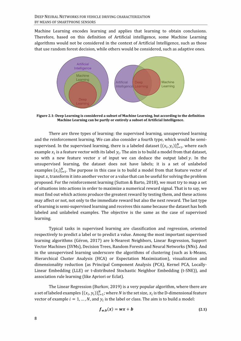
DEEP NEURAL NETWORKS FOR VEHICLE DRIVING CHARACTERIZATION BY MEANS OF SMARTPHONE SENSORS
8
Machine Learning encodes learning and applies that learning to obtain conclusions.
Therefore, based on this definition of Artificial intelligence, some Machine Learning
algorithms would not be considered in the context of Artificial Intelligence, such as those
that use random forest decision, while others would be considered, such as adaptive ones.
Figure 2.1: Deep Learning is considered a subset of Machine Learning, but according to the definition Machine Learning can be partly or entirely a subset of Artificial Intelligence.
There are three types of learning: the supervised learning, unsupervised learning
and the reinforcement learning. We can also consider a fourth type, which would be semi-
supervised. In the supervised learning, there is a labeled dataset {(𝑥𝑖 , 𝑦𝑖)}𝑖=1𝑁 , where each
example 𝑥𝑖 is a feature vector with its label 𝑦𝑖 . The aim is to build a model from that dataset,
so with a new feature vector 𝑥 of input we can deduce the output label 𝑦. In the
unsupervised learning, the dataset does not have labels; it is a set of unlabeled
examples {𝑥𝑖}𝑖=1𝑁 . The purpose in this case is to build a model from that feature vector of
input 𝑥, transform it into another vector or a value that can be useful for solving the problem
proposed. For the reinforcement learning (Sutton & Barto, 2018), we must try to map a set
of situations into actions in order to maximize a numerical reward signal. That is to say, we
must find out which actions produce the greatest reward by testing them, and these actions
may affect or not, not only to the immediate reward but also the next reward. The last type
of learning is semi-supervised learning and receives this name because the dataset has both
labeled and unlabeled examples. The objective is the same as the case of supervised
learning.
Typical tasks in supervised learning are classification and regression, oriented
respectively to predict a label or to predict a value. Among the most important supervised
learning algorithms (Géron, 2017) are k-Nearest Neighbors, Linear Regression, Support
Vector Machines (SVMs), Decision Trees, Random Forests and Neural Networks (NNs). And
in the unsupervised learning underscore the algorithms of clustering (such as k-Means,
Hierarchical Cluster Analysis (HCA) or Expectation Maximization), visualization and
dimensionality reduction (as Principal Component Analysis (PCA), Kernel PCA, Locally-
Linear Embedding (LLE) or t-distributed Stochastic Neighbor Embedding (t-SNE)), and
association rule learning (like Apriori or Eclat).
The Linear Regression (Burkov, 2019) is a very popular algorithm, where there are
a set of labeled examples {(𝑥𝑖 , 𝑦𝑖)}𝑖=1𝑁 ; where 𝑁 is the set size, 𝑥𝑖 is the D-dimensional feature
vector of example 𝑖 = 1, … , 𝑁, and 𝑦𝑖 is the label or class. The aim is to build a model:
𝒇𝒘,𝒃(𝒙) = 𝒘𝒙 + 𝒃 (2.1)

CHAPTER 2. INTRODUCTION TO DEEP NEURAL NETWORKS
9
which is a linear combination of features, with 𝑤 like a D-dimensional vector of
parameters and 𝑏 a real number. In order to predict the label 𝑦, we have to find the optimal
values of (𝑤∗, 𝑏∗), when the hyperplane is as close as possible to the training examples.
For instance, in the Figure 2.2 it is shown an example with one-dimensional cases
with green dots and regression line in red. This line fits as close as possible to the training
examples, so it can be used to predict a new value. In the case that the examples were vectors
with a dimension greater than 1, instead of a line it would be a plane for 𝐷 = 2, or a
hyperplane for 𝐷 > 2.
Figure 2.2: Example of Linear Regression. Image obtained from the book “The Hundred-Page Machine Learning Book” (Burkov, 2019).
In order to evaluate how good or bad the model is, it is necessary to use a
performance measure. If you want to evaluate how good the model is, you usually use a
utility function, or if you want to evaluate how bad it is, a cost function. If we use a cost
function we must therefore minimize it. Usually in Linear Regression, the average loss is
used as a cost function, which is the average of all penalties when the model is applied to
training data. To calculate the penalties it is normally used as loss function the squared error
loss (also known as mean squared error), (𝑓𝑤,𝑏(𝑥𝑖) − 𝑦𝑖)2
. Getting the following expression
to minimize:
𝟏
𝑵∑ (𝒇𝒘,𝒃(𝒙𝒊) − 𝒚𝒊)
𝟐𝒊=𝟏…𝑵 (2.2)
If 𝑦𝑖 is a binary, we would be in the case of a Logistic Regression, which despite its
name is a problem of classification and not regression. To get those outputs of 0 and 1, a
continuous function with domain (0, 1) is used, so if the value is close to 0, the negative label
is assigned and if the positive label is close to 1. A function that follows that requirement is
the sigmoid function 𝑓(𝑥) =1
1+𝑒−𝑥, obtaining the model to build as
𝒇𝒘,𝒃(𝒙) =𝟏
𝟏+𝒆−(𝒘𝒙+𝒃) (2.3)

DEEP NEURAL NETWORKS FOR VEHICLE DRIVING CHARACTERIZATION BY MEANS OF SMARTPHONE SENSORS
10
Another difference with Linear Regression, is that now instead of minimizing the
cost function, we try to maximize the likelihood. Therefore the optimization criterion is the
maximum likelihood:
𝑳𝒘,𝒃 = ∏ 𝒇𝒘,𝒃(𝒙𝒊)𝒚𝒊 (𝟏 − 𝒇𝒘,𝒃(𝒙𝒊))
(𝟏−𝒚𝒊)
𝒊=𝟏...𝑵 (2.4)
In order to avoid the numerical overflow, normally it is used the log-likelihood:
𝑳𝒐𝒈 𝑳𝒘,𝒃 = 𝐥𝐧(𝑳𝒘,𝒃(𝒙)) = ∑ [𝒚𝒊 𝐥𝐧 𝒇𝒘,𝒃(𝒙) + (𝟏 − 𝒚𝒊) 𝐥𝐧(𝟏 − 𝒇𝒘,𝒃(𝒙))]𝑵𝒊=𝟏 (2.5)
Among the most used optimization algorithms are the gradient descent or stochastic
gradient descent. The gradient descent (Géron, 2017) is an optimization algorithm used for
finding a minimum of a function. This algorithm tries to tweak parameters iteratively for
minimizing the cost function. It measures the local gradient of the error function with
regards to the parameters 𝑤 and 𝑏, and it goes in the direction of descending gradient. We
start at a random values of the parameters and we take proportional steps, trying each step
to decrease the cost function until it converges to the minimum (see Figure 2.3 a). The size
of the steps is called learning rate hyperparameter. If this hyperparameter is too small,
convergence may take a long time (Figure 2.3 b), if it is very high, we would jump across the
valley and end up on the other side (Figure 2.3 c) and maybe algorithm diverges. Another
type of common problem is to converge to a local minimum, which is not the global
minimum.
Figure 2.3: a) Gradient descent with a proper learning rate. b) Gradient descent with a too small learning rate. c) Gradient descent with a too high learning rate.
This optimization algorithm has many variants. For instance, the Minibatch
stochastic gradient descent (Burkov, 2019) that speeds up the computation because uses
smaller batches of the training data. Or the Adagrad, which scales the learning rate for each

CHAPTER 2. INTRODUCTION TO DEEP NEURAL NETWORKS
11
parameter. Also the Momentum, which orients the gradient in the relevant direction and
reduces the oscillations. Either RMSprop (Root Mean Square Propagation) or Adam
(Adaptive Moment Optimization) very used with the Neural Networks.
2.2. Introduction to Neural Networks
Neural Networks is an old idea, which came to be very widely used throughout the 1980’s
and 1990’s, but had fallen out of favor for a while (Ng, Cousera, Machine learning course,
2019). But thanks to the advance of graphics cards and the availability of large datasets,
nowadays, it is the state of the art technique for many different Machine Learning problems.
Neural Networks are algorithms that were originally motivated by the goal of having
machines that can mimic the brain. These were developed as simulating neurons or
networks of neurons in the brain. The neuron has a cell body (Figure 2.4) and a number of
input wires, called dendrites. These are like input wires, which receive inputs from other
locations. Neuron also has an output wire called axon, and this output wire is what it uses
to send signals to other neurons, that is to say, to send messages to other neurons. So, at a
simplistic level what a neuron is, is a computational unit that gets a number of inputs,
through it input wires, and does some computation and then, the outputs communicate via
its axon, to other nodes or to other neurons in the brain. The way that neurons communicate
with each other is with little pulses of electricity, they are also called spikes but that just
means pulses of electricity.
Figure 2.4: Neuron scheme1.
In artificial networks, every simple neuron is like a computational unit that behaves
as a logistic regression classifier. That it is to say, if we have the scheme shown in Figure 2.5
consisting of a neuron 𝑎, and we feed it with three inputs, the neuron will make a calculation
1 Image obtained from https://eversmarterworld.wordpress.com/2012/09/24/preserving-the-self-for-later-emulation-what-brain-features-do-we-need/

DEEP NEURAL NETWORKS FOR VEHICLE DRIVING CHARACTERIZATION BY MEANS OF SMARTPHONE SENSORS
12
and draw an output value. Mathematically, the neuron’s output is given by a function
hypothesis:
𝒇(𝒙) = 𝝈(𝑾𝒙 + 𝒃) (2.6)
In this example, 𝑥 = [𝑥1 𝑥2 𝑥3] is the input nodes; 𝑏 is the called bias unit or bias
neuron (𝑏 = 𝑥0), because 𝑥0 is equal to 1; 𝜎 is the activation function and 𝑊 = [𝑊1 𝑊2 𝑊3]
represents the parameters or weights associated to the model.
Figure 2.5: Neural Network with one neuron.
The bias neurons have the effect of increasing or lowering the input of the activation
function, depending on whether it is positive or negative, applying an affine transformation
to the output. The first layer is also called the input and the final layer the output layer.
Anything that isn't an input layer and isn't an output layer is known a hidden layer. Figure
2.6 shows the general scheme for a multilayer network; where 𝑎𝑖𝑙 is a neuron or activation
of unit 𝑖 in layer 𝑙.
Figure 2.6: Multilayer perceptron.
The particularity of the mathematical functions of Neural Networks is that they are
nested function (Burkov, 2019). In the case of a Neural Network of three layers, the function

CHAPTER 2. INTRODUCTION TO DEEP NEURAL NETWORKS
13
of the Neural Network will be as follows: 𝑓𝑁𝑁(𝑥) = 𝑓3 (𝑓2(𝑓1(𝑥))); with 𝑓1 and 𝑓2 as the
functions with the form seen above 𝑓𝑙(𝑧) = 𝜎𝑙(𝑊𝑙𝑧 + 𝑏𝑙), and 𝑓3 that can be a scalar function
for the regression task or also a vector function depending on the problem. 𝑙 is the layer
index, 𝜎 the activation function, 𝑊 the matrix of weights and 𝑏 the bias vector for each layer.
𝑊 and 𝑏 are parameters learned during the gradient descent in the optimization; and 𝜎 is
normally a nonlinear function. There are many types of activation functions (Graves, 2012);
some examples are shown below in Figure 2.7. One of most used is the sigmoid function
mentioned above 𝜎(𝑥) =1
1+𝑒−𝑥 and the hyperbolic tangent function 𝑡𝑎𝑛ℎ(𝑥) =𝑒2𝑥−1
𝑒2𝑥+1.
Figure 2.7: Activation functions.
How the neurons of a Neural Networks are connected is related to the learning
algorithm used for the network training. In general, there are three different classes of
network architectures (Haykin, 2009): single layer feedforward networks, multilayer
feedforward networks and recurrent networks. In the single layer feedforward networks,
there is an input layer of source nodes that projects directly onto an output layer of neurons,
but not vice versa; this net is strictly of a feedforward type; and there is a single layer,
referring to the output layer.
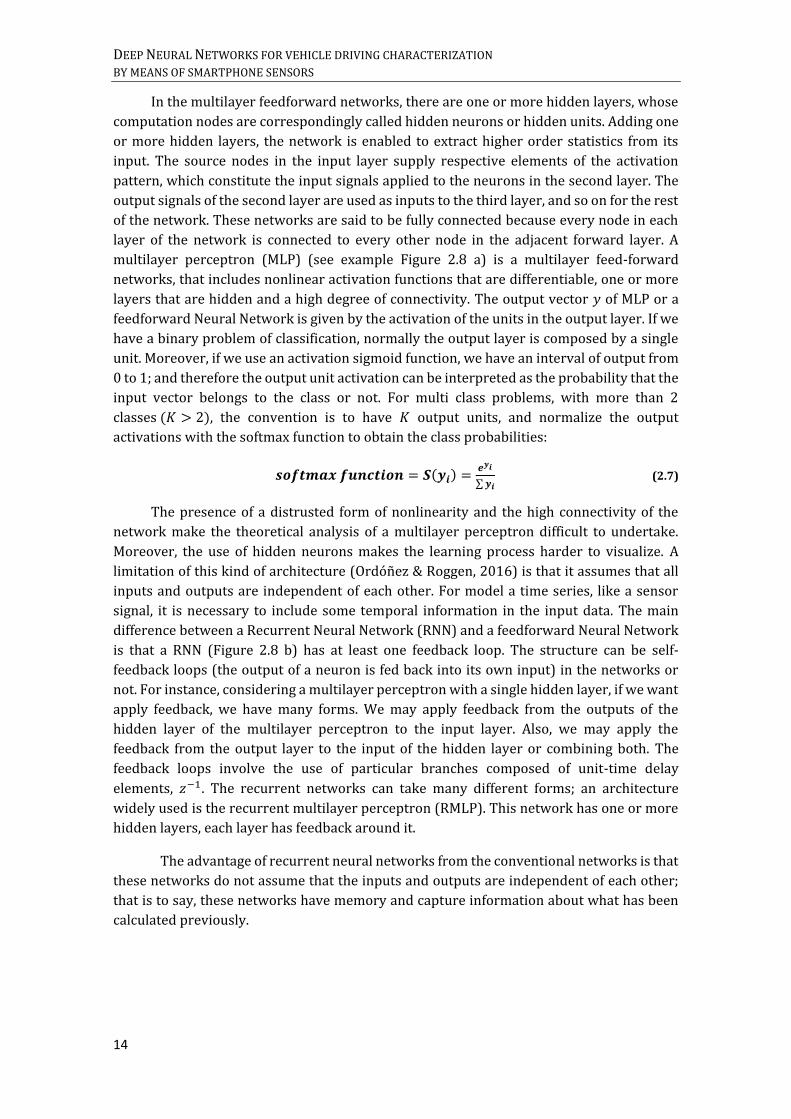
DEEP NEURAL NETWORKS FOR VEHICLE DRIVING CHARACTERIZATION BY MEANS OF SMARTPHONE SENSORS
14
In the multilayer feedforward networks, there are one or more hidden layers, whose
computation nodes are correspondingly called hidden neurons or hidden units. Adding one
or more hidden layers, the network is enabled to extract higher order statistics from its
input. The source nodes in the input layer supply respective elements of the activation
pattern, which constitute the input signals applied to the neurons in the second layer. The
output signals of the second layer are used as inputs to the third layer, and so on for the rest
of the network. These networks are said to be fully connected because every node in each
layer of the network is connected to every other node in the adjacent forward layer. A
multilayer perceptron (MLP) (see example Figure 2.8 a) is a multilayer feed-forward
networks, that includes nonlinear activation functions that are differentiable, one or more
layers that are hidden and a high degree of connectivity. The output vector 𝑦 of MLP or a
feedforward Neural Network is given by the activation of the units in the output layer. If we
have a binary problem of classification, normally the output layer is composed by a single
unit. Moreover, if we use an activation sigmoid function, we have an interval of output from
0 to 1; and therefore the output unit activation can be interpreted as the probability that the
input vector belongs to the class or not. For multi class problems, with more than 2
classes (𝐾 > 2), the convention is to have 𝐾 output units, and normalize the output
activations with the softmax function to obtain the class probabilities:
𝒔𝒐𝒇𝒕𝒎𝒂𝒙 𝒇𝒖𝒏𝒄𝒕𝒊𝒐𝒏 = 𝑺(𝒚𝒊) =𝒆𝒚𝒊
∑ 𝒚𝒊 (2.7)
The presence of a distrusted form of nonlinearity and the high connectivity of the
network make the theoretical analysis of a multilayer perceptron difficult to undertake.
Moreover, the use of hidden neurons makes the learning process harder to visualize. A
limitation of this kind of architecture (Ordóñez & Roggen, 2016) is that it assumes that all
inputs and outputs are independent of each other. For model a time series, like a sensor
signal, it is necessary to include some temporal information in the input data. The main
difference between a Recurrent Neural Network (RNN) and a feedforward Neural Network
is that a RNN (Figure 2.8 b) has at least one feedback loop. The structure can be self-
feedback loops (the output of a neuron is fed back into its own input) in the networks or
not. For instance, considering a multilayer perceptron with a single hidden layer, if we want
apply feedback, we have many forms. We may apply feedback from the outputs of the
hidden layer of the multilayer perceptron to the input layer. Also, we may apply the
feedback from the output layer to the input of the hidden layer or combining both. The
feedback loops involve the use of particular branches composed of unit-time delay
elements, 𝑧−1. The recurrent networks can take many different forms; an architecture
widely used is the recurrent multilayer perceptron (RMLP). This network has one or more
hidden layers, each layer has feedback around it.
The advantage of recurrent neural networks from the conventional networks is that
these networks do not assume that the inputs and outputs are independent of each other;
that is to say, these networks have memory and capture information about what has been
calculated previously.

CHAPTER 2. INTRODUCTION TO DEEP NEURAL NETWORKS
15
Figure 2.8: a) Example of fully connected feedforward network. b) Example of recurrent network.
2.3. Convolutional Neural Networks
Convolutional Neural Networks (CNNs) or CovNets are a type of Neural Network that share
their parameters across space, and are often used to process data with a known grid-like
topology (Goodfellow, Bengio, & Courville, 2016). For instance, it can be applied to time
series where the grid would be 1-D, or to images with 2-D pixel grids. The Figure 2.9 shows
an original image with a particular height and width, and its representation in the red, green
and blue channels, giving the image a depth, in this case 3.
Figure 2.9: Original image on the left and its respective decomposition in the RGB channels on the right.
Convolutional networks (Burkov, 2019) receive this name because they perform the
mathematical operation called convolution, in at least one of their layer, instead of matrix
multiplication. Each of the layers of the convolutional networks are made up of several

DEEP NEURAL NETWORKS FOR VEHICLE DRIVING CHARACTERIZATION BY MEANS OF SMARTPHONE SENSORS
16
convolution filters (also called kernels or patches), and each one also has the term bias that
must be added. For example, if we work with a 2-D image and a convolutional network of
one layer, each filter in the first layer will slide or convolve through the corresponding input
image, from left to right and top to bottom, and performing the convolution. In the Figure
2.10, there is an example of how the convolution would be performed on an image of 3x4,
with a filter of 2x2 and the associated bias. If we have 𝑁𝑙 filters in a given layer 𝑙, the output
of the convolutional layer 𝑙 will be a set of 𝑁𝑙 matrices. The size of the set of 𝑁𝑙 matrices is
called depth. In the case that the network has more convolutional layers, each layer will
consider the output of the previous layer as a collection or volume of image matrices.
Figure 2.10: Example of 2-D convolution.
The convolution of a volume of images with depth 𝐷 with a given filter, it will simply
be the sum of each of the convolutions. In the Figure 2.11 the result of a convolution applied
to a volume with depth 3 is shown.
Figure 2.11: Example of convolution with an input volume of depth 3.

CHAPTER 2. INTRODUCTION TO DEEP NEURAL NETWORKS
17
With the convolutional networks we form a kind of pyramid (Google course, 2019),
see Figure 2.12, where at the beginning we have an initial image size with some depth (in
the case of an RGB image, the depth will be 3). And after applying the convolutions, it will
go to progressively squeeze the spatial dimensions while increasing the depth, which
corresponds to the semantic complexity of the representation.
Figure 2.12: Spatial change of the dimensions of an image when applying 3 convolutional layers.
Both the filter matrices (one matrix for each filter in each layer) and the bias will be
parameters that will be optimized throughout the training process. In addition, after
carrying out the convolution and then adding the term bias, normally it is applied a
nonlinearity, such as the activation rectified linear unit (ReLU). ReLU is a nonlinear
activation function determined as 𝑓(𝑥) = max (𝑥, 0), which keeps a positive section and
reduces the negative section to zero (see Figure 2.13). Among the advantages of the ReLU
(Campesato, 2019) is that does not saturate in the positive region and models with ReLU
typically converge faster than those with other activation function.
Figure 2.13: ReLU activation function.
Therefore, hyperparameters that control the output volume in a convolutional
network are depth, stride and padding (Burkov, 2019). As we have commented, the depth

DEEP NEURAL NETWORKS FOR VEHICLE DRIVING CHARACTERIZATION BY MEANS OF SMARTPHONE SENSORS
18
is associated with the number of filters in the layer. The stride is the step size used for the
filter. That is, a stride of 1 in a 2-D image would involve moving only one pixel at a time. And
another hyperparameter is the padding. Padding is the width of the square of additional
cells with we surround the image, normally the additional cells are about zeros. If for
example the padding is 1, we will add a square of zeros around the border. Among the
reasons for using padding is that it allows controlling the spatial size of the output volumes
and doing a better scan of the boundaries of the image. Also, the output size will depend on
if we use a valid padding or a same padding. In the valid padding, the filter that moves
through the image, it does not go pass the edge of the image. In contrast to same padding,
where filter can go off the edge of the image and pad with zeros in such a way that the output
map size is exactly the same size as the input map size.
A technique widely utilized after the convolutional layer is to apply a pooling layer,
which also employs a filter with a moving window. The most common pooling layers are
max pooling and average pooling. To perform the pooling, we also have to choose the filter
size and the stride.
2.4. Recurrent Neural Networks
While convolutional networks share parameters across space in order to extract patterns,
Recurrent Neural Networks (RNNs) do it over time. They are normally used when the
attributes of the data are more dependent on each other; such as in text or speech
processing.
For instance, if we have a sequence of events over time (Google course, 2019), if the
sequence was stationary, the same classifier could be used at each instant of time. But if data
in each moment are related to each other, the past values must also be taken into account.
Recurrent networks will summarize the past and to provide that information to the
classifier. For that purpose, the classifiers will be connected to the input at every moment
of time and also at every moment of time we will have recurrent connections to the past.
In recurrent networks (Burkov, 2019) each unit 𝑢 of a given recurrent layer 𝑙, it has
a state ℎ𝑙,𝑢. This state can be understood as the memory of the unit. Each unit 𝑢 will receive
the state vector from the previous layer 𝑙 − 1 and the vector of states from this same layer
𝑙 from the previous time step. For example if training data is about text sentences, the input
matrix X will be formed by rows of feature vectors, 𝑋 = [
𝑥1
𝑥2
⋮𝑥𝐿
], with 𝑥𝑡 the feature vector in
the instant 𝑡 and 𝐿 the length of the sequence. In this case, each feature vector of input 𝑥𝑡
will be a word. Feature vectors will be read by the neural network sequentially in the order
of the time steps. In the Figure 2.14, the input sequence would consist of 4 feature vectors,
which in the case of text sentences correspond to 4 words. In order to update each status ℎ𝑙,𝑢𝑡
(at each time step 𝑡 in each unit 𝑢 of each layer 𝑙) we have to calculate a linear combination
of the input vector with the status from the previous time step ℎ𝑙,𝑢𝑡−1. To calculate this linear
combination, we use the parameters 𝑊 (in the Figure 2.14 would be the weight

CHAPTER 2. INTRODUCTION TO DEEP NEURAL NETWORKS
19
matrices 𝑊𝑥ℎ , 𝑊ℎℎ and 𝑊ℎ𝑦), and the final value ℎ𝑙,𝑢𝑡 is obtained by applying an activation
function after the linear combination. The output 𝑦𝑙𝑡 is normally a vector calculated for the
whole layer 𝑙 at once.
Figure 2.14: Example of a Recurrent Neural Network. Bias weights are omitted.
In the Figure 2.14, each time-stamp has an input, an output and hidden units
(Aggarwal, 2018). But according to the chosen application, it is possible missing inputs or
outputs at any particular time-stamp. For instance, the Figure 2.15 shows different
configuration examples (Karpathy, 2015). In the case of one to one, we go from fixed input
size to fixed output size, such as in image classification. In one to many, each input vector
can produce several outputs, such as when an image is translated into text. In many to one,
the process is the opposite, such as when a phrase is translated into a positive or negative
rating. Finally, in many to many (where the inputs and outputs can be synchronized or not),
is employed for example in translation or in video classification where we wish to label each
frame of the video.
Figure 2.15: Different configurations of recurring networks.

DEEP NEURAL NETWORKS FOR VEHICLE DRIVING CHARACTERIZATION BY MEANS OF SMARTPHONE SENSORS
20
In order to calculate the parameters of the recurrent network, we use the gradient
descent with backpropagation, specifically its use a special version of backpropagation
called backpropagation through time (BPTT).
2.4.1. Bidirectional Networks
For particular tasks, such as in applications of handwriting recognition, it is necessary to
access both past and future information (Graves, 2012). The Bidirectional Recurrent Neural
Networks (BRNN) offer a solution to this problem, since each training sequence goes
through two separate recurrent hidden layers, one forward and other backward connected
both to the same output layer (see Figure 2.16). Therefore, there are two separate states
ℎ𝑡(𝑓)
and ℎ𝑡(𝑏)
, for the forward and backward directions respectively (Aggarwal, 2018). Both
states receive input from the same vector and interact with the same output vector,
nevertheless ℎ𝑡(𝑓)
interact in the forwards direction, while ℎ𝑡(𝑏)
interact in the backwards
direction. In the same way, there are matrices of separate parameters for the forward and
backward. With 𝑊𝑥ℎ(𝑓)
, 𝑊ℎℎ(𝑓)
and 𝑊ℎ𝑦(𝑓)
for the input-hidden, hidden-hidden and hidden-
output forward matrices; and 𝑊𝑥ℎ(𝑏)
, 𝑊ℎℎ(𝑏)
and 𝑊ℎ𝑦(𝑏)
for the backward matrices. The
bidirectional equations are as follows:
𝒉𝒕(𝒇)
= 𝒕𝒂𝒏𝒉 (𝑾𝒙𝒉(𝒇)
𝒙𝒕 + 𝑾𝒉𝒉(𝒇)
𝒉𝒕−𝟏(𝒇)
)
𝒉𝒕(𝒃)
= 𝒕𝒂𝒏𝒉 (𝑾𝒙𝒉(𝒃)
𝒙𝒕 + 𝑾𝒉𝒉(𝒃)
𝒉𝒕+𝟏(𝒃)
)
𝒚𝒕 = 𝑾𝒉𝒚(𝒇)
𝒉𝒕(𝒇)
+ 𝑾𝒉𝒚(𝒃)
𝒉𝒕(𝒃)
(2.8)
Figure 2.16: Example of bidirectional network.

CHAPTER 2. INTRODUCTION TO DEEP NEURAL NETWORKS
21
2.4.2. Long Short-Term Memory
There are variations of the RNN which have turned out to be very effective models, such as
Gated Recurrent Neural Networks. These architectures include the Long Short-Term
Memory (LSTM) and the Gated Recurrent Unit (GRU).
Among the advantages of LSTM (Gers, Schraudolph, & Schmidhuber, Learning
precise timing with LSTM Recurrent Networks, 2002) versus the traditional RNNs are that
the LSTM works better on problems involving long time lags.
The traditional scheme of an LSTM is shown in the Figure 2.17. The basic unit in a
LSTM network is the memory block. The memory block can have one or more memory cells
and three adaptive, multiplicative gating units shared by all cells in the block. Moreover,
each memory cell has at its core a recurrently self-connected linear unit called Constant
Error Carousel (CEC), whose activations are called cell states. The input, forget and output
gate can be trained to learn respectively, what information to store in the memory, how long
to store it and when to read it out. When gates are closed (Gers, Schmidhuber, & Cummins,
Learning to forget: continual prediction with LSTM, 1999), the activations are around zero,
so irrelevant inputs and noise do not pass to the cell, and therefore the cell state does not
disturb the remainder of the network.
Figure 2.17: Traditional LSTM memory block with one cell. Image adapted from (Greff, Srivastava, Jan Koutník, Steunebrink, & Schmidhuber, 2015).
As (Gers, Schraudolph, & Schmidhuber, Learning precise timing with LSTM
Recurrent Networks, 2002) mention, one of the limitations of the LSTM is that each gate
receives connections from the input units and the outputs of all cells, but there is no direct
connection from the CEC. The same happens if several cells are present; when the output

DEEP NEURAL NETWORKS FOR VEHICLE DRIVING CHARACTERIZATION BY MEANS OF SMARTPHONE SENSORS
22
gate is closed none of the gates has access to the CECs they control. For these reasons a
variant was introduced, the LSTM with Peephole Connections (see Figure 2.18), which
consists of adding weighted peephole connections from the CEC to the gates of the same
memory block. So when the output gates are closed, all gates can continue consulting the
current state.
Figure 2.18: LSTM memory block with one cell and with peephole connections. Image obtained from (Greff, Srivastava, Jan Koutník, Steunebrink, & Schmidhuber, 2015).
The vector formulas for a LSTM layer forward pass are the following (Greff,
Srivastava, Jan Koutník, Steunebrink, & Schmidhuber, 2015):
𝒛𝒕 = 𝒕𝒂𝒏𝒉(𝑾𝒛𝒙𝒕 + 𝑹𝒛𝒚𝒕−𝟏 + 𝒃𝒛) block input (2.9)
𝒊𝒕 = 𝝈(𝑾𝒊𝒙𝒕 + 𝑹𝒊𝒚𝒕−𝟏 + 𝒑𝒊 ⊙ 𝒄𝒕−𝟏 + 𝒃𝒊) input gate (2.10)
𝒇𝒕 = 𝝈(𝑾𝒇𝒙𝒕 + 𝑹𝒇𝒚𝒕−𝟏 + 𝒑𝒇 ⊙ 𝒄𝒕−𝟏 + 𝒃𝒇) forget gate (2.11)
𝒄𝒕 = 𝒛𝒕 ⊙ 𝒊𝒕 + 𝒄𝒕−𝟏 ⊙ 𝒇𝒕 cell state (2.12)
𝒐𝒕 = 𝝈(𝑾𝒐𝒙𝒕 + 𝑹𝒐𝒚𝒕−𝟏 + 𝒑𝒐 ⊙ 𝒄𝒕 + 𝒃𝒐) output gate (2.13)
𝒚𝒕 = 𝒕𝒂𝒏𝒉(𝒄𝒕) ⊙ 𝒐𝒕 block output (2.14)
With 𝑥𝑡 like the input vector at time 𝑡. And 𝑊𝑧 , 𝑊𝑖 , 𝑊𝑓 and 𝑊𝑜as the input weights;
𝑅𝑧, 𝑅𝑖 , 𝑅𝑓 and 𝑅𝑜 as the recurrent weights; 𝑝𝑖 , 𝑝𝑓 and 𝑝𝑜 as the peephole weight; and, 𝑏𝑧,
𝑏𝑖 , 𝑏𝑓 and 𝑏𝑜as the bias weights. The non-linear activation functions are usually the
hyperbolic tangent (tanh) and the logistic sigmoid, 𝜎(𝑥). The symbol ⊙ indicates the
element-wise vector product.
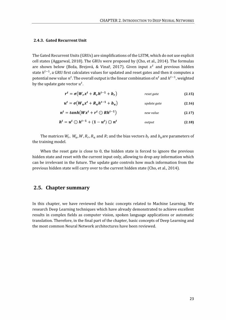
CHAPTER 2. INTRODUCTION TO DEEP NEURAL NETWORKS
23
2.4.3. Gated Recurrent Unit
The Gated Recurrent Units (GRUs) are simplifications of the LSTM, which do not use explicit
cell states (Aggarwal, 2018). The GRUs were proposed by (Cho, et al., 2014). The formulas
are shown below (Boža, Brejová, & Vinař, 2017). Given input 𝑥𝑡 and previous hidden
state ℎ𝑡−1, a GRU first calculates values for updated and reset gates and then it computes a
potential new value 𝑛𝑡 . The overall output is the linear combination of 𝑛𝑡 and ℎ𝑡−1, weighted
by the update gate vector 𝑢𝑡 .
𝒓𝒕 = 𝝈(𝑾𝒓𝒙𝒕 + 𝑹𝒓𝒉𝒕−𝟏 + 𝒃𝒓) reset gate (2.15)
𝒖𝒕 = 𝝈(𝑾𝒖𝒙𝒕 + 𝑹𝒖𝒉𝒕−𝟏 + 𝒃𝒖) update gate (2.16)
𝒏𝒕 = 𝒕𝒂𝒏𝒉(𝑾𝒙𝒕 + 𝒓𝒕 ⊙ 𝑹𝒉𝒕−𝟏) new value (2.17)
𝒉𝒕 = 𝒖𝒕 ⊙ 𝒉𝒕−𝟏 + (𝟏 − 𝒖𝒕) ⊙ 𝒏𝒕 output (2.18)
The matrices 𝑊𝑟 , 𝑊𝑢 , 𝑊, 𝑅𝑟 , 𝑅𝑢 and 𝑅; and the bias vectors 𝑏𝑟 and 𝑏𝑢are parameters of
the training model.
When the reset gate is close to 0, the hidden state is forced to ignore the previous
hidden state and reset with the current input only, allowing to drop any information which
can be irrelevant in the future. The update gate controls how much information from the
previous hidden state will carry over to the current hidden state (Cho, et al., 2014).
2.5. Chapter summary
In this chapter, we have reviewed the basic concepts related to Machine Learning. We
research Deep Learning techniques which have already demonstrated to achieve excellent
results in complex fields as computer vision, spoken language applications or automatic
translation. Therefore, in the final part of the chapter, basic concepts of Deep Learning and
the most common Neural Network architectures have been reviewed.


25
Chapter 3
Definitions and databases
s we mentioned in Chapter 1, the objective of the Thesis is the driving
characterization through the use of low-energy sensors on the smartphones,
specifically accelerometers. To perform this task, we believe it is important to clarify
some concepts, which we have reviewed in this chapter. First of all, we will present a brief
introduction to the most common motion sensors in these devices, Section 3.1. Then, we
will explain terminology employed and frequent procedures used throughout the Thesis,
Section 3.2, as well as specifications on the database and the software and hardware used,
Section 3.3.
3.1. Introduction to smartphone motion sensors for driving
characterization
Motion sensors, also known as motion detectors, allow to detect and to capture physical and
kinetic movements. Current smartphones have commonly a wide range of sensors (Figure
2.19), both motion sensors and location sensors. Accelerometers, gyroscopes or
magnetometers are among the most common motion sensors, while Global Positioning
System (GPS) is the most representative location sensor.
Accelerometers were introduced for the first time into smartphones on Apple
iPhone in 2007 to improve the user experience, rotating automatically the screen to match
device orientation. As (Vargha & Maia, 2010) explains, accelerometers measure the linear
acceleration, produced by gravity or by translation (movement), and the tilt angle.
Normally, typical consumer devices include 3-axis accelerometers (X, Y and Z axes) with
measurement ranges from ±1𝑔 (±9.8 𝑚/𝑠2) to ±8𝑔. One of the main limitations of
accelerometers is that they do not distinguish gravity from other specific accelerations and
translations; and also that the orientation works well when the axes of the accelerometers
are aligned with the gravity vector. However, if the axes are perpendicular to gravity vector,
it is necessary another sensor, like the gyroscope, to determine orientation changes.
A

DEEP NEURAL NETWORKS FOR VEHICLE DRIVING CHARACTERIZATION BY MEANS OF SMARTPHONE SENSORS
26
Figure 2.19: Common motion and location sensors present in smartphones.
Gyroscopes measures angular speeds and appeared on smartphones with the
iPhone 4 in 2010, which included a 3-axis gyroscope that allowed measuring pitch, roll, yaw
and rotation on gravity. As commented in the presentation of the iPhone 4, the gyroscope
together with the accelerometer provide 6-axis motion sensing, resolving some situations
in which accelerometers are more limited, such as rotation around gravity. Therefore,
gyroscopes (Vargha & Maia, 2010) measure the angular rate of velocity (rotation). An
important difference with accelerometers is that they are not affected by gravity, for this
reason gyroscopes are combined with accelerometers in order to separate gravity, linear
motion and rotational motion.
Also there are other common sensors in smartphones, such as the magnetic
compass. Magnetometers quantify magnetic fields and can be used to obtain heading (yaw
orientation) using magnetic north as reference. The main limitation of compass is that they
do not only respond to the earth’s magnetic field, but also to external noisy interferences,
like radio frequency signals or magnetic fields produced by magnets. Moreover, the earth’s
magnetic field can be often distorted indoors by building materials with iron.
As mentioned above, current smartphones have location sensors such as GPS, which
help to obtain the position and the heading. The summarized idea of GPS operation is as
follows. The GPS receiver gets signals from satellites in orbit. By means of the time
difference between the satellites transmitting the signal with the receivers obtaining it, it is
possible to establish how far they are from the satellites. The position of the satellites is
known; therefore with this and with the elapsed time, we can determine the receiver GPS
position in the three dimensions: east, north and altitude. To obtain this information, we
need at least the communication with three satellites, but for an accurate time calculation
and therefore an accurate position calculation, it is necessary the signals of a fourth satellite
(with the signals of four satellites the necessary equations of time can be solved without the
help of atomic clocks).
The use of these motion sensors is very demanded for tasks of detection or
recognition of activities, for instance for human caring systems or health and fitness

CHAPTER 3. DEFINITIONS AND DATABASES
27
monitoring. In works like (Hong, Kim, Ahn, & Kim, 2008), they already tried to recognize
daily living activities carried out by a person with wearable sensors, using in particular
accelerometers and RFID sensors. By means of accelerometers placed in the thigh, waist and
wrist of the users, they tried to classify 5 human body states (standing, lying, sitting, walking
and running). They also performed an RFID tagged of some objects to obtain additional
information about hand-motion (like reading, brushing hair, taking photos, etc.).
With the coming and development of smartphones, they gradually have been used
for the capture of different signals through the sensors that they have incorporated,
included for the monitoring of activities. Because of the fact that current smartphones have
grown in computing, networking and sensing-power. Table 2.1 shows a list with some of
the most common sensors that appear on smartphones (Ali, Khusro, Rauf, & Mahfooz,
2014).
Table 2.1: Common sensors in mobile phone systems.
Category Sensors
Tactile sensors Proximity sensor
Acceleration sensors Accelerometer, gyroscope
Thermal sensors Temperature sensor
Image sensors CMOS Camera sensor
Light sensors Ambient light sensor, back-illuminated sensor
Water sensors Moisture sensor, humidity sensor
Location sensors Compass, GPS
Height sensors Altimeter, barometer
Medical sensors Heart rate monitor sensor, biosensor
Acoustic sensors Microphone
Radio sensors Bluetooth, RFID
Time sensors Clock sensor
Beyond smartphones sensors are also commonly found in other wearable devices
such as smartwatches and bands. For instance, in (Zhang, et al., 2019) a tri-axial
accelerometer worn in a wrist smartwatch was used to collect a dataset, called Sanitation,
directed to identify between a set of seven types of daily work activity of sanitation workers
(walking, running, broom sweeping, sweeping, cleaning, dumping and daily activities like
sitting and smoking).
The fields in which sensors can be used are very large. At present, one notable area
is the characterization of driving, assistance systems or the world of self-driving or
autonomous cars. Driving characterization is frequently used in studies of driver behavior
and in analysis of external factors that may influence in this behavior, both for energy
efficiency and safety goals. Driver assistance systems are already a reality, incorporated into
most vehicles to increase road safety, provide frontal collision warning systems, lane change
assistants or cooperative adaptive cruise control (de Ponte Müller, Martín Navajas, & Strang,
2013). The concept of self-driving or autonomous car is based on cars that can operate
without the control and continuous supervision of a person. There are several autonomous
driving classifications adopted by the International Society of Automotive Engineers (SAE,
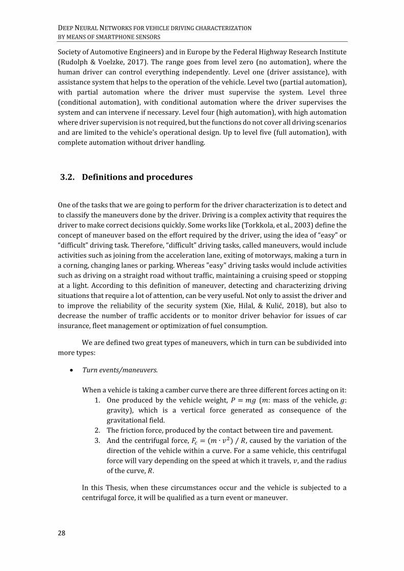
DEEP NEURAL NETWORKS FOR VEHICLE DRIVING CHARACTERIZATION BY MEANS OF SMARTPHONE SENSORS
28
Society of Automotive Engineers) and in Europe by the Federal Highway Research Institute
(Rudolph & Voelzke, 2017). The range goes from level zero (no automation), where the
human driver can control everything independently. Level one (driver assistance), with
assistance system that helps to the operation of the vehicle. Level two (partial automation),
with partial automation where the driver must supervise the system. Level three
(conditional automation), with conditional automation where the driver supervises the
system and can intervene if necessary. Level four (high automation), with high automation
where driver supervision is not required, but the functions do not cover all driving scenarios
and are limited to the vehicle's operational design. Up to level five (full automation), with
complete automation without driver handling.
3.2. Definitions and procedures
One of the tasks that we are going to perform for the driver characterization is to detect and
to classify the maneuvers done by the driver. Driving is a complex activity that requires the
driver to make correct decisions quickly. Some works like (Torkkola, et al., 2003) define the
concept of maneuver based on the effort required by the driver, using the idea of “easy” or
“difficult” driving task. Therefore, “difficult” driving tasks, called maneuvers, would include
activities such as joining from the acceleration lane, exiting of motorways, making a turn in
a corning, changing lanes or parking. Whereas "easy" driving tasks would include activities
such as driving on a straight road without traffic, maintaining a cruising speed or stopping
at a light. According to this definition of maneuver, detecting and characterizing driving
situations that require a lot of attention, can be very useful. Not only to assist the driver and
to improve the reliability of the security system (Xie, Hilal, & Kulić, 2018), but also to
decrease the number of traffic accidents or to monitor driver behavior for issues of car
insurance, fleet management or optimization of fuel consumption.
We are defined two great types of maneuvers, which in turn can be subdivided into
more types:
Turn events/maneuvers.
When a vehicle is taking a camber curve there are three different forces acting on it:
1. One produced by the vehicle weight, 𝑃 = 𝑚𝑔 (𝑚: mass of the vehicle, 𝑔:
gravity), which is a vertical force generated as consequence of the
gravitational field.
2. The friction force, produced by the contact between tire and pavement.
3. And the centrifugal force, 𝐹𝑐 = (𝑚 ∙ 𝑣2) ⁄ 𝑅, caused by the variation of the
direction of the vehicle within a curve. For a same vehicle, this centrifugal
force will vary depending on the speed at which it travels, 𝑣, and the radius
of the curve, 𝑅.
In this Thesis, when these circumstances occur and the vehicle is subjected to a
centrifugal force, it will be qualified as a turn event or maneuver.
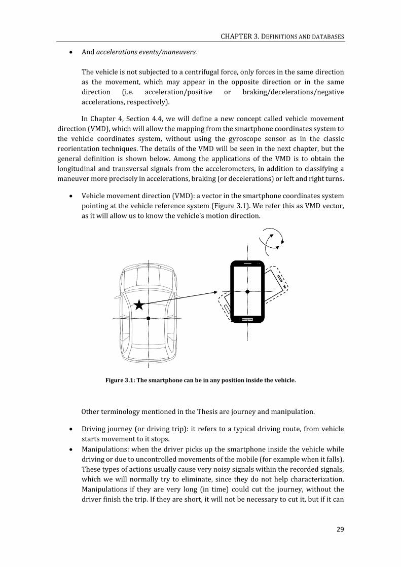
CHAPTER 3. DEFINITIONS AND DATABASES
29
And accelerations events/maneuvers.
The vehicle is not subjected to a centrifugal force, only forces in the same direction
as the movement, which may appear in the opposite direction or in the same
direction (i.e. acceleration/positive or braking/decelerations/negative
accelerations, respectively).
In Chapter 4, Section 4.4, we will define a new concept called vehicle movement
direction (VMD), which will allow the mapping from the smartphone coordinates system to
the vehicle coordinates system, without using the gyroscope sensor as in the classic
reorientation techniques. The details of the VMD will be seen in the next chapter, but the
general definition is shown below. Among the applications of the VMD is to obtain the
longitudinal and transversal signals from the accelerometers, in addition to classifying a
maneuver more precisely in accelerations, braking (or decelerations) or left and right turns.
Vehicle movement direction (VMD): a vector in the smartphone coordinates system
pointing at the vehicle reference system (Figure 3.1). We refer this as VMD vector,
as it will allow us to know the vehicle's motion direction.
Figure 3.1: The smartphone can be in any position inside the vehicle.
Other terminology mentioned in the Thesis are journey and manipulation.
Driving journey (or driving trip): it refers to a typical driving route, from vehicle
starts movement to it stops.
Manipulations: when the driver picks up the smartphone inside the vehicle while
driving or due to uncontrolled movements of the mobile (for example when it falls).
These types of actions usually cause very noisy signals within the recorded signals,
which we will normally try to eliminate, since they do not help characterization.
Manipulations if they are very long (in time) could cut the journey, without the
driver finish the trip. If they are short, it will not be necessary to cut it, but if it can

DEEP NEURAL NETWORKS FOR VEHICLE DRIVING CHARACTERIZATION BY MEANS OF SMARTPHONE SENSORS
30
cause the division of the journey into two subjourneys if the mobile changes its
position, since the VMD will change for each one of them.
For some procedures, the angle between two vectors will be calculated, as well as
the most representative vector within a set of vectors.
Angle between two vectors: calculation of the angle is done through scalar product
between two vectors (see example of Figure 3.2).
Figure 3.2: 3D vectors and formula to calculate angle between two vectors.
Representative vector within a set of vectors: For the calculation of this final
direction vector, which represents the average addresses of a cluster, we have
developed the method described below. The aim of the algorithm is to look for
vector clusters separated less than a maximum angle, to obtain a final direction
vector, which represents the average addresses of the clusters. And it is mainly
based on two ideas; the separation angle among the vectors and the number of
vectors. The process is the following:
1. We choose the vector (blue vector Figure 3.3 a)) that has the largest angle of
separation with any of the other vectors. In order to calculate the angle of
separation between vectors we create a matrix of angles, applying the above
mentioned formula. This vector will be the starting point (orange point
Figure 3.3 a)) for creating the sphere of minimum values (magenta circle
Figure 3.3 a)).
2. From this vector, we form a 3D sphere of minimum angles by looking for the
closest vector (magenta circle Figure 3.3 a)). This generates a path that will
go over through all the vectors (purple circle Figure 3.3 a)).
3. Taking into account the route of minimum angles, we group the vectors to
form clusters of vectors separated less than a maximum angle (green
clusters Figure 3.3 b)).

CHAPTER 3. DEFINITIONS AND DATABASES
31
4. For each cluster, we count the number of vectors. The cluster with the
biggest number will be taken as the final cluster and the definitive vector
direction (red vector Figure 3.3 c)) will be calculated as mean of all vectors
inside that cluster.
The purpose of the algorithm may vary depending on the application, in some cases
it may interest not to calculate a single direction for a set of vectors, but a direction for each
of the clusters.
Figure 3.3: Steps for creation of the minimum sphere. a) Minimum angles; b) Clusters with vectors separated less than a maximum angle; c) Good cluster and final direction.
The importance of driver recognition has reached many areas. Navigation
companies like TomTom already offer driver identification services. As they indicate, when
the vehicle is shared, the identification of the driver allows knowing who has the car or how
much time they spend on the road or in some place (Telematics, 2018). Companies that are
dedicated to fleet management, where it is important to know who is driving the vehicle to
provide personalized information, usually use methods that require physical devices in the
vehicle, such as card readers. Due to this interest, another task that will be carried out in the
DEEP NEURAL NETWORKS FOR VEHICLE DRIVING CHARACTERIZATION BY MEANS OF SMARTPHONE SENSORS
32
Thesis will be the recognition of the driver, both from the point of view of driver
identification and driver verification.
Driver identification: the driver classification within a close-set of drivers.
Driver verification: to check that a driver is really who she/he claims to be.
3.3. Database and hardware/software specifications
The use of sensors in the field of driving is growing in recent years due to the many
applications and benefits they can offer. From tasks oriented to safety, such as studying the
driver behavior for reducing the number of accidents, to autonomous driving, in order to
ensure that the vehicle can function correctly in all possible circumstances on a road. For all
these possible fields, the sensors are combined with sophisticated algorithms.
Among the possible set of sensors present in smartphones, we have decided to use
accelerometers to the driver characterization. Both the database used in the Chapter 4 for
the maneuvers characterization, TIDrivies_Maneuvers, and the database used in the Chapter
5 for the driver recognition, TIDrivies_IdenVer, have been provided by Telefónica R&D and
the spin-off of Telefónica R&D, Drivies, in a collaboration project with the Signal Processing
Applications Group (GAPS), of the Department of Signals, Systems and
Radiocommunications, “E.T.S.I. de Telecommunication”, “Universidad Politécnica de
Madrid”.
1. Database for the characterization of maneuvers, which we have called
TIDrivies_Maneuvers. More than 60000 real driving journeys have been collected
through the sensors present in smartphones, from more than 3000 different drivers.
The journeys have been recorded by both terminals with iOS and Android operating
systems. The main signals captured by these terminals have been accelerometers,
gyroscope (in the terminals that present this sensor) and GPS (only a few samples,
to limit excessive battery consumption during capture). Both the accelerometer and
gyroscope signals have been recorded at a frequency of 5 Hz. The set of journeys is
heterogeneous, with both urban, non-urban and mixed trips. Although the objective
is to perform these tasks with the exclusive use of the tri-axial accelerometer signals,
other sensors have been collected in order to verify that our results are consistent.
2. Database for driver identification and verification, named TIDrivies_IdenVer. It is a
specific database for these tasks. For each journey by car, there are the signals
captured by the smartphone sensors plus the signals recorded by OBD (On Board
Diagnostics) devices, specifically installed in the corresponding vehicles. It consists
of more than 23000 journeys of 83 drivers. The number of journeys per driver is
variable; around 50 drivers have more than 100 trips, more than 36 drivers have
more than 200 trips, of which 20 of them have more than 500 trips. Like in the
previous database, the analysis will be carried out exclusively with the
accelerometer signals, but the OBD information is needed, both for the labeling and
verification process.
CHAPTER 3. DEFINITIONS AND DATABASES
33
This Thesis focuses on the use of accelerometer sensors to perform driving
characterization tasks, as well as using Deep Learning instead of more traditional
techniques. The reason for using Deep Networks is that these allow reducing feature
engineering and to adapt more easily than many classic processing techniques. This fact has
caused that these are frequently implemented in tasks such as image classification, speaker
recognition or language translation. To implement Deep Learning models/architectures,
the main hardware and software used in the Thesis are specified below:
Nvidia Tesla K80 graphic card (dual GPU card, with 24 GB of GDDR5 memory, 480
GB/s of memory bandwidth and 4992 CUDA cores).
Development language: Python.
Deep learning open source software library: TensorFlow and Keras.
3.4. Chapter summary
In this chapter, a review of some of the most employed motion sensors in mobile devices
has been presented. Although current smartphones have both physical and virtual sensors;
in our case we want to emphasize the importance of physical sensors, which are hardware-
based sensors embedded directly into mobiles, and, more specifically, the motion sensors
used to obtain data directly measuring a kinetic characteristic. These sensors are being
widely used for many movement detection or recognition activities. In this work we will
contribute to the study of the use of the accelerometers in the area of the driving
characterization.
We have also defined in this chapter the most frequent concepts and habitual
procedures used throughout the Thesis, as well as we have presented the databases created
for the characterization and the specifications of the hardware and software employed.

35
Chapter 4
Driving maneuvers characterization
riving style influences many important factors such as safety, fuel or battery
consumption, gas emissions or traffic state, among others. Driving characterization
is deeply related to how drivers perform specific maneuvers or driving events. The
objective of this chapter is to propose several methods for driving maneuvers
characterization based on the processing of accelerometer signals recorded from drivers’
smartphones. As it is a main objective in this Thesis, the reason for relying only on
smartphones accelerometers is to promote the development of mobile phone applications
requiring low battery consumption.
The maneuvers of a vehicle are mainly concerned with the longitudinal and
transversal forces to the driving direction, and these forces are relatively easy to measure
with a smartphone, if the device is located in a fixed position inside the vehicle. As in our
case the mobile can be in any arbitrary position, we address the characterization of the
maneuvers through two different approaches. The first one makes a more general
classification of driving events, simply relating the maneuvers to two types, longitudinal and
transversal classes. This approach can be interesting to classify drivers based on
aggressiveness (risky and safe drivers), for car insurances or for battery consumption in
electric vehicles, among others. The second one performs a more precise classification,
distinguishing between positive and negative accelerations (i.e. acceleration and braking),
and between right and left turns. These types of solutions can be interesting, for instance,
for connecting the road with driving or for route reconstruction applications. Both
approaches are based on the use of the 3-axial accelerometer signals from a smartphone
with Neural Networks, proposing different Deep Learning models to face these tasks.
4.1. Related works in driving maneuver characterization
Driving characterization methods are usually based on maneuvers identification. In these
cases, the identification of maneuvers or events is a preliminary step, which leads to a
further driver behavior classification according to different criteria such as aggressiveness
(aggressive maneuvers or not). For instance, in (Eren, Makinist, Akın, & Yilmaz, 2012)
smartphone sensors as accelerometers, gyroscopes and magnetometers, are used to
D

DEEP NEURAL NETWORKS FOR VEHICLE DRIVING CHARACTERIZATION BY MEANS OF SMARTPHONE SENSORS
36
differentiate between risky and safe drivers. To do this, after an endpoint detection
algorithm, they estimate the amplitude range of sensor signals for detecting the most
important events using Dynamic Time Warping (DTW) and finally a Bayesian classifier for
maneuvers classification. In this work, authors mention the advantages of using
smartphones instead of external or vehicles sensors: “This choice provides us with a portable
setup, such that changing vehicles will not affect the portability of the system.” A major
limitation of this work is that templates for the events must be manually selected and
labeled, and due to the maneuvers have different durations, they need to employ the DTW.
Another limitation is that the phone must be placed in a fixed position inside the vehicle, so
they have the same reference system for all terminals.
Another work which uses the DTW for driving style recognition is (Johnson &
Trivedi, 2011). This work presents a platform called MIROAD (A Mobile Sensor-Platform
for Intelligent Recognition of Aggressive Driving), in order to determine the driver style, to
discriminate between non-aggressive and aggressive based on the recognition of different
types of events. Although they do not use extra equipment, only the smartphone with an
App installed, they employ several sensors: accelerometer, gyroscope, magnetometer, GPS
and camera. To detect the maneuvers they utilize endpoint detection algorithms with
thresholds that mark the beginning and end of events. For the classification, they compare
the maneuvers with templates using the DTW, and the template with the lowest warping
path cost is the closest match.
Current works like (Al-Din, 2018) also employ techniques such as the endpoint
detection algorithm followed by DTW for the identification and classification of events. They
identify 10 different types of maneuvers: acceleration straight road segment, acceleration
curved road segment, braking straight road segment, braking curved road segment, left lane
change straight road segment, left lane change curved road segment, right lane change
straight road segment, right lane change curved road segment, merging into highway and
exit from highway. To evaluate the abnormality level of an event (in hard, normal and light
maneuvers), they employ a specific feed-forward neural network (FFNN) classifier. The
signals used are the accelerometer, the gyroscope and the magnetometer of drivers’
smartphones. They also perform a transformation of the sensors data from the smartphone
coordinate system to the vehicle coordinate system.
The work presented by (Ferreira Júnior, et al., 2017) evaluates the performance of
multiple combinations of machine-learning algorithms, such as support vector machines
(SVM) or random forest (RF), applied in the motion sensors of Android smartphones to
detect aggressive driving events. Data used were recorded only by a smartphone, Motorola
XT1058, in a fixed position inside the same car. In total, they had 4 car trips of 13 min each,
done by two different drivers. Because they work with a small database, traditional machine
learning algorithms are a good solution for driving events detection. However, with larger
databases, it can be expected that Deep Learning techniques offer higher recognition
results. In fact, in a more recent work by the same authors (Carvalho, et al., 2017) they use
the same database to apply Deep Learning and to compare the benefits with different RNN
schemes. In their empirical evaluation, the Gated Recurrent Unit (GRU) was the most
reliable RNN to be deployed with the accelerometer data; the long short-term memory
(LSTM) and the simple RNN have a greater difference depending on the numbers of
neurons.
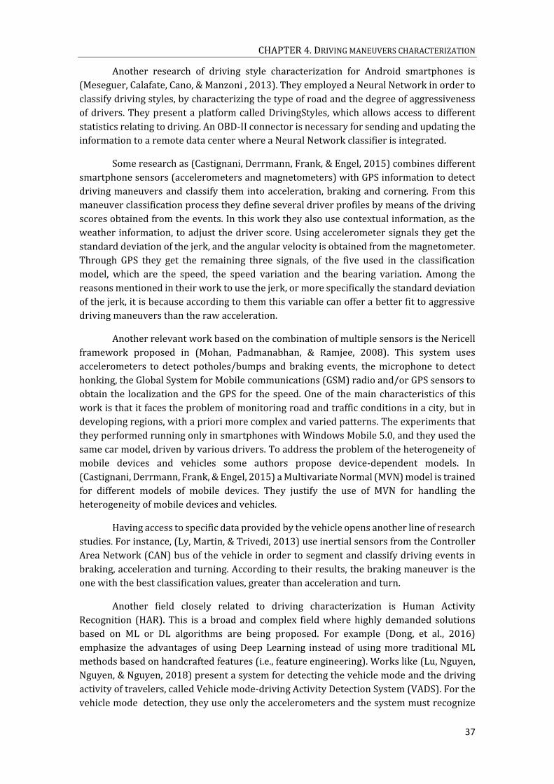
CHAPTER 4. DRIVING MANEUVERS CHARACTERIZATION
37
Another research of driving style characterization for Android smartphones is
(Meseguer, Calafate, Cano, & Manzoni , 2013). They employed a Neural Network in order to
classify driving styles, by characterizing the type of road and the degree of aggressiveness
of drivers. They present a platform called DrivingStyles, which allows access to different
statistics relating to driving. An OBD-II connector is necessary for sending and updating the
information to a remote data center where a Neural Network classifier is integrated.
Some research as (Castignani, Derrmann, Frank, & Engel, 2015) combines different
smartphone sensors (accelerometers and magnetometers) with GPS information to detect
driving maneuvers and classify them into acceleration, braking and cornering. From this
maneuver classification process they define several driver profiles by means of the driving
scores obtained from the events. In this work they also use contextual information, as the
weather information, to adjust the driver score. Using accelerometer signals they get the
standard deviation of the jerk, and the angular velocity is obtained from the magnetometer.
Through GPS they get the remaining three signals, of the five used in the classification
model, which are the speed, the speed variation and the bearing variation. Among the
reasons mentioned in their work to use the jerk, or more specifically the standard deviation
of the jerk, it is because according to them this variable can offer a better fit to aggressive
driving maneuvers than the raw acceleration.
Another relevant work based on the combination of multiple sensors is the Nericell
framework proposed in (Mohan, Padmanabhan, & Ramjee, 2008). This system uses
accelerometers to detect potholes/bumps and braking events, the microphone to detect
honking, the Global System for Mobile communications (GSM) radio and/or GPS sensors to
obtain the localization and the GPS for the speed. One of the main characteristics of this
work is that it faces the problem of monitoring road and traffic conditions in a city, but in
developing regions, with a priori more complex and varied patterns. The experiments that
they performed running only in smartphones with Windows Mobile 5.0, and they used the
same car model, driven by various drivers. To address the problem of the heterogeneity of
mobile devices and vehicles some authors propose device-dependent models. In
(Castignani, Derrmann, Frank, & Engel, 2015) a Multivariate Normal (MVN) model is trained
for different models of mobile devices. They justify the use of MVN for handling the
heterogeneity of mobile devices and vehicles.
Having access to specific data provided by the vehicle opens another line of research
studies. For instance, (Ly, Martin, & Trivedi, 2013) use inertial sensors from the Controller
Area Network (CAN) bus of the vehicle in order to segment and classify driving events in
braking, acceleration and turning. According to their results, the braking maneuver is the
one with the best classification values, greater than acceleration and turn.
Another field closely related to driving characterization is Human Activity
Recognition (HAR). This is a broad and complex field where highly demanded solutions
based on ML or DL algorithms are being proposed. For example (Dong, et al., 2016)
emphasize the advantages of using Deep Learning instead of using more traditional ML
methods based on handcrafted features (i.e., feature engineering). Works like (Lu, Nguyen,
Nguyen, & Nguyen, 2018) present a system for detecting the vehicle mode and the driving
activity of travelers, called Vehicle mode-driving Activity Detection System (VADS). For the
vehicle mode detection, they use only the accelerometers and the system must recognize

DEEP NEURAL NETWORKS FOR VEHICLE DRIVING CHARACTERIZATION BY MEANS OF SMARTPHONE SENSORS
38
when driving a car, a bus or a motorbike, as well as when the person is not driving and is
walking or cycling. For the driving activities like stopping, going straight and turning left or
right, in addition to the accelerometers they use the gyroscope and the magnetometer. In
(Vaizman, Ellis, & Lanckriet, 2017) authors try to automatically recognize the behavior and
environmental context of a person, using smartphone and smartwatch sensors. They
classify work and leisure activities, body movement and modes of transportation, among
others. Every minute recorded has multisensor measurements, and, among the main
contributions that they mention is that people use the devices naturally and in a free
position.
To provide a summary of these reference works, Table 4.1 presents a brief
description of every research, the signals and information that are used, the proposed
method or model, and the results and/or conclusions that can be drawn from it.
Table 4.1: Outstanding works related to maneuver characterization in the state of the art. The table has been sorted alphabetically according to the reference.
Ref. Description Signals Method Results and/or
conclusions
(Al-Din, 2018)
Identification and classification of highway
driving events in hard, normal and light.
Accelerometer, gyroscope and magnetometer
from smartphones.
Endpoint detection algorithm, DTW and
FFNN.
Good results in the classification of events, but few
examples. Set of 10 drivers doing the
same route.
(Carvalho, et al., 2017)
To detect aggressive driving events.
Accelerometers.
RNN architectures:
LSTM, GRU and SimpleRNN.
The GRU architecture
presented the best results using the
accelerometer data.
(Castignani, Derrmann,
Frank, & Engel, 2015)
Maneuvers classification in order to create a
driving score.
Accelerometers, magnetometer and
GPS. MVN.
The scores obtained for the driving
profile are highly correlated with
metrics based on speed time-series.
(Eren, Makinist, Akın, & Yilmaz,
2012)
To differentiate between risky and safe drivers.
Accelerometer, gyroscope and magnetometer.
Endpoint detection algorithm, DTW and Bayesian classifier.
93.3% correctly classified between
risky and safe drivers among a set
of 15 drivers.
(Ferreira Júnior, et al., 2017)
To detect aggressive driving events.
Accelerometer, linear acceleration, magnetometer, and
gyroscope.
Machine Learning
algorithms: ANN, SVM, RF
and BN.
The gyroscope and the accelerometer
are the most suitable sensors to detect the driving events. The ML algorithm that
works best for them is RF, and the second
one is ANN.
(Johnson & Trivedi, 2011)
To determinate the driver style (non-
aggressive and aggressive) and to recognize driving
maneuvers.
Accelerometer, gyroscope,
magnetometer, GPS and video.
Endpoint detection algorithm,
DTW.
The smartphones sensors can detect
movement with similar quality to a
vehicle CAN bus.

CHAPTER 4. DRIVING MANEUVERS CHARACTERIZATION
39
(Lu, Nguyen, Nguyen, &
Nguyen, 2018)
To detect the vehicle mode and the driving activity of travelers.
Accelerometers, gyroscope and magnetometer.
RF, Naïve Bayes,
Decision tree J48, kNN, SVM.
High classification rates. However, the
recognition of activities is limited
to the events of four datasets, from three
drivers.
(Ly, Martin, & Trivedi, 2013)
To classify driving events, to later
differentiate between two drivers.
Inertial sensors from the CAN bus
of the vehicle: lateral and
longitudinal accelerations, and
yaw angular velocity.
k-mean clustering and
SVM.
Braking is the most distinguishing feature vector
among acceleration, braking and turn maneuver events.
And combining turning and braking
events helps to differentiate better
between two similar drivers.
(Meseguer, Calafate, Cano, & Manzoni , 2013)
Classification of driving styles.
Data from the Electronic Control
Unit (ECU).
Neural Network.
Driving style defined by the type of road and the degree of
aggressiveness of the driver (quiet, normal
or aggressive).
(Mohan, Padmanabhan,
& Ramjee, 2008)
Monitoring of road and traffic conditions.
Accelerometers, microphone, GSM
radio and GPS.
Heuristic approaches
and threshold.
Need to implement it in a larger set of
vehicles and mobile devices, to observe
the robustness of the developed model.
(Vaizman, Ellis, & Lanckriet,
2017)
Recognition of the behavior and
environmental context of a person.
Smartphone sensors like
accelerometer, gyroscope, location, audio, and phone-state sensors. And
accelerometers from smartwatches.
Linear classifiers (logistic
regression) and basic heuristics.
Overall advantage of multisensor systems
over single-sensor systems.
4.2. Obtaining acceleration forces in the vehicle reference system
As we have seen in the previous section, most of state-of-the-art research on driving
characterization using smartphones requires that the mobile phone is located in a fixed
location inside the vehicle. Given a fix smartphone position, it is relatively easy to identify
which smartphone tri-axial accelerometer is oriented in the driving direction, thus
measures acceleration forces (i.e. accelerations and braking), and which one is transversal
to the driving direction, and thus measures transversal (i.e. left/right turns) vehicle forces.
Therefore, in fixed smartphone situations, it is relatively less complex to identify specific
driving maneuvers (e.g. harsh braking, cornering, etc.), required for developing a driving
characterization systems.
However, in scenarios in which the mobile can be freely located inside the vehicle,
as it is the case studied in this Thesis, the derivation of longitudinal and transversal
accelerometer forces from the smartphone, it is an important and challenging process,

DEEP NEURAL NETWORKS FOR VEHICLE DRIVING CHARACTERIZATION BY MEANS OF SMARTPHONE SENSORS
40
which must be addressed before driving maneuvers detection to develop driving
characterization.
To solve this issue some works as (Lu, Nguyen, Nguyen, & Nguyen, 2018) rely on the
analysis of several smartphone sensors (accelerometers, gyroscopes and magnetometers)
on a set of specific maneuvers as stopping, going straight, turning left and turning right. As
illustrated in Figure 4.1, the tri-axial accelerometers forces (𝑋1, 𝑌1, 𝑍1) in the smartphone
coordinates systems can be transformed to the vehicle coordinates system (𝑋2, 𝑌2, 𝑍2)
through some classical approaches as is the use of a rotation matrix 𝑅, equation (4.1):
(
𝒙𝟐
𝒚𝟐
𝒛𝟐
) = 𝑹 ∙ (
𝒙𝟏
𝒚𝟏
𝒛𝟏
) (4.1)
Where (𝑋1, 𝑌1, 𝑍1) in the smartphone usually corresponds to: x-axis, left to right axis
over the width of the screen, y-axis bottom to top axis over the length of the screen, and z-
axis, back to front axis over the depth of the phone .
Figure 4.1: The coordinates of the smartphone accelerometers (X1, Y1, Z1) are reoriented to the coordinates of the vehicle (X2, Y2, Z2).
The rotation matrix 𝑅 = 𝑅𝑥 × 𝑅𝑦 × 𝑅𝑧 is given by the following formulas:
𝑹𝒙 = (
𝟏 𝟎 𝟎
𝟎 𝐜𝐨𝐬 𝜷 − 𝐬𝐢𝐧 𝜷
𝟎 𝐬𝐢𝐧 𝜷 𝐜𝐨𝐬 𝜷
) (4.2)
𝑹𝒚 = (𝐜𝐨𝐬 𝜶 𝟎 − 𝐬𝐢𝐧 𝜶
𝟎 𝟏 𝟎
𝐬𝐢𝐧 𝜶 𝟎 𝐜𝐨𝐬 𝜶
) (4.3)
𝑹𝒛 = (𝐜𝐨𝐬 𝝋 𝐬𝐢𝐧 𝝋 𝟎
− 𝐬𝐢𝐧 𝝋 𝐜𝐨𝐬 𝝋 𝟎
𝟎 𝟎 𝟏
) (4.4)
where 𝛽, 𝛼 and 𝜑, are the Euler angles, referred to as pitch, roll and yaw, respectively. Pitch
is the rotation around the x-axis, roll the rotation around the y-axis and yaw the rotation
around the z-axis,
As proposed in several works as (Lu, Nguyen, Nguyen, & Nguyen, 2018), (Ferreira
Júnior, et al., 2017) or (Kanarachos, Christopoulos, & Chroneos, 2018), the rotation matrix

CHAPTER 4. DRIVING MANEUVERS CHARACTERIZATION
41
can be estimated from the behavior of accelerometers plus gyroscopes or magnetometers
while the car is performing some specific maneuvers. The main problem with these
solutions is that the magnetometer information may be affected by the metal frame of a
vehicle, giving us in some circumstances unreliable readings.
In our case, as we exclusively rely on accelerometers and the smartphone may be
located in any arbitrary position inside the vehicle, the estimation of this mapping from
smartphone to vehicle coordinates system is much more challenging. Consequently two
different approaches have been proposed:
In the first one (Section 4.3 Broad driving maneuver characterization), instead of a
precise coordinate system mapping, we are going to make an estimation of the
positions of the maneuvers through a simple projection from the smartphone
accelerometers (𝑋, 𝑌, 𝑍) to a 2D horizontal plane (𝑋ℎ , 𝑌ℎ), based on the estimation
of the gravity vector (that should correspond to the projected 𝑍ℎ axis). The
assumption is that in this 2D horizontal plane both the longitudinal and transversal
forces of the vehicle are represented. However, in this horizontal plane we do not
know the vehicle driving direction so we can only estimate broad driving maneuvers
as turning (without differentiating left and right turns) and non-turning (i.e.
acceleration or braking, without distinguishing them). Then, through three different
segmentation strategies of the events, we will address the classification of the
maneuvers with the raw original signals of the accelerometers.
In the second one (Section 4.4 Improved driving maneuver characterization), we
propose solving the mapping from the smartphone coordinates system to the
vehicle coordinates system through the estimation of what we referred to as vehicle
movement direction (VMD). In this case (as we will see in Section 4.4) a richer set of
driving maneuvers can be characterized.
4.3. Broad driving maneuver characterization
As commented before, in this section we address a broad driving maneuvers
characterization. In general, maneuvers characterization requires to address three
complementary process:
1) Detection, that is to identify a time segment where a maneuver is.
2) Segmentation, that is to divide the signal through the use of windowing across the
accelerometers (we will study fixed-length, variable-length and sliding window
segmentation)
3) And classification or identification of the particular type of maneuver (turn, non-
turn, etc.).
Next sections present three different methods for maneuver classification using
different windowing strategies (see Figure 4.2). The first step (Section 4.3.1 Energy-based
maneuvers time detection) describes the detection process, using a threshold on successive
measurements of the accelerometer horizontal projection energy (where the maneuvers

DEEP NEURAL NETWORKS FOR VEHICLE DRIVING CHARACTERIZATION BY MEANS OF SMARTPHONE SENSORS
42
space lies). This step will be common to the three methods developed. The three
segmentation methods employ Deep Learning techniques to the maneuver
characterization: using fixed-length windows (4.3.2 Maneuvers segmentation using fixed-
length windows for Deep Learning models), variable-length windows (4.3.3 Maneuvers
segmentation using variable-length windows for Deep Learning models), and sliding
windows (4.3.4 Maneuvers segmentation using sliding windows for Deep Learning models).
For each of the three segmentation strategies, the results obtained will be presented.
Figure 4.2: Diagram of broad driving maneuver characterization process.
4.3.1. Energy-based maneuvers time detection
We address the driving maneuvers detection using a projection of the smartphone tri-axial
accelerometer measurements on the horizontal plane, which we assume contains the
longitudinal and transversal driving forces. The module of the horizontal projection is used
to remove the effect of gravity on accelerometer signals and to obtain a plane where
longitudinal and transversal forces mainly related to driving maneuvers are represented.
To obtain it, we have followed the recommendations of works such as (Yang, 2009), based
on an estimation of the gravity vector in the smartphone coordinates system.
Below, we describe the process for calculating the horizontal projection vector, �̅�ℎ𝑖,
for an acceleration sample �̅�𝑖 = (𝑎𝑥𝑖, 𝑎𝑦𝑖
, 𝑎𝑧𝑖); with 𝑖 = 1,2, … , 10. This process is repeated
in each new window of 10 samples (2 seconds), until go through the complete signal.
1) First of all, we estimate the vertical acceleration vector, �̅�, that is the gravity. Works
as (Mizell, 2003) claim that a good estimation can be obtained using an average of
the signal over a reasonable time period. In our case, to estimate gravity, we have
use a sampling period of 250 samples (50 seconds) around the first sample window.
The reason for using this length, is that if we used smaller windows, we could
estimate the slow accelerations of the vehicle as gravity. Therefore, we calculate the

CHAPTER 4. DRIVING MANEUVERS CHARACTERIZATION
43
means of the respective axes for the sampling period, obtaining the gravity vector, �̅�,
to later normalize it, �̅�𝑛𝑜𝑟𝑚 .
�̅� = (𝒎𝒙, 𝒎𝒚, 𝒎𝒛) (4.5)
�̅�𝒏𝒐𝒓𝒎
=(𝒎𝒙, 𝒎𝒚 ,𝒎𝒛)
√𝒎𝒙𝟐+𝒎𝒚
𝟐+𝒎𝒛𝟐 (4.6)
Once the gravity, �̅�, vector has been obtained, first it is necessary to calculate the
vertical projection, to finally acquire the horizontal projection for each one of the
samples of said window. That is to say, each sample in the 10-sample window (2
seconds) shares the same gravity estimation. And this is updated for the next
window.
2) The vertical magnitude for the sample 𝑖, 𝑝𝑣𝑖, will be the dot product of the
acceleration vector in the sample 𝑖, �̅�𝑖 , and the normalized gravity vector.
𝒑𝒗𝒊
= ⟨�̅�𝒊, �̅�𝒏𝒐𝒓𝒎
⟩ (4.7)
And the projection of the acceleration onto the vertical component will be the
product of this magnitude with the normalized gravity vector.
�̅�𝒗𝒊
= 𝒑𝒗𝒊
∙ �̅�𝒏𝒐𝒓𝒎
(4.8)
3) Finally the horizontal projection, �̅�ℎ𝑖, of the acceleration vector �̅�𝑖 will be the
subtraction:
�̅�𝒉𝒊
= �̅�𝒊 − �̅�𝒗𝒊
(4.9)
This vector �̅�ℎ𝑖 is a horizontal plane that is orthogonal to the estimated gravity
vector �̅�.
After obtaining the horizontal projection, as commented before, this vector should
contain the longitudinal and transversal vehicle forces and therefore its energy could be
used to detect time segments where driving maneuvers occur. To illustrate this, Figure 4.3
and Figure 4.4 show different situations.
The Figure 4.3 a) shows an example of a driver with an Android smartphone located
in landscape position. The Figure 4.3 b), c) and d) shows respectively the raw
accelerometers signals, the horizontal projection module and the vertical projection module
captured. The module of the vertical projection, as can be seen, many corresponds to the
gravity force (it could also contains driving information related to the road type, bumps, pot
holes, etc.). Figure 4.4 shows the same information as before, but obtained from a
smartphone with iOS operating system located in another position (another common
position in many real cases). In this example, most of the gravity is contained by the -Z axis.

DEEP NEURAL NETWORKS FOR VEHICLE DRIVING CHARACTERIZATION BY MEANS OF SMARTPHONE SENSORS
44
Figure 4.3: Signals obtained from an Android smartphone. a) Position of the mobile while the journey was recorded. b) Raw accelerometers. c) Horizontal projection module. d) Vertical projection module.
Figure 4.4: Signals obtained from an iOS smartphone. a) Position of the mobile while the journey was recorded. b) Raw accelerometers. c) Horizontal projection module. d) Vertical projection module.

CHAPTER 4. DRIVING MANEUVERS CHARACTERIZATION
45
Once we have the horizontal projection vector available we can perform a simple
process to identify possible maneuvers segments through the measurement of its energy or
𝐿1 norm through a journey. We must point out that before energy detection, low-pass
filtering of the signals is carried out in order to eliminate high-pass frequencies that are not
related to driving. For more details about this process, consult the reference (Patent No.
US20160016590A1, 2014).
To identify those time segments where maneuvers can be located, we use a strategy
that compares the acceleration energy of consecutive windows of 10 samples with an
energy threshold. In order to consider whether or not every window can belong to a
segment susceptible to being a maneuver. Events with excessive energy values, above a
specific threshold, will be excluded since they generally correspond to smartphone
manipulations by the driver. To decide these thresholds, a study was made on a preliminary
database different to the database used in the tests of the present work. We validate the
results with the use of the gyroscope and the accelerometers, modifying different
experimental thresholds over the horizontal projections of the accelerations, most of the
significant driving maneuvers were detected.
After making an initial gross estimation of possible maneuvers time-segments, we
developed a post-processing step directed to delimit its start and end points more precisely.
This post-processing step will try to identify a segment centered on the main point of energy
in the maneuver and delimited by using a background noise. The cutting points of the
maneuvers will thus identified using a background noise threshold estimated at journey
level. The post-processing also includes a final step where maneuvers that are very close in
time may are fused together as part of a single larger maneuver.
The Figure 4.5 shows an example. The areas of maneuvers that would be detected
in a real journey with a first approximated or gross method have been marked in red dotted.
Then, we calculate the background noise threshold at journal level, represented by the
orange line. If we zoom in a part of the journey, the background noise zones will be the areas
below the threshold (Figure 4.5 a)). Small areas of background noise may come out;
therefore, if two maneuvering areas are close, they are joined together in one, marked with
a green box, see Figure 4.5 b).
To label the maneuvers, we have used both the accelerometer and gyroscope
information. For the tests in this Section 4.3 we only distinguish between two classes,
acceleration/deceleration maneuvers and turn/mixed maneuvers. Consequently, if the
event presents transversal forces, where the gyroscope module exceeds a particular energy
threshold, we will consider it to be a maneuver of the second class, otherwise we will label
it in the first class.
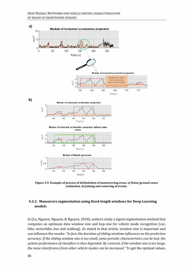
DEEP NEURAL NETWORKS FOR VEHICLE DRIVING CHARACTERIZATION BY MEANS OF SMARTPHONE SENSORS
46
Figure 4.5: Example of process of delimitation of maneuvering areas. a) Noise/ground zones estimation. b) Joining and centering of events.
4.3.2. Maneuvers segmentation using fixed-length windows for Deep Learning
models
In (Lu, Nguyen, Nguyen, & Nguyen, 2018), authors study a signal segmentation method that
computes an optimum data window size and hop-size for vehicle mode recognition (car,
bike, motorbike, bus and walking). As stated in that article, window size is important and
can influence the results: “In fact, the duration of sliding windows influences on the prediction
accuracy. If the sliding window size is too small, some periodic characteristics can be lost; the
system performance of classifiers is thus degraded. By contrast, if the window size is too large,
the noise interference from other vehicle modes can be increased.” To get the optimal values,

CHAPTER 4. DRIVING MANEUVERS CHARACTERIZATION
47
they use the prediction accuracies obtained with different classifiers. They initialize the
window size to 1 second and then, they increase iteratively the size. Also, they tested with
several overlapping values such of 75%, 50% and 25%. According to the reported results, a
general conclusion was that accuracy increasing, when increasing the window size up to a
certain saturation value that was 6 seconds. And the best overlapping ratio was 75%. For
this particular task, when the longer window size was, they captured more information of
vehicle mode.
In our work, since we have detected and delimited the maneuvers, we have decided
to study their different durations and to select a fixed window size, as representative as
possible for the complete dataset. This length must store enough useful information to carry
out the desired task, as well as not to be too large to do not increase the processing time and
to be able to apply such segmentation in shorter journeys. For the experimental framework
we used the maneuvers of a set of 40000 real driving journeys. And we have tested three
different Deep Learning models:
The first one is a two-layer Neural Network classifier using Feed Forward or Fully
Connected (FC) layers. The input for this model is a super vector where all the
window samples of the three-axis accelerometers are concatenated one after the
other (Figure 4.6). In the first layer, we applied the weights and the biases to X and
go through the ReLUs. The second layer has the weights and the biases, followed by
the softmax layer (to obtain the probabilities for each class).
Figure 4.6: Two-layer classifier applied for fixed-length window segmentation strategy, broad driving maneuvers characterization.
The second one is a two-layer Convolutional Neural Network (CNN) with 128
kernels. Each 1D kernel is used as a filter applied on each sensor, as a feature
extractor, followed by the previous classifier (Figure 4.7). In the CNN, every input
does not connect to every hidden neuron, instead of this, the connections are made
in small localized regions of the input.

DEEP NEURAL NETWORKS FOR VEHICLE DRIVING CHARACTERIZATION BY MEANS OF SMARTPHONE SENSORS
48
Figure 4.7: Convolutional Neural Network applied for fixed-length window segmentation strategy, broad driving maneuvers characterization.
To improve the previous results, we also tested Recurrent Neural Networks (RNN).
In particular, a Long Short-Term Memory (LSTM) network of two stacked layers.
Because normal CNN in order to extract patterns share parameters across space,
probably these types of networks are not the most suitable for our data. Perhaps, it
is better to use networks that take into account temporal dependencies. LSTM
networks are RNN that has into account the past. These perform a summary of what
happened before recursively and consist of repetitions of simple units as the shown
in Figure 4.8. These units take as input the past and new inputs and produces a new
prediction and a connection to the future (for more details about this type of
networks see Section 2.4.2 Long Short-Term Memory). In this architecture, we must
introduce at each step an instant of time for all the sensors, and the same time for
all training batch. Unlike the normal RNN that overwrite their content at each
instant of time, if the LSTM networks detect an important feature, they maintain it
in the memory, being able to take that feature a long distance and capturing possible
temporal dependencies. There are three types of LSTM cells:
o Basic LSTM cells: these cells in relation to the normal recurrent neural cells
add the forget gate.
o Full LSTM cells: in relation to the basic LSTM cells add the peepholes (so that
the cells control the gates).
o GRU cells: in relation to full LSTM cells, always show all content remains in
memory to other units.

CHAPTER 4. DRIVING MANEUVERS CHARACTERIZATION
49
Figure 4.8: Basic operation LSTM cell.
As we have mentioned, we have simplified the problem to only two classes, one
formed by accelerations and decelerations/brakings, and another one including both turns
and mixed events (turns together with accelerations and/or decelerations). The input
signals to the network will be the areas of maneuvers, and we are going to use the raw
accelerometers, without any type of processing.
In order to choose a first window size, we have studied the different durations of the
driving maneuver set (40000 journeys), obtaining the histogram shown in the Figure 4.9.
As we can observe, a good initial value can be set to 100 samples that equals 20 seconds
(sampling rate of 5 Hz).
Figure 4.9: Histogram of the maneuvers durations for a set of more than 40000 real driving journeys.

DEEP NEURAL NETWORKS FOR VEHICLE DRIVING CHARACTERIZATION BY MEANS OF SMARTPHONE SENSORS
50
There are maneuvers with lengths shorter and longer than that selected duration,
so we will perform the following data preparation. We exclusively use for the training,
events with 100 samples or less. When the event has a shorter duration, we seek the center
and move 50 samples right and left, if it is possible. In the Figure 4.10 an example is shown,
where the red dotted box shows a turning event, the blue dotted box one of acceleration and
the green dotted box the result of the process of improvement of the delimitation of the
maneuvers, after applying background noise thresholds, orange line (see process in Section
4.3.1 Energy-based maneuvers time detection).
Figure 4.10: Preparation of the windows of the network, for maneuvers of less than 100 samples of duration. a) Module of the horizontal projection of accelerations. b) Module of the filtered gyroscopes.
For the experiments the number of maneuvers is balanced, that is to say, the same
amount has been chosen for each of the classes, 208436; using 80% for training, 10% for
validation and the remaining 10% for testing. The summary of the results obtained with the
configurations mentioned above are shown in the Table 4.2.
The Table 4.2 shows that the classifier has offered slightly better results than
convolutional networks, with an overall accuracy of 72.5%. The first test for the recurrent
LSTM networks has been to apply to the same data set of 40000 journeys, like the used with
the classifier and the convolutional networks, a two-layer network with basic cells and 64
neurons per layer. The results obtained have been of an accuracy of 77.41%. If we added
the gyroscope information, the overall accuracy would grow up to 95.07%. As noted,
although using only the accelerometers makes the task more difficult, it achieves reasonable
values.
Recurrent networks seem to improve the results compared to the values obtained
with the classifier and the convolutional network. To increase the accuracies obtained, we

CHAPTER 4. DRIVING MANEUVERS CHARACTERIZATION
51
have augmented the dataset from 40000 journeys to 70000 journeys. We have tested for
the same basic cells with 64 neurons per layer, and almost 82% of accuracy is achieved. For
the same configuration, using only the accelerometers and increasing the data will suppose
an increase from 77.41% to 81.86%. In the case of using 6 channels, with the gyroscope
information, the increase would be from 95.07% to 96.92%.
Cross-validation is not frequently used in deep learning because it is
computationally expensive with a large dataset, this becomes useful when the dataset is
tiny. Normally, in this case, with a train/valid/test split is ok. Even so, we have decided to
do a test incorporating cross validation to ensure that the results are independent of the
partition between training data and test data. But, in order to not increase the training time
too much, we have reduced the neurons to 32. Although the results decrease slightly by
reducing the number of neurons per layer, these remain similar with a 79.56% of accuracy
in the test (see Table 4.2).
In order to compare the results with other type of LSTM cells, we have also used for
the same set of 70000 journeys, the full and GRU cells, for the two-layer network with 64
neurons per layer. The accuracies values are respectively 84.34% and 85.02%. It seems that
the configuration that offers the best performance is the LSTM network with GRU cells.
Training times are not excessively high for 64 neurons, around 4 hours.
Table 4.2: Results in maneuver classification experiments using fixed-length windows.
Network Window network
Signals No.
journeys No.
Classes Classes
Test accuracy
%)
Classifier (2 layers)
Fixed, 100
samples
Tri-axial accelerometers
(3 channels) 40000 2
Accelerations/decelerations; turns/mixed
72.5%
CNN (2 layers, 128
kernels)+classifier (2 layers)
Fixed, 100
samples
Tri-axial accelerometers
(3 channels) 40000 2
Accelerations/decelerations; turns/mixed
72.2%
LSTM (2 layers, 64
neurons, basic cell)
Fixed, 100
samples
Tri-axial accelerometers
(3 channels) 40000 2
Accelerations/decelerations; turns/mixed
77.41%
LSTM (2 layers, 64
neurons, basic cell)
Fixed, 100
samples
Tri-axial accelerometers,
gyroscope signals
(6 channels)
40000 2 Accelerations/decelerations;
turns/mixed 95.07%
LSTM (2 layers, 32
neurons, basic cell)
Fixed, 100
samples
Tri-axial accelerometers
(3 channels) 70000 2
Accelerations/decelerations; turns/mixed
79.56%
LSTM (2 layers, 64
neurons, basic cell)
Fixed, 100
samples
Tri-axial accelerometers
(3 channels) 70000 2
Accelerations/decelerations; turns/mixed
81.86%
LSTM (2 layers, 64
neurons, basic cell)
Fixed, 100
samples
Tri-axial accelerometer and gyroscope
signals (6 channels)
70000 2 Accelerations/decelerations;
turns/mixed 96.92%
LSTM (2 layers, 64
neurons, full cell)
Fixed, 100
samples
Tri-axial accelerometers
(3 channels) 70000 2
Accelerations/decelerations; turns/mixed
84.38%
LSTM (2 layers, 64
neurons, GRU cell)
Fixed, 100
samples
Tri-axial accelerometers
(3 channels) 70000 2
Accelerations/decelerations; turns/mixed
85.02%

DEEP NEURAL NETWORKS FOR VEHICLE DRIVING CHARACTERIZATION BY MEANS OF SMARTPHONE SENSORS
52
4.3.3. Maneuvers segmentation using variable-length windows for Deep Learning
models
The next step looking for improved results has been to use the real length of the maneuver,
instead of a fixed window of 100 samples. The main difficulty in this case is that the input
to the Neural Network will be sequences of variable lengths.
To implement RNN models on variable-length sequences using the TensorFlow
Deep Learning library, we have followed the proposal in (Hafner, 2016). The main idea
behind this is that the network must learn the information contained in the real duration of
each input signal, and not in more samples. If we use TensorFlow to implement the
recurrent networks, the batch used in training must be a fixed-sized tensor of:
𝑻𝒓𝒂𝒊𝒏𝒊𝒏𝒈 𝒃𝒂𝒕𝒄𝒉 = [𝒃𝒂𝒕𝒄𝒉 𝒔𝒊𝒛𝒆 × 𝒎𝒂𝒙 𝒍𝒆𝒏𝒈𝒕𝒉 × 𝒇𝒆𝒂𝒕𝒖𝒓𝒆𝒔] (4.10)
That is, we need to define that maximum length of the channels. As each maneuver
has a different length, it is difficult to reach a compromise. Therefore even we use this
technique of variable length sequences, we must define a maximum value of length,
however the network will only take into account the samples indicated for each signal. For
that purpose, the steps are the following:
1. We define the maximum length. Minor maneuvers are filled with zeros.
2. We create a binary mask, with ones for valid samples and zero for invalid samples
(it will be enough to add the ones in order to know the real length of a maneuver).
3. We use a dynamic network. This function allows unfolding our network, by means
of the parameter sequence_length, where we specify the calculated real lengths.
4. During the model training, TensorFlow will return zero vectors for states and
outputs after these sequence lengths specified above.
5. For the cost function, we mask out the unused frames and compute the mean error
over the sequence length by dividing by the actual length (in the blog of (Hafner,
2016) specifies that it is not really necessary to mask the cost and error functions,
because both prediction and target are zero vectors for the padding frames).
6. Finally for the classification, we must to feed the last output of the recurrent
network into a predictor (like a softmax layer). So we do not take the last frame, but
we take the last relevant frame (this last relevant output will be the one that feeds
on the next layer). Returning as output:
𝒐𝒖𝒕𝒑𝒖𝒕𝒏𝒆𝒘 = 𝒐𝒖𝒕𝒑𝒖𝒕[: , 𝒍𝒆𝒏𝒈𝒕𝒉 − 𝟏] (4.11)
Following this process, we have repeated the tests, selecting a window with a
maximum size of 100 samples as before. In addition, taking into account the histogram of
the Figure 4.9, we have also performed tests with a maximum window of 200 samples (40
seconds), because this value seems a reasonable window size, covering most of the available
maneuvers.

CHAPTER 4. DRIVING MANEUVERS CHARACTERIZATION
53
The results for 100 samples, taking into account in the network the variable length
of the maneuvers, increase the accuracy to 87.38%. If we increase the maximum window
length to 200 samples, accuracy goes up even more until 88.82%. The results have improved
at high rates; however training time has also risen to approximately 10 hours.
Table 4.3: Results in maneuver classification experiments using variable length windows.
Network Window network
Signals No.
journeys No.
Classes Classes
Test accuracy
(%)
LSTM (2 layers,
128 neurons, GRU cell)
Variable length,
100 samples
Tri-axial accelerometers
(3 channels) 70000 2
Accelerations/decelerations; turns/mixed
87.38%
LSTM (2 layers,
128 neurons, GRU cell)
Variable length,
200 samples
Tri-axial accelerometers
(3 channels) 70000 2
Accelerations/decelerations; turns/mixed
88.82%
4.3.4. Maneuvers segmentation using sliding windows for Deep Learning models
We have also decided to apply neural networks for decision making along a journey. That
is, to use sliding windows in order to evaluate to which class it belongs. As decisions are
made along the journey, there are no longer only two labels referring to the maneuvers, but
four categories in total: acceleration events, turn events, manipulations and zones of
background noise level. For these tests the training and testing set used has been reduced,
with 5000 journeys for the training and 300 different journeys for the testing. The reason
for reducing these sets is to ensure that the classes are balanced and there is the same
number of each of them in training. An example of the sliding window process is shown in
Figure 4.11 (in this case, the window size is 10 seconds and the overlapping rate is 50%).
The tests have been carried out varying the window size (6, 10 and 15.2 seconds),
the overlapping between windows (50%, 80%), the type of network (LSTM and
Bidirectional Recurrent Neural Networks) and the labelled way (whole window and last 2
second window). The results are shown in the Table 4.4.
For the test of 10 seconds and overlap of the 50%, with the previous LSTM network
and labeling considering the whole window, the results in general have been unbalanced.
Although for the acceleration, turn and manipulation classes, we have accuracies higher
than 75%. For the last class of background noise zones hardly reaches 50%, mainly
confusing this class with acceleration events. With this same configuration and overlap, we
have reduced the window size to 6 seconds and we have also increased it to 15.2 seconds.
But the results are very similar and the class of background noise zones is not correctly
predicted.
Then, we have repeated the experiment with a window size of 10 second, which
seems to offer slightly better results than the others, but decreasing the shift to 20% (80%
overlap). The results have improved slightly to 72%, but the class of background noise
zones hardly exceeds 52%.

DEEP NEURAL NETWORKS FOR VEHICLE DRIVING CHARACTERIZATION BY MEANS OF SMARTPHONE SENSORS
54
If we use another network, for windows size of 10 seconds and 50% overlap, we can
compare the results with the LSTM configuration. The selected network has been the
Bidirectional LSTM network, of one and two layers formed by GRU cells. But it does not
seem that the network change helps to improve the imbalance in the accuracies. We have
also tried a different labeling, considering the last 2 second window instead whole window.
But this also does not introduce improvements over previous tests.
Once all these changes have been made, we have performed several tests to find the
best configuration. For the moment is the Bidirectional LSTM network with one layer
formed by GRU cells, a window size of 10 seconds, shift 20% (2 seconds) and labelled way
with the last 2 second of the window. Nevertheless, the results remain unbalanced
according to the classes, with a general accuracy of 74%.
Table 4.4: Results in maneuver classification experiments using sliding window.
Network Window network
Labeled Signals No.
journeys No.
classes Classes
Test accuracy
(%)
LSTM (2 layers,
64 neurons, GRU cell)
Fixed, 10 second,
shift 50%
Whole window
Tri-axial acceleromete
rs (3 channels)
5300 4
Accelerations/decelerations; turns/mixed;
manipulation; background noise
zones
71% (but
unbalanced results in
the classes prediction)
LSTM (2 layers,
64 neurons, GRU cell)
Fixed, 6 second,
shift 50%
Whole window
Tri-axial acceleromete
rs (3 channels)
5300 4
Accelerations/decelerations; turns/mixed;
manipulation; background noise
zones
70% (but
unbalanced results in
the classes prediction)
LSTM (2 layers,
64 neurons, GRU cell)
Fixed, 15.2
second, shift 50%
Whole window
Tri-axial acceleromete
rs (3 channels)
5300 4
Accelerations/decelerations; turns/mixed;
manipulation; background noise
zones
70.75% (but
unbalanced results in
the classes prediction)
LSTM (2 layers,
64 neurons, GRU cell)
Fixed, 10 second,
shift 20%
Whole window
Tri-axial acceleromete
rs (3 channels)
5300 4
Accelerations/decelerations; turns/mixed;
manipulation; background noise
zones
72% (but
unbalanced results in
the classes prediction)
Bidirectional LSTM (1
layer, 64 neurons, GRU cell)
Fixed, 10 second,
shift 50%
Whole window
Tri-axial acceleromete
rs (3 channels)
5300 4
Accelerations/decelerations; turns/mixed;
manipulation; background noise
zones
73.5% (but
unbalanced results in
the classes prediction)
Bidirectional LSTM (2 layers, 64 neurons, GRU cell)
Fixed, 10 second,
shift 50%
Whole window
Tri-axial acceleromete
rs (3 channels)
5300 4
Accelerations/decelerations; turns/mixed;
manipulation; background noise
zones
71.5% (but
unbalanced results in
the classes prediction)
LSTM (2 layers,
64 neurons, GRU cell)
Fixed, 10 second,
shift 50%
Last 2 second
window
Tri-axial acceleromete
rs (3 channels)
5300 4
Accelerations/decelerations; turns/mixed;
manipulation; background noise
zones
72.75% (but
unbalanced results in
the classes prediction)
Bidirectional LSTM (1 layer,
64 neurons, GRU cell)
Fixed, 10
second, shift 20%
Last 2 second
window
Tri-axial acceleromet
ers (3 channels)
5300 4
Accelerations/decelerations; turns/mixed;
manipulation; background noise
zones
74% (but
unbalanced results in
the classes prediction)
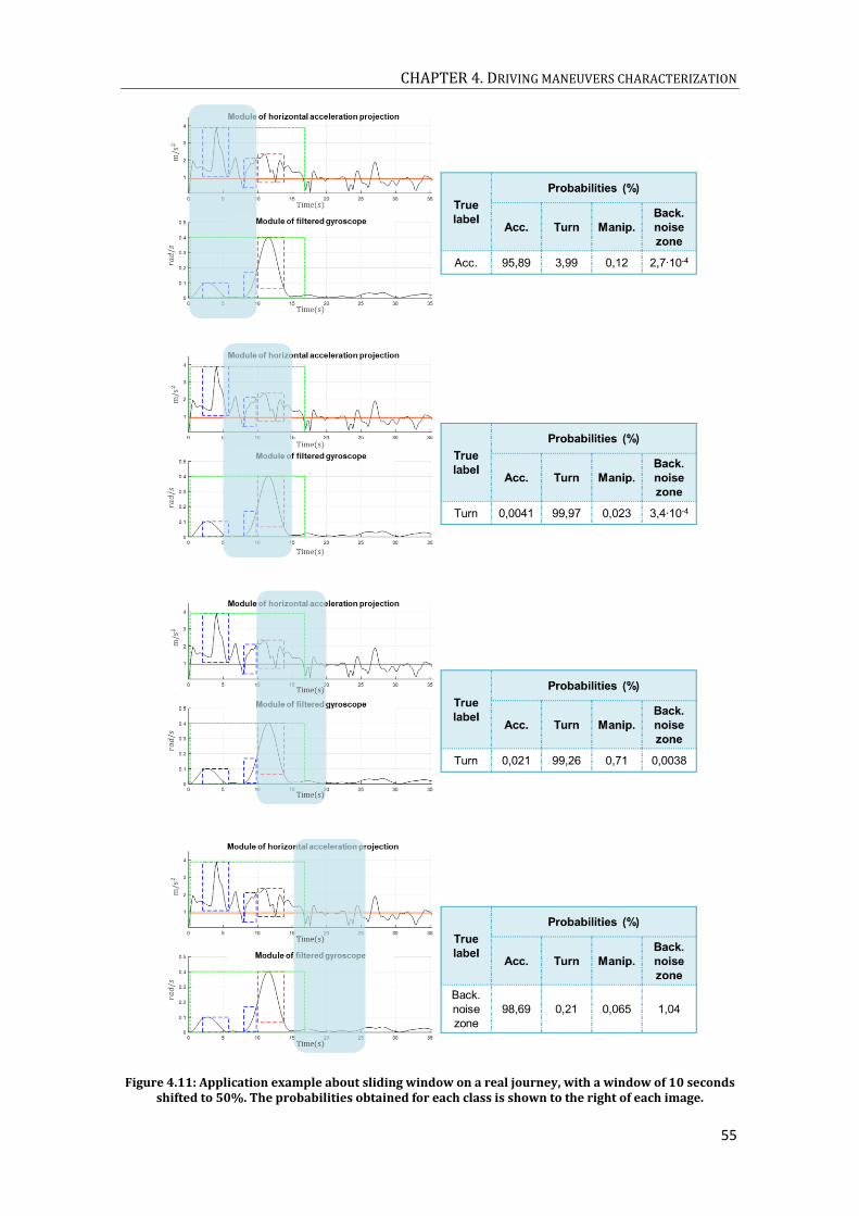
CHAPTER 4. DRIVING MANEUVERS CHARACTERIZATION
55
Figure 4.11: Application example about sliding window on a real journey, with a window of 10 seconds shifted to 50%. The probabilities obtained for each class is shown to the right of each image.

DEEP NEURAL NETWORKS FOR VEHICLE DRIVING CHARACTERIZATION BY MEANS OF SMARTPHONE SENSORS
56
The Figure 4.12 shows one of the examples obtained in the test, for the configuration
mentioned in the previous paragraph. It seems that the behavior along the journey is not
bad and the network errors could be corrected. Maybe we should use the projection of the
accelerometers instead of the raw signals to avoid these errors. We also tested adding the
horizontal projection, but the overall results remained very similar, slightly improving the
class of background noise zones, but slightly worsening the turn (the other two classes
remained similar).
Figure 4.12: Real example on driving journey, using for the maneuver classification a Bidirectional LSTM network of one layer (GRU cells), size windows of 10 seconds, shift 20% and labeling the last 2
second of the window. The first subplot presents the module of the horizontal acceleration projections, the second subplot the module of the filtered gyroscope and finally, the third subplot presents the final
probabilities obtained (adding the results in each moment of time).
Between the advantages of using sliding window it is found that, if it works properly,
it is not necessary to do any type of previous processing of the journeys (since it classifies
all the windows). Therefore to improve the results, we have maintained the classification in
four classes of the sliding window procedure, but we have trained and tested with
segmented windows, that is, indicating to the network the actual size according to the class
of each window.
The manipulations can have a long duration, so we have decided to slightly increase
the maximum segmented window size up to 260 samples. If we apply a LSTM network with
two stacked layers formed by GRU cells (64 neurons), the results are shown in the Table 4.5.
The final accuracy has increased to 77.25%. In addition, the results for each class are more

CHAPTER 4. DRIVING MANEUVERS CHARACTERIZATION
57
balanced, as we can see in the Figure 4.13 a). If we also increase both the training set and
the number of neurons to 128, the overall accuracy grows up to 80.5% (see Table 4.5). The
Figure 4.13 b) shows that from the acceleration events, 81% are correctly predicted as
accelerations and 16% are predicted as turn events, this class has improved by 9%. From
the turn events, 61% are correctly classified, this class has gotten worse by 3% (similar
results). The manipulations maintain the good percentage obtained previously. And from
the background noise zone class, 86% are correctly predicted, this class has improved by
7%.
Table 4.5: Results in maneuver classification experiments using sliding window and sequence variable length.
Network Window network
Signals No.
journeys No.
Classes Classes
Test accuracy
(%)
LSTM (2 layers,
64 neurons, GRU cell)
Variable length,
260 samples
Tri-axial accelerometers and horizontal
acceleration projections (6
channels)
5300 4 Accelerations/decelerations; turns/mixed; manipulation;
background noise zones
77.25%
LSTM (2 layers,
128 neurons, GRU cell)
Variable length,
260 samples
Tri-axial accelerometers and horizontal
acceleration projections (6
channels)
12000 4 Accelerations/decelerations; turns/mixed; manipulation;
background noise zones
80.5%
Figure 4.13: Confusion matrix obtained for the maneuver classification experiments using sliding window and sequence variable length. a) LSTM network with two stacked layers, GRU cells and 64
neurons. b) LSTM network with two stacked layers, GRU cells and 128 neurons.
4.3.5. Windowing strategies comparison
In this section we have addressed a broad driving maneuver characterization. For this
purpose, we have developed three different methods depending on the windowing strategy
used. The first common step to each of the methods is the detection of the maneuver, that

DEEP NEURAL NETWORKS FOR VEHICLE DRIVING CHARACTERIZATION BY MEANS OF SMARTPHONE SENSORS
58
is, to locate the beginning and the end, using the projection of the smartphone tri-axial
accelerometer measurements on the horizontal plane, which we assume contains the
longitudinal and transversal driving forces. To locate the position of events, we compare
the acceleration energy with a threshold, which will mark an approximate location. To
determine the beginning and the end, we use the specific background noise level of each
journey. Once the maneuvers have been located, we have applied three different
segmentation methods: fixed-length windows, variable-length windows and sliding
window. And we have used Deep Learning models, to classify the maneuvers into two types:
accelerations/decelerations and turns/mixed events.
The first method uses fixed-length windows for all maneuvers. Studying the
duration of the maneuvers that we have detected, we have selected a window length of 100
samples (20 seconds). The problem with this method is that although 100 samples is a size
that covers most durations (see Figure 4.9), there are shorter and longer events. Longer
maneuvers have been excluded from testing and for shorter maneuvers it is necessary to
center on the maneuver and take part of the environment to complete this length. The best
results have been obtained with a two-layer LSTM architecture, with GRU cells and 64
neurons by layer, obtaining an accuracy of 85.02%.
As we have commented, the main limitation of the previous method is that for
smaller maneuvers of 100 samples, it is necessary to collect information from the
environment, incorporating signals not directly related to the maneuver itself. To solve it,
the second method instead of using fixed windows employs windows of variable size, which
allows expanding the set of maneuvers to classify. Since Neural Networks need a fixed input
size for their tensors, we extend the 100 samples to 200 samples. Minor maneuvers of this
size are filled with zeros; however the network, both training and testing, will only take into
account the length indicated for each signal. The best results have been obtained again for
the two-layer LSTM network, with GRU cells, expanding the number of neurons to 128 per
layer and using a dynamic network. The accuracy for this method has increased to 88.82%.
Finally, we have used sliding windows along the journey. Now there are not only
two classes as in the previous methods, but as many classes as the type of information are
present in the journeys. We have grouped it into four types: windows with information
about acceleration/deceleration maneuvers, windows with information about turn/ mixed
maneuvers, manipulation windows and background noise windows. The first two
correspond to the classification of the events that we have carried out in the first methods.
The manipulations correspond to areas where there are high acceleration values, caused for
example by the driver taking the mobile phone with her hand. And the last class, background
noise zones are calm areas of the journey, where neither maneuvers related to driving nor
manipulations occur. Different window, overlap and label values have been tested. As this
kind of method allows us to use bidirectional neural networks, we have used it and the best
results have been obtained with this architecture, using an LSTM layer with 64 GRU
neurons, using windows of 10 seconds, 20% shift and labeling with the last two seconds of
the window. The results show an overall accuracy of 74%. These values are lower than those
obtained with the other methods and they are also unbalanced between the classes; as the
number of classes increases, the complexity also increases.
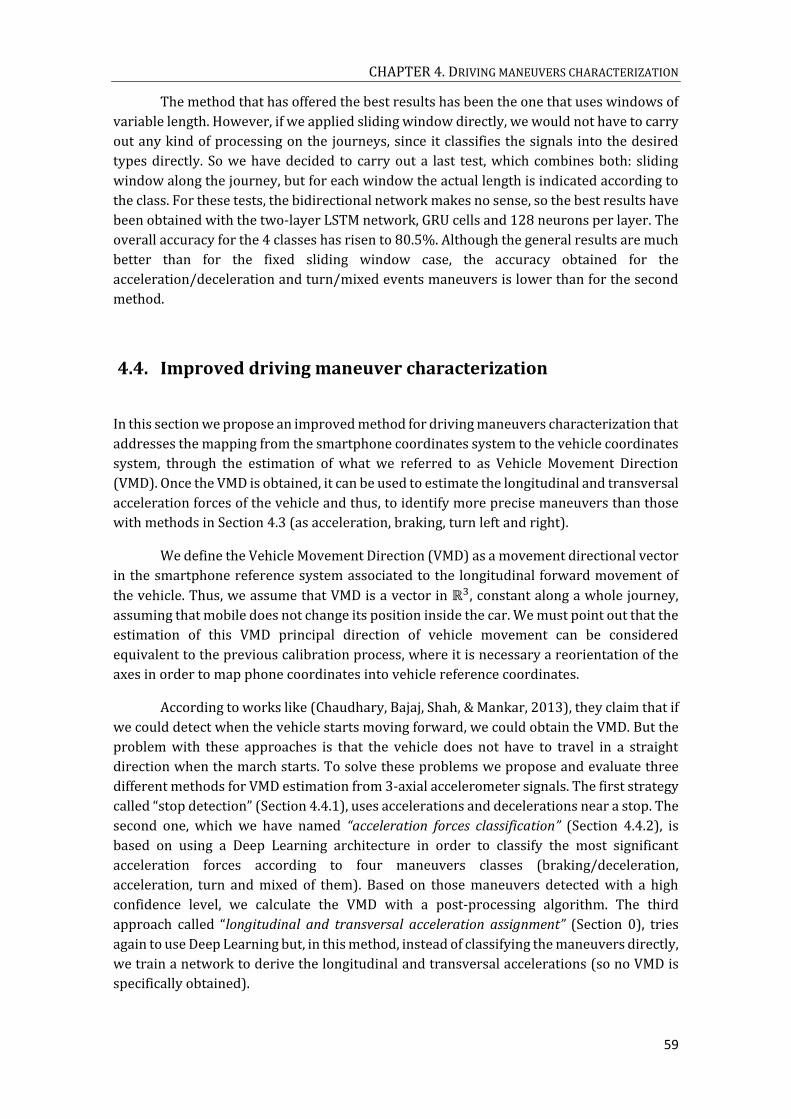
CHAPTER 4. DRIVING MANEUVERS CHARACTERIZATION
59
The method that has offered the best results has been the one that uses windows of
variable length. However, if we applied sliding window directly, we would not have to carry
out any kind of processing on the journeys, since it classifies the signals into the desired
types directly. So we have decided to carry out a last test, which combines both: sliding
window along the journey, but for each window the actual length is indicated according to
the class. For these tests, the bidirectional network makes no sense, so the best results have
been obtained with the two-layer LSTM network, GRU cells and 128 neurons per layer. The
overall accuracy for the 4 classes has risen to 80.5%. Although the general results are much
better than for the fixed sliding window case, the accuracy obtained for the
acceleration/deceleration and turn/mixed events maneuvers is lower than for the second
method.
4.4. Improved driving maneuver characterization
In this section we propose an improved method for driving maneuvers characterization that
addresses the mapping from the smartphone coordinates system to the vehicle coordinates
system, through the estimation of what we referred to as Vehicle Movement Direction
(VMD). Once the VMD is obtained, it can be used to estimate the longitudinal and transversal
acceleration forces of the vehicle and thus, to identify more precise maneuvers than those
with methods in Section 4.3 (as acceleration, braking, turn left and right).
We define the Vehicle Movement Direction (VMD) as a movement directional vector
in the smartphone reference system associated to the longitudinal forward movement of
the vehicle. Thus, we assume that VMD is a vector in ℝ3, constant along a whole journey,
assuming that mobile does not change its position inside the car. We must point out that the
estimation of this VMD principal direction of vehicle movement can be considered
equivalent to the previous calibration process, where it is necessary a reorientation of the
axes in order to map phone coordinates into vehicle reference coordinates.
According to works like (Chaudhary, Bajaj, Shah, & Mankar, 2013), they claim that if
we could detect when the vehicle starts moving forward, we could obtain the VMD. But the
problem with these approaches is that the vehicle does not have to travel in a straight
direction when the march starts. To solve these problems we propose and evaluate three
different methods for VMD estimation from 3-axial accelerometer signals. The first strategy
called “stop detection” (Section 4.4.1), uses accelerations and decelerations near a stop. The
second one, which we have named “acceleration forces classification” (Section 4.4.2), is
based on using a Deep Learning architecture in order to classify the most significant
acceleration forces according to four maneuvers classes (braking/deceleration,
acceleration, turn and mixed of them). Based on those maneuvers detected with a high
confidence level, we calculate the VMD with a post-processing algorithm. The third
approach called “longitudinal and transversal acceleration assignment” (Section 0), tries
again to use Deep Learning but, in this method, instead of classifying the maneuvers directly,
we train a network to derive the longitudinal and transversal accelerations (so no VMD is
specifically obtained).
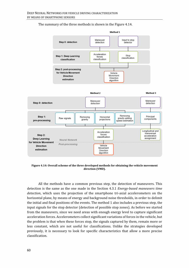
DEEP NEURAL NETWORKS FOR VEHICLE DRIVING CHARACTERIZATION BY MEANS OF SMARTPHONE SENSORS
60
The summary of the three methods is shown in the Figure 4.14.
Figure 4.14: Overall scheme of the three developed methods for obtaining the vehicle movement direction (VMD).
All the methods have a common previous step, the detection of maneuvers. This
detection is the same as the one made in the Section 4.3.1 Energy-based maneuvers time
detection, which uses the projection of the smartphone tri-axial accelerometers on the
horizontal plane, by means of energy and background noise thresholds, in order to delimit
the initial and final positions of the events. The method 1 also includes a previous step, the
input signals for the stop detector (detection of possible stop zones). As before we started
from the maneuvers, since we need areas with enough energy level to capture significant
acceleration forces. Accelerometers collect significant variations of forces in the vehicle, but
the problem is that when these forces stop, the signals captured by them, remain more or
less constant, which are not useful for classifications. Unlike the strategies developed
previously, it is necessary to look for specific characteristics that allow a more precise
classification.

CHAPTER 4. DRIVING MANEUVERS CHARACTERIZATION
61
4.4.1. Method 1: stop detection
The first method we have developed to obtain the VMD, we have called stop detection. The
process summary is shown in the Figure 4.15. The main idea is to use deep neural networks
to classify two different tasks, and later to combine the results offered by the classifiers
through an algorithm that calculates the final VMD. One of the networks will classify the
maneuvers into two classes: accelerations/decelerations and turns/mixed. In particular, we
are going to use the LSTM network with GRU cells for a segmentation of the maneuvers with
variable-length windows (maximum window size of 200 samples), due to the good results
shown in the tests of Section 4.3 Broad driving maneuver characterization. We will also
increase the number of neurons per layer to 128. The second network will be the stop
detector. The stop detector will indicate in which areas of the journey take place a stop. In
order to develop this method, we must detect both acceleration/deceleration maneuvers
and stops with the networks. If these conditions happen, the post-processing algorithm will
calculate the VMD by means of the accelerations and decelerations that occur near the stops,
based on the hypothesis that the acceleration event after a stop is an acceleration maneuver
per se, while the acceleration event previous to the stop will be a deceleration or braking.
Below we are going to detail the two strategies carried out for the stop detector, as well as
the algorithm developed to calculate the final VMD with the information of the maneuvers
and the stops.
Figure 4.15: Scheme method 1 of stop detection.
The two strategies in order to implement the stop detector are based on the type of
inputs that we are going to use, to classify them like stop or non-stop. For the first
experiment, we have trained a neural network that distinguishes between stop and no stop
considered as no stop any other signal (i.e. constant speed zones, maneuvers, etc.). For the

DEEP NEURAL NETWORKS FOR VEHICLE DRIVING CHARACTERIZATION BY MEANS OF SMARTPHONE SENSORS
62
second strategy, instead of passing the whole journey and instead of considering the no stop
areas how everything that is not a stop, we consider like no stop zones the areas of “nothing”
(areas where there is not neither event nor manipulation). To label the stops we had to use
a different database, in which we had OBD information. This can affect the detection of the
stops, since we train with a different database than the used in the test. Another factor that
can affect performance is that the stop database is not very large, no many stop examples
for training.
Therefore, as we have mentioned, for the first approach of the stop detector, we
consider as stop, any signal that is not a stop (speed of zero m/s), independently of the type
of information. For the train part we have used windows of 200 samples with a shift of the
20%, in a Bidirectional LSTM network with one layer formed by GRU cells. In addition to the
raw accelerometers, we have added the information of horizontal projections. In the Figure
4.16, we show the confusion matrices obtained based on the percentage of stops windows
that have been correctly classified, Figure 4.16 a), and the accuracy for each true class,
Figure 4.16 b). The rows are the true class and the columns are the predicted class. The
overall accuracy obtained is shown in the Table 4.6, with a value of 75.9% (sum of the main
diagonal of the matrix of Figure 4.16 a)). From the no stop windows, 74.4% are correctly
predicted as no stops and 25.6% are predicted as stop windows. From the stop windows
90.6% are correctly classified and 9.4% are classified as no stop (Figure 4.16 b)). As the
images show, despite obtaining a general accuracy of almost 76%, the results are not good
since too many stops are detected that are not.
Figure 4.16: Confusion matrix for the stop detector, strategy 1: a) according to the number of windows of each class, b) according to the type of force.
The second test has consisted of using as stops the areas of “nothing”, areas without
maneuvers and manipulations. Also, we have selected a more appropriate stop window size,
introducing the real size of those zones. For it, we have represented the lengths of both, stop
zones according to the OBD and non-stop zones, Figure 4.17, and based on them we have
selected a maximum sequence length of 500 samples.

CHAPTER 4. DRIVING MANEUVERS CHARACTERIZATION
63
Figure 4.17: Histogram of the stop and non-stop zones durations.
As in this case we have used the real length of the windows (windows padded), it
does not make much sense to use bidirectional networks. For this reason, for this strategy
we have employed a LSTM network with two stacked layers. The confusion matrices are
shown in the Figure 4.18. If we add the main diagonal of the matrix of the Figure 4.18. a),
we obtain that the overall accuracy is 74.2% (Table 4.6). Although the accuracy has
decreased slightly from 75.9% to 74.2%, these last results are positive since in this case the
network is distinguishing between windows that look alike (there are no maneuvers or
manipulations).
Figure 4.18: Confusion matrix for the stop detector, strategy 2: a) according to the number of windows of each class, b) according to the type of force.
Table 4.6: Results in stop classification.
Network Window network
Signals No.
journeys No.
classes Classes
Test accuracy
(%)
Bidirectional LSTM (1 layer, 64 neurons,
GRU cell)
Fixed, 200 samples, shift
20%
Tri-axial accelerometers and horizontal acceleration
projections (6 channels) 12000 2
Stop/no stop
75.9%
LSTM (2 layers, 64 neurons, GRU cell)
Variable length, 500
samples
Tri-axial accelerometers and horizontal acceleration
projections (6 channels) 12000 2
Stop/no stop
74.2%

DEEP NEURAL NETWORKS FOR VEHICLE DRIVING CHARACTERIZATION BY MEANS OF SMARTPHONE SENSORS
64
With the information of the events plus the information of the stops, an algorithm
can be developed to calculate the VMD, all without gyroscope. The algorithm developed is
based on the hypothesis that the acceleration event immediately before a stop is likely to be
a braking (deceleration), while the acceleration event immediately after will be an
acceleration (no deceleration). Therefore, we must look for stops with acceleration events
on one or both sides. If an event is between two stops, we consider it like an acceleration for
one stop and such as a braking for the next stop, it is mixed for the algorithm (do not confuse
with mixed maneuver).
The algorithm for obtaining the VMD is defined below. In addition to the conditions
described, we have demanded a quality requirement for the results in the classification of
events, with a probability threshold greater than 80%. The steps are the following:
1. We take all the events that the network has classified such as accelerations (with
high probability). With all those directions of the events, we get the orientation
directions (they can be 3, 2 or 1): directions where most of the vectors point; and
therefore it is probable that the final travel direction coincides with one of these
orientation directions (see Figure 4.19 a)).
2. We look for the acceleration and the braking events from the stops. Accelerations
and brakings must fit to some of the orientation directions, and these must have
opposite directions (see Figure 4.19 b)). Also, we require that at least 60% of stop
samples are below to the noise threshold to consider it valid. For the mixed events
located between two stops, we will have samples pointing to one direction and
others pointing to another, so we divide the samples. The resulting mixed directions
must be fitted to orientation directions and to the braking and accelerations
directions (of the stops) already categorized.
3. If the event samples from the stops have not passed the conditions, we calculate
orientation directions for turns. The turn orientation directions are obtained by
taking, from each turn maneuver, the 3 samples with maximum value in the module
of the horizontal projection. And then we use turn orientation directions to discard
invalid acceleration orientation directions.
In the Figure 4.19 a real example is shown, in which we have proceeded to calculate
the VMD of a journey. In general, to verify that the algorithm calculates a correct VMD, we
have compared the resulting direction with that obtained if we use both accelerometer and
gyroscope information. For the example of the image, the VMD obtained seems quite
reliable, with only 16° of difference with the direction using the gyroscope and the
accelerometers.
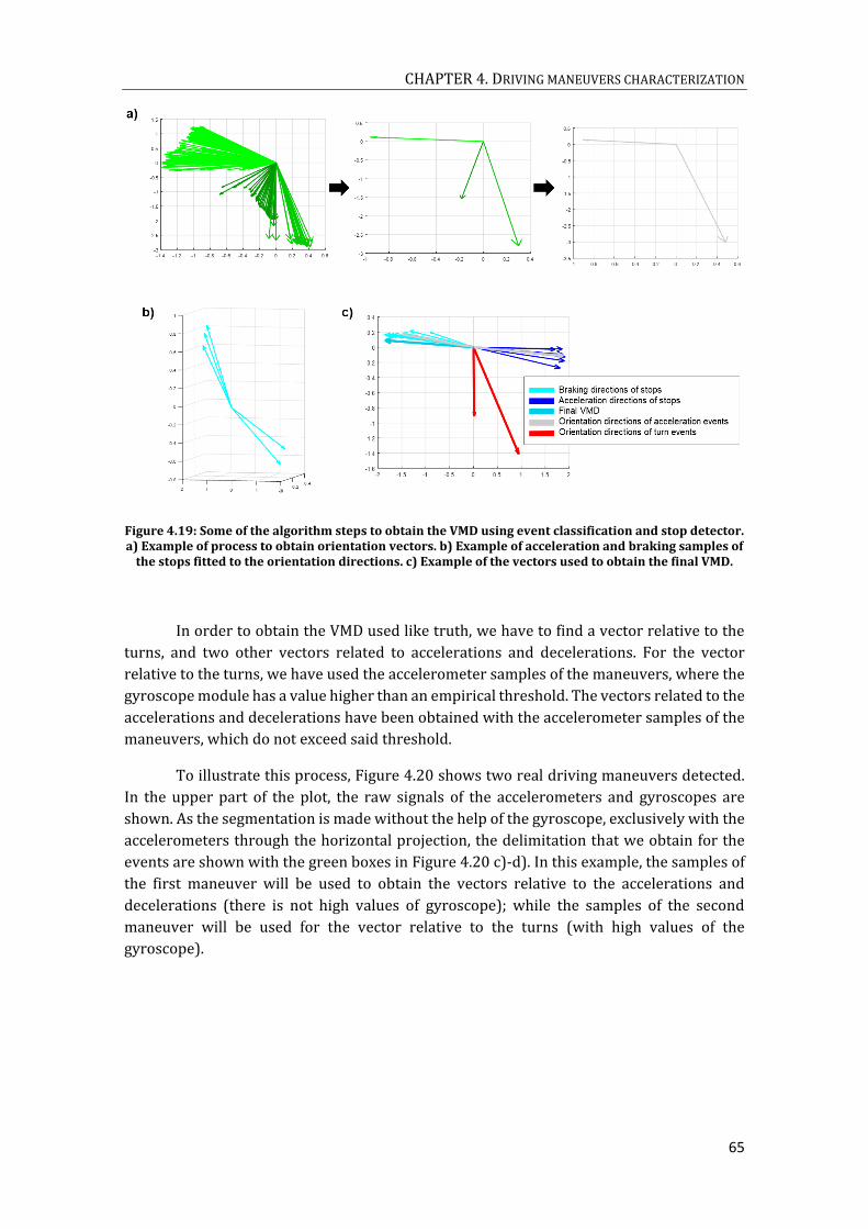
CHAPTER 4. DRIVING MANEUVERS CHARACTERIZATION
65
Figure 4.19: Some of the algorithm steps to obtain the VMD using event classification and stop detector. a) Example of process to obtain orientation vectors. b) Example of acceleration and braking samples of
the stops fitted to the orientation directions. c) Example of the vectors used to obtain the final VMD.
In order to obtain the VMD used like truth, we have to find a vector relative to the
turns, and two other vectors related to accelerations and decelerations. For the vector
relative to the turns, we have used the accelerometer samples of the maneuvers, where the
gyroscope module has a value higher than an empirical threshold. The vectors related to the
accelerations and decelerations have been obtained with the accelerometer samples of the
maneuvers, which do not exceed said threshold.
To illustrate this process, Figure 4.20 shows two real driving maneuvers detected.
In the upper part of the plot, the raw signals of the accelerometers and gyroscopes are
shown. As the segmentation is made without the help of the gyroscope, exclusively with the
accelerometers through the horizontal projection, the delimitation that we obtain for the
events are shown with the green boxes in Figure 4.20 c)-d). In this example, the samples of
the first maneuver will be used to obtain the vectors relative to the accelerations and
decelerations (there is not high values of gyroscope); while the samples of the second
maneuver will be used for the vector relative to the turns (with high values of the
gyroscope).
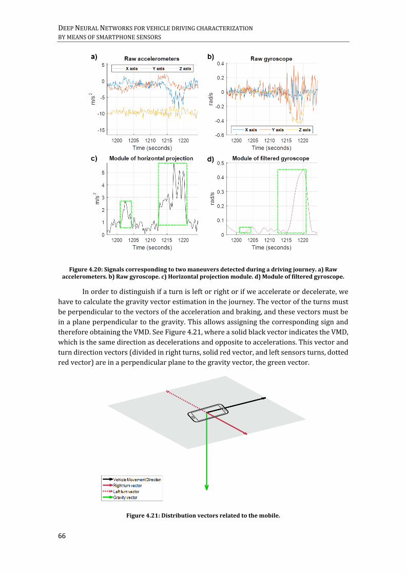
DEEP NEURAL NETWORKS FOR VEHICLE DRIVING CHARACTERIZATION BY MEANS OF SMARTPHONE SENSORS
66
Figure 4.20: Signals corresponding to two maneuvers detected during a driving journey. a) Raw accelerometers. b) Raw gyroscope. c) Horizontal projection module. d) Module of filtered gyroscope.
In order to distinguish if a turn is left or right or if we accelerate or decelerate, we
have to calculate the gravity vector estimation in the journey. The vector of the turns must
be perpendicular to the vectors of the acceleration and braking, and these vectors must be
in a plane perpendicular to the gravity. This allows assigning the corresponding sign and
therefore obtaining the VMD. See Figure 4.21, where a solid black vector indicates the VMD,
which is the same direction as decelerations and opposite to accelerations. This vector and
turn direction vectors (divided in right turns, solid red vector, and left sensors turns, dotted
red vector) are in a perpendicular plane to the gravity vector, the green vector.
Figure 4.21: Distribution vectors related to the mobile.
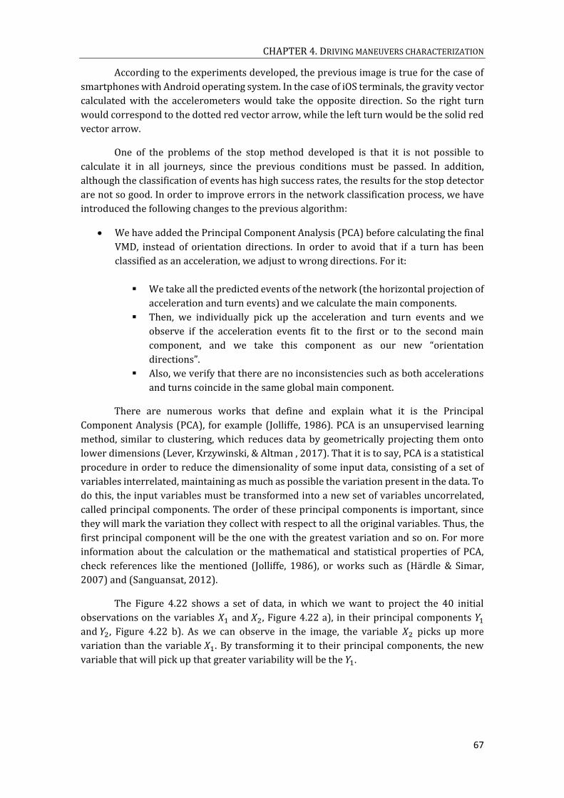
CHAPTER 4. DRIVING MANEUVERS CHARACTERIZATION
67
According to the experiments developed, the previous image is true for the case of
smartphones with Android operating system. In the case of iOS terminals, the gravity vector
calculated with the accelerometers would take the opposite direction. So the right turn
would correspond to the dotted red vector arrow, while the left turn would be the solid red
vector arrow.
One of the problems of the stop method developed is that it is not possible to
calculate it in all journeys, since the previous conditions must be passed. In addition,
although the classification of events has high success rates, the results for the stop detector
are not so good. In order to improve errors in the network classification process, we have
introduced the following changes to the previous algorithm:
We have added the Principal Component Analysis (PCA) before calculating the final
VMD, instead of orientation directions. In order to avoid that if a turn has been
classified as an acceleration, we adjust to wrong directions. For it:
We take all the predicted events of the network (the horizontal projection of
acceleration and turn events) and we calculate the main components.
Then, we individually pick up the acceleration and turn events and we
observe if the acceleration events fit to the first or to the second main
component, and we take this component as our new “orientation
directions”.
Also, we verify that there are no inconsistencies such as both accelerations
and turns coincide in the same global main component.
There are numerous works that define and explain what it is the Principal
Component Analysis (PCA), for example (Jolliffe, 1986). PCA is an unsupervised learning
method, similar to clustering, which reduces data by geometrically projecting them onto
lower dimensions (Lever, Krzywinski, & Altman , 2017). That it is to say, PCA is a statistical
procedure in order to reduce the dimensionality of some input data, consisting of a set of
variables interrelated, maintaining as much as possible the variation present in the data. To
do this, the input variables must be transformed into a new set of variables uncorrelated,
called principal components. The order of these principal components is important, since
they will mark the variation they collect with respect to all the original variables. Thus, the
first principal component will be the one with the greatest variation and so on. For more
information about the calculation or the mathematical and statistical properties of PCA,
check references like the mentioned (Jolliffe, 1986), or works such as (Härdle & Simar,
2007) and (Sanguansat, 2012).
The Figure 4.22 shows a set of data, in which we want to project the 40 initial
observations on the variables 𝑋1 and 𝑋2, Figure 4.22 a), in their principal components 𝑌1
and 𝑌2, Figure 4.22 b). As we can observe in the image, the variable 𝑋2 picks up more
variation than the variable 𝑋1. By transforming it to their principal components, the new
variable that will pick up that greater variability will be the 𝑌1.
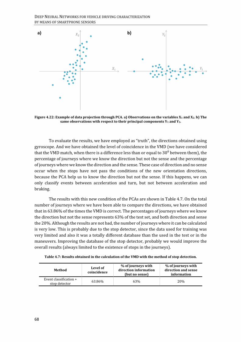
DEEP NEURAL NETWORKS FOR VEHICLE DRIVING CHARACTERIZATION BY MEANS OF SMARTPHONE SENSORS
68
Figure 4.22: Example of data projection through PCA. a) Observations on the variables X1 and X2. b) The same observations with respect to their principal components Y1 and Y2.
To evaluate the results, we have employed as “truth”, the directions obtained using
gyroscope. And we have obtained the level of coincidence in the VMD (we have considered
that the VMD match, when there is a difference less than or equal to 30⁰ between them), the
percentage of journeys where we know the direction but not the sense and the percentage
of journeys where we know the direction and the sense. These case of direction and no sense
occur when the stops have not pass the conditions of the new orientation directions,
because the PCA help us to know the direction but not the sense. If this happens, we can
only classify events between acceleration and turn, but not between acceleration and
braking.
The results with this new condition of the PCAs are shown in Table 4.7. On the total
number of journeys where we have been able to compare the directions, we have obtained
that in 63.86% of the times the VMD is correct. The percentages of journeys where we know
the direction but not the sense represents 63% of the test set, and both direction and sense
the 20%. Although the results are not bad, the number of journeys where it can be calculated
is very low. This is probably due to the stop detector, since the data used for training was
very limited and also it was a totally different database than the used in the test or in the
maneuvers. Improving the database of the stop detector, probably we would improve the
overall results (always limited to the existence of stops in the journeys).
Table 4.7: Results obtained in the calculation of the VMD with the method of stop detection.
Method Level of
coincidence
% of journeys with direction information
(but no sense)
% of journeys with direction and sense
information
Event classification + stop detector
63.86% 63% 20%

CHAPTER 4. DRIVING MANEUVERS CHARACTERIZATION
69
4.4.2. Method 2: acceleration forces classification
The first step of the method 2, based on the classification of acceleration forces in order to
obtain the VMD, is to detect the maneuvers as the image Figure 4.23 shows. But now the
classification of the events will be divided into 4 different types:
Maneuvers of braking (decelerations) without turn. For example, when a driver
decelerates but stays in the same driving lane.
Maneuvers of acceleration without turn. The same as in the previous class, but
accelerating, with forces in the opposite direction to the movement.
Pure turn. With transversal forces to the movement.
Mixed. All possible combinations of the three above maneuvers. For example, a
roundabout (braking + turn + acceleration)
Figure 4.23: Scheme method 2 of acceleration forces classification.
Once the maneuvers are obtained, and before the pre-processing prior to the
classification, we must get the ground truth of the data used in the training, now in four
classes. In order to obtain our ground truth, we are going to use accelerometer and
gyroscope sensors from mobile phones. But when these are tagged, we do not use again the
gyroscopes to classify the maneuvers. The segmentation of the maneuvers is necessary after
detection, since the labeling is done on that segmentation instead of on the complete
maneuver. For labeling, we are going to evaluate two criteria. The first one is if the window
maneuver has transversal forces to the movement (i.e., turns); and the second one, if there
are longitudinal forces of acceleration or deceleration.
To evaluate if the maneuver has transversal and longitudinal forces of acceleration
or deceleration, first it is necessary to find out the truth direction of the VMD (explained in
the previous method, 4.4.1 Method 1: stop detection), in order to be able to compare the
maneuvers samples with the driving direction afterwards. Once the VMD has been obtained,
the maneuvers can be classified in the four mentioned classes by means of the angle
between the maneuver samples and this direction (in the Section 4.4.4 Maneuver

DEEP NEURAL NETWORKS FOR VEHICLE DRIVING CHARACTERIZATION BY MEANS OF SMARTPHONE SENSORS
70
characterization by VMD, we show an example of classifying a maneuver with the VMD); and
this process can be performed for each journey.
We are not going to use classes such as the background noise zones or the
manipulations, we are only going to classify the maneuvers into 4 classes by means of sliding
window segmentation. Therefore, based on the previous results, we have decided to divide
the detected maneuvers into shorter windows of 10 s with an overlap of 5 s.
In this method we analyze different types of pre-processing of the input signals, in
order to improve the classification performance. The raw accelerometers will be taken as
baseline, and we will compare it with the same signals removing the gravity component of
the accelerations; with the accelerations projected to a plane perpendicular to the gravity;
and, finally, adding speed information, the speed estimation will be performed with the
strategy proposed in (Cervantes-Villanueva , Carrillo-Zapata, Terroso-Saenz , Valdes-Vela,
& Skarmeta, 2016). Therefore:
Raw accelerometer signals, the tri-axial components, without any type of pre-
processing. These will be used as a baseline.
Removing the gravity to each component of the accelerometers, to have the force of
the driving maneuvers.
Projecting the accelerations to a perpendicular plane to the gravity.
Speed estimation, added like a channel to the previous approach.
After several tests with different configurations, we have used for the classification
of the maneuvers, the network proposed in the Figure 4.24. The network has a
convolutional network of two layers, plus a recurrent network of two stacked layers and
GRU cells, and the last part of the classifier, with two fully connected plus a softmax layer.
Figure 4.24: Deep neural network architecture for maneuver classification.
The most common interpretation of the previous architecture is that convolutional
network layers act as feature extractor, providing a time-series of feature vectors as input
to recurrent networks, that model dynamic information in maneuvers. (Ordóñez & Roggen,
2016), in the area of activity recognition, use also convolutional networks as a feature
extractor. As they explain in their work, in domain 1D each kernel can be understood as a
filter that helps us to eliminate outliers, applying them on each sensor or each component

CHAPTER 4. DRIVING MANEUVERS CHARACTERIZATION
71
of the accelerometers in our case. To increase the deeper representation of the data, two
convolutional layers have been used. The first layer has 32 filters and the second layer 64
filters; using ReLU as activation function; and performs max pooling, maximum
neighborhood, to reduce the dimensionality.
The reason for adding the recurrent networks to the output of the convolutional
networks is to be able to learn and model the temporal information, collected in the feature
map at the output of the convolutional. The recurrent networks are GRU, because this type
offers very good results for time-series modeling. If our input signals will be the
accelerometers recorded with the smartphone (or variations of them), this architecture
becomes very powerful for learning the sequential features. In addition, the nodes of the
network are memory cells, which will allow us to update the states at each time instant,
storing the temporal relationships inside the maneuver. In the work of (Dong, et al., 2016)
compare different architectures and emphasized the benefits of using recurrent networks,
since these act like unfolded network across time steps. The GRU network consists of three
stacked layers, and each GRU layer is formed by 128 neurons.
Since our dataset contains a very large number of maneuvers for training, we expect
that the use of stacked layers can significantly improve the results. The output of the last
GRU layer is used as input to the last three layers of the architecture, consisting of two fully
connected layers and finally a Softmax layer, which will provide us the output probabilities
from network scores. The model was trained using an Adam optimizer for minimizing the
cross-entropy loss function. Trying to prevent overfitting, a dropout technique was added
at the output of the recurrent networks layer; we also used weight decay or L2
regularization; and max pooling in the convolutional layers to reduce the computational
cost reducing the number of parameters. Several learning rates were tested, selecting a low
value of 0.001, since although the optimization took longer, training results were more
reliable than with higher rates. Hyperparameter optimization was done through a grid
search using 10-fold cross-validation on the training dataset. The resulting
hyperparameters were then used to get the results in the test dataset.
To evaluate the model, different steps of the procedure have been taken into
account, as we done in the previous method. Since the purpose of the method is to obtain a
reliable VMD, the most important aim will be to compare if the direction estimated is close
to the true driving direction, measuring the difference in degrees. In addition, the number
of journeys in which it has been possible to estimate VMD will be an important metric. For
this case, the number of journeys in which VMD can be estimated will depend on the
detection or not of maneuvers associated with braking/decelerations or accelerations by
the neural networks; that is to say, that neural architecture predicts such classes.
Not only the evaluation of the model been considered, but also the interpretation of
the training process in the different layers of the Deep Learning architecture, through
techniques that allow visualizing data of high dimensionality, like t-distributed stochastic
neighbor embedding (t-SNE) (van der Maaten & Hinton, 2008). This interpretation has been
done through the visualization of the projection of the feature vectors obtained in the
previous layers to the decision making, that is, in the previous layers to the fully connected
layer. In particular, the outputs of the second convolutional network and the output of the
recurrent networks GRU of two stacked layers have been analyzed. The objective of
DEEP NEURAL NETWORKS FOR VEHICLE DRIVING CHARACTERIZATION BY MEANS OF SMARTPHONE SENSORS
72
visualizing the feature projections, in a function of different parameters, is to observe the
influence of these parameters in the decisions that are taken in each layer. For example, to
analyze aspects such as whether or not the output information of a layer is independent of
the position of the mobile, or whether it begins to show or not a capacity for discrimination
of the different types of acceleration forces. t-SNE technique converts the high-dimensional
Euclidean distances between data points into conditional probabilities, the similarities. To
find the low-dimensional data representation, t-SNE tries to minimize the error between
the conditional probability in the high-dimensional data points and in the low-dimensional
map points. For the calculation of the similarity between points in the low dimensional
space, it employs a Student-t distribution.
When using t-SNE, it is important to consider different values of the perplexity
parameter, which roughly represents the number of effective nearest neighbors to consider.
Depending on the density of data, some values are usually recommended; generally larger
datasets require higher perplexity values. Although the typical range for perplexity is
between 5 and 50, depending on the selected value, we can see it reflected in a greater
number of clusters. (Wattenberg, Viégas, & Johnson, 2016) analyzed multiple plots by
varying the perplexities. The recommended values by (van der Maaten & Hinton, 2008) are
in a range between 5 and 50, but may change for each data set. For instance, (Wattenberg,
Viégas, & Johnson, 2016) advise that for the t-SNE algorithm to operate properly, the
perplexity should have a value smaller than the number of points, and also that in order to
avoid weird shapes, the algorithm must be iterated until a stable configuration is reached,
since strange figures may be because the process has stopped very soon.
The total journeys have been divided into several subsets; training, validation and
testing. For training and validation, k-fold cross-validation was performed, with a k = 10,
using a total of 54403 journeys. Each maneuver is divided into overlapping windows (the
best segmentation option when combining a convolutional network and a recurrent
network, since windows of variable length do not apply in this case). Therefore, the
training/validation set has not been divided according to the number of journeys or
maneuvers, but as a function of the number of overlapping windows of each class (to avoid
skew problems). As we previously mentioned, for this study there are four classes: braking;
acceleration; turn; and, mixed. A total of 149157 maneuvers have been used for the
training/validation, corresponding to a total of 944384 overlapping windows already
balanced (236096 of each class), see Table 4.8 for the dissection by operating system.
Finally, different sets of journeys have been used to test and to visualize the classification
process in each part. To evaluate the results of the neural network as well as the success
rates in obtaining the VMD, a large set of tests has been used, consisting of a total of 9697
journeys of both operating systems (testing 1 in Table 4.8). Because obtaining the
projections of the feature vectors in the different parts of the architecture is very expensive
computationally, a smaller test set of 297 examples has been used, with journeys of both
operating systems also (testing 2 in Table 4.8). To test, it has not been necessary to balance
the data by class, for this reason the number of overlapping windows by label has not been
specified in Table 4.8 neither for testing 1 nor for testing 2.

CHAPTER 4. DRIVING MANEUVERS CHARACTERIZATION
73
Table 4.8: Number of journeys, maneuvers and overlapping windows used for the acceleration forces characterization, by operating system and dataset.
Dataset O.S. Journeys Maneuvers Overlapping
windows
Overlapping windows by
Class
Training / Validation Android 27526 75916 507316 126829
Training / Validation iOS 26877 73241 437068 109267
Testing 1 Android & iOS 9697 162109 1864871 -
Testing 2 Android & iOS 297 3778 40219 -
Below, we show the results obtained by following each of the four strategies
mentioned: raw accelerometers (no pre-processing), accelerometers removing gravity,
horizontal projections of the accelerations, and accelerometers removing gravity and
adding speed estimation.
Baseline: Raw accelerometer signals
In this type of test no preprocessing has been performed. We have simply used tri-axial
accelerometer signals of the sliding windows corresponding to the maneuvers and we have
introduced them in the network shown in the Figure 4.24. To evaluate the results obtained
in the network, we have calculated the confusion matrices based on two criteria for the 4
types of strategies. The first criterion represents the percentage of acceleration forces
windows that have been correctly classified, while the second criterion represents the
accuracy for each true class. For all matrices, the accuracy metric refers to rate of correctly
classified acceleration forces windows, the rows are the true class and the columns are the
predicted class (output of network).
The confusion matrices for the raw accelerometers are shown in the Figure 4.25.
Figure 4.25: Confusion matrix on raw accelerometers tests, method 2: a) according to the number of tested acceleration forces, b) according to the type of force.
The total accuracy obtained with the raw accelerometers has been 27.88%, the sum
of the main diagonal of the matrix shown in Figure 4.25 a). As mentioned, the test examples
have not been balanced, since it is not necessary, and of the 9697 journey, there are some
acceleration forces/classes that are more common along the routes. For example, observing
the confusion matrix of Figure 4.25 a), the classes more usual are the turn classes (45.81%,
DEEP NEURAL NETWORKS FOR VEHICLE DRIVING CHARACTERIZATION BY MEANS OF SMARTPHONE SENSORS
74
sum of the third row) and mixed classes (44.13%, sum of the fourth row). For instance, in
the case of acceleration, although 1.56% has been correctly classified, it also shows a high
error rate with the braking class, 1.11%. If we observe these same results but depending on
the accuracy for each true class, Figure 4.25 b), in the case of acceleration the right rate is
47.36% and the error rate with the class of braking is the 33.53%. The classes with the
highest rate have been the braking where the 57.99% are correctly predicted as braking.
These preliminary results have revealed that none of the classes worked reliably. In
any case, it must be taken into account that these results are predictions at the level of each
window, and the results when calculating the VMD along a whole journey with the post-
processing algorithm must be higher, since the algorithm performs a consistency with all
window decisions. These raw accelerometer results will be used as the baseline.
Later, these outputs of the neural network are used for the post-processing
algorithm applied to each journey in order to obtain the VMD. The algorithm, as in the
previous stop detection method, also employs conditions related to probability and the
analysis of main components. The details are the following:
Firstly, the probabilities obtained in the corresponding overlapping windows will
be added together and the final class will be the one with the greater probability
after the addition.
Only samples that exceed at least 1.5 times the background noise threshold,
estimated for the journey, will participate in the calculation of the VMD.
With the samples associated to the “good” mixed events (exceeding certain
probabilities) a principal component analysis (PCA) will be made to get the two
main directions of greater variability. As a result, most of the acceleration and
braking samples must fit to one of the previous directions, and the turn samples to
other perpendicular direction (also using samples with a certain probability).
The samples of acceleration and braking, which do not shift more than 45 degrees
from the direction of the principal component associated previously to the
longitudinal direction, will be used for the calculation of the VMD. This is as long as
they are in sets of at least three consecutive samples, to avoid possible loose samples
that deviate the results.
Finally, to estimate the final VMD, the average of the resulting acceleration samples
without gravity is calculated. To increase the reliability of the results, a higher
probability threshold has been required for journeys of less than 5 min, since longer
journeys usually have more maneuvers and, therefore, there is more consistency
with more decisions along the trip, compensating for possible failures of the
network.
Below are the results of the VMD obtained, depending on the number of samples
that are used for the estimation, see Table 4.9. A minimum of 15 samples is required,
obtaining only a success rate of 50.86% and estimating in 87.79% of the test journeys. When
demanding more samples to the algorithm of post-processing, the success rate in the
directions increases slightly, but reduces the number of journeys where it can be estimated.

CHAPTER 4. DRIVING MANEUVERS CHARACTERIZATION
75
The results are still very low with only 52.33% of correct directions, demanding 60 or more
samples for the calculation, and estimating in 67.67% of test journeys.
Table 4.9: VMD results using raw accelerometers, method 2.
Samples required to calculate the final VMD
% of journeys with angles between the estimated and
true directions ≤ 45⁰
% of journeys where it has been calculated
≥15 50.86 87.79
≥30 51.71 80.40
≥45 52.01 73.74
≥60 52.33 67.67
Removing Gravity from Accelerometer Signals
In this study a pre-processing step is applied to the raw accelerometer signals, before using
it as inputs to our Deep Learning architecture. This pre-processing step consists in removing
the gravity force from the accelerometer components. For this aim, an estimation of the
gravity force has been done, by means of the average of the 3-axis accelerometers in
background zones between maneuvers.
The results at the output of the neural network have been the following: final
accuracy obtained for the 4 classes of 59.81%, an increase of 31.93% with respect to
baseline. The classes with greater improvement have been (see Figure 4.26 a)) both
brakings as well as mixed events. Observing the accuracy for each true class (see Figure 4.26
b)), all have outperformed the 50% of success.
Figure 4.26: Confusion matrix on raw accelerometers tests removing gravity, method 2: a) according to the number of tested acceleration forces, b) according to the type of force.
Although we really have not normalized the inputs, because of the risk of losing the
maneuver information in sensor data, by removing the gravity component of the raw signals
we have moved the maneuver values to a more appropriate variation range of input to the
neural network. Components that do not carry out gravity information could have a mean
near to zero, but components with all gravity information could have a mean around ±9.8
m/s2. Removing gravity, we did some kind of “normalization” that could be the cause of this
improvement in the classification rates.

DEEP NEURAL NETWORKS FOR VEHICLE DRIVING CHARACTERIZATION BY MEANS OF SMARTPHONE SENSORS
76
The results in the VMD have been (see Table 4.10) better than those obtained with
raw accelerometers; by obtaining better network classifications, the post-processing
algorithm results have increased considerably. Demanding 15 samples, a 71.55% of success
rate is obtained, and it is possible to calculate this in the 82.86% of the journeys; 20.69%
more than in the baseline. Demanding 60 samples, the results go up to 74.86% success,
although the routes where this can be calculated are drastically lowered to 51.93%.
Table 4.10: VMD results using raw accelerometers removing gravity, method 2.
Samples required to calculate the final VMD
% of journeys with angles between the estimated and
true directions ≤ 45⁰
% of journeys where it has been calculated
≥15 71.55 82.86
≥30 73.03 71.08
≥45 73.95 60.73
≥60 74.86 51.93
Projecting the accelerations to a perpendicular plane to the gravity
Assuming that the driving maneuvers must be in a plane perpendicular to gravity, if we
project the accelerations on this horizontal plane, we could observe only the forces related
to driving. So using these horizontal projections could improve the classification rates, with
respect to the raw accelerometers or the results obtained by removing the gravity from
accelerometers. These projections are the same as those used in order to detect or delimit
the maneuvers (Section 4.3.1 Energy-based maneuvers time detection).
With the components of acceleration projected on the horizontal plane, like input
signals to the neural architecture, the total accuracy has been 43.37%, in Figure 4.27 a),
which is 15.49% more than that obtained with raw accelerometers. The results are similar
in the case of raw accelerometers removing gravity, slightly lower for the case of the most
useful classes such as braking and acceleration and slightly higher for the turns and mixed
classes, Figure 4.27 b).
Figure 4.27: Confusion matrix on horizontal projections tests, method 2: a) according to the number of tested acceleration forces, b) according to the type of force.
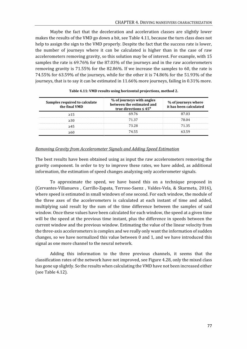
CHAPTER 4. DRIVING MANEUVERS CHARACTERIZATION
77
Maybe the fact that the deceleration and acceleration classes are slightly lower
makes the results of the VMD go down a bit, see Table 4.11, because the turn class does not
help to assign the sign to the VMD properly. Despite the fact that the success rate is lower,
the number of journeys where it can be calculated is higher than in the case of raw
accelerometers removing gravity, so this solution may be of interest. For example, with 15
samples the rate is 69.76% for the 87.03% of the journeys and in the raw accelerometers
removing gravity is 71.55% for the 82.86%. If we increase the samples to 60, the rate is
74.55% for 63.59% of the journeys, while for the other it is 74.86% for the 51.93% of the
journeys, that is to say it can be estimated in 11.66% more journeys, failing in 0.31% more.
Table 4.11: VMD results using horizontal projections, method 2.
Samples required to calculate the final VMD
% of journeys with angles between the estimated and
true directions ≤ 45⁰
% of journeys where it has been calculated
≥15 69.76 87.03
≥30 71.37 78.04
≥45 73.28 71.35
≥60 74.55 63.59
Removing Gravity from Accelerometer Signals and Adding Speed Estimation
The best results have been obtained using as input the raw accelerometers removing the
gravity component. In order to try to improve these rates, we have added, as additional
information, the estimation of speed changes analyzing only accelerometer signals.
To approximate the speed, we have based this on a technique proposed in
(Cervantes-Villanueva , Carrillo-Zapata, Terroso-Saenz , Valdes-Vela, & Skarmeta, 2016),
where speed is estimated in small windows of one second. For each window, the module of
the three axes of the accelerometers is calculated at each instant of time and added,
multiplying said result by the sum of the time difference between the samples of said
window. Once these values have been calculated for each window, the speed at a given time
will be the speed at the previous time instant, plus the difference in speeds between the
current window and the previous window. Estimating the value of the linear velocity from
the three-axis accelerometers is complex and we really only want the information of sudden
changes, so we have normalized this value between 0 and 1, and we have introduced this
signal as one more channel to the neural network.
Adding this information to the three previous channels, it seems that the
classification rates of the network have not improved, see Figure 4.28, only the mixed class
has gone up slightly. So the results when calculating the VMD have not been increased either
(see Table 4.12).

DEEP NEURAL NETWORKS FOR VEHICLE DRIVING CHARACTERIZATION BY MEANS OF SMARTPHONE SENSORS
78
Figure 4.28: Confusion matrix on raw accelerometers tests removing gravity and adding speed estimation, method 2: a) according to the number of tested acceleration forces, b) according to the type
of force.
Table 4.12: VMD results using raw accelerometers removing gravity adding speed estimation, method 2.
Samples required to calculate the final VMD
% of journeys with angles between the estimated and
true directions ≤ 45⁰
% of journeys where it has been calculated
≥15 67.31 83.03
≥30 68.97 71.15
≥45 69.99 60.67
≥60 70.39 51.23
Comparative study
In this subsection, we will compare both the results obtained from the output of the neural
network based on several metrics, as well as the percentage of success in calculating the
VMD.
Five different metrics commonly used in the literature have been used: accuracy,
which refers to the rate of correctly classified maneuvers; precision, that refers to the
proportion of predictions that have been correctly classified; recall, the rate of true labels
predicted; F1 score, harmonic mean of precision and recall; and, G mean, geometric mean.
The results are shown in the Figure 4.29. The baseline is the classifier with the raw
accelerometers as inputs.
As it is a multi-label problem, for each one of the metrics the corresponding formulas
have been applied by labels, calculating the metric for each label as if it were a binary
classification problem, and then averaging them. To get the mean, two usual forms have
been applied: macro-averaged (Figure 4.29 b)) and micro averaged (Figure 4.29 c)). The
main difference is that for macro-averaged, initially the formula of the metric is applied for
each class and then these are averaged; and for micro-averaged, firstly it is necessary to add
the true positives (TP), false positives (FP), true negatives (TN) and false negatives (FN) of
the six classes and once these four values are obtained, to apply them in the formula of the
corresponding metric.

CHAPTER 4. DRIVING MANEUVERS CHARACTERIZATION
79
Figure 4.29: Performance metrics for maneuvers classification. a) Accuracy. b) Macro-averaged metrics. c) Micro-averaged metrics.
It is possible to observe that the raw accelerometers removing gravity offer the best
results compared to other configurations, see Figure 4.29, going over the metric of most
other inputs. The results adding the information of the speed are similar; therefore, we are
going to take only the accelerometers without gravity as the best, since they require less
processing. The percentage of right maneuvers classified is 59.81% (accuracy), see Figure
4.29 a). The ratio of predictions correct are 31.84% and 33.16% for macro and micro
precision respectively; and the accuracy for the true labels are 65.76% for macro recall and

DEEP NEURAL NETWORKS FOR VEHICLE DRIVING CHARACTERIZATION BY MEANS OF SMARTPHONE SENSORS
80
59.81% for micro recall. The F1 score and the G mean are, respectively, 35.89%
(macro)/42.67% (micro) and 62.67% (macro)/59.81% (micro). The results of classification
are acceptable, since as mentioned the task of classifying these four classes is quite complex
using only accelerometers. We have improved baseline results, but they are still insufficient
for the accurate classification and do not provide excessively good results, probably for
several reasons. One reason may be the previous nature of the classes, which categorizing
them into a pure single class becomes complicated because the classes can easily present
patterns of other categories. For example, it is extremely tricky to find a pure turn event
(almost always these events have some longitudinal force). It is also important to highlight
that until selecting the Deep Learning model used, we tested with different Deep Learning
architectures consisting of several convolutional layers plus dense layers at the output,
without including the recurrent networks. However, the results obtained were worse more
than 5% with respect to the final selected model in the raw accelerometer tests. Among the
different recurrent networks tested were the long short-term memory (LSTM) and gated
recurrent unit (GRU) networks, but the LSTMs showed a result of around 3% lower average
compared to the GRUs.
In the following Table 4.13 are the results obtained in the estimation of the VMD
(percentage of correctly classified journeys) and the number of journeys where it can be
calculated, when we require 60 or more samples for each approach. As mentioned, in some
cases it may be interesting to obtain the direction in the greatest possible number of
journeys or, on the contrary, obtain a higher rate of success despite calculating it in a smaller
number of trips. Depending on this criterion, the most appropriate input may vary from
projections of accelerations over the horizontal plane or the raw accelerometers without
gravity. If we want to increase the reliability, we can demand more samples in the
calculation of the VMD, but the percentage of journeys where it is estimated will decrease
in all cases.
Table 4.13: Comparison of performances in VMD estimation when we require 60 or more samples.
Samples required to calculate the final VMD
% of journeys with angles between the estimated and
true directions ≤ 45⁰
% of journeys where it has been calculated
Raw accelerometers 52.33 67.67
Removing gravity 74.86 51.93
Horizontal projections 74.55 63.59
Removing gravity & adding speed information
70.39 51.23
Now we are going to try to interpret the training process in the different layers of
the Deep Learning architecture. For that, from a smaller set of journeys, the feature vectors
obtained in the outputs of the different network layers have been projected, using the t-SNE
algorithm. For this purpose, different values of perplexity have been tested, obtaining 50 as
the most optimal to visualize the groups. This perplexity value will also be used for the rest
of the tests. The first projection corresponds to the feature vector of the test set obtained at
the output of the second convolutional layer. The second projection corresponds to the
feature vector of the same test set but at the output of the recurrent networks. These feature

CHAPTER 4. DRIVING MANEUVERS CHARACTERIZATION
81
vectors have been projected in function on the type of class predicted by the network. And
in order to see the influence of how gravity is distributed among the three axes and the noise
threshold of the journey, these have also been shown as a function of them.
In Figure 4.30 a), we can see these projections when the raw accelerometers are
used as input.
Figure 4.30: Two-dimensional t-distributed stochastic neighbor embedding (t-SNE 2D) projections of feature vectors for raw accelerometers input signals to the output of the convolutional network (CNN)
(left representations) and gated recurrent unit (GRU) network (right representations). a), d) Projection depends on type of acceleration force. b), e) According to gravity distribution. c), f)
According to noise threshold of the journey (m/s2).

DEEP NEURAL NETWORKS FOR VEHICLE DRIVING CHARACTERIZATION BY MEANS OF SMARTPHONE SENSORS
82
It is possible to observe how the convolutional network by itself is not able to create
four unique clusters associated with the four output categories, although it is already
capable of grouping classes of different types that are mixed. On the contrary, the output of
the GRU recurrent networks, Figure 4.30 d), seems indeed to distinguish four big clusters,
in spite of the results being not optimal. In Figure 4.30 b), e), we draw these same
projections but as a function of how gravity is distributed between the axis of the
accelerometers. Firstly it is worth emphasizing that the most common mobile position for
the drivers is when the Z axis receives a great part of gravity, and the mobile is horizontal
with respect to the ground. At the output of the convolutional network, Figure 4.30 b) shows
that this distribution seems to be very important in network decisions; the X, Y and Z axes
appear to be in different groups, except obviously in the case of distributed, when there is
no axis that receives most of the gravity. Whereas at the output of the recurrent networks,
Figure 4.30 e), although they appear more mixed, it still seems a decisive parameter. Finally,
if we represent it as a function of the noise threshold of the journey, something similar to
the output of the convolutional network occurs, Figure 4.30 c), but not to the GRU, Figure
4.30 f); it seems that the network is able to discriminate independently of the noise
threshold, not perfectly but better than with the gravity distribution.
With the previous results, the importance of the gravity in the decision is
highlighted, and this can be one of the reasons why when we eliminate the component of
the gravity or we project them to a horizontal plane the rates improve regarding the raw
accelerometers. If now we paint these projections of the feature vectors but only at the
output of the recurrent networks, for the three remaining strategies: removing gravity
(Figure 4.31), projecting in the horizontal plane (Figure 4.32) and removing gravity and
adding the information of the speed (Figure 4.33), we can observe the independence with
respect to these two parameters, gravity and noise threshold, as well as the input that best
groups the clusters into four categories in which we remove the gravity of the raw
accelerometers, whether or not we add the speed information.
Figure 4.31: t-SNE 2D projections of feature vectors for raw accelerometers removing gravity input signals to the output of GRU network. a) Projection depends on type of acceleration force. b) According
to gravity distribution. c) According to noise threshold of the journey (m/s2).

CHAPTER 4. DRIVING MANEUVERS CHARACTERIZATION
83
Figure 4.32: t-SNE 2D projections of feature vectors for horizontal projections input signals to the output of GRU network. a) Projection depends on type of acceleration force. b) According to gravity
distribution. c) According to noise threshold of the journey (m/s2).
Figure 4.33: t-SNE 2D projections of feature vectors for raw accelerometers removing gravity input signals plus speed estimation to the output of GRU network. a) Projection depends on type of
acceleration force. b) According to gravity distribution. c) According to noise threshold of the journey (m/s2).
Summarizing the results, this method has shown its limitations, not being able to
estimate the direction in the whole set of routes and obtaining a success rate that does not
exceed approximately 75%. Therefore, we propose the following solution, which instead of
classifying directly with the acceleration forces, will try to predict the longitudinal and
transversal forces.
4.4.3. Method 3: longitudinal and transversal acceleration assignment
For the method 3 of longitudinal and transversal acceleration assignment, whose process is
shown in the Figure 4.34, the objective is to obtain the longitudinal and transversal
acceleration signals from the accelerometers. Once these signals are obtained, it is easy to
obtain the VMD or to classify the maneuvers.
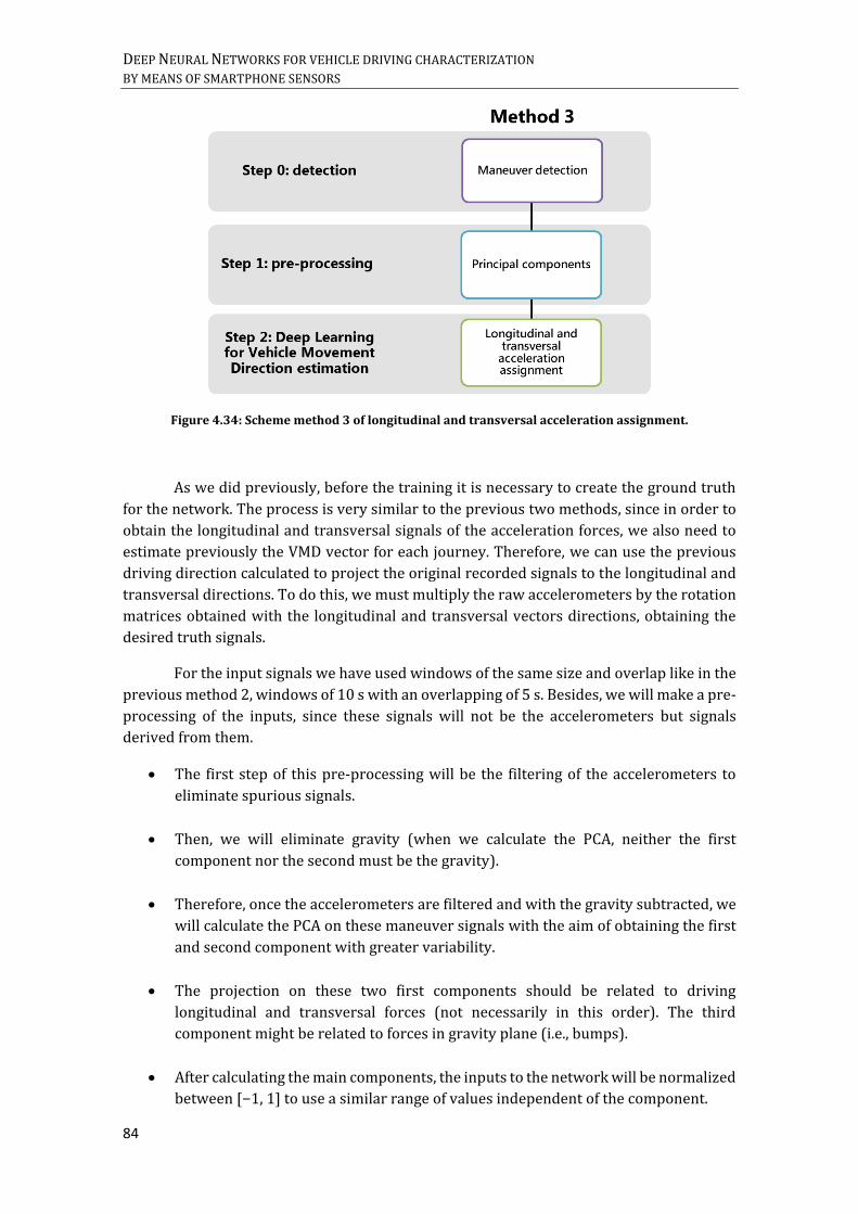
DEEP NEURAL NETWORKS FOR VEHICLE DRIVING CHARACTERIZATION BY MEANS OF SMARTPHONE SENSORS
84
Figure 4.34: Scheme method 3 of longitudinal and transversal acceleration assignment.
As we did previously, before the training it is necessary to create the ground truth
for the network. The process is very similar to the previous two methods, since in order to
obtain the longitudinal and transversal signals of the acceleration forces, we also need to
estimate previously the VMD vector for each journey. Therefore, we can use the previous
driving direction calculated to project the original recorded signals to the longitudinal and
transversal directions. To do this, we must multiply the raw accelerometers by the rotation
matrices obtained with the longitudinal and transversal vectors directions, obtaining the
desired truth signals.
For the input signals we have used windows of the same size and overlap like in the
previous method 2, windows of 10 s with an overlapping of 5 s. Besides, we will make a pre-
processing of the inputs, since these signals will not be the accelerometers but signals
derived from them.
The first step of this pre-processing will be the filtering of the accelerometers to
eliminate spurious signals.
Then, we will eliminate gravity (when we calculate the PCA, neither the first
component nor the second must be the gravity).
Therefore, once the accelerometers are filtered and with the gravity subtracted, we
will calculate the PCA on these maneuver signals with the aim of obtaining the first
and second component with greater variability.
The projection on these two first components should be related to driving
longitudinal and transversal forces (not necessarily in this order). The third
component might be related to forces in gravity plane (i.e., bumps).
After calculating the main components, the inputs to the network will be normalized
between [−1, 1] to use a similar range of values independent of the component.

CHAPTER 4. DRIVING MANEUVERS CHARACTERIZATION
85
The task of the neural network will be to assign each calculated component with the
corresponding longitudinal or transversal accelerations. The PCA gives the sign to the
components randomly, so the network must assign the correct sign, among the eight
possible combinations. The network used for this process is shown in the Figure 4.35. This
assignment will be constant along the journey and also, in order to help the network in this
process, we will add the estimate of normalized gravity (for each journey) before the final
stage of the classifier.
Figure 4.35: Deep neural network architecture for longitudinal and transversal prediction, method 3.
The eight possible combinations that can be produced are shown in the Table 4.14,
where PC makes reference to principal component, and L and T to longitudinal and
transversal respectively. One of the differences of this method with respect to the previous
ones is that the balancing of the data will not be performed depending on the type of
maneuver, but based on the combinations of the table, since the final objective of the
network is different.
Table 4.14: Possible combinations of the input signals for the method 3 training network.
Combinations Labels
PC1: L+; PC2: T+ 1 PC1: L+; PC2: T− 2 PC1: L−; PC2: T+ 3 PC1: L−; PC2: T− 4 PC1: T+; PC2: L+ 5 PC1: T+; PC2: L− 6 PC1: T−; PC2: L+ 7 PC1: T−; PC2: L− 8
The following image, Figure 4.37, shows a real example of driving maneuver. The
Figure 4.37 a) shows the signals that are introduced to the network, which correspond to
the PCA calculated on the accelerometers. As we can see in the Figure 4.37 c), this particular
maneuver corresponds to the route through a roundabout. We have obtained the map
through Google Maps and the GPS information that we had on this route. Predictions in this
method are made with the probabilities of the output of the network in overlapping sliding
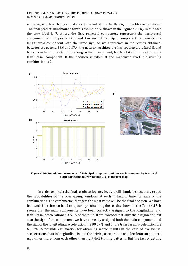
DEEP NEURAL NETWORKS FOR VEHICLE DRIVING CHARACTERIZATION BY MEANS OF SMARTPHONE SENSORS
86
windows, which are being added at each instant of time for the eight possible combinations.
The final predictions obtained for this example are shown in the Figure 4.37 b). In this case
the true label is 7, where the first principal component represents the transversal
component with opposite sign and the second principal component represents the
longitudinal component with the same sign. As we appreciate in the results obtained,
between the second 36.6 and 37.4, the network architecture has predicted the label 5, and
has succeeded in the sign of the longitudinal component, but has failed in the sign of the
transversal component. If the decision is taken at the maneuver level, the winning
combination is 7.
Figure 4.36: Roundabout maneuver. a) Principal components of the accelerometers. b) Predicted output of the maneuver method 3. c) Maneuver map.
In order to obtain the final results at journey level, it will simply be necessary to add
the probabilities of the overlapping windows at each instant of time for each of the
combinations. The combination that gets the most value will be the final decision. We have
followed this criterion in all test journeys, obtaining the results shown in the Table 4.15. It
seems that the main components have been correctly assigned to the longitudinal and
transversal accelerations 93.53% of the time. If we consider not only the assignment, but
also the sign of the component, we have correctly assigned both the main component and
the sign of the longitudinal acceleration the 90.07% and of the transversal acceleration the
61.62%. A possible explanation for obtaining worse results in the case of transversal
accelerations than in longitudinal is that the driving acceleration and deceleration patterns
may differ more from each other than right/left turning patterns. But the fact of getting

CHAPTER 4. DRIVING MANEUVERS CHARACTERIZATION
87
worse results in this acceleration is not a big problem, since the sign of transversal
acceleration can be easily derived, if we know both the sign of the longitudinal component
and the direction of the gravity force vector (see Figure 4.21). Consequently, beyond the
results in Table 4.15, we can say that the correct assignment of the sign for the transversal
component is also 90.07%.
Table 4.15: Results obtained for the longitudinal and transversal component prediction, method 3.
Principal Component Assignment
Principal Component and Sign Assignment of the Longitudinal
Component
Principal Component and Sign Assignment of the Transversal
Component
93.53% 90.07% 61.62%
4.4.4. Maneuver characterization by VMD
This section shows one of the applications mentioned that has the calculation of the VMD:
the maneuver classification. Therefore, when calculating the VMD we have a vector relative
to the longitudinal accelerations that follow the direction of the movement (the VMD), and
a vector relative to the transversal accelerations, perpendicular to the movement. The fact
of knowing these vectors allows you to accurately and reliably classify every moment of
maneuver time. We simply have to calculate the angle between the VMD vector and the
event raw acceleration samples. We considered that belongs to the category of accelerations
(accelerations or decelerations/braking) if the average of the all maneuver sample vectors
are parallel to the VMD and to the category of turns (left or right turns) if these are
perpendicular.
The Figure 4.37 shows a real example where we have drawn the 3-D vectors of the
samples (Figure 4.37 a)) of the maneuver of the Figure 4.37 b).
Figure 4.37: a) Driving maneuver vectors. b) Map maneuver with start at the purple point and end at the red point.
In the Figure 4.37 a) we can see the blue vector, which represents the VMD that we
have obtained (with method 3, Section 0); the green vector as the calculated gravity; and in
black the specific maneuver vectors corresponding to the accelerations/decelerations and
in red the left/right turns. The vectors of the maneuvers are in a plane perpendicular to the
gravity, and as it should be, the vectors of the accelerations and decelerations are parallel

DEEP NEURAL NETWORKS FOR VEHICLE DRIVING CHARACTERIZATION BY MEANS OF SMARTPHONE SENSORS
88
to the VMD, while the turns are perpendicular. The map of the maneuver (Figure 4.37 b))
shows a purple dot that indicates the start of the maneuver, while the red dot indicates the
end. The succession of most likely actions will be a braking before going through the
roundabout, with a right turn at the input and at the output, followed by another section in
a straight line with accelerations, as well as another turn to the right again with a slight
braking before being followed by an acceleration. It seems that this reasonable succession
of actions coincides with the results obtained. So, it is possible with a VMD calculated
correctly, use it to characterize maneuvers reliably.
4.4.5. Comparison with the state of the art
Finally, we have evaluated the three models developed to characterize the driving
maneuvers more precisely by means of the VMD, making use of the cybernetic theoretical
framework explained in (Simpkins & Simpkins, 2012). The following Table 4.16, with the
summary results obtained for our proposals, is presented. According to this model, the
driver behavior depends on the iterative execution of a repetitive loop of five elements:
sensing, information processing, decision making, feedback and action. As in (Kanarachos,
Christopoulos, & Chroneos, 2018)(where they use the cybernetics model to compare,
among other things, the transportation mode classification or the aggressive driver
behavior), key aspects like the signals, the decision-making framework, the sensor fusion
level, the noise rejection, the feedback level and the performance are evaluated. The fusion
in the three methods is smartphone-based because the raw data do not update to a server
that combines signals centrally. In the column of noise is specified No, indicating that there
is no probabilistic formulation for rejecting noise and outliers embedded in the signal. The
feedback is evaluated only based on its performance, not comparing it with other
performance. The metric used for the performance is the accuracy, with 63.86% in method
1, 74.86% in method 2 and 90.07% in method 3.
Table 4.16: Smartphone-based estimation of vehicle movement direction.
VMD Estimation
Method Signals Framework Fusion Noise Feedback Performance
Method 1 Accelerometers Neural
Networks Smartphone based fusion
No Compared
to me 63.86%
accuracy
Method 2 Accelerometers Neural
Networks Smartphone based fusion
No Compared
to me 74.86%
accuracy
Method 3 Accelerometers Neural
Networks Smartphone based fusion
No Compared
to me 90.07%
accuracy
One key point of our work, with respect to others that are state of the art, is that we
do not need a calibration. In addition, the database is very extensive since more than 60000
real driving journeys have been used, recorded in mobile phones with Android or iOS
operating systems, more than 100 different smartphones and more than 3000 different
drivers; so we consider the results obtained extremely reliable. Also, significant points are
that the device can go in any position for a more natural detection, and that we only use the
accelerometers. Using Deep Learning techniques for the best of the methods (the third), an
CHAPTER 4. DRIVING MANEUVERS CHARACTERIZATION
89
accuracy of 90.07% is obtained in the prediction of the VMD, which ensures the correct
classification of the maneuvers in at least that percentage of journeys. Therefore, the results
are totally comparable with other studies that use more sensors and thus need more
resources.
4.5. Conclusions
In this chapter we have addressed the maneuver characterization, through two different
strategies. The first one is based on the classification of the maneuvers, in a more general
way, distinguishing between events related to longitudinal and transversal forces to the
driving direction. The second of them allows a much more precise classification of the
maneuvers, not only distinguishing between accelerations and turns, but between
accelerations and brakings or left and right turns.
One of the first steps, common in both strategies, is the detection of maneuvers. For
the detection of maneuvers, we use the projection from the smartphone accelerometers to
a 2D horizontal plane. In this plane, the beginning and the end of the maneuvers can be
determined by means of energy thresholds calculated on said projection. For the first more
general strategy, once the positions of the maneuvers have been obtained, we done a
classification, using three different segmentation techniques: fixed-length windows,
variable-length windows and sliding windows. All applied to different models of Deep
Learning. The segmentation techniques that has offered the best results has been with the
variable-length windows. Probably because it allows to use the real length of the events.
With accuracy values of 88.82%, distinguishing between accelerations/decelerations and
turns/mixed maneuvers.
For the second strategy, which addresses classification more precisely, we have
developed three methods. The first one called “stop detection”, it is based on the hypothesis
that the maneuvers immediately performed after a stop will be acceleration maneuvers,
while the events immediately before the stop will be a deceleration or braking. With this
idea, we have combined the detection and classification of maneuvers along a journey, with
the detection of stops, through an algorithm that calculates the final vehicle movement
direction. The classification of the stops becomes a complicated task, since the type of signal
captured by the accelerometers is very similar when driving at constant speeds than when
we stop the vehicle, which results in detecting many stops that actually do not they are. This
causes that the conditions defined for the vehicle movement direction calculation algorithm
are very strict; therefore, the number of journeys where it can be calculated is very small.
The second method developed, “acceleration forces classification”, makes a previous
classification of the signals along the journey in order to obtain the vehicle movement
direction with that information. Specifically, it uses the maneuvers of the trip and classifies
them into 4 types; maneuvers of braking (decelerations) without turn, maneuvers of
acceleration without turn, pure turns and mixed events (that is, combinations of the above).
If a good characterization of the signals of the journey is achieved, it is possible through a
post-processing algorithm to obtain the movement direction of the vehicle. As we have

DEEP NEURAL NETWORKS FOR VEHICLE DRIVING CHARACTERIZATION BY MEANS OF SMARTPHONE SENSORS
90
observed throughout the chapter, the type of signal used in the network causes that the
results obtained in the classification vary greatly, offering better accuracy values the
accelerometer signals when we subtract gravity. Although the results are better for this
method than for the stop detector, they do not exceed those obtained with method 3.
The last method, method 3 of longitudinal and transversal acceleration assignment,
focuses the search of the vehicle movement direction in a different way to the previous ones.
It is also necessary to detect the maneuvers of the journey, but the objective is not that the
network classifies them, but from some pre-processed signals of the accelerometers it
learns to associate them with the longitudinal and transversal components of the
accelerations. If we can obtain the longitudinal or transversal accelerations, we can
automatically know the direction of movement. To prepare the signals at the input of the
network we have calculated the main components on the accelerometers, so that the first
and the second component collect the variability associated with driving maneuvers and
these facilitate the learning to the network for associating the components with
accelerations. The results obtained have been quite high, since we can calculate it in any trip
and also we have a success rate calculating the vehicle movement direction of 90.07%.
Using the method that has offered the best results, the method of longitudinal and
transversal acceleration assignment, we have utilized the vehicle movement direction
obtained for classifying a real driving maneuver. The fact of having this direction allows to
characterize the maneuver in a precise and reliable way at every moment of time.
91
Chapter 5
Driver recognition
iometric systems use physical or behavioral characteristics of a person to
authenticate their identity. These recognition systems are also being incorporated
into the driving area. Thereby, through physiological signals, such as facial features,
or through behavior patterns of a person, such as her/his voice, attempts are made in order
to incorporate such biometric systems for improving the vehicle safety. Biometrics
associated with driver recognition can be divided into two different tasks: driver
identification and driver verification. But not only driver recognition has appeared in
applications associated with safety, it is also attracting interest in other areas as fleet
management systems, car insurance or in the automobile industry for the improvement of
vehicle customization systems. Due to this increasing interest in driving characterization
systems, in this chapter we address both driver identification and verification using
smartphone signals that capture drivers’ behavior. As it is a global objective in this Thesis,
we will focus our research on drivers’ characterization using exclusively smartphone tri-
axial accelerometer sensors, as it will guarantee low-battery consumption applications.
The content in this chapter is organized as follows. Section 5.1 reviews the most
significant research in driver recognition systems. In Section 5.2 we address the driver
identification problem proposing the use of Convolutional and Recurrent Neural Networks
and exploring the advantage of relying on pre-trained models through Transfer Learning.
We also study several techniques to transform 1-D accelerometer signals into 2-D
representations suitable to be used is inputs of Deep Learning models developed for image
recognition. Experimental activities in driver identification has been designed for two
complementary scenarios. Subsection 5.2.2 considers drivers’ identification working
directly on accelerometers signals captured from mobile devices. In Subsection 5.2.3 we
study drivers’ identification from acceleration signals derived from GPS positions. The aim
of this second study was to contrast our results on a public database where previous
research works exist. Finally, Section 5.3 is devoted to drivers’ verification where models
based on Siamese Neural Networks, Embeddings and Triplet Loss training are explored.
B

DEEP NEURAL NETWORKS FOR VEHICLE DRIVING CHARACTERIZATION BY MEANS OF SMARTPHONE SENSORS
92
5.1. State of the art in driver recognition
Smartphones are one of the first devices to incorporate biometric technology into everyday
applications. Mobile devices perform users’ authentication using different modalities as
data from fingerprint sensors, images for facial or iris recognition, or speech. In this Thesis,
we try to contribute to the use of smartphones to implement biometric systems that
facilitate driver recognition, as another modality for people characterization. In particular,
we research on the use of accelerometer signals as sensors to model drivers’ behavior. The
hypothesis is that driver behavior is different and unique for each person, so it could be
used as a fingerprint for drivers’ identify. Within the driver recognition, two different tasks
are distinguished: identification and verification. Before reviewing specific research for
each of them, we will review the most relevant works on drivers’ behavior modelling.
As shown in (Figure 5.1), our driver recognition objective is to model the specific
driver behavior by using accelerometer signals captured by her/his mobile when she/he is
driving along any route. However, since most literature researches use other signals, such
as location or pedal signals, we propose also a second scenario. In this scenario, the
acceleration signals will be derived through GPS positions (which can influence the way of
identifying: will we identify how they drive or where they drive?).
Figure 5.1: Driver recognition objective: modeling specific driver behavior by using accelerometer signals.
Driver recognition can be applied to many tasks. For instance, in fleet management
systems; where it is necessary to know which fleet driver is making the journey. It is also
used in some types of secure transport, where vehicles can only be driven by authorized
staff. But recognition is relevant not only from the point of view of safety or control, but can
also be very useful for customization and comfort. For example, if we can identify who is the
driver within a family, the vehicle can automatically adjust some characteristics to that
driver, like radio or temperature. Besides, technology evolution has allowed to access and
to process a large amount of data, even in real time. Having a lot of driver information has
caused that insurance companies show interest in drivers’ identification and driving
modelling. There are already plans for vehicle insurance in accordance with the driving

CHAPTER 5. DRIVER RECOGNITION
93
behavior, by adjust their prices based on various factors, instead of a fixed premium per
year, such as the so-called Pay as you drive (PAYD) or Usage-Based Insurance (UBI). Real
examples of these plans are Snapshot of Progressive (Progressive, 2019) or PriPAYD
(Troncoso, Danezis, Kosta, Balasch, & Preneel, 2011).
We show below a summary of the most relevant works of the state-of-the-art in
driver recognition. For that purpose, we have divided this study according to different areas
of interest, presenting a review of some research that addresses the characterization
(Subsection 5.1.1), the driver identification (Subsection 0) and the driver verification
(Subsection 5.1.3). In driver identification, we have made a special mention to the
researches that uses Deep Learning techniques (Subsection 5.1.2.1), as well as the possible
applications (Subsection 5.1.2.2). For each of these subsections, the most outstanding works
and summary tables are presented.
5.1.1. General driving characterization
The characterization of the driver defines its behavior, for instance if a driver is
aggressive or not or what kind of actions she/he performs while driving. This has made that
many researches do not pursue a univocal identification of the driver, but to include the
driver within a category, such as aggressive or non-aggressive. Works like (Yan, Teng, Smith,
& Zhang, 2016) try to recognize driver conduct using Convolutional Networks. Among the
reasons they defend to perform the behavior characterization is the importance of
improving the road safety, since many of the accidents are caused by human errors. To do
this, they propose a system that consists of capturing an image while driving. This image is
used to analyze both the driver’s pose and the contextual information by exploring the skin-
like region. The skin-like regions are first extracted with a Gaussian Mixture Model (GMM)
algorithm of skin images, and then they are sent to a Convolutional Network that will
determine the action of the driver (for example if she/he is manipulating the cell phone,
eating, with hands on the steering wheel, etc.).
An interesting application of driver identification is privacy violation. Works like
(Enev, Takakuwa, Koscher, & Kohno, 2016) propose using driver identification to find out
who is driving a vehicle or to extract private information. For their experiments, they
selected the CAN2 bus sensors of the car and they worked with a set of 15 drivers.
Participants had to do a series of maneuvers in an isolated parking lot and to drive the
vehicle in traffic along a defined ∼ 50 mile loop. Driver identification decision was made by
a majority voting algorithm from all possible one-vs-one comparisons. With their results,
they observed that at least in a small dataset, it was possible to distinguish the driver using
only the in-car sensors; and that the more sensors were used the greater the ability to
2 “CAN protocol defines a generic communication standard for all the vehicle electronic devices. CAN protocol can cooperate with the OBD II diagnostic connector (http://obd2-elm327.com/) that provides a candidate list of vehicle parameters to monitor along with how to encode their data.” (Bernardi, Cimitile, Martinelli, & Mercaldo, 2018)
DEEP NEURAL NETWORKS FOR VEHICLE DRIVING CHARACTERIZATION BY MEANS OF SMARTPHONE SENSORS
94
distinguish them. This study is also very interesting since it formulates an important
question regarding the research in this chapter: is it possible to identify or to create a
fingerprint of a driver from the recordings of her/his journeys? And more specifically, what
sensors are necessary to carry out this identification? Would it be possible using only the
accelerometers of the driver smartphone? Moreover, as this work emphasizes, analyzing the
ability of different sensors for driver identification rises and important debate on the
privacy implications and potential misuse. Authors advocate to create policies that take into
account both the utility of the use of sensors and privacy issues: “Anecdotally, we find that
companies have, in the past, already used or know that they could use the data available on
vehicles in ways that some might consider privacy-violating. For example, Elon Musk (Tesla
Motors CEO) recently used vehicle sensor data to dispute the claims of a New York Times
journalist about the limited range of his car’s electric batteries (Musk demonstrated that
during a road test the NYT journalist took a detour and did not fully charge the vehicle)
(Undercoffler, 2013). Similarly, Ford sales executive Jim Farley was quoted as saying: “We
know everyone who breaks the law. We know when you are doing it. We have GPS in your car,
so we know what you are doing.” (Trop, 2014).”
CAN (Controller Area Network) bus signals are a rich source for driving
characterization as they allow transmitting a lot of vehicle information. An example of
driving identification system that uses CAN signals is presented in (Ly, Martin, & Trivedi,
2013). This work addresses a typical family scenario, where there are usually two or three
drivers for a single car; so they propose an identification of the driver for a set of 2 drivers
and in the same vehicle. It is true that the information provided by the CAN bus is very
valuable, but the fact of selecting these inputs means that we need a device for taking the
vehicle data, usually by connecting to the OBD connector of the car (commonly found under
the steering wheel). This is more invasive than using a mobile phone directly, hence our
interest in using only the smartphone.
In order to study behavior during driving, there are also works that use
unsupervised algorithms. For example, in (Guo, Liu, Zhang, & Wang, 2018) authors employ
an unsupervised model of Deep Learning, Autoencoders and Self-organized Maps (AESOM),
to study driving behavior and risk patterns using the Global Positioning System (GPS) data.
Using GPS data, they can measure speed changes, accelerations and decelerations or turns.
The model consists of an Autoencoder (AE) for feature learning followed by clustering using
Self-Organized Maps (SOMs), in order to classify the driver actions. The speed or overspeed
patterns are divided into 4 clusters: none, slight, moderate and heavy. Acceleration, braking
(deceleration) or turning are grouped in 3 clusters: slight, moderate or heavy.
Others works as the one in (Ferreira Júnior, et al., 2017) use a larger number of
sensors, specifically four smartphone sensors: accelerometer, linear acceleration,
magnetometer and gyroscope. In their research they emphasize the importance of how
driver behavior influences in traffic safety, in fuel energy consumption or in gas emissions.
Their objective is to detect aggressive/non-aggressive driving maneuvers, specifically seven
types of driving events: aggressive braking (or deceleration), aggressive acceleration,
aggressive left turns, aggressive right turns, aggressive left lane changes, aggressive right
lane changes and non-aggressive maneuvers. To do this, they compare four Machine
Learning algorithms: Artificial Neural Networks (ANN), Support Vector Machines (SVM),
Random Forest (RF) and Bayesian Network (BN). A limitation of this work is that it only

CHAPTER 5. DRIVER RECOGNITION
95
consider Android smartphone sensors to detect events, which can cause different results
depending on the type of operating system and mobile terminal. Among the conclusions that
they obtained are that according to the sensor combination and the method used for
classification, the improvement in the performance may differ importantly. So in our case,
using a single sensor can be challenging.
As mentioned before, Table 5.1 summarizes the reviewed works.
Table 5.1: State of the art in driving characterization (alphabetically ordered).
Ref. Description Signals Method Results and/or
conclusions
(Enev, Takakuwa, Koscher, &
Kohno, 2016)
Identification of 15 drivers. The same car,
during the same time of day, in an isolated
parking lot and in a predefined interurban loop spanning roughly
50 miles.
CAN bus sensors of the vehicle:
brake pedal, max engine torque, steering wheel,
lateral acceleration, fuel,
etc.
Machine learning
algorithms: SVM, RF, NB
and KNN
∼87.33% accuracy using brake pedal and 15 min of open-road.
100% using brake pedal and 1.5 h of journey. ∼91.33%
using all sensors in the parking lot and 8 min.
100% with all the sensors in the open-
road.
(Ferreira Júnior, et al.,
2017)
Detection of aggressive driving events.
Smartphone sensors: the
accelerometer, the linear
acceleration, the magnetometer and
the gyroscope.
ANN, SVM, RF and BN.
The gyroscope and the accelerometer are the most suitable sensors to detect the driving
events.
(Guo, Liu, Zhang, & Wang,
2018)
Classification of some driving behaviors as
speed changes, accelerations,
decelerations, turns or combination of them in none, slight, moderate
and heavy.
GPS. AESOM.
Behavior patterns can be observed, grouping the drivers according
to different criteria and speed classes and
maneuvers.
(Ly, Martin, & Trivedi, 2013)
Differentiation between two drivers.
Lateral and longitudinal
accelerations, and yaw angular
velocity.
k-mean clustering and SVM.
Braking is the most distinguishing feature
vector among acceleration, braking and turn maneuver
events. And combining turning and braking
events helps to differentiate better
between two similar drivers.
(Yan, Teng, Smith, & Zhang,
2016)
Action done by a particular person while driving: in a phone call,
eating, braking, with hands in the correct driving position on
wheel, playing phone or smoking.
Image captured while driving.
GMM and CNN.
Mean average precision (mAP) of
97.76%.

DEEP NEURAL NETWORKS FOR VEHICLE DRIVING CHARACTERIZATION BY MEANS OF SMARTPHONE SENSORS
96
5.1.2. Driver identification
In (Ezzini, Berrada, & Ghogho, 2018) driver identification is addressed using three different
databases. One of them includes data coming from the CAN bus of the car, another use data
from smartphones inside the vehicles (through an application), and the last one is a public
database that includes drivers’ physiological data. The database of smartphones collects
GPS information (speed, latitude, longitude, altitude, course, etc.), plus information from
accelerometers and gyroscopes. Moreover, the CAN bus database collects recorded video
signals while driving. In the public database physiological data comes from different types
of sensors: conductance skin, thermometers and ECG (electrocardiogram). In these
databases, driving is done on predefined routes, simulating sequences of different behaviors
such as normal, aggressive and drowsy driving. The algorithms used for identification are
Decision Trees, Extra Trees, RF, k-Nearest Neighbor (kNN), SVM, Gradient Boosting,
AdaBoost based on Decision Tree, and MLP. One of the conclusions they draw is that fuel-
related features seem to be the most relevant for driving style categorization. Another
important conclusion is that data collected from the brake pedal and the steering wheel are
very relevant for driving characterization. Although the performance obtained in this work,
in terms of driver identification accuracy, is high, the number of features employed to obtain
these results it is also very high, whereas the number of drivers is quite small. For instance,
in the CAN bus database they work with a small number of 10 drivers, 4 journeys per driver
and predefined routes.
A research similar to ours in terms of the data employed is (Phumphuang,
Wuttidittachotti, & Saiprasert, 2015), since it studies the use of accelerometers of the
drivers’ smartphones. But unlike us, the smartphones must be in a fixed position inside the
car. The fact that smartphones are in fixed position allows them to assign each axis to an
action. Specifically, in their case the X axis represents driving actions in side to side direction
(such as turn left and turn right); and the Y axis, driving actions in forward and backward
direction (such as accelerating and braking). In our case, we have the difficulty that the
mobile can go in any position, so gravity may affect each axis differently. Besides, not only
the smartphone can change their position in different trips, but it can also change its
position during the same journey. So, we need to detect these changes and divide the
journeys into several segments.
The work of (Chowdhury, Chakravarty, Ghose, Banerjee, & Balamuralidhar, 2018) is
also very relevant in this field. They also try to identify the driver through smartphone data.
To do this, they select the GPS and record the data from 38 drivers for two months.
Nevertheless, they do not perform the identification of the 38 drivers, they segregate them
in groups of 4 to 5 drivers. The GPS data they use are the speed, the location, the course and
the horizontal accuracy. From them, they obtain the longitudinal acceleration, the angular
speed, the lateral acceleration, the jerk (rate of change of acceleration) and jerk energy; in
addition to the first and second derivative with respect to time for speed, acceleration (both
longitudinal and lateral), jerk, jerk energy, and angular speed. Driving identification results
using RF obtain an average accuracy of 82.3%, when drivers are grouped in groups of 4 or
5 drivers. However, the accuracy when they use the whole set of the 38 drivers falls
CHAPTER 5. DRIVER RECOGNITION
97
significantly. The median accuracy obtained is 46% with standard deviation of 22%.
Although this work addresses the problem of identification using a single sensor, compared
to other works that are multisensor, we could ask again if when using GPS data: Is it the
identification due to the characterization of the driving style or to the characterization of
the route? Since as they comment: “It is to be noted that the authors of this paper played no
role in selecting drivers as well as the driving location. However, the subjects form a peer group
based on geography and it is assumed that they went about their normal lifestyles, usually
travelling from home to work and back, with one or two additional trips.” Therefore, using
signals related to localization could influence on the driving characterization process. On
the contrary, in our tests because we do not use location-related GPS data, we have not
created any group based on geography location of routes. Moreover, we use routes recorded
during all day and the routes can go through any path. Research such as (Ly, Martin, &
Trivedi, 2013), explicitly indicate that they decided not to use the GPS signal in order to the
results were independent of the route.
Another work that employs ML techniques is (Nishiwaki , et al., 2007). Due to the
good results that cepstral coefficients have shown in speech recognition, they decided to
perform a cepstral analysis in the signals of gas and brake pedal operations. Subsequently,
they use a GMM in order to model the features with cepstral coefficients. In this work, train
and test data are defined using different parts of the same route .That is, the first 3 minutes
of the journey is used for training and the next three minutes for testing, instead of using
different routes for training and testing. Their results show that gas pedal signals give better
performance than brake pedal signals, probably because drivers hit the gas pedal more
frequently than brake pedal signals. Using cepstral features they achieved an identification
rate of 76.8% for 276 drivers. Also (Martínez, Echanobe, & del Campo, 2016) utilize energies
in the frequency domain or cepstral coefficients like features. They use these features in an
ML model; specifically, they employ a single hidden-layer feedforward neural network.
They justify driver identification as a necessity for Advanced Driver Assistant Systems
(ADAS), systems that progress towards autonomous and connected driving. The number of
drivers that they study is 11, all of them perform the same route of around 25 km length.
They captured a total of 14 signals, including CAN-bus signals, gas pedal and brake pedal
sensors, frontal laser scanner, inertial measurement unit (IMU) with XYZ accelerometers
and measures of rotation rates (pitch, roll and yaw). From these 14 signals they obtain 42
features: temporal means, energies in the frequency domain and cepstral coefficients.
Experimental results were obtained by the whole set of 11 drivers as well as for subgroups
of 2, 3, 4 and 5 drivers. Accuracy results for 11 drivers was 84%, and 90% for the average
of the possible subgroups combinations.
There are also some research works not based on Machine Leaning nor Deep
Learning techniques, as for example (Wallace, et al., 2016). In this research, they work with
a set of 14 drivers, although the identification is done between pairs of drivers (resulting in
91 possible combinations of two drivers), and they use the two-phase acceleration
relationship for maximum and mean acceleration. In their experiments, they have seen an
important relationship between the mean and the maximum acceleration within the
acceleration maneuvers of a driver. There are large variations between these ratios for
different drivers, so this could be used to distinguish them.

DEEP NEURAL NETWORKS FOR VEHICLE DRIVING CHARACTERIZATION BY MEANS OF SMARTPHONE SENSORS
98
(Hallac, et al., 2016) mention that due to the improvement in technology, vehicles
have more reliable sensors, which help to navigate, to reduce accidents and to provide
comfortable rides. For example, cars have sensors to measure the fuel level, to report a
breakdown or to warn of a possible collision. In this work, driver characterization is
proposed through the characterization of turn maneuvers. They employ different sensor
signals from CAN bus of the car: GPS, steering wheel angle, steering velocity, steering
acceleration, vehicle velocity, vehicle heading, engine RPM, gas pedal position, brake pedal
position, forward acceleration, lateral acceleration, torque and throttle position. One of the
disadvantages of the test is that, although they use the 12 most frequent turns made by the
test drivers, these turns must be the same. That is to say, all drivers must perform the same
turn several times and then select the 12 most frequent, so the same maneuvers are
compared for all. The total set of drivers is 64 and 10 cars. For driver identification, they
analyze each turn independently and take 2 to 5 drivers for evaluations using Random
Forest models and obtaining an average accuracy of 76.9% for two-driver classification, and
50.1% for five drivers. The main conclusion in this work is that turn maneuvers can be very
useful in order to differentiate between drivers. This raises the question of: how the route
affects driver identification? Generally results on predefined routes reach high
identification rates, as they eliminate the route variability.
Table 5.2 shows the mentioned works.
Table 5.2: State of the art in driver identification (alphabetically ordered).
Ref. Description Signals Method Results and/or
conclusions
(Chowdhury, Chakravarty,
Ghose, Banerjee, &
Balamuralidhar, 2018)
Driver identification in groups of 4 to 5 drivers.
GPS data measurements: speed, location,
course and horizontal accuracy.
RF.
They segregate drivers in
different groups and analyze trips
for each group. Accuracy of 82.3% for driver groups
of 4–5.
(Ezzini, Berrada, & Ghogho,
2018)
Driver Identification From 6 to 10 drivers
depending on the database.
CAN bus, smartphone sensors and
physiological information.
Decision Tree, Extra Trees, RF,
kNN, SVM, Gradient Boosting,
AdaBoost based on Decision Tree
and MLP.
Fuel-related features seem to
be the most relevant to identify the
driving style.
(Hallac, et al., 2016)
Identification of the driver from a same turn maneuver, with a set of
2 to 5 drivers.
BUS can signals: steering wheel angle, steering
velocity, steering acceleration,
vehicle velocity and heading,
engine RPM, gas and brake pedal
positions, forward acceleration,
lateral acceleration,
torque and throttle position.
RF.
Average prediction
accuracy of 76.9% for two-driver
classification, and 50.1% for five
drivers.

CHAPTER 5. DRIVER RECOGNITION
99
(Martínez, Echanobe, & del Campo, 2016)
Driver identification in 11 drivers.
CAN-bus signals, gas pedal and brake pedal
sensors, frontal laser scanner,
accelerometers, pitch, roll and yaw.
A single hidden-layer
feedforward neural network.
For the identification of 11 drivers, the accuracy is the
84%. And for the average of the
possible subgroups
combinations is greater than 90%.
(Nishiwaki , et al., 2007)
Driver identification for 276 drivers.
Gas and brake pedal signals.
GMM. Identification rate
of 76.8%.
(Phumphuang, Wuttidittachotti,
& Saiprasert, 2015)
Driver identification by means of acceleration
variation.
Accelerations from a fixed
smartphone.
Principal Component
Analysis (PCA) and comparison with reference
pattern components.
They analyze the importance of
selecting the right variables to
correctly identify the driver.
Optimal value between 5 and 6
variables.
(Wallace, et al., 2016)
Driver identification. 14 drivers, but
identification is done between pairs of drivers
(91 possible combinations of two
drivers).
GPS, engine and dashboard parameters (inertial and
accelerator pedal position).
Two-phase acceleration
relationship (for the maximum
and mean acceleration
values within the acceleration
events).
They distinguish the 80% of the 91
possible driver pairs.
5.1.2.1. Deep Learning for driver identification
In (Dong, et al., 2016) driving styles are characterized using GPS data. They define driving
style like a signature for each driver, a complex combination of driving behaviors and habits
such as the way of accelerating, braking or turning and the combinations given by specific
driving contexts as roads, traffic conditions or weather. To realize this characterization they
use Deep Learning techniques. They defend to use Deep Learning techniques as a feature
extractor instead of handcrafted features due to five main reasons: “However, manually
defining the driving style by traditional feature engineering is challenging: (1) It heavily relies
on domain knowledge and human experience. (2) The discriminative power of the features is
often unknown before feeding into machine learning algorithms; so a common practice is to
enumerate as many features as possible and then apply feature selection, which requires
considerable efforts. (3) The best descriptors of driving patterns may change given different
data and contexts, e.g., drivers in China may have different driving patterns from those in US,
thus a generic model is often hard to obtain. (4) The feature designs are usually separated
from the learning algorithms, which cannot guarantee a best synergia between features and
algorithms. (5) Driving behaviors are typically a sequence of operations, therefore possible
combinations of features to define such sequences can be huge. It is hardly to find an optimal
driving style representations just by enumerations.” For doing this characterization, they
perform a transformation of the raw data to some statistical features and execute the
experiments using both convolutional and recurrent networks. Experimental results are
reported for the database used in Kaggle 2014 Driver Telematics Analysis competition. This
database include GPS data for a set of 2736 drivers, with 200 trips by driver (trips of
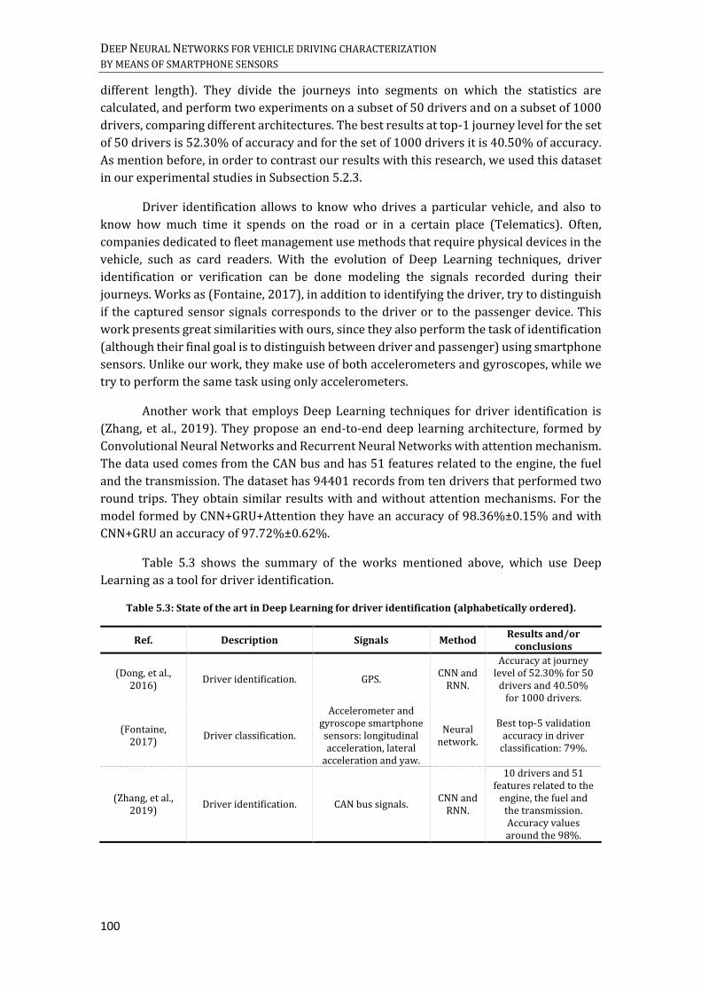
DEEP NEURAL NETWORKS FOR VEHICLE DRIVING CHARACTERIZATION BY MEANS OF SMARTPHONE SENSORS
100
different length). They divide the journeys into segments on which the statistics are
calculated, and perform two experiments on a subset of 50 drivers and on a subset of 1000
drivers, comparing different architectures. The best results at top-1 journey level for the set
of 50 drivers is 52.30% of accuracy and for the set of 1000 drivers it is 40.50% of accuracy.
As mention before, in order to contrast our results with this research, we used this dataset
in our experimental studies in Subsection 5.2.3.
Driver identification allows to know who drives a particular vehicle, and also to
know how much time it spends on the road or in a certain place (Telematics). Often,
companies dedicated to fleet management use methods that require physical devices in the
vehicle, such as card readers. With the evolution of Deep Learning techniques, driver
identification or verification can be done modeling the signals recorded during their
journeys. Works as (Fontaine, 2017), in addition to identifying the driver, try to distinguish
if the captured sensor signals corresponds to the driver or to the passenger device. This
work presents great similarities with ours, since they also perform the task of identification
(although their final goal is to distinguish between driver and passenger) using smartphone
sensors. Unlike our work, they make use of both accelerometers and gyroscopes, while we
try to perform the same task using only accelerometers.
Another work that employs Deep Learning techniques for driver identification is
(Zhang, et al., 2019). They propose an end-to-end deep learning architecture, formed by
Convolutional Neural Networks and Recurrent Neural Networks with attention mechanism.
The data used comes from the CAN bus and has 51 features related to the engine, the fuel
and the transmission. The dataset has 94401 records from ten drivers that performed two
round trips. They obtain similar results with and without attention mechanisms. For the
model formed by CNN+GRU+Attention they have an accuracy of 98.36%±0.15% and with
CNN+GRU an accuracy of 97.72%±0.62%.
Table 5.3 shows the summary of the works mentioned above, which use Deep
Learning as a tool for driver identification.
Table 5.3: State of the art in Deep Learning for driver identification (alphabetically ordered).
Ref. Description Signals Method Results and/or
conclusions
(Dong, et al., 2016)
Driver identification. GPS. CNN and
RNN.
Accuracy at journey level of 52.30% for 50
drivers and 40.50% for 1000 drivers.
(Fontaine, 2017)
Driver classification.
Accelerometer and gyroscope smartphone sensors: longitudinal acceleration, lateral
acceleration and yaw.
Neural network.
Best top-5 validation accuracy in driver
classification: 79%.
(Zhang, et al., 2019)
Driver identification. CAN bus signals. CNN and
RNN.
10 drivers and 51 features related to the
engine, the fuel and the transmission. Accuracy values around the 98%.

CHAPTER 5. DRIVER RECOGNITION
101
5.1.2.2. Driven identification applications
Another area where the driver identification is demanded is for shared car services. These
services, such as those offered by Uber or Cabify, work through an application that can be
downloaded on smartphones. With this application customers can request transport
vehicles with a driver. Most of these applications have a driver assessment system after
completing the journey, so that the customer has information about the driver and the
vehicle before requesting the trip and he/she can discard or select another request.
However, in countries such as China, there are cases of Uber drivers (Horwitz, 2015)
registering false trips or using multiple accounts to receive bonuses from the transport
company. Also in the United States there have been cases of false drivers of Uber (Petrow,
2016), as well as other types of problems (Who’sDrivingYou?, 2018), in which the
identification and verification of the driver is very important.
In (Moreira-Matias & Farah, 2017), driver identification is studied in tasks of sharing
scenarios, where several family members share the same vehicle. They have a database of
217 families (although they finally use 196) where, for each journey, different information
is available: as weekday, departure time, trip duration or the trip type (as home to home,
trips that start and end in the area around home; home to other, etc.), among others. By
focusing on the problem that several people share the same car, it is necessary to define a
model over each dataset/family. For identification they use a staked generalization, which
is a method that consists of using the output of other ML models as input to another learning
algorithm. The base methods used are Learning Vector Quantization (LVQ), Boosted C4.5,
RF and SVM. As final algorithm they use Naive Bayes (NB). The 5 predictive methods have
an accuracy greater than 80% for every of them. However, theirs stacking approach has a
higher accuracy on binary classification problems (only two members in the family) than in
multiclass problems (more than two members in the family). Among the advantages of this
proposal is that for the data collection they do not use extra equipment installed in the car,
but technology In-Vehicle Data Recorder (IVDR). The technology IVDR measure both driver
actions and movement performance of the vehicle, making it possible to use for example a
smartphone. On the other hand, the driver identification focuses on a very small set of
drivers by car, which varies from 2 to 4 drivers. Besides, the place can be a variable too
decisive to the driver identification, since normally drivers do the same route. It would be
positive to independent the results of this variable.
As we have repeatedly discussed in this chapter, one of the areas of application
where identification is most interesting is for fleet management systems. In (Tanprasert,
Saiprasert, & Thajchayapong, 2017) use the data of a fleet of 10 school bus drivers. Each
bus carries out the smartphone rigidly placed in horizontal above driver console, facing the
direction of travel. The signals used are the smartphone accelerometers (the
correspondence of the axes with the directions is already known a priori because the
smartphone is fixed: the X axis represents the vehicle’s lateral acceleration and the Y axis
represents the vehicle’s longitudinal acceleration) and the GPS (latitude, longitude,
instantaneous speed, heading, and altitude).

DEEP NEURAL NETWORKS FOR VEHICLE DRIVING CHARACTERIZATION BY MEANS OF SMARTPHONE SENSORS
102
Works like (Corbett, Alexis, & Watkins, 2018) stand for a continuous identification
of the driver, instead of relying on one-time account login authentication; to address
problems in ridesharing services such as the above mentioned. In their approach, they use
vehicle sensors and smartphones signals for identification. For a set of 5 drivers, making the
same route 5 times, in two different cars (driver 4 and 5 do not use car two). As classification
algorithm they use logistic regression, and their classification rates vary between 76.67%
and 100%. An important conclusion of his research is that classification rate when drivers
use a single car is always higher than when they use two different vehicles.
Due to the difficulties in interfering on real driving journeys, some researchers use
data from driving simulators. For example, (Zhang, Zhao, & Rong, 2014) create different
simulated scenarios and conclude that some actions as braking are very difficult to be
recreated in a simulator. Also, (Burton, et al., 2016) study continuous driver identification
along a journey, for 10 drivers, using simulated signals: vehicle position, speed, steering
wheel position, gas pedal position and brake pedal position.
Some of the advantages of driver identification are already commented on works as
(Bernardi, Cimitile, Martinelli, & Mercaldo, 2018): “driver identification may improve driver
experience allowing (i) a safer driving and an intelligent assistance in case of emergencies, (ii)
a more comfortable driving, and (iii) a reduction of the global environment problem”. Their
system is based on the use of a set of features that allows not only the identification of the
driver, but also the identification of the route and the driver’s familiarity with the vehicle.
They employ a MLP and like input signals, the signals coming from the CAN bus of the car,
like the CO2 consumption (average), the instantaneous cost for kilometer, the trip cost for
kilometer, the percentage load of the engine, the RPM of the engine, the cost of the consumed
fuel for trip, the gyroscope, the speed as measured from GPS unit, the speed difference
between GPS chipset and OBD, the instantaneous number of kilometers traveled for fuel
liter, the average number of kilometers traveled for fuel liter, the instantaneous liters
employed for 100 Km, the average liters employed for 100 Km and the distance traveled (in
km)/fuel consumed by the vehicle. In total, they have a group of 10 drivers. They divided
the tests into several datasets, depending on the drivers involved, the cars used and the
predefined routes taken. As an algorithm employed, like many works of literature, is the
MLP.
At the beginning of this section we mentioned that according to the application, it
may interest to include the driver within a category, for example aggressive or non-
aggressive. Also, within the area of identification, we may want to divide the studies into
different subgroups, which may have more similar characteristics to each other, to then
identify the drivers belonging to that subgroup. In the work of (Fung, et al., 2017), they focus
on older drivers (70 years and more). They try to identify the driver, within a set of 14
stable-health older drivers. They use acceleration and deceleration events, extracting a
series of features of these events. For classification, they use linear discriminant analysis
(LDA).
The summary of the previous works are listed in the Table 5.4.
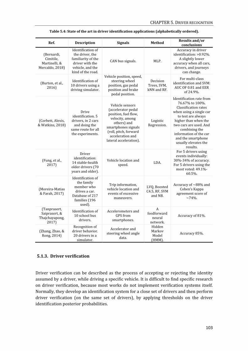
CHAPTER 5. DRIVER RECOGNITION
103
Table 5.4: State of the art in driver identification applications (alphabetically ordered).
Ref. Description Signals Method Results and/or
conclusions
(Bernardi, Cimitile,
Martinelli, & Mercaldo, 2018)
Identification of the driver, the
familiarity of the driver with the vehicle, and the kind of the road.
CAN bus signals. MLP.
Accuracy in driver identification: >0.92%.
A slightly lower accuracy when all cars, drivers, and journeys
can change.
(Burton, et al., 2016)
Identification of 10 drivers using a driving simulator.
Vehicle position, speed, steering wheel
position, gas pedal position and brake
pedal position.
Decision Trees, SVM, kNN and RF.
For multi-class identification and SVM: AUC OF 0.81 and EER
of 24.9%.
(Corbett, Alexis, & Watkins, 2018)
Drive identification. 5 drivers, in 2 cars
and doing the same route for all the experiments.
Vehicle sensors (accelerator pedal position, fuel flow,
velocity, among others) and
smartphones signals (roll, pitch, forward
acceleration and lateral acceleration).
Logistic Regression.
Identification rate from 76.67% to 100%.
Classification rates when using a single car
to test are always higher than when the
two cars are used. And combining the
information of the car and the smartphone usually elevates the
results.
(Fung, et al., 2017)
Driver identification:
14 stable-health older drivers (70 years and older).
Vehicle location and speed.
LDA.
For 5 drivers using events individually:
30%-34% of accuracy. For 5 drivers using the
most voted: 49.1%-60.5%.
(Moreira-Matias & Farah, 2017)
Identification of the family
member who drives a car.
Database of 217 families (196
used).
Trip information, vehicle location and events of excessive
maneuvers.
LVQ, Boosted C4.5, RF, SVM
and NB.
Accuracy of ∼88% and Cohen’s Kappa
agreement score of ∼74%.
(Tanprasert, Saiprasert, &
Thajchayapong, 2017)
Identification of 10 school bus
drivers.
Accelerometers and GPS from
smartphones.
A feedforward
neural network.
Accuracy of 81%.
(Zhang, Zhao, & Rong, 2014)
Recognition of driver behavior. 20 drivers in a
simulator.
Accelerator and steering wheel angle
data.
Hidden Markov Model
(HMM).
Accuracy 85%.
5.1.3. Driver verification
Driver verification can be described as the process of accepting or rejecting the identity
assumed by a driver, while driving a specific vehicle. It is difficult to find specific research
on driver verification, because most works do not implement verification systems itself.
Normally, they develop an identification system for a close set of drivers and then perform
driver verification (on the same set of drivers), by applying thresholds on the driver
identification posterior probabilities.

DEEP NEURAL NETWORKS FOR VEHICLE DRIVING CHARACTERIZATION BY MEANS OF SMARTPHONE SENSORS
104
For instance, (Il Kwak, Woo, & Kang Kim, 2016) create driver profiles from driver
identification, and used them to authenticate drivers. A driver is authenticated as a member
of a predefined class (10 authorized drivers) using thresholds on similarity scores. Driver
profiles are created from 15 features using CAN bus data: long term fuel, intake air pressure,
accelerator pedal value, fuel consumption, wheel velocity, etc. Profiles are defined by
predetermined journeys through three different road types, with a total of 4 journeys per
driver, driving the same car.
(Ezzini, Berrada, & Ghogho, 2018) performs the same strategy as in the previous
research, but expanding the study to two new datasets. One of them includes smartphone
signals (GPS and accelerometers), for a set of six drivers performing two types of predefined
routes. As before, when posterior driver identification probabilities in a journey test fall
below a given threshold, it is declared that the driver does not belong to the set of authorized
drivers.
The work presented in (Wahab, Quek, Keong Tan, & Takeda, 2009) recommends a
method of identification and verification based on a biometric driver recognition system,
using driving behavior. They follow a similar approach for accepting or rejecting a driver by
means of thresholds or rules. But unlike the previous ones, the verification is carried out for
each driver (not for a group). Driving data in this study was accelerator pedal pressure and
brake pedal pressure, for 3 groups of 10 drivers each one. First, they perform feature
extraction of the input signals using two schemes, Gaussian Mixture Models (GMMs) and
wavelet transform. The extracted features are then used in four different driver recognition
implementations: GMMs (introducing the original signals directly, without feature
extraction), multilayer perceptron (MLP), evolving fuzzy neural network (EFuNN) and
adaptive network-based fuzzy inference system (ANFIS). The car recording system needs
extra equipment as other signals (speech, image or location signals) were also captured.
Driver verification average Equal Error Rates (EER), using N-leave-one-out validation with
10 drivers per group, were from 3.44% to 5.02%.
Below we show Table 5.5, which summarizes the most relevant works in driver
verification. In the table, for each work, we present the signals used, the framework
proposed to driver verification, the performance and, finally, a short description of main
differences with respect to the research in this Thesis and/or some comments to be
highlighted.
The main differences between our study and most previous research are that we
perform the verification system individually for driver, not in relation to the membership of
a driver to an authorized group. We have also study a database of 25 drivers, with more
than 800 trips by driver; and our journeys are not pre-defined routes. As a consequence, the
complexity of the task will increase due to the number of drivers, the variability in routes
per driver, the diversity of mobile terminals and the diversity of car models. In addition, we
have limited our study to the exclusive use of tri-axial accelerometers signals, in order to
avoid the need for extra equipment in the vehicle, and also to avoid the excessive increase
of battery consumption.
Finally, Table 5.5 shows the summary of the works reviewed in driver verification.

CHAPTER 5. DRIVER RECOGNITION
105
Table 5.5: State of the art in driver verification (alphabetically sorted).
Ref. Signals Framework Performance Main difference from us/
Comments
(Ezzini, Berrada, &
Ghogho, 2018)
Three different databases: with vehicle sensors,
smartphone sensors, GPS
and other kind of information.
Machine Learning
algorithms.
For verification, they test the users in the classification model
with a threshold value of similarity, and when similarity exceeds the threshold (0.97), they verify as authorized
driver.
The verification is regarding an authorized user group or
not, it is not individual. Task more oriented to driver
identification. The first database is for 10
drivers using the vehicle sensors from CAN bus. The
second database use smartphones sensors
(gyroscope, accelerometers and GPS), but only for six
drivers and the drivers should performance different behaviors in two pre-
designed routes. The third database is more diverse and
has information like brightness, physiological data
or video rating data.
(Il Kwak, Woo, &
Kang Kim, 2016)
Vehicle sensors from the CAN
bus.
Machine Learning
algorithms.
For verification, they test the users in the classification model
with a threshold value of similarity, and when similarity exceeds the threshold (0.97), they verify as authorized
driver.
The verification is regarding an authorized user group or
not, it is not individual. 10 drivers using the same car
model, with 4 journeys per driver (two round trips) in 3
scenarios: city way, motor way and parking lot. They do
not use smartphones.
(Wahab, Quek,
Keong Tan, & Takeda,
2009)
Accelerator pedal pressure
and brake pedal pressure.
Gaussian Mixture Models
(GMMs), multilayer perceptron
(MLP), evolving
fuzzy neural network (EFuNN)
and adaptive network-
based fuzzy inference
system (ANFIS).
The average error rate for the experiments
varies from 3.44% to 5.02%. The best results are obtained using the combination of pedal
accelerator, brake pedal pressure and dynamics
of accelerator and brake pedal pressure.
Although they have 30 drivers, the tests were divided
into 3 groups, where each group comprises 10 drivers.
The results have been obtained by dividing the
drivers into groups of 10 and performing the average.
Therefore, there are more different values between
validation groups and between drivers within the
same validation group.
5.2. Driver identification
The purpose of this section is to contribute to close-set driver identification systems, using
Deep Learning techniques to model acceleration signals, recorded from drivers’
smartphone in a free position inside the car.
As in the previous chapter, Chapter 4 Driving maneuvers characterization, our goal
is to address driver identification using only the smartphone that the driver carries inside

DEEP NEURAL NETWORKS FOR VEHICLE DRIVING CHARACTERIZATION BY MEANS OF SMARTPHONE SENSORS
106
the vehicle (in a free position), and in particular modeling the tri-axial accelerometer
signals. Accelerometers are energy efficient devices, which in addition to minimize energy
consumption, they are also low-cost. In a future aimed at Internet of Things (IoT), we think
that similar behavioral models, based on low-cost hardware equipped only with
accelerometers, can also be very useful in many scenarios such as activity recognition or in
the characterization of autonomous systems (such as robots, drones, etc.). Moreover,
accelerometers are present in all mobile devices, avoiding the need to install extra
equipment in the vehicle or to access to sensors of the vehicle's Controller Area-Network
(CAN).
To address the driver identification, we study two different scenarios. The first one
(Subsection 5.2.2) uses raw accelerometer signals captured directly from smartphones, as
in the previous chapter. The second scenario (Subsection 5.2.3) uses acceleration signals
obtained from GPS data. The aim of this second scenario is to compare our driver
identification results with existing research using a public dataset from Kaggle “Driver
Telematics Analysis” AXA Competition (Kaggle, 2014).
Next, we will present the main guidelines that have led us to develop the
experimental framework for our research on driver identification.
5.2.1. Experimental framework
For the study of the first scenario (driver identification and verification using raw
accelerometer signals from smartphones) we used the TIDrivies_IdenVer database,
described in Chapter 3 Definitions and databases. This database has been provided by
Telefónica R&D and the spin-off of Telefónica R&D, Drivies. It is formed by 25 drivers with
801 real journeys per driver, giving a total of 20025 trips, and the drivers did not follow any
predefined route (they perform their usual daily driving journeys). The signals were
recorded at sampling frequency of 5 Hz, using the smartphones that the drivers carried
inside the vehicle
For the second scenario we use the dataset presented in the Kaggle AXA
Competition, called “Driver Telematics Analysis”, in which they proposed to use telematics
data to identify a driver signature (Kaggle, 2014). In this competition, AXA provided a
dataset of anonymized driver journeys. In total, they had a set of 2736 drivers and 200 trips
by driver. The goal of the competition was to create a telematics fingerprint capable of
distinguishing when a trip was driven by a given driver. The data offered for each journey
were the {𝑥, 𝑦} GPS positions , with their corresponding time, and a data sampling rate of 1
Hz. In order to protect the privacy of the drivers, the journeys where centered to start at the
origin (0,0), and then they were randomly rotated. Short-length trips were removed. The
design of AXA dataset includes a small number of false journeys among the 200 trips per
driver (these journeys not belonging to the corresponding driver are unknown).
It is important to point out that, though from different sources, both scenarios use
only accelerometers signals. In the first scenario these signals were directly obtained from
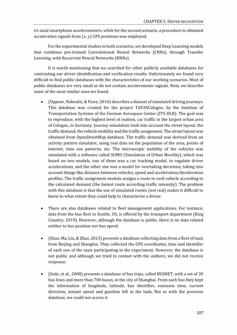
CHAPTER 5. DRIVER RECOGNITION
107
tri-axial smartphone accelerometers, while for the second scenario, a procedure to obtained
acceleration signals from {𝑥, 𝑦} GPS positions was employed.
For the experimental studies in both scenarios, we developed Deep Learning models
that combines pre-trained Convolutional Neural Networks (CNNs), through Transfer
Learning, with Recurrent Neural Networks (RNNs).
It is worth mentioning that we searched for other publicly available databases for
contrasting our driver identification and verification results. Unfortunately we found very
difficult to find public databases with the characteristics of our working scenarios. Most of
public databases are very small or do not contain accelerometer signals. Next, we describe
some of the most similar ones we found.
(Uppoor, Naboulsi, & Fiore, 2016) describes a dataset of simulated driving journeys.
This database was created for the project TAPASCologne, by the Institute of
Transportation Systems of the German Aerospace Center (ITS-DLR). The goal was
to reproduce, with the highest level of realism, car traffic in the largest urban area
of Cologne, in Germany. Journey simulation took into account the street layout, the
traffic demand, the vehicle mobility and the traffic assignment. The street layout was
obtained from OpenStreetMap database. The traffic demand was derived from an
activity pattern simulator, using real data on the population of the area, points of
interest, time use patterns, etc. The microscopic mobility of the vehicles was
simulated with a software called SUMO (Simulation of Urban Movility), which was
based on two models, one of them was a car tracking model, to regulate driver
accelerations, and the other one was a model for overtaking decisions; taking into
account things like distance between vehicles, speed and acceleration/deceleration
profiles. The traffic assignment module assigns a route to each vehicle according to
the calculated demand (the fastest route according traffic intensity). The problem
with this database is that the use of simulated routes (not real) makes it difficult to
know to what extent they could help to characterize a driver.
There are also databases related to fleet management applications. For instance,
data from the bus fleet in Seattle, US, is offered by the transport department (King
Country, 2019). However, although the database is public, there is no data related
neither to bus position nor bus speed.
(Zhao, Ma, Liu, & Zhao, 2013) presents a database collecting data from a fleet of taxis
from Beijing and Shanghai. They collected the GPS coordinates, time and identifier
of each one of the taxis participating in the experiment. However, the database is
not public and although we tried to contact with the authors, we did not receive
response.
(Sede, et al., 2008) presents a database of bus trips, called BUSNET, with a set of 30
bus lines and more than 700 buses, in the city of Shanghai. From each bus they kept
the information of longitude, latitude, bus identifier, emission time, current
direction, instant speed and gasoline left in the tank. But as with the previous
database, we could not access it.
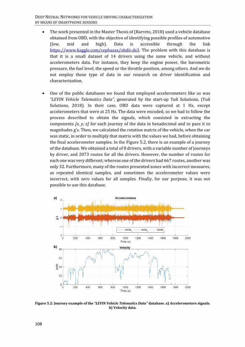
DEEP NEURAL NETWORKS FOR VEHICLE DRIVING CHARACTERIZATION BY MEANS OF SMARTPHONE SENSORS
108
The work presented in the Master Thesis of (Barreto, 2018) used a vehicle database
obtained from OBD, with the objective of identifying possible profiles of automotive
(low, mid and high). Data is accessible through the link
https://www.kaggle.com/cephasax/obdii-ds3. The problem with this database is
that it is a small dataset of 14 drivers using the same vehicle, and without
accelerometers data. For instance, they keep the engine power, the barometric
pressure, the fuel level, the speed or the throttle position, among others. And we do
not employ these type of data in our research on driver identification and
characterization.
One of the public databases we found that employed accelerometers like us was
“LEVIN Vehicle Telematics Data”, generated by the start-up Yuñ Solutions, (Yuñ
Solutions, 2018). In their case, OBD data were captured at 1 Hz, except
accelerometers that were at 25 Hz. The data were encoded, so we had to follow the
process described to obtain the signals, which consisted in extracting the
components [x, y, z] for each journey of the data in hexadecimal and to pass it to
magnitudes g's. Then, we calculated the rotation matrix of the vehicle, when the car
was static, in order to multiply that matrix with the values we had, before obtaining
the final accelerometer samples. In the Figure 5.2, there is an example of a journey
of the database. We obtained a total of 8 drivers, with a variable number of journeys
by driver, and 2073 routes for all the drivers. However, the number of routes for
each one was very different; whereas one of the drivers had 667 routes, another was
only 32. Furthermore, many of the routes presented zones with incorrect measures,
as repeated identical samples, and sometimes the accelerometer values were
incorrect, with zero values for all samples. Finally, for our purpose, it was not
possible to use this database.
Figure 5.2: Journey example of the “LEVIN Vehicle Telematics Data” database. a) Accelerometers signals. b) Velocity data.
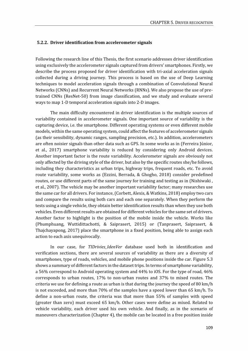
CHAPTER 5. DRIVER RECOGNITION
109
5.2.2. Driver identification from accelerometer signals
Following the research line of this Thesis, the first scenario addresses driver identification
using exclusively the accelerometer signals captured from drivers’ smartphones. Firstly, we
describe the process proposed for driver identification with tri-axial acceleration signals
collected during a driving journey. This process is based on the use of Deep Learning
techniques to model acceleration signals through a combination of Convolutional Neural
Networks (CNNs) and Recurrent Neural Networks (RNNs). We also propose the use of pre-
trained CNNs (ResNet-50) from image classification, and we study and evaluate several
ways to map 1-D temporal acceleration signals into 2-D images.
The main difficulty encountered in driver identification is the multiple sources of
variability contained in accelerometer signals. One important source of variability is the
capturing device, i.e. the smartphone. Different operating systems or even different mobile
models, within the same operating system, could affect the features of accelerometer signals
(as their sensibility, dynamic ranges, sampling precision, etc.). In addition, accelerometers
are often noisier signals than other data such as GPS. In some works as in (Ferreira Júnior,
et al., 2017) smartphone variability is reduced by considering only Android devices.
Another important factor is the route variability. Accelerometer signals are obviously not
only affected by the driving style of the driver, but also by the specific routes she/he follows,
including they characteristics as urban trips, highway trips, frequent roads, etc. To avoid
route variability, some works as (Ezzini, Berrada, & Ghogho, 2018) consider predefined
routes, or use different parts of the same journey for training and testing as in (Nishiwaki ,
et al., 2007). The vehicle may be another important variability factor; many researches use
the same car for all drivers. For instance, (Corbett, Alexis, & Watkins, 2018) employ two cars
and compare the results using both cars and each one separately. When they perform the
tests using a single vehicle, they obtain better identification results than when they use both
vehicles. Even different results are obtained for different vehicles for the same set of drivers.
Another factor to highlight is the position of the mobile inside the vehicle. Works like
(Phumphuang, Wuttidittachotti, & Saiprasert, 2015) or (Tanprasert, Saiprasert, &
Thajchayapong, 2017) place the smartphone in a fixed position, being able to assign each
action to each axis unequivocally.
In our case, for TIDrivies_IdenVer database used both in identification and
verification sections, there are several sources of variability as there are a diversity of
smartphones, type of roads, vehicles, and mobile phone positions inside the car. Figure 5.3
shows a summary of different factors in the dataset trips. In terms of smartphone variability,
a 56% correspond to Android operating system and 44% to iOS. For the type of road, 46%
corresponds to urban routes, 17% to non-urban routes and 37% to mixed routes. The
criteria we use for defining a route as urban is that during the journey the speed of 80 km/h
is not exceeded, and more than 70% of the samples have a speed lower than 65 km/h. To
define a non-urban route, the criteria was that more than 55% of samples with speed
(greater than zero) must exceed 65 km/h. Other cases were define as mixed. Related to
vehicle variability, each driver used his own vehicle. And finally, as in the scenario of
maneuvers characterization (Chapter 4), the mobile can be located in a free position inside
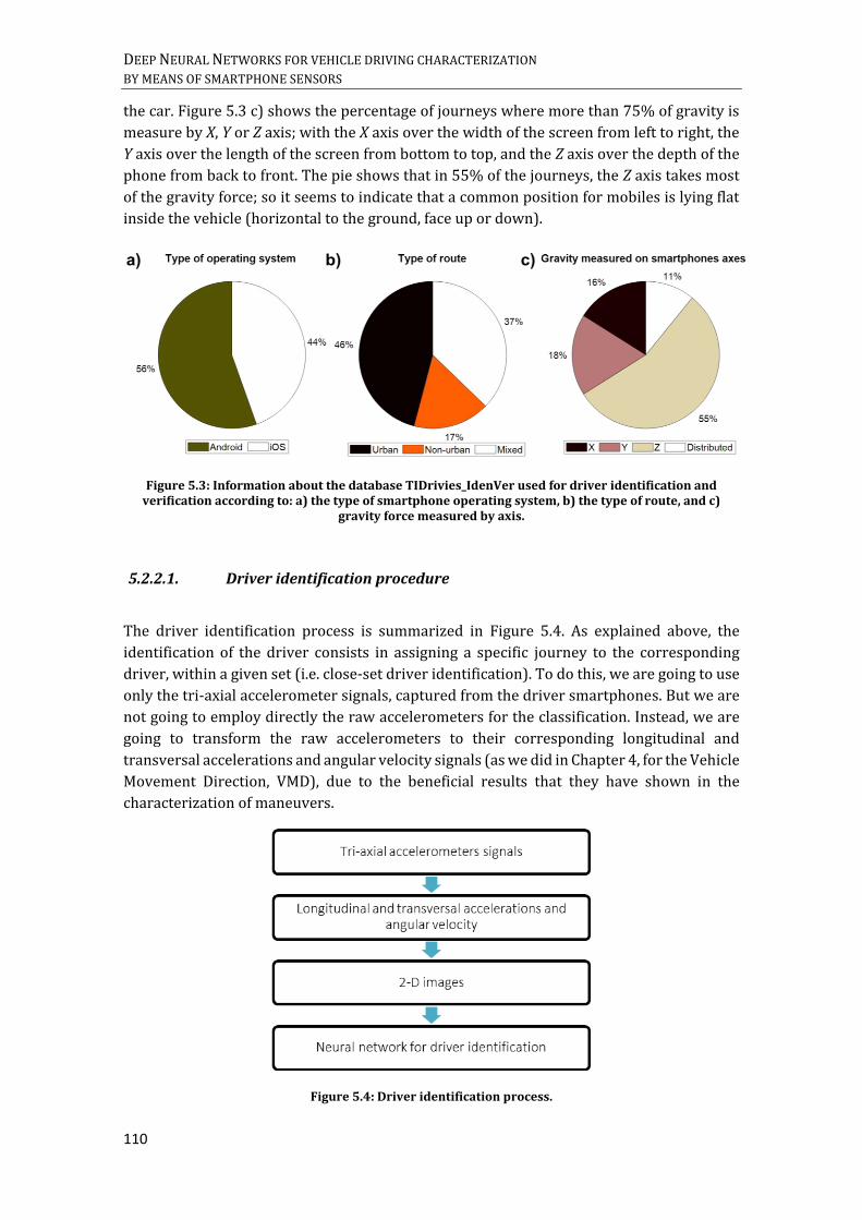
DEEP NEURAL NETWORKS FOR VEHICLE DRIVING CHARACTERIZATION BY MEANS OF SMARTPHONE SENSORS
110
the car. Figure 5.3 c) shows the percentage of journeys where more than 75% of gravity is
measure by X, Y or Z axis; with the X axis over the width of the screen from left to right, the
Y axis over the length of the screen from bottom to top, and the Z axis over the depth of the
phone from back to front. The pie shows that in 55% of the journeys, the Z axis takes most
of the gravity force; so it seems to indicate that a common position for mobiles is lying flat
inside the vehicle (horizontal to the ground, face up or down).
Figure 5.3: Information about the database TIDrivies_IdenVer used for driver identification and verification according to: a) the type of smartphone operating system, b) the type of route, and c)
gravity force measured by axis.
5.2.2.1. Driver identification procedure
The driver identification process is summarized in Figure 5.4. As explained above, the
identification of the driver consists in assigning a specific journey to the corresponding
driver, within a given set (i.e. close-set driver identification). To do this, we are going to use
only the tri-axial accelerometer signals, captured from the driver smartphones. But we are
not going to employ directly the raw accelerometers for the classification. Instead, we are
going to transform the raw accelerometers to their corresponding longitudinal and
transversal accelerations and angular velocity signals (as we did in Chapter 4, for the Vehicle
Movement Direction, VMD), due to the beneficial results that they have shown in the
characterization of maneuvers.
Figure 5.4: Driver identification process.

CHAPTER 5. DRIVER RECOGNITION
111
Once these temporal signals are obtained, they will be transformed to images (see
Figure 5.5), in order to take advantage of the power of deeper and pre-trained Convolutional
Neural Networks (CNNs).
Figure 5.5: 1D time series transformations to 2D images for driver identification.
The final architecture proposed for this driver identification is shown in Figure 5.6.
2D images are inputs (in our case three channels: for longitudinal and transversal
accelerations and angular velocity) to a Deep Learning model. The Deep Learning model is
composed by a sequence of three different Neural Networks. The first network is a pre-
trained CNN, in particular ResNet-50, that is followed by a Recurrent Neural Network
(RNN), and finally, Dense Layers with softmax to get output posterior probabilities per
driver. We choose three channels 224x224 2D images, since it is the input required by
ResNet-50. For the RNN, we use Gated Recurrent Units (GRUs), because this type of
networks offers accurate and efficient results for time series modeling. Finally, there is the
classifier with a Dense or Fully Connected layer followed by a softmax layer. After testing
several configurations, we used two GRU stacked layers of 128 neurons for the recurrent
block. In the last part of the model (Figure 5.6) a dense layer with 64 neurons and ReLU
activation, is followed with another dense layer with 25 units (for 25 drivers identification)
and softmax activation function. For training we used Adam optimizer minimizing the
categorical cross-entropy loss function. We also employed weight decay or L2
regularization. Several learning rates were tested, selecting a low value of 0.001(we found
it more reliable than higher rates).
Due to the important impact and success of Deep Learning in computer vision, we
decided to use CNN models trained for image classification and apply Transfer Learning for
our driver identification problem. Among the different CNN used in computer vision (VGG,
Inception, LeNet, AlexNet, ResNet, etc.) we decided to use ResNet-50 (ResNet-152 won the

DEEP NEURAL NETWORKS FOR VEHICLE DRIVING CHARACTERIZATION BY MEANS OF SMARTPHONE SENSORS
112
first place on the ImageNet Large Scale Visual Recognition Challenge (ILSVRC) of 2015 (He,
Zhang, Ren, & Sun, 2016)).
Figure 5.6: Deep Neural Network architecture for driver identification.
ResNet architectures come up to solve the difficulty to train Deep Neural Networks;
because adding more layers to an already deep model causes higher training errors. The
name of ResNet comes from the Deep Residual Network and in particular Resnet-50 refers
to the architecture with 50 residual layers. Deep Residual Networks were presented by
Microsoft Research in the ImageNet and COCO 2015 competitions, for image classification,
object detection and semantic segmentation (Dietz, 2017). These networks come up to solve
the difficulty to train Deep Neural Networks; because adding more layers to an already deep
model causes higher training errors. The ResNet (He, Zhang, Ren, & Sun, 2016) allows
training and optimizing networks in a simpler way; introducing residual deep learning
frameworks with shortcut connections. These connections perform a mapping, and their
outputs are added to the outputs of the stacked layers, which may omit one or more layers.
The advantage is that these shortcuts do not add extra parameters or computational
complexity. Each block is responsible for adjusting the output of the previous blocks, instead
of having to do it from scratch. The basic block presents variants such as the block “Residual
Bottleneck”, which use sets of three layers stacked instead of two as the basic ones, which
reduce and increase the dimensions.
Therefore, ResNets are architectures that stack building blocks, called Residual
Blocks. The scheme of the basic residual block of two layers is shown in Figure 5.7. The block
presents a shortcut connection that performs identity mapping, so at the output of the block
the propagated information plus the output of the stacked layers is added, 𝐹 (𝑥) + 𝑥.

CHAPTER 5. DRIVER RECOGNITION
113
Figure 5.7: Residual block (two-layer Residual Block).
In the ResNet-50 model, the residual bottleneck of two layers (Figure 5.7) is
replaced with a three layer bottleneck block, with 1𝑥1 convolutions and 3𝑥3 convolutions.
The general scheme of the Resnet-50 is shown in Figure 5.8, where blocks of two-layer
residual block have been colored in different colors, each color indicating a series of
convolutions of the same dimension.
Figure 5.8: Architecture 50-layer residual.

DEEP NEURAL NETWORKS FOR VEHICLE DRIVING CHARACTERIZATION BY MEANS OF SMARTPHONE SENSORS
114
Training ResNet architectures from scratch, depending on the task to be performed,
can be computationally expensive and it also usually needs a large amount of data to obtain
high accuracy. A possible solution to this problem is the Transfer Learning approach. As
defined in (Bailey Luttrell IV, Zhou, Zhang, Gong, & Zhang, 2017), Transfer Learning consists
in: “taking a model that was trained to recognize features in one domain and transferring its
knowledge and general feature extraction capabilities to another model which will learn more
specific features that apply to another domain”. Consequently when training our Deep
Leaning model (Figure 5.6) fine-tuning was applied on a pre-trained ResNet-50 model. That
is ResNet parameters were initialized on a pre-trained model and while GRU and Dense
Layer parameters are randomly initialized.
5.2.2.2. Transformation methods from 1-D to 2-D
In order to adapt our input accelerometer signals to the Deep Neural Network architecture
presented in Figure 5.6, it is necessary to carry out transformations of the temporal 1-D
signals to 2-D images. We have tested different methods to perform this 1D to 2D
transformations: Recurrence Plots (RP) (Schulz, Mentges, & Zielinski , 2016), Gramian
Angular Summation Field (GASF) (Tsai, Chen, & Wang, 2019), Gramian Angular Difference
Field (GADF) (Mitiche, et al., 2018), Markov Transition Field (MTF) (Wang & Oates, 2015),
spectrograms (Ruffini, et al., 2019) and the use of CNN to obtain a feature map from one of
its layers. Next, we describe each one of these 1D to 2D transformations.
Recurrence Plots (RPs)
The recurrence plot was described in (Eckmann, Kamphorst, & Ruelle, 1987). The RP is a
graphical tool, which through the transformation to images, allows exploring the 𝑑-
dimensional phase space trajectory of time series through a 2D representation of its
recurrences. In the work mentioned, they presented this visualization tool for measuring
the time constancy of dynamical systems. As they define: “Let 𝑥(𝑖) be the 𝑖-th point on the
orbit describing a dynamical system in 𝑑-dimensional space, for 𝑖 = 1, … , 𝑁. The recurrence
plot is an array of dots in a 𝑁𝑥𝑁 square, where a dot is placed at (𝑖, 𝑗) whenever 𝑥(𝑗) is
sufficiently close to 𝑥(𝑖)”. With 𝑖 and 𝑗 like times, so a recurrence plot describes time
correlation information. These are usually very symmetric with respect to the diagonal 𝑖 =
𝑗, since if 𝑥(𝑖) is close to 𝑥(𝑗) then 𝑥(𝑗) is close to 𝑥(𝑖); but it does not imply that they have
to be completely symmetrical. As an example of work that uses these transformations, is the
one of (Hatami, Gavet, & Debayle, 2018). They employ the conversion of time series to 2-D
images, to use them in a CNN for Time-Series Classification (TSC).
As (Eckmann, Kamphorst, & Ruelle, 1987) describes, in order to obtain the RP of a
time series {𝑢𝑖}, the following process must be followed:
To construct the 𝑑-dimensional orbit of 𝑥(𝑖), an embedding of dimension 𝑑, by the
method of time delays (for example, if 𝑢𝑖 are scalar, then 𝑥(𝑖) =
(𝑢𝑖 , 𝑢𝑖+1, … , 𝑢𝑖+𝑑−1)).

CHAPTER 5. DRIVER RECOGNITION
115
To choose 𝑟(𝑖) such that the ball of radius 𝑟(𝑖) centered at 𝑥(𝑖) in 𝑅𝑑 contains a
reasonable number of other points 𝑥(𝑗) of the orbit.
To plot a dot at each point (𝑖, 𝑗) for which 𝑥(𝑗) is in the ball of radius 𝑟(𝑖) centered
at 𝑥(𝑖).
Images from Figure 5.9 to Figure 5.14 show the transformations obtained for each
of the six methods employed, conversion methods from 1-D to 2-D, for the same maneuver
with a window length of 224 samples. Figure 5.9 shows the resulting images for each one of
the input channels with the RP method. It is possible to observe in the figure that, for the
three channels, the resulting images are not homogeneous, probably because these images
are more typical in stationary systems such as random time series. Instead, the abrupt
changes cause paler areas in the RP, coinciding with areas where accelerations or angular
velocity suffer variations, due to the maneuver itself. Vertical and horizontal lines indicate
that some states do not changes or change slowly for some time.
Gramian Angular Summation Field (GASF) & Gramian Angular Difference Field (GADF)
Both the frameworks for encoding time series like images called GASF and GADF and the
one presented below, called Markov Transition Field (MTF), were described in (Wang &
Oates, 2015).
In order to calculate GASF and GADF images, the temporal signals have to be
represented in polar coordinates and then each element of the matrix will be the cosine of
the sum of the angles for the GASF, or the sine of the difference between each point for the
GADF. If we represent the time series as: 𝑋 = {𝑥1, 𝑥2, … , 𝑥𝑛} with 𝑛 as the number of points,
and �̃� as the time series in polar coordinates; the resulting formulas for each method are as
follows (it is necessary to perform a rescale of 𝑋, between intervals [−1,1] or [0,1] before
the transition to polar coordinates):
𝑮𝑨𝑺𝑭 = [𝒄𝒐𝒔(𝝓𝒊 + 𝝓𝒋)] (5.1)
𝑮𝑨𝑫𝑭 = [𝒔𝒊𝒏(𝝓𝒊 − 𝝓𝒋)] (5.2)
𝝓 = 𝒂𝒓𝒄𝒐𝒔(�̃�𝒊), �̃�𝒊𝝐 �̃� (5.3)
Figure 5.10 shows the results for the GASF method, and Figure 5.11 for the GADF.
These figures correspond to the same maneuver presented for RP in Figure 5.9. For the
three cases, similar patterns can be observed in the resulting images, with the presence of
lines and clusters of different tones.
Markov Transition Field (MTF)
For Markov Transition Field, the transition probabilities of multiple intervals of the time
series are coded, creating the matrix of Markov transitions. To do this, the data is divided
into quantiles, and each element of the matrix indicates the probability of transition from

DEEP NEURAL NETWORKS FOR VEHICLE DRIVING CHARACTERIZATION BY MEANS OF SMARTPHONE SENSORS
116
one to another. Although the framework is obtained from the work of (Wang & Oates, 2015),
the process we followed is based on the work of (Campanharo, Sirer, Malmgren, Ramos, &
Amaral, 2011). The work of (Campanharo, Sirer, Malmgren, Ramos, & Amaral, 2011) creates
the Markov transition matrix as follows:
With 𝑋 like a time series and 𝑄 such as its quantile bins, it is assigned each 𝑥𝑖 to the
corresponding bins 𝑞𝑗 , with 𝑗 ∈ [1, 𝑄].
Then, counting transitions among quantile bins in the manner of a first order
Markov chain along the time axis, constructing the matrix W of 𝑄𝑥𝑄.
𝑤𝑖𝑗 will be the frequency with which a point in quantile 𝑞𝑗 is followed by a point in
quantile 𝑞𝑖 .
And finally, to do a normalization: ∑ 𝑤𝑖𝑗 = 1𝑗 .
(Wang & Oates, 2015) creates the Markov Transition Field matrix, from the above,
by spreading out the Markov transition matrix 𝑊, which contains the transition probability
on the magnitude axis, into the Markov transition field matrix, by considering the temporal
positions. The MTF formula is as follows:
𝑴 = [
𝒘𝒊𝒋|𝒙𝟏∈𝒒𝒊,𝒙𝟏∈𝒒𝒋 ⋯ 𝒘𝒊𝒋|𝒙𝟏∈𝒒𝒊,𝒙𝒏∈𝒒𝒋
⋮ ⋱ ⋮𝒘𝒊𝒋|𝒙𝒏∈𝒒𝒊,𝒙𝟏∈𝒒𝒋 ⋯ 𝒘𝒊𝒋|𝒙𝒏∈𝒒𝒊,𝒙𝒏∈𝒒𝒋
] (5.4)
with 𝑀𝑖𝑗 like transition probability of 𝑞𝑖 → 𝑞𝑗 .
As with the previous methods, the images resulting from applying it, on the chosen
maneuver, are shown in the Figure 5.12.
Spectrograms
Another common method to represent 1-D signals as 2-D images is the use of spectrograms.
For each input channel, we have applied the Short-time Fourier transform (STFT), using a
DFT with 448 (224*2) bins, on a sliding Hanning window of 10 samples, with a hop size of
50%. Then, we converted STFT magnitude to log scale, as it has been shown that log-scale
feature achieved faster convergence than the raw spectrogram (Zhang, Yu , & Hansen,
2017).
𝑺𝒑𝒆𝒄𝒕𝒓𝒐𝒈𝒓𝒂𝒎(𝒕, 𝒘) = |𝑺𝑻𝑭𝑻(𝒕, 𝒘)|𝟐 (5.5)
𝑺𝒑𝒆𝒄𝒕𝒓𝒐𝒈𝒓𝒂𝒎(𝒕, 𝒘)|𝒅𝑩 = 𝟐𝟎 𝐥𝐨𝐠𝟏𝟎 (|𝑺𝑻𝑭𝑻(𝒕,𝒘)|
𝟐∙𝟏𝟎−𝟓 ) (5.6)
For spectrograms it has been decided to use a window that corresponds to the actual
length of the maneuver, locating the beginning and the end of the event. As the network
inputs must be of fixed length and each maneuver has a different duration, we have taken
the solution proposed by (Zhang, Yu , & Hansen, 2017). In their work, they use Deep
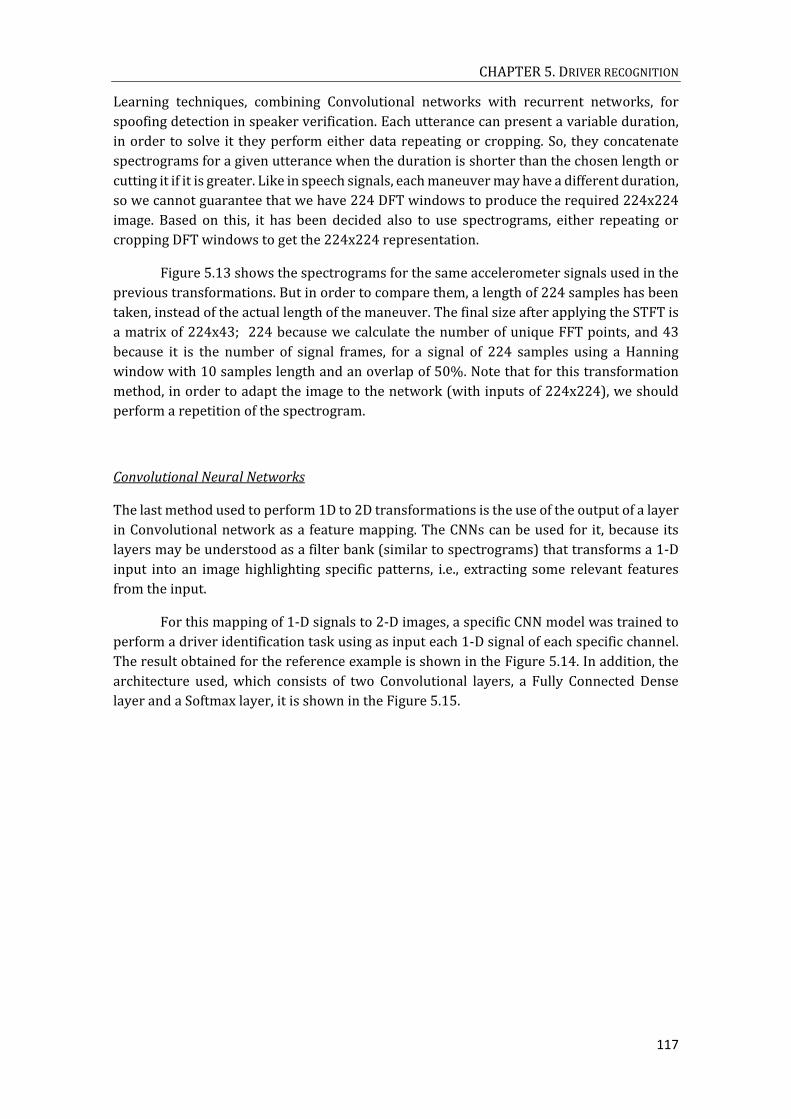
CHAPTER 5. DRIVER RECOGNITION
117
Learning techniques, combining Convolutional networks with recurrent networks, for
spoofing detection in speaker verification. Each utterance can present a variable duration,
in order to solve it they perform either data repeating or cropping. So, they concatenate
spectrograms for a given utterance when the duration is shorter than the chosen length or
cutting it if it is greater. Like in speech signals, each maneuver may have a different duration,
so we cannot guarantee that we have 224 DFT windows to produce the required 224x224
image. Based on this, it has been decided also to use spectrograms, either repeating or
cropping DFT windows to get the 224x224 representation.
Figure 5.13 shows the spectrograms for the same accelerometer signals used in the
previous transformations. But in order to compare them, a length of 224 samples has been
taken, instead of the actual length of the maneuver. The final size after applying the STFT is
a matrix of 224x43; 224 because we calculate the number of unique FFT points, and 43
because it is the number of signal frames, for a signal of 224 samples using a Hanning
window with 10 samples length and an overlap of 50%. Note that for this transformation
method, in order to adapt the image to the network (with inputs of 224x224), we should
perform a repetition of the spectrogram.
Convolutional Neural Networks
The last method used to perform 1D to 2D transformations is the use of the output of a layer
in Convolutional network as a feature mapping. The CNNs can be used for it, because its
layers may be understood as a filter bank (similar to spectrograms) that transforms a 1-D
input into an image highlighting specific patterns, i.e., extracting some relevant features
from the input.
For this mapping of 1-D signals to 2-D images, a specific CNN model was trained to
perform a driver identification task using as input each 1-D signal of each specific channel.
The result obtained for the reference example is shown in the Figure 5.14. In addition, the
architecture used, which consists of two Convolutional layers, a Fully Connected Dense
layer and a Softmax layer, it is shown in the Figure 5.15.

DEEP NEURAL NETWORKS FOR VEHICLE DRIVING CHARACTERIZATION BY MEANS OF SMARTPHONE SENSORS
118
Figure 5.9: Example of driving maneuver. a,b,c) Longitudinal acceleration, transversal acceleration and angular velocity of the original signals, respectively. d,e,f) Recurrence plot of the longitudinal
acceleration, transversal acceleration and angular velocity, respectively.

CHAPTER 5. DRIVER RECOGNITION
119
Figure 5.10: Example of driving maneuver. a,b,c) Longitudinal acceleration, transversal acceleration and angular velocity of the original signals, respectively. d,e,f) Gramian Angular Summation Field of
the longitudinal acceleration, transversal acceleration and angular velocity, respectively.
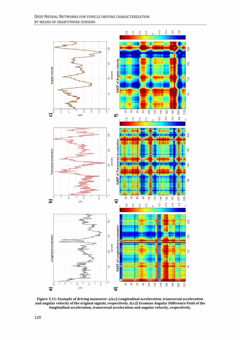
DEEP NEURAL NETWORKS FOR VEHICLE DRIVING CHARACTERIZATION BY MEANS OF SMARTPHONE SENSORS
120
Figure 5.11: Example of driving maneuver. a,b,c) Longitudinal acceleration, transversal acceleration and angular velocity of the original signals, respectively. d,e,f) Gramian Angular Difference Field of the
longitudinal acceleration, transversal acceleration and angular velocity, respectively.

CHAPTER 5. DRIVER RECOGNITION
121
Figure 5.12: Example of driving maneuver. a,b,c) Longitudinal acceleration, transversal acceleration and angular velocity of the original signals, respectively. d,e,f) Markov Transition Field of the
longitudinal acceleration, transversal acceleration and angular velocity, respectively.

DEEP NEURAL NETWORKS FOR VEHICLE DRIVING CHARACTERIZATION BY MEANS OF SMARTPHONE SENSORS
122
Figure 5.13: Example of driving maneuver. a,b,c) Longitudinal acceleration, transversal acceleration and angular velocity of the original signals, respectively. d,e,f) Spectrogram of the longitudinal
acceleration, transversal acceleration and angular velocity, respectively.

CHAPTER 5. DRIVER RECOGNITION
123
Figure 5.14: Example of driving maneuver. a,b,c) Longitudinal acceleration, transversal acceleration and angular velocity of the original signals, respectively. d,e,f) Features layers (from CNN) of the
longitudinal acceleration, transversal acceleration and angular velocity, respectively.
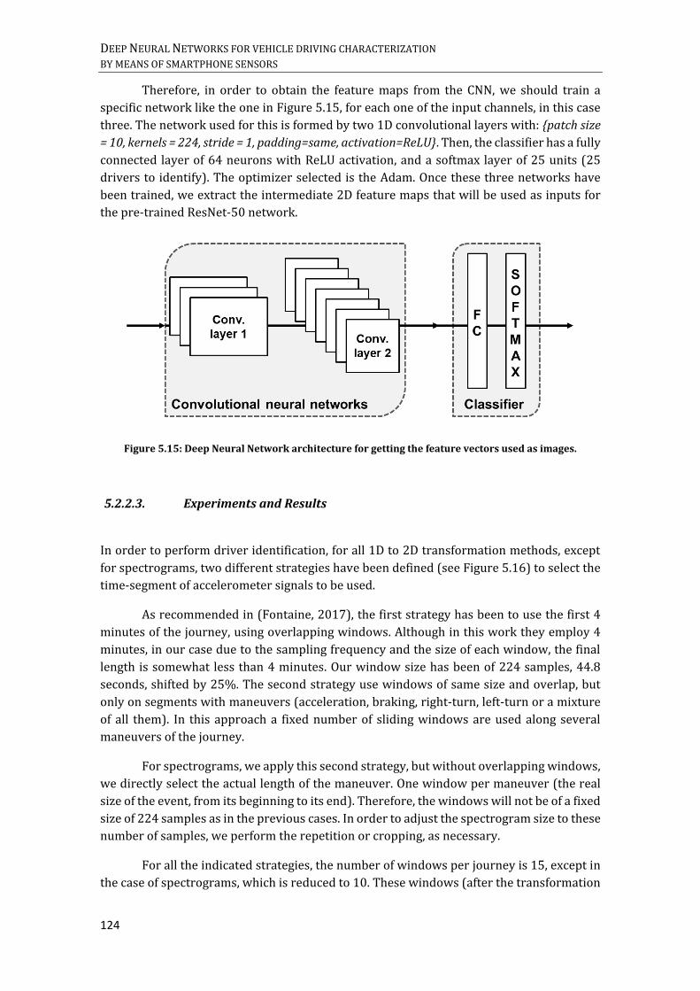
DEEP NEURAL NETWORKS FOR VEHICLE DRIVING CHARACTERIZATION BY MEANS OF SMARTPHONE SENSORS
124
Therefore, in order to obtain the feature maps from the CNN, we should train a
specific network like the one in Figure 5.15, for each one of the input channels, in this case
three. The network used for this is formed by two 1D convolutional layers with: {patch size
= 10, kernels = 224, stride = 1, padding=same, activation=ReLU}. Then, the classifier has a fully
connected layer of 64 neurons with ReLU activation, and a softmax layer of 25 units (25
drivers to identify). The optimizer selected is the Adam. Once these three networks have
been trained, we extract the intermediate 2D feature maps that will be used as inputs for
the pre-trained ResNet-50 network.
Figure 5.15: Deep Neural Network architecture for getting the feature vectors used as images.
5.2.2.3. Experiments and Results
In order to perform driver identification, for all 1D to 2D transformation methods, except
for spectrograms, two different strategies have been defined (see Figure 5.16) to select the
time-segment of accelerometer signals to be used.
As recommended in (Fontaine, 2017), the first strategy has been to use the first 4
minutes of the journey, using overlapping windows. Although in this work they employ 4
minutes, in our case due to the sampling frequency and the size of each window, the final
length is somewhat less than 4 minutes. Our window size has been of 224 samples, 44.8
seconds, shifted by 25%. The second strategy use windows of same size and overlap, but
only on segments with maneuvers (acceleration, braking, right-turn, left-turn or a mixture
of all them). In this approach a fixed number of sliding windows are used along several
maneuvers of the journey.
For spectrograms, we apply this second strategy, but without overlapping windows,
we directly select the actual length of the maneuver. One window per maneuver (the real
size of the event, from its beginning to its end). Therefore, the windows will not be of a fixed
size of 224 samples as in the previous cases. In order to adjust the spectrogram size to these
number of samples, we perform the repetition or cropping, as necessary.
For all the indicated strategies, the number of windows per journey is 15, except in
the case of spectrograms, which is reduced to 10. These windows (after the transformation
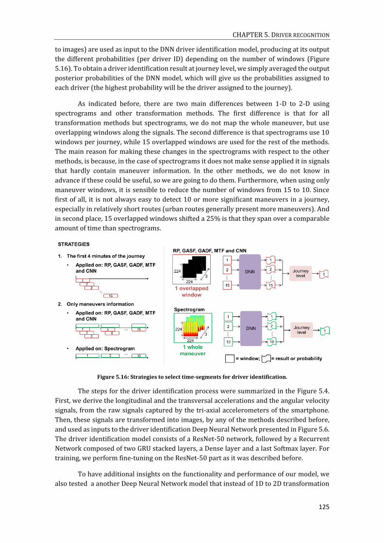
CHAPTER 5. DRIVER RECOGNITION
125
to images) are used as input to the DNN driver identification model, producing at its output
the different probabilities (per driver ID) depending on the number of windows (Figure
5.16). To obtain a driver identification result at journey level, we simply averaged the output
posterior probabilities of the DNN model, which will give us the probabilities assigned to
each driver (the highest probability will be the driver assigned to the journey).
As indicated before, there are two main differences between 1-D to 2-D using
spectrograms and other transformation methods. The first difference is that for all
transformation methods but spectrograms, we do not map the whole maneuver, but use
overlapping windows along the signals. The second difference is that spectrograms use 10
windows per journey, while 15 overlapped windows are used for the rest of the methods.
The main reason for making these changes in the spectrograms with respect to the other
methods, is because, in the case of spectrograms it does not make sense applied it in signals
that hardly contain maneuver information. In the other methods, we do not know in
advance if these could be useful, so we are going to do them. Furthermore, when using only
maneuver windows, it is sensible to reduce the number of windows from 15 to 10. Since
first of all, it is not always easy to detect 10 or more significant maneuvers in a journey,
especially in relatively short routes (urban routes generally present more maneuvers). And
in second place, 15 overlapped windows shifted a 25% is that they span over a comparable
amount of time than spectrograms.
Figure 5.16: Strategies to select time-segments for driver identification.
The steps for the driver identification process were summarized in the Figure 5.4.
First, we derive the longitudinal and the transversal accelerations and the angular velocity
signals, from the raw signals captured by the tri-axial accelerometers of the smartphone.
Then, these signals are transformed into images, by any of the methods described before,
and used as inputs to the driver identification Deep Neural Network presented in Figure 5.6.
The driver identification model consists of a ResNet-50 network, followed by a Recurrent
Network composed of two GRU stacked layers, a Dense layer and a last Softmax layer. For
training, we perform fine-tuning on the ResNet-50 part as it was described before.
To have additional insights on the functionality and performance of our model, we
also tested a another Deep Neural Network model that instead of 1D to 2D transformation
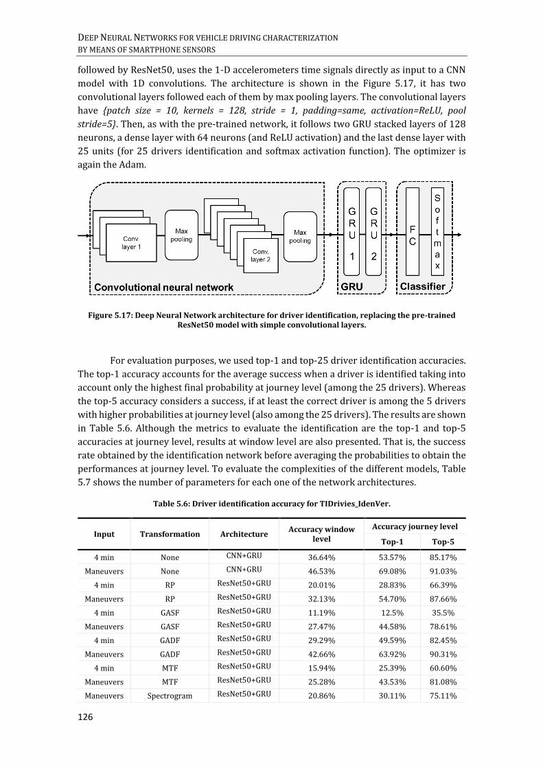
DEEP NEURAL NETWORKS FOR VEHICLE DRIVING CHARACTERIZATION BY MEANS OF SMARTPHONE SENSORS
126
followed by ResNet50, uses the 1-D accelerometers time signals directly as input to a CNN
model with 1D convolutions. The architecture is shown in the Figure 5.17, it has two
convolutional layers followed each of them by max pooling layers. The convolutional layers
have {patch size = 10, kernels = 128, stride = 1, padding=same, activation=ReLU, pool
stride=5}. Then, as with the pre-trained network, it follows two GRU stacked layers of 128
neurons, a dense layer with 64 neurons (and ReLU activation) and the last dense layer with
25 units (for 25 drivers identification and softmax activation function). The optimizer is
again the Adam.
Figure 5.17: Deep Neural Network architecture for driver identification, replacing the pre-trained ResNet50 model with simple convolutional layers.
For evaluation purposes, we used top-1 and top-25 driver identification accuracies.
The top-1 accuracy accounts for the average success when a driver is identified taking into
account only the highest final probability at journey level (among the 25 drivers). Whereas
the top-5 accuracy considers a success, if at least the correct driver is among the 5 drivers
with higher probabilities at journey level (also among the 25 drivers). The results are shown
in Table 5.6. Although the metrics to evaluate the identification are the top-1 and top-5
accuracies at journey level, results at window level are also presented. That is, the success
rate obtained by the identification network before averaging the probabilities to obtain the
performances at journey level. To evaluate the complexities of the different models, Table
5.7 shows the number of parameters for each one of the network architectures.
Table 5.6: Driver identification accuracy for TIDrivies_IdenVer.
Input Transformation Architecture Accuracy window
level
Accuracy journey level
Top-1 Top-5
4 min None CNN+GRU 36.64% 53.57% 85.17%
Maneuvers None CNN+GRU 46.53% 69.08% 91.03%
4 min RP ResNet50+GRU 20.01% 28.83% 66.39%
Maneuvers RP ResNet50+GRU 32.13% 54.70% 87.66%
4 min GASF ResNet50+GRU 11.19% 12.5% 35.5%
Maneuvers GASF ResNet50+GRU 27.47% 44.58% 78.61%
4 min GADF ResNet50+GRU 29.29% 49.59% 82.45%
Maneuvers GADF ResNet50+GRU 42.66% 63.92% 90.31%
4 min MTF ResNet50+GRU 15.94% 25.39% 60.60%
Maneuvers MTF ResNet50+GRU 25.28% 43.53% 81.08%
Maneuvers Spectrogram ResNet50+GRU 20.86% 30.11% 75.11%

CHAPTER 5. DRIVER RECOGNITION
127
4 min CNN feature layer ResNet50+GRU 36.52% 49.38% 85.77%
Maneuvers CNN feature layer ResNet50+GRU 48.58% 71.89% 92.03%
Table 5.7: Complexity for each driver identification architecture.
Architecture Parameters
Trainable No-Trainable TOTAL
CNN+GRU 375961 0 375961
ResNet50+GRU 24479897 53120 24533017
CNN 504448 0 504448
Results in Table 5.6 indicate that the transformation to images greatly influences the
model performance. The best results are obtained when using CNN on accelerometer
signals both in 1D to 2D transformation (ResNet50+GRU) or when using 1D convolutions
(CNN+GRU). ResNet50+GRU results (48.58% at window level, top-1 71.89%, top-5 92.03%)
are only slightly better than those from CNN+GRU (46.53% at window level, top-1 69,08%
, top-5 91.03%), which requires significantly less parameters (as Table 5.7 shows). Another
clear result is that maneuvers provide always better driver identification accuracy than
when using 4 minutes segments. Many state-of-the-art works already highlighted the
importance of using maneuvers to identify the driver, such as (Wallace, et al., 2016) or
(Hallac, et al., 2016).
A possible explanation of the low performance of RP, GASF, GADF and MTF methods
is that they are more effective in representing periodic signals than our non-stationary
accelerometer signals. In the case of spectrograms, despite transforming the whole
maneuver, it seems that the resulting images are not significant enough for an adequate
identification of the driver.
We have also calculated the confidence intervals on the performance of the
ResNet50+GRU model, when we use CNN on accelerometer signals to 2D transformation.
For this, we have used the Binomial confidence interval, since for each journey we have only
two options, to associate correctly or not the trip; and the probability of success is the same
for each one (1/25). Finally, we have obtained for a probability of 95% (desired confidence
interval), a confidence interval range from 70.50% to 73.28% (at journey level). That is to
say, the accuracy of the model is 71.89% ±1.39% at the 95% confidence level (see Table
5.8). If we also calculate it for the architecture of Figure 5.17, which replaces the 1D to 2D
transformation followed by ResNet50 by a CNN model with 1D convolutions, the result in
this case is of a confidence interval of 1.43% (Table 5.8). A less precise estimate, although
the statistical differences are not very significant.
Table 5.8: Confidence intervals for driver identification with the TIDrivies_IdenVer database.
Architecture Number of drivers 95% confidence interval
ResNet50+GRU 25 71.89% ± 1.39%
CNN+GRU 25 69.08% ± 1.43%

DEEP NEURAL NETWORKS FOR VEHICLE DRIVING CHARACTERIZATION BY MEANS OF SMARTPHONE SENSORS
128
Our main contribution with respect to existing driver identification research is to
propose a ResNet+GRU Deep Learning model that working only on smartphone
accelerometers, provides an accuracy better or similar than other approaches that require
more complex information as accelerometers and gyroscopes (Fontaine, 2017), GPS
(Chowdhury, Chakravarty, Ghose, Banerjee, & Balamuralidhar, 2018), or car CAN bus
signals (Bernardi, Cimitile, Martinelli, & Mercaldo, 2018). Another important value of our
research is the evaluation on a real driver dataset, since in most of the existing research
employ a small number of users, with predefined routes and often with the mobile in a fixed
position, as in (Tanprasert, Saiprasert, & Thajchayapong, 2017). Our best results, with a top-
1 accuracy of 71.89% and top-5 accuracy of 92.03%, can be compared to (Fontaine, 2017),
with top-5 accuracy of 79% (though they do not specify the number of drivers).
(Chowdhury, Chakravarty, Ghose, Banerjee, & Balamuralidhar, 2018) reports top-1
accuracy of 82.3% for driver groups of 4-5 people and (Tanprasert, Saiprasert, &
Thajchayapong, 2017) 81% top-1 accuracy for a set of 10 bus drivers, following a fixed
route.
5.2.2.4. Driver identification error analysis
Trying to gain better insights from the good results when using CNN feature maps, we must
remember that three different CNN models were trained to map each 1D channel signal to
one 2D image. Each one of these models were trained for a driver identification task. So, we
compare the driver identification accuracy for these three CNN mapping networks and
found that the best accuracy was for the longitudinal acceleration, followed by transversal
acceleration. This may indicate that the longitudinal information, which includes
maneuvers related to accelerations and decelerations, seems to be more discriminative to
identify drivers. Therefore, by selecting specific windows with longitudinal information (i.e.
large variability) more accurate results could be expected.
To further analyze the results obtained for the ResNet+GRU model, we have made
an individual study by driver. The total confusion matrix is shown in Figure 5.18. Figure
5.19 shows the individual accuracy rates for each of the drivers. In this figure, it can be
observed that even drivers with low top-1 accuracy, as drivers five or nine (top-1 accuracy
46.15% and 29.27%, respectively), have reasonable top-5 accuracies (83.33% and 92.68%).
Except for driver seven, the rest of drivers are correctly identify in a list of 5 most likely,
more than 80% of the time.

CHAPTER 5. DRIVER RECOGNITION
129
Figure 5.18: Confusion matrix for ResNet-50+GRU with feature maps, for TIDrivies_IdenVer.
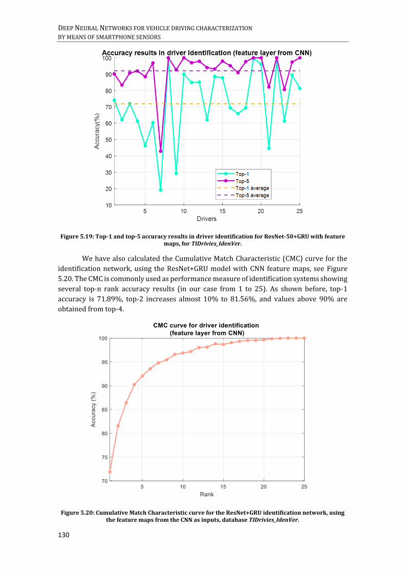
DEEP NEURAL NETWORKS FOR VEHICLE DRIVING CHARACTERIZATION BY MEANS OF SMARTPHONE SENSORS
130
Figure 5.19: Top-1 and top-5 accuracy results in driver identification for ResNet-50+GRU with feature maps, for TIDrivies_IdenVer.
We have also calculated the Cumulative Match Characteristic (CMC) curve for the
identification network, using the ResNet+GRU model with CNN feature maps, see Figure
5.20. The CMC is commonly used as performance measure of identification systems showing
several top-n rank accuracy results (in our case from 1 to 25). As shown before, top-1
accuracy is 71.89%, top-2 increases almost 10% to 81.56%, and values above 90% are
obtained from top-4.
Figure 5.20: Cumulative Match Characteristic curve for the ResNet+GRU identification network, using the feature maps from the CNN as inputs, database TIDrivies_IdenVer.

CHAPTER 5. DRIVER RECOGNITION
131
Trying to visualize a driver embedding we have extracted the feature map from the
last Dense layer (in the ResNet+GRU model), before the final Softmax layer, and then we
have averaged these vectors along a journey. The resulting vector can be seen as a
driver2vec or driver embeddings for each of the journeys. These driver embeddings can be
used to visualize driver clusters and then to explore the different drivers in terms of their
inter-driver (internal variability of a driver for her/his different journeys) and intra-driver
(variability with other drivers). For all the journeys of the 25 drivers in our database, we
visualize (see Figure 5.21) the corresponding driver2vect embeddings with t-distributed
stochastic neighbor embedding (t-SNE) algorithm. In Figure 5.21 we have encircled the
embeddings space for drivers eight, ten, nineteen and twenty two that can be easily
identified as they show low intra-driver and high inter-driver values (see their high
accuracy results in Figure 5.19). In this visualization we can also identify some drivers, as
drivers seven and nine, that show very high intra-driver variability and therefore low
identification accuracy as it can be seen in Figure 5.19.
Figure 5.21: Two-dimensional t-distributed stochastic neighbor embedding (t-SNE 2D) projections of the feature vectors of the dense layers, using CNN like inputs in the ResNet+GRU model. Projections for
25 drivers, database TIDrivies_IdenVer.
The drivers with the worst results were seven and nine, with a top-1 journey level
accuracy of 19.04% and 29.27% respectively (see confusion matrix of Figure 5.18). For
these drivers that obtain low accuracy values at top-1 journey level, we have also drawn
part of the trips, in order to observe if there are signals with strange behaviors or with low
or high noise levels. Figure 5.22 presents journeys of driver seven that have been confused
with driver eighteen. In particular for this driver, almost 25% of journeys confuse with
driver eighteen. For driver nine, we have drawn both journeys well classified as wrong

DEEP NEURAL NETWORKS FOR VEHICLE DRIVING CHARACTERIZATION BY MEANS OF SMARTPHONE SENSORS
132
classified, to observe possible differences, see Figure 5.23. In this case, driver nine confuses
53.22% of the journeys with driver twenty-five. Each section of the figures will present for
a journey area: the raw accelerometers and the module of the horizontal projection for
accelerations. The signal zones where maneuvers have been detected have also been
marked in dotted green, and a solid orange line has been drawn on the subplot of the
horizontal projection module, indicating the estimated background noise level.
Figure 5.22: Examples of test journey sections, representing for each one: the raw accelerometers and the horizontal projection modulus of the accelerations. a), b) and c): Journeys of driver seven, which the network has incorrectly classified for driver eighteen. d), e) and f): Journeys of driver eighteen
correctly identified.
On the left side of Figure 5.22, we have drawn three journeys of the driver seven,
which have been confused with driver eighteen: Figure 5.22 a), b) and c). And on the right
side, we have drawn three journeys of driver eighteen, correctly identified: Figure 5.22 d),
e) and f). Although the signals used in the network are the longitudinal and transversal
accelerations and the angular velocity, the departure signals (raw accelerometers) do not
have strange behaviors and do not present abnormal values. It also seems than the derived
signals from the raw accelerometers correctly independent network decisions from the
position of the mobile. Since both for the misclassified examples of driver seven, and for the
correctly classified examples of driver eighteen, there are cases where the axes measure
different values of gravity. Regarding the background noise level for each of them (orange
line in the horizontal projection module), in all cases they are values below 1 𝑚 𝑠2⁄ ;

CHAPTER 5. DRIVER RECOGNITION
133
therefore, wrong identification cannot be associated with low or high noise levels. In
addition, the maneuvers marked in green show events of different nature, both in duration
and type. No anomalies appear to be observed in the signals for said poor classification of
driver seven with eighteen. Besides for driver eighteen in these test examples, it has not
been incorrectly classified as seven in any case.
Driver nine is the second driver with a lower top-1 identification rate, 29.27%. In
this case, 53% of the journeys confuse them with driver twenty five. Despite the fact that
driver seven has the lowest accuracy of the whole group of drivers, their confusion is more
distributed. In contrast, for driver number nine, more than half of the time, the network
classifies it as driver twenty five. However, for driver twenty five, only one trip is incorrectly
classified as driver nine; so the confusion between them is not reciprocal. The Figure 5.23
shows six examples of journeys: two trips where driver nine is confused with driver twenty
five, two well-classified journeys for driver nine, and two well-classified journeys for driver
twenty five. As before, there are no important characteristics that explain these errors.
Figure 5.23: Examples of test journey sections, representing for each one: the raw accelerometers and the horizontal projection modulus. a) and b): Nine driver journeys incorrectly classified as twenty five
driver. c) and d): Nine driver journeys correctly classified. e) and f): Journeys of driver twenty five correctly identified.
Although from the previous examples of the individual journeys of driven seven and
nine, we have not appreciated errors that could be due to noise, we decided to make an
analysis for all the test journeys with all the drivers. As we have specified in the section 5.2.1
Experimental framework, each driver has a set of 801 journeys, of which 80% has been used

DEEP NEURAL NETWORKS FOR VEHICLE DRIVING CHARACTERIZATION BY MEANS OF SMARTPHONE SENSORS
134
for training and 20% for testing. Therefore, all drivers have the same number of trips under
test (160 journeys), and also following the training requirements, we have used only 15
windows per journey, although all available ones could be used. To analyze it we have
employed, as before, the background noise level of each journey (obtained from the
horizontal projection module of the accelerometers), to observe if there are differences
between more and less noisy trips. The signals used for the training are overlapping
windows through the maneuvers, but in order to analyze it we have not calculated the noise
in these maneuvers (because in these areas we would obtain higher values than normal),
but rather the background noise level of each journey.
Figure 5.24 shows the values obtained in the test, when the results obtained at
journey level have been correctly classified and when they have not. There are not many
differences between the two, in both cases the background noise is around 0.6 𝑚 𝑠2⁄ .
Figure 5.24: Background noise levels for the test journeys, according to whether these trips have been correctly associated with each driver or not.
Finally, we have carried out an analysis based on the maneuver present in each
window used in the identification tests. We have classified the corresponding windows in 6
types: only braking, only acceleration, braking&turn, acceleration&turn, only turn and a
mixture of all of them. Depending on the longitudinal and transversal acceleration forces
present in them. At window level, there are no significant differences, see Figure 5.25.
Maneuvers related to longitudinal accelerations, both acceleration and braking, seem to
offer higher accuracy values, than for example turns, associated with transversal forces.

CHAPTER 5. DRIVER RECOGNITION
135
Figure 5.25: Accuracies obtained for the windows of the test journeys, depending on the type of maneuver present in the windows.
5.2.3. Driver identification using acceleration signals derived from GPS
In the previous section we have used the TIDrivies_IdenVer database that includes
accelerometer signals captured by smartphones, for a set of 25 drivers and 801 journeys by
driver. The aim of this section is to contrast our driver identification results with state of
the art research using a publicly available database: the AXA Driver Telematics database.
As we presented in Section 5.2.1, this database contains driving journeys
represented in a 2D space by sequences of {𝑥, 𝑦} values at a sampling rate of 1 Hz; {𝑥, 𝑦}
values are obtained from GPS data.
In order to evaluate our Deep Learning models using AXA Driver Telematics data,
we developed an algorithm to obtain acceleration signals from these sequences of {𝑥, 𝑦}
positions. We considered this approach accurate enough, though it may introduce some
small inaccuracies due to both the transformation of {𝑥, 𝑦} sequences signals into
acceleration signals and errors in GPS measurements.
As the organizers of AXA competition indicated, driver characterization is
influenced by both the driving trip and the driver behavior: “The intent of this competition is
to develop an algorithmic signature of driving type. Does a driver drive long trips? Short trips?
Highway trips? Back roads? Do they accelerate hard from stops? Do they take turns at high
speed? The answers to these questions combine to form an aggregate profile that potentially
makes each driver unique. For this competition, Kaggle participants must come up with a
"telematic fingerprint" capable of distinguishing when a trip was driven by a given driver. The
features of this driver fingerprint could help assess risk and form a crucial piece of a larger
telematics puzzle.”

DEEP NEURAL NETWORKS FOR VEHICLE DRIVING CHARACTERIZATION BY MEANS OF SMARTPHONE SENSORS
136
As a good demonstration of this, is that the team that finished in second place (see
(Blog Kaggle, 2015)) combined trip matching with a driver signature model. In fact most of
participants used the Ramer–Douglas–Peucker (RDP) algorithm for trip matching. RDP
reduces the number of points in a line, by simplifying a polyline with respect to a pre-
defined tolerance value (Belussi, Catania, Clementini, & Ferrari, 2007). Therefore (see
Figure 5.26), it selects the vertex 𝑣 with maximum distance from the segment connecting
the endpoints of the polyline and compares such a distance with the tolerance value. If the
distance is greater, the polyline is divided into two polylines incident at 𝑣 and the process
is recursively applied. If the distance is lower, the polyline is approximated by the segment
itself.
Figure 5.26: Example of polyline with five vertices reduced to a polyline of three vertices with the RDP algorithm (tolerance e). a) Polyline of five vertices. b) Polyline of three vertices.
Although the winner team did not share his code, they specified that also employed
the RDP algorithm for trip matching and they combined it using Gradient Boosting with
some other driver behavioral features such as speed percentiles, acceleration, speed at
turning angles, total distance, deceleration and acceleration before and after stops, etc. The
driver identification accuracy, measured using the area under ROC curve, was 0.97983 for
the private leaderboard (obtained using approximately 70% of the test data) and 0.97946
for the public leaderboard (for approximately 30% of the test data). The results for the team
in second place were very similar, 0.97398 in the private leaderboard and 0.97334 in the
public leaderboard.
It is important to point out that in these works, the teams found that the trip-
matching was the most relevant information for obtaining these high accuracies in driver
identification. Consequently, as the aim in this Thesis is to work only using driver behavioral
features, we looked for some research using only this type of information on the AXA
database. With these characteristics we found the work of (Dong, et al., 2016).
(Dong, et al., 2016) published an article based on the experiments that they
performed in the AXA database. Their experiments included driver identification for several
subsets of the database. In particular, they tested two subsets, one with 50 drivers and
another one with 1000 drivers. In this work {𝑥, 𝑦} sequences were represented using
feature engineering to extract some statistical features. Using these features different
Machine Learning models, including Deep Learning, were tested. First, they segment the
signals into sections of length 𝐿𝑠, with a shift of 𝐿𝑠
2⁄ . For each segment, they calculate 5

CHAPTER 5. DRIVER RECOGNITION
137
features at every time point, called basic features: the speed norm, the difference of speed
norm, the acceleration norm, the difference of acceleration norm, and the angular speed.
From the resulting matrix of size 5 ∗ 𝐿𝑠, they finally get the statistical features used for
identification. To do this, for frames of 5 ∗ 𝐿𝑓 (with 𝐿𝑓 < 𝐿𝑠) and a shift of 𝐿𝑓
2⁄ , they
calculate the mean, the minimum, the maximum, the 25%, the 50%, and the 75% quartiles,
and the standard deviation of the basic features in each frame. Obtaining an array of 35
rows, representing the driving feature axis, and 2 ∗𝐿𝑠
𝐿𝑓⁄ columns, representing the time
axis. In particular, they use a 𝐿𝑠 of 256 seconds and a 𝐿𝑓 of 4 seconds. Similarly to our
research, they define three metrics to measure accuracy: window level accuracy (which
they call segments), top-1 journey level accuracy and top-5 journey level accuracy. For
driver identification they use 6 different models: a 1-D Convolutional network with pooling
layers (three convolution-pooling layers and three fully connected layers), a 1-D
Convolutional network without pooling layers (three convolution layers and three fully
connected layers), a Recurrent Neural network that use as input the features extracted at
the third convolutional layer in the pre-trained CNN (one layer and 100 neurons), a Neural
network of 1 layer and 100 neurons, a Neural network of 2 stacked layer (100 neurons in
each layer) and the Gradient Boosting Decision Tree (GBDT). With the GBDT, they also do a
test, but instead of using the statistical features, they test with a set of 57 manually features,
made up of both global features (as the mean, the minimum, the maximum, the standard
deviation, etc.) and local features (as the time duration of the whole trip, the trip length, the
average speed, among others). The results obtained are shown in the Table 5.9. For the set
of 50 drivers, the candidate that offers the best results is for the model with a Recurrent
Network of two stacked layers, employing as inputs the statistical features. Obtaining an
accuracy at window level of 34.8%, and at journey level top-1 and top-5 of 52.3% and
77.4%, respectively. In the case of 1000 drivers, they did not carry out the tests with all the
models. But among the architectures tested, the best performance is again with the
Recurrent Network of two stacked layers and the statistical features, with an accuracy at
window level and at journey top-1 and top-5 of 27.50%, 40.50% and 60.4%, respectively.
Table 5.9: Results of the work of (Dong, et al., 2016) for driver identification, in the database of AXA “Driver Telematics Analysis”.
Method No. drivers Accuracy at
window level (%)
Accuracy at journey level
top-1 (%)
Accuracy at window
level top-5 (%)
CNN without pooling layers 50 16.9 28.3 56.7 CNN 50 21.6 34.9 63.7
RNN of one layer pre-trained (using the features extracted at the
third convolutional layer in the pre-trained CNN
as inputs to train an RNN)
50 28.2 44.6 70.4
RNN of one layer 50 34.7 49.7 76.9 RNN of two staked layers 50 34.8 52.3 77.4
GBDT 50 18.3 29.1 55.9 GBDT on a set of 57 manually defined
driving behavior features 50 - 51.2 74.3
CNN 1000 23.4 26.7 46.7 RNN of two staked layers 1000 27.5 40.5 60.4
GBDT on a set of 57 manually defined driving behavior features
1000 - 9.2 15.8

DEEP NEURAL NETWORKS FOR VEHICLE DRIVING CHARACTERIZATION BY MEANS OF SMARTPHONE SENSORS
138
It is also important to note that although we have used the same database as in the
AXA competition, the comparison with (Dong, et al., 2016) will not be straight, because we
do not know exactly what subset of drivers for training and testing were used.
As discussed before, one of the main challenges in driver identification from
smartphones accelerometers is the robustness to undesired sources of variability (such as
the type of smartphone, the car model, type of route, or the position of the smartphone
inside the vehicle). Therefore, it is important to remark that some of these sources of
variability, that are present in TIDrivies_IdenVer dataset, does not affect AXA competition
database. For example, in AXA database, sequences of {𝑥, 𝑦} positions may have some noise
due inaccurate GPS measures, but this noise is expected to be very different -and with less
energy- than the common noise in tri-axial accelerometer devices. Also the variability due
the terminal position and the effect in accelerometers of road noise through gravity will not
be present in AXA database. In contrast to the absence of these variability sources, a peculiar
difficulty in AXA database is that, according its design, of the 200 initial journeys by driver,
there is a set of false trips, that is, routes that actually belong to another driver. This fact
obviously will make some errors even if the identification algorithm is working correctly
(but we have no way of checking these false trips as they are not identified in AXA database).
5.2.3.1. From {x,y} sequences to acceleration signals
The process to derive acceleration signals from sequences of 2D {𝑥, 𝑦} positions is
summarized below.
The first step was to divide the routes into segments, to avoid possible time breaks.
It was necessary to clean the data in order to address two main issues:
To remove some short segments of {𝑥, 𝑦} positions with impossible trajectories,
which are plausible due to invalid GPS measurements.
To remove some segments of {𝑥, 𝑦} with very close positions. This is generally due
to states where the car is stopped and again GPS measures show some variability.
Once a stop state is detected, the journey is divided in two sub-journeys.
After obtaining the subjourneys, the corresponding sequences of {𝑥, 𝑦} positions
were processed to obtain three signals: longitudinal and transversal accelerations, and
angular velocity. Note that these signals are the same that are available in TIDrivies_IdenVer
database. Though it is important to indicate that as {𝑥, 𝑦} positions are available for every
second, the sample rate now will be 1 Hz, while in TIDrivies_IdenVer was 5 Hz.
To derive these signals we performed the following steps. Using the first derivative
of {𝑥, 𝑦} positions we obtain the speed in X and Y axes. From these velocities we calculate
the corresponding X and Y accelerations deriving. Then, in order to obtain the longitudinal
and transversal accelerations, we projected accelerations on the (𝑥, 𝑦) velocity vector. To
improve the accuracy in these derivatives we used interpolation with splines. Once we have
the longitudinal and transversal accelerations, the angular velocity can be obtained by
means of the relation between the transversal component and the linear velocity (𝑤 = 𝑎𝑡 ⁄

CHAPTER 5. DRIVER RECOGNITION
139
𝑣). We estimate this linear velocity with the method described in (Cervantes-Villanueva ,
Carrillo-Zapata, Terroso-Saenz , Valdes-Vela, & Skarmeta, 2016).
Once we have longitudinal and transversal accelerations and angular velocity, in
order to use ResNet-50 network, we define a window size of 224 samples (that at 1Hz
represents 3.73 minutes of driving).
Next, as required in the driver identification process for TIDrivies_IdenVer
database), we now need a procedure to detect maneuver on AXA database signals. To this
end, we extract information on typical duration of acceleration maneuvers (braking and
accelerations) and turn maneuvers using the events obtained in Chapter 4 on
TIDrivies_IdenVer database. (Figure 5.27 a) represents a histogram of the durations of
acceleration maneuvers, and (Figure 5.27 b) for turn maneuvers. According to these
histograms, we decided to detect an acceleration/deceleration maneuver when longitudinal
acceleration exceeds an empirical threshold for 3 consecutive seconds, while for a turn
maneuver, when transversal acceleration is above another empirical threshold for at least
5 seconds.
Figure 5.27: Histogram of driving maneuver lengths in a set of 47240 journeys in TIDrivies_IdenVer database. a) Acceleration maneuvers duration. b) Turn maneuvers duration.

DEEP NEURAL NETWORKS FOR VEHICLE DRIVING CHARACTERIZATION BY MEANS OF SMARTPHONE SENSORS
140
Figure 5.28 shows an example of maneuver detection: the stem in cyan represents
the areas where the acceleration/deceleration maneuvers are detected and in red where
the turn events are detected. Now, we are working with a lower sampling frequency, 1 Hz
instead of 5 Hz, so the information present in the windows of 224 samples is equivalent to
3.73 minutes instead of 44.8 seconds like before. Each window, although with less
information per second, has more information about the journey. According to the cases
studied for this database, as the example of the figure, it seems that there are not too many
differences between selecting only maneuver windows, compared to selecting overlapping
consecutive windows. The overlapping consecutive windows frequently overlap with
maneuver information, so for this database we have decided to retake the strategy of the
first minutes of the journey.
Figure 5.28: Example of maneuver detection obtained empirically for the AXA Driver Telematics database. The stem in cyan represents the areas where the acceleration/deceleration maneuvers are
detected and in red where the turn events are detected. a) Speed. b) Longitudinal acceleration. c) Transversal acceleration. d) Angular velocity.

CHAPTER 5. DRIVER RECOGNITION
141
5.2.3.2. Experiments and results
AXA Driver Telematics database has sequences of {𝑥, 𝑦} positions, at 1Hz sampling rate, for
a total of 2739 drivers, with 200 journeys of different duration per driver. Once we have
longitudinal and transversal accelerations and angular velocity, we followed the same
driver identification process we used for TIDrivies_IdenVer database (5.2.2 Driver
identification from accelerometer signals). The whole process is shown in Figure 5.29. From
the sequences of {𝑥, 𝑦}positions, we calculate the acceleration. Then with this acceleration,
we obtain both the longitudinal and transversal accelerations associated (projecting on the
speed) and finally the angular velocity.
Figure 5.29: Driver identification process, for the AXA Driver Telematics database.
As for the Deep Learning model we studied for TIDrivies_IdenVer database (see
Figure 5.6, Section 5.2.2), 2-D images of three channels were generated from acceleration
and angular velocity 1D time series. The driver identification model then consist of a
ResNet-50 network followed by a Recurrent Neural Network (GRU) block followed by a
Dense and Softmax layers. As before, we tested the best procedure we found in Section 5.2.2
to transform 1D signals to 2D images using a convolutional network, Figure 5.15, for each
of the channels. For this new database, we trained again each convolutional network of
Figure 5.15 with the AXA journeys (we did not use the weights obtained with the database
of TIDrivies_IdenVer). And we employed for training the same set of 25 drivers that the one
used in the tests.
Based on previous tests for the TIDrivies_IdenVer database, our initial purpose was
to also use a fixed number of windows per journey. For the previous database we used 15,
but since we had longer windows we decided to reduce the number used to 10 as a first
approximation. Demanding this number of windows caused that from the 200 initial
journeys by driver, not all could be employed because they were shorter than the desired
size. In addition, the fact of requiring the same number of training and testing journeys for
all drivers had greatly reduced the number of available trips, obtaining in total 100 journeys

DEEP NEURAL NETWORKS FOR VEHICLE DRIVING CHARACTERIZATION BY MEANS OF SMARTPHONE SENSORS
142
by driver, 80 for training and 20 for testing. Due to the reduced number of trips, we decided
to use all the available windows, in order not to limit the available windows so drastically.
Driver identification performance results are presented in Table 5.10. Similarly as
in Section 5.2.2 (see 5.2.2.3 Experiments and Results), the accuracy results are given at
window level, as well as at top-1 and top-5 journey levels respectively. As it can be seen in
Table 5.10, the results for AXA are: window level 52.47%, top-1 66.97% and top-5 84.80%.
Previously, we had for the database of TIDrivies_IdenVer: window level 48.58%, top-1
71.89% and top-5 92.03%. We can conclude that results for TIDrivies_IdenVer are only
slightly better than those for AXA, and both results are competitive with an accuracy top-1
of almost 67%, and an accuracy top-5 of almost 85%.
Table 5.10: Results for driver identification using the ResNet50+GRU model, databases of AXA Driver
Database No.
drivers Network
Accuracy
At window
level (%)
At journey level top-1
(%)
At journey level top-5
(%)
AXA Driver Telematics
25 ResNet50+GRU 52.47% 66.97% 84.80%
TIDrivies_IdenVer 25 ResNet50+GRU 48.58% 71.89% 92.03%
As we done for the TIDrivies_IdenVer database, we have calculated the confidence
intervals on the performance of this model using the AXA database (see Table 5.11). As seen
in the table, for the AXA database there is a 95% likelihood that the range 63.85% to 70.09%
covers the true model accuracy. For this database, we have a larger confidence interval, so
we have a less precise estimate than with the TIDrivies_IdenVer dataset.
Table 5.11: Confidence intervals for driver identification using the ResNet50+GRU model.
Database No.
drivers Network 95% confidence interval
AXA Driver Telematics
25 ResNet50+GR
U 66.97% ± 3.12%
TIDrivies_IdenVer 25 ResNet50+GR
U 71.89% ± 1.39%
5.2.3.3. Driver identification error analysis
As we did for TIDrivies_IdenVer database (Section 5.2.2.4 Driver identification error
analysis), we have addressed an analysis of driver identification results for the set of 25
drivers. As Figure 5.30 shows, the overall accuracy top-1 is 66.97%. The worst performing
driver is driver nineteen with a top-1 accuracy of 40%. However, as we also observed
previously, although there are some drivers with poor top-1 accuracy, their top-5 is
significantly better. The drivers with the best results do not reach top-1 of 85% and slightly
higher than 90% for the top-5.
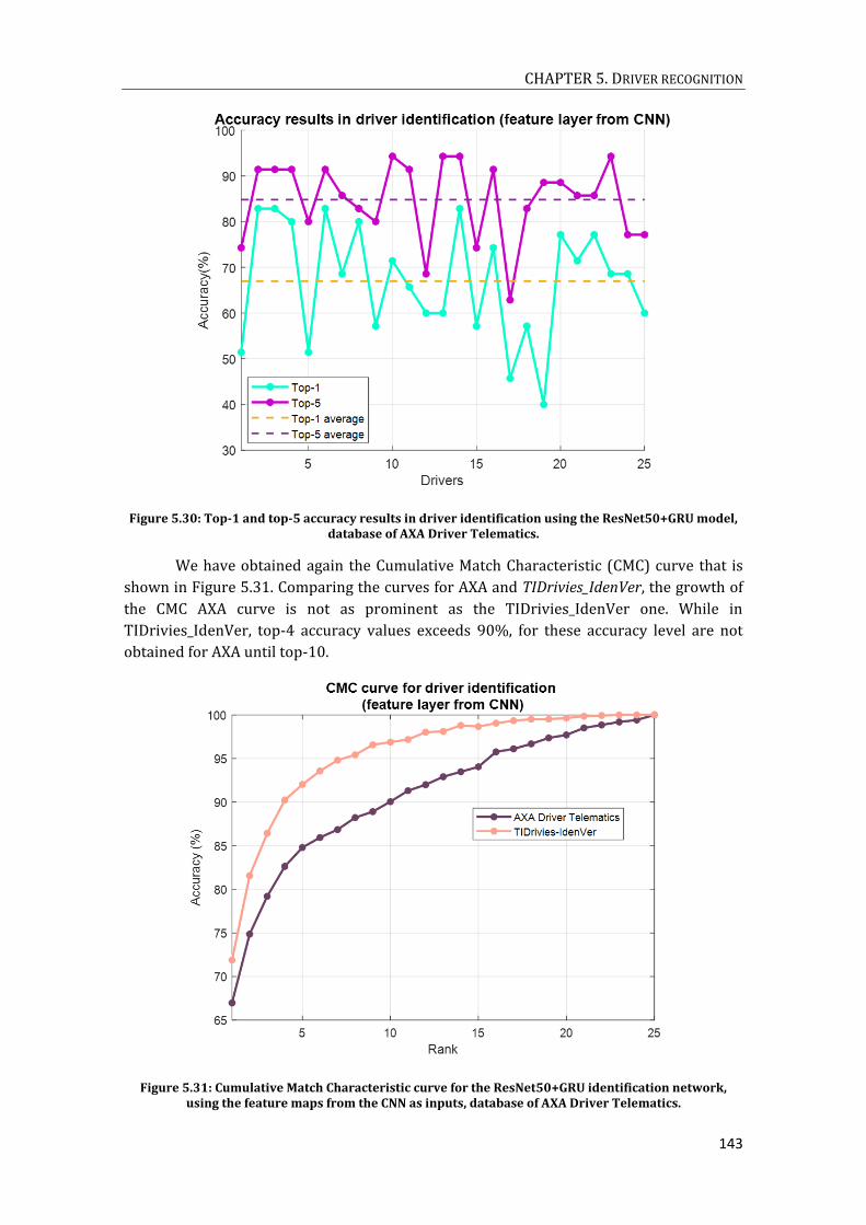
CHAPTER 5. DRIVER RECOGNITION
143
Figure 5.30: Top-1 and top-5 accuracy results in driver identification using the ResNet50+GRU model, database of AXA Driver Telematics.
We have obtained again the Cumulative Match Characteristic (CMC) curve that is
shown in Figure 5.31. Comparing the curves for AXA and TIDrivies_IdenVer, the growth of
the CMC AXA curve is not as prominent as the TIDrivies_IdenVer one. While in
TIDrivies_IdenVer, top-4 accuracy values exceeds 90%, for these accuracy level are not
obtained for AXA until top-10.
Figure 5.31: Cumulative Match Characteristic curve for the ResNet50+GRU identification network, using the feature maps from the CNN as inputs, database of AXA Driver Telematics.

DEEP NEURAL NETWORKS FOR VEHICLE DRIVING CHARACTERIZATION BY MEANS OF SMARTPHONE SENSORS
144
Finally, we have represented accuracy values for journeys with different number of
windows (Figure 5.32 a)) and for journeys with a minimum number of windows (Figure
5.32 b)). The overall accuracy at top-1 journey level was 66.97 % (red line, Figure 5.32 a)).
Increasing the number of windows per journey, accuracy obviously increases reaching a
75% for journeys with more than 12 windows.
Figure 5.32: Accuracies at window level, for the architecture of ResNet50+GRUs, based on: a) journeys with a given number of windows, b) journeys with a minimum number of windows.
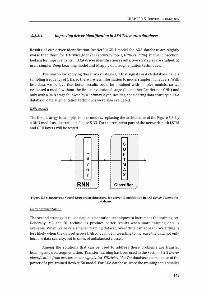
CHAPTER 5. DRIVER RECOGNITION
145
5.2.3.4. Improving driver identification in AXA Telematics database
Results of our driver identification ResNet50+GRU model for AXA database are slightly
worse than those for TIDrivies_IdenVer (accuracy top-1, 67% vs. 72%). In this Subsection,
looking for improvements in AXA driver identification results, two strategies are studied: a)
use a simpler Deep Learning model and b) apply data augmentation techniques.
The reason for applying these two strategies, it that signals in AXA database have a
sampling frequency of 1 Hz, so there are less information to model simpler maneuvers. With
less data, we believe that better results could be obtained with simpler models, so we
evaluated a model without the first convolutional stage (i.e. neither ResNet nor CNN) and
only with a RNN stage followed by a Softmax layer. Besides, considering data scarcity in AXA
database, data augmentation techniques were also evaluated.
RNN model
The first strategy is to apply simpler models, replacing the architecture of the Figure 5.6, by
a RNN model as illustrated in Figure 5.33. For the recurrent part of the network, both LSTM
and GRU layers will be tested.
Figure 5.33: Recurrent Neural Network architecture, for driver identification in AXA Driver Telematics database.
Data augmentation
The second strategy is to use data augmentation techniques to increment the training set.
Generally, ML and DL techniques produce better results when more training data is
available. When we have a smaller training dataset, overfitting can appear (overfitting is
less likely when the dataset grows). Also, it can be interesting to increase the data not only
because data scarcity, but in cases of unbalanced classes.
Among the solutions that can be used to address these problems are transfer
learning and data augmentation. Transfer learning has been used in the Section 5.2.2 Driver
identification from accelerometer signals, for TIDrivies_IdenVer database, to make use of the
power of a pre-trained ResNet-50 model. For AXA database, since the training set is smaller
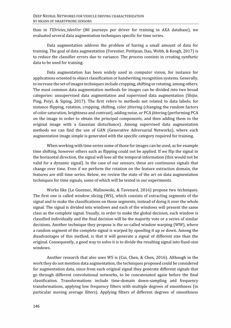
DEEP NEURAL NETWORKS FOR VEHICLE DRIVING CHARACTERIZATION BY MEANS OF SMARTPHONE SENSORS
146
than in TIDrivies_IdenVer (80 journeys per driver for training in AXA database), we
evaluated several data augmentation techniques specific for time series.
Data augmentation address the problem of having a small amount of data for
training. The goal of data augmentation (Forestier, Petitjean, Dau, Webb, & Keogh, 2017) is
to reduce the classifier errors due to variance. The process consists in creating synthetic
data to be used for training.
Data augmentation has been widely used in computer vision, for instance for
applications oriented to object classification or handwriting recognition systems. Generally,
to increase the set of images techniques include cropping, shifting or rotating, among others.
The most common data augmentation methods for images can be divided into two broad
categories: unsupervised data augmentation and supervised data augmentation (Shijie,
Ping, Peiyi, & Siping, 2017). The first refers to methods not related to data labels; for
instance flipping, rotation, cropping, shifting, color jittering (changing the random factors
of color saturation, brightness and contrast), adding noise, or PCA jittering (performing PCA
on the image in order to obtain the principal components, and then adding them to the
original image with a Gaussian disturbance). Among supervised data augmentation
methods we can find the use of GAN (Generative Adversarial Networks), where each
augmentation image simple is generated with the specific category required for training.
When working with time series some of those for images can be used, as for example
time shifting, however others such as flipping could not be applied. If we flip the signal in
the horizontal direction, the signal will lose all the temporal information (this would not be
valid for a dynamic signal). In the case of our sensors, these are continuous signals that
change over time. Even if we perform the rotation on the feature extraction domain, the
features are still time series. Below, we review the state of the art on data augmentation
techniques for time signals, some of which will be tested in our experiments.
Works like (Le Guennec, Malinowski, & Tavenard, 2016) propose two techniques.
The first one is called window slicing (WS), which consists of extracting segments of the
signal and to make the classifications on those segments, instead of doing it over the whole
signal. The signal is divided into windows and each of the windows will present the same
class as the complete signal. Usually, in order to make the global decision, each window is
classified individually and the final decision will be the majority vote or a series of similar
decisions. Another technique they propose is the so-called window warping (WW), where
a random segment of the complete signal is warped by speeding it up or down. Among the
disadvantages of this method, is that it will generate a signal of different size than the
original. Consequently, a good way to solve it is to divide the resulting signal into fixed-size
windows.
Another research that also uses WS is (Cui, Chen, & Chen, 2016). Although in the
work they do not mention data augmentation, the techniques proposed could be considered
for augmentation data, since from each original signal they generate different signals that
go through different convolutional networks, to be concatenated again before the final
classification. Transformations include time-domain down-sampling and frequency
transformations, applying low frequency filters with multiple degrees of smoothness (in
particular moving average filters). Applying filters of different degrees of smoothness
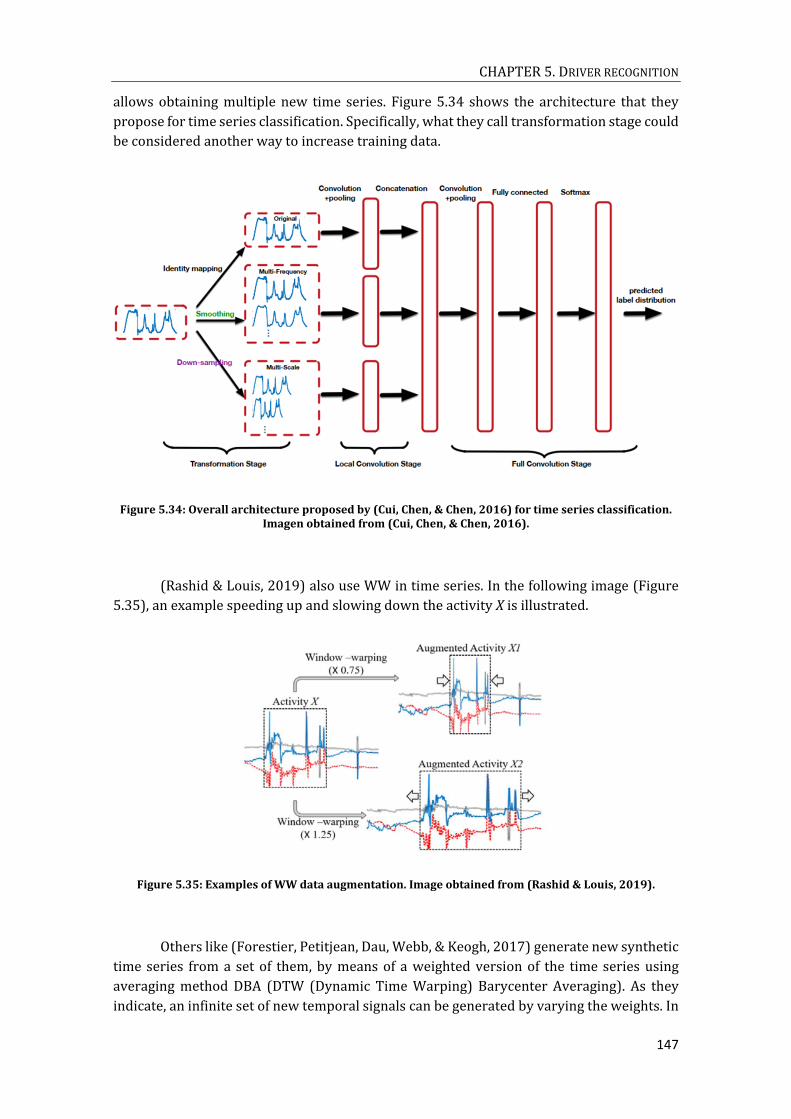
CHAPTER 5. DRIVER RECOGNITION
147
allows obtaining multiple new time series. Figure 5.34 shows the architecture that they
propose for time series classification. Specifically, what they call transformation stage could
be considered another way to increase training data.
Figure 5.34: Overall architecture proposed by (Cui, Chen, & Chen, 2016) for time series classification. Imagen obtained from (Cui, Chen, & Chen, 2016).
(Rashid & Louis, 2019) also use WW in time series. In the following image (Figure
5.35), an example speeding up and slowing down the activity X is illustrated.
Figure 5.35: Examples of WW data augmentation. Image obtained from (Rashid & Louis, 2019).
Others like (Forestier, Petitjean, Dau, Webb, & Keogh, 2017) generate new synthetic
time series from a set of them, by means of a weighted version of the time series using
averaging method DBA (DTW (Dynamic Time Warping) Barycenter Averaging). As they
indicate, an infinite set of new temporal signals can be generated by varying the weights. In

DEEP NEURAL NETWORKS FOR VEHICLE DRIVING CHARACTERIZATION BY MEANS OF SMARTPHONE SENSORS
148
Figure 5.36, an example of his work is presented (Petitjean, et al., 2016). The first plot on
the left (Figure 5.36 a) shows a set of input signals belonging to the same class, which are
going to be used under the algorithm. Successive plots (Figure 5.36 b,c) show the new time
series produced by the Euclidean average and produced by the DBA, respectively. As seen
in the image, the advantage of this method is that it better preserves the shape of the times
series than when we use the Euclidean average. But as inconvenient for its application to
our signal, is that it is difficult to find some input signals that can be averaged to generate
new signals. Because if we take maneuvers, although they belong to the same class, they
have different forms and durations and, if averaging them, the resulting signal could lose
valuable information contained in the maneuver itself.
Figure 5.36: Image obtained from (Petitjean, et al., 2016) a) Different input signals belonging to the same class. b) Average time series produced by Euclidean average. c) Average time series produced by
DBA.
In a related field where data augmentation for temporal signals is widely used is in
electroencephalography (EEG) signals classification; due to the difficulty of obtaining a
large set of brain signals (although acquisition methods have improved, they are usually
invasive). In (Zhang, Lei, & Li, 2018) noise is added to EEG signals, but unlike other works,
where they add it in the time domain, they perform a transformation to the frequency
domain and then add Gaussian perturbation to the amplitudes. The reasons mentioned by
the authors to add noise in this way, it is because the EEG has low signal-to-noise ratio, it is
non-stationary, and has insufficient spatial resolution compared to images. So, if the noise
was applied directly to the temporal signal, it may destroy important features of EEG
signals.
Besides, data augmentation can be applied or over the data-space domain, as for
example WW, or in the feature-space, as synthetic over-sampling (Wong, Gatt, Stamatescu,
& McDonnell, 2016). The over-sampling is very useful when the data classes are unbalanced.
A technique of over-sampling widely used is the one proposed in (Chawla, Bowyer, Hall, &
Kegelmeyer, 2002), called Synthetic Minority Over-Sampling Technique (SMOTE). In this
technique, synthetic examples are created in the feature-space from randomly selected
pairs of real world feature-examples from the minority class.
A research that performs data augmentation in the feature space applied to sensor
signals is ( Eyobu & Han, 2018). They employ wearable inertial measurement unit (IMU)
sensors to recognize between three types of activities: walking, sitting and standing. They
use accelerometer and gyroscope signals and their approach is to take the tri-axial
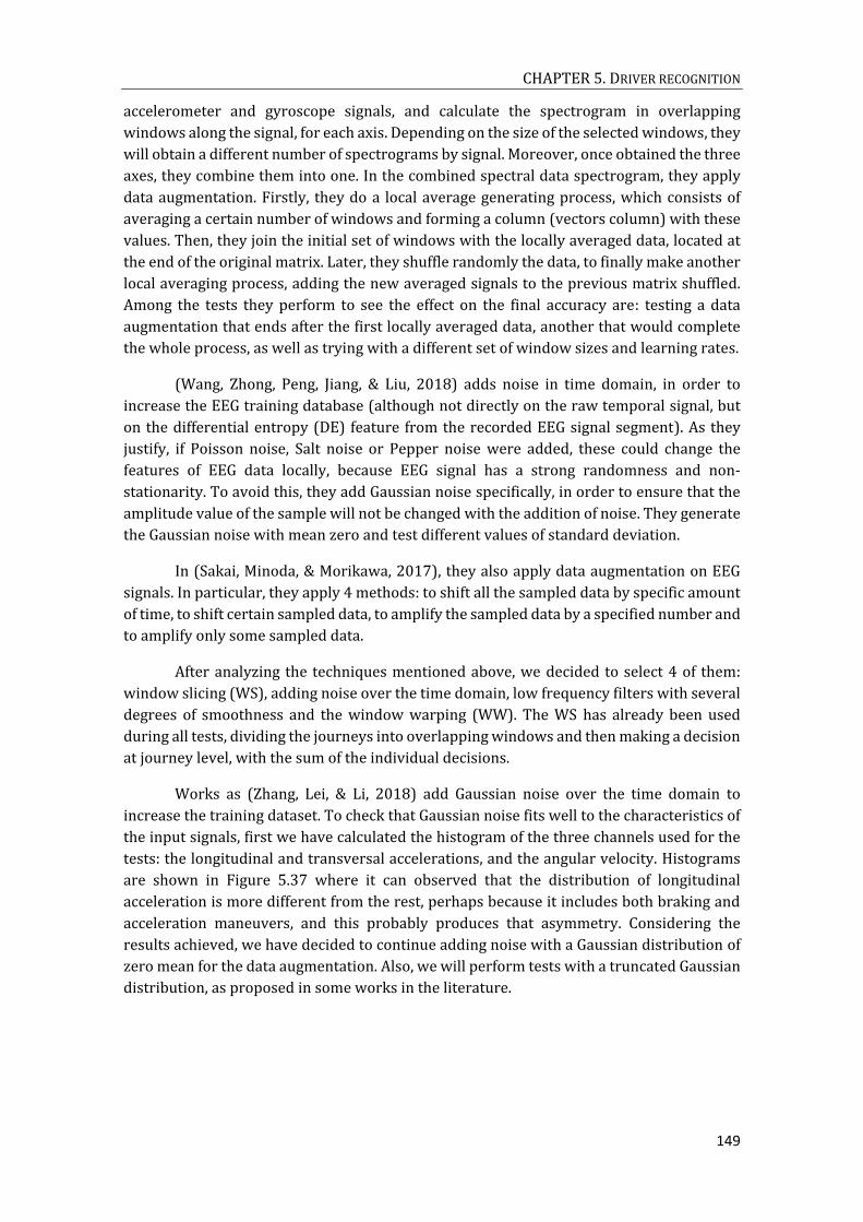
CHAPTER 5. DRIVER RECOGNITION
149
accelerometer and gyroscope signals, and calculate the spectrogram in overlapping
windows along the signal, for each axis. Depending on the size of the selected windows, they
will obtain a different number of spectrograms by signal. Moreover, once obtained the three
axes, they combine them into one. In the combined spectral data spectrogram, they apply
data augmentation. Firstly, they do a local average generating process, which consists of
averaging a certain number of windows and forming a column (vectors column) with these
values. Then, they join the initial set of windows with the locally averaged data, located at
the end of the original matrix. Later, they shuffle randomly the data, to finally make another
local averaging process, adding the new averaged signals to the previous matrix shuffled.
Among the tests they perform to see the effect on the final accuracy are: testing a data
augmentation that ends after the first locally averaged data, another that would complete
the whole process, as well as trying with a different set of window sizes and learning rates.
(Wang, Zhong, Peng, Jiang, & Liu, 2018) adds noise in time domain, in order to
increase the EEG training database (although not directly on the raw temporal signal, but
on the differential entropy (DE) feature from the recorded EEG signal segment). As they
justify, if Poisson noise, Salt noise or Pepper noise were added, these could change the
features of EEG data locally, because EEG signal has a strong randomness and non-
stationarity. To avoid this, they add Gaussian noise specifically, in order to ensure that the
amplitude value of the sample will not be changed with the addition of noise. They generate
the Gaussian noise with mean zero and test different values of standard deviation.
In (Sakai, Minoda, & Morikawa, 2017), they also apply data augmentation on EEG
signals. In particular, they apply 4 methods: to shift all the sampled data by specific amount
of time, to shift certain sampled data, to amplify the sampled data by a specified number and
to amplify only some sampled data.
After analyzing the techniques mentioned above, we decided to select 4 of them:
window slicing (WS), adding noise over the time domain, low frequency filters with several
degrees of smoothness and the window warping (WW). The WS has already been used
during all tests, dividing the journeys into overlapping windows and then making a decision
at journey level, with the sum of the individual decisions.
Works as (Zhang, Lei, & Li, 2018) add Gaussian noise over the time domain to
increase the training dataset. To check that Gaussian noise fits well to the characteristics of
the input signals, first we have calculated the histogram of the three channels used for the
tests: the longitudinal and transversal accelerations, and the angular velocity. Histograms
are shown in Figure 5.37 where it can observed that the distribution of longitudinal
acceleration is more different from the rest, perhaps because it includes both braking and
acceleration maneuvers, and this probably produces that asymmetry. Considering the
results achieved, we have decided to continue adding noise with a Gaussian distribution of
zero mean for the data augmentation. Also, we will perform tests with a truncated Gaussian
distribution, as proposed in some works in the literature.
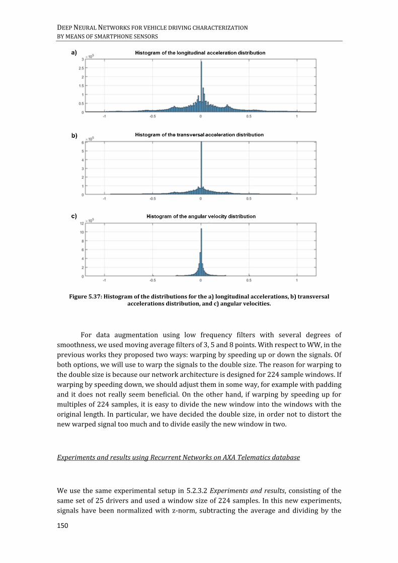
DEEP NEURAL NETWORKS FOR VEHICLE DRIVING CHARACTERIZATION BY MEANS OF SMARTPHONE SENSORS
150
Figure 5.37: Histogram of the distributions for the a) longitudinal accelerations, b) transversal accelerations distribution, and c) angular velocities.
For data augmentation using low frequency filters with several degrees of
smoothness, we used moving average filters of 3, 5 and 8 points. With respect to WW, in the
previous works they proposed two ways: warping by speeding up or down the signals. Of
both options, we will use to warp the signals to the double size. The reason for warping to
the double size is because our network architecture is designed for 224 sample windows. If
warping by speeding down, we should adjust them in some way, for example with padding
and it does not really seem beneficial. On the other hand, if warping by speeding up for
multiples of 224 samples, it is easy to divide the new window into the windows with the
original length. In particular, we have decided the double size, in order not to distort the
new warped signal too much and to divide easily the new window in two.
Experiments and results using Recurrent Networks on AXA Telematics database
We use the same experimental setup in 5.2.3.2 Experiments and results, consisting of the
same set of 25 drivers and used a window size of 224 samples. In this new experiments,
signals have been normalized with z-norm, subtracting the average and dividing by the

CHAPTER 5. DRIVER RECOGNITION
151
standard deviation (both obtained at journey level for the whole train dataset and applying
then these same training values to the test). Previously, with the ResNet-50 pre-trained
model that used images as input, we obtained worse results when we normalized, so we did
not apply it.
For the Recurrent Network model, initial tests using a two-layer LSTM with 64 cells,
followed by a Dense layer and an output Softmax layer showed overfitting with notable
differences in accuracy between training and testing. This could be because the model was
too complex for that dataset. Consequently, we found it necessary to increase the training
set and/or to reduce the model complexity (for example, using less layers or less neurons
per layer). Since regularization techniques (i.e. dropout) was already applied in the initial
tests we implemented the simplified model of Figure 5.33: a single Recurrent Network
directly followed by an output softmax layer. In addition, as a simple way of data
augmentation, we decided to reduce the window hop-size from 25% to 10%.
Results for different tests are shown in the Table 5.12. As shown in the table, using
a GRU layer with 64 neurons, the accuracy at window level was 43.51%, and at journey level
top-1 and top-5 of 57.71% and 82.63% respectively. Substituting the GRU layer by an LSTM
the accuracy values increased to 54.18% at window level and 67.31% and 85.71% top-1
and top-5 at journey level, respectively. We then increased the number of LSTM cells to 128,
and we reached accuracies of 61.54%, 73.25% and 87.31% for window level, and journey
level top-1, top-2, respectively. So far, globally with we have increased top-1 accuracy at
journey level from 66.97% (for the ResNet50+GRU network, with a window shift of 25%)
to 73.25% (for a LSTM layer with 128 neurons and hop-size of 10%).
Table 5.12: RNN model results for driver identification on AXA Driver Telematics, for 25 drivers.
No. drivers
Network Data
augmentation
Accuracy
At window
level (%)
At journey level top-1
(%)
At window level top-5
(%)
25 1 layer
GRU, 64 neurons
No 43.51% 57.71% 82.63%
25 1 layer
LSTM, 64 neurons
No 54.18% 67.31% 85.71%
25 1 layer
GRU, 128 neurons
No 58.38% 71.31% 86.40%
25
1 layer LSTM 128
neurons
No 61.54% 73.25% 87.31%
Results when using data augmentation techniques are shown in Table 5.13. The first
technique implemented has been to add Gaussian noise to the training set. In particular, we
added Gaussian noise of zero mean in the complete journey and then we divided the
journeys into windows. Firstly, we decided to do several tests using Gaussian noise with
zero mean and varying the standard deviation (0.001, 0.01, 0.02, 0.1, 0.2, 0.5), in order to
obtain an optimal value, that was found to be 0.01.

DEEP NEURAL NETWORKS FOR VEHICLE DRIVING CHARACTERIZATION BY MEANS OF SMARTPHONE SENSORS
152
Results for Gaussian noise without truncating were of 63.49%, 75.20% and 87.20%
for window level, journey level top-1 and top-5, respectively (which improves the values
regarding not using data augmentation techniques). We also implemented truncated
Gaussian noise, with zero mean and standard deviation 0.01, but truncated between [-0.02,
0.02]. Results are below those obtained previously (see (Table 5.13.)).
For testing data augmentation using low frequency filters (smoothing), as
mentioned before, we applied filters of 3, 5 and 8 points; creating 3 new sets and thus
multiplying the training set x4. However, results using this technique does not seem to
improve the results too much (window level accuracy of 62.01%, and top-1 and top-5
journey level accuracies of 72.46% and 87.54% respectively). (Table 5.13.)
The last data augmentation technique we tested was WW, expanding the signal to a
double size (i.e. from a window of 224 samples to a window 448 of samples) and then we
divided it into two 224 samples windows. Results using this technique worsened with
respect to not using it (accuracy at window level and accuracies at journey level top-1 and
top-5 of 47.59%, 63.08% and 83.54%, respectively, see Table 5.13).
Finally, we decided to use all the data generated for the individual augmentation
techniques. Two approaches were tested. The first one gathers all the data generated using
all the augmentation technique, so the training set was multiplied x11. The second one
eliminates WW data augmentation (since according to our previous results seems not to be
appropriate), so the training set is multiplied x9. Although both approaches increases the
accuracy, the best results are obtained for the second one has obtained with window level
accuracy of 65.13%, and journey level top-1 of 75.54% and top-5 of 87.09% (see Table
5.13). By analyzing the whole set of results in the table, it seems that the method that
contributes most to the improvement is the addition of Gaussian noise, although it
individually achieves lower accuracy than when using x9 combination, results are very
close.
Table 5.13: Results for driver identification, database of AXA Driver Telematics, for 25 drivers, applying data augmentation techniques.
No. drivers
Network Data
augmentation
Data augmentation
type
Accuracy At
window level (%)
At journey level top-1
(%)
At window level top-5
(%)
25 1 layer
LSTM, 128 neurons
Yes (x6) Gaussian noise:
𝜇 = 0, 𝜎 = 0.01.
63.49% 75.20% 87.20%
25 1 layer
LSTM, 128 neurons
Yes (x6)
Truncated Gaussian noise:
𝜇 = 0, 𝜎 = 0.01,
𝑡𝑟𝑢𝑛𝑐𝑎𝑡𝑒𝑑: [−2𝜎, 2𝜎].
59.88% 71.88% 87.08%
25 1 layer
LSTM, 128 neurons
Yes (x4)
Smoothing (filters of moving
average of 3, 5 y 8 points).
62.01% 72.46% 87.54%

CHAPTER 5. DRIVER RECOGNITION
153
25 1 layer
LSTM, 128 neurons
Yes (x3) Window warping
(double size). 47.59% 63.08% 83.54%
25 1 layer
LSTM, 128 neurons
Yes (x11)
Truncated Gaussian noise:
𝜇 = 0, 𝜎 = 0.01,
𝑡𝑟𝑢𝑛𝑐𝑎𝑡𝑒𝑑: [−2𝜎, 2𝜎]. Smoothing (filters of moving
average of 3, 5 y 8 points).
Window warping
(double size).
64.70% 74.74% 87.43%
25 1 layer
LSTM, 128 neurons
Yes (x9)
Gaussian noise: 𝜇 = 0,
𝜎 = 0.01. Smoothing (filters of moving
average of 3, 5 y 8 points).
65.13% 75.54% 87.09%
As a summary of the main conclusions that can be drawn from this experiments, we
can discuss the following ones. Different network configurations were tested, varying the
type of cell between LSTM and GRU, as well as the number of neurons by layer and the
number of layers. We tested several regulation techniques such as batch normalization and
dropout. In our experiments we found that the use of dropout was very important. Without
dropout the accuracy results were down more than 10% in most configurations. This did
not happen for the ResNet50+GRU model (in the same database, AXA Driver Telematics),
tested in Section 5.2.3.2, where better results were obtained without the use of dropout
(although with a difference around 1~2%), maybe because the network does not reach the
overfitting during the training. Another significant change in our experiments using a RNN
model on AXA database with respect to the results obtained with the pre-trained ResNet-
50+GRU model on database of TIDrivies_IdenVer, is that we modified the optimizer. We
changed the Adam optimizer for the RMSProp optimizer, because with Adam we found
many instabilities during training. For the LSTM layer model, we observed a trend to
overfitting if we did not apply regularization. Using Batch Normalization and dropout
together improved the results with respect to using each one individually. Although, if we
increased the dropout values too much, the accuracy worsened.
As we did in the previous tests, we have calculated again the confidence intervals on
the performance for this model (Table 5.14), replacing the previous architecture with a
simpler model and incorporating the data augmentation techniques of Gaussian noise and
smoothing. The accuracy is to 72.69% to 78.39%. Comparing with the results obtained for
the same AXA database and the ResNet50+GRU model, the LSTM architecture seems to be a
better option. Nevertheless, the tests done with database of TIDrivies_IdenVer offer the
smallest confidence interval of 1.39%, so the most precise estimate.
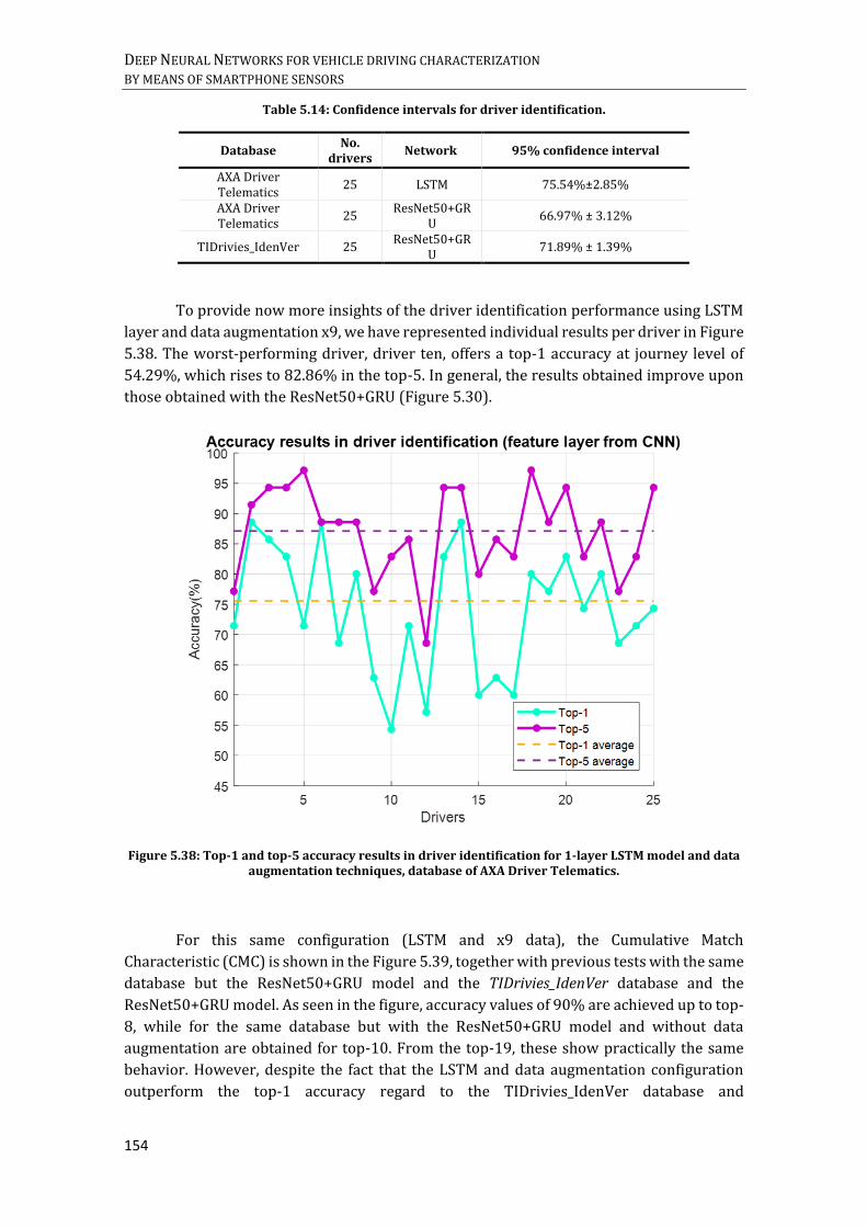
DEEP NEURAL NETWORKS FOR VEHICLE DRIVING CHARACTERIZATION BY MEANS OF SMARTPHONE SENSORS
154
Table 5.14: Confidence intervals for driver identification.
Database No.
drivers Network 95% confidence interval
AXA Driver Telematics
25 LSTM 75.54%±2.85%
AXA Driver Telematics
25 ResNet50+GR
U 66.97% ± 3.12%
TIDrivies_IdenVer 25 ResNet50+GR
U 71.89% ± 1.39%
To provide now more insights of the driver identification performance using LSTM
layer and data augmentation x9, we have represented individual results per driver in Figure
5.38. The worst-performing driver, driver ten, offers a top-1 accuracy at journey level of
54.29%, which rises to 82.86% in the top-5. In general, the results obtained improve upon
those obtained with the ResNet50+GRU (Figure 5.30).
Figure 5.38: Top-1 and top-5 accuracy results in driver identification for 1-layer LSTM model and data augmentation techniques, database of AXA Driver Telematics.
For this same configuration (LSTM and x9 data), the Cumulative Match
Characteristic (CMC) is shown in the Figure 5.39, together with previous tests with the same
database but the ResNet50+GRU model and the TIDrivies_IdenVer database and the
ResNet50+GRU model. As seen in the figure, accuracy values of 90% are achieved up to top-
8, while for the same database but with the ResNet50+GRU model and without data
augmentation are obtained for top-10. From the top-19, these show practically the same
behavior. However, despite the fact that the LSTM and data augmentation configuration
outperform the top-1 accuracy regard to the TIDrivies_IdenVer database and
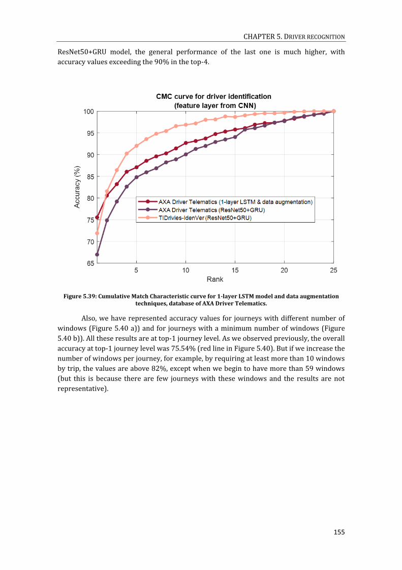
CHAPTER 5. DRIVER RECOGNITION
155
ResNet50+GRU model, the general performance of the last one is much higher, with
accuracy values exceeding the 90% in the top-4.
Figure 5.39: Cumulative Match Characteristic curve for 1-layer LSTM model and data augmentation techniques, database of AXA Driver Telematics.
Also, we have represented accuracy values for journeys with different number of
windows (Figure 5.40 a)) and for journeys with a minimum number of windows (Figure
5.40 b)). All these results are at top-1 journey level. As we observed previously, the overall
accuracy at top-1 journey level was 75.54% (red line in Figure 5.40). But if we increase the
number of windows per journey, for example, by requiring at least more than 10 windows
by trip, the values are above 82%, except when we begin to have more than 59 windows
(but this is because there are few journeys with these windows and the results are not
representative).

DEEP NEURAL NETWORKS FOR VEHICLE DRIVING CHARACTERIZATION BY MEANS OF SMARTPHONE SENSORS
156
Figure 5.40: Accuracies at window level, for 1-layer LSTM model and data augmentation techniques, database of AXA Driver Telematics, based on: a) journeys with a given number of windows, b) journeys
with a minimum number of windows.

CHAPTER 5. DRIVER RECOGNITION
157
5.2.3.5. Comparison with the state of the art
In order to compare our results with the work of (Dong, et al., 2016), we have expanded the
number of drivers to 50, without data augmentation and with the network of the Figure
5.33, formed by a LSTM layer with 256 neurons. We have not performed the tests with data
augmentation and 1000 drivers due to the high computational cost of the training. Although
we both use Deep Learning models, the main difference between their research and ours is
that we use accelerations derived from sequences of 2D {𝑥, 𝑦} positions as input signals, and
they work with statistical features extracted directly from the {𝑥, 𝑦} sequences. As we
already mentioned at the beginning of the Section 5.2.3, although we have used the same
database, the comparison is not straight, because we do not know exactly what subset of 50
drivers they have been employed.
The results for 50 drivers, increasing the number of neurons of the LSTM layer to
256, have been accuracy at window level of 60.06%, and top-1 and top-5 journey level of
71.60% and 83.54%, respectively (see Table 5.15). The best results in (Dong, et al., 2016)
were with a Neural network of 2 stacked layer and 100 neurons in each layer, obtaining
34.8%, 52.30% and 77.4% of accuracy at window level, top-1 and top-5 journey level,
respectively (Figure 5.9). So, we can conclude that our results outperform this state-of-the-
art research in the three metrics evaluated.
Table 5.15: Driver identification results for 50 drivers of the of AXA Driver Telematics
database.
Research Network No. drivers
Accuracy
At window
level (%)
At journey level top-1
(%)
At window level top-5
(%)
Our proposal
1 layer LSTM, 256 neurons 50 60.06% 71.60% 83.54%
(Dong, et al., 2016)
CNN without pooling layers 50 16.9 28.3 56.7
(Dong, et al., 2016)
CNN 50 21.6 34.9 63.7
(Dong, et al., 2016)
RNN of one layer pre-trained
50 28.2 44.6 70.4
(Dong, et al., 2016)
RNN of one layer 50 34.7 49.7 76.9
(Dong, et al., 2016)
RNN of two staked layers 50 34.8 52.3 77.4
(Dong, et al., 2016)
GBDT 50 18.3 29.1 55.9
(Dong, et al., 2016)
GBDT on a set of 57 manually defined driving behavior
features 50 - 51.2 74.3

DEEP NEURAL NETWORKS FOR VEHICLE DRIVING CHARACTERIZATION BY MEANS OF SMARTPHONE SENSORS
158
5.3. Driver verification
Driver verification is another area of driver biometrics that consists of checking if a driver
is really who she/he claims to be. Driver verification is important in anti-theft issues,
especially with the new technologies that are being implemented in cars. With the new
systems of Keyless Access, it is no longer necessary to insert the key to open the vehicles.
Simply with carrying the key, the system detects when the driver is between one and a half
meters distance from the vehicle, unlocking the car when opening the door or the trunk. As
well, cars include more computers on board, even there are vehicles connected to the
Internet. The drawback of these new systems is that cars are exposed to new vulnerabilities
that must be detected and resolved. Driver verification systems are not only important in
anti-theft tasks; they are also widely used in security, for the authentication of drivers and
authorized vehicles in restricted or private areas.
In order to face driver verification, we have implemented three different strategies
that were tested on the same database used in driver identification (Section 5.2 Driver
identification), TIDrivies_IdenVer database. Relying on our driver identification results that
suggest that maneuver regions (i.e. windows) have more discriminative power, we decided
to perform driver verification only on maneuver windows.
The first strategy was to explore the use of the so-called Siamese Neural networks.
The idea summarized behind these networks is to use two inputs, one with the real driver
and the other one with the person that we need to verify. Then, the network will output if
these inputs belong to the same person or not. The Siamese Networks were presented by
(Bromley, Guyon, LeCun, Sickinger, & Shah, 1993). These networks receive two inputs in
order to compare their patterns, and produce an output whose state value corresponds to
the similarity between these two patterns. That is to say, the two outputs of the twin
networks are considered as latent feature vectors that can be used as input to a similarity
function. This similarity function can be a simple cosine distance measure or a NN, for
example a Dense layer with a sigmoid unit, that generates an output score between [0, 1].
This technique is widely used for example in signature verification (Dey, et al., 2017), or in
speaker verification (Salehghaffari, 2018).
The second strategy has been the use of embeddings. Embeddings are, in our case,
representations of the driver at journey level rather than at window level, which are
obtained from a deep neural network. We train that deep neural network for the
identification task, and then embeddings obtained from it are used in verification.
Embeddings have been employed in speaker recognition, where they are described as a
fixed-length vector representing a speaker obtained from variable-length utterances, see
for example (Lozano-Diez, Plchot, Matejka, & Gonzalez-Rodriguez, 2018).
The third strategy we explored for driver verification was Triplet Loss training.
Here, during training, instead of having two inputs we will have three, since for each driver
example the network must learn to verify a positive example (from the same driver) and a
negative example (from another driver). These models are based on a different way of
calculating the losses, minimizing the distance between a base or anchor example and

CHAPTER 5. DRIVER RECOGNITION
159
another positive example of the same class, and maximizing the distance between the same
anchor and another negative example of different class. There are also numerous works, as
(Sankaranarayanan, Alavi, Castillo, & Chellappa, 2016) that use this kind of losses for face
verification, or (Bredin, 2017), where Triplet Loss training is used in speaker recognition.
5.3.1. Siamese Neural Networks
Different Deep Learning techniques have been used for the driver identification and
verification. Most Machine or Deep Learning algorithms require large amounts of training
data to obtain high accuracy results. For cases in which a large database is not available,
One-Shot Learning, presented in (Fei-Fei, Fergus, & Perona, 2006), was proposed based on
the idea of training new categories with few examples. Works as (Lake, Lee, Glass, &
Tenenbaum, 2014) or (Koch, Zemel, & Salakhutdinov, 2015) have suggested One-Shot
Learning for speech recognition and image classification. So, one-shot learning classification
is done under the condition that only a single example of each class can be observed before
making a prediction. In this type of networks the input is not directly classified, but by
means of a similarity function it is decided whether the two inputs are similar or not. For
this type of training, Siamese Networks are used, where we decide if a pair of inputs belongs
to the same class or not.
The term Siamese comes from twins, since the same network is used for each of the
two inputs, they share parameters with two copies of the same network. At the output of
the chosen network, we will obtain the features vectors that will be used as input to the
similarity function. If the inputs correspond to the same driver, it is expected that the
vectors will be similar, while if they correspond to different drivers they will be more
different. Usually, the function used to compare the vectors is a Dense layer with a sigmoid
unit that generates an output score between [0, 1].
We have evaluated Siamese networks for driver verification on a close-set of 25
drivers in TIDrivies_IdenVer database (the same dataset used in our driver identification
studies, Section 5.2 Driver identification). The Siamese architecture is shown in the Figure
5.41. The weights for the ResNet50+GRU models were initialized from driver identification
and then fine-tuned for driver verification.

DEEP NEURAL NETWORKS FOR VEHICLE DRIVING CHARACTERIZATION BY MEANS OF SMARTPHONE SENSORS
160
Figure 5.41: Siamese Neural network for driver verification.
The purpose of Siamese networks is to identify if the pair of examples belong to the
same class or not. So we train a Deep Network to verify if the twins introduced are of the
same driver or not. Therefore, each input will go through the same Deep Neural Network
(shared weights) in order to extract some features. After extracting these features, a
similarity is calculated through the absolute difference between said outputs, the L1
distance between the twin embeddings. In our case, we will not use sigmoid activation. As
our inputs are maneuver windows of a trip, we prefer the softmax activation. This will allow
to obtain the probabilities for each window, and then to perform a consistency analysis
along the journey, which will increase the success rate.
In order to evaluate the results, we have used different metrics: precision, recall and
F1 score. We have calculated them both for each driver and globally. The global results are
shown in the Table 5.16. Almost 80% of the predicted positive are actual positive
(precision). Regarding the rate of predicted positive with respect to the total of actual
positive (recall or true positive, TP) it represents 69.12%. If we observe the F1 score, which
is the weighted harmonic mean of precision and recall, it is of 74.09%.
Table 5.16: Results in driver verification for Siamese Neural Network.
Architecture Drivers Precision
(%) Recall
(%) F1 score
(%)
Siamese Neural Network All 79.83 69.12 74.09
Individual results for each driver is shown in Figure 5.42. It can be observed that
there are some drivers that present high verification results, as, for example, drive 3 with
100% precision, 72.73% recall and 84.21% F1-score. While other drivers seem to be more
difficult to verify, as it is the case of driver 17 (50% precision, 54.55% recall and 52.17%
F1-score).

CHAPTER 5. DRIVER RECOGNITION
161
Figure 5.42: Precision, Recall and F1 score per driver, for driver verification using Siamese Neural network architecture.
Typically, verification performance is evaluated with the Detection Error Tradeoff (DET)
and Receiver Operating Characteristics (ROC) curves. The curves for the case of the Siamese
network are shown in the Figure 5.43. From them, we can obtain an EER and AUC of 28.91%
and 78.67%, respectively.
Figure 5.43: Result curves for driver verification with Siamese Neural Network: DET plot (purple) and ROC plot (magenta), TIDrivies_IdenVer database.

DEEP NEURAL NETWORKS FOR VEHICLE DRIVING CHARACTERIZATION BY MEANS OF SMARTPHONE SENSORS
162
We have also carried out an analysis of the maneuvers that are most useful in
providing a correct verification. The results are shown in the Figure 5.44. These have been
obtained using all the test windows, before making the calculation at the journey level, that
is, for each of the individual windows. Analyzing the longitudinal and transversal
acceleration forces present in a window, we have classified every window in 6 classes (only
braking, only acceleration, braking&turn, acceleration&turn, only turn and a mixture of all
of them). Figure 5.44 shows accuracy results for different maneuvers in terms of True
Negatives (TN: correct detection of non-authorized drivers), True Positives (TP: correct
detection of non-authorized drivers) and Balanced Accuracy ((TP + TN) /2). According to
these results better accuracy is observed when using richer maneuvers (i.e. braking & turn,
acceleration & turn or a combination of them). Maneuvers that combine information in the
movement direction (acceleration or deceleration) with turns seem to be especially
discriminative considering the verification or authentication of the driver.
Figure 5.44: Accuracies obtained for classification of individual windows depending on the type of maneuver, with Siamese Neural Network architecture.
5.3.2. Embeddings
The typical network architecture used to obtain embeddings is presented below, Figure
5.45. The first part of the architecture before the pooling layer works at frame level, and it
is composed by several hidden layers that will receive the input on a frame-by-frame basis.
Then the pooling layer process the sequence of outputs from the previous layer and
provides an fixed-length vector representing a possible variable-length input sequence in a
latent embedding space. Pooling layer usually perform mean or standard deviation
estimations over time. Finally, after the pooling layer, some dense layers followed by a
softmax layer are used to obtain the final posterior classification probabilities.

CHAPTER 5. DRIVER RECOGNITION
163
Figure 5.45: Typical architecture for a DNN used for obtaining embeddings.
DNN embeddings have been proposed for speaker verification (Snyder, et al., 2016).
In this work a feed-forward DNN with four hidden layers, followed by a temporal pooling
layer is used. The input to the network is a sequence of stacked MFCCs, which are mapped
into a speaker embedding vector. The pooling layer aggregates the outputs of the previous
layer over time and computes the average and the standard deviation. Finally, a last hidden
layer followed by a linear output is used to produce the embedding. Through the PLDA, they
calculate the distance between two embeddings.
In this work (Snyder, Garcia-Romero, Povey, & Khudanpur, 2017) a slightly different
architecture to obtain the embeddings is presented. As before, the architecture consists of
some hidden layers before the pooling layer, but in this case two layers are used to obtain
the embeddings before a final softmax output layer. According to the reported results
significant improvements were obtained by using these two layers to obtain the
embeddings, especially for short-utterances.
Another work, which implements embeddings is (Li, et al., 2017). The embedding
system they use is composed by a neural network (they test two types, CNNs and RNNs)
working at frame-level part, followed by a pooling layer, an affine layer and a length
normalization layer. One of the peculiarities of this system is that for training they use triplet
loss. In addition, the pooling layer only performs time averaging, instead of average and
standard deviation as in other works. The affine layer is a dense layer without activation.
Based on these last two works, we have decided to address the following studies.
The network used to extract the embeddings was trained for driver identification. For the
extraction of embeddings, we have first grouped 15 maneuvers windows of 224 samples
creating a matrix of [15x224x3] for three channels: longitudinal and transversal
accelerations and angular velocity. Different combinations of convolutional and recurrent
networks before the pooling layer were tested: for example CNN of two layers + dense, CNN
of three layers + dense, CNN of two layers + GRU of 2 stacked layers + dense, CNN of two
layers + LSTM of 2 stacked layers + dense, LSTM of 2 stacked layers + dense, CNN of three
layers + LSTMs of 2 stacked layers + dense, among others. Pooling layers as well as the final
dense and softmax layers have been the same for all the combinations we tested. The
pooling layer calculates the mean and the standard deviation of the previous output and
concatenates them (for each journey). Finally, there are two dense layers (where do we get
the embeddings), plus a final softmax layer. One example of the network we used is shown
in the Figure 5.46. As mentioned before, these networks are simply used for the extraction

DEEP NEURAL NETWORKS FOR VEHICLE DRIVING CHARACTERIZATION BY MEANS OF SMARTPHONE SENSORS
164
of embeddings. Once embeddings are obtained, first we perform LDA to reduce their
dimensionality and then we trained a Gaussian PLDA model, to score the model with the
test data. We evaluate different number of parameters (from 32 to 128) for the frame-level
layers between. For the embeddings, we decided a final size of the dense layers of 64.
Figure 5.46: Example of one of the architecture used to extract the embeddings for the driver verification.
The problem is that the results obtained are very bad. Probably because the network
used to extract the embeddings, whose task is identification, already yields very low
accuracies (see Table 5.17). For example when before the pooling layer we apply a LSTM
network of two stacked layers, the results at journey level top-1 barely reach the 6% and at
journey level top-5 the 25%. If this network is not able to obtain good representations of
the trips at journey level, the representations will not be valid for the verification either. It
seems that this technique, from which we get an embedding from a complete journey, is not
adequate, does not seem discriminatory. Better results are obtained when training at
window level.
Table 5.17: Driver identification accuracy results with inputs at journey level, to obtain embeddings for driver verification task, database TIDrivies_IdenVer.
Architecture Accuracy journey level
Top-1 Top-5
3 CNN 3.80% 24.15%
2 CNN + 2 GRU 4.08% 24.80%
2 CNN + 2 LSTM 5.58% 24.77%
2 LSTM 4.35% 19.85%
3 CNN + 2 LSTM 4.28% 22.50%
5.3.3. Triplet loss
Triplet Loss architecture is another powerful way to learn latent representations or
embeddings based on the notion of similarity and dissimilarity. This was introduced by
(Weinberger & Saul, 2006). In their work they emphasize that the accuracy obtained in a
classification task can vary heavily depending on the metric used to calculate distances
between examples. They use the k-nearest neighbor (kNN) classification and train a metric
in order to neighbors belong to the same class are closer, while neighbors belong to different
classes are more separated. In the work presented in (Schroff, Kalenichenko, & Philbin,
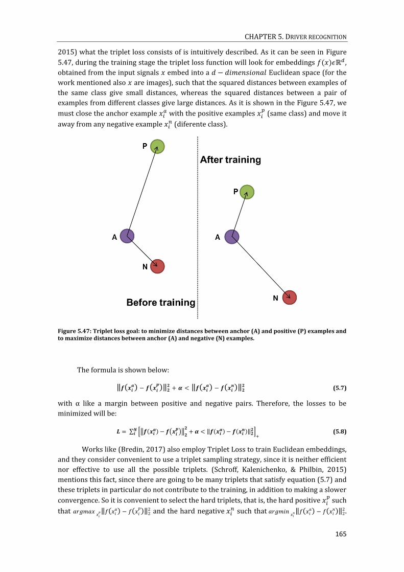
CHAPTER 5. DRIVER RECOGNITION
165
2015) what the triplet loss consists of is intuitively described. As it can be seen in Figure
5.47, during the training stage the triplet loss function will look for embeddings 𝑓(𝑥)𝜖ℝ𝑑 ,
obtained from the input signals 𝑥 embed into a 𝑑 − 𝑑𝑖𝑚𝑒𝑛𝑠𝑖𝑜𝑛𝑎𝑙 Euclidean space (for the
work mentioned also 𝑥 are images), such that the squared distances between examples of
the same class give small distances, whereas the squared distances between a pair of
examples from different classes give large distances. As it is shown in the Figure 5.47, we
must close the anchor example 𝑥𝑖𝑎 with the positive examples 𝑥𝑖
𝑝 (same class) and move it
away from any negative example 𝑥𝑖𝑛 (diferente class).
Figure 5.47: Triplet loss goal: to minimize distances between anchor (A) and positive (P) examples and to maximize distances between anchor (A) and negative (N) examples.
The formula is shown below:
‖𝒇(𝒙𝒊𝒂) − 𝒇(𝒙𝒊
𝒑)‖𝟐𝟐 + 𝜶 < ‖𝒇(𝒙𝒊
𝒂) − 𝒇(𝒙𝒊𝒏)‖𝟐
𝟐 (5.7)
with α like a margin between positive and negative pairs. Therefore, the losses to be
minimized will be:
𝑳 = ∑ [‖𝒇(𝒙𝒊𝒂) − 𝒇(𝒙𝒊
𝒑)‖
𝟐
𝟐+ 𝜶 < ‖𝒇(𝒙𝒊
𝒂) − 𝒇(𝒙𝒊𝒏)‖𝟐
𝟐]+
𝑵𝒊 (5.8)
Works like (Bredin, 2017) also employ Triplet Loss to train Euclidean embeddings,
and they consider convenient to use a triplet sampling strategy, since it is neither efficient
nor effective to use all the possible triplets. (Schroff, Kalenichenko, & Philbin, 2015)
mentions this fact, since there are going to be many triplets that satisfy equation (5.7) and
these triplets in particular do not contribute to the training, in addition to making a slower
convergence. So it is convenient to select the hard triplets, that is, the hard positive 𝑥𝑖𝑝
such
that 𝑎𝑟𝑔𝑚𝑎𝑥 𝑥𝑖
𝑝‖𝑓(𝑥𝑖𝑎) − 𝑓(𝑥𝑖
𝑝)‖22 and the hard negative 𝑥𝑖
𝑛 such that 𝑎𝑟𝑔𝑚𝑖𝑛 𝑥𝑖
𝑛‖𝑓(𝑥𝑖𝑎) − 𝑓(𝑥𝑖
𝑛)‖22.

DEEP NEURAL NETWORKS FOR VEHICLE DRIVING CHARACTERIZATION BY MEANS OF SMARTPHONE SENSORS
166
In our case, for the search of the hardest positive and negative we have used the generation
of triplet online, where we select them within a batch. If the batch has N examples, we
generate N embeddings. To obtain the triplets of the embeddings, we select within the valid
triplets (there are two examples with the same label but different, and an example with
different label to the previous one), the hardest positive and the hardest negative for each
anchor (calculating the distances between embeddings). As margin 𝛼, we selected a value
of 0.2, as it is a value widely used in other identification works (Hermans, Beyer, & Leibe,
2017).
To apply triplet loss training in driver verification, we must obtain some
embeddings from the input accelerometer signals (as it is shown in the Figure 5.48), and
then calculate the losses. The embeddings must collect the information of the trip at journey
level, so the input will not be the overlapping window of the maneuver, but a matrix with
all the maneuvers windows of the journey. That is, instead of using a window of 224 samples
for each of the three channels, matrices of 15x224 samples will be used for each of the three
channels (as before, there will be 15 windows per journey). As the previously trained
identification network uses individual windows as inputs, fine-tuning cannot be done in this
case. Therefore, it has been necessary to train a specific network in identification (we will
utilize the same as the one used previously, Figure 5.6), where the inputs are matrices of
journeys of 15x224. And, like in the Siamese networks, in order to carry out the verification,
we calculate the Euclidean distance with the embeddings to decide which pairs of examples
correspond to the same driver or not.
Figure 5.48: Triplet Loss training for driver verification.
For triplet loss trainings, the values of the metrics of precision, recall and F1 score
have also been obtained (see Table 5.18). However, the results do not reach the levels
obtained with the Siamese networks. Below, we show the overall values.
Table 5.18: Results in driver verification triplet loss training, TIDrives_IdenVer database.
Drivers Precision
(%) Recall
(%) F1 score
(%)
All 47.50 51.63 49.48
It seems that the network is not discriminant enough, in order to do the verification
task with this training model. The precision obtained is 47.50%; that is to say, about half of
the time incorrectly verify drivers. Regarding the recall, it is 51.63% (the rate of predicted
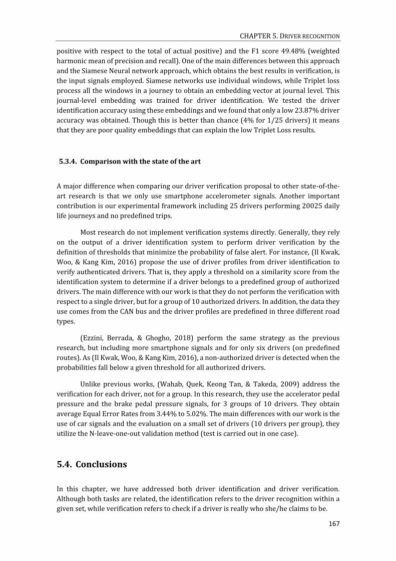
CHAPTER 5. DRIVER RECOGNITION
167
positive with respect to the total of actual positive) and the F1 score 49.48% (weighted
harmonic mean of precision and recall). One of the main differences between this approach
and the Siamese Neural network approach, which obtains the best results in verification, is
the input signals employed. Siamese networks use individual windows, while Triplet loss
process all the windows in a journey to obtain an embedding vector at journal level. This
journal-level embedding was trained for driver identification. We tested the driver
identification accuracy using these embeddings and we found that only a low 23.87% driver
accuracy was obtained. Though this is better than chance (4% for 1/25 drivers) it means
that they are poor quality embeddings that can explain the low Triplet Loss results.
5.3.4. Comparison with the state of the art
A major difference when comparing our driver verification proposal to other state-of-the-
art research is that we only use smartphone accelerometer signals. Another important
contribution is our experimental framework including 25 drivers performing 20025 daily
life journeys and no predefined trips.
Most research do not implement verification systems directly. Generally, they rely
on the output of a driver identification system to perform driver verification by the
definition of thresholds that minimize the probability of false alert. For instance, (Il Kwak,
Woo, & Kang Kim, 2016) propose the use of driver profiles from driver identification to
verify authenticated drivers. That is, they apply a threshold on a similarity score from the
identification system to determine if a driver belongs to a predefined group of authorized
drivers. The main difference with our work is that they do not perform the verification with
respect to a single driver, but for a group of 10 authorized drivers. In addition, the data they
use comes from the CAN bus and the driver profiles are predefined in three different road
types.
(Ezzini, Berrada, & Ghogho, 2018) perform the same strategy as the previous
research, but including more smartphone signals and for only six drivers (on predefined
routes). As (Il Kwak, Woo, & Kang Kim, 2016), a non-authorized driver is detected when the
probabilities fall below a given threshold for all authorized drivers.
Unlike previous works, (Wahab, Quek, Keong Tan, & Takeda, 2009) address the
verification for each driver, not for a group. In this research, they use the accelerator pedal
pressure and the brake pedal pressure signals, for 3 groups of 10 drivers. They obtain
average Equal Error Rates from 3.44% to 5.02%. The main differences with our work is the
use of car signals and the evaluation on a small set of drivers (10 drivers per group), they
utilize the N-leave-one-out validation method (test is carried out in one case).
5.4. Conclusions
In this chapter, we have addressed both driver identification and driver verification.
Although both tasks are related, the identification refers to the driver recognition within a
given set, while verification refers to check if a driver is really who she/he claims to be.
DEEP NEURAL NETWORKS FOR VEHICLE DRIVING CHARACTERIZATION BY MEANS OF SMARTPHONE SENSORS
168
We have presented a state of the art in this area, where we have seen that most of
existing research is focused in driver identification, using bus CAN signals of the vehicle and
a wide number of sensors. Among the most used sensors are the GPS or signals from pedals
such as the accelerator, brake or steering wheel.
For driver identification we have studied two scenarios, always using signals
corresponding to vehicle accelerations. The first scenario uses as inputs the accelerometer
signals of the driver smartphone. The smartphone can be located in any position inside the
vehicle. In this database, TIDrivies_IdenVer, we have studied driver identification on a set of
25 drivers with 801 journeys by driver using Deep Learning techniques. We have explored
Transfer Learning techniques, which use a model to recognize some features in one domain
and transfer their knowledge to another model in another domain. As we have transformed
the temporal 1-D input acceleration signals into 2-D images, we have specifically used the
pre-trained ResNet-50 model, trained on a large dataset (ImageNet) for image classification.
We have tested different procedures for mapping temporal 1-D input signals into 2-D
matrices: the Recurrence Plots (RP), the Gramian Angular Summation Field (GASF), the
Gramian Angular Difference Field (GADF), the Markov Transition Field (MTF), the
spectrogram and the feature maps obtained from the layers of convolutional networks. The
best results have been obtained with the Deep Learning model that uses CNN feature maps
for 1D to 2D transformation and ResNet-50 + GRU networks. Several strategies have been
proposed to select the most discriminative parts of the journey for driver identification,
concluding that maneuver areas give the best results. Classification accuracy at top-1
journey level of 71.89% and top-5 of 92.03% was obtained for the set of 25 drivers using
only 15 sliding windows per journey.
A second scenario for driver identification employs accelerations derived from
sequences of {𝑥, 𝑦} positions of the vehicle trajectory, in a 2D map at 1Hz sampling rate. This
scenario has been selected in order to compare our results with state-of-the art, since this
data was used in a Kaggle competition organized by AXA, called “Driver Telematics Analysis”.
As the number of journeys for training is not very high, we used 80 journeys per driver, we
studied several data augmentation techniques. The results obtained with the ResNet-
50+GRU model, for the TIDrivies_IdenVer database, were a top-1 and top-5 accuracies at
journey level of 66.97% and 84.80%, respectively. For the AXA database, we found that
using less complex models and incorporating data augmentation techniques, we have
achieved accuracies at journey level top-1 and top-5 of 75.54% and 87.09%, respectively.
This increase in accuracy can be explained for the less noisy signals derived from sequences
of {𝑥, 𝑦} positions. AXA drivers seem also to make similar routes (as can be concluded from
the good results on trip matching in Kaggle competition), so perhaps simpler models can
get advantage of this route-related patterns that can be modelled by Recurrent Networks
and thus improving driver characterization results.
Finally in this chapter, we have implemented three different strategies to carry out
driver verification: the use of Siamese Neural networks, the use of embeddings and triplet
loss trainings. The strategy with best results has been the use of Siamese Neural networks,
with global with a precision of 79.83%, recall of 69.12%, and F1 score of 74.09%.
An analysis of the architectures that have offered the best results in both
identification and verification, for the database of TIDrivies_IdenVer, it seems to indicate that

CHAPTER 5. DRIVER RECOGNITION
169
they are not directly correlated. Since there are drivers, as driver number five, which shows
very low identification accuracy but relatively good verification result. On the other hand,
other drivers, such as driver twenty, has a high identification rate but a low verification
result. As some studies, (Decann & Ross, 2012), demonstrate it is possible that a biometric
system performing well at verification can fail at identification, and vice versa. It is the
specific statistical distribution for inter-driver and intra-driver scores for each driver what
can explain these different results in verification and identification tasks.


171
Chapter 6
Conclusions and Future Work
n Chapter 1, Introduction, we commented that the main motivation of the Thesis was
the driving characterization, both from the point of view of detection and classification
of maneuvers, and from the driver recognition, using the accelerometers present in the
drivers' smartphones. Accelerometers are motion sensors incorporated in all current
smartphones. The main advantage of use compared to other signals is that these are cost
and energy efficient sensors that allow to capture characteristics related to driver behavior.
As characterization tool we have used Deep Learning techniques, in order to learn high level
features and to detect complex interactions.
6.1. Conclusions
Driver behavior characterization is closely related to maneuver or event characterization,
that is, how drivers perform maneuvers. Most state-of-the-art works, in order to define a
driving style, first address the event detection and classification.
As a first step towards that goal, we have studied the identification of the
maneuvering events. Since the driver smartphone can place in a free position, it is necessary
to obtain the acceleration forces in the vehicle's reference system, because the orientation
directions may be different on the journeys. Moreover, we do not have other sensors such
as the gyroscope or the magnetometer, so the transformation from the smartphone
reference system to the vehicle reference system has been carried out exclusively with
accelerometers, making it impossible to apply the typical rotation matrices used in the
literature. To address this mapping, we have developed two different approaches,
depending on the degree of classification desired. The first one allows a general
categorization, which can be useful for creating driver profiles based on criteria such as the
aggressiveness (risky and safe drivers) or for car insurances. While the second one,
performs a more precise maneuver classification, useful for instance in route reconstruction
applications. The most remarkable contribution of these approaches is the manner of
detecting and classifying maneuvers, without applying the rotation matrices mentioned
above and without a required fixed position of the mobile terminal, providing alternative
solutions to the current developed works.
I

DEEP NEURAL NETWORKS FOR VEHICLE DRIVING CHARACTERIZATION BY MEANS OF SMARTPHONE SENSORS
172
The first of the approaches implements a general maneuver characterization. In
order to create an independent reference system, we have accepted the assumption that in
a 2D horizontal plane, based on the estimation of the gravity vector, both the longitudinal
and transversal forces of the vehicle must be found. For the second approach, the mapping
of the maneuvers is not carried out to a horizontal plane, but we estimate what we have
called vehicle movement direction (VMD). This novel form of obtaining the movement
direction allows establishing a reference vector that is constant along the journey, as long
as the smartphone position does not change (where it is necessary to recalculate it), and
which replaces traditional calibration processes.
The first previous step before classification must be the maneuver detection, that is,
to identify the segment in the journey where a maneuver is. For this, we have used the
measurements of the horizontal plane. Through measures of the energy or L1 norm through
the journeys, as well as post-processing algorithms that allow better delimitations, this
horizontal plane provides a worthy detection system. This proposed detection and
delimitation procedure replaces other traditional methods, which used templates for
matching to reference patterns or needed a greater number of sensors.
When working with time series, it is a recurrent problem to find the most
appropriate way of segmenting the signals, since it is difficult to define significant
representations that simplify calculations and analysis. In the first approach focused on a
general classification of the maneuvers, in acceleration/deceleration and turn/mixed
events, we have studied three segmentation strategies: fixed-length windows, variable
length windows and sliding windows. The main problem of using fixed-length windows is
the difficulty of finding an appropriate length, which covers most of the available events.
According to the analysis we have done, it seems that most of the maneuvers have durations
of less than 20 seconds. However, if we take this length as the window size used in the
Neural Network inputs, we excludes other events of greater length and in the case of minor
maneuvers we need to incorporate information from the surrounding. For the second
segmentation strategy, we have used windows of variable length, based on the use of
dynamic networks in Tensor Flow, which allow us to learn the information contained in the
actual duration of the maneuver and to ignore the rest, specifying the real length in the
training. Using a two-layer LSTM network, we have obtained the best results for all the
maneuver classification tests carried out, with an accuracy of 88.82%. As we have just said,
these results are also better than the results obtained in the last strategy, which employs
sliding windows along the journey. The main advantage of using sliding window, is that we
do not need a pre-processing of the maneuvering areas, since the network classifies the
information of the windows directly, however this produces lower results with very
unbalanced classes.
The second approach allows a more specific maneuver categorization in classes
such as accelerations and decelerations or left and right turns, among others. In this case,
for the mapping we have based on the VMD, which represents the movement directional
vector in the smartphone reference system associated to the longitudinal forward
movement of the vehicle. As we have already commented, this directional vector offers a
novel form of classifying maneuvers with respect to the previous works in the literature. In
order to obtain it, we have proposed three different methods based on: the stop detection,

CHAPTER 6. CONCLUSIONS AND FUTURE WORK
173
the acceleration forces classification and the longitudinal and transversal acceleration
assignment.
The stop detection method is based on the development of two different classifiers:
the first of them detects acceleration/deceleration maneuvers, while the second detects
stop situations. Using a post-processing algorithm, the information from both is combined
to obtain the VMD. The stop classifier obtain a final accuracy of 74.2%. This task is difficult
since the accelerometers is very similar when driving at constant speed than when we stop
the vehicle. Also, because of the nature of the maneuvers, it is difficult to classify an event
as purely an acceleration or a deceleration, so it is important to create a robust consistency
algorithm, introducing energy conditions, deviation angle, probability values of the
classifier or Principal Component Analysis (PCA). One of the problems that has appeared in
this method, and it is very common in classification problems using deep networks, is the
size of the database. The database used for stops (we need truth stops to compare) is much
lower than that used with the maneuvers, which cause lower values in training.
Furthermore, one of the drawbacks of this method is that it cannot be applied to any
journey, since stops need to be detected (and vehicles not always need to stop). For
example, on a journey in a motorway it would be difficult to make a stop unless the start or
end of the trip is captured. The second method of acceleration forces classification directly
categorizes the maneuvers into braking (deceleration), acceleration, pure turn, and mixed
event. We tested different preprocessing of the input signals, but the best was removing the
gravity force from the accelerometer components. Gravity greatly influences the network's
decision process and it is possible to observe how in the CNN+GRU network this variable
was not independent until almost the output of the recurrent network, as was the case of
the noise level. We also done tests with the estimation of the linear speed, however a good
estimation is complicated and did not improve the previous results. The results also showed
that it is difficult to categorize a maneuver in a pure class because the classes can easily
present patterns of other groups. In the final estimation method of the VMD, we tried to
associate the principal components (PC) calculated on the filtered accelerometers and
without gravity with the longitudinal and transversal accelerations, training a network that
associated each PC with the accelerations considering the correct sign. This is the method
that has offered the best results with an overall accuracy of 90.07%. The tests showed that
it was easier to correctly assign the longitudinal accelerations than the transversal ones, a
possible explanation for this is that the driving acceleration and deceleration patterns may
differ more from each other than right/left turning patterns. It is important to mention that
the post-processing algorithms, which facilitate the VMD estimation, have been obtained
after following a detailed analysis of the signals employed, in order to add the conditions
that favor the correction of errors in network decision making. A common step that we have
done during the developed procedures has been to obtain the most significant vectors
within a set of them. For this, we have used our own clustering algorithm, which is based on
two main concepts, the separation angle between the vectors and the number of vectors.
On the other hand, another great important area in the driving characterization is
the driver recognition, directly related to biometric systems that use behavioral
characteristics of a person to authenticate their identity. Driver recognition systems include
two main tasks, driver identification and verification, which we have addressed differently.
Among the biggest difficulties of the driver recognition are the multiple sources of
DEEP NEURAL NETWORKS FOR VEHICLE DRIVING CHARACTERIZATION BY MEANS OF SMARTPHONE SENSORS
174
variability that appear with the signals employed, the noise of the accelerometer signals
(compared to other more attenuated as in the case of GPS), the capturing devices, the route
variability or the vehicle type. For the identification and verification analysis using
accelerometers, we have employed smartphones with both Android and iOS operating
systems, in different positions (free placed inside the car), routes both urban, non-urban
and mixed, and different vehicles.
For driver identification, we have addressed two different scenarios. In the first
scenario, we have directly used only the accelerometers, as well as in the maneuver
characterization. In the second scenario, we have used the acceleration signals obtained
from GPS data.
For the first scenario employing the tri-axial acceleration signals collected during
the driving journeys, we have combined the use of pre-trained CNNs (ResNet-50) from
image classification and Recurrent Neural Networks (RNNs), specifically a Gated Recurrent
Unit (GRU) network. In order to use these pre-trained networks, we have had to study
different mapping techniques for 1-D temporal acceleration signals into 2-D images. Not
many works in literature study these transformations of time series, so in this Thesis we
have contributed in this field with the analysis of the results obtained after applying six
different transformations in the accelerometer signals related to driving. The encoding
techniques implemented have been: the Recurrence Plots (RP), the Gramian Angular
Summation Field (GASF), the Gramian Angular Difference Field (GADF), the Markov
Transition Field (MTF), the spectrograms and the use of CNN to obtain a feature map from
one of its layers. The temporal signals transformed into images have been the longitudinal
and transversal accelerations and the angular velocity. The transformation to images
greatly influences the model performance. The best results have been obtained using CNN
on accelerometer signals. In addition, selecting input maneuvers as signals, rather than any
type of journey information, provide always better driver identification accuracy values.
One interesting conclusion of our test is that The RP, GASF, GADF and MTF methods seem
more effective in representing periodic signals than our non-stationary accelerometer
signals. And for the spectrograms, the images obtained are not significantly enough to
adequately represent the information for the identification. Among the three input signals
transformed into images, the performances are also different. The longitudinal acceleration
achieves higher accuracies, followed by transversal acceleration. This may indicate that the
maneuvers related to accelerations and decelerations seems to be more discriminative.
Although the identification task is complex, we obtained a top-1 accuracy of 71.89%, the
top-2 increases almost 10% to 81.56%, and values above 90% are obtained from top-4.
In the second scenario we have used an open database of the literature, formed by
driving journeys represented in a 2D space by sequences of {x,y} values, obtained from GPS
data. In order to compare our previous results with this database, it has been necessary to
transform these sequences of {x,y} positions into acceleration signals, which introduces, in
addition to the errors in the GPS measurements, possible conversion errors. The results
using the ResNet50+GRU model showed lower values than those obtained with the previous
database, formed by raw accelerometers. To improve the results we had to both simplify
the Deep Learning model (in this case the database had a smaller number of trips per
driver), as well as apply data augmentation techniques. The model used has been a
recurrent network of a single layer LSTM. As with the transformation of 1-D temporal

CHAPTER 6. CONCLUSIONS AND FUTURE WORK
175
signals to 2-D images, not many works apply the data augmentation directly to the times
series, so we have had to study specific techniques to increase our initial set of signals over
time. The techniques used have been to add Gaussian noise to the training set, to use low
frequency filters (smoothing), the window warping (WW) and a combination of them. The
best results have been achieved using the Gaussian noise and the low frequency filters
(training data was multiplied by 9), with a journey level top-1 of 75.54% and top-5 of
87.09%. Accuracy values of 90% are achieved up to top-8.
In the driver verification task, we have implemented three different strategies in the
reference database with raw accelerometers from smartphones. These strategies or
techniques have been typically applied to other tasks, such as speaker verification, so
through their study in this Thesis, we have been able to understand their performance in
driving signals. The first strategy uses Siamese networks, where from two input examples
the network must indicate if the inputs belong to the same person or not. For the second
strategy we have used embeddings, through representations of the driver at journey level
rather than at window level as in the previous case of the Siameses. The last strategy uses
Triplet Loss training, where we have three inputs and the network learns for each example
to verify a positive example (from the same driver) and a negative example (from another
driver). The best results have been obtained with the first strategy, the Siamese networks,
with a precision of 79.83%, a recall of 69.12% and an F1 score of 74.09%. The EER and AUC
are 28.91% and 78.67%, respectively. For the verification task, it seems that the most useful
maneuvers are events that contain braking & turn maneuvers, acceleration & turn
maneuvers or a combination of them, that is to say richer and more complex maneuvers, in
particular information in the movement direction (acceleration or deceleration) with turns.
The results obtained with both the embeddings and the Triplet Loss have been quite low. It
seems that the networks are not able to obtain good representations of the trips at journey
level, the representations have not been valid neither for the verification task nor
identification task. On the other hand, for Siamese networks that use window-level inputs,
the results are quite competitive.
Furthermore, after the tests carried out, it seems that do not exist a correlation
between the results obtained in identification with those obtained in verification. Because
there are drivers who obtain good performances in identification and bad in verification,
and vice versa. Probably due to the specific statistical distribution for inter-driver and intra-
driver scores for each driver.
6.2. Research contributions
The research contributions are shown below (these publications are ordered by date):
D. Jiménez, S. Hernández, J. Fraile-Ardanuy, J. Serrano, R. Fernández, F. Álvarez,
“Modelling the effect of driving habits on electrical vehicles energy
consumption using inertial sensors in smartphones,” Energies, vol. 11, no. 2,
Feb. 2018, 10.3390/en11020412.

DEEP NEURAL NETWORKS FOR VEHICLE DRIVING CHARACTERIZATION BY MEANS OF SMARTPHONE SENSORS
176
JCR section: Energy & Fuels; Impact factor (2018): 2.707; Q3.
Experiments in this article are part of the studies of Chapter 4 Driving maneuvers
characterization.
Abstract: Air pollution and climate change are some of the main problems that
humankind is currently facing. The electrification of the transport sector will help to
reduce these problems, but one of the major barriers for the massive adoption of
electric vehicles is their limited range. The energy consumption in these vehicles is
affected, among other variables, by the driving behavior, making range a value that
must be personalized to each driver and each type of electric vehicle. In this paper
we offer a way to estimate a personalized energy consumption model by the use of
the vehicle dynamics and the driving events detected by the use of the smartphone
inertial sensors, allowing an easy and non-intrusive manner to predict the correct
range for each user. This paper proposes, for the classification of events, a deep
neural network (Long-Short Time Memory) which has been trained with more than
22,000 car trips, and the application to improve the consumption model taking into
account the driver behavior captured across different trips, allowing a personalized
prediction. Results and validation in real cases show that errors in the predicted
consumption values are halved when abrupt events are considered in the model.
S. Hernández Sánchez, R. Fernández Pozo and L. A. Hernández Gómez, “Estimating
vehicle movement direction from smartphone accelerometers using deep
neural networks,” Sensors, vol. 18, no. 8, Aug. 2018, 10.3390/s18082624.
JCR section: Instruments & Instrumentation; Impact factor (2018): 3.031; Q1.
This article contains the research of Chapter 4 Driving maneuvers characterization.
Abstract: Characterization of driving maneuvers or driving styles through motion
sensors has become a field of great interest. Before now, this characterization used
to be carried out with signals coming from extra equipment installed inside the
vehicle, such as On-Board Diagnostic (OBD) devices or sensors in pedals. Nowadays,
with the evolution and scope of smartphones, these have become the devices for
recording mobile signals in many driving characterization applications. Normally
multiple available sensors are used, such as accelerometers, gyroscopes,
magnetometers or the Global Positioning System (GPS). However, using sensors
such as GPS increase significantly battery consumption and, additionally, many
current phones do not include gyroscopes. Therefore, we propose the
characterization of driving style through only the use of smartphone
accelerometers. We propose a deep neural network (DNN) architecture that
combines convolutional and recurrent networks to estimate the vehicle movement
direction (VMD), which is the forward movement directional vector captured in a

CHAPTER 6. CONCLUSIONS AND FUTURE WORK
177
phone's coordinates. Once VMD is obtained, multiple applications such as
characterizing driving styles or detecting dangerous events can be developed. In the
development of the proposed DNN architecture, two different methods are
compared. The first one is based on the detection and classification of significant
acceleration driving forces, while the second one relies on longitudinal and
transversal signals derived from the raw accelerometers. The final success rate of
VMD estimation for the best method is of 90.07%.
S. Hernández Sánchez, R. Fernández Pozo and L. A. Hernández Gómez, “Deep neural
networks for driver identification using accelerometer signals from
smartphones,” in Proceedings Business Information Systems (BIS), Sevilla, Spain,
2019.
Lecture Notes in Business Information Processing (LNBIP) book series, volume 354.
22nd International Conference, BIS 2019, Seville, Spain, June 26–28, 2019,
Proceedings, Part II.
This article contains the research of Chapter 5 Driver recognition.
Abstract: With the evolution of the onboard communications services and the
applications of ride-sharing, there is a growing need to identify the driver. This
identification, within a given driver set, helps in tasks of antitheft, autonomous
driving, fleet management systems or automobile insurance. The object of this paper
is to identify a driver in the least invasive way possible, using the smartphone that
the driver carries inside the vehicle in a free position, and using the minimum
number of sensors, only with the tri-axial accelerometer signals from the
smartphone. For this purpose, different Deep Neural Networks have been tested,
such as the ResNet-50 model and Recurrent Neural Networks. For the training,
temporal signals of the accelerometers have been transformed as images. The
accuracies obtained have been 69.92% and 90.31% at top-1 and top-5 driver level
respectively, for a group of 25 drivers. These results outperform works in the state
of the art, which can even utilize more signals (like GPS- Global Positioning System-
measurement data) or extra-equipment (like the Controller Area-Network of the
vehicle).
S. Hernández Sánchez, R. Fernández Pozo and L. A. Hernández Gómez, “Driver
identification and verification from smartphone accelerometers using deep
neural networks,” IEEE Transactions on Intelligent Transportation Systems.
Article accepted, pending publication.
This article contains the research of Chapter 5 Driver recognition.

DEEP NEURAL NETWORKS FOR VEHICLE DRIVING CHARACTERIZATION BY MEANS OF SMARTPHONE SENSORS
178
Abstract: This paper addresses driver identification and verification using Deep
Learning (DL) on tri-axial accelerometer signals from drivers’ smartphones. The
proposed driver identification architecture includes ResNet-50 followed by two
Stacked Gated Recurrent Units (SGRUs). ResNet provides a deep layer model, thanks
to shortcut connections, is able to extract rich features from accelerometers, and
GRU layers model the dynamics of drivers' behavior. ResNet-50 pre-trained on
image classification has been evaluated testing two approaches to map 1D
accelerometer signals into 2D images. Siamese Neural Networks and Triplet Loss
Training have been proposed for driver verification. The Siamese architecture is
built on the same ResNet-50 + GRU model of driver identification, while the Triplet
loss has required obtaining embeddings at journey level. Experimental results have
been obtained for a dataset of 25 drivers, performing 20,025 daily life journeys with
more than 800 per driver. Driver identification achieved top-1 and top-5 accuracies
of 71.89% and 92.02%, respectively, and driver verification a F1 score of 74.09%.
These results are competitive with state-of-the-art research that have generally
tested smaller databases (in many cases based only on predefined routes), and have
relied on information sources other than accelerometers, such as gyroscopes,
magnetometers and GPS. Therefore, we believe that the proposed DL architectures
are suitable for developing efficient driver monitoring applications based on only
energy-efficient smartphone accelerometer signals.
6.3. Future work
For future work we would like to differentiate between two types of lines. The first is about
research that we have already started, but either due to time constraints or limitations on
the available database, we have not been able to analyze in depth. While the second one is
about lines that have not been explored and would provide a good continuation to our work.
6.3.1. Developed work
Below we present complementary studies that we have developed throughout the Thesis
on driving characterization. These proposals have not been finalized and need further study.
6.3.1.1. Roundabout detector with Neural Networks
Another possible manner to calculate the VMD is through a roundabout detector. If we could
detect the roundabouts of a journey, these types of maneuvers could be divided into a
sequence of actions that help to obtain the mentioned VMD. As a limitation to this method,
it is that a roundabout will not be carried out on all the journeys.

CHAPTER 6. CONCLUSIONS AND FUTURE WORK
179
We have already started to implement it, for this by means of the dynamic time
warping (DTW) algorithm, we detected the roundabouts with gyroscope, in order to have a
truth database for the training with neural networks without gyroscope. We looked for only
five roundabout patterns, with the same shape but different lengths. The main problem was
to obtain the database for the training process, since using only five patterns, there were
only roundabouts of five sizes in the training. For the classification, we employed a sliding
window along the journeys, as well as only maneuver windows distinguishing between
normal events (accelerations/decelerations or turns) and roundabouts. If we used the first
strategy, almost all the events were classified as roundabouts. While if we used the second
one, the problem was that many normal turn events were classified like roundabouts, and
this caused that when we used them to obtain the VMD we could not deduce an adequate
rotation direction. Images of Figure 6.1 and Figure 6.2 show two examples obtained for each
of the strategies.
As future work it would be necessary to expand the database used for roundabout
detection, since it was very limited. As well as looking for a more effective manner to identify
roundabout patterns, since it was very dependent on the length of the maneuver.
Figure 6.1: Example of real journey, where the whole trip is classified according to two classes: no roundabout maneuver and roundabout maneuver. Driving events are marked with a green dotted box,
formed by a blue box when it corresponds to acceleration/deceleration zone and a red box when it corresponds to turn zone. Roundabouts are marked in a solid brown box. a) Module of the horizontal
projection of accelerations. b) Module of the filtered gyroscopes. c) Probabilities obtained in the classification by the neural network.
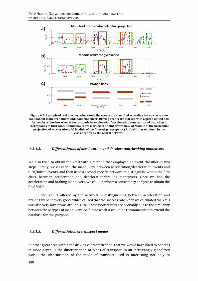
DEEP NEURAL NETWORKS FOR VEHICLE DRIVING CHARACTERIZATION BY MEANS OF SMARTPHONE SENSORS
180
Figure 6.2: Example of real journey, where only the events are classified according to two classes: no roundabout maneuver and roundabout maneuver. Driving events are marked with a green dotted box,
formed by a blue box when it corresponds to acceleration/deceleration zone and a red box when it corresponds to turn zone. Roundabouts are marked in a solid brown box. a) Module of the horizontal
projection of accelerations. b) Module of the filtered gyroscopes. c) Probabilities obtained in the classification by the neural network.
6.3.1.2. Differentiation of acceleration and deceleration/braking maneuvers
We also tried to obtain the VMD with a method that employed an event classifier in two
steps. Firstly, we classified the maneuvers between acceleration/deceleration events and
turn/mixed events, and then used a second specific network to distinguish, within the first
class, between acceleration and deceleration/braking maneuvers. Once we had the
acceleration and braking maneuvers, we could perform a consistency analysis to obtain the
final VMD.
The results offered by the network in distinguishing between acceleration and
braking were not very good, which caused that the success rate when we calculated the VMD
was also very low, it was around 40%. These poor results are probably due to the similarity
between these types of maneuvers. As future work it would be recommended to extend the
database for this purpose.
6.3.1.3. Differentiation of transport modes
Another great area within the driving characterization, that we would have liked to address
in more depth, is the differentiation of types of transport. In an increasingly globalized
world, the identification of the mode of transport used is interesting not only to

CHAPTER 6. CONCLUSIONS AND FUTURE WORK
181
contextualize the activity of a person, but also from a point of view of the sustainable
development of transport. Identifying it, we could analyze the traffic according to each mode
and even try to understand the driver behaviors according to different areas or regions.
In the Thesis we tried to differentiate the modes of transport using exclusively the
accelerometer signals captured with the smartphones. Identifying when people went or not
by car, differentiating it from trains, planes, boats, motorcycles and buses. And studying
different input signals for transport classification. The problem, as it happened before, was
that the database of the other modes of transport (not car) was very small. Despite this,
some of the conclusions we obtained were that the background noise areas seemed more
useful to distinguish modes of transportation (more than the maneuvering areas).
Differentiation of transport modes is incorporated in many of the activity
recognition applications. So it would be interesting to continue investigating this, expanding
the database of only accelerometers, since most of the state of the art research incorporate
a greater number of sensors.
6.3.1.4. Sequence-to-Sequence (Seq2Seq) networks to predict longitudinal and
transversal signals of accelerations
The Seq2Seq models convert sequences from one domain to sequences in another domain.
They are widely used for example in language translation or for free-from question
answering (generating a natural language answer given a natural language question). In
addition, for cases where the input and output do not have to be the same length, an RNN
that acts as an encoder and another RNN that acts as a decoder is usually used.
In order to predict the longitudinal and transversal signals, we used as inputs both
the projection of accelerations on the horizontal plane and the PC on filtered accelerometers
without gravity. We tried to predict the journey in frames of 2, 6 and 20 second overlapping
windows, using CNN+GRU and bidirectional networks. Bidirectional networks offered
better results than CNN+GRU, and 20-second windows than smaller windows. For the
assignments we used the correlations. The results obtained for the bidirectional network
case were a correct assignment of the longitudinal acceleration (modulus and sign) of
71.32% and of the transversal acceleration (modulus and sign) of 59.49%. However, the
mean square error obtained to calculate the losses during the training stages presented
relatively high values. And the scale of the predicted signals was much smaller than the
scales of the output signals to be predicted. For example, in the case of Figure 6.3, both the
main components and the signs are well assigned.

DEEP NEURAL NETWORKS FOR VEHICLE DRIVING CHARACTERIZATION BY MEANS OF SMARTPHONE SENSORS
182
Figure 6.3: Desired signals that we should predict against the results obtained as output in the Seq2Seq network. a) Original and predicted longitudinal signals. b) Original and predicted transversal signals.
This strategy to predict the longitudinal and transversal signals served as idea for
the design of method 3 “longitudinal and transversal acceleration assignment” in Chapter 4,
Section 4.4.3, converting a problem of prediction into a classification one. However a more
in-depth study would be necessary to solve the problems found.
6.3.1.5. i-vectors for driver identification
In speaker recognition, i-vectors were widely used (Dehak, Torres-Carrasquillo, Reynolds,
& Dehak, 2011) to represent an utterance. The i-vectors map a sequence of frames for a
given utterance into a low-dimensional vector space, called as the total variability space.
Normally, the procedure to obtain the i-vectors consists of the following steps:
1. The first step is to process the input signal for obtaining feature vectors which
represent the signals at frame level. Usually in speaker recognition extract the MFCC
features.
2. Then, it is necessary to train a UBM from all the training data. The UBM is defined
by the mean vector and the covariance matrix.
CHAPTER 6. CONCLUSIONS AND FUTURE WORK
183
3. Before, it is calculated the statistics needed for the i-vector model (the statistics
represent each frame according the UBM) and it is learnt the total variability
subspace. With all this, the i-vectors are calculated.
4. Finally, after calculating the i-vectors, the scoring is performed. In speaker
recognition, the use of a simple cosine distance scoring or a PLDA is widely
employed. Sometimes before applying the scoring technique, for example LDA is
applied to reduce dimensionality on the i-vectors.
Based on the good results obtained in speech area, we decided to test it for driver
identification. The problems appeared in the first step, to find a good way to extract the
features. Several tests were carried out varying the signals used to observe which one
achieved a better representation. We used among others:
The feature vector, of size [𝑛𝑥64], obtained at the output of a network (trained for
identification) formed by two convolutional layers, plus a GRU of two stacked layers
and dense layers. Using as input the horizontal projections plus the gyroscope
signals (6 channels in total).
The feature vector obtained with the same network mentioned above, but using the
longitudinal and transversal accelerations and the angular velocity (3 channels) as
inputs.
The Mel Frequency Cepstral Coefficients (MFCC) on the horizontal projections plus
the gyroscope signals.
The MFCC on longitudinal and transversal accelerations and the angular velocity.
None of the features seemed sufficiently representative. In the first two cases the
results on the network reached very low values. Even running the MFCCs, in case three and
four, through a simple fully connected layer classifier does not work well. In all cases, the
identification rates were extremely low, so when using the features in the i-vector
procedure, it did not give adequate results either. Perhaps the poor results obtained are due
to the number of drivers employed for the tests, 25 drivers. Normally, a very high number
is necessary for this type of models to work properly, in order to obtain a representative
global variability matrix.
As future work, it is necessary to expand the number of drivers employed, as well as
to study new ways of extracting features in order to improve the whole procedure and to
compare Deep Learning techniques with i-vectors.
6.3.2. Future new lines
There are also new lines that we would like to study, as a continuation of the work
developed. We detail them below:
To substitute or compare the results of new architectures such as the Capsule
Networks or the SincNets with the CNN standards.

DEEP NEURAL NETWORKS FOR VEHICLE DRIVING CHARACTERIZATION BY MEANS OF SMARTPHONE SENSORS
184
The Capsule Networks (CapsNets) were presented by (Sabour, Frosst, & Hinton,
2017). As they describe in the article: “A capsule is a group of neurons whose activity
vector represents the instantiation parameters of a specific type of entity such as an
object or an object part. We use the length of the activity vector to represent the
probability that the entity exists and its orientation to represent the instantiation
parameters. Active capsules at one level make predictions, via transformation
matrices, for the instantiation parameters of higher-level capsules. When multiple
predictions agree, a higher level capsule becomes active.” They not only reach the
state of the art on the MNIST dataset, but they had better results with multi-layer
capsule systems than with convolutional networks at recognizing highly
overlapping digits.
The SincNet is an architecture presented by (Ravanelli & Bengio, 2018) based on
CNN, where it should be parameterized sinc functions. That is, this type of networks
instead of learning all elements of each filter as in standard CNN, just learn low and
high cutoff frequencies. Among the advantages of this architecture are a fast
convergence, reduction of the number of parameters and facilitates interpretability.
Attention models.
The attention models was due to the work presented by (Bahdanau, Cho, & Bengio,
2015). It was originally developed for Machine Translation, but it has been extended
to numerous other application areas. The idea behind these models is computing a
set of attention weights, which provide contextual information (for example, from
the context of a sentence in the case of translation) and these tell us what we should
pay attention to the input signal.
To analyze tools that allow visualizing the internal behavior of the networks used.
To analyze the internal behavior of networks such as LSTMs, as in the work of (Guo,
Lin, & Antulov-Fantulin, 2019). In this research, they study the internal structure of
recurrent LSTM networks trained on time series, in order to learn variable hidden
states. That is, they try to distinguish the contribution in the prediction of different
variables in time series. For this, they interpret two relevant aspects to analyze both
the variable importance and the variable-wise temporal importance.
To extend our study to a larger population of drivers, as this would allow us to
analyze the influence of driver features, such as the age and experience of the driver,
as well as the type of road, car and traffic situation.
Cost parameters and energy consumption analysis for different combinations of
sensors, as well as comparison of results with the smartphone placed in a fixed
position inside the vehicle.

185
References
Eyobu, O., & Han, D. (2018). Feature representation and data augmentation for human activity
classification based on wearable IMU sensor data using a Deep LSTM Neural Network.
Sensors (Basel, Switzerland), 18(9).
Aggarwal, C. C. (2018). Neural Networks and Deep Learning. A Textbook.
Al-Din, M. S. (2018). Highway driving events identification and classification using smartphone.
International Conference on Circuits and Systems in Digital Enterprise Technology
(ICCSDET). Kottayam, India, India.
Ali, S., Khusro, S., Rauf, A., & Mahfooz, S. (2014). Sensors and mobile phones: evolution and
state-of-the-art. Pakistan Journal of Science, 66, 386-400.
Astarita, V., Guido, G., Edvige Mongelli, D., & Pasquale Giofrè, V. (2014). Ecosmart and
TutorDrive: tools for fuel consumption reduction. Proceedings of IEEE International
Conference on Service Operations and Logistics, and Informatics. Qingdao, China.
Bahdanau, D., Cho, K., & Bengio, Y. (2015). Neural machine translation by jointly learning to align
and translate. International Conference on Learning Representations (ICLR). San Diego,
CA.
Bailey Luttrell IV, J., Zhou, Z., Zhang, C., Gong, P., & Zhang, Y. (2017). Facial recognition via
Transfer Learning: Fine-Tuning Keras_vggface. In IEEE (Ed.), International Conference on
Computational Science and Computational Intelligence (CSCI). Las Vegas, NV, USA.
Barreto, C. A. (2018). Uso de técnicas de aprendizado de máquina para identificação de perfis de
uso de automóveis baseado em dados automotivos.
Belussi, A., Catania, B., Clementini, E., & Ferrari, E. (2007). Spatial data on the web. Springer.
Bengio, Y., & LeCun, Y. (2007). Scaling learning algorithms toward AI. In L. Bottou, O. Chapelle,
D. DeCoste, & J. Weston, Large-scale kernel machine (pp. 321-359). MIT Press.
Bergasa, L., Almería, D., Almazán, J., Yebes, J., & Arroyo, R. (2014). DriveSafe: An app for alerting
inattentive drivers and scoring driving behaviors. IEEE Intelligent Vehicles Symposium
Proceedings. Dearborn, MI, USA.
186
Bernardi, M., Cimitile, M., Martinelli, F., & Mercaldo, F. (2018). Driver and path detection
through time-series classification. Journal of Advanced Transportation, Article ID
1758731, 20 pages.
Blog Kaggle. (2015, April 20). Retrieved from AXA Winners' Interview: Learning Telematic
Fingerprints From GPS Data: http://blog.kaggle.com/2015/04/20/axa-winners-
interview-learning-telematic-fingerprints-from-gps-data/
Boža, V., Brejová, B., & Vinař, T. (2017). DeepNano: deep recurrent neural networks for base
calling in MinION nanopore reads. PLOS ONE 12(6).
Bredin, H. (2017). TristouNet: Triplet Loss for speaker turn embedding. International Conference
on Acoustics, Speech and Signal Processing (ICASSP) (pp. 5430-5434). New Orleans, USA:
IEEE.
Bromley, J., Guyon, I., LeCun, Y., Sickinger, E., & Shah, R. (1993). Signature verification using a
"Siamese" time delay Neural Network. International Journal of Pattern Recognition and
Artificial Intelligence.
Burkov, A. (2019). The hundred-page Machine Learning book (1 ed.). (K. D. Publishing, Ed.)
Burton, A., Parikh, T., Mascarenhas, S., Zhang, J., Voris, J., Artan, N., & Li, W. (2016). Driver
identification and authentication with active behavior modeling. 12th International
Conference on Network and Service Management (CNSM). Montreal, QC, Canada: IEEE.
Campanharo, A. S., Sirer, M. I., Malmgren, R. D., Ramos, F. M., & Amaral, L. A. (2011). Duality
between time series and networks. PLOS ONE, 6(8).
Campesato, O. (2019). TensorFlow 2 pocket primer. Mercury Learning and Information.
Carvalho, E., Ferreira, B., Ferreira, J., de Souza, C., Carvalho, H., Suhara, Y., . . . Pessin, G. (2017).
Exploiting the use of recurrent neural networks for driver behavior profiling.
International Joint Conference on Neural Networks (IJCNN). Anchorage, AK, USA: IEEE.
Castignani, G., Derrmann, T., Frank, R., & Engel, T. (2015). Validation study of risky event
classification using driving pattern factors. IEEE Symposium on Communications and
Vehicular Technology in the Benelux (SCVT). Luxembourg City, Luxembourg: IEEE.
Cervantes-Villanueva , J., Carrillo-Zapata, D., Terroso-Saenz , F., Valdes-Vela, M., & Skarmeta, A.
(2016). Vehicle maneuver detection with accelerometer-based classification. Sensors,
16(10).
Chaudhary, A., Bajaj, A., Shah, N., & Mankar, N. (2013). Mobile based monitoring of driving
patterns. Int. J. Comput.Sci. Manag. Res., 2(4).
Chawla, N., Bowyer, K., Hall, L., & Kegelmeyer, W. (2002). SMOTE: synthetic minority over-
sampling technique. Journal of Artificial Intelligence Research 16, 321–357.

187
Chen, Z., Yu, J., Zhu, Y., Chen, Y., & Li, M. (2015). D3: abnormal driving behaviors detection and
identification using smartphone sensors. 12th Annual IEEE International Conference on
Sensing, Communication, and Networking (SECON), (pp. 524-532). Seattle, WA, USA.
Cho, K., van Merrienboer, B., Gulcehre, C., Bahdanau, D., Bougares, F., Schwenk, H., & Bengio,
Y. (2014). Learning phrase representations using rnn encoder-decoder for statistical
machine translation. Proceedings of the Empiricial Methods in Natural Language
Processing (EMNLP), (pp. 1724-1734). Doha, Qatar.
Chowdhury, A., Chakravarty, T., Ghose, A., Banerjee, T., & Balamuralidhar, P. (2018).
Investigations on driver unique identification from smartphone’s GPS data alone.
Journal of Advanced Transportation.
Corbett, C., Alexis, J., & Watkins, L. (2018). Who’s driving you? 15th IEEE Annual Consumer
Communications & Networking Conference (CCNC). Las Vegas, NV, USA.
Cui, Z., Chen, W., & Chen, Y. (2016). Multi-scale Convolutional Neural Networks for time series
classification. arXiv preprint arXiv:1603.06995.
Dai, J., Teng, J., Bai, X., Shen, Z., & Xuan, D. (2010). Mobile phone based drunk driving detection.
4th International Conference on Pervasive Computing Technologies for Healthcare.
Munich, Germany.
de Ponte Müller, F., Martín Navajas, L., & Strang, T. (2013). Characterization of a laser scanner
sensor for the use as a reference system in vehicular relative positioning.
Communication Technologies for Vehicles: 5th International Workshop,
Nets4Cars/Nets4Trains 2013. Berlin, Heidelberg.
Decann, B., & Ross, A. (2012). Can a “poor” verification system be a “good” identification
system? A preliminary study. IEEE Inter. Workshop on Inform. Forensics and Security
(WIFS). Tenerife, Spain.
Dehak, N., Torres-Carrasquillo, P., Reynolds, D., & Dehak, R. (2011). Language recognition via
ivectors and dimensionality reduction. Interspeech, (pp. 857-860). Florence, Italy.
Dey, S., Dutta, A., Toledo, J., Ghosh, S., Llados, J., & Pal, U. (2017). SigNet: Convolutional Siamese
Network for writer independent offline signature verification. arXiv preprint
arXiv:1707.02131.
Dietz, M. (2017, May 2). Waya.ai. Retrieved from https://blog.waya.ai/deep-residual-learning-
9610bb62c355
Dong, W., Li, J., Yao, R., Li, C., Yuan, T., & Wang, L. (2016). Characterizing driving styles with deep
learning. arXiv Preprint arXiv:1607.03611.
Eckmann, J.-P., Kamphorst, S., & Ruelle, D. (1987). Recurrence plots of dynamical systems.
Europhys. Lett. 5, 973-977.
Enev, M., Takakuwa, A., Koscher, K., & Kohno, T. (2016). Automobile driver fingerprinting.
Proceedings on Privacy Enhancing Technologies, 34-51.
188
Eren, H., Makinist, S., Akın, E., & Yilmaz, A. (2012). Estimating driving behavior by a smartphone.
In IEEE (Ed.), IEEE Intelligent Vehicles Symposium. Alcala de Henares, Spain.
Ezzini, S., Berrada, I., & Ghogho, M. (2018). Who is behind the wheel? Driver identification and
fingerprinting. Journal of Big Data.
Fang, S.-H., Liao, H.-H., Fei, Y.-X., Chen, K.-H., Huang, J.-W., Lu, Y.-D., & Tsao, Y. (2016).
Transportation modes classification using sensors on smartphones. Sensors, 16(8).
Fazeen, M., Gozick, B., Dantu, R., Bhukhiya, M., & González, M. (2012). Safe driving using mobile
phones. EEE Transactions on Intelligent Transportation Systems, 13(3), 1462-1468.
Fei-Fei, L., Fergus, R., & Perona, P. (2006, April). One-shot learning of object categories. (IEEE,
Ed.) IEEE Transactions on Pattern Analysis and Machine Intelligence (TPAMI), 28(4).
Fernández Pozo, R., Hernández Gómez, L., López Meco, D., Bernat Vercher, J., & García Muñoz,
V. (2014, July 17). Patent No. US20160016590A1.
Ferreira Júnior, J., Carvalho, E., Ferreira, B., de Souza, C., Suhara, Y., Pentland, A., & Pessin, G.
(2017). Driver behavior profiling: An investigation with different smartphone sensors
and machine learning. PLOS ONE.
Fontaine, B. (2017, September 25). Sentiance. Retrieved from Applying deep learning to
distinguish drivers from passengers using sensor data:
https://www.sentiance.com/2017/09/25/deep-learning-on-passenger-and-driver-
behavior-analysis-using-sensor-data/
Forestier, G., Petitjean, F., Dau, H., Webb, G., & Keogh, E. (2017). Generating synthetic time
series to augment sparse datasets. IEEE International Conference on Data Mining
(ICDM). New Orleans, LA, USA: IEEE.
Fung, N., Wallace, B., Chan, A., Goubran, R., Porter, M., Marshall, S., & Knoefel, F. (2017). Driver
identification using vehicle acceleration and deceleration events from naturalistic
driving of older drivers. In IEEE (Ed.), IEEE International Symposium on Medical
Measurements and Applications (MeMeA). Rochester, MN, USA.
Géron, A. (2017). Hands-on machine learning with scikit-learn and TensorFlow: concepts, tools,
and techniques to build intelligent systems (1 ed.). O’Reilly Media.
Gers, F., Schmidhuber, J., & Cummins, F. (1999). Learning to forget: continual prediction with
LSTM. In IEEE (Ed.), International Conference on Artificial Neural Networks (ICANN'99),
(pp. 850-855). Edinburgh, Scotland.
Gers, F., Schraudolph, N., & Schmidhuber, J. (2002). Learning precise timing with LSTM Recurrent
Networks. Journal of Machine Learning Research 3, 115-143.
Goodfellow, I., Bengio, Y., & Courville, A. (2016). Deep Learning. (M. Press, Ed.)
Google course. (2019). Udacity Online Programs. Retrieved from Course of Deep Learning:
https://www.udacity.com/

189
Graves, A. (2012). Supervised sequence labelling with recurrent neural networks (1 ed., Vol. 385).
Springer-Verlag Berlin Heidelberg.
Greff, K., Srivastava, R., Jan Koutník, J., Steunebrink, B., & Schmidhuber, J. (2015). LSTM: a search
space odyssey. IEEE Transactions on Neural Networks and Learning Systems, 28.
Guo, J., Liu, Y., Zhang, L., & Wang, Y. (2018). Driving behaviour style study with a hybrid Deep
Learning framework based on GPS data. 10(7), 2351.
Guo, T., Lin, T., & Antulov-Fantulin, N. (2019). Exploring interpretable LSTM neural networks
over multi-variable data. 36th International Conference on Machine Learning (ICML).
Long Beach, CA, USA.
Hafner, D. (2016). Variable sequence lengths in TensorFlow. Retrieved from
https://danijar.com/variable-sequence-lengths-in-tensorflow/
Hallac, D., Sharang, A., Stahlmann, R., Lamprecht, A., Huber, M., Roehder, M., . . . Leskovec, J.
(2016). Driver identification using automobile sensor data from a single turn.
International Conference on Intelligent Transportation Systems (ITSC). Rio de Janeiro,
Brazil.
Härdle, W., & Simar, L. (2007). Applied multivariate statistical analysis. Springer.
Hatami, N., Gavet, Y., & Debayle, J. (2018). Classification of time-series images using Deep
Convolutional Neural Networks. Tenth International Conference on Machine Vision
(ICMV). Vienna, Austria.
Haykin, S. (2009). Neural networks and learning machines. Pearson Prentice Hall.
He, K., Zhang, X., Ren, S., & Sun, J. (2016). Deep residual learning for image recognition. In IEEE
(Ed.), Conference on Computer Vision and Pattern Recognition. Las Vegas, NV, USA.
Hemminki, S., Nurmi, P., & Tarkoma, S. (2013). Accelerometer-based transportation mode
detection on smartphones. Proceedings of the 11th ACM Conference on Embedded
Networked Sensor Systems. Roma, Italy.
Hermans, A., Beyer, L., & Leibe, B. (2017). In defense of the triplet loss for person re-
identification. arXiv preprint arXiv:1703.07737.
Hong, Y.-J., Kim, I.-J., Ahn, S., & Kim, H.-G. (2008). Activity recognition using wearable sensors
for elder care. Second International Conference on Future Generation Communication
and Networking, (pp. 302-305). Hainan Island.
Horwitz, J. (2015, June 9). Fake drivers and passengers are boosting Uber’s growth in China.
Retrieved from https://qz.com/423288/fake-drivers-and-passengers-are-boosting-
ubers-growth-in-china/
Il Kwak, B., Woo, J., & Kang Kim, H. (2016). Know your master: driver profiling-based anti-theft
method. 14th Annual Conference on Privacy, Security and Trust (PST). Auckland, New
Zealand: IEEE.

190
Johnson, D., & Trivedi, M. (2011). Driving style recognition using a smartphone as a sensor
platform. In IEEE (Ed.), 14th International IEEE Conference on Intelligent Transportation
Systems (ITSC). Washington, DC, USA.
Jolliffe, I. (1986). Principal component analysis. Springer Series in Statistics.
Kaggle. (2014, December 15). Retrieved from Driver Telematics Analysis:
https://www.kaggle.com/c/axa-driver-telematics-analysis
Kanarachos, S., Christopoulos, S.-R., & Chroneos, A. (2018). Smartphones as an integrated
platform for monitoring driver behaviour: The role of sensor fusion and connectivity.
Transportation Research Part C: Emerging Technologies, 95, 867-882.
Karaduman, M., & Eren, H. (2017). Deep learning based traffic direction sign detection and
determining driving style. International Conference on Computer Science and
Engineering (UBMK). Antalya, Turkey.
Karpathy, A. (2015, May 21). The unreasonable effectiveness of Recurrent Neural Networks.
Retrieved from http://karpathy.github.io/2015/05/21/rnn-effectiveness/
King Country. (2019). Retrieved July 2019, from
https://www.kingcounty.gov/depts/transportation/metro/travel-options/bus/app-
center/developer-resources.aspx
Koch, G., Zemel, R., & Salakhutdinov, R. (2015). Siamese neural networks for one-shot image
recognition. International Conference on Machine Learning (ICML).
Lake, B., Lee, C.-y., Glass, J., & Tenenbaum, J. (2014). One-shot learning of generative speech
concepts. Cognitive Science Society.
Le Guennec, A., Malinowski, S., & Tavenard, R. (2016). Data augmentation for time series
classification using convolutional neural networks. ECML/PKDD Workshop on Advanced
Analytics and Learning on Temporal Data. Riva Del Garda, Italy.
Lever, J., Krzywinski, M., & Altman , N. (2017). Principal component analysis. Nature Methods,
14, 641-642.
Li, C., Ma, X., Jiang, B., Li, X., Zhang, X., Liu, X., . . . Zhu, Z. (2017). Deep speaker: an end-to-end
neural speaker embedding system. arXiv Preprint arXiv:1705.02304.
Lozano-Diez, A., Plchot, O., Matejka, P., & Gonzalez-Rodriguez, J. (2018). DNN based embeddings
for language recognition. In IEEE (Ed.), International Conference on Acoustics, Speech
and Signal Processing (ICASSP). Calgary, AB, Canada.
Lu, D.-N., Nguyen, D.-N., Nguyen, T.-H., & Nguyen, H.-N. (2018). Vehicle mode and driving
activity detection based on analyzing sensor data of smartphones. Sensors, 18(1036).
Ly, M., Martin, S., & Trivedi, M. (2013). Driver classification and driving style recognition using
inertial sensors. In IEEE (Ed.), IEEE Intelligent Vehicles Symposium (IV). Gold Coast, QLD,
Australia.
191
Martínez, M., Echanobe, J., & del Campo, I. (2016). Driver identification and impostor detection
based on driving behavior signals. IEEE 19th International Conference on Intelligent
Transportation Systems (ITSC). Rio de Janeiro, Brazil: IEEE.
Meseguer, J., Calafate, C., Cano, J.-C., & Manzoni , P. (2013). DrivingStyles: a smartphone
application to assess driver behavior. In IEEE (Ed.), IEEE Symposium on Computers and
Communications (ISCC). Split, Croatia.
Mitiche, I., Morison, G., Nesbitt, A., Hughes-Narborough, M., Stewart, B., & Boreham, P. (2018).
Imaging time series for the classification of EMI discharge sources. Sensors (Basel), 18(9).
Mizell, D. W. (2003). Using gravity to estimate accelerometer orientation. Proceedings of the 7th
IEEE International Symposium on Wearable Computers (ISWC), (pp. 252-253).
Washington, DC, USA.
Mohan, P., Padmanabhan, V., & Ramjee, R. (2008). Nericell: rich monitoring of road and traffic
conditions using mobile smartphones. In Proceedings of the 6th ACM Conference on
Embedded Network Sensor Systems. Raleigh, NC, USA.
Moreira-Matias, L., & Farah, H. (2017). On developing a driver identification methodology using
invehicle data recorders. IEEE Transactions on Intelligent Transportation Systems, 18(9),
2387-2396.
Ng, A. (2018). Coursera-structuring machine learning projects. Retrieved October 10, 2018, from
https://es.coursera.org/lecture/machine-learning-projects/what-is-end-to-end-deep-
learning-k0Klk
Ng, A. (2019). Cousera, Machine learning course. Retrieved from https://www.coursera.org
Nishiwaki , Y., Ozawa, K., Wakita, T., Miyajima, C., Itou, K., & Takeda, K. (2007). Driver
identification based on spectral analysis of driving behavioral signals. In H. Abut, J.
Hansen, & K. Takeda (Eds.). Boston: Springer.
Ordóñez, F. J., & Roggen, D. (2016). Deep convolutional and LSTM recurrent neural networks for
multimodal wearable activity recognition. Sensors, 16(115).
Petitjean, F., Forestier, G., Webb, G., Nicholson, A., Chen, Y., & Keogh, E. (2016). Faster and more
accurate classification of time series by exploiting a novel dynamic time warping
averaging algorithm. Knowledge and Information Systems, 47(1), 1-26.
Petrow, S. (2016, October 12). I got taken for a ride by a fake Uber driver. Don’t become the next
victim. Retrieved from
https://eu.usatoday.com/story/tech/columnist/stevenpetrow/2016/10/12/fakeuber-
drivers-dont-become-next-victim/91903508/
Phumphuang, P., Wuttidittachotti, P., & Saiprasert, C. (2015). Driver identification using variance
of the acceleration data. International Computer Science and Engineering Conference
(ICSEC). Chiang Mai, Thailand: IEEE.

192
Progressive. (2019). Snapshot. Retrieved October 10, 2019, from Snapshot means BIG discounts
for good drivers: https://www.progressive.com/auto/discounts/snapshot/
Rashid, K., & Louis, J. (2019). Time-warping: a time series data augmentation of IMU data for
construction equipment activity Identification. Proceedings of the 36th International
Symposium on Automation and Robotics in Construction (ISARC), (pp. 651-657). Banff,
Alberta, Canada.
Ravanelli, M., & Bengio, Y. (2018). Speaker recognition from raw waveform with SincNet. IEEE
Spoken Language Technology Workshop (SLT). Athens, Greece.
Rudolph, G., & Voelzke, U. (2017, November 10). Fierce Electronics. Retrieved October 1, 2019,
from https://www.fierceelectronics.com/components/three-sensor-types-drive-
autonomous-vehicles
Ruffini, G., Ibañez, D., Castellano, M., Dubreuil-Vall, L., Soria-Frisch, A., Postuma, R., . . .
Montplaisir, J. (2019). Deep learning with EEG spectrograms in rapid eye movement
behavior disorder. Front Neurol, 10.
Sabour, S., Frosst, N., & Hinton, G. (2017). Dynamic routing between capsules. Conference on
Neural Information Processing Systems (NIPS). Long Beach, California, United States.
Sakai, A., Minoda, Y., & Morikawa, K. (2017). Data augmentation methods for machine-learning-
based classification of bio-signals. 10th Biomedical Engineering International Conference
(BMEiCON). Hokkaido, Japan: IEEE.
Salehghaffari, H. (2018). Speaker verification using Convolutional Neural Networks. arXiv
preprint arXiv: 1803.05427.
Sanguansat, P. (2012). Principal component analysis. IntechOpen.
Sankaranarayanan, S., Alavi, A., Castillo, C., & Chellappa, R. (2016). Triplet probabilistic
embedding for face verification and clustering. IEEE 8th International Conference on
Biometrics Theory, Applications and Systems (BTAS), (pp. 1-8). Niagara Falls, NY, EE.UU.
Schroff, F., Kalenichenko, D., & Philbin, J. (2015). FaceNet: a unified embedding for face
recognition and clustering. IEEE Conference on Computer Vision and Pattern Recognition
(CVPR). Boston, MA, USA: IEEE.
Schulz, J., Mentges, A., & Zielinski , O. (2016). Deriving image features for autonomous
classification from time-series recurrence plots. Journal of the European Optical Society-
Rapid Publications, 12(5).
Sede, M., Li, X., Li, D., Wu, M.-Y., Li, M., & Shu, W. (2008). Routing in large-scale buses ad hoc
networks. In IEEE (Ed.), Wireless Communications and Networking Conference. Las
Vegas, NV, USA.
Shijie, J., Ping, W., Peiyi, J., & Siping, H. (2017). Research on data augmentation for image
classification based on convolution neural networks. Chinese Automation Congress
(CAC). Jinan, China: IEEE.

193
Simpkins, C. A., & Simpkins, A. M. (2012). Cybernetics: or control and communications in the
animal and the machine. IEEE Robotics & Automation Magazine, 19(2).
Snyder, D., Garcia-Romero, D., Povey, D., & Khudanpur, S. (2017). Deep neural network
embeddings for text-independent speaker verification. Proceedings of Interspeech, (pp.
999-1003). Stockholm, Sweden.
Snyder, D., Ghahremani, P., Povey, D., Garcia-Romero, D., Carmiel, Y., & Khudanpur, S. (2016).
Deep Neural Network-based speaker embeddings for end-to-end speaker verification.
IEEE Spoken Language Technology Workshop (SLT), (pp. 165-170).
Sutton, R. S., & Barto, A. G. (2018). Reinforcement Learning (2 ed.). The MIT Press.
Tanprasert, T., Saiprasert, C., & Thajchayapong, S. (2017). Combining unsupervised anomaly
detection and neural networks for driver identification. Journal of Advanced
Transportation, Article ID 6057830, 13 pages.
Telematics, T. (2018). TomTom Telematics. Retrieved October 11, 2018, from
https://telematics.tomtom.com/en_gb/webfleet/fleet-management/driver-
identification/
Torkkola, K., Massey, N., Leivian, B., Wood, C., Summers, J., & Kundalkar, S. (2003). Classification
of critical driving events. Proceedings of the International Conference on Machine
Learning and Applications (ICMLA).
Troncoso, C., Danezis, G., Kosta, E., Balasch, J., & Preneel, B. (2011). PriPAYD: privacy-friendly
pay-as-you-drive insurance. (IEEE, Ed.) IEEE Transactions on Dependable and Secure
Computing, 8(5), 742-755.
Trop, J. (2014, January 10). The New York Times. Retrieved from The next data privacy battle
may be waged inside your car: https://www.nytimes.com/2014/01/11/business/the-
next-privacy-battle-may-be-waged-inside-your-car.html
Tsai, Y.-C., Chen, J.-H., & Wang, C.-C. (2019). Encoding candlesticks as images for patterns
classification using convolutional neural networks. arXiv preprint arXiv:1901.05237.
Undercoffler, D. (2013, February 11). Los Angeles Times. Retrieved from Tesla CEO Elon Musk
disputes N.Y. Times article on Model S range: https://www.latimes.com/business/la-
xpm-2013-feb-11-la-fi-hy-autos-tesla-model-s-ny-times-musk-battle-20130211-
story.html
Uppoor, S., Naboulsi, D., & Fiore, M. (2016). Vehicular mobility trace of the city of Cologne,
Germany. Retrieved July 26, 2019, from http://kolntrace.project.citi-lab.fr/
Vaizman, Y., Ellis, K., & Lanckriet, G. (2017). Recognizing detailed human context in the wild from
smartphones and smartwatches. (IEEE, Ed.) IEEE Pervasive Computing, 16(4), 62-74.
van der Maaten, L., & Hinton, G. (2008). Visualizing data using t-SNE. Journal of Machine
Learning Research 9, 2579-2605.

194
Vargha, D., & Maia, M. (2010). An overview of motion processing solutions for consumer
products. Retrieved July 17, 2019, from
https://www.digikey.com/Site/Global/Layouts/DownloadPdf.ashx?pdfUrl=023DBF7D7
9CD44E5BC112416E50149C2
Wahab, A., Quek, C., Keong Tan, C., & Takeda, K. (2009). Driving profile modeling and recognition
based on soft computing approach. IEEE Transactions on Neural Networks, 563-582.
Wallace, B., Goubran, R., Knoefel, F., Marshall, S., Porter, M., & Smith, A. (2016). Driver unique
acceleration behaviours and stability over two years. IEEE International Congress on Big
Data. San Francisco, CA, USA: IEEE.
Wang, F., Zhong, S.-h., Peng, J., Jiang, J., & Liu, Y. (2018). Data augmentation for EEG-based
emotion recognition with Deep Convolutional Neural Networks. International
Conference on Multimedia Modeling (MMM). 10705, pp. 82-93. Springer, Cham.
Wang, Z., & Oates, T. (2015). Imaging time-series to improve classification and imputation. IJCAI
2015 Proceedings of the 24th International Joint Conference on Artificial Intelligence.
Buenos Aires, Argentina.
Wattenberg, M., Viégas, F., & Johnson, I. (2016, October 13). Distill-latest articles about Machine
Learning. Retrieved from How to use t-SNE effectively:
https://distill.pub/2016/misread-tsne/
Weinberger, K., & Saul, L. (2006, January). Distance metric learning for large margin nearest
neighbor classification. Journal of Machine Learning Research, 10.
Who’sDrivingYou? (2018, August 22). Retrieved from
http://www.whosdrivingyou.org/rideshare-incidents
Wong, S., Gatt, A., Stamatescu, V., & McDonnell, M. (2016). Understanding data augmentation
for classification: when to warp? International Conference on Digital Image Computing:
Techniques and Applications (DICTA). Gold Coast, Australia.
World Health Organization. (2020, April). who. Retrieved from World Health Organization:
https://www.who.int/news-room/fact-sheets/detail/road-traffic-injuries
Xie, J., Hilal, A. R., & Kulić, D. (2018, June 15). Driving maneuver classification: a comparison of
feature extraction methods. IEEE Sensors Journal, 18(12).
Yan, S., Teng, Y., Smith, J., & Zhang, B. (2016). Driver behavior recognition based on Deep
Convolutional Neural Networks. Conference on Natural Computation, Fuzzy Systems and
Knowledge Discovery (ICNC-FSKD). Changsha, China.
Yang, J. (2009). Toward physical activity diary: motion recognition using simple acceleration
features with mobile phones. Proceedings of the 1st International Workshop on
Interactive Multimedia for Consumer Electronics (IMCE), (pp. 1-10). New York, NY, USA.
Yuñ Solutions. (2018, January). Levin vehicle telematics vehicle and driving data. Retrieved July
2019, from https://www.kaggle.com/yunlevin/levin-vehicle-telematics

195
Zhang, C., Yu , C., & Hansen, J. (2017). An investigation of deep-learning frameworks for speaker
verification antispoofing. IEEE Journal of Selected Topics in Signal Processing, 11(4), 684-
694.
Zhang, J., Wu, Z., Li, F., Xie, C., Ren, T., Chen, J., & Liu, L. (2019). A deep learning framework for
driving behavior identification on In-Vehicle CAN-BUS sensor data. Sensors, 19(6).
doi:10.3390/s19061356
Zhang, X., Zhao, X., & Rong, J. (2014). A study of individual characteristics of driving behavior
based on Hidden Markov model. Sensors & Transducers, 167(3), 194-202.
Zhang, X.-R., Lei, M.-Y., & Li, Y. (2018). An amplitudes-perturbation data augmentation method
in convolutional neural networks for EEG decoding. 5th International Conference on
Information, Cybernetics, and Computational Social Systems (ICCSS). Zhejiang, China.
Zhang, Y., Zhang, Z., Zhang, Y., Bao, J., Zhang, Y., & Deng , H. (2019). Human activity recognition
based on motion sensor using U-Net. IEEE Access, 7, 75213-75226.
Zhao, D., Ma, H., Liu, L., & Zhao, J. (2013). On opportunistic coverage for urban sensing. In IEEE
(Ed.), 10th International Conference on Mobile Ad-Hoc and Sensor Systems. Hangzhou,
China.


Colophon
Copyright © 2020 by Sara Hernández Sánchez. All rights reserved. No part of this publication
may be reproduced or transmitted in any form or by any means, electronic or mechanical,
including photocopy, recording, or any information storage and retrieval system, without
permission in writing from the author. Universidad Politécnica de Madrid has several rights
in order to reproduce and distribute electronically this document.