Citation: Patel, K.; Bhatt, C.; Mazzeo,

P.L. Deep Learning-Based Automatic

Detection of Ships: An Experimental

Study Using Satellite Images. J.

Imaging 2022, 8, 182. https://

doi.org/10.3390/jimaging8070182

Academic Editor: M. Donatello Conte

Received: 28 April 2022

Accepted: 23 June 2022

Published: 28 June 2022

Publisher’s Note: MDPI stays neutral

with regard to jurisdictional claims in

published maps and institutional affil-

iations.

Copyright: © 2022 by the authors.

Licensee MDPI, Basel, Switzerland.

This article is an open access article

distributed under the terms and

conditions of the Creative Commons

Attribution (CC BY) license (https://

creativecommons.org/licenses/by/

4.0/).

Journal of

Imaging

Article

Deep Learning-Based Automatic Detection of Ships:An Experimental Study Using Satellite ImagesKrishna Patel 1, Chintan Bhatt 2,* and Pier Luigi Mazzeo 3,*

1 Department of Computer Science & Engineering, Devang Patel Institute of Advance Technology andResearch (DEPSTAR), CHARUSAT Campus, Charotar University of Science and Technology (CHARUSAT),Changa 388421, India; krishnapatel.ce@charusat.ac.in

2 U & P U. Patel Department of Computer Engineering, Chandubhai S Patel Institute of Technology (CSPIT),CHARUSAT Campus, Charotar University of Science and Technology (CHARUSAT), Changa 388421, India

3 Institute of Applied Sciences and Intelligent Systems, National Research Council of Italy, 73100 Lecce, Italy* Correspondence: chintanbhatt.ce@charusat.ac.in (C.B.); pierluigi.mazzeo@cnr.it (P.L.M.)

Abstract: The remote sensing surveillance of maritime areas represents an essential task for bothsecurity and environmental reasons. Recently, learning strategies belonging to the field of machinelearning (ML) have become a niche of interest for the community of remote sensing. Specifically, amajor challenge is the automatic classification of ships from satellite imagery, which is needed fortraffic surveillance systems, the protection of illegal fisheries, control systems of oil discharge, and themonitoring of sea pollution. Deep learning (DL) is a branch of ML that has emerged in the last fewyears as a result of advancements in digital technology and data availability. DL has shown capacityand efficacy in tackling difficult learning tasks that were previously intractable. Specifically, DLmethods, such as convolutional neural networks (CNNs), have been reported to be efficient in imagedetection and recognition applications. In this paper, we focused on the development of an automaticship detection (ASD) approach by using DL methods for assessing the Airbus ship dataset (composedof about 40 K satellite images). The paper explores and analyzes the distinct variations of the YOLOalgorithm for the detection of ships from satellite images. A comparison of different versions of YOLOalgorithms for ship detection, such as YOLOv3, YOLOv4, and YOLOv5, is presented, after trainingthem on a personal computer with a large dataset of satellite images of the Airbus Ship Challengeand Shipsnet. The differences between the algorithms could be observed on the personal computer.We have confirmed that these algorithms can be used for effective ship detection from satellite images.The conclusion drawn from the conducted research is that the YOLOv5 object detection algorithmoutperforms the other versions of the YOLO algorithm, i.e., YOLOv4 and YOLOv3 in terms accuracyof 99% for YOLOv5 compared to 98% and 97% respectively for YOLOv4 and YOLOv3.

Keywords: image classification; deep learning; remote sensing; convolutional neural networks; shipsdetection; satellite images; surveillance

1. Introduction

In the last years, machine learning (ML) has become widespread and many artificialintelligence (AI) applications, have an impact on our daily life. These novel developments inAI are supported by a change in the approach to algorithm design. Specifically, data-drivenML has required a considerable level of manual feature engineering that utilized specialistknowledge from specific domains. The investigation of these data-driven techniques isknown as deep learning (DL) [1].

In terms of representation learning, DL is an excellent approach to be considered in theobject detection use cases. Therefore, DL adopts more advanced schemes, such as transferlearning (TL) [2], which refers to using a model which had been trained for a certain task toperform another task.

J. Imaging 2022, 8, 182. https://doi.org/10.3390/jimaging8070182 https://www.mdpi.com/journal/jimaging

J. Imaging 2022, 8, 182 2 of 17

The community of remote sensing (RS) is increasingly interested in addressing thechallenges of image detection through the application of ML and DL techniques. Shipdetection is of crucial importance to maritime surveillance, and can assist in monitoring andcontrolling illegal fishing, marine traffic, and similar activities along the sea boundary. Inthe last decades, automatic ship detection (ASD) has been a major challenge for researchersin the area of RS, and recent advances in RS technology have had a significant impact onthe variety of its application areas, including safety, illegal trading, pollution, spills, and oilslick monitoring. [1,3,4]. Nevertheless, there are still many drawbacks to be addressed, tocreate accurate and robust automatic identification systems (AIS), capable of dealing withcomplex scenarios, that is, those with variability in the shape and size of the target object,e.g., ASD.

ASD utilizes both extremely high frequency (HF) and the Global Positioning Sys-tem (GPS) to wirelessly identify the ship. However, not all ships are expected to havetransponders, and some are switched off on purpose to prevent radar detection. Instead,synthetic aperture radar (SAR) may be used, which obtains RS imagery by using radarsignals. Unlike visible light, radar signals are unaffected by variation in weather conditions,such as rain or clouds.

On the one hand, optical images are of a higher spatial resolution than most of theSAR images [5], making identification and recognition possible, as great improvementshave been made in the radar field (COSMO-SkyMed spotlight reaches to 1 m resolution).However, in case the ASD or the Vessel Monitoring System (VMS) system are unable toclassify the ship, it could suggest that the ship is potentially engaged in illegal activity orcould be considered as a different shape of floating object. Images of spatial resolution,other than those derived with SAR, are now possible due to the recent advances in visiblespectrum sensor technology. Several satellites (e.g., SPOT, RedEye, LandSat, QuickBird,and CBERS) are equipped with them. The main drawback of this type of images is thatit is suggested not to be used at night or in low light conditions or when it is cloudy. Inaddition, SAR requires a greater number of pairs of antenna or scan positions, also suitablefor slowly moving objects.

The use of SAR for ASD tasks has been extensively researched in the last two decades [6–8].Unlike the variety of feasibility studies for ASD based on SAR, optical imagery has been used infew research studies. Optical sensor developments have helped us to partially overcome thedisadvantages of SAR-based methods, and the authors focused on discovering the steps to betaken to gain improved classification accuracy, while also addressing the issues of real-timeASD [7]. Specifically, the detection of oriented objects from satellite photography is a complextask since the targeted objects can be visible from arbitrary directions and they are normallytightly packed. Recently, arbitrary-oriented object detection has received a lot of attention sincethey often appear in natural scenes, satellite photos, and RS images [9,10]. Additionally, othercontributions on SotA made use of known features extracted from photographs, by using bothcomputer vision and image processing techniques.

In the last few years, DL methods, such as convolutional neural networks (CNNs), havebeen shown to be effective in both image detection and recognition applications [10–12].One or more convolutional layers are used in CNNs, which are normally accompaniedby pooling layers and optional, completely connected layers, on top [11,12]. Moreover,Dropout and other regularization approaches have been used [13]. It has been proven thatmethods from the SotA of DL, e.g., YOLO9000, were unable to both detect and properlydetermine the total number of ships of small size by using satellite images [14]. A standardback-propagation method can be used to train these networks, but it needs a labeled datasetto measure the loss function gradient [15,16].

In this paper, we propose to take a step further in addressing discussed drawbacks ofAISs, in particular of ASD. Our solution based on a well-known CNN architecture is ableto define most distinguishing features for the given task if compared with hand-craftedfeatures. The proposed framework makes use of a preprocessing step to extract imagefeatures, which are then classified by using a CNN-based classifier. Specifically, different

J. Imaging 2022, 8, 182 3 of 17

CNNs (R-CNN, ResNet, Unet, YOLOv3, and YOLOv5) were considered for the automaticdetection of small size ships by using satellite images [17]. In order to assess our system,we tested it on a publicly available ship dataset composed of about 40 K satellite images,also containing moving ships.

The main contribution of this work is: (i) computation of data from satellite imagery;and (ii) successful detection of ships using the traditional YOLOv5 algorithm and compar-ing obtained results between the YOLOv3 and YOLOv4 with up to date well known CNNarchitectures.

The structure of the paper is as follows. Section 2 provides a brief summary of theSotA on ASD methods based on satellite images, also including those methods that useDL strategies for classification. Subsequently, Section 3 introduces our proposal for ASDusing DL. Section 4 provides both the considered datasets and a comprehensive analysis ofthe reported results derived from the conducted experiments. Finally, Section 5 providesthe more relevant conclusions drawn from this study and outlines lines of research to beaddressed in the future.

2. State-of-the-Art (SotA) on ASD

This section provides a brief overview of the SotA on ASD. Specifically, the con-tributions from the DL field have been of special interest to us for the purposes of thisresearch.

Due to natural variability in the ocean waves and the weather (e.g., clouds and rain),automatic ship detection and recognition represent a complex task if addressed withcommon approaches, e.g., those from computer vision or image processing. In particular,complex detection scenarios are those with variability in the shape and size of the targetobject, together with the behavior of natural resources, such as islets, cliffs, sandbanks, andcoral reefs.

Especially difficult conditions, such as variability in day lighting or atmospheric con-ditions, as well as images that include land area, pose an issue for conventional methods,as these images often produce false positives. As a result, many of the approaches havestopped making use of these types of source images in the datasets [18–23]. Other ap-proaches use a geographical information mask to disregard land areas or to differentiatepreviously seen sea and land zones, but even in this scenario, tiny islets and islands are notidentified and filtered out and may be mistaken in the recognition step [17]. Furthermore,this kind of approach is only applicable when using satellite images.

Regarding DL, there is no general code of practice for deciding the best choice ofnet-work architecture, the number of neurons per layer, and the total amount of layersmore suitable to use to properly address a given classification problem [23]. Specifically,DL is aimed at making multilayered neural networks to model high-degree representa-tions of input statistics. These statistics are given to the first layer in order to transformthem and next transfer the result to the next layer, then repeating the procedure till theremaining layers produce the desired outcome [24]. The first transition layers providelow-level features (e.g., edges, corners, and gradients, among others) at the same time as thesubsequent layers produce a growing high-degree representation of the maximum salientor consult-ant features. Then, DL has the benefit of no longer requiring hand-engineeredcharacteristic extraction. As an alternative, the most crucial capabilities are found out fromthe raw input records, and this is frequently known as “representation learning” [25–30].

In [31–33], several methods for optical RS using DL have been recently contributed.These approaches were proposed to detect objects and classify scenes in optical satellite im-agery such as residential zones, forest, and agricultural area. For instance, CNN activationsfrom the final convolutional layer were created at a couple of scales, after which they wereencoded into worldwide picture capabilities using widely used encoding methods to feeda classifier [34]. The approach was aimed at detecting ships in a harbor.

In [35], UNet model was used for the segmentation of ship from the SAR images. Thispaper proposed the UNet model and tested on the Airbus ship Challenge Dataset from

J. Imaging 2022, 8, 182 4 of 17

Kaggle. The result showed the F2-score of approximately 0.82 on different IoU thresholdvalues.

For the identification of ships from the Airbus satellite image dataset, Jaafar Alg-hazo [36] developed two CNN-based deep learning models, namely CNN model 1 andCNN model 2. The proposed methods could be utilised to address a variety of maritime-related issues, such as illegal fishing, maritime resource surveillance, and so on. The modelhad a maximum accuracy of 89%.

In [37], a new, deep learning-based, faster region-based convolutional neural network(Faster R-CNN) technique for detecting ships from two satellite image datasets, the 1786C-band Sentinel-1 and RADARSAT-2 vertical polarization, was introduced. The precisionand recall of the model were 89.23% and 89.14%, respectively.

Xin lou [38] proposed a generative transfer learning method that combined knowledgetransfer and ship detection. For ship detection, the images generated by the knowledgetransfer module were fed into a CNN-based detector model. The SAR Ship DetectionDataset (SSDD) and AIR-SARShip-1.0 Dataset were used in the experiment.

Figure 1 presents the total number of papers published for object detection overthe past six years until this year. Unlike approximations, such as VGG-16/19, AlexNet,and VGG-F/M/S, which were applied to scene classification, our proposal is based onmore suitable models, such as ResNet and YOLO, which have demonstrated to be moreappropriate for ASD [34]. Table 1 demonstrates the comparative analysis of the workcarried out on ship detection using the different datasets. Finally, our approach presentsa methodology that employs CNN technology to extract various distinct features fromsatellite imagery, which are then classified as ships. The next section introduces the detailsof our ASD framework.

J. Imaging 2022, 8, x FOR PEER REVIEW 4 of 17

In [35], UNet model was used for the segmentation of ship from the SAR images. This

paper proposed the UNet model and tested on the Airbus ship Challenge Dataset from

Kaggle. The result showed the F2-score of approximately 0.82 on different IoU threshold

values.

For the identification of ships from the Airbus satellite image dataset, Jaafar Alghazo

[36] developed two CNN-based deep learning models, namely CNN model 1 and CNN

model 2. The proposed methods could be utilised to address a variety of maritime-related

issues, such as illegal fishing, maritime resource surveillance, and so on. The model had a

maximum accuracy of 89%.

In [37], a new, deep learning-based, faster region-based convolutional neural net-

work (Faster R-CNN) technique for detecting ships from two satellite image datasets, the

1786C-band Sentinel-1 and RADARSAT-2 vertical polarization, was introduced. The pre-

cision and recall of the model were 89.23% and 89.14%, respectively.

Xin lou [38] proposed a generative transfer learning method that combined

knowledge transfer and ship detection. For ship detection, the images generated by the

knowledge transfer module were fed into a CNN-based detector model. The SAR Ship

Detection Dataset (SSDD) and AIR-SARShip-1.0 Dataset were used in the experiment.

Figure 1 presents the total number of papers published for object detection over the

past six years until this year. Unlike approximations, such as VGG-16/19, AlexNet, and

VGG-F/M/S, which were applied to scene classification, our proposal is based on more

suitable models, such as ResNet and YOLO, which have demonstrated to be more appro-

priate for ASD [34]. Table 1 demonstrates the comparative analysis of the work carried

out on ship detection using the different datasets. Finally, our approach presents a meth-

odology that employs CNN technology to extract various distinct features from satellite

imagery, which are then classified as ships. The next section introduces the details of our

ASD framework.

Figure 1. The number of papers on Ship Detection irrespective of region and country, (From 2016–

2022 (March month)).

Figure 1. The number of papers on Ship Detection irrespective of region and country, (from 2016–2022(March month)).

J. Imaging 2022, 8, 182 5 of 17

Table 1. Comparative Analysis of various Research work on Object Detection.

Paper Referred Dataset Pixel Size and Resolution Framework/Algorithm Precision/Recall/Accuracy

[23] SPOT-5 and Google EarthServices

Pixel Size 9000 × 9000 andResolution 5 m

Proposed method-based seasurface analysis Precision- 89.22% & Recall- 97.80%

[30] ImageNet LSVRC-2010 deep convolutional neuralnetwork Precision- 78.1% & Recall- 60.9%

[32] high-resolution remotesensing (HRRS) Pixel Size 600 × 600 CNN Accuracy- 94.6%

[35] Kaggle Dataset Pixel Size 768 × 768 UNet Accuracy- 82.3%

[36] Airbus Satellite ImageDataset Pixel Size 768 × 768 CNN based Deep Learning Accuracy- 89.7%

[37] RADARSET-2 andSentinel-1 Faster R-CNN Precision- 89.23% & Recall- 89.14%

[38] SAR Ship DetectionDataset (SSDD)

Knowledge Transfer Networkand CNN based detection

modelPrecision- 98.87% & Recall- 90.67%

[39] WorldView-2 and -3,GeoEye and Pleiades Resolution between 0.3 m and 0.5 m YOLOV2, YOLOV3, D-YOLO

and YOLTAverage Precision- 60% for vehicle

and 66% for vessel

[40] Google Earth Images Resolution be-tween 2 m and 0.4 mTwo staged

CNN-based ship detectiontechnique

Accuracy- 88.3%

[41] Google Earth Images Pixel Size ranges from 900 × 900to 3600 × 5400

Transferlearned Single-shot Multibox

Detector (SSD)Accuracy- 87.9%

3. Methodology

This section provides the specific design of our ASD system using DL. In particular,it is explained how to identify scenes with or without ships using the proposed process.First, the description will go through the dataset used in the paper and the most up-to-dateCNN algorithms (CNN, Region based CNN, ResNet. U-net). The various deep learningalgorithms (YOLOv3, YOLOv4, and YOLOv5) are then introduced and evaluated.

3.1. Dataset3.1.1. Shipsnet Dataset

In this paper, the experiment is carried out on the ship images taken from a satelliteimages dataset which was collected by the Kaggle platform [42]. These images show thesurface of earth, including roads, farmland, buildings, and other objects. PlanetScope hasobtained these satellite images of the San Pedro Bay and San Francisco Bay located in thedistricts of California. It contains 4 k RGB images with a pixel resolution of 80 × 80 for twodistinct classes: “ship” and “non-ship”.

Table 2 represents the total number of the images in each of the class (Ship and Non-ship). The images that contain a ship must show the entire appearance of a ship. It may bepossible that ships are in a different orientation and have different sizes, while they mayalso have atmospheric noises.

Table 2. Class-wise total number of sample images.

Class Number of Images

Non-ship 3000Ship 1000

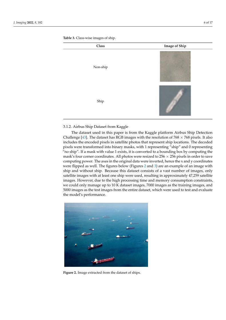
Table 3 demonstrates each class-wise image. A non-ship class is made up of one ormore of the following three elements: (1) bright pixels or strong linear features create anoise; (2) part of the ship in the image, and (3) other samples of various features, such asbuildings, roads, water, and so on.

J. Imaging 2022, 8, 182 6 of 17

Table 3. Class-wise images of ship.

Class Image of Ship

Non-ship

J. Imaging 2022, 8, x FOR PEER REVIEW 6 of 17

Table 2 represents the total number of the images in each of the class (Ship and Non-

ship). The images that contain a ship must show the entire appearance of a ship. It may

be possible that ships are in a different orientation and have different sizes, while they

may also have atmospheric noises. Table 3 demonstrates each class-wise image. A non-

ship class is made up of one or more of the following three elements: (1) bright pixels or

strong linear features create a noise; (2) part of the ship in the image, and (3) other samples

of various features, such as buildings, roads, water, and so on.

Table 2. Class-wise total number of sample images.

Table 3. Class-wise images of ship.

Class Image of Ship

Non-ship

Ship

3.1.2. Airbus Ship Dataset from Kaggle

The dataset used in this paper is from the Kaggle platform Airbus Ship Detection

Challenge [43]. The dataset has RGB images with the resolution of 768 × 768 pixels. It also

includes the encoded pixels in satellite photos that represent ship locations. The decoded

pixels were transformed into binary masks, with 1 representing “ship” and 0 representing

“no ship.” If a mask with value 1 exists, it is converted to a bounding box by computing

the mask’s four corner coordinates. All photos were resized to 256 × 256 pixels in order to

save computing power. The axes in the original data were inverted, hence the x and y

coordinates were flipped as well. The figures below (Figures 2 and 3) are an example of

an image with ship and without ship. Because this dataset consists of a vast number of

images, only satellite images with at least one ship were used, resulting in approximately

47,259 satellite images. However, due to the high processing time and memory consump-

tion constraints, we could only manage up to 10 K dataset images, 7000 images as the

training images, and 5000 images as the test images from the entire dataset, which were

used to test and evaluate the model’s performance.

Class Number of Images

Non-ship 3000

Ship 1000

Ship

J. Imaging 2022, 8, x FOR PEER REVIEW 6 of 17

Table 2 represents the total number of the images in each of the class (Ship and Non-

ship). The images that contain a ship must show the entire appearance of a ship. It may

be possible that ships are in a different orientation and have different sizes, while they

may also have atmospheric noises. Table 3 demonstrates each class-wise image. A non-

ship class is made up of one or more of the following three elements: (1) bright pixels or

strong linear features create a noise; (2) part of the ship in the image, and (3) other samples

of various features, such as buildings, roads, water, and so on.

Table 2. Class-wise total number of sample images.

Table 3. Class-wise images of ship.

Class Image of Ship

Non-ship

Ship

3.1.2. Airbus Ship Dataset from Kaggle

The dataset used in this paper is from the Kaggle platform Airbus Ship Detection

Challenge [43]. The dataset has RGB images with the resolution of 768 × 768 pixels. It also

includes the encoded pixels in satellite photos that represent ship locations. The decoded

pixels were transformed into binary masks, with 1 representing “ship” and 0 representing

“no ship.” If a mask with value 1 exists, it is converted to a bounding box by computing

the mask’s four corner coordinates. All photos were resized to 256 × 256 pixels in order to

save computing power. The axes in the original data were inverted, hence the x and y

coordinates were flipped as well. The figures below (Figures 2 and 3) are an example of

an image with ship and without ship. Because this dataset consists of a vast number of

images, only satellite images with at least one ship were used, resulting in approximately

47,259 satellite images. However, due to the high processing time and memory consump-

tion constraints, we could only manage up to 10 K dataset images, 7000 images as the

training images, and 5000 images as the test images from the entire dataset, which were

used to test and evaluate the model’s performance.

Class Number of Images

Non-ship 3000

Ship 1000

3.1.2. Airbus Ship Dataset from Kaggle

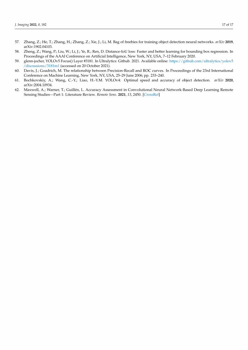
The dataset used in this paper is from the Kaggle platform Airbus Ship DetectionChallenge [43]. The dataset has RGB images with the resolution of 768 × 768 pixels. It alsoincludes the encoded pixels in satellite photos that represent ship locations. The decodedpixels were transformed into binary masks, with 1 representing “ship” and 0 representing“no ship”. If a mask with value 1 exists, it is converted to a bounding box by computing themask’s four corner coordinates. All photos were resized to 256 × 256 pixels in order to savecomputing power. The axes in the original data were inverted, hence the x and y coordinateswere flipped as well. The figures below (Figures 2 and 3) are an example of an image withship and without ship. Because this dataset consists of a vast number of images, onlysatellite images with at least one ship were used, resulting in approximately 47,259 satelliteimages. However, due to the high processing time and memory consumption constraints,we could only manage up to 10 K dataset images, 7000 images as the training images, and5000 images as the test images from the entire dataset, which were used to test and evaluatethe model’s performance.

J. Imaging 2022, 8, x FOR PEER REVIEW 7 of 17

Figure 2. Image extracted from the dataset of ships.

Figure 3. Dataset Image without ship.

3.2. Convolutional Neural Network

The most representative DL model is CNN. VGG16 was the popular CNN architec-

ture used for the object detection. Feature map is the name given to every layer of CNN.

The CNN input layer’s feature map is a three-dimensional matrices of pixel frequencies

for various color channels (e.g., RGB) [28]. Every single neuron in the preceding layer is

linked to a limited number of neurons in the layer above it (receptive field). The pre-

trained model is able to process any test image that is of the same size as the pre-trained

sample. If different sizes are given, rescaling or cropping operations must be performed

[28]. Additionally, some traditional drawbacks which come under the category of com-

puter vision can be reformulated as a high-dimensional matrix data transform issue and

can be addressed from multiple viewpoints, e.g., due to the huge learning power of deep

CNNs [44].

3.3. Region-Based CNN (R-CNN)

Methods for object detection based on area proposals have had a great deal of success

in natural scene photos in recent years. The architecture for detecting an object is divided

into two categories. The first categories rely on compiling a list of possible objects contain-

ing candidate area proposals. The second step focuses on fine-tuning the bounding box

coordinates and identifying the first-stage candidate region proposals into object groups

or contexts [45–49]. The region-based CNN (R-CNN) is the most significant technique

amongst all the region proposal-based methods. This is the first point where CNN models

are used to produce a number of unique features for the detection of objects, which results

Figure 2. Image extracted from the dataset of ships.

J. Imaging 2022, 8, 182 7 of 17

J. Imaging 2022, 8, x FOR PEER REVIEW 7 of 17

Figure 2. Image extracted from the dataset of ships.

Figure 3. Dataset Image without ship.

3.2. Convolutional Neural Network

The most representative DL model is CNN. VGG16 was the popular CNN architec-

ture used for the object detection. Feature map is the name given to every layer of CNN.

The CNN input layer’s feature map is a three-dimensional matrices of pixel frequencies

for various color channels (e.g., RGB) [28]. Every single neuron in the preceding layer is

linked to a limited number of neurons in the layer above it (receptive field). The pre-

trained model is able to process any test image that is of the same size as the pre-trained

sample. If different sizes are given, rescaling or cropping operations must be performed

[28]. Additionally, some traditional drawbacks which come under the category of com-

puter vision can be reformulated as a high-dimensional matrix data transform issue and

can be addressed from multiple viewpoints, e.g., due to the huge learning power of deep

CNNs [44].

3.3. Region-Based CNN (R-CNN)

Methods for object detection based on area proposals have had a great deal of success

in natural scene photos in recent years. The architecture for detecting an object is divided

into two categories. The first categories rely on compiling a list of possible objects contain-

ing candidate area proposals. The second step focuses on fine-tuning the bounding box

coordinates and identifying the first-stage candidate region proposals into object groups

or contexts [45–49]. The region-based CNN (R-CNN) is the most significant technique

amongst all the region proposal-based methods. This is the first point where CNN models

are used to produce a number of unique features for the detection of objects, which results

Figure 3. Dataset Image without ship.

3.2. Convolutional Neural Network

The most representative DL model is CNN. VGG16 was the popular CNN architectureused for the object detection. Feature map is the name given to every layer of CNN. TheCNN input layer’s feature map is a three-dimensional matrices of pixel frequencies forvarious color channels (e.g., RGB) [28]. Every single neuron in the preceding layer is linkedto a limited number of neurons in the layer above it (receptive field). The pre-trained modelis able to process any test image that is of the same size as the pre-trained sample. If differentsizes are given, rescaling or cropping operations must be performed [28]. Additionally,some traditional drawbacks which come under the category of computer vision can bereformulated as a high-dimensional matrix data transform issue and can be addressed frommultiple viewpoints, e.g., due to the huge learning power of deep CNNs [44].

3.3. Region-Based CNN (R-CNN)

Methods for object detection based on area proposals have had a great deal of suc-cess in natural scene photos in recent years. The architecture for detecting an object isdivided into two categories. The first categories rely on compiling a list of possible ob-jects containing candidate area proposals. The second step focuses on fine-tuning thebounding box coordinates and identifying the first-stage candidate region proposals intoobject groups or contexts [45–49]. The region-based CNN (R-CNN) is the most significanttechnique amongst all the region proposal-based methods. This is the first point whereCNN models are used to produce a number of unique features for the detection of objects,which results in a major performance improvement over previous attempts which reliedlargely on deformable component models (DCMs). R-CNN can be broken down into threebasic measures. First, it uses the method for selective search which performs the scanningoperation for a given input image for necessary objects, producing, on average, 2000 areaproposals. Second, utilizing a fine-tuned CNN model, each area proposal’s deep featuresare extracted and resized to a fixed scale (e.g., 224 × 224). In the final step, to label objectsfor each region proposal, each region proposal’s features are fed into a set of class-specificSVMs, and the object localizations are optimized using a linear regressor.

3.4. ResNet

Human-level image recognition has been achieved using deep CNNs. Low, middle,and high-level features and classifiers are extracted using deep CNNs. Moreover, in-creasing the number of stacked layers would increase the “levels” of features. Microsoft

J. Imaging 2022, 8, 182 8 of 17

created a platform for deep residual learning, named ResNet [50]. Instead of assumingthat a few stacked layers fit a preferred method of mapping directly, they let these layersmatch a residual mapping. To express F(x) + x, shortcut links with feedforward neuralnetworks are used, specifically links which are of shortcut that bypass one or more layers.Specifically, in-creased depth allows ResNets to achieve greater precision, resulting in betterperformance than previous networks. To fit dimensions, a stride of two is used in casethe shortcuts go through feature maps of two sizes. They are either two layers deep, i.e.,ResNet-18 and -34, or three layers deep, i.e., ResNet-50, 101, and 152.

3.5. U-Net

The U-Net model is a fast and precise CNN architecture for image segmentation [51].Convolutional layers were used to construct the model architecture and pixel-based imagesegmentation. U-Net outperforms traditional models. It also works with images from aminimal dataset. The presentation of this architecture started with the study of biomedicalimages. The pooling layer, i.e., the method of reducing dimension in height and width thatwe use in the convolutional neural network, is well-known. By maintaining a constantnumber of channels in the input matrix, the pooling layer reduces height and widthinformation. In summary, a pixel that reflects groups of pixels is referred to as the poolinglayer. The aim of these layers is to improve the output resolution. In the model, thesampled output is combined with high-resolution features for localization. Based on thisinformation, the goal of a sequential convolution layer is to generate more precise results. Asegmented output map is generated from the input images. There is no completely linkednumber of layers in the network model. Only convolution layers are included.

3.6. Theoretical Overview of YOLO Family Algorithms

Deep learning algorithms are classified into two categories, (i) one-stage classifiersand (ii) two-stage classifiers. Two-stage classifiers are responsible for generating a regionthat may include items. These are region are then classified into items by the neuralnetwork. Two-stage classifiers generate more results than single-stage classifiers; due tothe involvement of the different stages used in the process of detection, they have a slowerinference speed. In single-stage detectors, on the other hand, the region defining phase isskipped, and both object classification and detection are completed in one stage. Whencompared to two-stage classifiers, single-stage classifiers are faster.

YOLO (You Only Look Once) is a category of one-stage classifier deep learning frame-work that detects objects using a convolutional neural network. It is adopted by manyresearchers because of its detection speed and accuracy in the result. A variety of deeplearning algorithms exist, but none of them can perform object detection in a single run.On the other side, YOLO detects an object in a single run across a neural network, makingit ideal to use in real-time applications. Because of these qualities, the YOLO algo-rithm isa frequent choice from among the other algorithms of deep learning framework.

In YOLOv1 image is divided into equal-sized S × S grid cells. If the centre of the itemsfalls inside the cell, then object detection take place on each grid cell. With a confidencescore, each cell may anticipate a bounding box with a fixed B number. 5 values such as x, y,w, h, and confidence scores make up each bounding box [52,53]. The centres, width, andheight of the bounding box are represented by respectively x, y, w, and h. After predicting abounding box, IOU (intersection over union) is used by YOLO to find the correct boundingbox of an object for the grid cell. Non-max suppression is used by YOLO to reduce extrabounding boxes. If the IOU >= 0.5, then the extra bounding boxes with low confidencescore are removed by non-max suppression. The sum of squared error is used by the YOLOto determine loss.

Convolution layers are combined with the batch normalization in YOLOv2 to increaseaccuracy and minimize the problem of overfitting. To address this problem, in YOLOv3,Darknet 53 replaced the Darknet19 [54] due to its difficulty in detecting small objects. In thispaper, the residual block has been incorporated, which skips connections, and performs up-

J. Imaging 2022, 8, 182 9 of 17

sampling, considerably improving the algorithm’s accuracy. In YOLOv4, Dark-net 53 wasupdated to CSPDarknet53 to use as the feature extractors’ backbone, which significantlyenhanced the algorithm’s speed and accuracy. YOLOv5 is the most recent version of all theYOLO family algorithms, where Darknet was replaced by PyTorch.

Figure 4 depicts the YOLO algorithm’s overall design, while Table 4 highlights thedifferences between the YOLO family algorithms’ (YOLOv3, YOLOv4, and YOLOv5 algo-rithm) architectures. All of the algorithms have the same head and neural network type,but different backbone, neck, and loss functions.

J. Imaging 2022, 8, x FOR PEER REVIEW 9 of 17

In YOLOv1 image is divided into equal-sized S × S grid cells. If the centre of the items

falls inside the cell, then object detection take place on each grid cell. With a confidence

score, each cell may anticipate a bounding box with a fixed B number. 5 values such as x,

y, w, h, and confidence scores make up each bounding box [52,53]. The centres, width,

and height of the bounding box are represented by respectively x, y, w, and h. After pre-

dicting a bounding box, IOU (intersection over union) is used by YOLO to find the correct

bounding box of an object for the grid cell. Non-max suppression is used by YOLO to

reduce extra bounding boxes. If the IOU >= 0.5, then the extra bounding boxes with low

confidence score are removed by non-max suppression. The sum of squared error is used

by the YOLO to determine loss.

Convolution layers are combined with the batch normalization in YOLOv2 to in-

crease accuracy and minimize the problem of overfitting. To address this problem, in

YOLOv3, Darknet 53 replaced the Darknet19 [54] due to its difficulty in detecting small

objects. In this paper, the residual block has been incorporated, which skips connections,

and performs up-sampling, considerably improving the algorithm’s accuracy. In

YOLOv4, Dark-net 53 was updated to CSPDarknet53 to use as the feature extractors’ back-

bone, which significantly enhanced the algorithm’s speed and accuracy. YOLOv5 is the

most recent version of all the YOLO family algorithms, where Darknet was replaced by

PyTorch.

Figure 4 depicts the YOLO algorithm’s overall design, while Table 4 highlights the

differences between the YOLO family algorithms’ (YOLOv3, YOLOv4, and YOLOv5 algo-

rithm) architectures. All of the algorithms have the same head and neural network type,

but different backbone, neck, and loss functions.

Figure 4. Overall design of YOLO algorithm.

Table 4. The Architecture differences between the YOLO family algorithms.

Parameters YOLOv3 Algorithm YOLOv4 Algo-

rithm YOLOv5 Algorithm

Type of Neural Network Fully Convolutional Fully Convolu-

tional Fully Convolutional

Feature Extractor Darknet-53 CSPDarknet53 CSPDarknet53

Neck FPN SSP and PANet PANet

Head YOLO layer YOLO layer YOLO layer

Darknet53, the backbone of YOLOv3, extracts feature from an input image. The con-

volution layer is the backbone of a deep neural network, and its duty is to extract the

required information from the input image. As a neck, the feature pyramid network (FPN)

is utilized [51]. The neck, which is composed of several bottom-up and top-down paths,

is necessary for extracting feature maps from various stages, whereas the head is com-

posed of the YOLO layer. The head’s job is to perform the final prediction, which is a

vector of bounding box coordinates: class probability, width, class label, and height, in

one-stage detector. Feature extraction is done by supplying the image first to Darknet53,

Figure 4. Overall design of YOLO algorithm.

Table 4. The Architecture differences between the YOLO family algorithms.

Parameters YOLOv3 Algorithm YOLOv4 Algorithm YOLOv5 Algorithm

Type of Neural Network Fully Convolutional Fully Convolutional Fully ConvolutionalFeature Extractor Darknet-53 CSPDarknet53 CSPDarknet53

Neck FPN SSP and PANet PANetHead YOLO layer YOLO layer YOLO layer

Darknet53, the backbone of YOLOv3, extracts feature from an input image. Theconvolution layer is the backbone of a deep neural network, and its duty is to extractthe required information from the input image. As a neck, the feature pyramid network(FPN) is utilized [51]. The neck, which is composed of several bottom-up and top-downpaths, is necessary for extracting feature maps from various stages, whereas the head iscomposed of the YOLO layer. The head’s job is to perform the final prediction, which isa vector of bounding box coordinates: class probability, width, class label, and height, inone-stage detector. Feature extraction is done by supplying the image first to Darknet53,then providing the result generated from the Darknet53 to a FPN. Finally, the YOLO layeris responsible for generating the results.

3.6.1. YOLOv4 Architecture

The cross stage partial network (CSPNet) creates a new feature extractor backbonecalled CSPDarknet53 in the YOLOv4 Darknet, which is a modified version of YOLOv3.DenseNet [55,56], which has been upgraded, provides the basis for the convolution design.Dense block is used to transfer a copy of the feature map from the base layer to the next layer.DenseNet offers a lot of benefits, including lesser gradient vanishing difficulties, improvedlearning, improved backpropagation, and the removal of the processing bottleneck. Theneck is formed using the spatial pyramid pooling (SPP) layer and the path aggregationnetwork (PANet). The SPP layer and PANet are used to increase the receptive field andto extract important data from the backbone. A YOLO layer is also present on the head.Feature extraction from the image is performed by giving the image to CSPDarknet53, thensupplied to PANet for feature fusion. Finally, identical to YOLOv3, the results are generatedby the YOLO layer. YOLOv4 algorithm performance can be improved by utilizing thebag of freebies [57] and bag of specials [57]. Different techniques of augmentation, dropblock regularization, and complete IOU loss (CIOU), are included in the bag of freebies.

J. Imaging 2022, 8, 182 10 of 17

Diou-NMS [58] modified the path aggregation network, and mish activation is included inthe bag of specials.

3.6.2. YOLOV5 Architecture

YOLOv5 is more like its prior version release. PyTorch is used instead of Darknet.CSPDarknet53 is used as a backbone. The repeating gradient information in big backbonesand integration of gradient change into the feature map are handled by the backbone, whichspeeds up inference, improves the accuracy parameter, and decreases the size of the modelby lowering parameters. To boost information flow, a path aggregation network (PANet) isused as a neck. A new FPN with many bottom-up and top-down layers is used by PANet.This enhances the model’s low-level feature propagation. PANet improves the object’slocalization accuracy by improving localization in lower levels. Moreover, the YOLOv5head is identical to that of YOLOv4 and YOLOv3, resulting in three distinct feature mapoutputs for multiscale prediction. It also contributes towards the efficient prediction ofsmall to large objects in the model. Feature extraction from the image is performed bygiving the image to CSPDarknet53. Then, for feature fusion, PANet is used. Finally, theresults are generated by the YOLO layer. The YOLOv5 algorithm’s architecture is shown inFigure 5 The Focus layer evolved from the YOLOv3 framework [59].

J. Imaging 2022, 8, x FOR PEER REVIEW 11 of 17

Figure 5. Architecture of YOLOv5 algorithm.

The architectures of the three YOLO family algorithms, namely YOLOv3 algorithm,

YOLOv4 algorithm, and YOLOv5 algorithm, are fundamentally different. YOLOv3 lever-

ages the Darknet53 backbone, CSPdarknet53 is used in the YOLOv4 design, while the Fo-

cus layer is used in the YOLOv5 architecture. The Focus layer is originally introduced in

the YOLOv5 algorithm. The Focus layer replaces the first three layers in the YOLOv3 al-

gorithm. A Focus layer has the advantage of requiring less CUDA memory, having fewer

layers, and allowing for more forward and backward propagations [59].

4. Experimental Results

4.1. Experimental Setup

The methodology proposed in the paper was tested and executed on a personal com-

puter with the specifications as Intel(R) Core (TM) i5-8250U processor (Intel Corporation,

Santa Clara, CA, USA), NVIDIA® TITAN XP® 3840NVIDIA CUDA® architecture with 12

GB GDDR5X RAM of 16 GB (NVIDIA Corporation, Santa Clara, CA, USA), storage of 1TB

SSD, and Microsoft Windows 10 operating system (Microsoft, Redmond, WA, USA).

To train the neural networks, the open-source google colab has been used along with

Tesla P100-PCIE-16GB graphics cards (NVIDIA Corporation, Santa Clara, CA, USA). Dif-

ferent types of Google cloud computing services are offered, such as paid and free, which

can be utilized in a variety of computer applications. In terms of accuracy, it can be said

that YOLOV5I outperforms YOLOv4 and YOLOV3. We used the PyTorch framework to

train YOLOv5, and as the YOLOv4 algorithm and YOLOv3 algorithm are built in the

Darknet framework, the Darknet framework is used to train YOLOv3 and YOLOv4.

4.2. Evaluation Metrics

The F1 score and the mAP are used to compare the performance of the three YOLO

family algorithms, namely YOLOv3, YOLOv4, and YOLOv5. As seen in Equation (3), the

F1-score can be defined as the harmonic mean value of precision and recall [60]. It’s also

the model’s test accuracy. The highest possible F1 score value is 1, which indicates perfect

precision and memory, while the lowest possible value is 0, which indicates either zero

precision or recall. Furthermore, an average of the average precision of all the classes can

be defined as a mAP, indicated in Equation (5), where the number of queries is denoted

by q and average precision for that query is denoted by AveP(q). The mean of AP can then

be used to determine mAP. To determine the accuracy of machine learning algorithm a

mAP metric is also used. The true positive is the total number of ships detected by the

algorithm from satellite images. The number of false positives is the number of non-ship

objects that the algorithm mistakenly detects as a ship, and the number of false negatives

Figure 5. Architecture of YOLOv5 algorithm.

In YOLOv5, the first three layers of YOLOv3 are replaced by the single Focus layer.Furthermore, there is a convolution layer denoted by Conv. There are three convolutionlayers denoted by C3 and a module that is connected by bottlenecks. The network’s fixedsize constraint is removed by the SPP (spatial pyramid pooling) pooling layer, upsam-plingthe previous layer fusion in the adjacent node. Concat is a slicing layer that slices the layerbefore it. The last three Conv2d modules are detection modules that are employed in thenetwork’s head.

The architectures of the three YOLO family algorithms, namely YOLOv3 algorithm,YOLOv4 algorithm, and YOLOv5 algorithm, are fundamentally different. YOLOv3 lever-ages the Darknet53 backbone, CSPdarknet53 is used in the YOLOv4 design, while theFocus layer is used in the YOLOv5 architecture. The Focus layer is originally introducedin the YOLOv5 algorithm. The Focus layer replaces the first three layers in the YOLOv3algorithm. A Focus layer has the advantage of requiring less CUDA memory, having fewerlayers, and allowing for more forward and backward propagations [59].

4. Experimental Results4.1. Experimental Setup

The methodology proposed in the paper was tested and executed on a personal com-puter with the specifications as Intel(R) Core (TM) i5-8250U processor (Intel Corporation,

J. Imaging 2022, 8, 182 11 of 17

Santa Clara, CA, USA), NVIDIA® TITAN XP® 3840NVIDIA CUDA® architecture with12 GB GDDR5X RAM of 16 GB (NVIDIA Corporation, Santa Clara, CA, USA), storage of1TB SSD, and Microsoft Windows 10 operating system (Microsoft, Redmond, WA, USA).

To train the neural networks, the open-source google colab has been used alongwith Tesla P100-PCIE-16GB graphics cards (NVIDIA Corporation, Santa Clara, CA, USA).Different types of Google cloud computing services are offered, such as paid and free,which can be utilized in a variety of computer applications. In terms of accuracy, it can besaid that YOLOV5I outperforms YOLOv4 and YOLOV3. We used the PyTorch frameworkto train YOLOv5, and as the YOLOv4 algorithm and YOLOv3 algorithm are built in theDarknet framework, the Darknet framework is used to train YOLOv3 and YOLOv4.

4.2. Evaluation Metrics

The F1 score and the mAP are used to compare the performance of the three YOLOfamily algorithms, namely YOLOv3, YOLOv4, and YOLOv5. As seen in Equation (3), theF1-score can be defined as the harmonic mean value of precision and recall [60]. It’s alsothe model’s test accuracy. The highest possible F1 score value is 1, which indicates perfectprecision and memory, while the lowest possible value is 0, which indicates either zeroprecision or recall. Furthermore, an average of the average precision of all the classes canbe defined as a mAP, indicated in Equation (5), where the number of queries is denoted byq and average precision for that query is denoted by AveP(q). The mean of AP can then beused to determine mAP. To determine the accuracy of machine learning algorithm a mAPmetric is also used. The true positive is the total number of ships detected by the algorithmfrom satellite images. The number of false positives is the number of non-ship objects thatthe algorithm mistakenly detects as a ship, and the number of false negatives is the numberof ships that the algorithm fails to detect. Furthermore, the algorithms’ inference speed canbe determined by a frame per second (FPS). The frame rate is inversely proportional to thetime it takes to process a single frame of video. IOU is the ratio of the ground truth label’sarea of overlap to the prediction label’s area of union. To determine if a prediction is truepositive or false positive, an IOU threshold value was utilized. The average precision isthen calculated using the precision-recall curve. A mAP is defined as the average of theaverage precision of all the classes, as previously indicated. It’s worth mentioning thataccuracy is defined as the percentage of true predictions to total predictions. A model’sprecision is 100 percent if 50 predictions are produced and all of them are correct. Precisionis defined as the number of true objects in an image that are not considered, as shown inEquation (1). On the other hand, recall is defined as the ratio of correct predictions to theoverall number of objects in the image, as shown in Equation (2). For instance, if a modelpredicts 65 true objects in an image with 100 genuine objects, the recall is calculated to be65%. One cannot imply that the model is accurate if it shows high precision and recall. Analgorithm is stated as accurate if it has a good balance between precision and recall. Todetermine this, the same F1- score is used to check whether the model is accurate or not.

The paper aims to develop a real-time algorithm that can be utilized on a PersonalComputer (PC), specifically for detecting ships from satellite images which are small insize.

Precision = TP/(TP + FP) (1)

Recall = TP/(TP + FN) (2)

F-Measure = 2 (Precision · Recall)/(Precision + Recall) (3)

Accuracy = (TP + TN)/(TP + TN + FP + FN) (4)

mAP = ∑Qq = 1 AveP (q)/Q (5)

4.3. Analysis of the Results

To train the neural network, we first utilized YOLOv3 as a training optimizer usingstochastic gradient descent and 0.9 set as the momentum. Respectively, 0.001 and 0.0005

J. Imaging 2022, 8, 182 12 of 17

were the learning rate and weight decay. The training images’ height and width were416 × 416 pixels, respectively.

The YOLOv4 and YOLOv5 have been trained the same way the YOLOv3 algorithmwas trained, i.e., with identical parameters. Table 5 compares the three YOLO algorithmsfor the detection of ships from the Airbus Ship Challenge and Shipsnet satellite imagedataset. When compared to YOLOv3 and YOLOv4, YOLOv5 has a better mAP andF1 score, indicating that YOLOv5I shows greater accuracy in the detection of objectsthan YOLOv3 and YOLOv4 for the Airbus Ship Challenge and Shipsnet satellite imagesdataset. In this investigation, the YOLOv3 was found to be faster than the YOLOv4 andYOLOv5. Because it employs auto learning bounding boxes [61,62], YOLOv5 has a higheraccuracy than YOLOv4, which improves the algorithm’s accuracy. Because YOLOv3uses Darknet53, which has problems recognizing a tiny item, and YOLOv4 and YOLOv5employ CSPdarkent53, which increases overall accuracy, YOLOv4 and YOLOv5 showhigher accuracy than YOLOv3. YOLOv5

Table 5. Ship Detection results’ comparison using YOLOv3, YOLOv4 and YOLOv5 algorithms.

Evaluation Measures YOLOv3 Algorithm YOLOv4 Algorithm YOLOv5 Algorithm

F1-Score 0.56 0.58 0.61Recall 0.44 0.59 0.63

Precision 0.71 0.67 0.70mAP 0.49 0.61 0.65

The result of the application of the YOLO family algorithms to a satellite image is shownin Figure 6. In addition, Figure 7 depicts the performance of YOLO algorithms on a PC.

Table 5 displays the algorithms’ accuracy and recall. Table 6 provides the three YOLOalgorithms, average precision results of the ship labels. YOLOv3 shows a high precisionvalue but a low recall value, indicating that the YOLOv3 model has to be improved. For itsuse, there has to be a balance between precision and recall, which in turn is again reflectedin the method’s F1 score. Precision and recall are balanced in YOLOv4 and YOLOv5, as canbe seen. As a result, YOLOv4 and YOLOv5 have greater F1 scores than YOLOv3, despitethe fact that YOLOv3 shows high precision. It has been observed that a good balance ofprecision and recall in YOLOv4 and YOLOv5 has resulted in a high F1 score.

Table 6. Ship Detection-Average Precision Performance of YOLOv3, YOLOv4 and YOLOv5 algorithm.

Label YOLOv3 YOLOv4 YOLOv5

Ship 73.27 84.19 80.7

Figure 7 show that all three algorithms render good results in ship detection. Accu-racy is a key criterion to consider when selecting the best algorithm for detecting ships.According to the result received in Table 5 and Figure 7, we can conclude that YOLOv5I isbest as it has the highest accuracy in detecting ships from satellite images. Moreover, keepin mind that these algorithms have been evaluated on a PC to verify the results. On a PC,YOLOv5 achieves greater accuracy than other YOLO family algorithms, such as YOLOv3and YOLOv4. Employing YOLOv5 resulted in a modest speed loss (2.5 FPS) in comparisonto the YOLOv3 algorithm.

J. Imaging 2022, 8, 182 13 of 17

J. Imaging 2022, 8, x FOR PEER REVIEW 13 of 17

The result of the application of the YOLO family algorithms to a satellite image is

shown in Figure 6. In addition, Figure 7 depicts the performance of YOLO algorithms on

a PC.

Table 5 displays the algorithms’ accuracy and recall. Table 6 provides the three YOLO

algorithms, average precision results of the ship labels. YOLOv3 shows a high precision

value but a low recall value, indicating that the YOLOv3 model has to be improved. For

its use, there has to be a balance between precision and recall, which in turn is again re-

flected in the method’s F1 score. Precision and recall are balanced in YOLOv4 and

YOLOv5, as can be seen. As a result, YOLOv4 and YOLOv5 have greater F1 scores than

YOLOv3, despite the fact that YOLOv3 shows high precision. It has been observed that a

good balance of precision and recall in YOLOv4 and YOLOv5 has resulted in a high F1

score.

(a)

(b)

J. Imaging 2022, 8, x FOR PEER REVIEW 14 of 17

(c)

Figure 6. Result of Ship Detection using YOLO family algorithms: (a) YOLOv3 (b) YOLOv4 (c)

YOLOv5.

Table 6. Ship Detection-Average Precision Performance of YOLOv3, YOLOv4 and YOLOv5 algo-

rithm.

Label YOLOv3 YOLOv4 YOLOv5

Ship 73.27 84.19 80.7

Figure 7. Performance of YOLOv3, YOLOv4, and YOLOv5 on PC.

Figure 7 show that all three algorithms render good results in ship detection. Accu-

racy is a key criterion to consider when selecting the best algorithm for detecting ships.

According to the result received in Table 5 and Figure 7, we can conclude that YOLOv5I

is best as it has the highest accuracy in detecting ships from satellite images. Moreover,

keep in mind that these algorithms have been evaluated on a PC to verify the results. On

a PC, YOLOv5 achieves greater accuracy than other YOLO family algorithms, such as

YOLOv3 and YOLOv4. Employing YOLOv5 resulted in a modest speed loss (2.5 FPS) in

comparison to the YOLOv3 algorithm.

Figure 6. Result of Ship Detection using YOLO family algorithms: (a) YOLOv3 (b) YOLOv4(c) YOLOv5.

J. Imaging 2022, 8, 182 14 of 17

J. Imaging 2022, 8, x FOR PEER REVIEW 14 of 17

(c)

Figure 6. Result of Ship Detection using YOLO family algorithms: (a) YOLOv3 (b) YOLOv4 (c)

YOLOv5.

Table 6. Ship Detection-Average Precision Performance of YOLOv3, YOLOv4 and YOLOv5 algo-

rithm.

Label YOLOv3 YOLOv4 YOLOv5

Ship 73.27 84.19 80.7

Figure 7. Performance of YOLOv3, YOLOv4, and YOLOv5 on PC.

Figure 7 show that all three algorithms render good results in ship detection. Accu-

racy is a key criterion to consider when selecting the best algorithm for detecting ships.

According to the result received in Table 5 and Figure 7, we can conclude that YOLOv5I

is best as it has the highest accuracy in detecting ships from satellite images. Moreover,

keep in mind that these algorithms have been evaluated on a PC to verify the results. On

a PC, YOLOv5 achieves greater accuracy than other YOLO family algorithms, such as

YOLOv3 and YOLOv4. Employing YOLOv5 resulted in a modest speed loss (2.5 FPS) in

comparison to the YOLOv3 algorithm.

Figure 7. Performance of YOLOv3, YOLOv4, and YOLOv5 on PC.

5. Conclusions and Future Work

The main focus of this paper has been to evaluate an object detection system which de-tects ships from satellite images. YOLOv3 and YOLOv4 were tested, which are well-knownin the scientific community, and YOLOv5 was used in an experimental ship detection task,comparing YOLOv3 and YOLOv4 architectures to demonstrate that YOLOv5I outperformsthem in terms of detection accuracy of 99% compared to 98% and 97% respectively forYOLOv4 and YOLOv3. The algorithms’ performance was compared to see which methodgave the best results in ship detection. For training, testing, and validation, the Airbus ShipChallenge and Shipsnet satellite datasets were used, and the YOLO family algorithms werethen evaluated on a PC. According to the findings of our experiments, all three algorithmssatisfy the criteria for the ship detection. Given the results, YOLOv5 has been chosen asthe method with the highest accuracy in the detection of ships from satellite images. Thus,integrating YOLOv5 with the Airbus Ship Challenge and Shipsnet satellite datasets for shipdetection can be done quickly and accurately.

Future lines of research are going to focus on the incorporation of location featuresinto the object detection/classification scheme in order to determine the location of the ship.Moreover, new experiments must be carried out to test the different sensors, such as SARs,under extreme conditions, where visible spectrum imagery is unavailable, e.g., at night,when it is cloudy, or if there is fog. Additionally, different sensors can be integrated in amulti-modal scenario and saliency estimation methods may be used to not only classifywhether or not an image includes a ship, but also to obtain the exact position of the shipbeing identified and the other objects, such as yachts, boats, and aircraft. Future workwill also entail the adaption and usage of the range of available HPC (high performancecomputing) resources.

Author Contributions: K.P.: Data Curation, Investigation, Writing—original draft, C.B.: Methodol-ogy, Project administration, Writing—review and editing, P.L.M.: Methodology, Writing—review andediting. All authors have read and agreed to the published version of the manuscript.

Funding: This research received no external funding.

Data Availability Statement: Data available in a publicly accessible repository that does not issueDOIs. Publicly available datasets were analyzed in this study. This data can be found here: [https://www.kaggle.com/c/airbus-ship-detection/data] (accessed on 11 August 2021) and [https://www.kaggle.com/rhammell/ships-in-satellite-imagery] (accessed on 28 October 2021).

Conflicts of Interest: The authors declare no conflict of interest.

J. Imaging 2022, 8, 182 15 of 17

References1. Alzubaidi, L.; Zhang, J.; Humaidi, A.J.; Al-Dujaili, A.; Duan, Y.; Al-Shamma, O.; Santamaría, J.; Fadhel, M.A.; Al-Amidie, M.;

Farhan, L. Review of deep learning: Concepts, CNN architectures, challenges, applications, future directions. J. Big Data 2021, 8,1–74. [CrossRef] [PubMed]

2. Nascimento, R.G.D.; Viana, F. Satellite Image Classification and Segmentation with Transfer Learning. In Proceedings of theAIAA Scitech 2020 Forum, Orlando, FL, USA, 6–10 January 2020; p. 1864.

3. Stofa, M.M.; Zulkifley, M.A.; Zaki, S.Z.M. A deep learning approach to ship detection using satellite imagery. IOP Conf. Ser. EarthEnviron. Sci. 2020, 540, 012049. [CrossRef]

4. Zhang, R.; Li, S.; Ji, G.; Zhao, X.; Li, J.; Pan, M. Survey on Deep Learning-Based Marine Object Detection. J. Adv. Transp. 2021,2021, 5808206. [CrossRef]

5. Avolio, C.; Zavagli, M.; Paterino, G.; Paola, N.; Costantini, M. A Near Real Time CFAR Approach for Ship Detection on Sar DataBased on a Generalized-K Distributed Clutter Estimation. In Proceedings of the 2021 IEEE International Geoscience and RemoteSensing Symposium IGARSS, Brussels, Belgium, 11–16 July 2021; pp. 224–227.

6. Wang, N.; Wang, Y.; Er, M.J. Review on deep learning techniques for marine object recognition: Architectures and algorithms.Control Eng. Pract. 2020, 118, 104458. [CrossRef]

7. Ding, J.; Xue, N.; Xia, G.-S.; Bai, X.; Yang, W.; Yang, M.; Belongie, S.; Luo, J.; Datcu, M.; Pelillo, M.; et al. Object Detection in AerialImages: A Large-Scale Benchmark and Challenges. arXiv 2021, arXiv:2102.12219. [CrossRef]

8. Yang, X.; Yang, J.; Yan, J.; Zhang, Y.; Zhang, T.; Guo, Z.; Sun, X.; Fu, K. Scrdet: Towards more robust detection for small, cluttered androtated objects. In Proceedings of the IEEE/CVF International Conference on Computer Vision, Seoul, Korea, 27–28 October 2019.

9. Sun, Z.; Leng, X.; Lei, Y.; Xiong, B.; Ji, K.; Kuang, G. BiFA-YOLO: A Novel YOLO-Based Method for Arbitrary-Oriented ShipDetection in High-Resolution SAR Images. Remote Sens. 2021, 13, 4209. [CrossRef]

10. Ming, Q.; Zhou, Z.; Miao, L.; Zhang, H.; Li, L. Dynamic anchor learning for arbitrary-oriented object detection. arXiv 2020,arXiv:2012.04150.

11. Zhang, R.; Yao, J.; Zhang, K.; Feng, C.; Zhang, J. S-CNN-based ship detection from high-resolution remote sensing images. InProceedings of the International Archives of the Photogrammetry, Remote Sensing & Spatial Information Sciences, Prague, CzechRepublic, 12–19 July 2016.

12. Gallego, A.-J.; Pertusa, A.; Gil, P. Automatic Ship Classification from Optical Aerial Images with Convolutional Neural Networks.Remote Sens. 2018, 10, 511. [CrossRef]

13. Mishra, N.K.; Kumar, A.; Choudhury, K. Deep Convolutional Neural Network based Ship Images Classification. Def. Sci. J. 2021,71, 200–208. [CrossRef]

14. Redmon, J.; Farhadi, A. YOLO9000: Better, faster, stronger. In Proceedings of the IEEE Conference on Computer Vision andPattern Recognition, Honolulu, HI, USA, 21–26 July 2017; pp. 7263–7271.

15. Dey, N.; Bhatt, C.; Ashour, A.S. Big data for Remote Sensing: Visualization, Analysis and Interpretation; Springer: Cham, Switzerland, 2018.16. Bi, F.; Liu, F.; Gao, L. A Hierarchical Salient-Region Based Algorithm for Ship Detection in Remote Sensing Images. In Advances

in Neural Network Research and Applications; Zeng, Z., Wang, J., Eds.; Springer: Berlin/Heidelberg, Germany, 2010; pp. 729–738.[CrossRef]

17. Xia, Y.; Wan, S.; Jin, P.; Yue, L. A Novel Sea-Land Segmentation Algorithm Based on Local Binary Patterns for Ship Detection. Int.J. Signal Process. Image Process. Pattern Recognit. 2014, 7, 237–246. [CrossRef]

18. Corbane, C.; Marre, F.; Petit, M. Using SPOT-5 HRG Data in Panchromatic Mode for Operational Detection of Small Ships inTropical Area. Sensors 2008, 8, 2959–2973. [CrossRef]

19. Tang, J.; Deng, C.; Huang, G.-B.; Zhao, B. Compressed-Domain Ship Detection on Spaceborne Optical Image Using Deep NeuralNetwork and Extreme Learning Machine. IEEE Trans. Geosci. Remote Sens. 2014, 53, 1174–1185. [CrossRef]

20. Zou, Z.; Shi, Z. Ship Detection in Spaceborne Optical Image with SVD Networks. IEEE Trans. Geosci. Remote Sens. 2016, 54,5832–5845. [CrossRef]

21. Bengio, Y.; Courville, A.; Vincent, P. Representation learning: A review and new perspectives. IEEE Trans. Pattern Anal. Mach.Intell. 2013, 35, 1798–1828. [CrossRef] [PubMed]

22. Lin, H.; Shi, Z.; Zou, Z. Fully convolutional network with task partitioning for inshore ship detection in optical re-mote sensingimages. IEEE Geosci. Remote Sens. Lett. 2017, 14, 1665–1669. [CrossRef]

23. Yang, G.; Li, B.; Ji, S.; Gao, F.; Xu, Q. Ship Detection From Optical Satellite Images Based on Sea Surface Analysis. IEEE Geosci.Remote Sens. Lett. 2013, 11, 641–645. [CrossRef]

24. Arel, I.; Rose, D.C.; Karnowski, T.P. Deep Machine Learning—A New Frontier in Artificial Intelligence Research [ResearchFrontier]. IEEE Comput. Intell. Mag. 2010, 5, 13–18. [CrossRef]

25. Schmidhuber, J. Deep Learning in Neural Networks: An Overview. Neural Netw. 2015, 61, 85–117. [CrossRef]26. Martinez, H.P.; Bengio, Y.; Yannakakis, G.N. Learning deep physiological models of affect. IEEE Comput. Intell. Mag. 2013, 8,

20–33. [CrossRef]27. Srivastava, N.; Hinton, G.; Krizhevsky, A.; Sutskever, I.; Salakhutdinov, R. Dropout: A simple way to prevent neural networks

from overfitting. J. Mach. Learn. Res. 2014, 15, 1929–1958.28. Lecun, Y.; Bottou, L.; Bengio, Y.; Haffner, P. Gradient-based learning applied to document recognition. Proc. IEEE 1998, 86,

2278–2324. [CrossRef]

J. Imaging 2022, 8, 182 16 of 17

29. LeCun, Y.; Boser, B.; Denker, J.S.; Henderson, D.; Howard, R.E.; Hubbard, W.; Jackel, L.D. Backpropagation Applied toHandwritten Zip Code Recognition. Neural Comput. 1989, 1, 541–551. [CrossRef]

30. Krizhevsky, A.; Sutskever, I.; Hinton, G.E. Imagenet classification with deep convolutional neural networks. NIPS 2012, 60, 84–90.[CrossRef]

31. Zhu, X.X.; Tuia, D.; Mou, L.; Xia, G.S.; Zhang, L.; Xu, F.; Fraundorfer, F. Deep learning in remote sensing: A comprehensive reviewand list of resources. IEEE Geosci. Remote Sens. Mag. 2017, 5, 8–36. [CrossRef]

32. Hu, F.; Xia, G.-S.; Hu, J.; Zhang, L. Transferring Deep Convolutional Neural Networks for the Scene Classification of High-Resolution Remote Sensing Imagery. Remote Sens. 2015, 7, 14680–14707. [CrossRef]

33. Zhang, L.; Zhang, L.; Du, B. Deep learning for remote sensing data: A technical tutorial on the state of the art. IEEE Geosci. RemoteSens. Mag. 2016, 4, 22–40. [CrossRef]

34. Ball, J.E.; Anderson, D.T.; Chan Sr, C.S. Comprehensive survey of deep learning in remote sensing: Theories, tools, and challengesfor the community. J. Appl. Remote Sens. 2017, 11, 042609. [CrossRef]

35. Karki, S.; Siddhivinayak, K. Ship Detection and Segmentation using Unet. In Proceedings of the International Conference onAdvances in Electrical, Computing, Communication and Sustainable Technologies (ICAECT), Bhilai, India, 19–20 February 2021;pp. 1–7.

36. Alghazo, J.; Bashar, A.; Latif, G.; Zikria, M. Maritime ship detection using convolutional neural networks from satellite images. InProceedings of the 10th IEEE International Conference on Communication Systems and Network Technologies (CSNT), Bhopal,India, 18–19 June 2021; pp. 432–437.

37. Huang, X.; Zhang, B.; Perrie, W.; Lu, Y.; Wang, C. A novel deep learning method for marine oil spill detection from satellitesynthetic aperture radar imagery. Mar. Pollut. Bull. 2022, 179, 113666. [CrossRef]

38. Lou, X.; Liu, Y.; Xiong, Z.; Wang, H. Generative knowledge transfer for ship detection in SAR images. Comput. Electr. Eng. 2022,101, 108041. [CrossRef]

39. Ophoff, T.; Puttemans, S.; Kalogirou, V.; Robin, J.-P.; Goedemé, T. Vehicle and Vessel Detection on Satellite Imagery: A ComparativeStudy on Single-Shot Detectors. Remote Sens. 2020, 12, 1217. [CrossRef]

40. Ma, J.; Zhou, Z.; Wang, B.; Zong, H.; Wu, F. Ship Detection in Optical Satellite Images via Directional Bounding Boxes Based onShip Center and Orientation Prediction. Remote Sens. 2019, 11, 2173. [CrossRef]

41. Nie, G.-H.; Zhang, P.; Niu, X.; Dou, Y.; Xia, F. Ship Detection Using Transfer Learned Single Shot Multi Box Detector. ITM WebConf. 2017, 12, 01006. [CrossRef]

42. Ships in Satellite Imagery, “Shipsnet”. Kaggle. 2018. Available online: https://www.kaggle.com/rhammell/ships-in-satellite-imagery (accessed on 28 October 2021).

43. Airbus, “Airbus Ship Detection Challenge”. Kaggle. 2019. Available online: https://www.kaggle.com/c/airbus-ship-detection(accessed on 11 August 2021).

44. Simonyan, K.; Zisserman, A. Very deep convolutional networks for large-scale image recognition. arXiv 2014, arXiv:1409.1556.45. Azizpour, H.; Razavian, A.S.; Sullivan, J.; Maki, A.; Carlsson, S. Factors of transferability for a generic convnet representation.

IEEE Trans. Pattern Anal. Mach. Intell. 2015, 38, 1790–1802. [CrossRef] [PubMed]46. Yosinski, J.; Clune, J.; Bengio, Y.; Lipson, H. How transferable are features in deep neural networks? arXiv 2014, arXiv:1411.1792.47. Kang, L.; Ye, P.; Li, Y.; Doermann, D. Convolutional neural networks for no-reference image quality assessment. In Proceedings of

the IEEE conference on computer vision and pattern recognition, Columbus, OH, USA, 23–28 June 2014; pp. 1733–1740.48. Dodge, S.; Karam, L. Understanding how image quality affects deep neural networks. In Proceedings of the 2016 Eighth

International Conference on Quality of Multimedia Experience (QoMEX), Lisbon, Portugal, 6–8 June 2016; pp. 1–6.49. Yang, W.; Yin, X.; Xia, G.-S. Learning High-level Features for Satellite Image Classification with Limited Labeled Samples. IEEE

Trans. Geosci. Remote Sens. 2015, 53, 4472–4482. [CrossRef]50. Ajay, M.N.V.; Raghesh, K.K. A segmentation-based approach for improved detection of ships from SAR images using deep

learning models. In Proceedings of the 2021 2nd International Conference on Smart Electronics and Communication (ICOSEC-IEEE), Tamil Nadu, India, 7–9 October 2021; pp. 1380–1385. [CrossRef]

51. Li, D.; Xi, Y.; Zheng, P. Constrained robust feedback model predictive control for uncertain systems with polytopic description.Int. J. Control 2009, 82, 1267–1274. [CrossRef]

52. Bohara, M.; Patel, K.; Patel, B.; Desai, J. An AI Based Web Portal for Cotton Price Analysis and Pre-diction. In Proceedings of the3rd International Conference on Integrated Intelligent Computing Communication & Security (ICIIC 2021), Bangalore, India, 6–7June 2021; pp. 33–39.

53. Kothadiya, D.; Chaudhari, A.; Macwan, R.; Patel, K.; Bhatt, C. The Convergence of Deep Learning and Computer Vision:Smart City Applications and Research Challenges. In Proceedings of the 3rd International Conference on Integrated IntelligentCom-puting Communication & Security (ICIIC 2021), Bangalore, India, 6–7 June 2021; pp. 14–22.

54. Redmon, J. Darknet: Open Source Neural Networks in C; 2013–2016. Available online: https://pjreddie.com/darknet/ (accessedon 20 October 2021).

55. Lin, T.-Y.; Dollár, P.; Girshick, R.; He, K.; Hariharan, B.; Belongie, S. Feature pyramid networks for object detection. In Proceedingsof the IEEE Conference on Computer Vision and Pattern Recognition, Honolulu, HI, USA, 21–26 July 2017; pp. 2117–2125.

56. Iandola, F.; Moskewicz, M.; Karayev, S.; Girshick, R.; Darrell, T.; Keutzer, K. Densenet: Implementing efficient convnet descriptorpyramids. arXiv 2014, arXiv:1404.1869.

J. Imaging 2022, 8, 182 17 of 17

57. Zhang, Z.; He, T.; Zhang, H.; Zhang, Z.; Xie, J.; Li, M. Bag of freebies for training object detection neural networks. arXiv 2019,arXiv:1902.04103.

58. Zheng, Z.; Wang, P.; Liu, W.; Li, J.; Ye, R.; Ren, D. Distance-IoU loss: Faster and better learning for bounding box regression. InProceedings of the AAAI Conference on Artificial Intelligence, New York, NY, USA, 7–12 February 2020.

59. glenn-jocher, YOLOv5 Focus() Layer #3181. In Ultralytics: Github. 2021. Available online: https://github.com/ultralytics/yolov5/discussions/3181m1 (accessed on 20 October 2021).

60. Davis, J.; Goadrich, M. The relationship between Precision-Recall and ROC curves. In Proceedings of the 23rd InternationalConference on Machine Learning, New York, NY, USA, 25–29 June 2006; pp. 233–240.

61. Bochkovskiy, A.; Wang, C.-Y.; Liao, H.-Y.M. YOLOv4: Optimal speed and accuracy of object detection. arXiv 2020,arXiv:2004.10934.

62. Maxwell, A.; Warner, T.; Guillén, L. Accuracy Assessment in Convolutional Neural Network-Based Deep Learning RemoteSensing Studies—Part 1: Literature Review. Remote Sens. 2021, 13, 2450. [CrossRef]