Deduction of orbital velocities in disk galaxies - “Dark Matter” a myth?

Thierry De Mees [email protected]

Deduction of orbital velocities in disk galaxies.or: “Dark Matter”: a myth?

by using Gravitomagnetism.

T. De Mees - [email protected]

Summary

In my paper “A coherent dual vector field theory for gravitation” is explained how simply the Gravitation Theoryof Newton can be extended by transposing the Maxwell Electromagnetism into Gravitation. There exists indeed asecond field, which can be called: co-gravitation-, Gyrotation- (which I prefer), gravito-magnetic field and so on.In this paper, I will call this global theory the Maxwell Analogy for Gravitation (MAG) “Gyro-Gravitation”.

One of the many consequences of this Gyro-Gravitation Theory that I have written down, is that Dark Matter doesnot exist. At least far not in the quantities that someones expect, but rather in marginalized quantities. Manyresearchers suppose that disk galaxies cannot subsist without missing mass that, apparently, is invisible, and whichhas to be taken into account in the classic Newton-Kepler model to better explain the disk galaxies' shapes. An remarkable point is that Gyro-gravitation Theory is not only very close to GRT, but more important, easy tocalculate with, and coherent with Electromagnetism. It is no coincidence that nobody found the same result withGRT, not because GRT would obtain some other result, but because it is almost impossible to calculate with it.A demonstration is again given in this paper, where I deduce the general equations for the orbital velocities ofstars in disk galaxies, based on the assumption of a simple mass distribution of the initial spherical galaxy.

Index

1. Pro Memore : Symbols, basic equations and philosophy. / Maxwell Analogy Equations in short / The definitionof absolute local velocity.

2. Why do some scientists claim the existence of “dark matter”? / The orbital velocity of stars in a disk galaxy /What did Kepler claim ? / Is there a way to get the Kepler law working? / The easy solution: Black Matter /The other reasoning.

3. Pro Memore : Main dynamics of orbital systems. / Why the planets' orbits are plane and prograde / Equationsfor the accelerations nearby spinning stars.

4. From a spheric galaxy to a disk galaxy with constant stars' velocity. / The global stars' velocity in disk galaxies.

5. Origin of the variations in the stars' velocities. / The galaxy's bulge area / The zone near the bulge / The star'svelocities, farther in the disk / The global orbital velocities' equation of disk galaxies.

6. Conclusion : are large amounts of “dark matter” necessary to describe disk galaxies ?

7. References and interesting lecture.

© Feb. 2007 update 16/07/20101


1. Pro Memore : Symbols, basic equations and philosophy.

1.1 Maxwell Analogy Equations in short – The two fields.

The formulas (1.1) to (1.5) form a coherent set of equations, similar to the Maxwell equations. The electrical

charge q is substituted by the mass m, the magnetic field B by the Gyrotation ΩΩΩΩ , and the respective constants aswell are substituted (the gravitation acceleration is written as g and the universal gravitation constant as G =(4π ζ)-1. We use sign ⇐ instead of = because the right hand of the equation induces the left hand. This sign ⇐will be used when we want to insist on the induction property in the equation. F is the induced force, v the

velocity of mass m with density ρ. The operator × symbolizes the cross product of vectors. Vectors are written inbold.

F ⇐ m (g + v × Ω Ω Ω Ω ) (1.1)

∇∇∇∇ g ⇐ ρ / ζ (1.2)

(1.3)

where j is the flow of mass through a surface. The term ∂g/∂t is added for the same reasons as Maxwell did: thecompliance of the formula (1.3) with the equation :

It is also expected div ΩΩΩΩ ≡ ∇ ∇ ∇ ∇ ΩΩΩΩ = 0 (1.4)

and ∇∇∇∇× g ⇐ – ∂ ΩΩΩΩ / ∂ t (1.5)

All applications of the electromagnetism can from then on be applied on the gyrogravitation with caution. Also itis possible to speak of gyrogravitation waves.

1.2 The definition of absolute local velocity – The velocities are not relativistic.

When it comes to a competition between GRT and MAG, attention should be paid to two very importantdifferences.

The first one is that the actual MAG that I use is not really relativistic (although one could speak of semi-relativistic; I prefer to speak of Dopplerian). It works like the Newton and the Kepler theories, and like non-relativistic Electromagnetism. Newton and Kepler did not see that the second field existed, caused by the second term in G m m' (1+ v²/c²)/r².This expression is namely the simplest form for the Gyro-gravitation forces, and it is applicable between twoidentical moving masses in one dimension of place (see “A coherent dual vector field theory for gravitation”, lastchapter).This second term, which is very small and which is -by the way- often wrongly seen as an expression related torelativistic phenomena (I would rather say: transversal Doppler-effects), was not observed at that era. The relationto Doppler-effects will not further be discussed in this paper.

The extension of the theory for very fast velocities in non-steady systems has been settled by Oleg Jefimenko inseveral of his books, and is very analogical to what is called “relativistic electromagnetism”, where the fieldretardation -due to the finite velocity of gravitation- has been taken into account.

The consequence of this first difference is that in the framework of MAG, we should only study the kinds ofsteady systems, wherein the retardation of the fields, due to their finite velocity, is not of any crucial importance.

The second difference is that absolute velocity really exists. Not “absolute” with regard of the “centre” of ourUniverse, but “locally absolute” in the observed system wherein the forces interact within a given time-period.This means that the solar system can be studied as a closed system for “short” time periods of several years.However, I found that Mercury's perihelion advance is induced by the sun's motion in the Milky Way (see “Did

© Feb. 2007 update 16/07/20102

div j ⇐ – ∂ρ / ∂ t

c² ∇∇∇∇× ΩΩΩΩ ⇐ j / ζ + ∂g /∂ t


Einstein cheat ?”). Also the solar system, together with its motion in the Milky Way, can be seen as a closedsystem too. When the system of our Milky Way is considered, there is no need to also consider the cluster wherein our MilkyWay is just a tiny part of, etc.Without much more explanations, you feel already what I mean by “local absolute velocity”.One of the facets is indeed the place- and time-magnitude of what is to be observed or to be calculated. Yes, thatmagnitude can be 'the quantity of elapsed time' for that particular system as well. The gyrotation part of Mercury'sperihelion advance is only visible after many years compared with the very visible gravitational orbital motions ofthe system.

The correct way to settle it, is to understand that each gravitation field of any particle can be seen as the localabsolute velocity zero in relation to all the other particles. Not the observer can be at an absolute local velocity ofzero, unless he is a dynamic player in the system with a significant mass. Each motion of one body will generatethe gyrotation field onto any other body of the system and vice-versa. This means that in a moving two-body-system (without any other body in the universe), we have to consider the gravitation centre of the bodies as thezero velocity of the system, just as we used to for Newtonian systems, in high school. And every rotational motionof each particle plays a role in the gyrotation calculation of the system.

2. Why do some scientists claim the existence of “dark matter”?

2.1 The orbital velocity of stars in a disk galaxy – The velocities are constant.

One of the mysteries of the cosmos is the discovery that in disk galaxies, the velocity of the stars of the disk isalmost constant. The Milky way characteristics are shown in Fig. 1 (from Burton 1976 Ann. Rev. 14, 275, shownfrom the ADS).

Fig. 2.1.

The linear velocity of the stars is given by the curve Θ (R) and is fairly constant from the distance of 1 kpc from

the centre on. The curve σ (R) represents the observed mass surface density. This curve is smooth and resemble a

hyperbolic function. Much discussion exist on the correctness of curve σ (R) because of the very high luminosityof accretion disks nearby black holes, which give a high apparent mass that is not in correct relation with their realmass content.

In Fig. 2. some other velocities are shown of several other disk galaxies (from Rubin, Ford, and Thonnard 1978ApJL 225, L107, reproduced courtesy of the AAS). In general, we can say that the velocity of the stars is fairlyconstant, beginning at a distance of 2 or 3 kpc.

© Feb. 2007 update 16/07/20103


Fig. 2.2.Rotational velocities of stars in several disk galaxies. Most of them have a similar graphic: afast, almost linear increase near the nucleus, a small collaps of the velocity before 5 kpc, and astabilization in the disk at (nearly) one single velocity.

The centre of the bulge has no specific (average) velocity, which result in a zero velocity on the figure. The firstpart of the disk outside the bulge, at nearly 2,5 kpc has often gotten a some higher velocity. And over 4 kpc, thevelocity is almost linear, sometimes sinusoidal. Often, this linearity is almost constant or stays in a short range ofvalues.

2.2 What did Kepler claim ? – The velocities decrease with the distance.

In a planetary system as the solar system, the planets follow a quite simple rule. The square of the orbit velocity ofthe planet is inversely proportional to its distance from the sun. This law has been written down by Kepler.

v ² = G M / r (2.1)

For low velocities, this law is correct and can be applied in this paper as such, even if the correct equation forhigher velocities is somewhat different, as I explained in “On the orbital velocities nearby rotary stars and blackholes” , in chapter 3, equation (3.10).

By increasing distances from the sun, planets will rapidly decrease its orbit velocity. And this law is nothing morethan a geometrical one.There is no a priori reason that the same law wouldn't be true for stars in a galaxy. But reality is different !Equation (2.1) is extremely different from what is observed in galaxies.The purpose of this paper is to find out why this is so.

2.3 Is there a way to get the Kepler law working? – The easy hypothesis: Missing Mass

There is a logical problem, and it should be solved logically. Thus, in order to get disk galaxies complying withKepler's Law, what could be different that we cannot see? Galaxies and stars in general are observed, andclassified by its distance to us, their weight, their motion in relation to us and so on. For long time, we only hadlight as sole measuring instrument to define all these properties. Since a few decades, this has been extended bywaves of other frequencies than just light: X-rays.But still, the method is very uncertain if masses are not bright, but cold.At the other hand, the Kepler Law and Newton's laws only got two variables: mass and distance. The universalgravitation constant could be variable too, but until now, no evidence has been found for this.

© Feb. 2007 update 16/07/20104


Some scientists reasoned as follows: the only variable left is mass. The mass distribution needed for a constantvelocity of the stars must be totally different than what it looks like. Is the mass distribution different than whatwe can see? There must be Missing Mass.

2.4 The easy solution: Black Matter – The start of the myth.

This is how the myth of Missing Mass started, because some scientists reasoned strictly in the conservative way.The rest of the story is that if that missing mass is invisible and thus not bright, it must be Black Matter.However, we will see very soon that this way of thinking is incorrect.

2.5 The other reasoning – The meaning of the Kepler law.

I will not tell you anything new when saying that the Kepler Law for circular orbits is nothing more than anapplication of the geometrical relationship between a constant force (or a constant acceleration a) and a velocity vthat is perpendicular to that force (or acceleration a). It results in a circular path with radius r.

v ² = a r

Any force that stays perpendicular to the velocity obeys to this geometrical relationship. It is clear that with thisrelationship, any change of the acceleration allows a change of the velocity and/or the radius. This is the basic ideawhere I start from and which allows me to find the correct velocities of the stars in a disk galaxy.

3. Pro Memore : Main dynamics of orbital systems.

3.1 Why the planets' orbits are plane and prograde – The swivelling orbits.

The gravitation field of the sun is our zero velocity. The spinning sun gives a motion versus this gravitation field.This motion is responsible for the creation of a gyrotation field as explained in “A coherent dual vector fieldtheory for gravitation”. A magnetic-like gyrotation field around the sun will influence every moving object in itsneighbourhood, such like planets.

Fig. 3.1The planetary system under the gyrotational influence of the spinning Sun. Each orbitwill swivel until the sun's plane, with the result that the orbit becomes prograde.

These planets will undergo a force which is analogical to the Lorentz force (1.1). In my paper “Lectures on “Acoherent dual vector field theory for gravitation” ”, I explain in Lecture C how the planets move, depending fromtheir original motion. The Analogue Lorentz force pulls all the prograde planetary orbits towards the sun's equator,as explained in chapter 5 of “A coherent dual vector field theory for gravitation”. Since the gyrotation force is of amuch smaller order than the gravitation force, the entire orbit will swivel very slowly about the axis that is formedbetween the intersection of the orbit's plane and the sun's equatorial plane. This is due to the tangential componentof the gyrotation force. The orbit will progress towards the sun's equator. The orbit's radius will not change much

© Feb. 2007 update 16/07/20105

SunΩΩΩΩ

ωωωω

X

Y

Z

F

Planet with prograde orbitPlanet with

retrograde orbit

F y

aG m R

r ct = ′ω ω α2

2 252sin

aG m R

r cr = − ′2 2

2 25

ω ω αcos

R

aG m R

r cG m

r

aG m R

r cG m

r

x

y

,

,

sin cos

sin cos sin

tot

tot

= − ′ −

= − ′ −

3

5

3

5

2 2

2 2 2

2 2

2 2 2

ω ω α α

ω ω α α α


because the radial component of the gyrotation force is small as well. That component will only slightly changethe apparent mass of the planet, compared with its velocity and its orbit radius. The relationship between theseparameters is given in my paper “On the orbital velocities nearby rotary stars and black holes”, chapter 3,equation (3.10), admitting that the orbit radius remains quasi constant.

When the planet was originally orbiting in retrograde direction, the gyrotation force will push the planet awayfrom the sun's equator. Since the orbit's radius will only change very slightly during this orbital swivelling, theswivelling will continue until the entire orbit becomes prograde, and further converge to the sun's equator.

3.2 Equations for the accelerations nearby spinning stars.

In former papers, we found the equations for the accelerations upon an orbiting object about a spinning star, due tothe gravitation and gyrotation fields. The orbit here is not forming a plane that is going through the star's origin,but an orbit that is parallel to the star's equator. The reason for that choice will follow further on.

(3.1)

(3.2)

These can be written in the more adequate formulation in relation to the radial and the tangential components ofthe gyrotational part :

(3.3)

(3.4)

R is the star's radius, m the star's mass and ω the spinning velocity of the star; α is the angle between the star's

equator and the considered point p , ω' the orbit angular velocity of the point p (the parallel-orbiting object) and rthe distance from point p to the star's centre; c is the light's speed and G the universal gravitation constant.

4. From a spheric galaxy to a disk galaxy with constant stars' velocity.

4.1 The global stars' velocity in disk galaxies.

Relationship between the spherical and the disk galaxy.

We have to consider some other facts before we go for an analysis of the stars' velocities in the disk galaxy: weneed a reconstruction of the original spherical galaxy. And we analyse the disk part of the disk galaxy as well.

fig. 4.1The schematic view of a disk galaxy with radius RRRRe

. The bulge is nearly a sphere or an

ellipsoid. The bulge area, the disk and the fuzzy ends are studied separately. RRRR is the

considered place, r is the variable place (for integration).

© Feb. 2007 update 16/07/20106

- RRRRe

RRRRe

r RRRR

d dV r h r2 2= π d dV r r124= π

ρ ρ1

2

2= h

r

d

d

M r

rMR

1 0

0

b g = =constant

ρπ2

0

02r

Mr R h r

b g b g=

M rMR

r20

0

b g =

v

r

GM r

rg2

2

2= b g

d

d

M r

rMR

2 0

0

b g =


In fig. 4.1, we show the schematics of a disk galaxy, with the fuzzy ends of the disk –RRRRe

and RRRRe

, and with the

fuzzy bulge. The considered place p is at a distance RRRR from the galaxy's centre. The variable r is used forintegration purposes.

When we call the spherical galaxy “1” and the disk galaxy “2” the following infinitesimal volumes are :

and

Since for every concentric location r with the respective volumes of cases “1” and “2” we can say thatd dM M1 2= (because only the densities and the volumes got changed) , it follows that ρ ρ1 1 2 2d dV V=

or : (4.1)

The spherical density distribution is given by ρπ1

13

3

4r

M r

rb g b g= by definition,

or : d dM r r r r12

14b g b g= π ρ .

While the expression for the disk galaxy's mass is : d dM r r h r r2 22= π ρ b g b g .

In order to fix the ideas, we go further and we simplify as follows.

Idealizing and simplifying the gravitational part.

The value of M r1b g can be found by assuming that the density distribution of the original spherical galaxy

responds to a simple formula. We could sensibly simplify our analysis by assuming that for every concentric partof the spherical galaxy is valid that :

(4.2)

wherein M0 and R

0 are the total mass and the radius of the bulge. This choice is only made in order to get

simpler results. Besides, such a relationship is not totally unexpected: when we look at a spherical galaxy as asuccession of spherical layers that have the same thickness, from the bulge to the “end” of the galaxy, we canexpect that the masses could possibly be equal for each layer. The volume of each layer increases dramaticallywhile the mass for each layer stays the same. At the “end” of the galaxy, the density decreases dramatically aswell.

Combining (4.1) and (4.2) , we get for the disk galaxy :

(4.3)

Now, we also know that for the disk galaxy: d dM r r h r r2 22= π ρ b g b g , so that when combining with

(4.3) :

or (4.4)

Filling in this equation in the Kepler equation gives :

This means that in this special, simplified case, we get for the overall stars' velocity the simple equation:

© Feb. 2007 update 16/07/20107

vG MRg = 0

0


(4.5)

showing that the overall velocity of the stars in the disk of a disk galaxy is constant and equal to the Keplervelocity at the boundary of the bulge. Remark however that we just manipulated formula's mathematically without respecting the full physical meaningduring the deduction. Firstly, in (4.4) we considered only the mass from the galaxy's centre to the place r and notthe mass further away from the galaxy's centre. Secondly, we considered the mass to be concentrated into a pointmass at the galaxy's centre. Although the observed velocities stay in a restricted range, close to the velocity defined in (4.5), the reality showsslightly different local velocities. The origin of these differences interested me, and will be unveiled hereafter.

5. Origin of the variations in the stars' velocities.

5.1 The galaxy's bulge area.

5.1.1 Gyrotation acceleration of stars inside the bulge.

Let us start thinking of a spherical galaxy, whereof the centre is rotating, say, one or more massive black holes.These black holes are fast spinning, and many stars near the center of the spherical galaxy are spinning as well.

When we look at a disk galaxy, we observe that the central bulge is not a sphere like the sun, full of matter, butthat the bulge is a system by itself. The summation of the gyrotation field of all the fast spinning stars of the bulge creates a global, fuzzily spreadgyrotation field, which is difficult to analyze as long as the distribution of the spinning stars is unknown.

Since it is even more difficult to know the local gyrotation acceleration inside the bulge without knowing thelocations of the individual black holes, it seems that the spread of gyrotation would be rather -a priori- random-based. But even if there are several spinning black holes rotating in different directions through the bulge, the globalgyrotation field of the bulge apparently allowed the formation of the disk galaxy. The disk of the galaxy finds itsorigin in a global gyrotation field vector, which is perpendicular to the disk.

5.1.2 The fuzzy gyrotation field of the bulge.

Let us think of the fuzzy gyrotation field of the bulge again.

Theoretically, we get, based on (3.4) and with a good approximation, the tangential gyrotation acceleration :

(5.1)

where ω i symbolizes that the n fast spinning stars can be situated anywhere in the bulge. In fig 5.1 , the meaning

of the symbols is visually shown. The values Di and α

i are variables in time.

The locations and the parameters of the fast spinning stars and black holes are not known. Some statistics could beused here, but this is not the aim of the present paper.

© Feb. 2007 update 16/07/20108

aGc

m RDt

i i i

ii

i

n

= ′=∑

ω ω α5

22

2

21

sin

vG MRg ,0

0

03R Rb g =

aG MRg ,R R R

0

0

03

b g = −


fig. 5.1The bulge of the disk galaxy. A mass m at a vertical height H and a horizontal distance R

from the centre is influenced by the gyrotation of black hole i. The surroundings of the bulgeare fuzzy, caused by a random distribution of n black holes which result in unwell definedvectors of the gyrotation fields.

The local thickness of the bulge and its surroundings is symmetric for the z-axis and is determined by (5.1). Thesummation-part in equation (5.1) indeed represents a spread of gyrotation sources that has a standard deviationand results in a Gaussian probability curve around the x-y-plane, but also an axi-symmetric one about the z-axis.Even if the individual black holes are distributed randomly and asymmetrically, we may assume that the x-y- andthe z-distribution are Gaussian. This means that also in the z-direction, a number of stars inside and outside thebulge could have been trapped by some black holes whose rotation axis lays parallel to the x-y-plane.

The radial component of the gyrotation acceleration, as given in (3.3), is valid here as well, but its influence withregard to the stars' velocities is not significant compared to the gravitation part.

Concerning the influence of gyrotation and gravitation for the stars' velocities in the bulge, I expect that theeffective gyrotation acceleration in the bulge is low, because in (5.1), the number of fast spinning black holes willprobably be several thousands of times less than the total number of stars in the bulge. Moreover, the orientationof the fields of each black hole's gyrotation field will be randomized, so that the sum of all such fields will be verylimited. It follows that the gravitational acceleration is dominant inside and nearby the bulge.

5.1.3 Gravitational acceleration in the bulge.

Let us do now the easiest part of the work: the gravitation acceleration of the bulge. When the motion of the starsis not taken into account, we speak of pure gravitation. The Newton's law for the gravitation acceleration inside

homogene full spheres gives, at a radius RRRR :

(5.2)

With the little information we have got about the bulge, this is the best possible equation. The minus sign showsan attraction.

5.1.4 Stars' velocities in the bulge.

If only the gravitational part of the accelerations is significant for the orbital velocities, the star's orbital velocity at

a radius RRRR is defined by :

(for 0 < RRRR < R0) (5.3)

© Feb. 2007 update 16/07/20109

R ms

H X

Z

ωi D

i

mi

αi

aG M H

Hy( ) /bulge =

+0

2 2 3 2Rc h


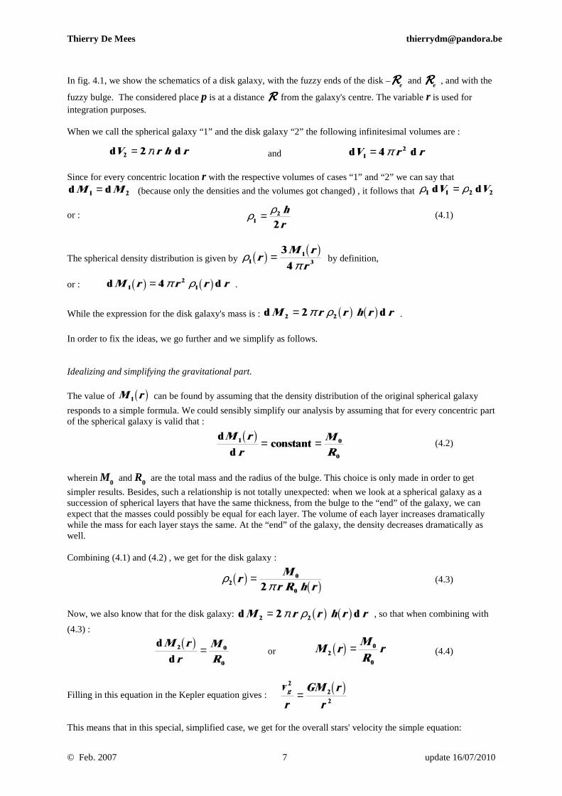
As observed, the velocity is linear with the radius inside the bulge (Zone 0).

fig. 5.2The orbital velocity in the bulge is linear and reaches its maximum at the bulge's boundary.

In fig. 5.2 we see the graphic of the velocities for such a bulge, arbitrary supposed here to be 10% of the diameterof the total disk.

5.2 The zone near the bulge.

5.2.1 More localized gyrotation activity.

The shape of the disk galaxy's section nearby the bulge is resembling a Gauss probability distribution. In thehorizontal direction (x-component), the 'random' distribution of spinning black holes in the bulge and the overallorbital motion of the stars in the bulge contribute in a more accentuated overall gyrotation vector that isperpendicular to the galaxy's disk. This means that the z-component of the gyrotation is far more dominant thanthe x-y-component.

The gyrotation forces constrain the orbits to swivel down, the more away they are from the bulge. This shape willinfluence the gravitational mass to be taken in account in that area, resulting in different orbital velocities.

5.2.2 The gravitational formulation.

The shape of the disk galaxy near the bulge is flattening the more we go away from its bulge.

For stars laying in the disk's plane at a radius (R 2 + H 2 )1/2 from the galaxy's centre (see fig.5.3) , the orbitvelocity will be defined by the mass contained within that radius. For that part of the equation we can argue thatthe relatively wide spread of the stars in this area allows us to use the Kepler equation near the bulge.

For any star in the galaxy, the bulge's area can be seen as a point mass with mass M0 . The corresponding orbit

acceleration is given by:

(5.4) (5.5)

But also the mass outside of that radius will influence that orbit velocity. That part of the equation will better bedescribed by a mass-distribution of a disk.

© Feb. 2007 update 16/07/20101

ab

R H

aG M

Hx( ) /bulge =

+0

2 2 3 2

R

Rc h

D D* γ β

H

dcos d d

coscos

( , ) * /a

G r h r r H r r

Hr

r DR

R

Rα

ρ α α

αβ

=+ −

+ −FHG

IKJ

b g b g b ge j2 2

2

3 2


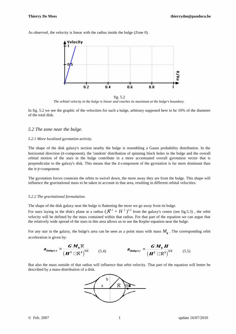
fig. 5.3The bulge area seen as a ellipsoid. A star, orbiting at a distance (R 2 + H 2)1/2 , will get agravitational influence which is equivalent to a point mass of the size of the bulge's mass.

For simplicity, we consider the bulge as a sphere with a radius R0 .

I will now find the gravity formulation for the disk outside the bulge. Then only, I will be able to deduct a globalformulation for the star's velocities nearby the bulge, and at any place in the disk as well.

5.3 The star's velocities, farther in the disk.

5.3.1 The basic gravitational equations.

Although (5.4) is an approximation for stars that are close to the bulge, it is quite close to reality. This will beclear when we analyse the disk's velocities. Hereafter, I deduct the detailed acceleration equations for any place inand close-by the disk.

fig. 5.4A star with mass m orbits about the bulge's nucleus. The infinitesimal ring of a certaindensity and height will be integrated in order to find the orbital velocity of the star.

In fig. 5.4 , r is the variable radius, R the horizontal distance and H the height of the star with mass m.

Following geometrical equations are valid : L² = H² + l² and D² = R² + H². (5.6.a) (5.6.b)

Remark that, for simplicity, we consider a disk with thickness zero. In reality, the disk's thickness is not zero,especially nearby the bulge. Therefore, the deduction hereafter is only valid at a certain distance of the bulge.

Now d d dM r h r r r= ρ αb g b g and dd

( , ) *

*

a GML

DLr DR α =

2(5.7.a) (5.7.b)

where d ( , ) *a r DR α is the infinitesimal centripetal acceleration in the direction of D * .

Also: lr

=−R cos

cos

αβ

and D r H* cos2 2 2= − +R αb g . (5.8.a) (5.8.b)

Thus, with (5.7.a) , (5.7.a) , (5.8.a) and (5.8.b) , equation (5.7.b) becomes :

(5.9)

.

Now : tansin

cosβ α

α=

−rrR

and cos tan/β β= +

−1 2 1 2c h . (5.10.a) (5.10.b)

© Feb. 2007 update 16/07/20101

d αd r

αrR

h/2ll

m

L

l

dcos d d

cos( , ) /

aG M

Rr r

H r rr xR

R

R Rα π

α α

α=

−

+ + −0

02 2 2 3 22 2

b gc h

dd d

cos( , ) /

aG M

RH r

H r rr zR

R Rα π

αα

=+ + −

0

02 2 2

3 22 2c h

a a rr x

R

r x

e

R

R

R( , ) ( , )d d dα

π

α α= zz0

2

0

a a rr z

R

r z

e

R

R

R( , ) ( , )d d dα

π

α α= zz0

2

0

aG M

RH

H H

R H

H H R Rx

e

e e

R

RR

R R R RR

R

R R R( )

sin cos

sin cos

sin cos

sin cosdα

π

πα α

α αα α

α αα= +

+ + + −− +

+ + + −

L

NMM

O

QPPz0

0

2 2

2 2 2 2 2 2

02 2

2 2 2 2 202

00

2

2 2 2c h c h


Using (4.3) , we find : dcos d d

cos( , ) * /

aG M

R

H r r

H r rr DR

R

R Rα π

α α

α=

+ −

+ + −0

0

2 2

2 2 2 3 22 2

b ge jc h

(5.11)

In order to find the horizontal and the vertical component of the acceleration, a projection with angle γ is needed.

Due to symmetry, I disregard the y-component in the plane of the disk.

which result in a multiplication of d ( , ) *a r DR α with cosγ for d ( , )a r xR α and with sinγ for d ( , )a r zR α :

Therefore, notice that : tancos

γα

=−HrR

(5.12)

Using (5.10.b) for the angle γ , and (5.12) , the following components are found:

(5.13)

and

(5.14)

Equation (5.14) is different from zero if H ≠ 0 . From (5.13) and (5.14) follow that the orientation γ of the

infinitesimal vector d a is given by (5.12).

The integration of both (5.13) and (5.14) has to be taken between the following limits (the same limits are validfor the x- and the z-component).

and (5.15) (5.16)

Remember that for the bulge part, we have got another equation. Of course, the integrals (5.15) and (5.16) are

meant to be non-trivial. The integral from 0 to 2π corresponds to twice the integral from 0 to π .

5.3.2 Finding the gravitational equations in the disk.

In the first place, we will integrate the x-component. Remember that the parameters R and H must be taken

constant during the integration. H is not supposed to describe the profile of the galaxy.

Integrating first for r , we find :

(5.17)

This integral has been taken between R0 and R

e .

Also the z-component can easily be integrated for r , which gives the following result:

© Feb. 2007 update 16/07/20101

aG M

R

H

H H

H R

H H R Rz

e

e e

R

R R

R R R RR

R

R R R( )

cos

sin cos

cos

sin cosdα

π

πα

α αα

α αα=

−

+ + + −−

−

+ + + −

L

NMM

O

QPPz0

02 2 2 2 2 2

0

2 2 2 2 202

00

2

2 2 2

b gc h

b gc h

aG M

RR

R Rx H

e

e e

R

R

R R R RR R R R( )

cos cosdα

π

π α αα= =

+ −−

+ −

LNMM

OQPPz0

0

02 2

0

202

00

2

2 2 2

aG MR

RR

R

RHe

e

e

eR

R

R R R

R R

R R R R

R

R,disk = =

−−

−

FHG

IKJ

LNMM

OQPP

−−

−−

FHG

IKJ

LNMM

OQPP

RS|T|

UV|W|

00

02

0

0

0

0

2

2 4

2

4

2ππ π

b g b g b g b gF F, ,

aG M G M

RRR

R

RHe

e

e

eR

R

R

R R R

R R

R R R R

R

R,tot = = +

−−

−

FHG

IKJ

LNMM

OQPP − −

−−

FHG

IKJ

LNMM

OQPP

RS|T|

UV|W|

00

20

02

0

0

0

0

2

2 4

2

4

2ππ π


vG M G M

RR

RR

RH

e

e

e

e

RR

R

R R

R R

R R R

R

R, tot = = +

−−

−

FHG

IKJ

LNMM

OQPP

−−

−−

FHG

IKJ

LNMM

OQPP

RS|T|

UV|W|

00 0

02

0

0

0

0

2

2 4

2

4

2ππ π



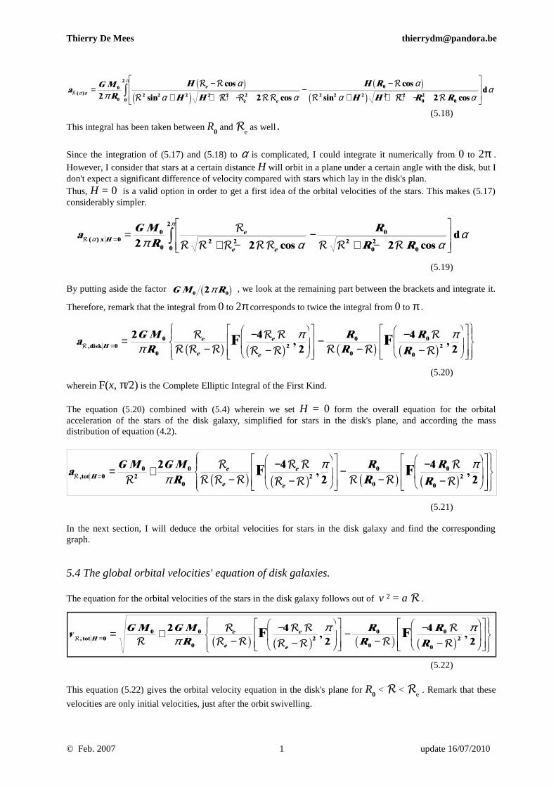
(5.18)

This integral has been taken between R0 and R

e as well.

Since the integration of (5.17) and (5.18) to α is complicated, I could integrate it numerically from 0 to 2π .However, I consider that stars at a certain distance H will orbit in a plane under a certain angle with the disk, but Idon't expect a significant difference of velocity compared with stars which lay in the disk's plan.Thus, H = 0 is a valid option in order to get a first idea of the orbital velocities of the stars. This makes (5.17)considerably simpler.

(5.19)

By putting aside the factor G M R0 02πb g , we look at the remaining part between the brackets and integrate it.

Therefore, remark that the integral from 0 to 2π corresponds to twice the integral from 0 to π .

(5.20)

wherein F(x, π/2) is the Complete Elliptic Integral of the First Kind.

The equation (5.20) combined with (5.4) wherein we set H = 0 form the overall equation for the orbitalacceleration of the stars of the disk galaxy, simplified for stars in the disk's plane, and according the massdistribution of equation (4.2).

(5.21)

In the next section, I will deduce the orbital velocities for stars in the disk galaxy and find the correspondinggraph.

5.4 The global orbital velocities' equation of disk galaxies.

The equation for the orbital velocities of the stars in the disk galaxy follows out of v ² = a R .

(5.22)

This equation (5.22) gives the orbital velocity equation in the disk's plane for R0 < R < R

e . Remark that these

velocities are only initial velocities, just after the orbit swivelling.

© Feb. 2007 update 16/07/20101

R 1 1,2 2 3 4 5 6 7 8 9 10v 1 0,83 1,54 1,75 1,84 1,92 2 2,07 2,17 2,34 2,78

d

d

M r

rMR

2 0

0

b g =


5.4.1 Interpreting the gravitational equations.

The velocities' table is easier to deduce numerically from (5.19) than using equation (5.22) , by avoiding the

Elliptic Integral. By choosing the values R0 1= and Re = 10 , and by varying R between 1 and 10 , thegeneral profile of the disk galaxy's orbital velocities will appear clearly enough. I leave to the reader to experimentwith other mass distributions and with more detailed data by using (5.17) and (5.18).

⇒

tab.5.1

Comparing the figures in tab.5.1 suggests that the galaxies NGC 4594 , NGC 2590 and NGC 1620 (see fig.2.2)respond quite well to the mass distribution of equation (4.2). Other mass distributions will result in other velocitydistributions.We are then able to link mass distributions to velocities and check the theory's validity.

6. Conclusion : are large amounts of “dark matter” necessary to describe disk galaxies ?

With the calculations in this paper, we demonstrated that the gyrotational swivelling of the orbits of elliptical orspherical galaxies permitted to find a consequent velocity deduction for the stars. The found velocities for a massdistribution of d dM r r M R2 0 0b g = gave encouraging results. They describe the stars' velocities of a certain

number of disk galaxies without the need of dark matter. The order in r of the last equation's right hand is zero.This kind of disk galaxies I will call galaxies of order zero.

The physical basics of the MAG theory, with swivelling orbits about spinning black holes in the bulge, seems tolead to at least one kind of disk galaxies: galaxies of order zero. The used mathematical model seems to be totally consistent with galaxies of order zero as well. But other ordersof disk galaxies have still to been analysed.

7. References and interesting lecture.

1. De Mees, T., A coherent dual vector field theory for gravitation, 2003.

2. De Mees, T., Lectures on “A coherent dual vector field theory for gravitation”, 2004.

3. De Mees, T., Discussion: the Dual Gravitation Field versus the Relativity Theory, 2004.

4. De Mees, T., Cassini-Huygens Mission, New evidence for the Dual Field Theory for Gravitation, 2004.

5. De Mees, T., Did Einstein cheat ? or, How Einstein solved the Maxwell Analogy problem, 2004.

6. Jefimenko, O., 1991, Causality, Electromagnetic Induction, and Gravitation, Electret Scientific , 2000.

7. Heaviside, O., A gravitational and electromagnetic Analogy, Part I, The Electrician, 31, 281-282, 1893

© Feb. 2007 update 16/07/20101

Deduction of orbital velocities in disk galaxies - “Dark Matter” a myth?

Documents

Transcript of Deduction of orbital velocities in disk galaxies - “Dark Matter” a myth?