1

Decision Under Risk, Time Constraints, and Opportunity Costs

JAN HAUSFELD & SVEN RESNJANSKIJ1

OCTOBER 2016

IFO INSTITUTE & UNIVERSITY OF KONSTANZ, DEPARTMENT OF ECONOMICS

Are decision errors compatible with rational behavior? We develop a model in which a

decision maker trades off using time for arriving at a risky decision and for pursuing an

alternative activity. When decision time increases the quality of the decision, rational

agents consider the opportunity cost of time when deciding on how much time to allocate

on decision making. In a lab experiment, we introduce exogenous variation in the

opportunity costs of time allocated to making risky decisions by reducing the subjects’

payoffs as decision time increases. Using structural estimations, we elicit preferences

and decision errors. We find no evidence that decreasing decision time in the face of

higher opportunity costs is irrational. Such a behavior is quite compatible with our model

of rational decision-making.

JEL codes: D03, D81, D83

Keywords: decision under risk, time constraints, opportunity costs, rational behavior,

lab experiment, structural estimation

I. Introduction

The quality of many important economic decisions depends on the individual characteristics of the

decision maker and the resources invested into the process of decision making. If investing more time

improves decision making, the optimal allocation of time and therefore the optimal quality of the

decision depends on the opportunity costs of time. We introduce and test a theoretical model in which a

1 Corresponding authors: Sven Resnjanskij, Ifo Institute – Leibniz Institute for Economic Research at the University of Munich e. V.,

resnjanskij@ifo.de. Jan Hausfeld, University of Konstanz, Department of Economics, Graduate School of Decision Sciences, Thurgau Institute

of Economics, Zukunftskolleg, jan.hausfeld@uni-konstanz.de. The authors thank for excellent research assistance and gratefully acknowledge

funding by the Graduate School of Decision Sciences at the University of Konstanz. The authors thank Urs Fischbacher, Heinrich Ursprung,

Ronald Hübner, Chris Starmer, Sebastian Fehrler, and Robert Sugden for their valuable comments and suggestions. This article has benefitted

from comments and suggestions by participants at the European ESA meeting in Heidelberg 2015, the THEEM in Kreuzlingen 2016, the TWI

group, and seminars in Konstanz. All remaining errors are ours.

2

decision maker (DM) rationally trades-off the costs and the quality of a decision under risk. Based on

the revealed preferences of the decision maker, the quality of a decision is measured by the number of

inconsistent choices in risky decisions.

Our economic model is based on the seminal work of Becker (1965) and Minzer (1963) on how

rational agents allocate time optimally recognizing that time has a (shadow) price determined by the

opportunity costs related to alternative time uses. Analyzing the investment of time into the quality of

economic decisions under risk, our work relates to behavioral studies on how time pressure induced by

fixed decision deadlines alters behavior under risk (Kocher, Pahlke, and Trautmann 2013; Nursimulu

and Bossaerts 2013).2 Stigler (1961) introduced the costs of information. Our study complements the

work of Caplin, Dean, and Martin (2011) on the effect of information search on decision making. Based

on the idea of Simon (1955), Caplin, Dean, and Martin (2011) investigate decisions in which not all

information is immediately available to the decision maker. Many important economic consumer

decisions, such as choosing the right pension plan or savings contract, share this feature. Modern

communication technologies provide easy access to all information is easily available. The evaluation

of these information can be seen as the binding constraint in the decision making process. This might

be especially true when risk is involved decision making, which is the concern of this paper.

In line with the Thinking, Fast and Slow metaphor (Kahneman 2011), we indeed find evidence for a

positive causal effect of increased time invested in the decision on the decision quality. However, our

interpretation of a fast decision is in stark contrast to the interpretation of fast and error prone as

irrational. Instead, the DM rationally chooses a lower decision quality by investing less time in the

decision, which is necessary to equalize the marginal utilities of time with respect to its different uses.

We conduct an experiment in which we exogenously vary the opportunity costs of time spent in the

choice between two monetary lotteries. We replicate the seemingly puzzling finding of a positive

correlation between decision errors and decision time, and show that this correlation is dominated by

the (omitted) difficulty of the decision. Instrumenting the decision time with opportunity costs, reveals

a strongly negative causal effect of decision time on errors. Confronted with higher opportunity costs, a

DM reduces time invested in the lottery decision which reduces decision quality and increases the

number of inferior lottery choices.

The notion of irrational behavior has often lead to paternalistic policies or more recently nudges to

improve individual decisions. This has been criticized as it assumes that some authority knows what is

best for the individual. Our approach suggests that, despite the presence of decision errors, agents are

indeed able to behave rationally and that public policy makers even without having full information

about the preferences have plenty of liberal measures to improve decision quality, i.e. by reducing the

decision complexity and information costs or increasing the decision making ability of agents.

2 In contrast to the experiments used in the literature on time pressure, in which a DM is forced by an exogenous time limit, our experimental

setting investigates the effect of time pressure as an endogenous outcome of a decision maker’s trade-off between costs and quality of a

decision.

3

In section II, we introduce our economic model. Section III describes the experiment to test the model

and the data set. Our structural estimation results are provided in section IV. Section VI discusses

potential extensions of our approach. We conclude in section VII.

II. Decision under Risk and Time-dependent Opportunity Costs

In this section, we present a model describing a rational decision maker who is faced with a risky

decision. The decision maker trades off investing time in making a correct lottery choice against a well-

defined opportunity cost of time. The risky choice is between two lotteries ℒ = {𝐿, 𝑅} where 𝑅

(𝐿) denotes the lottery with the higher (lower) expected utility.3 The agent decides on the optimal

allocation of time 𝑇 on the lottery decision 𝑡𝑑 and the alternative use 𝑡𝑜. 𝑢𝑑 denotes the expected utility

related to the lottery choice, whereas uo relates to the utility derived from the alternative use of time

which can be interpreted as opportunity costs of the lottery decision. The opportunity costs are

deterministic and increasing in 𝑡𝑜 (𝜕𝑢𝑜 𝜕𝑡𝑜⁄ > 0). Furthermore, opportunity costs may differ, which is

captured by 𝛼. A higher 𝛼 is assumed to increase the marginal utility of an additional second allocated

not to the lottery choice (𝜕2𝑢𝑜 𝜕𝑡𝑜𝜕𝛼⁄ > 0). The expected utility of the lottery decision depends on the

two available lotteries and the probability 𝜋 of selecting the lottery with the higher expected utility (𝑅).

The probability 𝜋 is increasing in the time invested in the decision (𝜕𝜋 𝜕𝑡𝑑⁄ > 0) and may also depend

on the individual characteristics 𝛾 such as education, skills, and the difficulty of the lottery decision 𝛿.

The agent maximizes

(1) max𝑡𝑜, 𝑡𝑑

𝑢𝑑(𝜋(𝑡𝑑, 𝛾, 𝛿) , ℒ) +𝑢𝑜(𝑡𝑜, 𝛼) s. t. 𝑡𝑜 + 𝑡𝑑 = 𝑇

The first order conditions require equality of the marginal utilities related to both time use opportunities.

(2) 𝜕𝑢𝑑

𝜕𝜋

𝜕𝜋

𝜕𝑡𝑑⏟ 𝑀𝑈𝑑

=𝜕𝑢𝑜

𝜕𝑡𝑜⏟𝑀𝑈𝑜

A higher probability 𝜋 increases 𝐸[𝑢𝑑] because it improves the chance of selecting the lottery with

higher expected utility4. The LHS of equation (2) describes the positive marginal utility of time spent

for the lottery decision. If we further assume5 𝜕2𝜋 𝜕𝑡𝑑2⁄ < 0, we find that 𝑀𝑈𝑑 is decreasing in 𝑡𝑑. The

RHS of equation (2) describes the marginal utility of time w.r.t. the alternative time use.

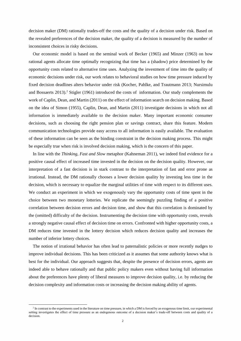
In our experiment, we use different treatments to vary the opportunity costs related to the lottery

decision. An increase of these costs is illustrated in Figure 1 by an upward shift of 𝑀𝑈𝑜 towards 𝑀𝑈𝑜′.

3 For the sake of a notational convenience, we assume 𝑅 ≻ 𝐿 ⟺ 𝐸[𝑢(𝑅)] > 𝐸[𝑢(𝐿)] throughout the paper. 4 The increase of 𝐸[𝑢𝑑] is zero if the two available lotteries yield the same expected utility (𝐸[𝑢(𝑅)] = 𝐸[𝑢(𝐿)]. 5 This assumption is intuitive. The probability 𝜋 has an upper bound of 1, leading to the intuitive assumption that 𝜋 approaches 1 with a

decreasing rate. In our two-lottery set up we can further assume π(0, γ, δ) = 0.5, which corresponds to a random choice between the lotteries if no resources are invested in the lottery decision.

4

FIGURE 1. OPTIMAL TIME INVESTET IN DECISION QUALITY

Notes: The figure presents the equilibrium condition in equation (2) based on the maximization problem (1). In the equilibrium, the optimal

decision time is chosen so that the marginal utilities form investing a unit of time in the lottery decision and in the alternative activity (𝑀𝑈𝑑

and 𝑀𝑈𝑜) are equalized. An increase in opportunity costs 𝛼 shifts the 𝑀𝑈𝑜 upwards to 𝑀𝑈𝑜′ and leads to lower optimal decision time.

From this simple model, we can derive the following prediction. An increase in the opportunity costs

reduces the optimal time invested in the lottery decision and therefore reduces the quality of the decision.

In line with rational behavior, we expect to see more errors in the lottery decisions because investing

more time to improve the lottery decision has to be traded off against the opportunity costs.

III. Data Collection and Experimental Design

Recruitment for Lab Experiment

112 subjects (28 in each treatment) were recruited with ORSEE (Greiner 2015) among the students

of the University of Konstanz. The experiment was programmed in z-Tree (Fischbacher 2007) and

conducted at Lakelab, the economics laboratory at the University of Konstanz. The experiment lasted

about 75 minutes and participants earned €14.29 on average (maximum €88.25, minimum €5.15). The

experiments took place between May and June 2015. Fehler! Verweisquelle konnte nicht gefunden

werden. in Appendix Fehler! Verweisquelle konnte nicht gefunden werden. provides summary

statistics containing socio-economic characteristics of all 112 subjects within the treatments.

Experimental Protocol

The experiment consisted of four parts (Figure 1). First, the participants completed all four questions

of the Berlin Numeracy Test in multiple choice format (Cokely et al. 2012). Second, subjects completed

the Multiple Price List (MPL) of Holt and Laury (2002).6

Afterwards, subjects played 180 lotteries with two states and a wide variety of probabilities.7 We use

a random lottery design which has been used in a several prominent experiments investigating decisions

6 The Berlin Numeracy test and the Holt-Laury task were incentivized. The payoffs were determined at the end of the experiment (after the

Raven’s Test) to rule out potential endowment effects in later stages of the experiment. 7 Appendix Fehler! Verweisquelle konnte nicht gefunden werden. presents the set of lottery pairs used in the experiment to gather the

choice data.

5

under risk (Harrison and Rutström 2008). Finally, subjects completed a smaller version of the Raven’s

Test.

FIGURE 2. SETUP OF THE EXPERIMENT

Note: The figure presents the timeline during the experimental sessions. Parts 1,2, and 4 were similar across treatment conditions. In part 3,

subjects in all treatments were confronted with the same set of 180 lottery choices, but with different opportunity costs related to the decision time.

Treatment-Dependent Opportunity Costs of Time

Time pressure in the lottery task was implemented by time dependent costs in a between subject design.

All subjects had a maximum time of 15 seconds to make a lottery choice. Subjects, not in the control

treatment, were told that they receive the outcome from the lottery plus points from a “Time Account”.

In each round, there were €3 on the time account and the time account yielded no negative points.

Every second (and millisecond) subjects lost8 a treatment dependent amount from their time account (10

cents, 30 cents, 100 cents). In addition to the 28 subjects in each of the three conditions, another 28

subjects were assigned to the control treatment. For subjects in the no time costs treatment, the time

dependent costs of the lottery decision were equal to zero.

IV. Estimation Results

Decision Time and Opportunity Costs

The model described in section II predicts a decrease in time invested in the lottery decision as

opportunity costs increase. Figure 3 presents the average time spent for a lottery decision in each

treatment. The decision time drops by more than 50% from 3.05 seconds in the treatment without

opportunity costs to 1.3 seconds in the treatment with the highest opportunity costs. With the exception

of the comparison between the 10 cent and 30 cent treatment, a t-test with standard errors clustered at

the subject level reveals significant differences (𝑝 < 0.01) across the time spent for the lottery decision

across all treatments.9

8 The instructions said “For every second faster than X seconds, you gain Y cents on your time account“, to avoid a loss frame. 9 These results also maintain for alternative nonparametric tests described in the notes below Figure 3.

6

FIGURE 3. TIME INVESTED IN THE LOTTERY DECISION

Notes: This graph plots the average time subjects spend for a lottery decision in the corresponding treatment and standard errors clustered at

the subject level based on 20160 lottery decision from 112 subjects. Significance of pairwise comparison across treatments is calculated using a t-test clustered at the subject level. Similar significance levels are achieved from using a (blockwise) bootstrapped t-test clustered at the

subject level with 1000 replications and a clustered Mann-Whitney U test. All differences across the control group and each treatment condition

are significant at the one percent level. *** Significant at the 1 percent level.

** Significant at the 5 percent level.

* Significant at the 10 percent level.

Structural Estimates

We use a structural approach to test whether higher opportunity costs reduce the time invested in the

quality of the lottery decision and therefore increase the number of lottery choices in favor of the lottery

with lower expected utility. We elicit the risk preferences, which determine the expected utility

associated with a lottery. Given the risk preferences, we then determine errors in the lottery choices. To

elicit risk preferences we assume a CRRA utility function 𝑢(𝑥) = 𝑥1−𝜌 (1 − 𝜌)⁄ . Furthermore, we

assume that errors in the lottery decision are more likely, if, ceteris paribus, the difference in the expected

utility (∆𝐸[𝑢]) of the two available lotteries is small. A lottery decision in favor of the preferred lottery

(𝑅) depends on ∆𝐸[𝑢] = 𝐸[𝑢(𝑅)]− 𝐸[𝑢(𝐿)] and the realization of a random decision error 휀~𝑁(0,1).

This implementation of a decision error is known as the Fechner error specification (Fechner 1860; Hey

and Orme 1994).10 The standard normal distribution of 휀 ensures that large realizations of the error term

are less likely than small ones. Whenever ∆𝐸[𝑢] + 𝜏 ⋅ 휀 < 0, the DM chooses the inferior lottery 𝐿 and

deviates from the EU prediction.11 The parameter 𝜏 measures the size of the error. A higher 𝜏 corresponds

to more expected decision errors. We estimate our structural parameters 𝜌 and 𝜏, to measure the risk

preference and errors in the lottery decision using the data on the lottery choice between the two

available lotteries in lottery pairs ℒ with the following equation:

(3) 𝐶ℎ𝑜𝑖𝑐𝑒 = ∆𝐸[𝑢(𝜌; ℒ)] + 𝜏 ⋅ 휀, 𝑤𝑖𝑡ℎ 휀~𝑁(0,1).

10 The Fechner error specification has been used as the main specification in several previous studies using stochastic expected utility

models, see for instance (Harrison, List, and Towe 2007; Bruhin, Fehr-Duda, and Epper 2010; Caplin, Dean, and Martin 2011). We discuss alternative error specifications in Appendix XXX based on stochastic expected utility models proposed in Harless and Camerer (1994) and

Loomes and Sugden (1995). Starmer (2000) provides a comprehensive review of different error specifications. 11 Appendix Fehler! Verweisquelle konnte nicht gefunden werden. presents a detailed derivation of our structural estimation procedure.

3.05

1.77 1.70

1.30

0

1

2

3

4

No Time Costs 10centTreatment

30centTreatment

100centTreatment

Decis

ion tim

e in

seconds

***

***

7

To test our theoretical predictions we allow 𝜌 and 𝜏 to depend on the treatment condition. We also

investigate potential heterogeneity with respect to individual characteristics of subjects as well as

estimates on the individual level.

Table 1 presents the structural estimates on the treatment level.12 The first three columns present

results of structural estimations without an explicit error term. We find no treatment effect on the risk

aversion parameter 𝜌. The estimates in columns (3) to (5) correspond to a joint estimation of risk

aversion and the decision error. We find no consistent evidence in favor a change in risk preferences as

a result of higher opportunity costs induced time pressure. The stability of risk preferences is therefore

a valid (implicit) assumption of our economic model in section II.13 However, we find a strong pattern

in the magnitude of decision errors. The errors increase most in the 100cent treatment. In all three

treatments the increase of decision errors is statistically significant. Based on the estimated coefficients

we find evidence that the largest magnitude of decision errors occurs in the treatment with the highest

opportunity costs. As the theoretical model predicts, lower investment (decision time) in the quality of

the lottery decision leads to more decision errors. These errors are identified as deviations from the EU

prediction. In column (5), we allow for heterogeneity in risk preferences and decision quality with

respect to gender (male), age, and numeracy skills (BNT). Male subjects conduct fewer decision errors

and are less risk averse. We find some evidence that lower numeracy skills, measure by the Berlin

Numeracy test (BNT) are correlated with a lower decision quality.

12 To be precise on the meaning of our statistical tests of the results in the table, the interpretation of our t-tests in the results table is as

follows: testing the treatment coefficients against zero, means we try to reject the hypothesis that the preference or error parameter is different

from the value of the control group (constant). Testing the coefficient of the constant in the risk preference (𝜌) equation against zero means trying to reject the null hypothesis of risk neutrality or expected value as choice criteria in the control group. Whereas testing the coefficient

of the constant in the decision error (𝜏) equation against zero, means trying to reject the hypothesis of a deterministic utility theory with no

decision errors, such that 𝐸𝑈(𝑅) > 𝐸𝑈(𝐿) ⇒ Pr(𝐶ℎ𝑜𝑖𝑐𝑒 = 𝑅) = 1, Pr(𝐶ℎ𝑜𝑖𝑐𝑒 = 𝐿) = 0 holds. 13 Based on stable preferences, we can interpret our model as a normative EU model, explaining how the DM should decide. Deviations

from the normative predictions can therefore be interpreted as undesirable decision errors.

8

TABLE 1—STRUCTURAL ESTIMATES

Only Risk Measure Risk & Error Measure

(1) (2) (3) (4) (5)

Parameter: ρ ρ ρ τ ρ τ ρ τ

Treatments 100cent Treatment -0.247 -0.139 -0.073 -0.074 0.130*** -0.138 0.118***

(3.146)

(1.956)

(0.125)

(0.136) (0.026)

(0.149) (0.028)

30cent Treatment -0.589 -0.172 -0.164 -0.154 0.065*** -0.160 0.040** (7.109)

(5.858)

(0.137)

(0.125) (0.018)

(0.118) (0.019)

10cent Treatment -0.624 -0.473 -0.181 -0.185 0.090*** -0.193* 0.051* (3.348)

(3.930)

(0.110)

(0.121) (0.034)

(0.108) (0.029)

Male -0.657 -0.162* -0.071*** (1.065)

(0.093) (0.026)

BNT correct -0.098 -0.040 -0.012* (0.194)

(0.038) (0.007)

Age (18) 0.027 0.024 -0.004 (0.079)

(0.015) (0.004)

constant 0.233 0.429 0.201*** 0.221*** 0.193*** 0.153*** 0.273** 0.234*** (0.151)

(0.336)

(0.064) (0.011)

(0.053) (0.013)

(0.111) (0.031)

p-value for joint significance in: Treatments 0.997 0.999 0.331 0.000 0.354 0.000 0.241 0.000

Log-Likelihood -13049 -13010 -11998 -11931 -11796

Subjects 112 112 112 112 112

Observations 20160 20160 20160 20160 20160

Notes: The dependent variables are the Arrow-Pratt measure of relative risk aversion (ρ) assuming CRRA utility and the Fechner error (τ).

Results in columns (1) – (2) correspond to estimations without any treatment dependent error specification. Results in columns (3) – (5)

correspond to joint estimates of ρ and τ. Block bootstrapped standard errors clustered at the individual level and based on 1000 replications are reported in parentheses.14

*** Significant at the 1 percent level.

** Significant at the 5 percent level. * Significant at the 10 percent level.

The results in Table 1 provide estimates on the treatment level. To check the robustness of our results,

we estimate the structural model for each subject individually and check whether we still identify the

pattern of the estimates in Table 1. Figure 4 plots the individual estimates within each treatment. Visual

inspection reveals a clear rise in the decision error as opportunity costs increase, whereas no clear trend

is observable in the estimated risk preferences. Statistical inference on the treatment differences based

on a nonparametric Mann-Whitney U test reveals quite similar p-values on the statistical differences

across treatments (𝑝∆𝜌: 𝑛𝑜 𝑣𝑠. 10 = 0.140, 𝑝∆𝜌: 𝑛𝑜 𝑣𝑠. 30 = 0.334, 𝑝∆𝜌: 𝑛𝑜 𝑣𝑠. 100 = 0.973). In contrast we

find a highly statistical significant increase in the decision error (𝑝∆𝜏: 𝑛𝑜 𝑣𝑠. 10 = 0.003, 𝑝∆𝜏: 𝑛𝑜 𝑣𝑠. 30 =

0.003, 𝑝∆𝜏: 𝑛𝑜 𝑣𝑠. 100 = 0.000).

14 Moffatt (2015) and Cameron and Miller (2015) provide the technical details on the bootstrap procedure.

9

FIGURE 4. INDIVIDUAL ESTIMATES

Notes: N=111. For one individual the maximum likelihood estimator did not converge. The 𝜌 estimate of 4 observations were smaller than -

10 and are therefore omitted. The 𝜏 estimate of one observation exceeds 1.4 and is omitted in the figure. The statistical tests are performed on the entire sample including the omitted outliers. Appendix Fehler! Verweisquelle konnte nicht gefunden werden. presents scatter plots

including the outliers and details about the nonparametric test.

Quantitative Size of Decision Errors

We established the existence of a treatment effect on the decision error by reporting a statistically

significant increase in the decision error. The question remains whether this increase is economically

significant or small enough that it can be ignored. The size of our decision error parameter 𝜏 is positive

but nonlinearly related to the probability of choosing the inferior lottery. The following example

illustrates the error mechanism for a representative lottery choice (∆𝐸[𝑢] = 0.11) assuming that the

lottery 𝑅 has a higher expected utility than lottery 𝐿. Based on the structural estimates in column 4 in

Table 1, Figure 5 illustrates the increase in the decision error as opportunity costs increase from zero

(control group) to 100 cents. The blue curve illustrates the estimated relatively low decision error (𝜏 =

0.153) in the no time pressure control group. The yellow curve corresponds to high decision error (𝜏 =

0.153 + 0.130 = 0.283) estimate for the 100 cent treatment. Given a lottery choice with ∆𝐸[𝑢] = 0.11,

the estimated treatment effect of the decision error of 𝜏 = 0.130 translates into an increase in the

probability of choosing the suboptimal lottery by 11 percentage points from 24 to 35%.15

15 A random choice would generate an error probability of 50%. Therefore, all improvements in the lottery decision are bounded within the

range between 50 to 100%. An increase by 12 percentage points therefore represents a quantitatively large effect. The decision errors in both

treatments increase as ∆𝐸[𝑢] becomes small. ∆𝐸[𝑢] = 0.11 represents an average utility difference across lotteries.

10

FIGURE 5. EFFECT OF AN INCREASE IN THE DECISION ERROR

Notes: This figure illustrates the effect of the estimated error (𝜏) on the probability of choosing the lottery with lower expected utility. In the

example, lottery R is the correct choice. The parameter values in the illustrated example are ∆𝐸[𝑢] = 0.11, 𝜏𝑛𝑜 = 0.153, 𝜏ℎ𝑖𝑔ℎ = 0.283 (0.153 +

0.130). The estimated 𝜏`s are taken from estimation results in column 4 in Table 1. The low error corresponds to the control group, whereas the high error estimate is based on the results for the high pressure (100cent) treatment group.

Further Results and Alternative Specifications

In Appendix Fehler! Verweisquelle konnte nicht gefunden werden., we discuss the influence of

measures of cognitive ability and education. The economic model of rationality described in section II

explicitly allows for a correlation between individual characteristics 𝛾 and the decision quality defined

as the probability to choose the superior lottery 𝜋, which is (negatively) related to the Fechner error 𝜏 in

the econometric specification decision errors. We find some evidence for a positive relation between

measures of cognitive skills and decision quality. Contrary to Dohmen et al. (2010), but in line with

Sutter et al. (2013) and Andersson et al. (2016 forthc.), we find no evidence for a link between cognitive

measures and risk preferences.

In Appendix Fehler! Verweisquelle konnte nicht gefunden werden., we check the validity of our

structural estimation and compare the risk preferences obtained from our structural estimations to the

estimates based on the Holt-Laury task (Holt and Laury 2002). The estimates from the Holt-Laury tasks

are correlated to the structural estimates. The Holt-Laury estimates might also serve as control for

individual heterogeneity in risk preferences within and across treatments.

The model described in section II assumes additive separable utility with respect to utility derived

from the lottery decision and the alternative opportunity. The rationale of additive utility comes from

the potential underlying trade-off between investing resources in a decision and deriving utility from

spending these resources for other utility generating activities.16 Our estimates are however robust

against relaxing these assumptions. In Fehler! Verweisquelle konnte nicht gefunden werden. in

Appendix Fehler! Verweisquelle konnte nicht gefunden werden., we provide evidence that error

16 One could for instance think of a situation in which a decision maker has to decide on alternative insurance contracts, while investing

more time in studying and understanding the consequences of each insurance contract has to be traded-off against spending this time for leisure

or work.

11

pattern and the stability of risk preferences described in our main results are unchanged if we assume

that the DM integrates the entire payoff from both time account and lottery choice into the lottery

decision. Results are also unchanged if we assume different initial endowments suggesting that our

results are not sensitive to different assumptions about narrow bracketing or mental accounting.

Appendix Fehler! Verweisquelle konnte nicht gefunden werden. provides results of our estimates

for subsamples of our lottery set. The results are quantitatively similar in each subsample, suggesting

that potential learning effects do not interact with our main results. In Appendix Fehler! Verweisquelle

konnte nicht gefunden werden., we fix different 𝜌 across subjects in order to investigate whether

pattern of the decision errors still prevails. Again, we find the same pattern that errors are lowest in the

no cost treatment. We obtain similar results when we relax the assumption of constant relative risk

aversion and use the more flexible expo-power utility function first proposed by Saha (1993). The

corresponding results are presented in Appendix Fehler! Verweisquelle konnte nicht gefunden

werden..

V. Empirical Puzzles Related to the Investment of Time in Economic Decisions

Two results of previous studies seem to be in stark contrast to the predictions of our economic model.

First, subjects were found to invest more time in lottery decisions when the utility difference between

two available lotteries is small and an improved quality of the lottery decision increases expected utility

only slightly (Dickhaut et al. 2013; Krajbich, Oud, and Fehr 2014). Second, longer decision times were

found to correlate with a higher incidence of decision errors.

In this section, we show that both puzzles can be explained by our model of rational agents. Particular,

we provide evidence that – while the correlation between decision time and quality is indeed negative –

the causal effect of an increase in decision time on the quality of the decision is positive as predicted by

our rational agent model.

Is time invested in economic decisions, when it doesn’t matter?

Gabaix et al. (2006), Chabris et al. (2009), Dickhaut et al. (2013), and Krajbich, Oud, and Fehr (2014)

find that more effort – as measured by decision time – is exerted when the utility difference between the

two possible choices is small. Substituting the time constraint into the maximization problem (1), the

agent chooses an optimal time span 𝑡𝑑∗ for selecting a lottery:

(4) 𝑚𝑎𝑥 𝑡𝑑 𝑈 ≡ 𝜋(𝑡𝑑 , 𝛾, 𝛿) ⋅ 𝐸[𝑢(𝑅)] + (1 − 𝜋(𝑡𝑑 , 𝛾, 𝛿)) ⋅ 𝐸[𝑢(𝐿)] +𝑢𝑜(1 − 𝑡𝑑 , 𝛼).

Based on the first order condition in equation (5), a smaller utility difference ∆𝐸[𝑢] = 𝐸[𝑢(𝑅)] −

𝐸[𝑢(𝐿)] makes a decision error less costly, and requires a lower 𝑡𝑑, since 𝜕𝜋 𝜕𝑡𝑑⁄ is assumed to be positive.

(5) 𝜕𝑈

𝜕𝑡𝑑= (𝐸[𝑢(𝑅)] − 𝐸[𝑢(𝐿)]) ⋅

𝜕𝜋

𝜕𝑡𝑑⏟>0

+𝜕𝑢𝑜

𝜕𝑡𝑑⏟<0

=!0

Moffatt (2005), Dickhaut et al. (2013), and Krajbich, Oud, and Fehr (2014) find exactly the opposite.

Based on their finding, Krajbich, Oud, and Fehr (2014) conclude that the observed pattern in time

12

allocation cannot be explained by a (stochastic) expected utility model and suggest the drift-diffusion

model (DDM) as a superior theoretical alternative. To investigate the discrepancy between these

findings and our model, we proceed as follows: We first provide a short review of the DDM. Then we

show that 𝜕𝑡𝑑∗ 𝜕∆𝐸[𝑢] < 0⁄ , can be rationalized the help of the model introduced in section I. Finally, we

estimate the DDM with our data and show that, contrary to Krajbich, Oud, and Fehr (2014), the DDM

does not provide strong support for the claim that decision time correlates negatively with the utility

difference (𝜕𝑡𝑑 𝜕∆𝐸[𝑢] < 0⁄ ).

As-If Expected Utility Model and the Neuro-founded Drift Diffusion Model.—While expected utility

(Neumann and Morgenstern 1944) has its roots in axiomatic theory, the drift diffusion model (DDM)

emulates the decisions process the human brain actually relies on. Decision values are encoded by

neurons that transmit all-or-nothing information (Krajbich, Oud, and Fehr 2014): only when the signals

add up to a sufficiently large boundary a decision will be made. Contrary to the process oriented DDM

that portrays the neuropsychological process, the expected utility model is usually interpreted as an as-

if model, i.e. a black box that does not describe the underlying mechanisms governing the decision

process.

Ratcliff (1978) introduced the drift-diffusion model of dynamic evidence accumulation processing to

predict both choice behavior and the distribution of decision times.17 The DDM assumes that the

decision maker observes two types of signals indicating the value of the two available lotteries and

continuously updates the resulting relative decision value (RDV). This process continues until a choice

specific threshold is reached. Figure 6 presents a graphical representation of the DDM. The bold line

shows how the RDV develops across time. The dashed line represents the drift rate (𝜇). The horizontal

long-dashed lines represent the threshold values (B) that trigger the choice of the respective lottery. NDT

denotes the non-decision part of time, usually interpreted as the time needed to encode the information

stimulus and to move to response execution (Ratcliff and McKoon 2008).18

17 For a recent survey on the drift-diffusion model see Ratcliff and McKoon (2008). For the description of the DDM we rely on Fehr and

Rangel (2011) and Krajbich, Oud, and Fehr (2014) who provide short surveys on the use of the DDM in the economic literature. 18 In our experiment, the non-decision time (NDT) could be interpreted as time subjects needed to use the computer mouse to indicate their

lottery choice as well as the time needed to visually recognize the information provided on the computer screen.

13

FIGURE 6. THE DRIFT DIFFUSION MODEL

Notes: … The example presented in the figure illustrates two evidence accumulation processes in which the decision maker decides for the superior lottery R (upper boundary). The two processes differ w.r.t. the drift or on how fast the evidence accumulation process drifts towards

the correct lottery decision.

The evolution of the RDV is a Brownian motion with a constant drift rate (𝜇). The Brownian motion

represents the stochastic part of the decision, whereas the drift rate towards the preferred option is

governed by the decision maker’s ability to discriminate between the lotteries and the quality of the

signals (possibly related to lottery difficulty). If the thresholds are relatively small and/or the drift rate

is low, the stochastic element of the process can dominate choice behavior and give rise to errors. In

Figure 6 this would mean that the RDV path hits the lower boundary.

Following Krajbich, Oud, and Fehr (2014), the difficulty of decision and therefore the drift rate is a

decreasing in the utility difference between the two available lotteries. The RDV evolves according to:

(6) 𝑅𝐷𝑉𝑡 = 𝑅𝐷𝑉𝑡−1 + 𝑣×∆𝐸[𝑢] + 휀.

The drift rate is determined by the product 𝑣×∆𝐸[𝑢]. The stochastic element of the choice process is

represented by 휀~𝑁(0, 𝜎2).

Theoretical and Empirical Predictions of the DDM with respect to decision time.—According to

equation (6), the drift diffusion model clearly predicts that decision time varies negatively with the

expected utility difference. When the expected utility difference in small (μ∆𝐸𝑈), the decision time is

longer than when the expected utility difference is large (𝜇∆𝐸𝑈̅̅ ̅̅ ̅̅ ), because it is more difficult to

discriminate between the two lotteries.19 As a result, the evidence accumulation process is slower. The

comparison of the two accumulation processes is illustrated in Figure 6. Similar to Moffatt (2005),

Dickhaut et al. (2013), Krajbich, Oud, and Fehr (2014),20 we find a robust negative correlation between

the time invested in the decision and the estimated expected utility difference (Figure 7).21

19 Fehr and Rangel (2011) summarize stylized facts related to the predictions of the DDM, including the prediction that difficulty as

measured by the utility difference, is positively related to the decision time. 20 Several studies find a robust negative correlation between the decision time and the difference in the values of choices (see e.g. (Gabaix

et al. 2006; Chabris et al. 2009). 21 A bivariate linear regression of decision time on ∆𝐸[𝑢] reveals a highly significant negative slope coefficient of −1.35 (𝑡 = 8.19, 𝑝 −

𝑣𝑎𝑙𝑢𝑒 < 0.001, 𝑛 = 19,906). Standard errors were clustered at the subject level.

14

FIGURE 7. EXPECTED UTILITY DIFFERENCE AND DECISION TIME

Notes: The Scatterplot presents decision times of 19980 individual lottery decisions obtained from 111 subjects. A nonparametric regression line (lowess) is overlaid on top of the data.

Based on their finding, Krajbich, Oud, and Fehr (2014) conclude that the DDM correctly predicts this

relationship, while an (stochastic) expected utility model does not. Our results do not support this view.

We allow the difficulty 𝛿 of a decision to codetermine the probability 𝜋(𝑡𝑑, 𝛾, 𝛿) of making a correct

decision. In line with the reasoning of the DDM, we set 𝛿 = ∆𝐸[𝑢] and assume 𝜕𝜋 𝜕(∆𝐸[𝑢])⁄ > 0.

Reformulating the first-order condition from equation (5) gives

(7) 𝜕𝑈

𝜕𝑡𝑑= ∆𝐸[𝑢]⏟ 𝑖𝑚𝑝𝑜𝑟𝑡𝑎𝑛𝑐𝑒𝑒𝑓𝑓𝑒𝑐𝑡

⋅𝜕𝜋(𝒕𝒅,𝜸,∆𝑬𝑼)

𝜕𝑡𝑑⏟ 𝑑𝑖𝑓𝑓𝑖𝑐𝑢𝑙𝑡𝑦𝑒𝑓𝑓𝑒𝑐𝑡

+𝜕𝑢𝑜

𝜕𝑡𝑑⏟<0

=!0.

Equation (7) illustrates the trade-off between responding to a higher difficulty and a lower importance

of the decision. A lower importance, denoted by a lower ∆𝐸[𝑢], enters the first factor of the product in

equation (7) and decreases (c.p.) the optimal time invested in the decision (𝑡𝑑∗) because 𝜋 is assumed to

be an increasing and concave (𝜕2𝜋 𝜕𝑡𝑑2⁄ < 0) function in 𝑡𝑑. But, a lower ∆𝐸[𝑢] also increases the

difficulty to identify the superior lottery. Assuming that a lower ∆𝐸[𝑢] will not only decrease the

probability to choose the superior lottery at any given decision time (𝜕𝜋 𝜕∆𝐸[𝑢]⁄ > 0), but also decreases

the marginal utility from spending an additional unit of time in the lottery decision

(𝜕2𝜋(𝑡𝑑 , 𝛾, ∆𝐸𝑈) (𝜕𝑡𝑑𝜕(∆𝐸𝑈)) ⁄ < 0), the difficulty effect will lead to more time invested in the lottery

choice and thereby counteracts the importance effect. Signing 𝜕𝑡𝑑∗ 𝜕∆𝐸𝑈⁄ is therefore an empirical

question. In contrast to the interpretation of Krajbich, Oud, and Fehr (2014), our results suggest that a

negative correlation between 𝑡𝑑 and ∆𝐸[𝑢] cannot be interpreted as evidence against the expected utility

model. We rather interpret the ability of the expected utility model to reveal the two opposing effects that

govern optimal decision time as a strength of the traditional model.

05

10

15

20

0 .2 .4 .6 .8 1

Individual choices Non-parametric regression line (lowess)

in s

econ

ds

De

cis

ion

Tim

e

EU differencebased on individual risk parameter estimates

15

Is time an essential resource in the decision production function?

Applications of the DDM usually find a puzzling empirical regularity – a negative correlation between

decision time and probability to choose the superior option. This finding is in stark contrast to the crucial

assumption that time is valuable resource in the production of sound economic reasoning (𝜕𝜋 𝜕𝑡𝑑⁄ > 0).

In the DDM the drift towards the preferred decision boundary causes a correct choice. However, the

lower the drift rate, the longer continues the accumulation process, and the more likely it becomes

(conditional on the fact that the RDV has still not reached the boundary of the superior option) that the

stochastic component of the DDM will cause the RDV to cross the boundary of the inferior option.

Hence, changes in the drift rate caused by a variation in the difficulty of a decision, produce a negative

correlation between decision time and quality.

In this subsection, we first show that – despite the presence of a negative correlation – the causal

effect of more time invested in the lottery decision on the quality of the decision is positive suggesting

that time can be interpreted as production factor in a capital-labor production framework of decision

quality (Camerer and Hogarth 1999). As a final exercise, we estimate the treatment effect of an increase

in opportunity costs within the DDM framework. The results suggest that the quantitative effects and

the underlying mechanisms of higher opportunity costs are similar in the neuro-founded and process-

oriented DDM and the expected utility model highlighting how well the as-if expected utility model can

represent the basic underlying choice mechanisms.

To reproduce the empirical evidence for a negative correlation between decision time and quality, we

estimate the following regression:

(8) 𝐶𝑜𝑟𝑟𝑒𝑐𝑡𝐶ℎ𝑜𝑖𝑐𝑒 = 𝛽1 + 𝛽2 𝐷𝑒𝑐𝑖𝑠𝑖𝑜𝑛𝑇𝑖𝑚𝑒 + 𝛃𝐗 + 휀,

where 𝐗 denotes a vector of additional controls. Column (1) in Table 2 contains the estimate of 𝛽2 based

on the linear probability model. The coefficient is negative and highly significant suggesting than an

additional second invested in the lottery decision reduces the probability of choosing the superior lottery

by 1.4 percentage points. A strong thread towards a causal interpretation is the difficulty of the lottery

decision, which is likely to be positively correlated with DecisionTime and negatively correlated the

probability of a CorrectChoice. Based on the standard omitted variable formulae, 𝛽2 is downward biased.

A straightforward approach to correct for the omitted variable bias is to try to control for the difficulty of the

decision. In model (3) in Table 2, we include the expected utility distance as proxy variable for the difficulty

in the regression.22 The effect of the expected utility difference (normalized to be between zero and one) is

positive and significant. The correlation between decision time and the correct choice probability is

essentially zero after including the expected utility difference as proxy for the decision difficulty. Still, there

is a lot of ambiguity around the difficulty measure w.r.t. to the functional form and the inherent subjective

nature of the difficulty of a decision.23 Therefore, it is illusive to claim that after controlling for the expected

utility difference, 𝛽2 can be interpreted as causal effect.

22 The underlying risk preferences used to calculate the expected utility difference are based on individual estimations for each subject as

presented in Figure 4. For a similar approach see Moffatt (2005). 23 See for instance Chabris et al. (2009) and Moffatt (2005) for alternative functional forms of the decision difficulty proxy variable. In

general, the construction of any difficulty measure seems to include some arbitrary and non-testable modelling choices.

16

We circumvent these problems with our research design. Our randomized opportunity cost treatments

provide us with the ideal instrument for the time invested in the decision. The increase in the opportunity

costs across our treatment conditions has a negative effect on the decision time, but is – conditional on

the decision time – completely unrelated to the lottery choice. We therefore use standard instrumental

variable techniques to identity the causal effect of decision time on the quality of the decision measured

as probability to choose the superior lottery. The results are presented in models (4) to (6) in Table 2.

The negative relation between the opportunity costs and the decision time, measured in the first stage as

the effect of the treatment dummies on the decision time produces a F-statistics on the instruments of

above 30.24 Based on the IV estimates, the resulting causal effect of a time investment on the decision

quality is positive and statistical significant and ranges from an improvement of 2.3 to 3.7 percentage

points in the probability of a correct choice for an additional second invested in the lottery decision.

TABLE 2— DECISION QUALITY AND TIME INVESTED IN THE DECISION

Dep. Variable: Correct Lottery Choice (binary)

LPM (OLS) 2SLS

(1) (2) (3) (4) (5) (6)

Decision Time -0.014*** -0.012** -0.001 0.023*** 0.023*** 0.037*** (0.005) (0.005) (0.005)

(0.008) (0.008) (0.008)

EV difference (abs) 0.049*** 0.051*** (0.003)

(0.003)

EU difference (abs) 0.593*** 0.646*** (0.039)

(0.037)

Constant 0.773*** 0.715*** 0.657*** 0.699*** 0.644*** 0.574*** (0.013) (0.013) (0.013)

(0.019) (0.020) (0.020)

Instrument for Decision Time – – – Treatment Dummies

First Stage F-Stat – – – 30.71 30.71 31.37

Subjects 111 111 111 111 111 111

Observations 19460 19460 19460 19460 19460 19460

Notes: OLS estimates ((1) - (3)) and IV 2SLS ((3) - (5)) are reported. The dependent variable is a binary variable equal to one if the lottery

with higher expected utility is chosen by the subject and zero otherwise. The underlying risk preferences are based on individual estimates of

the CRRA coefficient (presented in Figure 4). Heteroskedasticity-robust standard errors are reported in parentheses. *** Significant at the 1 percent level.

** Significant at the 5 percent level.

* Significant at the 10 percent level.

Finally, we show that the drift diffusion model, essentially predicts the same positive causal effect,

despite the fact that many studies using the DDM find a negative correlation between decision time and

quality. As discussed in the previous section, a higher difficulty of the decision results in a lower drift

rate. In addition, closer boundaries are affected by the speed-accuracy trade-off (Ratcliff and McKoon

2008).25 Closer boundaries decrease the decision time and consequently the opportunity costs of the

decision at the expense of more decision errors. Figure 8 illustrates the effect of closer boundaries. In

the right panel (b), closer boundaries decrease the expected time, the RDV needs to cross the upper

24 The quantitative dimension of the first stage results can be observed from Figure 3 and its explanation in section IV.A. 25 The speed accuracy trade-off is the term used in the psychological literature to describe the trade-off between faster and more accurate

decisions.

17

boundary. However, it becomes also more likely that the stochastic component of the accumulation

process will shift the RDV towards crossing the lower boundary and triggers an inferior lottery choice.

FIGURE 8. EFFECT OF A DECREASE IN THE BOUNDARIES OF THE DRIFT DIFFUSION MODEL

Notes: Panel (a) and (b) illustrate the change in the trade-off between costs of the decision, measured by the time invested in the decision and

the quality of the decision denoted as probability to choose the high EU lottery. Closer boundaries in panel (b) result in a decrease of the time

until a decision is triggered, but increases the likelihood to arrive at the lower boundary and choose the inferior lottery. In line with the comparative static results of the expected utility model, the change of the boundaries in the DDM can be interpreted as a result of an agent’s

optimal solution of trade-off between the opportunity costs of time and the quality of the decision.

Empirical studies lacking exogenous variation in the opportunity costs, may identify a negative

correlation between decision time and quality by variation in the difficulty among the decision tasks,

but are unable to establish causality. In the DDM the omitted variable bias related to the causal effect

of decision time on decision quality arises, if the researcher (i) a priori does not allow the boundaries to

be endogenously chosen or (ii) has no exogenous variation in the decision time which is independent of

the difficulty of the decision problem. To estimate the causal effect of time within the DDM framework,

we estimate the DDM parameters on the treatment level using the fast-DM software developed by (Voss

and Voss 2007; Voss, Voss, and Lerche 2015). Table 4 provides the results.

TABLE 3—ESTIMATES OF THE DRIFT DIFFUSION MODEL

Decision Criteria: Expected Utility

no cost 10 cent 30 cent 100 cent

Decision Boundaries (B) 2.73 1.70 1.60 1.34

p-value (H0: no cost = treatment) – [0.000] [0.000] [0.000]

Drift Rate (𝜇) 0.35 0.42 0.48 0.40 p-value (H0: no cost = treatment) – [0.058] [0.011] [0.227]

Non-Decisional Time (NDT) 1.25 1.07 1.09 0.87

p-value (H0: no cost = treatment) – [0.044] [0.056] [0.000]

Notes: Parameter estimates of the Drift diffusion model based on the estimation results in model 5 in Table 1 (N=112). P-values based on pairwise t-test on the difference of subjects in the control group (no cost) and subjects in the corresponding treatment are reported in brackets.

We set 𝜎 = 1 in the stochastic component of the DDM (휀~𝑁(0, 𝜎2)) to identify the parameters of the DDM ( see e.g. Ratcliff (1978), Krajbich, Oud, and Fehr (2014)). Since the position of the two lotteries was randomized in the experiment and both lotteries were presented

simultaneously, we fix the starting point of the RDV to the middle between the two lotteries (no initial bias towards a specific lottery). In

addition to the fitted parameters B, 𝜇, NDT, we also estimate the parameters related to the variability of the drift rate 𝜇 and the starting point of the RDV (results available on request). Rather similar results are obtained from using risk preferences from individual estimations (see Appendix Fehler! Verweisquelle konnte nicht gefunden werden., Fehler! Verweisquelle konnte nicht gefunden werden.).

In line with the economic intuition derived from the expected utility model, we find a statistical

significant decline in the boundaries as opportunity costs of the decision time increase. We also find

some (mixed) evidence for an increase in the drift rate. A higher drift rate would point towards a higher

decision quality, whereas lower boundaries increase the likelihood of choosing the inferior lottery. To

18

quantify the overall effect of an opportunity costs induced change in the decision time on the decision

quality, we estimate the partial effect of a change in the drift rate, the boundaries, and both

simultaneously on the decision quality, while keeping all other parameters of the DDM constant at their

sample means.

TABLE 4—PREDICTIONS OF THE DRIFT DIFFUSION MODEL

Pred. Prob. of Correct Choice (�̂�) Pred. Decision Time (𝑡�̂�)

no cost 10 cent 30 cent 100 cent no cost 10 cent 30 cent 100 cent

Prediction of the DDM due to change in

Boundaries (∆𝐵) 75.1% 66.6% 65.5% 63.2% 2.73 1.76 1.68 1.50

Drift (∆𝜇) 65.3% 68.2% 70.4% 67.3% 1.88 1.87 1.86 1.87

Both (∆𝐵 & ∆𝜇) 71.8% 66.9% 68.0% 62.7%

2.78 1.76 1.67 1.50

Notes: Predictions of the DDM for the Probability of a correct choice ((�̂�) and the decision time (𝑡�̂�) are presented. The predictions are based on 500001 simulations with all remaining parameters set at their sample mean values. The correct choice is determined from the utility difference based on the estimation results in model 5 in Table 1. Rather similar results are obtained from using risk preferences from individual

estimations (see Appendix Fehler! Verweisquelle konnte nicht gefunden werden., Fehler! Verweisquelle konnte nicht gefunden

werden.).

The simulation results based on the DDM suggest that a change in boundaries would predicts a decline

of the correct choice probability from 75.1 percent in the no cost control group to below 64 percent in

the 100cent treatment. This effect is partially offset by the simultaneous change in the drift rate. Overall,

based on the simulations of the DDM, the rise in the opportunity costs from zero to 100 cents per second,

decreases the time invested in the lottery decision from 2.78 to 1.5 seconds, which causes a decline in

probability of correct choice by more than 9 percentage points. Like the empirical and theoretical

consideration within the expected utility framework, the application of the DDM points towards a

positive causal effect of time investment on the quality of the decision.

In the final analysis, the expected utility model performs well as as-if model as it provides similar

results as the neuro-founded and decision process oriented DDM. The results from the DDM add

additional explanatory power to our argument that important mechanisms related to the trade-off

between the opportunity costs of time and the quality of decisions can be explained by a simple rational

utility model, like the one we suggest in the paper.

VI. Further Research and Limitations of the Study

We successfully test several comparative statics of the economic model introduced in section II and

demonstrate that decision errors cannot be simply interpreted as irrational behavior. However, our

theoretical framework does not provide an exact point estimate on the optimal allocation of time. This

would require further structural assumptions on the decision-making process captured by 𝜋 in our model.

The specific functional form of 𝜋 determines the rate of improvement in the lottery decision and is therefore

instrumental to determine the exact optimal time investment in the lottery choice.

Another open question is concerned to the influence of prior beliefs of the decision maker on the

range of outcomes, which may be reached by alternative lottery choices. We introduce an extension of

our model in Appendix Fehler! Verweisquelle konnte nicht gefunden werden. to capture the effect

of such prior beliefs. In our model, the entire uncertainty related to the lottery decision is captured in the

19

probability 𝜋, whereas the utility difference ∆𝐸[𝑢], which can be interpreted as measure of the

importance of the lottery decision, is predetermined and known to the decision maker. We relax this

assumption in Appendix Fehler! Verweisquelle konnte nicht gefunden werden. and assume that

∆𝐸[𝑢], is not deterministic but rather an à priori unknown random variable, which properties might be

learned by interpreting signals at a very early stage of the decision making process. As we demonstrate

in section V, even without an early stage, our basic model is able to produce similar predictions as the

process-oriented DDM.26

However, a straight-forward implication of such an initial stage would be that the DM would invest

more resources in the decision making process if early gathered information change the beliefs w.r.t. to

the importance of the decision by indicating higher lottery payoffs. Indeed, we find that higher payoffs

measured by either the dummy indication at least one state in which the payoff exceeds €20 or by the

sum of the lottery payoffs of the two available lotteries, lead to fewer decision errors.27 The extension

of the model adds additional insights for the decision making process at the cost of increased model

complexity and reduced ability to easily apply the model in other areas of economics in which the

process of decision making is of minor interest. Our intuition is that the most important economic

mechanisms can be described with our basic model.

VII. Conclusion

What kind of a model of rationality do we seek? We introduce a simple model in which a rational

decision maker trades-off the quality and opportunity costs of the decisions in a rational manner.

In contrast to related extensions of the rational model (Chabris et al. 2009; Dickhaut et al. 2013) our

model is parsimonious and simple enough to be integrated in applied economic work. It is in line with

basic economic reasoning that investing more resources in the production of sound economic decision

improves decision quality, and provides a number of testable predictions.

To test the prediction that decision errors can be rationalized by high opportunity costs, we test main

implications of our model using a structural econometric approach. Our study provides evidence that

decision errors vary positively with opportunity costs of decision making, which is in line with the

rational prediction that decision errors are more likely because higher opportunity costs induce a lower

time investment in the decision quality. Despite the existence of a negative correlation between decision

time and quality, we find a strong positive causal impact of an increase in time invested in the lottery

decision on the quality of the decision, which supports the validity of or economic model. We find no

evidence that risk preferences change with respect to decision time, which allows a normative

interpretation of the model based on the stable preference assumption (Stigler and Becker 1977).

26 Psychological models of decision making such as the drift diffusion model (see e.g. Ratcliff and McKoon (2008)) incorporate an initial

stage of the decision making process by estimating a non-decision time in which the DM scans the available information, before entering the

decision process. 27 Results are provided in Fehler! Verweisquelle konnte nicht gefunden werden. in Appendix Fehler! Verweisquelle konnte nicht

gefunden werden..

20

In the final analysis, our results suggest that so-called behavioral anomalies manifested as errors in

economic decisions might be the outcome of a rational trade-off, if (1) the problems are complex, (2)

opportunity costs of investing time and other resources to improve decision making are high, and (3)

individual decision skills are low. Remaining decision errors might then not be interpreted as irrational

behavior alone, but as a result of a rational trade-off under given constraints.

While our work on the foundation of preferences and decision making under risk is not directly policy

relevant at this stage. We believe that our work may lay the foundation for future applied work fostering

a wide range of policy implications. Starting with a normative model of decision making, we show that

decision makers follow more often the rational prediction, if cost for investing time in the decision is

low. Empirical studies find a wide range of irrational behavior in agents’ decisions making under risk,

for instance the poor quality of stock market investments of individual agents or the lack in the demand

of health insurance.

In a sense, our work is grounded in the theories of human capital and labor supply. No economist

would call it irrational that not every individual has the ability to earn the wage of a CEO of a large

company. In the same vein, we should not call it irrational that not everyone has the ability to always

make the best decision no matter how complex the decision is or how much resources are invested in

making the decision. In both cases, the productivity of the worker or the ability of the decision maker

depends on individual skills. The investment into these skills provide the rationale for education and

more general for the formation of human capital. In the basic labor-supply model, in addition to the

wage rate, income depends on the hours worked, determined by solving the trade-off between working

more and increase earnings or spending the time on alternative uses (i.e. leisure as determinant of the

opportunity costs of time). Similarly, the income earned from a decision depends on the time spent in

the decision-making process, which is determined by the same underlying trade-off.

In both tradeoffs, the rational solution is likely to be characterized by forgiven income, either by not

earning the full income or by not making the best decision with probability one, is not an outcome of

irrationality, but a rational response to the opportunity costs of time.

21

References

Andersson, Ola, Jean-Robert Tyran, Erik Wengström, and Håkan J. Holm. 2016 forthc. “Risk

Aversion Relates to Cognitive Ability: Preference or Noise?” Journal of the European Economic

Association.

Becker, Gary S. 1965. “A Theory of the Allocation of Time.” The Economic Journal, 75(299): 493–

517.

Ben Zur, Hasida and Shlomo J. Breznitz. 1981. “The effect of time pressure on risky choice

behavior.” Acta Psychologica, 47(2): 89–104.

Benjamin, Daniel J., Sebastian A. Brown, and Jesse M. Shapiro. 2013. “Who is 'Behavioral'?

Cognitive Ability and Anomalous Preferences.” Journal of the European Economic Association,

11(6): 1231–55.

Bruhin, Adrian, Helga Fehr-Duda, and Thomas Epper. 2010. “Risk and Rationality: Uncovering

Heterogeneity in Probability Distortion.” Econometrica, 78(4): 1375–412.

Camerer, Colin F. and Robin M. Hogarth. 1999. “The Effects of Financial Incentives in Experiments:

A Review and Capital-Labor-Production Framework.” Journal of Risk and Uncertainty, 19(1-3): 7–

42.

Cameron, Collin A. and Douglas L. Miller. 2015. “A Practitioner's Guide to Cluster-Robust

Inference.” Journal of Human Ressources, 50(2): 317–72.

Caplin, Andrew, Mark Dean, and Daniel Martin. 2011. “Search and Satisficing.” American

Economic Review, 101(7): 2899–922.

Chabris, Christopher F., Carrie L. Morris, Dmitry Taubinsky, David Laibson, and Jonathon P.

Schuldt. 2009. “The Allocation of Time in Decision Making.” Journal of the European Economic

Association, 7(2/3): 628–37.

Cokely, Edward T., Mirta Galesic, Eric Schulz, Saima Ghazal, and Rocio Garcia-Retamero. 2012.

“Measuring risk literacy: The Berlin Numeracy Test.” Judgment and Decision Making, 7(1): 25–47.

Conroy, R. M. 2012. “What hypotheses do "nonparametric" two-group tests actually test?” Stata

Journal, 12(2): 182–90.

Cox, James C. and Vjollca Sadiraj. 2006. “Small- and large-stakes risk aversion: Implications of

concavity calibration for decision theory.” Games and Economic Behavior, 56(1): 45–60.

Cox, James C., Vjollca Sadiraj, Ulrich Schmidt, and Raquel Carrasco. 2014. “Asymmetrically

Dominated Choice Problems, the Isolation Hypothesis and Random Incentive Mechanisms.” PLoS

ONE, 9(3): e90742.

Dickhaut, John, Vernon Smith, Baohua Xin, and Aldo Rustichini. 2013. “Human economic choice

as costly information processing.” Journal of Economic Behavior & Organization, 94(0): 206–21.

Dohmen, Thomas, Armin Falk, David Huffman, and Uwe Sunde. 2010. “Are Risk Aversion and

Impatience Related to Cognitive Ability?” American Economic Review, 100(3): 1238–60.

Fechner, Gustav T. 1860. Elemente der Psychophysik. 2 Vols. Leipzig: Breitkopf und Härtel.

22

Fehr, Ernst and Antonio Rangel. 2011. “Neuroeconomic Foundations of Economic Choice--Recent

Advances.” Journal of Economic Perspectives, 25(4): 3–30.

Fischbacher, Urs. 2007. “Z-Tree: Zurich Toolbox for Ready-Made Economic Experiments.”

Experimental Economics, 10(2): 171–78.

Friedman, Daniel, Mark R. Isaac, Duncan James, and Shyam Sunder. 2014. Risky Curves: On the

Empirical Failure of Expected Utility: Taylor & Francis.

Gabaix, Xavier, David Laibson, Guillermo Moloche, and Stephen Weinberg. 2006. “Costly

Information Acquisition. Experimental Analysis of a Boundedly Rational Model.” American

Economic Review, 96(4): 1043–68.

Greiner, Ben. 2015. “Subject pool recruitment procedures: organizing experiments with ORSEE.”

Journal of the Economic Science Association, 1(1): 114–25.

Harless, David W. and Colin F. Camerer. 1994. “The Predictive Utility of Generalized Expected

Utility Theories.” Econometrica, 62(6): 1251–89.

Harrison, Glenn W., John A. List, and Charles Towe. 2007. “Naturally Occurring Preferences and

Exogenous Laboratory Experiments: A Case Study of Risk Aversion.” Econometrica, 75(2): 433–

58.

Harrison, Glenn W. and Elisabet E. Rutström. 2008. “Risk Aversion in the Laboratory.” In Research

in Experimental Economics. Vol. 12, Risk Aversion in Experiments, ed. Glenn W. Harrison and

James C. Cox, 41–196. UK: Emerald Group Publishing Limited.

Hey, John D. and Chris Orme. 1994. “Investigating Generalizations of Expected Utility Theory Using

Experimental Data.” Econometrica, 62(6): 1291–326.

Holt, Charles A. and Susan K. Laury. 2002. “Risk Aversion and Incentive Effects.” The American

Economic Review, 92(5): 1644–55.

Kahneman, D. 2011. Thinking, Fast and Slow: Macmillan.

Kocher, Martin G., Julius Pahlke, and Stefan T. Trautmann. 2013. “Tempus Fugit: Time Pressure

in Risky Decisions.” Management Science, 59(10): 2380–91.

Krajbich, Ian, Bastiaan Oud, and Ernst Fehr. 2014. “Benefits of Neuroeconomic Modeling: New

Policy Interventions and Predictors of Preference.” American Economic Review, 104(5): 501–06.

Lévy-Garboua, Louis, Hela Maafi, David Masclet, and Antoine Terracol. 2011. “Risk aversion and

framing effects.” Experimental Economics, 15(1): 128–44.

Loomes, Graham and Robert Sugden. 1995. “Incorporating a stochastic element into decision

theories.” Papers and Proceedings of the Ninth Annual Congress European Economic Association,

39(3–4): 641–48.

Minzer, Jakob. 1963. “Market prices, opportunity costs, and income effects.” In Measurement in

economics;. Studies in mathematical economics and econometrics in memory of Yehuda Grunfeld,

ed. Carl F. Christ, 68. Stanford, Calif.: Stanford University Press.

Moffatt, Peter. 2015. Experimetrics. Econometrics for experimental economics. [S.l.]: Palgrave.

23

Moffatt, Peter G. 2005. “Stochastic Choice and the Allocation of Cognitive Effort.” Experimental

Economics, 8(4): 369–88.

Neumann, John von and Oskar Morgenstern. 1944. Economics, mathematics, Theory of games and

economic behavior. New York: Princeton University Press.

Nursimulu, Anjali D. and Peter Bossaerts. 2013. “Risk and Reward Preferences under Time

Pressure.” Review of Finance.

Palacios-Huerta, Ignacio and Roberto Serrano. 2006. “Rejecting small gambles under expected

utility.” Economics Letters, 91(2): 250–59.

Rabin, Matthew. 2000. “Risk Aversion And Expected-Utility Theory: A Calibration Theorem.”

Econometrica, 68(5): 1281–92.

Rabin, Matthew. 2013a. “An Approach to Incorporating Psychology into Economics.” The American

Economic Review, 103(3): 617–22.

Rabin, Matthew. 2013b. “Incorporating Limited Rationality into Economics.” Journal of Economic

Literature, 51(2): 528–43.

Ratcliff, Roger. 1978. “A theory of memory retrieval.” Psychological Review, 85(2): 59–108.

Ratcliff, Roger and Gail McKoon. 2008. “The Diffusion Decision Model: Theory and Data for Two-

Choice Decision Tasks.” Neural Computation, 20(4): 873–922.

Rubinstein, Ariel. 2006. “Dilemmas of an Economic Theorist.” Econometrica, 74(4): 865–83.

Saha, Atanu. 1993. “Expo-Power Utility: A 'Flexible' Form for Absolute and Relative Risk Aversion.”

American Journal of Agricultural Economics, 75(4): 905–13.

Simon, Herbert A. 1955. “A Behavioral Model of Rational Choice.” The Quarterly Journal of

Economics, 69(1): 99–118.

Starmer, Chris. 2000. “Developments in Non-Expected Utility Theory: The Hunt for a Descriptive

Theory of Choice under Risk.” Journal of Economic Literature, 38(2): 332–82.

Starmer, Chris and Robert Sugden. 1991. “Does the Random-Lottery Incentive System Elicit True

Preferences? An Experimental Investigation.” The American Economic Review, 81(4): 971–78.

Stigler, George J. 1961. “The Economics of Information.” Journal of Political Economy, 69(3): 213–

25.

Stigler, George J. and Gary S. Becker. 1977. “De Gustibus Non Est Disputandum.” The American

Economic Review, 67(2): 76–90.

Sutter, Matthias, Martin G. Kocher, Daniela Glätzle-Rützler, and Stefan T. Trautmann. 2013.

“Impatience and Uncertainty: Experimental Decisions Predict Adolescents' Field Behavior.” The

American Economic Review, 103(1): 510–31.

Thaler, Richard. 2016. “Behavioral Economics: Past, Present, and Future.” Presidential Address: 2016

AEA Annual Meeting.

Voss, Andreas and Jochen Voss. 2007. “Fast-dm: A free program for efficient diffusion model

analysis.” Behavior Research Methods, 39(4): 767–75.

24

Voss, Andreas, Jochen Voss, and Veronika Lerche. 2015. “Assessing Cognitive Processes with

Diffusion Model Analyses: A Tutorial based on fast-dm-30.” Frontiers in Psychology, 6.

Wakker, Peter P. 2008. “Explaining the characteristics of the power (CRRA) utility family.” Health

Economics, 17(12): 1329–44.

Wilcox, Nathaniel T. 2011. “Stochastically more risk averse: A contextual theory of stochastic discrete

choice under risk.” Journal of Econometrics, 162(1): 89–104.