The elusive costs and the immaterial gains of fiscal constraints

Journal of Public Economics 90 (2006) 1391–1414

www.elsevier.com/locate/econbase

The elusive costs and the immaterial gains

of fiscal constraints

Fabio Canova a,b,c, Evi Pappa c,d,e,*

a Universitat Pompeu Fabra, Spainb CREI, Spainc CEPR, Spaind UAB, Spain

e London School of Economics, UK

Received 16 December 2004; received in revised form 28 September 2005; accepted 4 January 2006

Available online 10 March 2006

Abstract

We study whether fiscal restrictions affect volatilities and correlations of macrovariables and the

probability of excessive debt for a sample of 48 US states. Fiscal constraints are characterized with a

number of indicators and volatilities and correlations are computed in several ways. The second moments of

macroeconomic variables in states with different fiscal constraints are economically and statistically similar.

Excessive debt and the mechanism linking budget deficit and excessive debts are independent of whether

tight or loose fiscal constraints are in place. Creative budget accounting may account for the results.

D 2006 Elsevier B.V. All rights reserved.

JEL classification: E3; E5; H7

Keywords: Fiscal restrictions; Excessive debt; Business cycles; US states

1. Introduction

The size of government deficits and the time path of debt are of central importance in the

design of stabilization policies. The fiscal conservatism that has emerged both in the US and in

Europe since the late 1980s and the constraints that have been imposed attempt to strike a

balance between tightening the control on government actions and leaving some room for active

demand management policies. Balance budget amendments and the Stability and Growth pact

0047-2727/$ -

doi:10.1016/j.j

* Correspon

Edifici-B, Cam

E-mail add

see front matter D 2006 Elsevier B.V. All rights reserved.

pubeco.2006.01.002

ding author. Universitat Autonoma de Barcelona, Departament d’Economia i d’Historia Economica,

pus de la UAB, 08193 Bellaterra, Barcelona, Spain.

ress: [email protected] (E. Pappa).

mailto:[email protected]

http://dx.doi.org/10.1016/j.jpubeco.2006.01.002

F. Canova, E. Pappa / Journal of Public Economics 90 (2006) 1391–14141392

are particular examples of this class of constraints. Both try to make governments more credible,

restricting the possibility that irresponsible policymakers run politically motivated deficits and

unsustainable levels of debt (see e.g. Diaz Gimenez et al., 2003; Andres and Domenec, 2002).

Such constraints are also thought to have two beneficial side effects: they may help to stabilize

the economy whenever fluctuations in expenditure are themselves an important source of

macroeconomic fluctuations; they may favor the pursuit of the price stability objective by central

banks.

Inflexible fiscal constraints have been criticized on a number of grounds. First, existing

arrangements have only notional costs for governments infringing the rules. For example, in the

past membership to the EMU strongly depended on deficit and debt policies, but initially

virtuous countries such as France, Germany, and The Netherlands have joined ranks with

initially less virtuous ones like Italy, Portugal and Greece in passing the upper bound set for the

deficit to GDP ratio in the last few years. Furthermore, in some of these countries, the net-of-

interest debt to GDP ratio again surpassed the 100% mark after the (mostly cosmetic) decline of

the late 1990s. In US states, budget gimmicks often allow state legislators to meet the balance

budget requirement by moving part of expenditure to less restricted branches of the

governments, or to escape the prohibition to issue debt by floating non-guaranteed (revenue)

bonds (as e.g. in the recent California debt crisis). Second, since deficit constraints inflexibly

limit the ability of governments to react to fluctuations in the local economy, two unpleasant

outcomes may be induced: the volatility of local macrovariables could be increased; economic

slowdowns may be transformed into full-fledged recessions. In fact, since expenditure must

follow the revenue cycle, deficit restrictions may make expenditure procyclical amplifying the

magnitude of the fluctuations, both in upturns and in downturns. Third, deficit and debt

restrictions have allocative and distributional effects with long lasting repercussions. Borrowing,

for example, may help to restore the optimality of competitive allocations in economies where

financial markets are undeveloped. Public finance principles also suggest spreading the burden

of certain type of expenditures over different periods/generations, so as to maintain a smooth

path for taxes. Fourth, tight constraints, which do not allow for some sensitivity of deficit and

debt to economic conditions, or apply to both consumption, investment and infrastructure

expenditures, have no reason to exist in countries where the political process allows the removal

of irresponsible politicians.

Both the arguments of critics and supporters of fiscal constraints have some vein of truth. On

theoretical grounds, it is hard to evaluate whether the medium term benefits obtained

constraining government actions exceed or not the short run costs incurred by the inability of

fiscal policy to react to business cycle conditions. It is therefore empirically that the crucial

question of the desirability of fiscal constraints needs to be evaluated. However, the existing

evidence on the issue is, at best, contradictory. For example, Canzoneri et al. (2002) suggest that

fiscal policy in the US and Europe has hardly focused on macroeconomic stabilization at least

over the last two decades, because of the lags in the legislative process and because automatic

stabilizers are roughly given over the business cycle. Hence, limiting fiscal actions cannot

dramatically alter the magnitude, the scope and the shape of cyclical fluctuations. Fatas and

Mihov (2003), on the other hand, indicate that fiscal constraints are beneficial because they limit

the variability of fiscal policy. Mountford and Uhlig (2002), Canova and Pappa (in press), and

Perotti (2004) have shown that expenditure shocks can at times produce economically significant

output and employment multipliers. On the other hand, standard dynamic general equilibrium

models of fiscal policy (see e.g. Baxter and King, 1993; Duarte and Wolman, 2002; Gali, Lopez

Salido and Valles, 2004; Pappa, 2004) have hard time to produce sizable fluctuations in response

F. Canova, E. Pappa / Journal of Public Economics 90 (2006) 1391–1414 1393

to fiscal disturbances in closed economy models calibrated to match salient features of OECD

business cycles.

While the literature has extensively examined whether fiscal restraints have provided some

safeguard against the misuse of public funds (see e.g. Poterba, 1994 and Bohn and Inman, 1996

for a positive view; Von Hagen, 1991, Milesi-Ferretti and Moriyama, 2004 and Von Hagen and

Wolff, 2004 for a negative one), the macroeconomic consequences of imposing fiscal constraints

have not been fully explored. Sorensen et al. (2001), Gali and Perotti (2003), Fatas and Mihov

(2003), and Lane (2003) have examined some aspects of the relationship between fiscal

variables and the macroeconomy, but to the best of our knowledge, no study has thoroughly

measured whether fiscal constraints alter the business cycle features of macroeconomic variables

and/or provide an insurance against excessive levels of public deficits and debt. We can think of

three reasons why the literature has been silent on these questions. First, it is difficult to find case

studies where tight fiscal constraints are imposed in situations where they were originally absent.

Second, over the cross-section, countries with loose deficit constraints tend to have tighter debt

constraints (and vice versa). Third, fiscal constraints may be subject to predictable changes at

election times, or at times of economic turmoil and this makes typical cross country data

unsuitable for the analysis.

This paper studies how fiscal constraints affect the macroeconomy using data from 48 US

states. US states provide an interesting laboratory to examine the relationship between the

macroeconomy and fiscal constraints for several reasons. First, the cross-section of US states is

rich enough to include cases where constraints are strict, others where they are somewhat looser

and one case where no fiscal restriction is in place (e.g. Vermont). Second, there is one state

(Tennessee) where the nature of fiscal restrictions has changed from loose to tight within the

sample. Third, the available data covers a sufficiently long span of time, including both

expansionary and recessionary periods, while a comparable data set for OECD countries is not

available. Finally, deficit and debt constraints typically exclude capital expenditure. Therefore,

they fall within the class of constraints which academics and policymakers may consider

desirable.

We construct business cycles statistics in a number of ways, accounting for the presence of

local, regional and national trends. States are grouped using a number of indicators capturing

different aspects of existing fiscal restrictions and statistics in different groups of states are

compared using both asymptotic and small sample tests. Excessive debt levels are defined both

according to an absolute measure and relative to the other states and the probability of running

excessive debt levels is made a function of business cycle conditions and of deficits.

Our results indicate that the macroeconomic consequences of fiscal constraints have been

overemphasized: direct business cycle costs are elusive and direct insurance gains are

immaterial. We find that while at times, point estimates and the sign of the business cycle

statistics in states with strict fiscal constraints differ from those in states with loose fiscal

constraints, differences are statistically insignificant and, often, economically unimportant. This

result holds regardless of how we define blooseQ or bstrictQ, of whether deficit, debt, or

institutional constraints are examined, of the type of statistical tests we employ, of the way we

eliminate trends from the data and, to a large extent, the statistics and the sample we consider.

Not only volatilities and correlations are similar but also important reduced form macroeconomic

relationships, such as the comovements between the size of the government and the cyclicality of

expenditure, or the volatility of the business cycle and the cyclicality of expenditure are

indistinguishable, on average, in states with tight or loose restrictions. Fiscal constraints do not

prevent states from running excessively high debt levels and, in fact, in the class of excessive


debt issuers, states with tight restrictions are more numerous. Finally, the quantitative

relationship between the probability of excessive debt, business cycle conditions and budget

deficits is independent of the presence of tight or loose fiscal constraints.

Why is it that fiscal restrictions appear to make so little macroeconomic difference? We show

that the ability of state governments to work around the constraints, either transferring

expenditure items to less restricted accounts/portions of the government, or to issue non-

guaranteed debt can explain why we fail to find any statistical and economic difference among

states with different fiscal constraints. Since balance budget constraints apply only to a portion of

the total budget and debt constraints refer only to guaranteed debt; since no formal provision for

the enforcement of the constraints exists and since rainy days funds effectively play a buffer-

stock role, limiting expenditure cuts at times when constraints become binding, it is perhaps not

surprising to find that fiscal restrictions do not alter the magnitude and the nature of

macroeconomic fluctuations nor provide insurance against excessively high levels of debt.

The rest of the paper is organized as follows. The next section describes how indicators

capturing deficit and debt restrictions are constructed. Section 3 presents the data and highlights

some methodological issues. Section 4 presents the results. Section 5 concludes.

2. Characterizing restrictions on government behavior

All US states, except Vermont, face some kind of deficit restrictions and the majority of them

also face debt restrictions. However, deficit restrictions are at times loosely formulated; in some

cases they are relatively flexible and impose only weak constraints on spending behavior, and in

others the debt limit is large enough to be hardly ever binding. Finally, the enforcement of

budget and debt constraints varies across states. Hence, it is important to appropriately

distinguish situations where constraints are strict from those where they are loose.

As far as deficits are concerned, restrictions can be imposed ex-ante, or ex-post. Ex-ante

restrictions require the governor to present, or the legislature to approve, a balance budget.

Submitting, or passing a balanced budget is a weak constraint since it does not exclude the

possibility that, at the end of the year, the state will actually run a deficit if economic conditions

are poor, or actual revenues are below the expected values. When ex-ante restrictions are used,

statutory, or constitutional provisions for balancing the deficit may be used to prevent perpetual

roll over into the infinite future. Therefore, the timing for balancing the budget can also serve to

induce fiscal discipline. With ex-post rules, the budget has to be balanced in each fiscal cycle

(typically 1, at times 2 years). This means that when economic activity falls short of

expectations, state tax rates must be increased, expenditure cut, or federal aid collected. If a

deficit remains it is carried over but is required to be balanced by the end of the next year. Note

that since ex-post rules apply only to the general fund, budget practices may still be unrestricted

if it is possible to shift items across accounts, or funds. For example, Poterba (1995) reports that

in one-fourth of US states balance budget constraints restrict less than 50% of total budget.

Furthermore, the presence of rainy days funds, which can be accumulated in expansions and

cushion unexpected shortfalls in revenues, may considerably ease the severeness of the

constraints imposed by ex-post rules.

To account for these differences, we follow Bohn and Inman (1996), and construct three

indicators capturing different aspects of deficit constraints. In the first (ex-ante), an entry of 1 is

given to states where the governor must submit, or the legislature must pass a balance budget

and 0 to the others. In the second (carryover), an entry of 1 is given to states which may not carry

over a deficit for more than a year and 0 to the rest. In the third (ex-post), a value of 1 is given to

Table 1

Budget characteristics of US states

State Ex-ante Carryover Ex-post ACIR Debt1 Debt2 Shortdebt Veto Court Constitution

AL 0 1 1 10 0 0 1 1 1 1

AZ 0 1 1 10 1 1 1 1 0 1

AR 0 1 1 9 1 0 1 1 1 0

CA 1 0 0 6 0 0 0 1 1 0

CO 0 1 1 10 0 0 1 1 0 1

CT 1 0 0 5 1 1 0 1 0 0

DE 0 1 1 10 1 0 0 1 0 0

FL 0 1 1 10 0 0 1 1 0 1

GA 0 1 1 10 1 0 0 1 1 1

ID 0 1 1 10 1 0 0 1 1 0

IL 1 0 0 4 1 0 0 1 1 0

IN 0 1 1 10 1 1 1 0 0 1

IA 0 1 1 10 1 1 0 1 0 0

KS 0 1 1 10 1 0 0 1 0 0

KY 0 1 1 10 1 1 0 1 1 0

LA 1 0 0 4 1 0 0 1 1 0

ME 0 1 1 9 0 0 0 0 0 0

MD 1 0 0 6 1 0 0 1 0 0

MA 1 0 0 3 1 0 0 1 0 0

MI 0 0 0 6 1 0 0 1 1 1

MN 0 1 1 8 1 1 0 1 1 0

MS 0 1 1 9 1 1 0 1 1 0

MO 0 1 1 10 1 0 1 1 0 0

MT 1 1 1 10 0 0 0 1 1 0

NE 0 1 1 10 1 1 1 1 0 0

NV 1 0 0 4 1 1 0 0 1 0

NH 1 0 0 2 1 0 0 0 0 0

NJ 0 1 1 10 1 1 1 1 0 0

NM 0 1 1 10 1 1 1 1 1 0

NY 1 1 0 3 0 0 0 1 0 0

NC 0 1 1 10 0 0 0 0 1 0

ND 0 1 1 8 1 0 1 1 1 0

OH 0 1 1 10 1 0 1 1 1 1

OK 0 1 1 10 0 0 0 1 1 0

OR 0 1 1 8 1 0 0 1 1 1

PA 1 0 0 6 1 1 0 1 1 1

RI 0 1 1 10 1 1 0 0 0 0

SC 0 0 1 10 1 0 1 1 0 0

SD 0 1 1 10 1 1 1 1 1 1

TN 0 0 1 10 1 0 1 1 1 0

TX 1 1 1 8 1 0 0 1 1 1

UT 0 1 1 10 1 0 0 1 0 1

VT 0 1 0 0 0 0 0 0 0 0

VA 0 1 1 8 1 1 1 1 0 0

WA 0 1 1 8 1 0 0 1 1 1

WV 0 1 1 10 1 0 0 1 1 1

WI 1 0 0 6 1 1 0 1 1 1

WY 0 1 1 8 1 1 1 1 0 0



states which are required to balance the budget within the current fiscal cycle and 0 to the others

(see first three columns of Table 1). Here we do not distinguish between constitutional and

statutory restrictions since we wish to measure the effects of fiscal constraints on state activity

and not to design institutions which more effectively limit government actions.

In general, the three indices have a great deal of overlap. For example, among the states with

ex-ante budget restrictions, three-fourths of them are allowed to carry over deficits for more than

1 year. For reference, Table 1 also reports the ACIR (1987) index. This index is a popular choice

in the literature. It ranks states based on the effectiveness of their deficit restrictions, and

combines the information contained in our three indicators using grades from 0 to 10 (with ten

being the most effective restrictions). Note that, if we dichotomize it assigning a 1 to states with

a grade of eight or above and a 0 to states with a grade of six or below (as in Sorensen et al.,

2001), it becomes perfectly collinear with the ex-post index.

As far as debt restrictions are concerned, constraints may refer to the total amount, or to the

short run component of debt; they can be stated in nominal terms, formulated in proportion of

revenues, or of the size of the states’ general fund. To capture these differences, we construct

three additional indicators. In the first (Debt1), a value of 1 is entered to states with some form of

debt restriction and 0 to the others. In the second (Debt2), a value of 1 is attributed to states

which either prohibit guaranteed (full faith and credit) debt, or allow a nominal amount below

200,000 dollars. A 0 is given to all other states. In the third (Shortdebt), a 1 is given to states

which prohibit the issue of short-term debt and a 0 to the others (see columns 5–7 in Table 1).

Finally, we construct three indicators capturing political/legal characteristics which may

influence the state’s fiscal stance. In the first (Veto), a value of 1 is given to all states where the

governor has line-item veto power on the budget and 0 to the others; in the second (Court), a

value of 1 is given to states where the Supreme Court is elected by voters and a value of 0 if it is

appointed by the Governor, or the legislature and in the third (Constitution), a 1 is given to states

that need a constitutional amendment to be able to borrow and 0 to the others.

As suggested by Mitchell (1967), Besley and Case (1993), or Bohn and Inman (1996) these

characteristics may affect the fiscal stance for the following reasons. First, since State Courts are

responsible for the enforcement of budget rules, it is conceivable that enforcement is less than

perfect and monitoring looser whenever Courts are appointed by those who also legislate the

budget. Second, since constitutional amendments are much harder to enact than referendums, or

simple legislative actions, states with such restrictions may face considerable constraints in their

ability to issue general obligation debt. Third, since fiscally conservative voters may held

Governors responsible for any marginal expansion of state budgets, governors seeking reelection

may be more active in controlling spending and deficits. One way to exercise this control is to

use the veto power. Hence, as noted by Holtz-Eakin (1988), or Carter and Schop (1990), states

where the governor has a line-item veto power may be less prone to run a deficit (see columns 8–

10 of Table 1).

3. The data and the methodology

The data we use is annual and comes mainly from the Bureau of the Census (BOC), or

the Bureau of Economic Analysis (BEA). Ideally, one would like to use quarterly data.

However, apart from a noisy measure of state income, neither macroeconomic nor fiscal

variables are available at this frequency. Furthermore, since the existing literature uses

annual data, this facilitates the comparison and the interpretation of the differences in

results. Gross state product (GSP) is measured in constant 1982 prices. Data from 1977 on


is from the Bureau of Economic Analysis (BEA) while before 1977 we use the series from

Oved Yosha’s US State-Level Macroeconomic Databank (http://www.tau.ac.il/yosha). GSP

data is converted in per-capita terms using state population and in real values using state

prices. State employment measures total full and part time, state and local employment in

thousands, while the unemployment rate measures average yearly rates. Both series are from

the Bureau of Labor Statistics (BLS).

State revenue measures real total state and local revenues; state expenditure measures direct

expenditures minus state capital outlays where direct expenditures include all expenditures

other than intergovernmental expenditures, which primarily falls on utilities. State debt

aggregates total state and local debt outstanding at the end of the fiscal year. It includes short-

term debt and long run guaranteed and non-guaranteed (revenue bonds) debt. State

expenditure, state deficits and state debts are considered in per-capita terms and, at times,

scaled by state GSP. Note also that we use total state and local expenditure to take into

account the possibility that expenditures are shifted to less restricted part of the government

whenever constraints become binding (i.e. in recessions). Similarly, state debt includes both

guaranteed and non-guaranteed debt. We create real variables deflating nominal ones with state

prices.

State prices are from Del Negro (1998) and constructed as follows. The price level for state i

is computed as: Pit =wiuPit

u+ (1�wiu)Pit

R, where PitR denotes the price level in rural areas of state i

and comes from the Monthly Labor Review data of the Bureau of Labor Statistics (after 1978)

and the bcost of living for intermediate level budgetQ from the same source (before 1978). wiu

measures the fraction of population living in rural areas of state i and comes from the Statistical

Abstract of the US. Pitu is constructed as Pit

u=P

Kk =1xi

kPik +(1�

PKk =1xi

k)PitB, where Pit

k is the

CPI in metropolitan area k obtained from the ACCRA (American Chamber of Commerce

Realtors Association) and the Bureau of Labor Statistics data on CPI for Urban Consumers (CPI-

U) and CPI by Regions and by Urban Population and xik is the percentage of urban population

living in metropolitan area k obtained from the Bureau of Economic Analysis site. PitB is the CPI

in other urban areas taken from the Monthly Labor Review data of the Bureau of Labor

Statistics. State CPI is normalized so that in each year their population average coincides with

the US CPI.1

Real per-capita output, employment and CPI prices at regional and US aggregate level are

from the BEA and the Federal Reserve Bank of St. Louis FREDII data bank, respectively.

We measure volatilities of state output, state employment and state prices (our three

macroeconomic variables) and their correlation with state expenditure in several ways.

In the business cycle literature, it is common to filter out long and short frequencies

fluctuations and concentrate on fluctuations which, on average, last between 2 and 6 years.

When comparing across units, however, one has to worry about the fact that cycles may have

different length in different units, or that trends may be common. Hence, in cross-sectional

comparisons, it is more typical to compute statistics using growth rates of the variables, or

scaling variables by appropriate averages. For the specific sample of US states, for example,

work by Carlino and Sill (1997) suggests the presence of distinct regional cycles in output data.

Since our sample is relatively short (it goes from 1969 to 2000), one also has to worry about the

1 Since CPI data is available only up to 1995, we have considered the GDP deflator as alternative. However, the latter

covers only the shorter sample 1985–2002. We have also tried to interpolate the latest values of the CPI series using GSP

Deflators. The results we present are independent of whether CPI or GDP deflators and of whether the shorter or the

interpolated series are used.

http://www.tau.ac.il/yosha


fact that standard filtering procedures may give a misleading picture of the variability and

correlation properties at business cycle frequencies.

For all these reasons, we present statistics computed scaling variables using their regional

counterpart, where regions are defined using the Bureau of Labor Statistics (BLS) classification,

and then examine, for robustness, whether and how conclusions about the relevance of fiscal

restrictions are affected when three alternative ways of treating trends in the variables are used

(HP filtering; first differencing the log of the raw data; scaling state variables by their

corresponding US variables).

In a study like ours, besides spurious trend effects, one should also worry about the presence

of measurement error. As long as it is uncorrelated with the presence/absence of fiscal

constraints, no systematic bias should be present. However, measurement error may artificially

increase the volatility of macro variables and therefore make our tests have low power. While

there is little in principle one can do to take care of this problem, our scaling by regional

variables should diminish the importance of measurement error if the latter is common across

regions. Furthermore, comparing alternative detrending procedures should help to quantify its

importance. In fact, while HP filtering is likely to leave the importance of high frequency

measurement errors unchanged, taking growth rates magnifies its importance. Finally, scaling by

US variables should decrease its importance if measurement error has similar properties across

all states.

Our examination of the effects of fiscal constraints is based primarily on two types of

tests. First, we present asymptotic v2-tests for the differences in the average moments of

detrended data. When the cross-section is large (which, unfortunately, is not in our case)

such an approach is equivalent to use an F-test to assess the significance of the bcoefficient in the regression xi=a +bDi +ei, where xi are estimated business cycle moments

and Di one of our fiscal indicators, once standard errors are adjusted to take into account

the fact that xi are estimated. Neglecting to correct for the fact that business cycle moments

are estimated may give a biased view of the importance of the restrictions and artificially

produce significant effects even when the btrueQ ones are negligible. Our non-parametric

approach does not suffer from error-in-variable problems which makes standard regression

analysis unreliable.

Our cross-section is relatively short and for some classifications we have groups with very

few states. Hence, small sample biases may be severe. For this reason, we also present a

nonparametric rank sum test. Since critical values of such a test have been tabulated for groups

with as little as three units (see e.g. Hoel, 1993), and since the test examines the entire cross-

sectional distribution, instead of just its first moments, it provides a more reliable picture of the

statistical significance of the differences.

When measuring the relationship between the probability of excessive debt and the presence

of tight or loose fiscal constraints, we run Probit regressions where a dummy variable, taking the

value of 0 if debt is below a certain threshold and 1 if above, is regressed on a number of macro

indicators for states with different restrictions. Since the definition of such a threshold is

arbitrary, we construct two measures, one absolute and one relative. The absolute measure takes

into account the level of either the debt to revenue ratio, or the debt to GSP ratio of each state:

we say, that a state has excessive debt if its debt to revenue ratio exceeds 20, or if debt to GSP

ratio exceeds 0.80, on average, over the sample. The relative measure instead considers the

distribution of debt to revenue, or debt to GSP ratios across states. We say that a state has

excessive debt if either its debt to revenue, or debt to GSP are in the upper tercile of the cross-

sectional distribution, either on average over the sample, or for at least 5 consecutive years. As

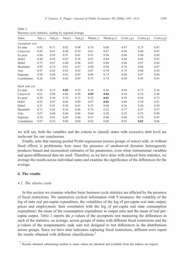
Table 2

Business cycle statistics, scaling by regional average

Index Var( y) Var( p) Var(n) Var( g) Mean( y) Mean( g/y) Corr( y,g) Corr(n,g) Corr( p,g)

Asymptotic test

Ex-ante 0.92 0.71 0.92 0.98 0.76 0.80 0.87 0.75 0.87

Carryover 0.85 0.81 0.90 0.70 0.61 0.87 0.94 0.80 0.92

Ex-post 0.84 0.95 0.91 0.81 0.93 0.98 0.96 0.98 0.89

Debt1 0.88 0.92 0.87 0.78 0.87 0.89 0.84 0.85 0.92

Debt2 0.72 0.87 0.80 0.96 0.87 0.88 0.96 0.87 0.88

Shortdebt 0.95 0.72 0.83 0.87 0.80 0.94 0.76 0.86 0.87

Veto 0.97 0.43 0.92 0.92 0.87 0.70 0.79 0.94 0.50

Supreme 0.90 0.88 0.92 0.83 0.88 0.75 0.96 0.97 0.90

Constitution 0.26 0.94 0.66 0.85 0.75 0.74 0.89 0.95 0.95

Rank sum test

Ex-ante 0.58 0.15 0.05 0.55 0.16 0.26 0.94 0.73 0.16

Carryover 0.61 0.98 0.86 0.90 0.05 0.04 0.34 0.16 0.48

Ex-post 0.50 0.36 0.76 0.71 0.22 0.01 0.59 0.64 0.72

Debt1 0.83 0.87 0.66 0.89 0.87 0.02 0.49 0.50 0.91

Debt2 0.21 0.91 0.38 0.81 0.35 0.68 0.56 0.24 0.58

Shortdebt 0.13 0.41 0.36 0.46 0.74 0.22 0.77 0.47 0.57

Veto 0.07 0.44 0.86 0.86 0.64 0.26 0.25 0.55 0.90

Supreme 0.34 0.81 0.60 0.40 0.53 0.46 0.86 0.70 0.45

Constitution 0.07 0.52 0.08 0.69 0.82 0.86 0.91 0.02 0.06


we will see, both the variables and the criteria to classify states with excessive debt level are

irrelevant for our conclusions.

Finally, note that running pooled Probit regressions (across groups of states) with, or without

fixed effects is problematic here since the presence of unobserved dynamic heterogeneity

produces biased and inconsistent estimates of the parameters, even when instrumental variables

and quasi-differenced data are used. Therefore, as we have done with reduced form statistics, we

average the results across individual states and examine the significance of the differences for the

average.

4. The results

4.1. The elusive costs

In this section we examine whether basic business cycle statistics are affected by the presence

of fiscal restrictions. We summarize cyclical information with 9 measures: the volatility of the

log of state real per-capita expenditure, the volatilities of the log of per-capita real state output,

prices and employment; their correlation with the log of per-capita real state consumption

expenditure; the mean of the consumption expenditure to output ratio and the mean of real per-

capita output. Table 2 reports the p-values of the asymptotic test measuring the differences in

each of the statistics, on average, across groups of states with different fiscal restrictions and the

p-values of the nonparametric rank sum test designed to test differences in the distributions

across groups. Since we have nine indicators capturing fiscal restrictions, different rows report

the results obtained with different classifications.2

2 Results obtained substituting median to mean values are identical and available from the authors on request.

Var(y)

0 250.000

0.006

0.012

0.018

Var(n)

0 250.000

0.006

0.012

0.018

Var(p)

0 250.00000

0.00025

0.00050

0.00075

Mean(log(g/y))

States0 25

12000

18000

24000

30000

Corr(y,g)

0 25-1.0

-0.5

0.0

0.5

1.0

Corr(n,g)

0 25-1.8

-0.9

0.0

0.9

Corr(p,g)

0 25-1.8

-0.9

0.0

0.9

mean(ypc)

States0 5 10 15 20 25 30 35 40 45

0.06

0.09

0.12

0.15

Fig. 1. Moments using the ex-post classification. A bar divides states without ex-post restrictions (first 13) from those with ex-post restrictions (last 35).

F.Canova,E.Pappa/JournalofPublic

Economics

90(2006)1391–1414

1400


The table has a very clear message: the presence of tighter budget, debt, or institutional

restrictions does not appear to matter for business cycle fluctuations in output, employment and

prices. This is true for the majority of the statistics we compute, for almost all the classifications

we employ to group states and for both types of tests. Note that mean differences are always

insignificant across groups while distributions are occasionally different with some indicators,

suggesting that higher moments of the distributions do at times differ. Also, while volatilities are

typically insignificantly different across groups, correlations do at times change and the

correlation which look most unstable is the one between prices and per-capita expenditure.

P-values are useful summary statistics but may hide important information. To give some

visual content to the results of Table 2, we plot in Fig. 1 the estimated values of the 9 statistics

for each of the 48 states when we use the ex-post indicator to group states. A vertical bar in each

graph cuts off the 13 states with loose restrictions (ex-post dummy equal to 0) from those with

strict ones (ex-post dummy equal to 1).

Few interesting features stand out from the figure. First, mean differences in volatilities are

not only statistically but also economically small. For example, average relative output volatility

in states with ex-post restrictions is only marginally higher than in states with no ex-post

restrictions (0.004% vs. 0.003%), and if we exclude a major outlier (Kentucky), the average

values are identical.3 Similarly, the average relative price volatility in states with ex-post

restrictions is identical to the one without (0.00028), if California is excluded, and the mean per-

capita income and the mean per-capita expenditure to output ratios are not only statistically but

also visually and economically similar across the two groups. Second, there are considerable

variations in the statistics within groups. For example, the volatility of relative employment

varies from 0.01 to 0.26 in both groups while the correlation between per-capita real

consumption expenditure and relative output ranges from �0.60 to 0.81 in states with loose

budget restrictions and from �0.80 to 0.76 in states with tight budget restrictions. Hence, our

failure to find statistically different types of fluctuations is the result of two different effects:

excluding outliers, mean differences across groups are small and the within group heterogeneity

is substantial. In other words, our fiscal indicators have only a very minor explanatory power for

the differences in means, volatilities and correlations across US states.

Although simple moments are unaffected by budget, debt and institutional differences, one

could conceive that important economic relationships could be altered by the presence of fiscal

constraints. In fact, much of the discussion in the literature has not focused on business cycle

moments but on the ability of governments to respond to cyclical fluctuations in the economy

when constraints are in place.

There is some evidence that government expenditure in OECD countries has played a

stabilizing role. For example, Gali (1994) and Fatas and Mihov (2001) found a significant

negative relationship between output volatility and government size (measured by the average

expenditure to output (G/Y) ratio) and/or the level of development (measured by the per-capita

GDP), while Lane (2003) found that more volatile economies tend to have more procyclical

government expenditure. Similarly, there seems to be some relationship between expenditure

volatility and macroeconomic volatility (e.g. Fatas and Mihov, 2003). Do US states conform to

this evidence? Is the magnitude and the significance of these relationships altered by fiscal

restrictions?

3 To convert these numbers into estimates of an intercept and slope of a regression of output volatility on a constant and

the ex-post dummy is easy. In fact, 0.003 is the intercept (corresponding to states with no restrictions) and 0.001 is the

slope.


US states are somewhat different from OECD countries, probably because of the smaller

average expenditure to GSP ratio (0.09 as opposed to 0.20). Nevertheless, the sign and the

significance of the relationships are broadly unaffected by the presence of tight fiscal

restrictions, no matter what classification is used to group states and what method we choose

to detrend the data. To illustrate this point, we present in Fig. 2 scatter plots of four

relationships that have attracted the attention of researchers (variability of expenditure and

variability of relative output; size of government expenditure and relative output volatility;

cyclicality of government expenditure and relative output volatility; cyclicality and size of

government expenditure) when the ex-post indicator is used to group states and regional

aggregates are used to detrend the data before variabilities and correlations are computed.

States without ex-post restrictions appear with a square; states with ex-post restrictions with a

star.

Take, for example, the relationship between the variability of government consumption

expenditure and the variability of relative output. For the whole sample, the slope of the

relationship is negligible (�0.08); for the sample of states without ex-post restrictions, the slope

is �0.41; and for the sample of states with restrictions, it is �0.03. However, the slopes for the

two different groups of states are insignificantly different from zero and insignificantly different

from each other. Therefore, although we find that ex-post restrictions reduce the point estimate

of this correlation, the relationship between output and expenditure volatility is, in general, small

and statistically similar across groups of states. A similar pattern also obtains when examining

var(g) vs var(y)

0

0,01

0,02

0,03

0,04

0,05

0,06

0,07

0,08

0,09

0 0,005 0,01 0,015 0,02

corr(g,y) vs mean (g/y)

-1

-0,8

-0,6

-0,4

-0,2

0

0,2

0,4

0,6

0,8

1

0,05 0,07 0,09 0,11 0,13 0,15

corr(g,y) vs var(y)

-1

-0,8

-0,6

-0,4

-0,2

0

0,2

0,4

0,6

0,8

1

0 0,005 0,01 0,015 0,02

var(y) vs mean(g/y)

0

0,02

0,04

0,06

0,08

0,1

0,12

0,14

0 0,005 0,01 0,015 0,02

Fig. 2. Macroeconomic relationships, ex-post classification. States without ex-post restrictions (13) appear with a square;

states with ex-post restrictions (35) with a star.


the relationship between cyclicality of expenditure and output volatility (see the lower left panel

of Fig. 2). The relationship appears to be quadratic and, for the whole sample, the slope of each

branch is 0.21.

For states without ex-post restrictions the shape is still quadratic but skewed to the left,

while for states with ex-post restrictions the shape is quadratic with skewness on the right.

Once again, if we exclude a few outliers in this last group, the two curves are statistically and

visually indistinguishable. Interestingly, (incorrectly) fitting a line to the points would produce

a positive relationship for the whole sample and a negative one for states without ex-post

restrictions. Therefore, one would conclude that in states with less restricted fiscal policy the

correlation between expenditure and relative output movements is low when the variability of

output is large, in contrast, e.g., with the findings of Lane (2003) for OECD countries. Finally,

no pattern is detectable for the other two statistics: each of the subgroups displays a large

dispersion and the presence of a few outliers within groups makes differences always

insignificant.4

4.1.1. Robustness

While the results of the previous subsection leaves little room for doubts, there is a number of

robustness checks one can undertake to make the conclusion that the direct business cycle costs

of fiscal constraints are negligible stronger.

We first check whether the presence of spurious trends, or of measurement errors may affect

the quality of the results we have presented. Table 3, which reports p-values for rank sum tests

when we compute business cycle moments detrending the raw data with an HP, or a growth

filter, or scale them by their US counterpart, suggests that results are robust to the treatment of

the trends, despite the relative short size of the sample. Hence, our inability to detect differences

is not driven by the way we compute business cycle statistics. Interestingly, scaling state

variables by US as opposed to regional aggregates produces similar results. Hence, controlling

for national cycles seems to be sufficient for our purposes: allowing for regional cycles does not

make differences in variabilities and correlations more evident.

As we mentioned, measurement error could also be an issue. The scaling by regional

variables we have chosen should, in principle, reduce its effect. However, a comparison across

detrending methods is useful, since the various approaches emphasize, or de-emphasize high

frequency measurement errors. Comparing Tables 2 and 3, one can see that results are roughly

unchanged. Hence, measurement error is unlikely to be a crucial factor in our analysis.

The analysis we have conducted so far assumes that our fiscal indicators are exogenous, but

there may be reasons to believe that they are not. In fact, states which are more prone to large

business cycle fluctuations (for example, because of the composition of their output) may be less

likely to impose fiscal restrictions than states where cyclical fluctuations are small. Similarly,

fiscal policy may be more restricted in states which are small and/or open to movements of

goods and people, since fiscal policy is likely to be less effective than in states which are large

and relatively close. This simple reverse causality hypothesis does not fit with the evidence we

have available. We have already mentioned that output composition is irrelevant to assess

whether fiscal constraints matter, or not. Moreover, within each group we have large and small

states (e.g. New York and Connecticut among the loose ones, Georgia and Delaware among the

strict ones) as we have states with high or low output variability (see Fig. 1).

4 No conclusion changes when relative employment in used in place of relative output in all the analysis.

Table 3

Business cycle statistics, rank sum test

Index Var( y) Var( p) Var(n) Var( g) Mean( y) Mean( g/y) Corr( y,g) Corr(n,g) Corr( p,g)

HP filtered data

Ex-ante 0.29 0.34 0.24 0.44 0.55 0.44 0.48 0.40 0.60

Carryover 0.48 0.30 0.44 0.10 0.65 0.10 0.16 0.29 0.96

Ex-post 0.65 0.54 0.44 0.11 0.88 0.04 0.39 0.15 0.71

Debt1 0.14 0.78 0.78 0.18 0.15 0.66 0.68 0.01 0.70

Debt2 0.05 0.86 0.34 0.69 0.73 0.65 0.77 0.10 0.81

Shortdebt 0.04 0.13 0.53 0.29 0.79 0.30 0.61 0.47 0.38

Veto 0.72 0.10 0.48 0.33 0.07 0.86 0.10 0.32 0.99

Supreme 0.37 0.09 0.38 0.44 0.28 0.46 0.90 0.31 0.15

Constitution 0.29 0.72 0.08 0.91 0.72 0.24 0.74 0.84 0.35

Growth rates

Ex-ante 0.63 0.58 0.77 0.92 0.88 0.24 0.41 0.99 0.84

Carryover 0.67 0.21 0.01 0.15 0.72 0.13 0.92 0.71 0.41

Ex-post 0.76 0.27 0.06 0.27 0.04 0.03 0.81 0.10 0.32

Debt1 0.52 0.28 0.08 0.57 0.13 0.04 0.62 0.66 0.89

Debt2 0.01 0.33 0.47 0.20 0.51 0.47 0.53 0.73 0.77

Shortdebt 0.05 0.38 0.77 0.86 0.94 0.91 0.42 0.53 0.17

Veto 0.23 0.14 0.46 0.08 0.83 0.57 0.81 0.81 0.52

Supreme 0.69 0.61 0.54 0.39 0.41 0.56 0.99 0.10 0.64

Constitution 0.47 0.84 0.49 0.49 0.16 0.43 0.48 0.54 0.44

Scaling by US average

Ex-ante 0.06 0.18 0.48 0.84 0.55 0.10 0.44 0.55 0.56

Carryover 0.10 0.51 0.57 0.90 0.12 0.96 0.52 0.65 0.52

Ex-post 0.94 0.29 0.56 0.78 0.04 0.36 0.43 0.98 0.59

Debt1 0.78 0.61 0.57 0.78 0.01 0.30 0.93 0.26 0.32

Debt2 0.76 0.84 0.98 0.93 0.89 0.61 0.96 0.21 0.28

Shortdebt 0.57 0.20 0.63 0.76 0.20 0.94 0.24 0.50 0.04

Veto 0.52 0.59 0.66 0.93 0.36 0.46 0.29 0.53 0.90

Supreme 0.28 0.81 0.67 0.54 0.90 0.77 0.08 0.95 0.45

Constitution 0.13 0.22 0.32 0.39 0.98 0.07 0.54 0.74 0.16


Endogeneity may also be related to cultural values. Fiscal policy can in fact be generically

less restrictive in states which traditionally had liberal administrations. For example Vermont, the

only state without any form of constraint had a democratic governor for the majority of the

sample, and New England states, which are at the bottom of the ACIR scale, have traditionally

been among the most liberally oriented states of the US. To counteract this regional bias, one

should also remember that local fiscal policy has become more restrictive in all US states after

the tax-revolt of the beginning of the 1980s and the widespread imposition of tax and

expenditure limits (the so-called TELs). Therefore, the relevant comparison may be across time

as opposed to across units, since states which were considered tight in the first part of the sample

may have become loose, on average, in the second part, or vice versa. One could also argue that

it is the ability to use buffer funds, such as rainy days funds, which may be the discriminating

factor to measure the tightness of fiscal constraints. Since rainy days funds are not a prerogative

of states with tight balance budget constraints and since all of the states with loose restrictions

had rainy days funds by the end of our sample, it is unlikely that conditioning on the presence of

rainy days funds will change the essence of our results.


One referee pointed out to us that although fiscal constraints have no impact on

macroeconomic performance unconditionally, it may be that, conditionally on factors such as

size, output composition, trade patterns, etc., fiscal constraints may have a small but significant

impact on macroeconomic variables. While we have found no reference in the literature to this

conditional type of effect, it is worth investigating whether, once we control for relevant cross-

sectional variables, our negative conclusion still holds.

In Table 4, we report p-values of a rank sum test for the equality of selected macroeconomic

statistics when we attempt to account for these possible omitted factors. We present tests for

equalities in the cross-sectional distribution of first and second business cycle moments across

groups when we condition on the presence, or the absence of rainy days funds at the end of the

sample; on the size of the states, where large states are those which are in the top quartile in

terms of population; on the composition of output, proxied here by the industrial employment,

and more industrial states are those with employment in manufacturing superior to 20% of the

total; when we compare Vermont to the 26 states with an ACIR index of 10 and when we

examine business cycle moments in New England and in Southern States. Moreover, we report

tests for the equality of the distributions in states with tight and loose restrictions for the

subsamples 1969–1980 and 1981–1995; and tests when an alternative measure of volatility

(interquartile range) is used. For the sake of space, we only present results obtained with the ex-

post and the Shortdebt classification but the conclusions are again independent of the indicator

used.

Our conclusions appear to be broadly unchanged. First, on average, volatilities and

correlations in states with rainy days funds and without them are similar as are those in large

and small states, or states with different shares of employment in manufacturing. Hence, once

regional trends are taken into account, size, output composition, or the access to rainy funds

does not seem to be a discriminating factor to classify cyclical fluctuations. In other words,

Table 4

P-values rank sum test: regional scaling

Index Vol( y) Vol(N) Vol( p) Corr( y,g) Corr(n,g) Corr( p,g

Rainy 0.17 0.44 0.41 0.14 0.83 0.70

Large 0.43 0.36 0.56 0.09 0.36 0.45

Output composition 0.26 0.12 0.39 0.15 0.11 0.66

Vermont 0.53 0.04 0.98 0.76 0.02 0.77

New England 0.61 0.03 0.82 0.81 0.64 0.82

Before 1980

Ex-post 0.56 0.50 0.87 0.24 0.56 0.40

Shortdebt 0.24 0.50 0.37 0.46 0.00 0.57

After 1980

Ex-post 0.12 0.62 0.07 0.51 0.74 0.79

Shortdebt 0.49 0.89 0.41 0.33 0.40 0.04

Tennessee

Before/After 1977 0.11 0.17 0.48 0.09 0.00 0.00

Interquartile range

Ex-post 0.06 0.47 0.34

Shortdebt 0.32 0.88 0.96

)


fiscal restrictions have negligible effects not only unconditionally, but also conditionally.

Second, again excluding employment volatility, the correlation between employment and

expenditure, there is no evidence that Vermont business cycle statistics are different from those

in states with an ACIR index of 10 nor that those of New England states are different from

those of Southern states. Hence, the cultural orientation of the state is probably unimportant in

understanding the relationship between business cycles and fiscal constraints. One could also

conjecture that the political orientation of federal governments may exogenously change the

tightness of the fiscal constraints – the idea being that Democratic administrations may be

more prone to request large Federal aid than Republican ones. These arguments appear to be

of scarce importance here for three reasons. First, Democratic administrations where present

only in 12 of the 31 years of the sample and in these years the magnitude (and the growth

rate) of the Federal aid transfers is not different from the magnitude (and the growth rate)

during Republican administrations. Second, on average, Federal aid accounts for less than

20% of state and local government expenditures. Third, the magnitude of Federal aid is

probably linked to the national business cycle: therefore scaling by aggregate variables should

take into account these factors. In fact, the p-values are practically unchanged using aggregate

instead of regional scaling. Therefore, failure to account for the size of the Federal aid cannot

explain the inability to detect differences in cyclical fluctuations across states with different

fiscal restrictions.

Our results appear to be robust also to the presence of potential structural breaks and to the

measurement of volatility. There are two exceptions to the rule, however: the correlation

between employment and expenditure before 1980 when the Shortdebt index is used is

significantly smaller in states with ex-post restrictions; the correlation of prices with expenditure

is lower in states with Shortdebt restrictions when the post 1980 sample is considered. Note that

since the interquartile range is much less sensitive than variances to measurement errors, Table 4

also confirms that this factor is minor in our analysis.

Our sample also contains an interesting case study which can be used to sharpen our

conclusions on the role of fiscal constraints for business cycle fluctuations. In fact, tight fiscal

constraints were imposed in Tennessee in 1977 and since then the state government has

undertaken its operation under a tight fiscal restriction regime. Such constraints have made the

magnitude of the deficits and of the debt to output ratio smaller and somewhat less volatile in

the second part of the sample and this is consistent with the claim that fiscal constraints

eliminate some erratic component in fiscal policy (see Fatas and Mihov, 2003), but such a

component is small relative to other factors so that the dynamics of macro variables is

unchanged. In fact, the p-values of a rank test for the equality in the distributions obtained in

the samples 1969–1977 and 1978–1995, suggest that volatilities are unchanged while the

correlation of employment and prices with government expenditure is statistically smaller in

the second sample.

In sum, all the evidence indicates that business cycle statistics are largely unaffected by the

presence of fiscal constraints. The conclusion is robust to the classification used to define states

with tight or loose fiscal restrictions, to the procedure used to calculate business cycle statistics,

the presence of conditioning variables and, to a large extent, to the tests used to evaluate the

differences across groups, the statistics employed, and the sample used for the analysis. The only

case study where fiscal constraints have changed over time confirms that the cyclicality of

macroeconomic variables is hardly related to the nature of fiscal constraints. We conclude that

the costs produced by stronger fiscal restrictions are elusive: the cyclical performance of state

economies appears to have little to do with the nature of fiscal constraints.


Our conclusions seem to contradict those presented by Fatas and Mihov (2003). The main

reason for the difference is the econometric methodology used: in fact, while we use a non-

parametric approach, they use a standard two-step regression. As we have mentioned, the

estimated importance of fiscal constraints in such regressions is incorrect because the analysis

neglects the fact that the left-hand side variables of the second regression are estimated and not

the true ones. Since estimates of standard errors are downward biased, differences across states

may become artificially significant.

4.2. The immaterial gains

The imposition of debt constraints was thought to provide some safeguard against debt

default. Mitchell (1967), for example, lists this as the major reason for having limits on debt

issues. One can think of deficit constraints as playing approximately the same role: as deficits

build up, year after year, the debt burden grows and the probability of a debt default increases. If

such an argument has any empirical relevance, the probability that a state runs an excessively

high debt level should be significantly larger in states with loose fiscal, or debt constraints – the

implicit assumption being that there is a linear proxy relationship between the probability of

excessively high debt level and the probability of a debt default. To verify this hypothesis, we

have constructed four different measures of excessive debt level, two based on the debt to

revenue level and two based on the debt to GSP ratio. In each case, we define excessiveness by

an absolute threshold, or relative to the other states. Results turn out to be broadly robust to the

definition used.

When we use the absolute measures, there are 16 states where the debt to revenue ratio

exceeds 20, on average over time, and 12 states where the debt to GSP ratio exceeds 0.80, on

average over time. When we use relative measures, we have 7 states which are in the upper

tercile of the debt to revenue ratio and 9 which are in the upper tercile of the debt to GSP ratio.

States appearing in all the four classifications are Connecticut, Delaware, Louisiana, New

Hampshire, Oregon, Rhode Island and Vermont. A quick run through these names indicates that

states with excessively high debt level are small and located either on the eastern, or the western

side of the country. As far as fiscal constraints are concerned, the list includes states which are

virtuous according to the ACIR classification (e.g. Oregon and Rhode Island) as well as states

which are not (e.g. New Hampshire and Vermont); states with quantitative debt limits (e.g.

Connecticut and Rhode Island) and states with no such limits (e.g. Delaware, or Louisiana) and

states with binding institutional constraints (Oregon) and states with no such constraints

(Vermont). Table 5 presents the exact break down of the states with excessively high debt levels

according to each of the definitions into those with loose and tight constraints, employing the

same classifications used in the previous section.

The table contains useful information. Regardless of whether we use absolute, or relative

measures and of whether we use debt to revenues, or debt to GSP ratios, in four of the nine

classifications (Carryover, Ex-post, Debt1 and Veto) the relative proportion of states with tight

fiscal constraints in the group of potential debt defaulters is larger than the proportion of states

with looser type of constraints and when absolute debt measures are used, the number of units

with tight constraints substantially exceeds the number of units with loose constraints.

Interestingly, different types of constraints imply different outcomes. In particular, tight

balance budget restrictions do not seem to keep debt to revenue, or debt to GSP under control,

neither in absolute nor in relative terms. Targeted debt restrictions seem more useful: numerical

limits as well as limits on short term debt tend to keep debt to revenue and debt to GSP ratio low,

Table 5

Number of states with excessively high debt

Ex-ante Carryover Ex-post Debt1 Debt2 Shortdebt Veto Court Constitution

Debt to Revenue, Absolute

Unrestricted 11 2 6 4 10 13 4 10 13

Restricted 5 14 10 12 6 3 12 6 3

Debt to Revenue, Relative

Unrestricted 4 3 4 1 5 7 3 5 6

Restricted 3 4 3 6 2 0 4 2 1

Debt to GSP, Absolute

Unrestricted 8 2 5 3 9 11 4 9 10

Restricted 4 10 7 9 3 1 9 3 2

Debt to GSP, Relative

Unrestricted 5 4 5 2 7 8 3 8 8

Restricted 4 5 4 7 2 1 6 1 1


both in relative and in absolute terms. Finally, while line item veto seems to be ineffective in

controlling the size of the debt, both Constitutional and Supreme Court restrictions do help and

almost as much as direct limits on debt (see for a similar argument Bohn and Inman, 1996).

In general, balance budget constraints do not necessarily safeguard states from having

excessively large debt nor do they induce them to control their growth: once the sum of non-

guaranteed to guaranteed debt is used, we find that both fiscally virtuous and less fiscally

virtuous states are among the most exposed to excessive debt problems.

Next, we estimate some simple probit models to try to understand if macroeconomic

variables, or fiscal deficits impact on the probability of excessive debt differently in states with

loose, or tight constraints. For this purpose, we construct a dummy series for each state which

takes the value of 1 at t if the state debt/revenue ratio (Debt/GSP ratio) is in the upper tercile of

the cross-sectional distribution and zero otherwise. We do this for Connecticut, Delaware,

Louisiana, Massachusetts, New Hampshire, New York, Oregon, Rhode Island and Vermont

which are the states which fit the typology of states with excessively high debt, on average. We

then run a non-linear regression where local business cycle conditions (measured by the state

unemployment rate and the ratio of state to US output) and the deficit to GSP ratio of the state

are used to explain this dummy variable. In particular, we are interested in knowing whether

states with tight constraints have a lower probability of being in the upper tercile of the cross-

sectional distribution and whether business cycle conditions and deficits to GSP ratios exert a

differential effect in states which face tight or loose fiscal restrictions – the prior being that after

controlling for deficit differences, business cycle conditions in states with tight constraints are

less likely to impact on the probability of excessive debt level. Table 6 reports the results; in

parenthesis are t-statistics. The column baverage likelihoodQ reports the predictive probability of

an excessive debt level on average: a value of 0.5 means that there are equal odds of being above

and below the threshold.

Table 6 confirms previous conclusions. First, both good and bad business cycle conditions

(relative to the national average) increase the probability that debt is bexcessively highQ. Forexample, high relative output is conducive to low debt levels in Louisiana while the opposite is

true in Connecticut, Oregon and Vermont. Note that a high unemployment rate produces a

positive and significant effect on the probability of excessive debt only in New York. Second,

Table 6

Probit regression

State GSP/Y Unemployment Deficit(�1) Average likelihood

Louisiana �0.94 (�1.99) �0.16 (1.25) �0.004 (2.06) 0.55

New Hampshire �0.25 (�0.63) �0.17 (�0.61) 0.009 (0.30) 0.86

Connecticut 1.19 (2.69) 0.06 (0.22) 0.008 (2.54) 0.78

Oregon 1.20 (1.66) 0.74 (1.23) 0.02 (1.65) 0.86

Rhode Island 0.09 (0.36) �0.10 (�0.77) 0.0001 (0.74) 0.51

Delaware 2.01 (1.13) 0.49 (0.89) 0.009 (1.15) 0.82

Vermont 3.00 (2.20) 0.05 (0.07) 0.016 (2.11) 0.80

New York 0.19 (0.91) 0.33 (1.94) �0.0002 (�0.30) 0.58

Delaware �0.15 (�0.96) �0.04 (�0.34) �0.006 (�0.59) 0.50


high deficit to GSP ratios are not necessarily linked to high probability of excessive debt: while

this is the case and significantly so in Connecticut, Oregon and Vermont, a high deficit to GSP

level significantly decreases the probability of excessive debt in Louisiana and has no significant

effects in the other 4 states. Third, neither the probability of high debt nor the impact of business

cycle conditions on this probability is linked to fiscal restrictions. For example, state deficit to

GSP ratio are insignificant in New Hampshire and Rhode Island, two states with very different

type of fiscal restrictions, and significant in Louisiana and Oregon, again two states with very

different budget and debt constraints. Moreover, states for which the fit is good (i.e., the average

likelihood is high) roughly span the whole ACIR scale: there is very little visual difference in the

estimated specification across groups and states with tight constraints do not necessarily have, on

average, a lower probability of having excessively high debt. Perhaps more surprisingly, tight

debt and institutional restrictions do not help in reducing the probability of excessively high

debt.

To conclude, the gains a state obtains by tightening its ability to run fiscal policy are close to

be immaterial. Some improvements can be obtained by either directly imposing restrictions to

nominal debt, or some institutional restrictions. However, even in this case, there is weak

evidence that tightly constrained states are less prone to accumulate excessive debt levels, or that

fiscal deficits lead to strongly corrective actions by state legislators to reduce the debt burden in

subsequent years.

4.3. Why are there so little differences?

Why is it that differences across groups in almost all the cyclical statistics we have collected

are insignificant? Why is it that fiscal restrictions do not shield states from having excessively

large debts? One reason, often cited in the literature (see Milesi-Ferretti, 2003) is that state

governments engage in creative accounting activities to avoid constraints when they become

binding. For example, governments that have difficulties balancing the budget may shift

expenditure items off-the-budget, or to less restricted branches, such as local governments.

Alternatively, if they are available, they may use stabilization funds to limit the effects of a

revenue crunch they may experience in recessions. Furthermore, as we have seen, debt

restrictions apply only to guaranteed debt. Hence, there may be an incentive for state

governments to swap non-guaranteed (revenue) for guaranteed debt when the borrowing limit

becomes binding-incentive which may be less important for states which do not face tight

restrictions. Since our expenditure series include both local and state expenditures and the debt

series measure total outstanding debt by state and local governments, contrary for example to


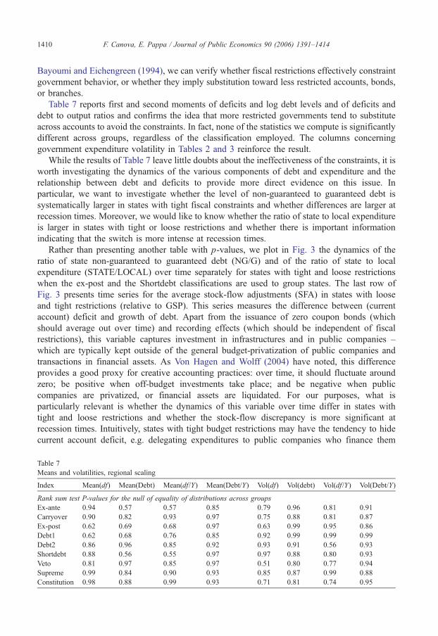
Bayoumi and Eichengreen (1994), we can verify whether fiscal restrictions effectively constraint

government behavior, or whether they imply substitution toward less restricted accounts, bonds,

or branches.

Table 7 reports first and second moments of deficits and log debt levels and of deficits and

debt to output ratios and confirms the idea that more restricted governments tend to substitute

across accounts to avoid the constraints. In fact, none of the statistics we compute is significantly

different across groups, regardless of the classification employed. The columns concerning

government expenditure volatility in Tables 2 and 3 reinforce the result.

While the results of Table 7 leave little doubts about the ineffectiveness of the constraints, it is

worth investigating the dynamics of the various components of debt and expenditure and the

relationship between debt and deficits to provide more direct evidence on this issue. In

particular, we want to investigate whether the level of non-guaranteed to guaranteed debt is

systematically larger in states with tight fiscal constraints and whether differences are larger at

recession times. Moreover, we would like to know whether the ratio of state to local expenditure

is larger in states with tight or loose restrictions and whether there is important information

indicating that the switch is more intense at recession times.

Rather than presenting another table with p-values, we plot in Fig. 3 the dynamics of the

ratio of state non-guaranteed to guaranteed debt (NG/G) and of the ratio of state to local

expenditure (STATE/LOCAL) over time separately for states with tight and loose restrictions

when the ex-post and the Shortdebt classifications are used to group states. The last row of

Fig. 3 presents time series for the average stock-flow adjustments (SFA) in states with loose

and tight restrictions (relative to GSP). This series measures the difference between (current

account) deficit and growth of debt. Apart from the issuance of zero coupon bonds (which

should average out over time) and recording effects (which should be independent of fiscal

restrictions), this variable captures investment in infrastructures and in public companies –

which are typically kept outside of the general budget-privatization of public companies and

transactions in financial assets. As Von Hagen and Wolff (2004) have noted, this difference

provides a good proxy for creative accounting practices: over time, it should fluctuate around

zero; be positive when off-budget investments take place; and be negative when public

companies are privatized, or financial assets are liquidated. For our purposes, what is

particularly relevant is whether the dynamics of this variable over time differ in states with

tight and loose restrictions and whether the stock-flow discrepancy is more significant at

recession times. Intuitively, states with tight budget restrictions may have the tendency to hide

current account deficit, e.g. delegating expenditures to public companies who finance them

Table 7

Means and volatilities, regional scaling

Index Mean(df) Mean(Debt) Mean(df/Y) Mean(Debt/Y) Vol(df) Vol(debt) Vol(df/Y) Vol(Debt/Y)

Rank sum test P-values for the null of equality of distributions across groups

Ex-ante 0.94 0.57 0.57 0.85 0.79 0.96 0.81 0.91

Carryover 0.90 0.82 0.93 0.97 0.75 0.88 0.81 0.87

Ex-post 0.62 0.69 0.68 0.97 0.63 0.99 0.95 0.86

Debt1 0.62 0.68 0.76 0.85 0.92 0.99 0.99 0.99

Debt2 0.86 0.96 0.85 0.92 0.93 0.91 0.56 0.93

Shortdebt 0.88 0.56 0.55 0.97 0.97 0.88 0.80 0.93

Veto 0.81 0.97 0.85 0.97 0.51 0.80 0.77 0.94

Supreme 0.99 0.84 0.90 0.93 0.85 0.87 0.99 0.88

Constitution 0.98 0.88 0.99 0.93 0.71 0.81 0.74 0.95

ex-postN

G/G

1978 1982 1986 1990 19940

25

50

75S

TA

TE

/LO

CA

L

1978 1983 1988 19931.17

1.26

1.35

1.44

tightloose

SF

A

1972 1979 1986 1993-0.16

-0.08

0.00

0.08

debt 1

1978 1982 1986 1990 1994-60

0

60

120

1978 1982 1986 1990 19941.1

1.2

1.3

1.4

1978 1983 1988 1993-0.07

0.00

0.07

0.14

tightloose

tightloose

tightloose

tightloose

tightloose

Fig. 3. Dynamics of government variables: states with tight (continuous line) and loose restrictions (dotted line).


with debt issues. Conversely, states with tight debt restrictions may force the stock-flow

adjustment to respond one by one to budget deficit, for example, acquiring fake assets in a

public company which in turn undertakes the current expenditure. Note also that the stock-

flow adjustment variable can turn negative without altering the deficit level. This can be

accomplished simply by selling off public companies.5

The evidence is generally consistent with the substitution hypothesis and confirms early

evidence by Von Hagen (1991). States with tight fiscal restrictions tend to use systematically

more non-guaranteed debt than states with loose restrictions. The difference is statistically

significant and, for the post-1980 period, economically relevant: in fact, after 1980, the ratio of

non-guaranteed to guaranteed debt increased on average 25 times in states with tight fiscal

restrictions and only by a factor of 2 in states with loose restrictions. The same pattern obtains

regardless of whether budget, or debt restrictions are in place: non-guaranteed (revenue) bonds

issues are systematically larger, no matter which classification we use.

We also find that states with loose restrictions tend to allocate more of the expenditures at the

state than at the local level than states with tight restrictions. The difference, on average, is

statistically significant when we use the ex-post classification but insignificant when the debt

classification is employed. In both cases, the time series for states with loose restrictions is above

the one with tight restrictions and in some years by more than 10%. A trend increase in the ratio

of state to local expenditure since the late 1980s, common to all states, is noticeable. This

increase is consistent with the establishment of stabilization funds at state level since the

5 The measurement of debt and deficit is very important to get a precise measure of the stock-flow adjustment existing

at each t. In general, since deficits are measured in accrual terms and debt is a cash concept, discrepancies may emerge.

Furthermore, the precise value of debt depends on whether it is recorded at face value or at market value. While these are

important concerns, they are somewhat tangential to our investigation. Since we are interested in highlighting differences

across states, as long as accounting practices are similar, the relative comparison is valid even if the absolute levels may

contain substantial measurement error.


beginning of the 1980s. Interestingly, none of the series displays any marked cyclical pattern and

this is the case in both types of states.

Finally, the stock flow adjustment series show that all states, regardless of the fiscal

constraint, resort to some creative accounting to hide current account expenditure. On

average, the stock-flow adjustment is negative. Therefore, rather than delegating expenditures

to public companies, US states, decrease their liabilities by selling off public companies, or

writing off the debt of public companies from the official state figures. Overall, differences

across groups of states are insignificant and roughly unrelated to national business cycle

conditions.

5. Conclusions

This paper analyzed whether tight fiscal constraints change the macroeconomic performance

of 48 US states. We study both the costs imposed by such constraints, measuring the relative

difference in volatility and the comovements of a number of macrovariables and a few important

macroeconomic relationships, and the gains enjoyed, by measuring both the relative probability

of excessive debt and its relationships with macroeconomic variables and deficits.

Our conclusion is that the macroeconomic consequences of fiscal constraints have been

overemphasized. While the sign and the magnitude of point estimates of cyclical statistics

are, at times, different, these differences are statistically insignificant and economically

unimportant. Our conclusions are robust in a number of dimensions, and in particular, do

not depend on the way we define blooseQ or bstrictQ, on whether deficit, debt, or institutional

constraints are in place, on the type of statistical tests we employ and, to a large extent, on

the statistics we consider, the detrending methods employed and the sample we use. We also

find that both states with loose and tight constraints are among those which run the risk of

having excessively high debt and that the relationship between excessive debt, state

macroeconomic conditions and deficits is independent of fiscal, debt and institutional

constraints.

We argue that fiscal constraints make little difference for the state economy because

governments can work around the constraints and transfer expenditure items to either less

restricted accounts or to less constrained portions of the government. We show that the dynamics

of total deficit and total debt are similar in states with loose or tight restrictions and that, on

average, states with tighter constraints substitute non-guaranteed to guaranteed debt and local to

state expenditure more than states with loose constraints. In addition, the presence of rainy days

funds offers an alternative substitution mechanism which permits to limit expenditure cuts at

times when the constraints become binding. Given that constraints apply only to a portion of the

total budget, that debt restrictions do not concern non-guaranteed debt, that no formal provision

for the enforcement of the constraints exists and that there are legal ways to work around the

rules, it is not surprising to find that tight constraints do not produce measurable benefits, or

significant costs.

Our results have important implications for the design of fiscal restrictions. Tight

constraints are neither a necessary nor a sufficient condition for good government

performance: in fact, they simply imply more creative accounting practices, unless they

come together with clearly stated and easily verifiable enforcement requirements. The design

of the enforcement mechanisms is therefore more important than the nature of the constraint.

In addition, tight constraints do not necessarily increase costs, or create benefits, if it is

possible to work around the constraints within the scope of the law. Clearly, our analysis can


not measure the benefits obtained from an improved reputation and neither can we measure

the gains obtained in terms of a better control of area wide inflation, when limits on local

governments are imposed.

Although it is tempting to extend the conclusions to the cross-section of European, or OECD

countries, a word of caution is necessary as the analogy between states and countries is limited

because of economic, political and institutional differences. First, as we have mentioned, the size

of government expenditure in GDP is much larger for countries than for states. Second,

institutional differences are significant, including much lower labor and capital mobility across

countries, and a much stronger inflexibility in current account government expenditure. Third,

US federal government acts as an insurance agency for US states in difficulty. Such an agency is

missing, for example, for EU countries.

Despite these differences, one cannot refrain from noticing that the proposed flexibilization

of the Stability and Growth Pact, which transforms constraints into rules, is unlikely to provide

a better framework where stabilization needs are properly weighted against the need to restraint

excessive deficits and debt levels. The original Pact was imperfect, for example, not

distinguishing between current account and capital account expenditures, but had already built-

in numerous ways to work around the inflexibility of the constraints. Adding further flexibility,

without altering the enforcement mechanism, is unlikely to change national fiscal authorities

practices.

Acknowledgment

Evi Pappa thanks the Spanish Ministry of Education and Science and FEDER through grant

SEC2003-306 from the Generalitat de Catalunya through the Barcelona Economics program

(CREA) and grant SGR2005-00447 for financial support.

References

Andres, Javier and Domenec, Rafael, 2002. Automatic Stabilizers and Monetary Rules in a Ricardian Economy,

Universidad de Valencia, mimeo.

Baxter, Marianne, King, Robert, 1993. Fiscal policy in general equilibrium. American Economic Review 83, 315–335.

Bayoumi, Tamin, Eichengreen, Barry, 1994. The political economy of fiscal restricions: implicationsfor europe from the

United States. European Economic Review 38, 783–791.

Besley, Timothy, Case, Anne, 1993. Political institutions and policy choices: evidence from the United States. Journal of

Economic Literature 41 (1), 7–73.

Bohn, Henning, Inman, Robert, 1996. Balance budget rules and public deficits: evidence from the US. Carnegie

Rochester Conference Series in Public Policy, vol. 45, pp. 13–76.

Canova, Fabio, Pappa, Evi, in press. Price Differentials in Monetary Unions: The Role of fiscal shocks, CEPR working

paper 3746, Economic Journal.

Canzoneri, Matthew, Cumby, Robert, Diba, B., 2002. Should the European Central Bank and the Federal reserve be

concerned about fiscal policy? Paper Presented at the Federal Reserve Bank of Kansas City’s Symposium

bRethinking Stabilization PolicyQ.Carlino, G., Sill, K., 1997. Regional economies: separating trends from cycles. Federal Reserve Bank of Philadelphia,

Business Review, May–June, 1–13.

Carter, John, Schop, David, 1990. Line-item veto: where is thy string? Journal of Economic Perspective 4, 103–118.

Del Negro Marco, 1998. Aggregate Risk Sharing Across US States and Across European Countries, Yale University,

mimeo.

Diaz Gimenez, Javier, Giovannetti, Giorgia, Marimon, Ramon, and Teles, Pedro, 2003. Nominal Debt as a Burden to

Monetary Policy, UPF mimeo.

Duarte, Margarida, Alexander, Wolman, 2002. Regional Inflation in a Currency Union: Fiscal Policy vs. Fundamentals,

mimeo Federal Reserve Bank of Richmond.


Fatas, Antonio, Mihov, Ilian, 2001. Government size and the automatic stabilizers: international and intranational

evidence. Journal of International Economics 55, 2–38.

Fatas, Antonio, Ilian, Mihov, 2003. The Macroeconomic Effects of Fiscal Rules in the US States, Insead, mimeo.

Gali, Jordi, 1994. Government size and macroeconomic stability. European Economic Review 38, 117–132.

Gali, J., Perotti, R., 2003. Fiscal policy and monetary integration in Europe. Economic Policy, CEPR, CES, MSH 18 (37),

533–572.

Gali, J., Lopez-Salido, J.D., Valles, J., 2004. Understanding the effects of government spending on consumption,

International Finance Discussion Papers, No. 805 Board of Governors of the Federal reserve System.

Hoel, P., 1993. Introduction to Mathematical Statistics. Wiley & Sons.

Holtz-Eakin, D., 1988. The line item veto and public sector budgets. Journal of Public Economics 36, 269–292.

Lane, Philip, 2003. The cyclical behavior of fiscal policy: evidence from the OECD. Journal of Public Economics 87,

2661–2675.

Milesi-Ferretti, GianMaria, 2003. Good, bad or ugly? On the effects of fiscal rules with creative accounting. Journal of

Public Economics 88, 377–394.

Milesi-Ferretti, GianMaria, Moriyama, K., 2004. Fiscal Adjustment in EU Countries: A Balance Sheet Approach. IMF

Working Paper.

Mitchell, 1967. The effectiveness of debt limits on state and local government borrowing. The Bulletin, vol. 45. New

York University, Institute of Finance.

Mountford, Andrew, Uhlig, Harald, 2002. What are the effects of fiscal policy shocks? CEPR Working Paper 3338.

Pappa, Evi, 2004. bNew Keynesian or RBC transmission? The effects of fiscal policy in labor marketsQ, IGIER Bocconi,

mimeo.

Perotti, Roberto, 2004. bEstimating the effects of fiscal policy in OECD countriesQ, IGIER Bocconi, mimeo.

Poterba, Jim, 1994. State responses to fiscal crises. The effects of budgetary institutions and politics. Journal of Political

Economy 102, 799–821.

Poterba, Jim, 1995. Balance budget rules and fiscal policy. Evidence from the States. National Tax Journal 48, 329–336.

Sorensen, Bent, Wu, Lisa, Yosha, Oved, 2001. Output fluctuations and fiscal policy: US state and local governments

1978–1994. European Economic Review 45, 1271–1310.

Von Hagen, Jurgen, 1991. A note on the empirical effectiveness of formal fiscal restraints. Journal of Public Economics

44, 199–210.

Von Hagen, Jurgen, Wolff, Guntram, 2004. What do deficits tell us about debts? Empirical evidence on creative

accounting with fiscal rules in the EU. CEPR Working Paper 4759.

The elusive costs and the immaterial gains of fiscal constraints

Documents

Transcript of The elusive costs and the immaterial gains of fiscal constraints