NBER WORKING PAPER SERIES

REDISTRIBUTING THE GAINS FROM TRADE THROUGH PROGRESSIVE TAXATION

Spencer G. LyonMichael E. Waugh

Working Paper 24784http://www.nber.org/papers/w24784

NATIONAL BUREAU OF ECONOMIC RESEARCH1050 Massachusetts Avenue

Cambridge, MA 02138June 2018

We would like to thank our discussant Oleg Itskhoki, Gordon Hanson, Stephen Redding, Referees,and participants at the NBER Trade and Labor Markets Conference and Vanderbilt University forvaluable comments and suggestions. The views expressed herein are those of the authors and do notnecessarily reflect the views of the National Bureau of Economic Research.¸˛¸˛

NBER working papers are circulated for discussion and comment purposes. They have not been peer-reviewed or been subject to the review by the NBER Board of Directors that accompanies officialNBER publications.

© 2018 by Spencer G. Lyon and Michael E. Waugh. All rights reserved. Short sections of text, notto exceed two paragraphs, may be quoted without explicit permission provided that full credit, including© notice, is given to the source.

Redistributing the Gains From Trade Through Progressive TaxationSpencer G. Lyon and Michael E. WaughNBER Working Paper No. 24784June 2018JEL No. E1,F11,H21

ABSTRACT

Should a nation's tax system become more progressive as it opens to trade? Does opening to trade change the benefits of a progressive tax system? We answer these question within a standard incomplete markets model with frictional labor markets and Ricardian trade. Consistent with empirical evidence, adverse shocks to comparative advantage lead to labor income losses for import-competition-exposed workers; with incomplete markets, these workers are imperfectly insured and experience welfare losses. A progressive tax system is valuable, as it substitutes for imperfect insurance and redistributes the gains from trade. However, it also reduces the incentives for labor to reallocate away from comparatively disadvantaged locations. We find that optimal progressivity should increase with openness to trade with a ten percentage point increase in openness necessitating a five percentage point increase in marginal tax rates for those at the top of the income distribution.

Spencer G. LyonNYU Stern School of Business44 West Fourth StreetNew York NY 10012spencerlyon2@gmail.com

Michael E. WaughStern School of BusinessNew York University44 West Fourth Street, Suite 7-160New York, NY 10012and NBERmwaugh@stern.nyu.edu

A Code Repository is available at https://github.com/mwaugh0328

1. Introduction

There are many concerns about the forces of globalization—that the losses from trade are large;that there are insufficient mechanisms to insure against these losses; that globalization simplypropagates existing inequality. The standard response to these concerns is helpful in theory:that there exists a Pareto improving transfer scheme that can compensate the losers from trade,yet still preserve the gains for the winners. In practice, this response is less helpful, given thelimited mechanisms and incentive problems that policy makers face in implementing any kindof transfer scheme.

Evidence suggests that these concerns about the forces of globalization are warranted. Autor,Dorn, and Hanson (2013) show that exposure to Chinese import competition has led to losses inlabor income and reductions in labor force participation for import-competition-exposed work-ers in the United States Krishna and Senses (2014) show that increases in import penetration areassociated with increases in labor income risk. Pavcnik (2017) surveys the growing body of ev-idence regarding trade’s affect on earnings and employment opportunities. Given that risksharing is often found to be incomplete (see, e.g., Cochrane (1991), Attanasio and Davis (1996)),this suggests that the labor market consequences of trade lead to welfare losses.

Policy need not be silent to these concerns. One way to mitigate and insure against these lossesis via the tax system. That is, the government could use a progressive tax system to providesocial insurance that helps transfer resources from the winners from trade to the losers.1 Thispaper evaluates this possibility by measuring both the optimal degree of tax progressivity andthe gains from progressivity as an economy opens to trade.

We implement these ideas by building off of our parallel work in Lyon and Waugh (2018). Inthis work, we develop an open-economy, standard incomplete markets model with frictionallabor markets. The open-economy aspect of our model builds on existing trade theory by de-veloping a dynamic Ricardian model of trade and frictional labor markets. As in the model ofEaton and Kortum (2002), there is a continuum of goods with competitive producers who areheterogenous in productivity; comparative advantage determines the pattern of trade. As inLucas and Prescott (1974) the labor market is frictional and labor can only move across differ-ent goods producing markets (within a country) after paying some cost.

As in the standard incomplete markets model (Huggett (1993), Aiyagari (1994)) households canself-insure by accumulating a non-state contingent asset. In addition, we endow householdswith several additional margins to mitigate labor income risk. Specifically, households can optout of the labor force and enjoy leisure and/or migrate to better labor markets.

1Varian (1980) and Eaton and Rosen (1980) are early contributions showing how a progressive tax system pro-vides social insurance.

1

These mechanisms give rise to an optimal degree of tax progressivity which balances the ben-efits of providing social insurance versus the costs of reducing labor supply and migration.Social insurance is valuable in our model because frictional labor markets and market incom-pleteness imply that households are exposed to idiosyncratic income risk, some of which istrade related. A progressive tax system provides a mechanism to substitute for imperfect in-surance against trade and non-trade related labor income risk.

On the other hand, a progressive tax system comes with the cost of reducing labor supplyand migration. As emphasized in the optimal taxation literature, labor income taxes reducethe incentive to work and, thus, shrinks the size of the pie available for redistribution. Ourmodel highlights a new, second cost of a progressive tax system—it reduces the incentives forlabor to migrate. A progressivity shrinks the gains to households from moving away fromlow-productivity to high-productivity places. Yet achieving allocative efficiency requires thecontinual movement of households from low- to high-productivity places. Thus, a progressivetax system contributes to the misallocation of households across space.

How the optimal degree of progressivity changes with increased openness to trade dependson the relative change in the benefits and costs. As an economy opens to trade, trade changesthe labor market consequences of various shocks, which, in turn, increases the benefits of socialinsurance. However, the quantitative issue is how the costs of redistribution change with in-creased openness to trade. Are reductions in labor supply more costly as we open to trade? Arereductions in migration more costly? We quantitatively answer these question in the followingway.

First, we place a restriction on the tax instruments the government has access to. In particular,we model the government as using a log-linear labor-income tax and transfer scheme to redis-tribute resources. In particular, we closely follow the approach of Benabou (2002), Conesa andKrueger (2006), and Heathcote, Storesletten, and Violante (2014) who parameterize the progres-sivity of net-taxes directly.2 As in that work, we take a stand on the social welfare function andwe measure the optimal degree of progressivity as the progressivity parameter that maximizessocial welfare.

Second, we calibrate the parameters of the model by having the model replicate key aggregateand cross-sectional moments of the US economy. Along with relatively standard parametervalues for preferences and technologies, we insure that the model replicates aggregate tradeexposure, internal migration rates, labor force participation rates, and the amount of indebted-ness of households in the US economy. A key issue is always the elasticity of labor supply andwe follow the work of Rogerson (1988) and more closely Chang and Kim (2007). In particular,

2Heathcote, Storesletten, and Violante (2014) show that this functional form provides a good approximation ofthe actual tax and transfer scheme in the US data. Guner, Kaygusuz, and Ventura (2014) provide an exploration ofthis and alternative tax functions.

2

the micro-labor supply elasticity is low (zero in our case) but can diverge from the aggregate la-bor supply elasticity due to movements in and out of the labor force, i.e., the extensive margin.This formulation is broadly consistent with the evidence in Keane (2011).

We use the calibrated model as laboratory to answer several questions.

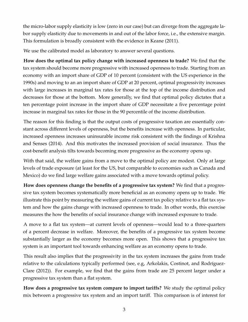
How does the optimal tax policy change with increased openness to trade? We find that thetax system should become more progressive with increased openness to trade. Starting from aneconomy with an import share of GDP of 10 percent (consistent with the US experience in the1990s) and moving to an an import share of GDP at 20 percent, optimal progressivity increaseswith large increases in marginal tax rates for those at the top of the income distribution anddecreases for those at the bottom. More generally, we find that optimal policy dictates that aten percentage point increase in the import share of GDP necessitate a five percentage pointincrease in marginal tax rates for those in the 90 percentile of the income distribution.

The reason for this finding is that the output costs of progressive taxation are essentially con-stant across different levels of openness, but the benefits increase with openness. In particular,increased openness increases uninsurable income risk consistent with the findings of Krishnaand Senses (2014). And this motivates the increased provision of social insurance. Thus thecost-benefit analysis tilts towards becoming more progressive as the economy opens up.

With that said, the welfare gains from a move to the optimal policy are modest. Only at largelevels of trade exposure (at least for the US, but comparable to economies such as Canada andMexico) do we find large welfare gains associated with a move towards optimal policy.

How does openness change the benefits of a progressive tax system? We find that a progres-sive tax system becomes systematically more beneficial as an economy opens up to trade. Weillustrate this point by measuring the welfare gains of current tax policy relative to a flat tax sys-tem and how the gains change with increased openness to trade. In other words, this exercisemeasures the how the benefits of social insurance change with increased exposure to trade.

A move to a flat tax system—at current levels of openness—would lead to a three-quartersof a percent decrease in welfare. Moreover, the benefits of a progressive tax system becomesubstantially larger as the economy becomes more open. This shows that a progressive taxsystem is an important tool towards enhancing welfare as an economy opens to trade.

This result also implies that the progressivity in the tax system increases the gains from traderelative to the calculations typically performed (see, e.g, Arkolakis, Costinot, and Rodrıguez-Clare (2012)). For example, we find that the gains from trade are 25 percent larger under aprogressive tax system than a flat system.

How does a progressive tax system compare to import tariffs? We study the optimal policymix between a progressive tax system and an import tariff. This comparison is of interest for

3

two reasons. First, in the United States, policy makers are taking a second look at anti-tradecommercial policy as a means to correct various imbalances and harms associated with trade.

Second, it has been argued that import tariffs and a progressive tax system may provide similarsocial insurance roles. Eaton and Grossman (1985) show that a motive for anti-trade commercialpolicy (i.e., a tariff) is to provide social insurance to the losers from trade (see, e.g., Corden (1974)and Baldwin (1982), as well). More starkly, Newbery and Stiglitz (1984) provide an example, ina setting with risk and incomplete markets, of free trade being Pareto inferior to autarky.3

To answer this final question, we measure the optimal policy mix between tax progressivityand import tariffs. In no cases do we find that a tariff is welfare-improving. The optimal mixis a zero tariff and a more progressive tax system as the economy becomes more exposed totrade.4

Related Literature. Conceptually, the ideas in this paper are closely related Rodrik (1997, 1998)and Epifani and Gancia (2009). Rodrik (1998) establishes a robust relationship between the sizeof a nation’s government and the extent to which it is open. An interpretation of this result isthat nations use government spending to provide social insurance against the ills of globaliza-tion. With that said, there is a disconnect between our work and Rodrik’s (1998) evidence. Inparticular, we hold government expenditures fixed and households do not value them. How-ever, our broader message—the increasing importance of government-provided social insur-ance with openness to trade—is very much consistent with Rodrik’s (1998) interpretation of thedata and the related arguments in Rodrik (1997).

At a mechanical level, this paper is closely related to the quantitative studies of Conesa andKrueger (2006) and Heathcote, Storesletten, and Violante (2014), who study the optimal pro-gressivity of the US tax scheme in heterogeneous agent, incomplete market models. As dis-cussed above, we closely follow their and Benabou’s (2002) approach to parameterizing the taxand transfer scheme and focus on the tension between social insurance and economic efficiency.There are two distinguishing features of our paper. First, we highlight a new and distinct ten-sion between social insurance and the misallocation of households across space. Second, wefocus on how optimal progressivity changes as an economy becomes more open to trade.

The cost of following the quantitative literature is that we restrict the class of instruments thesocial planner has access to. Thus our analysis leaves open questions if alternative tax instru-ments may perform better then a non-linear labor income tax. For example, Dixit and Norman(1986) demonstrate how how commodity taxation can redistribute the gains from trade in a

3We take the reason that insurance markets are missing as given; Dixit (1987, 1989a,b) shows how these conclu-sion depend upon the modeling as to why these markets are missing.

4Relative to Eaton and Grossman (1985) or Newbery and Stiglitz (1984), we speculate that in their settings enter-tain alternative policy instruments and do not endow households with partial insurance opportunities. Moreover,one caveat to this analysis is that the tariff policy we consider is stark—one uniform tariff for all imported goods.

4

Pareto improving way. Our economy is much richer with desires for social insurance and par-tial factor mobility, however, exploring alternative instruments is an important direction forfuture work.

With regard to open economy issues, Spector (2001) and Antras, De Gortari, and Itskhoki (2016)are closely related. Both papers focus on a static, open economy Mirrlees (1971) framework andstudy the welfare consequences of trade-induced inequality and its interaction with redistribu-tive polices. In particular, Antras, De Gortari, and Itskhoki (2016) study policies that take thesame form as in our paper. The distinguishing feature of our work is that we focus on very dif-ferent motives for redistributive taxation. In our model, the motive for progressive taxation isto provide social insurance and redistribute resources from the “lucky” towards the “unlucky.”This insurance motive is distinct from inequality aversion per se, as in Antras, De Gortari, andItskhoki (2016). This is the sense in which our paper builds most closely on the earlier work ofVarian (1980), Eaton and Rosen (1980), and Mirrlees (1974).

Our modeling framework is related, but distinct from, an exciting and growing body work ontrade and labor market dynamics (see, e.g., Kambourov (2009); Artuc, Chaudhuri, and McLaren(2010); Dix-Carneiro (2014); Caliendo, Dvorkin, and Parro (2015); Cosar, Guner, and Tybout(2016)).5 We depart from this literature by studying an economy in which households facelabor income shocks, incomplete markets, and partial self-insurance. The cost of this departureis that we are unable to incorporate the geographic and sectoral detail found in this work (see,e.g., Caliendo, Dvorkin, and Parro (2015)) due to computational complexities. With that said,the benefits from this departure are important for several reasons.

First, the focus on a setting with incomplete markets opens up the door to a motive for govern-ment policy to provide social insurance and increased social insurance as the economy opens totrade. In other words, this allows us to study the normative implications of alternative policyschemes as an economy opens to trade. In contrast, the normative prescriptions are unclear (aswell as unstudied) in previous work on trade and labor market dynamics.

Second, the migration motive in our model is for insurance. That is, households undertakecostly moves to escape negative labor market conditions in one location and capture favorablelabor market conditions in another location (see, e.g., Lagakos, Mobarak, and Waugh (2017)and references therein for the importance of this in the context of developing countries). Thismotive is distinct from the moving motive in the stationary equilibrium of Artuc, Chaudhuri,and McLaren (2010) and Caliendo, Dvorkin, and Parro (2015), which arises from shocks topreferences across locations, while income across locations is constant. Allowing for insurance-motivated moves is important as it creates a new, quantitatively important tension for policy

5While a static framework, Galle, Rodrguez-Clare, and Yi (2017) is a closely related as well. Similarly motivated,they explicitly study the aggregate and distributional consequences of trade in an environment without ex-posttransfers.

5

makers to confront. That is a progressive tax system must balance the gains from social insur-ance versus the losses in allocative efficiency that come with less migration.

2. Model

Here, we describe a model of international trade with households facing incomplete marketsand frictions to move across labor markets. The first subsection discusses the production struc-ture; the second subsection discusses the government and the tax function; the third discussesthe households.

Below, since we focus on the perspective of one country, country subscripts are omitted unlessnecessary. Similarly, because we focus on a stationary equilibrium, time subscripts are omittedunless necessary.

2.1. Production

The model has an intermediate-goods sector and a final good sector that aggregates the in-termediate goods. Within a country, there is a continuum of intermediate goods indexed byω ∈ [0, 1]. As in the Ricardian model of Dornbusch, Fischer, and Samuelson (1977) and Eatonand Kortum (2002), intermediate goods are not nationally differentiated. Thus, intermediateω produced in one country is a perfect substitute for the same intermediate ω produced byanother country.

Competitive firms produce intermediate goods with linear production technologies,

q(ω) = z(ω)`, (1)

where z is the productivity level of firms and ` is the number of efficiency units of labor. Inter-mediate goods productivity evolves stochastically according to an AR(1) process in logs

log zt+1 = φ log zt + εt+1, (2)

where εt+1 is distributed normally with mean zero and standard deviation σε. The innovationεt+1 is independent across time, goods, and countries.

Firms producing variety ω face competitive product and labor markets with households thatsupply labor elastically. Competition implies that a household choosing to work in market ωearns the value of its marginal product of labor, which is the price of the good times the firm’sproductivity z.

Transporting intermediate goods across countries is costly. Specifically, firms face iceberg tradecosts τ ≥ 1 when exporting their products. Abstracting from tariffs (which are discussed be-

6

low), this means that for a firm to deliver one unit of the intermediate good abroad, it mustproduce τ units for shipment.

Intermediate goods are aggregated by a competitive final-goods producer who has a standardCES production function:

Q =

[∫ 1

0

q(ω)ρdω

] 1ρ

, (3)

where q(ω) is the quantity of individual intermediate goods ω demanded by the final-goodsfirm, and ρ controls the elasticity of substitution across variety, which is θ = 1

1−ρ .

2.2. Government

The government consumes resources G, levies a labor income tax and transfer scheme, andtaxes imports via tariffs.

Government Consumption. We model government consumption of resourcesG as pure waste.That is, there is no service flow to households from the government’s consumption. Motivatingthis modeling choice is the difficulty in disciplining the utility value of public goods (see, e.g.,the discussion in Heathcote, Storesletten, and Violante (2014)). Thus, this choice reduces thenumber of free parameters we must take a stand on. The cost of this choice is that we abstractfrom a policy instrument—public goods provision—that also provides social insurance. Andwe lose the ability to speak to the evidence in Rodrik (1998) and the response of local publicgood provision in Feler and Senses (2017).

Labor Income Tax and Transfer Scheme. As in Benabou (2002) and Heathcote, Storesletten,and Violante (2014), we assume that net tax revenues are of the following parametric class:

T (w) = w − δw1−τp , (4)

where net tax revenues are T (w) and w is labor income. There are two parameters in (4). Theδ parameter determines the average rate and is chosen by the government such that its budgetis balanced. The parameter τp directly controls the progressivity of the tax scheme. This is thepolicy parameter of interest.

Heathcote, Storesletten, and Violante (2014) describe several ways to see how τp determinesthe progressivity. The most straightforward way is to note that 1 − τp equals one minus themarginal tax rate relative to one minus the average tax rate:

1− τp =1− T ′(w)

1− T (w)/w. (5)

7

Thus, when τp equals zero, marginal rates equal average rates—i.e., the tax system is neitherregressive nor progressive and is deemed “flat.” In contrast, when τp is greater than zero,marginal rates T ′(w) exceed average rates, T (w)/w and the tax system is deemed “progressive.”

In reality, the tax system is far more complex. We follow previous work by thinking about (4)vis-a-vis the data and the model as a scheme which encompass both the myriad of taxes andthe transfers. That is take-home pay in the model reflects pregovernment income minus taxesplus transfers. Heathcote, Storesletten, and Violante (2014); Guner, Kaygusuz, and Ventura(2014); Antras, De Gortari, and Itskhoki (2016), (all using different data sources) find that thisfunctional form provides a good approximation of the actual tax and transfer scheme in the USdata. In particular, Heathcote, Storesletten, and Violante (2014) and Antras, De Gortari, andItskhoki (2016) find very similar estimates of the τp parameter.

For our purpose, there are several weaknesses with this tax and transfer scheme. First, it ab-stracts from direct forms of compensation that depend upon the circumstances for income loss,such as trade adjustment and assistance programs. For example, the reduction in net taxes forhouseholds that experience an income reduction does not depend on weather or not if the lossin income is trade related. It does not provide direct insurance to trade-imposed losses. Thisis an abstraction in the sense that there are (i) some forms of direct compensation for trade-induced losses through TAAP and (ii) it does not allow us to explore the gains from more directforms of compensation.6.

The final issue is that we are ex-ante restricting the class of instruments the social planner hasaccess to. Thus our analysis leaves open questions if alternative tax instruments may performbetter then a non-linear labor income tax. This is an important omission relative to the classicwork of Dixit and Norman (1986) who demonstrate how commodity taxation can redistributethe gains from trade in a Pareto improving way.

Tariffs. The government imposes a tariff on imported intermediates, τf . Mechanically, thisvalue inflates the effective trade costs discussed above. Specifically, the total cost for importinga good will be:

τ = τ(1 + τf ). (6)

This means that to purchase one unit of the good, τ > 1 of the good must be shipped and (1+τf )

of the good must be delivered to the “dock.” Out of the units delivered to the dock, τf units arepaid to the government and one unit is delivered to the consumer.

While tariffs (in the US context) are generally small, entertaining this policy instrument allows

6The TAAP program appears to be quantitatively ineffective relative to traditional social insurance such associal security and disability insurance (see, e.g. Autor, Dorn, and Hanson (2013))

8

us to contrast the optimal labor income tax scheme versus a more “isolationist” approach ofrestricting trade to deal with the ill effects of globalization.

2.3. Households

Within a country, there is a continuum of infinitesimally small households of mass L. Eachhousehold is infinitely lived and maximizes expected discounted utility

E

∞∑t=0

βt{

log(ct)−Bh1−γt

1− γ

}, (7)

where E is the expectation operator and β is the subjective discount factor. Period utility de-pends on both consumption of the final good and the disutility of labor. As we discuss below,we model labor supply as being only on the extensive margin; thus, the parameter γ is irrele-vant.

Households live and work along the same dimension as the intermediate goods. That is, ahousehold’s location is given by ω—the intermediate goods sector in which it can work.

Given their current location, households can choose to work, to move and work someplace elsein the future, and to accumulate a non-state contingent asset. Below, we describe each of thesechoices in detail.

Working is a discrete choice between zero hours and h. Thus, the labor supply is purelyon the extensive margin. If a household works, it receives income from employment in theintermediate-goods sector in which the household resides. If a household does not work, itreceives zero income. In the following presentation, we normalize the value h equal to one.

Households can move to an alternative intermediate-goods sector ω′ at some cost. Paying m inunits of the final good allows the household to change where it can work in next period. Thevalue of the new location can take several forms. One is the best labor market, as in Lucas andPrescott (1974); an alternative is a random labor market. We focus on the latter specification.

Households residing in a intermediate-goods location face labor income risk associated withfluctuations in local productivity and fluctuations in world prices. We do not allow for anyinsurance markets against this risk, but let households accumulate a non-state contingent asseta that pays gross return R. We treat R as exogenous and not solved for in equilibrium. Aninterpretation is that this country faces a large supply of assets at this rate. Households face alower bound on asset holding −a, so agents can acquire debt up to the value a.

State Variables. The individual state variables of a household are its location ω and asset hold-ings a. The island-level state variable is the domestic productivity state and world price state.The aggregate state is a distribution over island-level state variables and asset holdings.

9

Let us expand on this a bit more. The wage per efficiency unit that a household receives isa important island-level object impacting individual decisions. The wage per efficiency unitdepends on the value of the marginal product of labor on that island. The marginal productdepends the island’s productivity level. The “value” part depends on (i) the world price for thegood produced on the island and (ii) the labor supply decisions of households residing on theisland. Given our preference specification in (7), households’ labor supply decisions dependon the distribution of asset holdings within the island. Thus, this is where the aggregate statematters for island-level outcomes.

We focus on a stationary equilibrium. That is, the aggregate state—the distribution over islandlevel states and assets holdings—is constant.7 Thus, to conserve on notation, we only carryaround the households specific state variables: its own asset holdings and island-level statevariables associated with its location. In particular, let s denote the domestic productivity andworld price combination associated with that island. Furthermore, because the CES aggregatoris symmetric over varieties, it is sufficient to index islands by their productivity and world pricestate. The wage per efficiency unit a household earns is w(s).

Budget Constraints. Given the description of the environment, the post-tax earnings of a work-ing household are

w(s) = δ(w(s)h

)1−τp. (8)

The household’s period t budget constraint (all denominated in units of the final good) is

at+1 + ct + ιm,tm ≤ Rat + ιn,twt(s), (9)

where the left-hand side are expenditures on new assets, consumption, and possibly movingcosts with ιm,t being an indicator function equaling one if a household moves and zero other-wise. The right-hand side are income payments from asset returns, post-tax income, with ιn,t

being an indicator function equaling one if a household works.

Recursive Formulation. The recursive formulation of the household’s problem is

V (a, s) = max [V s,w, V s,nw, V m,w, V m,nw] . (10)

that is a discrete choice among four options: the value of staying and working; the value ofstaying and not working; the value of moving and working; the value of moving and not work-ing. Unpacking each of these four options is the following. The value of staying and working

7Given an island with state s, denote the measure of agents with asset holdings a as λ(s, a). Stationarity impliesthat this value is constant.

10

is

V s,w(a, s) = maxa′≥−a

[u(Ra+ w(s)− a′)−B + βEV (a′, s’)] , (11)

where u is the utility value over consumption. The value of staying and not working is

V s,nw(a, s) = maxa′≥−a

[u(Ra− a′) + βEV (a′, s’)] . (12)

The value of moving and working is

V m,w(a, s) = maxa′≥−a

[u(Ra+ w(s)− a′ −m)−B + βV m(a′)] , (13)

where there are two key distinctions relative to (11). First, the moving cost, m is paid. Second,the continuation value is V m(a′) or the value associated with a move. Finally, the value ofmoving and not working is

V m,nw(a, s) = maxa′≥−a

[u(Ra− a′ −m) + βV m(a′)] . (14)

3. Equilibrium

We close the model by focusing on a small open economy equilibrium. The small open econ-omy assumption is that there is no feedback from home country actions into world prices andthe interest rate R.8

World Prices. World prices for commodity ω evolve according to an AR(1) process in logs:

log pw(ω)t+1 = φ log pw(ω)t + ε(ω)t+1, (15)

where ε(ω)t is distributed normally with mean zero and standard deviation σw and is indepen-dent of the innovation to the home country’s productivity εt.

A Note on Notation. We denote π(s) as the stationary distribution of productivity states andworld prices induced by (2) and (15). And denote µ(s) as the measure of households workingon an island with state s.

8Relative to the trade and labor market dynamics literature, this is similar to the second specification solved inArtuc, Chaudhuri, and McLaren (2010). Moreover, it has the advantage (say, relative to Caliendo, Dvorkin, andParro (2015)) of being relatively simple, yet allows us to specific about the interaction between trade flows andcapital flows.

11

3.1. Production Side of the Economy

Below, we describe the equilibrium conditions associated with the production side of the econ-omy. These take as given the choices of the household.

Final Goods Production. The final-goods producer’s problem is:

maxq(s)

PhQ−∫

sp(s)q(s)π(s)ds, (16)

which gives rise to the following the demand curve for an individual variety:

q(s) =

(p(s)

Ph

)−θQ. (17)

where Q is the aggregate demand for the final good; Ph is the price associated with the finalgood which will be carried around briefly, but is ultimately normalized to the value one.

Intermediate Goods Production. The intermediate-goods-producer’s problem is

maxq(s),`(s)

p(s)q(s)− w(s)`(s) (18)

or to choose the quantity produced to maximize profits. Competition implies that the wage perefficiency unit (in units of the final good) at which a firm hires labor is:

w(s) = p(s)z (19)

or the value of the marginal product of labor. Only at the wage in (19) are intermediate-goodsproducers willing to produce.

Intermediate Goods, International Trade, and Market Clearing. To formulate the pattern oftrade, we denote the set of prevailing prices that the final-goods producer in the home countryfaces as p(s) , τ pw. The final-goods producer purchases intermediate goods from the low-costsupplier. This decision gives rise to three cases with three different market-clearing conditions:if the good is non-traded; if the good is imported; and if the good is exported.9

Below, we describe demand and production in each of these cases.

• Non-traded. If the good is non-traded, then the domestic price for the home countrymust satisfy the following inequality: pw

τ< p(s) < τpw. That is, from the home country’s

perspective, it is optimal to source the good domestically and not optimal for the home

9This is more nuanced than the standard formulation in Eaton and Kortum (2002) due to the frictional labormarket. In our model, there are situations in which an intermediate good is both imported and produced domes-tically, which is not the case in the Eaton and Kortum (2002) model.

12

country to export the product.

In this case, the market-clearing condition is:(p(s)

Ph

)−θQ = z (µ(s)/π(s)) (20)

or that domestic demand equals production. The left-hand part is demand and the right-hand side is supply. That is the the productivity of domestic suppliers multiplied by thesupply of labor units in that market.

• Imported. If the good is imported, then the domestic price for the home country must bep(s) = τ pw. Why? If the price were lower, then it would not be imported. If the domesticprice were higher, then the good will be imported with not domestic production and, thus,the prevailing domestic price will equal the imported price. With frictional labor markets,there may be some domestic production so the quantity of imports is((

τ pwPh

)−θQ

)− z (µ(s)/π(s))︸ ︷︷ ︸

(1−τf ) imports

> 0. (21)

That is home demand (net of home production) is met by imports of the commodity, netof tariffs. Rearranging gives((

τ pwPh

)−θQ

)= z (µ(s)/π(s)) + (1− τf ) imports(s) (22)

or domestic demand equals domestic production plus imports net of tariffs.

• Exported. If the good is exported, then the prevailing price must be p(s)τ = pw. Why? Ifthe home price were larger, then the good would not be purchased on the world market.And the price can not be lower, as arbitrage implies that the price of the exported goodsold in the world market must equal the prevailing price in that market. Finally, note thatonly the trade cost, not the tariff, matters here. At this price, the quantity of exports is(

pw/τ

Ph

)−θQ− z (µ(s)/π(s))︸ ︷︷ ︸

− exports

< 0 (23)

or domestic demand net of production which should be negative, implying that the coun-

13

try is an exporter. Rearranging gives(pw/τ

Ph

)−θQ = z (µ(s)/π(s)) − exports(s) (24)

or domestic demand equals domestic production minus exports.

The Final Good and Market Clearing. The final good’s producer sells the final good to con-sumers. Thus, we have the following market-clearing condition

Q = C +G =

∫s

∫a

c(s, a)λ(s, a)da ds +G, (25)

where c(s, a) is the consumption policy function that satisfies the households’ problem, andλ(s, a) is the mass of consumers with state s and asset holding a (defined below in (26)). Thisrelationship says that household-level consumption—aggregated across all households— plusgovernment consumption must equal the aggregate production of the final good Q.

Market-clearing conditions for the intermediate goods in (20),(22), (24) and the aggregate finalgood in (25) summarize the equilibrium relationship on the production side of the economy.

3.2. Household Side of the Economy

The households in the economy make choices about where to reside, how much to work, andhow much to consume. Here, we describe the equilibrium conditions associated with thesechoices. In the discussion below, we define the following functions—{ ιm(s, a), ιn(s, a), ga(s, a) }—as the move, work, and asset policy functions that satisfy the households’ problem in (10).

Population and Labor Supply. We define the probability distribution of households acrossassets and states as λ(s, a). Furthermore, define the probability distribution of households inthe next period as λ′(s, a). The distribution of households evolves across time according to thefollowing law of motion:

λ′(s’, a′) =

∫s

∫a:a′=ga(s,a)

λ(s, a)(1− ιm(s, a))π(s’, s) + λ(s, a)ιm(s, a)π(s’) da ds. (26)

Equation (26) says the following: in the next period, the mass of households with asset holdingsa′ in state s’ equals the mass of household that do not move multiplied by the transition prob-ability that s transits to s’. This is the first term in equation (26). Plus the mass of householdsthat do move, multiplied by the probability that they end up in state s’. This is the second termin equation (26). The probability, π(s’), is given by the moving protocol—i.e., random assign-ment across islands according to the invariant distribution associated with π(s’, s). All of this is

14

conditional on those households that choose asset holdings equal to a′. This is denoted by theconditionality under the integral sign.

Given a distribution of households, the supply of labor to intermediate good producers withproductivity state s is, ∫

a

ιn(s, a)λ(s, a)da = µ(s), (27)

which is the size of the population residing in that market multiplied by the labor supply policyfunction and integrated over all asset states. This, then, connects the supply of labor withproduction in (20)-(24).

Asset Holdings and Consumption. The distribution of asset holdings and consumption takethe following form. Next period, aggregate net-asset holdings are

A′ =∫a

∫sga(s, a)λ(s, a)ds da. (28)

A couple of points about this are warranted. First, this is in aggregate—some households in thehome country may have positive holdings, while others may have negative holdings. Second,net asset holdings must always be claims on foreign assets since there is no domestic asset inpositive supply (such as capital).

Using the definition in (28) we can work from the consumers’ budget constraint and deriveaggregate consumption:

C =−A′ +RA+

∫a

∫s

{w(s)ιn(s, a)−mιm(s, a)

}λ(s, a)ds da. (29)

In words, aggregate consumption equals net asset purchases (the first two terms) plus wageincome net of moving costs.

3.3. Government

We assume that the government runs a balanced budget. Thus,

G =

∫a

∫sT (w(s))ιn(s, a)λ(s, a)dsdsda+ τf

∫sp(s)imports(s)ds, (30)

which says the following: Government spending must equal: (i) labor income tax revenuesconditional on working and then integrating over all markets and asset states; plus (ii) tariffrevenue from imports.

What does the government do in our economy? The spending level G, the tax progressivity τp

15

parameter, and the tariff rate are exogenously given. The government then picks the averagetax rate, δ, such that (30) holds.

3.4. A Stationary Small Open Economy (SSOE) Equilibrium

Given the equilibrium conditions from the production and household side of the economy, wedefine a “Stationary Small Open Economy (SSOE) Equilibrium” equilibrium.

A Stationary Small Open Economy (SSOE) Equilibrium. Given world prices {pw, R} andgovernment policy {G, τp, τf}, a stationary Small Open Economy Equilibrium is domestic prices{p(s)}, tax rate δ, policy functions { ga(s, a), ιn(s, a), ιm(s, a) }, and a probability distributionλ(s, a) such that

i Firms maximize profits, (16) and (18) ;

ii The policy functions solve the household’s optimization problem in (10);

iii Demand for the final and intermediate goods equals production, (20), (21), (23) and (25);

iv The government budget is balanced (30);

v The probability distribution λ(s, a) is a stationary distribution associated with{ ga(s, a), ιm(s, a), π(s’, s) }. That is, it satisfies

λ(s’, a′) =

∫s

∫a:a′=ga(s,a)

λ(s, a)(1− ιm(s, a))π(s’, s) + λ(s, a)ιm(s, a)π(s’)da ds. (31)

The idea behind the equilibrium definition is the following. The first bullet point (i) gives riseto the equilibrium conditions for the demand of intermediate goods in (17) and wages (19)at which firms are willing to produce. The second bullet point (ii) says that households areoptimizing.

At a superficial level, bullet (iii) says that demand must equal supply. It’s meaning, however,deeper. The households’ choices of the matter for both the demand and the supply side. Specif-ically, it requires that prices (and, hence, wages) must induce a pattern of (i) consumption and(ii) labor supply such that demand for goods equals the production of goods.

Bullet point (v) requires stationarity. Specifically, the distribution of households across produc-tivity and asset states is not changing. Mathematically, this means that distribution λ(s, a) mustbe such that when plugged into the law of motion in (26), the same distribution is returned.

Finally, note that there is no requirement that the asset market clears—i.e., that (28) equalszero. This is an aspect of the small open economy assumption. At the given world interest rate

16

R, the assets need not be in zero net supply. This implies that trade need not balance, as thetrade imbalance will reflect asset income on foreign assets and the acquisition of assets. Afteradjusting for moving costs, this implies that the current account and capital account are alwayszero in a stationary equilibrium, but that trade may be imbalanced.

Computation. Computing a stationary equilibrium for this economy deserves some discussion.First, this economy is unlike standard incomplete markets models in which only one or twoprices (e.g., one wage per efficiency unit and/ or the real interest rate) must be solved for. Incontrast, we must solve for an equilibrium function p(s). Thus, the iterative procedure is to (i)guess a price function; (ii) solve the household’s dynamic optimization problem; (iii) constructthe stationary distribution λ(s, a); (iv) check whether markets clear; and (v) update the pricefunction. See, e.g., Krusell, Mukoyama, and Sahin (2010), who solve a similar problem.

Second, an important observation is that the inequalities in (21) and (23) impose additionalstructure on an equilibrium. The key observation is that when domestic demand and supplyare not equal, the price in those markets must respect bounds on international arbitrage. Thisimplies that the problem of finding a price function consistent with a stationary equilibrium canbe represented as a mixed complementarity problem (see, e.g., Miranda and Fackler (2004)).Appendix B provides a complete description of our solution procedure.

4. Model Properties

This section describes some qualitative properties of the model. It borrows from our own par-allel work in Lyon and Waugh (2018), which studies the workings of the model. Below we focuson two issues: (i) the pattern of trade across labor markets; and (ii) how trade exposure affectswages and, in turn, the desire for social insurance.

4.1. Trade

To illustrate the pattern of trade across islands, first define the following statistic:

ω(s) :=p(s)zµ(s)

p(s)zµ(s) + p(s)imports(s)− p(s)exports(s). (32)

What does equation (32) represent? The denominator is the value of domestic consumption:everything domestically produced plus imports minus exports. The numerator is production.The interpretation of (32) is how much of domestic consumption at the island/variety level thehome country is producing. This is similar to the micro-level “home share” summary statisticemphasized in Arkolakis, Costinot, and Rodrıguez-Clare (2012). As we discuss below, thisstatistic (i) provides a clean interpretation of a labor market’s exposure to trade and (ii) is tightlyconnected with local labor market wages.

17

Figure 1 plots the home share (raised to the power of inverse θ) by world price and homeproductivity. There are three regions to take note of: where goods are imported, exported,and non-traded. First, in the regions where the home share lies below one, demand is greaterthan supply, and, hence, goods are being imported. This region naturally corresponds to thesituation with low world prices or low home productivity—i.e. the economy has a comparativedisadvantage in producing these commodities.

Second, in the regions where the home share lies above one, supply is greater than demand,and, hence, goods are being exported. This region corresponds to high world prices or highhome productivity. In other words, this is where the country has a comparative advantage andis an exporter of the commodities.

Third, there is the “table top” region in the middle, where the home share equals one. Hence,this is the region where the goods are non-traded. Exactly like the inner, non-traded region inthe Ricardian model of Dornbusch, Fischer, and Samuelson (1977), the reason is trade costs. Inthis region, world prices and domestic productivity are not high enough for a producer to bean exporter of these commodities given trade costs. Furthermore, world prices and domesticproductivity are not low enough to merit importing these commodities either. Thus, thesegoods are non-traded.

Finally, unlike Dornbusch, Fischer, and Samuelson (1977) or Eaton and Kortum (2002), it is im-portant to reflect on the stochastic nature of this economy. While the stationary equilibrium ofthe economy leads to the stationary pattern of trade seen in Figure 1, individual islands transitbetween different states (world prices and domestic productivity). For example, an island maybe an exporter, but given a sequence of bad productivity shocks, the island will stop exportingand maybe even become an importer of a commodity it once exported.

4.2. Trade and Wages

One can connect the pattern of trade across labor markets in Figure (1) with the structure ofwages in the economy. As we show in the Appendix and in Lyon and Waugh (2018), pre-taxreal wages in a market with state variable s equal

w(s) = ω(s)1θ µ(s)

−1θ z

θ−1θ C

1θ . (33)

Here ω(s) is the home share defined in (32); µ(s) = µ(s)π(s)

is the number of labor units; z is domesticproductivity; C is aggregate consumption.

Equation (33) connects the trade exposure measure in (32) with island-level wages. A smallerhome share implies that wages are lower with elasticity 1

θ. This means that if imports (relative

to domestic production) are larger, then wages in that labor market are lower. Similarly, a larger

18

03.85

0.5

2.85

1

2.12 3.851.57 2.85

Ho

me

Sh

are

1.5

2.121.16

Home Share

World Prices

1.57

2

0.86

Home Productivity

1.16

2.5

0.64 0.860.640.47 0.470.35 0.350.26 0.26

Figure 1: Trade: Home Share, ω(s)1θ

3.85

-2

2.85

-1

2.12 3.851.57

0

2.85

Lo

g (

Pre

-Tax

) W

ages

2.121.16

Wages

World Prices

1

1.570.86

Home Productivity

1.16

2

0.64 0.860.640.47 0.470.35 0.350.26 0.26

Figure 2: Wages

19

home share means that wages are higher.

While this looks like the “micro-level” analog of the aggregate result of Arkolakis, Costinot, andRodrıguez-Clare (2012) it is different in one important respect: the micro-level wage responseto micro-level trade exposure takes the opposite sign—a home share leads to lower wages.10 Away to understand this result is as follows: Wages reflect the value of the marginal product oflabor. In import competing islands, trade results in lower prices and, hence, the “value” partof the value of the marginal product of labor falls resulting in lower wages. The CES demandsystem provides a tight link between prices and shares, hence the way that the home shareenters into (33).

This result has a close relationship to the Specific Factors Model of trade (Samuelson (1971),Jones (1971)). Since labor is fixed (within the period), it is as if labor is the “specific factor” tothe island (rather than capital or land in the textbook treatment). Like in the textbook model,trade lowers the relative price of the imported good, lowering the relative value of the marginalproduct of that specific factor.

Figure 2 illustrates these observations by plotting the logarithm of pre-tax wages by worldprice and home productivity so it exactly matches up with Figure 1 . As equation (33) makesclear, there is a tight correspondence between wages and the home share in Figure 1. As inFigure 1, there are three regions to take note of. The first region is where import competitionis prevalent (low world prices or low home productivity) wages are low. The second regionis where exporting is prevalent. Exporting regions are able to capture high world prices, and,thus, wages are high in these islands. Finally, the center region is where commodities are non-traded. Here, the gradient of wages very much mimics the increase in domestic productivity.In contrast, where goods are imported or exported, the wage gradient mimics the the change inworld prices.

Equation (33) connects with the aggregate gains from trade. Any change in aggregate tradeexposure will also change in aggregate consumption, i.e. the C term. That is all workers benefitfrom the“aggregate gains to trade”, but the island-level incidence varies with its trade exposureand may mitigate or complectly offset the aggregate benefits from trade.

Again, it is important to reflect on the stochastic nature of this economy. While the stationaryequilibrium of the economy results in a stationary distribution of wages, individual islands(and households living on those islands) transit between different states (world prices and do-mestic productivity). For example, an island may be an exporter with households receivinghigh wages, but given a sequence of bad productivity shocks, the island will stop exporting,

10The sign also takes on the opposite value relative to new quantitative geography models (see, e.g., Redding(2016)). In these models, each location can produce all goods, so each location behaves in a similar manner toEaton and Kortum (2002).

20

and household wages will fall.

Outcomes of this nature—a sequence of uninsurable, bad shocks—motivate the desire for socialinsurance. International trade changes the labor market consequences of various shocks, which,in turn, change the demand for social insurance. Next we quantitatively weigh the benefits ofsocial insurance via progressive labor income taxation with the associated costs that come fromdistorting labor market participation decisions.

5. Calibration

Our calibration approach is rather pedestrian. We use existing parameter values from vari-ous literatures and then picks several parameter values so that the model replicates certainaggregate and cross-sectional moments in the US data. While we select parameters to target allmoments simultaneously, we choose each target moment with a specific parameter in mind asoutlined below.

Time Period and Geography. The time period is set to a year. Geographically, in our model,there is an abstract notion of an island, households living on that island, and working withinits labor market. For the purposes of disciplining the pattern of migration, we will think aboutthe empirical counterpart to an island as a Commuting Zone (see Tolbert and Sizer (1996)) andas used in Autor, Dorn, and Hanson (2013)).

Alternatives would be to think of an island as some cross between physical geography and anoccupation/industry. The benefit of our choice is that it provides a direct connection to Autor,Dorn, and Hanson’s (2013) evidence on trade’s effects at the commuting-zone level. Given theabove discussion about equation (33), this is consistent with their finding that commuting zoneswith increases in import exposure experience relative wage losses. The cost of this choice is thatalternative perspectives on geography in our model may affect how much income smoothinghouseholds can achieve through changing, say, occupations. And, in turn, this would affect thedesirability of social insurance.

Preferences. Given the time period we set discount factor equal to 0.95. Given our specificationin (7) and the restriction on labor supply, there is only one parameter to calibrate: B, which con-trols the disutility of working. We pick the disutility term B to match a labor force participationrate of 67 percent which corresponds with the average value across the period of 1990-2000 inUS data.

Related to this discussion is a question of the elasticity of labor supply. As in Rogerson andWallenius (2009) and Chang and Kim (2007), our restrictions on the choice sets of householdsimplies that at the micro-level, intensive margin labor supply elasticity is set to zero. In otherwords, conditional on participation, changes in labor earnings will not affect, say, hours worked.

21

While extreme, this specification is consistent with a wide range of studies that typically findlow elasticities (see, e.g., the evidence discussed in Keane (2011)). With that said, the micro-labor supply elasticity can diverge from the aggregate labor supply elasticity due to movementsin and out of the labor force, i.e., the extensive margin.

Financial Constraints. The borrowing limit parameter is calibrated to match properties of theaggregate wealth distribution. Krueger, Mitman, and Perri (2016) report from the Survey ofConsumer Finances that approximately 40 percent of households have zero or negative wealth.Thus, we choose the borrowing limit so that the model replicates this fact.

Productivity and World Prices. The productivity process in (2) and (15) leave three parametersto be calibrated: {φ, σz, σw}, the parameter controlling the persistence of the shocks and the sizeof the innovations.

We simplify the process more and restrict the standard deviation of innovations to productivityto be the same size as the standard deviation of innovations to world prices. A specification ofthis nature would make sense in a symmetric two-country world.

Given this restriction, we use existing estimates of labor income processes to discipline theseparameters. Specifically, we use the estimates from Kaplan (2012), which imply a value of0.95 for φ and a value of 0.026 for σz. Given the relationship between wages and productivitydescribed above, much of the economy will not be import- or export-exposed; thus, wages willmimic the productivity process z adjusted for the value of θ. Therefore, it is natural to have ourmodel to replicate these features of the data.

With that said, a key issue in this class of models is how persistent the shocks are and, morespecifically for our question, the permanence of the change in comparative advantage. Thisis important in that it will affect how insurable or uninsurable these shocks are and, thus, thedesirability of progressive taxation and social insurance. We speculate that the results of Kr-ishna and Senses (2014) and Hanson, Lind, and Muendler (2015) speak to these dynamics ofcomparative advantage, as well.

These parameters also play a deeper and less obvious role in determining how elastic aggregatetrade flows are to a change in trade frictions. Much like in the model of Eaton and Kortum(2002), the extent of technology heterogeneity controls how elastic trade flows are to changes intrade costs. Furthermore, per the insights of Arkolakis, Costinot, and Rodrıguez-Clare (2012),these parameters also partially control the aggregate gains from trade.

The final world price that we must calibrate is the gross real interest rate, R. We set this equalto 1.02, which corresponds with a two percent annual interest rate.

Migration Cost and Location Choice: We choose the migration cost to match the aggregatedata on migration rates across commuting zones. We use the the IRS migration data which

22

Table 1: Parameter Values

Parameter Value Target Moment/Notes

Discount Factor, β 0.95 —

Persistence of z and pw process 0.95 —

Std. Dev. of innovations to z and pw 0.17 —

World Interest Rate, R 1.02 —

Tax Progressivity 0.18 Heathcote, Storesletten, and Violante (2014)

Demand Elasticity 4.00 —

Disutility of work, B 1.51 Aggregate participation rate, 66 %

Migration Cost, m 0.85 Cross CMZ. migration rate, 3%

Borrowing Limit, −a 0.45 40 % households with ≤ 0 net worth

Trade Cost 2.32 Imports to GDP ratio 10%

uses the address and reported income on individual tax filings to track how many individualsmove in or out of a county. We compute that a bit over three percent of households move acrossa commuting zone at a yearly frequency. We pick the migration cost to target this value. This isslightly larger than the values reported in Molloy, Smith, and Wozniak (2011).

The eighth row of Table 1 reports the size of the moving cost. In the baseline economy, the sizeof the moving cost is about 60 percent of average (yearly) income. This is large, but substantiallysmaller than the costs estimated in Kennan and Walker (2011) who find they are on the orderof about three hundred thousand dollars.

A related issue is the specification of where moving households end up. As discussed above,we use the random labor market specification. That is upon moving, a household will end up ina random labor market, with the distribution function being the invariant distribution of labormarkets. This is a simplification, but a more flexible specification would allow us to think aboutthe worker-level evidence of Autor, Dorn, Hanson, and Song (2014) and the repeated exposureof certain workers to trade shocks.

Tax Function and Government Spending. We use the estimates from Heathcote, Storesletten,and Violante (2014) and set τp equal to 0.18. Using an alternative data set from the Congres-sional Budget Office, Antras, De Gortari, and Itskhoki (2016) find a very strong fit of the taxfunction in (4) and a similar estimate of progressivity. Guner, Kaygusuz, and Ventura (2014)provide an exploration of these issues as well and find similar performance of fit and estimates

23

of progressivity.

We set government spending, G, to be 19 percent of GDP. This is consistent with NationalAccounts data for the US over the past 20 years. Recall that the parameter δ on the tax functionis determined in equilibrium so that the government runs a balanced budget.

Demand Elasticity θ. Consistent with a wide range of estimates, we set its value equal tofour. The trade literature has put much effort into estimating this parameter, and the value fourlies within the middle of the range of recent estimates. At the lower end of the range are theestimates from Broda and Weinstein (2006) who find that the median elasticity across productcategories is around three. At the upper end of the range are aggregate estimates from Parro(2013) and Caliendo and Parro (2014); using aggregate tariff and trade flow data, they findvalues near five. Simonovska and Waugh (2014a) and Simonovska and Waugh (2014b) findvalues that lie in the middle around four.

Trade Costs and Tariffs. Tariffs are set to value zero. This is a rough approximation of currentobserved, trade weighted tariffs in the US. We choose the iceberg trade cost to target an aggre-gate import to GDP ratio of ten percent. This is consistent with the aggregate level of trade inin the mid-1990’s, pre-China WTO accession.

6. Optimal Progressivity and Openness to Trade

Given the calibrated model, we ask several questions of it. First, what trade-offs does the policymaker face? Second, how does the optimal tax policy change with increased openness to trade?Third, how does openness change the benefits of a progressive tax system? Below, we describethe social welfare function that the policy maker is maximizing and then answer each of thesequestions.

6.1. Social Welfare Function

We focus on a utilitarian planner that places equal weight on households within the domesticeconomy. That is,

W (τp, τ) =

∫s

∫a

V (a, s)λ(s, a)da ds, (34)

or the value function of a household integrated over markets and asset states with respect to thestationary distribution across those states λ(s, a). No weight is given to foreign agents. Here, weexplicitly index social welfare by the tax progressivity parameter and by the trade cost. Thus,given the social welfare function in (34), the optimal degree of progressivity is

τ ∗p (τ) = arg max W (τp, τ) (35)

24

that is, the tax progressivity parameter that maximizes social welfare. Here, we make explicitthat the tax progressivity parameter depends on the trade cost or the extent to which the econ-omy is open or closed. When presenting results, we convert welfare units into consumption-equivalent values—that is, the permanent percent change in consumption that must be allo-cated to make a household indifferent between living in the baseline economy and in an econ-omy with an alternative progressivity parameter τp.

When we compare social welfare across different levels of openness, we do not consider thetransition dynamics associated with the move to a more open regime. In Lyon and Waugh(2018), we find that welfare gains and costs of a trade shock are substantially larger and moredispersed once transition dynamics are taken into account. In particular, for certain segmentsof the population, the initial adjustment is quite costly. Given discounting, this suggests thatconsideration of transition dynamics would strengthen the argument for a more progressivetax system.

6.2. Optimal Progressivity and the Insurance, Misallocation Trade-off

What trade-offs does the planner face? Generally, these issues are well understood—the plan-ner trades of the gains from social insurance versus the costs of distorting incentives. Unique toour environment is that they key margin being distorted is the migration of labor across spacewhich leads to spatial misallocation and losses in allocative efficiency.

We explore these questions by tracing out social welfare for different levels of τp or tax progres-sivity. All other parameters are fixed. Furthermore, we report welfare relative to the baselineeconomy, thus, when τp = 0.18, the welfare gain equals zero.

Figure 3 shows that social welfare displays an inverted “U” shape as progressivity varies. Op-timal progressivity is the progressivity parameter associated with the peak of the inverted U.11

The reason behind the inverted U shape in Figure 3 is the trade-off between providing bettersocial insurance and distorting labor supply and migration and, hence, reducing the size of the“pie”. Figure 3 illustrates this point by plotting output versus tax progressivity. As progressiv-ity increases, output systematically declines.

To understand the mechanics as to why output is falling, we can perform the following decom-position of GDP in our model. Aggregate GDP in the economy is:

Y =

∫sw(s)µ(s)π(s)ds, (36)

11In our calibration, the US economy lies to the left of the optimal policy. In particular, the optimal progressivityis found to be 0.27, versus the current progressivity of 0.18 as measured by Heathcote, Storesletten, and Violante(2014). However, the welfare gains from a move to an optimally progressive system are very small—less than onetenth of a percent.

25

0.2 0.1 0.0 0.1 0.2 0.3 0.4 0.5 0.6Tax Progressivity

3.0

2.5

2.0

1.5

1.0

0.5

0.0

0.5

1.0

1.5W

elfa

re (C

E Un

its),

Perc

ent f

rom

Bas

elin

eOptimal Progressivity tau_p* = 0.27

US Data (HSV estimate) tau_p = 0.18

Figure 3: Social Welfare and Progressivity

0.2 0.1 0.0 0.1 0.2 0.3 0.4 0.5 0.6Tax Progressivity

4

3

2

1

0

1

Perc

enta

ge P

oint

s fro

m B

asel

ine

Optimal Progressivity tau_p* =0.27

GDPCovariance Term (Allocative Efficiency)

Figure 4: GDP, GDP Decomposition, and Progressivity26

that is the sum over labor earnings multiplied by the number of workers earning those earnings,i.e. total payments to labor. Following, Olley and Pakes (1996), we can express the left-handside of (36) as

Y = wµ(s) +

∫s(w(s)− w) (µ(s)− µ(s))π(s)ds︸ ︷︷ ︸

allocative efficiency

, (37)

where w is the average wage; µ(s) is aggregate labor supply. The first term in (37) wouldarise in a frictionless framework—wages are equalized across locations and hence aggregateoutput equals the wage multiplied by aggregate labor supply. The second term in (37) reflectsallocative efficiency. It is only present if there is some form of misallocation, i.e., wages are notequalized across islands.12 Moreover, since it is a covariance, it quantifies the extent to whichplaces with higher labor earnings have more people working. In other words, this term answersthe question: Are households allocated more or less efficiently?

Figure 4 plots output (blue solid) and the covariance term in (37) (red dashed). To the rightof current policy, that output systematically declines by large amounts. For example, a movefrom baseline policy to progressivity parameter of 0.40 leads to a two percent decrease in outputrelative to the baseline. A decrease in allocative efficiency accounts for almost all of the decreasein output.

Why is allocative efficiency falling? Because increased provision of social insurance reducesmigration. Figure 5 plots the percentage change in migration rates relative to the baseline econ-omy. Here, there are very large declines in migration as the tax system becomes more pro-gressive. Migration is important for allocative efficiency. When migration rates are high, morehouseholds move out of low productivity, low-comparative advantage islands into islands withmore favorable labor market conditions. As migration rates decline, allocative efficiency startsto fall and, in turn, output and aggregate productivity decline.

The reason for the fall in migration is because the need to migrate falls with the increasedprovision of social insurance. Households motive for migration is to avoid adverse shocks tofind a better income realization (see, e.g., Lagakos, Mobarak, and Waugh (2017)).13 As the taxsystem becomes more progressive, this provides households with better insurance and, thus,households migrate less often.

12The fact that this last term is active, suggests that our framework (this paper and Lyon and Waugh (2018)) hasan additional gains from trade relative to, say Eaton and Kortum (2002). If opening to trade incentives householdsto reallocate, then opening to trade will leads to a gains through a terms of trade effect and a new allocativeefficiency term which is not present in efficient frameworks (e.g.,Eaton and Kortum (2002))

13This mechanism is in contrast to the motive for moves in the stationary equilibrium of Artuc, Chaudhuri,and McLaren (2010) and Caliendo, Dvorkin, and Parro (2015). While similar in spirit to this model, labor earn-ings across regions/sectors are constant, and households move dynamically because of shocks to preferences, notbecause of unexpected shocks to labor earnings as in our model.

27

0.2 0.1 0.0 0.1 0.2 0.3 0.4 0.5 0.6Tax Progressivity

40

30

20

10

0

10Pe

rcen

tage

Poi

nts f

rom

Bas

elin

eMigrationLabor Supply

Figure 5: Migration, Labor Supply, Progressivity

The loss in output is not about labor supply. To see this, first note that aggregate labor supplyeffects would only show up in the first term in (37). Given that most of the movement is in theallocative efficiency term, this implies labor supply is not playing an important role. Figure 3further confirms this point by plotting labor supply. Labor supply changes by less than half apercentage point over the whole span of tax progressivity parameters.

There are several reasons why labor supply is not that responsive. First, the aggregate, averagetax rate is not changing across tax regimes because the rate of government spending pins thisvalue down and it is held constant throughout. Thus, any aggregate labor supply must comefrom only distributional effects. Second, the distributional effects are likely to be small as laborsupply at the micro level is inelastic. This largely follows from our choice to model labor supplyas being purely on the extensive margin

6.3. How Does the Optimal Policy Change with Openness to Trade?

To answer this question, we hold all calibrated values fixed, but change trade costs to targetseveral different regimes of openness. That is, we find the trade costs such that the calibratedeconomy delivers a 20, 30, and 40 percent import to GDP ratio. Then, for different regimes, we(i) trace out social welfare as a function of the tax progressivity parameter; and (ii) measure the

28

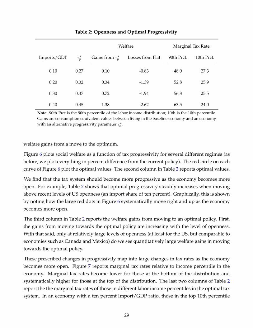
Table 2: Openness and Optimal Progressivity

Welfare Marginal Tax Rate

Imports/GDP τ∗p Gains from τ∗p Losses from Flat 90th Prct. 10th Prct.

0.10 0.27 0.10 -0.83 48.0 27.3

0.20 0.32 0.34 -1.39 52.8 25.9

0.30 0.37 0.72 -1.94 56.8 25.5

0.40 0.45 1.38 -2.62 63.5 24.0

Note: 90th Prct is the 90th percentile of the labor income distribution; 10th is the 10th percentile.Gains are consumption equivalent values between living in the baseline economy and an economywith an alternative progressivity parameter τ∗p .

welfare gains from a move to the optimum.

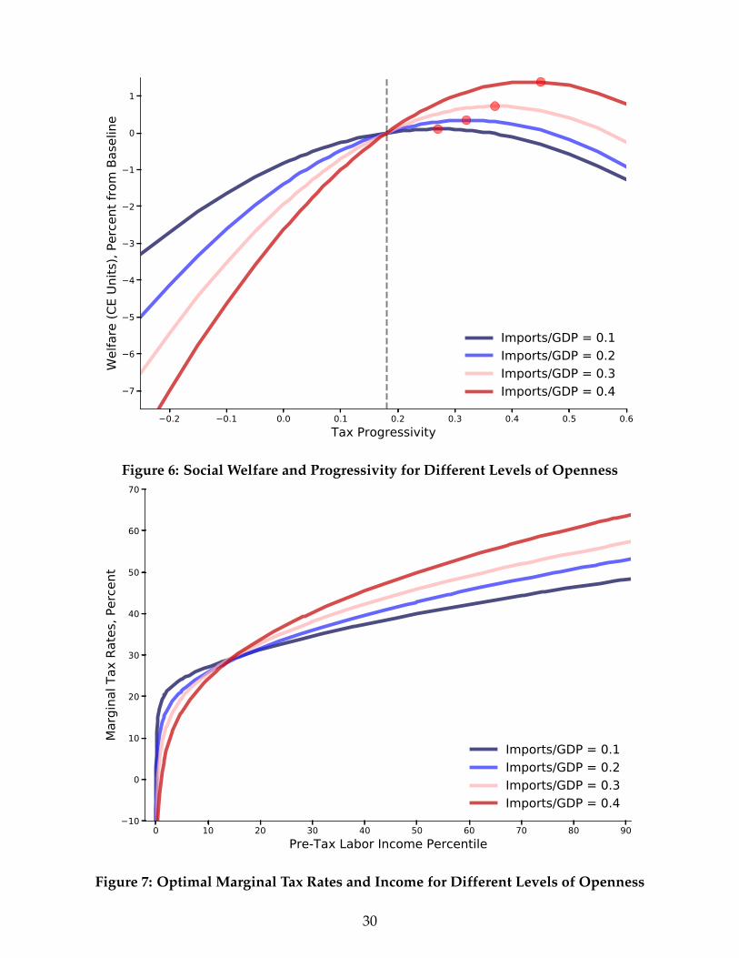
Figure 6 plots social welfare as a function of tax progressivity for several different regimes (asbefore, we plot everything in percent difference from the current policy). The red circle on eachcurve of Figure 6 plot the optimal values. The second column in Table 2 reports optimal values.

We find that the tax system should become more progressive as the economy becomes moreopen. For example, Table 2 shows that optimal progressivity steadily increases when movingabove recent levels of US openness (an import share of ten percent). Graphically, this is shownby noting how the large red dots in Figure 6 systematically move right and up as the economybecomes more open.

The third column in Table 2 reports the welfare gains from moving to an optimal policy. First,the gains from moving towards the optimal policy are increasing with the level of openness.With that said, only at relatively large levels of openness (at least for the US, but comparable toeconomies such as Canada and Mexico) do we see quantitatively large welfare gains in movingtowards the optimal policy.

These prescribed changes in progressivity map into large changes in tax rates as the economybecomes more open. Figure 7 reports marginal tax rates relative to income percentile in theeconomy. Marginal tax rates become lower for those at the bottom of the distribution andsystematically higher for those at the top of the distribution. The last two columns of Table 2report the the marginal tax rates of those in different labor income percentiles in the optimal taxsystem. In an economy with a ten percent Import/GDP ratio, those in the top 10th percentile

29

0.2 0.1 0.0 0.1 0.2 0.3 0.4 0.5 0.6Tax Progressivity

7

6

5

4

3

2

1

0

1W

elfa

re (C

E Un

its),

Perc

ent f

rom

Bas

elin

e

Imports/GDP = 0.1Imports/GDP = 0.2Imports/GDP = 0.3Imports/GDP = 0.4

Figure 6: Social Welfare and Progressivity for Different Levels of Openness

0 10 20 30 40 50 60 70 80 90Pre-Tax Labor Income Percentile

10

0

10

20

30

40

50

60

70

Mar

gina

l Tax

Rat

es, P

erce

nt

Imports/GDP = 0.1Imports/GDP = 0.2Imports/GDP = 0.3Imports/GDP = 0.4

Figure 7: Optimal Marginal Tax Rates and Income for Different Levels of Openness

30

of the labor income distribution have an marginal tax rate of 48 percent, the marginal tax ratefor those at the bottom of the distribution is about 27 percent. In the more open economy, withan import share of 40 percent, marginal tax rates of those in the top 10th percentile increase to63 percent, those at the bottom bottom 10th percentile decrease to 24 percent.

Overall, the elasticity of top tax rates to openness is 1/2. That is optimal policy dictates thata ten percentage point increase in imports as a fraction of GDP necessitates a five percentagepoint increase in marginal tax rates for those in the 90 percentile of the income distribution.

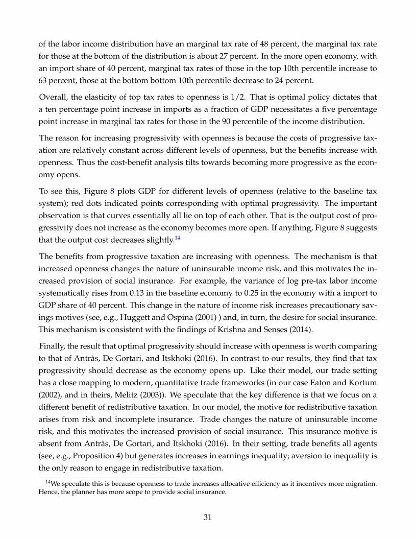
The reason for increasing progressivity with openness is because the costs of progressive tax-ation are relatively constant across different levels of openness, but the benefits increase withopenness. Thus the cost-benefit analysis tilts towards becoming more progressive as the econ-omy opens.

To see this, Figure 8 plots GDP for different levels of openness (relative to the baseline taxsystem); red dots indicated points corresponding with optimal progressivity. The importantobservation is that curves essentially all lie on top of each other. That is the output cost of pro-gressivity does not increase as the economy becomes more open. If anything, Figure 8 suggeststhat the output cost decreases slightly.14

The benefits from progressive taxation are increasing with openness. The mechanism is thatincreased openness changes the nature of uninsurable income risk, and this motivates the in-creased provision of social insurance. For example, the variance of log pre-tax labor incomesystematically rises from 0.13 in the baseline economy to 0.25 in the economy with a import toGDP share of 40 percent. This change in the nature of income risk increases precautionary sav-ings motives (see, e.g., Huggett and Ospina (2001) ) and, in turn, the desire for social insurance.This mechanism is consistent with the findings of Krishna and Senses (2014).

Finally, the result that optimal progressivity should increase with openness is worth comparingto that of Antras, De Gortari, and Itskhoki (2016). In contrast to our results, they find that taxprogressivity should decrease as the economy opens up. Like their model, our trade settinghas a close mapping to modern, quantitative trade frameworks (in our case Eaton and Kortum(2002), and in theirs, Melitz (2003)). We speculate that the key difference is that we focus on adifferent benefit of redistributive taxation. In our model, the motive for redistributive taxationarises from risk and incomplete insurance. Trade changes the nature of uninsurable incomerisk, and this motivates the increased provision of social insurance. This insurance motive isabsent from Antras, De Gortari, and Itskhoki (2016). In their setting, trade benefits all agents(see, e.g., Proposition 4) but generates increases in earnings inequality; aversion to inequality isthe only reason to engage in redistributive taxation.

14We speculate this is because openness to trade increases allocative efficiency as it incentives more migration.Hence, the planner has more scope to provide social insurance.

31

0.2 0.1 0.0 0.1 0.2 0.3 0.4 0.5 0.6

4

3

2

1

0GD

P, P

erce

ntag

e Po

ints

from

Bas

elin

e

Imports/GDP = 0.1Imports/GDP = 0.2Imports/GDP = 0.3Imports/GDP = 0.4

Figure 8: GDP and Progressivity for Different Levels of Openness

6.4. How Does Openness Change the Benefits of a Progressive Tax System?

While the welfare gains from moving toward the optimal policy may be small, this does notimply that a progressive tax policy is not beneficial as the economy opens to trade. In fact, aprogressive tax system plays an important role in an open economy. To illustrate this point, weask what the benefits of a progressive tax system are relative to a flat tax system and how theychange with the level of openness.

Figure 6 shows that the social welfare curves become more concave as the economy opens up.Relative to a flat tax system, this means the benefits of a progressive tax system become largeras the economy becomes more open. Unlike the benefits associated with the optimal policy,the gains are large even for current levels of openness. Table 2 reports that a move to a flat taxsystem at current levels of openness would lower welfare by almost one percent. For higherlevels of openness, a move to a flat tax system would erode welfare by more than two and halfpercent.

This result implies that the existing tax system complements the traditional gains from trade.With a flat tax system, the gains from trade associated with a move from a ten to 20 percentimport share lead to about a five and a half percent gain in welfare. However, if the tax system ismore progressive, even at the baseline of τp = 0.18, the welfare gains are just over seven percent.

32

In other words, the gains from trade increase by 25 percent with increases in progressivity.

This final point provides an interesting perspective on the historical evolution of tax policyand openness to trade. Antras, De Gortari, and Itskhoki (2016) find that the US tax systemhas declined in its progressivity—e.g., the measure τp declined from 0.25 in 1980 to 0.16 in2005. During this same time period, imports over GDP essentially doubled. That is as the USeconomy has open to trade, its tax system has become more regressive. Viewed through thelens of our model, this suggest that US tax policy was moving in the wrong direction giventrends in globalization. Moreover, the US has not gained what it could have from trade due tochanges in tax policy.

6.5. How Does a Progressive Tax System Compare to Tariffs?

How does a progressive tax system compare to import tariffs? This comparison is of interestfor two reasons. First, in the United States policy makers are taking a second look at anti-trade commercial policy as a means to correct various imbalances and harms associated withtrade. Moreover, the practical application of this tool may be easier, as the executive branch hasbroader authority over trade policy relative to changes in the tax code.

A second motive is that import tariffs and a progressive tax system may play similar socialinsurance roles. Early work by Corden (1974) and Baldwin (1982) speculate that one reasonfor tariffs is exactly to provide social insurance. Eaton and Grossman (1985) also show that amotive for a positive tariff is to provide social insurance. More starkly, Newbery and Stiglitz(1984), in a setting with risk and incomplete markets, provide an example that free trade isPareto inferior to autarky.

To compare a progressive tax system to import tariffs, we perform the following quantitativeexercises. Starting from our baseline economy, we compute and trace out social welfare underdifferent mixes of tariffs and tax progressivity.

One important issue is what to do with tariff revenue. Like tax revenue, we treat this as purewaste. Furthermore, we turn off the idea that the tariff becomes a substitute for income taxas a revenue collection device. To avoid this issue, for a given level of progressivity, we holdconstant average tax rates constant as we vary the tariff rate. So the way to think about thequestion is: “Given a labor income tax system, does a tariff improve welfare or not?”

Figures 9 and 10 illustrate the results. Each panel is an economy calibrated to a different level ofopenness—an import share of 20 percent and an import share of 40 percent and tax system withprogressivity of 0.18. On the horizontal axis, we have the import tariff and the tax progressivityparameter. On the vertical axis, we report welfare in consumption-equivalent units relative tothe baseline level of progressivity. The surface traces out welfare as we varied tariff rates andtax progressivity. The star indicates the optimal policy.

33

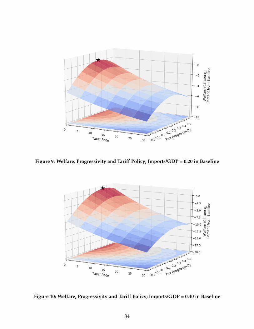
Tariff Rate

0 5 10 15 20 25 30 Tax Progressivity

0.20.1

0.00.1 0.2 0.3 0.4 0.5

Wel

fare

(CE

Units

), P

erce

nt fr

om B

asel

ine

10

8

6

4

2

0

Figure 9: Welfare, Progressivity and Tariff Policy; Imports/GDP = 0.20 in Baseline

Tariff Rate

0 5 10 15 20 25 30 Tax Progressivity

0.20.1

0.00.1 0.2 0.3 0.4 0.5

Wel

fare

(CE

Units

), P

erce

nt fr

om B

asel

ine

20.0

17.5

15.0

12.5

10.0

7.5

5.0

2.5

0.0

Figure 10: Welfare, Progressivity and Tariff Policy; Imports/GDP = 0.40 in Baseline

34

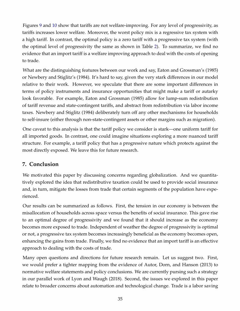
Figures 9 and 10 show that tariffs are not welfare-improving. For any level of progressivity, astariffs increases lower welfare. Moreover, the worst policy mix is a regressive tax system witha high tariff. In contrast, the optimal policy is a zero tariff with a progressive tax system (withthe optimal level of progressivity the same as shown in Table 2). To summarize, we find noevidence that an import tariff is a welfare improving approach to deal with the costs of openingto trade.

What are the distinguishing features between our work and say, Eaton and Grossman’s (1985)or Newbery and Stiglitz’s (1984). It’s hard to say, given the very stark differences in our modelrelative to their work. However, we speculate that there are some important differences interms of policy instruments and insurance opportunities that might make a tariff or autarkylook favorable. For example, Eaton and Grossman (1985) allow for lump-sum redistributionof tariff revenue and state-contingent tariffs, and abstract from redistribution via labor incometaxes. Newbery and Stiglitz (1984) deliberately turn off any other mechanisms for householdsto self-insure (either through non-state-contingent assets or other margins such as migration).

One caveat to this analysis is that the tariff policy we consider is stark—one uniform tariff forall imported goods. In contrast, one could imagine situations exploring a more nuanced tariffstructure. For example, a tariff policy that has a progressive nature which protects against themost directly exposed. We leave this for future research.

7. Conclusion

We motivated this paper by discussing concerns regarding globalization. And we quantita-tively explored the idea that redistributive taxation could be used to provide social insuranceand, in turn, mitigate the losses from trade that certain segments of the population have expe-rienced.

Our results can be summarized as follows. First, the tension in our economy is between themisallocation of households across space versus the benefits of social insurance. This gave riseto an optimal degree of progressivity and we found that it should increase as the economybecomes more exposed to trade. Independent of weather the degree of progressivity is optimalor not, a progressive tax system becomes increasingly beneficial as the economy becomes open,enhancing the gains from trade. Finally, we find no evidence that an import tariff is an effectiveapproach to dealing with the costs of trade.

Many open questions and directions for future research remain. Let us suggest two. First,we would prefer a tighter mapping from the evidence of Autor, Dorn, and Hanson (2013) tonormative welfare statements and policy conclusions. We are currently pursing such a strategyin our parallel work of Lyon and Waugh (2018). Second, the issues we explored in this paperrelate to broader concerns about automation and technological change. Trade is a labor saving

35

technology. It benefits many, but hurts those directly exposed to it. As exposure to this laborsaving technology increases, increasing progressivity improves welfare.

36

References

AIYAGARI, S. R. (1994): “Uninsured idiosyncratic risk and aggregate saving,” The QuarterlyJournal of Economics, 109(3), 659–684.

ANTRAS, P., A. DE GORTARI, AND O. ITSKHOKI (2016): “Globalization, Inequality and Wel-fare,” Discussion paper, National Bureau of Economic Research.

ARKOLAKIS, C., A. COSTINOT, AND A. RODRIGUEZ-CLARE (2012): “New Trade Models, SameOld Gains?,” American Economic Review, 102(1), 94–130.

ARTUC, E., S. CHAUDHURI, AND J. MCLAREN (2010): “Trade shocks and labor adjustment: Astructural empirical approach,” The American Economic Review, 100(3), 1008–1045.

ATTANASIO, O., AND S. J. DAVIS (1996): “Relative Wage Movements and the Distribution ofConsumption,” Journal of Political Economy, 104(6), 1227–1262.

AUTOR, D., D. DORN, AND G. H. HANSON (2013): “The China Syndrome: Local Labor MarketEffects of Import Competition in the United States,” The American Economic Review, 103(6),2121–2168.

AUTOR, D. H., D. DORN, G. H. HANSON, AND J. SONG (2014): “Trade adjustment: Worker-level evidence,” The Quarterly Journal of Economics, 129(4), 1799–1860.

BALDWIN, R. E. (1982): “The political economy of protectionism,” in Import competition andresponse, pp. 263–292. University of Chicago Press.

BENABOU, R. (2002): “Tax and Education Policy in a Heterogeneous-Agent Economy: WhatLevels of Redistribution Maximize Growth and Efficiency?,” Econometrica, 70(2), 481–517.

BRODA, C., AND D. E. WEINSTEIN (2006): “Globalization And The Gains From Variety,” Quar-terly Journal of Economics, 121(2).

CALIENDO, L., M. A. DVORKIN, AND F. PARRO (2015): “Trade and labor market dynamics,” .

CALIENDO, L., AND F. PARRO (2014): “Estimates of the Trade and Welfare Effects of NAFTA,”The Review of Economic Studies, p. rdu035.

CHANG, Y., AND S.-B. KIM (2007): “Heterogeneity and aggregation: Implications for labor-market fluctuations,” The American Economic Review, 97(5), 1939–1956.

COCHRANE, J. H. (1991): “A simple test of consumption insurance,” Journal of political economy,pp. 957–976.

37

CONESA, J. C., AND D. KRUEGER (2006): “On the optimal progressivity of the income tax code,”Journal of Monetary Economics, 53(7), 1425–1450.

CORDEN, W. M. (1974): Trade Policy and Economic Welfare. Oxford University Press.

COSAR, A. K., N. GUNER, AND J. TYBOUT (2016): “Firm dynamics, job turnover, and wagedistributions in an open economy,” The American Economic Review, 106(3), 625–663.

DIX-CARNEIRO, R. (2014): “Trade liberalization and labor market dynamics,” Econometrica,82(3), 825–885.

DIXIT, A. (1987): “Trade and insurance with moral hazard,” Journal of international economics,23(3-4), 201–220.

(1989a): “Trade and Insurance with Adverse Selection,” The Review of Economic Studies,56(2), 235–247.

(1989b): “Trade and Insurance with Imperfectly Observed Outcomes,” The QuarterlyJournal of Economics, 104(1), 195–203.

DIXIT, A., AND V. NORMAN (1986): “Gains from trade without lump-sum compensation,” Jour-nal of International Economics, 21(1-2), 111–122.

DORNBUSCH, R., S. FISCHER, AND P. A. SAMUELSON (1977): “Comparative advantage, trade,and payments in a Ricardian model with a continuum of goods,” The American EconomicReview, 67(5), 823–839.

EATON, J., AND G. M. GROSSMAN (1985): “Tariffs as Insurance: Optimal Commercial PolicyWhen Domestic Markets Are Incomplete,” The Canadian Journal of Economics / Revue canadi-enne d’Economique, 18(2), 258–272.

EATON, J., AND S. KORTUM (2002): “Technology, geography, and trade,” Econometrica, 70(5),1741–1779.

EATON, J., AND H. S. ROSEN (1980): “Optimal redistributive taxation and uncertainty,” TheQuarterly Journal of Economics, 95(2), 357–364.

EPIFANI, P., AND G. GANCIA (2009): “Openness, government size and the terms of trade,” TheReview of Economic Studies, 76(2), 629–668.

FELER, L., AND M. Z. SENSES (2017): “Trade shocks and the provision of local public goods,”American Economic Journal: Economic Policy, 9(4), 101–43.

38

GALLE, S., A. RODRGUEZ-CLARE, AND M. YI (2017): “Slicing the Pie: Quantifying the Aggre-gate and Distributional Effects of Trade,” Working Paper 23737, National Bureau of EconomicResearch.

GUNER, N., R. KAYGUSUZ, AND G. VENTURA (2014): “Income taxation of US households: Factsand parametric estimates,” Review of Economic Dynamics, 17(4), 559–581.

HANSON, G. H., N. LIND, AND M.-A. MUENDLER (2015): “The dynamics of comparativeadvantage,” Discussion paper, National Bureau of Economic Research.

HEATHCOTE, J., K. STORESLETTEN, AND G. L. VIOLANTE (2014): “Optimal tax progressivity:An analytical framework,” Discussion paper, National Bureau of Economic Research.

HUGGETT, M. (1993): “The risk-free rate in heterogeneous-agent incomplete-insuranceeconomies,” Journal of economic Dynamics and Control, 17(5), 953–969.

HUGGETT, M., AND S. OSPINA (2001): “Aggregate precautionary savings: when is the thirdderivative irrelevant?,” Journal of Monetary Economics, 48(2), 373–396.

JONES, R. (1971): “A Three Factor Model in Theory, Trade, and History,” in Trade, balance ofpayments and growth, ed. by R. M. J. V. Jagdish Bhagwati, Ronald Jones. North-Holland, Am-sterdam.

KAMBOUROV, G. (2009): “Labour Market Regulations and the Sectoral Reallocation of Workers:The Case of Trade Reforms,” Review of Economic Studies, 76(4), 1321–1358.

KAPLAN, G. (2012): “Inequality and the life cycle,” Quantitative Economics, 3(3), 471–525.

KEANE, M. P. (2011): “Labor supply and taxes: A survey,” Journal of Economic Literature, 49(4),961–1075.

KENNAN, J., AND J. R. WALKER (2011): “The effect of expected income on individual migrationdecisions,” Econometrica, 79(1), 211–251.

KRISHNA, P., AND M. Z. SENSES (2014): “International Trade and Labour Income Risk in theU.S.,” The Review of Economic Studies, 81(1), 186–218.

KRUEGER, D., K. MITMAN, AND F. PERRI (2016): “Macroeconomics and Household Hetero-geneity,” Handbook of Macroeconomics, 2, 843–921.

KRUSELL, P., T. MUKOYAMA, AND A. SAHIN (2010): “Labour-market matching with precau-tionary savings and aggregate fluctuations,” The Review of Economic Studies, 77(4), 1477–1507.

LAGAKOS, D., M. MOBARAK, AND M. E. WAUGH (2017): “The Welfare Effects of EncouragingRural-Urban Migration,” .

39

LUCAS, R. E., AND E. C. PRESCOTT (1974): “Equilibrium search and unemployment,” Journalof Economic Theory, 7(2), 188–209.

LYON, S., AND M. WAUGH (2018): “Quantifying the Losses from International Trade,” .

MELITZ, M. J. (2003): “The impact of trade on intra-industry reallocations and aggregate in-dustry productivity,” Econometrica, 71(6), 1695–1725.

MIRANDA, M. J., AND P. L. FACKLER (2004): Applied computational economics and finance.

MIRRLEES, J. (1974): “Notes on welfare economics, information and uncertainty,” Essays oneconomic behavior under uncertainty, pp. 243–261.

MIRRLEES, J. A. (1971): “An exploration in the theory of optimum income taxation,” The reviewof economic studies, 38(2), 175–208.

MOLLOY, R., C. L. SMITH, AND A. WOZNIAK (2011): “Internal migration in the United States,”The Journal of Economic Perspectives, 25(3), 173–196.

MORTEN, M. (2016): “Temporary migration and endogenous risk sharing in village india,”Discussion paper, National Bureau of Economic Research.

NEWBERY, D. M., AND J. E. STIGLITZ (1984): “Pareto inferior trade,” The Review of EconomicStudies, 51(1), 1–12.

OLLEY, G. S., AND A. PAKES (1996): “The Dynamics of Productivity in the TelecommunicationsEquipment Industry,” Econometrica, 64(6), 1263–1297.

PARRO, F. (2013): “Capital-skill complementarity and the skill premium in a quantitative modelof trade,” American Economic Journal: Macroeconomics, 5(2), 72–117.

PAVCNIK, N. (2017): “The Impact of Trade on Inequality in Developing Countries,” WorkingPaper 23878, National Bureau of Economic Research.

REDDING, S. J. (2016): “Goods trade, factor mobility and welfare,” Journal of International Eco-nomics, 101, 148–167.

RODRIK, D. (1997): Has Globalization Gone Too Far? Columbia University Press.

(1998): “Why do more open economies have bigger governments?,” Journal of politicalEconomy, 106(5), 997–1032.

ROGERSON, R. (1988): “Indivisible labor, lotteries and equilibrium,” Journal of monetary Eco-nomics, 21(1), 3–16.

40

ROGERSON, R., AND J. WALLENIUS (2009): “Micro and macro elasticities in a life cycle modelwith taxes,” Journal of Economic theory, 144(6), 2277–2292.

SAMUELSON, P. A. (1971): “Ohlin Was Right,” The Swedish Journal of Economics, 73(4), 365–384.

SIMONOVSKA, I., AND M. E. WAUGH (2014a): “The elasticity of trade: Estimates and evidence,”Journal of International Economics, 92(1), 34 – 50.

SIMONOVSKA, I., AND M. E. WAUGH (2014b): “Trade models, trade elasticities, and the gainsfrom trade,” Discussion paper, National Bureau of Economic Research.

SPECTOR, D. (2001): “Is it possible to redistribute the gains from trade using income taxation?,”Journal of International Economics, 55(2), 441–460.

TOLBERT, C. M., AND M. SIZER (1996): “US commuting zones and labor market areas: A 1990update,” .

VARIAN, H. R. (1980): “Redistributive taxation as social insurance,” Journal of public Economics,14(1), 49–68.

41

A. Connection with National Accounts

This section connects these equilibrium relationships to national income and product accounts(NIPA). This will help facilitate an understanding of the connection between trade imbalancesand household’s consumption-savings decisions. Note that in all of this derivation, we normal-ize the price of the final good to one.

The Income Side of NIPA. It is first useful to start from an income side measure of produc-tion (or GDP) in our economy. Given competition, the value of aggregate production of thefinal good must equal aggregate payments for intermediate goods. The latter equals aggregatepayments to labor in the production of all intermediate goods.

Y =

∫sw(s)µ(s)ds (38)

Examining (29) and (38) allows us to connect aggregate income with consumption. Specifi-cally, by integrating over the consumers budget constraint, then noting how total value addedmust equal take home pay plus taxes/transfers from the government, one can substitute (38)into (29). Then from the definition of the governments budget constraint (which includes taxrevenue and tariff revenue), we arrive at the following:

Y = C +G−RA+A′ −∫a

∫smιm(s, a)λ(s, a)ds da− τf

∫sp(s)imports(s)ds (39)

so aggregate income equals consumption (private and public) minus (i) returns on assets (ii)new purchases of assets (iii) plus moving costs (iv) minus tariff revenue. The last point followsfrom noting that government consumption is both tax revenue and tariff revenue.

This basically says that income/production must equal consumption net of income not associ-ated with production (i.e. returns on assets and home production) plus “investment” in assetsand moving costs. For example, if consumption is larger than income one reason is that (inaggregate) households (on net) are borrowing from abroad (A′ < 0).

Production Side of NIPA. The the value of aggregate production of the final good must equalthe value of intermediate goods production

Y =

∫sp(s)zµ(s)ds (40)

which we can then connect with the expenditure side of GDP through the market clearingconditions for intermediate goods and final goods. Specifically, by connecting the productionside with the demand side for non-traded goods in (20), imports in (22) and exports in (24) and

42

the equating final demand with consumption we have

Y = C + G+

∫sp(s)exports(s)ds− (1− τf )

∫sp(s)imports(s)ds (41)

= C +G+

∫sp(s)exports(s)ds−

∫sp(s)imports(s)ds. (42)

Or GDP equals consumption (private and public) plus exports minus imports.

Savings, Trade Imbalances, and Capital Flows. Finally, we can connect the income side andthe production side the national accounts to arrive at a relationship between asset holdings andtrade imbalances. By working with both (39) and (42) we get the following relationship

Y− C −G =

∫sp(s)exports(s)ds−

∫sp(s)imports(s)ds, (43)

=− rA+ (A′ −A) +

∫a

∫smιm(s, a)λ(s, a)ds da− τf

∫sp(s)imports(s)ds,

where r is the net real interest rate. This relationship says the following: aggregate savingsequals the trade imbalance. And this, in turn, we can connect the trade balance with the sav-ings decisions of the households. That is the trade balance equals payments on net asset hold-ings plus net change in asset holdings (adjusted for moving costs and tariff revenue). To mapthis into Balance of Payments language: the trade imbalance plus foreign income payments isthe current account; the capital account is the net change in foreign asset holdings; then (wesuspect) moving costs would show up as the “balancing item.”

To see this, consider the special case where moving costs are zero and tariffs are zero. Then wehave the relationship

Y − C −G =

∫sp(s)exports(s)ds−

∫sp(s)imports(s)ds = −rA+ (A′ −A). (44)

Here if exports are greater than imports, then this implies that the households in the homecountry are doing several things. The trade surplus may reflect that households (on net) aremaking debt payments (rA is negative). Second, the trade surplus may reflect that the house-holds (on net) are acquiring foreign assets (A′ −A is positive). Finally, note that in a stationaryequilibrium, the trade imbalance only reflects payments from foreign asset holdings. This im-plies that the current account and capital account are always zero in a stationary equilibrium,but that trade may be imbalanced.

43

B. Computational Appendix

This section describes our computational approach to solving and calibrating the model. Allmaterials are posted at https://github.com/mwaugh0328. The code is presented in twodifferent languages: Matlab and Julia. The implementation in both languages follows the samecore steps, but the details are slightly different. The discussion below follows the Matlalb codeand the instructions in the island solve progresive NAG.m file. For a detailed explanationof how the Julia code works, see the file model/README Julia.md.

• We approximate the continuous asset, productivity, and world price states by discretiza-tion. The asset space follows a non-uniform grid with grid points clustered near the bor-rowing constraint. The number of grid points was set to 50; the results are not sensitive toincreases in this number. We use the method of Rouwenhorst to discretize the productiv-ity and world price process. We use 10 states for productivity and world prices each, thusthere are 100 different states s.

• Guess a proposed price function p(s) and government policy δ.

• Compute after-tax wages.

• Solve the households problem in (10). This is performed using value function iteration.

One technique we use to facilitate finding a solution to the equilibrium is to “smooth”out the discrete choice problem. We do this by assuming that there are additive logisti-cally distributed preference shocks with parameter bsmth and these preference shocks areindependently distributed across each choice. These enter into the choice problem in (10)by adding onto each option. What this gives rise to is, for each asset holdings state andstate s, there will be a non-zero mass of households choosing all options. The probabili-ties take the familiar logit form. We tune the parameter bsmth to ensure that it is small andnot affecting the economics of the problem, but at the same time ensure that we find asolution.

Smoothing in this manner is important as it facilitates the use derivative based solvers infinding an equilibrium p(s). This in turn results in a dramatic speed-up in the computationof an equilibrium. See, e.g., Morten (2016) who employs a similar approach.

• Given the policy functions associated with the solution to the problem in (10), we computethe stationary distribution over assets and states s, i.e. λ(a, s) which is of size 50 (for eachasset state) and 100 for each state s. This process is sped up using sparse matrices, see thecode island invariant.m for details.

• Given the stationary distribution, we can compute excess demand functions for all islandss which also must respect the inequalities implied by (21) and (23). These conditions imply

44

that the problem of finding a price function consistent with a stationary equilibrium can berepresented as a mixed complementarity problem (see, e.g., Miranda and Fackler (2004)).To smooth out the nondifferentiability issues with the complementarity problem we passthe excess demand functions through Fischer’s function. Again, see Miranda and Fackler(2004).

• Update p(s) and government policy δ and proceed until convergence criteria are met.

In solving for the equilibrium, we employed derivative based solvers. One solver thatwe found much success with is the c05qc solver from Numerical Algorithms Group.MATLAB’s fsolve with central finite differences performed well too.

Our calibration approach employed the following technique. Let Θ be the parameter vectorwe chose to match some moments. In our specific case, this is Θ = {τ,m,B} or the trade cost,the moving cost, and the disutility of labor. We then jointly solved for {p(s), δ,Θ} in one step.That is we asked the algorithm described to find a price vector and set of parameters suchthat (i) equilibrium conditions are satisfied and (ii) model implied moments match our targetempirical moments. This avoided a more standard, but time consuming approach of guessinga Θ, solving for an equilibrium, updating Θ, etc. Extensive sensitivity analysis found no issuessurrounding multiplicity of equilibrium.

45