The Journal of Systems and Software 69 (2004) 115–128

www.elsevier.com/locate/jss

New methods for redistributing slack time in real-timesystems: applications and comparative evaluations

R.M. Santos, J. Urriza, J. Santos *, J. Orozco

Departamento de Ingenieria Electrica y Computadoras, Universidad Nacional del Sur, CONICET, Avda. Alem 1253, 8000 Bahia Blanca, Argentina

Received 23 July 2002; received in revised form 14 March 2003; accepted 15 March 2003

Abstract

This paper addresses the problem of scheduling hard and non-hard real-time sets of tasks that share the processor. The notions of

singularity and k-schedulability are introduced and methods based on them are proposed. The execution of hard tasks is postponed

in such a way that hard deadlines are not missed but slack time is advanced to execute non-hard tasks. In a first application, two

singularity methods are used to schedule mixed systems with hard deterministic sets and stochastic non-hard sets. They are com-

pared to methods proposed by other authors (servers, slack stealing), background and M/M/1. The metric is the average response

time in servicing non-hard tasks and the proposed methods show a good relative performance. In a second application, the previous

methods, combined with two heuristics, are used for the on-line scheduling of real-time mandatory/reward-based optional systems

with or without depreciation of the reward with time. The objective is to meet the mandatory time-constraints and maximize the

reward accrued over the hyperperiod. To the best of the authors’ knowledge, these are the only on-line methods proposed to address

the problem and outperform Best Incremental Return, often used as a yardstick.

� 2003 Elsevier Inc. All rights reserved.

Keywords: Mixed systems; Reward-based systems; Slack time; Scheduling

1. Introduction

Research in real-time systems covers several areas,

e.g. operating systems, programming languages, archi-

tecture, fault tolerance, scheduling, etc. (Stankovic,1988). In the classical definition, real-time systems are

those in which results must be not only correct from an

arithmetic-logical point of view but also produced be-

fore a certain instant, called deadline. If no deadline can

be missed, the system is said to be hard as opposed to

soft in which some deadlines may be missed. Scheduling

theory addresses the problem of meeting the specified

time constraints. When they are met the system is said tobe schedulable.

In 1973, Liu and Layland published a seminal paper

on the scheduling of hard real-time systems in a multi-

task-uniprocessor environment in which tasks are peri-

*Corresponding author. Tel.: +54-291-459-5181; fax: +54-291-459-

5154.

E-mail address: iesantos@criba.edu.ar (J. Santos).

0164-1212/$ - see front matter � 2003 Elsevier Inc. All rights reserved.

doi:10.1016/S0164-1212(03)00079-7

odic, independent and preemptible. This is the only type

of tasks considered on that paper.

Designing for the worst case (e.g. always maximum

execution time and minimum interarrival time for every

task) generally leads to an underutilization of resourceswhen the worst case does not take place. To this, the

unused time that appears, even in the worst case, when

there are no hard tasks with pending execution must be

added. In order to make the system more efficient by

using the time left free by the hard set, combined sets of

hard and non-hard real-time tasks were studied later,

among them:

(a) Mixed uniprocessor systems in which deterministic

hard real-time tasks share resources with stochastic

non-hard tasks (Sprunt et al., 1989; Lehoczky and

Ramos-Thuel, 1992; Strosnider et al., 1995) and

(b) hard mandatory/reward-based optional systems in

which tasks have a hard mandatory part and an op-

tional part with a non-decreasing reward function

associated with its execution (Dey and Kurose,1996; Aydin et al., 2001).

116 R.M. Santos et al. / The Journal of Systems and Software 69 (2004) 115–128

The least common multiple of the periods is called the

hyperperiod. The release of periodic tasks (ready to be

executed) and their processing are the same in each

hyperperiod. A certain fraction of the hyperperiod is

devoted to the execution of the periodic tasks and the

rest is idle time available for other uses. This time iscalled slack.

If the slack can be redistributed without compro-

mising the time constraints, the execution of tasks not

belonging to the real-time set can be made in such a way

that a better service is given. The problem, then, is

clearly defined as how to redistribute slack so that no

hard deadline is missed but the quality of service (QoS)

given to non-hard tasks is improved.Orozco et al. (2000) introduced the notions of sin-

gularity and k-schedulability, used in methods for

scheduling mixed systems. Later, Santos et al. (2002)

expanded its use to reward-based systems. The purpose

of this paper is to present a unified view of the theo-

retical approach and its applications. The results of ex-

tensive evaluations are analysed. The simulations are

described to the extent that their correctness can bevalidated and the results repeated. In the absence of

benchmarks, each simulation was performed using sets

of tasks similar to those proposed by authors of com-

peting methods to solve the same problem.

The rest of the paper is organized as follows: In

Section 2, previous related work is reviewed. In Section

3 the notions of k-schedulability and singularity are

presented and the new scheduling methods, based onthose notions, are described. In Sections 4 and 5, the

methods are applied to mixed and to reward-based

systems, respectively. In Section 6, conclusions are

drawn.

2. Related work

In what follows, previous related work of both types

of combined systems is reviewed.

2.1. Hard periodic/non-hard stochastic tasks

In this type of systems, called mixed, besides the hard

real-time set of tasks there are non-real-time tasks, with

no deadlines. It is a common model, well suited toproblems of the real world where hard tasks are periodic

and therefore deterministic, while non-real-time are

aperiodic and stochastic (Gonzalez Harbour and Sha,

1991; Lehoczky and Ramos-Thuel, 1992; Buttazzo and

Caccamo, 1999).

The problem of redistributing slack in mixed systems

has been addressed using servers and slack stealing.

Servers are periodic tasks created for servicing aperiodictasks. Three main types of servers have been proposed:

polling, sporadic and deferrable. The polling server runs

periodically at a period equal to the minimum period in

the set of tasks and the maximum execution time

schedulable within that period. This server loses the

unused slots in the period.

The sporadic (Sprunt et al., 1989; Gonzalez Harbour

and Sha, 1991) and the deferrable (Strosnider et al.,1995) servers allow their capacity to be used throughout

their periods (bandwidth preserving algorithms). They

only differ in the way their capacity is replenished. In

most applications, their performance is roughly similar.

In static slack stealing (Lehoczky and Ramos-Thuel,

1992; Ramos-Thuel, 1993), all the possible slack that

can be taken from the hard set without causing any

deadline to be missed is ‘‘stolen’’. It works by computingoff-line the slack available at each task invocation in the

hyperperiod. Results are saved in tables in the Operating

System kernel. Except in very simple cases, the tables are

rather large making the method unfeasible as a dynamic

on-line algorithm for most practical engineering appli-

cations. On top of that, periods must be rigorously ob-

served and no allowance for jitter can be made.

However this method gives the best average results andit is used as a sort of benchmark in the comparative

evaluations. An on-line version, dynamic slack stealing

(Davis et al., 1993) avoids some of those restrictions but

has a run time overhead such that it is unfeasible in

practice. All the methods described are greedy in the

sense that slack is used, at the highest priority level,

immediately after it becomes available.

When the methods proposed in this paper are appliedto the scheduling of mixed systems, they are not only

unaffected by jitter but profit from it. In addition to that,

when tasks are executed in less than their worst case

execution time, the methods automatically adjust

themselves to the varying conditions and take advantage

of that surplus time to improve the service of non-hard

tasks.

2.2. Hard mandatory/reward-based optional tasks

The processing of tasks decomposed in mandatory/

optional subtasks had been used previously in tradi-

tional iterative-refinement algorithms for imprecise

computation in which the aim was to minimize the

weighted sum of errors (Lin et al., 1987; Liu et al., 1991;

Shih and Liu, 1995).Dey and Kurose (1996), proposed two implementable

scheduling policies for a class of Increasing Reward with

Increasing Service (IRIS) problems. A top-level algo-

rithm, common to both policies, is executed at every

task arrival to determine the amount of service to be

allocated to each task; later, a bottom-level algorithm,

different for each policy, determines the order in which

tasks are executed. However, tasks are not decomposedin a mandatory (with a minimum service time) and an

optional part. Instead tasks receive whatever time can be

R.M. Santos et al. / The Journal of Systems and Software 69 (2004) 115–128 117

assigned to them before their deadline expires. Although

mandatory subtasks may be introduced, these will not

have guaranteed hard deadlines. In fact, an additional

performance metric, the probability of missing a task’s

deadline before it can receive its mandatory amount of

service, is introduced.Chung et al. (1990) proposed different mandatory first

schemes, all sharing the condition that mandatories are

always executed first. They differ in the policy according

to which optional parts are scheduled (earlier-deadline-

first, least-laxity-first, etc.). The time allocated to op-

tionals is not the result of slack reshuffling but mere

empty background time that appears when there are no

hard tasks to be executed. Aydin et al. (2001) comparedthe schemes and found that allocating background slack

to the optional contributing most to the total reward at

that moment produces the best results among all the

mandatory first methods. Because of this, the method is

called Best Incremental Return and it is often used as a

yardstick.

Aydin et al. (2001) presented an off-line reward-based

method. It is based on the use of linear programmingmaximizing techniques and this requires the reward

functions to be continuously differentiable. Also, in or-

der to reduce the number of unknowns, it imposes the

constraint that the optional part of each task receives

the same service time at every task instantiation, re-

sulting in a rather rigid system. In addition to that, the

proposed method provides solutions not only subject to

that constraint but also in which mandatory parts can-not be scheduled according to the Rate Monotonic

discipline unless the periods are harmonic. The use of

that discipline, important because it is a de facto stan-

dard, is then limited to that particular class of problems.

When the methods presented in the present paper are

applied to the scheduling of reward-based systems, the

only requirement imposed on the reward functions is

their computability at every instant. To the best of theauthors’ knowledge, these methods are the only ones

proposed up to now to schedule mandatory/optional

reward systems by an on-line redistribution of slack time.

3. k-Schedulability and singularities

When two or more periodic tasks compete for the useof the processor, some rules must be applied to allocate

its use. This set of rules is called priority discipline. In a

static fixed priority discipline all tasks are assigned a

priority once for all. If tasks are ordered by decreasing

rates or, what is the same, by increasing periods, the

discipline is called Rate Monotonic, notated RM. The

task with the shortest period has the highest priority.

Some additional rule must be provided to break ties.Liu and Layland (1973) proved that Rate Monotonic

is optimal among the Fixed Priority disciplines. It is

supported by the US Department of Defence and con-

sequently adopted, among others, by IBM, Honeywell,

Boeing, General Electric, General Dynamics, Magn-

avox, Mitre, NASA, Naval Air Warfare Center, Para-

max and McDonnell Douglas (Obenza, 1993). No doubt

it is a de facto standard, at least in the US. Therefore itmakes sense to use it whenever possible, especially in

applied systems that may find their way to the market.

Several methods have been proposed for testing the

RM schedulability of real-time systems (Liu and Lay-

land, 1973; Joseph and Pandya, 1986; Lehoczky et al.,

1989; Santos and Orozco, 1993). In the Empty Slots

method (Santos and Orozco, 1993), time is considered to

be slotted and the duration of one slot is taken as theunit of time. Slots are notated t and numbered 1, 2, . . . .The expressions at the beginning of slot t and instant tmean the same. Tasks are preemptible at the beginning

of slots. As proved by Liu and Layland (1973), the worst

case of load occurs when all tasks are released simulta-

neously at t ¼ 1.

A set of n independent preemptible periodic tasks is

completely specified as SðnÞ ¼ ðC1; T1;D1Þ;ðC2; T2;D2Þ; . . . ; ðCn; Tn;DnÞ, where Ci, Ti and Di, denote the

worst case execution time, the period and the deadline of

task i, denoted si, respectively. A common assumption is

that 8i Di ¼ Ti. In what follows, and for the sake of

simplicity, it is assumed that tasks are released at the

beginning of slots and that execution times, periods and

deadlines are multiples of the slot time. These constric-

tions can be easily relaxed.Santos and Orozco (1993) formally proved that SðnÞ

is RM schedulable iff

8i 2 ð1; 2; . . . ; nÞ Ti P least tjt ¼ Ci þXi�1

h¼1

ChtTh

� �ð1Þ

where de denotes the ceiling operator.

The RM scheduling does not leave empty slots if

there are tasks pending execution. Therefore, slots go

empty only when all the tasks released in the interval [1,empty slot] have been executed. The right hand member

of (1) represents the Cith slot left empty by Sði� 1Þ. Thecondition, therefore, is intuitively clear: si can be added

to the system of ði� 1Þ tasks keeping the expanded

system schedulable if and only if before its deadline

there are enough empty slots to execute it and to give

way to tasks of higher priority. Liu and Layland (1973)

proved that the worst case of load takes place when alltasks are released simultaneously at t ¼ 1.

The last term in the right hand member in (1) is called

the work function, denoted Wi�1ðtÞ. If M denotes the

hyperperiod (the least common multiple of the periods

of the n tasks), the expression

WnðMÞ ¼Xn

i¼1

CiMTi

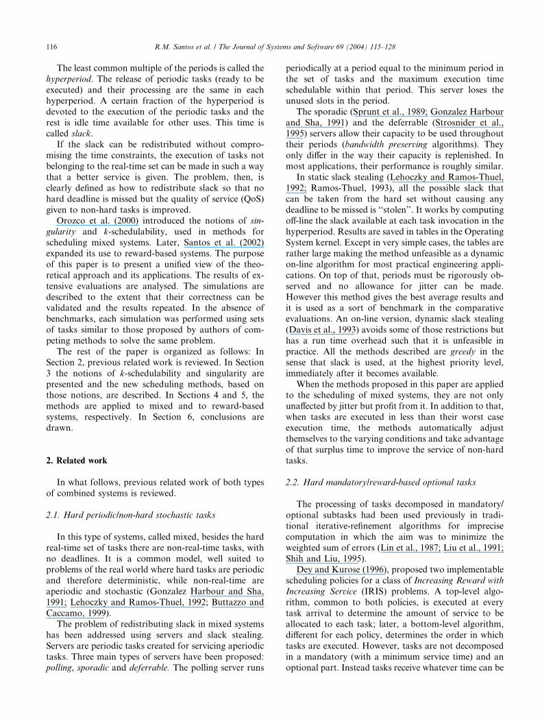
Table 1

The specification of the system

i Ci Ti

1 1 3

2 2 5

3 1 15

118 R.M. Santos et al. / The Journal of Systems and Software 69 (2004) 115–128

gives the number of slots necessary to process all the

tasks belonging to SðnÞ in the interval ½1;M �. The slack

(or number of empty slots in the hyperperiod) will be

M � WnðMÞ.

Example. Let S(3) be the system specified in Table 1.The three tasks are RM ordered

The test for the RM schedulability follows. It starts

with T1. Since there are no tasks of higher priority, the

first condition is

for i ¼ 1 T1 P least tjt ¼ 1

The first slot meeting the condition is t ¼ 1. Since

T1 ¼ 3P 1, the subsystem of only one task is RM

schedulable.

for i ¼ 2 T2 P least tjt ¼ 2þ dt=3e

The first slot meeting the condition is t ¼ 3. SinceT2 ¼ 5P 3, the subsystem of two tasks is RM schedu-

lable.

for i ¼ 3 T3 P least tjt ¼ 1þ 2dt=3e þ dt=5eThe first slot meeting the condition is t ¼ 5. Since

T3 ¼ 15P 5, the system of three tasks is RM schedula-

ble. In Fig. 1, the processing of the tasks is depicted.

Note that W3ð15Þ ¼ d15=3e þ 2d15=5e þ d15=15e ¼ 12.

The number of empty slots is therefore 15� 12 ¼ 3.

They are slots 9, 14 and 15.

The utilization factor of task si is defined as Ci=Ti.Conceptually it is the fraction of processor time used by

si. The total utilization factor is thenPn

i¼1 Ci=Ti. If it isless than 1, empty slots will be available to expand the

system by incorporating other tasks. If it is equal to 1,

the system is saturated and no task can be added. If it is

larger than 1, the system is oversaturated and unsched-

ulable whichever the policy used.

A hard real-time system SðnÞ is said to be k-RMschedulable if it is RM schedulable in spite of the fact

that in the interval between its release and its deadline,

Fig. 1. The evolution of the system. # denotes the release of the task.

each task admits that k slots are devoted to the execu-

tion of tasks not belonging to the system (Orozco et al.,

2000).

Theorem 1. A system SðnÞ is k-RM schedulable iff

8i 2 ð1; 2; . . . ; nÞ Ti P least tjt ¼ Ci þ k þ Wi�1ðtÞ

Proof. In order to meet its deadline after the worst case

of load of Sði� 1Þ, each task si must have Ci slots to be

executed, k slots to admit execution of tasks 62 SðnÞ andWi�1ðtÞ slots to allow the execution of tasks of higher

priority. h

It must be noted that k is the lower bound on fkigwhere ki is defined as

ki ¼ max kjTi P least tjt ¼ Ci þ k þ Wi�1ðtÞ ð2ÞThe complexity of the test for the k-schedulability is

the same as that for the RM schedulability. Santos and

Orozco (1993) proved it to be Oðn� TnÞ, where Tn de-

notes the maximum period in the system.

Corollary. If a hard real-time system SðnÞ is k-RMschedulable, the k first slots following the worst case ofload can be used to execute tasks 62 SðnÞ.

Proof. It follows from the definition of k-RM schedu-

lability and Theorem 1. h

A singularity, s, is a slot in which all the real-time

tasks released in ½1; ðs� 1Þ� have been executed. Note

that s� 1 can be either an empty slot or a slot in which a

last pending real-time task completes its execution. s is asingularity even if at t ¼ s, real-time tasks are released.

Theorem 2. If a hard real-time system SðnÞ is k-RMschedulable, the k slots of an interval ½s; ðsþ k � 1Þ� canbe used to execute tasks 2 SðnÞ.

Proof. At s� 1 the last pending task of the interval

½1; ðs� 1Þ� is executed. Therefore at t ¼ s there are at

most the same requirements that in the worst case of

load. Then, if SðnÞ is k-RM schedulable after the worst

case of load, it will be k-RM schedulable after s. h

A singularity si is a slot in which all tasks belonging

to SðiÞ, released in the interval ½1; ðsi � 1Þ� have been

executed.

The results presented above can be used to devise

methods for scheduling a set SðnÞ of hard periodic real-

time tasks sharing the processor with other, aperiodic,

tasks 62 SðnÞ. Two methods are proposed. The first one,

single singularity detection, notated SSD, is based on thedetection of s; whenever possible, k slots, slated for tasks

62 SðnÞ, are generated and used to service them. The

R.M. Santos et al. / The Journal of Systems and Software 69 (2004) 115–128 119

second method, multiple singularity detection, notated

MSD, refines the first one by detecting all singularities si.The basic SSD method is implemented by means of

one counter (content denoted AC). The algorithm is:

(1) AC ¼ k at t ¼ s.(2) Tasks 62 SðnÞ are executed if AC 6¼ 0.

(3) AC is decremented by one on each slot assigned to a

task 62 SðnÞ.

The basic MSD method is implemented by means of

n counters (contents denoted ACi). The algorithm is:

(1) 8g 2 f1; 2; . . . ; ig, ACg ¼ kg at t ¼ si.(2) Tasks 62 SðnÞ are executed if 8i 2 f1; 2; . . . ; ng

ACi 6¼ 0.

(3) 8i 2 f1; 2; . . . ; ngACi is decremented by one on each

slot assigned to a task 62 SðnÞ.

It must be noted that since empty slots are singular-

ities, counters will be reloaded at them.

4. Mixed systems

The methods, as explained in the previous section, are

directly applied to the scheduling of mixed systems in

which a set of periodic tasks is mixed with stochastic

aperiodic tasks. The hard set is RM scheduled and the

aperiodic tasks serviced in first in first out (FIFO) order.The FIFO queue is long enough for no aperiodic request

to be lost. A real world application would be a processor

controlling a section of an automated manufacturing

line. Reading data from sensors, processing them and

setting actuators are all periodic real-time tasks. Even-

tually, a human operator may require statistical infor-

mation about the process, the display of mimic screens,

etc. These would be aperiodic non-real-time tasks.Tia et al. (1996) proved that no algorithm can be

optimal in the sense of yielding the minimum response

time for every aperiodic request. What is sought here is

an on-line method that yields an average aperiodic delay

that compares favourably to delays produced by other

methods proposed to address the same problem.

Strosnider et al. (1995) designed the performance

evaluation methodology used in what follows. Themetric is average response time, defined as the time

elapsed between the release of the aperiodic task and the

completion of its execution, without causing any hard

task to miss its deadline.

Simulations are carried out for different utilization

factors of the periodic load, Up, and different utilization

factors and mean service time of the aperiodic load (Ua

and l, respectively). The average delay in servicing theaperiodic requests is determined for the polling and

deferrable servers, SSD, MSD and slack stealing. The

performance of background and M/M/1 is also deter-

mined. Background is the simplest way to schedule

slack. It consists in letting slots left empty by the peri-

odic set appear naturally and use them as they appear.

As can be seen it is absolutely passive. M/M/1 assumes

no periodic load and therefore gives a lower bound onthe average aperiodic delay. All the compared methods

are greedy. Two non-greedy methods proposed by Tia

et al. (1996) have an average performance similar to that

of the greedy methods.

The aperiodic arrival and service times follow a

Poisson and an exponential distribution respectively.

For each simulation, periods of 10 sets of 10 periodic

tasks each are generated at random with the only con-straints that the minimum period is 550 and the hyper-

period is 23 100. Execution times are adjusted to

produce the different utilization factors.

4.1. Setting the experiments

In each simulation, the periodic utilization factor is

kept constant (0.4, 0.5 and 0.6). The aperiodic utiliza-tion factor is varied in steps of 0.1 to produce total

utilization factors (periodic plus aperiodic) of up to 0.9.

In a first series of simulations, the ratio of aperiodic

utilization factor to deferrable server utilization factor,

Ua=UDES, is kept under 0.7. The mean service time

(l ¼ 5:5) is much smaller (two orders of magnitude)

than the server’s capacity, both measured in slots. In a

second series, Ua=UDES > 0:7 and the mean service time,although smaller than the server’s capacity, is substan-

tially increased (l ¼ 55).

4.2. Results obtained

Obtained results are presented in Figs. 2–4 for the

first series of simulations and Figs. 5–7 for the second

one. In both cases, the performance of the differentmethods for an increasing aperiodic load added to a

periodic load of constant utilization factor is depicted.

As could be expected, the maximum average response

time in the whole set of experiments takes place for the

background method combined with the higher utiliza-

tion factors and the higher mean service time (Fig. 7).

In both series, for a given periodic utilization factor,

the aperiodic average delay increases with the aperiodicload. This is a feature common not only to all sched-

uling methods but also to M/M/1. The following nota-

tion is used in the figures: BGR, background; POS,

polling server; DES, deferrable server; SSD, single sin-

gularity detection; MSD, multiple singularity detection;

SLS, slack stealing.

In the first series, MSD is close to slack stealing and

M/M/1. For the lower values of Up (0.4 and 0.5) theperformance of the deferrable server, although in be-

tween those of the singularity methods, is closer to SSD.

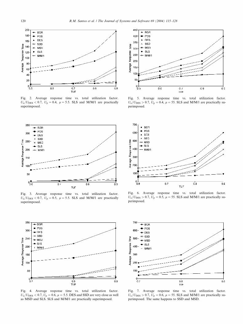
Fig. 2. Average response time vs. total utilization factor.

Ua=UDES < 0:7, Up ¼ 0:4, l ¼ 5:5. SLS and M/M/1 are practically

superimposed.

Fig. 3. Average response time vs. total utilization factor.

Ua=UDES < 0:7, Up ¼ 0:5, l ¼ 5:5. SLS and M/M/1 are practically

superimposed.

Fig. 4. Average response time vs. total utilization factor.

Ua=UDES < 0:7, Up ¼ 0:6, l ¼ 5:5. DES and SSD are very close as well

as MSD and SLS. SLS and M/M/1 are practically superimposed.

Fig. 5. Average response time vs. total utilization factor.

Ua=UDES > 0:7, Up ¼ 0:4, l ¼ 55. SLS and M/M/1 are practically su-

perimposed.

Fig. 6. Average response time vs. total utilization factor.

Ua=UDES > 0:7, Up ¼ 0:5, l ¼ 55. SLS and M/M/1 are practically su-

perimposed.

Fig. 7. Average response time vs. total utilization factor.

Ua=UDES > 0:7, Up ¼ 0:6, l ¼ 55. SLS and M/M/1 are practically su-

perimposed. The same happens to SSD and MSD.

120 R.M. Santos et al. / The Journal of Systems and Software 69 (2004) 115–128

R.M. Santos et al. / The Journal of Systems and Software 69 (2004) 115–128 121

For Up ¼ 0:6, it shows larger delays than both of the

singularity methods.

In the second series, the performances of both servers

converge. That kind of convergence also takes place

between the singularity methods. Although MSD sepa-

rates from slack stealing, both outperform the deferrableserver. MSD always produces better results than SSD.

This is basically because counters are reloaded more

often, therefore increasing the possibility of advancing

the execution of optionals. A feature common to all

methods is that for a given periodic utilization factor the

response is much slower for higher ratios Ua=UDES and

longer service times of the aperiodic load.

4.3. Analysis of results

The performance of the deferrable server vs. other

methods, for the case of a lightly loaded server, has been

analysed by Strosnider et al. (1995). Results presented

there were found to be consistent with those obtained in

the first series of simulations in which the aperiodic

utilization factor is less than 70% of the server’s utili-zation factor and the mean service time is much smaller

than the server’s capacity. Those facts, added to the

possibility of using the server’s capacity throughout the

period, make an earlier execution of many aperiodic

tasks possible, thus reducing the average response time.

In the second series of simulations, the server’s load is

increased. Its performance under this type of load was

not analysed by Strosnider et al. (1995). When the serveris saturated, an important fraction of the aperiodic load

is executed in background slots. As a consequence, the

relative advantages of the deferrable over the polling

server are lost and both performances converge. In the

same way, after the few slots available from the detec-

tion of singularities are used, the relative advantage of

MSD over SSD is lost and both performances also

converge. As a matter of fact, the second series of sim-ulations were performed first and it was the disagree-

ment with the results reported by Strosnider et al. (1995)

that pinpointed the importance of the ratio Ua=UDES

and the value of l in the relative performance of the

different methods. This only confirms the fact that per-

formances are highly dependent on the set of tasks used

to evaluate them.

From the point of view of the methods proposedhere, the important result is that since slack stealing is

an off-line method and background and the polling

server systematically show poor performances, the only

real contenders are the deferrable server and the singu-

larity methods. The deferrable server is consistently

outperformed by MSD, which, for light loads shows a

performance very close to slack stealing and M/M/1. In

the case of heavy loads, the deferrable server is evenoutperformed by the simpler SSD. The overhead of the

singularity methods is reduced to setting counters on

singular slots and regressing the count when slots are

allocated to the execution of non-hard tasks.

5. Reward-based systems

In the context of this section, a task can be seen as

si ¼ Mi [ Oi, where Mi and Oi denote the mandatory

and the optional parts or subtasks of si, with execution

times mi and oi respectively. Obviously, the previous

schedulability condition should be applied only to the

mandatory part to be RM scheduled.

Let SðnÞ ¼ fðm1; o1; T1;D1Þ; ðm2; o2; T2;D2Þ; . . . ; ðmn;on; Tn;DnÞg be the set of independent preemptible peri-odic mandatory/optional tasks to be scheduled using

RM for the mandatory subsystem and a reward-based

scheme for the optional subsystem. Following the as-

sumption that 8i Di ¼ Ti, the optional part of a task

must be executed within the period in which the man-

datory part was executed.

Associated to each optional part there is a reward

function. Realistic reward functions are non-decreasinglinear (constant returns) or concave (diminishing re-

turns). Maximizing the total reward is, in general, an

NP-hard problem (Aydin et al., 2001).

As opposed to other methods reviewed in Section 2,

in the singularity methods (Santos et al., 2002) the

mandatory subsystem is RM scheduled and the reward-

functions do not necessarily have to be continuously

differentiable. The methods can be used on-line, theyhave a light overhead and, in general, outperform the

best non-redistributive method. On top of that, when

there is a reduction in the worst-case execution time of a

mandatory part or the arrival of a task is delayed, that

gain time may be fully used for the execution of optional

parts. These, in turn, may even have different reward

functions along successive stretches of its execution or

change in reaction to the environment, making the sys-tem a truly adaptive one (Kuo and Mok, 1997). A real

world application would be autonomous mobile service

robots navigating in indoor environments (Surman and

Morales, 2000). When going along a corridor, the

measurement of the distance to the nearest wall must

have a better resolution than that to the opposite wall

and, therefore, its reward must be higher. When the

robot is far from a T-junction at the end of a corridor,measuring the distance to the wall in front pays a low

reward. When it is near the junction and must negotiate

the turn, a better resolution is needed and the reward

function is changed in order to increase it.

It must be pointed out that in what follows the only

restriction that will be imposed on the reward functions

is their computability at every slot of the optional part.

To the best of the authors’ knowledge, no other methodproposed up to know to address this problem shares this

advantage and the previous ones.

122 R.M. Santos et al. / The Journal of Systems and Software 69 (2004) 115–128

From the results in Section 3 it can be concluded that

if the mandatory subsystem is k-RM schedulable, the kslots of an interval ½s; ðsþ k � 1Þ� can be used to execute

tasks of the optional subsystem. The combination of

the single and multiple singularity methods, SSD and

MSD, with two sets of heuristic rules (1 and 2) producefour methods, generically notated SH (for singularity/

heuristic), for the on-line scheduling of real-time man-

datory/reward-based optional systems. They are specif-

ically designated SSD1, MSD1, SSD2 and MSD2.

Heuristics must be added because reshuffling slack by

advancing empty slots and executing optional parts in

them is not enough to improve performance. There will

be cases in which high reward optionals will be associ-ated to low priority mandatories and vice-versa. In those

cases, advancing the execution of optionals can produce

adverse results if an executed high priority mandatory

enables the execution of its low reward associated op-

tional, preempting the execution of a high reward op-

tional associated to a low priority mandatory not yet

executed.

The rationale for the first heuristic is to preclude theexecution of a low reward optional when the only reason

to do it is that its high priority mandatory has been

executed. If the highest reward optional is not available,

mandatories are executed in normal slots following the

RM discipline. The use of advanced slack is postponed

until the optional of highest reward is ready. The

method, therefore, is not greedy.

The rationale for the second heuristic is similar to thefirst one. However, if the highest reward optional is not

enabled, its associated mandatory is executed in the

available advanced slack slots, even at the cost of vio-

lating the RM ordering. The method is therefore greedy.

In what follows, the algorithms of the four methods

are described following the notation of Section 3. SSD1

steps are:

(1) AC ¼ k at t ¼ s.(2) If AC 6¼ 0 and there is not any pending mandatory

with an associated optional of higher reward thenan optional is executed else an RM ordered manda-

tory is executed.

(3) AC is decremented by one on each slot assigned to

an optional part.

SSD2 steps are:

(1) AC ¼ k at t ¼ s.(2) If AC 6¼ 0 and there is not any pending mandatory

with an associated optional of higher reward thenan optional is executed else that mandatory is exe-

cuted (even if it violates the RM ordering).

(3) AC is decremented by one on each slot assigned toan optional part or to a mandatory violating the

RM ordering.

MSD1 steps are:

(1) 8g 2 f1; 2; . . . ; ig, ACg ¼ kg at t ¼ si.(2) If 8i 2 f1; 2; . . . ; ng, ACi 6¼ 0 and there is not any

pending mandatory with an associated optional of

higher reward then an optional is executed else anRM ordered mandatory is executed.

(3) 8i 2 f1; 2; . . . ; ng, ACi is decremented by one on each

slot assigned to an optional part.

MSD2 steps are:

(1) 8g 2 f1; 2; . . . ; ig, ACg ¼ kg at t ¼ si.(2) If 8i 2 f1; 2; . . . ; ng, ACi 6¼ 0 and there is not any

pending mandatory associated with an optional of

higher reward then an optional is executed else that

mandatory is executed (even if it violates the RM or-

dering).

(3) If an optional is executed then 8i 2 f1; 2; . . . ; ng, ACi

is decremented by one else only the counters corre-

sponding to tasks of higher priority than the violat-

ing mandatory are decremented by one.

As explained in Section 3, it must be noted that since

empty slots are singularities, counters will be reloaded at

them. The methods are bandwidth preserving in the

sense that the slots generated at each singularity do not

necessarily have to be used immediately after it. A given

optional may wait until the next release of its associated

mandatory or until the next singularity. At that mo-ment, however, the counters are reloaded and reshuffled

slack slots are made available. Updating the counters is

the only overhead of the SH methods. As explained in

Section 2, if slack is not redistributed, the mandatory

parts are always executed first. Various disciplines can

be used to choose the optional to be executed but it has

been found that the best results are obtained if each

background empty slot is allocated to the optionalsubtask contributing most to the total reward. The

method is called best incremental return, notated BIR.

The following simple example is designed to illustrate

the basic mechanism behind the singularity methods

but, what is more, it provides important clues to explain

the results of the large simulations presented later.

Example. The system is specified in Table 2. Deadlinesare assumed equal to periods. Reward functions are

exponential and the SSD1 and BIR methods are used.

The mandatory subsystem is the one used in the example

in Section 3.

The evolution of the system, SSD1 scheduled, is

shown in the first line in Fig. 8. Its k, calculated using

expression (2), is 1. Thus at t ¼ 1, AC ¼ 1, but no op-

tional can be executed because no mandatory has

completed its execution. At t ¼ 2, O1 could be executed,

Table 2

The specification of the reward-based system

i mi oi Ti fi

1 1 2 3 5ð1� e�tÞ2 2 2 5 7ð1� e�5tÞ3 1 2 15 2ð1� e�3tÞ

Fig. 8. The evolution of the system. # denotes the release of the task.

R.M. Santos et al. / The Journal of Systems and Software 69 (2004) 115–128 123

but the scheduler prevents it because the execution ofM2

with an associated optional of higher reward is still

pending. At t ¼ 4, after executing M2, O2 is executed. Itis also executed at t ¼ 10 and t ¼ 15 after the counter is

reloaded. The total reward is 21.

When the same problem is scheduled with the BIR

method, the first slot of O2 is executed at t ¼ 9 and at

t ¼ 14. At t ¼ 15, the first slot of O3 is executed because

it pays a higher reward than the second slot of O2. Note

that slots 9, 14 and 15 were found to be the background

slots left empty by the mandatory subsystem in the ex-ample of Section 3. Total reward is only 17 and the re-

wards ratio (SSD1/BIR) is 1.22. It should be noted that

SSD1 reaches the optimal reward: three slots are avail-

able for optional executions and all of them are used to

process the optional of highest reward. The mandatory

utilization factor is 0.80.

If m3 ¼ 2, the mandatory utilization factor is 0.86.

There are two empty slots that SSD1 and BIR use at (4,15) and (14, 15), respectively. The rewards ratio is 1.37.

If m3 ¼ 3, the mandatory utilization factor is 0.93.

There is only one empty slot used by SSD at t ¼ 4 and

by BIR at t ¼ 15. However, the rewards ratio is only 1.0

because both methods execute the same optional. In this

Table 3

Specification of the synthetic set

Task Ti mi þ oi E

1 20 10 1

2 30 18 2

3 40 5 4

4 60 2 1

5 60 2 1

6 80 12 5

7 90 18 1

8 120 15 8

9 240 28 8

10 270 60 1

11 2160 300 5

case, advancing the execution does not produce a better

result. As can be seen the rewards ratio (SSD1/BIR)

increases with the mandatory utilization factor, reaches

a maximum circa 0.9 and then decreases.

The comparative evaluations were performed using:

(a) The synthetic set proposed in one of the outstanding

papers published on the subject (Aydin et al., 2001).

(b) Randomly generated sets of tasks and reward func-

tions invariant over time.

(c) Randomly generated sets of tasks and reward func-

tions that depreciate with time.

5.1. The synthetic set

It was chosen in the absence of a benchmark and in

order to have an evaluation unbiased in favour of the

SH methods. The set is presented in Table 3. There are

11 tasks with periods (equal to deadlines) in the range

20–2160 and whole (mandatory plus optional) worst-

case execution times in the range 10–300.

There are three general reward functions: exponen-tial, logarithmic and linear, with specific coefficients for

each task. For the three reward functions, the evaluation

started with a first instantiation in which all mandatory

execution times were taken equal to 1 slot, giving a total

mandatory utilization factor of 0.19. In the second in-

stantiation, mi ¼ 1 for i ¼ 1; 2; . . . ; 10, and m11 ¼ 101. In

successive instantiations, the mandatory execution times

were varied following an odometer-type mechanism,with different rates for each task. When the maximum

execution time is surpassed, mi has completed a ‘‘turn’’

and returns to 1. Then, mi�1 advances one position, etc.

This mechanism generates a wide variety of mi combi-

nations, more than 50 000 for each reward function and

each SH method. In the represented utilization’s factor

range [0.35, 0.95] many of them produce the same total

mandatory utilization factor down to the hundredthsand this fact allows the comparison between the SH

methods and BIR with 99% confidence intervals.

The metric used to evaluate the four SH methods is

the ratio between total reward obtained by each of them

xponential Logarithmic Linear

5ð1� e�tÞ 7 lnð20t þ 1Þ 5t0ð1� e�3tÞ 10 lnð50t þ 1Þ 7tð1� e�tÞ 2 lnð10t þ 1Þ 2t0ð1� e�0:5tÞ 5 lnð5t þ 1Þ 4t0ð1� e�0:2tÞ 5 lnð25t þ 1Þ 4tð1� e�tÞ 3 lnð30t þ 1Þ 2t7ð1� e�tÞ 8 lnð8t þ 1Þ 6tð1� e�tÞ 4 lnð6t þ 1Þ 3tð1� e�tÞ 4 lnð9t þ 1Þ 3t2ð1� e�0:5tÞ 6 lnð12t þ 1Þ 5tð1� e�tÞ 3 lnð15t þ 1Þ 2t

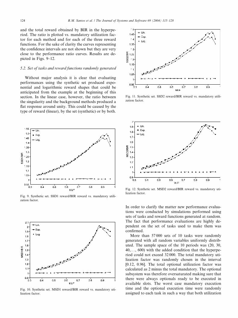
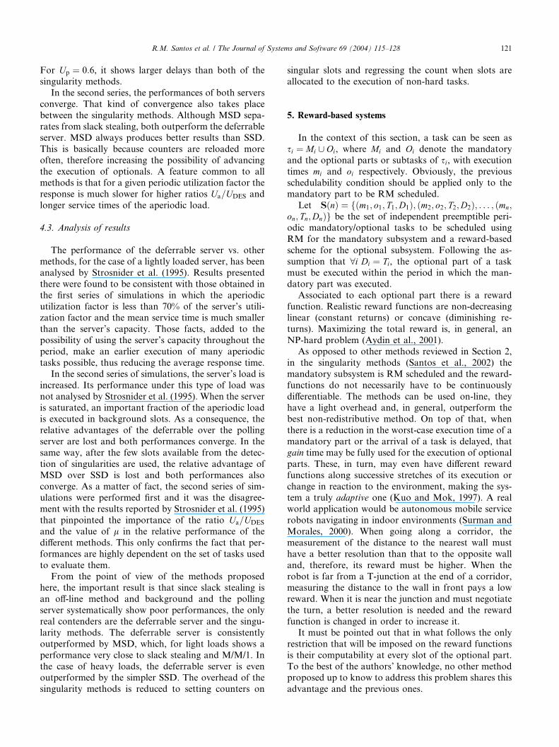
Fig. 11. Synthetic set. SSD2 reward/BIR reward vs. mandatory utili-

zation factor.

124 R.M. Santos et al. / The Journal of Systems and Software 69 (2004) 115–128

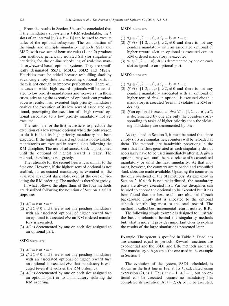
and the total reward obtained by BIR in the hyperpe-

riod. The ratio is plotted vs. mandatory utilization fac-

tor for each method and for each of the three reward

functions. For the sake of clarity the curves representing

the confidence intervals are not shown but they are very

close to the performance ratio curves. Results are de-picted in Figs. 9–12.

5.2. Set of tasks and reward functions randomly generated

Without major analysis it is clear that evaluating

performances using the synthetic set produced expo-

nential and logarithmic reward shapes that could be

anticipated from the example at the beginning of thissection. In the linear case, however, the ratio between

the singularity and the background methods produced a

flat response around unity. This could be caused by the

type of reward (linear), by the set (synthetic) or by both.

Fig. 9. Synthetic set. SSD1 reward/BIR reward vs. mandatory utili-

zation factor.

Fig. 10. Synthetic set. MSD1 reward/BIR reward vs. mandatory uti-

lization factor.

Fig. 12. Synthetic set. MSD2 reward/BIR reward vs. mandatory uti-

lization factor.

In order to clarify the matter new performance evalua-

tions were conducted by simulations performed using

sets of tasks and reward functions generated at random.

The fact that performance evaluations are highly de-

pendent on the set of tasks used to make them was

confirmed.

More than 57 000 sets of 10 tasks were randomlygenerated with all random variables uniformly distrib-

uted. The sample space of the 10 periods was (20, 30,

40,. . ., 600) with the added condition that the hyperpe-

riod could not exceed 32 000. The total mandatory uti-

lization factor was randomly chosen in the interval

[0.12, 0.96]. The total optional utilization factor was

calculated as 2 minus the total mandatory. The optional

subsystem was therefore oversaturated making sure thatthere were always optionals ready to be executed in

available slots. The worst case mandatory execution

time and the optional execution time were randomly

assigned to each task in such a way that both utilization

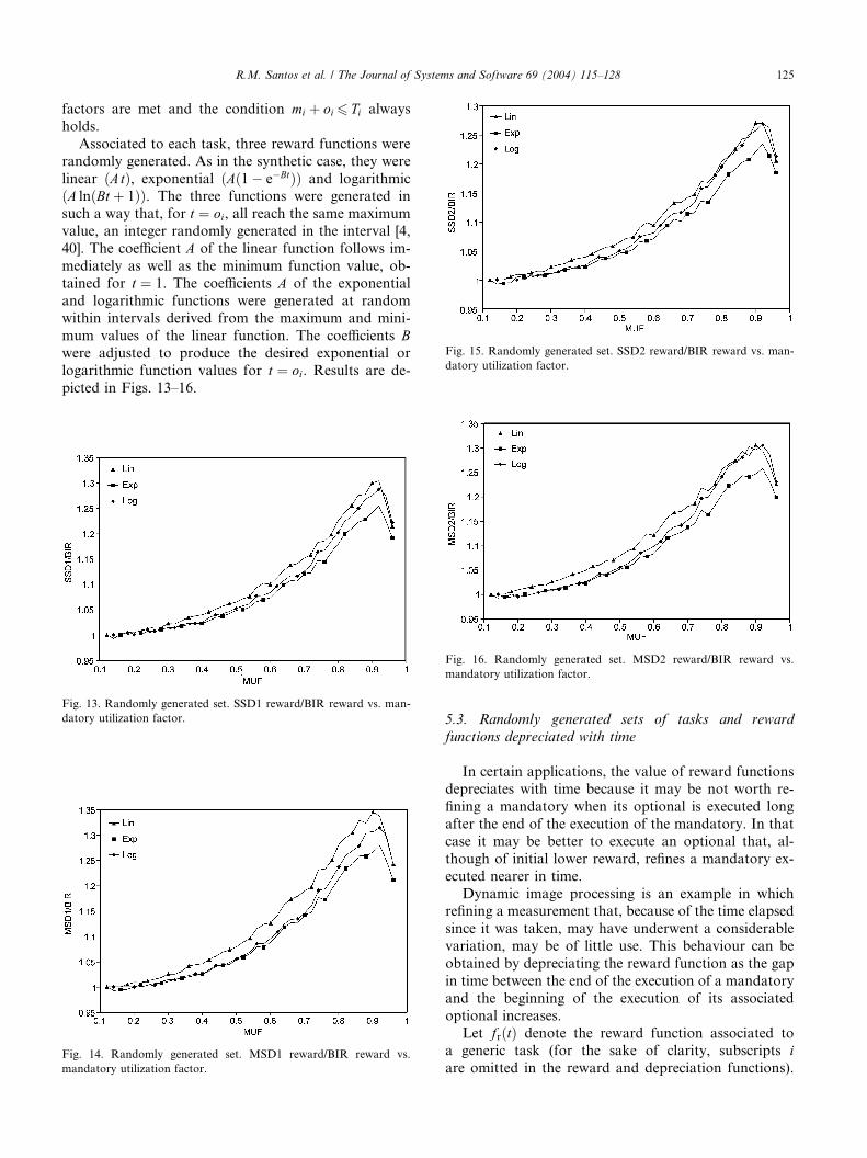
Fig. 15. Randomly generated set. SSD2 reward/BIR reward vs. man-

datory utilization factor.

R.M. Santos et al. / The Journal of Systems and Software 69 (2004) 115–128 125

factors are met and the condition mi þ oi 6 Ti always

holds.

Associated to each task, three reward functions were

randomly generated. As in the synthetic case, they were

linear ðAtÞ, exponential ðAð1� e�BtÞÞ and logarithmic

ðA lnðBt þ 1ÞÞ. The three functions were generated insuch a way that, for t ¼ oi, all reach the same maximum

value, an integer randomly generated in the interval [4,

40]. The coefficient A of the linear function follows im-

mediately as well as the minimum function value, ob-

tained for t ¼ 1. The coefficients A of the exponential

and logarithmic functions were generated at random

within intervals derived from the maximum and mini-

mum values of the linear function. The coefficients Bwere adjusted to produce the desired exponential or

logarithmic function values for t ¼ oi. Results are de-

picted in Figs. 13–16.

Fig. 13. Randomly generated set. SSD1 reward/BIR reward vs. man-

datory utilization factor.

Fig. 14. Randomly generated set. MSD1 reward/BIR reward vs.

mandatory utilization factor.

Fig. 16. Randomly generated set. MSD2 reward/BIR reward vs.

mandatory utilization factor.

5.3. Randomly generated sets of tasks and reward

functions depreciated with time

In certain applications, the value of reward functions

depreciates with time because it may be not worth re-

fining a mandatory when its optional is executed long

after the end of the execution of the mandatory. In that

case it may be better to execute an optional that, al-

though of initial lower reward, refines a mandatory ex-

ecuted nearer in time.

Dynamic image processing is an example in whichrefining a measurement that, because of the time elapsed

since it was taken, may have underwent a considerable

variation, may be of little use. This behaviour can be

obtained by depreciating the reward function as the gap

in time between the end of the execution of a mandatory

and the beginning of the execution of its associated

optional increases.

Let frðtÞ denote the reward function associated toa generic task (for the sake of clarity, subscripts iare omitted in the reward and depreciation functions).

Fig. 18. Depreciated set. SSD1 reward/BIR reward vs. mandatory

utilization factor.

126 R.M. Santos et al. / The Journal of Systems and Software 69 (2004) 115–128

Although the reward is a function of time, the function

itself may or may not vary with time. In the first case,

because of the reasons explained above, the function

may be depreciated from the moment the mandatory

finishes its execution. If te denotes the last slot of exe-

cution of the mandatory, the depreciation is given by afunction fd, decreasing with time and such that if Oi is

executed immediately after te, the reward is not depre-

ciated. If, on the contrary, there is a gap between te andthe first slot assigned to Oi or there are gaps between

slots assigned to Oi, the reward function is depreciated.

The maximum number of slots that can be assigned

to Oi is Ti � mi. This happens when mi successive slots

are assigned to Mi immediately after its release. fdðxÞmust then be defined in an interval ½0; Ti � mi�. fdð0Þ ¼ 1

and fdðTi � miÞ ¼ a, where a may be a random variable

uniformly distributed, for instance, in the sample space

[0.01, 0.1]. fd may be any decreasing function going

through those two points, for example

exp

�� j lnðaÞj

Ti � mix�

The reward function must not be depreciated if there

is not any gap between the end of the execution of Mi

and the beginning of Oi. Therefore, at t ¼ te þ 1, fdðxÞmust take the value 1. It follows that x ¼ t � te � 1. In

Fig. 17, the exponential depreciating function fdðxÞ is

depicted. It should be noted that the shorter the periodthe faster the function depreciates. Because of this, all

other conditions being equal, the scheduler will also tend

to execute less depreciated optionals, farther away from

its new mandatory instantiation.

In order to evaluate the performance of the SH

methods when scheduling systems with depreciating re-

wards, more than 40 000 sets of 10 tasks each were

randomly generated with all random variables uni-formly distributed. The sample space of the periods was

(10; 20; . . . ; 600) with hyperperiods not larger than

32 000. The total mandatory utilization factor varies in

the interval [0.12, 0.98]. The total optional mandatory

utilization factor was calculated as 2 minus the total

mandatory utilization factor; in that way, there are al-

ways optionals to be executed when empty slots appear.

Fig. 17. The exponential depreciation function fdðxÞ in ½0; Ti � mi�.

Mandatory and optional execution times were generated

at random but consistent with the utilization factors and

with the only restriction that mioi 6 Ti.Each reward function has its own depreciation func-

tion, both randomly generated. Thus the depreciated

reward function is

fdrðtÞ ¼ frðtÞfdðt � te � 1Þwith the proviso of suspending the decay of fd while Oi is

executed.

The simulations were performed with an exponential

depreciation as explained above. Results are depicted in

Figs. 18–21.

5.4. Analysis of results

Except for the linear reward function in the case of

the synthetic set, the curves representing the ratio of SH

rewards to BIR rewards have the same shape. The clues

to explaining this behaviour were anticipated in the

previous example.

Fig. 19. Depreciated set. MSD1 reward/BIR reward vs. mandatory

utilization factor.

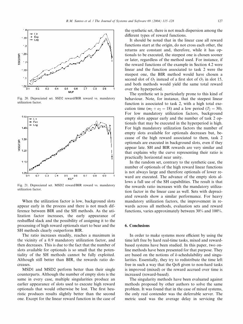
Fig. 20. Depreciated set. SSD2 reward/BIR reward vs. mandatory

utilization factor.

Fig. 21. Depreciated set. MSD2 reward/BIR reward vs. mandatory

utilization factor.

R.M. Santos et al. / The Journal of Systems and Software 69 (2004) 115–128 127

When the utilization factor is low, background slots

appear early in the process and there is not much dif-

ference between BIR and the SH methods. As the uti-

lization factor increases, the early appearance of

reshuffled slack and the possibility of assigning it to the

processing of high reward optionals start to bear and the

SH methods clearly outperform BIR.The ratio increases steadily, reaches a maximum in

the vicinity of a 0.9 mandatory utilization factor, and

then decreases. This is due to the fact that the number of

slots available for optionals is so small that the poten-

tiality of the SH methods cannot be fully exploited.

Although still better than BIR, the rewards ratio de-

creases.

MSD1 and MSD2 perform better than their singlecounterparts. Although the number of empty slots is the

same in every case, multiple singularities produce an

earlier appearance of slots used to execute high reward

optionals that would otherwise be lost. The first heu-

ristic produces results slightly better than the second

one. Except for the linear reward function in the case of

the synthetic set, there is not much dispersion among the

different types of reward functions.

It should be noted that in the linear case all reward

functions start at the origin, do not cross each other, the

returns are constant and, therefore, while it has op-

tionals to be executed, the steepest one is chosen sooneror later, regardless of the method used. For instance, if

the reward functions of the example in Section 4.2 were

linear and the function associated to task 2 were the

steepest one, the BIR method would have chosen a

second slot of O2 instead of a first slot of O3 in slot 15,

and both methods would yield the same total reward

over the hyperperiod.

The synthetic set is particularly prone to this kind ofbehaviour. Note, for instance, that the steepest linear

function is associated to task 2, with a high total exe-

cution time (m2 þ o2 ¼ 18) and a low period (T2 ¼ 30).

For low mandatory utilization factors, background

empty slots appear early and the number of task 2 op-

tionals that may be executed in the hyperperiod is high.

For high mandatory utilization factors the number of

empty slots available for optionals decreases but, be-cause of the high reward associated to them, task 2

optionals are executed in background slots, even if they

appear late. SH and BIR rewards are very similar and

that explains why the curve representing their ratio is

practically horizontal near unity.

In the random set, contrary to the synthetic case, the

number of optionals of the high reward linear functions

is not always large and therefore optionals of lower re-ward are executed. The advance of the empty slots al-

lows a full use of the SH capabilities. The result is that

the rewards ratio increases with the mandatory utiliza-

tion factor in the linear case as well. Sets with depreci-

ated rewards show a similar performance. For heavy

mandatory utilization factors, the improvement in re-

wards across all methods, evaluation sets and reward

functions, varies approximately between 30% and 100%.

6. Conclusions

In order to make systems more efficient by using the

time left free by hard real-time tasks, mixed and reward-

based systems have been studied. In this paper, two on-

line methods have been presented for that purpose. Theyare based on the notions of k-schedulability and singu-

larities. Essentially, they try to redistribute the time left

free in such a way that the QoS given to non-hard tasks

is improved (mixed) or the reward accrued over time is

increased (reward-based).

The singularity methods have been evaluated against

methods proposed by other authors to solve the same

problem. It was found that in the case of mixed systems,the only real contender was the deferrable server. The

metric used was the average delay in servicing the

128 R.M. Santos et al. / The Journal of Systems and Software 69 (2004) 115–128

non-hard tasks. The server’s performance was in be-

tween the two singularity methods’ performances for

light loads of the server. For heavy loads, it was out-

performed by both. For certain types of load, the more

sophisticated singularity method even approached M/

M/1, a lower bound on the average delay.In the case of reward-based systems, there are no

active on-line contenders. The singularity methods must

therefore be tested against methods that not only are

off-line but also require the reward functions to be

continuously differentiable because of the optimization

algorithm used. On the contrary, the only requirement

imposed by the singularity methods on the reward

functions is their computability at every slot. Also, re-ward functions may change in reaction to the environ-

ment making the system a truly adaptive one. Finally,

there are no restrictions for the use of the RM sched-

uling discipline, an important fact having in mind that it

is a de facto standard and the methods are applied to

products that may find their way to the market. The

metric used was the ratio of the rewards obtained by the

proposed methods and BIR, a passive non-redistributivemethod often used as a yardstick. For heavy utilization

factors, the improvement in the rewards ratio across all

the combinations of singularity methods and heuristics,

evaluation sets and reward functions, varied between

approximately 30% and 100%.

Since the singularity methods have proved to be a

useful tool for the redistribution of slack time, other

applications will be sought, for instance the determina-tion of fault tolerance in hard real-time systems.

Acknowledgement

The authors wish to express their sincere appreciation

to the anonymous referees for many helpful suggestions

that led to a definite improvement of the original version.

References

Aydin, H., Melhem, R., Moss�ee, D., Mej�ııa-Alvarez, P., 2001. Optimal

reward-based scheduling for periodic real-time tasks. IEEE Trans-

actions on Computers 50 (2), 111–130.

Buttazzo, G.C., Caccamo, M., 1999. Minimizing aperiodic response

times in a firm real-time environment. IEEE Transactions on

Software Engineering 25 (1), 22–32.

Chung, J.Y., Liu, J.W.S., Lin, K.J., 1990. Scheduling periodic jobs that

allow imprecise results. IEEE Transactions on Computers 19 (9),

1156–1173.

Davis, R.J., Tindell, K.W., Burns, A., 1993. Scheduling slack time

mixed priority preemptive systems. In: Proceedings IEEE Real

Time Systems Symposium. pp. 222–231.

Dey, J.K., Kurose, J., 1996. On line scheduling policies for a class of

IRIS (Increasing reward with increasing service) real-time tasks.

IEEE Transactions on Computers 46 (7), 802–813.

Gonzalez Harbour, M., Sha, L., 1991. An Application-Level Imple-

mentation of the Sporadic Server, Technical Report, CMU/SEI-91-

TR-26, Software Engineering Institute, Carnegie Mellon Univer-

sity.

Joseph, M., Pandya, P., 1986. Finding response times in a real-time

system. The Computer Journal 29 (5), 390–395.

Kuo, T.W., Mok, A.K., 1997. Incremental reconfiguration and load

adjustment in adaptive real-time systems. IEEE Transactions on

Computers 48 (12), 1313–1324.

Lehoczky, J.P., Ramos-Thuel, S., 1992. An optimal algorithm for

scheduling soft-aperiodic tasks fixed-priority preemptive systems.

In: Proceedings IEEE Real Time Systems Symposium. pp. 110–123.

Lehoczky, J., Sha, L., Ding, Y., 1989. The rate-monotonic scheduling

algorithm: Exact characterization and average case behaviour. In:

Proceedings IEEE Real Time Systems Symposium. pp. 166–

171.

Lin, K.J., Natarajan, S., Liu, J.W.S., 1987. Imprecise results: utilizing

partial computations in real-time systems. In: Proceedings IEEE

Real Time Systems Symposium. pp. 210–217.

Liu, C.L., Layland, J.W., 1973. Scheduling algorithms for multipro-

gramming in hard real-time environment. Journal of the ACM 20

(1), 46–61.

Liu, J.W.S., Lin, K.J., Shih, W.K., Yu, A.C.S., Chung, C., Yao, Y.,

Zhao, W., 1991. Algorithms for scheduling imprecise computa-

tions. IEEE Computer 24 (5), 58–68.

Obenza, R., 1993. Rate monotonic analysis for real-time systems.

IEEE Computer 26 (3), 73–74.

Orozco, J., Santos, R., Santos, J., Cayssials, R., 2000. Taking

advantage of priority inversions to improve the processing of

non-hard real-time tasks in mixed systems. In: Proceedings Work in

Progress Session IEEE Real Time Systems Symposium. pp. 13–

16.

Ramos-Thuel, S., 1993. Enhancing fault tolerance of real-time systems

through time redundancy, Ph.D. Thesis, Electrical and Computer

Engineering Department, Carnegie Mellon University.

Santos, J., Orozco, J., 1993. Rate monotonic scheduling in hard real-

time systems. Information Processing Letters 48, 39–45.

Santos, R.M., Urriza, J., Santos, J., Orozco, J., 2002. Heuristic use of

singularities for on-line scheduling of real-time mandatory/reward-

based optional systems. In: Proceedings 14th Euromicro Confer-

ence on Real Time Systems. pp. 103–110.

Shih, W.K., Liu, J.W.S., 1995. Algorithms for scheduling imprecise

computations with timing constraints to minimize maximum error.

IEEE Transactions on Computers 44 (3), 466–471.

Sprunt, B., Sha, L., Lehoczky, J.P., 1989. Aperiodic task scheduling

for hard real-time systems. Real-Time Systems 1 (1), 27–60.

Stankovic, J., 1988. Misconceptions about real-time computing. IEEE

Computer 21 (10), 10–19.

Strosnider, J.K., Lehoczky, J.P., Sha, L., 1995. The deferrable server

algorithm for enhanced aperiodic responsiveness in hard real-

time environments. IEEE Transactions on Computers 44 (1), 75–

91.

Surman, H., Morales, A., 2000. A five layer sensor architecture for

autonomous robots in indoor environments. In: Proceedings

International Symposium on Robotics and Automation. pp. 33–

38.

Tia, T.S., Liu, J.W.S., Shankar, M.S., 1996. Algorithms and optimality

of scheduling soft aperiodic requests in fixed-priority preemptive

systems. Real Time Systems 10 (1), 23–43.