PDF generated using the open source mwlib toolkit. See http://code.pediapress.com/ for more information.PDF generated at: Wed, 07 Jul 2010 00:08:49 UTC

Decision procedures inAlgebra and LogicReading material

ContentsArticlesSome background 1

Algebraic structure 1Mathematical logic 9Structure (mathematical logic) 22Universal algebra 29Model theory 34Proof theory 41Sequent calculus 44Python (programming language) 50Sage (mathematics software) 62

Decision procedures and implementations 69

Decision problem 69Boolean satisfiability problem 72Constraint satisfaction 79Rewriting 82Maude system 87Resolution (logic) 94Automated theorem proving 98Prover9 103Method of analytic tableaux 104Natural deduction 124Isabelle (theorem prover) 138Satisfiability Modulo Theories 140Prolog 144

ReferencesArticle Sources and Contributors 157Image Sources, Licenses and Contributors 159

Article LicensesLicense 160

1

Some background

Algebraic structureIn algebra, a branch of pure mathematics, an algebraic structure consists of one or more sets closed under one ormore operations, satisfying some axioms. Abstract algebra is primarily the study of algebraic structures and theirproperties. The notion of algebraic structure has been formalized in universal algebra.As an abstraction, an "algebraic structure" is the collection of all possible models of a given set of axioms. Moreconcretely, an algebraic structure is any particular model of some set of axioms. For example, the monster groupboth "is" an algebraic structure in the concrete sense, and abstractly, "has" the group structure in common with allother groups. This article employs both meanings of "structure."This definition of an algebraic structure should not be taken as restrictive. Anything that satisfies the axioms defininga structure is an instance of that structure, regardless of how many other axioms that instance happens to have. Forexample, all groups are also semigroups and magmas.

Structures whose axioms are all identitiesIf the axioms defining a structure are all identities, the structure is a variety (not to be confused with algebraic varietyin the sense of algebraic geometry). Identities are equations formulated using only the operations the structureallows, and variables that are tacitly universally quantified over the relevant universe. Identities contain noconnectives, existentially quantified variables, or relations of any kind other than the allowed operations. The studyof varieties is an important part of universal algebra.All structures in this section are varieties. Some of these structures are most naturally axiomatized using one or morenonidentities, but are nevertheless varieties because there exists an equivalent axiomatization, one perhaps lessperspicuous, composed solely of identities. Algebraic structures that are not varieties are described in the followingsection, and differ from varieties in their metamathematical properties.In this section and the following one, structures are listed in approximate order of increasing complexity,operationalized as follows:• Simple structures requiring but one set, the universe S, are listed before composite ones requiring two sets;• Structures having the same number of required sets are then ordered by the number of binary operations (0 to 4)

they require. Incidentally, no structure mentioned in this entry requires an operation whose arity exceeds 2;• Let A and B be the two sets that make up a composite structure. Then a composite structure may include 1 or 2

functions of the form AxA→B or AxB→A;• Structures having the same number and kinds of binary operations and functions are more or less ordered by the

number of required unary and 0-ary (distinguished elements) operations, 0 to 2 in both cases.The indentation structure employed in this section and the one following is intended to convey information. Ifstructure B is under structure A and more indented, then all theorems of A are theorems of B; the converse does nothold.Ringoids and lattices can be clearly distinguished despite both having two defining binary operations. In the case ofringoids, the two operations are linked by the distributive law; in the case of lattices, they are linked by theabsorption law. Ringoids also tend to have numerical models, while lattices tend to have set-theoretic models.Simple structures: No binary operation:• Set: a degenerate algebraic structure having no operations.

Algebraic structure 2

• Pointed set: S has one or more distinguished elements, often 0, 1, or both.• Unary system: S and a single unary operation over S.• Pointed unary system: a unary system with S a pointed set.Group-like structures:One binary operation, denoted by concatenation. For monoids, boundary algebras, and sloops, S is a pointed set.• Magma or groupoid: S and a single binary operation over S.

• Steiner magma: A commutative magma satisfying x(xy) = y.• Squag: an idempotent Steiner magma.• Sloop: a Steiner magma with distinguished element 1, such that xx = 1.

• Semigroup: an associative magma.• Monoid: a unital semigroup.

• Group: a monoid with a unary operation, inverse, giving rise to an inverse element.• Abelian group: a commutative group.

• Band: a semigroup of idempotents.• Semilattice: a commutative band. The binary operation can be called either meet or join.

• Boundary algebra: a unital semilattice (equivalently, an idempotent commutative monoid) with a unaryoperation, complementation, denoted by enclosing its argument in parentheses, giving rise to an inverseelement that is the complement of the identity element. The identity and inverse elements bound S. Also,x(xy) = x(y) holds.

Three binary operations. Quasigroups are listed here, despite their having 3 binary operations, because they are(nonassociative) magmas. Quasigroups feature 3 binary operations only because establishing the quasigroupcancellation property by means of identities alone requires two binary operations in addition to the group operation.• Quasigroup: a cancellative magma. Equivalently, ∀x,y∈S, ∃!a,b∈S, such that xa = y and bx = y.

• Loop: a unital quasigroup with a unary operation, inverse.• Moufang loop: a loop in which a weakened form of associativity, (zx)(yz) = z(xy)z, holds.

• Group: an associative loop.Lattice: Two or more binary operations, including meet and join, connected by the absorption law. S is both a meetand join semilattice, and is a pointed set if and only if S is bounded. Lattices often have no unary operations. Everytrue statement has a dual, obtained by replacing every instance of meet with join, and vice versa.• Bounded lattice: S has two distinguished elements, the greatest lower bound and the least upper bound. Dualizing

requires replacing every instance of one bound by the other, and vice versa.• Complemented lattice: a lattice with a unary operation, complementation, denoted by postfix ', giving rise to an

inverse element. That element and its complement bound the lattice.• Modular lattice: a lattice in which the modular identity holds.

• Distributive lattice: a lattice in which each of meet and join distributes over the other. Distributive lattices aremodular, but the converse does not hold.• Kleene algebra: a bounded distributive lattice with a unary operation whose identities are x"=x, (x+y)'=x'y',

and (x+x')yy'=yy'. See "ring-like structures" for another structure having the same name.• Boolean algebra: a complemented distributive lattice. Either of meet or join can be defined in terms of the

other and complementation.• Interior algebra: a Boolean algebra with an added unary operation, the interior operator, denoted by

postfix ' and obeying the identities x'x=x, x"=x, (xy)'=x'y', and 1'=1.

Algebraic structure 3

• Heyting algebra: a bounded distributive lattice with an added binary operation, relative pseudo-complement,denoted by infix " ' ", and governed by the axioms x'x=1, x(x'y) = xy, x'(yz) = (x'y)(x'z), (xy)'z = (x'z)(y'z).

Ringoids: Two binary operations, addition and multiplication, with multiplication distributing over addition.Semirings are pointed sets.• Semiring: a ringoid such that S is a monoid under each operation. Each operation has a distinct identity element.

Addition also commutes, and has an identity element that annihilates multiplication.• Commutative semiring: a semiring with commutative multiplication.• Ring: a semiring with a unary operation, additive inverse, giving rise to an inverse element equal to the

additive identity element. Hence S is an abelian group under addition.• Rng: a ring lacking a multiplicative identity.• Commutative ring: a ring with commutative multiplication.

• Boolean ring: a commutative ring with idempotent multiplication, equivalent to a Boolean algebra.• Kleene algebra: a semiring with idempotent addition and a unary operation, the Kleene star, denoted by postfix

* and obeying the identities (1+x*x)x*=x* and (1+xx*)x*=x*. See "Lattice-like structures" for anotherstructure having the same name.

N.B. The above definition of ring does not command universal assent. Some authorities employ "ring" to denotewhat is here called a rng, and refer to a ring in the above sense as a "ring with identity."Modules: Composite Systems Defined over Two Sets, M and R: The members of:1. R are scalars, denoted by Greek letters. R is a ring under the binary operations of scalar addition and

multiplication;2. M are module elements (often but not necessarily vectors), denoted by Latin letters. M is an abelian group under

addition. There may be other binary operations.The scalar multiplication of scalars and module elements is a function RxM→M which commutes, associates(∀r,s∈R, ∀x∈M, r(sx) = (rs)x ), has 1 as identity element, and distributes over module and scalar addition. If only thepre(post)multiplication of module elements by scalars is defined, the result is a left (right) module.• Free module: a module having a free basis, {e1, ... en}⊂M, where the positive integer n is the dimension of the

free module. For every v∈M, there exist κ1, ..., κn∈R such that v = κ1e1 + ... + κnen. Let 0 and 0 be the respectiveidentity elements for module and scalar addition. If r1e1 + ... + rnen = 0, then r1 = ... = rn = 0.• Algebra over a ring (also R-algebra): a (free) module where R is a commutative ring. There is a second binary

operation over M, called multiplication and denoted by concatenation, which distributes over module additionand is bilinear: α(xy) = (αx)y = x(αy).• Jordan ring: an algebra over a ring whose module multiplication commutes, does not associate, and respects

the Jordan identity.Vector spaces, closely related to modules, are defined in the next section.

Structures with some axioms that are not identitiesThe structures in this section are not varieties because they cannot be axiomatized with identities alone. Nearly all ofthe nonidentities below are one of two very elementary kinds:1. The starting point for all structures in this section is a "nontrivial" ring, namely one such that S≠{0}, 0 being the

additive identity element. The nearest thing to an identity implying S≠{0} is the nonidentity 0≠1, which requiresthat the additive and multiplicative identities be distinct.

2. Nearly all structures described in this section include identities that hold for all members of S except 0. In orderfor an algebraic structure to be a variety, its operations must be defined for all members of S; there can be nopartial operations.

Algebraic structure 4

Structures whose axioms unavoidably include nonidentities are among the most important ones in mathematics, e.g.,fields and vector spaces. Moreover, much of theoretical physics can be recast as models of multilinear algebras.Although structures with nonidentities retain an undoubted algebraic flavor, they suffer from defects varieties do nothave. For example, neither the product of integral domains nor a free field over any set exist.Arithmetics: Two binary operations, addition and multiplication. S is an infinite set. Arithmetics are pointed unarysystems, whose unary operation is injective successor, and with distinguished element 0.• Robinson arithmetic. Addition and multiplication are recursively defined by means of successor. 0 is the identity

element for addition, and annihilates multiplication. Robinson arithmetic is listed here even though it is a variety,because of its closeness to Peano arithmetic.• Peano arithmetic. Robinson arithmetic with an axiom schema of induction. Most ring and field axioms bearing

on the properties of addition and multiplication are theorems of Peano arithmetic or of proper extensionsthereof.

Field-like structures: Two binary operations, addition and multiplication. S is nontrivial, i.e., S≠{0}.• Domain: a ring whose sole zero divisor is 0.

• Integral domain: a domain whose multiplication commutes. Also a commutative cancellative ring.• Euclidean domain: an integral domain with a function f: S→N satisfying the division with remainder

property.• Division ring (or sfield, skew field): a ring in which every member of S other than 0 has a two-sided multiplicative

inverse. The nonzero members of S form a group under multiplication.• Field: a division ring whose multiplication commutes. The nonzero members of S form an abelian group under

multiplication.• Ordered field: a field whose elements are totally ordered.

• Real field: a Dedekind complete ordered field.The following structures are not varieties for reasons in addition to S≠{0}:• Simple ring: a ring having no ideals other than 0 and S.

• Weyl algebra:• Artinian ring: a ring whose ideals satisfy the descending chain condition.Composite Systems: Vector Spaces, and Algebras over Fields. Two Sets, M and R, and at least three binaryoperations.The members of:1. M are vectors, denoted by lower case letters. M is at minimum an abelian group under vector addition, with

distinguished member 0.2. R are scalars, denoted by Greek letters. R is a field, nearly always the real or complex field, with 0 and 1 as

distinguished members.Three binary operations.• Vector space: a free module of dimension n except that R is a field.

• Normed vector space: a vector space with a norm, namely a function M → R that is positive homogeneous,subadditive, and positive definite.• Inner product space (also Euclidean vector space): a normed vector space such that R is the real field,

whose norm is the square root of the inner product, M×M→R. Let i,j, and n be positive integers such that1≤i,j≤n. Then M has an orthonormal basis such that ei•ej = 1 if i=j and 0 otherwise; see free module above.

• Unitary space: Differs from inner product spaces in that R is the complex field, and the inner product has a different name, the hermitian inner product, with different properties: conjugate symmetric, bilinear, and

Algebraic structure 5

positive definite. See Birkhoff and MacLane (1979: 369).• Graded vector space: a vector space such that the members of M have a direct sum decomposition. See graded

algebra below.Four binary operations.• Algebra over a field: An algebra over a ring except that R is a field instead of a commutative ring.

• Jordan algebra: a Jordan ring except that R is a field.• Lie algebra: an algebra over a field respecting the Jacobi identity, whose vector multiplication, the Lie bracket

denoted [u,v], anticommutes, does not associate, and is nilpotent.• Associative algebra: an algebra over a field, or a module, whose vector multiplication associates.

• Linear algebra: an associative unital algebra with the members of M being matrices. Every matrix has adimension nxm, n and m positive integers. If one of n or m is 1, the matrix is a vector; if both are 1, it is ascalar. Addition of matrices is defined only if they have the same dimensions. Matrix multiplication,denoted by concatenation, is the vector multiplication. Let matrix A be nxm and matrix B be ixj. Then AB isdefined if and only if m=i; BA, if and only if j=n. There also exists an mxm matrix I and an nxn matrix Jsuch that AI=JA=A. If u and v are vectors having the same dimensions, they have an inner product, denoted〈u,v〉. Hence there is an orthonormal basis; see inner product space above. There is a unary function, thedeterminant, from square (nxn for any n) matrices to R.

• Commutative algebra: an associative algebra whose vector multiplication commutes.• Symmetric algebra: a commutative algebra with unital vector multiplication.

Composite Systems: Multilinear algebras. Two sets, V and K. Four binary operations:1. The members of V are multivectors (including vectors), denoted by lower case Latin letters. V is an abelian group

under multivector addition, and a monoid under outer product. The outer product goes under various names, andis multilinear in principle but usually bilinear. The outer product defines the multivectors recursively starting fromthe vectors. Thus the members of V have a "degree" (see graded algebra below). Multivectors may have an innerproduct as well, denoted u•v: V×V→K, that is symmetric, linear, and positive definite; see inner product spaceabove.

2. The properties and notation of K are the same as those of R above, except that K may have -1 as a distinguishedmember. K is usually the real field, as multilinear algebras are designed to describe physical phenomena withoutcomplex numbers.

3. The multiplication of scalars and multivectors, V×K→V, has the same properties as the multiplication of scalarsand module elements that is part of a module.

• Graded algebra: an associative algebra with unital outer product. The members of V have a direct sumdecomposition resulting in their having a "degree," with vectors having degree 1. If u and v have degree i and j,respectively, the outer product of u and v is of degree i+j. V also has a distinguished member 0 for each possibledegree. Hence all members of V having the same degree form an abelian group under addition.• Exterior algebra (also Grassmann algebra): a graded algebra whose anticommutative outer product, denoted

by infix ∧, is called the exterior product. V has an orthonormal basis. v1 ∧ v2 ∧ ... ∧ vk = 0 if and only if v1, ...,vk are linearly dependent. Multivectors also have an inner product.• Clifford algebra: an exterior algebra with a symmetric bilinear form Q: V×V→K. The special case Q=0

yields an exterior algebra. The exterior product is written 〈u,v〉. Usually, 〈ei,ei〉 = -1 (usually) or 1(otherwise).

• Geometric algebra: an exterior algebra whose exterior (called geometric) product is denoted byconcatenation. The geometric product of parallel multivectors commutes, that of orthogonal vectorsanticommutes. The product of a scalar with a multivector commutes. vv yields a scalar.• Grassmann-Cayley algebra: a geometric algebra without an inner product.

Algebraic structure 6

ExamplesSome recurring universes: N=natural numbers; Z=integers; Q=rational numbers; R=real numbers; C=complexnumbers.N is a pointed unary system, and under addition and multiplication, is both the standard interpretation of Peanoarithmetic and a commutative semiring.Boolean algebras are at once semigroups, lattices, and rings. They would even be abelian groups if the identity andinverse elements were identical instead of complements.Group-like structures

• Nonzero N under addition (+) is a magma.• N under addition is a magma with an identity.• Z under subtraction (−) is a quasigroup.• Nonzero Q under division (÷) is a quasigroup.• Every group is a loop, because a * x = b if and only if x = a−1 * b, and y * a = b if and only if y = b * a−1.• 2x2 matrices(of non-zero determinant) with matrix multiplication form a group.• Z under addition (+) is an abelian group.• Nonzero Q under multiplication (×) is an abelian group.• Every cyclic group G is abelian, because if x, y are in G, then xy = aman = am+n = an+m = anam = yx. In particular,

Z is an abelian group under addition, as is the integers modulo n Z/nZ.• A monoid is a category with a single object, in which case the composition of morphisms and the identity

morphism interpret monoid multiplication and identity element, respectively.• The Boolean algebra 2 is a boundary algebra.• More examples of groups and list of small groups.Lattices

• The normal subgroups of a group, and the submodules of a module, are modular lattices.• Any field of sets, and the connectives of first-order logic, are models of Boolean algebra.• The connectives of intuitionistic logic form a model of Heyting algebra.• The modal logic S4 is a model of interior algebra.• Peano arithmetic and most axiomatic set theories, including ZFC, NBG, and New foundations, can be recast as

models of relation algebra.Ring-like structures

• The set R[X] of all polynomials over some coefficient ring R is a ring.• 2x2 matrices with matrix addition and multiplication form a ring.• If n is a positive integer, then the set Zn = Z/nZ of integers modulo n (the additive cyclic group of order n ) forms

a ring having n elements (see modular arithmetic).Integral domains

• Z under addition and multiplication is an integral domain.• The p-adic integers.Fields

• Each of Q, R, and C, under addition and multiplication, is a field.• R totally ordered by "<" in the usual way is an ordered field and is categorical. The resulting real field grounds

real and functional analysis.• R contains several interesting subfields, the algebraic, the computable, and the definable numbers.

• An algebraic number field is a finite field extension of Q, that is, a field containing Q which has finite dimensionas a vector space over Q. Algebraic number fields are very important in number theory.

Algebraic structure 7

• If q > 1 is a power of a prime number, then there exists (up to isomorphism) exactly one finite field with qelements, usually denoted Fq, or in the case that q is itself prime, by Z/qZ. Such fields are called Galois fields,whence the alternative notation GF(q). All finite fields are isomorphic to some Galois field.• Given some prime number p, the set Zp = Z/pZ of integers modulo p is the finite field with p elements: Fp =

{0, 1, ..., p − 1} where the operations are defined by performing the operation in Z, dividing by p and takingthe remainder; see modular arithmetic.

Allowing additional structureAlgebraic structures can also be defined on sets with added structure of a non-algebraic nature, such as a topology.The added structure must be compatible, in some sense, with the algebraic structure.• Ordered group: a group with a compatible partial order. I.e., S is partially ordered.• Linearly ordered group: a group whose S is a linear order.• Archimedean group: a linearly ordered group for which the Archimedean property holds.• Lie group: a group whose S has a compatible smooth manifold structure.• Topological group: a group whose S has a compatible topology.• Topological vector space: a vector space whose M has a compatible topology; a superset of normed vector spaces.• Banach spaces, Hilbert spaces, Inner product spaces• Vertex operator algebras

Category theoryThe discussion above has been cast in terms of elementary abstract and universal algebra. Category theory is anotherway of reasoning about algebraic structures (see, for example, Mac Lane 1998). A category is a collection of objectswith associated morphisms. Every algebraic structure has its own notion of homomorphism, namely any functioncompatible with the operation(s) defining the structure. In this way, every algebraic structure gives rise to a category.For example, the category of groups has all groups as objects and all group homomorphisms as morphisms. Thisconcrete category may be seen as a category of sets with added category-theoretic structure. Likewise, the categoryof topological groups (whose morphisms are the continuous group homomorphisms) is a category of topologicalspaces with extra structure.There are various concepts in category theory that try to capture the algebraic character of a context, for instance• algebraic• essentially algebraic• presentable• locally presentable• monadic functors and categories• universal property.

Algebraic structure 8

See also• arity• category theory• free object• list of algebraic structures• list of first order theories• signature• variety

References• MacLane, Saunders; Birkhoff, Garrett (1999), Algebra (2nd ed.), AMS Chelsea, ISBN 978-0-8218-1646-2• Michel, Anthony N.; Herget, Charles J. (1993), Applied Algebra and Functional Analysis, New York: Dover

Publications, ISBN 978-0-486-67598-5A monograph available free online:• Burris, Stanley N.; Sankappanavar, H. P. (1981), A Course in Universal Algebra [1], Berlin, New York:

Springer-Verlag, ISBN 978-3-540-90578-3Category theory:• Mac Lane, Saunders (1998), Categories for the Working Mathematician (2nd ed.), Berlin, New York:

Springer-Verlag, ISBN 978-0-387-98403-2• Taylor, Paul (1999), Practical foundations of mathematics, Cambridge University Press,

ISBN 978-0-521-63107-5

External links• Jipsen's algebra structures. [2] Includes many structures not mentioned here.• Mathworld [3] page on abstract algebra.• Stanford Encyclopedia of Philosophy: Algebra [4] by Vaughan Pratt.

References[1] http:/ / www. thoralf. uwaterloo. ca/ htdocs/ ualg. html[2] http:/ / math. chapman. edu/ cgi-bin/ structures[3] http:/ / mathworld. wolfram. com/ topics/ Algebra. html[4] http:/ / plato. stanford. edu/ entries/ algebra/

Mathematical logic 9

Mathematical logicMathematical logic (formerly known as symbolic logic) is a subfield of mathematics with close connections tocomputer science and philosophical logic.[1] The field includes both the mathematical study of logic and theapplications of formal logic to other areas of mathematics. The unifying themes in mathematical logic include thestudy of the expressive power of formal systems and the deductive power of formal proof systems.Mathematical logic is often divided into the fields of set theory, model theory, recursion theory, and proof theory.These areas share basic results on logic, particularly first-order logic, and definability. In computer science(particularly in the ACM Classification) mathematical logic is seen as encompassing additional topics that are notdetailed in this article; see logic in computer science for those.Since its inception, mathematical logic has contributed to, and has been motivated by, the study of foundations ofmathematics. This study began in the late 19th century with the development of axiomatic frameworks for geometry,arithmetic, and analysis. In the early 20th century it was shaped by David Hilbert's program to prove the consistencyof foundational theories. Results of Kurt Gödel, Gerhard Gentzen, and others provided partial resolution to theprogram, and clarified the issues involved in proving consistency. Work in set theory showed that almost all ordinarymathematics can be formalized in terms of sets, although there are some theorems that cannot be proven in commonaxiom systems for set theory. Contemporary work in the foundations of mathematics often focuses on establishingwhich parts of mathematics can be formalized in particular formal systems, rather than trying to find theories inwhich all of mathematics can be developed.

HistoryMathematical logic emerged in the mid-19th century as a subfield of mathematics independent of the traditionalstudy of logic (Ferreirós 2001, p. 443). Before this emergence, logic was studied with rhetoric, through thesyllogism, and with philosophy. The first half of the 20th century saw an explosion of fundamental results,accompanied by vigorous debate over the foundations of mathematics.

Early historySophisticated theories of logic were developed in many cultures, including China, India, Greece and the Islamicworld. In the 18th century, attempts to treat the operations of formal logic in a symbolic or algebraic way had beenmade by philosophical mathematicians including Leibniz and Lambert, but their labors remained isolated and littleknown.

19th centuryIn the middle of the nineteenth century, George Boole and then Augustus De Morgan presented systematicmathematical treatments of logic. Their work, building on work by algebraists such as George Peacock, extended thetraditional Aristotelian doctrine of logic into a sufficient framework for the study of foundations ofmathematics (Katz 1998, p. 686).Charles Sanders Peirce built upon the work of Boole to develop a logical system for relations and quantifiers, whichhe published in several papers from 1870 to 1885. Gottlob Frege presented an independent development of logicwith quantifiers in his Begriffsschrift, published in 1879. Frege's work remained obscure, however, until BertrandRussell began to promote it near the turn of the century. The two-dimensional notation Frege developed was neverwidely adopted and is unused in contemporary texts.From 1890 to 1905, Ernst Schröder published Vorlesungen über die Algebra der Logik in three volumes. This worksummarized and extended the work of Boole, De Morgan, and Peirce, and was a comprehensive reference tosymbolic logic as it was understood at the end of the 19th century.

Mathematical logic 10

Foundational theories

Some concerns that mathematics had not been built on a proper foundation led to the development of axiomaticsystems for fundamental areas of mathematics such as arithmetic, analysis, and geometry.In logic, the term arithmetic refers to the theory of the natural numbers. Giuseppe Peano (1888) published a set ofaxioms for arithmetic that came to bear his name (Peano axioms), using a variation of the logical system of Booleand Schröder but adding quantifiers. Peano was unaware of Frege's work at the time. Around the same time RichardDedekind showed that the natural numbers are uniquely characterized by their induction properties. Dedekind (1888)proposed a different characterization, which lacked the formal logical character of Peano's axioms. Dedekind's work,however, proved theorems inaccessible in Peano's system, including the uniqueness of the set of natural numbers (upto isomorphism) and the recursive definitions of addition and multiplication from the successor function andmathematical induction.In the mid-19th century, flaws in Euclid's axioms for geometry became known (Katz 1998, p. 774). In addition to theindependence of the parallel postulate, established by Nikolai Lobachevsky in 1826 (Lobachevsky 1840),mathematicians discovered that certain theorems taken for granted by Euclid were not in fact provable from hisaxioms. Among these is the theorem that a line contains at least two points, or that circles of the same radius whosecenters are separated by that radius must intersect. Hilbert (1899) developed a complete set of axioms for geometry,building on previous work by Pasch (1882). The success in axiomatizing geometry motivated Hilbert to seekcomplete axiomatizations of other areas of mathematics, such as the natural numbers and the real line. This wouldprove to be a major area of research in the first half of the 20th century.The 19th century saw great advances in the theory of real analysis, including theories of convergence of functionsand Fourier series. Mathematicians such as Karl Weierstrass began to construct functions that stretched intuition,such as nowhere-differentiable continuous functions. Previous conceptions of a function as a rule for computation, ora smooth graph, were no longer adequate. Weierstrass began to advocate the arithmetization of analysis, whichsought to axiomatize analysis using properties of the natural numbers. The modern (ε, δ)-definition of limit andcontinuous functions was already developed by Bolzano in 1817 (Felscher 2000), but remained relatively unknown.Cauchy in 1821 defined continuity in terms of infinitesimals (see Cours d'Analyse, page 34). In 1858, Dedekindproposed a definition of the real numbers in terms of Dedekind cuts of rational numbers (Dedekind 1872), adefinition still employed in contemporary texts.Georg Cantor developed the fundamental concepts of infinite set theory. His early results developed the theory ofcardinality and proved that the reals and the natural numbers have different cardinalities (Cantor 1874). Over thenext twenty years, Cantor developed a theory of transfinite numbers in a series of publications. In 1891, he publisheda new proof of the uncountability of the real numbers that introduced the diagonal argument, and used this method toprove Cantor's theorem that no set can have the same cardinality as its powerset. Cantor believed that every set couldbe well-ordered, but was unable to produce a proof for this result, leaving it as an open problem in 1895 (Katz 1998,p. 807).

20th centuryIn the early decades of the 20th century, the main areas of study were set theory and formal logic. The discovery ofparadoxes in informal set theory caused some to wonder whether mathematics itself is inconsistent, and to look forproofs of consistency.In 1900, Hilbert posed a famous list of 23 problems for the next century. The first two of these were to resolve thecontinuum hypothesis and prove the consistency of elementary arithmetic, respectively; the tenth was to produce amethod that could decide whether a multivariate polynomial equation over the integers has a solution. Subsequentwork to resolve these problems shaped the direction of mathematical logic, as did the effort to resolve Hilbert'sEntscheidungsproblem, posed in 1928. This problem asked for a procedure that would decide, given a formalizedmathematical statement, whether the statement is true or false.

Mathematical logic 11

Set theory and paradoxes

Ernst Zermelo (1904) gave a proof that every set could be well-ordered, a result Georg Cantor had been unable toobtain. To achieve the proof, Zermelo introduced the axiom of choice, which drew heated debate and researchamong mathematicians and the pioneers of set theory. The immediate criticism of the method led Zermelo to publisha second exposition of his result, directly addressing criticisms of his proof (Zermelo 1908a). This paper led to thegeneral acceptance of the axiom of choice in the mathematics community.Skepticism about the axiom of choice was reinforced by recently discovered paradoxes in naive set theory. CesareBurali-Forti (1897) was the first to state a paradox: the Burali-Forti paradox shows that the collection of all ordinalnumbers cannot form a set. Very soon thereafter, Bertrand Russell discovered Russell's paradox in 1901, and JulesRichard (1905) discovered Richard's paradox.Zermelo (1908b) provided the first set of axioms for set theory. These axioms, together with the additional axiom ofreplacement proposed by Abraham Fraenkel, are now called Zermelo–Fraenkel set theory (ZF). Zermelo's axiomsincorporated the principle of limitation of size to avoid Russell's paradox.In 1910, the first volume of Principia Mathematica by Russell and Alfred North Whitehead was published. Thisseminal work developed the theory of functions and cardinality in a completely formal framework of type theory,which Russell and Whitehead developed in an effort to avoid the paradoxes. Principia Mathematica is consideredone of the most influential works of the 20th century, although the framework of type theory did not prove popularas a foundational theory for mathematics (Ferreirós 2001, p. 445).Fraenkel (1922) proved that the axiom of choice cannot be proved from the remaining axioms of Zermelo's settheory with urelements. Later work by Paul Cohen (1966) showed that the addition of urelements is not needed, andthe axiom of choice is unprovable in ZF. Cohen's proof developed the method of forcing, which is now an importanttool for establishing independence results in set theory.

Symbolic logic

Leopold Löwenheim (1915) and Thoralf Skolem (1920) obtained the Löwenheim–Skolem theorem, which says thatfirst-order logic cannot control the cardinalities of infinite structures. Skolem realized that this theorem would applyto first-order formalizations of set theory, and that it implies any such formalization has a countable model. Thiscounterintuitive fact became known as Skolem's paradox.In his doctoral thesis, Kurt Gödel (1929) proved the completeness theorem, which establishes a correspondencebetween syntax and semantics in first-order logic. Gödel used the completeness theorem to prove the compactnesstheorem, demonstrating the finitary nature of first-order logical consequence. These results helped establishfirst-order logic as the dominant logic used by mathematicians.In 1931, Gödel published On Formally Undecidable Propositions of Principia Mathematica and Related Systems,which proved the incompleteness (in a different meaning of the word) of all sufficiently strong, effective first-ordertheories. This result, known as Gödel's incompleteness theorem, establishes severe limitations on axiomaticfoundations for mathematics, striking a strong blow to Hilbert's program. It showed the impossibility of providing aconsistency proof of arithmetic within any formal theory of arithmetic. Hilbert, however, did not acknowledge theimportance of the incompleteness theorem for some time.Gödel's theorem shows that a consistency proof of any sufficiently strong, effective axiom system cannot be obtainedin the system itself, if the system is consistent, nor in any weaker system. This leaves open the possibility ofconsistency proofs that cannot be formalized within the system they consider. Gentzen (1936) proved theconsistency of arithmetic using a finitistic system together with a principle of transfinite induction. Gentzen's resultintroduced the ideas of cut elimination and proof-theoretic ordinals, which became key tools in proof theory. Gödel(1958) gave a different consistency proof, which reduces the consistency of classical arithmetic to that ofintutitionistic arithmetic in higher types.

Mathematical logic 12

Beginnings of the other branches

Alfred Tarski developed the basics of model theory.Beginning in 1935, a group of prominent mathematicians collaborated under the pseudonym Nicolas Bourbaki topublish a series of encyclopedic mathematics texts. These texts, written in an austere and axiomatic style,emphasized rigorous presentation and set-theoretic foundations. Terminology coined by these texts, such as thewords bijection, injection, and surjection, and the set-theoretic foundations the texts employed, were widely adoptedthroughout mathematics.The study of computability came to be known as recursion theory, because early formalizations by Gödel and Kleenerelied on recursive definitions of functions.[2] When these definitions were shown equivalent to Turing'sformalization involving Turing machines, it became clear that a new concept – the computable function – had beendiscovered, and that this definition was robust enough to admit numerous independent characterizations. In his workon the incompleteness theorems in 1931, Gödel lacked a rigorous concept of an effective formal system; heimmediately realized that the new definitions of computability could be used for this purpose, allowing him to statethe incompleteness theorems in generality that could only be implied in the original paper.Numerous results in recursion theory were obtained in the 1940s by Stephen Cole Kleene and Emil Leon Post.Kleene (1943) introduced the concepts of relative computability, foreshadowed by Turing (1939), and thearithmetical hierarchy. Kleene later generalized recursion theory to higher-order functionals. Kleene and Kreiselstudied formal versions of intuitionistic mathematics, particularly in the context of proof theory.

Subfields and scopeThe Handbook of Mathematical Logic makes a rough division of contemporary mathematical logic into four areas:1. set theory2. model theory3. recursion theory, and4. proof theory and constructive mathematics (considered as parts of a single area).Each area has a distinct focus, although many techniques and results are shared between multiple areas. The borderlines between these fields, and the lines between mathematical logic and other fields of mathematics, are not alwayssharp. Gödel's incompleteness theorem marks not only a milestone in recursion theory and proof theory, but has alsoled to Löb's theorem in modal logic. The method of forcing is employed in set theory, model theory, and recursiontheory, as well as in the study of intuitionistic mathematics.The mathematical field of category theory uses many formal axiomatic methods, and includes the study ofcategorical logic, but category theory is not ordinarily considered a subfield of mathematical logic. Because of itsapplicability in diverse fields of mathematics, mathematicians including Saunders Mac Lane have proposed categorytheory as a foundational system for mathematics, independent of set theory. These foundations use toposes, whichresemble generalized models of set theory that may employ classical or nonclassical logic.

Formal logical systemsAt its core, mathematical logic deals with mathematical concepts expressed using formal logical systems. Thesesystems, though they differ in many details, share the common property of considering only expressions in a fixedformal language, or signature. The system of first-order logic is the most widely studied today, because of itsapplicability to foundations of mathematics and because of its desirable proof-theoretic properties.[3] Strongerclassical logics such as second-order logic or infinitary logic are also studied, along with nonclassical logics such asintuitionistic logic.

Mathematical logic 13

First-order logicFirst-order logic is a particular formal system of logic. Its syntax involves only finite expressions as well-formedformulas, while its semantics are characterized by the limitation of all quantifiers to a fixed domain of discourse.Early results about formal logic established limitations of first-order logic. The Löwenheim–Skolem theorem (1919)showed that if a set of sentences in a countable first-order language has an infinite model then it has at least onemodel of each infinite cardinality. This shows that it is impossible for a set of first-order axioms to characterize thenatural numbers, the real numbers, or any other infinite structure up to isomorphism. As the goal of earlyfoundational studies was to produce axiomatic theories for all parts of mathematics, this limitation was particularlystark.Gödel's completeness theorem (Gödel 1929) established the equivalence between semantic and syntactic definitionsof logical consequence in first-order logic. It shows that if a particular sentence is true in every model that satisfies aparticular set of axioms, then there must be a finite deduction of the sentence from the axioms. The compactnesstheorem first appeared as a lemma in Gödel's proof of the completeness theorem, and it took many years beforelogicians grasped its significance and began to apply it routinely. It says that a set of sentences has a model if andonly if every finite subset has a model, or in other words that an inconsistent set of formulas must have a finiteinconsistent subset. The completeness and compactness theorems allow for sophisticated analysis of logicalconsequence in first-order logic and the development of model theory, and they are a key reason for the prominenceof first-order logic in mathematics.Gödel's incompleteness theorems (Gödel 1931) establish additional limits on first-order axiomatizations. The firstincompleteness theorem states that for any sufficiently strong, effectively given logical system there exists astatement which is true but not provable within that system. Here a logical system is effectively given if it is possibleto decide, given any formula in the language of the system, whether the formula is an axiom. A logical system issufficiently strong if it can express the Peano axioms. When applied to first-order logic, the first incompletenesstheorem implies that any sufficiently strong, consistent, effective first-order theory has models that are notelementarily equivalent, a stronger limitation than the one established by the Löwenheim–Skolem theorem. Thesecond incompleteness theorem states that no sufficiently strong, consistent, effective axiom system for arithmeticcan prove its own consistency, which has been interpreted to show that Hilbert's program cannot be completed.

Other classical logicsMany logics besides first-order logic are studied. These include infinitary logics, which allow for formulas toprovide an infinite amount of information, and higher-order logics, which include a portion of set theory directly intheir semantics.

The most well studied infinitary logic is . In this logic, quantifiers may only be nested to finite depths, as infirst order logic, but formulas may have finite or countably infinite conjunctions and disjunctions within them. Thus,for example, it is possible to say that an object is a whole number using a formula of such as

.Higher-order logics allow for quantification not only of elements of the domain of discourse, but subsets of thedomain of discourse, sets of such subsets, and other objects of higher type. The semantics are defined so that, ratherthan having a separate domain for each higher-type quantifier to range over, the quantifiers instead range over allobjects of the appropriate type. The logics studied before the development of first-order logic, for example Frege'slogic, had similar set-theoretic aspects. Although higher-order logics are more expressive, allowing completeaxiomatizations of structures such as the natural numbers, they do not satisfy analogues of the completeness andcompactness theorems from first-order logic, and are thus less amenable to proof-theoretic analysis.Another type of logics are fixed-point logics that allow inductive definitions, like one writes for primitive recursivefunctions.

Mathematical logic 14

One can formally define an extension of first-order logic — a notion which encompasses all logics in this sectionbecause they behave like first-order logic in certain fundamental ways, but does not encompass all logics in general,e.g. it does not encompass intuitionistic, modal or fuzzy logic. Lindström's theorem implies that the only extension offirst-order logic satisfying both the Compactness theorem and the Downward Löwenheim–Skolem theorem isfirst-order logic.

Nonclassical and modal logicModal logics include additional modal operators, such as an operator which states that a particular formula is notonly true, but necessarily true. Although modal logic is not often used to axiomatize mathematics, it has been used tostudy the properties of first-order provability (Solovay 1976) and set-theoretic forcing (Hamkins and Löwe 2007).Intuitionistic logic was developed by Heyting to study Brouwer's program of intuitionism, in which Brouwer himselfavoided formalization. Intuitionistic logic specifically does not include the law of the excluded middle, which statesthat each sentence is either true or its negation is true. Kleene's work with the proof theory of intuitionistic logicshowed that constructive information can be recovered from intuitionistic proofs. For example, any provably totalfunction in intuitionistic arithmetic is computable; this is not true in classical theories of arithmetic such as Peanoarithmetic.

Algebraic logicAlgebraic logic uses the methods of abstract algebra to study the semantics of formal logics. A fundamental exampleis the use of Boolean algebras to represent truth values in classical propositional logic, and the use of Heytingalgebras to represent truth values in intuitionistic propositional logic. Stronger logics, such as first-order logic andhigher-order logic, are studied using more complicated algebraic structures such as cylindric algebras.

Set theorySet theory is the study of sets, which are abstract collections of objects. Many of the basic notions, such as ordinaland cardinal numbers, were developed informally by Cantor before formal axiomatizations of set theory weredeveloped. The first such axiomatization, due to Zermelo (1908b), was extended slightly to becomeZermelo–Fraenkel set theory (ZF), which is now the most widely used foundational theory for mathematics.Other formalizations of set theory have been proposed, including von Neumann–Bernays–Gödel set theory (NBG),Morse–Kelley set theory (MK), and New Foundations (NF). Of these, ZF, NBG, and MK are similar in describing acumulative hierarchy of sets. New Foundations takes a different approach; it allows objects such as the set of all setsat the cost of restrictions on its set-existence axioms. The system of Kripke-Platek set theory is closely related togeneralized recursion theory.Two famous statements in set theory are the axiom of choice and the continuum hypothesis. The axiom of choice,first stated by Zermelo (1904), was proved independent of ZF by Fraenkel (1922), but has come to be widelyaccepted by mathematicians. It states that given a collection of nonempty sets there is a single set C that containsexactly one element from each set in the collection. The set C is said to "choose" one element from each set in thecollection. While the ability to make such a choice is considered obvious by some, since each set in the collection isnonempty, the lack of a general, concrete rule by which the choice can be made renders the axiom nonconstructive.Stefan Banach and Alfred Tarski (1924) showed that the axiom of choice can be used to decompose a solid ball intoa finite number of pieces which can then be rearranged, with no scaling, to make two solid balls of the original size.This theorem, known as the Banach-Tarski paradox, is one of many counterintuitive results of the axiom of choice.The continuum hypothesis, first proposed as a conjecture by Cantor, was listed by David Hilbert as one of his 23 problems in 1900. Gödel showed that the continuum hypothesis cannot be disproven from the axioms of Zermelo–Fraenkel set theory (with or without the axiom of choice), by developing the constructible universe of set

Mathematical logic 15

theory in which the continuum hypothesis must hold. In 1963, Paul Cohen showed that the continuum hypothesiscannot be proven from the axioms of Zermelo–Fraenkel set theory (Cohen 1966). This independence result did notcompletely settle Hilbert's question, however, as it is possible that new axioms for set theory could resolve thehypothesis. Recent work along these lines has been conducted by W. Hugh Woodin, although its importance is notyet clear (Woodin 2001).Contemporary research in set theory includes the study of large cardinals and determinacy. Large cardinals arecardinal numbers with particular properties so strong that the existence of such cardinals cannot be proved in ZFC.The existence of the smallest large cardinal typically studied, an inaccessible cardinal, already implies theconsistency of ZFC. Despite the fact that large cardinals have extremely high cardinality, their existence has manyramifications for the structure of the real line. Determinacy refers to the possible existence of winning strategies forcertain two-player games (the games are said to be determined). The existence of these strategies implies structuralproperties of the real line and other Polish spaces.

Model theoryModel theory studies the models of various formal theories. Here a theory is a set of formulas in a particular formallogic and signature, while a model is a structure that gives a concrete interpretation of the theory. Model theory isclosely related to universal algebra and algebraic geometry, although the methods of model theory focus more onlogical considerations than those fields.The set of all models of a particular theory is called an elementary class; classical model theory seeks to determinethe properties of models in a particular elementary class, or determine whether certain classes of structures formelementary classes.The method of quantifier elimination can be used to show that definable sets in particular theories cannot be toocomplicated. Tarski (1948) established quantifier elimination for real-closed fields, a result which also shows thetheory of the field of real numbers is decidable. (He also noted that his methods were equally applicable toalgebraically closed fields of arbitrary characteristic.) A modern subfield developing from this is concerned witho-minimal structures.Morley's categoricity theorem, proved by Michael D. Morley (1965), states that if a first-order theory in a countablelanguage is categorical in some uncountable cardinality, i.e. all models of this cardinality are isomorphic, then it iscategorical in all uncountable cardinalities.A trivial consequence of the continuum hypothesis is that a complete theory with less than continuum manynonisomorphic countable models can have only countably many. Vaught's conjecture, named after Robert LawsonVaught, says that this is true even independently of the continuum hypothesis. Many special cases of this conjecturehave been established.

Recursion theoryRecursion theory, also called computability theory, studies the properties of computable functions and the Turingdegrees, which divide the uncomputable functions into sets which have the same level of uncomputability. Recursiontheory also includes the study of generalized computability and definability. Recursion theory grew from of the workof Alonzo Church and Alan Turing in the 1930s, which was greatly extended by Kleene and Post in the 1940s.Classical recursion theory focuses on the computability of functions from the natural numbers to the naturalnumbers. The fundamental results establish a robust, canonical class of computable functions with numerousindependent, equivalent characterizations using Turing machines, λ calculus, and other systems. More advancedresults concern the structure of the Turing degrees and the lattice of recursively enumerable sets.Generalized recursion theory extends the ideas of recursion theory to computations that are no longer necessarily finite. It includes the study of computability in higher types as well as areas such as hyperarithmetical theory and

Mathematical logic 16

α-recursion theory.Contemporary research in recursion theory includes the study of applications such as algorithmic randomness andcomputable model theory as well as new results in pure recursion theory.

Algorithmically unsolvable problemsAn important subfield of recursion theory studies algorithmic unsolvability; a decision problem or function problemis algorithmically unsolvable if there is no possible computable algorithm which returns the correct answer for alllegal inputs to the problem. The first results about unsolvability, obtained independently by Church and Turing in1936, showed that the Entscheidungsproblem is algorithmically unsolvable. Turing proved this by establishing theunsolvability of the halting problem, a result with far-ranging implications in both recursion theory and computerscience.There are many known examples of undecidable problems from ordinary mathematics. The word problem for groupswas proved algorithmically unsolvable by Pyotr Novikov in 1955 and independently by W. Boone in 1959. The busybeaver problem, developed by Tibor Radó in 1962, is another well-known example.Hilbert's tenth problem asked for an algorithm to determine whether a multivariate polynomial equation with integercoefficients has a solution in the integers. Partial progress was made by Julia Robinson, Martin Davis and HilaryPutnam. The algorithmic unsolvability of the problem was proved by Yuri Matiyasevich in 1970 (Davis 1973).

Proof theory and constructive mathematicsProof theory is the study of formal proofs in various logical deduction systems. These proofs are represented asformal mathematical objects, facilitating their analysis by mathematical techniques. Several deduction systems arecommonly considered, including Hilbert-style deduction systems, systems of natural deduction, and the sequentcalculus developed by Gentzen.The study of constructive mathematics, in the context of mathematical logic, includes the study of systems innon-classical logic such as intuitionistic logic, as well as the study of predicative systems. An early proponent ofpredicativism was Hermann Weyl, who showed it is possible to develop a large part of real analysis using onlypredicative methods (Weyl 1918).Because proofs are entirely finitary, whereas truth in a structure is not, it is common for work in constructivemathematics to emphasize provability. The relationship between provability in classical (or nonconstructive) systemsand provability in intuitionistic (or constructive, respectively) systems is of particular interest. Results such as theGödel–Gentzen negative translation show that it is possible to embed (or translate) classical logic into intuitionisticlogic, allowing some properties about intuitionistic proofs to be transferred back to classical proofs.Recent developments in proof theory include the study of proof mining by Ulrich Kohlenbach and the study ofproof-theoretic ordinals by Michael Rathjen.

Connections with computer scienceThe study of computability theory in computer science is closely related to the study of computability inmathematical logic. There is a difference of emphasis, however. Computer scientists often focus on concreteprogramming languages and feasible computability, while researchers in mathematical logic often focus oncomputability as a theoretical concept and on noncomputability.The theory of semantics of programming languages is related to model theory, as is program verification (inparticular, model checking). The Curry-Howard isomorphism between proofs and programs relates to proof theory,especially intuitionistic logic. Formal calculi such as the lambda calculus and combinatory logic are now studied asidealized programming languages.

Mathematical logic 17

Computer science also contributes to mathematics by developing techniques for the automatic checking or evenfinding of proofs, such as automated theorem proving and logic programming.Descriptive complexity theory relates logics to computational complexity. The first significant result in this area,Fagin's theorem (1974) established that NP is precisely the set of languages expressible by sentences of existentialsecond-order logic.

Foundations of mathematicsIn the 19th century, mathematicians became aware of logical gaps and inconsistencies in their field. It was shownthat Euclid's axioms for geometry, which had been taught for centuries as an example of the axiomatic method, wereincomplete. The use of infinitesimals, and the very definition of function, came into question in analysis, aspathological examples such as Weierstrass' nowhere-differentiable continuous function were discovered.Cantor's study of arbitrary infinite sets also drew criticism. Leopold Kronecker famously stated "God made theintegers; all else is the work of man," endorsing a return to the study of finite, concrete objects in mathematics.Although Kronecker's argument was carried forward by constructivists in the 20th century, the mathematicalcommunity as a whole rejected them. David Hilbert argued in favor of the study of the infinite, saying "No one shallexpel us from the Paradise that Cantor has created."Mathematicians began to search for axiom systems that could be used to formalize large parts of mathematics. Inaddition to removing ambiguity from previously-naive terms such as function, it was hoped that this axiomatizationwould allow for consistency proofs. In the 19th century, the main method of proving the consistency of a set ofaxioms was to provide a model for it. Thus, for example, non-Euclidean geometry can be proved consistent bydefining point to mean a point on a fixed sphere and line to mean a great circle on the sphere. The resulting structure,a model of elliptic geometry, satisfies the axioms of plane geometry except the parallel postulate.With the development of formal logic, Hilbert asked whether it would be possible to prove that an axiom system isconsistent by analyzing the structure of possible proofs in the system, and showing through this analysis that it isimpossible to prove a contradiction. This idea led to the study of proof theory. Moreover, Hilbert proposed that theanalysis should be entirely concrete, using the term finitary to refer to the methods he would allow but not preciselydefining them. This project, known as Hilbert's program, was seriously affected by Gödel's incompleteness theorems,which show that the consistency of formal theories of arithmetic cannot be established using methods formalizable inthose theories. Gentzen showed that it is possible to produce a proof of the consistency of arithmetic in a finitarysystem augmented with axioms of transfinite induction, and the techniques he developed to so do were seminal inproof theory.A second thread in the history of foundations of mathematics involves nonclassical logics and constructivemathematics. The study of constructive mathematics includes many different programs with various definitions ofconstructive. At the most accommodating end, proofs in ZF set theory that do not use the axiom of choice are calledconstructive by many mathematicians. More limited versions of constructivism limit themselves to natural numbers,number-theoretic functions, and sets of natural numbers (which can be used to represent real numbers, facilitatingthe study of mathematical analysis). A common idea is that a concrete means of computing the values of the functionmust be known before the function itself can be said to exist.In the early 20th century, Luitzen Egbertus Jan Brouwer founded intuitionism as a philosophy of mathematics. This philosophy, poorly understood at first, stated that in order for a mathematical statement to be true to a mathematician, that person must be able to intuit the statement, to not only believe its truth but understand the reason for its truth. A consequence of this definition of truth was the rejection of the law of the excluded middle, for there are statements that, according to Brouwer, could not be claimed to be true while their negations also could not be claimed true. Brouwer's philosophy was influential, and the cause of bitter disputes among prominent mathematicians. Later, Kleene and Kreisel would study formalized versions of intuitionistic logic (Brouwer rejected formalization, and presented his work in unformalized natural language). With the advent of the BHK interpretation

Mathematical logic 18

and Kripke models, intuitionism became easier to reconcile with classical mathematics.

See also• List of mathematical logic topics• List of computability and complexity topics• List of set theory topics• List of first-order theories• Knowledge representation• Metalogic

References

Undergraduate texts• ; Burgess, John; (2002), Computability and Logic (4th ed.), Cambridge: Cambridge University Press,

ISBN 9780521007580 (pb.).• Enderton, Herbert (2001), A mathematical introduction to logic (2nd ed.), Boston, MA: Academic Press,

ISBN 978-0-12-238452-3.• Hamilton, A.G. (1988), Logic for Mathematicians (2nd ed.), Cambridge: Cambridge University Press,

ISBN 978-0-521-36865-0.• Katz, Robert (1964), Axiomatic Analysis, Boston, MA: D. C. Heath and Company.• Mendelson, Elliott (1997), Introduction to Mathematical Logic (4th ed.), London: Chapman & Hall,

ISBN 978-0-412-80830-2.• Schwichtenberg, Helmut (2003–2004), Mathematical Logic [4], Munich, Germany: Mathematisches Institut der

Universität München.• Shawn Hedman, A first course in logic: an introduction to model theory, proof theory, computability, and

complexity, Oxford University Press, 2004, ISBN 0198529813. Covers logics in close reation with computabilitytheory and complexity theory

Graduate texts• Andrews, Peter B. (2002), An Introduction to Mathematical Logic and Type Theory: To Truth Through Proof

(2nd ed.), Boston: Kluwer Academic Publishers, ISBN 978-1-4020-0763-7.• Barwise, Jon, ed. (1982), Handbook of Mathematical Logic, Studies in Logic and the Foundations of

Mathematics, North Holland, ISBN 978-0-444-86388-1.• Hodges, Wilfrid (1997), A shorter model theory, Cambridge: Cambridge University Press,

ISBN 978-0-521-58713-6.• (2003), Set Theory: Millennium Edition, Springer Monographs in Mathematics, Berlin, New York:

Springer-Verlag, ISBN 978-3-540-44085-7.• Shoenfield, Joseph R. (2001) [1967], Mathematical Logic (2nd ed.), A K Peters, ISBN 978-1-56881-135-2.• ; Schwichtenberg, Helmut (2000), Basic Proof Theory, Cambridge Tracts in Theoretical Computer Science (2nd

ed.), Cambridge: Cambridge University Press, ISBN 978-0-521-77911-1.

Mathematical logic 19

Research papers, monographs, texts, and surveys• Cohen, P. J. (1966), Set Theory and the Continuum Hypothesis, Menlo Park, CA: W. A. Benjamin.• Davis, Martin (1973), "Hilbert's tenth problem is unsolvable" [5], The American Mathematical Monthly (The

American Mathematical Monthly, Vol. 80, No. 3) 80 (3): 233–269, doi:10.2307/2318447, reprinted as anappendix in Martin Davis, Computability and Unsolvability, Dover reprint 1982. JStor [6]

• Felscher, Walter (2000), "Bolzano, Cauchy, Epsilon, Delta" [7], The American Mathematical Monthly (TheAmerican Mathematical Monthly, Vol. 107, No. 9) 107 (9): 844–862, doi:10.2307/2695743. JSTOR [8]

• Ferreirós, José (2001), "The Road to Modern Logic-An Interpretation" [9], Bulletin of Symbolic Logic (TheBulletin of Symbolic Logic, Vol. 7, No. 4) 7 (4): 441–484, doi:10.2307/2687794. JStor [10]

• Hamkins, Joel David; Löwe, Benedikt, "The modal logic of forcing", Transactions of the American MathematicalSociety, to appear. Electronic posting by the journal [11]

• Katz, Victor J. (1998), A History of Mathematics, Addison-Wesley, ISBN 0 321 01618 1.• Morley, Michael (1965), "Categoricity in Power" [12], Transactions of the American Mathematical Society

(Transactions of the American Mathematical Society, Vol. 114, No. 2) 114 (2): 514–538, doi:10.2307/1994188.• Soare, Robert I. (1996), "Computability and recursion" [13], Bulletin of Symbolic Logic (The Bulletin of Symbolic

Logic, Vol. 2, No. 3) 2 (3): 284–321, doi:10.2307/420992.• Solovay, Robert M. (1976), "Provability Interpretations of Modal Logic", Israel Journal of Mathematics 25:

287–304, doi:10.1007/BF02757006.• Woodin, W. Hugh (2001), "The Continuum Hypothesis, Part I", Notices of the American Mathematical Society 48

(6). PDF [14]

Classical papers, texts, and collections• Burali-Forti, Cesare (1897), A question on transfinite numbers, reprinted in van Heijenoort 1976, pp. 104–111.• Dedekind, Richard (1872), Stetigkeit und irrationale Zahlen. English translation of title: "Consistency and

irrational numbers".• Dedekind, Richard (1888), Was sind und was sollen die Zahlen? Two English translations:

• 1963 (1901). Essays on the Theory of Numbers. Beman, W. W., ed. and trans. Dover.• 1996. In From Kant to Hilbert: A Source Book in the Foundations of Mathematics, 2 vols, Ewald, William B.,

ed., Oxford University Press: 787–832.• Fraenkel, Abraham A. (1922), "Der Begriff 'definit' und die Unabhängigkeit des Auswahlsaxioms",

Sitzungsberichte der Preussischen Akademie der Wissenschaften, Physikalisch-mathematische Klasse,pp. 253–257 (German), reprinted in English translation as "The notion of 'definite' and the independence of theaxiom of choice", van Heijenoort 1976, pp. 284–289.

• Gentzen, Gerhard (1936), "Die Widerspruchsfreiheit der reinen Zahlentheorie", Mathematische Annalen 112:132–213, doi:10.1007/BF01565428, reprinted in English translation in Gentzen's Collected works, M. E. Szabo,ed., North-Holland, Amsterdam, 1969.

• Gödel, Kurt (1929), "Über die Vollständigkeit des Logikkalküls", doctoral dissertation, University Of Vienna.English translation of title: "Completeness of the logical calculus".

• Gödel, Kurt (1930), "Die Vollständigkeit der Axiome des logischen Funktionen-kalküls", Monatshefte fürMathematik und Physik 37: 349–360, doi:10.1007/BF01696781. English translation of title: "The completeness ofthe axioms of the calculus of logical functions".

• Gödel, Kurt (1931), "Über formal unentscheidbare Sätze der Principia Mathematica und verwandter Systeme I",Monatshefte für Mathematik und Physik 38 (1): 173–198, doi:10.1007/BF01700692, see On FormallyUndecidable Propositions of Principia Mathematica and Related Systems for details on English translations.

• Gödel, Kurt (1958), "Über eine bisher noch nicht benützte Erweiterung des finiten Standpunktes", Dialectica. International Journal of Philosophy 12: 280–287, doi:10.1111/j.1746-8361.1958.tb01464.x, reprinted in English

Mathematical logic 20

translation in Gödel's Collected Works, vol II, Soloman Feferman et al., eds. Oxford University Press, 1990.• van Heijenoort, Jean, ed. (1967, 1976 3rd printing with corrections), From Frege to Gödel: A Source Book in

Mathematical Logic, 1879-1931 (3rd ed.), Cambridge, Mass: Harvard University Press, ISBN 0-674-32449-8(pbk.)

• Hilbert, David (1899), Grundlagen der Geometrie, Leipzig: Teubner, English 1902 edition (The Foundations ofGeometry) republished 1980, Open Court, Chicago.

• David, Hilbert (1929), "Probleme der Grundlegung der Mathematik", Mathematische Annalen 102: 1–9,doi:10.1007/BF01782335. Lecture given at the International Congress of Mathematicians, 3 September 1928.Published in English translation as "The Grounding of Elementary Number Theory", in Mancosu 1998,pp. 266–273.

• (1943), "Recursive Predicates and Quantifiers" [15], American Mathematical Society Transactions (Transactionsof the American Mathematical Society, Vol. 53, No. 1) 54 (1): 41–73, doi:10.2307/1990131.

• Lobachevsky, Nikolai (1840), Geometrishe Untersuchungen zur Theorie der Parellellinien (German). Reprintedin English translation as "Geometric Investigations on the Theory of Parallel Lines" in Non-Euclidean Geometry,Robert Bonola (ed.), Dover, 1955. ISBN 0486600270

• (1915), "Über Möglichkeiten im Relativkalkül", Mathematische Annalen 76: 447–470, doi:10.1007/BF01458217,ISSN 0025-5831 (German). Translated as "On possibilities in the calculus of relatives" in Jean van Heijenoort,1967. A Source Book in Mathematical Logic, 1879–1931. Harvard Univ. Press: 228–251.

• Mancosu, Paolo, ed. (1998), From Brouwer to Hilbert. The Debate on the Foundations of Mathematics in the1920s, Oxford: Oxford University Press.

• Pasch, Moritz (1882), Vorlesungen über neuere Geometrie.• Peano, Giuseppe (1888), Arithmetices principia, nova methodo exposita (Italian), excerpt reprinted in English

stranslation as "The principles of arithmetic, presented by a new method", van Heijenoort 1976, pp. 83 97.• Richard, Jules (1905), "Les principes des mathématiques et le problème des ensembles", Revue générale des

sciences pures et appliquées 16: 541 (French), reprinted in English translation as "The principles of mathematicsand the problems of sets", van Heijenoort 1976, pp. 142–144.

• Skolem, Thoralf (1920), "Logisch-kombinatorische Untersuchungen über die Erfüllbarkeit oder Beweisbarkeitmathematischer Sätze nebst einem Theoreme über dichte Mengen", Videnskapsselskapet Skrifter, I.Matematisk-naturvidenskabelig Klasse 6: 1–36.

• Tarski, Alfred (1948), A decision method for elementary algebra and geometry, Santa Monica, California: RANDCorporation

• Turing, Alan M. (1939), "Systems of Logic Based on Ordinals", Proceedings of the London Mathematical Society45 (2): 161–228, doi:10.1112/plms/s2-45.1.161

• Zermelo, Ernst (1904), "Beweis, daß jede Menge wohlgeordnet werden kann", Mathematische Annalen 59:514–516, doi:10.1007/BF01445300 (German), reprinted in English translation as "Proof that every set can bewell-ordered", van Heijenoort 1976, pp. 139–141.

• Zermelo, Ernst (1908a), "Neuer Beweis für die Möglichkeit einer Wohlordnung", Mathematische Annalen 65:107–128, doi:10.1007/BF01450054, ISSN 0025-5831 (German), reprinted in English translation as "A new proofof the possibility of a well-ordering", van Heijenoort 1976, pp. 183–198.

• Zermelo, Ernst (1908b), "Untersuchungen über die Grundlagen der Mengenlehre", Mathematische Annalen 65:261–281, doi:10.1007/BF01449999.

Mathematical logic 21

External links• Mathematical Logic around the world [16]

• Polyvalued logic [17]

• forall x: an introduction to formal logic [18], by P.D. Magnus, is a free textbook.• A Problem Course in Mathematical Logic [19], by Stefan Bilaniuk, is another free textbook.• Detlovs, Vilnis, and Podnieks, Karlis (University of Latvia) Introduction to Mathematical Logic. [20] A

hyper-textbook.• Stanford Encyclopedia of Philosophy: Classical Logic [21] – by Stewart Shapiro.• Stanford Encyclopedia of Philosophy: First-order Model Theory [22] – by Wilfrid Hodges.• The London Philosophy Study Guide [23] offers many suggestions on what to read, depending on the student's

familiarity with the subject:• Mathematical Logic [24]

• Set Theory & Further Logic [25]

• Philosophy of Mathematics [26]

References[1] Undergraduate texts include Boolos, Burgess, and Jeffrey (2002), Enderton (2001), and Mendelson (1997). A classic graduate text by

Shoenfield (2001) first appeared in 1967.[2] A detailed study of this terminology is given by Soare (1996).[3] Ferreirós (2001) surveys the rise of first-order logic over other formal logics in the early 20th century.[4] http:/ / www. mathematik. uni-muenchen. de/ ~schwicht/ lectures/ logic/ ws03/ ml. pdf[5] http:/ / jstor. org/ stable/ 2318447[6] http:/ / links. jstor. org/ sici?sici=0002-9890%28197303%2980%3A3%3C233%3AHTPIU%3E2. 0. CO%3B2-E[7] http:/ / jstor. org/ stable/ 2695743[8] http:/ / links. jstor. org/ sici?sici=0002-9890(200011)107%3A9%3C844%3ABCED%3E2. 0. CO%3B2-L[9] http:/ / jstor. org/ stable/ 2687794[10] http:/ / links. jstor. org/ sici?sici=1079-8986%28200112%297%3A4%3C441%3ATRTMLI%3E2. 0. CO%3B2-O[11] http:/ / www. ams. org/ tran/ 0000-000-00/ S0002-9947-07-04297-3/ home. html[12] http:/ / jstor. org/ stable/ 1994188[13] http:/ / jstor. org/ stable/ 420992[14] http:/ / www. ams. org/ notices/ 200106/ fea-woodin. pdf[15] http:/ / jstor. org/ stable/ 1990131[16] http:/ / world. logic. at/[17] http:/ / home. swipnet. se/ ~w-33552/ logic/ home/ index. htm[18] http:/ / www. fecundity. com/ logic/[19] http:/ / euclid. trentu. ca/ math/ sb/ pcml/[20] http:/ / www. ltn. lv/ ~podnieks/ mlog/ ml. htm[21] http:/ / plato. stanford. edu/ entries/ logic-classical/[22] http:/ / plato. stanford. edu/ entries/ modeltheory-fo/[23] http:/ / www. ucl. ac. uk/ philosophy/ LPSG/[24] http:/ / www. ucl. ac. uk/ philosophy/ LPSG/ MathLogic. htm[25] http:/ / www. ucl. ac. uk/ philosophy/ LPSG/ SetTheory. htm[26] http:/ / www. ucl. ac. uk/ philosophy/ LPSG/ PhilMath. htm

Structure (mathematical logic) 22

Structure (mathematical logic)In universal algebra and in model theory, a structure consists of a set along with a collection of finitary functionsand relations which are defined on it.Universal algebra studies structures that generalize the algebraic structures such as groups, rings, fields, vectorspaces and lattices. The term (universal) algebra is used for structures with no relation symbols.[1]

Model theory has a different scope that encompasses more arbitrary theories, including foundational structures suchas models of set theory. From the model-theoretic point of view, structures are the objects used to define thesemantics of first-order logic.In database theory, structures with no functions are studied as models for relational databases, in the form ofrelational models.

DefinitionFormally, a structure can be defined as a triple consisting of a domain A, a signature σ, and aninterpretation function I that indicates how the signature is to be interpreted on the domain. To indicate that astructure has a particular signature σ one can refer to it as a σ-structure.

DomainThe domain of a structure is an arbitrary set; it is also called the underlying set of the structure, its carrier(especially in universal algebra), or its universe (especially in model theory). Very often the definition of a structureprohibits the empty domain.[2]

Sometimes the notation or is used for the domain of , but often no notational distinction is madebetween a structure and its domain. (I.e. the same symbol refers both to the structure and its domain.)[3]

SignatureThe signature of a structure consists of a set of function symbols and relation symbols along with a function thatascribes to each symbol s a natural number which is called the arity of s because it is the arity of theinterpretation of s.Since the signatures that arise in algebra often contain only function symbols, a signature with no relation symbols iscalled an algebraic signature. A structure with such a signature is also called an algebra; this should not beconfused with the notion of an algebra over a field.

Interpretation functionThe interpretation function I of assigns functions and relations to the symbols of the signature. Each functionsymbol f of arity n is assigned an n-ary function on the domain. Each relation symbol R of arity n isassigned an n-ary relation on the domain. A nullary function symbol c is called a constant

symbol, because its interpretation I(c) can be identified with a constant element of the domain.When a structure (and hence an interpretation function) is given by context, no notational distinction is madebetween a symbol s and its interpretation I(s). For example if f is a binary function symbol of , one simply writes

rather than .

Structure (mathematical logic) 23

ExamplesThe standard signature σf for fields consists of two binary function symbols + and ×, a unary function symbol −, andthe two constant symbols 0 and 1. Thus a structure (algebra) for this signature consists of a set of elements Atogether with two binary functions, a unary function, and two distinguished elements; but there is no requirementthat it satisfy any of the field axioms. The rational numbers Q, the real numbers R and the complex numbers C, likeany other field, can be regarded as σ-structures in an obvious way:

where

is addition of rational numbers,is multiplication of rational numbers,

is the function that takes each rational number x to -x, andis the number 0 andis the number 1;

and and are similarly defined.But the ring Z of integers, which is not a field, is also a σf-structure in the same way. In fact, there is no requirementthat any of the field axioms hold in a σf-structure.A signature for ordered fields needs an additional binary relation such as < or ≤, and therefore structures for such asignature are not algebras, even though they are of course algebraic structures in the usual, loose sense of the word.The ordinary signature for set theory includes a single binary relation ∈. A structure for this signature consists of aset of elements and an interpretation of the ∈ relation as a binary relation on these elements.

Induced substructures and closed subsetsis called an (induced) substructure of if

• and have the same signature ;• the domain of is contained in the domain of : ; and• the interpretations of all function and relation symbols agree on .The usual notation for this relation is .

A subset of the domain of a structure is called closed if it is closed under the functions of , i.e. ifthe following condition is satisfied: for every natural number n, every n-ary function symbol f (in the signature of

) and all elements , the result of applying f to the n-tuple is again an elementof B: .For every subset there is a smallest closed subset of that contains B. It is called the closed subsetgenerated by B, or the hull of B, and denoted by or . The operator is a finitary closure operator onthe set of subsets of .If and is a closed subset, then is an induced substructure of , where assigns to every symbol of σ the restriction to B of its interpretation in . Conversely, the domain of an inducedsubstructure is a closed subset.The closed subsets (or induced substructures) of a structure form a lattice. The meet of two subsets is theirintersection. The join of two subsets is the closed subset generated by their union. Universal algebra studies thelattice of substructures of a structure in detail.

Structure (mathematical logic) 24

ExamplesLet σ = {+, ×, −, 0, 1} be again the standard signature for fields. When regarded as σ-structures in the natural way,the rational numbers form a substructure of the real numbers, and the real numbers form a substructure of thecomplex numbers. The rational numbers are the smallest substructure of the real (or complex) numbers that alsosatisfies the field axioms.The set of integers gives an even smaller substructure of the real numbers which is not a field. Indeed, the integersare the substructure of the real numbers generated by the empty set, using this signature. The notion in abstractalgebra that corresponds to a substructure of a field, in this signature, is that of a subring, rather than that of asubfield.The most obvious way to represent a graph as a structure is with a signature σ consisting of a single binary relationsymbol E. The vertices of the graph form the domain of the structure, and for two vertices a and b,  means that a and b are connected by an edge. In this encoding, the notion of induced substructure is more restrictivethan the notion of subgraph. For example, let G be a graph consisting of two vertices connected by an edge, and let Hbe the graph consisting of the same vertices but no edges. H is a subgraph of G, but not an induced substructure. Thenotion in graph theory that corresponds to induced substructures is that of induced subgraphs.

Homomorphisms and embeddings

HomomorphismsGiven two structures and of the same signature σ, a (σ-)homomorphism from to is a map

which preserves the functions and relations. More precisely:

• For every n-ary function symbol f of σ and any elements , the following equation holds:.

• For every n-ary relation symbol R of σ and any elements , the following implicationholds:

.The notation for a homomorphism h from to is .For every signature σ there is a concrete category σ-Hom which has σ-structures as objects and σ-homomorphismsas morphisms.A homomorphism is sometimes called strong if for every n-ary relation symbol R and any elements

such that , there are such thatand The strong homomorphisms give

rise to a subcategory of σ-Hom.

EmbeddingsA (σ-)homomorphism is called a (σ-)embedding if it is one-to-one and• for every n-ary relation symbol R of σ and any elements , the following equivalence holds:

.Thus an embedding is the same thing as a strong homomorphism which is one-to-one. The category σ-Emb ofσ-structures and σ-embeddings is a concrete subcategory of σ-Hom.Induced substructures correspond to subobjects in σ-Emb. If σ has only function symbols, σ-Emb is the subcategoryof monomorphisms of σ-Hom. In this case induced substructures also correspond to subobjects in σ-Hom.

Structure (mathematical logic) 25

ExampleAs seen above, in the standard encoding of graphs as structures the induced substructures are precisely the inducedsubgraphs. However, a homomorphism between graphs is the same thing as a homomorphism between the twostructures coding the graph. In the example of the previous section, even though the subgraph H of G is not induced,the identity map id: H → G is a homomorphism. This map is in fact a monomorphism in the category σ-Hom, andtherefore H is a subobject of G which is not an induced substructure.

Homomorphism problemThe following problem is known as the homomorphism problem:

Given two finite structures and of a finite relational signature, find a homomorphism orshow that no such homomorphism exists.

Every constraint satisfaction problem (CSP) has a translation into the homomorphism problem.[4] Therefore thecomplexity of CSP can be studied using the methods of finite model theory.Another application is in database theory, where a relational model of a database is essentially the same thing as arelational structure. It turns out that a conjunctive query on a database can be described by another structure in thesame signature as the database model. A homomorphism from the relational model to the structure representing thequery is the same thing as a solution to the query. This shows that the conjunctive query problem is also equivalentto the homomorphism problem.

Structures and first-order logicStructures are sometimes referred to as "first-order structures". This is misleading, as nothing in their definition tiesthem to any specific logic, and in fact they are suitable as semantic objects both for very restricted fragments offirst-order logic such as that used in universal algebra, and for second-order logic. In connection with first-orderlogic and model theory, structures are often called models, even when the question "models of what?" has noobvious answer.

Satisfaction relation

Each first-order structure has a satisfaction relation defined for all formulas in the languageconsisting of the language of together with a constant symbol for each element of M, which is interpreted as thatelement. This relation is defined inductively using Tarski's T-schema.A structure is said to be a model of a theory T if the language of is the same as the language of T and everysentence in T is satisfied by . Thus, for example, a "ring" is a structure for the language of rings that satisfieseach of the ring axioms, and a model of ZFC set theory is a structure in the language of set theory that satisfies eachof the ZFC axioms.

Definable relations

An n-ary relation R on the universe M of a structure is said to be definable (or explicitly definable, or -definable) if there is a formula φ(x1,...,xn) such that

In other words, R is definable if and only if there is a formula φ such that

is correct.An important special case is the definability of specific elements. An element m of M is definable in if and onlyif there is a formula φ(x) such that

Structure (mathematical logic) 26

Definability with parameters

A relation R is said to be definable with parameters (or -definable) if there is a formula φ with parametersfrom such that R is definable using φ. Every element of a structure is definable using the element itself as aparameter.

Implicit definability

Recall from above that an n-ary relation R on the universe M of a structure is explicitly definable if there is aformula φ(x1,...,xn) such that

Here the formula φ used to define a relation R must be over the signature of and so φ may not mention R itself,since R is not in the signature of . If there is a formula φ in the extended language containing the language of

and a new symbol R, and the relation R is the only relation on such that , then R is said to beimplicitly definable over .There are many examples of implicitly definable relations that are not explicitly definable.

Many-sorted structuresStructures as defined above are sometimes called one-sorted structures to distinguish them from the more generalmany-sorted structures. A many-sorted structure can have an arbitrary number of domains. The sorts are part ofthe signature, and they play the role of names for the different domains. Many-sorted signatures also prescribe onwhich sorts the functions and relations of a many-sorted structure are defined. Therefore the arities of functionsymbols or relation symbols must be more complicated objects such as tuples of sorts rather than natural numbers.Vector spaces, for example, can be regarded as two-sorted structures in the following way. The two-sorted signatureof vector spaces consists of two sorts V (for vectors) and S (for scalars) and the following function symbols:

• +S and ×S of arity (S, S; S).• −S of arity (S; S).• 0S and 1S of arity (S).

• +V of arity (V, V; V).• −V of arity (V; V).• 0V of arity (V).

• × of arity (S, V; V).

If V is a vector space over a field F, the corresponding two-sorted structure consists of the vector domain, the scalar domain , and the obvious functions, such as the vector zero ,

the scalar zero , or scalar multiplication .Many-sorted structures are often used as a convenient tool even when they could be avoided with a little effort. Butthey are rarely defined in a rigorous way, because it is straightforward and tedious (hence unrewarding) to carry outthe generalization explicitly.In most mathematical endeavours, not much attention is paid to the sorts. A many-sorted logic however naturallyleads to a type theory. As Bart Jacobs puts it: "A logic is always a logic over a type theory." This emphasis in turnleads to categorical logic because a logic over a type theory categorically corresponds to one ("total") category,capturing the logic, being fibred over another ("base") category, capturing the type theory.[5]

Structure (mathematical logic) 27

Other generalizations

Partial algebrasBoth universal algebra and model theory study classes of (structures or) algebras that are defined by a signature anda set of axioms. In the case of model theory these axioms have the form of first-order sentences. The formalism ofuniversal algebra is much more restrictive; essentially it only allows first-order sentences that have the form ofuniversally quantified equations between terms, e.g.  x  y (x + y = y + x). One consequence is that the choice ofa signature is more significant in universal algebra than it is in model theory. For example the class of groups, in thesignature consisting of the binary function symbol × and the constant symbol 1, is an elementary class, but it is not avariety. Universal algebra solves this problem by adding a unary function symbol -1.In the case of fields this strategy works only for addition. For multiplication it fails because 0 does not have amultiplicative inverse. An ad hoc attempt to deal with this would be to define 0-1 = 0. (This attempt fails, essentiallybecause with this definition 0 × 0-1 = 1 is not true.) Therefore one is naturally led to allow partial functions, i.e.,functions which are defined only on a subset of their domain. However, there are several obvious ways to generalizenotions such as substructure, homomorphism and identity.

Structures for typed languagesIn type theory, there are many sorts of variables, each of which has a type. Types are inductively defined; given twotypes δ and σ there is also a type σ → δ that represents functions from objects of type σ to objects of type δ. Astructure for a typed language (in the ordinary first-order semantics) must include a separate set of objects of eachtype, and for a function type the structure must have complete information about the function represented by eachobject of that type.

Higher-order languagesThere is more than one possible semantics for higher-order logic, as discussed in the article on second-order logic.When using full higher-order semantics, a structure need only have a universe for objects of type 0, and theT-schema is extended so that a quantifier over a higher-order type is satisfied by the model if and only if it isdisquotationally true. When using first-order semantics, an additional sort is added for each higher-order type, as inthe case of a many sorted first order language.

Structures that are proper classesIn the study of set theory and category theory, it is sometimes useful to consider structures in which the domain ofdiscourse is a proper class instead of a set. These structures are sometimes called class models to distinguish themfrom the "set models" discussed above. When the domain is a proper class, each function and relation symbol mayalso be represented by a proper class.In Bertrand Russell's Principia Mathematica, structures were also allowed to have a proper class as their domain.

Structure (mathematical logic) 28

References• Burris, Stanley N.; Sankappanavar, H. P. (1981), A Course in Universal Algebra [1], Berlin, New York:

Springer-Verlag• Chang, Chen Chung; Keisler, H. Jerome (1989) [1973], Model Theory, Elsevier, ISBN 978-0-7204-0692-4• Diestel, Reinhard (2005) [1997], Graph Theory [6], Graduate Texts in Mathematics, 173 (3rd ed.), Berlin, New

York: Springer-Verlag, ISBN 978-3-540-26183-4• Ebbinghaus, Heinz-Dieter; Flum, Jörg; Thomas, Wolfgang (1994), Mathematical Logic (2nd ed.), New York:

Springer, ISBN 978-0-387-94258-2• Hinman, P. (2005), Fundamentals of Mathematical Logic, A K Peters, ISBN 978-1-56881-262-5• Hodges, Wilfrid (1993), Model theory, Cambridge: Cambridge University Press, ISBN 978-0-521-30442-9• Hodges, Wilfrid (1997), A shorter model theory, Cambridge: Cambridge University Press,

ISBN 978-0-521-58713-6• Marker, David (2002), Model Theory: An Introduction, Berlin, New York: Springer-Verlag,

ISBN 978-0-387-98760-6• Poizat, Bruno (2000), A Course in Model Theory: An Introduction to Contemporary Mathematical Logic, Berlin,

New York: Springer-Verlag, ISBN 978-0-387-98655-5• Rothmaler, Philipp (2000), Introduction to Model Theory, London: CRC Press, ISBN 9789056993139

External links• Semantics [7] section in Classical Logic [21] (an entry of Stanford Encyclopedia of Philosophy [8])

References[1] Some authors refer to structures as "algebras" when generalizing universal algebra to allow relations as well as functions.[2] This is similar to the definition of a prime number in elementary number theory, which has been carefully chosen so that the irreducible

number 1 is not considered prime.The convention that structures may not be empty is particularly important in logic, because several commoninference rules are not sound when empty structures are permitted.

[3] As a consequence of these conventions, the notation may also be used to refer to the cardinality of the domain of . In practice this

never leads to confusion.[4] Jeavons, Peter; David Cohen; Justin Pearson (1998), "Constraints and universal algebra", Annals of Mathematics and Artificial Intelligence

24: 51–67, doi:10.1023/A:1018941030227.[5] Jacobs, Bart (1999), Categorical Logic and Type Theory, Elsevier, pp. 1–4[6] http:/ / www. math. uni-hamburg. de/ home/ diestel/ books/ graph. theory/[7] http:/ / plato. stanford. edu/ entries/ logic-classical/ #4[8] http:/ / plato. stanford. edu

Universal algebra 29

Universal algebraUniversal algebra (sometimes called general algebra) is the field of mathematics that studies algebraic structuresthemselves, not examples ("models") of algebraic structures. For instance, rather than take particular groups as theobject of study, in universal algebra one takes "the theory of groups" as an object of study.

Basic ideaFrom the point of view of universal algebra, an algebra (or algebraic structure) is a set A together with a collectionof operations on A. An n-ary operation on A is a function that takes n elements of A and returns a single element ofA. Thus, a 0-ary operation (or nullary operation) can be represented simply as an element of A, or a constant, oftendenoted by a letter like a. A 1-ary operation (or unary operation) is simply a function from A to A, often denoted bya symbol placed in front of its argument, like ~x. A 2-ary operation (or binary operation) is often denoted by asymbol placed between its arguments, like x * y. Operations of higher or unspecified arity are usually denoted byfunction symbols, with the arguments placed in parentheses and separated by commas, like f(x,y,z) or f(x1,...,xn).Some researchers allow infinitary operations, such as where J is an infinite index set, thus leading into thealgebraic theory of complete lattices. One way of talking about an algebra, then, is by referring to it as an algebra ofa certain type , where is an ordered sequence of natural numbers representing the arity of the operations of thealgebra.

EquationsAfter the operations have been specified, the nature of the algebra can be further limited by axioms, which inuniversal algebra often take the form of identities, or equational laws. An example is the associative axiom for abinary operation, which is given by the equation x * (y * z) = (x * y) * z. The axiom is intended to hold for allelements x, y, and z of the set A.

VarietiesAn algebraic structure which can be defined by identities is called a variety, and these are sufficiently important thatsome authors consider varieties the only object of study in universal algebra, while others consider them an object.Restricting one's study to varieties rules out:• Predicate logic, notably quantification, including existential quantification ( ) and universal quantification (

)• Relations, including inequalities, both and order relationsIn this narrower definition, universal algebra can be seen as a special branch of model theory, in which we aretypically dealing with structures having operations only (i.e. the type can have symbols for functions but not forrelations other than equality), and in which the language used to talk about these structures uses equations only.Not all algebraic structures in a wider sense fall into this scope. For example ordered groups are not studied inmainstream universal algebra because they involve an ordering relation.A more fundamental restriction is that universal algebra cannot study the class of fields, because there is no type inwhich all field laws can be written as equations (inverses of elements are defined for all non-zero elements in a field,so inversion cannot simply be added to the type).One advantage of this restriction is that the structures studied in universal algebra can be defined in any categorywhich has finite products. For example, a topological group is just a group in the category of topological spaces.

Universal algebra 30

ExamplesMost of the usual algebraic systems of mathematics are examples of varieties, but not always in an obvious way –the usual definitions often involve quantification or inequalities.

Groups

To see how this works, let's consider the definition of a group. Normally a group is defined in terms of a singlebinary operation *, subject to these axioms:• Associativity (as in the previous section): x * (y * z)  =  (x * y) * z.• Identity element: There exists an element e such that for each element x, e * x  =  x  =  x * e.• Inverse element: It can easily be seen that the identity element is unique. If we denote this unique identity element

by e then for each x, there exists an element i such that x * i  =  e  =  i * x.(Sometimes you will also see an axiom called "closure", stating that x * y belongs to the set A whenever x and y do.But from a universal algebraist's point of view, that is already implied when you call * a binary operation.)Now, this definition of a group is problematic from the point of view of universal algebra. The reason is that theaxioms of the identity element and inversion are not stated purely in terms of equational laws but also have clausesinvolving the phrase "there exists ... such that ...". This is inconvenient; the list of group properties can be simplifiedto universally quantified equations if we add a nullary operation e and a unary operation ~ in addition to the binaryoperation *, then list the axioms for these three operations as follows:• Associativity: x * (y * z)  =  (x * y) * z.• Identity element: e * x  =  x  =  x * e.• Inverse element: x * (~x)  =  e  =  (~x) * x.(Of course, we usually write "x -1" instead of "~x", which shows that the notation for operations of low arity is notalways as given in the second paragraph.)What has changed is that in the usual definition there are:• a single binary operation (signature (2))• 1 equational law (associativity)• 2 quantified laws (identity and inverse)...while in the universal algebra definition there are• 3 operations: one binary, one unary, and one nullary (signature (2,1,0))• 3 equational laws (associativity, identity, and inverse)• no quantified lawsIt's important to check that this really does capture the definition of a group. The reason that it might not is thatspecifying one of these universal groups might give more information than specifying one of the usual kind of group.After all, nothing in the usual definition said that the identity element e was unique; if there is another identityelement e', then it's ambiguous which one should be the value of the nullary operator e. However, this is not aproblem because identity elements can be proved to be always unique. The same thing is true of inverse elements. Sothe universal algebraist's definition of a group really is equivalent to the usual definition.

Universal algebra 31

Basic constructionsWe assume that the type, , has been fixed. Then there are three basic constructions in universal algebra:homomorphic image, subalgebra, and product.A homomorphism between two algebras A and B is a function h: A → B from the set A to the set B such that, forevery operation f (of arity, say, n), h(fA(x1,...,xn)) = fB(h(x1),...,h(xn)). (Here, subscripts are placed on f to indicatewhether it is the version of f in A or B. In theory, you could tell this from the context, so these subscripts are usuallyleft off.) For example, if e is a constant (nullary operation), then h(eA) = eB. If ~ is a unary operation, then h(~x) =~h(x). If * is a binary operation, then h(x * y) = h(x) * h(y). And so on. A few of the things that can be done withhomomorphisms, as well as definitions of certain special kinds of homomorphisms, are listed under the entryHomomorphism. In particular, we can take the homomorphic image of an algebra, h(A).A subalgebra of A is a subset of A that is closed under all the operations of A. A product of some set of algebraicstructures is the cartesian product of the sets with the operations defined coordinatewise.

Some basic theorems• The Isomorphism theorems, which encompass the isomorphism theorems of groups, rings, modules, etc.• Birkhoff's HSP Theorem, which states that a class of algebras is a variety if and only if it is closed under

homomorphic images, subalgebras, and arbitrary direct products.

Motivations and applicationsIn addition to its unifying approach, universal algebra also gives deep theorems and important examples andcounterexamples. It provides a useful framework for those who intend to start the study of new classes of algebras. Itcan enable the use of methods invented for some particular classes of algebras to other classes of algebras, byrecasting the methods in terms of universal algebra (if possible), and then interpreting these as applied to otherclasses. It has also provided conceptual clarification; as J.D.H. Smith puts it, "What looks messy and complicated ina particular framework may turn out to be simple and obvious in the proper general one."

In particular, universal algebra can be applied to the study of monoids, rings, and lattices. Before universal algebracame along, many theorems (most notably the isomorphism theorems) were proved separately in all of these fields,but with universal algebra, they can be proven once and for all for every kind of algebraic system.

Category theory and operadsA more generalised programme along these lines is carried out by category theory. Given a list of operations andaxioms in universal algebra, the corresponding algebras and homomorphisms are the objects and morphisms of acategory. Category theory applies to many situations where universal algebra does not, extending the reach of thetheorems. Conversely, many theorems that hold in universal algebra do not generalise all the way to category theory.Thus both fields of study are useful.A more recent development in category theory that generalizes operations is operad theory – an operad is a set ofoperations, similar to a universal algebra.

Universal algebra 32

HistoryIn Alfred North Whitehead's book A Treatise on Universal Algebra, published in 1898, the term universal algebrahad essentially the same meaning that it has today. Whitehead credits William Rowan Hamilton and Augustus DeMorgan as originators of the subject matter, and James Joseph Sylvester with coining the term itself[1] .At the time structures such as Lie algebras and hyperbolic quaternions drew attention to the need to expand algebraicstructures beyond the associatively multiplicative class. In a review Alexander Macfarlane wrote: "The main idea ofthe work is not unification of the several methods, nor generalization of ordinary algebra so as to include them, butrather the comparative study of their several structures." At the time George Boole's algebra of logic made a strongcounterpoint to ordinary number algebra, so the term "universal" served to calm strained sensibilities.Whitehead's early work sought to unify quaternions (due to Hamilton), Grassmann's Ausdehnungslehre, and Boole'salgebra of logic. Whitehead wrote in his book:

"Such algebras have an intrinsic value for separate detailed study; also they are worthy of comparative study,for the sake of the light thereby thrown on the general theory of symbolic reasoning, and on algebraicsymbolism in particular. The comparative study necessarily presupposes some previous separate study,comparison being impossible without knowledge."[2]

Whitehead, however, had no results of a general nature. Work on the subject was minimal until the early 1930s,when Garrett Birkhoff and Øystein Ore began publishing on universal algebras. Developments in metamathematicsand category theory in the 1940s and 1950s furthered the field, particularly the work of Abraham Robinson, AlfredTarski, Andrzej Mostowski, and their students (Brainerd 1967).In the period between 1935 and 1950, most papers were written along the lines suggested by Birkhoff's papers,dealing with free algebras, congruence and subalgebra lattices, and homomorphism theorems. Although thedevelopment of mathematical logic had made applications to algebra possible, they came about slowly; resultspublished by Anatoly Maltsev in the 1940s went unnoticed because of the war. Tarski's lecture at the 1950International Congress of Mathematicians in Cambridge ushered in a new period in which model-theoretic aspectswere developed, mainly by Tarski himself, as well as C.C. Chang, Leon Henkin, Bjarni Jónsson, R. C. Lyndon, andothers.In the late 1950s, E. Marczewski[3] emphasized the importance of free algebras, leading to the publication of morethan 50 papers on the algebraic theory of free algebras by Marczewski himself, together with J. Mycielski, W.Narkiewicz, W. Nitka, J. Płonka, S. Świerczkowski, K. Urbanik, and others.

See also• category theory• graph algebra• homomorphism• lattice theory• signature• variety• clone• operad theory• model theory• Universal algebraic geometry

Universal algebra 33

References• Bergman, George M., 1998. An Invitation to General Algebra and Universal Constructions [4] (pub. Henry

Helson, 15 the Crescent, Berkeley CA, 94708) 398 pp. ISBN 0-9655211-4-1.• Birkhoff, Garrett, 1946. Universal algebra. Comptes Rendus du Premier Congrès Canadien de Mathématiques,

University of Toronto Press, Toronto, pp. 310–326.• Brainerd, Barron, Aug-Sep 1967. Review of Universal Algebra by P. M. Cohn. American Mathematical Monthly,

74(7): 878-880.• Burris, Stanley N., and H.P. Sankappanavar, 1981. A Course in Universal Algebra [1] Springer-Verlag. ISBN

3-540-90578-2 Free online edition.• Cohn, Paul Moritz, 1981. Universal Algebra. Dordrecht , Netherlands: D.Reidel Publishing. ISBN 90-277-1213-1

(First published in 1965 by Harper & Row)• Freese, Ralph, and Ralph McKenzie, 1987. Commutator Theory for Congruence Modular Varieties [5], 1st ed.

London Mathematical Society Lecture Note Series, 125. Cambridge Univ. Press. ISBN 0-521-34832-3. Freeonline second edition.

• Grätzer, George, 1968. Universal Algebra D. Van Nostrand Company, Inc.• Hobby, David, and Ralph McKenzie, 1988. The Structure of Finite Algebras [6] American Mathematical Society.

ISBN 0-8218-3400-2. Free online edition.• Jipsen, Peter, and Henry Rose, 1992. Varieties of Lattices [7], Lecture Notes in Mathematics 1533. Springer

Verlag. ISBN 0-387-56314-8. Free online edition.• Pigozzi, Don. General Theory of Algebras [8].• Smith, J.D.H., 1976. Mal'cev Varieties, Springer-Verlag.• Whitehead, Alfred North, 1898. A Treatise on Universal Algebra [9], Cambridge. (Mainly of historical interest.)

External links• Algebra Universalis [10]—a journal dedicated to Universal Algebra.

References[1] Grätzer, George. Universal Algebra, Van Nostrand Co., Inc., 1968, p. v.[2] Quoted in Grätzer, George. Universal Algebra, Van Nostrand Co., Inc., 1968.[3] Marczewski, E. "A general scheme of the notions of independence in mathematics." Bull. Acad. Polon. Sci. Ser. Sci. Math. Astronom. Phys.

6 (1958), 731-736.[4] http:/ / math. berkeley. edu/ ~gbergman/ 245/[5] http:/ / www. math. hawaii. edu/ ~ralph/ Commutator[6] http:/ / www. ams. org/ online_bks/ conm76[7] http:/ / www1. chapman. edu/ ~jipsen/ JipsenRoseVoL. html[8] http:/ / bigcheese. math. sc. edu/ ~mcnulty/ alglatvar/ pigozzinotes. pdf[9] http:/ / historical. library. cornell. edu/ cgi-bin/ cul. math/ docviewer?did=01950001& seq=5[10] http:/ / www. birkhauser. ch/ AU

Model theory 34

Model theoryIn mathematics, model theory is the study of (classes of) mathematical structures such as groups, fields, graphs, oreven universes of set theory, using tools from mathematical logic. A structure that gives meaning to the sentences ofa formal language is called a model for the language. If a model for a language moreover satisfies a particularsentence or theory (set of sentences), it is called a model of the sentence or theory. Model theory has close ties toalgebra and universal algebra.This article focuses on finitary first order model theory of infinite structures. Finite model theory, which concentrateson finite structures, diverges significantly from the study of infinite structures in both the problems studied and thetechniques used. Model theory in higher-order logics or infinitary logics is hampered by the fact that completenessdoes not in general hold for these logics. However, a great deal of study has also been done in such languages.

IntroductionModel theory recognises and is intimately concerned with a duality: It examines semantical elements by means ofsyntactical elements of a corresponding language. To quote the first page of Chang and Keisler (1990):

universal algebra + logic = model theory.In a similar way to proof theory, model theory is situated in an area of interdisciplinarity between mathematics,philosophy, and computer science. The most important professional organization in the field of model theory is theAssociation for Symbolic Logic.An incomplete and somewhat arbitrary subdivision of model theory is into classical model theory, model theoryapplied to groups and fields, and geometric model theory. A missing subdivision is computable model theory, butthis can arguably be viewed as an independent subfield of logic. Examples of early theorems from classical modeltheory include Gödel's completeness theorem, the upward and downward Löwenheim–Skolem theorems, Vaught'stwo-cardinal theorem, Scott's isomorphism theorem, the omitting types theorem, and the Ryll-Nardzewski theorem.Examples of early results from model theory applied to fields are Tarski's elimination of quantifiers for real closedfields, Ax's theorem on pseudo-finite fields, and Robinson's development of nonstandard analysis. An important stepin the evolution of classical model theory occurred with the birth of stability theory (through Morley's theorem onuncountably categorical theories and Shelah's classification program), which developed a calculus of independenceand rank based on syntactical conditions satisfied by theories. During the last several decades applied model theoryhas repeatedly merged with the more pure stability theory. The result of this synthesis is called geometric modeltheory in this article (which is taken to include o-minimality, for example, as well as classical geometric stabilitytheory). An example of a theorem from geometric model theory is Hrushovski's proof of the Mordell–Langconjecture for function fields. The ambition of geometric model theory is to provide a geography of mathematics byembarking on a detailed study of definable sets in various mathematical structures, aided by the substantial toolsdeveloped in the study of pure model theory.

ExampleTo illustrate the basic relationship involving syntax and semantics in the context of a non-trivial models, one canstart, on the syntactic side, with suitable axioms for the natural numbers such as Peano axioms, and the associatedtheory. Going on to the semantic side, one has the usual counting numbers as a model. In the 1930s, Skolemdeveloped alternative models satisfying the axioms. This illustrates what is meant by interpretating a language ortheory in a particular model. A more traditional example is interpreting the axioms of a particular algebraic systemsuch as a group, in the context of a model provided by a specific group.

Model theory 35

Universal algebraFundamental concepts in universal algebra are signatures σ and σ-algebras. Since these concepts are formallydefined in the article on structures, the present article can content itself with an informal introduction which consistsin examples of how these terms are used.

The standard signature of rings is σring = {×,+,−,0,1}, where × and + are binary, − is unary, and 0 and 1 arenullary.The standard signature of semirings is σsmr = {×,+,0,1}, where the arities are as above.The standard signature of (multiplicative) groups is σgrp = {×,−1,1}, where × is binary, −1 is unary and 1 isnullary.The standard signature of monoids is σmnd = {×,1}.A ring is a σring-structure which satisfies the identities u + (v + w) = (u + v) + w, u + v = v + u, u + 0 = u, u +(−u) = 0, u × (v × w) = (u × v) × w, u × 1 = u, 1 × u = u, u × (v + w) = (u × v) + (u × w) and (v + w) × u = (v ×u) + (w × u).A group is a σgrp-structure which satisfies the identities u × (v × w) = (u × v) × w, u × 1 = u, 1 × u = u, u × u−1

= 1 and u−1 × u = 1.A monoid is a σmnd-structure which satisfies the identities u × (v × w) = (u × v) × w, u × 1 = u and 1 × u = u.A semigroup is a σmnd-structure which satisfies the identity u × (v × w) = (u × v) × w.A magma is just a {×}-structure.

This is a very efficient way to define most classes of algebraic structures, because there is also the concept ofσ-homomorphism, which correctly specializes to the usual notions of homomorphism for groups, semigroups,magmas and rings. For this to work, the signature must be chosen well.Terms such as the σring-term t(u,v,w) given by (u + (v × w)) + (−1) are used to define identities t = t', but also toconstruct free algebras. An equational class is a class of structures which, like the examples above and many others,is defined as the class of all σ-structures which satisfy a certain set of identities. Birkhoff's theorem states:

A class of σ-structures is an equational class if and only if it is not empty and closed under subalgebras,homomorphic images, and direct products.

An important non-trivial tool in universal algebra are ultraproducts , where I is an infinite set indexinga system of σ-structures Ai, and U is an ultrafilter on I.While model theory is generally considered a part of mathematical logic, universal algebra, which grew out of AlfredNorth Whitehead's (1898) work on abstract algebra, is part of algebra. This is reflected by their respective MSCclassifications. Nevertheless model theory can be seen as an extension of universal algebra.

Finite model theoryFinite model theory is the area of model theory which has the closest ties to universal algebra. Like some parts ofuniversal algebra, and in contrast with the other areas of model theory, it is mainly concerned with finite algebras, ormore generally, with finite σ-structures for signatures σ which may contain relation symbols as in the followingexample:

The standard signature for graphs is σgrph={E}, where E is a binary relation symbol.

A graph is a σgrph-structure satisfying the sentences and .A σ-homomorphism is a map that commutes with the operations and preserves the relations in σ. This definition gives rise to the usual notion of graph homomorphism, which has the interesting property that a bijective homomorphism need not be invertible. Structures are also a part of universal algebra; after all, some algebraic structures such as ordered groups have a binary relation <. What distinguishes finite model theory from universal

Model theory 36

algebra is its use of more general logical sentences (as in the example above) in place of identities. (In amodel-theoretic context an identity t=t' is written as a sentence .)The logics employed in finite model theory are often substantially more expressive than first-order logic, thestandard logic for model theory of infinite structures.

First-order logicWhereas universal algebra provides the semantics for a signature, logic provides the syntax. With terms, identitiesand quasi-identities, even universal algebra has some limited syntactic tools; first-order logic is the result of makingquantification explicit and adding negation into the picture.A first-order formula is built out of atomic formulas such as R(f(x,y),z) or y = x + 1 by means of the Booleanconnectives and prefixing of quantifiers or . A sentence is a formula in which each occurrenceof a variable is in the scope of a corresponding quantifier. Examples for formulas are φ (or φ(x) to mark the fact thatat most x is an unbound variable in φ) and ψ defined as follows:

(Note that the equality symbol has a double meaning here.) It is intuitively clear how to translate such formulas intomathematical meaning. In the σsmr-structure of the natural numbers, for example, an element n satisfies theformula φ if and only if n is a prime number. The formula ψ similarly defines irreducibility. Tarski gave a rigorousdefinition, sometimes called "Tarski's definition of truth", for the satisfaction relation , so that one easily proves:

is a prime number.is irreducible.

A set T of sentences is called a (first-order) theory. A theory is satisfiable if it has a model , i.e. astructure (of the appropriate signature) which satisfies all the sentences in the set T. Consistency of a theory isusually defined in a syntactical way, but in first-order logic by the completeness theorem there is no need todistinguish between satisfiability and consistency. Therefore model theorists often use "consistent" as a synonym for"satisfiable".A theory is called categorical if it determines a structure up to isomorphism, but it turns out that this definition is notuseful, due to serious restrictions in the expressivity of first-order logic. The Löwenheim–Skolem theorem impliesthat for every theory T[1] which has an infinite model and for every infinite cardinal number κ, there is a model

such that the number of elements of is exactly κ. Therefore only finite structures can be described bya categorical theory.Lack of expressivity (when compared to higher logics such as second-order logic) has its advantages, though. Formodel theorists the Löwenheim–Skolem theorem is an important practical tool rather than the source of Skolem'sparadox. First-order logic is in some sense (for which see Lindström's theorem) the most expressive logic for whichboth the Löwenheim–Skolem theorem and the compactness theorem hold:

Compactness theorem

Every unsatisfiable first-order theory has a finite unsatisfiable subset.This important theorem, due to Gödel, is of central importance in infinite model theory, where the words "bycompactness" are commonplace. One way to prove it is by means of ultraproducts. An alternative proof uses thecompleteness theorem, which is otherwise reduced to a marginal role in most of modern model theory.

Model theory 37

Axiomatizability, elimination of quantifiers, and model-completenessThe first step, often trivial, for applying the methods of model theory to a class of mathematical objects such asgroups, or trees in the sense of graph theory, is to choose a signature σ and represent the objects as σ-structures. Thenext step is to show that the class is an elementary class, i.e. axiomatizable in first-order logic (i.e. there is a theory Tsuch that a σ-structure is in the class if and only if it satisfies T). E.g. this step fails for the trees, since connectednesscannot be expressed in first-order logic. Axiomatizability ensures that model theory can speak about the rightobjects. Quantifier elimination can be seen as a condition which ensures that model theory does not say too muchabout the objects.A theory T has quantifier elimination if every first-order formula φ(x1,...,xn) over its signature is equivalent moduloT to a first-order formula ψ(x1,...,xn) without quantifiers, i.e. holds in all models of T. For example the theory of algebraically closed fields in the signature σring=(×,+,−,0,1) hasquantifier elimination because every formula is equivalent to a Boolean combination of equations betweenpolynomials.A substructure of a σ-structure is a subset of its domain, closed under all functions in its signature σ, which isregarded as a σ-structure by restricting all functions and relations in σ to the subset. An embedding of a σ-structure

into another σ-structure is a map f: A → B between the domains which can be written as an isomorphism ofwith a substructure of . Every embedding is an injective homomorphism, but the converse holds only if the

signature contains no relation symbols.If a theory does not have quantifier elimination, one can add additional symbols to its signature so that it does. Earlymodel theory spent much effort on proving axiomatizability and quantifier elimination results for specific theories,especially in algebra. But often instead of quantifier elimination a weaker property suffices:A theory T is called model-complete if every substructure of a model of T which is itself a model of T is anelementary substructure. There is a useful criterion for testing whether a substructure is an elementary substructure,called the Tarski–Vaught test. It follows from this criterion that a theory T is model-complete if and only if everyfirst-order formula φ(x1,...,xn) over its signature is equivalent modulo T to an existential first-order formula, i.e. aformula of the following form:

,where ψ is quantifier free. A theory that is not model-complete may or may not have a model completion, which isa related model-complete theory that is not, in general, an extension of the original theory. A more general notion isthat of model companions.

CategoricityAs observed in the section on first-order logic, first-order theories cannot be categorical, i.e. they cannot describe aunique model up to isomorphism, unless that model is finite. But two famous model-theoretic theorems deal with theweaker notion of κ-categoricity for a cardinal κ. A theory T is called κ-categorical if any two models of T that are ofcardinality κ are isomorphic. It turns out that the question of κ-categoricity depends critically on whether κ is biggerthan the cardinality of the language (i.e.  + |σ|, where |σ| is the cardinality of the signature). For finite orcountable signatures this means that there is a fundamental difference between -cardinality and κ-cardinality foruncountable κ.The following characterization of -categoricity is due independently to Ryll-Nardzewski, Engeler andSvenonius:

Ryll-Nardzewski's theoremFor a complete first-order theory T in a finite or countable signature the following conditions are equivalent:

1. T is -categorical.

Model theory 38

2. For every natural number n, the Stone space Sn(T) is finite.3. For every natural number n, the number of formulas φ(x1, ..., xn) in n free variables, up to equivalence modulo

T, is finite.-categorical theories and their countable models have strong ties with oligomorphic groups. They are often

constructed as Fraïssé limits.Michael Morley's highly non-trivial result that (for countable languages) there is only one notion of uncountablecategoricity was the starting point for modern model theory, and in particular classification theory and stabilitytheory:

Morley's categoricity theoremIf a first-order theory T in a finite or countable signature is κ-categorical for some uncountable cardinal κ, thenT is κ-categorical for all uncountable cardinals κ.

Uncountably categorical (i.e. κ-categorical for all uncountable cardinals κ) theories are from many points of viewthe most well-behaved theories. A theory that is both -categorical and uncountably categorical is called totally

categorical.

Model theory and set theorySet theory (which is expressed in a countable language) has a countable model; this is known as Skolem's paradox,since there are sentences in set theory which postulate the existence of uncountable sets and yet these sentences aretrue in our countable model. Particularly the proof of the independence of the continuum hypothesis requiresconsidering sets in models which appear to be uncountable when viewed from within the model, but are countable tosomeone outside the model.The model-theoretic viewpoint has been useful in set theory; for example in Kurt Gödel's work on the constructibleuniverse, which, along with the method of forcing developed by Paul Cohen can be shown to prove the (againphilosophically interesting) independence of the axiom of choice and the continuum hypothesis from the otheraxioms of set theory.

Other basic notions of model theory

Reducts and expansionsA field or a vector space can be regarded as a (commutative) group by simply ignoring some of its structure. Thecorresponding notion in model theory is that of a reduct of a structure to a subset of the original signature. Theopposite relation is called an expansion - e.g. the (additive) group of the rational numbers, regarded as a structure inthe signature {+,0} can be expanded to a field with the signature {×,+,1,0} or to an ordered group with the signature{+,0,<}.Similarly, if σ' is a signature that extends another signature σ, then a complete σ'-theory can be restricted to σ byintersecting the set of its sentences with the set of σ-formulas. Conversely, a complete σ-theory can be regarded as aσ'-theory, and one can extend it (in more than one way) to a complete σ'-theory. The terms reduct and expansion aresometimes applied to this relation as well.

Model theory 39

InterpretabilityGiven a mathematical structure, there are very often associated structures which can be constructed as a quotient ofpart of the original structure via an equivalence relation. An important example is a quotient group of a group.One might say that to understand the full structure one must understand these quotients. When the equivalencerelation is definable, we can give the previous sentence a precise meaning. We say that these structures areinterpretable.A key fact is that one can translate sentences from the language of the interpreted structures to the language of theoriginal structure. Thus one can show that if a structure M interprets another whose theory is undecidable, then Mitself is undecidable.

Using the compactness and completeness theoremsGödel's completeness theorem (not to be confused with his incompleteness theorems) says that a theory has a modelif and only if it is consistent, i.e. no contradiction is proved by the theory. This is the heart of model theory as it letsus answer questions about theories by looking at models and vice-versa. One should not confuse the completenesstheorem with the notion of a complete theory. A complete theory is a theory that contains every sentence or itsnegation. Importantly, one can find a complete consistent theory extending any consistent theory. However, asshown by Gödel's incompleteness theorems only in relatively simple cases will it be possible to have a completeconsistent theory that is also recursive, i.e. that can be described by a recursively enumerable set of axioms. Inparticular, the theory of natural numbers has no recursive complete and consistent theory. Non-recursive theories areof little practical use, since it is undecidable if a proposed axiom is indeed an axiom, making proof-checking asupertask.The compactness theorem states that a set of sentences S is satisfiable if every finite subset of S is satisfiable. In thecontext of proof theory the analogous statement is trivial, since every proof can have only a finite number ofantecedents used in the proof. In the context of model theory, however, this proof is somewhat more difficult. Thereare two well known proofs, one by Gödel (which goes via proofs) and one by Malcev (which is more direct andallows us to restrict the cardinality of the resulting model).Model theory is usually concerned with first-order logic, and many important results (such as the completeness andcompactness theorems) fail in second-order logic or other alternatives. In first-order logic all infinite cardinals lookthe same to a language which is countable. This is expressed in the Löwenheim–Skolem theorems, which state thatany countable theory with an infinite model has models of all infinite cardinalities (at least that of the language)which agree with on all sentences, i.e. they are 'elementarily equivalent'.

TypesFix an -structure , and a natural number . The set of definable subsets of over some parameters is a Boolean algebra. By Stone's representation theorem for Boolean algebras there is a natural dual notion to this.One can consider this to be the topological space consisting of maximal consistent sets of formulae over . Wecall this the space of (complete) -types over , and write .Now consider an element . Then the set of all formulae with parameters in in free variables

so that is consistent and maximal such. It is called the type of over .One can show that for any -type , there exists some elementary extension of and some sothat is the type of over .Many important properties in model theory can be expressed with types. Further many proofs go via constructingmodels with elements that contain elements with certain types and then using these elements.Illustrative Example: Suppose is an algebraically closed field. The theory has quantifier elimination . This allows us to show that a type is determined exactly by the polynomial equations it contains. Thus the space of

Model theory 40

-types over a subfield is bijective with the set of prime ideals of the polynomial ring . This is the same set as thespectrum of . Note however that the topology considered on the type space is the constructible topology: a set oftypes is basic open iff it is of the form or of the form . This is finer than the Zariski topology.

Early historyModel theory as a subject has existed since approximately the middle of the 20th century. However some earlierresearch, especially in mathematical logic, is often regarded as being of a model-theoretical nature in retrospect. Thefirst significant result in what is now model theory was a special case of the downward Löwenheim–Skolemtheorem, published by Leopold Löwenheim in 1915. The compactness theorem was implicit in work by ThoralfSkolem,[2] but it was first published in 1930, as a lemma in Kurt Gödel's proof of his completeness theorem. TheLöwenheim–Skolems theorem and the compactness theorem received their respective general forms in 1936 and1941 from Anatoly Maltsev.

See also

• Axiomatizable class• Compactness theorem• Descriptive complexity• Elementary equivalence

• First-order theories• Forcing• Hyperreal number• Institutional model theory

• Kripke semantics• Löwenheim–Skolem theorem• Proof theory• Saturated model

References

Canonical textbooks• Chang, Chen Chung; Keisler, H. Jerome (1990) [1973]. Model Theory. Studies in Logic and the Foundations of

Mathematics (3rd ed.). Elsevier. ISBN 978-0-444-88054-3• Hodges, Wilfrid (1997). A shorter model theory. Cambridge: Cambridge University Press.

ISBN 978-0-521-58713-6

Other textbooks• Bell, John L.; Slomson, Alan B. (2006) [1969]. Models and Ultraproducts: An Introduction (reprint of 1974 ed.).

Dover Publications. ISBN 0-486-44979-3.• Ebbinghaus, Heinz-Dieter; Flum, Jörg; Thomas, Wolfgang (1994). Mathematical Logic. Springer.

ISBN 0-38794258-0.• Hinman, Peter G. (2005). Fundamentals of Mathematical Logic. A K Peters. ISBN 1-568-81262-0.• Hodges, Wilfrid (1993). Model theory. Cambridge University Press. ISBN 0-521-30442-3.• Marker, David (2002). Model Theory: An Introduction. Graduate Texts in Mathematics 217. Springer.

ISBN 0-387-98760-6.• Poizat, Bruno (2000). A Course in Model Theory. Springer. ISBN 0-387-98655-3.• Rothmaler, Philipp (2000). Introduction to Model Theory (new ed.). Taylor & Francis. ISBN 9056993135.

Model theory 41

Free online texts• Chatzidakis, Zoe (2001). Introduction to Model Theory [3]. pp. 26 pages in DVI format.• Pillay, Anand (2002). Lecture Notes – Model Theory [4]. pp. 61 pages.• Hodges, Wilfrid, First-order Model theory [22]. The Stanford Encyclopedia Of Philosophy, E. Zalta (ed.).• Simmons, Harold (2004), An introduction to Good old fashioned model theory [5]. Notes of an introductory

course for postgraduates (with exercises).• J. Barwise and S. Feferman (editors), Model-Theoretic Logics [6], Perspectives in Mathematical Logic, Volume 8New York: Springer-Verlag, 1985.

References[1] In a countable signature. The theorem has a straightforward generalization to uncountable signatures.[2] All three commentators [i.e. Vaught, van Heijenoort and Dreben] agree that both the completeness and compactness theorems were implicit

in Skolem 1923 [...], Dawson (1993).[3] http:/ / www. logique. jussieu. fr/ ~zoe/ papiers/ MTluminy. dvi[4] http:/ / www. math. uiuc. edu/ People/ pillay/ lecturenotes_modeltheory. pdf[5] http:/ / www. cs. man. ac. uk/ ~hsimmons/ BOOKS/ ModelTheory. pdf[6] http:/ / projecteuclid. org/ euclid. pl/ 1235417263

Proof theoryProof theory is a branch of mathematical logic that represents proofs as formal mathematical objects, facilitatingtheir analysis by mathematical techniques. Proofs are typically presented as inductively-defined data structures suchas plain lists, boxed lists, or trees, which are constructed according to the axioms and rules of inference of the logicalsystem. As such, proof theory is syntactic in nature, in contrast to model theory, which is semantic in nature.Together with model theory, axiomatic set theory, and recursion theory, proof theory is one of the so-called fourpillars of the foundations of mathematics.[1]

Proof theory is important in philosophical logic, where the primary interest is in the idea of a proof-theoreticsemantics, an idea which depends upon technical ideas in structural proof theory to be feasible.

HistoryAlthough the formalisation of logic was much advanced by the work of such figures as Gottlob Frege, GiuseppePeano, Bertrand Russell, and Richard Dedekind, the story of modern proof theory is often seen as being establishedby David Hilbert, who initiated what is called Hilbert's program in the foundations of mathematics. Kurt Gödel'sseminal work on proof theory first advanced, then refuted this program: his completeness theorem initially seemed tobode well for Hilbert's aim of reducing all mathematics to a finitist formal system; then his incompleteness theoremsshowed that this is unattainable. All of this work was carried out with the proof calculi called the Hilbert systems.In parallel, the foundations of structural proof theory were being founded. Jan Łukasiewicz suggested in 1926 that one could improve on Hilbert systems as a basis for the axiomatic presentation of logic if one allowed the drawing of conclusions from assumptions in the inference rules of the logic. In response to this Stanisław Jaśkowski (1929) and Gerhard Gentzen (1934) independently provided such systems, called calculi of natural deduction, with Gentzen's approach introducing the idea of symmetry between the grounds for asserting propositions, expressed in introduction rules, and the consequences of accepting propositions in the elimination rules, an idea that has proved very important in proof theory[2] . Gentzen (1934) further introduced the idea of the sequent calculus, a calculus advanced in a similar spirit that better expressed the duality of the logical connectives[3] , and went on to make fundamental advances in the formalisation of intuitionistic logic, and provide the first combinatorial proof of the consistency of Peano arithmetic. Together, the presentation of natural deduction and the sequent calculus introduced the

Proof theory 42

fundamental idea of analytic proof to proof theory,

Formal and informal proofThe informal proofs of everyday mathematical practice are unlike the formal proofs of proof theory. They are ratherlike high-level sketches that would allow an expert to reconstruct a formal proof at least in principle, given enoughtime and patience. For most mathematicians, writing a fully formal proof is too pedantic and long-winded to be incommon use.Formal proofs are constructed with the help of computers in interactive theorem proving. Significantly, these proofscan be checked automatically, also by computer. (Checking formal proofs is usually simple, whereas finding proofs(automated theorem proving) is generally hard.) An informal proof in the mathematics literature, by contrast,requires weeks of peer review to be checked, and may still contain errors.

Kinds of proof calculiThe three most well-known styles of proof calculi are:• The Hilbert calculi• The natural deduction calculi• The sequent calculiEach of these can give a complete and axiomatic formalization of propositional or predicate logic of either theclassical or intuitionistic flavour, almost any modal logic, and many substructural logics, such as relevance logic orlinear logic. Indeed it is unusual to find a logic that resists being represented in one of these calculi.

Consistency proofsAs previously mentioned, the spur for the mathematical investigation of proofs in formal theories was Hilbert'sprogram. The central idea of this program was that if we could give finitary proofs of consistency for all thesophisticated formal theories needed by mathematicians, then we could ground these theories by means of ametamathematical argument, which shows that all of their purely universal assertions (more technically theirprovable sentences) are finitarily true; once so grounded we do not care about the non-finitary meaning of theirexistential theorems, regarding these as pseudo-meaningful stipulations of the existence of ideal entities.The failure of the program was induced by Kurt Gödel's incompleteness theorems, which showed that anyω-consistent theory that is sufficiently strong to express certain simple arithmetic truths, cannot prove its ownconsistency, which on Gödel's formulation is a sentence.Much investigation has been carried out on this topic since, which has in particular led to:• Refinement of Gödel's result, particularly J. Barkley Rosser's refinement, weakening the above requirement of

ω-consistency to simple consistency;• Axiomatisation of the core of Gödel's result in terms of a modal language, provability logic;• Transfinite iteration of theories, due to Alan Turing and Solomon Feferman;• The recent discovery of self-verifying theories, systems strong enough to talk about themselves, but too weak to

carry out the diagonal argument that is the key to Gödel's unprovability argument.See also Mathematical logic

Proof theory 43

Structural proof theoryStructural proof theory is the subdiscipline of proof theory that studies proof calculi that support a notion of analyticproof. The notion of analytic proof was introduced by Gentzen for the sequent calculus; there the analytic proofs arethose that are cut-free. His natural deduction calculus also supports a notion of analytic proof, as shown by DagPrawitz. The definition is slightly more complex: we say the analytic proofs are the normal forms, which are relatedto the notion of normal form in term rewriting. More exotic proof calculi such as Jean-Yves Girard's proof nets alsosupport a notion of analytic proof.Structural proof theory is connected to type theory by means of the Curry-Howard correspondence, which observes astructural analogy between the process of normalisation in the natural deduction calculus and beta reduction in thetyped lambda calculus. This provides the foundation for the intuitionistic type theory developed by Per Martin-Löf,and is often extended to a three way correspondence, the third leg of which are the cartesian closed categories.

Proof-theoretic semanticsIn linguistics, type-logical grammar, categorial grammar and Montague grammar apply formalisms based onstructural proof theory to give a formal natural language semantics.

Tableau systemsAnalytic tableaux apply the central idea of analytic proof from structural proof theory to provide decision proceduresand semi-decision procedures for a wide range of logics.

Ordinal analysisOrdinal analysis is a powerful technique for providing combinatorial consistency proofs for theories formalisingarithmetic and analysis.

Logics from proof analysisSeveral important logics have come from insights into logical structure arising in structural proof theory.

See also• Proof techniques• Intermediate logics

References• J. Avigad, E.H. Reck (2001). “Clarifying the nature of the infinite”: the development of metamathematics and

proof theory [4]. Carnegie-Mellon Technical Report CMU-PHIL-120.• J. Barwise (ed., 1978). Handbook of Mathematical Logic. North-Holland.• 2πix.com: Logic [5] Part of a series of articles covering mathematics and logic.• A. S. Troelstra, H. Schwichtenberg (1996). Basic Proof Theory. In series Cambridge Tracts in Theoretical

Computer Science, Cambridge University Press, ISBN 0-521-77911-1.• G. Gentzen (1935/1969). Investigations into logical deduction. In M. E. Szabo, editor, Collected Papers of

Gerhard Gentzen. North-Holland. Translated by Szabo from “Untersuchungen über das logische Schliessen”,Mathematisches Zeitschrift 39: 176-210, 405-431.

• L. Moreno-Armella & B.Sriraman (2005).Structural Stability and Dynamic Geometry: Some Ideas on SituatedProof. International Reviews on Mathematical Education. Vol. 37, no.3, pp. 130–139 [6]

Proof theory 44

• J. von Plato (2008). The Development of Proof Theory [7]. Stanford Encyclopedia of Philosophy.• Wang, Hao (1981). Popular Lectures on Mathematical Logic. Van Nostrand Reinhold Company.

ISBN 0442231091.

References[1] E.g., Wang (1981), pp. 3–4, and Barwise (1978).[2] Prawitz (1965).[3] Girard, Lafont, and Taylor (1988).[4] http:/ / www. andrew. cmu. edu/ user/ avigad/ Papers/ infinite. pdf[5] http:/ / 2piix. com/ articles/ title/ Logic/[6] http:/ / www. springerlink. com/ content/ n602313107541846/ ?p=74ab8879ce75445da488d5744cbc3818& pi=0[7] http:/ / plato. stanford. edu/ entries/ proof-theory-development/

Sequent calculusIn proof theory and mathematical logic, sequent calculus is a family of formal systems sharing a certain style ofinference and certain formal properties. The first sequent calculi, systems LK and LJ, were introduced by GerhardGentzen in 1934 as a tool for studying natural deduction in first-order logic (in classical and intuitionistic versions,respectively). Gentzen's so-called "Main Theorem" (Hauptsatz) about LK and LJ was the cut-elimination theorem, aresult with far-reaching meta-theoretic consequences, including consistency. Gentzen further demonstrated thepower and flexibility of this technique a few years later, applying a cut-elimination argument to give a (transfinite)proof of the consistency of Peano arithmetic, in surprising response to Gödel's incompleteness theorems. Since thisearly work, sequent calculi (also called Gentzen systems) and the general concepts relating to them have beenwidely applied in the fields of proof theory, mathematical logic, and automated deduction.

IntroductionOne way to classify different styles of deduction systems is to look at the form of judgments in the system, i.e.,which things may appear as the conclusion of a (sub)proof. The simplest judgment form is used in Hilbert-stylededuction systems, where a judgment has the form

where is any formula of first-order-logic (or whatever logic the deduction system applies to, e.g., propositionalcalculus or a higher-order logic or a modal logic). The theorems are those formulae that appear as the concludingjudgment in a valid proof. A Hilbert-style system needs no distinction between formulae and judgments; we makeone here solely for comparison with the cases that follow.The price paid for the simple syntax of a Hilbert-style system is that complete formal proofs tend to get extremelylong. Concrete arguments about proofs in such a system almost always appeal to the deduction theorem. This leadsto the idea of including the deduction theorem as a formal rule in the system, which happens in natural deduction. Innatural deduction, judgments have the shape

where the 's and are again formulae and . In words, a judgment consists of a list (possibly empty) offormulae on the left-hand side of a turnstile symbol " ", with a single formula on the right-hand side. Thetheorems are those formulae such that (with an empty left-hand side) is the conclusion of a valid proof. (Insome presentations of natural deduction, the 's and the turnstile are not written down explicitly; instead atwo-dimensional notation from which they can be inferred is used).

Sequent calculus 45

The standard semantics of a judgment in natural deduction is that it asserts that whenever[1] , , etc., are alltrue, will also be true. The judgments

are equivalent in the strong sense that a proof of either one may be extended to a proof of the other.Finally, sequent calculus generalizes the form of a natural deduction judgment to

a syntactic object called a sequent. Again, and are formulae, and and are nonnegative integers, that is,the left-hand-side or the right-hand-side (or neither or both) may be empty. As in natural deduction, theorems arethose where is the conclusion of a valid proof.The standard semantics of a sequent is an assertion that whenever all of the 's is true, at least one of the willalso be true. One way to express this is that a comma to the left of the turnstile should be thought of as an "and", anda comma to the right of the turnstile should be thought of as an (inclusive) "or". The sequents

are equivalent in the strong sense that a proof of either one may be extended to a proof of the other.At first sight, this extension of the judgment form may appear to be a strange complication — it is not motivated byan obvious shortcoming of natural deduction, and it is initially confusing that the comma seems to mean entirelydifferent things on the two sides of the turnstile. However, in a classical context the semantics of the sequent can also(by propositional tautology) be expressed either as

(at least one of the A's is false, or one of the B's is true) or as

(it cannot be the case that all of the A's are true and all of the B's are false). In these formulations, the only differencebetween formulae on either side of the turnstile is that one side is negated. Thus, swapping left for right in a sequentcorresponds to negating all of the constituent formulae. This means that a symmetry such as De Morgan's laws,which manifests itself as logical negation on the semantic level, translates directly into a left-right symmetry ofsequents — and indeed, the inference rules in sequent calculus for dealing with conjunction (∧) are mirror images ofthose dealing with disjunction (∨).Many logicians feel that this symmetric presentation offers a deeper insight in the structure of the logic than otherstyles of proof system, where the classical duality of negation is not as apparent in the rules.

The system LKThis section introduces the rules of the sequent calculus LK (which is short for “logistischer klassischer Kalkül”), asintroduced by Gentzen in 1934. [2] A (formal) proof in this calculus is a sequence of sequents, where each of thesequents is derivable from sequents appearing earlier in the sequence by using one of the rules below.

Inference rulesThe following notation will be used:• known as the turnstile, separates the assumptions on the left from the propositions on the right• and denote formulae of first-order predicate logic (one may also restrict this to propositional logic),• , and are finite (possibly empty) sequences of formulae, called contexts,

• when on the left of the , the sequence of formulas is considered conjunctively (all assumed to hold at thesame time),

Sequent calculus 46

• while on the right of the , the sequence of formulas is considered disjunctively (at least one of the formulasmust hold for any assignment of variables),

• denotes an arbitrary term,• and denote variables,• denotes the formula that is obtained by substituting the term for the variable in formula ,• a variable is said to occur free within a formula if it occurs outside the scope of quantifiers or .• and stand for Weakening Left/Right, and for Contraction, and and for

Permutation.

Axiom: Cut:

Left logical rules: Right logical rules:

Left structural rules: Right structural rules:

Restrictions: In the rules (∀R) and (∃L), the variable y must not be free within Γ, A, or Δ.

An intuitive explanationThe above rules can be divided into two major groups: logical and structural ones. Each of the logical rulesintroduces a new logical formula either on the left or on the right of the turnstile . In contrast, the structural rulesoperate on the structure of the sequents, ignoring the exact shape of the formulae. The two exceptions to this generalscheme are the axiom of identity (I) and the rule of (Cut).Although stated in a formal way, the above rules allow for a very intuitive reading in terms of classical logic.Consider, for example, the rule (∧L1). It says that, whenever one can prove that Δ can be concluded from somesequence of formulae that contain A, then one can also conclude Δ from the (stronger) assumption, that A∧B holds.Likewise, the rule (¬R) states that, if Γ and A suffice to conclude Δ, then from Γ alone one can either still concludeΔ or A must be false, i.e. ¬A holds. All the rules can be interpreted in this way.For an intuition about the quantifier rules, consider the rule (∀R). Of course concluding that ∀x A holds just from thefact that A[y/x] is true is not in general possible. If, however, the variable y is not mentioned elsewhere (i.e. it canstill be chosen freely, without influencing the other formulae), then one may assume, that A[y/x] holds for any valueof y. The other rules should then be pretty straightforward.Instead of viewing the rules as descriptions for legal derivations in predicate logic, one may also consider them as instructions for the construction of a proof for a given statement. In this case the rules can be read bottom-up; for example, (∧R) says that, to prove that A∧B follows from the assumptions Γ and Σ, it suffices to prove that A can be concluded from Γ and B can be concluded from Σ, respectively. Note that, given some antecedent, it is not clear how

Sequent calculus 47

this is to be split into Γ and Σ. However, there are only finitely many possibilities to be checked since the antecedentby assumption is finite. This also illustrates how proof theory can be viewed as operating on proofs in acombinatorial fashion: given proofs for both A and B, one can construct a proof for A∧B.When looking for some proof, most of the rules offer more or less direct recipes of how to do this. The rule of cut isdifferent: It states that, when a formula A can be concluded and this formula may also serve as a premise forconcluding other statements, then the formula A can be "cut out" and the respective derivations are joined. Whenconstructing a proof bottom-up, this creates the problem of guessing A (since it does not appear at all below). Thecut-elimination theorem is thus crucial to the applications of sequent calculus in automated deduction: it states thatall uses of the cut rule can be eliminated from a proof, implying that any provable sequent can be given a cut-freeproof.The second rule that is somewhat special is the axiom of identity (I). The intuitive reading of this is obvious: everyformula proves itself. Like the cut rule, the axiom of identity is somewhat redundant: the completeness of atomicinitial sequents states that the rule can be restricted to atomic formulas without any loss of provability.Observe that all rules have mirror companions, except the ones for implication. This reflects the fact that the usuallanguage of first-order logic does not include the "is not implied by" connective that would be the De Morgandual of implication. Adding such a connective with its natural rules would make the calculus completely left-rightsymmetric.

An example derivationAs for an example, this is the sequential derivation of (A ∨ ¬A), known as the Law of excluded middle (tertiumnon datur in Latin).

This derivation also emphasizes the strictly formal structure of the sequent calculus. For example, the right logicalrules as defined above always act on the first formula of the right sequent, such that the application of (PR) isformally required. Note, though, that this is in part an artifact of the presentation, in the original style of Gentzen. Acommon simplification is the use of multisets of formulas, rather than sequences, eliminating the need for an explicitpermutation rule.

Sequent calculus 48

Structural rulesThe structural rules deserve some additional discussion.Weakening (W) allows the addition of arbitrary elements to a sequence. Intuitively, this is allowed in the antecedentbecause we can always add assumptions to our proof, and in the succedent because we can always allow foralternative conclusions.Contraction (C) and Permutation (P) assure that neither the order (P) nor the multiplicity of occurrences (C) ofelements of the sequences matters. Thus, one could instead of sequences also consider sets.The extra effort of using sequences, however, is justified since part or all of the structural rules may be omitted.Doing so, one obtains the so-called substructural logics.

Properties of the system LKThis system of rules can be shown to be both sound and complete with respect to first-order logic, i.e. a statement Afollows semantically from a set of premises Γ ( ) iff the sequent can be derived by the above rules.In the sequent calculus, the rule of cut is admissible. This result is also referred to as Gentzen's Hauptsatz ("MainTheorem").

VariantsThe above rules can be modified in various ways:

Minor structural alternativesThere is some freedom of choice regarding the technical details of how sequents and structural rules are formalized.As long as every derivation in LK can be effectively transformed to a derivation using the new rules and vice versa,the modified rules may still be called LK.First of all, as mentioned above, the sequents can be viewed to consist of sets or multisets. In this case, the rules forpermuting and (when using sets) contracting formulae are obsolete.The rule of weakening will become admissible, when the axiom (I) is changed, such that any sequent of the form

can be concluded. This means that proves in any context. Any weakening that appears in aderivation can then be performed right at the start. This may be a convenient change when constructing proofsbottom-up.Independent of these one may also change the way in which contexts are split within the rules: In the cases (∧R),(∨L), and (→L) the left context is somehow split into Γ and Σ when going upwards. Since contraction allows for theduplication of these, one may assume that the full context is used in both branches of the derivation. By doing this,one assures that no important premises are lost in the wrong branch. Using weakening, the irrelevant parts of thecontext can be eliminated later.

Sequent calculus 49

Substructural logicsAlternatively, one may restrict or forbid the use of some of the structural rules. This yields a variety of substructurallogic systems. They are generally weaker than LK (i.e., they have fewer theorems), and thus not complete withrespect to the standard semantics of first-order logic. However, they have other interesting properties that have led toapplications in theoretical computer science and artificial intelligence.

Intuitionistic sequent calculus: System LJSurprisingly, some small changes in the rules of LK suffice to turn it into a proof system for intuitionistic logic. Tothis end, one has to restrict to sequents with exactly one formula on the right-hand side, and modify the rules tomaintain this invariant. For example, (∨L) is reformulated as follows (where C is an arbitrary formula):

The resulting system is called LJ. It is sound and complete with respect to intuitionistic logic and admits a similarcut-elimination proof.

See also• Resolution (logic)

References• Girard, Jean-Yves; Paul Taylor, Yves Lafont (1990) [1989]. Proofs and Types [3]. Cambridge University Press

(Cambridge Tracts in Theoretical Computer Science, 7). ISBN 0-521-37181-3.

External links• A Brief Diversion: Sequent Calculus [4]

References[1] Here, "whenever" is used as an informal abbreviation "for every assignment of values to the free variables in the judgment"[2] Gentzen, Gerhard (1934/1935). "Untersuchungen über das logische Schließen. I". Mathematische Zeitschrift 39 (2): 176–210.

doi:10.1007/BF01201353.[3] http:/ / www. paultaylor. eu/ stable/ Proofs%2BTypes. html[4] http:/ / scienceblogs. com/ goodmath/ 2006/ 07/ a_brief_diversion_sequent_calc. php

Python (programming language) 50

Python (programming language)

Paradigm multi-paradigm: object-oriented, imperative, functional, reflective

Appeared in 1991

Designed by Guido van Rossum

Developer Python Software Foundation

Stable release 3.1.2/ March 21, 20102.7/ July 3, 2010

Typing discipline duck, dynamic, strong

Major implementations CPython, IronPython, Jython, Python for S60, PyPy, UnladenSwallow

Dialects Stackless Python, RPython

Influenced by ABC, ALGOL 68,[1] C, Haskell, Icon, Lisp, Modula-3, Perl, Java

Influenced Boo, Cobra, D, Falcon, Groovy, Ruby, JavaScript

OS Cross-platform

License Python Software Foundation License

Usual file extensions .py, .pyw, .pyc, .pyo, .pyd

Website www.python.org [2]

Python Programming at Wikibooks

Python is a general-purpose high-level programming language[3] whose design philosophy emphasizes codereadability.[4] Python aims to combine "remarkable power with very clear syntax",[5] and its standard library is largeand comprehensive. Its use of indentation for block delimiters is unusual among popular programming languages.Python supports multiple programming paradigms, primarily but not limited to object oriented, imperative and, to alesser extent, functional programming styles. It features a fully dynamic type system and automatic memorymanagement, similar to that of Scheme, Ruby, Perl, and Tcl. Like other dynamic languages, Python is often used as ascripting language, but is also used in a wide range of non-scripting contexts.The reference implementation of Python (CPython) is free and open source software and has a community-baseddevelopment model, as do all or nearly all of its alternative implementations. CPython is managed by the non-profitPython Software Foundation.

HistoryPython was conceived in the late 1980s[6] and its implementation was started in December 1989[7] by Guido vanRossum at CWI in the Netherlands as a successor to the ABC programming language (itself inspired by SETL)[8]

capable of exception handling and interfacing with the Amoeba operating system.[9] Van Rossum is Python'sprincipal author, and his continuing central role in deciding the direction of Python is reflected in the title given tohim by the Python community, Benevolent Dictator for Life (BDFL).

Python (programming language) 51

Python 2.0 was released on 16 October 2000, with many major new features including a full garbage collector andsupport for Unicode. However, the most important change was to the development process itself, with a shift to amore transparent and community-backed process.[10] Python 3.0, a major, backwards-incompatible release, wasreleased on 3 December 2008[11] after a long period of testing. Many of its major features have been backported tothe backwards-compatible Python 2.6.[12]

Programming philosophyPython is a multi-paradigm programming language. Rather than forcing programmers to adopt a particular style ofprogramming, it permits several styles: object-oriented programming and structured programming are fullysupported, and there are a number of language features which support functional programming and aspect-orientedprogramming (including by metaprogramming[13] and by magic methods).[14] Many other paradigms are supportedusing extensions, such as pyDBC[15] and Contracts for Python[16] which allow Design by Contract.Python uses dynamic typing and a combination of reference counting and a cycle-detecting garbage collector formemory management. An important feature of Python is dynamic name resolution (late binding), which bindsmethod and variable names during program execution.Rather than requiring all desired functionality to be built into the language's core, Python was designed to be highlyextensible. New built-in modules can be easily written in C, C++ or Cython. Python can also be used as an extensionlanguage for existing modules and applications that need a programmable interface. This design of a small corelanguage with a large standard library and an easily extensible interpreter was intended by Van Rossum from thevery start because of his frustrations with ABC (which espoused the opposite mindset).[6]

The design of Python offers only limited support for functional programming in the Lisp tradition. However,Python's design philosophy exhibits significant similarities to those of minimalist Lisp-family languages, such asScheme. The library has two modules (itertools and functools) that implement proven functional tools borrowedfrom Haskell and Standard ML.[17]

While offering choice in coding methodology, the Python philosophy rejects exuberant syntax, such as in Perl, infavor of a sparser, less-cluttered grammar. Python's developers expressly promote a particular "culture" or ideologybased on what they want the language to be, favoring language forms they see as "beautiful", "explicit" and "simple".As Alex Martelli put it in his Python Cookbook (2nd ed., p. 230): "To describe something as clever is NOTconsidered a compliment in the Python culture." Python's philosophy rejects the Perl "there is more than one way todo it" approach to language design in favor of "there should be one—and preferably only one—obvious way to doit".[18]

Python's developers eschew premature optimization, and moreover, reject patches to non-critical parts of CPythonwhich would offer a marginal increase in speed at the cost of clarity.[19] Python is sometimes described as "slow".[20]

However, by the Pareto principle, most problems and sections of programs are not speed critical. When speed is aproblem, Python programmers tend to try to optimize bottlenecks by algorithm improvements or data structurechanges, using a JIT compiler such as Psyco, rewriting the time-critical functions in "closer to the metal" languagessuch as C, or by translating (a dialect of) Python code to C code using tools like Cython.[21]

The core philosophy of the language is summarized by the document "PEP 20 (The Zen of Python)".[18]

Name and neologismsAn important goal of the Python developers is making Python fun to use. This is reflected in the origin of the name(based on the television series Monty Python's Flying Circus), in the common practice of using Monty Pythonreferences in example code, and in an occasionally playful approach to tutorials and reference materials.[22] [23] Forexample, the metasyntactic variables often used in Python literature are spam and eggs, instead of the traditional fooand bar.

Python (programming language) 52

A common neologism in the Python community is pythonic, which can have a wide range of meanings related toprogram style. To say that a piece of code is pythonic is to say that it uses Python idioms well, that it is natural orshows fluency in the language. Likewise, to say of an interface or language feature that it is pythonic is to say that itworks well with Python idioms, that its use meshes well with the rest of the language.In contrast, a mark of unpythonic code is that it attempts to write C++ (or Lisp, Perl, or Java) code in Python—thatis, provides a rough transcription rather than an idiomatic translation of forms from another language. The concept ofpythonicity is tightly bound to Python's minimalist philosophy of readability and avoiding the "there's more than oneway to do it" approach. Unreadable code or incomprehensible idioms are unpythonic.Users and admirers of Python—most especially those considered knowledgeable or experienced—are often referredto as Pythonists, Pythonistas, and Pythoneers.[24]

The prefix Py can be used to show that something is related to Python. Examples of the use of this prefix in names ofPython applications or libraries include Pygame, a binding of SDL to Python (commonly used to create games);PyS60, an implementation for the Symbian Series 60 Operating System; PyQt and PyGTK, which bind Qt and GTK,respectively, to Python; and PyPy, a Python implementation written in Python. The prefix is also used outside ofnaming software packages: the major Python conference is named PyCon.

UsagePython is often used as a scripting language for web applications, e.g. via mod_wsgi for the Apache web server.With Web Server Gateway Interface a standard API has been developed to facilitate these applications. Webapplication frameworks or application servers like Django, Pylons, TurboGears, web2py and Zope supportdevelopers in the design and maintenance of complex applications. Libraries like NumPy, SciPy and Matplotliballow Python to be used effectively in scientific computing.Python has been successfully embedded in a number of software products as a scripting language, including in finiteelement method software such as Abaqus, 3D animation packages such as Maya, MotionBuilder, Softimage, Cinema4D, BodyPaint 3D, modo, and Blender, and 2D imaging programs like GIMP, Inkscape, Scribus, and Paint ShopPro.[25] ESRI is now promoting Python as the best choice for writing scripts in ArcGIS.[26] It has even been used inseveral videogames.[27]

For many operating systems, Python is a standard component; it ships with most Linux distributions, with NetBSD,and OpenBSD, and with Mac OS X and can be used from the terminal. Ubuntu uses the Ubiquity installer, while RedHat Linux and Fedora use the Anaconda installer, and both installers are written in Python. Gentoo Linux usesPython in its package management system, Portage, and the standard tool to access it, emerge. Pardus uses it foradministration and during system boot.[28]

Python has also seen extensive use in the information security industry, including exploit development.[29]

Among the users of Python are YouTube[30] and the original BitTorrent client.[31] Large organizations that make useof Python include Google,[32] Yahoo!,[33] CERN,[34] NASA,[35] and ITA.[36] Most of the Sugar software for the OneLaptop Per Child XO, now developed at Sugar Labs, is written in Python.[37]

Python (programming language) 53

Syntax and semantics

Syntax-highlighted Python 2.x code.

Python was intended to be a highly readablelanguage. It is designed to have an unclutteredvisual layout, frequently using Englishkeywords where other languages usepunctuation. Python requires less boilerplatethan traditional manifestly typed structuredlanguages such as C or Pascal, and has asmaller number of syntactic exceptions andspecial cases than either of these.[38]

Indentation

Python uses whitespace indentation, ratherthan curly braces or keywords, to delimitblocks (a feature also known as the off-siderule). An increase in indentation comes aftercertain statements; a decrease in indentation signifies the end of the current block.[39]

Statements and control flowPython's statements include (among others):• The if statement, which conditionally executes a block of code, along with else and elif (a contraction of else-if).• The for statement, which iterates over an iterable object, capturing each element to a local variable for use by the

attached block.• The while statement, which executes a block of code as long as its condition is true.• The try statement, which allows exceptions raised in its attached code block to be caught and handled by except

clauses; it also ensures that clean-up code in a finally block will always be run regardless of how the block exits.• The class statement, which executes a block of code and attaches its local namespace to a class, for use in

object-oriented programming.• The def statement, which defines a function or method.• The with statement (from Python 2.6), which encloses a code block within a context manager (for example,

acquiring a lock before the block of code is run, and releasing the lock afterwards).• The pass statement, which serves as a NOP and can be used in place of a code block.• The assert statement, used during debugging to check for conditions that ought to apply.• The yield statement, which returns a value from a generator function. (From Python 2.5, yield is also an operator.

This form is used to implement coroutines -- see below.)• The print statement, which writes a value to an output stream (e.g. file or console). From Python 3, this statement

is replaced by a function.• The exec statement, which dynamically executes a string or file containing Python code in the form of one or

more statements. From Python 3, this statement is replaced by a function.Each statement has its own semantics: for example, the def statement does not execute its block immediately, unlikemost other statements.CPython does not support continuations, and according to Guido van Rossum it never will.[40] However, bettersupport for coroutine-like functionality is provided in 2.5, by extending Python's generators.[41] Prior to 2.5,generators were lazy iterators; information was passed unidirectionally out of the generator. As of Python 2.5, it ispossible to pass information back into a generator function.

Python (programming language) 54

ExpressionsPython expressions are similar to languages such as C and Java. Some important notes:• In Python 2, the / operator on integers does integer division, i.e. it truncates the result to an integer. In Python 3,

however, the result of / is always a floating-point value, and a new operator // is introduced to do integer division.This behavior can be enabled using the statement from __future__ import division.

• In Python, == compares by value, in contrast to Java, where it compares by reference (value comparisons in Javause the equals method). To compare by reference in Python, use the is operator.

• Python uses named and, or, not operators rather than symbolic &&, ||, !.• Python has an important type of expression known as a list comprehension. Recent versions of Python have

extended list comprehensions into a more general expression known as a generator expression.• Anonymous functions are implemented using lambda expressions; however, these are limited in that the body can

only be a single expression.• Conditional expressions in Python are written as y if x else z (different in order of operands from the ?: operator

common to many other languages).• Python makes a distinction between lists and tuples. Lists are written as [1, 2, 3] are mutable, and cannot be used

as the keys of dictionaries (dictionary keys must be immutable in Python). Tuples are written as (1, 2, 3), areimmutable and thus can be used as the keys of dictionaries. The parentheses around the tuple are optional in somecontexts. Tuples can appear on the left side of an equal sign; hence an expression like x, y = y, x can be used toswap two variables.

• Python has a "string format" operator %. This functions analogous to printf expressions in C, e.g. "foo=%sbar=%d" % ("blah", 2) evaluates to "foo=blah bar=2".

• Python has various kinds of strings.• Either single or double quotes can be used to quote strings. Unlike in Unix shell languages, Perl or

Perl-influenced languages such as Ruby or Groovy, single quotes and double quotes function identically, i.e.there is no string interpolation of $foo expressions.

• There are also multi-line strings, which begin and end with a series of three single or double quotes andfunction like here documents in shell languages, Perl and Ruby.

• Finally, all of the previously-mentioned string types come in "raw" varieties (denoted by placing a literal rbefore the opening quote), which do no backslash-interpolation and hence are very useful for regularexpressions or Windows-style paths; compare "@-quoting" in C#.

• Python has slice expressions on lists, denoted as ...[left:right] or ...[left:right:stride]. For example, if the variablenums is assigned the list [1, 3, 5, 7, 8, 13, 20], then:• nums[2:5] == [5, 7, 8], i.e. the slice goes up to, but not including, the right index.• nums[1:] == [3, 5, 7, 8, 13, 20], i.e. all elements but the first, because an omitted right index means "the end".• nums[:-3] == [1, 3, 5, 7], i.e. an omitted left index means "the start", and a negative index (either left or right)

counts from the end.• nums[:] makes a copy of the list. This means nums == nums[:] is true but nums is nums[:] is false. Changes to

the copy will not affect the original.• nums[1:5:2] == [3, 7], i.e. if three numbers are given, the third is the "stride", indicating in this case that

every second element will be selected.In Python, a distinction between expressions and statements is rigidly enforced, in contrast to languages such asCommon Lisp, Scheme or Ruby. This leads to some duplication of functionality, e.g.• list comprehensions vs. "for" loops• conditional expressions vs. "if" blocks• The eval() vs. exec() builtins (in Python 2, exec is a statement declarator); eval() is for expressions, exec() is for

statements.

Python (programming language) 55

Statements cannot be a part of an expression and so list and other comprehensions or lambda expressions, all beingexpressions, cannot contain statements. A particular case of this is that an assignment statement such as 'a =1' cannotform part of the conditional expression of a conditional statement, this has the advantage of avoiding a classic Cerror of mistaking an assignment token '=', for an equality operator '==' which would remain valid C in if (c = 1) { ...} but if c = 1: ... is invalid Python code.

MethodsMethods on objects are functions attached to the object's class; the syntax instance.method(argument) is, for normalmethods and functions, syntactic sugar for Class.method(instance, argument). Python methods have an explicit selfparameter to access instance data, in contrast to the implicit self in some other object-oriented programminglanguages (for example, Java, C++ or Ruby).[42]

TypingPython uses duck typing and has typed objects but untyped variable names. Type constraints are not checked atcompile time; rather, operations on an object may fail, signifying that the given object is not of a suitable type.Despite being dynamically typed, Python is strongly typed, forbidding operations that are not well-defined (forexample, adding a number to a string) rather than silently attempting to make sense of them.Python allows programmers to define their own types using classes, which are most often used for object-orientedprogramming. New instances of classes are constructed by calling the class (for example, SpamClass() orEggsClass()), and the classes themselves are instances of the metaclass type (itself an instance of itself), allowingmetaprogramming and reflection.Prior to version 3.0, Python had two kinds of classes: "old-style" and "new-style". Old-style classes were eliminatedin Python 3.0, making all classes new-style. In versions between 2.2 and 3.0, both kinds of classes could be used.The syntax of both styles is the same, the difference being whether the class object is inherited from, directly orindirectly (all new-style classes inherit from object and are instances of type).Here is a summary of Python's built-in types:

Type Description Syntax example

str An immutable sequence of Unicode characters 'Wikipedia'"Wikipedia""""Spanningmultiplelines"""

bytes An immutable sequence of bytes b'Some ASCII'b"Some ASCII"

list Mutable, can contain mixed types [4.0, 'string', True]

tuple Immutable, can contain mixed types (4.0, 'string', True)

set, frozenset Unordered, contains no duplicates {4.0, 'string', True}frozenset([4.0, 'string', True])

dict A mutable group of key and value pairs {'key1': 1.0, 3: False}

int An immutable fixed precision number of unlimited magnitude 42

float An immutable floating point number (system-defined precision) 3.1415927

complex An immutable complex number with real number and imaginaryparts

3+2.7j

bool An immutable truth value TrueFalse

Python (programming language) 56

long An immutable fixed precision number of unlimited magnitude 10L

While many programming languages round the result of integer division towards zero, Python always rounds it downtowards minus infinity; so that 7//3 is 2, but (−7)//3 is −3.Python provides a round function for rounding floats to integers. Version 2.6.1 and lower use round-away-from-zero:round(0.5) is 1.0, round(-0.5) is -1.0. Version 3.0 and higher use round-to-even: round(1.5) is 2.0, round(2.5) is 2.0.The Decimal type/class in module decimal (since version 2.4) provides exact numerical representation and severalrounding modes.

Implementations

CPythonThe mainstream Python implementation, known as CPython, is written in C meeting the C89 standard.[43] CPythoncompiles Python programs into intermediate bytecode,[44] which are then executed by the virtual machine.[45] It isdistributed with a large standard library written in a mixture of C and Python. CPython ships in versions for manyplatforms, including Microsoft Windows and most modern Unix-like systems. CPython was intended from almost itsvery conception to be cross-platform; its use and development on esoteric platforms such as Amoeba, alongsidemore conventional ones like Unix and Mac OS, has greatly helped in this regard.[46]

Stackless Python is a significant fork of CPython that implements microthreads; it does not use the C memory stack.It can be expected to run on approximately the same platforms that CPython runs on.Google started a project called Unladen Swallow in 2009 with the aims of increasing the speed of the Pythoninterpreter by 5 times and improving its multithreading ability to scale to thousands of cores.[47]

Alternative implementationsJython compiles the Python program into Java byte code, which can then be executed by every Java Virtual Machineimplementation. This also enables the use of Java class library functions from the Python program. IronPythonfollows a similar approach in order to run Python programs on the .NET Common Language Runtime. PyPy is anexperimental self-hosting implementation of Python, written in Python, that can output several types of bytecode,object code and intermediate languages. There also exist compilers to high-level object languages, with eitherunrestricted Python, a restricted subset of Python, or a language similar to Python as the source language. PyPy is ofthis type, compiling RPython to several languages; other examples include Pyjamas compiling to Javascript; ShedSkin compiling to C++; and Cython & Pyrex compiling to C.In 2005 Nokia released a Python interpreter for the Series 60 mobile phones called PyS60. It includes many of themodules from the CPython implementations and some additional modules for integration with the Symbianoperating system. This project has been kept up to date to run on all variants of the S60 platform and there areseveral third party modules available. The Nokia N900 also supports Python with gtk windows libraries, with thefeature that programs can be both written and run on the device itself. There is also a Python interpreter for WindowsCE devices (including Pocket PC). It is called PythonCE. There are additional tools available for easy applicationand GUI development.Around 2004 and 2006, the Pyastra project and the PyMite project started porting Python to some veryresource-constrained microcontrollers -- less than 4 KBytes of RAM.[48]

ChinesePython (中蟒) is a Python programming language using Chinese language lexicon. Besides reserved wordsand variable names, most data type operations can be coded in Chinese as well.

Python (programming language) 57

Interpretational semanticsMost Python implementations (including CPython, the primary implementation) can function as a command lineinterpreter, for which the user enters statements sequentially and receives the results immediately. In short, Pythonacts as a shell. While the semantics of the other modes of execution (bytecode compilation, or compilation to nativecode) preserve the sequential semantics, they offer a speed boost at the cost of interactivity, so they are usually onlyused outside of a command-line interaction (e.g., when importing a module).Other shells add capabilities beyond those in the basic interpreter, including IDLE and IPython. While generallyfollowing the visual style of the Python shell, they implement features like auto-completion, retention of sessionstate, and syntax highlighting.Some implementations can compile not only to bytecode, but can turn Python code into machine code. So far, thishas only been done for restricted subsets of Python. PyPy takes this approach, naming its restricted compilableversion of Python RPython.Psyco is a specialising just in time compiler that integrates with CPython and transforms bytecode to machine codeat runtime. The produced code is specialised for certain data types and is faster than standard Python code. Psyco iscompatible with all Python code, not only a subset.[49]

DevelopmentPython development is conducted largely through the Python Enhancement Proposal (or "PEP") process. PEPs arestandardized design documents providing general information related to Python, including proposals, descriptions,design rationales, and explanations for language features.[50] Outstanding PEPs are reviewed and commented uponby Van Rossum, the Python project's Benevolent Dictator for Life (leader / language architect).[51] CPython'sdevelopers also communicate over a mailing list, python-dev, which is the primary forum for discussion about thelanguage's development; specific issues are discussed in the Roundup bug tracker maintained at python.org.[52]

Development takes place at the self-hosted svn.python.org.CPython's public releases come in three types, distinguished by which part of the version number is incremented:• backwards-incompatible versions, where code is expected to break and must be manually ported. The first part of

the version number is incremented. These releases happen infrequently—for example, version 3.0 was released 8years after 2.0.

• major or 'feature' releases, which are largely compatible but introduce new features. The second part of theversion number is incremented. These releases are scheduled to occur roughly every 18 months, and each majorversion is supported by bugfixes for several years after its release.[53]

• bugfix releases, which introduce no new features but fix bugs. The third and final part of the version number isincremented. These releases are made whenever a sufficient number of bugs have been fixed upstream since thelast release, or roughly every 3 months. Security vulnerabilities are also patched in bugfix releases.[54]

A number of alpha, beta, and release-candidates are also released as previews and for testing before the final releaseis made. Although there is a rough schedule for each release, this is often pushed back if the code is not ready. Thedevelopment team monitor the state of the code by running the large unit test suite during development, and usingthe BuildBot continuous integration system.[55]

Python (programming language) 58

Standard libraryPython has a large standard library, commonly cited as one of Python's greatest strengths,[56] providing pre-writtentools suited to many tasks. This is deliberate and has been described as a "batteries included"[57] Python philosophy.The modules of the standard library can be augmented with custom modules written in either C or Python. Recently,Boost C++ Libraries includes a library, Boost.Python, to enable interoperability between C++ and Python. Becauseof the wide variety of tools provided by the standard library, combined with the ability to use a lower-level languagesuch as C and C++, which is already capable of interfacing between other libraries, Python can be a powerful gluelanguage between languages and tools.The standard library is particularly well tailored to writing Internet-facing applications, with a large number ofstandard formats and protocols (such as MIME and HTTP) already supported. Modules for creating graphical userinterfaces, connecting to relational databases, arithmetic with arbitrary precision decimals, manipulating regularexpressions, and doing unit testing are also included.[58]

Some parts of the standard library are covered by specifications (for example, the WSGI implementation wsgireffollows PEP 333 [59]), but the majority of the modules are not. They are specified by their code, internaldocumentation, and test suite (if supplied). However, because most of the standard library is cross-platform Pythoncode, there are only a few modules that must be altered or completely rewritten by alternative implementations.The standard library is not essential to run python or embed python within an application. Blender 2.49 for instanceomits most of the standard library.

Influences on other languagesPython's design and philosophy have influenced several programming languages, including:• Pyrex and its derivative Cython are code translators that are targeted at writing fast C extensions for the CPython

interpreter. The language is mostly Python with syntax extensions for C and C++ features. Both languagesproduce compilable C code as output.

• Boo uses indentation, a similar syntax, and a similar object model. However, Boo uses static typing and is closelyintegrated with the .NET framework.[60]

• Cobra uses indentation and a similar syntax. Cobra's "Acknowledgements" document lists Python first amonglanguages that influenced it.[61] However, Cobra directly supports design-by-contract, unit tests and optional statictyping.[62]

• ECMAScript borrowed iterators, generators, and list comprehensions from Python.[63]

• Go is described as incorporating the "development speed of working in a dynamic language like Python".[64]

• Groovy was motivated by the desire to bring the Python design philosophy to Java.[65]

• OCaml has an optional syntax, called twt (The Whitespace Thing), inspired by Python and Haskell.[66]

Python's development practices have also been emulated by other languages. The practice of requiring a documentdescribing the rationale for, and issues surrounding, a change to the language (in Python's case, a PEP) is also used inTcl[67] and Erlang[68] because of Python's influence.

Python (programming language) 59

See also• List of programming languages• Comparison of computer shells• Comparison of programming languages• List of Python software• List of integrated development environments for Python• Scripting language

Further reading• Payne, James (2010). Beginning Python: Using Python 2.6 and Python3.1 (1st ed.). Wrox.

ISBN 978-0470414637.• Beazley, David M. (2009). Python Essential Reference (4th ed.). Addison-Wesley Professional.

ISBN 978-0672329784.• Summerfield, Mark (2009). Programming in Python 3 [69] (2nd ed.). Addison-Wesley Professional.

ISBN 978-0321680563.• Lutz, Mark (2009). Learning Python (4th ed.). O'Reilly Media. ISBN 978-0596158064.• Hamilton, Naomi (5 August 2008). "The A-Z of Programming Languages: Python" [70]. Computerworld.

Retrieved 2010-03-31. - An interview with Guido Van Rossum on Python• Martelli, Alex; Ravenscroft, Anna; Ascher, David (2005). Python Cookbook (2nd ed.). O'Reilly Media.

ISBN 978-0596007973.• Pilgrim, Mark (2004). Dive Into Python [71]. Apress. ISBN 978-1590593561.• Downey, Allen B.. Think Python: How to Think Like a Computer Scientist [72].

External links• Official Python website [2]

• Python [73] at the Open Directory Project

References[1] "Interview with Guido van Rossum" (http:/ / www. amk. ca/ python/ writing/ gvr-interview). July 1998. . Retrieved 29 2007.[2] http:/ / www. python. org/[3] "What is Python Good For?" (http:/ / docs. python. org/ faq/ general. html#what-is-python-good-for). General Python FAQ. Python

Foundation. . Retrieved 2008-09-05.[4] "What is Python? Executive Summary" (http:/ / www. python. org/ doc/ essays/ blurb/ ). Python documentation. Python Foundation. .

Retrieved 2007-03-21.[5] "General Python FAQ" (http:/ / www. python. org/ doc/ faq/ general/ #what-is-python). python.org. Python Software Foundation. . Retrieved

2009-06-27.[6] "The Making of Python" (http:/ / www. artima. com/ intv/ pythonP. html). Artima Developer. . Retrieved 2007-03-22.[7] "A Brief Timeline of Python" (http:/ / python-history. blogspot. com/ 2009/ 01/ brief-timeline-of-python. html). Guido van Rossum. .

Retrieved 2009-01-20.[8] van Rossum, Guido. "[Python-Dev] SETL (was: Lukewarm about range literals)" (http:/ / mail. python. org/ pipermail/ python-dev/

2000-August/ 008881. html). . Retrieved 2009-06-27.[9] "Why was Python created in the first place?" (http:/ / www. python. org/ doc/ faq/ general/ #why-was-python-created-in-the-first-place).

Python FAQ. . Retrieved 2007-03-22.[10] A.M. Kuchling and Moshe Zadka. "What's New in Python 2.0" (http:/ / www. amk. ca/ python/ 2. 0/ ). . Retrieved 2007-03-22.[11] "Python 3.0 Release" (http:/ / python. org/ download/ releases/ 3. 0/ ). Python Software Foundation. . Retrieved 2009-07-08.[12] van Rossum, Guido (5 April 2006). "PEP 3000 -- Python 3000" (http:/ / www. python. org/ dev/ peps/ pep-3000/ ). Python Software

Foundation. . Retrieved 2009-06-27.[13] The Cain Gang Ltd.. "Python Metaclasses: Who? Why? When?" (http:/ / www. python. org/ community/ pycon/ dc2004/ papers/ 24/

metaclasses-pycon. pdf) (PDF). . Retrieved 2009-06-27.

Python (programming language) 60

[14] "3.3. Special method names" (http:/ / docs. python. org/ 3. 0/ reference/ datamodel. html#special-method-names). The Python LanguageReference. Python Software Foundation. . Retrieved 2009-06-27.

[15] Contracts for Python (http:/ / www. nongnu. org/ pydbc/ ), PyDBC[16] Contracts for Python (http:/ / www. wayforward. net/ pycontract/ ), pycontract[17] "6.5 itertools - Functions creating iterators for efficient looping" (http:/ / docs. python. org/ lib/ module-itertools. html). Docs.python.org. .

Retrieved 2008-11-24.[18] "PEP 20 - The Zen of Python" (http:/ / www. python. org/ dev/ peps/ pep-0020/ ). Python Software Foundation. 2004-08-23. . Retrieved

2008-11-24.[19] Python Culture (http:/ / www. python. org/ dev/ culture/ )[20] Python is... slow? (http:/ / peter. mapledesign. co. uk/ weblog/ archives/ python-is-slow) December 21st, 2004 — Peter Bowyer’s weblog][21] Python Patterns - An Optimization Anecdote (http:/ / www. python. org/ doc/ essays/ list2str. html)[22] Python Tutorial (http:/ / docs. python. org/ tut/ node3. html)[23] Python Challenge tutorial (http:/ / www. pythonchallenge. com/ )[24] David Goodger. "Code Like a Pythonista: Idiomatic Python" (http:/ / python. net/ ~goodger/ projects/ pycon/ 2007/ idiomatic/ handout.

html). .; "How to think like a Pythonista" (http:/ / python. net/ crew/ mwh/ hacks/ objectthink. html). .[25] Documentation of the PSP Scripting API can be found at JASC Paint Shop Pro 9: Additional Download Resources (http:/ / www. jasc. com/

support/ customercare/ articles/ psp9components. asp)[26] "About getting started with writing geoprocessing scripts" (http:/ / webhelp. esri. com/ arcgisdesktop/ 9. 2/ index.

cfm?TopicName=About_getting_started_with_writing_geoprocessing_scripts). November 2006. . Retrieved April 2007.[27] Two video games using Python are "Civilization IV" (http:/ / www. 2kgames. com/ civ4/ blog_03. htm). 2kgames.com. . Retrieved

2008-11-24. and CCP. "EVE Online | EVE Insider | Dev Blog" (http:/ / myeve. eve-online. com/ devblog. asp?a=blog& bid=488).Myeve.eve-online.com. . Retrieved 2008-11-24.

[28] ":: Pardus :: TÜBİTAK/UEKAE ::" (http:/ / www. pardus. org. tr/ eng/ projects/ comar/ PythonInPardus. html). Pardus.org.tr. . Retrieved2008-11-24.

[29] Products and discussion of this use of Python include "IMMUNITY : Knowing You're Secure" (http:/ / www. immunitysec. com/products-immdbg. shtml). Immunitysec.com. . Retrieved 2008-11-24.; CORE Security Technologies' open source software repository (http:/ /oss. coresecurity. com/ ); "Wapiti - Web application security auditor" (http:/ / wapiti. sourceforge. net/ ). Wapiti.sourceforge.net. . Retrieved2008-11-24.; "TAOF - theartoffuzzing.com - Home" (http:/ / www. theartoffuzzing. com/ joomla/ ). Theartoffuzzing.com. . Retrieved2008-11-24.; "[Dailydave] RE: Network Exploitation Tools aka Exploitation Engines" (http:/ / fist. immunitysec. com/ pipermail/ dailydave/2004-September/ 000851. html). Fist.immunitysec.com. . Retrieved 2008-11-24.

[30] "Coder Who Says Py: YouTube runs on Python!" (http:/ / sayspy. blogspot. com/ 2006/ 12/ youtube-runs-on-python. html).Sayspy.blogspot.com. December 12, 2006. . Retrieved 2008-11-24.

[31] Review of original BitTorrent software (http:/ / www. onlamp. com/ pub/ a/ python/ 2003/ 7/ 17/ pythonnews. html) at O'Reilly Python DevCenter

[32] "Quotes about Python" (http:/ / python. org/ about/ quotes/ ). Python.org. . Retrieved 2008-11-24.[33] "Organizations Using Python" (http:/ / wiki. python. org/ moin/ OrganizationsUsingPython). Python.org. . Retrieved 2009-01-15.[34] CERN Document Server: Record#974627: Python : the holy grail of programming (http:/ / cdsweb. cern. ch/ record/ 974627?ln=no)[35] "Python Success Stories" (http:/ / www. python. org/ about/ success/ usa/ ). Python.org. . Retrieved 2008-11-24.[36] Python Slithers into Systems by Darryl K. Taft (http:/ / www. eweek. com/ c/ a/ Application-Development/ Python-Slithers-into-Systems/ )[37] "What is Sugar? - Sugar Labs" (http:/ / sugarlabs. org/ go/ Sugar). sugarlabs.org. 2008-05-10. . Retrieved 0r-2-11.[38] "Is Python a good language for beginning programmers?" (http:/ / www. python. org/ doc/ faq/ general/

#is-python-a-good-language-for-beginning-programmers). General Python FAQ. Python Foundation. March 7, 2005. . Retrieved 2007-03-21.[39] Myths about indentation in Python (http:/ / www. secnetix. de/ ~olli/ Python/ block_indentation. hawk)[40] van Rossum, Guido (February 9, 2006). "Language Design Is Not Just Solving Puzzles" (http:/ / www. artima. com/ weblogs/ viewpost.

jsp?thread=147358). Artima forums. Artima. . Retrieved 2007-03-21.[41] van Rossum, Guido; Phillip J. Eby (April 21, 2006). "Coroutines via Enhanced Generators" (http:/ / www. python. org/ peps/ pep-0342.

html). Python Enhancement Proposals. Python Foundation. . Retrieved 2007-03-21.[42] "Why must 'self' be used explicitly in method definitions and calls?" (http:/ / www. python. org/ doc/ faq/ general/

#why-must-self-be-used-explicitly-in-method-definitions-and-calls). Python FAQ. Python Foundation. .[43] "PEP 7 - Style Guide for C Code" (http:/ / www. python. org/ dev/ peps/ pep-0007/ ). Python.org. . Retrieved 2008-11-24.[44] CPython byte code (http:/ / docs. python. org/ lib/ bytecodes. html)[45] Python 2.5 internals (http:/ / www. troeger. eu/ teaching/ pythonvm08. pdf)[46] "O'Reilly - An Interview with Guido van Rossum" (http:/ / www. oreilly. com/ pub/ a/ oreilly/ frank/ rossum_1099. html). Oreilly.com. .

Retrieved 2008-11-24.[47] ProjectPlan (http:/ / code. google. com/ p/ unladen-swallow/ wiki/ ProjectPlan), Plans for optimizing Python - unladen-swallow[48] PyMite: Python-on-a-chip (http:/ / wiki. python. org/ moin/ PyMite)[49] Introduction to Psyco (http:/ / psyco. sourceforge. net/ introduction. html)[50] PEP 1 -- PEP Purpose and Guidelines (http:/ / www. python. org/ dev/ peps/ pep-0001/ )[51] "Parade of the PEPs" (http:/ / www. python. org/ doc/ essays/ pepparade. html). Python.org. . Retrieved 2008-11-24.

Python (programming language) 61

[52] Cannon, Brett. "Guido, Some Guys, and a Mailing List: How Python is Developed" (http:/ / python. org/ dev/ intro/ ). python.org. PythonSoftware Foundation. . Retrieved 2009-06-27.

[53] Norwitz, Neal (8 April 2002]]). "[Python-Dev] Release Schedules (was Stability & change)" (http:/ / mail. python. org/ pipermail/python-dev/ 2002-April/ 022739. html). . Retrieved 2009-06-27.

[54] Baxter, Anthony; Aahz (2001-03-15). "PEP 6 -- Bug Fix Releases" (http:/ / python. org/ dev/ peps/ pep-0006/ ). Python SoftwareFoundation. . Retrieved 2009-06-27.

[55] Python Buildbot (http:/ / python. org/ dev/ buildbot/ ), Python[56] Przemyslaw Piotrowski, Build a Rapid Web Development Environment for Python Server Pages and Oracle (http:/ / www. oracle. com/

technology/ pub/ articles/ piotrowski-pythoncore. html), Oracle Technology Network, July 2006. Retrieved October 21, 2008.[57] "About Python" (http:/ / www. python. org/ about/ ). python.org. Python Software Foundation. . Retrieved 2009-06-27.[58] "PEP 327 - Decimal Data Type" (http:/ / www. python. org/ peps/ pep-0327. html). Python.org. . Retrieved 2008-11-24.[59] http:/ / www. python. org/ dev/ peps/ pep-0333/[60] "BOO - Gotchas for Python Users" (http:/ / boo. codehaus. org/ Gotchas+ for+ Python+ Users). Boo.codehaus.org. . Retrieved 2008-11-24.[61] "Cobra - Acknowledgements" (http:/ / cobra-language. com/ docs/ acknowledgements/ ). cobra-language.com. . Retrieved 2010-04-07.[62] "Cobra - Comparison to Python" (http:/ / cobra-language. com/ docs/ python/ ). cobra-language.com. . Retrieved 2010-04-07.[63] "proposals:iterators_and_generators [ES4 Wiki]" (http:/ / wiki. ecmascript. org/ doku. php?id=proposals:iterators_and_generators).

Wiki.ecmascript.org. . Retrieved 2008-11-24.[64] Kincaid, Jason (2009-11-10). "Google’s Go: A New Programming Language That’s Python Meets C++" (http:/ / www. techcrunch. com/

2009/ 11/ 10/ google-go-language/ ). TechCrunch. . Retrieved 2010-01-29.[65] James Strachan (2003-08-29). "Groovy - the birth of a new dynamic language for the Java platform" (http:/ / radio. weblogs. com/ 0112098/

2003/ 08/ 29. html). .[66] Mike Lin. ""The Whitespace Thing" for OCaml" (http:/ / people. csail. mit. edu/ mikelin/ ocaml+ twt/ ). . Retrieved 2009-04-12.[67] "TIP #3: TIP Format" (http:/ / www. tcl. tk/ cgi-bin/ tct/ tip/ 3. html). Tcl.tk. . Retrieved 2008-11-24.[68] EEP - Erlang Enhancement Proposal (http:/ / www. erlang. org/ eeps/ eep-0001. html)[69] http:/ / www. qtrac. eu/ py3book. html[70] http:/ / www. computerworld. com. au/ index. php/ id;66665771[71] http:/ / diveintopython. org/ toc/ index. html[72] http:/ / www. greenteapress. com/ thinkpython/ html/ index. html[73] http:/ / www. dmoz. org/ Computers/ Programming/ Languages/ Python/

Sage (mathematics software) 62

Sage (mathematics software)

Initial release 24 February 2005

Stable release 4.4.4 / June 23, 2010

Written in Python, Cython

Operatingsystem

Cross-platform

Platform Python

Type Computer algebra system

License GNU General Public License

Website www.sagemath.org [1]

Sage is a software application which covers many aspects of mathematics, including algebra, combinatorics,numerical mathematics, and calculus.The first version of Sage was released on 24 February 2005 as free and open source software under the terms of theGNU General Public License, with the initial goals of creating an "open source alternative to Magma, Maple,Mathematica, and MATLAB."[2] The lead developer of Sage, William Stein, is a mathematician at the University ofWashington.

Features

The Sage notebook document interface works with Firefox (and Mozilla), Opera,Konqueror, and Safari.

Some of the many features of Sageinclude[3] .

• A notebook document interface, forreview and re-use of previous inputsand outputs, including graphics andtext annotations usable from mostweb browsers including Firefox,Opera, Konqueror, and Safari. Asecure connection via HTTPS to thenotebook is supported whensecurity or confidentiality areimportant, and allows Sage to beused both locally and remotely.

• A text-based command lineinterface using IPython

• The Python programming language supporting procedural, functional and object oriented constructs.

Sage (mathematics software) 63

Equation solving and typesetting using the Sage notebook web interface.

• Support for parallel processingusing both multi-core processorsfound in many modern computers,multiple processors, in addition todistributed computing.

• Calculus using Maxima and SymPy• Numerical Linear Algebra using the

GSL, SciPy and NumPy.• Libraries of elementary and special

mathematical functions• 2D and 3D graphs of both functions

and data.• Matrix and data manipulation tools

including support for sparse arrays• Multivariate statistics libraries, using the functionality of R and SciPy.• A toolkit for adding user interfaces to calculations and applications.[4]

• Tools for image processing using Pylab as well as the Python programming language.• Graph theory visualization and analysis tools• Libraries of number theory functions• Import and export filters for data, images, video, sound, CAD, GIS, document and biomedical formats• Support for complex number, arbitrary precision and symbolic computation for functions where this is

appropriate.• Technical word processing including formula editing and the ability to embed Sage inside LaTeX documents [5]

• Network tools for connecting to SQL, Java, .NET, C++, FORTRAN provide by Twisted, This supports a largenumber of protocols including HTTP, NNTP, IMAP, SSH, IRC, FTP and others.

• Interfaces to some third-party software like Mathematica, Magma, and Maple, which allows users to combinesoftware and compare output and performance. It is thus also a "front-end" to other mathematical tools similar toGNU TeXmacs.

• MoinMoin as a Wiki system for knowledge management.• Documentation using Sphinx.• An automated test-suite, which allows for testing on an end-user's computer.Although not provided by Sage directly, Sage can be called from within Mathematica.[6] A Mathematica notebook isavailable for this.[7]

Design Philosophy of SageWilliam Stein realized several important facts when designing Sage.• To create viable alternatives to Magma, Maple, Mathematica, and MATLAB, would take hundreds, or thousands

of man-years if one started from the beginning.• There was a large collection of open-source mathematics software already written, but which was written in

different languages (C, C++, Fortran and Python being the most common).So rather than start from the beginning, Sage (which is written in Python and Cython) integrates all their specializedmathematics software into a common interface. A user needs to know only Python.Where no open-source option exists for a particular class of problem, then this would be written in Sage. But Sagedoes not reinvent the wheel. The same design philosophy is used in commercial mathematics program such asMathematica, but Sage can use a much wider range of open source software solutions than nonfree software, sincesome open source licensing imposes restrictions on commercial use of code.

Sage (mathematics software) 64

Sage development uses both students and professionals for development. The development of Sage is supported byboth volunteer work and grants.[8]

PerformanceBoth binaries and source code are available for sage from the download page. If Sage is built from source code,many of the included libraries such as ATLAS, FLINT, and NTL will be tuned and optimized for that computer,taking into account the number of processors, the size of their caches, whether there is hardware support for SSEinstructions etc.

Licensing and availabilitySage is free software, distributed under the terms of the GNU General Public License version 2+. Sage is available inmany ways:• The source code can be downloaded from the downloads page [9]. Although not recommended for end users,

development releases of Sage are also available.• Binaries can be downloaded for Linux, OS X and Solaris (both x86 and SPARC), though the latest version of

Sage does not build on Solaris x86, although it does on SPARC.• A live CD containing a bootable Linux operating system is also available. This allows Sage to be tried, without

being installed.• Users can use an online version of Sage at sagenb.org [10] or http:/ / t2nb. math. washington. edu:8000/ [11], but

with a limit to the amount of memory a user can use, as well as security restrictions.Although Microsoft was sponsoring a native version of Sage for the Windows operating system [12] , users ofWindows will currently have to use virtualization technology and run Sage under one of the aforementionedoperating systems. The preferred system is VirtualBox.

Software packages contained in SageAs stated above, the philosophy of Sage is to use existing open source libraries wherever they exist. Therefore itborrows from many projects in producing the final product.

Mathematics packages contained in Sage

Algebra GAP, Maxima, Singular

Algebraic Geometry Singular

Arbitrary Precision Arithmetic GMP, MPFR, MPFI, NTL

Arithmetic Geometry PARI/GP, NTL, mwrank, ecm

Calculus Maxima, SymPy, GiNaC

Combinatorics Symmetrica, Sage-Combinat

Linear Algebra ATLAS, BLAS, LAPACK, NumPy, LinBox, IML, GSL

Graph Theory NetworkX

Group Theory GAP

Numerical computation GSL, SciPy, NumPy, ATLAS

Number Theory PARI/GP, FLINT, NTL

Statistical computing R, SciPy

Sage (mathematics software) 65

Other packages contained in Sage

Command line IPython

Database ZODB, Python Pickles, SQLite

Graphical Interface Sage Notebook, jsmath

Graphics Matplotlib, Tachyon3d, GD,Jmol

Interactive programming language Python

Networking Twisted

Command interface examples

Calculusx,a,b,c = var('x,a,b,c')

log(sqrt(a)).simplify_log() # returns log(a)/2

log(a/b).simplify_log() # returns log(a) - log(b)

sin(a+b).simplify_trig() # returns cos(a)*sin(b) + sin(a)*cos(b)

cos(a+b).simplify_trig() # returns cos(a)*cos(b) - sin(a)*sin(b)

(a+b)ˆ5 # returns (b + a)ˆ5expand((a+b)ˆ5) # returns bˆ5 + 5*a*bˆ4 + 10*aˆ2*bˆ3 + # 10*aˆ3*bˆ2 + 5*aˆ4*b + aˆ5

limit((xˆ2+1)/(2+x+3*xˆ2), x=infinity) # returns 1/3limit(sin(x)/x, x=0) # returns 1

diff(acos(x),x) # returns -1/sqrt(1 - xˆ2)f = exp(x)*log(x)

f.diff(x,3) # returns e^x*log(x) + 3*e^x/x - 3*e^x/x^2 + 2*e^x/x^3

solve(a*x^2 + b*x + c, x) # returns [x == (-sqrt(b^2 - 4*a*c) -

b)/(2*a),

# x == (sqrt(b^2 - 4*a*c) - b)/(2*a)]

f = xˆ2 + 432/xsolve(f.diff(x)==0,x) # returns [x == 3*sqrt(3)*I - 3,

# x == -3*sqrt(3)*I - 3, x == 6]

Sage (mathematics software) 66

Differential equationst = var('t') # define a variable t

x = function('x',t) # define x to be a function of that variable

DE = lambda y: diff(y,t) + y - 1

desolve(DE(x(t)), [x,t]) # returns '%e^-t*(%e^t+%c)'

Linear algebraA = Matrix([[1,2,3],[3,2,1],[1,1,1]])

y = vector([0,-4,-1])

A.solve_right(y) # returns (-2, 1, 0)

A.eigenvalues() # returns [5, 0, -1]

B = Matrix([[1,2,3],[3,2,1],[1,2,1]])

B.inverse() # returns [ 0 1/2 -1/2]

# [-1/4 -1/4 1]

# [ 1/2 0 -1/2]

# Call numpy for the Moore-Penrose pseudo-inverse,

# since Sage does not support that yet.

import numpy

C = Matrix([[1 , 1], [2 , 2]])

matrix(numpy.linalg.pinv(C.numpy())) # returns [0.1 0.2]

# [0.1 0.2]

Number Theoryprime_pi(1000000) # returns 78498, the number of primes less than one

million

E = EllipticCurve('389a') # construct an elliptic curve from its

Cremona label

P, Q = E.gens()

7*P + Q # returns (2869/676 : -171989/17576 : 1)

HistoryOnly the major releases are listed below. Sage practices the "release early, release often" concept, with releases everytwo to three weeks.

Sage (mathematics software) 67

Sage versions

Version Release Date Description

0.1 January, 2005 Included Pari, but not GAP or Singular

0.2 - 0.4 March to July 2005 Cremona's database, multivariate polynomials, large finite fields and more documentation

0.5 - 0.7 August to September 2005 Vector spaces, rings, modular symbols, and windows usage

0.8 October 2005 Full distribution of GAP, Singular

0.9 November, 2005 Maxima and clisp added

1.0 February, 2006

2.0 January, 2007

3.0 April, 2008

4.0 May, 2009

5.0 future 5.0 Milestone [13]

In 2007, Sage won first prize in the scientific software division of Les Trophées du Libre, an internationalcompetition for free software.[14]

See also• Comparison of computer algebra systems• Comparison of statistical packages• Comparison of numerical analysis software

External links• Project home page [1]

• Official Sage Documentation Manual, Reference, Tutorials, ... [15]

• Sage introduction videos [16]

• Use Sage online in your web-browser [10]

• Free software brings affordability, transparency to mathematics [17]

• AMS Notices Opinion - Open Source Mathematical Software [18]

• W. Stein's blog post on history of Sage [19]

References[1] http:/ / www. sagemath. org/[2] Stein, William (2007-06-12). "SAGE Days 4" (http:/ / www. sagemath. org/ why/ stein-sd4. pdf). . Retrieved 2007-08-02.[3] Sage documentation (http:/ / www. sagemath. org/ help. html)[4] "Sage Interact functionality" (http:/ / wiki. sagemath. org/ interact). . Retrieved 2008-04-11.[5] The TeX Catalogue OnLine, Entry for sagetex, Ctan Edition (http:/ / www. ctan. org/ tex-archive/ help/ Catalogue/ entries/ sagetex. html)[6] http:/ / facstaff. unca. edu/ mcmcclur/ Mathematica/ Sage/ Calling Sage from Mathematica[7] http:/ / facstaff. unca. edu/ mcmcclur/ Mathematica/ Sage/ UsingSage. nb A Mathematica notebook to call Sage from Mathematica.[8] "Explicit Approaches to Modular Forms and Modular Abelian Varieties" (http:/ / www. nsf. gov/ awardsearch/ showAward.

do?AwardNumber=0555776). National Science Foundation. 2006-04-14. . Retrieved 2007-07-24.[9] http:/ / www. sagemath. org/ download. html[10] http:/ / www. sagenb. org/[11] http:/ / t2nb. math. washington. edu:8000/[12] Sage - Acknowledgment (http:/ / www. sagemath. org/ development-ack. html)[13] http:/ / trac. sagemath. org/ sage_trac/ milestone/ sage-5. 0

Sage (mathematics software) 68

[14] "Free Software Brings Affordability, Transparency To Mathematics" (http:/ / www. sciencedaily. com/ releases/ 2007/ 12/ 071206145213.htm). Science Daily. December 7, 2007. . Retrieved 2008-07-20.

[15] http:/ / www. sagemath. org/ doc/ index. html[16] http:/ / www. sagemath. org/ help-video. html[17] http:/ / www. physorg. com/ news116173009. html[18] http:/ / www. ams. org/ notices/ 200710/ tx071001279p. pdf[19] http:/ / sagemath. blogspot. com/ 2009/ 12/ mathematical-software-and-me-very. html

69

Decision procedures and implementations

Decision problem

A decision problem has only two possible outputs, yesor no (or alternately 1 or 0) on any input.

In computability theory and computational complexity theory, adecision problem is a question in some formal system with ayes-or-no answer, depending on the values of some inputparameters. For example, the problem "given two numbers x andy, does x evenly divide y?" is a decision problem. The answer canbe either 'yes' or 'no', and depends upon the values of x and y.

Decision problems are closely related to function problems, whichcan have answers that are more complex than a simple 'yes' or 'no'.A corresponding function problem is "given two numbers x and y,what is x divided by y?". They are also related to optimizationproblems, which are concerned with finding the best answer to aparticular problem.

A method for solving a decision problem given in the form of analgorithm is called a decision procedure for that problem. Adecision procedure for the decision problem "given two numbers xand y, does x evenly divide y?" would give the steps fordetermining whether x evenly divides y, given x and y. One suchalgorithm is long division, taught to many school children. If the remainder is zero the answer produced is 'yes',otherwise it is 'no'. A decision problem which can be solved by an algorithm, such as this example, is calleddecidable.

The field of computational complexity categorizes decidable decision problems by how difficult they are to solve."Difficult", in this sense, is described in terms of the computational resources needed by the most efficient algorithmfor a certain problem. The field of recursion theory, meanwhile, categorizes undecidable decision problems byTuring degree, which is a measure of the noncomputability inherent in any solution.Research in computability theory has typically focused on decision problems. As explained in the sectionEquivalence with function problems below, there is no loss of generality.

DefinitionA decision problem is any arbitrary yes-or-no question on an infinite set of inputs. Because of this, it is traditional todefine the decision problem equivalently as: the set of inputs for which the problem returns yes.These inputs can be natural numbers, but also other values of some other kind, such as strings of a formal language.Using some encoding, such as Gödel numberings, the strings can be encoded as natural numbers. Thus, a decisionproblem informally phrased in terms of a formal language is also equivalent to a set of natural numbers. To keep theformal definition simple, it is phrased in terms of subsets of the natural numbers.Formally, a decision problem is a subset of the natural numbers. The corresponding informal problem is that ofdeciding whether a given number is in the set.

Decision problem 70

ExamplesA classic example of a decidable decision problem is the set of prime numbers. It is possible to effectively decidewhether a given natural number is prime by testing every possible nontrivial factor. Although much more efficientmethods of primality testing are known, the existence of any effective method is enough to establish decidability.

DecidabilityA decision problem A is called decidable or effectively solvable if A is a recursive set. A problem is called partiallydecidable, semidecidable, solvable, or provable if A is a recursively enumerable set. Partially decidable problemsand any other problems that are not decidable are called undecidable.The halting problem is an important undecidable decision problem; for more examples, see list of undecidableproblems.

Complete problemsDecision problems can be ordered according to many-one reducibility and related feasible reductions such asPolynomial-time reductions. A decision problem P is said to be complete for a set of decision problems S if P is amember of S and every problem in S can be reduced to P. Complete decision problems are used in computationalcomplexity to characterize complexity classes of decision problems. For example, the Boolean satisfiability problemis complete for the class NP of decision problems under polynomial-time reducibility.

HistoryThe Entscheidungsproblem, German for "Decision-problem", is attributed to David Hilbert: "At [the] 1928conference Hilbert made his questions quite precise. First, was mathematics complete... Second, was mathematicsconsistent... And thirdly, was mathematics decidable? By this he meant, did there exist a definite method whichcould, in principle be applied to any assertion, and which was guaranteed to produce a correct decision on whetherthat assertion was true" (Hodges, p. 91). Hilbert believed that "in mathematics there is no ignorabimus' (Hodges, p.91ff) meaning 'we will not know'. See David Hilbert and Halting Problem for more.

Equivalence with function problemsA function problem consists of a partial function f; the informal "problem" is to compute the values of f on the inputsfor which it is defined.Every function problem can be turned into a decision problem; the decision problem is just the graph of theassociated function. (The graph of a function f is the set of pairs (x,y) such that f(x) = y.) If this decision problemwere effectively solvable then the function problem would be as well. This reduction does not respect computationalcomplexity, however. For example, it is possible for the graph of a function to be decidable in polynomial time (inwhich case running time is computed as a function of the pair (x,y) ) when the function is not computable inpolynomial time (in which case running time is computed as a function of x alone). The function f(x) = 2x has thisproperty.Every decision problem can be converted into the function problem of computing the characteristic function of theset associated to the decision problem. If this function is computable then the associated decision problem isdecidable. However, this reduction is more liberal than the standard reduction used in computational complexity(sometimes called polynomial-time many-one reduction); for example, the complexity of the characteristic functionsof an NP-complete problem and its co-NP-complete complement is exactly the same even though the underlyingdecision problems may not be considered equivalent in some typical models of computation.

Decision problem 71

Practical decisionHaving practical decision procedures for classes of logical formulas is of considerable interest for programverification and circuit verification. Pure Boolean logical formulas are usually decided using SAT-solvingtechniques based on the DPLL algorithm. Conjunctive formulas over linear real or rational arithmetic can be decidedusing the Simplex algorithm, formulas in linear integer arithmetic (Presburger arithmetic) can be decided usingCooper's algorithm or William Pugh's Omega test. Formulas with negations, conjunctions and disjunctions combinethe difficulties of satisfiability testing with that of decision of conjunctions; they are generally decided nowadaysusing SMT-solving technique, which combine SAT-solving with decision procedures for conjunctions andpropagation techniques. Real polynomial arithmetic, also known as the theory of real closed fields, is decidable, forinstance using the Cylindrical algebraic decomposition; unfortunately the complexity of that algorithm is excessivefor most practical uses.A leading scientific conference in this field is CAV.

See also• ALL (complexity)• Decidability (logic) – for the problem of deciding whether a formula is a consequence of a logical theory.• yes-no question• Optimization problem• Search problem• Counting problem (complexity)• Function problem

References• Hanika, Jiri. Search Problems and Bounded Arithmetic. PhD Thesis, Charles University, Prague. http:/ / www.

eccc. uni-trier. de/ static/ books/ Search_Problems_and_Bounded_Arithmetic/• Hodges, A., Alan Turing: The Enigma, Simon and Schuster, New York. Cf Chapter "The Spirit of Truth" for

some more history that led to Turing's work.Hodges references a biography of David Hilbert: Constance Reid, Hilbert (George Allen & Unwin;Springer-Verlag, 1970). There are apparently more recent editions.

• Kozen, D.C. (1997), Automata and Computability, Springer.• Hartley Rogers, Jr., The Theory of Recursive Functions and Effective Computability, MIT Press, ISBN

0-262-68052-1 (paperback), ISBN 0-07-053522-1• Sipser, M. (1996), Introduction to the Theory of Computation, PWS Publishing Co.• Robert I. Soare (1987), Recursively Enumerable Sets and Degrees, Springer-Verlag, ISBN 0-387-15299-7

Effective decision• Daniel Kroening & Ofer Strichman, Decision procedures, Springer, ISBN 978-3-540-74104-6• Aaron Bradley & Zohar Manna, The calculus of computation, Springer, ISBN 978-3-540-74112-1

Boolean satisfiability problem 72

Boolean satisfiability problemSatisfiability is the problem of determining if the variables of a given Boolean formula can be assigned in such away as to make the formula evaluate to TRUE. Equally important is to determine whether no such assignments exist,which would imply that the function expressed by the formula is identically FALSE for all possible variableassignments. In this latter case, we would say that the function is unsatisfiable; otherwise it is satisfiable. Toemphasize the binary nature of this problem, it is frequently referred to as Boolean or propositional satisfiability.The shorthand "SAT" is also commonly used to denote it, with the implicit understanding that the function and itsvariables are all binary-valued.

Basic definitions, terminology and applicationsIn complexity theory, the satisfiability problem (SAT) is a decision problem, whose instance is a Booleanexpression written using only AND, OR, NOT, variables, and parentheses. The question is: given the expression, isthere some assignment of TRUE and FALSE values to the variables that will make the entire expression true? Aformula of propositional logic is said to be satisfiable if logical values can be assigned to its variables in a way thatmakes the formula true. The boolean satisfiability problem is NP-complete. The propositional satisfiability problem(PSAT), which decides whether a given propositional formula is satisfiable, is of central importance in various areasof computer science, including theoretical computer science, algorithmics, artificial intelligence, hardware design,electronic design automation, and verification.A literal is either a variable or the negation of a variable (the negation of an expression can be reduced to negatedvariables by De Morgan's laws). For example, is a positive literal and is a negative literal.

A clause is a disjunction of literals. For example, is a clause.There are several special cases of the Boolean satisfiability problem in which the formulae are required to beconjunctions of clauses (i.e. formulae in conjunctive normal form). Determining the satisfiability of a formula inconjunctive normal form where each clause is limited to at most three literals is NP-complete; this problem is called"3SAT", "3CNFSAT", or "3-satisfiability". Determining the satisfiability of a formula in which each clause islimited to at most two literals is NL-complete; this problem is called "2SAT". Determining the satisfiability of aformula in which each clause is a Horn clause (i.e. it contains at most one positive literal) is P-complete; thisproblem is called Horn-satisfiability.The Cook–Levin theorem proves that the Boolean satisfiability problem is NP-complete, and in fact, this was thefirst decision problem proved to be NP-complete. However, beyond this theoretical significance, efficient andscalable algorithms for SAT that were developed over the last decade have contributed to dramatic advances in ourability to automatically solve problem instances involving tens of thousands of variables and millions of constraints.Examples of such problems in electronic design automation (EDA) include formal equivalence checking, modelchecking, formal verification of pipelined microprocessors, automatic test pattern generation, routing of FPGAs, andso on. A SAT-solving engine is now considered to be an essential component in the EDA toolbox.

Boolean satisfiability problem 73

Complexity and restricted versions

NP-completenessSAT was the first known NP-complete problem, as proved by Stephen Cook in 1971 (see Cook's theorem for theproof). Until that time, the concept of an NP-complete problem did not even exist. The problem remainsNP-complete even if all expressions are written in conjunctive normal form with 3 variables per clause (3-CNF),yielding the 3SAT problem. This means the expression has the form:

(x11 OR x12 OR x13) AND(x21 OR x22 OR x23) AND(x31 OR x32 OR x33) AND ...

where each x is a variable or a negation of a variable, and each variable can appear multiple times in the expression.A useful property of Cook's reduction is that it preserves the number of accepting answers. For example, if a graphhas 17 valid 3-colorings, the SAT formula produced by the reduction will have 17 satisfying assignments.NP-completeness only refers to the run-time of the worst case instances. Many of the instances that occur in practicalapplications can be solved much more quickly. See runtime behavior below.SAT is easier if the formulas are restricted to those in disjunctive normal form, that is, they are disjunction (OR) ofterms, where each term is a conjunction (AND) of literals (possibly negated variables). Such a formula is indeedsatisfiable if and only if at least one of its terms is satisfiable, and a term is satisfiable if and only if it does notcontain both x and NOT x for some variable x. This can be checked in polynomial time.

2-satisfiabilitySAT is also easier if the number of literals in a clause is limited to 2, in which case the problem is called 2SAT. Thisproblem can also be solved in polynomial time, and in fact is complete for the class NL. Similarly, if we limit thenumber of literals per clause to 2 and change the AND operations to XOR operations, the result is exclusive-or2-satisfiability, a problem complete for SL = L.One of the most important restrictions of SAT is HORNSAT, where the formula is a conjunction of Horn clauses.This problem is solved by the polynomial-time Horn-satisfiability algorithm, and is in fact P-complete. It can be seenas P's version of the Boolean satisfiability problem.Provided that the complexity classes P and NP are not equal, none of these restrictions are NP-complete, unlike SAT.The assumption that P and NP are not equal is currently not proven.

3-satisfiability3-satisfiability is a special case of k-satisfiability (k-SAT) or simply satisfiability (SAT), when each clause containsexactly k = 3 literals. It was one of Karp's 21 NP-complete problems.Here is an example, where ¬ indicates negation:

E = (x1 or ¬x2 or ¬x3) and (x1 or x2 or x4)E has two clauses (denoted by parentheses), four variables (x1, x2, x3, x4), and k=3 (three literals per clause).To solve this instance of the decision problem we must determine whether there is a truth value (TRUE or FALSE)we can assign to each of the literals (x1 through x4) such that the entire expression is TRUE. In this instance, there issuch an assignment (x1 = TRUE, x2 = TRUE, x3=TRUE, x4=TRUE), so the answer to this instance is YES. This isone of many possible assignments, with for instance, any set of assignments including x1 = TRUE being sufficient. Ifthere were no such assignment(s), the answer would be NO.Since k-SAT (the general case) reduces to 3-SAT, and 3-SAT can be proven to be NP-complete, it can be used to prove that other problems are also NP-complete. This is done by showing how a solution to another problem could

Boolean satisfiability problem 74

be used to solve 3-SAT. An example of a problem where this method has been used is "Clique". It's often easier touse reductions from 3-SAT than SAT to problems that researchers are attempting to prove NP-complete.3-SAT can be further restricted to One-in-three 3SAT, where we ask if exactly one of the variables in each clause istrue, rather than at least one. One-in-three 3SAT remains NP-complete.

Horn-satisfiabilityA clause is Horn if it contains at most one positive literal. Such clauses are of interest because they are able toexpress implication of one variable from a set of other variables. Indeed, one such clause can be rewritten as , that is, if are all true, then needs to be true as well.The problem of deciding whether a set of Horn clauses is satisfiable is in P. This problem can indeed be solved by asingle step of the Unit propagation, which produces the single minimal (w.r.t. the set of literal assigned to true)model of the set of Horn clauses.A generalization of the class of Horn formulae is that of renamable-Horn formulae, which is the set of formulae thatcan be placed in Horn form by replacing some variables with their respective negation. Checking the existence ofsuch a replacement can be done in linear time; therefore, the satisfiability of such formulae is in P as it can be solvedby first performing this replacement and then checking the satisfiability of the resulting Horn formula.

Schaefer's dichotomy theoremThe restrictions above (CNF, 2CNF, 3CNF, Horn) bound the considered formulae to be conjunction of subformulae;each restriction states a specific form for all subformulae: for example, only binary clauses can be subformulae in2CNF.Schaefer's dichotomy theorem states that, for any restriction to Boolean operators that can be used to form thesesubformulae, the corresponding satisfiability problem is in P or NP-complete. The membership in P of thesatisfiability of 2CNF and Horn formulae are special cases of this theorem.

Runtime behaviorAs mentioned briefly above, though the problem is NP-complete, many practical instances can be solved much morequickly. Many practical problems are actually "easy", so the SAT solver can easily find a solution, or prove that noneexists, relatively quickly, even though the instance has thousands of variables and tens of thousands of constraints.Other much smaller problems exhibit run-times that are exponential in the problem size, and rapidly becomeimpractical. Unfortunately, there is no reliable way to tell the difficulty of the problem without trying it. Therefore,almost all SAT solvers include time-outs, so they will terminate even if they cannot find a solution. Finally, differentSAT solvers will find different instances easy or hard, and some excel at proving unsatisfiability, and others atfinding solutions. All of these behaviors can be seen in the SAT solving contests.[1]

Extensions of SATAn extension that has gained significant popularity since 2003 is Satisfiability modulo theories (SMT) that canenrich CNF formulas with linear constraints, arrays, all-different constraints, uninterpreted functions, etc. Suchextensions typically remain NP-complete, but very efficient solvers are now available that can handle many suchkinds of constraints.The satisfiability problem becomes more difficult (PSPACE-complete) if we extend our logic to includesecond-order Booleans, allowing quantifiers such as "for all" and "there exists" that bind the Boolean variables. Anexample of such an expression would be:

Boolean satisfiability problem 75

SAT itself uses only quantifiers. If we allow only quantifiers, it becomes the Co-NP-complete tautologyproblem. If we allow both, the problem is called the quantified Boolean formula problem (QBF), which can beshown to be PSPACE-complete. It is widely believed that PSPACE-complete problems are strictly harder than anyproblem in NP, although this has not yet been proved.A number of variants deal with the number of variable assignments making the formula true. Ordinary SAT asks ifthere is at least one such assignment. MAJSAT, which asks if the majority of all assignments make the formula true,is complete for PP, a probabilistic class. The problem of how many variable assignments satisfy a formula, not adecision problem, is in #P. UNIQUE-SAT or USAT is the problem of determining whether a formula known to haveeither zero or one satisfying assignments has zero or has one. Although this problem seems easier, it has been shownthat if there is a practical (randomized polynomial-time) algorithm to solve this problem, then all problems in NP canbe solved just as easily.The maximum satisfiability problem, an FNP generalization of SAT, asks for the maximum number of clauses whichcan be satisfied by any assignment. It has efficient approximation algorithms, but is NP-hard to solve exactly. Worsestill, it is APX-complete, meaning there is no polynomial-time approximation scheme (PTAS) for this problemunless P=NP.

NP-Complete Solutions in SATTheorem (Karp-Lipton-Sipser): If NP ⊆ P/poly then PH = Σp2.Note if NP ⊆ P/poly then SAT has a polynomial-size circuit family.Namely, for some c > 0 there is a sequence of circuits W1,W2,W3,..., where Wn is a circuit of size nk decidingsatisfiability of all Boolean formulas whose encoding size is ≤ n.Of course, NP ⊆ P/poly merely implies the existence of such a family; there may be no easy way to construct thecircuits.

Lemma (Self-reducibility of SAT)There is a polynomial-time computable function h such that if {Wn}n≥1 is a circuit family that solves SAT, then forall Boolean formula ϕ:ϕ ∈ SAT iff h (ϕ, W|ϕ|) is a satisfying assignment for ϕ. (1)Proof: The main idea is to use the circuit to generate a satisfying assignment as follows.Ask the circuit if ϕ is satisfiable.If so, ask it if ϕ(x1 = T) (i.e., ϕ with the first variable assigned True) is satisfiable.The circuit’s answer allows us to reduce the size of the formula.If the circuit says no, we can conclude ϕ(x1 = F) is true, and have thus reduced the number of variables by 1.If the circuit says yes, we can substitute x1 = T and again reduced the number of variables by 1.Continuing this way, we can generate a satisfying assignment. This proves the Lemma. (Aside: The formal name forthe above property of SAT is downward self-reducibility. All NP-complete languages have this property.)QEDNow we prove the Theorem.We show NP ⊆ P/poly implies Πp2 ⊆ Σp2. Let L ∈ Πp2. Then there is a language L1 ∈ NP and c > 0 such that L ={x ∈ {0, 1}∗: ∀ y, |y|≤|x|c, (x, y) ∈ L1}. (2)Since L1 ∈ NP, there is a polynomial-time reduction, say g, from L1 to SAT.Thus ∀ z ∈ {0,1}∗: z ∈ L1 iff g(z) ∈ SAT.Suppose further that d > 0 is such that |g(z)|≤|z|d.Now we can rewrite (2) asL = {x ∈ {0,1}∗: ∀ y,|y|≤|x|c1, g(x, y) ∈ SAT}.

Boolean satisfiability problem 76

Note that |g(x, y)| ≤ (|x| + |y|)d.Let us simplify this as |x|cd.Thus if Wn≥1 is a nk-sized circuit family for SAT, then by 1) we have L = {x : ∀ y,|y|≤|x|c1, h(g(x, y), W|x|cd ) is asatisfying assignment for g(x, y)}.Now we are almost done.Even though there may be no way for us to construct the circuit for SAT, we can just try to “guess” it.Namely, an input x is in L iff ∃W, a circuit with |x|cd inputs and size |x|cdk such that ∀ y, |y|≤|x|c1, h(g(x, y), W) is asatisfying assignment for g(x, y).Since h is computable in polynomial time, we have thus shown L ∈ Σp2. QED1[2]

Algorithms for solving SATThere are two classes of high-performance algorithms for solving instances of SAT in practice: modern variants ofthe DPLL algorithm, such as Chaff, GRASP or march [3]; and stochastic local search algorithms, such as WalkSAT.A DPLL SAT solver employs a systematic backtracking search procedure to explore the (exponentially-sized) spaceof variable assignments looking for satisfying assignments. The basic search procedure was proposed in two seminalpapers in the early 60s (see references below) and is now commonly referred to as theDavis-Putnam-Logemann-Loveland algorithm (“DPLL” or “DLL”). Theoretically, exponential lower bounds havebeen proved for the DPLL family of algorithms.Modern SAT solvers (developed in the last ten years) come in two flavors: "conflict-driven" and "look-ahead".Conflict-driven solvers augment the basic DPLL search algorithm with efficient conflict analysis, clause learning,non-chronological backtracking (aka backjumping), as well as "two-watched-literals" unit propagation, adaptivebranching, and random restarts. These "extras" to the basic systematic search have been empirically shown to beessential for handling the large SAT instances that arise in Electronic Design Automation (EDA). Look-aheadsolvers have especially strengthened reductions (going beyond unit-clause propagation) and the heuristics, and theyare generally stronger than conflict-driven solvers on hard instances (while conflict-driven solvers can be muchbetter on large instances which have inside actually an easy instance).Modern SAT solvers are also having significant impact on the fields of software verification, constraint solving inartificial intelligence, and operations research, among others. Powerful solvers are readily available as free and opensource software. In particular, the conflict-driven MiniSAT [4], which was relatively successful at the 2005 SATcompetition [5], only has about 600 lines of code. An example for look-ahead solvers is march_dl [3], which won aprize at the 2007 SAT competition [5].Genetic algorithms and other general-purpose stochastic local search methods are also being used to solve SATproblems, especially when there is no or limited knowledge of the specific structure of the problem instances to besolved. Certain types of large random satisfiable instances of SAT can be solved by survey propagation (SP).Particularly in hardware design and verification applications, satisfiability and other logical properties of a givenpropositional formula are sometimes decided based on a representation of the formula as a binary decision diagram(BDD).Propositional satisfiability has various generalisations, including satisfiability for quantified Boolean formulaproblem, for first- and second-order logic, constraint satisfaction problems, 0-1 integer programming, and maximumsatisfiability problem.Many other decision problems, such as graph coloring problems, planning problems, and scheduling problems, canbe easily encoded into SAT.

Boolean satisfiability problem 77

See also• Unsatisfiable core• Satisfiability Modulo Theories

ReferencesReferences are listed in order by date of publishing:• M. Davis and H. Putnam, A Computing Procedure for Quantification Theory (doi:10.1145/321033.321034),

Journal of the Association for Computing Machinery, vol. 7, no. 3, pp. 201–215, 1960.• M. Davis, G. Logemann, and D. Loveland, A Machine Program for Theorem-Proving

(doi:10.1145/368273.368557), Communications of the ACM, vol. 5, no. 7, pp. 394–397, 1962.• S. A. Cook, The Complexity of Theorem Proving Procedures (doi:10.1145/800157.805047), in Proc. 3rd Ann.

ACM Symp. on Theory of Computing, pp. 151–158, Association for Computing Machinery, 1971.• Michael R. Garey and David S. Johnson (1979). Computers and Intractability: A Guide to the Theory of

NP-Completeness. W.H. Freeman. ISBN 0-7167-1045-5. A9.1: LO1 – LO7, pp. 259 – 260.• J. P. Marques-Silva and K. A. Sakallah, GRASP: A Search Algorithm for Propositional Satisfiability

(doi:10.1109/12.769433), IEEE Transactions on Computers, vol. 48, no. 5, pp. 506–521, 1999.• J.-P. Marques-Silva and T. Glass, Combinational Equivalence Checking Using Satisfiability and Recursive

Learning (doi:10.1109/DATE.1999.761110), in Proc. Design, Automation and Test in Europe Conference,pp. 145–149, 1999.

• R. E. Bryant, S. M. German, and M. N. Velev, Microprocessor Verification Using Efficient Decision Proceduresfor a Logic of Equality with Uninterpreted Functions [6], in Analytic Tableaux and Related Methods, pp. 1–13,1999.

• M. W. Moskewicz, C. F. Madigan, Y. Zhao, L. Zhang, and S. Malik, Chaff: engineering an efficient SAT solver(doi:10.1145/378239.379017), in Proc. 38th ACM/IEEE Design Automation Conference, pp. 530–535, LasVegas, Nevada, 2001.

• E. Clarke [7], A. Biere [8], R. Raimi, and Y. Zhu, Bounded Model Checking Using Satisfiability Solving(doi:10.1023/A:1011276507260), Formal Methods in System Design, vol. 19, no. 1, 2001.

• M. Perkowski and A. Mishchenko, "Logic Synthesis for Regular Layout using Satisfiability," in Proc. IntlWorkshop on Boolean Problems, 2002.

• G.-J. Nam, K. A. Sakallah, and R. Rutenbar, A New FPGA Detailed Routing Approach via Search-BasedBoolean Satisfiability (doi:10.1109/TCAD.2002.1004311), IEEE Transactions on Computer-Aided Design ofIntegrated Circuits and Systems, vol. 21, no. 6, pp. 674–684, 2002.

• N. Een and N. Sörensson, An Extensible SAT-solver (doi:10.1007/b95238), in Satisfiability Workshop, 2003.• D. Babić, J. Bingham, and A. J. Hu, B-Cubing: New Possibilities for Efficient SAT-Solving

(doi:10.1109/TC.2006.175), IEEE Transactions on Computers 55(11):1315–1324, 2006.• C. Rodríguez, M. Villagra and B. Barán, Asynchronous team algorithms for Boolean Satisfiability

(doi:10.1109/BIMNICS.2007.4610083), Bionetics2007, pp. 66–69, 2007.[1] "The international SAT Competitions web page" (http:/ / www. satcompetition. org/ ). . Retrieved 2007-11-15.[2] http:/ / groups. google. com/ group/ sci. math/ browse_thread/ thread/ 0e6b38c83b02e3c8#[3] http:/ / www. st. ewi. tudelft. nl/ sat/ march_dl. php[4] http:/ / www. cs. chalmers. se/ Cs/ Research/ FormalMethods/ MiniSat/[5] http:/ / www. satcompetition. org/[6] http:/ / portal. acm. org/ citation. cfm?id=709275[7] http:/ / www. cs. cmu. edu/ ~emc/[8] http:/ / fmv. jku. at/ biere/

Boolean satisfiability problem 78

External linksMore information on SAT:• SAT and MAX-SAT for the Lay-researcher (http:/ / users. ecs. soton. ac. uk/ mqq06r/ sat/ )SAT Applications:• WinSAT v2.04 (http:/ / users. ecs. soton. ac. uk/ mqq06r/ winsat/ ): A Windows-based SAT application made

particularly for researchers.SAT Solvers:• Chaff (http:/ / www. princeton. edu/ ~chaff/ )• HyperSAT (http:/ / www. domagoj-babic. com/ index. php/ ResearchProjects/ HyperSAT)• Spear (http:/ / www. domagoj-babic. com/ index. php/ ResearchProjects/ Spear)• The MiniSAT Solver (http:/ / minisat. se/ )• UBCSAT (http:/ / www. satlib. org/ ubcsat/ )• Sat4j (http:/ / www. sat4j. org/ )• RSat (http:/ / reasoning. cs. ucla. edu/ rsat/ home. html)• Fast SAT Solver (http:/ / dudka. cz/ fss) - simple but fast implementation of SAT solver based on genetic

algorithms• CVC3 (http:/ / www. cs. nyu. edu/ acsys/ cvc3/ )Conferences/Publications:• SAT 2009: Twelfth International Conference on Theory and Applications of Satisfiability Testing (http:/ / www.

cs. swansea. ac. uk/ ~csoliver/ SAT2009/ )• SAT 2008: Eleventh International Conference on Theory and Applications of Satisfiability Testing (http:/ /

wwwcs. uni-paderborn. de/ cs/ ag-klbue/ en/ workshops/ sat-08/ sat08-main. php)• SAT 2007: Tenth International Conference on Theory and Applications of Satisfiability Testing (http:/ / sat07.

ecs. soton. ac. uk/ )• Journal on Satisfiability, Boolean Modeling and Computation (http:/ / jsat. ewi. tudelft. nl)• Survey Propagation (http:/ / www. ictp. trieste. it/ ~zecchina/ SP/ )Benchmarks:• Forced Satisfiable SAT Benchmarks (http:/ / www. nlsde. buaa. edu. cn/ ~kexu/ benchmarks/ benchmarks. htm)• IBM Formal Verification SAT Benchmarks (http:/ / www. haifa. il. ibm. com/ projects/ verification/

RB_Homepage/ bmcbenchmarks. html)• SATLIB (http:/ / www. satlib. org)• Software Verification Benchmarks (http:/ / www. cs. ubc. ca/ ~babic/ index_benchmarks. htm)• Fadi Aloul SAT Benchmarks (http:/ / www. aloul. net/ benchmarks. html)SAT solving in general:• http:/ / www. satlive. org• http:/ / www. satisfiability. orgEvaluation of SAT solvers:• Yearly evaluation of SAT solvers (http:/ / www. maxsat. udl. cat/ )• SAT solvers evaluation results for 2008 (http:/ / www. maxsat. udl. cat/ 08/ ms08. pdf)

Boolean satisfiability problem 79

This article includes material from a column in the ACM SIGDA (http:/ / www. sigda. org) e-newsletter (http:/ /www. sigda. org/ newsletter/ index. html) by Prof. Karem Sakallah (http:/ / www. eecs. umich. edu/ ~karem)Original text is available here (http:/ / www. sigda. org/ newsletter/ 2006/ eNews_061201. html)

Constraint satisfactionIn artificial intelligence and operations research, constraint satisfaction is the process of finding a solution to a setof constraints that impose conditions that the variables must satisfy. A solution is therefore a vector of variables thatsatisfies all constraints.The techniques used in constraint satisfaction depend on the kind of constraints being considered. Often used areconstraints on a finite domain, to the point that constraint satisfaction problems are typically identified with problemsbased on constraints on a finite domain. Such problems are usually solved via search, in particular a form ofbacktracking or local search. Constraint propagation are other methods used on such problems; most of them areincomplete in general, that is, they may solve the problem or prove it unsatisfiable, but not always. Constraintpropagation methods are also used in conjunction with search to make a given problem simpler to solve. Otherconsidered kinds of constraints are on real or rational numbers; solving problems on these constraints is done viavariable elimination or the simplex algorithm.Constraint satisfaction originated in the field of artificial intelligence in the 1970s (see for example (Laurière 1978)).During the 1980s and 1990s, embedding of constraints into a programming language were developed. Languagesoften used for constraint programming are Prolog and C++.

Constraint satisfaction problemAs originally defined in artificial intelligence, constraints enumerate the possible values a set of variables may take.Informally, a finite domain is a finite set of arbitrary elements. A constraint satisfaction problem on such domaincontains a set of variables whose values can only be taken from the domain, and a set of constraints, each constraintspecifying the allowed values for a group of variables. A solution to this problem is an evaluation of the variablesthat satisfies all constraints. In other words, a solution is a way for assigning a value to each variable in such a waythat all constraints are satisfied by these values.In practice, constraints are often expressed in compact form, rather than enumerating all values of the variables thatwould satisfy the constraint. One of the most used constraints is the one establishing that the values of the affectedvariables must be all different.Problems that can be expressed as constraint satisfaction problems are the Eight queens puzzle, the Sudoku solvingproblem, the Boolean satisfiability problem, scheduling problems and various problems on graphs such as the graphcoloring problem.While usually not included in the above definition of a constraint satisfaction problem, arithmetic equations andinequalities bound the values of the variables they contain and can therefore be considered a form of constraints.Their domain is the set of numbers (either integer, rational, or real), which is infinite: therefore, the relations of theseconstraints may be infinite as well; for example, has an infinite number of pairs of satisfying values.Arithmetic equations and inequalities are often not considered within the definition of a "constraint satisfactionproblem", which is limited to finite domains. They are however used often in constraint programming.

Constraint satisfaction 80

SolvingConstraint satisfaction problems on finite domains are typically solved using a form of search. The most usedtechniques are variants of backtracking, constraint propagation, and local search. These techniques are used onproblems with nonlinear constraints.Variable elimination and the simplex algorithm are used for solving linear and polynomial equations andinequalities, and problems containing variables with infinite domain. These are typically solved as optimizationproblems in which the optimized function is the number of violated constraints.

ComplexitySolving a constraint satisfaction problem on a finite domain is an NP complete problem. Research has shown anumber of tractable subcases, some limiting the allowed constraint relations, some requiring the scopes of constraintsto form a tree, possibly in a reformulated version of the problem. Research has also established relationship of theconstraint satisfaction problem with problems in other areas such as finite model theory.

Constraint programmingConstraint programming is the use of constraints as a programming language to encode and solve problems. This isoften done by embedding constraints into a programming language, which is called the host language. Constraintprogramming originated from a formalization of equalities of terms in Prolog II, leading to a general framework forembedding constraints into a logic programming language. The most common host languages are Prolog, C++, andJava, but other languages have been used as well.

Constraint logic programmingA constraint logic program is a logic program that contains constraints in the bodies of clauses. As an example, theclause A(X):-X>0,B(X) is a clause containing the constraint X>0 in the body. Constraints can also be present in thegoal. The constraints in the goal and in the clauses used to prove the goal are accumulated into a set called constraintstore. This set contains the constraints the interpreter has assumed satisfiable in order to proceed in the evaluation.As a result, if this set is detected unsatisfiable, the interpreter backtracks. Equations of terms, as used in logicprogramming, are considered a particular form of constraints which can be simplified using unification. As a result,the constraint store can be considered an extension of the concept of substitution that is used in regular logicprogramming. The most common kinds of constraints used in constraint logic programming are constraints overintegers/rational/real numbers and constraints over finite domains.Concurrent constraint logic programming languages have also been developed. They significantly differ fromnon-concurrent constraint logic programming in that they are aimed at programming concurrent processes that maynot terminate. Constraint handling rules can be seen as a form of concurrent constraint logic programming, but arealso sometimes used within a non-concurrent constraint logic programming language. They allow for rewritingconstraints or to infer new ones based on the truth of conditions.

Constraint satisfaction 81

Constraint satisfaction toolkitsConstraint satisfaction toolkits are software libraries for imperative programming languages that are used to encodeand solve a constraint satisfaction problem.• Cassowary constraint solver is an open source project for constraint satisfaction (accessible from C, Java, Python

and other languages).• Comet, a commercial programming language and toolkit• Gecode, an open source portable toolkit written in C++ developed as a production-quality and highly efficient

implementation of a complete theoretical background.• JaCoP (solver) an open source Java constraint solver [1]

• Koalog [2] a commercial Java-based constraint solver.• logilab-constraint [3] an open source constraint solver written in pure Python with constraint propagation

algorithms.• MINION [4] an open-source constraint solver written in C++, with a small language for the purpose of specifying

models/problems.• ZDC [5] is an open source program developed in the Computer-Aided Constraint Satisfaction Project [6] for

modelling and solving constraint satisfaction problems.

Other constraint programming languagesConstraint toolkits are a way for embedding constraints into an imperative programming language. However, theyare only used as external libraries for encoding and solving problems. An approach in which constraints areintegrated into an imperative programming language is taken in the Kaleidoscope programming language.Constraints have also been embedded into functional programming languages.

See also• Constraint satisfaction problem• Constraint (mathematics)• Candidate solution• Boolean satisfiability problem• Decision theory

References• Apt, Krzysztof (2003). Principles of constraint programming. Cambridge University Press. ISBN 0-521-82583-0.• Dechter, Rina (2003). Constraint processing [7]. Morgan Kaufmann. ISBN 1-55860-890-7.• Dincbas, M.; Simonis, H.; Van Hentenryck, P. (1990). "Solving Large Combinatorial Problems in Logic

Programming". Journal of logic programming 8 (1-2): 75–93. doi:10.1016/0743-1066(90)90052-7.• Freuder, Eugene; Alan Mackworth (ed.) (1994). Constraint-based reasoning. MIT Press.• Frühwirth, Thom; Slim Abdennadher (2003). Essentials of constraint programming. Springer.

ISBN 3-540-67623-6.• Jaffar, Joxan; Michael J. Maher (1994). "Constraint logic programming: a survey". Journal of logic programming

19/20: 503–581. doi:10.1016/0743-1066(94)90033-7.• Laurière, Jean-Louis (1978). "A Language and a Program for Stating and Solving Combinatorial Problems".

Artificial intelligence 10 (1): 29–127. doi:10.1016/0004-3702(78)90029-2.• Lecoutre, Christophe (2009). Constraint Networks: Techniques and Algorithms [8]. ISTE/Wiley.

ISBN 978-1-84821-106-3.

Constraint satisfaction 82

• Marriot, Kim; Peter J. Stuckey (1998). Programming with constraints: An introduction. MIT Press.ISBN 0-262-13341-5.

• Rossi, Francesca; Peter van Beek, Toby Walsh (ed.) (2006). Handbook of Constraint Programming, [9]. Elsevier.ISBN 978-0-444-52726-4 0-444-52726-5.

• Tsang, Edward (1993). Foundations of Constraint Satisfaction [10]. Academic Press. ISBN 0-12-701610-4.• Van Hentenryck, Pascal (1989). Constraint Satisfaction in Logic Programming. MIT Press. ISBN 0-262-08181-4.

External links• CSP Tutorial [11]

References[1] http:/ / jacop. osolpro. com/[2] http:/ / www. koalog. com/[3] http:/ / www. logilab. org/ projects/ constraint[4] http:/ / minion. sourceforge. net/[5] http:/ / www. bracil. net/ CSP/ cacp/ cacpdemo. html[6] http:/ / www. bracil. net/ CSP/ cacp/[7] http:/ / www. ics. uci. edu/ ~dechter/ books/ index. html[8] http:/ / www. iste. co. uk/ index. php?f=a& ACTION=View& id=250[9] http:/ / www. elsevier. com/ wps/ find/ bookdescription. cws_home/ 708863/ description#description[10] http:/ / www. bracil. net/ edward/ FCS. html[11] http:/ / 4c. ucc. ie/ web/ outreach/ tutorial. html

RewritingIn mathematics, computer science and logic, rewriting covers a wide range of (potentially non-deterministic)methods of replacing subterms of a formula with other terms. What is considered are rewriting systems (also knownas rewrite systems or reduction systems). In their most basic form, they consist of a set of objects, plus relations onhow to transform those objects.Rewriting can be non-deterministic. One rule to rewrite a term could be applied in many different ways to that term,or more than one rule could be applicable. Rewriting systems then do not provide an algorithm for changing oneterm to another, but a set of possible rule applications. When combined with an appropriate algorithm, however,rewrite systems can be viewed as computer programs, and several declarative programming languages are based onterm rewriting.

Intuitive examples

LogicIn logic, the procedure for determining the conjunctive normal form (CNF) of a formula can be conveniently writtenas a rewriting system. The rules of such a system would be:

(double negative elimination)

(De Morgan's laws)

(Distributivity),

Rewriting 83

where the arrow ( ) indicates that the left side of the rule can be rewritten to the right side (so it does not denotelogical implication).

Abstract rewriting systemsFrom the above examples, it's clear that we can think of rewriting systems in an abstract manner. We need to specifya set of objects and the rules that can be applied to transform them. The most general (unidimensional) setting of thisnotion is called an abstract reduction system, (abbreviated ARS), although more recently authors use abstractrewriting system as well.[1] (The preference for the word "reduction" here instead of "rewriting" constitutes adeparture from the uniform use of "rewriting" in the names of systems that are particularizations of ARS. Becausethe word "reduction" does not appear in the names of more specialized systems, in older texts reduction system is asynonym for ARS).[2]

An ARS is simply a set A, whose elements are usually called objects, together with a binary relation on A,traditionally denoted by →, and called the reduction relation, rewrite relation[3] or just reduction.[2] This(entrenched) terminology using "reduction" is a little misleading, because the relation is not necessarily reducingsome measure of the objects; this will become more apparent when we discuss string rewriting systems further inthis article.Example 1. Suppose the set of objects is T = {a, b, c} and the binary relation is given by the rules a → b, b → a, a→ c, and b → c. Observe that these rules can be applied to both a and b in any fashion to get the term c. Such aproperty is clearly an important one. Note also, that c is, in a sense, a "simplest" term in the system, since nothingcan be applied to c to transform it any further. This example leads us to define some important notions in the generalsetting of an ARS. First we need some basic notions and notations.[4]

• is the transitive closure of , where = is the identity relation, i.e. is the smallest preorder(reflexive and transitive relation) containing . It is also called the reflexive transitive closure of .

• is , that is the union of the relation → with its inverse relation, also known as the symmetricclosure of .

• is the transitive closure of , that is is the smallest equivalence relation containing . It is alsoknown as the reflexive transitive symmetric closure of .

Normal forms, joinability and the word problemAn object x in A is called reducible if there exist some other y in A and ; otherwise it is called irreducibleor a normal form. An object y is called a normal form of x if , and y is irreducible. If x has a unique normalform, then this is usually denoted with . In example 1 above, c is a normal form, and . If everyobject has at least one normal form, the ARS is called normalizing.A related, but weaker notion than the existence of normal forms is that of two objects being joinable: x and y aresaid joinable if there exists some z with the property that . From this definition, it's apparent one maydefine the joinability relation as , where is the composition of relations. Joinability is usually denoted,somewhat confusingly, also with , but in this notation the down arrow is a binary relation, i.e. we write if xand y are joinable.One of the important problems that may be formulated in an ARS is the word problem: given x and y are theyequivalent under ? This is a very general setting for formulating the word problem for the presentation of analgebraic structure. For instance, the word problem for groups is a particular case of an ARS word problem. Centralto an "easy" solution for the word problem is the existence of unique normal forms: in this case if two objects havethe same normal form, then they are equivalent under . The word problem for an ARS is undecidable in general.

Rewriting 84

The Church-Rosser property and confluence

An ARS is said to possess the Church-Rosser property if and only if implies . In words, theChurch-Rosser property means that the reflexive transitive symmetric closure is contained in the joinability relation.Alonzo Church and J. Barkley Rosser proved in 1936 that lambda calculus has this property;[5] hence the name of theproperty.[6] (The fact that lambda calculus has this property is also known as the Church-Rosser theorem.) In an ARSwith the Church-Rosser property the word problem may be reduced to the search for a common successor. In aChurch-Rosser system, an object has at most one normal form; that is the normal form of an object is unique if itexists, but it may well not exist.Several different properties are equivalent to the Church-Rosser property, but may be simpler to check in anyparticular setting. In particular, confluence is equivalent to Church-Rosser. The notion of confluence can be definedfor individual elements, something that's not possible for Church-Rosser. An ARS is said:

• confluent if and only if for all w, x, and y in A, implies . Roughly speaking, confluence saysthat no matter how two paths diverge from a common ancestor (w), the paths are joining at some commonsuccessor. This notion may be refined as property of a particular object w, and the system called confluent if all itselements are confluent.

• locally confluent if and only if for all w, x, and y in A, implies . This property is sometimescalled weak confluence.

Theorem. For an ARS the following conditions are equivalent: (i) it has the Church-Rosser property, (ii) it isconfluent.[7]

Corollary.[8] In a confluent ARS if then• If both x and y are normal forms, then x = y.• If y is a normal form, then Because of these equivalences, a fair bit of variation in definitions is encountered in the literature. For instance, inBezem et al 2003 the Church-Rosser property and confluence are defined to be synonymous and identical to thedefinition of confluence presented here; Church-Rosser as defined here remains unnamed, but is given as anequivalent property; this departure from other texts is deliberate.[9] Because of the above corollary, one may define anormal form y of x as an irreducible y with the property that . This definition, found in Book and Otto, isequivalent to common one given here in a confluent system, but it is more inclusive in a non-confluent ARS.Local confluence on the other hand is not equivalent with the other notions of confluence given in this section, but itis strictly weaker than confluence.

Termination and convergenceAn abstract rewriting system is said to be terminating or noetherian if there is no infinite chain

. In a terminating ARS, every object has at least one normal form, thus it is normalizing.The converse is not true. In example 1 for instance, there is an infinite rewriting chain, namely

, even though the system is normalizing. A confluent and terminating ARS is calledconvergent. In a convergent ARS, every object has a unique normal form. But it is sufficient for the system to beconfluent and normalizing for a unique normal to exist for every element, as seen in example 1.Theorem (Newman's Lemma): A terminating ARS is confluent if and only if it is locally confluent.

Rewriting 85

String rewriting systemsA string rewriting system (SRS), also known as semi-Thue system, exploits the free monoid structure of thestrings (words) over an alphabet to extend a rewriting relation, R to all strings in the alphabet that contain left- andrespectively right-hand sides of some rules as substrings. Formally a semi-Thue systems is a tuple where is a (usually finite) alphabet, and R is a binary relation between some (fixed) strings in the alphabet, called rewriterules. The one-step rewriting relation relation induced by R on is defined as: for any strings s, and t in

if and only if there exist x, y, u, v in such that s = xuy, t = xvy, and u R v. Since is a relationon , the pair fits the definition of an abstract rewriting system. Obviously R is subset of . If therelation is symmetric, then the system is called a Thue system.In a SRS, the reduction relation is compatible with the monoid operation, meaning that implies

for all strings x, y, u, v in . Similarly, the reflexive transitive symmetric closure of ,denoted , is a congruence, meaning it is an equivalence relation (by definition) and it is also compatible withstring concatenation. The relation is called the Thue congruence generated by R. In a Thue system, i.e. if R issymmetric, the rewrite relation coincides with the Thue congruence .The notion of a semi-Thue system essentially coincides with the presentation of a monoid. Since is acongruence, we can define the factor monoid of the free monoid by the Thue congruence inthe usual manner. If a monoid is isomorphic with , then the semi-Thue system is called amonoid presentation of .We immediately get some very useful connections with other areas of algebra. For example, the alphabet {a, b} withthe rules { ab → ε, ba → ε }, where ε is the empty string, is a presentation of the free group on one generator. Ifinstead the rules are just { ab → ε }, then we obtain a presentation of the bicyclic monoid. Thus semi-Thue systemsconstitute a natural framework for solving the word problem for monoids and groups. In fact, every monoid has apresentation of the form , i.e. it may be always be presented by a semi-Thue system, possibly over aninfinite alphabet.The word problem for a semi-Thue system is undecidable in general; this result is sometimes know as thePost-Markov theorem.[10]

Term rewriting systemsA generalization of term rewrite systems are graph rewrite systems, operating on graphs instead of (ground-) terms /their corresponding tree representation.

Trace rewriting systemsTrace theory provides a means for discussing multiprocessing in more formal terms, such as via the trace monoidand the history monoid. Rewriting can be performed in trace systems as well.

PhilosophyRewriting systems can be seen as programs that infer end-effects from a list of cause-effect relationships. In thisway, rewriting systems can be considered to be automated causality provers.

Rewriting 86

Properties of rewriting systemsObserve that in both of the above rewriting systems, it is possible to get terms rewritten to a "simplest" term, wherethis term cannot be modified any further from the rules in the rewriting system. Terms which cannot be written anyfurther are called normal forms. The potential existence or uniqueness of normal forms can be used to classify anddescribe certain rewriting systems. There are rewriting systems which do not have normal forms: a very simple oneis the rewriting system on two terms a and b with a → b, b → a.The property exhibited above where terms can be rewritten regardless of the choice of rewriting rule to obtain thesame normal form is known as confluence. The property of confluence is linked with the property of having uniquenormal forms.

See also• Critical pair• Knuth-Bendix completion algorithm• L-system• Pure a programming language based on term rewriting.• Regulated rewriting• Rho calculus

References• Franz Baader and Tobias Nipkow (1999). Term rewriting and all that [11]. Cambridge University Press.

ISBN 0-521-77920-0. 316 pages. A textbook suitable for undergraduates.• Marc Bezem, J. W. Klop, Roel de Vrijer ("Terese"), Term rewriting systems, Cambridge University Press, 2003,

ISBN 0521391156. This is the most recent comprehensive monograph. It uses however a fair deal ofnon-yet-standard notations and definitions. For instance the Church-Rosser property is defined to be identicalwith confluence.

• Ronald V. Book and Friedrich Otto, String-rewriting Systems, Springer (1993).• Nachum Dershowitz and Jean-Pierre Jouannaud Rewrite Systems [12], Chapter 6 in Jan van Leeuwen (Ed.),

Handbook of Theoretical Computer Science, Volume B: Formal Models and Sematics., Elsevier and MIT Press,1990, ISBN 0-444-88074-7, pp. 243–320. The preprint of this chapter is freely available from the authors, but itmisses the figures.

External links• The Rewriting Home Page [13]

References[1] Bezem et al, p. 7,[2] Book and Otto, p. 10[3] Bezem et al, p. 7[4] Baader and Nipkow, pp. 8-9[5] Alonzo Church and J. Barkley Rosser. Some properties of conversion. Trans. AMS, 39:472-482, 1936[6] Baader and Nipkow, p. 9[7] Baader and Nipkow, p. 11[8] Baader and Nipkow, p. 12[9] Bezem et al, p.11[10] Martin Davis et al. 1994, p. 178[11] http:/ / books. google. com/ books?id=N7BvXVUCQk8C& dq[12] http:/ / citeseer. ist. psu. edu/ dershowitz90rewrite. html

Rewriting 87

[13] http:/ / rewriting. loria. fr/

Maude systemThe Maude system is an implementation of rewriting logic developed at SRI International. It is similar in its generalapproach to Joseph Goguen's OBJ3 implementation of equational logic, but based on rewriting logic rather thanorder-sorted equational logic, and with a heavy emphasis on powerful metaprogramming based on reflection.

Maude - the basicsMaude modules (rewrite theories) consists of a term-language plus sets of equations and rewrite-rules. Terms in arewrite theory are constructed using operators (functions taking 0 or more arguments of some sort, which return aterm of a specific sort). Operators taking 0 arguments are considered constants, and we construct our term-languageby these simple constructs.NOTE: If you want to test these examples on your own, you should start Maude with the option -no-prelude whichlets Maude know that none of its basic modules are included (like Maude's own NAT module which will cause aconflict).

Example 1

fmod NAT is

sort Nat .

op 0 : -> Nat [ctor] .

op s : Nat -> Nat [ctor] .

endfm

This rewrite theory specifies all the natural numbers. First we introduce the sort, saying that there exists a sort calledNat (short for natural numbers), and below is the specification of how these terms are constructed. The operator s inExample 1 is the successor function representing the next natural number in the sequence of natural numbers i.e.s(N) := N + 1. s(0) is meant to represent the natural number 1 and so on. 0 is a constant, it takes no inputparameter(s) but returns a Nat.

Example 2

fmod NAT is

sort Nat .

op 0 : -> Nat [ctor] .

op s : Nat -> Nat [ctor] .

op _+_ : Nat Nat -> Nat .

vars N M : Nat .

eq 0 + N = N .

eq s(N) + M = s (N + M) .

endfm

Maude system 88

In Example 2 we introduce the + sign meant to represent addition of natural numbers. Its definition is almostidentical to the previous one, with input and output sorts but there is a difference, its operator has underscores oneach side. Maude lets the user specify whether or not operators are infix, postfix or prefix (default), this is done usingunderscores as place fillers for the input terms. So the + operator takes its input on each side making it an infixoperator. Unlike our previous operator s which takes its input terms after the operator (prefix).

op + : Nat Nat -> Nat .

*** is the same as

op +__ : Nat Nat -> Nat . *** two underscores

The three stars are Maude's rest-of-line-comments and lets the parser know that it can ignore the rest of the line (notpart of the program), with parenthesis we get section comments:

*** rest of line is ignored by Maude

*** (

section

is

ignored by Maude

)

The extended Nat module also holds two variables and two sets of equations.

vars N M : Nat .

eq 0 + N = N .

eq s(N) + M = s (N + M) .

When Maude "executes", it rewrites terms according to our specifications. And this is done with the statement

reduce in <some module> : <some term> .

or the shorter form

red <some term> .

For this last statement to be used it is important that nothing is ambiguous. A small example from our rewrite theoryrepresenting the natural numbers:

reduce in NAT : s(0) + s(0) .

rewrites: 2 in 0ms cpu (0ms real) (~ rewrites/second)

result Nat: s(s(0))

Using the two equations in the rewrite theory NAT Maude was able to reduce our term into the desired term, therepresentation of the number two i.e. the second successor of 0. At that point no other application of the twoequations were possible, so Maude halts. Maude rewrites terms according to the equations whenever there is amatch between the closed terms that we try to rewrite (or reduce) and the left hand side of an equation in ourequation-set. A match in this context is a substitution of the variables in the left hand side of an equation whichleaves it identical to the term we try to rewrite/reduce.To illustrate it further we can look at the left hand side of the equations as Maude executes, reducing/rewriting theterm.

eq s(N) + M = s (N + M) .

Maude system 89

can be applied to the term:

s(0) + s(0)

since the substitution:

N => 0

M => s(0)

s(N) + M N => 0, M => s(0) == s(0) + s(0)

makes them identical, and therefore it can be reduced/rewritten using this equation. After this equation has beenapplied to the term, we are left with the term:

s (0 + s(0))

If we take a close look at that term we will see that it has a fitting substitution with matches the first equation, at leastparts of the term matches the first equation:

eq 0 + N = N .

substitution:

N => s(0)

s (0 + N) N => s(0) == s (0 + s(0))

0 + s(0) - matches first equation and is rewritten

As we can see the second substitution and rewrite step rewrites the an inner-term (the whole term does not match anyof the equations but the inner term does). Then we end up with our resulting term s(s(0)), and it can seem like a lot ofhassle to add 1 + 1, but hopefully you will soon see the strength of this approach.Another thing worth mentioning is that reduction/rewriting up to this point has taken something very important forgranted, which is:• Reduction/Rewriting terminates• Reduction/Rewriting is confluent (applying the equations in any order will eventually lead to the same resulting

term)This cannot be taken for granted, and for a rewrite theory to be sane, we have to ensure that equational application isconfluent and terminating. To prove that term-rewriting terminates is not possible in any instance, as we know fromthe halting problem. To be able to prove that term-rewriting (with regards to the equations) terminates, one canusually create some mapping between terms and the natural numbers, and show that application of the equationsreduces the associated value of the term. Induction then proves that it is a halting process since the event of findingsmaller natural numbers is a halting process. Naturally equation sets that can cause a term-rewrite to contain cycleswill not be terminating. To prove confluence is another important aspect since a rewrite theory lacking this abilitywill be rather flawed. To prove that the equation set is confluent one has to prove that any application of theequations to any belonging term will lead to the same resulting term (termination is a prerequisite). Details for howto prove termination or confluence will not be given here, it just had to be mentioned, since this is where equationsand rewrite-rules differ, which is the next topic of this short overview.

Maude system 90

Rewrite RulesUp to this point we have been talking about rewriting and reduction as more or less the same thing, our first rewritetheory had no rewrite rules, still we rewrote terms, so it is time to illustrate what rewrite rules are, and how theydiffer from the equations we have seen so far (they do not differ much from equations naturally since we talk aboutthe two concepts almost interchangeably).The module presented so far NAT which represented the natural numbers and addition on its elements, is considereda functional module/rewrite theory, since it contains no rewrite rules. Such modules are often encapsuled with afmod and endfm (instead of mod endm) to illustrate this fact. A functional module and its set of equations must beconfluent and terminating since they build up the part of a rewrite theory that always should compute the sameresult, this will be clear once the rewrite rules come into play.

Example 3

mod PERSON is

including NAT . *** our previous module

sort Person .

sort State .

op married : -> State [ctor] .

op divorced : -> State [ctor] .

op single : -> State [ctor] .

op engaged : -> State [ctor] .

op dead : -> State [ctor] .

op person : State Nat -> Person [ctor] .

var N : Nat .

var S : State .

rl [birthday] :

person (S, N) => person (S, N + s(0)) .

rl [get-engaged] :

person (single, N) => person (engaged, N) .

rl [get-married] :

person (engaged, N) => person (married, N) .

rl [get-divorced] :

person (married, N) => person (divorced, N) .

rl [las-vegas] :

Maude system 91

person (S, N) => person (married, N) .

rl [die] :

person (S, N) => person (dead, N) .

endm

This module introduces two new sorts, and a set of rewrite rules. We also include our previous module, to illustratehow equations and rewrite rules differ. The rewrite rules is thought of as a set of legal state changes, so whileequations hold the same meaning on both sides of the equality sign, rewrite rules do not (rewrite rules use a => tokeninstead of an equality sign). You are still the same person after your married (this is open for debate), but somethinghas changed, your marital status at least. So this is illustrated by a rewrite rule, not an equation. Rewrite rules do nothave to be confluent and terminating so it does matter a great deal what rules are chosen to rewrite the term. Therules are applied at "random" by the Maude system, meaning that you can not be sure that one rule is applied beforeanother rule and so on. If an equation can be applied to the term, it will always be applied before any rewrite rule.A small example is in order:

Example 4

rewrite [3] in PERSON : person (single, 0) .

rewrites: 4 in 0ms cpu (0ms real) (~ rewrites/second)

result Person: person (married, s(0))

Here we tell the Maude system to rewrite our input term according to the rewrite theory, and we tell it to stop after 3rewrite steps (remember that rewrite rules do not have to be terminating or confluent so an upper bound is not a badidea), we just want see what sort of state we end up in after randomly choosing 3 matching rules. And as you cansee the state this person ends up in might look a bit strange. (When you're married at the age of one you kind of stickout a bit in kindergarten I guess). It also says 4 rewrite steps, although we specifically stated an upper limit of 3rewrite steps, this is because rewrite steps that are the result of applying equations does not count (they do notchange the term, at least if the equations are sane). In this example one of the equations of the NAT module has beenused to reduce the term 0 + s(0) to s(0), which accounts for the 4'th rewrite step.To make this rewrite theory a bit less morbid, we can alter some of our rewrite rules a bit, and make themconditional rewrite rules, which basically means they have to fulfill some criteria to be applied to the term (otherthan just matching the left hand side of the rewrite rule).

crl [las-vegas] :

person (S, N) => person (married, N) if (S =/= married) /\ (S =/= dead) .

crl [die] :

person (S, N) => person (dead, N) if (S =/= dead) .

It seems reasonable that you cannot die once you're dead, and you cannot marry as long as you are married. Theleaning toothpicks (/\) are supposed to resemble a logical AND which means that both criteria have to be fulfilled tobe able to apply the rule (apart from term matching). Equations can also be made conditional in a similar manner.

Maude system 92

Why Rewriting Logic? Why Maude?

As you probably can tell Maude sets out to solve a different set of problems than ordinary imperative languages likeC, Java or Perl. It is a formal reasoning tool, which can help us verify that things are "as they should", and show uswhy they are not if this is the case. In other words Maude lets us define formally what we mean by some concept in avery abstract manner (not concerning ourselves with how the structure is internally represented and so on), but wecan describe what is thought to be the equal concerning our theory (equations) and what state changes it can gothrough (rewrite rules). This is extremely useful to validate security protocols and critical code. The Maude systemhas proved flaws in cryptography protocols by just specifying what the system can do (in a manner similar to thePERSON rewrite theory), and by looking for unwanted situations (states or terms that should not be possible toreach) the protocol can be showed to contain bugs, not programming bugs but situations happen that are hard topredict just by walking down the "happy path" as most developers do.We can use Maude's built-in search to look for unwanted states, or it can be used to show that no such states can bereached.A small example from our PERSON module once again.

search [1] in PERSON : person (single, 1) =>1 person (married, 2) .

No solution.

Here the Natural numbers have a more familiar look (the basic Maude modules prelude.maude has been loaded, thatcan be done with the command "in prelude", or 1 can be replaced by s(0) and 2 by s(s(0)) if you don't want to loadthe default Maude-modules), naturally Maude has built-in support for ordinary structures like integers and floats andso on. The natural numbers are still members of the built-in sort Nat. We state that we want to search for a transitionusing one rewrite rule (=>1), which rewrites the first term into the other. The result of the investigation is notshocking but still, sometimes proving the obvious is all we can do. If we let Maude use more than one step weshould see a different result:

search [1] in PERSON : person (single, 1) =>+ person (married, 2) .

Solution 1 (state 7)

states: 8 rewrites: 14 in 0ms cpu (0ms real) (~ rewrites/second)

To see what led us in that direction we can use the built in command show path which lets us know what ruleapplications led us to the resulting term. The token (=>+) means one or more rule application.

show path 7 .

state 0, Person: person (single, 1)

===[[rl person(S, N) => person(S, N + 1) [label 'birthday]] .]

===>

state 1, Person: person (single, 2)

===[[crl person(S, N) => person(married, N) if S =/= married = true /\ S =/= dead = true [label las-vegas]] .]

===>

state 7, Person: person (married, 2)

As we can see the rule application "birthday" followed by "las-vegas" got us where we wanted. Since all rewritetheories or modules with many possible rule applications will generate a huge tree of possible states to search forwith the search command, this approach is not always the solution. We also have the ability to control what ruleapplications should be attempted at each step using meta-programming, due to the reflective property or rewritinglogic. This subject of meta-programming and reflection requires a great deal of explanation for it to be simple, sothat will be left for another section.

Maude system 93

Maude is free software with great performance, and well written tutorials are available online (don't let this shorthowto scare you away).

References• Clavel, Durán, Eker, Lincoln, Martí-Oliet, Meseguer and Quesada, 1998. Maude as a Metalanguage [1], in Proc.

2nd International Workshop on Rewriting Logic and its Applications, Electronic Notes in Theoretical ComputerScience 15, Elsevier.

• Martí-Oliet and José Meseguer, 2002. Rewriting Logic: Roadmap and Bibliography [2]. Theoretical ComputerScience 285(2):121-154.

• Martí-Oliet and José Meseguer, 1993-2000. Rewriting Logic as a Logical and Semantic Framework [3] [4].Electronic Notes in Theoretical Computer Science 4, Elsevier.

External links• Maude homepage [5] at University of Illinois at Urbana-Champaign;• The Real-Time Maude Tool homepage [6] developed by Peter Csaba Ölveczky;• An introduction to Maude [7] by Neal Harman, Swansea University (errata [8])• The Policy And GOal based Distributed Architecture [9] written in Maude by SRI International.• Maude for Windows [10], the Maude installer for Windows, and Maude Development Tools [11], the Maude

Eclipse plugin developed by the MOMENT project [12] at Technical University of Valencia [13] (Spain).

References[1] http:/ / maude. cs. uiuc. edu/ papers/ abstract/ CDELMMQmetalanguage_1998. html[2] http:/ / maude. cs. uiuc. edu/ papers/ abstract/ MMroadmap_2001. html[3] http:/ / maude. cs. uiuc. edu/ papers/ abstract/ tcs4012. html[4] http:/ / maude. cs. uiuc. edu/ papers/ abstract/ MMlogframework_1993. html[5] http:/ / maude. cs. uiuc. edu/[6] http:/ / heim. ifi. uio. no/ ~peterol/ RealTimeMaude/[7] http:/ / www. cs. swan. ac. uk/ ~csneal/ MaudeCourse/ index. html[8] http:/ / www. cs. swan. ac. uk/ ~csmona/ cs213/ errata. txt[9] http:/ / pagoda. csl. sri. com/[10] http:/ / moment. dsic. upv. es/ mfw/[11] http:/ / moment. dsic. upv. es/ mdt/[12] http:/ / moment. dsic. upv. es[13] http:/ / www. upv. es

Resolution (logic) 94

Resolution (logic)In mathematical logic and automated theorem proving, resolution is a rule of inference leading to a refutationtheorem-proving technique for sentences in propositional logic and first-order logic. In other words, iterativelyapplying the resolution rule in a suitable way allows for telling whether a propositional formula is satisfiable and forproving that a first-order formula is unsatisfiable; this method may prove the satisfiability of a first-order satisfiableformula, but not always, as it is the case for all methods for first-order logic. Resolution was introduced by JohnAlan Robinson in 1965.

Resolution in propositional logic

Resolution ruleThe resolution rule in propositional logic is a single valid inference rule that produces a new clause implied by twoclauses containing complementary literals. A literal is a propositional variable or the negation of a propositionalvariable. Two literals are said to be complements if one is the negation of the other (in the following, is taken tobe the complement to ). The resulting clause contains all the literals that do not have complements. Formally:

whereall s and s are literals,

is the complement to , andthe dividing line stands for entails

The clause produced by the resolution rule is called the resolvent of the two input clauses.When the two clauses contain more than one pair of complementary literals, the resolution rule can be applied(independently) for each such pair. However, only the pair of literals that are resolved upon can be removed: allother pairs of literals remain in the resolvent clause. Note that resolving any two clauses that can be resolved overmore than one variable always results in a tautology.Modus ponens can be seen as a special case of resolution of a one-literal clause and a two-literal clause.

A resolution techniqueWhen coupled with a complete search algorithm, the resolution rule yields a sound and complete algorithm fordeciding the satisfiability of a propositional formula, and, by extension, the validity of a sentence under a set ofaxioms.This resolution technique uses proof by contradiction and is based on the fact that any sentence in propositional logiccan be transformed into an equivalent sentence in conjunctive normal form. The steps are as follows.• All sentences in the knowledge base and the negation of the sentence to be proved (the conjecture) are

conjunctively connected.• The resulting sentence is transformed into a conjunctive normal form with the conjuncts viewed as elements in a

set, S, of clauses.

• For example gives rise to the set.

• The resolution rule is applied to all possible pairs of clauses that contain complementary literals. After each application of the resolution rule, the resulting sentence is simplified by removing repeated literals. If the sentence contains complementary literals, it is discarded (as a tautology). If not, and if it is not yet present in the clause set

Resolution (logic) 95

S, it is added to S, and is considered for further resolution inferences.• If after applying a resolution rule the empty clause is derived, the original formula is unsatisfiable (or

contradictory), and hence it can be concluded that the initial conjecture follows from the axioms.• If, on the other hand, the empty clause cannot be derived, and the resolution rule cannot be applied to derive any

more new clauses, the conjecture is not a theorem of the original knowledge base.One instance of this algorithm is the original Davis–Putnam algorithm that was later refined into the DPLLalgorithm that removed the need for explicit representation of the resolvents.This description of the resolution technique uses a set S as the underlying data-structure to represent resolutionderivations. Lists, Trees and Directed Acyclic Graphs are other possible and common alternatives. Treerepresentations are more faithful to the fact that the resolution rule is binary. Together with a sequent notation forclauses, a tree representation also makes it clear to see how the resolution rule is related to a special case of thecut-rule, restricted to atomic cut-formulas. However, tree representations are not as compact as set or listrepresentations, because they explicitly show redundant subderivations of clauses that are used more than once in thederivation of the empty clause. Graph representations can be as compact in the number of clauses as listrepresentations and they also store structural information regarding which clauses were resolved to derive eachresolvent.

A simple example

In English: if a or b is true, and a is false or c is true, then either b or c is true.If a is true, then for the second premise to hold, c must be true. If a is false, then for the first premise to hold, b mustbe true.So regardless of a, if both premises hold, then b or c is true.

Resolution in first order logicIn first order logic, resolution condenses the traditional syllogisms of logical inference down to a single rule.To understand how resolution works, consider the following example syllogism of term logic:

All Greeks are Europeans.Homer is a Greek.Therefore, Homer is a European.

Or, more generally:

Therefore, To recast the reasoning using the resolution technique, first the clauses must be converted to conjunctive normalform. In this form, all quantification becomes implicit: universal quantifiers on variables (X, Y, …) are simplyomitted as understood, while existentially-quantified variables are replaced by Skolem functions.

Therefore, So the question is, how does the resolution technique derive the last clause from the first two? The rule is simple:• Find two clauses containing the same predicate, where it is negated in one clause but not in the other.

Resolution (logic) 96

• Perform a unification on the two predicates. (If the unification fails, you made a bad choice of predicates. Go backto the previous step and try again.)

• If any unbound variables which were bound in the unified predicates also occur in other predicates in the twoclauses, replace them with their bound values (terms) there as well.

• Discard the unified predicates, and combine the remaining ones from the two clauses into a new clause, alsojoined by the "∨" operator.

To apply this rule to the above example, we find the predicate P occurs in negated form¬P(X)

in the first clause, and in non-negated formP(a)

in the second clause. X is an unbound variable, while a is a bound value (atom). Unifying the two produces thesubstitution

X ↦ aDiscarding the unified predicates, and applying this substitution to the remaining predicates (just Q(X), in this case),produces the conclusion:

Q(a)For another example, consider the syllogistic form

All Cretans are islanders.All islanders are liars.Therefore all Cretans are liars.

Or more generally,∀X P(X) implies Q(X)∀X Q(X) implies R(X)Therefore, ∀X P(X) implies R(X)

In CNF, the antecedents become:¬P(X) ∨ Q(X)¬Q(Y) ∨ R(Y)

(Note that the variable in the second clause was renamed to make it clear that variables in different clauses aredistinct.)Now, unifying Q(X) in the first clause with ¬Q(Y) in the second clause means that X and Y become the same variableanyway. Substituting this into the remaining clauses and combining them gives the conclusion:

¬P(X) ∨ R(X)The resolution rule, as defined by Robinson, also incorporated factoring, which unifies two literals in the sameclause, before or during the application of resolution as defined above. The resulting inference rule is refutationcomplete, in that a set of clauses is unsatisfiable if and only if there exists a derivation of the empty clause usingresolution alone.

Resolution (logic) 97

Implementations• Carine• Gandalf• Otter• Prover9• SNARK• SPASS• Vampire

See also• Conjunctive normal form• Inverse resolution

References• J. Alan Robinson (1965), A Machine-Oriented Logic Based on the Resolution Principle. Journal of the ACM

(JACM), Volume 12, Issue 1, pp. 23–41.• Leitsch, Alexander (1997). The Resolution Calculus. Springer-Verlag.• Gallier, Jean H. (1986). Logic for Computer Science: Foundations of Automatic Theorem Proving [1]. Harper &

Row Publishers.

External links• Alex Sakharov, "Resolution Principle [2]" from MathWorld.• Alex Sakharov, "Resolution [3]" from MathWorld.• Notes on computability and resolution [4]

References[1] http:/ / www. cis. upenn. edu/ ~jean/ gbooks/ logic. html[2] http:/ / mathworld. wolfram. com/ ResolutionPrinciple. html[3] http:/ / mathworld. wolfram. com/ Resolution. html[4] http:/ / www. cs. uu. nl/ docs/ vakken/ pv/ resources/ computational_prop_of_fol. pdf

Automated theorem proving 98

Automated theorem provingAutomated theorem proving (ATP) or automated deduction, currently the most well-developed subfield ofautomated reasoning (AR), is the proving of mathematical theorems by a computer program.

Decidability of the problemDepending on the underlying logic, the problem of deciding the validity of a formula varies from trivial toimpossible. For the frequent case of propositional logic, the problem is decidable but NP-complete, and hence onlyexponential-time algorithms are believed to exist for general proof tasks. For a first order predicate calculus, with no("proper") axioms, Gödel's completeness theorem states that the theorems (provable statements) are exactly thelogically valid well-formed formulas, so identifying valid formulas is recursively enumerable: given unboundedresources, any valid formula can eventually be proven.However, invalid formulas (those that are not entailed by a given theory), cannot always be recognized. In addition,a consistent formal theory that contains the first-order theory of the natural numbers (thus having certain "properaxioms"), by Gödel's incompleteness theorem, contains true statements which cannot be proven. In these cases, anautomated theorem prover may fail to terminate while searching for a proof. Despite these theoretical limits, inpractice, theorem provers can solve many hard problems, even in these undecidable logics.

Related problemsA simpler, but related, problem is proof verification, where an existing proof for a theorem is certified valid. For this,it is generally required that each individual proof step can be verified by a primitive recursive function or program,and hence the problem is always decidable.Interactive theorem provers require a human user to give hints to the system. Depending on the degree ofautomation, the prover can essentially be reduced to a proof checker, with the user providing the proof in a formalway, or significant proof tasks can be performed automatically. Interactive provers are used for a variety of tasks, buteven fully automatic systems have proven a number of interesting and hard theorems, including some that haveeluded human mathematicians for a long time.[1] [2] However, these successes are sporadic, and work on hardproblems usually requires a proficient user.Another distinction is sometimes drawn between theorem proving and other techniques, where a process isconsidered to be theorem proving if it consists of a traditional proof, starting with axioms and producing newinference steps using rules of inference. Other techniques would include model checking, which is equivalent tobrute-force enumeration of many possible states (although the actual implementation of model checkers requiresmuch cleverness, and does not simply reduce to brute force).There are hybrid theorem proving systems which use model checking as an inference rule. There are also programswhich were written to prove a particular theorem, with a (usually informal) proof that if the program finishes with acertain result, then the theorem is true. A good example of this was the machine-aided proof of the four colortheorem, which was very controversial as the first claimed mathematical proof which was essentially impossible toverify by humans due to the enormous size of the program's calculation (such proofs are called non-surveyableproofs). Another example would be the proof that the game Connect Four is a win for the first player.

Automated theorem proving 99

Industrial usesCommercial use of automated theorem proving is mostly concentrated in integrated circuit design and verification.Since the Pentium FDIV bug, the complicated floating point units of modern microprocessors have been designedwith extra scrutiny. In the latest processors from AMD, Intel, and others, automated theorem proving has been usedto verify that division and other operations are correct.

First-order theorem provingFirst-order theorem proving is one of the most mature subfields of automated theorem proving. The logic isexpressive enough to allow the specification of arbitrary problems, often in a reasonably natural and intuitive way.On the other hand, it is still semi-decidable, and a number of sound and complete calculi have been developed,enabling fully automated systems. More expressive logics, such as higher order and modal logics, allow theconvenient expression of a wider range of problems than first order logic, but theorem proving for these logics is lesswell developed. The quality of implemented system has benefited from the existence of a large library of standardbenchmark examples — the Thousands of Problems for Theorem Provers (TPTP) Problem Library[3] — as well asfrom the CADE ATP System Competition (CASC), a yearly competition of first-order systems for many importantclasses of first-order problems.Some important systems (all have won at least one CASC competition division) are listed below.• E is a high-performance prover for full first-order logic, but built on a purely equational calculus, developed

primarily in the automated reasoning group of Technical University of Munich.• Otter, developed at the Argonne National Laboratory, is the first widely used high-performance theorem prover. It

is based on first-order resolution and paramodulation. Otter has since been replaced by Prover9, which is pairedwith Mace4.

• SETHEO is a high-performance system based on the goal-directed model elimination calculus. It is developed inthe automated reasoning group of Technical University of Munich. E and SETHEO have been combined (withother systems) in the composite theorem prover E-SETHEO.

• Vampire is developed and implemented at Manchester University [4] by Andrei Voronkov [5], formerly togetherwith Alexandre Riazanov [6]. It has won the "world cup for theorem provers" (the CADE ATP SystemCompetition) in the most prestigious CNF (MIX) division for eight years (1999, 2001–2007).

• Waldmeister is a specialized system for unit-equational first-order logic. It has won the CASC UEQ division forthe last ten years (1997–2006).

Deontic theorem provingDeontic logic concerns normative propositions, such as those used in law, engineering specifications, and computerprograms. In other words, propositions that are translations of commands or "ought" or "must (not)" statements inordinary language. The deontic character of such logic requires formalism that extends the first-order predicatecalculus. Representative of this is the tool KED.[7]

Popular techniques• First-order resolution with unification• Lean theorem proving• Model elimination• Method of analytic tableaux• Superposition and term rewriting• Model checking• Mathematical induction

Automated theorem proving 100

• Binary decision diagrams• DPLL• Higher-order unification

Available implementationsSee also: Category:Theorem proving software systems

Free software

• ACL2 • iProver • LoTREC • SAD [8]

• Alt-Ergo • IsaPlanner • MetaPRL • SNARK• Automath • Jape • NuPRL • SPASS• CVC • KED • Otter • Tau• E • KeY • Paradox • Theorema• EQP • KeYmaera • PhoX • Theorem Checker• Gandalf • LCF • Prover9 /

Mace4• Gödel-machines • Leo II [9] • PVS

Proprietary software including Share-alike Non-commercial

• Acumen RuleManager (commercial product) • Simplify• Alligator • SPARK (programming language)• CARINE • Spear modular arithmetic theorem prover• KIV • Theorem Proving System (TPS)• Prover Plug-In (commercial proof engine product) • Twelf• ProverBox • Vampire/Vampyre• ResearchCyc • Waldmeister

Notable people• Leo Bachmair, co-developer of the superposition calculus.• Woody Bledsoe, artificial intelligence pioneer.• Robert S. Boyer, co-author of the Boyer-Moore theorem prover, co-recipient of the Herbrand Award 1999.• Alan Bundy, University of Edinburgh, meta-level reasoning for guiding inductive proof, proof planning and

recipient of 2007 IJCAI Award for Research Excellence, Herbrand Award, and 2003 Donald E. WalkerDistinguished Service Award.

• William McCune [10] Argonne National Laboratory, author of Otter, the first high-performance theorem prover.Many important papers, recipient of the Herbrand Award 2000.

• Hubert Comon [11], CNRS and now ENS Cachan. Many important papers.• Robert Constable, Cornell University. Important contributions to type theory, NuPRL.• Martin Davis [12], author of the "Handbook of Artificial Reasoning", co-inventor of the DPLL algorithm, recipient

of the Herbrand Award 2005.• Branden Fitelson [13] University of California at Berkeley. Work in automated discovery of shortest axiomatic

bases for logic systems.• Harald Ganzinger, co-developer of the superposition calculus, head of the MPI Saarbrücken, recipient of the

Herbrand Award 2004 (posthumous).

Automated theorem proving 101

• Michael Genesereth [14], Stanford University professor of Computer Science.• Keith Goolsbey chief developer of the Cyc inference engine.• Michael J. C. Gordon led the development of the HOL theorem prover.• Gerard Huet [15] Term rewriting, HOL logics, Herbrand Award 1998• Robert Kowalski developed the connection graph theorem-prover and SLD resolution, the inference engine that

executes logic programs.• Donald W. Loveland [16] Duke University. Author, co-developer of the DPLL-procedure, developer of model

elimination, recipient of the Herbrand Award 2001.• Norman Megill, developer of Metamath, and maintainer of its site at metamath.org [17], an online database of

automatically verified proofs.• J Strother Moore, co-author of the Boyer-Moore theorem prover, co-recipient of the Herbrand Award 1999.• Robert Nieuwenhuis University of Barcelona. Co-developer of the superposition calculus.• Tobias Nipkow Technical University of Munich, contributions to (higher-order) rewriting, co-developer of the

Isabelle, proof assistant• Ross Overbeek Argonne National Laboratory. Founder of The Fellowship for Interpretation of Genomes [18]

• Lawrence C. Paulson University of Cambridge, work on higher-order logic system, co-developer of the Isabelleproof assistant

• David A. Plaisted University of North Carolina at Chapel Hill. Complexity results, contributions to rewriting andcompletion, instance-based theorem proving.

• John Rushby [19] Program Director - SRI International• J. Alan Robinson Syracuse University. Developed original resolution and unification based first order theorem

proving, co-editor of the "Handbook of Automated Reasoning", recipient of the Herbrand Award 1996• Jürgen Schmidhuber Work on Gödel Machines: Self-Referential Universal Problem Solvers Making Provably

Optimal Self-Improvements [20]

• Stephan Schulz, E theorem Prover.• Natarajan Shankar SRI International, work on decision procedures, little engines of proof, co-developer of PVS.• Mark Stickel SRI. Recipient of the Herbrand Award 2002.• Geoff Sutcliffe University of Miami. Maintainer of the TPTP collection, an organizer of the CADE annual

contest.• Dolph Ulrich [21] Purdue, Work on automated discovery of shortest axiomatic bases for systems.• Robert Veroff [22] University of New Mexico. Many important papers.• Andrei Voronkov [23] Developer of Vampire and Co-Editor of the "Handbook of Automated Reasoning"• Larry Wos [24] Argonne National Laboratory. (Otter) Many important papers. Very first Herbrand Award winner

(1992)• Wen-Tsun Wu Work in geometric theorem proving: Wu's method, Herbrand Award 1997

See also• Symbolic computation• Computer-aided proof• Automated reasoning• Formal verification• Logic programming• Proof checking• Model checking• Proof complexity• Computer algebra system• Program analysis (computer science)

Automated theorem proving 102

References• Chin-Liang Chang; Richard Char-Tung Lee (1973). Symbolic Logic and Mechanical Theorem Proving. Academic

Press1.• Loveland, Donald W. (1978). Automated Theorem Proving: A Logical Basis. Fundamental Studies in Computer

Science Volume 6. North-Holland Publishing.• Gallier, Jean H. (1986). Logic for Computer Science: Foundations of Automatic Theorem Proving [1]. Harper &

Row Publishers (Available for free download).• Duffy, David A. (1991). Principles of Automated Theorem Proving. John Wiley & Sons.• Wos, Larry; Overbeek, Ross; Lusk, Ewing; Boyle, Jim (1992). Automated Reasoning: Introduction and

Applications (2nd ed.). McGraw-Hill.• Alan Robinson and Andrei Voronkov (eds.), ed (2001). Handbook of Automated Reasoning Volume I & II.

Elsevier and MIT Press.• Fitting, Melvin (1996). First-Order Logic and Automated Theorem Proving [25] (2nd ed.). Springer.

References[1] W.W. McCune (1997). "Solution of the Robbins Problem" (http:/ / www. springerlink. com/ content/ h77246751668616h/ ). Journal of

Automated Reasoning 19 (3). .[2] Gina Kolata (December 10, 1996). "Computer Math Proof Shows Reasoning Power" (http:/ / www. nytimes. com/ library/ cyber/ week/

1210math. html). The New York Times. . Retrieved 2008-10-11.[3] http:/ / www. cs. miami. edu/ ~tptp/[4] http:/ / www. manchester. ac. uk/[5] http:/ / www. cs. man. ac. uk/ ~voronkov/[6] http:/ / www. freewebs. com/ riazanov/[7] Artosi, Alberto, Cattabriga, Paola and Governatori, Guido (1994-01-01). KED: A Deontic Theorem Prover. In: Biagioli, Carlo, Sartor,

Giovanni and Tiscornia, Daniela Workshop on Legal Application of Logic Programming, Santa Margherita Ligure, Italy, (60-76).[8] http:/ / nevidal. org/ sad. en. html[9] http:/ / www. leoprover. org[10] http:/ / www-unix. mcs. anl. gov/ ~mccune/[11] http:/ / www. lsv. ens-cachan. fr/ ~comon/[12] http:/ / www. cs. nyu. edu/ cs/ faculty/ davism/[13] http:/ / www. fitelson. org/[14] http:/ / logic. stanford. edu/ people/ genesereth/[15] http:/ / pauillac. inria. fr/ ~huet/[16] http:/ / www. cs. duke. edu/ ~dwl/[17] http:/ / www. metamath. org[18] http:/ / theseed. uchicago. edu/ FIG/ Html/ FIG. html[19] http:/ / www. csl. sri. com/ users/ rushby/[20] http:/ / www. idsia. ch/ ~juergen/ goedelmachine. html[21] http:/ / web. ics. purdue. edu/ ~dulrich/ Home-page. htm[22] http:/ / www. cs. unm. edu/ ~veroff/[23] http:/ / www. voronkov. com/[24] http:/ / www-unix. mcs. anl. gov/ ~wos/[25] http:/ / comet. lehman. cuny. edu/ fitting/

Prover9 103

Prover9Prover9 is an automated theorem prover for First-order and equational logic developed by William McCune.Prover9 is the successor of the Otter theorem prover.Prover9 is intentionally paired with Mace4, which searches for finite models and counterexamples. Both can be runsimultaneously from the same input, with Prover9 attempting to find a proof, while Mace4 attempts to find a(disproving) counter-example. Prover9, Mace4, and many other tools are built on an underlying library namedLADR to simplify implementation. Resulting proofs can be double-checked by Ivy, a proof-checking tool that hasbeen separately verified using ACL2.In July 2006 the LADR/Prover9/Mace4 input language made a major change (which also differentiates it fromOtter). The key distinction between "clauses" and "formulas" completely disappeared; "formulas" can now have freevariables; and "clauses" are now a subset of "formulas". Prover9/Mace4 also supports a "goal" type of formula,which is automatically negated for proof. Prover9 attempts to automatically generate a proof by default; in contrast,Otter's automatic mode must be explicitly set.Prover9 is under active development, with new releases every month or every other month. Prover9 is freesoftware/open source software; it is released under GPL version 2 or later.

Examples

SocratesThe traditional "all men are mortal", "Socrates is a man", prove "Socrates is mortal" can be expressed this way inProver9:

formulas(assumptions).

man(x) -> mortal(x). % open formula with free variable x

man(socrates).

end_of_list.

formulas(goals).

mortal(socrates).

end_of_list.

This will be automatically converted into clausal form (which Prover9 also accepts):

formulas(sos).

-man(x) | mortal(x).

man(socrates).

-mortal(socrates).

end_of_list.

Square Root of 2 is irrationalA proof that the square root of 2 is irrational can be expressed this way:

formulas(assumptions).

1*x = x. % identity

x*y = y*x. % commutativity

x*(y*z) = (x*y)*z. % associativity

( x*y = x*z ) -> y = z. % cancellation (0 is not allowed, so x!=0).

Prover9 104

%

% Now let's define divides(x,y): x divides y.

% Example: divides(2,6) is true b/c 2*3=6.

%

divides(x,y) <-> (exists z x*z = y).

divides(2,x*x) -> divides(2,x). % If 2 divides x*x, it divides x.

a*a = 2*(b*b). % a/b = sqrt(2), so a^2 = 2 * b^2.

(x != 1) -> -(divides(x,a) &

divides(x,b)). % a/b is in lowest terms

2 != 1. % Original author almost forgot this.

end_of_list.

External links• Prover9 home page [1]

• Prover9 - Mace4 - LADR forums [2]

• Formal methods (square root of 2 example) [3]

References[1] http:/ / www. cs. unm. edu/ ~mccune/ prover9/[2] http:/ / forums. prover9. org/[3] http:/ / dwheeler. com/ formal_methods/

Method of analytic tableaux

A graphical representation of a partially builtpropositional tableau

In proof theory, the semantic tableau (or truth tree) is a decisionprocedure for sentential and related logics, and a proof procedurefor formulas of first-order logic. The tableau method can alsodetermine the satisfiability of finite sets of formulas of variouslogics. It is the most popular proof procedure for modal logics(Girle 2000). The method of semantic tableaux was invented bythe Dutch logician Evert Willem Beth.

An analytic tableau has for each node a subformula of theformula at the origin. In other words, it is a tableau satisfying thesubformula property.

Introduction

For refutation tableaux, the objective is to show that the negationof a formula cannot be satisfied. There are rules for handling eachof the usual connectives, starting with the main connective. Inmany cases, applying these rules causes the subtableau to divideinto two. Quantifiers are instantiated. If any branch of a tableau leads to an evident contradiction, the branch closes.If all branches close, the proof is complete and the original formula is a logical truth.

Although the fundamental idea behind the analytic tableau method is derived from the cut-elimination theorem of structural proof theory, the origins of tableau calculi lie in the meaning (or semantics) of the logical connectives, as

Method of analytic tableaux 105

the connection with proof theory was made only in recent decades.More specifically, a tableau calculus consists of a finite collection of rules with each rule specifying how to breakdown one logical connective into its constituent parts. The rules typically are expressed in terms of finite sets offormulae, although there are logics for which we must use more complicated data structures, such as multisets, lists,or even trees of formulas. Henceforth, "set" denotes any of {set, multiset, list, tree}.If there is such a rule for every logical connective then the procedure will eventually produce a set which consistsonly of atomic formulae and their negations, which cannot be broken down any further. Such a set is easilyrecognizable as satisfiable or unsatisfiable with respect to the semantics of the logic in question. To keep track of thisprocess, the nodes of a tableau itself are set out in the form of a tree and the branches of this tree are created andassessed in a systematic way. Such a systematic method for searching this tree gives rise to an algorithm forperforming deduction and automated reasoning. Note that this larger tree is present regardless of whether the nodescontain sets, multisets, lists or trees.

Propositional logicThis section presents the tableau calculus for classical propositional logic. Tableau checks whether a given set offormulae is satisfiable or not. It can be used to check validity or entailment: a formula is valid if its negation isunsatisfiable and formulae imply if is unsatisfiable.The main principle of propositional tableau is to attempt to "break" complex formulae into smaller ones untilcomplementary pairs of literals are produced or no further expansion is possible.

Initial tableau for{(a⋁¬b)⋀b,¬a}

The method works on a tree whose nodes are labeled with formulae. At each step, this tree is modified; in thepropositional case, the only allowed changes are additions of nodes as descendant of a leaf. The procedure starts bygenerating the tree made of a chain of all formulae in the set to prove unsatisfiability. A variant to this starting step isto begin with a single-node tree whose root is labeled by ; in this second case, the procedure can always copy aformula in the set below a leaf. As a running example, the tableau for the set is shown.The principle of tableau is that formulae in nodes of the same branch are considered in conjunction while thedifferent branches are considered to be disjuncted. As a result, a tableau is a tree-like representation of a formula thatis a disjunction of conjunctions. This formula is equivalent to the set to prove unsatisfiability. The proceduremodifies the tableau in such a way that the formula represented by the resulting tableau is equivalent to the originalone. One of these conjunctions may contain a pair of complementary literals, which proves that that conjunction isunsatisfiable. If all conjunctions are proved unsatisfiable, the original set of formulae is unsatisfiable.

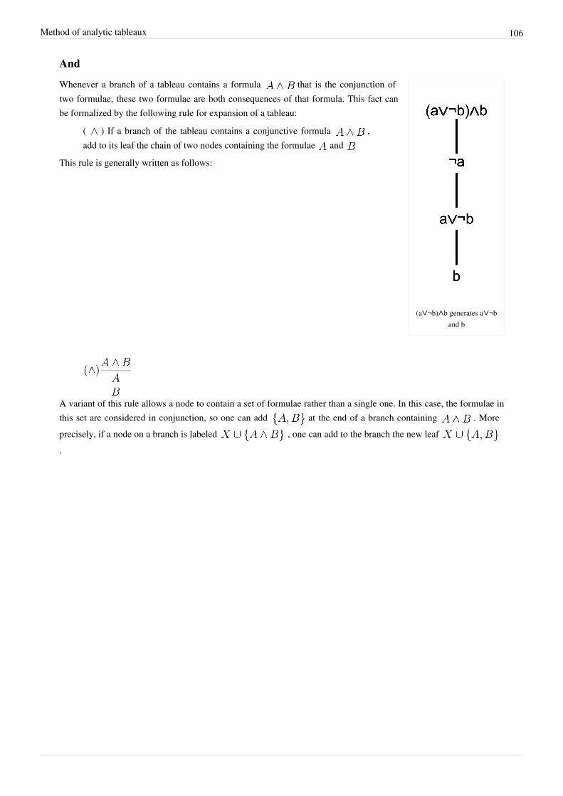
Method of analytic tableaux 106

And

(a⋁¬b)⋀b generates a⋁¬band b

Whenever a branch of a tableau contains a formula that is the conjunction oftwo formulae, these two formulae are both consequences of that formula. This fact canbe formalized by the following rule for expansion of a tableau:

( ) If a branch of the tableau contains a conjunctive formula ,add to its leaf the chain of two nodes containing the formulae and

This rule is generally written as follows:

A variant of this rule allows a node to contain a set of formulae rather than a single one. In this case, the formulae inthis set are considered in conjunction, so one can add at the end of a branch containing . Moreprecisely, if a node on a branch is labeled , one can add to the branch the new leaf .

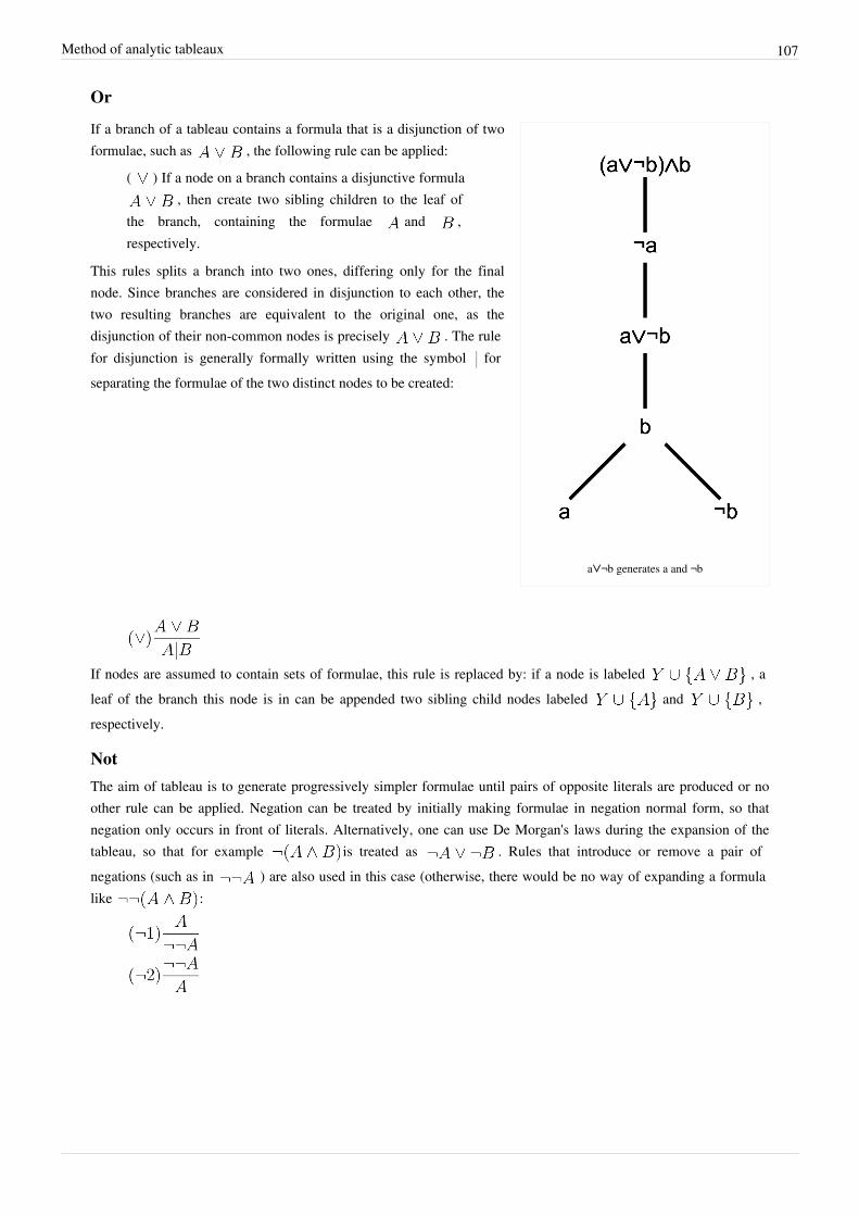
Method of analytic tableaux 107

Or

a⋁¬b generates a and ¬b

If a branch of a tableau contains a formula that is a disjunction of twoformulae, such as , the following rule can be applied:

( ) If a node on a branch contains a disjunctive formula, then create two sibling children to the leaf of

the branch, containing the formulae and ,respectively.

This rules splits a branch into two ones, differing only for the finalnode. Since branches are considered in disjunction to each other, thetwo resulting branches are equivalent to the original one, as thedisjunction of their non-common nodes is precisely . The rulefor disjunction is generally formally written using the symbol forseparating the formulae of the two distinct nodes to be created:

If nodes are assumed to contain sets of formulae, this rule is replaced by: if a node is labeled , aleaf of the branch this node is in can be appended two sibling child nodes labeled and ,respectively.

NotThe aim of tableau is to generate progressively simpler formulae until pairs of opposite literals are produced or noother rule can be applied. Negation can be treated by initially making formulae in negation normal form, so thatnegation only occurs in front of literals. Alternatively, one can use De Morgan's laws during the expansion of thetableau, so that for example is treated as . Rules that introduce or remove a pair ofnegations (such as in ) are also used in this case (otherwise, there would be no way of expanding a formulalike :

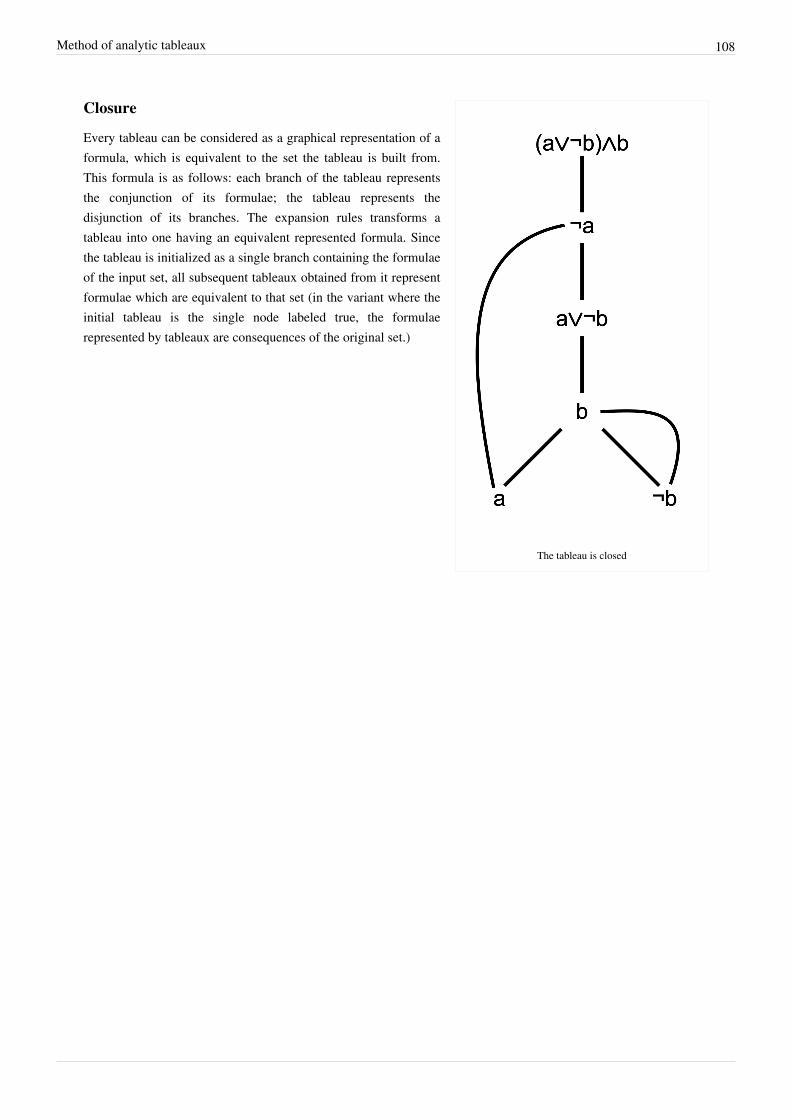
Method of analytic tableaux 108

The tableau is closed

Closure

Every tableau can be considered as a graphical representation of aformula, which is equivalent to the set the tableau is built from.This formula is as follows: each branch of the tableau representsthe conjunction of its formulae; the tableau represents thedisjunction of its branches. The expansion rules transforms atableau into one having an equivalent represented formula. Sincethe tableau is initialized as a single branch containing the formulaeof the input set, all subsequent tableaux obtained from it representformulae which are equivalent to that set (in the variant where theinitial tableau is the single node labeled true, the formulaerepresented by tableaux are consequences of the original set.)

Method of analytic tableaux 109

A tableau for the satisfiable set {a⋀c,¬a⋁b}: all rules havebeen applied to every formula on every branch, but thetableau is not closed (only the left branch is closed), as

expected for satisfiable sets

The method of tableaux works by starting with the initial setof formulae and then adding to the tableau simpler andsimpler formulae, while still preserving equivalent to theoriginal set, until contradiction is shown in the simple form ofopposite literals. Since the formula represented by a tableau isthe disjunction of the formulae represented by its branches,contradiction is obtained when every branch contains a pair ofopposite literals.Once a branch contains a literal and its negation, itscorresponding formula is unsatisfiable. As a result, this branchcan be now "closed", as there is no need to further expand it.If all branches of a tableau are closed, the formula representedby the tableau is unsatisfiable; therefore, the original set isunsatisfiable as well. Obtaining a tableau where all branchesare closed is a way for proving the unsatisfiability of theoriginal set. In the propositional case, one can also prove thatsatisfiability is proved by the impossibility of finding a closedtableau, provided that every expansion rule has been appliedeverywhere it could be applied. In particular, if a tableaucontains some open (non-closed) branches and every formulathat is not a literal has been used by a rule to generate a newnode on every branch the formula is in, the set is satisfiable.This rule takes into account that a formula may occur in morethan one branch (this is the case if there is at least a branching point "below" the node). In this case, the rule forexpanding the formula has to be applied so that its conclusion(s) are appended to all of these branches that are stillopen, before one can conclude that the tableau cannot be further expanded and that the formula is thereforesatisfiable.

Set-labeled tableauA variant of tableau is to label nodes with sets of formulae rather than single formulae. In this case, the initial tableauis a single node labeled with the set to be proved satisfiable. The formulae in a set are therefore considered to be inconjunction.The rules of expansion of the tableau can now work on the leaves of the tableau, ignoring all internal nodes. Forconjunction, the rule is based on the equivalence of a set containing a conjunction with the set containingboth and in place of it. In particular, if a leaf is labeled with , a node can be appended to itwith label :

For disjunction, a set is equivalent to the disjunction of the two sets and . As a result, if the first set labels a leaf, two children can be appended to it, labeled with the latter two formulae.

Finally, if a set contains both a literal and its negation, this branch can be closed:

Method of analytic tableaux 110

A tableau for a given finite set X is a finite (upside down) tree with root X in which all child nodes are obtained byapplying the tableau rules to their parents. A branch in such a tableau is closed if its leaf node contains "closed". Atableau is closed if all its branches are closed. A tableau is open if at least one branch is not closed.Here are two closed tableaux for the set X = {r0 & ~r0, p0 & ((~p0 ∨ q0) & ~q0)} with each rule application markedat the right hand side (& and ~ stand for and , respectively) {r0 & ~r0, p0 & ((~p0 v q0) & ~q0)} {r0 & ~r0, p0 & ((~p0 v q0) & ~q0)}

--------------------------------------(&) ------------------------------------------------------------(&)

{r0 , ~r0, p0 & ((~p0 v q0) & ~q0)} {r0 & ~r0, p0, ((~p0 v q0) & ~q0)}

-------------------------------------(id) ----------------------------------------------------------(&)

closed {r0 & ~r0, p0, (~p0 v q0), ~q0}

-------------------------------------------------------------(v)

{r0 & ~r0, p0, ~p0, ~q0} | {r0 & ~r0, p0, q0, ~q0}

-------------------------- (id) ---------------------- (id)

closed closed

The left hand tableau closes after only one rule application while the right hand one misses the mark and takes a lotlonger to close. Clearly, we would prefer to always find the shortest closed tableaux but it can be shown that onesingle algorithm that finds the shortest closed tableaux for all input sets of formulae cannot exist.

The three rules , and given above are then enough to decide if a given set of formulae innegated normal form are jointly satisfiable:

Just apply all possible rules in all possible orders until we find a closed tableau for or until weexhaust all possibilities and conclude that every tableau for is open.

In the first case, is jointly unsatisfiable and in the second the case the leaf node of the open branch gives anassignment to the atomic formulae and negated atomic formulae which makes jointly satisfiable. Classical logicactually has the rather nice property that we need to investigate only (any) one tableau completely: if it closes then

is unsatisfiable and if it is open then is satisfiable. But this property is not generally enjoyed by other logics.These rules suffice for all of classical logic by taking an initial set of formulae X and replacing each member C by itslogically equivalent negated normal form C' giving a set of formulae X' . We know that X is satisfiable if and only ifX' is satisfiable, so it suffices to search for a closed tableau for X' using the procedure outlined above.

By setting we can test whether the formula A is a tautology of classical logic:If the tableau for closes then is unsatisfiable and so A is a tautology since no assignmentof truth values will ever make A false. Otherwise any open leaf of any open branch of any open tableaufor gives an assignment that falsifies A.

ConditionalClassical propositional logic usually has a connective to denote material implication. If we write this connective as⇒, then the formula A ⇒ B stands for "if A then B". It is possible to give a tableau rule for breaking down A ⇒ Binto its constituent formulae. Similarly, we can give one rule each for breaking down each of ¬(A ∧ B), ¬(A ∨ B),¬(¬A), and ¬(A ⇒ B). Together these rules would give a terminating procedure for deciding whether a given set offormulae is simultaneously satisfiable in classical logic since each rule breaks down one formula into its constituentsbut no rule builds larger formulae out of smaller constituents. Thus we must eventually reach a node that containsonly atoms and negations of atoms. If this last node matches (id) then we can close the branch, otherwise it remainsopen.But note that the following equivalences hold in classical logic where (...) = (...) means that the left hand sideformula is logically equivalent to the right hand side formula:

Method of analytic tableaux 111

If we start with an arbitrary formula C of classical logic, and apply these equivalences repeatedly to replace the lefthand sides with the right hand sides in C, then we will obtain a formula C' which is logically equivalent to C butwhich has the property that C' contains no implications, and ¬ appears in front of atomic formulae only. Such aformula is said to be in negation normal form and it is possible to prove formally that every formula C of classicallogic has a logically equivalent formula C' in negation normal form. That is, C is satisfiable if and only if C' issatisfiable.

First-order logic tableauTableaux are extended to first order predicate logic by two rules for dealing with universal and existentialquantifiers, respectively. Two different sets of rules can be used; both employ a form of Skolemization for handingexistential quantifiers, but differ on the handling of universal quantifiers.The set of formulae to check for validity is here supposed to contain no free variables; this is not a limitation as freevariables are implicitly universally quantified, so universal quantifiers over these variables can be added, resulting ina formula with no free variables.

First-order tableau without unification

A first-order formula implies all formulae where is a ground term. The following inference rule istherefore correct:

where is an arbitrary ground term

Contrarily to the rules for the propositional connectives, multiple applications of this rule to the same formula maybe necessary. As an example, the set can only be proved unsatisfiable if both

and are generated from .Existential quantifiers are dealt with Skolemization. In particular, a formula with a leading existential quantifier like

generates its Skolemization , where is a new constant symbol.

where is a new constant symbol

Method of analytic tableaux 112

A tableau without unification for {∀x.P(x), ∃x.(¬P(x)⋁¬P(f(x)))}. For clarity, formulaeare numbered on the left and the formula and rule used at each step is on the right

The Skolem term is a constant (afunction of arity 0) because thequantification over does not occurwithin the scope of any universalquantifier. If the original formulacontained some universal quantifierssuch that the quantification over was within their scope, thesequantifiers have evidently beenremoved by the application of the rulefor universal quantifiers.

The rule for existential quantifiers introduces new constant symbols. These symbols can be used by the rule foruniversal quantifiers, so that can generate even if was not in the original formula but is a Skolemconstant created by the rule for existential quantifiers.The above two rules for universal and existential quantifiers are correct, and so are the propositional rules: if a set offormulae generates a closed tableau, this set is unsatisfiable. Completeness can also be proved: if a set of formulae isunsatisfiable, there exists a closed tableau built from it by these rules. However, actually finding such a closedtableau requires a suitable policy of application of rules. Otherwise, an unsatisfiable set can generate aninfinite-growing tableau. As an example, the set is unsatisfiable, but a closed tableau isnever obtained if one unwisely keeps applying the rule for universal quantifiers to , generating forexample . A closed tableau can always be found by ruling out this and similar"unfair" policies of application of tableau rules.The rule for universal quantifiers is the only non-deterministic rule, as it does not specify which term toinstantiate with. Moreover, while the other rules need to be applied only once for each formula and each path theformula is in, this one may require multiple applications. Application of this rule can however be restricted bydelaying the application of the rule until no other rule is applicable and by restricting the application of the rule toground terms that already appear in the path of the tableau. The variant of tableaux with unification shown belowaims at solving the problem of non-determinism.

First-order tableau with unificationThe main problem of tableau without unification is how to choose a ground term for the universal quantifier rule.Indeed, every possible ground term can be used, but clearly most of them might be useless for closing the tableau.A solution to this problem is to "delay" the choice of the term to the time when the consequent of the rule allowsclosing at least a branch of the tableau. This can be done by using a variable instead of a term, so that generates , and then allowing substitutions to later replace with a term. The rule for universal quantifiersbecomes:

Method of analytic tableaux 113

where is a variable not occurring everywhere else in the tableau

While the initial set of formulae is supposed not to contain free variables, a formula of the tableau contain the freevariables generated by this rule. These free variables are implicitly considered universally quantified.This rule employs a variable instead of a ground term. The gain of this change is that these variables can be thengiven a value when a branch of the tableau can be closed, solving the problem of generating terms that might beuseless.

if is the most general unifier of two literals and , where and the negation of occur in the same branch of the tableau, canbe applied at the same time to all formulae of the tableau

As an example, can be proved unsatisfiable by first generating ; the negation of thisliteral is unifiable with , the most general unifier being the substitution that replaces with ; applyingthis substitution results in replacing with , which closes the tableau.This rule closes at least a branch of the tableau -the one containing the considered pair of literals. However, thesubstitution has to be applied to the whole tableau, not only on these two literals. This is expressed by saying that thefree variables of the tableau are rigid: if an occurrence of a variable is replaced by something else, all otheroccurrences of the same variable must be replaced in the same way. Formally, the free variables are (implicitly)universally quantified and all formulae of the tableau are within the scope of these quantifiers.Existential quantifiers are dealt with by Skolemization. Contrary to the tableau without unification, Skolem termsmay not be simple constant. Indeed, formulae in a tableau with unification may contain free variables, which areimplicitly considered universally quantified. As a result, a formula like may be within the scope ofuniversal quantifiers; if this is the case, the Skolem term is not a simple constant but a term made of a new functionsymbol and the free variables of the formula.

where is a new function symbol and the free variables of

A first-order tableau with unification for {∀x.P(x), ∃x.(¬P(x)⋁¬P(f(x)))}. For clarity,formulae are numbered on the left and the formula and rule used at each step is on the

right

This rule incorporates a simplificationover a rule where are thefree variables of the branch, not of alone. This rule can be furthersimplified by the reuse of a functionsymbol if it has already been used in aformula that is identical to up tovariable renaming.

The formula represented by a tableau is obtained in a way that is similar to the propositional case, with the additional assumption that free variables are considered universally quantified. As for the propositional case, formulae in each branch are conjoined and the resulting formulae are disjoined. In addition, all free variables of the resulting formula are universally quantified. All these quantifiers have the whole formula in their scope. In other words, if is the

Method of analytic tableaux 114

formula obtained by disjoining the conjunction of the formulae in each branch, and are the free variables in it, then isthe formula represented by the tableau. The following considerations apply:• The assumption that free variables are universally quantified is what makes the application of a most general

unifier a sound rule: since means that is true for every possible value of , then is true for theterm that the most general unifier replaces with.

• Free variables in a tableau are rigid: all occurrences of the same variable have to be replaced all with the sameterm. Every variable can be considered a symbol representing a term that is yet to be decided. This is aconsequence of free variables being assumed universally quantified over the whole formula represented by thetableau: if the same variable occurs free in two different nodes, both occurrences are in the scope of the samequantifier. As an example, if the formulae in two nodes are and , where is free in both, theformula represented by the tableau is something in the form . This formula implies that

is true for any value of , but does not in general imply for twodifferent terms and , as these two terms may in general take different values. This means that cannot bereplaced by two different terms in and .

• Free variables in a formula to check for validity are also considered universally quantified. However, thesevariables cannot be left free when building a tableau, because tableau rules works on the converse of the formulabut still treats free variables as universally quantified. For example, is not valid (it is not true inthe model where , and the interpretation where ).Consequently, is satisfiable (it is satisfied by the same model and interpretation). However, aclosed tableau could be generated with and , and substituting with would generate a closure.A correct procedure is to first make universal quantifiers explicit, thus generating .

The following two variants are also correct.• Applying to the whole tableau a substitution to the free variables of the tableau is a correct rule, provided that this

substitution is free for the formula representing the tableau. In other worlds, applying such a substitution leads toa tableau whose formula is still a consequence of the input set. Using most general unifiers automatically ensuresthat the condition of freeness for the tableau is met.

• While in general every variable has to be replaced with the same term in the whole tableau, there are some specialcases in which this is not necessary.

Tableaux with unification can be proved complete: if a set of formulae is unsatisfiable, it has atableau-with-unification proof. However, actually finding such a proof may be a difficult problem. Contrarily to thecase without unification, applying a substitution can modify the existing part of a tableau; while applying asubstitution closes at least a branch, it may make other branches impossible to close (even if the set is unsatisfiable).A solution to this problem is that delayed instantiation: no substitution is applied until one that closes all branches atthe same time is found. With this variant, a proof for an unsatisfiable set can always be found by a suitable policy ofapplication of the other rules. This method however requires the whole tableau to be kept in memory: the generalmethod closes branches which can be then discarded, while this variant does not close any branch until the end.The problem that some tableaux that can be generated are impossible to close even if the set is unsatisfiable iscommon to other sets of tableau expansion rules: even if some specific sequences of application of these rules allowconstructing a closed tableau (if the set is unsatisfiable), some other sequences lead to tableau that cannot be closed.General solutions for these cases are outlined in the "Searching for a tableau" section.

Method of analytic tableaux 115

Tableau calculi and their propertiesA tableau calculus is a set of rules that allows building and modification of a tableau. Propositional tableau rules,tableau rules without unification, and tableau rules with unification, are all tableau calculi. Some importantproperties a tableau calculus may or may not possess are completeness, destructiveness, and proof confluence.A tableau calculi is said complete if it allows building a tableau proof for every given unsatisfiable set of formulae.The tableau calculi mentioned above can be proved complete.A remarkable difference between tableau with unification and the other two calculi is that the latter two calculi onlymodify a tableau by adding new nodes to it, while the former one allows substitutions to modify the existing part ofthe tableau. More generally, tableau calculi are classed as destructive or non-destructive depending on whether theyonly add new nodes to tableau or not. Tableau with unification is therefore destructive, while propositional tableauand tableau without unification are non-destructive.Proof confluence is the property of a tableau calculus to obtain a proof for an arbitrary unsatisfiable set from anarbitrary tableau, assuming that this tableau has itself been obtained by applying the rules of the calculus. In otherwords, in a proof confluent tableau calculus, from an unsatisfiable set one can apply whatever set of rules and stillobtain a tableau from which a closed one can be obtained by applying some other rules.

Proof proceduresA tableau calculus is simply a set of rules that tells how a tableau can be modified. A proof procedure is a method foractually finding a proof (if one exists). In other words, a tableau calculus is a set of rules, while a proof procedure isa policy of application of these rules. Even if a calculus is complete, not every possible choice of application of rulesleads to a proof of an unsatisfiable set. For example isunsatisfiable, but both tableaux with unification and tableaux without unification allow the rule for the universalquantifiers to be applied repeatedly to the last formula, while simply applying the rule for disjunction to the third onewould directly lead to closure.For proof procedures, a definition of completeness has been given: a proof procedure is strongly complete if it allowsfinding a closed tableau for any given unsatisfiable set of formulae. Proof confluence of the underlying calculus isrelevant to completeness: proof confluence is the guarantee that a closed tableau can be always generated from anarbitrary partially constructed tableau (if the set is unsatisfiable). Without proof confluence, the application of a'wrong' rule may result in the impossibility of making the tableau complete by applying other rules.Propositional tableaux and tableaux without unification have strongly complete proof procedures. In particular, acomplete proof procedure is that of applying the rules in a fair way. This is because the only way such calculi cannotgenerate a closed tableau from an unsatisfiable set is by not applying some applicable rules.For propositional tableaux, fairness amounts to expanding every formula in every branch. More precisely, for everyformula and every branch the formula is in, the rule having the formula as a precondition has been used to expandthe branch. A fair proof procedure for propositional tableaux is strongly complete.For first-order tableaux without unification, the condition of fairness is similar, with the exception that the rule foruniversal quantifier might require more than one application. Fairness amounts to expanding every universalquantifier infinitely often. In other words, a fair policy of application of rules cannot keep applying other ruleswithout expanding every universal quantifier in every branch that is still open once in a while.

Method of analytic tableaux 116

Searching for a closed tableauIf a tableau calculus is complete, every unsatisfiable set of formula has an associated closed tableau. While thistableau can always be obtained by applying some of the rules of the calculus, the problem of which rules to apply fora given formula still remains. As a result, completeness does not automatically implies the existence of a feasiblepolicy of application of rules that can always lead to building a closed tableau for every given unsatisfiable set offormulae. While a fair proof procedure is complete for ground tableau and tableau without unification, this is not thecase for tableau with unification.

A search tree in the space of tableau for {∀x.P(x), ¬P(c)⋁¬Q(c), ∃y.Q(c)}. Forsimplicity, the formulae of the set have been omitted from all tableau in the figure and a

rectangle used in their place. A closed tableau is in the bold box; the other branches couldbe still expanded.

A general solution for this problem isthat of searching the space of tableauuntil a closed one is found (if anyexists, that is, the set is unsatisfiable).In this approach, one starts with anempty tableau and then recursivelytries to apply every possible applicablerule. This procedure visit a (implicit)tree whose nodes are labeled withtableau, and such that the tableau in anode is obtained from the tableau in itsparent by applying one of the validrules.Since one such branch can be infinite,this tree has to be visited breadth-first rather than depth-first. This requires a large amount of space, as the breadth ofthe tree can grow exponentially. A method that may visit some nodes more than once but works in polynomial spaceis to visit in a depth-first manner with iterative deepening: one first visits the tree up to a certain depth, then increasesthe depth and perform the visit again. This particular procedure uses the depth (which is also the number of tableaurules that have been applied) for deciding when to stop at each step. Various other parameters (such as the size of thetableau labeling a node) have been used instead.

Reducing searchThe size of the search tree depends on the number of (children) tableau that can be generated from a given (parent)one. Reducing the number of such tableau therefore reduces the required search.A way for reducing this number is to disallow the generation of some tableau based on their internal structure. Anexample is the condition of regularity: if a branch contains a literal, using an expansion rule that generates the sameliteral is useless because the branch containing two copies of the literals would have the same set of formulae of theoriginal one. This expansion can be disallowed because if a closed tableau exists, it can be found without it. Thisrestriction is structural because it can be checked by looking at the structure of the tableau to expand only.Different methods for reducing search disallow the generation of some tableau on the ground that a closed tableau can still be found by expanding the other ones. These restrictions are called global. As an example of a global restriction, one may employ a rule that specify which of the open branches is to be expanded. As a result, if a tableau has for example two non-closed branches, the rule tells which one is to be expanded, disallowing the expansion of the second one. This restriction reduces the search space because one possible choice is now forbidden; completeness if however not harmed, as the second branch will still be expanded if the first one is eventually closed. As an example, a tableau with root , child , and two leaves and can be closed in two ways: applying first to and then to , or vice versa. There is clearly no need to follow both possibilities; one may consider only the case in which is first applied to and disregard the case in which it is first applied to . This is a global restriction because what allows neglecting this second expansion is the presence of the other tableau,

Method of analytic tableaux 117

where expansion is applied to first and afterwards.

Clause tableauxWhen applied to sets of clauses (rather than of arbitrary formulae), tableaux methods allow for a number ofefficiency improvements. A first-order clause is a formula that does not contain freevariables and such that each is a literal. The universal quantifiers are often omitted for clarity, so that forexample actually means . Note that, if taken literally, thesetwo formulae are not the same as for satisfiability: rather, the satisfiability is the same as thatof . That free variables are universally quantified is not a consequence of thedefinition of first-order satisfiability; it is rather used as an implicit common assumption when dealing with clauses.The only expansion rules that are applicable to a clause are and ; these two rules can be replaced by theircombination without losing completeness. In particular, the following rule corresponds to applying in sequence therules and of the first-order calculus with unification.

where is obtained by replacing every variable with a new one in

When the set to be checked for satisfiability is only composed of clauses, this and the unification rules are sufficientto prove unsatisfiability. In other worlds, the tableau calculi composed of and is complete.Since the clause expansion rule only generates literals and never new clauses, the clauses to which it can be appliedare only clauses of the input set. As a result, the clause expansion rule can be further restricted to the case where theclause is in the input set.

where is obtained by replacing every variable with a

new one in , which is a clause of the input setSince this rule directly exploit the clauses in the input set there is no need to initialize the tableau to the chain of theinput clauses. The initial tableau can therefore be initialize with the single node labeled ; this label is oftenomitted as implicit. As a result of this further simplification, every node of the tableau (apart of the root) is labeledwith a literal.A number of optimizations can be used for clause tableau. These optimization are aimed at reducing the number ofpossible tableaux to be explored when searching for a closed tableau as described in the "Searching for a closedtableau" section above.

Connection tableauConnection is a condition over tableau that forbids expanding a branch using clauses that are unrelated to the literalsthat are already in the branch. Connection and be defined in two ways:strong connectedness

when expanding a branch, use an input clause only if it contains a literal that can be unified with the negationof the literal in the current leaf

weak connectednessallow the use of clauses that contain a literal that unifies with the negation of a literal on the branch

Both conditions apply only to branches consisting not only of the root. The second definition allows for the use of aclause containing a literal that unifies with the negation of a literal in the branch, while the first only furtherconstraint that literal to be in leaf of the current branch.

Method of analytic tableaux 118

If clause expansion is restricted by connectedness (either strong or weak), its application produces a tableau in whichsubstitution can applied to one of the new leaves, closing its branch. In particular, this is the leaf containing theliteral of the clause that unifies with the negation of a literal in the branch (or the negation of the literal in the parent,in case of strong connection).Both conditions of connectedness lead to a complete first-order calculus: if a set of clauses is unsatisfiable, it has aclosed connected (strongly or weakly) tableau. Such a closed tableau can be found by searching in the space oftableaux as explained in the "Searching for a closed tableau" section. During this search, connectedness eliminatessome possible choices of expansion, thus reducing search. In other worlds, while the tableau in a node of the tree canbe in general expanded in several different ways, connection may allow only few of them, thus reducing the numberof resulting tableaux that need to be further expanded.This can be seen on the following (propositional) example. The tableau made of a chain for the set ofclauses can be in general expanded using each of the four input clauses, but connectiononly allows the expansion that uses . This means that the tree of tableaux has four leaves in general butonly one if connectedness is imposed. This means that connectedness leaves only one tableau to try and expand,instead of the four ones to consider in general. In spite of this reduction of choices, the completeness theorem impliesthat a closed tableau can be found if the set is unsatisfiable.The connectedness conditions, when applied to the propositional (clausal) case, make the resulting calculusnon-confluent. As an example, is unsatisfiable, but applying to generates the chain , which is not closed and to which no other expansion rule can be applied without violating either strong or weakconnectedness. In the case of weak connectedness, confluence holds provided that the clause used for expanding theroot is relevant to unsatisfiability, that is, it is contained in a minimally unsatisfiable subset of the set of clauses.Unfortunately, the problem of checking whether a clause meets this condition is itself a hard problem. In spite ofnon-confluence, a closed tableau can be found using search, as presented in the "Searching for a closed tableau"section above. While search is made necessary, connectedness reduces the possible choices of expansion, thusmaking search more efficient.

Regular tableauxA tableau is regular if no literal occurs twice in the same branch. Enforcing this condition allows for a reduction ofthe possible choices of tableau expansion, as the clauses that would generate a non-regular tableau cannot beexpanded.These disallowed expansion steps are however useless. If is a branch containing a literal , and is a clausewhose expansion violates regularity, then contains . In order to close the tableau, one needs to expand andclose, among others, the branch where , where occurs twice. However, the formulae in this branch areexactly the same as the formulae of alone. As a result, the same expansion steps that close also close

. This means that expanding was unnecessary; moreover, if contained other literals, its expansiongenerated other leaves that needed to be closed. In the propositional case, the expansion needed to close these leavesare completely useless; in the first-order case, they may only affect the rest of the tableau because of someunifications; these can however be combined to the substitutions used to close the rest of the tableau.

Method of analytic tableaux 119

Tableaux for modal logicsIn a modal logic, a model comprises a set of possible worlds, each one associated to a truth evaluation; anaccessibility relation tells when a world is accessible from another one. A modal formula may specify not onlyconditions over a possible world, but also on the ones that are accessible from it. As an example, is true in aworld if is true in all worlds that are accessible from it.As for propositional logic, tableaux for modal logics are based on recursively breaking formulae into its basiccomponents. Expanding a modal formula may however require stating conditions over different worlds. As anexample, if is true in a world then there exists a world accessible from it where is false. However, onecannot simply add the following rule to the propositional ones.

In propositional tableaux all formulae refer to the same truth evaluation, but the precondition of the rule above holdsin a world while the consequence holds in another. Not taking into account this would generate wrong results. Forexample, formula states that is true in the current world and is false in a world that is accessiblefrom it. Simply applying and the expansion rule above would produce and , but these two formulaeshould not in general generate a contradiction, as they hold in different worlds. Modal tableaux calculi do containrules of the kind of the one above, but include mechanisms to avoid the incorrect interaction of formulae referring todifferent worlds.Technically, tableaux for modal logics check the satisfiability of a set of formulae: they check whether there exists amodel and world such that the formulae in the set are true in that model and world. In the example above,while states the truth of in , the formula states the truth of in some world that is accessiblefrom and which may in general be different from . Tableaux calculi for modal logic take into account thatformulae may refer to different worlds.This fact has an important consequence: formulae that hold in a world may imply conditions over differentsuccessors of that world. Unsatisfiability may then be proved from the subset of formulae referring to the a singlesuccessor. This holds if a world may have more than one successor, which is true for most modal logic. If this is thecase, a formula like is true if a successor where holds exists and a successor where holds exists. In the other way around, if one can show unsatisfiability of in an arbitrary successor, the formulais proved unsatisfiable without checking for worlds where holds. At the same time, if one can showunsatisfiability of , there is no need to check . As a result, while there are two possible way to expand

, one of these two ways is always sufficient to prove unsatisfiability if the formula is unsatisfiable.For example, one may expand the tableau by considering an arbitrary world where holds. If this expansionleads to unsatisfiability, the original formula is unsatisfiable. However, it is also possible that unsatisfiability cannotbe proved this way, and that the world where holds should have been considered instead. As a result, one canalways prove unsatisfiability by expanding either only or only; however, if the wrong choice is donethe resulting tableau may not be closed. Expanding either subformula leads to tableau calculi that are complete butnot proof-confluent. Searching as described in the "Searching for a closed tableau" may therefore be necessary.Depending on whether the precondition and consequence of a tableau expansion rule refer to the same world or not,the rule is called static or transactional. While rules for propositional connectives are all static, not all rules for modalconnectives are transactional: for example, in every modal logic including axiom T, it holds that implies inthe same world. As a result, the relative (modal) tableau expansion rule is static, as both its precondition andconsequence refer to the same world.

Method of analytic tableaux 120

Formula-deleting tableauA way for making formulae referring to different worlds not interacting in the wrong way is to make sure that allformulae of a branch refer to the same world. This condition is initially true as all formulae in the set to be checkedfor consistency are assumed referring to the same world. When expanding a branch, two situations are possible:either the new formulae refer to the same world as the other one in the branch or not. In the first case, the rule isapplied normally. In the second case, all formulae of the branch that do not also hold in the new world are deletedfrom the branch, and possibly added to all other branches that are still relative to the old world.As an example, in S5 every formula that is true in a world is also true in all accessible worlds (that is, in allaccessible worlds both and are true). Therefore, when applying , whose consequence holds in a

different world, one deletes all formulae from the branch, but can keep all formulae , as these hold in the newworld as well. In order to retain completeness, the deleted formulae are then added to all other branches that stillrefer to the old world.

World-labeled tableauA different mechanism for ensuring the correct interaction between formulae referring to different worlds is toswitch from formulae to labeled formulae: instead of writing , one would write to make it explicit that

holds in world .All propositional expansion rules are adapted to this variant by stating that they all refer to formulae with the sameworld label. For example, generates two nodes labeled with and ; a branch is closedonly if it contains two opposite literals of the same world, like and ; no closure is generated if thetwo world labels are different, like in and .The modal expansion rule may have a consequence that refer to a different worlds. For example, the rule for would be written as follows

The precondition and consequent of this rule refer to worlds and , respectively. The various different calculiuse different methods for keeping track of the accessibility of the worlds used as labels. Some includepseudo-formulae like to denote that is accessible from . Some others use sequences of integers asworld labels, this notation implicitly representing the accessibility relation (for example, is accessiblefrom .)

Set-labeling tableauxThe problem of interaction between formulae holding in different worlds can be overcome by using set-labelingtableaux. These are trees whose nodes are labeled with sets of formulae; the expansion rules tell how to attach newnodes to a leaf, based only on the label of the leaf (and not on the label of other nodes in the branch).Tableaux for modal logics are used to verify the satisfiability of a set of modal formulae in a given modal logic.Given a set of formulae , they check the existence of a model and a world such that .The expansion rules depend on the particular modal logic used. A tableau system for the basic modal logic K can beobtained by adding to the propositional tableau rules the following one:

Intuitively, the precondition of this rule expresses the truth of all formulae at all accessible worlds,and truth of at some accessible worlds. The consequence of this rule is a formula that must be true at one ofthose worlds where is true.

Method of analytic tableaux 121

More technically, modal tableaux methods check the existence of a model and a world that make set offormulae true. If are true in , there must be a world that is accessible from andthat makes true. This rule therefore amounts to deriving a set of formulae that must be satisfiedin such .While the preconditions are assumed satisfied by , the consequences

are assumed satisfied in : same model but possibly different worlds. Set-labeledtableaux do not explicitly keep track of the world where each formula is assumed true: two nodes may or may notrefer to the same world. However, the formulae labeling any given node are assumed true at the same world.As a result of the possibly different worlds where formulae are assumed true, a formula in a node is notautomatically valid in all its descendants, as every application of the modal rule correspond to a move from a worldto another one. This condition is automatically captured by set-labeling tableaux, as expansion rules are based onlyon the leaf where they are applied and not on its ancestors.

Remarkably, does not directly extend to multiple negated boxed formulae such as in: while there exists an accessible world where is false and one in which

is false, these two worlds are not necessarily the same.Differently from the propositional rules, states conditions over all its preconditions. For example, it cannot beapplied to a node labeled by ; while this set is inconsistent and this could be easilyproved by applying , this rule cannot be applied because of formula , which is not even relevant toinconsistency. Removal of such formulae is made possible by the rule:

The addition of this rule (thinning rule) makes the resulting calculus non-confluent: a tableau for an inconsistent setmay be impossible to close, even if a closed tableau for the same set exists.

Rule is non-deterministic: the set of formulae to be removed (or to be kept) can be chosen arbitrarily; thiscreates the problem of choosing a set of formulae to discard that is not so large it makes the resulting set satisfiableand not so small it makes the necessary expansion rules inapplicable. Having a large number of possible choicesmakes the problem of searching for a closed tableau harder.This non-determinism can be avoided by restricting the usage of so that it is only applied before a modalexpansion rule, and so that it only removes the formulae that make that other rule inapplicable. This condition can bealso formulated by merging the two rules in a single one. The resulting rule produces the same result as the old one,but implicitly discard all formulae that made the old rule inapplicable. This mechanism for removing has beenproved to preserve completeness for many modal logics.Axiom T expresses reflexivity of the accessibility relation: every world is accessible from itself. The correspondingtableau expansion rule is:

This rule relates conditions over the same world: if is true in a world, by reflexivity is also true in the sameworld. This rule is static, not transactional, as both its precondition and consequent refer to the same world.This rule copies from the precondition to the consequent, in spite of this formula having being "used" togenerate . This is correct, as the considered world is the same, so also holds there. This "copying" isnecessary in some cases. It is for example necessary to prove the inconsistency of : the onlyapplicable rules are in order , from which one is blocked if is not copied.

Method of analytic tableaux 122

Auxiliary tableauxA different method for dealing with formulae holding in alternate worlds is to start a different tableau for each nowworld that is introduced in the tableau. For example, implies that is false in an accessible world, so onestarts a new tableau rooted by . This new tableau is attached to the node of the original tableau where theexpansion rule has been applied; a closure of this tableau immediately generates a closure of all branches where thatnode is, regardless of whether the same node is associated other auxiliary tableaux. The expansion rules for theauxiliary tableaux are the same as for the original one; therefore, an auxiliary tableau can have in turns other(sub-)auxiliary tableaux.

Global assumptionsThe above modal tableaux establish the consistency of a set of formulae, and can be used for solving the local logicalconsequence problem. This is the problem of telling whether, for each model , if is true in a world , then

is also true in the same world. This is the same as checking whether is true in a world of a model, in theassumption that is also true in the same world of the same model.A related problem is the global consequence problem, where the assumption is that a formula (or set of formulae) is true in all possible worlds of the model. The problem is that of checking whether, in all models where istrue in all worlds, is also true in all worlds.Local and global assumption differ on models where the assumed formula is true in some worlds but not in others.As an example, entails globally but not locally. Local entailment does not hold in amodel consisting of two worlds making and true, respectively, and where the second is accessible fromthe first; in the first world, the assumption is true but is false. This counterexample works because can beassumed true in a world and false in another one. If however the same assumption is considered global, is notallowed in any world of the model.These two problems can be combined, so that one can check whether is a local consequence of under theglobal assumption . Tableaux calculi can deal with global assumption by a rule allowing its addition to everynode, regardless of the world it refers to.

NotationsThe following conventions are sometimes used.

Uniform notationWhen writing tableaux expansion rules, formulae are often denoted using a convention, so that for example isalways considered to be . The following table provides the notation for formulae in propositional,first-order, and modal logic.

Method of analytic tableaux 123

Notation Formulae

Each label in the first column is taken to be either formula in the other columns. An overlined formula such as indicates that is the negation of whatever formula appears in its place, so that for example in formula the subformula is the negation of .Since every label indicates many equivalent formulae, this notation allows writing a single rule for all theseequivalent formulae. For example, the conjunction expansion rule is formulated as:

Signed formulaeA formula in a tableau is assumed true. Signed tableaux allows stating that a formula is false. This is generallyachieved by adding a label to each formula, where the label T indicates formulae assumed true and F those assumedfalse. A different but equivalent notation is that to write formulae that are assumed true at the left of the node andformulae assumed false at its right.

References• Bostock, David, 1997. Intermediate Logic. Oxford Univ. Press.• M D'Agostino, D Gabbay, R Haehnle, J Posegga (Eds), Handbook of Tableau Methods, Kluwer,1999.• Girle, Rod, 2000. Modal Logics and Philosophy. Teddington UK: Acumen.• Goré, Rajeev (1999) "Tableau Methods for Modal and Temporal Logics" in D'Agostino, M., Dov Gabbay, R.

Haehnle, and J. Posegga, eds., Handbook of Tableau Methods. Kluwer: 297-396.• Richard Jeffrey, 1990 (1967). Formal Logic: Its Scope and Limits, 3rd ed. McGraw Hill.• Raymond Smullyan, 1995 (1968). First Order-Logic. Dover Publications.• Melvin Fitting (1996). First-order logic and automated theorem proving (2nd ed.). Springer-Verlag.• Reiner Hähnle (2001). Tableaux and Related Methods. Handbook of Automated Reasoning• Reinhold Letz, Gernot Stenz (2001). Model Elimination and Connection Tableau Procedures. Handbook of

Automated Reasoning• Zeman, J. J. (1973) Modal Logic. [1] Reidel.

Method of analytic tableaux 124

External links• TABLEAUX [2]: an annual international conference on automated reasoning with analytic tableaux and related

methods.• JAR [3]: Journal of Automated Reasoning.• lolo [4]: a simple theorem prover written in Haskell that uses analytic tableaux for propositional logic.• tableaux.cgi [5]: an interactive prover for propositional and first-order logic using tableaux.

References[1] http:/ / www. clas. ufl. edu/ users/ jzeman/ modallogic/[2] http:/ / i12www. ira. uka. de/ TABLEAUX/[3] http:/ / www-unix. mcs. anl. gov/ JAR/[4] http:/ / lolo. svn. sourceforge. net/ viewvc/ lolo/[5] http:/ / www. ncc. up. pt/ ~pbv/ cgi/ tableaux. cgi

Natural deductionIn logic and proof theory, natural deduction is a kind of proof calculus in which logical reasoning is expressed byinference rules closely related to the "natural" way of reasoning. This contrasts with the axiomatic systems whichinstead use axioms as much as possible to express the logical laws of deductive reasoning.

MotivationNatural deduction grew out of a context of dissatisfaction with the axiomatizations of deductive reasoning commonto the systems of Hilbert, Frege, and Russell (see, e.g., Hilbert system). Such axiomatizations were most famouslyused by Russell and Whitehead in their mathematical treatise Principia Mathematica. Spurred on by a series ofseminars in Poland in 1926 by Łukasiewicz that advocated a more natural treatment of logic, Jaśkowski made theearliest attempts at defining a more natural deduction, first in 1929 using a diagrammatic notation, and later updatinghis proposal in a sequence of papers in 1934 and 1935. His proposals led to different notations such as Fitch-stylecalculus (or Fitch's diagrams) or Suppes' method of which e.g. Lemmon gave a variant called system L.Natural deduction in its modern form was independently proposed by the German mathematician Gentzen in 1935,in a dissertation delivered to the faculty of mathematical sciences of the university of Göttingen. The term naturaldeduction (or rather, its German equivalent natürliches Schließen) was coined in that paper:

Ich wollte zunächst einmal einen Formalismus aufstellen, der dem wirklichen Schließen möglichst nahekommt. So ergab sich ein „Kalkül des natürlichen Schließens“.(First I wished to construct a formalism that comes as close as possible to actual reasoning. Thus arose a"calculus of natural deduction".)—Gentzen, Untersuchungen über das logische Schließen (Mathematische Zeitschrift 39, pp.176–210, 1935)

Gentzen was motivated by a desire to establish the consistency of number theory, and he found immediate use for hisnatural deduction calculus. He was nevertheless dissatisfied with the complexity of his proofs, and in 1938 gave anew consistency proof using his sequent calculus. In a series of seminars in 1961 and 1962 Prawitz gave acomprehensive summary of natural deduction calculi, and transported much of Gentzen's work with sequent calculiinto the natural deduction framework. His 1965 monograph Natural deduction: a proof-theoretical study was tobecome a reference work on natural deduction, and included applications for modal and second-order logic.In natural deduction, a proposition is deduced from a collection of premises by applying inference rules repeatedly.The system presented in this article is a minor variation of Gentzen's or Prawitz's formulation, but with a closeradherence to Martin-Löf's description of logical judgments and connectives (Martin-Löf, 1996).

Natural deduction 125

Judgments and propositionsA judgment is something that is knowable, that is, an object of knowledge. It is evident if one in fact knows it. Thus"it is raining" is a judgment, which is evident for the one who knows that it is actually raining; in this case one mayreadily find evidence for the judgment by looking outside the window or stepping out of the house. In mathematicallogic however, evidence is often not as directly observable, but rather deduced from more basic evident judgments.The process of deduction is what constitutes a proof; in other words, a judgment is evident if one has a proof for it.The most important judgments in logic are of the form "A is true". The letter A stands for any expressionrepresenting a proposition; the truth judgments thus require a more primitive judgment: "A is a proposition". Manyother judgments have been studied; for example, "A is false" (see classical logic), "A is true at time t" (see temporallogic), "A is necessarily true" or "A is possibly true" (see modal logic), "the program M has type τ" (seeprogramming languages and type theory), "A is achievable from the available resources" (see linear logic), andmany others. To start with, we shall concern ourselves with the simplest two judgments "A is a proposition" and "Ais true", abbreviated as "A prop" and "A true" respectively.The judgment "A prop" defines the structure of valid proofs of A, which in turn defines the structure of propositions.For this reason, the inference rules for this judgment are sometimes known as formation rules. To illustrate, if wehave two propositions A and B (that is, the judgments "A prop" and "B prop" are evident), then we form thecompound proposition A and B, written symbolically as " ". We can write this in the form of an inferencerule:

This inference rule is schematic: A and B can be instantiated with any expression. The general form of an inferencerule is:

where each is a judgment and the inference rule is named "name". The judgments above the line are known aspremises, and those below the line are conclusions. Other common logical propositions are disjunction ( ),negation ( ), implication ( ), and the logical constants truth ( ) and falsehood ( ). Theirformation rules are below.

Introduction and eliminationNow we discuss the "A true" judgment. Inference rules that introduce a logical connective in the conclusion areknown as introduction rules. To introduce conjunctions, i.e., to conclude "A and B true" for propositions A and B,one requires evidence for "A true" and "B true". As an inference rule:

It must be understood that in such rules the objects are propositions. That is, the above rule is really an abbreviationfor:

This can also be written:

Natural deduction 126

In this form, the first premise can be satisfied by the formation rule, giving the first two premises of the previousform. In this article we shall elide the "prop" judgments where they are understood. In the nullary case, one canderive truth from no premises.

If the truth of a proposition can be established in more than one way, the corresponding connective has multipleintroduction rules.

Note that in the nullary case, i.e., for falsehood, there are no introduction rules. Thus one can never infer falsehoodfrom simpler judgments.Dual to introduction rules are elimination rules to describe how to de-construct information about a compoundproposition into information about its constituents. Thus, from "A ∧ B true", we can conclude "A true" and "B true":

As an example of the use of inference rules, consider commutativity of conjunction. If A ∧ B is true, then B ∧ A istrue; This derivation can be drawn by composing inference rules in such a fashion that premises of a lower inferencematch the conclusion of the next higher inference.

The inference figures we have seen so far are not sufficient to state the rules of implication introduction ordisjunction elimination; for these, we need a more general notion of hypothetical derivation.

Hypothetical derivationsA pervasive operation in mathematical logic is reasoning from assumptions. For example, consider the followingderivation:

This derivation does not establish the truth of B as such; rather, it establishes the following fact:If A ∧ (B ∧ C) is true then B is true.

In logic, one says "assuming A ∧ (B ∧ C) is true, we show that B is true"; in other words, the judgement "B true"depends on the assumed judgement "A ∧ (B ∧ C) true". This is a hypothetical derivation, which we write as follows:

The interpretation is: "B true is derivable from A ∧ (B ∧ C) true". Of course, in this specific example we actuallyknow the derivation of "B true" from "A ∧ (B ∧ C) true", but in general we may not a-priori know the derivation. Thegeneral form of a hypothetical derivation is:

Each hypothetical derivation has a collection of antecedent derivations (the Di) written on the top line, and a succedent judgement (J) written on the bottom line. Each of the premises may itself be a hypothetical derivation.

Natural deduction 127

(For simplicity, we treat a judgement as a premise-less derivation.)The notion of hypothetical judgement is internalised as the connective of implication. The introduction andelimination rules are as follows.

In the introduction rule, the antecedent named u is discharged in the conclusion. This is a mechanism for delimitingthe scope of the hypothesis: its sole reason for existence is to establish "B true"; it cannot be used for any otherpurpose, and in particular, it cannot be used below the introduction. As an example, consider the derivation of "A ⊃(B ⊃ (A ∧ B)) true":

This full derivation has no unsatisfied premises; however, sub-derivations are hypothetical. For instance, thederivation of "B ⊃ (A ∧ B) true" is hypothetical with antecedent "A true" (named u).With hypothetical derivations, we can now write the elimination rule for disjunction:

In words, if A ∨ B is true, and we can derive C true both from A true and from B true, then C is indeed true. Note thatthis rule does not commit to either A true or B true. In the zero-ary case, i.e. for falsehood, we obtain the followingelimination rule:

This is read as: if falsehood is true, then any proposition C is true.Negation is similar to implication.

The introduction rule discharges both the name of the hypothesis u, and the succedent p, i.e., the proposition p mustnot occur in the conclusion A. Since these rules are schematic, the interpretation of the introduction rule is: if from"A true" we can derive for every proposition p that "p true", then A must be false, i.e., "not A true". For theelimination, if both A and not A are shown to be true, then there is a contradiction, in which case every proposition Cis true. Because the rules for implication and negation are so similar, it should be fairly easy to see that not A and A ⊃⊥ are equivalent, i.e., each is derivable from the other.

Natural deduction 128

Consistency, completeness, and normal formsA theory is said to be consistent if falsehood is not provable (from no assumptions) and is complete if every theoremis provable using the inference rules of the logic. These are statements about the entire logic, and are usually tied tosome notion of a model. However, there are local notions of consistency and completeness that are purely syntacticchecks on the inference rules, and require no appeals to models. The first of these is local consistency, also known aslocal reducibility, which says that any derivation containing an introduction of a connective followed immediately byits elimination can be turned into an equivalent derivation without this detour. It is a check on the strength ofelimination rules: they must not be so strong that they include knowledge not already contained in its premises. Asan example, consider conjunctions.

------ u ------ w

A true B true

------------------ ∧I A ∧ B true ---------- ∧E

1

A true

⇒ ------ u

A true

Dually, local completeness says that the elimination rules are strong enough to decompose a connective into theforms suitable for its introduction rule. Again for conjunctions:

---------- u

A ∧ B true⇒ ---------- u ---------- u

A ∧ B true A ∧ B true---------- ∧E

1 ---------- ∧E

2

A true B true

----------------------- ∧I A ∧ B true

These notions correspond exactly to β-reduction (beta reduction) and η-conversion (eta conversion) in the lambdacalculus, using the Curry-Howard isomorphism. By local completeness, we see that every derivation can beconverted to an equivalent derivation where the principal connective is introduced. In fact, if the entire derivationobeys this ordering of eliminations followed by introductions, then it is said to be normal. In a normal derivation alleliminations happen above introductions. In most logics, every derivation has an equivalent normal derivation, calleda normal form. The existence of normal forms is generally hard to prove using natural deduction alone, though suchaccounts do exist in the literature, most notably by Dag Prawitz in 1961; see his book Natural deduction: aproof-theoretical study, A&W Stockholm 1965, no ISBN. It is much easier to show this indirectly by means of acut-free sequent calculus presentation.

Natural deduction 129

First and higher-order extensions

Summary of first-order system

The logic of the earlier section is an example of a single-sorted logic,i.e., a logic with a single kind of object: propositions. Many extensionsof this simple framework have been proposed; in this section we willextend it with a second sort of individuals or terms. More precisely, wewill add a new kind of judgement, "t is a term" (or "t term") where t isschematic. We shall fix a countable set V of variables, anothercountable set F of function symbols, and construct terms as follows:

v ∈ V------ var-F

v term

f ∈ F t1 term t

2 term ... t

n term

------------------------------------------ app-F

f (t1, t

2, ..., t

n) term

For propositions, we consider a third countable set P of predicates, and define atomic predicates over terms with thefollowing formation rule:

φ ∈ P t1 term t

2 term ... t

n term

------------------------------------------ pred-F

φ (t1, t

2, ..., t

n) prop

In addition, we add a pair of quantified propositions: universal (∀) and existential (∃):

------ u

x term

⋮ A prop

---------- ∀Fu

∀x. A prop

------ u

x term

⋮ A prop

---------- ∃Fu

∃x. A prop

These quantified propositions have the following introduction and elimination rules.

------ u

a term

⋮[a/x] A true

------------ ∀Iu, a

∀x. A true

∀x. A true t term-------------------- ∀E[t/x] A true

Natural deduction 130

[t/x] A true

------------ ∃I ∃x. A true

------ u ------------ v

a term [a/x] A true

⋮∃x. A true C true-------------------------- ∃Ea, u,v

C true

In these rules, the notation [t/x] A stands for the substitution of t for every (visible) instance of x in A, avoidingcapture; see the article on lambda calculus for more detail about this standard operation. As before the superscriptson the name stand for the components that are discharged: the term a cannot occur in the conclusion of ∀I (suchterms are known as eigenvariables or parameters), and the hypotheses named u and v in ∃E are localised to thesecond premise in a hypothetical derivation. Although the propositional logic of earlier sections was decidable,adding the quantifiers makes the logic undecidable.So far the quantified extensions are first-order: they distinguish propositions from the kinds of objects quantifiedover. Higher-order logic takes a different approach and has only a single sort of propositions. The quantifiers have asthe domain of quantification the very same sort of propositions, as reflected in the formation rules:

------ u

p prop

⋮ A prop

---------- ∀Fu

∀p. A prop

------ u

p prop

⋮ A prop

---------- ∃Fu

∃p. A prop

A discussion of the introduction and elimination forms for higher-order logic is beyond the scope of this article. It ispossible to be in between first-order and higher-order logics. For example, second-order logic has two kinds ofpropositions, one kind quantifying over terms, and the second kind quantifying over propositions of the first kind.

Different presentations of natural deduction

Tree-like presentationsGentzen's discharging annotations used to internalise hypothetical judgment can be avoided by representing proofsas a tree of sequents Γ ⊢A instead of a tree of A true judgments.

Sequential presentationsJaśkowski's representations of natural deduction led to different notations such as Fitch-style calculus (or Fitch'sdiagrams) or Suppes' method of which e.g. Lemmon gave a variant called system L.

Proofs and type-theoryThe presentation of natural deduction so far has concentrated on the nature of propositions without giving a formaldefinition of a proof. To formalise the notion of proof, we alter the presentation of hypothetical derivations slightly.We label the antecedents with proof variables (from some countable set V of variables), and decorate the succedentwith the actual proof. The antecedents or hypotheses are separated from the succedent by means of a turnstile (⊢).This modification sometimes goes under the name of localised hypotheses. The following diagram summarises thechange.

Natural deduction 131

---- u1 ---- u

2 ... ---- u

n

J1 J

2 J

n

⋮ J

⇒ u1:J

1, u

2:J

2, ..., u

n:J

n ⊢ J

The collection of hypotheses will be written as Γ when their exact composition is not relevant. To make proofsexplicit, we move from the proof-less judgement "A true" to a judgement: "π is a proof of (A true)", which is writtensymbolically as "π : A true". Following the standard approach, proofs are specified with their own formation rulesfor the judgement "π proof". The simplest possible proof is the use of a labelled hypothesis; in this case the evidenceis the label itself.

u ∈ V------- proof-F

u proof

--------------------- hyp

u:A true ⊢ u : A true

For brevity, we shall leave off the judgemental label true in the rest of this article, i.e., write "Γ ⊢ π : A". Let usre-examine some of the connectives with explicit proofs. For conjunction, we look at the introduction rule ∧I todiscover the form of proofs of conjunction: they must be a pair of proofs of the two conjuncts. Thus:

π1 proof π

2 proof

-------------------- pair-F

(π1, π

2) proof

Γ ⊢ π1 : A Γ ⊢ π

2 : B

------------------------ ∧IΓ ⊢ (π

1, π

2) : A ∧ B

The elimination rules ∧E1 and ∧E2 select either the left or the right conjunct; thus the proofs are a pair of projections— first (fst) and second (snd).

π proof

----------- fst-F

fst π proof

Γ ⊢ π : A ∧ B------------- ∧E

1

Γ ⊢ fst π : A

π proof

----------- snd-F

snd π proof

Γ ⊢ π : A ∧ B------------- ∧E

2

Γ ⊢ snd π : B

For implication, the introduction form localises or binds the hypothesis, written using a λ; this corresponds to thedischarged label. In the rule, "Γ, u:A" stands for the collection of hypotheses Γ, together with the additionalhypothesis u.

π proof

------------ λ-F

λu. π proof

Γ, u:A ⊢ π : B----------------- ⊃IΓ ⊢ λu. π : A ⊃ B

π1 proof π

2 proof

------------------- app-F

π1 π

2 proof

Γ ⊢ π1 : A ⊃ B Γ ⊢ π

2 : A

---------------------------- ⊃EΓ ⊢ π

1 π

2 : B

With proofs available explicitly, one can manipulate and reason about proofs. The key operation on proofs is thesubstitution of one proof for an assumption used in another proof. This is commonly known as a substitutiontheorem, and can be proved by induction on the depth (or structure) of the second judgement.Substitution theorem

If Γ ⊢ π1 : A and Γ, u:A ⊢ π2 : B, then Γ ⊢ [π1/u] π2 : B.So far the judgement "Γ ⊢ π : A" has had a purely logical interpretation. In type theory, the logical view is exchanged for a more computational view of objects. Propositions in the logical interpretation are now viewed as types, and proofs as programs in the lambda calculus. Thus the interpretation of "π : A" is "the program π has type

Natural deduction 132

A". The logical connectives are also given a different reading: conjunction is viewed as product (×), implication asthe function arrow (→), etc. The differences are only cosmetic, however. Type theory has a natural deductionpresentation in terms of formation, introduction and elimination rules; in fact, the reader can easily reconstruct whatis known as simple type theory from the previous sections.The difference between logic and type theory is primarily a shift of focus from the types (propositions) to theprograms (proofs). Type theory is chiefly interested in the convertibility or reducibility of programs. For every type,there are canonical programs of that type which are irreducible; these are known as canonical forms or values. Ifevery program can be reduced to a canonical form, then the type theory is said to be normalising (or weaklynormalising). If the canonical form is unique, then the theory is said to be strongly normalising. Normalisability is arare feature of most non-trivial type theories, which is a big departure from the logical world. (Recall that everylogical derivation has an equivalent normal derivation.) To sketch the reason: in type theories that admit recursivedefinitions, it is possible to write programs that never reduce to a value; such looping programs can generally begiven any type. In particular, the looping program has type ⊥, although there is no logical proof of "⊥ true". For thisreason, the propositions as types; proofs as programs paradigm only works in one direction, if at all: interpreting atype theory as a logic generally gives an inconsistent logic.Like logic, type theory has many extensions and variants, including first-order and higher-order versions. Aninteresting branch of type theory, known as dependent type theory, allows quantifiers to range over programsthemselves. These quantified types are written as Π and Σ instead of ∀ and ∃, and have the following formationrules:

Γ ⊢ A type Γ, x:A ⊢ B type----------------------------- Π-F

Γ ⊢ Πx:A. B type

Γ ⊢ A type Γ, x:A ⊢ B type---------------------------- Σ-F

Γ ⊢ Σx:A. B type

These types are generalisations of the arrow and product types, respectively, as witnessed by their introduction andelimination rules.

Γ, x:A ⊢ π : B-------------------- ΠI

Γ ⊢ λx. π : Πx:A. B

Γ ⊢ π1 : Πx:A. B Γ ⊢ π

2 : A

----------------------------- ΠE

Γ ⊢ π1 π

2 : [π

2/x] B

Γ ⊢ π1 : A Γ, x:A ⊢ π

2 : B

----------------------------- ΣI

Γ ⊢ (π1, π

2) : Σx:A. B

Γ ⊢ π : Σx:A. B---------------- ΣE

1

Γ ⊢ fst π : A

Γ ⊢ π : Σx:A. B------------------------ ΣE

2

Γ ⊢ snd π : [fst π/x] B

Dependent type theory in full generality is very powerful: it is able to express almost any conceivable property ofprograms directly in the types of the program. This generality comes at a steep price — checking that a givenprogram is of a given type is undecidable. For this reason, dependent type theories in practice do not allowquantification over arbitrary programs, but rather restrict to programs of a given decidable index domain, forexample integers, strings, or linear programs.Since dependent type theories allow types to depend on programs, a natural question to ask is whether it is possiblefor programs to depend on types, or any other combination. There are many kinds of answers to such questions. Apopular approach in type theory is to allow programs to be quantified over types, also known as parametricpolymorphism; of this there are two main kinds: if types and programs are kept separate, then one obtains asomewhat more well-behaved system called predicative polymorphism; if the distinction between program and typeis blurred, one obtains the type-theoretic analogue of higher-order logic, also known as impredicative polymorphism.Various combinations of dependency and polymorphism have been considered in the literature, the most famousbeing the lambda cube of Henk Barendregt.

Natural deduction 133

The intersection of logic and type theory is a vast and active research area. New logics are usually formalised in ageneral type theoretic setting, known as a logical framework. Popular modern logical frameworks such as thecalculus of constructions and LF are based on higher-order dependent type theory, with various trade-offs in terms ofdecidability and expressive power. These logical frameworks are themselves always specified as natural deductionsystems, which is a testament to the versatility of the natural deduction approach.

Classical and modal logicsFor simplicity, the logics presented so far have been intuitionistic. Classical logic extends intuitionistic logic with anadditional axiom or principle of excluded middle:

For any proposition p, the proposition p ∨ ¬p is true.

This statement is not obviously either an introduction or an elimination; indeed, it involves two distinct connectives.Gentzen's original treatment of excluded middle prescribed one of the following three (equivalent) formulations,which were already present in analogous forms in the systems of Hilbert and Heyting:

-------------- XM1

A ∨ ¬A true¬¬A true

---------- XM2

A true

-------- u

¬A true

⋮p true

------ XM3

u, p

A true

(XM3 is merely XM2 expressed in terms of E.) This treatment of excluded middle, in addition to being objectionablefrom a purist's standpoint, introduces additional complications in the definition of normal forms.A comparatively more satisfactory treatment of classical natural deduction in terms of introduction and eliminationrules alone was first proposed by Parigot in 1992 in the form of a classical lambda calculus called λμ. The keyinsight of his approach was to replace a truth-centric judgement A true with a more classical notion, reminiscent ofthe sequent calculus: in localised form, instead of Γ ⊢ A, he used Γ ⊢ Δ, with Δ a collection of propositions similarto Γ. Γ was treated as a conjunction, and Δ as a disjunction. This structure is essentially lifted directly from classicalsequent calculi, but the innovation in λμ was to give a computational meaning to classical natural deduction proofs interms of a callcc or a throw/catch mechanism seen in LISP and its descendants. (See also: first class control.)Another important extension was for modal and other logics that need more than just the basic judgement of truth.These were first described, for the alethic modal logics S4 and S5, in a natural deduction style by Prawitz in 1965,and have since accumulated a large body of related work. To give a simple example, the modal logic S4 requires onenew judgement, "A valid", that is categorical with respect to truth:

If "A true" under no assumptions of the form "B true", then "A valid".

This categorical judgement is internalised as a unary connective ◻A (read "necessarily A") with the followingintroduction and elimination rules:

A valid

-------- ◻I

◻ A true

◻ A true

-------- ◻E

A true

Note that the premise "A valid" has no defining rules; instead, the categorical definition of validity is used in itsplace. This mode becomes clearer in the localised form when the hypotheses are explicit. We write "Ω;Γ ⊢ A true"where Γ contains the true hypotheses as before, and Ω contains valid hypotheses. On the right there is just a singlejudgement "A true"; validity is not needed here since "Ω ⊢ A valid" is by definition the same as "Ω;⋅ ⊢ A true". Theintroduction and elimination forms are then:

Natural deduction 134

Ω;⋅ ⊢ π : A true-------------------- ◻I

Ω;⋅ ⊢ box π : ◻ A true

Ω;Γ ⊢ π : ◻ A true---------------------- ◻E

Ω;Γ ⊢ unbox π : A true

The modal hypotheses have their own version of the hypothesis rule and substitution theorem.

------------------------------- valid-hyp

Ω, u: (A valid) ; Γ ⊢ u : A true

Modal substitution theoremIf Ω;⋅ ⊢ π1 : A true and Ω, u: (A valid) ; Γ ⊢ π2 : C true, then Ω;Γ ⊢ [π1/u] π2 : C true.

This framework of separating judgements into distinct collections of hypotheses, also known as multi-zoned orpolyadic contexts, is very powerful and extensible; it has been applied for many different modal logics, and also forlinear and other substructural logics, to give a few examples. However, relatively few systems of modal logic can beformalised directly in natural deduction; to give proof-theoretic characterisations of these systems, extensions suchas labelling,[1] or systems of deep inference[2]

Comparison with other foundational approaches

Sequent calculusThe sequent calculus is the chief alternative to natural deduction as a foundation of mathematical logic. In naturaldeduction the flow of information is bi-directional: elimination rules flow information downwards by deconstruction,and introduction rules flow information upwards by assembly. Thus, a natural deduction proof does not have apurely bottom-up or top-down reading, making it unsuitable for automation in proof search, or even for proofchecking (or type-checking in type theory). To address this fact, Gentzen in 1935 proposed his sequent calculus,though he initially intended it as a technical device for clarifying the consistency of predicate logic. Kleene, in hisseminal 1952 book Introduction to Metamathematics (ISBN 0-7204-2103-9), gave the first formulation of thesequent calculus in the modern style.In the sequent calculus all inference rules have a purely bottom-up reading. Inference rules can apply to elements onboth sides of the turnstile. (To differentiate from natural deduction, this article uses a double arrow ⇒ instead of theright tack ⊢ for sequents.) The introduction rules of natural deduction are viewed as right rules in the sequentcalculus, and are structurally very similar. The elimination rules on the other hand turn into left rules in the sequentcalculus. To give an example, consider disjunction; the right rules are familiar:

Γ ⇒ A--------- ∨R

1

Γ ⇒ A ∨ B

Γ ⇒ B--------- ∨R

2

Γ ⇒ A ∨ B

On the left:

Γ, u:A ⇒ C Γ, v:B ⇒ C--------------------------- ∨LΓ, w: (A ∨ B) ⇒ C

Recall the ∨E rule of natural deduction in localised form:

Γ ⊢ A ∨ B Γ, u:A ⊢ C Γ, v:B ⊢ C--------------------------------------- ∨EΓ ⊢ C

Natural deduction 135

The proposition A ∨ B, which is the succedent of a premise in ∨E, turns into a hypothesis of the conclusion in the leftrule ∨L. Thus, left rules can be seen as a sort of inverted elimination rule. This observation can be illustrated asfollows:

natural deduction sequent calculus

------ hyp

|

| elim. rules

|

↓---------------------- ↑↓ meet↑|

| intro. rules

|

conclusion

⇒ --------------------------- init

↑ ↑| |

| left rules | right rules

| |

conclusion

In the sequent calculus, the left and right rules are performed in lock-step until one reaches the initial sequent, whichcorresponds to the meeting point of elimination and introduction rules in natural deduction. These initial rules aresuperficially similar to the hypothesis rule of natural deduction, but in the sequent calculus they describe atransposition or a handshake of a left and a right proposition:

---------- init

Γ, u:A ⇒ A

The correspondence between the sequent calculus and natural deduction is a pair of soundness and completenesstheorems, which are both provable by means of an inductive argument.Soundness of ⇒ wrt. ⊢

If Γ ⇒ A, then Γ ⊢ A.Completeness of ⇒ wrt. ⊢

If Γ ⊢ A, then Γ ⇒ A.It is clear by these theorems that the sequent calculus does not change the notion of truth, because the samecollection of propositions remain true. Thus, one can use the same proof objects as before in sequent calculusderivations. As an example, consider the conjunctions. The right rule is virtually identical to the introduction rule

sequent calculus natural deduction

Γ ⇒ π1 : A Γ ⇒ π

2 : B

--------------------------- ∧RΓ ⇒ (π

1, π

2) : A ∧ B

Γ ⊢ π1 : A Γ ⊢ π

2 : B

------------------------- ∧IΓ ⊢ (π

1, π

2) : A ∧ B

The left rule, however, performs some additional substitutions that are not performed in the correspondingelimination rules.

Natural deduction 136

sequent calculus natural deduction

Γ, v: (A ∧ B), u:A ⇒ π : C-------------------------------- ∧L

1

Γ, v: (A ∧ B) ⇒ [fst v/u] π : C

Γ ⊢ π : A ∧ B------------- ∧E

1

Γ ⊢ fst π : A

Γ, v: (A ∧ B), u:B ⇒ π : C-------------------------------- ∧L

2

Γ, v: (A ∧ B) ⇒ [snd v/u] π : C

Γ ⊢ π : A ∧ B------------- ∧E

2

Γ ⊢ snd π : B

The kinds of proofs generated in the sequent calculus are therefore rather different from those of natural deduction.The sequent calculus produces proofs in what is known as the β-normal η-long form, which corresponds to acanonical representation of the normal form of the natural deduction proof. If one attempts to describe these proofsusing natural deduction itself, one obtains what is called the intercalation calculus (first described by John Byrnes[3]), which can be used to formally define the notion of a normal form for natural deduction.The substitution theorem of natural deduction takes the form of a structural rule or structural theorem known as cutin the sequent calculus.Cut (substitution)

If Γ ⇒ π1 : A and Γ, u:A ⇒ π2 : C, then Γ ⇒ [π1/u] π2 : C.In most well behaved logics, cut is unnecessary as an inference rule, though it remains provable as a meta-theorem;the superfluousness of the cut rule is usually presented as a computational process, known as cut elimination. Thishas an interesting application for natural deduction; usually it is extremely tedious to prove certain properties directlyin natural deduction because of an unbounded number of cases. For example, consider showing that a givenproposition is not provable in natural deduction. A simple inductive argument fails because of rules like ∨E or Ewhich can introduce arbitrary propositions. However, we know that the sequent calculus is complete with respect tonatural deduction, so it is enough to show this unprovability in the sequent calculus. Now, if cut is not available as aninference rule, then all sequent rules either introduce a connective on the right or the left, so the depth of a sequentderivation is fully bounded by the connectives in the final conclusion. Thus, showing unprovability is much easier,because there are only a finite number of cases to consider, and each case is composed entirely of sub-propositionsof the conclusion. A simple instance of this is the global consistency theorem: "⋅ ⊢ ⊥ true" is not provable. In thesequent calculus version, this is manifestly true because there is no rule that can have "⋅ ⇒ ⊥" as a conclusion! Prooftheorists often prefer to work on cut-free sequent calculus formulations because of such properties.

References

Historical references• Stanaslaw Jaśkowski, 1934. On the Rules of Suppositions in Formal Logic.• Gerhard Gentzen, 1934/5. Untersuchungen uber das logische Schließen (English translation Investigations into

Logical Deduction in Szabo)

Textbooks, surveys and co• Jon Barwise and John Etchemendy, 2000. Language Proof and Logic. CSLI (University of Chicago Press) and

New York: Seven Bridges Press. A gentle introduction to first-order logic via natural deduction, by two first ratelogicians.

• Jean Gallier's excellent tutorial on Constructive Logic and Typed Lambda-Calculi, ftp:/ / ftp. cis. upenn. edu/ pub/papers/ gallier/ conslog1. ps.

• Jean-Yves Girard (1990). Proofs and Types [3]. Cambridge Tracts in Theoretical Computer Science. CambridgeUniversity Press, Cambridge, England. Translated and with appendices by Paul Taylor and Yves Lafont.

Natural deduction 137

• Per Martin-Löf (1996). "On the meanings of the logical constants and the justifications of the logical laws" [4].Nordic Journal of Philosophical Logic 1 (1): 11–60. Lecture notes to a short course at Università degli Studi diSiena, April 1983.

Other references• Frank Pfenning and Rowan Davies (2001). "A judgmental reconstruction of modal logic" [5]. Mathematical

Structures in Computer Science 11 (4): 511–540. doi:10.1017/S0960129501003322.• Alex Simpson, 1993. The Proof Theory and Semantics of Intuitionistic Modal Logic. PhD thesis, University of

Edinburgh.• Phiniki Stouppa, 2004. The Design of Modal Proof Theories: The Case of S5. MSc thesis, University of Dresden.

External links• Clemente, Daniel, "Introduction to natural deduction. [6]"• Domino On Acid. [7] Natural deduction visualized as a game of dominoes.• Pelletier, Jeff, "A History of Natural Deduction and Elementary Logic Textbooks. [8]"

References[1] The addition of labels to formulae permits much finer control of the conditions under which rules apply, allowing the more flexible

techniques of analytic tableux to be applied, as has been done in the case of labelled deduction. Labels also allow the naming of worlds inKripke semantics; Simpson (1993) presents an influential technique for converting frame conditions of modal logics in Kripke semantics intoinference rules in a natural deduction formalisation of hybrid logic.

[2] Stouppa (2004) surveys the application of many proof theories, such as Avron and Pottinger's hypersequents and Belnap's display logic tosuch modal logics as S5 and B.

[3] http:/ / www. cs. man. ac. uk/ ~pt/ stable/ Proofs+ Types. html[4] http:/ / docenti. lett. unisi. it/ files/ 4/ 1/ 1/ 6/ martinlof4. pdf[5] http:/ / www-2. cs. cmu. edu/ ~fp/ papers/ mscs00. pdf[6] http:/ / www. danielclemente. com/ logica/ dn. en. pdf[7] http:/ / www. winterdrache. de/ freeware/ domino/[8] http:/ / www. sfu. ca/ ~jeffpell/ papers/ pelletierNDtexts. pdf

Isabelle (theorem prover) 138

Isabelle (theorem prover)

Stable release Isabelle 2009-2

Written in Standard ML

Operatingsystem

Linux, Solaris, Mac OS X, Windows (Cygwin)

Type Mathematics

License BSD license

Website http:/ / isabelle. in. tum. de/

The Isabelle theorem prover is an interactive theorem proving framework, a successor of the Higher Order Logic(HOL) theorem prover. It is an LCF-style theorem prover (written in Standard ML), so it is based on a small logicalcore guaranteeing logical correctness. Isabelle is generic: it provides a meta-logic (a weak type theory), which isused to encode object logics like First-order logic (FOL), Higher-order logic (HOL) or Zermelo–Fraenkel set theory(ZFC). Isabelle's main proof method is a higher-order version of resolution, based on higher-order unification.Though interactive, Isabelle also features efficient automatic reasoning tools, such as a term rewriting engine and atableaux prover, as well as various decision procedures. Isabelle has been used to formalize numerous theorems frommathematics and computer science, like Gödel's completeness theorem, Gödel's theorem about the consistency of theaxiom of choice, the prime number theorem, correctness of security protocols, and properties of programminglanguage semantics. The Isabelle theorem prover is free software, released under the revised BSD license.

Example proofIsabelle's proof language Isar aims to support proofs that are both human-readable and machine-checkable. Forexample, the proof that the square root of two is not rational can be written as follows.

theorem sqrt2_not_rational:

"sqrt (real 2) ∉ ℚ"proof

assume "sqrt (real 2) ∈ ℚ" then obtain m n :: nat where

n_nonzero: "n ≠ 0" and sqrt_rat: "¦sqrt (real 2)¦ = real m / real n" and lowest_terms: "gcd m n = 1" ..

from n_nonzero and sqrt_rat have "real m = ¦sqrt (real 2)¦ * real n" by simp

then have "real (m²) = (sqrt (real 2))² * real (n²)" by (auto simp add: power2_eq_square)

also have "(sqrt (real 2))² = real 2" by simp

also have "... * real (n²) = real (2 * n²)" by simp

finally have eq: "m² = 2 * n²" ..

hence "2 dvd m²" ..

with two_is_prime have dvd_m: "2 dvd m" by (rule prime_dvd_power_two)

then obtain k where "m = 2 * k" ..

with eq have "2 * n² = 2² * k²" by (auto simp add: power2_eq_square mult_ac)

hence "n² = 2 * k²" by simp

hence "2 dvd n²" ..

with two_is_prime have "2 dvd n" by (rule prime_dvd_power_two)

with dvd_m have "2 dvd gcd m n" by (rule gcd_greatest)

with lowest_terms have "2 dvd 1" by simp

Isabelle (theorem prover) 139

thus False by arith

qed

UsageAmong other places, Isabelle has been applied by Hewlett-Packard in the design of the HP 9000 line of server'sRunway bus where it discovered a number of bugs uncaught by previous testing and simulation.[1]

More recently, Isabelle has also been used successfully in software implementation verification. In 2009, theL4.verified project at NICTA produced the first formal proof of functional correctness of a general-purposeoperating system kernel[2] : the seL4 (secure embedded L4) microkernel. The proof is constructed and checked inIsabelle/HOL and comprises over 200,000 lines of proof script. The verification covers code, design, andimplementation and the main theorem states that the C code correctly implements the formal specification of thekernel. The proof uncovered 160 bugs in the C code of the seL4 kernel, and about 150 issues in each of design andspecification.Larry Paulson keeps a list of research projects [3] that use Isabelle.

See also• Formal methods• Intelligible semi-automated reasoning• Lightweight Java

References• Lawrence C. Paulson: The foundation of a generic theorem prover. Journal of Automated Reasoning, Volume 5 ,

Issue 3 (September 1989), Pages: 363-397, ISSN 0168-7433• Lawrence C. Paulson: The Isabelle Reference Manual• M. A. Ozols, K. A. Eastaughffe, and A. Cant. "DOVE: Design Oriented Verification and Evaluation".

Proceedings of AMAST 97, M. Johnson, editor, Sydney, Australia. Lecture Notes in Computer Science (LNCS)Vol. 1349, Springer Verlag, 1997.

• Tobias Nipkow, Lawrence C. Paulson, Markus Wenzel: Isabelle/HOL - A Proof Assistant for Higher-Order Logic

External links• Isabelle website [4]

• The Archive of Formal Proofs [5]

• IsarMathLib [6]

References[1] Philip Wadler's "An Angry Half-Dozen" (http:/ / portal. acm. org/ citation. cfm?id=274933) (1998) attributes this result to: Albert J.

Camilleri. "A hybrid approach to verifying liveness in a symmetric multiprocessor". 10th International Conference on Theorem Proving inHigher-Order Logics, Elsa Gunter and Amy Felty, editors, Murray Hill, New Jersey, August 1997. Lecture Notes in Computer Science(LNCS) Vol. 1275, Springer Verlag, 1997

[2] Klein, Gerwin; Elphinstone, Kevin; Heiser, Gernot; Andronick, June; Cock, David; Derrin, Philip; Elkaduwe, Dhammika; Engelhardt, Kai;Kolanski, Rafal; Norrish, Michael; Sewell, Thomas; Tuch, Harvey; Winwood, Simon (October 2009). "seL4: Formal verification of an OSkernel" (http:/ / www. sigops. org/ sosp/ sosp09/ papers/ klein-sosp09. pdf). . Big Sky, MT, USA. pp. 207-200. .

[3] http:/ / www. cl. cam. ac. uk/ research/ hvg/ Isabelle/ projects. html[4] http:/ / isabelle. in. tum. de/[5] http:/ / afp. sourceforge. net/[6] http:/ / savannah. nongnu. org/ projects/ isarmathlib

Satisfiability Modulo Theories 140

Satisfiability Modulo TheoriesIn computer science, the Satisfiability Modulo Theories (SMT) problem is a decision problem for logical formulaswith respect to combinations of background theories expressed in classical first-order logic with equality. Examplesof theories typically used in computer science are the theory of real numbers, the theory of integers, and the theoriesof various data structures such as lists, arrays, bit vectors and so on.

Basic terminologyFormally speaking, an SMT instance is a formula in first-order logic, where some function and predicate symbolshave additional interpretations, and SMT is the problem of determining whether such a formula is satisfiable. Inother words, imagine an instance of the Boolean satisfiability problem (SAT) in which some of the binary variablesare replaced by predicates over a suitable set of non-binary variables. A predicate is basically a binary-valuedfunction of non-binary variables. Example predicates include linear inequalities (e.g., ) orequalities involving so-called uninterpreted terms and function symbols (e.g., where is some unspecified function of two unspecified arguments.) These predicates are classified according to the theorythey belong to. For instance, linear inequalities over real variables are evaluated using the rules of the theory oflinear real arithmetic, whereas predicates involving uninterpreted terms and function symbols are evaluated using therules of the theory of uninterpreted functions with equality (sometimes referred to as the empty theory [1]). Othertheories include the theories of arrays and list structures (useful for modeling and verifying software programs), andthe theory of bit vectors (useful in modeling and verifying hardware designs). Subtheories are also possible: forexample, difference logic is a sub-theory of linear arithmetic in which each inequality is restricted to have the form

for variables and and constant .Most SMT solvers support only quantifier free fragments of their logics.

Expressive power of SMTAn SMT instance is a generalization of a Boolean SAT instance in which various sets of variables are replaced bypredicates from a variety of underlying theories. Obviously, SMT formulas provide a much richer modelinglanguage than is possible with Boolean SAT formulas. For example, an SMT formula allows us to model thedatapath operations of a microprocessor at the word rather than the bit level.

SMT solversEarly attempts for solving SMT instances involved translating them to Boolean SAT instances (e.g., a 32-bit integervariable would be encoded by 32 bit variables with appropriate weights and word-level operations such as 'plus'would be replaced by lower-level logic operations on the bits) and passing this formula to a Boolean SAT solver.This approach, which is referred to as the eager approach, has its merits: by pre-processing the SMT formula into anequivalent Boolean SAT formula we can use existing Boolean SAT solvers "as-is" and leverage their performanceand capacity improvements over time. On the other hand, the loss of the high-level semantics of the underlyingtheories means that the Boolean SAT solver has to work a lot harder than necessary to discover "obvious" facts (suchas for integer addition.) This observation led to the development of a number of SMT solvers thattightly integrate the Boolean reasoning of a DPLL-style search with theory-specific solvers (T-solvers) that handleconjunctions (ANDs) of predicates from a given theory. This approach is referred to as the lazy approach.Dubbed DPLL(T) (Nieuwenhuis, Oliveras & Tinelli 2006) , this architecture gives the responsibility of Boolean reasoning to the DPLL-based SAT solver which, in turn, interacts with a solver for theory T through a well-defined interface. The theory solver need only worry about checking the feasibility of conjunctions of theory predicates passed on to it from the SAT solver as it explores the Boolean search space of the formula. For this integration to

Satisfiability Modulo Theories 141

work well, however, the theory solver must be able to participate in propagation and conflict analysis, i.e., it must beable to infer new facts from already established facts, as well as to supply succinct explanations of infeasibility whentheory conflicts arise. In other words, the theory solver must be incremental and backtrackable.CVC (for Cooperating Validity Checker) is an automatic theorem prover for the Satisfiability Modulo Theoriesproblem. It was developed originally by the Stanford Verification Group [2] as a successor to the Stanford ValidityChecker [3], but is now maintained primarily by researchers at New York University and the University of Iowa. Itslatest release is version 3.0 or CVC3. Previous releases were called CVC Lite (v2.0) and CVC (v1.0).

SMT for undecidable theoriesMost of the common SMT approaches support decidable theories. However, many real-world systems can only bemodelled by means of non-linear arithmetic over the real numbers involving transcendental functions, e.g. an aircraftand its behavior. This fact motivates an extension of the SMT problem to non-linear theories, e.g. determine whether

where

is satisfiable. Then, such problems become undecidable in general. (It is important to note, however, that the theoryof real closed fields, and thus the full first order theory of the real numbers, are decidable using quantifierelimination. This is due to Alfred Tarski.) The first order theory of the natural numbers with addition (but notmultiplication), called Presburger arithmetic, is also decidable. Since multiplication by constants can be implementedas nested additions, the arithmetic in many computer programs can be expressed using Presburger arithmetic,resulting in decidable formulas.Examples of SMT solvers addressing Boolean combinations of theory atoms from undecidable arithmetic theoriesover the reals are ABsolver (Bauer, Pister & Tautschnig 2007), which employs a classical DPLL(T) architecture witha non-linear optimization packet as (necessarily incomplete) subordinate theory solver, and HySAT-2, building on aunification of DPLL SAT-solving and interval constraint propagation called the iSAT algorithm (Fränzle et al.2007).

External links• SMT-LIB: The Satisfiability Modulo Theories Library [4]

• SMT-COMP: The Satisfiability Modulo Theories Competition [5]

• Decision procedures - an algorithmic point of view [6]

SMT solvers• ABsolver [7]

• Barcelogic [8]

• Beaver [9]

• Boolector [10]

• CVC3 [11]

• The Decision Procedure Toolkit (DPT) [12]

• Alt-Ergo [13]

• HySAT [14]

• MathSAT [15]

• OpenSMT, an Open-source lazy SMT Solver [16]

Satisfiability Modulo Theories 142

• SatEEn [17]

• Spear [18]

• STP [19]

• SWORD [20]

• veriT [21]

• Yices [22]

• Z3 [23]

References1. Bauer, A.; Pister, M.; Tautschnig, M. (2007), "Tool-support for the analysis of hybrid systems and models",

Proceedings of the 2007 Conference on Design, Automation and Test in Europe (DATE'07), IEEE ComputerSociety, pp. 1, doi:10.1109/DATE.2007.364411

2. Vijay Ganesh, Decision Procedures for Bit-Vectors [24], Arrays and Integers, Computer Science Department,Stanford University, Stanford, CA, USA, Sept 2007

3. Susmit Jha , Rhishikesh Limaye, and Sanjit A. Seshia. Beaver: Engineering an efficient SMT solver for bit-vectorarithmetic. [25] In Proceedings of 21st International Conference on Computer-Aided Verification , pages 668-674,2009.

4. R. E. Bryant, S. M. German, and M. N. Velev, "Microprocessor Verification Using Efficient Decision Proceduresfor a Logic of Equality with Uninterpreted Functions," in Analytic Tableaux and Related Methods, pp. 1–13,1999.

5. M. Davis and H. Putnam, A Computing Procedure for Quantification Theory (doi:10.1145/321033.321034),Journal of the Association for Computing Machinery, vol. 7, no., pp. 201–215, 1960.

6. M. Davis, G. Logemann, and D. Loveland, A Machine Program for Theorem-Proving(doi:10.1145/368273.368557), Communications of the ACM, vol. 5, no. 7, pp. 394–397, 1962.

7. Fränzle, M.; Herde, C.; Ratschan, S.; Schubert, T.; Teige, T. (2007), "Efficient Solving of Large Non-linearArithmetic Constraint Systems with Complex Boolean Structure" [26], JSAT Special Issue on SAT/CP Integration,1, pp. 209–236

8. D. Kroening and O. Strichman, Decision Procedures — an algorithmic point of view (2008), Springer(Theoretical Computer Science series) ISBN 978-3540741046.

9. G.-J. Nam, K. A. Sakallah, and R. Rutenbar, A New FPGA Detailed Routing Approach via Search-BasedBoolean Satisfiability (doi:10.1109/TCAD.2002.1004311), IEEE Transactions on Computer-Aided Design ofIntegrated Circuits and Systems, vol. 21, no. 6, pp. 674–684, 2002.

10. Nieuwenhuis, R.; Oliveras, A.; Tinelli, C. (2006), "Solving SAT and SAT Modulo Theories: From an AbstractDavis-Putnam-Logemann-Loveland Procedure to DPLL(T)" [27], Journal of the ACM, 53(6), pp. 937–977.

This article is adapted from a column in the ACM SIGDA [28] e-newsletter [29] by Prof. Karem Sakallah [30]

Original text is available here [31].

References[1] http:/ / www. csl. sri. com/ users/ demoura/ smt-comp/ introduction. shtml[2] http:/ / verify. stanford. edu[3] http:/ / verify. stanford. edu/ SVC/[4] http:/ / combination. cs. uiowa. edu/ smtlib/[5] http:/ / www. smtcomp. org[6] http:/ / www. decision-procedures. org:[7] http:/ / absolver. sourceforge. net/[8] http:/ / www. lsi. upc. edu/ ~oliveras/ bclt-main. html[9] http:/ / www. eecs. berkeley. edu/ ~jha/ beaver. html[10] http:/ / fmv. jku. at/ boolector/ index. html

Satisfiability Modulo Theories 143

[11] http:/ / www. cs. nyu. edu/ acsys/ cvc3/[12] http:/ / sourceforge. net/ projects/ dpt[13] http:/ / ergo. lri. fr/[14] http:/ / hysat. informatik. uni-oldenburg. de/[15] http:/ / mathsat4. disi. unitn. it/[16] http:/ / verify. inf. unisi. ch/ opensmt[17] http:/ / vlsi. colorado. edu/ ~hhkim/ sateen/[18] http:/ / www. cs. ubc. ca/ ~babic/ index_spear. htm[19] http:/ / sites. google. com/ site/ stpfastprover/[20] http:/ / www. informatik. uni-bremen. de/ agra/ eng/ sword. php[21] http:/ / www. verit-solver. org/[22] http:/ / yices. csl. sri. com/[23] http:/ / research. microsoft. com/ projects/ z3/[24] http:/ / people. csail. mit. edu/ vganesh/ Publications_files/ vg2007-PhD-STANFORD. pdf[25] http:/ / dx. doi. org/ 10. 1007/ 978-3-642-02658-4_53[26] http:/ / jsat. ewi. tudelft. nl/ content/ volume1/ JSAT1_11_Fraenzle. pdf[27] ftp:/ / ftp. cs. uiowa. edu/ pub/ tinelli/ papers/ NieOT-JACM-06. pdf[28] http:/ / www. sigda. org[29] http:/ / www. sigda. org/ newsletter/ index. html[30] http:/ / www. eecs. umich. edu/ ~karem[31] http:/ / www. sigda. org/ newsletter/ 2006/ eNews_061215. html

Prolog 144

Prolog

Paradigm Logic programming

Appeared in 1972

Designed by Alain Colmerauer

Majorimplementations

BProlog, Ciao Prolog, ECLiPSe, GNU Prolog, Logic Programming Associates, Poplog Prolog, P#, Quintus,SICStus, Strawberry, SWI-Prolog, tuProlog, YAP-Prolog

Dialects ISO Prolog, Edinburgh Prolog

Influenced Visual Prolog, Mercury, Oz, Erlang, Strand, KL0, KL1, Datalog

Prolog at Wikibooks

Prolog is a general purpose logic programming language associated with artificial intelligence and computationallinguistics.Prolog has its roots in formal logic, and unlike many other programming languages, Prolog is declarative: Theprogram logic is expressed in terms of relations, represented as facts and rules. A computation is initiated by runninga query over these relations.The language was first conceived by a group around Alain Colmerauer in Marseille, France, in the early 1970s andthe first Prolog system was developed in 1972 by Colmerauer with Phillipe Roussel.[1]

Prolog was one of the first logic programming languages, and remains among the most popular such languagestoday, with many free and commercial implementations available. While initially aimed at natural languageprocessing, the language has since then stretched far into other areas like theorem proving, expert systems, games,automated answering systems, ontologies and sophisticated control systems. Modern Prolog environments supportthe creation of graphical user interfaces, as well as administrative and networked applications.

Syntax and semanticsIn Prolog, program logic is expressed in terms of relations, and a computation is initiated by running a query overthese relations. Relations and queries are constructed using Prolog's single data type, the term. Relations are definedby clauses. Given a query, the Prolog engine attempts to find a resolution refutation of the negated query. If thenegated query can be refuted, i.e., an instantiation for all free variables is found that makes the union of clauses andthe singleton set consisting of the negated query false, it follows that the original query, with the found instantiationapplied, is a logical consequence of the program. This makes Prolog (and other logic programming languages)particularly useful for database, symbolic mathematics, and language parsing applications. Because Prolog allowsimpure predicates, checking the truth value of certain special predicates may have some deliberate side effect, suchas printing a value to the screen. Because of this the programmer is permitted to use some amount of conventionalimperative programming when the logical paradigm is inconvenient. It has a purely logical subset, called "pureProlog", as well as a number of extralogical features.

Prolog 145

Data typesProlog's single data type is the term. Terms are either atoms, numbers, variables or compound terms.• An atom is a general-purpose name with no inherent meaning. Examples of atoms include x, blue, 'Taco', and

'some atom'.• Numbers can be floats or integers.• Variables are denoted by a string consisting of letters, numbers and underscore characters, and beginning with an

upper-case letter or underscore. Variables closely resemble variables in logic in that they are placeholders forarbitrary terms.

• A compound term is composed of an atom called a "functor" and a number of "arguments", which are againterms. Compound terms are ordinarily written as a functor followed by a comma-separated list of argument terms,which is contained in parentheses. The number of arguments is called the term's arity. An atom can be regarded asa compound term with arity zero. Examples of compound terms are truck_year('Mazda', 1986) and'Person_Friends'(zelda,[tom,jim]).

Special cases of compound terms:• A List is an ordered collection of terms. It is denoted by square brackets with the terms separated by commas or in

the case of the empty list, []. For example [1,2,3] or [red,green,blue].• Strings: A sequence of characters surrounded by quotes is equivalent to a list of (numeric) character codes,

generally in the local character encoding or Unicode if the system supports Unicode. For example, "to be, or notto be".

Rules and factsProlog programs describe relations, defined by means of clauses. Pure Prolog is restricted to Horn clauses. There aretwo types of clauses: Facts and rules. A rule is of the form

Head :- Body.

and is read as "Head is true if Body is true". A rule's body consists of calls to predicates, which are called the rule'sgoals. The built-in predicate ,/2 (meaning a 2-arity operator with name ,) denotes conjunction of goals, and ;/2denotes disjunction. Conjunctions and disjunctions can only appear in the body, not in the head of a rule.Clauses with empty bodies are called facts. An example of a fact is:

cat(tom).

which is equivalent to the rule:

cat(tom) :- true.

The built-in predicate true/0 is always true.Given the above fact, one can ask:is tom a cat?

?- cat(tom).

Yes

what things are cats?

?- cat(X).

X = tom

Prolog 146

Due to the relational nature of many built-in predicates, they can typically be used in several directions. For example,length/2 can be used to determine the length of a list (length(List, L), given a list List) as well as to generate a listskeleton of a given length (length(X, 5)), and also to generate both list skeletons and their lengths together (length(X,L)). Similarly, append/3 can be used both to append two lists (append(ListA, ListB, X) given lists ListA and ListB)as well as to split a given list into parts (append(X, Y, List), given a list List). For this reason, a comparatively smallset of library predicates suffices for many Prolog programs.As a general purpose language, Prolog also provides various built-in predicates to perform routine activities likeinput/output, using graphics and otherwise communicating with the operating system. These predicates are not givena relational meaning and are only useful for the side-effects they exhibit on the system. For example, the predicatewrite/1 displays a term on the screen.

EvaluationExecution of a Prolog program is initiated by the user's posting of a single goal, called the query. Logically, theProlog engine tries to find a resolution refutation of the negated query. The resolution method used by Prolog iscalled SLD resolution. If the negated query can be refuted, it follows that the query, with the appropriate variablebindings in place, is a logical consequence of the program. In that case, all generated variable bindings are reportedto the user, and the query is said to have succeeded. Operationally, Prolog's execution strategy can be thought of as ageneralization of function calls in other languages, one difference being that multiple clause heads can match a givencall. In that case, the system creates a choice-point, unifies the goal with the clause head of the first alternative, andcontinues with the goals of that first alternative. If any goal fails in the course of executing the program, all variablebindings that were made since the most recent choice-point was created are undone, and execution continues withthe next alternative of that choice-point. This execution strategy is called chronological backtracking. For example:

mother_child(trude, sally).

father_child(tom, sally).

father_child(tom, erica).

father_child(mike, tom).

sibling(X, Y) :- parent_child(Z, X), parent_child(Z, Y).

parent_child(X, Y) :- father_child(X, Y).

parent_child(X, Y) :- mother_child(X, Y).

This results in the following query being evaluated as true:

?- sibling(sally, erica).

Yes

This is obtained as follows: Initially, the only matching clause-head for the query sibling(sally, erica) is the first one,so proving the query is equivalent to proving the body of that clause with the appropriate variable bindings in place,i.e., the conjunction (parent_child(Z,sally), parent_child(Z,erica)). The next goal to be proved is the leftmost one ofthis conjunction, i.e., parent_child(Z, sally). Two clause heads match this goal. The system creates a choice-pointand tries the first alternative, whose body is father_child(Z, sally). This goal can be proved using the factfather_child(tom, sally), so the binding Z = tom is generated, and the next goal to be proved is the second part of theabove conjunction: parent_child(tom, erica). Again, this can be proved by the corresponding fact. Since all goalscould be proved, the query succeeds. Since the query contained no variables, no bindings are reported to the user. Aquery with variables, like:

Prolog 147

?- father_child(Father, Child).

enumerates all valid answers on backtracking.Notice that with the code as stated above, the query ?- sibling(sally, sally). also succeeds. One would insertadditional goals to describe the relevant restrictions, if desired.

Loops and recursionIterative algorithms can be implemented by means of recursive predicates.

NegationThe built-in Prolog predicate \+/1 provides negation as failure, which allows for non-monotonic reasoning. The goal\+ illegal(X) in the rule

legal(X) :- \+ illegal(X).

is evaluated as follows: Prolog attempts to prove the illegal(X). If a proof for that goal can be found, the original goal(i.e., \+ illegal(X)) fails. If no proof can be found, the original goal succeeds. Therefore, the \+/1 prefix operator iscalled the "not provable" operator, since the query ?- \+ Goal. succeeds if Goal is not provable. This kind of negationis sound if its argument is "ground" (i.e. contains no variables). Soundness is lost if the argument contains variablesand the proof procedure is complete. In particular, the query ?- legal(X). can now not be used to enumerate all thingsthat are legal.

ExamplesHere follow some example programs written in Prolog.

Hello worldAn example of a query:

?- write('Hello world!'), nl.

Hello world!

true.

?-

Compiler optimizationAny computation can be expressed declaratively as a sequence of state transitions. As an example, an optimizingcompiler with three optimization passes could be implemented as a relation between an initial program and itsoptimized form:

program_optimized(Prog0, Prog) :-

optimization_pass_1(Prog0, Prog1),

optimization_pass_2(Prog1, Prog2),

optimization_pass_3(Prog2, Prog).

or equivalently using DCG notation:

program_optimized --> optimization_pass_1, optimization_pass_2,

optimization_pass_3.

Prolog 148

QuickSortThe QuickSort sorting algorithm, relating a list to its sorted version:

partition([], _, [], []).

partition([X|Xs], Pivot, Smalls, Bigs) :-

( X @< Pivot ->

Smalls = [X|Rest],

partition(Xs, Pivot, Rest, Bigs)

; Bigs = [X|Rest],

partition(Xs, Pivot, Smalls, Rest)

).

quicksort([]) --> [].

quicksort([X|Xs]) -->

{ partition(Xs, X, Smaller, Bigger) },

quicksort(Smaller), [X], quicksort(Bigger).

Dynamic programmingThe following Prolog program uses dynamic programming to find the longest common subsequence of two lists inpolynomial time. The clause database is used for memoization:

:- dynamic(stored/1).

memo(Goal) :- ( stored(Goal) -> true ; Goal, assertz(stored(Goal)) ).

lcs([], _, []) :- !.

lcs(_, [], []) :- !.

lcs([X|Xs], [X|Ys], [X|Ls]) :- !, memo(lcs(Xs, Ys, Ls)).

lcs([X|Xs], [Y|Ys], Ls) :-

memo(lcs([X|Xs], Ys, Ls1)), memo(lcs(Xs, [Y|Ys], Ls2)),

length(Ls1, L1), length(Ls2, L2),

( L1 >= L2 -> Ls = Ls1 ; Ls = Ls2 ).

Example query:

?- lcs([x,m,j,y,a,u,z], [m,z,j,a,w,x,u], Ls).

Ls = [m, j, a, u]

Prolog 149

ModulesFor programming in the large, Prolog provides a module system. The module system is standardised by ISO.[2]

However, not all Prolog compilers support modules and there are compatibility problems between the modulesystems of the major Prolog compilers.[3] Consequently, modules written on one Prolog compiler will not necessarilywork on others.

ParsingThere is a special notation called definite clause grammars (DCGs). A rule defined via -->/2 instead of :-/2 isexpanded by the preprocessor (expand_term/2, a facility analogous to macros in other languages) according to a fewstraightforward rewriting rules, resulting in ordinary Prolog clauses. Most notably, the rewriting equips the predicatewith two additional arguments, which can be used to implicitly thread state around, analogous to monads in otherlanguages. DCGs are often used to write parsers or list generators, as they also provide a convenient interface to listdifferences.

Parser exampleA larger example will show the potential of using Prolog in parsing.Given the sentence expressed in Backus-Naur Form:

<sentence> ::= <stat_part>

<stat_part> ::= <statement> | <stat_part> <statement>

<statement> ::= <id> = <expression> ;

<expression> ::= <operand> | <expression> <operator> <operand>

<operand> ::= <id> | <digit>

<id> ::= a | b

<digit> ::= 0..9

<operator> ::= + | - | *

This can be written in Prolog using DCGs, corresponding to a predictive parser with one token look-ahead:

sentence(S) --> statement(S0), sentence_r(S0, S).

sentence_r(S, S) --> [].

sentence_r(S0, seq(S0, S)) --> statement(S1), sentence_r(S1, S).

statement(assign(Id,E)) --> id(Id), [=], expression(E), [;].

expression(E) --> term(T), expression_r(T, E).

expression_r(E, E) --> [].

expression_r(E0, E) --> [+], term(T), expression_r(plus(E0,T), E).

expression_r(E0, E) --> [-], term(T), expression_r(minus(E0, T), E).

term(T) --> factor(F), term_r(F, T).

term_r(T, T) --> [].

term_r(T0, T) --> [*], factor(F), term_r(times(T0, F), T).

factor(id(ID)) --> id(ID).

factor(digit(D)) --> [D], { (number(D) ; var(D)), between(0, 9, D)}.

Prolog 150

id(a) --> [a].

id(b) --> [b].

This code defines a relation between a sentence (given as a list of tokens) and its abstract syntax tree (AST).Example query:

?- phrase(sentence(AST), [a,=,1,+,3,*,b,;,b,=,0,;]).

AST = seq(assign(a, plus(digit(1), times(digit(3), id(b)))), assign(b, digit(0))) ;

The AST is represented using Prolog terms and can be used to apply optimizations, to compile such expressions tomachine-code, or to directly interpret such statements. As is typical for the relational nature of predicates, thesedefinitions can be used both to parse and generate sentences, and also to check whether a given tree corresponds to agiven list of tokens. Using iterative deepening for fair enumeration, each arbitrary but fixed sentence and itscorresponding AST will be generated eventually:

?- length(Tokens, _), phrase(sentence(AST), Tokens).

Tokens = [a, =, a, (;)], AST = assign(a, id(a)) ;

Tokens = [a, =, b, (;)], AST = assign(a, id(b))

etc.

Higher-order programmingFirst-order logic does not allow quantification over predicates. A higher-order predicate is a predicate that takes oneor more other predicates as arguments. Since arbitrary Prolog goals can be constructed and evaluated at run-time, itis easy to write higher-order predicates like maplist/2, which applies an arbitrary predicate to each member of agiven list, and sublist/3, which filters elements that satisfy a given predicate, also allowing for currying.To convert solutions from temporal representation (answer substitutions on backtracking) to spatial representation(terms), Prolog has various all-solutions predicates that collect all answer substitutions of a given query in a list. Thiscan be used for list comprehension. For example, perfect numbers equal the sum of their proper divisors:

perfect(N) :-

between(1, inf, N), U is N // 2,

findall(D, (between(1,U,D), N mod D =:= 0), Ds),

sumlist(Ds, N).

This can be used to enumerate perfect numbers, and also to check whether a number is perfect.

Meta-interpreters and reflectionProlog is a homoiconic language and provides many facilities for reflection. Its implicit execution strategy makes itpossible to write a concise meta-circular evaluator (also called meta-interpreter) for pure Prolog code. Since Prologprograms are themselves sequences of Prolog terms (:-/2 is an infix operator) that are easily read and inspected usingbuilt-in mechanisms (like read/1), it is easy to write customized interpreters that augment Prolog withdomain-specific features.

Prolog 151

Turing completenessPure Prolog is based on a subset of first-order predicate logic, Horn clauses, which is Turing-complete. Turingcompleteness of Prolog can be shown by using it to simulate a Turing machine:

turing(Tape0, Tape) :-

perform(q0, [], Ls, Tape0, Rs),

reverse(Ls, Ls1),

append(Ls1, Rs, Tape).

perform(qf, Ls, Ls, Rs, Rs) :- !.

perform(Q0, Ls0, Ls, Rs0, Rs) :-

symbol(Rs0, Sym, RsRest),

once(rule(Q0, Sym, Q1, NewSym, Action)),

action(Action, Ls0, Ls1, [NewSym|RsRest], Rs1),

perform(Q1, Ls1, Ls, Rs1, Rs).

symbol([], b, []).

symbol([Sym|Rs], Sym, Rs).

action(left, Ls0, Ls, Rs0, Rs) :- left(Ls0, Ls, Rs0, Rs).

action(stay, Ls, Ls, Rs, Rs).

action(right, Ls0, [Sym|Ls0], [Sym|Rs], Rs).

left([], [], Rs0, [b|Rs0]).

left([L|Ls], Ls, Rs, [L|Rs]).

A simple example Turing machine is specified by the facts:

rule(q0, 1, q0, 1, right).

rule(q0, b, qf, 1, stay).

This machine performs incrementation by one of a number in unary encoding: It loops over any number of "1" cellsand appends an additional "1" at the end. Example query and result:

?- turing([1,1,1], Ts).

Ts = [1, 1, 1, 1] ;

This illustrates how any computation can be expressed declaratively as a sequence of state transitions, implementedin Prolog as a relation between successive states of interest.

Implementation

ISO PrologThe ISO Prolog standard consists of two parts. ISO/IEC 13211-1[4] , published in 1995, aims to standardize theexisting practices of the many implementations of the core elements of Prolog. It has clarified aspects of thelanguage that were previously ambiguous and leads to portable programs. ISO/IEC 13211-2[4] , published in 2000,adds support for modules to the standard. The standard is maintained by the ISO/IEC JTC1/SC22/WG17[5] workinggroup. ANSI X3J17 is the US Technical Advisory Group for the standard.[6]

Prolog 152

CompilationFor efficiency, Prolog code is typically compiled to abstract machine code, often influenced by the register-basedWarren Abstract Machine (WAM) instruction set. Some implementations employ abstract interpretation to derivetype and mode information of predicates at compile time, or compile to real machine code for high performance.Devising efficient implementation techniques for Prolog code is a field of active research in the logic programmingcommunity, and various other execution techniques are employed in some implementations. These include clausebinarization and stack-based virtual machines.

Tail recursionProlog systems typically implement a well-known optimization technique called tail call optimization (TCO) fordeterministic predicates exhibiting tail recursion or, more generally, tail calls: A clause's stack frame is discardedbefore performing a call in a tail position. Therefore, deterministic tail-recursive predicates are executed withconstant stack space, like loops in other languages.

TablingSome Prolog systems, (BProlog, XSB and Yap), implement an extension called tabling, which frees the user frommanually storing intermediate results.

Implementation in hardwareDuring the Fifth Generation Computer Systems project, there were attempts to implement Prolog in hardware withthe aim of achieving faster execution with dedicated architectures.[7] [8] [9] Furthermore, Prolog has a number ofproperties that may allow speed-up through parallel execution.[10] A more recent approach has been to compilerestricted Prolog programs to a field programmable gate array.[11] However, rapid progress in general-purposehardware has consistently overtaken more specialised architectures.

CriticismAlthough Prolog is widely used in research and education, Prolog and other logic programming languages have nothad a significant impact on the computer industry in general.[12] Most applications are small by industrial standardswith few exceeding 100,000 lines of code.[13] [14] Programming in the large is considered to be complicated becausenot all Prolog compilers support modules, and there are compatibility problems between the module systems of themajor Prolog compilers.[15] Portability of Prolog code across implementations has also been a problem butdevelopments since 2007 have meant: "the portability within the family of Edinburgh/Quintus derived Prologimplementations is good enough to allow for maintaining portable real-world applications."[16]

Software developed in Prolog has been criticised for having a high performance penalty, but advances inimplementation have made some of these arguments obsolete.[17]

Prolog 153

ExtensionsVarious implementations have been developed from Prolog to extend logic programming capabilities in numerousdirections. These include constraint logic programming (CLP), object-oriented logic programming (OOLP),concurrency, Linear Logic (LLP), functional and higher-order logic programming capabilities, plus interoperabilitywith knowledge bases:

ConstraintsConstraint logic programming is important for many Prolog applications in industrial settings, like time tabling andother scheduling tasks. Most Prolog systems ship with at least one constraint solver for finite domains, and often alsowith solvers for other domains like rational numbers.

Higher-order programmingHiLog and λProlog extend Prolog with higher-order programming features.

Object orientationLogtalk is an object-oriented logic programming language that can use most Prolog implementations as a back-endcompiler. As a multi-paradigm language, it includes support for both prototypes and classes, protocols (interfaces),component-based programming through category-based composition, event-driven programming, and high-levelmulti-threading programming.Oblog is a small, portable, Object-oriented extension to Prolog by Margaret McDougall of EdCAAD, University ofEdinburgh.

ConcurrencyProlog-MPI is an open-source SWI-Prolog extension for distributed computing over the Message PassingInterface.[18] Also there are various concurrent Prolog programming languages.[19]

Web programmingSome Prolog implementations, notably SWI-Prolog, support server-side web programming with support for webprotocols, HTML and XML.[20] There are also extensions to support semantic web formats such as RDF andOWL.[21] [22] Prolog has also been suggested as a client-side language.[23]

Other• F-logic extends Prolog with frames/objects for knowledge representation.• OW Prolog has been created in order to answer Prolog's lack of graphics and interface.• Cedar [24] free and basic prolog interpreter.

Interfaces to other languagesFrameworks exist which can provide a bridge between Prolog and the Java programming language:• JPL is a bi-directional Java Prolog bridge which ships with SWI-Prolog by default, allowing Java and Prolog to

call each other respectively. It is known to have good concurrency support and is under active development.• InterProlog [25], a programming library bridge between Java and Prolog, implementing bi-directional

predicate/method calling between both languages. Java objects can be mapped into Prolog terms and vice-versa.Allows the development of GUIs and other functionality in Java while leaving logic processing in the Prologlayer. Supports XSB, SWI-Prolog and YAP.

Prolog 154

• Prova provides native syntax integration with Java, agent messaging and reaction rules. Prova positions itself as arule-based scripting (RBS) system for middleware. The language breaks new ground in combining imperative anddeclarative programming.

• PROL [26] An embeddable Prolog engine for Java. It includes a small IDE and a few libraries.

Related languages• The Gödel programming language is a strongly-typed implementation of Concurrent constraint logic

programming. It is built on SICStus Prolog.• Visual Prolog, also formerly known as PDC Prolog and Turbo Prolog. Visual Prolog is a strongly typed

object-oriented dialect of Prolog, which is considerably different from standard Prolog. As Turbo Prolog it wasmarketed by Borland, but it is now developed and marketed by the Danish firm PDC (Prolog DevelopmentCenter) that originally produced it.

• Datalog is a subset of Prolog. It is limited to relationships that may be stratified and does not allow compoundterms. In contrast to Prolog, Datalog is not Turing-complete.

• CSC GraphTalk is a proprietary implementation of Warren's Abstract Machine, with additional object-orientedproperties.

• In some ways Prolog is a subset of Planner. The ideas in Planner were later further developed in the ScientificCommunity Metaphor.

HistoryThe name Prolog was chosen by Philippe Roussel as an abbreviation for programmation en logique (French forprogramming in logic). It was created around 1972 by Alain Colmerauer with Philippe Roussel, based on RobertKowalski's procedural interpretation of Horn clauses. It was motivated in part by the desire to reconcile the use oflogic as a declarative knowledge representation language with the procedural representation of knowledge that waspopular in North America in the late 1960s and early 1970s. According to Robert Kowalski, the first Prolog systemwas developed in 1972 by Alain Colmerauer and Phillipe Roussel.[27] The first implementations of Prolog wereinterpreters, however, David H. D. Warren created the Warren Abstract Machine, an early and influential Prologcompiler which came to define the "Edinburgh Prolog" dialect which served as the basis for the syntax of mostmodern implementations.Much of the modern development of Prolog came from the impetus of the fifth generation computer systems project(FGCS), which developed a variant of Prolog named Kernel Language for its first operating system.Pure Prolog was originally restricted to the use of a resolution theorem prover with Horn clauses of the form:

H :- B1, ..., B

n.

The application of the theorem-prover treats such clauses as procedures:

to show/solve H, show/solve B1 and ... and B

n.

Pure Prolog was soon extended, however, to include negation as failure, in which negative conditions of the formnot(Bi) are shown by trying and failing to solve the corresponding positive conditions Bi.Subsequent extensions of Prolog by the original team introduced Constraint logic programming abilities into theimplementations.

Prolog 155

See also• Comparison of Prolog implementations

References• William F. Clocksin, Christopher S. Mellish: Programming in Prolog: Using the ISO Standard. Springer, 5th ed.,

2003, ISBN 978-3540006787. (This edition is updated for ISO Prolog. Previous editions described EdinburghProlog.)

• William F. Clocksin: Clause and Effect. Prolog Programming for the Working Programmer. Springer, 2003,ISBN 978-3540629719.

• Michael A. Covington, Donald Nute, Andre Vellino, Prolog Programming in Depth, 1996, ISBN 0-13-138645-X.• Michael A. Covington, Natural Language Processing for Prolog Programmers, 1994, ISBN 0-13-62921• Robert Smith, John Gibson, Aaron Sloman: 'POPLOG's two-level virtual machine support for interactive

languages', in Research Directions in Cognitive Science Volume 5: Artificial Intelligence, Eds D. Sleeman and N.Bernsen, Lawrence Erlbaum Associates, pp 203-231, 1992.

• Leon Sterling and Ehud Shapiro, The Art of Prolog: Advanced Programming Techniques, 1994, ISBN0-262-19338-8.

• Ivan Bratko, PROLOG Programming for Artificial Intelligence, 2000, ISBN 0-201-40375-7.• Robert Kowalski, The Early Years of Logic Programming [28], CACM January 1988.• ISO/IEC 13211: Information technology — Programming languages — Prolog. International Organization for

Standardization, Geneva.• Alain Colmerauer and Philippe Roussel, The birth of Prolog [29], in The second ACM SIGPLAN conference on

History of programming languages, p. 37-52, 1992.• Richard O'Keefe, The Craft of Prolog, ISBN 0-262-15039-5.• Patrick Blackburn, Johan Bos, Kristina Striegnitz, Learn Prolog Now!, 2006, ISBN 1-904987-17-6.• David H D Warren, Luis M. Pereira and Fernando Pereira, Prolog - the language and its implementation

compared with Lisp. ACM SIGART Bulletin archive, Issue 64. Proceedings of the 1977 symposium on Artificialintelligence and programming languages, pp 109 - 115.

[1] Kowalski, R. A.. The early years of logic programming.[2] ISO/IEC 13211-2: Modules.[3] Paulo Moura, Logtalk in Association of Logic Programming Newsletter. Vol 17 n. 3, August 2004. (http:/ / www. cs. kuleuven. ac. be/ ~dtai/

projects/ ALP/ newsletter/ aug04/ nav/ print/ all. html#logtalk)[4] ISO/IEC 13211: Information technology — Programming languages — Prolog. International Organization for Standardization, Geneva.[5] WG17 Working Group (http:/ / www. sju. edu/ ~jhodgson/ wg17/ )[6] X3J17 Committee (http:/ / www. sju. edu/ ~jhodgson/ x3j17. html)[7] doi:10.1145/30350.30362[8] doi:10.1007/3-540-16492-8_73[9] doi:10.1145/36205.36195[10] doi:10.1145/504083.504085[11] http:/ / www. cl. cam. ac. uk/ ~am21/ research/ sa/ byrdbox. ps. gz[12] Logic programming for the real world. Zoltan Somogyi, Fergus Henderson, Thomas Conway, Richard O'Keefe. Proceedings of the ILPS'95

Postconference Workshop on Visions for the Future of Logic Programming.[13] ibid[14] The Prolog 1000 database http:/ / www. faqs. org/ faqs/ prolog/ resource-guide/ part1/ section-9. html[15] Paulo Moura, Logtalk in Association of Logic Programming Newsletter. Vol 17 n. 3, August 2004. (http:/ / www. cs. kuleuven. ac. be/

~dtai/ projects/ ALP/ newsletter/ aug04/ nav/ print/ all. html#logtalk)[16] Jan Wielemaker and Vıtor Santos Costa: Portability of Prolog programs: theory and case-studies (http:/ / www. swi-prolog. org/ download/

publications/ porting. pdf). CICLOPS-WLPE Workshop 2010 (http:/ / www. floc-conference. org/ CICLOPS-WLPE-accepted. html).[17] Leon Sterling: The Practice of Prolog. 1990, page 32.[18] http:/ / apps. lumii. lv/ prolog-mpi/[19] *Ehud Shapiro. The family of concurrent logic programming languages ACM Computing Surveys. September 1989.[20] doi:10.1017/S1471068407003237

Prolog 156

[21] Jan Wielemaker and Michiel Hildebrand and Jacco van Ossenbruggen (2007), S.Heymans, A. Polleres, E. Ruckhaus, D. Pearse, and G.Gupta, ed., "Using {Prolog} as the fundament for applications on the semantic web" (http:/ / ftp. informatik. rwth-aachen. de/ Publications/CEUR-WS/ Vol-287/ paper_1. pdf), Proceedings of the 2nd Workshop on Applicatiions of Logic Programming and to the web, Semantic Weband Semantic Web Services, CEUR Workshop Proceedings (Porto, Portugal: CEUR-WS.org) 287: 84--98,

[22] Processing OWL2 Ontologies using Thea: An Application of Logic Programming (http:/ / ceur-ws. org/ Vol-529/owled2009_submission_43. pdf). Vangelis Vassiliadis, Jan Wielemaker and Chris Mungall. Proceedings of the 5th International Workshop onOWL: Experiences and Directions (OWLED 2009), Chantilly, VA, United States, October 23-24, 2009

[23] doi:10.1017/S1471068401001211[24] http:/ / sites. google. com/ site/ cedarprolog/[25] http:/ / www. declarativa. com/ interprolog/[26] http:/ / igormaznitsa. com/ projects/ prol/ index. html[27] Kowalski, R. A.. The early years of logic programming.[28] http:/ / www. doc. ic. ac. uk/ ~rak/ papers/ the%20early%20years. pdf[29] http:/ / www. lim. univ-mrs. fr/ ~colmer/ ArchivesPublications/ HistoireProlog/ 19november92. pdf

External links• comp.lang.prolog FAQ (http:/ / www. logic. at/ prolog/ faq/ )• Prolog: The ISO standard (http:/ / pauillac. inria. fr/ ~deransar/ prolog/ docs. html)• DECsystem-10 Prolog User’s Manual (http:/ / www. cs. cmu. edu/ afs/ cs/ project/ ai-repository/ ai/ lang/ prolog/

doc/ intro/ prolog. doc) (plain text) describes a typical Edinburgh Prolog• Prolog Tutorial (http:/ / www. csupomona. edu/ ~jrfisher/ www/ prolog_tutorial/ contents. html) by J.R.Fisher• Runnable examples (http:/ / www. allisons. org/ ll/ Logic/ Prolog/ Examples/ ) by Lloyd Allison• On-line guide to Prolog Programming (http:/ / kti. ms. mff. cuni. cz/ ~bartak/ prolog/ index. html) by Roman

Bartak• Learn Prolog Now! (http:/ / www. learnprolognow. org/ ) by Patrick Blackburn, Johan Bos and Kristina Striegnitz• Prolog and Logic Programming (http:/ / www. cs. bham. ac. uk/ ~pjh/ prolog_course/ se207. html) by Dr Peter

Hancox• Building Expert Systems in Prolog (http:/ / www. amzi. com/ ExpertSystemsInProlog/ index. htm), online book

by Amzi! Inc.• Literate programming in Prolog (http:/ / en. literateprograms. org/ Category:Programming_language:Prolog)• Object Oriented Language: Prolog, OOLP and other extensions (http:/ / www. cetus-links. org/ oo_prolog. html)

by Richard Katz

Article Sources and Contributors 157

Article Sources and ContributorsAlgebraic structure  Source: http://en.wikipedia.org/w/index.php?oldid=366014989  Contributors: Abcdefghijk99, Adriatikus, Alexey Feldgendler, Algebraist, AnakngAraw, AxelBoldt, Berria,Bgohla, CRGreathouse, Charles Matthews, Charvest, Chromaticity, Crasshopper, Cronholm144, Danny, David Eppstein, Dmharvey, DustinBernard, Dysprosia, Estevoaei, FlyHigh, Franamax,Fropuff, G716, Galaxiaad, Giftlite, Goldencako, Grafen, Grubber, Hans Adler, HeikoEvermann, Ht686rg90, I paton, Icep, Icey, Ideyal, IronGargoyle, Jakob.scholbach, Jayden54, Jeepday,Johnfuhrmann, Jorgen W, Josh Parris, Jshadias, Kuratowski's Ghost, Kusma, Lethe, Marvinfreeman, MaxSem, Melchoir, Mets501, Michael Hardy, Michal.burda, Modify, Msh210, Mysdaao,Naddy, Netrapt, Nishantjr, Obradovic Goran, Olaf, Paul August, Puchiko, RedWolf, Revolver, RexNL, Reyk, Salix alba, Simon12, SoroSuub1, Spiderboy, Staecker, Szquirrel, Tobias Bergemann,Toby Bartels, Tomaxer, Tompw, Tristanreid, Trovatore, Varuna, Waltpohl, Wshun, Zinoviev, Zundark, 207 ,ينام anonymous edits

Mathematical logic  Source: http://en.wikipedia.org/w/index.php?oldid=370858737  Contributors: Aeosynth, Aleph4, Allan McInnes, Am Fiosaigear, Art LaPella, Atomique, Avaya1,AxelBoldt, Barnaby dawson, Beefalo, Bidabadi, Bjankuloski06en, Blah3, Bomac, Brian G. Wilson, Butane Goddess, CBM, CBM2, CRGreathouse, Chalst, Charles Matthews, Chira, Claygate,Compellingelegance, Conversion script, Cremepuff222, CuriousOne, Dan Gluck, David Shay, DavidCBryant, Davin, Dcoetzee, December21st2012Freak, Dgies, Dysprosia, Eduardoporcher,EugeneZelenko, Fleminra, FrankTobia, Gandalf61, Giftlite, Gregbard, Guardian of Light, Hairy Dude, Ham and bacon, Hans Adler, HedgeHog, Hotfeba, Icarus3, Iridescent, Irrªtiºnal,IsleLaMotte, Ivan Bajlo, JJL, Jagged 85, Jersey Devil, Jojit fb, Jon Awbrey, Julian Mendez, KDesk, KSchutte, Kntg, LAX, Lambiam, LarRan, Lebob, Leibniz, Lethe, Ling.Nut, Logic2go,Lycurgus, MK8, Malcolm, MathMartin, Matt Crypto, Meeples, Meloman, Metamusing, Michael Hardy, Mindmatrix, Modster, Mrdthree, Msh210, Musteval, Mwoolf, Myasuda, Nabeth, NickeLilltroll, Nigosh, Nixeagle, Nohat, Obradovic Goran, Ojigiri, Otto ter Haar, Ozob, Palaeovia, Paul August, Pcap, PergolesiCoffee, Persian Poet Gal, Piolinfax, Polyvios, Popopp, Qiemem,Razimantv, Recentchanges, Reinis, Renamed user 4, Reyk, Rick Norwood, Robertbyrne, Robin S, RockRockOn, Romanm, Rover6891, Rsimmonds01, Ruud Koot, Sa'y, Salix alba, Samohyl Jan,SaxTeacher, ScNewcastle, Sholto Maud, Skolemizer, Sligocki, Smimram, Smithpith, Snem, Spayrard, SpuriousQ, Stevenmitchell, Stotr, TakuyaMurata, Tales23, TeH nOmInAtOr, The Tetrast,The Wiki ghost, The undertow, TheIndianWikiEditor, Tillmo, Tkos, Tkuvho, Tobias Bergemann, Tony1, Tregoweth, Trovatore, Valeria.depaiva, VictorAnyakin, Wavelength, Wclark,WikiSBTR, Zhentmdfan, 167 anonymous edits

Structure (mathematical logic)  Source: http://en.wikipedia.org/w/index.php?oldid=371565325  Contributors: Algebraist, Archelon, CBM, D6, DWIII, Drpickem, Giftlite, Gregbard, Grubber,Hans Adler, Ht686rg90, Jabowery, Jorgen W, Jrtayloriv, Kwiki, Mhss, Michael Hardy, Oleg Alexandrov, Pcap, Physis, Ps ttf, Rorro, Salgueiro, Salix alba, Simon12, Spayrard, Swpb, Thehalfone,Trovatore, 16 anonymous edits

Universal algebra  Source: http://en.wikipedia.org/w/index.php?oldid=369074809  Contributors: ABCD, APH, Aleph4, AlexChurchill, Algebran, Alink, AllS33ingI, Andres, Arthur Rubin,AshtonBenson, AxelBoldt, Bryan Derksen, Chaos, Charles Matthews, D stankov, David Eppstein, Delaszk, Dysprosia, EmilJ, Fredrik, GTBacchus, Giftlite, Gvozdet, HStel, Hairy Dude, HansAdler, Heldergeovane, Henning Makholm, Ilovegrouptheory, Isnow, JaGa, Jrtayloriv, Knotwork, Kowey, Linas, Loupeter, Magidin, Michael Hardy, Mindmatrix, Msh210, Nbarth, Nicks221,Oursipan, Pavel Jelinek, Popopp, Revolver, Rgdboer, Rlupsa, Sam Hocevar, Sam Staton, Sanders muc, Sean Tilson, Smmurphy, Spakoj, Template namespace initialisation script, TheSeven,Tkeu, Toby, Toby Bartels, Tompw, Twisted86, Wiki alf, Youandme, Zaslav, Zundark, Zvar, 71 anonymous edits

Model theory  Source: http://en.wikipedia.org/w/index.php?oldid=368582330  Contributors: Algebraist, Ancheta Wis, Archelon, Arthur Rubin, Avaya1, Barkeep, Bcrowell, Bernard the Varanid,CBM, CRGreathouse, CarlHewitt, Chalst, Charles Matthews, Charles Moss, Chinju, Conversion script, Creidieki, Cyrusc, Damian Yerrick, Danadocus, David Eppstein, David Martland,Dcoetzee, DesolateReality, Dessources, Dysprosia, Elwikipedista, EmilJ, EmmetCaulfield, Eric119, Filemon, Floorsheim, Fred ulisses maranhão, Gauge, Giftlite, Gregbard, Groovenstein,Gryakj, Hairy Dude, Halibutt, Hans Adler, Henrygb, Ht686rg90, Iwnbap, James pic, Jason.grossman, Jim O'Donnell, Joejunsun, Jon Awbrey, JonathanZ, Jonsafari, Joriki, Josh Cherry, JoshuaDavis, Julian Mendez, Jusdafax, Karl-Henner, Klausness, Lambiam, Linas, Little Mountain 5, Loadmaster, Lottamiata, Loupeter, Lupin, Majorly, MartinHarper, MathMartin, Mdd, MichaelHardy, Mrw7, Msh210, NawlinWiki, Oleg Alexandrov, Ott2, Paine Ellsworth, Paul August, Pavel Jelinek, Payrard, Pcap, Peter M Gerdes, Pi zero, Pomte, Popopp, Pseudonomous, Qwfp, R.e.b.,Rcog, Revolver, Ringspectrum, Rotem Dan, RuM, Ruud Koot, SDaniel, Sam Hocevar, Sapphic, SaxTeacher, Shellgirl, Smimram, Snoyes, Sparky, Spellchecker, The Anome, Thehalfone, Tillmo,Tkuvho, Toby Bartels, Tomaz.slivnik, Tompsci, Trovatore, Valeria.depaiva, Viebel, WAREL, WikiSBTR, Youandme, Zero sharp, Zundark, 84 anonymous edits

Proof theory  Source: http://en.wikipedia.org/w/index.php?oldid=368525458  Contributors: Arthur Rubin, Brian0918, Bryan Derksen, CBM, CBM2, Cabe6403, Chalst, Charles Matthews,Comiscuous, David Eppstein, Dbtfz, Dicklyon, Dima125, Dominus, Dysprosia, Gene Nygaard, Giftlite, Gregbard, Hairy Dude, JRB-Europe, JRSpriggs, Jahiegel, Jni, Jorend, Jtauber, Kntg,Krappie, Kumioko, LaForge, Lambiam, Leibniz, Llywrch, Luqui, Magmi, Mannypabla, Markus Krötzsch, MattTait, Mav, Michael Hardy, Msh210, Nortexoid, Number 0, Pj.de.bruin, Porcher,Qxz, Rizome, Rotem Dan, Tbvdm, The Anome, Thisthat12345, Tillmo, Toby Bartels, Tong, Yonaa, Youandme, 47 anonymous edits

Sequent calculus  Source: http://en.wikipedia.org/w/index.php?oldid=370175686  Contributors: Albertzeyer, Aleph42, Allan McInnes, Angela, Canley, Chalst, Chinju, Clconway, Dbtfz, Dedalus(usurped), DrBob, E-boy, Erik Zachte, Gandalf61, Giftlite, Goodmorningworld, GregorB, Hamaryns, Henning Makholm, IsleLaMotte, Jamelan, Joriki, Jpbowen, Julian Mendez, Lambiam,Leibniz, Linas, Lregnier, Magnus Bakken, Markus Krötzsch, Mhss, Mkehrt, Noamz, Paul Conradi, Physis, Polux2001, Rjwilmsi, Salix alba, Shushruth, Skelta, Sky-surfer, Spayrard, SunCreator,The Anome, Thüringer, Tizio, Tony1, Waldir, Zundark, 36 anonymous edits

Python (programming language)  Source: http://en.wikipedia.org/w/index.php?oldid=372113529  Contributors: -Barry-, 0x6adb015, 130.94.122.xxx, 207.172.11.xxx, 24.49.40.xxx, 2disbetter, 4th-otaku, A D Monroe III, A plague of rainbows, A. Parrot, A.Ou, ABF, ALbertMietus, AThing, Abednigo, AbstractBeliefs, AdamGomaa, Adamnelson, Aeonimitz, Agnistus, AhmadH, Ahoerstemeier, Ahy1, Aidan W, Aim Here, Aitias, Akhristov, Akuchling, Akulo, Alan Liefting, Alex Heinz, Alex Libman, AlexLibman, Alexandre.tp, Alsh, AmRadioHed, Amakuha, Andre Engels, Andreas Eisele, Andrejj, Andrew Haji, Andrewjlockley, Andy Dingley, Antaeus Feldspar, Anthon.Eff, Anthoniraj, Antonielly, Anupamsr, Apparition11, Aranel, Archer3, Arichnad, Arite, Arkanosis, Arknascar44, Arny, Aronzak, Arved, Asqueella, Asuffield, Atheuz, Atomique, Auntof6, Avnit, AxelBoldt, Azimuts43, B7T, BartlebyScrivener, Bawolff, Beetle B., Bellhalla, Benjaminhill, Benwing, Bernd vdB, Betterusername, Bevo, Bitmuse, BlindWanderer, Bloodshedder, Blue bear sd, Bmk, Bobo192, Boffob, Bombastrus, Bondates, Boredzo, Borislav, Brainsik, Brainus, Brettlpb, Brion VIBBER, Bryant.cutler, Bsmntbombdood, Bugnot, C. A. Russell, C1932, CFeyecare, CRGreathouse, Cadr, Caim, Cameltrader, Captain panda, Carlj7, Catapult, Cburnett, Cdhitch, Cek, CharlesC, Chconline, Chealer, Cherlin, Chipp, Chmod007, Chowbok, Chri1753, Chris Chittleborough, Chris Roy, Chris the speller, Chrismith, ChuckEsterbrook, Ciphergoth, Cjbprime, Codeczero, Connelly, Conversion script, Coolboy1234, Coolperson3, CorbinSimpson, Cornellier, Ctachme, CubicStar, Cvrebert, Cybercobra, Cyp2il, Cícero, DHowell, Da monster under your bed, Dan Ros, Danakil, Daniel Hen, Daniel.Cardenas, Daniel.ugra, Daverose 33, David Woodward, Davide125, Dazmax, Dcoetzee, DeadEyeArrow, Dejavu12, Den fjättrade ankan, Dhart, Digamma, Disavian, Discospinster, Djmackenzie, Dmeranda, Docu, Dogcow, Dolcecars, Dolda2000, Domtyler, Dotancohen, DouglasGreen, Dougofborg, Dp462090, Draicone, Dreftymac, Drini, Drosboro, Drummle, Dvarrazzo, Dwheeler, Dysprosia, Eagleal, Eastwind, EatMyShortz, EdC, Edaelon, Eddie Parker, Edgeprod, EditAnon, Eduardofv, Edward, Egmontaz, Ehheh, Eivanec, Eiwot, El Cubano, Elliskev, Eloquence, Elykyllek, Enchanter, Enochlau, Epl18, Eric B. and Rakim, Erik Zachte, Erikcw, Error, Espen, Etz Haim, Eurleif, Euyyn, Faisal.akeel, Falcorian, Fancypantsss, FatalError, Feedmecereal, Fergofrog, Ferri, Fetofs, Fibonacci, Finell, FitzySpyder, Flammifer, Flarn2006, Flash200, Flatline, Flauto Dolce, Fleminra, Formulax, Frap, Fred Bradstadt, Fredrik, Freqsh0, Freshraisin, Friday13, Friedo, Fubar Obfusco, Furrykef, Fuzzyman, Fvw, Gamma, Garkbit, Garrett Albright, Garzo, Gauss, GeeksHaveFeelings, Generic Player, Gerrit, Gesslein, Giftlite, Gillwill, Gioto, GirasoleDE, Glenn, Gohst, Gokulmadhavan, GoodSirJava, Goodgerster, Goodone121, Gortsack, Graveenib, GreatWhiteNortherner, GreyTeardrop, Gronky, Guaka, Gutworth, H3h, H3llbringer, Habj, Hairy Dude, HalfShadow, Halo, Hannes Röst, Hansamurai, Hao2lian, Happenstance, Harmil, Hawaiian717, Hdante, HebrewHammerTime, HeikoEvermann, HelgeStenstrom, Herbee, Hervegirod, Hfastedge, Hom sepanta, Honeyman, Howcheng, HumbertoDiogenes, Hydrargyrum, Hypo, I80and, IW.HG, Iani, Ianozsvald, Idono, Ignacioerrico, Ilya, ImperatorPlinius, Imz, Inquam, Intgr, Iph, Isilanes, Itai, J E Bailey, J.delanoy, JLaTondre, JWB, JYOuyang, Jacob.jose, Jed S, Jeltz, JeremyA, Jerome Charles Potts, Jerub, Jhylton, Jin, Jkp1187, Jlf23, Jlin, JoaquinFerrero, Joe Chill, Jogloran, JohnElder, JohnWhitlock, Johnuniq, Jonik, Jorge Stolfi, Josh Parris, Josh the Nerd, JoshDuffMan, Joytex, Jsginther, Julesd, KDesk, Karih, Karl Dickman, Karol Langner, Katanzag, Kaustuv, Kazuo Moriwaka, Kbh3rd, Kbk, Kbrose, Kenliu, Kesla, Kim Bruning, KimDabelsteinPetersen, King of Hearts, Kkinder, Kl4m, Kl4m-AWB, Kneiphof, Koavf, KodiakBjörn, Korpios, Kozuch, Kris Schnee, Ksn, Kubanczyk, KumpelBert, Kuralyov, Kızılsungur, LFaraone, Lacker, Lambiam, LauriO, Laurusnobilis, Leafman, LeeHunter, Legoktm, Levin, LiDaobing, Lightst, Lino Mastrodomenico, LittleDan, Llamadog903, Loggie, LoveEncounterFlow, Lulu of the Lotus-Eaters, LunaticFringe, Lysander89, MER-C, MIT Trekkie, MMuzammils, Mac, Mach5, Macrocoders, Madmardigan53, Maduskis, Malleus Fatuorum, Marco42, Mark Krueger, Mark Russell, Marko75, Martin.komunide.com, MartinSpacek, Martinkunev, Martinultima, Massysett, Masud1011, Mathnerd314, Matt Crypto, Matthew Woodcraft, MatthewRayfield, Matusu, McSly, Mcherm, Mdd, Meduz, Memty, MesserWoland, Michal Nebyla, Midnight Madness, Mignon, Mikco, Mike Lin, Miles, Minghong, Mipadi, MisterSheik, Mjb, Mjpieters, MkClark, Modster, MosheZadka, Mpradeep, Mr Minchin, MrOllie, MrStalker, Mrsatori, Mtrinque, MuffinFlavored, Murmurr, Mykhal, NanoTy, Nanowolf, Nanshu, NapoliRoma, NathanBeach, Natrius, Ncmathsadist, Nealmcb, Nearfar, Neilc, Netoholic, Neuralwiki, Nevar stark, NevilleDNZ, Nguyen Thanh Quang, Nick Garvey, Nikai, Ninly, Nir Soffer, Nknight, Nkour, Noamraph, Noldoaran, Nono64, Northgrove, NotAbel, Nummify, Nzk, Obradovic Goran, Oda Mari, Oefe, Ohnoitsjamie, Olathe, OlavN, Oli Filth, Oliverlewis, Oneirist, Ossiemanners, Ozzmosis, P0lyglut, PHaze, Paddy3118, Palfrey, Papna, Patrickjamesmiller, Pcb21, Peak, Pelago, Pengo, Penguinzig, Pepr, Perfecto, PeterReid, Peterhi, Peterl, Peteturtle, Pharos, Philip Trueman, PhilipR, Phoe6, Physicistjedi, Phædrus, Piet Delport, Pillefj, Pmlineditor, Pointillist, Poor Yorick, Poromenos, Positron, Prolog, ProveIt, Prty, Pyritie, Python.tw, Pythonbook, Quadra23, Quartz25, QuicksilverJohny, QuicksilverPhoenix, Qwfp, RP459, Radagast83, Radenski, Radon210, Raghuraman.b, RazielZero, Rbonvall, Rdhettinger, Reb42, Recent Runes, RedWolf, Rich Farmbrough, RichNick, Richard001, Rjanag, Rjwilmsi, Rmt2m, Robinw77, Rodrigostrauss, Rogper, Roland2, Ronyclau, Rsocol, Rspeer, Rufous, Rummey, Rursus, Ruud Koot, S.Örvarr.S, SF007, Sabre23t, Sachavdk, Salmar, Sam Korn, Sam Pointon, Samohyl Jan, Samuel, Samuel Grant, SandManMattSH, Sander Säde, Sanxiyn, SardonicRick, Sarefo, Sbandrews, SciberDoc, Scorchsaber, Sealican, Sebb, Seidenstud, Sen Mon, Senordefarge, SergeyLitvinov, Serprex, Sgeo, Shadowjams, Shaolinhoward, Shervinafshar, Shimei, Shmorhay, Sidecharm10101, Sietse Snel, Silverfish, Simeon, Simetrical, Simxp, Sir Isaac, SkyWalker, Slitchfield, Smjg, Snori, Softarch Jon, Sooperman23, SophisticatedPrimate, Spaceyguy, Spebi, SpencerWilson, Squilibob, Sridharinfinity, Ssd, Stangaa, Starnestommy, Stephen Gilbert, Steveha, Strombrg, StuartBrady, Studerby, Style, Sunnan, Sverdrup, Swaroopch, TJRC, TXiKi, TakuyaMurata, Taniquetil, Tarquin, Technobadger, Teehee123, Telemakh0s, Template namespace initialisation script, Tennessee, Thatos, The Anome, The Kid, The Wild Falcon, The best jere, TheDolphin, TheParanoidOne, Thebrid, Thejapanesegeek, Thingg, Thumperward, Tide rolls, TimTay, Timmorgan, Timothy Clemans, Timwi, Tlesher, Tobias Bergemann, Tokigun, Tompsci, Tony Sidaway, Tony1, TonyClarke, Toussaint, Towel401, Trampolineboy, Traxs7, Troeger,

Article Sources and Contributors 158

Trogdor31, Tualha, TuukkaH, Unixguy, Unyoyega, UserVOBO, Uyuyuy99, VX, Verdlanco, Visor, Vl'hurg, Vorratt, Vsion, Wangi, WatchAndObserve, Wavelength, Weel, Wellington,WhatisFeelings?, Whowhat16, Wikiborg, Wiretse, Wlievens, WoLpH, Wrathchild, Wrp103, Ww, Wws, X96lee15, XDanielx, Xasxas256, Xaxafrad, Xdcdx, Yamaplos, Yath, Yellowstone6,Ygramul, Yoghurt, Yoric, Ytyoun, Yworo, ZeroOne, Zoicon5, Zondor, Zukeeper, Zundark, Пика Пика, 1143 ,دمحأ anonymous edits

Sage (mathematics software)  Source: http://en.wikipedia.org/w/index.php?oldid=370239636  Contributors: Aarktica, Agc, AlmostReadytoFly, Angry bee, AstronomyObserver, Baccyak4H,Balabiot, Benjaminevans82, Bkell, Bsilverthorn, CRGreathouse, Caco de vidro, ChrisEich, Cjfsyntropy, Cloudruns, Cole Kitchen, Cybercobra, DStoykov, DavidJoyner, DeluxNate, Den fjättradeankan, Dino, Disavian, Drkirkby, Dwheeler, Elvenlord Elrond, Flamingspinach, Fleetcommand, Frap, Free Software Knight, Fripp, Galoisgroupie, Gesslein, Giftlite, Gihanuk, Gioto,Glennklockwood, GreyTeardrop, Gutworth, Haraldschilly, Herbee, Hottscubbard, Isilanes, JLaTondre, Karnesky, Kay Dekker, Lambiam, Lightmouse, LinguistAtLarge, Masgatotkaca, MauryMarkowitz, Maxal, Melnakeeb, Mietchen, Mr.K., Mschu, Mudd1, Muro de Aguas, MySchizoBuddy, Mykhal, Nasa-verve, Neilc, Nv8200p, Ondra.pelech, Ovis23, Penfold1000, Peterih,Phatsphere, PhiJ, Piccolist, Pleasantville, Pythonicsnake, RDBury, ReTrY, Rich Farmbrough, Rjwilmsi, Robertwb, Rwwww, Scooty, Staecker, T68492, Taxman, Thoughtmeister,Throwawayhack, Thumperward, Timothy Clemans, Tobias Bergemann, Tuxcantfly, Uliba, VladimirReshetnikov, Vy0123, 111 anonymous edits

Decision problem  Source: http://en.wikipedia.org/w/index.php?oldid=350829942  Contributors: 128.138.87.xxx, Arthena, Ascánder, AxelBoldt, Baiji, CBM, CRGreathouse, Chinju, Conversionscript, Creidieki, Culix, Cwitty, David.Monniaux, Dcoetzee, Dlakavi, Drae, Dratman, Ehn, Eiji adachi, Gdr, Giftlite, Giraffedata, Gregbard, Hadal, Inkling, Iseeaboar, Jafet, Jonathan de BoynePollard, Kesla, Kragen, Krymson, Kurykh, Kuszi, LC, Lalaith, Lambiam, MIT Trekkie, Mandarax, MathMartin, Mellum, MementoVivere, NekoDaemon, Noroton, Nortexoid, Obradovic Goran,Od Mishehu, Oleg Alexandrov, Pakaran, Paul August, Pcap, Philgp, Pichpich, Pro8, RobinK, Salsa Shark, SalvNaut, Seb, Sho Uemura, Shreevatsa, Sligocki, Stevertigo, UberScienceNerd, Uday,Unixxx, UsaSatsui, Wavelength, Wvbailey, Ylloh, 36 anonymous edits

Boolean satisfiability problem  Source: http://en.wikipedia.org/w/index.php?oldid=371114588  Contributors: 151.99.218.xxx, Ahalwright, Alex R S, AndrewHowse, Ap, Artem M. Pelenitsyn,B4hand, Bovineboy2008, Brion VIBBER, CBM, CRGreathouse, Chalst, ChangChienFu, Conversion script, Creidieki, DBeyer, DFRussia, Damian Yerrick, David.Monniaux, Dcoetzee,Doomdayx, Drbreznjev, Dwheeler, Dysprosia, Elias, Enmiles, Everyking, Fancieryu, FlashSheridan, Fratrep, Gdr, Giftlite, Gregbard, Guarani.py, Gwern, Hans Adler, Hattes, Hh, Igor Markov, J.Finkelstein, Jan Hidders, Janto, Jecar, Jimbreed, Jok2000, Jon Awbrey, Jpbowen, Julian Mendez, Karada, Karl-Henner, LC, Leibniz, Localzuk, LouScheffer, Luuva, Maghnus, Mamling,MathMartin, Max613, McCart42, Mellum, Mets501, Mhym, Michael Hardy, Michael Shields, Miym, Mjuarez, Mmn100, Mqasem, Mutilin, Naddy, Night Gyr, Nilmerg, Obradovic Goran,Oerjan, Oliver Kullmann, PoeticVerse, PsyberS, Quaternion, RG2, Saforrest, Sam Hocevar, Schneelocke, Siteswapper, Sl, Tim Starling, Timwi, Tizio, Twanvl, Twiki-walsh, Vegasprof,Weichaoliu, Wik, Wvbailey, Yury.chebiryak, Yworo, Zander, Zarrapastro, Zeno Gantner, ZeroOne, Станиславъ, 122 anonymous edits

Constraint satisfaction  Source: http://en.wikipedia.org/w/index.php?oldid=370049676  Contributors: AndrewHowse, Antonielly, Auntof6, Carbo1200, D6, Deflective, Delirium, Diego Moya,EagleFan, EncMstr, Epktsang, Ertuocel, Grafen, Harburg, Jdpipe, LizBlankenship, MilFlyboy, Nabeth, Ott2, Radsz, Tgdwyer, That Guy, From That Show!, Timwi, Tizio, Uncle G, Vuara, 22anonymous edits

Rewriting  Source: http://en.wikipedia.org/w/index.php?oldid=359012309  Contributors: 16@r, Ancheta Wis, Antonino feitosa, Atoll, BillFlis, CRGreathouse, Charles Matthews, Dcoetzee,Dominus, Dysprosia, EdJohnston, Euyyn, Ezrakilty, Flashmob, Furrykef, Greenrd, H.Marxen, Hippie Metalhead, Itai, Joriki, Jpbowen, Linas, Mets501, Michael Hardy, Mikeblas, NekoDaemon,Oleg Alexandrov, Pcap, Pumpapa, Qwertyus, Rodrigo braz, Sigmundur, Simetrical, Spayrard, Stephan Schulz, TakuyaMurata, Thv, Wolfkeeper, 26 anonymous edits

Maude system  Source: http://en.wikipedia.org/w/index.php?oldid=367841751  Contributors: 0goodiegoodie0, A930913, Acipsen, Alexei Kopylov, Benbread, Bjarneh, CRGreathouse, Ceefour,Chalst, Cybertron3, Greenrd, Gwern, Jag2kn, Maneesh, Marknew, Mike.lifeguard, Mipadi, Pcap, Saviourmachine, Taemyr, TheParanoidOne, 22 anonymous edits

Resolution (logic)  Source: http://en.wikipedia.org/w/index.php?oldid=367133483  Contributors: Acipsen, Antonielly, Barnardb, CBM, Ceilican, Charles Matthews, Cloudyed, DVD R W,EatMyShortz, Ekspiulo, Esowteric, Fresheneesz, Gaius Cornelius, Gregbard, GregorB, Gubbubu, Hannes Eder, Henning Makholm, Hquain, Irbisgreif, JLD, Jiy, Jorend, Jpbowen, Kku, Kmweber,L1chn, Lagenar, Lifetime, Matt Kovacs, Methossant, Mikolasj, MoraSique, Mu, Mukerjee, N4nojohn, Ogai, P Carn, Pdbogen, Peter M Gerdes, Pgr94, Porphyrus, RatnimSnave, Ruud Koot,Simeon, Stephan Schulz, SwordAngel, Sławomir Biały, T boyd, Termar, Thaukko, Tizio, Toddst1, Xitdedragon, Zero sharp, 44 anonymous edits

Automated theorem proving  Source: http://en.wikipedia.org/w/index.php?oldid=370445938  Contributors: Adrianwn, Agent1, Akriasas, Alai, Algebraist, Ancheta Wis, Antonielly, Arapajoe,Arthur Rubin, AshtonBenson, AxelBoldt, BSoD, Beland, Bfinn, Bobblewik, Bracton, Brian Huffman, Brighterorange, CBM, CRGreathouse, CarolGray, Charles Matthews, Clconway,Conversion script, Cwitty, DaYZman, DainDwarf, Dcoetzee, Detla, Doezxcty, Dwheeler, Dysprosia, Ezrakilty, Geoffgeoffgeoff3, Giftlite, Grafen, GreyCat, Haberg, Iislucas, JHalcomb,JYOuyang, JakeVortex, Jimbreed, JohnAspinall, Jon Awbrey, JosefUrban, Jpbowen, Jrtayloriv, Karada, Krischik, Ksyrie, Lancebledsoe, Laurusnobilis, Loadmaster, Logperson, Lumingz,LunaticFringe, MaD70, McGeddon, Michael Bednarek, Michael Hardy, Michaeln, MovGP0, Nahaj, Nattfodd, Nealcardwell, Nehalem, Newbyguesses, Oleg Alexandrov, Paul Haroun,PaulBrinkley, Peter M Gerdes, PhS, Pintman, Pontus, Qwertyus, Rama, Ramykaram, Rjwilmsi, Rotem Dan, Saeed Jahed, Slawekk, Stephan Schulz, Tatzelworm, Taw, Tc, The Anome,TheosThree, Tim32, TittoAssini, Tizio, Tobias Bergemann, Uwe Bubeck, Wikinglouis, Zacchiro, Zmoboros, Zvika, 152 anonymous edits

Prover9  Source: http://en.wikipedia.org/w/index.php?oldid=315073595  Contributors: Dwheeler, Kariteh, Michael Kinyon, Pcap, Tobias Bergemann, 1 anonymous edits

Method of analytic tableaux  Source: http://en.wikipedia.org/w/index.php?oldid=369570540  Contributors: ArthurDenture, BrideOfKripkenstein, CBM, CBM2, Cetinsert, Chalst, CharlesMatthews, DHGarrette, DRap, Dbtfz, Giraffedata, Gregbard, Hekanibru, Hilverd, Kmicinski, LAX, Mets501, Michael Devore, Michael Hardy, Morven, Nlu, Nortexoid, Oleg Alexandrov, PaulConradi, Rjwilmsi, RobHar, S. Neuman, Salix alba, Sam Staton, Saurc zlunag, Stephan Schulz, Swartik, Tillmo, Tizio, WereSpielChequers, WillWare, XDanielx, 54 anonymous edits

Natural deduction  Source: http://en.wikipedia.org/w/index.php?oldid=371682652  Contributors: Aij, Aleph42, Alikhtarov, Ansa211, BD2412, Benwing, CBM2, Chalst, Charles Matthews,Chinju, Cholling, Clemente, Cmdrjameson, Comicist, Cybercobra, Dbtfz, Dgies, EdH, Givegains, Glenn Willen, Gregbard, Hairy Dude, Hugo Herbelin, Iridescent, Jeltz, Jleedev, Joriki, Kaustuv,Lipedia, Marc Mongenet, Mate Juhasz, Mhss, Michael Hardy, Oterhaar, Phil Boswell, Physis, Rowandavies, Rspeer, That Guy, From That Show!, The Cunctator, TheDean, Valeria.depaiva, VesaLinja-aho, Waldir, Welshbyte, William Lovas, 72 anonymous edits

Isabelle (theorem prover)  Source: http://en.wikipedia.org/w/index.php?oldid=370242889  Contributors: AN(Ger), Adrianwn, Alainr345, Alex Krauss, Ascánder, BillFlis, Caesura, Cek, Cwitty,David Haslam, Dcoetzee, Den fjättrade ankan, Drevicko, DvO, Everyking, Frap, GerwinKlein, Grafen, Greenrd, Gwern, Ixfd64, Jpbowen, Lambiam, Michael Hardy, RJFJR, Rich Farmbrough,Slawekk, Spayrard, Tbleher, Tillmo, Tobias Bergemann, Urhixidur, VictorPorton, Vkuncak, Zeno Gantner, Zoonfafer, 20 anonymous edits

Satisfiability Modulo Theories  Source: http://en.wikipedia.org/w/index.php?oldid=365436286  Contributors: Auntof6, Backjumper, CBM, Caerwine, Clconway, Companion^3, Esrogs, IgorMarkov, Jeff3000, LouScheffer, Malekith, Melchoir, Michael Hardy, Mutilin, Radagast83, Rich Farmbrough, Roberto.bruttomesso, Robthebob, Sheini, Trevor hansen, 47 anonymous edits

Prolog  Source: http://en.wikipedia.org/w/index.php?oldid=371754422  Contributors: 216.60.221.xxx, AaronSloman, Academic Challenger, Aenar, Agne27, Ahoerstemeier, Albmont,AlistairMcMillan, Alterego, AnarchyElmo, Andreas Kaufmann, Andrejj, Anger22, Angietigger, AnonMoos, BACbKA, Bfinn, Boleslav Bobcik, BorgQueen, Borislav, Brie0, Brion VIBBER, Cal1234, Camping Fag, Canderra, CanisRufus, CarlHewitt, Cbayly, Cedars, Chalst, Charles Matthews, Chinju, Cholling, Christian List, Chuunen Baka, Closedmouth, Connelly, Conversion script,Curtis, Cwolfsheep, Cybercobra, DNewhall, Damian Yerrick, Dan Atkinson, Danakil, Dancraggs, Dardasavta, David.Monniaux, Dcoetzee, DigitalCharacter, Dimiter Dobrev, Dimwell, DirkBeyer, Dmb000006, Dr Debug, Dysprosia, ESSch, Eaefremov, Ear1grey, EatMyShortz, Egmontaz, Elizabeth Safro, Elwikipedista, EngineerScotty, Epideme, Erez urbach, Falcon8765,FatalError, Fieldmethods, Fjarlq, Frank Shearar, Friedo, Fubar Obfusco, Furby100, Furrykef, GRBerry, Geodyde, Giulio.piancastelli, Grafikm fr, Gregbard, Grshiplett, Grunt, Gubbubu, Haakon,Hadal, Haham hanuka, Hairy Dude, Hooperbloob, Hqb, Hyad, Idont Havaname, Ihope127, Il hamster, Jacj, James Crippen, JanCux, Jeltz, Johnpool, Kazrak, Kinema, Kingpin13, Klausness,Kmarple1, Komap, Korath, Ksn, Kwertii, LOL, LadyEditor, Ldo, LiDaobing, Locke411, Logperson, Looxix, Luc4, Lukas Mach, Luna Santin, LunaticFringe, Maian, Malcolmxl5, Marc omorain,Marekpetrik, MarkWahl, Markus Kuhn, Marudubshinki, Matt.whitby, Mboverload, Memming, Merc, Michael Hardy, Mig21bp, NSR, Nasa-verve, Nemti, Nixdorf, NotInventedHere, NunoMorgadinho, Nzhou, Ojw, One, Optim, Paddu, PamD, Papppfaffe, ParkerJones2007, Pavel Vozenilek, Pgr94, Phatom87, Philip Trueman, Poor Yorick, Pseudomonas, Q0, Qeny, Quackor,Quamaretto, Qwertyus, Raven in Orbit, Rice Yao, Richard Katz, Risk one, Robert Kowalski, Rpinchbeck, Ruud Koot, Rwwww, Rwxrwxrwx, Sam Korn, San taunk, Sander123, Savidan,SchnitzelMannGreek, Shadow1, Sharcho, Skarebo, Sketch-The-Fox, Sockpuppet538, Spoon!, Stassats, StaticGull, Stephenw32768, SteveLoughran, Stevietheman, Strangerz, Susvolans, Sweavo,TakuyaMurata, Tannin, Taxelson, Template namespace initialisation script, The Wild Falcon, The undertow, Thomas Linder Puls, Thron7, Thumperward, Thüringer, Timmy12, Tinkar, Tizio,Tobias Bergemann, Tomaxer, Tournesol, Transys, TreasuryTag, Troels Arvin, Twinxor, UU, Ultraexactzz, Untalker, Urhixidur, Uriyan, Venar303, VictorAnyakin, Who, Willcannings, Xezlec,Yaztromo, Zayani, 613 anonymous edits

Image Sources, Licenses and Contributors 159

Image Sources, Licenses and ContributorsImage:Excluded middle proof.png  Source: http://en.wikipedia.org/w/index.php?title=File:Excluded_middle_proof.png  License: Public Domain  Contributors: Paul BraunerImage:Python logo.svg  Source: http://en.wikipedia.org/w/index.php?title=File:Python_logo.svg  License: unknown  Contributors: Artem Karimov, DzinX, Kulshrax, Lulu of the Lotus-Eaters,MesserWoland, Monobi, 2 anonymous editsFile:Wikibooks-logo-en.svg  Source: http://en.wikipedia.org/w/index.php?title=File:Wikibooks-logo-en.svg  License: logo  Contributors: User:Bastique, User:RamacImage:Python add5 syntax.png  Source: http://en.wikipedia.org/w/index.php?title=File:Python_add5_syntax.png  License: unknown  Contributors: User:Lulu of the Lotus-EatersImage:Sage logo new.png  Source: http://en.wikipedia.org/w/index.php?title=File:Sage_logo_new.png  License: Creative Commons Attribution 3.0  Contributors: The Sage teamFile:Sage - plot.png  Source: http://en.wikipedia.org/w/index.php?title=File:Sage_-_plot.png  License: unknown  Contributors: sageFile:SAGE equation solve.jpeg  Source: http://en.wikipedia.org/w/index.php?title=File:SAGE_equation_solve.jpeg  License: GNU Free Documentation License  Contributors: KolasImage:Decision_Problem.png  Source: http://en.wikipedia.org/w/index.php?title=File:Decision_Problem.png  License: GNU Free Documentation License  Contributors: User:RobinKImage:Partially built tableau.svg  Source: http://en.wikipedia.org/w/index.php?title=File:Partially_built_tableau.svg  License: GNU Free Documentation License  Contributors: RobHar, TizioImage:Prop-tableau-1.svg  Source: http://en.wikipedia.org/w/index.php?title=File:Prop-tableau-1.svg  License: Public Domain  Contributors: RobHar, TizioImage:Prop-tableau-2.svg  Source: http://en.wikipedia.org/w/index.php?title=File:Prop-tableau-2.svg  License: Public Domain  Contributors: RobHar, TizioImage:Prop-tableau-3.svg  Source: http://en.wikipedia.org/w/index.php?title=File:Prop-tableau-3.svg  License: Creative Commons Attribution-Sharealike 2.5  Contributors: RobHar, TizioImage:Prop-tableau-4.svg  Source: http://en.wikipedia.org/w/index.php?title=File:Prop-tableau-4.svg  License: GNU Free Documentation License  Contributors: RobHar, TizioImage:Non-closed propositional tableau.svg  Source: http://en.wikipedia.org/w/index.php?title=File:Non-closed_propositional_tableau.svg  License: GNU Free Documentation License Contributors: RobHar, TizioImage:First-order tableau.svg  Source: http://en.wikipedia.org/w/index.php?title=File:First-order_tableau.svg  License: GNU Free Documentation License  Contributors: RobHar, TizioImage:First-order tableau with unification.svg  Source: http://en.wikipedia.org/w/index.php?title=File:First-order_tableau_with_unification.svg  License: GNU Free Documentation License Contributors: RobHar, TizioImage:Search tree of tableau space.svg  Source: http://en.wikipedia.org/w/index.php?title=File:Search_tree_of_tableau_space.svg  License: GNU Free Documentation License  Contributors:RobHar, TizioFile:first order natural deduction.png  Source: http://en.wikipedia.org/w/index.php?title=File:First_order_natural_deduction.png  License: GNU Free Documentation License  Contributors:Darapti, Maksim

License 160

LicenseCreative Commons Attribution-Share Alike 3.0 Unportedhttp:/ / creativecommons. org/ licenses/ by-sa/ 3. 0/