Dear sirs,

We would like to thank the reviewers for the comments which helped improve the manuscript substantially.

We resubmit three documents:

• The answer to the reviewers (the present document)

• The reviewed manuscript with the track changes

• The reviewed manuscript without the track changes

In the answers to the reviewers, we also provide the part of the manuscript that has been modified with the

corresponding line numbers. The line numbers refer to the manuscript without track changes.

Reviewer 1

The manuscript is a very good contribution towards the use of coastal altimetry from ALES for local sea level

trend and sea level budget assessments. For this reason, the scope of the article goes beyond the regional

character of the study. While I strongly encourage the publication of this study, I must assign a major revision

due to two main points that the authors will find specified in the attached document alongside other minor

comments:

1) The insufficient description of the method to assess trends and in particular about the computation of the

uncertainty, which raises the suspect that a fundamental issue such as serial correlation in geophysical time

series is not being taken into account. The absence of such a description negatively affects the possible value of

the results and the discussion about statistical significance.

We would like to thank the reviewer for the comment which led to a modification of the manuscript.

To determine the effective number of degrees of freedom, we performed and analysed the variograms:

• of the detrended and deseasoned sea level anomaly (SLA) from the ALES-retracked satellite altimetry

dataset.

• of the detrended and deseasoned SLA from tide gauges.

• of the detrended and deseasoned SLA difference between the ALES-retracked satellite altimetry

dataset and the tide gauges.

• of the detrended and deseasoned SLA and of the thermosteric, halosteric and steric sea-level at each

hydrographic station.

We preferred the variogram to the classical autocorrelation function as the latter tends to mask the longer time

scales of variability. Variograms make a more honest and more stringent test of autocorrelation.

The reviewer will find the variograms and the corresponding analysis in Appendices A and B of the paper. The

reviewer will also find a new version of Figs. 8, 9 and 11, where the confidence intervals have been recalculated

to account for the effective number of degrees of freedom (number of data points divided by the time scale of

autocorrelation). We used the effective number of degrees of freedom to also recompute the fractal differences

(FD) in Section 4.3.

This modification only little altered our conclusions on the validation the first part of the paper. Indeed, we have

found that the SLA difference between the ALES-retracked satellite altimetry dataset and the tide gauges is

statistically different from zero at only 3 out 22 tide gauge locations: Tregde, Måløy and Bergen (versus 6

stations in the previous version).

On the contrary, it partly modified our conclusions on the second part of the paper. Because of the large

uncertainties, we have found that we need longer time series to assess the thermosteric, halosteric and steric

contributions to the sea-level trend at the hydrographic stations’ locations (in the text, we only give a qualitative

assessments of these contributions to the sea-level trends).

2) The several missing points and abundance of speculations in the discussion, in particular concerning the "sea

level budget", which actually cannot be defined as such, since it does not provide any assessment of the

components other than the steric ones. To solve this issue, the authors should either expand the discussion with

the necessary analysis or reduce the aims and ambitions of the paper for what concerns Section 5

We would like to thank the reviewer for the comment, which led to a substantial modification of the second part

of the manuscript.

We now state that we only determine the thermosteric, halosteric and steric contributions to the sea-level

variability while assessing the synergy between satellite altimetry and tide gauges along the Norwegian coast.

We have modified the second part of the paper as follows:

• (Lines 474 - 503) We present the linear trend of thermosteric, halosteric, and steric components of the

sea-level at each hydrographic station. We show the results with the corresponding confidence intervals

and, given the large uncertainties, we only qualitatively assess the contribution of both temperature and

salinity to the sea-level trend along the Norwegian coat between 2003 and 2018.

• (Lines 586 - 626) We present the empirical seasonal cycle of the thermosteric, halosteric and steric

components of the sea level at each hydrographic station in contrast to the more large-scale approaches

in the previous literature (e.g., Richter et al., 2012). We also assess their contribution to the seasonal

cycle of the sea-level at each hydrographic station.

In both cases, we find that the relative thermosteric, halosteric and steric contributions to the sea-level trend and

to the seasonal cycle of sea-level at each hydrographic station depends very little on whether we use the SLA

from satellite altimetry or from tide gauges.

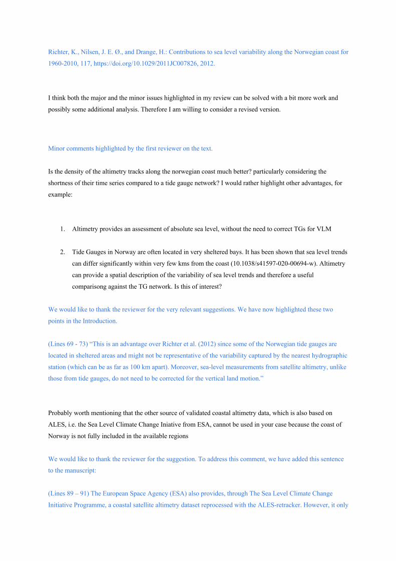
Richter, K., Nilsen, J. E. Ø., and Drange, H.: Contributions to sea level variability along the Norwegian coast for

1960-2010, 117, https://doi.org/10.1029/2011JC007826, 2012.

I think both the major and the minor issues highlighted in my review can be solved with a bit more work and

possibly some additional analysis. Therefore I am willing to consider a revised version.

Minor comments highlighted by the first reviewer on the text.

Is the density of the altimetry tracks along the norwegian coast much better? particularly considering the

shortness of their time series compared to a tide gauge network? I would rather highlight other advantages, for

example:

1. Altimetry provides an assessment of absolute sea level, without the need to correct TGs for VLM

2. Tide Gauges in Norway are often located in very sheltered bays. It has been shown that sea level trends

can differ significantly within very few kms from the coast (10.1038/s41597-020-00694-w). Altimetry

can provide a spatial description of the variability of sea level trends and therefore a useful

comparisong against the TG network. Is this of interest?

We would like to thank the reviewer for the very relevant suggestions. We have now highlighted these two

points in the Introduction.

(Lines 69 - 73) “This is an advantage over Richter et al. (2012) since some of the Norwegian tide gauges are

located in sheltered areas and might not be representative of the variability captured by the nearest hydrographic

station (which can be as far as 100 km apart). Moreover, sea-level measurements from satellite altimetry, unlike

those from tide gauges, do not need to be corrected for the vertical land motion.”

Probably worth mentioning that the other source of validated coastal altimetry data, which is also based on

ALES, i.e. the Sea Level Climate Change Iniative from ESA, cannot be used in your case because the coast of

Norway is not fully included in the available regions

We would like to thank the reviewer for the suggestion. To address this comment, we have added this sentence

to the manuscript:

(Lines 89 – 91) The European Space Agency (ESA) also provides, through The Sea Level Climate Change

Initiative Programme, a coastal satellite altimetry dataset reprocessed with the ALES-retracker. However, it only

covers the northern latitudes up to 60°N and, therefore, only part of the region of interest in this study

(Benveniste et al., 2020).

I am puzzled by this procedure. To my knowledge, the EOT11 tidal correction is provided as a field in

OpenADB, but not as separate tidal contribution. So how did you run the model to separate the contributions?

In any case, the simple fact that you produce monthly values of your tide gauges is enough to filter out the tidal

contribution, so I don't understand why this step is necessary.

We use the EOT11 tidal model to remove the low-frequency tides (such as the annual and the nodal tides)

because they would otherwise be present in the (monthly averaged) tide-gauge records. Indeed, due to their low-

frequency, their contribution is not averaged out when we average the signals at each tide gauge location.

I don't understand, are we talking about Tide Gauges or Hydrographic Stations?

In the text, we referred to the hydrographic stations. To avoid confusion, we deleted the phrase “As for the tide

gauges” at the beginning of Line 178.

I am not an expert of the variability of surface atmospheric temperature, but I would appreciate a comment in

the manuscript about the possible impact of comparing a dataset with such a coarse spatial resolution against

pointwise coastal measurements at the hydrographic stations

We removed the part where we compare the trend of the thermosteric sea-level with the atmospheric

temperature at 2 m. Indeed, the comparison between the two is made difficult by the large-uncertainty

associated with the thermosteric sea-level trend.

This section is insufficient. The following points need to be discussed:

1. First of all I would not call it "sea level decomposition". This is easily misunderstood with a

decomposition of the effects affecting sea level. You are simply fitting a trend and an annual sinusoid

to the time series. This is therefore a harmonic analysis

We would like to thank the reviewer for the suggestion. We have renamed the sub-section “Harmonic

analysis of sea-level” (Line 191).

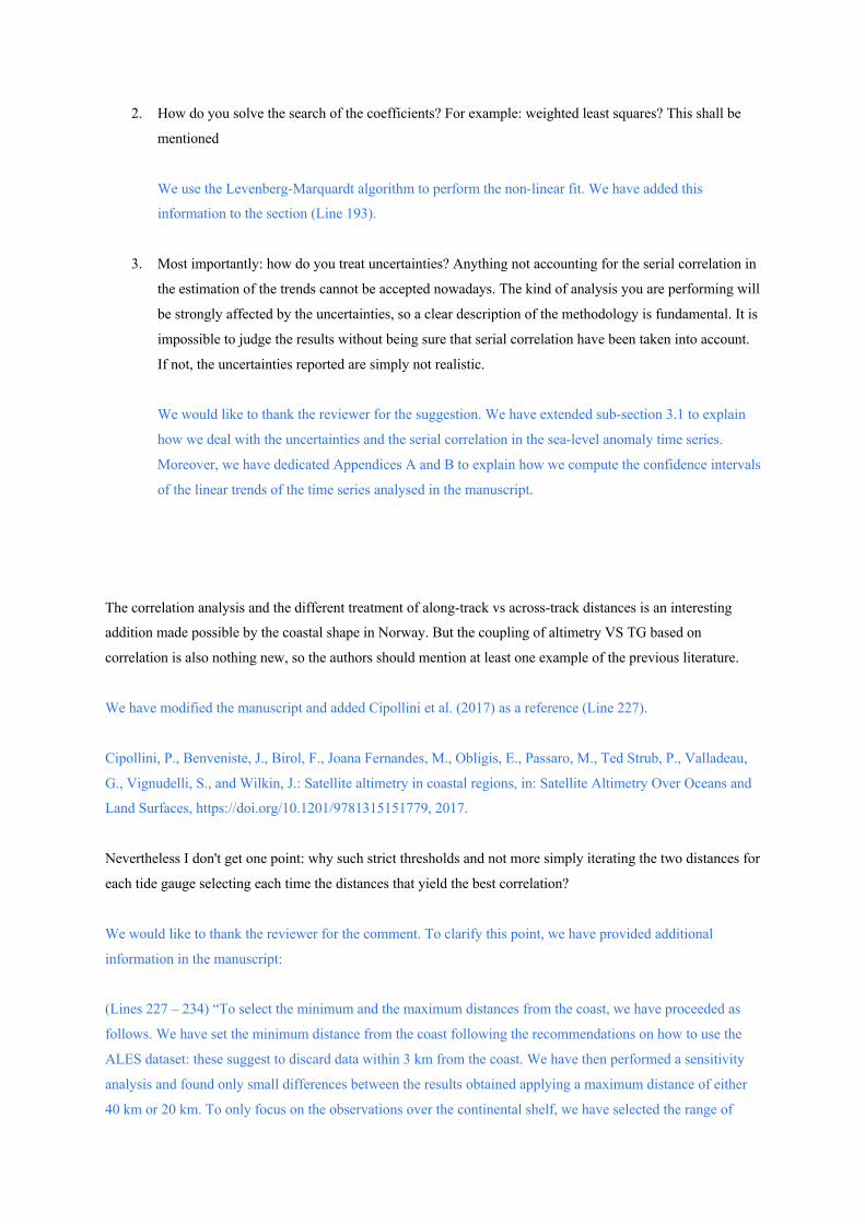
2. How do you solve the search of the coefficients? For example: weighted least squares? This shall be

mentioned

We use the Levenberg-Marquardt algorithm to perform the non-linear fit. We have added this

information to the section (Line 193).

3. Most importantly: how do you treat uncertainties? Anything not accounting for the serial correlation in

the estimation of the trends cannot be accepted nowadays. The kind of analysis you are performing will

be strongly affected by the uncertainties, so a clear description of the methodology is fundamental. It is

impossible to judge the results without being sure that serial correlation have been taken into account.

If not, the uncertainties reported are simply not realistic.

We would like to thank the reviewer for the suggestion. We have extended sub-section 3.1 to explain

how we deal with the uncertainties and the serial correlation in the sea-level anomaly time series.

Moreover, we have dedicated Appendices A and B to explain how we compute the confidence intervals

of the linear trends of the time series analysed in the manuscript.

The correlation analysis and the different treatment of along-track vs across-track distances is an interesting

addition made possible by the coastal shape in Norway. But the coupling of altimetry VS TG based on

correlation is also nothing new, so the authors should mention at least one example of the previous literature.

We have modified the manuscript and added Cipollini et al. (2017) as a reference (Line 227).

Cipollini, P., Benveniste, J., Birol, F., Joana Fernandes, M., Obligis, E., Passaro, M., Ted Strub, P., Valladeau,

G., Vignudelli, S., and Wilkin, J.: Satellite altimetry in coastal regions, in: Satellite Altimetry Over Oceans and

Land Surfaces, https://doi.org/10.1201/9781315151779, 2017.

Nevertheless I don't get one point: why such strict thresholds and not more simply iterating the two distances for

each tide gauge selecting each time the distances that yield the best correlation?

We would like to thank the reviewer for the comment. To clarify this point, we have provided additional

information in the manuscript:

(Lines 227 – 234) “To select the minimum and the maximum distances from the coast, we have proceeded as

follows. We have set the minimum distance from the coast following the recommendations on how to use the

ALES dataset: these suggest to discard data within 3 km from the coast. We have then performed a sensitivity

analysis and found only small differences between the results obtained applying a maximum distance of either

40 km or 20 km. To only focus on the observations over the continental shelf, we have selected the range of

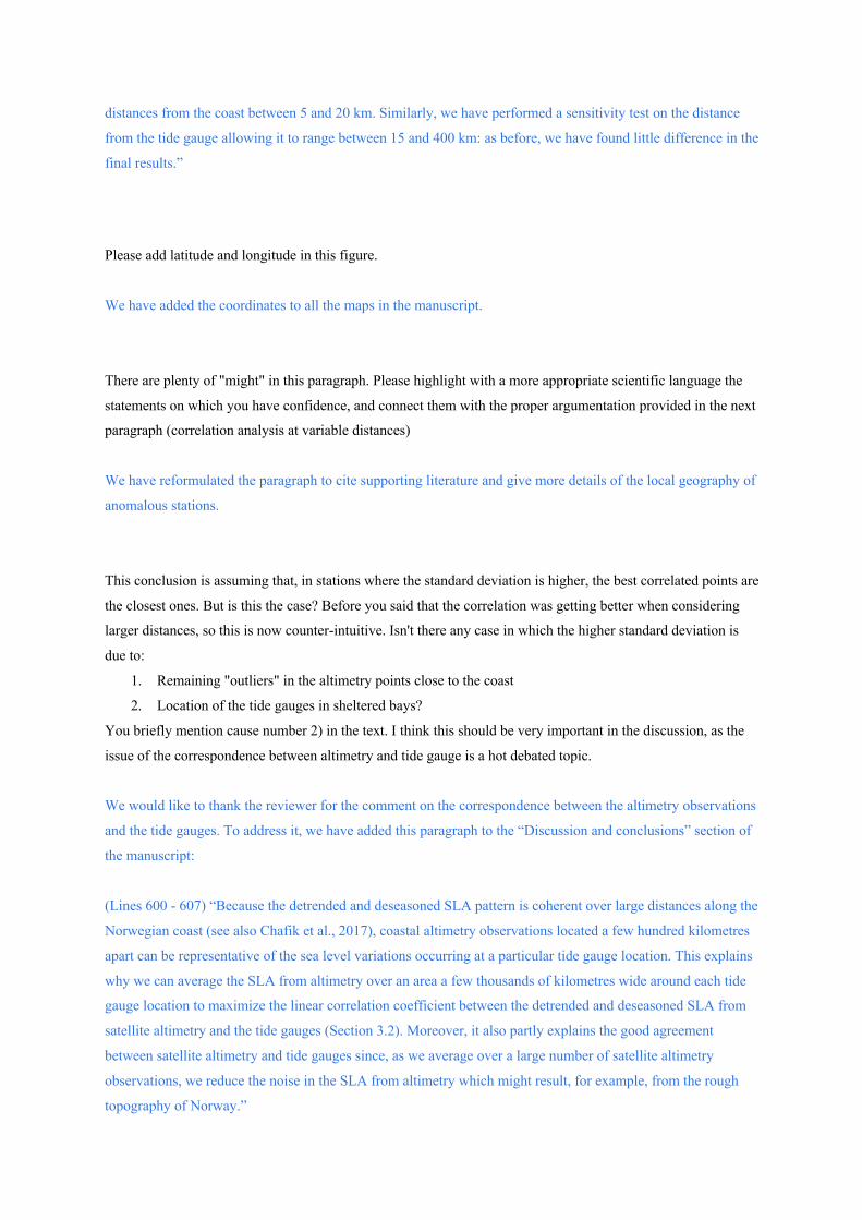
distances from the coast between 5 and 20 km. Similarly, we have performed a sensitivity test on the distance

from the tide gauge allowing it to range between 15 and 400 km: as before, we have found little difference in the

final results.”

Please add latitude and longitude in this figure.

We have added the coordinates to all the maps in the manuscript.

There are plenty of "might" in this paragraph. Please highlight with a more appropriate scientific language the

statements on which you have confidence, and connect them with the proper argumentation provided in the next

paragraph (correlation analysis at variable distances)

We have reformulated the paragraph to cite supporting literature and give more details of the local geography of

anomalous stations.

This conclusion is assuming that, in stations where the standard deviation is higher, the best correlated points are

the closest ones. But is this the case? Before you said that the correlation was getting better when considering

larger distances, so this is now counter-intuitive. Isn't there any case in which the higher standard deviation is

due to:

1. Remaining "outliers" in the altimetry points close to the coast

2. Location of the tide gauges in sheltered bays?

You briefly mention cause number 2) in the text. I think this should be very important in the discussion, as the

issue of the correspondence between altimetry and tide gauge is a hot debated topic.

We would like to thank the reviewer for the comment on the correspondence between the altimetry observations

and the tide gauges. To address it, we have added this paragraph to the “Discussion and conclusions” section of

the manuscript:

(Lines 600 - 607) “Because the detrended and deseasoned SLA pattern is coherent over large distances along the

Norwegian coast (see also Chafik et al., 2017), coastal altimetry observations located a few hundred kilometres

apart can be representative of the sea level variations occurring at a particular tide gauge location. This explains

why we can average the SLA from altimetry over an area a few thousands of kilometres wide around each tide

gauge location to maximize the linear correlation coefficient between the detrended and deseasoned SLA from

satellite altimetry and the tide gauges (Section 3.2). Moreover, it also partly explains the good agreement

between satellite altimetry and tide gauges since, as we average over a large number of satellite altimetry

observations, we reduce the noise in the SLA from altimetry which might result, for example, from the rough

topography of Norway.”

Such a consistent result is worth a couple of lines of discussion. Is one of the dataset over/underestimating the

annual cycle, or is this a reasonable result given that coastal seasonality is known to be higher than open ocean

one? And is there a correspondence between tide gauges located in enclosed bays and points in which the

difference reverses? And is this statistical significant at all, given the uncertainties (this comes back to my major

comment on the absence of description about uncertainties in the methodology)

We would like to thank the reviewer for the comment. To tackle it, we have added a paragraph to the Discussion

and Conclusions section of the manuscript:

(Lines 571 - 577) The ALES-retracked satellite altimetry dataset is found to underestimate the amplitude of the

annual cycle along large portions of the Norwegian coast (Fig. 6). Even though the difference between the two

sets of estimates is not significant at a 95% significance level (the 95% confidence interval is approximately

twice the standard error), we find this result interesting because of its consistency. We do not expect such a

consistency to depend on the ALES retracker since we find a comparable result when we use the along-track

(L3) conventional altimetry product (Fig. C3). We rather suspect a dependence of the amplitude of the annual

cycle on the bathymetry and, therefore, on the distance from the coast, as shown by Passaro et al. (2015) along

the Norwegian sector of the Skagerrak.

Passaro, M., Cipollini, P., and Benveniste, J.: Annual sea level variability of the coastal ocean: The Baltic Sea-

North Sea transition zone, 120, https://doi.org/10.1002/2014JC010510, 2015.

How do you explain instead the points in which the altimetry trend estimates within 5 km are much less in

agreement with TGs than the black dots? For example Viker to Helgeroa to Oslo in the south? Is this a problem

of residual outliers in your time series? I would have said so, but this looks more systematic. Moreover all trends

up to Bodo are lower at 5 km than at the black dots, why?

During the revision process, we noticed that we had at first corrected the tide gauge data for the geoid changes

from GIA, even though the altimetry data were not corrected for these two contributions. We reprocessed the

tide gauge data not to account for this contribution to the sea level and found a better agreement with the

altimetry data in Figs. 8 (where we compare the sea-level trends).

Moreover, we found that, with the newly reprocessed tide gauge data, restricting the altimetry observations to 5

km from the coast does not improve the agreement between the sea-level trend from altimetry and tide gauges.

As such, we modified the manuscript and not considered the 5 km case anymore.

This also changes the discussion section: we remove the paragraph where we discuss the possible dependence of

the sea-level trend on the distance from the coast.

Reviewer 2

The authors assess the quality of ALES-retracked altimetry data in terms of reproducing temporal variations of

sea level along the Norwegian coast, specifically the annual cycle and the trend, by comparison with available

tide gauge data. They then use the altimetry data in combination with observations from hydrographic stations

(with no tide gauge data there) to compare steric height variations to the total sea level variations.

Both issues of the paper, the quality assessment of the ALES-retracked altimetry as well as the analysis of sea

level variations along the Norwegian coast are interesting for the reasons stated by the authors. However, both

issues need more in-depth consideration. Also the methodology needs some additional descriptions.

It is not totally clear to me why the semi-annual cycle is fitted (eq. 1). It is never addressed anywhere later in the

paper (or I have misunderstood). Is it included only to prevent, in case of data gaps, that the running annual

mean reveals part of the seasonal signal, or aliasing issues? This has to be explained. If there is a signal with

amplitudes comparable to that of the annual cycle, it would also be interesting to see, as additional part of the

quality assessment, how, for this frequency, ALES-retracked altimetry compares to the tide gauges.

We would like to thank the reviewer for the comment on the semi-annual cycle.

We fitted the semi-annual cycle to account for asymmetry in the shape of the seasonal cycle. Leaving this signal

in would further increase the autocorrelation of the residuals, reduce the number of degrees of freedom and the

confidence intervals of the sea-level trend. However, we do not show the results for the semi-annual cycle (Fig.

R1) because it contributes little to the seasonal cycle of sea-level (Fig. 6). Indeed, the ratio between the

amplitude of the annual and of the semi-annual cycle ranges between 4, at Rørvik, and 21, at Oslo. Still, Figure

R1 indicates that it is preferable to estimate the semi-annual cycle than leave it out.

Fig. R1: Comparison between the amplitude of coastal sea-level semi-annual cycle from in situ measurements and

area-averaged remote-sensing data. At each tide gauge location, amplitude of the semi-annual cycle from the tide

gauges (a) and difference between the amplitude of the semi-annual cycle from the ALES-reprocessed altimetry

dataset and the tide gauges (b). The black, dashed line indicates the 66°N parallel.

The authors state that sea level data from the tide gauges have been corrected for geoid height changes with

respect to GIA. Is this correction applied to the altimetry data as well? If geoid height change from GIA is

considered, then also instantaneous adaptation from changed loading caused by the Greenland ice melt should

be included, which will probably outperform the GIA effect in most regions along the Norwegian coast

(Siegismund et al, 2020).

We would like to thank the reviewer for the comment.

Unlike the satellite altimetry dataset, the tide gauge data was corrected for geoid changes with respect to the

GIA. We have recorrected the tide gauge data not to account for the geoid height change correction, and we

have found a better agreement between the sea-level trends from tide gauges and satellite altimetry. This led to a

modification of Figs. 8 and 9.

Why is, at the end, not the full sea level variation budget considered, but only the steric effect? The abstract

states performance of the sea level budget. Consideration of the full budget would give the whole study more

weight. If this is not intended the authors should explain the reasons to the reader.

We apologize for the misleading title of the section as our intention was to focus on the steric contribution. We

have now changed the title and made it clearer that we only focus on the temperature and salinity contribution to

sea level (this issue was also pointed out by Reviewer 1).

In the paper, we only focus on the steric contribution to the sea-level while assessing the synergy between

satellite altimetry and in-situ data along the coast of Norway. The consideration of the full budget would be the

object of a further investigation in the future.

It isn’t clearly stated how the optimal distances from and along the coast for spatial averaging the altimetry data

are found. I guess, a set of distances is defined and the correlations are computed for each element? Please

explain.

We would like to thank the reviewer for the comment. To clarify this point, we have provided additional

information in the manuscript:

(Lines 227 – 234) “To select the minimum and the maximum distances from the coast, we have proceeded as

follows. We have set the minimum distance from the coast following the recommendations on how to use the

ALES dataset: these suggest to discard data within 3 km from the coast. We have then performed a sensitivity

analysis and found only small differences between the results obtained applying a maximum distance of either

40 km or 20 km. To only focus on the observations over the continental shelf, we have selected the range of

distances from the coast between 5 and 20 km. Similarly, we have performed a sensitivity test on the distance

from the tide gauge allowing it to range between 15 and 400 km: as before, we have found little difference in the

final results”.

It would be nice to see a direct comparison of conventional altimetry and ALES-retracked altimetry for the

Norwegian coast to see both, the improvements/changes in the observations dependend on location (and

specifically distance from the coast) as well as the added value caused by the improvements when investigating

spatio-temporal variations of sea level along the Norwegian coast. Direct comparison to Breili et al (2017) is not

feasible due to different methodology and period.

We would like to thank the reviewer for the comment. We have repeated the analysis using along-track (L3)

conventional satellite altimetry dataset (SEALEVEL_GLO_PHY_L3_REP_OBSERVATIONS_008_062

downloaded from the Copernicus marine website) and added the corresponding new figures in Appendix C. We

have also compared the results from ALES and from the conventional altimetry dataset in the Discussion and

Conclusions section of the manuscript.

(Lines 555 – 560) “Regarding the comparison between the ALES-retracked and the along-track (L3)

conventional altimetry datasets, we find that the former shows, on average, a 10% improvement, despite it being

well within the margins of error. This improvement is most evident at Bodø, Kabelvåg and Tromsø, in northern

Norway, where the agreement with the tide gauges improved by 19%, 23% and 24% respectively. The use of the

ALES retracker to more satellite altimetry missions, in order to have more observations and to cover the period

before July 2002, might help to reduce the uncertainties and return a more statistically significant result.”

(Lines 701 – 704) “We do not expect such a consistency to depend on the ALES retracker since we find a

comparable result when we use the along-track (L3) conventional altimetry product (Fig. C3). We rather suspect

a dependence of the amplitude of the annual cycle on the bathymetry and, therefore, on the distance from the

coast, as shown by Passaro et al. (2015) along the Norwegian sector of the Skagerrak.”

From the optimization of the distances for the spatial averaging of the altimetry data it seems that inclusion of

data more offshore than 20 km, which has been the a-priori fixed maximum distance, could even improve the

correlation with the tide gauge data. Has this been tested?

We would like to thank you for the suggestion. We repeated the procedure to colocate the satellite altimetry at

each tide gauge location, this time allowing the distance from the coast to range between 5 and 40 km (instead

of a maximum of 20 km, as in the manuscript).

At 14 out 22 tide gauges, the result does not change: the optimized distance from the coast and from the tide

gauge remains the same. The changes occur at three tide gauges in the south and west (Tredge, Bergen and

Ålesund) and at five tide gauges in north of Norway (between Andenes and Vardø), where the optimized

distance from the coast increases and ranges between 22.5 and 40 km.

Even though the optimized distance from the coast increases, the results in Figures 4, 6, 7 and 8 in the

manuscript change little and do not modify the message of the manuscript. Indeed, the linear correlation

coefficients increase by less than 2.5 %. The RMSD shows a larger, but still contained, improvement, with the

greatest variation occurring at Tromsø, where the RMSD decreases from 2.0 to 1.7 cm (approximately 15 %).

The amplitudes and phases of the annual cycle change by less than 9.5 % and less than 5 days respectively, and

the linear trends by less than 7.5 %.

To address the comment, we have modified the Methods section of the manuscript where we have specified the

sensitivity analysis performed:

(Lines 230 - 234) “We have then performed a sensitivity analysis and found only small differences between the

results obtained applying a maximum distance of either 40 km or 20 km. To only focus on the observations over

the continental shelf, we have selected the range of distances from the coast between 5 and 20 km. Similarly, we

have performed a sensitivity test on the distance from the tide gauge allowing it to range between 15 and 400

km: as before, we have found little difference in the final results.”

That could mean, that conventional altimetry data could be of comparable quality because either the errors of

the ALES-retracked altimetry data is still too high near the coast, or temporal variations are coherent for a wide

stripe along the Norwegian coast and data away from the coast can do the job as well. So what is really the

benefit from using the ALES-retracked data?

We would like to thank the reviewer for the comment which led to an extension of the manuscript. We extended

our analysis to conventional altimetry: the performance is comparable in terms of the amplitude and phase of the

annual cycle, while we find a 10% improvement in the sea level trend from ALES with respect to the one

provided by conventional altimetry.

The text in the manuscript has changed.

(Lines 555 – 560) “Regarding the comparison between the ALES-retracked and the along-track (L3)

conventional altimetry datasets, we find that the former shows, on average, a 10% improvement, despite it being

well within the margins of error. This improvement is most evident at Bodø, Kabelvåg and Tromsø, in northern

Norway, where the agreement with the tide gauges improved by 19%, 23% and 24% respectively. The use of the

ALES retracker to more satellite altimetry missions, in order to have more observations and to cover the period

before July 2002, might help to reduce the uncertainties and return a more statistically significant result.”

Minor issue:

In Figure 1 please mention, that the yellow diamonds are the hydrographic stations, and the red dots are the tide

gauges.

We would like to thank you for the suggestion. We have modified Figure 1 and its caption accordingly.

Modification of Figures 4 and 5

The RMSD between the detrended and deseasoned SLA from satellite altimetry and each tide gauge is:

𝑅𝑀𝑆𝐷 ='∑ )𝑆𝐿𝐴!"#$%&#'(,$ − 𝑆𝐿𝐴#$*&,!-,&,$-

./$01

𝑁

where N is the length of the time series derived by computing the difference between the detrended and

deseasoned SLA from satellite altimetry and the tide gauge. When we computed the RMSD in the original

manuscript, we did not account for the presence of missing values in the detrended and deseasoned SLA from

satellite altimetry and from the tide gauges. Therefore, we set N equal to 192 (the number of months between

January 2003 and December 2018). In the revised manuscript, we recomputed the RMSDs, this time accounting

for the number of missing values in the time series. While this change only slightly affects Figs. 4B and 5B (but

not the text describing them). Therefore, in the revised manuscript, we present the new version of Figs. 4 and 5.