ON THE DYNAMICS OF A SIRS MODEL

On the Dynamics of a SIRS Model

Mayrelly Valera

Universidad Centroccidental Lisandro Alvarado. Barquisimeto. [email protected]

Sael Romero

Universidad de Oriente - Nucleo de Sucre. Cumana. [email protected]

Teodoro Lara

Departamento de Fısica y Matematicas. Universidad de los Andes. [email protected]

Carlos Marrero

Universidad de Oriente - Nucleo Bolivar. [email protected]

Abstract

In this paper we work in a SIRS model similar to the one given in[5], we study its dynamics under different conditions, local and globalstability, and some type of bifurcation, no periodic orbits shows up.Two examples are also provided in order to illustrate particular casesof the general model, numerical implementation is performed to showbehavior of the particular model in each case.

Mathematics Subject Classification: 37N25, 92D25

Keywords: Epidemiological model, Stability, Bifurcation.

1 Introduction

The word epidemiology means the study of epidemics and epidemic diseases,its main objective consists in research the distribution and causes of populationdiseases. Even when during the first decades of past century most of the effortswere made only to the study epidemic and pandemic diseases nowadays thiswhole picture has changed dramatically since their methods and principles areused to attack other type of diseases and health conditions as well ([4, 7, 8]).

One of the most important mathematical tools used to model real life sit-uations are differential equations, the type of model we address here is known

Mathematica Aeterna, Vol. 4, 2014, no. 4, 297 - 306

as SIRS (Susceptible, Infective, Recovered individuals respectively), this ap-proach assumes the disease remains in the population for large period of timeand part of the recovered populations turns back to be susceptible again, fur-ther it also suppose newborns are also susceptible.

The phenomenon we study here is describe by a set of three differentialequations involving variables, depending on time, S, I, andRmentioned above.

2 Preliminary Notes

The model we consider here is inspired in [5] and given as

S ′ = B (N) + γR− bS −H (I, S) IS

I ′ = H (I, S) IS − (b+ v) I (1)

R′ = vI − (b+ γ)R.

We assume that all newborn individuals are susceptible, and that all coeffi-cients are positive; S represents susceptible individuals, I the infected and R

the recovered ones; H(I, S) is the incidence rate per infective individual, b isthe per capita death rate, γ is the per capita rate of loss of immunity, v isthe per capita recovery rate, and B (N) is a C1 function which represents the(non-negative) birth rate (a function of N = S + I + R). H(I, S) is assumedto be differentiable; further, for all I, H(I, 0) = 0 ∀I and ∂H

∂S> 0. The latter

condition reflects the biologically intuitive requirement that the incidence ratebe an increasing function of the number of susceptible.

By adding up the foregoing equations

S ′ + I ′ +R′ = B(N) − b(S + I +R).

So the behavior of the population is now described by

N ′ = B (N) − bN. (2)

Notice that solution of (2) exists locally and is unique. From now on weassume existence of N0 > 0 such that B(N0)− bN0 = 0 and its asymptoticallystability. In case these hypotheses do not take place we will be in the presenceof extinction or uncontrollable growth of the population. In this paper werestrict our study to the case S + I +R = N0 > 0.

For the sake of simplicity we normalize S, I and R, that is,

S =S

N0, I =

I

N0, R =

R

N0, b =

B(N0)

N0.

So (1) now looks like

S′

= b+ γR− bS −H(N0I,N0S)N0IS

I′

= H(N0I,N0S)N0IS − (b+ v)I

R′

= vI − (b+ γ)R,

298 Mayrelly Valera, Sael Romero, Teodoro Lara and Carlos Marrero

with S+ I+R = 1, and by setting H∗(I, S) = H(N0I,N0S)N0, above systembecomes

S′

= b+ γR − bS −H∗(I, S)IS

I′

= H∗(I, S)IS − (b+ v)I (3)

R′

= vI − (b+ γ)R,

omitting bars and keeping in mind we are studding (3) on S + I +R = 1 now,it is enough to consider the first two equations that look like

S ′ = (b+ γ) − (b+ γ)S − γI −H∗(I, S)IS (4)

I ′ = H∗(I, S)IS − (b+ v)I.

3 Main Results

Here we state and prove the main result of this research, numerical implemen-tation is also included.

Theorem 3.1 Let Ω = (I, S) : I ≥ 0, S ≥ 0, I+S ≤ 1, then Ω is positiveinvariant for the system (4).

Proof. Because I ′ +S ′ = b+γ− (b+γ)(I +S)−vI ≤ b+γ− (b+γ)(I +S),then (I + S)′ ≤ (b+ γ)(1 − (I + S)).

Since H(I, 0) > 0 and ∂H∂S

> 0 on Ω which is compact, so there exists h > 0such that |H(I, S)| ≤ h on Ω.

Remark 3.2 System (4) can be written as

(

I ′

S ′

)

= f

(

I

S

)

, with

f

(

I

S

)

=

f1

(

I

S

)

f2

(

I

S

)

hence it is readily to check existence of P > 0

such that ||f || ≤ P . But then we may assure existence of global solutions of(4).

In order to reduce number of parameters involved in (4) we perform thefollowing transformations

T = (b+ v)t, S(T ) = S((b+ v)t), I(T ) = I((b+ v)t), R(T ) = R((b+ v)t),

σ =1

b+ v, α =

γ + b

b+ v, β =

γ

b+ v.

On the Dynamics of a SIRS Model 299

So (4) becomes

S ′ = α− αS − βI − σH∗(I, S)IS (5)

I ′ = σH∗(I, S)IS − I.

Where the derivatives are taken with respect to the new time T , we examinethe case in which incidence rate H∗(I, S) = kIp−1Sq−1 with p ≥ 1, q > 1,k > 0 ([5]), and rewrite (5) as

I ′ = σkIpSq − I (6)

S ′ = α− αS − βI − σkIpSq.

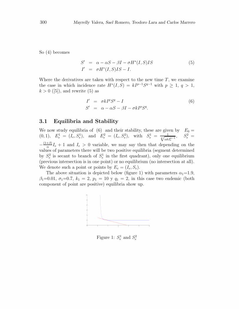
3.1 Equilibria and Stability

We now study equilibria of (6) and their stability, these are given by E0 =(0, 1), E1

e = (Ie, S1e ), and E2

e = (Ie, S2e ), with S1

e = 1q√

αkIp−1

e

, S2e =

− (1+β)α

Ie + 1 and Ie > 0 variable, we may say then that depending on thevalues of parameters there will be two positive equilibria (segment determinedby S2

e is secant to branch of S1e in the first quadrant), only one equilibrium

(previous intersection is in one point) or no equilibrium (no intersection at all).We denote such a point or points by Ee = (Ie, Se).

The above situation is depicted below (figure 1) with parameters α1=1.9,β1=0.01, σ1=0.7, k1 = 2, p1 = 10 y q1 = 2, in this case two endemic (bothcomponent of point are positive) equilibria show up.

−2 0 2 4 6 8 10−2

0

2

4

6

8

10

I

Figure 1: S1e and S2

e


The segment represents graphic of S2e and the hyperbola S1

e , if we increasep and keep fixed the rest of parameters the curve given by S1

e shows a similarbehavior to the one in the figure concerning the number of equilibria. Inconclusion, the possibilities for the equilibria are

1. Non endemic equilibria (E0 and no intersection of curves).

2. A non endemic equilibrium and one endemic (E0 and curves are tangent).

3. A non endemic equilibrium and two endemic (E0 and curves are secant).

Lemma 3.3 a) E0 is locally asymptotically stable.

b) Ee is locally asymptotically stable if

p < min

1 +(β + 1)

αqIe

Se

, 1 + α+ qIe

Se

.

Proof. Notice that Jacobian associated to (6) at (S, I) is given by

J(I, S) =

(

σkpIp−1Sq − 1 σkqIpSq−1

−β − σkpIp−1Sq −α− σkqIpSq−1

)

(7)

Therefore we get the first part by a direct application of Routh-Hurwitzcriterium and the last is just by checking that under the given hypothesis

det (J (Ee)) > 0, tr (J (Ee)) < 0.

Theorem 3.4 System (6) has no periodic orbits on Ω.

Proof. Let g(I, S) = 1I, I 6= 0, then

∂gf1

∂I+∂gf2

∂S= −α − σkqIpSq−1 < 0,

so by Dulac’s Criterium ([3, 6]) there are no periodic orbits.So far we have considered only p > 1, the case p = 1 it is worth to be

treated separately, in this case (6) becomes

I ′ = σkISq − IS ′ = α− αS − βI − σkISq (8)

and Jacobian

J (I, S) =

σkSq − 1 σkqISq−1

−β − σkSq −α − αkqISq−1

. (9)


Lemma 3.5 a) For σk ∈ (0, 1), E0 becomes locally asymptotically stable.

b) At σk = 1, E0 goes under a saddle node bifurcation.

c) For σk > 1, E0 is a saddle.

Proof. If λ1, λ2 are eigenvalues of J(E0) then

a) λ1 < 0 and λ2 < 0.

b) λ1 = 0 and λ2 = −α < 0.

c) λ1 · λ2 < 0.

Lemma 3.6 If σk > 1 then Ee is locally asymptotically stable in Ω interior.

Theorem 3.7 a) If σk ∈ (0, 1) then E0 is globally asymptotically stablein Ω interior.

b) If σk > 1 then E0 is a saddle, its stable manifold coincides with S axisand (Ee) is globally asymptotically stable in Ω interior.

Proof.

a) Under the given hypothesis I ′ < Sq − 1 < 0 therefore I ′(t, I0) < 0, t > 0so

limt→+∞

ψ(t, ρ) = (0, 1),

where ψ(t, ρ) is any solution of (8) such that ψ(0, ρ) = ρ ∈ R2.

b) It is clear E0 is a saddle; an eigenvector corresponding to eigenvalue λ2

(given in previous lemma) is v = (0, 1)T where T means transposed,of course the associated eigenspace is the set (0, a)T, a ∈ R whichcoincides with S axis. The rest of the proof follows from Dulac’s criterium(with g(I, S) = 1

I) and Poincare-Bendixson theorem.

3.2 Examples

Finally we deal with two examples, one for [2] and the other one from [1]. Thefirs one is given as

S ′ = −rSI − dS

I ′ = rSI − aI (10)

R′ = aI + dS.


Because the first two equations are independent of the third one, so is enoughto work with these two, that is

S ′ = −rSI − dS (11)

I ′ = rSI − aI.

Our first result goes as

Theorem 3.8 R2+ = (S, I) ∈ R2 : S > 0, I > 0 is positively invariant for

(11) .

Equilibria of (11) are E0 = (0, 0) and E1 = (ar,−d

r), but we disregard E1

since it does no have sense from biological point of view. Its jacobian at E0

is J(E0) =

(

−d 00 −a

)

, which means E0 es locally asymptotically stable.

Orbits of (11) are depicted below (Figure 2).

d = 0.6a = 0.8

r = 0.4

0 5 10 15 20 25 30 35 40 45 50

0

5

10

15

20

25

30

35

40

S

I

Figure 2: Susceptible vs Infected, r=0.4, d=0.6, a=0.8.

Proposition 3.9 System (11) has no periodic orbits in R2+.

Proof. Just take g(I, S) = 1I

and proceed as in pervious cases.By using Poincare-Bendixson ([3, 6]) and foregoing proposition we assure

global stability of E0.

Theorem 3.10 Variable I reaches a maximum when S = ar.

Proof. If we plug S into second equation of (11) then I ′ = 0 at S = ar

andI ′′ < 0 at this value for S.

If we denote by Imax the maximum of I and integrate the second equationof (11) with initial data S = S0 arbitrary but fixed, we get I ≡ I(t, S0, a) =KerS0te−at, t > 0, which is increasing as a function of S0 and a decreasing oneas a function of a.


In the SIR models considered so far immunity after recovery is permanent,this is no always the case because it may decrease when time goes by, sometimesvirus mutation triggers the epidemic again and in this situation immunity isnot so strong. Temporal immunity can be describe by a SIRS model in whichtransference rate from R to S is added to the model. The second modelincorporates temporal immunity and is given in [1] but it has not been studyin details. The model is given by

S ′ = −βSI + θR

I ′ = βSI − αI (12)

R′ = αI − θR,

where θ represents rate of loss of immunity and N , constant, is the whole sizeof the population; in this case (12) becomes

S ′ = −βSI + θN − θS − θI (13)

I ′ = βSI − αI,

and as previous done, we see Ω = (S, I) : S ≥ 0, I ≥ 0, S + I ≤ N ispositively invariant for (13), the corresponding equilibria are P1 = (N, 0) and

P2 =(

αβ, θ

α+θ

(

N − αβ

))

. We point out that Nβ − α < 0 implies P2 is out

of first quadrant. The Jacobian at P1 is J(P1) =

(

−θ −(βN + θ)0 βN − α

)

, with

eigenvalues λ1 = −θ < 0 y λ2 = βN − α. Notice that P1 is a saddle ifN > α

β, locally asymptotically stable if N < α

βand there exists a saddle node

bifurcation at N = αβ.

In the same fashion

J(P2) =

(

−(

θα+θ

(Nβ + θ))

−(α + θ)θ

α+θ(Nβ − α) 0

)

, det J(P2) = θ(Nβ − α)

and trJ(P2) = − θα+θ

(Nβ + θ) < 0. Therefore if N > αβ

then P2 is locallyasymptotically stable and there exists a saddle node bifurcation at N = α

β.

Remark 3.11 Notice that either α > Nβ or α < Nβ point P2 movestoward P1 as α → Nβ.

The incoming picture shows a bunch of orbit of (13) (Figure 3).


0 10 20 30 40 50 60

0

5

10

15

20

25

30

35

40

S

I

Figure 3: Susceptible vs Infected, N = 1, β=0.8, θ=0.6, α=0.8.

Proposition 3.12 System (13) has no periodic orbits in R2+.

Proof. Directly form Dulac’s Criterium with g(S, I) = 1SI

.Now we conclude global asymptotically stability of P1 (P2) under the con-

dition N < αβ

(N > αβ

respectively). The following picture depicts the case of

a saddle-node bifurcation of (13) (Figure 4).

Figure 4: Saddle node bifurcation at α = 0.8 = β.

References

[1] F. Brauer and C. Castillo, Mathematical Models in Population Biologyand Epidemiology, Springer, September 2011, Second edition, .

[2] J. M. Cushing, Differential Equations and Applied Approach, Pearson-Prentice Hall,2004, New Jersey.

[3] J. Hale and H. Kocak, Dynamics and Bifurcations, Springer-Verlag, 1991,New York.


[4] M. E. Halloran, Concepts of trasmision and dynamics, Oxford UniversityPress,2001, 56-85.

[5] M. Lizana and J. Rivero, Multiparametric bifurcations for a model inepidemiology, J. Math. Biol., 1996, 21-36.

[6] L. Perko, Differential Equations and Dynamical Systems, Springer,2001,Third edition, New York.

[7] J. Vasque, Epidemiologıa General de las Enfermedades InfecciosasTrasmisibles, Publisher, 2001, 10 edition, Barcelona.

[8] J. Vasque and A. Dominguez, Vigilancia Epidemiologica. Investigacionde Brotes Epidemicos, Piedrola Gil. Medicina Preventiva y SaludPublica,2001, 10 edition, Barcelona.


Received: March, 2014

ON THE DYNAMICS OF A SIRS MODEL

Documents

Transcript of ON THE DYNAMICS OF A SIRS MODEL