An efficient model for studying the dynamics of frustrated systems

Computer Physics Communications 183 (2012) 2089–2097

Contents lists available at SciVerse ScienceDirect

Computer Physics Communications

journal homepage: www.elsevier.com/locate/cpc

An efficient model for studying the dynamics of frustrated systemsAlejandro LeónFacultad de Ingeniería, Universidad Diego Portales, Santiago, Chile

a r t i c l e i n f o

Article history:Received 3 February 2012Received in revised form9 May 2012Accepted 9 May 2012Available online 19 May 2012

Keywords:Magnetic monopolesFrustrated systemsCellular automataSpin ice

a b s t r a c t

We present a model based on determinist cellular automata architecture for studying systems withfrustrated interactions that present elemental excitations, such as magnetic monopoles. This model isespecially designed to be applied for systems with components that have energy levels much higher thankT . This would imply that for these systems thermal fluctuations are negligible and they can be analyzedunder the supposition that the dynamic is produced at zero temperature. This category includes artificialmagnetic spin ice systems and donor and recipient electrical charge molecular systems. The dynamicsof these systems can be simulated in real time with this model, with a minimum of computationalrequirements. It can be an excellent complement to Monte Carlo methods and in some cases can evenreplace them directly. In this report, we show the designed structure and some interesting resultsobtained in studying the dynamics of emergent magnetic monopoles in artificial spin ice systems andexcitations in graphane molecular arrays.

© 2012 Elsevier B.V. All rights reserved.

Introduction

Artificial spin ice systems

Frustrated physical systems have interactions that cannot besimultaneously minimized. A consequence of this frustration isthat these systems present residual entropy at zero temperature.Water ice is one of the most often cited examples of thistype of system [1]. Natural spin ice systems in rare earthshave recently received much attention from researchers becauseelemental excitations equivalent to magnetic monopoles havebeen detected at sub-kelvin temperatures [2–4]. Artificial spinice systems are arrays of nanomagnets with anisotropy energyon the order of 104 K [5]. This allows their study at ambienttemperature and the simulation of the behavior of natural spin icesystems [6,7]. A recent report of Mengotti [8] reported the firstdirect observation of emergent magnetic monopoles in artificialspin ice systems. All these experimental results have providedconsiderable information about these frustrated systems, but at thesame time have raised many unanswered questions about somesituations on which experiments have not shed any light. Becauseof this, it is necessary to have robust models for simulating thecomplex dynamics of these elemental excitations.

Frustrated molecular systems

In many problems at the molecular level, electrical inter-action cannot be minimized completely owing to frustration.In particular, there is a proposal to propagate and process digital

E-mail address: [email protected].

0010-4655/$ – see front matter© 2012 Elsevier B.V. All rights reserved.doi:10.1016/j.cpc.2012.05.011

information using the polarization of a molecular array [9,10]. Inthe logic gates defined for this technological proposal, the phe-nomenon of frustration is presented in the minimization of elec-trostatic energy. To correctly assess the performance of these andsimilar systems, simplemodels are needed to simulate the dynam-ics of electrical charges in these systems.

Cellular automata (CA)

Cellular automata are models used to simulate the dynamicsof complex systems. The main idea is to define an array ofentities (cells of the automaton) that have a discrete set ofstates. The change of state of a particular cell is defined withupdating rules for the automaton and depends on the state ofthe cells being considered and the state of neighboring cells.A variety of models based on CA have been used to efficientlystudy problems in biology, physics, chemistry, engineering andmaterials sciences [11,12]. They represent an excellent alternativeto models based on differential equations and to Monte Carloalgorithms because they can simulate highly complex systemswith a low computational cost. The first attempt to use CA inthe study of magnetism was that with the model proposed byVichniac [13], which was subsequently developed by Pomeau [14]and Hermann [15] and is termed the VPH model. This is beingused to resolve an Ising type spin system. To avoid a ‘‘feedbackcatastrophe’’, the automaton is updated in more than one step.The model functions well at high temperatures (T > TC ), butfails at low temperatures. Subsequently, Ottavi et al. [16] used amicrocanonical algorithm in a CA to resolve the Ising spin system.A determinist version of thismodel provided acceptable results at alow temperature [16]. Amore recentmodel studies the Isingmodel

http://dx.doi.org/10.1016/j.cpc.2012.05.011

http://www.elsevier.com/locate/cpc

http://www.elsevier.com/locate/cpc

mailto:[email protected]

http://dx.doi.org/10.1016/j.cpc.2012.05.011

2090 A. León / Computer Physics Communications 183 (2012) 2089–2097

using a quantum algorithm in a cellular automaton [17]. The 2Dsimulation shows a good agreement with the analytical solution.Our work shows the design of a model based on the architectureof a cellular automaton for the study of frustrated magnetic andelectrical systems.

Frustrated cellular automata (FCA)

Our model consists of a cellular automaton composed of cellsthat are connected at n first neighbors. The number nwill be calledthe coordination number. Fig. 1 shows three examples where wecan apply the FCA model. Fig. 1(a) shows a squared network withn = 4. The cells of the automaton are represented by red andyellow circles. We can see in the figure that each cell is connectedat four first neighbors, such that each red cell is connected at fouryellow cells and each yellow cell is connected at four red cells.For this squared geometry, we have four connections (north, west,south and east). The ‘‘eastern’’ connection of the yellow cell isthe ‘‘western’’ connection of the red cell. With this color code, wecan define four connections that surround each cell. Horizontally,we have the ‘‘yellow–red’’ connections and the ‘‘red–yellow’’connections’’. Analogous to this, vertically, we have the same‘‘red–yellow’’ and ‘‘yellow–red’’ connections. By way of examples,Fig. 1(a) shows the horizontal ‘‘yellow–red’’ connections. Fig. 1(b)shows a hexagonal network as red and yellow circles with n = 3.Each red cell is connected to three yellow cells and vice versa, andFig. 1(b) shows the horizontal connections. A one-dimensional FCAis represented by the horizontal lines in Fig. 1(c) with n = 2 (in thiscase there are two kinds of connections). The updating functionu (t) is defined in n steps, updating the n nodes for each cell, asindicated in expression (1):

u1 (t) → u2 (t) 99K un (t) ⇒ u(t). (1)

In this expression, u1 represents the updating of connector 1, u2represents the updating of connector 2, etc. Once the updating ofthe connections is completed, the entire FCA has been updated.

Because the structure of the FCA model is completely general,the form of the function of partial uk updating depends onthe physical nature of the phenomenon that is being modeled.However, the FCA automaton was designed to study systemscomposed of magnetic nanoislands and polar molecular systemswith anisotropy energy much greater than kT . This implies thatthe thermal fluctuations are negligible and they can be consideredas systems with temperatures equivalent to 0 K. For magneticsystems, the connections correspond to magnetic nanoislands. Formolecular systems, the connections correspond to the directionof the electrical dipolar moment. In both cases, the partial ukupdating corresponds to reversing the magnetic or electricalmoment. A very important objective for the study of these systemsis to learn about the elemental excitations that are generated bythe collaboration of many of these entities (emergent magneticmonopoles, for example). Given this, the energy of the systemwasassessed in the framework of magnetic or electrical charges.

General conditions to be met by systems that are simulated with theFCA:

• The system must have a regular array of elementary entities(magnets or molecules).

• The energy barrier for reversal (or tunneling energy for themolecular case) must be much greater than the energy at roomtemperature.

The FCA algorithm

Having defined the structure of the FCA, we will now explainthe global functioning of the proposed architecture.

Step 1: A connection is chosen randomly, among the available n.Step 2: The automaton is reviewed in each cell and the chosen

connection at point 1 is updated (reversing the magnetic momentor electric moment).

If 1E ≤ −EAnisotropy, the change is accepted (magnetic case). If1E ≤ ETunneling, the change is accepted (molecular case).

Step 3: A connection is randomly chosen from among the n− 1and step 2 is repeated.

Step 4: Once the connections are completed, the globalupdating of the FCA is completed. At this stage, the physicalobservables of the system (polarization, density of the charges,Dirac string, etc.) are assessed.

Step 1 is repeated.The description of the FCA algorithm has been proposed in

general terms, but we can incorporate variants in step 1. Instead ofmaking the choice randomly, we can define a particular sequencefor making the partial uk updating, and maintain this sequence forall the steps of the algorithm. For example, for the square latticewework with the sequence u1 → u2 → u3 → u4. Another possiblevariation in step 1 of the FCA algorithm is to choose combinationsof connections in the network. For example, in the hexagonalnetwork we can choose the sequence [(u1 ∨ u2) → u3] (t) →

[(u1 ∨ u2) → u3] (t + 1). This sequence means choosing betweenconnectors 1 and 2, updating the chosen connector and thenupdating connector 3. In the following global step of the algorithmwe return to choosing between connectors 1 and 2, and the chosenconnector is updated and then connector 3 is updated. Thesevariants are not strictly necessary in the algorithm and are onlyused to efficiently study some observable in particular, as will beexplained further on in the applications.

Applications of the FCA

Emergent magnetic monopoles in the hexagonal network

To illustrate the behavior of themodel,we begin by studying thehexagonal network. The parameters used in this study correspondto those of the experimental work of Mengotti et al. [6]. Westudy the density of emergent monopoles in a global sequence ofmagnetic reversal.

The system studied in this work is a magnetic nanoisland arrayin a hexagonal lattice. Fig. 2(a) shows a scheme of the magneticbars arranged on the sides of a hexagon and Fig. 2(b) showsthe frustration in the hexagonal network. Three nanomagnetsconverge in the vertices of the hexagons, as can be appreciatedin Fig. 2. Topologically, we can define two non-equivalent verticesin the hexagonal lattice, vertices A and B. The two non-equivalentvertices form the unit cell of the entire array. The cell is shownin red in Fig. 2(a). In the magnetic charge model, the charges areconcentrated in these vertices. We define the magnetic charge ata vertex as −1, when two south poles and a north pole, of thethree nanomagnets that form the vertex, converge. Equally, wedefine the magnetic charge as +1, when two north poles and asouth pole converge in the vertex considered. Fig. 3 shows the arraywith an applied magnetic field. The upper left of Fig. 3 shows thearray subjected to a field in the direction of the negative axis x.In the lower left of the figure the field is shown directed to theright. The nanomagnets with the x component of the magneticmoment directed to the left are represented by gray bars, and thenanomagnets with the x component from the magnetic momentdirected to the right are represented by black bars. When thesample is totally magnetized in directions +x or −x, all the typeA vertices have +1 or −1 charges, while all the B vertices have −1or +1 charges. This can be seen in Fig. 3.

We suppose that we are under the condition of total magne-tization, with the magnetic field directed to the left (upper left

A. León / Computer Physics Communications 183 (2012) 2089–2097 2091

Fig. 1. (a) Square network with n = 4. The figure shows one of the four possible interactions that are updated (with the double blue arrow). We can see in the figure thatfor a yellow node the interaction is with a node to its right, while for a red node the interaction is to its left. (b) Hexagonal network with n = 3. The figure shows one ofthe possible interactions that is updated (with a double green arrow). (c) One-dimensional network with n = 3. (For interpretation of the references to colour in this figurelegend, the reader is referred to the web version of this article.)

Fig. 2. (a) Scheme of the nanomagnet array. (b) Frustration in the hexagonal network.

Fig. 3. Scheme of the nanomagnet array when the sample is totally saturated by the influence of an external magnetic field.

of Fig. 3). Under this condition, we define a positive and mobilemonopole, if a nanomagnet converging in a class A vertex invertsits magnetic moment. The charge of vertex A goes from qA =

−1 → q∗

A = +1 =⇒ 1qA = +2. If this is produced in aB type vertex, we define a negative monopole and would have

qB = +1 → q∗

B = −1 =⇒ 1qB = −2, where q∗

A and q∗

B rep-resent the charges of the vertex after the inversion and qA and qBrepresent the charges of the vertices A and B, respectively, in thetheir initial states. In this manner, when a nanomagnet inverts itsmagnetic moment, there emerges amonopole–antimonopole pair.


Fig. 4. (a) Scheme of the FCA cells. (b) Scheme of replacing the magnetic momentsby the magnetic charge model.

Fig. 5. Scheme of the configuration of charges in each vertex and of the lengthparameters.

If the three nanomagnets that converge in a vertex invert theirmo-ments, the condition 1qA = +2 and 1qB = −2 is also generated,but in this case the monopoles remain trapped and do not movethrough the sample.

The magnetic charge modelThe moment −→m of each nanoisland in this model is replaced by

two charges (one positive and the other negative), located at theends of the nanomagnet, as shown in Fig. 4(b). The magnitude ofeach charge is q =

ml , where l is the length of the bar. The total

charge in each vertex is the sum of the three charges associatedwith the vertex. Vertex j gives Qj =

kϵj qk and the total energy of

the system is given by the expression

U =

12

µ0

4π

i,j

QiQj

rij, i = j

fi, i = j.(2)

The term for i = j takes into account the interaction amongthe vertices of the array. The term i = j considers the energy ofthe site. This term considers the interaction among the ends of thethree nanomagnets that converge. Fig. 5 shows a scheme of theconfiguration of charges in each vertex and the parameters of theassociated length.

The energy in each vertex is given by the expression

fi =µ0

4π

q1q2d

+q1q3d

+q2q3d

. (3)

In accordance with the parameters of the hexagonal lattice,d =

√32 (a − l). Defining q0 =

ml and writing the energy in units of

µ0q204πa , the total energy can be written as

U =

12

i,j

QiQj

rij, i = j

2√3ε

{q1q2 + q1q3 + q2q3} , i = j.(4)

Here ε = 1−la . When the automaton is updated, the change in

total energy is registered (using Eq. (4)), that is, under themagneticcharge model. The interaction of the charges with the appliedmagnetic field and the anisotropy energy are added to the totalenergy.

Reversal of the magnetization for a sample with very few impurities(system 1)

The system studied (system 1) is composed of 4600 nanomag-nets, arranged in a region of 40 µm × 40 µm. The lattice constanthas a value of 577 nm and the length of the nanoislands is 470 nm.The anisotropy energy is 56× 104 K. The simulation contemplatesa completely magnetized nanoisland array with the magnetic mo-ment directed to the left. A magnetic field is applied to reversethe magnetization. The lower part of Fig. 6 shows the magneticaverage polarization per nanoisland, the total density of magneticmonopoles (includingmobile and non-mobile monopoles) and thedensity of the mobile monopoles (in units of total maximum den-sity of the monopole σmax), as a function of the applied magneticfield (in oersteds), in the first phase of magnetic reversal. This sys-tem has 5% of the nanomagnets with the magnitude at the mag-netic moment mi in the range 0.99 m ≤ mi ≤ m, where m is themoment when 95% of the nanoislands remain.

These results show thatmagnetic reversal begins at the extremeleft and right of the sample. North–south monopole pairs aregenerated in these extremes, but only one of them is mobile, whilethe other remains trapped in the end and does not contributeto the mobile density. Fig. 6 (upper part) shows a scheme fordifferent field values in the magnetic reversal of this system. It canbe seen clearly in Fig. 6 that the northern monopoles (red circles)are moving to the right and the southern monopoles (blue circles)are moving to the left in response to the applied magnetic field.Also, the Dirac string associated with the magnetic monopolescan be clearly seen. When the northern and southern fronts meetthey are annihilated as the Dirac strings are joined. Only trappedmonopoles (and not mobile monopoles) participate in the finalreversal process. This behavior can be seen from analysis of Fig. 6(lower part). Considering the graph of the density of the mobilemonopoles of Fig. 6, we can appreciate that the maximum densityof the mobile monopoles occurs at a magnetic field close to thecoercivity value (127 Oe) and the total density presents a smallplateau near to this value.

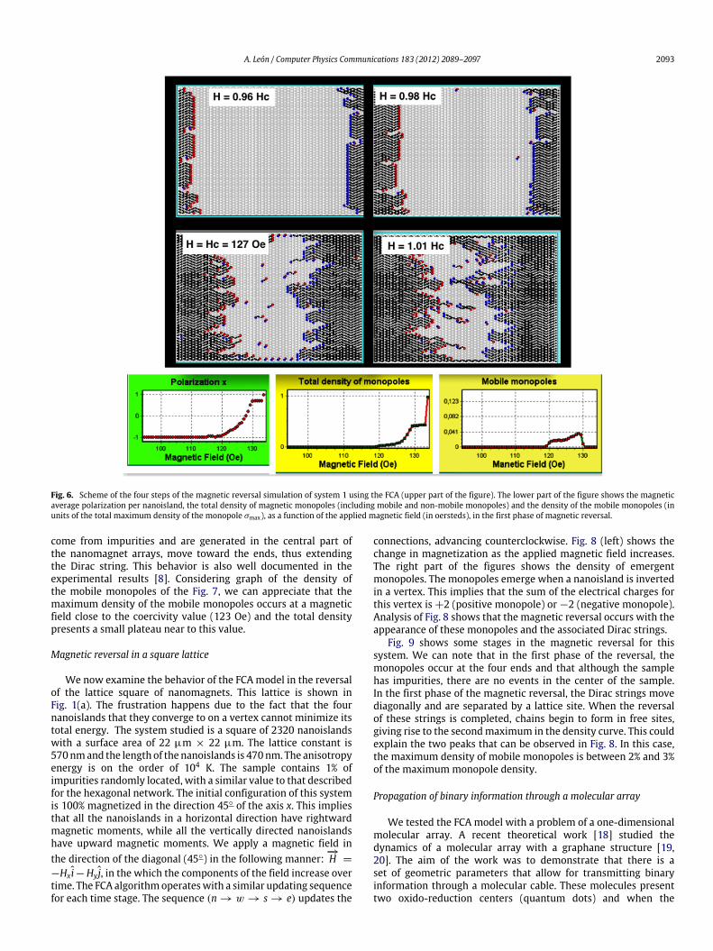
Magnetization reversal for a sample with impurities (system 2)System 2 has all the parameters of system 1, but with 10% of the

nanomagnets with the magnitude at the magnetic moment mi inthe range 0.9m ≤ mi ≤ m, wherem is themomentwhen90%of thenanoislands remain. The procedure for reversing magnetization isthe same as that used for the previous system. The study of themagnetic average polarization per nanoisland and of themonopoledensities is shown in Fig. 7. In contrast to the case for the study ofsystem1, the results of this simulation are in qualitative agreementwith the experimental results of the study by Mengotti et al. [8].The maximum density value of the emergent monopoles is closeto 10%, which corresponds to the data reported in the study [8].Themagnetic polarization curvepresents the same structure as theexperimental data. However, the experimental system ofMengottiet al. studied a central region of the sample (without consideringthe edges in the statistics); the results are similar to those of ourstudy (which considers the edges in the statistics). Consequently,we can conclude that there is little disorder in the experimentalsample.

Fig. 7 (upper part) shows part of themagnetic reversal sequencefor system 2. We can appreciate that owing to impurities themonopoles emerge randomly in the nanoisland array and not justat the ends, as in the first case. The emergent monopoles, which


Fig. 6. Scheme of the four steps of the magnetic reversal simulation of system 1 using the FCA (upper part of the figure). The lower part of the figure shows the magneticaverage polarization per nanoisland, the total density of magnetic monopoles (including mobile and non-mobile monopoles) and the density of the mobile monopoles (inunits of the total maximum density of the monopole σmax), as a function of the applied magnetic field (in oersteds), in the first phase of magnetic reversal.

come from impurities and are generated in the central part ofthe nanomagnet arrays, move toward the ends, thus extendingthe Dirac string. This behavior is also well documented in theexperimental results [8]. Considering graph of the density ofthe mobile monopoles of the Fig. 7, we can appreciate that themaximum density of the mobile monopoles occurs at a magneticfield close to the coercivity value (123 Oe) and the total densitypresents a small plateau near to this value.

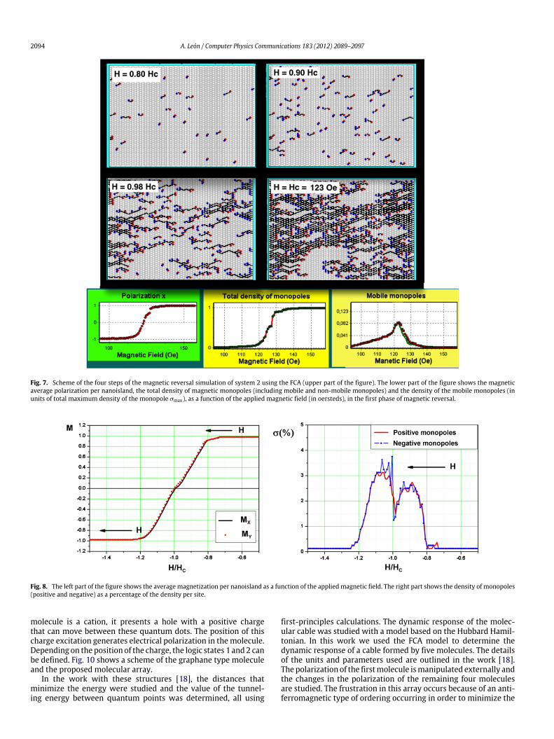
Magnetic reversal in a square lattice

We now examine the behavior of the FCA model in the reversalof the lattice square of nanomagnets. This lattice is shown inFig. 1(a). The frustration happens due to the fact that the fournanoislands that they converge to on a vertex cannot minimize itstotal energy. The system studied is a square of 2320 nanoislandswith a surface area of 22 µm × 22 µm. The lattice constant is570nmand the length of the nanoislands is 470nm. The anisotropyenergy is on the order of 104 K. The sample contains 1% ofimpurities randomly located, with a similar value to that describedfor the hexagonal network. The initial configuration of this systemis 100% magnetized in the direction 45◦ of the axis x. This impliesthat all the nanoislands in a horizontal direction have rightwardmagnetic moments, while all the vertically directed nanoislandshave upward magnetic moments. We apply a magnetic field inthe direction of the diagonal (45◦) in the following manner:

−→H =

−Hx i−Hy j, in the which the components of the field increase overtime. The FCA algorithmoperateswith a similar updating sequencefor each time stage. The sequence (n → w → s → e) updates the

connections, advancing counterclockwise. Fig. 8 (left) shows thechange in magnetization as the applied magnetic field increases.The right part of the figures shows the density of emergentmonopoles. The monopoles emerge when a nanoisland is invertedin a vertex. This implies that the sum of the electrical charges forthis vertex is +2 (positive monopole) or −2 (negative monopole).Analysis of Fig. 8 shows that the magnetic reversal occurs with theappearance of these monopoles and the associated Dirac strings.

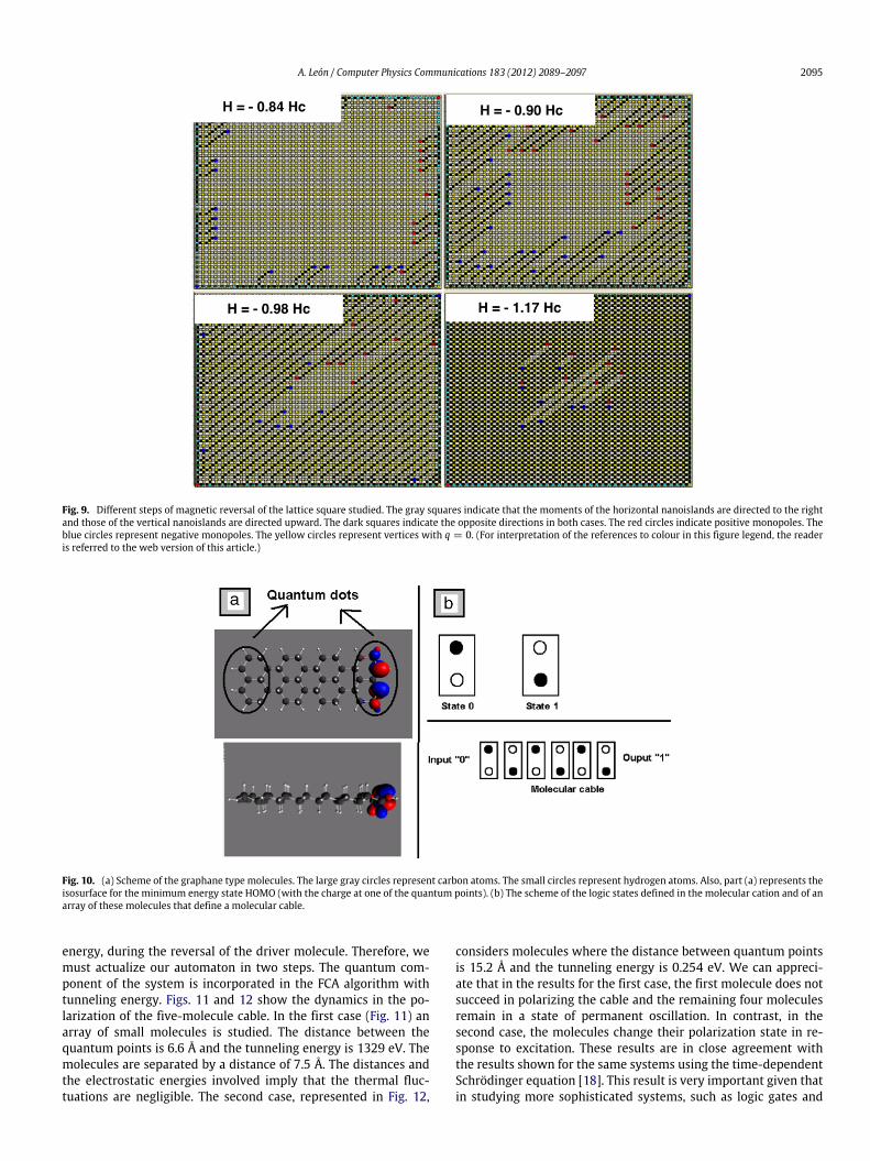
Fig. 9 shows some stages in the magnetic reversal for thissystem. We can note that in the first phase of the reversal, themonopoles occur at the four ends and that although the samplehas impurities, there are no events in the center of the sample.In the first phase of the magnetic reversal, the Dirac strings movediagonally and are separated by a lattice site. When the reversalof these strings is completed, chains begin to form in free sites,giving rise to the secondmaximum in the density curve. This couldexplain the two peaks that can be observed in Fig. 8. In this case,the maximum density of mobile monopoles is between 2% and 3%of the maximummonopole density.

Propagation of binary information through a molecular array

We tested the FCA model with a problem of a one-dimensionalmolecular array. A recent theoretical work [18] studied thedynamics of a molecular array with a graphane structure [19,20]. The aim of the work was to demonstrate that there is aset of geometric parameters that allow for transmitting binaryinformation through a molecular cable. These molecules presenttwo oxido-reduction centers (quantum dots) and when the


Fig. 7. Scheme of the four steps of the magnetic reversal simulation of system 2 using the FCA (upper part of the figure). The lower part of the figure shows the magneticaverage polarization per nanoisland, the total density of magnetic monopoles (including mobile and non-mobile monopoles) and the density of the mobile monopoles (inunits of total maximum density of the monopole σmax), as a function of the applied magnetic field (in oersteds), in the first phase of magnetic reversal.

Fig. 8. The left part of the figure shows the average magnetization per nanoisland as a function of the applied magnetic field. The right part shows the density of monopoles(positive and negative) as a percentage of the density per site.

molecule is a cation, it presents a hole with a positive chargethat can move between these quantum dots. The position of thischarge excitation generates electrical polarization in themolecule.Depending on the position of the charge, the logic states 1 and 2 canbe defined. Fig. 10 shows a scheme of the graphane type moleculeand the proposed molecular array.

In the work with these structures [18], the distances thatminimize the energy were studied and the value of the tunnel-ing energy between quantum points was determined, all using

first-principles calculations. The dynamic response of the molec-ular cable was studied with a model based on the Hubbard Hamil-tonian. In this work we used the FCA model to determine thedynamic response of a cable formed by five molecules. The detailsof the units and parameters used are outlined in the work [18].The polarization of the firstmolecule ismanipulated externally andthe changes in the polarization of the remaining four moleculesare studied. The frustration in this array occurs because of an anti-ferromagnetic type of ordering occurring in order to minimize the


Fig. 9. Different steps of magnetic reversal of the lattice square studied. The gray squares indicate that the moments of the horizontal nanoislands are directed to the rightand those of the vertical nanoislands are directed upward. The dark squares indicate the opposite directions in both cases. The red circles indicate positive monopoles. Theblue circles represent negative monopoles. The yellow circles represent vertices with q = 0. (For interpretation of the references to colour in this figure legend, the readeris referred to the web version of this article.)

Fig. 10. (a) Scheme of the graphane type molecules. The large gray circles represent carbon atoms. The small circles represent hydrogen atoms. Also, part (a) represents theisosurface for the minimum energy state HOMO (with the charge at one of the quantum points). (b) The scheme of the logic states defined in the molecular cation and of anarray of these molecules that define a molecular cable.

energy, during the reversal of the driver molecule. Therefore, wemust actualize our automaton in two steps. The quantum com-ponent of the system is incorporated in the FCA algorithm withtunneling energy. Figs. 11 and 12 show the dynamics in the po-larization of the five-molecule cable. In the first case (Fig. 11) anarray of small molecules is studied. The distance between thequantum points is 6.6 Å and the tunneling energy is 1329 eV. Themolecules are separated by a distance of 7.5 Å. The distances andthe electrostatic energies involved imply that the thermal fluc-tuations are negligible. The second case, represented in Fig. 12,

considers molecules where the distance between quantum pointsis 15.2 Å and the tunneling energy is 0.254 eV. We can appreci-ate that in the results for the first case, the first molecule does notsucceed in polarizing the cable and the remaining four moleculesremain in a state of permanent oscillation. In contrast, in thesecond case, the molecules change their polarization state in re-sponse to excitation. These results are in close agreement withthe results shown for the same systems using the time-dependentSchrödinger equation [18]. This result is very important given thatin studying more sophisticated systems, such as logic gates and


1.0

0.5

0.0

-0.5

-1.0

1.0

0.5

0.0

-0.5

-1.0

1.0

0.5

0.0

-0.5

-1.0

1.0

0.5

0.0

-0.5

-1.0

1.0

0.5

0.0

-0.5

-1.0

0 10 20

Time30 40 50

Time0 10 20 30 40 50

Time0 10 20 30 40 50

Time0 10 20 30 40 50

Time0 10 20 30 40 50

Fig. 11. Electrical polarization (in atomic units) of each molecule that forms the molecular cable for the small system explained in the text.

1.0

0.5

0.0

-0.5

-1.0

Time

1.0

0.5

0.0

-0.5

-1.0

1.0

0.5

0.0

-0.5

-1.0

1.0

0.5

0.0

-0.5

-1.0

1.0

0.5

0.0

-0.5

-1.0

0 20 40 60 80Time

....

0 20 40 60 80

Time0 20 40 60 80

Time0 20 40 60 80

Time0 20 40 60 80

Fig. 12. Electrical polarization (in atomic units) of each molecule that forms the molecular cable for the large system explained in the text.

circuits, the Hamiltonian formalism of Hubbard cannot be appliedto study the dynamic response.

Conclusion

This work presents a semi-deterministic model used tostudy frustrated systems. It is specifically designed for magneticnanoisland arrays and charged molecules, but can be appliedto any problem where there is frustration and where thermalfluctuations are negligible. The great advantage of themodel is thatit can make efficient simulations of highly complex phenomenain real time with a minimum of computational requirements.All the simulations shown in this paper were carried out using

in a personal desktop computer [21]. They represent a perfectcomplement to the methods based on Monte Carlo algorithms forstudying the elemental physics of problemswith quantumentities.

Acknowledgment

The author acknowledge the financial support of FONDECYTprogram grant 11100045.

References

[1] V.F. Petrenko, R.W. Whitworth, Physics of Ice, Oxford Univ. Press, 1999.[2] D.J.P. Morris, et al., Science 326 (2009) 411–414.


[3] T. Fennell, et al., Science 326 (2009) 415–417.[4] H. Kadowaki, et al., J. Phys. Soc. Japan 78 (2009) 103706.[5] R.F. Wang, et al., Nature 439 (2006) 303–306.[6] E. Mengotti, et al., Phys. Rev. B 78 (2008) 144402.[7] A. Remhof, et al., Phys. Rev. B 77 (2008) 134409.[8] E. Mengotti, et al., Nat. Phys. 7 (2011) 68.[9] A.O. Orlov, I. Amlani, G.H. Bernstein, C.S. Lent, G.L. Snider, Science 277 (1997)

928.[10] J. Jiao, G.J. Long, F. Grandjean, A.M. Beatty, T.P. Fehlner, J. Am. Chem. Soc. 125

(2003) 7522.[11] D. Griffeath, C. Moore (Eds.), New Constructions in Cellular Automata,

University Press, Oxford, 2003.

[12] A. León, Z. Barticevic, M. Pacheco, Solid State Commun. 152 (2012) 41–44.[13] G.Y. Vichniac, Physica D 10 (1984) 96.[14] Y. Pomeau, J. Phys. A 17 (1984) L-415.[15] H.J. Hermann, J. Stat. Phys. 45 (1986) 145.[16] H. Ottavi, O. Parodi, Simulation of the Ising model by cellular automata,

Europhys. Lett. 8 (1989) 741–746.[17] J.H. Cole, C.L. Hollenberg, S. Prawer, Comput. Phys. Comm. 161 (2004) 14.[18] A. León, M. Pacheco, Electronic and dynamics properties of a molecular wire

of graphane nanoclusters, Phys. Lett. A 375 (2011) 4190–4197.[19] J.O. Sofo, A.S. Chaudhari, G.D. Barber, Phys. Rev. B 75 (2007) 153401.[20] D.C. Elias, et al., Science 323 (2009) 610.[21] MacBook Pro, 2,7 GHz Intel Core i7.

An efficient model for studying the dynamics of frustrated systems

Documents

Transcript of An efficient model for studying the dynamics of frustrated systems