Innovative mathematical and numerical models for studying ...
377
Vicente Mataix Eugenio Oñate Riccardo Rossi Innovative mathematical and numerical models for studying the deformation of shells during industrial forming processes with the Finite Element Method Monograph CIMNE Nº-190, October 2020
-
Upload
khangminh22 -
Category
Documents
-
view
0 -
download
0
Transcript of Innovative mathematical and numerical models for studying ...

Vicente Mataix Eugenio Oñate Riccardo Rossi
Innovative mathematical and numerical models for studying
the deformation of shells during industrial forming processes
with the Finite Element Method
Monograph CIMNE Nº-190, October 2020

Innovative mathematical and numerical models for studying the
deformation of shells during industrial forming processes with
the Finite Element Method
Vicente Mataix Eugenio Oñate Riccardo Rossi
Monograph CIMNE Nº-190, October 2020
International Center for Numerical Methods in Engineering Gran Capitán s/n, 08034 Barcelona, Spain

INTERNATIONAL CENTER FOR NUMERICAL METHODS IN ENGINEERING Edificio C1, Campus Norte UPC Gran Capitán s/n 08034 Barcelona, Spain www.cimne.com First edition: October 2020 INNOVATIVE MATHEMATICAL AND NUMERICAL MODELS FOR STUDYING THE DEFORMATION OF SHELLS DURING INDUSTRIAL FORMING PROCESSES WITH THE FINITE ELEMENT METHOD Monograph CIMNE M190
The authors

Ce qui est simple est toujours faux. Ce qui ne l'est pas est inutilisable
Paul Valéry (1871 1945 AD, French poet, essayist, and philosopher)
Vicente Mataix Ferrándiz Page 3 of 374


Empty space
Essentially, all models are wrong, but some are useful
Aphorism, attributed to George E. P. Box (1919 2013 AD, British statistician)
Page 4 of 374 Vicente Mataix Ferrándiz


Abstract
This document contains the result resulting from the work in the doctoral thesis Innovative mathematicaland numerical models for studying the deformation of shells during industrial forming processes with theFinite Element Method. The objective of this thesis is to contribute to the development of finite elementmethods for the analysis of the stamping processes, an area of problems with a very clear industrialapplication. Indeed these kinds of problems involve multiple disciplines and require the understandingof different mechanical problems, being the most relevant disciplines the continuous mechanics, theplasticity, contact problems, among others, depending of the problematic of study.
To achieve the proposed goals, attention is focused in the first section of this thesis in the solid-shellelements, which are an attractive kind of element for the simulation of forming processes. This is due to thefact that any kind of generic 3D constitutive law can be employed without any kind of additional hypothesis,besides the thermomechanic problem is formulated without additional assumptions. Additionally this typeof element allows the three-dimensional description of the deformable body, thus contact on both sides ofthe element can be treated easily.
This work will present in first place the development of a triangular prism element as a solid-shell,for the analysis of thin/thick shell, undergoing large deformations. The element is formulated in Total
Lagrangian (TL) formulation, and employs the neighbour (adjacent) elements to perform a local patchto enrich the displacement field. In the original formulation a modified right CauchyGreen deformationtensor (C) is obtained; in the present work, a modified deformation gradient (F) is obtained, which allowsto generalise the methodology and thanks to this we are able to employ the push-forward and pullbackconcepts. The push-forward and pullback technique provide a mathematically consistent method fordefine the time derivatives of the tensors; and for example it can be employed to work with elasto-plasticity.
The element is based in three modifications: (a) a classical assumed strain approach for transverseshear strains (b) an assumed strain approach for the in-plane components using information fromneighbour elements and (c) an averaging of the volumetric strain over the element. The objective is touse this type of element for the simulation of shells avoiding transverse shear locking, improving themembrane behaviour of the in-plane triangle and to handle quasi-incompressible materials or materialswith isochoric plastic flow. The element considers just one Gauss point in the plane and a chosen numberof integration points along the axis, thanks to this it is possible to consider problems with a significantnon-linearity related to plasticity.
This work will continue presenting the contact formulation developed, which consists in state-of-artof the numerical contact mechanics formulation for implicit simulations. Consisting in an exact mortarintegration of the contact interface, this allows to obtain the most consistent integration possible betweenthe integration domains, as well as the most exact solution possible. The implementation also considersseveral optimisation algorithms, like the penalty constraint optimisation, but particularly remarkablethe consideration of a Augmented Lagrangian Method (ALM) with dual Lagrange multipliers, a newcontribution of this work. The latter allows to static condensate the system of equations, allowing to removethe Lagrange Multiplier (LM) of the resolution and therefore permitting the consideration of iterativesolvers. Additionally, the formulation has been properly linearised, ensuring the quadratic convergence ofthe problem. In order to solve the system of equations, a semi-smooth Newton method is considered,consisting in an active set strategy, extensible also in the case of frictional problems. The formulation worksboth for frictionless and frictional problems, the later essential for the simulation of forming processes.This frictional formulation is framed in the traditional friction models, like the Coulomb friction, but thedevelopment presented can be extended to any type of frictional model. This contact formulation is fullycompatible with the solid-shell introduced on this work.
Vicente Mataix Ferrándiz Page 5 of 374

The missing ingredient necessary in order to successfully perform the industrial processes wouldbe the constitutive models. This will be materialised in the plasticity formulation considered in this work.In these models, we will be able to consider large strain deformation plasticity models, with arbitrarycombination of yield surfaces and plastic potentials, the so-called non-associative models. In order tocompute the corresponding tangent tensor for these general laws, numerical implementations based onperturbation methods.
The final theoretical work of this thesis will consist in the developments of adaptive remeshingtechniques. In here, different approaches will be presented. Starting with the metric based techniques,including the level-set and Hessian approaches. These techniques are of general purpose, and canbe considered both in application of structural or Computational Fluid Dynamics (CFD) problems. Inaddition to this approach, the Super convergent Patch Recovery (SPR) error estimation method ispresented. This approach is more conventional than the former ones. In both cases, in the Hessian andthe SPR error estimation, have been extended in order to apply it to contact mechanics problems, maincontribution of this work in this field.
With all the former developments, we will be ready for the introduction of practical cases focused inthe context stamping processes. The most important point to highlight on this is that these examples willbe compared with the reference solutions available in the literature as a validation of the developmentspresented until this point.
The present document is organised as follows. The first chapter introduces the thesis, stating theobjectives and reviews the state-of-the-art on the most transcendental subjects. The second chapterdoes a shallow introduction of the continuous mechanics and Finite Element Method (FEM) concepts,required for following chapters. The third chapter derives the formulation of the solid-shell previouslymentioned and the free-rotation shell, which is the theoretical inspiration of the solid-shell presented,including several academic examples that are commonly employed in the literature as a benchmark ofshell elements. The fourth chapter will present the contact mechanics formulation developed, consistingin an implicit mortar ALM formulation, the chapter also includes several examples commonly found in theliterature, which are usually considered for validation. The next chapter presents the plasticity formulationused, including some technical details in the implementation side, some examples of validation will bealso introduced at the end of this chapter. The final theoretical chapter shows the adaptive remeshingalgorithms developed in the context of this work, and presents several examples, including not only solidmechanics cases, but also CFD. The next chapter encapsules some validation and application cases forstamping processes. The final chapter comprises the conclusions, as well as the future works comingafter the presented developments.
Keywords: metal-forming, stamping, shells, solid-shells, contact, plasticity,adaptive remeshing
Page 6 of 374 Vicente Mataix Ferrándiz

Resumen
La tesis doctoral Modelos matemáticos y numéricos innovadores para el estudio de la deformación deláminas durante los procesos de conformado industrial por el Método de los Elementos Finitos. pretendecontribuir al desarrollo de métodos de elementos finitos para el análisis de procesos de estampado, unárea problemática con una clara aplicación industrial. De hecho, este tipo de problemas multidisciplinaresrequieren el conocimiento de múltiples disciplinas, como la mecánica de medios continuos, la plasticidad,la termodinámica y los problemas de contacto, entre otros.
Para alcanzar los objetivos propuestos, la primera parte de esta tesis abarca los elementos de sólido-lámina. Este tipo de elemento resulta atractivo para la simulación de procesos de conformado, dado quecualquier tipo de ley constitutiva tridimensional puede ser formulada sin necesidad de considerar ningunaconjetura adicional. Además, este tipo de elementos permite realizar una descripción tridimensional delcuerpo deformable, por tanto, el contacto de ambas caras puede ser tratado fácilmente.
Este trabajo presenta en primer lugar el desarrollo de un elemento de sólido-lámina prismáticotriangular, para el análisis de láminas gruesas y delgadas con capacidad para grandes deformaciones.Este elemento figura en formulación Lagrangiana total, y emplea los elementos vecinos para podercomputar un campo de desplazamientos cuadráticos. En la formulación original, se obtenía un tensor deCauchy derecho modificado (C); sin embargo, en este trabajo, la formulación se extiende obteniendo ungradiente de deformación modificado (F), que permite emplear los conceptos de push-forward y pull-back.Dichos conceptos proveen de un método matemáticamente consistente para la definición de derivadastemporales de tensores y, por tanto, puede ser usado, por ejemplo, para trabajar con elasto-plasticidad.
El elemento se basa en tres modificaciones: (a) una aproximación clásica de deformaciones transver-sales de corte mixtas impuestas; (b) una aproximación de deformaciones impuestas para las componentesen el plano tangente de la lámina; y (c) una aproximación de deformaciones impuestas mejoradas en ladirección normal a través del espesor, mediante la consideración de un grado de libertad adicional. Losobjetivos son poder utilizar el elemento para la simulación de láminas sin bloquear por cortante, mejorar elcomportamiento membranal del elemento en el plano tangente, eliminar el bloqueo por efecto Poisson ypoder tratar materiales elasto-plásticos con un flujo plástico incompresible, así como materiales elásticoscuasi-incompresibles o materiales con flujo plástico isocórico. El elemento considera un único punto deGauss en el plano, mientras que permite considerar un número cualquiera de puntos de integración ensu eje, con el objetivo de poder considerar problemas con una significativa no linealidad en cuanto aplasticidad.
Este trabajo continúa con el desarrollo de la formulación de contacto empleada, una metodología quese encuentra en la bibliografía sobre la mecánica de contacto computacional para simulaciones implícitas.Dicha formulación consiste en una integración exacta de la interfaz de contacto mediante métodos demortero, lo que permite obtener la integración más consistente posible entre los dominios de integración,así como la solución más exacta posible. La implementación también considera varios algoritmos deoptimización, como la optimización mediante penalización. La contribución más notable de este trabajo esla consideración de multiplicadores de Lagrange aumentados duales como método de optimización. Estospermiten condensar estáticamente el sistema de ecuaciones, lo que permite eliminar los multiplicadoresde Lagrange de la resolución y, por lo tanto, permite la consideración de solvers iterativos. Además, laformulación ha sido adecuadamente linealizada, asegurando la convergencia cuadrática del problema.Para resolver el sistema de ecuaciones, se considera un método de Newton semi-smooth, que consisteen una estrategia de set activo, extensible también en el caso de problemas friccionales. La formulaciónes funcional tanto para problemas sin fricción como para problemas friccionales, lo que es esencial parala simulación de procesos de estampado. Esta formulación friccional se enmarca en los modelos defricción tradicionales, como la fricción de Coulomb, pero el desarrollo presentado puede extendersea cualquier tipo de modelo de fricción. Esta formulación de contacto es totalmente compatible con elelemento sólido-lámina introducido en este trabajo.
El componente necesario restante para la simulación de procesos industriales son los modelosconstitutivos. En este trabajo, esto se ve materializado en la formulación de plasticidad considerada.Estos modelos constitutivos se considerarán modelos de plasticidad para grandes deformaciones, conuna combinación arbitraria de superficies de fluencia y potenciales plásticos: los llamados modelos noasociados. Para calcular el tensor tangente correspondiente a estas leyes generales, se han consideradoimplementaciones numéricas basadas en métodos de perturbación.
Vicente Mataix Ferrándiz Page 7 of 374

Otra contribución fundamental de este trabajo es el desarrollo de técnicas para el remallado adaptativo,de las que se presentarán distintos enfoques. Por un lado, las técnicas basadas en métricas, incluyendolos enfoques level-set y Hessiano. Estas técnicas son de propósito general y pueden considerarse tantoen la aplicación de problemas estructurales como en problemas de mecánica de fluidos. Por otro lado, sepresenta el método de estimación de errores SPR, más convencional que los anteriores. En este ámbito,la contribución de este trabajo consiste en la estimación de error mediante las técnicas de Hessiano ySPR para la aplicación a problemas de contacto numérico. Con los desarrollos previamente introducidos,estaremos en disposición de introducir los casos de aplicación centrados en el contexto de procesos deestampado. Es relevante destacar que estos ejemplos son comparados con las soluciones de referenciadisponibles en la bibliografía como forma de validar los desarrollos presentados hasta este punto.
El presente documento está organizado de la siguiente manera. El primer capítulo establece losobjetivos y revisa la bibliografía acerca de los temas clave de este trabajo. El segundo capítulo hace unaintroducción de la mecánica de medios continuos y los conceptos relativos al Método de los Elementos
Finitos (MEF), necesarios en los desarrollos que se presentarán en los capítulos siguientes. El tercercapítulo aborda la formulación del elemento sólido-lámina, así como del elemento de lámina sin gradosde libertad de rotación que inspira el sólido-lámina desarrollado. Esta parte muestra varios ejemplosacadémicos que son comúnmente empleados en la bibliografía como problemas de referencia de láminas.El cuarto capítulo presenta la formulación desarrollada para la resolución de problemas de contactonumérico, consistente en una formulación implícita de integración exacta mediante métodos morteroy multiplicadores de Lagrange aumentados duales. Este capítulo incluye, asimismo, varios ejemploscomúnmente encontrados en la bibliografía, que generalmente son considerados para su validación. Elquinto capítulo presenta la formulación de plasticidad empleada, incluyendo algunos detalles técnicosdesde el punto de vista de la implementación, así como varios ejemplos de validación. El sexto capítulomuestra los algoritmos de remallado adaptativo desarrollados en el contexto de este trabajo, y presentavarios ejemplos, que incluyen no solo casos estructurales, sino también de mecánica de fluidos. Elséptimo capítulo encapsula algunos casos de validación y aplicación para procesos de estampado. Elcapítulo final comprende las conclusiones, así como los trabajos que podrían continuar el presenteestudio.
Palabras clave: Conformado metálico, estampado, láminas, sólido-lámina, contacto, plasticidad,mallado adaptativo
Page 8 of 374 Vicente Mataix Ferrándiz

Acknowledgements
I still remember the day I arrived to Barcelona 5 years ago to start my master thesis in FSI. My car, that I was supposedto take in order to bring all my stuff from Paris to Barcelona, just burn out the week before and I needed to take theTGV instead, with all my stuff. It is because of that I want to acknowledge in first place Katie, one of my roomies whenI arrived to Barcelona, who helped me that first day that I arrived to Barcelona to settle.
The next person I meet and I want to thank is my director Eugenio Oñate Ibañez de Navarra, who brings me theopportunity to work in this thesis, and had enough patience to deal with all the delays and problems that I had duringall this time. Especially the patience to deal with my continuous trips between Barcelona and Paris. I hope the resultobtained in this work was worth it. I would like to have a special acknowledge to Merce Alberich, who helped me witha lot of paper work, and to communicate with Eugenio. In the same line, I would like to notice the administratives inthe doctoral school, Silvia and Rosa, who help me with all the documents related with this thesis. I want to mentionthe support of the Generalitat de Catalunya which is funding my work with the grant FI AGAUR.
I want to especially thank to my co-director Riccardo Rossi for all the help and support during all this time.Particularly in the last year of the thesis, where the relationship became more difficult due to the distance. At theend I hope you accepted volcanic personality. I would like to thank to all the Kratos staff. Special remarks for CarlosRoig, aka Charlie for help me with all those programmation questions. To Jordi Cotela, who helped me in severaltechnical issues too, and at the end I hope understood my sense of humour. To Antonia Larese, who gave me severalacademic tips. Ilaria Iaconeta, who was a good friend and understands the pain of having a thesis finished, but notreally. And to Pooyan Dadvand for all the technical help and Kratos origin history. Thanks to all the team, to theprepost duo Enrique Escolano-Miguel Pasenau, to the fantastic duo Anna-Adrià, to the interfacer Javier Garate and tothe doctor mesh Abel Coll. Without you, all this work it would have been much more difficult.
Thanks to everyone I meet these years in Barcelona at the International Center for Numerical Methods in
Engineering (CIMNE), especially I want to thank to Rubén Zorrilla who was my office partner, and we have togetherso much metahumour, which is the best type of humour. To the rookies that I left in the office, Riccardo Tosi, MarcNuñez and Agustina Giuliodori. To Miguel Ángel Celigueta and Lucia Barbu, they are an adorable couple and I wishyou a lot of happiness together. To Eduardo Soudah, which passion for biomechanics is fascinating. To GuillermoCasas, with whom I have had the pleasure to share debates about politics from time to time. Miguel Maso, whois a wonderful person, and I wish him the best. To Pablo Becker and Marcelo Raschi, with whom I have enjoyedtechnical discussions. Ignasi Pouplana, who was the first person I meet in CIMNE, and who helped me so much atthe beginning, and with whom I enjoyed working at the end. To Lorenzo Gracia, who gave me such good times, andenjoyed so many paellas of mine. To Tomás Varona whose friendship I value so much and that I hope will last formany years. Finally, to Alejandro Cornejo, who helped me so much during the last stages of the thesis, but has alsoturned out to be one of my best friends. From Barcelona, I also like to address to Miguel Zatarain, who helped me tobreak routine when I was living in Barcelona, and who host me when I was not living there anymore.
To the people from Munich, which contribute so much to the StructuralMechanicsApplication, andtherefore help me directly and indirectly with the developments presented on this work. Remarks for Philipp Bucher,who controlled a very relevant part of my developments. And to Tobias Teschemacher who is the coolest guy I know,and I had a great time with him. I would like to mention to Roland Wüchner, who did everything in order I could go to ,but unfortunately I could not go at the end. Deeply thanks to Mohamed Khalil, who accompanied me during my firststeps in the world of numerical contact. Without you probably this thesis would be right now completely different. Alsocoming from , thanks to Elisa Magliozzi who ended being a very good friend, and to Anna Rehr, which master thesis Ihad the pleasure to supervise. From Inria I would like to acknowledge to Algiane Froehly, thanks to her, and to theMmg team, I could accomplish a very relevant part of my thesis.
Finally, but not for that reason less important, I want to thank to my family, to my father who has proven onceagain to have patience with me and my "obsessive perfectionism", to my mother who has given me so much support,and has suffered so much for me, and to my sister, that we have both had to leave the "terreta" in order to dedicateourselves to research. But I want to thank especially to my wife Sara, who has been the co-pilot of this work fromthe distance, and in the last stage together, she knows everything I have had to go through and do to get here, andsometimes she has had to suffer because of this.

Page 10 of 374 Vicente Mataix Ferrándiz

CONTENTS CONTENTS
Contents
I Theoretical framework 21
1 Introduction 23
1.1 Evolution of the stamping technology . . . . . . . . . . . . . . . . . . . . . . . . . . . . . . . . . . . 261.1.1 History of the stamping and forming technology . . . . . . . . . . . . . . . . . . . . . . . . . . 261.1.2 Historical review of Finite Element Analysis (FEA) of formability and forming technology . . . 27
1.2 Most common issues in forming processes . . . . . . . . . . . . . . . . . . . . . . . . . . . . . . . . 271.2.1 Springback . . . . . . . . . . . . . . . . . . . . . . . . . . . . . . . . . . . . . . . . . . . . . . 271.2.2 Wrinkling . . . . . . . . . . . . . . . . . . . . . . . . . . . . . . . . . . . . . . . . . . . . . . . 28
1.3 Objectives . . . . . . . . . . . . . . . . . . . . . . . . . . . . . . . . . . . . . . . . . . . . . . . . . . 29Bibliography of chapter . . . . . . . . . . . . . . . . . . . . . . . . . . . . . . . . . . . . . . . . . . . . . . 29
2 Finite Element formulation 33
2.1 Introduction . . . . . . . . . . . . . . . . . . . . . . . . . . . . . . . . . . . . . . . . . . . . . . . . . 332.2 Finite Element Method . . . . . . . . . . . . . . . . . . . . . . . . . . . . . . . . . . . . . . . . . . . 33
2.2.1 Introduction . . . . . . . . . . . . . . . . . . . . . . . . . . . . . . . . . . . . . . . . . . . . . 332.2.2 Concept of Finite Element (FE) . . . . . . . . . . . . . . . . . . . . . . . . . . . . . . . . . . 34
2.3 Solid mechanics . . . . . . . . . . . . . . . . . . . . . . . . . . . . . . . . . . . . . . . . . . . . . . . 362.3.1 Linear form . . . . . . . . . . . . . . . . . . . . . . . . . . . . . . . . . . . . . . . . . . . . . . 362.3.2 Non-linear form . . . . . . . . . . . . . . . . . . . . . . . . . . . . . . . . . . . . . . . . . . . 36
2.3.2.1 Deformation gradient . . . . . . . . . . . . . . . . . . . . . . . . . . . . . . . . . . . 372.3.2.2 Strain tensors . . . . . . . . . . . . . . . . . . . . . . . . . . . . . . . . . . . . . . . 37
2.4 Finite Element formulation for Computational Structural Dynamics (CSD) . . . . . . . . . . . . . . 382.4.1 Weak formulation in solids . . . . . . . . . . . . . . . . . . . . . . . . . . . . . . . . . . . . . 382.4.2 TL and Updated Lagrangian (UL) formulation . . . . . . . . . . . . . . . . . . . . . . . . . . 392.4.3 Solution of the non-linear-equilibrium equations system . . . . . . . . . . . . . . . . . . . . . . 40
2.4.3.1 Newton-Raphson method . . . . . . . . . . . . . . . . . . . . . . . . . . . . . . . . . 402.4.3.2 Line-search . . . . . . . . . . . . . . . . . . . . . . . . . . . . . . . . . . . . . . . . 412.4.3.3 Arc-length . . . . . . . . . . . . . . . . . . . . . . . . . . . . . . . . . . . . . . . . . 41
2.4.4 Time integration schemes . . . . . . . . . . . . . . . . . . . . . . . . . . . . . . . . . . . . . . 422.4.4.1 Newmark time scheme . . . . . . . . . . . . . . . . . . . . . . . . . . . . . . . . . . 432.4.4.2 Bossak algorithm . . . . . . . . . . . . . . . . . . . . . . . . . . . . . . . . . . . . . 432.4.4.3 α-generalised . . . . . . . . . . . . . . . . . . . . . . . . . . . . . . . . . . . . . . . 432.4.4.4 Backward Differentiation Formula (BDF) . . . . . . . . . . . . . . . . . . . . . . . 44
2.4.5 Damping matrix . . . . . . . . . . . . . . . . . . . . . . . . . . . . . . . . . . . . . . . . . . . 44Bibliography of chapter . . . . . . . . . . . . . . . . . . . . . . . . . . . . . . . . . . . . . . . . . . . . . . 45
3 Rotation-free shells and solid-shell elements 49
3.1 Introduction . . . . . . . . . . . . . . . . . . . . . . . . . . . . . . . . . . . . . . . . . . . . . . . . . 493.1.1 Historical outline . . . . . . . . . . . . . . . . . . . . . . . . . . . . . . . . . . . . . . . . . . . 49
3.2 State of the Art in shell formulation . . . . . . . . . . . . . . . . . . . . . . . . . . . . . . . . . . . . . 503.2.1 Element requisites and stabilisation techniques . . . . . . . . . . . . . . . . . . . . . . . . . . 50
Vicente Mataix Ferrándiz Page 11 of 374

CONTENTS CONTENTS
3.2.2 Shell formulations . . . . . . . . . . . . . . . . . . . . . . . . . . . . . . . . . . . . . . . . . . 513.3 Rotation-free shells . . . . . . . . . . . . . . . . . . . . . . . . . . . . . . . . . . . . . . . . . . . . . 52
3.3.1 Introduction . . . . . . . . . . . . . . . . . . . . . . . . . . . . . . . . . . . . . . . . . . . . . 523.3.2 Basic Shell Triangle . . . . . . . . . . . . . . . . . . . . . . . . . . . . . . . . . . . . . . . . . 52
3.3.2.1 Basics . . . . . . . . . . . . . . . . . . . . . . . . . . . . . . . . . . . . . . . . . . . 523.3.2.2 Shell kinematics . . . . . . . . . . . . . . . . . . . . . . . . . . . . . . . . . . . . . . 533.3.2.3 Constitutive models . . . . . . . . . . . . . . . . . . . . . . . . . . . . . . . . . . . . 53
3.3.3 Enhanced Basic Shell Triangle . . . . . . . . . . . . . . . . . . . . . . . . . . . . . . . . . . . 533.3.3.1 Total Lagrangian formulation . . . . . . . . . . . . . . . . . . . . . . . . . . . . . . . 54
3.3.3.1.1 Computation of the membrane strains . . . . . . . . . . . . . . . . . . . . . 543.3.3.1.2 Computation of the bending strains . . . . . . . . . . . . . . . . . . . . . . . 543.3.3.1.3 Tangent stiffness matrix . . . . . . . . . . . . . . . . . . . . . . . . . . . . . 55
3.4 Prismatic solid-shell . . . . . . . . . . . . . . . . . . . . . . . . . . . . . . . . . . . . . . . . . . . . . 553.4.1 Introduction . . . . . . . . . . . . . . . . . . . . . . . . . . . . . . . . . . . . . . . . . . . . . 553.4.2 Basic kinematics of the standard element . . . . . . . . . . . . . . . . . . . . . . . . . . . . . 563.4.3 Modifications of the standard element . . . . . . . . . . . . . . . . . . . . . . . . . . . . . . . 57
3.4.3.1 In plane behaviour . . . . . . . . . . . . . . . . . . . . . . . . . . . . . . . . . . . . 573.4.3.2 Transverse shear behaviour . . . . . . . . . . . . . . . . . . . . . . . . . . . . . . . 593.4.3.3 Transverse normal behaviour . . . . . . . . . . . . . . . . . . . . . . . . . . . . . . . 60
3.4.3.3.1 Enhanced Assumed Strain (EAS) formulation . . . . . . . . . . . . . . . . 613.4.3.3.2 Balance equation . . . . . . . . . . . . . . . . . . . . . . . . . . . . . . . . 613.4.3.3.3 Pull-Back and Push-Forward (Extension of the formulation) . . . . . . . . . . 62
3.5 Numerical examples . . . . . . . . . . . . . . . . . . . . . . . . . . . . . . . . . . . . . . . . . . . . . 633.5.1 Patch test . . . . . . . . . . . . . . . . . . . . . . . . . . . . . . . . . . . . . . . . . . . . . . 63
3.5.1.1 Membrane patch test . . . . . . . . . . . . . . . . . . . . . . . . . . . . . . . . . . . 633.5.1.2 Bending patch test . . . . . . . . . . . . . . . . . . . . . . . . . . . . . . . . . . . . 64
3.5.2 Cantilever . . . . . . . . . . . . . . . . . . . . . . . . . . . . . . . . . . . . . . . . . . . . . . 653.5.3 Cantilever subjected to end bending moment . . . . . . . . . . . . . . . . . . . . . . . . . . . 663.5.4 Frequencies test . . . . . . . . . . . . . . . . . . . . . . . . . . . . . . . . . . . . . . . . . . . 673.5.5 Cook membrane . . . . . . . . . . . . . . . . . . . . . . . . . . . . . . . . . . . . . . . . . . . 683.5.6 Scoordelis cylindrical roof test . . . . . . . . . . . . . . . . . . . . . . . . . . . . . . . . . . . 693.5.7 Sphere test . . . . . . . . . . . . . . . . . . . . . . . . . . . . . . . . . . . . . . . . . . . . . 703.5.8 Pull-out of an open-ended cylindrical shell . . . . . . . . . . . . . . . . . . . . . . . . . . . . . 713.5.9 Pinched semi-cylindrical . . . . . . . . . . . . . . . . . . . . . . . . . . . . . . . . . . . . . . 723.5.10 Slit test . . . . . . . . . . . . . . . . . . . . . . . . . . . . . . . . . . . . . . . . . . . . . . . . 733.5.11 Cylindrical panel test . . . . . . . . . . . . . . . . . . . . . . . . . . . . . . . . . . . . . . . . 743.5.12 Conical shell test . . . . . . . . . . . . . . . . . . . . . . . . . . . . . . . . . . . . . . . . . . 753.5.13 Wrinkling test . . . . . . . . . . . . . . . . . . . . . . . . . . . . . . . . . . . . . . . . . . . . 763.5.14 Fluid Structure Interaction (FSI)-Vein test . . . . . . . . . . . . . . . . . . . . . . . . . . . . 77
Bibliography of chapter . . . . . . . . . . . . . . . . . . . . . . . . . . . . . . . . . . . . . . . . . . . . . . 78
4 Contact mechanics 85
4.1 Introduction . . . . . . . . . . . . . . . . . . . . . . . . . . . . . . . . . . . . . . . . . . . . . . . . . 854.1.1 Historical outline . . . . . . . . . . . . . . . . . . . . . . . . . . . . . . . . . . . . . . . . . . . 854.1.2 Contact problem . . . . . . . . . . . . . . . . . . . . . . . . . . . . . . . . . . . . . . . . . . . 87
4.2 State of the Art in computational contact mechanics . . . . . . . . . . . . . . . . . . . . . . . . . . . 894.2.1 Introduction . . . . . . . . . . . . . . . . . . . . . . . . . . . . . . . . . . . . . . . . . . . . . 894.2.2 Discretisation . . . . . . . . . . . . . . . . . . . . . . . . . . . . . . . . . . . . . . . . . . . . 89
4.2.2.1 Node-To-Node (NTN) . . . . . . . . . . . . . . . . . . . . . . . . . . . . . . . . . . . 904.2.2.2 Node-To-Segment (NTS) . . . . . . . . . . . . . . . . . . . . . . . . . . . . . . . . 904.2.2.3 Contact Domain Method (CDM) . . . . . . . . . . . . . . . . . . . . . . . . . . . . 914.2.2.4 Segment-To-Segment (STS) (Mortar methods) . . . . . . . . . . . . . . . . . . . . 914.2.2.5 Other alternative methods . . . . . . . . . . . . . . . . . . . . . . . . . . . . . . . . 92
4.2.2.5.1 Isogeometric . . . . . . . . . . . . . . . . . . . . . . . . . . . . . . . . . . . 924.2.2.5.2 Smooth surface approximation . . . . . . . . . . . . . . . . . . . . . . . . . 93
Page 12 of 374 Vicente Mataix Ferrándiz

CONTENTS CONTENTS
4.2.2.6 Conclusion . . . . . . . . . . . . . . . . . . . . . . . . . . . . . . . . . . . . . . . . . 934.2.3 Optimisation method . . . . . . . . . . . . . . . . . . . . . . . . . . . . . . . . . . . . . . . . 93
4.2.3.1 Penalty Method (Penalty Method (PM)) . . . . . . . . . . . . . . . . . . . . . . . . . 934.2.3.2 Lagrange Multiplier Method (LMM) . . . . . . . . . . . . . . . . . . . . . . . . . . 944.2.3.3 ALM . . . . . . . . . . . . . . . . . . . . . . . . . . . . . . . . . . . . . . . . . . . . 944.2.3.4 Double Lagrange Multiplier Method (DLMM) . . . . . . . . . . . . . . . . . . . . . 944.2.3.5 Other alternative methods . . . . . . . . . . . . . . . . . . . . . . . . . . . . . . . . 95
4.2.3.5.1 Perturbed Lagrangian . . . . . . . . . . . . . . . . . . . . . . . . . . . . . . 954.2.3.5.2 Nitsche . . . . . . . . . . . . . . . . . . . . . . . . . . . . . . . . . . . . . . 954.2.3.5.3 Other minor mentions . . . . . . . . . . . . . . . . . . . . . . . . . . . . . . 95
4.2.4 Conclusion . . . . . . . . . . . . . . . . . . . . . . . . . . . . . . . . . . . . . . . . . . . . . . 954.2.5 Frictional models . . . . . . . . . . . . . . . . . . . . . . . . . . . . . . . . . . . . . . . . . . 96
4.3 Formulation . . . . . . . . . . . . . . . . . . . . . . . . . . . . . . . . . . . . . . . . . . . . . . . . . 964.3.1 Introduction . . . . . . . . . . . . . . . . . . . . . . . . . . . . . . . . . . . . . . . . . . . . . 964.3.2 Definition of the problem . . . . . . . . . . . . . . . . . . . . . . . . . . . . . . . . . . . . . . 974.3.3 Frictionless contact . . . . . . . . . . . . . . . . . . . . . . . . . . . . . . . . . . . . . . . . . 97
4.3.3.1 Strong formulation . . . . . . . . . . . . . . . . . . . . . . . . . . . . . . . . . . . . . 974.3.3.2 Weak formulation . . . . . . . . . . . . . . . . . . . . . . . . . . . . . . . . . . . . . 98
4.3.3.2.1 Scalar Lagrange multiplier . . . . . . . . . . . . . . . . . . . . . . . . . . . 984.3.3.2.1.1 LMM . . . . . . . . . . . . . . . . . . . . . . . . . . . . . . . . . . . 984.3.3.2.1.2 Penalty . . . . . . . . . . . . . . . . . . . . . . . . . . . . . . . . . . 994.3.3.2.1.3 ALM . . . . . . . . . . . . . . . . . . . . . . . . . . . . . . . . . . . 100
4.3.3.2.2 Vector Lagrange multiplier . . . . . . . . . . . . . . . . . . . . . . . . . . . 1014.3.3.2.2.1 LMM . . . . . . . . . . . . . . . . . . . . . . . . . . . . . . . . . . . 1014.3.3.2.2.2 ALM . . . . . . . . . . . . . . . . . . . . . . . . . . . . . . . . . . . 101
4.3.3.3 Augmented Lagrange multiplier parameters calibration . . . . . . . . . . . . . . . . . 1024.3.3.4 Discretisation and numerical integration . . . . . . . . . . . . . . . . . . . . . . . . . 103
4.3.3.4.1 Dual Lagrange multipliers . . . . . . . . . . . . . . . . . . . . . . . . . . . . 1034.3.3.4.1.1 Definition . . . . . . . . . . . . . . . . . . . . . . . . . . . . . . . . . 1034.3.3.4.1.2 Graphical representation . . . . . . . . . . . . . . . . . . . . . . . . . 1054.3.3.4.1.3 Derivatives . . . . . . . . . . . . . . . . . . . . . . . . . . . . . . . . 105
4.3.3.4.2 Mortar operators . . . . . . . . . . . . . . . . . . . . . . . . . . . . . . . . . 1054.3.3.4.2.1 Definition . . . . . . . . . . . . . . . . . . . . . . . . . . . . . . . . . 1054.3.3.4.2.2 Derivatives . . . . . . . . . . . . . . . . . . . . . . . . . . . . . . . . 108
4.3.3.4.3 Algebraic form of the problem . . . . . . . . . . . . . . . . . . . . . . . . . . 1084.3.3.4.3.1 Scalar LMM . . . . . . . . . . . . . . . . . . . . . . . . . . . . . . . 1084.3.3.4.3.2 Components LMM . . . . . . . . . . . . . . . . . . . . . . . . . . . . 1084.3.3.4.3.3 Penalty . . . . . . . . . . . . . . . . . . . . . . . . . . . . . . . . . . 1094.3.3.4.3.4 Scalar ALM . . . . . . . . . . . . . . . . . . . . . . . . . . . . . . . . 1094.3.3.4.3.5 Components ALM . . . . . . . . . . . . . . . . . . . . . . . . . . . . 109
4.3.3.4.4 Static condensation of the system in considering of the DLMM . . . . . . . . 1104.3.3.5 Work-flow. Solution algorithm . . . . . . . . . . . . . . . . . . . . . . . . . . . . . . . 1114.3.3.6 Active set strategy (Semi-smooth Newton Raphson) . . . . . . . . . . . . . . . . . . 112
4.3.4 Frictional contact . . . . . . . . . . . . . . . . . . . . . . . . . . . . . . . . . . . . . . . . . . 1134.3.4.1 Strong formulation . . . . . . . . . . . . . . . . . . . . . . . . . . . . . . . . . . . . . 113
4.3.4.1.1 Tangential contact condition - Coulomb’s law . . . . . . . . . . . . . . . . . 1134.3.4.2 Weak formulation . . . . . . . . . . . . . . . . . . . . . . . . . . . . . . . . . . . . . 114
4.3.4.2.1 LMM . . . . . . . . . . . . . . . . . . . . . . . . . . . . . . . . . . . . . . . 1144.3.4.2.2 Contact constraints . . . . . . . . . . . . . . . . . . . . . . . . . . . . . . . 1164.3.4.2.3 Penalty . . . . . . . . . . . . . . . . . . . . . . . . . . . . . . . . . . . . . . 1164.3.4.2.4 ALM . . . . . . . . . . . . . . . . . . . . . . . . . . . . . . . . . . . . . . . 117
4.3.4.3 Discretisation and numerical integration . . . . . . . . . . . . . . . . . . . . . . . . . 1184.3.4.3.1 Discrete contact condition in tangential direction . . . . . . . . . . . . . . . . 1184.3.4.3.2 Slip definition . . . . . . . . . . . . . . . . . . . . . . . . . . . . . . . . . . 1184.3.4.3.3 Algebraic form of the problem . . . . . . . . . . . . . . . . . . . . . . . . . . 120
Vicente Mataix Ferrándiz Page 13 of 374

CONTENTS CONTENTS
4.3.4.3.3.1 LMM . . . . . . . . . . . . . . . . . . . . . . . . . . . . . . . . . . . 1204.3.4.3.3.2 Penalty . . . . . . . . . . . . . . . . . . . . . . . . . . . . . . . . . . 1214.3.4.3.3.3 ALM . . . . . . . . . . . . . . . . . . . . . . . . . . . . . . . . . . . 121
4.3.4.4 Work-flow. Solution algorithm . . . . . . . . . . . . . . . . . . . . . . . . . . . . . . . 1224.3.4.5 Active set strategy (Semi-smooth Newton Raphson) . . . . . . . . . . . . . . . . . . 123
4.4 Contact detection. Search techniques . . . . . . . . . . . . . . . . . . . . . . . . . . . . . . . . . . . 1234.4.1 Introduction . . . . . . . . . . . . . . . . . . . . . . . . . . . . . . . . . . . . . . . . . . . . . 1234.4.2 Bounding volumes . . . . . . . . . . . . . . . . . . . . . . . . . . . . . . . . . . . . . . . . . . 124
4.4.2.1 Oriented Bounding Box (OBB) implementation . . . . . . . . . . . . . . . . . . . . 1244.4.2.1.1 Collision detection . . . . . . . . . . . . . . . . . . . . . . . . . . . . . . . . 1254.4.2.1.2 Collision detection with Separating Axis Theorem (SAT) . . . . . . . . . . 127
4.4.3 Tree structures . . . . . . . . . . . . . . . . . . . . . . . . . . . . . . . . . . . . . . . . . . . . 1284.4.4 Penetration definition . . . . . . . . . . . . . . . . . . . . . . . . . . . . . . . . . . . . . . . . 1294.4.5 Self-contact detection . . . . . . . . . . . . . . . . . . . . . . . . . . . . . . . . . . . . . . . . 130
4.4.5.1 Introduction . . . . . . . . . . . . . . . . . . . . . . . . . . . . . . . . . . . . . . . . 1304.4.5.2 Algorithm considered . . . . . . . . . . . . . . . . . . . . . . . . . . . . . . . . . . . 1314.4.5.3 Examples . . . . . . . . . . . . . . . . . . . . . . . . . . . . . . . . . . . . . . . . . 133
4.4.5.3.1 Planes detection . . . . . . . . . . . . . . . . . . . . . . . . . . . . . . . . . 1334.4.5.3.2 Tubular detection . . . . . . . . . . . . . . . . . . . . . . . . . . . . . . . . 1334.4.5.3.3 Contact example (S-shape profile) . . . . . . . . . . . . . . . . . . . . . . . 134
4.5 Numerical examples . . . . . . . . . . . . . . . . . . . . . . . . . . . . . . . . . . . . . . . . . . . . . 1354.5.1 Basic patch test . . . . . . . . . . . . . . . . . . . . . . . . . . . . . . . . . . . . . . . . . . . 135
4.5.1.1 Frictionless . . . . . . . . . . . . . . . . . . . . . . . . . . . . . . . . . . . . . . . . 1364.5.1.2 Frictional . . . . . . . . . . . . . . . . . . . . . . . . . . . . . . . . . . . . . . . . . . 136
4.5.2 Taylor patch test . . . . . . . . . . . . . . . . . . . . . . . . . . . . . . . . . . . . . . . . . . . 1374.5.2.1 2D . . . . . . . . . . . . . . . . . . . . . . . . . . . . . . . . . . . . . . . . . . . . . 1374.5.2.2 3D . . . . . . . . . . . . . . . . . . . . . . . . . . . . . . . . . . . . . . . . . . . . . 137
4.5.3 Friction base test . . . . . . . . . . . . . . . . . . . . . . . . . . . . . . . . . . . . . . . . . . 1384.5.4 Hertz problem . . . . . . . . . . . . . . . . . . . . . . . . . . . . . . . . . . . . . . . . . . . . 138
4.5.4.1 2D . . . . . . . . . . . . . . . . . . . . . . . . . . . . . . . . . . . . . . . . . . . . . 1394.5.4.1.1 Plane-sphere . . . . . . . . . . . . . . . . . . . . . . . . . . . . . . . . . . 1394.5.4.1.2 Cylinder-cylinder . . . . . . . . . . . . . . . . . . . . . . . . . . . . . . . . . 140
4.5.4.1.2.1 Frictionless case . . . . . . . . . . . . . . . . . . . . . . . . . . . . . 1404.5.4.1.2.2 Frictional case . . . . . . . . . . . . . . . . . . . . . . . . . . . . . . 142
4.5.4.2 3D . . . . . . . . . . . . . . . . . . . . . . . . . . . . . . . . . . . . . . . . . . . . . 1424.5.4.2.1 Plane-sphere . . . . . . . . . . . . . . . . . . . . . . . . . . . . . . . . . . 1424.5.4.2.2 Sphere-sphere . . . . . . . . . . . . . . . . . . . . . . . . . . . . . . . . . . 144
4.5.5 Teeth model . . . . . . . . . . . . . . . . . . . . . . . . . . . . . . . . . . . . . . . . . . . . . 1454.5.6 Energy conservation . . . . . . . . . . . . . . . . . . . . . . . . . . . . . . . . . . . . . . . . 1464.5.7 Double arc benchmark . . . . . . . . . . . . . . . . . . . . . . . . . . . . . . . . . . . . . . . 148
4.5.7.1 Frictionless . . . . . . . . . . . . . . . . . . . . . . . . . . . . . . . . . . . . . . . . 1494.5.7.2 Frictional . . . . . . . . . . . . . . . . . . . . . . . . . . . . . . . . . . . . . . . . . . 150
4.5.8 Arc pressing block . . . . . . . . . . . . . . . . . . . . . . . . . . . . . . . . . . . . . . . . . . 1514.5.9 Hyperelastic tubes . . . . . . . . . . . . . . . . . . . . . . . . . . . . . . . . . . . . . . . . . . 1524.5.10 Contacting cylinders . . . . . . . . . . . . . . . . . . . . . . . . . . . . . . . . . . . . . . . . . 153
4.5.10.1 Horizontal movement . . . . . . . . . . . . . . . . . . . . . . . . . . . . . . . . . . . 1534.5.10.2 Vertical movement . . . . . . . . . . . . . . . . . . . . . . . . . . . . . . . . . . . . . 154
4.5.11 Press fit . . . . . . . . . . . . . . . . . . . . . . . . . . . . . . . . . . . . . . . . . . . . . . . 1554.5.12 Ironing punch . . . . . . . . . . . . . . . . . . . . . . . . . . . . . . . . . . . . . . . . . . . . 157
4.5.12.1 Circular ironing . . . . . . . . . . . . . . . . . . . . . . . . . . . . . . . . . . . . . . 1574.5.12.2 Shallow ironing . . . . . . . . . . . . . . . . . . . . . . . . . . . . . . . . . . . . . . 159
4.6 Derivatives for contact mechanics linearization . . . . . . . . . . . . . . . . . . . . . . . . . . . . . . 1614.6.1 Derivatives for 2D contact . . . . . . . . . . . . . . . . . . . . . . . . . . . . . . . . . . . . . . 161
4.6.1.1 Jacobians . . . . . . . . . . . . . . . . . . . . . . . . . . . . . . . . . . . . . . . . . 1624.6.1.1.1 Theory . . . . . . . . . . . . . . . . . . . . . . . . . . . . . . . . . . . . . . 162
Page 14 of 374 Vicente Mataix Ferrándiz

CONTENTS CONTENTS
4.6.1.1.2 Convergence study . . . . . . . . . . . . . . . . . . . . . . . . . . . . . . . 1624.6.1.2 Shape functions . . . . . . . . . . . . . . . . . . . . . . . . . . . . . . . . . . . . . . 163
4.6.1.2.1 Theory . . . . . . . . . . . . . . . . . . . . . . . . . . . . . . . . . . . . . . 1634.6.1.2.2 Integration segments . . . . . . . . . . . . . . . . . . . . . . . . . . . . . . 1644.6.1.2.3 Local coordinates (Gauss points) . . . . . . . . . . . . . . . . . . . . . . . . 1654.6.1.2.4 Convergence study . . . . . . . . . . . . . . . . . . . . . . . . . . . . . . . 165
4.6.1.3 Dual shape functions . . . . . . . . . . . . . . . . . . . . . . . . . . . . . . . . . . . 1664.6.1.3.1 Theory . . . . . . . . . . . . . . . . . . . . . . . . . . . . . . . . . . . . . . 1664.6.1.3.2 Convergence study . . . . . . . . . . . . . . . . . . . . . . . . . . . . . . . 166
4.6.1.4 Normal and tangent vectors . . . . . . . . . . . . . . . . . . . . . . . . . . . . . . . 1674.6.1.4.1 Theory . . . . . . . . . . . . . . . . . . . . . . . . . . . . . . . . . . . . . . 1674.6.1.4.2 Convergence study . . . . . . . . . . . . . . . . . . . . . . . . . . . . . . . 168
4.6.2 Derivatives for 3D contact . . . . . . . . . . . . . . . . . . . . . . . . . . . . . . . . . . . . . . 1694.6.2.1 Jacobians . . . . . . . . . . . . . . . . . . . . . . . . . . . . . . . . . . . . . . . . . 170
4.6.2.1.1 Theory . . . . . . . . . . . . . . . . . . . . . . . . . . . . . . . . . . . . . . 1704.6.2.1.1.1 Integration segments derivatives . . . . . . . . . . . . . . . . . . . . 1704.6.2.1.1.2 Jacobian derivatives . . . . . . . . . . . . . . . . . . . . . . . . . . . 171
4.6.2.1.2 Convergence study . . . . . . . . . . . . . . . . . . . . . . . . . . . . . . . 1724.6.2.2 Shape functions . . . . . . . . . . . . . . . . . . . . . . . . . . . . . . . . . . . . . . 173
4.6.2.2.1 Theory . . . . . . . . . . . . . . . . . . . . . . . . . . . . . . . . . . . . . . 1734.6.2.2.2 Local coordinates (Gauss points) . . . . . . . . . . . . . . . . . . . . . . . . 1744.6.2.2.3 Convergence study . . . . . . . . . . . . . . . . . . . . . . . . . . . . . . . 175
4.6.2.3 Dual shape functions . . . . . . . . . . . . . . . . . . . . . . . . . . . . . . . . . . . 1764.6.2.3.1 Theory . . . . . . . . . . . . . . . . . . . . . . . . . . . . . . . . . . . . . . 1764.6.2.3.2 Convergence study . . . . . . . . . . . . . . . . . . . . . . . . . . . . . . . 176
4.6.2.4 Normal and tangent vectors . . . . . . . . . . . . . . . . . . . . . . . . . . . . . . . 1774.6.2.4.1 Theory . . . . . . . . . . . . . . . . . . . . . . . . . . . . . . . . . . . . . . 1774.6.2.4.2 Convergence study . . . . . . . . . . . . . . . . . . . . . . . . . . . . . . . 178
Bibliography of chapter . . . . . . . . . . . . . . . . . . . . . . . . . . . . . . . . . . . . . . . . . . . . . . 179
5 Plasticity 189
5.1 Introduction . . . . . . . . . . . . . . . . . . . . . . . . . . . . . . . . . . . . . . . . . . . . . . . . . 1895.1.1 Historical outline . . . . . . . . . . . . . . . . . . . . . . . . . . . . . . . . . . . . . . . . . . . 189
5.2 State of the Art in numerical plasticity . . . . . . . . . . . . . . . . . . . . . . . . . . . . . . . . . . . 1905.2.1 Historical outline . . . . . . . . . . . . . . . . . . . . . . . . . . . . . . . . . . . . . . . . . . . 1905.2.2 Constitutive models . . . . . . . . . . . . . . . . . . . . . . . . . . . . . . . . . . . . . . . . . 191
5.2.2.1 Yield criteria . . . . . . . . . . . . . . . . . . . . . . . . . . . . . . . . . . . . . . . . 1915.2.2.2 Yield surface hardening . . . . . . . . . . . . . . . . . . . . . . . . . . . . . . . . . . 192
5.3 Finite strain elasto-plastic models . . . . . . . . . . . . . . . . . . . . . . . . . . . . . . . . . . . . . 1925.3.1 Fundaments . . . . . . . . . . . . . . . . . . . . . . . . . . . . . . . . . . . . . . . . . . . . . 1935.3.2 Plastic loading surface . . . . . . . . . . . . . . . . . . . . . . . . . . . . . . . . . . . . . . . 194
5.3.2.1 Introduction . . . . . . . . . . . . . . . . . . . . . . . . . . . . . . . . . . . . . . . . 1945.3.2.2 Isotropic hardening . . . . . . . . . . . . . . . . . . . . . . . . . . . . . . . . . . . . 1945.3.2.3 Kinematic hardening . . . . . . . . . . . . . . . . . . . . . . . . . . . . . . . . . . . 1945.3.2.4 Stress-strain relation . . . . . . . . . . . . . . . . . . . . . . . . . . . . . . . . . . . 1955.3.2.5 Stability condition . . . . . . . . . . . . . . . . . . . . . . . . . . . . . . . . . . . . . 195
5.3.2.5.1 Local stability . . . . . . . . . . . . . . . . . . . . . . . . . . . . . . . . . . 1955.3.2.5.2 Global stability . . . . . . . . . . . . . . . . . . . . . . . . . . . . . . . . . . 196
5.3.2.6 Condition of unicity of solution . . . . . . . . . . . . . . . . . . . . . . . . . . . . . . 1965.3.3 Finite strain return mapping operations . . . . . . . . . . . . . . . . . . . . . . . . . . . . . . . 196
5.4 Large deformation elastic models . . . . . . . . . . . . . . . . . . . . . . . . . . . . . . . . . . . . . 1975.4.1 Introduction . . . . . . . . . . . . . . . . . . . . . . . . . . . . . . . . . . . . . . . . . . . . . 1975.4.2 Neo-Hookean material . . . . . . . . . . . . . . . . . . . . . . . . . . . . . . . . . . . . . . . 1985.4.3 Kirchhoff material . . . . . . . . . . . . . . . . . . . . . . . . . . . . . . . . . . . . . . . . . . 198
5.5 Implementation details . . . . . . . . . . . . . . . . . . . . . . . . . . . . . . . . . . . . . . . . . . . 198
Vicente Mataix Ferrándiz Page 15 of 374

CONTENTS CONTENTS
5.5.1 Introduction . . . . . . . . . . . . . . . . . . . . . . . . . . . . . . . . . . . . . . . . . . . . . 1985.5.2 Class structure in Kratos . . . . . . . . . . . . . . . . . . . . . . . . . . . . . . . . . . . . . . 1995.5.3 Numerical implementation tangent constitutive tensor . . . . . . . . . . . . . . . . . . . . . . . 200
5.5.3.1 Forward Finite Differences (FD) . . . . . . . . . . . . . . . . . . . . . . . . . . . . . 2015.5.3.2 Centered FD . . . . . . . . . . . . . . . . . . . . . . . . . . . . . . . . . . . . . . . . 2015.5.3.3 Numerical details . . . . . . . . . . . . . . . . . . . . . . . . . . . . . . . . . . . . . 201
5.6 Numerical examples . . . . . . . . . . . . . . . . . . . . . . . . . . . . . . . . . . . . . . . . . . . . . 2025.6.1 Introduction . . . . . . . . . . . . . . . . . . . . . . . . . . . . . . . . . . . . . . . . . . . . . 2025.6.2 Cube minimal example . . . . . . . . . . . . . . . . . . . . . . . . . . . . . . . . . . . . . . . 2025.6.3 Tensile test . . . . . . . . . . . . . . . . . . . . . . . . . . . . . . . . . . . . . . . . . . . . . . 2035.6.4 Application in Computational Contact Mechanics (CCM). Gears example . . . . . . . . . . . 204
Bibliography of chapter . . . . . . . . . . . . . . . . . . . . . . . . . . . . . . . . . . . . . . . . . . . . . . 206
6 Adaptative remeshing 211
6.1 Introduction . . . . . . . . . . . . . . . . . . . . . . . . . . . . . . . . . . . . . . . . . . . . . . . . . 2116.2 State of the Art in mesh refinement . . . . . . . . . . . . . . . . . . . . . . . . . . . . . . . . . . . . . 212
6.2.1 Mesh generation . . . . . . . . . . . . . . . . . . . . . . . . . . . . . . . . . . . . . . . . . . . 2126.2.2 Adaptive finite element refinement techniques . . . . . . . . . . . . . . . . . . . . . . . . . . . 213
6.3 Hessian based remeshing technique . . . . . . . . . . . . . . . . . . . . . . . . . . . . . . . . . . . . 2146.3.1 Error estimation . . . . . . . . . . . . . . . . . . . . . . . . . . . . . . . . . . . . . . . . . . . 214
6.3.1.1 Upper bound on the interpolation error . . . . . . . . . . . . . . . . . . . . . . . . . . 2146.3.1.2 Numerical computation of the interpolation error . . . . . . . . . . . . . . . . . . . . 2166.3.1.3 Mesh adaptation . . . . . . . . . . . . . . . . . . . . . . . . . . . . . . . . . . . . . . 2176.3.1.4 Computation of the relative error . . . . . . . . . . . . . . . . . . . . . . . . . . . . . 217
6.3.2 Metric based remeshing . . . . . . . . . . . . . . . . . . . . . . . . . . . . . . . . . . . . . . . 2186.3.2.1 Concept of metric . . . . . . . . . . . . . . . . . . . . . . . . . . . . . . . . . . . . . 2186.3.2.2 Metric intersection . . . . . . . . . . . . . . . . . . . . . . . . . . . . . . . . . . . . . 219
6.3.3 Hessian based metric measure . . . . . . . . . . . . . . . . . . . . . . . . . . . . . . . . . . . 2206.3.3.1 Hessian theory . . . . . . . . . . . . . . . . . . . . . . . . . . . . . . . . . . . . . . 2206.3.3.2 Numerical example . . . . . . . . . . . . . . . . . . . . . . . . . . . . . . . . . . . . 222
6.4 Level set based remeshing technique . . . . . . . . . . . . . . . . . . . . . . . . . . . . . . . . . . . 2236.4.1 Theory . . . . . . . . . . . . . . . . . . . . . . . . . . . . . . . . . . . . . . . . . . . . . . . . 2236.4.2 Numerical example . . . . . . . . . . . . . . . . . . . . . . . . . . . . . . . . . . . . . . . . . 224
6.5 SPR based remeshing technique . . . . . . . . . . . . . . . . . . . . . . . . . . . . . . . . . . . . . . 2256.5.1 Introduction . . . . . . . . . . . . . . . . . . . . . . . . . . . . . . . . . . . . . . . . . . . . . 2256.5.2 Theory . . . . . . . . . . . . . . . . . . . . . . . . . . . . . . . . . . . . . . . . . . . . . . . . 225
6.5.2.1 Error measures . . . . . . . . . . . . . . . . . . . . . . . . . . . . . . . . . . . . . . 2256.5.2.2 Error estimation . . . . . . . . . . . . . . . . . . . . . . . . . . . . . . . . . . . . . . 2256.5.2.3 Recovery based methods . . . . . . . . . . . . . . . . . . . . . . . . . . . . . . . . . 2266.5.2.4 Superconvergence concept . . . . . . . . . . . . . . . . . . . . . . . . . . . . . . . . 2266.5.2.5 SPR calculation . . . . . . . . . . . . . . . . . . . . . . . . . . . . . . . . . . . . . . 2276.5.2.6 Local mesh size . . . . . . . . . . . . . . . . . . . . . . . . . . . . . . . . . . . . . . 228
6.5.2.6.1 Compute h . . . . . . . . . . . . . . . . . . . . . . . . . . . . . . . . . . . . 2286.5.2.6.2 Compute respective metric . . . . . . . . . . . . . . . . . . . . . . . . . . . 229
6.5.3 Example . . . . . . . . . . . . . . . . . . . . . . . . . . . . . . . . . . . . . . . . . . . . . . . 2296.6 Internal values interpolation . . . . . . . . . . . . . . . . . . . . . . . . . . . . . . . . . . . . . . . . . 229
6.6.1 Theory . . . . . . . . . . . . . . . . . . . . . . . . . . . . . . . . . . . . . . . . . . . . . . . . 2296.6.2 Example . . . . . . . . . . . . . . . . . . . . . . . . . . . . . . . . . . . . . . . . . . . . . . . 230
6.7 Integration points values extrapolation . . . . . . . . . . . . . . . . . . . . . . . . . . . . . . . . . . . 2306.7.1 Introduction . . . . . . . . . . . . . . . . . . . . . . . . . . . . . . . . . . . . . . . . . . . . . 2316.7.2 Theory . . . . . . . . . . . . . . . . . . . . . . . . . . . . . . . . . . . . . . . . . . . . . . . . 2316.7.3 Numerical example . . . . . . . . . . . . . . . . . . . . . . . . . . . . . . . . . . . . . . . . . 232
6.8 Adaptive remeshing methods applied on CCM . . . . . . . . . . . . . . . . . . . . . . . . . . . . . . 2326.8.1 Level set metric . . . . . . . . . . . . . . . . . . . . . . . . . . . . . . . . . . . . . . . . . . . 233
6.8.1.1 Theory . . . . . . . . . . . . . . . . . . . . . . . . . . . . . . . . . . . . . . . . . . . 233
Page 16 of 374 Vicente Mataix Ferrándiz
CONTENTS CONTENTS
6.8.1.2 Numerical example . . . . . . . . . . . . . . . . . . . . . . . . . . . . . . . . . . . . 2336.8.2 Hessian metric . . . . . . . . . . . . . . . . . . . . . . . . . . . . . . . . . . . . . . . . . . . . 234
6.8.2.1 Theory . . . . . . . . . . . . . . . . . . . . . . . . . . . . . . . . . . . . . . . . . . . 2346.8.2.2 Numerical example . . . . . . . . . . . . . . . . . . . . . . . . . . . . . . . . . . . . 234
6.8.2.2.1 Simplest patch test . . . . . . . . . . . . . . . . . . . . . . . . . . . . . . . 2346.8.2.2.2 Punch test . . . . . . . . . . . . . . . . . . . . . . . . . . . . . . . . . . . . 235
6.8.3 SPR metric . . . . . . . . . . . . . . . . . . . . . . . . . . . . . . . . . . . . . . . . . . . . . 2376.8.3.1 Theory . . . . . . . . . . . . . . . . . . . . . . . . . . . . . . . . . . . . . . . . . . . 2376.8.3.2 Numerical examples . . . . . . . . . . . . . . . . . . . . . . . . . . . . . . . . . . . 239
6.8.3.2.1 Simplest patch test . . . . . . . . . . . . . . . . . . . . . . . . . . . . . . . 2396.8.3.2.2 Punch test . . . . . . . . . . . . . . . . . . . . . . . . . . . . . . . . . . . . 239
6.9 Remeshing workflow . . . . . . . . . . . . . . . . . . . . . . . . . . . . . . . . . . . . . . . . . . . . 2406.9.1 Level set and Hessian remeshing . . . . . . . . . . . . . . . . . . . . . . . . . . . . . . . . . 240
6.9.1.1 Standard problem . . . . . . . . . . . . . . . . . . . . . . . . . . . . . . . . . . . . . 2416.9.1.2 Contact problem . . . . . . . . . . . . . . . . . . . . . . . . . . . . . . . . . . . . . . 241
6.9.2 SPR remeshing . . . . . . . . . . . . . . . . . . . . . . . . . . . . . . . . . . . . . . . . . . . 2416.9.2.1 Standard problem . . . . . . . . . . . . . . . . . . . . . . . . . . . . . . . . . . . . . 2416.9.2.2 Contact problem . . . . . . . . . . . . . . . . . . . . . . . . . . . . . . . . . . . . . . 242
6.10 Numerical examples . . . . . . . . . . . . . . . . . . . . . . . . . . . . . . . . . . . . . . . . . . . . . 2426.10.1 Coarse sphere. Level set . . . . . . . . . . . . . . . . . . . . . . . . . . . . . . . . . . . . . . 2426.10.2 Beam problem. Hessian of displacement . . . . . . . . . . . . . . . . . . . . . . . . . . . . . 2436.10.3 Hertz problem. Hessian of contact and Von Mises (VM) stress . . . . . . . . . . . . . . . . . 2436.10.4 Hertz problem. SPR error computing . . . . . . . . . . . . . . . . . . . . . . . . . . . . . . . 2446.10.5 Contacting cylinders with adaptive remeshing . . . . . . . . . . . . . . . . . . . . . . . . . . . 246
6.11 CFD numerical examples . . . . . . . . . . . . . . . . . . . . . . . . . . . . . . . . . . . . . . . . . . 2496.11.1 Cavity. Level set . . . . . . . . . . . . . . . . . . . . . . . . . . . . . . . . . . . . . . . . . . . 2496.11.2 Embedded cylinder. Level set . . . . . . . . . . . . . . . . . . . . . . . . . . . . . . . . . . . 2496.11.3 Box isosurface example. Level set . . . . . . . . . . . . . . . . . . . . . . . . . . . . . . . . . 2506.11.4 Lamborghini. Level set . . . . . . . . . . . . . . . . . . . . . . . . . . . . . . . . . . . . . . . 2516.11.5 Channel CFD. Hessian of velocity . . . . . . . . . . . . . . . . . . . . . . . . . . . . . . . . . 251
6.11.5.1 2D cylinder channel . . . . . . . . . . . . . . . . . . . . . . . . . . . . . . . . . . . . 2526.11.5.2 3D sphere channel . . . . . . . . . . . . . . . . . . . . . . . . . . . . . . . . . . . . 253
Bibliography of chapter . . . . . . . . . . . . . . . . . . . . . . . . . . . . . . . . . . . . . . . . . . . . . . 254
II Application 259
7 Application 261
7.1 Introduction . . . . . . . . . . . . . . . . . . . . . . . . . . . . . . . . . . . . . . . . . . . . . . . . . 2617.2 Cylinder punch . . . . . . . . . . . . . . . . . . . . . . . . . . . . . . . . . . . . . . . . . . . . . . . 2617.3 Spherical punch . . . . . . . . . . . . . . . . . . . . . . . . . . . . . . . . . . . . . . . . . . . . . . . 262Bibliography of chapter . . . . . . . . . . . . . . . . . . . . . . . . . . . . . . . . . . . . . . . . . . . . . . 264
III Conclusions 267
8 Final conclusions 269
8.1 Introduction . . . . . . . . . . . . . . . . . . . . . . . . . . . . . . . . . . . . . . . . . . . . . . . . . 2698.2 Rotation free shells and solid-shell elements. Solid-shell . . . . . . . . . . . . . . . . . . . . . . . . . 2698.3 Contact mechanics . . . . . . . . . . . . . . . . . . . . . . . . . . . . . . . . . . . . . . . . . . . . . 2708.4 Plasticity . . . . . . . . . . . . . . . . . . . . . . . . . . . . . . . . . . . . . . . . . . . . . . . . . . . 2718.5 Adaptive remeshing . . . . . . . . . . . . . . . . . . . . . . . . . . . . . . . . . . . . . . . . . . . . . 2728.6 Application cases . . . . . . . . . . . . . . . . . . . . . . . . . . . . . . . . . . . . . . . . . . . . . . 2728.7 Other remarks . . . . . . . . . . . . . . . . . . . . . . . . . . . . . . . . . . . . . . . . . . . . . . . . 272
8.7.1 Other developments . . . . . . . . . . . . . . . . . . . . . . . . . . . . . . . . . . . . . . . . . 2728.7.2 Implicit approach . . . . . . . . . . . . . . . . . . . . . . . . . . . . . . . . . . . . . . . . . . 273
Vicente Mataix Ferrándiz Page 17 of 374

CONTENTS CONTENTS
8.7.3 Programming . . . . . . . . . . . . . . . . . . . . . . . . . . . . . . . . . . . . . . . . . . . . 273Bibliography of chapter . . . . . . . . . . . . . . . . . . . . . . . . . . . . . . . . . . . . . . . . . . . . . . 273
9 Future works 277
9.1 Solid-shell implementations . . . . . . . . . . . . . . . . . . . . . . . . . . . . . . . . . . . . . . . . . 2779.2 Contact mechanics . . . . . . . . . . . . . . . . . . . . . . . . . . . . . . . . . . . . . . . . . . . . . 2779.3 Plasticity . . . . . . . . . . . . . . . . . . . . . . . . . . . . . . . . . . . . . . . . . . . . . . . . . . . 2789.4 Adaptive remeshing . . . . . . . . . . . . . . . . . . . . . . . . . . . . . . . . . . . . . . . . . . . . . 2789.5 Metal stamping . . . . . . . . . . . . . . . . . . . . . . . . . . . . . . . . . . . . . . . . . . . . . . . 2789.6 Other points . . . . . . . . . . . . . . . . . . . . . . . . . . . . . . . . . . . . . . . . . . . . . . . . . 278Bibliography of chapter . . . . . . . . . . . . . . . . . . . . . . . . . . . . . . . . . . . . . . . . . . . . . . 278
Appendices 281
Appendices
A Theoretical complements 285
A.1 Pull-Back, Push-Forward fundamental concepts . . . . . . . . . . . . . . . . . . . . . . . . . . . . . . 285A.2 Mortar segmentation . . . . . . . . . . . . . . . . . . . . . . . . . . . . . . . . . . . . . . . . . . . . 285
A.2.1 Introduction . . . . . . . . . . . . . . . . . . . . . . . . . . . . . . . . . . . . . . . . . . . . . 285A.2.2 Exact integration vs Collocation . . . . . . . . . . . . . . . . . . . . . . . . . . . . . . . . . . 286
A.2.2.1 Theory . . . . . . . . . . . . . . . . . . . . . . . . . . . . . . . . . . . . . . . . . . . 286A.2.2.2 Solution study . . . . . . . . . . . . . . . . . . . . . . . . . . . . . . . . . . . . . . . 287
A.2.3 Delaunay vs Convex polygon construct . . . . . . . . . . . . . . . . . . . . . . . . . . . . . . 289A.3 Mesh tying . . . . . . . . . . . . . . . . . . . . . . . . . . . . . . . . . . . . . . . . . . . . . . . . . . 289
A.3.1 Introduction . . . . . . . . . . . . . . . . . . . . . . . . . . . . . . . . . . . . . . . . . . . . . 289A.3.2 Strong formulation . . . . . . . . . . . . . . . . . . . . . . . . . . . . . . . . . . . . . . . . . . 290A.3.3 Weak formulation . . . . . . . . . . . . . . . . . . . . . . . . . . . . . . . . . . . . . . . . . . 290A.3.4 Discretisation and numerical integration . . . . . . . . . . . . . . . . . . . . . . . . . . . . . . 291A.3.5 Numerical example . . . . . . . . . . . . . . . . . . . . . . . . . . . . . . . . . . . . . . . . . 292
Bibliography of chapter . . . . . . . . . . . . . . . . . . . . . . . . . . . . . . . . . . . . . . . . . . . . . . 292
B Implementation 295
B.1 Introduction . . . . . . . . . . . . . . . . . . . . . . . . . . . . . . . . . . . . . . . . . . . . . . . . . 295B.2 Kratos Multiphysics . . . . . . . . . . . . . . . . . . . . . . . . . . . . . . . . . . . . . . . . . . . . . 295
B.2.1 Introduction . . . . . . . . . . . . . . . . . . . . . . . . . . . . . . . . . . . . . . . . . . . . . 295B.2.2 Framework (Application Programming Interface (API)) . . . . . . . . . . . . . . . . . . . . . 296B.2.3 Introduction. Main classes . . . . . . . . . . . . . . . . . . . . . . . . . . . . . . . . . . . . . 296B.2.4 Model . . . . . . . . . . . . . . . . . . . . . . . . . . . . . . . . . . . . . . . . . . . . . . . . 297
B.2.4.1 Introduction . . . . . . . . . . . . . . . . . . . . . . . . . . . . . . . . . . . . . . . . 297B.2.4.2 ModelPart . . . . . . . . . . . . . . . . . . . . . . . . . . . . . . . . . . . . . . . . 297B.2.4.3 Submodelparts . . . . . . . . . . . . . . . . . . . . . . . . . . . . . . . . . . . . . . 297
B.2.5 Base classes . . . . . . . . . . . . . . . . . . . . . . . . . . . . . . . . . . . . . . . . . . . . 298B.2.6 Geometry . . . . . . . . . . . . . . . . . . . . . . . . . . . . . . . . . . . . . . . . . . . . . . 298B.2.7 Strategy . . . . . . . . . . . . . . . . . . . . . . . . . . . . . . . . . . . . . . . . . . . . . . 298B.2.8 Input-Output (IO) classes . . . . . . . . . . . . . . . . . . . . . . . . . . . . . . . . . . . . . 298B.2.9 Testing framework . . . . . . . . . . . . . . . . . . . . . . . . . . . . . . . . . . . . . . . . . . 298
B.3 Mmg library . . . . . . . . . . . . . . . . . . . . . . . . . . . . . . . . . . . . . . . . . . . . . . . . . 298B.3.1 What is Mmg and how does it work? . . . . . . . . . . . . . . . . . . . . . . . . . . . . . . . . 298B.3.2 Integration between Mmg and Kratos . . . . . . . . . . . . . . . . . . . . . . . . . . . . . . . 300
B.3.2.1 Introduction . . . . . . . . . . . . . . . . . . . . . . . . . . . . . . . . . . . . . . . . 300B.3.2.2 Class structure . . . . . . . . . . . . . . . . . . . . . . . . . . . . . . . . . . . . . . 300B.3.2.3 Submodelpart recovery . . . . . . . . . . . . . . . . . . . . . . . . . . . . . . . . . . 300
Bibliography of chapter . . . . . . . . . . . . . . . . . . . . . . . . . . . . . . . . . . . . . . . . . . . . . . 302
Page 18 of 374 Vicente Mataix Ferrándiz

CONTENTS CONTENTS
C Automatic differentiation 305
C.1 Introduction . . . . . . . . . . . . . . . . . . . . . . . . . . . . . . . . . . . . . . . . . . . . . . . . . 305C.2 Mathematical concepts . . . . . . . . . . . . . . . . . . . . . . . . . . . . . . . . . . . . . . . . . . . 306C.3 Implementation . . . . . . . . . . . . . . . . . . . . . . . . . . . . . . . . . . . . . . . . . . . . . . . 307
C.3.1 Principles of Automatic Differentiation . . . . . . . . . . . . . . . . . . . . . . . . . . . . . . . 307C.3.1.1 Derivation modes . . . . . . . . . . . . . . . . . . . . . . . . . . . . . . . . . . . . . 307C.3.1.2 Automatic Differentiation exceptions . . . . . . . . . . . . . . . . . . . . . . . . . . . 308
C.3.2 Kratos integration . . . . . . . . . . . . . . . . . . . . . . . . . . . . . . . . . . . . . . . . . . 309Bibliography of chapter . . . . . . . . . . . . . . . . . . . . . . . . . . . . . . . . . . . . . . . . . . . . . . 310
D Constrained optimisation problems 313
D.1 Introduction . . . . . . . . . . . . . . . . . . . . . . . . . . . . . . . . . . . . . . . . . . . . . . . . . 313D.2 Penalty method . . . . . . . . . . . . . . . . . . . . . . . . . . . . . . . . . . . . . . . . . . . . . . . 314
D.2.1 Introduction . . . . . . . . . . . . . . . . . . . . . . . . . . . . . . . . . . . . . . . . . . . . . 314D.2.2 Formulation . . . . . . . . . . . . . . . . . . . . . . . . . . . . . . . . . . . . . . . . . . . . . 314D.2.3 Applicability on contact problems . . . . . . . . . . . . . . . . . . . . . . . . . . . . . . . . . . 315
D.2.3.1 Adapted Penalty Method . . . . . . . . . . . . . . . . . . . . . . . . . . . . . . . . . 315D.3 Lagrange Multiplier method . . . . . . . . . . . . . . . . . . . . . . . . . . . . . . . . . . . . . . . . . 316
D.3.1 Introduction . . . . . . . . . . . . . . . . . . . . . . . . . . . . . . . . . . . . . . . . . . . . . 316D.3.2 Formulation . . . . . . . . . . . . . . . . . . . . . . . . . . . . . . . . . . . . . . . . . . . . . 316D.3.3 Applicability on contact problems . . . . . . . . . . . . . . . . . . . . . . . . . . . . . . . . . . 317
D.4 Augmented Lagrange Multiplier method . . . . . . . . . . . . . . . . . . . . . . . . . . . . . . . . . . 318D.4.1 Introduction . . . . . . . . . . . . . . . . . . . . . . . . . . . . . . . . . . . . . . . . . . . . . 318D.4.2 Formulation . . . . . . . . . . . . . . . . . . . . . . . . . . . . . . . . . . . . . . . . . . . . . 318
D.4.2.1 Standard formulation . . . . . . . . . . . . . . . . . . . . . . . . . . . . . . . . . . . 318D.4.2.2 Uzawa iteration . . . . . . . . . . . . . . . . . . . . . . . . . . . . . . . . . . . . . . 319
D.4.3 Applicability on contact problems . . . . . . . . . . . . . . . . . . . . . . . . . . . . . . . . . . 319D.4.3.1 Adapted Augmented Lagrangian Method . . . . . . . . . . . . . . . . . . . . . . . . 320
D.5 MultiPoint Constraint (Master-Slave elimination method) . . . . . . . . . . . . . . . . . . . . . . . . . 320D.5.1 Introduction . . . . . . . . . . . . . . . . . . . . . . . . . . . . . . . . . . . . . . . . . . . . . 321D.5.2 Formulation . . . . . . . . . . . . . . . . . . . . . . . . . . . . . . . . . . . . . . . . . . . . . 321D.5.3 Applicability on contact problems . . . . . . . . . . . . . . . . . . . . . . . . . . . . . . . . . . 321
D.6 Summary of the different methods . . . . . . . . . . . . . . . . . . . . . . . . . . . . . . . . . . . . . 322D.7 Numerical examples . . . . . . . . . . . . . . . . . . . . . . . . . . . . . . . . . . . . . . . . . . . . . 322
D.7.1 Initial spring wall problem . . . . . . . . . . . . . . . . . . . . . . . . . . . . . . . . . . . . . . 322D.7.1.1 Penalty method . . . . . . . . . . . . . . . . . . . . . . . . . . . . . . . . . . . . . . 323D.7.1.2 Lagrange multiplier method . . . . . . . . . . . . . . . . . . . . . . . . . . . . . . . . 324
D.7.2 Non-linear spring contact problem with wall . . . . . . . . . . . . . . . . . . . . . . . . . . . . 324D.7.2.1 Initial wall . . . . . . . . . . . . . . . . . . . . . . . . . . . . . . . . . . . . . . . . . 325
D.7.2.1.1 Lagrange multiplier method . . . . . . . . . . . . . . . . . . . . . . . . . . . 325D.7.2.1.1.1 Active set 1 . . . . . . . . . . . . . . . . . . . . . . . . . . . . . . . . 325D.7.2.1.1.2 Active set 2 . . . . . . . . . . . . . . . . . . . . . . . . . . . . . . . . 326D.7.2.1.1.3 Active set 3 . . . . . . . . . . . . . . . . . . . . . . . . . . . . . . . . 326
D.7.2.2 Moved wall . . . . . . . . . . . . . . . . . . . . . . . . . . . . . . . . . . . . . . . . . 327D.7.2.2.1 Penalty method . . . . . . . . . . . . . . . . . . . . . . . . . . . . . . . . . 327D.7.2.2.2 Lagrange multiplier method . . . . . . . . . . . . . . . . . . . . . . . . . . . 328
D.7.2.2.2.1 Active set 1 . . . . . . . . . . . . . . . . . . . . . . . . . . . . . . . . 328D.7.2.2.2.2 Active set 2 . . . . . . . . . . . . . . . . . . . . . . . . . . . . . . . . 329D.7.2.2.2.3 Active set 3 . . . . . . . . . . . . . . . . . . . . . . . . . . . . . . . . 330
D.7.2.2.3 Augmented Lagrange multiplier method . . . . . . . . . . . . . . . . . . . . 331D.7.2.2.3.1 ε = 0.5 . . . . . . . . . . . . . . . . . . . . . . . . . . . . . . . . . . 332D.7.2.2.3.2 ε = 1.0 . . . . . . . . . . . . . . . . . . . . . . . . . . . . . . . . . . 332D.7.2.2.3.3 ε = 5.0 . . . . . . . . . . . . . . . . . . . . . . . . . . . . . . . . . . 333D.7.2.2.3.4 ε = 10.0 . . . . . . . . . . . . . . . . . . . . . . . . . . . . . . . . . . 334
D.7.3 Over-constrained optimisation problem . . . . . . . . . . . . . . . . . . . . . . . . . . . . . . . 334
Vicente Mataix Ferrándiz Page 19 of 374

CONTENTS CONTENTS
Bibliography of chapter . . . . . . . . . . . . . . . . . . . . . . . . . . . . . . . . . . . . . . . . . . . . . . 336
E Mortar mapper 339
E.1 Introduction . . . . . . . . . . . . . . . . . . . . . . . . . . . . . . . . . . . . . . . . . . . . . . . . . 339E.2 Theory . . . . . . . . . . . . . . . . . . . . . . . . . . . . . . . . . . . . . . . . . . . . . . . . . . . . 340
E.2.1 General mapping theory . . . . . . . . . . . . . . . . . . . . . . . . . . . . . . . . . . . . . . 340E.2.2 Dual Lagrange multiplier mapping . . . . . . . . . . . . . . . . . . . . . . . . . . . . . . . . . 341
E.2.2.1 Introduction . . . . . . . . . . . . . . . . . . . . . . . . . . . . . . . . . . . . . . . . 341E.2.2.2 Theory . . . . . . . . . . . . . . . . . . . . . . . . . . . . . . . . . . . . . . . . . . . 341
E.2.3 Discontinuous meshes mapping . . . . . . . . . . . . . . . . . . . . . . . . . . . . . . . . . . 342E.2.3.1 Introduction . . . . . . . . . . . . . . . . . . . . . . . . . . . . . . . . . . . . . . . . 342E.2.3.2 Theory . . . . . . . . . . . . . . . . . . . . . . . . . . . . . . . . . . . . . . . . . . . 342
E.3 Numerical examples . . . . . . . . . . . . . . . . . . . . . . . . . . . . . . . . . . . . . . . . . . . . . 343E.3.1 Non-matching meshes of triangles . . . . . . . . . . . . . . . . . . . . . . . . . . . . . . . . . 343E.3.2 Non-matching meshes of triangles and quadrilaterals . . . . . . . . . . . . . . . . . . . . . . . 344E.3.3 Discontinuous meshes . . . . . . . . . . . . . . . . . . . . . . . . . . . . . . . . . . . . . . . 344
Bibliography of chapter . . . . . . . . . . . . . . . . . . . . . . . . . . . . . . . . . . . . . . . . . . . . . . 346
List of Tables 349
List of Figures 351
List of Algorithms 357
Glossaries 359
Acronyms . . . . . . . . . . . . . . . . . . . . . . . . . . . . . . . . . . . . . . . . . . . . . . . . . . . . . 359Mathematical symbols . . . . . . . . . . . . . . . . . . . . . . . . . . . . . . . . . . . . . . . . . . . . . . 363Rotation-free shell and solid-shell elements . . . . . . . . . . . . . . . . . . . . . . . . . . . . . . . . . . . 364Constraint enforcement and optimization . . . . . . . . . . . . . . . . . . . . . . . . . . . . . . . . . . . . 365Finite element framework . . . . . . . . . . . . . . . . . . . . . . . . . . . . . . . . . . . . . . . . . . . . . 366Other terms . . . . . . . . . . . . . . . . . . . . . . . . . . . . . . . . . . . . . . . . . . . . . . . . . . . . 368Mortar formulation . . . . . . . . . . . . . . . . . . . . . . . . . . . . . . . . . . . . . . . . . . . . . . . . . 368Contact mechanics . . . . . . . . . . . . . . . . . . . . . . . . . . . . . . . . . . . . . . . . . . . . . . . . 369Adaptive remeshing . . . . . . . . . . . . . . . . . . . . . . . . . . . . . . . . . . . . . . . . . . . . . . . . 371Plasticity and constitutive relations . . . . . . . . . . . . . . . . . . . . . . . . . . . . . . . . . . . . . . . . 373
Page 20 of 374 Vicente Mataix Ferrándiz

Part I
Theoretical framework
Vicente Mataix Ferrándiz Page 21 of 374


CHAPTER 1. INTRODUCTION
Chapter 1
Introduction
Figure 1.1: Examples of numerical simulation of forming. Source[OnlShe]
Stamping is a kind of manufacturing technology[BookAT12b; BookHu+13], where a sheet blank that has a simpleshape is plastically formed between tools or dies, to obtain product components with certain shape, size, andperformance (see Figure 1.1). Sheet metal, mould and stamping equipment are three major factors for stamping.Indeed, sheet metal forming processes usually produce little scraps and generate the final part geometry in a veryshort time, usually in one stroke or a few strokes of a press. As a result, sheet forming offers potential savings inenergy and material, especially in medium and large production quantities, where tool costs can be easily amortised.We can differentiate mainly two different technologies according to the working temperature, the hot stamping and thecold stamping; the first one is suitable to process a kind of sheet which has high resistance to deformation and lowplasticity, while the second one is employed for metal sheet stamping processes at room temperature.
The concept of formability[BookBan10] can be introduced, which is the capability of sheet metal to undergo plasticdeformation to a given shape without defects, and thus is one of the most relevant fields of study for the stampingprocesses. The defects have to be considered separately for the fundamental sheet metal forming procedures ofdeep drawing and stretching. The difference between these types of stamping procedures is based on the mechanicsof the forming process. Figure 1.2 illustrates that formability is a complex characteristic.
The increase along the time of the costs of material, energy and manpower require that sheet metal formingprocesses and tooling be projected and developed avoiding as much as possible the trial and error methodology, withthe shortest possible lead times. Owing to this reason, the concept of virtual manufacturing has been developed inorder to increase the industrial performances[BookBan10], being the most efficient way to reduce manufacturing timesand improving the final quality of the products. The finite element method is currently the most widely used numericalprocedure for simulating sheet metal forming processes. The structure of an expert system for the analysis of sheetmetal formability is illustrated by Figure 1.3. For the expert system[OnlShe] two broad divisions of methodologies can
Vicente Mataix Ferrándiz Page 23 of 374

CHAPTER 1. INTRODUCTION
Figure 1.2: Parameters influencing sheet metal formability. Inspired in[BookBan10]
be applied:
• Inverse One-step: In this approach all the deformation is assumed to happen in one increment or step and isthe inverse of the process which the simulation is meant to represent. The mesh initially is considered with theshape and material characteristics of the finished geometry, and is deformed to the flat pattern blank. Then thestrain computed in this inverse forming operation is then inverted to predict the deformation potential of the flatblank being deformed into the final part shape.
• Incremental analysis: This method starts with the mesh of the flat blank and simulate the deformation of theblank inside of tools modelled to represent a proposed manufacturing process. This incremental forming iscomputed "forward" from initial shape to finals, and is calculated over a number of time increments for start tofinish.
As the Incremental analysis includes the model of the tooling and allows for the definition of boundary conditionswhich more fully replicate the manufacturing proposal, incremental methods are more commonly used for processvalidation; in the other hand, Inverse One-step with its lack of tooling and therefore poor representation of process islimited to geometry based feasibility checks.
The increasing acceptance of these numerical approaches[BookBHS07] within both research and industrialenvironments is due to improved awareness, enhanced maturity of computational models and associated algorithmsand, more importantly, dramatic increases in computational power/cost ratios, due to this the cost of the simulationshas dropped drastically in the last years.
We can highlight the fact that during the last years a lot of significant advances have been archived in thedevelopment of finite element tools for the simulation of forming processes. Now the use of commercial codes is widelyused for the design and optimisation of these processes, particularly in highly competitive sectors of manufacturingindustry. The widespread acceptance of such methods stems in their capabilities to predict deformed shapes,manufacturing defects, forces involved in the process, residual stresses and inelastic strains. Such predictions, whichcan be usually obtained through relatively inexpensive numerical simulations, are of considerable assistance to thedesigner of forming operations, allowing to optimise the process parameters and manufactured product properties aswell as significantly reducing conception-to-production times. Despite such advances, there are still many complexproblems to solve, some of these problems are related directly with the complexity of the manufacturing process; butfrom a mechanical point of view forming problems are complex due to fact they join all the origins of non-linearity inthe mechanical problems, which are[BookWri08]:
Page 24 of 374 Vicente Mataix Ferrándiz

CHAPTER 1. INTRODUCTION
Figure 1.3: Structure of an expert system for the analysis of sheet metal formability. Inspired in [BookBan10]
• Geometrical nonlinearity: Large displacements and rotations have to be considered.
• Finite deformations: Not only the displacements are large, but also the strains.
• Physical nonlinearity: The non linear behaviour of the material, like in the case plasticity, essential to work informing simulations.
• Stability problems: Geometrical and material instability. Geometrical instability includes bifurcations likebuckling, or any snap-through behaviour. The material instability could be because of a instability in theequilibrium equations.
• Nonlinear boundary conditions: Contact between two bodies or deformation dependent of the loading,phenomena very frequent in the stamping processes.
• Coupled problems: Like thermomechanical problems, which are very frequent in forming processes or FSI,which appears for example in the hydroforming manufacturing processes.
For the practical[BookAT12b] and efficient use of these technologies, the knowledge of the principal variables ofthe sheet metal forming processes and their interactions is required. These variables include:
1. The flow behaviour and formability of the formed sheet material under processing conditions
2. Die geometry, materials and coatings
3. Friction and lubrication
4. The mechanics of deformation, i.e. strains, stresses and forces
Vicente Mataix Ferrándiz Page 25 of 374

1.1 Evolution of the stamping technology CHAPTER 1. INTRODUCTION
5. Characteristics of the sheet metal forming presses and tooling
6. Geometry, tolerances, surface finish and mechanical properties of the formed parts
7. The effects of the process on the environment
1.1 Evolution of the stamping technology
1.1.1 History of the stamping and forming technology
Stamping[BookHu+13] is a kind of metal processing method that has already existed in ancient times. The ancientstruck preformed metal blocks with hammers. Lately, 4000 years ago, in ancient China[ArtKC06] metal plasticwork can be traced back, mainly forging as a processing method. Today, sheet metal forming can be considered afully automatic mass production industry. It applications extend from household commodities like pans or cans, toautomotive and aeronautical industry, among other applications. We can consider the rise of the modern stampingera 200 years ago, during the Industrial Revolution in United Kingdom (UK). During these years, the development ofmodern iron technology contributed to the development of stamping procedures and machinery.
The car industry was probably the main responsible of the development of the stamping technology when the pricebecame a problem in the process of car popularisation. Thus using stamping to produce automotive parts becamepopular because of its contribution to lower the production cost; nowadays about 60-65% of the car parts are made bystamping.
We can enumerate the five stages that the stamping technology has experienced in developed countries[BookHu+13]during the 20th century as follows:
1. Before the Second World War (WWII), the stamping line was composed of manually loaded double-actiondrawing press and several single-action drawing presses. Being manually feed carried as result:
• Low production efficiency.
• Poor security conditions.
• Poor product quality.
2. During the 1960s, still the same technology was considered, but each press was equipped with a robot hand inorder to reduce manual labour.
3. In the 1970s, the automatic stamping line was established and could be controlled only by one or two operators.This increased productivity, as well as lowered costs and improved quality.
4. Later, in the 1980s, owing to the emergence of multistation presses, a double-action drawing press and amulti-station press were used for composing a stamping line.
5. Since the 1990s, the double-action drawing press was replaced as the leading equipment of stamping lines.To replace it, Numerical Controlled (NC) hydraulic cushion was installed into the first station of the largemulti-station press, which made this press form a flexible production unit independently.
Moving forward to the present, the automotive industry is the pillar industry of the national economy in many indus-trially developed countries or newly industrialising countries. For this reason the development of numerical methodsand design technologies has been crucial; where Computer-Aided Design (CAD)/Computer Aided Engineering
(CAE)/Computer Aided Manufacturing (CAM) integration technology is playing an increasingly important role inproduct design, mould design and manufacturing process.
Page 26 of 374 Vicente Mataix Ferrándiz

CHAPTER 1. INTRODUCTION 1.2 Most common issues in forming processes
1.1.2 Historical review of FEA of formability and forming technology
FEM[BookBHS07; BookBan10] has been developed and used for sheet forming simulations since the 1960s andearly 1970s, when the continuum mechanics foundations for problems involving large displacements and large strainsbecame well established. The establishment of 3D Non-Linear (NL) shell theory made it possible to analyse theforming process of some complex parts such as car bodies cover, and the algorithm for contact and friction problemstook geometric nonlinearity into consideration.
It was at the beginning of the 1970s when the first theoretically correct FE-formulation of the large deformationproblem was presented by Hibbit et al.[ArtHMR70] in a TL frame. Five years later, in 1975, McMeeking[ArtMR75],Rice and Bathe[ArtBRW75] presented correct UL formulations of the problem. At that time the simulations werebased in plane strain or axisymmetric formulations, and at that time sometimes the models lack full consistencyfrom a theoretical point of view. Later the 3D formulation of the sheet forming problem was presented by Wang andBudiansky in 1978[ArtWB78]. The following decade saw a high activity in the field.
The development took place along several different paths. Methods based on 2D as well as 3D formulations weredeveloped. Depending on the choice of description of motion, type of constitutive relations, and solution procedures,the methods were described as the solid approach, the static-implicit approach, the static-explicit approach, therigid-plastic approach and the flow approach (which have the disadvantage that any phenomenon related with elasticitycannot be simulated, as the springback ).
During this period of time (the 1980s) the flow and rigid-plastic approaches were more popular than the static-implicit one, mainly because they were more stable. The practical application of sheet forming simulations was toounstable procedures and excessive computing times, even for very small problems.
In 1989 Honecker [ArtHen89] and Mattiasson presented results from a study, in which the dynamic-explicitapproach was evaluated in application to sheet metal stamping, the results from this study were very promising. Sincesheet forming processes usually have much longer durations than what the dynamic, explicit method normally isintended for, the prerequisites for the problem have to be modified in some way, in order to fully utilise the benefits ofthe method, but with additional backwards like virtual inertial forces.
At early 1990s there was significant increase of the practical utilisation of sheet forming simulations within theindustry, and from the middle of this decade most companies within the automotive industry were performing sheetstamping simulations on a regular basis. Dynamic-explicit codes were dominating the software market, codes likeLS-DYNA and ABAQUS/Explicit appeared in the market. From the side of the static-implicit the code AutoForm
emerged from a research project at Eidgenössische Technische Hochschule (ETH) in Zurich at that time, whichused some innovative algorithms to enhance stability and computational efficiency. Besides this code is very extendedtoday, the software market is still dominated by various dynamic-explicit codes like LS-DYNA, ABAQUS/Explicit,PAM-STAMP 2G and STAMPACK.
To promote the research of sheet metal forming simulation and investigate the reliability of numerical analysisalgorithms, international research organisations have designed a series of standard questions, such as Ohio State
University (OSU), Verein Deutscher Ingenieure (VDI) and NUMISHEET. These questions aim to assess theperformance of the existing software to predict splitting, wrinkling, buckling, and springback.
1.2 Most common issues in forming processes
The following are the most common issues that every engineer who want to work with forming simulations should dealwith to perform a realistic and correct simulation of the problem. In addition to the following one the splitting problemcan be mentioned, which as the name indicates this defect appears when the material breaks, producing splits init.
1.2.1 Springback
Springback [BookBan07] is a particularly critical aspect of sheet metal forming (See Figure 1.4). Even relativelysmall amounts of springback in structures that are formed to a significant depth may cause the blank to distort tothe point that tolerances cannot be held. Such geometrical differences caused by springback mainly occur for threereasons:
Vicente Mataix Ferrándiz Page 27 of 374

1.2 Most common issues in forming processes CHAPTER 1. INTRODUCTION
Figure 1.4: Springback
• Due to interferences in the residual stress state of the formed parts
• After removal of the external forces
• Due to the Bauschinger [ArtBau86] effect. In a typical sheet metal forming process, a considerable amount ofmaterial undergoes non-proportional loading. It is well known that the mechanical response of metals dependsnot only on the current state but also on the previous deformation history. One of the phenomena related to thechange of mechanical properties during a non-proportional loading is the Bauschinger effect[BookBan10]. Newmaterials such as high-strength steel, aluminium and magnesium are particularly prone to springback.
To compensate for the springback effects the tool must be reworked, which causes further costs and requiresmore time. To avoid these additional efforts during die design, the simulation of springback becomes more and moreimportant in the forming simulation.
1.2.2 Wrinkling
Figure 1.5: Wrinkling phenomena
Compressive stresses are formed in the plane of the sheet results in wrinkling[ArtFO11; ArtCFM03; ArtCW00;ArtXSZ15], this kind of instability could occur during the forming process, producing an undesired shape and defectsin the final product. The tendency of wrinkling increases with:
• Unsupported length of sheet metal
• Decreasing thickness
• Not uniformity in thickness
• Lubricants trapped can also contribute to wrinkling
At the end this problematic is an instability that occurs due to the same reasons that buckling occurs for one-dimensional elements like beams, extended for two-dimensional elements. The Figure 3.32 shows us some exampleof wrinkling for simple problem of drape simulation.
Page 28 of 374 Vicente Mataix Ferrándiz

CHAPTER 1. INTRODUCTION 1.3 Objectives
1.3 Objectives
The main objective of this work is to advance in the development of FEM for the stamping processes, and do it in such a way that the resulting product of this work will be a robust tool with the capability of solve problems demanded by the industry, or in other words, a product with an able to compete in the market with the existing commercial solutions. To reach this aim the following goals are set:
• The implementation of a fully functional prismatic solid-shell element based in the formulation of Flores[ArtFlo13c;ArtFlo13a; ArtFlo13b], with the convenient modification of the formulation to be able of computing the push-
forward and pull-back. This goal has been reached satisfactory during the current course of doctorate.
• With the aim of a robust methodology to compute forming processes, the computations shown in this workwill focus in implicit methods, in contrast to the extended explicit approaches. The drawbacks of the implicitmethod[BookBan07] were the computation speed, the high memory requirements and the frequent convergenceproblems with complex processes; but fortunately the power of implicit methods is increasing more rapidlythan that of explicit methods. Implicit[BookBel+14] methods for the treatment of nonlinear constraints, such ascontact and friction, have been improved tremendously. Sparse iterative solvers have also become much moreeffective.
• The implementation of a fully functional contact method. In the literature[BookWri06; BookLau10; PhDYas11;PhDPop12; BookBel+14; ArtOAM08] it exists an extent discussion of which method could be the more adequatefor simulate these kinds of problems. In order to perform the most consistent simulation, the method chosen willbe the mortar method, which will be based in Popp[PhDPop12] work.
• The implementation of the required constitutive laws in order to obtain a good approach of the behaviours thatwill experiment the forming problems.
• Strategies of self-refinement[PhDHat03; ArtXSZ15; BookZZT13] will be considered. The objective is to be ableof computing any kind problem, starting from a coarse mesh; and refine whenever is necessary to obtain afeasible solution of the problem.
• At the end of the development cycle, different routines coming from the know-how[BookBan10; BookVal10;BookKoc08; BookHu+13; BookAT12a; BookTP07] of the industry will be implemented with the aim of obtain afully functional commercial software.
For more details related with the objectives the chapters 8.Final conclusions and 9.Future works contain thesepoints developed in greater depth.
Vicente Mataix Ferrándiz Page 29 of 374

1.3 Objectives CHAPTER 1. INTRODUCTION
Page 30 of 374 Vicente Mataix Ferrándiz

BIBLIOGRAPHY BIBLIOGRAPHY
Bibliography
Books
[BookAT12a] Sheet Metal Forming - Fundamentals. Taylan Altan and A. Erman Tekkaya. ASM International.2012.
[BookAT12b] Sheet Metal Forming: Processes and Applications. Taylan Altan and Erman Tekkaya. ASMInternational. 2012.
[BookBan07] Advanced Methods in Material Forming. Dorel Banabic. 2007.
[BookBan10] Sheet Metal Forming Processes: Constitutive Modelling and Numerical Simulation. Dorel Banabic.Springer-Verlag Berlin Heidelberg. 1st ed. 2010.
[BookBel+14] Nonlinear Finite Elements for Continua and Structures. Ted Belytschko, Wing Kam Liu,Brian Moran, and Khalil Elkhodary. Wiley. 2nd ed. 2014.
[BookBHS07] Encyclopedia of Computational Mechanics (3 Volume Set). René de Borst, T.J.R. Hughes, andErwin Stein. Wiley. 1st ed. 2007.
[BookHu+13] Theories, Methods and Numerical Technology of Sheet Metal Cold and Hot Forming: Analysis,Simulation and Engineering Applications. Ping Hu, Ning Ma, Li-zhong Liu, and Yi-guo Zhu.Springer-Verlag London. 1st ed. 2013.
[BookKoc08] Hydroforming for Advanced Manufacturing. M. Koc. CRC Press. 2008.
[BookLau10] Computational Contact and Impact Mechanics: Fundamentals of Modeling Interfacial Phenomenain Nonlinear Finite Element Analysis. Tod A. Laursen. Springer. 2010.
[BookTP07] Mechanics Modeling of Sheet Metal Forming. Sing C. Tang and Jwo Pan. Society of AutomotiveEngineers, Inc. 2007.
[BookVal10] Applied Metal Forming: Including FEM Analysis. Henry S. Valberg. Cambridge University Press. 1sted. 2010.
[BookWri06] Computational Contact Mechanics. Peter Wriggers. Springer. 2nd. 2006.
[BookWri08] Nonlinear finite element methods. Peter Wriggers. Springer. 1st ed. 2008.
[BookZZT13] The Finite Element Method: its Basis and Fundamentals. O. C. Zienkiewicz, J.Z. Zhu, andRobert L. Taylor. Butterworth-Heinemann. 7th ed. 2013.
Articles
[ArtBau86] “Über die Veränderung der Elastizitätsgrenze und der Festigkeit des Eisens und Stahls durchStrecken und Quetschen, durch Erwärmen und Abkühlen und durch oftmals wiederholteBeanspruchung”. Johann Bauschinger. In: Mitteilungen des mechanisch-technischenLaboratoriums der Königlich Technischen Hochschule München. No. 1, Vol. 13, 1886,
[ArtBRW75] “Finite element formulations for large deformation dynamic analysis”. Klaus-Jürgen Bathe,Ekkehard Ramm, and Edward L. Wilson. In: International Journal for Numerical Methods inEngineering. No. 2, Vol. 9, 1975, pp. 353–386. John Wiley & Sons, Ltd. DOI:10.1002/nme.1620090207.
Vicente Mataix Ferrándiz Page 31 of 374

PH.D.’S THESIS BIBLIOGRAPHY
[ArtCFM03] “Analytical and numerical investigation of wrinkling for deep-drawn anisotropic metal sheets”.J. P. de Magalhaes Correia, G. Ferron, and L. P. Moreira. In: International journal of mechanicalsciences. No. 6, Vol. 45, 2003, pp. 1167–1180. Elsevier.
[ArtCW00] “An analytical model for plate wrinkling under tri-axial loading and its application”. Jian Cao andXi Wang. In: International journal of mechanical sciences. No. 3, Vol. 42, 2000, pp. 617–633.Elsevier. DOI: 10.1016/s0020-7403(98)00138-6.
[ArtFlo13a] “A “Prism” solid element for large strain shell analysis”. Fernando G. Flores. In: Computer Methodsin Applied Mechanics and Engineering. Vol. 253, 2013, pp. 274–286. Elsevier. DOI:10.1016/j.cma.2012.10.001.
[ArtFlo13b] “Development of a non-linear triangular prism solid-shell element using ANS and EAS techniques”.Fernando G. Flores. In: Computer Methods in Applied Mechanics and Engineering. Vol. 266, 2013,pp. 81–97. Elsevier. DOI: 10.1016/j.cma.2013.07.014.
[ArtFlo13c] “Un Elemento Prisma Triangular De Sólido-lámina Para El Análisis Con Grandes Deformaciones”.Fernando G. Flores. In: Mecánica Computacional . Vol. Xxxii, 2013, pp. 63–87.
[ArtFO11] “Wrinkling and folding analysis of elastic membranes using an enhanced rotation-free thin shelltriangular element”. Fernando G. Flores and Eugenio Oñate. In: Finite Elements in Analysis andDesign. No. 9, Vol. 47, 2011, pp. 982–990. Elsevier. DOI: 10.1016/j.finel.2011.03.014.
[ArtHen89] “Finite-Element Procedures for 3D Sheet Forming Simulation”. A Henecker. In: . Vol. 457, 1989,
[ArtHMR70] “A finite element formulation for problems of large strain and large displacement”. Hugh D Hibbitt,Pedro V Marcal, and James R Rice. In: International Journal of Solids and Structures. No. 8, Vol. 6,1970, pp. 1069–1086. Elsevier. DOI: 10.1016/0020-7683(70)90048-x.
[ArtKC06] “Achievements of metal plastic working in ancient China”. WANG Kezhi and S Chen. In: J PlastEng. Vol. 6, 2006, pp. 114–125.
[ArtMR75] “Finite-element formulations for problems of large elastic-plastic deformation”.Robert M McMeeking and JR Rice. In: International Journal of Solids and Structures. No. 5, Vol. 11,1975, pp. 601–616. Elsevier. DOI: 10.1016/0020-7683(75)90033-5.
[ArtOAM08] “Algorithms and strategies for treatment of large deformation frictional contact in the numericalsimulation of deep drawing process”. M. C. Oliveira, J. L. Alves, and L. F. Menezes. In: Archives ofComputational Methods in Engineering. No. 2, Vol. 15, 2008, pp. 113–162. Springer. DOI:10.1007/s11831-008-9018-x.
[ArtWB78] “Analysis of sheet metal stamping by a finite-element method”. N-M Wang and Bernard Budiansky.In: Journal of Applied Mechanics. No. 1, Vol. 45, 1978, pp. 73–82. American Society of MechanicalEngineers. DOI: 10.1115/1.3424276.
[ArtXSZ15] “Drape simulation using solid-shell elements and adaptive mesh subdivision”. Q. Xie, K.Y. Sze, andY.X. Zhou. In: Finite Elements in Analysis and Design. Vol. 106, 2015, pp. 85–102. Elsevier. DOI:10.1016/j.finel.2015.08.001.
Ph.D.’s thesis
[PhDHat03] “Automated modeling and remeshing in metal forming simulation”. Nitin Vasant Hattangady. 2003.
[PhDPop12] “Mortar Methods for Computational Contact Mechanics and General Interface Problems”.Alexander Popp. 2012.
[PhDYas11] “Computational contact mechanics: geometry, detection and numerical techniques”.Vladislav A. Yastrebov. 2011.
Online resources
[OnlShe] Wikipedia. Sheet metal forming simulation. URL:https://en.wikipedia.org/wiki/Sheet_metal_forming_simulation.
Page 32 of 374 Vicente Mataix Ferrándiz

CHAPTER 2. FINITE ELEMENT FORMULATION
Chapter 2
Finite Element formulation
The limitations of the human mind aresuch that it cannot grasp the behaviour ofits complex surroundings and creations inone operation. Thus the process ofsubdividing all systems into theirindividual components or elements,whose behaviour is readily understood,and then rebuilding the original systemfrom such components to study itsbehaviour is a natural way in which theengineer, the scientist, or even theeconomist proceeds.
Olgierd C. (Olek)Zienkiewicz[BookZZT13]
(1921 - 2009 AD, British academic ofPolish descent.FEM pioneer)
2.1 Introduction
This chapter introduces the concepts underlying the nonlinear continuum mechanics for FEA. This is necessary inorder to understand the formulation exposed in following chapters, both for solid elements and for the understandingof the contact mechanics theory.
In the first section, the FEM theory is introduced (2.2.Finite Element Method), in the second section the solidmechanics theory is presented (2.3.Solid mechanics), the third and last section presents the application of the FEM inthe resolution of solid mechanics problems (2.4.Finite Element formulation for CSD).
2.2 Finite Element Method
2.2.1 Introduction
Physicists, engineers and mathematicians have been considering the Ordinary Differential Equation (ODE), andits generalisation in multiple variables the Partial Differential Equation (PDE), as a key tool in their fields sincethe calculus was created. Particularly physicists, and by extension engineers too, have been using the PDE as atool to describe a wide variety of physical phenomena such sound, heat, diffusion, electrostatics, electrodynamics,fluid dynamics, elasticity, among others. The description provided by this mathematical tool introduces a continuousproblem with a set of Boundary Conditions (BC), solvable only in a very limited range of cases and with a series ofhypotheses taken in order to simplify the problem. So that we extend the number of problems we are able to solve we
Vicente Mataix Ferrándiz Page 33 of 374

2.2 Finite Element Method CHAPTER 2. FINITE ELEMENT FORMULATION
can discretise the problem, and solve approximately considering a numerical approximation instead of an analyticalsolution. With the advent of modern computers discrete problems can generally be solved readily even if the numberof elements is very large.
This discretisation process has been an object of discussion, as well as has brought fruitful developments andsuccessive works. Each one of the methodologies arose has its advantages and its disadvantages, so when choosingone it may become a compromise solution or even a solution that takes into consideration several ones at the sametime. Mathematicians have developed general techniques applicable to different types of problems[BookZZT13],the most significative ones are the FD[ArtRic11], weighted residual procedures[BookFin13], the use of variationalmethods[ArtPom69], among others.
On the other hand, engineers with their more practical point of view took this decomposition principle and createan analogy between the discrete entities and finite portions of the continuum domain[BookZZT13], leading to thedevelopment of the first FE methods by Turner [ArtTur56] in 1956 when working for Boeing group. In any case, thefirst one considers the term FEM to refer to the method was Clough[ArtClo60] in 1960. Since then the developmentsof the FEM have been staggering1, and has been seen as a general method able to deal with any kind of continuummechanics problem, this means a general method to solve problems defined via PDE. This includes the developmentof different codes for the FEM, at the beginning these code developed at Berkeley was nameless[BookBel+14],engineers developed new applications by modifying and extending these early codes. The next generations becamemore sophisticated, name included, and grow and even became a commercial product. After that, many programmesappear, many commercial, many with educational purpose and even Free and Open Source Software (FOSS)
projects arise.
Other kinds of methods that it is relevant to mention, which follows a similar strategy on dividing the domain indiscrete entities, is the Finite Volume Method (FVM)[BookLL92]. This method allows to solve conservative problemby applying the divergence theorem in the discrete volumes, then the volume integrals in a PDE that contain adivergence term are converted to surface integrals. These terms are then evaluated as fluxes at the surfaces of eachfinite volume. Due to the latter limitation, only conservative problems can be solved2, the FEM are a method moresuitable to solve multi-physics and more general problems. This is the reason why this methodology is the chosenone, to deal with the physics of the different types of problems presented in this work.
2.2.2 Concept of FE
Here the concept of FE early introduced is detailed. Once the continuous problem is formulated in a PDE form, wecan proceed[BookZZT13] recasting the problem in an alternate form, denominated weak form from which we canapproximate the solution. A weak form to a set of PDE is obtained using the following steps[BookZZT13]:
1. Multiply each equation by an appropriate arbitrary function, denominated test function, defined in the domain ofinterest (Ωi ). The expression obtained is a function of functions called a functional.
2. Integrate this product over the space domain of the problem. This can be achieved following different methodolo-gies, the most common use, and the one considered in this work, is the weighted residuals Galerkin[ArtGal15]method, usually referenced as Galerkin method only. This approach consists in considering the same shapefunctions for the test functions than for the unkowns. The method of weighted residuals[BookFin13] is previousto the FEM, and its consideration as the integration method leads to the Generalized Finite Element Method
(GFEM).
3. Use integration by parts to reduce the order of derivatives to a minimum. Or use more advance techniques asthe Green’s theorem.
4. Introduce BC if possible. This depends on the nature of the BC, which may lead to a modification of theequations which define the problem, or just simple BC directly imposed over the system.
1For years journals as Journal of Applied Mechanics rejected papers on the FEM because it was considered no scientifically relevant[Book-Bel+14].
2It is possible to deal with not conservative problems with its respective additional treatment, see for example the work of Castro[ArtCGP06].
Page 34 of 374 Vicente Mataix Ferrándiz

CHAPTER 2. FINITE ELEMENT FORMULATION 2.2 Finite Element Method
The former procedure can be summarised conceptually as follows. We can take the Figure 2.1 as referenceproblems, a stationary heat equation with a non-uniform set of BC. Then we can reduce the FE problem to solve inthe following three steps:
1. We want to solve the Laplacian equation for the heat problem on a certain domain with a certain BC from Figure2.1a. Both the geometry and the BC considered on this setup are not trivial, meaning is not easy to obtain ananalytical solution. Then the weak problem is formulated. The Left-Hand Side (LHS) and Right-Hand Side
(RHS) is obtained from this weak form. We will solve the resulting system as any standard linear solver.
2. The domain is divided in discrete elements, like triangles as seen on Figure 2.1b. The previous weak form isintegrated in the discrete mesh, obtaining the respective system of equations.
3. After integrating on this discrete domain we are able to solve the PDE with our BC, obtaining as result thetemperatures seen on Figure 2.1c.
(a) Laplacian (∇2) problem with a set ofDirichlet BC
(b) Triangular mesh considered to discre-tise the domain
(c) Temperature distribution obtained
Figure 2.1: Minimal example of FEA for a Laplacian problem. Resolution using Mathematica[OnlWol]
In order to obtain the system of equations for the FEA problem, we need to derive the respective LHS and RHS.In order to do so, we need to use the derivative, which is a linear operation, and then can be applied systematically,and therefore it is a potentially automated task. This can be done in fact in an automatic manner using the Automatic
Differentiation (AD) procedure, which is detailed on the corresponding appendix C.Automatic differentiation.
The FEM can be used in order to solve a large range of problems, including complex NL problems. Without anunderstanding of the fundamentals, a finite element program is a black box that provides simulations[BookBel+14].However nonlinear FEA requires the understanding of the underlying theory, as well as an adequate level of experience.On this kind of simulation, many choices and pitfalls are taken into account, without it the analyst could providean incorrect diagnosis. On NL problems bifurcation or localisation may occur, and many times convergence of thenumerical analysis is not always obtained in nonlinear problems[BookWri08].
Because of this we directly address the literature where this nonlinear FEM is studied on detail. The workof Zienkiewicz[BookZTF14], Belytschko[BookBel+14], de Borst [BookBor+12] and Wriggers[BookWri08] are goodreferences. In summary, any NL FEA has the following steps[BookBel+14]:
Vicente Mataix Ferrándiz Page 35 of 374

2.3 Solid mechanics CHAPTER 2. FINITE ELEMENT FORMULATION
1. Development of a model: Which represents the phenomenon from a physical point of view.
2. Formulation of the governing equations: Translate the previous model into a set of PDE and its respectiveBC which allows to treat the problem mathematically.
3. Discretisation of the equations: This includes the selection of the most adequate method to solve it and thecorresponding framework.
4. Solution of the equations: This means not only the algebraic resolution of the system of equations, but alsothe definition of the discrete mesh and the proper solution strategy.
5. Interpretation of the results: Including its proper representation and post-process and reach the pertinentconclusions.
We need to differentiate between the origins of the NL in order to properly address its problematic. We can list thecauses of the nonlinearities in a FEA as the following six ones[BookWri08]:
• Geometrical nonlinearity: When large displacements and rotations have to be considered, because theeffects on the change on the geometry cannot be obviated.
• Finite deformations: Here not only the displacements are large but also the strains. Both of this NL arediscussed on the chapter dedicated to the element developed on this work, see 3.Rotation-free shells andsolid-shell elements.
• Physical nonlinearity: Many materials depict nonlinear behaviour, like plasticity or damage. This is studied onthis work on the respective chapter 5.Plasticity.
• Stability problems: We can differentiate between the geometrical and material instabilities. This instability iscomplex, and usually require specific strategies in order to be taken into account like the arc-length.
• Nonlinear boundary conditions: Like for example the contact between two bodies. This subject is treated ondeep in this work, for more information see 4.Contact mechanics.
• Coupled problems: When more than one type of problem is combined. Problems like FSI, thermomechanical,chemical reactions, etc.
2.3 Solid mechanics
2.3.1 Linear form
If we consider an infinitesimal strain-displacement the equations of Navier-Cauchy [BookZZT13] are expressed intensor notation as Equation (2.1).
Equation of motion (linear momentum): Which is an expression of Newton’s second law.
(2.1a) ∇ · σ + b = ρu
Strain-displacement equations: For infinitesimal strain (‖∇u‖ ≪ 1 and ‖u‖ ≪ 1) E ≈ e ≈ ε.
(2.1b) ε = 12
[∇u + (∇u)T
]
Constitutive equations: For elastic materials, Hooke’s law represents the material behaviour and relates theunknown stresses and strains. In this equation C represents the fourth-order constitutive tensor.
(2.1c) σ = σ(ε) for elastic materials σ = C : ε
2.3.2 Non-linear form
Now we consider a NL geometry and kinematics[OnlFin; BookBHS07; BookNPO09] the development for problemswhere the solid deals with deformations in which both rotations and strains are arbitrarily large.
Page 36 of 374 Vicente Mataix Ferrándiz
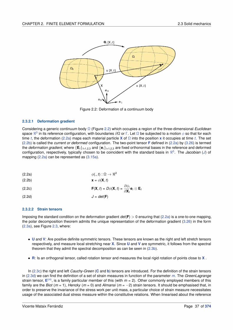
CHAPTER 2. FINITE ELEMENT FORMULATION 2.3 Solid mechanics
Figure 2.2: Deformation of a continuum body
2.3.2.1 Deformation gradient
Considering a generic continuum body Ω (Figure 2.2) which occupies a region of the three-dimensional Euclideanspace ℜ3 in its reference configuration, with boundaries ∂Ω or Γ. Let Ω be subjected to a motion φ so that for eachtime t , the deformation (2.2a) maps each material particle X of Ω into the position x it occupies at time t . The set(2.2b) is called the current or deformed configuration. The two-point tensor F defined in (2.2a) by (3.26) is termedthe deformation gradient, where EII=1,2,3 and eii=1,2,3 are fixed orthonormal bases in the reference and deformedconfiguration, respectively, typically chosen to be coincident with the standard basis in ℜ3. The Jacobian (J) ofmapping (2.2a) can be represented as (3.15a).
φ(., t) : Ω → ℜ3(2.2a)
x = φ(X, t)(2.2b)
F(X, t) = Dφ(X, t) =∂φi
∂XIei ⊗ EI(2.2c)
J = det(F)(2.2d)
2.3.2.2 Strain tensors
Imposing the standard condition on the deformation gradient det(F) > 0 ensuring that (2.2a) is a one-to-one mapping,the polar decomposition theorem admits the unique representation of the deformation gradient (3.26) in the form(2.3a), see Figure 2.3, where:
• U and V: Are positive definite symmetric tensors. These tensors are known as the right and left stretch tensorsrespectively, and measure local stretching near X. Since U and V are symmetric, it follows from the spectraltheorem that they admit the spectral decomposition as can be seen in (2.3b).
• R: Is an orthogonal tensor, called rotation tensor and measures the local rigid rotation of points close to X .
In (2.3c) the right and left Cauchy-Green (C and b) tensors are introduced. For the definition of the strain tensorsin (2.3d) we can find the definition of a set of strain measures in function of the parameter m. The GreenLagrangestrain tensor, E(m), is a family particular member of this (with m = 2). Other commonly employed members of thisfamily are the Biot (m = 1), Hencky (m = 0) and Almansi (m = −2) strain tensors. It should be emphasised that, inorder to preserve the invariance of the stress work per unit mass, a particular choice of strain measure necessitatesusage of the associated dual stress measure within the constitutive relations. When linearised about the reference
Vicente Mataix Ferrándiz Page 37 of 374

2.4 Finite Element formulation for CSD CHAPTER 2. FINITE ELEMENT FORMULATION
Figure 2.3: Polar decomposition of F
state, all strain measures give the standard small strain tensor.
F = R · U = V · R(2.3a)
U =3∑
i=1
λi li ⊗ li , V =3∑
i=1
λiei ⊗ ei , li = Rei(2.3b)
C = FT · F = U2, b = F · FT = V2(2.3c)
E(m) =
1m (Um − I) m 6= 0
ln(U) m = 0(2.3d)
Equivalently, in terms it spectral decomposition can be reformulated as (2.3e).
(2.3e)
E(m) =∑3
i=1 f (λi )li ⊗ li
f (λi ) =
1m
(λm
i − 1)
m 6= 0
ln(λi ) m = 0
We add to the former that all these strain tensors (E(m)) for any strain measure can be transformed between themin considering the push-forward (φ∗) and pull-back (φ∗) operations. This operation just requires, in addition to thegiven strain tensor in a given strain measure, the deformation gradient (F). For example, using the push-forward wecan transform the Green-Lagrange strain tensor into the Almansi strain tensor. With the pull-back operation, we canproceed in the opposite direction, from Almansi to Green-Lagrange. For more information about the procedure, weaddress to a dedicated Appendix section A.1.Pull-Back, Push-Forward fundamental concepts where the operation isdetailed.
2.4 Finite Element formulation for CSD
2.4.1 Weak formulation in solids
Here we introduce a summarise of the Galerkin method[OnlGal] for the deduction of the weak formulation, using asmain reference the work of Zienkiewicz[BookZZT13]. The deduction can be followed in (2.4).
Page 38 of 374 Vicente Mataix Ferrándiz

CHAPTER 2. FINITE ELEMENT FORMULATION 2.4 Finite Element formulation for CSD
First we divide the domain Ω in subdomains Ωe (elements), as well as the boundary Γ, (2.4a). In the following wewill represent the discrete form of the former continuous expressions as .
(2.4a)
Ω ≈ Ω =∑
e Ωe
Γ ≈ Γ =∑
e Γe =∑
et Γte (Neumann) +∑
eu Γue (Dirichlet)
For the displacement (u) we consider an approximation employing the shape functions (Nb) corresponding to theelements considered in our formulation, (2.4b).
(2.4b) u(ξ, t) = u =∑
b
Nb(ξ)ub(t) = N(ξ)u(t)
With the shape forms we can define the derivatives, needed to define the strain matrix (B), (2.4c). This matrix isnecessary in order to formulate the strain-displacement equation ε = Bu.
(2.4c) B =∂Na
∂ξ i=∂xj
∂ξ i
∂Na
∂xj, and in matrix form
∂Na
∂ξ= J
∂Na
∂x
Finally, the weak form of the equilibrium’s equation can be expressed as (2.4d). In this case we include thedynamic effects in order to be a proper CSD. For that we will consider the respective velocity u and acceleration u.The damping coefficient will be simplified with the parameter c, a better alternative will be shown at 2.4.5.Dampingmatrix. In here the body forces (b) as well as the external forces (t) are taken into consideration.
(2.4d) δWe(u) = δuT
[∫
Ωe
NTρNdΩu +
∫
Ωe
NT cNdΩu +
∫
Ωe
BTσdΩ−∫
Ωe
NT bdΩ−∫
Γ
NT tdΓ
]
That can be expressed in a semi-discrete form from (2.4e). In here we can express the stress divergence orstress force term (P), the mass matrix (M), the damping matrix (C) and the resulting external forces (f). P includes theresulting internal forces of the system.
(2.4e) Mu + Cu + P(σ) = f
Where the former components can be expressed as (2.4f). In case of considering a linear problem, the stressdivergence (P) can be obtained directly with the stiffness matrix (K) and its displacements (u).
(2.4f)
M =∑
e
∫
ΩeNTρNdΩ
C =∑
e
∫
ΩeNT cNdΩ
P =∑
e
∫
ΩeBTσdΩ
For linear elasticity P(e)(σ) = K(e)u
f =∑
e
(∫
ΩeNT BdΩ +
∫
ΓteNT tdΓ
)
2.4.2 TL and UL formulation
Extending the previous section, here we introduce the two possible formulation for the mechanic problem, the UL andTL formulation[BookBel+14]. In the TL form the only variable which depends on the deformation is the nominal stress(P, see Table 2.1), that is, it is the only variable which varies with time. In the UL form the domain of the element (or
Vicente Mataix Ferrándiz Page 39 of 374

2.4 Finite Element formulation for CSD CHAPTER 2. FINITE ELEMENT FORMULATION
body), the spatial derivatives ∂NI/∂xi and the Cauchy stress (σ) depends on the deformation, and hence on time,which complicates the derivation of the tangent stiffness.
(2.5a)
fint =∫
Ω0B0PdΩ0
KmatIJ =
∫
Ω0BT
0I
[CSE
]B0JdΩ0
KgeoIJ = I
∫
Ω0BT
0I [S] B0JdΩ0
(2.5b)
fint =∫
ΩBσdΩ
KmatIJ =
∫
ΩBT
I
[CσT
]BJdΩ
KgeoIJ = I
∫
ΩBT
I [σ] BJdΩ
The UL forms (2.5b) are generally easier to use than the TL forms (2.5a), since B is more easily constructed thanB0 and many material laws are developed in terms of rates of Cauchy stress (σ). The material stiffness in TL formcan be combined with the geometric stiffness in UL form or vice versa. In order to compute the material stiffnessmatrix (Kmat ), in addition to compute B for the TL and B0 for the UL, we need to compute the consistent constitutivetensor (C), CSE for TL and CσT for UL. The geometric stiffness matrix (Kgeo) depends on Second Piola-Kirchhoff
(PK2) (S) on the TL frame, but in the UL it depends on the Cauchy stress (σ). The element SPRISM (3.4.Prismaticsolid-shell) has been developed in TL formulation, but there is an intention to implement in UL as well.
The following, Table 2.1, will help to understand the different types stress measures and the possible transformationapplying the corresponding considering the push-forward (φ∗) and pull-back (φ∗) operations.
Cauchy stress σ Nominal stress P Second PK stress S Corotational Cauchy stress σ
σ= J−1F · P J−1F · S · FT JR · σ · RT
P= JF−1 · σ S · FT JU−1 · σ · RT
S= JF−1 · σF−T P · F−T JU−1 · σ · U−1
σ= RT · σ · R J−1U · P · R J−1U · S · U
τ= Jσ F · P F · S · FT JR · σ · RT
Table 2.1: Transformations of stresses. Source[BookBel+14]
2.4.3 Solution of the non-linear-equilibrium equations system
When we solve non-linear problems[BookOll14] we need to consider efficient methods designed for this purpose.This means the resolution of ∆ft+∆t
i = −J t+∆ti ·∆ut+∆t
i+1 , which can be carried basically by two kinds of methods, alinearisation based in the standard/modified Newton-Raphson (NR) technique or a Quasi-Newton approximationtechnique of the Jacobian matrix (J ). Both methods can be improved with the use of the convergence acceleratorsalgorithms. In the following we are going to present the NR method, the concept of line search, and the arc-lengthmethod.
2.4.3.1 Newton-Raphson method
This is the fastest convergence method to solve non-linear equations systems using the linearisation technique. Thistechnique assumes that the solution is convergent in the surroundings of it, being the convergence ratio in this casequadratic. Its solution comes from the inversion of the Jacobian operator (J ) from Equation (2.6). In our system ofequations J acts as the LHS.
(2.6) [∆u]t+∆ti+1 = −
[J t+∆t
i
]−1 · [∆f]t+∆ti
The advantages of the method can be listed as the followings:
• It always needs the tangent operator, which is not always easy to obtain, store and invert (for example in thecase of antisymmetric operators)
Page 40 of 374 Vicente Mataix Ferrándiz

CHAPTER 2. FINITE ELEMENT FORMULATION 2.4 Finite Element formulation for CSD
• The convergence velocity depends significantly on the initial guess solution
• The method can get stuck in a local minima, which could be difficult to leave afterwards
This will be the default strategy followed in our developments and problems. In the contact chapter, it will be shownthe strategies followed in order to adapt the NR strategy to the proper resolution of the contact problem.
2.4.3.2 Line-search
Zienkiewicz[BookZTF14] classifies this method in the category of convergence accelerators. The approach[BookZTF14]is based in the concept of the descent direction. This descent direction can be obtained applying different procedures,such the gradient descent, NR or quasi-Newton method. Independently of the approach, the method will proceed asthe following Algorithm 1.
Algorithm 1 Line-search
1: procedure Line-search2: Set iteration counter i = 0, and make an initial guess x0 for the minimum3: while (rhstotal > toleranceabs and ratio > tolerancerel ) and i < iterationmax do
4: Compute descent (or search) direction dx
5: Choose ηk (step size) to minimize the projection of the residual on the search direction: G(ηk ) = f (xk +ηk dx)6: Update xk+1 = xk + ηk dx
7: Update i = i + 1 and the RHS
This method is discarded, as cannot be used, at least without additional considerations, for CCM. We will thenfocus on the other two methods. In general, it is complex to consider convergence accelerators on contact problems,as the BC of the problem is continuously changing and this is troublesome for this kind of strategy.
2.4.3.3 Arc-length
Figure 2.4: Graphic representation of the arc-length method
Unstable behaviours[BookOll14] occur for various problems in structural mechanics, for which it is difficult to finda solution. To avoid this, a system of equilibrium equations with restrictions of type ∆f(u, u, u,λ) are usually used,where the magnitude of external force λfext is an unknown conditioned by an additional equation c(u,λ). The basicconcepts of the method are presented in (2.7) (see Figure 2.4).
Vicente Mataix Ferrándiz Page 41 of 374

2.4 Finite Element formulation for CSD CHAPTER 2. FINITE ELEMENT FORMULATION
Considering the following relations stating from the equilibrium equations (2.7a).
(2.7a)
(∂∆f
∂u
)
i
= Ji ,
(∂∆f
∂λ
)
i
= fext
It allows to rewrite the equilibrium equations as (2.7b).
(2.7b)
0 = ∆f (ui ,λi ) + Ji · δui+1 − fext · δλi+1
0 = c(u,λ)i+1
The displacement increment can be written as (2.7c), where umax is the total displacement with the last or maximalvalue of the external force and δu is the solution of the system of equations without correction and δλi+1 is the changeof the application factor of the load.
(2.7c) δui+1 = δui+1 + umaxi+1 δλi+1
(2.7d)
Ji · δui+1 = −[Mu + Cu + fint
i (u, u) − λi fext]
Ji · umax = fext
λi+1 = λi + δλi+1
With the basis developed previously (2.7) it is possible to implement different versions of the method. The versionimplemented in Kratos is based in different implementations from the literature[ArtFM93; ArtTL98; ArtCri83].
2.4.4 Time integration schemes
Taking the semi-discrete form of the dynamic principle, Equation (2.8), we obtain the equation governing the soliddynamics (CSD). We will express in this manner, instead of the proper residual form, Mu+Cu+LHSstatic
∆u = RHSstatic ,for being more illustrative showing the resulting structure when applying a certain time integration scheme.
(2.8) Mu + Cu + Ku + f = 0
We can now choose between the implicit and explicit approach, following[BookOll14] we can define them as thefollowing. If the response at current time depends completely from the solution in the current step then we are workingin a explicit solution, but in the other hand if the solution depends on velocity and the acceleration at current time, thenwe have an implicit solution. Considering the set of equations (2.9), which depend on the α parameter, then we cansay:
• Explicit: It states equilibrium at time t , with α = 0 (Forward Euler ). The displacement in next step is obtaineddepending on the velocity and displacement of the previous step. This methodology if simple in terms of structurerequires less memory storage, does not require expensive tangent operators, the algorithms obtained arereliable and it requires a very small time increment what it can be numerically expensive and unapproachable.
• Implicit: It formulates the equilibrium at time t + ∆t with α = 1 (Backward Euler ). The displacement in thenext step is obtained depending on the current time velocity and on the displacement of the previous step. Forthis approach the time increments can be much larger preserving stability, allows more precise solutions, butrequires the computation of the tangent operators (LHS) and large storage demand.
(2.9)
ut+∆t = ut + ∆tut+α∆t
ut+∆t = (1 − α)ut + αut+∆t
Page 42 of 374 Vicente Mataix Ferrándiz

CHAPTER 2. FINITE ELEMENT FORMULATION 2.4 Finite Element formulation for CSD
As we have said previously, the aim of this work will focus in an implicit solution; thus we need to discretise (2.8)with some temporal scheme, the ones that we present corresponds with the most extended in structural dynamics,the Newmark-β (2.4.4.1.Newmark time scheme) scheme, the Bossak scheme (2.4.4.2.Bossak algorithm) and theα-generalised (2.4.4.3.α-generalised). For additional literature related with structural dynamics, and in particularCSD, we recommend to consult the bibliography[BookCP12; BookOll14; BookRR12], where alternative schemes areexplained, and the stability and convergence of each one is deduced.
2.4.4.1 Newmark time scheme
Below with one step method employing Newmark schema we obtain (2.10).
(2.10)
(c3M + c2C + c1K)un+1 + fn+1 = 0
un+1 = un + ∆tun +(
12 − β
)∆t2un + β∆t2un+1
un+1 = un + (1 − γ)∆tun + γ∆tun+1
Where the coefficients of the scheme are c1 = 1, c2 = γβ∆t and c3 = 1
β∆t2 .
2.4.4.2 Bossak algorithm
The Kratos framework uses the Bossak [ArtWBZ80] algorithm by default for the time integration. This method is basedin the Newmark method, introducing additional parameters to dissipate spurious oscillations in the high frequencies.The parameters introduced modify the form of the equilibrium equation including an averaging process between thecurrent and the old-time station so to preserve the consistency requirements. The only variation respect Newmark isin the equilibrium equation (2.11).
(2.11) Mun+1−αB + Cun+1 + Kun+1 + f = 0
Where −13 < αB < 0, considering the Newmark parameters defined as γ = 1
2 − αB and β = (1−αB )2
4 . If αB = 0 weobtain the Newmark scheme unconditionally stable. The Bossak method present some implementation advantagesfor non-linear problems, owing to that the mass matrix is constant on Lagrangian meshes.
2.4.4.3 α-generalised
The α-generalised (Chung[ArtCH93]) is the generalisation of the time integration schemes, being the Newmark andBossak particular versions of him. In this case the method involves a modification of the equilibrium equation, with theαf the damping and elastic forces are taken into a linear combination and with αm the inertial forces are modified.With αm = αf = 0 the method obtained corresponds with Newmark. The expression of the method is presented in(2.12).
The equations from (2.10) corresponding to un+1 and un+1 remain exactly the same, except that the value theNewmark constants which are γ = 1
2 + αm − αf and β ≥ 14 + 1
2 (αf − αm) for an unconditionally stable solution.
(2.12a) Mun+1−αm + Cun+1−αf + Kun+1−αf + f = 0
Where each component of the displacement and its derivatives is calculated as:
(2.12b)
un+1−αm = (1 − αf )un+1 + αf un
un+1−αf = (1 − αm)un+1 + αmun
un+1−αf = (1 − αm)un+1 + αmun
Vicente Mataix Ferrándiz Page 43 of 374

2.4 Finite Element formulation for CSD CHAPTER 2. FINITE ELEMENT FORMULATION
2.4.4.4 BDF
The BDF is a family of implicit methods for numerical integration of ODE, originally proposed by Curtiss[ArtCH52].This family of methods is commonly used in stiff 3 ODE. Despite the method can be applied to any type of ODE, ifapplied directly to the Newton’s second laws we can obtain the following (2.13) for the BDF1 (backward Euler method)and BDF2 schemes.
The general formula of the BDF, for a variable depending on time, can be written as:
(2.13a)
dydt
= f (t , y ), y (t0) = y0
s∑
k=0
ak yn+k = ∆tβf (tn+s, yn+s)
In here s corresponds with the desired order of the scheme, and ∆t with the time increment. The ak and β parametersare obtained via Lagrange interpolation polynomials in order to achieve O(h)s. The BDF1 and BDF2 coefficientscorrespond with:
(2.13b)BDF1: yn+1 − yn = ∆tf (tn+1, yn+1)
BDF2: yn+2 −4
3yn+1 +
1
3yn =
2
3∆tf (tn+2, yn+2)
Applying this to Newton’s second laws, we obtain and to our system of equations (LHS and RHS). The definition of un+1
depends on the BC of the problem, and can be deduced from (2.13b) or by means of a second-order approximationlike un+1 = un + ∆tun + ∆t2
2 un.
(2.13c)dydt
n+1
=s∑
i=0
bdfiyn+1−i
(2.13d) BDF1:
un+1 = 1∆t u
n+1 − 1∆t u
n
un+1 = 1∆t u
n+1 − 1∆t u
nBDF2:
un+1 = 32∆t u
n+1 − 2∆t u
n + 12∆t u
n−1
un+1 = 32∆t u
n+1 − 2∆t u
n + 12∆t u
n−1
(2.13e) BDF1:
LHS = K + 1∆t2 M + 1
∆t C
RHS = f − Mu − CuBDF2:
LHS = K + 94∆t2 M + 3
2∆t C
RHS = f − Mu − Cu
In addition, in case an adaptive time step (∆t) is considered we need to update the BDF coefficients. If consideringρ = ∆tn
∆tn+1, then:
(2.13f)
BDF1: bdf0 =ρ
∆t, bdf1 = − ρ
∆t
BDF2: tcoeff =1
∆t + ∆tρ, bdf0 = tcoeff (ρ
2 + 2ρ), bdf1 = −tcoeff (ρ2 + 2ρ + 1), bdf2 = tcoeff
2.4.5 Damping matrix
The damping matrix presented in (2.4e) depends on the damping coefficient (c) of the given element e, which isnot always available. Usually a critical-damping ratio respect the critical is considered (ξ). With this critical-dampingratio we can estimate the damping matrix. In order to do so we will consider the classical Lord Rayleigh[BookRay77]damping. In this formulation, the damping matrix (C) is assumed to be proportional to the mass (M) and stiffness (K)matrices as in Equation (2.14a).
(2.14a) C = ηM + δK
3ODE unstable unless a small time increment is taken into account.
Page 44 of 374 Vicente Mataix Ferrándiz

CHAPTER 2. FINITE ELEMENT FORMULATION 2.4 Finite Element formulation for CSD
Figure 2.5: Graphic representation of Rayleigh damping matrix
In here η is the mass-proportional damping coefficient and δ are the stiffness-proportional damping coefficient. Takinginto consideration that the properties of the modal equations and the orthogonality conditions, we can express (2.14a)as (2.14b).
(2.14b) ξn =1
2ωnη +
ωn
2δ
In this expression we have the relationship between the n critical-damping ratio and the n natural frequency. Consider-ing two different natural frequencies, we can define a system of equations such as:
(2.14c)
[ξi
ξj
]
=1
2
[1ωi
ωi1ωj
ωj
] [ηδ
]
If damping for both frequencies is set to be equal, then the conditions associated with the proportionality factors canbe simplified as:
(2.14d) ξi = ξj = ξ therefore δ =2ξ
ωi + ωjand η = ωiωjδ
Vicente Mataix Ferrándiz Page 45 of 374

2.4 Finite Element formulation for CSD CHAPTER 2. FINITE ELEMENT FORMULATION
Page 46 of 374 Vicente Mataix Ferrándiz

BIBLIOGRAPHY BIBLIOGRAPHY
Bibliography
Books
[BookBel+14] Nonlinear Finite Elements for Continua and Structures. Ted Belytschko, Wing Kam Liu,Brian Moran, and Khalil Elkhodary. Wiley. 2nd ed. 2014.
[BookBHS07] Encyclopedia of Computational Mechanics (3 Volume Set). René de Borst, T.J.R. Hughes, andErwin Stein. Wiley. 1st ed. 2007.
[BookBor+12] Nonlinear Finite Element Analysis of Solids and Structures, 2nd edition. René de Borst,Mike A. Crisfield, Joris J. C. Remmers, and Clemens V. Verhoosel. Wiley. 2nd Edition. 2012.
[BookCP12] Dynamics of Structures. Ray W. Clough and Joseph Penzien. McGraw-Hill. 3rd ed. 2012. P. 752.
[BookFin13] The method of weighted residuals and variational principles. Bruce A Finlayson. Siam. 2013.
[BookLL92] Numerical methods for conservation laws. Randall J LeVeque and Randall J Leveque. Springer.1992.
[BookNPO09] Computational Methods for Plasticity Theory and Applications. E. A. de Souza Neto, D. Periæ, andD.R.J. Owen. Wiley. 2009.
[BookOll14] Nonlinear Dynamics of Structures. Sergio Oller. Springer International Publishing. 2014.
[BookRay77] Theory of Sound. Lord Rayleigh. 1877. P. 93.
[BookRR12] Elements of Structural Dynamics: A New Perspective. G. Visweswara Rao and Debasish Roy. 2012.
[BookWri08] Nonlinear finite element methods. Peter Wriggers. Springer. 1st ed. 2008.
[BookZTF14] The Finite Element Method for Solid and Structural Mechanics. O. C. Zienkiewicz, Robert L. Taylor,and David Fox. Butterworth-Heinemann. 7th ed. 2014.
[BookZZT13] The Finite Element Method: its Basis and Fundamentals. O. C. Zienkiewicz, J.Z. Zhu, andRobert L. Taylor. Butterworth-Heinemann. 7th ed. 2013.
Articles
[ArtCGP06] “High order finite volume schemes based on reconstruction of states for solving hyperbolic systemswith nonconservative products. Applications to shallow-water systems”. Manuel Castro,José Gallardo, and Carlos Parés. In: Mathematics of computation. No. 255, Vol. 75, 2006,pp. 1103–1134. DOI: 10.1090/s0025-5718-06-01851-5.
[ArtCH52] “Integration of stiff equations”. CF Curtiss and Joseph O Hirschfelder. In: Proceedings of theNational Academy of Sciences of the United States of America. No. 3, Vol. 38, 1952, p. 235.National Academy of Sciences. DOI: 10.1073/pnas.38.3.235.
[ArtCH93] “A time integration algorithm for structural dynamics with improved numerical dissipation: thegeneralized-α method”. Jintai Chung and GM Hulbert. In: Journal of applied mechanics. No. 2, Vol.60, 1993, pp. 371–375. American Society of Mechanical Engineers. DOI: 10.1115/1.2900803.
[ArtClo60] “The finite element method in plane stress analysis”. Ray W Clough. In: Proceedings of 2nd ASCEConference on Electronic Computation, Pittsburgh Pa., Sept. 8 and 9, 1960. 1960,
Vicente Mataix Ferrándiz Page 47 of 374

ONLINE RESOURCES BIBLIOGRAPHY
[ArtCri83] “An arc-length method including line searches and accelerations”. M. A. Crisfield. In: InternationalJournal for Numerical Methods in Engineering. No. 9, Vol. 19, 1983, pp. 1269–1289. John Wiley &Sons, Ltd. DOI: 10.1002/nme.1620190902.
[ArtFM93] “Geometrical interpretation of the arc-length method”. M. Fafard and B. Massicotte. In: Computers& Structures. No. 4, Vol. 46, 1993, pp. 603–615. DOI: 10.1016/0045-7949(93)90389-u.
[ArtGal15] “Series solution of some problems of elastic equilibrium of rods and plates”.Boris Grigoryevich Galerkin. In: Vestn. Inzh. Tekh. Vol. 19, 1915, pp. 897–908.
[ArtPom69] “K. Washizu, Variational Methods in Elasticity and Plasticity.(International Series of Monographs inAeronautics and Astronautics). X+ 348 S. m. Fig. Oxford/London/Edinburgh/NewYork/Toronto/Sydney/Paris/Braunschweig 1968. Preis geb. 120 s. net”. W Pompe. In:ZAMM-Journal of Applied Mathematics and Mechanics/Zeitschrift für Angewandte Mathematik undMechanik . No. 5, Vol. 49, 1969, pp. 319–319. Wiley Online Library. DOI:10.1002/zamm.19690490535.
[ArtRic11] “IX. The approximate arithmetical solution by finite differences of physical problems involvingdifferential equations, with an application to the stresses in a masonry dam”. Lewis Fry Richardson.In: Philosophical Transactions of the Royal Society of London. Series A, Containing Papers of aMathematical or Physical Character . No. 459-470, Vol. 210, 1911, pp. 307–357. The Royal SocietyLondon.
[ArtTL98] “A user-controlled arc-length method for convergence to predefined deformation states”. J. G. Tengand Y. F. Luo. In: Communications in Numerical Methods in Engineering. No. 1, Vol. 14, 1998,pp. 51–58. John Wiley & Sons, Ltd. DOI:10.1002/(sici)1099-0887(199801)14:1<51::aid-cnm130>3.0.co;2-l.
[ArtTur56] “Stiffness and deflection analysis of complex structures”. MJ Turner. In: journal of the AeronauticalSciences. No. 9, Vol. 23, 1956, pp. 805–823. DOI: 10.2514/8.3664.
[ArtWBZ80] “An alpha modification of Newmark’s method”. WL Wood, M Bossak, and OC Zienkiewicz. In:International Journal for Numerical Methods in Engineering. No. 10, Vol. 15, 1980, pp. 1562–1566.Wiley Online Library. DOI: 10.1002/nme.1620151011.
Online resources
[OnlFin] Wikipedia. Finite strain theory. URL:http://en.wikipedia.org/wiki/Finite_strain_theory.
[OnlGal] Wikipedia. Galerkin method. URL: http://en.wikipedia.org/wiki/Galerkin_method.
[OnlWol] Mathematica, Version 11.3. Wolfram Research Inc.
Page 48 of 374 Vicente Mataix Ferrándiz

CHAPTER 3. ROTATION-FREE SHELLS AND SOLID-SHELL ELEMENTS
Chapter 3
Rotation-free shells and solid-shell
elements
Things should be described assimply as possible, but no simpler.
Albert Einstein(1879 - 1955 AD, German-born
theoretical physicist)
3.1 Introduction
In first place we will introduce a simple historical outline in the shell theory. This will be extended in the state-of-the-artsection (3.2.State of the Art in shell formulation), the current state of the standard shell theory. The theories relative torotation-free formulation will be introduced in its respective sections.
In the following sections, we will introduce the element solid-shell developed to tackle the main aim of this work,the prismatic solid-shell element. This element has some resemblance with a previous work, the Enhanced Basic
Shell Triangle (EBST) element, a rotation-free shell, which considers the neighbour elements with the objective ofenrich quadratically the in-plane behaviour.
For that reason we will introduce in first place the rotation-free elements (3.3.Rotation-free shells), and later on wewill present the prismatic solid-shell element (3.4.Prismatic solid-shell). The examples of performance of the prismaticsolid-shell element can be found in the section concluding this chapter to this one, 3.5.Numerical examples.
3.1.1 Historical outline
The base of the shell theories can be found in the plate theory. This theory takes a similar approach to the beamtheory applied in thin geometries. The classic thin plate theory establishes that the normal remains straight andorthogonal to the middle plane after deformation[BookOña13]. This theory is based in the postulates presented inthe original work of Kirchoff in 1850[ArtKir50], despite some people associate this theory to some previous worksby Marie Sophie Germain[BookBD80; BookBD12] in 1811. We have some analytical solutions for this theory forrectangular plates, as the one presented by Navier in 1820. In here Naviernavier1820memoire introduced a simplemethod for finding the displacement and stress when a plate is simply supported. The idea was to express theapplied load in terms of Fourier components, find the solution for a sinusoidal load (a single Fourier component),and then superimpose the Fourier components to get the solution for an arbitrary load. Another analytical solutionwas proposed by Lévy [ArtLev99] in 1899, where the main difference with the Navier solution consists in start with an
Vicente Mataix Ferrándiz Page 49 of 374

3.2 State of the Art in shell formulation CHAPTER 3. ROTATION-FREE SHELLS AND SOLID-SHELL ELEMENTS
assumed form of the displacement and try to fit the parameters so that the governing equation and the boundaryconditions are satisfied.
An evolution to this theory, which can be applied to thick plates, is the thick plate theory proposed by Reiss-ner [ArtRei45] and Mindlin[ArtMin51]. This theory assumes that normals remain straight, though not necessarilyorthogonal to the middle plane after deformation. These two theories are complementary, and it is relevant to knowwhen to choose between them depending on the relative thickness of the element (usually we consider as thinelements when thickness
average side ≤ 110 ).
The shell theory will be therefore an extension of the previous postulates, but applied to non-planar sur-faces[BookOña13]. The non-coplanarity introduces membrane behaviour (axial force) in addition to the plateflexural resistance (bending and shear forces). The governing equations of a curved shell (equilibrium and kinematicequations, etc.) are more complex[BookKra67; ArtNio85; ArtNoo90a; BookTW59; ArtNoo90b] than in the case ofplates, mainly due to the curvature of the middle surface. This theory is introduced in first place by Love[ArtLov88] in1888, applied only for thin shells. This short introduction to the history of shell theory will be expanded in the shellstate-of-the-art section at 3.2.State of the Art in shell formulation, where some of these standard shell models will bepresented.
3.2 State of the Art in shell formulation
3.2.1 Element requisites and stabilisation techniques
As it is presented in the book of Wriggers[BookWri08], but also in the work of Belytschko[BookBel+14], the targetproperties of any new element, extensible to shell elements are the following1:
a) Locking free behaviour for incompressible materials
b) Good bending performance
c) No locking in thin elements
d) No sensitivity against mesh distortions
e) Good coarse mesh accuracy,
f) Simple implementation of nonlinear constitutive equations
g) Efficiency (particularly relevant in explicit simulations)
In order to achieve this objective there are different techniques[BookWri08], here we present a short summarisesof the most relevant:
1. Reduced integration and stabilisation: Consist in the consideration of reduced number of integration points,with the corresponding reduction in the computational cost and memory, especially in explicit algorithms. Thismethodology was developed in order to avoid locking in case of incompressibility. The principle from whichderives this technique is the fact that reduced integration is associated with rank deficiency of the tangentmatrices, which is cured with the consideration of stabilisation techniques. Because of this these elements needthe choice of artificial stabilisation parameters. Its main advantages are:
• Locking free for incompressibility
• Good coarse mesh accuracy
• Not sensitive against mesh distortions
• Can be used for arbitrary constitutive equations
2. Hybrid or mixed variational principles: These elements include additional Degree Of Freedom (DOF)
in order to stabilise the formulation. The main disadvantage is the requirement of adapting the constitutiverelationships.
1As we will see the element developed in this work, 3.4.Prismatic solid-shell, enjoy these advantages.
Page 50 of 374 Vicente Mataix Ferrándiz

CHAPTER 3. ROTATION-FREE SHELLS AND SOLID-SHELL ELEMENTS 3.2 State of the Art in shell formulation
3. Enhanced strain elements based on the Hu-Washizu principle: Within the enhanced strain formulations,nonconforming strain measures are introduced within the Hu-Washizu principle[ArtWas82]. The main elementsdeveloped concerning this principle are the ones present in the work of Simo[ArtSF89; ArtSFR89; ArtSFR90;ArtSRF90; ArtSK92; ArtSRF92; ArtSim93]. These elements fulfil all points of the previously mentionedrequirement, therefore they are well suited for all applications. Additionally these methods have been proven tobe efficient in order to overcome the hour glassing effect. This method includes techniques such as EAS andAssumed Normal Strain (ANS).
4. Mixed variational principles for problems with rotational DOF: In here the momentum and moment ofmomentum are weakly enforced. This leads to the symmetry of the stress tensor and therefore the rotationalDOF can be introduced as independent field variables.
5. Composite or macro elements: Here elements are constructed from subelements, which use simplified orspecial shape functions.
6. Higher order displacement elements: This technique consists in the consideration of higher order geometriesas quadratic or cubic, or even hierarchical shape functions using polynomials or Non-Uniform Rational B-
spline (NURB). In fact, this last option allows a more efficient formulation, being competitive with the otherapproaches.
In Wriggers[BookWri08], some other techniques are mentioned, such as nodal based elements or Cosserat pointelements.
3.2.2 Shell formulations
We can differentiate three different approaches[BookOña13] for the definition of a shell theory:
1. Classical shell theories: These formulations can be found summarised in several sources[BookNov59; Art-Nio85; BookWem82; BookGou12; BookCal89]. We can mention particularly the Discrete-Kirchhoff assumptions,as an extensively used methodology[ArtWOK68; ArtWem69; ArtDha69; ArtDha70; ArtDMM86; ArtMG86].
2. 3D elements of small thickness: This one it is not practical as it requires the consideration of very smallelements in order to avoid the ill-conditioning coming from a slender aspect ratio of the shell geometry.
3. Shell elements by degeneration of solid elements: These formulations, aka Degenerated Shell (DS),comes from the concept of enforcing the shell theory assumptions into the general 3D elasticity[ArtAIZ70]. Thisdenomination can be misleading and it is often used in order to differentiate the formulation from curved shellelements derived from standard shell theory. This kind of elements have enjoyed a lot of popularity, and severalauthors have significant contributions in this formulation[BookBD90; ArtPar79; ArtKan79; ArtHL81; ArtFV82].These kinds of elements, as a generalisation of the ReissnerMindlin shell theory suffer of membrane locking andtherefore require of some kind of stabilisation as the ones presented in 3.2.1.Element requisites and stabilisationtechniques, particularly reduced integration or assumed strain fields. The main difference between the DS andthe standard formulation is that in the case of the DS the Principle of Virtual Work (PVW) is written in termsof stresses and strains, as in solid elements, and the integrals are computed in the volume.
• Continuum-Based Resultant (CBR) shell theory: This theory introduces simplifications in DS elements,so that the PVW can be expressed in terms of resultant stresses and generalised strains, therefore theintegrals can be computed over the shell surface only. It exists a variation of this formulation called CBR-S,whereas an assumption we eliminate the z-dependence in the surface Jacobian (J).
Buechter and Ramm[ArtBR92] have compared between degenerated shell elements and those based on standardReissner-Mindlin/Naghdi type shell theory. In this work, they highlight the standard shell for practical purposes astheir formulation is generally simpler.
In addition, it is relevant to highlight the so-called . As mentioned in the stabilisation techniques in 3.2.1.Elementrequisites and stabilisation techniques, this methodology consists in the consideration of the same basis functions forrepresenting the geometry in CAD, like the NURB[BookHug+14; BookFHK02; BookPT97; BookRog00]. Thanks tothis, the FE analysis works on a geometrically exact model and no meshing is necessary[BookHBC09; ArtBen+10;ArtHCB05].
Vicente Mataix Ferrándiz Page 51 of 374

3.3 Rotation-free shells CHAPTER 3. ROTATION-FREE SHELLS AND SOLID-SHELL ELEMENTS
3.3 Rotation-free shells
3.3.1 Introduction
The next section introduces the rotation-free plates and shells developed in the last years by Eugenio Oñate etal.[ArtOF05; ArtFO05; ArtFO01; ArtOZ00; ArtFO11]; that despite the modifications and improvements realised inall this time, the principle is the same, a plate/shell that just consider displacement as degree of freedom in thenodes.
The traditional Kirchoff theory is enough to describe the most common cases of plates and shells, but in the caseswhere a thick shells approach is interesting to be considered, some difficulties appear associated to the C12 continuity,and then just cases which need C0 continuity have been used; in this sense the rotation free theories have beenpresented as a very interesting alternative.
3.3.2 Basic Shell Triangle
3.3.2.1 Basics
Let us consider a patch of four three node triangles from Figure 3.1a, where the main triangle corresponds with theone with the nodes marked with circles, and the external ones the marked with squares. To develop the formulationwe assume a constant curvature field, then the deflection is interpolated linearly in a standard finite element manneras (3.1a), and then calling the curvatures as (3.1b).
1
23
4
56
M
1
2 3
2 3
1
(a) Patch of three nodes triangular elements including thecentral triangle (M) and three adjacent triangles (1, 2 and 3)
1 2
3 45
6
η
ξ
. ..
GG
G
12
3
(b) Patch of elements in the isoparametric space
Figure 3.1: Patch of elements for Basic Shell Triangle (BST) and EBST
(3.1a) w =3∑
i=1
Lei we
i
Where Lei are the linear shape functions and we
i the nodal deflection of each node.
(3.1b) κ =
κxx
κyy
κxy
= κ
Where κ is the curvature vector and κ is the constant curvature field defined in (3.1c).
(3.1c) κ =1
AM
∫ ∫
AM
[
−∂2w∂x2
,−∂2w∂y2
,−2∂2w∂x∂y
]T
dA
Where AM is the area of the central triangle.
2The function f is said to be of (differentiability) class Ck if the derivatives f ′, f ′′, ..., f (k ) exist and are continuous (the continuity is implied bydifferentiability for all the derivatives except for f (k )).
Page 52 of 374 Vicente Mataix Ferrándiz

CHAPTER 3. ROTATION-FREE SHELLS AND SOLID-SHELL ELEMENTS 3.3 Rotation-free shells
3.3.2.2 Shell kinematics
Considering a shell of the initial thickness h0 and with an undeformable middle surface in Ω0 (ℜ3) with a boundary Γ0.The positions X and x of a point in the undeformed and the deformed configurations can be written as a function ofthe coordinates of the middle surface ϕ and the normal t3 at the point as (3.2a), where ξ and η are the curvilinearprincipal coordinates and ζ is the distance from the point to the middle surface in the undeformed configuration.
(3.2a)
X(ξ, η, ζ) = ϕ0(ξ, η) + λt03
x(ξ, η, ζ) = ϕ(ξ, η) + ζλt3
Defining λ as the parameter that relates the thickness at the present and initial configuration (3.2b).
(3.2b) λ =hh0
A convective system is computed at each point as (3.3).
(3.3)
gi (ζ) = ∂x∂ξi
i = 1, 2, 3
gα(ζ) = ∂(ϕ(ξ,η)+ζλt3)∂ξα
= ϕ′α + ζ(λt3)′α α = 1, 2
g3(ζ) = ∂(ϕ(ξ,η)+ζλt3)∂ζ = λt3
The curvatures of the middle surface are obtained by (3.4a).
(3.4a) καβ =1
2
(ϕ′α · t3′β + ϕ′β · t3′α
)= −t3 ·ϕ′αβ α,β = 1, 2
The deformation gradient tensor (F) is (3.4b).
(3.4b) F = [x′1, x′2, x′3] =[ϕ′1 + ζ(λt3)′1 ϕ′2 + ζ(λt3)′2 λt3
]
The product FT F = U2 = C (where U is the right stretch tensor, and C the right Cauchy-Green deformation tensor) canbe written as (3.4c).
(3.4c) U2 =
a11 + 2κ11ζλ a12 + 2κ12ζλ 0a12 + 2κ12ζλ a22 + 2κ22ζλ 0
0 0 λ2
→ if κ0ij = 0 →
a11 + 2χ11ζλ a12 + 2χ12ζλ 0a12 + 2χ12ζλ a22 + 2χ22ζλ 0
0 0 λ2
It is also useful to compute the eigendecomposition of U as (3.4d), where λα and rα are the eigenvalues andeigenvectors of U.
(3.4d) U =3∑
α=1
λαrα ⊗ rα
3.3.2.3 Constitutive models
For the constitutive model, we recommend to consult directly the literature[ArtOF05; ArtFO05; ArtFO01; ArtOZ00;ArtFO11]. It is possible to consider more than one constitutive model, and the ones presented in the references arefocused in cases where the objective is to calculate large strains of metal forming processes.
3.3.3 Enhanced Basic Shell Triangle
The following model corresponds with the enhanced version of the BST, called EBST, being the main features of thiselement:
• The geometry of the patch formed by the central element and the three adjacent elements is quadraticallyinterpolated from the position of the six nodes in the patch.
Vicente Mataix Ferrándiz Page 53 of 374

3.3 Rotation-free shells CHAPTER 3. ROTATION-FREE SHELLS AND SOLID-SHELL ELEMENTS
• Interpolated from the position of the six nodes in the patch. The membrane strains are assumed to vary linearlywithin the central triangle and are expressed in terms of the (continuous) values of the deformation gradient atthe mid-side points of the triangle.
• The assumed constant curvature field within the central triangle is obtained using now twice the values of the(continuous) deformation gradient at the mid-side points.
3.3.3.1 Total Lagrangian formulation
As mentioned above a quadratic approximation of the geometry of the four elements patch is chosen using the positionof the six nodes in the patch. It is useful to define the patch in the isoparametric space using the nodal positions givenin the Table 3.1 and Figure 3.1b. The quadratic interpolation is defined as (3.5a).
(3.5a) ϕ =6∑
i=1
Niϕi
(3.5b)N1 = ζ + ξη N4 = ζ
2 (ζ − 1)N2 = ξ + ηζ N5 = ξ
2 (ξ − 1)N3 = η + ζξ N6 = η
2 (η − 1)with ζ = 1 − ξ − η
The Cartesian derivatives are defined as (3.5c).
(3.5c)
[Ni ,1
Ni ,2
]
= J−1
[Ni ,ξ
Ni ,η
]
=
[ϕ0
′ξ · t1 ϕ0′η · t1
ϕ0′ξ · t1 ϕ0
′η · t2
] [Ni ,ξ
Ni ,η
]
1 2 3 4 5 6
ξ 0 1 0 1 -1 1η 0 0 1 1 1 -1
Table 3.1: Isoparametric coordinates of the six nodes in the patch of Figure 3.1b
3.3.3.1.1 Computation of the membrane strains :
We define the Green-Lagrange strains as (3.6a), and the virtual membrane strains as (3.6b). Differently from theoriginal BST element the membrane strains within the EBST element are now a function of the displacements of thesix patch nodes.
(3.6a) ǫm =3∑
i=1
1
2Ni
ϕi′1 ·ϕi
′1 − 1ϕi
′2 ·ϕi′2 − 1
2ϕi′1 ·ϕi
′2
(3.6b) δǫm =3∑
i=1
Ni
ϕi′1 · δ′1
i
ϕi′2 · δϕi
′2δϕi
′1 ·ϕi′2 + ϕi
′1 · δϕi′2
= Bmδa
p
3.3.3.1.2 Computation of the bending strains :
We employ the same curvature field assumed in the BST.
(3.7a) κ = 23∑
i=1
LMi ,1 00 LM
i ,2LM
i ,2 LMi ,1
[t3 ·ϕi
′1t3 ·ϕi
′2
]
Page 54 of 374 Vicente Mataix Ferrándiz

CHAPTER 3. ROTATION-FREE SHELLS AND SOLID-SHELL ELEMENTS 3.4 Prismatic solid-shell
The gradient is computed as (3.7b).
(3.7b)
[ϕi
′1ϕi
′2
]
=
[N i
1,1 N i2,1 N i
3,1 N ii+3,1
N i1,2 N i
2,2 N i3,2 N i
i+3,2
]
ϕ1
ϕ2
ϕ3
ϕi+3
Finally, the variation for curvature is (3.7c).
(3.7c)
δκ =23∑
i=1
LMi ,1 00 LM
i ,2LM
i ,2 LMi ,1
3∑
i=1
[N i
j ,1
(t3 · δuj
)
N ij ,2
(t3 · δuj
)
]
+
[N i
i+3,1
(t3 · δui+3
)
N ii+3,2
(t3 · δui+3
)
]
−3∑
i=1
(LM
i ,1ρ111 + LM
i ,2ρ11
)
(LM
i ,1ρ122 + LM
i ,2ρ22
)
(LM
i ,1ρ112 + LM
i ,2ρ12
)
(t3 · δui ) = Bbδap
3.3.3.1.3 Tangent stiffness matrix :
The tangent stiffness matrix is divided into material and geometric components. Being the material tangent matrixthe one showed in (3.8a), and the geometric tangent matrix the one from (3.8b).
Material stiffness matrix:
(3.8a) KM =
∫ ∫
A0M
BT DepBdA where B = Bm + Bb
Geometric stiffness matrix:
(3.8b) KG = KGm + KG
b
Where:
(3.8c) δuT KGm∆u =
AM
3
3∑
k=1
6∑
i=1
6∑
j=1
δui[
Nki ,1 Nk
i ,2
][
Nk11 Nk
12Nk
21 Nk22
] [Nk
j ,1
Nkj ,2
]
∆uj
with Nij = σmij
Numerical experiments[ArtFO05; ArtFO11] have shown that the bending part of the geometric stiffness is not soimportant and can be disregarded in the iterative process.
3.4 Prismatic solid-shell
3.4.1 Introduction
Solid-shells have been during the last fifteen years[ArtDB84; ArtHS98; ArtHSD00; ArtHau+01; ArtSou+05; ArtKGW06a;ArtPar+06] an important improvement in the shells simulations, providing reliable simulations and avoiding the prob-lematic that is associated to the kinematics hypothesis and plane stress constitutive laws related to the use of theshell element (or any kind of bidimensional elements as plates and membranes). The main advantages when usingsolid-shell elements are:
a) General 3D constitutive relations
b) Large transverse shear can be considered, and considering additional elements along the thickness improvethis behaviour
c) There does not need to consider transitions between solid and shell elements (all the elements are solids)
d) Contact forces can be introduced directly in the geometry and in a realistic way without any additional technique,which is especially important for the consideration of friction
Vicente Mataix Ferrándiz Page 55 of 374

3.4 Prismatic solid-shell CHAPTER 3. ROTATION-FREE SHELLS AND SOLID-SHELL ELEMENTS
e) The element is rotation-free, avoiding the storage and computation of these variables
f) In the case where we have non-parallel boundaries this can be modelled correctly
For the consideration of strongly non-linear problems, problems where the contact-friction, large deformationsand complex constitutive laws are considered, the use of low interpolation order elements is preferred. Most of theexisting solid-shells are linear hexahedron[ArtDB84; ArtHS98; ArtHSD00; ArtHau+01; ArtSou+05; ArtKGW06a;ArtPar+06; ArtSVR11; ArtAC09; ArtSAV11; ArtSR11; ArtSen+16] (usually trilinear 8-node brick), which have two maindisadvantages; the first one is the hourglass effect, which is called this way due to the characteristics shapes adoptedin the proper modes and a stabilisation is required to reduce these problems; the second problematic is the meshingof the plane, due to the fact that meshing quadrilateral is less performant than triangles. For this reasons the triangularprisms (wedges) could be considered an interesting alternative, especially for the second problem mentioned, but thiskind of geometry is not exempt of problematic, owing to the low order of interpolation of the geometry, when a lineartriangular prism is considered. This last problem can be solved with the consideration of the neighbours elements3, inconsequence the element becomes quadratic in the plane solving this last problem.
In addition to this, it is well known that low interpolation order elements in the standard displacement formulation(in contract to the mixed formulation) in the consideration of slender structures and incompressible materials suffersevere locking effects. The transverse shear locking provokes problems in the bending behaviour, especially whenmore slender is the element. The membrane locking appears especially in the initially curved shells when bending ispreponderant without middle surface stretching. A curvature thickness locking can appear in problems with initiallycurved geometry due to artificial transverse strains and stresses under pure bending. Finally, the volumetric lockingcan appear when the material present an incompressible, nearly incompressible behaviour or elastic-plastic materialswith isochoric plastic flow (typical in metals).
The element has been implemented into Kratos[OnlKra], the in-home FEM-Multiphysics open-source code,implemented in C++ with parallelisation capabilities. The pre/post-process of all the presented examples haven beenprocessed with GiD[OnlMel+16], the CIMNE software for pre and post processing.
3.4.2 Basic kinematics of the standard element
We can find the standard isoparametric interpolations for the linear 6-node triangular prism (or wedge) in (3.9), whereXI , xI and uI correspond with the original coordinates (or undeformed configuration), the current coordinates (ordeformed configuration) and the displacements in the node I respectively.
(3.9a) X(ξ) =6∑
I=1
N I(ξ)XI
(3.9b) x(ξ) =6∑
I=1
N I(ξ)xI =6∑
I=1
(XI + uI
)
The shape function N I(ξ) from (3.10) are defined in function of the local coordinates (ξ, η, ζ), where the tho firstdefine the position in the plane of the triangular base and the third one corresponds with the coordinate along theprism axis.
(3.10a)N1 = zL1, N2 = ξL1, N3 = ηL1
N4 = zL2, N5 = ξL2, N3 = ηL2
In this definition the third triangular coordinate and the axis interpolation is defined as:
(3.10b) z = 1 − ξ − η, L1 = 12 (1 − ζ), L2 = 1
2 (1 + ζ)
3Like in the EBST elements, see 3.3.Rotation-free shells.
Page 56 of 374 Vicente Mataix Ferrándiz
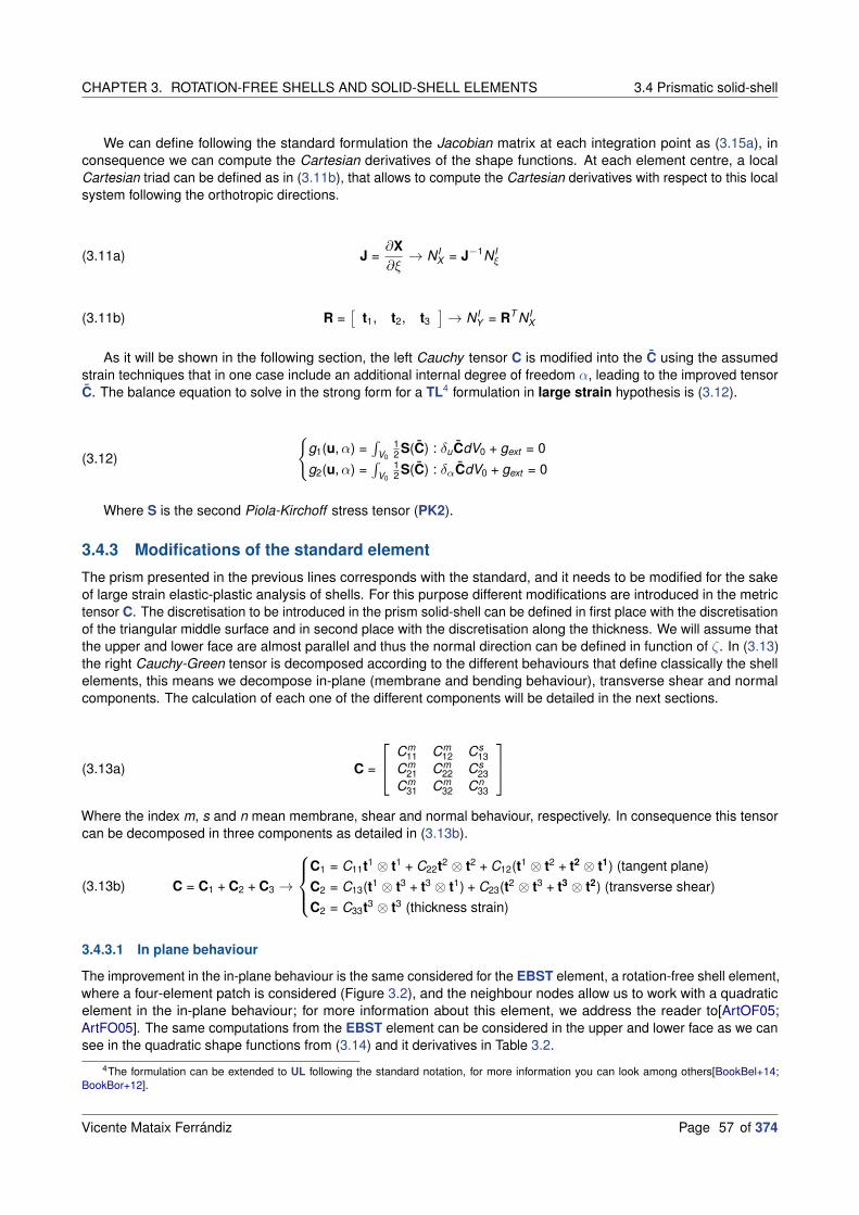
CHAPTER 3. ROTATION-FREE SHELLS AND SOLID-SHELL ELEMENTS 3.4 Prismatic solid-shell
We can define following the standard formulation the Jacobian matrix at each integration point as (3.15a), inconsequence we can compute the Cartesian derivatives of the shape functions. At each element centre, a localCartesian triad can be defined as in (3.11b), that allows to compute the Cartesian derivatives with respect to this localsystem following the orthotropic directions.
(3.11a) J =∂X
∂ξ→ N I
X = J−1N Iξ
(3.11b) R =[
t1, t2, t3
]→ N I
Y = RT N IX
As it will be shown in the following section, the left Cauchy tensor C is modified into the C using the assumedstrain techniques that in one case include an additional internal degree of freedom α, leading to the improved tensorC. The balance equation to solve in the strong form for a TL4 formulation in large strain hypothesis is (3.12).
(3.12)
g1(u,α) =∫
V0
12 S(C) : δuCdV0 + gext = 0
g2(u,α) =∫
V0
12 S(C) : δαCdV0 + gext = 0
Where S is the second Piola-Kirchoff stress tensor (PK2).
3.4.3 Modifications of the standard element
The prism presented in the previous lines corresponds with the standard, and it needs to be modified for the sakeof large strain elastic-plastic analysis of shells. For this purpose different modifications are introduced in the metrictensor C. The discretisation to be introduced in the prism solid-shell can be defined in first place with the discretisationof the triangular middle surface and in second place with the discretisation along the thickness. We will assume thatthe upper and lower face are almost parallel and thus the normal direction can be defined in function of ζ. In (3.13)the right Cauchy-Green tensor is decomposed according to the different behaviours that define classically the shellelements, this means we decompose in-plane (membrane and bending behaviour), transverse shear and normalcomponents. The calculation of each one of the different components will be detailed in the next sections.
(3.13a) C =
Cm11 Cm
12 Cs13
Cm21 Cm
22 Cs23
Cm31 Cm
32 Cn33
Where the index m, s and n mean membrane, shear and normal behaviour, respectively. In consequence this tensorcan be decomposed in three components as detailed in (3.13b).
(3.13b) C = C1 + C2 + C3 →
C1 = C11t1 ⊗ t1 + C22t2 ⊗ t2 + C12(t1 ⊗ t2 + t2 ⊗ t1) (tangent plane)
C2 = C13(t1 ⊗ t3 + t3 ⊗ t1) + C23(t2 ⊗ t3 + t3 ⊗ t2) (transverse shear)
C2 = C33t3 ⊗ t3 (thickness strain)
3.4.3.1 In plane behaviour
The improvement in the in-plane behaviour is the same considered for the EBST element, a rotation-free shell element,where a four-element patch is considered (Figure 3.2), and the neighbour nodes allow us to work with a quadraticelement in the in-plane behaviour; for more information about this element, we address the reader to[ArtOF05;ArtFO05]. The same computations from the EBST element can be considered in the upper and lower face as we cansee in the quadratic shape functions from (3.14) and it derivatives in Table 3.2.
4The formulation can be extended to UL following the standard notation, for more information you can look among others[BookBel+14;BookBor+12].
Vicente Mataix Ferrándiz Page 57 of 374

3.4 Prismatic solid-shell CHAPTER 3. ROTATION-FREE SHELLS AND SOLID-SHELL ELEMENTS
1 2
3 78
9
(a) 2D (b) 3D
Figure 3.2: Patch performed in the element considering the neighbour elements
(3.14)N1 = (z + ξη), N7 = z
2 (z − 1),N2 = (ξ + ηz), N8 = ξ
2 (ξ − 1),N3 = (η + zξ), N9 = η
2 (η − 1)
We define a local system of coordinates from (3.11b) taking as reference the components f1 and f2 in the tangentplane and f3 in the normal. In each mid-side point of the element, we compute the in-plane Jacobian as shown in(3.15a).
(3.15a) J =
[Xξ · t1 Xη · t1
Xξ · t2 Xη · t2
]
And in combination of the shape function derivatives we can compute the Cartesian derivatives in (3.15b).
(3.15b)
[N I
1N I
2
]K
= J−1K
[N Iξ
N Iη
]K
With the Cartesian derivatives, we can calculate the in-plane deformation gradient components fK1 and fK
2 , andwith it CK
ij which are averaged over each integration point along the thickness with (3.16a). As with the rotation-freeshells, when a neighbour is missing the values from the central node of the face are used for the averaging.
(3.16a) Cij (ξ) = L1C1ij + L2C2
ij
The variations are computed as (3.16b).
(3.16b) δ
12 C1112 C22
C12
= δ
12 C1
1112 C1
22
C112
L1 + δ
12 C2
1112 C2
22
C212
L2 = δ
E11
E22
2E12
1 2 3 7 8 9N Iξ −1 + η 1 − η z − ξ 1
2 − z ξ − 12 0
N Iη −1 + ξ z − η 1 − ξ 1
2 − z 0 η − 12
Table 3.2: Derivatives of the shape functions from (3.14)
At each face a modified tangent matrix Bf relating the incremental tensor components with the incrementaldisplacements δu can be written as shown in (3.17), where just the nodes from the face and its opposite neighbour is
Page 58 of 374 Vicente Mataix Ferrándiz
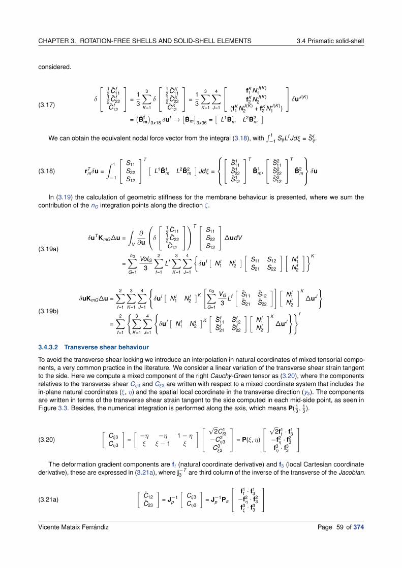
CHAPTER 3. ROTATION-FREE SHELLS AND SOLID-SHELL ELEMENTS 3.4 Prismatic solid-shell
considered.
(3.17)δ
12 C f
1112 C f
22
C f12
=1
3
3∑
K =1
δ
12 CK
1112 CK
22
CK12
=1
3
3∑
K =1
4∑
J=1
fK1 NJ(K )
1
fK2 NJ(K )
2
(fK1 NJ(K )
2 + fK2 NJ(K )
1 )
δuJ(K )
=(Bf
m
)
3x18δuf →
[Bm]
3x36=[
L1B1m L2B2
m
]
We can obtain the equivalent nodal force vector from the integral (3.18), with∫ 1−1 SijLf Jdξ = Sf
ij .
(3.18) rTmδu =
∫ 1
−1
S11
S22
S12
T
[L1B1
m L2B2m
]Jdξ =
S111
S122
S112
T
B1m,
S211
S222
S212
T
B2m
δu
In (3.19) the calculation of geometric stiffness for the membrane behaviour is presented, where we sum thecontribution of the nG integration points along the direction ζ.
(3.19a)
δuT KmG∆u =
∫
V
∂
∂u
δ
12 C1112 C22
C12
T
S11
S22
S12
∆udV
=nG∑
G=1
VolG3
2∑
f=1
Lf3∑
K =1
4∑
J=1
δuI[
N I1 N I
2
][
S11 S12
S21 S22
] [N I
1N I
2
]K
(3.19b)
δuKmG∆u =2∑
f=1
3∑
K =1
4∑
J=1
δuI[
N I1 N I
2
]K
[nG∑
G=1
VG
3Lf
[S11 S12
S21 S22
]] [N I
1N I
2
]K
∆uJ
=2∑
f=1
3∑
K =1
4∑
J=1
δuI[
N I1 N I
2
]K[
Sf11 Sf
12
Sf21 Sf
22
] [N I
1N I
2
]K
∆uJ
f
3.4.3.2 Transverse shear behaviour
To avoid the transverse shear locking we introduce an interpolation in natural coordinates of mixed tensorial compo-nents, a very common practice in the literature. We consider a linear variation of the transverse shear strain tangentto the side. Here we compute a mixed component of the right Cauchy-Green tensor as (3.20), where the componentsrelatives to the transverse shear Cη3 and Cξ3 are written with respect to a mixed coordinate system that includes thein-plane natural coordinates (ξ, η) and the spatial local coordinate in the transverse direction (y3). The componentsare written in terms of the transverse shear strain tangent to the side computed in each mid-side point, as seen inFigure 3.3. Besides, the numerical integration is performed along the axis, which means P( 1
3 , 13 ).
(3.20)
[Cξ3
Cη3
]
=
[−η −η 1 − ηξ ξ − 1 ξ
]
√2C1
t3−C2
η3
C3ξ3
= P(ξ, η)
√2f1
t · f13
−f2η · f2
3
f3η · f3
3
The deformation gradient components are ft (natural coordinate derivative) and f3 (local Cartesian coordinatederivative), these are expressed in (3.21a), where j−T
3 are third column of the inverse of the transverse of the Jacobian.
(3.21a)
[C12
C23
]
= J−1p
[Cξ3
Cη3
]
= J−1p Pa
f1t · f1
3−f2
η · f23
f3ξ · f3
3
Vicente Mataix Ferrándiz Page 59 of 374
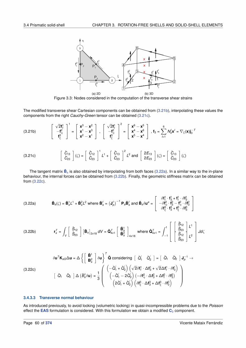
3.4 Prismatic solid-shell CHAPTER 3. ROTATION-FREE SHELLS AND SOLID-SHELL ELEMENTS
(a) 2D
x
x
x
x
(b) 3D
Figure 3.3: Nodes considered in the computation of the transverse shear strains
The modified transverse shear Cartesian components can be obtained from (3.21b), interpolating these values thecomponents from the right Cauchy-Green tensor can be obtained (3.21c).
(3.21b)
√2f1
t−f2
η
f3ξ
1
=
x3 − x2
x1 − x3
x2 − x1
,
√2f1
t−f2
η
f3ξ
2
=
x6 − x5
x4 − x6
x5 − x4
, f3 =6∑
I=1
N I3xI = ∇ξ(x)j−T
3
(3.21c)
[C13
C23
]
(ζ) =
[C12
C23
]1
L1 +
[C13
C23
]2
L2 and
[2E13
2E23
]
(ζ) =
[C13
C23
]
(ζ)
The tangent matrix Bs is also obtained by interpolating from both faces (3.22a). In a similar way to the in-planebehaviour, the internal forces can be obtained from (3.22b). Finally, the geometric stiffness matrix can be obtainedfrom (3.22c).
(3.22a) Bs(ζ) = B1sL1 + B2
sL2 where Bfs =(Jf
p
)−1PaBf
s and Bsδue =
δf1t · f1
3 + f1t · δf1
3−δf2
η · f23 − f2
η · δf23
δf3ξ · f3
3 + f3ξ · δf3
3
(3.22b) rTs =
∫
V
[S12
S23
][Bs]
2x18dV = QT
4x1
[B1
sB2
s
]
4x18
where QT4x1 =
∫ 1
−1
[S12
S23
]
L1
[S12
S23
]
L2
Jdζ
(3.22c)
δuT KsG∆u = ∆
[B1
B2s
]
δu
T
Q considering[
Q′
1 Q′
2
]=[
Q1 Q2
]J−1
p →
[Q1 Q2
]∆(B1
sδu)
=1
3
(
−Q′
1 + Q′
2
)(√2δf1
t ·∆f13 +
√2∆f1
t · δf13
)
(
−Q′
1 − 2Q′
2
) (−δf2
η ·∆f23 + ∆f2
t · δf23
)
(
2Q′
1 + Q′
2
)(
δf3ξ ·∆f3
3 + ∆f3ξ · δf3
3
)
3.4.3.3 Transverse normal behaviour
As introduced previously, to avoid locking (volumetric locking) in quasi-incompressible problems due to the Poissoneffect the EAS formulation is considered. With this formulation we obtain a modified C3 component.
Page 60 of 374 Vicente Mataix Ferrándiz

CHAPTER 3. ROTATION-FREE SHELLS AND SOLID-SHELL ELEMENTS 3.4 Prismatic solid-shell
3.4.3.3.1 EAS formulation :
In the standard EAS method the convective strain components are interpolated, in our case as we just want toimprove C3 and some modifications as presented below are considered. At the element centre (ξ = η = 1
3 and ζ = 0)the Cartesian deformation gradient, and in consequence the right Cauchy tensor, can be enhanced as shown in(3.23). So, in this EAS the changes will affect just to the C33 component, and the C13 and C23 are computed aspresented in the previous section.
(3.23) fC3 =
6∑
I=1
N IC3 XI → f3 = fC
3 eαζ → C33 = f3 · f3 = C233e2αζ
With this enhancement the deformation matrix, internal forces and geometric stiffness can be calculated as shownin (3.24).
(3.24a) δE33 =1
2δC33 = δfC
3 · f −C3 e2αζ + C33ζδα =
(6∑
I=1
N IC3 δu
I
)
· fC3 e2αζ + C33ζδα = e2αζBC
3 δue + C33ζδα
(3.24b) rTn =
∫
VB3S33dV =
∫ 1
−1e2αζBC
3 S33Jdζ = BC3 S33 with S33 =
∫ 1
−1e2αζS33Jdζ
(3.24c) δuT KGn∆u = δfC3 ·∆fC
3 S33 =6∑
I=1
(δuI)T6∑
J=1
N IC3 NJC
3 S33
11
1
∆uJ
3.4.3.3.2 Balance equation :
In the following lines, we will introduce the balance equation which allows us to obtain the implicit solution ofthe problem. Because we will focus in the implicit solution of the problem we will address the reader to[ArtFlo13c;ArtFlo13a; ArtFlo13b] where the explicit solution of the problem is presented too.
The balance equation related with α DOF from (3.12) can be expressed as (3.25a), where we can obtain theresidue and approximate the solution with a Newton-Rapson technique the residual can be nullified (3.25b).
(3.25a) δα
∫ 1
−1S33C33ζJdζ = 0 → rα =
∫ 1
−1S33C33ζJdζ
(3.25b)
∫ 1
−1
[∂S33C33
∂u∆u +
∂S33C33
∂α∆α
]
ζJdζ + rα = 0 with
∂S33C33
∂u= C33D3B + 2S33B3
∂S33C33∂α = C33
(D33C33ζ + 2S33ζ
)
The previous expression can be condensed in the following expression(3.25c), where after integrate the operators H
and kα are obtained.
(3.25c) H1x18∆u + kα∆α + rα = 0 then ∆α =rαkα
− 1
kαH∆u
Where:
(3.25d)
H1x18 =∫ 1−1
(C33D3B + 2S33B3
)ζJdζ
kα =∫ 1−1 C33
(C33D33 + 2S33
)ζ2Jdζ
Vicente Mataix Ferrándiz Page 61 of 374

3.4 Prismatic solid-shell CHAPTER 3. ROTATION-FREE SHELLS AND SOLID-SHELL ELEMENTS
If the expression is introduced in the balance equation associated with the displacement in (3.12) we can obtain(3.25e), which can be linearised in the expression (3.25f).
(3.25e) δuT∫
VBT SdV − δuT Gext = δuT r(u,α)
(3.25f)
∫ 1
−1
[
BT
(∂S
∂u∆u +
∂S
∂α∆α
)
+
(∂BT
∂u∆u +
∂BT
∂α∆α
)
S
]
Jdζ + r(u) = 0
∫ 1
−1
[BT(DB∆u + DT
3 C33ζ∆α)
+ SG∆u + 2S33BT3 ζ∆α
]Jdζ + r(u) = 0
∫ 1
−1
[(BT DBSG
)∆u +
(BT DT
3 C33 + 2S33BT3
)ζ∆α
]Jdζ + r(u) = 0
(KT∆u + HT
∆α)
+ r(u) = 0 → KT∆u − HT
(rαkα
+1
kαH∆u
)
+ r(u) = 0
Finally, all this can be expressed (3.25g) as a modification of the elemental tangent stiffness matrix and the internalforces.
(3.25g)
(
KT − HT 1
kαH
)
∆u − HT rαkα
+ r(u) = 0 →
KT = KT − HT 1kα
H
r = r − HT rαkα
3.4.3.3.3 Pull-Back and Push-Forward (Extension of the formulation) :
The formulation presented until now is broadly the formulation already presented in the works of FernandoFlores[ArtFlo13c; ArtFlo13a; ArtFlo13b], the main step forward of this work is the extension of the formulation. As wehave seen, the formulation presented allows us to obtain a modified left Cauchy tensor C. With this tensor we areable to obtain strains in a traditional way, g.e with Green-Lagrange, but we are unable to work with the Pull-Back andPush-Forward operations, these are, furthermore, the underlying operations in the constitutive operations in Kratos.The fundamental concepts for this are presented in the Appendix section A.1.Pull-Back, Push-Forward fundamentalconcepts.
In order to perform these operations, we need the deformation gradient F, or in our case F owing to we areworking with a modified right Cauchy tensor C. Obtain one from another is not a trivial operation, and we mustconsider additional assumptions to obtain our modified deformation gradient. In a standard formulation to obtain thedeformation gradient F we compute (3.26) from the material displacement gradient tensor ∇Xu, C can be obtainedeasily from here.
(3.26) F = ∇Xu + I → C = FT F
We will present now (3.27a) the polar decomposition of F, which will be the key idea considered to obtain F. Inthis decomposition R represents the proper orthogonal tensor and U is the right stretch tensor. The right stretchtensor can be computed from the square root of the right Cauchy tensor3.27b. The only remaining componentneeded to compute the F will be the modified proper orthogonal tensor where we will take the assumption that themodified rotation tensor (R) equals the rotation tensor (R), meaning R = R. The computation of this F is summarisedin (3.27c).
(3.27a) F = RU thus F = RU
(3.27b) U =√
C thus U =√
C
(3.27c) F = RU
C = FT F → U =√
C → R = F · U−1
U =√
C
Page 62 of 374 Vicente Mataix Ferrándiz

CHAPTER 3. ROTATION-FREE SHELLS AND SOLID-SHELL ELEMENTS 3.5 Numerical examples
3.5 Numerical examples
First of all, we consider as reference the results obtained with previous implementations of the element by Flo-res[ArtFlo13b; ArtFlo13a], as well as the results from [ArtSLL04; ArtKGW06b]. In the following, when "Ref." isdisplayed will refer to this; meanwhile when "Cal."5 is displayed the simulation will have been performed with thein-home implementation in Kratos.
3.5.1 Patch test
Coordinates [mm]
1: (0.04, 0.02)
2: (0.18, 0.03)
3: (0.16, 0.08)
4: (0.08, 0.08)
Figure 3.4: Patch test geometry
The first step in the implementation of an element into a FEM code is the verification of the kinematics, for thisreason the patch test is understood as a necessary condition for the convergence of the element. In the case ofsolid elements it is expected that when nodal displacements corresponding to a constant strain gradient (membranepatch test) are imposed, constant efforts are obtained in all the elements; so in owing to the SPRISM is in fact a solidelement this is the behaviour we should expect. In the case of a solid-shell element clearly, this must satisfy at leastthe membrane patch test and, although it may not be necessary, it is highly desirable that the element satisfies thebending patch test as this will lead to a more robust and reliable element.
Figure 3.4 shows a patch of elements that has been widely used to access quadrilateral shell elements andhexahedral solid shell elements, like where are working with prisms (wedges), we should split in two these elements.The size of the largest sides is a = 0.24mm and the size of the shortest side is b = 0.12mm, while the thicknessconsidered is t = 0.001mm. The lower surface has been located at coordinate z = −t/2. The mechanical propertiesof the material are: Youngs modulus E = 106MPa and Poisson ratio ν = 0.25. Because the problem consideredis linear just 2 integration points across the thickness are used located in the usual Gauss quadrature positions(ζ = ±1/
√3).
3.5.1.1 Membrane patch test
x
y
z0
3.3333e-09
6.6667e-09
1e-08
1.3333e-08
1.6667e-08
2e-08
2.3333e-08
2.6667e-08
3e-08
X-DISPLACEMENT
(a) Displacement X
x
y
z0
2.6667e-09
5.3333e-09
8e-09
1.0667e-08
1.3333e-08
1.6e-08
1.8667e-08
2.1333e-08
2.4e-08
Y-DISPLACEMENT
(b) Displacement Y
Figure 3.5: Solution for the displacement
The prescribed nodal displacements (on the boundary nodes) are defined by the linear functions (3.28), anduz = 0 only on the nodes in the lower face to allow contraction due to Poisson effect. Due to the pure membranestrains developed in this test, the internal DOF α obtained is zero and constant in all the elements.
(3.28)
ux =(x + y
2
)· 10−3
uy =(y + x
2
)· 10−3
5Or nothing more added.
Vicente Mataix Ferrándiz Page 63 of 374

3.5 Numerical examples CHAPTER 3. ROTATION-FREE SHELLS AND SOLID-SHELL ELEMENTS
x
y
z1.3333e+05
1.3333e+05
1.3333e+05
1.3333e+05
1.3333e+05
1.3333e+05
1.3333e+05
1.3333e+05
1.3333e+05
1.3333e+05
Sxx-CAUCHY STRESS TENSOR
(a) σxx
x
y
z1.3333e+05
1.3333e+05
1.3333e+05
1.3333e+05
1.3333e+05
1.3333e+05
1.3333e+05
1.3333e+05
1.3333e+05
1.3333e+05
Syy-CAUCHY STRESS TENSOR
(b) σyy
x
y
z40000
40000
40000
40000
40000
40000
40000
40000
40000
40000
Sxy-CAUCHY STRESS TENSOR
(c) σxy
Figure 3.6: Solution for the stress
Using the present element SPRISM the correct results are obtained for both the displacements of the interiornodes according to (3.28) (Figure 3.5)and the element stresses (σxx = σyy = 1333.3MPa and σ = 400Mpa, Figure3.6).
3.5.1.2 Bending patch test
x
y
z-1.5e-11
-1.1667e-11
-8.3333e-12
-5e-12
-1.6667e-12
1.6667e-12
5e-12
8.3333e-12
1.1667e-11
1.5e-11
X-DISPLACEMENT
(a) Displacement X
x
y
z-1.2e-11
-9.3333e-12
-6.6667e-12
-4e-12
-1.3333e-12
1.3333e-12
4e-12
6.6667e-12
9.3333e-12
1.2e-11
Y-DISPLACEMENT
(b) Displacement Y
Figure 3.7: Solution for the displacement
In this case the displacement field associated with a constant bending stress state is given by (3.29), that isprescribed on the exterior nodes of both shell faces.
(3.29)
ux =(x + y
2
)· z
2 · 10−3
uy =(y + x
2
)· z
2 · 10−3
uz =(x2 + xy + y2
)· 1
2 · 10−3
We obtain a value for the internal DOF α constant in all elements and equal to: α = 0.3333 · 10−8. The bendingstresses at the integration points are σxx = σyy = ±0.3849 Mpa6 and σxy± = 0.1155 Mpa7 (Figure 3.8), while thedisplacements at the interior nodes correspond exactly with the expression (3.29) (Figure 3.7). So in consequencethe element satisfies this test too.
6If we interpolate the values to the external faces we get σxx = σyy = ±0.6666 Mpa7Interpolated to the most external faces σxy± = 0.2000Mpa.
Page 64 of 374 Vicente Mataix Ferrándiz

CHAPTER 3. ROTATION-FREE SHELLS AND SOLID-SHELL ELEMENTS 3.5 Numerical examples
x
y
z-66.664
-51.85
-37.036
-22.221
-7.4071
7.4072
22.222
37.036
51.85
66.664
Sxx-CAUCHY STRESS TENSOR
(a) σxx
x
y
z-66.665
-51.85
-37.036
-22.221
-7.4071
7.4073
22.222
37.036
51.85
66.665
Syy-CAUCHY STRESS TENSOR
(b) σyy
x
y
z-19.999
-15.555
-11.111
-6.6664
-2.2221
2.2222
6.6665
11.111
15.555
19.999
Sxy-CAUCHY STRESS TENSOR
(c) σxy
Figure 3.8: Solution for the stress
3.5.2 Cantilever
X
Z
Y F
Figure 3.9: Cantilever with point load
A cantilever plate strip of length L = 10 mm width b = 1 mm and thickness t1 = 0.1 mm is subjected to atransverse load F = 40 N (Figure 3.9). For the selected Youngs modulus E = 106 MPa the behaviour is one withlarge displacements but small strains. Using different values of Poisson ratio (ν = 0.0, ν = 0.3, ν = 0.49, ν = 0.499and ν = 0.4999 (quasi-incompresible)) it can be assessed if the proposed assumed strain techniques allow to avoidrespectively the transverse shear locking, the Poisson effect locking and the volumetric locking. At the sametime, different geometries, with different numbers of divisions in length have been considered, see Figure 3.10, onein the width and one across the thickness with two integration points. The final deformed configurations (verticaldisplacement is 70% of the length) is achieved considering small load steps.
x y
z
(a) 8 divisions in length
x y
z
(b) 16 divisions in length
x y
z
(c) 24 divisions in length
x y
z
(d) 32 divisions in length
Figure 3.10: Cantilever geometries
The Figure 3.11b shows the maximum vertical displacement versus the load factor (from 0 to 1) for 5 differentvalues of the Poisson ratio, for the geometry of the 32 divisions in length. The case ν = 0 allows to compare with the
Vicente Mataix Ferrándiz Page 65 of 374

3.5 Numerical examples CHAPTER 3. ROTATION-FREE SHELLS AND SOLID-SHELL ELEMENTS
x y
z
0
0.00078853
0.0015771
0.0023656
0.0031541
0.0039427
0.0047312
0.0055197
0.0063083
0.0070968
Z-DISPLACEMENT
(a) Displacement for ν = 0.0 with 32 subdivisions
0 1 2 3 4 5 6 7 8Displacement z [mm]
0.0
0.2
0.4
0.6
0.8
1.0
Load
fact
or
Ref.ν = 0.0Sol.ν = 0.0Sol.ν = 0.3Sol.ν = 0.49Sol.ν = 0.499Sol.ν = 0.4999
(b) Evolution of displacement with load factor
0 5 10 15 20 25 30 35Number of elements
0
1
2
3
4
5
6
7
8
Disp
lace
men
t z [m
m]
Ref.ν= 0.0Ref.ν= 0.3Ref.ν= 0.499Ref.ν= 0.4999Cal.ν= 0.0Cal.ν= 0.3Cal.ν0.4Cal.ν0.499Cal.ν0.4999
(c) Comparision of results respect ν and the number of longitudinaldivisions
Figure 3.11: Solution
reference value (uz = 7.08mm) and to see if the approach used to cure transverse shear locking is adequate. Theresult obtained uz = 7.06mm indicates that effectively the element is free of transverse shear locking. The secondvalue of Poisson ratio (ν = 0.30) is used to assess if the EAS technique avoids the appearance of locking due to
Poissons effect. In this case the computed displacement is uz = 7.03mm that although it is not exactly the samevalue obtained for ν = 0 shows that the proposed method avoids the Poissons effect locking allowing a propergradation of the transverse normal strain. Finally, the last three values of Poisson ratio (0.49,0.499 and 0.4999) allowto observe if the performance of the element deteriorates significantly in the quasi-incompressible range. It can beseen that although differences grow with Poisson ratio, this is below 4% for the higher value considered.
Besides, Figure 3.11c plots the tip displacement as a function of the mesh density (number of divisions alongthe length) for four different Poissons ratio. In the reference results obtained by Fernando G. Flores it can be seenthat convergence deteriorates for Poissons ratio larger than 0.499; as it happens in our in-home implementation, butslightly less significant in this case.
3.5.3 Cantilever subjected to end bending moment
Figure 3.12 shows a cantilever subjected to end moment M. The problem has been considered in from thereference[ArtSLL04]. The cantilever forms a circular arc with its radius R given by the classical flexural formulaR = EI = M . Using the formula, the analytical normalised deflections can be derived to be (3.30) where M0 = EI = L.The maximum end moment Mmax is taken to be M0 at which the beam will be bent into a circle.
(3.30)UL
=M0
Msin
(MM0
− 1
)
,WL
=M0
M
(
1 − cos
(MM0
))
Page 66 of 374 Vicente Mataix Ferrándiz

CHAPTER 3. ROTATION-FREE SHELLS AND SOLID-SHELL ELEMENTS 3.5 Numerical examples
E=1.2×10⁶
ν = 0, L = 12
b = 1, h = 0.1
Mo = EI/L = 25/3
Mmax = 2πMo = 50π/3 initia
l mesh
M
M=0.35Mmax
M=0.7Mmax
M=Mmax
Figure 3.12: Cantilever subjected to end bending moment
Figure 3.13a plots the end moment against the vertical and horizontal tip deflections for different configurations ofthe geometry (8, 16 and 32 subdivisions) and Figure 3.13b portrays the deformed cantilever at M = Mmax .
0 2 4 6 8 10 12 14 16Displacement [m]
0.0
0.2
0.4
0.6
0.8
1.0
Mom
ent fac
tor
Ref. Disp. ZRef. Disp. XDisp. Z(8)Disp. X(8)Disp. Z(16)Disp. X(16)Disp. Z(24)Disp. X(24)Disp. Z(32)Disp. X(32)
(a) Initial geometry
y
x y
z
0
1.3355
2.6711
4.0066
5.3422
6.6777
8.0133
9.3488
10.684
12.02
|DISPLACEMENT|
GiD
x
(b) Deformed geometry
Figure 3.13: Solution for a cantilever subjected to an end bending moment
3.5.4 Frequencies test
0.00 0.02 0.04 0.06 0.08 0.10 0.12Number of elements
0
10
20
30
40
50
60
70
80
90
Disp
lace
men
t [mm]
Ref. Disp.Consistent Disp.Lumped Disp.
Figure 3.14: Frequencies behaviour test
This example (extracted from[ArtFlo13a; ArtOUS04]) considers the dynamic behaviour of a cantilever beam withlength, width and thickness L = 1; b = 0.1 and t = 0.01 respectively. The mechanical properties are Youngs modulus
Vicente Mataix Ferrándiz Page 67 of 374

3.5 Numerical examples CHAPTER 3. ROTATION-FREE SHELLS AND SOLID-SHELL ELEMENTS
E = 100GPa, Poissons ratio µ = 0 and mass density ρ = 1000kg/m3 . The point load applied at the free side (Figure3.9) has a value of 100N with a Heaviside step time function. As the problem is elastic with µ = 0 there is no Poissonseffect across the thickness nor volumetric locking. The behaviour is purely bending and it is useful to evaluate theshear locking and assess the proposed cure. The discretisation includes eight uniform divisions along the length, onein the width and one element through the thickness. The solution shown in Figure 3.14 a very close behaviour to thereference[ArtFlo13a], both for lumped and consistent mass matrix.
3.5.5 Cook membrane
This example (see Figure 3.15) involves a large amount of shear energy and is commonly used to assess in-planebending performance.
F
48
44
16
C
Figure 3.15: Cook ’s membrane geometry
Plane strain condition will be considered here with two different material behaviour: (a) a quasi-incompressibleelastic material with G = 80.1938GPa and K = 40.1 · 104GPa corresponding with a Poisson ratio µ = 0.4999 and(b) an elasticplastic material with elastic properties G = 80.1938GPa and K = 164.21GPa implying a Poisson ratioµ = 0.29 and J2 plasticity with isotropic hardening as a function of the effective plastic strain ep defined by (3.31) andthe values of the Table 3.3.
0 5 10 15 20 25 30 35Number of elements
2
3
4
5
6
7
8
Disp
lace
men
t [mm]
Ref. SouzaRef. Flores nu=0.499Ref. nu=0.4999Sol. nu=0.49Sol. nu=0.499Sol. nu=0.4999
(a) Displacement versus number of elements for the elastic case
0 5 10 15 20 25 30 35Number of elements
0
1
2
3
4
5
6
7
8
Disp
lace
men
t [m
m]
Ref. Displ. FloresRef. Displ. Q1P0Ref. Displ. Q1E4Displ. Sol.
(b) Displacement versus number of elements for the elastic-plastic case
Figure 3.16: Cook ’s membrane convergence solution
(3.31a) σ∗y = Linear hardening + Exponential hardening
Page 68 of 374 Vicente Mataix Ferrándiz

CHAPTER 3. ROTATION-FREE SHELLS AND SOLID-SHELL ELEMENTS 3.5 Numerical examples
(3.31b)
Linear hardening = σy + ep · θ · h
Exponential hardening = (σ0 − σ∞) · (1 − e−η·ep)
Yiled stress σy 0.45GPa Kinematic hardening modulus h 0.12924GPaReference hardening modulus σ0 0.45GPa Infinity hardening modulus σ∞ 0.715GPaHardeningexponent η 16.93 Pure isotropic hardening θ 1
Table 3.3: Isotropic-kinematic hardening law constans
The applied load is 100kN for the elastic case and 5kN for the elasticplastic material. The plane strain conditionimplies coefficient C33 = 1 at all points (α = 0), thus the version without ANS for the in-plane components locksdue to the almost incompressibility constraint in the same way that a constant strain triangle does. Because of thatthis example is intended to assess how the improvement in the membrane field collaborates to cure the volumetriclocking.
(a) Vertical displacement for the elastic case (32 elements ν = 0.4999) (b) Vertical displacement for the elastic-plastic case(16 elements)
Figure 3.17: Cook ’s membrane deformed shape solution
Figures 3.16a and 3.16b show a convergence analysis as the mesh is refined, where the vertical displacement ofthe point C has been plotted versus the number of divisions per side. In Figures 3.17a and 3.17b the deformed shapefor the elastic and elastic-plastic cases is shown. The results have been compared with the reference [ArtFlo13b], andother results presented in the same article, where the results that we have obtained present a very good convergencein comparison.
3.5.6 Scoordelis cylindrical roof test
In this example we proceed with a linear analysis of a cylindrical shell under self-weight, which is free along the oneside as can be seen in the Figure 3.18 and it has been simplified in one quarter of the original size with additionalconsideration of the symmetry conditions of the problem. We have considered five different geometric configurations,with a different number of elements across the side, until the convergence of the solution have been archived. As wehave mentioned previously, the problem is linear, therefore it is possible to solve the problem considering just twoGauss points across the thickness.
The problem is membrane dominant, that is why could be interesting to observe the relevance of the ANS forin-plane components in non-isochoric problems. The results obtained are shown in the Figure 3.19, where in Figure3.19b the results are compared with our reference[ArtFlo13a], having a very close convergence to the referencesolution. Besides the Figure 3.19a shows the deformed shape obtained for the maximum number of elements.
Vicente Mataix Ferrándiz Page 69 of 374

3.5 Numerical examples CHAPTER 3. ROTATION-FREE SHELLS AND SOLID-SHELL ELEMENTS
XY
Z
Diaphragm
300
symmetry
A
symmetry
free
300
α=40
Figure 3.18: Geometry of the scoordelis cylindrical roof
(a) Deformed shape of the scoordelis
0 5 10 15 20 25 30 35Number of elements
0.5
1.0
1.5
2.0
2.5
3.0
3.5
4.0Disp
lace
men
t [mm]
Ref. QuadraticRef. Non QuadraticSol. Quadratic
(b) Displacement versus number of elements
Figure 3.19: Solution for the scoordelis cylindrical roof
3.5.7 Sphere test
XY
Z
F
F
Free
Free
Symmetry
Symmetry
(a) (b)
Figure 3.20: Geometry of a semi-spherical shell with a hole, both original and deformed geometry
Some interesting kind of problem to check the suitability of the element is the problems where an initially doublecurved geometry. This problem (Figure 3.20) is analysed and solved recurrently in the context of large elasticdisplacements. The Figure 3.20 presents the geometry considered in the resolution of the problem, where once
Page 70 of 374 Vicente Mataix Ferrándiz

CHAPTER 3. ROTATION-FREE SHELLS AND SOLID-SHELL ELEMENTS 3.5 Numerical examples
again the symmetry has been considered to simplify the resolution of the problem. This kind of problem is mainlyan inextensional bending problem where Poisson effect has an important role in the behaviour of the structure, incontrast with the membrane effect that is less significant in this problem, on the other hand, the membrane lockingand the curvature-thickness looking could appear.
(a) Deformed shape of the semi-spherical shell
0.0 0.2 0.4 0.6 0.8 1.0Load factor
0
1
2
3
4
5
6
Disp
lace
men
t [mm]
Ref. point ARef. point BPoint A (32)Point B (32)Point A (16)Point B (16)Point A (8)Point B (8)
(b) Displacement versus load for R/t = 250
0.0 0.2 0.4 0.6 0.8 1.0Load factor
0
1
2
3
4
5
6
Disp
lace
men
t [mm]
Ref. point ARef. point BPoint A (32)Point B (32)Point A (24)Point B (24)
(c) Displacement versus load for R/t = 1000
Figure 3.21: Geometry of a semi-spherical shell with a hole solution
Several meshes have been considered, with 8, 16, 24 and 32 elements by side respectively, with a middle radius ofR = 10mm and thickness of t = 0.04mm (R/t = 250). The coarser is the element, the more it could suffer the lookingeffect due to the initial curvature, considering this when solutions more differ more than the 5% from the target values.We are considering the following mechanical properties, E = 6.825 · 104GPa and ν = 0.3. See Figure 3.21.
3.5.8 Pull-out of an open-ended cylindrical shell
Figure 3.22 shows an open-ended cylinder being pulled by a pair of radial forces P. The problem has been consideredin the Reference [ArtSLL04], among others. Owing to symmetry, just one-eighth of the shell is modelled.
The Figure 3.23a presents the convergence of the solution considering a different number of elements, having aconverged solution very close to the reference one[ArtSLL04]. The final deformation of the one-eight is shown inFigure 3.23b, showing that the problem involves very large displacements.
Vicente Mataix Ferrándiz Page 71 of 374

3.5 Numerical examples CHAPTER 3. ROTATION-FREE SHELLS AND SOLID-SHELL ELEMENTS
L
Y
X
Z
R
P
P
A
BC
free
edg
e
freeed
ge
P=40000
P=40000
E = 10.5 MPa
ν = 0.3125
R = 4.953 m
L = 10.35 m
h = 0.094 m
Pmax = 40000 N
Figure 3.22: The open-end cylindrical shell subjected to radial pulling forces.
0 1 2 3 4 5Displacement [mm]
0
500
1000
1500
2000
2500
3000
3500
4000
Point load [N]
Ref. WARef. UBRef. UCSol. WA(8)Sol. UB (8)Sol. UC (8)Sol. WA(16)Sol. UB (16)Sol. UC(16)
(a) Loaddeflection curves (b) The deformed shape
Figure 3.23: Solution of the open-ended cylindrical shell
3.5.9 Pinched semi-cylindrical
X
YZ
R
L
P clamped
free
W=0
A
E=2.0685×10 Pa;7ν =0.3
=2000
R= 1.016; L=3.048; h=0.03Figure 3.24: The semi-cylindrical shell subjected to an end pinching force
Figure 3.24 shows the semi-cylindrical shell[ArtSLL04] subjected to an end pinching force at the middle of thefree-hanging circumferential periphery. The other circumferential periphery is fully clamped. Along its longitudinaledges, the vertical deflection and the rotation about the Y -axis are restrained.
The solution obtained is shown in Figure 3.25, where the Figure 3.25a presents the load-deflection curve, thebehaviour in our obtained solution is slightly different from the one presented in the reference[ArtSLL04], this can be
Page 72 of 374 Vicente Mataix Ferrándiz

CHAPTER 3. ROTATION-FREE SHELLS AND SOLID-SHELL ELEMENTS 3.5 Numerical examples
due to the fact that we are taking the displacement in the point where the load is applied, meanwhile the referencesolutions corresponds to a shell and the solution corresponds with the displacement in the middle surface; a possiblethus to improve our solution way to tackle this problematic is adding an additional layer and plot the solution in thepoint belonging to the middle surface. Figure 3.25b presents the deformed shape obtained for the maximum value ofthe load.
0 500 1000 1500 2000Displacement [mm]
0
500
1000
1500
2000
Point loa
d [N
]
Reference (Shell)Sol. SolidShell(32)Sol. SolidShell(40)
(a) Loaddeflection curves (b) The deformed shape
Figure 3.25: Solution of the semi-cylindrical shell
3.5.10 Slit test
The Figure 3.26a shows the original geometry of an annular plate and it presents a large displacement (Figure3.26b) due to a load applied in one face while the other face is constrained. This problem is a common benchmarkconsidered to study the behaviour of shells under large rotations, in our case, as we are considering a solid-shell wedo not have rotations in our element and it could be considered as large displacement problems.
Ri
Re
Re=10
ν=0
Pmax=0.8
Ri=6
E=21x106
thick. = 0.03
(a) Initial geometry
X Y
Z
A
B
(b) Deformed geometry
Figure 3.26: Slit annular plate
The solution looks like the solution expected Figure 3.27b. A comparison of the results for the coarse mesh(Figure 3.27a) allows to observe the influence of the ANS for membrane part that for the maximum load factor indicatea difference in displacements larger than 4%. The results for the fine mesh are in excellent agreement with thoseprovided in[ArtFlo13b].
Vicente Mataix Ferrándiz Page 73 of 374

3.5 Numerical examples CHAPTER 3. ROTATION-FREE SHELLS AND SOLID-SHELL ELEMENTS
0 2 4 6 8 10 12 14 16 18Displacement [mm]
0.0
0.2
0.4
0.6
0.8
1.0
Load
factor
Ref. point ARef. point BPoint A (360)Point B (360)Point A (710)Point B (710)Point A (1440)Point B (1440)
(a) Displacement-load (b) Deformation solution
Figure 3.27: Slit annular plate solution
3.5.11 Cylindrical panel test
This example[ArtSLL04; ArtFlo13b] considers a rectangular cylindrical panel simple supported along the straightsides and free along the curved sides, that is subjected to a vertical point load in its centre (see Figure 3.28). Themiddle surface geometry is defined by the length of the panel L = 508mm, the radius of the cylinder R = 2540mm andthe half angle θ = 0.1rad . The behaviour of the panel presents a limit point, followed by a strong loss of strength anda final stiffening once the curvature is inverted. Two different thicknesses for the same mid-surface geometry havebeen considered t = 12.7mm and t = 6.35mm that for the thin case leads to a snap back of the loaded point. Thisexample has been widely used to assess the performance of shell elements and non-linear path-following techniques,like the arc-length.
L
P
X
Y
Z
θ
L
hinged
hinged
free
free
C
R = 2540, L = 254
θ = 0.1 radian
h = 12.7 or 6.35
Pmax = 3000
E = 3202.75 Pa
ν = 0.3
Figure 3.28: Geometry of the hinged cylindrical panel
For this problem two meshes have been considered with 8 and 16 elements per side. In this case 2 elements inthe thickness direction have been used that allows to introduce the hinge in the middle surface and then to comparewith solutions obtained with shell elements. The vertical displacement of the loaded point C.
Figures 3.29a and 3.29b show the evolution of the load-deflection compared with the reference[ArtSLL04], besidesthe Figures 3.29c and 3.29d present the deformed shape of the problem.
Page 74 of 374 Vicente Mataix Ferrándiz

CHAPTER 3. ROTATION-FREE SHELLS AND SOLID-SHELL ELEMENTS 3.5 Numerical examples
0.000 0.005 0.010 0.015 0.020 0.025 0.030 0.035 0.040Displacement [m]
−500
0
500
1000
1500
2000
2500
3000
Poin
t loa
d [N
]
Reference ShellSol. Solid-Shell (8)Sol. Solid-Shell (16)
(a) Thin geometry displacement-load
0.000 0.005 0.010 0.015 0.020 0.025 0.030Displacement [m]
0
500
1000
1500
2000
Point loa
d [N
]
Reference ShellSol. Solid-Shell (8)Sol. Solid-Shell (16)
(b) Thick geometry displacement-load
(c) Thin geometry displacement (d) Thick geometry displacement
Figure 3.29: Solution of the cylindrical panel
3.5.12 Conical shell test
This example is selected to demonstrate the ability of the developed finite element to deal with strongly non-linearsituations. The geometrical data are taken from[ArtKGW06b]. Here, elasticplastic material behaviour is assumed.All necessary material and geometrical data are depicted in Figure 3.30. The non-linear behaviour is computedusing an arc-length algorithm with displacement control. The constitutive law considered is a J2 hyperelastic-plasticmodel.
p r
R
L
t
p Geometry:
r = 1 m
R = 2 m
L = 1 m
t = 0.1 m
Load: p
Material:
E = 206.9 Pa
ν = 0.29
σy = 0.45 Pa
σ∞ = 0.715 Pa
h = 0.12924 Pa
η = 16.93
Figure 3.30: Geometry of the cone shell
The results are depicted in Figure 3.31a, where w denotes the vertical displacement of the upper edge. Theload deflection diagram demonstrates that our result is close in the order of magnitude to the reference, thus someimprovements are needed in the modelisation, in special the relative to the relative to the arc-length strategy. TheFigures 3.31b and 3.31c present the deformation and plastic strain in the last stages of the simulation.
Vicente Mataix Ferrándiz Page 75 of 374

3.5 Numerical examples CHAPTER 3. ROTATION-FREE SHELLS AND SOLID-SHELL ELEMENTS
0.0 0.5 1.0 1.5 2.0Displacement [m]
0.00
0.01
0.02
0.03
0.04
0.05
Poin
t loa
d [N
]
Reference Solution (16) Solution (8)
(a) Initial geometry
(b) Deformed geometry (c) Plastic strain
Figure 3.31: Cone-shell test
3.5.13 Wrinkling test
The problem consists[ArtTSW05; ArtFlo13a] of a square membrane (see Figure 3.32) with a side a = 229mm madeof a thin film of Mylar with a thickness t = 0.0762mm. The Mylar mechanical properties are E = 3790MPa andµ = 0.38. The top and bottom edges are clamped and the lateral edges are free. The top edge is subjected to auniform horizontal displacement ∆ = 1mm along the edge.
a
a
Δ
Figure 3.32: Square thin film under in-plane shear
Two uniforms structured meshes with 26 − 26 and 51 − 51 nodes, with 1250 and 5000 elements respectivelyhave been considered. Figure 3.33 plots two out-of-plane displacement profiles along the centre of the square in
Page 76 of 374 Vicente Mataix Ferrándiz

CHAPTER 3. ROTATION-FREE SHELLS AND SOLID-SHELL ELEMENTS 3.5 Numerical examples
both Cartesian directions, as well as the deformation obtained. The solution that we obtain are very close to thoseobtained in the reference [ArtFlo13a].
(a) Deformation with 25 elements per side (b) Deformation with 50 elements per side
0.00 0.05 0.10 0.15 0.20 0.25Coor. X
−4
−3
−2
−1
0
1
2
3
4
Disp
lace
men
t z [m
m]
Reference 25Reference 502550
(c) Transverse displacement profiles along the centre of the square:y = a/2
0.00 0.05 0.10 0.15 0.20 0.25Coor. Y
−2.0
−1.5
−1.0
−0.5
0.0
0.5
1.0
1.5
Disp
lace
men
t z [m
m]
Reference 25Reference 502550
(d) Transverse displacement profiles along the centre of the square:x = a/2
Figure 3.33: Solution of the wrinkling simulation
3.5.14 FSI-Vein test
An additional test that has been performed to check the robustness of the element, which consists in a simple FSI
simulation of an elastic vein. This element has clear advantages from the common approaches performed nowadays,which consist normally in the consideration of multiple layers of solid elements (usually hexahedron), despite the veinis under "shell stresses". This owing to the need of having a proper and correct definition of the irregular geometryand thickness that a real vein can show, besides a correct definition of the interface for a proper FSI simulation, whichcannot be correctly modelled with a conventional shell element. So this element has advantages of the solid element,and like the element is clearly created to compute "shell stresses" there does not need to consider additional layers ofsolid to enrich the behaviour of the solid.
This problem was originally proposed in [ArtNob01] and later reproduced in [PhDVMO09]. Its aim is to simulatethe FSI arising in the modelling of blood flow in the human cardiovascular system. As described in [PhDVMO09], theproblem consists of a thin elastic vessel, which in this case has been modelled with the current element consideringan hyperelastic constitutive law, conveying the blood flow, which is modelled as an incompressible fluid using theNavier-Stokes equations.
Vicente Mataix Ferrándiz Page 77 of 374

3.5 Numerical examples CHAPTER 3. ROTATION-FREE SHELLS AND SOLID-SHELL ELEMENTS
Regarding the geometry, it consists in a straight cylinder of radius r0 = 0.005m which length and thicknessare L = 0.05m and t = 0.001m. The blood physical parameters are ρf = 1000kg/m3 and dynamic viscosityµf = 0.003kg/ms, yielding a kinematic viscosity νf = 3e − 06m2/s. Regarding the solid parameters, the density isρs = 1200kg/m3 while the Poisson ratio and Young modulus are νs = 0.3 and E = 3e05Pa. Regarding the boundaryconditions, both sides of the vein are clamped (radial displacements allowed) and an overpressure of p = 1333.2Pa(see (3.32)) is imposed at the inlet boundary for 3ms.
(3.32) p =
1333.2 sin (2πt) if t ≤ 0.25ms
1333.2 if 0.00025 < t ≤ 0.275ms
1333.2 (1 − sin (2π(t − 0.275))) if 0.275ms < t ≤ 0.3ms
0.0 otherwise
0.000 0.002 0.004 0.006 0.008 0.010
t [s]
0.000
0.005
0.010
0.015
ur
[cm
]
l= 0.25 Valdés (2007)
l= 0.25 Present work
l= 0.5 Valdés (2007)
l= 0.5 Present work
l= 0.75 Valdés (2007)
l= 0.75 Present work
(a) Radial displacement
0.000 0.002 0.004 0.006 0.008 0.010
t [s]
0
500
1000
1500
p[N
/m
2]
l= 0.25 Valdés (2007)
l= 0.25 Present work
l= 0.5 Valdés (2007)
l= 0.5 Present work
l= 0.75 Valdés (2007)
l= 0.75 Present work
(b) Pressure
Figure 3.34: Solution of the FSI-Vein test
Figures 3.34a and 3.34b collects a comparison between the results in [PhDVMO09] and the obtained ones forthree control points placed at 0.25l , 0.5l and 0.75l , being l the tube length. Regarding the radial displacements(Figure 3.34a), it can be seen that the obtained results are similar to the reference ones. The major differences appearafter the peak value when the vein section is recovering its shape. Besides, this vein retraction is much clear in thepresented solution and can be clearly noted by the negative radial displacements. This behaviour is more similar toreal hemodynamics and has been also observed in similar problems in the literature [PhDCal06].
On the other hand, the pressure evolution is also assessed in Figure 3.34b. As can be noted, the pressure trendmatches the radial displacement evolution but some oscillations appear in the solution. Regarding the nature of theseoscillations, it can be asserted that they are not numeric, since one oscillation is developed in several time steps, andthis is done due to the fact that any non-reflecting boundary has been considered.
Page 78 of 374 Vicente Mataix Ferrándiz

BIBLIOGRAPHY BIBLIOGRAPHY
Bibliography
Books
[BookBD12] Sophie Germain: An essay in the history of the theory of elasticity. Louis L Bucciarelli andNancy Dworsky. Springer Science & Business Media. 2012.
[BookBD80] Sophie Germain: An Essay in the History of the Theory of Elasticity. Louis L.. Bucciarelli andNancy Dworsky. D. Reidel Publishing Company. 1980.
[BookBD90] Modélisation des structures par éléments finis: Solides élastiques. Jean-Louis Batoz andGouri Dhatt. Presses Université Laval. 1990.
[BookBel+14] Nonlinear Finite Elements for Continua and Structures. Ted Belytschko, Wing Kam Liu,Brian Moran, and Khalil Elkhodary. Wiley. 2nd ed. 2014.
[BookBor+12] Nonlinear Finite Element Analysis of Solids and Structures, 2nd edition. René de Borst,Mike A. Crisfield, Joris J. C. Remmers, and Clemens V. Verhoosel. Wiley. 2nd Edition. 2012.
[BookCal89] Theory of shell structures. Chris R Calladine. Cambridge university press. 1989.
[BookFHK02] Handbook of computer aided geometric design. Gerald Farin, Josef Hoschek, and M-S Kim.Elsevier. 2002.
[BookGou12] Analysis of shells and plates. Phillip L Gould. Springer Science & Business Media. 2012.
[BookHBC09] Isogeometric Analysis: Toward Integration of CAD and FEA. T.J.R. Hughes, Yuri Bazilevs, andJ. Austin Cottrell. Wiley. 1st ed. 2009.
[BookHug+14] Computer graphics: principles and practice. John F Hughes, Andries Van Dam, James D Foley,Morgan McGuire, Steven K Feiner, and David F Sklar. Pearson Education. 2014.
[BookKra67] Thin elastic shells: an introduction to the theoretical foundations and the analysis of their static anddynamic behavior. Harry Kraus. John Wiley & Sons. 1967.
[BookNov59] The theory of thin shells. Valentin Valentinovich Novozhilov. P. Noordhoff. 1959.
[BookOña13] Structural Analysis with the Finite Element Method Linear Statics: Volume 2. Beams, Plates andShells. Eugenio Oñate. Springer Netherlands. Jointly published with CIMNE, Barcelona,Spain2013. 2013.
[BookPT97] The NURBS book: monograph in visual communication, 1997. LA Piegl and W Tiller. Springer, NewYork. 1997.
[BookRog00] An introduction to NURBS: with historical perspective. David F Rogers. Elsevier. 2000.
[BookTW59] Theory of plates and shells. Stephen P Timoshenko and Sergius Woinowsky-Krieger. McGraw-hill.1959.
[BookWem82] Mechanics of solids with applications to thin bodies. Gerald Wempner. Springer Science &Business Media. 1982.
[BookWri08] Nonlinear finite element methods. Peter Wriggers. Springer. 1st ed. 2008.
Vicente Mataix Ferrándiz Page 79 of 374

ARTICLES BIBLIOGRAPHY
Articles
[ArtAC09] “An improved assumed strain solid–shell element formulation with physical stabilization forgeometric non-linear applications and elastic–plastic stability analysis”. Farid Abed-Meraim andAlain Combescure. In: International Journal for Numerical Methods in Engineering. No. 13, Vol. 80,2009, pp. 1640–1686. Wiley Online Library.
[ArtAIZ70] “Analysis of thick and thin shell structures by curved finite elements”. Sohrabuddin Ahmad,Bruce M. Irons, and O. C. Zienkiewicz. In: International Journal for Numerical Methods inEngineering. No. 3, Vol. 2, 1970, pp. 419–451. DOI: 10.1002/nme.1620020310.
[ArtBen+10] “Isogeometric shell analysis: The Reissner–Mindlin shell”. D.J. Benson, Y. Bazilevs, M.C. Hsu, andT.J.R. Hughes. In: Computer Methods in Applied Mechanics and Engineering. No. 5–8, Vol. 199,2010, pp. 276–289. DOI: 10.1016/j.cma.2009.05.011.
[ArtBR92] “Comparison of Shell Theory and Degeneration”. N Büchter and E Ramm. In: . 1992, pp. 15–30.Springer. DOI: 10.1007/978-3-7091-2604-2_2.
[ArtDB84] “A continuum mechanics based four-node shell element for general non-linear analysis”.Eduardo N. Dvorkin and Klaus-Jürgen Bathe. In: Engineering computations. No. 1, Vol. 1, 1984,pp. 77–88. MCB UP Ltd. DOI: 10.1108/eb023562.
[ArtDha69] “Numerical analysis of thin shells by curved triangular elements based on discrete Kirchhoffhypothesis”. G Dhatt. In: Proc. ASCE, Symp. on Applications of FEM in Civil Engineering,Vanderbilt Univ., Nashville, Tenn., 1969. 1969, pp. 13–14.
[ArtDha70] “An efficient triangular shell element”. GS Dhatt. In: AIAA Journal . No. 11, Vol. 8, 1970,pp. 2100–2102. DOI: 10.2514/3.6068.
[ArtDMM86] “A new triangular discrete Kirchhoff plate/shell element”. G. Dhatt, L. Marcotte, and Y. Matte. In:International Journal for Numerical Methods in Engineering. No. 3, Vol. 23, 1986, pp. 453–470.DOI: 10.1002/nme.1620230310.
[ArtFlo13a] “A “Prism” solid element for large strain shell analysis”. Fernando G. Flores. In: Computer Methodsin Applied Mechanics and Engineering. Vol. 253, 2013, pp. 274–286. Elsevier. DOI:10.1016/j.cma.2012.10.001.
[ArtFlo13b] “Development of a non-linear triangular prism solid-shell element using ANS and EAS techniques”.Fernando G. Flores. In: Computer Methods in Applied Mechanics and Engineering. Vol. 266, 2013,pp. 81–97. Elsevier. DOI: 10.1016/j.cma.2013.07.014.
[ArtFlo13c] “Un Elemento Prisma Triangular De Sólido-lámina Para El Análisis Con Grandes Deformaciones”.Fernando G. Flores. In: Mecánica Computacional . Vol. Xxxii, 2013, pp. 63–87.
[ArtFO01] “A basic thin shell triangle with only translational DOFs for large strain plasticity”.Fernando G. Flores and Eugenio Oñate. In: International Journal for Numerical Methods inEngineering. No. 1, Vol. 51, 2001, pp. 57–83. John Wiley & Sons, Ltd. DOI: 10.1002/nme.147.
[ArtFO05] “Improvements in the membrane behaviour of the three node rotation-free BST shell triangleusing an assumed strain approach”. Fernando G. Flores and Eugenio Oñate. In: ComputerMethods in Applied Mechanics and Engineering. No. 6–8, Vol. 194, 2005, pp. 907–932. DOI:10.1016/j.cma.2003.08.012.
[ArtFO11] “Wrinkling and folding analysis of elastic membranes using an enhanced rotation-free thin shelltriangular element”. Fernando G. Flores and Eugenio Oñate. In: Finite Elements in Analysis andDesign. No. 9, Vol. 47, 2011, pp. 982–990. Elsevier. DOI: 10.1016/j.finel.2011.03.014.
[ArtFV82] “Some results on the behaviour of Degenerated Shell (D.S.) elements”. G. Fezans and G. Verchery.In: Nuclear Engineering and Design. No. 1, Vol. 70, 1982, pp. 27–35. DOI:10.1016/0029-5493(82)90264-3.
[ArtHau+01] “Solid-shell’elements with linear and quadratic shape functions at large deformations with nearlyincompressible materials”. R. Hauptmann, S. Doll, M. Harnau, and K. Schweizerhof. In: Computers& Structures. No. 18, Vol. 79, 2001, pp. 1671–1685. Elsevier.
Page 80 of 374 Vicente Mataix Ferrándiz

BIBLIOGRAPHY ARTICLES
[ArtHCB05] “Isogeometric analysis: CAD, finite elements, NURBS, exact geometry and mesh refinement”.T.J.R. Hughes, J.A. Cottrell, and Y. Bazilevs. In: Computer Methods in Applied Mechanics andEngineering. No. 39, Vol. 194, 2005, pp. 4135–4195. DOI: 10.1016/j.cma.2004.10.008.
[ArtHL81] “Nonlinear finite element analysis of shells: Part I. three-dimensional shells”. Thomas J.R. Hughesand Wing Kam Liu. In: Computer Methods in Applied Mechanics and Engineering. No. 3, Vol. 26,1981, pp. 331–362. DOI: 10.1016/0045-7825(81)90121-3.
[ArtHS98] “A systematic development of ‘solid-shell’element formulations for linear and non-linear analysesemploying only displacement degrees of freedom”. R. Hauptmann and K. Schweizerhof. In:International Journal for Numerical Methods in Engineering. No. 1, Vol. 42, 1998, pp. 49–69. WileyOnline Library.
[ArtHSD00] “Extension of the’solid-shell’ concept for application to large elastic and large elastoplasticdeformations”. R. Hauptmann, K. Schweizerhof, and S. Doll. In: International Journal for NumericalMethods in Engineering. No. 9, Vol. 49, 2000, pp. 1121–1141.
[ArtKan79] “A simple and efficient finite element for general shell analysis”. Worsak Kanok-nukulchai. In:International Journal for Numerical Methods in Engineering. No. 2, Vol. 14, 1979, pp. 179–200.DOI: 10.1002/nme.1620140204.
[ArtKGW06a] “A robust non-linear solid shell element based on a mixed variational formulation”. Sven Klinkel,Friedrich Gruttmann, and Werner Wagner. In: Computer Methods in Applied Mechanics andEngineering. No. 1, Vol. 195, 2006, pp. 179–201. Elsevier. DOI:10.1016/j.cma.2005.01.013.
[ArtKGW06b] “A robust non-linear solid shell element based on a mixed variational formulation”. Sven Klinkel,Friedrich Gruttmann, and Werner Wagner. In: Computer Methods in Applied Mechanics andEngineering. No. 1–3, Vol. 195, 2006, pp. 179–201. Elsevier. DOI:10.1016/j.cma.2005.01.013.
[ArtKir50] “Über das Gleichgewicht und die Bewegung einer elastischen Scheibe.” Gustav Kirchhoff. In:Journal für die reine und angewandte Mathematik . No. 40, Vol. 1850, 1850, pp. 51–88. De Gruyter.
[ArtLev99] “Sur l’équilibre élastique d’une plaque rectangulaire”. Maurice Levy. In: Comptes Rendus Acad. Sci.Paris. Vol. 129, 1899, pp. 535–539.
[ArtLov88] “XVI. The small free vibrations and deformation of a thin elastic shell”.Augustus Edward Hough Love. In: Philosophical Transactions of the Royal Society of London.(A.).No. 179, 1888, pp. 491–546. The Royal Society London.
[ArtMG86] “A triangular thin-shell finite element based on discrete Kirchhoff theory”. S.S. Murthy andR.H. Gallagher. In: Computer Methods in Applied Mechanics and Engineering. No. 2, Vol. 54, 1986,pp. 197–222. DOI: 10.1016/0045-7825(86)90126-x.
[ArtMin51] “Influence of rotatory inertia and shear flexural motions of isotropic elastic plates”.Raymond D Mindlin. In: . 1951, DOI: 10.1007/978-1-4613-8865-4_29.
[ArtNio85] “Shell theory, vol. xiv”. Frithiof I Niordson. In: . 1985, Amsterdam, New York, NY, North-Holland:Elsevier Science Pub Co.
[ArtNob01] “Numerical approximation of fluid-structure interaction problems with application tohaemodynamics”. Fabio Nobile. In: . 2001, Epfl.
[ArtNoo90a] “Bibliography of monographs and surveys on shells”. Ahmed K Noor. In: Applied MechanicsReviews;(United States). No. 9, Vol. 43, 1990, DOI: 10.1115/1.3119170.
[ArtNoo90b] “Bibliography of Monographs and Surveys on Shells”. Ahmed K. Noor. In: Applied MechanicsReviews. No. 9, Vol. 43, 1990, pp. 223–234. DOI: 10.1115/1.3119170.
[ArtOF05] “Advances in the formulation of the rotation-free basic shell triangle”. Eugenio Oñate andFernando G. Flores. In: Computer Methods in Applied Mechanics and Engineering. No. 21–24, Vol.194, 2005, pp. 2406–2443. DOI: 10.1016/j.cma.2004.07.039.
[ArtOUS04] “Selective mass scaling for thin walled structures modeled with tri-linear solid elements”.L. Olovsson, M. Unosson, and K. Simonsson. In: Computational Mechanics. No. 2, Vol. 34, 2004,pp. 134–136. DOI: 10.1007/s00466-004-0560-6.
Vicente Mataix Ferrándiz Page 81 of 374

ARTICLES BIBLIOGRAPHY
[ArtOZ00] “Rotation-free triangular plate and shell elements”. Eugenio Oñate and Francisco Zarate. In:International Journal for Numerical Methods in Engineering. No. 1-3, Vol. 47, 2000, pp. 557–603.DOI: 10.1002/(sici)1097-0207(20000110/30)47:1/3<557::aid-nme784>3.0.co;2-9.
[ArtPar+06] “Sheet metal forming simulation using EAS solid-shell finite elements”. M.P.L. Parente,R.A. Fontes Valente, R.M. Natal Jorge, R.P.R. Cardoso, and Ricardo J. Alves de Sousa. In: FiniteElements in Analysis and Design. No. 13, Vol. 42, 2006, pp. 1137–1149. DOI:10.1016/j.finel.2006.04.005.
[ArtPar79] “A critical survey of the 9-node degenerated shell element with special emphasis on thin shellapplication and reduced integration”. H. Parisch. In: Computer Methods in Applied Mechanics andEngineering. No. 3, Vol. 20, 1979, pp. 323–350. DOI: 10.1016/0045-7825(79)90007-0.
[ArtRei45] “The effect of transverse shear deformation on the bending of elastic plates”. Eric Reissner. In: J.appl. Mech.. 1945, A69–a77.
[ArtSAV11] “On the use of EAS solid-shell formulations in the numerical simulation of incremental formingprocesses”. JIV Sena, RJ Alves de Sousa, and RAF Valente. In: Engineering Computations. No. 3,Vol. 28, 2011, pp. 287–313. Emerald Group Publishing Limited. DOI:10.1108/02644401111118150.
[ArtSen+16] “Single point incremental forming simulation with adaptive remeshing technique using solid-shellelements”. José IV Sena, Cedric Lequesne, Laurent Duchene, Anne-Marie Habraken,Robertt AF Valente, and Ricardo J Alves de Sousa. In: Engineering Computations. No. 5, Vol. 33,2016, pp. 1388–1421. Emerald Group Publishing Limited. DOI: 10.1108/ec-06-2015-0172.
[ArtSF89] “On a stress resultant geometrically exact shell model. Part I: Formulation and optimalparametrization”. J.C. Simo and D.D. Fox. In: Computer Methods in Applied Mechanics andEngineering. No. 3, Vol. 72, 1989, pp. 267–304. DOI: 10.1016/0045-7825(89)90002-9.
[ArtSFR89] “On a stress resultant geometrically exact shell model. Part II: The linear theory; Computationalaspects”. J.C. Simo, D.D. Fox, and M.S. Rifai. In: Computer Methods in Applied Mechanics andEngineering. No. 1, Vol. 73, 1989, pp. 53–92. DOI: 10.1016/0045-7825(89)90098-4.
[ArtSFR90] “On a stress resultant geometrically exact shell model. Part III: Computational aspects of thenonlinear theory”. J.C. Simo, D.D. Fox, and M.S. Rifai. In: Computer Methods in Applied Mechanicsand Engineering. No. 1, Vol. 79, 1990, pp. 21–70. DOI: 10.1016/0045-7825(90)90094-3.
[ArtSim93] “On a stress resultant geometrically exact shell model. Part VII: Shell intersections with 56-DOFfinite element formulations”. J.C. Simo. In: Computer Methods in Applied Mechanics andEngineering. No. 3, Vol. 108, 1993, pp. 319–339. DOI: 10.1016/0045-7825(93)90008-l.
[ArtSK92] “On a stress resultant geometrically exact shell model. Part V. Nonlinear plasticity: formulation andintegration algorithms”. J.C. Simo and J.G. Kennedy. In: Computer Methods in Applied Mechanicsand Engineering. No. 2, Vol. 96, 1992, pp. 133–171. DOI: 10.1016/0045-7825(92)90129-8.
[ArtSLL04] “Popular benchmark problems for geometric nonlinear analysis of shells”. K.Y. Sze, X.H. Liu, andS.H. Lo. In: Finite Elements in Analysis and Design. No. 11, Vol. 40, 2004, pp. 1551–1569. DOI:10.1016/j.finel.2003.11.001.
[ArtSou+05] “A new one-point quadrature enhanced assumed strain (EAS) solid-shell element with multipleintegration points along thickness: Part I—geometrically linear applications”.Ricardo J. Alves de Sousa, Rui P. R. Cardoso, Robertt A. Fontes Valente, Jeong-Whan Yoon,José J. Grácio, and Renato M. Natal Jorge. In: International journal for numerical methods inengineering. No. 7, Vol. 62, 2005, pp. 952–977. Wiley Online Library.
[ArtSR11] “A reduced integration solid-shell finite element based on the EAS and the ANS concept—Largedeformation problems”. Marco Schwarze and Stefanie Reese. In: International Journal forNumerical Methods in Engineering. No. 3, Vol. 85, 2011, pp. 289–329. Wiley Online Library. DOI:10.1002/nme.2966.
[ArtSRF90] “On a stress resultant geometrically exact shell model. Part IV: Variable thickness shells withthrough-the-thickness stretching”. J.C. Simo, M.S. Rifai, and D.D. Fox. In: Computer Methods inApplied Mechanics and Engineering. No. 1, Vol. 81, 1990, pp. 91–126. DOI:10.1016/0045-7825(90)90143-a.
Page 82 of 374 Vicente Mataix Ferrándiz

BIBLIOGRAPHY PH.D.’S THESIS
[ArtSRF92] “On a stress resultant geometrically exact shell model. Part VI: Conserving algorithms fornon-linear dynamics”. J.C. Simo, M. S. Rifai, and D. D. Fox. In: International Journal for NumericalMethods in Engineering. No. 1, Vol. 34, 1992, pp. 117–164. DOI: 10.1002/nme.1620340108.
[ArtSVR11] “Sheet metal forming and springback simulation by means of a new reduced integration solid-shellfinite element technology”. Marco Schwarze, Ivaylo N Vladimirov, and Stefanie Reese. In:Computer Methods in Applied Mechanics and Engineering. No. 5, Vol. 200, 2011, pp. 454–476.Elsevier. DOI: 10.1016/j.cma.2010.07.020.
[ArtTSW05] “Effective Modeling and Nonlinear Shell Analysis of Thin Membranes Exhibiting StructuralWrinkling”. Tessler Alexander, Sleight David W., and Wang John T. In: Journal of Spacecraft andRockets. No. 2, Vol. 42, 2005, pp. 287–298. American Institute of Aeronautics and Astronautics.DOI: 10.2514/1.3915.
[ArtWas82] “Variational methods in elasticity and plasticity Pergamon Press”. K Washizu. In: . 1982, Oxford,England.
[ArtWem69] “Finite elements, finite rotations and small strains of flexible shells”. Gerald Wempner. In:International Journal of Solids and Structures. No. 2, Vol. 5, 1969, pp. 117–153. Elsevier. DOI:10.1016/0020-7683(69)90025-0.
[ArtWOK68] “Finite-element analysis of thin shells”. Gerald A Wempner, John T Oden, and Dennis A Kross. In:Journal of the Engineering Mechanics Division. No. 6, Vol. 94, 1968, pp. 1273–1294. Asce.
Ph.D.’s thesis
[PhDCal06] “Simulación del flujo sanguneo y su interacción con la pared arterial mediante modelos deelementos finitos”. Francisco José Calvo Plaza. 2006.
[PhDVMO09] “Nonlinear Finite Element Analysis of Orthotropic and Prestressed Membrane Structures”.J. G. Valdés, J. Miquel, and Eugenio Oñate. Elsevier Science Publishers B. V. 2009.
Online resources
[OnlKra] Kratos Homepage. URL: http://www.cimne.com/kratos/.
[OnlMel+16] GiD Homepage. URL: http://www.gidhome.com/;%20https://www.gidhome.com/support/brand-resources/citing-gid/.
Vicente Mataix Ferrándiz Page 83 of 374

ONLINE RESOURCES BIBLIOGRAPHY
Page 84 of 374 Vicente Mataix Ferrándiz

CHAPTER 4. CONTACT MECHANICS
Chapter 4
Contact mechanics
Alan Turing is reported as sayingthat PDEs are made by God, theboundary conditions by the Devil!The situation has changed, Devil haschanged places... We can say thatthe main challenges are in theinterfaces, with Devil not far awayfrom them...
Jacques-Louis Lions(1928 - 2001 AD, French
mathematician)
4.1 Introduction
When speaking about CCM we need to know that the phenomenon covers an extended range of problems, anddepending of the problem we want to solve we will need to consider a different numerical technique[BookWri06]. Themost general one, and the one we are interest on is the resolution employing FEM, which can be applied in a largerange of problem, from small to large deformations and from linear to NL material behaviour. The second methodsare the Discrete Element Method (DEM) which study the interaction between a large number of particles cominginto contact. Finally, multibody systems, which describe rigid bodies interacting between them, creating a mechanism,and where contact may influence the behaviour of the system.
Despite the large number of topics covered by CCM, as we already mention, we will focus on the application ofFEM for the resolution of contact problems. This is consistent with the developments of the previous chapters areclassified on this type of method.
4.1.1 Historical outline
History of the contact mechanics is probably as long as the history of civilization. Practically any physical interactionbetween object involves contact and friction, making then the invention of the wheel probably the first human inventioninvolving this problematic. What we know for sure[BookPop10] is that the ancient Egyptians already employed oilreducing the friction between the wheels and the floor in order to facilitate the transportation of the pyramid blocks(Figure 4.1).
We then can jump to the modern contributions of Leonardo Da Vinci in the Codex-Madrid I, who experimentedwith the friction phenomenon. He studied the influence of the contact area on the friction, testing objects of thesame mass but different contact area, coming to the conclusion that the frictional force is proportional to the weight
Vicente Mataix Ferrándiz Page 85 of 374

4.1 Introduction CHAPTER 4. CONTACT MECHANICS
Figure 4.1: Representation of moving blocks during ancient Egypt. Source[BookPop10]
and independent of the contact area. This was a crucial influence to Charles Augustin Coulomb, French engineer,to which we must thank many of the expressions used in computational mechanics[ArtPP15], like the extendedexpression Fτ = µN, denominated Coulomb friction law. It is in 1785[ArtCou85], when in The theory of simplemachines differentiated for first time between kinetic and static friction.
The first mathematical contributions we have records off are attributed to Euler [ArtEul50a; ArtEul50b]1, whostudied the friction problem assuming that the roughness of the contact surfaces can be represented with a series oftriangles. This leads him to the conclusion that the static friction coefficient is larger than the dynamic one, whichmeans we need to apply a larger force in order to starting to move an object than once that the object is moving. In thesame way that we own the use of the Greek letter π to represent the circumference ratio, among other Greek lettersused as mathematical symbols, we own to Euler the use of µ in order to represent the friction coefficient.
During a long time, the contact conditions were modelled in a very experimental manner, as the lack of analyticalresults did not allow consider an alternative approach. It was Hertz with his2 On the contact of elastic solids[ArtHer82]who presented the first analytical solution for a contact problem. In 1882, Hertz solved the contact problem of twoelastic bodies with curved surfaces (Figure 4.2). This problem is so relevant that still today,this classical solutionprovides a foundation for modern problems in contact mechanics, and it is extensively used as the main benchmarkfor contact mechanics today[ArtSpe], as we will see in following sections.
Figure 4.2: Original Hertz paper in 1882. Source[ArtHer82]
The developments that happened just after that were motivated for its application to railways, reduction gears andto rolling contact bearing industry when Industrial Revolution was at full steam at the beginning of the XX th century.The analytical solutions that appeared during this time only allowed to solve a very limited rank of problems, limited to
1Being widely considered the most prolific mathematician of all time, there was almost no field that he did not study. As Pierre-Simon Laplacesaid: "Read Euler, read Euler, he is the master of us all".
2In German in the original version: Über die berührung fester elastische Körper und über die Harte
Page 86 of 374 Vicente Mataix Ferrándiz
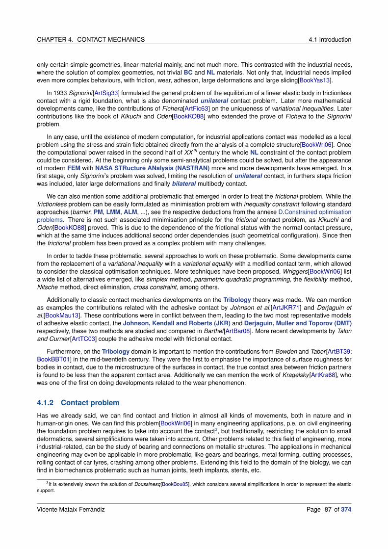
CHAPTER 4. CONTACT MECHANICS 4.1 Introduction
only certain simple geometries, linear material mainly, and not much more. This contrasted with the industrial needs,where the solution of complex geometries, not trivial BC and NL materials. Not only that, industrial needs impliedeven more complex behaviours, with friction, wear, adhesion, large deformations and large sliding[BookYas13].
In 1933 Signorini [ArtSig33] formulated the general problem of the equilibrium of a linear elastic body in frictionlesscontact with a rigid foundation, what is also denominated unilateral contact problem. Later more mathematicaldevelopments came, like the contributions of Fichera[ArtFic63] on the uniqueness of variational inequalities. Latercontributions like the book of Kikuchi and Oden[BookKO88] who extended the prove of Fichera to the Signoriniproblem.
In any case, until the existence of modern computation, for industrial applications contact was modelled as a localproblem using the stress and strain field obtained directly from the analysis of a complete structure[BookWri06]. Oncethe computational power raised in the second half of XX th century the whole NL constraint of the contact problemcould be considered. At the beginning only some semi-analytical problems could be solved, but after the appearanceof modern FEM with NASA STRucture ANalysis (NASTRAN) more and more developments have emerged. In afirst stage, only Signorini ’s problem was solved, limiting the resolution of unilateral contact, in furthers steps frictionwas included, later large deformations and finally bilateral multibody contact.
We can also mention some additional problematic that emerged in order to treat the frictional problem. While thefrictionless problem can be easily formulated as minimisation problem with inequality constraint following standardapproaches (barrier, PM, LMM, ALM, ...), see the respective deductions from the annexe D.Constrained optimisationproblems. There is not such associated minimisation principle for the fricional contact problem, as Kikuchi andOden[BookKO88] proved. This is due to the dependence of the frictional status with the normal contact pressure,which at the same time induces additional second order dependencies (such geometrical configuration). Since thenthe frictional problem has been proved as a complex problem with many challenges.
In order to tackle these problematic, several approaches to work on these problematic. Some developments camefrom the replacement of a variational inequality with a variational equality with a modified contact term, which allowedto consider the classical optimisation techniques. More techniques have been proposed, Wriggers[BookWri06] lista wide list of alternatives emerged, like simplex method, parametric quadratic programming, the flexibility method,Nitsche method, direct elimination, cross constraint, among others.
Additionally to classic contact mechanics developments on the Tribology theory was made. We can mentionas examples the contributions related with the adhesive contact by Johnson et al.[ArtJKR71] and Derjaguin etal.[BookMau13]. These contributions were in conflict between them, leading to the two most representative modelsof adhesive elastic contact, the Johnson, Kendall and Roberts (JKR) and Derjaguin, Muller and Toporov (DMT)
respectively, these two methods are studied and compared in Barthel [ArtBar08]. More recent developments by Talonand Curnier [ArtTC03] couple the adhesive model with frictional contact.
Furthermore, on the Tribology domain is important to mention the contributions from Bowden and Tabor [ArtBT39;BookBBT01] in the mid-twentieth century. They were the first to emphasise the importance of surface roughness forbodies in contact, due to the microstructure of the surfaces in contact, the true contact area between friction partnersis found to be less than the apparent contact area. Additionally we can mention the work of Kragelsky [ArtKra68], whowas one of the first on doing developments related to the wear phenomenon.
4.1.2 Contact problem
Has we already said, we can find contact and friction in almost all kinds of movements, both in nature and inhuman-origin ones. We can find this problem[BookWri06] in many engineering applications, p.e. on civil engineeringthe foundation problem requires to take into account the contact3, but traditionally, restricting the solution to smalldeformations, several simplifications were taken into account. Other problems related to this field of engineering, moreindustrial-related, can be the study of bearing and connections on metallic structures. The applications in mechanicalengineering may even be applicable in more problematic, like gears and bearings, metal forming, cutting processes,rolling contact of car tyres, crashing among other problems. Extending this field to the domain of the biology, we canfind in biomechanics problematic such as human joints, teeth implants, stents, etc.
3It is extensively known the solution of Boussinesq[BookBou85], which considers several simplifications in order to represent the elasticsupport.
Vicente Mataix Ferrándiz Page 87 of 374

4.1 Introduction CHAPTER 4. CONTACT MECHANICS
The physics of the contact interaction is particularly rich and complicated[PhDYas11], due to the multiscale andmultiphysical nature of the phenomenon. This kind of mechanical problems are classically formulated as a boundaryvalue problems, where the contact constraints are formulated as sets of inequalities, and the problem becomes evenmore complex when the frictional effect is assumed. A whole discussion about the constraints and optimisation canbe found in the Appendix D.Constrained optimisation problems. In fact, a proper treatment of the contact constraintrequires the consideration of the micromechanical approach, not only for the proper consideration of the frictionalbehaviour, but also in the normal contact[BookWri06].
These boundary conditions are solution dependent, which naturally leads to difficulties in the formulation of thefrictional contact problem, for example considering the Coulomb’s friction law yields to a non-smooth[BookAnd01]energy functional. Additionally the contacting bodies may penetrate each other or be separated, where with the FE
discretisation leads to mathematical and numerical difficulties. Another challenge is the boundary discretisation andmethods to surpass this problematic. These points are discussed on the state-of-the-art section (4.2.State of the Artin computational contact mechanics) and the formulation section (4.3.Formulation).
Finally, the algorithm considered for the detection phase can suppose a significant bottleneck in terms of efficiency.This is discussed and presented in deeper detail in the corresponding section 4.4.Contact detection. Searchtechniques.
First we should define the basic contact problem, Figure 4.3 illustrates a common contact problem. Every contactproblem is defined between two entities (not necessarily different, e.g self-contact) here noted as Ω
i for i = 1, 2. Thecontact problem occurs on the interface, where we want to link the displacements of the first domain (x1) with itsprojection over second domain (x2) in a local reference frame (n, τ 1 and τ 2). The contact problem will consist in avoidthe penetration in the normal direction between domains, and respect the tangent movement restriction imposed bythe frictional component of the contact.
Figure 4.3: Basic definition of the contact problem
It is important to distinguish that we can divide two types of contacts, the bilateral and unilateral , where the firstone supposes the contact between two or more deformable bodies, in contrast to the unilateral contact, where thecontact occurs between a rigid solid and a deformable solid. A priori for the problems of metal forming the second oneis enough to formulate the problem, but in order to consider more advanced problems in this field a priori is preferableto consider the bilateral case for being more general.
On Figure 4.4 the different states of the contact problem are presented. In here we can differentiate each one of
Page 88 of 374 Vicente Mataix Ferrándiz

CHAPTER 4. CONTACT MECHANICS 4.2 State of the Art in computational contact mechanics
Figure 4.4: Contact states. Based on[PhDYas11]
them, with its corresponding idealised simplification. The illustration shows two different bodies4, with its correspondingdenominations as master and slave. In the interface between the two bodies there is a local reference frame, definedby the normal and tangent directions on this interface. The states listed on this image can be listed as:
• a) Frictionless contact: This contact allows the movement in the tangent direction of the local reference frame,but does not allow the movement toward the opposite body. The idealisation will lead to a perfect rail, no friction,between the two bodies. This is what is usually denominated as Karush-Kuhn-Tucker (KKT) condition.
• b) Separation: This state is the absence of contact, meaning that the two bodies are not in contact any moreand therefore there is not interaction between them any more.
• c) Stick state: In the case of the frictional contact, before the threshold value is surpassed, whatever model offriction is considered, the two bodies will be fully tied,acting as one body. The idealisation will be this case willcorrespond with a sewing in the interface.
• d) Slip state: Once this threshold is surpassed, the bodies can move freely in the tangent direction. Will bethe same as the case a), but in this case the rail which idealises the interface will not be ideal, and thereforehindering the movement due to the present friction.
4.2 State of the Art in computational contact mechanics
4.2.1 Introduction
In this section we compare the existing methods, we can consider in order to solve the contact problem. Dueto the huge industrial and engineering interest in this type of problem, many developments exist, and thereforewe will focus on the most relevant ones on the sake of brevity. First, we will introduce the discretisation methodsavailable, following with the optimisation procedures necessaries to fulfil the contact inequality constraint. Finally, abrief introduction to existing techniques available to model the frictional behaviours will be presented. We addressto some additional monographs, which will provide a deeper outline of the State of the Art in CCM. We foundparticularly relevant to highlight the book of Wriggers[BookWri06], Laursen[BookLau10], Schweizerhof [BookSK13]and Yastrebov [BookYas13].
4.2.2 Discretisation
In order to solve the contact problem, several approaches can be considered from the point of view of the discretisation.When we mention discretisation, we refer the procedure followed for the integration of the interface. The followingones are the main methods that can be considered from this perspective.
4As previously stated, the contact may occur between more bodies, but here for the sake of simplicity, and in order to present the problem wewill consider only two bodies.
Vicente Mataix Ferrándiz Page 89 of 374

4.2 State of the Art in computational contact mechanics CHAPTER 4. CONTACT MECHANICS
4.2.2.1 NTN
Figure 4.5: NTN. Inspired[PhDYas11]
The discretisation of the contact interface is between a node of the slave domain to a node of the master domain(Figure 4.5), reason why the method is denominated this way. This method, originally proposed by Francavilla andZienkiewicz[ArtFZ75] in 1975 is the oldest and the simplest of all the discretisation methods available. We can list thepros and cons of the method as follows:
• Pros:
Passes the Taylor test [ArtTP] when the mesh is conforming
Simple conceptually and to implement. As it is node to node, which means that relate directly DOF, it ispossible to consider all kinds of constraint enforcement methodologies.
• Cons:
Small slip and small deformations. The method loses precision when the nodes move across the interfaceand the nodes are not coincident any more.
Related with previous method, the mesh must be conforming between interfaces. This constraint introducesa restriction in mesh generation.
4.2.2.2 NTS
Figure 4.6: NTS. Inspired[PhDYas11]
The discretisation of the contact interface is between a node of the slave domain to the surface of the masterdomain (Figure 4.6). Despite of being quite close in time to the NTN, in 1977 Hughes et al.[ArtHTK77] proposed theNTS, which already allowed to solve problems in large deformations. We can summarise the pros and cons of themethod in:
• Pros:
Simple and robust. The implementation is probably the most extended in FEA software.
Large deformations and large slip can be considered
Mesh independent. The meshes are not required to be conforming in the interface like in the NTN
Page 90 of 374 Vicente Mataix Ferrándiz
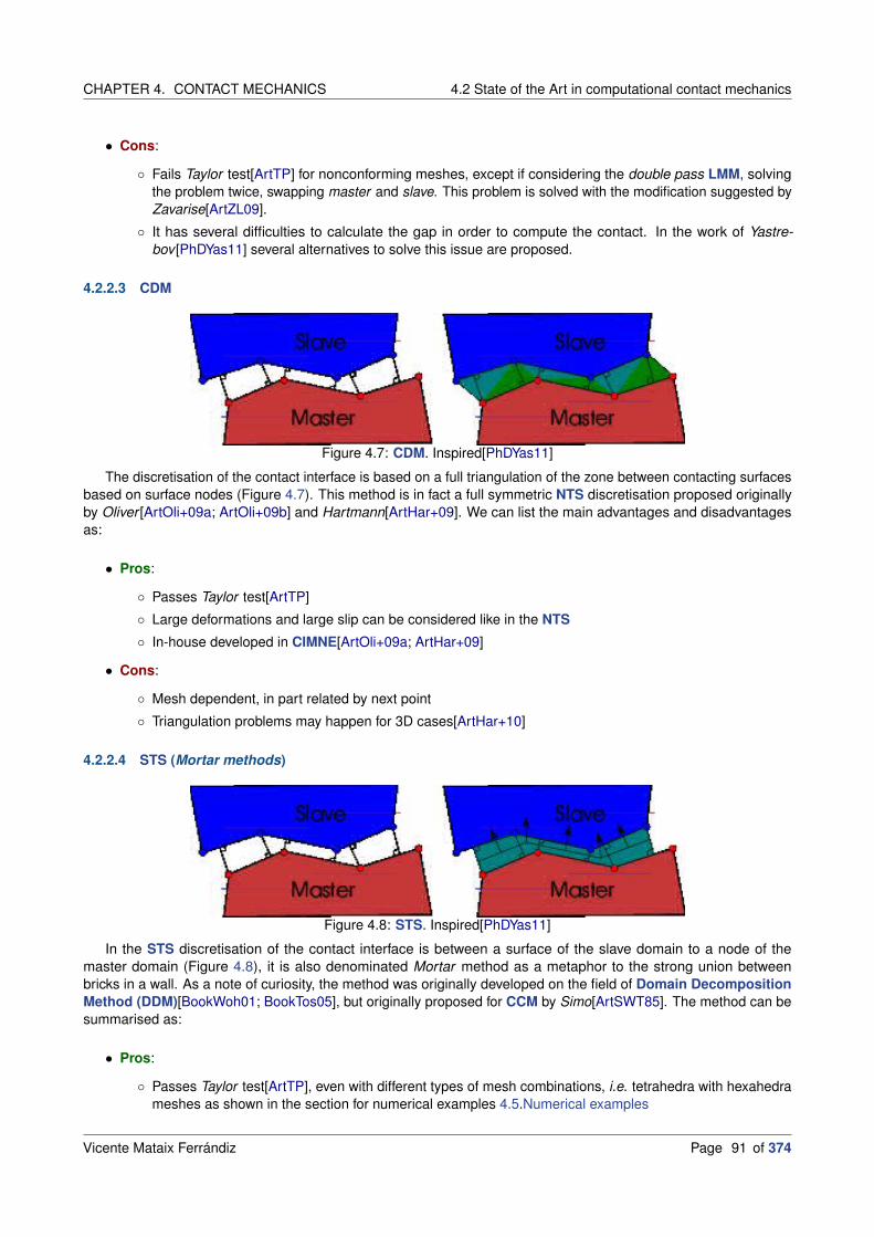
CHAPTER 4. CONTACT MECHANICS 4.2 State of the Art in computational contact mechanics
• Cons:
Fails Taylor test[ArtTP] for nonconforming meshes, except if considering the double pass LMM, solvingthe problem twice, swapping master and slave. This problem is solved with the modification suggested byZavarise[ArtZL09].
It has several difficulties to calculate the gap in order to compute the contact. In the work of Yastre-bov [PhDYas11] several alternatives to solve this issue are proposed.
4.2.2.3 CDM
Figure 4.7: CDM. Inspired[PhDYas11]
The discretisation of the contact interface is based on a full triangulation of the zone between contacting surfacesbased on surface nodes (Figure 4.7). This method is in fact a full symmetric NTS discretisation proposed originallyby Oliver [ArtOli+09a; ArtOli+09b] and Hartmann[ArtHar+09]. We can list the main advantages and disadvantagesas:
• Pros:
Passes Taylor test[ArtTP]
Large deformations and large slip can be considered like in the NTS
In-house developed in CIMNE[ArtOli+09a; ArtHar+09]
• Cons:
Mesh dependent, in part related by next point
Triangulation problems may happen for 3D cases[ArtHar+10]
4.2.2.4 STS (Mortar methods)
Figure 4.8: STS. Inspired[PhDYas11]
In the STS discretisation of the contact interface is between a surface of the slave domain to a node of themaster domain (Figure 4.8), it is also denominated Mortar method as a metaphor to the strong union betweenbricks in a wall. As a note of curiosity, the method was originally developed on the field of Domain Decomposition
Method (DDM)[BookWoh01; BookTos05], but originally proposed for CCM by Simo[ArtSWT85]. The method can besummarised as:
• Pros:
Passes Taylor test[ArtTP], even with different types of mesh combinations, i.e. tetrahedra with hexahedrameshes as shown in the section for numerical examples 4.5.Numerical examples
Vicente Mataix Ferrándiz Page 91 of 374

4.2 State of the Art in computational contact mechanics CHAPTER 4. CONTACT MECHANICS
Correct integration of contact forces. The method is consistent as both meshes are fully integrated.
Large deformations and large slip can be considered[ArtPL04]. The Mortar based formulation leads to aconsistent formulation of the frictional contact problem for large sliding and large deformations.
Additionally the Mortar formulation has been shown as being general enough. As a method coming fromDDM it can be considered in order to couple different types of problems in a Multiphysics way. The methodcan be considered on mapping techniques (see our appendix E.Mortar mapper) or to strongly coupleproblems with mesh tying techniques[PhDPop12]. The work of Seitz[ArtSWP18] shows a fully integratedMultiphysics with thermo-elasto-plastic frictional contact, or the FSI implementation in Popp[PhDPop12]thesis. The consideration of DLMM (4.2.3.4.DLMM) extends the application range of the formulation.
• Cons:
Complex implementation in 3D. We experienced great advances since Puso and Laursen[ArtPL04] andlater thanks to Brunssen[PhDBru08], Popp[PhDPop12] and Gitterle[PhDGit12]. The complexity comes fromthe 3D intersection between two flat geometries, Figure 4.9, which requires some additional considerations,especially when the Gateaux derivatives (see from appendixes 4.6.Derivatives for contact mechanicslinearization).
Figure 4.9: 3D segmentation between two triangles
4.2.2.5 Other alternative methods
The following section introduces some additional integration approaches existing in the state of art of the CCM. Manyof these approaches cannot be directly applied in a standard FEM formulation, but we consider them as interesting tomention.
4.2.2.5.1 Isogeometric :
In the recent years, the isogeometric analysis has been on the rise. The key concept underlying on this method isthe meshless integration. The integration is done directly on the NURB, avoiding them the necessity of the meshstep during the preprocess. This method originally developed by Hughes[BookHBC09] has grown significantly onlast years due to the continuous workflow integration between FEA and CAD. Additionally NURB provide an exactrepresentation of the surfaces and high order of integration during the FE computations.
The method has been considered particularly in order to represent surfaces, which suits to thin objects such as theones present during the forming simulations. Additionally to the corresponding shell formulation[ArtBen+11] contactformulations are needed. We can mention respect this, the works from Lorenzis[ArtLWZ12a; ArtLWZ12b].
Page 92 of 374 Vicente Mataix Ferrándiz

CHAPTER 4. CONTACT MECHANICS 4.2 State of the Art in computational contact mechanics
4.2.2.5.2 Smooth surface approximation :
In order to overcome the problematic from the discontinuity in the standard FEM interface, we may define a smoothapproach of the boundary[BookBHS07]. In order to do so, we can consider different types of discretisations, such asHermite, splines, Bézier surfaces or NURB.
Sometimes this last approach can also be denominated Segment-To-Analytical-Surface (STAS)[BookSK13],and can be found between the previous method (4.2.2.5.1.Isogeometric) and the standard FEM. There are differentways to approach analytically the surface. We can define this surface at the beginning of the simulation and then moveit, which implies that the surface is rigid and then limits the contact to unilateral cases[ArtWI93]. This is not necessarilya limit, if we think that in the case of forming processes the tools considered are de facto rigid. The second approachcan consist in consider standard FEM, with two deformable bodies and update the analytical surface continuously,this is for example done with Nagata[ArtNag05] patches by Neto[ArtNet+14; ArtNOM17].
4.2.2.6 Conclusion
After all the methods presented, and due to our consideration of standard FEM, we will consider as discretisationmethod the STS or Mortar approach (4.2.2.4.STS (Mortar methods)). This method will provide us the best standardFEM integration possible, despite its technical problems related to implementation details.
4.2.3 Optimisation method
The assumption of a known a priori contact surface allows to replace the variational inequality by a variational equalitywith an additional contact term. The form of this contact term depends upon the choice of the optimisation method.Owing to the fact that we have decided to implement a Mortar approach discretisation based in Popp[PhDPop12], ourinitial thought could be to consider as optimisation method the DLMM. In the following section, we will show the mostcommon approaches that could be taken into consideration in order to solve the CCM problem, justifying this way ourfinal choice.
The main optimisation methods are studied in detail in the corresponding appendix, we directly address toD.Constrained optimisation problems for further detail about these methods. In the mentioned appendix not only thedifferent methods are introduced, but also compared in detail between them, and its suitability for solving differenttypes of constrained problems.
4.2.3.1 Penalty Method (PM)
This is probably the most extended optimisation method considered on CCM, particularly in explicit approaches. Thecontact conditions are fulfilled exactly only in case of the infinite penalty parameter (ε), which results in ill-conditioning.For more details check D.2.Penalty method.
• Pros:
Very simple and robust. The simplicity of the method can be seen in the corresponding section in theoptimisation appendix D.2.Penalty method, and its robustness in the last numerical example shown(D.7.3.Over-constrained optimisation problem).
Pure displacement based formulation, no change in the system size.
• Cons:
The solution is inexact, which happens only in case of an infinite value of ε, making the system unsolvabledue to the deterioration on the condition number.
Choice of penalty parameter. If the value is chosen to small the penetration is large, if large as we havestated will ill-condition the system.
Vicente Mataix Ferrándiz Page 93 of 374

4.2 State of the Art in computational contact mechanics CHAPTER 4. CONTACT MECHANICS
4.2.3.2 LMM
Contact conditions are exactly satisfied by the introduction of an extra DOF called LM, and usually represented by theGreek letter λ. This and more is analysed in detail at D.3.Lagrange Multiplier method.
• Pros:
Exact solution is obtained when solving the system of equations. This is the main advantage of the LMM,and the reason of its extensive use in optimisation problems.
User independent. It does not depend, as in the case of the PM of a user-driven decision to choose aparameter.
• Cons:
Additional DOFs. The LHS of the system grows in ncontact additional DOF for the case of frictionlesscontact, and in 3 × ncontact in the case of frictionless with full λ components or for frictional problems. Herencontact is the number of nodes in contact.
Moderate convergence rate in the NR. Additionally the condition of the system is affected due to the zerodiagonal terms introduced by the Lagrange multipliers.
4.2.3.3 ALM
It is a LMM regularised by a PM. It yields a smooth energy functional and fully unconstrained problem, resultingin exact fulfilment of contact constrains with finite value of the penalty parameter (ε). For more details checkD.4.Augmented Lagrange Multiplier method. The method is successfully considered with a Mortar approach byCavalieri and Cardona[ArtCFC12; ArtCC12; ArtCC13a; ArtCC15; ArtCC13b].
The method is often considered as a synonym of the Uzawa iteration (see D.4.2.2.Uzawa iteration). Indeed theUzawa iteration is always applied to the ALM, but this is just one of the possible approaches possible to be consideredin order to solve the system. In the following when we mention the ALM we will refer to the standard approachwithout Uzawa iteration. This is due to the reason that the convergence order of the Lagrange multiplier becomeslinear.
• Pros:
Exact solution as in the case of the LMM. The result is not influenced by the penalty terms (ε).
No additional DOFs with Uzawa iteration algorithms. Otherwise the system of equations is increased inthe same way it is done in the standard LMM.
Smooth functional is obtained. See Figure D.4 from the appendix, compared with the Figure D.3.
Less sensitive to penalty choice compared with the PM. The penalty (ε) only contributes in smooth L, butdoes not affect the solution. Once the system has converged, the contribution of ε becomes zero.
• Cons:
In the case of an Uzawa iteration algorithm coming comes at the price of increased computational costsdue to an additional nonlinear iteration loop (augmentation), typically only showing a linear convergencerate.
4.2.3.4 DLMM
This concept of dual Lagrange multiplier was introduced first by Wohlmuth[ArtWoh02]. The method is an extension ofthe LMM, but the Lagrange multiplier (λ) are interpolated considering a different set of shape functions. These shapefunctions are locally supported and continuous dual basis functions.
• Pros:
Exact solution as in the LMM case
Page 94 of 374 Vicente Mataix Ferrándiz

CHAPTER 4. CONTACT MECHANICS 4.2 State of the Art in computational contact mechanics
System can be condensed, reducing the DOF respect the original, the system then becomes puredisplacement.
With regard to linear solvers, DLMM allows for an out-of-the-box application of state-of-the-art iterativesolution and preconditioning techniques, such as the Generalized Minimal RESidual (GMRES) iterativesolver. It can be used with Algebraic MultiGrid (AMG) methods if the proper modifications are taken intoaccount, like recent works of Wiesner [ArtWie+18].
• Cons: As the disadvantages of the LMM disappear, there is none. We can mention the fact that is slightly moredifficult to implement in comparison to the standard LMM.
4.2.3.5 Other alternative methods
The following are some other additional approaches possible to solve the optimisation problem related with contact.Here we will add the ones we have considered as most promising after the already presented, more methods arementioned in the optimisation appendix (D.1.Introduction).
4.2.3.5.1 Perturbed Lagrangian :
This special formulation can be used to combine both PM and LMM in a mixed formulation, therefore, similarto the already mentioned ALM. The method was considered originally by Oden[ArtOde81] in 1981. In this methodthe contribution of the Lagrange multiplier is regularised with the inclusion of a complementary term. This methodis discarded due to its limitations in order to consider the slip case in frictional simulations, where this is usuallydone with the inclusion of an incremental constitutive equation for the frictional behaviour considered[BookWri06].In addition to that we can mention as an advantage that the method does not deteriorate the conditioning of thesystem.
4.2.3.5.2 Nitsche :
Nitsche[ArtNit71] methods are based on a different concept respect the LMM. In here the stress vector on theinterface is computed from the stress field inside the solid body. The formulation usually includes a penalty termto avoid ill-conditioning, but in the same way as the ALM the constraint is enforced exactly and this term does nothave effect in the final solution. The resulting formulation does not introduce additional DOF, but as it formulates thestresses from the displacement field, this method becomes complex to formulate on NL cases.
An extended overview of recent advances of the method applied in CCM can be found in the work of Chouly [ArtCho+17].Here additional references can be found.
4.2.3.5.3 Other minor mentions :
We can mention additionally, some of them came directly from techniques applied on the DDM[BookWoh01]field. i.e. the Finite Element Tearing and Interconnect (FETI) methods[ArtDFS98] or monotone methods[ArtKor94;PhDKra01].
Another recent relevant contribution is the work of Hiermeier [ArtHWP18], who introduces a gradient based Mortarformulation, still based on LMM and ALM, which provides a symmetric system of equations to respect the active-setcontributions. A symmetric LHS has advantages as it allows to consider certain types of iterative solvers such as theConjugate Gradient (CG).
4.2.4 Conclusion
After all the methods here introduced, we conclude that we will combine two methodologies. In the Popp’s work[PhD-Pop12] and derived ones, the DLMM is considered in combination of a Non-Linear Complementary Function
(NCP). The resulting system is close to a ALM solution. We will take the dual shape functions considered on theDLMM in combination with the ALM approach used by Cavalieri and Cardona[ArtCFC12]. This means that we willwork with ALM displacement only approach due to the consideration of DLMM, but without using the Uzawa iterationalgorithm.
Vicente Mataix Ferrándiz Page 95 of 374

4.3 Formulation CHAPTER 4. CONTACT MECHANICS
Additionally we will consider the Adapted Augmented Lagrangian Method (AALM) by Busseta[PhDBus;ArtBMP] in order to enhance the method. Check D.4.3.1.Adapted Augmented Lagrangian Method for furtherdetail.
4.2.5 Frictional models
Figure 4.10: Friction cone for variants ofthe Coulomb law. Inspired [ArtRao16]
The frictional problem is quite complex by itself, but in this work we willfocus on simple models that will allow to introduce the phenomenonin our simulations, not taking into account the dynamic effects of thefriction[ArtPPS03]. Basically, the frictional behaviours are addressed inthis work are limited to simple frictional laws as Coulomb and Tresca. Thebasic definitions of these frictional laws are such as the follow[BookWP99],Equation (4.1). In here we can see as the Tresca law depends only ina constant threshold parameter g, meanwhile in the case of Coulomb itdepends on the normal reaction and the friction coefficient (µ).
(4.1)
Tresca: ‖FT‖ ≤ g
Coulomb: ‖FT‖ ≤ µ |FN |
In addition to these frictional models, there exist more advanced fric-tional models, like the ones in Figure 4.10. These laws express that thefriction no longer depends on the normal force when the latter surpassesa certain threshold. It is a kind of saturation of the friction threshold, whichis often considered in metal forming. The Coulomb cone can becomea truncated cone like in the Coulomb-Orowan and Shaw or a cylinder(Tresca). It is also possible to regularise the Coulomb law[BookWP99],this smoothes the law reducing part of the numerical problematics of the original piecewise function. i.e. square rootregularisation, hyperbolic tangent or a piecewise polynomial.
Besides of the pure frictional behaviour, the frictional models can incorporate additional effects, such as the wear,adhesion or variational evolutions in the friction coefficients[ArtRao16]. For more detailed frictional behaviours, we willaddress literature at the end of the section.
It is commonly admitted in the literature an analogy between plasticity and friction. In here the question ofapplicability of plasticity principles to frictional contact problems remains open. Indeed, the formulations of severalfrictional laws and its respective numerical procedures have been derived, many times taking into account on thisanalogy. The work of Antoni [ArtAnt17] analyses this phenomenon in detail.
Finally, we want to address some relevant works in the field of frictional behaviour in order to extend the shortsummary presented here. The book of Popov [BookPop10] is a very complete work about the friction in contact. Wecan also mention to more forming oriented manuscripts as Boisse[BookBAL03].
4.3 Formulation
4.3.1 Introduction
The following section presents the formulation employed in the derivation of the frictional Mortar contact con-dition formulation with Augmented Dual Lagrange Multiplier (ADLM), based mainly in the work of AlexanderPopp[PhDPop12; ArtPop+10], but also on Cavalieri and Cardona[ArtCC12; ArtCC13b] and the work of Yastre-bov [PhDYas11; BookYas13]. In addition to the mentioned work, this author has incorporated its own consideration,which will be highlighted.
The contact mechanics problems are based on the Initial Boundary Value Problem (IBVP) of non-linear solidmechanics and the unilateral contact constraints. After recapitulating some basic notation and the strong formulation,a weak formulation of the contact mechanics problems with two subdomains will be introduced. In contrast to the
Page 96 of 374 Vicente Mataix Ferrándiz

CHAPTER 4. CONTACT MECHANICS 4.3 Formulation
mesh tying case, see A.3.Mesh tying, unilateral contact leads to a constrained minimisation problem with inequalityconstraints, or more generally to so-called variational inequalities. It should be mentioned that both frictionless andfrictional contact can either be formulated as variational inequalities with a constrained solution or as saddle pointproblems based on Lagrange multipliers, where the focus will be on the latter approach here.
The motivation for dual Lagrange multipliers[BookWoh01; ArtWoh02] lies in the fact that an extension of the masterside basis functions to the slave side of the interface has a global support for standard Lagrange multipliers.
4.3.2 Definition of the problem
The basic fundamentals of a contact problem, featuring potentially large deformations and large sliding[ArtYL08;PhDPop12; BookWri06] will be formulated in the following lines (Figure 4.11). Reference configurations of twocontaining bodies are denoted by open sets Ω
1 and Ω2, and the deformations φ1 and φ2 of these two bodies are
to be found. We call Γu where the Dirichlet boundary conditions are prescribed, Γσ where the Neumann boundaryconditions are prescribed, and Γc where the contact constrains will be defined and enforced. The spatial counterpartsare denoted as γu , γσ ,and γc .
Figure 4.11: Definition of the contact problem
4.3.3 Frictionless contact
Before introduce the formulation employed for the frictional contact, the formulation for the frictionless will be introduced.Many terms are reused and common in both formulation, so the theoretical introduction for the frictional case willrequire a smaller effort.
4.3.3.1 Strong formulation
On each subdomain Ωi0, the IBVP of finite deformation elastodynamics needs to be satisfied, viz (4.2). In here we are
adding the BC terms to the linear form from the FE chapter, 2.3.1.Linear form, and splitting in two different domains(i = 1, 2) the problem. This includes the Dirichlet BC in (4.2b), the Neumann BC from (4.2c) and the initial BC definedin (4.2d) and (4.2e).
Vicente Mataix Ferrándiz Page 97 of 374

4.3 Formulation CHAPTER 4. CONTACT MECHANICS
∇ · σi + bi = ρi ui in Ωi × [0, T ](4.2a)
ui = ui on Γiu × [0, T ](4.2b)
σi · ni = ti on Γiσ × [0, T ](4.2c)
ui(Xi , 0
)= ui
0
(Xi)
in Ωi0(4.2d)
ui(Xi , 0
)= ui
0
(Xi)
in Ωi0(4.2e)
Figure 4.12: KKT conditions of non-penetration.
The contact constraints in normal direction are typicallygiven in form of Hertz-Signorini-Moreau (HSM) conditionsas given in (4.3), and Figure 4.12. In optimisation theory theseconditions are denominated usually as KKT5.
In the course of deriving a weak formulation, the balanceof linear momentum at the unilateral contact problem for theinterface Γ
ic is typically exploited and a Lagrange multiplier
vector field λn is introduced, thus setting the basis for a mixedvariational approach. Unilateral contact constraints are typi-cally formulated (and later also numerically evaluated) in thecurrent configuration.
(4.3) gn ≥ 0 , pn ≤ 0 , pngn = 0 on Γic × [0, T ]
4.3.3.2 Weak formulation
We will distinguish two different cases for the weak formulation, the first one considering the LM as a scalar variable.The second one considering the LM decomposed in its Cartesian components, which means that the contact pressurecan be represented as n · λ.
4.3.3.2.1 Scalar Lagrange multiplier :
In this case the LM corresponds directly with the contact pressure, which is the complementary form of the normalgap (gn). We present this form first, as it is simpler than the components form, where we will simply present the partsof the formulation changing respect the scalar form.
4.3.3.2.1.1 LMM :
The general theory for the LMM is presented and detailed in D.3.Lagrange Multiplier method. In the relative to theresolution of the contact problem, to start the derivation of a weak formulation of (4.2), appropriate solution spaces U i
and weighting spaces V i need to be defined as (4.4).
(4.4)
U i =
ui ∈ H1(Ω)‖ui = ui on Γiu
,
V i =δui ∈ H1(Ω)‖δui = 0 on Γ
iu
Additionally the Lagrange multiplier vector λn = λn · n = −t1c , which enforce the unilateral contact constraint(4.3),
represents the negative slave side contact traction t1c , is chosen from a corresponding solution space denoted as
M.
In terms of its classification in functional analysis, this space represents the dual space of the trace space L1 ofV1. In the given context, this means that M = H1/2(Γc) and L1 = H1/2(Γc), where M and L1 denote single scalarcomponents of the corresponding vector-valued spaces M and W .
5Moreau[ArtMor73] formulated this on 1974 expressed as sub-gradients. The expression from Karush[ArtKar39] is previous, from 1939.
Page 98 of 374 Vicente Mataix Ferrándiz

CHAPTER 4. CONTACT MECHANICS 4.3 Formulation
Based on these considerations, a saddle point type weak formulation is derived next. This can be done byextending the standard weak formulation of non-linear solid mechanics as defined to two subdomains and combiningit with the Lagrange multiplier coupling terms introduced in generic form. Find ui ∈ U i and λn ∈ M such that weobtain (4.5a), then once derived (4.6).
(4.5a) Lco(u,λn) =
∫
Γ1c
λn · gndΓico
Where gn is the continuous normal gap, that can be defined as (4.5b).
(4.5b) gn = n1 ·(u1 − u2
)
δL(u,λn) = δLV + δLM(4.6a)
δLV = −δLkin(ui , δui ) − δLint ,ext (ui , δui ) − δLco(λi , δui ) = 0 ∀δui ∈ V(4.6b)
δLM = − δLλ(ui , δλi ) ≥ 0 ∀δλi ∈ M(4.6c)
Herein, the kinetic contribution δLkin , the internal and external contributions δLint ,ext and the unilateral contactcontribution δLco to the overall virtual work on the two subdomains, as well as the weak form of the unilateral contactconstraint δLλ, have been abbreviated as (4.7).
− δLkin(u) =2∑
i=1
[∫
Ωi
ρi ui · δuidΩi
]
(4.7a)
− δLint ,ext (u) =2∑
i=1
[∫
Ωi
(∂σi
∂xj: δui + σi :
∂δui
∂xj− b · δui
)
dΩi −∫
Γiσ
ti · δuidΓiσ
]
(4.7b)
− δLco(u,λn) =
∫
Γ1c
λn · δgndΓ1co(4.7c)
− δLλ(u,λn) =
∫
Γ1c
δλn · gndΓ1co(4.7d)
The coupling terms on Γc also allow for a direct interpretation in terms of variational formulations and the principleof virtual work. Whereas the contribution in (4.7c) represents the virtual work of the unknown interface tractionsλ = t1
c = t2c , the contribution in (4.7d) ensures a weak, variationally consistent enforcement of the unilateral contact
constraint (4.3). Nevertheless, the concrete choice of the discrete Lagrange multiplier space Mh in the context ofmortar finite element discretisations is decisive for the stability of the method and for optimal a priori error bounds.Finally, it is pointed out that the weak formulation (4.6b) and (4.6c) possesses all characteristics of saddle pointproblems and Lagrange multiplier methods.
In contrast to the mesh tying case, where this mapping only came into play in the discrete setting, γ1c and γ2
ccannot even be guaranteed to be identical in the continuum framework for unilateral contact, because they not onlycomprise the actual contact surfaces but the potential contact surfaces.
As compared with the mesh tying case, it is noticeable that the weak formulation contains inequality (4.6c)conditions for unilateral contact. These require a particular numerical treatment based on active set strategies.
4.3.3.2.1.2 Penalty :
This optimisation method is better detailed in the corresponding section of the appendix, see D.2.Penalty method.The main advantages of this method is that does not require to add additional DOF to the system of equations,reducing the system of equations to be solved and that it does not introduce ill-conditioning problems to the system
Vicente Mataix Ferrándiz Page 99 of 374

4.3 Formulation CHAPTER 4. CONTACT MECHANICS
of equations resolution due to the introduction of saddle point in the formulation. The main disadvantage is that itnever achieves the exact solution as this would require the consideration of an infinite penalty, which will induceill-conditioning in the system. Therefore the main problem of this method is the chosen of the proper penalty value,enough to solve approximately the problem without the cited problematic.
The main difference from the formulation presented in (4.7), is the lack of (4.7d), as our formulation will no dealwith LM. Additionally (4.7c) will be rewritten as in (4.8b), which comes from (4.8a). In here the εn is a positive penaltyparameter corresponding to the normal contact.
− Lco(u) =1
2
∫
Γ1c
εn · δg2ndΓ1
co(4.8a)
− δLco(u) =
∫
Γ1c
εn · δgndΓ1co(4.8b)
4.3.3.2.1.3 ALM :
One of the main disadvantages of the standard Lagrange multiplier is the saddle point problem that appears inthe formulation. For solving that, an Augmented Lagrangian method to solve contact problems with friction wasproposed by Alart and Curnier [ArtAC91] based on a reformulation of the contact and friction laws into a system ofequations without inequalities. More details about ALM can be found in the optimisation appendix D.4.AugmentedLagrange Multiplier method. The resulting Lagrangian (L) can be seen as a combination of the standard LM
Lagrangian (4.3.3.2.1.1.LMM) and the penalty Lagrangian (4.3.3.2.1.2.Penalty).
Focusing in the functional relative to the contact (Lco(u,λn) = LVco + LM), we can rewrite (4.5a) as (4.9).
(4.9) Lco(u,λn) =
∫
Γ1c
kλn · gn +ε
2g2
n − 1
2ε〈kλn + εgn〉2dΓi
co
Where ε is a positive penalty parameter, k is a positive scale factor, and 〈〉 is the Macauley bracket operator, thatis (4.10).
(4.10) 〈x〉
x x ≥ 0
0 x < 0
This functional is C1 differentiable saddle-point, as shown in Figure D.4, from D.4.3.Applicability on contactproblems. The solution is obtained as the set of values that render this functional stationary.
The solution does not depend on the value of parameters ε and k . Nevertheless, the convergence rate doesdepend on their value. In numerical computations, default values of ε and k are selected in terms of a mean value ofthe Young modulus (E) of the bodies in contact and of a mean value of mesh size, as (4.11). Numerical examplesshow that this choice gives a better condition number of the iteration matrix than other choices. This is proven later at4.3.3.3.Augmented Lagrange multiplier parameters calibration, where a numerical experiment is provided, to illustrateon the influence of these parameters on the convergence properties.
(4.11) ε = k ≈ 10Emean
hmean
The functional (4.9) can be separated in two different parts, as can be seen in (4.12).
(4.12) Lco(u,λn) =
∫
Γ1c
kλn · gn + ε2 g2
ndΓico if kλn + εgn ≤ 0 (Contact zone)
− k2ελ
2n if kλn + εgn > 0 (Gap zone)
dΓ1co
Page 100 of 374 Vicente Mataix Ferrándiz

CHAPTER 4. CONTACT MECHANICS 4.3 Formulation
Finally, we can derive (4.12) to obtain the variational form from (4.13), where to simplify we define the augmentednormal pressure λn = kλn + εgn.
(4.13) δLco(u,λn) =
∫
Γ1c
λn · δgn + kgnδλn if λn ≤ 0 (Contact zone)
− k2
ε λnδλn if λn > 0 (Gap zone)dΓ1
co
The functional from (4.13) makes that the system obtained varies in function if the nodes are present in the contactor the gap zone, so the system is not a priori known and in the following to present the numerical discretisation willfocus in the solution obtained in the gap zone. Once this is derived the solution in the gap zone can be obtained in astraightforward way.
4.3.3.2.2 Vector Lagrange multiplier :
Here the vectorised, or by components, of frictionless contact formulation is presented. The main reason inorder to define it by this form is that the resulting system of equations can be statically condensed, thereforeremoving the corresponding LM DOF from the system of equations, and by this solving a system of equationspurely based on displacement DOF. This is done taking in consideration properties from the dual Lagrange multiplierwhich will be presented later on 4.3.3.4.1.Dual Lagrange multipliers. Of course the solution for the penalty method,4.3.3.2.1.2.Penalty, remains identical, as there is not any LM taking roles on the formulation.
The main modification which takes place on this formulation is the replacement of the contact pressure LM,or λn, by the consideration of a LM defined in the Cartesian components, represented as λ, where the normalcomponents (λn) are different or equal to zero, and the tangential ones (λτ ) are always zero. This can be summarisedin (4.14).
(4.14)
λn = n · λλτ = λ− n · (n · λ) = 0
4.3.3.2.2.1 LMM :
From the formulation stated at 4.3.3.2.1.1.LMM, we modify the terms from (4.7) related to the LM, resulting (4.15).(4.7c) will be reformulated as (4.15a) and (4.7d) into (4.15b).
(4.15a) δLco(u,λ) =
∫
Γ1c
λ ·(δu1 − δu2
)dΓ1
co
Where u2 are the displacement from the master side projected on the slave side.
(4.15b) δLλ(u,λ) =
∫
Γ1c
δ (n · λ) · gn − (λ− n · λ) (δλ− n · δλ) dΓ1co
4.3.3.2.2.2 ALM :
Taking as base the solution presented on 4.3.3.2.1.3.ALM, and the modifications introduced in the previoussection, we will need to define the augmented LM by components, as defined in (4.16).
(4.16) λ = kλ + εngn
Vicente Mataix Ferrándiz Page 101 of 374

4.3 Formulation CHAPTER 4. CONTACT MECHANICS
With this consideration, for the contact contributions of the potential, (4.12) will be reformulated as (4.17a) and(4.13) into (4.17b) respectively. Additionally,(4.7c), which defines the LM contribution will be rewritten as (4.17c). Onthese equations we will consider λn = k (n · λ) + εgn to simplify the expressions.
(4.17a) Lco(u,λ) =
∫
Γ1c
λn ·(u1 − u2
)+ ε
2 g2ndΓi
co if λn ≤ 0 (Contact zone)
− k2ελ
2 if λn > 0 (Gap zone)dΓ1
co
(4.17b) δLco(u,λ) =
∫
Γ1c
λn ·(δu1 − δu2
)+ kgnδλ · n if λn ≤ 0 (Contact zone)
− k2
ε λδλ if λn > 0 (Gap zone)dΓ1
co
(4.17c) δLλ(u,λ) =
∫
Γ1c
k (n · δλ) · gn −k2
ε(λ− n · λ) (δλ− n · δλ) dΓ1
co
4.3.3.3 Augmented Lagrange multiplier parameters calibration
The expression from Equation (4.11) is taken directly from literature[ArtCC12]. In here we present a simple patchtest[ArtTP] example, in order to show the influence of k and ε in the condition number (κ) of the LHS. We will see asthe ε affects always negatively to κ, this is proven in the optimisation appendix at D.7.2.2.3.Augmented Lagrangemultiplier method, meanwhile k can improve or worsen depending on the range value considered.
E Solid 1 ν Solid 1 E Solid 2 ν Solid 2100Pa 0.3 100Pa 0.3
Table 4.1: Parameters considered for ALM parameters calibration
The properties of the materials considered are listed on Table 4.1, these properties are quite simple numbers,this will allows later to compute easily the ALM parameters. Taking (4.11) and with the corresponding h≈ 10, ourreference values will correspond with ε = k = 100. In addition to the load considered in the top face of the punch blockis equal to 1Pa.
(4.18a) κ(A) =σmax(A)
σmin(A)(4.18b) κ(A) =
|λmax(A)||λmin(A)|
(a) Mesh of the patch test (b) Displacement solution for the
Figure 4.13: Condition number study for the ALM
Page 102 of 374 Vicente Mataix Ferrándiz
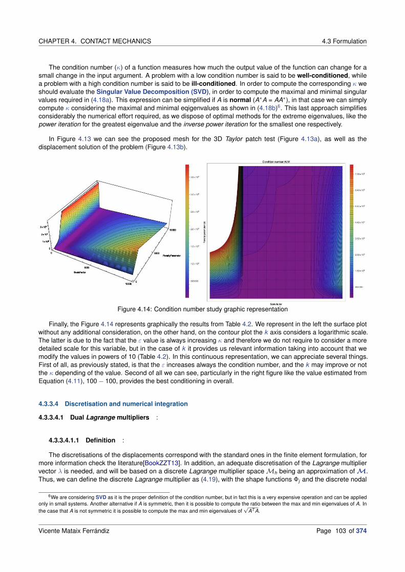
CHAPTER 4. CONTACT MECHANICS 4.3 Formulation
The condition number (κ) of a function measures how much the output value of the function can change for asmall change in the input argument. A problem with a low condition number is said to be well-conditioned, whilea problem with a high condition number is said to be ill-conditioned. In order to compute the corresponding κ weshould evaluate the Singular Value Decomposition (SVD), in order to compute the maximal and minimal singularvalues required in (4.18a). This expression can be simplified if A is normal (A∗A = AA∗), in that case we can simplycompute κ considering the maximal and minimal eqigenvalues as shown in (4.18b)6. This last approach simplifiesconsiderably the numerical effort required, as we dispose of optimal methods for the extreme eigenvalues, like thepower iteration for the greatest eigenvalue and the inverse power iteration for the smallest one respectively.
In Figure 4.13 we can see the proposed mesh for the 3D Taylor patch test (Figure 4.13a), as well as thedisplacement solution of the problem (Figure 4.13b).
Figure 4.14: Condition number study graphic representation
Finally, the Figure 4.14 represents graphically the results from Table 4.2. We represent in the left the surface plotwithout any additional consideration, on the other hand, on the contour plot the k axis considers a logarithmic scale.The latter is due to the fact that the ε value is always increasing κ and therefore we do not require to consider a moredetailed scale for this variable, but in the case of k it provides us relevant information taking into account that wemodify the values in powers of 10 (Table 4.2). In this continuous representation, we can appreciate several things.First of all, as previously stated, is that the ε increases always the condition number, and the k may improve or notthe κ depending of the value. Second of all we can see, particularly in the right figure like the value estimated fromEquation (4.11), 100 − 100, provides the best conditioning in overall.
4.3.3.4 Discretisation and numerical integration
4.3.3.4.1 Dual Lagrange multipliers :
4.3.3.4.1.1 Definition :
The discretisations of the displacements correspond with the standard ones in the finite element formulation, formore information check the literature[BookZZT13]. In addition, an adequate discretisation of the Lagrange multipliervector λ is needed, and will be based on a discrete Lagrange multiplier space Mh being an approximation of M.Thus, we can define the discrete Lagrange multiplier as (4.19), with the shape functions Φj and the discrete nodal
6We are considering SVD as it is the proper definition of the condition number, but in fact this is a very expensive operation and can be appliedonly in small systems. Another alternative if A is symmetric, then it is possible to compute the ratio between the max and min eigenvalues of A. Inthe case that A is not symmetric it is possible to compute the max and min eigenvalues of
√AT A.
Vicente Mataix Ferrándiz Page 103 of 374

4.3 Formulation CHAPTER 4. CONTACT MECHANICS
k ε κ k ε κ k ε κ1 1.00E-12 1.13E+05 10 1000 1.74E+04 1000 10 1.92E+041 1.00E-02 1.13E+05 10 10000 2.69E+05 1000 100 1.81E+041 1 1.13E+05 100 1.00E-12 1.74E+04 1000 1000 3.14E+041 10 1.18E+05 100 1.00E-02 1.74E+04 1000 10000 6.43E+041 100 1.63E+05 100 1 1.74E+04 10000 1.00E-12 6.64E+051 1000 6.15E+05 100 10 1.74E+04 10000 1.00E-02 6.63E+051 10000 2.69E+07 100 100 1.74E+04 10000 1 6.63E+0510 1.00E-12 1.74E+04 100 1000 1.74E+04 10000 10 6.63E+0510 1.00E-02 1.74E+04 100 10000 9.38E+04 10000 100 3.53E+0510 1 1.74E+04 1000 1.00E-12 6.60E+04 10000 1000 3.26E+0610 10 1.74E+04 1000 1.00E-02 6.60E+04 10000 10000 7.38E+0510 100 1.74E+04 1000 1 5.75E+05
Table 4.2: Results of numerical experiment for ALM parameters
Lagrange multipliers λh.
(4.19) λh =m1∑
i=1
Φj(ξ1, η1
)λj
Details on how to define dual Lagrange multiplier shape functions Φj using the so-called biorthogonality relationshipwith the standard displacement shape functions Nk have first been presented in Wohlmuth[ArtWoh02]. A commonnotation of the biorthogonality condition is (4.20), where Γ
1co,h represents the discrete contact interface.
(4.20)
∫
Γ1co,h
ΦjN1k dΓi
co = δjk
∫
Γ1co,h
N1k dΓi
co , j , k = 1, ..., m1
Herein, δjk is the Kronecker delta, and the most common choice m1 = n1 is assumed. For practical reasons, thebiorthogonality condition is typically applied locally on each slave element, represented with the index e, yielding(4.21), where m1
e represents the number of Lagrange multiplier nodes of the considered slave element.
(4.21)
∫
eΦjN
1k de = δjk
∫
eN1
k de , j , k = 1, ..., m1e
Combining the biorthogonality condition in (4.21) and the partition of unity property of the dual shape functions, itfollows that (4.22).
(4.22)
∫
eΦjde =
∫
eN1
j de , j = 1, ..., m1e
It is important to point out that the element-wise biorthogonality condition in (4.21) must be satisfied in the physicalspace, and not simply in the finite element parameter space. Consequently, a matrix system of size m1
e × m1e must be
solved on each slave element. The first step for doing this is to introduce unknown linear coefficients ajk such that(4.23).
(4.23) Φj (ξ, η) = ajk N1k (ξ, η) , Ae = [ajk ] ∈ R
m1e×m1
e
Page 104 of 374 Vicente Mataix Ferrándiz
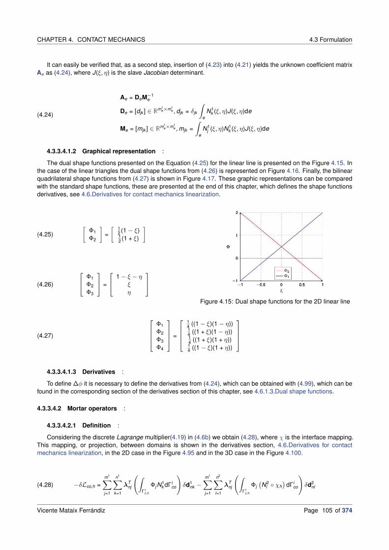
CHAPTER 4. CONTACT MECHANICS 4.3 Formulation
It can easily be verified that, as a second step, insertion of (4.23) into (4.21) yields the unknown coefficient matrixAe as (4.24), where J(ξ, η) is the slave Jacobian determinant.
(4.24)
Ae = DeM−1e
De = [djk ] ∈ Rm1
e×m1e , djk = δjk
∫
eN1
k (ξ, η)J(ξ, η)de
Me = [mjk ] ∈ Rm1
e×m1e , mjk =
∫
eN1
j (ξ, η)N1k (ξ, η)J(ξ, η)de
4.3.3.4.1.2 Graphical representation :
The dual shape functions presented on the Equation (4.25) for the linear line is presented on the Figure 4.15. Inthe case of the linear triangles the dual shape functions from (4.26) is represented on Figure 4.16. Finally, the bilinearquadrilateral shape functions from (4.27) is shown in Figure 4.17. These graphic representations can be comparedwith the standard shape functions, these are presented at the end of this chapter, which defines the shape functionsderivatives, see 4.6.Derivatives for contact mechanics linearization.
(4.25)
[Φ1
Φ2
]
=
[12 (1 − ξ)12 (1 + ξ)
]
(4.26)
Φ1
Φ2
Φ3
=
1 − ξ − ηξη
Figure 4.15: Dual shape functions for the 2D linear line
(4.27)
Φ1
Φ2
Φ3
Φ4
=
14 ((1 − ξ)(1 − η))14 ((1 + ξ)(1 − η))14 ((1 + ξ)(1 + η))14 ((1 − ξ)(1 + η))
4.3.3.4.1.3 Derivatives :
To define ∆φ it is necessary to define the derivatives from (4.24), which can be obtained with (4.99), which can befound in the corresponding section of the derivatives section of this chapter, see 4.6.1.3.Dual shape functions.
4.3.3.4.2 Mortar operators :
4.3.3.4.2.1 Definition :
Considering the discrete Lagrange multiplier(4.19) in (4.6b) we obtain (4.28), where χ is the interface mapping.This mapping, or projection, between domains is shown in the derivatives section, 4.6.Derivatives for contactmechanics linearization, in the 2D case in the Figure 4.95 and in the 3D case in the Figure 4.100.
(4.28) −δLco,h =m1∑
j=1
n1∑
k=1
λTnj
(∫
Γ1c,h
ΦjN1k dΓi
co
)
δd1nk −
m1∑
j=1
n2∑
l=1
λTnj
(∫
Γ1c,h
Φj(N2
l χh)
dΓico
)
δd2nl
Vicente Mataix Ferrándiz Page 105 of 374

4.3 Formulation CHAPTER 4. CONTACT MECHANICS
(a) Φ1 (b) Φ2
(c) Φ3
Figure 4.16: Dual shape functions for the 3D linear triangle
Numerical integration of the mortar coupling terms is exclusively performed on the slave side Γc,h of the interface.In (4.28), nodal blocks of the two mortar integral matrices commonly denoted as De and Me can be identified. Thisleads to the following definitions (4.29).
(4.29)
D[j , k ] = Djk Indim =
∫
Γ1c,h
ΦjN1k dΓi
coIndim , j = 1, ...m1 , k = 1, ...n1 =
ngp∑
g=1
wgφgjN1gk J1
g
M[j , l ] = Mjl Indim =
∫
Γ1c,h
Φj(N2
l χh)
dΓicoIndim , j = 1, ...m1 , k = 1, ...n2 =
ngp∑
g=1
wgφgjN2gk J1
g
With these matrices we can express the functional (4.28) in the following way (4.30) for the standard Lagrangemultiplier. This definition can be translated into the ALM formulation, but here we present the reasoning for thestandard Lagrange multiplier only, so the we can deduce the algebraic calculation of the discrete nodal weighted gap.In here, xn corresponds with the normal component of the coordinates of all the nodes, meanwhile xnS and xnM
Page 106 of 374 Vicente Mataix Ferrándiz

CHAPTER 4. CONTACT MECHANICS 4.3 Formulation
(a) Φ1 (b) Φ2
(c) Φ3 (d) Φ4
Figure 4.17: Dual shape functions for the 3D bilinear quadrilateral
correspond with the slave and master domain nodes respectively.
(4.30) −δLco,h = δxTnSDTλn − δxT
nMMTλn = δ[
xnN xnM xnS]
0
−MT
DT
= δxn
0
−MT
DT
︸ ︷︷ ︸
BTco
λn = δxTn fco(λn)
Herein, the discrete mortar unilateral contact operator Bco and the resulting discrete vector of unilateral contactforces fco(λn) = Bcoλn acting on the slave and the master side of the interface are introduced.
To finalise the discretisation of the considered unilateral contact problem, a closer look needs to be taken at theweak constraint contribution δLλh in (4.6c). Due to the saddle point characteristics and resulting symmetry of themixed variational formulation in (4.6b) and (4.6c), all discrete components of δLλ,h have already been introduced andthe final formulation is given as (4.31), with gn(x) = Bmtx · n representing the discrete unilateral contact constraint atthe coupling interface.
(4.31) −δLλ,h = δλTn DxnS − δλT
n MxnM = δλTn Bmtx · n = δλT
n gn(x)
Where, this discrete form of gn can be renamed as nodal weighted gap for each node (gn).
Vicente Mataix Ferrándiz Page 107 of 374

4.3 Formulation CHAPTER 4. CONTACT MECHANICS
4.3.3.4.2.2 Derivatives :
To obtain a fully quadratic convergence in the computation of the contact problem we should compute thederivatives of the Mortar operators, in consequence the derivatives of the Mortar operators are defined in itscorresponding section at the end of this chapter, see 4.6.Derivatives for contact mechanics linearization.
4.3.3.4.3 Algebraic form of the problem :
We will consider two cases for the matrix representation of the problem. The first one, corresponding to the scalarLM, presented in the corresponding section 4.3.3.2.1.Scalar Lagrange multiplier. This one cannot be condensed, andtherefore requires the direct resolution of the problem with all the DOF.
The second case corresponds with the vector representation of the LM, from the formulation presented in4.3.3.2.2.Vector Lagrange multiplier. This resulting system can be condensed due to the properties of the D,which is diagonal due to the consideration of the dual Lagrange multipliers, presented in 4.3.3.4.1.Dual Lagrangemultipliers.
4.3.3.4.3.1 Scalar LMM :
The following is the matrix form of the scalar form of the contact pressure, see 4.3.3.2.1.1.LMM. Once computedthe mortar operators, the resulting system for unilateral contact corresponds with (4.32a). In this representation7, andin the following ones, the subindex N represents all the DOF but the ones related with the contact problem, M willrepresent the master DOF and finally S will identify the slave DOF. At the same time, the slave DOF can be dividedbetween the active (A) and inactive (I) DOF. In here the residual for the LM, rλA
and rλI, corresponds in an algebraic
way with (4.32b). We call it algebraic way to the expression of the residual in considering the mortar operators (M, D).The corresponding LHS is defined by the derivatives of the mortar operators from 4.3.3.4.2.2.Derivatives.
KNN KNM KNSAKNSI
0 0
KNN KMM KMSAKMSI
− (n · MA)T − (n · MI )T
KSAN KSAM KSASAKSASI
(n · DAA)T (n · DAI )T
KSIN KSIM KSISAKSISI
(n · DIA)T (n · DII )T
0∂rλA
∂uM
∂rλA
∂uSA
∂rλA
∂uSI0 0
0 0 0 0 0 I
∆uN
∆uM
∆uSA
∆uSI
∆λA
∆λI
= −
rNrMrSA
rSI
rλA
rλI
(4.32a)
rλAn = −n · (Dx1 − Mx2)
rλI= λn
(4.32b)
4.3.3.4.3.2 Components LMM :
Here, the algebraic system upcoming from components representation of the LMM in the frictionless contactformulation is presented in (4.33a). The Lagrangian has been previously shown in 4.3.3.2.2.1.LMM. The maindifference is the full consideration of the mortar operators M and D.
(4.33a)
KNN KNM KNSAKNSI
0 0
KNN KMM KMSAKMSI
−MTA −MT
I
KSAN KSAM KSASAKSASI
DTAA DT
AI
KSIN KSIM KSISAKSISI
DTIA DT
II
0∂rλA
∂uM
∂rλA
∂uSA
∂rλA
∂uSI
∂rλA
∂λA0
0 0 0 0 0 I
∆uN
∆uM
∆uSA
∆uSI
∆λA
∆λI
= −
rNrMrSA
rSI
rλA
rλI
In the same way that in the previous definition for the scalar LM, but considering the penalisation of the tangentcomponents, we define the LM residuals rλA
and rλIin the Equation (4.33b). In here, and in the following, we define
7We will consider a very close notation with the one presented in Popp[PhDPop12].
Page 108 of 374 Vicente Mataix Ferrándiz

CHAPTER 4. CONTACT MECHANICS 4.3 Formulation
τ as the tangent direction of the λ, defining τ = λ−n(n·λ)‖λ−n(n·λ)‖ .
(4.33b)
rλA= n · (−n · (Dx1 − Mx2)) − τ · λ
rλI= λ
This system, as stated before can be statically condensed, this will be presented later (4.3.3.4.4.Static condensationof the system in considering of the DLMM) as it can be considered both for LMM and ALM formulations. Thismethodology can be considered too in the frictional formulation, which always requires to decompose the LM incomponents.
4.3.3.4.3.3 Penalty :
The formulation presented in 4.3.3.2.1.2.Penalty is the simplest of the introduced, as can be seen in (4.35a). It isrelevant to highlight that the inactive slave contact nodes do not add any contribution to the RHS and the LHS. Wewant to remark that we do not assume KMS , KSAM and KSIM to be zero, as these terms have contributions fromothers mechanical problems.
(4.34)
KNN KNM KNS
KMN KMM − ε
(
n · MT +
(
∂n·MT)
∂uMxM
)
KMS − ε
(
∂n·MT)
∂uSAxM
KSAN KSAM + ε∂(
n·DTA
)
∂uMxSA
KSASA+ ε
(
n · DTA +
∂(
n·DTA
)
∂uSAxSA
)
KSIN KSIM KSISI
∆uN
∆uM
∆uSA
∆uSI
= −
rNrM − εn · MxM
rSA+ εn · DAxSA
rSI
4.3.3.4.3.4 Scalar ALM :
Here the algebraic version of 4.3.3.2.1.3.ALM si presented in (4.35a), with the corresponding residual for the LM
defined in (4.35b).
KNN KNM KNSAKNSI
0 0
KNN KMM KMSAKMSI
− (kn · MA)T − (kn · MI )T
KSAN KSAM KSASAKSASI
(kn · DAA)T (kn · DAI )T
KSIN KSIM KSISAKSISI
(kn · DIA)T (kn · DII )T
0∂rλA
∂uM
∂rλA
∂uSA
∂rλA
∂uSI0 0
0 0 0 0 0 k2
ε I
∆uN
∆uM
∆uSA
∆uSI
∆λA
∆λI
= −
rNrMrSA
rSI
rλA
rλI
(4.35a)
rλAn = −kn · (Dx1 − Mx2)
rλI= k2
ε λn(4.35b)
4.3.3.4.3.5 Components ALM :
The final contribution that will be shown for the frictionless contact is the one relative to the ALM implementation for
Vicente Mataix Ferrándiz Page 109 of 374

4.3 Formulation CHAPTER 4. CONTACT MECHANICS
the vectorial LM from 4.3.3.2.2.2.ALM. The LHS can be seen in Equation (4.36a), and the LM RHS in (4.36b).
KNN KNM KNSAKNSI
0 0
KNN KMM KMSAKMSI
−kMTA −kMT
I
KSAN KSAM KSASAKSASI
kDTAA kDT
AI
KSIN KSIM KSISAKSISI
kDTIA kDT
II
0∂rλA
∂uM
∂rλA
∂uSA
∂rλA
∂uSI
∂rλA
∂λA0
0 0 0 0 0 k2
ε I
∆uN
∆uM
∆uSA
∆uSI
∆λA
∆λI
= −
rNrMrSA
rSI
rλA
rλI
(4.36a)
rλA= kn · (−n · (Dx1 − Mx2)) − k2
ε τ · λrλI
= k2
ε λ(4.36b)
4.3.3.4.4 Static condensation of the system in considering of the DLMM :
As mentioned before, it is possible to statically condensate the system of equations, solving a system in puredisplacements, instead of a system with displacements and LM. We already stated that this is possible to the diagonalproperty of the D when considering a DLMM formulation. The following presents the construction considered forthis system of equations that can be applied in any LHS where the LM considered is decomposed in Cartesiancomponents, both frictionless and frictional formulation. We describe the global LHS as shown in Equation (4.37),where the matrix is decomposed in 36 × 36.
(4.37)
KNN KNM KNSAKNSI
0 0
KNN KMM KMSAKMSI
KMLMAKMLMI
KSAN KSAM KSASAKSASI
KSALMAKSALMI
KSIN KSIM KSISAKSISI
KSILMAKSILMI
0 KLMAM KLMASAKLMASI
KLMALMA0
0 0 0 0 0 KLMILMI
∆uN
∆uM
∆uSA
∆uSI
∆λA
∆λI
= −
rNrMrSA
rSI
rλA
rλI
The last system presented can be simplified if we consider that KSILMA= 0, KSALMI
= 0 and ∆λI = 0.Additionally the KLMILMI
is diagonal, so its resolution is trivial, or can be applied by simply imposing λI = 0. Withthis we statically condensate (4.37) into (4.38). The resulting system is in pure displacement, instead of mixed.
(4.38)
KNN KNM KNSAKNSI
KNN + PKSAN KMM + PKSAM KMSA+ PKSASA
KMSI+ PKSASI
KSIN KSIM KSISAKSISI
CKSAN KLMAM + CKSAM KLMASA+ CKSASA
KLMASI+ CKSASI
∆uN
∆uM
∆uSA
∆uSI
= −
rNrM + PrSA
rLMA+ CrSA
rSI
In this last equation, operators P and C can be computed as follows in (4.39).
P =(K−1SALMA
KMALMA
)T(4.39a)
C =(K−1SALMA
KLMALMA
)T(4.39b)
Page 110 of 374 Vicente Mataix Ferrándiz

CHAPTER 4. CONTACT MECHANICS 4.3 Formulation
Finally, we can extract and deduce the expression necessary in order to compute the active LM in a standalonemanner as (4.40). This will be evaluated after computing the displacement DOF, from which it depends. It is importantto note that KSALMA
is a diagonal matrix, as is the result of the global assemble of the mortar operators D. Equation(4.40a) can be reformulated as Equation (4.40b).
KSAN · rN + KSAM ·∆uM + KSASA·∆uSA
+ KSASI·∆uSI
+ KSALMA·∆λA = rSA
(4.40a)
∆λA = K−1SALMA
(rSA
− KSAN · rN − KSAM ·∆uM − KSASI·∆uSI
− KSASA·∆uSA
)(4.40b)
4.3.3.5 Work-flow. Solution algorithm
The following section introduces the algorithm to be considered in order to solve the frictionless contact problem.It is relevant to highlight the fact that this algorithm is related with the semi-smooth strategy of the next section,4.3.3.6.Active set strategy (Semi-smooth Newton Raphson), and the previous one, 4.3.3.4.3.Algebraic form of theproblem. The algorithm is presented in Algorithm 2, here we will explain the differences between each one of theapproaches presented (standard LM, penalty, etc.), the approaches are similar but with slight differences that arerelevant to highlight.
The most significant difference across formulations is the threshold to be considered in the active set computation.For LM the threshold for each node to be checked is λi+1
nn+1 and for the ALM is kλi+1nn+1 − εngn. λnn+1 may correspond
with the LM for scalar LM or for the normal components (λn = n ·λ) in case of vector LM. In case of penalty formulationthe threshold would be −εngn. Additionally, it is important to separate the residual corresponding to the displacementsolution and the LM solution, in case that the problem considers LM.
Algorithm 2 Algorithm for the frictionless contact problem
1: procedure ALGORITHM FOR THE FRICTIONLESS CONTACT PROBLEM
2: t = 0 and i = 03: Initialise the solution for u0 = 0
4: In case of solving LM solution, Initialise the LM solution λ0 = 0 or λ0n = 0
5: Initialise the active set A01 and I0
1 such that A01 ∪ I0
1 = S and A01 ∩ I0
1 = ∅6: while t < tend do
7: t = t + ∆t and i = i + 18: Initialise the increment of solution for ∆ui
1 = 0
9: In case of solving LM solution, Initialise the LM increment of solution ∆λi1 = 0 or ∆λi
n1 = 0
10: Search for potential contact pairs, and if required update the pairs and the active set, respecting step 511: We define the problem as not converged conv = false12: while conv = false do
13: Find the solution corresponding to the system presented in 4.3.3.4.3.Algebraic form of the problem14: Update the solution, so ui
n+1 = uin + ∆ui
n+115: In case of LM solution λi
n+1 = λin + ∆λi
n+1 or λinn+1 = λi
nn + ∆λinn+1
16: Update the active set as in (4.41). The threshold for each one of the cases is represented in (4.42).
(4.41)I i+1
n+1 :=
j ∈ S|threshold i+1n+1 ≥ 0
Ai+1n+1 :=
j ∈ S|threshold i+1
n+1 < 0
(4.42) thresholdLM = λn or n · λ, thresholdPenalty = ǫgn, thresholdALM = kλn + ǫgn or kn · λ + ǫgn
17: Compute the corresponding residual to check (4.43).
(4.43) ‖ru‖ < toleranceu , ‖rλ‖ < toleranceλ
18: The solution is converged if Ai+1n+1 = Ai
n+1, I i+1n+1 = I i
n+1 and the residuals from (4.43) are converged.
The former algorithm, particularly the check of convergence can be appreciated in Figure 4.18, where the currentcontact convergence check present in Kratos is shown. In here the different types of residuals are check, as well as
Vicente Mataix Ferrándiz Page 111 of 374

4.3 Formulation CHAPTER 4. CONTACT MECHANICS
the active set check.
Figure 4.18: Example of convergence check in the frictionless contact
4.3.3.6 Active set strategy (Semi-smooth Newton Raphson)
As previously stated, the fully discretised unilateral contact problem introduces one significant complexity in theproblem resolution. This issue is the contact specific inequality constraints, which introduces two different sets ofdiscrete active and inactive constraints, which are unknown a priori. This previous dilemma does not appear for themesh tying case, see A.3.Mesh tying, where the subsets are known a priori. From a mathematical point of view, thisintroduces an additional source of non-linearity apart from the already existing geometric and material non-linearity.This issue can be solved with the consideration of an appropriate strategy, a common approach is the Primal-Dual
Active Set Strategies (PDASS), which is already presented in detail in the optimisation appendix (D.Constrainedoptimisation problems).
Figure 4.19: Nodal NCP function, or Lagrangian (L) contri-bution for the LM in the ALM
The principle behind any active set strategy for uni-
lateral contact is to iterate looking for the correct subsetof master-slave nodes in contact until there is not vari-ation in the respective subsets in the given time step. Inthe other hand, the contact non-linearity cannot be sim-ply solved in application of the PDASS. This is becausefinding the correct active set A cannot be resolved by astandard NR type approach.
Can be affirmed that in each one of the non-converged subsets we can apply an standard NR typealgorithm, in the same manner it is applied to the othertypes of non-linearity. These non-converged subsetsare obtained from rearranging the KKT conditions. InPopp[PhDPop12] the discrete KKT conditions are refor-mulated within a so-called NCP, this NCP is equivalentto the Lagrangian (L) contribution for the LM in the ALM,therefore in case of consider an ALM formulation it is defacto considered in the Lagrangian (L) definition. Equa-tion (4.44) shows the expression which defines the frictionless NCP. This corresponds with the augmented normalcontact pressure λn presented before (4.13), and the criteria will consist on activate/inactivate the corresponding nodeif the augmented contact pressure λn is in compression or traction correspondingly. The graphical representation canbe seen in Figure 4.19, where the equivalence with the KKT conditions is indicated in red colour, and this is driftedaccordingly to the penalty ε contribution.
(4.44) Cλn = kλn − max(0, kλn + εgn)
Hence, the PDASS considered accommodates derivative information on the subsets, allowing the resolution inconsidering NR algorithm also for the contact non-linearity. With the previous consideration, the contact problem canbe solved together with the other non-linearity, therefore we can consider one single iterative scheme. For the penaltyformulation, just in considering the algorithm presented in 4.3.3.5.Work-flow. Solution algorithm the PDASS is takeninto account with a standard NR strategy.
Page 112 of 374 Vicente Mataix Ferrándiz
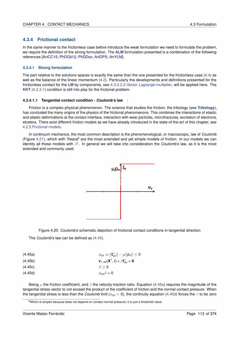
CHAPTER 4. CONTACT MECHANICS 4.3 Formulation
4.3.4 Frictional contact
In the same manner to the frictionless case before introduce the weak formulation we need to formulate the problem,we require the definition of the strong formulation. The ALM formulation presented is a combination of the followingreferences [ArtCC15; PhDGit12; PhDDoc; ArtDPS; ArtYLM].
4.3.4.1 Strong formulation
The part relative to the solutions spaces is exactly the same than the one presented for the frictionless case (4.4) aswell as the balance of the linear momentum (4.2). Particularly the developments and definitions presented for thefrictionless contact for the LM by components, see 4.3.3.2.2.Vector Lagrange multiplier, will be applied here. TheKKT (4.3.3.1) condition is still into play for the frictional problem.
4.3.4.1.1 Tangential contact condition - Coulomb’s law :
Friction is a complex physical phenomenon. The science that studies the friction, the tribology (see Tribology),has concluded the many origins of the physics of the frictional phenomenons. This combines the interactions of elasticand plastic deformations at the contact interface, interaction with wear particles, microfractures, excitation of electrons,etcetera. There exist different friction models as we have already introduced in the state-of-the-art of this chapter, see4.2.5.Frictional models.
In continuum mechanics, the most common description is the phenomenological, or macroscopic, law of Coulomb(Figure 4.21), which with Tresca8 are the most extended and yet simple models of friction. In our models we canidentity all these models with F . In general we will take into consideration the Coulomb’s law, as it is the mostextended and commonly used.
Figure 4.20: Coulomb’s schematic depiction of frictional contact conditions in tangential direction
The Coulomb’s law can be defined as (4.45).
φco := ‖tτco‖ − µ‖pn‖ ≤ 0(4.45a)
vτ ,rel (X1, t) + βtτco = 0(4.45b)
β ≥ 0(4.45c)
φcoβ = 0(4.45d)
Being µ the friction coefficient, and β the velocity-traction ratio. Equation (4.45a) requires the magnitude of thetangential stress vector to not exceed the product of the coefficient of friction and the normal contact pressure. Whenthe tangential stress is less than the Coulomb limit (φco < 0), the continuity equation (4.45d) forces the β to be zero
8Which is simpler because does not depend on contact normal pressure, it is just a threshold value.
Vicente Mataix Ferrándiz Page 113 of 374

4.3 Formulation CHAPTER 4. CONTACT MECHANICS
and, accordingly, the tangential relative velocity to be zero, this is called stick state. When the tangential stress is atthe Coulomb limit (φco = 0)), β may be greater than zero in (4.45d) and therefore the tangential stress is forced tooppose the relative tangential velocity in (4.45b), this is called the slip state.
The Figure 4.21 presents the graphical representation of Coulombs frictional conditions for 3D contact problems.The sub-Figure 4.21a introduces relation between the norm of the tangential velocity and the components of thetangential stress vector. In here the admissible points are situated either in the blue circle (β = 0, ‖ tτco ‖≤ µ ‖ pn ‖ |),which corresponds with the stick state; or on the surface of the semi-infinite cylinder (β ≥ 0, ‖ tτco ‖≤ µ ‖ pn ‖ |)marked with red colour, associated with the slip state. On the other hand, the sub-Figure 4.21b shows relationbetween the contact pressure and the components of the contact tangential stress vector. We can see in blue theinterior of the Coulombs cone ( ‖ tτco ‖≤ µ ‖ pn ‖ |), which represents the stick state. Contrarily the surface of thecone in red ( ‖ tτco ‖= µ ‖ pn ‖ |) exemplify the slip state.
(a) Relation between the norm of the tangential velocityand the components of the tangential stress vector
(b) Relation between the contact pressure and the compo-nents of the contact tangential stress vector
Figure 4.21: Graphical representation of Coulombs frictional conditions for 3D contact problem. Inspired [PhDYas11]
Additionally, the Table 4.3 shows the analogy mentioned in 4.2.5.Frictional models between the friction and theplasticity phenomenons. The relationship here corresponds with the one presented by Yastrebov [PhDYas11], a moredetailed analysis can be found in Antoni [ArtAnt17].
Friction Plasticity
Stick state Elastic deformationSlip state Plastic flowCoulombs’s cone ∂C(pn) Yield surfaceMaximal frictional stress ‖ tτco ‖= µ|pn| Yield strength
Table 4.3: Analogies between friction and plasticity
Finally, the definition of the tangent direction is needed. We use the complementary direction to the normal,so calling the normal as n we can define the tangent as (4.46a). With this we can define for example, the tangentLagrange multiplier as (4.46b).
τ = I − n ⊗ n(4.46a)
λτ = λ− nλn(4.46b)
4.3.4.2 Weak formulation
4.3.4.2.1 LMM :
Page 114 of 374 Vicente Mataix Ferrándiz
CHAPTER 4. CONTACT MECHANICS 4.3 Formulation
The weak formulation of these equations can be obtained again by multiplying (4.2) with the test function wi ∈ V i
and integrating in each domain i as (4.47).
(4.47) Li (ui ) =
∫
Ωi
[∇ · σi + bi
]· widΩi +
∫
Γiσ
[ti − σi · ni
]· widΓi
σ +
∫
Γico
[tico − σi · ni
]· widΓi
co = 0
From (4.47) the part corresponding to the frictional contact would the shown in (4.48).
(4.48) Lco(u,λ) =
∫
Γ1c
[tico − σi · ni
]dΓi
co
If we consider the test function wi as virtual displacements δu, and with the application of the Gauss divergencetheorem it is possible to determine the equivalent expression for the virtual work (4.49).
(4.49) δLi (ui , δui ) =
∫
Ωi
σi :∂δui
∂xjdΩi −
∫
Ωi
bi · δuidΩi −∫
Σiσ
ti · δuidΓiσ −
∫
Γico
tico · δuidΓi
co = 0∀δui ∈ V i
Equation (4.49) can be regrouped on contributions as in (4.7), obtaining (4.52).
− δLkin(u) =2∑
i=1
[∫
Ωi
ρi ui · δuidΩi
]
(4.50a)
− δLint ,ext (u) =2∑
i=1
[∫
Ωi
(
σi :∂δui
∂xj− b · δui
)
dΩi −∫
Γiσ
ti · δuiddΓiσ
]
(4.50b)
− δLco(u,λ) =
∫
Γ1co
t1co · δt1
cdΓ1co(4.50c)
Where tco represents the traction on the interface, the balance between the contact interface implies (4.51)
(4.51) t1codγ1 = −t2
codγ2
As in the frictionless case, we will take the slave surface as reference, this allows to rewrite the virtual work integralfor the contact as (4.52a).
(4.52a) δLco(u,λ) = −∫
Γ1co
t1co · δgdΓ1
co
Where g represents the general gap (4.52b) (instead of just normal gap).
(4.52b) g =(u1 − χ · u2
)
The Lagrange multipliers are introduced as additional unknowns on the slave contact surface and are identified as thenegative contact traction as (4.52c).
(4.52c) λ = −t1co
Vicente Mataix Ferrándiz Page 115 of 374

4.3 Formulation CHAPTER 4. CONTACT MECHANICS
4.3.4.2.2 Contact constraints :
The Equation (4.52a) is reformulated. Using the Lagrange multiplier in (4.52c) we can decompose into normaland tangential components λn and λτ (4.53).
λn ∈ R+0 : g(δλn − λn) ≥ 0∀δλn ∈ R+
0(4.53a)
λτ ∈ B(µλn) : vτ ,rel · (δλτ − λτ ) ≤ 0∀δλτ ∈ B(µλn)(4.53b)
Where B(µλn) is a (n1)-dimensional sphere with centre 0 and radius µ · λn and λτ is a trial force in the tangentialplane. It is the so-called principle of maximal dissipation representing Coulomb’s law of friction. Then (4.52a) can berewritten and the weak form of both normal and tangential contact conditions is obtained as (4.54).
λ ∈ M(λ) :
∫
λ1co
g(δλn − λn)dλ ≥ 0,(4.54a)
∫
λ1co
vτ ,rel (δλτ − λτ )dλ ≤ 0∀δλ ∈ M(λ)(4.54b)
Where M(λ) is the admissible solution space for the Lagrange multiplier and the test space for the trial forces δλ.It is a convex subset M(λ) ⊂ M which accommodates the restrictions of λ and δλ in (4.53). The subspace can berewritten as (4.55).
(4.55) M(λ) :=δλ ∈ M : 〈δλ,η〉 ≤ 〈µλn, ‖ητ‖〉,η ∈ L1 with ηn ≤ 0
Here 〈·, ·〉 is the duality pairing of the spaces M and V1 on γ1co given by (4.56).
(4.56) 〈δλ,η〉 :=
∫
γ1co
δληdγ
4.3.4.2.3 Penalty :
Before define the ALM frictional formulation, we introduce the penalty formulation for the frictional problem. TheALM formulation will result from the combination of this with the previous LMM. The Lagrangian (L) for the problem isdefined on (4.57a), separating the normal (4.57b) and tangent contributions (4.57c). In these expressions, tn
co = εngn
defines the normal contact traction and tτco = ετvτ ,rel corresponds to the tangent contact traction.
Lco(u) =
∫
Γ1c
ln + lτdΓico(4.57a)
ln(gn) =
− εn2 g2
n , tnco ≤ 0, (Contact zone)
0 , tnco > 0, (Gap zone)
(4.57b)
lτ (vτ ,rel ) =
− ετ2 vτ ,rel · vτ ,rel , ‖tτco‖ ≤ −µtn
co, stick
− µετ
tnco
2 vτ ,rel
‖vτ ,rel‖, ‖tτco‖ > −µtn
co, slip, tn
co ≤ 0, (Contact zone)
0 , tnco > 0, (Gap zone)
(4.57c)
With the Lagrangian (L) we can define the derivative in (4.58).
(4.58) δLco(u) =
∫
Γ1c
tnco · δgn + tτco · δvτ ,rel if ‖tτco‖ ≤ −µtn
co (Contact stick zone)
tnco · δgn − µtn
covτ ,rel
‖vτ ,rel‖δvτ ,rel if ‖tτco‖ > −µtn
co (Contact slip zone)
0 if tnco > 0 (Gap zone)
dΓico
Page 116 of 374 Vicente Mataix Ferrándiz

CHAPTER 4. CONTACT MECHANICS 4.3 Formulation
4.3.4.2.4 ALM :
In the very same way, we have defined an Augmented Lagrangian for the frictionless method we can definethe same for the frictional case. The ALM method to solve contact problems with friction was proposed by Alartand Curnier [ArtAC91], additionally to these references we have considered the work of Cardona[ArtCC15] andYastrebov [PhDYas11]. The solution obtained for the ALM results in a combination of the former LMM (4.3.4.2.1.LMM)and penalty (4.3.4.2.3.Penalty) solution.
Focusing in the functional relative to the contact (Lco(u,λ) = LVco + LM), we can rewrite (4.48) as (4.59).
(4.59) Lco(u,λ) =
∫
Γ1c
ln + lτdΓico
Being ln and lτ (4.60) the corresponding parts of the Augmented Lagrangian formulation for the normal andtangent contributions respectively.
(4.60a) ln(gn,λn) =
λngn − εn2 g2
n , λn ≤ 0, (Contact zone)
− k2
2εnλ2
n , λn > 0, (Gap zone)
With λn = kλn + εngn being the augmented Lagrange multiplier for the normal direction.
(4.60b)
lτ (vτ ,rel ,λτ ) =
λτ · vτ ,rel − ετ2 vτ ,rel · vτ ,rel , ‖λτ‖ ≤ −µλn, stick
− 12ετ
(k2λτ · λτ + 2µλn‖λτ‖ + µ2λ2
n
), ‖λτ‖ > −µλn, slip
, λn ≤ 0, (Contact zone)
− k2
2ετλτ · λτ , λn > 0, (Gap zone)
With λτ = kλτ + ετvτ ,rel being the augmented Lagrange multiplier for the tangent direction.
Where εn and ετ are a positive penalty parameter, both for normal and tangent direction, k is a positive scalefactor. Using the 〈〉 is the Macauley bracket operator, from (4.10), we can express everything as (4.61).
ln(gn,λn) =1
εn
(k2λ2
n − 〈λn〉2)
(4.61a)
lτ (vτ ,rel ,λτ ) =1
ετ
(k2λτ · λτ − ‖λτ‖2 − 〈‖λτ‖ − µ‖ − λn‖〉2
)(4.61b)
This functional is C1 differentiable saddle-point, as shown in Figure 4.22. The solution is obtained as the set ofvalues that render this functional stationary. The locus which corresponds to the solution in the normal direction ispresented in the optimisation appendix, D.4.3.Applicability on contact problems, in the Figure D.4.
As in the frictionless case, the solution does not depend on the value of parameters ε and k . Nevertheless,the convergence rate does depend on their value. Finally, we can derive (4.59) to obtain the variational form from(4.62).
(4.62)
δLco(u,λ) =
∫
Γ1c
λn · δgn + kgnδλn + λτ · δvτ ,rel + vτ ,rel · δλτ if ‖λτ‖ ≤ −µλn (Contact stick zone)
λn · δgn + kgnδλn − µλnλτ
‖λτ‖δvτ ,rel −
kλτ+µλnλτ
‖λτ‖
ετδλτ if ‖λτ‖ > −µλn (Contact slip zone)
− k2
εnλnδλn − k2
ετλτδλτ if λn > 0 (Gap zone)
dΓico
The functional from (4.62) makes that the system obtained varies in function if the nodes are present in the contact(slip or stick) or the gap zone, the system is not a priori known like in the frictionless case but with an additionalconfiguration.
Vicente Mataix Ferrándiz Page 117 of 374

4.3 Formulation CHAPTER 4. CONTACT MECHANICS
Figure 4.22: Augmented Lagrangian function for the frictional contact problem. Corresponding to (4.61b)
4.3.4.3 Discretisation and numerical integration
Many of the things defined for the frictionless case, like the definition of the dual Lagrange multipliers or the definitionof the mortar operators remain exactly the same. In this case we will focus in the kinematic definitions for the frictionalcase using the mortar operators, basically the definition of the discrete contact condition in the tangential directionand the slip in the discrete using the mortar operators.
4.3.4.3.1 Discrete contact condition in tangential direction :
Following the same procedure for the normal direction we can obtain the part equivalent for the tangential direction.The most relevant thing to take into account before any definition is the concept of the relative velocity in the tangentialdirection vτ ,rel , where we will use for our definition the discrete form of the material velocity field xi , which uses thesame shape functions for interpolation as the xi . We can then define (4.63).
(4.63)
∫
γ1c
vτ ,vel · (δλτ − λτ ) dγ
≈nslaves∑
j=1
(δλτ − λτ )T τ j
[∫
γ1c
ΦjN1j dγx1
j −nmaster∑
l=1
∫
γ1c
Φj(N2
l · ξ)
dγx2l
]
≥ 0∀δλ ∈ M(λ)
We can express this equation using the mortar operators, see 4.3.3.4.2, what will give us the following expression(4.64). Where vτ j is the weighted relative velocity.
(4.64)
∫
γ1c
vτ ,vel · (δλτ − λτ ) dγ ≈nslaves∑
j=1
(δλτ − λτ )T τ j
[
Dj x1j −
nmaster∑
l=1
Ml x2l
]
=nslaves∑
j=1
(δλτ − λτ )T vτ j ≥ 0
4.3.4.3.2 Slip definition :
An important aspect of a proper formulation of frictional laws in the finite sliding context is framed indiffer-ence[PhDGit12; ArtYLM] of the rate measures involved. This affects the tangential relative velocity of the contactingbodies (vτ ,rel ) in the considered case of frictional contact. This assures that this quantity is unaffected by any rigid
Page 118 of 374 Vicente Mataix Ferrándiz

CHAPTER 4. CONTACT MECHANICS 4.3 Formulation
body motion which the two contacting bodies might experience at the instant of the question. Mathematically, this canbe tested with formulating the tangential relative velocity vτ ,rel in an alternative reference frame. Then in the current(mortar projected) instance, we must ensure frame indifference.
Working in the time continuous case first, one may readily show that the tangential component of the mortarprojected tangential velocity is not frame indifferent (4.65a). Frame indifference is assessed by viewing the motionfrom another reference frame, denotes in the following by superscripts c(t), which can be related to the original spatialframe via (4.65b). Where c(t) is the relative rigid body translation between the original spatial frame and observer c(t),while a relative rotation is produced by the proper orthogonal tensor , (4.65c). The frame indifferent relative tangentialvelocity should satisfy. However, by considering the effect of the transformation (4.65b) on (4.65a), it is readily seenthat (4.65d).
vnononbjτ = τ j
[
Dj x1j −
nmaster∑
l=1
Ml x2l
]
(4.65a)
x(1∗)l = c(t) + Q(t)x1
l(4.65b)
v∗τ = Q(t)vτ(4.65c)
vnonobj∗τ = Q(t)vnonobj
τ − Q(t)
[
Djx1j −
nmaster∑
l=1
Mlx2l
]
· τ j(4.65d)
Because the term[
Djx1j −
∑nmaster
l=1 Mlx2l
]
6= 0 in general vnonobj∗τ does not satisfy the equation (4.65c), and thus
some modifications are required to this relative velocity measure to assure material frame indifference. It is possibleto restore the objectivity with the inclusion of the rate of a mortar projected distance between the two bodies, denotedas g. Then in consequence (4.66) is obtained.
(4.66) vτ = τ j
[
Dj x1j −
nmaster∑
l=1
Ml x2l − g
]
We obtain an expression which retains the interpretation of the tangential relative velocity in the case whereperfect sliding occurs (i.e. when g = 0), but which contains the modification necessary to make the velocity measureobjectives under all conditions of contact. This is readily seen by using direct calculation to exactly reexpress (4.66)as (4.67b), considering (4.67a).
g =d
dt
[
Djx1j −
nmaster∑
l=1
Mlx2l
]
=
[
Dj x1j −
nmaster∑
l=1
Ml x2l
]
+
[
Djx1j −
nmaster∑
l=1
Mlx2l
]
(4.67a)
vτ = τ j
[
Djx1j −
nmaster∑
l=1
Mlx2l
]
(4.67b)
The time derivatives of the mortar operators can be defined using any desired scheme, for example using thebackward Euler (4.68) scheme as time discretisation.
d (·)dt
≈ (·)t+∆t − (·)t
∆t(4.68a)
dD
dt≈
Dt+∆tl − Dt
j
∆t,
dM
dt≈ Mt+∆t
l − Mtl
∆t(4.68b)
Vicente Mataix Ferrándiz Page 119 of 374

4.3 Formulation CHAPTER 4. CONTACT MECHANICS
With this we can define tangential relative velocity vτ as (4.69a), that multiplies by ∆t gives us the nodal slipincrement uτ (4.69b).
vτ = τ j
[
Dt+∆tj − Dt
j
∆tx1
j −nmaster∑
l=1
Mt+∆tl − Mt
l
∆tx2
l
]
(4.69a)
uτ = τ j
[
(Dt+∆t
j − Dtj
)x1
j −nmaster∑
l=1
(Mt+∆t
l − Mtl
)x2
l
]
(4.69b)
4.3.4.3.3 Algebraic form of the problem :
The resulting systems of equations presented in this section will consider always a vectorial LM in the cases forthe LMM and ALM, as opposed to the solutions shown in 4.3.3.4.3.Algebraic form of the problem. Because of thisreason, we will be able to consider always the static condensation presented in 4.3.3.4.4.Static condensation of thesystem in considering of the DLMM for the LM approaches. It is also relevant to spotlight that in the following sectionsthe symbols representing the slip and stick states in addition to the states already presented in 4.3.3.4.3.1.ScalarLMM. These states are represented respectively as sl and st subindexes.
4.3.4.3.3.1 LMM :
Equation (4.70a) presents the system of equations relative to the standard LMM for the frictional problem. We cansee that, we have an additional block to block presented for the frictionless solution in 4.3.3.4.3.2.Components LMM.This is due to the fact that now the active DOF relative to the LM can be split into two different groups. The grouprelative to the slip state (sl) and the stick state (st). The residual of the contact solution is therefore also split intothese two subgroups, as see in Equation (4.70b).
(4.70a)
KNN KNM KNSAKNSI
0 0 0
KNN KMM KMSAKMSI
−MTAsl
−MTAst
−MTI
KSAN KSAM KSASAKSASI
DTAAsl
DTAAst
DTAI
KSIN KSIM KSISAKSISI
DTIAsl
DTIAst
DTII
0∂rλAsl∂uM
∂rλAsl∂uSAsl
∂rλAsl∂uSI
∂rλAsl∂λAsl
∂rλAsl∂λAst
0
0∂rλAst∂uM
∂rλAst∂uSAsl
∂rλAst∂uSI
∂rλAst∂λAsl
∂rλAsl∂λAsl
0
0 0 0 0 0 0 I
∆uN
∆uM
∆uSA
∆uSI
∆λAsl
∆λAst
∆λI
= −
rNrMrSA
rSI
rλAsl
rλAst
rλI
Equation (4.70b) shows the different residuals associated to the LM, and presented in Equation (4.70a). Therespective derived terms in the LHS, as in the frictionless case, require the mortar operators derivatives defined in4.3.3.4.2.2.Derivatives.
rλAsl= n · (−n · (Dx1 − Mx2)) − (τ · λ− F )
rλAst= n · (−n · (Dx1 − Mx2)) + uτ
rλI= λ
(4.70b)
F = −µλnτ(4.70c)
The F is the generic representation of the frictional threshold, we have already mentioned this in the sectiondedicated to the Coulomb’s frictional law (4.3.4.1.1.Tangential contact condition - Coulomb’s law). We will consider thisfrictional law, as our theoretical developments have departed from this hypothesis. In any case, the formulation canbe adapted to consider a different frictional criterion changing F from (4.70b), as well as in the corresponding activeset computation (see 4.3.4.4.Work-flow. Solution algorithm). The corresponding expression for F for the Coulomb’sfrictional law is presented in (4.70c), and it will be considered in the following for the standard LM. Additionally, uτ ,corresponds with the expression from Equation (4.69b).
Page 120 of 374 Vicente Mataix Ferrándiz

CHAPTER 4. CONTACT MECHANICS 4.3 Formulation
4.3.4.3.3.2 Penalty :
For the frictional solution, as we must split solution between the slip and the stick state and we lack of LM in oursystem, we separate the contact DOF between slip and stick in order to separate the contact contributions addedto the displacement DOF. Because of this, the system in Equation (4.71a) does not look as an square LHS, 6 × 3instead of 6 × 6, but it is actually a square system of equations.
(4.71a)
KNN KNM KNS
KslMN Ksl
MM − εn
(
n · MslT +∂(
n·MslT)
∂uMxslM
)
+ ∂FM
∂uMKslMS − εn
∂(
n·MslT)
∂uSAxslM + ∂FM
∂uSA
KslSAN Ksl
SAM + εn∂(
n·DslTA
)
∂uMxslSA
+ ∂FS
∂uMKslSASA
+ εn
(
n · DslTA +
∂(
n·DslTA
)
∂uSAxslSA
)
+ ∂FS
∂uSA
KstMN Kst
MM −(
εnn · MstT +∂(
n·MstT)
∂uMxstM
)
− εt∂uτ
∂uMKstMS − εn
∂(
n·MstT)
∂uSAxstM − εt
∂uτ
∂uSA
KstSAN Kst
SAM + εn∂(
n·DstTA
)
∂uMxslSA
+ εt∂uτ
∂uMKstSASA
+ εn
(
n · DstTA +
∂(
n·DstTA
)
∂uSAxslSA
)
+ εt∂uτ
∂uSA
KSIN KSIM KSISI
∆uN
∆uslM
∆uslSA
∆ustM
∆ustSA
∆uSI
= −
rNrslM − εnn · Mslxsl
M + FM
rslSA
+ εnn · DslAxsl
S + FS
rstM − εnn · Mstxst
M − εt uτ
rstSA
+ εnn · DstAxst
S + εt uτ
rSI
The frictional threshold (F ) for the penalty formulation, considering the Coulomb’s frictional law, corresponds withF = −µεngnτ . It consists in take the penalty approach for the normal contact pressure (εngn), and multiply by thefriction coefficient (µ) in the tangent direction (τ ). In this case, as we lack the LM solution in order to determine thetangent direction τ we must consider the direction of the slip increment (uτ ), defined as τ = uτ
‖uτ‖.
4.3.4.3.3.3 ALM :
As we have already pointed in 4.3.4.2.4.ALM we have to consider two different penalties, one in the normaldirection (εn) and the other one for the tangent direction (ετ ). This increases a little bit the complexity of the expressionsin comparison with the LMM one. In (4.72a) the resulting system of equations is shown.
(4.72a)
KNN KNM KNSAKNSI
0 0 0
KNN KMM KMSAKMSI
−kMTAsl
−kMTAst
−kMTI
KSAN KSAM KSASAKSASI
kDTAAsl
kDTAAst
kDTAI
KSIN KSIM KSISAKSISI
kDTIAsl
kDTIAst
kDTII
0∂rλAsl∂uM
∂rλAsl∂uSAsl
∂rλAsl∂uSI
∂rλAsl∂λAsl
∂rλAsl∂λAst
0
0∂rλAst∂uM
∂rλAst∂uSAsl
∂rλAst∂uSI
∂rλAst∂λAsl
∂rλAsl∂λAsl
0
0 0 0 0 0 0∂rλI
λI
∆uN
∆uM
∆uSA
∆uSI
∆λAsl
∆λAst
∆λI
= −
rNrMrSA
rSI
rλAsl
rλAst
rλI
As in the LMM case, we separate the LM residual in three parts, for inactive, active slip and active stick DOF. Theresulting residuals in (4.72b). In the case of the ALM, the F for the Coulomb’s frictional law is computed consideringthe augmented LM (λn) instead of the standard one (λn), this can be expressed as F = −µλnτ .
(4.72b)
rλAsl= kn · (−n · (Dx1 − Mx2)) − k2
εn
(τ · λ− F
k
)
rλAst= kn · (−n · (Dx1 − Mx2)) + k uτ
rλI= k2
εnn · λ + k2
εττ · λ
Vicente Mataix Ferrándiz Page 121 of 374

4.3 Formulation CHAPTER 4. CONTACT MECHANICS
4.3.4.4 Work-flow. Solution algorithm
The main changes relative to the solution loop presented in 4.3.3.5.Work-flow. Solution algorithm for the frictionlesssolution is the need to compute a more complex active set, which includes the slip and stick state, as well as thecomputation of the corresponding residuals for these states. The last stated, means that the residual correspondingto the LM is divided into three different components, the relative to the normal direction, the relative to the tangentdirection associated to the slip state, and finally the one obtained from the stick state. It is relevant to separate theresiduals from the slip/stick states, as the magnitude orders from these components change greatly and it may bedifficult to achieve a convergence if mixing them. We remark the need to do this search at each time step in order toadapt to the evolution of the geometry.
Algorithm 3 Algorithm for the frictional contact problem
1: procedure ALGORITHM FOR THE FRICTIONAL CONTACT PROBLEM
2: t = 0 and i = 03: Initialise the solution for u0 = 0
4: In case of solving LM solution, Initialise the LM solution λ0 = 0
5: Initialise the active set A01 and I0
1 such that A01 ∪ I0
1 = S and A01 ∩ I0
1 = ∅6: Initialise the slip/stick set A0
sl1 and A0st1 such that A0
sl1 ∪ A0st1 = A0
1 and A0sl1 ∩ A0
st1 = ∅7: while t < tend do
8: t = t + ∆t and i = i + 19: Initialise the increment of solution for ∆ui
1 = 0
10: In case of solving LM solution, Initialise the LM increment of solution ∆λi1 = 0
11: Search for potential contact pairs, and if required update the pairs and the active set, respecting step 512: We define the problem as not converged conv = false13: while conv = false do
14: Find the solution corresponding to the system presented in 4.3.4.3.3.Algebraic form of the problem15: Update the solution, so ui
n+1 = uin + ∆ui
n+1 and in case of LM solution λin+1 = λi
n + ∆λin+1
16: Update the active set as in (4.73). The threshold for each one of the cases is represented in (4.74).
(4.73)I i+1
n+1 :=
j ∈ S|threshold i+1n+1 ≥ 0
Ai+1n+1 :=
j ∈ S|threshold i+1
n+1 < 0
(4.74) thresholdLM = λn or n · λ, thresholdPenalty = ǫgn, thresholdALM = kλn + ǫgn or kn · λ + ǫgn
17: Update the slip/stick set as in (4.75). To evaluate this we require the frictional threshold F , consideringCoulomb’s law, for the cases represented in (4.76). We also require the tangent contact stress (tτco) (4.77).
(4.75)Ai+1
sln+1 :=
j ∈ A|tτco ≥ F i+1n+1
Ai+1stn+1 := j ∈ A|tτco < Fn+1
(4.76) FLM = µn · λ, FPenalty = µεngn, FALM = µ (kn · λ + εngn)
(4.77) tτLMco = ‖τ · λ‖, tτPenaltyco = ‖ετ uτ‖, tτALMco = ‖kτ · λ + ετ uτ‖
18: Compute the corresponding residual to check (4.78).
(4.78) ‖ru‖ < toleranceu , ‖rλn‖ < toleranceλn , ‖rλslτ‖ < toleranceλsl
τ, ‖rλst
τ‖ < toleranceλst
τ
19: Solution converged if Ai+1sln+1 = Ai
sln+1, Ai+1stn+1 = Ai
stn+1, I i+1n+1 = I i
n+1 and residuals (4.78) are converged.
As well as we did in the frictionless case, we present on Figure 4.23 the output in Kratos representing the NL
convergence check of a time step. We can appreciate the four different residuals which are check, in addition to the
Page 122 of 374 Vicente Mataix Ferrándiz

CHAPTER 4. CONTACT MECHANICS 4.4 Contact detection. Search techniques
two different active set checked.
Figure 4.23: Example of convergence check in the frictional contact
4.3.4.5 Active set strategy (Semi-smooth Newton Raphson)
Figure 4.24: NCP for the frictional contact problem.
The reformulation of frictional contact conditions is simi-lar to the frictionless case. As well as in the former case,the LM contribution of the Lagrangian (L) in the ALM
(4.60) replaces the NCP presented in Popp[PhDPop12]and Gitterle[PhDGit12]. This NCP takes the form of atwo component vector equation and is written as (4.79),the visual representation can be seen in Figure 4.24.This representation shows a distinctive behaviour for theslip/stick states in the similar manner to the one pre-sented in the Figure 4.22 for the frictional Lagrangian(L) contribution. As in the frictionless case, for the fric-tional problem the PDASS is taken into consideration inconsidering the workflow presented in 4.3.4.4.Work-flow.Solution algorithm.
(4.79) Cτ (λτ , uτ ) = max(µλn, ‖λτ‖)λτ − µmax(0,λn)λτ
4.4 Contact detection. Search techniques
4.4.1 Introduction
Detection phase it is quite different depending on if we are considering an implicit or an explicit approach[PhDYas11]:
• Explicit approach: Here, as the time step is usually very small, we need to detect the solids that actually havepenetrated each other, and apply the corresponding forces in order to repulse them. There are different ways toapply these repulsive forces, but the point is that we focus on real penetration, not estimations.
• Implicit approach: As the solution of the system depends on the values that have not been completed yet,we need to estimate potential pairings. With this potential pairing, we include the corresponding DOF, withthe corresponding additional Lagrange multiplier, and assemble the LHS and RHS related to these potentialpairings.
As the target of this work is the consideration of an implicit approach, we need to take care of the problematic ofthe former. The detection phase is crucial, as the additional DOF and assembling is not only numerically expensive,but the condition of the system is significantly affected by them.
Additionally, for a problem with n slave elements and m master elements, the cost of a naive brute force searchingalgorithms (searching all master elements for valid intersections with each slave element) is O(nm), which isunacceptable for a problem with a large amount of contact surface elements. The ultimate goal of a contact searchingalgorithm is to find all proximate slave-master element pairs. In conclusion, this phase may be as important as theformulation considered as it influences the whole resolution of the problem.
These methodologies have been particularly developed in recent years, thanks not only for FE requirements,but also computer graphics(physically based modelling, animation)[ArtZK12; ArtRKC02], robotics (motion planning,collision avoidance)[ArtTK14], industrial applications (virtual prototyping, assembly tests)[ArtFig10; ArtFF03] and
Vicente Mataix Ferrándiz Page 123 of 374

4.4 Contact detection. Search techniques CHAPTER 4. CONTACT MECHANICS
Figure 4.25: Conventional penetration estimations. Symmetric: a segment intersection; b volume intersection.Asymmetric: c,d segment in volume; e,f node in volume; g,h node under surface. Source[PhDYas11]
videogames[BookEri04; ArtCai+14], where the Collision Detection (CD) plays an important role in their respectivefields.
The penetration is another aspect to take into account when detecting potential contact pairs. There is a wholescience in the contact penetration or gap estimation. From the more conventional methods, Figure 4.25, through moreadvanced or recent methods such as the estimation of penetration by ray-tracing[ArtPR15a]. In this work we presentan approach consistent with the Mortar formulation considered for the contact computation.
In what follows, a contact searching algorithm with Bounding Volume Hierarchies (BVH) can be applied(4.4.3.Tree structures), furthermore, there are different kinds of bounding volumes that can be used to improve thissearch, see 4.4.2.Bounding volumes. Finally, the penetration estimation is an important step too, and the proposedapproach will be presented at 4.4.4.Penetration definition.
4.4.2 Bounding volumes
There are many kinds of DOP that can be used to define the bounding volumes, Figure 4.26a illustrates some of them.We address to the literature, particularly to the work of Dinas[ArtDB15], which summarises each methodology andmakes a comparison between them. There are several different ways to define a bounding volume for a geographicalregion.
The simplest DOP probably will be to consider the nodes inside a radius, a radius search or BS. Another verysimple solution, define a cuboid whose surfaces are parallel to the x − y , y − z and x − z surfaces, is called AABB,but these two methods have the drawback of the lack if tightness, and many slave and master surfaces are likely to betested for proximity even though they are not so close (Figure 4.26b). Another approach is the OBB, which is muchtighter and therefore giving a better fit, but with an additional computational cost and memory consumption. Finally, itcan be considered the k-DOP (convex hull) to define the bounding volumes, which are always tighter than AABB andmay be tighter or looser than OBB depending of the geometries of the objects. However the k-DOP are much simpler,cheaper and more efficient for the detection of k-DOP overlapping, which is quite relevant for our applications sincedeformation of contact bodies requires frequent updating of these volumes[ArtYL08].
In any case the Figure 4.26a as the decision to be taken results in a compromise solution between numerical cost,complexity and precision. For this reason the OBB has been chosen among all the options, as a intermediate solutionthat will satisfy the requirements. Originally a BS approach was chosen, but it was insufficient, as in order to detect allthe contact pairs, a large enough radius factor must be taken into account (see Figure 4.27a), returning many falsepotential pairs, which impoverished the convergence of the problem. Additionally, this approach is very dependent onthe radius r chosen, as can be seen in Figure 4.27b.
4.4.2.1 OBB implementation
Fortunately, we have plenty of documentation on how to implement this type of object thanks to its wide use invideo game graphics engines. Our implementation is based on the one considered in the documentation of theGeometricTools[BookEbe99] library and the tutorials found for game development[OnlCho].
Page 124 of 374 Vicente Mataix Ferrándiz

CHAPTER 4. CONTACT MECHANICS 4.4 Contact detection. Search techniques
(a) Types of Discretised Orientation Polytopes (DOP)
(b) Proximity tests for DOP
Figure 4.26: Types of bounding volumes. a) The radius search (Bounding Spheres (BS)). b) Axis-Aligned Bound-
ing Box (AABB). c) OBB. d) Discrete Orientation Polytopes (k-DOP) (convex hull). Inspired on [ArtYL08]
In order to define the collision algorithms, we can consider between two OBB we need to define the geometrywhich defines it properly. Considering we are in ℜ3. An OBB is defined[BookEbe99] by a centre C, a set of right-handed orthogonal axes A0, A1 and A2, and a set of real positive extends a0, a1 and a2. With this we can define theOBB as solid box following Equation (4.80a). Additionally Equation (4.80b) represents the eight vertices of the box,where |σi | = 1 for all i .
(4.80a) C +2∑
i=0
xiAi : |xi | ≤ |ai | for all i
(4.80b) C +2∑
i=0
σiaiAi
Our interest would be to build the OBB from a provided geometry in order to automate its construction. We havetwo options in 3D for surface geometries. The first approach takes the AABB, the lowest and highest point, and buildsand axes and defines an orthonormal base. The second approach will be based on the normal which defines thatsurface geometry. Taking this normal, we can define a base, rotate the points to this base and get the point at themaximum distance from the geometry centre. Combining the tangent base in order to define a vector in the directionto the furthest point, then the third axis is taken as the cross product of the normal and this vector. This last methoddefines a less arbitrary bounding box than the first one. The difference can be seen in Figure 4.29, where we buildthe OBB for 4 triangles, 2 in the top and 2 over the first ones. The first one, Figure 4.29a, may look more regular, butjust takes an arbitrary direction as all the nodes are in the same plane. The one from Figure 4.29b defines a largerOBB, and it is oriented to the furthest point from the centre, which is less arbitrary.
4.4.2.1.1 Collision detection :
Vicente Mataix Ferrándiz Page 125 of 374

4.4 Contact detection. Search techniques CHAPTER 4. CONTACT MECHANICS
(a) Poor search results obtained with the BS approach (b) Influence of radius in BS. Source[PhDYas11]
Figure 4.27: BS approach
Figure 4.28: OBB. Source[ArtRom11]
The simplest collision detection consists in two steps, a first stage where we check that the points of one OBB areinside the other, the second stage consists in check if there is an intersection between the faces of the OBB. Forthe first step, we need to define the inside operations for a OBB. In order to do, the simplest procedure consists inrotating the points so these points became oriented with the Cartesian axis, Equation (4.81) and (4.82), and thereforeconsider the standard AABB inside algorithm.
For 2D we consider the following signs:
(4.81a)sign2D
x =[−1.0 1.0 1.0 −1.0
]
sign2Dy =
[−1.0 −1.0 1.0 1.0
]
For each point i of the destination OBB:
(4.81b) xaabbi = Cdest + sign2D
xi Adest0 adest
0 + sign2Dyi Adest
1 adest1
We check if is inside the origin OBB:
(4.81c) ‖xaabbxi − Corig
x ‖ <= aorig0 and ‖xaabb
yi − Corigy ‖ <= aorig
1
For 3D we consider the following signs:
(4.82a)sign3D
x =[−1.0 1.0 1.0 −1.0 −1.0 1.0 1.0 −1.0
]
sign3Dy =
[−1.0 −1.0 1.0 1.0 −1.0 −1.0 1.0 1.0
]
sign3Dz =
[−1.0 −1.0 −1.0 −1.0 1.0 1.0 1.0 1.0
]
For each point i of the destination OBB:
(4.82b) xaabbi = Cdest + sign3D
xi Adest0 adest
0 + sign3Dyi Adest
1 adest1 + sign3D
zi Adest2 adest
2
We check if is inside the origin OBB:
(4.82c) ‖xaabbxi − Corig
x ‖ <= aorig0 and ‖xaabb
yi − Corigy ‖ <= aorig
1 and ‖xaabbzi − Corig
z ‖ <= aorig2
Page 126 of 374 Vicente Mataix Ferrándiz

CHAPTER 4. CONTACT MECHANICS 4.4 Contact detection. Search techniques
(a) AABB aligned OBB (b) Normal plane aligned
Figure 4.29: OBB from surfaces build comparison
For the intersection of the faces, the very same algorithms considered for the intersections of lines in 2D andquadrilaterals in 3D can be considered here. In total, the number of checks necessaries in order to check theintersection is 24 in 2D and 52 in 3D. Of course, not all checks are required. In case of one positive check we alreadyknow that there is at least one intersection.
4.4.2.1.2 Collision detection with SAT :
(a) Illustration of the separating axis theorem (I) (b) Illustration of the separating axis theorem (II)
Figure 4.30: Separating axis theorem
Figure 4.31: SAT concept. Source[OnlCho]
This algorithm is more refined than the previous one.In this case instead of direct check each one of thenodes and faces, we apply a very simple geometricalconcept. SAT[ArtRom11] is based on the separating axistheorem, Figure 4.30, which states that it is sufficientto find one axis that separates A and B to be sure thatthey are disjoint and so do not overlap. Therefore, if weare able to draw a line to separate two polygons, thenthey do not collide (Figure 4.31). This concept can beused not only between OBB but also between generalpolygons or even a polygon and a circle. The definitionof the SAT consists on two steps, during the first step wedefine each one of the potential planes to be checked,the definition of each plane is found in Equation (4.83),and secondly we check if there is a separation plane between the two OBB with the one presented on (4.84).
The normal vectors to be considered in 2D correspond with the right-handed orthogonal axes A0 and A1 from
Vicente Mataix Ferrándiz Page 127 of 374

4.4 Contact detection. Search techniques CHAPTER 4. CONTACT MECHANICS
both OBB, and the following cross-products:
(4.83a) n
Adest0 , Adest
1 , Aorig0 , A
orig1
Adest0 × A
orig0 , Adest
0 × Aorig1
Adest1 × A
orig0 , Adest
1 × Aorig1
The normal vectors to be considered in 3D correspond with the right-handed orthogonal axes A0, A1 and A2 fromboth OBB, and the following cross-products:
(4.83b) n
Adest0 , Adest
1 , Adest2 , A
orig0 , A
orig1 , A
orig2
Adest0 × A
orig0 , Adest
0 × Aorig1 , Adest
0 × Aorig2
Adest1 × A
orig0 , Adest
1 × Aorig1 , Adest
1 × Aorig2
Adest2 × A
orig0 , Adest
2 × Aorig1 , Adest
2 × Aorig2
In 2D the algorithm for checking if there is a separation plane, being n the normal which defines the plane:
(4.84a)
‖(Cdest − Corig) · n‖ >‖(Adest
0 adest0 ) · n‖ + ‖(Adest
1 adest1 ) · n‖+
‖(Aorig0 aorig
0 ) · n‖ + ‖(Aorig1 aorig
1 ) · n‖
In 3D the algorithm for checking if there is a separation plane:
(4.84b)
‖(Cdest − Corig) · n‖ >‖(Adest
0 adest0 ) · n‖ + ‖(Adest
1 adest1 ) · n‖ + ‖(Adest
2 adest2 ) · n‖+
‖(Aorig0 aorig
0 ) · n‖ + ‖(Aorig1 aorig
1 ) · n‖ + ‖(Aorig2 aorig
2 ) · n‖
The resulting number of checks therefore to be evaluated in this case would be of 8 for the 2D case and 15 in3D.
4.4.3 Tree structures
Figure 4.32: Space subdivision approaches
The tree structures are computer data structures that emulate a tree structure with a set of binary nodes[Book-FSS12], see Figure 4.33a. A node that is upper in the hierarchy respect to other nodes which is connected with him iscalled parent node, and node below is denominated child node. The node in the top of the tree is called root node,while the nodes in the bottom are called leaf nodes.
Page 128 of 374 Vicente Mataix Ferrándiz

CHAPTER 4. CONTACT MECHANICS 4.4 Contact detection. Search techniques
A data structure which stores the data points with respect to their position in space is needed to perform a searchfor neighbours. In two-dimensional spaces, the standard data structure is a quadtree, and the octree is analogue inthree-dimensional space.
The kd-tree data structure is based on a recursive subdivision of space into disjoint hyperrectangular regionscalled cells (see Figure 4.33b). Each node of the tree is associated with a region called box, and is associated with aset of data points that lie within this box. The root node of the tree is associated with a bounding box that contains allthe data points.
In addition to the data points themselves, a kd-tree is specified by two additional parameters, the bucket size
(threshold of the number of data points associated with a node) and a splitting rule (which determine how ahyperplane is selected). For more details look up the literature[ArtYL08; BookPhD06; OnlRtr].
(a) Binary tree (b) A kd-tree of bucket size one and the corresponding spacial decomposition
Figure 4.33: Tree structures
The binary structure tree that will be considered in this work will be therefore the kd-tree. This tree is alreadyavailable in the Kratos code.
4.4.4 Penetration definition
As we have already mentioned, the main difference in explicit and implicit simulation detection is that in the formercase we predict possible contact phenomena, and we define potential contact pairs before penetration happens. Thismeans that slave nodes approaching master surfaces have to be detected at a certain distance, which is usuallydenoted as Maximal Detection Distance (MDD). The MDD is a significative parameter of the detection procedure.This MDD should be considered as small as possible in order to avoid the creation of non-necessary contact pairs. Inorder to do that we should define an automatic procedure which defines this value in function of certain parameters,such as the element size (h). Once this is defined we need to estimate the penetration, so we can compare it with theMDD.
For that, we highlight that contact penetration estimation has its own advantages and disadvantages, and usuallythese techniques are uncoupled of the contact formulation considered. In order to compute a consistent penetration,or gap (gn), with the weighted gap (gn) computed during the contact contributions on 4.3.3.4.2.Mortar operators wewill consider this very same Mortar formulation as the base concept.
This is done using the Mortar mapper developed in this work. The concept is to map the coordinates of onedomain to the other, and once these coordinates have been mapped into a destination domain we can computethe consistent gap node-by-node applying the gn formula, gn = −n · (x1 − χhx2). The obtained gap is equal to theweighted gap divided by the total Mortar integration area which involves the node. This value has length units andtherefore can be compared with some reference length. This very same concept can be applied in order to compute aconsistent slip in case it is of interest (mostly for post-process motives).
We can illustrate this former concept with an example. The Figure 4.34 shows a full example, consistent in acircular surface and a plane surface, Figure 4.34a. As one of the sides is plane, it is easy to estimate the gap as they coordinate of the circular side. The nodal area corresponds with the integrated region in each node, which is thewhole section until the circular section does not intersect with the plane any more, see Figure 4.34b. With this we can
Vicente Mataix Ferrándiz Page 129 of 374

4.4 Contact detection. Search techniques CHAPTER 4. CONTACT MECHANICS
(a) Mesh of the example (b) Nodal area
(c) Consistent gap (d) Weighted gap
Figure 4.34: Consistent gap example. Circular surface vs plane
see as if dividing gn (Figure 4.34d) by the normal area, the consistent normal gap (gn) is obtained (Figure 4.34c). Thisone coincides with the predicted values (the height to the circular region).
A more complex case its illustrated in the Figure 4.35, where the double curvature considered to test the Mortarmapper in E.Mortar mapper is considered to compute a consistent gap. The first figure shows the mesh, Figure 4.35a,and the second one in Figure 4.35b. In this last image, we can see like the gap varies according to the curvature andfollowing the "parallel lines" that define this double curvature geometry. Some peaks appear in the nodes that belongto coarse mesh regions.
The details of the implementation of this mapper can be found in the respective appendix, E.Mortar mapper. Thedefinition of the consistent gap is detailed in the algorithm 8.
4.4.5 Self-contact detection
4.4.5.1 Introduction
There are mechanical problems for which the determination of the contact pairs is not trivial, and especially complexare the problems where we do not enforce any master-slave9 (or mortar and non-mortar ) relationship. For two ormore independent bodies a priori we can assign these relationships, but this is not the case for self-contact problems,where there is only one body which contact with itself as the name indicates. This class of contact problems needs aparticular contact detection procedure.
9We will consider the master-slave criteria considered in the formulation, as done by Popp[PhDPop12], where the slave conditions correspondwith the one where the integration is performed.
Page 130 of 374 Vicente Mataix Ferrándiz
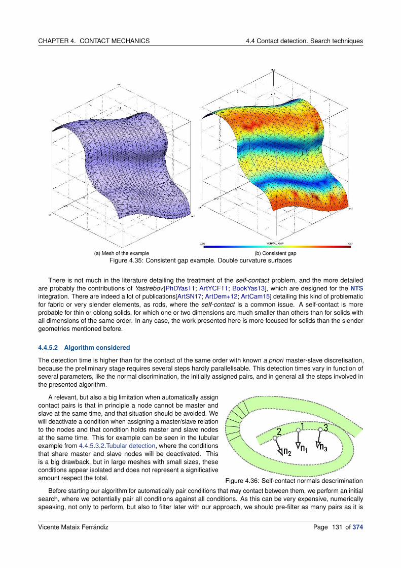
CHAPTER 4. CONTACT MECHANICS 4.4 Contact detection. Search techniques
(a) Mesh of the example (b) Consistent gap
Figure 4.35: Consistent gap example. Double curvature surfaces
There is not much in the literature detailing the treatment of the self-contact problem, and the more detailedare probably the contributions of Yastrebov [PhDYas11; ArtYCF11; BookYas13], which are designed for the NTS
integration. There are indeed a lot of publications[ArtSN17; ArtDem+12; ArtCam15] detailing this kind of problematicfor fabric or very slender elements, as rods, where the self-contact is a common issue. A self-contact is moreprobable for thin or oblong solids, for which one or two dimensions are much smaller than others than for solids withall dimensions of the same order. In any case, the work presented here is more focused for solids than the slendergeometries mentioned before.
4.4.5.2 Algorithm considered
The detection time is higher than for the contact of the same order with known a priori master-slave discretisation,because the preliminary stage requires several steps hardly parallelisable. This detection times vary in function ofseveral parameters, like the normal discrimination, the initially assigned pairs, and in general all the steps involved inthe presented algorithm.
Figure 4.36: Self-contact normals descrimination
A relevant, but also a big limitation when automatically assigncontact pairs is that in principle a node cannot be master andslave at the same time, and that situation should be avoided. Wewill deactivate a condition when assigning a master/slave relationto the nodes and that condition holds master and slave nodesat the same time. This for example can be seen in the tubularexample from 4.4.5.3.2.Tubular detection, where the conditionsthat share master and slave nodes will be deactivated. Thisis a big drawback, but in large meshes with small sizes, theseconditions appear isolated and does not represent a significativeamount respect the total.
Before starting our algorithm for automatically pair conditions that may contact between them, we perform an initialsearch, where we potentially pair all conditions against all conditions. As this can be very expensive, numericallyspeaking, not only to perform, but also to filter later with our approach, we should pre-filter as many pairs as it is
Vicente Mataix Ferrándiz Page 131 of 374

4.4 Contact detection. Search techniques CHAPTER 4. CONTACT MECHANICS
possible for us. The method which provides the best results, and the simplest, is probably to check the similaritybetween the normals of the conditions. If the normals are close, not necessarily equal, therefore we can consider thatthese are pointing in the same direction and therefore will not deal with contact. This can be appreciated in Figure4.36, where normals 1 and 3 are quite similar, so we can easily discriminate the pair 1 − 3. On the other hand, thedifference between 1 and 2 is more subjective and it will depend on the threshold we consider to discriminate the pair1 − 2.
Our proposal takes as a main hypothesis that the master/slave conditions are neighbours between them. Thisassumption is based on the fact that when we define manually certain conditions as the master or slave usuallywe define a region for each domain. Therefore, our goal is to replicate or mimic the behaviour that a human wouldconsider when assigning the domains. Therefore, we will create a list of potential slave conditions and we will fillthis list following a neighbourhood criterion. The idea is to create a list10 of conditions, that we will fill based on theproximity respect to the condition previously added to the list, except if we have already assigned that condition as amaster, in that case we will jump to the next candidate.
Algorithm 4 Self-contact detection algorithm
1: procedure SELF-CONTACT DETECTION ALGORITHM
2: We perform an initial search with all conditions againts all conditions3: for all node ∈ ContactMeshnodes do
4: Reset SLAVE flag5: Reset MASTER flag
6: for all condition ∈ ContactMeshconditions do
7: Reset SLAVE flag8: Reset MASTER flag9: Reset ACTIVE flag
10: We create a set ordered_conditions that will contain all conditions in order of proximity between them11: We add as first condition to this set one choosen arbitrarily12: We create a map containing the boundaries of all conditions13: for all condition ∈ ContactMeshconditions do
14: for all boundary ∈ conditionboundaries do
15: Insert the connectivity of the boundary and the geometry where it belongs
16: for all condition ∈ ordered_conditions do
17: for all boundary ∈ conditionboundaries do
18: if A neighbour is found then
19: Add that neighbour to ordered_conditions20: else
21: Add arbitrary condition not added previously to ordered_conditions
22: for all condition ∈ ordered_conditions do
23: for all pair ∈ conditionpotential − pairs do
24: if Condition are neighbours then
25: Skip to the next pair26: else
27: if Check the nodes of the pair are not SLAVE then
28: Assign MASTER flag to condition and nodes in the pair condition29: Clear pair condition database
30: if At least one pair is MASTER then
31: Assign SLAVE flag to condition and nodes
32: for all condition ∈ ContactMeshconditions do
33: if condition shares MASTER/SLAVE nodes then
34: Unset ACTIVE flag to condition35: else
36: Set ACTIVE flag to condition
10We have considered std::unordered_set in particular.
Page 132 of 374 Vicente Mataix Ferrándiz

CHAPTER 4. CONTACT MECHANICS 4.4 Contact detection. Search techniques
The previous list will be filled at first by an arbitrary condition, and starting from this first condition the rest of thelist will be filled. In order to determine the neighbours of each condition, we will create a map11 containing all theboundaries nodes and the original conditions where it belongs. Later, with this list of boundaries we will fill the set ofconditions progressively, adding a neighbour condition to the last one added. If no neighbour is found we will addother arbitrary conditions, not added previously.
Once we have filled the set of conditions, we proceed with the potential master/slave assignment. We iterate overthis set of ordering conditions, if the condition has been previously marked as masters we skip it, if for we check theirpotential pairs. If the conditions are neighbours, we skip to the next potential pair. In the opposite case, we mustcheck that no node of the potential pair is already assigned as slaves, if this is the case we can assume this pair is amaster surface, and we will clear its potential pairs, simplifying our assigning process. If the condition has any mastercondition assigned, we can assume is a slave condition. Finally, we will check if the conditions share master/slavenodes, if that is the case we deactivate the condition, if not we can consider is an active one.
All the previously stated procedure is summarised in the Algorithm 4, which additionally includes some additionalimplementation details, in any case we present it in the most pseudo-code way possible.
4.4.5.3 Examples
4.4.5.3.1 Planes detection :
The first example we will show is a very simple case where there is no node shared between the domains,and therefore we can easily manually assign the master/slave roles. If the procedure works properly will return theexpected result, which means that one plane will be fully master, and the other one will be fully slaves. This simplecase is part of the ContactStructuralMechanicsApplication test suite and it is located in the followingfile.
(a) Mesh of the example (b) Master flag (c) Slave flag
Figure 4.37: Self-contact detection simplest case, two parallel planes
The result can be seen in Figure 4.37, where we can appreciate like the lower plane is fully master (Figure 4.37b),and the upper plane fully slave (Figure 4.37c).
4.4.5.3.2 Tubular detection :
The case consists of a very simplified ring, formed on quadrilaterals. The complexity comes from the fact thatthere are shared nodes between the potential domains, which means that as we confront a pure self-contact problem.In this case we assign as initial potential pairs everything with everything, our procedure will filter this lately. This casecan be found as a test in here.
The first example is the case considering only one element of thickness. See Figure 4.38, were due to the initialassignment of everything with everything, the number of master conditions (Figure 4.38b) is larger than the numberof the slave ones (Figure 4.38c). This is due to the fact that as we follow the procedure, we set as master all thepotential pairs, before jump to the next potential slave condition. Additionally can be seen like those two conditionswill be inactive, as they share master and slave nodes simultaneously.
The second example is a little bit more complex, in here we consider two elements of thickness. This increasesthe complexity, as the neighbourhood is not as simple as in the first case. The results obtained, Figure 4.39, look likean extension of the former case. In that case, nothing else to add to the comments previously stated.
11We do this at the programming level considering std::unordered_map in this case.
Vicente Mataix Ferrándiz Page 133 of 374

4.4 Contact detection. Search techniques CHAPTER 4. CONTACT MECHANICS
(a) Mesh of the example (b) Master flag (c) Slave flag
Figure 4.38: Self-contact detection for simple tubular case
(a) Mesh of the example (b) Master flag (c) Slave flag
Figure 4.39: Self-contact detection for tubular case
4.4.5.3.3 Contact example (S-shape profile) :
The problem consists in a S-shape profile which is enforced to self-contact, where we impose a negative verticaldisplacement on the top face. The geometry and the mesh of the problem can be seen in Figure 4.40. It is relativelyeasy, but a bit tedious, to manually assign the master/slave pairs, at least for the initial deformations. Because of this,we can consider it as a good example to test the procedure. In any case the automatic assignment is not trivial as thenumber of triangular faces is large and the neighbourhood must be properly detected. The example can be found inthe Kratos Examples repository, in here.
The results can be seen in Figure 4.41. Where on Figure 4.41a the resulting displacement can be seen, with thecorresponding expected contact in the corners. Additionally the Figure 4.41b shows the master nodes, which are thevast majority and the Figure 4.41c the slave nodes, where the featured nodes correspond to the corners in contact.In order to better understand the result obtained it is relevant to remember the fact the domain considered as theone where to perform the integration is the slave side, therefore the default domain corresponds with the master one.Because of that, the most predominant domain the master side.
Page 134 of 374 Vicente Mataix Ferrándiz

CHAPTER 4. CONTACT MECHANICS 4.5 Numerical examples
(a) Mesh seen in front (b) Mesh seen in perspective
Figure 4.40: S-shape profile mesh (tetrahedra)
(a) Displacement (b) Master flag (c) Slave flag
Figure 4.41: S-shape profile resulting self-contact simulation
4.5 Numerical examples
The following section presents several examples commonly used in order to check the proper functioning of the CCM
implementations. The tests presented will go from less complex to more complex, starting from the most basic patchtests to the most common and complex contact benchmarks. The examples are solved considering ALM.
4.5.1 Basic patch test
(a) Straight interface (b) Slope interface
Figure 4.42: Geometries of the simplest patch test
Vicente Mataix Ferrándiz Page 135 of 374
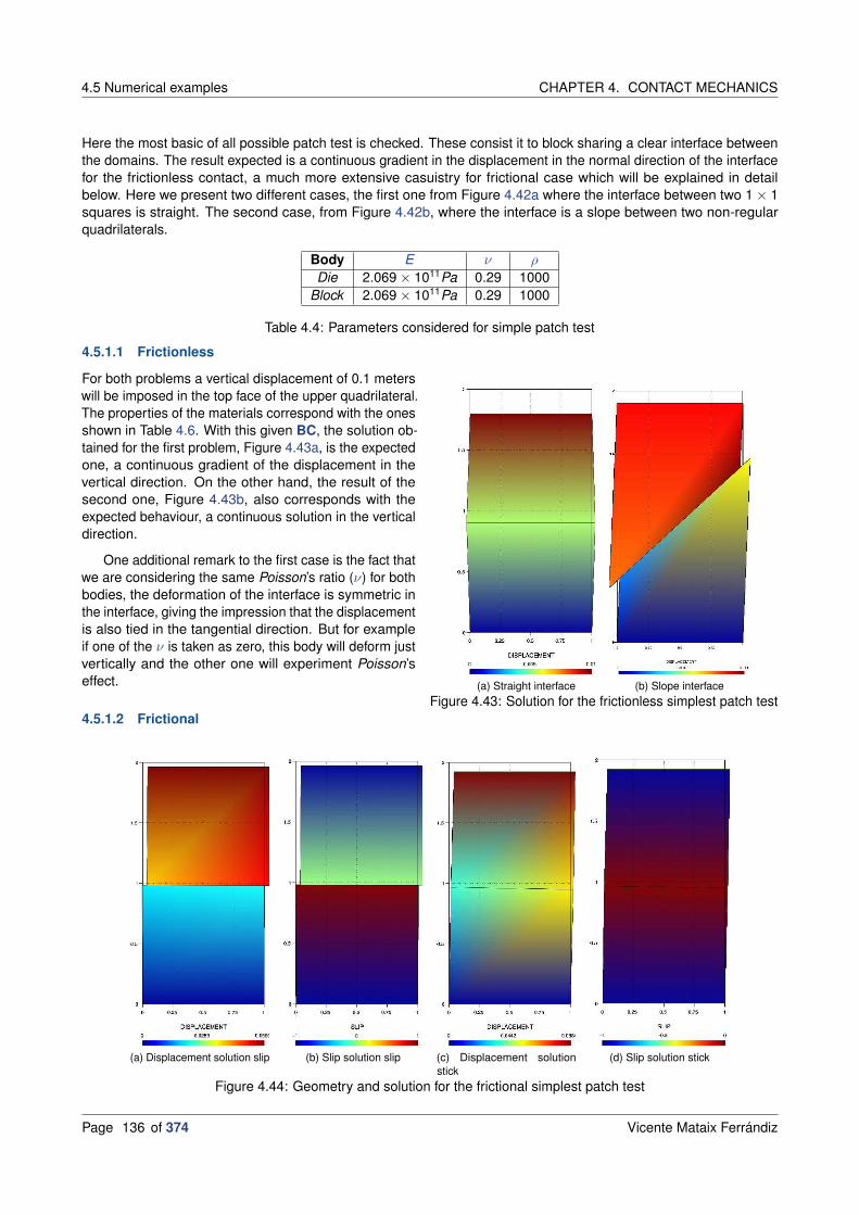
4.5 Numerical examples CHAPTER 4. CONTACT MECHANICS
Here the most basic of all possible patch test is checked. These consist it to block sharing a clear interface betweenthe domains. The result expected is a continuous gradient in the displacement in the normal direction of the interfacefor the frictionless contact, a much more extensive casuistry for frictional case which will be explained in detailbelow. Here we present two different cases, the first one from Figure 4.42a where the interface between two 1 × 1squares is straight. The second case, from Figure 4.42b, where the interface is a slope between two non-regularquadrilaterals.
Body E ν ρDie 2.069 × 10¹¹Pa 0.29 1000
Block 2.069 × 10¹¹Pa 0.29 1000
Table 4.4: Parameters considered for simple patch test
4.5.1.1 Frictionless
(a) Straight interface (b) Slope interface
Figure 4.43: Solution for the frictionless simplest patch test
For both problems a vertical displacement of 0.1 meterswill be imposed in the top face of the upper quadrilateral.The properties of the materials correspond with the onesshown in Table 4.6. With this given BC, the solution ob-tained for the first problem, Figure 4.43a, is the expectedone, a continuous gradient of the displacement in thevertical direction. On the other hand, the result of thesecond one, Figure 4.43b, also corresponds with theexpected behaviour, a continuous solution in the verticaldirection.
One additional remark to the first case is the fact thatwe are considering the same Poisson’s ratio (ν) for bothbodies, the deformation of the interface is symmetric inthe interface, giving the impression that the displacementis also tied in the tangential direction. But for exampleif one of the ν is taken as zero, this body will deform justvertically and the other one will experiment Poisson’seffect.
4.5.1.2 Frictional
(a) Displacement solution slip (b) Slip solution slip (c) Displacement solutionstick
(d) Slip solution stick
Figure 4.44: Geometry and solution for the frictional simplest patch test
Page 136 of 374 Vicente Mataix Ferrándiz

CHAPTER 4. CONTACT MECHANICS 4.5 Numerical examples
Here for the sake of simplicity only the problem with straight interface, from Figure 4.42a, will be studied. In thestudy we need to differentiate between two possible states in the frictional case, the slip and the stick state. In here, incontrast with the frictionless case, we set a vertical load in the top face of the upper element, additionally a tangentload in order to trigger the tangent behaviour. This problem thanks to its simplicity allows us to check the correctnessof the slip/stick state detection, where just adjusting the friction coefficient µ it is possible to change between one stateand the other. The first case corresponds with the slip states, where in Figures 4.44a and 4.44b we can appreciatelike a relative drift appears on the interface. On the other hand, on the Figures 4.44c and 4.44d, the solution forthe stick state is shown, and can be seen as the two blocks move in solidarity. Notice that Figures 4.44b and 4.44drepresent the SLIP flag, the value can be only 0 and 1, being 1 slip state, and 0 stick state.
4.5.2 Taylor patch test
The Taylor [ArtTP] patch test is slightly more complex problem than the former patch test. In this case the interface isnot coincident between th two domains, additionally a distributed load is considered in the upper face of the domains.The load considered is p = 10Pa, and the properties of the materials correspond with the ones shown in the Table 4.5.We will present the solution for the 2D and 3D problem.
Body E ν ρDie 3 × 10³Pa 0.4 1000
Block 3 × 10³Pa 0.4 1000
Table 4.5: Parameters considered for Taylor [ArtTP] patch test
4.5.2.1 2D
The Figure 4.45a illustrate the setup of the Taylor test in 2D. The solution obtained in the other hand correspondswith a continuous gradient of vertical displacement as shown in Figure 4.45b and a continuous vertical stress Figure4.45c.
(a) Setup (b) Displacement solution (c) Stress solution
Figure 4.45: Solution for the Taylor patch test in 2D
4.5.2.2 3D
(a) Setup (b) Displacement solution (c) Stress solution
Figure 4.46: Solution for the Taylor patch test in 3D
Vicente Mataix Ferrándiz Page 137 of 374

4.5 Numerical examples CHAPTER 4. CONTACT MECHANICS
For the 3D case, see Figure 4.46a, the same conclusions than in the 2D case can be applied here. Continuousgradient of displacement (Figure 4.46b) and continuous stress field (Figure 4.46c) in the vertical direction.
4.5.3 Friction base test
The following test, extracted from the work of Dong[ArtDon99], is a test which allows to study the effects in the contactfrictional behaviour with respect to different values of the friction coefficient µ. The properties of the bodies are theones shown in the Table 4.6, where µ has been considered with three different values, 0.25, 0.5 and 1. The geometryand mesh considered are the ones from Figure 4.47 and the load q = 20000KN/m. The solution is compared with theone in reference[ArtDon99] in Figure 4.48b, with a very good agreement. The solution from Figure 4.48a shows thedetachment that appears in the interface for µ = 0.25.
Body E ν µDie 2.1 × 10¹¹Pa 0.29 1, 0.5, 0.25
Block 2.1 × 10¹¹Pa 0.29 1, 0.5, 0.25
Table 4.6: Parameters considered for simple patch test
(a) Geometry (b) Mesh
Figure 4.47: Friction problem from Dong[ArtDon99]
(a) Displacement solution for µ = 0.25 (b) Solution compared with reference
Figure 4.48: Solution for pure friction problem
4.5.4 Hertz problem
We have already highlighted the relevance of this test in the former sections. This is the most commonly used andextended benchmark for contact mechanics, originally published by Hertz[ArtHer82] in 1882. This benchmark has theadvantage that the original solution is analytical and therefore we can compare with a solution that we have known a
Page 138 of 374 Vicente Mataix Ferrándiz

CHAPTER 4. CONTACT MECHANICS 4.5 Numerical examples
priori for different combinations of material and geometries. Using as main reference the solution of Zhu[ArtZhu12]for the analytical solutions of the different Hertz problems. We will study basically two cases, the rigid plane-spherecontact and sphere-sphere12 contact problem, both for 2D and 3D problems. It will be assumed we work under thehypothesis that we work in the domain of infinitesimal deformations.
4.5.4.1 2D
4.5.4.1.1 Plane-sphere :
The plane-sphere configuration from Figure 4.49 corresponds with the problem to solve, which requires in 2Dto be solved considering axisymmetric formulation. We specialise the resolution of the problem for a radius equalto 6.1237 meters, and pressure of P = 5 × 10⁵Pa. The properties considered for the two solids are represented onTable 4.7, where the plane can be considered de facto rigid. We have considered different mesh sizes, and we havecompared the results between then and the respective error.
Body E νSphere 1 × 10⁸Pa 0.29Block 1 × 1026Pa 0.29
Table 4.7: Parameters considered for 2D sphere-plane Hertz benchmark
(a) Setup (b) Mesh
Figure 4.49: Setup for the 2D sphere-plane Hertz benchmark
The analytical solution is presented in Equation (4.85), taken from the reference[ArtZhu12]. The Equation (4.85c)gives the analytical solution for the contact pressure in all the domain b, then the Equation (4.85d) provides thevertical displacement of the contact interface.
Eeff =1
1−ν21
E1+ 1−ν2
2E2
, r =√
x2 + y2(4.85a)
b = 3
√
3PπR3(1 − ν2)
4Eeff, p0 = 3P
R2
2b2, d0 =
b2
R, f0 =
3
√(
Eeff
√
Rd30
)4
(4.85b)
pn = p0
√
1 − r2
b2(4.85c)
y = −2
3p0πb2
√(
1 − r2
b2
)3
(4.85d)
As previously stated, the solution obtained corresponds with the solution for different mesh sizes. Figure 4.50apresents the different solutions for the vertical displacement for different mesh sizes, and Figure 4.50b the same but
12In 3D, in 2D a contact cylinder-cylinder will be considered
Vicente Mataix Ferrándiz Page 139 of 374

4.5 Numerical examples CHAPTER 4. CONTACT MECHANICS
for the contact pressure. It is notorious that the displacement solution converges even for very coarse meshes andthe pressure solution it is more difficult to be converged, particularly in the contact frontier. In fact, it can be noticedthat the finer mesh does not provide necessarily the better solution, and more intermediate meshes present betterresults.
(a) Displacement solution (b) Stress σyy solution
Figure 4.50: Solution compared for different mesh sizes for the 2D Hertz plane-sphere contact
This last statement can be seen in an easier manner in the solutions presented on Figure 4.51, where the error forthe displacement (Figure 4.51a) and the pressure (Figure 4.51b) are compared for different mesh sizes respect theanalytical solutions.
(a) Error in displacement solution (b) Error in stress σyy solution
Figure 4.51: Error compared for different mesh sizes for the 2D Hertz plane-sphere contact
4.5.4.1.2 Cylinder-cylinder :
The configuration for this problem is shown in Figure 4.52. This consists in two infinite cylinders, not to be confusedwith spheres, that become into contact. We will consider the parameters from Table 4.8. Additionally the followingvalues have been taken into account as BC and geometrical values: q = 0.05851Pa, p = 0.625Pa and R = 8m.
4.5.4.1.2.1 Frictionless case :
Page 140 of 374 Vicente Mataix Ferrándiz

CHAPTER 4. CONTACT MECHANICS 4.5 Numerical examples
Body E ν µUpper cylinder 200Pa 0.3 0.2Lower cylinder 200Pa 0.3 0.2
Table 4.8: Parameters considered for 2D cylinder-cylinder Hertz benchmark
(a) Setup (b) Mesh
Figure 4.52: Setup for the two cylinders Hertz benchmark
First we present the solution for the frictionless part. Considering µ = 0, the normal contact pressure correspondswith (4.86b). This is what is represented in Figure 4.53. The comparison with the analytical solution will be presentedall together with the frictional solution.
b = 2
√
2R2p(1 − ν2
)
Eπ(4.86a)
pn =4Rpπb2
√
b2 − x2(4.86b)
(a) Displacement solution (b) Stress σyy solution
Figure 4.53: Solution for the two cylinders frictionless Hertz benchmark
Vicente Mataix Ferrándiz Page 141 of 374

4.5 Numerical examples CHAPTER 4. CONTACT MECHANICS
4.5.4.1.2.2 Frictional case :
The solution considered has been taken from Wang[ArtWZ13] and Gitterle[PhDGit12], and the resulting iscompared with normal (4.86b) and tangential pressure (4.87b) of reference. Figure 4.54 presents and compares thesolution with the reference, showing a very good agreement with it.
c = b
√
1 − qµp
(4.87a)
pt = µ 4Rpπb2 (
√b2 − x2 −
√c2 − x2) if |x | ≤ c
pt = µ 4Rpπh2 (
√b2 − x2) if c < |x | ≤ b
(4.87b)
Figure 4.54: Solution for the two cylinders frictional Hertz benchmark
4.5.4.2 3D
4.5.4.2.1 Plane-sphere :
Figure 4.55: Mesh considered for 3D Hertz plane-sphere
The description and solution for this problem corre-spond with the previously introduced at 4.5.4.1.1.Plane-sphere, as this was solved considering an axisymmetry.We will consider a sphere of 12.2474 meters of diameterwith a load of p = 5 × 10⁵Pa and the material propertiesfrom Table 4.9. We consider two different mesh sizes,Figure 4.55 shows the finer mesh. The calculation isdone in just one static step. This problem can be foundin the following link.
We compare the resolution of both meshes with thereference solution. Figure 4.56 exposes the displace-ment and VM stress solution. For the displacement wegot a very good agreement with the analytical solutionin both cases, but particularly good in the case of therefined mesh, Figure 4.57a, in the case of the contactpressure we got a better approach within the finer case,Figure 4.58a.
Page 142 of 374 Vicente Mataix Ferrándiz

CHAPTER 4. CONTACT MECHANICS 4.5 Numerical examples
Body E νSphere 1 × 10⁸Pa 0.29Plane 2.1 × 10¹¹Pa 0.29
Table 4.9: Parameters considered for 3D Hertz plane-sphere problem
(a) Displacement solution (b) VM stress solution
Figure 4.56: Solution for the 3D Hertz plane-sphere contact
(a) Displacement solution (b) Stress σyy solution
Figure 4.57: Solution compared for different mesh sizes for the 3D Hertz plane-sphere contact
(a) Error in displacement solution (b) Error in stress σyy solution
Figure 4.58: Error compared for different mesh sizes for the 3D Hertz plane-sphere contact
Vicente Mataix Ferrándiz Page 143 of 374

4.5 Numerical examples CHAPTER 4. CONTACT MECHANICS
4.5.4.2.2 Sphere-sphere :
Figure 4.59: Reference solutionfor two spheres Hertz contact.Source[ArtZhu12]
This problem, which comes from here consists in two contactingspheres as seen in the reference solution from Figure 4.59. We con-sider two hemispheres of 12.2474 meters of diameter, and consideringan applied load of q = 1.0e3Pa. We can transform that given pressureto the corresponding force of the reference solution with F = q πD2
4 . Thecharacteristic parameters of the spheres are the ones present in Table4.10. The calculation is performed in just one static step.
As well as the cooperation with the reference solution, we will comparethe radius of the contact area and the maximum contact pressure, corre-sponding with the analytical solution from (4.88). The obtained solutionis compared with the reference one in (4.89), in here the maximal erroris around a 1%. The displacement and VM stress field from Figure 4.60shows the obtained solution.
Pmax =3F
2πa2(4.88a)
a = 3
√√√√√
3F[
1−v21
E1+ 1−v2
2E2
]
4(
1R1
+ 1R2
)(4.88b)
F = 1.0e3 · π · 12.24742
4= 150000/4 · π = 117808.787N(4.89a)
a = 0.6301m vs 0.627m → 0.5% error(4.89b)
Pmax = 1.41641 × 10⁵Pa vs 1.435467 × 10⁵Pa → 1.3% error(4.89c)
Body E νUpper body 1 × 10⁸Pa 0.29Lower body 1 × 10⁶Pa 0.29
Table 4.10: Parameters considered for 3D Hertz sphere-sphere problem
(a) Displacement solution (b) VM stress solution
Figure 4.60: Solution for two hemispheres Hertz contact
Page 144 of 374 Vicente Mataix Ferrándiz

CHAPTER 4. CONTACT MECHANICS 4.5 Numerical examples
4.5.5 Teeth model
The problem consists in a simplified model of a tooth with different types of layers, as the following: the first model withenamel-composite (Figure 4.61a) and the second one formed of enamel-dentine-composite (Figure 4.61b). The ideaunderlying this study is to compare the solutions between the two models and determine the benefits of the additionallayer of dentine as a reinforcement of the composed structure. The properties of each one of the layers of the modelappear on Table 4.11. It can be found here.
(a) Enamel-composite (b) Enamel-dentine-composite
Figure 4.61: Teeth layers model
Body E νPunch 2.069 × 10¹¹Pa 0.29
Enamel (color 3) 8 × 10¹⁰Pa 0.3Dentine (color 4) 2 × 10¹⁰Pa 0.3
Composite (color 2) 1.03 × 10¹⁰Pa 0.3
Table 4.11: Parameters considered for teeth model
(a) Enamel-composite displacement (b) Enamel-composite VM stress
(c) Enamel-dentine-composite displacement (d) Enamel-dentine-composite VM stress
Figure 4.62: Solution for teeth layers model
Figure 4.62 the solutions compared of both alternatives allows us to see the advantages of the additional layer ofdentine to the model.
Vicente Mataix Ferrándiz Page 145 of 374

4.5 Numerical examples CHAPTER 4. CONTACT MECHANICS
4.5.6 Energy conservation
The following is an example to show the energy conservation in a frictionless contact simulation. In order to do so wewill present the geometry shown in Figure 4.63. In this pictures what we see is a ring on 2m outer diameter and aninner diameter of 1.8m. Inside the ring we have a cylinder of 0.4m. The problem is a fully 3D simulation with 0.1mthickness in the Z axis. In this problem the cylinder is only subjected to its own weight. The inner cylinder is softerthan the outer ring, which we can consider rigid from a practical point of view, see Table 4.12.
(a) Mesh seen from the front (b) Mesh seen on perspective
Figure 4.63: Energy conservation test. Cylinder inside ring. The example can be found in here
Body E ν ρRing 2.069 × 10¹¹Pa 0.29 7850
Cylinder 2 × 10⁸Pa 0.29 1000
Table 4.12: Parameters considered for energy conservation testWith the given information, we can predict the exact movement of the body the total energy and the velocity in any
given time. For that we formulate the total energy as the total between the kinematic and the potential energy fromEquation (4.90a). In here h is the height of the cylinder in a given time, m the total mass of the cylinder , g the gravityand v its velocity. If we define as only DOF the angle between the cylinder and the centre, being θ = 0 then h = 0.7mand v = 0m/s as initial values. The total mass is as easy to calculate as m = 0.22 × π× 0.1 × 1000 = 4πkg. The totalenergy is then, taking into account the initial BC previously mentioned then (4.90b). With this we can easily estimatethe maximum velocity as Equation (4.90c).
Etot = Ekin + Epot = hmg +1
2mv2(4.90a)
Etot = 0.7 × 4π × 9.81 = 86.2632J(4.90b)
vmax =
√
2Etot
m= 3.7m/s(4.90c)
Then taking as DOF θ we must express then the velocity in terms of θ, considering the radius of the given trajectoryas R = 0.7 then v = Rθ. h can be represented with h = R(1 − sin(θ)). With this we can define the equation whichdefines analytically our movement as (4.91a). Replacing the operations properly, we obtain the following expression
Page 146 of 374 Vicente Mataix Ferrándiz

CHAPTER 4. CONTACT MECHANICS 4.5 Numerical examples
(4.91b). Solving the corresponding ODE the expression for θ results on Equation (4.91c).
Etot = R(1 − sin(θ))mg +1
2m(Rθ)2(4.91a)
θ =
√
2gR
sin(θ)(4.91b)
θ =1
2
(
π − 4am
(
1
4
(
−c1
√
2gR
+ t
(
−√
2gR
))∣∣∣∣∣2
))
(4.91c)
Where am is Jacobi elliptical function amplitude[OnlJac]. The constant c1 can be obtained replacing the BC
previously stated, giving us as result c1 = −0.990539. On Figure 4.64 we can see the comparison on the solutionobtained with the analytical reference. The error on the solution obtained is less than a 1%.
(a) Displacement evolution (b) Energy evolution
Figure 4.64: Evolution of displacement and energy compared with analytical solution
(a) t = 0.0s (b) t = 0.99s (c) t = 1.98s
(d) t = 2.97s (e) t = 3.96s
Figure 4.65: Solution of the problem at certains times. The time is specified in each subfigure
Vicente Mataix Ferrándiz Page 147 of 374

4.5 Numerical examples CHAPTER 4. CONTACT MECHANICS
The Figure 4.65 shows the energy conservation in our simulation, and we can see as at the predicted time thecylinder returns into its original position, then the loop starts over. The obtained maximum velocity coincides with thepredicted in (4.91c). Something that is relevant to remark is the fact as expected in a frictionless case, and thereforethere is no rotation movement, the contact point between the cylinder and the ring is always the same. Besides, theenergy is preserved despite the numerical dissipation due to Bossak scheme (see 2.4.4.2.Bossak algorithm).
4.5.7 Double arc benchmark
In this test case, we will consider the crushing of a hyperelastic bi-material half-ring on a hyperelastic base. This testmakes it possible to take into account large displacements, large deformations and large landslides coupled to contact/ non-contact transitions. The reference solutions have been taken from G. Drouet [PhDDro15] and K.Poulios andY.Renard [ArtPR15a]. The problem geometry as well as the boundary conditions are sketched below on Figure 4.66,both 2D and 3D. It can be found at the Examples repository.
(a) Geometry 2D (b) Geometry 3D
Figure 4.66: Double arc benchmark
(a) Hexahedra structured (b) Tetrahedra unstructured
Figure 4.67: Double arc meshes
Body E νFirst arc 3 × 10⁸Pa 0.32
Second arc 1 × 10⁹Pa 0.32Support material 1 × 10¹¹Pa 0.3
Table 4.13: Parameters considered for double arc benchmarkWe consider a hyperelastic half-ring composed of two materials (external 190mm and inner 170mm diameters)
and a hyperelastic base of length 250mm and height 50mm, see Figure. A vertical displacement of −90mm isimposed at each end of the half-ring and the base of the base is recessed. Two variables of interest are consideredmainly: the displacement of the middle of the half-ring as a function of the loading pitch (60 steps of loading from thecontact is used, ie about 1.16mm per loading step) and the contact pressure. On the other hand, an hyperelasticNeo-Hookean constitutive law is considered in both materials. The structure characteristic parameters are defined in
Page 148 of 374 Vicente Mataix Ferrándiz

CHAPTER 4. CONTACT MECHANICS 4.5 Numerical examples
Table 4.13. The time step is 0.0005seconds, while the total simulation time is 0.2seconds. With an increment of theimposed displacement equal to 0.4t . For the frictional case, the friction coefficient considered is µ = 0.5.
4.5.7.1 Frictionless
The problem stated above has been solved using an unstructured mesh of tetrahedra and a structured mesh ofhexahedron. The resulting deformation for the former case can be seen in the Figure 4.68.
(a) Solution 1 (b) Solution 2
(c) Solution 3 (d) Solution 4
Figure 4.68: Displacement solution for frictionless in double arc benchmark
Figure 4.69: Compared solution for frictionless in double arc benchmark
Vicente Mataix Ferrándiz Page 149 of 374

4.5 Numerical examples CHAPTER 4. CONTACT MECHANICS
We compare with the reference solution, Figure 4.69, where we have for the hexahedrical meshes a deviationfrom the reference solution for the last steps, where we have a larger deformation and finally a stabilisation of thedeformation. For the unstructured meshes of the tetrahedron, the results present more differences, respect thereference solution, higher deformation in general except for the last stages of the problem. In any case the resultsobtained are in very good agreement with the reference solution.
4.5.7.2 Frictional
(a) Solution 1 (b) Solution 2
(c) Solution 3 (d) Solution 4
Figure 4.70: Displacement solution for frictional in double arc benchmark
Figure 4.71: Compared solution for frictional in double arc benchmark
The solution for the frictional case can be seen in the following images, Figure 4.70, and the compared solutionwith the literature references (Figure 4.71), where the differences respect the reference are aligned with the ones
Page 150 of 374 Vicente Mataix Ferrándiz

CHAPTER 4. CONTACT MECHANICS 4.5 Numerical examples
already appreciated on the frictionless case. Besides, the effects of the friction can be noted in the way the arcdeforms in comparison of the frictionless case.
4.5.8 Arc pressing block
The problem consists in an arc and a block, in here the arc is pressed against the block. These two deformable solidsare considered as hyperelastic (Neo-Hookean), and the solid is formulated in UL framework. We consider threecases, depending of the relationship of stiffness between the arc and the block, the first one with a rigid block, thesecond one with a deformable block and the final one for deformable block with the arc being rigid. These propertiesare specified on Table 4.14. The BC consists on a displacement imposed is uy = t , with t = [0.0, 1.0] for the two firstcases, t = [0.0, 1.775] for the rigid arc. The example can be found here.
Body Constitutive Law (CL) E νArc (Rigid block) Neo-Hookean 68.96 × 10⁸Pa 0.32
Block (Rigid block) Neo-Hookean 68.96 × 10⁷Pa 0.32Arc (Deformable block) Neo-Hookean 68.96 × 10⁸Pa 0.32
Block (Deformable block) Neo-Hookean 68.96 × 10⁵Pa 0.32Arc (Deformable block-Rigid arc) Neo-Hookean 68.96 × 10⁹Pa 0.32
Block (Deformable block-Rigid arc) Neo-Hookean 68.96 × 10⁵Pa 0.32
Table 4.14: Parameters considered for arc pressing blocks
(a) Mesh 2D (b) Mesh 3D
Figure 4.72: Arc pressing block
Figure 4.73 summarises the solution obtained for each one of the material properties previously presented. Itcan be seen the effects of the relative stiffness in each one of the cases. Particularly in the case where the block isdefined and the arc is rigid (Figure 4.73b), and the case where the block is rigid (Figure 4.73c) and all the deformationlies in the arc.
(a) Deformable block (b) Rigid arc (c) Rigid block
Figure 4.73: Solution for different stiffness between the arc and the block
Vicente Mataix Ferrándiz Page 151 of 374

4.5 Numerical examples CHAPTER 4. CONTACT MECHANICS
4.5.9 Hyperelastic tubes
Figure 4.74: Mesh for hyperelastic tubes
The problem[ArtPR15a] consists in two cylin-ders, Figure 4.74, with hyperelastic be-haviour, as shown in the Table 4.15. Weimpose a vertical displacement uz = −0.01tin the upper cylinder, during a time interval oft = [0.0, 4], in 100 steps. The two cylindersdeal with finite deformations and are definedin a UL framework.
The two cylinders become into contactand deal with self-contact in the inner ring ofthe upper cylinder. For further details aboutthis example, the following link expands andpresents the necessary files.
Body CL E νUpper cylinder Neo-Hookean 10000Pa 0.3Lower cylinder Neo-Hookean 100000Pa 0.3
Table 4.15: Parameters considered for hyperelastic tubes
(a) t = 1s (b) t = 2s
(c) t = 3s (d) t = 4s
Figure 4.75: Displacement solution for hyperelastic tubes
Page 152 of 374 Vicente Mataix Ferrándiz

CHAPTER 4. CONTACT MECHANICS 4.5 Numerical examples
The Figure 4.75 presents the solution across different time steps, t = [0, 4]s. Additionally, Figure 4.76 shows asplit of the final configuration, t = 4s, so the deformation at the end of the simulation can be appreciated at Figure4.76a and the VM stress at Figure 4.76b. In this configuration the phenomenon of self-contact arises.
(a) Displacement (b) VM stress
Figure 4.76: Slice solution for hyperelastic tubes
4.5.10 Contacting cylinders
The following case consists in two deformable hemicylinders (Figure 4.77) which experiment large deformations withNeo-Hookean hyperelastic behaviour (Table 4.16). We applied two different movements in the base of the uppercylinder, first a horizontal movement (4.5.10.1.Horizontal movement) and later a vertical movement (4.5.10.2.Verticalmovement). The relative position of the hemicylinders changes slightly between the two configurations. The problemis studied again in the test cases from the adaptive refinement chapter, see 6.10.5.Contacting cylinders with adaptiveremeshing. These problems can be found here.
(a) Mesh 2D (b) Mesh 3D
Figure 4.77: Contacting cylinders mesh
Body CL E νUpper cylinder Neo-Hookean 2.1 × 10¹¹Pa 0.29Lower cylinder Neo-Hookean 2.1 × 10¹¹Pa 0.29
Table 4.16: Parameters considered for contacting cylinders
4.5.10.1 Horizontal movement
A horizontal displacement is imposed ux = 0.2t , for a time interval of t = [0, 2.5]s in 1000 steps. Figure 4.78 shows thedisplacement solution in different time steps, resulting in the reaction at the bottom of the lower hemicylinder fromFigure 4.79. The problem has been solved both considering frictionless (Figures 4.78a, 4.78b, 4.78c) and frictional(µ = 1) (Figures 4.78d, 4.78e, 4.78f)cases. The difference of behaviour between the two cases is notorious.
Vicente Mataix Ferrándiz Page 153 of 374

4.5 Numerical examples CHAPTER 4. CONTACT MECHANICS
(a) Frictionless t = 0.5s (b) Frictionless t = 1.0s (c) Frictionless t = 1.5s
(d) Frictional t = 0.5s (e) Frictional t = 1.0s (f) Frictional t = 1.5s
Figure 4.78: Solution for contacting cylinders with horizontal movement
Figure 4.79: Frictionless reaction solution in the lower cylinder for the horizontal movement
4.5.10.2 Vertical movement
(a) t = 0.5s (b) t = 1s
Figure 4.80: Solution for contacting cylinders with vertical movement
Page 154 of 374 Vicente Mataix Ferrándiz

CHAPTER 4. CONTACT MECHANICS 4.5 Numerical examples
For the vertical displacement is imposed uy = 0.1t , for a time interval of t = [0, 1]s in 200 steps. At Figure 4.80 thedeformation experimented is presented, as well as the reaction (Figure 4.81) in the base of the still hemicylinder.
Figure 4.81: Reaction solution in the lower cylinder for the vertical movement
4.5.11 Press fit
(a) Geometry
(b) Mesh 2D (c) Mesh 3D
Figure 4.82: Press fit problem
The problem consists of the numerical simulation of a press-fit process of a block in a channel accordingto[ArtFW06; ArtDSB15]. The geometric and material parameters are shown in the Figures 4.82, where the symmetryof the problem is used and only half of the domain is simulated. It is considered Neo-Hookean compressiblehyperelastic material for both components with the values from Table 4.17. With this problem, it is possible to evaluatethe behaviour of the contact element in a friction contact problem with large deformation and sliding.
Vicente Mataix Ferrándiz Page 155 of 374
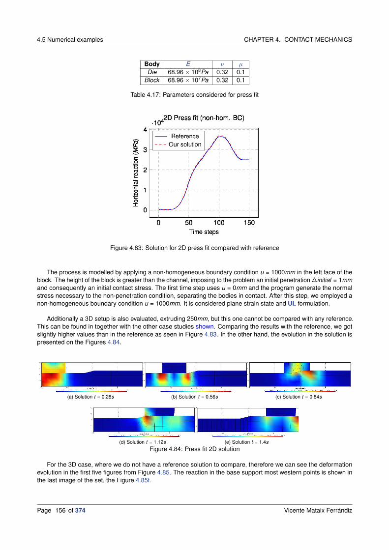
4.5 Numerical examples CHAPTER 4. CONTACT MECHANICS
Body E ν µDie 68.96 × 10⁸Pa 0.32 0.1
Block 68.96 × 10⁷Pa 0.32 0.1
Table 4.17: Parameters considered for press fit
Figure 4.83: Solution for 2D press fit compared with reference
The process is modelled by applying a non-homogeneous boundary condition u = 1000mm in the left face of theblock. The height of the block is greater than the channel, imposing to the problem an initial penetration ∆initial = 1mmand consequently an initial contact stress. The first time step uses u = 0mm and the program generate the normalstress necessary to the non-penetration condition, separating the bodies in contact. After this step, we employed anon-homogeneous boundary condition u = 1000mm. It is considered plane strain state and UL formulation.
Additionally a 3D setup is also evaluated, extruding 250mm, but this one cannot be compared with any reference.This can be found in together with the other case studies shown. Comparing the results with the reference, we gotslightly higher values than in the reference as seen in Figure 4.83. In the other hand, the evolution in the solution ispresented on the Figures 4.84.
(a) Solution t = 0.28s (b) Solution t = 0.56s (c) Solution t = 0.84s
(d) Solution t = 1.12s (e) Solution t = 1.4s
Figure 4.84: Press fit 2D solution
For the 3D case, where we do not have a reference solution to compare, therefore we can see the deformationevolution in the first five figures from Figure 4.85. The reaction in the base support most western points is shown inthe last image of the set, the Figure 4.85f.
Page 156 of 374 Vicente Mataix Ferrándiz

CHAPTER 4. CONTACT MECHANICS 4.5 Numerical examples
(a) Solution t = 0.28s (b) Solution t = 0.56s (c) Solution t = 0.84s
(d) Solution t = 1.12s (e) Solution t = 1.4s (f) Horizontal reaction in the base for 3D case
Figure 4.85: Press fit 3D solution
4.5.12 Ironing punch
The following are two examples extensively considered in the literature[ArtFW06; ArtHar+09; ArtPR15b], whichare the ironing tests. These tests consist in moving die along a solid block, undergoing large deformation in theprocess.
1. This case cannot be found in literature, and it is a little bit more challenging as the curvature of the contactingdie is higher than in the previous case, we will call this case as circular ironing (4.5.12.1.Circular ironing).
2. We will show the results obtained with the standard ironing test, called shallow ironing, which is the onecommonly referred on the literature (4.5.12.2.Shallow ironing). In this second case, we will consider both africtionless and a frictional case.
4.5.12.1 Circular ironing
In this case we will run the simulation just considering the frictionless case as our interest is to compare the behaviourbetween the two different geometries. The geometry of the problem is fully defined in the Figure 4.86a, and thehexahedral structured mesh considered in Figures 4.86b and 4.86c. The properties of the materials are identical forthe shallow ironing problem, with a Neo-Hookean material behaviour (5.4.2.Neo-Hookean material). We impose avertical displacement as uy = −t during the time interval t = [0, 1]s and ux = t − 1 at t = [1, 10]s keeping the previousvertical displacement. The example is found in the repository.
Body E νDie 68.96 × 10⁸Pa 0.32
Block 68.96 × 10⁷Pa 0.32
Table 4.18: Parameters considered for circular ironing
Vicente Mataix Ferrándiz Page 157 of 374

4.5 Numerical examples CHAPTER 4. CONTACT MECHANICS
(a) Geometry of the problem
(b) Mesh (c) Perspective of the Mesh
Figure 4.86: Circular ironing test
(a) t = 2.5s (b) t = 5s
(c) t = 7.5s (d) t = 10s
Figure 4.87: Circular ironing test solution
Figures 4.87 present the deformation evolution for this case in the interval going from t = [0, 10]s. The Figure 4.88shows the different solution obtained with respect the shallow ironing example.
Page 158 of 374 Vicente Mataix Ferrándiz

CHAPTER 4. CONTACT MECHANICS 4.5 Numerical examples
Figure 4.88: Comparison between the frictionless solutions of the shallow and the circular ironing
4.5.12.2 Shallow ironing
(a) Mesh seen from the front (b) Mesh seen on perspective
Figure 4.89: Shallow ironing test
On this case an indenter or die with a circular arc shaped bottom edge is pressed against a rectangular blockand is forced to slide along the block length, see Figure 4.89 where the geometry and mesh considered can beappreciated. The contacting bodies exhibit a Neo-Hookean material behaviour (5.4.2.Neo-Hookean material), with theparameters from Table 4.19. The problem solved on this case is fully 3D with a deep of 1m, but in many referencescan be found as a 2D case with plane strain hypothesis. The example can be found in here.
Body CL E ν µDie Neo-Hookean 68.96 × 10⁸Pa 0.32 0.3
Block Neo-Hookean 68.96 × 10⁷Pa 0.32 0.3
Table 4.19: Parameters considered for shallow ironingAlthough the performed simulation is quasi-static, the load steps are defined as a function of time for the sake
of presentation of the results. From t = [0, 1]s, the indenter is moved vertically towards the block until the verticaldisplacement reaches 1m. From t = [1, 12]s, the die is displaced horizontally by a total distance of 11m. Thisloading differs sometimes in the literature, because of that the results obtained must the translated to the equivalentdisplacement evolution process.
The Figures 4.90 compare the solution to the shallow ironing test between the friction and the frictional solution atdifferent times. We can appreciate that the frictional case indeed opposes the movement of the die. Figures 4.91
Vicente Mataix Ferrándiz Page 159 of 374

4.5 Numerical examples CHAPTER 4. CONTACT MECHANICS
compares the solution obtained with the reference[ArtPR15b]. In general the agreement is good with [ArtPR15b], andthen the solution can be considered as valid.
(a) Frictionless t = 2.5s (b) Frictionless t = 5s
(c) Frictional t = 2.5s (d) Frictional t = 5s
Figure 4.90: Shallow ironing test solution, comparing frictional and frictionless cases
(a) Frictionless solution (b) Frictional solution
Figure 4.91: Reaction solution for shallow ironing test
Page 160 of 374 Vicente Mataix Ferrándiz

CHAPTER 4. CONTACT MECHANICS 4.6 Derivatives for contact mechanics linearization
4.6 Derivatives for contact mechanics linearization
On this section we can find in extension the definition of the directional derivatives, also called Gateaux deriva-tives[BookBel+14], associated with the mortar operators (4.92) and the slip and gap (4.93). These derivatives willbe noted with ∆. With the components shown on (4.92), in addition to the derivatives of the normal and tangent(4.93), it is possible to define consistently the proper consistent linearisation of the tangent operator for the contactproblem. The derivatives of the normal and tangent must be taken into account in order to define the derivatives ofthe gap and the slip. Similar developments can be found on other works, as Popp[PhDPop12; ArtPGW09; ArtPop+10],Yang[ArtYLM], Hammer [PhDHam13] and Cavalieri [ArtCFC12; ArtCC15; ArtCC13b] work.
First the definitions concerning the 2D problem will be presented (4.6.1.Derivatives for 2D contact), later theconcerning to the 3D problem (4.6.2.Derivatives for 3D contact). The presenting work will focus particularly on thelinear shape functions, as long as or work focuses on linear geometries.
(4.92a) ∆D[j , k ] =
ngp∑
g=1
wg∆φgjN1gk J1
g +
ngp∑
g=1
wgφgj∆N1gk J1
g +
ngp∑
g=1
wgφgjN1gk∆J1
g
(4.92b) ∆M[j , l ] =
ngp∑
g=1
wg∆φgjN2gk J1
g +
ngp∑
g=1
wgφgj∆N2gk J1
g +
ngp∑
g=1
wgφgjN2gk∆J1
g
Expressing the computation of the weighted gap in an algebraic way, based on the mortar operators definition.
(4.93a) gi = ni · (Dnx1 − Mnx2)i
Being i the node index and n the current time step, then
(4.93b) ∆gi = ∆ni · (Dnx1 − Mnx2)i + ni · (∆Dnx1 −∆Mnx2 + Dn∆x1 − Mn∆x2)i
In the same way, expressing the slip on an algebraic way, the derivative of the slip would be:
(4.93c) uτ i = τ i · ((Dn − Dn−1) x1 − (Mn − Mn−1) x2)i
Being i the node index and n, n − 1 the current and previous time steps, then
(4.93d)
∆uτ i = ∆τ i · ((Dn − Dn−1) x1 − (Mn − Mn−1) x2)i
+ τ i · ((∆Dn − Dn−1) x1 − (∆Mn − Mn−1) x2)i
+ τ i · ((Dn − Dn−1)∆x1 − (Mn − Mn−1)∆x2)i
After the definition of the following directional derivatives (∆), it is necessary it is algebraic representation ofthem on an equivalent matrix-vector format. This process is quite standard for FE formulations, and in our case it isdone in an automatic way using the AD, for more details we address to the corresponding Appendix C.Automaticdifferentiation. The code for the tests for the quadratic convergence shown on the following sections are accessiblein the public repository of Kratos, implemented on Kratos C++ unittest format. The following link guides towardit.
4.6.1 Derivatives for 2D contact
In this section the derivatives concerning 2D linear lines, necessaries in order to properly compute the contact arepresented, see (4.92) and (4.93). The derivatives are tested using a set of pairs following the Figure 4.92 structure,the Table 4.20 contains the coordinates of the nodes of the actual configurations tested. The perturbations applied oneach pair are defined on Table 4.21, which lists the nodes perturbed and its amplitude.
Vicente Mataix Ferrándiz Page 161 of 374

4.6 Derivatives for contact mechanics linearization CHAPTER 4. CONTACT MECHANICS
Figure 4.92: Line validation geometries
Pair P11 P1
2 P21 P2
2
1[−1.0 0.0 0.0
] [1.0 0.0 0.0
] [1.2 0.0 0.0
] [−0.8 0.0 0.0
]
2[−1.0 0.0 0.0
] [1.0 0.0 0.0
] [1.2 1.0E−3 0.0
] [−0.8 1.0E−3 0.0
]
3[−1.0 0.0 0.0
] [−1.0 5.0E−3 0.0
] [−1.0 1.0E−3 0.0
] [−1.0 7.0E−4 0.0
]
Table 4.20: 2D lines pairs geometrical configuration
Case Node perturbed Perturbation amplitude
1 1 −5.0e − 22 1 −5.0e − 23 1 −1.0e − 1
Table 4.21: 2D lines pertubartion amplitudes
4.6.1.1 Jacobians
4.6.1.1.1 Theory :
As the integration of the mortar formulation is performed only in the slave (mortar) domain, then the derivative ofthe Jacobian is defined only on the slave domain. Taking into consideration the definition of the Jacobian as (4.94a), itis possible to define the directional derivative of the slave Jacobian determinant at each Gauss point in a 2D linearline as (4.94b). In order to simplify and due to its extended use, we will call det(J) as J.
(4.94a) J (ξ) =
∥∥∥∥∥
n∑
k=1
Nk ,ξ (ξ) xk
∥∥∥∥∥
(4.94b) ∆J(ξ1
g
)=
∑nk=1 Nk ,ξ
(ξ1
g
)xk
∥∥∑n
k=1 Nk ,ξ
(ξ1
g
)xk
∥∥·(
n∑
k=1
Nk ,ξ
(ξ1
g
)∆xk
)
4.6.1.1.2 Convergence study :
Finally, in the Figure 4.93, the convergence plot of the Jacobian derivatives for the 3 different geometrical pairsfrom Table 4.20 is shown. In this figure, and the followings, L2 represents the Euclidean norm of the error, differencebetween the estimated value and the exact one. The plot is created considering in the x-axis the amplitude of theperturbation, and in the y the logarithm of L2 of the error; therefore the slope indicates the convergence rate of theerror in function of the perturbation.
Page 162 of 374 Vicente Mataix Ferrándiz

CHAPTER 4. CONTACT MECHANICS 4.6 Derivatives for contact mechanics linearization
Figure 4.93: Convergence plot for the Jacobian derivatives for the 2D linear line
4.6.1.2 Shape functions
4.6.1.2.1 Theory :
The shape functions of both domains depend on the integration segments between the two domains on contact. Inorder to compute the shape functions of a 2D line, we do as (4.95a), Figure 4.94, where ξ corresponds with the localcoordinate of the line. With this, its derivatives depend only on the derivative of the local coordinate ξ (4.95b). Despitethe fact that lines in Figure 4.94 are not in contact, due to its relative position, will be affected by the perturbations,allowing to measure the derivative convergence.
(4.95a)
[N1
N2
]
=
[12 (1 − ξ)12 (1 + ξ)
]
(4.95b)
[∆N1
∆N2
]
=
[− 1
2∆ξ12∆ξ
]
Figure 4.94: Shape functions for the 2D linear line
For this reason we need to compute on first place the derivatives of the local coordinates, which depends on thederivatives of the integration segments. We will separate in two small sections those derivations. The derivation ofthese terms is based on the work of Laursen and Yang[ArtYLM] and Popp[PhDPop12].
Vicente Mataix Ferrándiz Page 163 of 374

4.6 Derivatives for contact mechanics linearization CHAPTER 4. CONTACT MECHANICS
4.6.1.2.2 Integration segments :
Figure 4.95: Integration segment for a linear line
The derivation of the integration points require the derivation of the integration segments. As previously presentedthis corresponds with the current and effective section of the line on contact, see Figure 4.95. As can be seen on thispicture we have two possible scenarios, one where the projected slave node (ξ1
a ) corresponds with the original slavenode and the second case corresponds with the counterpart scenario for the master side (ξ2
a). The same logic isapplied for the end integration segment coordinates (ξ1
b and ξ2b ). If the integrated node corresponds with the original
geometry the derivative therefore will be 0.
The derivative ∆ for this first scenario is presented on (4.96), where the sub-index a for the coordinates (x1a) and
normal (na) represent the first node on the slave side. On this case (4.96b) the shape functions and shape functiongradients are computed on ξ2
a .
(4.96a) ∆ξ1a = 0
(4.96b)
∆ξ2a = − 1
(∑nc
ml=1 N2
l ,ξx2l
)
nya −
(∑nc
ml=1 N2
l ,ξy2l
)
nxa
·
ncm∑
l=1
(N2
l ∆x2l
)−∆x1
a
nya −
ncm∑
l=1
(N2
l ∆y2l
)−∆y1
a
nxa
+
ncm∑
l=1
(N2
l x2l
)− x1
a
∆nya −
ncm∑
l=1
(N2
l y2l
)− y1
a
∆nxa
On the second case (4.97), as the slave side, which is our reference domain, does not correspond with itsprojection the n considered then is the one interpolated for the projected point. This means that the interpolationof the nodal normal will be computed. On this case (4.97a) the shape functions and shape function gradients arecomputed on ξ1
a .
(4.97a) ∆ξ1a =
numdenom
(4.97b)
denom = −
ncs∑
k=1
N1k ,ξx1
k
ncs∑
k=1
N1k ny
k
+
ncs∑
k=1
N1k ,ξy1
k
ncs∑
k=1
N1k nx
k
−
ncs∑
k=1
(N1
k x1k
)− x2
a
ncs∑
k=1
N1k ,ξny
k
+
ncs∑
k=1
(N1
k y1k
)− y2
a
ncs∑
k=1
N1k ,ξnx
k
Page 164 of 374 Vicente Mataix Ferrándiz

CHAPTER 4. CONTACT MECHANICS 4.6 Derivatives for contact mechanics linearization
(4.97c)
num =
ncs∑
k=1
(N1
k∆x1k
)−∆x2
a
ncs∑
k=1
N1k ny
k
−
ncs∑
k=1
(N1
k∆y1k
)−∆y2
a
ncs∑
k=1
N1k nx
k
+
ncs∑
k=1
(N1
k x1k
)− x2
a
ncs∑
k=1
N1k∆ny
k
−
ncs∑
k=1
(N1
k y1k
)− y2
a
ncs∑
k=1
N1k∆nx
k
(4.97d) ∆ξ2a = 0
4.6.1.2.3 Local coordinates (Gauss points) :
With the values obtained in the previous expression, it is possible to evaluate the ∆ of the Gauss Point (GP)
coordinates, and therefore calculate the values for the shape function derivatives. We evaluate those derivatives bothon the slave side (ξ1
g , (4.98a)) and the master side (ξ2g , (4.98b)).
For the slave side, we just need to apply the definition for the GP and derive it. As it consists on a simple sum, thederivative is straightforward.
(4.98a) ∆ξ1g =
1
2
(1 − ξg
)∆ξ1
a +1
2
(1 + ξg
)∆ξ1
b
For the master side, as it depends on a projection, the linearisation requires to take that projection into consideration,resulting the following expression. All the shape functions and shape function gradients are computed on ξ2
g .
(4.98b)
∆ξ2g = − 1
(∑nc
mk=1 N2
k ,ξx2k
)
nyg−(∑nc
mk=1 N2
k ,ξy2k
)
nxg
·[(∑nc
mk=1
(N2
k∆x2k
)−∆x1
g
)
nyg −
(∑nc
mk=1
(N2
k∆y2k
)−∆y1
g
)
nxg
+(∑nc
mk=1
(N2
k x2k
)− x1
g
)
∆nyg −
(∑nc
mk=1
(N2
k y2k
)− y1
g
)
∆nxg
]
4.6.1.2.4 Convergence study :
Finally, in the Figure 4.96, the convergence plot of the shape function derivatives for the 3 different geometricalpairs from Table 4.20 is shown.
Figure 4.96: Convergence plot for the shape function derivatives for the 2D linear line
Vicente Mataix Ferrándiz Page 165 of 374

4.6 Derivatives for contact mechanics linearization CHAPTER 4. CONTACT MECHANICS
4.6.1.3 Dual shape functions
4.6.1.3.1 Theory :
On standard FEM shape functions defined on the reference configuration, by definition these are not dependant ofthe deformation of the domain. This is not the case for dual shape functions, this is due to its intrinsic dependence onthe J of the slave side, see (4.99a). This means that our dual shape functions are deformation-dependant. In additionwe shall consider its dependence with the standard shape function derivatives. All this together give us the followingexpression (4.99b). The Ae definition is presented in the corresponding section, 4.3.3.4.1.Dual Lagrange multipliers,on the Equation (4.24).
(4.99a) Φ = AeN1
Ae(N, J)
N(N)
(4.99b) ∆Φ = Ae∆N1 + ∆AeN1
So in addition to the terms from the 4.6.1.2.Shape functions we need to evaluate the corresponding termsassociated to Ae (4.100).
(4.100)
∆Ae = ∆DeM−1e − De∆MeM−1
e
∆De = ∆[djk ] ∈ Rm1
e×m1e ,∆djk = δjk
ngp∑
g=1
wgN1gk∆J1
g
∆Me = ∆[mjk ] ∈ Rm1
e×m1e ,∆mjk =
ngp∑
g=1
wg
ngp∑
g=1
wgN1gjN
1gk∆J1
g
4.6.1.3.2 Convergence study :
Finally, in the Figure 4.97, the convergence plot of the dual shape function derivatives for the 3 different geometricalpairs from Table 4.20 is shown.
Figure 4.97: Convergence plot for the dual shape function derivatives for the 2D linear line
Page 166 of 374 Vicente Mataix Ferrándiz

CHAPTER 4. CONTACT MECHANICS 4.6 Derivatives for contact mechanics linearization
4.6.1.4 Normal and tangent vectors
4.6.1.4.1 Theory :
The linearisation of the tangent vectors is associated, as its definition depends on, on the linearisation of the normalvector. On these lines only the definition of the normal derivative, it is included as the definition of the tangent derivativeis defined as the cross product between the normal derivative and the out of plane vector (∆τ = vz ×∆n).
Figure 4.98: Normal average for a 2D line. Proposed by Taylor and Papadopoulos[ArtPT92]
The definition of the normal vector (n) for a 2D line is defined on (4.101a), where xi , yi correspond with thecoordinates of the i node of the line (1, 2). The unit normal corresponding to (4.101a) can be obtained with(4.101b).
Then the average normal[ArtPT92] (n) is defined as (4.101c), this definition is general and can be extended to 3D.Figure 4.98 represents the normal average for a 2D line. It is relevant to mention that the average normal (4.101c)is already computed over unitary normals, in contrast with the average area normal proposed by Popp[PhDPop12],this is done due to practical reasons, as this approach was significantly more robust (better convergence) in severalnumeric studies, particularly when coarse meshes were considered.
(4.101a) narea =
[y2
x1
]
−[y1
x2
]
(4.101b) n =narea
‖narea‖
In order to obtain the average normal we sum the normals of the neighbours entities (n) to the node, then we makeunitary dividing by its norm.
(4.101c) n =
∑nneighj
c=1 nc∥∥∥∥
∑nneighj
c=1 nc
∥∥∥∥
So, once defined the normal (4.102) and its average value (4.103) we can define its directional derivative.
(4.102a) ∆n =∆narea ‖narea‖ − narea∆ ‖narea‖
‖narea‖2
For the 2D line the resulting expression for the narea derivative will be (4.102b), which corresponds with taken thecorresponding unitary vector depending of the derivative evaluated.
(4.102b) ∆narea = ∆
[y2
x1
]
−∆
[y1
x2
]
Vicente Mataix Ferrándiz Page 167 of 374

4.6 Derivatives for contact mechanics linearization CHAPTER 4. CONTACT MECHANICS
For the directional derivative of the average normal, the resulting expression is decomposed in its differentcomponents.
(4.103a) ∆n =∆∑nneigh
j
c=1 nc
∥∥∥∥
∑nneighj
c=1 nc
∥∥∥∥−∑nneigh
j
c=1 nc∆
∥∥∥∥
∑nneighj
c=1 nc
∥∥∥∥
∥∥∥∥
∑nneighj
c=1 nc
∥∥∥∥
2
The first components are easy to obtain, as the derivative of a sum is the sum of its derivatives.
(4.103b) ∆
nneighj∑
c=1
nc =
nneighj∑
c=1
∆nc
The second components require to calculate the derivative of a norm, proceeding the standard manner the expressionobtained is (4.103c).
(4.103c) ∆
∥∥∥∥∥∥∥
nneighj∑
c=1
nc
∥∥∥∥∥∥∥
=
∑nneighj
c=1 nc∆∑nneigh
j
c=1 nc∥∥∥∥
∑nneighj
c=1 nc
∥∥∥∥
= n∆
nneighj∑
c=1
nc
Additionally in order to evaluate the value of the normal derivative on a specific GP, calculated on the correspondinglocal coordinates ξ1
g . The procedure to obtain is straightforward as only requires to apply the chain rule on the shapefunction interpolation of the normal evaluated on the GP (4.104).
(4.104) ∆ng =
ncs∑
k=1
N1k ,ξ
(ξ1
g
)∆ξ1
gnk +
ncs∑
k=1
N1k
(ξ1
g
)∆nk
4.6.1.4.2 Convergence study :
Finally, in the Figure 4.99, the convergence plot of the normal derivatives for the 3 different geometrical pairs fromTable 4.20 is shown.
Figure 4.99: Convergence plot for the normal derivatives for the 2D linear line
Page 168 of 374 Vicente Mataix Ferrándiz

CHAPTER 4. CONTACT MECHANICS 4.6 Derivatives for contact mechanics linearization
4.6.2 Derivatives for 3D contact
In this section the derivatives concerning 3D linear triangles and bilinear quadrilaterals, as part of (4.92) and (4.93)are presented. The main difference between this approach and the one provided for 2D cases is the segmentation ofthe surfaces, where the actual integration is done. The derivatives are tested using a set of pairs following the Figure4.100a structure and the Table 4.22 for the case of the triangle. Again, the perturbations applied on each pair aredefined on Table 4.23.
(a) Triangle validation geometries (b) Quadrilateral validation geometries
Pair P11 P1
2 P13 P2
1 P22 P2
3
1[0.0 0.0 0.0
] [1.0 0.0 0.0
] [0.0 1.0 0.0
] [0.0 1.0 1.0E−3
] [0.0 0.0 1.0E−3
] [1.0 0.0 1.0E−3
]
2[−0.1 0.1 1.0E−3
] [1.1 0.2 0.0
] [0.1 1.0 0.0
] [−0.1 1.3 1.0E−3
] [0.1 0.2 1.0E−3
] [1.2 0.2 2.0E−3
]
3[−0.1 0.1 1.0E−3
] [1.1 0.2 0.0
] [0.1 1.0 0.0
] [−0.1 1.3 1.0E−3
] [0.1 0.2 1.0E−3
] [1.2 0.2 2.0E−3
]
4[0.0 0.0 0.0
] [1.0 0.0 0.0
] [0.0 1.0 0.0
] [0.0 1.0 1.0E−3
] [0.0 0.0 1.0E−3
] [1.0 0.0 1.0E−3
]
5[−0.1 0.1 1.0E−3
] [1.1 0.2 0.0
] [0.1 1.0 0.0
] [−0.1 1.3 1.0E−3
] [0.1 0.2 1.0E−3
] [1.2 0.2 2.0E−3
]
6[0.0 0.0 0.0
] [1.0 0.0 0.0
] [0.0 1.0 0.0
] [−0.1 1.0 1.0E−3
] [0.0 0.0 1.0E−3
] [1.0 0.0 1.0E−3
]
Table 4.22: 3D triangles pairs geometrical configuration
Case Node perturbed (I) Perturbation amplitude (I) Node perturbed (II) Perturbation amplitude (II)
1 4 -5.0e-1 - -2 4 -5.0e-3 - -3 4 1.0e-1 5 1.0e-14 4 1.0e-1 5 5.0e-25 1 5.0e-2 - -6 4 -5.0e-2 - -
Table 4.23: 3D triangles pertubartion amplitudes
The derivative tests for quadrilateral pairs are defined following Figure 4.100b and Table 4.24. The Table 4.25defines the perturbations.
Pair P11 P1
2 P13 P1
4 P21 P2
2 P23 P2
4
1[0.0 0.2 1.0E−3
] [1.0 0.2 1.0E−3
] [1.1 1.1 0.0
] [0.2 1.0 0.0
] [−0.1 1.0 1.0E−3
] [1.0 1.1 1.0E−3
] [1.0 0.1 2.0E−3
] [0.0 0.1 2.0E−3
]
2[0.0 0.0 0.0
] [1.0 0.0 0.0
] [1.0 1.0 0.0
] [0.0 1.0 0.0
] [−0.1 1.0 1.0E−3
] [1.0 1.0 1.0E−3
] [1.0 0.0 1.0E−3
] [0.0 0.0 1.0E−3
]
3[0.0 0.3 2.0E−3
] [1.0 0.2 1.0E−3
] [1.2 1.1 0.0
] [0.2 1.1 0.0
] [−0.1 1.0 2.0E−3
] [1.2 1.1 2.0E−3
] [1.0 0.1 3.0E−3
] [0.1 0.1 3.0E−3
]
Table 4.24: 3D quadrilaterals pairs geometrical configuration
Case Node perturbed Perturbation amplitude
1 5 -5.0e-32 5 -5.0e-33 5 -5.0e-3
Table 4.25: 3D quadrilaterals pertubartion amplitudes
Vicente Mataix Ferrándiz Page 169 of 374

4.6 Derivatives for contact mechanics linearization CHAPTER 4. CONTACT MECHANICS
4.6.2.1 Jacobians
4.6.2.1.1 Theory :
4.6.2.1.1.1 Integration segments derivatives :
Before introduce the theory that defines the directional derivatives of the J, we need to introduce the derivatives ofthe segments obtained during the integration. The resulting operation is presented on the Figure 4.100, and detailedon Figure 4.101. For more details about the method followed in order to evaluate the mortar integration, we addressthe corresponding section A.2.Mortar segmentation, where we debate the two different integration methods studied,and reason why we decided to consider a segment base approach.
The Figure 4.100 just represents the intersection and clipping technique, where the intersected points generatethe triangles considered during the integration. The later, Figure 4.101, shows in deeper detail how this clippingtechnique works. The relevant part on this method is the consideration of the clipping coordinates, the resulting pointcoordinates (xclip) depend on the coordinates of the points from the slave segment (x1
1, x12) and master segment (x2
1,x2
2). This means that in order to compute properly the derivatives it is necessary to identify the corresponding nodeson the master and slave geometries when computing the clipping algorithm[BookSE02; BookHug+14].
Figure 4.100: Intersection and clipping procedure during mortar segmentation
Figure 4.101: Detail on intersection on mortar segmentation
We need to differentiate two different scenarios when obtaining the intersections:
• The point of the integration triangle is part of the original master/slave geometry. This case is less complex tocompute, as it takes directly the components of the master/slave side derivatives without direct dependence onthe counterpart domain.
Page 170 of 374 Vicente Mataix Ferrándiz

CHAPTER 4. CONTACT MECHANICS 4.6 Derivatives for contact mechanics linearization
• The point which integrates the integration triangle belongs to an intersection (most general case). All pointsshow on Figure 4.101 belong to this category.
For the first case, we need to differentiate if the node is a slave node (4.105a) or a master one (4.105b). Then itsderivatives are computed respectively according to (4.106), (4.106a) for the slave and (4.106b) for the master.
xclip = x1 −[(
x1 − x1plane
)· nplane
]nplane(4.105a)
xclip = x2 −[(
x2 − x1plane
)· nplane
]nplane(4.105b)
∆xclip = ∆(x1 −
[(x1 − x1
plane
)· nplane
]nplane
)
= ∆x1 −[(∆x1 −∆x1
plane
)· nplane +
(x1 − x1
plane
)·∆nplane
]nplane −
[(x1 − x1
plane
)· nplane
]∆nplane
(4.106a)
∆xclip = ∆(x2 −
[(x2 − x1
plane
)· nplane
]nplane
)
= ∆x2 −[(∆x2 −∆x1
plane
)· nplane +
(x2 − x1
plane
)·∆nplane
]nplane −
[(x2 − x1
plane
)· nplane
]∆nplane
(4.106b)
For the intersection case, we need to define the clip algorithm in order to obtain the corresponding coordinates.We will consider the Foley [BookHug+14] clipping algorithm can be defined as follows (4.107), an alternative approachcan be to project x1
1, x12, x2
1 and x22 into the auxiliary plane defined by nplane prior to compute the clipping coordinates.
The corresponding derivative, originally deduced by Puso and Laursen[ArtPL04], can be found in (4.108), where weneed to decompose into its different components due to long expression deduced.
(4.107) xclip = x11 −
(x1
1 − x21
)×(x2
2 − x21
)· nplane
(x1
2 − x11
)×(x2
2 − x21
)· nplane
(x1
2 − x11
)
(4.108a)∆xclip = ∆x1
1 −∆
((x1
1 − x21
)×(x2
2 − x21
)· nplane
(x1
2 − x11
)×(x2
2 − x21
)· nplane
(x1
2 − x11
)
)
= ∆x11 −
numdenom
(∆x1
2 −∆x11
)− ∆num · denom − num ·∆denom
denom2
(x1
2 − x11
)
The second term is quite complex, that’s why we have decomposed into different components. The expression for thenumerator corresponds with (4.108d), and (4.108e) for the denominator.
num =(x1
1 − x21
)×(x2
2 − x21
)· nplane(4.108b)
denom =(x1
2 − x11
)×(x2
2 − x21
)· nplane(4.108c)
Then the respective derivatives are defined as:
∆num = ∆((
x11 − x2
1
)×(x2
2 − x21
)· nplane
)
=((
x11 − x2
1
)×(x2
2 − x21
))·∆nplane +
((∆x1
1 −∆x21
)×(x2
2 − x21
)+(x1
1 − x21
)×(∆x2
2 −∆x21
))· nplane
(4.108d)
∆denom = ∆((
x12 − x1
1
)×(x2
2 − x21
)· nplane
)
=((
x12 − x1
1
)×(x2
2 − x21
))·∆nplane +
((∆x1
2 −∆x11
)×(x2
2 − x21
)+(x1
2 − x11
)×(∆x2
2 −∆x21
))· nplane
(4.108e)
4.6.2.1.1.2 Jacobian derivatives :
Once obtained the integration cell vertex derivatives we can define the corresponding derivative of J. As theintegration occurs on the cell vertex the proper Jacobian to consider is the J on the integration cell, Jclip, see (4.109a).
Vicente Mataix Ferrándiz Page 171 of 374

4.6 Derivatives for contact mechanics linearization CHAPTER 4. CONTACT MECHANICS
Considering the three vertices of the integration triangle as x1clip, x2
clip and x3clip, and its respective derivatives, then
derivative of Jclip can be calculated using (4.109b).
Jclip =∥∥(x2
clip − x1clip
)×(x3
clip − x1clip
)∥∥(4.109a)
∆Jclip = ∆∥∥(x2
clip − x1clip
)×(x3
clip − x1clip
)∥∥
=
(
x2clip − x1
clip
)
×(
x3clip − x1
clip
)
∥∥∥
(
x2clip − x1
clip
)
×(
x3clip − x1
clip
)∥∥∥
·[(∆x2
clip −∆x1clip
)×(x3
clip − x1clip
)]
+
(
x2clip − x1
clip
)
×(
x3clip − x1
clip
)
∥∥∥
(
x2clip − x1
clip
)
×(
x3clip − x1
clip
)∥∥∥
·[(
x2clip − x1
clip
)×(∆x3
clip −∆x1clip
)]
(4.109b)
4.6.2.1.2 Convergence study :
Figure 4.102: Convergence plot for the Jacobian derivatives for the 3D linear triangle
The convergence plot of the Jacobian derivatives for the 6 different geometrical pairs of the 3D linear trianglesfrom Table 4.22 can be found in the Figure 4.102.
Figure 4.103: Convergence plot for the Jacobian derivatives for the 3D bilinear quadrilateral
Page 172 of 374 Vicente Mataix Ferrándiz
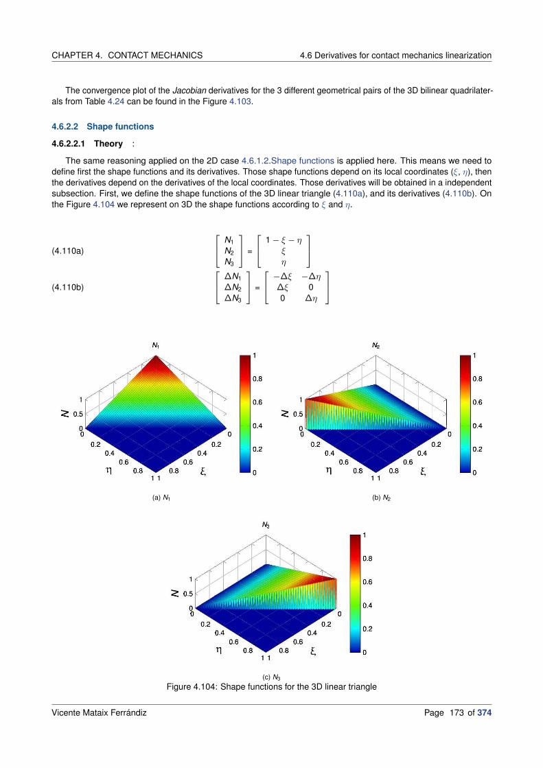
CHAPTER 4. CONTACT MECHANICS 4.6 Derivatives for contact mechanics linearization
The convergence plot of the Jacobian derivatives for the 3 different geometrical pairs of the 3D bilinear quadrilater-als from Table 4.24 can be found in the Figure 4.103.
4.6.2.2 Shape functions
4.6.2.2.1 Theory :
The same reasoning applied on the 2D case 4.6.1.2.Shape functions is applied here. This means we need todefine first the shape functions and its derivatives. Those shape functions depend on its local coordinates (ξ, η), thenthe derivatives depend on the derivatives of the local coordinates. Those derivatives will be obtained in a independentsubsection. First, we define the shape functions of the 3D linear triangle (4.110a), and its derivatives (4.110b). Onthe Figure 4.104 we represent on 3D the shape functions according to ξ and η.
N1
N2
N3
=
1 − ξ − ηξη
(4.110a)
∆N1
∆N2
∆N3
=
−∆ξ −∆η∆ξ 00 ∆η
(4.110b)
(a) N1 (b) N2
(c) N3
Figure 4.104: Shape functions for the 3D linear triangle
Vicente Mataix Ferrándiz Page 173 of 374

4.6 Derivatives for contact mechanics linearization CHAPTER 4. CONTACT MECHANICS
Second, we define the shape functions of the 3D bilinear quadrilateral and its derivatives at (4.111). The graphicrepresentation of the shape functions are shown in the Figure 4.105.
N1
N2
N3
N4
=
14 ((1 − ξ)(1 − η))14 ((1 + ξ)(1 − η))14 ((1 + ξ)(1 + η))14 ((1 − ξ)(1 + η))
(4.111a)
∆N1
∆N2
∆N3
∆N4
=
−∆ξ4 −∆η
4∆ξ4 −∆η
4∆ξ4
∆η4
−∆ξ4
∆η4
(4.111b)
(a) N1 (b) N2
(c) N3 (d) N4
Figure 4.105: Shape functions for the 3D bilinear quadrilateral
4.6.2.2.2 Local coordinates (Gauss points) :
Here we will define the derivatives of the corresponding GP local coordinates of the integration triangles, Figure4.101. Important to highlight the fact that the complexity of this task came from the fact that the inner GP from theintegration triangles must be projected into the master and slave domains. This, in the most general case requires theresolution of a NL problem with a NR iterative process.
Page 174 of 374 Vicente Mataix Ferrándiz

CHAPTER 4. CONTACT MECHANICS 4.6 Derivatives for contact mechanics linearization
To obtain the local coordinates ξ and η we will consider the expression proposed by Popp[ArtPGW09], butsimplified as our geometries are linear and consequently reduces the complexity of the system of equations. In orderto obtain the coordinates of the GP we use (4.112a), where we can see as the coordinates of the GP in the integrationtriangle (represented with N) has an equivalent on the master/slave geometries. With this expression we can definethis as a residual (4.112b) of a linear system of equations, which converges in one NL iteration. The complete systemof equations (4.112c) require to compute the corresponding Jacobian (J) (4.112d).
(4.112a)x1
g =∑nc
sk=1 N1
k x1k =∑3
i=1 Nixclip
x2g =∑nc
ml=1 N2
l x2l =∑3
i=1 Nixclip
(4.112b)RHS1 = x1
g
RHS2 = x2g
(4.112c) LHSi
[ξi
ηi
]
= RHSi ,i = 1, 2
Where LHSi corresponds with the Jacobian:
(4.112d) LHSi = J i =
[ ∑ncs
k=1 N ik ,ξxi
k∑nc
sk=1 N i
k ,ηxik
]
,i = 1, 2
With this we can define the equivalent expressions for the derivatives of the local coordinates (ξ and η), weredefine the RHS (4.113a), and using the same LHS (J) (4.112d), we can solve (4.113b) the new system of equationsin order to obtain our target derivatives.
(4.113a)RHS1 = ∆x1
g =∑3
i=1 Ni∆xclip
RHS2 = ∆x2g =∑3
i=1 Ni∆xclip
(4.113b)
[∆ξi
∆ηi
]
= LHS−1i RHSi ,i = 1, 2
4.6.2.2.3 Convergence study :
Figure 4.106: Convergence plot for the shape function derivatives for the 3D linear triangle
Vicente Mataix Ferrándiz Page 175 of 374

4.6 Derivatives for contact mechanics linearization CHAPTER 4. CONTACT MECHANICS
The convergence plot of the shape function derivatives for the 6 different geometrical pairs of the 3D lineartriangles from Table 4.22 can be found in the Figure 4.106.
Figure 4.107: Convergence plot for the shape function derivatives for the 3D bilinear quadrilateral
The convergence plot of the shape function derivatives for the 3 different geometrical pairs of the 3D bilinearquadrilaterals from Table 4.24 can be found in the Figure 4.107.
4.6.2.3 Dual shape functions
4.6.2.3.1 Theory :
The procedure to follow is identical to the one presented for the 2D case in 4.6.1.3.Dual shape functions. Noadditional modification is needed, except, of course, the corresponding computation on the integration triangles, whichmeans of the Jclip (4.6.2.1.Jacobians) and the use of the shape functions and derivatives already presented on theprevious section 4.6.2.2.Shape functions. Then we proceed with the convergence study.
4.6.2.3.2 Convergence study :
The convergence plot of the dual shape function derivatives for the 6 different geometrical pairs of the 3D lineartriangles from Table 4.22 can be found in the Figure 4.108.
Figure 4.108: Convergence plot for the dual shape function derivatives for the 3D linear triangle
Page 176 of 374 Vicente Mataix Ferrándiz

CHAPTER 4. CONTACT MECHANICS 4.6 Derivatives for contact mechanics linearization
The convergence plot of the dual shape function derivatives for the 3 different geometrical pairs of the 3D bilinearquadrilaterals from Table 4.24 can be found in the Figure 4.109.
Figure 4.109: Convergence plot for the dual shape function derivatives for the 3D bilinear quadrilateral
4.6.2.4 Normal and tangent vectors
4.6.2.4.1 Theory :
Figure 4.110: Normal average for a 3D geometry
As previously introduced, the tangent vector is taken as the complementary direction to the normal (4.114a), thenin order to define its derivative we just need to compute the normal derivative, then the computation of the tangentderivative will be automatically taken into account with the AD procedure. The definition of the normal for 3D surfacegeometries corresponds with (4.114b), where can be defined as the cross product between the rows of the Jacobianmatrix. Then we compute the unit normal the same way we do for the 2d case (4.101b).
The average normal behaves exactly the same to the definition presented for the 2D case (4.101c), the main
Vicente Mataix Ferrándiz Page 177 of 374

4.6 Derivatives for contact mechanics linearization CHAPTER 4. CONTACT MECHANICS
difference in the practical case came with the fact that the number of neighbours in 3D is not bounded, see Figure4.110, in contrast with the 2D case where there are only two potential neighbours.
τ = I − n × n(4.114a)
narea = x,ξ × x,η(4.114b)
Then in order to evaluate ∆ for the normal on 3D surfaces we can apply the chain rule to the previous definitionon (4.114b) and (4.101b). The resulting derivative (4.115) results as an addition.
(4.115a) ∆n =∆narea ‖narea‖ − narea∆ ‖narea‖
‖narea‖2 =∆(x,ξ × x,η
)‖x,ξ × x,η‖ −
(x,ξ × x,η
)∆ ‖x,ξ × x,η‖
‖x,ξ × x,η‖2
Where the first derivative is:
(4.115b) ∆(x,ξ × x,η
)=
ncs∑
k=1
Nk ,ξ∆xk
×
ncs∑
k=1
Nk ,ηxk
+
ncs∑
k=1
Nk ,ξxk
×
ncs∑
k=1
Nk ,η∆xk
And the second term:
(4.115c) ∆∥∥(x,ξ × x,η
)∥∥ =
(x,ξ × x,η
)∆(x,ξ × x,η
)
∥∥(x,ξ × x,η
)∥∥
= n∆(x,ξ × x,η
)
Finally, in order to obtain the derivative of the average normal we proceed following the same equation presentedfor the 2D case (4.103). The normal derivative for the GP also behaves the same way as in 2D (4.104).
4.6.2.4.2 Convergence study :
The convergence plot of the normal vector derivatives for the 6 different geometrical pairs of the 3D lineartriangles from Table 4.22 can be found in the Figure 4.111. We can appreciate that the convergence is greater thancubic.
Figure 4.111: Convergence plot for the normal vector derivatives for the 3D linear triangle
The convergence plot of the normal vector derivatives for the 3 different geometrical pairs of the 3D bilinearquadrilaterals from Table 4.24 can be found in the Figure 4.112.
Page 178 of 374 Vicente Mataix Ferrándiz

CHAPTER 4. CONTACT MECHANICS 4.6 Derivatives for contact mechanics linearization
Figure 4.112: Convergence plot for the normal vector derivatives for the 3D bilinear quadrilateral
Vicente Mataix Ferrándiz Page 179 of 374

4.6 Derivatives for contact mechanics linearization CHAPTER 4. CONTACT MECHANICS
Page 180 of 374 Vicente Mataix Ferrándiz

BIBLIOGRAPHY BIBLIOGRAPHY
Bibliography
Books
[BookAnd01] From Convexity to Nonconvexity. Anders Klarbring (auth.) R. P. Gilbert P. D. PanagiotopoulosP. M. Pardalos (eds.) Lars-Erik Andersson. Springer US. 1st ed. 2001.
[BookBAL03] Friction & flow stress in forming & cutting. Philippe Boisse, Taylan Altan, and Kees van Luttervelt.Sterling, VA: Kogan Page. 2003.
[BookBBT01] The friction and lubrication of solids. Frank Philip Bowden, Frank Philip Bowden, and David Tabor.Oxford university press. 2001.
[BookBel+14] Nonlinear Finite Elements for Continua and Structures. Ted Belytschko, Wing Kam Liu,Brian Moran, and Khalil Elkhodary. Wiley. 2nd ed. 2014.
[BookBHS07] Encyclopedia of Computational Mechanics (3 Volume Set). René de Borst, T.J.R. Hughes, andErwin Stein. Wiley. 1st ed. 2007.
[BookBou85] Application des potentiels à l’étude de l’équilibre et du mouvement des solides élastiques.Joseph Boussinesq. Gauthier-Villars, Imprimeur-Libraire. 1885.
[BookEbe99] Dynamic collision detection using oriented bounding boxes. David Eberly. 1999.
[BookEri04] Real-time collision detection. Christer Ericson. CRC Press. 2004.
[BookFSS12] OpenDSA: a creative commons active-ebook (abstract only). Eric Fouh, Maoyuan Sun, andClifford Shaffer. 2012. Pp. 721–721.
[BookHBC09] Isogeometric Analysis: Toward Integration of CAD and FEA. T.J.R. Hughes, Yuri Bazilevs, andJ. Austin Cottrell. Wiley. 1st ed. 2009.
[BookHug+14] Computer graphics: principles and practice. John F Hughes, Andries Van Dam, James D Foley,Morgan McGuire, Steven K Feiner, and David F Sklar. Pearson Education. 2014.
[BookKO88] Contact problems in elasticity: a study of variational inequalities and finite element methods.Noboru Kikuchi and John Tinsley Oden. siam. 1988.
[BookLau10] Computational Contact and Impact Mechanics: Fundamentals of Modeling Interfacial Phenomenain Nonlinear Finite Element Analysis. Tod A. Laursen. Springer. 2010.
[BookMau13] Contact, adhesion and rupture of elastic solids. Daniel Maugis. Springer Science & BusinessMedia. 2013.
[BookPhD06] R-Trees: Theory and Applications. Alexandros Nanopoulos PhD Apostolos N. Papadopoulos PhDYannis Theodoridis PhD (auth.) Yannis Manolopoulos PhD. Springer-Verlag London. 1st ed. 2006.
[BookPop10] Contact Mechanics and Friction: Physical Principles and Applications. Valentin L. Popov.Springer-Verlag Berlin Heidelberg. 1st ed. 2010.
[BookSE02] Geometric tools for computer graphics. Philip Schneider and David H Eberly. Elsevier. 2002.
[BookSK13] Computational Contact Mechanics: Geometrically Exact Theory for Arbitrary Shaped Bodies.Karl Schweizerhof and Alexander Konyukhov. Springer-Verlag Berlin Heidelberg. 1st ed. 2013.
[BookTos05] Domain Decomposition Methods — Algorithms and Theory. Andrea Toselli Olof B. Widlund (auth.)Springer-Verlag Berlin Heidelberg. 1st ed. 2005.
Vicente Mataix Ferrándiz Page 181 of 374
ARTICLES BIBLIOGRAPHY
[BookWoh01] Discretization Methods and Iterative Solvers Based on Domain Decomposition.Barbara I. Wohlmuth. Springer-Verlag Berlin Heidelberg. 1st ed. 2001.
[BookWP99] New Developments in Contact Problems. Peter Wriggers and Panagiotis Panagiotopoulos.Springer-Verlag Wien. 1st ed. 1999.
[BookWri06] Computational Contact Mechanics. Peter Wriggers. Springer. 2nd. 2006.
[BookYas13] Numerical Methods in Contact Mechanics. Vladislav A. Yastrebov. Wiley-ISTE. 1st ed. 2013.
[BookZZT13] The Finite Element Method: its Basis and Fundamentals. O. C. Zienkiewicz, J.Z. Zhu, andRobert L. Taylor. Butterworth-Heinemann. 7th ed. 2013.
Articles
[ArtAC91] “A mixed formulation for frictional contact problems prone to Newton like solution methods”. P. Alartand A. Curnier. In: Computer Methods in Applied Mechanics and Engineering. No. 3, Vol. 92, 1991,pp. 353–375. DOI: 10.1016/0045-7825(91)90022-x.
[ArtAnt17] “A further analysis on the analogy between friction and plasticity in Solid Mechanics”.Nicolas Antoni. In: International Journal of Engineering Science. Vol. 121, 2017, pp. 34–51.Elsevier. DOI: 10.1016/j.ijengsci.2017.08.012.
[ArtBar08] “Adhesive elastic contacts – JKR and more”. Etienne Barthel. In: Journal of Physics D: AppliedPhysics. Vol. 41, 2008, p. 163001. IOP Publishing. DOI:10.1088/0022-3727/41/16/163001.
[ArtBen+11] “A large deformation, rotation-free, isogeometric shell”. D.J. Benson, Y. Bazilevs, M.-C. Hsu, andT.J.R. Hughes. In: Computer Methods in Applied Mechanics and Engineering. No. 13, Vol. 200,2011, pp. 1367–1378. Elsevier. DOI: 10.1016/j.cma.2010.12.003.
[ArtBMP] “The adapted augmented Lagrangian method: a new method for the resolution of the mechanicalfrictional contact problem”. Philippe Bussetta, Daniel Marceau, and Jean-Philippe Ponthot. In:Computational Mechanics. No. 2, , pp. 259–275. DOI: 10.1007/s00466-011-0644-z.
[ArtBT39] “The area of contact between stationary and moving surfaces”. Frank Philip Bowden andDavid Tabor. In: Proceedings of the Royal Society of London. Series A. Mathematical and PhysicalSciences. No. 938, Vol. 169, 1939, pp. 391–413. The Royal Society London.
[ArtCai+14] “Collision detection using axis aligned bounding boxes”. Panpan Cai, Chandrasekaran Indhumathi,Yiyu Cai, Jianmin Zheng, Yi Gong, Teng Sam Lim, and Peng Wong. In: . 2014, pp. 1–14. Springer.DOI: 10.1007/978-981-4560-32-0_1.
[ArtCam15] “Computational modeling and simulation of rupture of membranes and thin films”.Eduardo MB Campello. In: Journal of the Brazilian Society of Mechanical Sciences andEngineering. No. 6, Vol. 37, 2015, pp. 1793–1809. Springer. DOI:10.1007/s40430-014-0273-5.
[ArtCC12] “An augumented lagrangian method to solve three-dimensional nonlinear contact problems”.FJ Calavalieri and Alberto Cardona. In: Latin American applied research. No. 3, Vol. 42, 2012,pp. 281–289. SciELO Argentina.
[ArtCC13a] “Three-dimensional numerical solution for wear prediction using a mortar contact algorithm”.Federico José Cavalieri and Alberto Cardona. In: International Journal for Numerical Methods inEngineering. No. 8, Vol. 96, 2013, pp. 467–486. Wiley Online Library. DOI: 10.1002/nme.4556.
[ArtCC13b] “An augmented Lagrangian technique combined with a mortar algorithm for modelling mechanicalcontact problems”. FJ Cavalieri and A Cardona. In: International Journal for Numerical Methods inEngineering. No. 4, Vol. 93, 2013, pp. 420–442. Wiley Online Library. DOI: 10.1002/nme.4391.
[ArtCC15] “Numerical solution of frictional contact problems based on a mortar algorithm with an augmentedLagrangian technique”. F. J. Cavalieri and A. Cardona. In: Multibody System Dynamics. No. 4, Vol.35, 2015, pp. 353–375. DOI: 10.1007/s11044-015-9449-8.
Page 182 of 374 Vicente Mataix Ferrándiz

BIBLIOGRAPHY ARTICLES
[ArtCFC12] “Un algoritmo de contacto mortar aplicable a problemas tridimensionales”. F.J. Cavalieri,V.D. Fachinotti, and A. Cardona. In: Revista Internacional de Métodos Numéricos para Cálculo yDiseño en Ingeniería. No. 2, Vol. 28, 2012, pp. 80–92. DOI:10.1016/j.rimni.2012.03.001.
[ArtCho+17] “An overview of recent results on Nitsche’s method for contact problems”. Franz Chouly,Mathieu Fabre, Patrick Hild, Rabii Mlika, Jerome Pousin, and Yves Renard. In: . 2017, pp. 93–141.Springer.
[ArtCou85] “The theory of simple machines”. CA Coulomb. In: Mem. Math. Phys. Acad. Sci . No. 161-331, Vol.10, 1785, p. 4.
[ArtDB15] “A literature review of bounding volumes hierarchy focused on collision detection”. Simena Dinasand José M Bañón. In: Ingeniería y competitividad . No. 1, Vol. 17, 2015, pp. 49–62. Universidaddel Vall.
[ArtDem+12] “Computational comparison of the bending behavior of aortic stent-grafts”. Nicolas Demanget,Stéphane Avril, Pierre Badel, Laurent Orgéas, Christian Geindreau, Jean-Noël Albertini, andJean-Pierre Favre. In: Journal of the mechanical behavior of biomedical materials. No. 1, Vol. 5,2012, pp. 272–282. Elsevier. DOI: 10.1016/j.jmbbm.2011.09.006.
[ArtDFS98] “Solution of coercive and semicoercive contact problems by FETI domain decomposition”.Zdenek Dostál, Ana Friedlander, and Sandra A Santos. In: Contemporary Mathematics. Vol. 218,1998, pp. 82–93. Providence, RI: American Mathematical Society. DOI:10.1090/conm/218/03003.
[ArtDon99] “A simple benchmark problem to test frictional contact”. CY Dong. In: Computer methods in appliedmechanics and engineering. No. 1-2, Vol. 177, 1999, pp. 153–162. Elsevier. DOI:10.1016/s0045-7825(98)00377-6.
[ArtDPS] “A frictional mortar contact approach for the analysis of large inelastic deformation problems”.T Doca, FM Andrade Pires, and JMA Cesar de Sa. In: International Journal of Solids andStructures. No. 9, , pp. 1697–1715. Elsevier. DOI: 10.1016/j.ijsolstr.2014.01.013.
[ArtDSB15] “High-order mortar-based element applied to nonlinear analysis of structural contact mechanics”.APC Dias, AL Serpa, and ML Bittencourt. In: Computer Methods in Applied Mechanics andEngineering. Vol. 294, 2015, pp. 19–55. Elsevier. DOI: 10.1016/j.cma.2015.05.013.
[ArtEul50a] “Sur la diminution de la resistance du frottement”. Leonhard Euler. In: Mémoires de l’académie dessciences de Berlin. 1750, pp. 133–148.
[ArtEul50b] “Sur le frottement des corps solides”. Leonhard Euler. In: Mémoires de l’Académie des Sciencesde Berlin. 1750, pp. 122–132.
[ArtFF03] “Collision Detection for Virtual Prototyping Environments”. Mauro Figueiredo and T Fernando. In: .2003, pp. 157–166.
[ArtFic63] “Sul problema elastostatico di Signorini con ambigue condizioni al contorno”. Gaetano Fichera. In:Atti Accad. Naz. Lincei Rend. Cl. Sci. Fis. Mat. Natur.(8). Vol. 34, 1963, pp. 138–142.
[ArtFig10] “S-cd: surface collision detection toolkit for virtual prototyping”. Mauro Figueiredo. In: IADISInternational Journal on Computer Science and Information Systems. Vol. 5, 2010, pp. 72–86.
[ArtFW06] “Mortar based frictional contact formulation for higher order interpolations using the moving frictioncone”. Kathrin A Fischer and Peter Wriggers. In: Computer methods in applied mechanics andengineering. No. 37-40, Vol. 195, 2006, pp. 5020–5036. Elsevier. DOI:10.1016/j.cma.2005.09.025.
[ArtFZ75] “A note on numerical computation of elastic contact problems”. A Francavilla and OC Zienkiewicz.In: International Journal for Numerical Methods in Engineering. No. 4, Vol. 9, 1975, pp. 913–924.Wiley Online Library. DOI: 10.1002/nme.1620090410.
[ArtHar+09] “A contact domain method for large deformation frictional contact problems. Part 2: Numericalaspects”. S. Hartmann, J. Oliver, R. Weyler, J.C. Cante, and J.A. Hernández. In: ComputerMethods in Applied Mechanics and Engineering. No. 33–36, Vol. 198, 2009, pp. 2607–2631. DOI:10.1016/j.cma.2009.03.009.
Vicente Mataix Ferrándiz Page 183 of 374

ARTICLES BIBLIOGRAPHY
[ArtHar+10] “A 3D frictionless contact domain method for large deformation problems”. S Hartmann, R Weyler,J Oliver, JC Cante, and JA Hernández. In: Computer Modeling in Engineering and Sciences(CMES). No. 3, Vol. 55, 2010, p. 211.
[ArtHer82] “Über die berührung fester elastische Körper und über die Harte”. H Hertz. In: Verhandlungen desVereins zur Beförderung des Gewerbefleisses. 1882,
[ArtHTK77] “A finite element method for large displacement contact and impact problems”. TJR Hughes,RL Taylor, and W Kanoknukulchai. In: Formulations and Computational Algorithms in FE Analysis.1977, pp. 468–495. MIT Press: Boston.
[ArtHWP18] “A truly variationally consistent and symmetric mortar-based contact formulation for finitedeformation solid mechanics”. Michael Hiermeier, Wolfgang A. Wall, and Alexander Popp. In:Computer Methods in Applied Mechanics and Engineering. Vol. 342, 2018, pp. 532–560. DOI:10.1016/j.cma.2018.07.020.
[ArtJKR71] “Surface energy and the contact of elastic solids”. Kenneth Langstreth Johnson, Kevin Kendall, andAD Roberts. In: Proceedings of the royal society of London. A. mathematical and physical sciences.No. 1558, Vol. 324, 1971, pp. 301–313. The Royal Society London.
[ArtKar39] “Minima of functions of several variables with inequalities as side constraints”. William Karush. In:M. Sc. Dissertation. Dept. of Mathematics, Univ. of Chicago. 1939,
[ArtKor94] “Monotone multigrid methods for elliptic variational inequalities I”. Ralf Kornhuber. In: NumerischeMathematik . No. 2, Vol. 69, 1994, pp. 167–184. Springer. DOI: 10.1007/s002110050178.
[ArtKra68] “Friction and wear”. IV Kragelsky. In: Mechanical Engineering, Moscow . 1968, Elsevier.
[ArtLWZ12a] “A mortar formulation for 3D large deformation contact using NURBS-based isogeometric analysisand the augmented Lagrangian method”. L. de Lorenzis, Peter Wriggers, and G. Zavarise. In:Computational Mechanics. No. 1, Vol. 49, 2012, pp. 1–20. Springer. DOI:10.1007/s00466-011-0623-4.
[ArtLWZ12b] “A mortar formulation for 3D large deformation contact using NURBS-based isogeometric analysisand the augmented Lagrangian method”. L. De Lorenzis, Peter Wriggers, and G. Zavarise. In:Computational Mechanics. No. 1, Vol. 49, 2012, pp. 1–20. Springer-Verlag. DOI:10.1007/s00466-011-0623-4.
[ArtMor73] “Systèmes élastoplastiques de liberté finie”. JEAN JACQUES Moreau. In: Travaux du Séminaired’Analyse Convexe. Vol. 3, 1973, p. 33.
[ArtNag05] “Simple local interpolation of surfaces using normal vectors”. Takashi Nagata. In: Computer AidedGeometric Design. No. 4, Vol. 22, 2005, pp. 327–347. DOI: 10.1016/j.cagd.2005.01.004.
[ArtNet+14] “Applying Nagata patches to smooth discretized surfaces used in 3D frictional contact problems”.D. M. Neto, M. C. Oliveira, L. F. Menezes, and J. L. Alves. In: Computer Methods in AppliedMechanics and Engineering. Vol. 271, 2014, pp. 296–320. Elsevier. DOI:10.1016/j.cma.2013.12.008.
[ArtNit71] “Über ein Variationsprinzip zur Lösung von Dirichlet-Problemen bei Verwendung von Teilräumen,die keinen Randbedingungen unterworfen sind”. Joachim Nitsche. In: . No. 1, Vol. 36, 1971,pp. 9–15.
[ArtNOM17] “Surface Smoothing Procedures in Computational Contact Mechanics”. D. M. Neto, M. C. Oliveira,and L. F. Menezes. In: Archives of Computational Methods in Engineering. No. 1, Vol. 24, 2017,pp. 37–87. DOI: 10.1007/s11831-015-9159-7.
[ArtOde81] “Exterior penalty methods for contact problems in elasticity”. JT Oden. In: . 1981, pp. 655–665.Springer. DOI: 10.1007/978-3-642-81589-8_33.
[ArtOli+09a] “A contact domain method for large deformation frictional contact problems. Part 1: Theoreticalbasis”. J. Oliver, S. Hartmann, J. C. Cante, R. Weyler, and J. A. Hernández. In: Computer Methodsin Applied Mechanics and Engineering. No. 33–36, Vol. 198, 2009, pp. 2591–2606. DOI:10.1016/j.cma.2009.03.006.
[ArtOli+09b] “A New Approach in Computational Contact Mechanics: The Contact Domain Method”. X Oliver,S Hartmann, JC Cante, R Weyler, and JA Hernández. In: CIMNE, Barcelona. 2009,
Page 184 of 374 Vicente Mataix Ferrándiz

BIBLIOGRAPHY ARTICLES
[ArtPGW09] “A finite deformation mortar contact formulation using a primal–dual active set strategy”.Alexander Popp, Michael W. Gee, and Wolfgang A. Wall. In: International Journal for NumericalMethods in Engineering. No. 11, Vol. 79, 2009, pp. 1354–1391. John Wiley & Sons, Ltd. DOI:10.1002/nme.2614.
[ArtPL04] “A mortar segment-to-segment contact method for large deformation solid mechanics”.Michael A. Puso and Tod A. Laursen. In: Computer Methods in Applied Mechanics and Engineering.No. 6–8, Vol. 193, 2004, pp. 601–629. Elsevier. DOI: 10.1016/j.cma.2003.10.010.
[ArtPop+10] “A dual mortar approach for 3D finite deformation contact with consistent linearization”.Alexander Popp, Markus Gitterle, Michael W. Gee, and Wolfgang A. Wall. In: International Journalfor Numerical Methods in Engineering. No. 11, Vol. 83, 2010, pp. 1428–1465. John Wiley & Sons,Ltd. DOI: 10.1002/nme.2866.
[ArtPP15] “The research works of Coulomb and Amontons and generalized laws of friction”. Elena Popovaand Valentin L Popov. In: Friction. No. 2, Vol. 3, 2015, pp. 183–190. Springer. DOI:10.1007/s40544-015-0074-6.
[ArtPPS03] “Vibration damping by friction forces: theory and applications”. Karl Popp, Lars Panning, andWalter Sextro. In: Modal Analysis. No. 3-4, Vol. 9, 2003, pp. 419–448. Sage Publications Sage CA:Thousand Oaks, CA. DOI: 10.1177/107754603030780.
[ArtPR15a] “An unconstrained integral approximation of large sliding frictional contact between deformablesolids”. Konstantinos Poulios and Yves Renard. In: Computers & Structures. Vol. 153, 2015,pp. 75–90. DOI: 10.1016/j.compstruc.2015.02.027.
[ArtPR15b] “An unconstrained integral approximation of large sliding frictional contact between deformablesolids”. Konstantinos Poulios and Yves Renard. In: Computers & Structures. Vol. 153, 2015,pp. 75–90. Elsevier. DOI: 10.1016/j.compstruc.2015.02.027.
[ArtPT92] “A mixed formulation for the finite element solution of contact problems”. Panayiotis Papadopoulosand Robert L Taylor. In: Computer Methods in Applied Mechanics and Engineering. No. 3, Vol. 94,1992, pp. 373–389. Elsevier. DOI: 10.1016/0045-7825(92)90061-n.
[ArtRao16] “Art of Modeling in Contact Mechanics”. Michel Raous. In: . Vol. 570, 2016, Springer. DOI:10.1007/978-3-319-40256-7_4.
[ArtRKC02] “Fast Continuous Collision Detection between Rigid Bodies”. Stephane Redon,Abderrahmane Kheddar, and Sabine Coquillart. In: Computer Graphics Forum. No. 3, Vol. 21, 2002,pp. 279–287. DOI: 10.1111/1467-8659.t01-1-00587.
[ArtRom11] “Advanced methods for robot-environment interaction towards an industrial robot aware of itsvolume”. Fabrizio Romanelli. In: Journal of Robotics. Vol. 2011, 2011, Hindawi. DOI:10.1155/2011/389158.
[ArtSig33] “Sopra alcune questioni di elastostatica”. Antonio Signorini. In: Atti della Societa Italiana per ilProgresso delle Scienze. No. Ii, Vol. 21, 1933, pp. 143–148.
[ArtSN17] “Woven fabrics computational simulation using beam-to-beam contacts formulation”.Mauro Takayama Saito and Alfredo Gay Neto. In: Revista Interdisciplinar De Pesquisa EmEngenharia. No. 22, Vol. 2, 2017, pp. 09–25.
[ArtSpe] “The Hertz contact problem with finite friction”. DA Spence. In: Journal of elasticity . No. 3-4, ,pp. 297–319. Springer. DOI: 10.1007/bf00126993.
[ArtSWP18] “A computational approach for thermo-elasto-plastic frictional contact based on a monolithicformulation using non-smooth nonlinear complementarity functions”. Alexander Seitz,Wolfgang A Wall, and Alexander Popp. In: Advanced Modeling and Simulation in EngineeringSciences. No. 1, Vol. 5, 2018, p. 5. Springer. DOI: 10.1186/s40323-018-0098-3.
[ArtSWT85] “A perturbed Lagrangian formulation for the finite element solution of contact problems”.Juan C Simo, Peter Wriggers, and Robert L Taylor. In: Computer methods in applied mechanicsand engineering. No. 2, Vol. 50, 1985, pp. 163–180. Elsevier. DOI:10.1016/0045-7825(85)90088-x.
Vicente Mataix Ferrándiz Page 185 of 374
PH.D.’S THESIS BIBLIOGRAPHY
[ArtTC03] “A model of adhesion coupled to contact and friction”. C. Talon and A. Curnier. In: EuropeanJournal of Mechanics - A/Solids. No. 4, Vol. 22, 2003, pp. 545–565. DOI:10.1016/s0997-7538(03)00046-9.
[ArtTK14] “Real-Time Hybrid Virtuality for Prevention of Excavation Related Utility Strikes”. Sanat Talmaki andVineet R. Kamat. In: Journal of Computing in Civil Engineering. No. 3, Vol. 28, 2014, p. 04014001.DOI: 10.1061/(asce)cp.1943-5487.0000269.
[ArtTP] “On a patch test for contact problems in two dimensions”. Robert L. Taylor andPanagiotis Panagiotopoulos. In: . ,
[ArtWI93] “On the treatment of nonlinear unilateral contact problems”. P Wriggers and M Imhof. In: Archive ofApplied Mechanics. No. 2, Vol. 63, 1993, pp. 116–129. Springer. DOI: 10.1007/bf00788917.
[ArtWie+18] “Algebraic multigrid methods for dual mortar finite element formulations in contact mechanics”.T. A. Wiesner, A. Popp, M. W. Gee, and W. A. Wall. In: International Journal for Numerical Methodsin Engineering. No. 4, Vol. 114, 2018, pp. 399–430. DOI: 10.1002/nme.5748.
[ArtWoh02] “A Comparison of Dual Lagrange Multiplier Spaces for Mortar Finite Element Discretizations”.Barbara I. Wohlmuth. In: ESAIM: Mathematical Modelling and Numerical Analysis. No. 6, Vol. 36,2002, pp. 995–1012. EDP Sciences. DOI: 10.1051/m2an:2003002.
[ArtWZ13] “Hertz Theory: Contact of Spherical Surfaces”. Q. Jane Wang and Dong Zhu. In: . 2013,pp. 1654–1662. Springer US. Boston, MA. DOI: 10.1007/978-0-387-92897-5_492.
[ArtYCF11] “A local contact detection technique for very large contact and self-contact problems: sequentialand parallel implementations”. VA Yastrebov, Georges Cailletaud, and Frédéric Feyel. In: . 2011,pp. 227–251. Springer. DOI: 10.1007/978-3-642-22167-5_13.
[ArtYL08] “A contact searching algorithm including bounding volume trees applied to finite sliding mortarformulations”. Bin Yang and TodA. Laursen. In: Computational Mechanics. No. 2, Vol. 41, 2008,pp. 189–205. Springer-Verlag. DOI: 10.1007/s00466-006-0116-z.
[ArtYLM] “Two dimensional mortar contact methods for large deformation frictional sliding”. Bin Yang,Tod A. Laursen, and Xiaonong Meng. In: International Journal for Numerical Methods inEngineering. No. 9, , pp. 1183–1225. Chichester, New York, Wiley [etc.] 1969-. DOI:10.1002/nme.1222.
[ArtZhu12] “Tutorial on hertz contact stress”. Xiaoyin Zhu. In: . Vol. 521, 2012, pp. 1–8.
[ArtZK12] “k-IOS: Intersection of spheres for efficient proximity query”. Xinyu Zhang and Young J. Kim. In:2012 IEEE International Conference on Robotics and Automation. 2012, pp. 354–359. DOI:10.1109/icra.2012.6224889.
[ArtZL09] “A modified node-to-segment algorithm passing the contact patch test”. Giorgio Zavarise andLaura De Lorenzis. In: International journal for numerical methods in engineering. No. 4, Vol. 79,2009, p. 379. DOI: 10.1002/nme.2559.
Ph.D.’s thesis
[PhDBru08] “Contact analysis and overlapping domain decomposition methods for dynamic and nonlinearproblems”. Stephan BrunSSen. 2008.
[PhDBus] “Modélisation et résolution du problème de contact mécanique et son application dans un contextemultiphysique”. Philippe Bussetta.
[PhDDoc] “Energy wear methods for dual-mortar contact analysis of frictional problems at finite inelasticstrains”. Thiago de Carvalho Rodrigues Doca.
[PhDDro15] “Local mortar method for contact problems with high order non-matching meshes”.Guillaume Drouet. 2015.
[PhDGit12] “A dual mortar formulation for finite deformation frictional contact problems including wear andthermal coupling”. Markus Gitterle. 2012.
Page 186 of 374 Vicente Mataix Ferrándiz

BIBLIOGRAPHY ONLINE RESOURCES
[PhDHam13] “Frictional mortar contact for finite deformation problems with synthetic contact kinematics”.Michael E. Hammer. 2013.
[PhDKra01] “Monotone multigrid methods for Signorini’s problem with friction”. Rolf H Krause. 2001.
[PhDPop12] “Mortar Methods for Computational Contact Mechanics and General Interface Problems”.Alexander Popp. 2012.
[PhDYas11] “Computational contact mechanics: geometry, detection and numerical techniques”.Vladislav A. Yastrebov. 2011.
Online resources
[OnlCho] Collision Detection Using the Separating Axis Theorem. URL:https://gamedevelopment.tutsplus.com/tutorials/collision-detection-
using-the-separating-axis-theorem-gamedev-169.
[OnlJac] Jacobi elliptic functions. URL: https://www.encyclopediaofmath.org/index.php/Jacobi_elliptic_functions.
[OnlRtr] Wikipedia. R-tree. URL: https://en.wikipedia.org/wiki/R-tree.
Vicente Mataix Ferrándiz Page 187 of 374

ONLINE RESOURCES BIBLIOGRAPHY
Page 188 of 374 Vicente Mataix Ferrándiz

CHAPTER 5. PLASTICITY
Chapter 5
Plasticity
As the water shapes itself to thevessel that contains it, so a wise manadapts himself to circumstances.
Confucius(551 - 479 BC, Chinese philosopher)
5.1 Introduction
The mathematical modelling of plasticity in solids and structures are essential for a good modulation of the formingprocesses[BookBan10]. As well as other industrial processes and applications, like the design of steel and concretecivil structures, or the understanding of the response of the soil or rocks in geotechnical problems[BookBHS07].We can shortly introduce[BookNPO09] that in contrast with the elastic constitutive laws, the elasticplastic laws arepath-dependent and dissipative[BookZTF14], this means that large part of the work expended in plastically deformingthe material is irreversibly converted to other forms of energy, generally heat[BookHil98]. The stress depends on theentire history of the deformation[BookHS98], and cannot be written as a single-valued function of the strain; rather itcan only be specified as a relation between rates of stress and strain[BookBel+14].
5.1.1 Historical outline
Plasticity is one of the most developed theories for describing material NL behaviour. The history of the studies inthis scientific discipline, which involves mathematics, physics and engineering applications is rich. For a completeoverview of the history of plasticity, we address directly to the overview presented on the book of Hill [BookHil98] andZyczkowski [BookZyc81], much more complete than the one presented here.
Having said that, the first developments came from the Coulomb[ArtCou76] contributions in 1776, when hepresented a work stating the dependence of the sliding resistance on a plane between two bodies, being a function ofthe adhesion and the frictional properties1. This work, together with the later developments published by Ponceletand Rankine, was useful for the calculation of retaining walls.
We can identify as the firsts[BookWei] properly speaking works on plasticity the contributions of Tresca[BookTre65]in 1864 on the extrusion of metals, this was the later denominated Tresca yield criterion, which states that the metalyields when the maximal shear stress surpasses a threshold. During that time, the also-French mathematician St.Venant [ArtSai70] introduced basic constitutive relations for perfectly plastic materials, where it related the direction onthe strain increase and the principal stresses. These developments were later extended to 3D by Lévy.
1We discuss in the contact chapter 4.Contact mechanics, the similarities between the frictional contact theory and the plasticity models.
Vicente Mataix Ferrándiz Page 189 of 374

5.2 State of the Art in numerical plasticity CHAPTER 5. PLASTICITY
In 1886 Bauschinger [ArtBau86] introduced the effect that now carries its name, which it consists in the factthat by deforming a metal in one direction until its elasticity limit has been exceeded, and then deforming it in theopposite direction, its proportionality limit in the latter direction is lower due to the material imperfections. It was beforethe First World War (WWI), in 1913, when Von Mises[ArtMis13] introduced the known as J2 theory. Later in 1924Prandtl [ArtPra24] extended the St. Venant work for elastic-plastic behaviour, which Reuss extended later to 3D. Itwas not until 1928 when Von Mises[ArtMis28] extended his previous theory considering the yield function as a plasticpotential in the incremental stressstrain relations of the flow theory. That very same year Prandtl tried to formulategeneral relations for hardening behaviour.
Figure 5.1: Liberty ships suddenly broke in halfwhile moored at the dock
In the period between wars, and especially during the WWII,many relevant developments were done on this field. The war stim-ulated research through problems such as the calculation of thestresses in autofrettaged gun barrels and of the forces resisting ashot penetrating armour plate[BookHil98].
Additionally to this, it is particularly known and interesting tohighlight the problems originated during the production of the Libertyships[ArtZha16]. These were cargo ships built in the United States
(U.S.) during WWII in order to provide goods and carry troops. Theinitial design was modified by the U.S. Maritime Commission toconform to make it quicker and cheaper to build, this new designconsisted on replace part of the riveting operations with welding.This was due because riveting represented the 30% of the workforcecosts. Unfortunately, no further studies were carried to understandto how welding would affect the structure[ArtGer12]. The rapid andmassive construction requirements originated several issues that many notes and trigger the alarm about a studythe reasons that induce these problems. Almost 1500 instances of significant brittle fractures were recorded (Figure5.1). Usually this problem is studied as a fracture phenomenon, but studies from Altstetter et al.[ArtAA95] proposedan alternative approach that enhanced localised plasticity might nucleate either ductile fracture or quasi-cleavage.In any case, these problems lead deeper studies on the NL behaviour of the materials and benefited therefore theunderstanding of the plasticity.
So in 1949 Prager [ArtPra49] proposed a framework for the plastic constitutive relations for hardening materialswith smooth yield functions. Two years later Drucker his material stability postulate. Together, they presented in1952[ArtDP52] its criterion, which tries to represent the plastic deformation of soils. This is a pressure-dependentmodel that determines whether a material has exceeded the elastic limit. On 1953 Koiter [ArtKoi53] generalised theplastic stress-strain relations for non-smooth yield functions.
The following developments, due to the rise of the computational power were more focus on the research on thenumerical analysis, especially after the 1970s, so it will be detailed in the next section 5.2.State of the Art in numericalplasticity.
5.2 State of the Art in numerical plasticity
5.2.1 Historical outline
We want to convey that the developments that will be shown in this work are within the classical theory, and we willnot be innovative in this matter. The work done in this field was needed in order to be able to address the formingprocess problem. So the first works that can be considered as reference, the foundations for the numerical plasticityincluding infinitesimal theory, can be found in the book from the 1950s of Hill [BookHil98] and later in the article ofKoiter [ArtKoi60].
Having said that, we can attribute[BookWei] to Duvaut and Lions[ArtDL76] the first study of the Boundary Value
Problem (BVP) of elasto-plasticity, who defined the problem as variational inequality2. Later Johnson[ArtJoh76] split
2See the Appendix D.Constrained optimisation problems for further detail. On this Appendix the inequality is treated in order to introduce themathematical concept necessaries to understand the CCM, but the theory can be applied on plasticity too.
Page 190 of 374 Vicente Mataix Ferrándiz

CHAPTER 5. PLASTICITY 5.2 State of the Art in numerical plasticity
this variational inequality in two steps, one to solve the steady state problem after removing the velocity and a secondstep to solve the velocity of the problem.
In 1985 J.C. Simo and R.L. Taylor [ArtST85], derived the consistent elasto-plastic tangent tensors. Cep. This resultcan be seen in the corresponding section at 5.5.3.Numerical implementation tangent constitutive tensor.
Later, incremental finite strain elasto-plasticity for stable states of equilibrium and the coercivity of internalenergy is presented by using multiplicative decomposition of strain, Frechet-derivatives and the chain rule, yieldingcorresponding consistent tangent operators with the same formal structure as for linearised strains, published byJ.C. Simo in 1988[ArtSim88a; ArtSim88b]. The theory related to this point is shown at 5.3.Finite strain elasto-plasticmodels. Additionally, in the range of large deformations, the original proposition for the multiplicative decomposition ofthe deformation gradient considered on this work can be attributed to Lee and Liu[ArtLL67].
In the last 20 years significant advances have been done, particularly on the development of finite deformation theo-ries in order to solve practical and industrial problems which involve large strains. In order to applied the correspondingNR strategy, we need the proper linearisation of the problem. In general these problems require to work with discreteequations, where only a few cases as the J2 flow theory can provide a closed-form solution. So general algorithms forthe return-mapping algorithms are needed. Denominating these procedures as Closest Point Projection Method
(CPPM), complete monographs about this subject can be found in the work of Lubliner [BookLub08] and Simo andHughes[BookHS98].
The main works we want to address for a deeper understanding for the reader, which analize from a extended pointof view and with a general purpose, are the books of Neto[BookNPO09], Lubliner [BookLub08], Simo[BookSim93] andSimo and Hughes[BookHS98].
5.2.2 Constitutive models
The following is a brief summary of the most commonly employed yield criteria (5.2.2.1.Yield criteria) and yield surfacehardening (5.2.2.2.Yield surface hardening).
5.2.2.1 Yield criteria
The discontinuity or yield criterion is a scalar function of tensor arguments that defines the elastic domain. It isregularly presented in the form Φ(σ,q), where σ is the Cauchy stress tensor, but can be represented with any stresstensor, and q are the (stress-like) internal variables, grouped as "back-stress". The surface limits the stress state, insuch a way that is not admissible any state outside the defined surface.
The following[BookNPO09; BookOll14] summarises some of the most common yield criteria used in engineeringpractice. We briefly summarise them, but for deeper understanding we recommend to attend to the literature.
• Tresca yield criterion: Originally presented in 1864[BookTre65]. It assumes that plastic yielding begins whenthe maximum shear stress reaches a critical value.
• Barret de Saint Venant yield criterion: Barret de Saint Venant, published in 1871[ArtSai70] a constitutiveequation for inelastic of an elastically rigid, perfectly plastifying solid material in plane stress state with thehypothesis of isotropic deformations, stating that the main axes of strain coincide with the main axes of stress.
• Von-Mises yield criterion: According to it the plastic yielding begins when the J2 stress deviator reaches acritical value. Where J2 cam is defined as (5.1).
(5.1) J2 =1
2tr (σdev )2
This is probably the most extended yield criterion, especially for metals.
• Mohr-Coulomb yield criterion: It is based on the assumption that the phenomenon of macroscopic plasticyielding is the result of frictional sliding between material particles.
• Drucker-Prager yield criterion: It states that plastic yielding begins when the J2 invariant of the deviatoricstress and the hydrostatic stress, p, reach a critical combination.
Vicente Mataix Ferrándiz Page 191 of 374

5.3 Finite strain elasto-plastic models CHAPTER 5. PLASTICITY
It is relevant to introduce here the concept of yield surface (Φ) and plastic potential (Γ) so we can define whatis an associated plastic flow rule and a non-associated plastic flow rule. When both potentials coincide, wehave an associated plastic flow rule, and a non-associated plastic flow rule otherwise. It can be interpreted assaying that the plastic strain increment vector is normal to the yield surface (Φ), this is denominated the normalityrule[BookOll14].
All the yield criteria presented here, except for Barret de Saint Venant, are available in Kratos at the moduleStructuralMechanicsApplication. This includes all the non-associated plastic flow rule combinations.See B.2.Kratos Multiphysics for further details of the Kratos structure and 5.5.Implementation details for the imple-mentation details of the constitutive models. For more detailed description on the yield criteria, we address directly tothe literature[BookOll14; BookNPO09].
5.2.2.2 Yield surface hardening
Essentially[BookNPO09], hardening is characterised by a dependence of yield stress level upon the history of plasticstraining to which the body has been subjected. The following are the main hardening behaviours (Figure 5.2summarises the two last types of hardening behaviours):
• Perfect plasticity: A material model is said to be perfectly plastic if no hardening is allowed, that is, the yieldstress level does not depend in any way on the degree of plastification. In this case, the yield surface remainsfixed regardless of any deformation process the material may experience.
• Isotropic hardening: A plasticity model is said to be isotropic hardening if the evolution of the yield surface issuch that, at any state of hardening, it corresponds to a uniform (isotropic) expansion/contraction of the initialyield surface, without translation. The movements of the yield surface can be:
Positive: When the surface experiences an expansion of the initial yield surface. This is also denominatedan isotropic hardening elasto-plastic process.
Null: When the plastic loading surface does not experience any evolution. Also referred as isotropicperfectly elasto-plastic process.
Negative: When there is a contraction in the initial yield surface. This corresponds with an isotropicsoftening elasto-plastic process.
• Kinematic hardening: Appears when the yield surfaces preserve their shape and size but translate in thestress space as a rigid body. It is frequently observed in experiments that, after being loaded (and hardened)in one direction, many materials show a decreased resistance to plastic yielding in the opposite direction.This phenomenon is known as the Bauschinger effect and can be modelled with the introduction of kinematichardening.
Figure 5.2: Types of hardening. Left: Isotropic hardening. Right: Kinematic hardening
5.3 Finite strain elasto-plastic models
In many industrial applications, such as the metal forming processes, we cannot take into account the infinitesimaldeformation hypothesis for the plasticity theory, without a significant loss in accuracy or even completely wrong
Page 192 of 374 Vicente Mataix Ferrándiz

CHAPTER 5. PLASTICITY 5.3 Finite strain elasto-plastic models
results[BookNPO09]. So, in order to tackle this kind of problem we need to formulate the problem in finite deformations.The following introduces the basic theoretical fundaments and applied concepts in order to formulate the finitedeformation elasto-plastic model.
5.3.1 Fundaments
The following introduces the base theoretical fundaments required to formulate the finite strain elasto-plastic prob-lem. The Equation (5.2) introduces the base formulation required for a finite strain elasto-plasticity[BookBHS07;BookNPO09] models.
Figure 5.3: Multiplicative decomposition of the deformation gradient F
1. Multiplicative decomposition of the deformation gradient F, being Fe and Fp the elastic and plastic strains (Figure5.3) originally proposed in [ArtLL67].
(5.2a) F = Fe · Fp
2. The free-energy potential Ψ(Ce,α) and elastic strain-stress relation for the stresses (S) in the intermediateconfiguration. In here Ce correspond with the elastic right Cauchy-Green tensor and the (strain-like) internalvariables (α) of the current constitutive model. With the free-energy potential it is possible to derive thehyperelastic law considered.
(5.2b)
S = 2 ∂Ψ∂Ce
S := Fe−1τFe−T = FpSFpT
3. Yield surface Φ(T, q) for the stress-like hardening variables q= −∂Ψ/∂α and the Mandel stress T= FeT τFe−T =CeS. The yield function will define the onset of the plastic yielding.
4. Plastic evolution equations, or dissipation potential, from which the flow rule and hardening law (evolution laws)for internal variables are derived. In order to define that we require of a plastic potential (Γ). Being Lp the plasticvelocity gradient and the general flow functions, Mp the plastic flow function and Mh the general hardening flowfunction.
(5.2c)
Lp = γ(Re)T ∂Γ
∂τ Re = γMp(T, q) (This expression is also known as the normality rule)
α = γMh(T, q)
For Lp= FpFp−1 and the plastic multiplier (γ), with Mp = ∂Γ∂T
and Mh = ∂Γ∂q
for the associative case.
5. Loading/unloading conditions, for the elasto-plastic model the KKT complementary conditions and the consis-tence condition during plastic loading.
(5.2d)
γ ≥ 0, Φ ≤ 0, γΦ = 0
γΦ = 0 (Consistency condition)
Vicente Mataix Ferrándiz Page 193 of 374

5.3 Finite strain elasto-plastic models CHAPTER 5. PLASTICITY
From these KKT conditions we can deduce[BookOll14]:
(5.2e)
Φ < 0 ⇒ γ = 0 Elastic behaviour or unloading,
Φ = 0 ⇒γ > 0γ = 0 Neutral plastic load
Φ > 0 ⇒ Incompatible state
Additionally in the case of numerical implementation it is necessary to implement return-mapping algorithmto obtain the current state of the material. In our case we take into consideration the implicit Backward Euleralgorithm, well known in the literature[ArtMT94]. More details concerning the return-mapping algorithm in thefollowing section,5.3.3.Finite strain return mapping operations.
5.3.2 Plastic loading surface
5.3.2.1 Introduction
In order to evaluate the plastic multiplier (γ), we will adopt the formulation from Oller [BookOll14; PhDOll88]. This willbe evaluated considering the plastic loading function in addition to the yield surface (Φ). In order to understand thedifference between these two functions, we need to define the influence in the constitutive behaviour by each one ofthe functions[BookOll14]. The limit between the elastic and the plastic areas is set through the yield surface (Φ) andfrom such limit this surface can move in the stress space, follow the evolution of the plastic process and transformitself into the so-called plastic loading surface. This function representing the plastic loading surface is simply thediscontinuity or yield limit function updated for each of the (stress-like) internal variables value (q) at every moment ofthe pseudo-time (t) of the elasto-plastic process. The phenomenon governing the yield surface change of position inthe stress space is known as plastic hardening, where some models have been introduced in the state-of-the-artsection, 5.2.2.2.Yield surface hardening, and now we detail the formulation for isotropic (5.3.2.2.Isotropic hardening)and kinematic hardening (5.3.2.3.Kinematic hardening).
5.3.2.2 Isotropic hardening
We define the isotropic hardening considering a plastic hardening function (K), which we generally define with the(stress-like) internal variables (q). In classic plasticity, it is defined depending on the internal variable of plastichardening, Equation (5.3).
(5.3) K(κp)
= f(κp)
Defining the hardening function (K) as an internal variable of the plastic process, we can obtain a more generalformulation, as seen in (5.4). In here the tensor function (hκ(σ, q)) and the scalar function (hκ(σ, q)) depends on theupdated tensor state and the internal variables.
(5.4)κp = γHκ(σ, q) = γ
[
hκ(σ, q) :∂Γ (σ;κp)
∂σ
]
K = γHK(σ, q) = hK(σ, q)κp
5.3.2.3 Kinematic hardening
As previously stated, the kinematic hardening consists in a translational motion of the plastic loading surface. Themotion depends on the kinematic plastic hardening internal variable (η), which defines the stress space origin, orback stress. The continuous change of position of this coordinate origin during the elasto-plastic process induces atranslational movement of the yield surface (Φ), which can be combined with an isotropic movement. We can expressthis in a general form as in the Equation (5.5).
(5.5) Φ(σ, q) = f (σ − η) −K = 0
Page 194 of 374 Vicente Mataix Ferrándiz

CHAPTER 5. PLASTICITY 5.3 Finite strain elasto-plastic models
In here the plastic hardening can be defined according to Prager and Melan as η = βκp, with β =√
ckεp
εp . ck
depends on the type of plastic potential considered, being ck = 23 hk for VM and Equation (5.6) in general.
(5.6) ck =
1
εprsε
prs·
√
σijεpij
f (σkl − ηkl )
· hk
5.3.2.4 Stress-strain relation
This can be obtained by the plastic yield general criterion and Pragers consistency condition, see Equation(5.7).
(5.7a)Φ(σ, q) = f (σ − η) −K = 0
Φ =∂Φ
∂σ: σ +
∂Φ
∂η: η +
∂Φ
∂KK = 0
⇒ ∂Φ
∂σ: σ +
∂Φ
∂η: η − K = 0
From this latter expression, and replacing η = βκp = ckεP then we can derive Equation (5.7b).
(5.7b)
∂Φ
∂σ: C : εe + ck
∂Φ
∂η: εP − hK
(hκ : εP
)= 0
[∂Φ
∂σ: C : ε
]
− γ
[∂Φ
∂σ: C :
∂Γ
∂σ− ck
∂Φ
∂η:∂Γ
∂σ+ hKhκ :
∂Γ
∂σ
]
= 0
From the latter expression, the plastic consistency factor (γ). The plastic multiplier defines a factor which evaluatesthe distance between an inadmissible tensor state outside the domain and the plastic loading surface. With this wedefine γ as in Equation (5.7c).
(5.7c) γ =∂Φ∂Γ : C : ε
[
−ck∂Φ
∂n:∂Γ
∂σ+ hκhκ :
∂Γ
∂σ
]
︸ ︷︷ ︸
A
+(∂Φ∂σ : C : ∂Γ
∂σ
)being γ ≥ 0
In here we have isolated A. If we consider a zero kinematic hardening (ck = 0) then A can be defined as:
(5.7d) A = − ∂Φ
∂κpσ = hKhκ :
∂Γ
∂σ
5.3.2.5 Stability condition
It is relevant to introduce here the concept of local stability condition, or Druckers stability condition. This concept isonly meaningful for the stability behaviour of a point in a solid, therefore in order to ensure the stability of the wholesolid we require to check the stability in each point if using this criterion. Besides, if the stability is loss in some pointsthis does not necessarily mean that the global stability has been lost. For example, in softening materials, in whichthe local stability condition may not be satisfied in some points, but globally may not be the case. The stability of thewhole solid can be proved by a weaker condition known as global stability condition.
5.3.2.5.1 Local stability :
The Druckers second postulates requires (5.8), and due to the fact that γ is always positive and defined in (5.7c),therefore can be ensured if the convexity of Γ, plastic potential, is required. One simple way to ensure γ > 0 and theconvexity of Γ is to impose an associated plastic flow rule ( ∂Γ
∂σ ∝ ∂Φ∂σ ).
(5.8) ε : C : εp = ε : C :
(
γ∂Γ
∂σ
)
≥ 0
Vicente Mataix Ferrándiz Page 195 of 374

5.3 Finite strain elasto-plastic models CHAPTER 5. PLASTICITY
5.3.2.5.2 Global stability :
For softening materials the previous postulate is sufficient, but not necessarily, stability condition. In order toformulate a global stability condition we will consider a weak form, as we do in order to formulate FEM. Defining Π
as the total energy in the system in the final configuration, Π∗ the total energy in the initial configuration and δu thevirtual displacement from the initial configuration to the final one. With this we define Equation (5.9), which definesthe equilibrium while applying the virtual displacement. In here, the variation of the total potential energy developed isnull.
(5.9) Π = Π∗ + δΠ +
1
2!δ2Π + · · · ⇒ ∆Π = Π− Π
∗ ∼= δΠ︸︷︷︸
0
+1
2!δ2Π + · · ·
As δΠ ≈ 0, the total increase of the virtual work is equal to the second variation of the functional and it is, therefore,the concave or convex stability condition of the functional. With this if ∆Π > 0 the original configuration is stable forany δu, and ∆Π < 0 is unstable. With this calling Ω0 the initial configuration and Ωp the plastic configuration, and as∆Π ∼= 1
2
∫
Ωδσ : δεdΩ we can define the global stability condition as (5.10).
(5.10) ∆Π ∼= 1
2
∫
Ω
δσ : δεdΩ =
[
1
2
∫
Ω0
δσ : δεdΩ +1
2
∫
Ωp
δσ : δεdΩ
]
∼=[∆ΠΩ0 + ∆ΠΩp
]> 0
5.3.2.6 Condition of unicity of solution
Considering two different virtual displacements, δu1 and δu2, the potential energy difference is equivalent to thepotential energy for a virtual displacement equivalent to the difference of those virtual displacements (∆(δu) =δu2 − δu1), with the corresponding increment on the strain (∆(δε)) and stress (∆(δσ)). The corresponding incrementin potential energy is Equation (5.11).
(5.11) ∆(δ2Π)
=
∫
Ω
∆(δσ) : ∆(δε)dΩ
= 0 There is no unicity of the solution6= 0 There is unicity of the solution
If ∆(δ2Π)
= 0 during the virtual displacement change ∆(δu), it means that the stress in both final configurationsare the same δσ1 = δσ2; in consequence, ∆(δσ) = δσ1 − δσ2 = 0. Therefore, there are two admissible andindependent of each other kinematic states δu1 6= δu2, but the stress increment is identical for both configurationsδσ1 = δσ2, which implies that there is not a single solution, but there exists a bifurcation. Considering the previouslystated kinematic states, if ∆
(δ2Π)6= 0, the unicity of the solution is guaranteed.
5.3.3 Finite strain return mapping operations
In addition to the formerly presented, we need to consider some additional concepts. Besides the multiplicativedecomposition between the elastic (Fe) and plastic (Fp) deformation gradient from (5.2a), we must decompose thesedeformation gradient in its stretch (Ue, Ve, Up, Vp) and rotation tensors (Re, Rp) as seen in (5.12).
(5.12)Fe = ReUe = VeRe
Fp = RpUp = VpRp
With this decomposition we are able to define the general elastic predictor/return-mapping algorithm. The crucialdifference between the discretisation of the large strain problem and the infinitesimal one lies in the numericalapproximation of the plastic flow equation, see (5.2c). In order to be consistent with the presented multiplicative
Page 196 of 374 Vicente Mataix Ferrándiz
CHAPTER 5. PLASTICITY 5.4 Large deformation elastic models
decomposition, we will consider an exponential map backward discretisation[BookNPO09]. Considering an implicitscheme algorithm, the resulting update formula for the plastic deformation gradient (Fp) results in (5.13).
(5.13a) Fpn+1 = exp
[
ReTn+1
∂Γ
∂τ
∣∣∣∣n+1
Ren+1
]
Fpn
In view of the isotropy of the tensor exponential function can be simplified as:
(5.13b) Fpn+1 = ReT
n+1 exp
[∂Γ
∂τ
∣∣∣∣n+1
]
Ren+1Fp
n
The incompressibility of the plastic flow for pressure insensitive flow potentials is carried over exactly to the incrementalrule (5.13b).
As we have adopted, a standard Backward Euler difference scheme to discretise the plastic flow equation, theupdating formula for the plastic deformation gradient will be refactored to (5.14). This formula in general is notvolume-preserving, therefore this solution will result in an accuracy loss in the resolution of elasto-plastic constitutiveequations of plastically incompressible models.
(5.14) Fpn+1 =
(
I − ReTn+1
∂Γ
∂τ
∣∣∣∣n+1
Ren+1
)−1
Fpn
With this, in order to update the elastic deformation gradient (Fe) we need to combine the definition of the plasticdeformation gradient (Fp) with the multiplicative elasto-plastic split, we obtain the following equivalent kinematic updateexpression in terms of the elastic deformation gradient (5.15).
(5.15a) Fen+1 = F∆Fe
nReTn+1 exp
[∂Γ
∂τ
∣∣∣∣n+1
]
Ren+1
The definition of the incremental deformation gradient is the following:
(5.15b) F∆ ≡ Fn+1 (Fn)−1
With this last expression we can compute the trial elastic deformation gradient, if we save the deformation gradientfrom the previously converged time step. This will help us to compte a consistent update of the elastic deformationgradient.
(5.15c) Fetrial = F∆Fn
In order to be consistent with the expression from (5.14), therefore we calculate the update of the elastic deformationgradient as:
(5.15d) Fen+1 = Fe
trial
(
I + ReTn+1
∂Γ
∂τ
∣∣∣∣n+1
Ren+1
)
5.4 Large deformation elastic models
5.4.1 Introduction
In order to consider elastic-plastic models with large deformations, we need to consider elastic models in largedeformations that will act as the predictors of our plastic behaviour, derived from the free-energy potential from (5.2b).The most commonly used models for that purpose are the hyperelastic ones. We will present the two hyperelasticmodels considered on this work, the Neo-Hookean and Kirchhoff material. Before introduce these models, wewill present the common theory that defines the hyperelastic materials. Hyperelastic materials[BookBel+14] are
Vicente Mataix Ferrándiz Page 197 of 374
5.5 Implementation details CHAPTER 5. PLASTICITY
characterised by the existence of a stored (or strain) energy function that is a potential for the stress (S) (5.16a). Inhere Ψ corresponds with the stored energy potential, on the other hand, w is a potential expressed in terms of theGreen-Lagrange strain.
(5.16a) S = 2∂Ψ(C)
∂C=∂w(E)
∂E
We can obtain in a similar manner the consistent tangent moduli CSE as (5.16b).
(5.16b) CSE = 4
∂2ψ(C)
∂C∂C=∂2w(E)
∂E∂E
5.4.2 Neo-Hookean material
This model is an extension of the isotropic linear Hookes law to finite strain. The material can be used to modelmaterials such as plastics and rubber-like substances. The corresponding potential is shown in the Equation (5.17a).With this and considering (5.16a) we can obtain the corresponding stresses (5.17b). In a similar manner, we canobtain with (5.16b) the consistent C can be obtained with (5.17c). In here λ0 = νE
(1+ν)(1−2ν) and µ0 = E2(1+ν) are the
Lamé constants.
(5.17a) Ψ(C) =1
2λ0(ln J)2 − µ0 ln J +
1
2µ0(trace C − 3)
(5.17b)S =λ0 ln JC−1 + µ0
(I − C−1
)
τ =λ0 ln JI + µ0(B − I)
(5.17c)CSE
ijkl =λC−1ij C−1
kl + µ(
C−1ik C−1
jl + C−1il C−1
kj
)
Cτijkl =λδijδkl + µ
(δikδjl + δilδkj
)
5.4.3 Kirchhoff material
The so-called Saint Venant-Kirchhoff material or just Kirchhoff material is probably the simplest NL elastic model. It isbasically an extension of the Hookes law. In cases where we have a problem in small strains and large rotations, thismaterial provides a proper NL behaviour. In this case the potential w can be expressed as (5.18a). With this we canobtain the corresponding CSE (5.18b) and the S (5.18c).
w =
∫
SijdEij =
∫
CijklEkldEij =1
2CijklEijEkl =
1
2E · C : E(5.18a)
CSE = λI ⊗ I + 2µI(5.18b)
S = λ trace(E)I + 2µE = C : E(5.18c)
5.5 Implementation details
5.5.1 Introduction
The following section will include a series of numerical details related with the implementation of the constitutivemodels presented in this chapter. In a first subsection, 5.5.2.Class structure in Kratos, we will detail the modularstructure followed in order to implement this numerical models inside Kratos. In this section only the isotropichardening constitutive laws are detailed, but the very same principle has been considered for the kinematic hardeningconstitutive laws. For further detail about Kratos structure, we directly address to the corresponding appendix,B.2.Kratos Multiphysics.
The last subsection will introduce the numerical methods considered in order to obtain the tangent operators ofthe respective constitutive models, 5.5.3.Numerical implementation tangent constitutive tensor.
Page 198 of 374 Vicente Mataix Ferrándiz

CHAPTER 5. PLASTICITY 5.5 Implementation details
5.5.2 Class structure in Kratos
Figure 5.4: Elastic-plastic CL class structure
Vicente Mataix Ferrándiz Page 199 of 374

5.5 Implementation details CHAPTER 5. PLASTICITY
The class structure of the CL implemented in Kratos can be summarised as shown in Figure 5.4. This provides amodular interface similar to a Matrioshka, where the classes are recursively inside the others. In this class structure,we can appreciate like the templates are an essential part in the design. The main components of the CL are:
• PlasticPotential: Corresponds with Γ. It depends on the Voigt size (TVoigtSize). This class definesthe plastic potential derivative.
• YieldSurface: Corresponds with Φ. This depends on the PlasticPotential. It is the class responsibleof the equivalent stress and its derivative.
• GenericConstitutiveLawIntegratorPlasticity: With a derived class for Finite Strain (FS). De-pends on the YieldSurface. This is the class responsible of computing and integrate the stress vector.
• GenericSmallStrainIsotropicPlasticity: Depends on GenericConstitutiveLawIntegratorPlasticityThis is the CL which actually computes the response, for Small Strain (SS).
• GenericFiniteStrainIsotropicPlasticity: The same as the previous case, but for FS. Additionallyto the GenericFiniteStrainConstitutiveLawIntegratorPlasticity also depends on the FS
elastic CL from 5.4.Large deformation elastic models.
• ConstitutiveLaw: Finally, everything it also derives from the base CL, which defines the base API forconstitutive models.
• Parameters: The CL operates with the Parameters class which is extensively used as input class.
In conclusion, this is a generic interface for constructing elastic-plastic constitutive laws, which allows an extensivecombination. The drawback to this is a significative increase at the compilation time for each combination.
5.5.3 Numerical implementation tangent constitutive tensor
It is not always possible to obtain the consistent tangent constitutive tensor in an analytical expression, or if possiblethis one is not trivial. The class structure shown in the previous section 5.5.2.Class structure in Kratos allows toobtain a large number of elastic-plastic non-associated CL combinations, and the corresponding C which obtainmentis not as simple as in the associated cases. In order to obtain the consistent C we proceed with a numerical procedurebased in the stress vector perturbation method[ArtMar+08; ArtMOB11]. This procedure is based in the conceptfrom Equation (5.19) from Barbu[PhDBar16] and Cornejo[PhDCor], where the components of C are associated tothe increases in the stresses and the strain[ArtMOB11]. An alternative method to the previously stated would beconsidering the AD, as the method is applied with a Forward Euler scheme is denominated sometimes as Forward
Automatic Differentiation (FAD)[ArtCOH14; ArtRH15].
(5.19) C = C tijkl =
∂σij
∂εekl
Here εekl corresponds with the elastic components of the strain tensor.
Particularly for the elasto-plastic tangent operator (Cep) is given by the expression of (5.20). This expression is noteasy to compute in general, due to this, it is interesting to have a numerical alternative that provides us a generalmethod for computing the tangent tensor.
(5.20) Cep = C −
[Cp : ∂Γ
∂σ
]⊗[∂Φ∂σ : C
]
hchκ : ∂Γ∂σ +
(∂Φ∂σ : Cp : ∂Γ
∂σ
)
Page 200 of 374 Vicente Mataix Ferrándiz

CHAPTER 5. PLASTICITY 5.5 Implementation details
5.5.3.1 Forward FD
This is the approach followed by Martinez[ArtMar+08; ArtMOB11]. The approach takes only the first-order term of theTaylor expansion of (5.19). This leads to the forward FD from Equation (5.21a). Applying this FD to (5.19) we obtainthe expression of Equation (5.21b). We can appreciate that this method implies to probate and calculate the stress 6times in case of a 3D Voigt notation strain tensor is considered, therefore this is an expensive procedure, but can beacceptable in case of an implicit approach as ours.
The Forward difference can be defined as follows:
(5.21a)
(∂u∂x
)
i
≈ ui+1 − ui
∆x
Applying to our problem:
(5.21b) C = C tijkl ≈
∆σij
∆εekl
≈σεe
kl +∆εekl
ij − σεe
klij
∆εekl
Unfortunately, this approach is a mere first order O(h), Figure 5.5, so in order to ensure the quadratic convergenceof the NR we recommend to consider the approach of the following section (5.5.3.2.Centered FD).
5.5.3.2 Centered FD
Applying a Taylor expansion to the criteria previously shown, and considering central difference approach (5.22a),we can obtain a second order approach O(h)2[ArtPRH00]. The rate of convergence can be proved to be quadratic inthis case, see Figure 5.5. In this case the drawback is that the number of perturbations required is double than theprevious scheme, so the computational cost increase must be collated with the convergence boost obtained; thereforethis will depend of the type of problem solved and the number of DOF of the system.
The definition of a central difference is the following:
(5.22a)
(∂u∂x
)
i
≈ ui+1 − ui−1
2∆x
We can apply this to the former (5.19) and then obtain:
(5.22b) C = C tijkl ≈
∆σij
∆εekl
≈σεe
kl +∆εekl
ij − σεe
kl−∆εekl
ij
2∆εekl
This method is considered by default for constitutive relations in the software MFront developed by Helfer [ArtHPF15].This software is specialised in the modelling of generic constitutive behaviours, showing up the generality and powerof the method.
5.5.3.3 Numerical details
In Kratos, as any standard FE code, the constitutive equations of the material provide for a certain deformationalstate (ε or F), the associated the stress tensor and its internal variables (α). From the resulting tensile-deformationstate, a small disturbance is applied to ε or F, and the stresses associated with this new deformation are computed.These stresses, together with the perturbation applied, will be used to calculate C by means of the equations shown.This procedure will be repeated for each component of the corresponding strain tensor (ε) or the deformation gradient(F).
From the mathematical point of view, the ideal perturbation should be ∆ε→ 0 to obtain the exact C. Of coursefrom a numerical point of view this is not possible, and we must compute finite value such that the approximation isnumerically close to the analytical value but free of numerical issues. For this, we will consider the Martinez[ArtMOB11]criteria, shown in Equation (5.23).
(5.23)if εj 6= 0 → ∆εj = εj · 10−5
if εj = 0 → ∆εj = min |εk | · 10−5 ∀k = 1, n εk 6= 0
Vicente Mataix Ferrándiz Page 201 of 374

5.6 Numerical examples CHAPTER 5. PLASTICITY
Figure 5.5: Consistent constitutive tensor perturbation method convergence. The code which tests the convergencerate can be found here
Applying this, we ensure that the increase will be always close to the initial configuration. The only drawback ofthe process described is that it can provide values of the perturbation near zero. i.e., when one of the components ofthe ε is close to zero. In this situation, the Equations (5.21b) or (5.22b) may lead to an indeterminacy. In order toavoid this situation, we need to ensure that the value of the perturbation is large enough, for that we can impose thecondition[ArtMOB11] from Equation (5.24).
(5.24) ∆εj > max εk · 10−10 ∀k = 1, n
5.6 Numerical examples
5.6.1 Introduction
The following section introduces three minimal examples to show the results obtained with the implementationpresented. First a minimal cube, one hexahedron element, is tested considering the proposed class structureapproach and compared with the exact consistent Von Mises yield criterion. The second example is a tensile test,comparing the solution obtained with different types of elements. The third example is the application of the CL to acontact problem.
5.6.2 Cube minimal example
Figure 5.6: Simple cube geome-try. Only one 8-node hexahedron
The problem here presented consists in a very simple mesh, consisting in only onehexahedron element, Figure 6.17. The size of the cube is 1×1×1. In this examplewe will compare the solution obtained with an analytical consistent elastic-plasticlaw with an associative Von Mises yield criterion (J2) with the CL derived of ourclass structure previously presented.
So, this example will compare the solution obtained for an elastic-perfectlyplastic CL with the following parameters Table 5.1. In addition to the former, forour implementation, a large value for the fracture energy must be considered inorder to properly model the perfect plasticity (i.e. 1016).
The nodes from the base (1, 2, 3, 4 in Figure 6.17) will be considered fixed, therest of the nodes (5, 6, 7, 8 in Figure 6.17) will be moved according to the followingpattern (5.25), where ω is the frequency of the movement and will be consideredto be ω = 5Hz.
Page 202 of 374 Vicente Mataix Ferrándiz

CHAPTER 5. PLASTICITY 5.6 Numerical examples
E ν γc
2 · 1011Pa 0.3 9Pa
Table 5.1: Parameters considered for the cube minimal example
(5.25a) u = Ax1 + Bx2
Where:
(5.25b) x1 = sin(ωt)X, x2 = sin(2ωt)X
(5.25c) A =
10−10 −2 · 10−10 05 · 10−11 7 · 10−11 10−11
−2 · 10−11 0 −3 · 10−10
, B =
0 7 · 10−10 02.5 · 10−10 1.7 · 10−10 10−11
0 10−10 −3 · 10−10
Figure 5.7: Von Mises stresses compared with the reference solution. The test can be found here
Finally, Figure 5.7 shows the solution comparison. We can see that the obtained solution is coincident with thereference solution. We can also appreciate that as expected in a elastic-perfectly plastic case the γc acts as theasymptotic value of the equivalent stress, Von Mises in this case.
5.6.3 Tensile test
(a) Perspective of the geometry
(b) Mesh of hexahedra
(c) Mesh of tetrahedra
(d) Mesh of wedges
Figure 5.8: Mesh comparisons. It can be found here
The problem consists on a tensile test. Three different meshes have been created, see Figure 5.8, in order tovalidate the computation of the internal energy dissipation, which depends on the element length as previously shown.The test in general also shows the proper work of the implemented CL.
Vicente Mataix Ferrándiz Page 203 of 374

5.6 Numerical examples CHAPTER 5. PLASTICITY
The geometry can be appreciated in Figure 5.8a. The meshes of hexahedra and wedges are structured (Figures5.8b and 5.8d), on the other hand, the mesh of tetrahedra is unstructured (Figure 5.8c). We are in tensile bar withthe following sizes 0.2 × 0.5 × 5.39 and the material properties shown in Table 5.2. Additionally in all cases, anassociative Von Mises model is considered, with an exponential softening as hardening curve.
E ν γc Gf Max. stress position Maximum stress Friction angle Dilatancy angle
2 · 1011Pa 0.29 2 · 108Pa 4 · 105 0.1 210 · 106Pa 32 32Table 5.2: Parameters considered for the tensile test
(a) Mesh of hexahedra
(b) Mesh of tetrahedra
(c) Mesh of wedges
Figure 5.9: Resulting plastic dissipation
The left side is blocked and the right side of the tensile bar is moved with a pacing of ux = 0.003t , being t the timevariable which goes from 0.847 to 20. The resulting plastic dissipation at the end of the simulation (Figure 5.10) foreach mesh corresponds with Figure 5.9.
Figure 5.10: Resulting displacement for the mesh of hexahedra
From the Figure 5.9 we can appreciate the effect of the mesh element in the results obtained. The mesh ofhexahedra from Figure 5.9a shows us a homogeneous distribution of the values. From the mesh of tetrahedra, weobtain a distribution with higher peaks and narrower than the previous case. Finally, in the case of the wedges,where the mesh is structured but non-symmetric, we can appreciate a very significative influence of the mesh. Thedistribution obtained depends on the mesh orientation.
With this we can conclude that the mesh has a significative role on the results obtained from the point of viewof the CL considered. Because of this we must pay attention to the values considered and the mesh and elementtype considered.
5.6.4 Application in CCM. Gears example
Page 204 of 374 Vicente Mataix Ferrándiz

CHAPTER 5. PLASTICITY 5.6 Numerical examples
Figure 5.11: Gears example mesh
The following is an example of a con-tact problem considering a plasticitylaw. The problem consists in two gears,one is fixed, the other has a rotationalmovement imposed. The rotationalmovement imposed in the smaller gearcorresponds with Equation (5.26). Themovement is such as the two gearscome into contact.
(5.26)
ux = x0 − R cos(
atan(
y0
x0
)
− ωt)
uy = y0 − R sin(
atan(
y0
x0
)
− ωt)
The contact area is a small regioncompared with the rest of the geometryof the problem as seen in Figure 5.11.Because of this, the contacting geardoes not experiences any significativemovement or increase of stresses in aoverall view, see Figure 5.13. Is on thedetails of Figure 5.12 where we canappreciate that the larger gear is theone which experiences highest stresses. Because of this, it is the larger gear which exceeds γc and then yields, asseen in Fugure 5.12c.
This example can be found in Kratos examples repository. Additionally to the current setup linear elastic case isalso present.
E ν γc Gf
2 · 1011Pa 0.29 525106Pa 1 · 108Pa
Table 5.3: Parameters considered for gear example
The parameters are the ones considered in Table 5.3. As an elastic-perfectly plastic in an associative VM yieldcriterion (J2) the only plasticity parameters we need to define are γc and Gf . In order to compute the contact inconsidering this NL behaviour, the only precaution needed is to adjust the initial contact pair detection to avoid initialoverpressures due to contact pairs in tension that are not supposed to come into contact.
(a) Displacement solution (b) VM stress (c) Plastic dissipation
Figure 5.12: Detail solution for the displacement, VM stress and plastic dissipation
Vicente Mataix Ferrándiz Page 205 of 374
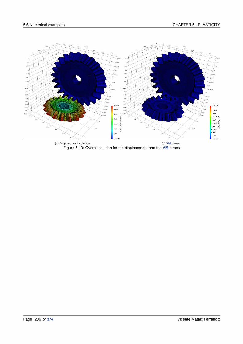
5.6 Numerical examples CHAPTER 5. PLASTICITY
(a) Displacement solution (b) VM stress
Figure 5.13: Overall solution for the displacement and the VM stress
Page 206 of 374 Vicente Mataix Ferrándiz

BIBLIOGRAPHY BIBLIOGRAPHY
Bibliography
Books
[BookBan10] Sheet Metal Forming Processes: Constitutive Modelling and Numerical Simulation. Dorel Banabic.Springer-Verlag Berlin Heidelberg. 1st ed. 2010.
[BookBel+14] Nonlinear Finite Elements for Continua and Structures. Ted Belytschko, Wing Kam Liu,Brian Moran, and Khalil Elkhodary. Wiley. 2nd ed. 2014.
[BookBHS07] Encyclopedia of Computational Mechanics (3 Volume Set). René de Borst, T.J.R. Hughes, andErwin Stein. Wiley. 1st ed. 2007.
[BookHil98] The mathematical theory of plasticity. R. Hill. Clarendon Press; Oxford University Press. 1998.
[BookHS98] Computational Inelasticity. T.J.R. Hughes and J.C. Simo. Springer-Verlag New York. 1st ed. 1998.
[BookLub08] Plasticity theory. Jacob Lubliner. Dover Publications. web draft. 2008.
[BookNPO09] Computational Methods for Plasticity Theory and Applications. E. A. de Souza Neto, D. Periæ, andD.R.J. Owen. Wiley. 2009.
[BookOll14] Nonlinear Dynamics of Structures. Sergio Oller. Springer International Publishing. 2014.
[BookSim93] Topics in the numerical analysis and simulation of classical plasticity. JC Simo. Elsevier Amsterdam.1993.
[BookTre65] Mémoire sur l’écoulement des corps solides, par MH Tresca. Henri Tresca. Noblet et Baudry. 1865.
[BookWei] Plasticity: Mathematical Theory and Numerical Analysis. B. Daya Reddy (auth.) Weimin Han.Springer-Verlag New York. 2nd ed.
[BookZTF14] The Finite Element Method for Solid and Structural Mechanics. O. C. Zienkiewicz, Robert L. Taylor,and David Fox. Butterworth-Heinemann. 7th ed. 2014.
[BookZyc81] Combined loadings in the theory of plasticity. Michal Zyczkowski. Springer Science & BusinessMedia. 1981.
Articles
[ArtAA95] “Hydrogen-enhanced localization of plasticity in an austenitic stainless steel”. Daniel P Abrahamand Carl J Altstetter. In: Metallurgical and Materials transactions A. No. 11, Vol. 26, 1995,pp. 2859–2871. Springer. DOI: 10.1007/bf02669644.
[ArtBau86] “Über die Veränderung der Elastizitätsgrenze und der Festigkeit des Eisens und Stahls durchStrecken und Quetschen, durch Erwärmen und Abkühlen und durch oftmals wiederholteBeanspruchung”. Johann Bauschinger. In: Mitteilungen des mechanisch-technischenLaboratoriums der Königlich Technischen Hochschule München. No. 1, Vol. 13, 1886,
[ArtCOH14] “Automatic differentiation for numerically exact computation of tangent operators in small-andlarge-deformation computational inelasticity”. Qiushi Chen, Jakob T Ostien, and Glen Hansen. In: .2014, pp. 289–296. DOI: 10.1002/9781118889879.ch38.
Vicente Mataix Ferrándiz Page 207 of 374

ARTICLES BIBLIOGRAPHY
[ArtCou76] “An attempt to apply the rules of maxima and minima to several problems of stability related toarchitecture”. CA Coulomb. In: Mémoires de l’Académie Royale des Sciences. Vol. 7, 1776,pp. 343–382.
[ArtDL76] “Inequalities in Mechanics and Physics Springer Verlag Berlin”. G Duvaut and JL Lions. In: . 1976,Heidelberg New York.
[ArtDP52] “Soil mechanics and plastic analysis or limit design”. Daniel Charles Drucker and William Prager. In:Quarterly of applied mathematics. No. 2, Vol. 10, 1952, pp. 157–165. DOI:10.1090/qam/48291.
[ArtGer12] “8 - Modeling hydrogen induced damage mechanisms in metals”. W. Gerberich. In: . Vol. 1, 2012,pp. 209–246. Woodhead Publishing. DOI: 10.1533/9780857095374.2.209.
[ArtHPF15] “Implantation de lois de comportement mécanique à l’aide de MFront: simplicité, efficacité,robustesse et portabilité”. Thomas Helfer, Jean-Michel Proix, and Olivier Fandeur. In: . 2015, Giens,France.
[ArtJoh76] “Existence theorems for plasticity problems”. Claes Johnson. In: Journal de Mathématiques Pureset Appliquées. No. 4, Vol. 55, 1976, pp. 431–444. Gauthier-villars 120 Blvd Saint-germain, 75280Paris, France.
[ArtKoi53] “Stress-strain relations, uniqueness and variational theorems for elastic-plastic materials with asingular yield surface”. Warner Tjardus Koiter. In: Quarterly of applied mathematics. No. 3, Vol. 11,1953, pp. 350–354. DOI: 10.1090/qam/59769.
[ArtKoi60] “General theorems for elastic plastic solids”. Warner Tjardus Koiter. In: Progress of SolidMechanics. 1960, pp. 167–221. North Holland Press.
[ArtLL67] “Finite-strain elastic—plastic theory with application to plane-wave analysis”. EH Lee and DT Liu.In: Journal of applied physics. No. 1, Vol. 38, 1967, pp. 19–27. Aip. DOI: 10.1063/1.1708953.
[ArtMar+08] “A numerical procedure simulating RC structures reinforced with FRP using the serial/parallelmixing theory”. Xavier Martinez, Sergio Oller, Fernando Rastellini, and Alex H Barbat. In:Computers & Structures. No. 15-16, Vol. 86, 2008, pp. 1604–1618. Elsevier. DOI:10.1016/j.compstruc.2008.01.007.
[ArtMis13] “Mechanik der festen Körper im plastisch-deformablen Zustand”. R v Mises. In: Nachrichten vonder Gesellschaft der Wissenschaften zu Göttingen, Mathematisch-Physikalische Klasse. Vol. 1913,1913, pp. 582–592.
[ArtMis28] “Mechanik der plastischen Formänderung von Kristallen”. R von Mises. In: ZAMM-Journal ofApplied Mathematics and Mechanics/Zeitschrift für Angewandte Mathematik und Mechanik . No. 3,Vol. 8, 1928, pp. 161–185. Wiley Online Library.
[ArtMOB11] “Caracterización de la delaminación en materiales compuestos mediante la teora de mezclasserie/paralelo”. Xavier Martnez, Sergio Oller, and E Barbero. In: Revista internacional de métodosnuméricos para cálculo y diseño en ingeniera. No. 3, Vol. 27, 2011, pp. 189–199. Elsevier.
[ArtMT94] “A return mapping algorithm for isotropic elastoplasticity”. Anton Matzenmiller and Robert L Taylor.In: International journal for numerical methods in engineering. No. 5, Vol. 37, 1994, pp. 813–826.Wiley Online Library. DOI: 10.1002/nme.1620370507.
[ArtPra24] “Spannungsverteilung in plastischen Körpern”. Ludwig Prandtl. In: . 1924, pp. 43–54.
[ArtPra49] “Recent developments in the mathematical theory of plasticity”. William Prager. In: Journal ofapplied physics. No. 3, Vol. 20, 1949, pp. 235–241. Aip. DOI: 10.1063/1.1698348.
[ArtPRH00] “Numerical differentiation for local and global tangent operators in computational plasticity”.Agustín Pérez-Foguet, Antonio Rodríguez-Ferran, and Antonio Huerta. In: Computer Methods inApplied Mechanics and Engineering. No. 1, Vol. 189, 2000, pp. 277–296. Elsevier. DOI:10.1016/s0045-7825(99)00296-0.
[ArtRH15] “Automatic differentiation for stress and consistent tangent computation”. Steffen Rothe andStefan Hartmann. In: Archive of Applied Mechanics. No. 8, Vol. 85, 2015, pp. 1103–1125. Springer.DOI: 10.1007/s00419-014-0939-6.
Page 208 of 374 Vicente Mataix Ferrándiz

BIBLIOGRAPHY PH.D.’S THESIS
[ArtSai70] “Memóire sur l’établissement des équations differéntielles des mouvements intérieurs opérés dansles corps solides ductiles au delá des limites oú l’élasticité pourrait les ramener á leur premier état”.Barre de Saint-Venant. In: Compt. Rend . Vol. 70, 1870, pp. 473–480.
[ArtSim88a] “A framework for finite strain elastoplasticity based on maximum plastic dissipation and themultiplicative decomposition: Part I. Continuum formulation”. Juan C Simo. In: Computer methodsin applied mechanics and engineering. No. 2, Vol. 66, 1988, pp. 199–219. Elsevier. DOI:10.1016/0045-7825(88)90076-x.
[ArtSim88b] “A framework for finite strain elastoplasticity based on maximum plastic dissipation and themultiplicative decomposition. Part II: computational aspects”. Juan C Simo. In: Computer methodsin applied mechanics and engineering. No. 1, Vol. 68, 1988, pp. 1–31. Elsevier. DOI:10.1016/0045-7825(88)90104-1.
[ArtST85] “Consistent tangent operators for rate-independent elastoplasticity”. Juan C Simo andRobert Leroy Taylor. In: Computer methods in applied mechanics and engineering. No. 1, Vol. 48,1985, pp. 101–118. Elsevier. DOI: 10.1016/0045-7825(85)90070-2.
[ArtZha16] “Technical problem identification for the failures of the liberty ships”. Wei Zhang. In: Challenges. No.2, Vol. 7, 2016, p. 20. Multidisciplinary Digital Publishing Institute. DOI:10.3390/challe7020020.
Ph.D.’s thesis
[PhDBar16] “Numerical simulation of fatigue processes: application to steel and composite structures”.Lucia Gratiela Barbu. Universitat Politècnica de Catalunya. 2016.
[PhDCor] “Coupled formulation between the finite element method and the discrete element method forstudying multi-fracture processes in solids and structures”. Alejandro Cornejo.
[PhDOll88] “Un modelo de daño continuo para materiales-friccionales”. Sergio Oller. 1988.
Vicente Mataix Ferrándiz Page 209 of 374

PH.D.’S THESIS BIBLIOGRAPHY
Page 210 of 374 Vicente Mataix Ferrándiz
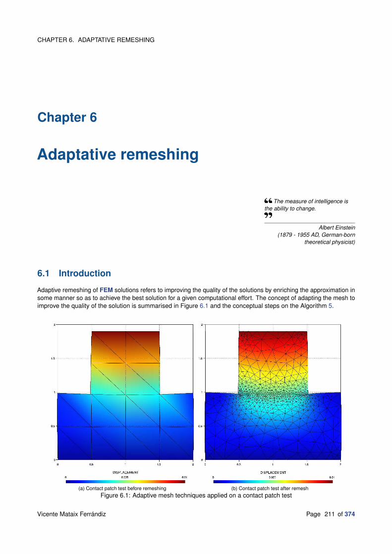
CHAPTER 6. ADAPTATIVE REMESHING
Chapter 6
Adaptative remeshing
The measure of intelligence isthe ability to change.
Albert Einstein(1879 - 1955 AD, German-born
theoretical physicist)
6.1 Introduction
Adaptive remeshing of FEM solutions refers to improving the quality of the solutions by enriching the approximation insome manner so as to achieve the best solution for a given computational effort. The concept of adapting the mesh toimprove the quality of the solution is summarised in Figure 6.1 and the conceptual steps on the Algorithm 5.
(a) Contact patch test before remeshing (b) Contact patch test after remesh
Figure 6.1: Adaptive mesh techniques applied on a contact patch test
Vicente Mataix Ferrándiz Page 211 of 374

6.2 State of the Art in mesh refinement CHAPTER 6. ADAPTATIVE REMESHING
Thus the objective of adaptive remeshing is to obtain a mesh which is optimal, in the sense that the computationalcosts involved are minimal under the constraint that the error in the FE solution is below a certain limit and, if possible,distributed over the entire mesh. In order to do that we need to estimate the magnitude of the error of the FE solutions.This is not trivial, as we do not know a priori the solution of the problem. Which means we need to develop techniqueswhich can estimate the error of the finite element solution from the known data[BookWri08], this means, on thegeometry, material data and our current approximate solution.
Algorithm 5 Adaptive refinement process
1: procedure ADAPTIVE REFINEMENT PROCESS
2: Select an initial mesh, which approximates accurately the geometry3: while error > tolerance do
4: Solve the discrete problem5: Compute error estimators or error indicators6: if error > tolerance then
7: A new mesh has to be constructed8: The already computed deformations and internal variables have to be projected onto the new mesh
This chapter introduces the adaptive remeshing techniques developed in order to improve the quality of thesolution. First the state-of-the-art of the respective techniques will be introduced on 6.2.State of the Art in meshrefinement, later the different approaches followed to define the mesh metrics, each one with its respective section:Hessian metric (6.3.Hessian based remeshing technique), level set metric (6.4.Level set based remeshing technique),next the SPR method is presented (6.5.SPR based remeshing technique), later a short section dedicated to theinternal values interpolation techniques (6.6.Internal values interpolation) and finally an adaptation of the formermethods applied on CCM (6.8.Adaptive remeshing methods applied on CCM). Part of this work has been publishedby Cornejo and Mataix [ArtCor+19].
6.2 State of the Art in mesh refinement
6.2.1 Mesh generation
During the last years, many techniques have emerged for this purpose. The early works from O.C. Zienkiewicz[ArtZP71]on 1970s, which was only based on the geometries boundaries of the domain size and the required distribution ofelement size1. Since then many different technologies have arise, including mapping techniques, semi-automaticremeshing methods, where the domain had to be subdivided manually in an initial stage into simpler subdomains[Art-TWM82]. This methodology then deals with know-how dependency from the user, and that is generally limited forstructured meshes (quadrilaterals and hexahedra).
Alternatively to the structured meshes algorithms can find the family of unstructured meshes techniques. Incontrast with the previous ones, these methods deal with the called simplex geometries, corresponding to trianglesin two dimensions and tetrahedra in three dimensions. These techniques are based mainly in four families ofalgorithms[BookZZT13; BookWri08]:
• Delaunay triangulation methods[ArtBow81].
• The advancing front method[ArtLo85].
• Tree methods, quadtrees for two dimensions and octrees for the three-dimensional cases[ArtYS84].
• The algorithm of recursive region splitting[ArtRRS95] places nodes on the boundary of the region to be meshedby considering a certain density distribution.
These techniques can be used additionally for the remesh of unstructured quadrilateral meshes with thecombination of subsequent triangles, and the use of octree meshes for the automatic generation of hexahedricmeshes[BookZZT13; ArtPJR17; ArtPVR18].
1Isoparametric mapping method
Page 212 of 374 Vicente Mataix Ferrándiz

CHAPTER 6. ADAPTATIVE REMESHING 6.2 State of the Art in mesh refinement
6.2.2 Adaptive finite element refinement techniques
Mesh adaptation is now widely used in numerical simulations to improve the accuracy of the solutions as wellas to capture the behaviour of physical phenomena[ArtFA05]. This technique allows to reduce considerably thecomputational cost, associated with the corresponding DOF reduction, but obtaining an accurate solution neverthe-less[ArtAF03].
This allows to compute complex problems with good results in three dimensions without dealing with the problematicof the initial remeshing during pre-process, which can be a time consuming and error-prone[BookZZT13] task.Additionally, allowing to adapt the computation during the simulation evolution, which alternative implies the creationduring the first stage a mesh that fits all the problem evolution, which can be a priori not known.
The process is called adaptation due to the existing dependence nature, the process depends on the previousresults[BookZZT13]; these methodologies were introduced originally by Babuka and Rheinboldt [ArtBR78][ArtBR79]on the late 70s. The reasons for doing these adaptive procedures can be summarised, for solid mechanics problems,displacements and stress errors should be contained in a certain tolerance. A very common approach of this is thecomputation of the error energy norm and prescribing a threshold in order to not exceed a certain percentage of thetotal energy norm.
In order to doing so several techniques exist, like the Recovery by Equilibrium of Patches (REP) techniques.One of the most extended techniques based on REP is the SPR by Zienkiewicz and Zhu [ArtZZ92]. Of course themethodologies based on REP are not the only ones available to measure the error, also from Zienkiewicz and Zhuwe can find techniques as the recovery methods[ArtZZ87]. From Babuka and Rheinboldt [ArtBR78] we can find theresidual-based methods, these methodologies as the name suggest estimate the error from the residual obtained onthe finite element approximation. We can also find relevant contributions in the field of mesh adaptability based on thesolution error in the work of Oñate and Bugeda[ArtOB93; ArtOña+06; ArtBO94]. To study on detail all the techniquespreviously mentioned we address to the book of E.Stein et al.[BookRam01], a complete compendium of works fromdifferent authors addressing a set of complex NL problems.
Recently techniques based on the Hessian have emerged[ArtWes+03], this requires that the variable to be usedas error estimation to be twice continuously differentiable in the case we consider an analytical solution, or otherwiserequires to us to be able to numerically estimate this second derivative. This methodology has additionally theadvantage of giving a proper measure in order to create an anisotropic new mesh, anisotropic meshes are thosethat employ extremely narrow mesh elements. This type of meshes have the advantage to reduce the number ofnew elements necessary on regions where the minimal size required would imply a high number of elements in caseof considering an isotropic mesh. These last techniques are the ones consider on this study and the theoreticalbackground will be expanded on the theory section (6.3.Hessian based remeshing technique).
Figure 6.2: Concept of h-refinement and p-refinement
Finally, we can identify several procedures for the finite element mesh refinement[BookWri08], the most common
Vicente Mataix Ferrándiz Page 213 of 374

6.3 Hessian based remeshing technique CHAPTER 6. ADAPTATIVE REMESHING
are the following four:
• h-refinement: The same type of elements is used but their size is changed. See Figure 6.2. This method canbe divided at the same time on:
Enrichment: Also called element division. At the same time, we can distinguish between hanging nodesand transition elements methods.
Remeshing: A complete new mesh is generated.
• p-refinement: Where the same size of element is considered, but the polynomial order of the elements isaltered hierarchically. See Figure 6.2. Here the size of the local matrices of the elements is increased, with itcorresponding computational cost in computing and assembling.
• hp-refinement: This last technique consists in a combination of the two previous methods.
• r-refinement: Replaces finite element nodes such that the element sizes are optimised within a FE mesh inorder to reduce the overall error of the FE solution. The convergence to the exact solution for this method is notguaranteed[BookZZT13].
The methodology considered on this work corresponds with the h-refinement, in particular we will consider theremeshing technique, which means as already introduced, that we will create a whole new mesh. In order to do so wewill consider the Mmg library, an anisotropic metric based remeshing library. For more details we will address thecorresponding section in the appendixes B.3.Mmg library.
6.3 Hessian based remeshing technique
In this section we analyse on detail the techniques considered for remeshing. In order to understand the conceptsconsidered on the contact applied remeshing (6.8.2.Hessian metric), we need to introduce first the concepts of errorapplied to a general PDE (6.3.1.Error estimation), later the concept of metrics is introduced (6.3.2.Metric basedremeshing) and general Hessian based metric measure (6.3.3.Hessian based metric measure). The section will endwith the introduction of the transfer operators used for the damage.
6.3.1 Error estimation
6.3.1.1 Upper bound on the interpolation error
We consider a general pde defined in a bounded domain Ω of ℜ3 where u denotes the exact solution of the problem.We will call to uh the FE solution obtained in a certain mesh Th, and therefore we can define the solution error eu asthe difference between these two values, (6.1). Using this error, we desire to generate a new mesh Th on which theerror eu computed on this mesh new mesh, is bounded by a given tolerance value.
(6.1) eu = u − uh
Usually, the approximation error is usually significantly difficult to quantify, and depends intrinsically of the nature ofthe PDE which define the problem. Because of this is interesting to define an indirect approach[ArtFA05] which allowsus to estimate eu. If we define Πhu as the interpolation of the solution u in the mesh Th, therefore the interpolationerror (eu) will be defined as the difference between the exact solution and this interpolated one, (6.2).
(6.2) eu = u − Πhu
The Cea’s lemma[ArtCea64] it is an important tool for proving error estimates for the FEM applied to elliptic PDE,although it is possible to prove that this approach also works well for hyperbolic PDE.
(6.3) ‖u − uh‖ ≤ c‖u − Πhu‖
Page 214 of 374 Vicente Mataix Ferrándiz
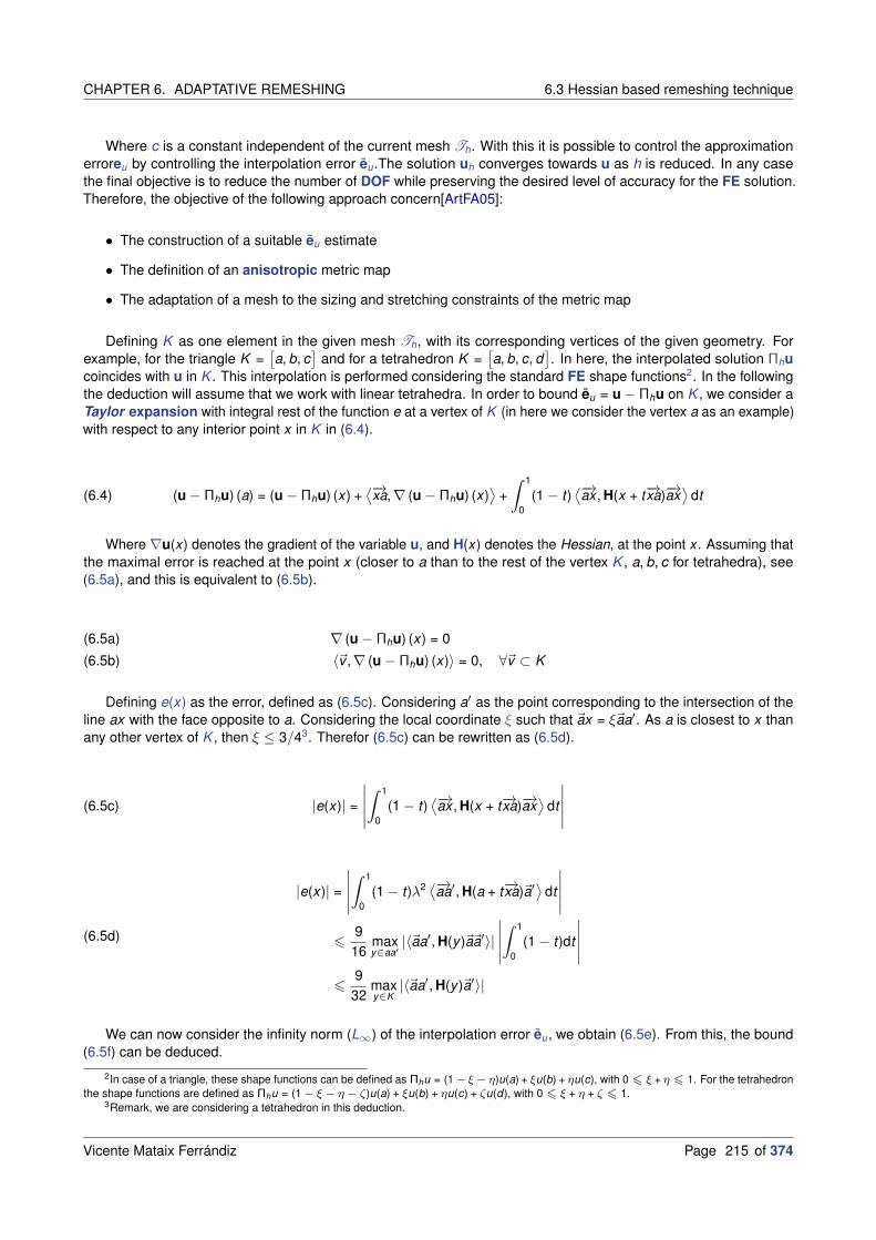
CHAPTER 6. ADAPTATIVE REMESHING 6.3 Hessian based remeshing technique
Where c is a constant independent of the current mesh Th. With this it is possible to control the approximationerroreu by controlling the interpolation error eu.The solution uh converges towards u as h is reduced. In any casethe final objective is to reduce the number of DOF while preserving the desired level of accuracy for the FE solution.Therefore, the objective of the following approach concern[ArtFA05]:
• The construction of a suitable eu estimate
• The definition of an anisotropic metric map
• The adaptation of a mesh to the sizing and stretching constraints of the metric map
Defining K as one element in the given mesh Th, with its corresponding vertices of the given geometry. Forexample, for the triangle K =
[a, b, c
]and for a tetrahedron K =
[a, b, c, d
]. In here, the interpolated solution Πhu
coincides with u in K . This interpolation is performed considering the standard FE shape functions2. In the followingthe deduction will assume that we work with linear tetrahedra. In order to bound eu = u − Πhu on K , we consider aTaylor expansion with integral rest of the function e at a vertex of K (in here we consider the vertex a as an example)with respect to any interior point x in K in (6.4).
(6.4) (u − Πhu) (a) = (u − Πhu) (x) +⟨−→xa,∇ (u − Πhu) (x)
⟩+
∫ 1
0(1 − t)
⟨−→ax , H(x + t−→xa)−→ax⟩
dt
Where ∇u(x) denotes the gradient of the variable u, and H(x) denotes the Hessian, at the point x . Assuming thatthe maximal error is reached at the point x (closer to a than to the rest of the vertex K , a, b, c for tetrahedra), see(6.5a), and this is equivalent to (6.5b).
∇ (u − Πhu) (x) = 0(6.5a)
〈~v ,∇ (u − Πhu) (x)〉 = 0, ∀~v ⊂ K(6.5b)
Defining e(x) as the error, defined as (6.5c). Considering a′ as the point corresponding to the intersection of theline ax with the face opposite to a. Considering the local coordinate ξ such that ~ax = ξ~aa′. As a is closest to x thanany other vertex of K , then ξ ≤ 3/43. Therefor (6.5c) can be rewritten as (6.5d).
(6.5c) |e(x)| =
∣∣∣∣∣
∫ 1
0(1 − t)
⟨−→ax , H(x + t−→xa)−→ax⟩
dt
∣∣∣∣∣
(6.5d)
|e(x)| =
∣∣∣∣∣
∫ 1
0(1 − t)λ2
⟨−→aa′, H(a + t−→xa)~a′⟩
dt
∣∣∣∣∣
69
16maxy∈aa′
|〈~aa′, H(y )~a~a′〉|∣∣∣∣∣
∫ 1
0(1 − t)dt
∣∣∣∣∣
69
32maxy∈K
|〈~aa′, H(y )~a′〉|
We can now consider the infinity norm (L∞) of the interpolation error eu, we obtain (6.5e). From this, the bound(6.5f) can be deduced.
2In case of a triangle, these shape functions can be defined as Πhu = (1 − ξ− η)u(a) + ξu(b) + ηu(c), with 0 6 ξ + η 6 1. For the tetrahedronthe shape functions are defined as Πhu = (1 − ξ − η − ζ)u(a) + ξu(b) + ηu(c) + ζu(d), with 0 6 ξ + η + ζ 6 1.
3Remark, we are considering a tetrahedron in this deduction.
Vicente Mataix Ferrándiz Page 215 of 374

6.3 Hessian based remeshing technique CHAPTER 6. ADAPTATIVE REMESHING
‖u − Πhu‖∞,K 69
32maxy∈K
∣∣∣
⟨−→aa′, H(y )
−→aa′⟩∣∣∣(6.5e)
‖u − Πhu‖∞,K 69
32maxy∈K
⟨−→aa′, |H(y )|
−→aa′⟩
(6.5f)
As in (6.5f) the bound depends on the extremum x , which is not known a priori, we can reformulate it as (6.5g).The former equation defines a bound in the case where the maximum error is achieved inside the element K . Inthe case where the maximum error is obtained on the element face, then the corresponding expression coincideswith (6.5h). In the case where the maximum value is obtained along an element edge, the expression changes to(6.5i).
‖u − Πhu‖∞,K 69
32maxy∈K
max~v⊂K
〈~v , |H(y )|~v〉(6.5g)
‖u − Πhu‖∞,K 62
9max
y∈[a,b,c]max
~v⊂[a,b,c]〈~v , |H(y)|~v〉(6.5h)
‖u − Πhu‖∞,K 61
8maxy∈ab
⟨−→ab, |H(y)| −→ab
⟩
(6.5i)
As a summary, that will be taken into consideration as a base for deductions in the next section, relation (6.5f)provides a proper bound for the interpolation error on an element K .
6.3.1.2 Numerical computation of the interpolation error
Taking (6.5f), where the upper bound on the interpolation error (eu), we can reformulate it as (6.6a), in here cd is aconstant related to the space dimension. The former expression has some drawbacks, as the two maximum valuesrequired are complex to compute.
(6.6a) ‖u − Πhu‖∞,K 6 cd maxx∈K
max~v⊂K
〈~v , |H(x)|~v〉
Because of that, we introduce the edges of K to replace the maximum value associated with all vectors includedin K . As any vector ~v of K can be written as linear combination of the edges of K , it yields (6.6b), where EK is the setof edges of K .
(6.6b) ∀~v ⊂ K , ‖~v‖|H(x)| 6 maxe∈EK
‖~e‖|H(x)|
This allows us to rewrite the upper bound from (6.6a) as (6.6c). In this expression the RHS term is not trivial tonumerically evaluate. So we must assume the existence of a metric tensor M (K ) as defined in (6.6d). This metric M
is such that the region defined by 〈~v , M (K )~v〉|∀~v ⊂ K is minimal in volume.
(6.6c) ‖u − Πhu‖∞,K 6 cd maxx∈K
maxe∈EK
〈~e, |H(x)|~e〉
(6.6d) maxx∈K
〈~e, |H(x)|~e〉 6 〈~e, M (K )~e〉, ∀e ∈ EK
Page 216 of 374 Vicente Mataix Ferrándiz

CHAPTER 6. ADAPTATIVE REMESHING 6.3 Hessian based remeshing technique
Finally, the interpolation error εK on an element K is given by the following relationship (6.6e).
(6.6e) εK = c maxe∈EK
〈~e, M (K )~e〉
The former relation relates the interpolation error εK to the square of the largest edge length in K with respect tothe metric M . This implies that it is possible to control the interpolation error on the mesh Th by controlling the lengthof the mesh edges in K .
6.3.1.3 Mesh adaptation
From (6.6e), which defines εK , we can deduce that if the εK is fixed, the only remaining variable left to change is theedge length of K . The objective will be adapt the mesh edges in order that the interpolation error will be equidistributedover the adapted mesh, meaning that we aim to obtain the desired error level with a minimum number of DOF underfixed constraints.
Considering ε the maximum level of error tolerated on the mesh elements. The mesh edges must be such that(6.7a).
(6.7a) ε = c〈~e,−→A (K )~e〉, ∀e ∈ EK
Considering (6.7b) the target metric tensor, this expression leads to (6.7c).
M (K ) =cεM (K )(6.7b)
〈~e, M (K )~e〉 = 1, ∀e ∈ EK(6.7c)
(6.7c) is equivalent to define the edge length with respect to the metric M (K ). In order to evaluate the length, weneed to consider the Euclidean norm of a vector ~u (L2) for a metric M is defined as (6.7d), and the distance betweentwo points given by (6.7e).
‖~u‖M =√
〈~u,~u〉M =√
t~uM~u(6.7d)
dM (A, B) = lM (−→AB) = ‖−→AB‖M =
√
t−→ABM
−→AB(6.7e)
In consequence, the relation (6.7b) is equivalent to (6.7f), which prescribes edges of unit length for any edge of Kin order to bound the interpolation error εK on K by a value ε.
(6.7f)(lM (K )(~e)
)2= 1
The equation (6.7f) introduces the notion of unit mesh as the target optimal mesh. An optimal mesh is the meshon which the interpolation error εK is distributed uniformly and bounded by a tolerance value ε.
6.3.1.4 Computation of the relative error
Finally, the relation (6.6c) gives us an absolute bound on the interpolation error εK . [ArtFA05] considers a relativebound on this error and therefore defining an estimate of the relative error. Doing this will provide a metric independentof the nature of the physical problem, this allows to combine different variables together. Equation (6.8a) introduces
Vicente Mataix Ferrándiz Page 217 of 374

6.3 Hessian based remeshing technique CHAPTER 6. ADAPTATIVE REMESHING
how to compute dimensionless variables and introduces a relative error. We will present our own normalisationprocedures in the following sections.
(6.8a)
∥∥∥∥
u − Πhu
|u|ǫ
∥∥∥∥∞,K
6 cd maxx∈K
max~e∈EK
⟨
~e,|H(x)||u(x)|ǫ
~e
⟩
In here |u|ǫ = max(|u|, ǫ‖u‖∞,Ω
). Additionally we must take into account that the solutions vary from several orders
of magnitude. It is often difficult to capture the weakest phenomena via mesh adaptation. [ArtFA05] proposes as apotential solution the consideration of a local error estimation in order to overcome this problem. Additionally[ArtCIA07;ArtCas+97], the error estimate can also be normalised using the local value of the gradient (∇) norm (L2) of thevariable u, weak phenomena can be captured even in cases where the variables deal with sudden variations, likeshocks or BC dependent variables. In [ArtFA05] the following error estimate (6.8b) is proposed. Where h is theelement size on the mesh Th and 0 < α < 1.
(6.8b)
∥∥∥∥
u − Πhu
|α|u|ǫ + h‖∇u‖2
∥∥∥∥∞,K
6 c maxx∈K
maxe∈EK
⟨
~e,|H(x)|
α|u(x)|ǫ + h‖∇u(x)‖2~e
⟩
6.3.2 Metric based remeshing
With the concepts introduced in 6.3.1.Error estimation we are now ready to introduce the Hessian metric[ArtFA05]. Inhere, we will introduce in first place the concept of metric (6.3.2.1.Concept of metric), then we will show the intersectionoperations needed in case than more than one metric is taken into consideration (6.3.2.2.Metric intersection).
(a) Metric analogy (b) Intersection
Figure 6.3: Metric analogies. Images from [ArtFA05]
6.3.2.1 Concept of metric
The metric represents the operator which is equivalent to a geometric interpolation law on h on the edge[ArtFA05].Let M be a discrete metric field defined at the vertices of a mesh Th of a domain Ω. Thanks to the interpolationoperation, we have a continuous metric field in the whole domain, i.e. a Riemannian metric space (M (x))x∈Ω. Thisrepresentation of the metric field depends on Th as the interpolation law is applied at the element level.
In order to compute the length, we can consider two points in the domain, a and b. The length of the segmentbetween this two points can be computed as Gaussian integration as seen in (6.9), where αi corresponds with the
Page 218 of 374 Vicente Mataix Ferrándiz

CHAPTER 6. ADAPTATIVE REMESHING 6.3 Hessian based remeshing technique
barycentric coefficients and ωi the integration weight. In here where M (a + αiab) is the metric at the i th Gauss point.With the former expression, the concept of metric can be understood.
(6.9) ℓM (ab) =
∫ 1
0
√
tabM (a + tab)abdt ≈k∑
i=1
ωi
√
tabM (a + αiab) ab
The notion of length in a metric space is related to the notion of metric[ArtAF03] and therefore to an adequatedefinition of the scalar product in the vector space considered. Define a metric tensor at a point P, respect an elementK , from a mesh Th it considering a matrix M (d × d) symmetric positive defined and not degenerated. In threedimensions the we can consider (6.10), which can be assimilated to the analogy of an ellipsoid (Figure 6.3a).
(6.10)M =
a b cb d ec e f
such that a > 0, d > 0, f > 0
and det(M ) > 0, considering a, b, c, d , e ∈ R
The tensor M can be diagonalised because it is symmetrical. Then, M can be written M = RΛR−1, where R
is the matrix of the eigenvectors and Λ the matrix of the eigenvalues of M . It should be noted that this decompositionis not unique, indeed one can take any eigenvector of the subspace associated with one of the eigenvalues or it isenough to invert columns of R and Λ.
To illustrate the effect of the metric on the actual mesh, we can observe the Figure 6.4, where the metrics presenton the nodes sketch the tetrahedra accordingly.
Figure 6.4: Effects of the metric on a tetrahedra
6.3.2.2 Metric intersection
Frequently, one is brought to work with several metrics. In the case where several metrics are specified at the samepoint of the mesh, we try to define a single metric that takes into account all these metrics, that is to say to define themetric given by the intersection of all these metrics.
To define the intersection of two metrics, we use the fact that a metric tensor is represented geometrically by atwo-dimensional ellipse or a three-dimensional ellipsoid. The metric intersection consists then in keeping the mostrestrictive size constraint in all directions imposed by this set of metrics[ArtFA05] (see Figure 6.8b).
The simultaneous reduction enables to find a common basis (e1, e2 and e3) such that M1 and M2 are congruent
Vicente Mataix Ferrándiz Page 219 of 374

6.3 Hessian based remeshing technique CHAPTER 6. ADAPTATIVE REMESHING
to a diagonal matrix, in this basis then N is introduced:
(6.11a) N = M−11 M2
N can be diagonalised in R, because it is symmetrical in the metric M1. The base in question is given by thenormalised eigenvectors of N that we note e1, e2 and e3 (they form a base because N is diagonalisable). Theeigenvalues of M1 and M2 are found in this base using the Rayleigh quotient:
(6.11b) λi = eti M1ei and µi = et
i M2ei
Considering P = (e1e2e3) be the matrix the columns of which are the eigenvectors of N , common basis of bothmetrics, so it can diagonalise at the same time M1 and M2.
(6.11c)
M1 = P−t
λ1 0 00 λ2 00 0 λ3
P−1
M2 = P−t
µ1 0 00 µ2 00 0 µ3
P−1
Computing the metric intersection as:
(6.11d) M1∩2 = M1 ∩ M2 = P−t
max(λ1,µ1) 0 00 max(λ2,µ2) 00 0 max(λ3,µ3)
P−1
6.3.3 Hessian based metric measure
Taking as starting point the concepts introduced in 6.3.1.Error estimation, and the concepts of metrics from previoussections, we are now ready to introduce the Hessian based metric (M ). We can summarise the following propertiesintroduced by Alauzet [ArtAF03]:
• The analysis and results obtained are not asymptotic, which means that the size of the mesh h is not tending tozero. This solves some potential errors.
• It is based in the Hessian (H) of the solution.
• The obtained metric is anisotropic. This leads to reduce the number of degrees of freedom to solve theproblem as compared to the equivalent isotropic mesh, for the same level of accuracy[ArtFA05].
• It is independent of the nature of the operator, so it can be used with any type of equation.
6.3.3.1 Hessian theory
We can compute the Hessian[ArtWes+03] matrix (H) of a scalar variable f as proposed in Equation (6.12).
(6.12)
H =
∂2f
∂x21
· · · ∂2f∂x1 ∂xn
.... . .
...
∂2f∂xn ∂x1
· · · ∂2f∂x2
n
or just:
Hi ,j =∂2f∂xi∂xj
Page 220 of 374 Vicente Mataix Ferrándiz

CHAPTER 6. ADAPTATIVE REMESHING 6.3 Hessian based remeshing technique
We remark the fact that the mathematical concept underlying in the consideration of the Hessian in mesh adaptationhas been already introduced in 6.3.1.3.Mesh adaptation. Once the Hessian matrix (H) has been computed, we cancompute the corresponding anisotropic metric by the following (6.13)[ArtFA05]. We highlight that for anisotropic
remeshing the resulting metric M , no additional operations are needed as the Hessian (H) already provides ananisotropic mesh.
M = RtΛ
tR with(6.13a)
Λ = diag(λi )(6.13b)
Being the eigenvalues from Equation (6.13) equivalent to the expression from Equation (6.13c). In here we willconsider both the maximum (hmax ) and minimum (hmin) desired mesh sizes.
(6.13c) λi = min
(
max
(cd|λi |ǫ
,1
h2max
)
,1
h2min
)
Being ǫ the error threshold and cd a constant ratio of a mesh constant and the interpolation ratio4. For an isotropicmesh the metric (Miso) will be a diagonal matrix, where each element of the diagonal corresponds with the maximumeigenvalue as seen in Equation (6.13d), where R corresponds with the eigenvectors matrix of M .
(6.13d) Miso = diag(max(λi )) =
max(λi ) 0 00 max(λi ) 00 0 max(λi )
On the other hand, we can enforce a higher level of anisotropy using the anisotropic ratio (ρ) on the mesh inconsideration of a relative anisotropic radius (Rλrel ) as seen in the metric (Maniso) in Equation (6.13e).
(6.13e) Maniso = RtΛanisoR
Being the matrix Λaniso equivalent to Equation (6.13f). In here we consider the minimum between the maximaleigenvalue and the corresponding eigenvalue. This value is at the same time compared with the relative radius, wherethe maximum between the two values is taken into consideration.
(6.13f) Λaniso =
max(min(λ1, λmax ), Rλrel ) 0 00 max(min(λ2, λmax ), Rλrel ) 00 0 max(min(λ3, λmax ), Rλrel )
The relative radius then can be calculated using Equation (6.13g).
(6.13g)Rλrel = |λmax − Rλ| where:
Rλ = (1 − ρ)|λmax − λmin|4ǫ can be taken as 10−6 as reference value. In the other hand cd can be considered as 2
9 for 2D cases and 932 for 3D cases.
Vicente Mataix Ferrándiz Page 221 of 374

6.3 Hessian based remeshing technique CHAPTER 6. ADAPTATIVE REMESHING
6.3.3.2 Numerical example
Figure 6.5: Initial mesh
The objective is to remesh the structured 1 mesh with the scalar function from Figure 6.5 and (6.14). The originalmesh has a high number of elements structured, our objective is to obtain an unstructured mesh where the smallerelements will be around our objective function. The χ shaped function (6.14):
(6.14)f (x , y ) = tanh(−100(y − 0.5 − 0.25 sin(2πx)))
+ tanh(100(y − x))
The results obtained can be seen on Figure 6.6b, here the smaller elements are around the χ shape that can beseen in the Figure 6.6a showing the scalar function representation.
(a) Scalar function (b) New mesh
Figure 6.6: Solution for the example
Page 222 of 374 Vicente Mataix Ferrándiz

CHAPTER 6. ADAPTATIVE REMESHING 6.4 Level set based remeshing technique
6.4 Level set based remeshing technique
6.4.1 Theory
On the following section, the fundamentals of the level set technique for building a mesh metric are presented. Theconcepts of the metric already presented in the previous section (6.3.2.Metric based remeshing) are taken intoaccount. We compute the gradient (6.15) of a scalar variable f in order to compute an anisotropic metric to remesh,using the procedure from (6.16). On Figure 6.7 the gradient of a distance function is presented as an example. Theformer example is shown in detail on the section 6.4.2.Numerical example.
(6.15) ∇f =∂f∂x
i +∂f∂y
j +∂f∂z
k
Figure 6.7: Scalar and its gradient
We compute the following auxiliary coefficients (6.16), with them we can calculate the metric for the 2D cases(6.16c) and for 3D cases (6.16d). Calling h the element size, ρ the anisotropic ratio, the metric M , f the scalar valueand ∇f the gradient from that scalar.
(6.16a)
c0 = 1.0h2 Isotropic metric
c1 = c0ρ2 Applying anisotropic ratio
(6.16b) M = c0n ⊗ n + c1(I − n ⊗ n), with n =∇f
‖∇f‖
Then for 2D:
(6.16c) M =
(c0(1 −∇f 2
x ) + c1∇f 2x (c1 − c0)∇fx∇fy
(c1 − c0)∇fx∇fy c0(1 −∇f 2y ) + c1∇f 2
y
)
And for 3D:
(6.16d) M =
c0(1 −∇f 2x ) + c1∇f 2
x (c1 − c0)∇fx∇fy (c1 − c0)∇fx∇fz(c1 − c0)∇fx∇fy c0(1 −∇f 2
y ) + c1∇f 2y (c1 − c0)∇fy∇fz
(c1 − c0)∇fx∇fz (c1 − c0)∇fy∇fz c0(1 −∇f 2z ) + c1∇f 2
z
Vicente Mataix Ferrándiz Page 223 of 374

6.4 Level set based remeshing technique CHAPTER 6. ADAPTATIVE REMESHING
6.4.2 Numerical example
The challenge consists in meshing anisotropically the geometry using as metric measure the gradient of the distance,measured previously with an octree mesher GiD[OnlMel+16]. The geometry chosen is taken from the Stanford 3DScanning Repository, and it denominated Stanford bunny [BookRH12], see Figure 6.8a.
The mesh corresponding before remeshing corresponds with Figure 6.8b, the surrounding mesh to the isosurfaceis relatively coarse and does not fit the isosurface geometry.
(a) Stanford’s bunny (b) Original octree mesh
Figure 6.8: Stanford’s Bunny example
On Figure 6.9 the solution obtained is presented. In Figure 6.9a the anisotropy distribution (ρ) is represented inisosurfaces around the bunny. The resulting mesh, which fits the zero distance isosurface of the bunny, can be seenat Figure 6.9b.
(a) Anisotropic ratio (b) Mesh after remeshing
Figure 6.9: Resulting mesh after remeshing
Page 224 of 374 Vicente Mataix Ferrándiz

CHAPTER 6. ADAPTATIVE REMESHING 6.5 SPR based remeshing technique
6.5 SPR based remeshing technique
6.5.1 Introduction
As we already mentioned previously, the SPR method was proposed by Zienkiewicz and Zhu in 1992[ArtZZ92], andcontinued with later contributions[ArtZZ95]. In order to present the method, the underlying concepts related with errormeasure and error estimation will be introduced. We remark that the basic concept of error estimation has beenalready introduced in 6.3.1.Error estimation, here we will extend those definitions.
6.5.2 Theory
6.5.2.1 Error measures
The most basic error measure (evar ) would be to simply sustract the obtained solution in the FEA (uh) to the exactsolution (u), this can be extended to any value we want to use as reference like stresses or strains (6.17). Nonethelessthese local error measures are in general not applicable for a refinement strategy as many singularities, like zero-sizeelements, may occur. Because of that various error norms (‖e‖2
E ) representing an integral quantity are chosen tomeasure the error[BookZZT13], Equation (6.18) presents the energy norms as an example. It is relevant to mentionthat according to this concept, it is not always necessary for the mesh in the entire model to be refined. This can beseen once we consider the Saint-Venants Principle, which enforces that the local stresses in one region do not affectthe stresses elsewhere.
(6.17)eu = u − uh
eε = ε− εh
eσ = σ − σh
The global energy norm can be defined as (6.18a).
(6.18a) ‖e‖2E =
∫
Ω
(σ − σh)TC−1 (σ − σh) dΩ
The sum of the local energy norm of each element (K ) contributions (6.18b).
(6.18b) ‖e‖2E =
∑
K
[∫
ΩK
(σ − σh)TC−1 (σ − σh) dΩ
]
=∑
K
‖e‖2E ,K
6.5.2.2 Error estimation
Unfortunately, these errors measure is not possible to obtain in practice, as we do not know the exact solution most ofthe time, so we need to calculate an estimation of the error (evar ), in such a way that ‖evar‖ ≈ ‖evar‖. Usually an aposteriori error estimators are used. These types of error estimators are calculated based on a reference solutionof the problem which is usually obtained by a computation on a coarse mesh. On the other hand, an a priori errorestimators estimate the error before a solution is calculated. Due to the nature of the present work, an a posteriorierror estimator will be considered.
The a posteriori error estimators can be divided on[BookAO11]:
• Residual based method: These methods can be divided on:
Explicit residual methods: Explicit schemes involve a direct computation using available data. Theexplicit residual method employs the residuals in the current approximation.
Implicit residual methods: Implicit schemes involve the solution of an algebraic system of equations.The error is estimated via the element residual method indirectly, it generally involves the solution of asmall linear algebraic system.
Vicente Mataix Ferrándiz Page 225 of 374
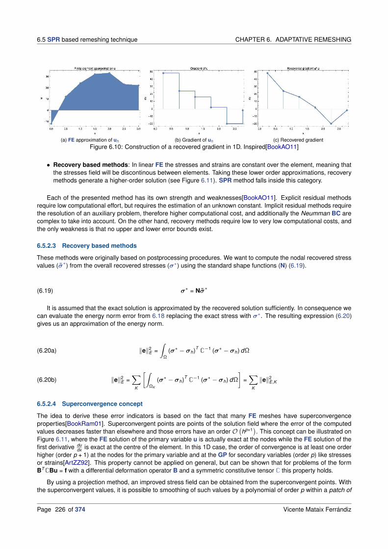
6.5 SPR based remeshing technique CHAPTER 6. ADAPTATIVE REMESHING
(a) FE approximation of uh (b) Gradient of uh (c) Recovered gradient
Figure 6.10: Construction of a recovered gradient in 1D. Inspired[BookAO11]
• Recovery based methods: In linear FE the stresses and strains are constant over the element, meaning thatthe stresses field will be discontinous between elements. Taking these lower order approximations, recoverymethods generate a higher-order solution (see Figure 6.11). SPR method falls inside this category.
Each of the presented method has its own strength and weaknesses[BookAO11]. Explicit residual methodsrequire low computational effort, but requires the estimation of an unknown constant. Implicit residual methods requirethe resolution of an auxiliary problem, therefore higher computational cost, and additionally the Neumman BC arecomplex to take into account. On the other hand, recovery methods require low to very low computational costs, andthe only weakness is that no upper and lower error bounds exist.
6.5.2.3 Recovery based methods
These methods were originally based on postprocessing procedures. We want to compute the nodal recovered stressvalues (σ∗) from the overall recovered stresses (σ∗) using the standard shape functions (N) (6.19).
(6.19) σ∗ = Nσ∗
It is assumed that the exact solution is approximated by the recovered solution sufficiently. In consequence wecan evaluate the energy norm error from 6.18 replacing the exact stress with σ∗. The resulting expression (6.20)gives us an approximation of the energy norm.
(6.20a) ‖e‖2E =
∫
Ω
(σ∗ − σh)TC−1 (σ∗ − σh) dΩ
(6.20b) ‖e‖2E =
∑
K
[∫
ΩK
(σ∗ − σh)TC−1 (σ∗ − σh) dΩ
]
=∑
K
‖e‖2E ,K
6.5.2.4 Superconvergence concept
The idea to derive these error indicators is based on the fact that many FE meshes have superconvergenceproperties[BookRam01]. Superconvergent points are points of the solution field where the error of the computedvalues decreases faster than elsewhere and those errors have an order O
(hp+1
). This concept can be illustrated on
Figure 6.11, where the FE solution of the primary variable u is actually exact at the nodes while the FE solution of thefirst derivative du
dx is exact at the centre of the element. In this 1D case, the order of convergence is at least one orderhigher (order p + 1) at the nodes for the primary variable and at the GP for secondary variables (order p) like stressesor strains[ArtZZ92]. This property cannot be applied on general, but can be shown that for problems of the formBT CBu = f with a differential deformation operator B and a symmetric constitutive tensor C this property holds.
By using a projection method, an improved stress field can be obtained from the superconvergent points. Withthe superconvergent values, it is possible to smoothing of such values by a polynomial of order p within a patch of
Page 226 of 374 Vicente Mataix Ferrándiz

CHAPTER 6. ADAPTATIVE REMESHING 6.5 SPR based remeshing technique
(a) Optimal sampling points for the function (b) Optimal sampling points for the gradient
Figure 6.11: Optimal sampling points in 1D linear elements. Source[BookZZT13]
Figure 6.12: SPR example for linear triangles. Source[BookZZT13]
elements for which the number of sampling points can be taken as greater than the number of parameters in thepolynomial. For simplex linear elements5, which are used in this work, it has been shown that the average valueof the derivatives at mid sides of adjacent elements are superconvergent[ArtChu80; ArtLev82] (see Figure 6.12).Additionally in order to avoid the singularity on the LHS of the system we need to solve for the stress recovery, someadditional precautions must be taken into account on the corner elements, with an incomplete patch. One possibleway to deal with this issue is to calculate the recovered solution from a valid neighbour patch to the original patch. It isrelevant to highlight that the optimal sampling points are considered the centroidal points for the construction of arecovered stress field[ArtZZ92], for further detail see[BookZZT13].
6.5.2.5 SPR calculation
Based on the procedure described in the previous section, we want to construct a solution field with superconvergentproperties in the whole domain from the superconvergent sampling points. In order to do so, we will apply a smoothingof the stress values within an element patch considering a least-square polynomial fit. In the following, the conceptsand procedures important for SPR-based error estimation are presented in (6.21).
Defining the polynomial of order p that will be considered on the recover. Being ai is a set of unknown parametersand p contains appropriate polynomial terms. x represents the coordinates respect the interior vertex node of thepatch. Then we can deduce (6.21a).
(6.21a)σ∗
i = pai
p =[
1 x y z ... zp ]
ai =[
a1 a2 ... am]T
5Linear 2D triangular elements, and the linear tetrahedra in extension for 3D.
Vicente Mataix Ferrándiz Page 227 of 374

6.5 SPR based remeshing technique CHAPTER 6. ADAPTATIVE REMESHING
Our objective is to minimise the following (6.21b).
(6.21b) minai
Π = minai
1
2
n∑
k=1
[σh,i − σ∗
i
]2= min
ai
1
2
n∑
k=1
[σh,i − pai
]2
This minimisation defines the following system of equations with LHS and RHS.
(6.21c)LHSai = RHSi
LHS =∑n
k=1 p ⊗ p
RHSi =∑n
k=1 pσh,i
The superconvergent nodal stresses may be computed by different patches adding and averaging its correspondingcontribution to the shared nodes.
Finally, it is important to analyse the singularities on the patch, like the corner nodes, where the LHS from (6.21c)becomes singular. In order to solve that issue in [ArtZZ92] it is proposed to calculate the nodal superconvergentstress values for boundary nodes from an interior patch.
6.5.2.6 Local mesh size
6.5.2.6.1 Compute h :
With the previous error computed, we are now able to compute the element size h. In order to do so we apply themethodology from Zienkiewicz[BookZZT13], summarised in Equation (6.22).
The relative energy norm error (η) should be below a certain threshold value (ηthreshold ). We can consider the errorestimated previously in all the following expressions. It is considered[BookZZT13] to be necessary to remesh in everyentity where η ≤ 1.
(6.22a) η =‖e‖E
‖u‖E≈ ‖e‖E
‖u‖E≤ ηthreshold
In the former expression, the total energy of deformation (‖u‖E ) is expressed as (6.22b)6.
(6.22b) ‖u‖2E =
∫
Ω
σC−1σdΩ
With this we can define the threshold error (‖e‖threshold ) as (6.22c).
(6.22c) ‖e‖threshold = ηthreshold‖u‖E = ηthreshold
√
‖uh‖2E + ‖e‖2
E
We are interested on distribute this error uniformly across all the nK elements, then the threshold error for eachelement (‖e‖threshold ,K ) would be (6.22d).
(6.22d) ‖e‖threshold ,K = ηthreshold
√
‖uh‖2 + ‖e‖2
nK≈ ηthreshold
√
‖uh‖2 + ‖e‖2
nK:= eK
With this we can define the refinement ratio for each element (ξK ) as in (6.22e). We can assume that the error perelement (‖e‖K ) is proportional to the mesh size (h) to the polynomial power (6.22f). With the previous expression, andconsidering the refinement ratio for each element (ξK ) the new element size (hnew ) can be defined as (6.22g).
ξK =‖eK‖eK
(6.22e)
‖e‖K ∝ hp(6.22f)
hnew =h
p√ξK
(6.22g)
6C−1 implies that depending on the material considered, the method may not be applicable.
Page 228 of 374 Vicente Mataix Ferrándiz

CHAPTER 6. ADAPTATIVE REMESHING 6.6 Internal values interpolation
6.5.2.6.2 Compute respective metric :
The previously calculated element size must be transformed into the metric format, 6.3.2.Metric based remeshing,in order to be used with the Mmg library. In order to do so, as the size obtained corresponds with an isotropic mesh itwill be as easy as a diagonal tensor, see (6.13d), such that we obtain the final expression from Equation (6.23).
(6.23) M = δij1
h2new
6.5.3 Example
We can illustrate the method with the following example, Figure 6.13. In here we have a simple cantilever beam with adistributed load. We start with the mesh from Figure 6.13a. Computing the energy error norm with the SPR the finalmesh from Figure 6.13b is obtained. We can appreciate that the error is reduced significantly from Figures 6.13c to6.13d. Additionally the displacement changes significantly too from Figures 6.13e to 6.13f with the finer mesh (thedeformation factor is tweaked in order to fit better on these pages).
(a) Initial mesh (b) Final mesh
(c) Error (Initial mesh) (d) Error (Final mesh)
(e) Displacement (Initial mesh) (f) Displacement (Final mesh)
Figure 6.13: SPR example
6.6 Internal values interpolation
6.6.1 Theory
In order to recover the internal values information after remeshing, necessary in order to be able to work withconstitutive models that depend on historical values, as the plasticity models used on this work. The Figure 6.14shows graphically how each one of the transfer operators work[ArtGJ06], we can be listed as (all of them available onKratos):
• CPT (Figure 6.14a): It just takes the value from the closest point. It provides acceptable results at low cost.
• SFT (Figure 6.14c): It interpolates the values using the standard FEM shape functions. Leads to an artificialdiffusion of the value, but preserves the original shape of the value profile.
Vicente Mataix Ferrándiz Page 229 of 374

6.7 Integration points values extrapolation CHAPTER 6. ADAPTATIVE REMESHING
(a) Closest Point Transfer (CPT) (b) Least-Square projection Transfer (LST)
(c) Shape Function projection Transfer (SFT)
Figure 6.14: Transfer operators. Source[ArtGJ06]
• LST (Figure 6.14b): It considers a least-square transfer across the closest points. Probably the most accuratetechnique but computationally more expensive.
From the methodologies listed above the used in our simulations is the CPT, due to the fact that is the mostcommonly used on the literature[ArtChi+12]. There are more available techniques, we address the work of Bus-setta[ArtBBP] for alternative mesh transfers operators.
6.6.2 Example
(a) The problem of reference
(b) Original mesh (c) Resulting mesh
Figure 6.15: The beam problem of reference for the internal interpolation
The problem presented consists in a very simple beam of 10 × 1 as seen on Figure 6.15a. On this mesh weconsider a simple plasticity law, and we wan to see if we are able to preserve the plastic strain between the initialmesh (Figure 6.15b) and the final mesh (Figure 6.15c).
The results we wan to interpolate are shown in Figure 6.16a. Considering the CPT method (Figure 6.16b) theresulting plastic strain profile is quite close to the original one. On the other hand, we have the results for the LST
from Figure 6.16c, which solution is much smoother, but as previously stated this may lead to an artificial diffusion ofthe target value.
6.7 Integration points values extrapolation
Page 230 of 374 Vicente Mataix Ferrándiz

CHAPTER 6. ADAPTATIVE REMESHING 6.7 Integration points values extrapolation
(a) Resulting values at the original mesh
(b) Interpolated results with CPT (c) Interpolated results with LST
Figure 6.16: The beam problem of reference for the internal interpolation
6.7.1 Introduction
In order to be able to consider some GP as a candidate variable to apply the level-set (6.4.Level set based remeshingtechnique) or the Hessian (6.3.Hessian based remeshing technique) approach we need to transfer and extrapolatethe values from the integration points to the nodes of the mesh. The technique required to do so is presented in thefollowing.
6.7.2 Theory
Applying the same concepts considered for stress recovery[BookCA01], we can extrapolate the values from theintegration points. Taking into account the concept of the integration values can be defined with the standard shapefunction definition and nodal values, Equation (6.24a). With this definition we can define a matrix operation whichwill allow to extrapolate locally the values from the GP, as seen in Equation (6.24b). In here n corresponds with thenumber of nodes in the element and m with the number of GP.
(6.24a) value (ξ, η, ζ) =[
value1 · · · valuen]
N1...
Nn
(6.24b)
value1...
valuen
=
N11 · · · Nm
1...
. . ....
Nn1 · · · Nm
n
valuegp1
...valuegp
m
The recovered values from the integration points locally calculated for each element, generally exhibit jumpsbetween elements. In order to smooth these jumps, we can compute averaged nodal integration values. The twomain methods in order to do so are:
1. Unweighted averaging: Where we assign the same weight to all elements that meet at a node
2. Weighted averaging: The weight assigned to element contributions depends on a certain value. For example,the integration weight of each GP, the element geometry or the element type
From these methods we will consider a weighted averaging based on the integration weights of each GP. In orderto do so, the corresponding average value at each node will be the one shown in Algorithm 6.
Vicente Mataix Ferrándiz Page 231 of 374

6.8 Adaptive remeshing methods applied on CCM CHAPTER 6. ADAPTATIVE REMESHING
Algorithm 6 Compute of nodal average value
1: procedure COMPUTE OF NODAL AVERAGE VALUE
2: Reset the nodal average value on the mesh wnode
3: for all node ∈ Meshnodes do
4: wnode = 0
5: We add the contribution of each GP
6: for all element ∈ Meshelements do
7: for all GP ∈ element do
8: Compute Jacobian J, integration weight wgp and shape functions N
9: for all node ∈ element do
10: wnode+ = NnodeJwgp
In order to compute the smooth result, we just need to sum the corresponding contribution of each GP multipliedby wnode, as seen in Equation (6.25).
(6.25) valuenode =elem∑
i=0
gp∑
j=0
NnodeJwgp
wnodevaluegp
6.7.3 Numerical example
Figure 6.17: Cantilever mesh and geometry
The following example consists in avery simple structural problem. I willconsist in a variable height cantileverconsidering linear elastic plain strainconstitutive model. The parametersconsidered are standard steel, see Ta-ble 6.1. Figure 6.18 shows the solu-tion obtained. On Figure 6.18a wecan see the VM stress before beingrecovered, and in Figure 6.18b the so-lution after consider the algorithm pre-sented.
E ν ρ2.069 · 1011Pa 0.29 7850kg/m3
Table 6.1: Parameters considered for cantilever example
(a) VM stress non-extrapolated (b) VM stress extrapolated
Figure 6.18: Resulting VM stress before and after recover
6.8 Adaptive remeshing methods applied on CCM
In this section we will introduce the particularities necessaries in order to evaluate the remeshing techniques on thecontact problems. The discontinuity and continuous evolution of the boundary, the nonlinearity of the problem itself,
Page 232 of 374 Vicente Mataix Ferrándiz

CHAPTER 6. ADAPTATIVE REMESHING 6.8 Adaptive remeshing methods applied on CCM
introduce several challenges that must be taken into account in order to properly evaluate the problem.
Especially in the case of CCM, an adaptive refinement procedure is very beneficial: Particularly in the transitionbetween the contact zone and the non-contact zone, the exact solution might not be covered appropriately by theFE-solution, for example due to a C0-continuity in the contact pressure. A fine mesh in this area gives the possibility tocover the contact behaviour appropriately while the computational costs are kept low due to a coarse mesh in areaswhere the solution behaves nicely and can be covered by fewer elements.
6.8.1 Level set metric
6.8.1.1 Theory
One first approach we can think in order to remesh the contact problem is the consideration of a level set, see6.4.Level set based remeshing technique. This approach is adequate for fluid simulations were with this technique,it is possible to remesh in the boundary layer of the fluid . This is commonly used in CFD[ArtSAS13], particularlyin embedded/immersed formulations, which is known to be crucial for accuracy. An equivalent to this last approachcould be considering the equivalent to the distance gradient in CCM, which would be the gap gradient. In order tocompute the consistent gap, we will consider the formulation proposed in 4.4.4.Penetration definition. In the followingnumerical example, we will study if this approach fits our needs.
6.8.1.2 Numerical example
(a) Original mesh (b) Normal gap original
Figure 6.19: Hertz geometry considered. Example here
In order to study the suitability of the method, we can consider a relatively simple geometry so we can see if thissolution fulfils our problematic. We will consider an Hertz-like geometry from Figure 6.19. This geometry is commonlyconsidered as a benchmark in CCM, but additionally we can even compute analytically the gap (gn). The initial meshis on Figure 6.19a and the gap representation in the Figure 6.19b.
(a) Resulting mesh (b) Normal gap solution
Figure 6.20: Solution obtained
Vicente Mataix Ferrándiz Page 233 of 374

6.8 Adaptive remeshing methods applied on CCM CHAPTER 6. ADAPTATIVE REMESHING
Applying the level-set technique the resulting mesh, Figure 6.20, shows us a finer mesh around the contactingzone, but with an anisotropy that a priori does not benefit us. Therefore the we can conclude that the level-set
approach does not provide a good mesh estimation for contact problems.
6.8.2 Hessian metric
6.8.2.1 Theory
The next approach we want to consider in the CCM is the Hessian based remeshing procedure. This technique isdescribed in detail in the previous section 6.3.Hessian based remeshing technique. We want to consider severalvariables which provide an adequate description of the contact problem so the mesh will be finer in the interest regions,especially the boundary region that deals with the contact problem.
The variables that can be taken into account can be many, one of them may be the displacement, but this choicedoes not provide a good information. In a generic CSD may be a good approach7, as the displacement may be arelevant variable which describes in a good manner the problem itself. But, for example, in a contact problem wherethe both domains are already in contact this variable will not be very helpful to describe our problem. A variable moreassociated to CCM is the contact pressure, but this one it is available only in the contacting interface, therefore noaffecting the whole domain, and not providing a full information of the problem. Due to the intersection capabilitiesof the metric-based technique, see 6.3.2.2.Metric intersection, we can consider one or two additional variableswhich will provide a full information of the domain. We think in two different variables which are natural to consideron this problem, the VM equivalent stress and the strain-energy. They are natural in the sense that many CCM
problems involve plasticity too, and in consequence are descriptive of the whole problem. In summary, the contactstress will provide us information about the contact boundary, and this information will be complemented with the VM
equivalent stress and the strain-energy. The example shown in 6.8.2.2.2.Punch test explores the consideration or notconsideration of the strain-energy in combination of the VM stress.
So we can consider the contact stress on both sides of the problem, not just in the slave domain, we must map thevalues from the slave domain to the master domain. In order to do so, and trying to be the most consistent possiblewith the formulation considered, we will apply the Mortar mapper developed in this work, see E.Mortar mapper. Withthis, the domain will be remeshed equally, or proportionally, in each one of the contact domains. Additionally, theVM equivalent stress must be extrapolated to the nodes in considering the method present in 6.7.Integration pointsvalues extrapolation. In order to normalise these values, so the metric obtained is not so restrictive, we will consider anormalisation factor which will depend on the Young modulus (E) and the Poisson ratio (ν). These values are takeninto account in order to have a magnitude order to the stresses. The Equation (6.26) shows the normalisation factor(fnorm) considered in our formulations. This value has been obtained via numerical experimentation to get a proportionof factors providing a reasonable value.
(6.26) fnorm =20
ν2E
6.8.2.2 Numerical example
6.8.2.2.1 Simplest patch test :
The following is the simplest contact patch test possible, with only two blocks, and the displacements in the outerlines being fixed in the x axis. The geometry and the mesh of the problem considered can be seen in Figure 6.21,using triangular elements so we can remesh with Mmg. The continuous distribution of displacements in this problemcan be seen in Figure 6.21b. A contact patch test is a problem where the distribution of the stresses is constant. Theconstant stresses can be observed on Figure 6.21c. The solution presented is interesting on this contest due to thecomputed Hessian will be zero, as there is no variation on the stresses, Figure 6.21d, and therefore in theory theobtained mesh with this method will be the original one, or the minimal sizes we impose on the resolution. Thereforethis is just an illustrative case to show in which cases the method will preserve the original mesh.
7This is not the case for 6.10.2.Beam problem. Hessian of displacement, where the frequency corresponds with a highly oscillating beam.
Page 234 of 374 Vicente Mataix Ferrándiz

CHAPTER 6. ADAPTATIVE REMESHING 6.8 Adaptive remeshing methods applied on CCM
(a) Mesh (b) Displacement (c) VM stress (d) Hessian 2D
Figure 6.21: Simplest patch test
6.8.2.2.2 Punch test :
The numerical example will consist in a simple punch test in plane strain with a very coarse mesh. The problem isremeshed considering an Hessian metric. The metric intersects the contact pressure, VM stress and additionally thestrain energy. We will evaluate 4 steps of ∆t = 0.5s, with a vertical displacement in the top face of uy = −0.01t . Theremesh will be performed each 2 steps. The material considered is steel for both domains (Table 6.2).
Domain E νUpper domain 2 · 1011Pa 0.29Lower domain 2 · 1011Pa 0.29
Table 6.2: Parameters considered for the Hessian remesh punch test
(a) Original mesh (b) Displacement original (c) Strain energy (d) VM stress
Figure 6.22: Punch test geometry considered. Solution t = 0.5s. Example here
We will compare the solution between taking into account the strain energy and without it. As the initial mesh isvery coarse it does not provide much information, but in the later steps we can see as the mesh is refined around criticspoints. The original mesh, as well as the displacement, strain energy and VM stress can be found in 6.22.
The Figure 6.23 shows the solution at t = 1.0s considering the Hessian metric for the contact stress and the VM
stress. This solution can be compared with the solution provided with the metric that also considers the strain energyin the Figure 6.24. Both solutions are very similar, this is in part due to the fact that the first mesh is very coarse andthe information which provides is limited. Anyhow, there are some small differences in the distributions obtained, andthe ones which consider the strain energy provides a more detailed distribution in the solution achieved.
Solutions from Figures 6.25 and 6.26 show the results at t = 2.0s. In this case, as the previous mesh providedmuch more information than the original one, the final meshes are better defined.
Vicente Mataix Ferrándiz Page 235 of 374

6.8 Adaptive remeshing methods applied on CCM CHAPTER 6. ADAPTATIVE REMESHING
(a) Solution mesh (b) Displacement solution (c) Strain energy (d) VM stress
Figure 6.23: Punch test solution for VM stress and contact stress Hessian at t = 1.0s
(a) Solution mesh (b) Displacement solution (c) Strain energy (d) VM stress
Figure 6.24: Punch test solution for strain energy, VM stress and contact stress Hessian at t = 1.0s
(a) Solution mesh (b) Displacement solution (c) Strain energy (d) VM stress
Figure 6.26: Punch test solution for strain energy, VM stress and contact stress Hessian at t = 2.0s
In both cases, Figures 6.25a and 6.26a show meshes which are finer in the contact boundary, as we must expect,as well as the points where the displacement is imposed, and therefore the reactions are concentrated in that region.Both meshes are quite similar, but the solutions obtained differ significantly, in the case of considering the strainenergy too, the solution profile of the VM stress and the energy is more detailed and closer to the expected solution.In the other hand, the displacement solution, Figures 6.25b and 6.26b, converges quite fast in comparison with theother variables, as expected. This faster convergence was mentioned previously in the SPR section, in Figure 6.11from 6.5.2.2.Error estimation.
Here, we remember that the intersection concepts have always provided the most restrictive of all the providesmetrics, so the consideration of the additional variable always provides additional information without worsening theprevious solution. Of course, this does not mean we can intersect all the possible variables, as our interest is to define
Page 236 of 374 Vicente Mataix Ferrándiz

CHAPTER 6. ADAPTATIVE REMESHING 6.8 Adaptive remeshing methods applied on CCM
(a) Solution mesh (b) Displacement solution (c) Strain energy (d) VM stress
Figure 6.25: Punch test solution for VM stress and contact stress Hessian at t = 2.0s
a good mesh to solve our problem of interest, and so we should focus on those variables that are representativeof the phenomenon of study, as we have shown in this example. We could for example, consider in addition thedisplacement, but as the displacement field is relatively homogeneous in this problem, and as the initial surfaces arealready in contact, the information which is provided is not very relevant.
6.8.3 SPR metric
6.8.3.1 Theory
The adapation of the method for CCM was first introduced by Wriggers[ArtWS98]. In order to do so, the stressrecovery on contact boundaries needs some special consideration[BookRam01]. This approach states that eachnode on the slave contact boundary Γ
1c (standard patch) is associated with the closest node in the master contact
boundary Γ2c (extended patches), as seen in Figure 6.27. The continuity requirements inside the patch system are
given by Equation (6.27). On these expressions (·)e and (·)s represent the external patch and the standard patchrespectively. (·)Γ represents that it is computed on the boundary.
Figure 6.27: SPR contact interface example for linear triangles. Inspired[ArtWS98; BookZZT13]
The normal component:
(6.27a) N(PΓ
s as − PΓ
eae)
= 0 on ΓC
The tangent component:
(6.27b) T(PΓ
s as)
= 0 and T(PΓ
eae)
= 0 on ΓC
Vicente Mataix Ferrándiz Page 237 of 374

6.8 Adaptive remeshing methods applied on CCM CHAPTER 6. ADAPTATIVE REMESHING
The normal and tangent vectors, are a the transposition in Voigt notation8 of the following (6.27c).
(6.27c) Nexpanded =
n2x nx ny nx nz
ny nx n2y ny nz
nznx nzny n2z
and Texpanded =
τx nx τx ny + nxτy τx nz + nxτz
τy nx + nyτx τy ny τy nz + nyτz
τznx + nzτx τzny + nzτy τznx
As a new contribution adapting to our formulation Wriggers[ArtWS98] work, the contact constraint is enforced withthe ALM method. Due to this the method SPR presented in Wriggers[ArtWS98] must be adapted in order to considerLagrange multipliers instead of the penalty method. The main difference is that the contact pressure is an unknownof the system of equations instead of an estimated value from the current geometrical configuration. With this, thecontact boundary conditions are enforced at each node l of the contact boundary for the normal direction (6.28), forthe tangent direction is the same as in Equation (6.27b). In here λn is the augmented contact pressure obtained fromthe ALM formulation.
For the slave domain (standard patch):
(6.28a) N (xl ) PΓ
s (xl ) as − λn (xl ) = 0 on Γ1C
For the master domain (extended patch):
(6.28b) N (xl ) PΓ
e (xl ) ae − (λn χ) (xl ) = 0. on Γ2C
On this expression χ represents the mapping operation. This is done considering the mortar mapper developed (seecorresponding Appendix E.Mortar mapper) for a consistent computation of the normal gap (gn) during the contactsearch (4.4.Contact detection. Search techniques).
We must now minimise the expressions from Equation (6.29). It should be noticed that the patches on the standardand extended side are not coupled. On these expressions, εn and ετ are the normal and tangent penalties, which donot necessarily coincide with the ones taken into consideration on the ALM formulation.
For the slave domain (standard patch):
(6.29a) minai
Π = minai
n∑
k=1
[σh (xk ) − Ps (xk ) a]2 +m∑
l=1
(
εn[NPΓ
s (xl ) a − λn (xl )]2
+ ετ[TPΓ
s (xl ) a]2)
For the master domain (extended patch):
(6.29b) minai
Π = minai
n∑
k=1
[σh (xk ) − Pe (xk ) a]2 +m∑
l=1
(
εn[NPΓ
e (xl ) a − (λn χ) (xl )]2
+ ετ[TPΓ
e (xl ) a]2)
The former, leads to the following equation system on Equation (6.30).
For the slave domain (standard patch):
(6.30a)
LHSslavea = RHSslave
LHSslave =nslave∑
k=1
PTs (xk ) Ps (xk ) +
mslave∑
l=1
(εnPΓ T
s (xl ) NT NPΓ
s (xl ) + ετPΓ Ts (xl ) TT TPΓ
s (xl ))
RHSslave =nslave∑
k=1
Ps (xk )σh (xk ) +mslave∑
l=1
[εnλn (xl )
]
For the master domain (extended patch):
(6.30b)
LHSmaster a = RHSmaster
LHSmaster =nmaster∑
k=1
PTe (xk ) Pe (xk ) +
mmaster∑
l=1
(εnPΓT
e (xl ) NT NPΓ
e (xl ) + ετPΓTe (xl ) TT TPΓ
e (xl ))
RHSmaster =nmaster∑
k=1
Pe (xk )σh (xk ) +mmaster∑
l=1
[εn(λn χ) (xl )
]
8As the Voigt notation is not standard we present the whole matrix form.
Page 238 of 374 Vicente Mataix Ferrándiz

CHAPTER 6. ADAPTATIVE REMESHING 6.8 Adaptive remeshing methods applied on CCM
6.8.3.2 Numerical examples
6.8.3.2.1 Simplest patch test :
Figure 6.28: Error obtained
We will consider the same example from 6.8.2.2.1.Simplest patch test in orderto show that with the proposed method, where the resulting mesh corresponds withthe original mesh. Following the same reasoning from that previous case, we cancalculate the corresponding error in the integration points. We expect that it will bezero, Figure 6.28, as the stress is equal in all the points of the problem.
In conclusion, the mesh that will be obtained with this procedure will coincide againwith the original one. One more time, the patch test allows us to show the relationshipbetween stress distribution and the resulting metrics.
6.8.3.2.2 Punch test :
The following is a very simple punch test, the geometry is exactly the same shownin the Hessian example (6.8.2.2.2.Punch test). The problem consists in one 2 × 1lower block and one 1 × 1 upper block, with a very coarse mesh, as seen in Figure6.29a. We impose a small vertical displacement of 0.1 m in the top of the upper block.The Figure 6.29 shows the evolution of the mesh in each NL iteration, where the thirdand fourth are almost identical, when the error has converged. The second mesh(Figure 6.29b) is a very bad estimation, very fine a uniformly distributed, as the errorfrom the first coarser mesh (Figure 6.31a) does not provide much information. In thefollowing iterations (Figure 6.29c and 6.29d) we can appreciate as the mesh is fineracross the points with higher demand, as expected.
(a) Initial mesh (b) First NL iteration (c) Second NL iteration (d) Third NL iteration
Figure 6.29: Mesh evolution
(a) Initial mesh (b) First NL iteration (c) Second NL iteration (d) Third NL iteration
Figure 6.30: Error solution
Additionally the error, Figure 6.30, on these NL iterations is significantly smaller than in the previous ones. Butmore importantly, the mesh is more homogeneous, which is one of the objectives of the methodology to distribute the
Vicente Mataix Ferrándiz Page 239 of 374

6.9 Remeshing workflow CHAPTER 6. ADAPTATIVE REMESHING
error equally between the elements of the mesh.
(a) Initial mesh (b) First NL iteration (c) Second NL iteration (d) Third NL iteration
Figure 6.31: Displacement solution
Finally, as in the Hessian case from 6.8.2.2.2.Punch test, we see as the displacement converges faster than theprevious values (Figure 6.31). As we have already stated, this is expected, as seen in 6.5.2.2.Error estimation.
6.9 Remeshing workflow
The following summarises the simulation workflow followed during the contact simulations. We will differentiatebetween the standard remeshing process considered during the Level set and the Hessian metrics, and the workflowfollowed for the SPR metric computation, which are slightly different.
6.9.1 Level set and Hessian remeshing
(a) Standard problem (b) Contact problem
Figure 6.32: Workflow for Level set /Hessian metric remesh
Page 240 of 374 Vicente Mataix Ferrándiz

CHAPTER 6. ADAPTATIVE REMESHING 6.9 Remeshing workflow
We can differentiate between the standard problem and the contact problem.
6.9.1.1 Standard problem
For the standard case, we will compute the metric once the NL loop is converged, and the metric and the remesh willbe computed independently of the previous solution, this means that we will not check any value is below a certainthreshold. After remesh the information, the nodal and integration solutions, must be recovered. Once the solutionstage is computed we will need to re-initialise the solvers and processes if the problem has been remeshed in orderto restore the problem before execute the next time step.
6.9.1.2 Contact problem
The main difference between the standard problem and the contact one is that to avoid problematic and duplicatedconditions the associated conditions are removed and cleared, this will be recovered after re-initialise the processes.In addition to that we will remap the contact stresses between domains and extrapolate the VM and the strain energy.After that some additional information must be cleared, as the contact flags and the contact model parts.
6.9.2 SPR remeshing
(a) Standard problem (b) Contact problem
Figure 6.33: Workflow for SPR metric remesh
For the error estimation case the procedure is slightly different, not only because the error must be computed, butalso because if the error is below a certain threshold the remeshing is not executed.
6.9.2.1 Standard problem
The main difference respect 6.9.1.1.Standard problem is that once the NL loop has converged, we will need tocompute the recovered stress in the nodes, to later compute the estimated stress on the nodes. With this we will
Vicente Mataix Ferrándiz Page 241 of 374

6.10 Numerical examples CHAPTER 6. ADAPTATIVE REMESHING
compute the estimated error, if the error is below a certain threshold the time solution stage will be finished, if not withthe previous values we will estimate the size of the elements, and with it, the corresponding metrics.
6.9.2.2 Contact problem
Additionally to the previous consideration for the SPR error metric, we will consider the modifications from 6.9.1.2.Con-tact problem, except that the extrapolation of integration values is not required and the mapping of the contact stressesis performed before computing the error on the mesh.
6.10 Numerical examples
This section will show more advanced cases than the previously presented. The ones formerly introduced actedas proof of concept to the concepts that were introduced in the respective sections. In this section we will focus instructural cases, but we will dedicate an additional section to CFD cases, 6.11.CFD numerical examples, in order toshow up that this adaptive remeshing techniques are generic and can be considered in problems of different physicalnature.
6.10.1 Coarse sphere. Level set
Figure 6.34: Distance function
In this problem we remesh using the gradient of the distance function,which is the distance to the plane contained in the sphere centre.The function can be seen in the Figure 6.34, which corresponds witha linear distance and a constant gradient.
The solution obtained can be seen in Figure 6.35, where despitethe original coarse configuration, the final one is smoothed due tothe inner Bezier cubic surface considered by the Mmg library (seeB.3.1.What is Mmg and how does it work?).
It can be seen like the elements in the centre, where the dis-tance function is zero, are the smaller ones, and the ones moreanisotropic.
(a) Original mesh (b) Resulting mesh
Figure 6.35: Mesh before and after remesh for coarse mesh. Example
Page 242 of 374 Vicente Mataix Ferrándiz

CHAPTER 6. ADAPTATIVE REMESHING 6.10 Numerical examples
6.10.2 Beam problem. Hessian of displacement
Geometry of beam example
Mesh of beam exampleFigure 6.36: Coarse mesh distance function
The problem corresponds with a steel cantilever 10 × 1 andconsidering as only load self-weight, see Figure 6.36. Theinitial mesh considered is the coarse mesh from Figure 6.36.We consider a simulation of 1s with ∆t = 0.01s. The wholeexample can be found in here.
The final configuration, displacement and mesh can beseen in Figure 6.37. Due to the high natural frequency ofthe problem, the displacement is not a good measure for theHessian metric, as the high number of oscillations induce theresulting mesh in Figure 6.37. Where the distribution is not ho-mogeneous, and does not follow any particular pattern.
Figure 6.37: Final configuration of the beam example
6.10.3 Hertz problem. Hessian of contact and VM stress
The problem consists in a Hertz contact problem remeshing considering the Hessian of the VM stress and the contactpressure. We will consider a significant top pressure in order to maximise the contact area, which will help us toevaluate the quality of the solution achieved, reason why the solution may look so deformed. We will not take intoconsideration the strain energy,as the effect of this variable have been already taken into account in the punch testexample from 6.8.2.2.2.Punch test. The materials of this problem can be found in Table 6.3, where the base can beconsidered rigid respect to the die.
Domain E νUpper domain 2 · 108Pa 0.35Lower domain 2 · 1011Pa 0.29
Table 6.3: Parameters considered for the Hessian remesh Hertz exampleThere are 10 steps ∆t = 0.1s, and the remesh is executed each 3 steps starting in the 4th. The load applied
depends on time, and it is equal to q = 107t Pa. The example can be located in Kratos repository.
The first step, Figure 6.38, is a very coarse mesh, but dense enough to provide the information needed in order toestimate properly the required mesh. Looking at the VM stress from Figure 6.38c we can predict where the mesh willbecome denser, this corresponds mostly with the contact interface. Particularly taking into account that we considerthe contact pressure in addition to the VM stress, this area will be especially enhanced. Anyhow, despite not beingterrible, the mesh provides an improved information about the VM equivalent stress.
(a) Mesh (b) Displacement (c) VM stress
Figure 6.38: Hertz solution step 1
Vicente Mataix Ferrándiz Page 243 of 374

6.10 Numerical examples CHAPTER 6. ADAPTATIVE REMESHING
The solution in the second mesh, Figure 6.39, refines the mesh in the required regions predicted previously. Inaddition to the contact interface, the loaded face is also enhanced, this is expected as is the region of the problemwhere the loads are concentrated.
(a) Mesh (b) Displacement (c) VM stress
Figure 6.39: Hertz solution step 4
The third mesh, Figure 6.40, is more defined than the previous one, with less anisotropic elements near the loadface. Additionally, as the contact zone is wider than in the previous case, the refined contact zone is extended.
(a) Mesh (b) Displacement (c) VM stress
Figure 6.40: Hertz solution step 7
Finally, we can notice that the final mesh it almost identical to the previous one, Figure 6.41. This is an indicativethat the current mesh already fits our requirements. In these two last meshes the VM stress is well represented afterthe refinement.
(a) Mesh (b) Displacement (c) VM stress
Figure 6.41: Hertz solution step 10
6.10.4 Hertz problem. SPR error computing
Now we take the same problem from 6.10.3.Hertz problem. Hessian of contact and VM stress, but we will considerthe SPR metric instead of the Hessian. This will allow us to compare the solution obtained with both methods inaddition to the previous punch examples. On the first step, we can observe as the error is mainly concentrated on thecontact boundary, Figure 6.42c, this is what is expected like in the former Hessian case.
With the former error estimation, the obtained mesh is the one from Figure 6.43a. The elements are relativelysmall in the contact zone, as the error was concentrated due to the initial coarse mesh. In this new step, the error is
Page 244 of 374 Vicente Mataix Ferrándiz

CHAPTER 6. ADAPTATIVE REMESHING 6.10 Numerical examples
(a) Mesh (b) Displacement (c) Error GP
Figure 6.42: Hertz solution step 1
quite uniform on the sphere, Figure 6.43c. Therefore, we can expect that the elements will become more uniform, andbecome bigger, as the current mesh provides more information than the initial one.
(a) Mesh (b) Displacement (c) Error GP
Figure 6.43: Hertz solution step 4
(a) Mesh (b) Displacement (c) Error GP
Figure 6.44: Hertz solution step 7
(a) Mesh (b) Displacement (c) Error GP
Figure 6.45: Hertz solution step 10
For the third step, the mesh becomes more uniform, Figure 6.44a, as previously mentioned. In any case itpreserves the smaller elements in the contact interface and in the loaded face as it is supposed to be.
Vicente Mataix Ferrándiz Page 245 of 374

6.10 Numerical examples CHAPTER 6. ADAPTATIVE REMESHING
The last mesh, Figure 6.45, is quite similar to the previous step, as it is similar to the resulting mesh obtainedwith the Hessian metric, Figure 6.41. So, even if the approaches are quite different both methods provide reasonableresults a relatively similar outcome.
One important difference with the Hessian solution is that the rigid base preserves the same mesh for all steps.This makes sense, as the stress distribution is constant for a rigid media. This doe snot happens in the Hessian caseas we map the contact stress generating a variation on the contact boundary.
6.10.5 Contacting cylinders with adaptive remeshing
(a) 2D (b) 3D
Figure 6.46: Initial mesh in contacting cylinders
The problem consists in a two cylinders with a very coarse mesh, Figure 6.46, where we impose a horizontalmovement in the upper cylinder. This case is already presented in the contact chapter, 4.5.10.Contacting cylinders,but preserving the same mesh. The cylinders are formulated as solids in TL framework with hyperelastic behaviour,with the properties from Table 6.4. We impose a horizontal movement x = 0.2t at the upper cylinder, so the twocylinders contact between them. The problem has been remeshed each 2.5e − 2s, and the total simulation time is1.5s. In order to define the metric, the Hessian of the contact stress and the VM stress has been considered. Thisexample is located at the Kratos repository.
Domain E νUpper domain 2 · 1010Pa 0.35Lower domain 2 · 1010Pa 0.35
Table 6.4: Parameters considered for the Hessian remesh contacting cylinders exampleWe present both the results from a 2D slice and a 3D perspective. The sliced section allows to better appreciate
the element size evolution, as well as the value distribution inside the geometry. We complement with the 3Drepresentation which allows us to picture the whole problem and the spatial variation in the values. In the followingwe represent the solution each ∆t = 0.35s, so we have 4 steps fully represented. The values presented are thedisplacement of the configuration, the element size and the VM stress.
(a) Displacement (b) Element size (c) VM stress
Figure 6.47: Contacting cylinders solution at t = 0.35s
Page 246 of 374 Vicente Mataix Ferrándiz

CHAPTER 6. ADAPTATIVE REMESHING 6.10 Numerical examples
(a) Displacement (b) Element size (c) VM stress
Figure 6.48: Contacting cylinders perspective solution at t = 0.35s
The solution obtained at t = 0.35s, Figures 6.47 and 6.48, shows like the region with the smaller elements is theexpected one, the contact region, where the values of the contact pressure and the VM stresses are concentrated.This is even more notorious at t = 0.7s, Figures 6.49 and 6.50, where the contact zone is expanded and thereforethere are more elements reduced in the remeshing process. The last steps, from Figures 6.51, 6.52, 6.53 and 6.54,are basically the opposite deformation from the previous ones, and the conclusions from these steps can be extendedhere.
(a) Displacement (b) Element size (c) VM stress
Figure 6.49: Contacting cylinders solution at t = 0.70s
(a) Displacement (b) Element size (c) VM stress
Figure 6.50: Contacting cylinders perspective solution at t = 0.70s
Vicente Mataix Ferrándiz Page 247 of 374
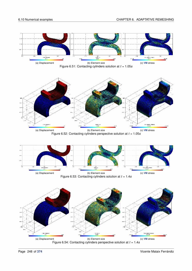
6.10 Numerical examples CHAPTER 6. ADAPTATIVE REMESHING
(a) Displacement (b) Element size (c) VM stress
Figure 6.51: Contacting cylinders solution at t = 1.05s
(a) Displacement (b) Element size (c) VM stress
Figure 6.52: Contacting cylinders perspective solution at t = 1.05s
(a) Displacement (b) Element size (c) VM stress
Figure 6.53: Contacting cylinders solution at t = 1.4s
(a) Displacement (b) Element size (c) VM stress
Figure 6.54: Contacting cylinders perspective solution at t = 1.4s
Page 248 of 374 Vicente Mataix Ferrándiz

CHAPTER 6. ADAPTATIVE REMESHING 6.11 CFD numerical examples
6.11 CFD numerical examples
6.11.1 Cavity. Level set
This is a very simple remeshing example, where we remesh a cavity 1 × 1 uses the distance to the centre asdestination function. In Figure 6.55 it can be seen as the original mesh is homogeneous (Figure 6.55a) and the sizeof the mesh is equal for all elements (Figure 6.55b). The resulting mesh has the smaller elements around the centreof the square (Figure 6.55c) and the size is distributed depending on the closeness to the centre (Figure 6.55d). Theexample can be found here.
(a) Original mesh (b) Original nodal size (c) Resulting mesh (d) Resulting nodal size
Figure 6.55: Mesh before and after remesh cavity case
6.11.2 Embedded cylinder. Level set
The problem consists in an anisotropic remeshing of a 2D fluid channel with a cylinder, using as level-set the distancefunction. It consists in a channel 5 × 1, a cylinder of 0.3m diameter, Figure 6.56.
Figure 6.56: Embedded cylinder geometry
We start with a very refined mesh of 40000 nodes and it is simplified to a mesh of just 2500 nodes, centred aroundthe cylinder of interest, Figure 6.57. The example can be found in the Kratos Examples repository.
Vicente Mataix Ferrándiz Page 249 of 374

6.11 CFD numerical examples CHAPTER 6. ADAPTATIVE REMESHING
(a) Original mesh
(b) Resulting mesh
Figure 6.57: Mesh before and after remesh embedded case
6.11.3 Box isosurface example. Level set
In this case the challenge consists in meshing anisotropically the geometry using again the gradient of the distance.The initial mesh has a large number of elements (Figure 6.58a), we want to reduce them (Figure 6.58b). Additionallythe remesher will consider the isosurface and we will remove the elements with a negative distance (see Figure 6.59).The example can be found in the following link.
(a) Original mesh (b) Resulting mesh
Figure 6.58: Base mesh before and after remesh boxes with isosurface
(a) Original mesh (b) Resulting mesh
Figure 6.59: Mesh before and after remesh boxes with isosurface
Page 250 of 374 Vicente Mataix Ferrándiz

CHAPTER 6. ADAPTATIVE REMESHING 6.11 CFD numerical examples
6.11.4 Lamborghini. Level set
(a) Lamborghini (I) (b) Lamborghini (II)
Figure 6.60: Standard Triangle Language (STL) geometry for the Lamborghini
The problem corresponds with the Figure 6.60, the geometry is quite more complex than the previous casesconsidered. The challenge consists in meshing anisotropically the geometry using the gradient of the distance,previously measured with an octree mesher (GiD[OnlMel+16]). The idea behind this is to have a boundary layeraround the car, so in case of a CFD simulation the details on the aerodynamics study can be captured. The STL fileused and the rest of required files can be found here. The mesh corresponding before remeshing corresponds withthe one shown in Figure 6.61. In here we can appreciate like the mesh elements are isotropic, and does not fit theprofile of the car.
(a) Detail on original mesh (b) Distance function before remesh
Figure 6.61: Original mesh for the Lamborghini
The resulting mesh can be found in the Figure 6.62, where we see that the mesh follows the profile of the car, andit does in an anisotropic way. Besides, it preserves the distance map from the original mesh.
(a) Detail on resulting mesh (b) Distance function resulting remesh
Figure 6.62: Resulting mesh for the Lamborghini
6.11.5 Channel CFD. Hessian of velocity
The following examples consist in two channels, one in 2D and the next one in 3D. In both cases it has been consideredthe Hessian of the velocity to define the metric of the problem.
Vicente Mataix Ferrándiz Page 251 of 374

6.11 CFD numerical examples CHAPTER 6. ADAPTATIVE REMESHING
6.11.5.1 2D cylinder channel
This case consists in an adaptive remeshing of a 2D fluid channel with cylinder using Hessian of velocity as metricmeasure. It consists in a channel 3 × 1, a cylinder of 0.5m diameter, see Figure 6.63a. Additionally the BC are thefollowing: An inlet velocity of 1m/s, wall conditions in the upper and lower boundary and a zero pressure in the outlet.The total time of the simulation is 5s with a time step of ∆t = 0.01s. The remeshing is performed each 20 steps. Themesh corresponding before remeshing corresponds with Figure 6.64a.
(a) Geometry (b) Mesh
Figure 6.63: Geometry and initial mesh in 2D channel. The example can be found here
The results obtained correspond with the following, Figure 6.64. In these figures we can appreciate like the meshfits the movement of the fluid, and particularly have refined the contour of the cylinder.
(a) Step 101 (b) Step 181
(c) Step 261 (d) Step 341
(e) Step 421 (f) Step 501
Figure 6.64: Solution in 2D channel
The mesh also captures the whirlpools of the flow and its adapt to them. In the other hand the inlet, which is a BC
and therefore the velocity is imposed, preserves practically the same mesh in each of the steps.
Page 252 of 374 Vicente Mataix Ferrándiz
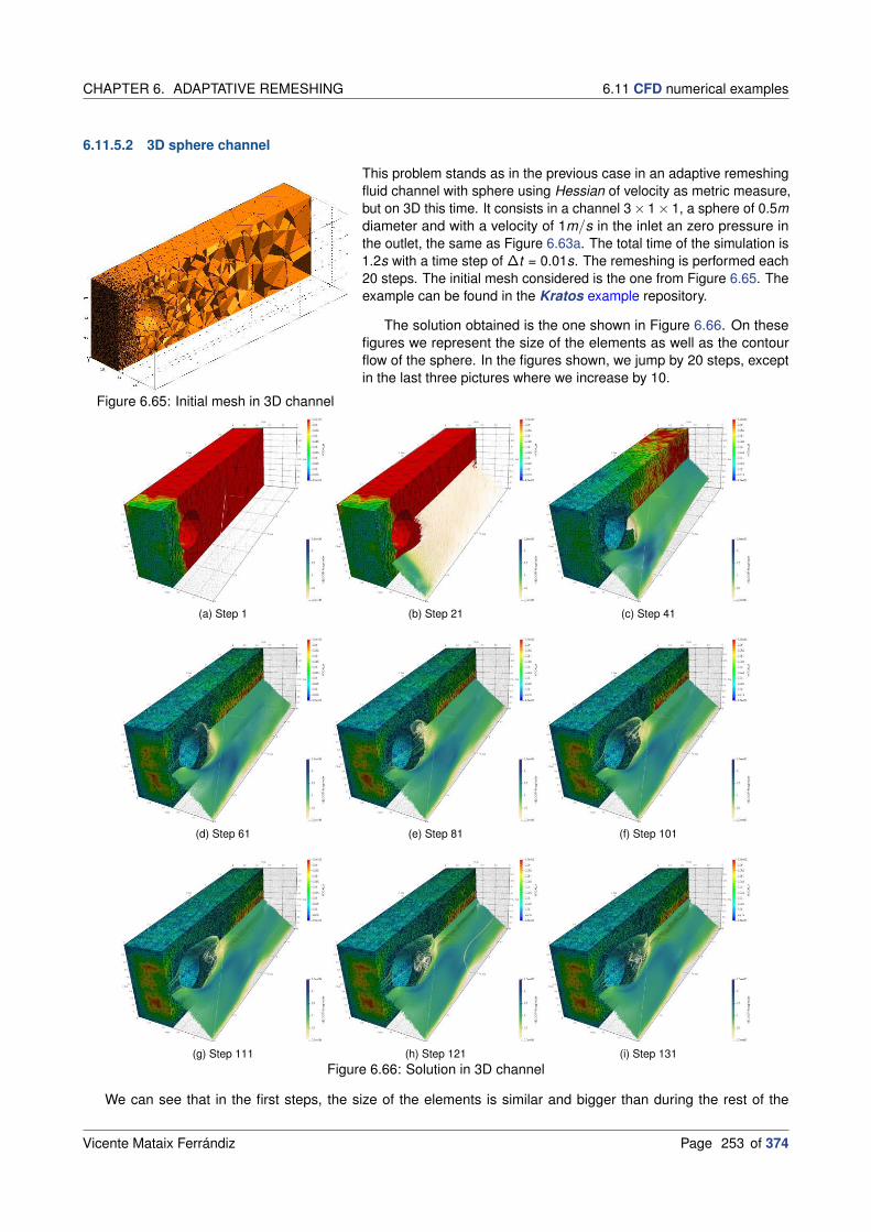
CHAPTER 6. ADAPTATIVE REMESHING 6.11 CFD numerical examples
6.11.5.2 3D sphere channel
Figure 6.65: Initial mesh in 3D channel
This problem stands as in the previous case in an adaptive remeshingfluid channel with sphere using Hessian of velocity as metric measure,but on 3D this time. It consists in a channel 3× 1× 1, a sphere of 0.5mdiameter and with a velocity of 1m/s in the inlet an zero pressure inthe outlet, the same as Figure 6.63a. The total time of the simulation is1.2s with a time step of ∆t = 0.01s. The remeshing is performed each20 steps. The initial mesh considered is the one from Figure 6.65. Theexample can be found in the Kratos example repository.
The solution obtained is the one shown in Figure 6.66. On thesefigures we represent the size of the elements as well as the contourflow of the sphere. In the figures shown, we jump by 20 steps, exceptin the last three pictures where we increase by 10.
(a) Step 1 (b) Step 21 (c) Step 41
(d) Step 61 (e) Step 81 (f) Step 101
(g) Step 111 (h) Step 121 (i) Step 131
Figure 6.66: Solution in 3D channel
We can see that in the first steps, the size of the elements is similar and bigger than during the rest of the
Vicente Mataix Ferrándiz Page 253 of 374

6.11 CFD numerical examples CHAPTER 6. ADAPTATIVE REMESHING
simulation, especially in the downstream where the velocity where the fluid has not started to flow yet. Once the flowstarts to evolve, the elements start to be reduced. But it is significative that the stall of the flow keeps a relative smallsize of the elements. The smaller elements are always the only surrounding the sphere. Finally, reached certain pointthe flow around the sphere is fully formed.
Page 254 of 374 Vicente Mataix Ferrándiz

BIBLIOGRAPHY BIBLIOGRAPHY
Bibliography
Books
[BookAO11] A posteriori error estimation in finite element analysis. Mark Ainsworth and J Tinsley Oden. JohnWiley & Sons. 2011.
[BookCA01] Introduction to finite element methods. Felippa C.A. 2001.
[BookRam01] Error-controlled adaptive finite elements in solid mechanics.Ekkehard Ramm E. Rank R. Rannacher K. Schweizerhof E. Stein W. Wendland G. Wittum PeterWriggers Walter Wunderlich Erwin Stein. John Wiley & Sons. 2001.
[BookRH12] Virtual reality in medicine. Robert Riener and Matthias Harders. Springer Science & BusinessMedia. 2012.
[BookWri08] Nonlinear finite element methods. Peter Wriggers. Springer. 1st ed. 2008.
[BookZZT13] The Finite Element Method: its Basis and Fundamentals. O. C. Zienkiewicz, J.Z. Zhu, andRobert L. Taylor. Butterworth-Heinemann. 7th ed. 2013.
Articles
[ArtAF03] “Estimateur d’erreur géométrique et métriques anisotropes pour l’adaptation de maillage. Partie I :aspects théoriques”. Frédéric Alauzet and Pascal Frey. In: . No. Rr-4759, 2003,
[ArtBBP] “Efficient 3D data transfer operators based on numerical integration”. Philippe Bussetta,Romain Boman, and Jean-Philippe Ponthot. In: International Journal for Numerical Methods inEngineering. No. 3-4, , pp. 892–929. Wiley Online Library. DOI: 10.1002/nme.4821.
[ArtBO94] “A methodology for adaptive mesh refinement in optimum shape design problems”. G. Bugeda andE. Oñate. In: Computing Systems in Engineering. No. 1, Vol. 5, 1994, pp. 91–102. DOI:10.1016/0956-0521(94)90040-x.
[ArtBow81] “Computing dirichlet tessellations”. Adrian Bowyer. In: The computer journal . No. 2, Vol. 24, 1981,pp. 162–166. Oxford University Press. DOI: 10.1093/comjnl/24.2.162.
[ArtBR78] “A-posteriori error estimates for the finite element method”. Ivo Babuka and Werner C Rheinboldt.In: International Journal for Numerical Methods in Engineering. No. 10, Vol. 12, 1978,pp. 1597–1615. Wiley Online Library.
[ArtBR79] “Adaptive approaches and reliability estimations in finite element analysis”. I Babuka andWC Rheinboldt. In: Computer Methods in Applied Mechanics and Engineering. Vol. 17, 1979,pp. 519–540. Elsevier.
[ArtCas+97] “Anisotropic unstructured mesh adaption for flow simulations”. M. J. Castro-Daz, F. Hecht,B. Mohammadi, and O. Pironneau. In: International Journal for Numerical Methods in Fluids. No. 4,Vol. 25, 1997, pp. 475–491. DOI:10.1002/(sici)1097-0363(19970830)25:4<475::aid-fld575>3.0.co;2-6.
[ArtCea64] “Approximation variationnelle des problèmes aux limites”. Jean Cea. In: Annales de l’InstitutFourier . No. 2, Vol. 14, 1964, pp. 345–444. Imprimerie Durand. 28 - Luisant. DOI:10.5802/aif.181.
Vicente Mataix Ferrándiz Page 255 of 374

ARTICLES BIBLIOGRAPHY
[ArtChi+12] “An adaptive algorithm for cohesive zone model and arbitrary crack propagation”.Vincent Chiaruttini, Dominique Geoffroy, Vincent Riolo, and Marc Bonnet. In: European Journal ofComputational Mechanics. No. 3-6, Vol. 21, 2012, pp. 208–218. Taylor & Francis. DOI:10.1080/17797179.2012.744544.
[ArtChu80] “Optimal Points Of The Stresses For Triangular Linear Element [J]”. Chen Chuan-miao. In:Numerical Mathematics A Journal of Chinese Universities. Vol. 2, 1980,
[ArtCIA07] “Introduction à l’analyse numérique matricielle et à l’optimisation”. Philippe G CIARLET. In: . 2007,Dunod.
[ArtCor+19] “Combination of an adaptive remeshing technique with a coupled FEM–DEM approach for analysisof crack propagation problems”. Alejandro Cornejo, Vicente Mataix, Francisco Zárate, andEugenio Oñate. In: Computational Particle Mechanics. 2019, pp. 1–18. Springer. DOI:10.1007/s40571-019-00306-4.
[ArtFA05] “Anisotropic mesh adaptation for CFD computations”. P.J. Frey and F. Alauzet. In: ComputerMethods in Applied Mechanics and Engineering. No. 48–49, Vol. 194, 2005, pp. 5068–5082. DOI:10.1016/j.cma.2004.11.025.
[ArtGJ06] “Plastic model with non-local damage applied to concrete”. Peter Grassl and Milan Jirásek. In:International Journal for Numerical and Analytical Methods in Geomechanics. No. 1, Vol. 30, 2006,pp. 71–90. Wiley Online Library. DOI: 10.1002/nag.479.
[ArtLev82] “Stress sampling points for linear triangles in the finite element method”. N Levine. In: Numericalanalysis report . Vol. 10, 1982, p. 82.
[ArtLo85] “A new mesh generation scheme for arbitrary planar domains”. SH Lo. In: International Journal forNumerical Methods in Engineering. No. 8, Vol. 21, 1985, pp. 1403–1426. Wiley Online Library. DOI:10.1002/nme.1620210805.
[ArtOB93] “A study of mesh optimality criteria in adaptive finite element analysis”. Eugenio Oñate andG. Bugeda. In: Engineering Computations: Int J for Computer-Aided Engineering. No. 4, Vol. 10,1993, pp. 307–321. DOI: 10.1108/eb023910.
[ArtOña+06] “Error estimation and mesh adaptivity in incompressible viscous flows using a residual powerapproach”. Eugenio Oñate, Joaquin Arteaga, Julio Garca, and Roberto Flores. In: ComputerMethods in Applied Mechanics and Engineering. No. 4, Vol. 195, 2006, pp. 339–362. DOI:10.1016/j.cma.2004.07.054.
[ArtPJR17] “Identifying combinations of tetrahedra into hexahedra: a vertex based strategy”. Jeanne Pellerin,Amaury Johnen, and Jean-Francois Remacle. In: Procedia engineering. Vol. 203, 2017, pp. 2–13.Elsevier. DOI: 10.1016/j.proeng.2017.09.779.
[ArtPVR18] “There are 174 Subdivisions of the Hexahedron into Tetrahedra”. Jeanne Pellerin, Kilian Verhetsel,and Jean-Francois Remacle. In: . 2018, p. 266. DOI: 10.1145/3272127.3275037.
[ArtRRS95] “Automatic Mesh Generation for Plates and Shells”. Ernst Rank, Martin Rücker, andManfred Schweingruber. In: Proc. of 6th ICCCBE, Berlin. 1995,
[ArtSAS13] “A novel level set-based immersed-boundary method for CFD simulation of moving-boundaryproblems”. Mukul Shrivastava, Amit Agrawal, and Atul Sharma. In: Numerical Heat Transfer, Part B:Fundamentals. No. 4, Vol. 63, 2013, pp. 304–326. Taylor & Francis. DOI:10.1080/10407790.2013.756258.
[ArtTWM82] “Boundary-fitted coordinate systems for numerical solution of partial differential equations—areview”. Joe F Thompson, Zahir UA Warsi, and C Wayne Mastin. In: Journal of computationalPhysics. No. 1, Vol. 47, 1982, pp. 1–108. Elsevier. DOI: 10.1016/0021-9991(82)90066-3.
[ArtWes+03] “Anisotropic mesh adaption Governed by a Hessian Matrix Metric”. Wilfried Wessner, Hajdin Ceric,Clemens Heitzinger, Andreas Hossinger, and Siegfried Selberherr. In: . 2003,
[ArtWS98] “Different a posteriori error estimators and indicators for contact problems”. P Wriggers andO Scherf. In: Mathematical and computer modelling. No. 4-8, Vol. 28, 1998, pp. 437–447. Elsevier.DOI: 10.1016/s0895-7177(98)00133-2.
Page 256 of 374 Vicente Mataix Ferrándiz

BIBLIOGRAPHY ONLINE RESOURCES
[ArtYS84] “Automatic three-dimensional mesh generation by the modified-octree technique”. Mark A Yerryand Mark S Shephard. In: International Journal for Numerical Methods in Engineering. No. 11, Vol.20, 1984, pp. 1965–1990. Wiley Online Library. DOI: 10.1002/nme.1620201103.
[ArtZP71] “An automatic mesh generation scheme for plane and curved surfaces by‘isoparametric’co-ordinates”. OC Zienkiewicz and DV Phillips. In: International Journal forNumerical Methods in Engineering. No. 4, Vol. 3, 1971, pp. 519–528. Wiley Online Library.
[ArtZZ87] “A simple error estimator and adaptive procedure for practical engineerng analysis”.Olgierd C Zienkiewicz and Jian Z Zhu. In: International journal for numerical methods inengineering. No. 2, Vol. 24, 1987, pp. 337–357. Wiley Online Library. DOI:10.1002/nme.1620240206.
[ArtZZ92] “The superconvergent patch recovery (SPR) and adaptive finite element refinement”.OC Zienkiewicz and JZ Zhu. In: Computer Methods in Applied Mechanics and Engineering. No.1-3, Vol. 101, 1992, pp. 207–224. Elsevier. DOI: 10.1016/0045-7825(92)90023-d.
[ArtZZ95] “Superconvergence and the superconvergent patch recovery”. OC Zienkiewicz and JZ Zhu. In:Finite elements in analysis and design. No. 1-2, Vol. 19, 1995, pp. 11–23. Elsevier. DOI:10.1016/0168-874x(94)00054-j.
Online resources
[OnlMel+16] GiD Homepage. URL: http://www.gidhome.com/;%20https://www.gidhome.com/support/brand-resources/citing-gid/.
Vicente Mataix Ferrándiz Page 257 of 374

ONLINE RESOURCES BIBLIOGRAPHY
Page 258 of 374 Vicente Mataix Ferrándiz

Part II
Application
Vicente Mataix Ferrándiz Page 259 of 374


CHAPTER 7. APPLICATION
Chapter 7
Application
The hour has arrived to abandontheories and go directly to what ispractical.
Samael Aun Weor(1917 - 1977 AD, Writer)
7.1 Introduction
This chapter introduces several application test cases, integrating all the formulation and parts developed andpresented in this work. The cases presented are mainly taken from the work of Oñate[ArtOZ83]. From this work thecases considered consist in a case with a cylinder punch and a spherical punch. In the original work, the solutionwas obtained considering an axisymmetric viscous shell formulation when we will consider a full 3D J2 elasto-plasticmodel simulation. The solution obtained will be compared with the reference presented in this work.
7.2 Cylinder punch
The geometry of this test is represented in the Figure 7.1. We have transformed the dimensions from the original workin Imperial System to International System. The problem consists in a cylindrical punch, with a blank holder, a die anda sheet of 8.96mm of thickness. In this case the frictional coefficient (µ) is the same in all the contactong interfaces,and equal to 0.2.
Figure 7.1: Cylinder punch case
Figure 7.2 shows the mesh considered for the simulation of the cylinder punch case. In this case we have
Vicente Mataix Ferrándiz Page 261 of 374

7.3 Spherical punch CHAPTER 7. APPLICATION
considered the full geometry, instead of considering some simplification taking into account the symmetry of theproblem.
(a) Mesh (b) Mesh cut
Figure 7.2: Mesh considered in the cylinder punch case
In the Figure 7.3 we compare the solution obtained with the original experimental results and the numericalsolution obtained in the reference. Our solution obtained does not coincide with the experimental solution, but iscloser in comparison to the reference numerical solution.
Figure 7.3: Solution for cylinder punch test
7.3 Spherical punch
Figure 7.4 shows the geometry of the spherical punch case. The case consists in a spherical punch, with thecorresponding die, a blank holder and a metal sheet. In the original work, the problem was evaluated with threedifferent µ between the sheet and the punch, µ1 = 0.04, µ1 = 0.2 and µ1 = 0.5 in order to be compared with the
Page 262 of 374 Vicente Mataix Ferrándiz

CHAPTER 7. APPLICATION 7.3 Spherical punch
experimental result. Here we will just consider only µ1 = µ2 = 0.04, as in the original work the best solution comparedwith the experimental was obtained for this case.
(a) 2D sketch with measurements (b) 3D representation
Figure 7.4: Spherical punch case
In this case, instead of a full 3D case, we have considered a quarter of the full geometry, as seen in the Figure7.5a. The Figure 7.5 also shows the solution obtained at some points of the punch travel.
(a) Mesh (b) Solution uz = 11mm
(c) Solution uz = 16mm (d) Solution uz = 21mm
Figure 7.5: 3D solution for the case µ1 = 0.04 and µ2 = 0.04
The Figure 7.6 shows a comparison of the solution obtained with the original experimental results and the
Vicente Mataix Ferrándiz Page 263 of 374

7.3 Spherical punch CHAPTER 7. APPLICATION
numerical solution obtained in the reference for µ = 0.04. Our solution in certain points is closer to the experimentalresult, but in some of the last steps the difference is greater.
Figure 7.6: Solution for spherical punch test
Page 264 of 374 Vicente Mataix Ferrándiz

BIBLIOGRAPHY BIBLIOGRAPHY
Bibliography
Articles
[ArtOZ83] “A viscous shell formulation for the analysis of thin sheet metal forming”. E. Onate andO.C. Zienkiewicz. In: International Journal of Mechanical Sciences. No. 5, Vol. 25, 1983,pp. 305–335. DOI: 10.1016/0020-7403(83)90011-5.
Vicente Mataix Ferrándiz Page 265 of 374

ARTICLES BIBLIOGRAPHY
Page 266 of 374 Vicente Mataix Ferrándiz

Part III
Conclusions
Vicente Mataix Ferrándiz Page 267 of 374


CHAPTER 8. FINAL CONCLUSIONS
Chapter 8
Final conclusions
Both if you think you can do itand if you dont, you are in the right
Henry T. Ford(1863 - 1947 AD, Engineer,
Industrialist and Philanthropist)
8.1 Introduction
As can be seen in the previous chapters, the main objectives delimited for this doctorate work have been reached.This means the understanding of the concepts necessary in order to simulate forming processes[BookBan10]. Thisincludes the implementation of a prismatic solid-shell element[ArtOF05; ArtFlo13a; ArtFlo13b] in order to properlysimulate the sheet behaviour without the drawbacks of a standard shell element, the proper implementation of acomputational contact mechanics algorithm[BookLau10; BookWri06; BookBel+14; ArtYL08; PhDPop12; PhDYas11],the development of elastoplastic CL[BookNPO09] which allow to simulate the forming processes, and the additionof adaptive remeshing techniques to the formula in order to perform the most accurate simulation possible whilepreserving the minimal computational cost. All of this is not possible without a deep understanding of the FEM appliedin the resolution of highly non-linear problems[BookZZT13; BookZTF14; BookBHS07; BookWri08; BookOll14], andhow to tackle and couple all these non-linearities between them. In addition, reaching until this point this also meansthat the structure of the Kratos code and C++ programming language have been mastered.
The objectives not reached in the present thesis, as well as other restlessness, are presented in the next chapter9.Future works. Many significant left open after this work, as the metal forming processes and other similar industrialprocesses involve problem of a very diverse typology, being very difficult to tackle all of them in just work.
8.2 Rotation free shells and solid-shell elements. Solid-shell
The prismatic solid-shell element implemented (3.4.Prismatic solid-shell) is fully functional, as can be seen in thetest cases shown in 3.5.Numerical examples. The element is basically based in the formulation of Flores[ArtFlo13c;ArtFlo13a; ArtFlo13b], but modified in such a way that the methods of push-forward and pull-back can be used, seeA.1.Pull-Back, Push-Forward fundamental concepts, making the element fully compatible with the constitutive lawsimplemented in Kratos. Focusing in the test cases from each one of them, we can conclude that:
• Cook’s membrane test: Figures 3.17 represent the behaviour of the Cook’s membrane, respectively elasticand elasto-plastic, both obtained considering an implicit scheme. The results present even less than thereference[ArtFlo13b] locking for the elastic case and similar behaviour for the elasto-plastic case.
Vicente Mataix Ferrándiz Page 269 of 374

8.3 Contact mechanics CHAPTER 8. FINAL CONCLUSIONS
• Open ended cylindrical shell test: The results (Figure 3.23) agree with the solution from [ArtSLL04].
• Slit test: Can be seen (Figure 3.27) that with the refinement of the mesh the solution tends to the correct one[ArtSLL04].
• Panel test: The panel test is a common test which presents a highly non-linear behaviour, and it is necessaryan arc-length to compute. The results obtained, Figures 3.29, show a clear agreement with the reference[ArtSLL04].
• Sphere test: The Figure 3.21 presents the results obtained for the semi-spherical shell with a ratio R/t = 1000,which agrees with the results from [ArtSLL04].
• Cone-shell test: This problem is commonly considered to study the combination both plasticity and geometricalnon-linearity, the results shown in Figure 3.31 differ from [ArtKGW06], but with a close behaviour.
• Wrinkling test: This behaviour is originated owing to an instability, and needs the consideration of dynamic(kinematic) forces for a correct simulation. The results obtained (Figure 3.33) are in agreement with thereference[ArtFlo13b].
Additionally the element has been proved to be a good alternative to the traditional shells for a FSI simulation,in 3.5.14.FSI-Vein test a simulation of an elastic vein is performed. The absence of rotational DOF as well as theexistence of two facets instead of one, differencing the inner and outer face of the structure interacting with the fluid,have proved the suitability of the element for this kind of simulation.
8.3 Contact mechanics
The chapter 4.Contact mechanics contains the developments done in this thesis concerning the CCM. This chapterconstitutes the most relevant piece of work of all the existing document. The chapter starts introducing an historicaloutline of the CCM, as well an introduction on the state-of-art of the contact techniques, compared within them, inorder to chose the one finally considered.
This implementation consists in state-of-art of the numerical contact mechanics formulation for implicit simulations,combining the contributions of Alexander Popp[PhDPop12; ArtPop+10], Cavalieri and Cardona[ArtCC12; ArtCC13]and the work of Yastrebov [PhDYas11; BookYas13], with off course several contributions of the author.
The formulation, 4.3.Formulation, rests in an exact mortar integration of the contact interface. This exact integrationin the FE geometry allows to obtain the most consistent integration possible between the integration domains, andtherefore the most exact solution possible. We have considered different optimisation algorithms, mainly the LMM,the PM and particularly the consideration of a ALM with dual Lagrange multipliers, a new contribution of this work,combining the contributions of Popp and Cavalieri. This dual LM allows us to condensate statically the system ofequations, taking off the LM of the resolution and therefore permitting the consideration of iterative solvers. Theformulation has been properly linearised, ensuring the quadratic convergence of the problem. As resolution strategywe have considered a semi-smooth Newton method, which consists in an active set strategy, extensible also in thecase of frictional problems. The formulation works both for frictionless and frictional problems, the later essential forthe simulation of forming processes. In here we have presented the developments corresponding to Coulomb friction,but giving the possibility to be extended to any type of frictional model.
In order to properly model the contact simulations, the algorithms of contact detection are detailed. Contactdetection is a very relevant subject in the relative of the convergence and resolution of the problem. In 4.4.Contactdetection. Search techniques, in first place the bounding volumes are presenting, highlighting the OBB in 4.4.2.1.OBB
implementation which is the technique mainly considered. The corresponding section continues with the introductionof the tree structures (4.4.3.Tree structures) that can be considered in order to perform a search algorithm. In herealso the techniques considered in order to define a consistent gap (4.4.4.Penetration definition) and a self-contactalgorithm 4.4.5.Self-contact detection, both of them newly contributions of this work. Both techniques have beenproved successful with a series of tests included in the respective sections.
Respecting the tests, we have evaluated several test, most of them reference in the literature. The most relevanttests can be summarised as follows:
Page 270 of 374 Vicente Mataix Ferrándiz

CHAPTER 8. FINAL CONCLUSIONS 8.4 Plasticity
• A basic patch test, 4.5.1.Basic patch test which allows us to evaluate both if the frictionless and frictionalformulation work as it supposed. This is expanded with the Taylor [ArtTP] patch test 4.5.2.Taylor patch test, andit’s frictional equivalent 4.5.3.Friction base test.
• Then the Hertz[ArtHer82] test, the main contact reference problem is tested, 4.5.4.Hertz problem, bothfrictionless and frictional cases. In here, the analytical solution is obtained in both cases.
• The following test is a new contribution of this work. It consists in a pure frictionless case where the energy mustbe conserved. In here we deduce the analytical solution with the energy conservation principle and comparewith the solution obtained. The results agree with the analytical solution, with a very small error, that can beattributed to the numerical dissipation of the time integration scheme. See 4.5.6.Energy conservation.
• The double arc benchmark 4.5.7.Double arc benchmark, is also a very extended solution in the literature. Thesolution we obtained corresponds with the expected one, both in the frictionless and in the frictional case.
• The hyperelastic tubes, 4.5.9.Hyperelastic tubes are an interesting solution that includes self-contact. Thesolution obtained is the expected one.
• The contacting cylinders are another literature reference problem. In 4.5.10.Contacting cylinders the solutionobtained is presented.
• The press fit is a frictional validation test, where we obtain almost the same solution as the reference. See4.5.11.Press fit.
• Finally, the ironing tests from 4.5.12.Ironing punch, are commonly considered in the literature as validation tests.Our solution corresponds with the one found in the literature.
The chapter concludes with the deduction of the directional derivatives, which are necessary for a properlinearisation of the problem and obtain the desired quadratic convergence of the problem. The derivatives obtainedhave been shown to converge quadratically as expected and necessary.
8.4 Plasticity
In 5.Plasticity the developments concerning the elasto-plastic models considered is presented. This chapter alsostarts with a short introduction of the state-of-art of these constitutive models, as well as a very short historicaloutline.
The main contribution of this work has been, the introduction a modular large strain elasto plastic model. Thisis noted as modular, as it allows the combination of arbitrary of yield surfaces and plastic potential, the so-callednon-associated elasto-plastic CL. The implementation details of these modular classes are shown in 5.5.2.Classstructure in Kratos. This implementation takes as base the developments from Cornejo[PhDCor], and extends it inorder to deal with large strain behaviours.
In order to deal with the computation of the consistent tangent tensor on these non-associate constitutive laws, anumerical approach has been considered in 5.5.3.Numerical implementation tangent constitutive tensor. In orderto obtain this consistent C we proceed with a numerical procedure based in the stress vector perturbation method.Two different approaches are shown, one of first order and another one of second order, with its correspondingcomputational cost, precision and convergence rate.
Additionally, the chapter presents some numerical examples in order to prove that the methodology works. Startingfrom very simple cases of validation as the minimal cube considered in 5.6.2.Cube minimal example, where the CL
has been compared with a perfect J2 of reference, providing the correct solution. The next case tested consisted in amore complex tensile test, from 5.6.3.Tensile test, where the solution obtained corresponds with the expected one,but also showing a slightly mesh dependency in the solution. The final test consisted in a CCM test, 5.6.4.Applicationin CCM. Gears example, consisting in two gears dealing with contact in a very small contact region, showing thepossibility of coupling these two kinds of phenomena simultaneously.
Vicente Mataix Ferrándiz Page 271 of 374

8.5 Adaptive remeshing CHAPTER 8. FINAL CONCLUSIONS
8.5 Adaptive remeshing
The chapter 6.Adaptative remeshing contains the developments done in the field of the adaptive remeshing. Thechapter includes an initial introduction and state-of-art of the field, that can result very practical in anyone beenintroduced in the topic. Aside of this, we have shown different approaches, from more conventional SPR errormeasures with isotropic remeshing, as seen in 6.5.SPR based remeshing technique; to approaches based in thecomputation of the Hessian error measure, which in contrast provides an anisotropic mesh, seen in 6.3.Hessianbased remeshing technique. Both techniques have been compared, and have been proven to be very capable inorder to work with structural problems, but in the case of Hessian metric we are able to consider in a larger range ofcases.
Additionally both techniques have been adapted to the contact mechanics problem 6.8.Adaptive remeshingmethods applied on CCM, which is the main contribution of this work. The case of the SPR consists in the adaptationof the previous work of Wriggers[ArtWS98] to the ALM contact formulation developed. The real novelty consists in theHessian error measure for CCM, where we have considered the intersection of the different contact related metrics,like the contact pressure and the VM stress. Both techniques have ben shown effective, but the results got from theHessian technique show to be more promising.
In addition to the methods previously mentioned, techniques able to deal with both interpolation and extrapolationof integration values have been implemented in order to accommodate some needs during the remeshing process.These techniques are detailed respectively in 6.6.Internal values interpolation and 6.7.Integration points valuesextrapolation.
In the relative of the test cases, the chapter includes an extensive list of tests, this includes structural problems from6.10.Numerical examples and the CFD application examples from 6.11.CFD numerical examples. This last categoryshows how the Hessian metric is general enough to deal with a different type of physical problems, particularlyinteresting the channel cases from 6.11.5.Channel CFD. Hessian of velocity. The example more characteristic,and the pride of this work is the adaptive remeshing case of the contacting cylinders in large deformations from6.10.5.Contacting cylinders with adaptive remeshing.
The library considered in order to implement these remeshing techniques, Mmg, is introduced in its correspondingAppendix B.3.Mmg library.
8.6 Application cases
In the final chapter 7.Application, which additionally corresponds with the final part of this work. What this chaptershows is that an initial capability to perform metal forming processes is proven. The combination of the former pointshave allowed to perform these simulations. Additionally, as short summary of the chapter, the results obtained differslightly with the results present in the main reference[ArtOZ83], but in the comparison with the experimental resultsthe solution presented resembles more to the latter.
8.7 Other remarks
In here we will present others remarks, that not constitute the main subject of this work, but we consider important toappend to what have been said until this point, in order to have a more accurate picture of what has been done andachieved.
8.7.1 Other developments
The appendices include different developments tangent to main developments already presented. For example,from the mortar formulation considered CCM problems can be considered in order to compute mesh tying problemsA.3.Mesh tying, or an explicit mapping algorithm (E.Mortar mapper). This mapping algorithm has allowed to computea consistent gap with the mortar formulation considered during the contact pair search. Also the details of the mortarsegmentation algorithms considered can be found in A.2.Mortar segmentation.
Page 272 of 374 Vicente Mataix Ferrándiz

CHAPTER 8. FINAL CONCLUSIONS 8.7 Other remarks
In order to obtain a consistent formulation for the contact mechanics problems, meaning with quadratic conver-gence, the AD[ArtGru82; ArtKor97; ArtKor02; BookWri08] methodology has been considered. This methodology ispresented in an independent Appendix, see C.Automatic differentiation.
Also, as a complement, which helps in a proper understanding of the constraint optimisation considered in thecontact mechanics formulations, a complete Appendix has been considered, D.Constrained optimisation problems.Where the mathematical concepts and details of these methodologies are presented.
8.7.2 Implicit approach
All the simulations and tests have been performed with an implicit approach, as one of the mains aims of this researchis to focus in this kind of solution. Some of the problems computed in this work are highly nonlinear, especiallydue to the challenging nonlinearities associated with the computational contact and elastoplastic constitutive laws.This has also implied the necessity of improving the implementation of algorithms related with the implicit resolutionof the system of equations. This includes the improvement of the NR with the inclusion of active-set strategies,necessaries in order to properly consider the contact problem in an implicit manner. Other developments not includedin this work, but that have helped to improve the implicit approach include the implementation of different constraintsimposing techniques with the consideration of MultiPoint Constraint (MPC), as well as different systems of equationsassemblers.
8.7.3 Programming
As a final remark, and non-necessarily related with the subject treated in this work, we find relevant to highlight that inorder to achieve the results and solutions presented the author has learnt to deal with collaborative development for theKratos project. The structure and fundaments of the Kratos code has been understood, but also the understandingthe workflow of a version control software as git is. The main characteristics of Kratos are introduced in its respectiveAppendix B.2.Kratos Multiphysics. The author has become an important member of the Kratos community, and wefeel the need to mention.
Vicente Mataix Ferrándiz Page 273 of 374

8.7 Other remarks CHAPTER 8. FINAL CONCLUSIONS
Page 274 of 374 Vicente Mataix Ferrándiz

BIBLIOGRAPHY BIBLIOGRAPHY
Bibliography
Books
[BookBan10] Sheet Metal Forming Processes: Constitutive Modelling and Numerical Simulation. Dorel Banabic.Springer-Verlag Berlin Heidelberg. 1st ed. 2010.
[BookBel+14] Nonlinear Finite Elements for Continua and Structures. Ted Belytschko, Wing Kam Liu,Brian Moran, and Khalil Elkhodary. Wiley. 2nd ed. 2014.
[BookBHS07] Encyclopedia of Computational Mechanics (3 Volume Set). René de Borst, T.J.R. Hughes, andErwin Stein. Wiley. 1st ed. 2007.
[BookLau10] Computational Contact and Impact Mechanics: Fundamentals of Modeling Interfacial Phenomenain Nonlinear Finite Element Analysis. Tod A. Laursen. Springer. 2010.
[BookNPO09] Computational Methods for Plasticity Theory and Applications. E. A. de Souza Neto, D. Periæ, andD.R.J. Owen. Wiley. 2009.
[BookOll14] Nonlinear Dynamics of Structures. Sergio Oller. Springer International Publishing. 2014.
[BookWri06] Computational Contact Mechanics. Peter Wriggers. Springer. 2nd. 2006.
[BookWri08] Nonlinear finite element methods. Peter Wriggers. Springer. 1st ed. 2008.
[BookYas13] Numerical Methods in Contact Mechanics. Vladislav A. Yastrebov. Wiley-ISTE. 1st ed. 2013.
[BookZTF14] The Finite Element Method for Solid and Structural Mechanics. O. C. Zienkiewicz, Robert L. Taylor,and David Fox. Butterworth-Heinemann. 7th ed. 2014.
[BookZZT13] The Finite Element Method: its Basis and Fundamentals. O. C. Zienkiewicz, J.Z. Zhu, andRobert L. Taylor. Butterworth-Heinemann. 7th ed. 2013.
Articles
[ArtCC12] “An augumented lagrangian method to solve three-dimensional nonlinear contact problems”.FJ Calavalieri and Alberto Cardona. In: Latin American applied research. No. 3, Vol. 42, 2012,pp. 281–289. SciELO Argentina.
[ArtCC13] “An augmented Lagrangian technique combined with a mortar algorithm for modelling mechanicalcontact problems”. FJ Cavalieri and A Cardona. In: International Journal for Numerical Methods inEngineering. No. 4, Vol. 93, 2013, pp. 420–442. Wiley Online Library. DOI: 10.1002/nme.4391.
[ArtFlo13a] “A “Prism” solid element for large strain shell analysis”. Fernando G. Flores. In: Computer Methodsin Applied Mechanics and Engineering. Vol. 253, 2013, pp. 274–286. Elsevier. DOI:10.1016/j.cma.2012.10.001.
[ArtFlo13b] “Development of a non-linear triangular prism solid-shell element using ANS and EAS techniques”.Fernando G. Flores. In: Computer Methods in Applied Mechanics and Engineering. Vol. 266, 2013,pp. 81–97. Elsevier. DOI: 10.1016/j.cma.2013.07.014.
[ArtFlo13c] “Un Elemento Prisma Triangular De Sólido-lámina Para El Análisis Con Grandes Deformaciones”.Fernando G. Flores. In: Mecánica Computacional . Vol. Xxxii, 2013, pp. 63–87.
Vicente Mataix Ferrándiz Page 275 of 374

PH.D.’S THESIS BIBLIOGRAPHY
[ArtGru82] “Automatic Differentiation: Techniques and Applications. Lecture Notes in Computer Science 120.”F. Grund. In: ZAMM - Journal of Applied Mathematics and Mechanics / Zeitschrift für AngewandteMathematik und Mechanik . No. 7, Vol. 62, 1982, pp. 355–355. DOI:10.1002/zamm.19820620735.
[ArtHer82] “Über die berührung fester elastische Körper und über die Harte”. H Hertz. In: Verhandlungen desVereins zur Beförderung des Gewerbefleisses. 1882,
[ArtKGW06] “A robust non-linear solid shell element based on a mixed variational formulation”. Sven Klinkel,Friedrich Gruttmann, and Werner Wagner. In: Computer Methods in Applied Mechanics andEngineering. No. 1–3, Vol. 195, 2006, pp. 179–201. Elsevier. DOI:10.1016/j.cma.2005.01.013.
[ArtKor02] “Multi-language and Multi-environment Generation of Nonlinear Finite Element Codes”. J. Korelc.In: Engineering with Computers. No. 4, Vol. 18, 2002, pp. 312–327. DOI:10.1007/s003660200028.
[ArtKor97] “Automatic generation of finite-element code by simultaneous optimization of expressions”.Joe Korelc. In: Theoretical Computer Science. No. 1, Vol. 187, 1997, pp. 231–248. DOI:10.1016/s0304-3975(97)00067-4.
[ArtOF05] “Advances in the formulation of the rotation-free basic shell triangle”. Eugenio Oñate andFernando G. Flores. In: Computer Methods in Applied Mechanics and Engineering. No. 21–24, Vol.194, 2005, pp. 2406–2443. DOI: 10.1016/j.cma.2004.07.039.
[ArtOZ83] “A viscous shell formulation for the analysis of thin sheet metal forming”. E. Onate andO.C. Zienkiewicz. In: International Journal of Mechanical Sciences. No. 5, Vol. 25, 1983,pp. 305–335. DOI: 10.1016/0020-7403(83)90011-5.
[ArtPop+10] “A dual mortar approach for 3D finite deformation contact with consistent linearization”.Alexander Popp, Markus Gitterle, Michael W. Gee, and Wolfgang A. Wall. In: International Journalfor Numerical Methods in Engineering. No. 11, Vol. 83, 2010, pp. 1428–1465. John Wiley & Sons,Ltd. DOI: 10.1002/nme.2866.
[ArtSLL04] “Popular benchmark problems for geometric nonlinear analysis of shells”. K.Y. Sze, X.H. Liu, andS.H. Lo. In: Finite Elements in Analysis and Design. No. 11, Vol. 40, 2004, pp. 1551–1569. DOI:10.1016/j.finel.2003.11.001.
[ArtTP] “On a patch test for contact problems in two dimensions”. Robert L. Taylor andPanagiotis Panagiotopoulos. In: . ,
[ArtWS98] “Different a posteriori error estimators and indicators for contact problems”. P Wriggers andO Scherf. In: Mathematical and computer modelling. No. 4-8, Vol. 28, 1998, pp. 437–447. Elsevier.DOI: 10.1016/s0895-7177(98)00133-2.
[ArtYL08] “A contact searching algorithm including bounding volume trees applied to finite sliding mortarformulations”. Bin Yang and TodA. Laursen. In: Computational Mechanics. No. 2, Vol. 41, 2008,pp. 189–205. Springer-Verlag. DOI: 10.1007/s00466-006-0116-z.
Ph.D.’s thesis
[PhDCor] “Coupled formulation between the finite element method and the discrete element method forstudying multi-fracture processes in solids and structures”. Alejandro Cornejo.
[PhDPop12] “Mortar Methods for Computational Contact Mechanics and General Interface Problems”.Alexander Popp. 2012.
[PhDYas11] “Computational contact mechanics: geometry, detection and numerical techniques”.Vladislav A. Yastrebov. 2011.
Page 276 of 374 Vicente Mataix Ferrándiz
CHAPTER 9. FUTURE WORKS
Chapter 9
Future works
The future belongs to those whobelieve in the beauty of their dreams
Eleanor Roosevelt(1884 - 1962 AD, American political
figure, diplomat and activist)
In this chapter we present the future developments that will follow to this work. The following are ideas that due tothe time constraints, and to limit the study of this work, have not been included in this final work. We will split, thefuture works, relating with each one of the subjects tackled in these pages.
9.1 Solid-shell implementations
• Adapt the element from 3.4.Prismatic solid-shell, in order to properly support the UL framework.
• The reduced integration hexahedral solid-shell element from Flores[ArtFlo16] could be a good element in orderto complement the element presented on this work in 3.4.Prismatic solid-shell.
9.2 Contact mechanics
• The implementations presented on this work are mainly focused on serial implementations and only OpenMP.In order to make these implementations truly High Performance Computing (HPC) it is necessary to extendthe formulation to Message Passing Interface (MPI), particularly using the Trilinos API exposed in Kratos.
• Improve the robustness of the method with iterative solvers, particularly with AMG solvers, that Kratos makesuse of.
• Trying to bring to Kratos the latest implementations emerged in the literature, like the matrix-symmetric contactproblem presented in [ArtHWP18].
• Extend the formulations in order to consider different formulations. Like the Material Point Method (MPM) orthe Iso-Geometric Analysis (IGA)[ArtLWZ12a; ArtLWZ12b; ArtSei+16] formulation. These formulations havealready initial implementations of contact constraints in the current Kratos.
• Extend the contact formulation to other types of elements, like shells or beams[ArtSN17], and combinations ofthese elements between them.
• Clean up, and refactor of the code in Kratos. Particularly reduce the compilation and linking times.
Vicente Mataix Ferrándiz Page 277 of 374
9.3 Plasticity CHAPTER 9. FUTURE WORKS
• Consideration of the contact formulation, and couple it with problems of another nature like FSI.
• Extension and modularisation of the frictional models, in order to be able to consider general frictional modelsof any type.
• Application to optimisation problems[Bookaut; BookAll07].
9.3 Plasticity
• The definition of thermomechanical behaviour. The definition of thermic deformations, as well as othersthermomechanical behaviours and couplings. Particularly focused in large deformation formulations[ArtLub04].
• The consideration, and extension, of general and large deformation anisotropic material behaviours. This isnecessary in order to properly simulate som metal stamping phenomena[ArtCJL02; ArtGW02].
• Coupling of Kratos with the code MFront [ArtHPF15].
• Extend the testing and validation of the CL in the Kratos framework.
9.4 Adaptive remeshing
• Extension of the adaptive remeshing techniques to HPC and MPI.
• Application of the adaptive remeshing techniques developed on this work in problems of different nature andcouplings. For example, consider it in order to remesh the background mesh present in the MPM formulation.
• Enhance current implementations in order to remesh element types not supported currently, like hexahedra.
9.5 Metal stamping
• Improve and extend the implementations focused on metal stamping simulations.
• Validate the code considering more extended benchmarks.
9.6 Other points
• Refactor, clean up and improvement of the existing code of Kratos in all levels.
• Extension of the current AD[ArtKor97; ArtKor02] implementations, in order to simplify its use and its generality.It would be nice to apply this technique, not only in the derivation of element, but the definition of CL or frictionallaws.
• Extend and improve the explicit formulation that was developed and dropped during the development of thiswork.
• Extend the current Graphic User Interface (GUI) implementations.
• Extend Kratos integration with new libraries and features.
Page 278 of 374 Vicente Mataix Ferrándiz

BIBLIOGRAPHY BIBLIOGRAPHY
Bibliography
Books
[BookAll07] Conception optimale de structures (Mathématiques et Applications). Grégoire Allaire. Springer. 1sted. 2007.
[Bookaut] Shape Optimization by the Homogenization Method. Grégoire Allaire (auth.) Springer-Verlag NewYork. 1st ed.
Articles
[ArtCJL02] “Modeling the Bauschinger effect for sheet metals, part I: theory”. B.K. Chun, J.T. Jinn, andJ.K. Lee. In: International Journal of Plasticity . No. 5–6, Vol. 18, 2002, pp. 571–595. DOI:10.1016/s0749-6419(01)00046-8.
[ArtFlo16] “A simple reduced integration hexahedral solid-shell element for large strains”. Fernando G. Flores.In: Computer Methods in Applied Mechanics and Engineering. Vol. 303, 2016, pp. 260–287. DOI:10.1016/j.cma.2016.01.013.
[ArtGW02] “Role of plastic anisotropy and its evolution on springback”. Lumin Geng and R.H. Wagoner. In:International Journal of Mechanical Sciences. No. 1, Vol. 44, 2002, pp. 123–148. DOI:10.1016/s0020-7403(01)00085-6.
[ArtHPF15] “Implantation de lois de comportement mécanique à l’aide de MFront: simplicité, efficacité,robustesse et portabilité”. Thomas Helfer, Jean-Michel Proix, and Olivier Fandeur. In: . 2015, Giens,France.
[ArtHWP18] “A truly variationally consistent and symmetric mortar-based contact formulation for finitedeformation solid mechanics”. Michael Hiermeier, Wolfgang A. Wall, and Alexander Popp. In:Computer Methods in Applied Mechanics and Engineering. Vol. 342, 2018, pp. 532–560. DOI:10.1016/j.cma.2018.07.020.
[ArtKor02] “Multi-language and Multi-environment Generation of Nonlinear Finite Element Codes”. J. Korelc.In: Engineering with Computers. No. 4, Vol. 18, 2002, pp. 312–327. DOI:10.1007/s003660200028.
[ArtKor97] “Automatic generation of finite-element code by simultaneous optimization of expressions”.Joe Korelc. In: Theoretical Computer Science. No. 1, Vol. 187, 1997, pp. 231–248. DOI:10.1016/s0304-3975(97)00067-4.
[ArtLub04] “Constitutive theories based on the multiplicative decomposition of deformation gradient:Thermoelasticity, elastoplasticity, and biomechanics”. Vlado A Lubarda. In: Applied MechanicsReviews. No. 2, Vol. 57, 2004, pp. 95–108. DOI: 10.1115/1.1591000.
[ArtLWZ12a] “A mortar formulation for 3D large deformation contact using NURBS-based isogeometric analysisand the augmented Lagrangian method”. L. de Lorenzis, Peter Wriggers, and G. Zavarise. In:Computational Mechanics. No. 1, Vol. 49, 2012, pp. 1–20. Springer. DOI:10.1007/s00466-011-0623-4.
Vicente Mataix Ferrándiz Page 279 of 374

ARTICLES BIBLIOGRAPHY
[ArtLWZ12b] “A mortar formulation for 3D large deformation contact using NURBS-based isogeometric analysisand the augmented Lagrangian method”. L. De Lorenzis, Peter Wriggers, and G. Zavarise. In:Computational Mechanics. No. 1, Vol. 49, 2012, pp. 1–20. Springer-Verlag. DOI:10.1007/s00466-011-0623-4.
[ArtSei+16] “Isogeometric dual mortar methods for computational contact mechanics”. Alexander Seitz,Philipp Farah, Johannes Kremheller, Barbara I. Wohlmuth, Wolfgang A. Wall, and Alexander Popp.In: Computer Methods in Applied Mechanics and Engineering. Vol. 301, 2016, pp. 259–280. DOI:10.1016/j.cma.2015.12.018.
[ArtSN17] “Woven fabrics computational simulation using beam-to-beam contacts formulation”.Mauro Takayama Saito and Alfredo Gay Neto. In: Revista Interdisciplinar De Pesquisa EmEngenharia. No. 22, Vol. 2, 2017, pp. 09–25.
Page 280 of 374 Vicente Mataix Ferrándiz

BIBLIOGRAPHY ARTICLES
Vicente Mataix Ferrándiz Page 281 of 374

ARTICLES BIBLIOGRAPHY
Page 282 of 374 Vicente Mataix Ferrándiz

Appendices
Vicente Mataix Ferrándiz Page 283 of 374


APPENDIX A. THEORETICAL COMPLEMENTS
Appendix A
Theoretical complements
The devil is in the detail.
Ludwig Mies van der Rohe(1886 - 1969 AD, German-born
architect)
A.1 Pull-Back, Push-Forward fundamental concepts
In this appendix we introduce the concepts of pull-back and push-forward necessaries to understand the conceptsintroduced previously, the main reference for this has been taken from [BookBel+14]. These operations allow usto have a unified description between the Eulerian and Lagrangian tensors. In (A.1) we can appreciate someexamples.
A push-forward by F of the Lagrangian vector dX to the current configuration gives the Eulerian vector dx:
(A.1a) dx = F · dX ≡ φ∗dX
The pull-back by F−1 of the Eulerian vector dx to the reference configuration gives dX.
(A.1b) dX = F−1 · dx ≡ φ∗dx
Where φ∗ and φ∗ represent the push-forward and pull-back operations respectively.
If we extend these operations, we can consider the pull-back and push-forward operations on second-ordertensors to obtain the relationships between these tensors in the deformed and undeformed configurations. Theseconcepts provide us a mathematically consistent method for define the pseudo-time derivatives of the tensors,called Lie-derivatives. Considering all this, the operations can be considered for example to obtain a formulation ofhyperelastic-plastic constitutive model based on the multiplicative decomposition of the deformation gradient (F), formore information we address[BookBel+14].
A.2 Mortar segmentation
A.2.1 Introduction
In this section we analyse in detail, the segmentation method chooses in order to compute the mortar contactconstraints. In a first section, the discussion will be focused around the integration method considered, in a secondsection the triangulation methods considered on 3D will be presented.
Vicente Mataix Ferrándiz Page 285 of 374

A.2 Mortar segmentation APPENDIX A. THEORETICAL COMPLEMENTS
A.2.2 Exact integration vs Collocation
A.2.2.1 Theory
In this section we study the two different approaches for the mortar method, the exact integration (also denominatedsegment base) and the collocation method (usually called element base). The first one as the method indicates,consists on the decomposition and exact integration of the master and slave segments (Figure A.1), and is theapproach follows in Popp[PhDPop12]. The second alternative (Figure A.2) consists in consider a big number of GP
on the integration of the pair, the GP inside the opposite pair are considered into integration, and the ones outside arediscarded.
Figure A.1: Exact segmentation method for integration. Figure inspired on Popp[PhDPop12]
On the latter method, the integration points are not distributed following any Gauss quadrature, but distributeduniformly in all the geometry, thats why the method is denominated collocation method. If the number of collocationpoints is big enough, the result will be close to the exact solution. Apart from the mortar methods, this approach isextensively considering on the isogeometric analysis[ArtAur+10; ArtSch+13].
Figure A.2: Collocation method for integration. Figure inspired on Popp[PhDPop12]
From the point of view of the implementation, the element base is a significantly easier method to implement, asthere are not many modifications to a standard FE implementation, only a check for the inside/outside GP. Additionallythe values and derivatives definitions are exactly equal in 2D and 3D, additionally do not depend on the segmentation,being considerably easier.
On the other hand, the exact integration, particularly complex on 3D, which requires to property implement theclipping procedure (4.105) and triangulation (see A.2.3.Delaunay vs Convex polygon construct), in addition to thecorresponding derivatives from 4.6.2.Derivatives for 3D contact. This is quire more complex, but as it will be shown(A.2.2.2.Solution study), the costs languish before the advantages.
The results of the study here presented comes from the experience as both approaches have been considered in
Page 286 of 374 Vicente Mataix Ferrándiz

APPENDIX A. THEORETICAL COMPLEMENTS A.2 Mortar segmentation
the mortar implementation for the contact mechanics. The results obtained with the collocation method drive us takeas final approach the exact integration method, and the results and developments present on this work come from thisintegration method. Similar results were obtained by Farah[ArtFPW14], where both methods were tested and theconclusions obtained were similar.
A.2.2.2 Solution study
Figure A.3: Taylor patch test[ArtTP]
Here we study how the solution obtained with both methods, on Farah[ArtFPW14] work the comparison is done in amore complex setup, but we will show a simpler case which analytic solution, that even in that case does not fulfil theanalytic solution. We will consider a classical problem which is used on benchmarking the contact formulation, thismethod was particularly extended for testing the NTS formulations. Figure A.3 shows this test, called Taylor patchtest[ArtTP].
(a) Vertical displacement (b) Detail displacement on the interface
Figure A.4: Displacement on Taylor test
The problem consists on two solid blocks contacting on the interface, with a distributed load on the top block.The solution expected is a continuous field of displacements plus a constant contact pressure which coincides
Vicente Mataix Ferrándiz Page 287 of 374

A.2 Mortar segmentation APPENDIX A. THEORETICAL COMPLEMENTS
with the applied load in the top. We will consider for this problem E = 1000, ν = 0.4 and the distributed load asp = 10Pa.
In our study we analyse the convergence of λn in the resolution of the problem with a different number of GP
on the collocation. We do so, because λn takes longer to converge to the analytical solution. On the other hand,displacements converge even considering a low number of GP. Farah[ArtFPW14] also studies the convergence of λn,but additionally checks the convergence of the energy error.
(a) Augmented contact pressure with mortar segmentation (b) Augmented contact pressure with mortar collocation with 200 GP
Figure A.5: Compared solution for the augmented contact pressure
On Figure A.4 we can see the solution of the vertical displacements of the problem, particularly on the subfigureA.4a. Then in the subfigure A.4b the detail on the interface is appreciated, here we can see that in the deformedconfiguration the interface does not match any more. This loss of matching across of the interfaces is the reason whythe collocation method has problems to converge.
(a) Vertical displacement convergence for different number of GP (b) Augmented contact pressure convergence for different number of GP
Figure A.6: Convergence of the solution for different number of GP
The next Figure shows the solution for the augmented contact pressure, where Figure A.5a shows the exactsolution, corresponding with λn = −10Pa. The Figure A.5b presents the solution for 200 GP with the collocationmethod. Both solutions look very close, for more details we will address a more detailed plot next.
Page 288 of 374 Vicente Mataix Ferrándiz

APPENDIX A. THEORETICAL COMPLEMENTS A.3 Mesh tying
The last figure, Figure A.6, tries to represent with more detail the convergence of the solution for the verticaldisplacement and for λn. On the first one, Figure A.6a, it can be appreciated that the vertical displacement convergesand gives the correct solution with a very small number of GP. On the other hand, Figure A.6b shows the convergenceof the augmented contact pressure, and even for a large number of GP the exact solution is not obtained, despite ofbeing close and getting closer with the grow of the number of GP.
A.2.3 Delaunay vs Convex polygon construct
On this section we will study the three different approaches, we can consider in order to build the integration trianglesconsidered on the mortar segmentation from a cloud of points obtained during the clipping procedure. These methodsare:
• The Delaunay triangulation[Onl]: The procedure (Figure A.7a) generates a set of triangles from a set of points.The method maximises the minimum angle of all the angles of the triangles in the triangulation. In the caseof convex polygons (see next point) the number of triangles generated corresponds with (n − 2), being n thenumber of vertices. The method must not be confused with Constrained Delaunay Triangulation (CDT),which is an improved version of the method allowing to fix segments.
• The convex polygon construct: Also called fan triangulation, due to the resulting aspect of this method (FigureA.7b). This method it is only applicable in the case that the points configure a convex polygon, which means onlyin polygons in which no line segment between two points on the boundary ever goes outside the polygon[Onl].The most important property of this kind of polygon is that every convex polygon admits a fan triangulation in(n − 2) triangles1.
• The third method is the so-called centre-based triangulation, see Figure A.7c. This method is discardedbecause generates n triangles from n vertices (then more expensive than the previous alternatives). The onlyadvantage compared with the previous alternative is the fact that the aspect ratio of the generated triangles is,in general, better than the one obtained with the fan triangulation.
Comparing three methods, the Delaunay triangulation it is for sure the most general method, but algorithmicallymore complex to implement and significantly more expensive in computational cost. This method is in fact implementedas optional in Kratos, considering the robust and extensively use triangle library. On the other side, the fantriangulation is restricted to fewer cases (convex polygons), but the implementation is much simpler, easier and lesserror-prone. The third method, centre-based triangulation, despite of giving a better aspect ratio triangulation, hasas the main disadvantage that, as previously mentioned, generates a higher number of triangles, being then from acomputational point of view, more expensive.
It is important to highlight the fact that choose between these two methods is easier if we take into consideration thatthe geometries considered for the contact problems are linear all of them. This implies that the resulting segmentation(Figure A.1) will always provide us a convex polygon, which means we can apply the fan triangulation method.For this reason, because for a convex polygon the advantages outweigh the disadvantages.
A.3 Mesh tying
A.3.1 Introduction
The following section presents the formulation employed in the derivation of the mesh tying condition formulationwith dual Lagrange multiplier, based in the work of Alexander Popp[PhDPop12; ArtPop+10]. The aim of this sectionis to shortly introduce the mesh tying formulation, which can be considered as the base formulation for the contactformulation from 4.3.Formulation. This formulation is simpler and allows to understand and check how the mortarintegration works.
The mesh tying problem is based on the IBVP of non-linear solid mechanics and the tied contact constraints. Afterrecapitulating some basic notation and the strong formulation, a weak formulation of the mesh tying problem withtwo subdomains will be introduced. Here, only the interpretation as constrained minimisation problem is considered,leading to an indefinite saddle point formulation based on Lagrange multipliers.
1This is determined by the results obtained by Catalan, particularly in application of the Catalan number[ArtKG11]
Vicente Mataix Ferrándiz Page 289 of 374

A.3 Mesh tying APPENDIX A. THEORETICAL COMPLEMENTS
(a) Delaunay triangulation
(b) Fan triangulation. Inspired on[Onl] (c) Center-based triangulation
A.3.2 Strong formulation
On each subdomain Ωi0, the initial boundary value problem of finite deformation elastodynamics needs to be satisfied,
this means to follow (A.2). The tied contact constraint, also formulated in the reference configuration, is given as(A.2f).
∇ · Pi + bi0 = ρi
0ui in Ωi0 × [0, T ](A.2a)
ui = ui on Γiu × [0, T ](A.2b)
Pi · Ni = ti0 on Γ
iσ × [0, T ](A.2c)
ui(Xi , 0
)= ui
0
(Xi)
in Ωi0(A.2d)
ui(Xi , 0
)= ˆui
0
(Xi)
in Ωi0(A.2e)
u1 = u2 on Γic × [0, T ](A.2f)
In the course of deriving a weak formulation, the balance of linear momentum at the mesh tying interface Γic is
typically exploited and a LM vector field λ is introduced, thus setting the basis for a mixed variational approach.
A.3.3 Weak formulation
To start the derivation of a weak formulation of (A.2), appropriate solution spaces U i and weighting spaces V i needto be defined as (A.3).
(A.3)
U i =
ui ∈ H1(Ω)‖ui = ui on Γiu
,
V i =δui ∈ H1(Ω)‖δui = 0 on Γ
iu
Page 290 of 374 Vicente Mataix Ferrándiz

APPENDIX A. THEORETICAL COMPLEMENTS A.3 Mesh tying
Additionally the Lagrange multiplier vector λ = −t1c , which enforces the mesh tying constraint(A.2f), represents
the negative slave side contact traction t1c , is chosen from a corresponding solution space denoted as M. In terms of
its classification in functional analysis, this space represents the dual space of the trace space W1 of V1. In the givencontext, this means that M = H1/2(Γc) and L1 = H1/2(Γc), where M and L1 denote single scalar components of thecorresponding vector-valued spaces M and W .
Based on these considerations, a saddle point type weak formulation is derived next. This can be done byextending the standard weak formulation of NL solid mechanics as defined to two subdomains and combining it withthe LM coupling terms introduced in generic form. Find ui ∈ U i and λ ∈ M such that we obtain (A.4).
−δLkin(ui , δui ) − δLint ,ext (ui , δui ) − δLmnt (λ
i , δui ) = 0 ∀δui ∈ V(A.4a)
− δLλ(ui , δλi ) = 0 ∀δλi ∈ M(A.4b)
Herein, the kinetic contribution δLkin, the internal and external contributions δLint ,ext and the mesh tying interfacecontribution δLmnt to the overall virtual work on the two subdomains, as well as the weak form of the mesh tyingconstraint δLλ, have been abbreviated as (A.5).
− δLkin =2∑
i=1
[∫
Ωi0
ρi0ui · δuidV0
]
(A.5a)
− δLint ,ext =2∑
i=1
[∫
Ωi0
(Si : δEi − b · δui
)dV0 −
∫
Γiσ
ti0 · δuidA0
]
(A.5b)
− δLmnt =2∑
i=1
[∫
Γic
λ ·(δu1 − δu2
)dA0
]
(A.5c)
− δLλ =2∑
i=1
[∫
Γic
δλ ·(u1 − u2
)dA0
]
(A.5d)
The coupling terms on Γc also allow for a direct interpretation in terms of variational formulations and the principleof virtual work. Whereas the contribution in (A.5c) represents the virtual work of the unknown interface tractionλ = t1
c = t2c , the contribution in (A.5d) ensures a weak, variational consistent enforcement of the tied contact constraint
(A.2f). Nevertheless, the concrete choice of the discrete LM space Mh in the context of mortar finite elementdiscretisations is decisive for the stability of the method and for optimal a priori error bounds. Finally, it is pointedout that the weak formulation (A.4a) and (A.4b) possesses all characteristics of saddle point problems and Lagrangemultiplier methods.
A.3.4 Discretisation and numerical integration
The part relative to the dual LM it is detailed in the respective section 4.3.3.4.1.Dual Lagrange multipliers, and theMortar operators from 4.3.3.4.2.Mortar operators. This development is identical for the mesh tying formulation, andwill not be repeated.
Finally, once computed the mortar operators, the resulting system for mesh tying corresponds with (A.6). This canbe statically condensed, as Alexander Popp shows in [PhDPop12]. With this the LM can be removed of the systemthanks to the diagonal property of D when considering the dual LM, making a pure displacement formulation (in casethe tied DOF corresponds with the displacements).
(A.6)
KNN KNM KNS 0
KNN KMM 0 −MT
KSN 0 KSS DT
0 −M D 0
∆dN
∆dM
∆dS
∆λ
= −
rNrMrSrλ
Vicente Mataix Ferrándiz Page 291 of 374

A.3 Mesh tying APPENDIX A. THEORETICAL COMPLEMENTS
A.3.5 Numerical example
E Solid 1 ν Solid 1 E Solid 2 ν Solid 22 · 108Pa 0.35 2 · 108Pa 0.35
Table A.1: Parameters considered for the mesh tying example
(a) Mesh front (b) Mesh perspective
Figure A.7: Mesh tying example
The following example, with the mesh presented onFigure A.7, consists in a L shaped solid, where we con-sider as a different body the circular section from theangled corner. The mesh interface between the solidsdoes not match. The problem is formulated as solidformulated on TL framework, considering Neo-Hookeanhyperelastic material with the properties from the TableA.1. We apply in the upper corner a vertical displace-ment equal to t . with t going from [0, 2]s, the lower corneris fixed.
The solution obtained is shown in Figure A.8, it canbe seen that the continuity in the interface is preserved,despite the large displacement solution. From a practicalpoint of view is like considering a continuous elementof the whole domain. This is basically the type of for-mulation originally considered in the original Mortar forDDM[BookWoh01; BookTos05].
(a) Solution at t = 0.5s (b) Solution at t = 1.0s (c) Solution at t = 1.5s (d) Solution at t = 2.0s
Figure A.8: Solution for mesh tying example
Page 292 of 374 Vicente Mataix Ferrándiz

BIBLIOGRAPHY BIBLIOGRAPHY
Bibliography
Books
[BookBel+14] Nonlinear Finite Elements for Continua and Structures. Ted Belytschko, Wing Kam Liu,Brian Moran, and Khalil Elkhodary. Wiley. 2nd ed. 2014.
[BookTos05] Domain Decomposition Methods — Algorithms and Theory. Andrea Toselli Olof B. Widlund (auth.)Springer-Verlag Berlin Heidelberg. 1st ed. 2005.
[BookWoh01] Discretization Methods and Iterative Solvers Based on Domain Decomposition.Barbara I. Wohlmuth. Springer-Verlag Berlin Heidelberg. 1st ed. 2001.
Articles
[ArtAur+10] “Isogeometric collocation methods”. F Auricchio, L Beirao Da Veiga, TJR Hughes, A_ Reali, andG Sangalli. In: Mathematical Models and Methods in Applied Sciences. No. 11, Vol. 20, 2010,pp. 2075–2107. World Scientific. DOI: 10.1142/s0218202510004878.
[ArtFPW14] “Segment-based vs. element-based integration for mortar methods in computational contactmechanics”. Philipp Farah, Alexander Popp, and Wolfgang A. Wall. In: Computational Mechanics.No. 1, Vol. 55, 2014, pp. 209–228. DOI: 10.1007/s00466-014-1093-2.
[ArtKG11] “Some divisibility properties of Catalan numbers”. Thomas Koshy and Zhenguang Gao. In: TheMathematical Gazette. Vol. 95, 2011, pp. 96–102. DOI: 10.1017/s002555720000245x.
[ArtPop+10] “A dual mortar approach for 3D finite deformation contact with consistent linearization”.Alexander Popp, Markus Gitterle, Michael W. Gee, and Wolfgang A. Wall. In: International Journalfor Numerical Methods in Engineering. No. 11, Vol. 83, 2010, pp. 1428–1465. John Wiley & Sons,Ltd. DOI: 10.1002/nme.2866.
[ArtSch+13] “Isogeometric collocation: Cost comparison with Galerkin methods and extension to adaptivehierarchical NURBS discretizations”. Dominik Schillinger, John A Evans, Alessandro Reali,Michael A Scott, and Thomas JR Hughes. In: Computer Methods in Applied Mechanics andEngineering. Vol. 267, 2013, pp. 170–232. Elsevier. DOI: 10.1002/pamm.201310049.
[ArtTP] “On a patch test for contact problems in two dimensions”. Robert L. Taylor andPanagiotis Panagiotopoulos. In: . ,
Ph.D.’s thesis
[PhDPop12] “Mortar Methods for Computational Contact Mechanics and General Interface Problems”.Alexander Popp. 2012.
Online resources
[Onl] Wikipedia. Convex polygon. URL: https://en.wikipedia.org/wiki/Convex_polygon.
Vicente Mataix Ferrándiz Page 293 of 374

ONLINE RESOURCES BIBLIOGRAPHY
[Onl] Wikipedia. Delaunay triangulation. URL:https://en.wikipedia.org/wiki/Delaunay_triangulation.
[Onl] Wikipedia. Fan triangulation. URL:https://en.wikipedia.org/wiki/Fan_triangulation.
Page 294 of 374 Vicente Mataix Ferrándiz

APPENDIX B. IMPLEMENTATION
Appendix B
Implementation
If I have seen further, it is bystanding on the shoulders of Giants.
Isaac Newton(1643 - 1727 AD, Englishmathematician, physicist,astronomer, theologian)
B.1 Introduction
The following appendix introduces the main codes used on the developments of this work. The first one is themultiphysics framework Kratos (B.2.Kratos Multiphysics), where most of the developments were done. The nextsection is the remeshing library denominated Mmg (B.3.Mmg library) considered on the adaptive remeshing chapter(6.Adaptative remeshing).
B.2 Kratos Multiphysics
B.2.1 Introduction
Figure B.1: Kratos Multiphysics logo. Image from Kratos web
The implementation shown in this research has been done on the Kratos multi-physics framework. Kratos[PhDDad07;ArtDRO10] is a framework for building multidisciplinary finite element programs. We can summarise the followingfeatures:
• Kernel: The kernel and application approach is used to reduce the possible conflicts arising between developersof different fields.
• Object Oriented (OO): The modular design, hierarchy and abstraction of these approaches fit to the generality,flexibility and reusability required for the current and future challenges in numerical methods. Summarised asMulti-Layer Design Approach (MLDA). The main code is developed in C++ and the Python language is usedfor scripting. The C++ practises are focus on modern guidelines[BookAle01; BookMey14]
Vicente Mataix Ferrándiz Page 295 of 374

B.2 Kratos Multiphysics APPENDIX B. IMPLEMENTATION
• Open source: The Berkeley Software Distribution (BSD) licence allows to use and distribute the existingcode without any restriction, but with the possibility to develop new parts of the code on an open or close basisdepending on the developers. Additionally Kratos can be obtained for free.
• HPC: Kratos is build-in as a powerful multiphysics HPC[ArtDad+13]. Kratos is based on Trilinos MPI andOpenMP.
B.2.2 Framework (API)
B.2.3 Introduction. Main classes
(a) Kratos classes
(b) Kratos MLDA
Figure B.2: Source[ArtDRO10], updated with therecent classes added
The OO design from Figure B.2a provides different classes nec-essary for a FE simulation which ensure the reusability and ex-tensibility of the code. Here, basic numerical concepts are rep-resented by classes like Vector, Matrix and Quadrature.Node, Element, Condition, and DoF are defined directlyfrom FE concepts. Model, Mesh and Properties are fromthe practical methodology used in FE modelling complemented byModelPart, and SpatialContainer, for organising betterall data necessary for analysis. IO, LinearSolver, Process,and Strategy represent the different steps of a FE programflow. Finally, Kernel and Application are defined for librarymanagement and its interface definition.
In the MLDA each object only interfaces with other objects inits layer or in layers below its layer (Figure B.2b). This approachis used to reduce the dependency of different parts which isbeneficial for the reduction of conflicts between different parts ofthe code[ArtDRO10].
The Applications considered and developed for this workare the following:
• Core: Where the main classes are declared, FigureB.2a. It also includes several algorithms and utilitiescommon to all the Applications, like the NR or theBuilderAndSolver.
• StructuralMechanicsApplication: Where the el-ements, conditions and CL are implemented. Also otherutilities and strategies are implemented here. The elementsfrom 3.Rotation-free shells and solid-shell elements andthe CL from 5.Plasticity can be found here.
• ContactStructuralMechanicsApplication: Wherethe conditions, strategies and algorithms presented on4.Contact mechanics can be found.
• MeshingApplication: All the developments relativewith Mmg and the metric and remeshing techniques1 from6.Adaptative remeshing. The details of the Mmg integra-tion can be found in B.3.2.Integration between Mmg andKratos.
The following sections will summarise the main classes existing in Kratos.
1The SPR error algorithms are located in the StructuralMechanicsApplication and ContactStructuralMechanicsApplication.
Page 296 of 374 Vicente Mataix Ferrándiz
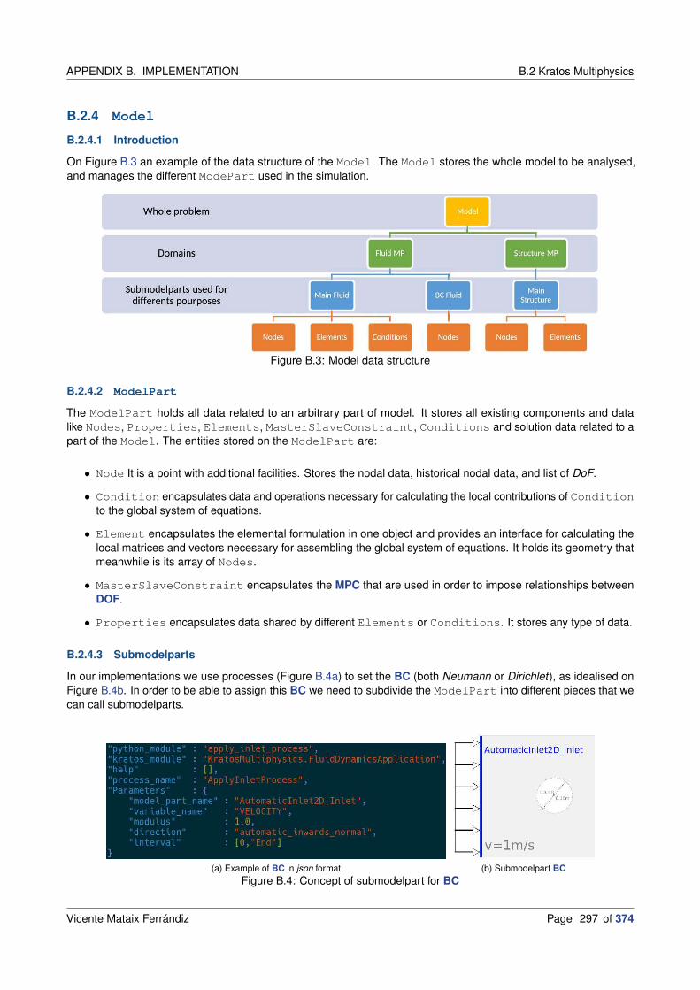
APPENDIX B. IMPLEMENTATION B.2 Kratos Multiphysics
B.2.4 Model
B.2.4.1 Introduction
On Figure B.3 an example of the data structure of the Model. The Model stores the whole model to be analysed,and manages the different ModePart used in the simulation.
Figure B.3: Model data structure
B.2.4.2 ModelPart
The ModelPart holds all data related to an arbitrary part of model. It stores all existing components and datalike Nodes, Properties, Elements, MasterSlaveConstraint, Conditions and solution data related to apart of the Model. The entities stored on the ModelPart are:
• Node It is a point with additional facilities. Stores the nodal data, historical nodal data, and list of DoF.
• Condition encapsulates data and operations necessary for calculating the local contributions of Conditionto the global system of equations.
• Element encapsulates the elemental formulation in one object and provides an interface for calculating thelocal matrices and vectors necessary for assembling the global system of equations. It holds its geometry thatmeanwhile is its array of Nodes.
• MasterSlaveConstraint encapsulates the MPC that are used in order to impose relationships betweenDOF.
• Properties encapsulates data shared by different Elements or Conditions. It stores any type of data.
B.2.4.3 Submodelparts
In our implementations we use processes (Figure B.4a) to set the BC (both Neumann or Dirichlet), as idealised onFigure B.4b. In order to be able to assign this BC we need to subdivide the ModelPart into different pieces that wecan call submodelparts.
(a) Example of BC in json format (b) Submodelpart BC
Figure B.4: Concept of submodelpart for BC
Vicente Mataix Ferrándiz Page 297 of 374

B.3 Mmg library APPENDIX B. IMPLEMENTATION
B.2.5 Base classes
In here we detail some relevant classes which define the basic behaviour of Kratos. The classes used in the FEM
are already defined in B.2.4.2.ModelPart. Apart of these classes, we have another relevant base class, as the baseProcess, which defines the common interface of the processes. The Process is a class which evaluates differenttypes of algorithms, like searches, interpolate values, etc.
B.2.6 Geometry
The Geometry is the base class which defines all the common methods of interest in a geometry, such as volume,area, shape functions, etc. The standard geometries store an array of nodes or points.
B.2.7 Strategy
The strategies are responsible on solving the system of equations. There are 4 types of strategies:
• BuilderAndSolver: This is the base class which defines the necessary methods to assemble the system ofequations. I order to do so it asks the Element, Condition and MasterSlaveConstraint for its localcontribution and assemble them in a global system depending of the DoF order.
• Scheme: This class provides the implementation of the basic tasks that are needed by the solution strategy inorder to integrate the solution over the time. Check algorithms on 2.4.4.Time integration schemes.
• ConvergenceCriteria: This is the base class to define the different convergence criterion considered.Here the residual/solution increment or any other criteria is taken into account in order to check if converged.
• SolvingStrategy: This is the base class from which we will derive all the strategies (line-search, NR, etc.).See 2.4.3.Solution of the non-linear-equilibrium equations system. It is the class responsible of actually solvingthe problem. It integrates all the former classes.
B.2.8 IO classes
In this class we can include the classes dedicated to read external files, such as the *.mdpa files, default input forKratos. We can include the utilities used to read *.json files. These are the default file types used to define theparameters of the problem and the material Properties. Additionally, in the IO category, we can include classessuch the Logger which is used to show/register/save the simulated information.
B.2.9 Testing framework
The testing framework is very relevant in Kratos, and have allowed a faster in Kratos than the former to theintroduction of this technology. Unittest are extensibility used on Information and Communications Technology
(ICT) to ensure code quality. An unittest is a software testing method by which individual units of the source code,hence the name comes, are tested to determine whether they behave as intended. We can differentiate in Kratos
two different approaches for the unittest :
• Python tests: These tests are based in the Python unittest framework, which was originally inspired byJUnit. With this framework we can test and check methods exported to Python and run full short problems inorder to check that the results obtained are the expected.
• C++ tests: This is a custom Kratos testing framework where the test is fully written in C++.
B.3 Mmg library
B.3.1 What is Mmg and how does it work?
Mmg is an open source software for anisotropic automatic remeshing for unstructured meshes based on Delaunaytriangulation. It is licenced under a GNU Lesser General Public License (LGPL) licence and it has been integrated
Page 298 of 374 Vicente Mataix Ferrándiz

APPENDIX B. IMPLEMENTATION B.3 Mmg library
Figure B.5: Mmg logo. Image from Mmg web
in Kratos[ArtDRO10] via the mmg_process.h in the MeshingApplication. It provides 3 applications and 4libraries:
• The mmg2d application and the libmmg2d library: adaptation and optimisation of a two-dimensional triangula-tion and generation of a triangulation from a set of points or from given boundary edges.
• The mmgs application and the libmmgs library: adaptation and optimisation of a surface triangulation andisovalue discretisation.
• The mmg3d application and the libmmg3d library: adaptation and optimisation of a tetrahedral mesh andimplicit domain meshing.
• The libmmg library gathering the libmmg2d, libmmgs and libmmg3d libraries.
The Mmg remeshing process modifies the mesh[BookDob12][ArtDDF14] iteratively until be in agreement with theprescribed sizes on the idealised (Figure B.6) contour (and directions in case of anisotropic mesh). The softwarereads the mesh and the metric, then the mesh is modified using local mesh modifications of which an intersubsectionprocedure based on anisotropic Delaunay kernel.
(a) A piece of parametric Bézier cubic surface associated to triangle T (b) The resulting configuration of the vertex relocation procedure
Figure B.6: Mmg idealised geometry. Source[ArtDDF14]
We can resume the algorithm in following steps:
1. Mmg tries to have a good approximation of the surface (with respect to the Hausdorff parameter).
2. It remeshes on geometric criteria. Mmg scans the surface tetrahedra and splits the tetrahedra using prede-fined patterns if the Hausdorff distance[BookRW09] between the surface triangle of the tetra and its curverepresentation doesn’t respect the Hausdorff parameter.
3. The library scans again the surface tetrahedra and collapses all the edges at a Hausdorff distance smaller thana threshold defined in function of the Hausdorff parameter.
4. Next it intersects the provided metric and a surface metric computed at each point from the Hausdorff parameterand the curvature tensor at the point.
Vicente Mataix Ferrándiz Page 299 of 374

B.3 Mmg library APPENDIX B. IMPLEMENTATION
5. Then Mmg smooths the metric to respect the gradation parameter. The metrics are iteratively propagated untilthe respect of the gradation everywhere.
6. Following it remeshes the surface tetrahedra in order to respect the new metric.
7. Finally, it remeshes both the volume and surface to have edges between 0.6 and 1.3 (in the metric). The longedges are cut and short ones are deleted (collapsed).
B.3.2 Integration between Mmg and Kratos
B.3.2.1 Introduction
In order to understand the integration between Kratos and Mmg is important to understand the data structureof Kratos. We address in first place to the corresponding section about Model structure on the Kratos API
(B.2.4.Model).
B.3.2.2 Class structure
Figure B.7: Mmg-Kratos integration
The implementation of Mmg into Kratos isdone in the MeshingApplication. TheUnified Modeling Language (UML) dia-gram presented on Figure B.7 shows howthe implementation is done.
In here we see like there is an auxil-iary class called MMGUtilities, which iscalled by the MMGProcess, which is theprocess called for remeshing and MMGIO
which can be used to read write Mmg IO
files.
MMGUtilities is the class responsi-ble to interact with the Mmg API. Due tostructure in Mmg library, a template ar-gument must be considered in order tocall the respective methods for each oneof the specialised includes (libmmg2d.h,libmmg3d.h and libmmgs.h).
Additionally the MMGProcess integratesall the steps during the remesh process, in-cluding the value interpolation and the in-ternal variables recovery from 6.6.Internalvalues interpolation. After its execution allthe solvers and the processes must be ini-tialised.
B.3.2.3 Submodelpart recovery
Figure B.8: Concept of colours
As we have previously mentioned, on B.2.4.3.Submodel-parts we need to subdivide the mesh into submodelpartsso we can apply BC. In order to preserve that informa-tion after remeshing we need to create an identificationsystem, so we are able to create a unique ID that willallow us to reconstruct the submodelpart structure afterremeshing, this methodology is commonly called colouridentification. This is thanks to the API of Mmg which al-lows to preserve a reference number, which works as anID. In Figure B.8 we see the concept of this idea.
Page 300 of 374 Vicente Mataix Ferrándiz
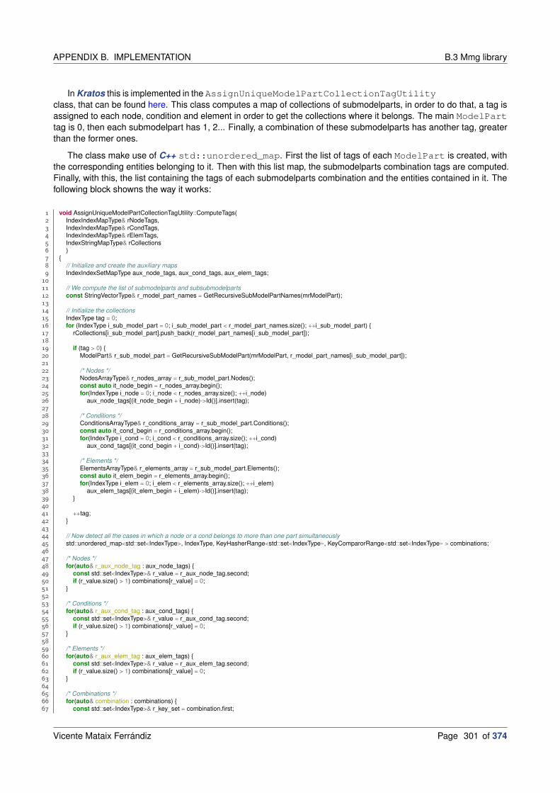
APPENDIX B. IMPLEMENTATION B.3 Mmg library
In Kratos this is implemented in the AssignUniqueModelPartCollectionTagUtilityclass, that can be found here. This class computes a map of collections of submodelparts, in order to do that, a tag isassigned to each node, condition and element in order to get the collections where it belongs. The main ModelParttag is 0, then each submodelpart has 1, 2... Finally, a combination of these submodelparts has another tag, greaterthan the former ones.
The class make use of C++ std::unordered_map. First the list of tags of each ModelPart is created, withthe corresponding entities belonging to it. Then with this list map, the submodelparts combination tags are computed.Finally, with this, the list containing the tags of each submodelparts combination and the entities contained in it. Thefollowing block showns the way it works:
1 void AssignUniqueModelPartCollectionTagUtility::ComputeTags(2 IndexIndexMapType& rNodeTags,3 IndexIndexMapType& rCondTags,4 IndexIndexMapType& rElemTags,5 IndexStringMapType& rCollections6 )7 8 // Initialize and create the auxiliary maps9 IndexIndexSetMapType aux_node_tags, aux_cond_tags, aux_elem_tags;
10
11 // We compute the list of submodelparts and subsubmodelparts12 const StringVectorType& r_model_part_names = GetRecursiveSubModelPartNames(mrModelPart);13
14 // Initialize the collections15 IndexType tag = 0;16 for (IndexType i_sub_model_part = 0; i_sub_model_part < r_model_part_names.size(); ++i_sub_model_part) 17 rCollections[i_sub_model_part].push_back(r_model_part_names[i_sub_model_part]);18
19 if (tag > 0) 20 ModelPart& r_sub_model_part = GetRecursiveSubModelPart(mrModelPart, r_model_part_names[i_sub_model_part]);21
22 /* Nodes */23 NodesArrayType& r_nodes_array = r_sub_model_part.Nodes();24 const auto it_node_begin = r_nodes_array.begin();25 for(IndexType i_node = 0; i_node < r_nodes_array.size(); ++i_node)26 aux_node_tags[(it_node_begin + i_node)->Id()].insert(tag);27
28 /* Conditions */29 ConditionsArrayType& r_conditions_array = r_sub_model_part.Conditions();30 const auto it_cond_begin = r_conditions_array.begin();31 for(IndexType i_cond = 0; i_cond < r_conditions_array.size(); ++i_cond)32 aux_cond_tags[(it_cond_begin + i_cond)->Id()].insert(tag);33
34 /* Elements */35 ElementsArrayType& r_elements_array = r_sub_model_part.Elements();36 const auto it_elem_begin = r_elements_array.begin();37 for(IndexType i_elem = 0; i_elem < r_elements_array.size(); ++i_elem)38 aux_elem_tags[(it_elem_begin + i_elem)->Id()].insert(tag);39 40
41 ++tag;42 43
44 // Now detect all the cases in which a node or a cond belongs to more than one part simultaneously45 std::unordered_map<std::set<IndexType>, IndexType, KeyHasherRange<std::set<IndexType», KeyComparorRange<std::set<IndexType» > combinations;46
47 /* Nodes */48 for(auto& r_aux_node_tag : aux_node_tags) 49 const std::set<IndexType>& r_value = r_aux_node_tag.second;50 if (r_value.size() > 1) combinations[r_value] = 0;51 52
53 /* Conditions */54 for(auto& r_aux_cond_tag : aux_cond_tags) 55 const std::set<IndexType>& r_value = r_aux_cond_tag.second;56 if (r_value.size() > 1) combinations[r_value] = 0;57 58
59 /* Elements */60 for(auto& r_aux_elem_tag : aux_elem_tags) 61 const std::set<IndexType>& r_value = r_aux_elem_tag.second;62 if (r_value.size() > 1) combinations[r_value] = 0;63 64
65 /* Combinations */66 for(auto& combination : combinations) 67 const std::set<IndexType>& r_key_set = combination.first;
Vicente Mataix Ferrándiz Page 301 of 374
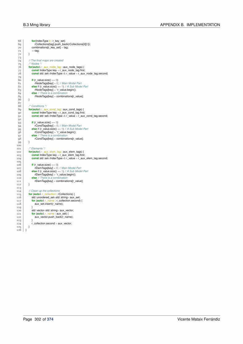
B.3 Mmg library APPENDIX B. IMPLEMENTATION
68 for(IndexType it : r_key_set)69 rCollections[tag].push_back(rCollections[it][0]);70 combinations[r_key_set] = tag;71 ++tag;72 73
74 // The final maps are created75 /* Nodes */76 for(auto& r_aux_node_tag : aux_node_tags) 77 const IndexType key = r_aux_node_tag.first;78 const std::set<IndexType>& r_value = r_aux_node_tag.second;79
80 if (r_value.size() == 0)81 rNodeTags[key] = 0; // Main Model Part82 else if (r_value.size() == 1) // A Sub Model Part83 rNodeTags[key] = *r_value.begin();84 else // There is a combination85 rNodeTags[key] = combinations[r_value];86 87
88 /* Conditions */89 for(auto& r_aux_cond_tag : aux_cond_tags) 90 const IndexType key = r_aux_cond_tag.first;91 const std::set<IndexType>& r_value = r_aux_cond_tag.second;92
93 if (r_value.size() == 0)94 rCondTags[key] = 0; // Main Model Part95 else if (r_value.size() == 1) // A Sub Model Part96 rCondTags[key] = *r_value.begin();97 else // There is a combination98 rCondTags[key] = combinations[r_value];99
100
101 /* Elements */102 for(auto& r_aux_elem_tag : aux_elem_tags) 103 const IndexType key = r_aux_elem_tag.first;104 const std::set<IndexType>& r_value = r_aux_elem_tag.second;105
106 if (r_value.size() == 0)107 rElemTags[key] = 0; // Main Model Part108 else if (r_value.size() == 1) // A Sub Model Part109 rElemTags[key] = *r_value.begin();110 else // There is a combination111 rElemTags[key] = combinations[r_value];112 113
114 // Clean up the collections115 for (auto& r_collection : rCollections) 116 std::unordered_set<std::string> aux_set;117 for (auto& r_name : r_collection.second) 118 aux_set.insert(r_name);119 120 std::vector<std::string> aux_vector;121 for (auto& r_name : aux_set) 122 aux_vector.push_back(r_name);123 124 r_collection.second = aux_vector;125 126
Page 302 of 374 Vicente Mataix Ferrándiz

BIBLIOGRAPHY BIBLIOGRAPHY
Bibliography
Books
[BookAle01] Modern C++ design: generic programming and design patterns applied. Andrei Alexandrescu.Addison-Wesley. 2001.
[BookDob12] MMG3D: user guide. Cécile Dobrzynski. 2012.
[BookMey14] Effective modern C++: 42 specific ways to improve your use of C++ 11 and C++ 14. Scott Meyers.O’Reilly Media, Inc. 2014.
[BookRW09] Variational analysis. R Tyrrell Rockafellar and Roger J-B Wets. Springer Science & Business Media.2009.
Articles
[ArtDad+13] “Migration of a generic multi-physics framework to HPC environments”. Pooyan Dadvand,Riccardo Rossi, Marisa Gil, Xavier Martorell, J Cotela, Edgar Juanpere, Sergio R Idelsohn, andEugenio Oñate. In: Computers & Fluids. Vol. 80, 2013, pp. 301–309. Elsevier.
[ArtDDF14] “Three-dimensional adaptive domain remeshing, implicit domain meshing, and applications to freeand moving boundary problems”. C. Dapogny, C. Dobrzynski, and P. Frey. In: Journal ofComputational Physics. Vol. 262, 2014, pp. 358–378. DOI: 10.1016/j.jcp.2014.01.005.
[ArtDRO10] “An object-oriented environment for developing finite element codes for multi-disciplinaryapplications”. Pooyan Dadvand, Riccardo Rossi, and Eugenio Oñate. In: Archives of computationalmethods in engineering. No. 3, Vol. 17, 2010, pp. 253–297. Springer.
Ph.D.’s thesis
[PhDDad07] “A framework for developing finite element codes for multi-disciplinary applications.”Pooyan Dadvand. Universitat Politècnica de Catalunya. 2007.
Vicente Mataix Ferrándiz Page 303 of 374

PH.D.’S THESIS BIBLIOGRAPHY
Page 304 of 374 Vicente Mataix Ferrándiz

APPENDIX C. AUTOMATIC DIFFERENTIATION
Appendix C
Automatic differentiation
God does not care about ourmathematical difficulties - heintegrates empirically.
Albert Einstein(1879 - 1955 AD, German-born
theoretical physicist)
C.1 Introduction
The AD[ArtGru82; ArtKor97; ArtKor02; BookWri08], also called algorithmic differentiation or computational
differentiation. It consists in a set of techniques to numerically evaluate the derivative of a function specified bya computer program. This is possible to the main principle which defines the derivative operation, which is thedifferentiation of an algorithm by the use of the chain rule. This operation is completely linear, so it can be easilyadapted to any problem, nevertheless of the complexity. As said Korelc[BookJo16] says, the main advantages of theAD are:
• Automatic generated codes are highly efficient if the software employed does the corresponding optimisationsproperly.
• The symbolic formulation is more compressed, for example we only work on the definition of the energy potential,and thus gives fewer possibilities of an error.
• The code generated can be adjusted to specific problems, leading to on-demand numerical code generation.
• The code can be generated for different environments and multi-languages from the same symbolic description.
• Some complex and error-prone operations, such algebraic operations are done automatically.
• Simplifies the implementation of multiphysics problems, as the symbolic definitions are purely mathematical andnot related to any specific problem.
Of course the methodology is not free of controversy or drawbacks, the quantity of code generated can beenormous and less general compared with the manual counterpart, this implies bigger source code files and highercompilation and linking times.
In order to compute the AD we need a Symbolic and Algebraic Computational Systems (SAC) for the manip-ulation of mathematical expressions in symbolic form. Some know commercial SAC systems are Mathematica orMaple. From the Open Source Software (OSS) side, we can find the open-source symbolic Python based package,
Vicente Mataix Ferrándiz Page 305 of 374

C.2 Mathematical concepts APPENDIX C. AUTOMATIC DIFFERENTIATION
Sympy [Onl]. SAC systems cannot be used in directly to define the solution of the problem, as in the case of complexengineering problems, the uncontrollable growth of expressions and consequently redundant operations leads toinefficient codes.
In addition we can mention the Hybrid Object-Oriented (HOO)[BookJo16] approach, an intermediate solution.This approach has brought a new perspective for the development of complex software and several OO FE environ-ments have been developed. The HOO systems are in general restricted to a particular type of formulations wherethe strong form to the element equations can be defined. With this the expression growth problem mentioned for SAC
is reduced, since the symbolic code derivation is used on the resolution of simpler sub-problems. The most relevantexamples of this approach can be found on the OSS environments of FreeFem++ (Hecht [ArtHec+09]) and FEniCS(Logg[ArtLog07]).
C.2 Mathematical concepts
Figure C.1: AD concept
The NR method (C.1) gives us quadratic convergence(C.2).
(C.1)
We start with u0
R(ui + ∆ui ) ≈ R(ui ) + ∂R∂u
(ui )∆ui = 0
Solving → ∆ui = −(∂R∂u
)−1R(ui )
ui+1 = ui + ∆ui
Convergence when: ‖∆ui‖ < ǫu or/and ‖R‖ < ǫr
(C.2) limk→∞
‖xk+1 − xsol‖‖xk − xsol‖2
= M, with M > 0
Then (C.1) gives us the definition of the RHS and the LHS (C.3). In consequence it is possible to use the AD toobtain the exact definition of the system and achieve quadratic convergence
(C.3) RHS =∂δW∂δu
, LHS = −∂RHS
∂u
Sometimes the LHS matrix is called tangent matrix, this is due to the mathematical concept underlying thederivation of the RHS vector necessary to obtain the consistent LHS from (C.3), where in a Single Degree Of
Freedom (SDOF) problem the graphic representation of derivatives corresponds with the tangent in the givenfunctional (See Figure C.2).
From a developer point of view the main advantages of this technique is the fact that it reduces the developmenttime, reduces the computation time, and gives us robust and consistent code where the step of consistent linearisation
Page 306 of 374 Vicente Mataix Ferrándiz

APPENDIX C. AUTOMATIC DIFFERENTIATION C.3 Implementation
Figure C.2: NR representation for a SDOF
is considerably simplified. Furthermore, the time that will be required modify the code will be only the needed tomodify the function to derive with AD, or the only thing that is actually debugged is the functional, not the generatedcode. This technique has been already used successfully for contact problems by Jakub Lengiewicz[ArtLKS11;ArtSLK10].
C.3 Implementation
In the implementations presented in this work for the AD derivations, we have used Sympy [Onl]. The quality of thecode obtained is lesser than in the case of the code developed by Korelc[ArtKor97; ArtKor02] AceGen[Onl], but wehave a full control of the whole workflow and the implementations actually done.
In the following section, we will introduce the principles of AD (C.3.1.Principles of Automatic Differentiation), whichwill help us to understand the design choices taken of the last section. The last section (C.3.2.Kratos integration) weintroduce the integration between Kratos and Sympy and the modular design followed in order to consider properlythe derivative definition without explicit definition of the values involved and get a fully quadratic convergence.
C.3.1 Principles of Automatic Differentiation
C.3.1.1 Derivation modes
As we said previously, the AD is based on the execution of elementary operations with known derivatives, each one ofthem can be evaluated exactly with the chain rule, independently of the complexity of the formulation. We can definetwo procedures[BookJo16], the forward mode and the backward mode. We can show this using the example shownin [BookJo16], taking as reference the equation from (C.4a).
(C.4a) f = bc with b =n∑
i=1
a2i and c = sin(b)
Vicente Mataix Ferrándiz Page 307 of 374

C.3 Implementation APPENDIX C. AUTOMATIC DIFFERENTIATION
Considering ai as n independent variables. The forward mode (C.4b) accumulates the derivatives of intermediatevariables with respect to the independent variables.
(C.4b)
∇b =dbdai
= 2xi for i = 1, 2, · · · , n
∇c =dcdai
= cos(b)∇bi for i = 1, 2, · · · , n
∇f =dfdai
= ∇bic + b∇ci for i = 1, 2, · · · , n
On the other hand, the backward mode, (C.4c), propagates adjoints x = ∂f∂x , which are the derivatives of the final
values, with respect to intermediate variables.
(C.4c)
f =dfdf
= 1 1
c =dfdc
=∂f∂c
f = bf 1
b =dfdb
=∂f∂b
f +∂c∂b
c = cf + cos(c)c 1
∇f = ai =∂b∂ai
b = 2ai b for i = 1, 2, · · · , n
The implementations on C.3.2.Kratos integration consider basically the forward mode. A proper implementa-tion[BookJo16] makes use of both approaches and combine them in order to obtain the most efficient approachaccording to the estimated work ratio (C.5). On this equation the work ratio of the forward mode is proportional to thenumber of independent variables, and in the case of backward mode to the number of scalar-valued functions.
(C.5) wratio(f (a)) =cost(f (a), ∂f
∂a )
cost(f (a))
C.3.1.2 Automatic Differentiation exceptions
Here we introduce the concept of AD exceptions, these exceptions appear on the derivative of an implicit dependence.For example, let’s consider the following nonlinear equation (C.6a), which we will solve via the NR method. If weassume that (C.6a) depends on an additional independent variable a, as shown on (C.6b). If u depends on a, this willintroduce an additional implicit dependence on R (C.6c). This kind of implicit dependency appears in many non-linearproblems, for example on sensibility analysis or in order to obtain a fully consistent tangent on elasto-plasticityproblems or in contact problems in large deformations and the boundary moves significantly. In order to computethe derivatives of this implicit dependence, we can apply the chain rule as in (C.6d). This can be solved by a directapplication of the AD, but an alternative approach is to take into account the AD exceptions.
(C.6a) R(u) = 0
(C.6b) R(u, a) = 0
(C.6c) R(u(a), a) = 0
(C.6d)DR
Da=∂R
∂u
∂u
∂a+∂R
∂a= 0
Page 308 of 374 Vicente Mataix Ferrándiz

APPENDIX C. AUTOMATIC DIFFERENTIATION C.3 Implementation
(C.6e)∂u
∂a= −
(∂R
∂u
)−1∂R
∂a
If R is defined by an algorithm then we can obtain the tangent matrix needed in the NR scheme can be obtainedby AD. Let’s define the computational derivative concept (C.7a). Then we can define the computational derivative of(C.6b) on (C.7b). It is here where we can proceed in two ways, or directly deriving and solving in each step (C.6e),which can be very costly, or we can apply the AD exceptions.
(C.7a)δ (·)δ (·)
(C.7b)∂R
∂u:=δR
δu, and
∂R
∂a:=δR
δa
There are two types of AD exceptions, the local exception (C.8a) or the global exception (C.8b). The differencebetween both exceptions is basically as the name indicates that in the case global exception the exceptions aredefined globally, hence valid for every AD procedure call, while it applies only for the specific call. The approachfollowed in our implementation would be closer to this last exception, as the derivatives are defined in a modular way.For more details follow the next section.
(C.8a)DfDa
:=δf (a, u(a))
δa
∣∣∣∣
DuDa =−
(δRδu
)−1δRδa
(C.8b)
u := u|DuDa =−
(δR
δu
)−1δR
δa
· · ·· · ·DfDa
:=δf (a, u(a))
δa
C.3.2 Kratos integration
The classical way of optimising expressions[BookJo16] in Computer Algebra Systems (CAS) are searching forcommon sub-expressions before the generation of code is done. This can be insufficient when applied to generalnon-linear problems. This means that in the case of using Sympy environment directly, it is not possible to obtaincomplex or highly non-linear FE with this approach.
The design of our AD implementation has in mind these restrictions, and because of this, several utilities whichintegrate the Sympy environment has been implemented into Kratos. These utilities introduce simpler techniquesthan the ones developed Korelc for AceGen1, but enough in order to obtain a relatively complex formulation.
The approach followed in order to take into account the AD exceptions (C.3.1.2.Automatic Differentiation ex-ceptions) is the definition of the derivatives (4.6.Derivatives for contact mechanics linearization) as independentcomputations.
In order to do that, on the Sympy implementations we have defined an implicit dependency respect of the DOF ofthe terms with derivatives, defined in a standalone way. Those algebraic expressions are carried during all the AD
procedures and finally replaced with the corresponding exceptions on the last stage of the code generation.
1Like the techniques of Simultaneous Stochastic Simplification[BookJo16].
Vicente Mataix Ferrándiz Page 309 of 374

C.3 Implementation APPENDIX C. AUTOMATIC DIFFERENTIATION
This integration can be represented in a UML diagram, Figure C.3. On this Figure we can distinguish the previouslystated steps. We define a base template in C++ code, which is empty, and the AD generator created based onSympy fills the template based in a given Galerkin functional. The derivatives are computed a priori, and the codegenerated includes them implicitly until the C++ code conversion steps, where are replaced with the externallycomputed values.
Figure C.3: AD workflow in a UML diagram
Page 310 of 374 Vicente Mataix Ferrándiz

BIBLIOGRAPHY BIBLIOGRAPHY
Bibliography
Books
[BookJo16] Automation of Finite Element Methods. Peter Wriggers (auth.) Joe Korelc. Springer InternationalPublishing. 1st ed. 2016.
[BookWri08] Nonlinear finite element methods. Peter Wriggers. Springer. 1st ed. 2008.
Articles
[ArtGru82] “Automatic Differentiation: Techniques and Applications. Lecture Notes in Computer Science 120.”F. Grund. In: ZAMM - Journal of Applied Mathematics and Mechanics / Zeitschrift für AngewandteMathematik und Mechanik . No. 7, Vol. 62, 1982, pp. 355–355. DOI:10.1002/zamm.19820620735.
[ArtHec+09] “Freefem++, ver. 3.7”. F Hecht, O Pironneau, A Le Hyaric, and K Ohtsuka. In: . 2009,
[ArtKor02] “Multi-language and Multi-environment Generation of Nonlinear Finite Element Codes”. J. Korelc.In: Engineering with Computers. No. 4, Vol. 18, 2002, pp. 312–327. DOI:10.1007/s003660200028.
[ArtKor97] “Automatic generation of finite-element code by simultaneous optimization of expressions”.Joe Korelc. In: Theoretical Computer Science. No. 1, Vol. 187, 1997, pp. 231–248. DOI:10.1016/s0304-3975(97)00067-4.
[ArtLKS11] “Automation of finite element formulations for large deformation contact problems”.Jakub Lengiewicz, Joe Korelc, and Stanisaw Stupkiewicz. In: International Journal for NumericalMethods in Engineering. No. 10, Vol. 85, 2011, pp. 1252–1279. Wiley Online Library. DOI:10.1002/nme.3009.
[ArtLog07] “Automating the finite element method”. Anders Logg. In: Archives of Computational Methods inEngineering. No. 2, Vol. 14, 2007, pp. 93–138. Springer. DOI: 10.1007/s11831-007-9003-9.
[ArtSLK10] “Sensitivity analysis for frictional contact problems in the augmented Lagrangian formulation”.Stanisaw Stupkiewicz, Jakub Lengiewicz, and Joe Korelc. In: Computer Methods in AppliedMechanics and Engineering. No. 33-36, Vol. 199, 2010, pp. 2165–2176. Elsevier. DOI:10.1016/j.cma.2010.03.021.
Online resources
[Onl] AceGen. Multi-language, Multi-environment Numerical Code Generation. URL:https://www.wolfram.com/products/applications/acegen/.
[Onl] SymPy is a Python library for symbolic mathematics. URL: https://www.sympy.org/.
Vicente Mataix Ferrándiz Page 311 of 374

ONLINE RESOURCES BIBLIOGRAPHY
Page 312 of 374 Vicente Mataix Ferrándiz
APPENDIX D. CONSTRAINED OPTIMISATION PROBLEMS
Appendix D
Constrained optimisation problems
The mathematical sciencesparticularly exhibit order, symmetry,and limitation; and these are thegreatest forms of the beautiful.
Aristotle(384 - 322 BC, Greek philosopher)
D.1 Introduction
The following appendix introduces the concepts concerning the constraint optimisation needed in the resolution ofthe contact problems. These optimisation methods are of general use from a mathematical point of view and can befound extensively on the literature[BookLei04; ArtQS99], especially to the kind of problems we are interested to solvethat are the contact problems[BookAnd01; BookYas13]. The main problematic motivating us to study these constraintoptimisation methodologies is the existence of many physical phenomena such as the impact, friction, among others;which can be studied with mathematical models with some kind of discontinuous or non-smooth behaviour. In detail,this problem suffers of bifurcation points, therefore, may lead to non-smooth dynamic systems, where the dynamic ineach mode is associated with a different set of smooth differential equations[BookLei04].
The methods we are going to present in this annexe are the following ones:
• Penalty method (also known as exterior point method[PhDYas11]). This is probably the simplest and probablymost extended method. The last statement comes particularly true when the method can deal with explicitcontributions, then used on explicit simulations. For more details and deeper explanation see D.2.Penaltymethod.
• Lagrange multiplier method. The LM can be given a rigorous justification within the context of the variationalcalculus[BookCA01], and in contrast to penalty method gives an exact solution. How it is derived and severaladditional details are presented on D.3.Lagrange Multiplier method.
• Augmented Lagrange Multiplier method. The ALM basically combines the former methods, for a deeperunderstanding see D.4.Augmented Lagrange Multiplier method.
There is another method that we consider is important to highlight, this is the resolution of MPC (see D.5.MultiPointConstraint (Master-Slave elimination method)) with the master-slave elimination method. This method is not anoptimisation method by itself, but can be used in order to impose constraints of interest in the resolution of mechanicalproblems. The main reason to mention it in addition to the previous methods, it is due to the fact is available on
Vicente Mataix Ferrándiz Page 313 of 374

D.2 Penalty method APPENDIX D. CONSTRAINED OPTIMISATION PROBLEMS
B.2.Kratos Multiphysics natively. Unfortunately, it is not particularly good to deal with complex contact constraints as itwill be shown later.
There are many methods omitted on this list1, as we said we will present and study just the methods used in thedevelopments concerning this work.
D.2 Penalty method
D.2.1 Introduction
The PM method can be idealised as the presence of fictitious elastic structural elements (Figure D.1) which enforcethe constraint approximately for mechanical problems[BookCA01]. In the most general case, it can be defined aspenalty functional appended to our functional of interest, which increases accordingly to how severely the constraint isviolated[BookKO88].
Figure D.1: Analogy between penalty method and springs. Image from [BookYas13]
D.2.2 Formulation
In order to formulate a generic constrained problem and solve it with the PM we just need to add the following to ourfunctional (D.1).
We start with the following base functional and the following constraint. It can be extended to any number ofconstraints, in fact, at contrary to other optimisation methods LM can deal with overconstrained problems (this doesnot mean it will fulfil all of them satisfactory).
(D.1a)
f (w , x) = Base functional
constraint ≤ 0
Where w and x are the test function and DOF respectively. Then we add the following penalty functional to our basefunctional. The objective of this penalty term is precisely to penalise the infringement of this constraint.
(D.1b) fp(w , x) = f (w , x) +ε
2max(0, constraint)2
Where ε is our penalty parameter. Simple, yet powerful and generic.
As in any functional, in order to deduce the corresponding LHS and RHS we do the following (D.2) (as followsit will be the same for the rest of methods). This is already stated on the appendix concerning AD (C.Automaticdifferentiation).
(D.2a) RHS(x) =∂fp(w , x)
∂w
(D.2b) LHS(x) = −∂RHS(x)
∂x1In [PhDYas11; BookWri06] we can see the following methods as an extension of the list presented: Barrier method (also known as interior
points method), perturbed Lagrangian[ArtSWT85a], Nitsche[ArtNit71] method, cross-constraint method.
Page 314 of 374 Vicente Mataix Ferrándiz

APPENDIX D. CONSTRAINED OPTIMISATION PROBLEMS D.2 Penalty method
D.2.3 Applicability on contact problems
The penalty method is general and powerful enough to be applied on contact problems. So in case we want tointroduce it into a contact problem we can do the following (D.12).
We define the non-penetration condition, together with the HSM.
(D.3a) g ≥ 0, σn ≤ 0, gσn = 0, σt = 0
In order to fulfil these conditions, we can define the contact pressure as a continuous function of the penetration.
(D.3b)
g ≥ 0, σn = 0, gσn = 0g < 0, σn = εn(−g) < 0, gσn 6= 0
This approximation implies that the non-penetration condition is not respected, but the penetration movement isresisted, the deeper is the penetration the stronger is the reaction. Then the energy accumulated on these continuouslinear springs is:
(D.3c) fp(x) = f (x) −∫ −〈−g〉
0εn 〈−g′〉 dg′ =
∫ −〈−g〉
0εng′dg′ =
1
2εn〈−g〉2
Where 〈〉 are the Macaulay brackets. Integrating over the boundary, over the normal direction, the contribution to thebalance of virtual works writes as:
(D.3d) δfp(x) = δf (x) +
∫
Γ1c
εn (−gn) δgndΓ1c =
∫
Γ1c
εn(〈−gn〉
)δgndΓ1
c
D.2.3.1 Adapted Penalty Method
On (D.12) the ε is constant, in contrast we can adapt dynamically the value of ε in order to improve the convergenceof the system. Bussetta[ArtBMP] presents the Adapted Penalty Method (APM) as a plausible method from doingso. The concept is summarised on the Figure D.2, where the function F that defines the ε varies in function of thepenetration (gn), see (D.4).
Figure D.2: Representation of F . Image from [ArtBMP]
(D.4a) εni+1 = F(|gi | , gmin, gmax
)εni
(D.4b) F(|gi | , gmin, gmax
)=
|gi |gmax
if |gi | > gmax|gi |gmin
if |gi | < gmin
1 else
This is important because as we have previously stated, the choice of the penalty coefficients is of the utmostimportance in order to get an effective solution. The smaller these coefficients are, the result obtained may notrespect the imposed contact constraint, allowing penetrations. On the other hand, a large value of these coefficientsmay induce numerical oscillations and ill-conditioning of the system of equations, preventing the convergence of thealgorithm. There are other alternative proposals to this in order to improve the PM, with more layers of complexity, likefor example the consideration of a double penalty[PhDHet14].
Vicente Mataix Ferrándiz Page 315 of 374

D.3 Lagrange Multiplier method APPENDIX D. CONSTRAINED OPTIMISATION PROBLEMS
D.3 Lagrange Multiplier method
D.3.1 Introduction
The LMM[BookIK08], named after Joseph-Louis Lagrange, is used on optimisation theory to find the extremum, saddlepoint, of a functional subjected to equality constraints[BookAkh88]. The basic idea is to convert a constrainedproblem into a form such that the derivative test of an unconstrained problem can still be applied[OnlLag], the obtainedfunctional is called Lagrangian (L(x ,λ)). On this Lagrangian functional, we add a new unknown called Lagrangemultiplier, usually referred as λ. The great advantage of this method is that it allows the optimisation to be solvedwithout explicit parameterisation in terms of the constraints.
D.3.2 Formulation
The Lagrangian is constructed in the following manner (D.5b), this for problems where the constraint is not limited byany inequality. For problems where we deal with inequality constraints, we need to formulate the problem followingsome kind of active set strategies[PhDYas11], we can define three types of PDASS(D.5d), graphical examples for abetter understanding of the problem will be presented on the section D.7.2.Non-linear spring contact problem withwall.
We want to minimize f subjected to g.
(D.5a) ming(x)=0
f (x) → ∇Lλ(x ,λ) = 0
Where the Lagrangian is defined as follows:
(D.5b) Lλ(x ,λ) = f (x) + λg(x)
The gradient (∇) of L can be defined as:
(D.5c) ∇Lλ(x ,λ) =
[∂Lλ
∂x∂Lλ
∂λ
]
=
[∂f (x)∂x + λ∂g(x)
∂xg(x)
]
= 0
In case we wan to to consider to solve a problem with inequality constraint we can consider the following three activeset strategies (PDASS), where 〈〉 denotes the Macaulay brackets, used to describe the ramp function:
(D.5d)
Active set strategy 1: g(x) > 0 : f (x) g(x) ≤ 0 : Lλ(x ,λ)
Active set strategy 2: λ > 0 : f (x) λ ≤ 0 : Lλ(x ,λ)
Active set strategy 3: g(x) > 0 and λ > 0 : f (x) g(x) ≤ 0 or λ ≤ 0 : Lλ(x ,λ)
These strategies, combined with (D.5b) can be expressed the following way, with the Macaulay bracket.
(D.5e)
Active set strategy 1: Lλ(x ,λ) = f (x) − 〈−λ〉 g(x)
Active set strategy 2: Lλ(x ,λ) = f (x) − λ 〈−g(x)〉Active set strategy 3: Lλ(x ,λ) = f (x) − 〈−λ〉 g(x) − λ 〈−g(x)〉 − 〈λ〉 〈g(x)〉
The influence of each of the PDASS can be summarised as:
1. This one is based on the check of the violation of the g, it is the most commonly used due to its robust-ness[PhDYas11], but with a higher number of NL iterations in order to converge.
2. This one checks the positivity of λ. This one may lead to the continuous switch between the base functional (f )and the Lagrangian Lλ, lacking the robustness provided by the first strategy, even despite of having a fasterrate of convergence on ideal conditions.
3. The third alternative provides the robustness of the first strategy and the rate of convergence of the second one,but also may diverge faster in case the initial solution is far from the final one. This last point forces to considera slow loading of the problem, or a fine-tuning in the BC.
Page 316 of 374 Vicente Mataix Ferrándiz

APPENDIX D. CONSTRAINED OPTIMISATION PROBLEMS D.3 Lagrange Multiplier method
The solution of our minimisation problem is a stationary point in (D.5b), but usually not all stationary problemsof the Lagrangian(D.5b) are solutions of the initial minimisation problem. The resulting system of equations has ahigher number of unknowns with the corresponding additional computational cost. Additionally if we compute theHessian (H) of the Lagrangian functional, we will obtain the corresponding LHS of our optimisation problem, being thegradient equivalent to minus RHS.
First define H as the derivative of the gradient
(D.6a) H(x) = ∇g(x) =
∇g1(x)T
∇g2(x)T
...∇gn(x)T
Then we can compute the H from the gradient (D.5c).
(D.6b) H(Lλ(x ,λ)) =
[∂2Lλ
∂x2∂2Lλ
∂λ∂x∂2Lλ
∂x∂λ∂2Lλ
∂λ2
]
=
[∂2f (x)∂x2
∂g(x)∂x
∂g(x)∂x 0
]
On (D.6) the H of L is shown, and at (D.6b) we can see the typical LHS structure for a problem solved with LMM.In here the equations have a zero diagonal for each multiplier term. Thus, special care is needed in the solutionprocess to avoid division by the zero diagonal[BookZTF14]. This issue is partially solved with the use of ALM.
D.3.3 Applicability on contact problems
Figure D.3: Lagrangian function for the contact problem
Following the same reasoning of D.2.3.Applicability on contact problems, we can define a functional for contactmechanics using the LMM. The HSM conditions (D.3a) are still applied here, then we can obtain the correspondingLagrangian (D.7).
Defining λn as the normal Lagrange multiplier which defines the normal contact pressure.
(D.7a) Lλ (x ,λ) = f (x) +
∫
Γ1l
λgn(x)dΓ1c
The variation of the Lagrangian then can be expressed as:
(D.7b) δLλ (x ,λ) = δf (x) +
∫
Γc
gn(x)δλ + λδgn(x)dΓc = 0
Vicente Mataix Ferrándiz Page 317 of 374

D.4 Augmented Lagrange Multiplier method APPENDIX D. CONSTRAINED OPTIMISATION PROBLEMS
Where λn and gn have to be fulfilled the minimisation problem with inequality constraints (D.3a). This means that from(D.5d) the preferable strategy would be the third one.
We can represent (D.7) on the locus2 of Figure D.3, where (D.7) is represented on function of gn and λn. On thisfigure we can appreciate the fact that on tension state (λn > 0) there is no solution to the functional (zero solutions),this generates a discontinuity which affects the resolution the resulting system of equations. This last problematic canbe solved precisely with the application of ALM.
D.4 Augmented Lagrange Multiplier method
D.4.1 Introduction
The ALM was originally introduced by Arrow and Solow [ArtAS58], and later improved by Powell and Hestenes[ArtPow69;ArtHes69], reason why was originally named as the multiplier method of Hestenes and Powell. The method consistson a regularised version of LMM[PhDYas11]. This regulazations occurs via the inclusion of penalty parameter, butonce the problem has reached convergence the influence of the penalty parameters disappears, resulting in exactfulfilment of the constraint.
D.4.2 Formulation
D.4.2.1 Standard formulation
The Lagrangian is constructed in the following manner (D.8b), this is basically the combination of the PM and theLMM (D.8a). This method was generalised by Rockafellar [ArtRoc73b; ArtRoc73a] for inequality constraints (D.8c), inthis particular case g(x) ≥ 0.
The Lagrangians for the PM and LMM as previously redefined are:
(D.8a) fp(x) = f (x) +1
2εg(x)2; Lλ(x ,λ) = f (x) + λg(x)
Combination of previous methods, we obtain the augmented Lagrangian.
(D.8b) Lλ (x ,λ) = Lλ (x ,λ) +1
2εg(x)2 = f (x) + λg(x) +
1
2εg(x)2
Expressed as inequality constraints g(x) ≥ 0:
(D.8c) Lλ(x ,λ) = f (x) − 1
2ε
(
λ2 − 〈− (λ + εg(x))〉2)
In an expanded form, it rewrites as:
(D.8d) Lλ(x ,λ) = f (x) +
λg(x) + 1
2εg(x)2 ,λ + εg(x) ≤ 0− 1
2ελ2 ,λ + εg(x) > 0
We can call λ + εg(x) as λ, or augmented Lagrangian. The gradient (∇) of (D.8d) can be expressed as:
(D.8e) ∇Lλ(x ,λ) = ∇f (x) +
[
(λ + εg(x)) ∂g(x)∂x
g(x)
]
, λ ≤ 0[
0−λ
ε
]
, λ > 0
Equivalent to what is done in (D.6) we can obtain the Hessian (H) of (D.8b). In (D.9) we see that in this case, wehave partially solved the issue concerning to the zero terms appearing on the diagonal, compared to the previouslyobtained H. The problematic have been solved partially because only affects to the inactive set (λ > 0), in the case
2A locus is the set of all points (usually forming a curve or surface) satisfying some condition.
Page 318 of 374 Vicente Mataix Ferrándiz

APPENDIX D. CONSTRAINED OPTIMISATION PROBLEMS D.4 Augmented Lagrange Multiplier method
of the active set we still have to deal with this issue. A Generalized Newton-Raphson method (GNM) was proposedby Alart and Curnier for nonsmooth potential for the ALM[ArtAla88; ArtAC91; ArtAla97].
(D.9) H(Lλ(x ,λ)) =
[∂2Lλ
∂x2∂2Lλ
∂λ∂x∂2Lλ
∂x∂λ∂2Lλ
∂λ2
]
=
[∂2f (x)∂x2 + ∂2g(x)
∂x2 (λ + εg(x)) + ε(
∂g(x)∂x
)2∂g(x)∂x
∂g(x)∂x 0
]
, λ ≤ 0
[∂2f (x)∂x2 00 1
ε
]
, λ > 0
D.4.2.2 Uzawa iteration
So as we have seen, we still have some problematic from the standard LMM, like the zero diagonal terms or the non-positivity of the Lagrange multiplier. In order to solve that, on 1958 the Japanese economist Uzawa presented[ArtAS58;ArtAHU58] an alternative approach in order to solve this problematic following an iterative approach, known as Uzawaalgorithm[Onl].
Let’s decompose the increment of the Lagrangian into two different components, one for the x DOF and the otherfor the update of the Lagrange multiplier (D.10).
Calling λi and xi the respective solution for the NL iteration number i . Then we can define the augmentedLagrangian in a given increment of a NL iteration as:
(D.10a) Lλ (xi + ∆xi ,λi + ∆λi ) ≈ Lλ (xi + ∆xi ,λi ) +∂Lλ (x ,λi )
∂λ
∣∣∣∣λi
∆λi + O(λ2
i
)= 0
We can do the same for the ∆x term, and expand it.
(D.10b)Lλ (xi + ∆xi ,λi ) ≈ Lλ (xi ,λi ) + ∂Lλ(x ,λi )
∂x
∣∣∣xi
∆xi = 0[
f (xi ) + λig (xi ) + 12εg (xi )
2]
+[∂f (x)∂x + [λi + εg(x)]
]∂g(x)∂x ]|xi
∆xi + O(x2
i
)= 0
Finally, concerning the Lagrange multiplier we apply an update procedure:
(D.10c) λi+1 = λi + εg (xi ) , ∆λi = εg (xi )
Convergence of this method is linear for the part relative to the Lagrange multiplier (O (λi )), as we have removed thesecond order part of (D.10a). Besides the advantage of the method is that the L is smooth so that a standard NR isapplicable.
For the present work, the standard approach has been taken into consideration. On the contact chapter of thiswork the details concerning why the standard ALM approach has been chosen instead of the Uzawa iteration, checkthe corresponding section for further details, 4.3.3.2.1.3.ALM.
D.4.3 Applicability on contact problems
Following a similar criteria to the one employed on (D.7), the equivalent formulation can be obtained for the ALM , see(D.11). In contrast to the locus for the LMM, the corresponding locus for the ALM (Figure D.4) is C1 differentiablesaddle-point, with the corresponding advantages for the resolution of the problem. Like the existence of a system ofequations contributions (LHS, RHS) even for λn > 0.
Again, considering λn as the normal contact stress, and calling λn the augmented contact stress, computed asλ = λ + εgn(x).
(D.11a) Lλ(x ,λ) = f (x) +
∫
Γ1l
λgn(x) + 1
2εgn(x)2 , λ ≤ 0− 1
2ελ2 , λ > 0
dΓ1c
The variation of the augmented Lagrangian then can be expressed as:
(D.11b) δLλ (x ,λ) = δf (x) +
∫
Γc
δλgn(x) + (λ + εgn(x)) δgn(x) , λ ≤ 0−λ
ε δλ , λ > 0dΓc = 0
Vicente Mataix Ferrándiz Page 319 of 374

D.5 MultiPoint Constraint (Master-Slave elimination method)APPENDIX D. CONSTRAINED OPTIMISATION PROBLEMS
Figure D.4: Augmented Lagrangian function for the contact problem
D.4.3.1 Adapted Augmented Lagrangian Method
Algorithm 7 Adaptation of normal penalty coefficient[ArtBMP]
Require: εn, gi and gi−1
1: procedure ADAPTATION OF NORMAL PENALTY COEFFICIENT
2: if gi × gi−1 < 0 then
3: if gi × gi−1 < 0 then
4: εn =∣∣(εngi−1) /gi ×
(|gi | + gmax
)/ (gi − gi−1)
∣∣
5: else
6: εn = |εngi−1/ (10gi )|7: else if gi > gmax then
8: if |gi − gi−1| > max(gi/10, gi−1/10, 5gmax
)then
9: εn = 2εn
10: else if |gi | = |gi−1| ± 1% < 10gmax then
11: εn = εn
(√(|gi | /gmax − 1
)+ 1)2
12: else if gi > gmax then
13: εn = 2εn(gi−1/gi
)
14: else
15: εn = εn
((√(|gi | /gmax − 1
)+ 1))
16: else
17: εn = εn
On the expressions from (D.11) it is assumed that the ε is constant, but there are techniques which adaptdynamically the value of ε in order to improve the convergence of the system. We can mention in particular thework of Bussetta[PhDBus; ArtBMP] who created AALM, an ALM with a corresponding algorithm in order to updatethe ε in function of the current penetration (gn). On Algorithm 7 the procedure is detailed, here three cases can bedistinguished: The sign of gn changes (gi × gi−1 < 0), the absolute value of gn is more relevant than the defined limit(gi > gmax), or the last case where the absolute value of gn is smaller than the limit (gi > gmax).
D.5 MultiPoint Constraint (Master-Slave elimination method)
Page 320 of 374 Vicente Mataix Ferrándiz
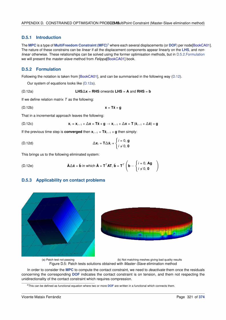
APPENDIX D. CONSTRAINED OPTIMISATION PROBLEMSD.5 MultiPoint Constraint (Master-Slave elimination method)
D.5.1 Introduction
The MPC is a type of MultiFreedom Constraint (MFC)3 where each several displacements (or DOF) per node[BookCA01].The nature of these constrains can be linear if all the displacement components appear linearly on the LHS, and non-linear otherwise. These relationships can be solved using the former optimisation methods, but in D.5.2.Formulationwe will present the master-slave method from Felippa[BookCA01] book.
D.5.2 Formulation
Following the notation is taken from [BookCA01], and can be summarised in the following way (D.12).
Our system of equations looks like (D.12a).
(D.12a) LHS∆x = RHS onwards LHS = A and RHS = b
If we define relation matrix T as the following:
(D.12b) x = Tx + g
That in a incremental approach leaves the following:
(D.12c) xi = xi−1 + ∆x = Tx + g → xi−1 + ∆x = T (xi−1 + ∆x) + g
If the previous time step is converged then xi−1 = Txi−1 + g then simply:
(D.12d) ∆xi = T∆xi +
i = 0, g
i 6= 0, 0
This brings us to the following eliminated system:
(D.12e) A∆x = b in which A = TT AT, b = TT
(
b −
i = 0, Ag
i 6= 0, 0
)
D.5.3 Applicability on contact problems
(a) Patch test not passing (b) Not matching meshes giving bad quality results
Figure D.5: Patch tests solutions obtained with Master -Slave elimination method
In order to consider the MPC to compute the contact constraint, we need to deactivate them once the residualsconcerning the corresponding DOF indicates the contact constraint is on tension, and them not respecting theunidirectionality of the contact constraint which requires compression.
3This can be defined as functional equation where two or more DOF are written in a functional which connects them.
Vicente Mataix Ferrándiz Page 321 of 374

D.6 Summary of the different methods APPENDIX D. CONSTRAINED OPTIMISATION PROBLEMS
Unfortunately, the MPC method presented with Master -Slave elimination method does not give a good solutiononce the meshes are not matching (similar to a NTN method) for a problem of deformable domains. The solutionspresented on Figure D.5 represent the solution obtained with this method. The weights have been obtained with amortar segmentation, therefore exact, and the results obtained are not good.
The first case, Figure D.5a, represents a 3D patch test, with not matching meshes, in this case the constraintis fulfilled, but as both domains are deformable the resulting solution is not continuous. The solution from FigureD.5b deals with the same problem, but with a higher number of DOF, then the bad quality of the results is even morenoticeable.
In order to obtain good results with the methods, the master domain must be rigid, or quasi-rigid, or the meshes tomatch between the interface of the domains.
D.6 Summary of the different methods
The presented methods can be summarised in the following table, see D.1, inspired and expanded from [BookCA01].ALM and LMM are virtually identical except for the dependence of the ALM of the penalty (not affecting the finalsolution). Additionally the ALM retains partially the positive definiteness due to the fact that adds relatively smallterms on the diagonal of the LHS matrix.
Method Master-Slave Elimination PM LMM ALM
Generality Fair Excellent Excellent ExcellentEase of implementation Poor to fair Good Fair FairSensitivity to user decisions High High Small to none SmallAccuracy Variable Variable Excellent ExcellentSensitivity as regards constraint dependence High None High HighRetains positive definiteness Yes Yes No Partially
Table D.1: Comparison of different methods presented
Apart from ALM there are other methods that try to tackle the issues presented by LMM. In short we can list thefollowing two methods:
• Double Lagrange multiplier: The Lagrange doubles4 (used in the Castem2000 code) avoids the issuesfrom the LMM provoked by the non-positive LHS matrix obtained with the method. This method duplicatesthe number of Lagrange multipliers and adds some dummy terms to the LHS matrix, which increases thecomputational cost but makes the LHS positive defined. For further details see [Onl].
• Perturbed Lagrangian: Simo, Wriggers and Taylor proposed a perturbed Lagrangian formulation for thesolution of contact problems. That formulation can be classified as a stabilised method, preserving the stabilityof the discretised problem if the penalty parameter, ε, is small enough. For further details see [ArtSWT85b].
D.7 Numerical examples
In this section we compare the different approaches introduced (except for D.5.MultiPoint Constraint (Master-Slaveelimination method)). The problems vary on complexity, and helps us to understand the way these different methodsbehave when computing the corresponding contribution of the constraints.
D.7.1 Initial spring wall problem
We start with a very simple case from[PhDYas11]. This problem consists on a SDOF problem, where we idealised asingle spring with a wall constraint that does not allow a penetration, see Figure D.6, which means that x ≥ 0. Thefunction can be defined as follows (D.13), where k represents the stiffness of the spring. The base functional can bedefined as f (x) = 1
2 k (x + 1)2. Taking k = 2.
4Not to be confused with the dual Lagrange multiplier presented on this work.
Page 322 of 374 Vicente Mataix Ferrándiz

APPENDIX D. CONSTRAINED OPTIMISATION PROBLEMS D.7 Numerical examples
Figure D.6: Simplified contact problem within spring and a wall
(D.13)
f (x) = 12 k (x + 1)2
Subjectted to x ≥ 0
D.7.1.1 Penalty method
Figure D.7: Solution for a SDOF solved with PM, comparing different values of ε
This can be formulated as follows for PM.
(D.14) fp(x) =1
2k (x + 1)2 +
ε
2
(max 0, x
)2
Taking (D.14) and applying (D.2) iteratively with a NR we can solve the problem. On Figure D.7 we can appreciatethe solutions obtained for different values of ε. It can be seen as ε grows the solution comes closer to the actual
Vicente Mataix Ferrándiz Page 323 of 374

D.7 Numerical examples APPENDIX D. CONSTRAINED OPTIMISATION PROBLEMS
Iteration x fp1 1 42 −1 106
3 −2 × 10⁻⁶ 8.40465 × 10⁻¹¹
Table D.2: Convergence on fp with PM for (D.13)
solution of the problem. This problem takes in total three NL iterations to converge starting with x = 1 for a ε = 106,see Table D.2, and even with this value the constraint is not completely satisfied.
D.7.1.2 Lagrange multiplier method
Now we can formulate the corresponding Lagrangian of (D.13) for the LMM. The (D.15) shows the proper potential ofour problem with LMM. In this example we will only show one of the possible alternatives in order to compute the λconstraint, the next section D.7.2.Non-linear spring contact problem with wall will show the three possible alternativesavailable when computing the LMM contribution.
(D.15) Lλ(x) =1
2k (x + 1)2 + min 0,λ x
Figure D.8: Solution for a SDOF solved with LMM
Iteration x λ Lλ
1 1 0 4.123112 0 −2 0
Table D.3: Convergence on Lλ with LMM for (D.13)
On the other hand, the convergence of (D.13) with LMM is achieved in only 2 iterations, see Table D.3, reachingadditionally the exact solution and satisfying exactly the constraint imposed. On the Figure D.8 we can see thefull space of solutions x − λ, including the respective constraint and appreciate the convergence in only two NL
iterations.
D.7.2 Non-linear spring contact problem with wall
The following example[PhDYas11; BookYas13], again as seen on Figure D.6, is a simple unidimensional constrainedoptimisation problem, which can show us the influence of each one of the methodologies when solving these kinds of
Page 324 of 374 Vicente Mataix Ferrándiz
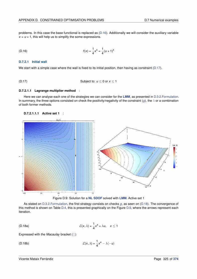
APPENDIX D. CONSTRAINED OPTIMISATION PROBLEMS D.7 Numerical examples
problems. In this case the base functional is replaced as (D.16). Additionally we will consider the auxiliary variablex = u + 1, this will help us to simplify the some expressions.
(D.16) f (x) =1
4x4 =
1
4(u + 1)4
D.7.2.1 Initial wall
We start with a simple case where the wall is fixed to its initial position, then having as constraint (D.17).
(D.17) Subject to: u ≤ 0 or x ≤ 1
D.7.2.1.1 Lagrange multiplier method :
Here we can analyse each one of the strategies we can consider for the LMM, as presented in D.3.2.Formulation.In summary, the three options consisted on check the positivity/negativity of the constraint (g), the λ or a combinationof both former methods.
D.7.2.1.1.1 Active set 1 :
Figure D.9: Solution for a NL SDOF solved with LMM. Active set 1
As stated on D.3.2.Formulation, the first strategy consists on checks g, as seen on (D.18). The convergence ofthis method is shown on Table D.4, this is presented graphically on the Figure D.9, where the arrows represent eachiteration.
(D.18a) L(x ,λ) =1
4x4 + λu, x ≤ 1
Expressed with the Macaulay bracket (〈〉)
(D.18b) L(x ,λ) =1
4x4 − λ〈−u〉
Vicente Mataix Ferrándiz Page 325 of 374

D.7 Numerical examples APPENDIX D. CONSTRAINED OPTIMISATION PROBLEMS
Iteration x λ Error
1 0.0 0.0 1.02 1.0 0.0 1.03 1.0 1.0 2.2204510−16
Table D.4: First active set strategy convergence on Lλ with LMM for (D.16)
D.7.2.1.1.2 Active set 2 :
In this second case, what is checked is the negativity of λ (D.19). For this case, still quite simple, the NL iterationsgive the same result, see Table D.5, which coincides with Table D.4. The convergence path is presented on FigureD.10.
(D.19a) L(x ,λ) =1
4x4 + λu, λ ≤ 0
Expressed with the Macaulay bracket (〈〉)
(D.19b) L(x ,λ) =1
4x4 − 〈−λ〉u
Iteration x λ Error
1 0.0 0.0 1.02 1.0 0.0 1.03 1.0 1.0 2.2204510−16
Table D.5: Second active set strategy convergence on Lλ with LMM for (D.16)
Figure D.10: Solution for a NL SDOF solved with LMM. Active set 2
D.7.2.1.1.3 Active set 3 :
In the last active set case, which checks simultaneously both g and λ (D.20). Again, for this simple case, the NL
iterations give the same convergence path, see Table D.6, which coincides with Table D.4 and Table D.5. The pathcoincides, see Figure D.11.
(D.20a) L(x ,λ) =1
4x4 + λu, λ ≤ 0 x ≤ 1
Page 326 of 374 Vicente Mataix Ferrándiz

APPENDIX D. CONSTRAINED OPTIMISATION PROBLEMS D.7 Numerical examples
Expressed with the Macaulay bracket (〈〉)
(D.20b) L(x ,λ) =1
4x4 − 〈−λ〉u − λ〈−u〉 + 〈−λ〉〈−u〉
Iteration x λ Error
1 0.0 0.0 1.02 1.0 0.0 1.03 1.0 1.0 2.2204510−16
Table D.6: Third active set strategy convergence on Lλ with LMM for (D.16)
Figure D.11: Solution for a NL SDOF solved with LMM. Active set 3
D.7.2.2 Moved wall
In order to make the problem more difficult and appreciate better the differences across methodologies, we willpartially move the wall which defines our constraint. This example is taken from Yastrebov [PhDYas11], where othermoving configurations are presented apart of the following.
(D.21) Subject to: u + 0.9 ≤ 0.0
Moving the wall 0.9m, the resulting constraint will be (D.21). The resulting case is significantly more complex, andas it will be shown in the next sections, the convergence rate changes from one method to others, some of them evendiverging the solution.
D.7.2.2.1 Penalty method :
In the case of the PM no tuning is required and the convergence is obtained in a straightforward manner. The onlything that affects the solution is ε value. On Figure D.12 different solutions are presented for different values of ε, thetrend to the exact solution can be appreciated.
For a value of ε = 106 the correct solution can be achieved, see Table D.7. In here it can be appreciated that onthe iteration 7 we sudden increase on the error, this is due to entering on the penalised region (u > 0.9). In any casethe number of NL iteration needed is quite high, 9 iterations, for a SDOF problem.
Vicente Mataix Ferrándiz Page 327 of 374

D.7 Numerical examples APPENDIX D. CONSTRAINED OPTIMISATION PROBLEMS
Iteration u Error
1 0.0 1.02 −0.333333 0.2962963 −0.555556 0.08779154 −0.703704 0.02601235 −0.802469 0.007707356 −0.868313 0.002283667 −0.912209 12208.58 −0.9 0.00004107499 −0.9 1.7180710−12
Table D.7: Convergence with PM for (D.21)
Figure D.12: Solution for a NL SDOF problem solved with PM, comparing different values of ε. Moved wall
D.7.2.2.2 Lagrange multiplier method :
Following the same reasoning from D.7.2.1.1.Lagrange multiplier method, and applying it for (D.21). On thissection the L to be derived are not detailed, as it follows the same principle. The exact solution of the problem isu = −0.9 and λ = −0.001.
D.7.2.2.2.1 Active set 1 :
Iteration u λ Error
1 − 13 0 8
272 −0.555556 0 0.08779153 −0.703704 0 0.02601234 −0.802469 0 0.007707355 −0.868313 0 0.002283666 −0.912209 0 0.01222727 −0.9 −0.000958925 0.0000410758 −0.9 −0.001 2.168410−19
Table D.8: First active set strategy convergence on Lλ with LMM for (D.16) with moved wall
The Table D.8 presents the convergence path that is also represented on Figure D.13. Compared with theunmoved wall, the problem requires a higher number of iterations in order to converge, and it basically moves across
Page 328 of 374 Vicente Mataix Ferrándiz

APPENDIX D. CONSTRAINED OPTIMISATION PROBLEMS D.7 Numerical examples
the u axis, but at the end it finally converges.
Figure D.13: Solution for a NL SDOF solved with LMM. Active set 1. Moved wall
D.7.2.2.2.2 Active set 2 :
Figure D.14: Solution for a NL SDOF solved with LMM. Active set 2. Moved wall
On this case the problem doesn’t even converge to the right solution, as can be seen on Table D.9, and fromFigure D.14 we can notice as it doesn’t move arrived certain point. If we extend the number of NL iterations to 20 wedon’t get the proper solution either, the NL loop remains around the same values.
On Figure D.14 another relevant point is the fact that the functional is almost flat, explaining part of the difficultycoming from this active set strategy, it is not possible to find a local minima on these cases.
In the last active set we will see as this problematic is no more. Other initial conditions can be tried for the L, but theidea is to compare the presented methods across them, and showing the problematic presented on D.3.2.Formulation,where we introduced that the second active set converges faster than the first one, but in case we are far from thesolution we can deal with the divergence on the NR iteration.
Vicente Mataix Ferrándiz Page 329 of 374

D.7 Numerical examples APPENDIX D. CONSTRAINED OPTIMISATION PROBLEMS
Iteration u λ Error
1 − 13 0 0.639455
2 −0.9 0.459259 0.0013 −0.933333 0.459259 0.0002962964 −0.955556 0.459259 0.00008779155 −0.97037 0.459259 0.00002601236 −0.980247 0.459259 7.70735−6
7 −0.986831 0.459259 2.28366−6
8 −0.991221 0.459259 6.76639−7
9 −0.994147 0.459259 2.00486−7
10 −0.996098 0.459259 5.94032−8
Table D.9: Second active set strategy convergence on Lλ with LMM for (D.16) with moved wall
D.7.2.2.2.3 Active set 3 :
On the case of the third active set strategy on Table D.10 we have exactly the same convergence path as TableD.8, despite of that the graphical representation differs, Figure D.15.
Iteration u λ Error
1 − 13 0 8
272 −0.555556 0 0.08779153 −0.703704 0 0.02601234 −0.802469 0 0.007707355 −0.868313 0 0.002283666 −0.912209 0 0.01222727 −0.9 −0.000958925 0.0000410758 −0.9 −0.001 2.168410−19
Table D.10: Third active set strategy convergence on Lλ with LMM for (D.16) with moved wall
Figure D.15: Solution for a NL SDOF solved with LMM. Active set 3. Moved wall
We can infer in a simplified manner that the third active set strategy will behave as the best option of the two otheralternative strategies, despite this is not always true as already stated on D.3.2.Formulation. The following section willintroduce the ALM resolution, so it will be possible to compare with the presented here for LMM, which in addition tothe convergence of the problem improves the conditioning of the system of equations.
Page 330 of 374 Vicente Mataix Ferrándiz

APPENDIX D. CONSTRAINED OPTIMISATION PROBLEMS D.7 Numerical examples
D.7.2.2.3 Augmented Lagrange multiplier method :
The equation (D.22) shows the resulting L for the ALM method for this problem.
(D.22) Lλ (u,λ) =
12 k (u + 1)4 + λ(u + 0.9) + 1
2ε(u + 0.9)2, λ + ε(u + 0.9) ≤ 012 k (u + 1)4 − 1
2ελ2 λ + ε(u + 0.9) > 0
We will see like the different values of ε give us a similar convergence rate, but the condition number (κ) of theLHS varies in function of ε. In order to properly prove that we need the definition of κ (D.23), the proper definition of κdefines it as the ratio of the largest to smallest singular value in the singular value decomposition of a matrix, thismeans it requires to compute the SVD of the LHS, which is an expensive operation and complex. We can simplifyand estimate κ as the ratio between the largest to smallest eigenvalue, which are not necessarily coincident.
(D.23) κ(A) ≈ |λmax||λmin|
In order to do so, we need then to define the LHS from (D.22), considering (D.2), we can deduce (D.24), recallingthe augmented Lagrange multiplier as λ = λ + ε(u + 0.9).
(D.24a) RHS(u,λ) = δLλ (u,λ) =
[2k (u + 1)3 + λ
u + 0.9
]T [δuδλ
]
= 0, λ ≤ 0 (Active)[
2k (u + 1)3
−λε
]T [δuδλ
]
= 0, λ > 0 (Inactive)
(D.24b) LHS(x) = ∆δLλ (u,λ) =
[δuδλ
]T [6k(u + 1)2 + ε 1
1 0
] [δuδλ
]
, λ ≤ 0 (Active)[δuδλ
]T [6k(u + 1)2 0
0 − 1ε
] [δuδλ
]
, λ > 0 (Inactive)
From (D.24b) we can calculate κ, in the case of inactive set is trivial as the LHS is diagonal (D.25a). On thisresulting expression, κ grows linearly with ε. For the active set case, we obtain (D.25b) as expression defining κ. Onthis case the condition number of the LHS grows quadratically to the ε. In conclusion, for a high ε, in comparison withthe stiffness of the problem, κ become very high which means we have an ill-conditioned problem, affecting theprecision of the solution and its convergence; but, on the other hand, the energy functional becomes smooth, as wewill state next.
(D.25a) κinactive(LHS) ≈
6kεu2, 1ε ≤ 6ku2
16ku2ε , 1
ε > 6ku2 assuming1
ε≤ 6ku2 then ∼ kε
(D.25b) κactive(LHS) ≈ 1
2
(6k(u + 1)2 + ε
)(√
(6k(u + 1)2 + ε
)2+ 4 +
(6k(u + 1)2 + ε
))
+ 1 ∼ (k + ε)2
Another important point to highlight is that all the graphical representation of the L shows a continuous fieldwithout flat areas (See Figures D.16, D.17, D.18, D.19). This already gives us an idea how the method already solvessome problems presented on the previous section (D.7.2.2.2.Lagrange multiplier method) with the LMM, avoiding theneed of choose between different active set strategies.
Vicente Mataix Ferrándiz Page 331 of 374

D.7 Numerical examples APPENDIX D. CONSTRAINED OPTIMISATION PROBLEMS
D.7.2.2.3.1 ε = 0.5 :
Our first case with ε = 0.5 show a very similar convergence path to the one presented on D.7.2.2.2.1.Active set 1,Table D.11, but the functional from Figure D.16 is smoother than the one from Figure D.13.
Iteration x λ Error
1 − 13 0 0.296296
2 −0.555556 0 0.08779153 −0.703704 0 0.02601234 −0.802469 0 0.007707355 −0.868313 0 0.002283666 −0.912209 0 0.01222727 −0.9 −0.000958925 0.0000410758 −0.9 −0.001 4.33681−19
Table D.11: Convergence on Lλ with ALM for (D.22) with ε = 0.5
Figure D.16: Solution for a NL SDOF solved with ALM. ε = 0.5. Moved wall
D.7.2.2.3.2 ε = 1.0 :
On this second case with ε = 1.0 the Table D.12 presents practically the same path as Table D.11, with theexception that once the solution enters in the inactive region the error changes slightly. The Figure D.17 is evensmoother than Figure D.16.
Iteration x λ Error
1 − 13 0 0.296296
2 −0.555556 0 0.08779153 −0.703704 0 0.02601234 −0.802469 0 0.007707355 −0.868313 0 0.002283666 −0.912209 0 0.01679387 −0.9 −0.000958925 0.0000410758 −0.9 −0.001 1.0842−18
Table D.12: Convergence on Lλ with ALM for (D.22) with ε = 1.0
Page 332 of 374 Vicente Mataix Ferrándiz

APPENDIX D. CONSTRAINED OPTIMISATION PROBLEMS D.7 Numerical examples
Figure D.17: Solution for a NL SDOF solved with ALM. ε = 1.0. Moved wall
D.7.2.2.3.3 ε = 5.0 :
Iteration x λ Error
1 − 13 0 0.296296
2 −0.555556 0 0.08779153 −0.703704 0 0.02601234 −0.802469 0 0.007707355 −0.868313 0 0.002283666 −0.912209 0 0.0615887 −0.9 −0.000958925 0.0000410758 −0.9 −0.001 2.60209−18
Table D.13: Convergence on Lλ with ALM for (D.22) with ε = 5.0
Figure D.18: Solution for a NL SDOF solved with ALM. ε = 5.0. Moved wall
Vicente Mataix Ferrándiz Page 333 of 374

D.7 Numerical examples APPENDIX D. CONSTRAINED OPTIMISATION PROBLEMS
For the case with ε = 5.0, we have again a very similar NL loop, Table D.13, converging again in 8 NL iterations.The only value that changes again is the error when crossing the constraint threshold. On the other side, the FigureD.13 shows a significant aspect on the L representation.
D.7.2.2.3.4 ε = 10.0 :
With ε = 10.0 we have again a very similar NL convergence, Table D.14, but the graphical representation of Lfathom the change of aspect on L already seen in the previous case, see Figure D.19.
Iteration x λ Error
1 − 13 0 0.296296
2 −0.555556 0 0.08779153 −0.703704 0 0.02601234 −0.802469 0 0.007707355 −0.868313 0 0.002283666 −0.912209 0 0.1220217 −0.9 −0.000958925 0.0000410758 −0.9 −0.001 3.90313−18
Table D.14: Convergence on Lλ with ALM for (D.22) with ε = 10.0
Figure D.19: Solution for a NL SDOF solved with ALM. ε = 10.0. Moved wall
D.7.3 Over-constrained optimisation problem
The next example[Onl], and last one on this section, concerns an optimisation problem over-constrained, that will beshown as an example of problem that can be solved with the PM, but not with the most advanced methodologies asthe LMM or the ALM. The problem to solve of interest is shown in (D.26).
(D.26)
Minimize f (x) = (x1 − 6)2 + (x2 − 7)2
subject to g1(x) = −3x1 − 2x2 + 6 ≤ 0g2(x) = −x1 + x2 − 3 ≤ 0g3(x) = x1 + x2 − 7 ≤ 0g4(x) = 2
3 x1 − x2 − 43 ≤ 0
This function and constrains can be seen visually on Figure D.20, here we can appreciate the constraints, as thelimits on the functional representation.
Page 334 of 374 Vicente Mataix Ferrándiz

APPENDIX D. CONSTRAINED OPTIMISATION PROBLEMS D.7 Numerical examples
Figure D.20: Graphic representation of (D.26)
This equation becomes (D.27), where ε is the penalty parameter.
(D.27)
fp(ε, x)) = (x1 − 6)2 + (x2 − 7)2
+ ε(max 0,−3x1 − 2x2 + 6
)2
+ ε(max 0,−x1 + x2 − 3
)2
+ ε(max 0, x1 + x2 − 7
)2
+ ε
(
max
0,2
3x1 − x2 −
4
3
)2
Considering (D.2) and solving applying a NR iterative resolution we can obtain the correct solution in 4 stepsstarting from x = 0, y = 0 with ε = 106, as can be seen on Table D.15.
Iteration x y fp1 0 0 2
√468000384000085
2 0 3 14.42223 6 7 1.69706 × 10⁷
4 3 4 1.97134 × 10⁻⁹
Table D.15: Convergence on fp with penalty method for D.26
On the other hand, if we try to solve this problem using a LMM, we will find problems to solve due to the
Vicente Mataix Ferrándiz Page 335 of 374

D.7 Numerical examples APPENDIX D. CONSTRAINED OPTIMISATION PROBLEMS
overconstraint of the problem. If we formulate (D.26) considering for example the second active set strategy from(D.5e), with x = 6, y = 7, λi = 0 for i = 1, 2, 3, 4, the resulting LHS will be (D.28). This is a matrix is rank 2, being a6 × 6 matrix, which means that the system of equations is not solvable.
(D.28) LHS =
−2 0 0 0 0 00 −2 0 0 0 00 0 0 0 0 00 0 0 0 0 00 0 0 0 0 00 0 0 0 0 0
Same happens considering the first active set strategy, which is more robust. The underlying problem is theoverconstrained problem, which we have already shown, is not a problem for a PM. This is a small example thatshows that LMM despite being a powerful and generic technique it is not applicable for all cases.
Page 336 of 374 Vicente Mataix Ferrándiz

BIBLIOGRAPHY BIBLIOGRAPHY
Bibliography
Books
[BookAkh88] The calculus of variations. Naum Ilich Akhiezer. CRC Press. 1988.
[BookAnd01] From Convexity to Nonconvexity. Anders Klarbring (auth.) R. P. Gilbert P. D. PanagiotopoulosP. M. Pardalos (eds.) Lars-Erik Andersson. Springer US. 1st ed. 2001.
[BookCA01] Introduction to finite element methods. Felippa C.A. 2001.
[BookIK08] Lagrange multiplier approach to variational problems and applications. Kazufumi Ito andKarl Kunisch. Siam. 2008.
[BookKO88] Contact problems in elasticity: a study of variational inequalities and finite element methods.Noboru Kikuchi and John Tinsley Oden. siam. 1988.
[BookLei04] Dynamics and Bifurcations of Non-Smooth Mechanical Systems.Professor Dr. Henk Nijmeijer (auth.) Dr. Remco I. Leine. Springer-Verlag Berlin Heidelberg. 1st ed.2004.
[BookWri06] Computational Contact Mechanics. Peter Wriggers. Springer. 2nd. 2006.
[BookYas13] Numerical Methods in Contact Mechanics. Vladislav A. Yastrebov. Wiley-ISTE. 1st ed. 2013.
[BookZTF14] The Finite Element Method for Solid and Structural Mechanics. O. C. Zienkiewicz, Robert L. Taylor,and David Fox. Butterworth-Heinemann. 7th ed. 2014.
Articles
[ArtAC91] “A mixed formulation for frictional contact problems prone to Newton like solution methods”.Pierre Alart and Alain Curnier. In: Computer methods in applied mechanics and engineering. No. 3,Vol. 92, 1991, pp. 353–375. Elsevier. DOI: 10.1016/0045-7825(91)90022-x.
[ArtAHU58] “Studies in linear and non-linear programming”. Kenneth J Arrow, Leonid Hurwicz, andHirofumi Uzawa. In: . 1958, Cambridge Univ. Press.
[ArtAla88] “Multiplicateurs “augmentés” et méthode de Newton généralisée pour contact avec frottement”.P Alart. In: Report, Document LMA-DME-EPFL, Lausanne. 1988,
[ArtAla97] “Méthode de Newton généralisée en mécanique du contact”. Pierre Alart. In: Journal demathématiques pures et appliquées. No. 1, Vol. 76, 1997, pp. 83–108. Elsevier.
[ArtAS58] “Gradient methods for constrained maxima, with weakened assumptions”. KENNETH J Arrow andROBERT M Solow. In: Studies in linear and nonlinear programming. 1958, pp. 166–176. StanfordUniversity Press, Stanford, CA.
[ArtBMP] “The adapted augmented Lagrangian method: a new method for the resolution of the mechanicalfrictional contact problem”. Philippe Bussetta, Daniel Marceau, and Jean-Philippe Ponthot. In:Computational Mechanics. No. 2, , pp. 259–275. DOI: 10.1007/s00466-011-0644-z.
[ArtHes69] “Multiplier and gradient methods”. Magnus R Hestenes. In: Journal of optimization theory andapplications. No. 5, Vol. 4, 1969, pp. 303–320. Springer. DOI: 10.1007/bf00927673.
Vicente Mataix Ferrándiz Page 337 of 374

PH.D.’S THESIS BIBLIOGRAPHY
[ArtNit71] “Über ein Variationsprinzip zur Lösung von Dirichlet-Problemen bei Verwendung von Teilräumen,die keinen Randbedingungen unterworfen sind”. Joachim Nitsche. In: . No. 1, Vol. 36, 1971,pp. 9–15.
[ArtPow69] “A method for nonlinear constraints in minimization problems”. Michael JD Powell. In: Optimization.1969, pp. 283–298. Academic Press.
[ArtQS99] “A survey of some nonsmooth equations and smoothing Newton methods”. Liqun Qi andDefeng Sun. In: . 1999, pp. 121–146. Springer. DOI: 10.1007/978-1-4613-3285-5_7.
[ArtRoc73a] “The multiplier method of Hestenes and Powell applied to convex programming”.R Tyrell Rockafellar. In: Journal of Optimization Theory and applications. No. 6, Vol. 12, 1973,pp. 555–562. Springer. DOI: 10.1007/bf00934777.
[ArtRoc73b] “A dual approach to solving nonlinear programming problems by unconstrained optimization”.R Tyrrell Rockafellar. In: Mathematical programming. No. 1, Vol. 5, 1973, pp. 354–373. Springer.DOI: 10.1007/bf01580138.
[ArtSWT85a] “A perturbed Lagrangian formulation for the finite element solution of contact problems”.Juan C Simo, Peter Wriggers, and Robert L Taylor. In: Computer methods in applied mechanicsand engineering. No. 2, Vol. 50, 1985, pp. 163–180. Elsevier. DOI:10.1016/0045-7825(85)90088-x.
[ArtSWT85b] “A perturbed Lagrangian formulation for the finite element solution of contact problems”.Juan C. Simo, Peter Wriggers, and Robert L. Taylor. In: Computer Methods in Applied Mechanicsand Engineering. No. 2, Vol. 50, 1985, pp. 163–180. DOI: 10.1016/0045-7825(85)90088-x.
Ph.D.’s thesis
[PhDBus] “Modélisation et résolution du problème de contact mécanique et son application dans un contextemultiphysique”. Philippe Bussetta.
[PhDHet14] “The Bipenalty Method for Explicit Structural Dynamics”. Jack Hetherington. 2014.
[PhDYas11] “Computational contact mechanics: geometry, detection and numerical techniques”.Vladislav A. Yastrebov. 2011.
Online resources
[Onl] Algorithms for Constrained Optimization. URL: https://www.me.utexas.edu/~jensen/ORMM/supplements/units/nlp_methods/const_opt.pdf.
[Onl] Dualisation of the boundary conditions. URL:https://www.code-aster.org/V2/doc/v11/en/man_r/r3/r3.03.01.pdf.
[Onl] Wikipedia. Uzawa iteration. URL: https://en.wikipedia.org/wiki/Uzawa_iteration.
[OnlLag] Wikipedia. Lagrange multiplier. URL:http://en.wikipedia.org/wiki/Lagrange_multiplier.
Page 338 of 374 Vicente Mataix Ferrándiz
APPENDIX E. MORTAR MAPPER
Appendix E
Mortar mapper
Projections are just bullshit.They’re just guesses.
Jason Fried(Software entrepreneur)
E.1 Introduction
This appendix introduces the mapper developed using the Mortar formulation[ArtDB06; ArtND08]. The goal of amap is the distribution of the variable of interest from the origin mesh to the destination mesh, see Figure E.1a. Thismethod provides an exact decomposition of the target mesh (Figure E.1b). With this, the procedure of mappinghas the advantage of conserving, in a weak sense at least, the important physical quantities such as mass, energy,etc. Additionally this method satisfies the equilibrium in a weak manner, being then consistent with the FEM
formulation.
The mapping is used on this work in order to compute a consistent gap between meshes during the searchprocess, see Algorithm 8, in order to discard poor contact candidates. Poor candidates can be defined as the contactcandidates that will not activate during the whole NL iteration process. The inclusion of these candidates may bedifficult the convergence of the active-set strategy, then increasing the number of NL iterations computed during theNR strategy.
Algorithm 8 Consistent gap computation
1: procedure CONSISTENT GAP COMPUTATION
2: Reset auxiliar values for nodal coordinates on origin mesh xaux
3: for all node ∈ OriginMeshnodes do
4: xaux = xnode
5: for all node ∈ DestinationMeshnodes do
6: xaux = 0
7: Map xaux from OriginMeshnodes → DestinationMeshnodes
8: for all node ∈ DestinationMeshnodes do
9: From node get the normal (n)10: gconsistent = −n · (xnode − xaux)
The reason why the very same Mortar formulation has been taken into consideration are, first the developmentsare shared between the two frameworks; second the consistency between the results obtained between the system ofequations and the search process; but primarily the quality of the results. On this last point, the results that can be
Vicente Mataix Ferrándiz Page 339 of 374

E.2 Theory APPENDIX E. MORTAR MAPPER
obtained with this method are between the best options available[ArtBBP]. Precisely on Bussetta[ArtBBP] the threetypes of data transfer procedures are discussed:
• Element Transfer Method (ELM): The simplest one consists on map the value depending only on the location ofthe destination mesh on the origin mesh. Methods on this category we can find the nearest element [MasBuc17]or nearest neighbour [MasBuc17] mappers.
• Procedures based on the weak conservation of the data field. The presented method (sometimes called ELM)would we encompassed on this category. Other techniques defined on this category can be Finite Volume
Transfer Method (FVTM)[ArtBBP], which consists on decide the meshes on Finite Volumes (FV) elementsand the transfer is computed between FV meshes.
• These are the procedures based on reconstruction of the field in the neighbourhood of this point. On thiscategory we can find the modern technique Moving Least Square (MLS)[ArtCho+05; ArtLIC07]. Additionallyon [ArtYu+08; ArtHC90; ArtDHC92] we can find more examples of this kind of methodology. This concept isconsidered on the method presented on E.2.3.Discontinuous meshes mapping, where the nodes close to thediscontinuity are taken into consideration to reconstruct the field.
(a) Concept of mapper between two meshes (b) Mortar integration mapping between two meshes
Figure E.1: Mapping concepts
The Mortar formulation employed, based on the concept of dual[ArtWoh02; ArtWoh11] LM, which allows toevaluate in a simplified manner the data transference between meshes. This method has been already presented onthe corresponding contact sections (4.2.3.4.DLMM). Instead of solving a whole assembled system of the transferoperators, the dual LM allows to assemble it in a diagonal manner, which can be solved in a trivial manner. There arealternatives methodologies for using the Mortar formulation without solving directly the system of equations, such theJacobian-Free Newton Krylov (JFNK) approach by Hansen[ArtHan11].
E.2 Theory
E.2.1 General mapping theory
Based on the concepts introduced on the work of Ute[MasIsr06] and Jaiman[ArtJai+06], we can start defining theconsistent transfer operation between meshes (E.1).
(E.1a) f = Mcu
Where the matrices and vectors can be defined as:
(E.1b)
Mc =∫
ΓdN i
d N id dΓd
f =∫
ΓdN i
d N jouj
odΓd
Page 340 of 374 Vicente Mataix Ferrándiz

APPENDIX E. MORTAR MAPPER E.2 Theory
And u = uid the nodal values of the destination mesh. The index i represents the i th NL iteration. We can define the
RHS and RHS of our respective system of equations.
(E.1c)
RHS = f − Mcui
LHS = −∂RHS∂u
= Mc
With the RHS and the LHS we can obtain the update of the update of u, ∆u.
(E.1d) ui+1 = ui + ∆u
Where:
(E.1e) ∆u = LHS−1RHS = M−1c (f − Mcui ) = M−1
c f − ui
This methodology implies the whole system integration, and resolution of the whole system of equations. OnE.2.2.Dual Lagrange multiplier mapping we will introduce how with the consideration of dual Lagrange multiplier theMc becomes diagonal, MD, with the respective advantages.
E.2.2 Dual Lagrange multiplier mapping
E.2.2.1 Introduction
As previously stated, using the dual Lagrange multiplier allows to solve the exact system of equations with theinversion of a diagonal matrix, trivial operation that can be parallelised. The theory introducing the concept of dualLagrange multiplier was first introduced by Wohlmuth[ArtWoh02], who used as an alternative method for DDM. Thesenonstandard Lagrange multiplier spaces provided optimal discretisation schemes and a locally supported basis forthe associated constrained mortar spaces.
E.2.2.2 Theory
Algorithm 9 Explicit contribution of the pairs during dual λ mortar mapping
1: procedure EXPLICIT CONTRIBUTION OF THE PAIRS
2: while (rhstotal > toleranceabs and ratio > tolerancerel ) and i < iterationmax do
3: Reset global residual norm rhstotal
4: Reset auxiliar values for nodal residual rhsnode
5: Reset weight areas wnode
6: for all elem ∈ DestinationMeshelements do
7: if Areamortar segmentation > tolerance then
8: Calculate D and M
9: Calculate local residual (E.2a) and the local weight area (E.2b)
10: for all node ∈ DestinationMeshnodes do
11: Compute ud = ud + rhsnodewnode
12: Compute rhstotal = rhstotal + rhs2node
13: Compute the residual norm: rhstotal = rhstotalndof
14: if i = 0 then
15: rhstotal0 = rhstotal
16: Compute ratio = rhstotalrhstotal0
17: i = i + 1
We address the theory of the dual Lagrange multiplier previously presented, 4.3.3.4.1.Dual Lagrange multipliers,which means that we can focus on the required operations starting from the theory already presented in E.2.1.Generalmapping theory, and modify some specific operations with our alternative λ.
On Algorithm 9 we present the solution designed to obtain the explicit contributions of the pairs, for them computethe mapping. From Algorithm 9 we need to define some missing concepts (E.2). Being known D and M in every pairof entities, where D is assumed to be diagonal as previously stated, then the explicit contribution of errors and weight
Vicente Mataix Ferrándiz Page 341 of 374

E.2 Theory APPENDIX E. MORTAR MAPPER
areas are (E.2a) and (E.2b) respectively. Where the sub-index node refers to the pair entities which share certainnodes.
(E.2a) rhsnode =Nnode∑
elem=1
Melemuelemo − Delemuelem
d
(E.2b) wnode =Nnode∑
elem=1
Delem(inode, inode)
E.2.3 Discontinuous meshes mapping
E.2.3.1 Introduction
This is an innovative contribution of this work, which allows to transfer data between two discontinuos meshes. Wewill call a discontinuos mesh to the mesh that is not watertight, which means that the nodes are not necessarilyshared between the entities which conform the mesh. This means that following the metaphor of a container, in caseof being filled with water, the water would leak across the gaps between the nodes of the mesh, reason why is calledwatertight.
This development can be used on embedded CFD simulations, where the condition of watertight mesh is notguaranteed, especially from meshes imported from STL files, which usually undergo these problematic.
E.2.3.2 Theory
Algorithm 10 Explicit contribution of the pairs during dual λ mortar discontinuous mapping
1: procedure EXPLICIT CONTRIBUTION OF THE PAIRS ON DISCONTINUOUS MAPPING
2: Create an inverse database (pairing destination-origin entities and vice-versa)3: while (rhstotal > toleranceabs and ratio > tolerancerel ) and i < iterationmax do
4: Reset global residual norm rhstotal
5: Reset auxiliar values for nodal residual rhsnode
6: Reset weight areas wnode
7: for all elem ∈ DestinationMeshelements do
8: if Areamortar segmentation > tolerance then
9: Calculate D and M
10: Calculate local residual (E.2a) and the local weight area (E.2b)11: for all node ∈ elem do
12: Local wlocal = D(node, node) contribution13: Local h equivalent to length of elem14: for all pairinv ∈ eleminverse paired do
15: for all nodeaux ∈ pairinv do
16: Compute distance d between node and nodeaux
17: Compute local weight area discontinuous contribution (E.3)
18: for all node ∈ DestinationMeshnodes do
19: Compute ud = ud + rhsnode
wdiscontinuousnode
20: Compute rhstotal = rhstotal + rhs2node
21: Compute the residual norm: rhstotal = rhstotalndof
22: if i = 0 then
23: rhstotal0 = rhstotal
24: Compute ratio = rhstotalrhstotal0
25: i = i + 1
This method preserves the properties presented on E.2.2.Dual Lagrange multiplier mapping, which meansthat the corresponding system of equations keeps the possibility to be solved in a simplified manner. The main
Page 342 of 374 Vicente Mataix Ferrándiz
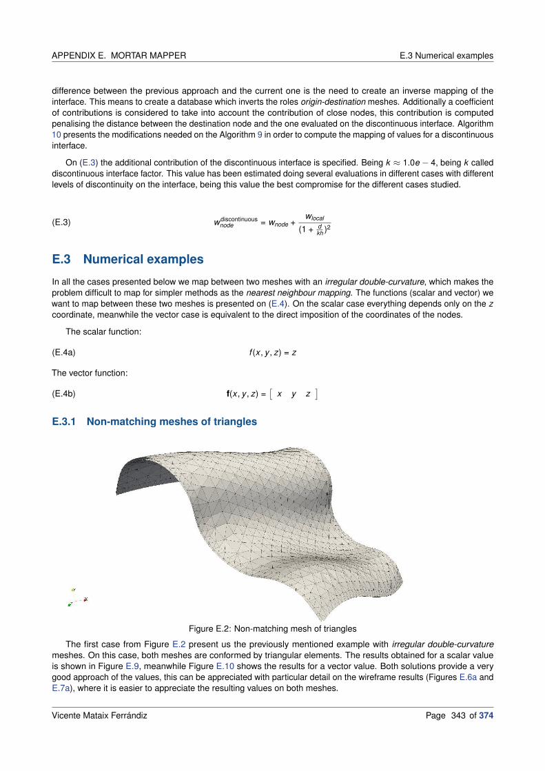
APPENDIX E. MORTAR MAPPER E.3 Numerical examples
difference between the previous approach and the current one is the need to create an inverse mapping of theinterface. This means to create a database which inverts the roles origin-destination meshes. Additionally a coefficientof contributions is considered to take into account the contribution of close nodes, this contribution is computedpenalising the distance between the destination node and the one evaluated on the discontinuous interface. Algorithm10 presents the modifications needed on the Algorithm 9 in order to compute the mapping of values for a discontinuousinterface.
On (E.3) the additional contribution of the discontinuous interface is specified. Being k ≈ 1.0e − 4, being k calleddiscontinuous interface factor. This value has been estimated doing several evaluations in different cases with differentlevels of discontinuity on the interface, being this value the best compromise for the different cases studied.
(E.3) wdiscontinuousnode = wnode +
wlocal
(1 + dkh )2
E.3 Numerical examples
In all the cases presented below we map between two meshes with an irregular double-curvature, which makes theproblem difficult to map for simpler methods as the nearest neighbour mapping. The functions (scalar and vector) wewant to map between these two meshes is presented on (E.4). On the scalar case everything depends only on the zcoordinate, meanwhile the vector case is equivalent to the direct imposition of the coordinates of the nodes.
The scalar function:
(E.4a) f (x , y , z) = z
The vector function:
(E.4b) f(x , y , z) =[
x y z]
E.3.1 Non-matching meshes of triangles
Figure E.2: Non-matching mesh of triangles
The first case from Figure E.2 present us the previously mentioned example with irregular double-curvaturemeshes. On this case, both meshes are conformed by triangular elements. The results obtained for a scalar valueis shown in Figure E.9, meanwhile Figure E.10 shows the results for a vector value. Both solutions provide a verygood approach of the values, this can be appreciated with particular detail on the wireframe results (Figures E.6a andE.7a), where it is easier to appreciate the resulting values on both meshes.
Vicente Mataix Ferrándiz Page 343 of 374

E.3 Numerical examples APPENDIX E. MORTAR MAPPER
(a) Scalar solution as a wireframe (b) Scalar solution as a continuous field
Figure E.3: Scalar solution for non-matching mesh of triangles
(a) Vector solution as a wireframe (b) Vector solution as a continuous field
Figure E.4: Vector solution for non-matching mesh of triangles
E.3.2 Non-matching meshes of triangles and quadrilaterals
The case from Figure E.5 instead of being fully meshed on triangles as Figure E.2, or even fully meshed withquadrilaterals, presents both types of geometries. The origin mesh consists on triangular entities, meanwhile thedestination mesh is integrated by quadrilateral entities. This case shows how it is possible not only map values acrossnon-conformant meshes, but also between different types of geometries, with the additional complexity.
The results obtained on scalar and vector fields (Figures E.9 and E.10) show again a good matching between theorigin and destination values.In the same way as the previous example, the wireframe (Figures E.6a and E.7a) andcontinuous field solutions (Figures E.6b and E.7b) are presented.
E.3.3 Discontinuous meshes
Figure E.8: Detail of the non-matching mesh discontinuous of triangles
Page 344 of 374 Vicente Mataix Ferrándiz

APPENDIX E. MORTAR MAPPER E.3 Numerical examples
Figure E.5: Non-matching mesh of triangles and quadrilaterals
(a) Scalar solution as a wireframe (b) Scalar solution as a continuous field
Figure E.6: Scalar solution for non-matching mesh of triangles and quadrilaterals
The following case may a priori look similar to Figure E.2, that’s why Figure E.8 zooms into the detail of the mesh, sothe discontinuity of the meshes is appreciated. Due to this the standard mapper cannot be applied, and the methodpresented on E.2.3.Discontinuous meshes mapping must be taken into consideration.
The results obtained are again being of good quality despite of the existence of this discontinuity on the mesh,both for scalar and vector fields (Figures E.9 and E.10 respectively).
(a) Scalar solution as a wireframe (b) Scalar solution as a continuous field
Figure E.9: Scalar solution for non-matching discontinuous mesh of triangles
Vicente Mataix Ferrándiz Page 345 of 374

E.3 Numerical examples APPENDIX E. MORTAR MAPPER
(a) Vector solution as a wireframe (b) Vector solution as a continuous field
Figure E.7: Vector solution for non-matching mesh of triangles and quadrilaterals
(a) Vector solution as a wireframe (b) Vector solution as a continuous field
Figure E.10: Vector solution for non-matching discontinuous mesh of triangles
Page 346 of 374 Vicente Mataix Ferrándiz

BIBLIOGRAPHY BIBLIOGRAPHY
Bibliography
Articles
[ArtBBP] “Efficient 3D data transfer operators based on numerical integration”. Philippe Bussetta,Romain Boman, and Jean-Philippe Ponthot. In: International Journal for Numerical Methods inEngineering. No. 3-4, , pp. 892–929. Wiley Online Library. DOI: 10.1002/nme.4821.
[ArtCho+05] “An improved interface element with variable nodes for non-matching finite element meshes”.Young-Sam Cho, Sukky Jun, Seyoung Im, and Hyun-Gyu Kim. In: Computer Methods in AppliedMechanics and Engineering. No. 27-29, Vol. 194, 2005, pp. 3022–3046. Elsevier. DOI:10.1016/j.cma.2004.08.002.
[ArtDB06] “Information transfer between incompatible finite element meshes: application to coupledthermo-viscoelasticity”. David Dureisseix and Henri Bavestrello. In: Computer Methods in AppliedMechanics and Engineering. No. 44-47, Vol. 195, 2006, pp. 6523–6541. Elsevier. DOI:10.1016/j.cma.2006.02.003.
[ArtDHC92] “Automatic adaptive remeshing for numerical simulations of metalforming”. M Dyduch,AM Habraken, and Serge Cescotto. In: Computer Methods in Applied Mechanics and Engineering.No. 1-3, Vol. 101, 1992, pp. 283–298. Elsevier. DOI: 10.1016/0045-7825(92)90026-g.
[ArtHan11] “A Jacobian-free Newton Krylov method for mortar-discretized thermomechanical contactproblems”. Glen Hansen. In: Journal of Computational Physics. No. 17, Vol. 230, 2011,pp. 6546–6562. Elsevier. DOI: 10.1016/j.jcp.2011.04.038.
[ArtHC90] “An automatic remeshing technique for finite element simulation of forming processes”.AM Habraken and Serge Cescotto. In: International Journal for Numerical Methods in Engineering.No. 8, Vol. 30, 1990, pp. 1503–1525. Wiley Online Library. DOI: 10.1002/nme.1620300811.
[ArtJai+06] “Conservative load transfer along curved fluid–solid interface with non-matching meshes”.Rajeev K Jaiman, Xiangmin Jiao, Philippe H Geubelle, and Eric Loth. In: Journal of ComputationalPhysics. No. 1, Vol. 218, 2006, pp. 372–397. Elsevier. DOI: 10.1016/j.jcp.2006.02.016.
[ArtLIC07] “Variable-node elements for non-matching meshes by means of MLS (moving least-square)scheme”. Jae Hyuk Lim, Seyoung Im, and Young-Sam Cho. In: International Journal for NumericalMethods in Engineering. No. 7, Vol. 72, 2007, pp. 835–857. Wiley Online Library. DOI:10.1002/nme.1988.
[ArtND08] “A computational strategy for thermo-poroelastic structures with a time–space interface coupling”.David Néron and David Dureisseix. In: International Journal for Numerical Methods in Engineering.No. 9, Vol. 75, 2008, pp. 1053–1084. Wiley Online Library. DOI: 10.1002/nme.2283.
[ArtWoh02] “A Comparison of Dual Lagrange Multiplier Spaces for Mortar Finite Element Discretizations”.Barbara I. Wohlmuth. In: ESAIM: Mathematical Modelling and Numerical Analysis. No. 6, Vol. 36,2002, pp. 995–1012. EDP Sciences. DOI: 10.1051/m2an:2003002.
[ArtWoh11] “Variationally consistent discretization schemes and numerical algorithms for contact problems”.Barbara Wohlmuth. In: Acta Numerica. Vol. 20, 2011, pp. 569–734. DOI:10.1017/s0962492911000079.
Vicente Mataix Ferrándiz Page 347 of 374

MASTER’S THESIS. BIBLIOGRAPHY
[ArtYu+08] “Three-dimensional RITSS large displacement finite element method for penetration of foundationsinto soil”. L Yu, J Liu, XJ Kong, and Y Hu. In: Computers and Geotechnics. No. 3, Vol. 35, 2008,pp. 372–382. Elsevier. DOI: 10.1016/j.compgeo.2007.08.007.
Master’s thesis.
[MasBuc17] Development and Implementation of a Parallel Framework for Non-Matching Grid Mapping.Philipp Bucher. 2017.
[MasIsr06] Implementation of an Algorithm for Data Transfer on the Fluid-Structure Interface betweenNon-Matching Meshes in Kratos and an Algorithm for the Generation. Ute Israel. 2006.
Page 348 of 374 Vicente Mataix Ferrándiz
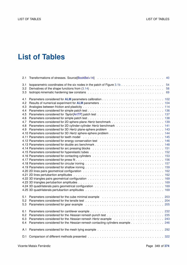
LIST OF TABLES LIST OF TABLES
List of Tables
2.1 Transformations of stresses. Source[BookBel+14] . . . . . . . . . . . . . . . . . . . . . . . . . . . . 40
3.1 Isoparametric coordinates of the six nodes in the patch of Figure 3.1b . . . . . . . . . . . . . . . . . . 543.2 Derivatives of the shape functions from (3.14) . . . . . . . . . . . . . . . . . . . . . . . . . . . . . . . 583.3 Isotropic-kinematic hardening law constans . . . . . . . . . . . . . . . . . . . . . . . . . . . . . . . . 69
4.1 Parameters considered for ALM parameters calibration . . . . . . . . . . . . . . . . . . . . . . . . . . 1024.2 Results of numerical experiment for ALM parameters . . . . . . . . . . . . . . . . . . . . . . . . . . . 1044.3 Analogies between friction and plasticity . . . . . . . . . . . . . . . . . . . . . . . . . . . . . . . . . . 1144.4 Parameters considered for simple patch test . . . . . . . . . . . . . . . . . . . . . . . . . . . . . . . . 1364.5 Parameters considered for Taylor [ArtTP] patch test . . . . . . . . . . . . . . . . . . . . . . . . . . . . 1374.6 Parameters considered for simple patch test . . . . . . . . . . . . . . . . . . . . . . . . . . . . . . . . 1384.7 Parameters considered for 2D sphere-plane Hertz benchmark . . . . . . . . . . . . . . . . . . . . . . 1394.8 Parameters considered for 2D cylinder-cylinder Hertz benchmark . . . . . . . . . . . . . . . . . . . . 1414.9 Parameters considered for 3D Hertz plane-sphere problem . . . . . . . . . . . . . . . . . . . . . . . 1434.10 Parameters considered for 3D Hertz sphere-sphere problem . . . . . . . . . . . . . . . . . . . . . . . 1444.11 Parameters considered for teeth model . . . . . . . . . . . . . . . . . . . . . . . . . . . . . . . . . . 1454.12 Parameters considered for energy conservation test . . . . . . . . . . . . . . . . . . . . . . . . . . . 1464.13 Parameters considered for double arc benchmark . . . . . . . . . . . . . . . . . . . . . . . . . . . . . 1484.14 Parameters considered for arc pressing blocks . . . . . . . . . . . . . . . . . . . . . . . . . . . . . . 1514.15 Parameters considered for hyperelastic tubes . . . . . . . . . . . . . . . . . . . . . . . . . . . . . . . 1524.16 Parameters considered for contacting cylinders . . . . . . . . . . . . . . . . . . . . . . . . . . . . . . 1534.17 Parameters considered for press fit . . . . . . . . . . . . . . . . . . . . . . . . . . . . . . . . . . . . . 1564.18 Parameters considered for circular ironing . . . . . . . . . . . . . . . . . . . . . . . . . . . . . . . . . 1574.19 Parameters considered for shallow ironing . . . . . . . . . . . . . . . . . . . . . . . . . . . . . . . . . 1594.20 2D lines pairs geometrical configuration . . . . . . . . . . . . . . . . . . . . . . . . . . . . . . . . . . 1624.21 2D lines pertubartion amplitudes . . . . . . . . . . . . . . . . . . . . . . . . . . . . . . . . . . . . . . 1624.22 3D triangles pairs geometrical configuration . . . . . . . . . . . . . . . . . . . . . . . . . . . . . . . . 1694.23 3D triangles pertubartion amplitudes . . . . . . . . . . . . . . . . . . . . . . . . . . . . . . . . . . . . 1694.24 3D quadrilaterals pairs geometrical configuration . . . . . . . . . . . . . . . . . . . . . . . . . . . . . 1694.25 3D quadrilaterals pertubartion amplitudes . . . . . . . . . . . . . . . . . . . . . . . . . . . . . . . . . 169
5.1 Parameters considered for the cube minimal example . . . . . . . . . . . . . . . . . . . . . . . . . . 2035.2 Parameters considered for the tensile test . . . . . . . . . . . . . . . . . . . . . . . . . . . . . . . . . 2045.3 Parameters considered for gear example . . . . . . . . . . . . . . . . . . . . . . . . . . . . . . . . . 205
6.1 Parameters considered for cantilever example . . . . . . . . . . . . . . . . . . . . . . . . . . . . . . . 2326.2 Parameters considered for the Hessian remesh punch test . . . . . . . . . . . . . . . . . . . . . . . . 2356.3 Parameters considered for the Hessian remesh Hertz example . . . . . . . . . . . . . . . . . . . . . 2436.4 Parameters considered for the Hessian remesh contacting cylinders example . . . . . . . . . . . . . . 246
A.1 Parameters considered for the mesh tying example . . . . . . . . . . . . . . . . . . . . . . . . . . . . 292
D.1 Comparison of different methods presented . . . . . . . . . . . . . . . . . . . . . . . . . . . . . . . . 322
Vicente Mataix Ferrándiz Page 349 of 374

LIST OF TABLES LIST OF TABLES
D.2 Convergence on fp with PM for (D.13) . . . . . . . . . . . . . . . . . . . . . . . . . . . . . . . . . . . 324D.3 Convergence on Lλ with LMM for (D.13) . . . . . . . . . . . . . . . . . . . . . . . . . . . . . . . . . . 324D.4 First active set strategy convergence on Lλ with LMM for (D.16) . . . . . . . . . . . . . . . . . . . . . 326D.5 Second active set strategy convergence on Lλ with LMM for (D.16) . . . . . . . . . . . . . . . . . . . 326D.6 Third active set strategy convergence on Lλ with LMM for (D.16) . . . . . . . . . . . . . . . . . . . . 327D.7 Convergence with PM for (D.21) . . . . . . . . . . . . . . . . . . . . . . . . . . . . . . . . . . . . . . 328D.8 First active set strategy convergence on Lλ with LMM for (D.16) with moved wall . . . . . . . . . . . . 328D.9 Second active set strategy convergence on Lλ with LMM for (D.16) with moved wall . . . . . . . . . . 330D.10 Third active set strategy convergence on Lλ with LMM for (D.16) with moved wall . . . . . . . . . . . 330D.11 Convergence on Lλ with ALM for (D.22) with ε = 0.5 . . . . . . . . . . . . . . . . . . . . . . . . . . . 332D.12 Convergence on Lλ with ALM for (D.22) with ε = 1.0 . . . . . . . . . . . . . . . . . . . . . . . . . . . 332D.13 Convergence on Lλ with ALM for (D.22) with ε = 5.0 . . . . . . . . . . . . . . . . . . . . . . . . . . . 333D.14 Convergence on Lλ with ALM for (D.22) with ε = 10.0 . . . . . . . . . . . . . . . . . . . . . . . . . . 334D.15 Convergence on fp with penalty method for D.26 . . . . . . . . . . . . . . . . . . . . . . . . . . . . . 335
Page 350 of 374 Vicente Mataix Ferrándiz
LIST OF FIGURES LIST OF FIGURES
List of Figures
1.1 Examples of numerical simulation of forming. Source[OnlShe] . . . . . . . . . . . . . . . . . . . . . . 231.2 Parameters influencing sheet metal formability. Inspired in[BookBan10] . . . . . . . . . . . . . . . . . 241.3 Structure of an expert system for the analysis of sheet metal formability. Inspired in [BookBan10] . . . 251.4 Springback . . . . . . . . . . . . . . . . . . . . . . . . . . . . . . . . . . . . . . . . . . . . . . . . . 281.5 Wrinkling phenomena . . . . . . . . . . . . . . . . . . . . . . . . . . . . . . . . . . . . . . . . . . . . 28
2.1 Minimal example of FEA for a Laplacian problem. Resolution using Mathematica[OnlWol] . . . . . . . 352.2 Deformation of a continuum body . . . . . . . . . . . . . . . . . . . . . . . . . . . . . . . . . . . . . 372.3 Polar decomposition of F . . . . . . . . . . . . . . . . . . . . . . . . . . . . . . . . . . . . . . . . . . 382.4 Graphic representation of the arc-length method . . . . . . . . . . . . . . . . . . . . . . . . . . . . . 412.5 Graphic representation of Rayleigh damping matrix . . . . . . . . . . . . . . . . . . . . . . . . . . . . 45
3.1 Patch of elements for BST and EBST . . . . . . . . . . . . . . . . . . . . . . . . . . . . . . . . . . . 523.2 Patch performed in the element considering the neighbour elements . . . . . . . . . . . . . . . . . . 583.3 Nodes considered in the computation of the transverse shear strains . . . . . . . . . . . . . . . . . . 603.4 Patch test geometry . . . . . . . . . . . . . . . . . . . . . . . . . . . . . . . . . . . . . . . . . . . . . 633.5 Solution for the displacement . . . . . . . . . . . . . . . . . . . . . . . . . . . . . . . . . . . . . . . . 633.6 Solution for the stress . . . . . . . . . . . . . . . . . . . . . . . . . . . . . . . . . . . . . . . . . . . . 643.7 Solution for the displacement . . . . . . . . . . . . . . . . . . . . . . . . . . . . . . . . . . . . . . . . 643.8 Solution for the stress . . . . . . . . . . . . . . . . . . . . . . . . . . . . . . . . . . . . . . . . . . . . 653.9 Cantilever with point load . . . . . . . . . . . . . . . . . . . . . . . . . . . . . . . . . . . . . . . . . . 653.10 Cantilever geometries . . . . . . . . . . . . . . . . . . . . . . . . . . . . . . . . . . . . . . . . . . . . 653.11 Solution . . . . . . . . . . . . . . . . . . . . . . . . . . . . . . . . . . . . . . . . . . . . . . . . . . . 663.12 Cantilever subjected to end bending moment . . . . . . . . . . . . . . . . . . . . . . . . . . . . . . . 673.13 Solution for a cantilever subjected to an end bending moment . . . . . . . . . . . . . . . . . . . . . . 673.14 Frequencies behaviour test . . . . . . . . . . . . . . . . . . . . . . . . . . . . . . . . . . . . . . . . . 673.15 Cook ’s membrane geometry . . . . . . . . . . . . . . . . . . . . . . . . . . . . . . . . . . . . . . . . 683.16 Cook ’s membrane convergence solution . . . . . . . . . . . . . . . . . . . . . . . . . . . . . . . . . . 683.17 Cook ’s membrane deformed shape solution . . . . . . . . . . . . . . . . . . . . . . . . . . . . . . . . 693.18 Geometry of the scoordelis cylindrical roof . . . . . . . . . . . . . . . . . . . . . . . . . . . . . . . . . 703.19 Solution for the scoordelis cylindrical roof . . . . . . . . . . . . . . . . . . . . . . . . . . . . . . . . . 703.20 Geometry of a semi-spherical shell with a hole, both original and deformed geometry . . . . . . . . . 703.21 Geometry of a semi-spherical shell with a hole solution . . . . . . . . . . . . . . . . . . . . . . . . . . 713.22 The open-end cylindrical shell subjected to radial pulling forces. . . . . . . . . . . . . . . . . . . . . . 723.23 Solution of the open-ended cylindrical shell . . . . . . . . . . . . . . . . . . . . . . . . . . . . . . . . 723.24 The semi-cylindrical shell subjected to an end pinching force . . . . . . . . . . . . . . . . . . . . . . . 723.25 Solution of the semi-cylindrical shell . . . . . . . . . . . . . . . . . . . . . . . . . . . . . . . . . . . . 733.26 Slit annular plate . . . . . . . . . . . . . . . . . . . . . . . . . . . . . . . . . . . . . . . . . . . . . . . 733.27 Slit annular plate solution . . . . . . . . . . . . . . . . . . . . . . . . . . . . . . . . . . . . . . . . . . 743.28 Geometry of the hinged cylindrical panel . . . . . . . . . . . . . . . . . . . . . . . . . . . . . . . . . . 743.29 Solution of the cylindrical panel . . . . . . . . . . . . . . . . . . . . . . . . . . . . . . . . . . . . . . . 753.30 Geometry of the cone shell . . . . . . . . . . . . . . . . . . . . . . . . . . . . . . . . . . . . . . . . . 753.31 Cone-shell test . . . . . . . . . . . . . . . . . . . . . . . . . . . . . . . . . . . . . . . . . . . . . . . 76
Vicente Mataix Ferrándiz Page 351 of 374

LIST OF FIGURES LIST OF FIGURES
3.32 Square thin film under in-plane shear . . . . . . . . . . . . . . . . . . . . . . . . . . . . . . . . . . . 763.33 Solution of the wrinkling simulation . . . . . . . . . . . . . . . . . . . . . . . . . . . . . . . . . . . . . 773.34 Solution of the FSI-Vein test . . . . . . . . . . . . . . . . . . . . . . . . . . . . . . . . . . . . . . . . 78
4.1 Representation of moving blocks during ancient Egypt. Source[BookPop10] . . . . . . . . . . . . . . 864.2 Original Hertz paper in 1882. Source[ArtHer82] . . . . . . . . . . . . . . . . . . . . . . . . . . . . . . 864.3 Basic definition of the contact problem . . . . . . . . . . . . . . . . . . . . . . . . . . . . . . . . . . . 884.4 Contact states. Based on[PhDYas11] . . . . . . . . . . . . . . . . . . . . . . . . . . . . . . . . . . . 894.5 NTN. Inspired[PhDYas11] . . . . . . . . . . . . . . . . . . . . . . . . . . . . . . . . . . . . . . . . . . 904.6 NTS. Inspired[PhDYas11] . . . . . . . . . . . . . . . . . . . . . . . . . . . . . . . . . . . . . . . . . . 904.7 CDM. Inspired[PhDYas11] . . . . . . . . . . . . . . . . . . . . . . . . . . . . . . . . . . . . . . . . . 914.8 STS. Inspired[PhDYas11] . . . . . . . . . . . . . . . . . . . . . . . . . . . . . . . . . . . . . . . . . . 914.9 3D segmentation between two triangles . . . . . . . . . . . . . . . . . . . . . . . . . . . . . . . . . . 924.10 Friction cone for variants of the Coulomb law. Inspired [ArtRao16] . . . . . . . . . . . . . . . . . . . . 964.11 Definition of the contact problem . . . . . . . . . . . . . . . . . . . . . . . . . . . . . . . . . . . . . . 974.12 KKT conditions of non-penetration. . . . . . . . . . . . . . . . . . . . . . . . . . . . . . . . . . . . . . 984.13 Condition number study for the ALM . . . . . . . . . . . . . . . . . . . . . . . . . . . . . . . . . . . . 1024.14 Condition number study graphic representation . . . . . . . . . . . . . . . . . . . . . . . . . . . . . . 1034.15 Dual shape functions for the 2D linear line . . . . . . . . . . . . . . . . . . . . . . . . . . . . . . . . . 1054.16 Dual shape functions for the 3D linear triangle . . . . . . . . . . . . . . . . . . . . . . . . . . . . . . . 1064.17 Dual shape functions for the 3D bilinear quadrilateral . . . . . . . . . . . . . . . . . . . . . . . . . . . 1074.18 Example of convergence check in the frictionless contact . . . . . . . . . . . . . . . . . . . . . . . . . 1124.19 Nodal NCP function, or Lagrangian (L) contribution for the LM in the ALM . . . . . . . . . . . . . . . 1124.20 Coulomb’s schematic depiction of frictional contact conditions in tangential direction . . . . . . . . . . 1134.21 Graphical representation of Coulombs frictional conditions for 3D contact problem. Inspired [PhDYas11]1144.22 Augmented Lagrangian function for the frictional contact problem. Corresponding to (4.61b) . . . . . . 1184.23 Example of convergence check in the frictional contact . . . . . . . . . . . . . . . . . . . . . . . . . . 1234.24 NCP for the frictional contact problem. . . . . . . . . . . . . . . . . . . . . . . . . . . . . . . . . . . . 1234.25 Conventional penetration estimations. Symmetric: a segment intersection; b volume intersection.
Asymmetric: c,d segment in volume; e,f node in volume; g,h node under surface. Source[PhDYas11] 1244.26 Types of bounding volumes. a) The radius search (BS). b) AABB. c) OBB. d) k-DOP (convex hull).
Inspired on [ArtYL08] . . . . . . . . . . . . . . . . . . . . . . . . . . . . . . . . . . . . . . . . . . . . 1254.27 BS approach . . . . . . . . . . . . . . . . . . . . . . . . . . . . . . . . . . . . . . . . . . . . . . . . . 1264.28 OBB. Source[ArtRom11] . . . . . . . . . . . . . . . . . . . . . . . . . . . . . . . . . . . . . . . . . . 1264.29 OBB from surfaces build comparison . . . . . . . . . . . . . . . . . . . . . . . . . . . . . . . . . . . 1274.30 Separating axis theorem . . . . . . . . . . . . . . . . . . . . . . . . . . . . . . . . . . . . . . . . . . 1274.31 SAT concept. Source[OnlCho] . . . . . . . . . . . . . . . . . . . . . . . . . . . . . . . . . . . . . . . 1274.32 Space subdivision approaches . . . . . . . . . . . . . . . . . . . . . . . . . . . . . . . . . . . . . . . 1284.33 Tree structures . . . . . . . . . . . . . . . . . . . . . . . . . . . . . . . . . . . . . . . . . . . . . . . . 1294.34 Consistent gap example. Circular surface vs plane . . . . . . . . . . . . . . . . . . . . . . . . . . . . 1304.35 Consistent gap example. Double curvature surfaces . . . . . . . . . . . . . . . . . . . . . . . . . . . 1314.36 Self-contact normals descrimination . . . . . . . . . . . . . . . . . . . . . . . . . . . . . . . . . . . . 1314.37 Self-contact detection simplest case, two parallel planes . . . . . . . . . . . . . . . . . . . . . . . . . 1334.38 Self-contact detection for simple tubular case . . . . . . . . . . . . . . . . . . . . . . . . . . . . . . . 1344.39 Self-contact detection for tubular case . . . . . . . . . . . . . . . . . . . . . . . . . . . . . . . . . . . 1344.40 S-shape profile mesh (tetrahedra) . . . . . . . . . . . . . . . . . . . . . . . . . . . . . . . . . . . . . 1354.41 S-shape profile resulting self-contact simulation . . . . . . . . . . . . . . . . . . . . . . . . . . . . . . 1354.42 Geometries of the simplest patch test . . . . . . . . . . . . . . . . . . . . . . . . . . . . . . . . . . . 1354.43 Solution for the frictionless simplest patch test . . . . . . . . . . . . . . . . . . . . . . . . . . . . . . . 1364.44 Geometry and solution for the frictional simplest patch test . . . . . . . . . . . . . . . . . . . . . . . . 1364.45 Solution for the Taylor patch test in 2D . . . . . . . . . . . . . . . . . . . . . . . . . . . . . . . . . . . 1374.46 Solution for the Taylor patch test in 3D . . . . . . . . . . . . . . . . . . . . . . . . . . . . . . . . . . . 1374.47 Friction problem from Dong[ArtDon99] . . . . . . . . . . . . . . . . . . . . . . . . . . . . . . . . . . . 1384.48 Solution for pure friction problem . . . . . . . . . . . . . . . . . . . . . . . . . . . . . . . . . . . . . . 1384.49 Setup for the 2D sphere-plane Hertz benchmark . . . . . . . . . . . . . . . . . . . . . . . . . . . . . 139
Page 352 of 374 Vicente Mataix Ferrándiz

LIST OF FIGURES LIST OF FIGURES
4.50 Solution compared for different mesh sizes for the 2D Hertz plane-sphere contact . . . . . . . . . . . 1404.51 Error compared for different mesh sizes for the 2D Hertz plane-sphere contact . . . . . . . . . . . . . 1404.52 Setup for the two cylinders Hertz benchmark . . . . . . . . . . . . . . . . . . . . . . . . . . . . . . . 1414.53 Solution for the two cylinders frictionless Hertz benchmark . . . . . . . . . . . . . . . . . . . . . . . . 1414.54 Solution for the two cylinders frictional Hertz benchmark . . . . . . . . . . . . . . . . . . . . . . . . . 1424.55 Mesh considered for 3D Hertz plane-sphere . . . . . . . . . . . . . . . . . . . . . . . . . . . . . . . . 1424.56 Solution for the 3D Hertz plane-sphere contact . . . . . . . . . . . . . . . . . . . . . . . . . . . . . . 1434.57 Solution compared for different mesh sizes for the 3D Hertz plane-sphere contact . . . . . . . . . . . 1434.58 Error compared for different mesh sizes for the 3D Hertz plane-sphere contact . . . . . . . . . . . . . 1434.59 Reference solution for two spheres Hertz contact. Source[ArtZhu12] . . . . . . . . . . . . . . . . . . 1444.60 Solution for two hemispheres Hertz contact . . . . . . . . . . . . . . . . . . . . . . . . . . . . . . . . 1444.61 Teeth layers model . . . . . . . . . . . . . . . . . . . . . . . . . . . . . . . . . . . . . . . . . . . . . 1454.62 Solution for teeth layers model . . . . . . . . . . . . . . . . . . . . . . . . . . . . . . . . . . . . . . . 1454.63 Energy conservation test. Cylinder inside ring. The example can be found in here . . . . . . . . . . . 1464.64 Evolution of displacement and energy compared with analytical solution . . . . . . . . . . . . . . . . 1474.65 Solution of the problem at certains times. The time is specified in each subfigure . . . . . . . . . . . . 1474.66 Double arc benchmark . . . . . . . . . . . . . . . . . . . . . . . . . . . . . . . . . . . . . . . . . . . 1484.67 Double arc meshes . . . . . . . . . . . . . . . . . . . . . . . . . . . . . . . . . . . . . . . . . . . . . 1484.68 Displacement solution for frictionless in double arc benchmark . . . . . . . . . . . . . . . . . . . . . . 1494.69 Compared solution for frictionless in double arc benchmark . . . . . . . . . . . . . . . . . . . . . . . 1494.70 Displacement solution for frictional in double arc benchmark . . . . . . . . . . . . . . . . . . . . . . . 1504.71 Compared solution for frictional in double arc benchmark . . . . . . . . . . . . . . . . . . . . . . . . . 1504.72 Arc pressing block . . . . . . . . . . . . . . . . . . . . . . . . . . . . . . . . . . . . . . . . . . . . . . 1514.73 Solution for different stiffness between the arc and the block . . . . . . . . . . . . . . . . . . . . . . . 1514.74 Mesh for hyperelastic tubes . . . . . . . . . . . . . . . . . . . . . . . . . . . . . . . . . . . . . . . . . 1524.75 Displacement solution for hyperelastic tubes . . . . . . . . . . . . . . . . . . . . . . . . . . . . . . . . 1524.76 Slice solution for hyperelastic tubes . . . . . . . . . . . . . . . . . . . . . . . . . . . . . . . . . . . . 1534.77 Contacting cylinders mesh . . . . . . . . . . . . . . . . . . . . . . . . . . . . . . . . . . . . . . . . . 1534.78 Solution for contacting cylinders with horizontal movement . . . . . . . . . . . . . . . . . . . . . . . . 1544.79 Frictionless reaction solution in the lower cylinder for the horizontal movement . . . . . . . . . . . . . 1544.80 Solution for contacting cylinders with vertical movement . . . . . . . . . . . . . . . . . . . . . . . . . 1544.81 Reaction solution in the lower cylinder for the vertical movement . . . . . . . . . . . . . . . . . . . . . 1554.82 Press fit problem . . . . . . . . . . . . . . . . . . . . . . . . . . . . . . . . . . . . . . . . . . . . . . 1554.83 Solution for 2D press fit compared with reference . . . . . . . . . . . . . . . . . . . . . . . . . . . . . 1564.84 Press fit 2D solution . . . . . . . . . . . . . . . . . . . . . . . . . . . . . . . . . . . . . . . . . . . . . 1564.85 Press fit 3D solution . . . . . . . . . . . . . . . . . . . . . . . . . . . . . . . . . . . . . . . . . . . . . 1574.86 Circular ironing test . . . . . . . . . . . . . . . . . . . . . . . . . . . . . . . . . . . . . . . . . . . . . 1584.87 Circular ironing test solution . . . . . . . . . . . . . . . . . . . . . . . . . . . . . . . . . . . . . . . . 1584.88 Comparison between the frictionless solutions of the shallow and the circular ironing . . . . . . . . . . 1594.89 Shallow ironing test . . . . . . . . . . . . . . . . . . . . . . . . . . . . . . . . . . . . . . . . . . . . . 1594.90 Shallow ironing test solution, comparing frictional and frictionless cases . . . . . . . . . . . . . . . . . 1604.91 Reaction solution for shallow ironing test . . . . . . . . . . . . . . . . . . . . . . . . . . . . . . . . . . 1604.92 Line validation geometries . . . . . . . . . . . . . . . . . . . . . . . . . . . . . . . . . . . . . . . . . 1624.93 Convergence plot for the Jacobian derivatives for the 2D linear line . . . . . . . . . . . . . . . . . . . 1634.94 Shape functions for the 2D linear line . . . . . . . . . . . . . . . . . . . . . . . . . . . . . . . . . . . 1634.95 Integration segment for a linear line . . . . . . . . . . . . . . . . . . . . . . . . . . . . . . . . . . . . 1644.96 Convergence plot for the shape function derivatives for the 2D linear line . . . . . . . . . . . . . . . . 1654.97 Convergence plot for the dual shape function derivatives for the 2D linear line . . . . . . . . . . . . . 1664.98 Normal average for a 2D line. Proposed by Taylor and Papadopoulos[ArtPT92] . . . . . . . . . . . . . 1674.99 Convergence plot for the normal derivatives for the 2D linear line . . . . . . . . . . . . . . . . . . . . 1684.100Intersection and clipping procedure during mortar segmentation . . . . . . . . . . . . . . . . . . . . 1704.101Detail on intersection on mortar segmentation . . . . . . . . . . . . . . . . . . . . . . . . . . . . . . 1704.102Convergence plot for the Jacobian derivatives for the 3D linear triangle . . . . . . . . . . . . . . . . . 1724.103Convergence plot for the Jacobian derivatives for the 3D bilinear quadrilateral . . . . . . . . . . . . . 1724.104Shape functions for the 3D linear triangle . . . . . . . . . . . . . . . . . . . . . . . . . . . . . . . . . 173
Vicente Mataix Ferrándiz Page 353 of 374

LIST OF FIGURES LIST OF FIGURES
4.105Shape functions for the 3D bilinear quadrilateral . . . . . . . . . . . . . . . . . . . . . . . . . . . . . . 1744.106Convergence plot for the shape function derivatives for the 3D linear triangle . . . . . . . . . . . . . . 1754.107Convergence plot for the shape function derivatives for the 3D bilinear quadrilateral . . . . . . . . . . 1764.108Convergence plot for the dual shape function derivatives for the 3D linear triangle . . . . . . . . . . . 1764.109Convergence plot for the dual shape function derivatives for the 3D bilinear quadrilateral . . . . . . . . 1774.110Normal average for a 3D geometry . . . . . . . . . . . . . . . . . . . . . . . . . . . . . . . . . . . . . 1774.111Convergence plot for the normal vector derivatives for the 3D linear triangle . . . . . . . . . . . . . . . 1784.112Convergence plot for the normal vector derivatives for the 3D bilinear quadrilateral . . . . . . . . . . . 179
5.1 Liberty ships suddenly broke in half while moored at the dock . . . . . . . . . . . . . . . . . . . . . . 1905.2 Types of hardening. Left: Isotropic hardening. Right: Kinematic hardening . . . . . . . . . . . . . . . 1925.3 Multiplicative decomposition of the deformation gradient F . . . . . . . . . . . . . . . . . . . . . . . . 1935.4 Elastic-plastic CL class structure . . . . . . . . . . . . . . . . . . . . . . . . . . . . . . . . . . . . . . 1995.5 Consistent constitutive tensor perturbation method convergence. The code which tests the convergence
rate can be found here . . . . . . . . . . . . . . . . . . . . . . . . . . . . . . . . . . . . . . . . . . . 2025.6 Simple cube geometry. Only one 8-node hexahedron . . . . . . . . . . . . . . . . . . . . . . . . . . . 2025.7 Von Mises stresses compared with the reference solution. The test can be found here . . . . . . . . . 2035.8 Mesh comparisons. It can be found here . . . . . . . . . . . . . . . . . . . . . . . . . . . . . . . . . . 2035.9 Resulting plastic dissipation . . . . . . . . . . . . . . . . . . . . . . . . . . . . . . . . . . . . . . . . . 2045.10 Resulting displacement for the mesh of hexahedra . . . . . . . . . . . . . . . . . . . . . . . . . . . . 2045.11 Gears example mesh . . . . . . . . . . . . . . . . . . . . . . . . . . . . . . . . . . . . . . . . . . . . 2055.12 Detail solution for the displacement, VM stress and plastic dissipation . . . . . . . . . . . . . . . . . . 2055.13 Overall solution for the displacement and the VM stress . . . . . . . . . . . . . . . . . . . . . . . . . 206
6.1 Adaptive mesh techniques applied on a contact patch test . . . . . . . . . . . . . . . . . . . . . . . . 2116.2 Concept of h-refinement and p-refinement . . . . . . . . . . . . . . . . . . . . . . . . . . . . . . . . 2136.3 Metric analogies. Images from [ArtFA05] . . . . . . . . . . . . . . . . . . . . . . . . . . . . . . . . . 2186.4 Effects of the metric on a tetrahedra . . . . . . . . . . . . . . . . . . . . . . . . . . . . . . . . . . . . 2196.5 Initial mesh . . . . . . . . . . . . . . . . . . . . . . . . . . . . . . . . . . . . . . . . . . . . . . . . . 2226.6 Solution for the example . . . . . . . . . . . . . . . . . . . . . . . . . . . . . . . . . . . . . . . . . . 2226.7 Scalar and its gradient . . . . . . . . . . . . . . . . . . . . . . . . . . . . . . . . . . . . . . . . . . . 2236.8 Stanford’s Bunny example . . . . . . . . . . . . . . . . . . . . . . . . . . . . . . . . . . . . . . . . . 2246.9 Resulting mesh after remeshing . . . . . . . . . . . . . . . . . . . . . . . . . . . . . . . . . . . . . . 2246.10 Construction of a recovered gradient in 1D. Inspired[BookAO11] . . . . . . . . . . . . . . . . . . . . . 2266.11 Optimal sampling points in 1D linear elements. Source[BookZZT13] . . . . . . . . . . . . . . . . . . . 2276.12 SPR example for linear triangles. Source[BookZZT13] . . . . . . . . . . . . . . . . . . . . . . . . . . 2276.13 SPR example . . . . . . . . . . . . . . . . . . . . . . . . . . . . . . . . . . . . . . . . . . . . . . . . 2296.14 Transfer operators. Source[ArtGJ06] . . . . . . . . . . . . . . . . . . . . . . . . . . . . . . . . . . . . 2306.15 The beam problem of reference for the internal interpolation . . . . . . . . . . . . . . . . . . . . . . . 2306.16 The beam problem of reference for the internal interpolation . . . . . . . . . . . . . . . . . . . . . . . 2316.17 Cantilever mesh and geometry . . . . . . . . . . . . . . . . . . . . . . . . . . . . . . . . . . . . . . . 2326.18 Resulting VM stress before and after recover . . . . . . . . . . . . . . . . . . . . . . . . . . . . . . . 2326.19 Hertz geometry considered. Example here . . . . . . . . . . . . . . . . . . . . . . . . . . . . . . . . 2336.20 Solution obtained . . . . . . . . . . . . . . . . . . . . . . . . . . . . . . . . . . . . . . . . . . . . . . 2336.21 Simplest patch test . . . . . . . . . . . . . . . . . . . . . . . . . . . . . . . . . . . . . . . . . . . . . 2356.22 Punch test geometry considered. Solution t = 0.5s. Example here . . . . . . . . . . . . . . . . . . . . 2356.23 Punch test solution for VM stress and contact stress Hessian at t = 1.0s . . . . . . . . . . . . . . . . 2366.24 Punch test solution for strain energy, VM stress and contact stress Hessian at t = 1.0s . . . . . . . . 2366.26 Punch test solution for strain energy, VM stress and contact stress Hessian at t = 2.0s . . . . . . . . 2366.25 Punch test solution for VM stress and contact stress Hessian at t = 2.0s . . . . . . . . . . . . . . . . 2376.27 SPR contact interface example for linear triangles. Inspired[ArtWS98; BookZZT13] . . . . . . . . . . 2376.28 Error obtained . . . . . . . . . . . . . . . . . . . . . . . . . . . . . . . . . . . . . . . . . . . . . . . . 2396.29 Mesh evolution . . . . . . . . . . . . . . . . . . . . . . . . . . . . . . . . . . . . . . . . . . . . . . . 2396.30 Error solution . . . . . . . . . . . . . . . . . . . . . . . . . . . . . . . . . . . . . . . . . . . . . . . . 2396.31 Displacement solution . . . . . . . . . . . . . . . . . . . . . . . . . . . . . . . . . . . . . . . . . . . . 240
Page 354 of 374 Vicente Mataix Ferrándiz
LIST OF FIGURES LIST OF FIGURES
6.32 Workflow for Level set /Hessian metric remesh . . . . . . . . . . . . . . . . . . . . . . . . . . . . . . 2406.33 Workflow for SPR metric remesh . . . . . . . . . . . . . . . . . . . . . . . . . . . . . . . . . . . . . . 2416.34 Distance function . . . . . . . . . . . . . . . . . . . . . . . . . . . . . . . . . . . . . . . . . . . . . . 2426.35 Mesh before and after remesh for coarse mesh. Example . . . . . . . . . . . . . . . . . . . . . . . . 2426.36 Coarse mesh distance function . . . . . . . . . . . . . . . . . . . . . . . . . . . . . . . . . . . . . . . 2436.37 Final configuration of the beam example . . . . . . . . . . . . . . . . . . . . . . . . . . . . . . . . . . 2436.38 Hertz solution step 1 . . . . . . . . . . . . . . . . . . . . . . . . . . . . . . . . . . . . . . . . . . . . 2436.39 Hertz solution step 4 . . . . . . . . . . . . . . . . . . . . . . . . . . . . . . . . . . . . . . . . . . . . 2446.40 Hertz solution step 7 . . . . . . . . . . . . . . . . . . . . . . . . . . . . . . . . . . . . . . . . . . . . 2446.41 Hertz solution step 10 . . . . . . . . . . . . . . . . . . . . . . . . . . . . . . . . . . . . . . . . . . . . 2446.42 Hertz solution step 1 . . . . . . . . . . . . . . . . . . . . . . . . . . . . . . . . . . . . . . . . . . . . 2456.43 Hertz solution step 4 . . . . . . . . . . . . . . . . . . . . . . . . . . . . . . . . . . . . . . . . . . . . 2456.44 Hertz solution step 7 . . . . . . . . . . . . . . . . . . . . . . . . . . . . . . . . . . . . . . . . . . . . 2456.45 Hertz solution step 10 . . . . . . . . . . . . . . . . . . . . . . . . . . . . . . . . . . . . . . . . . . . . 2456.46 Initial mesh in contacting cylinders . . . . . . . . . . . . . . . . . . . . . . . . . . . . . . . . . . . . . 2466.47 Contacting cylinders solution at t = 0.35s . . . . . . . . . . . . . . . . . . . . . . . . . . . . . . . . . 2466.48 Contacting cylinders perspective solution at t = 0.35s . . . . . . . . . . . . . . . . . . . . . . . . . . . 2476.49 Contacting cylinders solution at t = 0.70s . . . . . . . . . . . . . . . . . . . . . . . . . . . . . . . . . 2476.50 Contacting cylinders perspective solution at t = 0.70s . . . . . . . . . . . . . . . . . . . . . . . . . . . 2476.51 Contacting cylinders solution at t = 1.05s . . . . . . . . . . . . . . . . . . . . . . . . . . . . . . . . . 2486.52 Contacting cylinders perspective solution at t = 1.05s . . . . . . . . . . . . . . . . . . . . . . . . . . . 2486.53 Contacting cylinders solution at t = 1.4s . . . . . . . . . . . . . . . . . . . . . . . . . . . . . . . . . . 2486.54 Contacting cylinders perspective solution at t = 1.4s . . . . . . . . . . . . . . . . . . . . . . . . . . . 2486.55 Mesh before and after remesh cavity case . . . . . . . . . . . . . . . . . . . . . . . . . . . . . . . . . 2496.56 Embedded cylinder geometry . . . . . . . . . . . . . . . . . . . . . . . . . . . . . . . . . . . . . . . . 2496.57 Mesh before and after remesh embedded case . . . . . . . . . . . . . . . . . . . . . . . . . . . . . . 2506.58 Base mesh before and after remesh boxes with isosurface . . . . . . . . . . . . . . . . . . . . . . . . 2506.59 Mesh before and after remesh boxes with isosurface . . . . . . . . . . . . . . . . . . . . . . . . . . . 2506.60 STL geometry for the Lamborghini . . . . . . . . . . . . . . . . . . . . . . . . . . . . . . . . . . . . . 2516.61 Original mesh for the Lamborghini . . . . . . . . . . . . . . . . . . . . . . . . . . . . . . . . . . . . . 2516.62 Resulting mesh for the Lamborghini . . . . . . . . . . . . . . . . . . . . . . . . . . . . . . . . . . . . 2516.63 Geometry and initial mesh in 2D channel. The example can be found here . . . . . . . . . . . . . . . 2526.64 Solution in 2D channel . . . . . . . . . . . . . . . . . . . . . . . . . . . . . . . . . . . . . . . . . . . 2526.65 Initial mesh in 3D channel . . . . . . . . . . . . . . . . . . . . . . . . . . . . . . . . . . . . . . . . . . 2536.66 Solution in 3D channel . . . . . . . . . . . . . . . . . . . . . . . . . . . . . . . . . . . . . . . . . . . 253
7.1 Cylinder punch case . . . . . . . . . . . . . . . . . . . . . . . . . . . . . . . . . . . . . . . . . . . . . 2617.2 Mesh considered in the cylinder punch case . . . . . . . . . . . . . . . . . . . . . . . . . . . . . . . . 2627.3 Solution for cylinder punch test . . . . . . . . . . . . . . . . . . . . . . . . . . . . . . . . . . . . . . . 2627.4 Spherical punch case . . . . . . . . . . . . . . . . . . . . . . . . . . . . . . . . . . . . . . . . . . . . 2637.5 3D solution for the case µ1 = 0.04 and µ2 = 0.04 . . . . . . . . . . . . . . . . . . . . . . . . . . . . . 2637.6 Solution for spherical punch test . . . . . . . . . . . . . . . . . . . . . . . . . . . . . . . . . . . . . . 264
A.1 Exact segmentation method for integration. Figure inspired on Popp[PhDPop12] . . . . . . . . . . . . 286A.2 Collocation method for integration. Figure inspired on Popp[PhDPop12] . . . . . . . . . . . . . . . . . 286A.3 Taylor patch test[ArtTP] . . . . . . . . . . . . . . . . . . . . . . . . . . . . . . . . . . . . . . . . . . . 287A.4 Displacement on Taylor test . . . . . . . . . . . . . . . . . . . . . . . . . . . . . . . . . . . . . . . . 287A.5 Compared solution for the augmented contact pressure . . . . . . . . . . . . . . . . . . . . . . . . . 288A.6 Convergence of the solution for different number of GP . . . . . . . . . . . . . . . . . . . . . . . . . . 288A.7 Mesh tying example . . . . . . . . . . . . . . . . . . . . . . . . . . . . . . . . . . . . . . . . . . . . . 292A.8 Solution for mesh tying example . . . . . . . . . . . . . . . . . . . . . . . . . . . . . . . . . . . . . . 292
B.1 Kratos Multiphysics logo. Image from Kratos web . . . . . . . . . . . . . . . . . . . . . . . . . . . . 295B.2 Source[ArtDRO10], updated with the recent classes added . . . . . . . . . . . . . . . . . . . . . . . 296B.3 Model data structure . . . . . . . . . . . . . . . . . . . . . . . . . . . . . . . . . . . . . . . . . . . . 297B.4 Concept of submodelpart for BC . . . . . . . . . . . . . . . . . . . . . . . . . . . . . . . . . . . . . . 297
Vicente Mataix Ferrándiz Page 355 of 374

LIST OF FIGURES LIST OF FIGURES
B.5 Mmg logo. Image from Mmg web . . . . . . . . . . . . . . . . . . . . . . . . . . . . . . . . . . . . . 299B.6 Mmg idealised geometry. Source[ArtDDF14] . . . . . . . . . . . . . . . . . . . . . . . . . . . . . . . 299B.7 Mmg-Kratos integration . . . . . . . . . . . . . . . . . . . . . . . . . . . . . . . . . . . . . . . . . . 300B.8 Concept of colours . . . . . . . . . . . . . . . . . . . . . . . . . . . . . . . . . . . . . . . . . . . . . 300
C.1 AD concept . . . . . . . . . . . . . . . . . . . . . . . . . . . . . . . . . . . . . . . . . . . . . . . . . 306C.2 NR representation for a SDOF . . . . . . . . . . . . . . . . . . . . . . . . . . . . . . . . . . . . . . . 307C.3 AD workflow in a UML diagram . . . . . . . . . . . . . . . . . . . . . . . . . . . . . . . . . . . . . . . 310
D.1 Analogy between penalty method and springs. Image from [BookYas13] . . . . . . . . . . . . . . . . 314D.2 Representation of F . Image from [ArtBMP] . . . . . . . . . . . . . . . . . . . . . . . . . . . . . . . . 315D.3 Lagrangian function for the contact problem . . . . . . . . . . . . . . . . . . . . . . . . . . . . . . . . 317D.4 Augmented Lagrangian function for the contact problem . . . . . . . . . . . . . . . . . . . . . . . . . 320D.5 Patch tests solutions obtained with Master -Slave elimination method . . . . . . . . . . . . . . . . . . 321D.6 Simplified contact problem within spring and a wall . . . . . . . . . . . . . . . . . . . . . . . . . . . . 323D.7 Solution for a SDOF solved with PM, comparing different values of ε . . . . . . . . . . . . . . . . . . 323D.8 Solution for a SDOF solved with LMM . . . . . . . . . . . . . . . . . . . . . . . . . . . . . . . . . . . 324D.9 Solution for a NL SDOF solved with LMM. Active set 1 . . . . . . . . . . . . . . . . . . . . . . . . . . 325D.10 Solution for a NL SDOF solved with LMM. Active set 2 . . . . . . . . . . . . . . . . . . . . . . . . . . 326D.11 Solution for a NL SDOF solved with LMM. Active set 3 . . . . . . . . . . . . . . . . . . . . . . . . . . 327D.12 Solution for a NL SDOF problem solved with PM, comparing different values of ε. Moved wall . . . . . 328D.13 Solution for a NL SDOF solved with LMM. Active set 1. Moved wall . . . . . . . . . . . . . . . . . . . 329D.14 Solution for a NL SDOF solved with LMM. Active set 2. Moved wall . . . . . . . . . . . . . . . . . . . 329D.15 Solution for a NL SDOF solved with LMM. Active set 3. Moved wall . . . . . . . . . . . . . . . . . . . 330D.16 Solution for a NL SDOF solved with ALM. ε = 0.5. Moved wall . . . . . . . . . . . . . . . . . . . . . . 332D.17 Solution for a NL SDOF solved with ALM. ε = 1.0. Moved wall . . . . . . . . . . . . . . . . . . . . . . 333D.18 Solution for a NL SDOF solved with ALM. ε = 5.0. Moved wall . . . . . . . . . . . . . . . . . . . . . . 333D.19 Solution for a NL SDOF solved with ALM. ε = 10.0. Moved wall . . . . . . . . . . . . . . . . . . . . . 334D.20 Graphic representation of (D.26) . . . . . . . . . . . . . . . . . . . . . . . . . . . . . . . . . . . . . . 335
E.1 Mapping concepts . . . . . . . . . . . . . . . . . . . . . . . . . . . . . . . . . . . . . . . . . . . . . . 340E.2 Non-matching mesh of triangles . . . . . . . . . . . . . . . . . . . . . . . . . . . . . . . . . . . . . . 343E.3 Scalar solution for non-matching mesh of triangles . . . . . . . . . . . . . . . . . . . . . . . . . . . . 344E.4 Vector solution for non-matching mesh of triangles . . . . . . . . . . . . . . . . . . . . . . . . . . . . 344E.8 Detail of the non-matching mesh discontinuous of triangles . . . . . . . . . . . . . . . . . . . . . . . 344E.5 Non-matching mesh of triangles and quadrilaterals . . . . . . . . . . . . . . . . . . . . . . . . . . . . 345E.6 Scalar solution for non-matching mesh of triangles and quadrilaterals . . . . . . . . . . . . . . . . . . 345E.9 Scalar solution for non-matching discontinuous mesh of triangles . . . . . . . . . . . . . . . . . . . . 345E.7 Vector solution for non-matching mesh of triangles and quadrilaterals . . . . . . . . . . . . . . . . . . 346E.10 Vector solution for non-matching discontinuous mesh of triangles . . . . . . . . . . . . . . . . . . . . 346
Page 356 of 374 Vicente Mataix Ferrándiz

LIST OF ALGORITHMS LIST OF ALGORITHMS
List of Algorithms
1 Line-search . . . . . . . . . . . . . . . . . . . . . . . . . . . . . . . . . . . . . . . . . . . . . . . . . 412 Algorithm for the frictionless contact problem . . . . . . . . . . . . . . . . . . . . . . . . . . . . . . . 1113 Algorithm for the frictional contact problem . . . . . . . . . . . . . . . . . . . . . . . . . . . . . . . . . 1224 Self-contact detection algorithm . . . . . . . . . . . . . . . . . . . . . . . . . . . . . . . . . . . . . . 1325 Adaptive refinement process . . . . . . . . . . . . . . . . . . . . . . . . . . . . . . . . . . . . . . . . 2126 Compute of nodal average value . . . . . . . . . . . . . . . . . . . . . . . . . . . . . . . . . . . . . . 2327 Adaptation of normal penalty coefficient[ArtBMP] . . . . . . . . . . . . . . . . . . . . . . . . . . . . . 3208 Consistent gap computation . . . . . . . . . . . . . . . . . . . . . . . . . . . . . . . . . . . . . . . . 3399 Explicit contribution of the pairs during dual λ mortar mapping . . . . . . . . . . . . . . . . . . . . . . 34110 Explicit contribution of the pairs during dual λ mortar discontinuous mapping . . . . . . . . . . . . . . 342
Vicente Mataix Ferrándiz Page 357 of 374

LIST OF ALGORITHMS LIST OF ALGORITHMS
Page 358 of 374 Vicente Mataix Ferrándiz

Acronyms Acronyms
Glossaries
Acronyms
AABB Axis-Aligned Bounding Box.
AALM Adapted Augmented Lagrangian Method.
AD Automatic Differentiation.
ADLM Augmented Dual Lagrange Multiplier.
AGAUR Agència de Gestió d’Ajuts Universitaris i de Recerca.
ALM Augmented Lagrangian Method.
AMG Algebraic MultiGrid.
ANS Assumed Normal Strain.
API Application Programming Interface.
APM Adapted Penalty Method.
BC Boundary Conditions.
BDF Backward Differentiation Formula.
BS Bounding Spheres.
BSD Berkeley Software Distribution.
BST Basic Shell Triangle.
BVH Bounding Volume Hierarchies.
BVP Boundary Value Problem.
CAD Computer-Aided Design.
CAE Computer Aided Engineering.
CAM Computer Aided Manufacturing.
CAS Computer Algebra Systems.
CBR Continuum-Based Resultant.
CCM Computational Contact Mechanics.
Vicente Mataix Ferrándiz Page 359 of 374

Acronyms Acronyms
CD Collision Detection.
CDM Contact Domain Method.
CDT Constrained Delaunay Triangulation.
CFD Computational Fluid Dynamics.
CG Conjugate Gradient.
CIMNE International Center for Numerical Methods in Engineering.
CL Constitutive Law.
COF Coefficient Of Friction.
CPPM Closest Point Projection Method.
CPT Closest Point Transfer.
CSD Computational Structural Dynamics.
DDM Domain Decomposition Method.
DEM Discrete Element Method.
DLMM Double Lagrange Multiplier Method.
DMT Derjaguin, Muller and Toporov.
DOF Degree Of Freedom.
DOP Discretised Orientation Polytopes.
DS Degenerated Shell.
EAS Enhanced Assumed Strain.
EBST Enhanced Basic Shell Triangle.
ELM Element Transfer Method.
ETH Eidgenössische Technische Hochschule.
FAD Forward Automatic Differentiation.
FD Finite Differences.
FE Finite Element.
FEA Finite Element Analysis.
FEM Finite Element Method.
FETI Finite Element Tearing and Interconnect.
FOSS Free and Open Source Software.
FS Finite Strain.
FSI Fluid Structure Interaction.
FV Finite Volumes.
FVM Finite Volume Method.
Page 360 of 374 Vicente Mataix Ferrándiz

Acronyms Acronyms
FVTM Finite Volume Transfer Method.
GFEM Generalized Finite Element Method.
GMRES Generalized Minimal RESidual.
GNM Generalized Newton-Raphson method.
GP Gauss Point.
GUI Graphic User Interface.
HOO Hybrid Object-Oriented.
HPC High Performance Computing.
HSM Hertz-Signorini-Moreau.
IBVP Initial Boundary Value Problem.
ICT Information and Communications Technology.
IGA Iso-Geometric Analysis.
IO Input-Output.
JFNK Jacobian-Free Newton Krylov.
JKR Johnson, Kendall and Roberts.
k-DOP Discrete Orientation Polytopes.
KKT Karush-Kuhn-Tucker.
LBB Ladykaja-Babuska-Brezzi.
LGPL GNU Lesser General Public License.
LHS Left-Hand Side.
LM Lagrange Multiplier.
LMM Lagrange Multiplier Method.
LST Least-Square projection Transfer.
MDD Maximal Detection Distance.
MDOF Multiple Degrees Of Freedom.
MEF Método de los Elementos Finitos.
MFC MultiFreedom Constraint.
MLDA Multi-Layer Design Approach.
MLS Moving Least Square.
MPC MultiPoint Constraint.
MPI Message Passing Interface.
MPM Material Point Method.
Vicente Mataix Ferrándiz Page 361 of 374

Acronyms Acronyms
NASTRAN NASA STRucture ANalysis.
NC Numerical Controlled.
NCP Non-Linear Complementary Function.
NL Non-Linear.
NR Newton-Raphson.
NTN Node-To-Node.
NTS Node-To-Segment.
NURB Non-Uniform Rational B-spline.
OBB Oriented Bounding Box.
ODE Ordinary Differential Equation.
OO Object Oriented.
OOP Object Oriented Programming.
OSS Open Source Software.
OSU Ohio State University.
PDASS Primal-Dual Active Set Strategies.
PDE Partial Differential Equation.
PK1 First Piola-Kirchhoff .
PK2 Second Piola-Kirchhoff .
PM Penalty Method.
PVW Principle of Virtual Work.
REP Recovery by Equilibrium of Patches.
RHS Right-Hand Side.
SAC Symbolic and Algebraic Computational Systems.
SAT Separating Axis Theorem.
SDOF Single Degree Of Freedom.
SFT Shape Function projection Transfer.
SPR Super convergent Patch Recovery.
SS Small Strain.
STAS Segment-To-Analytical-Surface.
STL Standard Triangle Language.
STS Segment-To-Segment.
SVD Singular Value Decomposition.
Page 362 of 374 Vicente Mataix Ferrándiz

Mathematical symbols Mathematical symbols
TL Total Lagrangian.
UK United Kingdom.
UL Updated Lagrangian.
UML Unified Modeling Language.
U.S. United States.
VDI Verein Deutscher Ingenieure.
VM Von Mises.
WWI First World War.
WWII Second World War.
Mathematical symbols
C0 The class C0 consists of all continuous functions.
C1 The class C1 consists of all differentiable functions whose derivative is continuous; such functions are calledcontinuously differentiable.
Ck When the function f is said to be of k order differentiability.
∆ Symbol for directional derivative, corresponding with the partial derivative respect the DOF.
H It is a square matrix of second-order partial derivatives of a scalar-valued function or scalar field.
J For the Jacobian. When the matrix is a square matrix, both the matrix and its determinant are referred to as theJacobian. Except explicitly stated the latter is the case.
κ The condition number of a function measures how much the output value of the function can change for a smallchange in the input argument. A problem with a low condition number is said to be well-conditioned, while aproblem with a high condition number is said to be ill-conditioned.
〈〉 Macaulay brackets, these are a notation used to describe the ramp function.
L2 The Euclidean norm. As p = 2 in Lp. L2 =√∑2
i=1 ‖xi‖2.
L∞ The infinity norm. As p approaches ∞ the Lp approaches the infinity norm or maximum norm. L∞ = maxi ‖xi‖.
Lp The p norm. For p = 1 we get the taxicab norm, for p = 2 we get the Euclidean norm. Lp =(∑n
i=1 ‖xi‖p) 1
p .
∇ The vector derivative of a scalar field f .
∇2 Laplace operator or Laplacian is a differential operator given by the divergence of the gradient of a function onEuclidean space.
π Ratio of the circumference of a circle to its diameter.
Second order PDE Second order linear PDE are classified as either elliptic, hyperbolic, or parabolic. Any secondorder linear PDE in two variables can be written in the form: Auxx + 2Buxy + Cuyy + Dux + Euy + Fu + G = 0.
Vicente Mataix Ferrándiz Page 363 of 374

Rotation-free shell and solid-shell elements Rotation-free shell and solid-shell elements
elliptic PDE Second order PDE is elliptic when: B2 − AC < 0.
hyperbolic PDE Second order PDE is hyperbolic when: B2 − AC > 0.
Taylor expansion Taylor series is a representation of a function as an infinite sum of terms that are calculated fromthe values of the function’s derivatives at a single point. f (a) + f ′(a)
1! (x − a) + f ′′(a)2! (x − a)2 + f ′′′(a)
3! (x − a)3 + · · · .
Rotation-free shell and solid-shell elements
α The additional internal degree of freedom considered in the stabilisation.
kα The stiffness contribution by the α DOF in the SPRISM element.
AM The area of the central triangle of the EBST element.
C13 The mixed component in axial-normal direction of the left Cauchy tensor in the SPRISM element.
C23 The mixed component in shear-normal direction of the left Cauchy tensor in the SPRISM element.
C3 The third row of the left Cauchy tensor in the SPRISM element.
C33 The normal direction component of the left Cauchy tensor in the SPRISM element.
Cη3 The transverse shear component in η direction of the left Cauchy tensor in the SPRISM element.
Cξ3 The transverse shear component in ξ direction of the left Cauchy tensor in the SPRISM element.
I The node I index in the SPRISM element.
N I(ξ) The shape functions in the node I in the SPRISM element.
uI The displacements in the node I in the SPRISM element.
xI The current coordinates (or deformed configuration) in the node I in the SPRISM element.
XI The original coordinates (or undeformed configuration) in the node I in the SPRISM element.
κ The constant curvature field in the EBST element.
κ The curvature vector in the EBST element.
C The improved left Cauchy tensor in the SPRISM element.
C33 The normal direction component of the improved left Cauchy tensor in the SPRISM element.
F The improved deformation gradient tensor (F) in the SPRISM element.
R The improved rotation tensor (R) in the SPRISM element.
U The improved right stretch tensor (U) in the SPRISM element.
λα The eigenvalues of U in the EBST element.
rα The eigenvectors of U in the EBST element.
f1 The deformation gradient components in the first in-plane direction (ξ) in the SPRISM element.
f2 The deformation gradient components in the second in-plane direction (η) in the SPRISM element.
f3 The deformation gradient components in the normal direction (ζ) in the SPRISM element.
ft The deformation gradient components in natural coordinate derivative in the SPRISM element.
Page 364 of 374 Vicente Mataix Ferrándiz

Constraint enforcement and optimization Constraint enforcement and optimization
h0 The initial thickness of the shell.
Lei The linear shape functions of each node in the EBST element.
ϕ The coordinates of the middle surface in the EBST element.
t3 The normal in the middle surface in the EBST element.
ζ The distance from the point to the middle surface in the undeformed configuration in the EBST element.
nG The number of integration points along the direction ζ in the SPRISM element.
wei The nodal deflection of each node in the EBST element.
H This is an auxiliary relation operator between the α DOF and the displacement DOF derived from the formulationin the SPRISM element.
rα The residual contribution by the α DOF in the SPRISM element.
Bm The membrane tangent matrix contribution in the SPRISM element.
Bf The modified tangent matrix in the SPRISM element.
B3 The normal direction tangent matrix contribution in the SPRISM element.
Bs The shear tangent matrix contribution in the SPRISM element.
λ The parameter that relates the thickness at the present and initial configuration in the EBST element.
y3 The spatial local coordinate in the transverse direction in the SPRISM element.
Constraint enforcement and optimization
λn The augmented contact stress vector, used on the ALM for contact problems. Corresponds with nλn.
L This is the symbol used to represent the Lagrangian functional. Different Lagrangian can be obtained depending ofthe formulation considered.
Lλ This is the Lagrangian resulting of the ALM method.
Lλ This is the Lagrangian resulting of the LMM method.
λ Lagrange multiplier symbols. The Greek letter λ is equivalent to the Latin letter l , representing then the name of themathematician that gives the name to the method.
λ On a ALM formulation, we call augmented Lagrange multiplier the value obtained after adding to our λ thecontribution of the constraint multiplied by a ε value λ + εg(x).
λn Lagrange multiplier used on normal contact. It corresponds with the normal contact pressure.
λn The augmented contact stress, used on the ALM for contact problems, computed as λn = λn + εg(x), if the scalefactor k is taken into consideration then can be evaluated as λn = kλn + εg(x).
λτ Lagrange multiplier used on frictional contact. It corresponds with the frictional contact pressure.
λ Lagrange multiplier vector field.
g Constraint, subjects to certain restrictions a function during optimisation problems.
Vicente Mataix Ferrándiz Page 365 of 374

Finite element framework Finite element framework
f The symbol considered to represent the function to optimise on optimisation problems.
fp This is the function augmented with the PM.
ε The penalty symbol, used to represent a value considered in order to impose a certain restriction a optimisationproblem resolution. The value must be relatively big to the system of equation considered in order to take effectover the problem resolution. An infinite value would provide a exact fulfill of the constraint, but at the same timenumerically impossible to be solved.
εn The penalty ε on the normal direction.
ετ The penalty ε on the tangent direction.
Finite element framework
αf The damping introduced on the elastic forces in the α-generalised scheme.
αm The damping introduced on the inertial forces in the α-generalised scheme.
α The parameter considered in the conceptual definition of the explicit and implicit schemes on the equilibriumequation, being explicit when α = 0 and implicit when α = 1.
B The strain matrix, which gives the strain-displacement equation ε = Bu.
b The left Cauchy-Green tensor.
Γ Represents the boundary in a generic solid.
Γ0 Represents the boundary in a generic solid in the initial configuration.
C The right Cauchy-Green tensor.
O(h)s Represents an order s approximation in an integration scheme.
c The damping coefficient.
ccr The critical damping coefficient. Critical damping occurs when the damping coefficient is equal to the undampedresonant frequency of the oscillator.
ξ Critical-damping ratio, usually expressed in % of ccr .
δ Stiffness-proportional damping coefficient.
η Mass-proportional damping coefficient.
F The deformation gradient is the derivative of each component of the deformed x vector with respect to eachcomponent of the reference X vector.
R It is the rotation tensor.
U It is the right stretch tensor.
V It is the left stretch tensor.
δu The infinitesimal incremental of displacements.
C0 It consists of all continuous functions.
C1 It consists of all differentiable functions whose derivative is continuous; such functions are called continuouslydifferentiable.
Page 366 of 374 Vicente Mataix Ferrándiz

Finite element framework Finite element framework
ˆ Represents a discretisation of the continuous form.
wgp The integration weight in a certain GP.
C The damping matrix.
K The stiffness matrix.
Kgeo The geometric stiffness matrix.
Kmat The material stiffness matrix.
M The mass matrix.
P Stress divergence or stress force term.
ξ The first local coordinate for the surface geometries, also corresponds with the local derivative on the line.
η The second local coordinate for the surface and volume geometries.
ζ The third local coordinate for the volume geometries.
∇Xu The material displacement gradient tensor.
ncm Number of nodes in the given master condition.
ncs Number of nodes in the given slave condition.
J The Jacobian operator during the NR procedure. It corresponds with the LHS of the system of equations.
φ An arbitrary motion for a given solid.
u The increment of position or displacement.
u The velocity of a certain material point.
u The acceleration of a certain material point.
X The initial position of each material particle.
x The current position of each material particle.
φ∗ It represents the pull-back operation.
φ∗ It represents the push-forward operation.
ℜ3 Represents the three-dimensional Euclidean space.
ρ The density of a given material.
f The resulting vector of forces.
N The shape function is the function which interpolates the solution between the discrete values obtained at themesh nodes in the FEM.
Nb The shape functions corresponding to the elements considered.
Ni The shape function value on the node i in a certain GP.
Ω Represents a generic solid for our problem.
Ω0 Represent the solid in the initial configuration.
Vicente Mataix Ferrándiz Page 367 of 374

Other terms Mortar formulation
Ωe Represent the discrete elements e which conform the domain.
Ωi Represent the i solid of the contact problem.
Ωi0 Represent the i solid of the contact problem in the initial configuration.
m The parameter used to define a certain strain measure.
E(m) The strain tensor for a given strain measure in function of the parameter m.
σ Cauchy stress.
σ Corotational Cauchy stress.
τ First Piola-Kirchhoff (PK1) stress.
P Nominal stress (transpose of PK1 stress).
S PK2 stress.
t Represents the time on our problem.
∆t Represents the time increment ina given step.
Other terms
git Git is a free and open source distributed version control system designed to handle everything from small to verylarge projects with speed and efficiency. See link.
C++ It is a general-purpose programming language created as an extension of the C programming language, butObject Oriented Programming (OOP) designed.
Kratos Kratos Multiphysics (A.K.A Kratos) is a framework for building parallel multidisciplinary simulation software.Modularity, extensibility and HPC are the main objectives. Kratos has BSD license and is written in C++ withextensive Python interface. See B.2.Kratos Multiphysics.
Mmg Mmg is an open source software for simplicial remeshing. See B.3.Mmg library.
OpenMP Open Multi-Processing is an API that supports multi-platform shared memory multiprocessing programming.
Trilinos An OO software framework for the solution of large-scale, complex multi-physics engineering and scientificproblems.
Mortar formulation
Ae The coefficient matrix for dual λ shape functions.
De Auxiliar matrix necessary in order to compute Ae. The D is used to represent that represents the slave side.
Me Auxiliar matrix necessary in order to compute Ae. The M is used to represent that represents the master side.
ξ1a On the mortar integrated line corresponds with the local coordinate of the first segment point on the slave side.
ξ1b On the mortar integrated line corresponds with the local coordinate of the second segment point on the slave side.
ξ2a On the mortar integrated line corresponds with the local coordinate of the first segment point on the master side.
ξ2b On the mortar integrated line corresponds with the local coordinate of the second segment point on the master
side.
Page 368 of 374 Vicente Mataix Ferrándiz

Contact mechanics Contact mechanics
Jclip The J corresponding to the integration triangle during 3D mortar segmentation.
mortar Mortar finite element methods (segment-to-segment) allow for a variationally consistent treatment of contactconditions despite the fact that the underlying contact surface meshes are non-matching or/and non-conforming.
D Mortar operator corresponding with the slave side. When using DLMM the matrix is diagonal. It is a matrix of n × nsize.
M Mortar operator corresponding with the master side. It is a matrix of m × n size.
nplane Normal which defines the auxiliary plane considered during the mortar segmentation procedure.
N The shape functions in the integration triangles during the 3D surface-mortar segmentation.
xclip The resulting point coordinates of the clipping algorithm between the segments from the master and slave side.
x11 The first node coordinates on the slave side during a clipping procedure.
x12 The second node coordinates on the slave side during a clipping procedure.
x21 The first node coordinates on the master side during a clipping procedure.
x22 The second node coordinates on the master side during a clipping procedure.
Contact mechanics
Bco The discrete mortar unilateral contact operator.
bilateral Contact between two or more deformable solids.
unilateral Contact between a deformable and a rigid solid.
Tribology The science that covers the interfacial behaviour related to frictional response. Tribology covers topics likeadhesion, friction, wear, lubrication, thermal contact or electric contact.
W This space represents the dual space of the trace space of V.
β The velocity-traction ratio in friction theory.
µ The friction coefficient, also denominated Coefficient Of Friction (COF), is a dimensionless scalar value whichdescribes the ratio of the force of friction between two bodies and the force pressing them together.
g The Tresca law constant threshold parameter.
F Represents the friction threshold, corresponding with µN in the case of the Coulomb frictional law.
Γc The contact boundary conditions in the initial configuration.
γc The contact boundary conditions in the current configuration.
Γ1c The contact boundary conditions in the initial configuration in the domain first domain.
Γ2c The contact boundary conditions in the initial configuration in the domain second domain.
Γic The contact boundary conditions in the initial configuration in the domain i .
Γσ The Neumann boundary conditions in the initial configuration.
Γu The Dirichlet boundary conditions in the initial configuration.
Vicente Mataix Ferrándiz Page 369 of 374

Contact mechanics Contact mechanics
gn The normal gap considered during the contact computations. Can be defined as the closest distance to a certainobject in the normal direction.
tco It represents the traction on the interface.
tnco It represents the contact normal stress on the interface.
tτco It represents the contact tangent stress on the interface.
χ Represents the contact interface mapping. This means that the values from the domain 1 are projected into thedomain 2.
χh Represents the discrete contact interface mapping. Discrete version of χ.
M The Lagrange multiplier solution space.
M The vector Lagrange multiplier solution space.
Mh The discrete vector Lagrange multiplier solution space.
ln The normal contribution for the ALM frictional contact.
ξ2g The local coordinates corresponding to the GP on the master side.
ξ1g The local coordinates corresponding to the GP on the slave side.
n Represents the unitary normal vector for a given point.
τ Represents the complementary direction to the normal vector n.
τ 1 Represents the first unitary tangent vector for a given point.
τ 2 Represents the second unitary tangent vector for a given point.
lτ The frictional (tangent) contribution for the ALM frictional contact.
narea Represents the area normal vector for a given point. The area normal corresponds with the vector perpendicularto the surface at a given point.
n Represents the averaged normal vector between adjacent entities.
n The normal of a neighbour entity to a given node.
k The scale factor used in order to define the contact L contribution. Helps to improve the condition number (κ) ofthe system of equations.
t1c The slave side contact traction.
c(t) Corresponds with the observer frame, which is frame indifferent.
Q(t) An orthogonal tensor considered in the slip frame indifferent formulation.
c(t) It is the relative rigid body translation between the original spatial frame and observer c(t).
vτ ,rel It represents the tangential relative velocity of the contacting bodies.
uτ It represents the nodal slip increment.
vτ It represents the tangential relative velocity.
U i The solution spaces defined on the contact problem.
V i The weighting spaces defined on the contact problem.
Page 370 of 374 Vicente Mataix Ferrándiz

Adaptive remeshing Adaptive remeshing
A This symbol is used in order to represent the slave active DOF in the algebraic representations of the contactproblem.
I This symbol is used in order to represent the slave inactive DOF in the algebraic representations of the contactproblem.
M This symbol is used in order to represent the master DOF in the algebraic representations of the contact problem.
N This symbol is used in order to represent the DOF which are not involved in the contact problem.
S This symbol is used in order to represent the slave DOF in the algebraic representations of the contact problem.
sl This symbol is used in order to represent the slave active slip DOF in the algebraic representations of the contactproblem.
st This symbol is used in order to represent the slave active stick DOF in the algebraic representations of the contactproblem.
u2 The displacements of the second (master) domain projected on the first (slave) domain on contact simulations.
δLco The unilateral contact contribution to the energy potential.
gn It represents the nodal weighted gap.
vτ j It represents the weighted relative velocity.
δLint ,ext The internal and external contributions to the energy potential.
δLkin The kinematic contribution to the energy potential.
δLλ The unilateral contact constraint contribution to the energy potential.
δLmnt The mesh tying interface contribution to the energy potential.
x1 The coordinates on the first (slave) domain on contact simulations.
x2 The coordinates on the second (master) domain on contact simulations.
x2 The coordinates of the second (master) domain projected on the first (slave) domain on contact simulations.
xn The normal components of the coordinates of all nodes.
xnM The normal components of the coordinates of the master nodes.
xnS The normal components of the coordinates of the slave nodes.
Adaptive remeshing
Rλrel This anisotropic relative radius is considered in order to enforce a higher level of anisotropy on the Hessianmetric tensor.
ρ The anisotropic ratio of the mesh, which indicates the anisotropic shape factor of the element, with 1 being isotropicmesh and 0 a collapsed geometry.
anisotropic Anisotropic meshes are those that employ extremely narrow mesh elements.
e1 The first component of the common basis in a metric (M ).
e2 The second component of the common basis in a metric (M ).
e3 The third component of the common basis in a metric (M ).
Vicente Mataix Ferrándiz Page 371 of 374

Adaptive remeshing Adaptive remeshing
f Scalar function used on the remeshing chapter to introduce concepts.
h The element size on the mesh.
hmax The maximum element size on the mesh.
hmin The minimum element size on the mesh.
hnew The new element size on the mesh.
εK This interpolation error defined in the Hessian metric remeshing.
ε The maximum level of error tolerated on the mesh elements.
Πhu The linear interpolation of u in the mesh Th in considering the FE shape functions (N).
K This identifies the element number K on the mesh Th.
M The metric which defines the size of the elements in a mesh in all the directions.
M1 The first metric considered in a metric intersection.
M2 The second metric considered in a metric intersection.
Maniso The metric considered in anisotropic mesh.
M This metric defines a region that is minimal in volume.
c A constant independent of the current mesh Th.
cd A constant ratio of a mesh constant.
e(x) The vertices of a given geometry.
EK It is the set of edges of K .
ǫ The error threshold for the Hessian metric.
Miso The metric considered in isotropic mesh.
Λ Eigenvalues matrix of M .
N The common basis between two different metrics (M ).
P Eigenvectors matrix of N .
R Eigenvectors matrix of M .
Th It represents a certain mesh.
fnorm The normalisation factor considered during the Hessian metric computation to adequate to the magnitude orderof the problem.
P The reference point considered in the construction of a metric.
ai The set of unknown parameters during the SPR.
evar The error measure for a certain variable var .
evar The error estimation for a certain variable var .
‖e‖2E The energy norm considered as an error measure.
Page 372 of 374 Vicente Mataix Ferrándiz

Plasticity and constitutive relations Plasticity and constitutive relations
‖e‖K The actual error in the element K .
η The relative energy norm error.
ηthreshold The relative energy norm error limit, or threshold, or sometimes also denominated permissible value.
σ∗ The nodal recovered stress values.
p The polynomial terms used to recover the stresses during the SPR.
σ∗ The overall recovered stress values.
ξK The refinement ratio for each element when considering an adaptive remeshing.
‖e‖threshold The threshold error considered on the adaptive remeshing.
‖e‖threshold ,K The permissible error in the element K .
‖u‖E The total energy of deformation.
u The exact solution of the PDE problem.
eu The FE error, the difference between the exact solution u and the FE solution uh.
eu The interpolation error, the difference between the exact solution u and the interpolated solution Πhu.
uh The FE-solution.
x It represents the coordinates respect the interior vertex node of the patch x − xc .
Plasticity and constitutive relations
associated plastic flow rule An associated flow rule can be interpreted as saying that the plastic strain incrementvector is normal to the yield surface (Φ). This is denominated the normality rule.
non-associated plastic flow rule A non-associated flow rule is the normality rule is not fulfilled.
Ω0 The initial configuration.
Ωp The plastic configuration.
C The constitutive tensor.
CσT Material tangent moduli relating Truesdell rate of Cauchy stress tensor to the rate of deformation tensor.
Fe The elastic deformation gradient.
Fp The plastic deformation gradient.
Rp The plastic rotation tensor.
Re The elastic rotation tensor.
Ue, Ve The elastic stretch tensors (right and left).
Up, Vp The plastic stretch tensor (right and left).
εekl The elastic components of the strain tensor.
Ce The elastic right Cauchy-Green tensor. Calculated as Ce := (Fe)T · Fe.
Cep The elasto-plastic tangent operator.
Vicente Mataix Ferrándiz Page 373 of 374

Plasticity and constitutive relations Plasticity and constitutive relations
Ψ The free-energy potential.
α The (strain-like) internal variables of the constitutive model.
J2 The VM criterion. Denominated that way as corresponds with the second deviatoric stress invariant. It alsorepresents the distortion strain energy.
η The kinematic plastic hardening internal variable.
T The Mandel stress tensor. The Mandel stress tensor is a convenient stress measure for finite plasticity.
Gf Fracture energy, the energy that has to be dissipated to open a fracture in a unitary area of the material.
ν The Poisson ratio.
γc The yield stress.
E The Young modulus of the material.
p The hydrostatic stress.
Mp The plastic flow functions.
Mh The general hardening flow function.
K The plastic hardening function, which depends on the mechanical process.
A The plastic hardening parameter.
hκ(σ, q) The scalar function of plastic hardening.
hκ(σ, q) The tensor function of plastic hardening.
κp The internal variable of plastic hardening.
γ The plastic multiplier. Also denominated plastic consistency factor, it is a non-negative scalar which is determinedby the Prager consistency condition.
Γ The plastic potential.
Lp The plastic velocity gradient.
q The (stress-like) internal variables of the constitutive model, usually the hardening variables.
S The stresses in the intermediate configuration.
Ψ The stored energy potential for an hyperelastic material.
w The stored energy potential for an hyperelastic material expressed in terms of the Green-Lagrange strain.
ε The strain tensor in Voigt notation.
σ The stress tensor in Voigt notation.
Π The total energy in the system in the final configuration.
Π∗ The total energy in the system in the initial configuration.
Φ The yield surface or discontinuity surface. Also denominated potential plastic surface.
Page 374 of 374 Vicente Mataix Ferrándiz