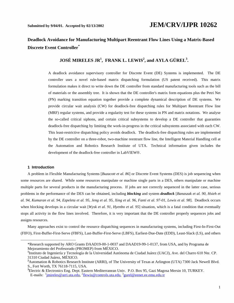
Submitted by 9/04/01. Accepted by 02/13/2002 JEM/CRV/IJPR 10262

Deadlock Avoidance for Manufacturing Multipart Reentrant Flow Lines Using a Matrix-Based

Discrete Event Controller*

JOSÉ MIRELES JR1, FRANK L. LEWIS2, and AYLA GÜREL3.

A deadlock avoidance supervisory controller for Discrete Event (DE) Systems is implemented. The DE

controller uses a novel rule-based matrix dispatching formulation (US patent received). This matrix

formulation makes it direct to write down the DE controller from standard manufacturing tools such as the bill

of materials or the assembly tree. It is shown that the DE controller's matrix form equations plus the Petri Net

(PN) marking transition equation together provide a complete dynamical description of DE systems. We

provide circular wait analysis (CW) for deadlock-free dispatching rules for Multipart Reentrant Flow line

(MRF) regular systems, and provide a regularity test for these systems in PN and matrix notations. We analyse

the so-called critical siphons, and certain critical subsystems to develop a DE controller that guaranties

deadlock-free dispatching by limiting the work-in-progress in the critical subsystems associated with each CW.

This least-restrictive dispatching policy avoids deadlock. The deadlock-free dispatching rules are implemented

by the DE controller on a three-robot, two-machine reentrant flow line, the Intelligent Material Handling cell at

the Automation and Robotics Research Institute of UTA. Technical information given includes the

development of the deadlock-free controller in LabVIEW.

1 Introduction A problem in Flexible Manufacturing Systems [Buzacott et al. 86] or Discrete Event Systems (DES) is job sequencing when

some resources are shared. While some resources manipulate or machine single parts in a DES, others manipulate or machine

multiple parts for several products in the manufacturing process. If jobs are not correctly sequenced in the latter case, serious

problems in the performance of the DES can be obtained, including blocking and system deadlock [Banaszak et al. 90, Hsieh et

al. 94, Kumaran et al. 94, Ezpeleta et al. 95, Jeng et al. 95, Xing et al. 96, Fanti et al. 97-01, Lewis et al. 98]. Deadlock occurs

when blocking develops in a circular wait [Wysk et al. 91, Hyenbo et al. 95] situation, which is a fatal condition that eventually

stops all activity in the flow lines involved. Therefore, it is very important that the DE controller properly sequences jobs and

assigns resources.

Many approaches exist to control the resource dispatching sequences in manufacturing systems, including First-In-First-Out

(FIFO), First-Buffer-First-Serve (FBFS), Last-Buffer-First-Serve (LBFS), Earliest-Due-Date (EDD), Least-Slack (LS), and others

*Research supported by ARO Grants DAAD19-00-1-0037 and DAAD19-99-1-0137, from USA, and by Programa de Mejoramiento del Profesorado (PROMEP) from MÉXICO. 1Instituto de Ingeniería y Tecnología de la Universidad Autónoma de Ciudad Juárez (UACJ), Ave. del Charro 610 Nte. CP. 31310 Ciudad Juárez, MÉXICO. 2Automation & Robotics Research Institute (ARRI), of The University of Texas at Arlington (UTA) 7300 Jack Newell Blvd. S., Fort Worth, TX 76118-7115, USA. 3Electric & Electronics Eng. Dept. Eastern Mediterranean Univ. P.O. Box 95, Gazi Magosa Mersin 10, TURKEY.

E-mails: 1jmireles@arri.uta.edu, 2flewis@controls.uta.edu, 3gurel@eenet.ee.emu.edu.tr

1

[Panwalkar et al 77]. Rigorous analysis for some of these algorithms has been done for the case of unbounded buffer lengths.

For instance, [Kumar et al. 92-95] has shown that LBFS yields bounded buffer stability in the case of a single part reentrant flow-

line (RF), However, in actual manufacturing systems, the buffer lengths are usually finite, which introduces the possibility of

system deadlock. Moreover, little rigorous work has been done for dispatching in multipart RF (MRF) with finite buffers. In this

paper we provide a technique for avoiding deadlock in MRF with finite buffers by restricting the work-in-progress (WIP) in

certain “critical subsystems”. This is a rigorous notion related to the idea of ‘CONWIP’ [Spearman et al. 90]. All computations

are performed using straightforward matrix algorithms, including computation of the critical subsystems, for any MRF in a certain

general class.

This paper presents the development and implementation of an augmented discrete event controller for MRF systems that is

based on the decision-making matrix formulation introduced in [Lewis 92, Lewis et al. 93ab]. Important features of this matrix

formulation are that it uses a logical algebra, not the Max/Plus algebra [Cofer et al. 92], and that it can be described directly from

standard manufacturing tools that detail product requirements, job sequencing [Warfield 73, Steward 62-81ab] and resource

requirements [Kusiak et al. 91-92].

We describe the DE controller (DEC) formulation, and show how to analyse and compute in matrix notation for regular MRF

systems the circular waits, their critical siphons, certain critical subsystems and critical resources. Regular systems do not contain

critical resources or key resources [Gurel et al. 00]. These critical resources are critical structured-placed resources that migh

lead to Second Level Deadlock (SLD) [Fanti et al. 97-01] situations in MRF/FMRF systems. We present a matrix regularity test

for the presence/absence of critical resources. Then, for regular MRF systems, we integrate deadlock-free dispatching rules into

our augmented DEC matrix formulation by limiting the work-in-progress (WIP) in the critical subsystems. This least-restrictive

dispatching policy avoids deadlock. We demonstrate that this matrix formulation is computationally efficient for control of MRF

systems. We provide an implementation example of the augmented DEC on a 3 robot Intelligent Material Handling (IMH)

robotic workcell at UTA’s Automation & Robotics Research Institute (ARRI). A detailed exposition of the development of the

DEC for the workcell is given, including all steps needed to implement the controller. Technical information includes this

implementation in a graphical environment, LabVIEW.

2 Matrix-Based Discrete Event Controller A novel Discrete Event Controller (DEC) for manufacturing workcells was described in [Lewis et al. 93-94, Pastravanu et al.

94a, Tacconi et al. 97, Mireles et al. 01a-b]. This DEC is based on matrices, and it was shown to have important advantages in

design, flexibility and computer simulation. The definition of the variables of the Discrete Event Controller is as follows. Let v

be the set of tasks or jobs used in the system, r the set of resources that implement/perform the tasks, u the set of inputs or parts

entering the DES. The DEC Model State Equation is described as

Cucurv uFuFrFvFx ⊗⊕⊗⊕⊗⊕⊗= (1)

where:

x is the task or state logical vector,

is the job sequencing matrix, vF

is the resource requirements matrix, rF

2

is the input matrix, uF

is the conflict resolution matrix, and ucF

uc is a conflict resolution vector.

This DEC equation is performed in the AND/OR algebra. That is, multiplication ⊗ represents logical “AND,” addition ⊕

represents logical “OR,” and the over-bar means logical negation (used as in [Pastravanu et al. 94].) From the model state

equation, the following four interpretations are obtained. The job sequencing matrix Fv reflects the states to be launched based on

the current finished jobs. It is the matrix used by [Steward 81ab] and others [Whitney 91] and can be written down from the

manufacturing Bill of Materials, by using knowledge representation for assembly planning [Wolter et al.. 92]. Harris has

demonstrated the capabilities of generating plans for this matrix representation [Harris 00]. The resource requirement matrix Fr

represents the set of resources needed to fire possible job states this is the matrix used by [Kusiak et al. 91-92]. The input matrix

Fu determines initial states fired from the input parts. The conflict resolution matrix Fuc prioritises states launched from the

external dispatching input u , which has to be derived via some decision making algorithm [Panwalkar et al. 77, Graves 81].

The importance of this equation is that it incorporates matrices F

C

v and Fr, previously used in heuristic manufacturing systems

analysis, into a rigorous mathematical framework for DE system computation.

For a complete DEC formulation, one must introduce additional matrices, Sr and Sv, as described next. The state logic

obtained from the state equation is used to calculate the jobs to be fired (or task commands), to release resources, and to inform

about the final products produced by the system. These three important features are obtained by using the three equations:

Start Equation (task commands) xSv VS ⊗= (2)

Resource Release Equation xSr rS ⊗= (3)

Product Output Equation xSy y ⊗= (4)

Figure 1 shows the DEC based on the matrix formulation as used to control job sequences and resource assignment of a

workcell. Subscript “s” on the vectors v and r denotes “start.” Thus, v and r are outputs from the workcell measured by sensors,

while vs and rs are commands to the workcell to begin jobs or set resources as “released.”

[insert figure 1 about here]

2.1 Matrix Formulation and Petri-Nets There is a very close relationship between the DEC just described and Petri Net (PN) tools [Zhou 93, Murata 89]. The

Incidence Matrix [Peterson 81] of the PN equivalent to the DE controller is obtained by defining the activity completion matrix

and the activity start matrix as:

Activity Completion Matrix ][ ucrvu FFFFF = (5)

Activity Start Matrix (6) TTuc

Tr

Tv

Tu SSSSS ][=

Then, the PN’s Incidence Matrix is defined as

],,,[ ucT

ucrT

rvT

vuT

uT FSFSFSFSFSM −−−−=−= , (7)

where Su and Suc are zero matrices.

3

If we define the set X containing the elements of x (the state controller vector), and A as the set of activities containing the

vectors v and r, (i.e. A= ), then it has been shown that (A,X,F

rv

T, S) is a PN [Pastravanu et al. 94ab]. This allows one to

directly draw the PN of a system given the matrices F and S or vice versa.

The elements of matrices F and S, are either ‘zero’ or ‘one’. FT is the PN input incidence matrix and S is the PN output

incidence matrix. The fi,j elements of Fv which are set to ‘one’, state that to fire transition xi, the job vj needs to be finished; the fi,j

elements of Fr set to ‘one’, indicate that to fire transition xi, the resource rj needs to be available; the si,j elements of Sv set to

‘one’, indicate that to start job vj, the transition xi needs to be finished; and the set of si,j elements from Sr are set to ‘one’ to

indicate that the resource ri is released after the transition xj is finished.

If the marking vector m(t) from a PN is defined as

m(t) = [ u ]Tc

TTT tutrtvt )(,)(,)(,)( T. (8)

For a specific time iteration t, then the PN marking transition equation [Peterson 81] is

. (9) )(][)()()1( txFStmxMtmtm TT −+=+=+

2.2 Complete Dynamical Description for DES A major gap in PN theory has been its inability to provide a complete dynamical description of a DES. The marking

transition equation (9) provides a partial description [Peterson 1981], but it is not known in the literature how to generate the

allowable firing vector x(t). This deficiency is repaired by using the matrix-based DEC controller equation (1) together with the

PN marking transition equation. The key is to note that the vector x(t) in (9) is identical to the vector x in the DEC equation (1) at

time t.

To put the DEC eqs. into a format convenient for simulation, one may write (1) as mFx ⊗= or

)(][][)()( turvuFFFFtmFtx cucrvu ⊕=⊕= (10)

The complete dynamical description of the DES, as described in [Mireles et al. 01-b], is provided by the PN marking eq. (9),

plus the DEC equation (10). Note that we are using the Timed Places Petri Net (TPPN) representation of PNs [López-Mellado

95].

To simulate DES on a digital computer, one must split (9) into two parts. Thus, m(t) is split into two vectors, the pending

marking vector mp and available resources and finished jobs marking vector ma,

)()()( tmtmtm pa +=. (11)

The pending marking vector contains all new jobs and any unfinished jobs or currently in process,

)()()1( txStmtm Tpp +=+

. (12)

The available marking vector equation takes away tokens from ma corresponding to which resources are no longer available and

the jobs that have just finished.

)()()1( txFtmtm aa −=+ . (13)

Note that adding (12) and (13) gives (9).

4

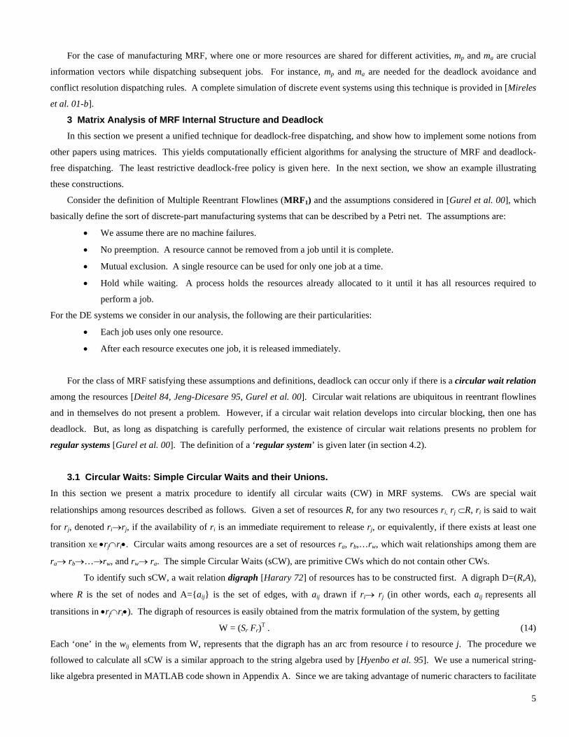
For the case of manufacturing MRF, where one or more resources are shared for different activities, mp and ma are crucial

information vectors while dispatching subsequent jobs. For instance, mp and ma are needed for the deadlock avoidance and

conflict resolution dispatching rules. A complete simulation of discrete event systems using this technique is provided in [Mireles

et al. 01-b].

3 Matrix Analysis of MRF Internal Structure and Deadlock In this section we present a unified technique for deadlock-free dispatching, and show how to implement some notions from

other papers using matrices. This yields computationally efficient algorithms for analysing the structure of MRF and deadlock-

free dispatching. The least restrictive deadlock-free policy is given here. In the next section, we show an example illustrating

these constructions.

Consider the definition of Multiple Reentrant Flowlines (MRF1) and the assumptions considered in [Gurel et al. 00], which

basically define the sort of discrete-part manufacturing systems that can be described by a Petri net. The assumptions are:

• We assume there are no machine failures.

• No preemption. A resource cannot be removed from a job until it is complete.

• Mutual exclusion. A single resource can be used for only one job at a time.

• Hold while waiting. A process holds the resources already allocated to it until it has all resources required to

perform a job.

For the DE systems we consider in our analysis, the following are their particularities:

• Each job uses only one resource.

• After each resource executes one job, it is released immediately.

For the class of MRF satisfying these assumptions and definitions, deadlock can occur only if there is a circular wait relation

among the resources [Deitel 84, Jeng-Dicesare 95, Gurel et al. 00]. Circular wait relations are ubiquitous in reentrant flowlines

and in themselves do not present a problem. However, if a circular wait relation develops into circular blocking, then one has

deadlock. But, as long as dispatching is carefully performed, the existence of circular wait relations presents no problem for

regular systems [Gurel et al. 00]. The definition of a ‘regular system’ is given later (in section 4.2).

3.1 Circular Waits: Simple Circular Waits and their Unions. In this section we present a matrix procedure to identify all circular waits (CW) in MRF systems. CWs are special wait

relationships among resources described as follows. Given a set of resources R, for any two resources ri, rj ⊂R, ri is said to wait

for rj, denoted ri→rj, if the availability of ri is an immediate requirement to release rj, or equivalently, if there exists at least one

transition x∈•rj∩ri•. Circular waits among resources are a set of resources ra, rb,…rw, which wait relationships among them are

ra→ rb→…→rw, and rw→ ra. The simple Circular Waits (sCW), are primitive CWs which do not contain other CWs.

To identify such sCW, a wait relation digraph [Harary 72] of resources has to be constructed first. A digraph D=(R,A),

where R is the set of nodes and A={aij} is the set of edges, with aij drawn if ri→ rj (in other words, each aij represents all

transitions in •rj∩ri•). The digraph of resources is easily obtained from the matrix formulation of the system, by getting

W = (Sr Fr)T . (14)

Each ‘one’ in the wij elements from W, represents that the digraph has an arc from resource i to resource j. The procedure we

followed to calculate all sCW is a similar approach to the string algebra used by [Hyenbo et al. 95]. We use a numerical string-

like algebra presented in MATLAB code shown in Appendix A. Since we are taking advantage of numeric characters to facilitate

5

multiplication of matrices, this algorithm is restricted to nine digits, and so we are restricted to identify all sCW of systems having

nine resources maximum. To increase the number of resources in the algorithm, we can use a binary approach (paper to appear),

but this is not our main concern in this paper. The number of rows of the resulting matrix from this algorithm is the number of

sCW, and its columns correspond to the resources present in the system. In this matrix, an entry of ‘one’ in position (i,j) means

that resource j is included in the ith sCW.

Unfortunately, to be able to analyze the MRF system and its possible deadlock structures we need to identify all CWs,

not only simple circular waits. The entire set of CWs are the sCW plus the circular waits composed of unions of non-disjoint

sCW (unions through shared resources among sCW.) In figure 2, we show a LabVIEW diagram that calculates all CWs from the

sets of all sCW; it uses Gurel’s algorithm (from [Lewis et al. 98]) in MATLAB script code but uses matrices for efficiency of

computations.

[insert figure 2 about here]

Using this diagram/code, we obtain two resulting matrices, Cout and G. Cout provides the set of resources which compose every

CW (in rows), that is, an entry of ‘one’ on every (i,j) position means that resource j is included in the ith CW. G provides the set

of composed CWs (rows) from unions of sCW (columns), that is, an entry of ‘one’ on every (i,j) position means that jth sCW is

included in the ith composed CW. In section 5.1 one can find the resulting matrices for a given example.

3.2 Deadlock Analysis: Identifying Critical Siphons and Critical Subsystems. In this section, we apply PN and matrix-based notions to calculate specific PN-place sets associated with each CW. The

determination of these sets is required so that we can identify possible circular blocking (CB) [Ezpeleta et al. 95, Xing et al. 96,

Lewis et al. 98, Gurel et al. 00] phenomena or deadlock situations. After computing the sets, we will provide computationally

efficient matrix-based algorithms for a least restrictive deadlock-free dispatching policy. These sets are highly tied to siphons

associated with each CW. A siphon set has a behavioural property that if it is token-free under some marking, then it will remain

token-free under each successor marking. Such property may leads to CB, i.e. deadlock. A set of places S is a siphon if and only

if for all places pi∈S one has • pi⊂Uj{pi• } for some {pj}⊂S.

Three important sets associated with the CWs C are the siphon-job sets Js(C), the critical siphons, Sc(C), and critical

subsystems, Jo(C). The critical siphon of a CW is the smallest siphon containing the CW. Note that if the critical siphon ever

becomes empty, the CW can never again receive any tokens. This is, the CW has become a circular blocking. The siphon-job

set, Js(C), is the set of jobs which, when added to the set of resources contained in CW C, yields the critical siphon. The critical

siphons of that CW C are the conjunction of sets Js(C) and C. The critical subsystems of the CW C, are the job sets J(C) from that

C not contained in the siphon-job set Js(C) of C. That is Jo(C)= J(C)\ Js(C). The job sets of CW C are defined by J(C) = ∪r∈C J(r),

for J(r)=r••∩J, where J is the set of all jobs.

We now provide computational tools to determine the siphon-job sets Js(C), the critical siphons, Sc(C), and critical

subsystems, Jo(C), for every CW C. To determine such sets, we need to calculate the set of adding transitions T and

clearing transitions . T are the set of transitions that, when fired, add tokens to the CW C. On the contrary,

are the set of transitions which, when fired, subtract tokens from C. are the set of input and output transitions

from C. These sets of transitions are important in keeping track of the tokens inside every CW C, and hence in determining the

status of tokens inside the critical siphon.

••+ = CC \C

CC ••− = \TC+C

−CT •• CC and

6

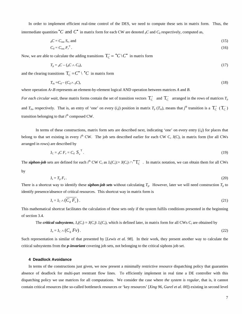
In order to implement efficient real-time control of the DES, we need to compute these sets in matrix form. Thus, the

intermediate quantities in matrix form for each CW are denoted •• CC and dC and Cd respectively, computed as,

dC = Cout Sr, and (15)

Cd = Cout FrT . (16)

Now, we are able to calculate the adding transitions T in matrix form ••+ = CC \C

Tp = dC – (dC ∧ Cd), (17)

and the clearing transitions in matrix form CC ••− = \TC

Tm =Cd – (Cd ∧ dC), (18)

where operation A∧B represents an element-by-element logical AND operation between matrices A and B.

For each circular wait, these matrix forms contain the set of transition vectors and T arranged in the rows of matrices T+CT −

C p

and Tm, respectively. That is, an entry of ‘one’ on every (i,j) position in matrix Tp (Tm), means that jth transition is a T ( T )

transition belonging to that i

+C

−C

th composed CW.

In terms of these constructions, matrix form sets are described next, indicating ‘one’ on every entry (i,j) for places that

belong to that set existing in every ith CW. The job sets described earlier for each CW C, J(C), in matrix form (for all CWs

arranged in rows) are described by

JC = dC Fv = Cd . (19) TvS

The siphon-job sets are defined for each ith CW Ci as Js(Ci):= J(Ci) ∩ . In matrix notation, we can obtain them for all CWs

by

+•CT

Js = Tp Fv . (20)

There is a shortcut way to identify these siphon-job sets without calculating Tp. However, later we will need construction Tp to

identify presence/absence of critical resources. This shortcut way in matrix form is

Js = JC ∧ )d vFC( . (21)

This mathematical shortcut facilitates the calculation of these sets only if the system fulfils conditions presented in the beginning

of section 3.4.

The critical subsystems, Jo(Ci) = J(Ci)\ Js(Ci), which is defined later, in matrix form for all CWs Ci are obtained by

Jo = JC ∧ . (22) )( d FvC

Such representation is similar of that presented by [Lewis et al. 98]. In their work, they present another way to calculate the

critical subsystems from the p-invariant covering job sets, not belonging to the critical siphons job set.

4 Deadlock Avoidance In terms of the constructions just given, we now present a minimally restrictive resource dispatching policy that guaranties

absence of deadlock for multi-part reentrant flow lines. To efficiently implement in real time a DE controller with this

dispatching policy we use matrices for all computations. We consider the case where the system is regular, that is, it cannot

contain critical resources (the so-called bottleneck resources or ‘key resources’ [Xing 96, Gurel et al. 00]) existing in second level

7

deadlock structures [Fanti et al. 97-01]. Section 4.2 describes a mathematical test to verify that the MRF system is regular. If

that is not the case, we can still use this matrix formulation, but with a different dispatching policy designed for systems

containing second level deadlock structures. We will present such dispatching policy in a forthcoming work.

4.1 Dispatching Policy In this section we consider dispatching for regular systems. A matrix test for nonregularity is given in the next section. In

[Lewis et al. 98] was given a minimally restrictive dispatching policy for regular systems that avoids deadlock for the class of

MRF considered in this paper. To understand this policy, note that, for this class of systems, a deadlock is equivalent to a circular

blocking (CB). There is a CB if and only if there is an empty circular wait (CW). However, this is possible (for regular systems)

iff the corresponding critical siphon is empty. By construction, this is equivalent to all jobs of the circular wait being in the

Critical Subsystem. In terms of PN, there is a deadlock iff all tokens of the CW are in the Critical Subsystem.

Therefore, the key to deadlock avoidance is to ensure that the WIP in the Critical Subsystems is limited to one less job

than the total number of initial tokens in the CW (i.e. the total number of resources available in the CW). Due to the necessity

and sufficiency of all the conditions just outlined, this MAXWIP policy is the least restrictive policy that guarantees absence of

deadlock. It is very easy to implement. Preliminary off-line computations using matrices are used to compute the Critical

Systems. A supervisor is assigned to each Critical Subsystem (CS) who is responsible for dynamic dispatching by counting the

jobs in that CS and ensuring that they do not violate the following condition, for each CW Ci,

m(Jo(Ci)) < mo(Ci). (23)

That is, the number of enabled places contained in the CS for each Ci must not reach the total number of resources contained in

that Ci.

For the implementation of the DE controller in this paper, and differing from the definition of sets considered in [Huang et al.

96, Lewis et al. 98, Gurel et al. 00], we are considering row vectors instead of column vectors (this is needed to separate properly

sets contained in each CW Ci.) That is, matrix form sets having ‘ones’ on every entry (i,j) indicate places that belong to that set

existing in every ith row CW.

In our implementation example, in every DE iteration, we use FBFS dispatching policy. Generally, FBFS maximizes WIP

and machine percent utilization. However, it is known that FBFS often results in deadlock. Therefore, we combine FBFS with

our deadlock avoidance test (23). Thus, before we dispatch the FBFS resolution, we examine the marking outcome with our

deadlock policy. If this resulting outcome does not satisfy (23), then the algorithm denies or pre-filters in real time the firing and

we apply again the FBFS conflict resolution strategy for the next possible allowable firing sequence. Therefore, using FBFS

while permitted, we will try to satisfy in most of the current status of the cell the case m(Jo(Ci)) = mo(Ci)-1. The later condition is

the so called MAXWIP policy, defined in [Huang et al. 96].

The dispatching policy for the case one has a regular system follows three main steps:

First, based on the structure of the system defined by matrices F and S, we use (22) to obtain for all CWs its corresponding

critical subsystems Jo(CW). In matrix form (having all CWs), Jomxn has m rows as CWs, and n columns as total # resource-jobs in

the system.

Second, for every DE-iteration, one must calculate from the current marking vector, mcurrent, the corresponding possible

successor-marking vector, mpossible. Equation (9), which can be split into eqs. (12) and (13) provide this possible successor

(ma(t+1) = mpossible, ma(t) = mcurrent). However, for a given mcurrent vector, since it is possible to have enabled more than one

transition rs•, for rs be a shared resource, marking mpossible can have negative elements due to (13). That is, it is possible that the

8

marking vector mpossible has negative number(s) in the r(t) section from the general marking vector m(t), if more than one resource-

jobs, v(t), are attempt to fire from one single shared resource, r(t)=rs (verify from (8) that r(t) is part of m(t), as well as v(t) and

uc(t)). That is why the marking mpossible has to be 'filtered' by a conflict resolution dispatching policy to deny negative elements.

We 'filter' negative numbers from mpossible by setting to zero the non-desired resource-jobs elements in vector uc(t) from the

current marking vector mcurrent. uc(t) is strategically preset full of ones in mcurrent before one starts every new DE iteration (set of

these three steps), and adjusted during the calculation of mpossible to solve any possible conflict on shared resources. This is how

we are able to calculate mpossible having no negative numbers.

Third, once selected the candidate mpossible, to avoid deadlock one must verify the condition m(Jo(Ci))<mo(Ci) for every CW

Ci. This can be accomplished by extracting from marking mpossible the v(t) vector, defined as vpossible, and performing

||Joi ^ vpossible|| < ||Couti|| (24)

for Joi be ith row vector from Jo, Couti be the ith row (or ith CW) vector from Cout, and ||V|| be the Σvi, for vi be the ith element of

vector V.

If for any DE iteration, (24) does not hold, one must eliminate the resource-job from vpossible that is attempting to cause circular

blocking in that ith CW. This elimination can be accomplished by a high order conflict resolution among different machines

(notice that for this case, this resolution is not among resource-jobs from a single resource-machine). The resource-jobs that

might attempt to cause deadlock problems are found by

vproblemi = (vpossible- (vpossible^ vcurrent))^Joi (25)

The high order conflict resolution strategy has to be accomplished among elements from each vproblemi, and the chosen resource-

job not to be fired must be cleared (set to zero) from uc from mcurrent and restart second step.

To be prepared for this high-order conflict resolution strategy for the DEC implementation, one must decide among strictly trap-

job sets contained in vectors Joi (for each ith CW). That is, one must decide among resource-jobs contained in ith row from JQs

when the following condition holds

||Joipossible || >= ||Couti||, (26)

for ||Joipossible || be the number of jobs contained in Jo present in the current vpossible vector from the ith CW. In words,

condition (26) verifies condition m(Jo(CW))<mo(CW) for the attempted firing vector vpossible, and if (26) holds, resolution among

jobs in vector vproblemi has to be solved. Such resource-jobs are contained in the same ith row from JQs.

4.2 Identifying Critical and Key Resources, Second Level Deadlock. There is a certain pathological case which requires extreme care in deadlock-avoidance dispatching. This case occurs

where there exist the so called Second Level Deadlock (SLD) [Fanti et al. 97-01] structures in the system. SLD exist on the

presence of critical resources, known as bottlenecks [Gurel et al 00], and key resources [Xing 96]. Gurel refers to bottleneck

resources as the structured-placed bottleneck resources, not the well known timed bottleneck resources. These structures are

identified by analysing interconnectivities in circular wait relationships and its siphons [Xing 96, Gurel et al 00] and/or by

accomplishing digraph connectivity-analysis on resources and jobs [Fanti et al. 97-01]. We now define these critical resource

structures using matrices.

The following refinements are needed later for the definition of critical resources in matrix form. These sets indicate

‘one’ on every entry (i,j) for places that belong to that set existing in every ith CW, Ci.

The trap-job set for every ith CW Ci, defined as JQ(Ci) = J(Ci) ∩ , is computed in the i•−

CT th row of the matrix

9

JQ = Tm . (27) TvS

The siphon-trap-job sets, JSQ(Ci) = Js(Ci)∩JQ(Ci), are the intersection of the siphon-job and trap-job sets,

which in matrix notation, they are

JSQ = Js ∧JQ (28)

The strictly siphon-job set is defined as (CsJ i) = Js(Ci) \ JSQ(Ci), and in matrix form it is

JSs = Js – (Js ∧ JSQ) (29)

The strictly trap-job set is defined as J (CQˆ

i) = JQ(Ci) \ JSQ(Ci) ), and in matrix form it is

JQs = JQ – (JQ ∧JSQ) (30)

The neutral-job set is defined as JN(Ci) = J(Ci)\ ( (CsJ i) (CQJ∪ i)), and in matrix form it is

JN = JC – [JC ∧(JSs + JQs)] ) (31)

The strictly neutral-job set is defined as (CNJ i) = JN(Ci) \ JSQ(Ci), and in matrix form it is

JNs = JC – (JC ∧ JSQ) (32)

The earlier described critical subsystems, Jo(Ci), which are needed in our deadlock-free algorithm, can also be defined from these

quantities for all CW by

Jo = JQs ∨ JNs . (33)

For the calculation of critical resources, and regularity test of the MRF system, we need to identify the precedent

transitions Tpre(Ci) and the posterior transitions Tpos(Ci) for the associated critical subsystem. They are defined as

Tpre(Ci) = •QJ (Ci) = •Jo(Ci) \ Jo(Ci)•, which once they are fired will augment by 1 the number of tokens in the critical

subsystem associated to Ci, and

Tpos(Ci)= •sJ (Ci)= Jo(Ci) • \ •Jo(Ci), which once they are fired will diminish by 1 the number of tokens in the critical

subsystem associated to C.

The sets Tpre(Ci) and Tpos(Ci) are determined respectively in matrix form for all C in the system by

Tpre = ( Jo Sv ) – [ ( Jo Sv ) ∧( Jo FvT) ] , and (34)

Tpos = (Jo FvT) – [ ( Jo Sv ) ∧( Jo Fv

T) ] (35)

To define critical resources, we must determine the presence of cyclic circular wait (CCW) loops in the DE system.

These specify a particular sharing among circular waits that needs special attention for deadlock-free dispatching [Xing 96, Gurel

et al. 00], and are a requisite for existence of critical resources. These are structured-placed (among CWs) bottlenecks. To

identify whether if the system has cyclic circular wait (CCW) loops, let Ci and Cj be two circular waits with

Tpos(Ci) ∩Tpre(Cj)≠∅ and Tpre(Ci) ∩Tpos(Cj)≠∅. (36)

If that is the case, then we got a CCW. The matrix test to find CCW loops among all CWs is

CCW = (Tpre TposT) ∧ (Tpre Tpos

T)T. (37)

If we define || C || = Σcij, for cij be the (i,j) element of matrix C, then, if ||CCW|| > 0 we have an irregular system,

otherwise, the system is regular. If we have CCW loops, CCW is a symmetric matrix having non-zero elements in each ccwij, for

CW i (indicated by row i from CCW) and CW j (column) be respectively Ci and Cj from [19].

10

The transitions that interconnect such CCWs are needed to define critical resources. We can use matrix CCW and the

precedent and posterior matrix transitions Tpre and Tpos to identify such transitions.

preT =(CCW Tpos) ∧ Tpre (38)

posT =(CCW Tpre) ∧ Tpos (39)

We call them the cyclic precedent and cyclic posterior transitions, (38) and (39) respectively.

The definition of a critical CW is as follows: Given PN N, and its initial marking mo, let {Ci, Cj} be a CCW such that

| Ci ∩ Cj | = 1 and let Ci ∩ Cj = {rb}. If Tpos(Ci)∩ Tpre(Cj) ⊂ rb• and Tpos(Cj)∩ Tpre(Ci) ⊂ rb

•, then {Ci, Cj } is said to be a critical

CW and rb is called its critical resource (structured-placed bottleneck resource [Gurel et al. 00]). If in addition mo(rb) = 1, then rb

is called key resource.

Then, since we already identify the cyclic precedent and cyclic posterior transitions for all CCW in the system, we can

proceed to identify the critical resources using the following straightforward matrix formula

ResCW = (T Fposˆ

r) ∧ (T Fpreˆ

r) (40)

ResCW provides, for each CW, the set of critical resources shared with other CWs in one or more CCW. If this matrix is

zero, there are no critical resources and hence no key resources. Further analysis of shared critical resources will be described in a

forthcoming paper soon.

[insert figure 3 about here]

[insert figure 4 about here]

5 Implementation With the purpose of showing the flexibility of this matrix approach, consider two possible PN structures A and B, shown

respectively in figures 3 and 4, which can be implemented in the Intelligent Material Handling cell of ARRI to ‘manufacture’ two

products. We use term ‘manufacture’ since our machines are simulated machines. However, our resources are real robotic

systems which we intent to perform the MRF sequence problem. By applying steps from sections 3 and 4.2, we will show that

one of these systems is irregular. Then, we implement the deadlock-free dispatching in the regular system. The Fv, SvT, Fr and Sr

T

matrices for these PN systems are shown in LabVIEW discrete format in figures 5 and 6. In the LabVIEW discrete representation

of matrices, each black circle is a ‘one’ and the others are ‘zero’.

[insert figure 5 about here]

[insert figure 6 about here]

5.1 Determining the MRF Structure Taking advantage that LabVIEW can use MATLAB script code, we created a small program that uses matrices Sr

T and

Fr, to internally calculate the digraph matrix W, (14), and use MATLAB script code to get the matrix containing the simple

circular waits, sCW, for both systems. The diagram code for this small program is shown in figure 7. Not all MATLAB code is

shown in this diagram because the MATLAB script window was resized, the complete MATLAB code is presented in Appendix

A. Also, in LabVIEW, we can represent each program in a single block-function, which can be used inside diagram code from

other programs. Figure 8 shows the representation of such block-function which diagram is shown in figure 7. Later, we will

show the entire LabVIEW diagram containing all interconnected block-functions. The digraph of resources, W matrix, for

systems A and B is shown in figure 9. The output matrix, shown as L (for loops) in figures 7 and 8, contains all simple circular

waits (sCW) from systems A and B and they are shown in figure 10.

11

[insert figure 7 about here]

[insert figure 8 about here]

[insert figure 9 about here]

[insert figure 10 about here]

From the number of rows in matrices from figure 10, we can see that we found two sCW in system A, and three sCW in

system B. System A has one sCW composed by R3 and M1 and other composed by resources R2 and M2. System B has one

sCW composed by M1 and R1, other composed by M2 and R2, and the third one composed by resources C1, C2, R1 and R2.

The next step is to use Gurel’s algorithm to calculate matrix Cout (shown in figure 2). For our system A, Cout is equal to

matrix sCW, and G matrix is a 2x2 identity matrix. That means that there is no shared resource interconnecting any sCW, and

that the system does not have composed circular waits. At this point, we can say that there is not critical resources in system A,

because critical resources are resources that interconnect CW or sCW (if we continue performing the analysis for system A, we

will get this conclusion, i.e. system A does not have critical resources, and so that system A is a regular). But, even if we have

shared resources among sCW, that does not guarantee we have critical resources in the system. That is why we offer the matrix

test (37). For system B, figure 11 parts a) and b) show the resulting matrices Cout and G. Figure 11 part c) shows the block

representation of Gurel's algorithm/diagram from figure 2, showing output matrices, Cout and G, on its right side. We remind the

reader that G provides the set of composed CWs (rows) from unions of sCW (columns), that is why, as an example from system

B, the set of resources of composed CW C4 (composed of resources on 4th row of Cout) contain the resources from sCW C1 (1st

column of G) and sCW C3 (3rd column of G). System B has a total of six CWs, three sCW (first three rows of Cout) and three

composed of unions of such sCW (last three rows of Cout).

[insert figure 11 about here]

[insert figure 12 about here]

5.2 Verifying Absence of Critical Resources, Regularity test At this point, we need to verify whether if system B has a critical resource. For that, we follow the procedure in section

4.2. First, we calculate the input and output transitions for every CW in matrices dC and Cd, equations (15) and (16). For system

B, these set of transitions are shown in figure 12.

Once found the input and output transitions for each cycle or CW, we proceed to calculate the adding, clearing

transitions and the job sets, Tp, Tm and JC respectively, by using eqs. (17), (18) and (19). Tp and Tm are needed to calculate the

siphon-job and trap-job sets, and with these constructions, we calculate the critical subsystems for each CW of the system. Matrix

Jo contains all critical subsystems for all CWs of the system. Figure 13 shows the LabVIEW diagram code that implements eqs.

(15) through (22) and (27) though (33). Figure 14 shows resulting matrices from eqs. (26)-(36) for system B.

[insert figure 13 about here]

[insert figure 14 about here]

We present in figure 15 the adding, clearing and the intersection of input and output transitions for the first CW shown in

the first row of Cout (composed of resources M1 and R1). This result is obtained by combining resulting matrices from figure 12

and matrices Tp and Tm (denoted as “T+” and “T-” respectively in figure 14).

[insert figure 15 about here]

The last step is described in section 4.2, which provides the formulation to identify possible critical resources using the

matrices we just got. Applying eqs. (34) and (35), the corresponding precedent and posterior transitions for each CW are

contained in matrices Tpre and Tpos respectively, and shown in figure 16.

12

If eqn. (36) is satisfied, we got a cyclic circular wait composed of two or more CWs. For system B, condition (36) is

TRUE for the case i=2 and j=3 or j=4. Figure 17 part a) shows the resulting matrix test CCW. We can see that we had just found

that for system B, CW C2 is connected with CWs C3 and C4 through a critical resource. This means that C2 can be described as Ci

and that CW3 and CW4 can be described as Cj as defined in condition (36).

The calculated ResCW matrix is shown in figure 17, part b). We can see that the shared critical resource for our system B

is R2, which relates C2, C3 and C4. Since mo(R2) = 1, R2 is a key resource. We conclude System B is an irregular system.

[insert figure 16 about here]

[insert figure 17 about here]

[insert figure 18 about here]

[insert figure 19 about here]

5.3 Implementation of Deadlock Avoidance Policy on Regular Systems

Once proven that system A is a regular system, to implement the deadlock-free dispatching rule, we proceed to follow

steps shown in Section 4.1. First, we calculate the critical subsystems matrix Jo. Such matrix can be found by using the

LabVIEW diagram shown in figure 13. Figure 18 shows the resulting Jo matrix for system A.

The subsequent explanations will refer to figure 19, which shows the LabVIEW diagram containing the main loop of the

DE real time controller implemented at ARRI. The input parameters to the main WHILE loop are shown in the left side of the

figure. The input parameters are Matrices F and S, critical subsystems and initial marking vectors.

Matrices F and S are concatenated by the blocks near the denoted circles (A) and (B) using a LabVIEW concatenation

function-block. Notice that two extra matrices were added to such matrices F and S, Fy and Fx. Matrix Fy is the output matrix of

the system, and matrix Fx is an extra matrix needed to facilitate the control of firing transitions and number of tokens in the DE

controller system. The use of these matrices will be explained in a forthcoming paper soon. They do not alter the matrix

formulation, the deadlock-free dispatching policy, neither all calculations contained in this paper.

For the implementation of this DE controller, the critical subsystems are an input parameter to the main loop. This

means that the critical subsystems are pre-calculated before the DE controller loop starts. The denoted circle (C), refers to the

block shown in figure 8, which calculates the simple circular waits sCW of the system. Then, the block near to denoted circle

(D), uses these sCW in matrix form, and matrices Fv, Fr, Sv, and Sr, to calculate the siphon-job sets, the critical subsystems and the

number of resources associated for each CW (as calculated by LabVIEW function-blocks on figure 13). Notice that system A

does not contain any composed circular waits, but this block (near denoted circle (D)) calculates them internally (if any) and

verifies that the system is regular.

The other input parameters to the main WHILE loop are the initial marking vectors of the DE system. Two marking

vectors are used, the one defined in (8) with the addition of vectors y(t) and x(t) (the output marking vector, and the extra marking

vector needed for matrix Fx), and a sensors marking vector. The sensors marking vector was included to facilitate the control of

information provided from the sensors in the simulated machines M1 and M2. The detail of this implementation will be

published in a technical paper. Again, these extra vectors do not need any further mathematical explanation or add complication

to the current analysis of this paper.

The main loop performs the second and third steps described in section 4.1. Before we start performing these steps, the

DE controller has to update the marking vector depending on the information provided by the sensors in the cell. This is

accomplished by the block below remark circle (E), inside the main WHILE loop. After the refinement of the sensor marking

vector is made, steps two and three are applied inside the internal WHILE loop having denoted marks (F)-(I).

13

The second step is performed in remarks (F), (G) and (H). Equations (10) and (9) are accomplished inside the block

below remark circle (F). This block receives mcurrent and obtains a candidate mpossible (as described in the first part of the second

step of section 4.1). Then, block over remark circle (G) filters the mcurrent, depending on the first outcome mpossible for the case it

needs to perform conflict resolution on shared resources. That is, for the case mpossible has negative numbers. The resulting vector

from block denoted (G) will be a new mcurrent vector that will not lead any conflict on the subsequent outcome vector mpossible.

Equations (10) and (9) are accomplished again in block denoted with remark circle (H) and the resulting vector is a marking

mpossible without any negative numbers.

The third step is performed in remark (I). Block denoted in remark (I) verifies condition (24) and applies equation (25),

if necessary. That is, it compares subset marking vector vpossible with each of Jo, and if necessary, calculates the resource-jobs that

attempt to cause a deadlock problem, vproblemi. If necessary, the same block performs a high order conflict resolution strategy. If

that is the case, a TRUE signal is activated to perform a second iteration of the entire sequence of steps in section 4.1, but with a

new filtered marking vector mcurrent having ‘zeros’ on the non-desired jobs on its uc(t) vector (as detailed on second step from

section 4.1). Otherwise, it uses the resulting mpossible marking from denoted block (H) as the resulting firing marking vector.

Figure 20 shows the Discrete Events of the implementation run for system A. This figure was obtained in real-time

directly from our DE controller implementation in LabVIEW. On the figure the discrete duration of the robotic jobs are shown.

Every line represents a discrete event for every robotic job, and it has only two states, high and low (or ON and OFF), meaning

executing robotic job and not executting such robotic job respectively. Notice that for every robot/resource (R1x, R2x and R3x),

only one robotic job goes high at any time.

[insert figure 20 about here]

6. Conclusions.

We presented a deadlock avoidance supervisory DE controller for Multipart Reentrant Flow line (MRF) regular systems.

A regularity test for MRF systems was provided. This test was presented in matrix form, and identifies critical and key resources

shared among circular resource loops that lead to second level deadlock structures on MRF systems. The DE controller presented

here uses a rule-based matrix dispatching formulation. On-line deadlock-free dispatching rules for MRF systems were

implemented by this DE matrix controller. This was accomplished by analysing circular waits for possible deadlock situations

while analysing the so-called critical siphons, and certain critical subsystems. In addition to deadlock-free dispatching rules,

conflict resolution strategies are implemented by the DE controller. Technical information given included the development of the

deadlock-free controller and implementation in a graphical environment, LabVIEW®. Future research on Free-choice MRF

systems, second level deadlock structures having critical resources, as well as shared resource conflict resolution strategies will be

performed.

14

Appendix A: String algebra algorithm function [L] = StringM(W) % This program finds loops in Adjacency matrices or Digraphs matrices % It finds all simple Circular Waits (CW) between resources. % The limitation is a 9x9 matrix, i.e. nine resources !! % %example: For his Digraph, you can see that there are nine simple loops: % r1 r2 r3 r4 r5 %W=[0 0 1 1 0 % r1 (Two arcs connect Resource 1 to resources 3 and 4.) % 1 0 1 0 1 % r2 % 1 1 0 0 1 % r3 % 0 1 0 0 1 % r4 % 0 0 0 1 0]; % r5 % %[c] = StringM(W) % % The output is: % Loops = [13, 23, 45, 132, 142, 1254, 2354, 1423, 13542 ] % So, loops are formed between resources {1 and 3}, {2 and 3}, {4 and 5}, {1, 3 and 2}, etc. [a,b] = size(W); w=W; % This part fixes the '1' row elements by 'row' for row=2:a w(row,:)=W(row,:)*row; end %w = 0 0 1 1 0 % 2 0 2 0 2 % 3 3 0 0 3 % 0 4 0 0 4 % 0 0 0 5 0 % We are only interested in the premultiplication of the upper triangular elements BB = triu(w); BB = BB-diag(diag(BB)); %BB = 0 0 1 1 0 % 0 0 2 0 2 % 0 0 0 0 3 % 0 0 0 0 4 % 0 0 0 0 0 Loops=0; % Initially no Loops are identified ! while (sum(sum(BB))>0) [BBrow,BBcol] = size(BB); if (BBcol==a) W1 = BB; BB = 0; else W1(:,1:b)=BB(:,1:b); BB=BB(:,a+1:BBcol); end % This part eliminates one matrix from BB and fills it in W1. % W1 will generate (possibly) more childs (the travel of the token) % Such matrix childs will be safe on BB again. % For example, when m=3: for m=1:a %Creates first matrices from rows of w A=w(m,:); AA = A; for num = 2:b AA = [AA;A.*ones(1,a)]; end %AA = 3 3 0 0 3 % 3 3 0 0 3 % 3 3 0 0 3 % 3 3 0 0 3 % 3 3 0 0 3 %Adds column *10 from W1 B=W1(:,m); for num = 2:b B = [B,W1(:,m)]; end %B = 1 1 1 1 1 % 2 2 2 2 2 % 0 0 0 0 0 % 0 0 0 0 0 % 0 0 0 0 0 if (sum(sum(B)))>0

15

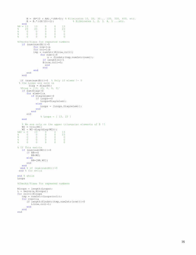
B = (B*10 + AA).*(AA>0); % Eliminates 10, 20, 30... 120, 320, 450, etc. B = B.*((B/10)>1); % Eliminates 1, 2, 3, 4, 5 ...etc. end %B = 13 13 0 0 13 % 23 23 0 0 23 % 0 0 0 0 0 % 0 0 0 0 0 % 0 0 0 0 0 %Checks/fixes for repeated numbers if (sum(sum(B)))>0 for row=1:a for col=1:b tmp = num2str(B(row,col)); for num=1:9 n = findstr(tmp,num2str(num)); if length(n)>1 B(row,col)=0; end end end end end if (sum(sum(B)))>0 % Only if elems != 0 % the Loops are save in Diag = diag(B); %Diag = [13, 23, 0, 0, 0]' if sum(Diag)>0 for elem=1:a if Diag(elem)>0 if Loops==0 Loops=Diag(elem); else Loops = [Loops,Diag(elem)]; end end end % Loops = [ 13, 23 ] end % We are only on the upper triangular elements of B !! W2 = triu(B); W2 = W2-diag(diag(W2)); %W2 = 0 13 0 0 13 % 0 0 0 0 23 % 0 0 0 0 0 % 0 0 0 0 0 % 0 0 0 0 0 % If This matrix if (sum(sum(W2)))>0 if BB==0 BB=W2; else BB=[BB,W2]; end end end % if (sum(sum(B)))>0 end % for m=1:a end % while Loops %Checks/fixes for repeated numbers Nloops = length(Loops); L = zeros(a,Nloops); for col=1:Nloops tmp = num2str(Loops(col)); for row=1:a if length(findstr(tmp,num2str(row)))>0 L(row,col)=1; end end end

16

References ANTSAKLIS, P.J. and PASSINO, K.M., 1992, An Introduction To Intelligent And Autonomous Control Systems. (Kluwer,

Boston, MA.)

BANASZAK, Z. A. and KROGH, B. H., 1990 Deadlock avoidance in flexible manufacturing systems with concurrently

competing process flows. IEEE Trans. Robotics and Automation, RA-6, pp. 724-734.

BUZACOTT, J.A. and YAO, D.D., 1986, Flexible manufacturing systems: A Review of Analytical Models. Management Sci. 7,

pp. 890-905.

COFER, D. D. and GARG, V.K., 1992, A timed model for the control of discrete event systems involving decisions in the

Max/Plus algebra. Proc. Of the 31st Conf. On Decision and Control, pp.3363-3368.

EZPELETA S. D., COLOM, J. M., and MARTINEZ, J., 1995, A Petri Net based deadlock prevention policy for flexible

manufacturing systems. IEEE Trans. Robotics and Automation, RA-11, pp. 173-184.

FANTI M.P., MAIONE, B., MASCOLO, S., and TURCHIANO, B., 1997, Event-based feedback control for deadlock avoidance

in flexible production systems. IEEE Transactions on Robotics and Automation, 13 (3).

FANTI M.P., MAIONE, B., and TURCHIANO, B., 2001, Distributed event-control for deadlock avoidance in automated

manufacturing systems. International Journal of Production Research, 39 (9), pp. 1993-2021.

GRAVES S.C. A review of production scheduling., 1981, Operations Research, 29 (4).

GUREL A., BOGDAN, S., and LEWIS, F.L. , 2000, Matrix approach to deadlock-free dispatching in multi-class finite buffer

flowlines. IEEE Transactions on Automatic Control, 45 (11), pp. 2086-2090.

HARARY F. Graph Theory., 1972, (Addison-Wesley Pub. Co., Massachusetts).

HARRIS B., COOK, D., and LEWIS, F., 2000, Automatically Generating Plans for Manufacturing. Journal of Intelligent

Systems, 10 (3), pp. 279-319.

HSIEH F.-S., and CHANG, S.-C., 1994, Dispatching-driven deadlock avoidance controller synthesis for flexible manufacturing

systems. IEEE Trans. Robotics and Automation, RA-11, pp. 196-209.

HUANG H.-H., LEWIS, F.L., and TACCONI, D., 1996, Deadlock analysis using a new matrix-based controller for reentrant

flow line design. Proceedings of the 1996 Industrial Electronics, Control, and Instrumentation. IEEE IECON 22nd

International Conference on, 1, pp. 463 -468.

HYUENBO C., KUMARAN, T. K., and WYSK, R. A., 1995, Graph-theoretic deadlock detection and resolution for flexible

manufacturing systems. IEEE Transactions on Robotics and Automation, 11 (3), pp. 413-421.

JENG M.D., and DICESARE, F., 1995, Synthesis using resource control nets for modelling shared-resource systems. IEEE

Trans. Robotics and Automation, RA-11, pp. 317-327.

KUMAR, S. and KUMAR, P. R., 1992, Performance bound for queueing networks and scheduling policies. Technical report,

Coordinated Science Lab., U. of Illinois, Urbana, IL.

KUMAR, P.R., 1993, Re-entrant lines, Queueing systems: theory and applications. Switzerland, 13, pp. 87-110.

17

KUMAR, P.R. and KUMAR, S. P., 1995, Stability of queueing networks and scheduling polices. IEEE Trans. In Automatic

Contrl, 40 (2), pp. 251-260.

KUMARAN, T. K., CHANG, W., CHO, N., and WYSK, R. A., 1994, A structured approach to deadlock detection, avoidance,

and solution in flexible manufacturing systems. International Journal of Production Research, 32, pp. 2361-2379.

KUSIAK, A. and AHN, J., 1991, A resource-constrained job shop scheduling problem with general precedence constraints.

Working paper, no. 90-03, Iowa.

KUSIAK A. and AHN, J., 1992, Intelligent scheduling of automated machining systems. Computer Integrated Manufacturing

Systems, 5 (1), pp.3-14.

LEWIS F. L., 1992, A control system design philosophy for discrete event manufacturing systems. Proc. Int. Symp. Implicit and

Nonlinear Systems, pp. 42-50, Arlington, TX.

LEWIS, F.L., HUANG, H.-H., and JAGANNATHAN, S., 1993a, A systems approach to discrete event controller design for

manufacturing systems control. Proceedings of the 1993 American Control Conference (IEEE Cat. No.93CH3225-0).

American Autom. Control Council, Evanston, IL, USA, 2, pp.1525-1531.

LEWIS F.L., PASTRAVANU, O.C., and HUANG, H.-H., 1993b, Controller design and conflict resolution for discrete event

manufacturing systems. Proceedings of the 32nd IEEE Conference on Decision and Control (Cat. No.93CH3307-6).

IEEE, New York, NY, USA, (4), pp. 3288-3293.

LEWIS F.L., and HUANG, H.-H., 1994a, Control system design for flexible manufacturing systems, In A. Raouf and M. Ben

Daya, Flexible Manufacturing Systems: Recent Developments, Elsevier (1994 a).

LEWIS F.L., HUANG, H.-H., PASTRAVANU, O.C., and A. GÜREL., 1994b, A matrix formulation for design and analysis of

discrete event manufacturing systems with shared resources. 1994 IEEE International Conference on Systems, Man, and

Cybernetics. Humans, Information and Technology (Cat. No.94CH3571-5). 2, New York, NY, USA. pp.1700-1705.

LEWIS F.L., GUREL A., BOGDAN S., DOCANALP A., PASTRAVANU O.C., 1998, Analysis of deadlock and circular waits

using a matrix model for flexible manufacturing systems. Automatica, 34 (9), pp.1083-100. Publisher: Elsevier, UK.

LÓPEZ-MELLADO E., 1995, Simulation of timed petri net models. Systems, Man and Cybernetics, 1995. Intelligent Systems for

the 21st Century., IEEE International Conference on , Volume: 3 , pp. 2270 –2273.

MIRELES, J. and LEWIS, F.L., 2001a, On the development and implementation of a matrix-based discrete event controller.

MED01, Proceedings of the 9th Mediterranean Conference on Control and Automation. June 27-29 2001. Dubrovnik,

Croatia. Published on CD, reference MED01-012.

MIRELES, J., and LEWIS F.L., 2001b, Intelligent material handling: development and implementation of a matrix-based discrete

event controller. IEEE Transactions on Industrial Electronics, 48 (6), pp. 1087-1097.

MURATA, T., 1989, Petri Nets: properties, analysis and applications. Proceedings of the IEEE, 77 (4), pp.541-580.

PANWALKAR S.S. and ISKANDER, W., 1977, A survey of scheduling rules, Operations Research, 26, pp. 45-61.

18

PASTRAVANU O.C., GÜREL, A., LEWIS, F. L. and HUANG, H.-H., 1994a, Rule-based controller design algorithm for

discrete event manufacturing systems. Proceedings of the 1994 American Control Conference (Cat. No.94CH3390-2).

IEEE, New York, NY, USA, 1, pp.299-305.

PASTRAVANU, O. C., GÜREL, A. and LEWIS, F. L. 1994b, Petri Net based deadlock analysis in flowshops with kanban-type

controllers. 10th ISPE/IFAC International Conference on CAD/CAM, Robotics and Factories of the Future CARs & FOF

`94. Information Technology for Modern Manufacturing. Conference Proceedings. OCRI Publications. pp.75-80. Kanata,

Ont., Canada.

PETERSON J.L. 1981, Petri Net theory and the modelling of systems. Prentice-Hall., Englewood Cliffs, NJ, USA.

STEWARD, D.V., 1962, On an approach to techniques for the analysis of the structure of large systems of equations. SIAM

Review, 4 (4), pp. 321-342.

STEWARD, D. V., 1981a, The design structure system: a method for managing the design of complex systems. IEEE Trans. On

Engineering Management, EM-28 (3), pp. 71-74.

STEWARD, D. V., 1981b, Systems analysis and management: structure, strategy, and design. (Petrocelli Books, New York.)

SPEARMAN, M.L., WOODRUFF, D.L., and HOPP, W.J., 1990, CONWIP: a pull alternative to Kanban. Int. J. Production

Research, 28 (5), pp. 879-894.

TACCONI D.A. and LEWIS F.L., 1997, A new matrix model for discrete event systems: application to simulation. IEEE Control

Systems.

WARFIELD J. N., 1973, Binary matrices in system modeling. IEEE Transactions on Systems, Man & Cybernetics, SMC-3 (5),

pp.441-9. USA.

WHITNEY D. E., EPPINGER, S.D., SMITH R.P, and GEBALA, D.A.., 1991, Organizing the tasks in complex design projects.

Computer-Aided Cooperative Product Development. MIT-JSME Workshop Proceedings. Berlin, Germany, Springer-

Verlag. pp. 229-252.

WOLTER, J., CHAKRABARTY, S., and TSAO J., 1992, Mating constraint languages for assembly sequence planning.

Proceedings. 1992 IEEE International Conference on Robotics And Automation (Cat. No.92CH3140-1). IEEE Computer

Soc. Press., Los Alamitos, CA, USA., 3, pp.2367-2374.

WYSK, R. A., YANG, N. S. and JOSHI, S., 1991, Detection of deadlocks in flexible manufacturing cells. IEEE Trans. Robotics

Automation, RA-7, 853-859.

XING K. Y., HU, B.S., and CHEN, H.X., 1996, Deadlock avoidance policy for petri-net modeling of flexible manufacturing

systems with shared resources. Automatic Control, IEEE Transactions on , 41, issue 2 , Pp. 289-295.

ZHOU M., and DICESARE, F., 1993, Petri Nets Synthesis For Discrete Event Control Of Manufacturing Systems, (Kluwer

Academic Publishers.)

19