A Continuum Model for a Re-entrant Factory

OPERATIONS RESEARCHVol. 54, No. 5, September–October 2006, pp. 933–950issn 0030-364X �eissn 1526-5463 �06 �5405 �0933

informs ®

doi 10.1287/opre.1060.0321©2006 INFORMS

A Continuum Model for a Re-entrant Factory

Dieter ArmbrusterDepartment of Mathematics, Arizona State University, Tempe, Arizona 85287-1804, [email protected]

Daniel E. MarthalerNorthrup Grumman Integrated Systems, Western Region, 17066 Goldentop Road, 9V21/R3-2, San Diego, California 92127-2412,

[email protected]

Christian RinghoferDepartment of Mathematics, Arizona State University, Tempe, Arizona 85287-1804, [email protected]

Karl KempfDecision Technologies, Intel Corporation, 5000 West Chandler Boulevard, MS CH3-10, Chandler, Arizona 85226,

[email protected]

Tae-Chang JoMathematics Department, Inha University, 253, Yonghyun-Dong, Nam-Ku, Incheon, 402-751, South Korea, [email protected]

High-volume, multistage continuous production flow through a re-entrant factory is modeled through a conservation lawfor a continuous-density variable on a continuous-production line augmented by a state equation for the speed of theproduction along the production line. The resulting nonlinear, nonlocal hyperbolic conservation law allows fast and accuratesimulations. Little’s law is built into the model. It is argued that the state equation for a re-entrant factory should benonlinear. Comparisons of simulations of the partial differential equation (PDE) model and discrete-event simulations arepresented. A general analysis of the model shows that for any nonlinear state equation there exist two steady states ofproduction below a critical start rate: A high-volume, high-throughput time state and a low-volume, low-throughput timestate. The stability of the low-volume state is proved. Output is controlled by adjusting the start rate to a changed demandrate. Two linear factories and a re-entrant factory, each one modeled by a hyperbolic conservation law, are linked to provideproof of concept for efficient supply chain simulations. Instantaneous density and flux through the supply chain as well aswork in progress (WIP) and output as a function of time are presented. Extensions to include multiple product flows andpreference rules for products and dispatch rules for re-entrant choices are discussed.

Subject classifications : production/scheduling: approximations; simulations: efficiency; mathematics.Area of review : Manufacturing, Service, and Supply Chain Operations.History : Received January 2003; revisions received October 2003, April 2004, April 2005; accepted September 2005.

1. IntroductionIn recent years, fast scalable simulations of productionflows in a supply chain have become an important researchtopic (Scalable Enterprise Initiative 1999). While the long-term goal is to optimize production across the whole sup-ply chain, an intermediate goal is to generate simulationtools that support the exploration of business questions,and to pose “what if?” questions on these simulations.Because most production deals with individual parts andthe processes that these parts undergo, the natural methodof choice for accurate simulations is discrete-event simula-tors. While they have been very successful on the factorylevel (Law and Kelton 1991), e.g., to simulate semiconduc-tor production lines, they are relatively slow, and it seemsobvious that they are not scalable to a full supply chain.This paper proposes to develop a new approach to the

simulation of production flow in analogy to traffic flow.Specifically, we will model the dynamics of material flow

through a factory via a hyperbolic conservation law. Themain variable that is modeled will be the density of prod-uct in a factory. The specifics of the production processwill enter into a state equation relating the velocity of theproduct to the density of the material in the factory. Thefocus in our model is on re-entrant factories because theyrepresent the most important part of arguably the most effi-cient current production systems, the production of semi-conductor devices. However, we maintain that our approachcan be tailored to many other production strategies andprocesses. The major advantage of hyperbolic conservationlaw models is the existence of a large body of numericalcodes to solve such equations efficiently.The rest of this paper is organized as follows: §2 dis-

cusses the basic model and its relationship to traffic mod-eling. The shape of the state equation for acyclic andre-entrant flows is discussed. It shows that a hyperbolicconservation law can be written that corresponds to Little’s

933

Armbruster, Marthaler, Ringhofer, Kempf, and Jo: A Continuum Model for a Re-entrant Factory934 Operations Research 54(5), pp. 933–950, © 2006 INFORMS

law. Section 3 briefly discusses the numerical method tosimulate our re-entrant factory model. We discuss the appli-cability and limitations of our model and compare it toseveral discrete-event simulations in §4. Section 5 discussesthe existence of multiple equilibria for a nonlinear stateequation with constant start rates into a factory. There existtwo equilibria: an equilibrium where a high product densitymoves slowly, and another one where a low product densitymoves fast, such that the product of speed times densitygives the same production rate in both cases. We will showthat only the low-density equilibrium is stable under per-turbations. Section 6 deals with the issue of controlling theoutput of the factory by adjusting the start rate to a changeddemand rate. Section 7 shows proof of concept for the orig-inal goal of fast supply chain simulations: We link threenodes, two linear factories, and a re-entrant factory, eachone modeled by a hyperbolic conservation law. The modelof the linear factories has been discussed in Armbrusteret al. (2004). Instantaneous density, as well as flux throughthe supply chain for several scenarios, is shown. Work inprogress (WIP) and output as a function of time are pre-sented. We conclude with a discussion of the influence ofdispatch rules and an outlook on attempts to derive thecontinuum models from first principles.

2. The ModelThere are currently three major approaches to simulate pro-duction flows: Discrete-event simulations (DES), fluid net-works, and conventional queueing network models. DEShas successfully been used in large simulations for semi-conductor factories (for instance, Chen et al. 1988 andLaw and Kelton 1991), but typically is very time con-suming. Fluid models (Dai and Weiss 1996, Kumar 1993)come from traffic theory and were introduced by Newell(1965, 1973) to approximately solve queueing problems.They consider the length of a queue q�t� as a continuousvariable whose rate of change is given by

dq

dt={��t�−��t� for q�t� �= 0�

0 for q�t�= 0�(1)

where ��t� is the arrival rate and ��t� is the processingrate of the queue. This basic building block for a queuecan be connected to a work-conserving fluid model by feed-ing the outflux of each queue into other queues. Dai andWeiss (1996) have analyzed the relationship between thestability of the fluid model and the stability of schedulingpolicies for the associated queueing networks. Here, stabil-ity of the fluid model is represented by the boundedness ofthe fluid variables for a given influx ��t�, which is assumedto be less than the smallest processing rate �i�t� of a queuein the network. Stability in the queueing theory sense isgiven by a unique stationary distribution for the under-lying stochastic process describing the queueing network.Dai and Weiss (1996) in particular showed that a queue-ing discipline is stable if the corresponding fluid model is

stable. Queueing network models have successfully beenused, for instance, to develop input and priority sequencingpolicies in two-station networks (Wein 1990).Fluid models have several distinct shortcomings:• They do not model stochasticity very well. Either ��t�

and ��t� are mean rates, in which case Equation (1) isa fully deterministic system and stochasticity is not mod-eled at all, or ��t� and ��t� are stochastic processes thatallow some theoretical analysis, but drastically diminish theadvantages of a continuum model as a simulation tool.• Assuming constant production rates, fluid models are

too rigid. If they are stable, there will never be any WIPwaiting in a queue, and if they are unstable, the queueswill explode. Similarly, fluctuations in one queue can nevertravel downstream (or upstream) to the next queue unlessthe queue actually becomes zero.• While a fluid network models the WIP with a con-

tinuous variable, it models machines as individual discretequeues. With several hundred production steps for a typicalchip, it is reasonable to also approximate the productionsteps along a continuum.Systems dynamics (Forrester 1962) is related in spirit to

a fluid model. It will derive ordinary differential equations(ODEs) that model the flow from one machine to anotherand analyze the resulting large system of ODEs. However,it is unclear how the correct throughput time will be incor-porated in such a system. Either the ODEs will becomedelay equations (which makes them much harder to solve),or intermediate states will have to be introduced (Hines2003). In any case, the changes in throughput time due toincreased load in a factory will not be included.Queueing network models have their own limitations:• While they can deal with several re-entrant steps by

introducing different customer classes, their complexityexplodes as the number of machines increases.• They solve control-type problems for a queueing net-

work in steady state, i.e., all their result are valid in thelimit as t→�.• They have to ignore all incidence in the factories that

cannot be modeled by queueing type of behavior (see belowfor examples).In a modern semiconductor factory, we are interested in

modeling and simulating on the order of 250 productionsteps executed on about 100 machines, with a re-entrantpart of the production line that cycles about 15–20 times.In addition, the life cycle of a product is of the order ofone year, whereas the throughput time lies between 40 and60 days. Hence, it is unlikely that the factory is ever runfor any longer amount of time in steady state, and we areespecially interested in transient behavior of such systems.A model that addresses these issues can be derived fromtraffic modelling: The simplest model for traffic on a one-lane highway without on and off ramps is a hyperbolicconservation law of the form

��

�t+ ��v��

�x= 0� (2)

Armbruster, Marthaler, Ringhofer, Kempf, and Jo: A Continuum Model for a Re-entrant FactoryOperations Research 54(5), pp. 933–950, © 2006 INFORMS 935

where subscripts denote partial differentiation. The velocityv�� is described by a state equation relating vehicle veloc-ity v and vehicle density � through (Lighthill and Whitham1955, Helbing 1996)

v��x� t��= v0(1− ��x� t�

�m

)� (3)

with �m the capacity of the highway. This is called theLighthill-Whitham model and is the first step in a hierarchyof traffic models (Helbing 1996).We propose a full-continuum model for the production

flow through a re-entrant factory with a similar structure:Let x be a continuous variable representing completion ofthe product, i.e., product at x = 0 denotes a raw productand parts at x = 1 denote a finished product. While x = 0corresponds to the entry into the factory and x = 1 corre-sponds to the exit from the factory, there is no one-to-onecorrespondence between factory floor space and x. How-ever, there is a unique production process assigned to everyx-value. Assuming a high-volume, many-stage factory, wemodel production flow with a continuum variable on a con-tinuum domain. We write u�x� t� for the density of productat stage x and at time t. Assuming a unique entry and exitfor the factory, i.e., all product enters at x= 0 and leaves atx= 1, and assuming a 100% yield, the density must satisfy

�u

�t+ ��v�u�u�

�x= 0� (4)

where

v�u�=��u� (5)

is the state equation relating the speed of the product mov-ing through the factory to the amount of product in the fac-tory, i.e., to WIP. Note that the units of u are [parts][stage]and the units of v�u�u are [parts][time]. This suggests thatin conventional nomenclature of process control and per-formance simulation, u�x� t� represents local WIP densityand the flux u�x� t�v�x� t� is the local throughput at stage xat time t, respectively. Recently, based on the earlier workof Graves (1985) and Karmarkar (1989), Asmundsson et al.(2002) have developed a similar idea. To model the nonlin-ear response of the throughput to an increase in WIP, theyintroduce the idea of nonlinear clearing functions of theform

throughput= ��WIP�WIP� (6)

Because throughput is a flux, ��WIP� is a velocity, andhence equivalent to our state equation ��u� (Equation (5)).Asmundsson et al. (2002) choose specific nonlinear clear-ing functions motivated by the theory of queueing net-works, but emphasize that only empirical data will be ableto decide the correct clearing function for a particular prob-lem. They do not incorporate their clearing function idea

into a differential equation. Instead, they use the clearingfunction to generate a linearization of the supply chainplanning problem that can be solved via an LP algorithm.The basic issue for our model is to come up with a use-

ful state equation ��u�. As a starting point, the model hasto respect the fundamental law of factory physics, Little’slaw (Little 1961). For a single factory, Little’s law may bewritten as

N = �� (7)

where N is the time-averaged load of the factory (WIP),� is the mean cycle or throughput time over all outputs(TPT), and � is the start rate. Little’s law is fundamen-tally a deterministic law and results from mass conserva-tion. However, by amending it with a description of thestochastic processes in a factory, we can generate a stateequation characterizing the factory. In its simplest case, thestochastic process is represented by its means. For instance,modeling a factory as a single linear queue with Markovarrival and processing rates (an M/M/1 queue), the meanthroughput time � can be determined as a function of thestart rate � and processing rate � (Gross and Harris 1985)to be

� = 1

�−�� (8)

Therefore, the relationship between WIP and throughputtime becomes

� = 1��1+N�� (9)

Equation (8) shows that � becomes the maximal or criticalstart rate. With v = 1/� , we have the desired state equa-tion. Equation (9) shows that WIP is a linear function ofthe throughput time with a slope �. The linear relationshipbetween TPT and WIP is intuitively obvious: A part enter-ing the queue will have to wait until the queue is served(N/� timeunits) plus its own processing time, 1/� timeunits.A linear relationship as in Equation (9) is true for a

queueing network that has product form (Nelson 1995), i.e.,the whole network can be replaced by an effective queue.BCMP networks (Baskett et al. 1975) and Kelly networks(Nelson 1995) are of product type. Such networks havequite restrictive conditions on the stochastic processes ofthe network. In general, the Pollaczek Khintchine formula(Gross and Harris 1985) suggests that the mean throughputtime depends on the first- and second-order moments (themeans and the variances) of all the stochastic processesinvolved, and hence in general may lead to a nonlinearstate equation ��. Specifically, any process that increasesvariance as the load in the factory is increased will leadto a nonlinear state equation. For instance, the detailedempirical analysis by Chen et al. (1988) of a re-entrant


semiconductor factory shows that a discrete-event simula-tion based on a product network predicts throughput timeswithin about 10% of the actual throughput times. It dependson your point of view whether 10% accuracy is a large or asmall number for describing a factory that is a billion-dollarinvestment. Lu et al. (1994) show that through dispatch andscheduling rules, one can reduce the variance of throughputtimes inside semiconductor manufacturing plants. Hence,there are several key factors that will lead to a queueingnetwork that cannot be approximated by a product networkwith constant production rates:• Chen et al. (1988) report that 35% of the throughput

time of a chip in the Hewlett Packard (HP) factory studiedwas used up on engineering holds. Basically, those are thequeues in front of a human operator, who has to determinewhether the previous process worked properly or whetherreworking is in order. While Chen et al.’s work analyzesa development factory, which may result in a higher inci-dence of human operator interactions than in a regularproduction fab, it is nevertheless true for all human oper-ators that they do not have a constant production rate. Forinstance, it is known that bank tellers work faster if thequeues in front of them are larger. However, they often dothat by cutting corners and reducing quality of service. Fora model of a semiconductor factory with constant yield,this may lead to the paradoxical effect that the operatorswork faster, but due to errors the mean throughput time ofthe good chips will actually increase.• Recent simulations of fully automated 300 mm wafer

fabs (Shikalgar et al. 2002) show that increased loadingmay lead to crowding effects of the transportation sys-tem, in turn leading to nonlinear dependence of throughputon WIP.• Scheduling and dispatch policies play a major role:

Kumar (1993) discusses a mixed push/pull policy that leadsto a blowup in inventory even though all start rates aresmaller than all production rates.• Similarly, the effects of hot lots and other priority rules

for multiproduct flows will destroy the product property ofa queueing network. DeJong and Wu (2002), for instance,show that priority lots have an exponential impact on thethroughput of the nonpriority lots.• Even for the restricted models of fluid networks

(which do not include operator interactions and multiprod-uct flows), Dai and Weiss (1996) showed that dispatch andscheduling policies play a major role in the stability of thequeuing regime.• Daganzo (2003), in discussing the application of traffic

flow models on controls and release strategies for a wholesupply chain, analyzes situations where the state equation isless determined by any physical constraints, but determinedby the reorder policies in the supply chain.• Finally, there is anecdotal evidence from real re-

entrant factories (Kempf 2001) that show a stronger thanlinear increase in the average throughput time � as the load-ing of the factory is increased.

Unfortunately, the true state equation for a re-entrant fac-tory is not known, as large factories are rarely (if ever) runin equilibrium, and controlled experiments are obviouslyimpossible. It is worth noting here that standard discrete-event simulators may not be a good substitute for realexperiments, specifically if human interaction is part of thecause for the increase in variance (Spier and Kempf 1995).For future reference, we restate the full model, with f �x�

an initial density distribution, and taking into account thatv does not depend on x:

�u

�t+ v�u��u

�x= 0�

u�x�0�= f �x��u�0� t�v�t�= ��t��

(10)

with a state equation

v�u�=��u�� (11)

As in the above examples, the velocity given by the stateequation is a functional of u and typically depends on thetotal WIP in the factory, i.e., on

∫ 10 u�x� t�dx or on suitably

weighted WIP distributions. Note that the start rate ��t�into the factory enters as the boundary condition for thelocal throughput at x= 0.Our model shares many features with thermodynamic

transport equations. In particular, modeling the relationshipbetween density and velocity through a state equation istypically called an adiabatic approximation: Factory flow ismodeled as if it were always in equilibrium, following adia-batically the state Equation (11). In the thermodynamics ofgases, this corresponds to the ideal gas equations. Elemen-tary physics tells us that the ideal gas equations are strictlyvalid only for infinitesimally slow perturbations. Neverthe-less, they are a good approximation for many experiments.Similarly, we can expect that fast transients will be mod-eled poorly, but that slow transients and averages will bemodeled very well. An adiabatic model is the first closureof a hierarchy of moment expansions for the time evolutionof the probability distribution of the parts moving througha factory. A more elaborate model including the first-ordermoment leading to a dynamic equation for the evolutionof the velocity is presented in Armbruster et al. (2004).Moment expansions have the advantage of finding the timeevolution of average quantities of a stochastic process viathe solution of deterministic equations instead of throughrepeated simulations.

3. Simulations

3.1. The Method

A typical numerical method to solve Equation (10) is afirst-order conservative up-winding scheme. A conservativenumerical method is one in which the total mass in the


computational domain will be conserved, or at the veryleast will vary correctly, provided the boundary conditionsare properly imposed (LeVeque 1998).To implement this method, we first partition the spa-

tial space into equal subintervals of width h� Let 0 =x0� x1� � � � � xN = 1 be the endpoints of these subintervals.To advance the solution on these endpoints forward in time,the first requirement to be met is that the time step k satisfythe Courant-Friedrich-Levy (CFL) condition

0�v�tn�k

h� 1�

where tn is the current time (LeVeque 1992). This condi-tion prevents the numerical solution from traveling fasterthan the true solution. We compute the velocity, v�tn� =��

∫ 10 u�x� tn�dx�, via an extended Simpson’s rule quadra-

ture.Obtaining the time step, we may advance the solution at

each grid point xj , j = 0� � � � �N , by

u�xj� tn+ k�= u�xj� tn�−k

hv�tn��u�xj� tn�− u�xj−1� tn��

where k is the time step, and the spatial step h is given byh= 1/�N − 1�� To advance the solution at the left bound-ary, we use the boundary condition for the start rate � inEquation (10) and the propagation scheme

u�x0� tn+ k�= u�x0� tn�−k

h�v�tn�u�x0� tn�−��tn��

3.2. A Basic Simulation

Utilizing the numerical method of §3.1, we run the initialboundary value problem (10) for a state equation of theLighthill-Whitham traffic model of the form

v�u�= v0(1− u�t�

L

)� (12)

with

u�t�=∫ 1

0u�x� t�dx�

Here, v0 is the speed for the empty factory and L isthe maximal load (capacity of the factory). The influx isgiven by

��t�={2�016� t < 0�

2�139� t > 0�

This corresponds to a switch from steady state u1 = 2�8to a new steady state u2 = 3�1 (see below). The parametervalues used are v0 = 1, L= 10, and f �x�= 2�8. Figures 1and 2 show a snapshot of the solution at t = 1�2641 and theoutflux as a function of time, respectively. We see that the

Figure 1. Snapshot of the density u�x� for the solutionof system (10) and (12) at time t = 1�2641.

0 0.2 0.4 0.6 0.8 1.02.80

2.85

2.90

2.95

3.00

3.05

x

u(x,

1.26

41)

Note. Note that the true solution is discontinuous, while numerical dissi-pation smoothes the corners.

density is asymptotically approaching a stable steady-statedensity of u2 = 3�1.Figure 2 shows an important concept that is typical for

re-entrant manufacturing systems that has so far receivedlittle attention in the literature. The outflux "�t�= u�1� t� ·v�t� initially declines when the influx increases. The intu-itive reason for this in the context of re-entrant manufac-turing systems is the fact that an increase in material atthe beginning of the production line competes for machineavailability with all the other requests. In particular, anincrease at the front of the production line may slow downwafers at the end of the production line as long as theystill have to go through the same re-entrant machine. Thiseffect is known as an inverse response in control theory andis most pronounced for push and first-in-first-out (FIFO)

Figure 2. Outflux as a function of time for the basicsimulation.

0 2 4 6 8 101.95

2.00

2.05

2.10

2.15

Time

ω(t

)

Note. Note the transient time for the solution to reach steady state.


policies. After the initial WIP profile has left the factory(which happens at about t = 1�5), the outflux increasesdrastically because the density jump entered into the factoryat t = 0 has reached the end x= 1. We see that, asymptot-ically, a steady outflux of approximately 2.14 is reached.The time to do these computations is not an issue here.

All the figures in this paper were generated on a regularPC with a code written in C within seconds, to a couple ofminutes, of processing time.

4. Discrete-Event Simulations vs.PDE Models

To compare the PDE models with standard discrete-event simulations, we have performed two sets of experi-ments: We have generated a discrete-event simulation in #(Hofkamp and Rooda 2002) and studied the transientbehavior of throughput and throughput time for a step-upexperiment in the influx. We also simulate a temporaryoverload for a reverse production line. In a second experi-ment, we have used a large-scale model of an Intel factoryand compare the discrete-event simulation of a four-levelstep-up experiment to the corresponding PDE simulation.

4.1. A Relatively Small Re-entrant Factory

A PDE model like Equation (10) is based on a continuumapproximation for the amount of material in the factory(leading to a density u) and a continuum approximationfor the number of stages in a factory (leading to an inde-pendent variable x describing the degree of completion ofthe product). Hence, although it is tempting to compare thePDE simulations with queuing models like tandem queues(Newell 1979) or other simple queueing networks (Dai andVande Vate 2000), such comparisons are a new researchproject altogether: Typically, a queueing problem that issolvable is based on a small number of machines and asmall number of steps. That is exactly the limit in whichwe do not expect the PDE to behave very well. It would beinteresting to study how the queueing model approaches aPDE model in the limit of many machines and many steps,but this is clearly beyond the current state of our under-standing (but see Lefeber 2004). In the meantime, whatcan be done is to compare the PDE model with discrete-event simulations. To do so, we first need to reflect on theparameterization of the PDE model: Much like the clearingfunction approach, the basic PDE model treats the wholefactory as a black box whose input-output characteristicsare given by the state equation for the velocity (Equa-tion (11)). Hence, for a given dispatch policy and a givenproduct mix inside the factory, we can either experimen-tally or via simulations find a state equation characterizingthe steady-state behavior of the factory under such circum-stances. The PDE will then allow us to simulate the behav-ior of the factory for non steady behavior such as start-upramps and increases or decreases of the start rates. We do

not at present study questions of optimizing dispatch poli-cies or product mixes.For our first experiment, the simulated network con-

sists of five machines and is re-entrant, i.e., the productionrecipe requires that each lot will have to go through thefive machines four times before it exits. We model onlytwo types of stochastic processes: a stochastic arrival pro-cess into the factory and a stochastic exit process for everymachine. Both processes are represented by exponentialdistributions: The arrival process has an exponentially dis-tributed interarrival time whose mean we vary; the machineprocesses have exponentially distributed processing timeswith a mean of 0.12 for the first machine and a mean of0.10 for the other four machines. We typically start up withan empty factory. To determine the state equation represent-ing the steady-state behavior, we simulate a discrete-eventsimulation run for between 500 and 4,000 time units—long enough such that any trace of the initial transient hasdisappeared by about 1/3 of the simulation time interval.We then use the last half of the simulation time intervalto determine average throughput, average throughput time,and average WIP. Averaging over about 50 runs constitutesan experiment. We then repeat the experiments until wereach a predetermined confidence interval for the calcu-lated averages (typically 5%). Figure 3 shows seven datapoints for throughput time versus WIP for the above exper-iment with a push policy. The data look almost linear andsuggest a state equation for an equivalent single M/M/1queue, i.e., we use a least-squares approximation of theform ��u�= au+ b, where u is the total WIP in the fac-tory. The fact that the factory seems to be represented byan equivalent queue is presumably a result of the fact that

Figure 3. Seven data points for a state equationdescribing the relationship betweenthroughput time and WIP.

161284

14

12

10

WIP

8

6

4

20

Cyc

le-tim

e


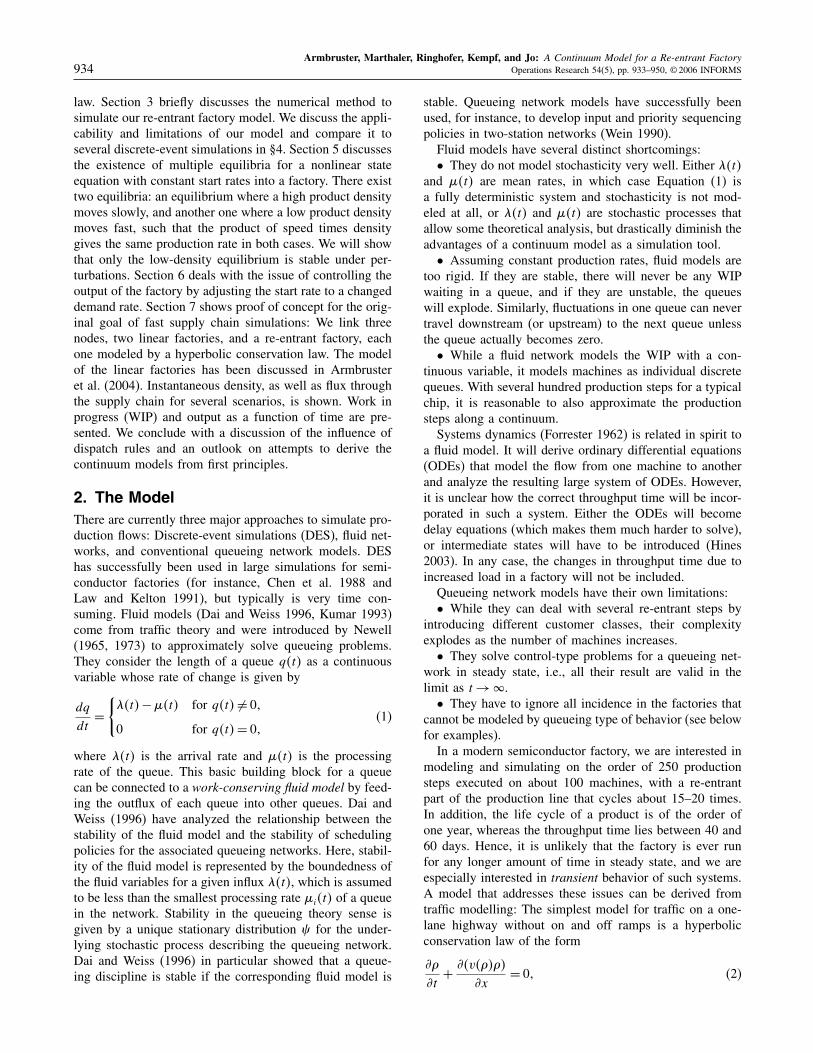
Figure 4. A ramp-up experiment showing a discrete-event simulation and PDE model: (a) Outfluxand (b) TPT as a function of time.

200 400 600 800 1,000 1,200 1,400 1,600 1,800

0.5

1.0

1.5

Out 0807 pull

200 400 600 800 1,000 1,200 1,400 1,600 1,800

4

5

6

7

8

9

10

TPT 0807 pull

(a)

(b)

we did not include any stochastic processes in the discrete-event simulation that may generate crowding behavior, asdiscussed in §2.We use this state equation to generate PDE simulations.

Trivially, the PDE simulation is very good for predict-ing the steady-state throughput and throughput time fora discrete-event simulation experiment with an arbitrarysteady influx, confirming the linear least-square fit for thedata. Comparing the PDE simulation to step-up experi-ments shows some nice agreement and some opportuni-ties for further improvement: We increase the arrival ratefrom 1/0�9 and 1/0�8, respectively, to 1/0�7. With a criti-cal capacity of about �= 1/0�6, this corresponds to a stepfrom 65% and 75% capacity to 85% capacity, respectively.We present four figures: Figure 4 shows time series forthe throughput and the throughput time as a function oftime for a ramp-up experiment from 75% capacity to 85%capacity with pull policy. The noisy curve is the average

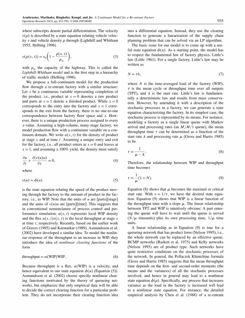
Figure 5. Like Figure 4, with a push policy and azoom into the transition: (a) Output and(b) Throughput time.

850 900 950 1,000 1,050 1,100 1,150 1,200

0.7

0.8

0.9

1.0

1.1

1.2

1.3

1.4

1.5

Out 0907 push

800 850 900 950 1,000 1,050 1,100 1,150 1,200 1,250

5

6

7

8

9

10

11

12

13

14

TPT 0907 push

(a)

(b)

of the discrete-event simulations; the continuous curve isthe PDE simulation with the state equation generated fromFigure 3.Figure 5 zooms into the transition time series for the

throughput and the throughput time of a ramp-up experi-ment from 65% capacity to 85% capacity with push policy.Note that the throughput times for push and pull policiesare very different, and hence we have to use a differentstate equation for each policy. While the transients in bothcases are not perfectly resolved, the agreement is not badeither. The large downward spike in the throughput for thePDE simulation results from the fact that in our modelthe velocity is spatially uniform and depends on the totalWIP in the factory. Hence, any increase in WIP (through,e.g., an increase in influx) will lead to an instantaneousinverse response, i.e., a reduction in velocity and henceto an instantaneous reduction in outflux. Obviously, oursimulation factory is not re-entrant enough for such a strongreaction.


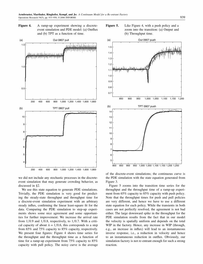
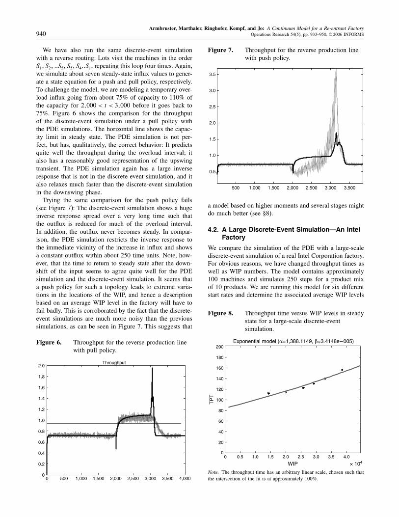
We have also run the same discrete-event simulationwith a reverse routing: Lots visit the machines in the orderS1� S2� ��S5� S5� S4��S1, repeating this loop four times. Again,we simulate about seven steady-state influx values to gener-ate a state equation for a push and pull policy, respectively.To challenge the model, we are modeling a temporary over-load influx going from about 75% of capacity to 110% ofthe capacity for 2�000 < t < 3�000 before it goes back to75%. Figure 6 shows the comparison for the throughputof the discrete-event simulation under a pull policy withthe PDE simulations. The horizontal line shows the capac-ity limit in steady state. The PDE simulation is not per-fect, but has, qualitatively, the correct behavior: It predictsquite well the throughput during the overload interval; italso has a reasonably good representation of the upswingtransient. The PDE simulation again has a large inverseresponse that is not in the discrete-event simulation, and italso relaxes much faster than the discrete-event simulationin the downswing phase.Trying the same comparison for the push policy fails

(see Figure 7): The discrete-event simulation shows a hugeinverse response spread over a very long time such thatthe outflux is reduced for much of the overload interval.In addition, the outflux never becomes steady. In compar-ison, the PDE simulation restricts the inverse response tothe immediate vicinity of the increase in influx and showsa constant outflux within about 250 time units. Note, how-ever, that the time to return to steady state after the down-shift of the input seems to agree quite well for the PDEsimulation and the discrete-event simulation. It seems thata push policy for such a topology leads to extreme varia-tions in the locations of the WIP, and hence a descriptionbased on an average WIP level in the factory will have tofail badly. This is corroborated by the fact that the discrete-event simulations are much more noisy than the previoussimulations, as can be seen in Figure 7. This suggests that

Figure 6. Throughput for the reverse production linewith pull policy.

0 500 1,000 1,500 2,000 2,500 3,000 3,500 4,0000

0.2

0.4

0.6

0.8

1.0

1.2

1.4

1.6

1.8

2.0Throughput

Figure 7. Throughput for the reverse production linewith push policy.

500 1,000 1,500 2,000 2,500 3,000 3,500

0.5

1.0

1.5

2.0

2.5

3.0

3.5

a model based on higher moments and several stages mightdo much better (see §8).

4.2. A Large Discrete-Event Simulation—An IntelFactory

We compare the simulation of the PDE with a large-scalediscrete-event simulation of a real Intel Corporation factory.For obvious reasons, we have changed throughput times aswell as WIP numbers. The model contains approximately100 machines and simulates 250 steps for a product mixof 10 products. We are running this model for six differentstart rates and determine the associated average WIP levels

Figure 8. Throughput time versus WIP levels in steadystate for a large-scale discrete-eventsimulation.

0 0.5 1.0 1.5 2.0 2.5 3.0 3.5 4.0

× 104

0

20

40

60

80

100

120

140

160

180

200

WIP

TP

T

Exponential model (α=1,388.1149, β=3.4148e–005)

Note. The throughput time has an arbitrary linear scale, chosen such thatthe intersection of the fit is at approximately 100%.


and throughput times in steady state. This results in Fig-ure 8. The interpolating curve in the figure follows a sug-gestion by Asmundsson et al. (2002) and is a least-squarefit of the six data points to

� = W

��1− e−)W � � (13)

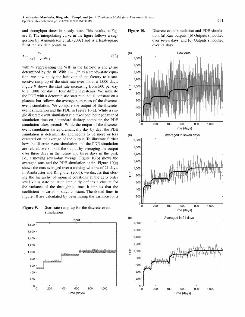
with W representing the WIP in the factory; � and ) aredetermined by the fit. With v= 1/� as a steady-state equa-tion, we now study the behavior of the factory to a suc-cessive ramp-up of the start rate over about a 1,000 days.Figure 9 shows the start rate increasing from 500 per dayto a 1,000 per day in four different plateaus. We simulatethe PDE with a deterministic start rate that is constant on aplateau, but follows the average start rates of the discrete-event simulation. We compare the output of the discrete-event simulation and the PDE in Figure 10(a). While a sin-gle discrete-event simulation run takes one hour per year ofsimulation time on a standard desktop computer, the PDEsimulation takes seconds. While the output of the discrete-event simulation varies dramatically day by day; the PDEsimulation is deterministic and seems to be more or lesscentered on the average of the output. To illustrate furtherhow the discrete-event simulation and the PDE simulationare related, we smooth the output by averaging the outputover three days in the future and three days in the past,i.e., a moving seven-day average. Figure 10(b) shows theaveraged outs and the PDE simulation again. Figure 10(c)shows the outs averaged over a moving window of 21 days.In Armbruster and Ringhofer (2005), we discuss that clos-ing the hierarchy of moment equations at the zero orderlevel via a state equation implicitly defines a closure forthe variance of the throughput time. It implies that thecoefficient of variation stays constant. The dotted lines inFigure 10 are calculated by determining the variance for a

Figure 9. Start rate ramp-up for the discrete-eventsimulations.

0 200 400 600 800 1,0000

200

400

600

800

1,000

1,200

1,400

1,600

1,800

Time (days)

In

Input

Figure 10. Discrete-event simulation and PDE simula-tion: (a) Raw outputs, (b) Outputs smoothedover seven days, and (c) Outputs smoothedover 21 days.

0 200 400 600 800 1,0000

200

400

600

800

1,000

1,200

1,400

1,600

1,800

Time (days)

0 200 400 600 800 1,000

Time (days)

0 200 400 600 800 1,000

Time (days)

Out

Raw data

0

200

400

600

800

1,000

1,200

1,400

1,600

1,800

Out

Averaged in seven days(b)

0

200

400

600

800

1,000

1,200

1,400

1,600

1,800

Out

(a)

(c) Averaged in 21 days


given plateau of the outputs. Assuming then that the coef-ficient of variation stays constant, the dotted lines are themean± the standard deviation. It seems that the PDE andits associated standard deviation are a good description ofa smoothed transient process.This comparison allows us to make an interesting obser-

vation that we most likely would not expect to find if we aredoing only a pure discrete-event simulation. As discussedpreviously, for a re-entrant factory, an increase in the startrate leads to an inverse response in the output, i.e., theoutput initially drops before it increases to the new level.The direct discrete-event simulation Figure 10(a) shows nosuch inverse response; if it is there it is masked in the rawoutputs by the daily variation in the outputs. It is also notcommonly found in the reality of the factory, due in part tothe fact that operators are paid to maintain or increase theoutputs, and hence they will work hard to speed up WIPat the end of the production line (Kempf 2001). However,the smoothed outputs in Figures 10(b) and 10(c) indicatethat, without the change of output policies resulting fromoperator interference, the inverse response can be found inthe discrete-event simulation too, and it follows quite wellthe PDE simulation. The reason why the inverse responsefor the discrete-event simulations and the PDE for the Intelfactory agree much better than for the simulations in §4.1presumably depends on the fact that the Intel factory ismuch more re-entrant and that the relative change in itsload is much lower than in the other simulations.

5. EquilibriaFor the rest of this paper, we assume a nonlinear stateequation analogous to the Lighthill-Whitham traffic model(Equation (12)), repeated here for convenience:

v�u�= v0(1− u�t�

L

)� (14)

Note, however, that all the analysis in the following chap-ters can easily be adapted to fit any other state equation.We begin by determining the steady-state solutions.

Proposition 1. For a given (constant) influx ��t�= �, themodel (10) and (14) has two steady states:

u+ = L2+√L2

4− �Lv0

and u− = L2−√L2

4− �Lv0�

provided 4�/v0 <L.

Proof. Let uss represent a constant solution to Equation(10). Then, the boundary condition becomes a quadraticequation

u2ss −Luss +�L

v0= 0� (15)

and the solutions to this quadratic equation are u+ andu−. �

This implies that a re-entrant factory has two modesof steady operations that generate the same throughput: ahigh-WIP, high-TPT state and a low-WIP, low-TPT state.Note that any state equation that grows stronger than linearwill show two equilibria.

Proposition 2. The high-WIP, high-TPT state, u+, is un-stable, while the low-WIP, low-TPT, u−, is stable to pertur-bations.

Proof. Perturbing the solution near a steady state uss , wewrite u�x� t�= uss +p�x� t�, and insert into system (10),

�p

�t�x�t�+v0

(1− 1

L

∫ 1

0�uss+p�x�t��dx

)�p

�x�x�t�=0�

u�x�0�= uss +p�x�0��

�uss +p�x�0��v0(1− 1

L

∫ 1

0�uss +p�x� t��dx

)= ��

(16)

Linearizing the PDE and the boundary condition by dis-carding higher-order terms of p�x� t�, we get a linear uni-directional wave equation with constant speed vss ,= v�uss�and an integral boundary condition:

�p

�t�x� t�+ v�uss�

�p

�x�x� y�= 0�

u�x�0�= uss +p�x�0��

−ussv0L

∫ 1

0p�x� t�dx+ vssp�0� t�= 0�

(17)

Taking the time derivative of the boundary condition andsolving for �d/dt�p�0� t�, we find

d

dtp�0� t�= ussv0

Lvss

∫ 1

0

�p

�t�x� t�dx

=−ussv0Lvss

∫ 1

0vss�p

�x�x� t�dx

= ussv0L�p�0� t�−p�1� t��

To go from the second to the third equation, the waveequation for ��p/�t��x� t� (17) was used to replace �p/�twith −v�uss��p/�x�. Because Equation (17) has a con-stant wavespeed vss , the solution at the right boundaryis p�1� t� = p�0� t − 1/vss�. Hence, with � = 1/vss , . =ussv0/L, and z�t�= p�0� t�, stability of the steady state ussis determined by the stability of the trivial solution of thedelay differential equation (Kuang 1993)

d

dtz�t�−.z�t�+.z�t− ��= 0� (18)

Its characteristic equation is

0−.+.e−0� = 0�

Obviously, 0 = 0 is a solution. This corresponds to the factthat the system is a conservation law, and hence is neutrally


stable towards all perturbations that preserve the load (thisreflects the fact that any factory can be run at any load witha constant WIP policy (CONWIP)) (Spearman et al. 1989).Define h�0� ��= �0−.�e0� +. and consider h�0� �� as

a function of real 0. Then,

h�0� ��= 0� h�.� ��= . > 0�

and

�h

�0�0� ��= e0� + �0−.��e0��

�h

�0�0� ��= 1− �.�

Hence, if � > .−1� then ��h/�0��0� �� < 0, which impliesthat there is a 1> 0 such that when 0< 0 � 1, h�0� �� < 0.Because h�.� �� > 0, there is at least one 0, 1� 0., withh�0� ��= 0. Hence, the characteristic equation always hasa positive root, signifying an unstable trivial solution. Con-versely, if � < .−1, then h�0� �� > 0 everywhere. Hence,there are no � > 0 that solve the characteristic equation,and the trivial solution is stable.It is easy to see that u+ implies that � > 1/., while

u− implies � < 1/., which proves the claim. �

Note that for a state equation v�u�= v0/�1+ u� (Equa-tion (9)), which describes a simple linear queue (or aproduct network), there exists only one stable equilibrium.Furthermore, it is easy to show that for any state equationv�u� = ��u� that slows down faster with increasing loadthan a simple queue, there exist two equilibria and that thehigh-speed, low-WIP equilibrium is stable, while the low-speed, high-WIP equilibrium is unstable. In particular, thesingularity at u = L is not a necessary condition for theexistence of the two equilibria.The relationship of these results to standard queueing

theory is the following: Consider a small WIP perturbationof a steady state—for instance, a localized WIP increases,but keeps the start rate the same throughout. The pertur-bation will travel downstream and will eventually leavethe factory. In the stable steady state, the perturbation willhave generated secondary perturbations that are smallerthan the initial perturbation and, hence, eventually the sys-tem will return to equilibrium. In the unstable steady state,an increase in WIP will slow down the system even more,leading to an even bigger increase in WIP—i.e., the sec-ondary perturbations are bigger than the original one and,hence, eventually WIP will increase to infinity. For tradi-tional queueing systems this corresponds to the examplesof scheduling policies for re-entrant flows (Dai and Weiss1996, Lu et al. 1994) that will lead to the growth of WIPwithout bound, although the utilization (measured as thestart rate relative to the processing rate of the bottleneck)stays below one.

6. ControlThe simplest control problem associated with running afactory is to change the production flow of the factory fromone steady state, corresponding to outflux that meets a spe-cific constant demand, to another one. Let us assume thatthe demand d�t� changes in the following way:

d�t�={d1� t < 0�

d2� t > 0�

The control problem is to design an influx ��t� that wouldmove the system from the equilibrium u1 corresponding toa production rate of d1, to a new equilibrium u2 correspond-ing to a production rate d2. The outflux and the equilibriumdensities ui are related as

di = uiv0(1− ui

L

)� (19)

The influx ��t� is uniquely determined by the boundarycondition at the left: ��t� = u�0� t�v�t�, where the veloc-ity depends on the global load. Hence, to generate a WIPprofile that has a discontinuous step from an equilibriumu�x� = u1 to new value u2 at time t = 0, we choose thefollowing influx:

��t�=

u1v0

(1− u1

L

)� t < 0�

u2v0

(1− 1

L

[∫ x�t�

0u2 ds+

∫ 1

x�t�u1 ds

])�

0< t < ��

(20)

where x�t� is the characteristic for the discontinuity ema-nating from x = 0, t = 0 in the xt-plane. At t = � , thediscontinuity is at x�� = 1, and we have a new equilib-rium profile u�x� = u2. Because u1 and u2 are constants,Equation (20) reduces to

��t�=

u1v0

(1− u1

L

)� t<0�

u2v0

(1− 1

L�u1+�u2−u1�x�t��

)� 0<t<��

u2v0

(1− u2

L

)� � <t�

(21)

The characteristic x�t� is the solution of the initial valueproblem x�t�= v�u�x�t�� t�, i.e.,

x�t�= v0(1− 1

L

[∫ x�t�

0u2 ds+

∫ 1

x�t�u1 ds

])� (22)

x�0�= 0�


Because u1 and u2 are constants, the integrals can be eval-uated and Equation (22) reduces to a simple linear ODE.Its solution is

x�t�= L− u1u2 − u1

(1− exp

(v0�u1 − u2�t

L

))� (23)

and hence ��t� yields

��t�=

u1v0

(1− u1

L

)� t<0�

v0u2�L−u1�L

exp(v0�u1−u2�

Lt

)� 0<t<��

u2v0

(1− u2

L

)� � <t�

(24)

Solving x�t�= 1 for t gives

� = L

u1 − u2ln(L− u2L− u1

)� (25)

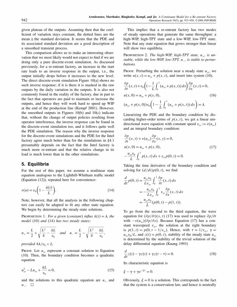
Using the numerical method described in §3.1, the sys-tem was run with the parameter values v0 = 1, u1 =2�8, u2 = 3�1, and L = 10. With these values, we get� = 1�42. For t > � , we continue the steady influx � =u2v0�1− u2/L�. Figure 11(a) shows a WIP profile and Fig-ure 11(b) shows the resulting outflux: Upon the introduc-tion of u2 into the factory, the total load increases, andhence the velocity decreases. The velocity continues todecrease for t < � . Therefore, the outflux given by "�t�=u1v�t� decreases as well, until the new density u = u2reaches the end of the production line.If the change in demand happens without sufficient

notice, then there exists a time lag during which the fac-tory will not produce according to the new demand, as canbe seen in Figure 11(b). During the transition between theequilibria we produce an outflux "�t�= u�1� t�v�t� whilewe wished to produce an outflux of d2. The differencebetween actual and desired production up to time t is calledthe backlog. It may be written as

b�t�= u2(1− u2

L

)t−

∫ t

0"�s�ds� (26)

An optimal control problem can now be defined that asksfor the input function ��t� that moves the factory fromone steady state to another in shortest time, subject to theconstraint of a zero backlog. Formally, we write

minT

subject to

�u

�t+ ��v�u�u�

�x= 0�

v�u�= v0(1− u�t�

L

)for t � T �

u�x�0�= u1�v�u�u�0� t�= ��t��

(27)

Figure 11. (a) Snapshot of the density u�x� for thesolution of Equation (10). The influx isgiven by Equation (24). Note that with thisstart rate, the density is piecewise constant.(b) Outflux; note that the flux is constantafter the transient time of moving betweenthe steady states.

0 0.2 0.4 0.6 0.8 1.02.70

2.75

2.80

2.85

2.90

2.95

3.00

3.05

3.10

3.15

3.20

u(x,

t=0.

2812

)

0 0.5 1.0 1.5 2.0 2.51.90

1.95

2.00

2.05

2.10

2.15

2.20

Time

ω(t

)

(a)

(b)

x

and

b�t�=∫ t

0�d2 − v�s�u�1� s��ds = 0 for t � T � (28)

Standard optimal control approaches in the production andinventory modeling context (e.g., Gershwin et al. 1985)cannot solve our problem here: They are based on ODEsthat cannot take into account the slowdown of the fac-tory, as the load in the factory increases due to the controlactions. Lefeber (2004) suggested an approach based oncontrol theory of delay systems. Whether such an approachwill work for the re-entrant factory with its large delaysremains to be proven.As we currently cannot solve the optimal control prob-

lem in its general setting, we are going to solve the fol-lowing simplified problem: We assume that we want to gofrom an equilibrium solution u1 to an equilibrium solution


u2 through one intermediate constant density u = u3. Wewill find the optimal level u3 and the optimal time thatthe system will stay in that intermediate equilibrium. Whilethis constraint mostly is dictated by the fact that we can-not solve optimal control problems for nonlinear hyperbolicequations, it is not entirely unreasonable to have this addi-tional constraint: We are trying to find the input sequencethat solves the optimal control problem and, in doing so,limits the disruption of the WIP profile to two-step func-tions. Clearly, from a resources and management point ofview it is desirable to have a product density in the fac-tory that is as homogeneous as possible. Furthermore, wehope that this approach can be the basis for a numericalalgorithm that solves the original optimal control problem(WIP).We therefore assume that the solution at x= 0 takes the

following form:

u�0� t�=

u1� t < 0�

u3� 0< t < T �

u2� T < t�

(29)

i.e., we enter the intermediate density u3 for T time units.Note that once we enter the desired density u2, there is stillthe transition time � before the system is completely inequilibrium. Under the assumption that v0� u1� u2� and Lare known, there are two parameters, u3 and T , to choose.Therefore, the requirements for a �u3� T � pair to satisfy are

u2

(1− u2

L

)�T + ��−

∫ T+�

0"�s�ds = 0� (30)

There are two cases to consider.

6.1. u3 Saturates the Factory

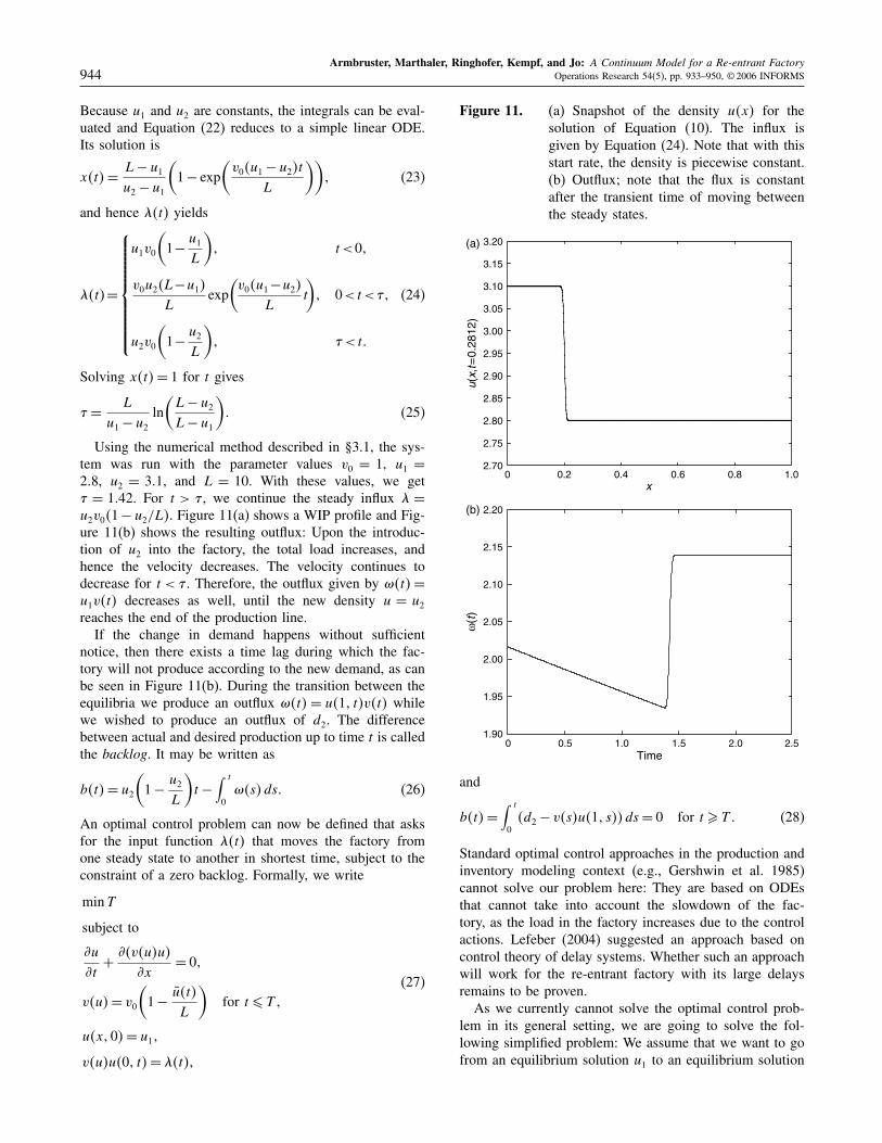
Here we seek to move to an intermediate equilibrium solu-tion, u3� and remain on it for some time before movingagain to the final equilibrium solution u2. The method ofLagrange multipliers and simple algebra allows us to findthe optimal values for the intermediate level u3 and the timeT to stay on that intermediate level. As an example, forv0 = 1, u1 = 1�8, u2 = 3�5, and L= 10, we find a minimumtime for u3 = 5�29321 and T = 2�85286. Figures 12(a) and12(b) show the start rate and backlog for the optimal solu-tion with these parameter values. The drop at around t = 4is due to the inverse response again. As we lower the startrate, we reduce WIP in the factory, and hence speed upproduction and subsequently increase the output. In ordernot to overproduce, we need to start less for a short amountof time.

6.2. Small Backlog—u3 Does Not Saturate

Here we input the intermediate state u3 only for a timet < �u3 , such that the factory never saturates on u3. Therewill be three stages to the transient in moving from u1 to

Figure 12. (a) Start rate ��t� and (b) Backlog b�t� forthe optimal parameters discussed in §6.1.

0

1

2

3

4

5

Influ

x

–1 1 2 3 4 5 6 7t

–0.5

0

0.5

1.0

1.5

2.0

Bac

klog

–1 1 2 3 4 5 6 7

t

(a)

(b)

Note. Note that after t ≈ 6�2421, the influx is at the new steady state andthe backlog stays zero.

u2: The first stage will be introducing the density u3 intothe factory. The discontinuity from u1 to u3 moves throughthe factory along the characteristic x1�t�. This will yield adecreasing velocity because the load keeps increasing. Thiswill last until t = T � at which time the introduction of u2


will begin. The discontinuity from u3 to u2 will move alonga characteristic called x2�t�. This second stage will consistof the time needed to purge the factory of u1� so that onlyu2 and u3 are left. This time will be referred to as T + T1.The third and final stage will be the expulsion of u3 fromthe factory at which time the new equilibrium is reached.We call this time t = T +T1+� and we are seeking a mini-mum time subject to the backlog constraint (30) by varyingthe two free parameters u3 and T1� Again, straightforwardalgebra and the method of Lagrange multipliers allows usto find the minima.We find that for every choice of u1, u2, and L that we

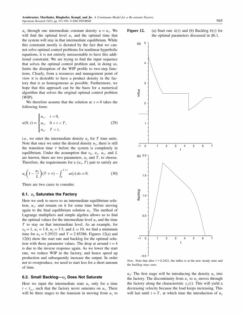
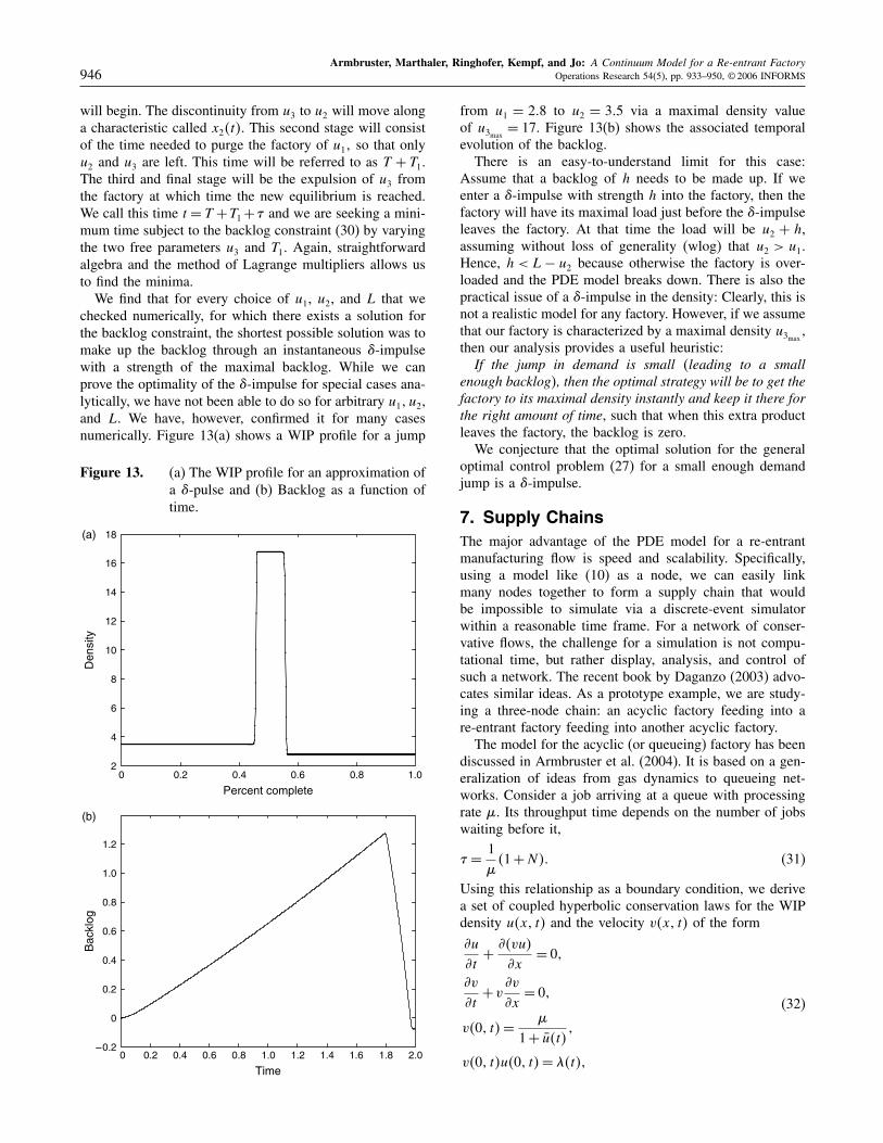
checked numerically, for which there exists a solution forthe backlog constraint, the shortest possible solution was tomake up the backlog through an instantaneous 1-impulsewith a strength of the maximal backlog. While we canprove the optimality of the 1-impulse for special cases ana-lytically, we have not been able to do so for arbitrary u1� u2,and L. We have, however, confirmed it for many casesnumerically. Figure 13(a) shows a WIP profile for a jump

Figure 13. (a) The WIP profile for an approximation ofa 1-pulse and (b) Backlog as a function oftime.

0 0.2 0.4 0.6 0.8 1.02

4

6

8

10

12

14

16

18

Percent complete

Den

sity

0 0.2 0.4 0.6 0.8 1.0 1.2 1.4 1.6 1.8 2.0–0.2

0

0.2

0.4

0.6

0.8

1.0

1.2

Time

Bac

klog

(a)

(b)

from u1 = 2�8 to u2 = 3�5 via a maximal density valueof u3max = 17. Figure 13(b) shows the associated temporalevolution of the backlog.There is an easy-to-understand limit for this case:

Assume that a backlog of h needs to be made up. If weenter a 1-impulse with strength h into the factory, then thefactory will have its maximal load just before the 1-impulseleaves the factory. At that time the load will be u2 + h,assuming without loss of generality (wlog) that u2 > u1.Hence, h < L− u2 because otherwise the factory is over-loaded and the PDE model breaks down. There is also thepractical issue of a 1-impulse in the density: Clearly, this isnot a realistic model for any factory. However, if we assumethat our factory is characterized by a maximal density u3max ,then our analysis provides a useful heuristic:If the jump in demand is small �leading to a small

enough backlog�, then the optimal strategy will be to get thefactory to its maximal density instantly and keep it there forthe right amount of time, such that when this extra productleaves the factory, the backlog is zero.We conjecture that the optimal solution for the general

optimal control problem (27) for a small enough demandjump is a 1-impulse.

7. Supply ChainsThe major advantage of the PDE model for a re-entrantmanufacturing flow is speed and scalability. Specifically,using a model like (10) as a node, we can easily linkmany nodes together to form a supply chain that wouldbe impossible to simulate via a discrete-event simulatorwithin a reasonable time frame. For a network of conser-vative flows, the challenge for a simulation is not compu-tational time, but rather display, analysis, and control ofsuch a network. The recent book by Daganzo (2003) advo-cates similar ideas. As a prototype example, we are study-ing a three-node chain: an acyclic factory feeding into are-entrant factory feeding into another acyclic factory.The model for the acyclic (or queueing) factory has been

discussed in Armbruster et al. (2004). It is based on a gen-eralization of ideas from gas dynamics to queueing net-works. Consider a job arriving at a queue with processingrate �. Its throughput time depends on the number of jobswaiting before it,

� = 1

��1+N�� (31)

Using this relationship as a boundary condition, we derivea set of coupled hyperbolic conservation laws for the WIPdensity u�x� t� and the velocity v�x� t� of the form

�u

�t+ ��vu�

�x= 0�

�v

�t+ v �v

�x= 0�

v�0� t�= �

1+ u�t� �

v�0� t�u�0� t�= ��t��

(32)


where � is again the arrival rate and u�t� = ∫ 10 u�x� t�dx

is again the total load (WIP). The first equation in system(32) again has the form of a hyperbolic conservation law.However, instead of the heuristic state equation used in there-entrant model (10) that relates the velocity to the density,we have a Burger’s equation for the time evolution of thevelocity. Note that the boundary condition for v provides anonlocal feedback of the history of the production on thecurrent velocity through the length of the queue in front ofan incoming part. This model for the queueing system ismore sophisticated than the model for the re-entrant systembecause it allows for nonadiabatic relaxation of the velocityfields, and hence a better modeling of transient phenomena.In addition, in contrast to the heuristics of §2, it has beenrigorously derived in Armbruster et al. (2004).It is straightforward to link the two models together to

form a supply chain. We assume no buffers in between fac-tories, and hence the outflux of one factory becomes theinflux of the next. This implies, if we extend our comple-tion variable x to cover the whole chain, that the flux willbe a continuous variable of x while the density will showdiscontinuous jumps between factories.In all experiments, because the PDE models are deter-

ministic moment equations, steady-state modeling is notinteresting: Either on the average the influx is below capac-ity, in which case we find a stable equilibrium given bythe state equation; or the influx is above capacity, in whichcase WIP will explode. However, the PDE models allowus to focus on simulations driven by a time-dependentinflux ��t�.

7.1. Experiment 1: Short-Time Overload of theQueuing Factory

Figure 14 shows snapshots of a steady-state density andflux for a linear chain of three factories—two identi-cal queue modules surrounding a re-entrant module. Eachmodule makes up one-third of the total x-axis. The raw

Figure 14. Snapshot of the steady-state density and fluxin the three-node chain.

0 0.2 0.4 0.6 0.8 1.00

1

2

3

Den

sity

0 0.2 0.4 0.6 0.8 1.00

0.5

1.0

1.5

Flu

x

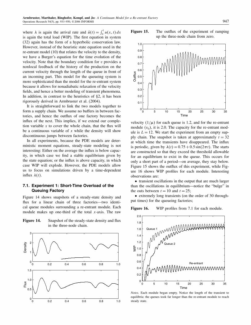
Figure 15. The outflux of the experiment of rampingup the three-node chain from zero.

0 5 10 15 20 25 30 350

0.1

0.2

0.3

0.4

0.5

0.6

0.7

0.8

0.9

1.0

Time

Out

flux

velocity �1/�� for each queue is 1.2, and for the re-entrantmodule �v0�, it is 2.0. The capacity for the re-entrant mod-ule is L= 12. We start the experiment from an empty sup-ply chain. The snapshot is taken at approximately t = 32at which time the transients have disappeared. The influxis periodic, given by ��t�= 0�75+ 0�5 sin�23t�. The startsare constructed so that they exceed the threshold allowablefor an equilibrium to exist in the queue. This occurs foronly a short part of a period—on average, they stay below.Figure 15 shows the outflux of this experiment, while Fig-ure 16 shows WIP profiles for each module. Interestingobservations are:• transient oscillations in the output that are much larger

than the oscillations in equilibrium—notice the “bulge” inthe outs between t = 10 and t = 25;• extremely long transients (on the order of 30 through-

put times) for the queueing factories;

Figure 16. WIP profiles from 7.1 for each module.

0 5 10 15 20 25 30 350

0.2

0.4

0.6

0.8

1.0

1.2

1.4

1.6

1.8

2.0

Time

WIP

Queue 2

Re-entrant

Queue 1

Notes. Each module began empty. Notice the length of the transient toequilibria: the queues took far longer than the re-entrant module to reachsteady state.


• the re-entrant factory equilibrates much faster than thequeueing factories; and• the re-entrant factory acts as a damping device reduc-

ing the amplitude of the oscillations in WIP in the down-stream factory.

7.2. Experiment 2: Stronger Overload of theQueuing Factory

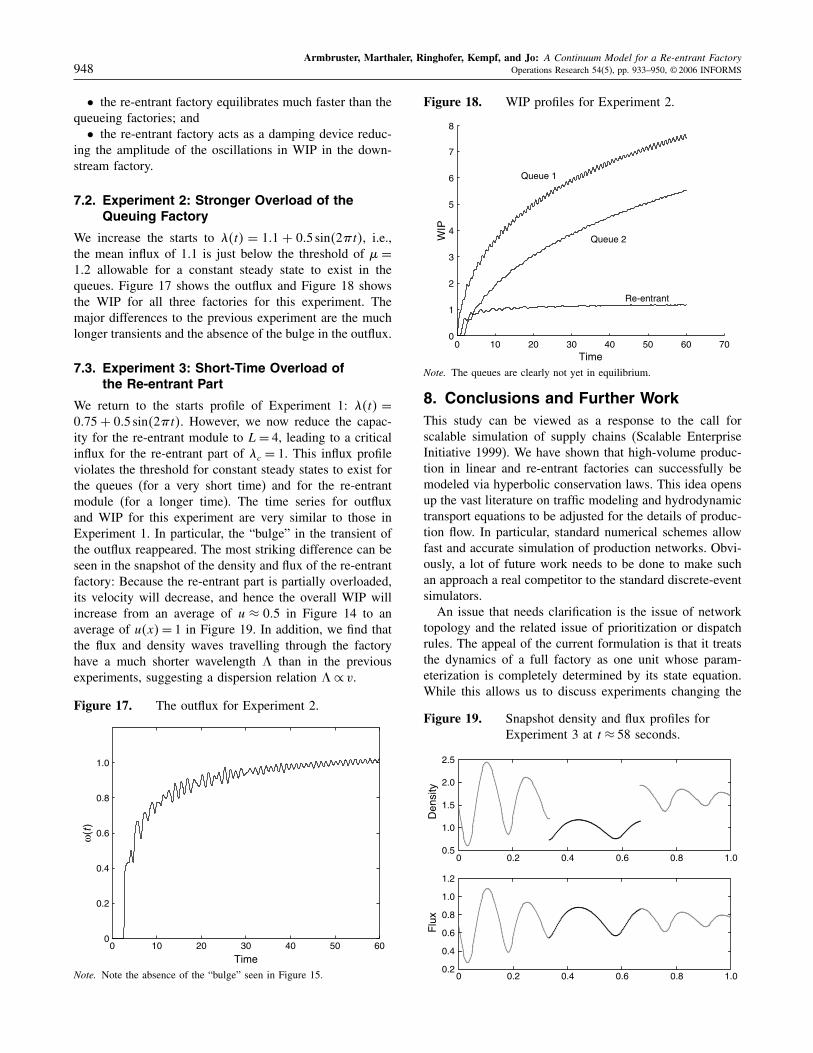
We increase the starts to ��t� = 1�1 + 0�5 sin�23t�, i.e.,the mean influx of 1�1 is just below the threshold of �=1�2 allowable for a constant steady state to exist in thequeues. Figure 17 shows the outflux and Figure 18 showsthe WIP for all three factories for this experiment. Themajor differences to the previous experiment are the muchlonger transients and the absence of the bulge in the outflux.

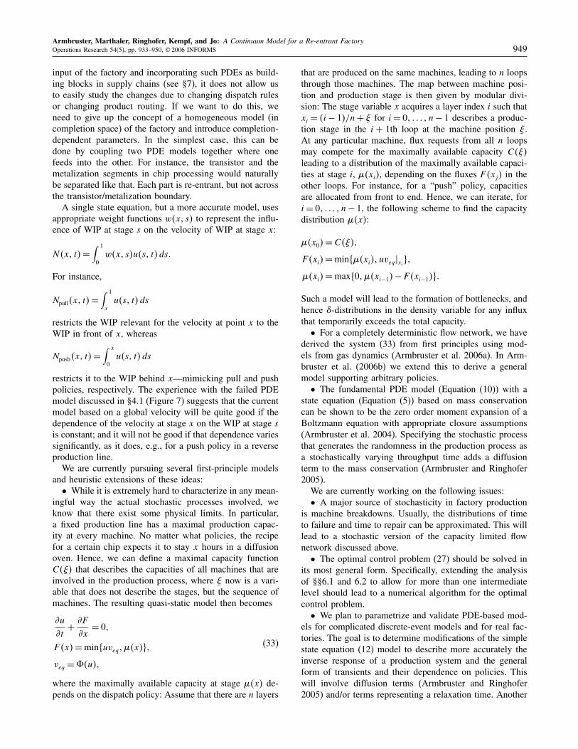
7.3. Experiment 3: Short-Time Overload ofthe Re-entrant Part

We return to the starts profile of Experiment 1: ��t� =0�75+ 0�5 sin�23t�. However, we now reduce the capac-ity for the re-entrant module to L= 4, leading to a criticalinflux for the re-entrant part of �c = 1. This influx profileviolates the threshold for constant steady states to exist forthe queues (for a very short time) and for the re-entrantmodule (for a longer time). The time series for outfluxand WIP for this experiment are very similar to those inExperiment 1. In particular, the “bulge” in the transient ofthe outflux reappeared. The most striking difference can beseen in the snapshot of the density and flux of the re-entrantfactory: Because the re-entrant part is partially overloaded,its velocity will decrease, and hence the overall WIP willincrease from an average of u ≈ 0�5 in Figure 14 to anaverage of u�x�= 1 in Figure 19. In addition, we find thatthe flux and density waves travelling through the factoryhave a much shorter wavelength 5 than in the previousexperiments, suggesting a dispersion relation 5∝ v.Figure 17. The outflux for Experiment 2.

0 10 20 30 40 50 600

0.2

0.4

0.6

0.8

1.0

Time

ω(t

)

Note. Note the absence of the “bulge” seen in Figure 15.

Figure 18. WIP profiles for Experiment 2.

0 10 20 30 40 50 60 700

1

2

3

4

5

6

7

8

Time

WIP

Queue 1

Queue 2

Re-entrant

Note. The queues are clearly not yet in equilibrium.

8. Conclusions and Further WorkThis study can be viewed as a response to the call forscalable simulation of supply chains (Scalable EnterpriseInitiative 1999). We have shown that high-volume produc-tion in linear and re-entrant factories can successfully bemodeled via hyperbolic conservation laws. This idea opensup the vast literature on traffic modeling and hydrodynamictransport equations to be adjusted for the details of produc-tion flow. In particular, standard numerical schemes allowfast and accurate simulation of production networks. Obvi-ously, a lot of future work needs to be done to make suchan approach a real competitor to the standard discrete-eventsimulators.An issue that needs clarification is the issue of network

topology and the related issue of prioritization or dispatchrules. The appeal of the current formulation is that it treatsthe dynamics of a full factory as one unit whose param-eterization is completely determined by its state equation.While this allows us to discuss experiments changing the

Figure 19. Snapshot density and flux profiles forExperiment 3 at t ≈ 58 seconds.

0 0.2 0.4 0.6 0.8 1.00.5

1.0

1.5

2.0

2.5

Den

sity

0 0.2 0.4 0.6 0.8 1.00.2

0.4

0.6

0.8

1.0

1.2

Flu

x


input of the factory and incorporating such PDEs as build-ing blocks in supply chains (see §7), it does not allow usto easily study the changes due to changing dispatch rulesor changing product routing. If we want to do this, weneed to give up the concept of a homogeneous model (incompletion space) of the factory and introduce completion-dependent parameters. In the simplest case, this can bedone by coupling two PDE models together where onefeeds into the other. For instance, the transistor and themetalization segments in chip processing would naturallybe separated like that. Each part is re-entrant, but not acrossthe transistor/metalization boundary.A single state equation, but a more accurate model, uses

appropriate weight functions w�x� s� to represent the influ-ence of WIP at stage s on the velocity of WIP at stage x:

N�x� t�=∫ 1

0w�x� s�u�s� t�ds�

For instance,

Npull�x� t�=∫ 1

xu�s� t�ds

restricts the WIP relevant for the velocity at point x to theWIP in front of x, whereas

Npush�x� t�=∫ x

0u�s� t�ds

restricts it to the WIP behind x—mimicking pull and pushpolicies, respectively. The experience with the failed PDEmodel discussed in §4.1 (Figure 7) suggests that the currentmodel based on a global velocity will be quite good if thedependence of the velocity at stage x on the WIP at stage sis constant; and it will not be good if that dependence variessignificantly, as it does, e.g., for a push policy in a reverseproduction line.We are currently pursuing several first-principle models

and heuristic extensions of these ideas:• While it is extremely hard to characterize in any mean-

ingful way the actual stochastic processes involved, weknow that there exist some physical limits. In particular,a fixed production line has a maximal production capac-ity at every machine. No matter what policies, the recipefor a certain chip expects it to stay x hours in a diffusionoven. Hence, we can define a maximal capacity functionC�0� that describes the capacities of all machines that areinvolved in the production process, where 0 now is a vari-able that does not describe the stages, but the sequence ofmachines. The resulting quasi-static model then becomes

�u

�t+ �F�x

= 0�

F �x�=min9uveq��x�:�

veq =;�u��(33)

where the maximally available capacity at stage ��x� de-pends on the dispatch policy: Assume that there are n layers

that are produced on the same machines, leading to n loopsthrough those machines. The map between machine posi-tion and production stage is then given by modular divi-sion: The stage variable x acquires a layer index i such thatxi = �i− 1�/n+ 0 for i= 0� � � � � n− 1 describes a produc-tion stage in the i + 1th loop at the machine position 0.At any particular machine, flux requests from all n loopsmay compete for the maximally available capacity C�0�leading to a distribution of the maximally available capaci-ties at stage i, ��xi�, depending on the fluxes F �xj� in theother loops. For instance, for a “push” policy, capacitiesare allocated from front to end. Hence, we can iterate, fori= 0� � � � � n− 1, the following scheme to find the capacitydistribution ��x�:

��x0�=C�0��F �xi�=min9��xi�� uveq�xi :��xi�=max90��xi−1�− F �xi−1�:�

Such a model will lead to the formation of bottlenecks, andhence 1-distributions in the density variable for any influxthat temporarily exceeds the total capacity.• For a completely deterministic flow network, we have

derived the system (33) from first principles using mod-els from gas dynamics (Armbruster et al. 2006a). In Arm-bruster et al. (2006b) we extend this to derive a generalmodel supporting arbitrary policies.• The fundamental PDE model (Equation (10)) with a

state equation (Equation (5)) based on mass conservationcan be shown to be the zero order moment expansion of aBoltzmann equation with appropriate closure assumptions(Armbruster et al. 2004). Specifying the stochastic processthat generates the randomness in the production process asa stochastically varying throughput time adds a diffusionterm to the mass conservation (Armbruster and Ringhofer2005).We are currently working on the following issues:• A major source of stochasticity in factory production

is machine breakdowns. Usually, the distributions of timeto failure and time to repair can be approximated. This willlead to a stochastic version of the capacity limited flownetwork discussed above.• The optimal control problem (27) should be solved in

its most general form. Specifically, extending the analysisof §§6.1 and 6.2 to allow for more than one intermediatelevel should lead to a numerical algorithm for the optimalcontrol problem.• We plan to parametrize and validate PDE-based mod-

els for complicated discrete-event models and for real fac-tories. The goal is to determine modifications of the simplestate equation (12) model to describe more accurately theinverse response of a production system and the generalform of transients and their dependence on policies. Thiswill involve diffusion terms (Armbruster and Ringhofer2005) and/or terms representing a relaxation time. Another


goal will be to determine the discretization error associ-ated with treating a fundamentally discrete problem as acontinuous flow.• While we showed the feasibility of linking hyperbolic

conservation laws together to make a simple linear chain,this is really just a proof of concept. The real test forthe usefulness of our approach will be whether relevantbusiness questions can be answered for a supply networkby linking our nodes together and performing simulations.This may involve the development of an object-orientedsimulation interface. A related project uses the PDE-basedmodels as the predictive model for attempts to optimizethe behavior of a whole supply chain via model predictivecontrol (MPC) algorithms (Wang et al. 2004).

AcknowledgmentsThe authors thank Edward Yellig of Intel Corporation forexecuting the simulation runs. John Fowler, Daniel Rivera,and Matthias Kawski and their students helped to focus theauthors’ ideas through many constructive discussions. The# simulations are extensions of codes written by R. vanden Berg and E. Lefeber. Dieter Armbruster and ChristianRinghofer were supported by NSF grant DMS-0204543.Support from Intel Corporation is also gratefully acknowl-edged.

ReferencesArmbruster, D., C. Ringhofer. 2005. Thermalized kinetic and fluid models

for re-entrant supply chains. SIAM J. Multiscale Modeling Simulation3(4) 782–800.

Armbruster, D., P. Degond, C. Ringhofer. 2006a. A model for the dynam-ics of large queuing networks and supply chains. SIAM J. Appl. Math.66(3) 896–920.

Armbruster, D., P. Degond, C. Ringhofer. 2006b. Kinetic and fluid modelsfor supply chains supporting policy attributes. Transportation TheoryStatist. Phys. Forthcoming.

Armbruster, D., D. Marthaler, C. Ringhofer. 2004. Kinetic and fluidmodel hierarchies for supply chains. SIAM J. Multiscale Modeling 243–61.

Asmundsson, J., R. Uzsoy, R. L. Rardin. 2002. Compact nonlinear capac-ity models for supply chains: Methodology. Preprint, Purdue Univer-sity, West Lafayette, IN.

Baskett, F., K. M. Chandy, R. R. Muntz, F. G. Palacios. 1975. Open, closedand mixed networks of queues with different classes of customers.J. Assoc. Comput. Machinery 22 248–260.

Chen, H., J. M. Harrison, A. Mandelbaum, A. Van Ackere, L. M. Wein.1988. Empirical evaluation of a queueing network model for semi-conductor wafer fabrication. Oper. Res. 36 202–215.

Daganzo, C. F. 2003. A Theory of Supply Chains. Springer Verlag,Heidelberg, Germany.

Dai, J. G., J. H. Vande Vate. 2000. The stability of two-station multitypefluid networks. Oper. Res. 48(5) 721–744.

Dai, J. G., G. Weiss. 1996. Stability and instability of fluid models forcertain re-entrant lines. Math. Oper. Res. 21 115–134.

DeJong, C. D., S. P. Wu. 2002. Simulating the transport and schedul-ing of priority lots in semiconductor factories. J. L. Snowdon, J. M.Charnes, eds. Proc. 34th Winter Simulation Conf. ACM, San Diego,CA, 1387–1391.

Forrester, J. W. 1962. Industrial Dynamics. MIT Press, Cambridge, MA.

Gershwin, S. B., R. Akella, Y. F. Choong. 1985. Short-term produc-tion scheduling of an automated manufacturing facility. IBM J. Res.Develop. 29(4) 392–400.

Graves, S. C. 1985. A tactical planning model for a job shop. Oper. Res.34 525–533.

Gross, D., C. M. Harris. 1985. Fundamentals of Queueing Theory. Wiley,New York.

Helbing, D. 1996. Traffic modeling by means of physical concepts. D. E.Wolf, M. Schreckenberg, A. Bachem, eds. Workshop on Traffic andGranular Flow. World Scientific, Singapore, 87–104.

Hines, J. 2003. Personal communication. Massachusetts Institute of Tech-nology, Cambridge, MA.

Hofkamp, A. T., J. E. Rooda. 2002. Chi reference manual. Technische Uni-versiteit Eindhoven, Eindhoven, The Netherlands. Retrieved Novem-ber 2002 http://se.wtb.tue.nl/documentation/.

Karmarkar, U. S. 1989. Capacity loading and release planning in work-in-progess (WIP) and lead-times. J. Manufacturing Oper. Management2 105–123.

Kempf, K. 2001. Personal communications. Intel Corporation, Chandler,AZ.

Kuang, Y. 1993. Delay Differential Equations. Academic Press, Boston,MA.

Kumar, P. R. 1993. Re-entrant lines. Queueing Systems 13 87–110.Law, A. M., W. D. Kelton. 1991. Simulation Design and Analysis.

McGraw-Hill, New York.Lefeber, E. 2004. Nonlinear models for control of manufacturing systems.

G. Radons, R. Neugebauer, eds. Nonlinear Dynamics of ProductionSystems. Wiley-VCH, Berlin, Germany, 71–84.

LeVeque, R. J. 1992. Numerical Methods for Conservation Laws.Birkhäuser-Verlag, Basel, Switzerland.

LeVeque, R. J. 1998. Finite difference methods for differential equations.Draft version for use in AMath 585-6, University of Washington,Seattle, WA.

Lighthill, M. J., G. B. Whitham. 1955. On kinematic waves II. A theoryof traffic flow on long crowded roads. Proc. Roy. Soc. Ser. A 229317–345.

Little, J. D. C. 1961. A proof for the queuing formula L= �W . Oper. Res.9 383–387.

Lu, S. C. H., D. Ramaswamy, P. R. Kumar. 1994. Efficient schedulingpolicies to reduce mean and variance of cycle-time in semiconduc-tor manufacturing plants. IEEE Trans. Semiconductor Manufacturing7(3) 374–385.

Nelson, R. 1995. Probability, Stochastic Processes, and Queueing Theory.Springer Verlag, New York.

Newell, G. F. 1965. Approximation methods for queues with applicationto the fixed-cycle traffic light. SIAM Rev. 7(2) 223–240.

Newell, G. F. 1973. Scheduling, location, transportation and continuummechanics; some simple approximations to optimization problems.SIAM J. Appl. Math. 25(3) 346–360.

Newell, G. F. 1979. Approximate Behavior of Tandem Queues. SpringerVerlag, Berlin, Germany.

Scalable Enterprise Initiative. 1999. Document 99-149, National ScienceFoundation.

Shikalgar, S. T., D. Fronckowiak, E. A. MacNair. 2002. 300 mm waferfabrication line simulation model. J. L. Snowdon, J. M. Charnes,eds. Proc. 34th Winter Simulation Conf. ACM, San Diego, CA,1365–1368.

Spearman, M. L., D. L. Woodruff, W. J. Hopp. 1989. CONWIP: A pullalternative to Kanban. Internat. J. Production Res. 28(5) 879–894.

Spier, J., K. Kempf. 1995. Simulation of emergent behavior in manufac-turing systems. Proc. 6th SEMI/IEEE Adv. SemiCond. ManufacturingConf. IEEE, New York, 90–94.

Wang, W., D. E. Rivera, K. G. Kempf, K. D. Smith. 2004. A model predic-tive control strategy for supply chain management in semiconductormanufacturing under uncertainty. Proc. 2004 Amer. Control Conf.,Boston, MA, 4577–4582.

Wein, L. M. 1990. Scheduling networks of queues: Heavy traffic analysisof a two-station network with controllable inputs. Oper. Res. 38(6)1065–1078.

A Continuum Model for a Re-entrant Factory

Documents

Transcript of A Continuum Model for a Re-entrant Factory