HAL Id: tel-01928584https://tel.archives-ouvertes.fr/tel-01928584

Submitted on 20 Nov 2018

HAL is a multi-disciplinary open accessarchive for the deposit and dissemination of sci-entific research documents, whether they are pub-lished or not. The documents may come fromteaching and research institutions in France orabroad, or from public or private research centers.

L’archive ouverte pluridisciplinaire HAL, estdestinée au dépôt et à la diffusion de documentsscientifiques de niveau recherche, publiés ou non,émanant des établissements d’enseignement et derecherche français ou étrangers, des laboratoirespublics ou privés.

Contribution à la modélisation eulérienne unifiée del’injection : de la zone dense au spray polydispersé

Mohamed Essadki

To cite this version:Mohamed Essadki. Contribution à la modélisation eulérienne unifiée de l’injection : de la zone denseau spray polydispersé. Mathématiques générales [math.GM]. Université Paris Saclay (COmUE), 2018.Français. NNT : 2018SACLC024. tel-01928584

NN

T:2

018S

AC

LC02

4 Contribution to a unified Eulerian modelingof fuel injection: from dense liquid to

polydisperse evaporating sprayThèse de doctorat de l’Université Paris-Saclay

préparée à CentraleSupélec

Ecole doctorale n574 École doctorale de mathématiques Hadamard ( EDMH)Spécialité de doctorat: Mathématiques appliquées

Thèse présentée et soutenue à Gif-sur-Yvette, le 13 Février 2018, par

Mohamed ESSADKIComposition du Jury :

Frédéric LAGOUTIÈREProfesseur, Université Claude Bernard Lyon 1 PresidentDaniele MARCHISIOProfesseur, Université Politecnico di Torino RapporteurJean-Marc HERARDDirecteur de recherche, EDF-DRD RapporteurStéphane VINCENTIngénieur de recherche, Université Paris-Est Marne-la-Vallée ExaminateurMarc MASSOTProfesseur, Ecole Polytechnique Directeur de thèseStephane de CHAISEMARTINIngénieur de recherche, IFPEN Promoteur de thèseFrédérique LAURENTDirectrice de recherche, (CNRS, EM2C) Co-directrice de thèseAdam LARATIngénieur de recherche, (CNRS, EM2C) Co-encadrant de thèseGrégoire ALLAIREProfesseur, Ecole Polytechnique InvitéFrançois-Xavier DEMOULINProfesseur, Université de Rouen InvitéSibendu SOMIngénieur de recherche, Argonne National Laboratory Invité

ii

Remerciements

Je tiens tout d’abord à remercier les membres du jury: D. Marchisio, J.M. Herard, G. Allaire,H. Kuipers, F. Lagoutière, S. Vincent, M. Massot, F. Laurent, S. De Chaisemartin, S. Sibenduet F.X. Demoulin pour l’intérêt qu’ils ont accordé à ce travail. J’ai été très honoré par leurprésence et les échanges qu’on a eu à propos de la soutenance et du manuscrit de la thèse.

IFPEN et le laboratoire EM2C à l’école CentraleSupélec, par les moyens humains, matériels etfinanciers m’ont permis de réaliser cette thèse dans un très bon environnement de travail avecbeaucoup de facilités. Je remercie IFPEN de m’avoir financé durant les trois ans de la thèseet de leur accueil dans le département mathématiques appliquées. Je remercie également lelaboratoire EM2C, l’école CentraleSupélec et l’école doctorale de mathématiques Hadamard dem’avoir fourni les moyens dont j’ai eu besoin et aussi d’avoir contribué au financement de mesdifférents déplacements (des formations, des conférences et des séminaires).

Avoir bien réussi une thèse n’aurait pas été possible sans l’équipe d’encadrement. J’ai une grandechance d’avoir des encadrants pas que des bons scientifiques mais aussi des personnes avec destrès grandes qualités humaines. Grâce à eux, j’ai pu surmonter les différentes difficultés durantces trois ans. Je tiens à les remercier très chaleureusement et je resterai toujours reconnaissantà leur aide, leur effort et leur investissement. Je voudrai aussi les remercier de la liberté qu’ilsm’ont laissée pour orienter mes travaux de thèse. Merci Marc, Stephane, Frédérique et Adampour votre confiance, votre écoute et votre attention à la qualité du travail. Je garderai toujoursdes bons souvenirs de nos échanges, les séances du travail et aussi les moments de soulagement.Je tiens à saluer particulièrement Marc pour sa capacité à gérer les situations de tension etpréserver un bon climat d’échange. Ensuite, je remercie Stéphane Jay qui a suivi avec un grandintérêt l’avancement de cette thèse.

Durant les trois années, j’ai eu la chance de travailler avec d’autres personnes que mes encadrants.Tout d’abord, je remercie F. Drui pour sa collaboration. Je tiens aussi à remercier mes collèguesdu laboratoire de Coria, en particulier F.X Demoulin, T. Ménard, J. Réveillon, B. Duret, S.Puggelli et R. Canu pour les différentes interactions qu’on a eu lors de mes visites à Rouen. Jesouhaite aussi remercier J. Jung, A. Larat, M. Pelletier, et V. Perrier avec qui j’ai gardé desbons souvenirs de l’été de CEMRACS 2016.

Je remercie tous mes collègues et les personnels du laboratoire EM2C et IFPEN que j’ai eu leplaisir de côtoyer et d’échanger avec eux durant les trois années de la thèse. Je souhaite unebonne continuation pour tous les doctorants qui ont soutenu leurs thèses et le meilleur pour lafin pour les autres.

Enfin, je remercie ma famille et mes amis de m’avoir soutenu dans mes choix et d’avoir cru enmoi. En particulier mes parents que je les remercie de tout mon cœur, merci papa et mercimaman.

Résumé : L’injection directe à haute pression du carburant dans les moteurs à combustioninterne permet une atomisation compacte et efficace. Dans ce contexte, la simulation numériquede l’injection est devenue un outil fondamental pour la conception industrielle. Cependant,l’écoulement du carburant liquide dans une chambre occupée initialement par l’air est un écoule-ment diphasique très complexe ; elle implique une très large gamme d’échelles. L’objectif de cettethèse est d’apporter de nouveaux éléments de modélisation et de simulation afin d’envisager unesimulation prédictive de ce type d’écoulement avec un coût de calcul abordable dans un contexteindustriel. En effet, au vu du coût de calcul prohibitif de la simulation directe de l’ensemble deséchelles spatiales et temporelles, nous devons concevoir une gamme de modèles d’ordre réduitprédictifs. En outre, des méthodes numériques robustes, précises et adaptées au calcul de hauteperformance sont primordiales pour des simulations complexes.

Cette thèse est dédiée au développement d’un modèle d’ordre réduit Eulérien capable de captertant la polydispersion d’un brouillard de goutte dans la zone dispersée, que la dynamique del’interface dans le régime de phases séparées. En s’appuyant sur une extension des méth-odes de moments d’ordre élevé à des moments fractionnaires qui représentent des quantitésgéométriques de l’interface, et sur l’utilisation de variables géométriques en sous-échelle dansla zone où l’interface gaz-liquide ne peut plus être complètement résolue, nous proposons uneapproche unifiée où un ensemble de variables géométriques sont transportées et valides dansles deux régimes d’écoulement. Cette approche permet le traitement d’un brouillard d’objetsnon sphériques et dégénère naturellement vers un modèle de moment d’ordre élevé fractionnairedans le cas sphérique ; elle a la même capacité que le modèle EMSM de D. Kah ou le modèlemulti-fluide de décrire la polydispersion.

Le développement d’un modèle fiable pour la dynamique de l’interface lorsqu’une échelle derésolution est fixée, repose sur l’analyse de simulation directes issues du code ARCHER du CO-RIA. Pour cela nous avons conçu un nouvel algorithme d’évaluation des propriétés interfaciales,surface et courbures, à partir d’un champ de fonction distance. Il repose sur la préservationd’invariants géométriques et topologiques de l’interface et permet de passer d’un statistique del’interface à une statistique d’objets. Il s’agit d’un point clef pour proposer des fermetures denotre modèle réduit.

Ensuite, des schémas numériques d’ordre élevé en espace et en temps, précis et robustes ontété développés. Ils ont la particularité de préserver des espaces convexes et assurent donc lapréservation de l’espace des moments d’ordre élevé, propriété que l’on appelle aussi réalisabilité.Cette condition est nécessaire à la reconstruction d’une distribution de taille continue à partir decet ensemble fini de moments fractionnaire transportés, reconstruction obtenue par maximisationde l’entropie de Shannon. Enfin, nous fournissons un nouvel algorithme pour une résolutionprécise et robuste de l’évaporation. Un traitement spécifique par rapport au cas des momentsentiers est proposé pour assurer la précision. En effet, la dynamique de l’évaporation nécessitede prendre en compte des moments d’ordres négatifs.

Afin de gagner en précision et de réduire le coût du calcul, les modèles développés ont étéimplémentés dans un code parallèle avec maillage adaptatif dynamique. Les résultats montrentune très bonne performance en calcul parallèle, tout en conservant une résolution précise etrobuste. Enfin, une seconde implémentation du modèle dans un programme basé sur des tâcheset qui utilise un ordonnanceur d’exécution pour des architecture multi-cœurs hétérogènes, montreque les GPUs peuvent être utilisés pour accélérer les tâches qui nécessitent un calcul à forteintensité arithmétique.

Abstract: Direct fuel injection systems are widely used in combustion engines to better atomizeand mix the fuel with the air. The design of new and efficient injectors needs to be assistedwith predictive simulations. The fuel injection process involves different two-phase flow regimesthat imply a large range of scales. In the context of this PhD, two areas of the flow are formallydistinguished: the dense liquid core called separated phases and the polydisperse spray obtainedafter the atomization. The main challenge consists in simulating the combination of these regimeswith an acceptable computational cost. Direct Numerical Simulations, where all the scales needto be solved, lead to a high computational cost for industrial applications. Therefore, modelingis necessary to develop a reduced order model that can describe all regimes of the flow. This alsorequires major breakthrough in terms of numerical methods and High Performance Computing(HPC).

This PhD investigates Eulerian reduced order models to describe the polydispersion in thedisperse phase and the gas-liquid interface in the separated phases. First, we rely on the momentmethod to model the polydispersion in the downstream region of the flow. Then, we proposea new description of the interface by using geometrical variables. These variables can providecomplementary information on the interface geometry with respect to a two-fluid model tosimulate the primary atomization. The major contribution of this work consists in using aunified set of variables to describe the two regions: disperse and separated phases. In the caseof spherical droplets, we show that this new geometrical approach can degenerate to a momentmodel similar to Eulerian Multi-Size Model (EMSM). However, the new model involves fractionalmoments, which require some specific treatments. This model has the same capacity to describethe polydispersion as the previous Eulerian moment models: the EMSM and the multi-fluidmodel. But, it also enables a geometrical description of the interface.

A novel algorithm to extract some interfacial quantities from a level-set field is developed inthis work. The algorithm is consistent with geometrical and topological invariants. It aimsat post-processing DNS results of representative configurations. This tool should be helpful inmodeling and closing the evolution equations of the interfacial variables.

In terms of numerical methods, the robustness and the accuracy are two important pointsfor a predictive simulation. High order numerical schemes with strong stability properties areproposed in the present work. The proposed methods ensure the preservation of the momentvariables in the moments space. This is a necessary condition for the reconstruction of thesize distribution from a finite set of its moments. In the present work, we use a continuousreconstruction of the size distribution, which maximizes the Shannon entropy for a given setof fractional moments. Finally, we provide a novel algorithm for an accurate resolution of theevaporation, which requires specific treatment compared to the case of integer moments, sinceit involves negative order moments.

In order to gain more accuracy and to reduce the computation cost, the fractional momentsmodel, dedicated to the simulation of an evaporating polydisperse spray, is implemented in anAdaptive Mesh Refinement (AMR) and parallel code. The results show a good parallel scala-bility, while keeping a good resolution using AMR grids. Finally, a second implementation ofthis model in a task-based program, which uses a runtime scheduler of the tasks in heteroge-neous multi-cores, shows that GPUs can accelerate the tasks that require intensive arithmeticcomputations.

Contents

1 Introduction 11.1 General context and main objective . . . . . . . . . . . . . . . . . . . . . . . . . . 11.2 State of the art of numerical modeling of two-phase flows . . . . . . . . . . . . . . 5

1.2.1 DNS two-phase flow models . . . . . . . . . . . . . . . . . . . . . . . . . . 61.2.2 Reduced order models . . . . . . . . . . . . . . . . . . . . . . . . . . . . . 71.2.3 Adaptive Mesh Refinement techniques applied for two-phase flow simulations 10

1.3 Main contributions and manuscript organization . . . . . . . . . . . . . . . . . . 11

I Two phase flows models 15

2 Two-fluid models for separated phases 172.1 Introduction . . . . . . . . . . . . . . . . . . . . . . . . . . . . . . . . . . . . . . . 172.2 Local instantaneous formulation of each phase . . . . . . . . . . . . . . . . . . . . 18

2.2.1 Local conservative equations . . . . . . . . . . . . . . . . . . . . . . . . . . 182.2.2 Gas-liquid interface and jump conditions . . . . . . . . . . . . . . . . . . . 18

2.3 Averaging conservative equations . . . . . . . . . . . . . . . . . . . . . . . . . . . 192.3.1 Ensemble average . . . . . . . . . . . . . . . . . . . . . . . . . . . . . . . . 192.3.2 Governing averaged equations . . . . . . . . . . . . . . . . . . . . . . . . . 202.3.3 Volume fraction transport equation . . . . . . . . . . . . . . . . . . . . . . 23

2.4 Closures and Classifications . . . . . . . . . . . . . . . . . . . . . . . . . . . . . . 232.5 Mathematical structure of the equations . . . . . . . . . . . . . . . . . . . . . . . 252.6 Interface sharpening methods . . . . . . . . . . . . . . . . . . . . . . . . . . . . . 272.7 Sub-scale interface modeling . . . . . . . . . . . . . . . . . . . . . . . . . . . . . . 282.8 Conclusion . . . . . . . . . . . . . . . . . . . . . . . . . . . . . . . . . . . . . . . . 29

3 Eulerian modeling of spray 313.1 Introduction . . . . . . . . . . . . . . . . . . . . . . . . . . . . . . . . . . . . . . . 313.2 Gaseous phase description . . . . . . . . . . . . . . . . . . . . . . . . . . . . . . . 32

3.2.1 Governing equations . . . . . . . . . . . . . . . . . . . . . . . . . . . . . . 323.2.2 Closure models . . . . . . . . . . . . . . . . . . . . . . . . . . . . . . . . . 333.2.3 Dimensionless variables . . . . . . . . . . . . . . . . . . . . . . . . . . . . 34

3.3 Kinetic spray modeling . . . . . . . . . . . . . . . . . . . . . . . . . . . . . . . . . 353.3.1 William-Boltzmann equation . . . . . . . . . . . . . . . . . . . . . . . . . 353.3.2 Source term closure models . . . . . . . . . . . . . . . . . . . . . . . . . . 363.3.3 Gas-spray source terms . . . . . . . . . . . . . . . . . . . . . . . . . . . . 393.3.4 Simplified modeling framework . . . . . . . . . . . . . . . . . . . . . . . . 403.3.5 Dimensionless William-Boltzmann equation . . . . . . . . . . . . . . . . . 40

3.4 Eulerian moment method . . . . . . . . . . . . . . . . . . . . . . . . . . . . . . . 41

viii Contents

3.4.1 Eulerian Polykinetic modeling . . . . . . . . . . . . . . . . . . . . . . . . . 423.4.2 Polydisperse sprays . . . . . . . . . . . . . . . . . . . . . . . . . . . . . . . 45

3.5 Conclusion . . . . . . . . . . . . . . . . . . . . . . . . . . . . . . . . . . . . . . . . 48

II Contribution to a unified modeling of disperse and separated phases 51

4 High order fractional moment for evaporating sprays: toward a geometricaldescription 534.1 Introduction . . . . . . . . . . . . . . . . . . . . . . . . . . . . . . . . . . . . . . . 534.2 Integer high order size moments modeling and mathematical properties . . . . . . 54

4.2.1 Integer moment space and properties . . . . . . . . . . . . . . . . . . . . . 544.2.2 Continuous reconstruction of the size distribution . . . . . . . . . . . . . . 564.2.3 Limitation of the integer moments to a disperse phase model . . . . . . . 57

4.3 Improvement of the gas-liquid interface description in two-fluid models . . . . . . 574.3.1 Definition of the geometrical variables of the gas-liquid interface . . . . . . 584.3.2 Transport equations of the geometrical variables . . . . . . . . . . . . . . 58

4.4 Geometrical high order moments model . . . . . . . . . . . . . . . . . . . . . . . 594.4.1 Interfacial geometrical variables for the disperse phase . . . . . . . . . . . 594.4.2 The governing moment equation . . . . . . . . . . . . . . . . . . . . . . . 604.4.3 Fractional moments space . . . . . . . . . . . . . . . . . . . . . . . . . . . 614.4.4 Maximum Entropy reconstruction . . . . . . . . . . . . . . . . . . . . . . . 634.4.5 Algorithm of the NDF reconstruction through the Entropy Maximization 65

4.5 Conclusion . . . . . . . . . . . . . . . . . . . . . . . . . . . . . . . . . . . . . . . . 66

5 Statistical modeling of the gas-liquid interface 675.1 Introduction . . . . . . . . . . . . . . . . . . . . . . . . . . . . . . . . . . . . . . . 675.2 Surface element properties and probabilistic description of the gas-liquid interface 68

5.2.1 Surface definition . . . . . . . . . . . . . . . . . . . . . . . . . . . . . . . . 685.2.2 Intrinsic gas-liquid interface variables . . . . . . . . . . . . . . . . . . . . . 695.2.3 Time evolution of interfacial variables . . . . . . . . . . . . . . . . . . . . 715.2.4 General statistical description of the interface . . . . . . . . . . . . . . . . 725.2.5 Averaged quantities and moments of the SDF . . . . . . . . . . . . . . . . 73

5.3 Probabilistic description of the gas-liquid interface for a disperse phase . . . . . . 745.3.1 Surface density function in the context of discrete particles . . . . . . . . 745.3.2 Link between the DSDF and a NDF: derivation of a Williams-Boltzmann-

like equation . . . . . . . . . . . . . . . . . . . . . . . . . . . . . . . . . . 775.4 High order geometrical size moments for polydisperse evaporating sprays of spher-

ical droplets . . . . . . . . . . . . . . . . . . . . . . . . . . . . . . . . . . . . . . . 795.5 Unified averaged surface density function for disperse and separated phases . . . 81

5.5.1 Averaged interfacial quantities and appropriate phase space variables . . . 815.5.2 Generalized Number density function . . . . . . . . . . . . . . . . . . . . . 83

5.6 Algorithms and techniques for the numerical computation of the curvatures andof the SDF . . . . . . . . . . . . . . . . . . . . . . . . . . . . . . . . . . . . . . . 84

5.7 Numerical test with DNS simulations . . . . . . . . . . . . . . . . . . . . . . . . . 875.7.1 Droplets homeomorphic to spheres . . . . . . . . . . . . . . . . . . . . . . 875.7.2 Two droplets collision . . . . . . . . . . . . . . . . . . . . . . . . . . . . . 90

5.8 Conclusion . . . . . . . . . . . . . . . . . . . . . . . . . . . . . . . . . . . . . . . . 93

6 Methodology and modeling of separated and disperse phases 95

Contents ix

6.1 Introduction . . . . . . . . . . . . . . . . . . . . . . . . . . . . . . . . . . . . . . . 956.2 Averaged geometrical quantities to describe disperse and separated phases . . . . 96

6.2.1 Common moments of the SDF and the NDF . . . . . . . . . . . . . . . . . 966.2.2 The volumetric distribution and the volume fraction variable . . . . . . . 97

6.3 Interface sub-scale modeling . . . . . . . . . . . . . . . . . . . . . . . . . . . . . . 996.3.1 Resolved and unresolved scales of a two fluid model . . . . . . . . . . . . . 996.3.2 The sub-scale geometrical moments . . . . . . . . . . . . . . . . . . . . . . 1006.3.3 Sub-scale and two-fluid model interactions . . . . . . . . . . . . . . . . . . 1026.3.4 A simplified model for the unresolved scales . . . . . . . . . . . . . . . . . 104

6.4 DNS post-processing toward a modeling of the sub-scales . . . . . . . . . . . . . . 1106.4.1 Plateau-Rayleigh simulation . . . . . . . . . . . . . . . . . . . . . . . . . . 1106.4.2 Jet simulation . . . . . . . . . . . . . . . . . . . . . . . . . . . . . . . . . . 112

6.5 Conclusion and perspectives . . . . . . . . . . . . . . . . . . . . . . . . . . . . . . 116

III Numerical methods 119

7 Numerical resolution of the transport equations of the fractional momentsmodel 1217.1 Introduction . . . . . . . . . . . . . . . . . . . . . . . . . . . . . . . . . . . . . . . 1217.2 Realizable Kinetic Finite Volume (KFV) schemes . . . . . . . . . . . . . . . . . . 122

7.2.1 Derivation of 1D finite volume kinetic scheme for fractional moments equa-tions . . . . . . . . . . . . . . . . . . . . . . . . . . . . . . . . . . . . . . . 123

7.2.2 First order scheme . . . . . . . . . . . . . . . . . . . . . . . . . . . . . . . 1247.2.3 Second order scheme . . . . . . . . . . . . . . . . . . . . . . . . . . . . . . 125

7.3 Realizable discontinuous Galerkin method . . . . . . . . . . . . . . . . . . . . . . 1277.3.1 General DG discretization . . . . . . . . . . . . . . . . . . . . . . . . . . . 1287.3.2 Polynomial basis choice and quadrature integration . . . . . . . . . . . . . 1297.3.3 Positivity limitation . . . . . . . . . . . . . . . . . . . . . . . . . . . . . . 1317.3.4 Maximum principle on the velocity . . . . . . . . . . . . . . . . . . . . . . 133

7.4 Numerical tests and validation . . . . . . . . . . . . . . . . . . . . . . . . . . . . 1337.4.1 Advection test case . . . . . . . . . . . . . . . . . . . . . . . . . . . . . . . 1347.4.2 Compression test case . . . . . . . . . . . . . . . . . . . . . . . . . . . . . 1367.4.3 Robustness and capacity of capturing δ-shocks . . . . . . . . . . . . . . . 139

7.5 Conclusion . . . . . . . . . . . . . . . . . . . . . . . . . . . . . . . . . . . . . . . . 141

8 A new algorithm for the time integration of the source terms in the fractionalmoments model 1438.1 Introduction . . . . . . . . . . . . . . . . . . . . . . . . . . . . . . . . . . . . . . . 1438.2 Resolution of the evaporation . . . . . . . . . . . . . . . . . . . . . . . . . . . . . 143

8.2.1 Exact kinetic solution through the method of characteristics . . . . . . . . 1448.2.2 Fully kinetic scheme . . . . . . . . . . . . . . . . . . . . . . . . . . . . . . 1458.2.3 Inefficiency of the original EMSM algorithm for evaporation . . . . . . . . 1458.2.4 Adapted evaporation scheme for fractional moments . . . . . . . . . . . . 1468.2.5 A specific quadrature for negative moment order . . . . . . . . . . . . . . 148

8.3 Evaporation coupled with drag . . . . . . . . . . . . . . . . . . . . . . . . . . . . 1518.4 Numerical results . . . . . . . . . . . . . . . . . . . . . . . . . . . . . . . . . . . . 151

8.4.1 Evaporation in 0D simulation . . . . . . . . . . . . . . . . . . . . . . . . . 1528.4.2 Accuracy of the NEMO algorithm for a linear evaporation rate . . . . . . 1538.4.3 2D complete simulation: transport, evaporation and drag force . . . . . . 156

x Contents

8.5 Conclusion . . . . . . . . . . . . . . . . . . . . . . . . . . . . . . . . . . . . . . . . 158

IV High performance computing and adaptive mesh refinement 159

9 Implementing and testing the fractional moment model for spray simulationin an AMR code 1619.1 Introduction . . . . . . . . . . . . . . . . . . . . . . . . . . . . . . . . . . . . . . . 1619.2 AMR generalities . . . . . . . . . . . . . . . . . . . . . . . . . . . . . . . . . . . . 1629.3 The p4est library . . . . . . . . . . . . . . . . . . . . . . . . . . . . . . . . . . . . 164

9.3.1 Management of adaptive meshes . . . . . . . . . . . . . . . . . . . . . . . 1649.3.2 Main functionalities of p4est . . . . . . . . . . . . . . . . . . . . . . . . . 166

9.4 The CanoP code . . . . . . . . . . . . . . . . . . . . . . . . . . . . . . . . . . . . . 1679.4.1 CanoP code architecture . . . . . . . . . . . . . . . . . . . . . . . . . . . . 1689.4.2 Object-oriented programming in CanoP . . . . . . . . . . . . . . . . . . . 170

9.5 Numerical resolution of a spray model in a cell-based AMR . . . . . . . . . . . . 1729.5.1 The kinetic finite volume scheme on non-conforming meshes . . . . . . . . 1729.5.2 Refinement criterion . . . . . . . . . . . . . . . . . . . . . . . . . . . . . . 173

9.6 Results . . . . . . . . . . . . . . . . . . . . . . . . . . . . . . . . . . . . . . . . . . 1749.6.1 Droplet cloud in Taylor-Green vortices . . . . . . . . . . . . . . . . . . . . 1759.6.2 Taylor-Green evaporating spray . . . . . . . . . . . . . . . . . . . . . . . . 1829.6.3 Homogeneous isotropic turbulence in 2D/3D . . . . . . . . . . . . . . . . . 185

9.7 Conclusion . . . . . . . . . . . . . . . . . . . . . . . . . . . . . . . . . . . . . . . . 189

10 The StarPU Runtime scheduler and the acceleration of the source term com-putations 19110.1 Introduction . . . . . . . . . . . . . . . . . . . . . . . . . . . . . . . . . . . . . . . 19110.2 StarPU . . . . . . . . . . . . . . . . . . . . . . . . . . . . . . . . . . . . . . . . . 192

10.2.1 StarPU tasks . . . . . . . . . . . . . . . . . . . . . . . . . . . . . . . . . . 19210.2.2 Schedulers . . . . . . . . . . . . . . . . . . . . . . . . . . . . . . . . . . . . 19310.2.3 Task overhead . . . . . . . . . . . . . . . . . . . . . . . . . . . . . . . . . . 194

10.3 RKDG task-based programming implementation . . . . . . . . . . . . . . . . . . 19410.3.1 Principal task formulation of RKDG method . . . . . . . . . . . . . . . . 19410.3.2 Data buffers and memory allocation . . . . . . . . . . . . . . . . . . . . . 19610.3.3 Description of the tasks . . . . . . . . . . . . . . . . . . . . . . . . . . . . 197

10.4 Results . . . . . . . . . . . . . . . . . . . . . . . . . . . . . . . . . . . . . . . . . . 20010.4.1 Mesh convergence study . . . . . . . . . . . . . . . . . . . . . . . . . . . . 20010.4.2 Parallel efficiency . . . . . . . . . . . . . . . . . . . . . . . . . . . . . . . . 20110.4.3 Source terms acceleration through GPU . . . . . . . . . . . . . . . . . . . 202

10.5 conclusion . . . . . . . . . . . . . . . . . . . . . . . . . . . . . . . . . . . . . . . . 206

General conclusion and perspectives 207

A Realistic droplet models 211

B Evolution equation for the area density measure 215

C Taking into account the degrees of freedom of the DG discretization 217

References 228

List of Figures

1.1 Fuel injector device. Source: "www.slideshare.net/amgadradhihadi/common-rail-diesel-fuel-systems". . . . . . . . . . . . . . . . . . . . . . . . . . . . . . . . . . . 2

1.2 Sketch of a liquid fuel injection and examples of separated-phases and disperse-phase zones, reprinted from Drui(2017). . . . . . . . . . . . . . . . . . . . . . . . 4

1.3 Comparison between experimental results Matas and Cartellier(2013) (left) andDNS simulation of a liquid jet atomization through the hybrid VOF/Level Setsharp interface approach Vaudor et al.(2017) (right). . . . . . . . . . . . . . . . . 7

3.1 Simulation of the MERCATO test rig of ONERA Vié et al.(2013a). Vapor fuelmass fraction obtained for monodisperse spray (left) and for a polydisperse sprayusing multi-fluid model (right) for non-reactive conditions. . . . . . . . . . . . . . 31

3.2 Steady solution of two inertial particle jets (St 20) injected in a compressivevelocity field:1- In left Lagrangian particles 2-In right number density (m−3 )solution obtained with Anisotropic Gaussian model Doisneau(2013) and whitelines represent the lower and upper Lagrangian trajectories for each jet. . . . . . 43

3.3 Size distribution with the Multi-Fluid method: the arrows show the evaporationand momentum fluxes from a section to another. . . . . . . . . . . . . . . . . . . 46

3.4 Reconstruction of the size distribution through entropy maximisation (red dashedline), the real size distribution (black solid line). . . . . . . . . . . . . . . . . . . . 48

5.1 Illustration of the spatial decomposition, with subspaces containing only one par-ticle. . . . . . . . . . . . . . . . . . . . . . . . . . . . . . . . . . . . . . . . . . . . 75

5.2 Neighboring vertices and surface elementsM(V) around the vertex V. . . . . . . 855.3 Droplet surface colored according to the mean curvature values at the surfaces

for two different times. . . . . . . . . . . . . . . . . . . . . . . . . . . . . . . . . . 875.4 Numerical SDF over the domain space as a function of the Gauss curvature:

localized SDF (dashed-line), averaged SDF with k 25 (triangle) and k 55(solid line). . . . . . . . . . . . . . . . . . . . . . . . . . . . . . . . . . . . . . . . 88

5.5 Numerical SDF over the domain space as a function of the mean curvature: lo-calized SDF (dashed-line), averaged SDF with k 25 (triangle) and k 55 (solidline). . . . . . . . . . . . . . . . . . . . . . . . . . . . . . . . . . . . . . . . . . . 88

5.6 Numerical GNDF over the domain space as a function of the Gauss curvature:localized GNDF (dashed-line), averaged GNDF with k 25 (triangle) and k 55(solid line). . . . . . . . . . . . . . . . . . . . . . . . . . . . . . . . . . . . . . . . 89

5.7 Numerical GNDF over the domain space as a function of the mean curvature:localized GNDF (dashed-line), averaged GNDF with k 25 (triangle) and k 55(solid line). . . . . . . . . . . . . . . . . . . . . . . . . . . . . . . . . . . . . . . . 89

5.8 Simulation of collision and stretching separation of two droplets. Surface coloredaccording to the local mean curvature (H) value. . . . . . . . . . . . . . . . . . . 91

xii List of Figures

5.9 Time evolution of the total surface area∫

x Σ(x)dx: without averaging (dashed-line), with scale average k 20 (solid line). . . . . . . . . . . . . . . . . . . . . . 92

5.10 Time evolution of the total mean curvature∫

x ΣH(x)dx: without averaging(dashed-line), with scale average k 20 (solid line). . . . . . . . . . . . . . . . . . 92

5.11 Time evolution of the total gauss curvature∫

x ΣG(x)dx: without averaging (dashed-line), with scale average k 20 (solid line). . . . . . . . . . . . . . . . . . . . . . 93

6.1 Illustration of the interface diffusion of a two-fluid (or mixture) model, and sub-scale representation of the two-phase interface, reprinted from Drui(2017). . . . . 99

6.2 (G,H)-plan: non-valid curvatures H2 < G (hashed region), resolved curvatures(blue region) and unresolved curvatures (the rest of the domain). . . . . . . . . . 101

6.3 Number density ΣG of the droplets given at four times for the injection of non-spherical droplets. . . . . . . . . . . . . . . . . . . . . . . . . . . . . . . . . . . . 108

6.4 Surface area density Σ of thedroplets given at four times for the injection of non-spherical droplets. . . . . . . . . . . . . . . . . . . . . . . . . . . . . . . . . . . . 109

6.5 The gas-liquid interface of Plateau-Rayleigh simulation. The two solid lines inthe left-top corner determine the domain of the simulation. . . . . . . . . . . . . 111

6.6 Gauss and mean curvatures of the gas-liquid interface without spatial averagingat two instants: left (t tb) and right (t td). The red points correspond to leftpart of . . . . . . . . . . . . . . . . . . . . . . . . . . . . . . . . . . . . . . . . . . 112

6.7 Gauss and mean curvatures of the gas-liquid interface corresponding to fourinstants of the Plateau-Rayleigh simulation: interface curvatures in the partlz ≥ z > lz/2 (red cross) and in the part 0 ≤ z ≤ lz/2 (blue cross). . . . . . . . . 113

6.8 The gas-liquid interface of the liquid jet simulation at t 0.66 µs. The rectanglesshow three regions considered for the extraction of curvatures. . . . . . . . . . . . 114

6.9 SDF as function of (H,G) integrated over the sub-domain 1. . . . . . . . . . . . . 1156.10 SDF as function of (H,G) integrated over the sub-domain 2. . . . . . . . . . . . . 1156.11 SDF as function of (H,G) integrated over the sub-domain 3. . . . . . . . . . . . . 116

7.1 Sketch of finite volume representations in a cell. Left piecewise-constant repre-sentation used at first order. Right piecewise-linear reconstruction of the solutionto achieve second order accuracy. . . . . . . . . . . . . . . . . . . . . . . . . . . . 125

7.2 Illustration of the cell edges and of the orientation of their normal and tangen-tial vectors used in DG discretization scheme (7.28). The points in the interiorrepresents the Gauss-Legendre quadrature points for k 2. . . . . . . . . . . . . 129

7.3 Illustration of the limitation procedure: the solution associated to a GLL quadra-ture point U n+1

q U h (tn+1 , xq) is lying outside the space of constraints, the redpoint shows its projection on the border of this space. . . . . . . . . . . . . . . . 132

7.4 Initial moments for the advection case: m0/2 (cross), m1/2 (circle), m2/2 (square)and m3/2 (triangle). . . . . . . . . . . . . . . . . . . . . . . . . . . . . . . . . . . . 134

7.5 Number density for the advection case at t 2. Left: using KFV scheme of order1 (cross) and order 2 (circle). Right: using RKDG scheme order 1 (cross), order2 (circle) and order 3 (square). . . . . . . . . . . . . . . . . . . . . . . . . . . . . 135

7.6 Error curves of m0 with respect to grid refinement in logarithm scale. Left: KFVschemes. Right: RKDG schemes. First order (cross) and second order (circle) forthe two scheme types and third order (square) only for RKDG scheme. . . . . . . 135

7.7 Initial condition for the compression test case. Left: Initial moment fields, thecurves represent the moment with decreasing order in terms of value. Right:initial velocity . . . . . . . . . . . . . . . . . . . . . . . . . . . . . . . . . . . . . . 137

List of Figures xiii

7.8 Illustration of the characteristic curves of the solution corresponding to the secondtest case. Remind that the equation on the velocity is a Burger’s equation. . . . . 137

7.9 Number density for the compression test case at t 0.4 (left) and t 0.8 (right).Solution obtained with the KFV scheme of order 1 (cross) and order 2 (circle). . 138

7.10 Number density for the compression test case at t 0.4 (left) and t 0.8 (right).Solution obtained with the RKDG scheme of order 1 (cross), order 2 (circle) andorder 3 (square). . . . . . . . . . . . . . . . . . . . . . . . . . . . . . . . . . . . . 138

7.11 Error curves of m0 with respect to grid refinement in logarithm scale. Left: KFVschemes and on the right: RKDG schemes. First order (cross) and second order(circle) for the two scheme types and third order (square) only for RKDG scheme. 138

7.12 Initial condition for the crossing case. Left: Initial moment fields, the curvesrepresent the moment with decreasing order in terms of value. Right: initialvelocity. . . . . . . . . . . . . . . . . . . . . . . . . . . . . . . . . . . . . . . . . . 139

7.13 Number density for the crossing test case at t 0.25 (left) and t 0.5 (right).Solution obtained with KFV scheme of order 1 (cross) and order 2 (circle). . . . . 140

7.14 Number density for the crossing test case at t 0.4 (left) and t 0.8 (right).Solution obtained with KFV scheme of order 1 (cross) and order 2 (circle). . . . . 140

8.1 Initial size distribution (dashed line) and the reconstructed size distribution att 0.2: kinetic solution (solid line), EMSM (cross), fully kinetic scheme (circle). . 147

8.2 Solutions of the reconstructed size distribution using: NEMO with nq− 1

(cross), fully-kinetic (circle), exact kinetic solution (solid line) and the initialdistribution (dashed line), at time t 0.1 (left) and t 0.2 (right). . . . . . . . . 152

8.3 Evolution of the relative moment errors (in percent): m0 (solid line), m1/2 (dash-dotted line), m1 (cross) and m3/2 (circle). Left: fully kinetic algorithm; Right:NEMO algorithm (nq

− 1). . . . . . . . . . . . . . . . . . . . . . . . . . . . . . 1528.4 The ME reconstructed NDF (solid line) and the initial discontinuous NDF (dashed

line). . . . . . . . . . . . . . . . . . . . . . . . . . . . . . . . . . . . . . . . . . . . 1548.5 Solutions of the reconstructed size distribution at at t 0.3 (left) and t 0.6

(right) using: NEMO with nq− 1 (cross), fully-kinetic (circle), exact kinetic

solution (solid line) and the initial distribution (dashed line). . . . . . . . . . . . 1548.6 Evolution of the relative moment errors (in percent): m0 (solid line), m1/2 (dash-

dotted line), m1 (cross) and m3/2 (circle). Left: fully kinetic algorithm using∆t 6.e − 3; Right: NEMO algorithm using nq

− 1 and ∆t 6.e − 3. . . . . . . 1548.7 Evolution of the relative moment errors (in percent) using NEMO algorithm

(nq− 2 and dt 6e − 3): m0 (solid line), m1/2 (Dash-dotted line), m1 (cross)

and m3/2 (circle). . . . . . . . . . . . . . . . . . . . . . . . . . . . . . . . . . . . . 1558.8 The evolution of the NDF in the case of a linear evaporation rate: initial ME

reconstructed solution (dashed line), NEMO algorithm using nq− 1 (cross),

fully kinetic algorithm (circle) and exact kinetic solution (solid line), at timest 0.3 and t 0.6. . . . . . . . . . . . . . . . . . . . . . . . . . . . . . . . . . . . 155

8.9 Evolution of the moment errors (in percent) relatively to their initial value calcu-lated with fully kinetic algorithm (left) and NEMO algorithm (right): m0 (solidline), m1/2 (dash-dotted line), m1 (cross) and m3/2 (circle). . . . . . . . . . . . . . 155

8.10 The spatial distribution of the volume fraction for the Taylor-Green simulationat t 0.5. The computation is carried out in a uniform grid 128 × 128. . . . . . . 157

8.11 The spatial distribution of the volume fraction for the Taylor-Green simulationat t 1.0. The computation is carried out in a uniform grid 128 × 128. . . . . . . 157

xiv List of Figures

9.1 Illustration of AMR techniques: left (block-based AMR method) and right (cell-based AMR method). . . . . . . . . . . . . . . . . . . . . . . . . . . . . . . . . . 163

9.2 Topological elements numbering. Reprinted from Burstedde et al.(2011). . . . . . . . . 1659.3 z-order traversal of the quadrants in one tree of the forest and load partition into

four processes. Dashed line: z-order curve. Quadrant label: z-order index. Color:MPI process. . . . . . . . . . . . . . . . . . . . . . . . . . . . . . . . . . . . . . . 166

9.4 General CanoP architecture. . . . . . . . . . . . . . . . . . . . . . . . . . . . . . . 1689.5 Sketch of the CanoP code structure and calls for p4est functions, reprinted from

Drui(2017). . . . . . . . . . . . . . . . . . . . . . . . . . . . . . . . . . . . . . . . 1699.6 Zoom in the init part structure and calls for p4est functions, reprinted from

Drui(2017). . . . . . . . . . . . . . . . . . . . . . . . . . . . . . . . . . . . . . . . 1699.7 Zoom in the mesh adapt part structure and calls for p4est functions, reprinted

from Drui(2017). . . . . . . . . . . . . . . . . . . . . . . . . . . . . . . . . . . . . 1699.8 Zoom in the refine callback function, that informs p4est if the cell should be

refined. Reprinted from Drui(2017). . . . . . . . . . . . . . . . . . . . . . . . . . 1709.9 Zoom in the replace callback function, that computes the value of the newly

created quadrants. Reprinted from Drui(2017). . . . . . . . . . . . . . . . . . . . 1709.10 Diagram of the principal class objects in CanoP code. . . . . . . . . . . . . . . . . 1719.11 Non-conforming grid and the different fluxes associated with cell q in one space

direction. . . . . . . . . . . . . . . . . . . . . . . . . . . . . . . . . . . . . . . . . 1729.12 Stationary gaseous velocity vector field of the Taylor-Green vortices and spray

initial number density. . . . . . . . . . . . . . . . . . . . . . . . . . . . . . . . . . 1769.13 The initial NDF in the dashed line and its reconstruction through ME in the solid

line. . . . . . . . . . . . . . . . . . . . . . . . . . . . . . . . . . . . . . . . . . . . 1779.14 Taylor-Green simulation using the second order scheme in adaptive refinement

grid, the maximum level is lmax 9 and the minimum level is lmin 4 . . . . . . 1789.15 The AMR grid in the case of Taylor-Green with non evaporating spray, with

lmax 9, lmin 4 and threshold ξ 5.e − 7: at t 0.5 (left) and t 1.0 (right). . 1799.16 L1-error for the first order scheme in logarithm scale versus the minimum level

of compression lmin plotted for different maximum refined levels lmax: using ξ

1.e − 6 (left) and ξ 1.e − 7 (right). . . . . . . . . . . . . . . . . . . . . . . . . . 1809.17 L1-error for second order scheme in logarithm scale versus the minimum level of

compression lmin plotted for different maximum refined levels lmax: using ξ

1.e − 6 (left) and ξ 1.e − 7 (right). . . . . . . . . . . . . . . . . . . . . . . . . . 1819.18 Strong scaling of the second order scheme in AMR grid, the maximum level is

lmax 9 and the minimum level is lmin 4. . . . . . . . . . . . . . . . . . . . . . 1819.19 Strong scaling of the Taylor-Green evaporated case in AMR grid, the maximum

level is lmax 9 and the minimum level is lmin 4 . . . . . . . . . . . . . . . . . 1839.20 Evaporating Taylor-Green simulation using second order scheme for transport in

AMR grid with lmax 9, lmin 4 and ξ 5.e − 7. . . . . . . . . . . . . . . . . . 1849.21 The AMR grid in the case of Taylor-Green evaporating spray, with lmax 9,

lmin 4 and threshold ξ 5.e − 7. . . . . . . . . . . . . . . . . . . . . . . . . . . 1849.22 Number density m0 at t 1.8 with AMR ( lmax 10 and lmin 6) and with

threshold ξ 5.e − 7. . . . . . . . . . . . . . . . . . . . . . . . . . . . . . . . . . . 1869.23 Evolution of the segregation with time for the Lagrangian (black line), Eulerian

on uniform grid 1024 × 1024 (blue line) and Eulerian with AMR (red line). . . . . 1879.24 Number density of the droplets given by the moment m0, on an AMR grid at

t 12. . . . . . . . . . . . . . . . . . . . . . . . . . . . . . . . . . . . . . . . . . 1889.25 The AMR grid at t 12. . . . . . . . . . . . . . . . . . . . . . . . . . . . . . . . 188

List of Figures xv

9.26 Evolution of the segregation with time for the Lagrangian simulation (black solidline) and our Eulerian model with AMR (red dotted line). . . . . . . . . . . . . 189

10.1 Task size overhead with the eager scheduler: scalability results obtained withduration of tasks varying between 4 and 4096 µs on two different machines.Reprinted from Essadki et al.(2017). . . . . . . . . . . . . . . . . . . . . . . . . . 194

10.2 Partitioning of an initial mesh ofNx 30 × N y 30

cells into NPartX 2 × NPartY 2

225 cells domains. . . . . . . . . . . . . . . . . . . . . . . . . . . . . . . . . . . . 19810.3 Partition (in blue) with its overlap (in red) in the East, North, West and South

direction. Data of each partition is composed of these five handles. . . . . . . . . 19810.4 Copy to overlaps tasks, example with two domains. The global computational

domain is vertically divided into two parts, blue (left) and green (right). The greenone is supplemented with a west overlap, whereas the blue one is supplementedwith an east overlap. One residual computation includes two communicationstasks: copying the right column of the blue domain into the west overlap of thegreen domain, and copying the left column of the green domain into the eastoverlap of the blue domain. . . . . . . . . . . . . . . . . . . . . . . . . . . . . . . 199

10.5 Task diagram built by StarPU for one time iteration of our first order RKDGtask-driven implementation on two subdomains, hence the horizontal symmetry. . 200

10.6 Convergence curves for m0 with respect to the grid refinement in logarithm scale.On the left RKDG of order 1 and on the right RKDG of order 2. Errors arecomputed using norm L1 (plus), L2 (cross) and L∞ (diamond). . . . . . . . . . . . 201

10.7 Strong scaling with eager scheduler: scalability results obtained on 2 dodeca-core Haswell Intel Xeaon E5-2568 architecture using first order scheme (left) andsecond order scheme (right) with NPart varying from 1 to 576. . . . . . . . . . . . 202

10.8 The numerical solution of the evaporating droplets number density using thesecond order RKDG scheme: at t 0.5 (left) and t 1.0 (right). . . . . . . . . . 202

10.9 Gantt chart for 5 time iterations of the second order RKDG scheme on four CPUsand using eager scheduler. Source term tasks correspond to the blue stripes, thered stripes correspond to slipping time and the other colors correspond to theother tasks. . . . . . . . . . . . . . . . . . . . . . . . . . . . . . . . . . . . . . . . 203

10.10Gantt chart for 10 time iterations of the second order RKDG scheme on fourCPUs and one CPU. Source term tasks correspond to the blue stripes and thered stripes correspond to slipping time: using eager scheduler (top) and dmdascheduler (down). . . . . . . . . . . . . . . . . . . . . . . . . . . . . . . . . . . . . 205

Chapter 1

Introduction

1.1 General context and main objective

In the last decade, with the large change of the Earth’s climate, the increase of energy demandand the growth of the world population, the world faces new challenges to ensure an efficientand rational use of energy. Fossil fuels are the most consumed primary energy sources thathave enabled a large industrial and economic growth all over the world. Although differentnew energy forms have been developed in the recent years to substitute old energy ones, theuse of fossil fuels still remains the main energy source for the transport sector. However, theincreasing cost of extraction and the depletion of oil wells require new engineering solutions toincrease the efficiency of engines and thereby reduce the fuel consumption. Furthermore, thecombustion of the fuel implies production of pollutants that are the main cause of the globalwarming such as CO2, which is one the most prominent greenhouse gases and nitrogen oxides(NOx), soot and other particles that are the most relevant for air pollution. In this context,automotive engines are deeply concerned by these issues. Many research and engineering studiesare conducted in order to better understand the combustion mechanisms and to develop moreefficient engines. One of the most used methods that helped in the past to develop the currenttechnologies consists in experimenting and prototyping new designs, before going toward a largeindustrial production. While experiments are still a necessary step to develop and improve newtechnologies, it can imply high costs in the research & development stage. Also, from a feasibil-ity standpoint, taking measurements of an experimental setup can sometimes be very difficultwith the current probe technologies. For these reasons, it is relevant to assist the design of newcombustion engines with predictive numerical simulations that can bring more information onthe combustion regimes as well as on the global behavior of the engine.

The flow in combustion devices involves very complex physical phenomena. Indeed, the multi-scale character is very present at different levels:

• First, the flow is turbulent and it is characterized by high Reynolds numbers ReL ∼ 104

estimated with respect to the typical dimension of diesel combustion chamber L ∼ 10cm.The turbulent scales vary between large scales described by the dimensions of the com-bustion chamber L ∼ 10cm and the dissipative eddy scales given by the Kolmogorov scaleη ∼ 20 µm.

• The second difficulty involved in the combustion lies in the reactive character of the flow.Combustion is a set of chemical reactions that releases heat energy. Indeed, the very hot

2 Introduction

Figure 1.1: Fuel injector device. Source: "www.slideshare.net/amgadradhihadi/common-rail-diesel-fuel-systems".

flame in combustion chamber is caused by a highly exothermic reaction taking place in avery thin zone ∼ 1mm. The turbulent flow in the combustion chamber and its interactionwith an unstable flame front involving a large set of species and reactions generate an evenlarger spectrum of scales in both space and time.

• Finally, the combustion in direct injection engine involves a complex two-phase flow. Thecombustion of two phases is significantly different from the purely gaseous one. Indeed, thetwo-phase flow of the liquid fuel and the air has a direct impact on the combustion regimeand on the emission of pollutants. The liquid fuel is injected in the combustion chamberat high velocity. In diesel combustion engine, the two-phase flow regimes are characterizedby high Weber numbers1 We > 40 and Ohnesorge numbers2 0.04 < Oh < 0.07. For suchconfiguration, we obtain a wide range of the gas-liquid interface and droplet scales, whichare mainly given between the diameter of the fuel injector nozzle ∼ 200 µm and the smalldroplets obtained after the atomization ∼ 1 µm.

Even with the high increase of the High Performance Computing (HPC) infrastructures, a DirectNumerical Simulation of such flows, where all the scales need to be solved, is still not affordablein realistic configurations of high Reynolds and Weber numbers. For this reason, the modeling ofthe turbulence, the combustion and the two-phase flow is necessary to decrease the computationalcost. In the present PhD, we focus on the modeling of the multi-scale character of the two-phaseflow involved in combustion engines.Recently, the high pressure direct systems have been widely used to deliver the fuel in the

combustion chamber at the right time and with a controlled metering. The main purpose of thesedevices is to atomize the liquid fuel by generating a spray of small droplets. The spray can beevaporated rapidly compared to a bulk liquid and well mixed with the air. Thereby, it improves

1Weber number is a dimensionless variable that measures the ratio between disruptive (aerodynamic) andcohesive (surface tension) forces

2Ohnesorge number is a dimensionless number that measures the ratio of viscosity forces with surface tensioneffects.

Introduction 3

the combustion efficiency and reduces the emissions of soot and unburnt fuel. Furthermore,modern injection systems use electronic metering to supply the engine by the required amount,depending on the desired power output. An example of modern injector is illustrated in Figure1.1, where we can distinguish three main injector components:

A. The nozzle outlet is a very small hole of a diameter ∼100 µm in the injector and is thefinal element of the injection system before the fuel enters to the combustion chamber.

B. The valve needle is slidable part within the injector. In the rest state, the needle tip isloaded onto the nozzle seat by the injector spring combined with hydraulic pressure, whichkeeps the nozzle orifice closed.

C. The high pressure fuel pump is responsible for compressing the fuel to the pressurerequired for high pressure injection and which can go up to 2000 bar for diesel engine.

The two-phase flow occurring inside the nozzle and the combustion chamber leads to more diffi-culties in the numerical modeling and simulation of automotive engine flows. First, the fuel flowwithin the injector is mainly a monophasic liquid phase. But, the rapid opening and closingof the valve and the cross-section variation cause vortices and pressure drop. It results in alocal and fast phase transition, known as the cavitation phenomenon. Therefore, the formationof vapor bubbles and pockets was observed inside the carrier liquid phase Sibendu et al.(2011);Le Martelot(2013); Le Martelot et al.(2014). The cavitation is also one of the underlying physicsimpacting the liquid disintegration at the downstream of the injector. The jet coming out of thenozzle is a bulk liquid which is separated from the gaseous phase inside the combustion chamberand the liquid phase is not immediately atomized. Close to the nozzle outlet, the two-phase flowis called separated phases. The atomization starts right at the exit of the flow. Instabilitiesof different natures contribute more or less to the liquid fragmentation: 1-Kelvin-Helmotz in-stability due to the difference between the phase velocities, 2-Rayleigh-Taylor instability due tothe mass ratio between the two fluids and 3-Plateau-Rayleigh instability due to interface forcesthat leads to the separation of drops. These instabilities contribute to a nonlinear growth ofsmall gas-liquid interface deformations, which creates unstable ligaments and drops. The atom-ization in the separated phases is called the primary breakup. In the transition zone ofthe fuel injection, we find structures of different scales: bulk liquid, ligaments and drops. As wemove downstream of the flow, the bulk liquid disintegrates further to drops and ligaments. Thefirst generated drops are mainly unstable because of their large Weber number. Therefore, thesedrops can undergo a secondary breakup, which yields to a polydisperse spray of droplets (largerange of droplet sizes). The typical range of the generated droplet diameters is [1 µm, 50 µm] fordiesel engines. In the downstream region, the obtained two-phase flow regime is called dispersephase and it consists of spherical and small droplets carried in the continuous gaseous phase. Ithas been shown that the polydisperse character of the spray has a key influence and should bedescribed in any attempt of modeling such flows. The challenge is to provide a model as well asa numerical strategy, which are able to capture the large scale spectrum (see Figure 1.2) of theseparated and disperse phases and to provide predictive numerical simulations. It is as much ascientific challenge as an applicative one.

IFP Energies nouvelles (IFPEN) is widely involved in the development of new predictive modelsand numerical simulation softwares to contribute and develop solutions for these challenges. Theinstitute has been leading ambitious projects, covering the entire modeling and experiments ofautomotive engines, going from the interior flow in the nozzle to the complete combustion,power generation and exhaust gas. It has also designed global system simulators to predict the

4 Introduction

Separated-phase zone

Disperse-phase zone

Figure 1.2: Sketch of a liquid fuel injection and examples of separated-phases and disperse-phasezones, reprinted from Drui(2017).

global behavior of the system under multiple combustion cycles. IFPEN in collaboration withits institute and laboratory partners conducts different research project to develop innovativesolutions for these issues. In the following, we present a short list of these works to emphasizethe importance of the fuel injection and two-phase combustion modeling:

• Two-phase flow combustion models were developed for automotive engine applications(diesel and gasoline engines). The ECFM model developed in Colin et al.(2003) for thecombustion of perfectly or partially mixed mixtures has shown a great success for gasolineengine simulations, giving the good mixing of the gasoline with the air. In order to extendthe model for Diesel applications, the model ECFM3Z Colin and Benkenida(2004); Bohbotet al.(2016) consider three zones: air, fuel and mixing zone to model diffusion flame. Thelist of IFPEN contributions in this domain is not restricted to these two model examples.But we aim, through this focus, at underlining the importance of the two-phase flows inthe combustion modeling, especially for diesel engines where the fuel is not immediatelyevaporated after the injection.

• The first attempts to use Eulerian models for simulating the full liquid injection wereconducted in the industrial code IFP-C3D Vessiller(2007); Truchot(2005) using two-fluidmodels. The adopted approach was more dedicated to separated phases two-phase flowsthan to sprays. Even though the method was used to simulate the separated and dispersedphases, the model stays far from an accurate description of the interface topology and thepolydisperse character of an evaporating spray. Indeed, the fluid topology is given onlythrough the volume fraction and the surface area density (the expected surface area perunit of volume). Another recent attempt to simulate both the separated and dispersephases, was conducted in Devassy et al.(2015). The authors suggested to consider a two-phase flow model with seven-equation model of Saurel and Abgrall(1999). Then, theycouple it with two surface area density equations: one for the disperse phase and theother for the separated phases. However, the strategy to use two different surface areadensities depends on the modeling of the exchange terms between the separated phasesand the disperse phase. Furthermore, it fails in providing accurate description of the

Introduction 5

polydispersion.

• For the disperse phase, the most natural way to describe the droplet dynamics is theLagrangian approach. This approach is widely used to simulate the spray in engines.Lagrangian methods benefit from a simple implementation, do not require sophisticatedmodeling and do not introduce any numerical diffusion. A Lagrangian description of thespray has been successfully coupled with an Eulerian RANS description of the gas flowin Bohbot et al.(2009); Vié et al.(2010). However, the Lagrangian description is still notappropriate to describe a bulk liquid in the separated phases zone. Recently, new Eulerianmodels dedicated to polydisperse evaporating sprays de Chaisemartin(2009); Kah(2010);Vié et al.(2013b); Emre(2014) were developed in joint works between the EM2C laboratoryand IFPEN. Their approach represents a potential alternative to Lagrangian models thatcan simulate an evaporating polydisperse spray at reasonable computational cost Massotet al.(2010); Kah et al.(2012). This is a first step to unify the spray description with theseparated phases, which is naturally modeled in an Eulerian framework.

This list of contributions shows the involvement of IFPEN and EM2C laboratory in developingnumerical models of fuel injection and two-phase flow combustion. We would like to clarify thatby this list, we mainly focused on IFPEN and EM2C laboratory projects to present the generalcontext of this PhD, while a more general state of the art will be presented later. This brief reviewpoints out the fact that mainly each type of model is suited for one flow area: separated anddisperse phase. And even with some recent contributions to couple the models, we are still farfrom having reached a unified model that can simulate both regions simultaneously. It has indeedbeen a challenge to correctly model the atomization and the polydispersion in an industrialcontext with reasonable computational resources. In this PhD thesis, conducted jointly atIFPEN, EM2C laboratory and CMAP laboratory, we aim at contributing and bringing innovativesolutions to develop a new numerical model that can tackle simultaneously the different injectionzones and can be implemented in High Performance Computing (HPC) applications. Such amodel needs to consider the main physical phenomena that control the main flow characters:the interaction between the gas and the liquid, the interface topology evolution, the polydispersecharacter of the disperse phase and the related phenomena as evaporation, heating and dragforce. Furthermore, we aim at ensuring the well-posedness of the model and developing robustand accurate numerical schemes. Before detailing this PhD contribution, we first present in thefollowing section a general state of the art of different contributions in numerical modeling oftwo-phase flows. In this review, we will particularly focus on the modeling of the two regimes:separated phases and disperse phase.

1.2 State of the art of numerical modeling of two-phase flows

A possible classification of two-phase flow models can be conducted through a separation oftwo-phase flow regimes: separated phases or disperse liquid phase. In the literature, wefind different types of two-phase flow models. Each approach depends on the flow regime as wellas the physical phenomena that need to be correctly captured. We first classify the models intwo categories:

• DNS two-phase flow models: in this category of model, we need to solve all the scales.We underline that the smallest scale here is not only defined by the smallest eddy as forturbulent monophasic flows, but also depends on the smallest droplet diameter.

• Reduced order models: we mean by this class all models that use macroscopic quantities

6 Introduction

to describe the flow without the need to solve all the scales. In this case, we often resolvelarge scales whereas below a give spatial scale, the sub-scales phenomena are modeled.

In the following, we discuss in more details these different methods. Along this review, weemphasize the industrial and academic context of the model applications as well as the use ofthe different approaches to simulate the separated or/and disperse phases.

1.2.1 DNS two-phase flow models

In Direct Numerical Simulation (DNS) of two-phase flows, each phase dynamics is resolvedseparately through monophasic Navier-Stokes equations, while the jumps in the property fieldsare properly handled across the interface. The jump relations between the two phases shouldinclude surface tension effects. In this class of methods, the gas-liquid interface has to bedetermined with appropriate techniques. These methods are thus well-suited for separated-phase configurations. When it comes to moving boundary problems, one typically distinguishesbetween two approaches: interface tracking and interface capturing.

• Interface tracking methods: these methods treat the interface as a sharp interface whosemotion is followed explicitly either by a moving grid that follows the fluid motion or byusing Lagrangian-markers at the interface. We refer here to the most common trackingmethods: Front Tracking method Unverdi and Tryggvason(1992); Hirt et al.(1974); Pianetet al.(2010) and Marker-and-cell (MAC) scheme Harlow and Welch(1965). These methodsdo not lead to diffuse the interface, but can require sophisticated geometrical algorithms tohandle topology change of the gas-liquid interface (interface pinching or merging, breakupand coalescence).

• Interface capturingmethods: in this type of methods, the interface is not determined ex-plicitly, but instead it is represented thanks to a scalar function. The most common meth-ods are VOF method Hirt and Nichols(1981); Agbaglah et al.(2017), Level Set method Gh-ods and Herrmann(2013) or a combined VOF and Level Set method Menard et al.(2007);Lebas et al.(2009). In VOF method, the volume fraction of the cell occupied by one ofthe phases can be calculated by solving a transport equation. The transport equation ofthe volume fraction is often derived from the mass conservation equation by consideringincompressible or weakly compressible liquid phase. VOF method is a mass conservativemethod but it can suffer from high numerical diffusion. Level Set method uses a signeddistance function to the interface, such that it gives a signed distance between each pointin the domain and the gas-liquid interface. For example a positive distance in the liquidsub-domain and a negative distance in the gas sub-domain. The distance function is ad-vected with the fluid velocity. At the interface, the Level-Set function is equal to zero andthe fluid velocity defines a gas-liquid interface velocity in the case when we do not considerphase transition. However, to ensure that the function remains a signed distance functiona redistancing algorithm is applied. Compared to VOF method, Level-Set is more accuratein capturing the gas-liquid interface but it can suffer from mass loss. For this reason, aCombined Level Set and VOF method can be used to gain accuracy and to ensure massconservation of primary breakup simulations (see Figure 1.3). Interface capturing meth-ods can handle efficiently topological changes without the need for additional treatments.However the breakup process is mesh depending and the mesh convergence is still an openissue for this type of methods.

DNS two-phase flow codes, such as the ARCHER code Menard et al.(2007); Vaudor et al.(2017),may be used for simulations of some academic simple injection configurations. The results of

Introduction 7

Figure 1.3: Comparison between experimental results Matas and Cartellier(2013) (left) andDNS simulation of a liquid jet atomization through the hybrid VOF/Level Set sharp interfaceapproach Vaudor et al.(2017) (right).

these simulations help to better understand the phenomena, since accurate information on de-tailed physics is sometimes hard to extract from experimental measurements Lebas et al.(2009);Fuster et al.(2009); Desjardins et al.(2013); Ghods and Herrmann(2013); Le Chenadec andPitsch(2013); Vaudor et al.(2017). However, configurations at large Reynolds and Weber num-bers, that characterize a turbulent flow and high interface instabilities, may be extremely costlyto compute. Besides, it may fail in predicting the smallest interfacial structures, such as the verysmall droplets or thin ligaments. Therefore, while DNS is of great interest in academic research,it is not appropriate for a direct industrial use.

1.2.2 Reduced order models

Reduced-order models intend to avoid the simulation of the smallest scales of the configuration byproviding a description and the evolution laws only for some macroscopic quantities of interest.For example, the volume fraction of the phases in mixture zones and the surface area density ofthe two-phase interface can be used to describe the gas-liquid interface. So far, however, thesemodels inherently depend on the two-phase flow regime: separated or disperse phase regimes.Building up a multi-scale and accurate model with the capacity of resolving the whole injectionprocess is a challenging task, that can be addressed either by coupling models associated to thetwo main flow classes, namely the disperse and separated phase flows, or by developing a unifiedapproach.

1.2.2.1 Reduced order models for the disperse phase

The main challenge in simulating the disperse phase consists in describing some droplet relevantproperties as the size (polydispersion), the velocity (polykinetic) and the temperature distribu-tions as well as the gas-droplet interactions, while ensuring a reasonable computational cost. Inreduced order models of the disperse phase, the gas-liquid interface and the flow surroundingthe droplets are not resolved. Furthermore, we often suppose a spherical shape of droplets. Twolevels of modeling can be envisioned, based on a deterministic or a probabilistic approach.

• For a deterministic approach, the droplets are tracked in the flow using a pure Lagrangianmethod. Each droplet is tracked by solving the evolution of its center position, velocity,size, temperature, etc. We refer to this method by the Discrete Particle Simulation (DPS)Mashayek(1998); Zhu et al.(2007); García et al.(2007); Zamansky et al.(2016). Deter-

8 Introduction

ministic Lagrangian methods combine an efficient modeling of the polydispersion and thepolykinetic features of the flow and high numerical resolution since they do not introducenumerical diffusion as in the case of Eulerian methods. However, Lagrangian methodssuffer from important drawbacks: 1- the coupling with Eulerian description of the gasis still an open question since it involves two ways of description that are fundamentallydifferent, 2- the method can require high computational cost when we use a large numberof droplets and 3- complex and costly dynamic load balancing algorithms are needed toensure a good parallel computation scaling.

• On the other hand, probabilistic approaches, also called kinetic-based models, can be usedto simulate the disperse phase flow. They rely on a number density function (NDF), thatsatisfies a generalized population balance equation (GPBE), also known as the Williams-Boltzmann Equation (WBE) Williams(1958). The phase space of the NDF can includedifferent physical properties of the disperse droplets such as velocity, size, temperature,etc. However, the large phase-space dimension makes the direct resolution by determin-istic methods of the WBE quickly unaffordable. Within this category, a wide range ofmethods have been used to reduce the dimension and resolve the WBE with a reasonablecomputational cost. First, the stochastic Lagrangian Monte-Carlo approach Bird(1994) isbased on samples of representative particles, which are tracked using a Lagrangian methodand that allows to estimate the evolution of NDF. Even though this approach can be con-sidered as the most accurate for solving WBE, it still suffers from the same drawbacks asthe deterministic Lagrangian methods. In order to cope with these difficulties, one canuse a Eulerian kinetic-based model. Two main features need to be correctly modeled in aEulerian framework: the polydispersion and the polykinetic features. In this review, werestrict the discussion to the modeling contributions of the polydispersion, since it is a keyfeature for spray combustion models Vié et al.(2013a); Hannebique et al.(2013) and thereader can refer to chapter 3 for more details on the polykinetic modeling. In Eulerianmodeling, the polydispersion is described using macroscopic/statistical quantities. Themain difficulty consists in choosing the relevant information to capture the size distribu-tion. In the literature, three type of Eulerian kinetic-based models for the description ofspray polydispersity can be found:

A. sectional or multi-fluid models consist in discretizing the size phase space into sizebins, called sections since the work of Greenberg et al.(1993). In this class of methods,WBE is integrated over each section to derive equations on moments up to the secondorder defined for each section de Chaisemartin et al.(2009); Doisneau(2013); Laurentet al.(2016); Sibra(2015).

B. quadrature-moment methods such as QMOM, CQMOM or DQMOM Marchisio andFox(2005) consider the NDF as a sum of Dirac-delta functions,

C. EQMOM Nguyen et al.(2016); Yuan et al.(2012) propose a continuous reconstructionof the NDF by extending the Dirac-delta functions to kernels,

D. high order moments with a continuous reconstruction of the size distribution devel-oped in Kah et al.(2012); Emre et al.(2015); Massot et al.(2010); Vié et al.(2013b). Ateach step, a continuous NDF maximizing the Shannon entropy is reconstructed fromthe high order moments Mead and Papanicolaou(1984), with a complete coverage ofthe whole moment space.

These different methods rely on statistical information of the size distribution given by itsmoments, instead of solving directly the WBE. In this PhD, we choose to use the highorder moments with a continuous reconstruction through entropy maximization. In fact,

Introduction 9

this method avoids to use several sections and saves computational time Kah(2010); Kahet al.(2015). It is also possible to use a hybrid method by using few sections to cap-ture the size-velocity correlation (one velocity by size-section). Moreover, the continuousreconstruction allows a more accurate and consistent evaluation of the evaporation flux,compared to the discontinuous approach used in the quadrature-moment methods, as wellas a comprehensive description of the moment space. This method will be discussed furtherin chapter 3 and compared with the two other Eulerian methods.

1.2.2.2 Reduced order models for separated phases

Among the various approaches that may be used in separated-phases regimes, where the dynam-ics of an interface has to be resolved, or at least its main features, let us mention the two-fluidmodels or the interface mixture models. The two-fluid models, usually denoted 6- or 7-equation models refer to averaged two-phase models that consider two velocities: one velocityby phase, while interface mixture models suppose an equilibrium between the two velocities andcan be obtained through a relaxation process from the 6- or 7-equations models. In the presentthesis, we will simply denote the two classes of models "two-fluid models".

Such two-fluid models are given by various systems of PDEs that describe the evolution of av-eraged quantities of the flow as in Chanteperdrix et al.(2002); Murrone and Guillard(2005);Bernard-Champmartin and De Vuyst(2014). These equations may be derived through an aver-aging procedure Ishii(1975); Drew and Passman(1999), or by using a variational principle Gavri-lyuk and Saurel(2002); Drui et al.(2016b). In both cases, they stand for a spatial-, temporal-or ensemble-averaged two-phase flow. This class of models describe a mixture of the two phasesand can not in general provide a sharp representation of the interface, which is smoothed out bythe averaging process. Indeed, the two phases can be present at any given location, according tothe values of a characteristic function, that is generally the volume fraction of one of the phases.Traditionally, these models provide little information about the sub-scale interfacial structures.The volume fraction is often the only variable used to describe the flow topology.

Recent works, as in Drui et al.(2016b), have shown that they can be enriched with further sub-scale physics and can describe some disperse phase regimes. Yet, such models are far from theability to deal with polydispersity, in the way kinetic-based models and particularly Eulerianmoment models do. From a numerical point of view, two-fluid models are used for simulationsof separated phases and interfacial configurations, where the exact location of the interface isnot reconstructed, but lies in a mixture zone due to the modeling and numerical approximation.Although the numerical diffusion can be reduced by using more accurate numerical schemes,the spreading of the interface is still a main bottleneck of these methods for the simulation ofatomization.

There also exists some compressible models, which can deal with "sharp" interface descriptionand for which the volume fraction is either 0 or 1 such as in Allaire et al.(2002); Kokh andLagoutière(2010), as well as Chanteperdrix et al.(2002); Drui et al.(2016b). Even is such modelsyield some maximum principles and admit some well-posed discontinuous solutions in volumefraction, they can not really constitute a DNS-like model for our purpose and some of thesemodels can also be interpreted as mixture models such as in Chanteperdrix et al.(2002); Druiet al.(2016b).

10 Introduction

1.2.2.3 Some contributions to couple separated phases and disperse phase ap-proaches

Recent works have been devoted to the numerical coupling between separated phases and dis-perse phase approaches. Among them, Le Touze et al Le Touze(2015) proposed to couple atwo-fluid model for separated phases with a multi-fluid model for the disperse phase. Up tonow, the exchange terms between both models depend on the configuration of the atomizationand cannot predict the generated distribution in size of the disperse droplets from the atom-ization. One can also mention the Eulerian-Lagrangian Spray Atomization (ELSA) techniqueVallet and Borghi(1999); Vallet et al.(2001); Lebas et al.(2009), where a two-fluid model is en-hanced with an equation for the expected surface area density in the dense zones. This modelis then coupled with a Lagrangian approach for the simulation of the disperse phase in thedilute zones. In Devassy et al.(2015), the same set of equations is used with a differentiationbetween the variables describing the disperse and separated phases. Two additional equationson the expected density area are also used: one for the separated phases and one for the dispersephase. So far, these approaches do not provide a unified description of the whole atomizationprocess (from the separated phase to the spray of droplets) and fail in providing an accuratedescription of the polydispersion for the disperse phase. Indeed, in the works presented above,the description of the gas-liquid interface geometry relies on one or two variables only, that arethe volume fraction and the expected surface area density. This information is not sufficient toreconstruct a NDF of a polydisperse spray.

1.2.3 Adaptive Mesh Refinement techniques applied for two-phase flow sim-ulations

The accuracy of the numerical resolution is an important point for predictive simulations andespecially for Eulerian two-phase flow simulations. In the separated phases, it is importantto capture accurately the gas-liquid interface dynamics and to limit the numerical diffusion ofthe interface. While for the disperse phase, the concentration of droplets is a key feature forpredictive combustion simulations. One of the possible solutions consists in using a high ordernumerical method to limit the numerical diffusion. Nevertheless the spatial representation ofthe flow using sufficient spatial discretization plays a crucial role to properly describe the phys-ical dynamics of the problem. Furthermore, the numerical diffusion of the interface can not becompletely eliminated using only high order numerical scheme. Recently, Adaptive Mesh Re-finement (AMR) techniques have been widely used to simulate two-phase flows in very complexsimulations that require a high numerical resolution Drui(2017); Zuzio and Estivalezes(2011);Herrmann(2010); Herrmann(2008). These techniques allow an accurate spatial representationof the flow where it is needed while saving computational time and memory. However, handlingdynamically adapting grids increases the complexity compared to fixed ones. The adaptation ofthe meshes leads to high overheads (the excess time spent in AMR specific use in comparisonwith an equivalent fixed grid use). Furthermore, a good load balancing algorithm is required toensure a high parallel scalability. Let us just mention here that recent developments of AMRcodes and libraries have lead to highly scalable methods, well-suited for HPC simulations. Forexample the p4est library Burstedde et al.(2011) was shown to scale up to 458, 000 cores. Wepresent in more details this library and the different challenges facing AMR applications inchapter 9.

Introduction 11

1.3 Main contributions and manuscript organization

According to the above discussion and the comparison between DNS and reduced order modelsor between Lagrangian and Eulerian models, we make the choice of developing Eulerian re-duced order models. Indeed, Eulerian framework is more suitable to design a unified model forthe disperse and separated phases. Furthermore, in industrial applications, DNS models leadto high computational cost, which we may reduce thanks to Eulerian reduced order models.Nevertheless, the discussion has also highlighted two majors difficulties encountered in Eulerianreduced order two-phase flow modeling: the first one concerns the need of efficient modeling ofthe spray polydispersion in the disperse phase, while the second concerns the description of thegas-liquid interface topology in the separated phases region that can allow an efficient modelingof the atomization. For the polydispersion, we rely on the pioneering work of Kah(2010), wherea set of high order size-moments with a continuous reconstruction of the size distribution is usedto model an evaporating polydisperse spray. However, this approach is restricted to sphericaldroplets. Therefore, an extension to a more general gas-liquid interface topology would allowan efficient coupling with a separated phases model and also enhance the sub-scale descriptionof the gas-liquid interface.

The contributions of this PhD in the numerical modeling and the simulation of the whole injec-tion process cover three different fields: mathematical modeling, numerical methods and highperformance computing. These contributions are detailed in four parts as follows:

• Two phase flows modeling: In this first part, we provide a detailed analysis of theexisting two fluid and moment-method models, to simulate respectively separated anddisperse phases. The objective of this first study is to determine the key features of thetwo regions and to investigate the main difficulties encountered for the two models. Thereview will allow to identify the difficulties in coupling the two approaches and to choose arelevant strategy that aims at describing both regions with a similar set of variables. First,chapter 2 provides a general derivation of two-fluid models based on the ensemble averagingprocess. We discuss the main mathematical and physical properties of the obtained models.In this chapter, we also highlight the main difficulties in capturing the interface becauseof the numerical diffusion. Special treatments are proposed in the literature to limit thenumerical diffusion of the interface. Although, in two-fluid models, the interface describedby the volume fraction will spread due the large deformations and instabilities of theinterface. In this case, some contribution propose to use additional variables as the surfacearea density to enhance the gas-liquid interface description. However, in chapter 3, we showthat these two variables are not sufficient to describe the polydispersion in the dispersephase. The kinetic-based approach of spray and the derivation of moment models from theWilliams-Boltzmann equation is detailed in this chapter. We present the different momentmodels that are used in the literature to tackle some common and known issues relatedto Eulerian spray modeling such as the polydispersion and the polykinetic features. Themain conclusion to be drawn from this study is that: we need to come up with a unifiedset of macroscopic quantities to describe the flow in separated and disperse phases, suchthat the variables can provide a sufficient description of the polydispersion and enrich theinterface description of two-fluid models.

• Contribution to a unified modeling of disperse and separated phases: In thesecond part, we propose to study the possibility of describing gas-liquid interfaces by us-ing new geometrical information, such as the volume fraction, surface area density andcurvatures (mean and Gauss curvatures). In chapter 4, we show that these geometricalvariables can be related to high-order fractional moments for spray of spherical droplets.

12 Introduction

We also introduce the mathematical properties of the model and show that we can preserveall the advantages of the previously introduced high order moment methods Kah(2010).Moreover, we generalize useful properties of the fractional moment space such as canon-ical moments as well as lower principal representation Dette and Studden(1997). Theseproperties are relevant ingredients to design high order robust schemes and algorithms thatsolve a high order moment system. Finally, we extend the continuous reconstruction of theNDF through the maximization of Shannon entropy to this new set of moments. Inspiredby the pioneering works of Pope(1988) for the description of the dynamics of flames, inchapter 5, we define a Surface Density Function (SDF) within a different phase space: inour work, it is composed of the mean and Gauss curvatures and the interfacial velocity.The key issue is to make the link between the statistics of a local description of the inter-face through geometrical variables, such as curvatures, and the statistical description ofisolated objects through a number density function in an appropriate phase space. UsingGauss-Bonnet formula, we show that such link is possible between the two distributions.The link between the two different statistics proposes new perspectives and options todevelop a unified approach for the two regimes of the two-phase flows. We also propose, inthe same chapter, a new numerical procedure for the computation of the curvatures and ofthe different statistical distributions (SDF or NDF, based on a characteristic spatial aver-aging size) from the values of a Level Set function. These new algorithms, which proposean evaluation of curvatures and surface area coherent with geometrical and topological in-variant, are eventually applied to the post-processing of some DNS simulations, obtainedwith the ARCHER code Menard et al.(2007); Vaudor et al.(2017). Finally, in chapter 6,we present some work in progress in order to develop a unified model for both disperseand separated phases. The objective of these contributions is to develop a sub-scale modelfor the interface based on geometrical moments proposed in chapter 5 and coupling thisdescription with a two-fluid model, which degenerates toward a "sharp" interface model,when no sub-scale model is needed. We also emphasize the importance to extract the cur-vatures and their evolutions from DNS simulations, in order to propose closure relationsof this sub-scale model.

• Numerical methods: In this part, we focus on the numerical resolution of the fractionalmoment model to simulate a polydisperse evaporating spray of spherical droplets. For thispurpose, splitting techniques are used to split the resolution of the convective part and thesource terms. In chapter 7, we propose two different scheme types to numerically resolvethe convective part of the system of equations: Kinetic Finite Volume (KFV) scheme andRunge-Kutta Discontinuous Galerkin (RKDG) scheme. The KFV scheme is based on akinetic approach Bouchut et al.(2003); de Chaisemartin(2009) to derive expressions of thenumerical fluxes used on the finite volume scheme. We rely on the work of Kah et al.(2012)to design numerical scheme for the transport equations of the moments up to the secondorder accuracy, while ensuring the realizability of the moments: each component of themoment vector is a moment of the same positive NDF. We also show how to go furtherin the accuracy order by using RKDG scheme, while ensuring the realizability of thescheme. For the two schemes (KFV and RKDG), we succeed in ensuring the realizabilityof the moments and the robustness of the schemes in critical situation as Delta-shock dueto a monokinetic assumption. We show these results in a set of 1D test cases, where adetailed study of the accuracy order is discussed. Chapter 8 presents the design of originalnumerical tools that achieve a very accurate resolution of the evaporation and the dragforce, while ensuring the realizability of the moments. A new realizable algorithm tosolve the evolution of fractional moments due to the evaporation is proposed. It involvesnegative order moments and requires an original strategy compared to the integer moment

Introduction 13

problem Massot et al.(2010). The accuracy and robustness of the proposed strategy is thenassessed by a careful investigation of the numerical errors as well as a detailed comparisonwith the original approach in 0D and 2D academic configurations.

• High performance computing and adaptive mesh refinement: In the last part,we present the implementation of the fractional moments in two parallel academic codesthat aim at saving computational resources and speedup the numerical resolution. Inchapter 9, we present CanoP code Drui(2017). It is a C/C++ code, developed within thecollaboration of Maison de la Simulation, IFPEN, EM2C and CMAP laboratories. It isbased on p4est Burstedde et al.(2011), a library providing Adaptive Mesh Refinement(AMR) capability highly scalable in massively parallel computations. The developmentof CanoP was achieved with the idea of a generic framework in which all future modelsand schemes could be integrated. The CanoP code and its first performance results arepresented for the fractional moment model to simulate an evaporating polydisperse spray,while further performance results using a two-fluid model can be found in Drui(2017).Finally in chapter 10, we present a task-based program implementation in a 2D code usingStarPU library Augonnet et al.(2011) to schedule the tasks among CPUs and GPUs. Themain result of this second work underlines the capacity of the GPUs to speedup sometasks that require intensive arithmetic computation as the resolution of the evaporationof the spray model and the benefit of using Runtime tasks Scheduler to optimize thecomputational time.

This present work was supported by a grant from IFP Energies nouvelles, and benefited froma support from EM2C laboratory, Ecole de mathématiques d’HADAMARD (EDMH) and ANR(Modélisation de l’atomisation d’un jet liquide avec transition sous- et super-critique "ANR-14-CE22-0014", project coordinator: Dr. Thomas Schmitt). The support of EDMH for CEMER-ACS 2016 is gratefully acknowledge.

These contributions resulted in publications in international journals and proceedings:

• M. Essadki, S. de Chaisemartin, F. Laurent, A. Larat, M. Massot, and S. Jay. Highorder moment methods and adaptive mesh refinement for polydisperse evaporating spraysimulations. Oil & Gas Science and Technology 71 (5) , 2016.

• M. Essadki, S. de Chaisemartin, F. Laurent, and M. Massot. High order moment modelfor polydisperse evaporating sprays towards interfacial geometry description. in revision forSIAM Journal on Applied Mathematics, 2017. Available in "https://arxiv.org/abs/1608.07148".

• M. Essadki, F. Drui, S. de Chaisemartin, A. Larat, T. Ménard, and M. Massot. Statisticalmodeling of the gas-liquid interface using geometrical variables: toward a unified descriptionof the disperse and separated phase flows, submitted to IJMF. Submitted to InternationalJournal of Multiphase-Flow, 2017. Available in "https://arxiv.org/abs/1710.04585".

• M. Essadki, J. Jung, A. Larat, M. Pelletier and V. Perrier. A Task-driven implementationof a numerical solver for hyperbolic conservation laws. ESAIM Proceedings 2017, pp. 1-16

• R. Canu, C. Dumouchel, B. Duret, M. Essadki, M. Massot, T. Ménard, S. Puggelli, J.Reveillon, and F. Demoulin. Where does the drop size distribution come from? ILASSConference paper, pages 1–8, 2017

Part I

Two phase flows models

Chapter 2

Two-fluid models for separated phases

2.1 Introduction

In this chapter, we present a specific class of two-fluid models to simulate the separated phasesregime. At a macroscopic scale, the real gas-liquid interface is a sharp surface. However, theimpact of different sources of fluctuations and uncertainties makes its exact location hard topredict. In this case, the interface in two fluid models is represented by a thick layer. Indeed,the two-fluid models can be interpreted by considering a statistical averaging across multiplepossible realizations of the flow. Each realization can have a different position of the gas-liquidinterface depending on the fluctuations and the interface instabilities. In this representation,we can consider a spreading interface that represents the average of different sharp interfacerealizations.

The objective of this chapter is first to provide a general derivation of two-fluid models basedon the ensemble averaging process. We highlight some important properties that a physicallyand mathematically consistent model should satisfy. In the present work, we consider hyperbolicmodels for which we can derive an entropy equation. A model that satisfies these requirements ismost likely to be a well-posed model. On the other hand, the closure of the source terms shouldbe physically consistent with the second principle of thermodynamics. Finally, our modelingstrategy consists in keeping the interface as sharp as possible, when the flow uncertainties (initialconditions, geometry, instabilities, turbulence, etc.) are small enough. This is the case of thegas-liquid interface that is very close to the nozzle. For this reason, it is important to counterthe artificial diffusion due to the numerical resolution. Special treatments are proposed in theliterature Kokh and Lagoutière(2010); Shukla et al.(2010); So et al.(2012); Tiwari et al.(2013)1

to sharpen the interface and limit the numerical diffusion. But as we move downstream, theinterface instabilities increase and lead to high fluctuations and interface instabilities. In thiszone, the two-fluid models diffuse the volume fraction of one of the two phases. This variablerepresents a statistical averaging over multiple realizations of the presence function of this phase.To enhance this statistical representation of the interface, additional interfacial variables as thesurface area density can be used to better account for the interface topology.

1The methods cited here are different and applied for different class of models that are not necessary suitablefor two-fluid models.

18 Chapter 2 - Two-fluid models for separated phases

2.2 Local instantaneous formulation of each phase

In this section, we consider two separated phases occupying the domain Ω. Each phase k l , g,where l stands for the liquid phase and g for the gaseous phase, occupies a sub-domain Ωk (t) ⊂Ω, where t is the time. We assume a zero thickness of the gas-liquid interface. Consequently,the gas-liquid interface ∂Ωk

(Ωl ∩Ωg

)\ ∂Ω defines a surface embedded in a 3D domain and

we have:

Ωl ∪Ωg Ω, (2.1)

this equation expresses the saturation of the domain by the two phases.

2.2.1 Local conservative equations

The conservative equations derived in each sub-domain Ωk are the classical single phase Navier-Stokes equations. The mass, the momentum and the energy equations can be given in thefollowing form:

∂tρkφ + ∇x ·(ρkφuk

) ∇x ·

(ψ)+ S, (2.2)

where ρk is the mass density and uk is the velocity of the phase k. The variables φ, ψ and Sare summarized in the following table:

Equation φ ψ SMass 1 0 0

Momentum uk T k −pkI + τk ρk gEnergy ek + 1/2u2

k −T k · uk + q ρk g · uk + r

where pk is the pressure of the phase k, g the body force per unit mass, τk the viscous stresstensor, r an additional volumetric energy source term and q the conductivity thermal flux. Thisset of equations is valid for the phase k, when x ∈ Ωk (t). Closure relations are needed to fullyclose the system of equations. Considering compressible flows, equation of states for each phaseare used to relate the pressure to the mass density or/and the internal energy. Other closurerelations are related to the physical fluid properties. For example, the viscous stress tensor canbe related to the velocity derivatives in the case of Newtonian-fluid Candel(1990).

τk µk

(∇x (uk ) + ∇x (uk )t

)−

2

3µk∇x · (uk )I , (2.3)

where µk is the dynamic viscosity of the phase k.

2.2.2 Gas-liquid interface and jump conditions

The gas liquid interface is represented by a surface that separates the two fluids. A deterministiccharacterization of the interface is given by the characteristic function:

χk (t , x)

1, if x ∈ Ωk

0, otherwise(2.4)

Part I - Two phase flows models 19

The characteristic function satisfies the following differential equation, in the sense of distribu-tions Drew and Passman(1999):

∂tχk + vI · ∇x (χk ) 0, (2.5)

where vI is the interface velocity.

Boundary conditions are needed at the frontiers of each sub-domain Ωk . These conditions arewritten as jump relations across the interface. A derivation of jump conditions can be found inDrew and Passman(1999) (chapter 2 and 8). Here, we express these relations in the case wherethe phase transition is neglected:

A. jump condition for mass:

[ρ(u − vI ) · n]I 0, (2.6)

B. jump condition for momentum:

[ρu(u − vI ) · n − T · n]I σHn , (2.7)

C. jump condition for energy:

[ρ(e + 1/2u2

)(u − vI ) · n − (T · u)n]I σHn · vI +∇x · (σvI ) −

dI ei

dt− ei∇s · (vI ), (2.8)

where []I denotes the jump condition across the interface, ei the surface internal energy density,σ the surface tension, H the mean curvature of the interface, n the normal at the interface,dI•

dt∂•∂t

+ vI · ∇x · (•) the material derivative at the interface and ∇s · (•) the tangentialdivergence at its surface.

In the context of DNS Menard et al.(2007); Pianet et al.(2010); Agbaglah et al.(2017), theinterface can be determined explicitly using some specific tracking or capturing interface tech-niques. One can then directly solve the local instantaneous equation (2.2) and use jump relations(2.6)-(2.8) to couple the two phases. However, these methods are very expensive in terms ofcomputational cost and provide details which are not required in an industrial context. For thesereasons, we focus on the derivation and the modeling of averaged transport equations, wherenot all the scales are resolved.

2.3 Averaging conservative equations

2.3.1 Ensemble average

Due to many uncertainties (initial conditions, boundary conditions, fluctuations of some sourceterms and turbulence), a two-phase flow experiment can have many possible realizations, whichdiffer essentially at small scales. These differences can be observed at microscopic scales (verysmall scales compared to the apparatus scale), even for two exactly similar experimental setups.However, the measurements at large scales are reproducible. Often, for engineering interestsonly averaged/macroscopic quantities matter. The solutions are indistinguishable at this scale.Hence, it is convenient to consider an averaging representation of the flow (volume, time orstatistical averaging). In the following, we introduce the concept of the ensemble averaging,

20 Chapter 2 - Two-fluid models for separated phases

which is a statistical averaging approach. The result of one experiment is called a realization. Thespace of all realizations is parametrized by a certain variable µ. The ensemble of experiments ofthe same system setup, where the large and medium scales are very similar and indistinguishablefrom a macroscopic point of view, is called the realization ensemble and denoted by E. For agiven realization µ ∈ E, a field variable of the flow f (t , x; µ) depends on the realization µ.Finally, we suppose that the realization ensemble is measurable (see Drew and Passman(1999)for more details) and we can evaluate the probability of any realization event A ⊂ E, as follows

P(µ ∈ A) ∫µ∈A

dm(µ), (2.9)

where m is the associated probability measure which satisfies∫µ∈E

dm(µ) 1.

Based on these definitions, we define the ensemble averaging operator 〈•〉. We apply this operatorto the field on realizations f (t , x; µ) to obtain the averaged / macroscopic field:⟨

f⟩

(t , x) ∫µ∈E

f (t , x; µ)dm(µ). (2.10)

In practice, we only have a finite ensemble of experiments or simulations. Therefore, we ap-proximate the ensemble averaging operator through a simple averaging over a finite sample ofrealizations Ed (µi)1≤i≤N :

⟨f⟩

(t , x) '1

N

N∑i1

f (t , x; µi). (2.11)

In the following, and without losing generality, the definition of the ensemble average operatorwill be not explicitly given. But, we consider a general average operator, which we denote by〈•〉 and which satisfies the following properties:⟨

f + g⟩

⟨

f⟩+

⟨g⟩,⟨

θ f⟩

θ⟨

f⟩,

〈θ〉 θ,⟨∂t f

⟩ ∂t

⟨f⟩,⟨

∇x ·(

f)⟩

∇x ·(⟨

f⟩),

(2.12)

where θ is a scalar coefficient. The first three relations are called the Reynolds rules, the forthis the Leibniz rule, and the fifth is called the Gauss rule.

Other averages can also be used, like the space average or the time average, see Ishii(1975); Drewand Passman(1999) for further details. We underline that these different average operators leadto a similar set of averaged equations, where only the interpretation of the averaged terms candiffer.

2.3.2 Governing averaged equations

The local conservative equations (2.2), given for one realization, are valid for a phase k whenx ∈ Ωk . To write a system of equations valid in the whole domain, we use the characteristicfunction. By combining both equations (2.2) and (2.5), we can write:

∂t(χkρkφ

)+ ∇x ·

(χkρkφuk

) ∇x ·

(χkψ

)+ χkS + [ρφ(u − vI ) − ψ] · ∇x (χk ). (2.13)

Part I - Two phase flows models 21

Now, by applying the averaging operator defined in the previous section, we obtain the followinggeneral form of the averaged equations:

∂t⟨χkρkφ

⟩+∇x ·

(⟨χkρkφuk

⟩) ∇x ·

(⟨χkψ

⟩)+ 〈χkS〉+

⟨[ρφ(u − vI ) − ψ] · ∇x (χk )

⟩. (2.14)

To write the averaged conservative equations in a proper form, we use three types of averag-ing variables. Let us consider a variable field f (t , x; µ), where µ again refers to a one givenrealization. The different averaging operators are defined as follows:

• Phase average:

fχk (t , x)

⟨χk f

⟩αk

. (2.15)

where αk 〈χk〉 is the volume fraction.

• Favre average:

fχkρk (t , x)

⟨χkρk f

⟩αkρk

χk. (2.16)

• Interfacial average

f i (t , x) ⟨nk · ∇x (χk ) f

⟩〈nk · ∇x (χk )〉

, (2.17)

where nk is the normal vector at the interface and is oriented towards the other phasek′ , k.

Conservation of mass the averaged mass equation corresponds to φ 1 in equation (2.14).This equation involves the following averaged quantities: the volume fraction αk , the averagedmass density ρχk

k and the averaged velocity uχkρkk of the phase k. Then, we can write the averaged

mass conservation equation of the phase k as follows:

∂tαkρχkk + ∇x ·

(αkρ

χkk uχkρk

k

) Γk , (2.18)

where Γk ⟨ρk [uk − vI ] · ∇x (χk )

⟩is the source term due to phase-change, i.e evaporation or

condensation. When the phase-change is negelected, this term is equal to zero according to themass jump condition (2.6). In the general case, we have:

Γl + Γg 0. (2.19)

This condition ensures the conservation of the total mass of the two phases.

Conservation of momentum the averaged momentum equation corresponds to φ uk . Theconvective part of the equation can be decomposed as follows:⟨

χkρk uk ⊗ uk⟩ αkρ

χkk uχkρk

k ⊗ uχkρkk − αkτ

tk , (2.20)

where τtk −

⟨χkρk (uk − uχkρk

k ) ⊗ (uk − uχkρkk )

⟩/αk is the Reynolds (fluctuation) stress tensor

in the context of two-fluid modeling. It has a similar effect as the Reynolds stress tensor inmonophasic Navier-Stokes equations for turbulent flows.

22 Chapter 2 - Two-fluid models for separated phases

Following the same steps as in Drew and Passman(1999) (chapter 11), the interfacial momen-tum source term, which corresponds to the last term in the RHS of equation (2.13), can bedecomposed as follows:

M k ⟨[ρk uk ⊗ (uk − vI ) − T ] · ∇x (χk )

⟩ Γk um

i ,k + pki∇x (αk ) + M d

k ,(2.21)

where Γk umi ,k

⟨ρk uk ⊗ (uk − vI ) · ∇x (χk )

⟩is the interfacial momentum source due to phase

change, pki is the interfacial averaged pressure of the phase k and the term M d

k defines aninterfacial force density:

M dk

⟨(pk − pk

i)∇x (χk ) − τk · ∇x (χk )⟩. (2.22)

The averaged momentum equation of the phase k can be finally written as follows:

∂tαkρχkk uχkρk

k + ∇x ·(αkρ

χkk uχkρk

k ⊗ uχkρkk

) −∇x

(αk pχk

k

)+ ∇x ·

(αk (τχk

k + τtk )

)+Γk um

i ,k + pki∇x (αk ) + M d

k .(2.23)

Conservation of energy the averaged energy equation of the phase k, given by φ Ek

ek + 1/2u2k , can be derived in a similar way as the previous transport equations. The averaged

transport energy equation reads:

∂t (αkρχkk E

χkρkk ) + ∇x ·

(αkρ

χkk E

χkρkk uχkρk

k

) −∇x ·

(αk

(Tχkk · u

χkρkk + qχk

k + qtk

))+ΓkEk ,i +Πk ,

(2.24)

where qtk −

⟨χk

(ρk (Ek − Ek

χkρk )I + T)·(uk − uk

χkρk)⟩/αk is the total fluctuation energy flux.

This term can be decomposed into different fluctuation terms (internal energy, kinetic energy andshear fluctuations), as was suggested in Drew(1983). The term ΓkEm

k ,i ⟨ρkEk (uk − vI ) · ∇x (χk )

⟩is the interfacial energy source term due to phase change. And finally,Πk

⟨(T · uk + q) · ∇x (χk )

⟩is the sum of interfacial work and heat source terms.

In the following, we omit the bar notation used for the average quantities. We also supposeone interface velocity vI uk

i and one interface pressure pI pki for both phases. In the

first equality, the effect of the phase change on the interface velocity is neglected. While forthe second one, we neglect the surface tension effect on the interface pressure. We underlinethat these assumptions do not require any equilibrium assumption between the velocity or thepressure of the two phases.

Finally, we obtain three equations given in (2.18), (2.23) and (2.24) for each phase. Theseequations are written here in a general form. Indeed, no assumptions on the interface topologyand the equilibrium between the phases have been yet used. The obtained system of equationsis a non-conservative system because of the product terms of the interface variables (velocityand pressure) and the gradient of the volume fraction. These terms condition the mathematicalstructure of the equations and they require specific treatments for their numerical resolutionSaurel and Abgrall(1999).

Part I - Two phase flows models 23

2.3.3 Volume fraction transport equation

In this section, we consider compressible flows. In the case where the flow is incompressible,the derivation of the volume fraction equation is straightforward from the mass conservationequation (2.18). But, the compressible case is more complicated. Indeed, when we apply theaverage operator on the kinematic equation of the presence function (2.5), we obtain:

∂t 〈χk〉 + 〈uk · ∇x (χk )〉 0. (2.25)

So far, we do not know how to express properly the term 〈uk · ∇x (χk )〉 as a differential termof the averaged variables of the problem. Consequently, some contributions propose to use apostulated equation for the volume fraction Bergles et al.(1981) or by deriving the transportequation from some thermodynamic considerations. The second approach is more consistentwith the second principle of thermodynamics. Baer and Nunziato Baer and Nunziato(1986)were the first to derive the equation on α based on this approach. The resulting equation reads:

∂tαk + vI · ∇x (αk ) Sα , (2.26)

where vI is a mean interface velocity, which is often modeled using the two phases velocities andSα is a source term which is often written as a pressure relaxation term Sα µ(pk − pk′ ) andµ is a parameter of the model. This relaxation represents the rate of expansion of the volumefraction to tend the pressures towards equilibrium as pointed by Saurel and Metayer(2000).Even if equation (2.26) is widely used in many two-phase flows modeling, we underline that itsinterpretation is still misunderstood in the case of a dilute disperse phase Lhuillier et al.(2013).

2.4 Closures and Classifications

The averaged conservative equations, presented in the previous section, are given in a generalunclosed form. At this level, we have six transport equations (three for the liquid and threefor the gas) or seven equations when adding a transport equation on the volume fraction. Theunclosed terms need be modeled and expressed as a function of the variables of the system(αl , ρk , uk , Ek ). These terms can be classified as follows:

A. unclosed thermodynamic terms can be closed through an appropriate Equation of State(EoS). For example, a pressure law pk (ρk , ek ) needs to be specified for each material k.

B. the volume fraction αk is used in this chapter as a variable of the problem. In other classof models, this term is not transported and it can be obtained by using a mechanicalequilibrium assumption between the gas and the liquid pressures, see Drui et al.(2016b)and related references:

pl (ml/αl , el) pg (mg/(1 − αl), eg), (2.27)

where mk αkρk .

C. fluctuation terms τtkand qt

k are related to the fluctuation part of the transport variables.The modeling of these terms is often inspired from turbulent modeling works, where thefluctuation tensors are expressed as additional diffusion terms in the system of equationsDevassy et al.(2015).

D. interfacial quantities pI and vI , are involved in the conservative equations as multipliersof gradient terms. Consequently their expression conditions the mathematical structure

24 Chapter 2 - Two-fluid models for separated phases

of the system and the wave dynamics in the flow. One should be careful in modelingthese terms in a way that ensures good mathematical properties. Indeed, it is importantto express the interfacial variable as a function of the problem variables in a way thatthe convective part of the system of equations is hyperbolic and it satisfies an additionalentropy equation in the case of regular solutions Seguin(2002). This will be discussedfurther in the following section.

E. exchange source terms between the two phases Γk , Γk umk ,i, ΓkEm

k ,i, M dk and Πk need to

be modeled according to the physical process and the studied phenomenon. Neverthe-less, these source terms should be dissipative, in order to satisfy the second principle ofthermodynamics Baer and Nunziato(1986); Guillemaud(2007b); Guillemaud(2007a). Thefulfillment of this condition provides admissible closure for the exchange terms as statedby Baer and Nunziato(1986).

So far, we have seven equations (three for each phase) and a transport equation on the volumefraction. In the literature, other two-fluid/mixture2 models involves different number of averagedequations. In general, this number goes from seven equations down to three, depending on thenature of the equilibrium expected between the two phases: the more equilibrium the smallestnumber of equations. The equilibrium assumption can be classified as follows:

• kinematic equilibrium: u g u l,

• mechanical equilibrium: pg pl,

• thermal equilibrium: Tg Tl,

• the thermodynamic equilibrium corresponds to both a mechanical and a thermal equilib-rium.

The seven-equation model supposes a full disequilibrium between the phases. A first model ofthis type was proposed by Baer and Nunziato Baer and Nunziato(1986). The mathematicalproperties of the model was then studied in different works Saurel and Abgrall(1999); Gavrilyukand Saurel(2002); Gallouet et al.(2004); Saurel et al.(2009); Ambroso et al.(2009). In the casewhere the diffusion terms, the external source terms (body force, radiation) and the phase changeare neglected, this model reads:

∂tαl + vI · ∇x (αl) µ(pl − pg),

∂tαkρk + ∇x(αkρk uk

) 0,

∂tαkρk uk + ∇x(αk (ρk uk ⊗ uk + pkI)

) pI∇x (αl) + λ(uk − uk′ ),

∂tαkρkEk + ∇x(αk (ρkEk + pk )uk

) pIvI∇x (αl) + λvI · (uk − uk′ ) − pIµ(pk − pk′ ).

(2.28)

The coefficients λ and µ are relaxation coefficients, which derive the system to equilibrium forinfinite values. When one or two of these variables tend to infinity, we can reduce the number ofequations and it is possible to derive some other models by this way. For example by letting λand µ go to infinity and supposing a thermal equilibrium between the two phases, one can showthat the seven-equation model can degenerate to the Homogeneous Equilibrium Model (HEM)Barberon and Helluy(2005); Faccanoni et al.(2012); Drui et al.(2016b); Hurisse(2017).

2An averaged two-phase flow model is considered as mixture model when we consider one velocity for the twophases.

Part I - Two phase flows models 25

2.5 Mathematical structure of the equations

In the following, we discuss some mathematical properties of the convective part of the averagedtwo-phase flow models. A wide range of these models can be found in the literature. They candiffer in numerous ways: the number of equations, the equilibrium assumptions between thephases, the closure relations of the interfacial variables and the considered EoS. The objective isnot to give an exhaustive analysis of all two-fluid models. However, we present some conditions,especially on the interfacial variables, which ensure good mathematical properties of the model.We restrict our study to the convective part of the equations. For the sake of simplicity, weconsider a 1D domain. In general, the convective part of two-fluid models can be written in 1Din the following form:

∂tU + ∂x (F (U )) + B(U )∂xU 0, (2.29)

where U ∈ Rm is the vector of transported variables, the map F : Rm→: Rm is the flux function,

B(U ) is m × m matrix, which mainly depends on the intefacial variables and 3 ≤ m ≤ 7 is thenumber of transported equations that depends on the equilibrium assumptions between the twophases. In the case of the model given in (2.28) (m 7), these variables can be expressed asfollows:

U

*...........,

αlαlρl

(1 − αl)ρgαlρl ul

(1 − αl)ρg ugαlρlEl

(1 − αl)ρgEg

+///////////-

, F (U )

*...........,

0αlρl ul

(1 − αl)ρg ugαlρl u2

l + αl pl(1 − αl)ρg u2

g + (1 − αl)pg

αl (ρlEl + pl)ul(1 − αl)(ρgEg + pg)ug

+///////////-

(2.30)

and

B (U )

*...........,

vI , 0, . . . , 00, 0, . . . , 00, 0, . . . , 0−pi , 0, . . . , 0pi , 0, . . . , 0−pi vi , 0, . . . , 0pi vi , 0, . . . , 0

+///////////-

(2.31)

Considering regular solutions of the system (2.29), we can write the convective part in a quasi-linear form:

∂tU + A(U )∂xU 0, (2.32)

where A(U ) ∇U (F (U )) + B (U ) is a m × m matrix. The system is hyperbolic if the matrixA(U ) is diagonalizable and all their eigenvalues are reals. Physically, this means that the wavesof the system travel at defined real velocities. In the case where one of the eigenvalues has animaginary part, the system leads to some singularities Ndjinga(2007). Consequently, the modelis mathematically an ill-posed model. Another important property of the system of equationsis the existence of an entropy equation. In general, an entropy is a convex function η(U ) of thevariables of the system. In the case of the existence of regular solution of the original system(2.29), this quantity satisfies a transport equation in the following form:

∂tη + ∂x f (η) 0, (2.33)

26 Chapter 2 - Two-fluid models for separated phases

where f (η) ∈ R is the entropy flux.

In the case of the seven-equation model of Baer & Nunziato, the system of equations has anentropy equation given by the entropy η

∑k αkρk sk and its flux f (η)

∑k αkρk sk uk , where

sk is the physical entropy of the material k that satisfies the Gibbs relation:

dsk dek

Tk+

pk

Tkd(

1

ρk

). (2.34)

In the case of weak solutions3 of the original system of equations (2.29), the entropy equationbecomes an inequality ∂tη + ∂x f (η) ≥ 0 Godlewski and Raviart(1996). For a given initial andboundary conditions for which a weak solution exists, the entropic inequality allows to define aunique weak solution. The hyperbolic and the existence of an entropy equation are two importantmathematical properties that can help in the well-posedness of the model. Consequently, robustnumerical schemes are more likely to provide stable simulations.

The different assumptions that one can consider such as compressibility effects, equilibrium as-sumptions between the two phases and closure relations of the interface pressure and velocityhave a direct impact on the hyperbolicity of the obtained equations and the existence of an en-tropy equation. It is important to preserve these properties, when we model the two phases. Infact, a good physical model is most likely to have good mathematical properties as it was pointedby Drew and Passmann Drew and Passman(1999). However, some common assumptions usedin two-fluid modeling can lead to a non-hyperbolic system. Let us give two examples. First, it isvery common to suppose that the liquid phase is incompressible and that the interface pressureis imposed by the gas pressure pI pg p. This modeling assumption seems to be physicallyreasonable and justified by the fact that the liquid has a very low compressibility and a veryshort time-scale of the pressure relaxation toward an equilibrium pressure, compared with othertime scales. Nonetheless, it yields a non-hyperbolic system of equations and thus an ill-posedmathematical model Saurel and Abgrall(1999). Another ill-posed model occurs when a mechan-ical equilibrium between the two thermodynamic pressures pl (ρl , el) pg (ρg , eg) is imposed.This type of model is known as the six-equation model (mass, momentum and energy), whilethe volume fraction is obtained from the pressure equilibrium assumption. The six-equationmodel has been shown to be non-hyperbolic in Boure(1997). Yet, this model was widely usedin nuclear engineering. We refer here to the work of Ishii & Hibiki Ishii and Hibiki(2011) andMorel Morel(1997). Their choice was justified by the fact that the propagation of sound waves isnot paramount in their studies. Plus, they use an additional diffusion terms, which stabilize thenumerical resolution. In the opposite, Saurel and Abgrall(1999) showed that, when both phasesare considered as compressible with two different pressures, the system of equations has moredegrees of freedom and it is possible to obtain hyperbolic model provided that we use consistentclosures of the interface variables. Another point that affects the hyperbolic property and thenature of the system waves is the interface variables. Saurel and Metayer(2000) and Delhayeand Boure(1982) suggest the following expressions:

pI ∑

kl ,gαk (pk + ρk (vI − uk )2),

vI ∑

kl ,gαkρk uk/

∑kl ,g

αkρk ,(2.35)

These relations lead to a hyperbolic system. Indeed, by using these relations in the system (2.28),we can show in 1D that the seven-equation model has seven eigenvalues (uk , vI , uk±ck ), where ckis the speed of sound in phase k. The eigenvalues are distinct, thus we have a strictly hyperbolic

3weak solution is defined as the solution of the differential equations in the sense of distributions.

Part I - Two phase flows models 27

system, except when locally some eigenvalues are degenerate. Furthermore, the second equationof (2.35) ensures that the characteristic field associated with vI is linearly degenerates, whichallows to simplify the derivation of an approximate solution of Riemann problem Saurel andAbgrall(1999).

The fundamental conclusion of this section is that additional relations can simplify the modelingbut it can also lead to some mathematical difficulties. For this reason, one needs to be aware ofthese issues in order to be able to propose a physically consistent model but also a mathematicallywell-posed system of equations.

2.6 Interface sharpening methods

So far, we have discussed the physical consistency and the mathematical properties of two-fluidmodels. However, their accuracy has not yet been considered. As explained before, two-fluidmodels can spread the interface by including, in the source terms of the model, some fluctuationeffects on the flow. The diffusion process of the two-fluid model interface is interpreted asthe averaged evolution across multiple realizations of the real interface. It is important thatthe source terms can reproduce correctly this process, when the fluctuations and the interfaceinstabilities are very high. Otherwise, we need to preserve a sharp interface. However, classicalnumerical methods produce artificial diffusion of contact discontinuities, resulting in an artificialfluid mixing at the interface. This numerical diffusion is not a physical process. As consequence,it will destroy the interface, in a region where the real interface is not necessary deformed.Furthermore, in the region where the interface is very deformed, the numerical diffusion will leadto overestimate these deformations. For this reason, it is important to counter the numericaldiffusion of the interface and to preserve the large interface structures, especially near the nozzleoutlet. In the literature, different contributions have addressed this problem in different manners.First, high order numerical schemes generally decrease the numerical diffusion of the solution.This works well for regular solutions. In the presence of the interface, it is not obvious to preservea sharp interface, while ensuring a non oscillating solution. Another possibility consists in usinga locally high grid resolution. This can be achieved using Adaptive Mesh Refinement (AMR)codes, see Drui et al.(2016a); Drui(2017) and references therein. A third option, to cope with thisproblem, is to use anti-diffusive numerical schemes. We refer here to the works So et al.(2012)and Kokh and Lagoutière(2010), where the method has been used for a sharp two-phase flowmodel4. However, these methods rely on the underlying numerical scheme as it was pointed byTiwari et al.(2013). Furthermore, some anti-diffusion methods So et al.(2012) can over-sharpenthe interface and lead to some numerical instabilities. Finally, additional source terms can beenvisioned to regularize the interface and keep an approximately constant-thickness interfaceTiwari et al.(2013); Shukla et al.(2010). But, these source terms can be incompatibles withthe thermodynamics of the two-fluid model. Tiwari et al.(2013) have developed a consistentinterface regularization source term. In their work, they show some promising results using acompressible bubble collapse test case. They compared their results with other methods thatregularize the interface So et al.(2012); Shukla et al.(2010) and with a semi-analytic solution.The result obtained by their method shows a good evaluation of the bubble compression and agood preservation of the interface-thickness. Although, it is important to point out that manyof these methods depend on some parameters which need to be initially determined by the user.It will be worthwhile, in future work, to relate these parameters to some relevant variables of

4the five-equation model used in Kokh and Lagoutière(2010) diffuses the interface only numerically, for thisreason the model is consider as a sharp interface model. This model does not belong to the class of models thatwe present in the present chapter.

28 Chapter 2 - Two-fluid models for separated phases

the model.

2.7 Sub-scale interface modeling

Two-fluid models are often restricted to describe the interface by one interface function, whichis here given by the volume fraction variable. This variable varies smoothly in the interfacezone because of the artificial diffusion. The regularization interface methods, discussed in theprevious section, can success in limiting the diffusion in an approximately constant-thin zone.The thickness of this zone is often given by few computational cells. Therefore, even in op-timistic cases, we are not able to capture the interface at scales smaller than the mesh size.This problem is more relevant in the intermediate zone where the atomization occurs and in thedisperse phase zone. These zones present very small interface scales compared to coarse meshes.In order to recover some interface topology information, some additional topological variablescan be transported. In the modeling of the primary atomization, many contributions Devassyet al.(2015); Lebas et al.(2009); Morel(1997) have used an additional transport equation for asurface area density variable. Drew(1990) proposed to go further in describing the interface byusing two interface curvatures in addition to the volume fraction and the surface area density.The derivation of transport equations of these geometrical interface variables is not straight-forward. To illustrate this difficulty, the transport equation of a surface area density will bepresented in the following. The curvature variables are the subject of the second part of thismanuscript and will not be presented in this chapter.

Area density transport equation The surface area density is defined as the mean interfacialarea per unit of volume. This is an important quantity to better account for the interface topol-ogy and for an accurate modeling of the exchange transfer terms at the interface. Furthermore,this quantity and the volume fraction provide an estimation of a mean droplet size in a dispersephase flow d ΣI/(6α), where ΣI is the surface area density. We can express this quantity, inthe context of ensemble average, as follows:

ΣI 〈δI (t , x)〉 , (2.36)

where

δI (t , x) | |∇x (χk (t , x)) | |, (2.37)

is the instantaneous area concentration. We underline that the derivation in (2.37) is defined inthe sense of distributions. The instantaneous area concentration (IAC) was introduced in thefirst time in Kataoka(1986), where the surface of the gas-liquid interface is defined as zeros of afunction g(x , t) 0. In this context, IAC was defined as follows:

δI (t , x) | |∇x(g)| |δ(g(t , x)). (2.38)

Both definitions (2.37) and (2.38) are in fact equivalents. We can show this result by usingthe fact that χk H (g(t , x)) or χk H (−g(t , x)), where H is the Heaviside function. InMorel(2015), a transport equation for the IAC is derived:

∂tδI + ∇x · (δIvI ) δI∇s · (vI ), (2.39)

where ∇s · (•) (I − n ⊗ n) : ∇x (•) is the surface divergence operator. The averaged transportequation of the surface area density can be obtained by applying the averaging operator:

∂tΣI + ∇x · (ΣIvI ) 〈δI∇s · (vI )〉 . (2.40)

Part I - Two phase flows models 29

This equation does not take into account discontinuous phenomena, like the breakage or thecoalescence. To take these phenomena into consideration, we need to add some source terms inthis equation Morel(2015). The term in the RHS is the surface stretching source term. Thisterm needs also to be closed and related to the transported variables. Other transport equationsfor the surface area density have been proposed in the literature see Vallet et al.(2001); Devassyet al.(2015); Lebas et al.(2009) and references therein. The derivation of transport equation isbased on phenomenological modeling of the interface stretching and diffusion due to interfacefluctuation:

∂tΣI + ∇x · (ΣI u) ∇x · (Ds∇x (ΣI )) + (A + a)ΣI − VsΣI , (2.41)

where Ds is a diffusion coefficient, 1/A and 1/a are two different production time scales and Vsis a destruction coefficient homogeneous to a velocity.

We also underline that the concept of the surface area density was used in combustion fieldCandel and Poinsot(1990).

2.8 Conclusion

Two-fluid models can be derived from a statistical average approach. This class of models issuitable to simulate the separated two-phase flows, where the details on the gas-liquid interfaceare not completely resolved. In the literature a wide range of two-fluid models are consid-ered. Each model depends on some equilibrium assumptions and closure relations. This chapterpresents paramount elements that can help to choose or to derive a mathematically and phys-ically consistent model. First, it is important to satisfy some mathematical properties, suchas the hyperbolicity of the convective part of the system of equations and the existence of anentropy equation. Furthermore, the modeling of the source terms should be globally dissipa-tive to satisfy the second law of thermodynamics. Finally, the source terms should include thefluctuations and the sub-scale effects on the mean flow. While, the numerical diffusion of theinterface should be countered and limited using consistent methods.

This brief review on two-fluid models highlights a crucial difficulty in modeling the interface.Indeed, the statistical description of the interface through the volume fraction is still very poorto take into account complex interface topology. An accurate description of the interface sub-scale is important to model the primary atomization. Consequently, two-fluid models are notyet mature to describe correctly the whole process of fuel injection. The main topic of this PhDconsists in enriching the interface by introducing new interface variables. But before we presentour approach to this issue, in the following chapter, we first present an overview of the existingEulerian moment models to describe the disperse phase.

Chapter 3

Eulerian modeling of spray

3.1 Introduction

In the previous chapter, we showed that two-fluid models can be used to model separated two-phase flows. This type of flow is present close to the outlet nozzle of fuel injectors. Additionaltransport equations like a surface area-density transport equation can be used to enhance thegas-liquid interface description and to capture the primary atomization in the intermediate in-jection zone. However, even by using this variable, the current two-fluid models fail to accuratelysimulate the flow in the downstream region. Indeed, the atomization of the liquid fuel yieldsto a polydisperse evaporating spray. This spray consists of a cloud of small droplets of differ-ent sizes, carried by the continuous gaseous phase. The volume fraction and the surface areadensity variables can only estimate a mean diameter of the droplets, while the size distributionremains unknown. For combustion applications, it is important to capture the evaporation andthe mixing of the fuel with the oxidant (air). These mechanisms are mainly controlled by thepolydispersion character of the spray (see Figure 3.1) and also by the transport of the gas species.Actual two-fluid models are not yet able to describe accurately this polydispersion. Further-more, there is no model that can describe and simulate accurately the two zones of the flow:disperse and separated phases. Therefore, in spray-combustion simulations, we often considerthat the boundary conditions are moved downstream into the disperse region, and the spray isinjected with an initial distribution (without taking into account the primary atomization pro-cess). This distribution is mainly obtained from experimental data. In this context, the gaseousphase is simulated on an Eulerian grid, while droplets can be simulated using Lagrangian Apte

Figure 3.1: Simulation of the MERCATO test rig of ONERA Vié et al.(2013a). Vapor fuelmass fraction obtained for monodisperse spray (left) and for a polydisperse spray using multi-fluidmodel (right) for non-reactive conditions.

32 Chapter 3 - Eulerian modeling of spray

et al.(2003); Sanjosé et al.(2011); Cunha(2018) or Eulerian models Martinez et al.(2010); Emreet al.(2015); Kah et al.(2015); Vié et al.(2015b). In this chapter, we present a general overviewof the Eulerian spray models based on the moments method. For these models, we consider thegas mixture as the carrier and continuous phase, described as a monophasic flow. The sprayconsists of disperse droplets of presumed interface shape (spherical droplet), which can be de-scribed accurately with a kinetic approach Williams(1958). Starting from this kinetic equation,reduced models can be derived using the moments method. Eventually, the interaction betweenthe two phases is taken into account through additional source terms.

3.2 Gaseous phase description

3.2.1 Governing equations

As mentioned in the introduction, accurate description of the gaseous phase mixture is animportant element for an accurate prediction of the combustion. Indeed, the reaction ratedepends on the local mass fraction of each species involved in the different intermediary chemicalmechanisms. Such relation can be derived from kinetic chemical considerations Poinsot andVeynante(2005). Navier-Stokes equations for a multi-species reactive flow can be used to simulatethe continuous gaseous phase. In the following, we suppose that the disperse phase occupieslocally a small volume fraction, such that its interaction with the gaseous phase can be modeledsimply through source terms in Navier-Stokes equations. The Eulerian equations for the gasphase can be obtained by expressing mass, momentum and energy balances on a control volumeCandel(1990):

∂t ρg + ∇x ·(ρg u g

) Sm ,

∂t (ρgYk ) + ∇x ·(ρg u gYk

) −∇x ·

(ρgYk udi f f

k

)+ ωk + Sspecies

k ,

∂t (ρg u g) + ∇x ·(ρg u g ⊗ u g

) −∇x

(Pg

)+ ∇x · (τ) + Smom ,

∂t (ρg hsg) + ∇x ·

(ρg u g hs

g

) −∇x ·

(q)+ ∂t (Pg) + τ : ∇x

(u g

)+ ωT + Senth .

(3.1)

where ρg is the mass density of the gas mixture, u g is the gas velocity, hsg is the sensible

enthalpy of the mixture and Pg is the mixture gas pressure. These variables characterize theglobal mixture of the gas and depend on its composition, which is described by the mass fractionYk ρk/ρg of each species k, and where ρk is the mass density of the species k. The globalmixture quantities satisfy:

nsp∑k1

ρk ρg ,

nsp∑k1

Yk uk u g andnsp∑k1

Yk hsk hs

g . (3.2)

where uk is the velocity of species k. Since the species velocity is not necessarily equal to themixture gas velocity, the relative velocity udi f f

k uk − u g is the diffusion velocity of the speciesk within the gas mixture. The sensible enthalpy hs

k hk − h0k of the species k is defined as the

difference of the total enthalpy hk of the species k and the enthalpy of formation h0k defined at a

standard pressure and temperature. The sensible enthalpy of the gas mixture can be expressedusing the heat capacity of the gas mixture Cp ,g (T)

∑nsp

k1 YkCp ,k (T) as follows:

hsg

∫ Tg

T0

Cp ,g (T) dT. (3.3)

Part I - Two phase flows models 33

The right hand side of the system (3.1) corresponds to the evaporation and drag source termsof the disperse phase, the chemical reactions of the species and some diffusion terms due to thespecies diffusion velocity, dynamic viscosity and thermal fluxes. The source terms related to thedisperse phase are: Sm the mass source term due to the spray evaporation, Smom the momentumsource due to the evaporation and drag force of the disperse phase and Senth energy source termdue to the disperse phase. Then, the other source terms are: Sspecies

k the evaporation sourceterm of the species k, ωk the reactive rate due to chemical reaction of the species k, τ the viscousstress tensor, ωT the heat release source term due to chemical reaction and q the thermal flux.

3.2.2 Closure models

The system of equations (3.1) consists of 2+ nsp + d equations, where d is the space dimension.The unknown variables to be solved are the mass density ρg, the velocity u g, the sensibleenthalpy of the gas mixture hs

g and the mass fraction Yk of each species. The system of equationsneeds some closure assumptions and additional relations to relate the different terms to thetransported variables of the problem. The unclosed source terms due to the disperse phase willbe discussed later in this chapter. The source terms due to the chemical reactions depend on thereactive rate of these reactions. For this reason, one needs to conduct chemical kinetic studiesto determine the different intermediate reaction steps and identify the preponderant reactions.Arrhenius law allows to estimate the reaction rate after identifying the important intermediatereaction steps. If we neglect the diffusion of the mass due to temperature gradients, known alsoby the Soret effect, we can then use the Fick’s law:

Yk udi f fk −Dk ∂x · (Yk ) (3.4)

where Dk is the diffusion coefficient of species k into the mixture. In the momentum equation,we consider a Newtonian fluid to express the viscous stress tensor:

τ µg

(∇x

(u g

)+ ∇x

(u g

) t)−

2

3µg∇x ·

(u g

)I , (3.5)

where µg is the dynamic viscosity of the gas.

The heat release due to the combustion chemical reactions can be computed after determiningthe chemical reaction rate of each species as follows:

ωT

nsp∑k1

ωk h0k . (3.6)

The energy flux can be modeled by a Fourier’s law and a term associated with different enthalpyspecies diffusion:

q −λg∂x Tg + ρg

nsp∑k1

hk udi f fk Yk . (3.7)

Equations (3.4)-(3.7) close the source terms of system (3.1) excepted the source terms related tothe spray. In the case of a one way-coupling, these terms are neglected, and thus the system isfully closed. But in such case, we cannot simulate gaseous fuel production through evaporation.Accurate modeling of source terms due to the disperse phase will be presented later in thischapter, where a two-way coupling model framework is considered. This second approach ismore accurate to describe the gas-spray interactions.

34 Chapter 3 - Eulerian modeling of spray

3.2.3 Dimensionless variables

In this section, we present the dimensionless equations of the gaseous phase and we introducein this context the different dimensionless variables that control the flow regime. First, let usintroduce the characteristic variables: U0, the reference macroscopic velocity and x0, the refer-ence length of the domain, which allow to define a reference time scale for the gas: τg x0/U0.These quantities, along with the physical constants for a reference physical mixture, ρ∞, µ∞,Cp ,∞, T∞, W∞ are taken to define the dimensionless system. The reference pressure is definedby P∞ ρ∞RT∞/W∞. For any variables a, its dimensionless value a is given by a a/a0 ora a/a∞. To derive the dimensionless equations, we define a normalization Reynolds numberbased on the reference quantities:

Re0 ρ∞ x0 U0

µ∞. (3.8)

The molecular transports of species and heat are characterized by the following dimensionlessvariables Poinsot and Veynante(2005):

Sck µg

ρgDk, Pr

Cp ,gµg

λg, Lek

λg

ρg Cp ,g Dk. (3.9)

The Schmidt number Sck for the species k compares momentum dissipation and species k molec-ular diffusion, whereas the Prandtl number Pr compares the thermal diffusivity λg/ρgCp ,g tothe mechanical diffusivity µg/ρg. The mass and thermal diffusivity are compared via the Lewisnumber Lek Sck/Pr. In order to obtain a simple form of the dimensionless system of equations,similar to the original one, we introduce the quantities:

µ?g µg

Re0, D?

k µg

ρg Re0 Sck, λ?g

Cp ,g µg

Re0 Pr. (3.10)

With these definitions, the Schmidt, Prandtl and Lewis numbers are given by:

Sck µ?g

ρg D?k, Pr

Cp ,g µ?g

λ?g, Lek

λ?g

ρg Cp ,g D?k

. (3.11)

In this framework, we can write the gaseous system in non dimensional form, obtained fromequation (3.1). To lighten the notations, we use for dimensionless variables, the same variablesas for the original ones:

∂t ρg + ∇x ·(ρg u g

) Sm ,

∂t (ρgYk ) + ∇x ·(ρg u gYk

) ∇x ·

(ρgD?

k ∇x (Yk ))+ ωk + Sspecies

k ,

∂t (ρg u g) + ∇x ·(ρg u g ⊗ u g

) −

1

γ∞M2∇x

(Pg

)+ ∇x · (τ) + Smom ,

∂t (ρg hs ) + ∇x ·(ρg u g hs

) −∇x ·

(q?

)+γ∞ − 1

γ∞∂t (Pg)

+M2(γ∞ − 1) τ : ∇x(u g

)+ ωT + Senth ,

(3.12)

with

q? −λ?g ∂x Tg + ρg

nsp∑k1

hk D?k ∇x (Yk ). (3.13)

Part I - Two phase flows models 35

We define the reference Mach number M, and the ratio γ∞ between the reference heat capacities:

M U0√

γ∞ RW∞T∞

, with γ∞ Cp ,∞

Cv ,∞. (3.14)

3.3 Kinetic spray modeling

In this section, we consider a dilute disperse phase 10−4 < αl < 10−2, which consists of smalldroplets supposed of spherical shape. In this case, the gas-liquid interface is not solved. Thisassumption is valid for a low aerodynamic Weber number, which for a droplet of diameter d isdefined as follows:

Weg ρg d | |u g − u l | |

2

σ. (3.15)

The Weber number characterizes the ratio of the inertial forces with the surface tension effects,as estimated by the surface tension σ. A critical Weber number Wecri ' 12 is often used toclassify the droplets into stable and unstable. In the disperse phase region of the fuel injection,the Weber number of the droplets obtained after the primary breakup, can vary from low valuesWeg < Wecri that corespondents to very small and stable droplets, and medium or high valuesWeg >> Wecri, for which the droplets can undergo secondary breakup to generate smallerdroplets of low Weber number.

The so-called kinetic approach represents the spray at a mesoscopic level by using a numberdensity function (NDF). In this framework, we use a statistical description of the dropletspopulation based on a set of variables characterizing the droplets (size, velocity, temperature,etc.). These variables are used as the internal variables of the NDF. Thus, the NDF can give richinformation about the spray such as the polydispersion and the polykinetic (velocity distribution)spray features. In the following, we denote by ξd to the internal variables of the NDF. We usethe ensemble average over realizations (see chapter 2) to define the NDF. Considering Nmax, themaximum droplet number in the domain, we define the NDF as follows:

f (t , x; ξd) ⟨Nmax∑

j1

δ(x − x j (t))δ(ξd − ξd , j (t))⟩, (3.16)

where 〈•〉 is the ensemble average operator defined in section 2.10 and x j (t) and ξd , j (t) arerespectively the position and the phase variable of droplet j at time t for one realization.

3.3.1 William-Boltzmann equation

In spray modeling for combustion, we often characterize each droplet, by its size φ, its velocity c,and its temperature T. These three variables are going to be the internal variables ξd (φ, c , Td)of the NDF. The size variable can be the volume, the surface or the radius of the droplet. We canalso consider more than one size variable to characterize the droplets, when the droplet shape isnot spherical. In the following, we suppose a spherical shape for droplets and we use the surfacearea as the only size variable φ S. The number density function f (t , x , S, c , Td) represents theprobable density number of droplets located at position x, traveling with velocity c and havingsize S and temperature Td. To derive a transport equation for the NDF, we further assume

36 Chapter 3 - Eulerian modeling of spray

droplet independence, that can be linked with the molecular chaos assumption in the kinetictheory of gases. We can then derive the following Generalized Population Balance equation

∂t f + ∂x ·(c f

)+ ∂c ·

(a f

)+ ∂S

(RS f

)+ ∂Td

(ET f

) Γ + Q, (3.17)

known also by the Williams-Boltzmann (WB) equation Williams(1958), where:

• ∂t f + ∂x · (c f ) represents the free transport of the spray;

• a dt (c) is the acceleration applied on the droplets per unit mass;

• RS dt (S) is the rate of change of the size S of the droplets;

• ET dt (Td) is the rate of change of the droplets temperature due to heat transfer;

• Γ is the rate of change of distribution function f due to collisions;

• Q is the rate of change of f due to particles formation by secondary break-up.

3.3.2 Source term closure models

Acceleration the droplet acceleration is due to different forces applied on it. In general, wecan decompose the forces into four contributions:

a 1

mp(FG + FD + Fvm + FL), (3.18)

where mp is the mass of the droplet, FG is the buoyancy force, FD is the drag force applied bythe gas, Fvm is the virtual mass force and corresponds to the acceleration of the gas carried bythe particle and FL represents the lift force due to droplet rotation.

In the following, we focus on the drag term. Indeed, it was shown in Dufour(2005) that for agas-liquid flow where ρg/ρl < 10−2, the drag force is the dominant force. A general expressionfor the drag force is given by, O’Rourke(1981); Sirignano(1999).

F 1

8ρg CD S

(u g − c

)| |u g − c | |, (3.19)

where CD is the drag coefficient. This coefficient depends on the particle shape, as well as onthe flow parameters such as the Reynolds number, the Mach number, the turbulence, etc. Forspherical droplets, we can focus only on the variation of CD with the Reynolds number basedon the relative velocity:

Rep ρgS1/2

| |u g − c | |√πµg

. (3.20)

Two regimes can be considered: first the Stokes flow regime where the drag coefficient variesinversely with the Reynolds number, for Rep < 1000; second the inertial range regime wherethe drag coefficient approaches a nearly constant value, see Clift et al.(1978) for details. Forlow relative velocity, the drag coefficient is given by the Stokes law, proposed by C.G. Stokes in1851:

CD 24

Rep, Rep < 1. (3.21)

Part I - Two phase flows models 37

In this case the drag force term writes:

a mp18 π µg

ρl S

(u g − c

) mp

(u g − c)τp (S)

, (3.22)

where

τp (S) ρl S

18 π µg, (3.23)

is a characteristic response time of the droplet to the gas dynamic. for the sake of simplicity,the Stokes law is used to model the force acting on the droplets in the following.

Evaporation and heat rate the droplet size decreases due to the evaporation. Its dilatationdue to heating is neglected in this study. We assume that the evaporation process is slow enoughto consider a steady state and the evaporated liquid is diffused in the gaseous phase following aFick’s law. Thus, in the limit of no chemical reaction, RS reads Sirignano(1999):

RS 4πρg

ρlShcDy f log(1 + Bm), (3.24)

where Bm is the spalding mass transfer number, Shc is the convective Sherwood number andDy f is the Fick’s law binary coefficient. Further details about these quantities are given inde Chaisemartin(2009). If no other convective correction is taken into account, it leads to thed2 law, Godsave(1953); Spalding(1953):

RS −K, (3.25)

where K is a constant independent of the droplet size, but which may depend on the local gascondition. In the following, we adopt this model to close the evaporation rate.

A model for the heat rate can be also derived from the film theory around an isolated droplet.In Sirignano(1999), the heat rate is expressed, for the same condition considered to express theevaporation rate, as follows:

ET 6πρg

ρlSCp ,lShcDy f log(1 + Bm)

(Cp ,g (Tg (∞) − [T]s

BT− Lv

), (3.26)

where Tg (∞) is the gas temperature beyond the diffusive thermal boundary layer, [T]s is thetemperature at the droplet surface, Lv is the latent heat of vaporization and BT is the spaldingdimensionless heat transfer number. Let us give expressions for spalding dimensionless transfernumbers and the relation between them:

Bm [YF]s − [YF]∞

1 − [YF]s, BT

ρg | |u g − c | |Cp ,g

hc, BT (Bm + 1)

Shc

Nuc

ShPr , (3.27)

where [YF]s is the fuel mass fraction at the droplet surface, [YF]∞ is the fuel mass fraction beyondthe diffusive mass boundary layer and hc is the convective modified heat transfer coefficient. Ac-cording to the film theory, the relative velocity between the gas and the droplet reduces boundarylayer around the droplets. Therefore some correction models on the Sherwood and the Nusseltnumbers have been proposed in the literature Abramzon and Sirignano(1989); Sirignano(1999);Faeth(1983).

38 Chapter 3 - Eulerian modeling of spray

Coalescence and collision source terms The velocity dispersion of droplets around themean motion can cause collisions between droplets. Different possible scenarios can be consid-ered when two or more droplets collide. The droplets may coalesce to form one single droplet,rebound or explode to form a large number of other droplets. In the following, we considercollision kinetic modeling for spray, which is detailed in Drew and Passman(1999). The sprayis assumed to be dilute. Therefore, binary collisions (collision of two droplets) are the mostprobable scenario. The collision source term in WB equation has two contributions Γ Γc +Γr ,where Γc represents collisions resulting in coalescence and Γr collisions resulting in rebounds.

As presented in Laurent(2002); Laurent et al.(2004); Doisneau et al.(2013), the coalescence termis written as the sum of the coalescence part Γ+

c forming droplets at size and velocity (S, c) andthe coalescence part Γ−c which leads to the disappearance of the droplets parametrized by (S, c).Following the same derivation as in Laurent(2002), we can express the two terms as follows:

Γ+c

1

2

∫S?

∫c? Ecoal(S, S?)B(S, S?) |c − c?| f (S, c) f (S?, c?) J dS?dc?,

Γ−c −

∫S?

∫c?

Ecoal(S, S?)B(S, S?) |c − c?| f (S, c) f (S?, c?) JdS?dc?.

(3.28)

where Ecoal is the probability of the coalescence of two colliding droplets. In the production term,we count all the possible collisions between a droplet parametrized by (S?, c?) and a dropletparametrized (S, c) resulting in a single droplet parametrized by (S, c). For fixed (S?, c?),the mass and momentum conservation leads to a one-to-one transformation (S, c) → (S, c) :

S3/2 S3/2− S?3/2 ,

c S3/2c − S?3/2c?

S3/2 − S?3/2.

(3.29)

J is the Jacobian of this transformation. The collision cross section is:

B(S, S?) π(R(S) + R(S?)

)2, (3.30)

where the droplet radius is R(S) (S/(4π))1/2.

The rebound term Γr can be modeled using the generalized Boltzmann collision operator forhard-sphere inelastic binary collisions Drew and Passman(1999):

Γr

∫∞

0

(1 − Ecoal(S, S?))B(S, S?)

1

π

∫R3

∫S+

[f (S, c′′) f (S?, c′′)

α(S, S?)2− f (S, c) f (S?, c?)

]g · n dndc?dS?,

(3.31)

where n (x − x∗)/|x − x∗ | is the unit vector in the direction between the droplet centers,g c − c? is the relative velocity before collision, and 0 ≤ α ≤ 1 is the coefficient of restitutionwith the property α(S, S?) α(S?, S). The surface S+ is the unit half sphere on which g ·n > 0.The double-prime variables denote values before the inverse collision, which are defined in terms

Part I - Two phase flows models 39

of the pre-collision values by Fox and Vedula(2010).

c′′ c −S?3/2(1 + α(S, S?))α(S, S?)(S3/2 + S?3/2)

(g · n)n ,

c?′′ c? +S3/2(1 + α(S, S?))

α(S, S?)(S3/2 + S?3/2)(g · n)n.

(3.32)

In the case of elastic rebounds, one has α 1.

Breakup source terms the secondary breakup of droplets is mainly due to aerodynamicforces of the gas, where high relative velocity between the gas and the disperse phase causesthe deformation and eventually breakage of the droplets. The surface tension of the gas-liquidinterface counteracts this process. Thus, the dimensionless Weber number is a physical criterionthis phenomenon:

We 2Rρg | |u g − c | |

σ, (3.33)

where R is the droplet radius, c its velocity and σ is the surface tension. For Weber numberWe > 12, secondary break-up has to be taken into account. In this part, we recall briefly the mainpoints to model the break-up operator Q, where more details can be found in Hylkema(1999);Villedieu and Hylkema(2000).

The breakup operator can be decomposed into two contributions Q Q+ + Q−:

Q+(t , x; c , S) ∫

c?∫

S? νbup (c?, S?)h(c , S, c?, S?) f (t , x , c?, S?)dS?dc?,

Q−(t , x; c , S) −νbup (c , S) f (t , x , c , S),(3.34)

where h(c , S, c?, S?) is the number of droplets parametrized by (c , S) produced by the breakageof a droplet parametrized by (c?, S?) and νbup (c , S) is an average frequency of breakup for adroplet parameterized by (c , S). These two functions are often expressed as function of the localgas properties and the Weber number, using empirical relations, Dufour(2005); O’Rourke andAmsden(1987).

3.3.3 Gas-spray source terms

The source terms arising in the gaseous equations (3.1) and which are related to the influenceof the dispersed liquid phase on the carrier gaseous phase can be now expressed thanks to thekinetic spray modeling. These terms represent:

• the variation of mass density, for the mixture and for individual species, due to sprayvaporization,

• the variation of momentum of the spray, due to spray vaporization and to external forces,

• and finally the variation of enthalpy per unit mass, due to spray vaporization and to heattransfer.

40 Chapter 3 - Eulerian modeling of spray

Sm −

$ρl

√S

4√π

RS f dS dc dT,

Sspeciesk −

$ΩSurf

k ρl

√S

4√π

RS f dS dc dT,

Smom −

$ρl c

√S

4√π

RS f dS d dT −$

ρlS3/2

6√π

F f dS dc dT,

Senth −

$ρl Cp ,l T

√S

4√π

RS f dS dc dT −$

ρlS3/2

6√π

Cp ,l ET f dS dc dT,

(3.35)

whereΩSurfk is the evaporation flux fraction for species k, from liquid surface to gas. If we suppose

that all fuel species evaporate in the same way, the evaporation flux fraction of the species isgiven by the mass fraction of the species in the liquid fuel decomposition: ΩSurf

k ρk ,l/ρl, whereρk ,l is the mass concentration of the species k in liquid fuel. One has to note that to obtainthe expression Senth, we assume that no reaction is happening at the droplet surface. We thusconsider that droplets evaporate before burning.

Two-way coupling is taken into account here, the gas influence on the spray resulting in F, RSand ET coefficients, depending on both gas and liquid local properties. The influence of thespray over the gas is taken into account by the source terms of Eq. (3.35).

3.3.4 Simplified modeling framework

In the following of this chapter, we place ourselves in the region beyond a secondary break-up.After this process, the droplets are stable since the cohesive forces due to the surface tensionare stronger than the destructive forces related mainly to the aerodynamic forces. We can thenneglect the break-up operator. The thermal inertia can also be neglected when the droplets aresmall enough. Finally, we consider a dilute spray, where the collision between the droplets is alsonegligeable. Therefore, the NDF becomes f (t , x , c , S) and the WB equation (3.17) is reducedto:

∂t f + ∂x ·(c f

)+ ∂c ·

(F f

)+ ∂S

(K f

) 0, (3.36)

where F u g − cτp (S)

is the drag force modeled by using the Stokes law as it was proposed in (3.22)

and K is a constant evaporation rate given by the d2 evaporation law, (3.25).

3.3.5 Dimensionless William-Boltzmann equation

In this section, we derive a dimensionless kinetic equation. We consider the reference gas vari-ables defined in section 3.2.3 and some additional variables that characterize the droplets: thereference size S0 and the reference droplet density n0 N0/xd

0 , for a physical space with d spatialdimensions and total droplet number in the entire domain N0. We introduce the dimensionlessvariables of the disperse phase:

S SS0,

c c

U0.

(3.37)

Part I - Two phase flows models 41

In this framework, the dimensionless NDF f can be written as follows:

f (t , x , S, c) Ud

0S0

n0f (t , x , S, c). (3.38)

The dimensionless formulation for the drag force and the evaporation rate is given by:

F x0

U20

F ,

K x0

U0S0K.

(3.39)

The dimensionless drag force can also be rewritten as follows:

F u g − c

St(S)(3.40)

where St(S) S0τp (S)/τg is the Stokes number, which characterizes the response of the dropletto the gas dynamics. Considering dimensionless variables, William-Boltzmann equation is rewrit-ten as follows:

∂t f + ∂x ·(c f

)+ ∂c ·

(u g − c

St(S)f)−K ∂S f . 0, (3.41)

In the following of this chapter, we only use dimensionless quantities, and for the sake of legibility,we will omit the bar sign. We also use a reference size equal to the maximum droplet size, suchthat S ∈ [0, 1].

3.4 Eulerian moment method

Given the high dimension of the variables space of the WB equation, its discretization forindustrial applications is not attainable under reasonable CPU time. Since a high accuracyon the resolution of the distribution of droplets is not necessary for the applications we areconcerned with, and only macroscopic quantities are needed, an Eulerian moment method canbe a promising alternative for an approximate resolution. In this approach, we consider themoments of the NDF over the phase space (velocity and size):

Mi , j,k ,l

∫ 1

0

∫R3

Sl c ix c j

y ckz f (t , x , c , S)dSd3c. (3.42)

The moments of the NDF are macroscopic features of the statistics of the flow. As we increase thenumber of moments, we approach further to the mesoscopic description given by the NDF. Fromthe WB equation (3.36), we can derive transport equations on the moments of the NDF in thephysical space. With this method, we reduce the dimension to the time and space dimension,where numerical resolution is affordable for realistic configurations. However, reducing thedimension of the phase space variables will generate some modeling difficulties. Indeed, the useof moments method results in information loss, and yields an unclosed system of moments. Infact, the transport equation of a given set of size-velocity moments involves other moments ofhigher order or, in some cases like evaporation, the knowledge of the entire size distributionMassot et al.(2010). Therefore, we need closure assumption for the unclosed terms. The closureassumptions depend on the set of transported moments. For some applications, we need totransport a large number of moments in velocity and size in order to be accurate enough. Tochoose an adequate modeling strategy, two main spray features should be taken into account:

42 Chapter 3 - Eulerian modeling of spray

• Polykinetic feature of the droplet velocity distribution, i.e. the co-existence of severaldroplet velocities at the same time and location, is a peculiarity of the disperse phasedynamics. Due to the difference in droplet inertia, the droplet velocities can be uncorre-lated, which can lead to different droplet velocities at the same location. This issue can beneglected in the case of very small droplets, characterized by a low Stokes number, wherethe droplets are more likely to follow the gas flow. But in the case of medium and largedroplets, we can encounter Particle Trajectory Crossings (PTC). The PTC can occur fordroplets of different sizes (hetero-PTC) or of the same size (homo-PTC). In this case, oneneeds to keep some information about the velocity dispersion in the Eulerian frameworkby considering higher order velocity moments.

• Polydisperse feature of the droplet size distribution, i.e. the co-existence of droplets ofdifferent sizes at the same location, is an important parameter to consider in sprays mod-eling. Indeed, the different interactions with the continuous phase depend on the dropletsize, such that the response of two droplets of different sizes to the continuous phase isdifferent. Furthermore, the polydispersion has a direct impact on the polykinetic feature,since the droplets velocity is highly correlated to their size distribution, Vié et al.(2013b).

In the following, we discuss these two important issues, which are related to moment modelingand we present some existing modeling strategy to cope with these Eulerian modeling difficulties.In the following, we consider that the NDF has the following presumed form:

f (t , x; S, c) n(t , x , S)φu (t , x , c − ud (t , x , S)), (3.43)

where∫

c φu (t , x , c)dc 1 and∫

c cφu (t , x , c)dc 0.

3.4.1 Eulerian Polykinetic modeling

In this part, we discuss some models aimed at capturing the velocity distribution: starting fromthe basic mono-kinetic assumption for the velocity distribution, where we consider a uniquespray velocity for all droplets at a given time and position, to some more complex models wherewe take into account the variance in the velocity distribution and some anisotropy features ofjet crossings. The main difficulty for dilute spray consists in dealing with high Knudsen flowregimes. In such case, we can not use some equilibrium assumption as in the kinetic theoryfor dense gas flows, where the collision operator in the Boltzmann equation leads to a Gaussianvelocity distribution. Thus, in dilute spray, as for rarefied gas, the velocity distribution has nopreferential form. In the literature, two approaches are used to close the velocity moments trans-port equations: 1- Algebraic-ClosureBased Moment Methods (ACBMM), where a limited set ofmoments are transported, usually up to second order and the higher order moments involvedin the system are expressed explicitly using lower moments thanks to an equilibrium assump-tion inspired from RANS turbulence modeling. 2- Kinetic-Based Moment Methods (KBMM),which we use in the following to model the polykinetic aspect of the spray. In this approach, wetransport a set of moments of the velocity distribution. Then, in order to close at higher ordermoments involved in the transport equation, we associate the transported moments to a familyof velocity distributions with a sufficient number of parameters to control the given set of mo-ments. Two possible forms of the distribution closures have been studied in the literature. Thefirst one consists in using quadrature methods, where the distribution is approximated by a sumof weighted Dirac distributions see Marchisio et al.(2003) and references therein. The secondapproach consists in using an anisotropic Gaussian distribution Vié et al.(2015a); Dupif(2018),or multi-Gaussian distribution, when moments up to the second order are used. The anisotropic

Part I - Two phase flows models 43

Figure 3.2: Steady solution of two inertial particle jets (St 20) injected in a compressivevelocity field:1- In left Lagrangian particles 2-In right number density (m−3 ) solution obtainedwith Anisotropic Gaussian model Doisneau(2013) and white lines represent the lower and upperLagrangian trajectories for each jet.

Gaussian has robust mathematical properties (hyperbolicty) and shows a sufficient capacity incapture PTC as illustrated in Figure 3.2.

In this paragraph, we present briefly the model that we can derive, when assuming anisotropicGaussian distribution in velocity, we also suppose that the size and the velocity are uncorrelated:ud (t , x; S) ud (t , x). The velocity distribution expresses as follows:

φu (t , x , c) 1

(2π)d/2 detΣexp

(−

1

2cTΣ−1c

), (3.44)

where d is the spatial dimension and Σ 1

n

∫c (c − up) ⊗ (c − up) f dc is the covariance matrix.

Integrating equation (3.36), multiplied by the vector (1, c , c ⊗ c)t , over the velocity phase spaceleads to the following system of conservation laws with source terms related to the drag accel-eration:

∂tm + ∇ · (F (m)) S(m). (3.45)

In two dimensions (d 2), we transport six moments, which corresponds to the number densityn(t , x), the mean vector u (u , v)T and the superior triangular part of the symmetric energy

tensor nE 1

2n(u ⊗ u + Σ):

m

*........,

m0,0

m1,0

m0,1

m2,0

m1,1

m0,2

+////////-

n

*........,

1uv

u2 + Σ11

uv + Σ12

v2 + Σ22

+////////-

. (3.46)

The flux vector F (m) depends on the third order velocity moments. Under the assumption onthe shape of the velocity distributions (3.44), those can be expressed as function of the covariancematrix Σ and of the mean velocity vector ud (u , v):

F (m)

*........,

u vu2 + Σ11 uv + Σ12

vu + Σ12 v2 + Σ22

u3 + 3uΣ11 u2v + vΣ11 + 2uΣ12u2v + 2uΣ12 + vΣ11 uv2 + 2vΣ12 + uΣ22uv2 + uΣ22 + 2vΣ12 v3 + 3vΣ22

+////////-

. (3.47)

44 Chapter 3 - Eulerian modeling of spray

Finally, the source term corresponding to the drag effects following a Stokes law reads:

S(m) n

St(S)

*........,

0ug − uvg − v

2uug − 2u2− 2Σ11

uvg + ug v − 2uv − 2Σ122vvg − 2v2

− 2Σ22

+////////-

. (3.48)

The LHS of the system can be written as the following form:

∂t n + ∇ · (nud) 0,∂t nud + ∇ · (nud ⊗ ud + P) 0,∂t nE + ∇ · ((nE + P)ud) 0,

(3.49)

where the pressure tensor P is related to the covariance matrix Σ as follows:

P nΣ. (3.50)

The covariance matrix Σ which measures the velocity dispersion in different space directions canbe expressed algebraically as a function of the moments up to second order:

Σ11 m2,0 − m1,0m1,0

m0,0, Σ12

m1,1 − m1,0m0,1

m0,0, Σ22

m0,2 − m0,1m0,1

m0,0. (3.51)

This model degenerates to the Gaussian isotropic model, when the covariance matrix is pro-portional to the identity matrix Σ σId. In this case, it is sufficient to take only the trace ofthe energy tensor ne nTr(E)

∫c | |c | |

2 f (c)dc into account. The system of equations (3.49)becomes:

∂t n + ∇ · (nud) 0,∂t nud + ∇ ·

(nud ⊗ ud + p

) 0,

∂t ne + ∇ ·((ne + p)ud

) 0,

(3.52)

where p nσ n(e −1

2| |ud | |

2)/d and d is again the space dimension. The two last systems ofequations are strictly hyperbolic. In the case when the velocity dispersion is neglected σ 0,the model degenerates to the pressureless model:

∂t n + ∇ · (nud) 0,∂t nud + ∇ · (nud ⊗ ud) 0, (3.53)

This last model corresponds to the monokinetic assumption and which is only weakly hyperbolic:the system of equation in each transport direction has one real eigenvalue given by the velocity.The monokinetic assumption is valid for low Stokes numbers, where PTC can be neglected sincethe particles acts as tracers of the gas field. In the case where PTC occurs, this model leads tosingular accumulation of droplets, and so to an overestimation of droplet segregation comparedwith anisotropic and isotropic Gaussian models Vié et al.(2015a); Sabat(2016). Another wayto capture PTC consists in using quadrature methods like QMOM method, see Marchisio andFox(2005) for more details.

Part I - Two phase flows models 45

3.4.2 Polydisperse sprays

3.4.2.1 Multi-fluid approach

Multi-fluid approach or sectional method consists in discretizing the size variables into compactintervals, called size-sections. The discretization in size is given by a finite sequence (Si)1≤i≤Ns ,where Ns > 1 is the number of size-sections and we have:

0 S0 < S2 < . . . < SNs 1. (3.54)

A system of conservation laws can be then derived for averaged variables over each size-section.These averaged quantities correspond to moments of the NDF integrated on each interval[S j , S j+1]. In this part, we present a first order version of the multi-fluid approach Laurentet al.(2004); de Chaisemartin(2009), where only one size and one velocity moments are used foreach size-section, this approach is called the One-Size Moment (OSM) method. In the OSMmethod, the size and the velocity distributions are two piecewise constant functions of the size,such that for S ∈ [S j , S j+1] we have:

n(t , x , S) ρ( j)κ( j) ,

ud (t , x , S) u ( j)d (t , x),

(3.55)

where ρ( j) is the mass density of the droplets in the j-th section, given by:

ρ( j) (t , x) ∫ S j+1

S j

ρl

6√π

S3/2n(S)dS, (3.56)

so, that:

κ( j)

6√π

ρl

5/2

S5/2j+1 − S5/2

j

. (3.57)

Then, we can derive conservation equations for each size-section, by integrating the semi kineticsystem (3.53) and by assuming a monokinetic-assumption in each section:

∂tρ( j) + ∇ ·(ρ( j)u ( j)

d

) −

(E( j)1 + E( j)

2

)ρ( j) + E( j+1)

1 ρ( j+1) ,

∂tρ( j)u ( j)d + ∇ ·

(ρ( j)u ( j)

d ⊗ u ( j)d

) −

(E( j)1 + E( j)

2

)ρ( j)u ( j)

d

+E( j+1)1 ρ( j+1)u ( j+1)

d + ρ( j)F ( j) .

(3.58)

where the averaged drag force in section j is:

ρ( j)F ( j)

S j+1∫S j

ρl

6√π

S3/2u g (t , x) − ud (t , x , S)

St(S)n(t , x , S)dS,

ρ( j) 5

3

(S3/2j+1 − S3/2

j )S

(S5/2j+1 − S5/2

j )

u g − u ( j)d

θS.

(3.59)

where S (S j+1+S j)/2 is the mean surface area of the droplets in the section j, used to evaluatethe averaged drag force in this section. The evaporation terms E( j)

1 and E( j)2 write:

E( j)1

5S3/2j

2(S5/2j+1 − S5/2

j )RSS j (3.60)

46 Chapter 3 - Eulerian modeling of spray

Figure 3.3: Size distribution with the Multi-Fluid method: the arrows show the evaporation andmomentum fluxes from a section to another.

and

E( j)2

5S3/2j

2(S5/2j+1 − S5/2

j )

S j+1∫S j

3

2

√

SRS (S)dS. (3.61)

The last term can be simplified further in the case of a constant evaporation rate. The systemof equation (3.58) can be seen as a finite volume discretization in size variable, as illustrated infigure 3.3.

The OSM is a first order accurate model in the size discretization ∆S, which leads to a highnumerical diffusion and requires a great number of sections to counterbalance its drawbacks. TheTwo-Size moments (TSM) method, where two size-moments are used by section, was proposed inLaurent(2006) to increase the accuracy. In this case, linear (Aff-TSM) Laurent(2006); Laurentet al.(2016) or exponential reconstruction (Exp-TSM) Dufour(2005) of the size distribution areenvisioned to close the model. The TSM method has been tested and shown a good accuracy inthe evaluation of the evaporation and the drag force, since it provides more accurate informationat the section boundaries. Finally, we underline that a combined TSM (for the size distribution)and Anisotropic Gaussian (for the velocity distribution) model has been recently developedto take into account both the polydispersion and the polykinetic features of realistic sprayconfigurations Boileau et al.(2016).

3.4.2.2 High order size moments

A second idea to capture the polydispersion, without need to discretize the size space into severalsections, consists in transporting high order size moments. This method was first introducedin Massot et al.(2010); Kah et al.(2012), where the authors have developed the EMSM modelunder a monokinetic assumption:

f (t , x , c , S) n(t , x , S)δ(c − ud (t , x)). (3.62)

Part I - Two phase flows models 47

In this section, we recall briefly the main concept of this approach, while more details are givenin the next chapter. Considering the presumed NDF (3.62), we define its k-th size moments asfollows:

mk

∫ 1

0

Sk n(S)dS. (3.63)

Then a system of equations for a set of N moments and 1 momentum to solve for the velocityfield, can be derived from the WB equation (3.41):

∂t m0 + ∂x .(m0ud) ψ0+ − ψ

0− ,

∂t m1 + ∂x .(m1ud) ψ1+ − ψ

1− −K m0 ,

∂t m2 + ∂x .(m2ud) ψ2+ − ψ

2− − 2K m1 ,

......

∂t mN−1 + ∂x .(mN−1ud) ψN−1+ − ψN−1

− − (N − 1)K mN−2 ,

∂t (m1u) + ∂x .(m1ud ⊗ ud) −K m0ud + (ψ1+ − ψ

1−)ud

+m0

u g − ud

θ,

(3.64)

where ψk− Sk

min n(Smin) (resp. ψk+ Sk

max n(Smax)) is the instantaneous disappearance flux(resp. appearance flux) coming from other sections. Here, we choose to write the system ofequations using the size-section [Smin , Smax] instead of [0, 1], in order the possibility to extendthe model to an hybrid high order size-moment and sectional model. This hybrid model satisfiessimilar equations as in (3.64) for each size section by substituting the interval [Smin , Smax] by[S j , S j+1] for 1 ≤ j ≤ Ns .

In the case of single section, we have [Smin , Smax] [0, 1]. In this case, we have n(Smax 1) 0then for all k ≥ 0 ψk

+ 0 . And since Smin 0 then for all k > 0 ψk− 0 and ψ0

− n(S 0).The Stokes number has been supposed to depend linearly on the droplet surface: St(S) θS,where θ τp (S0)/τg and S0 is the reference size variable used in 3.3.5, τp is defined in (3.23).We choose to write the system of equation using the size-section [Smin , Smax] instead of [0, 1],to show that we can also extend the model in a combined EMSM and multi-fluid approach,where we replace [Smin , Smax] by [S j , S j+1] for each size-section 0 ≤ j ≤ Ns (see the definition ofsize-section in the previous section).

Yet, the system is not fully closed because the value n(S 0) is unknown. It can be interpretedas the instantaneous droplets disappearance flux by evaporation.

To close the system, we need a smooth reconstruction of the NDF n(S) and this is done by themaximization of the following Shannon entropy:

H(n) −∫ 1

0

n(s) ln(n(s))ds . (3.65)

The existence and uniqueness of a density function n which maximizes the Shannon entropy andsatisfies:

m0 ∫ 1

0n(S)dS,

......

mN−1 ∫ 1

0SN−1n(S)dS,

(3.66)

48 Chapter 3 - Eulerian modeling of spray

Figure 3.4: Reconstruction of the size distribution through entropy maximisation (red dashedline), the real size distribution (black solid line).

was proved in Mead and Papanicolaou(1984), and the solution is shown to have the followingform:

n(S) exp(−(λ0 + λ1S + . . . + λN−1SN−1)

), (3.67)

where coefficients λk , are determined from the system (3.66). In the same article, the au-thors propose an algorithm to solve this constrained optimization problem, based on a Newton-Raphson method. Figure 3.4 illustrates a reconstructed size-distribution through entropy max-imisation and using the first four order moments of a real size distribution.

The resolution of the transport equation of high order moments with source terms needs specialtreatment due to the complexity of the moment space. These issues will be discussed in moredetails in chapters 3, 6 and 7.

3.5 Conclusion

A general framework of an Eulerian spray modeling based on a kinetic approach is presentedin this chapter. The gaseous phase (carrier phase) is described by the Navier Stokes equationsincluding species transport equations to take into account the reactive character of the flow. Inthe case of a dilute spray, the interaction with the disperse phase can be taken into accountthrough source terms. A description of the disperse phase at a mesoscopic level is given by theWilliams-Boltzmann equation. From this equation, an hierarchy of models can be derived basedon the moments method. The size-velocity moments order are discussed along this chapter. Thechoice of the model and of the closure hypotheses depend on the level of the description needed tocapture the polydispersion or/and the polykinetic features of the spray. For the polydispersion,two types of models are proposed: the multi-fluid models and high order size-moment models(EMSM). The EMSM model shows to be a promising method to capture the polydisperion ofthe spray without the need of a fine size discretization. Furthermore, a hybrid method thatcombines EMSM and multi-fluid would allow to capture the size-velocity correlation using asmall number of size-sections. Another way to capture the size-velocity was proposed by Vié

Part I - Two phase flows models 49

et al Vié et al.(2013b). The authors developed the CSVM to extend the EMSM model and totake into account the size-velocity correlation using only one size-section. In the following, weadopt the high order size-moments approach to model the spray and capture the polydispersion.However, the size-moments used in the EMSMmodel are restricted to describe the polydispersionof spherical droplets. We need to keep in mind that the disperse phase is obtained from theatomization of the fuel in the separated phases zone, where the gas-liquid interface geometryhas an important influence on the atomization process. It is then important to find a set ofthe size-moments that can be extended and related to some intrinsic variables in the separatedphases.

Part II

Contribution to a unified modeling ofdisperse and separated phases

Chapter 4

High order fractional moment forevaporating sprays: toward ageometrical description

4.1 Introduction

As it was discussed in the general introduction, one of the main difficulties in fuel injectionmodeling consists in designing a model with a unified description for the separated phases andthe disperse phase zones. In chapters 2 and 3, we have presented two families of reduced ordermodels, which can be used separately in each of the two zones. However, none of these twomodels is suitable to the simulation of the whole injection process. Separated two-fluid models(chapter 2) suffer from a high artificial mixing near the interface, which as a consequence, leadsto interface geometry loss. On the other hand, Eulerian spray models (see chapter 3) suffer fromthe inefficiency in describing complex polydispersion. Even if the EMSM and the multi-fluidmodels have shown promising results in modeling the polydispersion of spherical droplets andevaluating accurately the evaporation fluxes, an initial size distribution is required to launchthe simulations. In the present work, we propose to resolve the polydispersion by using a set ofsize-moments, which can be identified as averages of the gas-liquid interface geometry variables,Drew(1990). Indeed, we show that some geometrical variables can be expressed as fractionalsize-moments of the NDF.

In this chapter, we introduce the mathematics fundamentals of the new fractional momentsmodel. We show that we can preserve the advantages of the previous methods Kah et al.(2012);Massot et al.(2010) in terms of both mathematical properties and numerical tools, but with amuch higher potential in terms of coupling with a sub-scale description of a complex interface.First, we recall some properties of the moments space in the case of integer moments, beforegeneralizing these results to the case of fractional moments. The evaporation flux is evaluatedusing Maximum Entropy (ME) reconstruction based on fractional moments1. The existenceand uniqueness of this convex optimization problem under constraints are given in Mead andPapanicolaou(1984) in the case of integer moments. While some elements of the proof for the

1Entropy maximization with fractional moments is used in Inverardi et al.(2003); Gzyl and Tagliani(2010)as a remedy to ill-conditioning related to a high number of integer moments Talenti(1987). The consideredset of fractional moments is then recovered from the integer ones, and their orders are optimized to minimizethe entropy difference with the real function. In the present contribution, a known and small set of fractionalmoments is used, deduced from physical considerations, in such a way that the problematic is different.

54 Chapter 4 - High order fractional moment for evaporating sprays:toward a geometrical description

fractional moments case can be found in Kapur and Kesavan(1992), we propose a complete proofin the case of a special set of fractional moments. Moreover, we generalize useful properties tothe fractional moment space, such as canonical moments, as well as lower principal representa-tion, Dette and Studden(1997). These properties are relevant ingredients to design high orderrealizable schemes and algorithms to solve a high order moments system. These results will bedirectly used in chapters 7 and 8 to design robust and accurate numerical schemes for the modelproposed in this chapter.

4.2 Integer high order size moments modeling and mathematicalproperties

In this part, we discuss the mathematical properties of the EMSM model presented briefly in3.4.2.2. In this model, a set of integer size-moments is used to capture the polydispersion, wherethe size is given by the surface area of the droplets:

mk

∫ 1

0

Sk n(S)dS. (4.1)

We recall that here, as in the previous chapter, we use dimensionless variables (Smax 1). Theset of integer moments satisfies the following system of equation:

∂tm0 + ∂x .(m0u) −Kn(t , x , S 0) ,∂tm1 + ∂x .(m1u) −K m0 ,

......

∂tmN + ∂x .(mN u) −NK mN−1 ,

∂t (m1u) + ∂x .(m1u ⊗ u) −K m0u +m0

u g − uθ

.

(4.2)

Here again, we use the same notations as in the previous chapter. The unclosed term −Kn(t , x , S

0) expresses the pointwise disappearance flux of droplets through evaporation. Even though, thisterm is involved only in the first equation, it contributes to the evolution of the other momentsin the same way through the terms −kKmk−1 as shown in Massot et al.(2010). In the following,we present the definition of the moment space and some useful properties in the case of integermoments. Then, we discuss the continuous reconstruction of the size distribution used in thework of Kah(2010) to close the EMSM model.

4.2.1 Integer moment space and properties

We denote by P([0, 1]) the set of all probability density measures of the interval [0, 1]. Then,the Nth "normalized" moment space MN is defined as follows:

MN cN (µ), µ ∈ P

, cN (c0(µ), . . . , cN (µ))t , ck (µ)

∫ 1

0

xkµ(x)dx. (4.3)

Let us notice that c0 1, since we use probability density measures. In our case, we cannormalize by m0 to associate each moment vector (m0 , . . . ,mN )t to a normalized moment vector(c0 , . . . , cN )t

∈ MN , where ck mk/m0.

Definition The Nth moment space is defined as the set of vectors m, for which the normalizedvector by m0 belongs to the Nth normalized moment space, MN .

Part II - Contribution to a unified modeling of disperse and separatedphases

55

The characterization of the moment space can be done through the characterization of thenormalized moment space. The normalized moment space is a convex and bounded space butit has a complex geometry. The major challenges for numerical simulations of a moment modelconsist in designing numerical schemes, which can ensure that the moment vector cN belongsto MN at all time. For this reason, it is important to characterize this space. The positivity ofHankel-Hadamard determinants is a necessary and sufficient condition for the vector cN to bein the normalized moment space MN . As it was proposed in Dette and Studden(1997), theseconditions read as follows:

Proposition 4.2.1 cN belongs to MN if and only if for all d 0, 1 and m ≥ 0, we havedet (H2m+d) ≥ 0 and det (H2m+d) ≥ 0, where:

H2m+d *..,

cd . . . cm+d...

...cm+d . . . c2m+d

+//-

H2m+d *..,

c1−d − c2−d . . . cm − cm+1...

...cm − cm+1 . . . c2m−1+d − c2m+d

+//-

(4.4)

Canonical moments: the moment space can also be characterized by the canonical momentsDette and Studden(1997). The geometry of the space of the canonical moments vectors ismuch simpler since it is the cube [0, 1]N . Let us consider a normalized moment vector cN

(c0 , . . . , cN )t . We denote by P(cN ) ⊂ P([0, 1]) the set of all probability density measures, whosefirst N + 1 moments are given by the vector cN :

cN

∫ 1

0

*....,

1S...

SN

+////-

µ(S)dS. (4.5)

As long as cN−1 belongs to the interior ofMN−1, the canonical moment vector pN (p1 , . . . , pN )t

associated to cN can be defined as follows:

pk ck − c−k (ck−1)

c+k (ck−1) − c−k (ck−1), (4.6)

where 1 ≤ k ≤ N and the variables c−k (ck−1) and c+k (ck−1) depend on the moment vector of orderk − 1, ck−1 ∈ Mk−1 as follows:

c−k (ck−1) minµ∈P(ck−1)

ck (µ), c+k (ck−1) maxµ∈P(ck−1)

ck (µ). (4.7)

Then, a vector mN belongs to the moment space if and only if the associated canonical momentvector belongs to the compact space [0, 1]N . Also it is in the interior of the moment space if andonly if the canonical moment vector is in ]0, 1[N .

An algorithm, given in Dette and Studden(1997), allows to go from moments to canonicalmoments and conversely. In the case of moments up to order three, we can use the following

56 Chapter 4 - High order fractional moment for evaporating sprays:toward a geometrical description

algebraic expressions:

p1 m1

m0,

p2 m0m2 −m2

1

(m1 −m0)m1,

p3 (m1 −m0)(m1m3 −m2

2)

(m1 −m0)(m0m2 −m21).

(4.8)

Lower and upper principal representation The Hausdorff finite moment problem associ-ated to cN consists in finding a positive distribution µ ∈ P([0, 1]) such that:

ck

∫ 1

0

xkµ(x)dx. (4.9)

For a moment vector cN lying in the interior of the normalized moment space, it has an infinity ofsolutions. In this condition, we also have c−N+1

< c+N+1and the two moments vectors c−N+1

(cN ) (c0 , . . . , cN , c−N+1

)t and c+N+1(cN ) (c0 , . . . , cN , c+N+1

)t belong to the boundary of the normalizedmoment space. Now, the Hausdorff finite moment problem associated to these moments of orderN + 1 has a unique solution. We call lower (respectively upper) principal representation, thedistribution µ− (respectively µ+) which is the solution of the Hausdorff problem associated toc−N+1

(cN ) (respectively c+N+1(cN )). The two distributions µ− and µ+ can be written as a sum of

weighted delta Dirac distributions and are also two different solutions of the Hausdorff problemassociated to cN . The Product-Difference (PD) algorithm Gordon(1968) allows to compute theabscissas and weight of the lower principal representations. This algorithm consists in findingweights (wi)i∈[1,s] and abscissas (Si)i∈[1,s], such that:

m

*....,

m0

m1...

mN

+////-

*.....,

∑si1 wi∑s

i1 wiSi...∑s

i1 wiSNi

+/////-

, (4.10)

where N 2s − 1. This algorithm is used to evaluate the decreasing droplet sizes due toevaporation for the EMSM model Massot et al.(2010).

4.2.2 Continuous reconstruction of the size distribution

Massot et al.(2010) proposed to use a continuous reconstruction of the size distribution throughthe maximization of the Shannon entropy:

H(n) −∫ 1

0

n(S) ln(n(S))dS. (4.11)

The existence and uniqueness of a size distribution nME (S) that maximizes the Shannon entropyand is the solution of the finite Hausdorff moment problem (3.66) was proved in Mead andPapanicolaou(1984) for the moments of integer order, when the moment vector belongs to theinterior of the moment space. The solution is shown to have the following form:

n(S) exp(−(λ0 + λ1S + . . . + λN SN )

), (4.12)

Part II - Contribution to a unified modeling of disperse and separatedphases

57

where the coefficients λi are determined by system (3.66). The resolution of this nonlinearproblem can be achieved by using Newton-Raphson method. The limitation of this algorithmat the moment space boundary, or equivalently when the ME reconstructed size-distributionapproaches a sum of Dirac distributions, is discussed in Massot et al.(2010). Vié et al.(2013b)proposed some more advanced solutions to cope with this problem, by tabulating the coefficientsdepending on the moments and by using an adaptive support for the integral calculation. Thesetechniques have an accurate computation of the integral moments, when the NDF is nearlysingular and accelerate the convergence of the Newton-Raphson algorithm.

4.2.3 Limitation of the integer moments to a disperse phase model

Even though this high order moment formalism provides some key information about the poly-dispersion using only one size-section, it is important to realize that its use is restricted to thedisperse phase zone. Coupling such an approach with a separated phases model requires somecomplementary information, which two-fluid models can usually not provide. Indeed, separatedtwo-fluid models consider the interface as a smooth transition layer, within which importantinformation about the interface geometry have been lost. A first step would be to enrich theseparated two-fluid model as in Drui et al.(2016b) in order to transport averaged geometricalvariables to gain accuracy about the interface geometry. Nevertheless, even in the framework ofsuch an enriched two-fluid model, the coupling of two very different models is usually a rathercumbersome task and relies on parameters the described physics will depend on.

Consequently, we adopt an original strategy and build a high order moment model for thedisperse phase. This new approach possesses the same key properties as the EMSM model interms of accuracy, robustness and computational cost. But, it involves a different set of variablesthat describes the averaged interface geometry, so that we end up with a set of common variablesin the two zones. This can potentially help in building a single unified model able to capturethe proper physics in both zones. In order to introduce the new set of variables, we first haveto recall the natural geometrical variables in the separated phases zone, before extending thisdescription to the disperse phase.

4.3 Improvement of the gas-liquid interface description in two-fluid models

In chapter 2, we explain that in the separated phases, one can use two-fluid models when theinterface does not need to be resolved. However, this type of model spreads the interface. Thisdiffusion can erase some important two-phase flow structures and thus, leads to an inaccurateprediction of the atomization in the intermediate zone of the fuel injection. Some contributions inthe literature proposed to limit the diffusion of the interface, either by using numerical solutionsor by adding some anti-diffusion source terms (see chapter 2 for more details). In the presentwork, we focus in modeling the interface sub-scales, when the interface is strongly deformed andno more captured by two-fluid models. We interpret the zone where the interface is diffusedas an ensemble of interface realizations. In this representation, the interface can be describedstatistically using some averaged variables. In chapter 2, we have presented some works on themodeling of primary atomization, where the gas-liquid interface description is enriched withan additional surface area density variable. In this chapter, we step further in enriching thegas-liquid interface using the geometrical averaged variables proposed by Drew(1990).

58 Chapter 4 - High order fractional moment for evaporating sprays:toward a geometrical description

4.3.1 Definition of the geometrical variables of the gas-liquid interface

In the following, we use the same notations as the one introduced in chapter 2. We recall that theDIMs are obtained by averaging the monophasic fluid equations. The obtained equations involvethe volume fraction, interpreted as the volume portion occupied by a given phase. This variableallows to locate the interface up to the averaging scale and is then a first piece of informationabout the interface geometry:

αk (t , x) 〈χk (t , x′)〉 , (4.13)

where χk is the presence function (see equation (2.4)).

The second variable considered in Drew(1990) and used also in other two-phase flow modelsVallet et al.(2001); Lebas et al.(2009) is the interfacial area density. This variable is importantin the modeling of exchange terms (evaporation, thermal transfer and drag force) as well asprimary atomization. It is interpreted as the ratio of the surface area of an interface to thevolume it occupies.

Σ(t , x) 〈| |∇χk (t , x′) | |〉 . (4.14)

So far, the interface description is still incomplete, since no information on the interface shapehas been given. In fact, the small details of the interface can not be modeled accurately usingonly two geometrical variables. Drew proposed to introduce the mean curvature H

12 (k1 + k2)

and the Gauss curvature G k1k2 of the interface, where k1 and k2 are the two principalcurvatures (a rigorous definition of these curvatures can be found in chapter 5). These variablesare defined only at the interface. Therefore, we need a specific averaging for these interfacialvariables. To do so, we introduce the interfacial averaging operator (•), defined as follows:

Σ (•)(t , x) 〈(•) | |∇χk (t , x′) | |〉 (4.15)

As an example, the interfacial averaged Gauss and mean curvatures are defined as follows :

ΣH(t , x) 〈H | |∇χk (t , x′) | |〉 ,ΣG(t , x) 〈G | |∇χk (t , x′) | |〉 .

(4.16)

4.3.2 Transport equations of the geometrical variables

From a kinematic evolution of the surface, Drew(1990) derived evolution equations of the twocurvatures. In this derivation, Drew considered a normal interface velocity vI vI n, where nis the normal vector at the surface, oriented toward the gas phase. These equations read asfollows:

dI Hdt

−1

2∇2I (vI ) − (2H2

− G)vI ,

dI Gdt

−H∇2I (vI ) +√

H2 − G(∂2vI

∂y∗12−∂2vI

∂y∗22

) − 2HGvI ,(4.17)

wheredI•

dt ∂t•+vI ·∇x (•) is a Lagrangian time derivative following an interface point.The first

terms appearing on the right-hand side of equations (5.15) involve a surface Laplace operator.The superscript ∗ refers to the principal direction of curvature (see chapter 5 for more details).

Part II - Contribution to a unified modeling of disperse and separatedphases

59

By using the evolution equation on the presence function (2.5), we can derive an equation onthe Instantaneous Area concentration (IAC) variable | |∇x (χk ) | |:

dI| |∇x (χk ) | |

dt (vI H − ∇I · (vI )) | |∇x (χk ) | |. (4.18)

By combining the evolution equation on the curvatures (4.17) and the evolution equation on(4.18), we obtain the following equations:

∂t | |∇x (χk ) | | + ∇x · (| |∇x (χk ) | |vI ) vI H | |∇x (χk ) | |

∂t H | |∇x (χk ) | | + ∇x · (H | |∇x (χk ) | |vI ) −1

2∇2I (vI ) | |∇x (χk ) | | − (H2

− G)vI | |∇x (χk ) | |

∂t G | |∇x (χk ) | | + ∇x · (G | |∇x (χk ) | |vI ) −H∇2I (vI ) | |∇x (χk ) | |+√

H2 − G( ∂2vI∂y∗1

2 −∂2vI∂y∗2

2 ) | |∇x (χk ) | | − HGvI | |∇x (χk ) | |.

(4.19)

In Drew(1990), transport equations of the averaged geometrical variables (αk ,Σ,ΣH ,ΣH) havebeen derived by averaging these equations and the kinematic equation of the presence function(2.5) using the ensemble averaging operator. However, the final set of equations involve sourceterms that are unclosed. In chapter 5, we show how to derive similar equations using a differentapproach that can provide us by more details and understanding of the unclosed source terms.In the following of this chapter, we simplify the modeling framework by considering sphericaldroplets, then we derive the equations of these averaged geometrical quantities.

4.4 Geometrical high order moments model

4.4.1 Interfacial geometrical variables for the disperse phase

Let us consider a population of spherical droplets represented by their size distribution n(t , x , S).Then, by analogy with the separated phases, we wish to express the averaged geometrical vari-ables: the volume fraction, the interface area density, the Gauss curvature and the mean curva-ture in the disperse phase. In the separated case, the definition of these geometrical variables isbased on the phase function χk . This function contains all the microscopic information aboutthe interface. In the disperse phase, we use the statistical information about the droplets dis-tribution, which is given by the size distribution n(t , x , S). Considering this function, we definethese different geometrical variables in the context of a polydisperse spray as follows:

A. The volume fraction αd is the sum of the volume of each droplet divided by the occupiedvolume at a given position. Since n(t , x , S) is a number of droplets per unit volume andsurface area, the volume fraction writes:

αd

∫ 1

0

V (S)n(t , x , S)dS. (4.20)

The droplet being spherical, V (S) S3/2

6√π.

B. The interfacial area density Σd is the sum of the surface of each droplet divided by theoccupied volume at a given position:

Σd

∫ 1

0

Sn(t , x , S)dS. (4.21)

60 Chapter 4 - High order fractional moment for evaporating sprays:toward a geometrical description

C. For a spherical droplet, the two principal curvatures are equal everywhere on the dropletsurface: k1 k2

2√π√

S. But since we use the mean and Gauss curvatures, we can define

two different averaged quantities. Let us notice that, in the case of separated phases, theaverage mean and Gauss curvatures were defined as an average over a volume and weighedby the interfacial area. In the disperse phase case, this becomes:

ΣdHd ∫ 1

0H(S)Sn(t , x , S)dS,

ΣdGd ∫ 1

0G(S)Sn(t , x , S)dS,

(4.22)

where H(S) 2√π√

Sand G(S)

4πSd . These four geometrical variables can be expressed as

fractional moments of the size distribution:

ΣdGd 4πm0/2 ,

ΣdHd 2√πm1/2 ,

Σd m1/2 ,αd

16√π

m3/2 ,

(4.23)

where mk/2 ∫ 1

0Sk/2n(S)dS.

In fact, these moments can be expressed as integer moments by a simple variable substitution:x √

S. However, we prefer to hold the droplet surface as the size variable, since we consider a

d2 evaporation law, for which the evaporation rate RS dSdt

is constant.

4.4.2 The governing moment equation

In this section, we derive from the kinetic equation (3.41), in the same way as it was done inthe derivation of the EMSM model, a high order fractional moment model. This model givesthe evolution of the average geometrical interfacial variables due to transport, evaporation anddrag force. The system reads:

∂tm0/2+ ∂x ·(m0/0u

) −Kn(t , x , S 0),

∂tm1/2+ ∂x ·(m1/2u

) −

K

2m−1/2 ,

∂tm2/2+ ∂x ·(m2/2u

) −Km0/2 ,

∂tm3/2+ ∂x ·(m3/2u

) −

3K

2m1/2 ,

∂t(m2/2u

)+ ∂x ·

(m2/2u ⊗ u

) −Km0/2u + m0/2

u g − uθ

,

(4.24)

where −Kn(t , x , S 0) represents the pointwise disappearance flux, and the moment of nega-tive order, m−1/2

∫ 1

0S−1/2n(t , S)dS, naturally appears in the system after integrating by part

the evaporation term in the WBE. In the following, these terms and the associated instanta-neous fluxes will be closed by a smooth reconstruction of the size distribution through entropymaximization.

The use of fractional moments introduces a new mathematical framework of modeling as wellas some numerical difficulties, which require specific treatments. In the following, we generalizethe mathematical properties, presented in 4.2.1 for integer moments, to the case of fractionalmoments. These results will be used to design realizable numerical schemes in chapters 7 and8, i.e. schemes that ensure the preservation of the moment vector in the moment space.

Part II - Contribution to a unified modeling of disperse and separatedphases

61

4.4.3 Fractional moments space

The purpose of this part is to extend the definition and the properties of the integer momentsspace to the fractional moments space, in order to provide necessary tools to characterize thetopology of this space. This will be of paramount importance to design realizable numericalschemes. In the following, we use the normalized fractional moments ck/2 mk/2/m0/2.

Definition We define the Nth normalized fractional moment space as follows:

M1/2N ([0, 1])

cN/2(µ), ∀µ ∈ P

([0, 1]

), cN/2(µ) (c0/2(µ), c1/2(µ), . . . , cN/2(µ))t ,

where P([0, 1]) denotes the set of probability density measures defined on the interval [0, 1] andck/2

∫ 1

0xk/2µ(x)dx.

The fractional moments can be expressed as integer moments by using the following substitutionr2 x:

ck/2(µ) ∫ 1

0

xk/2µ(x)dx

∫ 1

0

rk (2rµ(r2))︸ ︷︷ ︸µ(r)

dr. (4.25)

This relation expresses an identification between the fractional moment ck/2(µ) of the measureµ and the integer moment ck ck (µ) of the measure µ(r) 2rµ(r2). In the following, weuse these notations to differentiate between the two types of the moments. With this simpleidentification, we will take benefit from the already existing results on the integer moment space,and extend them to the case of fractional moments.

Canonical fractional moments for a fractional moment vector cN/2 ∈ M1/2N ([0, 1]), we de-

note by PN (cN/2) the set of all measures µ ∈ P([0, 1]), which are the solution of the followingfinite Hausdorff problem:

ck/2

∫ 1

0

xk/2µ(x)dx , k/2 ≤ N/2. (4.26)

If cN/2 (c0/2 , . . . , cN/2)t belongs to the interior of M1/2N ([0, 1]), we can show that the set

PN (cN/2) is infinite. Indeed, these results were shown in Dette and Studden(1997) for integermoments, and its generalization to fractional moments is straightforward thanks to the identi-fication (4.25). Furthermore, the set of c(N+1)/2(µ), where µ ∈ P(cN/2), is a non empty closeinterval, so that we can define:

c−(N+1)/2(cN/2) minµ∈P(cN/2)

c(N+1)/2(µ)

, c+(N+1)/2(cN/2) max

µ∈P(cN/2

c(N+1)/2(µ)

. (4.27)

We define the canonical fractional moment as follows:

pk/2 ck/2 − c−k/2(ck/2)

c+k/2(ck/2) − c−k/2(ck/2). (4.28)

The canonical moment vector belongs to [0, 1]N , which has a simpler topology compared tothe moment space. By using the results obtained on the canonical integer moments Dette

62 Chapter 4 - High order fractional moment for evaporating sprays:toward a geometrical description

and Studden(1997), we can write the algebraic relation between fractional moments and theircorresponding canonical moments, in the case of N 3, by using the identification (4.25):

p1/2 m1/2

m0/2, p2/2

m0/2m1/2 −m21/2

(m0/2 −m1/2)m1/2), p3/2

(m0/2 −m1/2)(m1/2m3/2 −m22/2)

(m0m2/2 −m21/2)(m1/2 −m2/2)

. (4.29)

The lower and upper principal representation associated to the fractional moments:if the moment vector cN/2 ∈ M

1/2N , the vector c±(N+1)/2 (c0/2 , . . . , cN/2 , c±(N+1)/2(cN/2)) belongs

to the boundary of the moment spaceM1/2N+1

, and the measure set PN+1(c±(N+1)/2) µ± has onlyone element. The measure µ+ (resp µ−) is called the upper (resp lower) principal representation.In the case of an integer moment vector cN , it was shown in Dette and Studden(1997) that thelower and upper principal representation (µ+ and µ−) can be expressed as sum of ns ≤ (N+1)/2weighted delta-Dirac functions (we count the abscissas in the interior ]0, 1[ as 1 and the ones atthe extremities, 0 or 1, as 1/2):

µ±(r) ns∑

i1

w±i δr±i(r), (4.30)

we recall that the subscript • is used for integer moments and its corresponding measure, whichare related to the fractional moments according to the identification (4.25). The Product-Difference (PD) algorithm Gordon(1968) can be used to determine the weights and the abscis-sas of the lower principal representation depending on the moments cN . In other words, thisalgorithm solves the following non-linear system:

ck

ns∑i1

w−i rk− , k 0, 1, . . . ,N. (4.31)

To sump up, the identification (4.25) allows us to relate the lower principal representation µ−of some fractional moments, to the lower principal representation µ− of its associated integermoments as follows:

µ−(x) 1

2√

xµ−(√

x). (4.32)

Proposition 4.4.1 Let r be a positive real number, then for all positive real x we have:

δr (√

x)2√

x δr2 (x). (4.33)

Using the last proposition, we deduce that:

µ−(x) ns∑

i1

w−i δx−i (x), (4.34)

where x−i (r−i )2 and w−i w−i .Thus, we can reuse the PD algorithm to determine the weights and abscissas of the lowerprincipal representation for fractional moments.

Part II - Contribution to a unified modeling of disperse and separatedphases

63

4.4.4 Maximum Entropy reconstruction

NDF reconstruction through the Maximum Entropy (ME) formalism provides a smooth recon-struction to close the moments system (4.24) as it was done in the EMSM model. The MEreconstruction consists in maximizing the Shannon entropy defined in (4.11), under the con-straints that the first N + 1 (in our case N 3) fractional moments of the size distribution areequal to the real moments

mk/2

∫ 1

0

Sk/2n(S)dS, k 0 . . .N. (4.35)

4.4.4.1 Existence and uniqueness of the solution

In this part, we give a proof of the existence and uniqueness of the ME distribution function.We mention that the case of the integer moments has been already treated in Mead and Pa-panicolaou(1984). We have used some of its ideas. But the present proof is completely differentand simplified. Indeed, Mead and Papanicolaou(1984) have used the monotonic properties ofthe moments, which is a characterization of the integer moments space, to prove the existenceof the ME solution. In our case, we will only use the definition of the fractional moments space.

The ME problem reads:

max

H[n]−

∫ 1

0

n(S) ln(n(S))dS, mk/2

∫ 1

0

Sk/2n(S)dS, k0 . . .N, (4.36)

where mN/2 (m0/2 ,m1/2 , ..,mN/2) is a moment vector in the interior of the fractional momentspace M1/2

N ([0, 1]).

Lemma 4.4.2 If the constrained optimization problem (4.36) admits a solution, then this solu-tion is unique and can be written in the following form:

nME (S) exp(−λ0 −

N∑i1

λiSi/2), (4.37)

where λ (λ0 , .., λN )t∈ RN . Moreover, this problem is equivalent to finding an extremum of

the potential function:

G(λ0 , . . . , λN ) ∫ 1

0

exp(−λ0 −

N∑i1

λiSi/2)dS +

N−1∑k0

λkmk/2. (4.38)

Proof: The Lagrangian function associated to this standard constrained optimization problemis:

L(n , λ) H[n] − (λ0 − 1)(∫ 1

0

n(s)ds −m0

)−

N∑i1

[λi

(∫ 1

0

s i/2n(s)ds −mi/2

)], (4.39)

where λ (λ0 , .., λN ) is the vector of the Lagrange’s multipliers.Let us suppose that, for a given moment vector mN , there exists a number density function nME

64 Chapter 4 - High order fractional moment for evaporating sprays:toward a geometrical description

which is the solution of the ME problem (4.36). Then, there exists a vector λME for which thedifferential of the Lagrange function L(n , λ) vanishes at the point (nME , λME):

DL(nME , λ) · (h , dλ 0) ∫ 1

0h(s)

[−ln(nME (s)) −

N∑i0λi s i/2

]ds 0,

∂L∂λi

(nME , λ) ∫ 1

0s i/2nME (s)ds −mi/2 0,

(4.40)

where h is a positive function and DL(nME , λ)· is the differential of the Lagrange function atthe point (nME , λME). Since the system (4.40) is valid for all h, it yields:

nME (S) exp(−λ0 −

N∑i1λiSi/2),

mk/2 ∫ 1

0sk/2 exp(−λ0 −

N∑i1λi s i/2)ds .

(4.41)

The problem then consists in finding a vector λ (λ0 , .., λN ) in RN that satisfies the momentequations in system (4.41). This problem is equivalent to find an optimum of the potentialfunction G(λ0 , .., λN ) defined in (4.38).

The Hessian matrix H defined by Hi , j ∂2G∂λi∂λ j

is a positive definite matrix, which ensuresuniqueness of an eventual existing solution.

Let us then study the function G.

Lemma 4.4.3 The function G, defined in (4.38), is a continuous function in RN , and goes toinfinity when | |λ | | → +∞.

Proof: Let us suppose that the last assertion is wrong, so there exists a sequence (λ(n))n0,1,..

such that | |λ(n)| | → +∞ when n → +∞ and sup

n

G(λ(n))

< +∞ .

Hence, there exists A ∈ R such that:

G(λ(n)) ∫ 1

0

exp(−N∑

i0

λ(n)i Si/2)dS +

N∑k0

λ(n)k mk/2 < A. (4.42)

We write for each n ∈ N, λ(n) λn (α(n)

0 , α(n)0 , . . . , α(n)

N ), such that∑N

i0(α(n)i )2 1 and λ(n)

→

+∞.Since the sequence (α(n))n0,1.. is a bounded sequence, we can subtract a convergent subsequence(αφ(n))n, where φ : N→ N is an increasing function and:

limn→+∞

αφ(n)i αi . (4.43)

To simplify the notation, we can directly consider that α(n)i → αi when n → +∞.

We note by Q (n) (x) ∑N

i0(α(n)i x i/2) and Q(x)

∑Ni0 αi x i/2.

Since the vector mN/2 (m0/2 ,m1/2 , ..,mN/2) is a moment vector, there exists a non-negativedistribution function f such that mk/2

∫ 1

0sk/2 f (s)ds for k 0, . . .N, and

G(λ(n)) ∫ 1

0

exp(−λ(n)Q (n) (s))ds +∫ 1

0

λ(n)Q (n) (s) f (s)ds ≤ A. (4.44)

Part II - Contribution to a unified modeling of disperse and separatedphases

65

Since the first integral is positive∫ 1

0

Q (n) (s) f (s)ds ≤Aλ(n) . (4.45)

When n tends to infinity, we get:∫ 1

0

Q(s) f (s)ds ≤ 0. (4.46)

We have Q , 0, f ≥ 0 and f , 0, and since Q is a continuous function, it follows from theinequality (4.46) that there exists [a , b] ⊂ [0, 1] in which Q(s) ≤ −B and B > 0. Since Q (n)

converges uniformly to Q in [0, 1], then, for all s ∈ [a , b] and for the large enough values of n:

Q (n) (s) < −B/2. (4.47)

Using these results in the inequality (4.44), as well as αnk mk/2 ≥ −m0, we get:

A ≥

∫ ba (exp(−λ(n)Q (n) (s)))ds +

∑Ni0 λ

(n)i mi/2 ,

≥ (b − a)exp(λ(n) ( B2 )) − λ(n)Nm0 ,

(4.48)

In the limit when n goes to infinity, we get the contradiction +∞ < A, thus concluding theproof.

Theorem 4.4.4 If the vector mN/2 (m0/2 ,m1/2 , ..,mN/2) belongs to the interior of the Nthfractional moment space, then the constrained optimization (4.36) problem admits a unique so-lution, which is in the following form:

nME (S) exp(−λ0 −

N∑i1

λiSi/2). (4.49)

Proof: The proof is straightforward by using the two last lemmas.

4.4.5 Algorithm of the NDF reconstruction through the Entropy Maximiza-tion

The reconstruction of the NDF through the maximization of the Shannon entropy goes back tofinding the Lagrange’s multipliers λ0 . . . λN such that:

mk/2

∫ 1

0

Sk/2 exp(−(λ0 +

N∑i1

λiSi/2)dS, (4.50)

where k 0, . . . ,N. Solving this nonlinear system is equivalent to minimizing the convexfunction G(λ). We solve the problem by using Newton-Raphson iteration as proposed in Meadand Papanicolaou(1984). The ME reconstruction is then summed up in Algorithm 1.

The integral computations are done by using Gauss-Legendre quadrature. In Mead and Papan-icolaou(1984), it is shown that 24-point quadrature is very efficient to calculate accurately thedifferent integral expressions involved in Algorithm 1.

66 Chapter 4 - High order fractional moment for evaporating sprays:toward a geometrical description

Algorithm 1 ME algorithmChoose initial guess of the vector λ.

δk/2 ← mk/2 −∫ 1

0Sk/2 exp(−

N∑i0λiSi/2)

while | |δ | | > εm0 dofor i , j < N do

Hi , j ←∫ 1

0S(i+ j)/2 exp(−

N∑i0λiSi/2)

end forλ ← λ − H−1 · δfor k < N do

δk/2 ← mk/2 −∫ 1

0Sk/2 exp(−

N∑i0λiSi/2)

end forend while

4.5 Conclusion

In this chapter, we have proposed a new model for an evaporating polydisperse spray withthe capacity of describing the interface geometry in the disperse phase. This description isestablished by analogy with the interface description in interfacial flow. The present model isa first step toward a coupling with a two-fluid model, where additional transport equations ofgeometrical variables are used. In this way, these information allow to describe the atomizationprocess and to capture the polydispersion in the disperse phase. The present model, dedicatedto the simulation of an evaporating spray, involves high order fractional size-moments, where thesize is the droplet area. The fractional moments space and its properties have been discussedduring this chapter. They will be used in chapters 7 and 8 to develop robust, accurate andrealizable numerical schemes. Furthermore, we have extended the continuous reconstructionthrough entropy maximization of integer moments Massot et al.(2010) to the case of fractionalmoments. Finally, we emphasize that this model can be extended to the case of a two-waycoupling and to an anisotropic Gaussian closure in velocity for a more accurate modeling of thedisperse phase features. However, the main challenge for the continuity of this work will liein the modeling of the averaged geometrical variables evolution in the separated phases zone,where the key atomization mechanisms generating the polydisperse sprays are to be found.

Chapter 5

Statistical modeling of the gas-liquidinterface

5.1 Introduction

In the previous chapter, we discussed how to enrich the gas-liquid interface description by usingnew geometrical information: the mean and Gauss curvatures, the surface area density and thevolume fraction. These four variables have been related to high-order fractional size-momentsmodel for sprays of spherical droplets and can be then used to describe the polydispersion ofthe droplets. In the present chapter, we continue at investigating the possibility to describethe gas-liquid interfaces by using geometrical information. First, inspired by the pioneeringworks of Pope(1988) for the description of the dynamics of flames, we define a Surface DensityFunction (SDF) within a different phase space. In our work, the phase space of this distributionis composed of the mean and Gauss curvatures and the interfacial velocity. The key issue isto make the link between the statistics of a local description of the interface and the statisticaldescription of isolated objects through a number density function in an appropriate phase space.A discrete formalism of the SDF is then proposed to describe disperse phase flows. In thiscase, the geometrical quantities are averaged on the surface of isolated droplets or bubbles.We show that the system of equations of the moments of the discrete SDF can degenerateto the fractional moments model, that we have proposed in the previous chapter for spraysof spherical droplets. Going forward into a full generalization of the interface description, wedefine a spatially Averaged SDF (ASDF). This is based on an averaging kernel bounded to asmall region around the interface. When performed in a consistent way, this process preservessome necessary topological properties of the gas-liquid interface description. This leads us to thedefinition of a Generalized NDF (GNDF), which can be used for both separated and dispersephases and which is shown to degenerate into a standard NDF in the disperse region. In the lastsection, we finally propose a new numerical procedure for the computation of the curvatures andof the different statistical distributions (SDF or NDF, based on a characteristic spatial averagingsize) from the values of a Level Set function. These new algorithms are eventually applied tothe post-processing of some DNS simulations, obtained with the ARCHER code, developedat CORIA laboratory Menard et al.(2007). The meaning of the obtained numerical results istwo fold: they assess the theoretical part of this work by proving that we can indeed turn aninterfacial information into a statistics of countable objects, but they also pave the way to a newway of analyzing DNS of interfacial flows.

68 Chapter 5 - Statistical modeling of the gas-liquid interface

5.2 Surface element properties and probabilistic description ofthe gas-liquid interface

Immiscible two-phase flows, such as gas-liquid mixtures, are characterized by the presence of asharp interface. Indeed, the gas-liquid interface thickness being of the order of the molecularmean free path (λ 10 nm), it is smaller than the microscopic length scales of the vast majorityof two-phase flow applications. Thus, at macroscopic scale, this interface can be represented asa 2D dynamic surface embedded in a 3D domain. In the following, we consider a two-phase flow(gas and liquid) within a finite 3D domain Ωx. Let us denote by ΣI (t) the moving surface thatseparates both phases. First, we do not make any assumption on the flow topology (separatedor disperse). We start by defining a 2D surface and some intrinsic geometrical variables insubsections 5.2.1-5.2.3. Then in subsection 5.2.4, we introduce a statistical description of thegas-liquid interface similar to Pope’s description of flames dynamics and propagation Pope(1988).

5.2.1 Surface definition

Since we are dealing with disperse and separated phases in the same domain, the moving surfaceΣI (t) is not necessarily a connected set: in general it consists in a set of closed (disperse phase)and unclosed (bulk phase) connected sub-surfaces. Therefore, the global surface ΣI (t) can bewritten as a union of connected sub-surfaces Σi (t):

ΣI (t) Nmax⋃

i1

Σi (t), (5.1)

that are separated in the sense that, for i , j:

min(x ,y)∈Σi (t)×Σ j (t)

(| |x − y | |) > 0.

Now, let us consider two standard descriptions of a moving surface. First, the surface can bedefined as the set of zeros of a time-space function (t; x) 7→ g(t; x):

ΣI (t) x ∈ Ωx; g(t; x) 0. (5.2)

The function g satisfies the following kinematic equation:

∂g∂t

+ vIg· ∇(g) 0, (5.3)

where vIg (t; x) is an interface velocity, whose definition is discussed thereafter. Let us call this

approach: the "implicit definition of a surface".

On the other hand, the "explicit definition of a surface", also called the "parametric surface",consists in using two real parameters u , v and parametric functions:

X I (t; .) :

Ui −→ Ωx

(u , v) 7−→ X I (t; u , v) , i ∈ 1, ...,Nmax , (5.4)

where Ui is a subset of 2, such that:

Σi (t) X I (t; u , v); (u , v) ∈ Ui . (5.5)

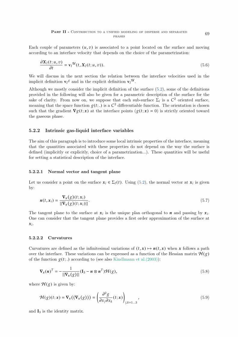
Part II - Contribution to a unified modeling of disperse and separatedphases

69

Each couple of parameters (u , v) is associated to a point located on the surface and movingaccording to an interface velocity that depends on the choice of the parametrization:

∂X I (t; u , v)∂t

vIU (t ,X I (t; u , v)). (5.6)

We will discuss in the next section the relation between the interface velocities used in theimplicit definition vI

g and in the explicit definition vIU .

Although we mostly consider the implicit definition of the surface (5.2), some of the definitionsprovided in the following will also be given for a parametric description of the surface for thesake of clarity. From now on, we suppose that each sub-surface Σi is a C2 oriented surface,meaning that the space function g(t; .) is a C2 differentiable function. The orientation is chosensuch that the gradient ∇g(t; x) at the interface points (g(t; x) 0) is strictly oriented towardthe gaseous phase.

5.2.2 Intrinsic gas-liquid interface variables

The aim of this paragraph is to introduce some local intrinsic properties of the interface, meaningthat the quantities associated with these properties do not depend on the way the surface isdefined (implicitly or explicitly, choice of a parametrization...). These quantities will be usefulfor setting a statistical description of the interface.

5.2.2.1 Normal vector and tangent plane

Let us consider a point on the surface x i ∈ ΣI (t). Using (5.2), the normal vector at x i is givenby:

n(t , x i) ∇x

(g)(t; x i)

| |∇x(g)(t; x i) | |

. (5.7)

The tangent plane to the surface at x i is the unique plan orthogonal to n and passing by x i.One can consider that the tangent plane provides a first order approximation of the surface atx i.

5.2.2.2 Curvatures

Curvatures are defined as the infinitesimal variations of (t , x) 7→ n(t , x) when x follows a pathover the interface. These variations can be expressed as a function of the Hessian matrix H (g)of the function g(t; .) according to (see also Kindlmann et al.(2003)):

∇x (n)T −

1

| |∇x(g)| |

(I3 − n ⊗ nT )H (g), (5.8)

where H (g) is given by:

H (g)(t; x) ∇x((∇x

(g)))

(∂2g

∂x j∂xk(t; x)

)j,k1...3

, (5.9)

and I3 is the identity matrix.

70 Chapter 5 - Statistical modeling of the gas-liquid interface

It can be shown that there exists an orthonormal basis e∗1 , e∗

2 of the tangent plane at thesurface point x i, such that the restriction of the matrix ∇x (n)T to the tangent plane is a 2 × 2diagonal matrix Kindlmann et al.(2003). In other words, in the orthonormal basis e∗1 , e

∗

2 , n,∇x (n)T reads:

∇x (n)T

*.,

κ1 0 σ10 κ2 σ20 0 0

+/-, (5.10)

where κ1 ≥ κ2 are the two principal curvatures and (σ1 , σ2) are two real variables. The eigen-vectors e∗1 , e

∗

2 corresponding to the eigenvalues (κ1 , κ2) are also called the principal directionsof the surface at x i.

Instead of using the two principal curvatures, one can consider the mean curvature H and theGauss curvature G, defined by:

H 1

2(κ1 + κ2),

G κ1κ2.(5.11)

Indeed, the mapping (κ1 , κ2) ∈ R2; κ1 ≥ κ2

−→

(H,G) ∈ R2+; H2

≥ G

(κ1 , κ2) 7−→ (H,G), (5.12)

is one-to-one.

5.2.2.3 Area density measure and stretch rate

The last quantity needed in the following is an evaluation of the interface area within any controlvolume. For this purpose, one defines the area density measure as follows, see Morel(2015) andrelated works:

δI (t; x) | |∇x(g)| | δ(g(t , x)), (5.13)

where δ denotes the Dirac measure. Consequently, for any volume V, the area AV (t) of surfacecontained in V at time t is given by:

AV (t) ∫Ωx

1V (x)δI (t; x)dx ,

where 1V (x) is the characteristic function of volumeV. It is important to note that the measureδI does not depend on the choice of g. It is thus an intrinsic property of the interface.

5.2.2.4 Interface velocity

We have seen in paragraph 5.2.1 that the interface velocity may have multiple definitions, ac-cording to the definition of the interface (implicit (5.2) or explicit (5.4)) or the choice of theparametrization. Let us choose here a unique definition of this velocity.

As underlined in Drew(1990), one can see that the evolution of the interface according to (5.3)only depends on the normal component of vI

g. Let us then introduce vI vIg· n, that is

unambiguously defined, and the interface velocity by:

vI vI n , (5.14)

Part II - Contribution to a unified modeling of disperse and separatedphases

71

By considering a point X I (t; u , v) on the surface for a given parametrization and the applicationϕ : (t; u , v) 7→ g(t; X I (t; u , v)), one can show the following relation with the the velocity vI

U

defined in (5.6):

vI vIU· n.

Now, let us consider that the interface lies in a medium, whose velocity is U(t , x). Moreover, thisinterface may propagate, normal to itself, at a velocity Ve n relative to the medium Pope(1988).This is for example the case of a flame that separates burnt and unburnt gases, for which theflame speed Ve depends on the chemical reactions rates. Or in the case of two-phase flows, Vemay characterize the rate of phase transitions, such as evaporation. The interfacial velocity isthen related to these quantities through:

vI (U · n) + Ve .

5.2.3 Time evolution of interfacial variables

In this paragraph, we present the evolution equations for surface element properties based on theworks of Drew(1990). Let us mention that the choice in the definition of the interface velocityaffects the expression of the evolution laws for the curvatures and the area density measure. Herewe consider the interface velocity defined by (5.14). Then, the time evolution of the curvaturescan be expressed as follows:

H −1

2∇2T (vI ) − (2H2

− G)vI ,

G −H∇2T (vI ) +√

H2 − G(∂2vI

∂y∗12−∂2vI

∂y∗22

) − 2 H G vI ,(5.15)

where • ∂t •+vI · ∇x•, denotes the Lagrangian time derivative, ∇2T ∂2y1 +∂2y2 is the tangential

Laplacian operator (y1 and y2 can be any two orthonormal directions tangential to the surface),and y∗k is the coordinate along the principal directions e∗k , k 1, 2. In B, we derive the equationfor δI . This equation reads:

δI − (∇x · vI ) δI + 2H vI δI . (5.16)

In equation (5.16), one can identify the second term in the right-hand side with the stretchingrate S, which is defined in Pope(1988) as an intrinsic property. For an interface velocity that isnormal to the interface, its equation reads:

S 2H vI . (5.17)

Another important point in the comparison with Pope’s equations is to note that in Pope(1988),the interface velocity is defined as the sum of the fluid velocity and the propagation velocity ofthe flame interface due to chemical reaction (combustion). Consequently, this leads to differentequations for H, G and S.

The system (5.15) is not closed, because of the second order derivatives of the interfacial velocityin the two principal directions. For future works, these terms need to be modeled, but this isnot the objective of the present work. An interpretation of the different terms occurring in thesystem of equation (5.15) can be found in Drew(1990).

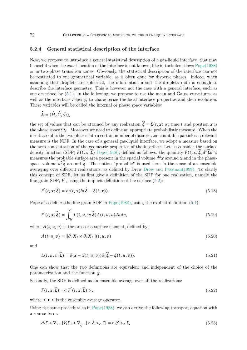
72 Chapter 5 - Statistical modeling of the gas-liquid interface

5.2.4 General statistical description of the interface

Now, we propose to introduce a general statistical description of a gas-liquid interface, that maybe useful when the exact location of the interface is not known, like in turbulent flows Pope(1988)or in two-phase transition zones. Obviously, the statistical description of the interface can notbe restricted to one geometrical variable, as is often done for disperse phases. Indeed, whenassuming that droplets are spherical, the information about the droplets radii is enough todescribe the interface geometry. This is however not the case with a general interface, such asone described by (5.1). In the following, we propose to use the mean and Gauss curvatures, aswell as the interface velocity, to characterize the local interface properties and their evolution.These variables will be called the internal or phase space variables:

ξ (H , G, vI ),

the set of values that can be attained by any realization ξ ξ(t , x) at time t and position x isthe phase space Ωξ. Moreover we need to define an appropriate probabilistic measure. When theinterface splits the two phases into a certain number of discrete and countable particles, a relevantmeasure is the NDF. In the case of a general gas-liquid interface, we adopt a measure based onthe area concentration of the geometric properties of the interface. Let us consider the surfacedensity function (SDF) F(t , x; ξ) Pope(1988), defined as follows: the quantity F(t , x; ξ)d5ξd3xmeasures the probable surface area present in the spatial volume d3x around x and in the phase-space volume d5ξ around ξ. The notion "probable" is used here in the sense of an ensembleaveraging over different realizations, as defined by Drew Drew and Passman(1999). To clarifythis concept of SDF, let us first give a definition of the SDF for one realization, namely thefine-grain SDF, F

′, using the implicit definition of the surface (5.2):

F′

(t , x; ξ) δI (t , x)δ(ξ − ξ(t , x)). (5.18)

Pope also defines the fine-grain SDF in Pope(1988), using the explicit definition (5.4):

F′

(t , x , ξ) ∫U

L(t , u , v; ξ)A(t , u , v)dudv , (5.19)

where A(t , u , v) is the area of a surface element, defined by:

A(t; u , v) | |∂uX I × ∂vX I | |(t; u , v) (5.20)

and

L(t , u , v; ξ) δ(x − x(t , u , v))δ(ξ − ξ(t , u , v)). (5.21)

One can show that the two definitions are equivalent and independent of the choice of theparametrization and the function g.

Secondly, the SDF is defined as an ensemble average over all the realizations:

F(t , x; ξ) < F′

(t , x; ξ) >, (5.22)

where < • > is the ensemble average operator.

Using the same procedure as in Pope(1988), we can derive the following transport equation witha source term:

∂t F + ∇x · vI F + ∇ξ · < ξ >c F < S >c F, (5.23)

Part II - Contribution to a unified modeling of disperse and separatedphases

73

where the conditional expectation of a scalar ψ is defined by:

< ψ >c< ψF

′ (t , x; ξ) >

F(t , x; ξ).

The SDF evolves due to two main contributions: the left-hand side of equation (5.23) contributesto the evolution of F in the phase-space Ωξ and in the physical space Ωx. This evolution isexpressed as divergences of conservative fluxes. The source terms of the right-hand side ofequation (5.23) express the evolution of the surface area due to stretching.

The conditional expectations of H, G and S may be obtained from their Lagrangian timeevolution (5.15) by applying the ensemble averaging and by using the linearity of the averageoperator, which reads (λ is a constant):

< λa + b > λ < a > + < b >,

as well as Gauss and Leibniz rules:

< ∂t a > ∂t < a > and < ∂x a > ∂x < a > .

Then, the averaged evolution equations read:

< H >c −1

2< ∇2T (vI ) >c − (2H2

− G) (vI · < n >c),

< G >c −H < ∇2T (vI ) >c +

√H2 − G

⟨∂2vI

∂y∗12−∂2vI

∂y∗22

⟩c

− 2HG (vI · < n >c),

< S >c 2H (vI · < n >c).

(5.24)

One can note that some terms are unclosed in these equations. These are the conditionalexpectations of:

• the normal vector < n >c,

• the second order derivatives of the interfacial velocity < ∇2T (vI ) >c,

• the evolution of the interfacial velocity < vI >c.

These terms need to be modeled and related to the internal flow dynamics of the gas and liquidphases.

5.2.5 Averaged quantities and moments of the SDF

The numerical resolution of equation (5.23) is unreachable for most applications because ofthe large dimension of the phase space Ωξ. In fact, solving the exact SDF would provide alevel of detail on the flow, which is often not needed. Moreover, the large amount of dataproduced to attain this level of detail may hide the prevailing macroscopic features we arelooking for. Therefore, we only aim at predicting some macroscopic variables of the flow, thatensure a satisfactory result for most industrial applications. Drew Drew(1990) derived Eulerianequations for the evolution of the following averaged quantities: the expected surface densityΣ(t , x), the interfacial-expected mean and Gauss curvatures, H, G and the volume fractionα(t , x). In the present approach, we can not express the volume fraction as a function of theSDF without making a topological assumption on the gas-liquid interface. Therefore, in thispart we temporarily restrict our study to the first three averaged interfacial quantities.

74 Chapter 5 - Statistical modeling of the gas-liquid interface

In terms of moments of the SDF, Σ(t , x), H and G can be expressed as follows:

Σ(t , x) M0,0,0(t , x),Σ(t , x)H M1,0,0(t , x),Σ(t , x)G M0,1,0(t , x),

(5.25)

where the moments read:

Mi , j,l (t , x) ∫Ωξ

H iG jVI ,xlx VI ,y

ly VI ,zlz F(t , x; ξ)d5ξ , (5.26)

and l (lx , ly , lz).

Then, by multiplying the SDF evolution equation (5.23) by H iG jVI ,xlx VI ,y

ly VI ,zlz and integrating

over the whole phase-space domain, we can derive the evolution equations for the three quantitiesof interest:

∂tΣ + ∇x · (Σ vI ) ∫ξ< S >c F(t , x; ξ) d5ξ ,

∂tΣH + ∇x ·(Σ H vI

) ∇x ·

(ΣH(vI − vI

H ))

+∫ξ< S + H/H >c HF(t , x; ξ) d5ξ ,

∂tΣG + ∇x ·(Σ G vI

) ∇x ·

(ΣG(vI − vI

G))

+∫ξ< S + G/G >c GF(t , x; ξ) d5ξ.

(5.27)

We can notice three types of averaged interfacial velocity that read:

Σ vI ∫ξvI F(t , x; ξ) d5ξ ,

Σ H vIH

∫ξvI HF(t , x; ξ) d5ξ ,

Σ G vIG

∫ξvI GF(t , x; ξ) d5ξ.

(5.28)

Using the time evolution of both curvatures and of the stretch factor (5.15) in the system ofequations (5.27), we can show that this system is equivalent to the system derived by Drew inDrew(1990). However, two closure issues need to be tackled at two different stages for futureworks. First, we need time evolution laws to close the conditional averages (< H >c , < G >c , <S >c), as already mentioned for the transport equation of the SDF. Next, we need to proposea procedure to reconstruct the SDF from the known moments. Let us underline that, by usingonly the three first moments M0,0,0, M1,0,0, M0,1,0, we can not capture the variance of the phase-space coordinates. One should consider higher order moments. However, one must be carefulwhen reconstructing the SDF in this case. Indeed, the curvatures (H , G) must satisfy H2

≥ G(see equation (5.12)), and the SDF reconstruction has to respect this constraint.

5.3 Probabilistic description of the gas-liquid interface for a dis-perse phase

5.3.1 Surface density function in the context of discrete particles

The SDF measures the pointwise probable area concentration for a probabilistic event, which ischaracterized by the phase space variables ξ H , G, vI ∈ Ωξ and evaluated at a local point

Part II - Contribution to a unified modeling of disperse and separatedphases

75

E1 E2 E3

E4

E5E6

Figure 5.1: Illustration of the spatial decomposition, with subspaces containing only one particle.

x ∈ Ωx. This probabilistic description is a pointwise description of the interface, which makes itgeneral and valid for both separated and disperse phases. However, in the case of a disperse flow,a point-particle approach is usually considered. Each particle, droplet or bubble, is reduced to apoint, characterized by some averaged and global quantities, such as: the velocity of the center ofmass, the particle size (measured by volume, surface area or diameter), etc... and the statisticsare conducted on a number of objects. In order to adapt the statistical approach presented in theprevious section to a discrete formalism for a disperse phase, we first define interfacial quantitiesthat are averaged over the surface of each particle. Then, we define a discrete surface densityfunction (DSDF) that may characterize the dispersion in size and in shape of the population ofparticles.

Let us consider an isolated particle pk of surface Σk , supposed to be smooth. Let us also

consider a partition of the domain Ωx

Nmax⋃k1

Ek , such that each sub-domain Ek contains exactly

one particle pk , as illustrated in Figure 5.1. For a quantity φ(t , x), that can be a scalar (likecurvatures) or a vector (like a velocity), we define its interface average φk (t , x) over the particlesurface Σk as follows:

φk (t , xk ) 1

Sk

∫x∈Ek

φ(t , x)δI (t , x)d3x , (5.29)

where Sk is the total surface area of the particle:

Sk

∫x∈Ek

δI (t , x)d3x ,

and xk its center of mass.

From now on, we consider each particle pk as punctual, located at its center of mass xk (t),having a surface area Sk and the averaged interface properties ξk Hk ,Gk , vI k . We define theDSDF by:

Fd (t , x , ξ) <Nmax∑k1

Sk (t)δ(x − xk (t))δ(ξ − ξk (t)) > (5.30)

where Nmax is the maximum number of particles in the domain Ωx over all realizations. One cannote that we have chosen to locate the particles at their centers of mass. However, the surfaceaveraging procedure involves a surface barycenter defined by xk 1/Sk

∫Σk

xdS(x). In order tocope with our choice, which is more practical as far as the particle dynamics is considered, we

76 Chapter 5 - Statistical modeling of the gas-liquid interface

propose to express the mean interface velocity as:

vI k (t) dxk (t)

dt+ Vk (t),

where Vk (t) is a fluctuation velocity, that stands for the particle shape deformations. In thefollowing, this fluctuation velocity is neglected and we simply consider that the averaged interfacevelocity of a particle pk reads:

vI k (t) dxk (t)

dt. (5.31)

The DSDF (5.30) verifies a similar transport equation as (5.23):

∂t Fd+ ∇x ·

(vI Fd

)+ ∇ξ ·

(<

˙ξ >c Fd

)<

˙S >c Fd . (5.32)

Once more, the time evolution of the averaged curvatures needs to be modeled in order to closethe system of equations. This is work in progress and is out of the scope of the present paper.

The "localized" SDF defined in section 5.2.4 and the DSDF are two different functions. Nonethe-less, they contain similar pieces of information about the gas-liquid interface properties. Indeed,both functions provide the probable surface area of the interface having some geometrical prop-erties given by the phase-space variables. For the "localized" SDF, the phase-space variablesare given by the localized interface properties at a surface point, while for the DSDF, we haveconsidered interface properties averaged by object (particle). The link between the two functionscan be seen through the first order moments of the two functions:

Proposition 5.3.1 Given a subdomain E ⊂ Ωx, such that its border does not cut any particle,the integral over this subdomain of the zeroth and first order moments of the two functions areequal: ∫

x∈E

∫ξ∈Ωξ

F(t , x; ξ) d5ξd3x ∫

x∈E

∫ξ∈Ωξ

Fd (t , x; ξ) d5ξd3x∫x∈E

∫ξ∈Ωξ

ξ lF(t , x; ξ) d5ξd3x ∫

x∈E

∫ξ∈Ωξ

ξ lFd (t , x; ξ) d5ξd3x(5.33)

where ξ l ∈H , G, vI x , vI y , vI z

.

Proof: We illustrate this result for a moment of order one on G and zero on the other phasevariables (ξ l G):∫

x∈E

∫ξ∈Ωξ

GF(t , x; ξ) d5ξd3x <∫

x∈E G(t; x) δI (x) d3x >

<∑k

∫x∈Ek∩E

G(t; x) δI (x) d3x >

<∑

k; xk (t)∈ESkGk >

<∑

k; xk (t)∈E

∫x∈Ek

∫ξ∈Ωξ

GFd (t , x , ξ) d5ξd3x >

∫

x∈E

∫ξ∈Ωξ

GFd (t , x , ξ) d5ξd3x.

(5.34)

We recall that the zeroth and first-order moments are related to the expected surface densityand the two curvatures (Σ,ΣH ,ΣG), defined in (5.25), and to the expected interface velocity,

Part II - Contribution to a unified modeling of disperse and separatedphases

77

defined in (5.28). In this work, we give a great importance to these quantities because theycontain some topological information about the gas-liquid interface, such as the number densityof particles, as we will show in next section. we underline that any future definition of a newSDF should preserve these moments.

5.3.2 Link between the DSDF and a NDF: derivation of a Williams-Boltzmann-like equation

Let us now present the relation between the DSDF (5.30) and a number density function (NDF)for particles, using a geometrical property of the averaged Gauss curvature, known as the Gauss-Bonnet formula.

Let M be a 3D bounded object and (M) its surrounding surface, supposed to be smooth. TheGauss-Bonnet formula applied to (M) states that Abbena et al.(2006):∫

x∈(M)G(x)dS(x) 2π χ(M), (5.35)

where χ(M) is the Euler characteristic of the surface (M) and is a topological invariant,meaning that two homeomorphic surfaces have the same Euler characteristic. In the following, weconsider smooth particle surfaces, that are all homeomorphic to a sphere, the Euler characteristicof which is 2. Therefore, we can relate the averaged Gauss curvature over the surface of a particlepk to its surface area by:

Sk 4π

Gk. (5.36)

SinceSkGk

4π 1 for each particle, we are able to count the total number of particles, just by

looking at the interface average of G. Then, we can derive a relation between the DSDF Fd anda Number Density Function (NDF) f . This relation is given by the following proposition.

Proposition 5.3.2 When the two-phase flow is purely disperse, the distribution functionG4π

Fd (t , x; ξ)

is equal to the NDF f (t , x; ξ) for a phase space made of the averaged curvatures and interfacevelocity ξ H , G, vI :

G4π

Fd (t , x; ξ) f (t , x; ξ) (5.37)

Proof:

G4π

Fd (t , x; ξ) <Nmax∑k1

Sk (t)δ(x − xk (t))

G4π

δ(ξ − ξk (t))) >,

<Nmax∑k1

Sk (t)δ(x − xk (t))

Gk (t)4π

δ(ξ − ξk (t)) >,

<Nmax∑k1

δ(x − xk (t))δ(ξ − ξk (t)) >,

f (t , x; ξ).

(5.38)

78 Chapter 5 - Statistical modeling of the gas-liquid interface

From the transport equation of the DSDF (5.32), we can derive a General Popolation BalanceEquation (GPBE) for f (t , x; ξ), that is similar to the Williams-Boltzmann equation:

∂t f + ∇x · vI f + ∇ξ · <˙ξ >c f *

,<

˙S >c + <

˙G

G>c+

-f . (5.39)

The right-hand term behaves as a source term. We can relate this term to topological evolutionsof the Euler characteristic of droplets due to fragmentation, coalescence, ects.

Let us now consider a set of droplets that do not break up, nor coalesce and which are all thetime homeomorphic to spheres. Using the Gauss-Bonnet result (5.36), we can show that:

˙Sk −

˙Gk (t)

Gk (t). (5.40)

Therefore, without break-up nor coalescence, equation (5.39) reduces to:

∂t f + ∇x · vI f + ∇ξ · <˙ξ >c f 0. (5.41)

Equation (5.41) represents the time evolution of the particles NDF due to transport in physicalspace at the velocity of their center of mass, and the evolution of the internal variables, whichrepresents the particle surface deformations and their acceleration by interaction with the carriergas.

Now, we consider the volume of particles as an additional variable of the phase-space. Let usunderline that adding the volume to the phase-space variables is specific to particles and can notbe easily conducted within the general statistical approach for gas-liquid interface, as introducedin section 5.2.4. Furthermore, we also replace the averaged Gauss curvature by the surface areaof the particles, since the two variables are related by (5.36). In the following, we denote the newphase-space variables by ξ

v H , S, v , vI , where S 4π/G is the surface area of the particles

and v is their volume. A new NDF may be defined as follows:

f (t , x , ξv) <

Nmax∑k1

δ(x − xk (t))δ(ξv− ξ

vk (t)) > . (5.42)

Next, we focus on the evolution of the expected-average terms of the gas-liquid interface: theinterface density area Σ(t , x), the mean and Gauss curvatures, H(t , x) and G(t , x), introducedin section 5.2.4 and the volume fraction α(t , x). In the current context, these terms can beexpressed as first order moments of the NDF as follows:

α(t , x) M0,0,1,0(t , x),Σ(t , x) M0,1,0,0(t , x),Σ(t , x)H M1,1,0,0(t , x),Σ(t , x)G 4πM0,0,0,0(t , x),

(5.43)

where the moments of the NDF now read:

Mi , j,k ,l (t , x) ∫ξ

v∈Ωξ

H iS j vkVI ,xlx VI ,y

ly VI ,zlz f (t , x; ξ

v) d5ξ

v, (5.44)

Part II - Contribution to a unified modeling of disperse and separatedphases

79

and l (lx , ly , lz). By considering the corresponding moments of the dynamics of the NDF(5.41), we can obtain the equations of the three expected interfacial variables and the volumefraction:

∂tα + ∂x · α(t , x)vI ∇x ·(α(t , x)(vI − vI

α))+

∫ξ

v< v >c f (t , x; ξ

v)d5ξ

v,

∂tΣ + ∂x · Σ(t , x)vI

∫ξ

v< −S >c f (t , x; ξ

v)d5ξ

v,

∂tΣH + ∂x · ΣHvI ∇x ·(ΣH(vI − vI

H ))+

∫ξ

v< −SH + HS >c f (t , x; ξ

v)d5ξ

v,

∂tΣG + ∂x · ΣGvI ∇x ·(ΣG(vI − vI

G)).

(5.45)

The divergence terms appearing in the right-hand side of the system express the correlationbetween the velocity and the rest of the phase space variables. In the case where the velocityis uncorrelated with v ,H,G, these terms vanish. Under this hypothesis, the only remainingsource terms are related to the shape deformation and to the compressibility of the particles.Also, the last equation would have no source term: the deformation of particles does not affectthe quantity ΣG. Indeed, according to Gauss-Bonnet this quantity is the expected numberdensity of particles, the evolution of which is only due to convection or coalescence and break-upof the particles. Since we have supposed that the particles do not break-up nor coalesce, theparticles number density is simply convected at velocity vI .

In the following section, we propose a simplified closed model of this system in the case of apolydisperse evaporating spray, where the droplets are supposed to remain spherical at any time.

5.4 High order geometrical size moments for polydisperse evap-orating sprays of spherical droplets

Remark 1 From now on, we omit the subscript • for the phase-space variables.

In this part, we show that the system of equations given in (5.45) can degenerate to the fractionalmoments model described in chapter 4 in the case of spherical droplets and under the sameassumptions as the ones used in that chapter. In the following, we suppose that the sprayis dilute and the Weber number is low enough, so that coalescence and fragmentation of thedroplets can be neglected. Finally, we assume that thermal transfer can also be neglected, sothat the temperature of the droplets can be ignored. Under the hypothesis that the dropletsstay spherical at all times, the NDF writes:

f (t , x; H, S, v , vI ) N (t , x; S, vI ) δ(H − H(S)) δ(v − v(S)), (5.46)

where the mean curvature, H(S) √

4π/S, and the volume of the drops, v(S) S3/2/(6√π),

are two functions of the surface S. Therefore, we can reduce the phase-space variables to thesurface area S and the averaged interface velocity vI . Let us also note that under the assumptionof the incompressibility of the droplet and a uniform evaporation at the droplet surface, vI isnow equal to vp, the velocity of the mass center of the droplet. In the following, we considerdimensionless variables, so that the surface area S ∈ [0, 1]. The droplet acceleration vp is equalto the sum of forces per unit of mass acting on the droplet. In the following, we consider thatthe only force acting on the droplets is the drag due to the carrier gas. This can be modeled in

80 Chapter 5 - Statistical modeling of the gas-liquid interface

a first time by a linear Stokes law:

vp u g − vp

St(S), (5.47)

where St(S) θS is the Stokes number, which depends linearly on the surface area S. Thecoefficient θ depends on the physical properties of the gas and the liquid. Since we considerspherical and non-deforming droplets, the evolution of the surface area is only due to evaporation.The Lagrangian-time derivative of the surface area is equal to the evaporation:

S RS (S). (5.48)

Assuming a d2 law for the phenomenon, the evaporation rate is constant: RS (S) −K. Con-sidering the spherical assumption of the droplets, we can show the following relations:

v −3

2

1

6√π

S1/2K

H 1

2

√4π

1

S3/2K

(5.49)

To simplify the distribution on the velocity, we consider a monokinetic assumption de Chaise-martin et al.(2009):

N (t , x; S, vp) n(t , x , S) δ(vp − up (t , x)), (5.50)

The averaged interfacial quantities (volume fraction, surface area density and Gauss and meancurvatures), that have been expressed as moments of the NDF f (t , x; H, S, v , vI ) in equations(5.43) and (5.44), can now be expressed as moments of the simplified NDF n(t , x , S) as follows:

ΣdGd 4πm0 ,ΣdHd 2

√πm1/2 ,

Σd m1 ,

αd 1

6√π

m3/2 ,

(5.51)

where a fractional size-moment is given by:

mk/2(t , x) ∫ 1

0

Sk/2n(t , x , S)dS. (5.52)

Now, from equations (5.45), (5.51), (5.48), (5.49) and (5.47), we can derive the following systemof equations on the fractional size-moments:

∂tm0 + ∂x ·(m0up

) −K (t , x , S 0),

∂tm1/2 + ∂x ·(m1/2up

) −

K

2m−1/2 ,

∂tm1 + ∂x ·(m1up

) −Km0 ,

∂tm3/2 + ∂x ·(m3/2up

) −

3K

2m1/2 ,

∂t (m1u) + ∂x ·(m1up ⊗ up

) −Km0up + m0

u g − up

θ,

(5.53)

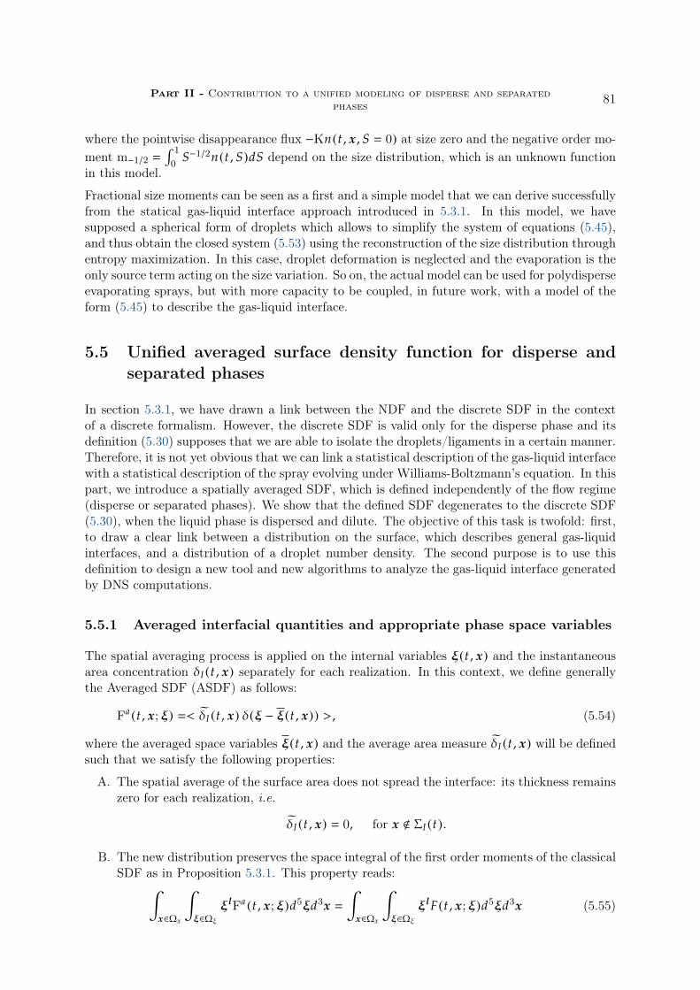
Part II - Contribution to a unified modeling of disperse and separatedphases

81

where the pointwise disappearance flux −Kn(t , x , S 0) at size zero and the negative order mo-ment m−1/2

∫ 1

0S−1/2n(t , S)dS depend on the size distribution, which is an unknown function

in this model.

Fractional size moments can be seen as a first and a simple model that we can derive successfullyfrom the statical gas-liquid interface approach introduced in 5.3.1. In this model, we havesupposed a spherical form of droplets which allows to simplify the system of equations (5.45),and thus obtain the closed system (5.53) using the reconstruction of the size distribution throughentropy maximization. In this case, droplet deformation is neglected and the evaporation is theonly source term acting on the size variation. So on, the actual model can be used for polydisperseevaporating sprays, but with more capacity to be coupled, in future work, with a model of theform (5.45) to describe the gas-liquid interface.

5.5 Unified averaged surface density function for disperse andseparated phases

In section 5.3.1, we have drawn a link between the NDF and the discrete SDF in the contextof a discrete formalism. However, the discrete SDF is valid only for the disperse phase and itsdefinition (5.30) supposes that we are able to isolate the droplets/ligaments in a certain manner.Therefore, it is not yet obvious that we can link a statistical description of the gas-liquid interfacewith a statistical description of the spray evolving under Williams-Boltzmann’s equation. In thispart, we introduce a spatially averaged SDF, which is defined independently of the flow regime(disperse or separated phases). We show that the defined SDF degenerates to the discrete SDF(5.30), when the liquid phase is dispersed and dilute. The objective of this task is twofold: first,to draw a clear link between a distribution on the surface, which describes general gas-liquidinterfaces, and a distribution of a droplet number density. The second purpose is to use thisdefinition to design a new tool and new algorithms to analyze the gas-liquid interface generatedby DNS computations.

5.5.1 Averaged interfacial quantities and appropriate phase space variables

The spatial averaging process is applied on the internal variables ξ(t , x) and the instantaneousarea concentration δI (t , x) separately for each realization. In this context, we define generallythe Averaged SDF (ASDF) as follows:

Fa (t , x; ξ) < δI (t , x) δ(ξ − ξ(t , x)) >, (5.54)

where the averaged space variables ξ(t , x) and the average area measure δI (t , x) will be definedsuch that we satisfy the following properties:

A. The spatial average of the surface area does not spread the interface: its thickness remainszero for each realization, i.e.

δI (t , x) 0, for x < ΣI (t).

B. The new distribution preserves the space integral of the first order moments of the classicalSDF as in Proposition 5.3.1. This property reads:∫

x∈Ωx

∫ξ∈Ωξ

ξ lFa (t , x; ξ)d5ξd3x

∫x∈Ωx

∫ξ∈Ωξ

ξ lF(t , x; ξ)d5ξd3x (5.55)

82 Chapter 5 - Statistical modeling of the gas-liquid interface

where l ∈ 0, 15 , l1+· · ·+ l5 ≤ 1 and ξ ξ1 , . . . , ξ5. We recall that this property ensuresthe possibility to express the expected-mean interfacial quantities (Σ(t , x), H(t , x), G(t , x))as moments of the new averaged SDF.

C. The new SDF can be related to the discrete SDF, when the domain contains a dilutedisperse phase, such that the larger particle diameter is smaller than the inter-particledistance. We express this relation for a volume space E ⊂ Ωx, where the border of thedomain does not cross any particle, as follows:∫

x∈EFa (t , x; ξ)d3x

∫x∈E

Fd (t , x; ξ)d3x. (5.56)

In these conditions, we can relate the spatial-averaged SDF to the NDF of the particles inthe same way as in section 5.3.2.

To fulfill the first requirement A, we propose to define the averaged quantities as follows:

δI (x) Θh (t , x)δI (t , x), (5.57)

ξ(t , x)

1

Θh (t , x)

∫y∈Ωx

w(x; y − x) δI (t , y)ξ(t , y)d3y , if Θh (t , x) > 0

Not defined otherwise

(5.58)

and

Θh (t , x) ∫

y∈Ωx

w(x; y − x) δI (t , y)d3y , (5.59)

where w(x; r y − x) is a convolution kernel. The function w(x; r) is chosen such that itvanishes for large | |r | | > h, where h > 0 is a characteristic spatial length scale, independent fromthe position x. The case where Θh (t , x) 0, the averaged interfacial variables are not definedand can take any real value, since no interface exists in the vicinity of the position x.

The kernel function is designed such that the SDF (5.54), satisfies the two remaining require-ments (B and C).

For the second requirement B, we can show that equation (5.55) is satisfied if we have, for anyy ∈ Ωx:∫

x∈Ωx

w(x , y − x)δI (t , x)d3x 1. (5.60)

Finally, for the third requirement property C, we look for a spatial-average of the interfacialvariables (5.58) that can degenerate to an interfacial average over one particle surface (5.29),when the inter-particle distance is much larger than the particles diameters. We can reach thisgoal by first choosing a length scale h larger than the maximum of particle diameters and smallerthan the inter-particle distance. Then we propose to use the following kernel function, whichsatisfies the condition (5.60):

w(x; r) 1| |r | |<h (r)∫

x′∈Vh (x+r) δI (x′)d3x′, (5.61)

where Vh (x) y ∈ Ωx; | |x − y | | < h. Therefore, w(x , r) represents the inverse of the surfacearea included inVh (x + r). In the case where no interface exists in the volumeVh (x + r), w(x , r)is not defined and can take any real value without affecting the definition of the averaged SDF.

Part II - Contribution to a unified modeling of disperse and separatedphases

83

5.5.2 Generalized Number density function

Using the averaged SDF defined in the previous section, we can define the following distributionfunction:

Definition We define the Generalized Number Density Function (GNDF) as follows:

fΣ(t , x; ξ) |G |4π

Fa (t , x; ξ). (5.62)

Now, let us consider a disperse phase made of Nmax non-spherical particles (droplets or bubbles),pk , k 1, . . . ,Nmax whose external boundaries are denoted by Σk , k 1, . . . ,Nmax and theircenter of mass by xk , k 1, . . . ,Nmax. By considering a sufficiently large length scale averagingh (for example larger than the particle diameter), we can ensure the positivity of the averagedGauss curvature. In this case, we can simply write the GNDF as follows:

fΣ(t , x; ξ) G4π

Fa (t , x; ξ). (5.63)

In the following, we consider a dilute disperse phase, such that the inter-distance between thedroplets is larger than the droplet diameter. Using a length scale h larger than the dropletdiameter, we show the link between the GNDF and the classic NDF, as it was stated in thethird requirement C of the last section. To conduct this derivation, we use the notations ofsection 5.3.1, which introduced the discrete formalism of the particles.

Proposition 5.5.1 If E is a space volume whose borders do not cross any particle, then the two

integrals of the GNDF fΣ(t , x; ξ) G4π

Fa (t , x; ξ) and the NDF f (t , x; ξ) ever E are equal:

∫x∈E

fΣ(t , x; ξ)d3x

∫x∈E

f (t , x; ξ)d3x. (5.64)

Proof: If h is larger than the largest particle diameter and smaller than the smallest inter-particle distance, then ωk x ∈ Ωx , min

y∈Σk| |x − y | | ≤ h is a subdomain of Ωx which contains

only the particle pk . Also, all the interfacial information is contained within the intersection ofthese subdomains ∩Nmax

k1 ωk , so that one can write:

∫x∈E

GFa (t , x; ξ)d3x <Nmax∑k1

∫ωk∩E

G δI (t , x) δ(ξ − ξ(t , x)d3x>,

<Nmax∑k1

∫ωk∩E

Gk δI (t , x) δ(ξ − ξk )d3x>,

<∑

k ,xk∈E

Gk Sk δ(ξ − ξk )

>,

4π <∑

k ,xk∈E

δ(ξ − ξk )

>,

4π∫

x∈E f (t , x; ξ)d3x ,

(5.65)

To pass from the third to the fourth equality, we have used Gauss-Bonnet formula and havesupposed that all droplets are homeomorphic to a sphere.

84 Chapter 5 - Statistical modeling of the gas-liquid interface

This result shows a general interpretation for the NDF, which is not restricted to a discreteformalism. In the same way as in section 5.3.1, we can derive the GPBE satisfied by the GNDF:

∂t fΣ + ∇x · vI fΣ + ∇ξ · < ξ >c fΣ < Γ >c fΣ , (5.66)

where Γ S +GG is a source term of topology variation and which can be related mainly to the

breakup and coalescence phenomena.

Now, it is more obvious that the SDF and NDF are strongly related. The SDF can be seen as theorigin of the NDF as it was discussed in Canu et al.(2017). The averaged SDF allows to considera generic statistical description of the gas-liquid interface, which can also be directly related tothe NDF in the case of dilute disperse phase, as it is stated by proposition 5.5.1. Indeed, byusing the spatial averaging procedure, we are able to isolate droplets in dilute disperse phaseregion, and thus we can compute the NDF from the averaged SDF.

5.6 Algorithms and techniques for the numerical computation ofthe curvatures and of the SDF

In this part, we apply the results of the previous section to the design of a new numericaltool dedicated to the post-processing of DNS two-phase flows simulations. Such tool allows toenhance the analysis of the gas-liquid interface evolution. The DNS computations are performedusing the ARCHER code Menard et al.(2007), where a combined VOF and level-set approachis used to capture the interface, and a ghost method is applied to represent accurately the jumpof variables across the liquid-gas interface.

Some numerical tools to compute the curvatures and the surface area of the gas-liquid interfacepresent in each cell are already available in the ARCHER code Canu et al.(2017). Unfortunately,these quantities being computed separately, the Gauss-Bonnet formula can not be numericallysatisfied. For this reason, we choose to compute the curvatures and the surface element areasby using the algorithm presented thereafter. Such algorithm will allow to obtain the numberdensity function of droplets in DNS simulations, by using simple computations on the surfaceand without the need of an algorithm that isolates the droplets Kang et al.(2000).

The new algorithm is implemented independently from the ARCHER code, from which onlythe distance function (Level-Set) data is used. The different algorithm steps are summarized asfollows:

• The gas-liquid interface is discretized with a 2D triangulated mesh using the MarchingCubes algorithm Thomas et al.(2003). This algorithm takes the 3D level-set scalar fieldas an input and returns a 2D meshed surface. This mesh is described with two arrays: thearray of vertices, V of dimension nv × 3, and the array of faces (defined by three vertices),F of dimension n f × 3 which defines the connectivity between vertices. In this work, weuse the Python package sckimage Van der Walt et al.(2014) to triangulate the surface.

• For each vertex V ∈ [1, nv], O(V) denotes the set of neighbors of V: V′ is a neighbor ofV if both vertices share a same face f ∈ [1, n f ]. By abuse of notation, O(V) also denotesthe set of faces V belongs to and for each f ∈ O(V), n(f) denotes the normal vector to theface, oriented toward the gas phase.

• In the neighbourhood of V, we define its dual cell M(V) as a mix between the Voronoicell (Figure 5.2b) and the barycentric cell (Figure 5.2a) around V, as proposed in Meyer

Part II - Contribution to a unified modeling of disperse and separatedphases

85

•V

•

•

•

•

•

M(V)

(a)M(V) is a barycentric cell.

•V

•

•

•

•

•

M(V)

(b) M(V) is a Voronoi cell.

•V

•

•V’

•

•

•

TαV,V’

βV,V’

θT

(c) Illustration of angles.

Figure 5.2: Neighboring vertices and surface elements M(V) around the vertex V.

et al.(2001). Simply, for each triangular face f containing V, the Voronoi contour is con-sidered if all the angle are acute. The barycentric contour is considered otherwise. Also,θf denotes the angle at vertex V in f, see Figure 5.2c, and A[f ,V] area(f ∩M(V)) isthe area of the dual cell within the face f. Then, the discrete local area A[V], normal n[V]and Gauss curvature G[V] can be computed:

A[V] ∑

f∈O(V)

A[f ,V], n[V]

∑f∈O(V)

A[f ,V]n(f)

∑

f∈O(V)A[f ,V]n(f)

,

G[V] *.,2π −

∑f∈O(V)

θf+/-/A[V].

(5.67)

• Finally, for each neighbour V′ of V, αV,V′ and βV,V′ denote the two angles facing the edge[V,V′], without distinction, as illustrated in Figure 5.2c. Now, the local discrete meancurvature reads:

H[V] 1

2A[V]

∑V′∈O(V)

(cot(αV′,V) + cot(βV′,V)

) (V[V] −V[V′])

)· n[V]. (5.68)

After computing the local geometrical quantities, we can evaluate the fine-grain localized SDFfor one simulation, i. e. one realization. In the following, the phase space variables are restrictedto the two curvatures ξ (H,G) ∈ Ωξ: we do not consider the interface velocity. This 2D spaceis discretized into nh × ng phase-space cells Ci , j, such that the discrete phase space variables areexpressed as follows:

ξ i , j (Hi ,G j) ξmin + (i∆H, j∆G), (i , j) ∈ [1, nh] × [1, ng],

where ∆H (Hmax −Hmin)/nh, ∆G (Gmax −Gmin)/ng and the subscripts min and max referrespectively to the minimum and maximum values obtained by (5.67) and (5.68). The integralof the fine-grain localized SDF over a subdomain E ⊂ Ωx can be approximated by:∫

x∈EF′

(t , x; ξ i , j)d3x '1

∆H∆G

nv∑V1

A[V] ICi , j (ξ[V]) IE (V[V]) (5.69)

where F′ (t , x; ξ i , j) is the fine-grain SDF defined in (5.18), ICi , j (.) is the characteristic function

of the cell Ci , j:

Ci , j ξ′, |H′ − Hi , j | ≤ ∆H/2 and |G′ − Gi , j | ≤ ∆G/2,

86 Chapter 5 - Statistical modeling of the gas-liquid interface

and IE (.) is the characteristic function of the sub-domain E. In the following, we take E Ωx.Thus the last equation becomes:∫

x∈Ωx

F′

(t , x; ξ i , j)d3x '1

∆H∆G

nv∑V1

A[V] ICi , j (ξ[V]). (5.70)

Using this numerical approximation, we define the numerical fine-grain SDF integrated in thewhole domain as follows:

F′

(ξ i , j) 1

∆H∆G

nv∑V1

A[V] ICi , j (ξ[V]). (5.71)

To evaluate the averaged fine-grain SDF (5.54), we first calculate the averaged area and curva-tures at each vertex V ∈ [1, nv]. These averaged quantities depend on the length scale h. Inthe following, we take h (k/2)∆x, where ∆x is the size of the level-set computation cells andk ≥ 1 is an integer value to be set by the user. We denote by Ak [V] and ξ

k[V] the numerical

approximation of the averaged area and curvatures, defined in (5.57), (5.58) and (5.61) andwhich are numerically evaluated as follows:

Ak [V] ∑

V′∈Ok (V)

A[V′]Sk [V′]

A[V],

ξk[V]

1

Ak [V]

∑V′∈Ok (V)

ξ[V′]A[V′]Sk [V′]

A[V],(5.72)

where Ok (V) is the set of vertices V′, such that | |V[V] −V[V′]| |2 ≤ k/2∆x and

Sk [V′] ∑

V′′∈Ok (V′)

A(V′′

).

The numerical fine-grain averaged SDF is given by:

F′a

(ξ i , j) 1

∆H∆G

nv∑V1

Ak [V]ICi , j (ξk[V]). (5.73)

Then, the GNDF can be evaluated numerically as follows:

N′

(ξ i , j) 1

∆H∆G

nv∑V1

|Gk[V]|

4πAk [V]ICi , j (ξ

k[V]). (5.74)

We recall that the spatial averaging of the curvatures and surface area distribution introducedin section 5.5.1, has been designed such that the first order moments of the SDF (5.55) arepreserved. We can verify this property numerically as follows:∫

ΩxΣ(t , x)dx '

∑V

A[V] ∑V

Ak [V],∫ΩxΣH(t , x)dx '

∑V

H[V]A[V] ∑V

Hk[V]Ak [V],∫

ΩxΣG(t , x)dx '

∑V

G[V]A[V] ∑V

Gk[V]Ak [V].

(5.75)

Part II - Contribution to a unified modeling of disperse and separatedphases

87

(a) t 8.54 × 10−5s (b) t 7.624 × 10−3s

Figure 5.3: Droplet surface colored according to the mean curvature values at the surfaces fortwo different times.

5.7 Numerical test with DNS simulations

In this part, we use the ARCHER code to perform some two-phase flows direct numericalsimulations. The algorithms described in the previous section will be used to post-process thelevel-set data in order to compute the fine-grain SDF and NDF of a single simulation (onerealization). Two numerical tests, with and without topological changes, allow to test thealgorithm and the capacity to find some geometrical and topological feature of the gas-liquidinterface, depending on a chosen averaging characteristic length-scale h defined in the previoussection.

5.7.1 Droplets homeomorphic to spheres

In the first configuration, we consider five initial spherical water droplets of radii r ∈ [0.33 mm, 1 mm]injected at a velocity 5 m/s in a 1 cm3 periodic cubic domain of initially still gas. Classical wa-ter/air properties are used here. The initial positions of the droplets centers are chosen randomly,with the constraint however that the inter-droplet distance ddrop (computed from the dropletsurface) is larger than 2rmax, where initially rmax 1 mm. Due to the difference between thegas and the droplet velocities, the shape of the droplets is deformed in time without break-up(the maximum Weber number is Wemax < 1). In Figure 5.3, we display an illustration of thedroplets at two successive times. The color indication at the droplet surfaces shows an estimateof the mean curvature. This first case is envisioned in the framework of no topological changes.

In Figure 5.4 (respectively 5.5), we plot the SDF for different averaged scales as a functionof the Gauss (respectively the mean) curvature. The localized SDF, plotted with a blue line,corresponds to the length scale average h ∆x/2. In this case, the SDF is continuous and wecan not identify the surface area contribution of each droplet. But, by using larger scales ofaverage (h 25∆x/2 and h 55∆x/2), we see that we can identify five peaks which correspondto the five droplets. Indeed, when ddrop > h 55∆x/2 > rmax, for any point x situated at theinterface of a droplet, the space volume Vh (x) y ∈ Ωx; | |x − y | | < h contains that, and

88 Chapter 5 - Statistical modeling of the gas-liquid interface

0 2 4 6 8

·106

0

0.5

1

1.5·10−5

G

SDF(G

)

(a) t 8.54 × 10−5s

0 2 4 6 8

·106

0

0.5

1

1.5·10−5

G

SDF(G

) ∆x25∆x55∆x

(b) t 7.624 × 10−3s

Figure 5.4: Numerical SDF over the domain space as a function of the Gauss curvature:localized SDF (dashed-line), averaged SDF with k 25 (triangle) and k 55 (solid line).

-3.0 -2.5 -2.0 -1.5 -1.0 -0.5

·103

0

0.5

1

1.5·10−5

H

SDF(H

)

(a) t 8.54 × 10−5s

-3.0 -2.5 -2.0 -1.5 -1.0 -0.5

·103

0

0.5

1

1.5·10−5

H

SDF(H

) ∆x25∆x55∆x

(b) t 7.624 × 10−3s

Figure 5.5: Numerical SDF over the domain space as a function of the mean curvature: localizedSDF (dashed-line), averaged SDF with k 25 (triangle) and k 55 (solid line).

only that, droplet. Thus, for each droplet we compute one average mean and Gauss curvatures.Consequently, in this case the averaged SDF becomes a sum of Dirac delta function.

In Figure 5.6 (respectively 5.7), we display the GNDF for different averaging scales. Thesedistributions are obtained from the averaged SDFs using (5.74). When the averaging scale h islarger than the droplet diameters, we obtain five peaks of value 1. Then, we can count the rightnumber of droplets for each averaged Gauss or mean curvature thanks to Gauss-Bonnet formulawith a proper evaluation of the curvature and using our averaging approach. This assesses theproposed theoretical and algorithmic approach within the framework of no topological change.

Part II - Contribution to a unified modeling of disperse and separatedphases

89

0 2 4 6 8

·106

0

0.5

1

G

N(G

)

(a) t 8.54 × 10−5s

0 2 4 6 8

·106

0

0.5

1

GN(G

) ∆x25∆x55∆x

(b) t 7.624times10−3s

Figure 5.6: Numerical GNDF over the domain space as a function of the Gauss curvature:localized GNDF (dashed-line), averaged GNDF with k 25 (triangle) and k 55 (solid line).

-3.0 -2.5 -2.0 -1.5 -1.0 -0.5

·103

0

0.5

1

H

N(H

)

(a) t 8.54 × 10−5s

-3.0 -2.5 -2.0 -1.5 -1.0 -0.5

·103

0

0.5

1

H

N(H

) ∆x25∆x55∆x

(b) t 7.624times10−3s

Figure 5.7: Numerical GNDF over the domain space as a function of the mean curvature:localized GNDF (dashed-line), averaged GNDF with k 25 (triangle) and k 55 (solid line).

90 Chapter 5 - Statistical modeling of the gas-liquid interface

5.7.2 Two droplets collision

In this section, we consider a simulation of a two water droplets collision in the stretching sepa-ration regime Ashgriz and Poo(1990). The two droplets are initially separated (Figure 5.8a) in aperiodic domain, with initial velocities. The collision leads to the temporary coalescence of thetwo droplets (Figure 5.8b) by forming a one unstable big droplet. Due to competition betweeninertial effect and surface tension, the unstable droplet deforms, first into a torus shape (Figure5.8c) and finally breaks up into small different droplets (Figure 5.8d).The parameters of collision yield some important topological changes and are given in the fol-lowing Table 5.1:

Ds (µm) Dl (µm) Uc (m.s−1) We ρlUc Ds

σ x260 400 4 60 0.42

Table 5.1: Parameters of droplet collision. Subscript s and l are related respectively to thesmall and large droplets. Uc is their relative velocity and x the dimensionless impact parameterAshgriz and Poo(1990). Classical water and air properties are used.

In this simulation, we compute the time evolution of the volume integral over the whole compu-tational domain of the zero and first order moments of the localized and averaged SDFs (Σ, ΣH,ΣG). We can see from Figures 5.9-5.11, that the moments of the averaged and localized SDFare equal at all time. This equality corresponds to the requirement B. The first two Figures5.9-5.10 correspond respectively to the total surface area and the total mean curvature. Thesetwo quantities evolve continuously and we can identify from the two curves the different dropletstates:

• t ∈ [0, 2]: the two droplets are initially separated,

• t ∈ [2, 12]: coalescence and stretching of the two droplets are characterized by a minimumtotal surface area at t ∈ [3, 4], just after the coalescence. Then a maximum surface area isreached at t ∈ [11, 12], just before the breakup occurs, when the thin liquid film reachesits maximum length. In the same time, we obtain a minimum of the absolute value ofthe total mean curvature. This can be explained by the positive values of mean curvatureduring coalescence.

• t ∈ [12, 40]: breakup cascade and coalescence of some small droplets take place. The totalsurface area decreases while the absolute value of the mean curvature increases,

• t ∈ [40, 80]: in the final state, we obtain five droplets, where we have a convergence of thetotal surface area and the total mean curvature toward stable values.

The evolution of total Gauss curvature illustrated in Figure 5.11 is discontinuous and by dividingthis quantity by 4π, we obtain integer values. Indeed, the quantity 1/(4π)

∫x ΣGdx is equal to

the sum of the half of the Euler characteristic of the objects included in the entire domain. Thisquantity will allow us to evaluate the topology evolution. In the case of droplets homeomorphicto spheres, we get the droplets number in the domain. This is the case here with the exceptionof the period of time between time t 10 and t 20, where this quantity drops down from 1to −2 and then increases to 0 and 1 before reaching 2 again, with two objects homeomorphic toa sphere. During this interval of time, the big droplet formed by the coalescence deforms intoa torus shape with several holes and with satellite droplets and then we come back to a regulartorus with another droplet homeomorphic to a sphere, that is a total characteristic of 1, beforethe torus closes, that is a characteristic of 2, and then breaks into a total of three droplets at

Part II - Contribution to a unified modeling of disperse and separatedphases

91

(a) t 1 (b) t 7

(c) t 14 (d) t 60

Figure 5.8: Simulation of collision and stretching separation of two droplets. Surface coloredaccording to the local mean curvature (H) value.

92 Chapter 5 - Statistical modeling of the gas-liquid interface

0 20 40 60 80

0.7

0.8

0.9

1·10−6

time

Σ

∆x10∆x

Figure 5.9: Time evolution of the total surface area∫

x Σ(x)dx: without averaging (dashed-line),with scale average k 20 (solid line).

0 20 40 60 80

−5

−4

−3

·10−3

time

ΣH

∆x10∆x

Figure 5.10: Time evolution of the total mean curvature∫

x ΣH(x)dx: without averaging(dashed-line), with scale average k 20 (solid line).

time 20.

Thus, the proposed approach not only can lead to a statistics of objects through spatial aver-aging, when the whole set of objects are homeomorphic to spheres, but also provides some keyinformations about the topology of the interface.

Part II - Contribution to a unified modeling of disperse and separatedphases

93

0 20 40 60 80

−2

0

2

4

6

time

ΣG/(4π

)

∆x10∆x

Figure 5.11: Time evolution of the total gauss curvature∫

x ΣG(x)dx: without averaging(dashed-line), with scale average k 20 (solid line).

5.8 Conclusion

In this chapter, we have proposed a new statistical approach of the gas-liquid interface dedicatedto two-phase flow modeling based on geometrical interface variables.

Relying on a statistical description of the interface between the two phases, the first contributionhas been to propose a transport equation for a surface density function valid for both regimes:disperse and separated phases. The related phase space has been identified: it includes thecurvatures and the velocity of the interface. An original link between such a surface densityfunction formalism and its application to obtain statistics at the level of objects, such as thenumber density function (NDF) for sprays of droplets, has been proposed by introducing thediscrete SDF (DSDF). The DSDF is only valid for disperse phase and supposes that we canisolate droplets/bubbles in small volumes. However, it allows to describe droplets and bubbleswith arbitrary shapes as long as they are homeomorphic to a sphere and this provides us withan interesting theoretical framework, which naturally degenerates to the previous work whenthe objects are spherical (chapter 4).

In a second main contribution, we have defined the spatially averaged SDF (ASDF), with anaveraging kernel bounded to a small region around the interface and which preserves someinformation of the standard SDF given by the first moments of this distribution. We haveshown that the ASDF degenerates to the DSDF, when the liquid or gas phase is disperse.In this case, the link with the NDF can be identified straightforwardly and explicitly. Wehave then shown how we can derive reduced-order models from an equation on the SDF usingthe moments of these distributions. However, we still need a closure modeling in situationsof complex topological changes, while we have illustrated that in some simplified situations(spherical droplets), a closure model can be derived similar to the one given in 4.

Finally, to illustrate and assess the theoretical part, we have designed a new algorithm to extractthe curvatures and the two different distributions NDF and SDF from a level-set field obtainedwith the DNS ARCHER code. This new algorithm preserves some geometrical and topologicalinformation, which essentially allows us to compute a NDF from an ASDF. This new tool willserve, in the next chapter and also in future work, to post-process more representative two-phase flows DNS simulations Canu et al.(2017), with and without topological changes, and thuspropose closure modeling of the curvatures evolutions and possibly closure of the distributionfrom its moments.

Chapter 6

Methodology and modeling ofseparated and disperse phases

Remark 2 By means of the present chapter, we will clarify our strategy to develop a unifiedmodel for both the disperse and separated phases. For this purpose, we work in collaboration withthe CORIA laboratory to investigate some DNS two-phase flow computations that can providea deep insight on the flow evolution and to model the transfer from resolved scales to sub-scalesand vice-versa. The contribution of this chapter is still a work in progress, where we proposesome new ideas and recommendations that need to be investigated in future works.

6.1 Introduction

In the last two chapters, we have introduced a new approach to describe the separated and thedisperse phases, based on some geometrical variables of the gas-liquid interface. The proba-bilistic approach given by the Surface Density Function (SDF) and its link with the NDF haveallowed to describe, within a unified framework, the disperse and separated regimes of the two-phase flow. In the case of spherical droplets, we have managed to derive a closure model thatinvolves averaged geometrical variables to describe the polydispersion of an evaporating spray.Nevertheless, we still have to further clarify our approach to design a unified closed model thatcan simulate the whole injection process.

Our modeling strategy consists in coupling a two-fluid model as the one proposed in Drui(2017)with a sub-scale model to simulate the flow in the whole domain. First, the two-fluid modelsolves the main interface structures in the separated phases. While the finest interface scales orthe disperse phase will be modeled by an appropriate sub-scale approach. In the present work,we use the averaged geometrical quantities that we introduced in the last two chapters: thesurface area density and the averaged mean and Gauss curvatures. These quantities are used toderive a sub-scale model for the unresolved interfaces and the disperse phase. In the separatedphases, these quantities are expressed as moments of the SDF and they provide a statisticaldescription of the interface topology, the ligaments and the drops. In the disperse phase, thesame quantities have been expressed as the moments of the NDF to model the polydispersion.Another important variable is the volume fraction. The volume fraction of the disperse phase isexpressed by using the droplet volume as an additional internal variable of the NDF. However,its expression in the separated phases has not yet been clarified. In the present chapter, we showhow to express the four variables (volume fraction, surface area density and averaged mean and

96 Chapter 6 - Methodology and modeling of separated and dispersephases

Gauss curvatures) in the two regions of the flow. In the second part of this chapter, we classifythe internal variables into resolve and unresolved scales, and then we discuss the interactionbetween a two-fluid model and a sub-scale model that we express as a system of equations onthe averaged geometrical variables. Finally, the time evolution of the internal variables of thetwo distributions (SDF and NDF), as well as the stretching factor and the breakup rate willneed to be simplified and closed. For this objective, we propose to investigate DNS computationsthat can provide more information on the gas-liquid interface evolution and to understand themechanisms that controls this evolution.

6.2 Averaged geometrical quantities to describe disperse and sep-arated phases

The Averaged SDF (ASDF) and the localized SDF, introduced in the last chapter, are twodifferent distributions on the surface and are defined independently of the flow regime: separatedor disperse phases. However, the two distributions share the same first order moments. Themain objective of introducing the ASDF was to show a link between a statical description ofthe surface and the statistics on isolated objects. In the present chapter, the averaged or thelocalized SDF will be written in the following form:

F(t , x; ξ) ⟨Σh (t , x)δ(ξ − ξ(t , x))

⟩, (6.1)

where Σh (t , x) is a surface area measure and ξ(t , x) is a vector of localized or averaged interfacialquantities: mean and Gauss curvatures and interface velocity. We underline that one can obtainthe localized SDF from the averaged SDF by making the spatial averaging scale h → 0 (seechapter 5). From now on, by abuse of notation, we simply call the different distributions onthe surface by SDF and only when we need some higher level of precision to emphasize thedifferences between the distributions, we will use the proper notations.

Even though the SDF is defined independently of the flow regimes, the NDF is still the appropri-ate distribution to describe the sprays. Thus, we use the SDF to describe the separated phases,while the NDF is used once the spray is generated. Two sets of internal variables are considered:1- For the SDF, we use the mean H and Gauss G curvatures and the interface velocity vI , 2-For the NDF, we use the surface area S 4π/G > 0, the mean radius R 1/(−H) > 0 and themass velocity vb of the droplet, where • stands for the average over the droplets surface anddefined in (5.29).

We summarize the statistical description of the two zones in Table 6.1.

6.2.1 Common moments of the SDF and the NDF

As explained in the previous two chapters, we reduce the evolution equation on the SDF orthe NDF by deriving a system of equations on the moments of one of these distributions. Oneof the relevant question that needs further investigations is the number of moments needed toobtain a sufficient description of the flow features. Concerning the polydispersion of a cloudspherical droplets, it is clear that the minimum number of moments that allows to reconstructa distribution with of a non-zero variance is three. In the EMSM model of Kah(2010), fourinteger size-moments have been used to capture the polydispersion. Therefore, we will need atleast four moments (without counting the moments on the velocity) to obtain the same levelof the description as the EMSM model for polydispersion. However, the number of moments

Part II - Contribution to a unified modeling of disperse and separatedphases

97

separated phases disperse phase

ξs (H,G, vI ) ξd (R, S, vb)

F(t , x; ξs ) ⟨Σh (t , x)δ(ξs − ξs (t , x))

⟩f (t , x; ξd)

⟨∑kδ(x − xk (t))δ(ξd − ξd k (t))

⟩dt (F)︸︷︷︸

Transport

+ ∂ξs·

(⟨ξs

⟩c

F)︸ ︷︷ ︸

Interface evolution

⟨S

⟩c

F︸ ︷︷ ︸Surface stretching

dt f︸︷︷︸Transport

+ ∂ξd·

(⟨ξd

⟩c

f)︸ ︷︷ ︸

Droplet evolution

〈χ/χ〉c f︸ ︷︷ ︸Topology variation

Table 6.1: A summary of the two descriptions of the disperse and the separated phases, lineby line we have: the internal variables, the distributions and their transport equations. Wheref (t , x; ξd) is the NDF, S is the stretch rate factor, χ is the euler characteristic (see the lastchapter for more details) and dt (F) ∂t F + vI∇x · (F) and dt ( f ) ∂t f + vb∇x ·

(f)are the

Lagrangian-time derivatives following respectively the interface and the droplet velocity.

separated phases disperse phase

Σ ∫Ωξs

F(t , x; ξs )d5ξs Σd ∫Ωξd

S f (t , x; ξd)d5ξd

ΣHs ∫Ωξs

HF(t , x; ξs )d5ξs ΣdHd ∫Ωξd

R−1S f (t , x; ξd)d5ξd

ΣGs ∫Ωξs

GF(t , x; ξs )d5ξs ΣdGd 4π∫Ωξd

f (t , x; ξd)d5ξd

Table 6.2: The surface area density and the averaged mean and Gauss curvatures defined asmoments of the SDF or the NDF.

to describe the topology in the separated phases is still an open question. In the last twochapters, four mean quantities have been identified to describe the gas-liquid interface and thepolydispersion. These variables are: the surface area density, the averaged Gauss and meancurvatures and the volume fraction. The three first variables are common for both the disperseand the separated phases. We summarize their expressions in the following table: The averagedgeometrical quantities given in Table 6.2 are the same quantities in the two regions of the flow,even if we are using two different distributions and internal variables. We can show this resultby using Proposition 5.5.1. This shows the possibility to describe both regions using commonvariables.

6.2.2 The volumetric distribution and the volume fraction variable

In this section, we propose a solution to define correctly the volume fraction in the two regionsof the flow. In the disperse phase, the natural way to obtain the volume fraction is to use thevolume of the droplets as an additional internal variable, such that the phase space of the NDFbecomes ξd (R, S, v , vb) and v is the droplets volume. In this case, the volume fraction of thedisperse phase reads:

αd

∫ξd

v f (t , x; ξd)d ξd . (6.2)

98 Chapter 6 - Methodology and modeling of separated and dispersephases

However, in the case of separated phases, we can not obtain a similar expression with the SDF.Indeed, the SDF is a distribution that measures the probable surface area having some giveninterfacial properties. As a matter of fact, it can not cope with the volume occupied by the liquidor the gas phase. We propose then to extend the definition of the SDF to be able to recover thevolume fraction in a consistent way. For this purpose, we rely on the idea presented in Canuet al.(2017), where we use the distance function on the gas-liquid interface as an additionalinternal variable. The new distribution, contrary to the SDF, provides information on thevolume occupied by each of the two phases, by giving the distribution of the flow with respect tothe distance to the interface. We call this new distribution the Volumetric SDF (VSDF), whichis defined here as follows:

Fφ (t , x; φ, ξs ) ⟨δ(φ − φ(t , x))δ(ξs − ξs (t , x))

⟩, (6.3)

where the internal variables are composed of the distance function φ, the Gauss and the meancurvatures and the interface velocity ξs (H , G, vI ). But here, the vector ξs (t , x) is differentfrom the one defined for the SDF. Indeed, the curvatures and the velocity at a point x aredefined as the properties of the iso-surface level set that crosses this point, i.e. the curvaturesat points x are the curvatures of the surface defined by the points y such that φ(t , y) φ(t , x).Finally, the quantity Fφ (t , x; φ, ξs )dxdφd ξs measures the probable volume of the point y withina volume space [x , x + dx] such that φ(t , y) ∈ [φ, φ + dφ] and ξs (t , y) ∈ [ξs , ξs + d ξs ]. Afterthis definition, different questions may arise. The first is the physical meaning of the level-setiso-surface and their associated surface properties: curvatures and velocity. Up to now, wehave not investigated this new distribution. But, a similar distribution has been explored byDumouchel et al.(2015) to introduce similarity scales concept in the atomization process. Thesecond question concerns the relation between the SDF and the VSDF. We can derive such alink for the localized SDF. Indeed, the definition of the SDF is independent of the definition ofthe surface function g(t , x) (see chapter 5). Therefore, we can take g(t , x) φ(t , x). In thiscase, the localized SDF can be expressed as follows:

F(t , x; ξs )

⟨δ(φ(t , x)

)δ(ξs − ξs (t , x)

)⟩,

Fφ (t , x; φ 0, ξs ),(6.4)

since φ(t , x) is a distance function and | |∇x(φ)| | 1.

Now, it is possible to express the volume fraction of the liquid by using the VSDF. Let us supposethat the positive level-set corresponds to the liquid phase. In this case, the liquid volume fractioncan be expressed as follows:

α(t , x) ∫φ≥0

∫ξs

Fφ (t , x; φ, ξs )dφd ξs . (6.5)

The surface area density and the two averaged curvatures are now a function of the distancefunction:

Σ(t , x; φ) ∫ξs

Fφ (t , x; φ, ξs )d ξs

ΣH(t , x; φ) ∫ξs

HFφ (t , x; φ, ξs )d ξs

ΣG(t , x; φ) ∫ξs

GFφ (t , x; φ, ξs )d ξs

(6.6)

These variables describe the average geometry of a level-set iso-surface at a given distance φ withrespect to the gas-liquid interface. The averaged geometrical variables describing the gas-liquidinterface is then given for φ 0.

Part II - Contribution to a unified modeling of disperse and separatedphases

99

6.3 Interface sub-scale modeling

6.3.1 Resolved and unresolved scales of a two fluid model

We recall that our strategy consists in using an appropriate two-fluid model to describe thelarge scales, while improving the description of the small scales by using moments of the NDF,of the SDF or of the VSDF. Close enough to the nozzle outlet, the interface is not so muchdeformed. A two-fluid model can then capture accurately the interface, provided that we areusing a sufficient resolution. However, in the transition zone or in the disperse phase region, itis difficult to keep an accurate description of the real interface using a two-fluid model at anaffordable computational cost. The interface will be diffused in a thick region. In this region,the volume fraction of the two-fluid model varies smoothly between 0 to 1, as it is illustratedin Figure 6.1. Some interface sharpen methods discussed in section 2.6 can be used to limit theartificial numerical diffusion. While the small scales compared to the grid resolution should bemodeled.

Figure 6.1: Illustration of the interface diffusion of a two-fluid (or mixture) model, and sub-scale representation of the two-phase interface, reprinted from Drui(2017).

By using the averaged geometrical quantities, we aim at modeling the sub-scale of the gas-liquidinterface and the disperse phase. For this reason, it is important to introduce a threshold scaleδs that separates the scales between resolved and unresolved ones. A scale l that verifies l ≥ δsis a resolved scale with respect to the two-fluid resolution while l < δs is an unresolved scale.The definition of the threshold scale obviously depends on the grid resolution. But, its definitionshould be studied theoretically in order to define the required range of resolved scales that enablean accurate description of the mean flow, and also in order to define an adequate range of sub-scales that can have some "universal" feature laws to model. Another point that will also needto be clarified, is the relation between the threshold scale δs and the averaging scale h used todefine the ASDF (see chapter 5 for more details). This question is not yet investigated. But,since the moments of the ASDF are dedicated to model the scales lower than δs , h should be atleast smaller than δs . In future work, the threshold scale δs and the averaged scale h need to beclarified further and interlinked to the physical properties and the computational parameters.

In the following, we characterize the internal variables of the different distributions dependingon the threshold scale δs . First, the two principal curvatures (see the definition in chapter 5) of

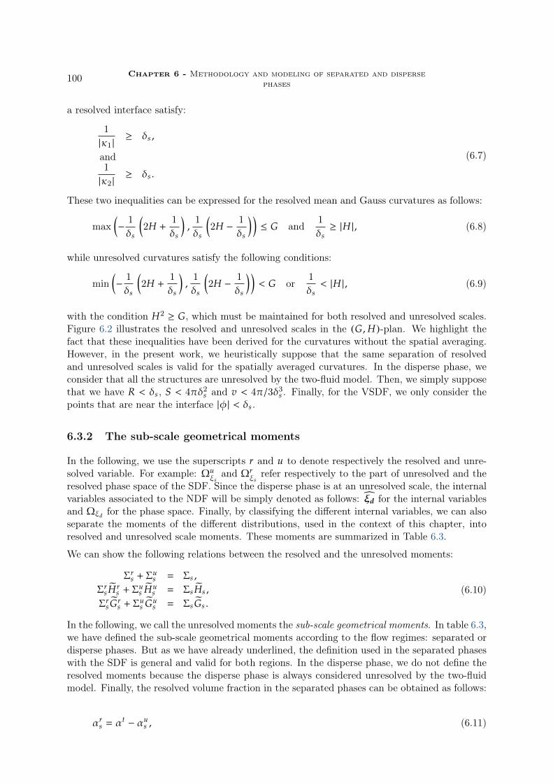
100 Chapter 6 - Methodology and modeling of separated and dispersephases

a resolved interface satisfy:

1

|κ1 |≥ δs ,

and1

|κ2 |≥ δs .

(6.7)

These two inequalities can be expressed for the resolved mean and Gauss curvatures as follows:

max(−

1

δs

(2H +

1

δs

),

1

δs

(2H −

1

δs

))≤ G and

1

δs≥ |H |, (6.8)

while unresolved curvatures satisfy the following conditions:

min(−

1

δs

(2H +

1

δs

),

1

δs

(2H −

1

δs

))< G or

1

δs< |H |, (6.9)

with the condition H2≥ G, which must be maintained for both resolved and unresolved scales.

Figure 6.2 illustrates the resolved and unresolved scales in the (G,H)-plan. We highlight thefact that these inequalities have been derived for the curvatures without the spatial averaging.However, in the present work, we heuristically suppose that the same separation of resolvedand unresolved scales is valid for the spatially averaged curvatures. In the disperse phase, weconsider that all the structures are unresolved by the two-fluid model. Then, we simply supposethat we have R < δs , S < 4πδ2s and v < 4π/3δ3s . Finally, for the VSDF, we only consider thepoints that are near the interface |φ | < δs .

6.3.2 The sub-scale geometrical moments

In the following, we use the superscripts r and u to denote respectively the resolved and unre-solved variable. For example: Ωu

ξsand Ωr

ξsrefer respectively to the part of unresolved and the

resolved phase space of the SDF. Since the disperse phase is at an unresolved scale, the internalvariables associated to the NDF will be simply denoted as follows: ξd for the internal variablesand Ωξd for the phase space. Finally, by classifying the different internal variables, we can alsoseparate the moments of the different distributions, used in the context of this chapter, intoresolved and unresolved scale moments. These moments are summarized in Table 6.3.

We can show the following relations between the resolved and the unresolved moments:

Σrs + Σ

us Σs ,

Σrs Hr

s + Σus Hu

s Σs Hs ,

Σrs Gr

s + Σus Gu

s Σs Gs .(6.10)

In the following, we call the unresolved moments the sub-scale geometrical moments. In table 6.3,we have defined the sub-scale geometrical moments according to the flow regimes: separated ordisperse phases. But as we have already underlined, the definition used in the separated phaseswith the SDF is general and valid for both regions. In the disperse phase, we do not define theresolved moments because the disperse phase is always considered unresolved by the two-fluidmodel. Finally, the resolved volume fraction in the separated phases can be obtained as follows:

αrs α

t− αu

s , (6.11)

Part II - Contribution to a unified modeling of disperse and separatedphases

101

G

H

δ−1s

δ−1s

δ−2sδ−2s

Figure 6.2: (G,H)-plan: non-valid curvatures H2 < G (hashed region), resolved curvatures(blue region) and unresolved curvatures (the rest of the domain).

separated phases disperse phase

Σrs

∫Ωrξs

F(t , x; ξsr)d5ξs

rnot defined

Resolved Σrs Hr

s ∫

ξsr∈Ωr

ξs

Hr F(t , x; ξsr)d5ξs

rnot defined

scales Σrs Gr

s ∫Ωrξs

Gr F(t , x; ξsr)d5ξs

rnot defined

Σu ∫Ωrξs

F(t , x; ξsr)d5ξs

rΣd

∫Ωξd

S f (t , x; ξd)d5ξd

Unresolved ΣuHus

∫Ωrξs

HF(t , x; ξsu)d5ξs

uΣdHd

∫Ωξd

R−1S f (t , x; ξd)d5ξd

scales ΣHus

∫Ωuξs

GF(t , x; ξd)d5ξsu

ΣdGd ∫Ωξd

f (t , x; ξd)d5ξd

αus

∫φr∈[0,δs ]

∫Ωuξs

Fφ (t , x; φu , ξsu)d5ξs

udφu αd

∫Ωξd

v f (t , x; ξd)d5ξd

Table 6.3: Separation of the moments into resolved and unresolved in separated and dispersephases.

102 Chapter 6 - Methodology and modeling of separated and dispersephases

where αt is the total volume fraction, the same as the one used in the two-fluid model.

After this separation of the scales, two different strategies can be envisioned to model the fuelinjection process. First, one can couple a two-fluid model with two systems of equations on thegeometrical variables: one for the resolved moments and an other one for the sub-scale geometri-cal moments. This idea is pretty similar to the one proposed in Devassy et al.(2015). Indeed, theauthors have coupled the seven-equation two-fluid model and two systems of transport equationson the surface area density and the volume fraction: one associated to the separated phases andthe second to the disperse phase. However, with this strategy, we can have some redundant infor-mation in our case. Indeed, the resolved volume fraction defined in 6.11 can be used to evaluatethe curvatures associated to the resolved scales in as similar way as in Brackbill et al.(1992).The second strategy consists in coupling a two-fluid model with the system of equations on thesub-scale geometrical variables. As shown in table 6.3, these variables can have two representa-tions: moments of the SDF and the VSDF or moments of the NDF. However, we underline againthat these two sets of variables are the same. In modeling, it is often simple to consider thesub-scale as a population of non-spherical droplets rather than dealing with complex interfacetopology. While from an another point of view, such assumption leads to inaccurate modelingof the primary atomization. In future work, we will need to investigate carefully the differentvarious strategies and to choose simplified but also physically valid assumptions. The final modelshould be able to predict the final polydispersion of droplets obtained from the primary and thesecondary atomizations.

6.3.3 Sub-scale and two-fluid model interactions

In this section, we discuss the interactions between a sub-scale interface model and a two-fluidmodel. The sub-scale model is given by the dynamics of the sub-scale geometrical moments(αu

s ,Σus ,Σ

uHus ,Σ

uGus ). The interactions between the two models should be expressed through

exchange source terms. First, it is clear that the dynamics of the sub-scale geometrical momentsare controlled by the dynamics of the mean scales of the flow. Indeed, the deformation andthe atomization of the interface generate more smaller scales, which can not be captured bythe two-fluid model. The two-fluid model behaves as it is diffusing the interface. This diffusionprocess can be explained by considering a statistical average over many realizations, where theuncertainties are very high. Consequently, this process generates sub-scales from the resolvedscales. Meanwhile other phenomena such as the coalescence can have an opposite effect. Wecan derive the system of equations of the sub-scale geometrical moments from the evolutionequations of the SDF and the VSDF. The obtained equations read as follows:

∂tΣu + ∇x · (Σu vI )

∫ξs

u < S >c F(t , x; ξsu) d5ξ + JΣr⇔u ,

∂tΣuHu

s + ∇x ·(Σu Hu

s vI)

∇x ·(ΣuHu

s (vI − vIH )

)+

∫ξs

u < S + H/H >c HF(t , x; ξsu) d5ξs

u+ JΣHs

r⇔u ,

∂tΣGus + ∇x ·

(Σu Gu

s vI)

∇x ·(ΣuGu

s (vI − vIG)

),

+∫ξs

u < S + G/G >c Gus F(t , x; ξs

u) d5ξsu+ JΣGs

r⇔u ,

∂tαus + ∇x ·

(αu

s vI)

∇x ·(αu

s (vI − vIα)

)+

∫φ∈[0,δs ]

∫ξs

u < S >c Fφ (t , x; φ, ξsu) d5ξs

udφ + Jαs

r⇔u ,

Part II - Contribution to a unified modeling of disperse and separatedphases

103

(6.12)

where the different averaged velocities (vI , vIH , vI

G , vIα) are defined in (5.28) by substituting ξs

by ξsu. This system of equations is slightly different from the one derived in (5.27) or in (5.45).

Indeed, the integration over the internal variables is restricted to the unresolved phase spaceΩuξs⊂ Ωξs . For this reason, we obtain two different parts of the source terms in the RHS of the

equations. The first part is similar to the source terms obtained in (5.27) or (5.45). These sourceterms express the evolution of the internal variables within the unresolved phase space Ωu

ξsand

the stretching of the interface sub-scale part. The second type of source terms is related to theproduction and the destruction of the sub-scales from or to the resolved scales, i.e. the resolvedscales become unresolved and vice versa. These source terms are expressed as follows:

JΣr⇔u ∫

∂Ωuξs

(⟨ξs

⟩c· nξs

)F(t , x; ξs )d ξs ,

JΣHr⇔u

∫∂Ωu

ξs

(⟨ξs

⟩c· nξs

)HF(t , x; ξs )d ξs ,

JΣGr⇔u

∫∂Ωu

ξs

(⟨ξs

⟩c· nξs

)GF(t , x; ξs )d ξs ,

Jαr⇔u ∫

φ∈[0,δs ]

∫∂Ωu

ξs

(⟨ξs

⟩c· nξs

)Fφ (t , x; φ, ξs )d ξs dφ,

(6.13)

where ∂Ωuξs

is the boundary of the phase space Ωuξs

and nξs is the normal vector at the bound-

ary set. These source terms can be separated into production terms when(⟨ξs

⟩c· nξs

)≥ 0 and

destruction terms when(⟨ξs

⟩c· nξs

)< 0. The production corresponds to the interface defor-

mations and the primary atomization, while the destruction corresponds to the coalescence andthe segregation of the small scales, nourishing larger scales. For this reason, the modeling ofthese source terms has to be coupled with the two-fluid model, especially for the modeling ofthe sub-scales production.

Let us now consider the effects of the unresolved scales on the two-fluid model, and how they maybe accounted for. In Drui et al.(2016b), a two-fluid model is derived from Hamilton’s variationalprinciple following Gavrilyuk and Saurel(2002). Drui et al use a sub-scale energy interfacepulsations as an additional kinetic energy in the Hamiltonian formulation. Furthermore, a sub-scale dissipation was associated to the pulsation kinetic energy. The obtained model depends ontwo parameters, interpreted as a micro-inertia and a micro-viscosity associated to the gas-liquidinterface sub-scale. By considering a monodisperse bubbly flow, the micro-inertia and the micro-viscosity of the bubble pulsations have been identified and related to the bubble radius and otherphysical variables of the flow. The effects of these sub-scale features on the two-fluid model wereidentified by investigating their effects on the dispersion relations of the sound speed. The sub-scale geometrical moments should allow a more accurate description of the interface sub-scale.It will be then important to benefit from this advantage to include more physical effects in thetwo-fluid model. For example, a surface potential energy could be written as a function of thesequantities. In the same way, the pulsation energy could apply to deformed interface and then, thevolume variations would be functions of the geometrical variables. Departing from these energiesand using the procedure based on Hamilton’s variational principle and the second principle ofthermodynamics, as explained in Drui(2017), we may enrich again the two-phase models. Theseworks are the subject of two PhDs Cordesse(2019) and Di Battista(2020). The first one aims atenriching the two-fluid model with more disequilibrium between the two phases, while ensuringa well-posed mathematical properties. The second aims at enriching the two-phase models usingthe Hamilton’s variational principle that includes the sub-scale geometrical moments.

104 Chapter 6 - Methodology and modeling of separated and dispersephases

6.3.4 A simplified model for the unresolved scales

In the previous section, we wrote a general form of a system of equations satisfied by the sub-scalegeometrical moments. The source terms involved in this system need to be closed by proposingan evolution of the curvatures and the stretching factor, as well as a proper reconstruction ofthe SDF and of the VSDF. In the following, we show how to close the model in a simplified case.For this purpose, we consider the following assumptions:

• the sub-scales are represented by a disperse phase and the sub-scale geometrical momentswill be expressed as moments of the NDF f (t , x; R, S, v , vb),

• we use the mixture two-fluid model developed in Drui(2017) and we suppose a very dilutedisperse phase α << 1. Consequently, this mixture model is used to simulate the continu-ous gaseous phases (by assuming a negligible volume fraction in the two-fluid model). Theonly interaction that we consider between the gaseous phase and the disperse phase is dueto the exchange in momentum through the drag force exerted by the gas on a droplet.The drag force is modeled using the Stokes law:

F u g − vb

θS, (6.14)

where θ 18πµg

ρlis a constant coefficient.

• we assume a monokinetic assumption for the droplet velocity:

f (t , x; R, S, v , vb) N (t , x; R, S, v) δ(vb − up (t , x)), (6.15)

• we suppose that at a given position and time all the droplets can be parametrized withone size variable and we choose here the surface area S:

N (t , x; R, S, v) n(t , x; S) δ(R − R(t , x; S)) δ(v − v(t , x; S)), (6.16)

where R(t , x; S) 1/(2√π)a(t , x)S1/2 and v(t , x; S) 1/(6

√πb(t , x)S3/2. The two scalars

a(t , x) and b(t , x) will be related to the moments of the NDF. We can also remark thatfor a(t , x) 1. and b(t , x) 1., we obtain the condition of spherical droplets and theaveraged geometrical quantities can be expressed again as fractional moments of n(t , x; S),as presented in chapter 4,

• we neglect the source terms that generate the sub-scale quantities from the resolved scales,i.e. Jψr⇔u 0, where ψ α,Σ,ΣH ,ΣG,

The volume fraction, the surface area density and the two averaged mean and Gauss curvaturescan be written as a function of the fractional size moments of the reduced distribution n(t , x; S)and the two variables a(t , x) and b(t , x) ,as follows:

ΣdGd (t , x) 4πm0(t , x),

ΣdHd (t , x) 1

2√π

a(t , x)m1/2(t , x),

Σd (t , x) m1(t , x),

αd (t , x) 1

6√π

b(t , x)m3/2(t , x),

(6.17)

Part II - Contribution to a unified modeling of disperse and separatedphases

105

where mk/2 ∫ Smax

0Sk/2n(t , x; S)dS and Smax 4πδ2s . To have closure relations between the

four sub-scale geometrical moments and the two variables a(t , x) and b(t , x), we transportthe following six quantities (ΣdGd ,ΣdHd ,Σd , αd ,m1/2 ,m3/2). The system of equations of thesequantities can be derived from the evolution equation of the NDF given in Table 6.1. Theobtained equations read as follows:

∂tΣdGd + div(ΣdGd up) 4π∫ Smax

0

⟨χχ

⟩c

n(t , x , S)dS,

∂tΣH + div(Hup) 1

2√π

a(t , x)∫ Smax

0

⟨χχ+

SS+

HH

⟩c

S1/2n(t , x , S)dS,

∂tΣ + div(Σup) ∫ Smax

0

⟨χχ+

SS

⟩c

Sn(t , x , S)dS,

∂tαd + div(αd up) 1

6√π

b(t , x)∫ Smax

0

⟨χχ+

vv

⟩c

S3/2n(t , x , S)dS,

∂tm1/2 + div(m1/2up) ∫ Smax

0

⟨χχ+ 1/2

SS

⟩c

S1/2n(t , x , S)dS,

∂tm3/2 + div(m3/2up) ∫ Smax

0

⟨χχ+ 3/2

SS

⟩c

S3/2n(t , x , S)dS,

∂tΣup + div(Σup ⊗ up) ∫ Smax

0

⟨χχ+

SS

⟩c

Sup n(t , x , S)dS + m0

u g − up

θ.

(6.18)

The source terms in the RHS of the equations depend on the time evolution of the internalvariables that are given by 〈v〉c,

⟨R⟩

cand

⟨S⟩

c, as well as the breakup rate of the droplets

expressed as the time derivative of the logarithm of the Euler characteristic (we suppose thedroplets are homeomorph to spheres) 〈χ/χ〉c. In the present work, we consider a simplifymodeling of the secondary atomization inspired from the wave breakup model Reitz(1987):

A. Wave model assumes that the time of breakup and the resulting droplet size are relatedto the fastest-growing Kelvin-Helmholtz instability. The maximum growth-rate of a smallperturbation on the interface corresponds to a frequency wbu and a wave number λbu thatare expressed as function of the Weber and Ohnesorge numbers as follows:

wbu

(0.34 + 0.38We1.5g

)(1 + Oh)(1 + 1.4(Oh

√Weg)0.6

(σ

ρl r3

)0.5,

λbu

9.02(1 + 0.45Oh0.5) (

1. + 0.4(Oh

√Weg

))1 + 0.81We1.67g

r,

(6.19)

where Weg ρl | |up (t , x) − u g (t , x) | |r

σand Oh

µl

ρl rσ. the variables ρl and µl are

respectively the mass density and the viscosity of the liquid, σ is the surface tension andr √

S is an approximate radius for a droplet of surface area S. Thus, the breakup timeis given as follows:

τbu (Weg ,Oh) 3.76B1r

λbu wbu. (6.20)

Finally, we use the breakup time to model the breakup rate:⟨χχ

⟩c

τ−1bu (Weg ,Oh), if

√S > B0λbu ,

0, otherwise,

106 Chapter 6 - Methodology and modeling of separated and dispersephases

where B0 and B1 are two parameters of the wave breakup model.

B. We suppose incompressible droplets and each fragmentation of a droplet generates newdroplets with the same volume:

〈v〉c −τ−1bu v , if

√S > B0λbu ,

0, otherwise.

C. Finally, for the evolution of the surface area and the mean radius, we consider each breakupis followed by a relaxation toward a spherical form of the droplets:⟨

S⟩

c

τ−1bu

(6√πv2/3

− S), if

√S > B0λbu ,

0, otherwise,

and ⟨R⟩

c

τ−1bu

((3

4πv)1/3− R

), if

√S > B0λbu ,

0, otherwise.

These relations close the model in the chosen simplified framework.

Some elements on the numerical resolution: The numerical resolution of system (6.18)is achieved through an operator splitting Doisneau et al.(2014); Descombes et al.(2014), wherethe transport part (LHS of the equations) and the source terms (RHS of the equations) aresolved independently. The numerical resolution of the transport part is similar to the one of thefractional moments (4.24) and the difficulties to comply with the realizability issues are the samefor the two models. The reader can refer to chapter 7, where robust and accurate numericalschemes are proposed for the numerical resolution of the fractional moment model in the case ofspherical droplets. For the numerical resolution of source terms, we use the DQMOM approach.In this case, the distribution in size n(t; S) (the space is no more considered in the source termsresolution) is first approximated by a sum of Dirac distributions:

n(t; S) ∑l1,2

nl (t)δ(S − Sl (t)), (6.21)

such that the abscissas Sl (t) and the weights nl (t) are related to the fractional moments of thedistribution n(t; S) as follows:

mk/2(t) ∑l1,2

nl (t)Sk/2l (t), (6.22)

where k 0, . . . , 3. In the DQMOM approach, we solve the evolution of the abscissas and theweights due to source terms. Using the evolution equation of the NDF, we can show that thesequantities satisfy the following ODE system for l 1, 2:

dnl

dt(t) τ−1bu ,l nl (t),

dSl

dt(t) τ−1bu ,l

(6√πvl (t)2/3 − Sl (t)

),

dRl

dt(t) τ−1bu ,l

((3

4πvl (t)

)1/3− Rl (t)

),

dvl

dt(t) −τ−1bu ,l vl (t),

(6.23)

Part II - Contribution to a unified modeling of disperse and separatedphases

107

where τbu ,l is the breakup time (6.20) computed for each quadrature abscissa. The abscissas (sur-face areas) Sl (tn), at the nth iteration, are computed by using the PD algorithm Gordon(1968)which solves the system (6.22) and the initial volumes and radii are computed as follows:

Rl (tn) 1

2√π

a(tn)S1/2l (tn),

vl (tn) 1

6√π

b(tn)S3/2l (tn).

(6.24)

The time integration of this ODE in [tn , tn+1] allows to approximate the solution of the trans-ported variables at t tn+1 as follows:

mk/2(tn+1) ∑

l1,2nl (tn+1)Sk/2

l (tn+1),

ΣdHd (tn+1) ∑

l1,2nl (tn+1)Sl (tn+1)R−1l (tn+1),

αd (tn+1) ∑

l1,2nl (tn+1)vl (tn+1),

(6.25)

2D jet of non-spherical droplets: In the following, we consider a 2D rectangular domainof size [−0.5, 0.5] × [−0.5, 0.5] (we use dimensionless variables). On the top (y 0.5), bottom(y −0.5) and right (x 0.5) faces, we use the Neumann boundary conditions. On the left face(x −0.5), we consider a small hole in the middle. The hole is of radius ηin j 1.e − 2. Fromthe hole outlet, we inject droplets of uniform size distribution:

n(t , y , S) 1, (6.26)

where S ∈ [0, 1] and −ηin j < y < ηin j. The initial droplets are not spherical with: a 0.7 andb 0.5. The droplets are injected with the following velocity profile at x −0.5:

ex · vb (t , y) 5 cos4(πy

2ηin j),

e y · vb (t , y) 0.(6.27)

The gas of a mass density ρg 1 is also injected with following velocity field:

ex · u g (t , y) 8 cos4(πy

2ηin j),

e y · u g (t , y) 0.(6.28)

The injection velocities of the gas and of the droplets are different. It leads to a strong relativevelocity between the two phases and then to the fragmentation of the droplets. The numericalsimulation is performed in Adaptive Mesh Refinement framework using the CanoP code, whichwill be presented later in chapter 9. The minimum cell size of the mesh is ∆xmin 2−9 and themaximum size is ∆xmax 2−7. Figures 6.3 and 6.4 illustrate respectively the number density(ΣGd) and surface are density at four different instants. We can remark the fragmentation byobserving a global increase of number density and surface area density over time.

We recall that this simulation and the used model do not represent any realistic configuration.The coupling with the two-fluid model has not yet been completely achieved. Indeed, we usedthe mixture model of Drui(2017) to simulate the gas flow by assuming a negligible volumefraction. The objective of this first work is to illustrate the possibility of modeling the sub-scaleswith non-spherical droplets and takes into account the fragmentation and the two-way coupling

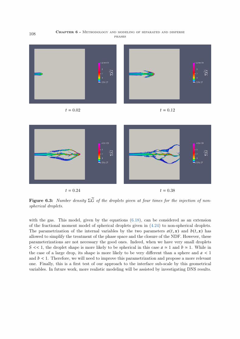
108 Chapter 6 - Methodology and modeling of separated and dispersephases

t 0.02 t 0.12

t 0.24 t 0.38

Figure 6.3: Number density ΣG of the droplets given at four times for the injection of non-spherical droplets.

with the gas. This model, given by the equations (6.18), can be considered as an extensionof the fractional moment model of spherical droplets given in (4.24) to non-spherical droplets.The parametrization of the internal variables by the two parameters a(t , x) and b(t , x) hasallowed to simplify the treatment of the phase space and the closure of the NDF. However, theseparameterizations are not necessary the good ones. Indeed, when we have very small dropletsS << 1, the droplet shape is more likely to be spherical in this case a ' 1 and b ' 1. While inthe case of a large drop, its shape is more likely to be very different than a sphere and a < 1and b < 1. Therefore, we will need to improve this parametrization and propose a more relevantone. Finally, this is a first test of our approach to the interface sub-scale by this geometricalvariables. In future work, more realistic modeling will be assisted by investigating DNS results.

Part II - Contribution to a unified modeling of disperse and separatedphases

109

t 0.02 t 0.12

t 0.24 t 0.38

Figure 6.4: Surface area density Σ of thedroplets given at four times for the injection of non-spherical droplets.

110 Chapter 6 - Methodology and modeling of separated and dispersephases

6.4 DNS post-processing toward a modeling of the sub-scales

In the previous section, we explained our strategy to couple a two-fluid model with a sub-scalemodel based on the sub-scale geometrical moments. The sub-scale model depends on the timeevolution of the internal variables of the SDF or of the NDF as well as the surface stretchingand the breakup source terms. For future work, these terms will need to be correctly modeledand related to the transport variables of the flow. The main goal of this section is to extractthe evolution of such geometrical properties from DNS test cases. The well-known Archer codeMenard et al.(2007); Vaudor et al.(2017), where a combined VOF and Level-set approach isused to capture the interface and a ghost-fluid method is applied to represent accurately thejump of the variables across the liquid-gas interface, has been used to this end. We also use thealgorithm presented in chapter 5 to extract the curvatures and to compute the two distributions:the SDF and the NDF. In this section, we present two numerical test cases:

• Rayleigh-Plateau test-case is presented to characterize the evolution of the interfacecurvatures in a simple breakup case, where a liquid column is split into several droplets

• Liquid jet test-case is a primary break-up simulation of an injected liquid. In this sim-ulation, we show that the distribution of the curvatures on the interfaces can provide uswith relevant information on the flow topology.

6.4.1 Plateau-Rayleigh simulation

We consider an initial cylindrical column of liquid with a small sinusoidal deformation at theinterface. The initial level-set function is given in cylindrical coordinates as follows:

φ(t 0; r, θ, z) (r − R)(1 + ε sin(2πkz z)), (6.29)

where kz is a wave number satisfying kzR 0.7, R 3.34 × 10−5m being the radius of thecylinder and ε 0.1. Using the symmetry properties of this case, we only simulate a quarter ofthe cylinder, where the symmetric boundary conditions have been employed in a computationalbox lx × l y × lz where lx l y 1. × 10−4m and lz 1.5 × 10−4m. We discretize the domaininto 64 × 64 × 96 Cartesian elements. The liquid and the gas properties are reported in table6.4. In figure 6.5, four time frames have been selected as in Canu et al.(2017) to show thebreak-up process, which is conducted by the Plateau-Rayleigh instability. The four instantscorrespond to the initial configuration at ta 0.s, the deformation of the cylinder with thegeneration of the bottle-neck at tb 1.83×10−4s, the break-up moment at tc 1.86×10−4s andthe final generation of droplets at td 2.07 × 10−4s. To have a deeper insight in the evolutionof the curvatures, we chose these four instants to extract the mean and Gauss curvatures atthe interface defined by φ(t; x) 0. The spatial averaging of the curvatures presented in thelast chapter is used here. In fact, the spatial averaging permits to obtain a structured and aclear picture of this evolution, compared to the case without averaging, where a large amountof noise is present, as illustrated in Figure 6.6. In Figure 6.7, we display the spatially averagedcurvatures in the (G,H)-plan using a spatial averaging scale h 6∆x, where ∆x is the mesh

ρl µl ρg µg σkg.m−3 kg.m−1.s−1 kg.m−3 kg.m−1.s−1 kg.s−2

1000 1, 0.10−3 1.0 1, 879.10−3 0, 072

Table 6.4: Physical properties of the Rayleigh-Plateau simulation.

Part II - Contribution to a unified modeling of disperse and separatedphases

111

ta 0.0s tb 1.83 × 10−4s

tc 1.86 × 10−4s td 2.07 × 10−4s

Figure 6.5: The gas-liquid interface of Plateau-Rayleigh simulation. The two solid lines in theleft-top corner determine the domain of the simulation.

size. In the same figure, we plot the two lines limiting the resolved and the unresolved scaleswith a threshold scale δs 3dx. At the initial time t ta, the cylinder is weakly deformed andall the curvature points in the (G,H)-plan are all gathered around the vertical line at G 0. Att tb, the cylinder is sufficiently deformed and the curvatures form an arc in (G,H)-plan. Wealso remark negative values of the Gauss curvature (top-right of Figure 6.7) that corresponds tothe saddle points in the middle of the cylinder. In the bottom-left corner of Figure 6.7, whichcorresponds to the break-up time t tc, the arc formed in the previous step breaks up and twoseparated clouds of points can be identified. At the final time t td, we obtain two dropletsof approximately spherical shapes and of two different sizes. In bottom-right of Figure 6.7, twocloud of points are positioned close to the curve G H2. The one with the highest curvaturescorresponds to the smallest droplet and the other to the biggest droplet.

The evolution in the (G,H)-plan reveals relevant information on the evolution of the gas-liquidinterface. For example, a slow evolution toward high curvatures can reveal the development ofsome initial instabilities, while fast evolution accompanied with high curvatures can be relatedto the variation on the interface topology. Plateau-Rayleigh instabilities represent one of thebreakup mechanisms of realistic injection configurations. It is important to classify the differentmechanisms and to choose representative configurations as the one proposed here to understand

112 Chapter 6 - Methodology and modeling of separated and dispersephases

tb 1.83 × 10−4s td 2.07 × 10−4s

Figure 6.6: Gauss and mean curvatures of the gas-liquid interface without spatial averaging attwo instants: left (t tb) and right (t td). The red points correspond to left part of

ρl µl ρg µg σkg.m−3 kg.m−1.s−1 kg.m−3 kg.m−1.s−1 kg.s−2

776 4.0 × 10−3 1.3 1, 78 × 10−3 0.072

Table 6.5: Physical properties of the gas and the liquid used in the jet flow simulation.

and model the evolution of the curvatures depending on each mechanisms.

6.4.2 Jet simulation

In this section, we present some first results of a common work with the Coria laboratory topost-process the primary breakup of a liquid jet using the Archer code. We underline that asimilar simulation has been used in Lebas et al.(2009) to close the ELSA model.

The diameter of the injector nozzle is 100 µm, the size of the domain is 765 µm×765 µm×3060 µmand the injection velocity is 25 m/s. The characteristic of the flow is given in Table 6.5. Weuse a uniform 3D Cartesian grid, which is composed of 128 × 128 × 512 cubic cells. Figure 6.8illustrates the gas-liquid interface obtained at t 0.66 µs. One can identify three regions of theprimary breakup of the liquid jet. In the region close to the nozzle, the interface of the liquidjet has a quasi-cylindrical shape. In the middle of the domain, the interface is widely deformedand we can remark the ligaments formation. In the last part of the domain, some ligaments aredetached from the liquid core and break into a large range of drop sizes. However, the liquidcore is not totally atomized in this simulation. In the following, we compute the distribution ofthe surface curvatures in three different sub-domains. These sub-domains are illustrated by redrectangles in Figure 6.8 and they correspond to:

• Sub-domain 1 is situated close to the nozzle outlet and is given by 0 ≤ z ≤ 32dx, wherethe z-axis is parallel to the principal jet direction.

• Sub-domain 2 is a part of domain situated in the middle of the jet and is given by 192 ≤z ≤ 224dx.

• Sub-domain 3 is situated in the downstream of the jet and is given by 480dx ≤ z ≤ 512dx.

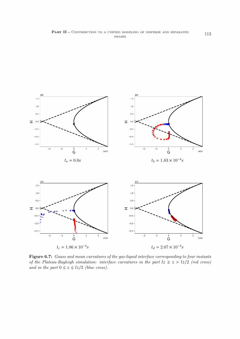
Part II - Contribution to a unified modeling of disperse and separatedphases

113

ta 0.0s tb 1.83 × 10−4s

tc 1.86 × 10−4s td 2.07 × 10−4s

Figure 6.7: Gauss and mean curvatures of the gas-liquid interface corresponding to four instantsof the Plateau-Rayleigh simulation: interface curvatures in the part lz ≥ z > lz/2 (red cross)and in the part 0 ≤ z ≤ lz/2 (blue cross).

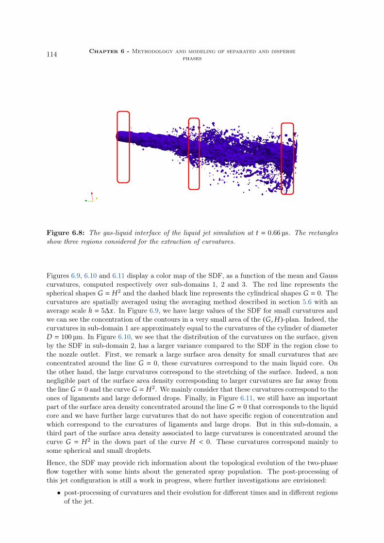
114 Chapter 6 - Methodology and modeling of separated and dispersephases

Figure 6.8: The gas-liquid interface of the liquid jet simulation at t 0.66 µs. The rectanglesshow three regions considered for the extraction of curvatures.

Figures 6.9, 6.10 and 6.11 display a color map of the SDF, as a function of the mean and Gausscurvatures, computed respectively over sub-domains 1, 2 and 3. The red line represents thespherical shapes G H2 and the dashed black line represents the cylindrical shapes G 0. Thecurvatures are spatially averaged using the averaging method described in section 5.6 with anaverage scale h 5∆x. In Figure 6.9, we have large values of the SDF for small curvatures andwe can see the concentration of the contours in a very small area of the (G,H)-plan. Indeed, thecurvatures in sub-domain 1 are approximately equal to the curvatures of the cylinder of diameterD 100 µm. In Figure 6.10, we see that the distribution of the curvatures on the surface, givenby the SDF in sub-domain 2, has a larger variance compared to the SDF in the region close tothe nozzle outlet. First, we remark a large surface area density for small curvatures that areconcentrated around the line G 0, these curvatures correspond to the main liquid core. Onthe other hand, the large curvatures correspond to the stretching of the surface. Indeed, a nonnegligible part of the surface area density corresponding to larger curvatures are far away fromthe line G 0 and the curve G H2. We mainly consider that these curvatures correspond to theones of ligaments and large deformed drops. Finally, in Figure 6.11, we still have an importantpart of the surface area density concentrated around the line G 0 that corresponds to the liquidcore and we have further large curvatures that do not have specific region of concentration andwhich correspond to the curvatures of ligaments and large drops. But in this sub-domain, athird part of the surface area density associated to large curvatures is concentrated around thecurve G H2 in the down part of the curve H < 0. These curvatures correspond mainly tosome spherical and small droplets.

Hence, the SDF may provide rich information about the topological evolution of the two-phaseflow together with some hints about the generated spray population. The post-processing ofthis jet configuration is still a work in progress, where further investigations are envisioned:

• post-processing of curvatures and their evolution for different times and in different regionsof the jet.

Part II - Contribution to a unified modeling of disperse and separatedphases

115

Figure 6.9: SDF as function of (H,G) integrated over the sub-domain 1.

Figure 6.10: SDF as function of (H,G) integrated over the sub-domain 2.

116 Chapter 6 - Methodology and modeling of separated and dispersephases

Figure 6.11: SDF as function of (H,G) integrated over the sub-domain 3.

• computing the SDF and the NDF using a time average over different iterations to obtainconsistent distributions.

• defining of a convenient threshold scale δs for a similar configuration with respect to thereduced order model, where we use a coarsened meshes compare to DNS. Then, we wouldcompute the exchange source terms defined in (6.13) between the resolved and unresolvedscales using DNS results.

6.5 Conclusion and perspectives

Throughout this chapter, we have explained how to use the geometrical description of the in-terface presented in the previous chapters, in order to come up with a unified model for thedisperse and separated phases. Three main points have been discussed during this presentation:the sub-scale geometrical moments, the coupling with a two-fluid model and the usefulness ofDNS computations to propose closures of the model and to investigate the modeling assumptions.

Up to now, it seems that the sub-scale geometrical moments play an important role to com-plete the sub-scale information on the gas-liquid interface. The sub-scale variables can alsoenrich the two-fluid model as it was already illustrated in the work of Drui(2017). Futureworks Cordesse(2019); Di Battista(2020) aim at going further in this direction by including thesub-scale geometrical moments on a two-fluid model using a procedure based on Hamilton’svariational principle and the second principle of thermodynamics. Finally, we underline that thedifferent ideas proposed in this chapter are still under development and open questions requirefurther investigations. The following lists contain some of these remaining issues:

Part II - Contribution to a unified modeling of disperse and separatedphases

117

• theoretical investigation of the threshold scale δs : this scale should be defined with respectto an injection benchmark simulation withe the reduced order model. It also defines theminimum mesh size needed to correctly capture the mean scales of the flow. The scaleslower than δs should likely have some universal structures that can allow to simplify thephase space of the distribution and their evolution:

⟨H

⟩c,⟨G⟩

c,⟨S

⟩cto model the primary

atomization or the terms⟨S⟩

c, 〈v〉c,

⟨R⟩

cand 〈χ/χ〉c, to model the secondary breakup.

• influence of the averaged scale h on the DNS curvature post-processing and on the sub-scales modeling: as it was illustrated in the Plateau-Rayleigh simulation, this scale has aninfluence on the post-processing results. Without averaging, the curvatures contain a largenoise, which makes its difficult to analyze. On the contrary, a large spatial averaging leadsto some important loss in structures of these curvatures. In terms of modeling, we wouldlike to have enough information on the interface in the separated phases to capture theatomization, while in disperse phase we estimate that the averaged internal variables overdroplet surface are sufficient to model the dynamics of the droplets from a macroscopicpoint of view.

• evaluating the exchange fluxes between a two-fluid model and the sub-scales equations:the source terms expressed in (6.13) can be first computed directly by using DNS results.The results obtained from such a DNS post-processing will be used to relate these sourceterms to the variables of the used two-fluid model.

Finally, let us underline that it is the first time DNS data are analyzed with curvatures evaluation.This post-processing of the gas-liquid interface is consistent with geometrical and topologicalinvariants (see chapter 5). This should provide a tool to better understand and analyze thephysics of such flows.

Part III

Numerical methods

Chapter 7

Numerical resolution of the transportequations of the fractional momentsmodel

7.1 Introduction

In this chapter, we focus on the numerical resolution of the transport part of the fractionalmoments model presented in chapter 4. In fact, we can split the resolution of the transportpart (LHS of system (4.24)) from the source terms (RHS of system (4.24)), by mean of operatorsplitting techniques Doisneau et al.(2014); Descombes et al.(2014). The numerical resolution ofthe source terms is treated in chapter 8. The transport part of the system of equations (4.24)is similar to the one of the EMSM model Kah et al.(2012). This system of equations can bewritten as follows:

∂tU + ∇x · (F (U )) 0, (7.1)

where U t (m0/2 ,m1/2 ,m2/2 ,m3/2 ,m2/2ut ), F (U ) (F 1(U ) . . .F d (U )), d is the space di-

mension and F α (U ) uαU for 1 ≤ α < d.

The system of equations (7.1) has similar mathematical properties as the pressureless gas dy-namic (PGD) model of de Chaisemartin et al.(2009). Indeed, the system is only weakly hyper-bolic: it has only one real eigenvalue and four linearly independent eigenvectors in each direction,instead of 4+ d ( 4+ d is the equations number). In the case of Particle Trajectory Crossing, themodel implies the segregation of the droplets in infinitely fine zones, which is known as δ-shocks.For the numerical resolution of this system, we need to cope with different challenges. First,accurate resolution is required to limit the numerical diffusion. To satisfy this first requirementat a reasonable computational cost, high order numerical schemes can be used. The secondissue concerns the robustness of the numerical scheme. High order numerical schemes can causeoscillations of the solution near the zones where the solution is singular (δ-shocks). A familiarsolution to this issue consists in using artificial diffusion to suppress the spurious oscillations.However, this type of methods depends on some parameters and shock capturing sensors, whichneed to be adapted for each situation. Also the accuracy of the method is generally reduced.It is then important to develop robust numerical schemes, which do not depend on additionalparameters and preserve the order accuracy of regular solutions. Finally, the realizability of

122 Chapter 7 - Numerical resolution of the transport equations of thefractional moments model

the moments (a non negative NDF can be associated to every set of moments) is an essentialcondition to ensure a physical solution and to allow everywhere the well-posedness of the MEalgorithm presented in chapter 4. A naive numerical schemes can update the moments set in awrong way that leads to a non-realizable set of moments.

In the present work, we propose two numerical scheme classes. The first one is a finite volumediscretization based on a kinetic approach Bouchut et al.(2003); de Chaisemartin et al.(2009).We call this class of schemes the Kinetic Finite Volume (KFV) class. In this method, we computethe numerical flux based on the exact solution of a kinetic transport equation. To achieve highorder accuracy, non-constant reconstruction is needed to evaluate the numerical fluxes. However,the reconstruction should preserve the moments vector within the moment space to ensure therealizability of the numerical scheme. This condition is satisfied by using a slope limitation onthe reconstructed canonical moments (see chapter 4 for the definition of the canonical moments),in the same way as it was proposed in the first time by Kah et al.(2012). To step forward inimproving the accuracy of the numerical resolution and developing higher order schemes, we usea Rung-Kutta Discontinuous Galerkin discretization Cockburn and Shu(1998), as the secondclass of the schemes used to solve system (7.1). Indeed, Discontinuous Galerkin (DG) schemeis a promising alternative compared to standard finite volume methods. This choice can bejustified for two reasons. First, finite volume methods require large extended stencils to achievehigh order accuracy, which can be restrictive for the scalability of parallel computations. On thecontrary, DG methods use a compact stencil since the degrees of freedom are store within eachcomputational cell (similar idea as the Finite Element method). Finally, to ensure a realizableresolution of the moments, we adopt a similar limitation method as the one proposed in Zhangand Shu(2011); Zhang et al.(2012).

7.2 Realizable Kinetic Finite Volume (KFV) schemes

The use of Cartesian grids in physical space enables to use a dimensional splitting algorithm.Dimensional splitting consists in solving the system of equations separately and successively ineach direction during a time step ∆t. In this case, we can reuse a 1D finite volume scheme toupdate the solution. In the following, we choose to present the scheme in a two dimensionalspace in order to lighten the notations and we denote by u (u , v) the 2D velocity vector.

Let∆tγ • be an operator associated to a 1D finite volume scheme, which can be used to update

the solution in a direction γ x , y during a time step ∆t. The dimensional splitting leads to anadditional error in the numerical resolution. The order of the additional error depends on thesplitting algorithm. In the present work, we use two types of splitting:

• Godunov or Lie splitting method is a first order method, where the solution is updatedsuccessively for each direction as follows:

U n ,∗i ∆t

x U ni , U n+1

i ∆ty U n ,∗

i . (7.2)

• Strang splitting method is a second order accurate method when the finite volume 1Doperator∆t

γ • is also of second order. The solution is updated in this case as follows:

U n+1i ∆t/2

x ∆ty ∆t/2

x U ni . (7.3)

Part III - Numerical methods 123

In the following, we detail the finite volume 1D operator ∆tx •, which corresponds to a finite

volume discretization of the free transport equations in one direction (we focus on the x-directionhere):

∂tmk/2 + ∂x (mk/2u) 0,∂t (m2/2u) + ∂x (m2/2uu) 0,

(7.4)

where k 0, . . . , 3.

As it was discussed in the introduction, we encounter two main difficulties in the resolution ofthis system. The first one corresponds to the possible appearance of strong singularities (knownas δ-shocks), which occur when the monokinetic assumption is violated. This can happen whentrajectory crossings take place and lead to particles accumulation in a very small volume. Then,the numerical scheme has to be able to capture these shocks and ensure a stable solution. Thesecond issue concerns the realizability of the numerical scheme (the moment set approximationcan be associated to a non-negative NDF). In the following, we show how to cope with theseissues using a kinetic approach.

7.2.1 Derivation of 1D finite volume kinetic scheme for fractional momentsequations

We consider a uniform discretization (xi)i1,...Nx of a 1D compact domain [xmin , xmax]. Suchthat we have:

xmin + ∆x/2 x1 < x2 < . . . < xNx xmax − ∆x/2, andxmax − xmin

Nx ∆x , (7.5)

where xi is the center of cell i ∈ [1,Nx]. We denote by xi+1/2 xi + ∆x/2 (respectively xi−1/2

xi −∆x/2) the right (respectively the left) face of cell i. In the finite volume representations, welook for an approximation of the solution at a discrete time tn:

U ni '

1

∆x

∫ xi+1/2

xi−1/2

U (tn , x)dx , (7.6)

where tn ∑n

j1 ∆t j (with t0 0) and ∆t j t j−t j−1 is the time step. The time step should satisfya Courant-Friedrichs-Lewy (CFL) condition to ensure the stability of the numerical solution.By integrating equation (7.4) over time [tn , tn+1] and space [xi−1/2 , xi+1/2], the finite volumenumerical scheme reads:

U n+1i U n

i −∆t∆x

(F i+1/2 − F i−1/2

). (7.7)

The numerical fluxes F i±1/2 evaluated at the faces are an approximation of the exact mean-timeflux:

F i±1/2 '1

∆t

∫ tn+1

tn

F (t , xi±1/2)dt (7.8)

The numerical flux F i±1/2 can be approximated using the left and the right states with respectto the considered face:

F i+1/2 F (U i ,U i+1)F i−1/2 F (U i−1 ,U i)

(7.9)

124 Chapter 7 - Numerical resolution of the transport equations of thefractional moments model

de Chaisemartin(2009) proposed a finite volume kinetic scheme to solve the monokinetic multi-fluid model based on the same approach as in Bouchut et al.(2003), used to solve the PGDsystem of equations. Following the same idea, Kah et al.(2012) proposed an extention of thekinetic numerical scheme for higher order size-moments model. In the following, we use thisapproach to express the numerical fluxes of the present system of equations (7.1). The mainsteps to derive the kinetic scheme for system (7.4) are briefly presented as follows:

A. We consider the equivalent kinetic system to the pressureless system (7.4), as was proposedin Bouchut et al.(2003):

∂t f + ∂x (cx f ) 0 , andf (t , x , c , S) n(t , x , S)δ(c − u), (7.10)

B. We express the exact finite volume fluxes as a function of the NDF f (t , x , c , S).

1

∆t

∫ tn+1

tn

F (t , xi±1/2)dt 1

∆t

∫ tn+1

tn

∫ 1

S0

∫c(cx ,cy )

cxV (S, c) f (t , x , c , S)dSdc , (7.11)

where V (S, c) (1, S1/2 , S, S3/2 , Scx , Scy).

C. We split the fluxes in two integral parts: the first F+

i+1/2 (resp the second F−i+1/2) corre-sponds to the droplet of positive velocity cx ≥ 0 (resp negative velocity cx < 0). Then, weuse the exact solution of the kinetic system (7.10), to express the fluxes as a function ofthe NDF at time tn:

f (t , x , c , S) f (tn , x − cx (t − tn), c , S) (7.12)

for t ∈ [tn , tn+1].

D. Finally, the fluxes are expressed as functions of the known moments and velocities att tn:

F+

i+1/2 1

∆t

xi+1/2∫xi−1/2

U (tn , x)1Σ+ (x)dx ,

F−i+1/2 1

∆t

xi+3/2∫xi+1/2

U (tn , x)1Σ− (x)dx ,

(7.13)

where Σ± x′,±(xi+1/2 − ∆tu(tn , x′)) < ±x′

. The global numerical flux is then:

F i±1/2 F+

i±1/2 + F−i±1/2. (7.14)

7.2.2 First order scheme

For a first order scheme, we consider a constant piecewise reconstruction for the moments andfor the velocity (see Figure 7.1-left). In this case, the numerical scheme turns to be a simpleupwind scheme, where the numerical fluxes express as follows:

F i+1/2

*..........,

mn0,i

mn1/2,i

mn1,i

mn3/2,i

mn1,i u

ni

mn1,i v

ni

+//////////-

max(uni , 0) +

*..........,

mn0,i+1

mn1/2,i+1

mn1,i+1

mn3/2,i+1

mn1,i+1un

i+1mn

1,i vni+1

+//////////-

min(uni+1 , 0), (7.15)

Part III - Numerical methods 125

Figure 7.1: Sketch of finite volume representations in a cell. Left piecewise-constant represen-tation used at first order. Right piecewise-linear reconstruction of the solution to achieve secondorder accuracy.

The numerical scheme is stable under a CFL condition which reads:

∆t∆x

CFL max |uni |, (7.16)

where CFL ≤ 1. Under this condition, we can also show that the updated solution at tn+1 (7.7) inthe cell i can be written as a convex combination of the solution at tn in the cells i−1, i , and i+1.Since the moments space is a convex space, the numerical scheme is intrinsically realizable.

7.2.3 Second order scheme

Usually, high order finite volume schemes use non-constant reconstructions of the transportedvariables (see figure 7.1-right) to better evaluate the fluxes at the interfaces of the cells. Themain difficulty consists in reconstructing a realizable moments solution. Kah et al.(2012) de-signed a realizable second order kinetic scheme for the EMSM model. Instead of reconstructingdirectly the integer moments, the authors proposed to use a linear reconstruction of the canonicalmoments associated to integer moments. Indeed, the canonical moments live in the simple space[0, 1]N (N 3 for the EMSM model), while the moment space has a rather complex geometry.Furthermore, the canonical moments are also simply transported variables:

∂t pk + u∂x pk 0, (7.17)

where pk are the canonical integer moments defined in (4.6). Therefore, these quantities satisfy amaximum principle. In the following, we adopt the same approach with some slight adaptationsto the fractional moments case.

7.2.3.1 Reconstruction of the transported variables

The reconstructed variables are the moment m0/2, the canonical moments associated this timeto the fractional moments (p1/2 , p2/2 , p3/2) (see the definition in (4.28)) and the two velocity

126 Chapter 7 - Numerical resolution of the transport equations of thefractional moments model

components (u , v).

m0/2(x) m0/2,i + Dm0,i (x − xi),p1/2(x) p1/2,i + Dp1,i (x − xi),p2/2(x) p2/2,i + Dp2,i (x − xi),p3/2(x) p3/2,i + Dp3,i (x − xi),

u(x) ui + Dui (x − xi),v(x) vi + Dvi (x − xi),

(7.18)

where x ∈ [xi−1/2 , xi+1/2]. Generally the quantities with the bar are different from the cellquantities pk/2,i, ui and vi and they are determined depending on the slopes and the followingconservation properties:

mn1/2,i

1

∆x

∫ xi+1/2

xi−1/2m0/2(x)p1/2(x)dx ,

mn2/2,i

1

∆x

∫ xi+1/2

xi−1/2m0/2(x)p1/2(x)[(1 − p1/2)p2/2 + p1/2](x)dx ,

mn3/2,i

1

∆x

∫ xi+1/2

xi−1/2m0/2p1/2

(1 − p1/2)(1 − p2/2)p2/2p3/2 + [(1 − p1/2)p2/2 + p1/2]

2 (x)dx ,

mn2/2,i u

ni

1

∆x

∫ xi+1/2

xi−1/2m0/2(x)p1/2(x)[(1 − p1/2)p2/2 + p1/2](x)u(x)dx.

(7.19)

Compared to the expressions developed in the case of the EMSM model, only the last integralexpression is different. In fact, the velocity is weighted by the moment m1 m2/2 for bothmodels. But with fractional moments, m2/2 acts as a second order moment. For this reason, theexpression of the moment m2/2 as a function of the canonical moments is different from the onein the case of the integer moments.

Following the same derivation as in Kah et al.(2012), we show that the bar terms can be writtenas follows:

pk/2,i ak ,i + bk ,iDpk ,i ,ui au ,i + bu ,iDui ,

(7.20)

where for each k, ak ,i and bk ,i are independent of Dpk ,i, and au ,i and bu ,i are independent ofDui.

7.2.3.2 Slope limitation

In order to satisfy the maximum principle for the transported quantities (the canonical momentsand the velocity) and the positivity of the number density m0/2, the slopes should be calculatedcarefully. Following the development done in Kah et al.(2012), the slopes are calculated asfollows:

Dm0,i φ(mn0/2,i−1 ,m

n0/2,i ,m

n0/2,i+1) min *

,

|mn0/2,i+1 −mn

0/2,i |

∆x,|mn

0/2,i −mn0/2,i−1 |

∆x,2mn

0/2,i

∆x+-,

Dpk ,i φ(pnk/2,i−1 , p

nk/2,i , p

nk/2,i+1) min *

,

|pnk/2,i+1 − ak ,i |

∆x + 2bk ,i,|ak ,i − pn

k/2,i−1 |

∆x − 2bk ,i+-,

Dui φ(uni−1 , u

ni , u

ni+1) min

(|un

i+1 − uni |

∆x + 2bu ,i,|un

i − uni−1 |

∆x − 2bu ,i,

1

dt

),

Part III - Numerical methods 127

(7.21)

where φ(a , b , c) 1/2(s gn(b − a) + s gn(c − b)) and s gn(x) is the sign of x.

Using equations (7.19), (7.20) and (7.21), the slopes and the bar variables can be expressed asfunctions of the current and neighbor cell variables. However, these algebra relations are quiteheavy. Therefore, their calculation is achieved using the Maple software.

7.2.3.3 Fluxes Computation

After computing the slopes and the bar variables, the fluxes can be computed as follows:

F+

i+1/2 1

dt

∫ xi+1/2

xLi+1/2

m0/2

*........,

1p1/2

p1/2[(1 − p1/2)p2/2 + p1/2]p1/2

(1 − p1/2)(1 − p2/2)p2/2p3/2 + [(1 − p1/2)p2/2 + p1/2]

2p1/2[(1 − p1/2)p2/2 + p1/2]up1/2[(1 − p1/2)p2/2 + p1/2]v

+////////-

dx ,

(7.22)

and

F−i+1/2 −1

dt

∫ xRi+1/2

xi+1/2

m0/2

*........,

1p1/2

p1/2[(1 − p1/2)p2/2 + p1/2]p1/2

(1 − p1/2)(1 − p2/2)p2/2p3/2 + [(1 − p1/2)p2/2 + p1/2]

2p1/2[(1 − p1/2)p2/2 + p1/2]up1/2[(1 − p1/2)p2/2 + p1/2]v

+////////-

dx ,

(7.23)

such that

xLi+1/2 xi+1/2 − dt

(ui +∆x2 Dui)+

1 + dtDui,

xRi+1/2 xi+1/2 − dt

(ui+1 −∆x2 Dui+1)−

1 + dtDui+1,

(7.24)

where (ψ)+ 1/2(|ψ | + ψ) and (ψ)− 1/2(−|ψ | + ψ).

The expressions inside the integrals are polynomial functions of x of order up to 6, their calcu-lation can be achieved by using four points of the Gauss-Legendre quadrature.The CFL condition for the second order scheme reads:

∆t∆x

CFL max (|ui | + |Dui |∆x/2) (7.25)

where CFL ≤ 1 is defined by the user.

7.3 Realizable discontinuous Galerkin method

The original DG method was introduced by Reed and Hill Reed and Hill(1973). Recentlythe DG method has been widely used in different numerical simulation fields and especially

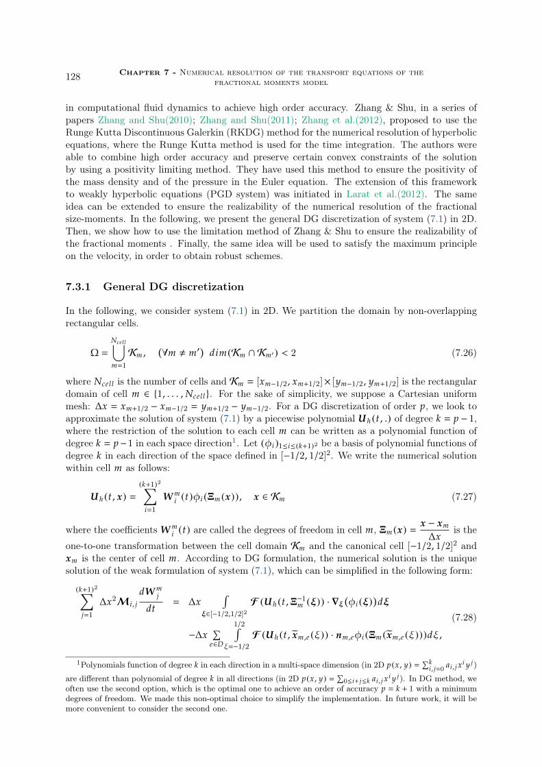
128 Chapter 7 - Numerical resolution of the transport equations of thefractional moments model

in computational fluid dynamics to achieve high order accuracy. Zhang & Shu, in a series ofpapers Zhang and Shu(2010); Zhang and Shu(2011); Zhang et al.(2012), proposed to use theRunge Kutta Discontinuous Galerkin (RKDG) method for the numerical resolution of hyperbolicequations, where the Runge Kutta method is used for the time integration. The authors wereable to combine high order accuracy and preserve certain convex constraints of the solutionby using a positivity limiting method. They have used this method to ensure the positivity ofthe mass density and of the pressure in the Euler equation. The extension of this frameworkto weakly hyperbolic equations (PGD system) was initiated in Larat et al.(2012). The sameidea can be extended to ensure the realizability of the numerical resolution of the fractionalsize-moments. In the following, we present the general DG discretization of system (7.1) in 2D.Then, we show how to use the limitation method of Zhang & Shu to ensure the realizability ofthe fractional moments . Finally, the same idea will be used to satisfy the maximum principleon the velocity, in order to obtain robust schemes.

7.3.1 General DG discretization

In the following, we consider system (7.1) in 2D. We partition the domain by non-overlappingrectangular cells.

Ω

Ncell⋃m1

Km ,(∀m , m′

)dim(Km ∩Km′) < 2 (7.26)

where Ncell is the number of cells and Km [xm−1/2 , xm+1/2]× [ym−1/2 , ym+1/2] is the rectangulardomain of cell m ∈ 1, . . . ,Ncell . For the sake of simplicity, we suppose a Cartesian uniformmesh: ∆x xm+1/2 − xm−1/2 ym+1/2 − ym−1/2. For a DG discretization of order p, we look toapproximate the solution of system (7.1) by a piecewise polynomial U h (t , .) of degree k p − 1,where the restriction of the solution to each cell m can be written as a polynomial function ofdegree k p−1 in each space direction1. Let (φi)1≤i≤(k+1)2 be a basis of polynomial functions ofdegree k in each direction of the space defined in [−1/2, 1/2]2. We write the numerical solutionwithin cell m as follows:

U h (t , x) (k+1)2∑

i1

W mi (t)φi (Ξm (x)), x ∈ Km (7.27)

where the coefficients W mi (t) are called the degrees of freedom in cell m, Ξm (x)

x − xm

∆xis the

one-to-one transformation between the cell domain Km and the canonical cell [−1/2, 1/2]2 andxm is the center of cell m. According to DG formulation, the numerical solution is the uniquesolution of the weak formulation of system (7.1), which can be simplified in the following form:

(k+1)2∑j1

∆x2M i , j

dW mj

dt ∆x

∫ξ∈[−1/2,1/2]2

F (U h (t ,Ξ−1m (ξ)) · ∇ξ(φi (ξ)

)dξ

−∆x∑

e∈D

1/2∫ξ−1/2

F (U h (t , xm ,e (ξ)) · nm ,eφi (Ξm (xm ,e (ξ)))dξ,

(7.28)

1Polynomials function of degree k in each direction in a multi-space dimension (in 2D p(x , y) ∑k

i , j0 ai , j x i y j)

are different than polynomial of degree k in all directions (in 2D p(x , y) ∑

0≤i+ j≤k ai , j x i y j). In DG method, weoften use the second option, which is the optimal one to achieve an order of accuracy p k + 1 with a minimumdegrees of freedom. We made this non-optimal choice to simplify the implementation. In future work, it will bemore convenient to consider the second one.

Part III - Numerical methods 129

S

E

N

W

• •

••

~nN~tN

~tE

~nE

~tS~nS

~tW

~nW

Figure 7.2: Illustration of the cell edges and of the orientation of their normal and tangentialvectors used in DG discretization scheme (7.28). The points in the interior represents the Gauss-Legendre quadrature points for k 2.

where M i , j ∫ξ∈[−1/2,1/2]2

φiφ j dξ is the mass matrix. This matrix is independent of cell m.And D N,W, S, E is the set of cell edges as illustrated in Figure 7.2, nm ,e is the normalvector of edge e oriented outward of cell m and xm ,e (ξ) are the positions along of edge e ∈ Dfor ξ ∈ [−1/2, 1/2], which are defined as follows:

xm ,e (ξ) xm + ∆x/2nm ,e + (ξ∆x)tm ,e , (7.29)

where tm ,e is a tangent vector of edge e (see Figure 7.2).

The solution is discontinuous at the edges, what allows DG methods to capture shocks of hy-perbolic equations. The flux F (U h (t , xe (ξ)) at edge e is approximated with a numerical flux,as for finite volume schemes. The numerical flux, computed at a given edge e, depends on thefollowing left and right state of the solution with respect to the edge e:

U−h (t , xm ,e (ξ)) limγ→0−

U h (t , xe (ξ) + γnm ,e ),

U+

h (t , xm ,e (ξ)) limγ→0+

U h (t , xe (ξ) + γnm ,e ).(7.30)

In the following, we use the upwind numerical flux such that we have:

F (U h (t , xe (ξ)) · (±eγ) ±Fγ (U−h (t , xm ,e (ξ)),U+

h (t , xm ,e (ξ))), (7.31)

where γ x , y are the two space directions and the numerical flux Fγ (., .) is defined in (7.15).

7.3.2 Polynomial basis choice and quadrature integration

In order to simplify the presentation of the method in 2D, we use two indexes for the degreesof freedom (W α, β)1≤α, β≤k+1 and the polynomial basis (φα, β)1≤α, β≤k+1. We also consider thateach cell is indexed by two variables m ∈ ~1; Ncell → (mx ,my) ∈ ~1; Nx × ~1; Ny one foreach direction:

my

[ mNx

]

mx m − Nx my

(7.32)

130 Chapter 7 - Numerical resolution of the transport equations of thefractional moments model

where Nx (resp Ny) is the number of cells in direction of x (resp y) and Ncell Nx Ny.

For the polynomial basis, we choose the Lagrangian polynomial basis associated to 2D abscissapoints of Gauss Legendre quadrature in [−1/2, 1/2]2:

φα, β (ξ) (ξx , ξy)) Lα (ξx)Lβ (ξy) (7.33)

and

Lα (ξ)

∏β,α (ξ − ξβ)∏β,α (ξα − ξβ)

, (7.34)

where ξα′, β′ (ξα′ , ξβ′) and (ξα′)1≤α′≤k+1 is the abscissas of the (k + 1)-point Gauss-Legendrequadrature in [−1/2, 1/2]. In this case, the degrees of freedom are equal to the values of thesolution at the points xα, β Ξm (ξα, β) for each cell m:

Uh (t , xα, β) W mα, β . (7.35)

This choice will simplify the resolution of the source terms (see appendix C), where we solvedirectly an Ordinary Differential equation (ODE) for each degrees of freedom separately. Solverof ODE source terms is presented in chapter 8.

The integrals in (7.28) can be approximated by quadratures of sufficient accuracy. An analysisof the requirement on the quadrature choice, presented in Cockburn et al.(1990), shows thata quadrature that is exact for polynomials of order 2k + 1, is sufficient to preserve the orderaccuracy of the DG scheme. In this work, we use k+1-point Gauss-Legendre quadrature in eachdirection to evaluate respectively 2D and 1D integrals. This integral approximation is an exactevaluation of the integral for the polynomial functions of degree 2k + 1. The numerical scheme(7.28) becomes:(M

dW m

dt

)α, β

1

∆x∑

0≤α′, β′≤k+1wα′wβ′

(F (W α′, β′) · ∇ξ

(φα, β (ξα′, β′)

))−

1

∆x∑

0≤β′≤k+1wβ′

(φα, β (ξmx+1/2, β′)(Fx

(W L

mx+1/2, β,W R

mx+1/2, β

)−

φα, β (ξmx−1/2, β′)Fx(W L

mx−1/2, β′,W R

mx−1/2, β′))

−1

∆x∑

0≤α′≤k+1wα′

(φα, β (ξα′,my+1/2)F y

(W L

α′,my+1/2,W R

α′,my+1/2

)−

φα, β (ξα′,my−1/2)F y(W L

α′,my−1/2,W R

α′,my−1/2

)),

(7.36)

where the subscripts mγ ± 1/2 (γ x , y) refer to the positions in the cell edges, for exampleξα′,my±1/2 (ξα′ ,±1/2) and W α,my±1/2 U h (Ξ(ξα′,my±1/2)), etc. The two superscripts L and Rare used to denote respectively, the left and right state solution with respect to the correspondingedge. Finally, this system can be written as an ODE system of the unknown vector of degreesof freedom:

dW m

dt RHS(W m ,W m ,N ,W m ,W ,W m ,S ,W m ,E), (7.37)

where W m ,e is the vector of degrees of freedom in the neighbor cell which shares edge e withcell m. This ODE can be integrated with a time integrator of order p k + 1, in order toobtain a global numerical scheme of the same order. In the present work, we use a k + 1-stepsRunge-Kutta method Gottlieb et al.(2001).

Part III - Numerical methods 131

7.3.3 Positivity limitation

In this section, we explain how we can preserve the realizability constraint on the moments. Forthis purpose, we use the same idea as the one proposed by Zhang et al.(2012). This method hasalready been used for the Euler equation. The method can be also used, in general, to preserveconvex constraint of the solution of hyperbolic equations. The moment space is a convex set,which allows to apply this method to the present system of equations.

Since the Lagrangian basis function sum to 1 within one cell, by summing over all the degrees offreedom in equation (7.28), and using the forward Euler discretization in time, we obtain thatthe scheme followed by the mean value in a cell reads:

Wm ,n+1

Wm ,n−∆t∆x

∑e∈D

1/2∫ξ−1/2

F(U L

h (t , xe (ξ)),U Rh (t , xe (ξ); nm ,e )

)dξ, (7.38)

where Wm ,n

∫

x∈KmU h (tn , x)dx is the mean solution in cell m at t tn.

The main idea of Zhang & Shu consists in using a quadrature rule which solves for the meansolution in the cell exactly. Using adequate quadrature points, the authors showed that theupdated mean solution (7.38) can then be written as a convex combination of the solution atthese quadrature points. Thus, the updated mean solution is realizable. This result is valid whenwe use a realizability preserving numerical flux as the one proposed in (7.15) and an adequateCFL condition. In 2D, Zhang & Shu used two sets of quadrature points in [−1/2, 1/2]2 given bythe Gauss-Legendre-Lobbato (GLL) quadrature abscissas:

Sx (ξα , ξr ) : 1 ≤ α ≤ k + 1, 1 ≤ r ≤ k + 2

Sy (ξs , ξβ) : 1 ≤ r ≤ k + 2, 1 ≤ β ≤ k + 1,(7.39)

where (ξr )1≤r≤k+2 is the sequence of 1D Gauss-Lobbato abscissas of order k+2. The main resultof Zhang & Shu work can be summarized in the following proposition:

Proposition 7.3.1 Let G be a convex set, and we suppose that for all ξ ∈ Sx ∪ Sy we haveU h (tn ,Ξm (ξ)) ∈ G and the resolution of (7.36) is achieved with a realizability preserving nu-merical flux, then the mean solution at tn+1 tn + ∆t belongs to the convex set G, W

m ,n+1∈ G

under the following CFL condition:

∆t∆x

CFLw1

max(|λxl |) + max(|λy

l |)(7.40)

where CFL ≤ 1, w1 is the first Gauss-Labotto weight of order k + 2 and λxl (respectively λy

l ) arethe eigenvalues of the hyperbolic system in the direction x (respectively y). In the present case,system (7.1) is weakly hyperbolic: it has one eigenvalue in each direction λx

l u and λyl v.

We underline that the above proposition can be generalized to the case of other Strong StabilityPreserving (SSP) time integrator Gottlieb et al.(2001).

132 Chapter 7 - Numerical resolution of the transport equations of thefractional moments model

•

•

•

G

un+1

un+1q

θq un+1q + (1 − θq)un+1

∂G

Figure 7.3: Illustration of the limitation procedure: the solution associated to a GLL quadraturepoint U n+1

q U h (tn+1 , xq) is lying outside the space of constraints, the red point shows itsprojection on the border of this space.

In the following, we define a convex set Gε parametrized by a small variable ε:

Gε U (mt ,m1ut )t: c(m) ∈ M1/2

3 , and p(c) ∈ [ε, 1 − ε]3 (7.41)

where c(m) (m1/2/m0/2 ,m2/2/m0/2 ,m3/2/m0/2) is the normalized fractional moment associ-ated to the moment vector m and p(c) is the canonical fractional moment defined in 4.4.3. Theparameter ε > 0 is chosen by the user to be strictly positive to force the moment vector tostay in the interior of the moment space and keep a strictly distance from the moment spaceborder. Indeed, for a moment vector in or very close to the moment space border, the recon-struction of the NDF through entropy maximization encounters some numerical difficulties, seeVié et al.(2013b). In practice, we set ε 1.e−4. For the resolution of the numerical scheme,we use a family of SSP Runge-Kutta method Gottlieb et al.(2001) and the realizability preserv-ing upwind numerical flux, defined in (7.15). So far, the only remaining point is to ensure therealizability of the solution at GLL points:(

∀x ∈ Ξm (Sx ∪ Sy)), U h (t , x) ∈ Gε , (7.42)

at each time step. Indeed, the initial condition is supposed to be physical and thus realizableeverywhere, in particular at the quadrature points. By using a realizability-preserving numericalflux, SSP time integrator and keeping the restricted CFL condition, we obtain realizable meanvalues in each cell for the first step. But nothing ensures the realizability at the GLL points.Therefore, we use a limitation procedure, after each time step, to bring the solution at GLLpoints back in the convex space Gε. Let us suppose that at the time tn the mean solution is inthe space Gε. We denote by (xq)1≤q≤2(k+1)(k+2) a sequence of points of Ξm (Sx ∪ Sy). Since Gε isa convex set, there exists a unique θq ∈ [0, 1], so that U h (tn , xq) θqU h (tn , xq) + (1−θq)W

m ,n

lies on the boundary of Gε, see Figure 7.3. The numerical solution is then corrected as follows:

Wm ,n+1α, β θW m ,n+1

α, β + (1 − θ)Wn+1

, θ min1≤q≤2(k+1)(k+2)

(θq) (7.43)

This limitation procedure preserves the mean cell value, therefore the numerical method remainsconservative and it is shown in Zhang and Shu(2011) that the accuracy of the scheme is notimpacted in the case of regular solutions. The solution U h (t , x) is then (k + 1)th order accurateand realizable at all GLL quadrature nodes.

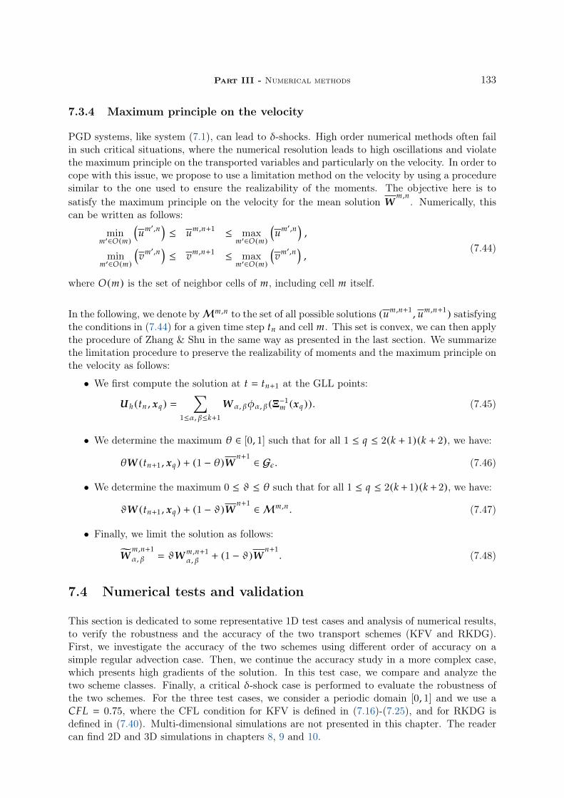
Part III - Numerical methods 133

7.3.4 Maximum principle on the velocity

PGD systems, like system (7.1), can lead to δ-shocks. High order numerical methods often failin such critical situations, where the numerical resolution leads to high oscillations and violatethe maximum principle on the transported variables and particularly on the velocity. In order tocope with this issue, we propose to use a limitation method on the velocity by using a proceduresimilar to the one used to ensure the realizability of the moments. The objective here is tosatisfy the maximum principle on the velocity for the mean solution W

m ,n. Numerically, this

can be written as follows:

minm′∈O(m)

(um′,n

)≤ um ,n+1

≤ maxm′∈O(m)

(um′,n

),

minm′∈O(m)

(vm′,n

)≤ vm ,n+1

≤ maxm′∈O(m)

(vm′,n

),

(7.44)

where O(m) is the set of neighbor cells of m, including cell m itself.

In the following, we denote byMm ,n to the set of all possible solutions (um ,n+1 , um ,n+1) satisfyingthe conditions in (7.44) for a given time step tn and cell m. This set is convex, we can then applythe procedure of Zhang & Shu in the same way as presented in the last section. We summarizethe limitation procedure to preserve the realizability of moments and the maximum principle onthe velocity as follows:

• We first compute the solution at t tn+1 at the GLL points:

U h (tn , xq) ∑

1≤α, β≤k+1

W α, βφα, β (Ξ−1m (xq)). (7.45)

• We determine the maximum θ ∈ [0, 1] such that for all 1 ≤ q ≤ 2(k + 1)(k + 2), we have:

θW (tn+1 , xq) + (1 − θ)Wn+1∈ Gε . (7.46)

• We determine the maximum 0 ≤ ϑ ≤ θ such that for all 1 ≤ q ≤ 2(k +1)(k +2), we have:

ϑW (tn+1 , xq) + (1 − ϑ)Wn+1∈ M

m ,n . (7.47)

• Finally, we limit the solution as follows:

Wm ,n+1α, β ϑW m ,n+1

α, β + (1 − ϑ)Wn+1. (7.48)

7.4 Numerical tests and validation

This section is dedicated to some representative 1D test cases and analysis of numerical results,to verify the robustness and the accuracy of the two transport schemes (KFV and RKDG).First, we investigate the accuracy of the two schemes using different order of accuracy on asimple regular advection case. Then, we continue the accuracy study in a more complex case,which presents high gradients of the solution. In this test case, we compare and analyze thetwo scheme classes. Finally, a critical δ-shock case is performed to evaluate the robustness ofthe two schemes. For the three test cases, we consider a periodic domain [0, 1] and we use aCFL 0.75, where the CFL condition for KFV is defined in (7.16)-(7.25), and for RKDG isdefined in (7.40). Multi-dimensional simulations are not presented in this chapter. The readercan find 2D and 3D simulations in chapters 8, 9 and 10.

134 Chapter 7 - Numerical resolution of the transport equations of thefractional moments model

7.4.1 Advection test case

In this section, we consider a simple advection with a constant velocity u −1. The initialmoments are presented in Figure 7.4 and are expressed as follows:

mk/2(t 0, x) 2

k + 2(S(k+2)/2

max − S(k+2)/2min ) exp(−(x − xc)2/σ2x) (7.49)

where (Smin , Smax) (0.3, 0.7), xc 0.5 and σx 0.1. The initial moments correspond tothe moments of a rectangular spray size distribution n(t , S) 1[Smin ,Smax ](S) multiplied by aGaussian spatial distribution.

Figure 7.4: Initial moments for the advection case: m0/2 (cross), m1/2 (circle), m2/2 (square)and m3/2 (triangle).

In Figure 7.5, we compare the numerical solutions of KFV (order 1 and 2) with RKDG (order 1,2 and 3). The first order solution of both schemes leads to a high numerical diffusion, while thesecond order is accurate enough to preserve the spatial profile after crossing twice the domain att 2. However, the second order RKDG scheme is more accurate, such that we can not identifythe difference with the exact solution. Figure 7.6 gives more details of the convergence order ofthe different schemes. In the logarithmic scale, the L1-errors of the solution obtained with thesecond order RKDG decreases asymptotically with a slope of −2.5 and the third order RKDGwith a slope −3.3, while for the second order KFV scheme the errors decreases only with a slopeof −1.55 as we increase − ln(∆x).

Part III - Numerical methods 135

Figure 7.5: Number density for the advection case at t 2. Left: using KFV scheme of order1 (cross) and order 2 (circle). Right: using RKDG scheme order 1 (cross), order 2 (circle) andorder 3 (square).

Figure 7.6: Error curves of m0 with respect to grid refinement in logarithm scale. Left: KFVschemes. Right: RKDG schemes. First order (cross) and second order (circle) for the twoscheme types and third order (square) only for RKDG scheme.

136 Chapter 7 - Numerical resolution of the transport equations of thefractional moments model

7.4.2 Compression test case

We consider an initial size distribution with a form depending on the coordinate space x. Infact, we need a non trivial initial size-space distribution, such that the slopes used in the secondorder scheme of the FKV method do not vanish all the time. The chosen initial size distributionhas the following profile:

n(t 0, S, x) 10 exp

(−

(x − xc)2

σ2x

)exp *

,−

(√

S − (1 − x)/2)2

σ2R

+-, (7.50)

where xc 0.25, σx 0.1 and σR 0.3. The initial velocity field is initiated as follows:u(t 0, x) 0.5 − x x < 0.5,u(t 0, x) 0. x ≥ 0.5.

(7.51)

Figure 7.7 shows the initial conditions for the fractional moments and the velocity. We canobtain an analytic solution of this test case using the characteristic curves method. For t < 1.0,the characteristic curves do not cross as shown in Figure 7.8, and we can show that the NDFsolution of the transport equation (7.10), can be written as follows:

n(t , S, x) 1

1. − tn(0, S, xo (t; x))

xo (t; x) x − 0.5t1. − t

(7.52)

At t 1.0 (see Figure 7.8), all the characteristic curves cross at point (t 1.0, x 0.5), whatleads to a δ-Dirac distribution in space. In the following, we study the numerical accuracy ofthe two methods KFV and RKDG. We investigate the numerical solution for t ≤ 0.8, beforethe formation of the shock. In Figures 7.9-7.10, we display the solution at two different times(t 0.4 and t 0.8) and we use the two method using different orders. The first order versionof the two schemes smears out the solution, in the same way, due to a high numerical diffusion.Furthermore, it is simple to show that the first order KFV scheme is equivalent to the RKDGone. Nonetheless, the solutions obtained with the two methods higher order resolution aredifferent. We can first remark the gain of accuracy brought by the second order RKDG andKFV in comparison to the first order scheme. But the numerical solution obtained with theRKDG second order scheme is more accurate than the one obtained with KFV second orderscheme. To go further in this analysis, we compute the L1

−error at t 0.8 for each numericalschemes and for different orders depending on the grid size. In Figure 7.11, we display theconvergence curves, highlighting the difference of precision between the two methods (KFV andRKDG). As it can be seen from these curves, the order accuracy of the KFV is much lower thanthe theoretical order. Indeed, the order of accuracy of the first order is around 0.4 and the secondorder is only 1.3. The low resolution of KFV is due to the numerical diffusion, which is presentnaturally for the first order, while for the second order, it is introduced by the slope limitationprocedure. Indeed, this is a difficult test case, where the solution starts to have high gradientvariations as we can see in Figure 7.9. The slope limitation procedure ensures the realizability ofthe moments and the maximum principle on the velocity and canonical moments. But has a costin terms of accuracy. However, RKDG second and third order seem not to be so affected by theZhang & Shu limitation procedure. For the second order RKDG, the logarithmic of L1

− errorof the solution decreases with a slope of 2.02 and the third order RKDG with a slope of 2.64depending on − ln(dx).

Part III - Numerical methods 137

Figure 7.7: Initial condition for the compression test case. Left: Initial moment fields, thecurves represent the moment with decreasing order in terms of value. Right: initial velocity

Figure 7.8: Illustration of the characteristic curves of the solution corresponding to the secondtest case. Remind that the equation on the velocity is a Burger’s equation.

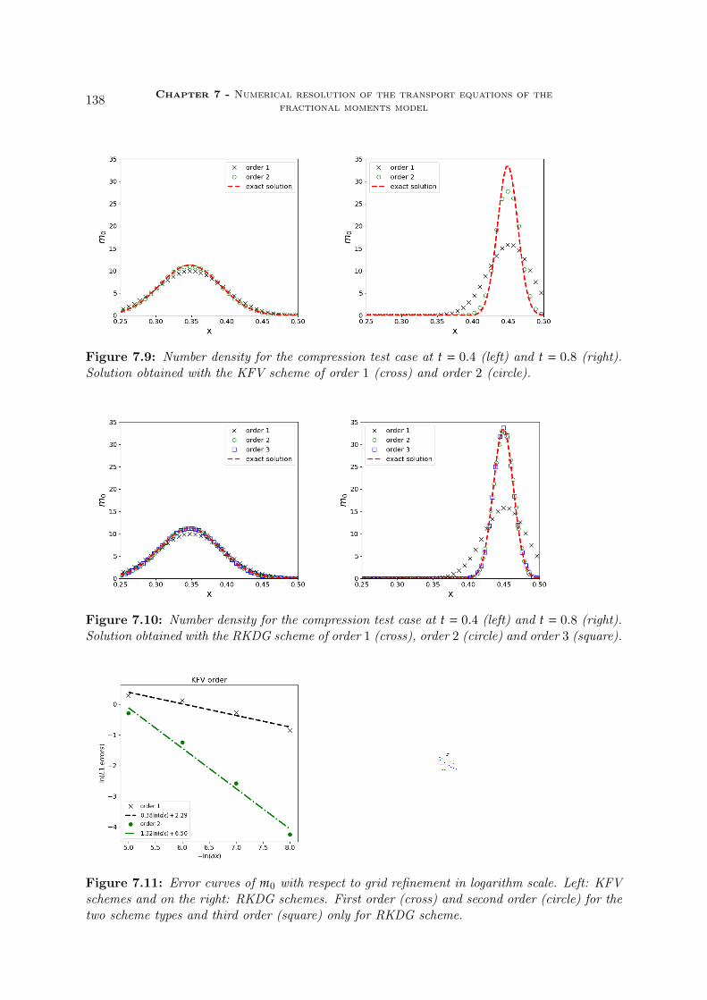
138 Chapter 7 - Numerical resolution of the transport equations of thefractional moments model

Figure 7.9: Number density for the compression test case at t 0.4 (left) and t 0.8 (right).Solution obtained with the KFV scheme of order 1 (cross) and order 2 (circle).

Figure 7.10: Number density for the compression test case at t 0.4 (left) and t 0.8 (right).Solution obtained with the RKDG scheme of order 1 (cross), order 2 (circle) and order 3 (square).

Figure 7.11: Error curves of m0 with respect to grid refinement in logarithm scale. Left: KFVschemes and on the right: RKDG schemes. First order (cross) and second order (circle) for thetwo scheme types and third order (square) only for RKDG scheme.

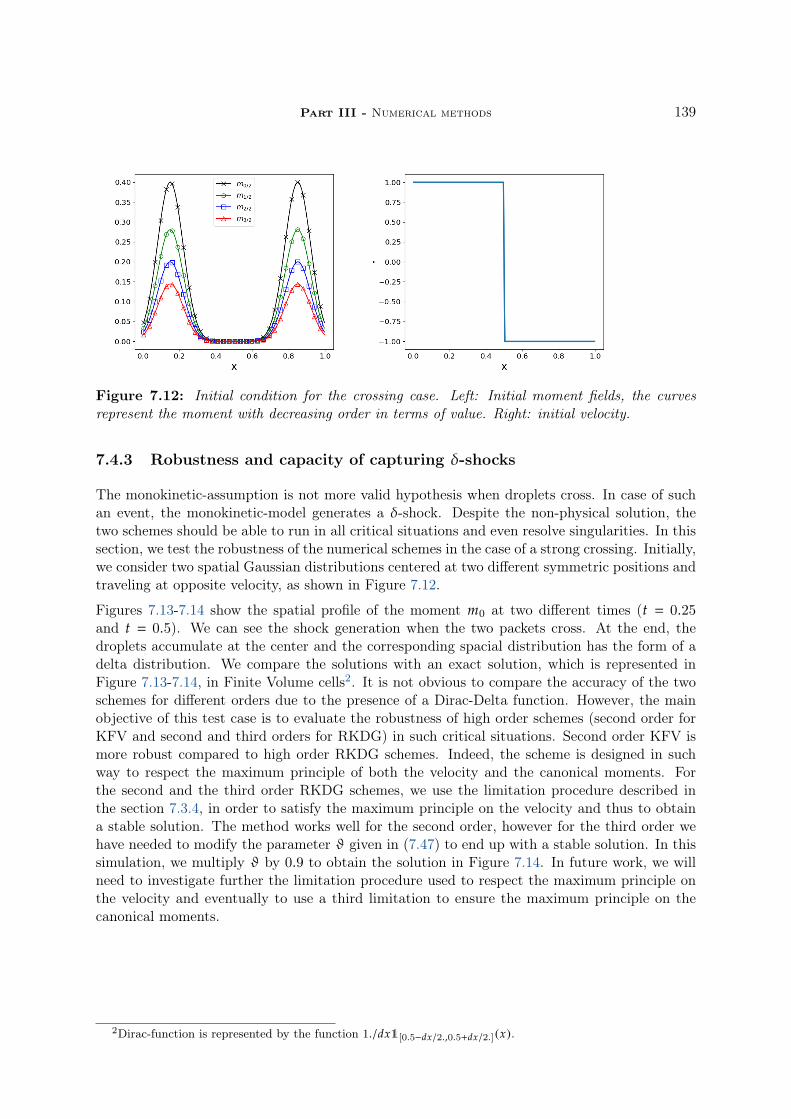
Part III - Numerical methods 139

Figure 7.12: Initial condition for the crossing case. Left: Initial moment fields, the curvesrepresent the moment with decreasing order in terms of value. Right: initial velocity.

7.4.3 Robustness and capacity of capturing δ-shocks

The monokinetic-assumption is not more valid hypothesis when droplets cross. In case of suchan event, the monokinetic-model generates a δ-shock. Despite the non-physical solution, thetwo schemes should be able to run in all critical situations and even resolve singularities. In thissection, we test the robustness of the numerical schemes in the case of a strong crossing. Initially,we consider two spatial Gaussian distributions centered at two different symmetric positions andtraveling at opposite velocity, as shown in Figure 7.12.

Figures 7.13-7.14 show the spatial profile of the moment m0 at two different times (t 0.25and t 0.5). We can see the shock generation when the two packets cross. At the end, thedroplets accumulate at the center and the corresponding spacial distribution has the form of adelta distribution. We compare the solutions with an exact solution, which is represented inFigure 7.13-7.14, in Finite Volume cells2. It is not obvious to compare the accuracy of the twoschemes for different orders due to the presence of a Dirac-Delta function. However, the mainobjective of this test case is to evaluate the robustness of high order schemes (second order forKFV and second and third orders for RKDG) in such critical situations. Second order KFV ismore robust compared to high order RKDG schemes. Indeed, the scheme is designed in suchway to respect the maximum principle of both the velocity and the canonical moments. Forthe second and the third order RKDG schemes, we use the limitation procedure described inthe section 7.3.4, in order to satisfy the maximum principle on the velocity and thus to obtaina stable solution. The method works well for the second order, however for the third order wehave needed to modify the parameter ϑ given in (7.47) to end up with a stable solution. In thissimulation, we multiply ϑ by 0.9 to obtain the solution in Figure 7.14. In future work, we willneed to investigate further the limitation procedure used to respect the maximum principle onthe velocity and eventually to use a third limitation to ensure the maximum principle on thecanonical moments.

2Dirac-function is represented by the function 1./dx1[0.5−dx/2.,0.5+dx/2.](x).

140 Chapter 7 - Numerical resolution of the transport equations of thefractional moments model

Figure 7.13: Number density for the crossing test case at t 0.25 (left) and t 0.5 (right).Solution obtained with KFV scheme of order 1 (cross) and order 2 (circle).

Figure 7.14: Number density for the crossing test case at t 0.4 (left) and t 0.8 (right).Solution obtained with KFV scheme of order 1 (cross) and order 2 (circle).

Part III - Numerical methods 141

7.5 Conclusion

This chapter is dedicated to high order and realizable numerical schemes to solve the transportpart of the fractional moment model presented in chapter 4. Two types of schemes are presentedduring this chapter. The first one is based on a finite volume discretization. The numericalflux is obtained by using the equivalence between the fractional moments PGD-like system andkinetic equation for a monokinetic distribution in the velocity. We show how we can obtain firstand second order schemes, while ensuring the realizability of the moments and also satisfyingthe maximum principle on the velocity and on the canonical moments. We refer to this type ofscheme by Kinetic Finite Volume (KFV) schemes. The second type is the Runge Kutta GalerkinDiscontinuous (RKDG) scheme. The method can be extended to an arbitrary order of accuracy.The realizability of the moments is ensured by using the limitation procedure proposed the firsttime by Zhang & Shu. We have also used this limitation technique to ensure the maximumprinciple on the velocity. In fact, the maximum principle on the velocity allows to obtain astable solution, especially in the critical case of δ-shocks formation. However, we still havesome open issues to ensure the robustness of high order RKDG schemes in such cases. Indeed,we show in the last test case that we need to tune the limitation coefficient to obtain a stablesolution for the third order RKDG scheme. On the other side, KFV shows a robust behaviorin this critical situation. Finally, we show for other test cases that we obtain accurate solutionsusing high order RKDG schemes compared to KFV schemes. Furthermore, the accuracy ordersobtained with the RKDG are very close to the theoretical ones. While for KFV schemes, wefind that the second order improve the accuracy compared to the first order, but the accuracyorder is lower than the theoretical order because of the slope limitation.

Chapter 8

A new algorithm for the timeintegration of the source terms in thefractional moments model

8.1 Introduction

This chapter presents a numerical procedure for the resolution of the source terms of the frac-tional moments model derived in chapter 4. Recall that the numerical resolution of the transportpart has been treated in chapter 7. The resolution of the source terms turns to a time integra-tion of an ODE system. However, classical ODE solvers do not ensure the realizability of themoments. In the present work, we propose a new realizable algorithm to solve the evolutionof the fractional moments due to evaporation. The resolution of the evaporation is first doneby evaluating the droplets disappearance flux. The reconstruction through Maximum Entropyformalism is used here to evaluate this flux. Then, we compute the internal size evolution byusing a specific quadrature, which involves negative order moments and requires an originalstrategy compared to the integer moment problem Massot et al.(2010). Indeed, we show thatthe evaporation algorithm proposed for the EMSM model is not accurate to evaluate correctlythe evaporation in the case of the fractional moments model. The proposed strategy is thenassessed by a careful investigation of the numerical errors, as well as a detailed comparison withanalytic solutions in 0D test cases. Finally, we compare the EMSM and the fractional momentsmodel on 2D acedemic configuration. In this last simulation, we conduct a complete resolutionof the system of equations (4.24) including the transport and the evaporation and the drag forcesource terms.

8.2 Resolution of the evaporation

Let us consider a pure evaporation, without transport nor drag. The kinetic equation in thiscase reads:

∂t n − ∂S (Kn) 0. (8.1)

144 Chapter 8 - A new algorithm for the time integration of the sourceterms in the fractional moments model

The equations corresponding to the fractional moments model with a continuous reconstructionof the NDF through Entropy maximization reads:

dtm0/2 −KnME|S0 ,

dtm1/2 −K

2m−1/2 ,

dtm2/2 −Km0/2 ,

dtm3/2 −3K

2m1/2 ,

(8.2)

where the instantaneous disappearance flux for zero size, KnME|S0(m0/2 ,m1/2 ,m2/2 ,m3/2) is

obtained through an Entropy Maximization detailed in section 4.4.5. The RHS of this ODEsystem corresponds to the evaporation source term of the system of equations (4.24).

Solving this system using classical integrator such as Euler or Runge-Kutta methods does notensure the realizability of the moments Massot et al.(2010). This property is essential for robust-ness and accuracy to reconstruct a positive NDF. For this reason, we design a new algorithm tosolve the evaporation based on the kinetic evolution of the NDF, given by equation (8.1). First,we present a simple method to compute directly the updated moments from the exact kineticsolution of the NDF. This method is not well suitable for real spray applications with complexevaporation laws, because it requires intense arithmetic computations. However, we use thismethod as a reference solution. The evaporation algorithm used for the EMSM model can beused for general evaporation law with less arithmetic operations. We will show in a second partthat this algorithm is inaccurate when evaluating the evaporation in the case of the fractionalmoments model. Finally, we highlight the main problem of this algorithm and we propose a newstrategy to cope with this difficulty.

8.2.1 Exact kinetic solution through the method of characteristics

The exact solution of the NDF evolution, in the case of d2 evaporation law, can be obtainedeasily by solving analytically the kinetic equation (8.1):

n(t , S) n(0, S + Kt). (8.3)

For more general evaporation law, when the evaporation rate RS (S) is a smooth function ofthe size, the kinetic equation can be solved by using the method of characteristics. Indeed, bymultiplying the kinetic equation by RS (S), we obtain the following equation in the functionΓ(t , S) RS (S)n(t , S):

∂tΓ(t , S) + RS (S)∂S (Γ(t , S)) 0. (8.4)

Then, for a given initial time t0 and size So, we define the one variable function g(t)

Γ(t , φ(t; t0 , So)), such that φ(t; t0 , So) is the characteristic curve verifying:

dφ(t; t0 , So)dt

RS (φ(t; t0 , So)),

φ(t0; t0 , So) So .(8.5)

It is a simple fact that the derivative of g(t) vanishes, and thus, we obtain the following expres-sion:

Γ(t , φ(t; t0 , So)) Γ(t0 , So). (8.6)

Part III - Numerical methods 145

Finally, we obtain the exact solution of the size distribution as follows:

n(t , S) RS (φ(t0; t , S))

RS (S)n(t0 , φ(t0; t , S)). (8.7)

8.2.2 Fully kinetic scheme

At each time step tn, the reconstructed NDF nME (t tn , S) is determined using the MEalgorithm. The exact kinetic solution of the NDF can then be expressed analytically as afunction of this initial NDF thanks to (8.3), for a d2 evaporation law. Finally, the updatedmoments are computed as follows:

mk/2(tn + ∆t) ∫ 1

0Sk/2n(tn + ∆t , S)dS

∫ 1

0Sk/2n(tn , S + K∆t)dS

∫ 1−K∆t0

Sk/2n(tn , S + K∆t)dS

∫ 1

K∆t (S − K∆t)k/2nME (tn , S)dS.

(8.8)

In these equalities, we consider n(t , S ≥ 1) 0, since the dimensionless maximum size isSmax 1.

The integral calculation can be achieved by using a Gauss-Legendre quadrature. The method issimple and accurate. However, its extension to complex evaporation laws, where the evaporationrate depends on several parameters, could involve heavy calculations. To clarify this point, weconsider a smooth evaporation rate RS (S), function of the droplet size. Using the solution (8.7),we can that the updated moments can be expressed as follows:

mk/2(tn+1) ∫ 1

φ(tn ;tn+1 ,0)φ(tn+1; tn , s)k/2n(tn , s)ds . (8.9)

To compute accurately this integral, we use 24 Gauss quadrature points. However, we alsoneed to compute the size φ(tn+1 , tn , S j), for all abscissas S j of the 24-quadrature points andφ(tn; tn+1 , 0), by solving the ODE system (8.5). For this reason, we consider this direct methodin solving the moments will be very costly in terms of CPU time.

8.2.3 Inefficiency of the original EMSM algorithm for evaporation

Massot et al Massot et al.(2010) proposed a realizable algorithm to solve correctly the evapo-ration moment system in the case of integer moments. The idea of this algorithm is also basedon the known solution of the kinetic equation (8.1). In order to design a generalized algorithmfor a d2 evaporation law or for more complex laws, while keeping low computational cost, thecalculation of the moments is done in three steps instead of computing directly the integrals(8.13) or (8.9) using a large number of Gauss-Legendre quadratures. This algorithm reads inthe case of fractional moments as follows:

• From the moment vector m(tn) (m0/2 ,m1/2 ,m2/2 ,m3/2)t , we reconstruct the NDF byusing the ME algorithm. Then, we compute the disappearance flux of the droplets which

146 Chapter 8 - A new algorithm for the time integration of the sourceterms in the fractional moments model

will be totally evaporated at the next step:

Φ−(tn) ∫ K∆t

0

nME (tn , s)*....,

1

s1/2

ss3/2

+////-

ds . (8.10)

• Using the Product-Difference (PD) algorithm Gordon(1968), we compute the abscissasS j ≥ K∆t and the weights w j ≥ 0 of the lower principal representation of the moments1

m[K∆t ,1](tn) m(tn) −Φ−(tn). This corresponds to solving the system:

m[K∆t ,1]k/2 (tn)

2∑j1

w jSk/2j , k ∈ 0, 1, 2, 3, (8.11)

where m[K∆t ,1](tn) is the moment vector on [K∆t , 1].

• Finally, we calculate the moments at the next step:

mk/2(tn + ∆t) 2∑

j1

w j (S j −K∆t)k/2. (8.12)

However, this algorithm is not adapted for the fractional moments and can not predict thecorrect kinetic evolution of the NDF. We illustrate this problem in Figure 8.1. Two solutions ofthe NDF are constructed through ME algorithm from two solutions of the moments: the firstset of moments is computed using the above algorithm and the second one by using the fullykinetic scheme. These two solutions are compared to the exact kinetic solution as proposedin equation (8.3). The NDF obtained with the fully kinetic scheme fits accurately the exactsolution. However, the one obtained using the above algorithm shows the inefficiency of thismethod to predict the right kinetic evolution of the NDF from the fractional moments. Inthe next section, we give a mathematical explanation of this unexpected failure of the methoddescribed above, then we propose a new original solution to adapt the algorithm.

8.2.4 Adapted evaporation scheme for fractional moments

In order to understand the inefficiency of the previous algorithm proposed in section 8.2.3, wepropose to consider again a constant evaporation rate RS (S) −K. The moment solutionexpressed directly from the exact kinetic solution reads:

mk/2(t+∆t)∫ 1

0Sk/2n(t+∆t , S)dS

∫ 1

0Sk/2n(t , S+K∆t)dS

∫ 1+K∆tK∆t (S−K∆t)k/2n(t , S)dS

∫ 1

K∆t (S−K∆t)k/2n(t , S)dS.(8.13)

In the previous equality, we consider that n(t , S) 0 for S ≥ 1. In the following, we show thatthe updated moments can be written as a function of an infinite set of moments on the support[K∆t , 1].

Lemma 8.2.1 For all positive integer k and for all x ∈ [−1, 1] the function f : x → (1 − x)k/2

admits a power series which converges normally to the function f :

(1 − x)k/2

+∞∑n0

ak/2n xn , (8.14)

1We can also use hybrid approach with multi-size sections, in this case we take into account the evaporationfluxes coming from the right section: m(tn ) −Φ(i)

− (tn ) +Φ(i+1)− (tn ), where i indexes the size-section.

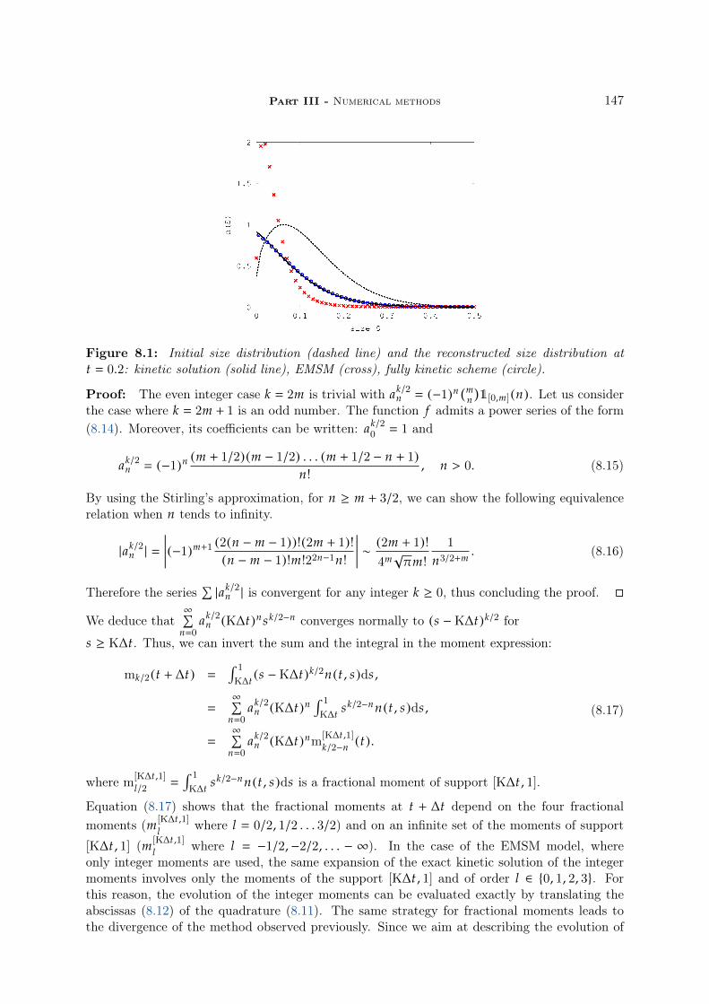
Part III - Numerical methods 147

Figure 8.1: Initial size distribution (dashed line) and the reconstructed size distribution att 0.2: kinetic solution (solid line), EMSM (cross), fully kinetic scheme (circle).

Proof: The even integer case k 2m is trivial with ak/2n (−1)n (m

n)1[0,m](n). Let us consider

the case where k 2m + 1 is an odd number. The function f admits a power series of the form(8.14). Moreover, its coefficients can be written: ak/2

0 1 and

ak/2n (−1)n (m + 1/2)(m − 1/2) . . . (m + 1/2 − n + 1)

n!, n > 0. (8.15)

By using the Stirling’s approximation, for n ≥ m + 3/2, we can show the following equivalencerelation when n tends to infinity.

|ak/2n |

(−1)m+1 (2(n − m − 1))!(2m + 1)!

(n − m − 1)!m!22n−1n!

∼

(2m + 1)!4m√πm!

1

n3/2+m . (8.16)

Therefore the series∑|ak/2

n | is convergent for any integer k ≥ 0, thus concluding the proof.

We deduce that∞∑

n0ak/2

n (K∆t)n sk/2−n converges normally to (s −K∆t)k/2 for

s ≥ K∆t. Thus, we can invert the sum and the integral in the moment expression:

mk/2(t + ∆t) ∫ 1

K∆t (s −K∆t)k/2n(t , s)ds ,

∞∑

n0ak/2

n (K∆t)n∫ 1

K∆t sk/2−n n(t , s)ds ,

∞∑

n0ak/2

n (K∆t)nm[K∆t ,1]k/2−n (t).

(8.17)

where m[K∆t ,1]l/2

∫ 1

K∆t sk/2−n n(t , s)ds is a fractional moment of support [K∆t , 1].

Equation (8.17) shows that the fractional moments at t + ∆t depend on the four fractionalmoments (m[K∆t ,1]

l where l 0/2, 1/2 . . . 3/2) and on an infinite set of the moments of support

[K∆t , 1] (m[K∆t ,1]l where l −1/2,−2/2, . . . − ∞). In the case of the EMSM model, where

only integer moments are used, the same expansion of the exact kinetic solution of the integermoments involves only the moments of the support [K∆t , 1] and of order l ∈ 0, 1, 2, 3. Forthis reason, the evolution of the integer moments can be evaluated exactly by translating theabscissas (8.12) of the quadrature (8.11). The same strategy for fractional moments leads tothe divergence of the method observed previously. Since we aim at describing the evolution of

148 Chapter 8 - A new algorithm for the time integration of the sourceterms in the fractional moments model

the moments through the evolution of a minimal number of quadrature nodes, we propose anew quadrature, suitable for fractional moments, such that the updated moments in (8.12) canapproximate accurately the exact kinetic evolution (8.17).

8.2.5 A specific quadrature for negative moment order

Our objective is to find an adequate quadrature with the lowest possible quadrature number nq,such that the following approximation:

mk/2(t + ∆t) ≈nq∑j1

w j (S j − K∆t)k/2 , (8.18)

is accurate. More precisely, we would like to find a quadrature such that the difference, fork ∈ 0, 1, 2, 3

εk/2(∆t) mk/2(t + ∆t) −nq∑j1

w j (S j −K∆t)k/2

∞∑

n0ak/2

n (K∆t)n *,

m[K∆t ,1]k/2−n (t) −

nq∑j1

w jSk/2−nj

+-,

(8.19)

is at least o(∆t) to ensure the convergence of the numerical scheme. It is a difficult task toprove such a result, but we provide here a first result is this direction. Our strategy consists inusing a quadrature, which cancels a finite set of the first terms in the sum (8.19), by enforcing

Ep/2 m[K∆t ,1]p/2 (t)−

nq∑j1

w jSp/2j to be zero for p ∈ −2nq

− , . . . , 2, 3. Thus 2nq fractional moments

on [K∆t , 1] are considered, with nq nq− + 2, from order −nq

− to 3/2. As soon as nq−≥ 0,

this is sufficient to have ε0/2 0 and ε2/2 0. The following Lemma shows the existence anduniqueness of such quadrature and gives the corresponding value of the error terms εk/2(∆t).

Lemma 8.2.2 Let(m

[K∆t ,1]p/2

)p∈−2nq− ,...,3

be a set of fractional moments on [K∆t , 1] in the inte-

rior of the moment space and nq− a non negative integer. There exists a unique set of abscissas

(S j) j∈1,...,nq and weights (w j) j∈1,...,nq , with nq nq− + 2 such that

∀k ∈ −2nq− , . . . , 3 m

[K∆t]k/2

nq∑j1

w jSk/2j . (8.20)

Moreover one have w j w′j r2nq

−

j and S j r2j , where r j and w′j are the abscissas and weights of

the Gauss quadrature corresponding to the moments mk m[K∆t ,1]k/2+nq−

for k ∈ 0, . . . , 2nq − 1.Using this quadrature, the error terms defined by (8.19) can be written:

ε0/2(∆t) 0, ε1/2(∆t) *,

+∞∑nnq−1

a1/2n E(2n−1)/2+-

(K∆t)1/2 ,

ε2/2(∆t) 0, ε3/2(∆t) *,

+∞∑nnq

a3/2n E(2n−3)/2+-

(K∆t)3/2 ,(8.21)

where Ep/2 (K∆t)p/2 *,m

[K∆t ,1]−p/2 (t) −

nq∑j1

w jS−p/2j

+-is bounded by m

[K∆t ,1]0/2 .

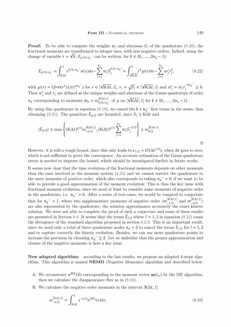
Part III - Numerical methods 149

Proof: To be able to compute the weights w j and abscissas S j of the quadrature (8.20), thefractional moments are transformed to integer ones, with non negative orders. Indeed, using thechange of variable r

√S, Ep/2+nq− can be written, for k ∈ 0, . . . , 2nq − 1:

Ep/2+nq−

∫ 1

K∆tsk/2−nq

−

n(s)ds−nq∑j1

w jSk/2−nq

−

j

∫ 1

√K∆t

rkµ(r)dr−nq∑j1

w′j rkj , (8.22)

with µ(r) (2rn(r2))/(r2nq−

) for r ∈ [√

K∆t , 1], r j √

S j ∈ [√

K∆t , 1] and w′j w j r−2nq

−

j ≥ 0.Then w′j and r j are defined as the unique weights and abscissas of the Gauss quadrature of order

nq corresponding to moments mk m[K∆t ,1]k/2+nq−

of µ on [√

K∆t , 1] for k ∈ 0, . . . , 2nq − 1.

By using this quadrature in equation (8.19), we cancel the k + nq− first terms in the series, thus

obtaining (8.21). The quantities Ep/2 are bounded, since S j ≥ K∆t and

|Ep/2 | ≤ max

(K∆t)p/2m[K∆t ,1]−p/2 , (K∆t)p/2

nq∑j1

w jS−p/2j

≤ m

[K∆t ,1]0/2 .

However, it is still a rough bound, since this only leads to ε1/2 O(∆t1/2), when ∆t goes to zero,which is not sufficient to prove the convergence. An accurate estimation of the Gauss quadratureerrors is needed to improve the bound, which should be investigated further in future works.

It seems now clear that the time evolution of the fractional moments depends on other momentsthan the ones involved in the moment system (4.24) and we cannot restrict the quadrature tothe mere moments of positive order, which also corresponds to taking nq

− 0, if we want to beable to provide a good approximation of the moment evolution. This is thus the key issue withfractional moment evolution, since we need at least to consider some moments of negative orderin the quadrature, i.e. nq

− > 0. After a series of test-cases, we would be tempted to conjecturethat for nq

− 1, where two supplementary moments of negative order (m[K∆t ,1]−1/2 and m[K∆t ,1]

−2/2 )are also represented by the quadrature, the solution approximates accurately the exact kineticsolution. We were not able to complete the proof of such a conjecture and some of these resultsare presented in Section 8.4. It seems that the terms El/2 where l 1, 2 in equation (8.21) causethe divergence of the standard algorithm proposed in section 8.2.3. This is an important result,since we need only a total of three quadrature nodes nq 3 to cancel the terms El/2 for l 1, 2and to capture correctly the kinetic evolution. Besides, we can use more quadrature points toincrease the precision by choosing nq

−≥ 2. Let us underline that the proper approximation and

closure of the negative moments is here a key issue.

New adapted algorithm: according to the last results, we propose an adapted 4-steps algo-rithm. This algorithm is named NEMO (Negative Moments) algorithm and described below:

A. We reconstruct nME (S) corresponding to the moment vector m(tn) by the ME algorithm,then we calculate the disappearance flux as in (8.10),

B. We calculate the negative order moments in the interval [K∆t , 1]

m[K∆t ,1]−a/2

∫ 1

K∆ts−a/2nME (s)ds , (8.23)

150 Chapter 8 - A new algorithm for the time integration of the sourceterms in the fractional moments model

for a 1, . . . , 2nq−, where 2nq

−≥ 2 is the number of additional moments of negative order

used in this algorithm and chosen by the user. The other moments of positive order arecomputed using the disappearance flux:

m[K∆t ,1]k/2 mk/2(0) −Φ−,k/2(tn), k 0, . . . , 3, (8.24)

where Φ is the disappearance flux given in (8.10).

C. The abscissas S j r2j ∈ [K∆t , 1] and the weights w j w′j r2nq

−

j of the quadrature corre-

sponding to the moments m[K∆t ,1]p/2 for p −2nq

− , . . . , 3 are computed using the Product-

Difference Algorithm Gordon(1968) corresponding to the moments mk m[K∆t ,1]k/2+nq−

fork ∈ 0, . . . , 2nq − 1, leading to

m[K∆t ,1]p/2

nq∑j1

w jSp/2j , p −2nq

− , . . . , 3 (8.25)

D. Finally, we calculate the updated moments as follows:

mk/2(tn + ∆t) nq∑j1

w j (S j −K∆t)k/2. (8.26)

The singularities of the negative moments integrals, when ∆t is very small, limits the use of highvalues of nq

−. But in practice K∆t > 1.e − 4 and we will show that the choice of nq− 1 or

nq− 2 are sufficient to obtain an accurate solution. In these cases, the integral computation

of the negative order moments can be achieved correctly with 24 Gauss-Legendre quadraturepoints. For more complex evaporation laws, the algorithm can be straightforwardly general-ized by computing the Lagrangian evolution of the abscissas. In other words, equation (8.26)becomes:

mk/2(tn + ∆t) nq∑j1

w j φ(tn + ∆t; tn , S j)k/2 , (8.27)

and the integral of negative moments in (8.23) becomes:

m[K∆t ,1]−a/2

∫ 1

φ(tn ;tn+∆t ,0)s−a/2nME (s)ds . (8.28)

Remark 3 The realizability of the moment is satisfied for this new algorithm. Indeed, theProduct-Difference Algorithm ensures that the abscissas S j ≥ K∆t in equation (8.25). Therefore,the updated moments in (8.26) correspond to a positive distribution.

Part III - Numerical methods 151

8.3 Evaporation coupled with drag

In this paragraph, we present a coupled solver for the spray evolution under evaporation anddrag force. The corresponding system of equations reads:

dtm0 −Kn(S 0),

dtm1/2 −K

2m−1/2 ,

dtm1 −Km0 ,

dtm3/2 −3K

2m1/2 ,

dt (m1u) −Km0u + m0

u g − uθ

.

(8.29)

Since the first four equations do not depend on the last one, the updated moments can becomputed using the NEMO algorithm. For the last equation, we use the method developed inVié et al.(2013b) to solve the velocity evolution due to the drag force and evaporation.

The momentum evolution is conducted in two steps: first, we remove the part of the droplets,which will completely evaporate during the time interval [tn , tn+1], by evaluating the disappear-ance fluxes of the moments and momentum:

U[K∆t ,1]

U −

(Φ−Φ−,2/2u

), (8.30)

where U (m0/2 , . . . ,m3/2 ,m2/2ut )t and Φ− is the disappearance flux vector of the moments(8.10). Then, we use the lower principal representation to approximate the size distribution ofthe moments on the support [K∆t , 1] (8.25). The computation of the moments is achieved with(8.26). To update the momentum in this last step, we consider a size-velocity correlation, suchthat, at a given time t ∈ [tn , tn+1], we attribute the velocity c i (t) to each abscissa Si (t). Then,we write:

(m1u)[K∆t ,1](t) nq∑i1

wiSi (t)c i (t), (8.31)

the abscissas Si (t) and the velocities c i (t) are determined by solving the following ODE systems:

dc i

dt −

u g − c i

θSi, c i (t tn) u(tn),

dSi

dt −K, Si (t tn) Si (tn)

(8.32)

The final momentum is computed at t tn+1 using equation (8.31). The method can begeneralized to more complex evaporation law by replacing −K in equation (8.32) by a generalevaporation rate RS (S), see appendix A.

8.4 Numerical results

This section is dedicated to some representative test-cases and analysis of the numerical results,to verify the robustness and the accuracy of the proposed numerical schemes. First, we testthe new evaporation algorithm in the case of a d2 law with K 1, for two different initial

152 Chapter 8 - A new algorithm for the time integration of the sourceterms in the fractional moments model

Figure 8.2: Solutions of the reconstructed size distribution using: NEMO with nq− 1 (cross),

fully-kinetic (circle), exact kinetic solution (solid line) and the initial distribution (dashed line),at time t 0.1 (left) and t 0.2 (right).

Figure 8.3: Evolution of the relative moment errors (in percent): m0 (solid line), m1/2 (dash-dotted line), m1 (cross) and m3/2 (circle). Left: fully kinetic algorithm; Right: NEMO algorithm(nq− 1).

conditions. An evaporation test in the case of non constant evaporation rate is also given as acomplementary result, to show that the present algorithm is not restricted to d2 law. Finally,a 2D case of an evaporating spray in the presence of a steady gas field, given by Taylor-Greenvortices, is presented, in order to qualify the robustness and accuracy of the method comparedto the EMSM in the same configuration. In this last simulation, we have used the second orderFinite Volume Kinetic (FVK) scheme to solve the transport part. The same simulation usingRKDG method is presented in chapter 10.

8.4.1 Evaporation in 0D simulation

8.4.1.1 Evaporation with a d2 law for an initial smooth NDF

In this section, we use an initial smooth NDF, which is the same initial condition as the oneused in Figure 8.1:

n0(S) exp(−20(S1/2− 1/4)2(S1/2

+ 1)). (8.33)

We underline that this distribution can be written in the form of a ME-reconstructed NDF,which is given in (4.37).

Part III - Numerical methods 153

In this section, we compare the fully-kinetic and NEMO algorithms (nq− 1), using the time

step ∆t 0.002, with the exact kinetic solution. In Figure 8.2, we plot the ME-reconstructedNDFs from the solution of the moments obtained respectively by the two methods and theexact kinetic distribution at t 0.1 and t 0.2. One can see that the two ME-reconstructeddistributions follow accurately the exact distribution. Capturing the correct size distributionusing only four moments is not an obvious result. However, the results obtained with NEMOalgorithm are more attractive, since we obtain the same accuracy using only three quadraturenodes compared with the 24-quadrature nodes of the fully kinetic scheme. To go further inthe quantitative comparison, Figure 8.3 shows the evolution of the relative error of the fourfractional moments. We can see that for the two algorithms the moment errors relatively to theinitial values do not exceed 0.3%.

8.4.1.2 d2 law evaporation for a discontinuous initial NDF

In this second case, we test the new algorithm NEMO in the case of a discontinuous initialNDF:

n0(S)

1, if S ∈ [0.1, 0.6]

0, otherwise(8.34)

The initial NDF defined in (8.34) and the initial ME reconstructed NDF are plotted in Figure8.4. In Figure 8.5, we present the reconstructed NDF computed using the theNEMO algorithmwith nq

− 1 at two different times. In the same figures, we compare these results to the onesobtained with the fully kinetic solution and the exact kinetic solution2. As in the previous case,the NEMO algorithm shows an accurate prediction of the exact kinetic solution. Furthermore,Figure 8.6 shows that the relative error of the moments are less than 1.%, in the case of NEMOalgorithm with nq

− 1 and ∆t 6.e − 3. This is an accurate result. However, we can see thatthe fully-kinetic algorithm is more accurate and the moment relative errors do not exceed 0.3%.We can improve the accuracy of the NEMO algorithm by using a smaller time step ∆t 6.e−4or by using nq

− 2 and keeping the same time step as the previous case. In Figure 8.7, wepresent the relative moment errors using NEMO algorithm with nq

− 2 and ∆t 6.e − 3. Inthis case, we are in the same level of accuracy as the fully kinetic algorithm.

8.4.2 Accuracy of the NEMO algorithm for a linear evaporation rate

NEMO scheme has been developed under the assumption of a d2 law, but as it was explained be-fore, the algorithm can be generalized to more complex laws by solving the Lagrangian equation(8.5) for each abscissas S j given in the third step of the algorithm. In this section, we propose toevaluate the accuracy of the algorithm in the case where the evaporation rate depends linearlyon the size:

Rs (S) −(a + bS). (8.35)

The exact kinetic solution can be computed according to equation (8.7). In the following, we seta 0.5 and b 1. Figure 8.8 presents the NDFs computed by the NEMO algorithm, the fullykinetic algorithm and compares them to the exact solution at t 0.3 and t 0.6. The relativeerror are given in Figure 8.9. We can see from these results, the accuracy of the generalizedNEMO algorithm to predict the kinetic evolution.

2The exact kinetic solution is computed for the initial ME reconstructed size distribution.

154 Chapter 8 - A new algorithm for the time integration of the sourceterms in the fractional moments model

Figure 8.4: The ME reconstructed NDF (solid line) and the initial discontinuous NDF (dashedline).

Figure 8.5: Solutions of the reconstructed size distribution at at t 0.3 (left) and t 0.6(right) using: NEMO with nq

− 1 (cross), fully-kinetic (circle), exact kinetic solution (solidline) and the initial distribution (dashed line).

Figure 8.6: Evolution of the relative moment errors (in percent): m0 (solid line), m1/2 (dash-dotted line), m1 (cross) and m3/2 (circle). Left: fully kinetic algorithm using ∆t 6.e−3; Right:NEMO algorithm using nq

− 1 and ∆t 6.e − 3.

Part III - Numerical methods 155

Figure 8.7: Evolution of the relative moment errors (in percent) using NEMO algorithm(nq

− 2 and dt 6e − 3): m0 (solid line), m1/2 (Dash-dotted line), m1 (cross) and m3/2

(circle).

Figure 8.8: The evolution of the NDF in the case of a linear evaporation rate: initial MEreconstructed solution (dashed line), NEMO algorithm using nq

− 1 (cross), fully kineticalgorithm (circle) and exact kinetic solution (solid line), at times t 0.3 and t 0.6.

Figure 8.9: Evolution of the moment errors (in percent) relatively to their initial value cal-culated with fully kinetic algorithm (left) and NEMO algorithm (right): m0 (solid line), m1/2

(dash-dotted line), m1 (cross) and m3/2 (circle).

156 Chapter 8 - A new algorithm for the time integration of the sourceterms in the fractional moments model

8.4.3 2D complete simulation: transport, evaporation and drag force

After the model and the numerical schemes have been tested in 0D and 1D, we propose inthis part to compare in a classical 2D configuration, the present model and numerical schemeswith the EMSM model, in a case where we consider transport, evaporation and drag. Thesimulations are performed using the CanoP code, developed within the collaboration of Maisonde la Simulation, IFPEN and EM2C Laboratory. It is based on the p4est library Bursteddeet al.(2011), a library providing highly scalable in massively parallel computations AdaptiveMesh Refinement (AMR) capability Drui et al.(2016a); Essadki et al.(2016). In the presentsimulation, we use only a uniform grid, since we are not concerned with AMR in the presentwork. In the following, we consider an evaporating spray in the presence of Taylor-Green vorticesfor the gas, which is a steady solution of the inviscid incompressible Euler equations. The non-dimensional velocity field of the gas is given as follows:

ug (x , y) sin(2πx) cos(2πy),vg (x , y) − cos(2πx) sin(2πy), (8.36)

where (x , y) ∈ [0, 1]2 and we consider periodic boundary conditions. Initially, the spray islocalized in the bottom-left vortex. The initial spatial size-distribution is given as follow:

n(t , x , S) 1[a ,b](S)1x′,| |x−xc | |2<

√2r

(x) exp(−||x − xc | |22/r2), (8.37)

where [a , b] [0.25, 0.75], xc (0.15, 0.15) and r 0.1. The initial Stokes number computed ac-cording to the mean size S m1/m0 is equal to St(S) 0.05, which is close to the critical Stokesnumber Stc 1/8π ' 0.04 de Chaisemartin(2009). The Stokes number decreases over the timebecause of the evaporation. The spray evaporation rate is K 0.5. Figures 8.10-8.11 presentthe computed spatial distribution of the volume fraction at two different times, using the EMSMmodel (left) and the new fractional moment model (right). We have used the second order KFVscheme for the transport resolution in both cases and the EMSM evaporation algorithm to solveevaporation in the EMSM model and the NEMO algorithm with nq

− 1 for the fractionalmoments. For the EMSM model, the volume fraction is not resolved but it is calculated throughME reconstruction of the size distribution α (1/6

√π)

∫ 1

0S3/2nME (S)dS. Instead, for the new

model with fractional moments, the volume fraction is directly calculated by (1/6√π)m3/2. The

results of the two computations are closely similar, and the L1-norm difference relatively to theinitial volume fraction field is less than 3% at t 1. This validates the results of the new model.In fact, the EMSM model was compared with the Multi-fluid model in Kah et al.(2012), andthis comparison showed a high capacity of the EMSM model to predict the evaporation and themean dynamics3 of the spray.

3Both the EMSM model and the present model, with one size-section, are limited in predicting the size-conditioned dynamics compared with Multi-fluid model because the Stokes number is computed with mean size.The extension of the EMSM model to CSVM model Vié et al.(2013b) tackles these issues.

Part III - Numerical methods 157

Figure 8.10: The spatial distribution of the volume fraction for the Taylor-Green simulation att 0.5. The computation is carried out in a uniform grid 128 × 128.

Figure 8.11: The spatial distribution of the volume fraction for the Taylor-Green simulation att 1.0. The computation is carried out in a uniform grid 128 × 128.

158 Chapter 8 - A new algorithm for the time integration of the sourceterms in the fractional moments model

8.5 Conclusion

This chapter presents the time integration of the source terms involved in the fractional momentsmodel. A new realizable algorithm to solve the evaporation is proposed in this work. Theproposed strategy consists in making the link between the kinetic evolution of the NDF and thuscapture the evolution of the fractional moments due to evaporation. We found that the momentsof negative order should be taken into account for an accurate evaluation of the evaporation. Theproposed NEMO algorithm, which is based on these developments, has improved remarkablythe convergence and the accuracy of the solution. The new algorithm is validated in a setof 0D simulations. So far, the present chapter with chapters 4 and 7 give complete buildingblocks of a new spray model and dedicated robust and accurate numerical methods to simulatea polydisperse evaporating spray. A first result is presented in this chapter for a 2D academicconfiguration and compared to the EMSM model. In the next part of this manuscript, weshow more advanced simulations using two different parallel codes, to evaluate the parallelperformance.

Part IV

High performance computing andadaptive mesh refinement

Chapter 9

Implementing and testing thefractional moment model for spraysimulation in an AMR code

9.1 Introduction

The two previous chapters were mainly dedicated to the numerical resolution of the system ofequations of the fractional moments model to simulate an evaporating polydisperse spray. Weshowed in these chapters, how we can improve the accuracy of the resolution by using robustand accurate high order schemes. Nevertheless, in many computational fluid dynamics appli-cations as in two-phase flow ones, the spatial representation of the phenomena is localized inthin regions. Therefore, very fine meshes may be needed in some specific locations of the com-putational domain to capture correctly these small scale structures, such as gas-liquid interface,flame front, etc. A uniform mesh would impose to use very fine meshes in the whole domain toobtain an accurate resolution. Consequently, the simulation would require high computationalresources. When the small scales are localized in certain static zones of the domain, one mayuse fixed unstructured grids. In this case, the meshes are designed before the start of the sim-ulation and kept fixed during the computation. The user then determines a priori the regionswhere high resolution is needed. However, for non-stationary and complex flows, such as theapplications of our interest: an evolving gas-liquid interface in separated phases flow Drui(2017)and a dynamic spray in a combustion chamber, fixed unstructured grids fail to provide an ac-curate numerical resolution with low computational cost. Another alternative to reduce thesecomputing requirements and to track a gas-liquid interface or dynamics of droplet segregationsis to rather consider Adaptive Mesh Refinement (AMR) grids. Here, the meshes are refined orcoarsened dynamically during the computation, thus, AMR can save computational time andmemory in such applications, while ensuring an accurate numerical resolution.

However, developing an efficient AMR code can be a very complex task that needs to take intoconsideration different issues related to the management of adaptive meshes and parallel compu-tations. Indeed, managing the meshes (refining/coarsening cells, iterating within the cells,. . .)is not free in terms of CPU and leads to an extra computational time (overhead of mesh man-agement) compared to a pure Cartesian mesh. In order to have an interesting performancecompared with standard uniform grids code, the overheads of AMR should be lower than the

162 Chapter 9 - Implementing and testing the fractional moment modelfor spray simulation in an AMR code

CPU time spent in the numerical resolution. The second issue concerns the scalability of theAMR code in parallel computations. Refining and coarsening the meshes need to be accompa-nied with a load balancing algorithm to ensure the partition of the load between the differentcomputational resources after each operation on the meshes. Finally, structured AMR, whichis the considered method in the following, needs some special methods to represent complexdomain geometries.

In this chapter, we present the CanoP code Drui et al.(2016a) that enables to solve systems ofbalance laws with finite volume schemes on 2D and 3D adptive grids. CanoP is based on thep4est library Burstedde et al.(2011). We present here the main features of this library, thatallows to manage dynamically meshes in a massively parallel context. The implementation ofthe kinetic finite volume scheme in a non-conforming meshes, applied to the fractional momentsmodel to simulate evaporating polydisperse spray, is also presented in this chapter. Finally,a series of test-cases is presented and analyzed, thus assessing the proposed approach and itsparallel computational efficiency while evaluating its potential for complex applications.

9.2 AMR generalities

In the following, we consider only structured AMR (SAMR) methods. Contrary to unstructuredAMR (UAMR), SAMR methods do not require to store explicitly all neighborhood relations(connectivities) between mesh elements. SAMR methods allow to develop an efficient mappingof the meshes, that can be encoded cheaply, compared to UAMR. However, SAMR methodsare less flexible at mapping complex domain geometries compared to UAMR. This will requirespecial treatments that we discuss in the present chapter. In the following, we simply substituteSAMR by AMR. In the literature, one finds two AMR approaches:

A. Block-based AMR methods Berger and Oliger(1984); Dubey et al.(2014) rely on pre-defined blocks (also called macro-meshes). Then, each block is refined or coarsened uni-formly during the computation. Each macro-mesh consists of elementary meshes that canbe mapped with regular grids and permit to reuse uniform mesh code. The Block-basedAMR methods are easier to implement and do not need complicated encoding methods.However, they are less flexible in refining/coarsening the meshes since each macro-meshhas to be uniformly refined or coarsened, what is not optimal in terms of the compressionrate (η) defined by:

η Nunif − NAMR

Nunif, (9.1)

where Nunif is the number of cells in a uniform grid with spatial discretization as fine asthe finest cells of the AMR grid, and NAMR is the total number of cells in the AMR grid.

B. Tree-based or cell-based AMR methods are more flexible in refining and coarsening themeshes, which allows to reach higher compression rate. Indeed, the mesh refinement isperformed through a recursive refinement of each cell independently of the other cells (seeFigure 9.1). The recursive refinement stages of the mesh can be represented by a treestructure. The tree consists of nodes related by edges. Each node of the tree can be aparent of four (respectively eight) children in the case of 2D (respectively 3D) space domainor/and a child of another parent node. In this tree-structure, the nodes of the tree arecalled octant in 3D or quadrant in 2D. Each octant (respectively quadrant) is either a leaf

Part IV - High performance computing and adaptive mesh refinement 163

Figure 9.1: Illustration of AMR techniques: left (block-based AMR method) and right (cell-based AMR method).

or has eight (respectively four) children. The coarsen operation consists in replacing someleaves by their parent, while refining consists in creating new children quadrants/octants(new leaves) from a leaf quadrant/octant. The computational cells of the physical domaincorrespond to the leaves of the octree (in 3D) or quadtree (in 2D). It is then importantto have an efficient encoding scheme. One could store the whole tree structure, since itcontains all the connectivities between the cells. However, this solution stores unnecessarytree-data and consumes memory. Furthermore, the iteration among the cells (the leavesof the tree), like finding neighbors of a given cell, can lead in the worst cases to the wholetree traversal. For this reason, it is more convenient to consider a linear storage of theleaves using minimal possible mesh-data. It allows to encode cheaply the cell positionsand connectivities in a linear array.

Some AMR definitions in this paragraph, we sum up some import definitions related toAMR and more specifically to the tree-based AMR approach, that will be used in this chapter.

• Octree/quadtree: these two words already used in the introduction of the tree-basedapproach, denote the recursive tree structure, where the nodes correspond to an octant(3D) or a quadrant (2D). An octree (respectively quadtree) can be associated with 3D(respectively 2D) domains.

• level of refinement: the level of refinement of an octant/quadrant corresponding to thetree root is zero. Recursively, the level of refinement of a child octant/quadrant lc is itsparent refinement level lp plus one: lc lp + 1.

• non conforming mesh: in AMR grids, a cell can have more than one neighbor at each ofits faces. This occurs when the level of refinement is different between the two neighboringcells. We underline that, in such situation, one needs to adapt the numerical method tonon-conforming meshes.

• meta-data: the set of data used to manage the mesh. They can contain the connectivitybetween a set of trees used to map a domain, cell coordinates, refinement level, etc.

From now on, by abuse of notation, we use the notation of 3D space domain(octant, octree,cube, etc.) even for 2D domains.

164 Chapter 9 - Implementing and testing the fractional moment modelfor spray simulation in an AMR code

Different AMR libraries and codes are developed and referenced in the literature. We refer hereto Drui(2017) for a general review of the existing AMR codes and methods. In the following,we choose to use the p4est library to manage adaptive refinement meshes in parallel context.The choice of this library is guided by its high parallel performance, it can allow an interestingcompression ratio of the data by using the cell-based AMR approach, it is an agnostic library(independent of the numerical method and the models) and it can handle domains with complexgeometries.

9.3 The p4est library

The p4est library is a tree-based and parallel AMR library written in C programming language.This library has shown a good parallel scalability up to O(105) CPU cores Burstedde et al.(2011).The p4est library makes a heavy use of the z-order space filling curve to manage the meshes.It can map domains of complex geometry by using a set of octrees (called a forest). It alsoprovides the user with different functionalities to manage the meshes in a parallel computationwith sufficient flexibility to implement different numerical schemes and different models. In thefollowing, we present the outlines of the p4est library: how the meshes are stored and managedand the main functionalities provided by this library to develop new applications.

9.3.1 Management of adaptive meshes

Octrees connectivity p4est enables to use an initial coarse-discretization of a physical spacethat can be defined manually by the user, or generated by some meshing software, such as CUBITor Gmsh. The initial discretization, also called macro-mesh, allows to map complex domaingeometry. However, it has to respect the following rules: 1-it is made of four-angled cells in 2Dand hexahedral cells in 3D, 2-it should be conforming. In this representation, each macro cellcovers a subdomain of the global domain that can be refined recursively into a tree structure(octree), where the collection of octrees that maps the whole domain is called here a forest ofoctrees. Each macro cell is mapped by a one-to-one correspondence to a reference cube. Thesemacro-cubes represent the octant-root of the octrees. Their topological elements are: 6 facesin 3D and 4 in 2D; 12 edges in 3D (there is no edges in 2D); and 8 corners in 3D and 4 in2D. Figure 9.2 illustrates the indexes of these elements used by p4est. The elements indexingdepends on the orientation of the axes (x , y , z) used in the octree. Let us underline that, for twoadjacent trees, p4est allows to have different coordinate systems. Therefore, the connectivityand orientation between the octrees are encoded in two arrays of dimension K × n f , where Kis the number of the octrees, n f 2d is the number of octree faces and d is the dimension ofthe physical space. The first array takes as entries an octree index k ∈ 0, 1, . . . , K − 1 anda face f ∈ 0, . . . , n f − 1 and returns the neighboring octree k′ which shares the face f withthe octree k: NO( f , k) k′. For the same entries, the second array NF encodes in one integernumber: the corresponding index number f ′ of the face f with respect to the octree k′ andthe relative orientation r ∈ 0, . . . , 2d

− 1 of the face f ′ with respect to the face f , since theorientation of the coordinate system can be different for two different octrees, such that we haveNF(k , f ) n f r + f ′ ∈ 0, . . . , 2d n f − 1. For more details about the connectivity encoding, werefer the reader to Burstedde et al.(2011).

Part IV - High performance computing and adaptive mesh refinement 165

Figure 9.2: Topological elements numbering. Reprinted from Burstedde et al.(2011).

Linear storage and cells encoding in p4est , only the leaves of an octree are stored usingthe z-order curve (Morton’s index). Since cells are linearly stored, its partition between MPIprocesses is simple. If the computational load is the same for all the domain cells, the targetnumber of octants in the process p, denoted by Np, can be derived from the total number ofoctants N and the number of processes P, according to Burstedde et al.(2011), as follows:

Np

[N (p + 1)

P

]−

[NpP

]. (9.2)

In the case of non-uniform computational load between cells, the user can attribute a weightfor each octant. The weight should be proportional to an estimated computational time in theoctant.

The linear storage also simplify the iteration among the octant and the search of the neighbors. Inforest of trees, an octant is uniquely defined by its corresponding octree number, the coordinateposition of its front lower left corner and the level of refinement. First, p4est groups the octantsper-octree array. Therefore, It does not require to store the octree number associated to eachoctant. For each octree, p4est stores the position x , y , z ∈ 0, . . . , 2b

−1 of the lower left cornerof an octant respect to the coordinate system of the octree and the level of refinement 0 ≤ l ≤ b,where b is the maximum level of refinement fixed in the p4est library. The relative coordinatesof an octant in an octree are stored with d × b bits. The integer-based representation of theoctant coordinate positions avoids topological errors due to roundoff of floating-point errors.Finally, to store an octant position in a linear array, p4est encodes the position (x , y , z) in aninteger m using d × b bits as follows:

m23i+2 z2i , m2

3i+1 y2i , m2

3i x2i , (9.3)

where 0 ≤ i ≤ b − 1. The notation •2 indicates numbers written in base 2 and •2i is the i-th bit of the binary representation. We underline that the physical coordinates are computedthrough the transformation mapping function between the macro-mesh and its cube [0, 2b

− 1]d

octree-representation.

166 Chapter 9 - Implementing and testing the fractional moment modelfor spray simulation in an AMR code

0 1

2 34

56 7

8 9

Root

0 1 2 300 01 10 11

4 5

6 7 8 9

00 01 10 11

00 01 10 11

Figure 9.3: z-order traversal of the quadrants in one tree of the forest and load partition intofour processes. Dashed line: z-order curve. Quadrant label: z-order index. Color: MPI process.

9.3.2 Main functionalities of p4est

In this section, we summarize the main functionalities of p4est used to manage the meshesin parallel simulations. The library p4est has been developed to serve as a parallel cell-basedAMR-grid generator and manager for an increasingly large spectrum of physical applications,since there is a decoupling between the mesh and the numerical resolution. Moreover, due to itsflexibility, p4est library is easy to use in the development of new numerical simulation codes.In fact, while p4est handles the meta-data of the mesh structure, it is up to the user to definethe application data per cells such as: density, velocity, energy, moments, etc, as well as thefunctions that can be used in the numerical computation such as: update the data, computethe reconstruction variables (slopes, gradients, interpolations, etc.) used mainly for high ordernumerical schemes, mark the cells to be refined or coarsened, etc. The functions defined bythe user is used as callback functions of p4est functions. Here, we summarize the main p4estfunctions as follows:

• Create new refined forest and repartition the load between MPI processes.

• Iterate among quadrants and call a call-back function defined by the user to mark thequadrants to be refined (creation of new children) or coarsened (remove the quadrantsfrom the tree).

• Ensure 2:1 balance (the size ratio between two neighbouring quadrant does not exceedtwo).

• Partition the linearly stored mesh between the processes after each modification of thetrees.

• Communicate the data of the quadrants located at the boundaries of each "processor-decomposition" domain to the neighboring processors, by mean of ghost quadrants.

To sum up, the p4est library only manages the meta-data associated with the mesh structure,and no application is associated with the library. The user has to specify the application data,also called user-data in this chapter, and implements the functions that will perform tasks inthe user-data. These user-defined functions are mainly call-back functions called by the p4estfunctions defined above.

Part IV - High performance computing and adaptive mesh refinement 167

9.4 The CanoP code

CanoP is a C/C++ code, that can be used to solve systems of balance laws with Finite Volume(FV) schemes on 2D and 3D adaptive grids. The management of the meshes is based on thep4est library, where p4est functions are used to create the meshes, allocate the memory, refineand coarsen meshes and distribute the load between MPI processes. CanoP can be considered asan abstraction layer of p4est library, which facilitates the implementation of new applicationsand benefits from a flexible use of p4est. Thus, the implementation of new applications can beachieved with minimum programming efforts: the user needs to specify a data model specificto his application (for example: density, velocity, energy, etc.) encapsulated in a C++ object,which is denoted by user_data and he needs to define specific functions (function to computenumerical fluxes of a FV scheme, update the solution, mark cells to be refined or coarsened,etc.). These functions defined by the user are used as callback functions of other common CanoPfunctions or p4est functions.

CanoP code is developed within a collaboration between La Maison de la Simulation, EM2Claboratory, CMAP laboratory and IFPEN. The collaboration between these institutes hasallowed to implement different physical applications using different FV schemes:

• a scalar advection upwind solver was implemented during CEMERACS 2014 summerschool, and it was the first application in CanoP. The objective, during this project,was to experience the p4est library and its performances in parallel computations Druiet al.(2016a),

• Euler’s equations with gravity source terms are solved using a HLLC scheme for the con-vective part and an elliptic solver for the gravity source term. This model is used mainlyfor astrophysics applications,

• 3-equation system to model two-phase flows is solved numerically with a Suliciu’s solverDrui et al.(2016b). This model is tested and compared with some experimental data andDNS code results Drui(2017),

• spray models based on moment methods (fractional and integer size moments), presentedin chapters 2 and 3, are also implemented and tested in CanoP code Essadki et al.(2016),

• and a new two-phase flow model, coupling a moment model for spray with a two-fluidmodel for separated phases is still under development.

CanoP code is permanently evolving, because of the continuous integration of new applications.Indeed, the main objective of this code is to facilitate for new users the integration of newapplications without modifying the main code structure. Therefore, an effort has been recentlyconducted to split the code into two parts:

• The solver part is the CanoP core, common to the different applications and the differentlibraries used in this code. It is in this part where CanoP calls the different p4est functionsto manage the mesh and defines some common functions for all CanoP applications.

• The application part is dedicated to the user, where he defines his desired data modelsuser_data and specific functions to be used as callback functions called by p4est functionor other common functions defined in the solver part.

In order to simplify even more the process of integrating new application, a refactoring of thecode using C++ classes and templates has recently been conducted to make the solver part moregeneric. New applications can now be implemented without the need to modify in the solver

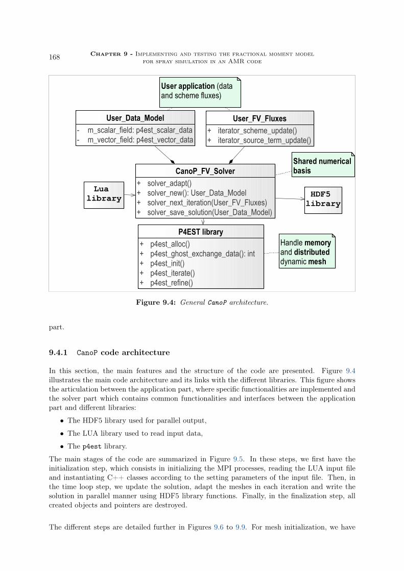
168 Chapter 9 - Implementing and testing the fractional moment modelfor spray simulation in an AMR code

CanoP_FV_Solver

+ solver_adapt()+ solver_new(): User_Data_Model+ solver_next_iteration(User_FV_Fluxes)+ solver_save_solution(User_Data_Model)

User_Data_Model

- m_scalar_field: p4est_scalar_data- m_vector_field: p4est_vector_data

User_FV_Fluxes

+ iterator_scheme_update()+ iterator_source_term_update()

P4EST library

+ p4est_alloc()+ p4est_ghost_exchange_data(): int+ p4est_init()+ p4est_iterate()+ p4est_refine()

HDF5 library

Lua library

Handle memory and distributed dynamic mesh

Shared numerical basis

User application (data and scheme fluxes)

Figure 9.4: General CanoP architecture.

part.

9.4.1 CanoP code architecture

In this section, the main features and the structure of the code are presented. Figure 9.4illustrates the main code architecture and its links with the different libraries. This figure showsthe articulation between the application part, where specific functionalities are implemented andthe solver part which contains common functionalities and interfaces between the applicationpart and different libraries:

• The HDF5 library used for parallel output,

• The LUA library used to read input data,

• The p4est library.

The main stages of the code are summarized in Figure 9.5. In these steps, we first have theinitialization step, which consists in initializing the MPI processes, reading the LUA input fileand instantiating C++ classes according to the setting parameters of the input file. Then, inthe time loop step, we update the solution, adapt the meshes in each iteration and write thesolution in parallel manner using HDF5 library functions. Finally, in the finalization step, allcreated objects and pointers are destroyed.

The different steps are detailed further in Figures 9.6 to 9.9. For mesh initialization, we have

Part IV - High performance computing and adaptive mesh refinement 169

Initialization init MPI

init solver luaL_newstate, lua_intexpr...

init mesh p4est_new, p4est_load, p4est_refine

Time loop while t < tmax

solver update p4est_iterate, p4est_ghost_exchange_data...

mesh adapt p4est_refine, p4est_load_partition...

output p4est_save, H5Dwrite

Destroy

Figure 9.5: Sketch of the CanoP code structure and calls for p4est functions, reprinted fromDrui(2017).

Init mesh load file?

load file p4est_load_ext

yes

create connectivity

no

p4est_connectivity_new_copy

new forest p4est_new_ext

for i ∈ [Lmin , Lmax ]

coarsen p4est_coarsen_ext

Figure 9.6: Zoom in the init part structure and calls for p4est functions, reprinted fromDrui(2017).

Mesh adapt mark cells p4est_iterate

refine p4est_refine_ext

coarsen p4est_coarsen_ext

2:1 balance p4est_balance_ext

partition p4est_partition_ext

Figure 9.7: Zoom in the mesh adapt part structure and calls for p4est functions, reprintedfrom Drui(2017).

170 Chapter 9 - Implementing and testing the fractional moment modelfor spray simulation in an AMR code

refinecallback function replace flag

return old flag

Figure 9.8: Zoom in the refine callback function, that informs p4est if the cell should be refined.Reprinted from Drui(2017).

replacecallback function nb of outgoing quads?

copy to new quads

N 1refining

mean value over N

N > 1coarsening

copy to new quad

Figure 9.9: Zoom in the replace callback function, that computes the value of the newly createdquadrants. Reprinted from Drui(2017).

two possibilities: the first consists in loading the meta-data (mesh data) and solution datafrom a previous output simulation or to create new mesh and a new initial solution. For meshadaptation (Figure 9.7), the function p4est_iterate is called to iterate over all the octants andflag cells to be coarsened or refined according to the refinement criterion and the refinementthresholds that are provided by the parameters of the simulation. Then, p4est_refine_ext andp4est_coarsen_ext are called to refine or coarsen the meshes. In this second stage, two types ofdata have to be updated: the meta-data (p4est mesh data) and the solution data (user_data)in the new cells. To refine and coarsen the meshes, CanoP uses the flags determined in theprevious step and calls the replace callback function to copy the data of a parent octant in itschildren octant when it is about refining a cell or average the old children variables in their newparent octant when it consists in coarsening cells. Once the adaptation of the mesh is over, thefunction p4est_partition_ext is called to redistribute the load between the processors.

9.4.2 Object-oriented programming in CanoP

The first versions of CanoP were written in a standard C language. Consequently, the implemen-tation of new application has often required to modify the code structure and to use preprocessorconditions (#ifdef, etc) each time some parts of the code were not generic. Difficulties have thenarisen about the code readability and maintenance. A recent refactoring of the code and usingobject-oriented programming (OOP) C++ language allowed to improve its readability and theextensibility. Indeed, the actual version benefits from the different advantages of C++ classes,template classes and inheritance. The re-factored code proposes:

• a clear modular structure of the code through abstract classes,

• a complete separation between the solver part and the application part allowing new usersto implement new applications without affecting the rest of the code,

• a simplify maintenance and a better readability.

Part IV - High performance computing and adaptive mesh refinement 171

Figure 9.10: Diagram of the principal class objects in CanoP code.

Figure 9.10 illustrates the main classes used in the code, which are separated into abstractclasses that belong to the solver part and implemented classes defined in the application part.The classes in the application part inherit from the abstract classes of the solver part. The classSolver is the principal class that provides all necessary information of the simulation: meta-data (p4est mesh data), user data (data per cell) and simulation parameters. The parent classcontains:

• the class SolverWrap encapsulating the p4est meta-data,

• the class SolverCoreBase defining an interface to the user_data,

• the class UserDataMangerCore containing quadrant data functions,

• and the class IteratorsBase defining the iterators functions (the callback function calledby p4est_iterate).

All these classes are abstract classes and are instantiated in the initialization step (see theprevious section), where constructors of the inherited classes of the application part are used inthis step. We underline that each application defines its owns classes derived mainly from theabstract classes of the solver part and Figure 9.10 illustrates only a case with one application.

172 Chapter 9 - Implementing and testing the fractional moment modelfor spray simulation in an AMR code

To sum up, CanoP was developed with the idea to simplify the use of p4est library and to shareit for several applications more easily. Now, CanoP provides to new users a simple frameworkto implement their applications and benefit from the high performance of the p4est library. Anew implementation will only consist in providing the data model (user_data), implementingthe numerical scheme (a function to compute the numerical flux for the finite volume scheme)and the refinement criterion or using the already existing implementations.

9.5 Numerical resolution of a spray model in a cell-based AMR

9.5.1 The kinetic finite volume scheme on non-conforming meshes

The kinetic finite volume (KFV) numerical scheme presented in section 7.2 dedicated to theresolution of the transport part of the system of moment equations (7.1), needs to be adaptedto non conforming meshes. As in chapter 7, we use a dimensional splitting. In the following,we consider only the transport step in the x-direction. Let us denote by q a 2D non conformingcell verifying the 2 : 1 size balance, which means that the size ratio of two neighboring cells iseither 1, 2 or 1/2. In general, we write the finite volume scheme in q as follows:

U n+1q U n

q −∆t∆xq

(Fq+1/2 − Fq−1/2), (9.4)

where U (m0/2 , . . . ,m3/2 ,m2/2u ,m2/2v)t is the vector of conservative variables of the system(7.1) and q − 1/2 (resp. q + 1/2) refers to the left (resp. right) faces in the x-direction. Toillustrate how we adapt the scheme in a 2:1 balanced mesh, let us consider the case when thecell q has two neighboring cells on his right: ηr

1 and ηr2 as is illustrated in Figure 9.11. The flux

across the common edge depends on the states of the three cells q, ηr1 and ηr

2:

F i+1/2 F (U nq ,U

nηr1,U n

ηr2), (9.5)

The exact expression of the fluxes, derived from the integral expression of the moments and thekinetic solution (7.13), is:

Fq+1/2 F+

q+1/2 + F−q+1/2 , (9.6)

•

•

•

•

F (ηl→ q)

F (q → ηl1)

F (q → ηl2)

qηr1

ηr2

ηl

Figure 9.11: Non-conforming grid and the different fluxes associated with cell q in one spacedirection.

Part IV - High performance computing and adaptive mesh refinement 173

such that

F+

q+1/2 1

∆yq∆t

∫x(x ,y)∈q

U (tn , x)1Σ+q (∆t) (x , y)dxdy , (9.7)

and

F−q+1/2 1

∆yq∆t

( ∫x(x ,y)∈ηr

1U (tn , x)1Σ−

ηr1

(∆t) (x , y)dxdy

+∫

x(x ,y)∈ηr2

U (tn , x)1Σ−ηr2

(∆t) (x , y)dxdy).

(9.8)

Where for a cell c, Σ±c (x′, y) ∈ c ,±(xc+1/2 − ∆tu(tn , x′)) < ±x′

is the set of droplets in the

cell c that will reach its right (resp. left) side during the time [tn , tn+1 tn + ∆t].

In the case of first order scheme, the solution is constant per cell and the numerical flux can beexpressed as follows:

Fq+1/2 ∆xηr

1

∆xqF

(U q ,U ηr

1

)+∆xηr

2

∆xqF

(U q ,U ηr

2

), (9.9)

where the flux F(U i ,U j

)is computed as in the case of a uniform mesh, using equation (7.15).

The variable ∆xi is the length of the cell i.

For the second order, we use affine reconstruction of the transported variables: canonical mo-ments and velocity as explained in chapter 7. However, in the case of non-conforming meshes,there are different ways to reconstruct the solution based on the states of the neighboring cellsand their positions. A first possibility consists in estimating a gradient tensor of the transportedvariables from the whole neighboring cells. In CanoP, we use a simple way to compute the slopes.We illustrate the method in the case of Figure 9.11: cell q has a double-size neighbor ηl on itsleft and two half-size neighbors ηr

1 and ηr2 on its right. We first compute the slopes of the recon-

structed variables (canonical moments and the velocity) as in (7.21) using the cells (ηl , q , ηr1),

then we compute the slopes in the same way but using now (ηl , q , ηr2). The final slopes are

computed as the minmod limiter of the two last slopes. Since cells of different sizes are used andthe limitation of the slopes is rather restrictive, second order is not guaranteed near extrema ofthe solution. However the robustness and the realizability of the method are ensured. Moreoverthe results show a good accuracy improvement compared to the first order scheme.

9.5.2 Refinement criterion

The determination of an efficient criterion remains a complex subject, since the simulationdepends on the physical phenomena and on the numerical methods. Multiresolution analysisprovides some robust tools to compress the data using wavelet functions and control the com-pression errors at each refinement level (see Muller(2003), Harten(1995) and Duarte(2011) andthe references therein). In CanoP, these methods are difficult to implement because the treestructure does not respect some necessary properties (like threaded tree, see Harten(1995)) formultiresolution methods. Therefore, we use a heuristic criterion based on some consideration of

174 Chapter 9 - Implementing and testing the fractional moment modelfor spray simulation in an AMR code

the main results cited in Harten(1995).Harten Harten(1995) introduced a method to control the error, based on an interpolating func-tion to approximate the variables at refined level l+1 from the coarsen level l, then he computesthe details which are the difference between the predictive variables and the true variables. Thedetails are considered as the errors at level l. Following Harten’s idea, we implement a refine-ment criterion adapted to CanoP for spray applications. The method consists in estimating themoment m0 for the children quadrants of a given parent quadrant q. The prediction is based onthe slope computation in each direction for each face depending on the neighbor quadrants notnecessary of the same size as the quadrant q1.

m0(x , y)

m0,q + Dm l0(x − xq ) + Dmu

0 (y − yq ), if (x , y) ∈ child1

m0,q + Dmr0(x − xq ) + Dmu

0 (y − yq ), if (x , y) ∈ child2

m0,q + Dm l0(x − xq ) + Dmd

0 (y − yq ), if (x , y) ∈ child3

m0,q + Dmr0(x − xq ) + Dmd

0 (y − yq ), if (x , y) ∈ child4

(9.10)

The subscripts l , r, d , u refer respectively to the left, right, down and up edge. Dm j0 is the slope

variation in the direction x if j l or j r and y otherwise. Finally, the children index followsthe z-order.

The slopes are computed from the neighboring quadrants. To illustrate this calculation for theslopes in direction x, we consider the case of Figure 9.11:

Dm l0

m0,q − m0,ηl

(∆xq + ∆xηl )/2,

Dmr0

(m0,ηr1+ m0,ηr

2)/2 − m0,q

(∆xq + ∆xηr1)/2

.(9.11)

Let us emphasize that the reconstruction in (9.10) does not necessarily respect some physicaland mathematical properties (the conservation of the variables, the maximum principle and therealizability). In fact, the reconstruction is only used to estimate the error and is not used inthe numerical scheme.Then we compute the L1-norm of the difference between m0,q and the predicted m0(x , y).

err(m0)q

∫q|m0,q − m0(x , y) |dxdy , (9.12)

where |q | is the total surface of the quadrant q.

This estimated error is used as a refinement criterion, such that the error is compared to a giventhreshold ξ and if err(m0)q > ξ then the quadrant is refined. If all siblings of a given quadrantverify err(m0)q < cξ then the quadrant is marked for coarsening. The parameter c ≤ 1 is chosenby the user.

9.6 Results

This section is dedicated to some numerical results using CanoP code. We use the KFV numericalscheme to solve the convective part of the system of equations (7.1). This scheme is presented

1 For Harten’s predictor operator, the author used neighbors of the same level to predict the variable in thenext high level).

Part IV - High performance computing and adaptive mesh refinement 175

in chapter 7 for the case of uniform meshes. In the present chapter, we use its extension inthe case of non-conforming meshes. The resolution of the source term is detailed in chapter 8.The robustness and the accuracy of these methods have been verified in the last two chaptersin a set of 0D, 1D and 2D uniform Cartesian tests. Now, we aim at proving that 1- the AMRsolver reaches a very nice level of accuracy once we have chosen a proper refinement criterion, 2-the proposed strategy is valid for complex droplet models, that is for source term with a muchhigher level of complexity leading to much higher arithmetic intensity and 3- that we have ahigh level of scalability and efficiency of the parallel implementation of the numerical strategyrelying on realizable schemes and splitting methods.

To do so, we have chosen three test-cases:

• The first case consists in a localized spray in the presence of Taylor-Green (TG) vortices,Figure 9.12. This case though simple, does illustrate a realistic configuration occurring inautomotive engine, where the droplets are concentrated in some local regions, while largevacuum regions can be found everywhere else. This first case is a non evaporating spray.Here, we only assess the performance of the AMR calculation compared to a uniform gridand then study the scalability at a given level of accuracy.

• The second case is the same as the first one, but with an evaporating spray. The objec-tive of this simulation is twofold. First, we show the robustness and the accuracy of theevaporation algorithm coupled with transport and drag. Second, the evaporation algo-rithm is representative of the high arithmetic intensity within an embarrassingly parallelconfiguration using operator splitting. The aim is to illustrate the impact of the AMRtechniques coupled to the operator splitting on the computational cost for intensive sourceterms, such as the inversion algorithm used to reconstruct the approximated spray densityfunction.

• The third case is a non evaporating Homogeneous Isotropic Turbulence in 2D and 3D.A comparison of droplet segregation is conducted for an AMR Eulerian solution with auniform Eulerian solution and a Lagrangian reference solution. This comparison showsthe efficiency of the AMR Eulerian solution to predict correctly the main physical featureswith low computational resources. The gain in the CPU time is obtained in this frameworkof a much richer configuration in terms of physics, while in a really non-favorable case sincethe spray is present in the whole domain.

For the three cases, we fix the CFL (7.25) at CFL 0.9 and the constant c used in the refinementcriterion at c 2−(d+1), where d is the space dimension .

9.6.1 Droplet cloud in Taylor-Green vortices

We simulate a non evaporating polydisperse spray in a two dimensional periodic domain in thepresence of Taylor-Green vortices for the gas. This gas velocity profile is a steady solution of theinviscid incompressible Euler equations. The non-dimensional velocity field of the gas is givenby the following expression:

ug (x , y) sin(2πx)cos(2πy),vg (x , y) −cos(2πx)sin(2πy), (9.13)

where (x , y) ∈ [0, 1]2.Initially, we consider a motionless cloud located in the bottom-left vortex in Figure 9.12.

The initial spatial distribution of the spray is Gaussian inside a small disk of a radius r 0.1and equals to zero outside. The initial size distribution, uniform inside the disk, is equal to 1

176 Chapter 9 - Implementing and testing the fractional moment modelfor spray simulation in an AMR code

Figure 9.12: Stationary gaseous velocity vector field of the Taylor-Green vortices and sprayinitial number density.

Part IV - High performance computing and adaptive mesh refinement 177

Figure 9.13: The initial NDF in the dashed line and its reconstruction through ME in the solidline.

for S ∈ [0, Smid] and 0 otherwise. The moments are thus given by:

mk/2(t 0, x) 2

k + 2(S(k+2)/2

mid )exp(−||x − xc | |22/r2), (9.14)

where k 0 . . . 3, Smid 0.5 and | |x − xc | |22 ≤ r. The initial exact size distribution as well as

its Maximum Entropy reconstructed density nME (S) from the four fraction moments (9.14) arepresented in Figure. 9.13 for x xc.

We consider low inertia droplets such that the mean Stokes number2 St 0.025 is less than thecritical value Stc 1/(8π). It has been shown in de Chaisemartin et al de Chaisemartin(2009),that for St < Stc the droplets stay in their origin vortex and cannot travel from one to another,while, for St ≥ Stc they are ejected out of their original vortices. In this last configuration,we encounter particle trajectory crossings, that are not taken into account in the monokineticassumption considered here and lead to delta-shocks. Notice that these singularities are com-pletely handled numerically, thanks to the Kinetic Finite Volume (KFV) numerical scheme andthe robustness is ensured as it was shown in chapter 7.

In Figure 9.14, we display the spatial evolution of the number density m0 using a second orderscheme and AMR grid at different times, as well as the mesh grid given at two instants in Figure9.15. The maximum refinement level is lmax 9 and the minimum level is lmin 4. We use therefinement criterion presented in the section 9.5.2 and choose a small threshold ξ 1.e − 7.

2The mean Stokes number is computed with respect to the mean droplet size S m2/2/m0/2.

178 Chapter 9 - Implementing and testing the fractional moment modelfor spray simulation in an AMR code

t 0.25 t 0.5

t 0.75 t 1.

Figure 9.14: Taylor-Green simulation using the second order scheme in adaptive refinementgrid, the maximum level is lmax 9 and the minimum level is lmin 4

Part IV - High performance computing and adaptive mesh refinement 179

Figure 9.15: The AMR grid in the case of Taylor-Green with non evaporating spray, withlmax 9, lmin 4 and threshold ξ 5.e − 7: at t 0.5 (left) and t 1.0 (right).

9.6.1.1 Refinement criterion and solution quality

In this section, we study the influence of the refinement criterion in the accuracy of the solutionand its impact on the computational time. The objective is to show that we can keep an accuratesolution while reaching a high compression rate, thus saving time and memory. It also allowsto set up a fair framework in order to conduct a parallel efficiency study in the next subsection.After investigating the influence of the refinement criterion depending on the order of the scheme,we focus on the intrinsic accuracy of the solution.

Threshold relative compression CPUξ L1-error rate % time1.e − 7 0.7% 87.3% 5.81

5.e − 7 5.2% 92.4% 3.89

1.e − 6 10.1% 94.4% 3.24

5.e − 6 29.6% 97.3% 1.71

1.e − 5 35.4% 97.8% 1.15

Table 9.1: Relative L1-error, compression rate and CPU time depending on the threshold ξusing the first order scheme.

In Tables 9.1 and 9.2, we present the results for the first order and the second order schemeusing 36 processors. The L1-error is computed relatively to the solution on a refined uniformgrid 512×512, considered as the reference solution. The compression rate and the CPU time arealso provided. The purpose is to evaluate the impact of the compression rate on both accuracyand computational efficiency.

The two tables show a significant CPU time saving compared to the reference solution. Firstfor the first order scheme, the CPU time of the reference solution (uniform meshes) is 29.15s.Using the smallest threshold ξ 1.e − 7, we reduce the computation time by a factor of fivewith a good level of precision. We could save more CPU time and memory (see the compressionrate) by increasing the threshold but we lose the accuracy of the solution. For ξ ≥ 1.e − 6, therelative L1-error is more than 10%. Since the computing time of the second order finite volumescheme is much larger than the communication and mesh adaptation time, we save more CPUtime in this case, whereas the CPU time used in the computation of the second order reference

180 Chapter 9 - Implementing and testing the fractional moment modelfor spray simulation in an AMR code

Threshold relative compression CPUξ L1-error rate % time1.e − 7 0.6% 88.8% 28.38

5.e − 7 3.2% 92.6% 19.32

1.e − 6 5.3% 94.7% 14.65.e − 6 15.6% 97.2% 6.91.e − 5 19.7% 97.7% 3.73

Table 9.2: Relative L1-error, compression rate and CPU time depending on the threshold ξusing the second order scheme.

Figure 9.16: L1-error for the first order scheme in logarithm scale versus the minimum levelof compression lmin plotted for different maximum refined levels lmax: using ξ 1.e − 6 (left)and ξ 1.e − 7 (right).

solution is much larger: 231.63s. By using mesh adaptation with the threshold ξ 1.e − 7, wereduce this CPU time by a factor of eight, maintaining a good precision. We could save moreCPU time and memory by choosing ξ 1.e − 6 with a good accuracy (relative L1-error ∼ 5%).Let us underline that these two tables do not compare the solution accuracy depending on thescheme order because the relative L1-error is computed for each order as the difference betweenthe solution on a uniformly refined grid and the solution for an adaptively refined grid using thesame order.

In a second study, we consider a common reference solution for the first and second order sim-ulations. The reference solution is computed using a second order scheme on a uniform grid of1024 × 1024 cells, which corresponds to the level l 10. The two Figures 9.16 and 9.17 showthat the relative L1-error does not evolve much when we vary the minimum level except when wereach a uniform grid. However, for a given maximum level of refinement, there is a strong impactof ξ on the ability of the adapted solution (lmin < lmax) to capture an accurate solution. In factfor each maximal level of refinement, there is a threshold in terms of refinement criterion abovewhich compressing the solution deteriorates its quality. Its is clear in Figure 9.16 and 9.17 thatξ 1.e − 7 is below this threshold and ξ 1.e − 6 is above it. For ξ 1.e − 7 the relative-errorremains almost constant and we can use mesh refinement while preserving an accurate solution,whereas for ξ 1.e − 6, we can observe that mesh refinement for lmax 9 results in a clearincrease of the error. Once we have found a well chosen threshold, for which the accuracy of theuniform and AMR solutions are equivalent, we can then study the computational efficiency andparallel performance of the numerical strategy.

Part IV - High performance computing and adaptive mesh refinement 181

Figure 9.17: L1-error for second order scheme in logarithm scale versus the minimum level ofcompression lmin plotted for different maximum refined levels lmax: using ξ 1.e − 6 (left) andξ 1.e − 7 (right).

Figure 9.18: Strong scaling of the second order scheme in AMR grid, the maximum level islmax 9 and the minimum level is lmin 4.

9.6.1.2 Parallel performance

We assess the parallel performance by measuring the computational time of various operations:

• Solver time corresponds to the time needed in the finite volume scheme and source evalu-ation in the splitting strategy,

• Adaptation time corresponds to the time of refinement, coarsening, partitioning and 2:1size balancing,

• And finally the total time which is the sum of both solver and adaptation times withoutI/O.

We use the second order Taylor-Green simulation in an adaptive refinement grid such that themaximum level l 9 corresponds to the finest meshes and the minimum level l 4 correspondsto the coarsest meshes. We choose the previously obtained threshold ξ 5.e − 7 to ensure thequality of the compressed solution.

182 Chapter 9 - Implementing and testing the fractional moment modelfor spray simulation in an AMR code

In Figure 9.18, we display strong scaling results. The simulation is performed in CentraleSupleccluster (2 Intel Xeon procs, memory per node 24Go, total core number 156) using up to 60MPI processes. The solver time (transport and drag) shows an efficiency of more than 88%.The adaptation time shows a weak efficiency due to the large time spent in the communicationbetween processors essentially for the balance algorithm Burstedde et al.(2011). Nevertheless,the global time of computation shows a good parallel performance and the efficiency reaches81% for 60 processors. In fact, the solver time represents 85% of the total CPU time. Let usunderline that the number of effective cells in this simulation with a compression rate of about90% is close to 30,000 so that an efficiency of 81% on 60 cores is very satisfactory.

9.6.2 Taylor-Green evaporating spray

Using exactly the same configuration with Stokes number St 0.025, we switch to an evaporatingspray with K 1/2. Since we use an inversion algorithm in order to reconstruct the NDF fromthe moments by ME algorithm in each cell and time step for the evaluation of the disappearanceflux of droplet at zero size, we expect a significant computational cost related to source terms.Thus, this simulation is representative of the complexity that we will have to face by switchingto more complex droplet models in realistic configurations.

Table 9.3 presents the computational time ratio spent in solving each part of the numericalresolution: the transport and the source terms, using two uniform grids (256×256 and 512×512)and running the simulation on 96 processors. As expected, the resolution of the source termsrequires around 95% of the total time. It is then interesting to investigate how the meshadaptation behaves in such a configuration, where the operator splitting technique, used hereto solve independently the source terms in various cells, can lead to an embarrassingly parallelconfiguration.

Transport solver Source term solver512 × 512 2.2% 97.5%

256 × 256 5.6% 93.5%

Table 9.3: Time ratio (in percent) spent in transport solver and source solver (including evap-oration and drag) using 96 MPI processes on a uniform mesh.

In the previous study without evaporation, ξ 5.e − 7 was shown to be an adequate thresholdfor a high compression and good solution quality, therefore we maintain this value in the presentcase. Figure 9.20 shows the spatial number density at four different times of the evaporatingTaylor-Green simulation on AMR grid (lmax 9 and lmin 4) and Figure 9.21 presents thecorresponding meshes. Compared to the simulation running on the uniform grid 512 × 512, therelative L1-error of the AMR solution computed at t 0.5 is 3.9%, the compression rate is 97.7%and we have reduced the computational time by a factor of more than 45. In fact, the CPUtime used in the resolution of evaporation is much larger than the CPU time that we spend inthe resolution of the transport and the mesh adaptation. More precisely, in this simulation, theCPU time spent in the evaporation resolution is 76.5s, the transport resolution 2.4s and themesh adaptation 5.2s, which means that the evaporation alone takes more than 90% of the totalCPU time, Table 9.4 gives further details of the time ratio spending at each operation using

Part IV - High performance computing and adaptive mesh refinement 183

Figure 9.19: Strong scaling of the Taylor-Green evaporated case in AMR grid, the maximumlevel is lmax 9 and the minimum level is lmin 4

MPI process Mesh Transport Source termnumber adaptation solver solver1 0.1% 2.5% 97.3%

24 0.7% 2.2% 97.3%

60 0.9% 2.2% 95.7%

84 4.8% 2.7% 91.6%

96 6.16% 2.8% 90.5%

Table 9.4: The time ratio (in percent) spent at each operation: Transport solver and Sourceterm solver (Evaporation +drag) for different MPI process number.

different MPI process number. In Figure 9.19, we present the strong scaling of the various stepof the solving process (mesh adaptation, transport solver, source term solver and the total time).Up to 60 processes, we observe a good scalability. Once again, let us insist on the fact that for60 processes and considering the level of compression reached, we end up with about 100 cellsper core, which is few but still has a good level of efficiency. The transport part has about 80%of efficiency and the source term scales vary properly considering that load balancing could bealso a problem (p4est also provides the ability to integrate computational complexity in thethe load balance algorithm, which has not been used in the present simulations). Increasingthe number of processes to 96, we have a remarkable decrease of the scalability, which reaches56% for transport resolution, and that can be explained by the very small number of cells perprocess, which is going to kill the efficiency in terms of communications. However, the totalefficiency is still about 67%, which shows both the efficiency of CanoP and p4est as well as theproper choice of the numerical strategy.

184 Chapter 9 - Implementing and testing the fractional moment modelfor spray simulation in an AMR code

t 0.25 t 0.50

t 0.75 t 1.0

Figure 9.20: Evaporating Taylor-Green simulation using second order scheme for transport inAMR grid with lmax 9, lmin 4 and ξ 5.e − 7.

Figure 9.21: The AMR grid in the case of Taylor-Green evaporating spray, with lmax 9,lmin 4 and threshold ξ 5.e − 7.

Part IV - High performance computing and adaptive mesh refinement 185

9.6.3 Homogeneous isotropic turbulence in 2D/3D

In this section, we assess the code behavior in a more complex gaseous flow field representativeof complex applications, where the spray is to be found everywhere in the domain. We considera non evaporating spray respectively in a two- and three-dimensional configurations with afrozen Homogeneous Isotropic Turbulence (HIT) of the gas. The HIT gas field was generatedindependently by Sabat et al.(2014) with the ASPHODELE code of CORIA Reveillon andDemoulin(2007), that solves the three-dimensional Navier-Stokes equations for the gas phaseunder the low-Mach assumption.

2D HIT The characteristics of this HIT are given in Table 9.5, where Ret is the turbulentReynolds number, ut is the velocity root-mean-square, ε is the mean dissipation rate, ηk is thescale of smallest structures, lint is the integral scale of the turbulence, τk is the Kolmogorovtime scale of the turbulence, and τint is the eddy turnover time. We consider a non evaporatingspray. The initial spatial distribution is uniform.

Ret ut ε ηk lint τk τint7.12 0.1 0.01 0.022 0.1 0.36 1.0

Table 9.5: Turbulence properties of the frozen HIT gaseous flow field.

In order to limit the Particle Trajectory Crossings and to have comparable results betweenthe monokinetic Eulerian simulation and the Lagrangian simulation, we consider low inertiadroplets such that the Stokes number is taken St 0.5 based on τk . Numerical dissipationin the simulation of Eulerian models for spray dynamics is a key issue, since we have to usevery robust numerical schemes due to the presence of singularities and asymptotic limits (zerodensity), but still want an accurate resolution in the smooth regions. In particular, numericaldissipation has a negative effect in predicting properly segregation of the spray in turbulentflows.

In order to limit this diffusion, we use the second order scheme and AMR in order to reachan accurate resolution in the regions of high concentration, while limiting the computationalcost and memory trace. Figure 9.22 shows the spatial distribution of the number density atdimensionless time t 5 (this dimensionless time corresponds to t 1.8s in the real time,because the characteristic time in this case is τk 0.36s). The droplets are ejected from vorticesand concentrated in zones of low vorticity, thus, they segregate in regions of low vorticity. Thesegregation is computed using the spray moment m0 as follows:

< (m0)2 >< m0 >2

where < • >1

V

∫V• dV .

In Figure. 9.23, we compare the time evolution of the segregation for a Lagrangian simulation(see Sabat et al.(2014)) and two Eulerian simulations :

• on uniform grid of 1024 × 1024 cells;

• using AMR with lmax 10 and lmin 6.

In both Eulerian simulations, we make a small error on the segregation compared to the La-grangian simulation. However, the three results stay closely comparable. Furthermore, thesegregation evolution of the two Eulerian simulations is closely the same. Therefore, we preserve

186 Chapter 9 - Implementing and testing the fractional moment modelfor spray simulation in an AMR code

Figure 9.22: Number density m0 at t 1.8 with AMR ( lmax 10 and lmin 6) and withthreshold ξ 5.e − 7.

the same solution quality while using less cells in AMR simulation. We have reduced the com-putational time by a factor of two compared to the uniform grid computation and we obtain acompression rate of 55%. Let us underline that the chosen configuration is probably the worstconfiguration for such a strategy. However, we wanted to investigate the ability of the proposedstrategy to cope with such a case, knowing that in realistic configurations, the flow is going tobe turbulent, whereas the spray is going to occupy only a fraction of the computational domain.

3D HIT A 3D simulation of the spray in the presence of a frozen homogeneous isotropic tur-bulence was performed to test the AMR capacity in compressing the solution. The characteristicof the HIT is given in Table 9.6. The mean Stokes number of the polydisperse spray is taken asSt 0.5.

Ret ε ηk τk TKE25 1e − 3 3.2e − 2 1. 1.e − 2

Table 9.6: Turbulence properties of the frozen HIT gaseous flow field in 3D.

The simulation is performed with an adaptive mesh, where the maximum and minimum refine-ment levels, lmax 9 and lmin 7, correspond respectively to a mesh of size δxmin 2−9 andδxmax 2−7 for a dimensionless grid [0, 1]3 (the real physical domain dimension is 5m×5m×5m).In Figure 9.24, we display a three cut sections of the spray density, as well as the correspondingmesh in Figure 9.25. The first figure shows the segregation of the spray in low vorticity regions.For the present choice of refinement criterion, the compression rate is 91.56%. In Figure 9.26,

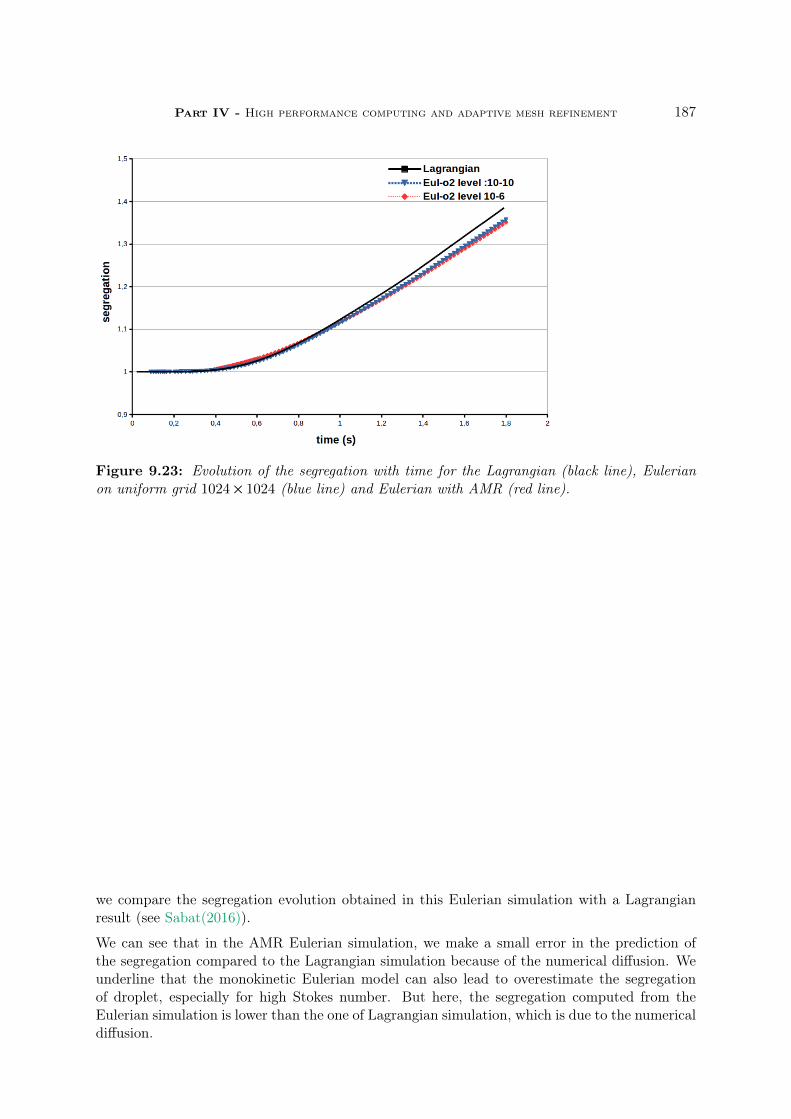
Part IV - High performance computing and adaptive mesh refinement 187

Figure 9.23: Evolution of the segregation with time for the Lagrangian (black line), Eulerianon uniform grid 1024 × 1024 (blue line) and Eulerian with AMR (red line).

we compare the segregation evolution obtained in this Eulerian simulation with a Lagrangianresult (see Sabat(2016)).

We can see that in the AMR Eulerian simulation, we make a small error in the prediction ofthe segregation compared to the Lagrangian simulation because of the numerical diffusion. Weunderline that the monokinetic Eulerian model can also lead to overestimate the segregationof droplet, especially for high Stokes number. But here, the segregation computed from theEulerian simulation is lower than the one of Lagrangian simulation, which is due to the numericaldiffusion.

188 Chapter 9 - Implementing and testing the fractional moment modelfor spray simulation in an AMR code

Figure 9.24: Number density of the droplets given by the moment m0, on an AMR grid att 12.

Figure 9.25: The AMR grid at t 12.

Part IV - High performance computing and adaptive mesh refinement 189

Figure 9.26: Evolution of the segregation with time for the Lagrangian simulation (black solidline) and our Eulerian model with AMR (red dotted line).

9.7 Conclusion

The aim of this chapter was first to present CanoP AMR code, which is based on the p4est libraryfor mesh management in parallel computation. The main feature of this code is its flexibility andeasiness to implement new finite volume applications and benefit from the efficiency of the p4estlibrary with less programming effort. Different applications have been already implemented andtested. In this chapter, we also show how to extend the kinetic finite volume scheme in non-conforming meshes used here for the numerical resolution of the fractional moments modelto simulate an evaporating polydisperse spray. A set of numerical tests, using the fractionalmoments model presented in chapter 4, have been performed in CanoP code to validate thenumerical strategy and the parallel performance. The implementation of more complex andphysical models with the possibility to couple a spray model with a two fluid model for thesimulation of the whole process injection is envisioned in future works. In the present work,we show that we can reach a level of accuracy for AMR solution equivalent to uniform-meshsolution with lower computational time and memory. We also show a good scaling in parallelcomputation, especially for high workload per-cell compared to the communication and meshmanagement time. This is the case for the second order scheme for the transport and the sourceterm that requires high arithmetic intensity. In future works, we aim to go further in developinghigh order schemes using Discontinuous Galerkin (DG) method. This method uses local degreesof freedom and do not require large stencil to achieve high order, which makes the method moreattractive for AMR, since other methods that use large stencil may be expensive due to the needof recursive research of neighboring cells.

Chapter 10

The StarPU Runtime scheduler andthe acceleration of the source termcomputations

This chapter is based on the work of Essadki et al.(2017), during CEMRACS 2015summer school

10.1 Introduction

Nowadays, multi-cores machines are equipped with different Processing Unit (PU) types. Weclassify these devices into CPUs and accelerators (GPUs, Xeon-Phi, etc). Accelerators can ac-celerate numerical computations that involve intensive arithmetics. GPUs, for instance, aremassively parallel devices, that can run Single Instruction Multiple Data (SIMD) programs veryefficiently. Consequently, they can speed up the execution of tasks that perform intensive arith-metic operations on multiple data points simultaneously. However, it is not obvious to takeadvantages from these technologies without taking into consideration the architecture hetero-geneity of the new generation of multi-cores machines. They involve different types of PUs andnon uniform memory access. Indeed, approaching the theoretical performance of these archi-tectures is a complex issue. The high performance computing community needs to face thischallenge and propose reliable solutions that can allow other scientific communities to benefitfrom the computing power of these technologies. Many research efforts have focused on en-hancing existing solutions: programming languages, compilers and libraries that can take intoconsideration accelerator-based machines. However, these solutions rely on a statistic distribu-tion of the work among the processing units that is generally determined manually by the user.Another recent possible solution consists in using a runtime scheduler. Its role is to distributethe tasks of a program among the available computation resources (CPUs and accelerators)and to manage the memory, following a strategy that can optimize the CPU time and memoryconsumption.

StarPU Runtime Scheduler Augonnet et al.(2011) is a good candidate to provide these perfor-mances. In this chapter, we present the main results of the HODINS (High Order DIscontinu-ous methods with ruNtime Scheduler) project conducted during the CEMRACS 2016 summerschool. During this project, we experienced StarPU in a 2D code, where we have solved nu-merically hyperbolic equations with possible source terms using Runge Kutta Discontinuous

192 Chapter 10 - The StarPU Runtime scheduler and the acceleration ofthe source term computations

Galerkin (RKDG) methods, which have been presented in chapter 7. The choice of Discontin-uous Galerkin (DG) method is guided by its arbitrarily high order accuracy, its compactnessand its memory locality. Two models have been separately implemented and tested in this 2Dcode: the Euler equations and the fractional moments model for polydisperse and evaporatingsprays (see chapter 4 for more details). The main objective of this chapter is to illustrate anew solution that can accelerate the numerical simulation of complex models, similar to the oneof the fractional moment model (chapter 4), thanks to a dynamic offloading of some tasks inGPUs, while using the numerical framework that has been presented in chapters 7-8. In thischapter, we briefly present the main features of StarPU and the implementation of the RKDGin a task-based program using StarPU library. Finally, we perform a set of numerical teststo first validate our implementation, assess and analyze the granularity of the tasks comparedwith the task overhead, the parallel performance of the code and the acceleration of the sourceterms resolution thanks to an execution on GPUs.

10.2 StarPU

StarPU is a task-based programming library for hybrid architectures. Therefore, the numericalmethod should be formulated in terms of tasks that can be executed in parallel. In StarPU,the tasks of an application are translated in a Direct Acyclic Graph (DAG) of tasks, where thenodes represent the tasks and the edges between the nodes express the dependencies betweenthe associated tasks. The dependency is expressed implicitly through read/write access modefor each data memory i.e. for example if we submit successively two tasks "T1" and "T2", whichperform some operations on the same data memory, such that the task "T1" reads the datawhile the task "T2" writes in the same data, the task "T2" then depends on the task "T1". Afterspecifying the attributes of a task (data to handle, kernel functions, access mode to data, ects.),the function startpu_insert() is used to submit the task. The task insertion is asynchronous,where the tasks can be inserted each one after the other even if the first task is not yet executed.Following the order of task submissions and data dependencies, StarPU generates DAG of tasksand then distributes the tasks among the available computational resources

10.2.1 StarPU tasks

A StarPU task is made of:

• kernels are the functions that will be executed on a dedicated architecture: CPU, GPU,etc. A task may have the choice between different kernels implementation and it is the roleof the StarPU scheduler to distribute the tasks on the available processing units followinga certain criterion (in general minimizing the global execution time).

• data handles are the memory managers. Each data handle can be viewed as the encap-sulation of a memory allocation, which allows to keep trace of the action (read or/andwrite) of the task kernel on the memory layout. In particular, this allows to build the taskdependency graph.

• a codelet, the task descriptor. It contains numerous information about the task, includingthe number of data handles, the list of available kernels implemented to execute this task(for CPU, CUDA (for GPUs), OpenCL, ects.) and the memory access mode for each datahandle: "Read" (R), "Write" (W) or "Read and Write" (RW).

We illustrate the creation, definition and submission of a task in StarPU in the following

Part IV - High performance computing and adaptive mesh refinement 193

example:

A. We first create an empty task:

Algorithm 2 Create a taskstarpu_task *task_A = starpu_task_create();

B. We provide this task with the data buffers, which are encapsulated in data_handle StarPU ob-ject:

Algorithm 3 Example of encapsulating a data_handle bufferstarpu_data_handle_t data;starpu_matrix_data_register(&data,STARPU_MAIN_RAM, ptr_data ,. . .);/* a method toencapsulate the ptr_data in data StartPU structure*/task_A->handles[0] = data;

C. Then, we define the codelet that contains the kernel functions, the number of data buffersand the mode of the access to the data_handle buffer:

Algorithm 4 Example to define a codeletstarpu_codelet_init(&cl_A);cl_A.nbuffers = 1; /*in this example we consider only one buffer */cl_A.modes[0] = STARPU_W; /*state of data_handle: STARPU_W is only for write,STARPU_R is only for read and STARPU_RW is for read and write*/cl_A.cpu_funcs[0]=cpu_kernel_A;/*precise the CPU kernel function to execute the task ina CPU*/cl_A.cuda_funcs[0]=cuda_kernel_A;/*precise the CUDA kernel function to execute the taskin GPU*/task_A->cl=&cl_A;

D. The kernel functions can be written for different devices. Below, we give prototypes forCPU and CUDA kernels:

Algorithm 5 Kernel function CPU and CUDA prototypesvoid cpu_kernel_A(void *buffers[], void *cl_arg);void extern "C++" void cuda_kernel_A(void *buffers[], void *cl_arg) ;

E. Finally we can submit the task as follows:

Algorithm 6 Submit a taskint submit_status = starpu_task_submit(task_A);

10.2.2 Schedulers

The purpose of the scheduler is to launch the tasks when they become ready to be executed. InStarPU, many different scheduling policies are available. In the present work, we consider onlythe two following:

194 Chapter 10 - The StarPU Runtime scheduler and the acceleration ofthe source term computations

0

5

10

15

20

25

0 5 10 15 20 25

speedup

number of cores

48

163264

128256512

102420484096linear

2 dodeca-core Haswell Intel

0

10

20

30

40

50

60

70

0 10 20 30 40 50 60 70

speedup

number of cores

59

173365

129257513

102520494097linear

Xeon Phi KNL

Figure 10.1: Task size overhead with the eager scheduler: scalability results obtained withduration of tasks varying between 4 and 4096 µs on two different machines. Reprinted fromEssadki et al.(2017).

• the eager scheduler: it is the default scheduler. It uses a central task queue. As soon asa worker has finished a task, the next task in the queue is submitted to this worker.

• the dmda scheduler: this scheduler takes into account the performance models and the datatransfer time for the tasks. It schedules the tasks so as to minimize their completion timeby carefully choosing the optimal execution architecture.

10.2.3 Task overhead

StarPU tasks management is not free in terms of CPU time. In fact, each task executionpresents a latency called "overhead". We want to know when this additional time can beneglected or not. There is a StarPU benchmark that allows to measure the minimal durationof a task to ensure a good scalability. We send 1000 short tasks with the same (short) durationvarying between 4 and 4096 µs and we study the scalability. In Figure 10.1, we plot the resultsobtained on a 2 dodeca-core Haswell Intel Xeon E5-2680 and on a Xeon Phi KNL with thescheduler eager. On few cores, we have a good scalability result, even if the duration of thetasks is short (< 0.2ms). On many cores, we need longer tasks duration to get satisfying scaling(≈ 1ms).

To sum up, if the duration of the tasks is smaller than the microsecond, their overhead cannotbe neglected anymore.

10.3 RKDG task-based programming implementation

10.3.1 Principal task formulation of RKDG method

In this section, we present the essential steps in the implementation of a RKDG scheme to solvehyperbolic equations system with the source terms. The implementation is done in a 2D code,where we solve numerically the Euler equations or the fractional moment model (see chapter 4).In the following, we present a generic implementation of the two models, while we focus onlyon the fractional moments model for the numerical tests. The two systems of equations can bewritten in the following form:

∂tU + ∂xF x (U ) + ∂yF y (U ) S(U ), (10.1)

Part IV - High performance computing and adaptive mesh refinement 195

where U ∈ RnVar is the vector of conservative variables, nVar being the number of these vari-ables (for Euler equations nVar 4 and for fractional moments model nVar 6), F (U ) (F x (U ),F y (U )

)is the flux tensor and S(U ) is a source term.

The discontinuous Galerkin discretization of the transport part is given in (7.28) and (7.36). Werecall here the integral version of this scheme:

(k+1)2∑j1∆x2M i , j

dW mj

dt ∆x

∫ξ∈[−1/2,1/2]2

F (U h (t ,Ξ−1m (ξ)) · ∇ξ(φi (ξ)

)dξ

−∆x∑

e∈D

1/2∫ξ−1/2

F (U h (t , xm ,e (ξ)) · nm ,eφi (Ξm (xm ,e (ξ)))dξ.

(10.2)

See chapter 7 for the definition of the different terms in this equation.

As we can see from this scheme, some terms can be precomputed in the beginning of a simulation.These terms are:

• 1D and 2D Gauss-Legendre quadratures: we use these two quadratures to evaluate theintegrals involved in the scheme (10.2).

• 2D Gauss-Legendre-Lobbato (GLL) quadrature nodes: these points are used in the limita-tion procedure of the Zhang & Shu method Zhang et al.(2012) (see section 7.3.3 for moredetails).

• The values of the gradient of the polynomial basis, at 2D Gauss-Legendre quadrature

points of the domain[−

1

2,1

2

]2. Indeed, the first term in the RHS of equation (10.2) is an

integrated using 2D 2D Gauss-Legendre quadrature and it involves the gradients of thepolynomial basis.

• The values of the polynomial basis, computed at the 1D Gauss-Legendre quadrature points

on the four edges of the domain[−

1

2,1

2

]2are used in the second of the RHS of equation

(10.2).

These terms are precomputed before submitting any task and stored in 1D and 2D arrays.

In the following, we consider uniform and Cartesian 2D grids. First, we compute the initialsolution in each cell node. The number of degrees of freedom (k + 1)2 in a cell is given by thenumerical order of the DG discretization p k +1, where k is the polynomial degree used in theDG method. The temporal integration is preformed through an explicit Runge-Kutta method.Each step of Runge-Kutta method is updated as follows:

A. First, we check if the time step ∆t satisfies the CFL condition (7.40). In the actual versionof the code, the time step is fixed by the user. For future work, we will use a variable timestep, which satisfies the CFL condition.

B. We compute the first part of the Right Hand Side (RHS) of the scheme (10.2), whichcorresponds to the integral in a cell of the flux F (U h) multiplied by the gradient ofthe polynomial basis elements. This integral is approximated by a 2D Gauss-Legendrequadrature approximation.

C. For each cell, we interpolate the solution at the 1D Gauss-Legendre quadrature nodesof the edges of the cell. After performing this interpolation for all cells, we obtain twovalues for each node in a given edge: those are used to compute a numerical flux. For

196 Chapter 10 - The StarPU Runtime scheduler and the acceleration ofthe source term computations

the fractional moments model, we use the upwind numerical flux described in (7.31) and(7.15).

D. For each cell, we compute the last part of the RHS of equation (10.2), by integratingthe numerical flux multiplied by the polynomial basis elements over each edge of thecomputational cell. For this purpose, we use the numerical fluxes computed in the previousstep.

E. The RHS of (10.2) is now completely computed. The ODE system (10.2) can be thenintegrated according to the corresponding Runge-Kutta step.

F. In the case of the fractional moments model with evaporation source term, we applythe modified limitation procedure of Zhang & Shu in the solution at 2D Gauss-Legendrequadrature points1 for each cell as described in appendix C.

G. The source term is integrated at each degree of freedom see section 8.3.

H. We interpolate the solution at the GLL points. Then, we apply the limitation method ofZhang & Shu at these points (see section 7.3.3 for more details).

10.3.2 Data buffers and memory allocation

Since the tasks dependency graph is based on the memory dependency between successive tasks,memory allocation is a crucial part of our application. This starts with the definition of thefollowing two structures: Cell and Edge. The Cell structure corresponds to internal variables ineach computational cell and which contains an array of nDoF×nVar variables: nVar conservativevariables per cell node and nDoF degrees of freedom. For the Euler model, the conservativevariables are the mass density, the two momentum components and the total energy thus nVar 4, while for the fractional moments nVar 6 and the conservative variables are the four fractionalmoments and the two components of the velocity weighted by the surface area density of thedroplets: (m0/2 ,m1/2 ,m2/2 ,m3/2 ,m2/2u ,m2/2v) (see chapter 4 for the definition of the fractionalmoments). The Edge structure contains nEdge × nVar conservative variables. This structurecorresponds to the interpolated solution in each edge. Finally, we summarize the principalCell and Edge variables used in our implementation as follows:

• u, the computed solution is a Cell object buffer. In each mesh cell, it contains nDoF×nVar floats, where nDoF (k + 1)2 is the number of degrees of freedom for each cell,k p − 1 is the polynomial order in DG discretization and p is the theoretical order ofaccuracy.

• u0, the copy of the computed solution is a Cell object buffer. It copies and saves thecontents of u at the beginning of each time iteration. The value u0 does not vary duringthe internal steps of the Runge-Kutta method.

• RHS, the vector of residuals is a Cell object buffer. This variable corresponds to theRight Hand Side (RHS) of equation (10.2) multiplied by ∆t. At each Runge-Kutta stagestep 1 ≤ s ≤ k + 1, the update is done by:

u a (k+1)s u0 + b (k+1)

s (u + RHS) (10.3)

where a (k+1)s and b (k+1)

s are the Runge-Kutta coefficients given in the table 10.1.1We call it here a modified limitation procedure, because normally the limitation of Zhang & Shu is located

at the GLL points to compute the coefficient θ (see chapter 7), but here we use directly the Gauss-Legendrepoints which corresponds to the degrees of freedom. Thus, we obtain a realizable degrees of freedom which canbe integrated to solve the source terms.

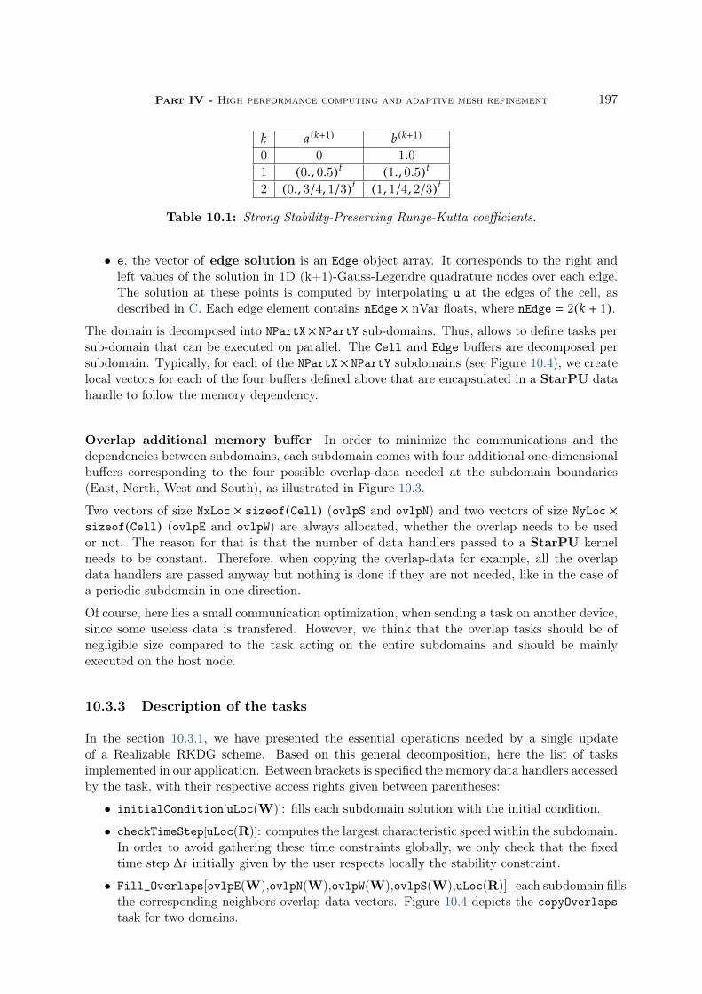
Part IV - High performance computing and adaptive mesh refinement 197

k a (k+1) b (k+1)

0 0 1.01 (0., 0.5)t (1., 0.5)t

2 (0., 3/4, 1/3)t (1, 1/4, 2/3)t

Table 10.1: Strong Stability-Preserving Runge-Kutta coefficients.

• e, the vector of edge solution is an Edge object array. It corresponds to the right andleft values of the solution in 1D (k+1)-Gauss-Legendre quadrature nodes over each edge.The solution at these points is computed by interpolating u at the edges of the cell, asdescribed in C. Each edge element contains nEdge × nVar floats, where nEdge 2(k + 1).

The domain is decomposed into NPartX× NPartY sub-domains. Thus, allows to define tasks persub-domain that can be executed on parallel. The Cell and Edge buffers are decomposed persubdomain. Typically, for each of the NPartX× NPartY subdomains (see Figure 10.4), we createlocal vectors for each of the four buffers defined above that are encapsulated in a StarPU datahandle to follow the memory dependency.

Overlap additional memory buffer In order to minimize the communications and thedependencies between subdomains, each subdomain comes with four additional one-dimensionalbuffers corresponding to the four possible overlap-data needed at the subdomain boundaries(East, North, West and South), as illustrated in Figure 10.3.

Two vectors of size NxLoc × sizeof(Cell) (ovlpS and ovlpN) and two vectors of size NyLoc ×sizeof(Cell) (ovlpE and ovlpW) are always allocated, whether the overlap needs to be usedor not. The reason for that is that the number of data handlers passed to a StarPU kernelneeds to be constant. Therefore, when copying the overlap-data for example, all the overlapdata handlers are passed anyway but nothing is done if they are not needed, like in the case ofa periodic subdomain in one direction.

Of course, here lies a small communication optimization, when sending a task on another device,since some useless data is transfered. However, we think that the overlap tasks should be ofnegligible size compared to the task acting on the entire subdomains and should be mainlyexecuted on the host node.

10.3.3 Description of the tasks

In the section 10.3.1, we have presented the essential operations needed by a single updateof a Realizable RKDG scheme. Based on this general decomposition, here the list of tasksimplemented in our application. Between brackets is specified the memory data handlers accessedby the task, with their respective access rights given between parentheses:

• initialCondition[uLoc(W)]: fills each subdomain solution with the initial condition.

• checkTimeStep[uLoc(R)]: computes the largest characteristic speed within the subdomain.In order to avoid gathering these time constraints globally, we only check that the fixedtime step ∆t initially given by the user respects locally the stability constraint.

• Fill_Overlaps[ovlpE(W),ovlpN(W),ovlpW(W),ovlpS(W),uLoc(R)]: each subdomain fillsthe corresponding neighbors overlap data vectors. Figure 10.4 depicts the copyOverlapstask for two domains.

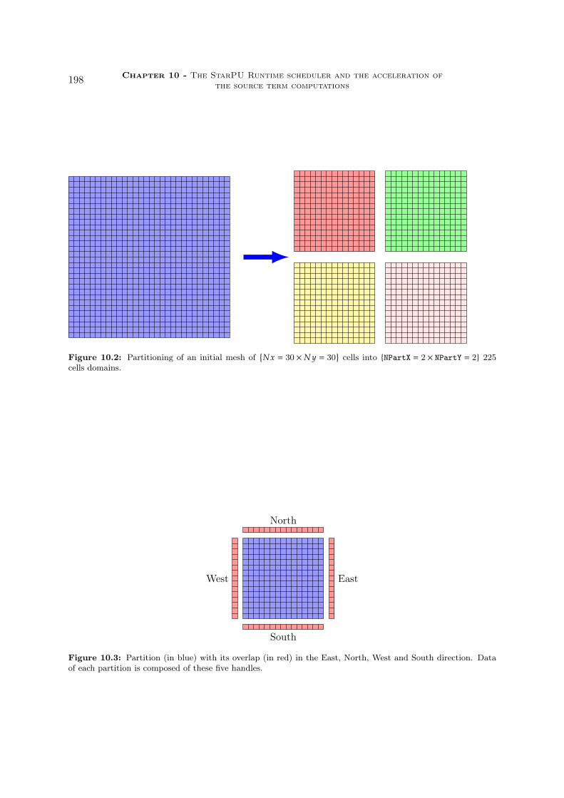
198 Chapter 10 - The StarPU Runtime scheduler and the acceleration ofthe source term computations

Figure 10.2: Partitioning of an initial mesh ofNx 30 × N y 30

cells into NPartX 2 × NPartY 2 225

cells domains.

North

South

EastWest

Figure 10.3: Partition (in blue) with its overlap (in red) in the East, North, West and South direction. Dataof each partition is composed of these five handles.

Part IV - High performance computing and adaptive mesh refinement 199

East West

Copy

Copy

Figure 10.4: Copy to overlaps tasks, example with two domains. The global computationaldomain is vertically divided into two parts, blue (left) and green (right). The green one issupplemented with a west overlap, whereas the blue one is supplemented with an east overlap.One residual computation includes two communications tasks: copying the right column of theblue domain into the west overlap of the green domain, and copying the left column of the greendomain into the east overlap of the blue domain.

• interpolate[uLoc(R), eLoc(W)]: for each cell, we interpolate the solution, given by thedegrees of freedom and which is stored in uLoc, in 1D Gauss nodes over the four edges ofthe cell. We store the interpolated solution to the edges in eLoc.

• InnerNumericalFluxes[eLoc(RW) ]: computes the numerical flux at 1D Gauss-Legendrequadrature points over the edges of the subdomain, except those of the boundaries. Finally,we store the numerical fluxes in eLoc.

• project[uLoc(R),eLoc(R),RHS(W)]: computes the residual at each 2D Gauss-Legendrequadrature points in the cells. The residual corresponds to the RHS of (10.2).

• RK_update[uLoc(RW),RHS(R)]: updates the numerical solution subdomain-wise, thanksto the update relation (10.3).

• Source_term[uLoc(RW)]: integrates the ODE system corresponding to the source terms.

• Positivity[uLoc(RW)]: applies the limitation procedure of Zhang & Shu to ensure real-izable solution at GLL points.

The corresponding task diagram for one time step and two sub-domains is given in Figure 10.5.This graph is an output we can get from StarPU to verify the correct sequence of the tasks.

200 Chapter 10 - The StarPU Runtime scheduler and the acceleration ofthe source term computations

MOTHER

initialCondition

initialCondition

gatherForOutput

checkTimeStep

Fill Overlaps

Fill Overlaps

Fill Overlaps

Fill Overlaps

Interpolate

gatherForOutput

checkTimeStep

Interpolate

switch

sync_task

sync_task

outputTask switch switch

BorderNumericalFluxes

BorderNumericalFluxes

InnerNumericalFluxes

Projection

InnerNumericalFluxes

Projection

RK Update

RK Update

Positvity

Positvity

Source_Term

Source_Term

computeErrors

switch

Figure 10.5: Task diagram built by StarPU for one time iteration of our first order RKDGtask-driven implementation on two subdomains, hence the horizontal symmetry.

10.4 Results

In this section, we study the numerical accuracy of the RKDG scheme and the performanceof our task-driven implementation on test cases solving the two-dimensional fractional momentequations over a 2D periodic domain. We perform two numerical test cases. The first oneis a simple advection with a constant velocity and without source terms and the second onecorresponds to an evaporation spray in the presence of a steady gas flow: Taylor-green vortices.In the first test case, we study the accuracy of the first and the second order RKDG scheme in a2D domain. Using the advection test case, we perform a strong scaling study and we investigatethe influence of the granularity of the tasks on the parallel efficiency. Finally, we use the secondtest case to illustrate the benefit of scheduling the tasks between CPUs and accelerators (GPUs).We show that the integration of source terms is very CPU time consuming, when its computationcan be remarkably accelerated ton GPUs.

10.4.1 Mesh convergence study

We consider an advection of fractional moments with a constant velocity vector (u , v) (1, 1)in a periodic domain. The initial moments are expressed as follows:

mk/2(t 0, x) 2

k + 2(S(k+2)/2

max −S(k+2)/2max )r(x−xc), r(x) 1+1(| |x | |2<0.25) cos4(4π | |x | |2), (10.4)

where xc (0.5, 0.5). The initial solution corresponds to the moments of rectangular sizedistribution n(t , S) 1[Smin ,Smax ](S) multiplied by a spatial distribution given by r(x − xc). The

Part IV - High performance computing and adaptive mesh refinement 201

2−52−62−72−8

10−3

10−2

10−1

10.88

10.91

10.87

∆x

Err

or

RKDG Order1

2−52−62−72−8

10−5

10−4

10−3

11.98

11.97

12.07

∆x

RKDG Order2

L1-errorL2-errorL∞-error

Figure 10.6: Convergence curves for m0 with respect to the grid refinement in logarithm scale.On the left RKDG of order 1 and on the right RKDG of order 2. Errors are computed usingnorm L1 (plus), L2 (cross) and L∞ (diamond).

exact solution is a simple advection at the initial uniform velocity (u , v) (1, 1). In Figure 10.6,we show the convergence results obtained with RKDG of order one and two. In this figure, wedisplay in a logarithmic scale the L1, L2 and L∞ numerical error depending on ∆x. We obtain anorder accuracy close to the theoretical order. For the RKDG of order one, the numerical ordercomputed from the error solution of m0/2 is around 0.9 for the three norms. For the secondorder moment, the order accuracy for m0/2 is around 2.0 for the three norms. This validates theimplementation of our numerical method up to the second order.

10.4.2 Parallel efficiency

In this section, we perform a strong scaling study using the same test case. We recall thatthe source terms are still not activated here. In the following, we keep the same problem size256 × 256 cells and we increase the number of cores. We analyze the parallel efficiency of ourimplementation and its dependency on the domain partition number and the size of the tasks.Indeed, it is important to have a sufficient number of domain partitions, at least the numberof cores, in order to allow StarPU to distribute the tasks among the available CPU resourcesand perform some scheduling optimization that can for example reduce the computational timedepending on the scheduler policy. The second point concerns the size of the tasks. As discussedin the section 10.2.3, the task management by StarPU presents a time overhead. To obtain agood scalability, the task duration should be much larger enough than the overhead time. To sumup, in order to scale correctly on many cores, we need a sufficient number of long duration tasks.In Figure 10.7, we display the speedup curves of parallel computation for different numbers ofdomain partition NPart: using the first and the second order RKDG schemes. In this figure,we distinguish three situations. First, the cases for which we do not provide enough tasksNPart < 24. In these cases, the parallel computation does not scale correctly (NPart 1and9).The second type of curves corresponds to large number of partition: NPart 256, 576 (for firstorder RKDG scheme) and NPart 576 (for second order), which are saturated due to taskoverhead. And finally, the cases where we use the right number of partition that allows toobtain a good scaling: NPart 25, 64 (resp NPart 25, 64, 256) for the first order (resp second

202 Chapter 10 - The StarPU Runtime scheduler and the acceleration ofthe source term computations

0 5 10 15 20 250

5

10

15

20

25

number of cores

spee

dup

NPart=1NPart=9NPart=25NPart=64NPart=256NPart=576y=x

0 5 10 15 20 250

5

10

15

20

25

number of cores

spee

dup

Figure 10.7: Strong scaling with eager scheduler: scalability results obtained on 2 dodeca-coreHaswell Intel Xeaon E5-2568 architecture using first order scheme (left) and second order scheme(right) with NPart varying from 1 to 576.

Figure 10.8: The numerical solution of the evaporating droplets number density using thesecond order RKDG scheme: at t 0.5 (left) and t 1.0 (right).

order). The granularity of the tasks does not only depend on the number of cells but also onthe amount of the work in each cell. That explains why the first order saturates faster than thesecond order when we increase the number of partitions.

10.4.3 Source terms acceleration through GPU

In this section, we use the same numerical test case as the one described in section 8.4.3.The numerical resolution is achieved through a second order RKDG scheme with the algorithmdescribed in 8.3 to integrate the source terms (drag force and evaporation). Zhang & Shu methodis activated to ensure realizable a solution at Gauss-Legendre-Lobbato and Gauss Legendrepoints. Figure 10.8 shows the numerical results at two different times.

First, we evaluate the execution time of the different tasks in CPUs. Figure 10.9 shows a Ganttchart of the time duration of each task for 5 iterations and the distribution of the tasks betweenfour CPU cores.

Part IV - High performance computing and adaptive mesh refinement 203

Figure 10.9: Gantt chart for 5 time iterations of the second order RKDG scheme on fourCPUs and using eager scheduler. Source term tasks correspond to the blue stripes, the redstripes correspond to slipping time and the other colors correspond to the other tasks.

It is clear that the execution time of the source term tasks are mush larger than the other taskones. The source term tasks require intensive arithmetic operations because of the reconstruc-tion of the size distribution by entropy maximization. Accelerator devices can accelerate theexecution and reduce the computational time in these cases. In the following, we test the exe-cution time of 50 iterations on a 256 × 256 mesh with or without GPU. Table 10.2 summarizesthe computational time for different subdomain decomposition and using the eager or the dmdascheduler.

As it is expected, we see that activating the GPU immediately decreases the computationaltime for both eager and dmda schedulers. However, the eager scheduler is not smart enoughto anticipate the global computational time of the tasks. Consequently, it distributes the tasksbetween GPUs and CPUs without taking into account the performance of each processing unitin executing the tasks. Using the dmda scheduler, we remark a gain in performance by betterdistributing the tasks on their best devices: this is illustrated on the Gantt charts in Figure 10.10for both eager and dmda schedulers. On the top figure, we look at the task scheduling in CPUsand GPUs using the eager scheduler. First, we can see, as mentioned before, that the executionof source terms on the CPUs takes an important time while their execution in GPUs is muchfaster. The total execution time is reduced thanks to the GPUs but it could be reduced furtherwith a smarter scheduler. For the dmda scheduler, the first tasks are distributed randomly inCPUs and GPUs since we do not initially provide a performance model of the tasks. But, afterfew iterations the dmda scheduler uses the performance of CPUs and GPUs on executing the firstiterations to build a performance model of tasks execution on the different available PUs. Forthe last iterations, we see that the source terms tasks are mostly executed on the GPUs. Thisexplains why, when turning the dmda scheduler on, the computational time is again reduced by

204 Chapter 10 - The StarPU Runtime scheduler and the acceleration ofthe source term computations

scheduler part. 0 GPU 1 GPU

eager

2 × 2 529.608 549.1662 × 4 536.686 299.0484 × 4 530.345 193.6454 × 8 536.425 185.621

dmda

2 × 2 790.951 130.222 × 4 679.207 92.62174 × 4 564.299 100.0194 × 8 540.095 137.222

Table 10.2: Computational time (in seconds) for 50 iterations on a 256 × 256 domain dividedinto 2× 2, 2× 4, 4× 4 or 4× 8 subdomains, when activating or not a GPU accelerating unit andusing the eager or dmda scheduler.

more than a factor of 2. Nonetheless, we also see that some red stripes corresponding to slippingtime, still remain on the CPU line, meaning that one could gain even a little more by activatingthe computation of the transport tasks on the GPU card.

Part IV - High performance computing and adaptive mesh refinement 205

Figure 10.10: Gantt chart for 10 time iterations of the second order RKDG scheme on fourCPUs and one CPU. Source term tasks correspond to the blue stripes and the red stripes corre-spond to slipping time: using eager scheduler (top) and dmda scheduler (down).

206 Chapter 10 - The StarPU Runtime scheduler and the acceleration ofthe source term computations

10.5 conclusion

In this chapter, we explore the possibility to reduce the computational time by taking advantagesof nowadays heterogeneous supercomputer architectures. The proposed solution consists inimplementing our numerical method in a task-based programming environment and in usinga runtime scheduler to distribute the tasks among the different processing units (CPUs andaccelerators) in a smart way. For this purpose, we use the StarPU runtime scheduler.

We have described and shown experimentally the main features of our code and the decompo-sition of the numerical method steps into different tasks. For the numerical resolution, we useon RKDG scheme with an arbitrarily high order implementation. This method is presented indetails in chapter 7, where we show how to ensure a realizable and a robust solution, while theimplementation in a task-based manner is described in this chapter. For this implementation, wevalidate the numerical method up to the second order. Then, we investigate the parallel scalingof the computations and its dependency on the number of domain decompositions and the size ofthe tasks. The main conclusion of this part shows that a correct scaling on many cores requiresa sufficient number of tasks of long duration. Finally, we use GPUs to accelerate tasks thatrequire intensive arithmetic computations. That is the case for source terms of the fractionalmoments model, but it can be generalized for other tasks that require an important workload.We also illustrate briefly the impact of the scheduler policy in distributing the tasks betweenthe different PUs and in reducing the computational time. These encouraging results show apromising potential of tasked-based programming with a runtime scheduler to take benefit fromthe new hybrid-multicores machines and reduce the computational time of complex simulations.

General conclusion and perspectives

The studies conducted in this PhD thesis are dedicated to the numerical simulations of thefuel injection in combustion chambers and in particular automotive engines. In this context,we aim at developing new solutions that can enable the design of new combustion chambersthrough new models as well as robust and accurate numerical methods, which can simulate thewhole injection process. At the same time, we need to satisfy some industrial requirements interms of predictive simulation, but still ensuring an acceptable computational cost and a highperformance computing on parallel architectures. The numerical modeling of the fuel injectionflow raises a number of challenges and difficulties. Indeed, we have to deal with a two-phaseflow that involves multi-scale processes. In this complex flow, many physical phenomena playan important role: the turbulence, the deformation of the gas-liquid interface, the breakupmechanisms, the polydisperse cloud of droplets and the interaction between the two phases(evaporation, drag force, etc.). Direct Numerical Simulation aims at solving all the involvedscales and provides fine details about the flow. Therefore, it is computationally very expensivefor industrial applications. For this reason, developing Eulerian reduced order models is apromising option for industrial applications. In this type of models, the equations are not solvedfor all the scales, but instead the small scale effects are taken into account through an appropriatesub-scale description, where a threshold scale has been chosen.

Up to now, the existing reduced order two-phase flow models can not simulate the whole injectionprocess, instead each of these models depends on the flow regime: separated or disperse phases.In this PhD, we have considered two reduced-order models families. First, the two-fluid andhomogeneous models are suitable to simulate the injection flow in the separated phases region.However, we have underlined two major difficulties: the artificial diffusion of the interface andthe the lack of information at the interface sub-scales. Second, we choose the Eulerian momentapproach to simulate the disperse phase and in particular the high order size-moment with acontinuous reconstruction of the size distribution as it was done in the EMSM model Kah(2010).This Eulerian model shows good results to capture the polydispersion using only one size-section.However, it is important to point out that the EMSM model is restricted to spherical dropletsand it is not yet adapted for a coupling with a separated phases sub-scale model, when theinterface has complex topology. Therefore, to design a unified model based on these two modelsfamilies (two-fluid and high order size-moment models) as well as robust and accurate numericalmethods dedicated to highly parallel computation, we have addressed these issues in three mainaxes:

• In terms of modeling: we have proposed a new approach to design a unified model forboth separated and disperse phases. Our strategy consists in introducing variables thatcan be defined for all regimes and can be used to enhance the sub-scale description ofthe interface and at the same time to describe the polydispersion in the disperse phase.Such strategy would allow to avoid a coarse coupling between two different models usingdifferent variables. In this perspective, we have introduced new concepts and tools to

208 Conclusion

model the sub-scales:

– First, we have defined a new distribution on surface, called SDF, to extend the distri-bution in number given by the NDF for the disperse phase. The phase space of thisnew distribution is decomposed of the mean and Gauss curvatures and the interfacevelocity. We also derived the link between the two distributions SDF and NDF. TheSDF is defined independently of the flow regime and it can be related to the NDFin the case of a dilute disperse phase. Evolution equation of the SDF describes theevolution of the interfacial variables and the surface stretching. From this equation,we have derived a system of the SDF moments. We have also showed that the firstorder moments of the SDF are the averaged geometrical variables of the gas-liquidinterface proposed in Drew(1990).

– In the case of spherical droplets, we showed that the averaged geometrical variablesare expressed as fractional size-moments of the NDF, where the size is given bythe surface area of the droplets. We also showed that the different properties ofinteger moments already used for the EMSM model can be extended and used for thefractional moments model. In chapter 8, we showed that the new fractional momentsmodel has the same capacity to describe the polydispersion as the EMSM model.

– In chapter 6, we have classified the internal variables of the SDF into resolved andunresolved phase space. The moments of the SDF integrated only over the unresolvedpart of the phase space define the sub-scale geometrical moments. The equationssatisfied by these sub-scale variables involve exchange source terms with the resolvedscales. These source terms will have to be closed and related to the variables of atwo-fluid model.

– Finally, we have designed an algorithm to compute the curvatures from a level-setfield dedicated to the post-processing of DNS two-phase flow simulations. This newalgorithm preserves some geometrical and topological information, which essentiallyallows us to compute a NDF from an averaged SDF. The main objective of suchpost-processing is to provide a deep insight on the evolution of the flow and proposeclosure relations of the source terms involved in the system of equations of the sub-scale geometrical moments.

• In terms of numerical schemes: we have developed accurate and robust numericalschemes for the resolution of the fractional size-moment model dedicated to the numer-ical simulation of polydisperse and evaporating spherical droplets. In this context, wehave adopted a discretization strategy based on an operator splitting method, where weseparately solve the transport part, then the source terms of the system of equations.

– For the numerical resolution of the transport part of the equations, we proposed twotypes of numerical method. The first one is based on a Finite Volume Kinetic (FVK)discretization de Chaisemartin(2009); Kah et al.(2012). From this approach, realiz-able and robust schemes up to the second order have been derived. The second one isthe Runge Kutta Discontinuous Galerkin (RKDG) scheme Cockburn and Shu(1998).The realizability of this method is ensured through a limitation method developedin Zhang et al.(2012). The RKDG method is an arbitrary high order scheme. Inour work, we limited the study to the third order. A comparison between the FVKand RKDG methods was conducted in chapter 7. The comparison shows accurateresults of RKDG compared to FVK. However, FVK schemes are more robust andstable in critical situations such as delta-shock formation that appears in the case ofthe jet-crossing.

Conclusion 209

– In chapter 8, we proposed an original ODE solver to solve the evolution of the mo-ments due to the source terms. A new evaporation solver dedicated to the fractionalmoments is developed based on ideas similar to the ones proposed the first time inMassot et al.(2010). In fact, we use a continuous reconstruction through entropy max-imization to evaluate the disappearance fluxes due to the evaporation and we combinea kinetic-based scheme with a Direct Quadrature Method of Moment to evaluate theevolution of the size. However, the new algorithm involves negative order moments.Thus, special treatments have been proposed in chapter 8 to deal with this difficulty.

• In terms of scientific and high performance computing: we have studied somesolutions in order to save the computational CPU time and memory or to accelerate someintensive arithmetic tasks, while ensuring an accurate resolution and parallel computationsin standard and heterogeneous architectures.

– First, we implemented the fractional moments model in the CanoP code, which isbased on the p4est AMR cell-based library. The choice of using cell-based AMR wasinitially determined by the high resolution needed for localized sharp interfaces, as inseparated-phase flows Drui(2017). The results of a series of 2D and 3D simulationsin chapter 9 showed that the use of AMR grids can preserve the accuracy of thesolution and reduce significantly the computational time compared to the uniformgrids. Furthermore, we showed a good parallel performance in CPUs machine thanksto the p4est library which is not obvious to obtain for an AMR grid.

– On the other hand, we implemented the fractional moments model in a 2D task-basedprogram using the StarPU library to schedule the tasks in heterogeneous architectures(CPUs and accelerators). StarPU scheduler distributes the different tasks among theavailable computation resources and manages the memory following a strategy thatcan optimize the consumption of CPU time and memory. The results showed animportant acceleration of tasks that require intensive arithmetic computations and inparticular the ODE evaporation solver. These encouraging results show a promisingpotential of tasked-based programs with a runtime scheduler to take benefit fromthe new hybrid-multicore machines and reduce the computational time of complexsimulations.

The present PhD proposes new solutions for the numerical simulation of the fuel injection interms of modeling, numerical method and high performance computing. The results obtained inthese three major fields are encouraging to continue the investigation in these directions. Futureworks should provide appropriate closures for the sub-scale model proposed in chapter 6, ensurea robust and accurate resolution of this model and satisfy a good scalability in massively parallelcomputation using AMR grids. The future works can follow the following directions:

• First, in terms of modeling, closure expressions of the time evolution of interfacial variables(curvatures and interface velocity) should be derived by post-processing and analyzing re-alistic jet DNS results in different regions of the jet as it was illustrated in chapter 6.The statistical evolution of the curvatures and the interface velocity need to be closed andexpressed as a function of the transported variables of the two-fluid model and the othersub-scales variables. Furthermore, we need to propose an appropriate reconstruction of theSDF or the multi-variable NDF. Closing these terms will allow to close the source termsinvolved in the system of equations of the sub-scale geometrical moments (see chapter 6for more details). On the other hand, we will need to take into account the effect of thesub-scales on two-fluid models. A first contribution to enrich a two-fluid model with somemicro-scale effects is proposed in the PhD of Drui(2017). The proposed model has been

210 Conclusion

derived from the Hamilton’s variational and the second thermodynamics principles Gavri-lyuk and Saurel(2002), where a pulsation energy is used in the Hamiltonian formulation.The obtained two-fluid model takes into account some micro-inertia and micro-viscosity ef-fects that are related to the pulsations of the interface. However, this model is restricted tospherical and monodisperse bubbles/droplets. In Di Battista(2020); Cordesse(2019) PhDs,a similar work aims at expressing some surface energies as a function of the sub-scale ge-ometrical moments. Then, by using these energies in the Hamiltonian formulation, theauthors aim at deriving a new two-fluid model that takes into consideration the sub-scaledescription given by the sub-scale geometrical moments.

• Second, in terms of the numerical implementation and the parallel computing, we willpursue the developments in CanoP code. The next step would be the implementation ofthe Galerkin Discontinuous scheme in AMR grid. The implementation in uniform 1Dand 2D grids has been already investigated and showed very promising results. Now, weshould adapt the scheme to non-conforming meshes. We will first implement this methodin the fractional moments model for the disperse phase and the mixture two-fluid modelDrui et al.(2016b) for separated phases. Furthermore, the improvement of the numericalaccuracy also requires to control the compression error generated by the computationson adapted grids. More appropriate refinement strategies could be considered by usinga multiresolution approach Harten(1994); Duarte(2011) or by using criteria based on thelocal truncation error as in Berger and Oliger(1984). Finally, developments of methods toenable the computation over heterogeneous architectures should be considered to benefitfrom the performance of the accelerators to run some specific tasks and also to ensure theparallel scaling in the new multi-core heterogeneous machines.

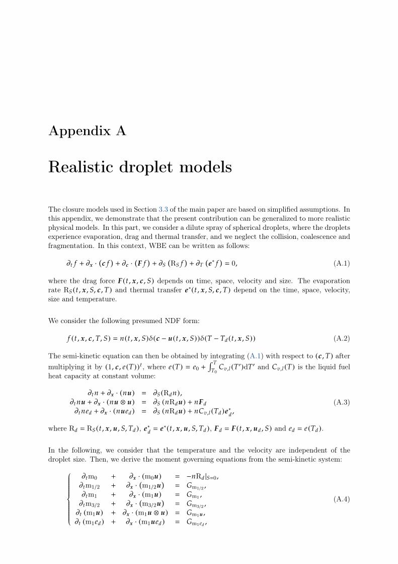
Appendix A

Realistic droplet models

The closure models used in Section 3.3 of the main paper are based on simplified assumptions. Inthis appendix, we demonstrate that the present contribution can be generalized to more realisticphysical models. In this part, we consider a dilute spray of spherical droplets, where the dropletsexperience evaporation, drag and thermal transfer, and we neglect the collision, coalescence andfragmentation. In this context, WBE can be written as follows:

∂t f + ∂x ·(c f

)+ ∂c ·

(F f

)+ ∂S

(RS f

)+ ∂T

(e∗ f

) 0, (A.1)

where the drag force F (t , x , c , S) depends on time, space, velocity and size. The evaporationrate RS (t , x , S, c , T) and thermal transfer e∗(t , x , S, c , T) depend on the time, space, velocity,size and temperature.

We consider the following presumed NDF form:

f (t , x , c , T, S) n(t , x , S)δ(c − u(t , x , S))δ(T − Td (t , x , S)) (A.2)

The semi-kinetic equation can then be obtained by integrating (A.1) with respect to (c , T) aftermultiplying it by (1, c , e (T))t , where e (T) e0 +

∫ TT0

Cv ,l (T′)dT′ and Cv ,l (T) is the liquid fuelheat capacity at constant volume:

∂t n + ∂x · (nu) ∂S (Rd n),∂t nu + ∂x · (nu ⊗ u) ∂S (nRd u) + nFd∂t ned + ∂x · (nued) ∂S (nRd u) + nCv ,l (Td)e∗d ,

(A.3)

where Rd RS (t , x , u , S, Td), e∗d e∗(t , x , u , S, Td), Fd F (t , x , ud , S) and ed e (Td).

In the following, we consider that the temperature and the velocity are independent of thedroplet size. Then, we derive the moment governing equations from the semi-kinetic system:

∂tm0 + ∂x · (m0u) −nRd |S0 ,∂tm1/2 + ∂x ·

(m1/2u

) Gm1/2 ,

∂tm1 + ∂x · (m1u) Gm1 ,∂tm3/2 + ∂x ·

(m3/2u

) Gm3/2 ,

∂t (m1u) + ∂x · (m1u ⊗ u) Gm1u ,∂t (m1ed) + ∂x · (m1ued) Gm1ed ,

(A.4)

212

where the source terms are expressed as follows:

Gmk/2 −

∫ 1

0k/2Sk/2−1Rd (S)n(S)dS,

Gm1u −u∫ 1

0Rd (S)n(S)dS +

∫ 1

0SFd (S)n(S)dS,

Gm1ed −ed∫ 1

0Rd (S)n(S)dS + Cv ,l (Td)

∫ 1

0Se∗d (S)n(S)dS.

(A.5)

The closure of the system is achieved by a continuous reconstruction through the maximizationof Shannon Entropy.

We use the operator splitting technique to solve numerically the system (A.4). The transportpart can be solved in the same way as it was done in chapter 7 of the paper. In the following, wefocus on the resolution of the source term part. Let us consider a spatial homogeneous domain,where only source terms are involved, the equation system becomes:

dtM S(t ,M) (A.6)

whereM (m0 ,m1/2 ,m1 ,m3/2 ,m1u ,m1ed)T is the unknown vector andS (−Rd nME (m) |S0 ,Gm0 ,Gm1/2 ,Gm1 ,Gm3/2 ,Gm1u ,Gm1ed )T is the source term. The four mo-ments are computed by using NEMO algorithm with a slight adaptation in the fourth step,where equation (8.26) is replaced by:

mk/2(tn + dt) nq∑j1

w j φ(tn + dt; tn , S j)k/2 , (A.7)

where the weight w j and abscissas S j are determined in the third step of the algorithm and theφ(t; t0 , So) is defined as follows:

dφ(t; t0 , So)dt

RS (t , φ(t; t0 , So), u , Td),

φ(t0; t0 , So) So ,(A.8)

where the temperature Td can be determined from the averaged internal energy ed.

The updated velocity and the internal energy are computed using the CQMOM technique, asexplained in the section 8.3 of the paper. For t ∈ [tn , tn+1], we write after subtracting thedisappearance flux from the moments:

(m1u)[φ(tn ;tn+1 ,0),1](t)

nq∑i1

wi φ(t; tn , Si)c i (t)

(m1ed)[φ(tn ;tn+1 ,0),1](t)

nq∑i1

wi φ(t; tn , Si)ei (t)(A.9)

with

dc i

dt F (t , φ(t; tn , Si), c i)

c i (t tn) u(tn),(A.10)

Appendix A - Realistic droplet models 213

and

dei

dt e∗(t , φ(t; tn , Si), c i , Td)

ei (t tn) ed (tn),(A.11)

We recall that the superscript [φ(tn; tn+1 , 0), 1] refers to the moments of the measure defined inthe support [φ(tn; tn+1 , 0), 1], where φ(tn; tn+1 , 0) is the size of the last evaporated droplet.

214

Appendix B

Evolution equation for the area densitymeasure

In this section, let us derive the evolution equation for the area density measure δI . First, letus recall that δI is defined as a distribution function by:

δI (t , x) | |∇x(g(t , x)

)| | δ(g(t , x)).

The Lagrangian derivative • of δI reads:

δI (t , x) ∂tδI + vI · ∇x (δI ) [∂t

(| |∇x

(g(t , x)

)| |)+ vI · ∇x

((| |∇x

(g(t , x)

)| |))

] δ(g(t , x))+ [∂t

(δ(g(t , x))

)+ vI · ∇x

((δ(g(t , x))

))] | |∇x

(g(t , x)

)| |

The second term in the right-hand side of the previous equality is null, because of the equationon g(t , x) which is:

∂t g + vI · ∇x(g) 0.

Let us now compute the first term. On a one hand, we have:

∂t(| |∇x

(g(t , x)

)| |)∇x

(g(t , x)

)| |∇x

(g(t , x)

)| |· ∂t

(∇x

(g(t , x)

)) n · ∇x

((∂t g(t , x)

)) −n · ∇x

((vI · ∇x

(g(t , x)

))) −n · ∇x

((vI | |∇x

(g(t , x)

)| |)).

On the other hand, one computes:

vI · ∇x((| |∇x

(g(t , x)

)| |))

vI n · ∇x((| |∇x

(g(t , x)

)| |))

n · ∇x((

vI | |∇x(g(t , x)

)| |))− ||∇x

(g(t , x)

)| |n · ∇x ((vI ))

And finally, one can find that:

δI (t , x) −||∇x(g(t , x)

)| |n · ∇x ((vI )) δ(g(t , x))

−δI n · ∇x ((vI )). (B.1)

216

Equation (B.1) can be further developed, by noting that:

−δI n · ∇x ((vI )) −δI [∇x · vI − vI∇x · n]

and

∇x · n 2H.

Finally, one has:

δI (t , x) −δI ∇x · vI + 2HδIvI . (B.2)

Appendix C

Taking into account the degrees offreedom of the DG discretization

In this section, we reuse the same notation as in section 7.3. The objective is to present theresolution of source terms in the framework of the Runge Kutta Discontinuous Galerkin (RKDG)discretization. We recall that the solution in a cell m is written as follows:

U h (t , x) (k+1)d∑

i1

W mi (t)φi (Ξm (x)), (C.1)

where d is the space dimension. In chapter 7, the method is presented for d 2, but itsextension to other dimension is straightforward. We use, as in the last chapter, a Lagrangianpolynomial basis associated to the abscissa of (k + 1)2 Gauss Legendre quadrature points inthe domain [−1/2, 1/2]d. We denote simply by (xq)1≤q≤(k+1)d the sequence of abscissa points ofGauss Legendre quadrature in the domain of the cell m. We have then for all 1 ≤ q ≤ (k + 1)d:

U h (t , xq) W mq (t). (C.2)

Considering only the source terms part of the system of equations, we can show that each degreeof freedom W m

q (t) satisfies the ODE system (8.29) and its evolution can be solved using themethod described in section 8.3. However, we need to ensure that the solution at Gauss-Legendrepoints is realizable, i.e. the first four components of W m

q (t)[1 : 4] (mm ,q0 (t), . . . ,mm ,q

3/2 (t))t

represent real fractional moments. Indeed, the limitation procedure of Zhang et al.(2012) ensuresa realizable solution only at the Gauss-Legendre-Lobatto (GLL) points and for the mean solutionin the cell. Our solution consists in using the same limitation procedure but this time at theGauss-Legendre points instead of the GLL points. Thus, we obtain a realizable solution for thedegree of freedoms, which can be updated using the source terms solver presented in the section8.3. The final resolution with transport RKDG transport scheme can be summarized as follows:

• We solve the ODE system (7.36), using a Runge-Kutta method, to compute the evolutionof degrees of freedom due to the transport in the physical space.

• We apply the limitation procedure to ensure the realizability at Gauss-Legendre points 1.

• We solve the source terms ODE (8.29) for each degree of freedom.

1The coefficient θ in (7.46) is computed here according to Gauss-Legendre points instead of Gauss-Legendre-Lobbato points.

218

• We apply the limitation procedure given in (7.47) to ensure the realizability of the momentsand the maximum principle on the velocity at GLL points.

We note that we can alternate the resolution of the transport part and the source terms topreserve high order resolution.

References

E. Abbena, S. Salamon, and A. Gray.Modern Differential Geometry of Curves and Surfaceswith MATHEMATICA. CRC Press, 2006. (p. 77)

B. Abramzon and W. A. Sirignano. Droplet vaporisation model for spray combustion cal-culations. International Journal of Heat and Mass Transfer, 9:1605–1618, 1989. (p. 37)

G. Agbaglah, R. Chiodi, and O. Desjardins. Numerical simulation of the initial destabi-lization of an air-blasted liquid layer. Journal of Fluid Mechanics, 812:1024–1038, 2017.(p. 6, 19)

G. Allaire, S. Clerc, and S. Kokh. A five equation model for the simulation of interfacesbetween compressible fluids. J Comp Phys, 181(2):577–616, 2002. (p. 9)

A. Ambroso, C. Chalons, F. Coquel, and T. Galié. Relaxation and numerical approxima-tion of a two-fluid two-pressure diphasic model. ESAIM: Mathematical Modelling andNumerical Analysis, 43(6):1063–1097, 2009. (p. 24)

S. V. Apte, K. Mahesh, P. Moin, and J. C. Oefelein. Large-eddy simulation of swirlingparticle-laden flows in a coaxial-jet combustor. IJMF, 29(8):1311–1331, 2003. (p. 32)

N. Ashgriz and J. Poo. Coalescence and separation in binary collisions of liquid drops. J.Fluid Mech, 221:183 – 204, 1990. (p. 90)

C. Augonnet, S. Thibault, R. Namyst, and P.-A. Wacrenier. StarPU: a unified platformfor task scheduling on heterogeneous multicore architectures. Concurrency and Com-putation: Practice and Experience, 23(2):187–198, 2011. (p. 13, 191)

M. R. Baer and J. W. Nunziato. A two-phase mixture theory for the deflagration-to-detonation transition (DDT) in reactive granular materials. International Journal ofMultiphase Flow, 12(6):861–889, 1986. (p. 23, 24)

T. Barberon and P. Helluy. Finite volume simulation of cavitating flows. Computers &Fluids, 34(7):832 – 858, 2005. (p. 24)

M. J. Berger and J. Oliger. Adaptive mesh refinement for hyperbolic partial differentialequations. Journal of Computational Physics, 53(3):484–512, 1984. (p. 162, 210)

A. E. Bergles, J. G. Collier, J. M. Delhaye, G. F. Hewitt, and F. Mayinger. Two-PhaseFlow and Heat Transfer in the Power and Process Industries. Hemisphere PublishingCorporation, New York, 1981. (p. 23)

A. Bernard-Champmartin and F. De Vuyst. A low diffusive lagrange-remap scheme for thesimulation of violent air–water free-surface flows. Journal of Computational Physics,274:19–49, 2014. (p. 9)

G. A. Bird. Molecular gas dynamics and the direct simulation of gas flows. Oxford SciencePublications, 42, 1994. (p. 8)

J. Bohbot, O. Colin, A. Velghe, J.-B. Michel, M. Wang, P. K. Senecal, and E. Pomraning.An innovative approach combining adaptive mesh refinement, the ecfm3z turbulentcombustion model, and the tki tabulated auto-ignition model for diesel engine cfdsimulations. In SAE Technical Paper. 2016. (p. 4)

J. Bohbot, N. Gillet, and A. Benkenida. IFP-C3D: an unstructured parallel solver for

220 References

reactive compressible gas flow with spray.Oil & Gas Science and Technology, 64(3):309–335, 2009. (p. 5)

M. Boileau, J. Lagarde, V. Dupif, F. Laurent, and M. Massot. Two-size moment Eulerianmulti-fluid method describing the statistical trajectory crossing: modeling and numer-ical scheme. In 9th International Conference on Multiphase Flow, Proceedings of the9th International Conference on Multiphase Flow. Firenze, Italy, 2016. (p. 46)

F. Bouchut, S. Jin, and X. Li. Numerical approximations of pressureless and isothermalgas dynamics. SIAM J. Num. Anal., 41:135–158, 2003. (p. 12, 122, 124)

J. A. Boure. Wave phenomena and one-dimensional two-phase flow models. MultiphaseScience and Technology, 9(1):37–62, 1997. (p. 26)

J. Brackbill, D. Kothe, and C. Zemach. A continuum method for modeling surface tension.Journal of Computational Physics, 100(2):335 – 354, 1992. (p. 102)

C. Burstedde, L. C. Wilcox, and O. Ghattas. p4est: Scalable algorithms for paralleladaptive mesh refinement on forests of octrees. SIAM Journal on Scientific Computing,33(3):1103–1133, 2011. (p. xiv, 10, 13, 156, 162, 164, 165, 182)

S. Candel. Mécabique des fluides. Dunod, Paris, 1990. (p. 18, 32)S. Candel and T. Poinsot. Flame stretch and the balance equation for the flame area.

Combustion Science and Technology, 70:1–15, 1990. (p. 29)R. Canu, C. Dumouchel, B. Duret, M. Essadki, M. Massot, T. Ménard, S. Puggelli,

J. Reveillon, and F. Demoulin. Where does the drop size distribution come from?ILASS Conference paper, pages 1–8, 2017. (p. 84, 93, 98, 110)

S. de Chaisemartin. Eulerian models and numerical simulation of turbulent dispersionfor polydisperse evaporation sprays. Ph.D. thesis, Ecole Centrale Paris, France, 2009.Available on TEL : http://tel.archives-ouvertes.fr/tel-00443982/en/. (p. 5,12, 37, 45, 124, 156, 177, 208)

S. de Chaisemartin, L. Fréret, D. Kah, F. Laurent, R. Fox, J. Reveillon, and M. Mas-sot. Eulerian models for turbulent spray combustion with polydispersity and dropletcrossing. Comptes Rendus Mécanique, 337:438–448, 2009. Special Issue ’Combustionfor Aerospace Propulsion’. (p. 8, 80, 121, 122)

G. Chanteperdrix, P. Villedieu, and J. Vila. A compressible model for separated two-phaseflows computations. In ASME Fluids Engineering Division Summer Meeting. Montreal,2002. (p. 9)

R. Clift, J. R. Grace, and M. E. Weber. Bubbles, Drop and Particles. Academic Press,New York, 1978. (p. 36)

B. Cockburn, S. Hou, and C.-W. Shu. The runge-kutta discontinuous galerkin method forconservation laws v. Mathematics of Computation, 54:545–581, 1990. (p. 130)

B. Cockburn and C.-W. Shu. The runge-kutta discontinuous galerkin method for con-servation laws v. Journal of Computational Physics, 141(2):199–224, 1998. (p. 122,208)

O. Colin and A. Benkenida. The 3-Zones Extended Coherent Flame Model (ECFM3Z)for Computing Premixed/Diffusion Combustion. Oil & Gas Science and Technology,59(6):593–609, 2004. (p. 4)

O. Colin, A. Benkenida, and C. Angelberger. Ignition and Combustion Phenomena inHighly Stratified Gasoline Engines. Oil & Gas Science and Technology, 58(1):47–62,2003. (p. 4)

P. Cordesse. Study of combustion instabilities in liquid-propellant rocket engines: diffuseinterface model and kinetic model coupling for primary atomization simulations. Ph.D.thesis, Université Paris-Saclay, Polytechnique, 2019. (p. 103, 116, 210)

L. Cunha. Simulation aux Grandes échelles de la Dynamique des Flammes Diphasiques

References 221

en Ecoulement Tournant soumises à une modulation externe. Ph.D. thesis, UniversitéParis-Saclay, CentraleSupélec, 2018. (p. 32)

J. M. Delhaye and J. A. Boure. General equations and two-phase flow modeling, in Hand-book of Multiphase Systems. Academic Press, Inc., Boston, MA, 1982. (p. 26)

S. Descombes, M. Duarte, T. Dumont, F. Laurent, V. Louvet, and M. Massot. Analysis ofoperator splitting in the non-asymptotic regime for nonlinear reaction-diffusion equa-tions. application to the dynamics of premixed flames. SIAM J. Numerical Analysis,52:1311–1334, 2014. (p. 106, 121)

O. Desjardins, J. McCaslin, M. Owkes, and P. Brady. Direct numerical and large-eddysimulation of primary atomization in complex geometries. Atomization and Sprays,23(11):1001–1048, 2013. (p. 7)

H. Dette and W. J. Studden. The theory of canonical moments with applications in statis-tics, probability, and analysis. John Wiley & Sons Inc., New York, 1997. (p. 12, 54,55, 61, 62)

M. B. Devassy, C. Habchi, and E. Daniel. Atomization modelling of liquid jets using atwo-surface-density approach. Journal of Atomization and Sprays, 25(1):47–80, 2015.(p. 4, 10, 23, 28, 29, 102)

R. Di Battista. Eulerian unified modeling for separated and disperse two-phase flows basedon a geometrical treatment of the interface. Ph.D. thesis, Université Paris-Saclay, Poly-technique, 2020. (p. 103, 116, 210)

F. Doisneau. Eulerian modeling and simulation of polydisperse moderately dense co-alescing spray flows with nanometric-to-inertial droplets: application to SolidRocket Motors. Ph.D. thesis, Ecole Centrale Paris, 2013. Available at http://tel.archives-ouvertes.fr/tel-00966185. (p. xi, 8, 43)

F. Doisneau, F. Laurent, A. Murrone, J. Dupays, and M. Massot. Eulerian multi-fluidmodels for the simulation of dynamics and coalescence of particles in solid propellantcombustion. J. Comp. Phys., 234:230–262, 2013. (p. 38)

F. Doisneau, A. Sibra, J. Dupays, A. Murrone, F. Laurent, and M. Massot. Numericalstrategy for unsteady two-way coupled polydisperse sprays: application to solid-rocketinstabilities. Journal of Propulsion and Power, 3:727–748, 2014. (p. 106, 121)

D. Drew and S. Passman. Theory of multicomponent fluids, volume 135. Springer, 1999.(p. 9, 19, 20, 22, 26, 38, 72)

D. A. Drew. Mathematical modeling of two-phase flow. Ann. Rev. Fluid. Mech., 15:261–91,1983. (p. 22)

D. A. Drew. Evolution of geometric statistics. SIAM J. Appl. Math., 50(3):649–666, 1990.(p. 28, 53, 57, 58, 59, 70, 71, 73, 74, 208)

F. Drui. Eulerian modeling and simulations of separated and disperse two-phase flows:development of a unified modeling approach and associated numerical methods for highlyparallel computations. Ph.D. thesis, Université Paris-Saclay, CentraleSupélec, 2017.(p. xi, xii, xiv, 4, 10, 13, 27, 95, 99, 103, 104, 107, 116, 161, 164, 167, 169, 170, 209)

F. Drui, A. Fikl, P. Kestener, S. Kokh, A. Larat, V. Le Chenadec, and M. Massot. Ex-perimenting with the p4est library for AMR simulations of two-phase flows. ESAIM :Proceedings and Surveys, 53:232–247, 2016a. (p. 27, 156, 162, 167)

F. Drui, S. Kokh, A. Larat, and M. Massot. A hierarchy of simple hyperbolic two-fluidmodels for bubbly flows. submitted, pages 1–23, 2016b. Available on HAL, https://hal.archives-ouvertes.fr/hal-01349441. (p. 9, 23, 24, 57, 103, 167, 210)

M. Duarte. Adaptive numerical methods in time and space for the simulation of multi-scale reaction fronts. Ph.D. thesis, Ecole Centrale de Paris, 2011. Available on TELhttps://tel.archives-ouvertes.fr/tel-00667857. (p. 173, 210)

222 References

A. Dubey, A. Almgren, J. Bell, M. Berzins, S. Brandt, G. Bryan, P. Colella, D. Graves,M. Lijewski, F. Löffler, et al. A survey of high level frameworks in block-structuredadaptive mesh refinement packages. Journal of Parallel and Distributed Computing,74(12):3217–3227, 2014. (p. 162)

G. Dufour. Modélisation multi-fluide eulérienne pour les écoulements diphasiques à inclu-sions dispersées. Ph.D. thesis, Université Toulouse III, 2005. (p. 36, 39, 46)

C. Dumouchel, T. Ménard, and W. Aniszewski. Towards an interpretation of the scale dif-fusivity in liquid atomization process: An experimental approach. Physica A: StatisticalMechanics and its Applications, 438(Supplement C):612 – 624, 2015. (p. 98)

V. Dupif. Modeling and simulation of two-phase flows inside solid rocket motors throughan eulerian approach with size and velocity polydispersion. Ph.D. thesis, Paris-SaclayUniversity, 2018. (p. 42)

O. Emre. Modeling of spray polydispersion with two-way turbulent interactions for highpressure direct injection in engines. Ph.D. thesis, Ecole Centrale Paris, 2014. Availableon TEL https://tel.archives-ouvertes.fr/tel-01089937. (p. 5)

O. Emre, D. Kah, S. Jay, Q.-H. Tran, A. Velghe, S. De Chaisemartin, F. Laurent, andM. Massot. Eulerian Moment Methods for Automotive Sprays. Atomization and Sprays,25:189–254, 2015. (p. 8, 32)

M. Essadki, S. de Chaisemartin, M. Massot, F. Laurent, A. Larat, and S. Jay. High ordermoment methods and adaptive mesh refinement for polydisperse evaporating spraysimulations. Oil & Gas Science and Technology, 71:1–25, 2016. (p. 156, 167)

M. Essadki, J. Jung, A. Larat, M. Pelletier, and V. Perrier. A task-driven implementationof a simple numerical solver for hyperbolic conservation laws. Submitted to ESAIM:PROCEEDINGS AND SURVEYS, 2017. (p. xv, 191, 194)

G. Faccanoni, S. Kokh, and G. Allaire. Modelling and simulation of liquid-vapor phasetransition in compressible flows based on thermodynamical equilibrium. ESAIM: Math-ematical Modelling and Numerical Analysis, 46(5):1029–1054, 2012. (p. 24)

G. M. Faeth. Evaporation and combustion of spray. Progress in Energy and Combustion-Science, 9:1–76, 1983. (p. 37)

R. O. Fox and P. Vedula. Quadrature-based moment model for moderately dense polydis-perse gas-particle flows. Ind. Eng. Chem., 49:5174–5187, 2010. (p. 39)

D. Fuster, A. Bagu, T. Boeck, L. L. Moyne, A. Leboissetier, S. Popinet, P. Ray, R. Scar-dovelli, and S. Zaleski. Simulation of primary atomization with an octree adaptive meshrefinement and VOF method. International Journal of Multiphase Flow, 35(1):550–565,2009. (p. 7)

T. Gallouet, J.-M. Hérard, and N. Seguin. Numerical modeling of two-phase flows usingthe two-fluid two-pressure approach. Mathematical Models and Methods in AppliedSciences, 14(05):663–700, 2004. (p. 24)

M. García, E. Riber, O. Simonin, and T. Poinsot. Comparison between euler/euler andeuler/lagrange les approaches for confined bluff-body gas-solid flow. In InternationalConference on Multiphase Flow, pages CD–ROM – S3–Fri–A–62. Liepzig, Germany,2007. (p. 7)

S. Gavrilyuk and R. Saurel. Mathematical and numerical modeling of two-phase compress-ible flows with micro-inertia. Journal of Computational Physics, 175:326–360, 2002.(p. 9, 24, 103, 210)

S. Ghods and M. Herrmann. A consistent rescaled momentum transport method for sim-ulating large density ratio incompressible multiphase flows using level set methods.Physica Scripta, 2013(T155):014050, 2013. (p. 6, 7)

E. Godlewski and P.-A. Raviart. Numerical approximation of hyperbolic systems of con-

References 223

servation laws, volume 118. Springer-Verlag, New York, 1996. (p. 26)G. A. E. Godsave. Studies of the combustion of drops in a fuel spray: the burning of

single drops of fuel. In Proceedings of the 4th Symp. (International) on Combustion,The Comb. Institute, pages 818–830. Baltimore, 1953. (p. 37)

R. Gordon. Error bounds in equilibrium statistical mechanics. Journal of MathematicalPhysics, 9:655–663, 1968. (p. 56, 62, 107, 146, 150)

S. Gottlieb, C.-W. Shu, and E. Tadmor. Strong stability-preserving high-order time dis-cretization methods. SIAM Review, 43(1):89–112, 2001. (p. 130, 131, 132)

J. Greenberg, I. Silverman, and Y. Tambour. On the origin of spray sectional conservationequations. Combustion and Flame, 93:90–96, 1993. (p. 8)

V. Guillemaud. Modélisation et simulation numérique des écoulements diphasiques par uneapproche bifluide à deux pressions. Ph.D. thesis, 2007a. 2007AIX11005. (p. 24)

V. Guillemaud. Modelling and numerical simulation of strongly unbalanced two-phaseflows. In 18th AIAA Computational Fluid Dynamics Conference. 2007b. (p. 24)

H. Gzyl and A. Tagliani. Hausdorff moment problem and fractional moments. Appl. Math.Comput., 216(11):3319–3328, 2010. (p. 53)

G. Hannebique, P. Sierra, E. Riber, and B. Cuenot. Large Eddy Simulation of reactivetwo-phase flow in an aeronautical multipoint burner. Flow, Turbulence and Combustion,accepted in September 2012, 2013. (p. 8)

F. Harlow and J. E. Welch. Numerical calculation of time-dependent viscous incompressibleflow of fluid with free surface. Physics of Fluids, 8(12):2182–2189, 1965. (p. 6)

A. Harten. Adaptive multiresolution schemes for shock computations. Journal of Compu-tational Physics, 115:319–338, 1994. (p. 210)

A. Harten. Multiresolution algorithms for the numerical solution of hyperbolic conservationlaws. Communication on Pure Applied Mathematics, 48:1305–1342, 1995. (p. 173, 174)

M. Herrmann. A balanced force refined level set grid method for two-phase flows on un-structured flow solver grids. Journal of Computational Physics, 227:2674–2706, 2008.(p. 10)

M. Herrmann. A parallel eulerian interface tracking/lagrangian point particle multi-scalecoupling procedure. Journal of Computational Physics, 229:745–759, 2010. (p. 10)

C. Hirt, A. Amsden, and J. Cook. An arbitrary lagrangian-eulerian computing method forall flow speeds. Journal of Computational Physics, 14(3):227–253, 1974. (p. 6)

C. Hirt and B. Nichols. Volume of fluid (vof) method for the dynamics of free boundaries.Journal of Computational Physics, 39(1):201–225, 1981. (p. 6)

O. Hurisse. Numerical simulations of steady and unsteady two-phase flows using a homo-geneous model. Computers & Fluids, 152(Supplement C):88 – 103, 2017. (p. 24)

J. Hylkema. Modélisation cinétique et simulation numérique d’un brouillard dense de gout-telettes. Application aux propulseurs à poudre. Ph.D. thesis, ENSAE, 1999. (p. 39)

P. N. Inverardi, G. Pontuale, A. Petri, and A. Tagliani. Hausdorff moment problem viafractional moments. Appl. Math. Comput., 144(1):61–74, 2003. (p. 53)

M. Ishii. Thermo-Fluid dynamic theory of two-phase flow. Eyrolles, 1975. (p. 9, 20)M. Ishii and T. Hibiki. Thermo-Fluid Dynamics of Two-Phase Flow. 2. Springer-Verlag

New York, 2011. (p. 26)D. Kah. Taking into account polydispersity in the framework of a coupled Euler-

Lagrange approach for the modeling of liquid fuel injection in internal combustion en-gines. Ph.D. thesis, Ecole Centrale de Paris, 2010. Available online at http://tel.archives-ouvertes.fr/tel-00618786/en/. (p. 5, 9, 11, 12, 54, 96, 207)

D. Kah, O. Emre, Q. Tran, S. de Chaisemartin, S. Jay, F. Laurent, and M. Massot.High order moment method for polydisperse evaporating spray with mesh movement:

224 References

application to internal combustion engines. Int. J. Multiphase Flows, 71:38–65, 2015.(p. 9, 32)

D. Kah, F. Laurent, M. Massot, and S. Jay. A high order moment method simulatingevaporation and advection of a polydisperse spray. Journal of Computational Physics,231(2):394–422, 2012. (p. 5, 8, 12, 46, 53, 121, 122, 124, 125, 126, 156, 208)

M. Kang, R. Fedkiw, and X.-D. Liu. A boundary condition capturing method for mul-tiphase incompressible flow. Journal of Scientific Computing, 15(3):323–360, 2000.(p. 84)

J. N. Kapur and H. K. Kesavan. Entropy optimization principles with applications. Aca-demic Press, Inc., Boston, MA, 1992. (p. 54)

I. Kataoka. Local instant formulation of two-phase flow. International Journal of Multi-phase Flow, 12(5):745 – 758, 1986. (p. 28)

G. Kindlmann, R. Whitaker, T. Tasdizen, and T. Moller. Curvature-based transfer func-tions for direct volume rendering: Methods and applications. In Proceedings of the 14thIEEE Visualization 2003 (VIS’03), pages 67–. IEEE Computer Society, Washington,DC, USA, 2003. (p. 69, 70)

S. Kokh and F. Lagoutière. An anti-diffusive numerical scheme for the simulation of in-terfaces between compressible fluids by means of a five-equation model. Journal ofComputational Physics, 229:2773–2809, 2010. (p. 9, 17, 27)

A. Larat, M. Massot, and A. Vié. A stable, robust and high order accurate numericalmethod for eulerian simulation of spray and particle transport on unstructured meshes.In Proceedings of the summer program 2012, Center for Turbulence Research, StanfordUniversity, pages 1–10. 2012. (p. 128)

F. Laurent. Modélisation mathématique et numérique de la combustion de brouillards degouttes polydispersés. Ph.D. thesis, Université Claude Bernard, Lyon 1, 2002. (p. 38)

F. Laurent. Numerical analysis of eulerian multi-fluid models in the context of kinetic for-mulations for dilute evaporating sprays. Mathematical Modeling and Numerical Anal-ysis, 3:431–468, 2006. (p. 46)

F. Laurent, M. Massot, and P. Villedieu. Eulerian multi-fluid modeling for the numericalsimulation of coalescence in polydisperse dense liquid sprays. Journal of ComputationalPhysics, 194:505–543, 2004. (p. 38, 45)

F. Laurent, A. Sibra, and F. Doisneau. Two-size moment Eulerian multi-fluid model:a robust and high-fidelity description of polydisperse moderately dense evaporatingsprays. Comm. in Comput. Phys., 20:902–943, 2016. (p. 8, 46)

V. Le Chenadec and H. Pitsch. A monotonicity preserving conservative sharp interfaceflow solver for high density ratio two-phase flows. J. Comput. Phys., 249:185–203,2013. (p. 7)

S. Le Martelot. Contribution á la simulation numérique directe de l’ébullition. Ph.D. thesis,Aix Marseille Université, 2013. (p. 3)

S. Le Martelot, R. Saurel, and B. Nkonga. Towards the direct numerical simulation ofnucleate boiling flows. International Journal of Multiphase Flow, 66:62–78, 2014. (p. 3)

C. Le Touze. Coupling between separated and dispersed two-phase flow models for thesimulation of primary atomization in cryogenic combustion. Ph.D. thesis, UniversiteNice Sophia Antipolis, 2015. Available on TEL https://tel.archives-ouvertes.fr/tel-01250527. (p. 10)

R. Lebas, T. Menard, P. A. Beau, A. Berlemont, and F. X. Demoulin. Numerical simulationof primary break-up and atomization: DNS and modelling study. Int. J. MultiphaseFlows, 35(3):247–260, 2009. (p. 6, 7, 10, 28, 29, 58, 112)

D. Lhuillier, C.-H. Chang, and T. G. Theofanous. On the quest for a hyperbolic effective-

References 225

field model of disperse flows. Journal of Fluid Mechanics, 731:184–194, 2013. (p. 23)D. Marchisio and R. Fox. Solution of population balance equations using the direct quadra-

ture method of moments. Journal of Aerosol Science, 36:43–73, 2005. (p. 8, 44)D. Marchisio, J. Pikturna, R. Fox, and R. Vigil. Quadrature method of moments for

population-balance equations. AIChE Journal, 49(5):1266–1276, 2003. (p. 42)L. Martinez, A. Benkenida, and B. Cuenot. A model for the injection boundary conditions

in the context of 3D simulation of diesel spray: methodology and validation. Fuel,89(1):219–228, 2010. (p. 32)

F. Mashayek. Direct numerical simulations of evaporating droplet dispersion in forcedmach number turbulence. Heat Mass Transfer, 52:2601–2617, 1998. (p. 7)

M. Massot, F. Laurent, D. Kah, and S. de Chaisemartin. A robust moment method forevaluation of the disappearance rate of evaporating sprays. SIAM J. Appl. Math.,70:3203–3234, 2010. (p. 5, 8, 13, 41, 46, 53, 54, 56, 57, 66, 143, 144, 145, 209)

J.-P. Matas and A. Cartellier. Flapping instability of a liquid jet. Comptes Rendus Mé-canique, 341(1):35 – 43, 2013. Combustion, spray and flow dynamics for aerospacepropulsion. (p. xi, 7)

L. R. Mead and N. Papanicolaou. Maximum entropy in the problem of moments. J. Math.Phys., 25(8):2404–2417, 1984. (p. 8, 48, 53, 56, 63, 65)

T. Menard, S. Tanguy, and A. Berlemont. Coupling level set/VOF/ghost fluid methods:Validation and application to 3D simulation of the primary break-up of a liquid jet.International Journal of Multiphase Flow, 33(5):510–524, 2007. (p. 6, 12, 19, 67, 84,110)

M. Meyer, M. Desbrun, P. Schroder, and A. H. Barr. Discrete differential-geometry op-erators for triangulated 2-manifolds. Visualization and Mathematics III, pages 35–57,2001. (p. 85)

C. Morel. Modélisation multidimensionnelle des écoulement diphasique gaz-liquid. Ph.D.thesis, Ecole Centrale de Paris, 1997. (p. 26, 28)

C. Morel. Mathematical Modeling of Disperse Two-Phase Flows. Springer InternationalPublishing, 2015. (p. 28, 29, 70)

S. Muller. Adaptive Multiscale Schemes for Conservation Laws. Springer, 2003. (p. 173)A. Murrone and H. Guillard. A five equation reduced model for compressible two phase

flow problems. Journal of Computational Physics, 205:664–698, 2005. (p. 9)M. Ndjinga.Quelques aspects de modélisation et dánalyse des sytèmes issus des écoulements

diphasique. Ph.D. thesis, Centrale Paris, 2007. (p. 25)T. T. Nguyen, F. Laurent, R. O. Fox, and M. Massot. Solution of population balance

equations in applications with fine particles: mathematical modeling and numericalschemes. J. Comp. Phys., 325:129–156, 2016. (p. 8)

P. J. O’Rourke. Collective drop effects on vaporizing liquid sprays. Ph.D. thesis, PrincetonUniversity, 1981. (p. 36)

P. J. O’Rourke and A. Amsden. The tab method for numerical calculation of spray dropletbreakup. Technical Report 87545, Los Alamos National Laboratory, Los Alamos, NewMexico, 1987. (p. 39)

G. Pianet, S. Vincent, J. Leboi, J. P. Caltagirone, and M. Anderhuber. Simulating com-pressible gas bubbles with a smooth volume tracking 1-fluid method. InternationalJournal of Multiphase Flow, 36:273–283, 2010. (p. 6, 19)

T. Poinsot and D. Veynante. Theoretical and numerical combustion - Second Edition.2005. (p. 32, 34)

S. B. Pope. The evolution of surfaces in turbulence. Journal of Engineering Science,6(5):445–469, 1988. (p. 12, 67, 68, 71, 72)

226 References

W. Reed and T. Hill. Triangular mesh methods for the neutron transport equation. 1973.(p. 127)

R. D. Reitz. Mechanisms of atomization processes in high-pressure vaporizing sprays. At-omization and Spray Technology, 3:309–337, 1987. (p. 105)

J. Reveillon and F. Demoulin. Effects of the preferential segregation of droplets on evapo-ration and turbulent mixing. Journal of Fluid Mechanics, 583:273–302, 2007. (p. 185)

M. Sabat. Eulerian modeling and numerical methods for the description of turbulent poly-disperse sprays. Ph.D. thesis, Université Paris-Saclay, CentraleSupélec, 2016. (p. 44,187)

M. Sabat, A. Larat, A. Vié, and M. Massot. On the development of high order realizableschemes for the Eulerian simulation of disperse phase flows: a convex-state preservingDiscontinuous Galerkin method. Journal of Computational Multiphase Flows, 6(3):247–270, 2014. (p. 185)

M. Sanjosé, J.-M. Senoner, F. Jaegle, B. Cuenot, S. Moreau, and T. Poinsot. Fuel injec-tion model for Euler-Euler and Euler-Lagrange Large-Eddy Simulations of an evap-orating spray inside an aeronautical combustor. International Journal of MultiphaseFlow, 37(5):514–529, 2011. (p. 32)

R. Saurel and R. Abgrall. A multiphase godunov method for compressible multifluid andmultiphase flows. Journal of Computational Physics, 150(2):425 – 467, 1999. (p. 4, 22,24, 26, 27)

R. Saurel and O. L. Metayer. A multiphase model for compressible flows with interfaces,shocks, detonation waves and cavitation. Journal of Fluid Mechanic, 431:239–271, 2000.(p. 23, 26)

R. Saurel, F. Petitpas, and R. A. Berry. Simple and efficient relaxation methods for in-terfaces separating compressible fluids, cavitating flows and shocks in multiphase mix-tures. Journal of Computational Physics, 228:1678–1712, 2009. (p. 24)

N. Seguin. Modélisation et simulation numérique des écoulements diphasiques. Theses,Université de Provence - Aix-Marseille I, 2002. Available on: https://tel.archives-ouvertes.fr/tel-00003139/file/tel-000031391.pdf. (p. 24)

R. K. Shukla, C. Pantano, and J. B. Freund. An interface capturing method for the simu-lation of multi-phase compressible flows. Journal of Computational Physics, 229:7411–7439, 2010. (p. 17, 27)

S. Sibendu, I. R. Anita, E. L. Douglas, and K. A. Suresh. Effect of nozzle orifice geometryon spray, combustion, and emission characteristics under diesel engine conditions. Fuel,90(3), 2011. (p. 3)

A. Sibra. Eulerian Multi-Fluid modeling and simulation of evaporation and combustion ofpolydisperse sprays in solid rocket motors. Theses, Université Paris-Saclay, 2015. (p. 8)

W. Sirignano. Fluid dynamics and transport of droplets and sprays. Cambridge UniversityPress, New York, 1999. (p. 36, 37)

K. So, X. Hu, and N. Adams. Anti-diffusion interface sharpening technique for two-phasecompressible flow simulations. Journal of Computational Physics, 231:4304–4323, 2012.(p. 17, 27)

D. B. Spalding. The combustion of liquid fuels. In Proceedings of the 4th Symp. (Interna-tional) on Combustion, The Comb. Institute, pages 847–864. Baltimore, 1953. (p. 37)

G. Talenti. Recovering a function from a finite number of moments. Inverse Problems,3(3):501–517, 1987. (p. 53)

L. Thomas, L. Hélio, V. Antonio Wilson, and T. Geovan. Efficient implementation ofmarching cubes cases with topological guarantees. Journal of Graphics Tools, 8(2):1–15, 2003. (p. 84)

References 227

A. Tiwari, J. B. Freund, and P. Carlos. A diffuse interface model with immiscibility preser-vations. Journal of Computational Physics, 231:4304–4323, 2013. (p. 17, 27)

B. Truchot. Développement et validation d’un modèle eulérien en vue de la simulationdes jets de carburants dans les moteurs à combustion interne. Ph.D. thesis, InstitutNational Polytechnique de Toulouse, 2005. (p. 4)

S. O. Unverdi and G. Tryggvason. A front-tracking method for viscous, incompressible,multi-fluid flows. Journal of Computational Physics, 100(1):25 – 37, 1992. (p. 6)

A. Vallet and R. Borghi. Modélisation eulerienne de l’atomisation d’un jet liquide. ComptesRendus de l’Académie des Sciences - Series IIB - Mechanics-Physics-Astronomy,327(10):1015 – 1020, 1999. (p. 10)

A. Vallet, A. Burluka, and R. Borghi. Development of a eulerian model for the "atomiza-tion" of a liquid jet. Atomization and Sprays, 11:619–642, 2001. (p. 10, 29, 58)

G. Vaudor, T. Ménard, W. Aniszewski, M. Doring, and A. Berlemont. A consistent massand momentum flux computation method for two phase flows. application to atomiza-tion process. Computers & Fluids, 152(Supplement C):204 – 216, 2017. (p. xi, 6, 7,12, 110)

C. Vessiller. Contribution à l’étude des brouillards denses et dilués par la simulationnumérique Euler/Euler et Euler/Lagrange. Ph.D. thesis, Ecole Centrale Paris, 2007.(p. 4)

A. Vié, F. Doisneau, and M. Massot. On the Anisotropic Gaussian closure for the predictionof inertial-particle laden flows. Comm. in Comput. Phys., 17(1):1–46, 2015a. (p. 42,44)

A. Vié, B. Franzelli, Y. Gao, T. Lu, and M. Ihme. Analysis of segregation and bifurcation inturbulent spray flames: a 3d counterflow configuration. Proceedings of the CombustionInstitute, 35:1675–1683, 2015b. (p. 32)

A. Vié, S. Jay, B. Cuenot, and M. Massot. Accounting for Polydispersion in the EulerianLarge Eddy Simulation of an Aeronautical-type Configuration. Flow Turbulence andCombustion, 90(3):545–581, 2013a. (p. xi, 8, 31)

A. Vié, F. Laurent, and M. Massot. Size-velocity correlations in high order moment meth-ods for polydisperse evaporating sprays: modeling and numerical issues. J. Comp.Phys., 237:277–310, 2013b. (p. 5, 8, 42, 49, 57, 132, 151, 156)

A. Vié, M. Sanjosé, S. Jay, B. Cuenot, and M. Massot. Evaluation of a multifluid meso-scopic eulerian formalism on the large eddy simulation of an aeronautical-type config-uration. In International Conference on Multiphase Flow 2010. 2010. (p. 5)

P. Villedieu and J. Hylkema. Modèles numériques lagrangiens pour la phase dispersée dansles propulseurs à poudre. Rapport Final 1/3784.00/DTIM, ONERA, 2000. (p. 39)

S. Van der Walt, J. L. Schönberger, J. Nunez-Iglesias, F. Boulogne, J. D. Warner, N. Yager,E. Gouillart, and T. a. Yu. scikit-image: image processing in python. PeerJ, 2:e453,2014. (p. 84)

F. Williams. Spray combustion and atomization. Physics of Fluids, 1:541–545, 1958. (p. 8,32, 36)

C. Yuan, F. Laurent, and R. Fox. An extended quadrature method of moments for popu-lation balance equations. Atomization and Sprays, 51(1):1–23, 2012. (p. 8)

R. Zamansky, F. Coletti, M. Massot, and A. Mani. Turbulent thermal convection drivenby heated inertial particles. Journal of Fluid Mechanics, 809:390–4437, 2016. (p. 7)

X. Zhang and C.-W. Shu. On maximum-principle-satisfying high order schemes for scalarconservation laws. J. Comput. Phys., 229(9):3091–3120, 2010. (p. 128)

X. Zhang and C.-W. Shu. Positivity-preserving high order discontinuous galerkin schemesfor compressible euler equations with source terms. J. Comput. Phys., 230(4):1238–

228 References

1248, 2011. (p. 122, 128, 132)X. Zhang, Y. Xia, and C.-W. Shu. Maximum-principle-satisfying and positivity-preserving

high order discontinuous galerkin schemes for conservation laws on triangular meshes.J. Sci. Comput., 50(1):29–62, 2012. (p. 122, 128, 131, 195, 208, 217)

H. Zhu, Z. Zhou, R. Yang, and A. Yu. Discrete particle simulation of particulate systems:Theoretical developments. Chemical Engineering Science, 62:3378–3396, 2007. (p. 7)

D. Zuzio and J. Estivalezes. An efficient block parallel amr method for two phase interfacialflow simulations. Computers & Fluids, 44(1):339 – 357, 2011. (p. 10)

Titre : Contribution à la modélisation eulérienne unifiée de l’injection : de la zone dense au spraypolydispersé.Mots Clefs : Écoulements diphasiques; spray polydisperse; phases séparée; méthodes numeriquesd’order élevée; géometrie d’interface; modèles bifluides; schémas cinétiques; realizabilité; Calcul HautePerformance.

Résumé :

L’injection directe à haute pression du carburant dansles moteurs à combustion interne permet une atomisa-tion compacte et efficace. Dans ce contexte, la simula-tion numérique de l’injection est devenue un outil fon-damental pour la conception industrielle. Cependant,l’écoulement du carburant liquide dans une chambre oc-cupée initialement par l’air est un écoulement diphasiquetrès complexe ; elle implique une très large gammed’échelles. L’objectif de cette thèse est d’apporter denouveaux éléments de modélisation et de simulationafin d’envisager une simulation prédictive de ce typed’écoulement avec un coût de calcul abordable dans uncontexte industriel. En effet, au vu du coût de cal-cul prohibitif de la simulation directe de l’ensemble deséchelles spatiales et temporelles, nous devons concevoirune gamme de modèles d’ordre réduit prédictifs. En

outre, des méthodes numériques robustes, précises etadaptées au calcul de haute performance sont primor-diales pour des simulations complexes.Cette thèse est dédiée au développement d’un modèled’ordre réduit Eulérien capable de capter tant la polydis-persion d’un brouillard de goutte dans la zone dispersée,que la dynamique de l’interface dans le régime de phasesséparées. En s’appuyant sur une extension des méth-odes de moments d’ordre élevé à des moments fraction-naires qui représentent des quantités géométriques del’interface, et sur l’utilisation de variables géométriquesen sous-échelle dans la zone où l’interface gaz-liquidene peut plus être complètement résolue, nous pro-posons une approche unifiée où un ensemble de variablesgéométriques sont transportées et valides dans les deuxrégimes d’écoulement [. . .].

Title: Contribution to a unified Eulerian modeling of fuel injection: from dense liquid to polydispersespray

Keywords : Two-phase flows; polydisperse sprays; separated phases; high order moment methods;interface geometry; two-fluid models; kinetic-based numerical schemes; realizability; HPC.Abstract:

Direct fuel injection systems are widely used in combus-tion engines to better atomize and mix the fuel withthe air. The design of new and efficient injectors needsto be assisted with predictive simulations. The fuel in-jection process involves different two-phase flow regimesthat imply a large range of scales. In the context of thisPhD, two areas of the flow are formally distinguished:the dense liquid core called separated phases and thepolydisperse spray obtained after the atomization. Themain challenge consists in simulating the combinationof these regimes with an acceptable computational cost.Direct Numerical Simulations, where all the scales needto be solved, lead to a high computational cost for in-dustrial applications. Therefore, modeling is necessaryto develop a reduced order model that can describe allregimes of the flow. This also requires major break-through in terms of numerical methods and High Per-formance Computing (HPC).This PhD investigates Eulerian reduced order models todescribe the polydispersion in the disperse phase and

the gas-liquid interface in the separated phases. First,we rely on the moment method to model the polydis-persion in the downstream region of the flow. Then,we propose a new description of the interface by usinggeometrical variables. These variables can provide com-plementary information on the interface geometry withrespect to a two-fluid model to simulate the primary at-omization. The major contribution of this work consistsin using a unified set of variables to describe the tworegions: disperse and separated phases. In the case ofspherical droplets, we show that this new geometricalapproach can degenerate to a moment model similar toEulerian Multi-Size Model (EMSM). However, the newmodel involves fractional moments, which require somespecific treatments. This model has the same capacityto describe the polydispersion as the previous Eulerianmoment models: the EMSM and the multi-fluid model.But, it also enables a geometrical description of the in-terface [. . .].

Université Paris-Saclay

Espace Technologique / Immeuble Discovery

Route de l’Orme aux Merisiers RD 128 / 91190 Saint-Aubin, France