Health, environment and economic development - TEL - Thèses

HAL Id: tel-01078742https://tel.archives-ouvertes.fr/tel-01078742

Submitted on 30 Oct 2014

HAL is a multi-disciplinary open accessarchive for the deposit and dissemination of sci-entific research documents, whether they are pub-lished or not. The documents may come fromteaching and research institutions in France orabroad, or from public or private research centers.

L’archive ouverte pluridisciplinaire HAL, estdestinée au dépôt et à la diffusion de documentsscientifiques de niveau recherche, publiés ou non,émanant des établissements d’enseignement et derecherche français ou étrangers, des laboratoirespublics ou privés.

Health, environment and economic developmentAlassane Drabo

To cite this version:Alassane Drabo. Health, environment and economic development. Economics and Finance. Universitéd’Auvergne - Clermont-Ferrand I, 2011. English. �NNT : 2011CLF10376�. �tel-01078742�

https://tel.archives-ouvertes.fr/tel-01078742

https://hal.archives-ouvertes.fr

Université d’Auvergne Clermont-Ferrand I

Faculté des Sciences Economiques et de Gestion

École Doctorale des Sciences Économiques, Juridiques et de Gestion

Centre d’Etudes et de Recherches sur le Développement International (CERDI)

SANTE, ENVIRONNEMENT ET DEVELOPPEMENT ECONOMIQUE.

HEALTH, ENVIRONMENT, AND ECONOMIC DEVELOPMENT.

Thèse Nouveau Régime

Présentée et soutenue publiquement le 12 décembre 2011

Pour l’obtention du titre de Docteur ès Sciences Economiques

Par

Alassane DRABO

Sous la direction de

Mme la Directrice de Recherche CNRS Martine AUDIBERT et de Mme le Professeur Pascale COMBES MOTEL

Membres du Jury :

Jean Pierre Angelier Professeur à l’Université Pierre Mendès France, Grenoble

Mathilde Maurel Directrice de recherche CNRS, Université de Paris 1 Panthéon-Sorbonne.

Théophile T. Azomahou Professeur à United Nations University (UNU-MERIT) et à University of Maastricht.

Martine Audibert Directrice de recherche CNRS, Université d’Auvergne (CERDI).

Pascale Combes Motel Professeur à l’Université d’Auvergne (CERDI).

3

L’Université d’Auvergne Clermont 1 n’entend donner aucune approbation ni

improbation aux opinions émises dans les thèses. Ces opinions doivent être

considérées comme propres à leurs auteurs.

5

Remerciements

A l’issue de ces années de thèse très enrichissantes, je tiens à adresser mes

remerciements les plus sincères à l’ensemble des personnes qui ont contribué de loin ou de

près à la réalisation de ce projet. Plus particulièrement, je remercie mes directrices de thèse,

Martine Audibert et Pascale Combes Motel pour l’encadrement, l’attention, le soutien, leur

disponibilité, les encouragements et les conseils dont j’ai bénéficié tout au long de cette thèse

et qui ont contribué à ma maturité.

Mes remerciements vont également aux membres du jury Jean Pierre Angelier,

Théophile T. Azomahou, Mathilde Maurel, pour m’avoir fait l’honneur d’évaluer ce travail.

Mes remerciements s’adressent aussi à toute l’équipe du CERDI, tant au personnel

enseignant, chercheur, administratif, et étudiant qu’a mes amis a Clermont et ailleurs.

Je souhaite également exprimer mes remerciements à mes collègues, amis et ainés

Tidiane Kinda, Gaoussou Diarra, Souleymane Diarra, Michael Kolie, Jules Tapsoba, Christian

Ebeke, Lacina Condé, Yacouba Gnêgnê, Léandre Bassolé, Luc Désiré Omgba, Fousseini

Traoré, Linguère M’baye, Maelan Le Goff, Adama Ba, Hang Xiong, Joel Cariolle, Bachirou

Diallo, René Tapsoba, Thierry Kangoye, Romuald Kinda, Ulrich Zombre, Felix Badolo,

Cathérine Korachais, Omar Kanj, Dao Seydou, Zorobabel Bicaba, Taro Boel, Hélène Ehrhart,

Faustin Kutshienza, Sébastien Marchand, Luc Moulin, sans oublier mes frères et soeurs de

l’Association des Burkinabé de Clermont-Ferrand (A.BU.C) et tous les participants des

conférences auxquelles j’ai participé.

Enfin, je tiens à exprimer ma profonde reconnaissance à Aïssata Coulibaly, à mes frères

Ousmane, Seydou, Mohamed, Adama et ma sœur Awa pour leur amour, leur confiance, leur

patience et leurs soutiens indéfectibles.

7

Table of contents

CHAPTER 1: GENERAL INTRODUCTION AND OVERVIEW ...................................................................................... 9

PART I: HEALTH, ENVIRONMENT AND INEQUALITIES .................................................................. 25

CHAPTER 2: IMPACT OF INCOME INEQUALITY ON HEALTH: DOES ENVIRONMENT QUALITY MATTER? ............. 29

CHAPTER 3: INTRA COUNTRIES HEALTH INEQUALITIES AND AIR POLLUTION IN DEVELOPING COUNTRIES: DO

POLITICAL INSTITUTIONS PROTECT THE POOR?.................................................................................................. 65

PART II: HEALTH, ENVIRONMENT AND ECONOMIC GROWTH .................................................. 107

CHAPTER 4: GLOBAL BURDEN OF DISEASE AND ECONOMIC GROWTH .............................................................. 113

CHAPTER 5: INTERRELATIONSHIPS BETWEEN ENVIRONMENT QUALITY, HEALTH AND ECONOMIC ACTIVITY: WHAT CONSEQUENCES FOR ECONOMIC CONVERGENCE? ................................................................................. 147

9

Chapter 1: General Introduction and

Overview

11

1.1. Background

Defined as “development that meets the needs of the present without compromising the ability

of future generations to meet their needs” according to the Brundtland Commission (1987),

the aim of sustainable development is to provide a long term vision for the society. The

different elements that constitute this concept are often organized into three dimensions or

pillars: (environmental, economic and social). The environmental one consists in the security

of the living and physical environment, including natural resources, while the economic one

reflects efficient, stable and sustainable economic growth that is not made at the expense of

intergenerational equity. The social dimension is devoted to a good life for all individuals. It

includes empowerment, fight against poverty, equity, access to social security, education and

good health for all the population.1

Among these three dimensions of sustainable development, the environmental one is the most

known and is even mostly used to represent all the other dimensions. This is probably

because, absent from economic field during many years, environmental concerns are more

and more present in development strategies since the 1960s. It is nowadays difficult to obtain

funding for development projects without quoting environmental advantages and the way

environmental degradations caused by the projects are solved. More research papers are

published on environmental issues by academics, and environmental preoccupations are at the

core of many international meetings. It is one of the eight MDGs (goal 7) adopted by the

United Nations in 2000.

1 The three pillars of Sustainable Development are refered in many United Nations documents since the Brundtland Report, such as the Johannesburg Declaration on Health and Sustainable Development (Munasinghe 1993)

12

Policy makers, scholars as well as international community are more interested in this concept

not only because it is salable (marketable) but also because it plays an important role in the

development process and the sustainability of economic development.

The relationships between the three pillars of sustainable development are diversely assessed

in the literature, especially when health indicators are used to represent the social dimension

(See Figure 1.1). Scholars generally choose two among these three dimensions and investigate

their association. Environmental economists are interested in the associations between

environmental quality and economic indicators, and usually analyze the link in a bidirectional

way.

Figure 1. 1: Relationships linking the three pillars of sustainable development.

Source: adapted from Adams, WM. 2001, p. 128.

Economic Dimension: income growth, stability, efficiency.

Social Dimension: health, education, poverty, equity.

Environmental Dimension : Biodiversity, natural resources,

pollution

Environmental impact Valuation

Internalization

Income distribution Job

Targeted assistance

Empowerment Consultation

Pluralism

13

On the one hand, studies highlight the ways economic activities may affect the quality of

environment. Since the early 1990s, empirical works on this field of research have found this

relationship between economy and environment as an inverted-U curve called Environmental

Kuznets Curve (EKC) (Grossman and Krueger 1993, 1995), analogous to the pattern Kuznets

(1955) found between income inequality and economic development. Indeed, according to

this hypothesis, environmental degradation tends to rise faster than income growth in the early

stages of economic development, then slows down, reaches a turning point and declines with

further income growth (Figure 1.2). This hypothesis is not rejected by many studies, even if

some authors point out some weakness of these studies and infirm this conclusion (see for

instance Carson (2010) or Stern (2004)). It is highlighted in Carson (2010) that the reduced-

form nature of the EKC models used in the literature limits the potential policy implications

of the results. There is therefore a need for structural models taking into account the likely

role of health variables, and the reserse causality linking environment to economic growth in

order to propose suitable recommendations to policy makers.

14

Figure 1. 2: The Environmental Kuznets Curve (relationship between environment and

economic development)

On the other hand, environmental degradation in turn reduces economic performance through

its effect on the productivity and the level of human and physical capital. Through its effect

on population health, environmental degradation reduces labour supply and labour

productivity.

Starting in 1960s, awareness of the environment as important predictor of output growth has

steadily increased. Development economists have realized that, their findings based on

neoclassical growth models would be incomplete without taking into account environmental

concerns (Dagusta & Heal, 1974; Solow, 1974). Since this period many growth model have

been developed incorporating environmental issues. Following Panayotou (2000), they can be

classified in four main categories: i) optimal growth models, ii) models of the environment as

a factor of production, iii) endogenous growth models of environmental degradation and

Pre-industrial economies

Industrial economies Post-industrial

economies

(service economies)

Stages of economic development

Environmental degradation

Source: Panayotou (2003, pp. 46)

15

growth, and iv) “other macroeconomic models” of environmental degradation including

overlapping generation models, and multisectoral models of growth and the environment in

the presence of trade.

Health economists are interested in the relationship between economic indicators and

population’s health, and more precisely the effect of health on economic activity (for a

literature review, see Audibert, 2010, Schultz, 2010). Besides its direct and immediate effect

on people well-being, health status is an important predictor of individual incomes

improvements as well as country level economic prosperity (Weil, 2007). Firstly, good health

improves the productivity of workers (Hoddinott, 2009) and increases the number of people

available as work force in a given population. Secondly, it indirectly improves economic

outcome through its effect on education. Improvements in health raise the motivation to

attend high level schooling, since the returns to investments in schooling are valuable over a

longer working life. Healthier students also have more attendance and higher cognitive

functioning, and thus receive a better education for a given level of schooling (Thuilliez,

2009). Moreover, good health encourages more saving and thus investment and per capita

productive capital (Chakraborty, 2004).

Figure 1.3 highlights the association between health outcomes and Gross Domestic Product

(GDP) per capita respectively when health is measured by infant mortality rate, under five

mortality rate, crude death rate and life expectancy.

All these graphs confirm the association between GDP per capita and health status explained

above, since health outcomes improve with the level of income. This positive and concave

relationship is known in health economics as the Preston curve (Deaton, 2003; Preston 1975).

16

Figure 1. 3: Link between GDP per capita and health outcomes 0

50

10

01

50

20

0

Infa

nt

mo

rta

lity

ra

te

0 10000 20000 30000 40000GDP per capita

01

00

20

03

00

Un

de

r 5

mo

rta

lity

ra

te0 10000 20000 30000 40000

GDP per capita

51

01

52

02

53

0

To

tal

de

ath

ra

te

0 10000 20000 30000 40000GDP per capita

40

50

60

70

80

Lif

e e

xp

ec

tan

cy

0 10000 20000 30000 40000GDP per capita

Source: Author with data from World bank and WHO

From these two empirical relationships (environment-economic growth, and health-economic

activity), we can infer the existence of the obvious relationship between population’s health,

and environmental degradation. Figure 1.4 shows the number of deaths from some

environmental infections as percentage of total death in 2004 around the world. From this

17

graph, it appears clearly that the poorest regions such as Sub-Saharan Africa and South Asia

suffer more from environmental degradation.

Figure 1. 4: Death from environmental disease as percentage of total death in 2004

Source : Author’s construction with data from WHO.

18

The relationships between these three pillars (economy, social, and environment) remain less

studied and explored despite the important challenges and policy implications it may arouse

for developing countries. In fact, from our knowledge, existing empirical studies do not

investigate simultaneously the link among the three pillars. Health status may play important

role in the relation linking environmental degradation and economic preoccupations.

Similarly, physical environment variations are not negligible in the association between

economy and health. Moreover, the relationships among these three dimensions may imply

important consequences for poor countries. This raises the necessity to investigate these

complex relationships and its consequences for these countries. This dissertation aims to

analyze theoretically as well as empirically the association among population health,

environmental degradation and economic development, its consequences for developing

countries, and some effective policy responses. Before examining in details all these issues in

the following chapters, let explore the outline and main results of this dissertation.

1.2. Outline and main results

This dissertation extends some previous important results on health and the environment by

establishing a link between the three dimensions of sustainable development. It is organized

in two main parts which themselves embed two chapters. The first part (Chapters 2 and 3) is

devoted to the relationship between the three pillars by focusing on a particular aspect of each

of them, namely, health (social dimension), pollution (environmental dimension), and income

inequalities (economic dimension). It focuses on health outputs of development process by

introducing inequality variables in the established link between health and environment;

taking two perspectives (see Figure 1.5).

19

In the literature, income inequality is theoretically and empirically found to have a negative

effect on population’s health through four main mechanisms: absolute income, relative

income, psychosocial, and Neo-materialism hypotheses. Despite the large debate on income

inequality as a likely determinant of environmental degradation on the one hand, and the

literarature on the effect of pollution on health on the other hand (see Figure 1.5), no study

from our knowledge is interested in the probably role of pollution in the relationship linking

income distribution and population health. We bridge this gap by investigating how

environmental degradation could be considered as an additional channel through which

income inequality affects infant and child mortality (Chapter 2).

The theoretical and econometric analyses show that income inequalities negatively affect

environmental quality, and environment degradation worsens population’s health. This

confirms that environment quality is an important channel through which income inequalities

affect population health. These results hold for air pollution indicators (PM10 and SO2) and

water pollution indicator (BOD).

Besides income distribution concern, intra country health inequalities represent an important

issue largely approached in the health economics literature. Indeed, in health and

environmental economics literature, many studies have assessed the association between

environmental degradation and health outcomes. Chapter 3 goes beyond this literature by

focusing on health inequalities both between and within developing countries.

Theoretically, it is argued that differential in exposition to air pollution among income classes,

prevention ability against health effect of environment degradation, capacity to respond to

disease caused by pollutants and susceptibility of some groups to air pollution effect are

sufficient to expect a positive link between air pollution and income related health inequality.

Furthermore, in democratic countries, this heterogeneity in the health effect of pollution may

20

be reduced since good institutions favour universal health policy issues, information and

advices about hygiene and health practices, and health infrastructures building. Using quintile

data from surveys and measuring health inequality as the distribution of health outcome

among income quintiles, our econometric results show that sulphur dioxide emission (SO2)

and particulate matter (PM10) are in part responsible for the large disparities in infant and

child mortalities between and within developing countries. In addition, we found that

democratic institutions play the role of social protection by mitigating this effect for the

poorest income classes and reducing the health inequality it provokes.

Figure 1. 5: Health, Environment, and Inequalities.

Source: Author’s construction based on Adams, WM. 2001, p. 128.

The first part allowed us to understand how health and environment are linked to inequalities.

The second part of the dissertation focuses on growth output of the development process,

Income Inequalities

Health Pollution

Income Related Health Inequalities

Chapter 2

Chapter 3

21

taking into account the quality of the environment and population health. Also based on the

three pillars of sustainable development and constituted of two chapters (chapters 4 and 5), it

is particularly interested in the inversed-U shaped relationship between economic

development and environmental degradation. It investigates through the association between

economic development, health, and environment, the risk of weak economic convergence

because of bad health and environmental degradation in poor countries (see Figure 1.6).

The assessment of the role played by health outcome on economic growth arouses at least two

important problems. First, the direction of the causality is often questioned and becomes

subject of a vigorous debate. For some authors, diseases or poor health have contributed to

poor growth performances especially in low-income countries. For others, the effect of health

on growth is relatively small, even if one considers that investments which could improve

health should be done. Besides occurred biases in health measurement. Indeed, commonly

used health indicators in macroeconomic studies (e.g. life expectancy, infant mortality or

prevalence rates for specific diseases such as malaria or HIV/AIDS) imperfectly represent the

global health status of populations. Health is rather a complex notion and includes several

dimensions which concern fatal (deaths) and non-fatal issues (prevalence and severity of

cases) of illness. The effects of health on economic growth vary accordingly with the health

indicator used and the countries included in the analyses. The Chapter 4 (part II) analyze this

issue by assessing the effect of a global health indicator on growth, the so-called disability-

adjusted life year (DALY) that was proposed by the World Bank and the WHO in 1993.

Growth convergence equations are run on 159 countries over the 1999-2004’ period, where

the potential endogeneity of the health indicator is dealt for. The negative effect of poor health

on economic growth is not rejected thus reinforcing the importance of MDGs.

The Chapter 5 extends these analyses, and studies economic convergence with traditional

health indicators taking into account the role of the environment. It focuses on the

22

interrelationships between health, environment, and economic growth, and studies the

implications of this relationship for economic convergence through theoretical and empirical

models. Environmental variables are introduced in the augmented Solow growth model in

order to show the consequences of environmental degradation in terms of economic

convergence. To empirically assess these issues, we proceeded to an econometric analysis

through three equations: a growth equation including environmental variable, a health

equation and an environment equation. We found that environmental degradation affects

negatively economic activity and reduces the ability of poor countries to reach developed ones

economically. Moreover, as pollution has a negative effect on health, the effect of

environment degradation on economic growth is reinforced. This implies that environmental

quality could be considered as a constraint for economic convergence.

Figure 1. 6: Health, Environment, and Economic Growth.

Source: Author’s construction based on Adams, WM. 2001, p. 128

Income Prosperity

Health Pollution

Chapter 4

Chapter 5

25

Part I: health, environment and

inequalities

27

Introduction

Based on the development challenges faced by developing countries, the United

Nations established on September 2000 eight measurable development goals to be achieved

by these countries by 2015. Environmental sustainability and population’s health, already

recognized as two important pillars of sustainable development, constitute together half (four

out of eight) of these goals (goals 4, 5, 6, and 7). The achievement of these two objectives

requires the knowledge of the factors that determine them, but it is also important to find the

relationship linking them.

Theoretical and empirical works on the association between environmental degradation and

population’s health generally find consensual results. It is shown that the direct and obvious

consequence of environmental degradation is the deterioration of population’s health (Pearce

and Warford 1993).

On the other hand, income distribution is considered in the literature to be a determinant of

both environmental degradation and population health. Some authors showed that an increase

in income inequality degrades physical environment (Boyce, 1994; Ravallion et al., 2000),

while others highlight its effect in terms of damage to population’s health (Deaton, 2003;

Babones, 2008).

Despite the potential relationship between health, environment, and inequalities, it did not

arouse much interest to researchers, especially for developing countries. The first part of the

dissertation bridges this gap by analyzing the relationship between health, environment and

inequalities. It is subdivided into two chapters (chapters 2 and 3). The first chapter entitled

“Impact of Income Inequality on Health: Does Environment Quality Matter?” extends the

literature on the association between the distribution of income and health status. It

28

investigates theoretically and empirically, how environmental degradation could be

considered as an additional channel through which income inequality affects infant and child

mortality.

Then, chapter 3 entitled “Do Political Institutions protect the poor? Intra Countries Health

Inequalities and Air Pollution in Developing Countries”, analyses the association between the

degradation of air quality (measured by sulphur dioxide emission per capita (SO2) and

particulate matter less than 10 µm aerodynamic diameter (PM10)), and health inequality

between and within developing countries. It explores also the role of political institutions in

this relationship.

It is globally found that environmental variables play important role in the relation linking

health and inequalities. In fact, the effect of income distribution on health is partly channeled

by pollution, and environmental degradation exacerbates income related health inequality.

29

Chapter 2: Impact of Income

Inequality on Health: Does

Environment Quality Matter?2

2 A version of this chapter was published under the reference: Drabo, A., 2011. Impact of income inequality on health: does environment quality matter? Environment and Planning A, 43(1), 146-165.

31

2.1. Introduction

Population health is an important economic concern for many developing countries. It plays a

crucial role in the development process, since it constitutes a component of investment in

human capital and workforce is the most abundant production factor in these countries. It

constitutes also a major preoccupation for the international community, especially when it is

considered as a public good. The importance given to health status could be illustrated

through its relatively high weight among the Millennium Development Goals (MDGs), of

which three are related to health preoccupations. It is therefore important to know the factors

that influence population health in order to undertake suitable economic policy.

Rodgers (1979) is one of the first economists to consider income distribution as a determinant

of health outcomes. He shows that income inequality influences health status not only in

developed countries, but also in developing countries, opening the debate about the

association between income distribution and health. Wilkinson (1992) reopens the debate

showing that income inequality is an essential determinant of health status in eleven

industrialized countries. Even though major part of the studies on this topic confirm the

negative effect of inequality on health, some authors reject this hypothesis and show that high

inequality may be indifferent to health status or improve it (Pampel and Pellai 1986 ; Mellor

and Mylio, 2001; Deaton, 2003).

All the mechanisms through which income distribution impacts health status developed in the

literature show that an increase in income inequality worsens population health. These

mechanisms rely on the absolute and relative income hypothesis, psychosocial hypothesis and

neo-materialism hypothesis as well (Mayer and Sarin, 2005). In this paper we add the

environment as another mechanism through which income distribution could affect health

status. During the past fifteen years, with the emergence of environmental concerns, many

32

studies examine the association between income inequality and natural environment quality.

But they found different results. On the one hand, some authors show that more inequality

may improve environmental quality (Scruggs, 1998; Ravallion et al., 2000). On the other

hand, other studies underline the negative impact of inequality on environmental quality

(Boyce, 1994; Torras & Boyce, 1998). If environmental quality is degraded by an increase in

inequality, it may be a channel that reinforces the negative effect of the other mechanisms.

But if it is improved by an increase in inequality, it maybe a mechanism that mitigates or

cancels the negative effect predicted by the other mechanisms and justify discrepancies

between the findings.

Our results show theoretically and empirically that an increase in income inequality is

detrimental to the environment and that environmental quality is itself an important

contributor to health status. That is, an increase in inequality worsens population’s health via

environmental degradation.

The rest of this chapter is organized in four sections. Section 2 reviews the literature on the

association between income distribution, environmental degradation and population’s health.

In this section we explain why and how income inequality affects health before introducing

the arguments that defend the association between income distribution and environmental

quality. In section 3, we investigate empirically the effects of income distribution on health

via environment quality. The last section concludes.

33

2.2. Literature review

The relationship between income inequality and population health has been investigated by

many macroeconomic studies during the past 15 years. Scholars examine how and why

income inequality affects health theoretically and empirically within and between nations. We

will first review the traditional mechanisms, namely the ways income distribution affects

population’s health already developed in the literature. Then, we will explain how income

inequality impacts health through environmental degradation.

2.2.1. Traditional effects of income inequality on health

Theoretically, four mechanisms are underlined, through which income inequality can harm

directly population health (Mayer & Sarin, 2005).

The first mechanism is the absolute income hypothesis. In fact, income may be an important

determinant of population health, since it allows them to buy better nutrition or medical care

or reduces their stress. If the relationship between an individual income level and its health

status is linear, an extra unit of income will have the same effect on health regardless of

whether it goes to the rich or to the poor. In this case taking a unit of income from the rich and

giving it to the poor will lower health status among the rich and raise it among the poor by

exactly equal amounts, leaving the global health unchanged. The reality is that standard

economic models predict that the health gains from an extra unit of income should diminish as

income rises (Preston, 1975; Laporte, 2002; Deaton, 2003; Backlund et al., 1996; Babones,

2008), in other words, health should be a concave function of income. That is, a transfer of a

unit of income from the rich to the poor might improve aggregate population’s health status.

34

The second mechanism developed in the literature is the relative income hypothesis. The

effect of economic inequality is likely to depend to some extent on the geographic proximity

of the rich to the poor (Mayer & Sarin, 2005). In fact, if people assess their income by

comparing themselves to their neighbours, the income of others can affect their health. The

chronic stress provoked by this comparison may lower resistance to some diseases and cause

premature death. For Wilkinson (1997), if individuals evaluate their well-being by comparing

themselves to others with more income than themselves, increases in economic inequality will

engender low control, insecurity, and loss of self esteem.

According to Subramanian et al. (2002, p.289), these two first hypotheses are not really

independent.

The third way developed in the literature through which income inequality may worsen

population health is psychosocial hypothesis. Inequality can impact health through social

comparisons by reducing social capital, trust and efficacy (Kawachi & Kennedy, 1997; Bobak

et al., 2000). According to Wilkinson (1996), income inequality worsens health because a low

ranking in the social hierarchy produces negative emotions such as shame and distrust that

lead to worse health via neuro-endocrine mechanisms and stress-induced behaviors such as

smoking, excessive drinking, taking dangerous drugs, and other risky activities (Mayer &

Sarin, 2005). Lynch et al. (2001) found weak associations between a variety of measures of

the psychosocial environment, (distrust, belonging to organizations, volunteering, and

efficacy), and infant mortality, but they found that economic inequality is strongly related to

infant deaths.

Neo-materialism hypothesis is the fourth mechanism through which income inequality may

harm health status. According to some authors defending this idea, income inequality affects

health mainly through its effect on the level and the distribution of material resources

35

(Coburn, 2000 and Lynch, 2000). This argument suggests that poor health could be the

consequence of an increase in income inequality that reduces state spending on medical care,

goods and services for the poor.

If theoretically, all the arguments found in the literature indicate a negative impact of income

inequality on health status, empirical findings are far from a consensus (Subramanian and

Kawachi, 2003, 2004; Lynch et al., 2004). Lynch et al. (2004) review 98 aggregate and

multilevel studies to examine the associations between income inequality and health. They

conclude that overall, there seems to be little support for the idea that income inequality is a

major, generalizable determinant of population health differences within or between rich

countries. Income inequality may, however, directly influence some health outcomes, such as

homicide in some contexts. Mayer & Sarin (2005) review ten studies that use cross-sectional

data to estimate the association between economic inequality and infant mortality. Eight of

these ten use cross-national data and produce eleven estimates. Nine find that more unequal

countries have higher infant mortality rates, and two (Pampel & Pellai, 1986; Mellor& Milyo,

2001) find that more unequal countries have lower infant mortality rates than countries with

less inequality. Wilkinson & Pickett (2006) compiled one 168 analyses in 155 papers

reporting research findings on the association between income distribution and population

health, and classified them according to how far their findings supported the hypothesis that

greater income differences are associated with lower standards of population health. They find

that for 87 of these studies the coefficient of income inequality is always statistically

significant with the correct sign. 44 present mixed results and 37 no significant coefficient.

They explain the divergence of empirical findings by the size of area, choice of control

variables and don’t find any explanation for some international studies.

36

It is worth noting that theoretical works on income inequality and health are mainly based on

individual or household considerations whereas empirical studies are generally interested in

more aggregate levels (state or country level).

We argue here that in addition to the traditional mechanisms through which income inequality

degrades population’s health, there exists at least another channel through which income

inequality may affect health, namely environmental quality.

2.2.2 Income inequality and environment

A large body of research has reported strong associations between income inequality and

environmental degradation: some theoretical arguments are used to explain how income

inequality may improve environmental quality (Scruggs, 1998; Ravallion et al., 2000; Heering

et al., 2001) while other scholars defend the detrimental effect of increasing inequalities on

environment (Boyce, 1994; Torras & Boyce, 1998).

For those supporting the environmental improvement effect, income inequality can increase

environment protection through individual preference toward environmental quality. In fact,

for a given level of average income, greater inequality means not only higher incomes for the

rich, but also lower incomes for the poor. Assuming that the income elasticity of demand for

environmental quality is positive3, and taking a unit of income from the poor and giving it to

the rich increases the demand for environmental quality of the rich, but at the same time it

decreases the demand of the poor. The net effect on environmental quality depends on

whether the demand-income relation is linear, concave or convex (Scruggs, 1998; Boyce,

2003). If this relation is linear, the transfer will not have any effect on environmental quality

3 This supposes that environmental quality is a normal good

37

since an extra unit of income will have the same effect on environmental demand regardless

of whether it goes to the rich or to the poor. If the environmental demand is linked to income

by a convex (concave) relation, the transfer of income from the poor to the rich will increase

(decrease) environmental demand.

It is more convincing to assume that the wealthiest prefer more environmental quality than the

poor for many reasons. First, economic theories suggest that the rich prefer less environmental

degradation than the poor. This may be due to the fact that environmental quality is a superior

good of which demand increases faster than income (Baumol and Oates, 1988). This is one of

the explanations behind the environmental Kuznets Curve (EKC) hypothesis (Grossman &

Krueger, 1995). As argued by Scruggs (1998), greater demand for environmental protection

among the wealthiest is also expected to result in a greater willingness and ability to pay for

more environmental protection. In addition, wealth increases individuals’ concern for the

future, maybe because they expect higher life expectancies than the poorest or because it

increases their concern for their children in the future. Another reason to explain why rich

prefer more environmental quality is that environmental protests are usually composed of

middle and upper classes, not the poor (Dalton, 1994).

Income inequality can also reduce environmental degradation through the marginal propensity

to emit (MPE) as argued by Ravallion et al. (2000). According to these authors, each

individual has an implicit demand function for carbon emissions since the consumption of

almost every good implies some emissions either directly via consumption or indirectly via its

own production. They call marginal propensity to emit (MPE) the derivative of this implicit

demand function with respect to income. If poor people have a higher (lower) MPE than rich

ones, a redistribution policy that reduces inequalities will increase (decrease) carbon

emissions. One can assume that the poorests have higher MPE than wealthiests, first because

less emission goods need high technology and are thus generally expensive. Therefore, the

38

poorest cannot afford it. In addition, poor tend to use energy less efficiently than the rich,

which entails a higher MPE (Ravallion et al., 2000).

If these arguments predict an improvement of environment quality channelled by income

inequality, it is also largely argued by some authors that inequality may degrade environment

rather than improving it.

Boyce (1994) is the first author to examine how income inequalities affect environmental

degradation. He supports the hypothesis that greater inequality may increase environmental

degradation and this for two reasons. First, he argues that a greater inequality increases the

rate of environmental time preference for both poor and rich. In fact, when inequality

increases, the poor tend to overexploit natural capital, because they perceive it as the only

resource they have and the only source of income that can help them secure their survival.

This environmental effect of poverty is largely emphasized in the literature (Reardon and

Vosti, 1995; and known as “poverty environment thesis” since the Brundtland (1987) report.

This hypothesis suggests that the poor are both the agents and victims of environmental

degradation. In addition to the poverty effect, economic inequality often provokes political

instability and risks of revolts. This leads rich people to prefer a policy that consists in

exploiting the environment and investing the returns abroad rather than investing in the

protection of local natural resources. Therefore, for Boyce an increase in inequality induces

both rich and poor to degrade more their own environment. The second argument put forward

concerns the power of the richest. Boyce (1994) argues that in a society with greater

inequality, rich people are likely to have large political power and can heavily influence

decisions on environmentally damaging projects. Such decisions are based on the competition

between those who benefit from the environmentally degrading action and those who bear the

costs of it. Boyce (1994) argues that rich people are generally the winners, while poor people

tend to be the losers of the investments that have an ecological impact. Therefore, economic

39

inequality favours the implementation of environmentally damaging projects and investments

since it “reinforces the power of the rich to impose environmental costs on the poor”

(Ravallion et al., 2000, p.656). Scruggs (1998) has criticized the hypotheses supported by

Boyce. He states that the influence via cost-benefit analysis is based on two wrong

assumptions. First, according to Scruggs, “Evidence indicates that better off members of

society tend to have higher environmental concern than those with lower income” (Scruggs,

1998, p.260). Moreover Boyce (1994) assumes that a democratic social choice criterion leads

to higher environmental protection than a non-democratic decision process (i.e. a power-

weighted social decision rule), while evidence suggests that this is not necessarily true.

Another theoretical argument to explain why more inequality leads to more degradation is

developed by Borghesi (2000). He argues that “much of the theoretical environmental

literature has stressed the need of cooperative solutions to environmental problems. In an

unequal society this is more difficult to achieve than in an equal society since there are

generally more conflicts among the political agents (government, trade unions, lobbies etc...)

on many social issues. In this sense, greater inequality can contribute to increase

environmental degradation” (Borghesi, 2000 p. 4).

In addition to these arguments, some theoretical model supports the environmental degrading

effect of income inequality. It is the case of Magnani (2000) who examines the impact of

income distribution on public research and development expenditures for environmental

protection. Through a model in which social decisions are determined by the preferences of

the median voter, she hypothesizes that income inequality reduces pro-environmental public

spending due to a “relative income effect,” and higher inequality shifts the preferences of

those with below-average income in favour of greater consumption of private goods and

lower expenditure on environmental public goods.

40

Marsiliani and Renström (2000) have also recently investigated how income distribution

affects political decisions on environmental protection. Through an overlapping-generations

model, they show that the higher the level of inequality in terms of median-mean distance, the

lower the pollution tax set by a majority elected representative. Therefore, inequality induces

redistribution policies that distort economic decisions and lower production. Inequality may

be negatively correlated with environmental protection as it leads to less stringent

environmental policies.

It is a priori difficult to predict the effect of income distribution on environment quality

theoretically even though degrading effect seems in our viewpoint more convincing. Let us

see empirical findings.

Empirically studie on the relation between income distribution and environment quality are

quite not consensual. In Appendix 2.1, we report nine important papers and thirty one studies

on the association between income distribution and environment quality. Among these

studies, ten conclude that inequality improves environment quality, nine find the opposite

conclusion and twelve don’t find any significant association. Let explore some of them.

Scruggs (1998) performs two cross-country empirical analyses to assess the effect of income

inequality on the environment through pooled models. In the first one, four different

pollutants (sulphur dioxide, particulate matter, fecal coliform and dissolved oxygen) are used

as dependant variable in a panel of 22 up to 29 countries. The second investigation examines

the impact of several variables on a composite index of environmental quality in a panel of 17

OECD countries. This index is constructed by combining five pollution indicators.

In the first case, he finds conflicting results: greater inequality improves environmental

quality for one environmental indicator (particulates), whereas the opposite holds for the other

indicator (dissolved oxygen). For the other indicators (sulphur dioxide, fecal coliform), the

41

coefficients are not statistically significant. In the second analysis, income inequality

decreases environmental degradation.

Through a panel of 42 countries in the period 1975-92, Ravallion et al. (2000) first estimate

CO2 emissions as a cubic function of average per capita income and of population and time

trend. They estimate their equation with fixed effect model and simple pooled model using

ordinary least squares. They conclude that higher inequality within countries reduces carbon

emissions. However, the impact of income distribution on the environment decreases at

higher average incomes.

Borghesi (2000) performs an empirical analysis similar to that of Ravallion et al. (2000). He

uses CO2 per capita as environmental variable and Gini from Deninger and Squire as income

inequality indicator with a panel of 37 countries from 1988-1995. In the pooled OLS model,

an increase in inequality lowers CO2 emissions, whereas it does not have a significant impact

on CO2 emissions according to the FE model.

Magnani (2000) assessed the impact of inequality on R&D expenditures for the environment

taken “as proxy for the intensity of public engagement in environmental problems” through

pooled ordinary least squares and random effects estimations. Using a panel of 19 OECD

countries in the period 1980-1991, he finds that higher inequality reduces environmental care,

however, the effect is statistically significant at 5% level in the pooled ordinary least squares

model only.

Using the principal components analysis, Boyce et al. (1999) statistically estimate a measure

of inter-state variations in power distribution based on voter participation, tax fairness,

Medicaid accessibility, and educational attainment levels. They find that income inequality,

per capita income, race, and ethnicity affect power distribution in the expected directions.

Inequality in power distribution is associated with lower environmental policies, and these in

42

turn are associated with higher environmental stress. Both environmental stress and power

inequality are associated with adverse public health outcomes.

Torras and Boyce (1998) examine the effect of income distribution on a set of water and air

pollution variables using the Global Environment Monitoring System (GEMS) data, Gini

index, adult literacy rates and an aggregate of political rights and civil liberties.

With an OLS estimation, they obtain mixed results on the environmental impact of income

inequality. The Gini coefficient is positive for some environmental indicators and negative for

others.

It is also possible that more environmental degradation increases income inequality. In fact,

environmental degradation in many ways affects the livelihood of the poor. The poorest are

vulnerable to environmental degradation since they depend heavily on natural resources and

have less alternative resources. They are also exposed to environment hazards and are less

capable of coping with environmental risks (Dasgupta & Maler, 1994; World Bank, DFID,

EC, UNDP, 2002). Furthermore, the rich are more capable of looking after themselves from

environmental diseases than the poorest.4

This review explains the complexity of the relation between income distribution and

environment. Figure 2.1 summarizes the relation linking income inequality and population’s

health, by emphasizing what is done in this chapter. Indeed, we combine the literature on the

association between income inequality and environment, and that linking environment and

income distribution to explore the probably role of pollution as a channel through inequalities

affect population health.

4 This is not the object of the present study.

43

Figure I.2. 1: Relations between Income level, Income Inequality, Ecological

Degradation and Health

Source: Author

2.3. Empirical analysis

2.3.1 Estimations

The analysis is subdivided into three steps. We examine, first, the impact of income inequality

on environmental quality. Then, we study the association between environment quality and

health status. Finally, we assess these two effects simultaneously.

Based on important existing literature on the determinants of environmental degradation

(Heering et al., 2001, Gangadharan and Valenzuela, 2001), the econometric relation between

inequality and environment can be written as:

ln( )it i it k kit it

env INEQ Xλ β δ ε= + + + (2.3.1)

Where ln(env) and INEQ represent respectively the logarithm of environment quality and

income inequality measure. k

X is the matrix of the control variables. The country fixed

effects are represented by i

λ and it

ε is the error term.

Income inequalities Population health

Income inequalities Environmental degradation

44

This equation could be estimated by the Ordinary Least Squares (OLS), but it is very likely

that the income distribution variable suffers from endogeneity problem. Indeed, three sources

of endogeneity are generally pointed out in the literature. Endogeneity may firstly be caused

by the reverse causality between the variable of interest and the dependent variable. Another

source of endogeneity is omitted variables bias. This problem occurs when there is a third

variable, which could simultaneously affect the variable of interest and the dependent

variable. Finally, endogeneity may be caused by measurement error.

The environmental degradation may increase income inequality as explained in section 2, and

this potential simultaneity can be a source of endogeneity. In order to solve this problem, we

define as instrumental variable the dependency ratio and we estimate equation (2.3.1) with the

Two Step Least Square (2SLS) method. As a proxy for demographic variable, age

dependency ratio is an important determinant of income inequality because of its distributive

effect and it is less convincing to argue that it affects directly environment quality.

In the second model, health status is expressed as a function of environmental quality and

other explanatory variables.


Health env Zη γ θ ω= + + + (2.3.2)

Where health represents health status measure and it

Z is the matrix of the control variables.

iη represents the country fixed effects and

itω is the error term.

Equation (2.3.2) is estimated with standard fixed effects since we do not expect any potential

source of endogeneity of our variable of interest (environment) that may lead to biased

estimate of γ . Indeed, in our model, we do not expect any mechanism through which

population health may affect environment quality. One could suppose that health may impact

environment through its effect on income and development level. Even though this argument

45

seems less relevant, it cannot affect our identification strategy since we control for

development level. To avoid endogeneity problem caused by omitted variables bias in the

model, we control for all potential variables which could simultaneously affect the

environment quality and population health.

These two equations allow the assessment of the association between income distribution and

environment on one hand, and the relation linking health and environment on the other hand.

But, it is not sufficient to draw a conclusion whether the health effect of inequality is

channelled by environment, since correlation is not transitive. To clearly shed light this effect,

we estimate simultaneously equation 2.3.1 and equation 2.3.2.

ln( )


it i it k kit it

env INEQ X

Health env Z

λ β δ ε

η γ θ ω

= + + +

= + + + (2.3.3)

This model is estimated with Three Stages Least Square method (3SLS). It takes into account

the likely correlation between the error terms of the two equations, the endogeneity issue of

environmental variable, and the heteroscedasticity as well as the serial correlation of the error

terms.

2.3.2 Data and variables

The data used in this chapter cover the period 1970-2000 subdivided into 6 periods of 5 years

and we retain for the basic regression 90 developed and developing countries (because of data

availability, see Appendix 2.2). As health variable we use the logit of under five survival rate

(LOGIT SURVIVAL). The under-five survival indicator is limited asymptotically, and an

increase in this indicator does not represent the same performance when its initial level is

weak or high. The best functional form to examine that is where the variable is expressed into

a logistic form, as Grigoriou (2005) underlined, we also use the logarithmic form.

46

log survival= ln( )1

survivalit

survival−.

Data on infant and under five mortality rates are from the UN Inter-agency Group (WHO,

UNICEF, the World Bank, and UNPD) for Child Mortality Estimation.5

The environmental quality is represented by three variables: the particulate matter less than 10

µm aerodynamic diameter (PM10)6, the biological oxygen demand per capita (BOD) both

taken from the World Bank World Development Indicator (WDI 2007) and the sulphur

dioxide emission per capita (SO2) from Stern (2005). For these variables, a higher value

indicates more environmental degradation. PM10 and SO2 are air pollution indicators and

BOD in a water quality indicator.

Income inequality is measured by the Gini coefficient (ranging from 0, low inequality to 1,

high inequality) taken from the database created by Galbraith and associates and known as the

University of Texas Inequality Project (UTIP) database. It contains two different types of data

on inequality: the UTIP-UNIDO and the EHII indexes. The EHII (that we use here) is an

index of Estimated Household Income Inequality and is built combining the information in

the Deninger and Squire (D&S) data with the information in the UTIP-UNIDO data.7 The

Gini coefficient representes graphically the area between the Lorenz curve and the line of

equality.

The other explanatory variables have been chosen from existing published papers

(Gangadharan & Valenzuela, 2001). In fact, in the environmental equation, we use:

5 These data are available at: http://www.childmortality.org/

6 See Dockery (2009) for a large explanation of particulate air pollution.

7 These data are available at: http://utip.gov.utexas.edu/data.html

47

The gross domestic product per capita (GDPCAP) and its square are introduced to control for

the EKC. The hypothesis is verified if the coefficient of GDP per capita is positive and its

square negative. We also control for demographic condition via population density

(POPDENS) and the percentage of urban population (Urban POP.). Foreign direct investment

(FDI), and trade openness (OPEN), are introduced to control for the economic openness of the

country. All these indicators as well as the dependency ratio (DEPENDENCY), our

instrument of income distribution, are taken from WDI 2007, and the Percentage of "no

schooling" in the total population (SCHOOL) from Barro and Lee (2000).

For health equation, we control for the vaccination rate against diphtheria, pertussis and

tetanus (DPT), fertility rate (total births per woman) from WDI 2007, and the Percentage of

"no schooling" in the total population (SCHOOL).

Appendix 2.3 summarizes the characteristics of the main variables. This appendix shows the

mean, the minimum, the maximum, the standard deviation, the coefficient of variation, the

characteristics and sources of each variable. These statistics are completed by Appendix 2.4

which presents the correlation between important variables. These statistics are confirmed by

Figure 2.2, which displays the statistical relation between inequality and environmental

variables. These relations are just a simple correlation and don’t take into account the

influence of other variables. The econometric section will solve for this.

48

Figure I.2. 2: Correlation between income inequality and environment quality

23

45

6P

art

icu

late

Ma

ter

(lo

g)

.2 .3 .4 .5 .6Income inequality

-30

-25

-20

-15

SO

2 p

er

ca

pit

a (

log

).2 .3 .4 .5 .6

Income inequality

-18

-16

-14

-12

-10

BO

D p

er

ca

pit

a (

log

)

.2 .3 .4 .5 .6Income inequality

Source: Author

49

2.3.3 Results

2.3.3.1. Income inequality and environmental quality

Table 2. 1: Impact of income inequality on environment quality

INDEPENDENT VARIABLES

2SLS FIXED EFFECTS ESTIMATIONS

DEPENDENT VARIABLES

(1) (2) (3)

SO2 BOD PM10

INEQUALITY 1.557* 0.358** -0.00800

(1.650) (2.005) (-0.0235)

GDPCAP 4.293*** 0.0261 -0.681

(6.623) (0.193) (-1.614)

GDPCAP SQUARE -0.198*** -0.00760 0.0378

(-4.562) (-0.859) (1.393)

POP. DENSITY 1.119*** -0.0224 -0.633***

(3.093) (-0.301) (-2.883)

SCHOOL -0.188 0.116 -0.388

(-0.367) (1.148) (-1.144)

FDI -0.308 0.488*** -0.104

(-0.308) (2.821) (-0.310)

OPENNESS -0.360 -0.198*** 0.254***

(-1.626) (-5.292) (2.908)

URBAN POPULATION 2.831*** -0.268* -0.379

(3.371) (-1.664) (-0.753)

Time dummy YES YES YES

Observations 483 369 214

NB countries 86 87 75

R-squared 0.37 0.21 0.57 ***significant at 1%, **significant at 5%, *significant at 10%. t-statistics enter parenthesis.

Income inequality (INEQUALITY) is instrumented by dependency ratio. The first step estimation results are presented in appendix 2.5.

50

The results obtained from equation (2.3.1) for the whole sample (developed and developing

countries), are reported in Table 2.1. The column 1 of this table shows the results when the

logarithm of sulphur dioxide emission per capita (SO2) is used as environmental variable. The

environmental Kuznets Curve (EKC) hypothesis is verified, since the coefficient of the

logarithm of GDP per capita (GDPCAP) is positive and statistically significant, and the

coefficient of its square (GDPCAPSQ) is negative and also significant. In this column, the

coefficient of inequality variable (INEQUALITY) is positive and statistically significant at

10%, showing that an increase in income inequality worsens environmental quality.

Columns 2 and 3 summarize the results when the biological demand (BOD) and the

particulate matter (PM10) are respectively used as environmental variables. The important

results remain unchanged, namely, income inequality is an important cause of environment

degradation, except for PM10 where the coefficient of inequality is not statistically

significant.

2.3.3.2. Environment and health

The effect of environmental quality on health status (equation 2.3.2) is estimated with

standard fixed effects model and the results are reported in table 2.2.

Column 1 presents the results when environment quality is measured by SO2 emission. All

the explanatory variables have the expected sign and are statistically significant, except the

education indicator (SCHOOL) which is not statistically significant. GDP per capita lagged

(GDPCAP) and immunization rate (IMDPT) improve the survival rate while fertility rate

(FERT) and environment quality (BOD) degrades it. The negative and significant coefficient

of SO2 shows that air pollution worsens health status as expected in the literature review.

Columns 2 and 3 show the results when BOD and PM10 are respectively used as

51

environmental indicators. All these columns underline the negative effect of air and water

pollution on population’s health.

Table 2. 2: Impact of environment quality on health

INDEPENDENT VARIABLE

OLS FIXED EFFETS ESTIMATION

Dependent variable: Health: (under 5 survival rate)

1 2 3

GDPCAP 0.548*** 0.565*** 0.374***

(10.05) (8.848) (4.668)

IMDPT 0.431*** 0.515*** 0.478***

(5.418) (5.505) (3.918)

SCHOOL 0.108 0.125 0.633

(0.444) (0.434) (1.615)

FERT -0.208*** -0.185*** -0.123***

(-7.136) (-5.395) (-3.351)

SO2 -0.205***

(-8.154)

BOD -0.230***

(-4.368)

PM10 -0.436***

(-5.783)

CONSTANT -3.554*** -2.539*** 1.655**

(-6.027) (-3.838) (2.029)

Time dummy YES YES YES


R-squared 0.70 0.67 0.59

Number of id 95 93 96

***significant at 1%, **significant at 5%, *significant at 10%. t-statistics enter parenthesis.

52

2.3.3.3. Income inequality, environment and health

To assess the role of environmental degradation as a channel of transmission of the impact of

income inequality on health status, Equation (2.3.1) and (2.3.2) are estimated simultaneously

with 3SLS method and the results are presented in Table 2.3.

Table 2. 3: Three stages least square estimation of environmental and health equations

INDEPENDENT VARIABLE

DEPENDENT VARIABLES: (1) (2) (3) (4) (5) (6)

SO2 HEALTH BOD HEALTH PM10 HEALTH

INEQUALITY 1.619* 1.514*** 3.248*** (1.709) (7.227) (4.663)

SO2 -0.217*** (-4.363)

BOD -0.292 (-1.320)

PM10 -0.370*** (-4.351)

GDPCAP 2.060*** 0.738*** -0.0925 0.559*** 1.431*** 0.548*** (5.801) (14.82) (-1.196) (14.57) (5.407) (9.918)

GDPCAP SQ -0.109*** 0.00231 -0.0916*** (-5.106) (0.496) (-5.870)

POP. DENS. -0.112*** -0.0589*** 0.0521** (-3.254) (-7.877) (2.082)

FDI -0.846 0.538 -0.139 (-0.433) (1.257) (-0.117)

OPENNESS -0.163 0.0318 -0.296*** (-1.130) (1.025) (-2.831)

URBAN POP. 1.516*** -0.0242 0.0940 (4.533) (-0.338) (0.392)

SCHOOL -0.476 -1.250*** -0.235*** -1.094*** 1.146*** -0.587** (-1.435) (-7.671) (-3.519) (-5.689) (4.054) (-2.447)

VACCINATION 0.318** 0.273** 0.427** (2.526) (2.415) (2.191)

FERTILITY -0.128*** -0.139*** -0.169*** (-5.406) (-4.451) (-5.076)

CONSTANTE -21.45*** -5.138*** 0 0 -3.218*** 0 (-14.62) (-5.019) (-2.887)

Time dummy YES YES YES YES YES YES Observations 347 347 344 344 219 219 R-squared 0.54 0.89 0.42 0.91 0.45 0.91


53

The first two columns of this table present the results when environment is measured by SO2

per capita. Columns (3) and (4) show the results when SO2 is replaced by BOD, while the two

the results from PM10 as environmental variable are presented in the last two columns.

Columns (1), (3) and (5) confirm the results obtained in Table 1, namely increasing income

inequality degrades the physical environment. Columns (2), (4) and (6) highlight that, these

pollutions from income distribution are harmful for under five mortality rate.

2.4. Conclusion and policy implications

The purpose of this chapter was to investigate the effect of income distribution on health

which passes through environmental quality. Theoretically, we show that environment

degradation could be consider as a channel through which income inequality affects

population health in addition to the traditional mechanisms found in the literature.

Empirically, we demonstrate through an accurate econometric analysis that income inequality

affects negatively environmental quality and this environmental degradation worsens

population’s health. This confirms that environment quality is an important channel through

which income inequality affects population health. These results hold for air pollution

indicators (PM10 and SO2) and water pollution indicator (BOD). It is also robust for rich and

developing countries.

As policy implication, our results mean that income inequality is bad for health and

environment, and countries with high income inequality may implement distributive policy in

order to avoid its negative impact on health. Moreover, this chapter underlines the importance

of income distribution in the achievement of the Millennium Development Goals.

54

International community as well as governments should pay more attention to the

consequences of their policies on income inequality in order to improve health outcomes and

physical environment quality.

The allocation of resources either in the form of public programs or direct public investment

in health and environmental infrastructure, should focus on targeting the income gaps in the

communities rather than poor households only, Because investments in the reduction of

inequalities have an externality effect on household health and environment. Publicly funded

programs need to recognize and capture this externality.

Given the importance of our findings for policy makers, they should be confirmed or extended

by future researches. This work is based on country level data. One way it could be extended

is by exploring individual or state level data in order to confirm or reject our results. We have

just used three environmental indicators and Gini coefficient as income inequality indicator.

Another way to extend it is to verify whether our conclusions are robust or not to other

environmental and inequality variables.

55

APPENDICES 2

Appendix 2.1: literature review on the empirical studies linking income inequality and environment.

study year inequality

variable

environment

measure

effect of

inequality

data estimator review other

covariates

effect sig.

Level

Clément and Meunie

2008 gini

WIDER

SO2 emission impr. 10% 83 developing

and transition

countries in 1988-2003

OLS

Cahiers du

GREThA n° 2008-

13

GDP, GDP², GDP 3

BOD emission degr. 1%

Heering, N., Mulatu

A. and, Bulte E.

2001 gini index

access to safe water, access to sanitation, and deforestation

degr. 1%

16-country sample of

sub-Saharan African

countries

pooled

Ecological

Economics 38,

359–367

GDP, GDP² carbon dioxide

emissions, nitrogen

depletion, and phosphorus depletion

impr. 1%

sulfur dioxide impr. NO

56


variable

environment

measure

effect of

inequality


covariates

effect sig.

Level

and particulate concentrations

Borghesi 2000

Gini (Deninger

and Squire)

CO2 per capita

impr. 1% panel of 37 countries

from 1988-1995

OLS pooled model

NOTA DI

LAVORO

83.2000

GDP, GDP², GDP3,

Population density,

industry share. degr. NO fixed

effects

Marsiliani and

Renström 2000

ratio of households ranked at

top 90th percentile

to the median

household

sulfur, Nitrogen oxides and

carbon dioxide

degr.

1%

two panels of 7 and 10 industrializ

ed countries

over 1978-1997

simple OLS CentER

working paper

n.2000-34

GDP ML

impr. fixed

effects

Magnani 2000

quintiles 1 / quintiles

4 Public R&D

expenditure for environmental

protection

degr.

10% 17

developed countries

fixed effects & random effects

Ecological

Economics 32

(2000) 440 431–

443

GDP, GDP², Time trend

gini NO

Ravallion M., Heil

2000 gini index CO2 per capita impr. 5% panel of 42 countries in

fixed effects &

Oxford Econom

GDP, GDP²,

57


variable

environment

measure

effect of

inequality


covariates

effect sig.

Level

M., Jalan emission the period 1975-92

pooled OLS

ic Papers, 52:651-

669

Population

Boyce et al. 1999 power

inequality environment

policy degr. 1%

50 US states in 1990's

OLS

Ecological

Economics 29

(1999) 127–140

manufacturing share,

urbanization and population

density

Scruggs L.A. 1998

Gini (Deninger

and Squire)

sulfur dioxide impr. 1% 25–29 countries for

3 periods: 1979–1982, 1983–1986 and 1987–

1990

OLS pooled model

Ecological

Economics 26

(1998) 259–275

Democracy, Income,

Industrialize site, periode

particulate matter impr. NO

fecal coliform degr. NO

dissolved oxygen degr. 1%

Torras and Boyce

1998 gini (low income)

Sulfur dioxide degr. 1%

287 stations in 58

countries OLS

Ecological

Economics 25

(1998) 147–160

GDP, GDP², GDP3, literacy

rate, right

Smoke degr. 1%

Heavy particles impr. 1%

Dissolved oxygen

impr. 1%

58


variable

environment

measure

effect of

inequality


covariates

effect sig.

Level

Fecal coliform impr. NO

Safe water (%) degr. 1%

Sanitation (%) degr. NO

gini (high income)

Sulfur dioxide impr. 1%

Smoke impr. NO

Heavy particles degr. NO

Dissolved oxygen

degr. NO

Fecal coliform impr. 1%

Safe water (%) degr. NO

Sanitation (%) degr. NO

59

Appendix 2.2: Country list

World bank country World bank country ARG Argentina JOR Jordan AUS Australia JPN Japan AUT Austria KEN Kenya BDI Burundi KOR Korea, Rep. BEL Belgium KWT Kuwait BEN Benin LBR Liberia BGD Bangladesh LKA Sri Lanka BOL Bolivia LSO Lesotho BRA Brazil MEX Mexico BWA Botswana MOZ Mozambique CAF Central African Republic MUS Mauritius CAN Canada MWI Malawi CHL Chile MYS Malaysia CHN China NIC Nicaragua CMR Cameroon NLD Netherlands COG Congo, Rep. NOR Norway COL Colombia NPL Nepal CRI Costa Rica NZL New Zealand CYP Cyprus PAK Pakistan DEU Germany PAN Panama DNK Denmark PER Peru DOM Dominican Republic PHL Philippines DZA Algeria PNG Papua New Guinea ECU Ecuador POL Poland EGY Egypt, Arab Rep. PRT Portugal ESP Spain PRY Paraguay FIN Finland RWA Rwanda FJI Fiji SEN Senegal

FRA France SLE Sierra Leone GBR United Kingdom SLV El Salvador GHA Ghana SWE Sweden GMB Gambia, The SWZ Swaziland GRC Greece SYR Syrian Arab Republic GTM Guatemala TGO Togo HND Honduras THA Thailand HTI Haiti TTO Trinidad and Tobago

HUN Hungary TUN Tunisia IDN Indonesia TUR Turkey IND India UGA Uganda IRL Ireland URY Uruguay IRN Iran, Islamic Rep. USA United States ISL Iceland VEN Venezuela, RB ISR Israel ZAF South Africa ITA Italy ZMB Zambia JAM Jamaica ZWE Zimbabwe

60

Appendix 2.3: descriptive statistics

MEAN MINIMUM MAXIMUM COEF. VAR.

STAND. DEV.

NB. OBS. CHARACTERISTICS SOURCES

LOGIT SURVIVAL 2,988 0,672 5,293 0,4062438 1,214262 478

logit of survival rate (log survival/log(1-survival)) WHO

PM10 65,858 13,410 237 0,7147875 47,07434 224 carbon dioxide emission as ratio of GDP WDI 2007

BOD 0,198 0,116 0,342 0,2399657 0,0474592 220 biological oxygen demand as ratio of GDP WDI 2007

SO2 0,000 0,000 0,001 2,688387 0,0000455 223 sulfur dioxide emission as ratio of GDP Stern 2004

INEQUALITY 0,417 0,266 0,642 0,1473903 0,0615115 485 Estimated Household Income Inequality UTIP database

GDPCAP 6280 122,617 36160 1,261498 7922,295 485 Gross Domestic Product per capita WDI 2007

SCHOOL 0,305 0,000 0,930 0,8898199 0,271307 485 Unschooled population WDI 2007

IMDPT 0,711 0,012 0,990 0,3504164 0,2490928 351 Immunization rate WDI 2007

FERT 3,997 1,180 8,494 0,4924775 1,968499 485 fertility rate WDI 2007

POPDENS 98,714 1,568 951,972 1,26521 124,894 485 population density WDI 2007

URBAN POP. 0,560 0,053 0,982 0,4255331 0,2382587 224 Proportion of urban population WDI 2007

61

Appendix 2.4: correlations between important variables

LOGIT SURVIVAL

CO2 BOD SO2 EHII GDPCAP SCHOOL IMDPT FERT POPDENS

LOGIT SURVIVAL 0.94*

LIFE EXPECT 0.30* 1.00

CO2 -0.45* 0.01 1.00

BOD -0.19* 0.06 0.20* 1.00

SO2 -0.62* -0.17* 0.13* 0.11* 1.00

EHII 0.81* 0.17* -0.47* -0.14* -0.61* 1.00

GDPCAP -0.86* -0.29* 0.33* 0.12* 0.52* -0.63* 1.00

SCHOOL 0.64* 0.17* -0.20* -0.03* -0.30* 0.44* -0.59* 1.00

FERT -0.90* -0.30* 0.32* 0.22* 0.57* -0.68* 0.84* -0.61* 1.00

POPDENS 0.17* -0.01 0.12* -0.11* -0.11* 0.11* -0.12* 0.05 -0.25* 1.00

FERTILIZER 0.40* 0.02 -0.11* -0.08* -0.27* 0.41* -0.31* 0.25* -0.32* 0.12*

*significant at 10%.

62

Appendix 2.6: First step estimation results

INDEPENDENT VARIABLES

DEPENDENT VARIABLES (FIRST STEP ESTIMATIONS)

(1)

INEQUALITY

GDPCAP -0,146

-2,99

GDPCAPSQ 0,007

2,63

POPDENS 0,047

3,46

SCHOOL 0,0023

0,08

URBAN POP. -8,14E-06

-2,48

FDI 0,0635

0,88

OPEN 0,0036

0,25

DEPENDENCY -0,0031

-3,24

Observations 367

NB countries 86


65

Chapter 3: Intra Countries Health

Inequalities and Air Pollution in

Developing Countries: Do Political

Institutions protect the poor?

67

3.1. Introduction

The importance of human capital in general and population health in particular as a

component of economic development predictors, has been investigated by many scholars

(Cuddington & Hancock, 1994; Caselli et al., 1996; Bhargava et al., 2001; Carstensen &

Gundlach, 2006; Sachs & Warner, 1997). It is recognized by economists as well as

international community that health contributes largely to the improvement of population

welfare and economic growth through productivity and availability of healthy workforce

(Bloom et al., 2001; Weil, 2007). Environment quality is commonly accepted as one of these

determinants that may influence population health. Indeed, many studies have assessed the

association between air pollution and health status through macroeconomic studies

(Gangadharan & Valenzuela, 2001) as well as microeconomic studies (Burnett & Krewski,

1994; Jerrett et al., 2005). Some authors showed that air quality degradation increases all

causes mortality (Woodruff et al., 1997; Gangadharan & Valenzuela, 2001; Chay et al. 2003;

Aunan & Pan, 2004; Jerrett et al., 2005) while others confirm its impact on cause-specific

mortality or morbidity (Aunan & Pan, 2004; Burnett & Krewski, 1994; Jerrett et al., 2005).

Moreover, other scholars investigated the heterogeneity in the health effect of air pollution

according to socioeconomic status (Charafeddine & Boden, 2008; O’Neill et al., 2003), but

these studies remain theoretical or specific in a given region and focus only on health status.

In addition, international studies on this topic are based on average health in the population.

One of the drawbacks of the use of average health is its inability to take into account the

extent of health disparities within a population, given the differential in policy response.8 This

can be solved by using health distribution. In this chapter, we investigate how air pollution

8 Sahn et al. (2003) demonstrate within-country variation is the source of most inequality, rather than the differences between countries

68

may impact income related health inequality within a country and the role of political

institutions in such relation using data from developing countries.

Some theoretical arguments - namely, heterogeneity in exposition to air pollution among

income classes, prevention ability against health effect of environment degradation, ability to

respond to sickness caused by pollutants and susceptibility of some groups to air pollution

effect – allow us to predict a larger impact of pollution on the poorest as compare to its effect

on the richest class of income. Therefore, this may increase income related health disparities

among the population. Good political institutions may mitigate this health inequality effect of

environmental degradation through universal health policy issues, information and advices

about health practices, and health infrastructures availability.

This chapter is different from previous literature since it is the first, from our knowledge, that

explicitly links air pollution to within country health inequalities. Moreover, it uses a rich

database from the World Bank that allows us to take into account both within and between

countries characteristics of health outcomes.

Our empirical results confirm our theoretical expectations. Indeed, air pollution degrades

population health and the poorest populations suffer more from this degradation than the

richest. This heterogeneity in health consequences of pollution is alleviated by good political

institutions.

The rest of the chapter is organized as follows. In section 2 we define and discuss the different

measures of health inequalities in the literature. Section 3 develops the theoretical links

between health inequalities, air pollution and political environment. In this section we explore

how environmental degradation may increase this disparities and the role of institutions

quality. Section 4 is devoted to the empirical design. We expose the econometric

methodology and the data we use in this section. The results are presented in section 5 and

section 6 presents some robustness checks. Finally section 7 concludes.

69

3.2. Health inequality: definition and measures

Health inequality in a population can be defined as the differences, variations, and disparities

in health achievements among individuals or groups of this population. This descriptive term

includes health inequity which is the normative part of health inequality since it depends on

personal judgement (Kawachi et al. 2002; Braveman and Tarimo, 2002).9 As argued by

Deaton & Paxson (1998), the measurement of health inequality raises at least two important

issues. First, the identification of a reliable and available measure of health status data can be

considered as a challenge. Several indicators are suggested in the literature, but all of them are

source of critics or suffer from data unavailability. Fang et al. (2010) classified these

indicators into two categories. The traditional one based on ill health incidents such as vital

statistics, disease statistics and children growth data. The second category constituted of

newer indicators focuses on healthy life span such as potential years of life lost (PYLL), life

expectancy free of disability (LEFD), active life expectancy (ALE), disability adjusted life

years (DALY) and disability adjusted life expectancy (DALE). Another important issue is

whether the chosen indicator is qualitative or quantitative. The qualitative or categorical data

prevents the straightforward use of traditional tools of distributional analysis, such as the

Lorenz curve, in evaluating inequality. Allison & Foster (2004) present a methodology for

evaluating overall inequality in health when the data are qualitative rather than quantitative in

nature.

Once the appropriated measure of health is identified, the second issue is how to measure

inequality in health status. In economic literature, health inequality is assessed through two

different approaches. On the one hand, some scholars measure health inequality through the

9 Some determinants of intra country health inequality are presented in appendix 3.1.

70

distribution of health status across individuals in a population, like measures of income

distribution in a population (Legrand 1987; Kawachi et al. 2002; Sahn et al., 2003, Sahn,

2009). Indicators from this approach include the Lorenz curve, the gini coefficient or other

measures of health dispersion (Wagstaff & van Doorslaer, 2004). On the other hand

researchers assess health distribution by measuring health difference across social groups

(income class, social class, age, race, place or neighbouring) and these indicators include the

index of dissimilarity (ID), the slope relative indices of inequality, the index of concentration,

the range, the pseudo lorenz curve, the adapted gini coefficient. Some measures that are based

on both health and social position utilize the ordered nature of socioeconomic status (the slope

and the concentration index) while others including the adapted Gini coefficient and the index

of dissimilarity do not.

As argue by Kunst (2008), the choice of measuring method depends on the health outcomes

of interest, the data sources that can be accessed, and the socioeconomic information that is

available. For Manor et al. (1997), the measures based only on the distribution of health are

inadequate in examining social inequalities in health. The joint distribution of both health and

socioeconomic status should be considered in this context. Wagstaff et al. (1991) and

Schneider et al. (2002) detailed the calculation methods and the advantages and disadvantages

of the various measurements. According to Szwarcwald (2002), the measure of variations in

health status across individuals in a population depends at the same time on the performance

of the health system in diminishing the socioeconomic health inequalities and the extent of the

income inequalities in the population. So, it is a matter of choice whether one should or

should not consider the distribution of the population across socioeconomic groups. If one

considers that what is important about health inequalities is to assess the magnitude of the

inter-individual differences in health status, the index of health inequalities will inevitably

reflect the inequality in socioeconomic status. If the main goal is to assess the performance of

71

health systems, this is clearly a restriction because the extent of inequalities in socioeconomic

status within the population is generally outside the field of control of public health policies

and actions. According to Levine et al. (2001) inequality in health is a relative rather than an

absolute concept, and ratios rather than absolute differences are a more valid measure of

inequality. They calculated time series for black/white ratios of age-adjusted, all-cause

mortality and life expectancy in the USA. Lai et al. (2008) used two classes of generalized

Gini coefficients (G1 and G2) of life expectancy to measure health inequalities among the

provinces of China and the states of the United States. G1 is the measure of individual/mean

absolute differences and G2 measures inter-individual absolute differences. For China, their

results indicated that there was statistically significant health inequality by both G1 and G2.

However, for the US, their results showed that there was significant health inequality by G1

but no statistical significance was found in health inequality by G2. Overall, from their study,

China has higher health inequality than the United States.

In this chapter, the second approach of measuring health inequality is used. More precisely,

we compare health status between income quintile classes.

3.3. Health inequality, pollution and institutions quality

A healthy labour force is essential for the development of an economy and requires a healthy

environment (clean air, water, recreation and wilderness). As argue by Pearce & Warford

(1993), the immediate and most important consequences of environmental degradation are

damage to human health through different forms of diseases. Many authors have assessed

how air quality may be associated to population’s health. Scholars showed that air pollution

may increase mortality rate (Woodruff et al., 1997; Gangadharan & Valenzuela, 2001; Chay

et al. 2003; Aunan & Pan, 2004; Jerrett et al., 2005). Aunan & Pan (2004) propose exposure-

response functions for health effects of PM10 and SO2 pollution in China, based on Chinese

72

epidemiological studies. They found 0.03% (S.E. 0.01) and 0.04% (S.E. 0.01) increase in all-

cause mortality per µg/m3 PM10 and SO2, respectively. Furthermore, Jerrett et al. (2005)

investigated whether chronic exposure to particulate air pollution is significantly associated

with mortality when the effects of other social, demographic, and lifestyle confounders are

taken into account. Their results show substantively large and statistically significant health

effects for women and men.

The link between pollution and particular illness, such as cardio-respiratory disease (Aunan &

Pan, 2004; Burnett & Krewski, 1994; Jerrett et al., 2005), asthma (Nauenberg & Basu, 1999)

and congenital anomalies (Rankin et al., 2009) was also studied. Burnett & Krewski (1994)

find strong associations between the number of daily health events (hospital admissions or

emergency-room visits for respiratory illnesses) and daily levels of ambient air pollutants in

the vicinity of several hospitals with data obtained from 164 acute-care hospitals in Ontario

over the May-to-August period from 1983 to 1988 and a random-effects relative-risk

regression model. Rankin et al. (2009) investigate the association between exposure to

particulate matter with aerodynamic diameter less than 4 mg/m3 (BS) and sulphur dioxide

(SO2) during the first trimester of pregnancy and risk of congenital anomalies through a case–

control study design among deliveries to mothers resident in the UK Northern health region

during 1985–1990 and logistic regression models. They found a significant but weak positive

association between nervous system anomalies and BS, but not with other anomaly subtypes.

For SO2, they found a significant negative association with congenital heart disease combined

and patent ductus arteriosus.

In addition to the effect of air pollution on population health, this chapter assesses the

association between pollution and income related health inequalities within a country. At least

three theoretical arguments allow the expectation of a positive association between physical

environment quality and inequalities in health. Firstly, air pollution exposure is differentially

73

distributed by income level. Indeed, poor communities are more likely to be exposed than

others, since they generally live in more polluted area and they cannot afford moving from

polluted area to a less polluted one. That is at the core of environment justice movement.

Moreover, poor people are more exposed to pollutants at work. Populations with less wealth

are more likely to be employed in dirtier occupations and may also be more likely to be

exposed to pollutants indoors from heating and cooking. That may be due to the low and less

prestigious position their generally occupied. The heterogeneity of exposure over space varies

by pollutant type. Fine particles are distributed fairly homogeneously over large urban areas

due mostly to the contribution of small, long-range transport particles (O’Neill et al., 2003).

Secondly, at a given level of exposition, rich communities have more prevention than poor. In

fact, because their parents are poor, some children do not have access to immunization against

illness caused or conveyed by air pollution such as meningitis. Poor communities may also

lack access to stores that sell fresh fruits and vegetables or the income to buy them, resulting

in reduced intake of antioxidant vitamins that can protect against adverse consequences of air

pollution exposure (Romieu et al., 1998; O’Neill et al., 2003). Another way of prevention is to

respect certain rules of hygiene. For example, protection of foods by covering them and the

purchase of packaged products may reduce the health consequences of exposure. But these

rules are more respected by the rich than the poor because of education and financial reasons.

This differential prevention deepens inequalities in health caused by pollution since it

mitigates the consequences for the wealthier. Finally, differential access to medical care

(because of inequalities in access to health insurance) is another fact explaining inequalities in

the health effect of air pollution. Indeed, poor people may not have the appropriate

prescription for a respiratory condition such as asthma. Medication can alleviate symptoms

aggravated by pollution exposure, and more consistent use of corticosteroids lowers baseline

inflammation, potentially lowering responsiveness to pro-inflammatory pollutants (O’Neill et

74

al., 2003). All that arguments increase the vulnerability of income disadvantaged population

as compare to the richest. Makri & Stilianakis (2008) identify and evaluate information on

population characteristics associated with vulnerability to ambient air pollution from a risk

analysis perspective and based on available evidence. They found higher risks for foetuses

and children, the elderly, and persons with pre-existing diseases. They also found that

epidemiologic evidence of higher risks for racial minorities and social economically

disadvantaged populations may be partly related to physiological capacity due to pre-existing

diseases as well as health status. Charafeddine & Boden (2008) showed that income

inequality plays a modifier role in the association between general self-reported health and

particulate pollution. They hypothesize that individuals living in states with lower income

inequality are significantly more likely to report fair or poor health if they lived in counties

where particulate pollution is high. But, their results contradict their hypothesis.

In countries with good institutions, these disparities in health effect of air pollution could be

mitigated. Institutions are understood here as democratic principles, such as regular elections,

universal suffrage, representation, one person–one vote, multiparty competition, and civil

liberties. Thus, good institutions might produce competition for popular support among

leaders who are trying to conserve or win elected office. Democratic institutions might

therefore reduce health effect of pollution of the poor through their general impact on

universal health policy issues, such as universal access to high quality services and universal

health insurance and accessible programs. Good institutions may in addition, provide

information and advices about hygiene, good health practice, and other knowledge useful for

the population in general, and the poorest in particular. Political institutions could also

alleviate social disparities and income inequalities that results from greater political voice and

participation. Finally, governments are likely to build infrastructures (road, hospital) that

could reduce air pollution or its effect for the poor. By contrast, authoritarian regimes prevent

75

human development, since its improvement mobilizes citizens to advocate for greater

participation and more resources (Ruger, 2005).

Figure 3.1 depicts the inter quintiles distribution of mortality rates among regions (top graphs)

as well as pollution level (bottom left) and institutional quality (bottom right). From this

figure we can notice that mortality rates are more unequally distributed in Sub Saharan Africa

(SSA) and South Asia (SA) than other region.

Figure I.3. 1: Distributions of Mortality rates and its link to pollution and institution by

region

050

10

015

020

0U

nde

r F

ive

Mo

rtalit

y R

ate

EAP ECA LAC MENA SA SSA

Quintiles distribution by region

20

40

60

80

10

0In

fant

Mort

alit

y R

ate


Quintiles distribution by region

050

10

015

0P

art

icu

late

Matte

r (P

M10

)


02

46

810

Institu

tio

n q

ualit

y


Source: Construction of author

These regions are also those with more Particulate Matter (PM10) emission. Middle East and

North Africa (MENA) and East Asia and Pacific (EAP) also experience high pollution level,

but inter quintiles health inequality is not very large. This may be due to the fact they have the

76

best political institutions. This statistically shows that there is a link between health

inequality, air pollution and political institutions.

3.4. Empirical design

3.4.1 Estimation methodology

The object of this chapter is to evaluate the effect of air pollution on income related health

inequalities and the role of political institutions in mitigating such impact. For this purpose,

three econometric models are successively estimated:

The first equation assesses the effect of air pollution on health inequality between countries,

while controlling for other potential determinants of health outcomes. Based on some existing

empirical works (Gwatkin et al., 2007; Berthelemy & Seban, 2009; white et al., 2003), the

following model is specified:

'ijt ijt jt i ijthealth X environmentβ δ µ ε= + + + (3.4.1)

Where, the variable ijthealth represents the health outcomes (infant and child mortality rates)

of the ith quintile in country j in the year t. environment represents the variable of air pollution

(sulphur dioxide emission per capita and particulate matter) and X is the vector of control

variables (mother education, gross domestic product per capita, immunization rate against

DPT, fertility rate, population density and the percentage of urban population). iµ represents

the quintile fixed effect and ijtε is the error terms. In this model, the coefficient of the

environmental variable (δ ) is of special interest. We expect a positive coefficient since this

expresses the deterioration of population health caused by an increasing in environment

pollution (marginal effect).

77

This equation is estimated with the ordinary least squares since we do not expect any potential

source of endogeneity (reverse causality, omitted variables, measurement errors) of our

variable of interest (environment) that may lead to biased estimate of δ .

In order to assess the heterogeneity in the effect of pollution on health within population, we

add the interactions terms of quintile dummies and environmental variables and we obtain the

following model:

5'

2

( * )ijt ijt jt i jt i i ijt

i

health X environment environmentβ δ λ µ µ ε=

= + + + +∑ (3.4.2)

In this model the marginal effect of air pollution on quintile ith‘s health outcomes is:

( )

( )i

i

health

environmentδ λ

∂= +

∂. We expect a higher impact of environment degradation on health

for poor income quintile as compare to richer ones ( 2 3 4 5λ λ λ λ> > > ) and environment

quality may be considered as a determinant of income related health inequality. Similar

approach is used in Fay et al. (2005), Berthelemy & Seban (2009).

Finally, we assess whether political institutions may mitigate this gap in the health effect of

environment among poor and rich income classes. For this aim, we include in equation (3.4.2)

the interaction term of environment, quintile dummies and institution variable, the interaction

term of environment and institution variable, and the interaction term of institution and

quintile dummies. The third model can be written as follows:

5 5'

2 25

2

( * ) ( * )

( * ) ( * * )

ijt ijt jt i jt i i jt i

i i

jt i jt i i ijt

i

health X environment environment institution

environment institution environment institution

β δ λ µ ϕ µ

ψ γ µ µ ε

= =

=

= + + +

+ + + +

∑ ∑

∑(3.4.3)

Where, institution denotes political institution variables. The marginal effect of environment

on the health outcomes of quintile i becomes: ( )

( )*( )

ii i

healthinstitution

environmentδ λ ψ γ

∂= + + +

∂.

78

This marginal effect depends on institutions quality, and its effect is given by:

2 ( )

( ) ( )i

i

health

environment institutionψ γ

∂= +

∂ ∂. Political institutions alleviate the disparities in the

health effect of environment if γ is higher for rich income classes as compare to poor income

quintiles, namely, 2 3 4 5γ γ γ γ< < < .

Like the first equation (3.4.1), equations (3.4.2) and (3.4.3) are estimated with ordinary least

squares and we make a cluster for each country, and all variables are expressed in natural

logarithm.


Data come from different sources and are largely utilized in health economics literature.

Health outcomes: Data on health variables are taken from the study leaded by Gwatkin and al.

(2007) on Health, Nutrition and Population in 56 developing countries (see Appendix 3.2),

and all the data are disaggregated by income quintiles. In this database, more than half of the

countries are African. The report of Gwatkin et al. (2007) is based on data drawn from several

demographic and health surveys (DHS) conducted in these countries. These surveys target

especially maternal and child health with a standardized questionnaire. Data also include

socioeconomic variables like mother education for each quintile.

The report includes several indicators of health status and utilization of health services. In this

chapter, we are only interested in infant and under five mortality rates. These data have

already been used in the literature by Fay et al. (2005), Ravallion (2007), McGillivray et al.

(2008) and Berthelemy & Seban (2009). We use the logistic form of mortality rates.10

10 The mortality indicators are limited asymptotically, and an increase in this indicator does not represent the same performance when its initial level is weak or high, the best functional form to examine is that where the variable is expressed as a logit (Grigoriou 2005).

79

Appendix 3.3 presents important statistics of health, education and fertility indicators for each

income quintile. This table points out the large disparities among income classes in favor of

rich people for all these variables. Figure 3.2 confirms this inequality for mortality rates.

Environmental quality variable: Air pollution is represented by two indicators. The first is

sulphur dioxide emission per capita (SO2) taken from the database compiled by stern (2005)

and used in many papers (De Melo et al., 2008). The second environmental indicator is

particulate matter less than 10 µm aerodynamic diameter (PM10)11 taken from World

Development Indicator 2007 (WDI 2007).

Institution indicators: There are many sources of institution data. Here, we used indicators

compiled by "International Country Risk Guide" (ICRG) and freedom house (corruption,

military in politics, bureaucracy quality, law and order, democracy accountability and internal

conflict indices for ICRG and freedom status index for freedom house). The ICRG model for

forecasting political risk was created in 1980 by the editors of International Reports, a weekly

newsletter on international finance and economics. They produce a comprehensive system

that enables various types of risk to be measured and compared between countries. The

system is based on a set of components for political risk. Each component is assigned a

maximum numerical value (risk points), with the highest number of points indicating the

lowest potential risk for that component and the lowest number (0) indicating the highest

potential risk.

Government Stability index is an assessment both of the government’s ability to carry out its

declared program(s), and its ability to stay in office. The risk rating assigned is the sum of

11 See Dockery (2009) for a large explanation of particulate air pollution.

80

three subcomponents (Government Unity, Legislative Strength and Popular Support).

Corruption index is an assessment of corruption within the political system.

Figure I.3. 2: Comparison of mortality rates among asset quintiles

Source: Author’s construction with data from Gwatkin et al. (2007)

Such corruption is a threat to foreign investment for several reasons: it distorts the economic

and financial environment; it reduces the efficiency of government and business by enabling

people to assume positions of power through patronage rather than ability; and, last but not

least, introduces an inherent instability into the political process.

81

The institutional strength and quality of the bureaucracy is another shock absorber that tends

to minimize revisions of policy when governments change. Therefore, high points are given to

countries where the bureaucracy has the strength and expertise to govern without drastic

changes in policy or interruptions in government services. In these low-risk countries, the

bureaucracy tends to be somewhat autonomous from political pressure and to have an

established mechanism for recruitment and training. Countries that lack the cushioning effect

of a strong bureaucracy receive low points because a change in government tends to be

traumatic in terms of policy formulation and day-to-day administrative functions.

The military is not elected by anyone. Therefore, its involvement in politics is a diminution of

democratic accountability. However, it also has other significant implications.

Democracy Accountability is a measure of how responsive government is to its people, on the

basis that the less responsive it is, the more likely it is that the government will fall, peacefully

in a democratic society, but possibly violently in a non-democratic one. The points in this

component are awarded on the basis of the type of governance enjoyed by the country in

question.

Law and Order are assessed separately. The Law sub-component is an assessment of the

strength and impartiality of the legal system, while the Order sub-component is an assessment

of popular observance of the law.

Internal Conflict is an assessment of political violence in the country and its actual or

potential impact on governance. The highest rating is given to those countries where there is

no armed or civil opposition to the government and the government does not indulge in

arbitrary violence, direct or indirect, against its own people. The lowest rating is given to a

country embroiled in an on-going civil war. The risk rating assigned is the sum of three

subcomponents (Civil War/Coup Threat, Terrorism/Political Violence and Civil Disorder).

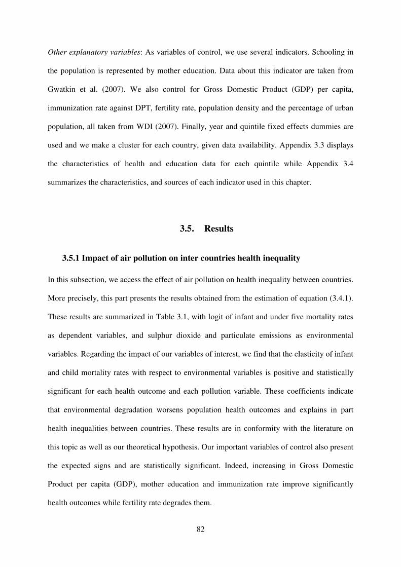
82

Other explanatory variables: As variables of control, we use several indicators. Schooling in

the population is represented by mother education. Data about this indicator are taken from

Gwatkin et al. (2007). We also control for Gross Domestic Product (GDP) per capita,

immunization rate against DPT, fertility rate, population density and the percentage of urban

population, all taken from WDI (2007). Finally, year and quintile fixed effects dummies are

used and we make a cluster for each country, given data availability. Appendix 3.3 displays

the characteristics of health and education data for each quintile while Appendix 3.4

summarizes the characteristics, and sources of each indicator used in this chapter.

3.5. Results

3.5.1 Impact of air pollution on inter countries health inequality

In this subsection, we access the effect of air pollution on health inequality between countries.

More precisely, this part presents the results obtained from the estimation of equation (3.4.1).

These results are summarized in Table 3.1, with logit of infant and under five mortality rates

as dependent variables, and sulphur dioxide and particulate emissions as environmental

variables. Regarding the impact of our variables of interest, we find that the elasticity of infant

and child mortality rates with respect to environmental variables is positive and statistically

significant for each health outcome and each pollution variable. These coefficients indicate

that environmental degradation worsens population health outcomes and explains in part

health inequalities between countries. These results are in conformity with the literature on

this topic as well as our theoretical hypothesis. Our important variables of control also present

the expected signs and are statistically significant. Indeed, increasing in Gross Domestic

Product per capita (GDP), mother education and immunization rate improve significantly

health outcomes while fertility rate degrades them.

83

Table 3. 1: Impact of air pollution on health inequalities between countries

Dependent variables

(1) (2) (3) (4)

independent variables child

mortality infant

mortality child

mortality infant

mortality

Sulphur dioxide emission (SO2) 0.0861** 0.0695**

(2.610) (2.692)

Particulate Matter (PM10) 0.125** 0.127**

(2.092) (2.254)

fertility rate 0.521*** 0.342*** 0.627*** 0.451***

(5.000) (3.233) (5.125) (3.530)

schooling -0.0661 -0.0616 -0.0211 -0.0155

(-1.615) (-1.564) (-0.544) (-0.430)

immunization rate -0.673*** -0.499*** -0.656*** -0.496***

(-4.412) (-3.611) (-4.069) (-3.401)

institution quality 0.0329 0.0396 0.0279 0.0346

(0.993) (1.321) (0.620) (0.899)

GDP per capita -0.358*** -0.234*** -0.304*** -0.186**

(-6.372) (-4.134) (-4.182) (-2.649)

urban population -0.0946 -0.0950 -0.0381 -0.0409

(-0.908) (-0.847) (-0.374) (-0.381)

population density 0.0115 0.0340 -0.0300 0.000896

(0.390) (1.269) (-1.215) (0.0355)

Constant 3.678*** 1.682** 1.173 -0.556

(4.267) (2.234) (1.274) (-0.612)

year dummies yes yes yes yes

quintile dummies yes yes yes yes

Observations 300 300 330 330

R-squared 0.87 0.78 0.86 0.79 ***significant at 1%, **significant at 5%, *significant at 10%. t-statistics enter parenthesis.

84

3.5.2 Heterogeneity in the health effect of air pollution (intra country

inequalities)

In the previous subsection, we found that pollution is in part responsible to health inequality

between countries. This section extends these results and explores whether environmental

degradation may contribute to within country income related health inequalities. It presents

the results obtained from the estimation of equation (3.4.2) and these results are summarized

in Table 3.2. In this table, the coefficients of interest are those of the interaction terms of

environmental variables and quintile dummies ( iλ ).

These coefficients are higher for poor quintiles as compare to those of richest quintiles. In

addition, they are negative and statistically significant for richest quintiles and not significant

for poorest quintiles. These results show that, environmental degradation degrades more the

health outcomes of poorest quintiles than it worsens those of the richest quintiles. This

heterogeneity in the health effect of air pollution increases income related health inequality

within country. These results are in conformity with our theoretical hypothesis and arguments.

Besides these findings, all the variables already analysed in previous subsection present the

correct signs and are statistically significant.

85

Table 3. 2: Impact of air pollution on health inequalities within countries

Dependent variables

Sulphur dioxide emission

(SO2) Particulate Matter

(PM10)

(1) (2) (3) (4)

Independent variables Child

mortality Inf. mortality Child

mortality Inf.

mortality

air pollution 0.129*** 0.116*** 0.208** 0.187**

(3.395) (3.459) (2.352) (2.238)

(air pollution)x(quintile 2) -0.0321 -0.0209 -0.0176 -0.0181

(-1.307) (-0.969) (-0.412) (-0.426)

(air pollution)x(quintile 3) -0.0479** -0.0592** -0.0511 -0.0394

(-2.021) (-2.268) (-0.978) (-0.694)

(air pollution)x(quintile 4) -0.0549* -0.0591 -0.0979 -0.0794

(-1.938) (-1.567) (-1.278) (-0.938)

(air pollution)x(quintile 5) -0.0823* -0.0934* -0.192** -0.128

(-1.706) (-1.680) (-2.256) (-1.514)

fertility rate 0.505*** 0.323*** 0.665*** 0.478***

(4.884) (3.063) (5.086) (3.500)

schooling -0.0776* -0.0754* -0.000414 -0.00177

(-1.848) (-1.928) (-0.00939) (-0.0425)

immunization rate -0.658*** -0.481*** -0.680*** -0.512***

(-4.337) (-3.571) (-4.204) (-3.470)

institution quality 0.0321 0.0387 0.0290 0.0353

(0.956) (1.277) (0.639) (0.904)

GDP per capita -0.357*** -0.232*** -0.303*** -0.185**

(-6.325) (-4.133) (-4.095) (-2.586)

urban population -0.0978 -0.0988 -0.0313 -0.0361

(-0.948) (-0.893) (-0.302) (-0.329)

population density 0.00958 0.0316 -0.0264 0.00340

(0.329) (1.202) (-1.028) (0.129)

Constant 4.242*** 2.286*** 0.740 -0.874

(4.871) (2.900) (0.737) (-0.866)


quintile dummies yes yes yes yes


R-squared 0.87 0.78 0.87 0.79 ***significant at 1%, **significant at 5%, *significant at 10%. t-statistics enter parenthesis.

86

3.5.3 Roles of political institutions in the health inequality effect of pollution

We have previously found that pollution is harmful for population health and the poorest

income classes are those that suffer more from this effect. This section is devoted to the roles

played by political institutions regarding this effect of air pollution on health inequality. It

shows the results obtained from the estimation of equation (3.4.3) and the findings are

presented in table 3.3.

In this table, we are interested by the coefficients of the interaction terms of environmental

variables, institutions and quintile dummies ( iγ ). These coefficients are higher for richest

quintiles than poorest quintiles. That result demonstrates that good political institutions

mitigate more the health effect of air pollution for the poorest quintiles than they do for

richest income classes. We can conclude that political institutions contribute to reduce the

health inequalities created by environmental degradation by mitigating its impact on the poor.

To test the robustness of our result to the choice of institutional indicator, we replace our

institutional variable (military in politics) by successively bureaucracy quality, corruption,

law and order, democracy accountability, internal conflict, and freedom status indices. The

results obtained are presented in Appendix 3.5 and they remain unchanged, namely, the

coefficients of the interaction terms of environmental variables, institutions and quintile

dummies ( iγ ) are higher for richest income quintiles as compared to poorest ones.

87

Table 3. 3: Social protection role of political institutions

Dependent variable Sulphur dioxide emission (SO2) Particulate Matter (PM10)

(1) (2) (3) (4) Independent variables Inf. mortality Child mortality Inf. mortality Child mortality air pollution 0.280*** 0.319*** 0.0718 0.0963 (2.996) (3.086) (0.467) (0.558) (air pollution)x(quintile 2) 0.0102 0.0116 0.129 0.156 (0.180) (0.232) (1.431) (1.599) (air pollution)x(quintile 3) -0.140 -0.109 0.0995 0.125 (-1.596) (-1.418) (1.022) (1.307) (air pollution)x(quintile 4) -0.107 -0.107 0.0323 0.0447 (-1.157) (-1.307) (0.220) (0.336) (air pollution)x(quintile 5) -0.290*** -0.281*** 0.0266 -0.00222 (-3.090) (-3.085) (0.229) (-0.0189) (institution)x(quintile 2) -0.117 -0.162 0.241* 0.287** (-0.557) (-0.788) (1.758) (2.072) (institution)x(quintile 3) 0.272 0.201 0.217 0.282* (1.009) (0.829) (1.386) (1.903) (institution)x(quintile 4) 0.146 0.162 0.162 0.222 (0.542) (0.645) (0.621) (0.939) (institution)x(quintile 5) 0.664** 0.675** 0.219 0.285 (2.282) (2.265) (0.908) (1.209) (institution)x(air pollution) -0.0388** -0.0449** 0.0401 0.0396 (-2.191) (-2.274) (0.749) (0.685) (institution)x(air pollution)x(quintile 2) -0.00852 -0.0121 -0.0585** -0.0688** (-0.500) (-0.719) (-2.033) (-2.255) (institution)x(air pollution)x(quintile 3) 0.0236 0.0179 -0.0568 -0.0710** (1.142) (0.957) (-1.636) (-2.120) (institution)x(air pollution)x(quintile 4) 0.0139 0.0144 -0.0438 -0.0551 (0.684) (0.736) (-0.766) (-1.047) (institution)x(air pollution)x(quintile 5) 0.0543** 0.0550** -0.0581 -0.0730 (2.532) (2.478) (-1.095) (-1.386) fertility rate 0.328*** 0.504*** 0.471*** 0.661*** (3.035) (4.552) (3.601) (5.274) schooling -0.107*** -0.107*** -0.0261 -0.0212 (-2.904) (-2.804) (-0.613) (-0.473) immunization rate -0.538*** -0.732*** -0.542*** -0.724*** (-4.374) (-4.650) (-4.176) (-4.859) GDP per capita -0.241*** -0.371*** -0.179** -0.299*** (-4.560) (-6.783) (-2.411) (-3.841) institution quality -0.434* -0.518** -0.110 -0.112 (-1.945) (-2.118) (-0.455) (-0.441) urban population -0.0944 -0.0953 -0.0272 -0.0177 (-0.939) (-1.016) (-0.238) (-0.157) population density 0.0551* 0.0358 0.0137 -0.0141 (1.765) (1.047) (0.487) (-0.500) Constant 4.588*** 6.981*** -0.318 1.295 (3.175) (3.996) (-0.289) (1.052) year dummies yes yes yes yes quintile dummies yes yes yes yes Observations 300 300 330 330 R-squared 0.80 0.88 0.79 0.87

88

3.6. Robustness checks

In the previous section we showed that air pollution is more disastrous for poor people’s

health (poor income quintiles health) than that of rich people (rich income quintile), and

therefore increases income related health inequality within population. One could argue that

these results suffer from at least three drawbacks. First, because environmental variable is not

disaggregated by asset quintile, we did not take into account country fixed effects and this

could bias our results. The second problem also comes from the structure of our data. In fact,

the dependent variables (health variables) are more disaggregated than the variables of

interest (environment and institution variables), and that may downward-bias the standard

deviations because of Moulton bias (Moulton, 1987 and 1990). Moulton (1990) demonstrated

that if the disturbances are correlated within the groupings that are used to merge aggregated

with micro data, the standard errors from Ordinary Least Squares (OLS) are seriously biased

downward. Third, one could argue that we assessed the effect of environment on health

inequality, but we did not use explicitly any health inequality indicator. To solve for this, we

replace health indicator by the range, more precisely we use as alternative dependent variable

the logarithmic form of the ratio of the first quintile of mortality rates to those of the fifth

quintile. This indicator is largely used in the literature to measure health inequality (Wagstaff

et al. 1991; Levine et al. 2001). That is, all the variables are expressed in country level.

'jt jt jt i jthealth X environmentβ δ µ ε= + + + (3.6.1)

The results obtained from the estimation of this equation with fixed effect are presented in

Appendix 3.6. The coefficients of environment indicators are positive and statistically

significant showing that air pollution increases mortality gap between rich and poor asset

groups in a given country, and this confirms our previous results.

89

To verify the role played by institutions quality in this effect of pollution on health inequality,

we add to the previous equation the interaction term of environment and institutional variables

and we obtain the following equation.

' ( * )jt jt jt jt jthealth X environment environment institutionβ δ ψ ε= + + + (3.6.2)

We also estimate this equation with fixed effect and the results are summarized in Appendix

3.7. The coefficients of environment indicators remain positive and statistically significant,

and those of the interaction terms are negative and significant.

These results confirm our previous findings, namely good political institutions contribute to

reduce the health inequalities created by environmental degradation. However, as argued by

Wagstaff et al. (1991), the range overlooks what is going on in the intermediate groups. The

gap between the first and the fifth quintiles might, for example, remain unchanged, but the

extent of inequality between the intermediate quintiles might well be diminishing (or

increasing). In addition, it does not take into account the sizes of the indicators being

compared. This can lead to misleading results when comparisons are performed over time or

across countries.

This can be solved by using as health inequality indicator, the concentration index of

mortality rates. This indicator is commonly used to represent health inequality, because of its

affinity with the Gini coefficient, its visual representation by means of the Concentration

Curve and the ease with which it can be decomposed. It can be calculated at individual level

as well as socioeconomic group level (income quintile level). It cannot be lower than -1 and

higher than 1. A negative (positive) value of the concentration index of mortality rates

designates a more concentrated mortality within poor (rich) people. A zero value indicates an

equal distribution of mortality according to income quintiles.

90

As argued by Erreygers (2006), this indicator is far from perfect. The first criticism is from

Wagstaff (2005). He argues that if the health variable is binary, the bounds of the

Concentration Index depend upon the mean of the health variable. The bounds turn out to be

much wider for populations with a low mean than for populations with a high mean. To

address this issue, he proposes to divide the health Concentration Index by its upper bound.

According to Erreygers (2006) Wagstaff procedure exaggerates the correction it applies to the

index and to its bounds, and an alternative solution has been formulated originally by

Wagstaff et al. (1991). This indicator called Generalized health Concentration Index is

obtained by multiplying the health Concentration Index by the average health level.

We use in this section as alternative health inequality indicator in equations (3.6.1) and (3.6.2)

the Generalized Concentration Index of mortality rates. The results obtained with fixed effects

estimator are presented in Appendix 3.8 and Appendix 3.9 respectuvely. They remain similar

to previous results.

3.7. Concluding remarks

This chapter extends economic literature on the association between environment and health

by investigating the responsibility of air pollution in the explanation of health inequalities

both between and within developing countries. It examines also the importance of the role

played by good political institutions in this effect.

We argue that population belonging to poorest income quintiles are those likely to suffer more

from environmental degradation, because they receive the highest exposure, and this exposure

then exercises larger effects on their health than it does on the average population.

Furthermore, richest communities have more prevention than poorest and have more access to

medical care when they are sick from pollution.

91

In countries with good political institutions, this heterogeneity in the health effect of pollution

may be mitigated since these institutions favour universal health policy issues, information

and advices about hygiene, and health infrastructures building.

Globally, our econometric results corroborate these theoretical arguments and hypothesis

about the positive association between air pollution and income related health inequalities. In

addition, our empirical results confirm the significant role played by democratic institutions in

protecting poor population from environmental degradation.

These important findings raise some policy implications. First, to be effective, health policies

should not be based only on average health of a given population, but also on its distribution.

In addition, differential distribution of health effects of pollution should be considered

alongside differential distribution of the benefits related to the emission sources. Indeed, those

who pollute more in a population, such as car ownership may compensate those who bear the

adverse effect by paying a tax. Finally, improving political institutions is not only important

for economic growth, but it is also essential for population wellbeing.

This study could be extended in many ways. Firstly, a limit of this work is doubtless the

unavailability of environmental data varying across income quintiles. This kind of data takes

into account the differential of exposure. Future works on this topic should solve for this and

test our hypothesis with more accurate data. Researchers may also use other environmental

and health indicators to verify our hypothesis. We focus only on developing countries. It will

be interesting to extend our results by testing whether they may be generalized for developed

countries or compare them across different geographical regions.

92

APPENDICES 3

Appendix 3.1: determinants of health inequality in the literature

Human capital in general and particularly population health is one of the most important

factors in economic development and a healthy labour force is essential for the development.

Average health in a population alone is not sufficient, since it could hide a large disparity in

health. Both mean health and health distribution should be considered. In economic literature,

many factors have been underlined as health inequality determinants.

- Income: The first determinant of inequalities is income and income inequality. In fact,

countries with higher income are more able to implement effective health policies and provide

high quality health services for all the population everywhere. A simple example is the

availability of hospitals and physicians in developed countries. In poor countries, high quality

health services are concentrated in big cities and only a small amount of population has

access. Income inequality also explains health disparities because individual income level

affects health through its effect on consumption behaviour (against malnutrition), drinking

water quality (hygiene), clothes, housing, preventive cure and information. Inequality in

health, then, increases difference in health outcomes within individuals. Ourti et al (2009)

show that, theoretically, both income growth and reductions in social inequalities in health

and income can be achieved only under very specific conditions concerning the type of

growth and the income responsiveness of health. According to them, income growth and

income inequality have a direct and indirect effect on income-related health inequality. The

sign of the direct effects can be derived a priori, but not of the indirect effects. The expected

93

direct effect of proportional income growth depends crucially on the slope of the income

elasticity. If this elasticity is rising (decreasing) with income on average, income-related

health inequality will increase (decline). With respect to the direct effect of changes in income

inequality, they find increasing (decreasing) income-related health inequality in case of on

average pro-rich (pro-poor) evolving income inequality in combination with an income

elasticity that increases (decreases) with income on average. They investigate empirically

whether these conditions were met in Europe in the 1990s using panel data from the European

Community Household Panel. Their results show that in most countries, the income elasticity

of health was positive and increases with income, and that income growth was not pro-rich in

most European countries, resulting in small or negligible reductions in income inequality. The

combination of both findings explains the modest increases in income-related health

inequality in the majority of countries. Tubeuf (2009) used an innovative methodology to

measure income related health inequalities using the concentration index, and investigated the

relationships between income, income inequality, various social determinants, and health. His

results show an income-related health inequality favouring individuals with a higher income.

Moreover, income level, supplementary private health insurance, education level, and social

class account for the main contributions to inequality. Therefore reducing income inequality is

not sufficient to lower income-related health inequalities and needs to be supplemented with

the reduction of the relationship between income and health and the reduction of income

inequality over socioeconomic status.

- Education: The distribution of education also may provoke health inequality within a

population, (Grossman, 1972; Schultz, 2002) since education influences consumption

behaviour and improves knowledge about health care (hygiene, contraception). In addition,

more educated people know about and ask for beneficial health procedure such as quitting

94

smoking; getting flu shots; wearing seat belts and driving a car with airbags; eating fruits and

vegetables; exercising regularly. Rahkonen et al. (1995) compare whether the relationship

between social class and health is similar among young men and women at different age

groups in Britain and Finland and examine at what age social class differences in self-reported

health and illness among young adults emerge. They found that the best discriminator of

differences in ill-health among young adults both in Finland and Britain was education.

- Distribution of health care services: The disparities in the availability of health care services

across regions of a country induce health inequality since some populations easily have access

to health services and other cannot have access to such services when they need them. Using

cross-sectional data from 31 provinces, Fang et al (2010) measured the degree of regional

health inequality in China and identified its determinants through canonical correlation

analysis. They found that there existed distinct regional disparities in health in China, which

were mainly reflected in Maternal & Child Health and Infectious Diseases, not in the average

life expectancy. They also showed that the regional health inequality was associated with not

only the distribution of wealth, but also the distribution of health resources and primary health

care services.

- Place and neighbouring: Place and neighbouring also may influence health inequality.

Using place as a relational space linked to where people live, work and play, Bernard et al.

(2007) conceptualise the nature of neighbourhoods as they contribute to the local production

of health inequalities in everyday life. They propose that neighbourhoods essentially involve

the availability of, and access to, health-relevant resources in a geographically defined area.

They argue that such availability and access are regulated according to four different sets of

rules: proximity, prices, rights, and informal reciprocity. Their theoretical framework

95

supposes that these rules give rise to five domains, the physical, economic, institutional, local

sociability, and community organisation domains which cut across neighbourhood

environments through which residents may acquire resources that shape their lifecourse

trajectory in health and social functioning.

- Health insurance: Countries with effective health insurance system are more likely to have

less disparity in health outcomes. In fact, health insurance increases the access to health care

services by reducing the burden of health cost and by improving prevention. In his analysis

Tubeuf (2009) shows that health insurance contributes to reduce health inequality.

96

Appendix 3.2: list of countries in the regression sample country name Year country name Year Armenia 2000 Madagascar 1997 Benin 1996, 2001 Mali 1995, 2001

Burkina Faso 1992, 1998, 2003 Mozambique 1997, 2003

Bangladesh 1996, 1999, 2004 Mauritania 2000

Bolivia 1998, 2003 Malawi 1992, 2000 Brazil 1996 Namibia 1992, 2000 Central African Republic 1994 Niger 1998 Côte d'Ivoire 1994 Nigeria 1990, 2003

Cameroon 1991, 1998, 2004 Nicaragua 1997, 2001

Colombia 1995, 2000, 2005 Nepal 1996, 2001

Comoros 1996 Pakistan 1990 Dominican Republic 1996, 2002 Peru 1996, 2000 Egypt 1995, 2000 Philippines 1998, 2003 Eritrea 1995 Paraguay 1990 Ethiopia 2000 Rwanda 2000 Gabon 2000 Senegal 1997

Ghana 1993, 1998, 2003 Chad 1996, 2004

Guinea 1999 Togo 1998 Guatemala 1995, 1998 Turkmenistan 2000 Haiti 1994, 2000 Turkey 1993, 1998

Indonesia 1997, 2002 Tanzania 1996, 1999, 2004

India 1992, 1998 Uganda 1995, 2000 Jordan 1997 Uzbekistan 1996 Kazakhstan 1995, 1999 Vietnam 1997, 2002

Kenya 1993, 1998, 2003 Yemen 1997

Kyrgyzstan 1997 South Africa 1998 Cambodia 2000 Zambia 1996, 2001 Morocco 1992, 2003 Zimbabwe 1994, 1999

97

Appendix 3.3: Summary Statistics by quintile

Variables Obs Mean Std. Dev. Min Max

Full sample

Infant mortality (a) 380 72.13 33.75 11.90 187.70

Child mortality (b) 380 113.80 67.00 14.20 354.90

Fertility rate (c) 380 4.55 1.80 1.20 8.50

Female educational attainment (d) 380 50.44 31.94 0.50 99.80

Poorest quintile (based on an "asset index")



Fertility rate (c) 76 5.92 1.48 2.20 8.50


Second quintile



Fertility rate (c) 76 5.14 1.55 1.80 8.20


Third quintile



Fertility rate (c) 76 4.68 1.65 1.40 7.80


Fourth quintile



Fertility rate (c) 76 4.02 1.61 1.50 7.20


Richest quintile



Fertility rate (c) 76 2.96 1.15 1.20 6.20


Notes : (a) Infant mortality: number of deaths to children under twelve months of age per 1,000 live births, based on experience during the ten years before the survey. (b) Child mortality: number of deaths to children under five years of age per 1,000 live births, based on experience during the ten years before the survey. (d) Fertility rate: average number of births a woman could expect to have during her lifetime if she followed the levels of fertility currently observed at every age. The TFR is calculated as the sum of average annual age specific fertility rates for all reproductive age groups (usually 15-49 years) in the three years before the survey. (c) Female educational attainment: percent of women aged 15-49 years who had completed the fifth grade

98

Appendix 3.4. Data characteristics and sources

Variables mean min max Coef. var. Obs. characteristics Sources

Infant mortality rate 74,65 22,1 147,4 0,39 95

Number of deaths to children under twelve months of age per 1,000 live births, based on experience during the ten years before the

survey. Gwatkin et al. (2007)

Under five mortality rate 118,6 25,7 302,6 0,51 95

Number of deaths to children under five years of age per 1,000 live births, based on experience during the ten years before the

survey. Gwatkin et al. (2007)

Sulphur dioxide emission (SO2)

239,86 0,53

2926,53 2,18 73 sulphur dioxide emission

Stern (2005)

Particulate Matter (PM10) 77,99 7,3 225,86 0,62 82 particulate matter less than 10 µm aerodynamic diameter WDI 2007

urban population percentage 38,43 11,4 80,1 0,47 95 Proportion of urban population WDI 2007

99

Variables mean min max Coef. var. Obs. characteristics Sources

population density 110,19 1,85 1156,4 1,75 95 Population density WDI 2007

fertility rate 5,88 2,2 8,5 0,26 95

Average number of births a woman could expect to have during her lifetime if she followed the levels of fertility currently observed at

every age.

Gwatkin et al. (2007)

schooling 30,25 0 99,1 0,92 94 Percent of women aged 15-49 years who had completed the fifth

grade. Gwatkin et al. (2007)

GDP per capita 815,38

120,11 4286,5 1,03 95 Gross Domestic Product per capita WDI 2007

100

Appendix 3.5: Robustness checks : Social protection role of political institutions.

Dependent variables

(1) (2) (3) (4) (5) (6) (7) (8) (9) (10) (11) (12)

Independent variables inf. mort. child mort. inf. mort. child mort. inf. mort. child mort. inf. mort. child mort. inf. mort. child mort. inf. mort. child mort.

air pollution 0.153** 0.153*** 0.184** 0.196** 0.0339 0.0110 0.120* 0.114 0.0509 0.104 0.223** 0.259***

(2.683) (2.862) (2.225) (2.654) (0.447) (0.147) (1.953) (1.632) (0.498) (0.829) (2.665) (2.936)

(air pollution)x(quintile 2) 0.0341 0.0290 0.0596 0.0627* 0.0984*** 0.0846** 0.0760** 0.0607* 0.119* 0.107 0.0602 0.00915

(0.758) (0.963) (1.351) (1.712) (3.565) (2.437) (2.048) (1.886) (1.860) (1.489) (0.836) (0.149)

(air pollution)x(quintile 3) -0.0580 -0.0320 -0.0224 0.00145 0.0447 0.0865* -0.0640 -0.0332 -0.0908 -0.0568 -0.128* -0.102*

(-1.049) (-0.621) (-0.306) (0.0244) (0.801) (1.877) (-0.807) (-0.500) (-1.110) (-0.798) (-2.004) (-1.772)

(air pollution)x(quintile 4) -0.137* -0.0948 -0.116 -0.0940 -0.0262 0.0497 -0.150** -0.106* -0.119 -0.119 -0.163* -0.151*

(-1.842) (-1.293) (-0.772) (-0.795) (-0.420) (0.943) (-2.152) (-1.964) (-1.146) (-1.300) (-1.905) (-1.859)

(air pollution)x(quintile 5) -0.245*** -0.181** -0.234 -0.177 0.00118 0.0739 -0.116 -0.0857 -0.379*** -0.317*** -0.457*** -0.417***

(-3.602) (-2.444) (-1.571) (-1.365) (0.00734) (0.508) (-0.759) (-0.614) (-3.361) (-3.024) (-4.204) (-4.459)

(institution)x(quintile 2) -0.355 -0.387*** -0.364** -0.430*** -0.725*** -0.694*** -0.400*** -0.385** -0.518** -0.520* -0.117 -0.0543

(-1.542) (-2.958) (-2.369) (-2.777) (-4.960) (-2.950) (-2.907) (-2.406) (-2.121) (-1.769) (-1.013) (-0.489)

(institution)x(quintile 3) 0.0590 -0.0332 -0.164 -0.221 -0.605* -0.759*** 0.00889 -0.0641 0.126 0.0423 0.115 0.0936

(0.228) (-0.141) (-0.585) (-0.975) (-1.940) (-3.107) (0.0352) (-0.302) (0.438) (0.163) (1.250) (1.074)

(institution)x(quintile 4) 0.623 0.370 0.264 0.182 -0.0138 -0.467 0.363 0.199 0.238 0.273 0.170 0.162

(1.456) (0.954) (0.404) (0.368) (-0.0343) (-1.523) (1.403) (0.972) (0.627) (0.866) (1.328) (1.350)

(institution)x(quintile 5) 1.124** 0.764* 0.644 0.434 -0.445 -0.813 0.0739 0.00179 1.080** 0.900** 0.559*** 0.522***

(2.631) (1.832) (0.917) (0.725) (-0.430) (-0.882) (0.126) (0.00334) (2.608) (2.278) (3.398) (3.666)

(institution)x(air pollution)x(quintile 2) -0.0252 -0.0265*** -0.024** -0.0296** -0.060*** -0.0584*** -0.0312*** -0.0298** -0.0411** -0.0406* -0.0103 -0.00561

(-1.531) (-2.956) (-2.077) (-2.359) (-4.785) (-2.907) (-2.805) (-2.274) (-2.186) (-1.782) (-1.142) (-0.633)

(institution)x(air pollution)x(quintile 3) 0.0110 0.00482 -0.00615 -0.0102 -0.0507** -0.0633*** 0.00237 -0.00449 0.00855 0.00225 0.00746 0.00583

(0.562) (0.279) (-0.296) (-0.584) (-2.057) (-3.212) (0.124) (-0.277) (0.413) (0.120) (1.077) (0.850)

(institution)x(air pollution)x(quintile 4) 0.0563* 0.0380 0.0268 0.0203 -0.00539 -0.0410* 0.0300 0.0171 0.0161 0.0170 0.0115 0.0105

(1.765) (1.328) (0.553) (0.558) (-0.180) (-1.814) (1.544) (1.114) (0.597) (0.740) (1.175) (1.138)

(institution)x(air pollution)x(quintile 5) 0.0956*** 0.0678** 0.0541 0.0377 -0.0326 -0.0649 0.00793 0.000878 0.0813*** 0.0666** 0.0430*** 0.0392***

(3.081) (2.261) (1.006) (0.827) (-0.417) (-0.927) (0.177) (0.0217) (2.754) (2.372) (3.386) (3.558)

(institution)x(air pollution) -0.0188 -0.0147 -0.0279 -0.0274 0.0344 0.0507 -0.000535 0.00673 0.0192 0.00839 -0.0109 -0.0134

(-0.644) (-0.538) (-1.044) (-1.142) (1.032) (1.488) (-0.0283) (0.326) (0.660) (0.248) (-1.373) (-1.606)

fertility rate 0.353*** 0.528*** 0.336*** 0.515*** 0.419*** 0.694*** 0.338*** 0.520*** 0.342*** 0.524*** 0.360*** 0.546***

(3.085) (4.843) (3.108) (4.938) (3.540) (5.686) (2.937) (4.565) (2.977) (4.807) (3.542) (5.887)

101

Dependent variables

(1) (2) (3) (4) (5) (6) (7) (8) (9) (10) (11) (12)

Independent variables inf. mort. child mort. inf. mort. child mort. inf. mort. child mort. inf. mort. child mort. inf. mort. child mort. inf. mort. child mort.

schooling -0.0862** -0.0859* -0.0744* -0.0765* -0.0601* -0.0747* -0.0833** -0.0863* -0.0904** -0.0864* -0.0870** -0.0853*

(-2.119) (-1.943) (-1.891) (-1.818) (-1.680) (-1.985) (-2.035) (-1.948) (-2.092) (-1.860) (-2.114) (-2.009)

immunization rate -0.380*** -0.583*** -0.47*** -0.650*** -0.228* -0.339** -0.428*** -0.601*** -0.402*** -0.603*** -0.343** -0.524***

(-2.864) (-3.780) (-3.513) (-4.293) (-1.831) (-2.243) (-3.099) (-3.808) (-2.790) (-3.541) (-2.398) (-3.173)

GDP per capita -0.219*** -0.342*** -0.23*** -0.353*** -0.235*** -0.328*** -0.237*** -0.357*** -0.220*** -0.350*** -0.242*** -0.370***

(-3.303) (-4.851) (-4.014) (-6.142) (-4.226) (-5.305) (-4.231) (-6.093) (-3.865) (-5.953) (-4.328) (-6.719)

institution quality -0.225 -0.154 -0.268 -0.266 0.395 0.599 0.0280 0.0887 0.249 0.0986 -0.180 -0.220*

(-0.575) (-0.420) (-0.772) (-0.882) (0.886) (1.340) (0.113) (0.329) (0.581) (0.198) (-1.668) (-1.988)

urban population -0.104 -0.106 -0.102 -0.104 -0.0642 -0.0570 -0.0913 -0.0906 -0.101 -0.0939 -0.0918 -0.0887

(-0.843) (-0.896) (-0.879) (-0.952) (-0.649) (-0.574) (-0.832) (-0.842) (-0.953) (-0.942) (-0.813) (-0.825)

population density 0.0377 0.0153 0.0349 0.0132 0.0393 0.0377 0.0278 0.00991 0.0213 0.00474 0.0203 -0.00226

(1.390) (0.497) (1.308) (0.443) (1.312) (1.134) (1.059) (0.317) (0.680) (0.140) (0.678) (-0.0690)

Constant 2.240* 4.105*** 2.953** 4.893*** -0.0392 0.726 2.121* 3.812*** 1.201 3.752* 3.484** 5.803***

(1.916) (3.652) (2.319) (3.903) (-0.0349) (0.609) (1.878) (2.964) (0.779) (1.987) (2.632) (4.056)

Institution indicators Bureaucracy quality corruption index freedom status democracy accountability law and order internal conflict

year dummies yes yes yes yes yes yes yes yes yes yes yes yes

quintile dummies yes yes yes yes yes yes yes yes yes yes yes yes

Observations 300 300 300 300 360 360 300 300 300 300 300 300

R-squared 0.80 0.88 0.79 0.87 0.74 0.84 0.79 0.87 0.79 0.87 0.79 0.87 ***significant at 1%, **significant at 5%, *significant at 10%. t-statistics enter parenthesis.

103

Appendix 3.6: Effect of air pollution on health inequality

Dependent variable: log of the Ratio of poorest quintile to richest quintile of infant mortality rate (Q1/Q5)

VARIABLES (1) (2)

Sulphur dioxide emission (SO2) 0.0541***

(4.045)

Particulate Matter (PM10) 0.968***

(5.412)

fertility rate ratio (Q1/Q5) 0.838*** 0.760***

(8.662) (3.411)

Schooling ratio (Q1/Q5) 1.086 3.883**

(1.330) (2.493)

Schooling 68.78*** -29.04

(4.057) (-1.550)

Institution quality -0.159*** 0.0720

(-3.688) (1.301)

GDP per capita -4.016*** 0.668

(-8.938) (1.597)

Immunization ratio (Q1/Q5) 3.294*** 1.688*

(11.45) (1.690)

Constant 18.70*** -9.814***

(7.569) (-2.880)

Fixed effects yes yes

Quintiles dummy yes yes

Observations 60 66

R-squared 0.94 0.84 Note: ***significant at 1%, **significant at 5%, *significant at 10%. t-statistics enter

parenthesis.

104

Appendix 3.7: Role of political institutions in the effect of air pollution on health inequality

Dependent variable: log of the Ratio of poorest quintile to richest quintile of infant mortality rate

(Q1/Q5)

VARIABLES (1) (2) (3) (4)

Sulphur dioxide emission (SO2) 0.371* 0.967*** 1.100*** 0.305***

(1.991) (22.92) (5.070) (5.538)

(Sulphur dioxide emission)x(institution) -0.0783* -0.286*** -0.265*** -0.0297***

(-1.707) (-21.10) (-5.145) (-5.442)

Institution quality -1.193* -4.066*** -4.054*** -0.422***

(-1.965) (-22.08) (-5.565) (-6.242)

fertility rate ratio (Q1/Q5) 1.188*** 1.737*** 0.820*** 1.089***

(4.454) (39.10) (11.23) (10.87)

Schooling ratio (Q1/Q5) 1.601* 4.732*** 0.612 1.809***

(1.914) (22.33) (1.188) (3.694)

Schooling 78.34*** 39.00*** 15.19 34.35***

(5.885) (13.63) (1.504) (4.555)

GDP per capita -5.412*** -4.361*** -0.0215 -3.888***

(-5.172) (-40.11) (-0.0559) (-8.264)

Immunization ratio 4.205*** 6.444*** 2.572*** 3.828***

(6.187) (38.85) (17.13) (13.25)

Constant 29.58*** 28.92*** 12.48*** 21.92***

(3.847) (29.48) (5.295) (6.692)

Institution quality indicator corruption index

Bureaucracy quality

law and order

internal conflict

Fixed effects yes yes yes yes



R-squared 0.95 0.99 0.97 0.96 Note: ***significant at 1%, **significant at 5%, *significant at 10%. t-statistics enter

parenthesis.

105

Appendix 3.8: Effect of air pollution on health inequality

Dependent variable: Generalized Concentration index of

infant mortality rate

VARIABLES (1) (2)

Sulphur dioxide emission (SO2) -0.00121***

(-5.911)

Particulate Matter (PM10) -0.00883***

(-4.525)

fertility rate ratio (Q1/Q5) -0.00479*** -0.00815***

(-2.983) (-3.935)

schooling concentration index -1.122 2.619***

(-1.565) (4.966)

schooling -1.396*** 0.0986

(-7.114) (0.523)

Institution quality 0.00446*** -0.00225***

(4.148) (-3.166)

GDP per capita 0.0732*** -0.00914

(8.958) (-1.622)

Immunization ratio (Q1/Q5) -0.0122*** 0.0135

(-3.754) (1.477)

Constant -0.390*** 0.0650

(-9.511) (1.596)

Fixed effects yes yes

year dummies yes yes

Observations 60 66

R-squared 0.97 0.77 Note: ***significant at 1%, **significant at 5%, *significant at 10%. t-statistics enter

parenthesis.

106

Appendix 3.9: Role of political institutions in effect of air pollution on health inequality

Dependent variable: Generalized Concentration index of infant mortality rate

VARIABLES (1) (2) (3) (4)

Sulphur dioxide emission (SO2) -0.00671*** -0.00798*** -0.0285*** -0.00414***

(-37.62) (-70.49) (-14.90) (-36.68) (Sulphur dioxide emission)x(institution) 0.00140*** 0.00242*** 0.00695*** 0.000398***

(29.64) (65.79) (14.66) (38.15)

Institution quality 0.0220*** 0.0331*** 0.107*** 0.00641***

(39.67) (66.75) (14.36) (39.77)

fertility rate ratio (Q1/Q5) -0.0115*** -0.0133*** -0.0036*** -0.0105***

(-32.50) (-180.1) (-4.670) (-64.31)

schooling concentration index -0.416*** 0.344*** -0.444*** -0.0460***

(-4.366) (80.10) (-6.109) (-3.082)

schooling -1.455*** -0.626*** 0.209*** -0.413***

(-46.64) (-91.34) (4.103) (-21.31)

GDP per capita 0.0912*** 0.0539*** -0.0372*** 0.0621***

(78.93) (176.8) (-5.696) (41.23)

Immunization ratio (Q1/Q5) -0.0237*** -0.0230*** 0.00338** -0.0191***

(-42.15) (-51.19) (2.444) (-26.11)

Constant -0.555*** -0.389*** -0.171*** -0.406***

(-77.07) (-146.1) (-8.083) (-38.31)

Institution quality indicator corruption

index Bureaucracy

quality law and

order internal conflict

Fixed effects yes yes yes yes



R-squared 0.98 0.98 0.99 0.99

Note: ***significant at 1%, **significant at 5%, *significant at 10%. t-statistics enter parenthesis.

107

Part II: health, environment and

economic growth

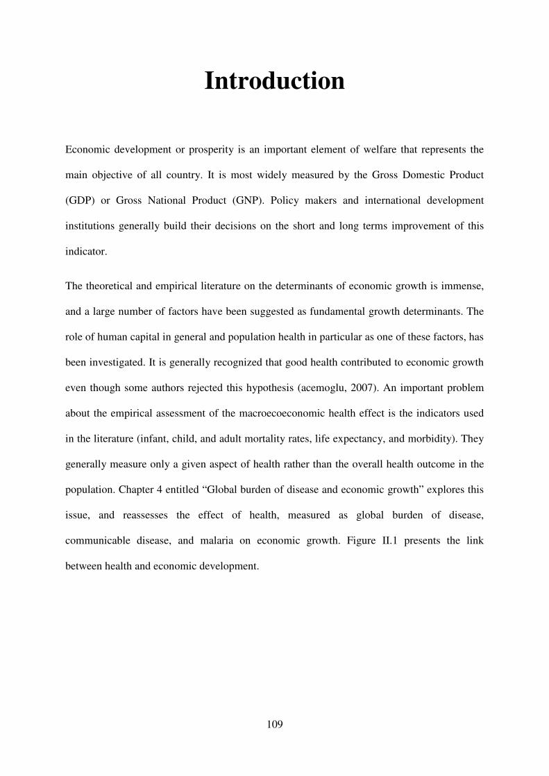
109

Introduction

Economic development or prosperity is an important element of welfare that represents the

main objective of all country. It is most widely measured by the Gross Domestic Product

(GDP) or Gross National Product (GNP). Policy makers and international development

institutions generally build their decisions on the short and long terms improvement of this

indicator.

The theoretical and empirical literature on the determinants of economic growth is immense,

and a large number of factors have been suggested as fundamental growth determinants. The

role of human capital in general and population health in particular as one of these factors, has

been investigated. It is generally recognized that good health contributed to economic growth

even though some authors rejected this hypothesis (acemoglu, 2007). An important problem

about the empirical assessment of the macroecoeconomic health effect is the indicators used

in the literature (infant, child, and adult mortality rates, life expectancy, and morbidity). They

generally measure only a given aspect of health rather than the overall health outcome in the

population. Chapter 4 entitled “Global burden of disease and economic growth” explores this

issue, and reassesses the effect of health, measured as global burden of disease,

communicable disease, and malaria on economic growth. Figure II.1 presents the link

between health and economic development.

110

Figure II. 1: Interrelationships between environment, health, and economic development

(+)

(-)/(+) (+) (+)

EKC

(-)

Source : Author

Despite the large literature on the empirical studies on growth determinants, some important

potential omitted determinants remain less investigated, such as environmental quality. In fact

as shown in Figure II, environmental degradation may affect economic activity directely, or

indirectely through the reduction of the level and the productivity of human capital. Air

pollutions measured by CO2, SO2, NOx, CO, traffic noise, affect health and leave people

unable to work over short or long periods and reduce the productivity of those who work. The

assessment of this impact is crucial since it gives additional support on the importance of

environmental quality to policy makers.

By illustrating the link between population health and economic growth on one the hand, and

the relationship linking economic development to environmental quality on the other hand,

Figure II.1 highlights the simultaneous association between environment, health, and

Environmental Quality

Economic Convergence

Health Status

Economic Development

111

economic development. These interrelationships between the three pillars of sustainable

development are less approached in the literature from our knowledge despite the importance

of the implications in terms of policy recommendation. Indeed, these interrelationships

penalizes the economic progress in developing countries unlike in developed ones, and reduce

the ability of poor countries to catch up rich ones. This reduction of the speed of economic

convergence is shown in Figure II.1.

Chapter 5, entitled “Interrelationships among health, environment quality and economic

activity: What consequences for economic convergence?” deals with these issues by (i)

analyzing environmental variables as additional determinant of economic growth, (ii)

investigating the interrelationships between environment, health, and economic development,

and (iii) assessing the effect of environmental degradation on economic convergence.

On the whole, it is shown that water and air pollutions are important determinants of

economic growth, and reduce the ability of poor countries to decrease the gap with developed

economies. In addition, the detrimental effect of poor health on economic growth is not

rejected.

113

Chapter 4: Global burden of disease

and economic growth12

12

This chapter was written in collaboration with Dr. Martine Audibert and Prof. Pascale Combes Motel. A shorter version was submitted to Journal of Health Economics.

115

4.1. Introduction

Human capital investments are known for a long time as basic candidates explaining

growth performances (e. g. Schultz, 1961). Sen’s works on human capabilities and the

emergence of AIDS have renewed the interest given to the link between health, welfare, and

prosperity. At a microeconomic level, several studies found that poor health have negative

effects on economic prosperity and living conditions.13 At a macroeconomic level, the

Commission on Macroeconomics and Health (2001) concluded that diseases raise barriers to

economic growth and that countries have to invest in health. Several authors have considered

that communicable diseases, among others, had contributed to slow down economic

development of low income countries. The latter proposition is still hotly debated as some

methodological issues are not satisfactorily addressed (see the comprehensive and critical

review of Packard, 2009). For instance, Acemoglu and Johnson (2006), using international

data from the epidemiological transition period, find that an increase in life expectancy

generated by a decrease in mortality rates had a small positive effect on growth which grows

over the post epidemiological transition. The latter was not enough important to compensate

for increases in population. This study makes reminiscent previous results of Barlow (1968)

with regard to malaria eradication and of Over (1992) with regard to economic effects of

AIDS as well. In the same vein, Bell, Bruhns and Gersbach (2006), using an overlapping

generations model simulate relaxed effects of AIDS on economic growth in Kenya by 2050.

There are at least three reasons that could explain difficulties to assess health impacts at the

macroeconomic level and therefore fuel the debate. First, links between health and

development or growth are complex and health effect could, as we saw in Chapter 4, also be

13 The literature on links between health and economic well-being or prosperity at microeconomic level is abundant. See e.g. Strauss and Thomas (2007) for literature review.

116

channelled by education levels, the environment, and cultural behaviours as well. When, due

to missing adequate indicators, these behaviours are not dealt for in the model, the estimated

health effect will be biased or hidden by unobserved heterogeneity (Thomas, 2009; Strauss

and Thomas, 2007; Hurd and Kapteyn, 2003). Second, health is subject to measurement errors

due to poor measurement facilities such as lack of good equipment and materials for setting

appropriate diagnosis, as well as low human resource training, deficient registration,

measurement variability over the day (e.g. blood pressure) or the year (e. g. malaria

indicators). Third, health status is a rather complex notion that includes several dimensions.

Researchers face a wide array of health indicators addressing one specific dimension of

health. Consequently, using one or the other is not equivalent.

Partly due to these difficulties of measuring multiple dimensions of health and therefore

global health status, macroeconomic effects of health have been more still studied using

health indicators such as life expectancy at birth, infant mortality rates, or nutritional status

measures. Existing results can be questioned by addressing specifically the choice of health

status indicators, which is the subject of this Chapter.

The rest of the chapter is organized as follows. Section 2 is devoted to health measurement

issue. Different measures of health indicators used in the growth literature are discussed

before exploring the more global one on which the analysis is focused. Section 3 reviews the

theoretical and empirical literature on the link between health outcomes and economic

performances. The empirical setting and the results are presented in section 4 and 5. Section 6

concludes.

117

4.2. Looking for a global health indicator

Health measurement is a hard task since, contrary to economic indicators, health is multi-

dimensional,14 and measured with errors. Moreover, researchers, either in a perspective of

public health initiatives, health research, or economic health research, have been developing a

wide array of health indicators, among which few however are satisfactorily measured

(Murray and Frenk, 2008; Murray, 2007).15 If it is crucial to understand what each indicator

measures (Strauss and Thomas, 2008), it is also important to insure that health indicators fit

the purposes of studies.

The most commonly used indicators of health conditions at the macroeconomic level are

life expectancy at birth and infant mortality rates (Strauss and Thomas, 2008). Those

indicators are considered reflecting the general health conditions and supposed to be

positively associated with economic growth. It is true that life expectancy at birth is higher

and infant mortality lower in richer countries than in poorer countries. Indeed, the correlation

between life expectancy at birth and GDP per capita is not systematic as life expectancy is

lower (or higher) than expected given GDP per capita in countries like Southern Africa,

Gabon or Indonesia (for examples, see Strauss and Thomas, 2008). Per capita incomes have

diverged over time while life expectancy and infant mortality have converged (Deaton, 2006;

Jack and Lewis, 2009). Life expectancy and infant mortality are inadequate indicators of the

population’s health in high income countries and for several upper middle income countries

where life expectancy at birth is high and infant mortality very low or low. For low and lower

middle income countries, those indicators are more adequate due to their poor levels. For that

14 Whatever the approach chosen (medical, self-assessment or functional) for measuring health, poor health is considering as a deviation between the observed health and a norm. This deviation may occur into either, physical, mental, or social well-being dimension.

15 For a discussion on the issue and challenge of health measurement, see Mwabu, 2007; Strauss and Thomas, 2008; Murray and Frenk, 2008; Audibert, 2009).

118

reason, studying the relationships between health and economic development or growth in

cross-country studies using infant mortality or life expectancy at birth is not really

appropriate, mainly due to the fact that it does not exhibit enough variability in upper middle

and high income countries.

As underlined by Jack and Lewis (2009), the effect of a population’s health status on

national income varies accordingly with the health indicator used. Most health indicators used

in the literature capture one dimension of the population health. They either relate to fatal (life

expectancy,16 mortality indicators) or to non-fatal (morbidity indicators) issue of illness

(Audibert, 2009). For example, the emergence of HIV/AIDS and its high prevalence (more

than 15%) in some southern African countries (Botswana, Lesotho, Namibia, South Africa,

Swaziland, Zambia, and Zimbabwe, UNAIDS17), have both motivated several studies

focusing on their economic effects. But, little evidence of a correlation between HIV/AIDS

and GDP per capita was found (Strauss and Thomas, 2008). With the renewed interest for

malaria, some authors (Sachs and Malaney, 2002; McCarthy, Wolf and Wu, 2000) have

investigated its effect on African countries growth. But, those indicators neither take into

account other dimensions of health, such as invalidity, handicap or social consequences, nor

multidimensional characteristics of health.

The main thesis of this chapter is that macroeconomic effects of the global health status are

accurately caught by the Disability-Adjusted Life Year (DALY) per capita calculated by the

World Health Organization (WHO). This indicator was put forward by the World Bank and

the World Health Organisation in 1993 (the World Bank, 1993). It represents “a one lost year

of healthy life and extends the concept of potential years of life lost due to premature death to

16 In low income countries, life expectancy is mainly determined by infant mortality, and also in countries where AIDS prevalence is high, by AIDS mortality.

17 http://www.unaids.org/en/CountryResponses/Regions/SubSaharanAfrica.asp.

119

include equivalent years of healthy life lost by virtue of being in states of poor health or

disability” (WHO, 2008).18 “The sum of the DALYs across the population represents the

burden of disease and can be thought of as a measurement of the gap between current health

status and an ideal health situation where the entire population lives to an advanced age, free

of disease and disability” (WHO, 2008). DALYs were calculated initially for about one

hundred causes and diseases and all over the world and were not updated since 2000. From

2000 to 2004 however, DALYs are also available on a regional basis. DALYs are commonly

used in cost-effectiveness analyses but, to the best of our knowledge, have never been used in

macroeconomic analyses since DALYs at the country level are only available for 2002 and

2004.

Any indicator, including DALYs, is amenable to criticism with a particular emphasis on

weighting (namely age and disease severity) and discounting (e.g. Anand and Hanson, 1998).

A large revision has been however implemented, mainly by the Institute of Health Metrics,

which is in charge of DALYs updating (Lopez et al, 2006). This does not prevent however

this indicator from being a serious candidate for representing population global health status,

deriving from illness consequences which are taken into consideration in a single indicator.

Appendix 4.1, Appendix 4.2, Appendix 4.3 and Appendix 4.4 present the relationships

between different DALY indicators and traditional health measures (Life Expectancy at birth,

Infant Mortality Rate and Child Mortality Rate) as well as GDP per capita. It appears clearly

that even though there is a positive correlation between DALYs and traditional health

indicators, the correlation between them is far from perfect.

18 The DALYs for each health condition are the sum of the years of life lost (YLL) due to premature mortality and the years lost due to disability (YLD) for incident cases of the health condition. YLL are calculated from the number of deaths at each age multiplied by a global standard life expectancy for each age. YLD is the number of incident cases in a particular period × average duration of the disease × weight factor. The weight factor reflects the severity of the disease on a scale from 0 (perfect health) to 1 (death). For additional information, see WHO, http://www.who.int/healthinfo/global_burden disease/metrics_daly/en/.

120

4.3. Relationship between health and growth

This chapter lies on the idea of health being a capital: people are endowed an initial stock

which can depreciate through time with age but which is the subject of investments

(Grossman, 1972; see Mwabu, 2007 for a literature review on the concept of health capital).

From such a perspective, Van Zon and Muysken (2005) mention two positive effects of health

on economic growth. First, a better health status of population increases labour efficiency;

second, human capital accumulation requires “health hours”. These effects add to those of

Bloom and Canning (2000) who argue that improvements in longevity increase savings and in

turn investments; moreover there exists a demographic dividend generated by a decline in

child mortality. The effect of health on economic growth has also been the subject of

theoretical investigations. One may refer to the augmented Solow model developed and tested

by Mankiw et al. (1992). Other authors have included health in optimal Cass-Koopmans like

growth models and thereby justified its inclusion in conditional convergence analyses as well:

the productivity in the health sector has a positive impact on all steady state variables

(Muysken et al. 2003). At last, health investments are taken into account in endogenous

growth models à la Lucas (1988) with two characteristics: health is produced with decreasing

returns whereas human capital is built with increasing returns. Health can either be a

complement or a substitute to growth when the effect of health on longevity is internalised

(van Zon & Muysken, 2001). Neo-schumpeterian growth models also allow identifying

several channels through which population health impacts their long run growth performance.

One of these channels puts forward the ability of health improvements to stabilise the gap in

living standards relatively to technology leaders (Howitt, 2005).

121

If at a micro-level, empirical studies found that poor health has an economic effect through

several channels (e.g. Audibert 2010), this effect is less evident at a macro-level. The

Preston’s curve (1975) establishes an upward shifting relationship between life expectancy

and national income per capita between 1900 and 1960. The Preston curve does not have

sound theoretic foundations. It is at best a correlation which neither gives pieces information

on the sense of the causality nor on the different channels through which health may impact

economic growth.

These channels may be identified. The first is that healthier people are more productive

and supply labour more efficiently. Indeed, they can work harder and longer, and think more

clearly. Health status may also improve economic outcomes through its effect on education.

Improvements in health raise the motivation to attend high level schooling, since the returns

to investments in schooling are valuable over a longer working life. Healthier children and

students also have more attendance and higher cognitive functioning, and thus receive a better

education for a given level of schooling (see for example, Thuilliez, 2009). Furthermore lower

mortality rates and higher life expectancies encourage savings for retirement, and thus raise

investment levels and capital per worker. Appendix 4.5 gives a synthesis of some of the main

studies that explored the connection between health and economic prosperity. We discuss here

some major results.

Some scholars assess empirically how health indicators may influence economic returns in

a specific region using individual or household data while others measure the same effect at

more aggregated level, between countries or regions. All these studies could be divided

according to the health indicators considered. Indeed, a number of studies rely on health

inputs whereas others use health outcomes. Health inputs are the physical factors that

influence an individual’s health and encompass nutrition variables, exposure to pathogens,

and availability of medical care (Weil, 2007). Health outcomes are related to the health status

122

of an individual or a given population. These include health indicators broadly considered

such as life expectancy, mortality indicators, the ability to work hard, and cognitive

functioning as well as specific illness such as malaria, AIDS/HIV, Guinea worm, cancer,

prevalence or incidence, etc.

Researchers generally conclude that population health remains an important predictor of

economic outcomes. Life expectancy at birth positively impact economic performances

(Barro & Lee, 1994; Cuddington & Hancock, 1994; Barro & Sala-I-Martin, 1995, 2004;

Barro, 1996; Sach & Warner, 1997; Bloom & Malaney, 1998; Bloom et al., 2000, 2005, 2009;

Arora, 2001; Acemoglu & Johnson, 2007, 2009). Bloom et al. (2004) show that life

expectancy has a positive, sizable, and statistically significant effect on aggregate output even

when experience of the workforce is controlled for. Sala-i-Martin et al. 2004 departing from

the numerous potential explanatory variables in cross-country growth regressions, implement

a model selection criterion. The set of explanatory variables which emerges from the analysis

includes human capital variables and more especially life expectancy at birth. Acemoglu and

Johnson’s results (2007) are less conclusive with results indicating that increases in life

expectancy have no significant effect on output per capita.19

Mortality or survival variables are also used in the literature as overall health outcome

indicators that impact economic growth (Hamoudi & Sachs, 1999; Bhargava et al. 2001;

Weil, 2007; Lorentzen et al. 2005). Using cross-national and sub-national data, Lorentzen et

al. (2005) argue that high adult mortality rates reduce economic growth by shortening time

horizons since they favour riskier behaviours, higher fertility rates, and lower investments in

physical capital. Other authors are interested in the impact of specific diseases on economic

returns. In fact, many diseases like HIV/AIDS and malaria are found to have a negative effect

19 Even though, Bloom, Canning & Fink (2009) disagree with their results, Acemoglu and Johnson still maintained their position in their 2009 paper.

123

on the economy (Cuddington & Hancock, 1994; Gallup & al, 1999; Bonnel, 2000; Gallup &

Sachs, 2001; Sachs, 2003; Bell, Devarajan and Gerbasch 2003; McDonald & Roberts, 2006;

Audibert et al., 1998, 1999, 2003, 2006, 2009). McDonald & Roberts (2006) have calculated

that the elasticity of economic growth to HIV/AIDS prevalence in Africa is -0.59. Carstensen

& Gundlach (2006) found that malaria prevalence causes quantitatively important negative

effects on income even after controlling for institutional quality. And, Gallup and Sachs

(2001) argued that wiping out malaria from sub-Saharan Africa could increase that

continent’s per capita growth rate to at least 2.6% a year.

Empirical studies thus do not deliver clear cut effects of health on economic growth:

several authors find a negative and significant effect, while others do not. The fact that usual

health measures (prevalence, incidence, mortality rate, life expectancy at birth) do not give an

accurate measure of the disease burden, may explain that. By including diseases that cause

early death but little disability such as diseases that do not cause death but do cause disability,

the DALY potentially gives a good indication of the disease burden (WHO, 2008) whatever

the main causes of this burden.20

4.4. Empirical framework

The analysis of the effect of health on economic growth is based on the augmented

neoclassical growth equation, which includes the global health status variable as a regressor

combined with initial GDP per capita as catch up variable and other exogenous variables

controlling for steady states.

20 70% of the disease burden is from communicable diseases in Africa, 70% is from non-communicable diseases in high income countries while the part of communicable and non-communicable diseases is equal in middle-income countries (WHO, 2008).

124

Where yi is the annual growth rate of GDP per capita with subscript i designating the

country; Healthi is the global health indicator, DALY; is the matrix of the k control

variables and εi is the independently and identically distributed error terms; α, β and δ are

parameters to be estimated. Regional dummy variables are included to control for regional

specific effects.


The data used in this Chapter cover the period 2000 to 2004. yi is thus the annual average

growth rate on the 2000-2004 period; control variables are average values over the same

period. DALYS per capita were calculated for 153 WHO member states (see countries in

Appendix 4.11). However, on the studied period, DALYs are available at the country level

(country DALY) in 2002 and 2004 only. From 2000 to 2002 and in 2004, DALY are available

at a regional level according to the WHO’s classification (regional DALY). In order to cope

with data availability, we propose to calculate country Dalys in different ways.

First we can use country DALYs in 2002 or in 2004 (DALY 2002; DALY 2004) assuming

that the figures are representative of the health status over the period under study (Columns 1

and 2 in Table 1). We then use the average country DALY value, calculated with the 2002

and 2004 data (DALY 2002-2004, Column 3 in Table 1). Finally, we calculate a corrected

DALY. Under the hypothesis that the gap between the DALY of a country and the DALY of

the WHO region is constant on the 2000-2004’s period, the regional DALY is weighted by

the ratio of the 2004 country level DALY over the 2004 regional DALY (Column 4 in Table

1). It allows generating DALY at the country level over the whole period and then generates

the average value for DALYs. More precisely:

125

with

The causes of disease burden differ according to income levels (see footnote 20). In

developing countries it is mainly caused by communicable diseases, whereas in rich countries

non-communicable diseases are the principal source of disease burden. This characteristic is

taken into account while calculating DALYs with respect to communicable diseases and to

non-communicable diseases as well. Environmental diseases constitute a non-negligible part

of communicable and non-communicable diseases. It is estimated that environmental risk

factors contribute to 24% of global burden of disease from all causes (in DALYs), and 23% of

of all deaths (Prüss-Üstün and Corvalan, 2011). Finally as malaria and HIV/AIDS constitute

respectively a large part of the disease burden in low income countries, and are the fifth main

diseases in the world (WHO, 2008), DALYs with respect to both diseases are also considered

in the econometric analysis.

We consider several control variables X, which are either assumed from the theoretical

model or inferred from other cross-country analyses of Solow augmented growth regressions.

Initial GDP per capita allows considering conditional convergence when it exhibits a negative

effect on growth; annual growth rates of population and investment ratio to GDP have

respectively a negative and positive effect on growth (e.g. Mankiw et al. 1992). In addition to

the global health indicator, other human capital variables are included. Lagged female school

enrollment rates are preferred to male school enrollment as it may also reflect the inequalities

that impact growth. Lagged variables may cope with endogeneity bias.

Our second group of control variables includes the Government consumption ratio to GDP,

openness and inflation rates, and institutions quality. The government consumption does not

have a clear-cut effect on growth (Barro, 1992). For the advocates of bigger government, its

126

programs provide valuable public goods such as education, health and infrastructure.

Government expenditures can also reinforce economic growth by stimulating the demand side

of the economy. However, the proponents of smaller government argue that higher spending

reduces economic growth by transferring additional resources from the productive sector of

the economy to government, which uses them less efficiently. In addition, the expansion of

public sector discourages efforts to implement pro-growth policies (tax reform and personal

retirement accounts), since the existence of budget deficits can be used as argument to oppose

policies that would strengthen the economy (Mitchell, 2005). Openness and inflation allow

taking economic policy variables with respectively a positive and a negative effect on growth.

Goog institutions are recognized as important determinant of economic performance since

property rights and rule of law affect the incentives to invest and innovate (Acemoglu,

Johnson and Robinson, 2000). We measure institutional quality using an index of rule of law

taken from Kaufmann et al. (2009). This index covers 168 countries, and by construction has

a mean of zero and a standard deviation of 1.

Summary statistics are reported in Appendix 4.6 and Appendix 4.7.

4.4.2 Econometric specification

OLS estimation of equation (1) is potentially biased. First there can be a simultaneity bias

between global health status and growth (e.g. Bonnel 2000; Bloom, Canning and Malaney

2000; Sachs et al. 1999, 2003; Strauss and Thomas, 2008; Schultz, 2008). Under the

hypothesis that faster growing economies have a better health outcome, OLS estimates of

health effects on growth are positively biased. Measurement errors of the global health

indicator may also induce downward biased estimators (attenuation bias). To deal with these

problems, we draw on instrumental variables techniques and therefore identify several

instruments.

127

The first instrument is malaria ecology developed by Kiszewski et al. (2004) and first used

in cross-country regressions by Sachs (2003) and Carstensen and Gundlach (2006). Malaria

ecology is built upon climatic factors and specific biological properties of each regionally

dominant malaria vector which only reflects the forces of biological evolution and is thus

independent from present health interventions and economic conditions. Moreover germs

likely to be affected by economic conditions or public health interventions (like mosquito

abundance, for example) do not enter the calculation of the index (Kiszewski et al. 2004;

Carstensen and Gundlach 2006).

The other instrument used in this chapter is the proportion of each country’s population

threatened by a risk of malaria transmission in 1994 (Sachs 2003). This indicator affects

current economic growth only through health status and is unlikely affected by current

economic conditions.

4.5. Econometric results

Equation (1) is estimated with the heteroskedastic-efficient two-step generalized method of

moments (IV-GMM) estimator which generates efficient coefficients as well as consistent

standard errors estimates. The efficiency gains of this estimator relative to the traditional

IV/2SLS estimator derive from the use of the optimal weighting matrix, the over-identifying

restrictions of the model, and the relaxation of the independently and identically distributed

(i.i.d.) assumption. For an exactly-identified model, the efficient GMM and traditional

IV/2SLS estimators coincide, and under the assumptions of conditional homoskedasticity and

independence, the efficient GMM estimator is the traditional IV/2SLS estimator (Hayashi

2000 pp.206-13 and 226-27; Baum et al. 2007).

128

4.5.1 Results

The effect of DALYs due to HIV/AIDS on economic development is not estimated for two

reasons. First, we did not find a valid and relevant instrument for HIV/AIDS. The instrument

used in the literature is the lagged HIV/AIDS variable (McDonald and Roberts, 2006) and we

do not have relevant data for that. The second reason is that HIV/AIDS is always associated to

co-infections that enter into the group of communicable and non-communicable diseases such

as tuberculosis, hepatitis C, liver disease (see for example Sharifi-Mood and Metanat, 2006;

Amin et al. 2004). We may thus suppose that the effect of HIV/AIDS may be caught by

communicable and non-communicable DALYs.

Besides that restriction, our results stress that health status is an important predictor of

economic development on a large sample of poor and rich countries. Efficient-GMM

estimations are presented in Table 4.1 below. The quality of the instruments is either validated

by the Shea R², or the statistic of Fisher and the Hansen over-identification test of the first

stage estimation results presented in Appendix 4.9.

The first four columns report estimates with the global DALYs. Contrary to OLS

estimates,21 global health is found to have a negative and statistically significant effect on

economic growth thus corroborating the attenuation bias. This result is robust to all the

variants of DALYs (country or regional estimations of DALYs, Columns 1 to 4). The

marginal effect of the DALY health indicator on growth is significant whatever its calculation

(Table 4.1). Contrary to what expected, the coefficient and then the effect of DALYs for

communicable diseases (Column 5) are not different from that of the global DALYs. It may

21 OLS estimates of equation (1) are reported in Appendix 4.8.

129

reflect the importance of communicable diseases in health status in the world (40% of total

DALYs) and as a barrier to economic development. Malaria has however a strong negative

effect on economic growth: the coefficient of DALYs for malaria is higher (-0.365) than the

coefficients of global DALYs or communicable DALY, also indicating that malaria is one

among other health main causes.

Moreover, the other explanatory variables present the expected signs apart from the

population growth rate and the education variable. The convergence hypothesis is not

rejected, inflation rate reduces economic growth and investment rate improves it. We also find

that Government spending is negatively related to economic growth (Landau, 1983). As found

in the literature (Knowles and Owen 1994, Berthélemy et al. 1997), education is not

significant.

130

Table 4. 1: Two-step GMM estimation of economic effects of DALYs per capita

Dependent variable: GDP per capita growth Independent variables (1) (2) (3) (4) (5) (6) (7) DALY in 2002 -0.111** (2.47) DALY in 2004 -0.108** (2.55) DALY 2002-2004 -0.110** (2.53) Corrected DALYs -0.108*** (2.61) Communicable DALY -0.119*** (2.64) Infectious DALY -0.157** (2.54) Malaria DALY -0.365** (2.36) Log initial GDP per capita -0.010*** -0.008** -0.009** -0.009*** -0.009** -0.008** -0.005* (2.61) (2.49) (2.57) (2.59) (2.56) (2.44) (1.74) Investment ratio to GDP 0.127*** 0.105*** 0.116*** 0.102** 0.110*** 0.123*** 0.129*** (3.71) (2.58) (3.13) (2.54) (2.86) (3.27) (3.38) Population growth rate 0.002 0.002 0.002 0.002 0.003 0.002 0.004* (0.55) (0.87) (0.71) (0.82) (1.31) (0.60) (1.77) Government consumption -0.108*** -0.119*** -0.114*** -0.117*** -0.117*** -0.111*** -0.134*** (2.94) (3.26) (3.12) (3.21) (3.14) (3.02) (3.76) Openness 0.006 0.004 0.005 0.004 0.003 0.005 0.002 (1.60) (1.34) (1.52) (1.27) (1.03) (1.33) (0.62) Inflation rate -0.018** -0.018** -0.018** -0.016** -0.014* -0.009 -0.026** (2.13) (2.29) (2.22) (2.04) (1.91) (1.09) (2.10) School enrolment lagged -0.000 -0.000 -0.000 -0.000 -0.000 -0.000 -0.000 (0.97) (1.21) (1.09) (1.18) (1.06) (0.35) (1.25) Institutions -0.001 -0.003 -0.002 -0.002 -0.001 -0.000 -0.003 (0.19) (0.73) (0.45) (0.61) (0.16) (0.09) (0.64) Constant 0.147*** 0.136*** 0.141*** 0.141*** 0.127*** 0.111*** 0.080*** (2.93) (2.92) (2.95) (2.99) (3.00) (2.91) (2.65) Observations 138 138 138 138 138 138 138 R² 0.345 0.396 0.380 0.393 0.410 0.374 0.411 Shea R2 0.146 0.232 0.190 0.208 0.191 0.157 0.483 Fisher F statistic 6.811 13.726 9.750 11.984 10.924 8.869 54.800 (p-value) 0.0016 0.0000 0.0001 0.0000 0.0000 0.0003 0.0000 Hansen OID p-value 0.467 0.481 0.470 0.624 0.764 0.708 0.274 Note: Health variables are instrumented by Malaria Ecology and Malaria Risk. ***significant at 1%, **significant at 5%, *significant at 10%. Robust t-statistics in parentheses.

4.5.2 Robustness analyses

Our previous results may still be questioned. First, they may be due to the large health

outcome gap between developed and developing countries, and may not satisfactorily explain

development gaps between developing or developed countries. Secondly, it is relevant to

131

investigate the role of health in the explanation of development differential within countries

which somehow share a common characteristic related to poor basic health infrastructures.

Our growth regression is therefore estimated on a low and middle-income countries sub-

sample of which results are presented in Table 4.2. First stage estimation results are presented

in Appendix 4.10. They are similar to those obtained on the whole sample, namely, health

remains an important determinant of economic growth. Coefficients are slightly smaller than

those previously obtained on the whole sample (0.083 against 0.108 for Corrected DALYs;

0.324 against 0.365 for Malaria DALYs).

These results suppose that there are other limiting global factors to growth other than

health such as education quality which may be not satisfactorily measured.

132

Table 4. 2: Two-steps GMM estimation of economic effect of DALYs per capita, developing countries

Dependent variable: GDP per capita growth Independent. variables (1) (2) (3) (4) (5) (6) (7) DALY in 2002 -0.077** (2.01) DALY in 2004 -0.084** (2.07) DALY 2002-2004 -0.080** (2.05) Corrected DALYs -0.083** (2.10) Communicable DALY -0.091** (2.05) Infectious DALY -0.108** (2.06) Malaria DALY -0.324* (1.88) Log initial GDP per capita -0.008** -0.008* -0.008* -0.008** -0.008* -0.007* -0.005 (1.98) (1.91) (1.95) (1.97) (1.95) (1.86) (1.44) Investment ratio to GDP 0.128*** 0.110** 0.119*** 0.109** 0.117*** 0.127*** 0.124*** (3.25) (2.45) (2.86) (2.46) (2.78) (3.02) (2.62) Population growth rate -0.002 -0.002 -0.002 -0.002 -0.001 -0.001 -0.002 (0.71) (0.92) (0.81) (0.86) (0.19) (0.56) (0.96) Government consumption -0.098*** -0.109*** -0.103*** -0.107*** -0.109*** -0.102*** -0.130*** (2.66) (2.90) (2.80) (2.86) (2.85) (2.76) (3.21) Openness 0.001 -0.001 0.000 -0.001 -0.001 -0.000 -0.001 (0.15) (0.10) (0.04) (0.15) (0.18) (0.06) (0.21) Inflation rate -0.021** -0.021** -0.021** -0.019** -0.018** -0.015* -0.028* (2.14) (2.17) (2.16) (2.04) (1.98) (1.67) (1.94) School enrolment lagged -0.000 -0.000 -0.000 -0.000 -0.000 -0.000 -0.000 (0.70) (0.93) (0.81) (0.88) (0.72) (0.15) (1.01) Institutions 0.002 0.001 0.002 0.001 0.002 0.003 0.002 (0.52) (0.18) (0.36) (0.21) (0.45) (0.60) (0.35) Constant 0.130*** 0.134*** 0.132*** 0.137*** 0.124*** 0.104*** 0.102*** (3.11) (3.05) (3.09) (3.08) (3.13) (3.24) (2.90) Observations 103 103 103 103 103 103 103 R² 0.447 0.446 0.452 0.447 0.464 0.468 0.421 SheacR2 0.189 0.265 0.229 0.241 0.211 0.199 0.486 Fisher F statistic 7.748 13.360 10.178 11.784 10.090 9.725 48.174 (p-value) 0.0008 0.0000 0.0001 0.0000 0.0001 0.0002 0.0000 Hansen OID p-value 0.689 0.671 0.679 0.796 0.876 0.862 0.381 Note: Health variables are instrumented by Malaria Ecology and Malaria Risk. ***significant at 1%, **significant at 5%, *significant at 10%. Robust t-statistics in parentheses.

4.5.3 Effect of a standard deviation decrease of the DALYs on growth

In the previous subsection, we showed that population health measured by the global

burden of disease has a negative impact on economic development. This result can be

133

quantified by simulating the effect of a one standard deviation increase of the DALYs on

economic growth. The first and third columns of Table 4.3 present respectively the change in

economic growth due to one standard deviation decrease of DALYs on the whole sample and

that of developing countries. For the total DALYs and communicable diseases DALYs, the

effect ranges from 0,44 to 0,50 percentage points on the whole sample and around 0.30

percentage points on the developing countries sample. More importantly, this health impact

doubles for infectious diseases and is multiplied by ten for malaria DALYs. The second

column of Table 3 shows the average economic growth on the whole sample after

experiencing one standard deviation decrease of the DALYs. The average economic growth

changes from 4% to around 5.5%, and is even around 10% for malaria DALYs. A similar

figure is observed for developing countries sample in the last column. This is largely due to

high standard deviation of malaria indicator (around 0.154 against 0.062). One standard

deviation decrease of malaria DALYs has the same effect in terms of gain in economic

growth on the two samples, while the same decrease in the other sources of DALYs improves

more economic growth in the whole sample than in the developing countries sample. This

result shows that more efforts must be undertaken on the fight against malaria to enhance

economic prosperity in poor countries.

Table 4. 3: Effect of a standard deviation decrease of the global burden of disease on economic growth

Whole sample Developing countries sample

Change (∆y) Effect (y+∆y) Change (∆y) Effect (y+∆y)

DALY in 2002 0,00504 0,04537 0,00297 0,04547

DALY in 2004 0,00455 0,04488 0,00337 0,04587

DALY 2002-2004 0,00473 0,04507 0,00315 0,04565

Corrected DALYs 0,00442 0,04476 0,00324 0,04574

Communicable DALY 0,00534 0,04568 0,00405 0,04655

Infectious DALY 0,00976 0,05010 0,00566 0,04816

Malaria DALY 0,05630 0,09663 0,05609 0,09859

134


This chapter deeply assesses the effect of health on economic growth. It contributes to the

debate on the relationship between health outcomes and economic performance by paying a

particular attention to global health status measurement issues. Using the Disability-Adjusted

Life Year proposed by the World Bank and World Health Organization in 1993, we argue

that, traditional health indicators such as life expectancy and mortality rates are not relevant

proxies of health status in a population. They present many drawbacks and are devoted to a

particular health problem, and they do not measure the gap between current health status and

an ideal health situation where the entire population lives to an advanced age, free of disease

and disability.

Several remarks can be drawn from our results. First, as the results were very similar

whatever the estimation of DALYs used (corrected DALYs, country DALYs or regional

DALYs), it appears that regional DALYs can be considered as good proxies of the disease

burden of each country within a region. Estimating country DALYs each year does not seem

to be necessary. Secondly we highlight and confirm the role of poor health in the economic

development. This result has been established using a global health outcome which takes into

consideration mortality, morbidity, and disability consequences of health as well. Thus, we

estimated the effect of global health, and not only the effect of specific diseases or fatal

diseases consequences. However, this indicator that can be calculated for a group of particular

diseases such as communicable diseases, or for a specific disease, such as malaria, allow us to

estimate the economic burden of diseases that remain an important impediment to economic

development especially in low income countries.

135

These results call for important and relevant policy recommendations, especially for the

developing world.

For this challenge to be transformed into an opportunity, accurate health policies should be

implemented, such as efficient health spending. More attention should be paid to water and

sanitation that are the main determinants of communicable diseases such as diarrheal diseases.

International community should also help national health policy makers through their support

and pressure. This could be done through increasing health sector assistance and the

promotion of good institutions. Brain drain in health sector also should be transformed into

brain gain through support to physicians from poor countries.

136

Appendices 4

Appendix 4.1: Relationship between Corrected DALY, traditional health indicators and GDP per capita.

30

40

50

60

70

80

0 .2 .4 .6 .8Corrected DALY

95% CI Fitted values

Life Expectancy

050

100

150



Infant Mortality Rate

0100

200

300



Under 5 Mortality Rate

-20000

0200004000060000



GDP per Capita

Source: Authors’ construction with data from World Bank and WHO.

Appendix 4.2: Relationship between Communicable Corrected DALY, traditional health indicators and GDP per capita.

30

40

50

60

70

80

0 .2 .4 .6Communicable Corrected Daly


Life expectancy

050

100

150




0100

200

300




-20000

0200004000060000



GDP per capita


137

Appendix 4.3: Relationship between Non Communicable Corrected DALY, traditional health indicators and GDP per capita.

40

50

60

70

80

.08 .1 .12 .14 .16 .18Non Communicable Corrected Daly


Life Expectancy

050

100

150




-100

0100

200

300




010000

20000

30000

40000

50000



GDP per Capita

Source: Author’s construction with data from World Bank and WHO. Appendix 4.4: Relationship between Malaria Corrected DALY, traditional health indicators and GDP

per capita.

40

50

60

70

80

0 .02 .04 .06 .08 .1Malaria Corrected Daly


Life Expectancy

050

100

150




0100

200

300




-20000

0200004000060000



GDP per Capita


138

Appendix 4.5: Literature review on the effect of health on economic growth

Study Health

indicator Coefficient

(standard error) data Estimator Other covariates

Barro and Lee (1994)

Life expectancy

0.073 (0.013)

Two periods n=85 for 1965–75, n=95 for 1975–85

SUR with country random effects

Male and female secondary schooling, I/GDP, G/GDP,

log(1+black market premium), revolutions

Cuddington and Hancock (1994)

AIDS

0.2- 0.3% points lost in the medium

case and 1.2- 1.5 in the

lower case

Each five year age cohort from 1985-

2010 in Malawi

simulation Na

Barro and Sala IMartin (1995)

Life expectancy

0.058 (0.013)

Two periods n=87 for 1965–75, n=97 for 1975–85

SUR with country random effects

Male and female secondary and higher education, log(GDP) · human

capital, public spending on education/ GDP, investment/GDP,

government consumption/GDP, log(1+black market premium),

political instability, growth rate in terms of trade

Barro (1996) Life

expectancy 0.042 (0.014)

Three periods 1965–75,

n=80; 1975–85, n=87; 1985–90,

N=84

3SLS using lagged values of some regressions as

instruments, period random effects

Male secondary and higher schooling, log(GDP) · male schooling, log fertility rate,

government consumption ratio, rule of law index, terms of trade change,

democracy index, democracy index squared, inflation rate,

continental dummies

Caselli, Esquivel, and Lefort (1996)

Life expectancy

-0.001 (0.032)

25-year panel at 5-year intervals, 1960–85,

n=91

GMM (Arellano- Bond method)

Male and female schooling, I/GDP, G/GDP, black market premium,

revolutions

Sachs and Warner (1997)

Life expectancy

45.48 (2.60) 25-year cross-section, N=79

OLS

Openness, openness xlog(GDP), land-locked, government saving,

tropical climate, institutional quality, natural resource exports,

growth in economically active population minus population growth life

expectancy squared

-5.40 (2.41)

139

Study Health



Bloom and Sachs (1998)

Life expectancy

0.037 (0.011) 25-year cross-section, 1965–

90, n=65 OLS

Log secondary schooling, openness, institutional quality, central

government deficit, percentage area in tropics, log coastal population

density, log inland population density, total population growth rate, working- age population growth rate, Africa dummy

Bloom and Malaney (1998)

Life expectancy


90, n=77 OLS

Population growth, growth of economically active populations, log years of secondary schooling,

natural resource abundance, openness, institutional quality,

access to ports, average government savings, tropics, ratio of coastline

distance to land area

Bloom and Williamson (1998)

Life expectancy


90, n=78 OLS

Population growth rate, working- age population growth rate, log years of secondary schooling, natural resource abundance,

openness, institutional quality, access to port, average government

savings rate, tropics dummy, ratio of coastline to land area

Gallup, Sachs. and Mellinger (1999)

life expectancy

2.4 (1.34)

25-year cross-section, 1965–

90, n=75

2SLS with malaria index instrument by temperate (temperate, boreal, and polar eco-zones), desert (tropical and subtropical deserts), subtropical (non desert subtropical), and

tropical (non desert tropical)

Years of secondary schooling, openness, quality of public

institutions, population within 100 kilometers of the coast, malaria

index in 1966, change in malaria index from 1966 to 1994 Malaria index

1966 -2.6 (0.67)

Hamoudi and Sachs (1999)

Life expectancy


95, n=78 OLS

Institutional quality, openness, net government savings, tropics land

area, log coastal population density, population growth rate, working-age

population growth rate, Africa dummy

Infant mortality rate

-0.0002 (0.00008)

140

Study Health



Bloom, Canning and Malaney (2000)

Life expectancy

0.019 (0.012) 25-year cross section, 1965–

90, n=80 2SLS

Log of ratio of total population to working-age population, tropics, log

of years of secondary schooling, openness, institutional quality,

population growth rate, working age population growth rate

Bonnel (2000)

HIV/AIDS -0.7% points

per year

1990- 1997 African

countries OLS and 2SLS

Log GDP 1990, Log phone per capita, Macro rating, Law rating, Primary enrollment rate, Malaria

morbidity and dummy

Ranis and Steward (2000)

Life expectancy

0.06 (0.016)

N=73 developing countries

Cross country 1960-1992

2SLS using lagged values as instruments

change in the log of life expectancy 1962-82, gross domestic investment,

income distribution, regional dummies,

Bhargava, Jamison, Lau, and Murray (2001)

Adult survival rate

0.358 (0.114) 25-year panel

at 5-year intervals,

1965–90, n= 92

Dynamic random effects Tropics, openness, log fertility, log

(Investment/GDP) ASR xlog (GDPC)

-0.048 (0.016)

Mayer (2001)

Probability of survival by

age and gender groups

0,8 and 1,5%

Panel of 18 countries over

1975, 1980 and 1985

Granger-type causality tests

Schooling, investment, Government consumption and fertility

Gallup and Sachs (2001)

falciparum malaria index

-2.5 (0.71) 25-year cross-section, 1965–

90, n=75

2SLS with the prevalence of 53 different Anopheles mosquito vectors in each

country in 1952 as instrument

Years of secondary schooling, openness, quality of public

institutions, population within 100 kilometers of the coast, malaria

index in 1966, change in malaria index from 1966 to 1994 life

expectancy 3.0 (0.84)

Arora (2001)

Stature at Adulthood,

Life Expectancy

30- 40%

10 developed countries over the course of 100 to 125

years

Cointegration and Error-Correction

Na

Sachs (2003) Malaria Risk -1.43 (0.35) Cross- country regression in 1995, N=101

2SLS with Malaria Ecology as instrument

rules of law

Bloom, Canning and Sevilla (2004)

Life expectancy

0.040 (0.019) every 10 years from 1960 to

1990

Nonlinear two stage least squares with lagged as

instrument

Capital, labor, Schooling, Experience, Technological catch-up coefficient, Percentage of land area

in the tropics and Governance

141

Study Health



Aguayo-Rico, and Guerra-Turrubiates (2005)

Health services,

0,0021 (0.006)

N=104 panel 1970, 1980 and 1990

OLS capital, labor, schooling,

Environment Lifestyles

0.0016 (0.0002)

total health index

0.0015 (0.0001)

Bloom and Canning (2005)

Adult survival rate

0.03 (0.009) 5 years panel from 1960 to

1995 OLS

capital, labor, schooling, Environment, Technological catch-up coefficient, Percentage of land

area in the tropics, Openness, Percentage oft land within 100 kilometers of the coast, Ethno-

linguistic fractionalization, Institutional quality

Lorentzen, McMillan and Wacziarg (2005)°

adult mortality rate

-8.564 (2.23)

cross-country 1960-2000

2SLS with malaria ecology, climatic factors

and geographic characteristic as

instruments

investment, education, Government consumption, openness, population,

interstate battle death crude death rate

-145.765 (64.78)

infant mortality rate

-31.644 (6.92)

Acemoglu and Johnson (2006)

Life expectancy

-1.43 (2.24)

Panel 1940-1980, N=234

and 47 countries

2SLS with predicted mortality, as instrument

Population, investment, education

Carstensen and Gundlach (2006)

Malaria risk -1.31 (0.42) Cross country of 45 countries

2SLS with malaria ecology as instrument

Institutional quality, climatic factors and geographic characteristic

McDonald and Roberts (2006)

HIV/AIDS -0.59%

Panel of each five year from 1960 to 1998

for all countries.

2SLS with lagged as instruments and GMM

Income per capita, investment, population growth, schooling,

proteins, malaria, infant mortality, life expectancy.

Weil (2007)

height, adult survival rates,

and age at menarche

9.9-12.3% income

variation explained by

health

cross- country regression in 1996, N=73

2SLS with health inputs as instruments

investment, education

142

Appendix 4.6: Variables characteristics and sources

mean min max Coef of

Var. Std error Source GDP. growth 0,04 -0,06 0,13 0,65 0,03 WDI

Corrected DALYs 0,27 0,10 0,83 0,65 0,17 WHO

DALY 2002-2004 0,27 0,10 0,89 0,66 0,18 WHO

DALY in 2002 0,28 0,10 0,95 0,68 0,19 WHO

DALY in 2004 0,26 0,10 0,82 0,64 0,17 WHO

Communicable DALY 0,13 0,004 0,64 1,30 0,17 WHO

Infectious DALY 0,08 0,001 0,56 1,47 0,12 WHO

Malaria DALY 0,01 0,00 0,09 1,95 0,02 WHO

Malaria Ecology 3,86 0,00 31,55 1,77 6,85 Sachs 2003

Malaria Risk 0,37 0,00 1,00 1,18 0,44 Sachs 2003

Investment ratio to GDP 0,21 0,08 0,57 0,33 0,07 WDI

Population growth rate 1,38 -1,10 7,07 0,86 1,20 WDI Government consumption 0,16 0,05 0,53 0,40 0,07 WDI

Openness 0,86 0,22 2,68 0,48 0,42 WDI

Inflation rate 0,10 -0,01 2,03 2,36 0,23 WDI

School enrollment 100,77 36,53 144,52 0,17 16,75 WDI

rule of law -0,05 -1,90 2,01 -19,93 0,96 Kaufmann

Kraay

Appendix 4.7: Correlation between the main variables

GDP

Growth Corrected DALYs

DALY 2002-2004

DALY in 2002

DALY in 2004

Communicable DALY

Infectious DALY

Corrected DALYs 0,005 1,00

DALY 2002-2004 0,03 0,99* 1,00

DALY in 2002 0,03 0,97* 0,99* 1,00

DALY in 2004 0,03 1,00* 0,99* 0,97* 1,00

Commun. DALY -0,02 0,99* 0,98* 0,97* 0,98* 1,00

Infectious DALY -0,08 0,95* 0,96* 0,95* 0,94* 0,97* 1,00

Malaria DALY 0,03 0,84* 0,83* 0,80* 0,84* 0,84* 0,78*

143

Appendix 4.8: OLS estimation of the economic effects of health status Dependent variable: GDP per capita growth Independent. variables (1) (2) (3) (4) (5) (6) (7) DALY in 2002 -0.013 (0.49) DALY in 2004 -0.019 (0.60) DALY 02-04 -0.016 (0.54) Corrected DALYs -0.023 (0.81) Communicable DALY -0.034 (1.20) Infectious DALY -0.044 (1.43) Malaria DALY -0.183 (1.62) Log initial GDP per capita -0.004 -0.004 -0.004 -0.005* -0.005** -0.005* -0.005* (1.55) (1.57) (1.56) (1.72) (1.99) (1.98) (1.85) Investment ratio to GDP 0.119*** 0.116*** 0.118*** 0.115*** 0.114*** 0.117*** 0.116*** (3.71) (3.64) (3.69) (3.61) (3.59) (3.62) (3.54) Population growth rate 0.005* 0.005** 0.005** 0.005** 0.006** 0.005* 0.006** (1.96) (2.02) (1.99) (2.01) (2.16) (1.93) (2.36) Government consumption -0.088*** -0.089*** -0.089*** -0.089*** -0.091*** -0.091*** -0.100*** (2.84) (2.81) (2.82) (2.81) (2.80) (2.86) (2.97) Openness 0.004 0.004 0.004 0.004 0.004 0.004 0.003 (1.26) (1.19) (1.23) (1.17) (1.07) (1.14) (0.93) Inflation rate -0.025** -0.025** -0.025** -0.024** -0.023** -0.021** -0.026** (2.46) (2.40) (2.43) (2.36) (2.36) (2.34) (2.31) School enrolment lag -0.000 -0.000 -0.000 -0.000 -0.000 -0.000 -0.000 (0.28) (0.34) (0.31) (0.40) (0.45) (0.28) (0.62) Institutions -0.004 -0.004 -0.004 -0.004 -0.004 -0.004 -0.004 (1.19) (1.21) (1.19) (1.18) (1.02) (1.05) (0.98) Constant 0.051* 0.055* 0.053* 0.060** 0.064*** 0.058*** 0.060*** (1.76) (1.82) (1.77) (2.10) (2.65) (2.83) (2.62) Regional dummies yes yes yes yes yes yes yes Observations 153 153 153 153 153 153 153 R² 0.378 0.380 0.379 0.382 0.389 0.391 0.388 Note: ***significant at 1%, **significant at 5%, *significant at 10%. Robust t-statistics in parentheses.

144

Appendix 4.9: first stage estimation results (whole sample) ++ (1) (2) (3) (4) (5) (6) (7) DALY

2002 DALY 2004

DALY 02-04

Corr. DALY

Comm. DALY

Infect. DALY

Mal. DALY

Malaria Ecology 0.006** 0.006** 0.006** 0.005* 0.004 0.003* 0.002*** (2.16) (2.43) (2.36) (1.97) (1.64) (1.77) (5.54) Malaria Risk 0.084* 0.087** 0.085** 0.102** 0.104*** 0.075** 0.015*** (1.82) (2.44) (2.13) (2.56) (2.76) (2.33) (2.96) Regional dummies yes yes yes yes yes yes yes Observations 138 138 138 138 138 138 138 Fisher F-Stat. 6.81 13.72 9.75 11.98 10.92 8.86 54.80 Shea partial R² 0.14 0.23 0.19 0.20 0.19 0.15 0.48 Hansen OID p-val. 0.46 0.48 0.47 0.62 0.76 0.70 0.27 Note: ***significant at 1%; **significant at 5%; *significant at 10%. t-statistics in parentheses. ++ We show only the coefficients of the instruments, but all the exogenous variables are included in the regressions

Appendix 4.10: first stage estimation results (Developing countries) ++

(3) (4) (2) (1) (5) (6) (7) DALY

2002 DALY 2004

DALY 02-04

Corr. DALY

Comm. DALY

Infect. DALY

Mal. DALY

Malaria Ecology 0.006** 0.006** 0.006** 0.005** 0.004* 0.004* 0.002*** (2.40) (2.61) (2.58) (2.11) (1.75) (1.95) (5.36) Malaria Risk 0.123** 0.110*** 0.117*** 0.128*** 0.125*** 0.104*** 0.015** (2.44) (2.97) (2.72) (3.14) (3.08) (2.90) (2.50) Regional dummies yes yes yes yes yes yes yes Observations 103 103 103 103 103 103 103 Fisher F-Stat. 7.74 13.36 10.17 11.78 10.09 9.72 48.17 Shea partial R² 0.19 0.26 0.23 0.24 0.21 0.20 0.48 Hansen OID p-val.

0.69 0.67 0.68 0.79 0.87 0.86 0.38

Note: ***significant at 1%; **significant at 5%; *significant at 10%. t-statistics in parentheses. ++ We show only the coefficients of the instruments, but all the exogenous variables are included in the regressions

145

Appendix 4.11: List of countries Low-income Lower-middle-income Upper-middle-income High-income

Benin Albania Argentina Bahrain

Burkina Faso Algeria Belarus Estonia

Burundi Armenia Belize Israel

Cambodia Azerbaijan Botswana Kuwait

Central African Republic Bhutan Brazil Malta

Chad Bolivia Bulgaria Oman

Comoros Cameroon Chile Slovenia

Congo, Dem. Rep. Cape Verde Costa Rica Trinidad and Tobago

Cote d'Ivoire China Croatia United Arab Emirates

Eritrea Colombia Dominica Australia

Ethiopia Congo, Rep. Fiji Austria

Gambia, The Djibouti Gabon Belgium

Ghana Dominican Republic Grenada Canada

Guinea Ecuador Jamaica Czech Republic

Guinea-Bissau Egypt, Arab Rep. Kazakhstan Denmark

Kenya El Salvador Latvia Finland

Kyrgyz Republic Georgia Libya France

Liberia Guatemala Lithuania Germany

Madagascar Guyana Malaysia Greece

Malawi Honduras Mauritius Hungary

Mali India Mexico Iceland

Mauritania Indonesia Panama Ireland

Mozambique Iran, Islamic Rep. Poland Italy

Nepal Jordan Romania Japan

Niger Lesotho Russian Federation Korea, Rep.

Nigeria Macedonia, FYR Seychelles Luxembourg

Pakistan Maldives South Africa Netherlands

Rwanda Moldova St. Kitts and Nevis New Zealand

Sao Tome and Principe Mongolia St. Lucia Norway

Senegal Morocco St. Vincent and the Grenadines Portugal

Sierra Leone Namibia Suriname Slovak Republic

Tajikistan Nicaragua Turkey Spain

Tanzania Paraguay Uruguay Sweden

Togo Peru Venezuela, RB Switzerland

Uganda Philippines United Kingdom

Uzbekistan Sri Lanka United States

Vietnam Sudan

Yemen, Rep. Swaziland

Zambia Syrian Arab Republic

Zimbabwe Thailand

Tonga

Tunisia

Ukraine

147

Chapter 5: Interrelationships

between environment quality, health

and economic activity: What

consequences for economic

convergence?22

22

A version of this chapter was published under the reference: Drabo, A., 2010. ''Environment Quality and

Economic Convergence: Extending Environmental Kuznets Curve Hypothesis.'' Economics Bulletin, 30(2), 1617-1632.

149

5.1. Introduction

Environmental protection is an important issue that is gradually more present in the

development strategies. It occupies a significant place in economic policies and constitutes a

major concern for the international community. This concern expressed at international level,

is illustrated in many international meetings and conferences: two Nobel Peace Prizes were

awarded to the personalities who raised public awareness on environmental issue (Wangari

Maathai 2004 and Al Gore 2007), it is at the of the creation of the Intergovernmental panel on

Climate Change (IPCC), and it is one of the eight Millennium Development Goals (MDGs)

adopted by the United Nations in 2000. In fact, 192 United Nations member states undertook

in 2000 to “integrate the principles of sustainable development into country policies and

programmes; reverse loss of environmental resources; reduce biodiversity loss and halve, by

2015, the proportion of people without sustainable access to safe drinking water and basic

sanitation.” This great interest is explained by the fact that environment is intimately

connected to a viable ecosystem as explained by the United Nations Secretary General in the

United Nations Environmental Programme (UNEP) 2007 annual Report: “it keeps the

climate stable, clothes our backs, provides the medicines we need and protects us from

radiation from space.”

Although environmental protection is nowadays an important emerging concept, the search

for a large and sustainable pro poor economic growth remains a necessity and a priority for all

economies. The simultaneous pursuit of these two objectives, gives rise to the question of

what is the relationship between economic activity and environmental degradation. During the

early decades, many authors tried to give theoretical and empirical responses to this question

and the most popular remains the Environmental Kuznets Curve Hypothesis (EKC). The EKC

(Grossman 1995; Grossman and Krueger 1995; Torras and Boyce 1998) describes the

relationship between declining environmental quality and income as an inverted-U, that is, in

150

the course of economic growth and development, environmental quality initially worsens but

ultimately increases with improvements in income levels.

The relationship between income and environmental quality should not be limited to the EKC,

since the environmental degradation in turn can have significant effects on economic activity

(Bovenberg and Smulders 1995 and 1996; Bruvoll et al. 1999). These effects impact growth

through many channels among which health status. Indeed, environmental degradation

reduces the availability labour force, and decrease the productivity of those who are working

because of the health problem it provokes. Some works estimate the cost of pollution, and

they show that morbidity and mortality should be considered (Scapecchi 2008).

This interrelationship between environment, health, and economic activity can have different

consequences depending on the development level and this can slow down the speed of

economic convergence. In fact, given the environmental Kuznets Curve hypothesis, in the

early stage of economic development, the gain from income growth could be cancelled or

mitigated by environmental degradation through populations’ health (and other channels) and

create a vicious circle in economic activity unlike in developed countries. This in turn could

slow down economic convergence.

The aim of this chapter is to assess i) the impact of environmental degradation on economic

convergence, and ii) the role played by the relationship among environmental quality, health,

and economic activity on the modification of the speed of convergence due to environmental

variation.

The interest of this chapter comes from the fact that very few studies are interested, in a

simultaneous way, in these three elements (or pillars) in spite of the importance granted by the

international community. The major part of international studies on this relation, nevertheless,

focuses on the EKC hypothesis and those interested in the reverse causality are mainly

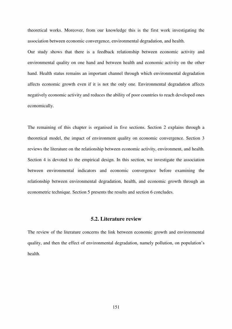
151

theoretical works. Moreover, from our knowledge this is the first work investigating the

association between economic convergence, environmental degradation, and health.

Our study shows that there is a feedback relationship between economic activity and

environmental quality on one hand and between health and economic activity on the other

hand. Health status remains an important channel through which environmental degradation

affects economic growth even if it is not the only one. Environmental degradation affects

negatively economic activity and reduces the ability of poor countries to reach developed ones

economically.

The remaining of this chapter is organised in five sections. Section 2 explains through a

theoretical model, the impact of environment quality on economic convergence. Section 3

reviews the literature on the relationship between economic activity, environment, and health.

Section 4 is devoted to the empirical design. In this section, we investigate the association

between environmental indicators and economic convergence before examining the

relationship between environmental degradation, health, and economic growth through an

econometric technique. Section 5 presents the results and section 6 concludes.

5.2. Literature review

The review of the literature concerns the link between economic growth and environmental

quality, and then the effect of environmental degradation, namely pollution, on population’s

health.

152

5.2.1 Economic growth and environment

Growth and economic convergence

Solow (1956) growth model has been tested and improved by economists. It was generalized

by Barro and Sala-i-Martin (1992), Mankiw, Romer and Weil (1992), Levine and Renelt

(1992) with the conditional convergence. Conditional convergence implies that countries will

reach their own steady states. Hence, when looking for convergence in a cross country study,

it is necessary to control for differences in steady states of different countries. The choice of

control variables is crucial because the statistical significant level as well as the coefficient

amplitude of the variable of interest is sensitive to this choice (Levine and Renelt 1992).

Mankiw, Romer and Weil (1992) provided an analysis of economic convergence by adding

human capital, represented by education level, to Solow’s model (1956) and they showed that

their results fit better to the predictions of Solow theoretical model. Knowles and Owen

(1994) completed this work by adding health as second human capital variable.

All these improvements are important but not enough because they do not take into account

the role that could play some omitted variables, in particular the environmental quality which

arouses a renewed interest these last years with the natural resources curse and EKC

hypothesis.

Consideration of the environmental aspect

The existence of an intrinsic relation between economic activity and environmental quality

remains evident. At the theoretical level several authors tried to give an explanation to the

way the environment degradation could impact economic activity (Bovenberg and Smulders

1995 and 1996; Bruvoll et al. 1999; Resosudarmo and Thorbecke 1996; Hofkes 1996;

Geldrop and Withagen 2000). These theoretical works can be divided into four major

categories following Panayotou (2000) (See Appendix 5.1). Optimal growth models built on a

153

Ramsey (1928) model, as extended by Koopmans (1960) and Cass (1965), constitute the first

category (Keeler et al. 1971; Mäler 1974; Gruver 1976; Brock 1977; Becker 1982; Tahvonen

and Kuuluvainen 1994; Selden and Song 1995 and Stokey 1998). Some of these models

considered the effects of pollution on growth path (Keeler et al. 1971; Gruver 1976, Van der

Ploeg and Withagen 1991) whereas others focused on natural resources depletion (Dasgupta

and Heal 1974; Solow 1974). In general, models of pollution and optimal growth suggest that

some abatement or curtailment of growth will be optimal.

The second category considers not only pollution as an argument of production and utility

functions, but also it includes environment itself as a factor of production (Lopez 1994;

Chichilnisky 1994; Geldrop and Withagen 2000). This measure of environmental quality can

be conceptualized as a stock that is damaged by production or pollution. The presence of

environmental stock in the production function means that optimal pollution taxes or

regulations are not sufficient to achieve the optimal level of environmental quality in the

steady state.

The third group is constituted of endogenous growth models that relax the neoclassical

specification of the production function assumed in the optimal growth models (Bovenberg

and Smulders 1995 and 1996; Hofkes 1996; Ligthhard and Van der Ploeg 1994; Gradus and

Smulders 1993, and Stokey 1998). Based on the works of Romer (1986, 1990), these models

are characterised by constant or increasing returns to scale to some factors, or a class of

factors, because private returns on investment may differ from the social returns on

investment, often because of externality effects. This category consists in extending this new

growth theory to include the environment or pollution as factor of production and

environment quality as an argument of the utility function. Bovenberg and Smulders (1995,

1996) modify the Romer (1986) model to include the environment as a factor of production.

Lighhard and Van der Ploeg (1994), Gradus and Smulders (1993) and Stockey (1998) extend

154

the simple “AK” used by Barro by including environment. Hung, Chang and Blackburn

(1994) use the Romer (1990) work. In general, optimal pollution control requires a lower

level of growth than would be achieved in the absence of pollution.

Finally, we have other models that connect environmental degradation and economic growth.

This category includes the overlapping generation model based on Diamond (1965), it is the

case of John and Pecchenino (1994, 1995). We also have a two country general equilibrium

model of growth and environment in presence of trade (Copeland and Taylor 1994). These

models reinforce the results of the optimal growth models.

At the empirical level, the effect of environment on growth is studied by two papers through

the different channels such as labour supply, labour productivity, and physical capital, using

simulation Models. Bruvol et al. (1999) estimated the cost to society of environmental

constraints, called environmental drag, in Norwegian economy through a dynamic resource

environment applied model (DREAM). Their simulation indicates that the environmental drag

reduces annual economic growth rate by about 0,82 percentage points because of the fall in

labour supply and capital between 1988 and 2030. Indeed, the corrosion from pollution is

estimated to increase the depreciation rate of public and private investment, and the

depreciation of public capital increases public consumption, which crowds out private

consumption. In addition, their results show that, with an increase of 28%, health damages

from emissions are the most important compared to other damage factors, and contribute to

39% of the total disutility. The other main cost components to development are congestion

and traffic accidents.

Moreover, Resosudarmo and Thorbecke (1996) show through the Social Environmental

Accounting Matrix (SEAM) and some simulations with Indonesian data, that the

improvement of environment quality by the “Blue Sky Program” reduces health problems,

and therefore stimulates economic growth.

155

Effect of economic growth on environment: The EKC hypothesis

We have shown that environmental quality affects economic performance. Economic activity

in turn may deteriorate environment quality (Shafik 1994, Mansour 2004; Yadav 1997; WRI

1996; Hettige, Mani and Wheeler 1998). During the 1990’s, scholars have investigated

theoretically and empirically the effect of economic development on pollution, and the most

popular finding remains the Environmental Kuznets Curve Hypothesis (EKC). The EKC

(Grossman 1995; Grossman and Krueger 1995; Torras and Boyce 1998) describes the

relationship between declining environmental quality and income as an inverted-U, that is, in

the course of economic growth and development, environmental quality initially worsens but

ultimately improves with improvements in income level. The first explanation for the EKC

relationship is that the environment can be thought of as a luxury good. In the early stage of

economic development a country would be unwilling to exchange consumption for

investment in environmental regulation, hence environmental quality declines. When the

country reaches the threshold level of income, its citizens start to demand improvement in

environmental quality. Another explanation of the EKC hypothesis is that countries pass

through technological life cycles, as they move from high polluting technology (agriculture-

based economies) to less polluting technology (service-based systems). In addition to these

macroeconomic explanations, the EKC hypothesis is supported by some microeconomic

foundations (Andreoni and Levinson 2001).

5.2.2 Environment and health

Healthy population is essential for the development of an economy and requires a healthy

environment (clean air, water, recreation and wilderness). As argued by Pearce & Warford

(1993), the immediate and most important consequences of environmental degradation are

156

damages to human health through different forms of diseases. Many authors have assessed

how air quality may be associated to population’s health. Some scholars showed that air

pollutions increase mortality rate (Woodruff et al., 1997 ; Gangadharan & Valenzuela, 2001;

Chay et al. 2003; Aunan & Pan, 2004; Jerrett et al., 2005).

Other authors assess the link between pollution and particular illness, such as cardio-

respiratory disease (Aunan & Pan, 2004; Burnett & Krewski, 1994; Jerrett et al., 2005),

asthma (Nauenberg & Basu, 1999) and congenital anomalies (Rankin et al., 2009).

There is therefore a link between environmental quality, people health and economic

performance. This interrelationship provokes different consequences depending on

development level if the EKC hypothesis is verified. In countries below EKC income

threshold, all attempts to boost economic growth (without abatement) will result in greater

environmental degradation. And this will burden economic growth through health and other

channels creating a vicious circle. However, when countries above the EKC income threshold

try to boost their economic growth, their environment quality will be improved and therefore

they will be in a virtuous circle. That will penalize poor countries by slowing down the speed

of convergence if they do not take care of environmental concern.

5.3. Environmental quality and economic convergence: The model

The object of this model is to theoretically investigate the association between environmental

quality and economic convergence. We introduce environment variable in an augmented

Solow growth model, and we observe the consequences on economic convergence process. In

this model, unlike Mankiw, Romer and Weil (1992), environmental capital and human capital

are treated as labour augmenting rather than entering the production function as separate

factors of production (Knowles and Owen, 1997).

157

We begin this model by a neoclassical growth model.

1it it it

Y K Lα α−=)

(3.10)

Where Y is the real output, K is the stock of physical capital, α is the capital share, 1-α is the

labour share, and

1 2it it it it it

L A Q H Lθ θ=

) (3.11)

L is the raw labour input, A the technological progress, Q is the natural environment quality

and H is the measure of human capital. L)

represents an effective labour input. 1θ and 2θ

represent the labour augmenting elasticities of environment and human capital.

The equation (3.10) can be written in per unit of effective labour:

i t i ty k

α=)

(3.12)

With it it it

y Y L=))

and it it it

k K L=)

. We assume that L, Q, H and A grow at constant rate n, q,

h and g respectively.

The accumulation of physical capital can be modelled as (3.13).

.

( )it ki it i t itk s y n kδ= − +

) ) (3.13)

Where ki

s is the proportion of income invested in physical capital and δ is the physical

capital depreciation rate. 1 2i i i in n g q hθ θ= + + +)

Following MRW (1992), we can show that (3.13) gives (3.14) and (3.15) at steady state:

[ ]1 (1 )* ( )

i ki ik s n

αδ

−= +

) (3.14)

[ ](1 )* ( )

i ki iy s n

α αδ

−= +

) ) (3.15)

Where the asterisk indicates the steady state value. The steady state values of output and

capital per effective unit of labour are determined by the rate of investment in physical capital

and the rate of growth of labour force, environment, education and technology.

Replacing (3.15) into (3.12), and using natural logarithms, we obtain (3.16).

158

*

0ln( ) ln ln( ) ln( ) 1ln( ) 2 ln( )1 1

iti ki it it

it

YA gt n s Q H

L

α αδ θ θ

α α= + − + + + +

− −

) (3.16)

The equation (3.16) shows that the investment in physical capital, human capital and natural

environment improvement impacts positively the production per capita.

The variable *Y cannot be observed since it supposes that we are at the steady state at the

estimation period and this is a strong assumption. To solve for this problem, we use the

linearization method of MRW (1992), Islam (1995), Bassanini and Scarpetta (2001 and 2007)

and we have:

*ln (ln ln )it t

d y dt y yλ= − − (3.17)

where Y

yL

= and (1 )( )i inλ α δ= − +)

is the speed of convergence. This speed of convergence

changes with the addition of environmental variables through 1 iqθ , since

1 2i i i in n g q hθ θ= + + +)

. An improvement in environment quality increases the speed of

convergence.

The transition dynamics through the steady state can be written as (3.18).

*ln ln (ln ln )t t s t s

y y y yψ− −− = − (3.18)

Where (t-s) is a period arbitrary chosen.

Replacing steady state y value by it value in current period, (3.16) gives (3.19).

0ln( ) ln( ) ln ln( ) ln( )1 1

1ln( ) 2 ln( ) ln( )

it it s i ki

it it it s

y y A gt n s

Q H y

α αψ ψ ψ δ ψ

α αψθ ψθ ψ

−

−

− = + − + +− −

+ + −

)

(3.19)

Where (1 e x p ( ) )i tψ λ= − −

Equation (3.19) can be simplified by adding both ln( )t s

y − to the left and right hand sides in

order to have only ln( )t

y as left hand side member and we obtain (3.20).

159

0ln( ) ln ln( ) ln( )1 1

1ln( ) 2 ln( ) exp( ) ln( )

it i ki

it it it s

y A gt n s

Q H t y

α αψ ψ ψ δ ψ

α αψθ ψθ λ −

= + − + +− −

+ + + −

)

(3.20)

This equation (3.20) shows that environment quality is an important determinant of economic

development.

5.4. Empirical analysis

5.4.1 Methodology

The analysis is subdivided into four main steps. First, the effect of environment quality on

economic outcomes is assessed through the introduction of pollution indicators in an

augmented neoclassical growth model. Then, we evaluate how these variables affect the

ability of poor countries to catch up the rich ones by adding to the previous model the

interaction term between initial gross domestic product (GDP) per capita and environmental

variable. The third model investigates the role played by health in the impact of

environmental variables on economic outcomes. Finally, we develop an explanation to this

effect of pollution on convergence by estimating simultaneously a growth equation, a health

equation, and an environmental equation to highlight the interrelationships between these

three variables.

Economic growth and environment

Based on the neoclassical augmented growth model, the effect of environment on economic

growth could be specified as follows:

'1 1 2gdpc git it it k kit itdpc envir Xα α α υ−= + + + (4.1)

Where itgdpc and itenvir represent respectively the logarithmic form of GDP per capita and

the environment quality of country i in period t . X is the matrix of the control variables

160

including health introduced in the model, and which have been used frequently in the

empirical literature.23 it

ν is the error term. The coefficient of the economic catch up variable

1α is expected to be superior to 0 and inferior to 1 (0< 1α <1) according to the economic

convergence hypothesis. We expect 2α to be inferior to 0 ( 2α <0).

Using panel data, the econometric model takes into account countries specific effects and

time-invariant heterogeneity. As we saw above, there is a reverse causality in the relationship

between environment and economic outcomes. According to the Environmental Kuznets

Curve hypothesis, the development level of a country has a significant effect on its level of

pollution (Grossman & Krueger, 1995). Moreover, environmental indicator could also be a

proxy of some variables that have a significant effect on economic growth, such as the

technology use. The instrumental variable methods with the Two Steps Least Squares (2SLS)

estimator might be appropriated in this case. But, this estimator applied to our model raises a

problem because of its dynamic characteristics. Indeed it leads to a biased estimation of 1α

since 1itgdpcap − and itν are correlated. The Generalized Method of Moments (GMM) applied

for dynamic panel data is suitable to consistently estimate 1α and also the coefficients of

predetermined and endogenous variables. We use the System-GMM estimator which

combines equation in levels and differences, and then exploits additional moment conditions

(Blundell and Bond, 1998). Predetermined and endogenous variables are instrumented by

their lagged values in levels and differences.24 Two specification tests check the validity of

the instruments. The first is the standard Sargan/Hansen test of over-identifying restrictions.

The second test examines the hypothesis that there is no second-order serial correlation in the

first-difference residuals.

23

These variables are listed in the next subsection.

24 The paper uses the two-step System-GMM estimator with the Windmeijer (2005) correction for finite sample

bias.

161

The following model is then estimated:

'1 1 2gdpc git it it k kit i t itdpc envir Xα α α µ κ υ−= + + + + + (4.2)

Where The country and time fixed effects are represented respectively by i

µ and t

κ .

Economic convergence and environment

To assess the impact of environmental quality on economic convergence, we introduce the

interaction term between lag GDP per capita and environment as additional variable into the

previous model.

' '1 1 2 3 1gdpc g (g ) * ( )it it it it it k kit i t itdpc envir dpc envir Xα α α α µ κ υ− −= + + + + + +

(4.3)

In this model the catch up coefficient is '1 3

1

( )*

( )t

t

gdpcenvir

gdpcα α

−

∂= +

∂ and this is a function of

environmental quality. '1α is expected to be 0< '

1α <1, 2α <0 and 3α >0.

Environment, health, and growth

The previous models allowed to assess the impact of environment degradation on economic

growth and economic convergence when health status is among control variables. However,

this remains insufficient because it does not take into account the interrelation between health,

environment and economic growth. Moreover, it does not allow assessing the impact of

environment degradation which affects growth through health. To assess this, we add to

previous equation two other equations: an equation of health, and an equation of environment.

Through these additional equations, we assess the impact of income and environmental

degradation on health. Generally it is assumed that health outcomes of a population improve

when the economy grows and this improvement are made easy by the rise in general standard

of living (access to educational opportunities and health services). Health depends also on the

162

quality of physical environment such as the amount of air pollution and the quality of drinking

water. At the same time, the quality of a country’s physical environment is a result of certain

growth factors in the economy (intensive use of land, forest, air and water pollution). The

existing health theoretical models, including that of Grossman (1972) are not adapted to our

econometric health equation. We follow Gangadharan and Valenzuela (2001) by expressing

health as a function of income, physical environment quality and other control variables.

( , ( , ), )it it it it it it

h f gdpc envir gdpc z w= (4.4)

Where h is health indicator, z the non economic variables that determine environment

quality and w the non economic variables that determine health status (provision and access

to health services, physicians number, immunization rate, education). When we ignore the

determinants of environment quality, the health equation can be written as (see Chapter 4):

0 1 2 3it it it ith gdpc envir wβ β β β ρ= + + + + (4.5)

Here our purpose is to highlight the relation between economic development and

environmental quality. Economic growth is generally made at the cost of a deterioration of the

quality of the natural environment. But through which analytical relation development level

affects environment? It is generally found that income is linked to environment quality

through an inverted U relationship (EKC hypothesis). In our model environment quality is

explained by income and some social variables.

21 2 3it it it it itenvir c gdpc gdpc zγ γ γ η= + + + + (4.6)

Where z is a vector of variables that could affect environment quality such as population

density.

We estimate equations (4.2), (4.5) and (4.6) by the Three Steps Least Square method (3SLS).

In addition to the explanation it brings to our results, the argument that guides this choice is

the ability of this method to take into account the fact that the dependent variable of some

equations can be used as explanatory variables in others. In fact in our system, the variable of

163

economic activity is both used as dependent variable and explanatory variable, it is the same

for health and environment quality. This simultaneity bias can be corrected for each equation

by the 2SLS method and for the system by the 3SLS.

5.4.2 Variables and data

This study is based on a panel data of 117 developed and developing countries for which data

are available from 1971 to 2000 subdivided into five year periods.25 The economic outcome is

measured by GDP per capita based on purchasing power parity (PPP) in constant 2005

international dollars. This indicator is taken from the World Development Indicators (WDI

2008) of the World Bank. Environment quality is represented by three pollution indicators,

carbon dioxide emission in metric tons per capita (CO2) and sulphur dioxide emission

milligrams per GDP (SO2) for air pollution and Biological Oxygen Demand in milligrams per

worker (BOD) for water pollution. The CO2 is a global measure of air pollution and affects

health mainly through climate change induced diseases (Diarrhoeal diseases, malaria, selected

unintentional injuries, protein-energy malnutrition). The SO2 is a local air pollutant and

affects population health through Respiratory infections, selected cardiopulmonary diseases,

lung cancer. BOD is a measure of the oxygen used by micro-organisms to decompose waste.

Micro-organisms such as bacteria are responsible for decomposing organic waste. When

organic matter such as dead plants, leaves, grass clippings, manure, sewage, or even food

waste is present in a water supply, the bacteria will begin the process of breaking down this

waste. If there is a large quantity of organic waste in the water supply, there will also be a lot

of bacteria present working to decompose this waste. In this case, the demand for oxygen will

25 The time periods are1971-1975 ; 1976-1980 ; 1981-1985 ; 1986-1990 ; 1991-1995 ; 1996-2000.

164

be high (due to all the bacteria) so the BOD level will be high (CIESE26). The BOD degrades

health outcomes through Diarrhoeal diseases, trachoma, schistosomiasis, ascariasis,

trichuriasis, hookworm disease. The BOD and CO2 are also taken from WDI 2008 while

Sulfur dioxide emission (SO2) is from the dataset compiled by David Stern27 in 2004. The

health indicator used is the infant mortality rate (IMR). Infant mortality is preferred in this

Chapter because of data availability, since the DALYs are not available at country level for a

time longue period. As this indicatorr is limited asymptotically, and an increase in this

indicator does not represent the same performance when its initial level is weak or high, the

best functional form to examine is that where the variable is expressed as a logit, following

Grigoriou (2005), we use the logistic form of this variable.

log ( ) log( )1

IMRit IMR

IMR=

−.

We use as control variables in the growth equation (Equation 4.2), the investment ratio

measured by the Gross Fixed Capital Formation as percentage of GDP, human capital

accumulation (education), and annual population growth rate. These variables are traditionally

used in the empirical assessment of growth determinants (see Mankiw et al, 1992) and largely

discussed in the theoretical model. We also control for trade openness (ratio of the sum of

import and export to GDP), household final consumption per capita, financial development

(money and quasi money as a ratio of GDP), institutions quality, and inflation rate to capture

macroeconomic stability, and policy information.

The variables that explain health (Equation 4.5) are the economic development level, the

supply of health services and infrastructures (immunization rate against DPT, the number of

26 According to the Center for Improved Engineering and Science Education (CIESE): http://www.k12science.org/curriculum/waterproj/bod.shtml

27 We thank David Stern for the provision of data

165

physicians per 1000 inhabitants), and demographic variables (women fertility rate, and the

percentage of urban population).

Finally, with regard to the environmental equation, we use as determinant of environmental

pollution, the GDP per capita and GDP per capita squared to verify the EKC hypothesis,

Income inequality (measured by the Gini coefficient), and demographic variables (women

fertility rate, and the percentage of urban population).

All these indicators are taken from World Bank World Development Indicators (WDI 2008)

apart from our institutions quality indicator taken from polity IV, and the variable used is

polity2; the variable of education quality from Barro and Lee 2000; and the income inequality

indicator taken from the database created by Galbraith and associates and known as the

University of Texas Inequality Project (UTIP) database. The descriptive statistics, the

definitions and the sources of these variables as well as the list of countries are respectively

presented in the appendix 5.2, appendix 5.3 and appendix 5.4.

5.5. Econometric results

We begin by discussing the results from the estimation of the growth model, then, we present

the results obtained with the simultaneous estimation of the three equations.

5.5.1 Economic growth and the environment

The results obtained from the estimation of equation 4.2 are presented in the first three

columns of Table 5.1. The dependent variable is GDP per capita and our variable of interest is

environment quality, measured by three different indicators (SO2 per GDP, CO2 per capita

and BOD per worker). This equation is estimated with the two-steps System-GMM estimator

and environmental variables are taken as endogenous and then instrumented by at least their

166

second order lags.28 Results suggest that environmental degradations have a negative and

statistically significant effect on economic growth whatever the environmental indicator

considered, infant mortality has a negative and significant effect on economic growth. A 1%

increase in SO2, CO2, and BOD emissions provokes a reduction of economic growth rate of

0.622, 0.007, and 0.666 points of percentage respectively.

Another interesting result is the coefficient of the catch up variable. Indeed, the coefficient of

lagged GDP per capita is around 0.91, this corresponds to a rate of convergence of about 2%

per year. That means that, each year poor countries reduce their gap to their steady state to 2

percent. This convergence rate is closed to that found in the literature. Health incator appears

with a negative and significant coefficient, showing the negative effect of infant mortality on

economic growth as in Chapter 4.

Regarding the control variables, only investment, institutions quality and inflation rate appear

statistically significant. In fact, investment, trade openness and institution quality increase

economic growth while inflation rate reduces it.

28 To prevent the problem of the proliferation of instruments commonly faced in this methodology, we restrict the maximum number of lags at 5, what leads us to a maximum number of instruments equal to 26.

167

Table 5. 1: Two-step System-GMM results of the effect of environmental variables on Economic growth and convergence

Dependent variables: GDP per capita PPP in constant value 2005

SO2 per GDP

CO2 per capita

BOD per worker

SO2 per GDP

CO2 per capita

BOD per worker

VARIABLES (1) (2) (3) (4) (5) (6) Log Initial GDP per capita 0.913*** 0.917*** 0.907*** 0.903*** 0.936*** 0.675***

(14.73) (8.73) (42.12) (13.40) (5.19) (6.74) (Environment)x(Initial GDP) 2.313** 0.013*** 0.910**

(2.36) (2.98) (2.40)

Environmental variables -0.622** -0.007* -0.666* -16.547** -0.128*** -7.692**

(2.00) (1.93) (1.66) (2.36) (2.94) (2.42)

Population growth -0.000 0.003 -0.008 0.001 -0.002 0.006

(0.06) (0.53) (0.99) (0.33) (0.26) (0.53)

Log Schooling 0.013* 0.005 0.011 0.005 0.002 0.014

(1.94) (0.45) (1.16) (0.75) (0.19) (1.07)

Log Investment rate -0.015 0.091*** 0.051 0.090*** 0.134*** 0.064*

(0.44) (3.68) (1.64) (3.26) (3.36) (1.85)

Health -0.048*** -0.044*** -0.028* -0.040*** -0.035*** -0.080***

(4.03) (4.15) (1.77) (3.26) (2.66) (2.63)

Openness 0.056** 0.018 0.037 0.023 0.018 -0.036

(2.32) (0.75) (1.53) (1.46) (0.72) (0.95)

Log Consumption 0.049 0.050 0.043** 0.041 0.018 0.078

(0.88) (0.59) (2.36) (0.76) (0.13) (1.15)

Financial development -94.851 -66.054 -132.090*** -83.703 -102.375 151.914

(1.25) (1.41) (2.95) (1.19) (1.60) (1.37)

polity2 0.001 0.002** 0.002** 0.003*** 0.002** 0.002*

(1.31) (2.21) (1.98) (2.76) (2.17) (1.72)

inflation 0.005* -0.003*** -0.003*** -0.002*** -0.003*** -0.002***

(1.72) (5.44) (5.91) (5.18) (3.70) (2.60)

Constant 0.228 -0.066 0.357* 0.106 -0.067 1.732***

(1.31) (0.30) (1.93) (0.69) (0.17) (2.85)

Observations 235 239 203 235 239 203

Countries 68 69 63 68 69 63

AR1 0.019 0.009 0.014 0.004 0.010 0.010

AR2 0.127 0.094 0.117 0.128 0.115 0.151

Hansen p-value 0.388 0.156 0.259 0.389 0.285 0.139

Number of instruments 26 17 15 17 17 19

Note: Robust t-statistics in parentheses. Standard errors are corrected by the Windmeijer (2005) method designed for finite sample bias in a two-step System-GMM estimator. * p < 0.10, ** p < 0.05, *** p < 0.01

168

5.5.2 Economic convergence and environment quality

To assess empirically whether pollution affects the speed of convergence, equation 4.3 is

estimated under the hypothesis that environmental variables and the interaction term are

endogenous. As previously argued, environmental degradation may reduce the ability of

poorer countries to catch up richer ones. The results obtained are summarized in the last three

columns (4, 5 and 6) of Table 5.1. The coefficients of our variables of interest have the correct

signs and are statistically significant. Indeed, the lag of GDP per capita and its interaction

term with environmental indicators have positive coefficients, while pollution variables have

negative coefficients. This means that the speed of convergence of an economy depends on its

pollution level. More precisely, a high level of environmental degradation increases the

marginal effect of lag GDP per capita on its current level and therefore reduces the speed of

convergence. Environment quality can be viewed as an obstacle for developing countries by

reducing their ability to get closer to developed countries economically, given the

Environmental Kuznets Curve hypothesis.

The scarcity of education data reduces the number of countries in our sample, since it is not

available for many countries. In order to control for the robustness of our results, we

estimated our models without the education variable. The results are presented in Table 5.2.

The sample size increases from 68 countries to 86 and the results remain unchanged, namely,

environmental degradation affects the ability of poor economies to cach up developed ones.

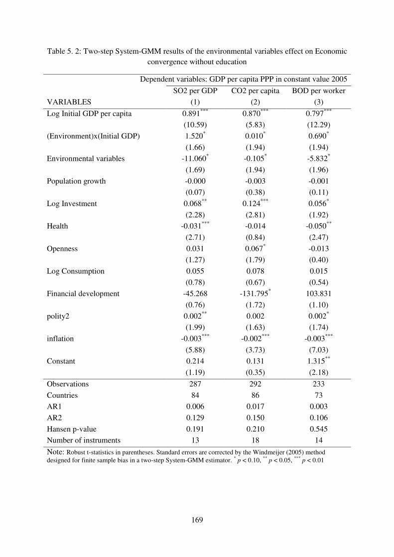
169

Table 5. 2: Two-step System-GMM results of the environmental variables effect on Economic convergence without education

Dependent variables: GDP per capita PPP in constant value 2005

SO2 per GDP CO2 per capita BOD per worker

VARIABLES (1) (2) (3)

Log Initial GDP per capita 0.891*** 0.870*** 0.797***

(10.59) (5.83) (12.29)

(Environment)x(Initial GDP) 1.520* 0.010* 0.690*

(1.66) (1.94) (1.94)

Environmental variables -11.060* -0.105* -5.832*

(1.69) (1.94) (1.96)

Population growth -0.000 -0.003 -0.001

(0.07) (0.38) (0.11)

Log Investment 0.068** 0.124*** 0.056*

(2.28) (2.81) (1.92)

Health -0.031*** -0.014 -0.050**

(2.71) (0.84) (2.47)

Openness 0.031 0.067* -0.013

(1.27) (1.79) (0.40)

Log Consumption 0.055 0.078 0.015

(0.78) (0.67) (0.54)

Financial development -45.268 -131.795* 103.831

(0.76) (1.72) (1.10)

polity2 0.002** 0.002 0.002*

(1.99) (1.63) (1.74)

inflation -0.003*** -0.002*** -0.003***

(5.88) (3.73) (7.03)

Constant 0.214 0.131 1.315**

(1.19) (0.35) (2.18)


Countries 84 86 73

AR1 0.006 0.017 0.003

AR2 0.129 0.150 0.106

Hansen p-value 0.191 0.210 0.545

Number of instruments 13 18 14

Note: Robust t-statistics in parentheses. Standard errors are corrected by the Windmeijer (2005) method designed for finite sample bias in a two-step System-GMM estimator. * p < 0.10, ** p < 0.05, *** p < 0.01

170

5.5.3 Interrelationships between income, health and environment

To take into account the interrelationships between health, environment and economic

growth, and to assess the impact of environmental degradation which affects growth through

health, we estimate simultaneously equations (4.2), (4.5) and (4.6) with the Three Steps Least

Squares (3SLS) estimator. The results obtained are presented in table 5.3.

The first three columns of this table (columns 1, 2 and 3) present the results when sulphur

dioxide per GDP (SO2) is used as environmental indicator. These results show that

environmental degradation and mortality rate (as in Chapter 4) reduce economic growth

(Column 1). GDP per capita, immunisation rate, and physicians number are factors that

contribute to improve health status, while environment degradation and fertility rate worsen it

(Column 2). The positive coefficient of environment variable combined with the negative

effect of health on growth does not rejet our theoretical argument, namely health is an

important channel through which pollution affects economic growth. The results of the

environmental quality equation in column 3 indicate that the coefficient of income per capita

is positive and significant at 1%, showing that economic activity deteriorates environment

quality. But the negative and significant coefficient of income square indicates that the

negative effect of GDP on environment quality is conditioned to an income threshold above

which the effect becomes positive and income improves environment quality confirming the

Environmental Kuznets Curve hypothesis (EKC). The six last columns of this table present

the results when carbon dioxide per GDP (columns 4, 5 and 6) and the biological oxygen

demand (columns 7, 8 and 9) are used as environmental variables. The environmental

variables have the expected sign and the EKC hypothesis is verified in each case.

171

Table 5. 3: 3SLS estimation of the interrelationships between health, environment and economic

3SLS estimation of the relationships between health, environment and economic activity

GDP per

capita Inf.

Mort. Rate

SO2 per GDP

GDP per capita

Inf. Mort. Rate

CO2 per capita

GDP per capita

Inf. Mort. Rate

BOD per worker

VARIABLES (1) (2) (3) (4) (5) (6) (7) (8) (9)

Pop. growth -0.00696 0.00187 -0.00570

(-1.197) (0.408) (-1.008)

Initial GDP 0.920*** 0.979*** 0.905***

(54.32) (29.17) (67.29)

Schooling 0.0245*** 0.0244*** 0.0244**

(2.900) (3.214) (2.545)

Investment 0.0884*** 0.113*** 0.0454**

(5.016) (4.898) (2.007)

Health -0.091*** -0.154*** -0.0897***

(-4.594) (-7.337) (-3.033)

Log Cons. -0.00927 -0.00996 0.0269*

(-0.393) (-0.593) (1.869)

Financial dev.

-129.5 -17.75 -28.18

(-1.473) (-0.473) (-0.584)

polity2 0.00119 0.000830 0.00203***

(1.322) (1.143) (2.826)

inflation -0.000972 -0.00229 -0.00214

(-0.630) (-1.418) (-1.383)

Immunization -0.85*** -0.33*** -0.49***

(-5.272) (-2.729) (-3.417)

Physician -0.0789* -0.0596 -0.13***

(-1.951) (-1.577) (-3.014)

Fertility rate 0.645*** 0.925*** 0.602***

(6.697) (8.245) (5.263)

Environment -0.069*** 0.465*** -0.0550** 0.458*** -0.0992 0.845***

(-3.180) (6.216) (-2.568) (5.114) (-1.281) (3.298) GDP per

capita -0.19*** 4.045*** -0.94*** 4.455*** -0.35*** 0.308

(-3.520) (5.464) (-9.285) (7.825) (-7.731) (1.615) (GDP per capita) ²

-0.26*** -0.18*** -0.0213*

(-6.089) (-5.588) (-1.875)

inequality -0.00165 -0.005 0.0125***

(-0.169) (0.60) (4.511)

Constant -0.252** 0.887* -20.3*** -0.615** 3.655*** -23.3*** -0.0273 0.832 -3.202***

(-2.518) (1.755) (-6.573) (-2.291) (4.684) (-9.858) (-0.353) (1.371) (-4.087)

Observations 179 179 179 216 216 216 180 180 180

R-squared 0.993 0.724 0.197 0.994 0.798 0.817 0.997 0.840 0.262

Note : Robust t-statistics in parentheses. * p < 0.10, ** p < 0.05, *** p < 0.01. All the independent variables are in natural logarithmic form, except health variable, population growth, polity2 and

inflation rate.

172

The 3SLS estimations of these three equations allow us to draw some conclusions: there is an

inverse causality between economic activity and environmental degradation and health status

is an important channel through which environment degradation affects economic growth

even if it is not alone. The effect of economic activity on environment quality being

dependent on income level, countries whose income is below the EKC income threshold will

slow down in a poverty trap due to environment degradation. However, those whose income

is above this threshold will be in a virtuous circle due to the improvement of environment

quality. This could reduce the ability of poor countries to catch up the rich ones. Any

ambitious economic policy must take into account environmental concerns to avoid it

perverse effects.


The main goal of this chapter is the analysis of the interrelationships between health, income

and environment degradation, and its consequences on economic convergence process. We

introduce environment variable in a growth model and we measure econometrically its effect

on economic growth. Our results show that environmental degradation negatively affects

economic activity and reduces the ability of poor countries to reach their steady state. This

reinforces our theoretical argument according to which environment quality improvement

plays a considerable role in economic convergence process. Two-steps GMM and Least

square estimations of growth, environment, and health equations allow us to verify the inverse

causality between environment quality and economic growth and between economic growth

and health. Health status remains an important channel through which environment

degradation affects economic growth even if it is not alone. Poor countries which have chosen

rapid economic growth at the price of environment quality will penalise themselves and have

173

little chance to reach their goal. Such policy can reduce growth through health and other

channels.

Poor countries cannot postpone attending environmental concerns in the hope that the

environment will improve with increased incomes and avoid poverty trap due to environment

degradation. Policy makers in these countries should in contrary take into account

environmental concerns as promoted by international community through the MDGs.

This chapter can also be placed into the debate about development aid effectiveness. In fact, a

development assistance based on less polluting production technology will help poor

countries to avoid the vicious circles shown in this chapter.

One way this research can be extended is to use other health and environment indicators and

compare the results for each indicator. Another way to extend this chapter is the use of other

technical approach in order to confirm our idea.

174

APPENDICES 5

Appendix 5.1: Classification of macroeconomic models of environmental degradation and growth

groups characteristics models remarks

Optimal growth

models build on

a Ramsey (1928),

Koopmans

(1960) and Cass

(1965).

These are dynamic optimization

models, in which the utility-

maximization problem of the infinitely

lived consumer is solved using the

techniques of optimal control theory.

Either the stock or the flow of

pollution is an argument of both the

production function and the utility

function of the representative

consumer. These models extend the

basic dynamic optimization of

Ramsey, Cass and Koopmans to

include the disutility of pollution that

arises as a result of economic activity.

Brock and Taylor

(2004), Keeler et al.

(1971), D’Arge and

Kogiku (1973), Mäler

(1974), Forster (1973),

Gruver (1976), Brock

(1977), Becker (1982),

Tahvonen and

Kuuluvainen (1994),

Selden and Song

(1995), Stokey (1998)

Provide in general of

theoretical foundation for the

empirically observed

Environmental Kuznets

Curve, and the Steady state

level of consumption and

capital accumulation is lower

than the steady state

consumption and capital

accumulation of a model

without pollution

Models of the

Environment as a

Factor of

Production

In addition to the use of pollution as an

argument of the production and utility

function these models include the

environment itself. Environment is

interpreted as a stock natural capital

that the economy is endowed with or

the aggregate level of environmental

Lopez (1994), and

Chichilinsky (1994).

Property rights are decisive

in determining whether

environmental degradation

eventually declines with

growth.

175

quality.

Endogenous

Growth Models

of Environmental

Degradation and

Growth.

Inclusion of the environment or

pollution as a factor of production and

environmental quality as an argument

of the utility function Endogenous

Growth Models of Romer (1986,

1990), Barro (1990), Robelo (1991)

and Lucas (1988).

Bovenberg and

Smulders (1995,

1996), Ligthhard and

van der Ploeg (1994),

Gradus and Smulders

(1993), Stokey (1998),

Hung, Chang, and

Blackburn (1994)

The conclusions are similar

to the ambiguous predictions

of the neo-classical growth

models because the results

again depend on the form of

the utility function.

Other

Macroeconomic

Models of

Environmental

Degradation and

Growth

Several other macroeconomic models

of environmental degradation and

growth different from those already

discussed could be found.

The many-goods

general equilibrium

model with two

regions (North and

South) of Copeland

and Taylor (1994) and

the overlapping

generation’s model of

John and Pecchenino

(1994, 1995) based on

Diamond (1965).

Source : Author based on Panayotou (2000).

176

Appendix 5.2 : Descriptive Statistics

Variable Obs Mean Std. Dev. Min Max

GDP per capita 259 11212.43 10918.89 355.8692 55491.52

Inf. Mort. rate 259 36.90442 33.55625 3.48 138.656

SO2 per GDP 253 0.0069203 0.017175 0.0000922 0.1760821

CO2 per capita 259 5.060414 5.543132 0.0319344 35.87007

BOD per worker 256 0.1950967 0.0519381 0.0694487 0.4478187

Pop. growth 259 1.337404 3.075527 -44.40836 5.603235

school 211 23.11564 22.01362 0 84.1

investment 258 20.90701 5.34708 9.488747 40.29905

openness 256 68.85741 39.29941 2.003065 238.6728

consumption 219 4469.355 5270.451 87.23995 22281.84

Financial Dev. 221 44.7538 32.07666 9.198633 227.4642

polity2 226 3.879646 6.691901 -10 10

Inflation rate 254 38.59134 190.1751 -1.659683 2342.221

Immunization 259 81.51004 16.49692 24 99

Physician 259 1.445306 1.155825 .0198895 4.173381

Fertility rate 259 3.132003 1.578447 1.152 7.845

inequality 259 42.36337 6.444149 26.135 64.2473

177

Appendix 5.3 : Variables definitions and sources

Variables characteridtics sources

GDP per capita gross domestic product per capita WDI 2008

Inf. Mort. rate infant Mortality rate UNICEF

SO2 per GDP sulphur dioxide emission per GDP David Stern

CO2 per capita Carbon dioxide emission per capita WDI 2008

BOD per worker Biological Oxygen Demande per worker WDI 2008

Pop. growth population growth rate WDI 2008

school Percentage of "no schooling" in the total

population Barro and Lee 2000

investment gross fixed capital formation WDI 2008

openness Ratio of the sum of export and import to

GDP WDI 2008

consumption Household final consumption rate per capita WDI 2008

Financial Dev. Money and quasi money as a ratio of GDP WDI 2008

polity2 institution quality polity IV

Inflation rate consumption index price WDI 2008

Immunization immunization rate against DPT WDI 2008

Physician number of physicians per 1000 inhabitants WDI 2008

Fertility rate women fertility rate WDI 2008

inequality gini coefficient of income university of Texas income

inequality

178

Appendix 5.4 : list of countries in the sample Country name Country name Country name Albania Greece Norway Argentina Guatemala Nepal Armenia Honduras New Zealand Australia Croatia Oman Austria Haiti Pakistan Azerbaijan Hungary Panama Belgium Indonesia Peru Bangladesh India Philippines

Bulgaria Ireland Papua New Guinea

Bahrain Iran, Islamic Rep. Poland Belize Iceland Portugal Bolivia Israel Paraguay Brazil Italy Romania

Bhutan Jamaica Russian Federation

Botswana Jordan Rwanda Central African Republic Japan Saudi Arabia Canada Kenya Senegal Chile Kyrgyz Republic Singapore China Korea, Rep. El Salvador Cote d'Ivoire Kuwait Suriname Cameroon Sri Lanka Slovak Republic Congo, Rep. Lithuania Slovenia Colombia Luxembourg Sweden Cape Verde Latvia Swaziland

Costa Rica Morocco Syrian Arab Republic

Cyprus Moldova Thailand Germany Madagascar Tonga

Denmark Mexico Trinidad and Tobago

Algeria Macedonia, FYR Tunisia Ecuador Malta Turkey Egypt, Arab Rep. Myanmar Uganda Spain Mongolia Ukraine Ethiopia Mozambique Uruguay Finland Mauritius United States

Fiji Malawi St. Vincent and the Grenadines

France Malaysia Venezuela, RB Gabon Namibia South Africa

179

United Kingdom Nigeria Zambia Ghana Netherlands

183

General Conclusion

185

The achievement of the millennium development goals adopted by the United Nations in

September 2000 by the target date 2015 remains an important concern. Therefore, all the

studies and efforts aiming to reduce poverty rate, to improve population’s health and physical

environmental quality are welcome. It is commonly recognized by scholars, policy makers as

well as the international community that better health outcome is an important predictor of

economic development and poverty reduction, since it increases the productivity and the

availability of the labour force, and the accumulation of physical capital. It is also largely

accepted and documented that sustainable economic development requires clean physical

environment, and economic growth is an important determinant of environmental quality.

But, less attention has been given to the simultaneous association among human capital,

natural capital, and economic development.

This dissertation bridged this gap by analyzing theoretically as well as empirically the

interrelationships among population’s health, environmental degradation and economic

development, its consequences for developing countries, and some effective policy responses.

Four important issues are theoretically and empirically addressed in this dissertation: (i) What

role does environmental degradation play in the association between income distribution and

health? (ii) Is environmental degradation a determinant of the large health inequality observed

between and within developing countries? (iii) Does the global burden of disease matter for

economic development? (iv) How do the interrelationships among health, environmental

quality and economic development affect the ability of poor countries to converge towards

developed ones economically?

The first part answered to the first two questions through chapter 2 and chapter 3. The second

chapter analyzed whether environmental degradation could be considered as an additional

channel through which income inequality affects infant and child mortality. The third chapter

186

analyzed the role played by the degradation of air quality in health inequalities between and

within developing countries, and the role of political institutions in this relationship.

Indeed, the theoretical and empirical results show that income inequality affects negatively

environmental quality and environment degradation worsens population’s health. Another

interesting result is that air and water pollutions are important channel through which income

inequality affects population health.

The chapter 3 showed that the large inequalities in infant and child mortality rates between

and within developing countries are partly attributable to air pollution. More precisely,

population belonging to poorest income quintiles are those likely to suffer more from

environmental degradation, because they receive the highest exposure, and this exposure then

exercises larger effects on their health than it does on the average population. Furthermore,

richest communities have more prevention than the poorest and have more access to medical

care when they are sick from pollution. Another interesting finding of this chapter is the role

of political institutions in this relationship. In countries with good political institutions, this

heterogeneity in the health effect of pollution is reduced since these institutions favour

universal health policy issues, information and advices about hygiene, and health

infrastructures building.

The second part of the dissertation responded to the two last questions (chapter 4 and chapter

5). The chapter 4 assessed empirically the effect of health (global burden of disease,

communicable disease, and malaria) on economic growth. The interrelationships among

health, environment, and economic development as well as the consequences of these

interrelationships on the convergence of poor countries towards developed countries are

investigated theoretically and empirically in the last Chapter.

187

The investigation of the role of health outcomes in economic growth (chapter 4) showed that

health indicators, when correctly measured by the gap between current health status and an

ideal health situation where the entire population lives to an advanced age, free of disease and

disability, and when accurately instrumented, have significant impact on economic

performance unlike the recent works of Acemoglu and Robinson (2009). This important effect

of health status in the economic development process holds for more aggregate health

outcomes as well as less aggregated health measurement (communicable diseases and

malaria), and for the overall sample of countries as well as the sample of developing

countries. This is particularly more important for developing world where health situation is

catastrophic. Indeed, improving health situation could be considered as an opportunity since it

will give them enough rooms to foster economic performance and reduce poverty level.

The examination of the interrelationships among population’s health, environmental

degradation and economic development (chapter 5) pointed out important results.

Theoretically as well as empirically, we found that water pollution and the degradation of air

quality negatively affect economic performance. Moreover, the Environmental Kuznets Curve

(EKC) hypothesis is verified, namely, environmental degradation rises faster in the early

stages of economic development, then slows down, reaches a turning point and declines with

further income growth. Health status remains an important channel through which

environment degradation affects economic growth even if it is not alone. Another important

finding is that, environment degradation reduces the ability of poor countries to reach

developed one economically. This reinforces our argument according to which environment

quality improvement plays a considerable role in economic convergence process.

These results call for important policy implications. First, there are important

interrelationships among the MDGs adopted by the United Nations in September 2000,

therefore efforts might be focused simultaneously on all of them instead of making a

188

hierarchy among them. Making choices among them and postponing some to the future will

create a kind of “weak link” and prevent the achievement of all the targets. Health

preoccupations (Goals 4, 5 and 6) are important determinants of poverty reduction (Goal 1)

through economic growth and it is difficult to improve health status without improving the

income level.

Moreover developing countries cannot postpone attending environmental concerns (Goal 7) in

the hope that the environment will improve with increased incomes and avoid poverty trap

due to environment degradation. This behaviour could seriously constrain their performance.

Policy makers in these countries should in contrary take into account environmental concerns

as promoted by the international community through the MDGs.

Environmental quality could be improved using the existing environmental friendly

technologies, and research and development (R&D) programmes. This will help developing

countries to innovate and encourage learning by doing, which is important to reduce

abatement cost. Moreover the effectiveness of development aid should take into account

environmental concerns. In fact, a development assistance based on less polluting production

technology will help poor countries to avoid the vicious circles shown in this dissertation.

Another important policy implication comes from chapter 2. Given that developing countries

are characterized by high income inequality, their government may implement distributive

policy in order to avoid its negative impact on environment and health. Moreover, income

distribution is an important predictor in the achievement of the Millennium Development

Goals. The international community as well as governments should pay more attention to the

consequences of their policies on income inequality in order to improve health outcomes and

physical environment quality.

189

Finally, to be effective, health policies should not be based only on average health of a given

population, but also on its distribution. In addition, differential distribution of health effects of

pollution should be considered alongside differential distribution of the benefits related to the

emission sources. Indeed, those who pollute more in a population, such as car ownership may

compensate those who bear the adverse effect by paying a tax. Moreover, improving political

institutions is not only important for economic growth, but it is also essential for population

wellbeing.

191

References

193

Abegunde, D., Stanciole A., 2006. “An estimation of the economic impact of chronic

noncommunicable diseases in selected countries”, WHO Working Paper, CHP

department.

Acemoglu, D., Johnson, S., and Robinson, J.A., 2000. “The Colonial Origins of Comparative

Development: An Empirical Investigation.” NBER Working Paper 7771. Cambridge,

MA

Acemoglu, D., Johnson, S., 2009. “Disease and Development: The Effect of Life Expectancy

on Economic Growth”, In: Michael Spence and Maureen Lewis (Eds), Health and

Growth Chapter 4, Commission on Growth and Development.

Acemoglu, D., Johnson, S., 2007. “Disease and Development: The Effect of Life Expectancy

on Economic Growth”. Journal of Political Economy, 115(6): 925-985.

Agras, J., Chapman, D., 1999. “A dynamic approach to environmental Kuznets curve

hypothesis”, Ecological Economic, 28: 267-277

Allison, R.A., Foster, J.E., 2004. “Measuring health inequality using qualitative data”,

Journal of Health Economics 23: 505–524

Anand, S., Ravallion, M., 1993. “Human Development in Poor Countries: On the Role of

Private Incomes and Public Services”, Journal of Economic Perspectives 7: 133-50.

Anand, S., Hanson, K., 1998. “DALYs: efficiency versus equity”, World Development, 26(2):

307-310.

Andreoni, J., Levinsion, A., 1998. “The Simple Analysis of the Environmental Kuznets

Curve”, NBER Working Paper Series 6739.

Aguayo-Rico, A., Guerra-Turrubiates, I., A., 2005. “Empirical Evidence of the Impact of

Health on Economic Growth”, Political Economy, 14(8)

194

Arellano, M., Borrego, C., 1995. “Symmetrically Normalized Instrumental Variables

Estimation of Error Components Models”, Journal of Econometrics, 68: 29-52.

Arellano, M., Bond, S., 1991. “Some test of Specification for Panel Data: Monte Carlo

Evidence and an Application to Employment Equation”, Review of economic Studies,

58: 277-2997.

Arnold, J., Bassanini, A., Scarpetta, S., 2007. “Solow or Lucas ? Testing growth models using

panel data from OECD countries.” Economics Department working papers N°592

Arora, S., 2001. “Health, Human Productivity, and Long-Term Economic Growth”, The

Journal of Economic History, 61(3): 699-749.

Audibert, M., 1986. “Agricultural non-wage production and health status: a case study in a

tropical environment”, Journal of Development Economics 24: 275-291.

Audibert, M., 1997a. “La cohésion sociale est-elle un facteur de l’efficience technique des

exploitations agricoles en économie de subsistance?” Revue d’Economie du

Développement. 3 : 69-90.

Audibert, M., 1997b. “Technical inefficiency effects among paddy farmers at the ‘Office du

Niger’, Mali, West Africa”, Journal of Productivity Analysis 8 : 379-394.

Audibert, M., 2009. “Issues and Challenges of Measurement of Health: Implications for

Economic Research”, Health Economic Growth Framework Paper, HEGPR_02, 29p.

Audibert, M., 2010. Endemic Diseases and Agricultural Productivity: Challenges and Policy

Response. Journal of African Economies, Oxford University Press, vol. 19(3), 110-

165.

Audibert, M., Brun, J-F., Mathonnat, J., Henry, M-C., 2003. “Malaria and Property

Accumulation in Rice Production Systems in the Savannah Zone of Cote d'Ivoire”,

Tropical Medicine and International Health, 8(5): 471-483

195

Audibert, M., Brun, J-F., Mathonnat, J. Henry, M-C., 2006. “Malaria, Production and Income

of the Producers of Coffee and Cocoa: an Analysis from Survey Data in Côte d’Ivoire.

Malaria, coffee and cocoa production and income”, CERDI, études et documents,

2006 n° 31

Audibert, M., Brun, J-F., Mathonnat, J., Henry, M-C., 2006. “Effets économiques du

paludisme sur les cultures de rente : l’exemple du café et du cacao en Côte d’Ivoire”.

Revue d'Economie du Développement, 23(1-2) : 145-166

Audibert, M., Etard J-F., 1998. “Impact of schistosomiasis on rice production and efficiency

in Mali.” Journal of African Economies, 7 (2) : 185-207.

Audibert, M., Nzeyimana, I., Mathonnat, J. & Henry, M-C., (1999), “Rôle du paludisme dans

l'efficience technique des producteurs de coton du nord de la Côte d'Ivoire”, Revue

d'Economie du Développement, 121-148

Aunan, K., Pan, X.C., 2004. “Exposure-response functions for health effects of ambient air

pollution applicable for China – a meta-analysis”, Science of the Total Environment

329: 3–16

Babones, S.J., 2008. “Income inequality and population health: Correlation and causality”,

Social Science & Medicine 66: 1614-1626

Backlund, E., Sorlie P., Johnson, N., 1996. “The shape of the relationship between income

and mortality in the United States: evidence from the national longitudinal mortality

survey”. Annals of Epidemiology, 6: 12-20

Barlow, R., 1968. “The economic effects of malaria eradication. Bureau of Public Health

Economics”. Research Series 15: 167p.

Barro, J.R., Lee J-W., 2000. “International Data on Educational Attainment: Updates and

Implications”. CID Working Paper No. 42.

196

Barro, J.R., Sala-i-Martin, X., 1992. “Convergence, Journal of Political Economy”, C: 223-

251.

Barro, J.R., Sala-i-Martin, X., 1996. “La croissance économique”, Collection Sciences

économiques

Barro, J.R., 1989. “Economic Growth in Cross section of Countries”, NBER Working Paper

No 3120, Cambridge.

Barro, J.R., 1992. “Economic growth in a cross section of countries”, The Quarterly Journal

of Economics, 106(2): 407-443.

Barro, J.R., 1996. “Health and Economic Growth”. Harvard University, Cambridge, MA.

Barro, J.R., Lee, J-W., 1994. “Sources of economic growth”, Carnegie-Rochester Conference

Series on Public Policy 40: 1–46.

Barro, J.R., Sala-I-Martin X, 1995. “Economic Growth”. New York: McGraw-Hill.

Bassanini A., Scarpetta, S., 2001. “Does Human Capital Matter for Growth in OECD

Countries? Evidence from Poold Mean-Group Estimates”, OECD Department

Working Paper No. 282

Baum, C. F., Schaffer, M. E., Stillman, S., 2007. “Enhanced routines for instrumental

variables/GMM estimation and testing”. Unpublished working paper, forthcoming.

Baum, J.K., Myers, R.A., Kehler, D.G., Worm, B., Harley, S.J., Doherty, P.A., 2003.

“Collapse and conservation of shark populations in the Northwest Atlantic”. Science

299: 389–392.

Baumol, W., Oates, W., 1988. “The Theory of Environmental Policy”. Cambridge University

Press, Cambridge, UK.

Baumol, W.J., 1986. “Productivity Growth, Convergence and Welfare: What the Long Run

Data Show”, American Economic Review, LXXVI: 1072-1085.

Becker, G.S., 1965. “A theory of allocation of time”, Economic Journal, 75: 493-517.

197

Becker, R.A., 1982. “Intergenerational Equity: The Capital-Environment Trade-Off”, Journal

of Environmental Economics and Management, 9: 165-185.

Bell, C, Bruhns R., Gersbach H., 2006. “Economic growth, education, and AIDS in Kenya”,

Policy Research Working Paper 4025, The World Bank, Development Economics.

Bell, C., Devarajan, S., Gersbach, H., 2003. “The Long-run Economic Costs of AIDS: Theory

and an Application to South Africa”. World Bank Economic Review 20(1): 55-89.

Bernard, P., Charafeddine, R., Frohlich, K. L., Daniel, M., Kestens, Y., & Potvin, L., 2007.

“Health inequalities and place: A theoretical conception of neighbourhood”, Social

Science & Medicine 65: 1839–1852

Berthelemy, J.-C., Seban, J., 2009. “Dépenses de santé et équité dans l’accès aux services de

santé dans les pays en développement”. Revue d’économie du développement, 23(1) :

33–71.

Berthélemy, J-C, Dessus, S., Varoudakis, A., 1997. “Capital humain et croissance: le rôle du

régime commercial”. Revue économique, 48(3): 419-428.

Bhargava, A., Jamison, D.T., Lau, L.J., Murray, C.J.L., 2001. “Modeling the Effects of Health

on Economic Growth”, Journal of Health Economics, 20: 423-440.

Bloom D.E., Canning D., Sevilla J., 2001. “The Effect of Health on Economic Growth:

Theory and Evidence”, Working Paper 8587.

Bloom D.E., Canning D., 2000. “Health and Economic Growth: Reconciling the Micro and

Macro Evidence”, CDDRL Working Paper.

Bloom D.E., Canning D., Fink G., 2009. “Disease and Development Revisited”, NBER

working paper 15137

Bloom, D.E., Canning, D., Malaney, P.N., 2000. “Demographic change and economic growth

in Asia”, Population and Development Review, 26(supp.): 257– 290

198

Bloom, D.E., Williamson, J.G., 1998. “Demographic transitions and economic miracles in

emerging Asia”. World Bank Economic Review, 12(3): 419–455.

Bloom, D.E., Sachs, J., 1998. “Geography, demography, and economic growth in Africa”.

Brookings Papers on Economic Activity, 2: 207–273.

Bloom, D., Malaney, P.N., 1998. “Macroeconomic consequences of the Russian mortality

crisis”, World Development, 26: 2073–2085.

Bloom, D.E., Canning, D., Sevilla, J., 2004. “The effect of health on economic growth: A

production function approach”, World Development, 32(1): 1-13.

Bloom, D.E., Canning, D., Sevilla, J., 2001. “The Effect of Health on Economic Growth:

Theory and Evidence”, Working Paper 8587

Bloom, D.E., Canning, D., Fink, G., 2009. “Disease And Development Revisited”. Harvard

School of Public Health, working paper, June.

Blundell, R., Bond, S., 1998. “Initial Conditions and Moment Restrictions in Dynamic Panel

Data Models.” Journal of Econometrics, 87: 115-143.

Bobak, M., Pikhart, H., Rose, R., Hertzman, C., Marmot, M., 2000. “Socioeconomic factors,

material inequalities, and perceived control in self-rated health: cross-sectional data

from seven post-communist countries”. Social Science & Medicine, 51: 1343-1350.

Bonnel, R., 2000. “HIV/AIDS: Does it increase or decrease growth in Africa?” World Bank,

ACTAfrica (AIDS Campaign Team for Africa), November, Washington, D.C.

Borghesi, S., 2000. “Income Inequality and the Environmental Kuznets Curve”, NOTA DI

LAVORO 83.2000

Bovenberg A.L., Smulder, S., 1995. “Environmental quality pollution-augmenting

technological change in a two sector endogenous growth model”, Journal of Public

Economics, 1: 369-391

199

Bovenberg A.L., Smulder, S., 1996. “Transitional impacts of environmental policy in an

endogenous growth model”, International Economic Review, 37: 861-893.

Boyce, J.K., Klemer, A.R., Templet, P.H., Willis, C.E., 1999. “Power Distribution, the

Environment, and Public Health: A State-level Analysis”, Ecological Economics 29:

127-140.

Boyce, J.K. 2003. “Inequality and Environmental Protection”, Political Economy Research

Institute Working Paper, n° 52.

Boyce, J.K., 1994. “Inequality as a cause of environmental degradation”, Ecological

Economics 11: 169–178.

Braveman, B., Tarimo, E., 2002. “Social inequalities in health within countries: not only an

issue for affluent nations”. Social Science & Medicine, 54: 1621–1635

Brock, W.A., Taylor, M.S., 2004. “The green Solow Model”, NBER Working Paper No.

10557

Brock, W.A., 1977. “A Polluted Golden Age”, Economics of Natural Environmental

Resources. Gordon and Breach, New York, N.Y. p 441-461

Brock, W.A., Taylor, M.S., 2005. “Economic Growth and the Environment: A Review of

Theory and Empirics”. Handbook of Economic Growth, Volume 1B. Edited by

Philippe Aghion and Steven N. Durlauf

Bruvol, A., Glomsrod, S. Vennemo, H., 1999. “Environnemental drag : evidence from

Norway”, Ecological Economics 30: 235-249

Burnett, R. Krewski D., 1994. “Air Pollution Effects on Hospital Admission Rates: A

Random Effects Modeling Approach”, The Canadian Journal of Statistics, Special

Issue on the Analysis of Health and Environmental Data, 22(4): 441-458

Carson, R.T., 2010. “The Environmental Kuznets Curve: Seeking Empirical Regularity and

Theoretical Structure”. Review of Environmental Economics and Policy, 4(1), p.3 -23.

200

Carstensen K., Gundlach E., 2006. “The Primacy of Institutions Reconsidered: Direct Income

Effects of Malaria Prevalence”, The World Bank Economic Review, 20(3).

Caselli, F., Esquivel, G., Lefort, F., 1996. “Reopening the Convergence Debate: A New Look

at Cross-Country Growth Empirics”. Journal of Economic Growth 1(3): 363–89.

Cass, D., 1965. “Optimal Growth in an Aggregate Model of Capital Accumulation”, Review

of Economic Studies, 32: 233-240.

Chakraborty, G., 2004. “Endogenous lifetime and economic growth.” Journal of Economic

Theory, 116 (2004) 119–137.

Charafeddine, R., Boden, L.I., 2008. “Does income inequality modify the association between

air pollution and health?” Environmental Research 106, 81–88

Chay, K.Y., Greenstone, M., 2003. “The Impact of Air Pollution on Infant Mortality:

Evidence from Geographic Variation in Pollution Shocks Induced by a Recession”,

The Quarterly Journal of Economics, 118(3): 1121-1167

Chichilnisky, G., 1994. “North-South Trade and the Global Environment”, The American

Economic Review 84: 851-874.

Clément, M. & Meunie, A., 2008. “Economic Growth, inequality and environment quality:

An empirical analysis applied to developing and transition countries”, Cahiers du

GREThA n° 2008-13

Coburn, D., 2000. “Income inequality, social cohesion and the health status of populations:

the role of neo-liberalism”, Social Science and Medecine, 51: 135-146

Commission on Macroeconomics and Health, 2001. “Macroeconomics and health: investing

in health for economic development”. Geneva: WHO.

Copeland, B.R., and Taylor, M.S., 1994. “North-South Trade and the Environment”, Quaterly

Journal of Economics 109(3): 755-785

201

Cuddington, J.T., Hancock J.D., 1994. “Assessing the Impact of AIDS on the Growth Path of

the Malawian Economy”, Journal of Development Economics 43: 363-368.

D’Arge, R.C., Kogiku, K.C., 1973. “Economic Growth and the Environment”. Review of

Economic Studies 40(1): 61-77

Dalton, R.,1994. “The Green Rainbow: Environmental Groups in Western Europe”. Yale

University Press, New Haven, CT.

Dasgupta P., Heal, G., 1974. “The Optimal Depletion of Exhaustible Resources”, Review of

Economic Studies, Symposium on the Economics of Exhaustible Resources, pp. 3-28

Dasgupta, P., Maler, K., 1994. “Poverty, institutions, and the environmental-resource base”.

Washington, D.C.: World Bank.

De Melo, J., Mathys, N.A., Grether, J.M., 2008. “Global Manufacturing SO2 Emissions: Does

Trade Matter?”, Centro Studi Luca D’agliano Development Studies Working Papers

N. 263.

Deaton, A., 2006. “Global Patterns of Income and Health: Facts, Interpretations, and

Policies”, NBER Working Paper W12735, National Bureau of Economic Research,

Cambridge.

Deaton, A., 2003. “Health, inequality, and economic development”, Journal of Economic

Literature, 41: 113-158

Deaton, A.S., Paxson, C.H., 1998. “Aging and Inequality in Income and Health”, The

American Economic Review, 88(2)

Diamond, P., 1965. “National Debt in a Neoclassical Growth Model”, American Economic

Review 55: 1126-1150

Dockery, D.W., 2009. “Health Effects of Particulate Air Pollution”, AEP Vol. 19, No. 4, 257-

263

202

Erreygers, G., 2006. “Correcting the Concentration Index”. University of Antwerp, Faculty of

Applied Economics, Research Paper 2006-027.

Evans, M.F., Smith, V.K., 2005. “Do new health conditions support mortality – air pollution

effects?” Journal of Environmental Economics and Management, 50: 496-518.

Fang, P., Dong, S., Xiao, J., Liu, C., Feng, X. & Wang, Y., 2010. “Regional inequality in

health and its determinants: Evidence from China”, Health Policy 94: 14–25

Fay, M., Leipziger, D., Wodon, Q., Yepes, T., 2005. “Achieving Child-Health-Related

Millenium Development Goals: The Role of Infrastructure”, World Development

33(8): 1267-1284.

Fielding, D., McGillivray M., Sebastian, T., 2008. “Achieving Health, Wealth and Wisdom:

Links Between Aid and the Millennium Development Goals”, in Mark McGillivray

(Ed.) Achieving the Millenium Development Goals, Palgrave Mc Millan, 208 p.

Filmer, D., Prichett, L., 1999. “The impact of public spending on health: Does money

matter?” Social Science & Medicine, 49:1309–1323.

Forster, B.A., 1973. “Optimal Capital Accumulation in a Polluted Environment”, Rev.

Economic. Stud. 39: 544-547.

Franco, A., Alvarez-Dardet, C. & Ruiz, M. T., 2004. “Effect of democracy on health:

ecological study”, BMJ; 329: 1421–4

Galbraith, J.K., Kum, H., 2005. “Estimating the inequality of household incomes: A statistical

approach to the creation of a dense and consistent global data set”. Review of Income

and Wealth, 51(1): 115–143.

Gale, L., Mendez, J.A.,1998. “A note on the relationship between, trade, growth, and the

environment”. International Review of Economics and Finance 7 (1): 53–61.

203

Galeotti, M., Lanza, A., 1999. “Desperately seeking environmental kuznets”, Working Paper

CRENoS 199901, Centre for North South Economic Research, University of Cagliari

and Sassari, Sardinia.

Gallup, J.L., Sachs, J.D., 2001. “The economic burden of malaria”, The American Journal of

Tropical Medicine and Hygiene, 85-96.

Gallup, J.L, Sachs J.D, Mellinger A.D.,1999. “Geography and Economic Development”,

International Regional Science Review 22(2): 179–232.

Gangadharan, L., Valenzuela, M.R., 2001. “Interrelationships between income, health and the

environment: extending the Environmental Kuznets Curve hypothesis”, Ecological

Economics 36: 513–531

Geldrop, V., and Withagen, C., 2000. “Natural Capital and Sustainability”, Ecological

Economics, 323: 445-455.

Gradus, R., and Smulders, S., 1993. “The Trade off between Environment Care and Long –

term Growth- Pollution in the three Prototype Growth Models”. Journal of Economic,

581: 25-51

Grigoriou, C., 2005, “Essais sur la vulnérabilité des enfants dans les pays en développement:

l’impact de la politique économique”, Thèse pour le doctorat ès sciences économiques,

Université d’Auvergne, Centre d’Etudes and de Recherches sur le Développement

International

Grossman, G., Krueger, A.B., 1995. “Pollution Growth and the environment”, Quaterly

Journal of Economics, 110: 353-377

Grossman, M., 1972. “On the Concept of Health Capital and the Demand for Health”. Journal

of Political Economy, 80(2): 223-255.

Gruver, J.W., 1976. “Optimal Investment in Pollution Control Capital in a Neoclassical

Context”, Journal of Environmental Economics and Management 3, 165-177

204

Gwatkin, D.R., Shea, R., Johnson, K., Suliman, E., Wagstaff, A., Amouzou A., 2007. “Socio-

Economic Differences in Health, Nutrition, and Population Within Developing

Countries, An Overview”. Produced by the World Bank in collaboration with the

Government of the Netherlands and Swedish International Development Cooperation

Agency, Washington DC.

Hamoudi, A., Sachs, J., 1999. “Economic Consequences of Health Status: A Review of the

Evidence”. Working Paper no. 30. Harvard Center for International Development,

Cambridge, MA.

Hanmer, L., Lensink, R., White, H., 2003. “Infant and Child Mortality in developing

countries: Analysing the data for Robust Determinants”. The Journal of Development

Studies, vol. 40, N°1.

Hausman, J., 1978. “Specification Test in Econometrics”. Econometrica, 46: 1251-1271.

Hayashi, F., “Econometrics”. 2000. Princeton: Princeton University Press.

Heerink, N., Mulatu, A., Bulte, E., 2001. “Income inequality and the environment:

aggregation bias in environmental Kuznets curves”. Ecological Economics, 38(3),

p.359-367.

Hettige, H., Mani, M., Wheeler, D., 1998. “Industrial Pollution and Economic Development”,

Policy research working paper 1876, World Bank

Hilton, H., Levinson, A., 1998. “Factoring the Environmental Kuznets Curve: Evidence from

automotive lead emissions”. Journal of Environmental Economics and Management

35: 126–141.

Holfes, M.W., 1996. “Modelling sustainable development: an economy-ecology integrated

model”, Economic Modelling, 13: 333-353

Howitt, P., 2005. “Health, Human Capital, and Economic Growth: A Schumpeterian

Perspective”. in G. López-Casasnovas, B. Rivera, & L. Currais, ed. Health and

205

economic growth: findings and policy implications. Cambridge MA: MIT Press, p.

19-40.

Hung, V.T.Y., Chang, P., Blackburn, K., 1993. “Endogenous Growth, Environment and

R&D.”, Fondazione ENI Enrico Mattei, Nota di Lavoro 23.93.

Hurd, H., Kapteyn, A., 2003. “Health, Wealth, and the role of Institutions”. The Journal of

Human Resources, 38(2): 386-415.

Islam, N., 1995. “Growth Empirics: A Panel Data Approach”, The Quarterly Journal of

Economics, 110: 1127-1170.

Jack, W, Lewis, M., 2009. “Health investments and economic growth: Macroeconomic

evidence and microeconomic foundations”, in Michael Spence and Maureen Lewis

(Eds), Health and Growth Chapter 1, Commission on Growth and Development.

Jerrett, M., Buzzelli M., Burnett, R.T., DeLuca, P.F., 2005. “Particulate air pollution, social

confounders, and mortality in small areas of an industrial city”, Social Science &

Medicine 60: 2845–2863

John, A. Pecchenino, R., 1994. An Overlapping Generation Model of Growth and the

Environment, The Economic Journal 104: 1393-1410

Kaufmann, R.K., Davidsdottir, B., Pauly, P., 1998. “The determinants of atmospheric SO2

concentration: Reconsidering the environmental Kuznets curve”, Ecological


Kawachi, I., Kennedy B.P., 1997. “Social Capital, income inequality, and mortality”,

American Journal of Public Health, 87(9): 1491-1498

Kawachi, I., Subramanian, S.V., Almeida-Filho, N., 2002. “A glossary for health

inequalities”, Journal of Epidemiological Community Health; 56: 647–652

Keeler, E., Spence, M., Garnham, D., 1971. “The Optimal Control of Pollution”, Journal of

Economic Theory, 4: 19-34.

206

King R.G., Rebbelo, S.T., 1989. “Transitional Dynamics and Economic Growth in the

Neoclassical Model”, NBER Working Paper No 3185, Cambridge.

Kiszewski, A., Mellinger A., Malaney P., Spielman A., Sachs S.E., Sachs J.D., 2004. A

Global Index of the Stability of Malaria Transmission Based on the Intrinsic Properties

of Anopheline Mosquito Vectors. American Journal of Tropical Medicine and

Hygiene 70(5): 486-498

Knowles, S., Owen P.D., 1994, “Health Capital and Cross-country variation in income per

capita in the Mankiw-Romer-Weil model”, Economics Letter, 48(1): 99-106

Koopmans, T.C., 1965. "On the Concept of Optimal Economic Growth," in The Econometric

Approach to Development Planning, North-Holland Publ. Co. and Rand McNally,

1966, a reissue of Pontificiae Academiae Scientiarum Scripta Varia, 28: 225-300.

Kunst A., 2008. “Development of health inequalities indicators for the Eurothine project”.

Erasmus MC Rotterdam.

Kuznets, S., 1955. “Economic Growth and Income Inequality”. American Economic Review,

45(1): 1-28

Lai, D., Huang, J., Risser, J.M., Kapadia, A.S., 2008. “Statistical Properties of Generalized

Gini Coefficient with Application to Health Inequality Measurement”, Soc Indic Res,

87:249–258

Laporte, A., 2002. “A note on the use of a single inequality index in testing the effect of

income distribution on mortality”, Social Science and Medecine, 55: 1561-1570

Le Grand, J., 1987. “Inequalities in Health Some International Comparisons”. European

Economic Review 31: 182-191.

Levine, R.S., and Renelt, D., 1992. “A Sensitivity Analysis of Cross Country Growth

Regressions”, American Economic Review, 82: 942-963

207

Levine, R.S., Foster, J.E., Fullilove, R.E., Fullilove, M.T., Briggs, N.C., Hull, P.C., Husaini,

B.A., Hennekens, C.H., 2001. “Black-White Inequalities in Mortality and Life

Expectancy, 1933-1999: Implications for Healthy People 2010”, Health Disparities,

474-483

Ligthart, J.E., Van Der Ploeg, F., 1994. “Pollution, the Cost of Public funds and Endogenous

Growth”, Economic Letter, 339-349.

Lopez, A.D., Mathers CD, Ezzati M, Murray CJL, Jamison D.T., 2006. “Global burden of

disease and risk factors”, New York, Oxford University Press.

Lopez, R., 1994. “The Environment as a factor of production: the Effect of Economic Growth

and Trade Liberalization”, Journal of Environmental Economics and Management 27:

163-184.

Lorentzen, P., McMillan, J., Wacziarg R., 2008. “Death and development”. Journal of

Economic Growth, 13(2), 81-124.

Lucas, R., 1988. “On the Mechanics of Economic Development”, Journal of Monetary

Economics, Vol. 22 (1): 3-42.

Lynch, H.W., Smith, G, Kaplan, G., House, J.S., 2000. “Income inequality and mortality:

Importance to health of individual income, psychosocial environment and material

condition”, British Medical Journal, 320: 1200-4.

Lynch, H.W., Smith, G.D., Hillemeier, M., Shaw, M., Raghunathan, T., Kaplan, G.A., 2001.

“Income Inequality, the psychosocial environment, and health: comparison of wealthy

nations”. The Lancet, 358: 194-200.

Lynch, J., Smith, G.D., Harper, S., Hillemeier, M., Ross, N., Kaplan, G.A., 2004. “Is income

inequality a determinant of population health?” Part 1. A systematic review. Milbank

Quarterly, 82: 5-99.

208

Magnani, E., 2000. “The environmental Kuznets curve, environmental protection policy and

income distribution”, Ecological Economics, 32: 431-443.

Makri, A., Stilianakis, N.I., 2008. “Vulnerability to air pollution health effects”, International

Journal of Hygiene and Environmental Health, 211: 326–336

Mäler, K.G., 1974. “Environmental Economics: A theoretical Inquiry”, The Johns

Hopkins University Press.

Mankiw, N.G., Romer, D., Weil, D.N., 1992. “A Contribution to the Empirics of Economic

Growth.” The Quarterly Journal of Economics, 107(2): 407-437.

Manor, O., Matthews, S., Powew, C., 1997. “Comparing measures of health inequality”,

Social Science and Medicine, 45(5): 761-771

Mansour S.A., 2004. “pesticide exposure – Egyptian scene”, Toxicology, 198: 91-115.

Marsiliani, L., Renström, T.I., 2000. “Inequality, environmental protection and growth”,

CentER working paper n.2000-34, Tilburg University, The Netherlands.

Mayer, D., 2001. “The Long term impact of health of economic growth”. World Development,

1025-1031.

Mayer, S.E., Sarin A., 2005. “Some mechanisms linking economic inequality and infant

mortality”. Social Science and Medecine, 60: 439-455.

McCarthy, F.D., Wolf, H., Wu Y., 2000. “Malaria and Growth”, Policy Research Working

Paper 2303, The World Bank.

McDonald, S., Roberts, J., 2006. “AIDS and economic growth: A human capital approach”,

Journal of Development Economics 80: 228– 250

Mellor, J., Milyo J., 2001. “Reexamining the evidence of an ecological association between

income inequality and health”. Journal of Health Politics, Policy and Law, 26(3): 487-

522.

209

Mitchell, D.J., 2005. “The Impact of Government Spending on Economic Growth.” The

Heritage Foundation, No. 1831.

Moulton, B.R., 1987. “Diagnostics for Group Effects in Regression Analysis”, Joumal of

Business and Economic Statistics 5: 275-282.

Moulton, B.R., 1990. “An Illustration of a Pitfall in Estimating the Effects of Aggregate

Variables on Micro Units”, The Review of Economics and Statistics, 72(2): 334-338

Murray C.J.L, Frenk J., 2008. “Health metrics and evaluation: strengthening the science”,

Lancet 371: 1191-1199.

Murray, C.J.L., 2007. “Good practices for health statistics: lessons from the Millennium

Development Goal health indicators”, Lancet 369: 862-873.

Muysken, J., Yetkiner, I.H., Ziesemer, T., 2003. “Health, labour productivity and growth”. In

H. Hagemann & S. Seiter, ed. Growth Theory and Growth Policy. Routledge Studies

in International Business and the World Economy. London: Routlledge: 187–205.

Mwabu, G., 2007. “Health Economics for Low-Income Countries”, in T.P. Schultz & J. A.

Strauss, ed. Handbook of Development Economics. Amsterdam: Elsevier North

Holland, 3305-3374.

Nauenberg, E., Basu, K., 1999. “Effect of Insurance Coverage on the Relationship between

Asthma Hospitalizations and Exposure to Air Pollution”, Public Health Reports,

114(2): 135-148

O’Neill, M.S., Jerrett, M., Kawachi, I., Levy, J.I., Cohen, A.J., Gouveia, N., Wilkinson, P.,

Fletcher, T., Cifuentes, L., Schwartz, J., 2003. “Health, Wealth, and Air Pollution:

Advancing Theory and Methods”, Environmental Health Perspectives, volume

111(16)

210

Ourti, T.V., Doorslaer, E.V., & Koolman, X., 2009. “The effect of income growth and

inequality on health inequality: Theory and empirical evidence from the European

Panel”, Journal of Health Economics 28: 525–539

Over, M., 1992. “The macroeconomic impact of AIDS in Sub-Saharan Africa”, AFTPN

Technical Working Paper, Population, Health and Nutrition Division, Africa Technical

Department, Washington D.C, World Bank.

Packard, R.M., 2009. “Roll back malaria, roll in development? Reassessing the economic

burden of malaria”, Population & Development Review, 35(1): 53-87.

Pampel, F., Pellai, V., 1986. “Patterns and determinants of infant mortality in develeloped

nations”, Demography, 23(4): 525-541.

Panayotou, T., 2000. “Economic growth and the environment”, CID working paper no. 56

Panayotou, T., 2003. “Economic Growth and the Environment”. Economic Survey of Europe,

No. 2

Pearce, D.W., Warford J.J., 1993. “World Without End: Economics, Environment and

Sustainable Development”, Oxford University Press, Oxford, pp. 163-175.

Peters, A., Douglas, W.D., James, E.M., Murray, A.M., 2001, Increase particulate air

pollution and the triggering of myocardial infarction, Circulation, 103, 2810-2815

Ploeg, F.V.D., Withagen, C., 1991. “Pollution Control and the Ramsey Problem”,

Environmental and Resource Economics 1: 215-236

Poloniecki J.D., Atkinson R. W., De Leon A. P. and Anderson H. R., 1997. “Daily time series

for cardiovascular hospital admissions and previous day’s air pollution in London,

UK”. Occupational & Environmental Medicine, 54: 535-540.

Preston, S.H., 1975. “The Changing Relation Between Mortality and Level of Economic

Development”, Population Studies, 29(2): 231-248.

Programme des Nations Unies pour l’Environnement UNEP, 2007. Annual report

211

Prüss-Üstün, A., and Corvalán, C., 2006. Preventing disease through healthy environments.

Towards an estimate of the environmental burden of disease. World Health

Organization.

Rahkonen, O., Arber, S., & Lahelma, E., 1995. “Health inequalities in early adulthood: a

comparison of young men and women in Britain and Finland”, Social Sciences &

Medicine, 41(2): 163-172

Ramsey, F.P., 1928. “A mathematical Theory of Saving”, Economic Journal 38, 543-559.

Ranis, G., Stewart, F., Ramirez, A., 2000. “Economic growth and human Development”,

World Development, 28: 197-219.

Rankin, J., Chadwick, T., Natarajan, M., Howel, D., Pearce, P., Pless-Mulloli, T., 2009.

“Maternal exposure to ambient air pollutants and risk of congenital anomalies”,

Environmental Research, 109: 181–187

Ravallion, M., 2007. “Achieving Child-Health-Related Millenium Development Goals: The

Role of Infrastructure – A Comment”, World Development 35(5): 920-928.

Ravallion, M., Heil, M., Jalan, J., 2000. “Carbon emissions and income inequality”, Oxford

Economic Papers, 52:651-669

Reardon, T. &Vosti, S.A., 1995. Links between rural poverty and the environment in

developing countries: Asset categories and investment poverty. World Development,

23(9), p.1495-1506.

Rebbelo, S., 1991. “Long Run Policy Analysis and Long Run Growth”, Journal of Political

Economy, XCIX: 500-521.

Resosudarmo, B.P., Thorbecke, E., 1996. “The impact of environment policies on household

income for different socio-economic classes: the case of air pollutants in Indonesia”,

Ecological Economics, 172: 83-94.

212

Ricci, F., 2007. “Channels of transmission of environmental policy to economic growth: A

Survey of the Theory”, Ecological Economics, 604: 688-699.

Rodgers, G.B., 1979. “Income and Inequality as determinants of mortality: An international

cross-section analysis.” Population studies, 32: 343-351

Romer, P.M., 1989. “Capital Accumulation in the Theory of Long Run Growth”, in R.J. Barro

éd., Modern Business Cycle Theory.

Romer, P.M., 1986. “Increasing Returns and Long Run Growth”, Journal of Political

Economy 94: 1002-1037

Romer, P.M., 1990. “Endogenous Technological Change”, Journal of Political Economy 71-

101.

Romieu, I., Meneses, F., Ramirez, M., Ruiz, S., Perez P.R., Sienra J.J., 1998. “Antioxidant

supplementation and respiratory functions among workers exposed to high levels of

ozone”. Am J Respir Crit Care 158:226–232.

Ruger, J.P., 2005. “Democracy and health”, Quarterly Journal Medecine; 98:299–304

Sachs, J., Malaney P.N., 2002. “The economic and social burden of malaria”, Nature,

415(6872): 680-685.

Sachs J., 2003. “Institutions Don’t Rule: Direct Effects of Geography on Per Capita Income”,

Working Paper 9490.

Sachs, J., Warner, A., 1997. “Sources of Slow Growth in African Economies”, Journal of

African Economics 6(3): 335-76.

Sahn, D.E., Pradhan, M., David E., Younger, S.D., 2003. “Decomposing world health

inequality”. Journal of Health Economics, 22: 271–293

Sahn, D.E., 2009. “Health Inequality across Populations of Individuals”. Paper prepared for

the AERC Health, Economic Growth and Poverty Reduction in Africa Framework

Papers Review Workshop.

213

Sala-i-Martin, X., 1997. “I Just Run Two Million Regression”, American Economic Review,

87: 178-183.

Sala-i-Martin, X., Doppelhofer, G. Miller, R.I., 2004. “Determinants of Long-Term Growth:

A Bayesian Averaging of Classical Estimates (BACE) Approach.” The American

Economic Review, 94(4): 813-835.

Samet, J.M., 2000. “The National Morbidity, and Air Pollution Study.” Health Effect Institute

Number 94 Part II.

Scapecchi, P., 2008. “The Health Costs of Inaction with Respect to Air Pollution”, OECD

Environment Working Papers, No. 2, OECD Publishing.

Schirnding, V.Y., 2002. “International Environmental Law and Global Public Health”,

Bulletin of WHO, 80 12.

Schneider, M.C, Castillo-Salgado, C., Bacallao, J., Loyola, E, Mujica, O.J., Vidaurre, M.,

2002. “Methods for measuring inequalities in health. Revista Panamericana de Salud

Publica” 12:398–414.

Schultz T.P, Tansel A., 1997. “Wage and labor supply effects of illness in Cote d'Ivoire and

Ghana: instrumental variable estimates for days disabled”, Journal of Development

Economics 53: 251-286.

Schultz, T.P., 2008. “Health Human Capital and Economic Development”, Paper presented at

the African Economic Research Consortium Biannual Workshop, Plenary session,

November, Nairobi, Kenya.

Schultz, P.T., 2002. “Why Governments Should Invest More to Educate Girls.” World

Development, 30(2):207-225.

Schultz, T.P, 2010. “Health Human Capital and Economic Development”. Journal of African

Economies 19(suppl 3):

Schultz, T.W., 1961. Investment in Human Capital, American Economic Review, LI, 1- 17.

214

Schwartz, J., Zanobetti, A., 2000. “Using Meta-smoothing to estimate dose-response trends

across multiple studies, with application to air pollution and daily death”,

Epidemiology, 11: 666-672.

Schwartz, J., 1999. “Air pollution and hospital admissions for heart disease in eight U.S

Counties.” Epidemiology, 10: 17-22

Schwartz, J., Morris, R., 1995, “Air pollution and hospital admissions for cardiovascular

disease in Detroit, Michigan.” American Journal of Epidemiology, 142: 23-35.

Scruggs, L.A., 1998. “Political and economic inequality and the environment”, Ecological


Selden, T.M., Song, D., 1994. “Environmental Quality and Development : Is There a Kuznets

Curve for Air Pollution Emissions ?” Journal of Environmental Economics and

Management, 27: 147-162.

Selden, T.M., Song, D., 1995. “Neoclassical Growth, the J Curve for Abatement, and the

Inverted U Curve for Pollution,” Journal of Environmental Economics and

Management, 29: 162-168.

Shafik, N., 1994. “Economic development and environment quality: an econometric

analysis”, Oxford Economic Paper, 46: 757-773.

Shafik, N., Bandyopadhyay, S., 1994. “Economic Growth and Environmental Quality: Time

Series and Cross Country Evidence”. The World Bank, Washington, DC.

Solow, R., 1974. “Intergenerational Equity and Exhaustible Resources”, Rev. Economic.

Studies Symposium Issue 29-46.

Solow, R.M., 1956. “A contribution to the theory of economic growth”, Quarterly Journal of

Economics, LXX: 65-94.

Stern, D.I., 2004. “The Rise and Fall of the Environmental Kuznets Curve”. World

Development, 32(8), p.1419-1439.

215

Stern, D. I., 2005. "Global sulfur emissions from 1850-2000", Chemosphere, Vol. 58

Stokey, N.L., 1998. “Are There Limits to Growth?” International Economic Review 39: 1-31.

Strauss, J, Thomas D., 2007. “Health over the life course”, in T. Paul Schultz and J Strauss

(eds.), Handbook of Development Economics, vol 4, Chapter 54, Amsterdam: North

Holland, 3375-3474.

Subramanian, S.V., Kawachi, I., 2003. Response: In defence of the income inequality

hypothesis. International Journal of Epidemiology, 32(6), p.1037 -1040.

Subramanian, S.V., Kawachi, I., 2004. Income Inequality and Health: What Have We

Learned So Far? Epidemiologic Reviews, 26(1), p.78 -91.

Szwarcwald, C.L., 2002. “On the World Health Organisation’s measurement of health

inequalities,” Journal of Epidemiological Community Health; 56:177–182

Tahvonen, O., Kuuluvainen, J., 1993. “Economic Growth, Pollution and Renewble

Resources”, Journal of Environmental Economics and Management, 24: 101-118.

Thomas, D., 2009. “The causal effect of health on social and economic prosperity: Methods

and findings”, Health Economic Growth Framework Paper, HEGPR_07.

Thuilliez J, 2009. « L’impact du paludisme sur l’éducation primaire : une analyse en coupe

transversale des taux de redoublement et d’achèvement », Revue d'économie du

développement, 23, 1-2 167-201.

Torras, M., Boyce, J.K., 1998. “Income, inequality, and environmental quality: An

international cross-sectional analysis.” Ecological Economics 25: 147–160.

Tubeuf, S., 2009. “Les inégalités de santé selon le revenu en France en 2004 : décomposition

et explications”, Revue d’Epidémiologie et de Santé Publique 57: 319–328

United Nations Economic Commission for Africa (UNECA), Africa United Commission

(AUC) and African Development Bank (AfDB), 2010. “Assessing Progress Towards

the Millennium Development Goals in Africa, Copenhagen.

216

Van Zon, A., Muysken, J., 2001. “Health and endogenous growth”. Journal of Health

Economics, 20(2): 169-185

Van Zon, A., Muysken, J., 2005. “Health as a principal determinant of economic growth”. in

G. López-Casasnovas, B. Rivera, & L. Currais, ed. Health and Economic Growth.

Findings and Policy Implications. Cambridge MA: MIT Press, p. 41–63.

Wagstaff, A., van Doorslaer, E., 2004. “Overall versus socioeconomic health inequality: a

measurement framework and two empirical illustrations”. Health Economics;13: 297–

301.

Wagstaff, A., Pa, P., Van Doorslaer, E., 1991. “On the measurement of inequalities in health”,

Social Science and Medicine, 33(5): 545-557

Weil, D., 2007. “Accounting for the Effect of Health on Economic Growth.” The Quaterly

Journal of Economics, 122(3): 1265- 1306

Wilkinson, R.G. 1996. “Unhealthy Societies: the Afflictions of Inequality”, London, England:

Routledge.

Wilkinson, R.G., Pickett, K. E., 2006. “Income inequality and population health: a review and

explanation of the evidence”. Social Science & Medicine, 62, 1768-1784.

Wilkinson, R.G., 1997. “Income inequality and social cohesion”, American Journal of Public

Health, 87: 104-106

Wilkinson, R.G., 1992. “Income Distribution and Life Expectancy”, British Medical Journal,

304: 165-168

Wilson, C., Tisdell, C., 2001. “Why farmers continue to use pesticides despite environmental,

health and sustainability costs”, Ecological Economics, 39: 449-462

Windmeijer, F., 2005. “A finite sample correction for the variance of linear efficient two-step

GMM estimators.” Journal of Econometrics 126: 25–51

217

Woodruff, T.J., Grubl, J. & Schoendorf, K. C., 1997. “The Relationship between Selected

Causes of Postneonatal Infant Mortality and Particulate Air Pollution in the United

States”, Environmental Health Perspectives, 105(6)

World Bank, 2007. “World Development Indicators”, Washington D.C.

World Bank, Department for International Development (DFID) UK , European Commission

(EC) & United Nations Development Program (UNDP), 2002. “Linking Poverty

Reduction and Environmental Management - Policy Challenges and Opportunities.”

Washington, DC

World Bank. World development report, 1993. “Investing in health”. New York, Oxford

University Press for the World Bank.

World Health Organization (WHO), 2008. “The Global Burden of Disease, 2004 update.”

Geneva, Switzerland: World Health Organization

World Bank (the), 2008.”Poverty and the Environment.Understanding the Linkages at the

Household”. Environment Department, 40218

WRI, 1996. “Pesticide and Immune System: The public Health Risk”, World Resources

Institute, Washington,DC. In: Mansour S. A., 2004, pesticide exposure – Egyptian

scene, Toxicology, 198: 91-115.

Yadav, S.N., 1997. "Dynamic Optimization of Nitrogen Use When Groundwater

Contamination Is Interlised at the Standard in the Long Run”, American Journal of

Agricultural Economics 79: 931–945.

Zanobetti, A., Schwartz J., 2000. “Race, gender and Social stutus as modifiers of the effects

of PM10 on mortality”, Journal of Occupational and Environmental Medecine, 425:

469-474.

Zellner, A., 1962. “An efficient method of estimating seemingly unrelated regression and

tests of aggregation bias”, American Statistics Associatiation, 57: 348-368

219

Contents

REMERCIEMENTS ..................................................................................................................... 5 TABLE OF CONTENTS ............................................................................................................... 7

CHAPTER 1: GENERAL INTRODUCTION AND OVERVIEW .......................................................... 9 1.1. Background ............................................................................................................ 11 1.2. Outline and main results ........................................................................................ 18

PART I: HEALTH, ENVIRONMENT AND INEQUALITIES ........................................ 25

CHAPTER 2: IMPACT OF INCOME INEQUALITY ON HEALTH: DOES ENVIRONMENT QUALITY

MATTER? ............................................................................................................................... 29 2.1. INTRODUCTION ....................................................................................................... 31 2.2. LITERATURE REVIEW ................................................................................................ 33

2.2.1. Traditional effects of income inequality on health .............................................. 33 2.2.2 Income inequality and environment ..................................................................... 36

2.3. EMPIRICAL ANALYSIS ............................................................................................... 43 2.3.1 Estimations ........................................................................................................... 43 2.3.2 Data and variables ................................................................................................ 45 2.3.3 Results .................................................................................................................. 49

2.3.3.1. Income inequality and environmental quality .............................................. 49 2.3.3.2. Environment and health ................................................................................ 50 2.3.3.3. Income inequality, environment and health ................................................. 52

2.4. CONCLUSION AND POLICY IMPLICATIONS ................................................................ 53 APPENDICES 2 ................................................................................................................... 55

CHAPTER 3: INTRA COUNTRIES HEALTH INEQUALITIES AND AIR POLLUTION IN DEVELOPING

COUNTRIES: DO POLITICAL INSTITUTIONS PROTECT THE POOR? ............................................ 65 3.1. INTRODUCTION ....................................................................................................... 67

3.2. HEALTH INEQUALITY: DEFINITION AND MEASURES ................................................ 69 3.3. HEALTH INEQUALITY, POLLUTION AND INSTITUTIONS QUALITY ............................ 71 3.4. EMPIRICAL DESIGN ................................................................................................... 76

3.4.1 Estimation methodology ...................................................................................... 76 3.4.2 Data and variables ................................................................................................ 78

3.5. RESULTS .................................................................................................................... 82 3.5.1 Impact of air pollution on inter countries health inequality ................................. 82 3.5.2 Heterogeneity in the health effect of air pollution (intra country inequalities) .... 84 3.5.3 Roles of political institutions in the health inequality effect of pollution ............ 86

3.6. ROBUSTNESS CHECKS................................................................................................ 88

220

3.7. CONCLUDING REMARKS ............................................................................................ 90 APPENDICES 3 ................................................................................................................... 92

PART II: HEALTH, ENVIRONMENT AND ECONOMIC GROWTH ....................... 107

CHAPTER 4: GLOBAL BURDEN OF DISEASE AND ECONOMIC GROWTH ................................... 113 4.1. INTRODUCTION ............................................................................................................ 115

4.2. LOOKING FOR A GLOBAL HEALTH INDICATOR ........................................................... 117

4.3. RELATIONSHIP BETWEEN HEALTH AND GROWTH ...................................................... 120

4.4. EMPIRICAL FRAMEWORK ............................................................................................ 123

4.4.1 Data and variables .............................................................................................. 124 4.4.2 Econometric specification .................................................................................. 126

4.5. ECONOMETRIC RESULTS ............................................................................................. 127

4.5.1 Results ................................................................................................................ 128 4.5.2 Robustness analyses ........................................................................................... 130 4.5.3 Effect of a standard deviation decrease of the DALYs on growth ..................... 132

4.6. CONCLUDING REMARKS .............................................................................................. 134

APPENDICES 4 ...................................................................................................................... 136

CHAPTER 5: INTERRELATIONSHIPS BETWEEN ENVIRONMENT QUALITY, HEALTH AND

ECONOMIC ACTIVITY: WHAT CONSEQUENCES FOR ECONOMIC CONVERGENCE? ................... 147 5.1. INTRODUCTION ............................................................................................................ 149

5.2. LITERATURE REVIEW .................................................................................................. 151

5.2.1 Economic growth and environment ................................................................... 152 5.2.2 Environment and health ..................................................................................... 155

5.3. ENVIRONMENTAL QUALITY AND ECONOMIC CONVERGENCE: THE MODEL .............. 156

5.4. EMPIRICAL ANALYSIS .................................................................................................. 159

5.4.1 Methodology ...................................................................................................... 159 5.4.2 Variables and data .............................................................................................. 163

5.5. ECONOMETRIC RESULTS ............................................................................................. 165

5.5.1 Economic growth and the environment ............................................................. 165 5.5.2 Economic convergence and environment quality .............................................. 168 5.5.3 Interrelationships between income, health and environment ............................. 170

5.6. CONCLUDING REMARKS ................................................................................................ 172 APPENDICES 5 ................................................................................................................. 174 GENERAL CONCLUSION ....................................................................................................... 183

REFERENCES ..................................................................................................................... 191

CONTENTS ........................................................................................................................... 219

221

List of Tables

Table 2. 1: Impact of income inequality on environment quality ............................................ 49 Table 2. 2: Impact of environment quality on health ............................................................... 51 Table 2. 3: Three stages least square estimation of environmental and health equations ........ 52

Table 3. 1: Impact of air pollution on health inequalities between countries .......................... 83 Table 3. 2: Impact of air pollution on health inequalities within countries ............................. 85 Table 3. 3: Social protection role of political institutions ........................................................ 87

Table 4. 1: Two-step GMM estimation of economic effects of DALYs per capita ............... 130 Table 4. 2: Two-steps GMM estimation of economic effect of DALYs per capita, developing

countries .......................................................................................................................... 132 Table 4. 3: Effect of a standard deviation decrease of the global burden of disease on

economic growth ............................................................................................................. 133

Table 5. 1: Two-step System-GMM results of the effect of environmental variables on Economic growth and convergence ................................................................................ 167

Table 5. 2: Two-step System-GMM results of the environmental variables effect on Economic convergence without education ....................................................................................... 169

Table 5. 3: 3SLS estimation of the interrelationships between health, environment and economic ......................................................................................................................... 171

223

List of Figures

Figure 1. 1: Relationships linking the three pillars of sustainable development. ..................... 12 Figure 1. 2: The Environmental Kuznets Curve (relationship between environment and

economic development) .................................................................................................... 14 Figure 1. 3: Link between GDP per capita and health outcomes ............................................. 16 Figure 1. 4: Death from environmental disease as percentage of total death in 2004.............. 17 Figure 1. 5: Health, Environment, and Inequalities. ................................................................ 20 Figure 1. 6: Health, Environment, and Economic Growth. ...................................................... 22

Figure I.2. 1: Relations between Income level, Income Inequality, Ecological Degradation and Health ................................................................................................................................ 43

Figure I.2. 2: Correlation between income inequality and environment quality ...................... 48

Figure I.3. 1: Distributions of Mortality rates and its link to pollution and institution by region ........................................................................................................................................... 75

Figure I.3. 2: Comparison of mortality rates among asset quintiles ........................................ 80

Figure II. 1: Interrelationships between environment, health, and economic development .. 110

226

Résumé de la thèse

Cette thèse étudie théoriquement et empiriquement les interrelations entre la santé de la population, la dégradation de l'environnement et le développement économique, ses conséquences pour les pays en développement, et fournit certaines réponses en termes de politique économique. Elle est subdivisée en deux parties. La première partie s’intéresse à la relation entre l’environnement, la santé, et les inégalités. Elle analyse dans un premier temps l’hypothèse selon laquelle la dégradation de l'environnement pourrait être considérée comme un canal supplémentaire par lequel les inégalités de revenu affectent les taux de mortalité infantile et juvénile (chapitre 2). Nos travaux théoriques et empiriques montrent que les inégalités de revenu affectent négativement la qualité de l'air et de l'eau, et cela à son tour dégrade la santé de la population. Par conséquent, la dégradation de l'environnement peut être considérée comme un canal non négligeable à travers lequel les inégalités de revenu influence l’état de santé. Il est ensuite démontré que les émissions de dioxyde de soufre (SO2) et celles des micro-particules (PM10) sont en partie responsables des grandes disparités dans la mortalité infantile et juvénile au sein des pays pauvres (chapitre 3). En outre, nos résultats soutiennent l’idée selon laquelle les institutions démocratiques jouent un rôle de protection sociale en atténuant cet effet pour les classes de revenu les plus pauvres et ainsi réduisent les inégalités de santé provoquées par la pollution. La deuxième partie évalue le lien entre la santé, l'environnement et la croissance économique. Le Chapitre 4 évalue l'effet de la santé (charge globale de la maladie, maladies transmissibles et paludisme) sur la croissance économique. Ce chapitre montre que les indicateurs de santé, lorsqu'ils sont correctement mesurés par l'écart entre l'état de santé actuel et une situation de santé idéal où toute la population vit à un âge avancé, indemne de maladie et d'invalidité, et lorsqu’ils sont convenablement instrumentés, ont un impact négatif significatif sur la performance économique. Les conséquences de ces interactions sur la convergence économique des pays pauvres vers leur état régulier, sont théoriquement et empiriquement analysées dans le dernier chapitre. Il en ressort que la dégradation de l'environnement réduit la capacité des pays pauvres d'atteindre leur état regulier, renforçant ainsi notre argument théorique selon lequel l’amélioration de la qualité de l'environnement joue un rôle considérable dans le processus de convergence économique. En outre, la dégradation de la qualité de l'air et de l'eau affecte négativement la performance économique, et l'état de santé demeure un canal important par lequel la dégradation de l'environnement agit sur la croissance économique même si elle n'est pas le seul. L’hypothèse de la courbe environnementale de Kuznets (EKC) est également vérifiée.

Summary of the thesis

This dissertation investigates theoretically and empirically the interrelationships among population’s health, environmental degradation and economic development, its consequences for developing countries, and some effective policy responses. The first part explores the association between health, environment, and inequalities. It firstly analyzes whether environmental degradation could be considered as an additional channel through which income inequality affects infant and child mortality (chapter 2). Theoretical and empirical investigations show that income inequality affects negatively air and water quality, and this in turn worsens population’s health. Therefore, environmental degradation is an important channel through which income inequality affects population health. Then, it is shown that sulphur dioxide emission (SO2) and particulate matter (PM10) are in part responsible for the large disparities in infant and child mortalities between and within developing countries (chapter 3). In addition, we found that democratic institutions play the role of social protection by mitigating this effect for the poorest income classes and reducing the health inequality it provokes. The second part is devoted to the link among health, environment, and economic growth. The effect of health (global burden of disease, communicable disease, and malaria) on economic growth is assessed in Chapter 4. This chapter shows that health indicators, when correctly measured by the gap between current health status and an ideal health situation where the entire population lives to an advanced age, free of disease and disability, and when accurately instrumented have significant impact on economic performance. The consequences of these interrelationships on the convergence of poor countries towards their steady state are theoretically and empirically investigated in the last Chapter (chapter 5). It is found that environment degradation reduces the ability of poor countries to reach their own steady state, reinforcing our argument according to which environment quality improvement plays a considerable role in economic convergence process. Moreover, the degradation of air and water quality affects negatively economic performance, and health status remains an important channel through which environment degradation affects economic growth even if it is not alone. The Environmental Kuznets Curve (EKC) hypothesis is also verified.

Keywords: Disease Global Burden, DALYs, economic growth, Environmental quality, Health indicator, economic convergence, income inequality, instrumental variables method, health inequality, air pollution, political institutions, social protection

Health, environment and economic development - TEL - Thèses

Documents

Transcript of Health, environment and economic development - TEL - Thèses